1

Faculteit Bio-ingenieurswetenschappen

Academiejaar 2011 – 2012

De relatie tussen abiotische bodemcondities, de bodemfauna en de

vegetatiesamenstelling van heischrale graslanden en graslanden onder

natuurherstel

Elyn Remy

Promotors: Prof. dr. ir. Kris Verheyen en dr. ir. An De Schrijver

Co-promotor: Dr. Eduardo de la Peña

Masterproef voorgedragen tot het behalen van de graad van

Master in de bio-ingenieurswetenschappen: Bos- en Natuurbeheer

2

Faculty Bioscience Engineering

Academic year 2011 – 2012

The relationship between abiotic soil characteristics, soil fauna

and vegetation composition of acidic, nutrient-poor grasslands

and grasslands under nature restoration

Elyn Remy

Promoters: Prof. dr. ir. Verheyen Kris and dr. ir. An De Schrijver

Co-promoter: Dr. Eduardo de la Peña

Master thesis proposed to obtain the degree of Master of Bioscience Engineering: Forest and

Nature management

3

“This master thesis is an examination document not corrected for possible stated mistakes. In

publications, referring to actual master thesis is allowed with the written permission of the

promoters.”

The promoters: The student:

Prof dr. ir. Kris Verheyen Elyn Remy

Dr. ir. An de Schrijver

4

Acknowledgements

First of all, I’d like to thank An De Schrijver. She accompanied me on all my field trips, aided with plant

identifications and created a spontaneous working atmosphere. She answered all my questions, both related

to the experiments and to the statistical analysis, and made time to guide me through the process of writing

a master thesis. She was truly a great mentor!

My co-promoter, Eduardo de la Peña, the “insect-specialist”, helped me with the analysis of the soil fauna.

The Berlese-Tullgren extraction was performed using his advice. He also taught me how to examine the

bacterial community through the use of Ecoplates. He made sure I could use the needed equipment.

I wish to thank my second promoter, Kris Verheyen, for giving me supporting advice and critics. Furthermore,

for answering all my questions regarding the statistical program RStudio, I’d like to thank Lander Baeten. A

word of gratitude to everybody at the Department of Forest and Water Management, Ghent University, for

the friendly and helpful atmosphere, especially to Luc and Greet for performing the chemical analysis of my

soil samples. Thanks to Predrag Miljkovic, the student who did his internship at the Laboratory of Forestry,

when I executed the vegetation surveys. Whenever he had time, he came along and helped with plant

identifications and taking soil samples.

Last but not least, I want to thank my family and friends, for listening to my constant talking about the

fascinating fauna and flora of acidic, nutrient-poor grasslands. Special thanks go to my brother, who reread

the whole document.

Elyn Remy

June 4th 2012

5

Summary

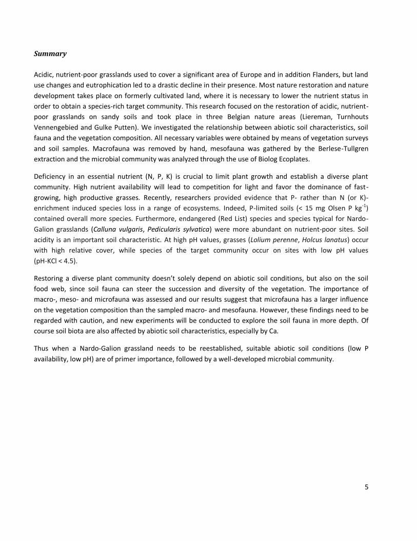
Acidic, nutrient-poor grasslands used to cover a significant area of Europe and in addition Flanders, but land

use changes and eutrophication led to a drastic decline in their presence. Most nature restoration and nature

development takes place on formerly cultivated land, where it is necessary to lower the nutrient status in

order to obtain a species-rich target community. This research focused on the restoration of acidic, nutrient-

poor grasslands on sandy soils and took place in three Belgian nature areas (Liereman, Turnhouts

Vennengebied and Gulke Putten). We investigated the relationship between abiotic soil characteristics, soil

fauna and the vegetation composition. All necessary variables were obtained by means of vegetation surveys

and soil samples. Macrofauna was removed by hand, mesofauna was gathered by the Berlese-Tullgren

extraction and the microbial community was analyzed through the use of Biolog Ecoplates.

Deficiency in an essential nutrient (N, P, K) is crucial to limit plant growth and establish a diverse plant

community. High nutrient availability will lead to competition for light and favor the dominance of fast-

growing, high productive grasses. Recently, researchers provided evidence that P- rather than N (or K)-

enrichment induced species loss in a range of ecosystems. Indeed, P-limited soils (< 15 mg Olsen P kg-1)

contained overall more species. Furthermore, endangered (Red List) species and species typical for Nardo-

Galion grasslands (Calluna vulgaris, Pedicularis sylvatica) were more abundant on nutrient-poor sites. Soil

acidity is an important soil characteristic. At high pH values, grasses (Lolium perenne, Holcus lanatus) occur

with high relative cover, while species of the target community occur on sites with low pH values

(pH-KCl < 4.5).

Restoring a diverse plant community doesn’t solely depend on abiotic soil conditions, but also on the soil

food web, since soil fauna can steer the succession and diversity of the vegetation. The importance of

macro-, meso- and microfauna was assessed and our results suggest that microfauna has a larger influence

on the vegetation composition than the sampled macro- and mesofauna. However, these findings need to be

regarded with caution, and new experiments will be conducted to explore the soil fauna in more depth. Of

course soil biota are also affected by abiotic soil characteristics, especially by Ca.

Thus when a Nardo-Galion grassland needs to be reestablished, suitable abiotic soil conditions (low P

availability, low pH) are of primer importance, followed by a well-developed microbial community.

6

Samenvatting

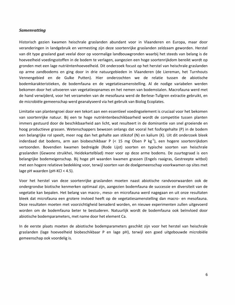
Historisch gezien kwamen heischrale graslanden abundant voor in Vlaanderen en Europa, maar door

veranderingen in landgebruik en vermesting zijn deze soortenrijke graslanden zeldzaam geworden. Herstel

van dit type grasland gaat veelal door op voormalige landbouwgronden waarbij het steeds van belang is de

hoeveelheid voedingsstoffen in de bodem te verlagen, aangezien een hoge soortenrijkdom bereikt wordt op

gronden met een lage nutriëntenhoeveelheid. Dit onderzoek focust op het herstel van heischrale graslanden

op arme zandbodems en ging door in drie natuurgebieden in Vlaanderen (de Liereman, het Turnhouts

Vennengebied en de Gulke Putten). Hier onderzochten we de relatie tussen de abiotische

bodemkarakteristieken, de bodemfauna en de vegetatiesamenstelling. Al de nodige variabelen werden

bekomen door het uitvoeren van vegetatieopnames en het nemen van bodemstalen. Macrofauna werd met

de hand verwijderd, voor het verzamelen van de mesofauna werd de Berlese-Tullgren extractie gebruikt, en

de microbiële gemeenschap werd geanalyseerd via het gebruik van Biolog Ecoplates.

Limitatie van plantengroei door een tekort aan een essentieel voedingselement is cruciaal voor het bekomen

van soortenrijke natuur. Bij een te hoge nutriëntenbeschikbaarheid wordt de competitie tussen planten

immers gestuurd door de beschikbaarheid aan licht, wat resulteert in de dominantie van snel groeiende en

hoog productieve grassen. Wetenschappers bewezen onlangs dat vooral het fosforgehalte (P) in de bodem

een belangrijke rol speelt, meer nog dan het gehalte aan stikstof (N) en kalium (K). Uit dit onderzoek bleek

inderdaad dat bodems, arm aan biobeschikbaar P (< 15 mg Olsen P kg-1), een hogere soortenrijkdom

vertoonden. Bovendien kwamen bedreigde (Rode Lijst) soorten en typische soorten van heischrale

graslanden (Gewone struikhei, Heidekartelblad) meer voor op deze arme bodems. De zuurtegraad is een

belangrijke bodemeigenschap. Bij hoge pH waarden kwamen grassen (Engels raaigras, Gestreepte witbol)

met een hogere relatieve bedekking voor, terwijl soorten van de doelgemeenschap voorkwamen op sites met

lage pH waarden (pH-KCl < 4.5).

Voor het herstel van deze soortenrijke graslanden moeten naast abiotische randvoorwaarden ook de

ondergrondse biotische kenmerken optimaal zijn, aangezien bodemfauna de successie en diversiteit van de

vegetatie kan bepalen. Het belang van macro-, meso- en microfauna werd nagegaan en uit onze resultaten

bleek dat microfauna een grotere invloed heeft op de vegetatiesamenstelling dan macro- en mesofauna.

Deze resultaten moeten met voorzichtigheid benaderd worden, en nieuwe experimenten zullen uitgevoerd

worden om de bodemfauna beter te bestuderen. Natuurlijk wordt de bodemfauna ook beïnvloed door

abiotische bodemparameters, met name door het element Ca.

In de eerste plaats moeten de abiotische bodemparameters geschikt zijn voor het herstel van heischrale

graslanden (lage hoeveelheid biobeschikbaar P en lage pH), terwijl een goed uitgebouwde microbiële

gemeenschap ook voordelig is.

7

Table of content

1. Introduction .......................................................................................................................................... 10

2. Literature review ................................................................................................................................... 11

2.1. Acidic, nutrient-poor grasslands.......................................................................................................... 11

2.2. Plant diversity and abiotic soil properties............................................................................................ 12

2.2.1. Introduction ................................................................................................................................. 12

2.2.2. Nitrogen ...................................................................................................................................... 12

2.2.3. Soil pH ......................................................................................................................................... 14

2.2.4. Phosphorus .................................................................................................................................. 16

2.3. Plant diversity and productivity .......................................................................................................... 18

2.4. Soil fauna............................................................................................................................................ 18

2.4.1. Introduction ................................................................................................................................. 18

2.4.2. Microfauna .................................................................................................................................. 19

2.4.3. Mesofauna................................................................................................................................... 20

2.4.4. Macrofauna ................................................................................................................................. 21

2.5. Vegetation and soil fauna ................................................................................................................... 22

2.6. Ex-agricultural land ............................................................................................................................. 24

2.6.1. Secondary succession and soil fauna ............................................................................................ 24

2.6.2. Nature restoration ....................................................................................................................... 26

2.7. Plant species diversity and the composition of the soil food web ........................................................ 28

3. Materials and methods ............................................................................................................................. 29

3.1. Study area .......................................................................................................................................... 29

3.2. Vegetation surveys ............................................................................................................................. 30

3.3. Abiotic soil properties ......................................................................................................................... 30

3.4. Soil fauna............................................................................................................................................ 30

3.4.1. Invertebrate community .............................................................................................................. 30

3.4.2. Microbial community ................................................................................................................... 31

3.5. Data analysis....................................................................................................................................... 32

3.5.1. Diversity indices ........................................................................................................................... 32

3.5.2. Weighted mean Ellenberg scores ................................................................................................. 33

8

3.5.3. Ordination ................................................................................................................................... 33

3.5.4. Classification ................................................................................................................................ 34

3.5.5. Statistical analysis (Mixed models and Mantel test) ..................................................................... 34

4. Results...................................................................................................................................................... 35

4.1. Vegetation .......................................................................................................................................... 35

4.1.1. Weighted mean Ellenberg scores ................................................................................................. 35

4.1.2. Species diversity and composition ................................................................................................ 36

4.1.3. Classification ................................................................................................................................ 37

4.2. Abiotic soil conditions ......................................................................................................................... 38

4.3. Soil fauna............................................................................................................................................ 39

4.3.1. Macro- and mesofauna ................................................................................................................ 39

4.3.2. Microfauna .................................................................................................................................. 41

4.4 Relationship between biotic and abiotic features................................................................................. 42

4.4.1. Relationship between vegetation composition and abiotic soil characteristics ............................. 42

4.4.2. Relationship between soil fauna and abiotic soil characteristics ................................................... 44

4.4.3. Relationship between vegetation composition and soil fauna ...................................................... 47

5. Discussion ............................................................................................................................................. 50

5.1. Relationship between vegetation composition and soil abiotic characteristics .................................... 50

5.2. Relationship between soil fauna and abiotic soil characteristics .......................................................... 53

5.3. Relationship between vegetation composition and soil fauna ............................................................. 55

6. Conclusion and future research ............................................................................................................. 58

7. List of abbreviations and symbols .......................................................................................................... 59

8. References ............................................................................................................................................ 60

9. Appendices ............................................................................................................................................ 72

Appendix I: VIF factors ............................................................................................................................... 72

Appendix II: Overview of plant species, Shannon-Wiener diversity index and eveness ............................... 73

Appendix III: Overview Stress value ........................................................................................................... 75

Appendix IV: NMDS ordination diagrams based on the vegetation surveys ................................................ 76

Appendix V: TWINSPAN ............................................................................................................................. 81

Appendix VI: The relationship between pH-KCl and exchangeable Al ......................................................... 87

Appendix VII: NMDS ordination diagrams based on macro- and mesofauna .............................................. 88

9

Appendix VIII: Biolog Ecoplates .................................................................................................................. 94

Appendix VIIII: NMDS ordination diagrams based on the ACWD values of 31 carbon sources .................... 96

Appendix X: Mixed models ...................................................................................................................... 102

Appendix XI: NMDS correlations .............................................................................................................. 108

Appendix XII: CCA .................................................................................................................................... 110

Appendix XIII: Mantel test ....................................................................................................................... 111

Appendix XIIII: The relationship between Olsen P concentration and the number of Red List species ...... 112

10

1. Introduction Acidic, nutrient-poor grasslands used to cover a significant area of Europe and in addition Flanders. In upland

sites they still occur in large areas, but in lowland area, such as the Netherlands and Belgium they are rare

and constrained in size (www.natuurkennis.nl). In Great Britain, these grasslands still cover an extensive area

(UK Biodiversity Group, 1998).Through land use changes, mainly intensive agriculture, soils became more

alkaline and nutrient-rich, inducing a strong decline in the appearance of these grasslands. Also

abandonment of the management led to a considerable decline in the presence of acidic, nutrient-poor

grasslands (Ellenberg, 1996), especially in Central Europe, where they almost exclusively occur in nature

reserves (Duprè et al., 2010).

Nitrogen (N) and phosphorus (P) are the two most important limiting nutrients in nutrient-poor semi-natural

grasslands (Van Landuyt et al., 2008). Not only direct application of fertilizers but also atmospheric deposition

enriched soils, causing a significant species loss (Wassen et al., 2005; Maskell et al., 2010). High N availability

will favor the dominance of fast-growing, high productive grasses such as Agrostis capillaris in dry conditions

and Molinia caerulea in wet conditions (www.natuurkennis.nl). Fertilization leads also to high P availability.

Moreover, sulphur (S) and N deposition will acidify soil via precipitated acids, oxidation of dry-deposited

compounds, loss of basic cations and nitrification1 (Stevens et al., 2009). Over the last three decades,

deposition of S compounds has decreased drastically in North America and Europe, but N deposition rates

have barely changed (NEGTAP, 2001). Wet acidic, nutrient-poor grasslands are faced with a third threat,

namely dessication (www.natuurkennis.nl).

Most nature restoration and nature development takes place on formerly cultivated land, where it is

necessary to lower the nutrient status in order to obtain a species-rich target community (Marrs and Gough,

1989). This is especially the case for P, a relative insoluble element with a long persistence in soil (Wild,

1988). Restoring a diverse plant community doesn’t solely depend on abiotic soil conditions, but also on the

soil food web. Bacteria and fungi insure the breakdown of organic matter to inorganic compounds,

determining the availability of nutrients to plants (Bardgett, 2005). They can also enhance nutrient

acquisition of plants through symbiotic relationships. Other soil animals influence the nutrient cycling by

feeding on microbes and changing the amount and form of organic matter in soil. Soil fauna can also affect

plants directly as pathogens or root feeders (Bardgett, 2005).

Many studies have focused on the role of N and P in the restoration of species-rich grassland (Janssens et al.,

1998; Critchley et al., 2002; Gilbert et al., 2009; Maskell et al., 2010), while other researchers investigated soil

fauna and their impact on plant community (Spehn et al., 2000; De Deyn et al., 2003: Sugiyama et al., 2008;

Eisenhauer et al., 2011; Sabais et al., 2011). The goal of this study is to link both views and to retrieve the

relationship between abiotic soil conditions, the soil fauna and the vegetation structure and composition of

acidic, nutrient-poor grasslands. In this study we focus on the abundance of earthworms, beetles, mites,

1 Nitrification is the oxidation of ammonium (NH4+) to nitrate (NO3

-). During this process two protons (H+) are released,

accelerating soil acidification.

11

springtails, nematodes, potworms and bacteria and their relationship with vegetation diversity and

composition, as well with soil conditions, being P availability (Olsen-P and total P), pH and exchangeable

concentrations of aluminium (Al) and calcium (Ca).

In the next section (§2) a summary is given of the results of previous and related research. Afterwards the

materials and methods (§3) of this study are mentioned, followed by an overview of the results (§4). These

are critically reviewed in the discussion (§5), from which a conclusion (§6) is drawn.

2. Literature review

2.1. Acidic, nutrient-poor grasslands Nardo-Galion grasslands are dominated by grasses (Poaceae), sedges (Cyperaceae), rushes (Juncaceae), forbs

and dwarf shrubs. Frequently occurring plant species are matt-grass (Nardus stricta), heath grass (Danthonia

decumbens), common tormentil (Potentilla erecta), heather (Calluna vulgaris), bog heather (Erica tetralix)

and purple moor grass (Molinia caerulea). Mosses found in this type of grassland are neat feather-moss

(Scleropodium purum), hypnum moss (Hypnum cupressiforme) and common haircap moss (Polytrichum

commune). Not much animals are bound to this habitat, since mostly the area of this type of grassland is too

small as is the case for Flanders (e.g. for breeding birds, foxes,…) and due to a low food supply (low numbers

of mice are quite typical). Overall, Nardo-Galion grasslands contain a rich fungal diversity, butterflies, e.g. the

alcon blue (Maculinea alcon), spiders and ground beetles (www.natuurkennis.nl). Some rare reptile species

occurring are the viviparous lizard (Lacerta vivipara) and the smooth snake (Coronella austriaca).

The soil is strong to moderately acid, with a pH range of 4 to 6. The soil texture is often sandy to sandy loam.

In Flanders, the most important differential factor is moisture content, defining wet and dry acidic, nutrient-

poor grasslands. Wet representatives are characterized by a groundwater level at a surface level during

wintertime and a groundwater level deeper than 1.5 m during summertime.

Nardo-Galion grasslands resulted from extensively cultivated grass- and hayfields in large parts of Central and

Western Europe (Ceulemans et al., 2009). On the other hand they can also originate from disturbing

(mowing, burning, sod-cutting, treading) heath land communities. They differ from the latter in that they are

more diverse and not dominated by low-remaining shrubs. Intensive forest management can also lead to this

biotope. Degradation was initiated by the application of manure, leading to forest or intensively managed

grassland. When management is abandoned, this grassland evolves to heathland on the most poor and

undisturbed fields. However, due to high atmospheric deposition succession will take place in different

stages: first grasses will dominate, followed by brushwood and finally forest will develop

(http://www.inbo.be/docupload/1521.pdf).

Management consists of not interfering, mowing once a year (e.g. in the beginning of August for Gulke

Putten), extensive grazing (by sheep, goat, ponies, donkeys or Galloway cows) or burning (detrimental to

fauna and not an option in densely populated areas). More nutrient-rich grasslands can be mown twice a

12

year (end of June and beginning of September) to lower the nutrient status

(http://www.inbo.be/docupload/1521.pdf).

2.2. Plant diversity and abiotic soil properties

2.2.1. Introduction

Grasslands of the highest botanical value are generally found on nutrient-poor soils. Species richness

diminishes with increasing nutrient availability, which favors competitive species capable of rapid growth and

biomass accumulation, such as perennial grasses (Bakker and Berendse, 1999). Thus, nutrient limitation is

one of the most important factors influencing plant community structure (Critchley et al., 2002).

Unfortunately, most soils are disturbed by human activities, which lead to eutrophication, acidification,

desiccation, … (Bakker and Berendse, 1999). Since the 1950s, most farmers have been applying fertilizers to

increase the yield of their land. This residual soil fertility may form a major obstacle in the restoration of

degraded semi-natural grasslands. Restoration of ecological diversity in grassland communities requires,

besides suitable abiotic conditions, an appropriate management and colonization of the target species

(Critchley et al., 2002). These measures can only be effective if the atmospheric deposition of nutrients

doesn’t exceed critical levels. The critical N load for Nardo-Galion grassland lies between 10 and 20 kg N ha-1

yr-1 (Decleer, 2007). In the past, this limit was exceeded in densely populated and industrialized regions such

as Flanders, but nowadays the average yearly deposition equals 20,4 kg N ha-1, whereas this amounted to

32,7 kg N ha-1 in 1990 (MIRA Achtergronddocument 2011 Vermesting).

2.2.2. Nitrogen

World-wide deposition of NOx and NHx more than tripled between 1860 and the early 1990s (Galloway et al.,

2004). Since the 1990s acidifying deposition (of Sox, NHx and NOx) has declined in Flanders and Western

Europe, although this is less pronounced for NHx and NOx (http://www.milieurapport.be). Most of the N input

(84%) either accumulates in the soil or leaves the system by nitrate leaching, denitrification or ammonia

volatilization (Van Der Meer, 1982). This N deposition has direct effects, e.g. a higher N supply to the

vegetation (Bakker and Berendse, 1999), but also indirect effects, resulting from the increasing rate of

accumulation of soil organic matter. This has in turn led to an accelerated increase in N mineralization during

succession (Berendse, 1990). Other indirect effects are soil acidification (see § 2.2.3.), base cation depletion

(Ca2+, Mg2+ and K+) and higher Al3+ concentrations (which are both linked to soil acidification) (Bowman et al.,

2008). In most communities, fast growing perennial grasses benefit from the increase in N supply, since they

outcompete a great variety of low-statured or slow-growing species adapted to nutrient-poor soils (Bakker

and Berendse, 1999).

The effect of N deposition on different vegetation types (forest understoreys, grasslands, heathlands,

freshwater wetlands, salt marshes and bogs) has been studied by a meta-analysis conducted by De Schrijver

et al. (2011), based on data from North America, Europe and Australia. The impact of cumulative N input on

these vegetation types and the present growth forms (forbs, graminoids, shrubs, bryophytes and lichens) was

analyzed. The response of both vegetation types and growth forms was very variable, in that grasslands and

salt marshes showed an increase in biomass as a result of N addition, while heathlands, bogs and freshwater

wetlands had a neutral response and forest understoreys a negative response. Forb and shrub biomass didn’t

13

change following N addition, whereas bryophyte biomass decreased and graminoid biomass increased. Grass

species are able to react fast on increased N availability, producing more biomass, and consequently more

litter as a result of N input. This limits place and light availability for other low-statured species, such as forbs

(e.g. Bobbink, 1991; Wedin and Tilman, 1996). Also bryophytes are not able to cope with increasing plant

cover (Virtanen et al., 2000). Arróniz-Crespo et al. (2008) investigated the impact of N deposition on two

bryophyte species within acidic grassland. Their abundance strongly declined but differed between the

species, indicating that some species are more tolerant. This was also reflected in the shoot K concentration,

which decreased for one species due to the exchange of NH4+ and K+ or due to a direct toxic effect of N,

causing leakage of K+ ions (Pearce et al., 2003). Ericaceous shrubs are not favoured by high N input, since they

own an N-conserving strategy, which is necessary to survive in low-nutrient environments (Chapman et al.,

2006). Several authors (Krupa, 2003; Kleijn et al., 2008) proved that shrubs and forbs are sensitive to high

NH4+ concentrations, whereas graminoids are not (van den Berg et al., 2005). Concerning species richness, all

vegetation types combined showed a significant decline, but when considered separately only heathland and

grassland had a negative correlation with N addition. Furthermore, species richness decline in grasslands and

heathlands was significantly correlated to the cumulative N input, with a fast species loss at low levels of

cumulative N input or at the beginning of the addition, followed by an increasingly slower species loss at

higher cumulative N inputs.

Maskell et al. (2010) stated that N deposition affected species richness and vegetation composition in

different habitats (heathland, acid, calcareous and mesotrophic grassland), having a positive influence on

grasses but a negative one on the presence of forbs, the latter being different to what De Schrijver et al.

(2011) found (neutral response). They showed that in acid grassland and heathland acidification rather than

increased fertility was responsible for species loss, in contrast with calcareous grasslands where the decline in

species was allocated to eutrophication. Thus, the relationship between plant traits and N deposition differed

in different habitat types.

Duprè et al. (2010) focused on the effect of N deposition on species richness and composition in European,

acidic grasslands (situated in Great Britain, Germany and the Netherlands). Mean Ellenberg values (see §

3.5.2.) for light (mL), moisture (mF), soil pH (mR) and fertility (mN) were calculated and cumulative N

deposition was estimated. Mean R and N values lay between 2 and 4, but some plots had values lower than

2, demonstrating the acid and nutrient-poor soil conditions. Most variation in species composition was

explained by mean R and mean N values. Models were established to explain the variation in species richness

and based on several variables. Area was strongly positively related to species richness. Geographical

variables (longitude and altitude) had weak effects, but latitude was correlated with species richness

(increasing with increasing latitude in Great Britain, but decreasing in Germany). The greatest impact was

noticed for mean R, positively related to dicots and negatively to grasses. The second most important

variable was N deposition, influencing the number of all grasses (positively), dicots and bryophytes

(negatively) in all three countries. In time a clear increase in the proportion of grasses and ruderals could be

seen in Germany and the Netherlands (based on data since 1940s, lacking for Great Britain). In contrast,

dwarf shrubs and many herbaceous dicots (forbs) became less frequent, except species bound to more fertile

grasslands e.g. Rumex acetosa. Abandoning management of grasslands (grazing, mowing) can contribute to

14

the reduction of species diversity and favor growth of grasses. Sulphur (S) deposition was not retained in the

experiment, due to the strong correlation with N deposition. Furthermore, since soils are characterized by a

low pH, the acidifying effect of S deposition was negligible.

Also Stevens et al. (2010) investigated to what extent N deposition forms a threat to species richness of acid

grasslands. All grasslands were situated in the Atlantic biogeographic zone of Europe. They too observed a

negative exponential relationship between species diversity and N deposition, indicating higher species loss

at low cumulative N addition. This can be clarified by the extinction of N-sensitive species at lower cumulative

levels, resulting in a plant community of less sensitive species and thus reducing species loss when N keeps

accumulating. Via multiple regression they identified other drivers, responsible for species loss. At high

deposition rates soil pH and nitrate concentrations are the next most important variables, at low deposition

rates this seemed to be the extent of extractable aluminium (Al). These results implicate that protection of

sensitive grasslands (low buffer capacity, due to low concentration of base cations, Skiba et al., 1989) can

only be obtained when atmospheric deposition remains very low (Emmet, 2007). Nowadays, deposition has

to be below a critical load of 10 to 20 kg N ha-1 (Bobbink et al., 2003), but these experiments show that such a

deposition might already result in a significant species loss. In accordance to other studies (Bakker and

Berendse, 1999; Duprè et al., 2010; Maskell et al., 2010) the greatest decline was accounted for by forbs. In

2009, Stevens et al. defined indicators to deduce the impact of N deposition on acid grasslands. They

concluded that presence or absence of species, nor plant cover are suitable indicators (due to other drivers

such as management and land use history), but species richness, forb richness and the grass:forb ratio are

more appropriate.

2.2.3. Soil pH

The atmospheric deposition of nitrogenous and sulphuric compounds has caused a significant increase in the

rate of soil acidification. Luckily, deposition of sulphuric compounds has declined, but this doesn’t apply for N

deposition (Bakker and Berendse, 1999). Acidification can result from the dissolution of carbon dioxide (CO2)

to carbonic acid (H2CO3), from nitrification, from atmospheric pollution and natural sources (volcanic

eruptions) and from the breakdown of organic matter rich in phenolic and carboxyl groups (Bardgett, 2005).

Plant species richness in grassland communities has been found to be strongly correlated with soil pH (Grime

J.P., 1979). This is confirmed by Critchley et al. (2002), who stated that soil pH showed the strongest

relationship with the vegetation of lowland grasslands in Great Britain, followed by total N and organic

matter. The same was retrieved by an experiment of Duprè et al. (2010) where soil pH was the main driver of

species richness on acidic grasslands, resulting in a positive influence on total number of vascular plants and

the portion of dicots. Only grasses experienced a negative influence of increasing pH. Most European plant

species show an ecological optimum around higher pH values (i.e. higher than pH values of acidic grasslands)

(Schuster and Diekmann, 2003), meaning that a decrease in soil pH will lead to a decline in species that do

not tolerate acid soils. Indeed many species are sensitive to high H+ or Al3+ concentrations (Kleijn et al., 2008).

Few species are able to tolerate a lowering of soil pH and the few that can, such as Molinia caerulea, are able

to dominate (Maskell et al., 2010). Bryophytes seem to be sensitive to Al3+, which becomes available in high

concentrations at soil pH lower than 4.5 (Virtanen et al., 2000). Soil pH also affects the bioavailability and

15

mobility of other metals (Tyler and Olsson, 2001), such as lead (Pb) and iron (Fe) which show the same

behavior towards soil acidity, becoming more available at pH values below 5 (Stevens et al., 2009).

Thus soil pH clearly influences vegetation, but also the rate of nutrient availability (cations, P) and soil biota

(Bardgett, 2005). In acidic soils (pH below 4.5), unstable clay minerals release soluble Al (Kennedy, 1992),

which can be toxic to plants and microbes. Ions such as calcium (Ca), potassium (K) and magnesium (Mg)

leach out and are replaced by protons (H+) and Al (Jönsson et al., 2003). Increasing the concentration of base

cations (Ca, K and Mg) in the soil solution can mitigate Al toxicity (Alva et al., 1986). Under acid conditions,

most P is found in the form of Fe and Al phosphates, compounds that are not fit for plant uptake. Phosphates

will generate soluble P by dissolving, a reaction triggered by the rise of the pH, with a highest P availability

between pH values of 6 and 7 (see § 2.2.4.). All soil organisms are tolerant for certain pH ranges. For instance,

earthworms do not tolerate acid soils well (except epigeic species) (Edwards, 2009), but enchytraeid worms

(also known as potworms) do, making them the functionally dominant soil organisms in these circumstances

(Bardgett, 2005).

The soil acidity of formerly cultivated land is influenced by reforestation in several ways: by atmospheric

depositions, by the quality of the litter, by symbiotic relationships when planting trees living in symbiosis with

N-fixing bacteria and by nutrient uptake (De Schrijver et al., 2011). De Schrijver et al. (2011) investigated soils

in West Flanders that were for at least 50 years under cultivation and the impact of different tree species on

soil acidification. According to de Vries and Breeuwsma (1986), leaf litter with poor quality produces more

organic acids. N2-fixing bacteria raise the amount of reactive N in the soil (Compton et al., 2003). Tree roots

excrete H+ to solve the disequilibrium between anions and cations, caused by a higher uptake of cations

(Nilsson et al., 1982). Acid soils contain higher Al3+ and lower exchangeable base cation concentrations

(Bowman et al., 2008). This was demonstrated for increasing forest age, which was accompanied by a

decrease in soil pH and exchangeable Ca2+ and an increase in exchangeable Al3+ (De Schrijver et al., 2011).

This doesn’t only impact trees (lower uptake, damaged root structure and function) (Weber-Blaschke et al.,

2002), but also soil fauna e.g. burrowing earthworm species (sum of endogeic and anecic species) (Muys and

Granval, 1997). These earthworm species play an important role in litter decomposition (Edwards, 2009).

Poor leaf litter quality (high C and lignin concentration, low Ca2+ concentration) induces absence of burrowing

species, enhancing litter accumulation. The influence of acidifying processes diminished with soil depth (for

all tree species Al3+ concentrations declined with depth, for two species soil pH and Ca2+ increased and the

other three species showed no response for the latter two variables, possibly due to bioturbation by

earthworm burrying). Thus, burrowing earthworms mitigate soil acidification by mixing the topsoil with litter,

by mixing upper layers with deeper soil layers (richer in base cations) and by egesting casts2 (De Schrijver et

al., 2011).

2 Mineral soil and organic matter are mixed in the gut of earthworms and enriched with organic secretions. This slurry is

colonized by microbes, responsible for the breakdown of soil organic matter. When the casts are egested (in soil or on

the surface), microbes remain active, enhancing soil fertility.

16

2.2.4. Phosphorus

Not only N and pH should be regarded, also P and K should be taken into account since grasslands of high

botanical value are generally associated with lower levels of these nutrients (Critchley et al., 2002). Soil

consists of inorganic (minerals or salts) and organic P (humus). P occurs in nature mainly in the form of

phosphates, chemical bounds of P and oxygen (Schoumans et al., 2008). P is mainly utilized by plants as

inorganic phosphates.

Soil P can be divided into three major pools that are in dynamic equilibrium (Stevenson and Cole, 1999;

Richter et al., 2006): labile, slowly cycling, and occluded P pools. Labile P is available for immediate biological

uptake (by flora and fauna) (Tiessen and Moir, 2008) and consists of phosphate in soil solution or phosphates

that desorbs or mineralizes from (in)organic soil compounds (Vandecar, 2009). Slowly cycling P is phosphate

adsorbed onto soil particles, inorganic and organic phosphate that has reacted with elements (such as Ca, Al

or Fe), and more stable organic P. This type of P can easily be converted to the labile P pool (Richter et al.,

2006). Phosphates can also be occluded, meaning that they remain in the soil for years without being

available to plants. Consequently they have little impact on soil fertility (Stevenson and Cole, 1999). The

occluded P pool consists of insoluble inorganic compounds and organic compounds that are resistant to

mineralisation by microorganisms. Highest concentrations of Al and Fe compounds are measured in acid soils

(pH < 5), enhancing the process of fixation (i.e. the adsorption of phosphates). In soils with a pH value over 5,

phosphates can combine with Ca, which reaches a maximum concentration at pH 7.5. Most soil P occurs in

organic form e.g. as orthophosphate monesters or inositol phosphates (Bardgett, 2005).

Rooney et al. (2009) found that phosphate addition to acidic upland grassland soil significantly increased root

biomass, shoot biomass (especially of Lolium perenne, followed by Festuca ovina), soil pH, and microbial

activity. The increase in microbial activity as a result of phosphate addition reflects P limitations in natural

acidic grasslands. Both microbes and plants require P for their growth. In which form P occurs in soil (mineral

or organic) is dependent on several factors e.g. soil type, pH, vegetation type or fertilizer application (Curtin

and Smillie, 1984; Daly et al., 2001). Plants preferably use labile, inorganic phosphates (Curtin and Smillie,

1984), but this fraction is generally low in unimproved Nardo-Galion grassland. Thus, plants depend on the

microbial community for making phosphates bioavailable, through breakdown of organic matter and

solubilization of insoluble phosphates (Troeh and Thompson, 1993). Since the importance of P is known,

farmers have added soluble phosphates, available for uptake by plants and microbes to their land to increase

productivity (Withers et al., 2001). Rooney et al. (2009) also followed the change, resulting from phosphate

addition, in the fungal and bacterial community, which are responsible for P cycling (Bardgett, 2005). Results

showed that both communities decreased in biomass after phosphate addition and that the effect is

dependent on the aboveground plant species. The decrease of fungal biomass is probably due to a negative

response of mycorrhizal fungi (Rooney et al, 2009). Mycorrhizal fungi play an import role in nutrient limited

soils, where they aid plants in the acquisition of nutrients (especially N and P) (Bardgett, 2005), but become

rather redundant when P is added to soil. Arróniz-Crespo et al. (2008) tested the influence of simultaneous

addition on N and P on bryophytes, showing that some species were benefited by this treatment, while slow-

growing species were not. Wassen et al. (2005) provided evidence that P- rather than N-enrichment induced

species loss in a range of ecosystems (from terrestrial freshwater wetland to moist grassland) throughout

17

temperate Eurasia. This transect coincides with a decline in atmospheric N deposition. They confirmed that

highest diversity was obtained at intermediate productivity (between 200 and 600 g m-2) and at intermediate

tissue N:P ratios. Endangered species were most abundant on P-limited sites and their proportion increased

with increasing P-limitation. Fertilization has strongly enhanced P-availability (Gough and Marrs, 1990) and

the conservation of endangered species necessitates the restoration of P-limited ecosystems. These findings

were confirmed by Ceulemans et al. (2011), who selected nutrient-poor semi-natural grasslands in Western

Europe (United Kingdom, France and Belgium) based on a soil fertility gradient. More grassland species were

negatively influenced by elevated P availability (30 %) compared to elevated N availability (8 %). Furthermore,

they linked P susceptibility to plant traits, indicating that species characterized by stress tolerance, low

maximum canopy height and symbiosis with arbuscular mycorrhizae3 are more sensitive to high P levels.

There are several methods to extract P, but Olsen's method of P extraction is recommended for analyzing

soils of areas identified for habitat creation; values of less than 10 mg kg-1 will give the greatest potential for

the restoration of species-rich mesotrophic grassland (Gilbert et al., 2009). This is confirmed by Hommel et al.

(2006), who found a reference value of 5 to 9 mg P kg-1 for both dry and wet nutrient-poor, acidic grasslands.

Herr et al. (2011) found similar results and consider 15 mg Olsen P kg-1 as a threshold value to recreate a

diverse target community (Nardo-Galion grassland and heathland). Janssens et al. (1998) investigated the

relationship between soil chemical factors and plant diversity in old permanent grasslands of West and

Central Europe. They found the highest diversity at sites where the P concentration was below the optimum

for plant nutrition (50 to 80 mg P kg-1). Based on their findings, P concentration (extracted by acetate and

EDTA) and species richness are correlated by a humped-back curve reaching an optimum amount of species

around 40 mg P kg-1. The same relationship accounts for the Shannon-Wiener diversity index and the rarity

index (based on a relative rarity coefficient for each plant per region). This humped-back curve doesn’t apply

to other soil factors such as pH and organic matter content, indicating a more complex interplay between

these factors and species number. Ceulemans et al. (2009) stated that an optimal reestablishment of Nardo-

Galion grassland can be obtained at P availability lower than 3 mg kg-1. However, this low value results from

the applied technique to measure plant available P. In this experiment P values were measured by means of

ion exchange membranes, a technique which extracts less P to soil than the Olsen or NH4Ac-EDTA extraction

method. Applying P to a P-limited soil favors the abundance of legumes (Bobbink, 1991; Elisseou et al., 1995),

since this element is necessary for nodulation (Dunlop and Hart, 1987). This would in turn lead to a higher soil

N content via symbiotic fixation, which has been proven for Trifolium repens (Caradus and Snaydon, 1988).

3 Mycorrhizae are symbiotic relationships between fungi and vascular plants, insuring a more elaborate nutrient and

water uptake and a higher resistance (against heat, salt, heavy metals) for plants, while fungi obtain photosynthetic

compounds necessary for their growth (http://www.arboris.be). There are three types of mycorrhizae: endomycorrhizae

(fungal hyphae penetrate plant cells), ectomycorrhizae (fungal hyphae remain extracellular) and ericoid mycorrhizae

(symbiosis with plants of the family Ericaceae). Endomycorrhizae form vesicles (storage organs) and arbuscules (transfer

structures) inside the plant (http://dnn.cropower.com).

18

2.3. Plant diversity and productivity Tilman et al. (1996) stated that plant diversity influences grassland productivity and sustainability. Plant

species in a diverse community complement each other in the use of resources, utilizing limiting nutrients

more effectively. This is known as the diversity-productivity hypothesis. Both soil extractable NH4+ and NO3

-

decreased with increasing species richness, and undisturbed, native grasslands showed the same results. By

using resources more efficiently, nutrient leaching, diminishes, leading to a more sustainable (or closed)

nutrient cycle, which is known as the diversity-sustainability hypothesis. Bezemer and van der Putten (2007)

conducted an experiment to confirm the statement of Tilman et al. (1996). Different levels of species richness

were established (no sowing, 4 and 15 species sowed) and related to temporal stability. Non-sown plots,

where succession occurred naturally, showed the highest species richness, Shannon diversity and lowest

biomass production. A low biomass production could be explained by the restricted presence of legumes,

which were strongly related to biomass production. Extinction and colonization rates were lowest for the

plots with highest amount of sown species, resulting in a higher temporal stability. These results seem

contradictory to what Tilman et al. stated, but can be reconciled, since the plant species in the non-sown

plots were early-successional species (rapid growth, low competiveness), contributing to a low temporal

stability. Thus species composition and species richness are important drivers of ecosystem functioning

(Tilman et al., 2007).

2.4. Soil fauna

2.4.1. Introduction

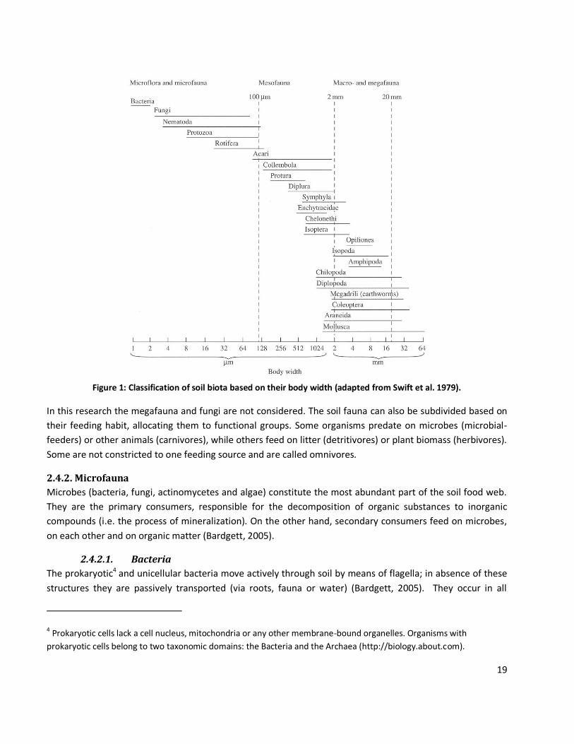
The soil foodweb consists of microbes (bacteria and fungi), microfauna (body width < 0.1 mm; e.g. protozoa

and nematodes), mesofauna (body width 0.1 – 2.0 mm; e.g. microarthropods and potworms), macrofauna

(body width > 2.0 mm; e.g. earthworms and millipedes) and megafauna (e.g. some earthworms, Mollusca

and Coleoptera) (Bardgett, 2005; see Figure 1). Soil organisms can also be classified based on their body

length, resulting in three categories: micro-, meso- and macrofauna. Soil animals are assigned to the same

categories as based on their body width, except for the nematodes, who are now allocated to the mesofauna

(Coleman et al., 2004).

19

Figure 1: Classification of soil biota based on their body width (adapted from Swift et al. 1979).

In this research the megafauna and fungi are not considered. The soil fauna can also be subdivided based on

their feeding habit, allocating them to functional groups. Some organisms predate on microbes (microbial-

feeders) or other animals (carnivores), while others feed on litter (detritivores) or plant biomass (herbivores).

Some are not constricted to one feeding source and are called omnivores.

2.4.2. Microfauna

Microbes (bacteria, fungi, actinomycetes and algae) constitute the most abundant part of the soil food web.

They are the primary consumers, responsible for the decomposition of organic substances to inorganic

compounds (i.e. the process of mineralization). On the other hand, secondary consumers feed on microbes,

on each other and on organic matter (Bardgett, 2005).

2.4.2.1. Bacteria

The prokaryotic4 and unicellular bacteria move actively through soil by means of flagella; in absence of these

structures they are passively transported (via roots, fauna or water) (Bardgett, 2005). They occur in all

4 Prokaryotic cells lack a cell nucleus, mitochondria or any other membrane-bound organelles. Organisms with

prokaryotic cells belong to two taxonomic domains: the Bacteria and the Archaea (http://biology.about.com).

20

habitat types, surviving the most extreme conditions. Extracellular enzymes are produced to break down

organic matter. Other abilities can be attributed to certain bacterial genera, such as nitrification (by nitrifying

genera Nitrosomonas and Nitrobacter) and N fixation (by the symbiotic genus Rhizobium and the free living

genera Azotobacter and Clostridium) (Bardgett, 2005). Pasture soil can contain up to 1.8 107 cells per cubic

cm, while arable soil counts up to 2.1 1010 cells cm-3 (Torsvik et al., 2002).

2.4.2.2. Fungi

Fungi are eukaryotic5, filamentous organisms, consisting of hyphae (Bardgett, 2005). These hyphae form a

mycelium, which can weigh as much as 250 kg ha-1 in the upper 5 cm of grassland soil (Bardgett et al, 1993a).

The mycelium has several functions: degrading organic matter with extracellular enzymes, exploiting new

nutrient-rich regions and translocating nutrients through the mycelial network (Boddy, 1999). Fungi play

other important roles, as plant pathogens and food source of microbial-feeding soil fauna. They optimize and

stabilize soil structure by bounding particles together. Some fungi establish mutualistic associations with

plant roots (mycorrhizae), supplying the plant with nutrients, and receiving photosynthetic compounds in

return (Bardgett, 2005).

2.4.3. Mesofauna

2.4.3.1. Nematodes (Nematoda)

Nematodes (or roundworms) need a water film in the soil pores to be able to move, feed and reproduce.

They can be subdivided in functional groups according to the morphology of their mouthparts, since they can

be bacterial-feeders, herbivores, fungal-feeders, omnivores and carnivores (Bardgett, 2005). Because

nematodes are bound to certain states of ecosystems (old versus young, annual crops versus perennial

crops,…) they can be used as indicators for the ecosystem condition (Yeates, 1999;Ferris et al., 2001).

Nematodes seek actively spots in soil with high concentrated organic matter, such as the rhizosphere (the

region of the soil influenced by roots, root metabolites and associated micro-organisms) (Griffiths and Caul,

1993).

2.4.3.2. Springtails (Collembola)

Springtails are wingless insects of a few millimeters, with six abdominal segments occurring in all biomes

(Coleman et al., 2004). They are named after a springing apparatus ventrally on the abdomen, absent in

groups living in deeper soil layers. These groups also lack eyes and pigmentation according to Petersen

(2002). In the rhizosphere they are very numerous, reaching up to 100 000 organisms per square meter. Their

feeding source consists mainly of fungi.

2.4.3.3. Mites (Acari)

Mites posses rounded body forms and have in temperate grassland an equal biomass as springtails. Four

suborders occur frequently in soils: the Oribatei, the Prostigmata, the Mesostigmata and the Astigmata.

5 Eukaryotic cells have a cell nucleus and membrane-bound organelles, increasing the complexity and size of the cells.

Cells of animals, plants, fungi and protists (i.e the four kingdoms of the domain Eukarya) are eukaryotic

(http://www.cod.edu).

21

Species of these suborders differ in their feeding habit. Oribatid mites are fungivorous and/or detritivorous.

They are characterized by juvenile polymorphism (immature stadia do not resemble the adult stadium), slow

reproduction and high abundance in soil (negatively affected by cultivation, descending the number of

oribatid mites to 25 000/m²). They have a sclerotized (often calcerous) exoskeleton, lacking in the other

suborders (Coleman et al., 2004). They influence litter decomposition and nutrient cycling indirectly by

feeding (Petersen and Luxton, 1982). Mesostigmatic mites are mainly predators (the smaller ones predate on

nematodes, the larger ones on other microarthropods and their eggs), a few are fungivorous. Walter and

Ikonen (1989) proved in grasslands in the west of the United States that nematodes were mostly predated by

mesostigmatic mites. Prostigmatic mites are very diverse and can be predators (mostly of nematodes or

other microarhtropods and their eggs, just like mesostigmatic mites), microbial feeders, plant feeders or

parasites (Kethley, 1990). The biomass of prostigmatic mites is generally small, compared to the other

suborders, although their numbers are higher in temperate than in (sub)tropical habitats (Luxton, 1981b).

Astigmatic mites are most abundant in moist, organic soils (Coleman et al., 2004). Most of them are microbial

feeders, although some can live on fungi, algae or plant material (Philips, 1990).

2.4.3.4. Potworms (Enchytraeidae)

These are an important family of the oligochaeta, just like earthworms (discussed in § 2.4.4.1.). They are

much smaller than earthworms (up to 20 mm) and unpigmented (Coleman et al., 2004). They can be

distinguished from nematodes by their round body shape. 19 of the 28 genera are terrestrial, the other

genera occur in marine or freshwater habitats. Enchytraeid densities of grasslands lay between 2000 and

more than 20 000 individuals per square meter, lowering when land is being cultivated and highest in acid,

undisturbed ecosystems (van Vliet, 2000). Potworms ingest mineral and organic matter, such as plant

material, fungi and bacteria. They influence the microbial community by predation, diminishing the microbial

population, but enhancing the microbial activity. Soil structure is also affected by potworms, through the

excretion of fecal pellets and the creation of pores (Coleman et al., 2004).

2.4.4. Macrofauna

2.4.4.1. Earthworms (Lumbricidae)

Earthworms are physiologically adapted to all habitats characterized by enough soil water and a favorable

temperature for at least some part of the year. Inopportune periods are overcome by entering a temporary

dormant state (the aestivation or diapause) or by making a resistant cocoon that hatches when proper

conditions are met (Edwards and Bohlen, 1996). Their densities range from 10 to more than 2000 organisms

per square meter. Temperate grasslands can count 50 to 200 individuals per square meter, with the lower

value being typical for acid soils (Coleman et al., 2004). Land management is detrimental to earthworm

populations. In contrast, soils under nature restoration show a rise in earthworm densities (Edwards and

Bohlen, 1996). They can be assigned to one of the three ecological groups, following Bouché (1977): epigeics

(worms living in and feeding on leaf litter); anecics (worms forming vertical burrows in the soil) and endogeics

(worms inhabiting the mineral soil horizon and making horizontal burrows). Epigeic earthworms can be 15 cm

large and are pigmented bright red or red-brown. They utilize organically enriched substrates, such as plant

litter and the carbon-rich upper layers of the soil. Endogeic earthworms are often unpigmented and become

up to 20 cm. They live and feed in the soil up to 80 cm deep. Anecic earthworms live in burrows in the soil,

22

but feed on leaf litter. They are darkly colored at the head end (red or brown) and have paler tails

(http://www.earthwormsoc.org.uk). Earthworms form an important part of the soil fauna, as they are

ecosystem engineers. They influence the soil structure by forming burrows, hereby creating pores, which

facilitate aeration and infiltration. Leaf litter is pulled into the burrows and digested, resulting in the

production of casts. After some time (when all organic matter is decomposed) casts may harden into soil

aggregates (Coleman et al., 2004).

2.4.4.2. Other macrofauna

Isopoda

These saprovoreous crustaceans occur in a variety of habitats, but are susceptible to desiccation (Coleman et

al., 2004).

Diplopoda

Millipedes or Diplopoda are important saprophages of forests, where they are major consumers of organic

matter (Coleman et al., 2004).

Chilopoda

Centipedes or Chilopoda are predators in soil and litter, occurring in many biomes. Just like millipedes and

Isopoda, they are sensitive to desiccation (Coleman et al., 2004).

Hymenoptera

This order consists of ants and ground-dwelling wasps (Coleman et al., 2004). Ants are important soil

predators, due to their impact on soil structure as “ecosystem engineers” (Hölldobler and Wilson, 1990).

They change nutrient levels in soil by building nests and gathering food and predate on a wide variety of

animals, thus influencing the local food web indirectly and directly (http://www.sciencedaily.com).

Larvae

Juvenile stadia of Coleoptera (beetles) and Diptera (flies and mosquitoes) inhabit soil. The order of the

beetles consists of soil species that are predators, phytophages or saprovores. Many species of the Diptera

pupate in soil, thus being part of the soil food web. Fly larvae are saprovores or predators (Coleman et al.,

2004).

2.5. Vegetation and soil fauna Several experiments have tried to define the relationship between the aboveground biomass (vegetation)

and the soil fauna. In a study of an experimental grassland site in Germany, Gastine et al. (2003) found no

effects of plant diversity or functional group identity on several soil properties (including soil N availability,

microbial activity, and abundance and diversity of fauna). According to Sugiyama et al. (2008) eukaryote and

prokaryote abundance is driven by different parameters, whereby prokaryote (or bacterial) richness depends

on soil characteristics, while eukaryote diversity (protista, nematodes, microarthropods and mainly fungi)

depends on the vegetation structure. The higher the floral diversity, the higher the litter heterogeneity and

by consequence the soil decomposer group will be more diverse (Sugiyama et al., 2008).

23

Salamon et al. (2004) found in grassland field trials that plant species richness had no effect on the total

diversity of Collembola. This study was part of the BIODEPTH (Biodiversity and ecological processes in

terrestrial herbaceous ecosystems) project and conducted in Switzerland on calcareous, loamy soils. The

previously arable land was ploughed, left bare over the winter and harrowed. However, the number of

Collembola increased in the presence of a plant functional group, namely the legumes6, benefiting from

higher litter quality and the higher microbial biomass in the rhizosphere of these plants. But Sabais et al.

(2011) demonstrated that Collembola density and diversity increased with plant species and plant functional

group richness. This study was conducted as part of the Jena experiment, a large biodiversity experiment

located in the floodplain of the Saale river in Germany. The site was formerly used as an arable field and

ploughed and harrowed several times before the experiment was established. The Collembola benefited

from higher food resources, namely from a higher quantity and quality of litter and a higher root and

microbial biomass. Changes in the Collembolan community will impact plant productivity and composition,

because the primary producers rely on microbial and animal decomposers in terms of nutrient availability

(Bardgett, 2005). The Collembola also steer the microbial community, directly by feeding on them and

indirectly by changing the nutrient availability (Griffiths and Bardgett, 1997). By feeding of meso- and

macrofauna on microbes, the microbial activity will increase and thus the plant nutrient availability (Spehn et

al., 2000).

Spehn et al. (2000) examined the effect of plant diversity on soil heterotrophic activity in grassland

ecosystems, located on formerly cropped calcareous, loamy soils in Switzerland. They found that the

reduction in plant biomass (due to a lower number of plant species) had more pronounced effects on voles

and earthworms than on microbes. This means that higher trophic levels are more strongly affected than

lower trophic levels, but all trophic levels will be influenced. Microbial biomass will decrease, because less

organic carbon sources enter the soil, thus limiting soil microbial activity (Smith and Paul, 1990; Van de Geijn

and van Veen, 1993). Consequently, mesofauna, depending on bacteria and macrofauna as a food supply,

may suffer from plant diversity loss. Thus, reducing the plant biomass affects the whole decomposer

community. Koricheva et al. (2000) also investigated the response of different trophic groups of invertebrates

to manipulations of plant diversity in grasslands. They found that the populations of the most sedentary and

host specific herbivores were stronger influenced by plant species and functional group diversity than the less

specialized or more mobile species. The activity and total number of predators was negatively correlated with

plant species and functional group richness, meaning that monocultures counted more predators. The

presence of legumes induced a higher number of invertebrates. The proportion of the other two functional

groups, grasses and non-legume forbs, had no significant impact on the different trophic groups of

invertebrates.

6 Legumes are able to fixate atmospheric nitrogen (N2), through a symbiotic relationship with bacteria (rhizobia).

Rhizobia are attracted to the roots by plant organic molecules, flavonoides. Bacterial infection is followed by local rapid

growth of the plant tissue, creating nodules. Plants provide rhizobia with water and nutrients, while the bacteria

produce plant available N from N2 (http://www.public.iastate.edu/~teloynac/354n2fix.pdf).

24

Eisenhauer et al. (2011) studied the effect of plant species richness in experimental grassland on nematodes.

He found that herbivorous nematodes dominated soils with low vegetation diversity, while species-rich plots

were dominated by microbivorous nematodes. Thus higher plant species richness evokes a shift in the

abundance of two functional groups of nematodes, hereby positively affecting the plant performance by

stimulating nutrient cycling. De Deyn et al. (2004) showed in experimental grassland trials that the soil

nematode community structure and diversity is driven by both species diversity and species identity (i.e.

plant species), but the effect of certain plant species was stronger than diversity treatments. Plant species

identity affected primary and secondary decomposers more than carnivorous and omnivorous nematodes

(i.e. the higher trophic levels), confirming that feeding groups closely interacting with plants are more fiercely

influenced. Root zones of Holcus lanatus, Agrostis capillaris and Centaurea jacea showed highest abundance

of plant-feeding nematodes. Moreover, the feeding type of the nematodes varied between the plant species,

where grass species (H. lanatus and A. capillaris) favored the dominance of ecto- and semi-endoparasites,

while forb species (C. jacea) favored sedentary endo- and ectoparasites. The positive impact of plant species

diversity can be allocated to the complementarity in resource quality, rather than the increase in total

resource quantity.

The relationship works in both directions, since soil fauna influences the grassland succession and diversity

and plant community diversity and structure steers soil fauna. The soil invertebrates enhance secondary

succession by preferably feeding on the mid-succession dominant plant species, hereby suppressing them

and insuring a high diversity (De Deyn et al., 2003). Eisenhauer et al. (2010) showed that soil arthropods are

beneficially to plant performance in grasslands ecosystems of different diversity. They investigated the effect

of the application of a contact insecticide on soil fauna and two plant functional groups, grasses and forbs.

The insecticide reduced soil herbivore abundance, which would lead to a higher plant biomass in the treated

plots. However, this was not the case, indicating the importance of soil decomposer animals. Especially

Collembola densities were affected negatively by the insecticide (except some families). Changes in this

trophic group led to a decline in nutrient mineralization (and thus plant nutrient availability) and alteration of

the soil microbial community, suppressing plant growth. Numbers of soil predators diminished too. The

impact of soil arthropods was not dependent of plant functional group (both grasses and forbs showed the

same results), nor of the resident plant community.

2.6. Ex-agricultural land

2.6.1. Secondary succession and soil fauna

Soil fauna influences vegetation directly as parasites, root feeders, pathogens or via a symbiotic relationship

(van der Putten et al., 1993) and indirectly by decomposing litter, soil organic matter and root exudates

(Wardle, 2002). Kardol et al. (2007) investigated the microbe-mediated plant-soil feedback7 on ex-arable land

in the Netherlands (loamy soil with a neutral pH and rich in N and P). To retrieve the influence of the

microbial community on plant community, they used microcosms (soil cores of the same width and depth)

7 The plant-soil feedback is defined as the interaction between (a)biotic soil conditions and vegetation (Bever et al.,

1997).

25

planted with monocultures and mixtures of early-successional and mid-successional species (both containing

grasses and forbs). In a second phase the plant-soil feedback was determined by planting seedlings (with the

same establishment as the first set-up) in the soil obtained from the first stage of the experiment. The

process of plant-soil feedback consists of two phases. In the first phase, plants alter the structure of the soil

community (Chanway et al., 1991, Kowalchuk et al., 2002) what results in a negative (reduced growth) or a

positive feedback (increased growth) on plant performance (Bever et al., 1997, Thrall et al., 1997). The

responses differed for the monocultures (showing both negative and neutral responses), but in mixed plots

the plant-soil feedback response of the early-successional species was negative. This response is attributed to

plant pathogens and root feeders, and not to nutrient depletion, since there was no difference in shoot

biomass between the first and the second stage of the experiment. Furthermore, they showed that the

composition of mid-successional species is determined by the history of the soil, i.e. the presence and

identity of early-successional species. Mid-successional grasses are for instance favored on soils previously

established by early-successional forbs. This corresponds with the findings of Bezemer et al. (2006) who

investigated the effects of plant species and plant functional group on abiotic and microbial soil properties

and their impact on plant-soil feedback. The experiments were conducted on fields under nature restoration

since 1996, consisting of two soil types, sandy and chalk soils. Determination of the microbial community was

assessed by means of the phospholipid fatty acids (PLFA). They retrieved a significant relationship between

plant species and soil chemical properties on sandy soils, while monoculture identity (i.e. the species

constituting the monoculture) affected the PLFA composition on chalk soils. Furthermore, chalk soils

demonstrated a significant soil-species interaction, indicating that plant performance depended on the fact

of soils were formerly planted with the same species. Plant performance on sandy soils on the other hand

depended on the plant functional group (grass or forb) previously grown on the soil, performing better on

‘forb soil’. Thus soil type influences plant-soil feedback, where the response on sandy soils is steered by

abiotic features and by soil biota on chalk soils. This evidence should also be taken into account in restoration

management.

Another experiment was conducted by Kardol et al. (2006) to find the temporal variation in the plant-soil

feedback. Several sandy and sandy loam abandoned fields in the Netherlands were defined as early-

successional, mid-successional and late-successional fields. Microcosms were planted with species (two

grasses and two forbs), typical for each succession stage. After the first harvest, soils were replanted with the

same species to account for plant community feedback. Early-successional species showed a negative

feedback (producing less biomass in the second set-up) and mid-successional species were indifferent to the

manipulations (neutral feedback). Shoot biomass of late-successional species was higher in the second

growth period and higher when grown in late-successional soil, indicating a positive plant-soil feedback. This

didn’t result out of relaxed competition, nor of decreased nutrient availability (in accordance with the results

of the previous section), but was due to a change in the soil fauna composition. Bacterial biomass didn’t

change during the experiment, but fungal and mycorrhizal biomass reached a maximum in late-successional

soil. Thus on short time scales (less than decades), plant succession may mainly be dependent on the

presence of harmful and beneficial organisms in the rhizosphere (Van der Putten et al., 1993; Bever, 2003)

instead of changing abiotic soil properties. A second conclusion is that negative plant–soil feedback enhances

26

succession in early stages and positive plant–soil feedback retards succession in later stages (while

aboveground herbivory has the reverse effect) (Kardol et al., 2006).

In another study, Kardol et al. (2009) focused on the effect of secondary succession on oribatid mites and

nematodes on well-drained, sandy soils. They determined diversity on three levels: the α-diversity (diversity

of the sampled plot), β-diversity (diversity between plots) and γ-diversity (diversity of a whole region)

(Whittaker, 1960). Their goal was to prove that each biodiversity scale increased with time (being the time of

cessation of agricultural practices). Formerly arable land was selected in the Netherlands and classified as an

early, a mid or a late stage of succession. A semi-natural heathland was taken as reference ecosystem.

Abundance of oribatid mites increased toward the reference system, while nematode density showed no

difference in the four succession stages (γ-diversity). The other diversity scales showed different evolutions,

since α-diversity was highest in mid-successional and reference sites for mites and in mid- and late-

successional sites for nematodes. In contrast, β-diversity diminished towards the late-successional sites for

mites and was lowest in early-successional sites for nematodes. Thus nematode communities became more

heterogeneous during succession and were dependent on the historical legacy of land cultivation, whereas

the β-diversity of mites depended on the colonization process and became more homogeneous (Gormsen et

al., 2006; Zaitsev et al., 2006). Low α-diversity of mites could be explained by limited colonization of the local

species pool, while α-diversity of nematodes is steered by the dominant vegetation (dominant plant species

favour certain nematode taxa), which also explains a nearly constant γ-diversity. It can be concluded that

changes in diversity, as a result of abandonment of agricultural practices, depend on the observed scale and

species.

Since nematodes are fast-reproductive organisms, they react rather fast on land use changes (Hànel, 2003),

making them ideal indicators for changes in the soil food web. Kardol et al. (2005) hypothesized that plant

and nematode community show the same development towards a semi-natural reference condition on sandy

and sandy loam ex-arable soils in the Netherlands. Results demonstrated that total densities of nematodes

in the ex-arable fields did not differ from those in semi-natural fields. But the proportion of the functional

groups changed, as was reflected by the Channel Index (CI), the weighted ratio of opportunistic bacterial and

fungal feeding nematodes (Ferris and Matute, 2003). The CI and the field age were positively related,

indicating a change in dominance of bacterial feeding to fungal feeding nematodes. Plant community did

change toward the reference site, in case of a matt-grass sward, but not for the heath land communities,

while nematode communities showed an opposite evolution, suggesting that nematode and plant similarities

correlated with different reference sites. The similarity of the plant community to the semi-natural sites was

highest in the two fields that were less recently abandoned, whereas the similarity for the nematodes was

highest in sites, characterized by intermediate lengths of abandonment. The relative nematode community

similarity to the semi-natural sites was higher than relative plant community similarity (except for the two

oldest fields).

2.6.2. Nature restoration

In an experiment, again conducted by Kardol et al. (2009), a formerly cultivated sandy field in the

Netherlands (from which 50 cm of the topsoil was removed) was covered by hay and/or soil and alternatively

transplanted with turfs. These two approaches were used to find out if simultaneous input of seeds and soil

27

organisms facilitate the development towards the target community. None of the performed actions had an

impact on nematode abundance, nor on taxonomic composition. Pywell et al. (2007) conducted studies on

turf transplantation and evaluated the impact on plant species composition and abiotic soil conditions,

without regarding the effect of soil organisms. They attributed the poor reestablishment of plant species to

different physical, chemical or hydrological soil properties between both donor and receptor sites. Kardol et

al. (2009) noticed a sole difference in soils where the topsoil wasn’t removed (bacterial feeders dominated

these soils). Abiotic soil conditions were similar throughout the different treatments (hay, soil, hay + soil, turf

and control). Soils, from which the topsoil was removed, had lower N mineralization, lower P bioavailability,

total N, total P and organic matter concentrations and lower moisture content. However, the plant

community seemed affected by spreading of hay and hay and soil, but not by turfs or the application of soil

alone. Transplanting turfs is not an effective way to obtain nature restoration, because species did not leave

the turfs (P. Kardol 2006, Netherlands Institute of Ecology [NIOO-KNAW], personal observation), due to

unfavorable abiotic or biotic conditions. Plant communities of soils from which the topsoil isn’t removed,

differ significantly from soils that are digged off, being dominated by ruderal, nitrophilous species and having

a lower species richness. Introduction of hay (containing mainly grass seeds, Smith et al., 1996) resulted in

the establishment of more common species and after five years the plant community still differed

significantly from the target community. Over time, all treatments at the digged of receptor site converged to

a low productive, species-rich grassland, although convergence with the target community was not obtained,

whereas species richness didn’t increase in the no topsoil removal treatment (Kardol et al., 2009).

Since grasslands of high floristic diversity are bound to sites characterized by low soil extractable P

concentration, P concentrations should be lowered on formerly cultivated land (Janssens et al., 1998).

However, this is not easily achieved, due to the stability of P in soil. P can be linked to clays, limestone and

minerals (e.g. Ca, Fe and Al), explaining its high retention even long after agricultural practices have ceased.

N, on the other hand, leaches quickly but can be replenished in several ways, such as by atmospheric

deposition, fixation by legumes and mineralization (Janssens et al., 1998). Rapid reduction of P availability

can be achieved by chemical amelioration. Addition of Al sulphate insured the binding of P, making it

unavailable to plant uptake. However, plant diversity didn’t increase (even decreased initially), probably due

to a decline of soil pH, caused by Al phosphate, favoring grasses such as Holcus lanatus (Gilbert et al., 2003).

Furthermore, chemical materials could be potentially toxic and are preferably not used in nature restoration

(Walker et al., 2004). The same accounts for deturfing (removing the topsoil), which can damage underlying

archaeological features, the seed bank and the soil fauna community (Swash and Belding, 1999). The desired

species could directly be introduced through sowing, where highest seeding rates gave the best results

(Stevenson et al., 1995). These findings were true for calcareous soils, but not for acid soils, where high soil

pH (> 4) and competitive interactions from ruderal species limited the establishment of the target community

(Owen and Marrs, 2000a). Addition of the hemi-parasite Rhinanthus minor has proven to negatively influence

the dominance of grasses, insuring suitable gaps for the establishment of herbs (Davies et al., 1997).

Reducing the nutrient status can also be done by traditional ways, such as sod-cutting, digging off the top soil

and mowing. The disadvantages of the first two methods are the removal of soil fauna and part of the seed

bank. Furthermore, the dept till which soil will be removed, has to be measured based on phosphate

concentrations. Mowing on the other hand will lose effectiveness after several years, since shortage in N and

28

K will cause a decline in production (Oomes et al., 1990). New techniques have been developed, e.g. mining.

Productivity is kept at a high level, through appropriate application of manure, hereby insuring that the

vegetation will withdraw most of the soil phosphates. Using this technique will require a long time before the

desired phosphate concentration is obtained (Chardon W.J., 2008).

2.7. Plant species diversity and the composition of the soil food web Several scientists have investigated the link between plant diversity, the bacterial community and ecosystem

processes. Higher plant production, and not higher plant diversity per se, induces higher microbial biomass

and higher microbial activity (Brodie et al., 2002; Zak et al., 2003), except for N mineralization and the rate of

C cycling, since these features depended on plant diversity. Elevated plant species richness alters the ratio of

N mineralization and immobilization, leading to a net supply of plant available N, which will in time lead to a

higher plant production (Zak et al., 2003). Stephan et al. (2000) wanted to retrieve the link between plant

diversity and culturable soil bacteria on former arable land. The site used for this experiment was part of the

BIODEPTH project and contained calcareous nutrient-rich soil. Screening of the bacterial activity and

functional diversity was conducted by Biolog Ecoplates (see § 3.4.2.). Plant species richness increased

catabolic activity and microbial diversity (use of different carbon-oxidation pathways, Staddon et al., 1998).

Plant functional group effects differed, whereby forbs didn’t influence the microbial community, whereas

legumes increased both activity and diversity. Similarly, testing the effect of plant species identity, showed

only a significant response for the legume Trifolium repens (Stephan et al., 2000).

Plant species adapted to particular habitat conditions are provided with specific ecophysiological traits

(Grime, 1979), and these traits can also determine soil biological properties, such as the rate of

decomposition of litter (Grime et al. 1996; Cornelissen and Thompson, 1997; Wardle et al., 1998; Cornelissen

et al., 1999). Fast-growing plant species, proliferating in fertile soils, allocate most of their C to rapid growth,

insuring a high photosynthetic capacity, and producing easily decomposable litter that is rich in nutrients. On

the other hand, slow-growing species, bound to conditions of low nutrient availability tend to be small,

producing nutrient-poor foliage and litter that is rich in resistant compounds, e.g. lignin and phenolics. Soil

food web structure and nutrient turnover are affected by these plant traits, in that fast-growing plants lead

to bacterial-dominated food webs and fast nutrient turnover. In contrast slow-growers favor a fungal-

dominated food web (fungi and their consumers, such as fungal-feeding collembolans and mites) and slow

nutrient cycling (Coleman et al., 1983; Moore and Hunt, 1988). High quality litter (low C:N ratio) of fast-

growing plants stimulates the growth and activity of bacteria and their consumers (e.g. bacterial feeding

protozoa and nematodes) leading to enhanced decomposition and nutrient turnover, further benefitting the

rapid growth of plant species adapted for fertile sites (Bardgett, 2005)

29

3. Materials and methods

3.1. Study area Three nature areas were examined; two of them are situated in the province of Antwerp (Turnhouts

Vennengebied and Liereman) and one of them lies in West Flanders (Gulke Putten).

The first nature reserve, Turnhouts Vennengebied (51°22'0.70"N, 4°56'19.08"O), lies in the municipalities of

Turnhout and Merksplas. Turnhouts Vennengebied consists of heath, forests, meadows and fens. It is

considered as one of the most important areas for the conservation of heath land communities in Belgium

(http://nl.wikipedia.org). Because of the diversification of the landscape a lot of birds find a suitable habitat,

such as meadow birds like the blacktailed godwit (Limosa limosa), the lapwing (Vanellus vanellus) and the

curlew (Numenius arquata) (http://www.vogelsvanbelgie.be). The whole area of 541 ha is part of Natura

2000 and in 2006 a Life project (‘Life Turnhouts Vennengebied’) started with the intension of restoring heath,

fens and poor, acidic grasslands on former agricultural land. LIFE is the EU’s financial instrument supporting

environmental and nature conservation projects throughout the EU, as well as in some candidate, acceding

and neighbouring countries (http://ec.europa.eu/environment/life). Despite the sensitive species and

habitats, agriculture and recreation are still possible. At present over 400 ha are managed by the non-profit

association Natuurpunt. Two other organizations, the Agency for the Environment and Forest (ANB) and the

Flemish Land Agency (VLM), are responsible for the nature development in this reserve. Nature development

is the area-specific restoration, development and protection of valuable nature by arranging an area as

suitably as possible and allowing a suitable environment to form (http://www.stropersbos.be/nieuws.pdf).

This project is coupled to the ambitious Life project, coordinated by Natuurpunt. In the past few years the

most sensitive parcels were obtained by land consolidation, so that farmers could continue their activities in

less sensitive areas. Parts of the topsoil, which consists of sand and loam, will be removed to create nutrient

poor conditions, suited for the rare fauna and flora, typical for heathland with moist and wet fens. Other

ongoing actions are sodcutting, creating a mosaic landscape with the original microrelief, dredge the existing

fens, grazing by Fjord horses and donkeys and removing coniferous forest (http://www.life-

turnhoutsvennengebied.be).

The second nature area lies in the vicinity of the first, namely in the municipality of Oud-Turnhout,

approximately six kilometers from the city of Turnhout. Other surrounding municipalities are Ravels and

Arendonk. Landscape the Liereman (51°20'12.39"N, 5° 0'53.25"O) is one of the oldest protected nature

reserves in Belgium and comprises an area of 435 ha. The environment alternates between meadows,

forests, wet and dry heath, peatland, dunes and sweet gale (Myrica gale) scrubs. It is managed by

Natuurpunt (http://www.natuurpunt.be). In 2004, a Life project (‘Life Landschap de Liereman’) was started to

restore the natural habitats consistent with the European Council Directive 92/43/EEC on the restoration and

protection of natural habitats and wild fauna and flora, known as the Habitats Directive. The main aim of the

Habitats Directive is to promote the maintenance of biodiversity by requiring member states to take

measures to maintain or restore natural habitats and wild species listed on the Annexes to the Directive at a

favourable conservation status (http://jncc.defra.gov.uk/page-1374). This project ended in September 2010

(http://www.natuurpunt.be).

30

Gulke Putten (51° 4'44.16"N, 3°20'8.52"O) lies in Wingene, bordering the community of Ruiselede and

comprises an area of 99 ha. In 1969 it became officially a nature reserve with a surface area of only 1.25 ha.

In 2001, its surface area was significantly enlarged, as the area no longer served as a radio broadcasting

station, but became military domain. The broadcasting facilities are still protected as industrial patrimony. As

the area is owned by the military forces, it is not accessible for recreation. This nature reserve is also

managed by Natuurpunt. Through an appropriate management of sodcutting, mowing, cutting, grazing by

Galloway cows and not interfering, rare relict species and habitats can be restored and preserved. Gulke

Putten is part of the Flemish Ecological Network (VEN) and the Natura 2000 network. The management and

development are supported by the European Union through a Life-project, called 'Life Vlaams Veldgebied'

(http://www.natuurpunt.be). The landscape consists of heath, lanes, coppice, former agricultural fields and

meadows, scrubs, poor grasslands, open spots and deciduous and coniferous forests

(http://www.studiokontrast.com).

3.2. Vegetation surveys In total we examined 51 parcels: 11 plots in Liereman (L), 17 in Turnhouts Vennengebied (TV) and 23 in Gulke

Putten (GP). In most of the parcels five subplots of 2 m x 2 m were laid out, except for the very small parcels

(2 or 3 subplots) and the homogenous rich agricultural grasslands (3 subplots). In these subplots, we

determined the different species and estimated their relative cover (in %, with a least estimated cover of 1

%). The cover and the number of different mosses were also taken into account.

3.3. Abiotic soil properties In each subplot, we took five soil samples of 10 cm deep by means of a soil auger. The five samples were

bulked to one sample per subplot. Soil samples were dried for 48 h at 40 °C before sieving over a 2 mm mesh.

pH-KCl is measured using a glass electrode (Orion, model 920A) after extracting 14 ml soil in a 70 ml KCl (1M)

solution. Total soil P concentration was determined according to the colorimetric malachite green procedure

(Lajtha et al. 1999) after acid wet digestion of 0.2 g soil with HClO4/HNO3/H2SO4 in Teflon pots at 150°C during

4 hours. As a measure of soil inorganic P availability, Olson P values were determined by shaking 2 g dry soil

for 30 min with 0.5 M NaHCO3 at pH 8.5 and subsequent colorimetric analysis of the extracts using the

malachite green procedure (Lajtha et al. 1999). Exchangeable Al and Ca concentrations were determined by

atomic absorption spectrometry after extracting 5 g of dry soil in 100 ml BaCl2 (0.1M).

3.4. Soil fauna In three of the five subplots (subplot one, three and five) of each parcel, five soil samples of 10 cm deep were

taken and again bulked. They were stored in the fridge (max. 5°C) and searched for macrofauna. Found

animals (earthworms, spiders, ants, Coleoptera larvae and Diptera larvae) were removed manually and put in

ethanol (70 % diluted in H2O). Part of the soil was put in a Falcon tube and stored in the freezer. These

samples were used to determine the microbial abundance and diversity.

3.4.1. Invertebrate community

Micro- and mesofauna were collected by means of the Berlese-Tullgren extraction (Finnamore et al. 1998). A

portion of fresh soil was placed in the funnel over a metallic sieve (with a mesh size of approximately 1 mm).

Above the funnels electric lamps (150 Watt, infrared) were installed, which served as a heat source. As a

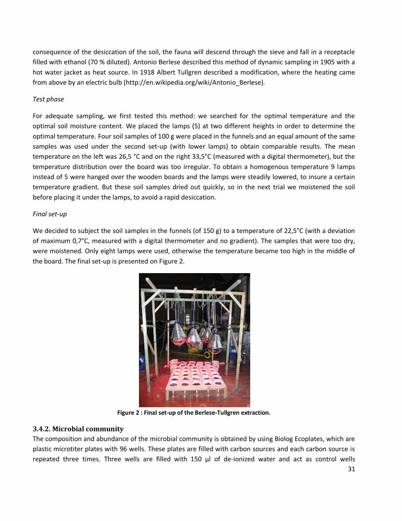
31

consequence of the desiccation of the soil, the fauna will descend through the sieve and fall in a receptacle

filled with ethanol (70 % diluted). Antonio Berlese described this method of dynamic sampling in 1905 with a

hot water jacket as heat source. In 1918 Albert Tullgren described a modification, where the heating came

from above by an electric bulb (http://en.wikipedia.org/wiki/Antonio_Berlese).

Test phase

For adequate sampling, we first tested this method: we searched for the optimal temperature and the

optimal soil moisture content. We placed the lamps (5) at two different heights in order to determine the

optimal temperature. Four soil samples of 100 g were placed in the funnels and an equal amount of the same

samples was used under the second set-up (with lower lamps) to obtain comparable results. The mean

temperature on the left was 26,5 °C and on the right 33,5°C (measured with a digital thermometer), but the

temperature distribution over the board was too irregular. To obtain a homogenous temperature 9 lamps

instead of 5 were hanged over the wooden boards and the lamps were steadily lowered, to insure a certain

temperature gradient. But these soil samples dried out quickly, so in the next trial we moistened the soil

before placing it under the lamps, to avoid a rapid desiccation.

Final set-up

We decided to subject the soil samples in the funnels (of 150 g) to a temperature of 22,5°C (with a deviation

of maximum 0,7°C, measured with a digital thermometer and no gradient). The samples that were too dry,

were moistened. Only eight lamps were used, otherwise the temperature became too high in the middle of

the board. The final set-up is presented on Figure 2.

Figure 2 : Final set-up of the Berlese-Tullgren extraction.

3.4.2. Microbial community

The composition and abundance of the microbial community is obtained by using Biolog Ecoplates, which are

plastic microtiter plates with 96 wells. These plates are filled with carbon sources and each carbon source is

repeated three times. Three wells are filled with 150 µl of de-ionized water and act as control wells

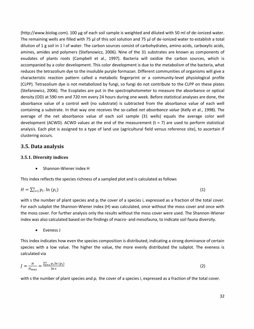
32

(http://www.biolog.com). 100 µg of each soil sample is weighted and diluted with 50 ml of de-ionized water.

The remaining wells are filled with 75 µl of this soil solution and 75 µl of de-ionized water to establish a total

dilution of 1 g soil in 1 l of water. The carbon sources consist of carbohydrates, amino acids, carboxylic acids,

amines, amides and polymers (Stefanowicz, 2006). Nine of the 31 substrates are known as components of

exudates of plants roots (Campbell et al., 1997). Bacteria will oxidize the carbon sources, which is

accompanied by a color development. This color development is due to the metabolism of the bacteria, what

reduces the tetrazolium dye to the insoluble purple formazan. Different communities of organisms will give a

characteristic reaction pattern called a metabolic fingerprint or a community-level physiological profile

(CLPP). Tetrazolium dye is not metabolized by fungi, so fungi do not contribute to the CLPP on these plates

(Stefanowicz, 2006). The Ecoplates are put in the spectrophotometer to measure the absorbance or optical

density (OD) at 590 nm and 720 nm every 24 hours during one week. Before statistical analyses are done, the

absorbance value of a control well (no substrate) is subtracted from the absorbance value of each well

containing a substrate. In that way one receives the so-called net absorbance value (Kelly et al., 1998). The

average of the net absorbance value of each soil sample (31 wells) equals the average color well

development (ACWD). ACWD values at the end of the measurement (t = 7) are used to perform statistical

analysis. Each plot is assigned to a type of land use (agricultural field versus reference site), to ascertain if

clustering occurs.

3.5. Data analysis

3.5.1. Diversity indices

Shannon-Wiener index H

This index reflects the species richness of a sampled plot and is calculated as follows

(1)

with s the number of plant species and pi the cover of a species i, expressed as a fraction of the total cover.

For each subplot the Shannon-Wiener index (H) was calculated, once without the moss cover and once with

the moss cover. For further analysis only the results without the moss cover were used. The Shannon-Wiener

index was also calculated based on the findings of macro- and mesofauna, to indicate soil fauna diversity.

Eveness J

This index indicates how even the species composition is distributed, indicating a strong dominance of certain

species with a low value. The higher the value, the more evenly distributed the subplot. The eveness is

calculated via

(2)

with s the number of plant species and pi the cover of a species i, expressed as a fraction of the total cover.

33

3.5.2. Weighted mean Ellenberg scores

Ellenberg’s indicator values are used to order plants with the same ecological traits in classes. These classes

consist of a nine point scale for soil acidity (R), productivity/nutrients (N), soil humidity (F), continentality (K),

soil salt content (S) and light (L). For each subplot the weighted mean Ellenberg value for acidity (mR), light

(mL), humidity (mF) and productivity (mN) was calculated via the following formula

(3)

with mN1 the weighted mean value of N for subplot 1, N1 the value of N for species 1 and x11 the cover of

species 1 in subplot 1 (in %). The same calculation was executed for mL, mR and mF.

3.5.3. Ordination

Ordination techniques are used to represent the relationship between species composition and the

underlying environmental gradients in a low-dimensional space. Via ordination, similarities between species

and samples will be detected and projected onto two dimensions in such a way that species and samples

most similar to one another will be close together, while dissimilar species and samples will appear farther

apart. The closer the species is to a subplot, the higher its abundance in that subplot (Verheyen, 2011). These

results can be related to environmental gradients, in order to determine which factors influence the

community structure. This is the principle of indirect (or unconstrained) ordination techniques, e.g.

Detrended Correspondence Analysis (DCA), Principal Components Analysis (PCA) and Non-Metric

Multidimensional Scaling (NMDS). Direct (or constrained) ordination techniques, such as Canonical

Correspondence Analysis (CCA) and Redundancy Analysis (RDA), instantly use environmental gradients to

order species and samples onto the ordination scheme. The length of gradient (a measure for species

turnover) determines if the response is linear (< 3) or unimodal (> 4) and consequently which technique

should be used, since PCA is applicable in case of a linear response and DCA when the response is unimodal.

Based on the value of the length of gradient DCA was performed, but due to inappropriate ordination

diagrams, NMDS was used, where an arch effect rarely occurs. This method analyses the matrix of

dissimilarities between n samples and finds a configuration of these objects in a k-dimensional ordination

space (k = 2), so that those distances in ordination space correspond to dissimilarities. The term ‘Stress’

measures the lack of fit between distances in ordination space and dissimilarities.

(4)

where is the distance between sample points in the ordination diagram, is the dissimilarity in the

original matrix of distances and f() is a non-metric monotonous transformation (Leps and Smilauer, 2003).

NMDS sometimes can’t represent all relationships accurately, which is reflected by a high Stress value.

Contrary to eigenvector methods such as PCA, NMDS calculations do not maximize the variability associated

with individual axes of the ordination, meaning that NMDS axes are arbitrary, so the final plots can be

rotated, centered, and inverted (http://www.ohio.edu). Environmental factors are added to the ordination

diagram as arrows. The direction of the arrow shows the direction of the strongest gradient or change in the

variable. The length of the arrow is proportional to the correlation between ordination and environmental

34

variable and this is often called the strength of the gradient. The goodness of fit of the environmental factor

is the squared correlation coefficient (r²). This is defined as

(5)

where ss_w and ss_t are within-group and total sums of squares.

For each variable group a separate CCA was done (abiotic variables, macro- and mesofauna, and microfauna).

The forward selection option was used to exclude non-significant variables. Next, the unique fraction of

variance explained by one set of variables and not shared with other sets was obtained by partial CCA, in

which the significant member variables of the concerning group are used as constraining variables, while the

significant variables of all other sets are treated as covariables (Borcard et al., 1992). ANOVA was executed to

ascertain the significance of the used and retained models.

3.5.4. Classification

Classification aims the same as ordination, in that both are multivariate techniques who wish to visualize the

community structure in an accurate way. Clustering of samples can be obtained by several methods:

hierarchical (usually displayed by a dendrogram) versus non-hierarchical, divisive (from the top) versus

agglomerative (from the bottom) and monothetic (division based on a single attribute) versus polythetic

(division based on multiple attributes). Two-way indicator species analysis (TWINSPAN) is an example of a

hierarchical, divisive and polythetic classification method (Leps and Smilauer, 2003). The TWINSPAN method

was performed with the program PCORD, with 0, 2, 5, 10 and 20 as cutlevels and a minimum group size of

five species for division. The Mann-Whitney-Wilcoxon test is used to decide whether the population

distributions are identical, without assuming them to follow the normal distribution (www.r-tutor.com).

3.5.5. Statistical analysis (Mixed models and Mantel test)

Normality was tested with SPSS 19.0 through a Shapiro-Wilk normality test. To ascertain there was no

multicollinearity between the predictor variables, variance inflation factors (VIF) were calculated as follows:

(6)

Low VIF values (i.e smaller than three) indicate low collinearity and allow the variables to be used in the same

model. So-called mixed-effect models (or just mixed models) are often appropriate for representing

clustered, and therefore dependent data, for instance, when data are collected hierarchically, as is in our

case (subplots in plots, plots in areas). Mixed models were performed in RStudio. First, a null model was

constructed, to which the predictor variables were added. Calculation of the intra-class correlation (ICC)

shows the proportion of total variance due to the hierarchy in the data, meaning that the remaining variance

can be described by predictor variables, where is the variance of the intercept and

is the variance of

the residuals:

(7)

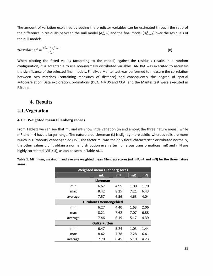
35

The amount of variation explained by adding the predictor variables can be estimated through the ratio of

the difference in residuals between the null model ( and the final model (

over the residuals of

the null model:

(8)

When plotting the fitted values (according to the model) against the residuals results in a random

configuration, it is acceptable to use non-normally distributed variables. ANOVA was executed to ascertain

the significance of the selected final models. Finally, a Mantel test was performed to measure the correlation

between two matrices (containing measures of distance) and consequently the degree of spatial

autocorrelation. Data exploration, ordinations (DCA, NMDS and CCA) and the Mantel test were executed in

RStudio.

4. Results

4.1. Vegetation

4.1.1. Weighted mean Ellenberg scores

From Table 1 we can see that mL and mF show little variation (in and among the three nature areas), while

mR and mN have a larger range. The nature area Liereman (L) is slightly more acidic, whereas soils are more

N-rich in Turnhouts Vennengebied (TV). The factor mF was the only floral characteristic distributed normally,

the other values didn’t obtain a normal distribution even after numerous transformations. mR and mN are

highly correlated (VIF > 3), as can be seen in Table AI.1.

Table 1: Minimum, maximum and average weighted mean Ellenberg scores (mL,mF,mR and mN) for the three nature

areas.

Weighted mean Ellenberg sores

mL mF mR mN

Liereman

min 6.67 4.95 1.00 1.70

max 8.42 8.25 7.21 6.43

average 7.57 6.56 4.63 4.04

Turnhouts Vennengebied

min 6.27 4.40 1.63 2.06

max 8.21 7.62 7.07 6.88

average 7.46 6.19 5.17 4.39

Gulke Putten

min 6.47 5.24 1.03 1.44

max 8.42 7.78 7.28 6.41

average 7.70 6.45 5.10 4.23

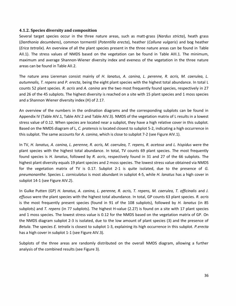
36

4.1.2. Species diversity and composition

Several target species occur in the three nature areas, such as matt-grass (Nardus stricta), heath grass

(Danthonia decumbens), common tormentil (Potentilla erecta), heather (Calluna vulgaris) and bog heather

(Erica tetralix). An overview of all the plant species present in the three nature areas can be found in Table

AII.1). The stress values of NMDS based on the vegetation can be found in Table AIII.1. The minimum,

maximum and average Shannon-Wiener diversity index and eveness of the vegetation in the three nature

areas can be found in Table AII.2.

The nature area Liereman consist mainly of H. lanatus, A. canina, L. perenne, R. acris, M. caerulea, L.

autumnalis, T. repens and P. erecta, being the eight plant species with the highest total abundance. In total L

counts 52 plant species. R. acris and A. canina are the two most frequently found species, respectively in 27

and 26 of the 45 subplots. The highest diversity is reached on a site with 15 plant species and 1 moss species

and a Shannon Wiener diversity index (H) of 2.17.

An overview of the numbers in the ordination diagrams and the corresponding subplots can be found in

Appendix IV (Table AIV.1, Table AIV.2 and Table AIV.3). NMDS of the vegetation matrix of L results in a lowest

stress value of 0.12. When species are located near a subplot, they have a high relative cover in this subplot.

Based on the NMDS diagram of L, C. pratensis is located closest to subplot 5-2, indicating a high occurrence in

this subplot. The same accounts for A. canina, which is close to subplot 7-2 (see Figure AIV.1).

In TV, H. lanatus, A. canina, L. perenne, R. acris, M. caerulea, T. repens, R. acetosa and L. hispidus were the

plant species with the highest total abundance. In total, TV counts 69 plant species. The most frequently

found species is H. lanatus, followed by R. acris, respectively found in 31 and 27 of the 66 subplots. The

highest plant diversity equals 19 plant species and 2 moss species. The lowest stress value obtained via NMDS

for the vegetation matrix of TV is 0.17. Subplot 2-1 is quite isolated, due to the presence of G.

pneumonanthe. Species L. corniculatus is most abundant in subplot 4-5, while H. lanatus has a high cover in

subplot 14-1 (see Figure AIV.2).

In Gulke Putten (GP) H. lanatus, A. canina, L. perenne, R. acris, T. repens, M. caerulea, T. officinalis and J.

effusus were the plant species with the highest total abundance. In total, GP counts 63 plant species. R. acris

is the most frequently present species (found in 91 of the 108 subplots), followed by H. lanatus (in 85

subplots) and T. repens (in 77 subplots). The highest H-value (2.27) is found on a site with 17 plant species

and 1 moss species. The lowest stress value is 0.12 for the NMDS based on the vegetation matrix of GP. On

the NMDS diagram subplot 2-3 is isolated, due to the low amount of plant species (3) and the presence of

Betula. The species E. tetralix is closest to subplot 1-3, explaining its high occurrence in this subplot. P.erecta

has a high cover in subplot 1-1 (see Figure AIV.3).

Subplots of the three areas are randomly distributed on the overall NMDS diagram, allowing a further

analysis of the combined results (see Figure 3).

37

Figure 3: NMDS ordination diagram based on the vegetation surveys in Liereman, Turnhouts Vennengebied and Gulke

Putten (black = Liereman, red = Turnhouts Vennengebied, green = Gulke Putten).

4.1.3. Classification

TWINSPAN led to three division levels (see Figure 4). Group 0 and 1 significantly differ based on all abiotic soil

characteristics and all weighted mean Ellenberg scores. Group 00 and 01 differ in all variables, except for mL.

Values for exchangeable Ca and mL do not differ significantly for group 11 and 10, whereas values of all other

variables do. Divergence of groups 010 and 011 is based on differences in exchangeable Ca, mL and mN. mN

is determinant in separating groups 110 and 111. Group 00 isn’t divided, since subdivisions contain an

insufficient number of subplots, while group 10 can’t be divided since variables do not differ significantly (p <

0.05). Correlations between TWINSPAN groups and abiotic soil characteristics and between TWINSPAN

groups and mean weighted Ellenberg scores, can be found in Table AV.1, along with the two-way ordered

tables (Figure AV.1).

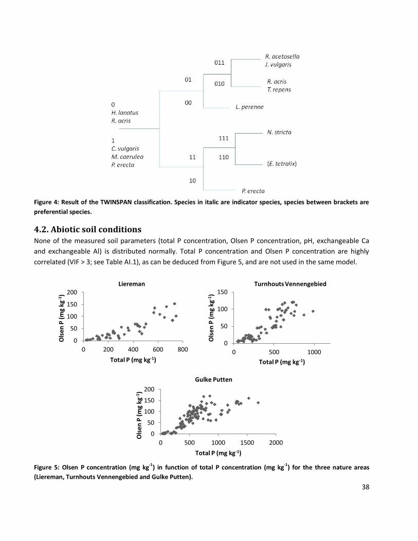
38

Figure 4: Result of the TWINSPAN classification. Species in italic are indicator species, species between brackets are

preferential species.

4.2. Abiotic soil conditions None of the measured soil parameters (total P concentration, Olsen P concentration, pH, exchangeable Ca

and exchangeable Al) is distributed normally. Total P concentration and Olsen P concentration are highly

correlated (VIF > 3; see Table AI.1), as can be deduced from Figure 5, and are not used in the same model.

Figure 5: Olsen P concentration (mg kg-1) in function of total P concentration (mg kg-1) for the three nature areas

(Liereman, Turnhouts Vennengebied and Gulke Putten).

0

50

100

150

200

0 200 400 600 800

Ols

en P

(m

g kg

-1)

Total P (mg kg-1)

Liereman

0

50

100

150

0 500 1000

Ols

en P

(m

g kg

-1)

Total P (mg kg-1)

Turnhouts Vennengebied

0

50

100

150

200

0 500 1000 1500 2000

Ols

en P

(m

g kg

-1)

Total P (mg kg-1)

Gulke Putten

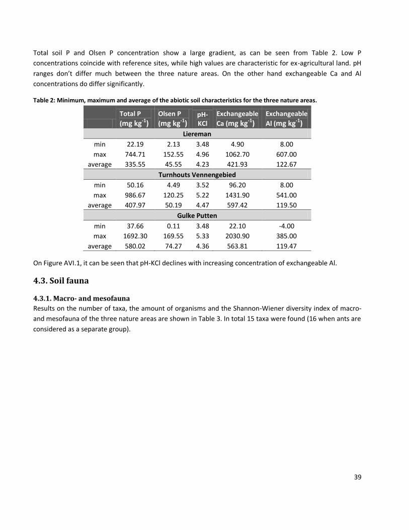
39

Total soil P and Olsen P concentration show a large gradient, as can be seen from Table 2. Low P

concentrations coincide with reference sites, while high values are characteristic for ex-agricultural land. pH

ranges don’t differ much between the three nature areas. On the other hand exchangeable Ca and Al

concentrations do differ significantly.

Table 2: Minimum, maximum and average of the abiotic soil characteristics for the three nature areas.

Total P

(mg kg-1) Olsen P

(mg kg-1) pH-KCl

Exchangeable

Ca (mg kg-1)

Exchangeable

Al (mg kg-1)

Liereman

min 22.19 2.13 3.48 4.90 8.00

max 744.71 152.55 4.96 1062.70 607.00

average 335.55 45.55 4.23 421.93 122.67

Turnhouts Vennengebied

min 50.16 4.49 3.52 96.20 8.00

max 986.67 120.25 5.22 1431.90 541.00

average 407.97 50.19 4.47 597.42 119.50

Gulke Putten

min 37.66 0.11 3.48 22.10 -4.00

max 1692.30 169.55 5.33 2030.90 385.00

average 580.02 74.27 4.36 563.81 119.47

On Figure AVI.1, it can be seen that pH-KCl declines with increasing concentration of exchangeable Al.

4.3. Soil fauna

4.3.1. Macro- and mesofauna

Results on the number of taxa, the amount of organisms and the Shannon-Wiener diversity index of macro-

and mesofauna of the three nature areas are shown in Table 3. In total 15 taxa were found (16 when ants are

considered as a separate group).

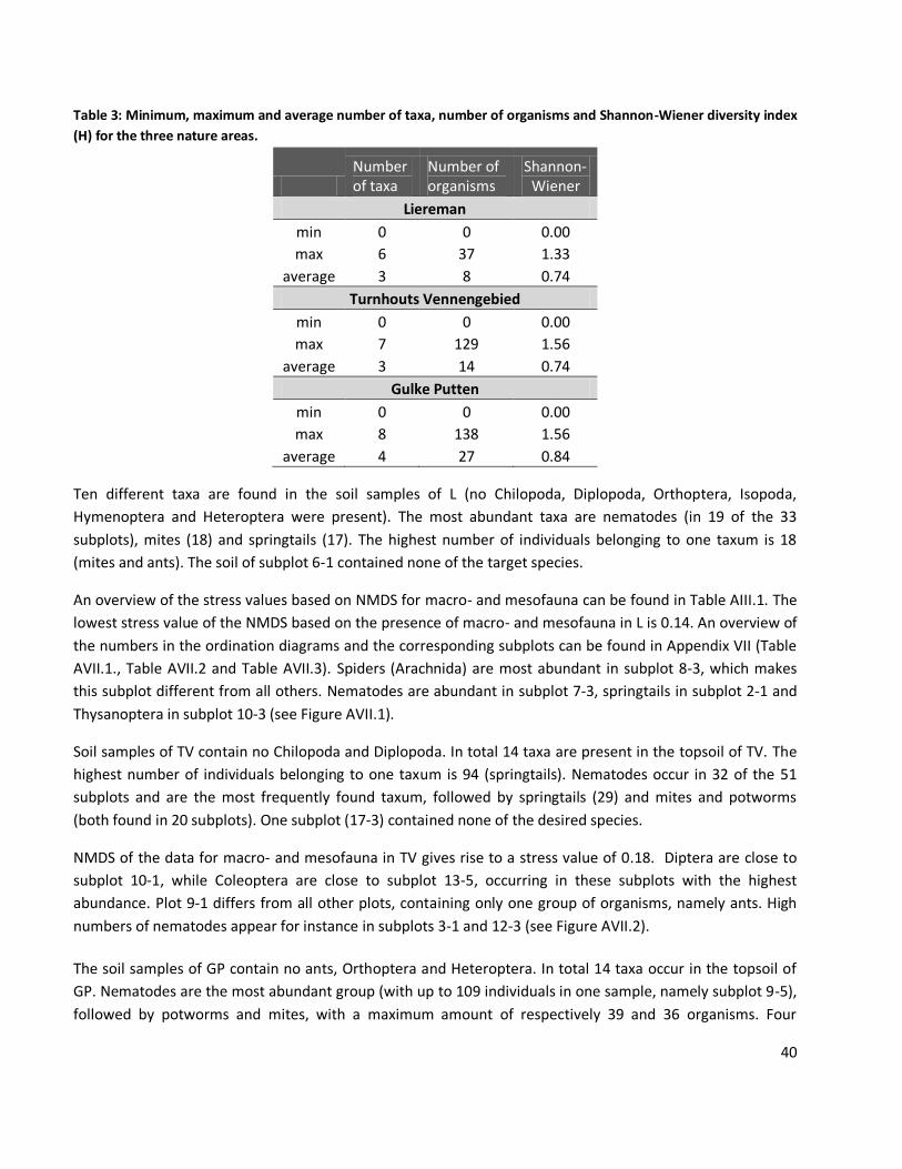
40

Table 3: Minimum, maximum and average number of taxa, number of organisms and Shannon-Wiener diversity index

(H) for the three nature areas.

Number of taxa

Number of organisms

Shannon-Wiener

Liereman

min 0 0 0.00

max 6 37 1.33

average 3 8 0.74

Turnhouts Vennengebied

min 0 0 0.00

max 7 129 1.56

average 3 14 0.74

Gulke Putten

min 0 0 0.00

max 8 138 1.56

average 4 27 0.84

Ten different taxa are found in the soil samples of L (no Chilopoda, Diplopoda, Orthoptera, Isopoda,

Hymenoptera and Heteroptera were present). The most abundant taxa are nematodes (in 19 of the 33

subplots), mites (18) and springtails (17). The highest number of individuals belonging to one taxum is 18

(mites and ants). The soil of subplot 6-1 contained none of the target species.

An overview of the stress values based on NMDS for macro- and mesofauna can be found in Table AIII.1. The

lowest stress value of the NMDS based on the presence of macro- and mesofauna in L is 0.14. An overview of

the numbers in the ordination diagrams and the corresponding subplots can be found in Appendix VII (Table

AVII.1., Table AVII.2 and Table AVII.3). Spiders (Arachnida) are most abundant in subplot 8-3, which makes

this subplot different from all others. Nematodes are abundant in subplot 7-3, springtails in subplot 2-1 and

Thysanoptera in subplot 10-3 (see Figure AVII.1).

Soil samples of TV contain no Chilopoda and Diplopoda. In total 14 taxa are present in the topsoil of TV. The

highest number of individuals belonging to one taxum is 94 (springtails). Nematodes occur in 32 of the 51

subplots and are the most frequently found taxum, followed by springtails (29) and mites and potworms

(both found in 20 subplots). One subplot (17-3) contained none of the desired species.

NMDS of the data for macro- and mesofauna in TV gives rise to a stress value of 0.18. Diptera are close to

subplot 10-1, while Coleoptera are close to subplot 13-5, occurring in these subplots with the highest

abundance. Plot 9-1 differs from all other plots, containing only one group of organisms, namely ants. High

numbers of nematodes appear for instance in subplots 3-1 and 12-3 (see Figure AVII.2).

The soil samples of GP contain no ants, Orthoptera and Heteroptera. In total 14 taxa occur in the topsoil of

GP. Nematodes are the most abundant group (with up to 109 individuals in one sample, namely subplot 9-5),

followed by potworms and mites, with a maximum amount of respectively 39 and 36 organisms. Four

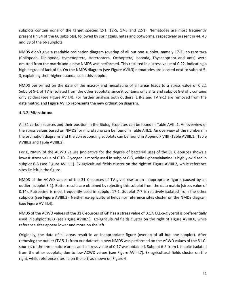
41

subplots contain none of the target species (2-1, 12-5, 17-3 and 22-1). Nematodes are most frequently

present (in 54 of the 66 subplots), followed by springtails, mites and potworms, respectively present in 44, 40

and 39 of the 66 subplots.

NMDS didn’t give a readable ordination diagram (overlap of all but one subplot, namely 17-2), so rare taxa

(Chilopoda, Diplopoda, Hymenoptera, Heteroptera, Orthoptera, Isopoda, Thysanoptera and ants) were

omitted from the matrix and a new NMDS was performed. This resulted in a stress value of 0.22, indicating a

high degree of lack of fit. On the NMDS diagram (see Figure AVII.3) nematodes are located next to subplot 5-

3, explaining their higher abundance in this subplot.

NMDS performed on the data of the macro- and mesofauna of all areas leads to a stress value of 0.22.

Subplot 9-1 of TV is isolated from the other subplots, since it contains only ants and subplot 8-3 of L contains

only spiders (see Figure AVII.4). For further analysis both outliers (L 8-3 and TV 9-1) are removed from the

data matrix, and Figure AVII.5 represents the new ordination diagram.

4.3.2. Microfauna

All 31 carbon sources and their position in the Biolog Ecoplates can be found in Table AVIII.1. An overview of

the stress values based on NMDS for microfauna can be found in Table AIII.1. An overview of the numbers in

the ordination diagrams and the corresponding subplots can be found in Appendix VIIII (Table AVIIII.1., Table

AVIIII.2 and Table AVIIII.3).

For L, NMDS of the ACWD values (indicative for the degree of bacterial use) of the 31 C-sources shows a

lowest stress value of 0.10. Glycogen is mostly used in subplot 6-3, while L-phenylalanine is highly oxidized in

subplot 6-5 (see Figure AVIIII.1). Ex-agricultural fields cluster on the right of Figure AVIIII.2, while reference

sites lie left in the figure.

NMDS of the ACWD values of the 31 C-sources of TV gives rise to an inappropriate figure, caused by an

outlier (subplot 5-1). Better results are obtained by rejecting this subplot from the data matrix (stress value of

0.14). Putrescine is most frequently used in subplot 17-1. Subplot 7-7 is relatively isolated from the other

subplots (see Figure AVIIII.3). Neither ex-agricultural fields nor reference sites cluster on the NMDS diagram

(see Figure AVIIII.4).

NMDS of the ACWD values of the 31 C-sources of GP has a stress value of 0.17. D,L-α-glycerol is preferentially

used in subplot 18-3 (see Figure AVIIII.5). Ex-agricultural fields cluster on the right of Figure AVIIII.6, while

reference sites appear lower and more on the left.

Originally, the data of all areas result in an inappropriate figure (overlap of all but one subplot). After

removing the outlier (TV 5-1) from our dataset, a new NMDS was performed on the ACWD values of the 31 C-

sources of the three nature areas and a stress value of 0.17 was obtained. Subplot 6-3 from L is quite isolated

from the other subplots, due to low ACWD values (see Figure AVIIII.7). Ex-agricultural fields cluster on the

right, while reference sites lie on the left, as shown on Figure 6.

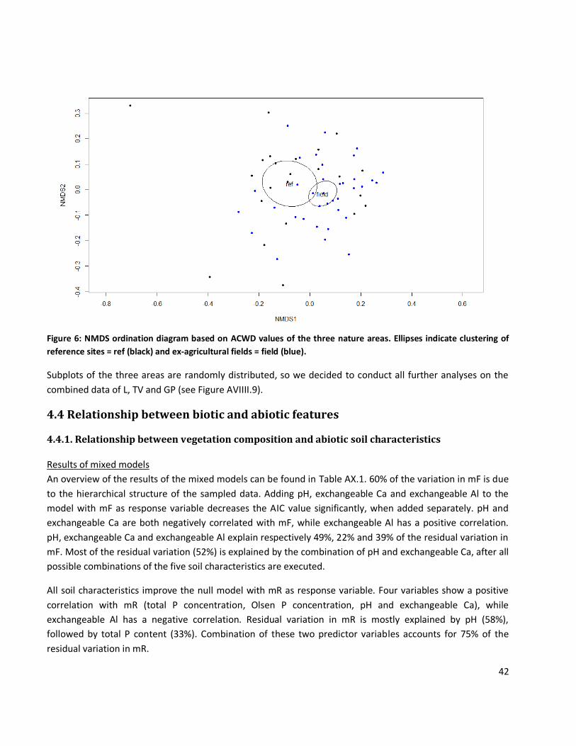
42

Figure 6: NMDS ordination diagram based on ACWD values of the three nature areas. Ellipses indicate clustering of

reference sites = ref (black) and ex-agricultural fields = field (blue).

Subplots of the three areas are randomly distributed, so we decided to conduct all further analyses on the

combined data of L, TV and GP (see Figure AVIIII.9).

4.4 Relationship between biotic and abiotic features

4.4.1. Relationship between vegetation composition and abiotic soil characteristics

Results of mixed models

An overview of the results of the mixed models can be found in Table AX.1. 60% of the variation in mF is due

to the hierarchical structure of the sampled data. Adding pH, exchangeable Ca and exchangeable Al to the

model with mF as response variable decreases the AIC value significantly, when added separately. pH and

exchangeable Ca are both negatively correlated with mF, while exchangeable Al has a positive correlation.

pH, exchangeable Ca and exchangeable Al explain respectively 49%, 22% and 39% of the residual variation in

mF. Most of the residual variation (52%) is explained by the combination of pH and exchangeable Ca, after all

possible combinations of the five soil characteristics are executed.

All soil characteristics improve the null model with mR as response variable. Four variables show a positive

correlation with mR (total P concentration, Olsen P concentration, pH and exchangeable Ca), while

exchangeable Al has a negative correlation. Residual variation in mR is mostly explained by pH (58%),

followed by total P content (33%). Combination of these two predictor variables accounts for 75% of the

residual variation in mR.

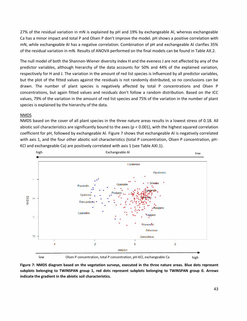
43

27% of the residual variation in mN is explained by pH and 19% by exchangeable Al, whereas exchangeable

Ca has a minor impact and total P and Olsen P don’t improve the model. pH shows a positive correlation with

mN, while exchangeable Al has a negative correlation. Combination of pH and exchangeable Al clarifies 35%

of the residual variation in mN. Results of ANOVA performed on the final models can be found in Table AX.2.

The null model of both the Shannon-Wiener diversity index H and the eveness J are not affected by any of the

predictor variables, although hierarchy of the data accounts for 50% and 44% of the explained variation,

respectively for H and J. The variation in the amount of red list species is influenced by all predictor variables,

but the plot of the fitted values against the residuals is not randomly distributed, so no conclusions can be

drawn. The number of plant species is negatively affected by total P concentrations and Olsen P

concentrations, but again fitted values and residuals don’t follow a random distribution. Based on the ICC

values, 79% of the variation in the amount of red list species and 75% of the variation in the number of plant

species is explained by the hierarchy of the data.

NMDS NMDS based on the cover of all plant species in the three nature areas results in a lowest stress of 0.18. All

abiotic soil characteristics are significantly bound to the axes (p < 0.001), with the highest squared correlation

coefficient for pH, followed by exchangeable Al. Figure 7 shows that exchangeable Al is negatively correlated

with axis 1, and the four other abiotic soil characteristics (total P concentration, Olsen P concentration, pH-

KCl and exchangeable Ca) are positively correlated with axis 1 (see Table AXI.1).

Figure 7: NMDS diagram based on the vegetation surveys, executed in the three nature areas. Blue dots represent

subplots belonging to TWINSPAN group 1, red dots represent subplots belonging to TWINSPAN group 0. Arrows

indicate the gradient in the abiotic soil characteristics.

high low Olsen P concentration, total P concentration, pH-KCl, exchangeable Ca

low high Exchangeable Al

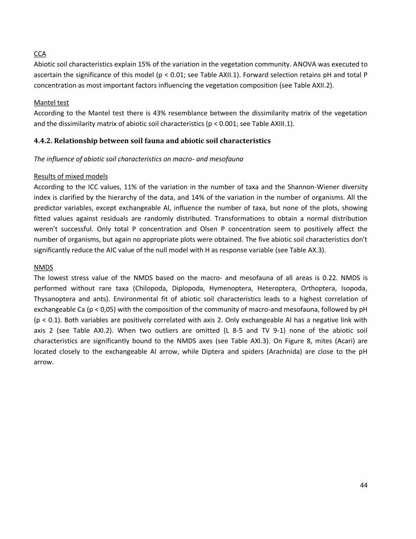
44

CCA

Abiotic soil characteristics explain 15% of the variation in the vegetation community. ANOVA was executed to

ascertain the significance of this model (p < 0.01; see Table AXII.1). Forward selection retains pH and total P

concentration as most important factors influencing the vegetation composition (see Table AXII.2).

Mantel test

According to the Mantel test there is 43% resemblance between the dissimilarity matrix of the vegetation

and the dissimilarity matrix of abiotic soil characteristics (p < 0.001; see Table AXIII.1).

4.4.2. Relationship between soil fauna and abiotic soil characteristics

The influence of abiotic soil characteristics on macro- and mesofauna

Results of mixed models

According to the ICC values, 11% of the variation in the number of taxa and the Shannon-Wiener diversity

index is clarified by the hierarchy of the data, and 14% of the variation in the number of organisms. All the

predictor variables, except exchangeable Al, influence the number of taxa, but none of the plots, showing

fitted values against residuals are randomly distributed. Transformations to obtain a normal distribution

weren’t successful. Only total P concentration and Olsen P concentration seem to positively affect the

number of organisms, but again no appropriate plots were obtained. The five abiotic soil characteristics don’t

significantly reduce the AIC value of the null model with H as response variable (see Table AX.3).

NMDS

The lowest stress value of the NMDS based on the macro- and mesofauna of all areas is 0.22. NMDS is

performed without rare taxa (Chilopoda, Diplopoda, Hymenoptera, Heteroptera, Orthoptera, Isopoda,

Thysanoptera and ants). Environmental fit of abiotic soil characteristics leads to a highest correlation of

exchangeable Ca (p < 0,05) with the composition of the community of macro-and mesofauna, followed by pH

(p < 0.1). Both variables are positively correlated with axis 2. Only exchangeable Al has a negative link with

axis 2 (see Table AXI.2). When two outliers are omitted (L 8-5 and TV 9-1) none of the abiotic soil

characteristics are significantly bound to the NMDS axes (see Table AXI.3). On Figure 8, mites (Acari) are

located closely to the exchangeable Al arrow, while Diptera and spiders (Arachnida) are close to the pH

arrow.

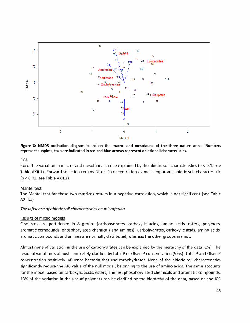
45

Figure 8: NMDS ordination diagram based on the macro- and mesofauna of the three nature areas. Numbers represent subplots, taxa are indicated in red and blue arrows represent abiotic soil characteristics.

CCA 6% of the variation in macro- and mesofauna can be explained by the abiotic soil characteristics (p < 0.1; see

Table AXII.1). Forward selection retains Olsen P concentration as most important abiotic soil characteristic

(p < 0.01; see Table AXII.2).

Mantel test The Mantel test for these two matrices results in a negative correlation, which is not significant (see Table AXIII.1).

The influence of abiotic soil characteristics on microfauna

Results of mixed models C-sources are partitioned in 8 groups (carbohydrates, carboxylic acids, amino acids, esters, polymers,

aromatic compounds, phosphorylated chemicals and amines). Carbohydrates, carboxylic acids, amino acids,

aromatic compounds and amines are normally distributed, whereas the other groups are not.

Almost none of variation in the use of carbohydrates can be explained by the hierarchy of the data (1%). The

residual variation is almost completely clarified by total P or Olsen P concentration (99%). Total P and Olsen P

concentration positively influence bacteria that use carbohydrates. None of the abiotic soil characteristics

significantly reduce the AIC value of the null model, belonging to the use of amino acids. The same accounts

for the model based on carboxylic acids, esters, amines, phosphorylated chemicals and aromatic compounds.

13% of the variation in the use of polymers can be clarified by the hierarchy of the data, based on the ICC

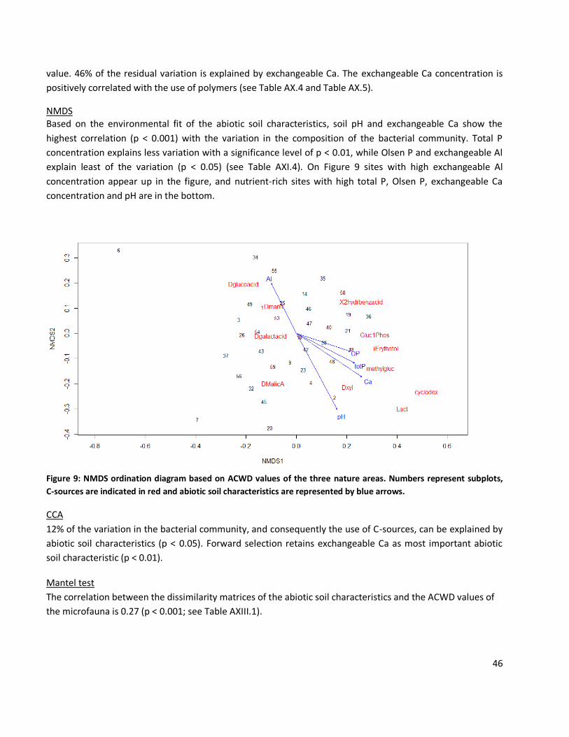
46

value. 46% of the residual variation is explained by exchangeable Ca. The exchangeable Ca concentration is

positively correlated with the use of polymers (see Table AX.4 and Table AX.5).

NMDS Based on the environmental fit of the abiotic soil characteristics, soil pH and exchangeable Ca show the

highest correlation (p < 0.001) with the variation in the composition of the bacterial community. Total P

concentration explains less variation with a significance level of p < 0.01, while Olsen P and exchangeable Al

explain least of the variation (p < 0.05) (see Table AXI.4). On Figure 9 sites with high exchangeable Al

concentration appear up in the figure, and nutrient-rich sites with high total P, Olsen P, exchangeable Ca

concentration and pH are in the bottom.

Figure 9: NMDS ordination diagram based on ACWD values of the three nature areas. Numbers represent subplots,

C-sources are indicated in red and abiotic soil characteristics are represented by blue arrows.

CCA

12% of the variation in the bacterial community, and consequently the use of C-sources, can be explained by

abiotic soil characteristics (p < 0.05). Forward selection retains exchangeable Ca as most important abiotic

soil characteristic (p < 0.01).

Mantel test

The correlation between the dissimilarity matrices of the abiotic soil characteristics and the ACWD values of

the microfauna is 0.27 (p < 0.001; see Table AXIII.1).

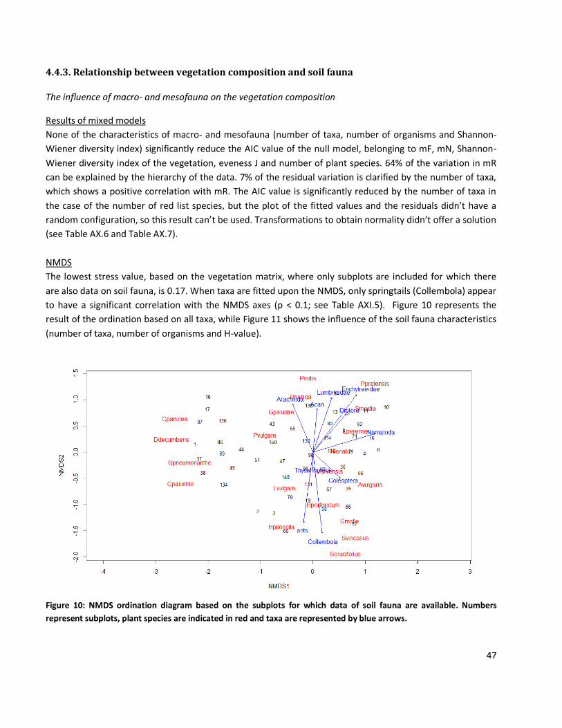
47

4.4.3. Relationship between vegetation composition and soil fauna

The influence of macro- and mesofauna on the vegetation composition

Results of mixed models

None of the characteristics of macro- and mesofauna (number of taxa, number of organisms and Shannon-

Wiener diversity index) significantly reduce the AIC value of the null model, belonging to mF, mN, Shannon-

Wiener diversity index of the vegetation, eveness J and number of plant species. 64% of the variation in mR

can be explained by the hierarchy of the data. 7% of the residual variation is clarified by the number of taxa,

which shows a positive correlation with mR. The AIC value is significantly reduced by the number of taxa in

the case of the number of red list species, but the plot of the fitted values and the residuals didn’t have a

random configuration, so this result can’t be used. Transformations to obtain normality didn’t offer a solution

(see Table AX.6 and Table AX.7).

NMDS

The lowest stress value, based on the vegetation matrix, where only subplots are included for which there

are also data on soil fauna, is 0.17. When taxa are fitted upon the NMDS, only springtails (Collembola) appear

to have a significant correlation with the NMDS axes (p < 0.1; see Table AXI.5). Figure 10 represents the

result of the ordination based on all taxa, while Figure 11 shows the influence of the soil fauna characteristics

(number of taxa, number of organisms and H-value).

Figure 10: NMDS ordination diagram based on the subplots for which data of soil fauna are available. Numbers

represent subplots, plant species are indicated in red and taxa are represented by blue arrows.

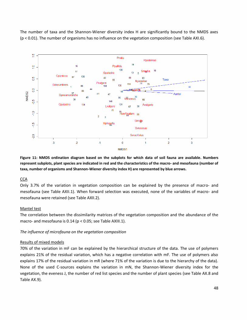
48

The number of taxa and the Shannon-Wiener diversity index H are significantly bound to the NMDS axes

(p < 0.01). The number of organisms has no influence on the vegetation composition (see Table AXI.6).

Figure 11: NMDS ordination diagram based on the subplots for which data of soil fauna are available. Numbers

represent subplots, plant species are indicated in red and the characteristics of the macro- and mesofauna (number of

taxa, number of organisms and Shannon-Wiener diversity index H) are represented by blue arrows.

CCA

Only 3.7% of the variation in vegetation composition can be explained by the presence of macro- and

mesofauna (see Table AXII.1). When forward selection was executed, none of the variables of macro- and

mesofauna were retained (see Table AXII.2).

Mantel test

The correlation between the dissimilarity matrices of the vegetation composition and the abundance of the

macro- and mesofauna is 0.14 (p < 0.05; see Table AXIII.1).

The influence of microfauna on the vegetation composition

Results of mixed models

70% of the variation in mF can be explained by the hierarchical structure of the data. The use of polymers

explains 21% of the residual variation, which has a negative correlation with mF. The use of polymers also

explains 17% of the residual variation in mR (where 71% of the variation is due to the hierarchy of the data).

None of the used C-sources explains the variation in mN, the Shannon-Wiener diversity index for the

vegetation, the eveness J, the number of red list species and the number of plant species (see Table AX.8 and

Table AX.9).

Taxa

H

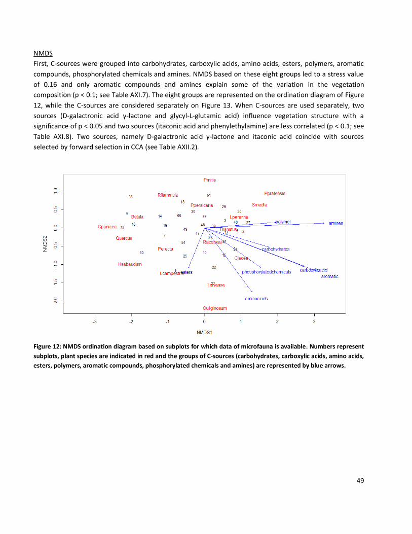
49

NMDS

First, C-sources were grouped into carbohydrates, carboxylic acids, amino acids, esters, polymers, aromatic

compounds, phosphorylated chemicals and amines. NMDS based on these eight groups led to a stress value

of 0.16 and only aromatic compounds and amines explain some of the variation in the vegetation

composition (p < 0.1; see Table AXI.7). The eight groups are represented on the ordination diagram of Figure

12, while the C-sources are considered separately on Figure 13. When C-sources are used separately, two

sources (D-galactronic acid γ-lactone and glycyl-L-glutamic acid) influence vegetation structure with a

significance of p < 0.05 and two sources (itaconic acid and phenylethylamine) are less correlated (p < 0.1; see

Table AXI.8). Two sources, namely D-galactronic acid γ-lactone and itaconic acid coincide with sources

selected by forward selection in CCA (see Table AXII.2).

Figure 12: NMDS ordination diagram based on subplots for which data of microfauna is available. Numbers represent

subplots, plant species are indicated in red and the groups of C-sources (carbohydrates, carboxylic acids, amino acids,

esters, polymers, aromatic compounds, phosphorylated chemicals and amines) are represented by blue arrows.

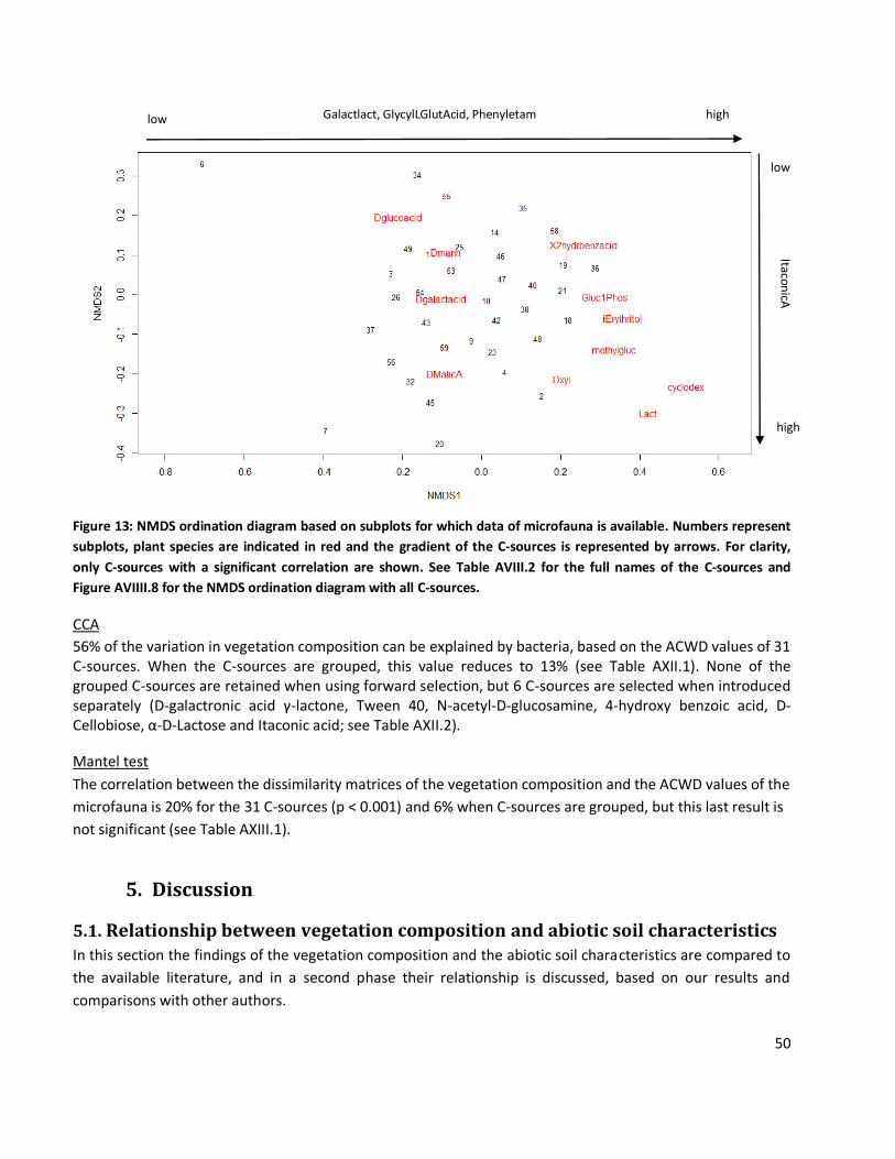
50

Figure 13: NMDS ordination diagram based on subplots for which data of microfauna is available. Numbers represent

subplots, plant species are indicated in red and the gradient of the C-sources is represented by arrows. For clarity,

only C-sources with a significant correlation are shown. See Table AVIII.2 for the full names of the C-sources and

Figure AVIIII.8 for the NMDS ordination diagram with all C-sources.

CCA

56% of the variation in vegetation composition can be explained by bacteria, based on the ACWD values of 31 C-sources. When the C-sources are grouped, this value reduces to 13% (see Table AXII.1). None of the grouped C-sources are retained when using forward selection, but 6 C-sources are selected when introduced separately (D-galactronic acid γ-lactone, Tween 40, N-acetyl-D-glucosamine, 4-hydroxy benzoic acid, D-Cellobiose, α-D-Lactose and Itaconic acid; see Table AXII.2).

Mantel test

The correlation between the dissimilarity matrices of the vegetation composition and the ACWD values of the

microfauna is 20% for the 31 C-sources (p < 0.001) and 6% when C-sources are grouped, but this last result is

not significant (see Table AXIII.1).

5. Discussion

5.1. Relationship between vegetation composition and abiotic soil characteristics In this section the findings of the vegetation composition and the abiotic soil characteristics are compared to

the available literature, and in a second phase their relationship is discussed, based on our results and

comparisons with other authors.

high low Galactlact, GlycylLGlutAcid, Phenyletam

low

high

ItaconicA

51

The value mL was not considered in the analysis, since it was consistently high (ranging between six and

eight), reflecting that all plant species need a lot of light to be able to grow. Species with a light value of less

than six are considered forest species, that is species of the understory (1–3) or canopy gaps of moderate size

(4–5) (Ellenberg, 1988). The high light values of our experiment indicate that plants need an open habitat.

The present species are found in dry to moist environments, since mF ranges between 5.0 and 8.2 in the

three study areas. mR and mN show a stronger variation, whereby mR lies between 1 and 7 for the three

areas, characterizing the soils as strongly acidic to weakly acidic and even weakly basic. mN varies between 1

and 6 for L and GP, meaning that soils have a low N concentration at low mN values and have an

intermediate N concentration at a value of 6. TV has a slightly higher minimum, indicating that soils are richer

in N, compared to the other nature areas. The large variation in mR and mN converges with the succession

gradient of nutrient-rich ex-agricultural land to nutrient-poor, acidic reference sites. The highest amount of

plant species occurs in TV, but target species are sown in this nature area.

Based on the classification technique, the vegetation can be divided in two groups. These two groups differ

on all variables (weighted mean Ellenberg scores and abiotic soil characteristics), but the strongest

significance accounts for mN. Species of the first group are typical for nutrient-rich soils (H. lanatus and R.

acris), while species of the second group are characteristic for nutrient-poor sites (C. vulgaris, P. erecta and

M. caerulea, all frequently present in Nardo-Galion grasslands). The first group is further divided in two

subgroups, with L. perenne as indicator species for the first subdivision. Preferential species for the second

subdivision are L. hispidus and L. autumnalis. These species grow on moderately rich soils, whereas plants of

the first subdivision have a high fertility requirement (http://plants.usda.gov), thus nutrient availability steers

this division. The second subdivision can be split in a group of plants occurring on calcareous, N-rich soils

(such as R. acris and T. repens), while R. acetosella and J. vulgaris are indicative for the second group. These

plant species grow on acid, N-rich soils (http://www.soortenbank.nl), so exchangeable Ca concentration

drives this separation. The second group of the first subdivision (characterized by species of nutrient-poor

sites) can be divided in two groups, based on the Olsen P concentration and mR. One group is represented by

P. erecta, and the second group is represented by C. vulgaris, which needs more acid soils. The latter can be

split in two, where one group is characterized by E. tetralix, a heathland species, and the second group by N.

stricta. Other plant species in this group are D. decumbens and C. panicea, both occur on rather nutrient-

poor, acid soils.

There are two methods for measuring soil pH: pH-KCl (used in this master thesis) and pH-H2O, where pH-KCl

has consistently lower values than pH-H2O. pH-KCl values can be converted to pH-H2O values via the formula

(9)

(Azedevoa et al., submitted) resulting in a range of 4.5 to 6.2 pH-H2O, which is consistent with the pH range,

typical for Nardo-Galion grassland, according to Zwaenepoel and Stieperaere (2002) and Herr et al. (2011).

Protons bound to clay particles and humus are released when KCl is added to soil, but not when H2O is added

(only free protons are measured) (http://www.agriton.nl), explaining the higher values of pH-H2O. On Figure

AVI.1 the concentration of exchangeable Al starts to rise when pH-KCl reaches a value of 4. This is consistent

with Kennedy (1992) who stated that in acidic soils (pH-H2O below 4.5) unstable clay minerals release soluble

52

Al, which becomes bioavailable. Within the pH range of 4.5 to 6.0, soil acidity is buffered by cation exchange

processes (Ulrich, 1983). The pH will drop when base saturation of the exchange complex is depleted, and

this results in an increased leaching of base cations, increased Al mobilization and enhanced Al:Ca ratios (Van

Breemen et al., 1982). Al is an abundant metal in the earth’s crust, where it is part of most clay particles.

When the soil pH is above 5.5, the Al in soils remains in a solid combination with other elements and is not

harmful to plants. As the pH drops below 5.5, Al containing materials begin to dissolve

(http://www.soiltesting.okstate.edu). Below a pH-H2O value of about 4.2, Al is released and can become toxic

for plants and soil fauna (Falkengren-Grerup and Tyler, 1993), thus below this threshold only species tolerant

of Al toxicity are found (Grime et al., 2007). However, it is difficult to make a generalization of this threshold,

since it appears to be different for each plant species and soil type (Boxman et al., 1991).

The range of Olsen P and total P concentration indicates that sites where cessation of agriculture happened

recently as well as reference sites were sampled. Reference values for total P and Olsen P concentration of

Nardo-Galion grasslands are 145 to 450 mg total P kg-1 and 5 to 9 mg Olsen P kg-1 (Hommel, 2006) or 11 mg

Olsen P kg-1, according to Zwaenepoel and Stieperaere (2002). Indeed, our reference sites have an Olsen P

concentration between < 0.1 and 20 mg P kg-1 and a total P concentration between 22 and 319 mg P kg-1. Ex-

agricultural land shows a large variation in total P and Olsen P concentration (from 75 to 1692 mg total P kg -1

and from 10 to 170 mg Olsen P kg-1). Rooney et al. (2009) found that phosphate addition to acidic upland

grassland soil significantly increases soil pH, confirming the results of mixed models, where higher total P

concentration and Olsen P concentration result in an increasing mR (measure for pH). However, this was not

clearly reflected by the measured pH values, where high values (> 4.5) occur on soils with high total P

concentration, but not in the case of Olsen P concentration. P bioavailability is profoundly influenced by

changes in soil pH. In agricultural soils, the pH-H2O is generally maintained between 6 and 7, since this pH

range corresponds to the range with the highest fraction of bioavailable P (Stevenson and Cole, 1999). In soils

with lower pH, Fe and Al phosphates can be formed, whereas Ca phosphates occur in soils with higher pH

(Bardgett, 2005). On the other hand, mR is lower on more acid soils, where higher exchangeable Al

concentrations occur.

A rise in pH should increase the number of dicots and negatively influence grasses, according to Duprè et al.

(2010), but this wasn’t true for our results, since grasses have a higher cover on sites with a high mR value

(> 5). Duprè et al. investigated unfertilized acidic grasslands (indicated by the range of mR from 1 to 5), while

we included ex-agricultural land in our experiment, and this can explain the different findings. M. caerulea, a

species that tolerates acid soils well, has indeed the highest relative cover on sites with pH-KCl below 4,

supporting the findings of Maskell et al. (2010).

According to Wassen et al. (2005) endangered species are most abundant on P-limited sites and their

proportion increases with increasing P-limitation. This was confirmed by this master thesis, since the number

of Red List species strongly decreased with increasing Olsen P concentration. More than two Red List species

occur on sites with Olsen P concentration below 30 mg kg-1, while more than four species occur on sites with

less than 15 mg P kg-1 (see Figure AXIIII.1).

53

Values of less than 10 mg Olsen P kg-1 will give the greatest potential for the restoration of species-rich

mesotrophic grassland (Gilbert et al., 2009), while Hommel et al. (2006) state 5 to 9 mg P kg -1 as reference

value. Herr et al. (2011) consider 15 mg Olsen P kg-1 as a threshold value to recreate a diverse target

community. Our results support the findings of Herr et al. (2011), as highest species richness (more than 16

species) is obtained on sites with less than 15 mg Olsen P kg-1. Furthermore, species typical for Nardo-Galion

grassland (C. vulgaris, P. sylvatica) occur on sites with less than 20 mg Olsen P kg-1 and less than

300 mg P kg-1.

Nutrient-rich sites are clearly separated from nutrient-poor sites on Figure 7. This is confirmed by the plant

species (such as L. perenne, P. annua, P. pratensis and S. media on nutrient-rich sites and P. erecta and C.

palustris on nutrient-poor soils) and the direction of the arrows, indicating a larger gradient in pH, total P

concentration, Olsen P concentration and exchangeable Ca, on nutrient-rich sites. Nutrient-poor sites are

characterized by high exchangeable Al concentrations. According to NMDS, pH and exchangeable Al play the

most important role in vegetation composition. Our results confirm the findings of Critchley et al. (2002),

since pH shows the highest impact on the vegetation composition. Since Al has a high impact on the

vegetation, it is probably already released. Thus, our threshold for Al toxicity possibly lies higher than

indicated by Falkengren-Grerup and Tyler (1993). Forward selection retains pH and total P concentration as

driving factors of the structure of the vegetation community. When soluble phosphates are added to soil,

productivity of the land increases (Withers et al., 2001), but Wassen et al. (2005) provided evidence that

highest diversity was obtained at sites with intermediate productivity (between 200 and 600 g plant biomass

m-2). Thus P plays an important role in determining plant species diversity, and consequently the vegetation

composition.

It can be concluded that abiotic soil characteristics highly influence the vegetation composition, as is

confirmed by the Mantel test and CCA.

5.2. Relationship between soil fauna and abiotic soil characteristics

Influence of storage time on the efficiency of soil fauna extraction

The low number of organisms, found in L, is probably due to a longer storage time, compared to the soil

samples of TV and GP. Soil samples of TV and GP were almost immediately used for the Berlese-Tullgren

extraction, while soil samples of L stayed in the refrigerator for 4 weeks, since the extraction technique had

to be optimized. Eisenhauer et al. (2011) conducted an experiment on soil nematode communities, where

soil samples were stored at 5° C for less than a week. Lakly and Crossley (2000) investigated the impact of

storage on the efficiency of the Berlese-Tullgren extraction for mites. One set of soil samples was

immediately set up for extraction, while the other sets were stored in a 6° C refrigerator for 48, 96, 144 and

192 h. The number of mites they recovered decreased linearly with longer storage time, thus storage time

should be kept as short as possible. However, the Shannon Wiener diversity index shows only little difference

between the three nature areas, indicating that despite mortality a representative image of the soil fauna is

still obtained. Indeed, the same taxa occur in the soil samples of the three nature areas. To ascertain this

statement, new soil samples should be taken and the extractions should be repeated.

54

Influence of abiotic soil characteristics on macro- and mesofauna

According to Kardol et al. (2009) the abundance of oribatid mites increases towards the reference system,

while nematode density shows no difference in γ-diversity. Our results show that more mites occur on sites

with less than 100 mg Olsen P kg-1 and less than 800 mg P kg-1, indicating that agriculture has been stopped

for a while or that P has been added less intensely on these sites. Indeed, nematodes are more abundant on

sites with 60 to 170 mg Olsen P kg-1 and 400 to 1400 mg P kg-1 than on sites with lower P concentration,

indicating a constant γ-diversity. However, extraction might not have been optimal, due to the storage time

and the technique. Several other techniques exist to extract nematodes, such as the Baermann extraction,

centrifugation or flotation methods (Ruess, 1995) or decantation (De Deyn et al., 2003). Potworms thrive well

in acid, nutrient-poor soils (Bardgett, 2005), as is confirmed by our results, since a higher number of

potworms was found on soils with less than 100 mg Olsen P kg-1 and pH-KCl values beneath 4.

More mites occur on sites with a higher Al content, according to their position in Figure 8. When comparing

this with the findings of Kardol et al. (2009) we see that mite α-diversity is indeed highest in reference sites.

Our results differ slightly from Kardol’s results for the nematodes, since they occur with the highest numbers

in early- and mid-successional stages (indicated by their position in the middle of the figure), whereas Kardol

et al. (2009) found that nematodes were more abundant in mid- and late-succession sites. In another

experiment, Kardol et al. (2005) demonstrated that the proportion of the nematode functional groups

changed from ex-arable fields to semi-natural fields. In semi-natural fields more bacterial feeding nematodes

occurred, while the number of fungal feeding nematodes declined. However, allocating nematodes to

functional groups wasn’t in the scope of this master thesis, due to the limited time frame.

Since earthworms do not tolerate acid soils well, according to Edwards (2009), but enchytraeid worms do,

they should be the functionally dominant soil organisms in acid, nutrient-poor grasslands (Bardgett, 2005).

Earthworms appear slightly higher than potworms on Figure 8, indicating their preference for soils with

higher total P concentration, pH and exchangeable Ca. Our collection of earthworms wasn’t thoroughly

enough to conclude if they were dominated by potworms on reference sites. There are different methods to

sample earthworms, such as combining litter sorting (in forest ecosystems), extraction with mustard solution,

hand sorting (applied in this experiment, but on a small soil sample, while dimensions of 0.3 x 0.3 with 20 cm

depth are recommended) (De Schrijver et al., 2011) and electrical extraction (Bohlen et al., 1995).

According to the used techniques (CCA and Mantel test) there’s only a low impact of abiotic soil

characteristics on macro- and mesofauna. This is reflected by the different results, since NMDS indicates pH

and exchangeable Ca as most important factors influencing the soil fauna community, while forward

selection retains Olsen P concentration as most important variable. In temperate regions, such as Flanders,

lime and fertilizers are commonly added to agricultural soil, inducing a raise in pH and soil fertility. The main

nutrients of applied fertilizers are N, P and K (Haynes and Naidu, 1998). Ca is an important soil element, since

it neutralizes soil acidity and creates a healthy environment for soil biota (www.emep.int). Moreover, the

Ca2+ ion serves as a universal messenger, transmitting signals from the eukaryotic cell surface to the interior

of the cell (Dominguez, 2004). Changes in the concentration of Ca2+ have been associated with the regulation

55

of a variety of cellular processes, such as cell differentiation, transport, motility, gene expression, stress

signals, metabolism, cell cycle and pathogenesis (Sanders et al., 1999; Whitaker and Larman, 2001).

Influence of abiotic soil characteristics on microfauna

In Figure AVIII.1 is shown that L has the lowest ACWD value for all groups of C-sources, except for

phosphorylated chemicals, meaning that bacteria are less active in L.

High quality litter (low C:N ratio) of fast-growing plants stimulates the growth and activity of bacteria and

their consumers (e.g. bacterial feeding protozoa and nematodes) leading to enhanced decomposition and

nutrient turnover, further benefitting the rapid growth of plant species adapted for fertile sites (Bardgett,

2005). However, we found no evidence for this statement, in that fertile soils (high total P and Olsen P

concentration) didn’t have higher ACWD values for the eight groups of C-sources.

According to NMDS, pH, exchangeable Ca and total P concentration influence the microbial community most.

The role of exchangeable Ca and total P concentrations is confirmed by mixed models. Furthermore,

exchangeable Ca is the only abiotic soil characteristic retained by forward selection, stressing its importance

for soil microbes. The role of Ca can be explained by the findings of Smith (1995), who found evidence that

calcium is involved in a number of bacterial processes such as maintenance of cell structure, motility, cell

division, gene expression and cell differentiation processes.

The results of mixed models and NMDS seem to contradict each other for nutrient-poor soils. Higher total P

concentrations and consequently higher Olsen P concentrations, along with higher Ca concentrations favor

bacteria oxidizing carbohydrates, since the AIC value of the null model reduces significantly when these

variables are introduced separately. Furthermore, higher Ca concentrations lead to a higher use of polymers.

On Figure 6 reference sites are separated from ex-agricultural sites. But according to Figure 9, bacteria on

acid, nutrient-poor sites oxidize more L-phenylalanine, N-acetyl-D-glucosamine and D-glucosaminic acid,

which are respectively an amino acid, a carbohydrate and a carboxylic acid. On the other hand bacteria in rich

soils utilize mainly α-D-lactose (carbohydrate), D-xylose (carbohydrate), α-cyclodextrin (polymer) and glycyl-

L-glutamic acid (amino acid). So for rich soils results are mainly compatible, since more carbohydrates and

polymers are used in soils with higher total P concentration and exchangeable Ca. Rooney et al. (2009) found

that phosphate addition increased microbial activity, but we can’t offer any study that confirms a higher

oxidation of carbohydrates in nutrient-rich soils.

We can conclude that the microbial community is more influenced by abiotic soil characteristics than macro-

and mesofauna.

5.3. Relationship between vegetation composition and soil fauna

Influence of macro- and mesofauna on vegetation composition

Sabais et al. (2011) demonstrated that Collembola density and diversity increased with plant species and

plant functional group richness, but Salamon et al. (2004) found no effect of species richness on the total

56

diversity of Collembola. In our case, the number of Collembola is highest on sites with an intermediate

number of plant species (eight to ten). The same accounts for Acari, Nematoda and Enchytraeidae, where the

highest number of organisms occurs on sites with seven to ten plant species. Higher plant diversity insures an

elevated quantity and quality of plant residues, which serve as food resource (Sabais et al., 2011). However,

invertebrate soil fauna enhances secondary succession and local plant species diversity. The soil fauna

steered the plant community towards the dominance of plant species from the late succession (target)

community (De Deyn et al., 2003). Indeed, most reference sites (containing species typical for Nardo-Galion

grasslands) count higher numbers of nematodes, springtails and potworms. Based on Figure 11 rich soils

(characterized by species such as L. perenne) should contain more taxa, slightly more organisms and have a

higher diversity. The highest number of taxa (> 6) and organisms (> 100) occurred on soils with more than 50

mg bioavailable P kg-1, while the highest Shannon-Wiener diversity index (>1.4) occurred on nutrient-poor

and nutrient-rich soils. I expect that on these soils (with a large amount of organisms, but an inappropriate

Olsen P concentration for the establishment of Nardo-Galion species) succession towards the target

community will continue once the desired P availability is reached. Extraction of soil fauna will be repeated

and based on these results we will see if this explanation still holds.

A higher number of taxa induces a rise in mR, since soil fauna decomposes litter, soil organic matter and root

exudates (Wardle, 2002) insuring a high plant nutrient availability and a rise of soil pH, as can be deduced

from the findings of Rooney et al. (2009).

Figure 10 confirms our previous finding, namely that nematodes occur especially on early- and mid-

successional sites. The arrow representing the nematodes coincides with the sites characterized by species

typically found on nutrient-rich soils, such as L. perenne and R. acris. Mites should be more present in acid

soils, consequently I expected that the arrow, which represents mites would point to the left, but this isn’t

the case. In fact, none of the arrows, representing taxa point to the left, indicating that vegetation

composition on acid, nutrient-poor soils isn’t primarily driven by the investigated groups of macro- and

mesofauna. For instance we didn’t allocate macro- and mesofauna to different functional groups, whereas

Eisenhauer et al (2011) demonstrated that simple plant communities and species-rich plant communities

differ in their functional structure of the soil food web. Our results confirm the findings of Bezemer et al.

(2006) who found that plant-soil feedback responses in sandy soils are based on abiotic soil properties, while

soil biota (microbes) altered the plant-soil feedback in chalk soils. The soil of the three nature areas,

investigated in this master thesis is mainly composed of sand.

Overall, we conclude that macro- and mesofauna are of minor importance for the vegetation composition of

acidic, nutrient-poor grasslands.

Influence of microfauna on vegetation composition

According to Staddon et al. (1998), plant species richness increases catabolic activity and microbial diversity

(use of the different carbon-oxidation pathways). In their experiment they also used Biolog microtiter plates.

However, we didn’t find higher ACWD values (or oxidation rates) with higher plant species richness. Of course

the number of C-sources used in the microtiter plates is limited and this can create a bias. Stephan et al.

57

(2000) showed that forbs didn’t influence the microbial community, whereas legumes increased both activity

and diversity. Testing the effect of plant species identity, showed only a significant response for the legume

Trifolium repens. In our case the presence of T. repens didn’t evoke higher ACWD-values of none of the

groups of C-sources (higher relative cover of this plant species didn’t increase ACWD-values). Zak et al. (2003)

found that changes in microbial community biomass, activity and composition resulted from higher levels of

plant production, rather than plant diversity. We didn’t measure plant biomass, but the most productive

sites, were the ones where agriculture recently ceased and with low species richness (mainly L. perenne, H.

lanatus and R. acris). Furthermore, Brodie et al. (2002) investigated the bacterial community across a floristic

gradient (from a Nardo-Galion grassland to an improved pasture) by means of Biolog microtiter plates and

found an increase of bacterial numbers and microbial activity with decreasing plant diversity. These findings

support our results. Moreover, they investigated which C-sources contributed most to the differences in the

microbial communities of the Nardo-Galion grassland and the pasture. Differences in soil microbial

community carbon utilization could be attributed to D-serine (a C-source we didn’t use) and α-cyclodextrin.

Comparing our ACWD values of reference sites and ex-agricultural land confirms the difference in the use of

α-cyclodextrin. The ACWD values of the carbohydrates α-D-lactose and D-xylose also showed large

differences for reference sites and ex-agricultural land. Indeed the use of polymers, such as α-cyclodextrin,

influences vegetation composition, since higher oxidation of polymers reduces mF and increases mR

according to the technique of mixed models. The results of NMDS are contradictory, saying that the use of

amines and aromatic compounds influences vegetation composition more than bacterial use of other C-

sources.

There’s a larger gradient in C-sources on nutrient-rich soils (characterized by e.g. L. perenne and T. officinalis)

according to Figure 13, explaining the higher use (ACWD values) on ex-agricultural land. N-acetyl-D-

glucosamine and Tween 40 are more used on reference sites compared to ex-agricultural land, indicated by

their higher ACWD values.

According to CCA and the Mantel test a significant part of the variation in vegetation composition can be

clarified by the bacterial use of several C-sources. This can be explained by the findings of Van der Putten et

al. (1993) and Bever (2003), who stated that on short time scales, plant succession may mainly be dependent

on the presence of harmful (pathogens) and beneficial organisms (who decompose litter, soil organic matter

and root exudates or establish a symbiotic relationship) in the rhizosphere, instead of abiotic soil properties.

Soil bacteria are important for the nutrient cycling in ecosystems, degrading organic compounds that can be

taken up by plants. They can favor some species by providing N through symbiosis (genus Rhizobium) or as

free-living bacteria (genera Azotobacter and Clostridium) (Bardgett, 2005). When C-sources are grouped,

averages are used (omitting part of the data), and this could explain their low correlation with the vegetation

matrix (Mantel test) and their low contribution to the variation in the vegetation composition (CCA).

58

6. Conclusion and future research

Most nature restoration takes place on formerly cultivated land, which makes it necessary to reduce the

nutrient level to obtain the target plant community. Especially P should receive attention, due to its long

retention time in soil. Species richness appears to be low on ex-agricultural land, whereas target species can

be found on reference sites with low P availability. Particularly endangered species are susceptible to high P

levels. Soil acidity (and consequently exchangeable Al) are also important factors, influencing the vegetation

composition by suppressing sensitive species, while others get the opportunity to dominate (such as M.

caerulea). Clearly, there’s a relationship between abiotic soil characteristics and the vegetation composition

of acidic, nutrient-poor grasslands.

Abiotic soil characteristics have more impact on the bacterial community than on macro- and mesofauna.

The interplay of Olsen P concentration, soil pH and exchangeable Ca influences the macro- and mesofauna,

while exchangeable Ca is retained as most important soil property when microfauna is considered. Soil biota

attach more importance to calcium, which has a role in cell regulation, signal transduction and neutralizes

soil acidity.

Based on our results, the bacterial community has a larger influence on the vegetation composition of Nardo-

Galion grasslands than macro- and mesofauna. Bacteria were more active on high-productive ex-agricultural

land, especially the use of polymers differentiates reference sites from ex-agricultural land.

In order to reestablish a Nardo-Galion grassland, abiotic soil conditions certainly need to be considered and

probably the microbial community as well. Biolog ecoplates have several constraints: they only contain

culturable bacteria, the used substrates are not necessarily the substrates present in soil and fungi do not

metabolize tetrazolium dye (Stefanowicz, 2006). So analysis of the microbial community can be repeated

with other techniques, such as DNA extraction or phospholipid fatty acids (PLFA) analysis, where total

microbial biomass is quantified and the microbial community is assessed. Furthermore, the role of fungi

should be investigated, to find out if they interfere with our recent results. Analysis of the macro- and

mesofauna could be conducted based on their feeding habit (functional groups). In the future, vegetation

surveys and soil analysis can be repeated to ascertain if succession towards the target community continues

on ex-agricultural land.

59

7. List of abbreviations and symbols

Abbreviation/Symbol Meaning

L Liereman

TV Turnhouts Vennengebied

GP Gulke Putten

H Shannon-Wiener diversity index

J Eveness

PCA Principal Components Analysis

DCA Detrended Correspondence Analysis

NMDS Non-Metric Multidimensional Scaling

CCA Canonical Correspondence Analysis

TWINSPAN Two-way indicator species analysis

VIF Variance inflation factors

ICC Intra-class correlation

N Nitrogen

P Phosphorus

K Potassium

Ca Calcium

Mg Magnesium

Al Aluminium

Pb Lead

mL Weighted mean Ellenberg score for light

mF Weighted mean Ellenberg score for soil humidity

mR Weighted mean Ellenberg score for soil acidity

mN Weighted mean Ellenberg score for productivity

ACWD Average color well development

60

8. References Websites http://www.vogelsvanbelgie.be/Natuurgebied_TurnhoutsVennengebied.html, consulted on 28 October 2011. http://nl.wikipedia.org/wiki/Turnhouts_Vennengebied, consulted on 28 October 2011. http://www.vlm.be/lijsten/projectfiches/Pages/TurnhoutsVennengebied.aspx, consulted on 28 October 2011. http://www.natuurpunt.be/centra-landschap-de-liereman_12.aspx, consulted on 28 October 2011. http://nl.wikipedia.org/wiki/De_Liereman, consulted on 29 October 2011. http://www.studiokontrast.com/nr/07_gulke.html, consulted on 29 October 2011. http://en.wikipedia.org/wiki/Antonio_Berlese, consulted on 30 October 2011. http://www.biolog.com/pdf/eco_microplate_sell_sheet.pdf, consulted on 30 October 2011. http://6csnfn.pjoes.com/pdf/15.5/669-676.pdf, consulted on 1 November 2011. http://ec.europa.eu/environment/life, consulted on 25 November 2011. http://www.life-turnhoutsvennengebied.be, consulted on 25 November 2011. http://www.stropersbos.be/nieuws/overzicht/lekenverslag-stropers-a4-eng-website.pdf, consulted on 25 November 2011. http://jncc.defra.gov.uk/page-1374, consulted on 25 November 2011. http://www.natuurpunt.be/nl/natuurbehoud/life-natura-/life-landschap-de-liereman_759.aspx, consulted on 25 November 2011. http://www.natuurpunt.be/natuurgebied-gulke-putten_347.aspx, consulted on 25 November 2011. http://www.public.iastate.edu/~teloynac/354n2fix.pdf, consulted on 10 February 2012. http://www.earthwormsoc.org.uk/earthworm-information/earthworm-diversity1, consulted on 10 February 2012. http://www.inbo.be/docupload/1521.pdf, consulted on 12 February 2012. http://www.synbiosys.alterra.nl/help/Indicatiegetallen.htm, consulted on 15 February 2012. http://www.sciencedaily.com/releases/2011/01/110131133227.htm, consulted on 8 March 2012. http://biology.about.com/od/cellanatomy/ss/prokaryotes.htm, consulted on 8 March 2012. http://www.cod.edu/people/faculty/fancher/prokeuk.htm, consulted on 8 March 2012. http://www.arboris.be/NL_ARBORIS.BE/NL_mycor.htm, consulted on 9 March 2012. http://dnn.cropower.com/language/en-US/Mycorrhiza/Endomycorrhiza.aspx, consulted on 9 March 2012. http://www.natuurkennis.nl/index.php?hoofdgroep=2&niveau=3&subgroep=110&subsubgroep=1027&subsubsubgroep=250, consulted on 9 March 2012. http://www.natuurkennis.nl/index.php?hoofdgroep=2&niveau=4&subgroep=110&subsubgroep=1027&subsubsubgroep=250&deel=bedr, consulted on 9 March 2012. http://www.ohio.edu/plantbio/staff/mccarthy/multivariate/PCO&NMDS.pdf, consulted on 21 April 2012. http://plants.usda.gov/java/charProfile?symbol=LOPE, consulted on 30 May 2012. http://www.soortenbank.nl/soorten.php?soortengroep=flora_nl&id=2449, consulted on 30 May 2012. http://www.agriton.nl/agriph.html, consulted on 30 May 2012. http://www.soiltesting.okstate.edu, consulted on 30 May 2012. http://www.r-tutor.com/elementary-statistics/non-parametric-methods/mann-whitney-wilcoxon-test, consulted on 31 May 2012. http://www.emep.int/assessment/Part1/083-086_05-Basecation-Part1.pdf, consulted on 31 May 2012.

http://www.milieurapport.be/nl/feitencijfers/MIRA-T/milieuthemas/verzuring/verzurende-depositie/potentieel-verzurende-depositie/, consulted on 1 June 2012.

61

Articles Alva A.K., Edwards D.G., Asher C.J., Blamey F.P.C. (1986). Effects of phosphorus/aluminum molar ratio and calcium concentration on plant response to aluminum toxicity. Soil Science Society of America Journal 50, 133–137. Arróniz-Crespo M., Leake J.R., Horton P. and Phoenix G.K. (2008). Bryophyte physiological responses to, and recovery from, long-term nitrogen deposition and phosphorus fertilization in acidic grassland. New phytologist 180, 864-874.

Azevedoa L. B., van Zelma R., Hendriksa A. J., Bobbink R. and Huijbregtsa M. A. J. Global assessment of the effects of terrestrial acidification on plant species richness. Submitted to Environmental Pollution. Bakker J.P. and Berendse F. (1999). Constraints in the restoration of ecological diversity in grassland and heathland communities. Tree 14, 2. Bamforth S.S. (1980). Terrestrial protozoa. Journal of Protozoology 27, 33-36. Bardgett R.D., Frankland J.C. and Whittaker J.B. (1993a). The effects of agricultural practices on soil biota of some upland grasslands. Agriculture, Ecosystems and Environment 45, 25-45. Bardgett R.D. (2005). The Biology of soil: A community and ecosystem approach. Oxford University Press. Berendse F. (1990). Organic matter accumulation and nitrogen mineralization during secondary succession in heathland ecosystems. Journal of Ecology 78, 413-427. Bever J. D., Westover K. M. and Antonovics J. (1997). Incorporating the soil community into plant population dynamics: the utility of the feedback approach. Journal of Ecology 85. Bever J.D. (2003). Soil community feedback and the coexistence of competitors: conceptual framework and empirical tests. New Phytologist 157, 465–473. Bezemer T.M., Lawson C.S., Hedlund C., Edwards A.R., Brooks A.J., Igual J.M., Mortimer S.R. and Van Der Putten W.H. (2006). Plant species and functional group effects on abiotic and microbial soil properties and plant-soil feedback responses in two grasslands. Journal of Ecology 94, 893-904. Bezemer T.M. and van der Putten W.H. (2007). Diversity and stability in plant communities. Nature 446, doi: 10.1038/nature05749. Berge E., Bartnicki J., Olendrzynski K and Tsyro S.G. (1999). Long-term trends in emissions and transboundary transport of acidifying air pollution in Europe. Journal of Environmental Management 57, 31-50. Bobbink R. (1991). Effects of nutrient enrichment in Dutch chalk grassland. Journal of Applied Ecology 28, 28-41. Bobbink R., Ashmore M., Braum S., Fluckinger W. and Van Den Wyngaert I.J.J. (2003). Empirical nitrogen critical loads for natural and semi-natural ecosystems: 2002 update. In: Achermann B., Bobbink R. (Eds.),

62

Empirical Critical Loads for Nitrogen, Environmental Documentation No. 164 Air. Swiss Agency for Environment, Forest and Landscape SAEFL, Berne. Boddy L. (1999). Saprotrophic cord-forming fungi: meeting the challenge of heterogeneous environments. Mycologia 91, 13-32. Bohlen P.J., Parmalee R.W., Blair J.M., Edwards C.A. and Stinner B.R. (1995). Efficacy of methods for manipulating earthworm populations in large scale field experiments in agroecosystems. Soil Biology and Biochemistry 27, 993-997. Borcard D., Legendre P. and Drapeau P. (1992). Partialling out the spatial component of ecological variation.

Ecology 73, 1045-1055.

Bowman W.D., Cleveland C.C., Halada L., Hresko J. and Baron J.S. (2008). Negative impact of nitrogen deposition on soil buffering capacity. Nature Geoscience 1, 767-770. Boxman A.W., Krabbendam H., Bellemakers M.J.S. and Roelofs J.G.M. (1991). Effect of ammonium and aluminium on the development and nutrition of Pinus nigra in hydroculture. Environmental Pollution 73, 119-136. Brodie E., Edwards S. and Clipson N. (2002). Bacterial community dynamics across a floristic gradient in a temperate upland grassland ecosystem. Microbial Ecology 44, 260-270. Caradus J.R. and Snaydon R.W. (1988). Effect of grass competition, cutting frequency, and soil type on the phosphorus response of semi-natural populations of white clover. New Zealand Journal of Agricultural Research 31, 95-103. Ceulemans T., Hens M., Honnay O. and Merckx R. (2009). Vermesting en soortenrijkdom in heischrale graslanden. Natuur.focus 8, 90-95. Ceulemans T., Merckx R., Hens M. and Honnay O. (2011). A trait-based analysis of the role of phosphorus vs. nitrogen enrichtment in plant species loss across North-west European grasslands. Journal of Applied Ecology 48, 1155-1163. Chanway C. P., Turkington R. and Holl F. B. (1991). Ecological implications of specificity between plants and rhizosphere micro-organisms. Advances in Ecological Research 21. Chapman S.K., Langley J.A., Hart S.C. and Koch G.W. (2006). Plants actively control nitrogen cycling: uncorking the microbial bottleneck. New Phytologist 169, 27-34. Chardon W.J. (2008). Uitmijnen of afgraven van voormalige landbouwgronden ten behoeve van natuurontwikkeling. Een studie in het kader van ‘Bodemdiensten’. Wageningen, Alterra, Alterra-rapport 1683. 25 blz.; 43 ref. Coleman D.C., Reid C.P.P. & Cole C.V. (1983). Biological strategies of nutrient cycling in soil systems. Advances in Ecological Research 13, 1-55.

63

Coleman D.C., Crossley D.A. Jr. and Hendrix P.F. (2004). Fundamentals of soil ecology, second edition. Elsevier Academic Press. Compton J.E., Church M.R., Larned S.T. and Hogsett W.E. (2003). Nitrogen export from forested watershed in the Oregon Coast Range: the role of N2-fixing red alder. Ecosystems 6, 773-785. Cornelissen J.H.C. and Thompson K. (1997). Functional leaf attributes predict litter decomposition rate in herbaceous plants. New Phytologist 135, 573-582. Cornelissen J.H.C., Perez-Harguindeguy N., Diaz S., Grime J.P., Marzano B., Cabido M. et al. (1999). Leaf structure and defence control litter decomposition rate across species, life forms and continents. New Phytologist 143, 191-200. Critchley C.N.R., Chambers B.J., Fowbert J.A., Sanderson R.A., Bhogal A. and Rose S.C. (2002). Association between lowland grassland plant communities and soil properties. Biological Conservation 105, 199-215. Curtin D. and Smillie G.W. (1984). Influence of liming on soluble and labile P in fertilized soil. Communications Soil Science and Plant Analysis 15, 177-188. Daly K., Jeffrey D. and Tunney H. (2001). The effect of soil type on phosphorus sorption and capacity and desorption dynamics in Irish grassland soils. Soil Use and Management 17, 12-20. Davies D.M., Graves J.D., Elias C.O. and Williams P.J. (1997). The impact of Rhinanthus spp. on sward productivity and composition: implications for the restoration of species-rich grasslands. Biological Conservation 82, 87-93. Decleer K. (red) (2007). Europees beschermde natuur in Vlaanderen en het Belgisch deel van de Noordzee. Habitattypen / Dier- en plantensoorten. Mededelingen van het Instituut voor Natuur- en Bosonderzoek INBO.M.2007.01, Brussel. 584 p. De Deyn G.B., Raaijmakers C.E., Zoomer H.R., Berg M.P., de Ruiter P.C., Verhoef H.A., Bezemer T.M. and van der Putten W.H. (2003). Soil invertebrate fauna enhances grassland succession and diversity. Nature 422: 711-713. De Deyn G.B., Raaijmakers C.E., van Ruijven J., Berendse F. And van der Putten W.H. (2004). Plant species identity and diversity effects on different trophic levels of nematodes in the soil food web. Oikos 106, 576-586. De Schrijver A., De Frenne P., Ampoorter E., Van Nevel L., Demey A., Wuyts K. And Verheyen K. (2011). Cumulative nitrogen input drives species loss in terrestrial ecosystems. Global Ecology and Biogeography, doi: 10.1111/j. 1466-8238.2011.00652.x De Schrijver A., De Frenne P., Staelens J., Verstraeten G., Muys B., Vesterdal L., Wuyts K., Van Nevel L., Schelfhout S., De Neve S. And Verheyen K. (2011). Tree species traits cause divergence in soil acidification during four decades of postagricultural forest development. Global Change Biology, doi 10.1111/j. 1365-2486.2011.02572.x

64

De Schrijver A., Vesterdal L., Hansen K., De Frenne P., Augusto L., Achat D.L. et al. (2011). Four decades of post-agricultural forest development have caused major redistributions of soil phosphorus fractions. Oecologia, doi 10.1007/s00442-011-2185-8. de Vries W. and Breeuwsma A. (1986). Relative importance of natural and anthropogenic proton sources in soils in the Netherlands. Water Air and Soil Pollution 28, 173–184. Dominguez D.C. (2004). Calcium signalling in bacteria. Molecular Microbiology 54, 291-297. Dunlop J. and Hart A.L. (1987). Mineral nutrition. In White Clover. Eds. M.J. Baker and W.M. Williams pp. 153-173. C.A.B. International, Wallingford, UK. Duprè C., Stevens C.J., Ranke T., Bleekers A., Peppler-Lisbach C., Gowing D.J.G., Dise N.B., Dorland E., Bobbink R. And Diekmann M. (2010). Changes in species richness and composition in European acidic grasslands over the past 70 years: the contribution of cumulative atmospheric nitrogen deposition. Global Change Biology 16, 344-357. Edwards C.A. and Bohlen P.J. (1996). “Earthworm Biology and Ecology” (3rd edition). Chapman and Hall, London. Edwards C.A. (2009). Earthworm Ecology. CRC Press, Boca Raton, FL. Eisenhauer N., Sabais A.C.W., Schonert F. & Scheu S. (2010). Soil arthropods beneficially rather than detrimentally impact plant performance in experimental grassland systems of different diversity. Soil Biology & Biochemistry 42, 1418-1424. Eisenhauer N., Migunova V.D., Ackermann M., Ruess L. and Scheu S. (2011). Changes in plant species richness induce functional shifts in soil nematode communities in experimental grassland. Plos one 6,9. Elisseou G.C., Veresoglou D.S. and Mamolos A.P. (1995). Vegetation productivity and diversity of acid grasslands in northern Greece as influenced by winter rainfall and limiting nutrients. Acta Oecologica 16, 687-702. Ellenberg, H. (1988). Vegetation ecology of central Europe. – Cambridge University Press. Emmet B.A. (2007). Nitrogen saturation of terrestrial ecosystems: some recent findings and their implications for our conceptual framework. Water Air and Soil Pollution Focus 7, 99-109. Falkengren-Grerup U. and Tyler G. (1993). Experimental-evidence for the relative sensitivity of deciduous forest plants to high soil acidity. Forest Ecology and Management 60, 311-326. Ferris H., Bongers T. and de Goede R.G.M. (2001). A framework for soil foodweb diagnostics: extensions of the nematode faunal analysis concept. Applied Soil Ecology 18, 13-29. Ferris H. and Matute M.M. (2003). Structural and functional succession in the nematode fauna of a soil food web. Applied Soil Ecology 23, 933.

65

Finnamore A.T., Winchester N.N., Behan-Pelletier V.M. (1998). Protocols for measuring biodiversity: arthropod monitoring in terrestrial ecosystems. EMAN and Partners publications. Galloway J.N., Dentener F.J., Capone D.G., Boyer E.W., Howarth R.W., Seitzinger S.P., Asner G.P., Cleveland C.C., Green P.A., Holland E.A., Karl D.M., Michael A.F., Porter J.H., Townsen A.R. and Vörösmarty C.J. (2004). Nitrogen cycles: past, present, and future. Biogeochemistry 70, 153-226. Gastine A., Scherer-Lorenzen M. And Leadley P.W. (2003). No consistent effects of plant diversity on root biomass, soil biota and soil abiotic conditions in temperate grassland communities. Applied soil ecology 24, 101-111. Gilbert J., Gowing D.J.G. and Loveland P. (2003). Chemical amelioration of high phosphorus availability in soil to aid the restoration of species-rich grassland. Ecological Engineering 19, 297-304. Gilbert J., Gowing D. and Wallace H. (2009). Available soil phosphorus in semi-natural grasslands: Assessment methods and community tolerances. Biological conservation 142, 1074-1083.

Gormsen D., Hedlund K. and Wang H.F. (2006). Diversity of soil mite communities when managing plant communities on set-aside arable land. Applied Soil Ecology 31, 147–158.

Gough M.W. and Marrs R.H.A. (1990). A comparison of soil fertility between semi-natural and agricultural plant communities: implications for the creation of species-rich grassland on abandoned agricultural land. Biological Conservation 51, 83-96.

Griffiths B.S. and Bardgett R.D. (1997). Interactions between microbial feeding invertebrates and soil microorganisms. In: van Elasas, J.D., Wellington, E., Trevors, J.T.(Eds.), Modern Soil Microbiology. Marcell Dekker, New York, pp. 165-182.

Griffiths B.S. and Caul S. (1993). Migration of bacterial-feeding nematodes, but not protozoa, to decomposing grass residues. Biology and Fertility of Soils 15, 201-207.

Grime J.P. (1979). Plant strategies and vegetation processes. John Wiley, Chichester, UK.

Grime J.P., Cornelissen J.H.C, Thompson K. & Hodgson J.G. (1996). Evidence of a causal connection between anti-herbivore defence and the decomposition rate of leaves. Oikos 77, 489-494.

Grime J.P., Hodgson J.G. and Hunt R. (2007). Comparative plant ecology: A Functional Approach to Common British Species. Unwin Hyman, London.

Gruber N. and Galloway J.N. (2008). An earth-system perspective of the global nitrogen cycle. Nature 451, 293-296.

Hànel L. (2003). Recovery of soil nematode populations from cropping stress by natural secondary succession to meadow land. Applied Soil Ecology 22, 2555.

Herr C., De Becker P. and Hens M. (2011). Ecohydrologisch en bodemkundig onderzoek i.f.v. herstelmaatregelen aan Achelse Kluis. Rapporten van het Instituut voor Natuur- en Bosonderzoek 2011 (6). Instituut voor Natuur- en Bosonderzoek, Brussel.

66

Hölldobler B. and Wilson E.O. (1990). “The Ants”. Belknap Press, Harvard University, Cambridge.

Hommel P.W.F.M., Brouwer E., Lucassen E.C.H.E.T., Smolders A.J.P. and de Waal R.W. (2006). Selectie van ecologisch relevante bodemeigenschappen; Een verkennend onderzoek aan de hand van 92 SBB-referentiepunten; 119 pp.

Ito M. and Abe W. (2001). Micro-distribution of soil inhabiting tardigrades (Tardigrada) in a sub-alpine coniferous forest of Japan. Zoologischer Anzeiger 240, 403-407.

Janssens F., Peeters A., Tallowin J.R.B., Bakker J.P., Bekker R.M., Fillat F. And Oomes M.J.M. (1998). Relationship between soil chemical factors and grassland diversity. Plant and Soil 202, 69-78.

Jönsson U., Rosengren U., Thelin G. and Nihlgard B. (2003). Acidification-induced chemical changes in coniferous forest soils in southern Sweden 1988-1999. Environmental pollution 123, 75-83.

Kardol P., Bezemer T.M., van der Wal A. and van der Putten W.H. (2005). Successional trajectories of soil nematode and plant communities in a chronosequence of ex-arable lands. Biological Conservation 126, 317-327.

Kardol P., Bezemer T.M. and van der Putten W.H. (2006). Temporal variation in plant-soil feedback controls succession. Ecology Letters 9, 1080-1088.

Kardol P., Cornips N.J., Van Kempen M.M.L., Bakx-Schotman J.M.T. and van der Putten W.H. (2007). Microbe-mediated plant-soil feedback causes historical contingency effects in plant community assembly. Ecological Monographs 72, 147-162. Kardol P., Bezemer T.M. and van der Putten W.H. (2009). Soil organism and plant introductions in restoration of species-rich grassland communities. Restoration Ecology 17, 258-269. Kardol P., Newton J.S., Bezemer T.M., Maraun M. and van der Putten W.H. (2009). Contrasting diversity patterns of soil mites and nematodes in secondary succession. Acta oecologica 35, 603-609. Kemmers R., Bloem J. & Faber J. (2010). Bodembiota en stikstofstromen in schraalgraslanden; Effecten op de vegetatie. Wageningen, Alterra, Alterra-rapport 1979. 44 blz.; 11 fig.; 10 tab.; 23 ref. Kennedy I.R. (1992). Acid Soil and Acid Rain, 2nd edn., John Wiley, NY. Kethley J. (1990). Acarina: Prostigmata (Actenidida). In “Soil Biology Guide” (D.L. Dindal, ed.), pp.667-756. Wiley, New York. Kleijn D., Bekker R.M., Bobbink R., de Graaf M.C.C. and Roelofs J.G.M. (2008). In search for key biogeochemical factors affecting plant species persistence in heathland and acidic grasslands: a comparison of common and rare species. Journal of Applied Ecology 45, 680-687. Krupa S.V. (2003). Effects of atmospheric ammonia (NH3) on terrestrial vegetation; a review. Environmental Pollution 124, 179-221.

67

Koricheva J., Mulder C.P.H., Schmid B., Joshi J. and Huss-Danell K. (2000). Numerical responses of different trophic groups of invertebrates to manipulations of plant diversity in grasslands. Oecologia 125, 271-282. Kowalchuk G. A., Buma D. S., de Boer W., Klinkhamer P. G. L. and van Veen J. A. (2002). Effects of aboveground plant species composition and diversity on the diversity of soil-borne micro-organisms. Antonie van Leeuwenhoek International Journal of General and Molecular Microbiology 81, 509. Lajtha, K., Driscoll, C.T., Jarrell, W.M. & Elliot, E.T. (1999) Soil phosphorus. Standard Methods in Long Term Ecological Research (eds G.P. Robertson, D.C. Coleman, C.S. Bledsoe & P. Sollins), pp. 166–182. Oxford University Press, New York. Lakly M.B. and Crossley D.A. JR. (2000). Tullgren extraction of soil mites (Acarina): effect of refrigeration time on extraction efficiency. Experimental and Applied Acarology 24, 135-140. Leps J. and Smilauer P. (2003). Multivariate analysis of ecological data using CANOCO. Cambridge University Press. Louisier J.D. and Bamforth S.S. (1990). Soil protozoa. In “Soil Biology Guide” (D.L. Dindal, ed.), pp. 97-136. Wiley, New York.

Luxton M.(1981b). Studies on the prostigmatic mites of a Danish beech wood soil. Pedobiologia 22, 277-303.

Marrs R.H. and Gough M.W. (1989). Soil fertility – a potential problem for habitat restoration. In: G.P. Buckley (Ed.), Biological Habitat Restoration, Bellhaven Press, London, pp. 29-44.

Maskell L.C., Smart S.M., Bullock J.M., Thompson K. and Stevens C.J. (2010). Nitrogen deposition causes widespread loss of species richness in British habitats. Global change biology 16, 671-679.

MIRA (2011) Milieurapport Vlaanderen, Achtergronddocument 2011 Vermesting. Overloop S., Bossuyt M., Claeys D., D’hooghe J., Elsen A., Eppinger R., Wustenberghs H., Vlaamse Milieumaatschappij, www.milieurapport.be. Moore J.C. and Hunt H.W. (1988). Resource compartmentation and the stability of real ecosystems. Nature 333, 261-263.

Muys B. and Granval P. (1997). Earthworms as bio-indicators of forest site quality. Soil Biology and Biochemistry 29, 323-328.

NEGTAP (National expert group on transboundary air pollution), 2001. Transboundary Air Pollution: Acidification, Eutrophication, and Ground-level Ozone in the UK. CEH, Edinburgh.

Nilsson S.I., Miller H.G. and Miller J.D. (1982). Forest growth as a possible cause of soil and water acidification: an examination of the concepts. Oikos 39, 40-49.

Oomes M.J.M. (1990). Changes in dry matter and nutrient yields during the restoration of species-rich grasslands. Journal of Vegetable Science 1,333-338.

68

Owen K.M. and Marrs R.H. (2000a). Creation of heathland on former arable land at Minsmere, Suffolk, UK: the effects of soil acidification on the establishment on Calluna and ruderal species. Biological Conservation 93, 9-18.

Pearce I.S.K., Woodin S.J., and van der Wal R. (2003). Physiological and growth responses of the montane bryophyte Racomitrium lanuginosum to atmospheric nitrogen deposition. New Phytologist 160, 145-155.

Petersen H.A. and Luxton M. (1982). A comparative analysis of soil fauna populations and their role in decomposition processes. Oikos 39, 287-388.

Petersen H. (2002). Collembolan ecology at the turn of the millennium. Pedobiologia 46, 246-260.

Philips J.R. (1990). Acarina: Astigmata (Acaridida). In “Soil Biology Guide” (D.L. Dindal, ed.), pp. 757-778. Wiley, New York.

Pywell R. F., Bullock J. M., Tallowin J. B., Walker K. J., Warman E. A. and Masters G. (2007). Enhancing diversity of species-poor grasslands: an experimental assessment of multiple constraints. Journal of Applied Ecology 44, 81–94.

Richter D.D., Allen H.L., Li J., Markewits D., Raikes J. (2006). Bioavailability of slowly cycling soil phosphorus: major restruc-turing of soil P fractions over four decades in an aggrading forest. Oecologia 150, 259–271. Rooney D.C. and Clipson N.J.W. (2009). Phosphate addition and plant species alters microbial community structure in acidic upland grassland soil. Microbial Ecology 57, 4-13. Ruess L. (1995). Studies on the nematode fauna of an acid forest soil: spatiam distribution and extraction. Nematologica 41, 229-239. Sabais A.C.W., Scheu S. and Eisenhauer N. (2011). Plant species richness drives the density and diversity of Collembola in temperate grassland. Acta Oecologica 37, 195-202. Salamon J.A., Schaefer M., Alphei J., Schmid B. and Scheu S. (2004). Effects of plant diversity on Collembola in an experimental grassland ecosystem. Oikos 106, 51-60. Sanders D., Brownlee C. And Harper J.F. (1999). Communicating with calcium. Plant Cell 11, 691-706. Schoumans O.F., Willems J. & van Duinhoven G. (2008). 30 vragen en antwoorden over fosfaat in relatie tot landbouw en milieu. Wageningen, Alterra, 53 blz. Schuster B. and Diekmann M. (2003). Changes in species density along the soil pH gradient – evidence from German plant communities. Folia Geobotanica 38, 367-379. Skiba U., Cresser M.S., Derwent R.G. and Futty D.W. (1989). Peat acidification in Scotland. Nature 337, 68-70. Smith J. and Paul E. (1990). The significance of soil microbial biomass estimations. In Soil Biochemistry. Eds. J. Bollag. and G. Stotzky. Pp. 357-393. Marcel Dekker, New York.

69

Smith R. S., Pullan S. and Shiel R. S. (1996). Seed shed in the making of hay from mesotrophic grassland in a field in Northern England: effects of hay cut date, grazing and fertilizer in a split-plot experiment. Journal of Applied Ecology 33, 833–841. Spehn E.M., Joshi J., Schmid B., Alphei J. and Körner C. (2000). Plant diversity effects on soil heterotrophic activity in experimental grassland ecosystems. Plant and soil 224, 217-230. Staddon W.J., Duchesne L.C. and Trevors J.T. (1998). Impact of clear-cutting and prescribed burning on microbial diversity and community structure in a Jack pine (Pinus banksiana Lamb.) clear-cut using BIOLOG gram-negative microplates. World Journal of Microbiology and Biotechnology 14, 119-123. Stephan A., Meyer A.H. and Schmid B. (2000). Plant diversity affects culturable soil bacteria in experimental grassland communities. Journal of Ecology 88, 988-998. Stevens C.J., Dise N.B. and Gowing D.J. (2009). Regional trends in soil acidification and exchangeable metal concentrations in relation to acid deposition rates. Environmental pollution 157, 313-319. Stevens C.J., Maskell L.C., Smart S.M., Caporn S.J.M, Dise N.B. and Gowing D.J.G. (2009). Identifying indicators of atmospheric nitrogen deposition impacts in acid grasslands. Biological Conservation 142, 2069-2075. Stevens C.J., Duprè C., Dorland E., Gaudnik C., Gowing D.J.G., Bleeker A., Diekmann M., Alard D., Bobbink R., Fowler D., Corcket E., Mountford J.O., Vandvik V., Aarrestad P.A., Muller S. and Dice N.B. (2010). Nitrogen deposition threatens species richness of grasslands across Europe. Environmental Pollution 158, 2940-2945. Stevenson F.J. and Cole M.A. (1999). The phosphorus cycle. In: Stevenson F.J., Cole M.A. (eds) Cycles of soil: carbon nitrogen, phosphorus, sulfur, micronutrients. Wiley, New York, pp 279–329. Stevenson M.J., Bullock J.M. and Ward L.K. (1995). Re-creating semi-natural communities: effect of sowing rate on establishment of calcareous grassland. Restoration Ecology 3, 279-289.

Sugiyama S., Zabed H.M. and Okubo A. (2008). Relationships between soil microbial diversity and plant community structure in seminatural grasslands. Grassland science 54, 117-124.

Swash G. and Belding R. (1999). Arable reversion in environmentally sensitive areas and countryside stewardship schemes. Guidelines for project officers. Farming and Rural Conservation Agency.

Thrall P. H., Bever J. D., Mihail J. D. and Alexander H. M. (1997). The population dynamics of annual plants and soilborne fungal pathogens. Journal of Ecology 85, 313 .

Tiessen H. and Moir J.O. (2008). Characterization of available P by sequential extraction. In: Carter M.R. (ed) Soil sampling and analysis, 2nd edn. Can Soc Soil Sci/Lewis, New York, pp 293–306. Tilman D., Wedin D. & Knops J. (1996). Productivity and sustainability influenced by biodiversity in grassland ecosystems. Nature 379, 718-720.

Tilman D., Reich P.B. and Knops J. (2007). Replying to: T.M. Bezemer & W.H. van der Putten Nature 446, doi: 10.1038/nature05749.

70

Torsvik V., Ovreas L. and Thingstad T.F. (2002). Prokaryotic diversity: magnitude, dynamics and controlling factors. Science 296, 1064-1066.

Troeh F.R. and Thompson L.M. (eds) (1993). Soils and soil fertility. Oxford University Press, New York.

Tyler G. and Olsson T. (2001). Concentrations of 60 elements in the soil solution as related to soil acidity. European Journal of Soil Science 52, 151-165.

UK Biodiversity Group, 1998. Tranche 2 Action Plans. Terrestrial and Freshwater Habitats, vol. II. UKBG/English Nature, Peterborough.

Vandecar K.L. (2009). Biotic and abiotic controls on diurnal fluctuations in labile soil phosphorus of a wet tropical forest. Ecology 90, 2547–2555. Van De Geijn S.C. and van Veen J.A. (1993). Implications of increased carbon dioxide levels for carbon input and turnover in soils. Vegetatio 104/105, 283-292.

Van Der Meer H.G. (1982). Effective use of nitrogen on grassland farms, in Efficient Grassland Farming (Occasional Symposium of the British Grassland Society, No 14) (Corrall, A.J., ed.), pp. 61-68, British Grassland Society, Reading.

Van der Putten W.H., van Dijk C. & Peters B.A.M. (1993). Plantspecific soil–borne diseases contribute to succession in foredune vegetation. Nature 362, 53–55.

Van Vliet P.C.J. (2000). Enchytraeids. In “Handbook of Soil Science” (M. Summer, ed.), pp. C70-C77. CRC Press, Boca Raton, FL.

Verheyen K. (2011). Lecture and practical notes of ‘Vegetatiekunde’.

Virtanen R., Johnston A.E., Crawley M.J. and Edwards G.R. (2000). Bryophyte biomass and species richness on the park grass experiment, Rothamsted, UK. Plant Ecology 151, 129-141.

Walker K.J., Stevens P.A., Stevens D.P., Mountford J.O., Manchester S.J. and Pywell R.F. (2004). The restoration and re-creation of species-rich lowland grassland on land formerly managed for intensive agriculture in the UK. Biological Conservation 119, 1-18.

Whitaker M. and Larman M.G. (2001). Calcium and mitosis. Cell and Developmental Biology 12, 53-58.

Wild A. (Ed.), Soil Conditions and Plant Growth, eleventh ed., Longman, Harlow 1988.

Walter D.E. and Ikonen E.K. (1989). Species, guilds and functional groups: taxonomy and behavior in nematophagous arthropods. Journal of Nematology 21, 315-327.

Wardle D.A., Barker G.M., Bonner K.I. and Nicholson K.S. (1998). Can comparative approaches based on plant ecophysiological traits predict the nature of biotic interactions and individual plant species effects in ecosystems? Journal of Ecology 86, 405-420.

Wardle D.A. (2002). Communities and ecosystems. Linking the aboveground and belowground components. Princeton University Press, Princeton, New Jersey.

71

Wassen M.J., Venterink H.O., Lapshina E.D. and Tanneberger F. (2005). Endangered plants persist under phosphorus limitation. Nature Letters 437, doi:10.1038/nature03950.

Yeates G.W. (1999). Effects of plants on nematode community structure. Annual Review of Phytopathology 37, 127-149.

Weber-Blaschke G., Claus M. and Rehfuess K.E. (2002). Growth and nutrition of ash (Fraxinus excelsior L.), and sycamore (Acer pseudoplatanus L.) on soils of different base saturation in pot experiments. Forest Ecology and Management 167, 43-56.

Wedin D.A and Tilman D. (1996). Influence of nitrogen loading and species composition on the carbon balance of grasslands. Science 274, 1720-1723.

Withers P.J.A., Edwards A.C. and Foy R.H. (2001). Phosphorus cycling in UK agriculture and implications for phosphorus loss from soil. Soil Use and Management 17, 139-149. Zaitsev A.S.,Wolters V.,Waldhardt R. and Dauber, J. (2006). Long-term succession of oribatid mites after conversion of croplands to grasslands. Applied Soil Ecology 34, 230–239. Zak D.R., Holmes W.E., White D.C., Peacock A.D. and Tilman D. (2003). Plant diversity, soil microbial communities, and ecosystem function: are there any links ? Ecology 84, 2042-2050. Zwaenepoel A. and Stieperaere H. (2002). Systematiek van natuurtypen voor Vlaanderen: 6.5 Graslanden, heischrale graslanden, hoofdstuk 16: heischraal grasland (Nardo-Galion). Instituut voor Natuur- en Bosonderzoek, Brussel. Zwart K.B. and Darbyshire J.F. (1991). Growth and nitrogenous excretion of a common soil flagellate, Spumella sp. European Journal of Soil Science 43, 145-157.

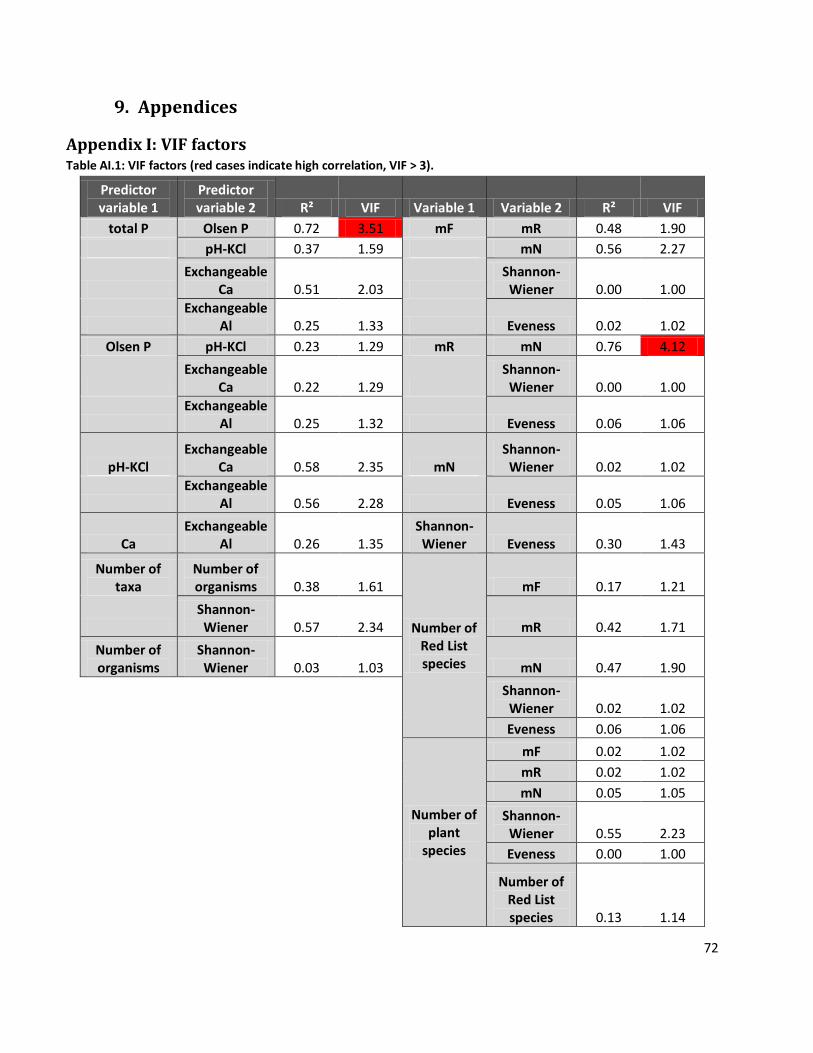
72

9. Appendices

Appendix I: VIF factors Table AI.1: VIF factors (red cases indicate high correlation, VIF > 3).

Predictor variable 1

Predictor variable 2 R² VIF Variable 1 Variable 2 R² VIF

total P Olsen P 0.72 3.51 mF mR 0.48 1.90

pH-KCl 0.37 1.59 mN 0.56 2.27

Exchangeable

Ca 0.51 2.03 Shannon-

Wiener 0.00 1.00

Exchangeable

Al 0.25 1.33 Eveness 0.02 1.02

Olsen P pH-KCl 0.23 1.29 mR mN 0.76 4.12

Exchangeable

Ca 0.22 1.29 Shannon-

Wiener 0.00 1.00

Exchangeable

Al 0.25 1.32 Eveness 0.06 1.06

pH-KCl Exchangeable

Ca 0.58 2.35 mN Shannon-

Wiener 0.02 1.02

Exchangeable

Al 0.56 2.28 Eveness 0.05 1.06

Ca Exchangeable

Al 0.26 1.35 Shannon-Wiener Eveness 0.30 1.43

Number of taxa

Number of organisms 0.38 1.61

Number of Red List species

mF 0.17 1.21

Shannon-Wiener 0.57 2.34 mR 0.42 1.71

Number of organisms

Shannon-Wiener 0.03 1.03 mN 0.47 1.90

Shannon-Wiener 0.02 1.02

Eveness 0.06 1.06

Number of plant

species

mF 0.02 1.02

mR 0.02 1.02

mN 0.05 1.05

Shannon-Wiener 0.55 2.23

Eveness 0.00 1.00

Number of Red List species 0.13 1.14

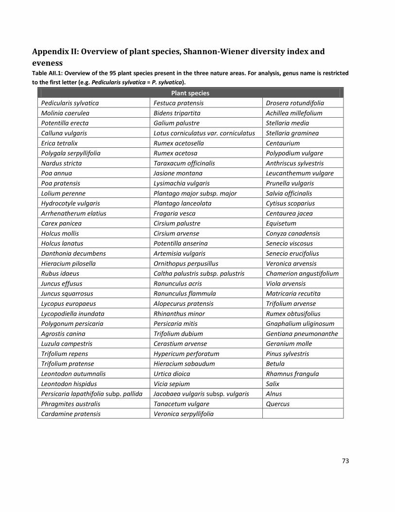
73

Appendix II: Overview of plant species, Shannon-Wiener diversity index and

eveness Table AII.1: Overview of the 95 plant species present in the three nature areas. For analysis, genus name is restricted

to the first letter (e.g. Pedicularis sylvatica = P. sylvatica).

Plant species

Pedicularis sylvatica Festuca pratensis Drosera rotundifolia

Molinia caerulea Bidens tripartita Achillea millefolium

Potentilla erecta Galium palustre Stellaria media

Calluna vulgaris Lotus corniculatus var. corniculatus Stellaria graminea

Erica tetralix Rumex acetosella Centaurium

Polygala serpyllifolia Rumex acetosa Polypodium vulgare

Nardus stricta Taraxacum officinalis Anthriscus sylvestris

Poa annua Jasione montana Leucanthemum vulgare

Poa pratensis Lysimachia vulgaris Prunella vulgaris

Lolium perenne Plantago major subsp. major Salvia officinalis

Hydrocotyle vulgaris Plantago lanceolata Cytisus scoparius

Arrhenatherum elatius Fragaria vesca Centaurea jacea

Carex panicea Cirsium palustre Equisetum

Holcus mollis Cirsium arvense Conyza canadensis

Holcus lanatus Potentilla anserina Senecio viscosus

Danthonia decumbens Artemisia vulgaris Senecio erucifolius

Hieracium pilosella Ornithopus perpusillus Veronica arvensis

Rubus idaeus Caltha palustris subsp. palustris Chamerion angustifolium

Juncus effusus Ranunculus acris Viola arvensis

Juncus squarrosus Ranunculus flammula Matricaria recutita

Lycopus europaeus Alopecurus pratensis Trifolium arvense

Lycopodiella inundata Rhinanthus minor Rumex obtusifolius

Polygonum persicaria Persicaria mitis Gnaphalium uliginosum

Agrostis canina Trifolium dubium Gentiana pneumonanthe

Luzula campestris Cerastium arvense Geranium molle

Trifolium repens Hypericum perforatum Pinus sylvestris

Trifolium pratense Hieracium sabaudum Betula

Leontodon autumnalis Urtica dioica Rhamnus frangula

Leontodon hispidus Vicia sepium Salix

Persicaria lapathifolia subp. pallida Jacobaea vulgaris subsp. vulgaris Alnus

Phragmites australis Tanacetum vulgare Quercus

Cardamine pratensis Veronica serpyllifolia

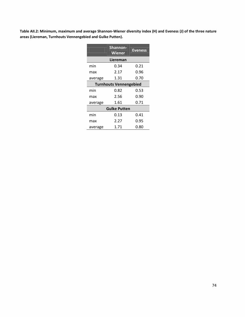
74

Table AII.2: Minimum, maximum and average Shannon-Wiener diversity index (H) and Eveness (J) of the three nature

areas (Liereman, Turnhouts Vennengebied and Gulke Putten).

Shannon-

Wiener Eveness

Liereman

min 0.34 0.21

max 2.17 0.96

average 1.31 0.70

Turnhouts Vennengebied

min 0.82 0.53

max 2.56 0.90

average 1.61 0.71

Gulke Putten

min 0.13 0.41

max 2.27 0.95

average 1.71 0.80

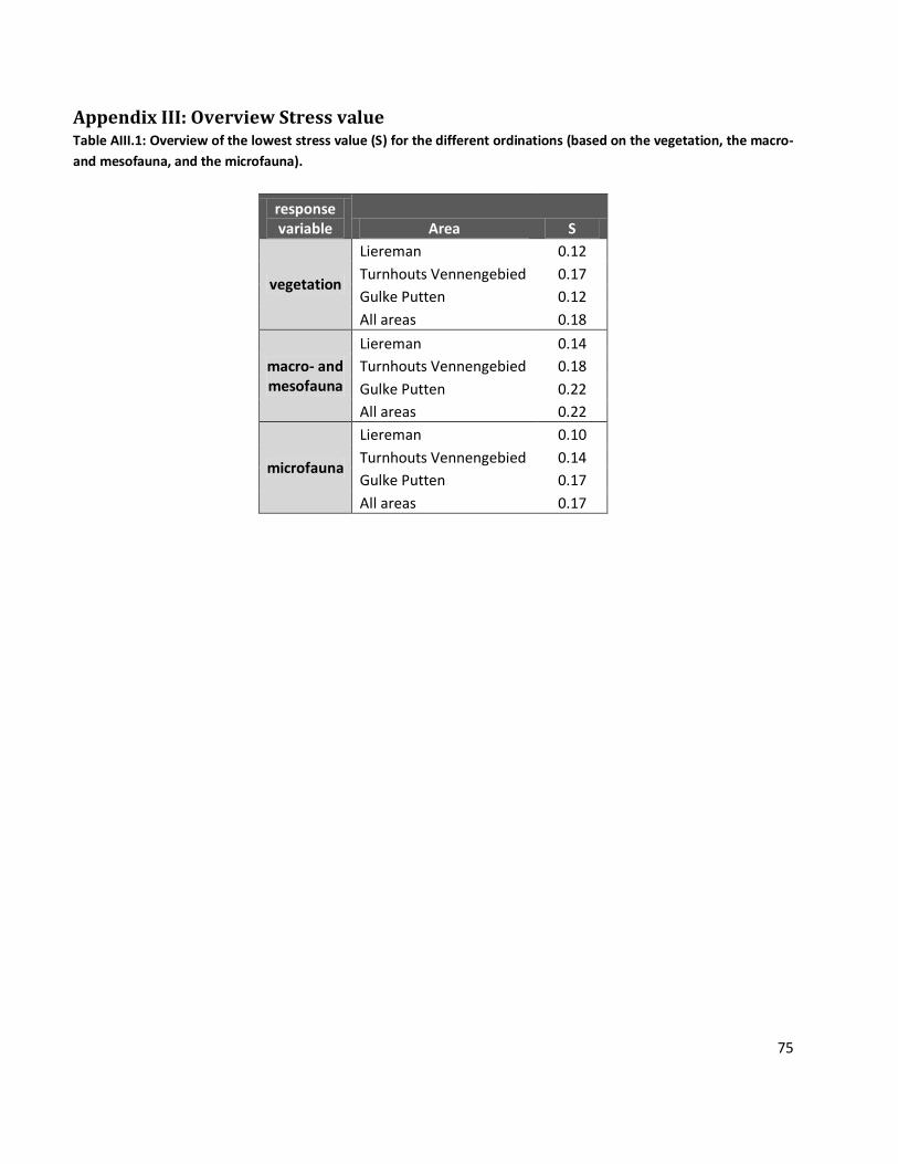
75

Appendix III: Overview Stress value Table AIII.1: Overview of the lowest stress value (S) for the different ordinations (based on the vegetation, the macro-

and mesofauna, and the microfauna).

response variable Area S

vegetation

Liereman 0.12

Turnhouts Vennengebied 0.17

Gulke Putten 0.12

All areas 0.18

macro- and mesofauna

Liereman 0.14

Turnhouts Vennengebied 0.18

Gulke Putten 0.22

All areas 0.22

microfauna

Liereman 0.10

Turnhouts Vennengebied 0.14

Gulke Putten 0.17

All areas 0.17

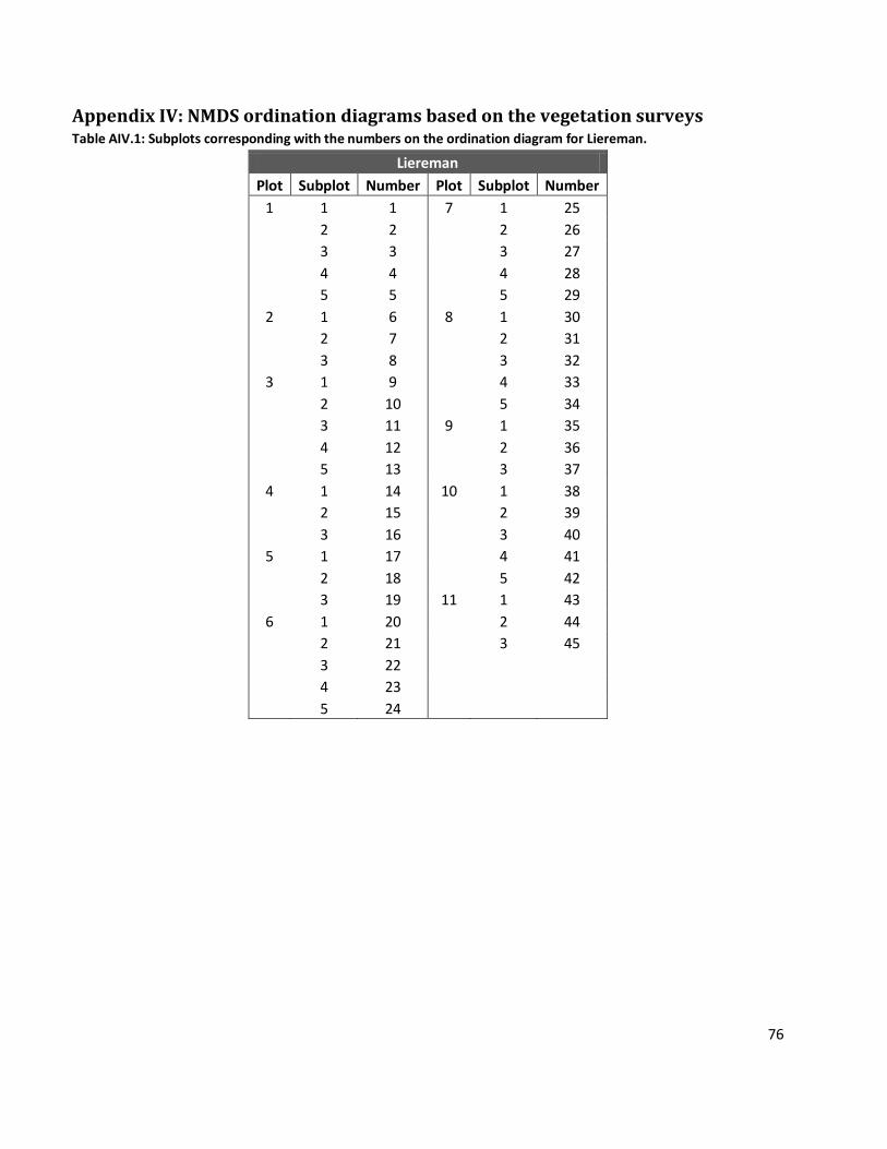
76

Appendix IV: NMDS ordination diagrams based on the vegetation surveys Table AIV.1: Subplots corresponding with the numbers on the ordination diagram for Liereman.

Liereman

Plot Subplot Number Plot Subplot Number

1 1 1 7 1 25

2 2

2 26

3 3

3 27

4 4

4 28

5 5

5 29

2 1 6 8 1 30

2 7

2 31

3 8

3 32

3 1 9

4 33

2 10

5 34

3 11 9 1 35

4 12

2 36

5 13

3 37

4 1 14 10 1 38

2 15

2 39

3 16

3 40

5 1 17

4 41

2 18

5 42

3 19 11 1 43

6 1 20

2 44

2 21

3 45

3 22

4 23

5 24

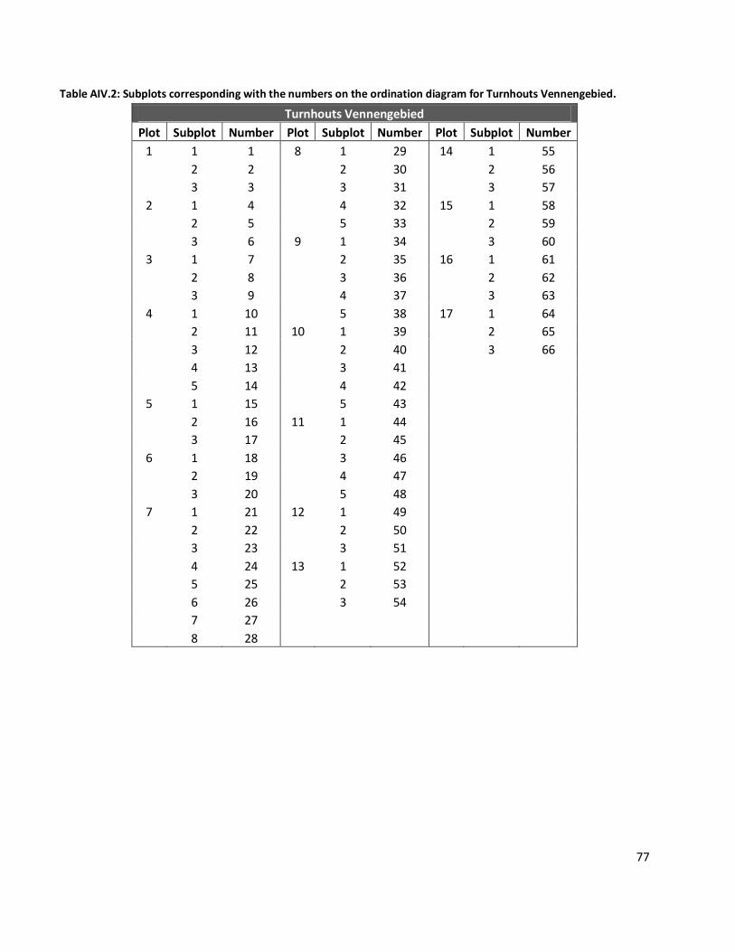
77

Table AIV.2: Subplots corresponding with the numbers on the ordination diagram for Turnhouts Vennengebied.

Turnhouts Vennengebied

Plot Subplot Number Plot Subplot Number Plot Subplot Number

1 1 1 8 1 29 14 1 55

2 2 2 30 2 56

3 3 3 31 3 57

2 1 4 4 32 15 1 58

2 5 5 33 2 59

3 6 9 1 34 3 60

3 1 7 2 35 16 1 61

2 8 3 36 2 62

3 9 4 37 3 63

4 1 10 5 38 17 1 64

2 11 10 1 39 2 65

3 12 2 40 3 66

4 13 3 41

5 14 4 42

5 1 15 5 43

2 16 11 1 44

3 17 2 45

6 1 18 3 46

2 19 4 47

3 20 5 48

7 1 21 12 1 49

2 22 2 50

3 23 3 51

4 24 13 1 52

5 25 2 53

6 26 3 54

7 27

8 28

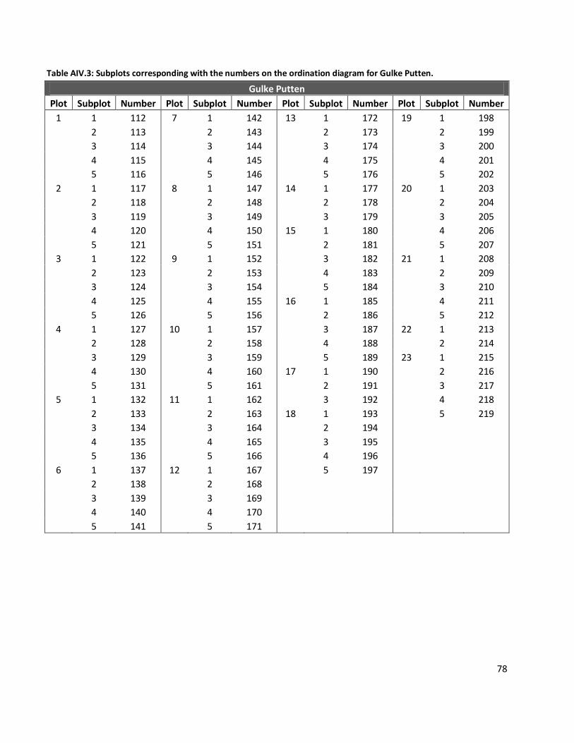
78

Table AIV.3: Subplots corresponding with the numbers on the ordination diagram for Gulke Putten.

Gulke Putten

Plot Subplot Number Plot Subplot Number Plot Subplot Number Plot Subplot Number

1 1 112 7 1 142 13 1 172 19 1 198

2 113 2 143 2 173 2 199

3 114 3 144 3 174 3 200

4 115 4 145 4 175 4 201

5 116 5 146 5 176 5 202

2 1 117 8 1 147 14 1 177 20 1 203

2 118 2 148 2 178 2 204

3 119 3 149 3 179 3 205

4 120 4 150 15 1 180 4 206

5 121 5 151 2 181 5 207

3 1 122 9 1 152 3 182 21 1 208

2 123 2 153 4 183 2 209

3 124 3 154 5 184 3 210

4 125 4 155 16 1 185 4 211

5 126 5 156 2 186 5 212

4 1 127 10 1 157 3 187 22 1 213

2 128 2 158 4 188 2 214

3 129 3 159 5 189 23 1 215

4 130 4 160 17 1 190 2 216

5 131 5 161 2 191 3 217

5 1 132 11 1 162 3 192 4 218

2 133 2 163 18 1 193 5 219

3 134 3 164 2 194

4 135 4 165 3 195

5 136 5 166 4 196

6 1 137 12 1 167 5 197

2 138 2 168

3 139 3 169

4 140 4 170

5 141 5 171

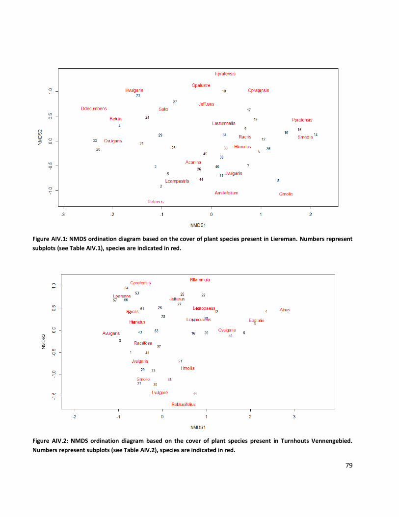
79

Figure AIV.1: NMDS ordination diagram based on the cover of plant species present in Liereman. Numbers represent

subplots (see Table AIV.1), species are indicated in red.

Figure AIV.2: NMDS ordination diagram based on the cover of plant species present in Turnhouts Vennengebied.

Numbers represent subplots (see Table AIV.2), species are indicated in red.

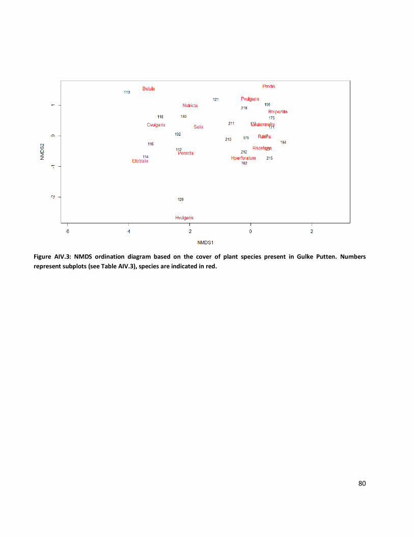
80

Figure AIV.3: NMDS ordination diagram based on the cover of plant species present in Gulke Putten. Numbers

represent subplots (see Table AIV.3), species are indicated in red.

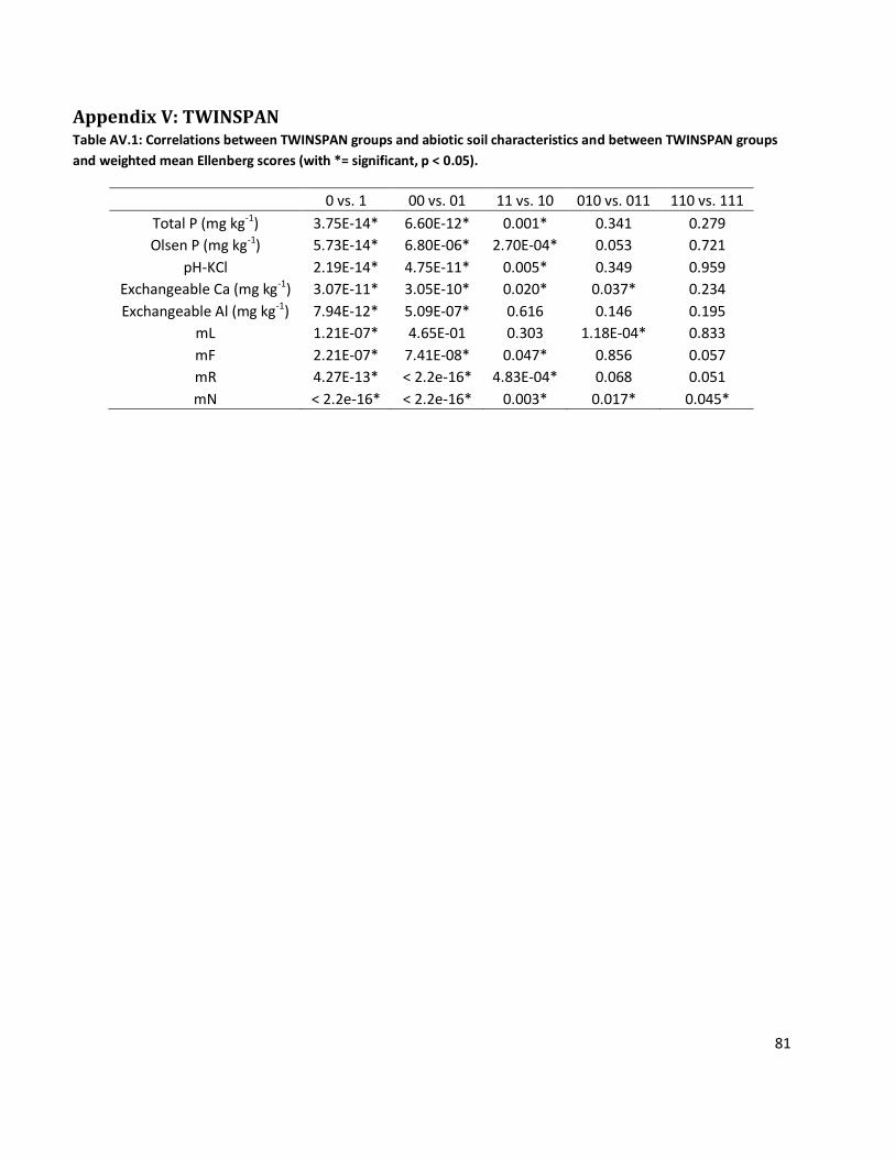
81

Appendix V: TWINSPAN Table AV.1: Correlations between TWINSPAN groups and abiotic soil characteristics and between TWINSPAN groups

and weighted mean Ellenberg scores (with *= significant, p < 0.05).

0 vs. 1 00 vs. 01 11 vs. 10 010 vs. 011 110 vs. 111

Total P (mg kg-1) 3.75E-14* 6.60E-12* 0.001* 0.341 0.279

Olsen P (mg kg-1) 5.73E-14* 6.80E-06* 2.70E-04* 0.053 0.721

pH-KCl 2.19E-14* 4.75E-11* 0.005* 0.349 0.959

Exchangeable Ca (mg kg-1) 3.07E-11* 3.05E-10* 0.020* 0.037* 0.234

Exchangeable Al (mg kg-1) 7.94E-12* 5.09E-07* 0.616 0.146 0.195

mL 1.21E-07* 4.65E-01 0.303 1.18E-04* 0.833

mF 2.21E-07* 7.41E-08* 0.047* 0.856 0.057

mR 4.27E-13* < 2.2e-16* 4.83E-04* 0.068 0.051

mN < 2.2e-16* < 2.2e-16* 0.003* 0.017* 0.045*

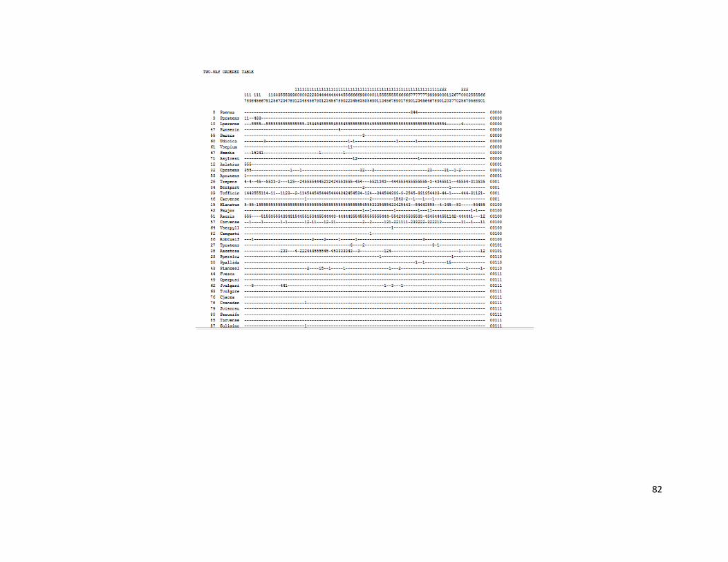
82

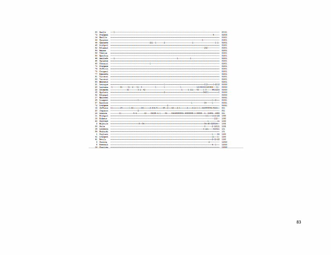
83

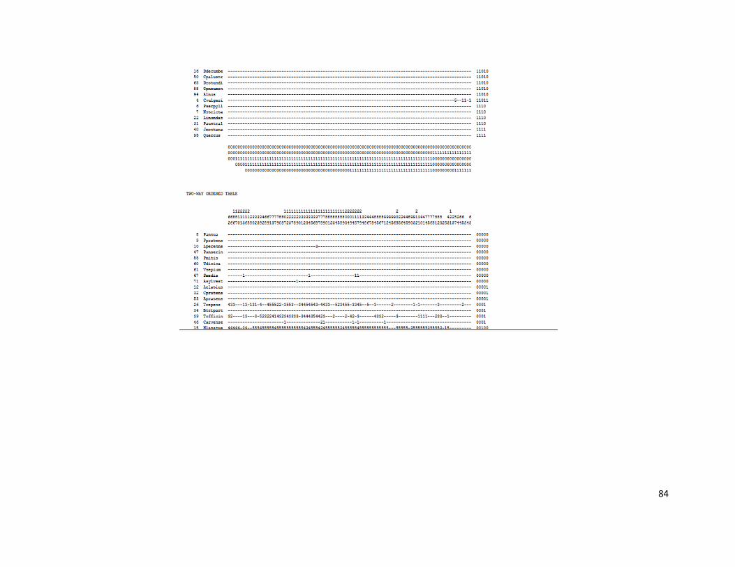
84

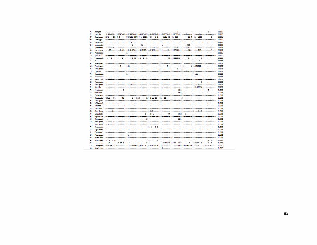
85

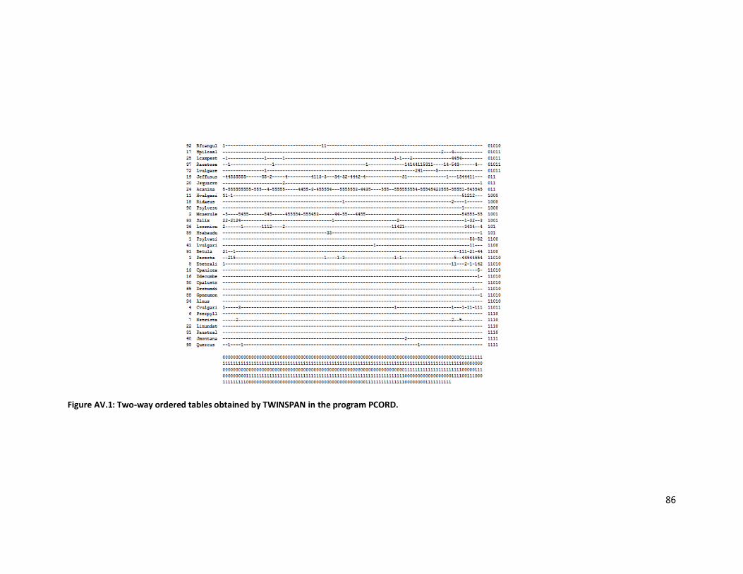
86

Figure AV.1: Two-way ordered tables obtained by TWINSPAN in the program PCORD.

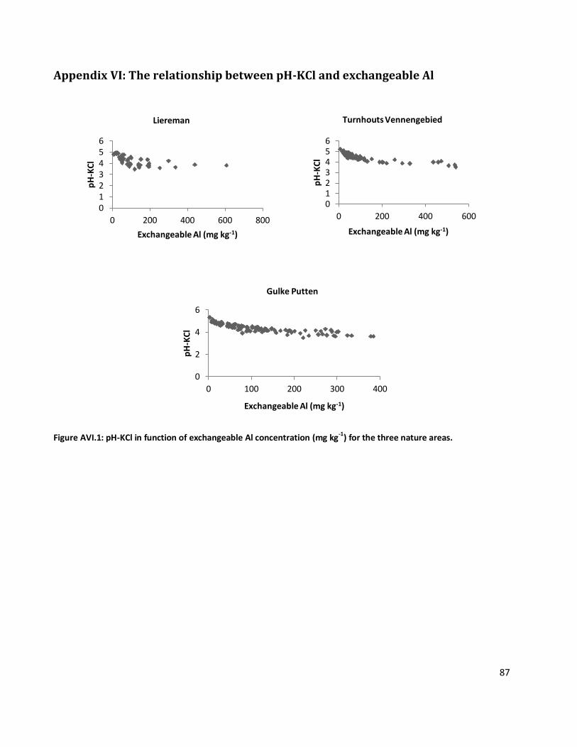
87

Appendix VI: The relationship between pH-KCl and exchangeable Al

Figure AVI.1: pH-KCl in function of exchangeable Al concentration (mg kg-1) for the three nature areas.

0 1 2 3 4 5 6

0 200 400 600 800

pH

-KC

l

Exchangeable Al (mg kg-1)

Liereman

0 1 2 3 4 5 6

0 200 400 600

pH

-KC

l

Exchangeable Al (mg kg-1)

Turnhouts Vennengebied

0

2

4

6

0 100 200 300 400

pH

-KC

l

Exchangeable Al (mg kg-1)

Gulke Putten

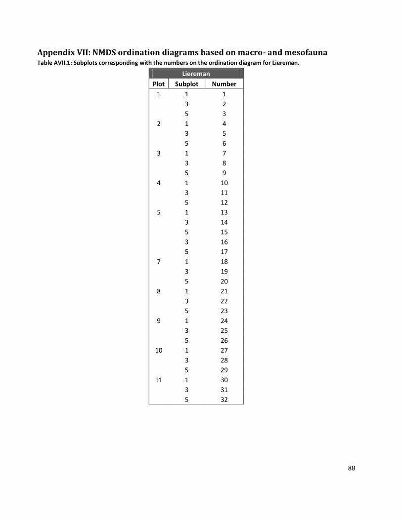
88

Appendix VII: NMDS ordination diagrams based on macro- and mesofauna Table AVII.1: Subplots corresponding with the numbers on the ordination diagram for Liereman.

Liereman

Plot Subplot Number

1 1 1

3 2

5 3

2 1 4

3 5

5 6

3 1 7

3 8

5 9

4 1 10

3 11

5 12

5 1 13

3 14

5 15

3 16

5 17

7 1 18

3 19

5 20

8 1 21

3 22

5 23

9 1 24

3 25

5 26

10 1 27

3 28

5 29

11 1 30

3 31

5 32

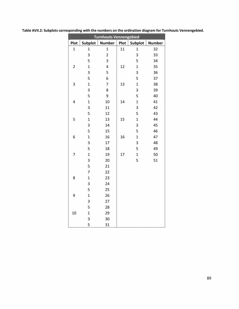
89

Table AVII.2: Subplots corresponding with the numbers on the ordination diagram for Turnhouts Vennengebied.

Turnhouts Vennengebied

Plot Subplot Number Plot Subplot Number

1 1 1 11 1 32

3 2 3 33

5 3 5 34

2 1 4 12 1 35

3 5 3 36

5 6 5 37

3 1 7 13 1 38

3 8 3 39

5 9 5 40

4 1 10 14 1 41

3 11 3 42

5 12 5 43

5 1 13 15 1 44

3 14 3 45

5 15 5 46

6 1 16 16 1 47

3 17 3 48

5 18 5 49

7 1 19 17 1 50

3 20 5 51

5 21

7 22

8 1 23

3 24

5 25

9 1 26

3 27

5 28

10 1 29

3 30

5 31

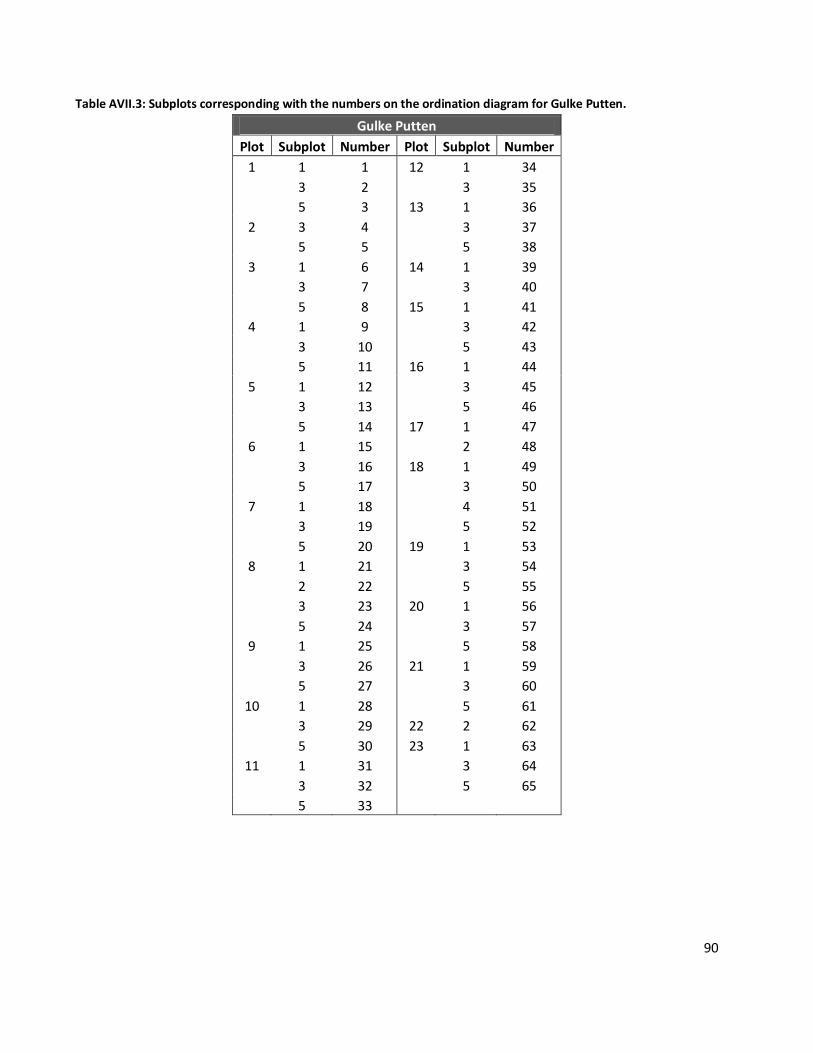
90

Table AVII.3: Subplots corresponding with the numbers on the ordination diagram for Gulke Putten.

Gulke Putten

Plot Subplot Number Plot Subplot Number

1 1 1 12 1 34

3 2 3 35

5 3 13 1 36

2 3 4 3 37

5 5 5 38

3 1 6 14 1 39

3 7 3 40

5 8 15 1 41

4 1 9 3 42

3 10 5 43

5 11 16 1 44

5 1 12 3 45

3 13 5 46

5 14 17 1 47

6 1 15 2 48

3 16 18 1 49

5 17 3 50

7 1 18 4 51

3 19 5 52

5 20 19 1 53

8 1 21 3 54

2 22 5 55

3 23 20 1 56

5 24 3 57

9 1 25 5 58

3 26 21 1 59

5 27 3 60

10 1 28 5 61

3 29 22 2 62

5 30 23 1 63

11 1 31 3 64

3 32 5 65

5 33

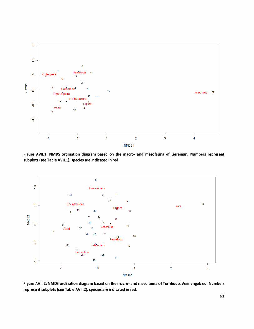
91

Figure AVII.1: NMDS ordination diagram based on the macro- and mesofauna of Liereman. Numbers represent

subplots (see Table AVII.1), species are indicated in red.

Figure AVII.2: NMDS ordination diagram based on the macro- and mesofauna of Turnhouts Vennengebied. Numbers

represent subplots (see Table AVII.2), species are indicated in red.

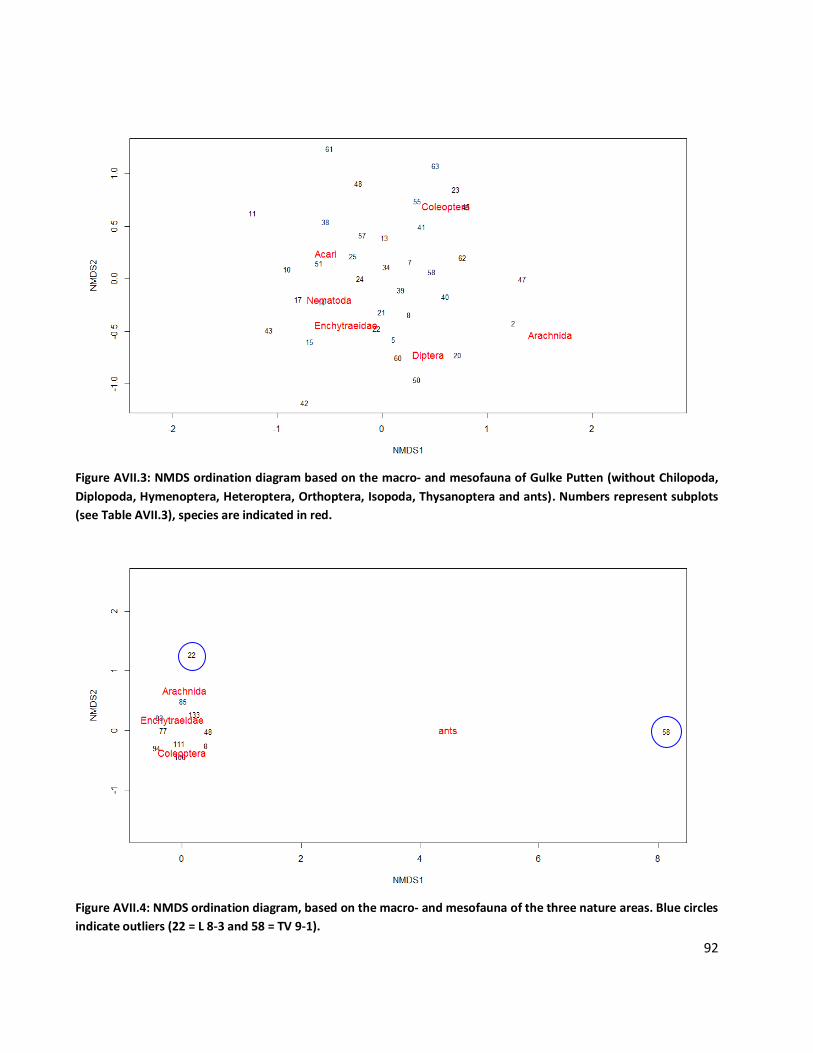
92

Figure AVII.3: NMDS ordination diagram based on the macro- and mesofauna of Gulke Putten (without Chilopoda,

Diplopoda, Hymenoptera, Heteroptera, Orthoptera, Isopoda, Thysanoptera and ants). Numbers represent subplots

(see Table AVII.3), species are indicated in red.

Figure AVII.4: NMDS ordination diagram, based on the macro- and mesofauna of the three nature areas. Blue circles

indicate outliers (22 = L 8-3 and 58 = TV 9-1).

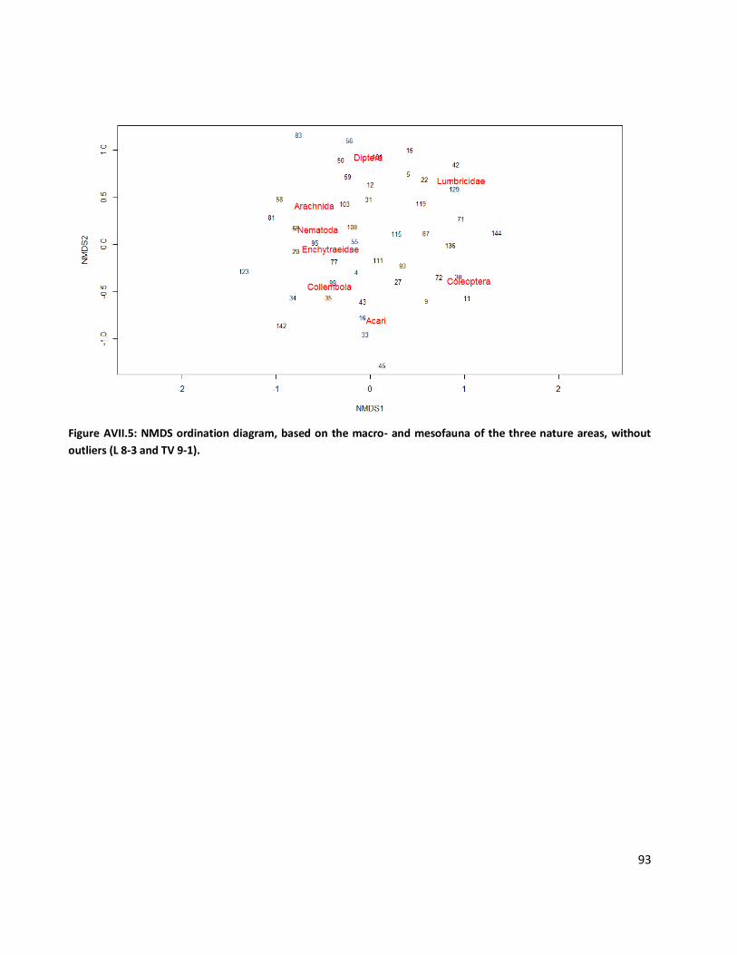
93

Figure AVII.5: NMDS ordination diagram, based on the macro- and mesofauna of the three nature areas, without

outliers (L 8-3 and TV 9-1).

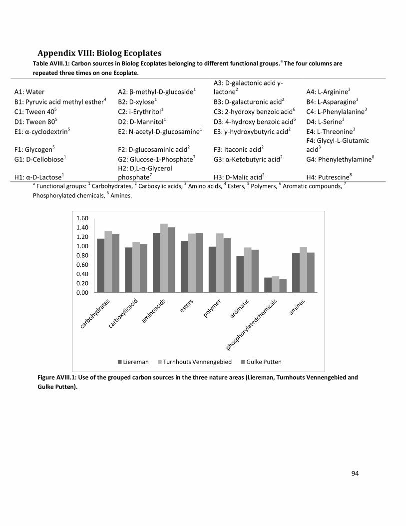
94

Appendix VIII: Biolog Ecoplates Table AVIII.1: Carbon sources in Biolog Ecoplates belonging to different functional groups.

a The four columns are

repeated three times on one Ecoplate.

A1: Water A2: β-methyl-D-glucoside1 A3: D-galactonic acid γ-lactone2 A4: L-Arginine3

B1: Pyruvic acid methyl esther4 B2: D-xylose1 B3: D-galacturonic acid2 B4: L-Asparagine3

C1: Tween 405 C2: i-Erythritol1 C3: 2-hydroxy benzoic acid6 C4: L-Phenylalanine3

D1: Tween 805 D2: D-Mannitol1 D3: 4-hydroxy benzoic acid6 D4: L-Serine3

E1: α-cyclodextrin5 E2: N-acetyl-D-glucosamine1 E3: γ-hydroxybutyric acid2 E4: L-Threonine3

F1: Glycogen5 F2: D-glucosaminic acid2 F3: Itaconic acid2 F4: Glycyl-L-Glutamic acid3

G1: D-Cellobiose1 G2: Glucose-1-Phosphate7 G3: α-Ketobutyric acid2 G4: Phenylethylamine8

H1: α-D-Lactose1 H2: D,L-α-Glycerol phosphate7 H3: D-Malic acid2 H4: Putrescine8

a Functional groups:

1 Carbohydrates,

2 Carboxylic acids,

3 Amino acids,

4 Esters,

5 Polymers,

6 Aromatic compounds,

7

Phosphorylated chemicals, 8 Amines.

Figure AVIII.1: Use of the grouped carbon sources in the three nature areas (Liereman, Turnhouts Vennengebied and

Gulke Putten).

0.00

0.20

0.40

0.60

0.80

1.00

1.20

1.40

1.60

Liereman Turnhouts Vennengebied Gulke Putten

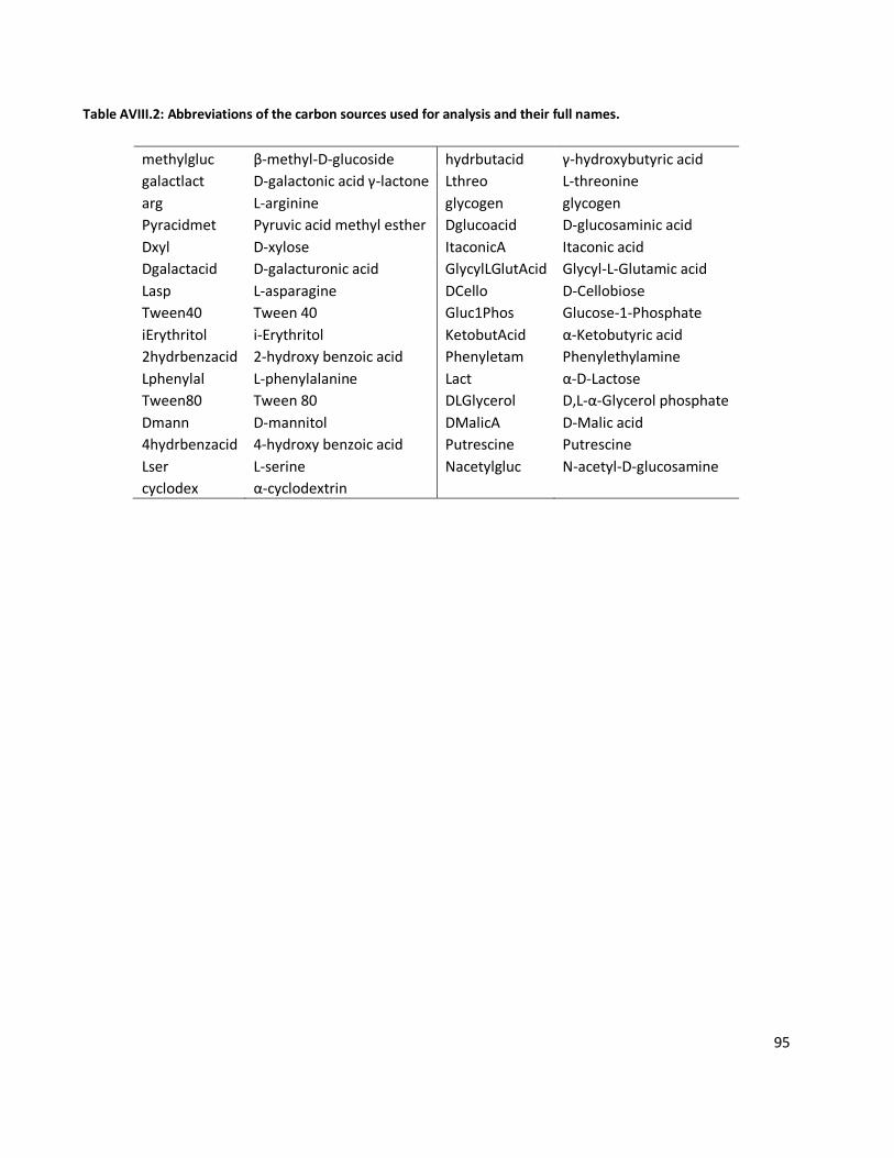
95

Table AVIII.2: Abbreviations of the carbon sources used for analysis and their full names.

methylgluc β-methyl-D-glucoside hydrbutacid γ-hydroxybutyric acid

galactlact D-galactonic acid γ-lactone Lthreo L-threonine

arg L-arginine glycogen glycogen

Pyracidmet Pyruvic acid methyl esther Dglucoacid D-glucosaminic acid

Dxyl D-xylose ItaconicA Itaconic acid

Dgalactacid D-galacturonic acid GlycylLGlutAcid Glycyl-L-Glutamic acid

Lasp L-asparagine DCello D-Cellobiose

Tween40 Tween 40 Gluc1Phos Glucose-1-Phosphate

iErythritol i-Erythritol KetobutAcid α-Ketobutyric acid

2hydrbenzacid 2-hydroxy benzoic acid Phenyletam Phenylethylamine

Lphenylal L-phenylalanine Lact α-D-Lactose

Tween80 Tween 80 DLGlycerol D,L-α-Glycerol phosphate

Dmann D-mannitol DMalicA D-Malic acid

4hydrbenzacid 4-hydroxy benzoic acid Putrescine Putrescine

Lser L-serine Nacetylgluc N-acetyl-D-glucosamine

cyclodex α-cyclodextrin

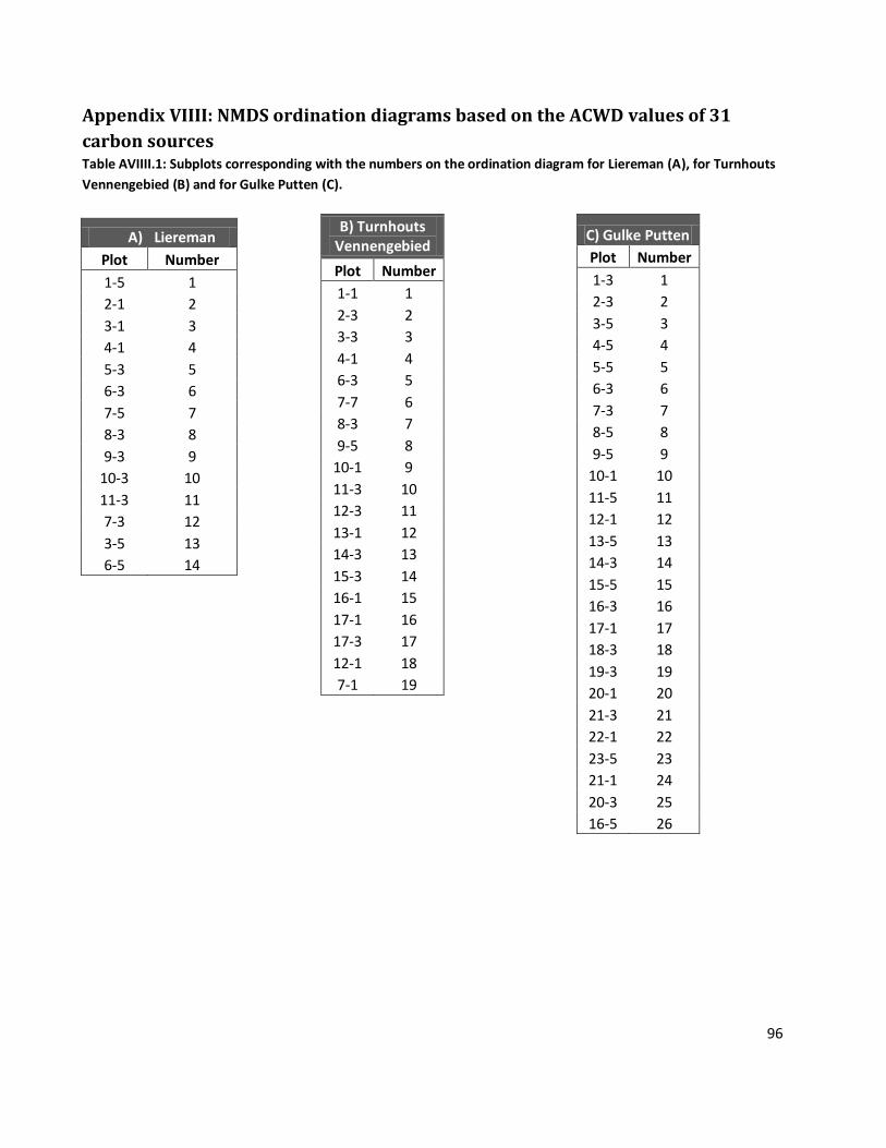
96

Appendix VIIII: NMDS ordination diagrams based on the ACWD values of 31

carbon sources Table AVIIII.1: Subplots corresponding with the numbers on the ordination diagram for Liereman (A), for Turnhouts

Vennengebied (B) and for Gulke Putten (C).

A) Liereman

Plot Number

1-5 1

2-1 2

3-1 3

4-1 4

5-3 5

6-3 6

7-5 7

8-3 8

9-3 9

10-3 10

11-3 11

7-3 12

3-5 13

6-5 14

B) Turnhouts Vennengebied

Plot Number

1-1 1

2-3 2

3-3 3

4-1 4

6-3 5

7-7 6

8-3 7

9-5 8

10-1 9

11-3 10

12-3 11

13-1 12

14-3 13

15-3 14

16-1 15

17-1 16

17-3 17

12-1 18

7-1 19

C) Gulke Putten

Plot Number

1-3 1

2-3 2

3-5 3

4-5 4

5-5 5

6-3 6

7-3 7

8-5 8

9-5 9

10-1 10

11-5 11

12-1 12

13-5 13

14-3 14

15-5 15

16-3 16

17-1 17

18-3 18

19-3 19

20-1 20

21-3 21

22-1 22

23-5 23

21-1 24

20-3 25

16-5 26

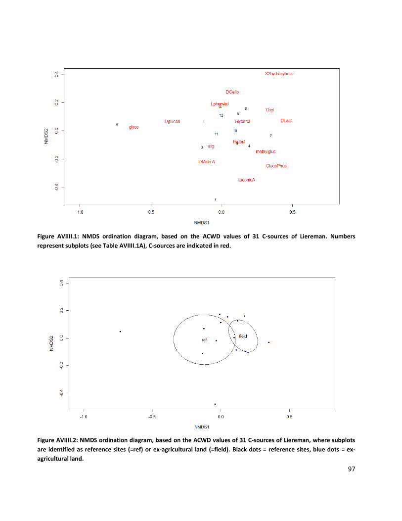
97

Figure AVIIII.1: NMDS ordination diagram, based on the ACWD values of 31 C-sources of Liereman. Numbers

represent subplots (see Table AVIIII.1A), C-sources are indicated in red.

Figure AVIIII.2: NMDS ordination diagram, based on the ACWD values of 31 C-sources of Liereman, where subplots

are identified as reference sites (=ref) or ex-agricultural land (=field). Black dots = reference sites, blue dots = ex-

agricultural land.

98

Figure AVIIII.3: NMDS ordination diagram, based on the ACWD values of 31 C-sources of Turnhouts Vennengebied.

Numbers represent subplots (see Table AVIIII.1B), C-sources are indicated in red.

Figure AVIIII.4: NMDS ordination diagram, based on the ACWD values of 31 C-sources of Turnhouts Vennengebied,

where subplots are identified as reference sites (=ref) or ex-agricultural land (=field). Black dots = reference sites,

blue dots = ex-agricultural land.

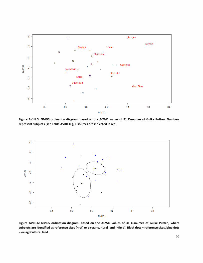
99

Figure AVIIII.5: NMDS ordination diagram, based on the ACWD values of 31 C-sources of Gulke Putten. Numbers

represent subplots (see Table AVIIII.1C), C-sources are indicated in red.

Figure AVIIII.6: NMDS ordination diagram, based on the ACWD values of 31 C-sources of Gulke Putten, where

subplots are identified as reference sites (=ref) or ex-agricultural land (=field). Black dots = reference sites, blue dots

= ex-agricultural land.

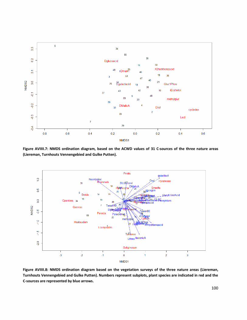
100

Figure AVIIII.7: NMDS ordination diagram, based on the ACWD values of 31 C-sources of the three nature areas

(Liereman, Turnhouts Vennengebied and Gulke Putten).

Figure AVIIII.8: NMDS ordination diagram based on the vegetation surveys of the three nature areas (Liereman,

Turnhouts Vennengebied and Gulke Putten). Numbers represent subplots, plant species are indicated in red and the

C-sources are represented by blue arrows.

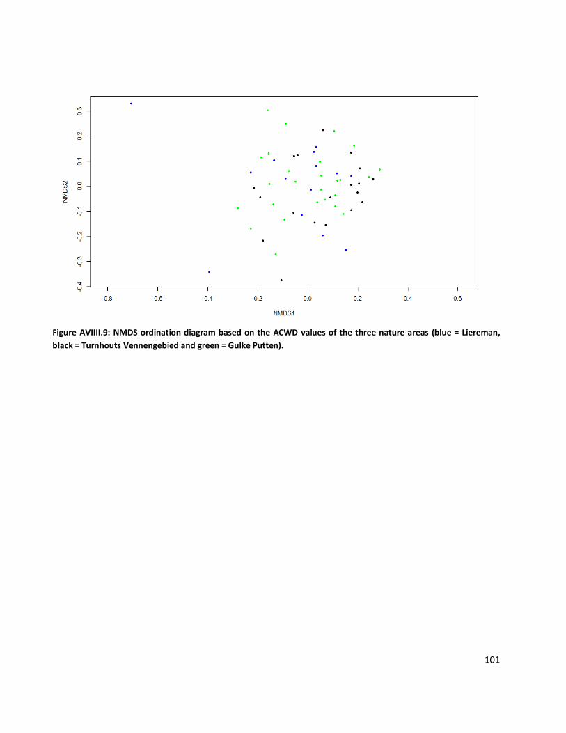
101

Figure AVIIII.9: NMDS ordination diagram based on the ACWD values of the three nature areas (blue = Liereman,

black = Turnhouts Vennengebied and green = Gulke Putten).

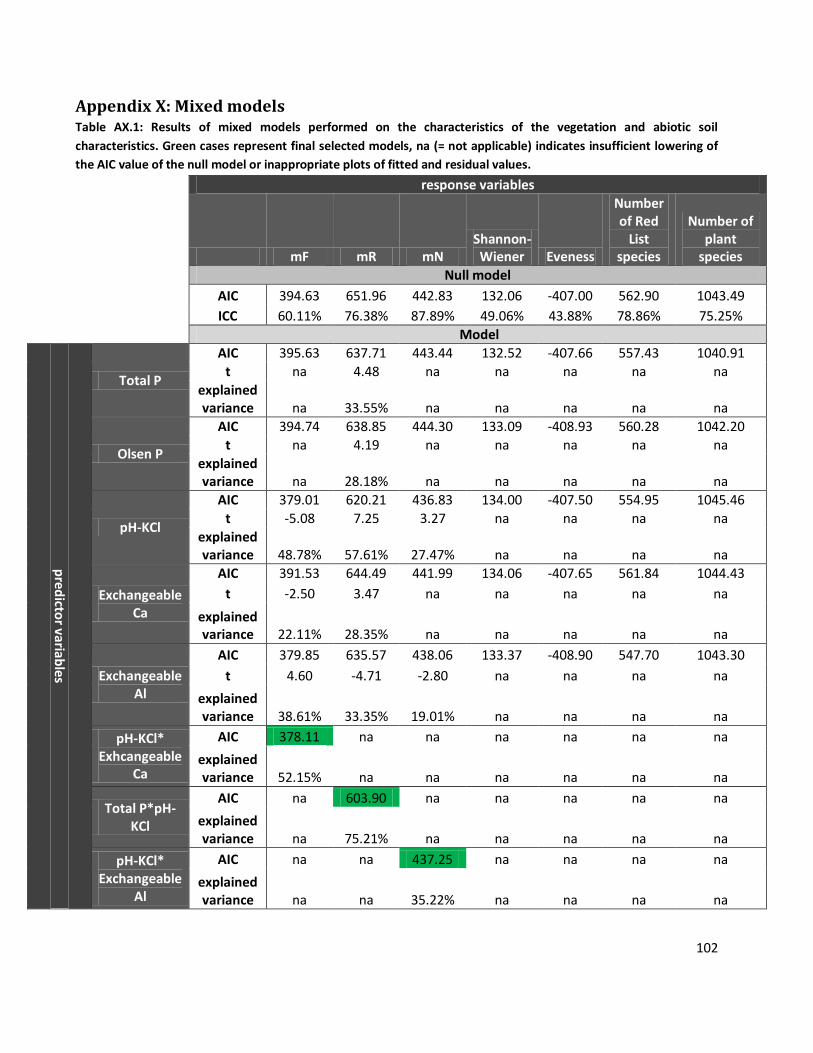
102

Appendix X: Mixed models Table AX.1: Results of mixed models performed on the characteristics of the vegetation and abiotic soil

characteristics. Green cases represent final selected models, na (= not applicable) indicates insufficient lowering of

the AIC value of the null model or inappropriate plots of fitted and residual values.

response variables

mF mR mN

Shannon-Wiener Eveness

Number of Red

List species

Number of plant

species

Null model

AIC 394.63 651.96 442.83 132.06 -407.00 562.90 1043.49

ICC 60.11% 76.38% 87.89% 49.06% 43.88% 78.86% 75.25%

Model

pre

dicto

r variable

s

Total P

AIC 395.63 637.71 443.44 132.52 -407.66 557.43 1040.91

t na 4.48 na na na na na

explained variance na 33.55% na na na na na

Olsen P

AIC 394.74 638.85 444.30 133.09 -408.93 560.28 1042.20

t na 4.19 na na na na na

explained variance na 28.18% na na na na na

pH-KCl

AIC 379.01 620.21 436.83 134.00 -407.50 554.95 1045.46

t -5.08 7.25 3.27 na na na na

explained variance 48.78% 57.61% 27.47% na na na na

Exchangeable Ca

AIC 391.53 644.49 441.99 134.06 -407.65 561.84 1044.43

t -2.50 3.47 na na na na na

explained variance 22.11% 28.35% na na na na na

Exchangeable Al

AIC 379.85 635.57 438.06 133.37 -408.90 547.70 1043.30

t 4.60 -4.71 -2.80 na na na na

explained variance 38.61% 33.35% 19.01% na na na na

pH-KCl* Exhcangeable

Ca

AIC 378.11 na na na na na na

explained variance 52.15% na na na na na na

Total P*pH-KCl

AIC na 603.90 na na na na na

explained variance na 75.21% na na na na na

pH-KCl* Exchangeable

Al

AIC na na 437.25 na na na na

explained variance na na 35.22% na na na na

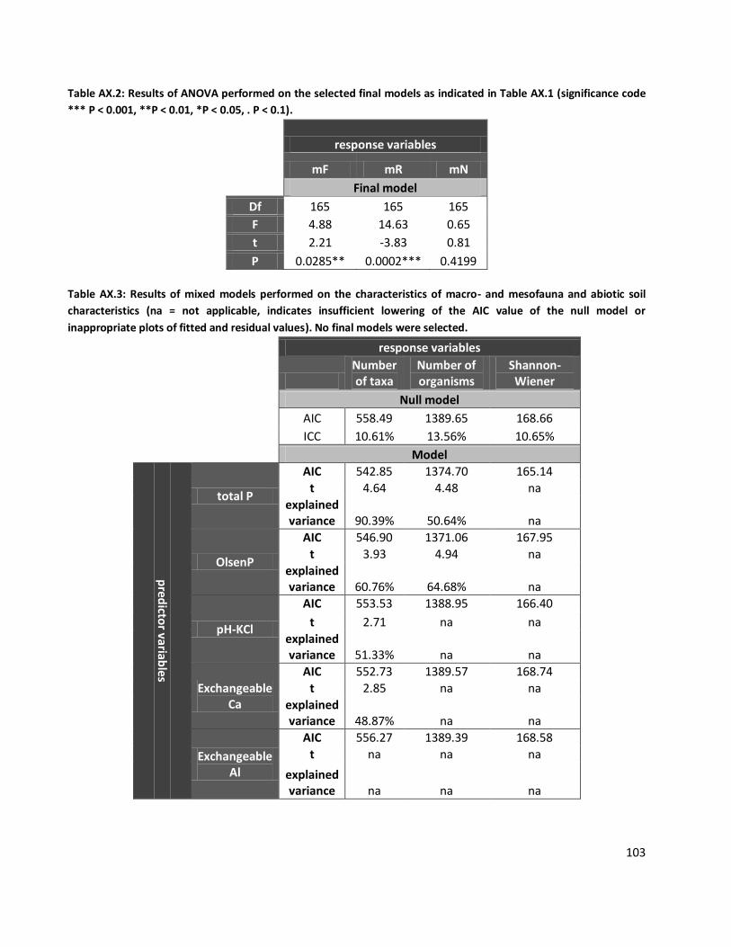
103

Table AX.2: Results of ANOVA performed on the selected final models as indicated in Table AX.1 (significance code

*** P < 0.001, **P < 0.01, *P < 0.05, . P < 0.1).

response variables

mF mR mN

Final model

Df 165 165 165

F 4.88 14.63 0.65

t 2.21 -3.83 0.81

P 0.0285** 0.0002*** 0.4199

Table AX.3: Results of mixed models performed on the characteristics of macro- and mesofauna and abiotic soil

characteristics (na = not applicable, indicates insufficient lowering of the AIC value of the null model or

inappropriate plots of fitted and residual values). No final models were selected.

response variables

Number of taxa

Number of organisms

Shannon-Wiener

Null model

AIC 558.49 1389.65 168.66

ICC 10.61% 13.56% 10.65%

Model

pre

dicto

r variables

total P

AIC 542.85 1374.70 165.14

t 4.64 4.48 na

explained variance 90.39% 50.64% na

OlsenP

AIC 546.90 1371.06 167.95

t 3.93 4.94 na

explained variance 60.76% 64.68% na

pH-KCl

AIC 553.53 1388.95 166.40

t 2.71 na na

explained variance 51.33% na na

Exchangeable Ca

AIC 552.73 1389.57 168.74

t 2.85 na na

explained variance 48.87% na na

Exchangeable Al

AIC 556.27 1389.39 168.58

t na na na

explained variance na na na

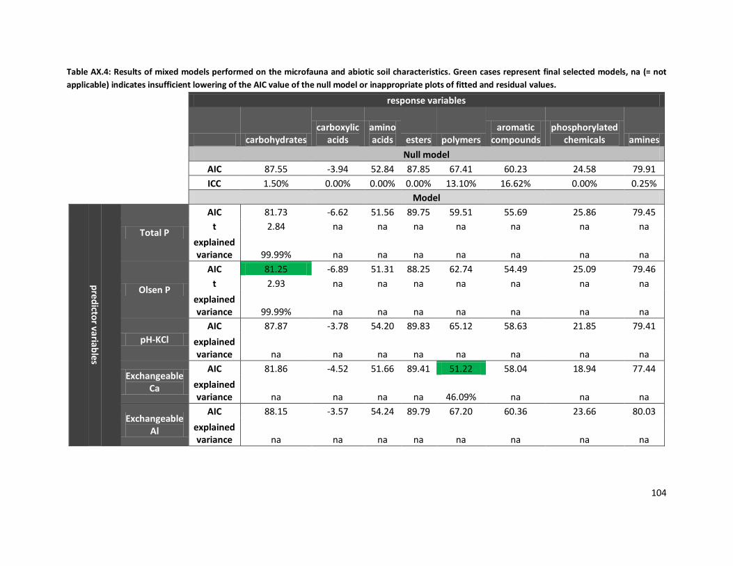
104

Table AX.4: Results of mixed models performed on the microfauna and abiotic soil characteristics. Green cases represent final selected models, na (= not

applicable) indicates insufficient lowering of the AIC value of the null model or inappropriate plots of fitted and residual values.

response variables

carbohydrates

carboxylic acids

amino acids esters polymers

aromatic compounds

phosphorylated chemicals amines

Null model

AIC 87.55 -3.94 52.84 87.85 67.41 60.23 24.58 79.91

ICC 1.50% 0.00% 0.00% 0.00% 13.10% 16.62% 0.00% 0.25%

Model

pre

dicto

r variable

s

Total P

AIC 81.73 -6.62 51.56 89.75 59.51 55.69 25.86 79.45

t 2.84 na na na na na na na

explained variance 99.99% na na na na na na na

Olsen P

AIC 81.25 -6.89 51.31 88.25 62.74 54.49 25.09 79.46

t 2.93 na na na na na na na

explained variance 99.99% na na na na na na na

pH-KCl

AIC 87.87 -3.78 54.20 89.83 65.12 58.63 21.85 79.41

explained variance na na na na na na na na

Exchangeable Ca

AIC 81.86 -4.52 51.66 89.41 51.22 58.04 18.94 77.44

explained variance na na na na 46.09% na na na

Exchangeable Al

AIC 88.15 -3.57 54.24 89.79 67.20 60.36 23.66 80.03

explained variance na na na na na na na na

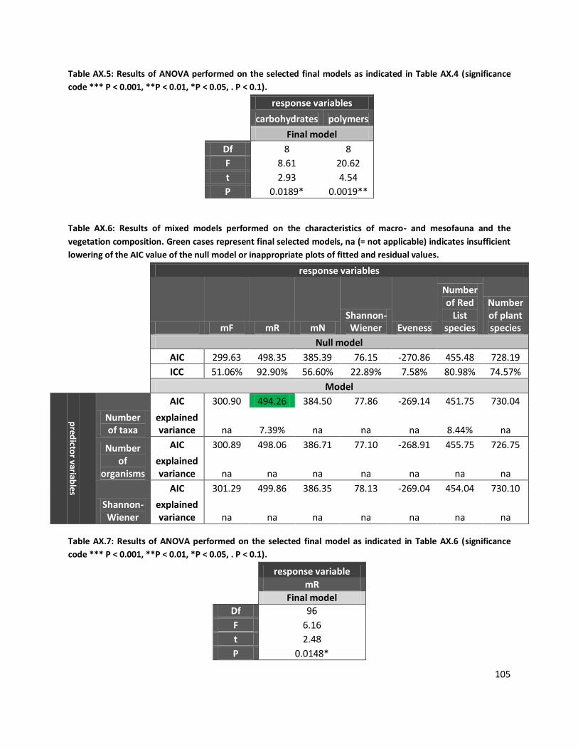
105

Table AX.5: Results of ANOVA performed on the selected final models as indicated in Table AX.4 (significance

code *** P < 0.001, **P < 0.01, *P < 0.05, . P < 0.1).

response variables

carbohydrates polymers

Final model

Df 8 8

F 8.61 20.62

t 2.93 4.54

P 0.0189* 0.0019**

Table AX.6: Results of mixed models performed on the characteristics of macro- and mesofauna and the

vegetation composition. Green cases represent final selected models, na (= not applicable) indicates insufficient

lowering of the AIC value of the null model or inappropriate plots of fitted and residual values.

response variables

mF mR mN

Shannon-Wiener Eveness

Number of Red

List species

Number of plant species

Null model

AIC 299.63 498.35 385.39 76.15 -270.86 455.48 728.19

ICC 51.06% 92.90% 56.60% 22.89% 7.58% 80.98% 74.57%

Model

pred

ictor variab

les

Number of taxa

AIC 300.90 494.26 384.50 77.86 -269.14 451.75 730.04

explained variance na 7.39% na na na 8.44% na

Number of

organisms

AIC 300.89 498.06 386.71 77.10 -268.91 455.75 726.75

explained variance na na na na na na na

Shannon-Wiener

AIC 301.29 499.86 386.35 78.13 -269.04 454.04 730.10

explained variance na na na na na na na

Table AX.7: Results of ANOVA performed on the selected final model as indicated in Table AX.6 (significance

code *** P < 0.001, **P < 0.01, *P < 0.05, . P < 0.1).

response variable

mR

Final model

Df 96

F 6.16

t 2.48

P 0.0148*

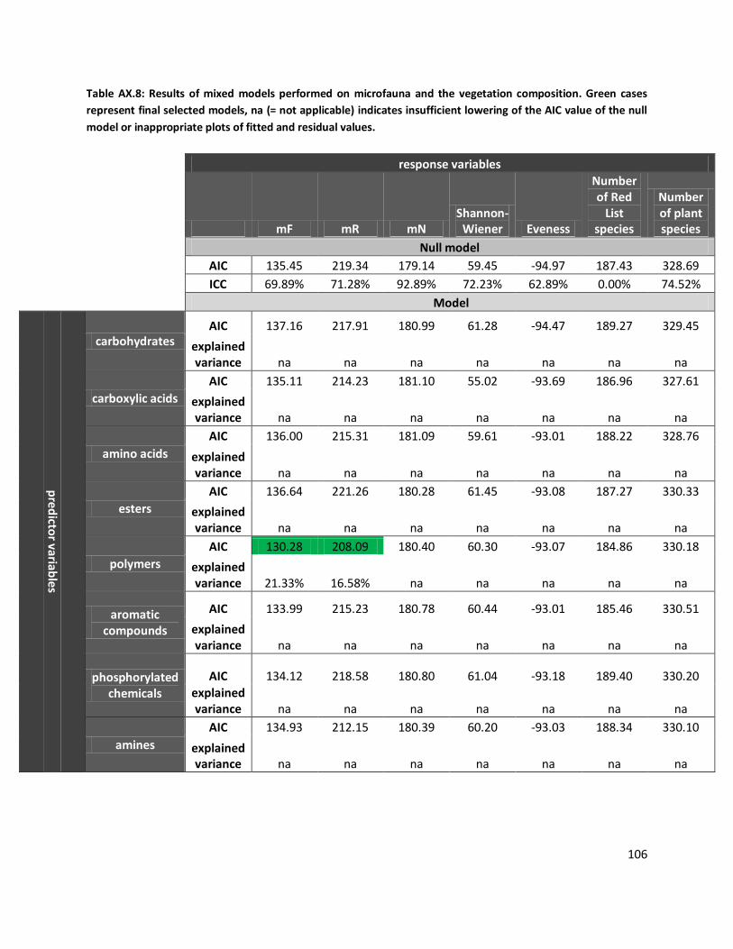
106

Table AX.8: Results of mixed models performed on microfauna and the vegetation composition. Green cases

represent final selected models, na (= not applicable) indicates insufficient lowering of the AIC value of the null

model or inappropriate plots of fitted and residual values.

response variables

mF mR mN

Shannon-Wiener Eveness

Number of Red

List species

Number of plant species

Null model

AIC 135.45 219.34 179.14 59.45 -94.97 187.43 328.69

ICC 69.89% 71.28% 92.89% 72.23% 62.89% 0.00% 74.52%

Model

pre

dicto

r variable

s

carbohydrates AIC 137.16 217.91 180.99 61.28 -94.47 189.27 329.45

explained variance na na na na na na na

carboxylic acids

AIC 135.11 214.23 181.10 55.02 -93.69 186.96 327.61

explained variance na na na na na na na

amino acids

AIC 136.00 215.31 181.09 59.61 -93.01 188.22 328.76

explained variance na na na na na na na

esters

AIC 136.64 221.26 180.28 61.45 -93.08 187.27 330.33

explained variance na na na na na na na

polymers

AIC 130.28 208.09 180.40 60.30 -93.07 184.86 330.18

explained variance 21.33% 16.58% na na na na na

aromatic compounds

AIC 133.99 215.23 180.78 60.44 -93.01 185.46 330.51

explained variance na na na na na na na

phosphorylated chemicals

AIC 134.12 218.58 180.80 61.04 -93.18 189.40 330.20

explained variance na na na na na na na

amines

AIC 134.93 212.15 180.39 60.20 -93.03 188.34 330.10

explained variance na na na na na na na

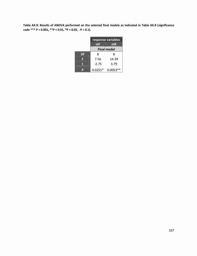
107

Table AX.9: Results of ANOVA performed on the selected final models as indicated in Table AX.8 (significance

code *** P < 0.001, **P < 0.01, *P < 0.05, . P < 0.1).

response variables

mF mR

Final model

Df 8 8

F 7.56 14.39

t -2.75 3.79

P 0.0251* 0.0053**

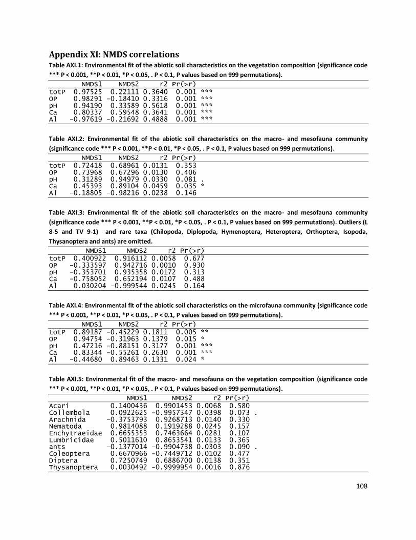
108

Appendix XI: NMDS correlations Table AXI.1: Environmental fit of the abiotic soil characteristics on the vegetation composition (significance code

*** P < 0.001, **P < 0.01, *P < 0.05, . P < 0.1, P values based on 999 permutations).

NMDS1 NMDS2 r2 Pr(>r) totP 0.97525 0.22111 0.3640 0.001 *** OP 0.98291 -0.18410 0.3316 0.001 *** pH 0.94190 0.33589 0.5618 0.001 *** Ca 0.80337 0.59548 0.3641 0.001 *** Al -0.97619 -0.21692 0.4888 0.001 ***

Table AXI.2: Environmental fit of the abiotic soil characteristics on the macro- and mesofauna community

(significance code *** P < 0.001, **P < 0.01, *P < 0.05, . P < 0.1, P values based on 999 permutations).

NMDS1 NMDS2 r2 Pr(>r) totP 0.72418 0.68961 0.0131 0.353 OP 0.73968 0.67296 0.0130 0.406 pH 0.31289 0.94979 0.0330 0.081 . Ca 0.45393 0.89104 0.0459 0.035 * Al -0.18805 -0.98216 0.0238 0.146

Table AXI.3: Environmental fit of the abiotic soil characteristics on the macro- and mesofauna community

(significance code *** P < 0.001, **P < 0.01, *P < 0.05, . P < 0.1, P values based on 999 permutations). Outliers (L

8-5 and TV 9-1) and rare taxa (Chilopoda, Diplopoda, Hymenoptera, Heteroptera, Orthoptera, Isopoda,

Thysanoptera and ants) are omitted.

NMDS1 NMDS2 r2 Pr(>r) totP 0.400922 0.916112 0.0058 0.677 OP -0.333597 0.942716 0.0010 0.930 pH -0.353701 0.935358 0.0172 0.313 Ca -0.758052 0.652194 0.0107 0.488 Al 0.030204 -0.999544 0.0245 0.164

Table AXI.4: Environmental fit of the abiotic soil characteristics on the microfauna community (significance code

*** P < 0.001, **P < 0.01, *P < 0.05, . P < 0.1, P values based on 999 permutations).

NMDS1 NMDS2 r2 Pr(>r) totP 0.89187 -0.45229 0.1811 0.005 ** OP 0.94754 -0.31963 0.1379 0.015 * pH 0.47216 -0.88151 0.3177 0.001 *** Ca 0.83344 -0.55261 0.2630 0.001 *** Al -0.44680 0.89463 0.1331 0.024 *

Table AXI.5: Environmental fit of the macro- and mesofauna on the vegetation composition (significance code

*** P < 0.001, **P < 0.01, *P < 0.05, . P < 0.1, P values based on 999 permutations).

NMDS1 NMDS2 r2 Pr(>r) Acari 0.1400436 0.9901453 0.0068 0.580 Collembola 0.0922625 -0.9957347 0.0398 0.073 . Arachnida -0.3753793 0.9268713 0.0140 0.330 Nematoda 0.9814088 0.1919288 0.0245 0.157 Enchytraeidae 0.6655353 0.7463664 0.0281 0.107 Lumbricidae 0.5011610 0.8653541 0.0133 0.365 ants -0.1377014 -0.9904738 0.0303 0.090 . Coleoptera 0.6670966 -0.7449712 0.0102 0.477 Diptera 0.7250749 0.6886700 0.0138 0.351 Thysanoptera 0.0030492 -0.9999954 0.0016 0.876

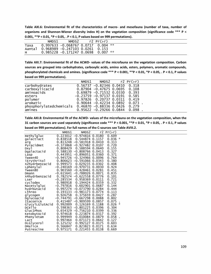
109

Table AXI.6: Environmental fit of the characteristics of macro- and mesofauna (number of taxa, number of

organisms and Shannon-Wiener diversity index H) on the vegetation composition (significance code *** P <

0.001, **P < 0.01, *P < 0.05, . P < 0.1, P values based on 999 permutations).

NMDS1 NMDS2 r2 Pr(>r) Taxa 0.997633 -0.068767 0.0717 0.004 ** Aantal 0.968989 -0.247103 0.0261 0.153 H 0.985228 -0.171247 0.0698 0.007 **

Table AXI.7: Environmental fit of the ACWD- values of the microfauna on the vegetation composition. Carbon

sources are grouped into carbohydrates, carboxylic acids, amino acids, esters, polymers, aromatic compounds,

phosphorylated chemicals and amines. (significance code *** P < 0.001, **P < 0.01, *P < 0.05, . P < 0.1, P values

based on 999 permutations).

NMDS1 NMDS2 r2 Pr(>r) carbohydrates 0.56737 -0.82346 0.0410 0.318 carboxylicacid 0.87904 -0.47675 0.0695 0.108 aminoacids 0.69879 -0.71532 0.0330 0.393 esters -0.23759 -0.97137 0.0191 0.585 polymer 0.97826 0.20737 0.0311 0.419 aromatic 0.90644 -0.42234 0.0892 0.073 . phosphorylatedchemicals 0.46870 -0.88336 0.0426 0.279 amines 0.95622 -0.29266 0.0844 0.098 . Table AXI.8: Environmental fit of the ACWD- values of the microfauna on the vegetation composition, when the

31 carbon sources are used separately (significance code *** P < 0.001, **P < 0.01, *P < 0.05, . P < 0.1, P values

based on 999 permutations). For full names of the C-sources see Table AVIII.2.

NMDS1 NMDS2 r2 Pr(>r) methylgluc 0.223012 -0.974816 0.0180 0.609 galactlact 0.838518 0.544874 0.1157 0.036 * arg 0.813248 -0.581918 0.0410 0.313 Pyracidmet -0.373868 -0.927482 0.0107 0.720 Dxyl 0.808429 0.588594 0.0640 0.155 Dgalactacid 0.588130 -0.808766 0.0413 0.327 Lasp 0.443951 -0.896051 0.0360 0.371 Tween40 -0.945726 -0.324966 0.0096 0.764 iErythritol 0.806623 -0.591066 0.0343 0.380 X2hydrbenzacid 0.999573 0.029235 0.0302 0.408 Lphenylal -0.240169 -0.970731 0.0030 0.924 Tween80 0.903560 -0.428461 0.0281 0.451 Dmann -0.615641 -0.788026 0.0071 0.835 X4hydrbenzacid 0.782574 -0.622558 0.0776 0.101 Lser -0.285534 0.958369 0.0111 0.721 cyclodex 0.980918 0.194424 0.0359 0.332 Nacetylgluc -0.797816 0.602901 0.0687 0.144 hydrbutacid 0.997274 -0.073790 0.0284 0.444 Lthreo 0.193133 -0.981173 0.0774 0.113 glycogen 0.926758 0.375659 0.0427 0.287 Dglucoacid -0.744791 -0.667298 0.0088 0.802 ItaconicA 0.415487 -0.909599 0.0857 0.075 . GlycylLGlutAcid 0.992009 0.126169 0.1188 0.026 * DCello 0.598363 -0.801225 0.0396 0.304 Gluc1Phos 0.654329 -0.756210 0.0399 0.336 KetobutAcid 0.974618 0.223874 0.0317 0.392 Phenyletam 0.999949 0.010084 0.0879 0.058 . Lact 0.997464 0.071173 0.0642 0.127 DLGlycerol 0.125232 0.992127 0.0175 0.603 DMalicA 0.566847 0.823823 0.0171 0.634 Putrescine 0.975171 0.221455 0.0138 0.669

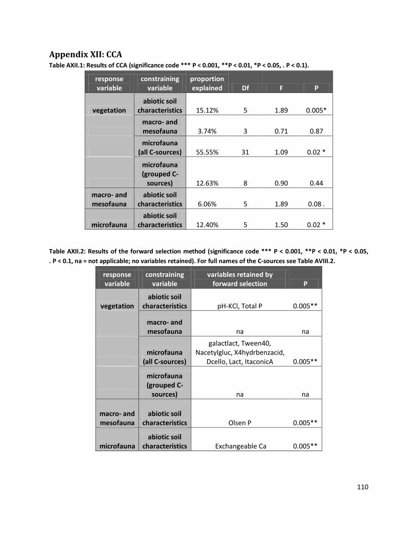
110

Appendix XII: CCA Table AXII.1: Results of CCA (significance code *** P < 0.001, **P < 0.01, *P < 0.05, . P < 0.1).

response variable

constraining variable

proportion explained Df F P

vegetation abiotic soil

characteristics 15.12% 5 1.89 0.005*

macro- and mesofauna 3.74% 3 0.71 0.87

microfauna

(all C-sources) 55.55% 31 1.09 0.02 *

microfauna (grouped C-

sources) 12.63% 8 0.90 0.44

macro- and mesofauna

abiotic soil characteristics 6.06% 5 1.89 0.08 .

microfauna abiotic soil

characteristics 12.40% 5 1.50 0.02 *

Table AXII.2: Results of the forward selection method (significance code *** P < 0.001, **P < 0.01, *P < 0.05,

. P < 0.1, na = not applicable; no variables retained). For full names of the C-sources see Table AVIII.2.

response variable

constraining variable

variables retained by forward selection P

vegetation abiotic soil

characteristics pH-KCl, Total P 0.005**

macro- and mesofauna na na

microfauna

(all C-sources)

galactlact, Tween40, Nacetylgluc, X4hydrbenzacid,

Dcello, Lact, ItaconicA 0.005**

microfauna (grouped C-

sources) na na

macro- and mesofauna

abiotic soil characteristics Olsen P 0.005**

microfauna abiotic soil

characteristics Exchangeable Ca 0.005**

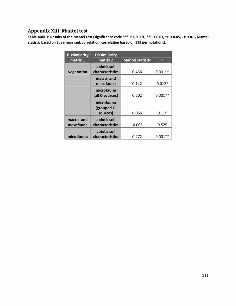
111

Appendix XIII: Mantel test Table AXIII.1: Results of the Mantel test (significance code *** P < 0.001, **P < 0.01, *P < 0.05, . P < 0.1, Mantel

statistic based on Spearman rank correlation, correlation based on 999 permutations).

Dissimilarity matrix 1

Dissimilarity matrix 2 Mantel statistic P

vegetation abiotic soil

characteristics 0.436 0.001**

macro- and mesofauna 0.142 0.012*

microfauna

(all C-sources) 0.202 0.001**

microfauna (grouped C-

sources) 0.065 0.115

macro- and mesofauna

abiotic soil characteristics -0.005 0.525

microfauna abiotic soil

characteristics 0.272 0.001**

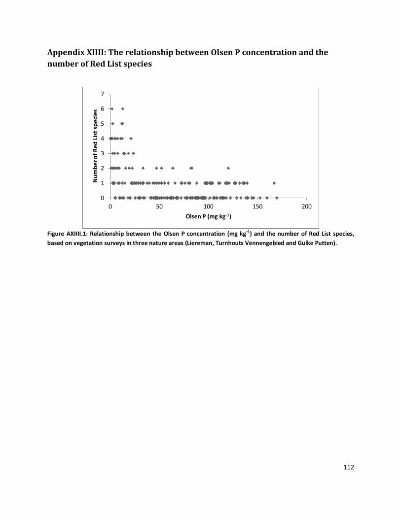
112

Appendix XIIII: The relationship between Olsen P concentration and the

number of Red List species

Figure AXIIII.1: Relationship between the Olsen P concentration (mg kg-1) and the number of Red List species,

based on vegetation surveys in three nature areas (Liereman, Turnhouts Vennengebied and Gulke Putten).

0

1

2

3

4

5

6

7

0 50 100 150 200

Nu

mb

er

of

Re

d L

ist

spe

cie

s

Olsen P (mg kg-1)