
UNIVERSITEIT DELFT Faculteit Elektrotechniek, Wiskunde en Informatica TENTAMEN NUMERIEKE METHODEN...
73
CTB2400 – Numerieke methoden voor differentiaalvergelijkingen April 2013 Januari 2012 Januari 2013 Augustus 2011 Augustus 2012 Juni 2011 Juli 2012 April 2011 April 2012 Januari 2011 Tentamenbundel Civiele Techniek Het Gezelschap "Practische Studie"
Transcript of UNIVERSITEIT DELFT Faculteit Elektrotechniek, Wiskunde en Informatica TENTAMEN NUMERIEKE METHODEN...

CTB2400 – Numerieke methoden voor differentiaalvergelijkingen
April 2013 Januari 2012 Januari 2013 Augustus 2011 Augustus 2012 Juni 2011 Juli 2012 April 2011 April 2012 Januari 2011
Tentamenbundel Civiele Techniek Het Gezelschap "Practische Studie"
TECHNISCHE UNIVERSITEIT DELFTFaculteit Elektrotechniek, Wiskunde en Informatica
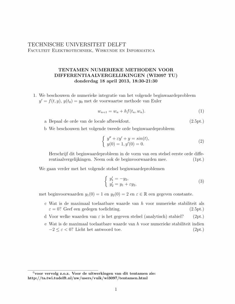
TENTAMEN NUMERIEKE METHODEN VOORDIFFERENTIAALVERGELIJKINGEN (WI3097 TU)
donderdag 18 april 2013, 18:30-21:30
1. We beschouwen de numerieke integratie van het volgende beginwaardeprobleemy′ = f(t, y), y(t0) = y0 met de voorwaartse methode van Euler
wn+1 = wn + hf(tn, wn). (1)
a Bepaal de orde van de locale afbreekfout. (2.5pt.)
b We beschouwen het volgende tweede orde beginwaardeprobleem{y′′ + εy′ + y = sin(t),y(0) = 1, y′(0) = 0.
(2)
Herschrijf dit beginwaardeprobleem in de vorm van een stelsel eerste orde diffe-rentiaalvergelijkingen. Neem ook de beginvoorwaarden mee. (1pt.)
We gaan verder met het volgende stelsel beginwaardeproblemen{y′1 = −y2,y′2 = y1 + εy2,
(3)
met beginvoorwaarden y1(0) = 1 en y2(0) = 2 en ε ∈ R een gegeven constante.
c Wat is de maximaal toelaatbare waarde van h voor numerieke stabiliteit alsε = 0? Geef een gedegen toelichting. (2.5pt.)
d Voor welke waarden van ε is het gegeven stelsel (analytisch) stabiel? (2pt.)
e Wat is de maximaal toelaatbare waarde van h voor numerieke stabiliteit indien−2 ≤ ε < 0? Licht het antwoord toe. (2pt.)
0voor vervolg z.o.z. Voor de uitwerkingen van dit tentamen zie:http://ta.twi.tudelft.nl/nw/users/vuik/wi3097/tentamen.html
1
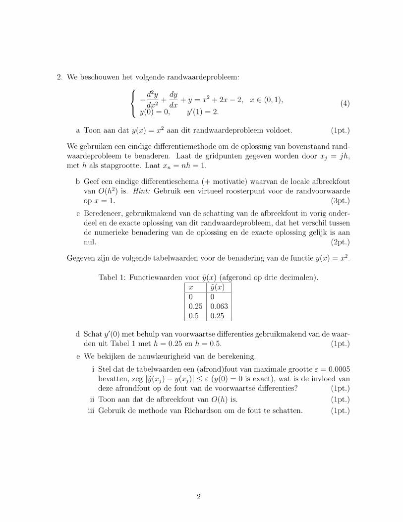
2. We beschouwen het volgende randwaardeprobleem: −d2y
dx2+
dy
dx+ y = x2 + 2x− 2, x ∈ (0, 1),
y(0) = 0, y′(1) = 2.(4)
a Toon aan dat y(x) = x2 aan dit randwaardeprobleem voldoet. (1pt.)
We gebruiken een eindige differentiemethode om de oplossing van bovenstaand rand-waardeprobleem te benaderen. Laat de gridpunten gegeven worden door xj = jh,met h als stapgrootte. Laat xn = nh = 1.
b Geef een eindige differentieschema (+ motivatie) waarvan de locale afbreekfoutvan O(h2) is. Hint: Gebruik een virtueel roosterpunt voor de randvoorwaardeop x = 1. (3pt.)
c Beredeneer, gebruikmakend van de schatting van de afbreekfout in vorig onder-deel en de exacte oplossing van dit randwaardeprobleem, dat het verschil tussende numerieke benadering van de oplossing en de exacte oplossing gelijk is aannul. (2pt.)
Gegeven zijn de volgende tabelwaarden voor de benadering van de functie y(x) = x2.
Tabel 1: Functiewaarden voor y(x) (afgerond op drie decimalen).x y(x)0 00.25 0.0630.5 0.25
d Schat y′(0) met behulp van voorwaartse differenties gebruikmakend van de waar-den uit Tabel 1 met h = 0.25 en h = 0.5. (1pt.)
e We bekijken de nauwkeurigheid van de berekening.
i Stel dat de tabelwaarden een (afrond)fout van maximale grootte ε = 0.0005bevatten, zeg |y(xj)− y(xj)| ≤ ε (y(0) = 0 is exact), wat is de invloed vandeze afrondfout op de fout van de voorwaartse differenties? (1pt.)
ii Toon aan dat de afbreekfout van O(h) is. (1pt.)
iii Gebruik de methode van Richardson om de fout te schatten. (1pt.)
2
TECHNISCHE UNIVERSITEIT DELFTFaculteit Elektrotechniek, Wiskunde en Informatica
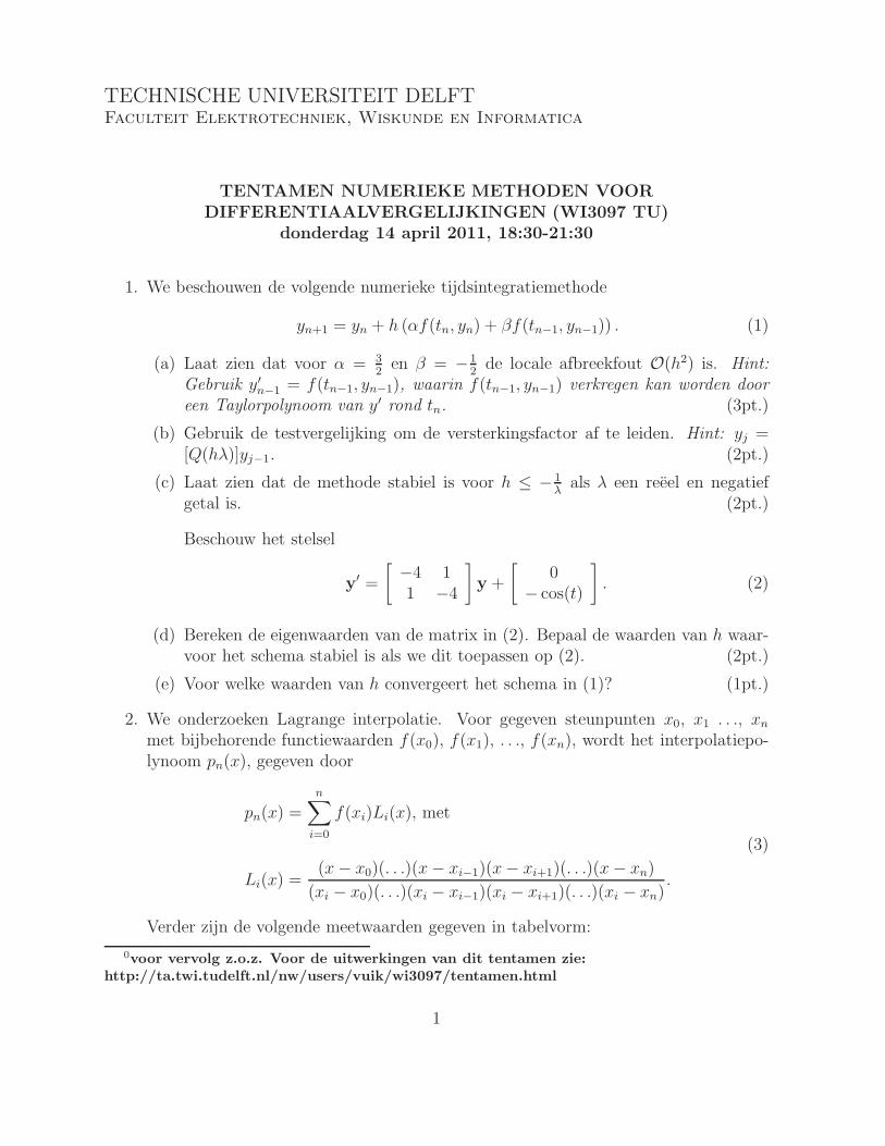
TENTAMEN NUMERIEKE METHODEN VOORDIFFERENTIAALVERGELIJKINGEN (WI3097 TU)
donderdag 14 april 2011, 18:30-21:30
1. We beschouwen de volgende numerieke tijdsintegratiemethode
yn+1 = yn + h (αf(tn, yn) + βf(tn−1, yn−1)) . (1)
(a) Laat zien dat voor α = 32
en β = −12
de locale afbreekfout O(h2) is. Hint:
Gebruik y′
n−1 = f(tn−1, yn−1), waarin f(tn−1, yn−1) verkregen kan worden door
een Taylorpolynoom van y′ rond tn. (3pt.)
(b) Gebruik de testvergelijking om de versterkingsfactor af te leiden. Hint: yj =[Q(hλ)]yj−1. (2pt.)
(c) Laat zien dat de methode stabiel is voor h ≤ − 1λ
als λ een reeel en negatiefgetal is. (2pt.)
Beschouw het stelsel
y′ =
[
−4 11 −4
]
y +
[
0− cos(t)
]
. (2)
(d) Bereken de eigenwaarden van de matrix in (2). Bepaal de waarden van h waar-voor het schema stabiel is als we dit toepassen op (2). (2pt.)
(e) Voor welke waarden van h convergeert het schema in (1)? (1pt.)
2. We onderzoeken Lagrange interpolatie. Voor gegeven steunpunten x0, x1 . . ., xn
met bijbehorende functiewaarden f(x0), f(x1), . . ., f(xn), wordt het interpolatiepo-lynoom pn(x), gegeven door
pn(x) =
n∑
i=0
f(xi)Li(x), met
Li(x) =(x − x0)(. . .)(x − xi−1)(x − xi+1)(. . .)(x − xn)
(xi − x0)(. . .)(xi − xi−1)(xi − xi+1)(. . .)(xi − xn).
(3)
Verder zijn de volgende meetwaarden gegeven in tabelvorm:
0voor vervolg z.o.z. Voor de uitwerkingen van dit tentamen zie:http://ta.twi.tudelft.nl/nw/users/vuik/wi3097/tentamen.html
1
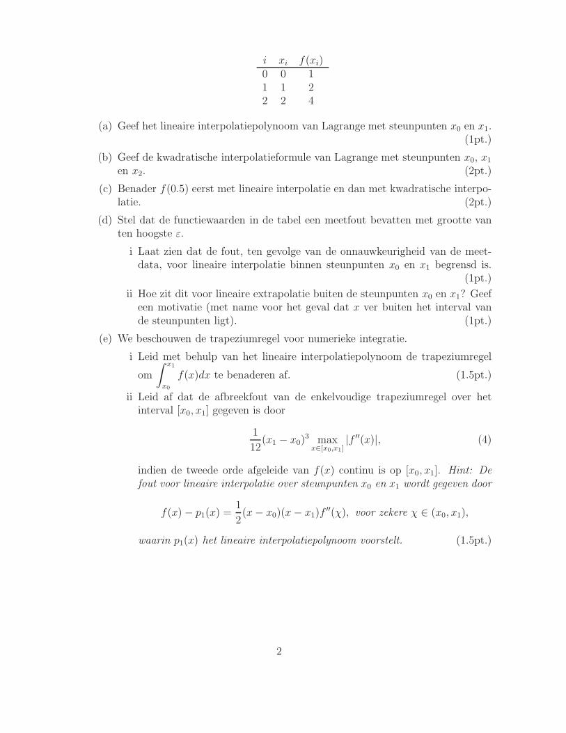
i xi f(xi)0 0 11 1 22 2 4
(a) Geef het lineaire interpolatiepolynoom van Lagrange met steunpunten x0 en x1.(1pt.)
(b) Geef de kwadratische interpolatieformule van Lagrange met steunpunten x0, x1
en x2. (2pt.)
(c) Benader f(0.5) eerst met lineaire interpolatie en dan met kwadratische interpo-latie. (2pt.)
(d) Stel dat de functiewaarden in de tabel een meetfout bevatten met grootte vanten hoogste ε.
i Laat zien dat de fout, ten gevolge van de onnauwkeurigheid van de meet-data, voor lineaire interpolatie binnen steunpunten x0 en x1 begrensd is.
(1pt.)
ii Hoe zit dit voor lineaire extrapolatie buiten de steunpunten x0 en x1? Geefeen motivatie (met name voor het geval dat x ver buiten het interval vande steunpunten ligt). (1pt.)
(e) We beschouwen de trapeziumregel voor numerieke integratie.
i Leid met behulp van het lineaire interpolatiepolynoom de trapeziumregel
om
∫ x1
x0
f(x)dx te benaderen af. (1.5pt.)
ii Leid af dat de afbreekfout van de enkelvoudige trapeziumregel over hetinterval [x0, x1] gegeven is door
1
12(x1 − x0)
3 maxx∈[x0,x1]
|f ′′(x)|, (4)
indien de tweede orde afgeleide van f(x) continu is op [x0, x1]. Hint: De
fout voor lineaire interpolatie over steunpunten x0 en x1 wordt gegeven door
f(x) − p1(x) =1
2(x − x0)(x − x1)f
′′(χ), voor zekere χ ∈ (x0, x1),
waarin p1(x) het lineaire interpolatiepolynoom voorstelt. (1.5pt.)
2
TECHNISCHE UNIVERSITEIT DELFTFaculteit Elektrotechniek, Wiskunde en Informatica
TENTAMEN NUMERIEKE METHODEN VOORDIFFERENTIAALVERGELIJKINGEN (WI3097 TU)
donderdag 19 april 2012, 18:30-21:30
1. We beschouwen de volgende methode voor de integratie van het beginwaardeprobleemy′ = f(t, y), y(t0) = y0
w∗n+1 = wn + hf(tn, wn)
wn+1 = wn + h(a1f(tn, wn) + a2f(tn+1, w
∗n+1)
) (1)
a Toon aan dat de locale afbreekfout van de bovenstaande methode van de ordeO(h) is als a1 + a2 = 1. Voor welke waarde van a1 en a2 is de locale afbreekfoutvan de orde O(h2)? (3 pt.)
b Laat zien dat de versterkingsfactor voor algemene a1 en a2 gegeven wordt door
Q(hλ) = 1 + (a1 + a2)hλ + a2(hλ)2. (2)
(2 pt.)
c Beschouw λ < 0 en (a1 + a2)2 − 8a2 < 0, leid de stabiliteitsvoorwaarde af waar
h aan moet voldoen. (2 pt.)
d Beschouw het volgende stelsel{y′
1 = −y1y2,y′
2 = y1y2 − y2,(3)
Laat zien dat de Jacobiaan van het rechterlid (die gebruikt wordt voor linea-risatie van het stelsel) voor beginvoorwaarde y1(0) = 1 en y2(0) = 2 gegevenwordt door (
−2 −12 0
).
(1.5 pt.)
e Beschouw nu de numerieke methode in vergelijking (1) voor het geval dat a1 =a2 = 1/2 toegepast op stelsel (3). Is de methode stabiel rond de beginvoorwaardey1(0) = 1 en y2(0) = 2 en stapgrootte h = 1 (+ motivatie)? (1.5 pt.)
0voor vervolg z.o.z. Voor de uitwerkingen van dit tentamen zie:http://ta.twi.tudelft.nl/nw/users/vuik/wi3097/tentamen.html
1
2. We beschouwen het volgende randwaardeprobleem:
(P1)
−v′′ + v = 2 + x(2− x), x ∈ (0, 1),
v(0) = 0, v′(1) = 0.
a Laat zien dat v(x) = x(2− x) de oplossing is van randwaardeprobleem (P1). (1pt.)
b Geef de eindige differentie discretisatie met fout van O(h2) (+ bewijs), waarin hde afstand tussen gridpunten voorstelt (Hint: gebruik een virtueel gridpunt bijx = 1). De discretisatie moet symmetrisch zijn. (3 pt.)
c Geef het stelsel vergelijkingen dat verkregen wordt na eindige differentie discreti-satie met drie (na verwerking van het virtuele gridpunt) onbekenden (h = 1/3).(2 pt.)
d Bereken de fout van de numerieke oplossing, en verklaar uw antwoord. (1 pt.)
e Vervolgens, beschouwen we het volgende niet–lineaire stelsel vergelijkingen18v1 − 9v2 + v2
1 = 209,
−9v1 + 18v2 + v22 = 20
9.
Voer een stap met de methode van Newton uit op bovenstaand stelsel waarin uv1 = v2 = 0 gebruikt als beginschatting. (3 pt.)
2
TECHNISCHE UNIVERSITEIT DELFTFaculteit Elektrotechniek, Wiskunde en Informatica
TENTAMEN NUMERIEKE METHODEN VOORDIFFERENTIAALVERGELIJKINGEN (WI3097 TU)
donderdag 25 augustus 2011, 18:30-21:30
1. We beschouwen de volgende predictor-corrector methode voor de integratie van hetbeginwaardeprobleem y′ = f(t, y), y(t0) = y0:
w∗n+1 = wn + hf(tn, wn),
wn+1 = wn + h((1− θ)f(tn, wn) + θf(tn+1, w
∗n+1)
),
(1)
waarin h de tijdstap, θ een reeel getal (0 ≤ θ ≤ 1) en wn de numerieke oplossing optijdstip tn voorstelt.
(a) Toon aan dat de locale afbreekfout van de bovenstaande methode voor 0 ≤ θ ≤ 1van de orde O(h) en voor θ = 1
2van de orde O(h2) is (N.B. Dit moet afgeleid
worden voor de algemene differentiaalvergelijking y′ = f(t, y)). (3 pt)
(b) Leid af dat de versterkingsfactor van deze methode gegeven wordt door
Q(hλ) = 1 + hλ + θ(hλ)2.
(2 pt)
(c) Gegeven is het tweede orde beginwaardeprobleem:
y′′ + 4y′ + 8y = t2 − 1, y(0) = 0 en y′(0) = 1.
Schrijf dit als een stelsel eerste orde differentiaalvergelijkingen(x′
1
x′2
)= A
(x1
x2
)+
(f(t)g(t)
).
Geef f en g en laat zien dat A =
(0 1−8 −4
). (11
2pt)
(d) Doe een stap met de methode gegeven in (1) met h = 1 en θ = 12. (11
2pt)
(e) Voor welke θ ∈ [0, 1] is de methode gegeven in (1) met h = 1 stabiel bij hettoepassen op het stelsel gegeven in onderdeel (c). Geef een duidelijke motivatie.hallo (2 pt)
0voor vervolg z.o.z. Voor de uitwerkingen van dit tentamen zie:http://ta.twi.tudelft.nl/nw/users/vuik/wi3097/tentamen.html
1
2. (a) We zoeken een formule van de vorm:
Q(h) =α0
h2f(0) +
α1
h2f(h) +
α2
h2f(2h),
zodatf ′′(0)−Q(h) = O(h).
Geef het lineaire stelsel vergelijkingen waar α0, α1 en α2 aan moeten voldoen.hallo (2 pt)
(b) De oplossing van het in het vorige onderdeel afgeleide stelsel wordt gegeven doorα0 = 1, α1 = −2 en α2 = 1. Geef voor deze waarden een uitdrukking voor deafbreekfout f ′′(0)−Q(h). (2 pt)
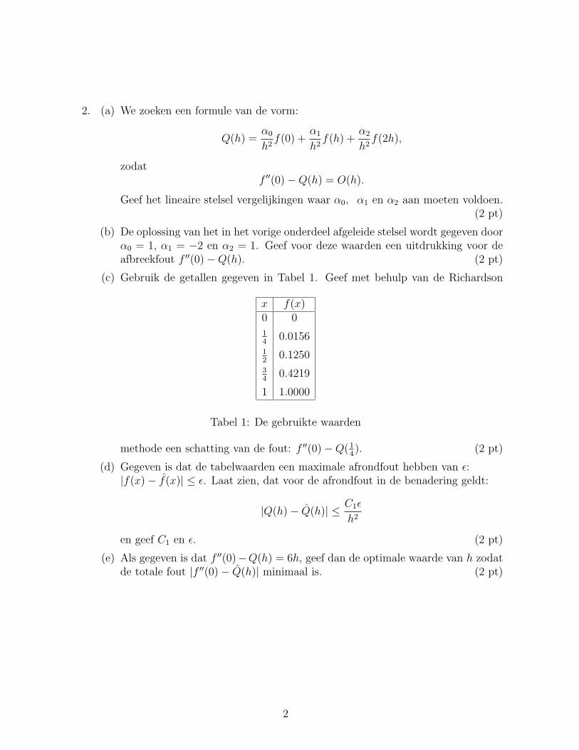
(c) Gebruik de getallen gegeven in Tabel 1. Geef met behulp van de Richardson
x f(x)0 014
0.015612
0.125034
0.4219
1 1.0000
Tabel 1: De gebruikte waarden
methode een schatting van de fout: f ′′(0)−Q(14). (2 pt)
(d) Gegeven is dat de tabelwaarden een maximale afrondfout hebben van ε:|f(x)− f(x)| ≤ ε. Laat zien, dat voor de afrondfout in de benadering geldt:
|Q(h)− Q(h)| ≤ C1ε
h2
en geef C1 en ε. (2 pt)
(e) Als gegeven is dat f ′′(0)−Q(h) = 6h, geef dan de optimale waarde van h zodatde totale fout |f ′′(0)− Q(h)| minimaal is. (2 pt)
2
TECHNISCHE UNIVERSITEIT DELFTFaculteit Elektrotechniek, Wiskunde en Informatica
TENTAMEN NUMERIEKE METHODEN VOORDIFFERENTIAALVERGELIJKINGEN (WI3097 TU)
donderdag 30 augustus 2012, 18:30-21:30
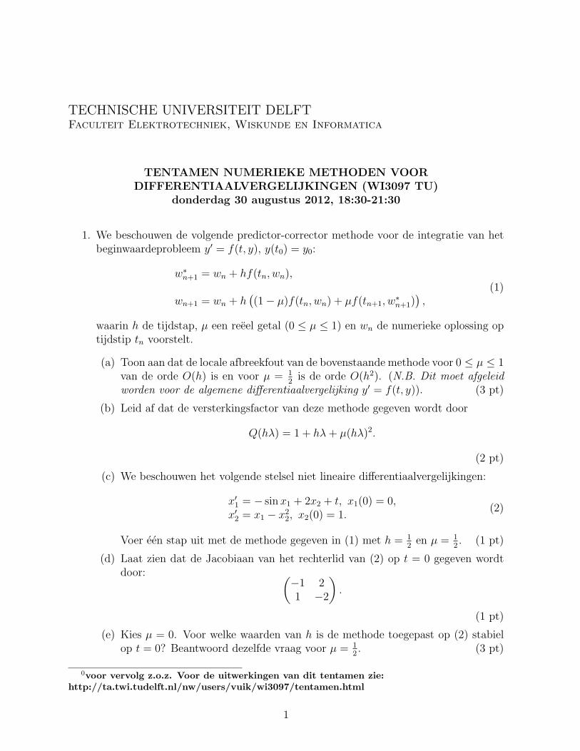
1. We beschouwen de volgende predictor-corrector methode voor de integratie van hetbeginwaardeprobleem y′ = f(t, y), y(t0) = y0:
w∗n+1 = wn + hf(tn, wn),
wn+1 = wn + h((1− µ)f(tn, wn) + µf(tn+1, w
∗n+1)
),
(1)
waarin h de tijdstap, µ een reeel getal (0 ≤ µ ≤ 1) en wn de numerieke oplossing optijdstip tn voorstelt.
(a) Toon aan dat de locale afbreekfout van de bovenstaande methode voor 0 ≤ µ ≤ 1van de orde O(h) is en voor µ = 1
2is de orde O(h2). (N.B. Dit moet afgeleid
worden voor de algemene differentiaalvergelijking y′ = f(t, y)). (3 pt)
(b) Leid af dat de versterkingsfactor van deze methode gegeven wordt door
Q(hλ) = 1 + hλ + µ(hλ)2.
(2 pt)
(c) We beschouwen het volgende stelsel niet lineaire differentiaalvergelijkingen:
x′1 = − sin x1 + 2x2 + t, x1(0) = 0,
x′2 = x1 − x2
2, x2(0) = 1.(2)
Voer een stap uit met de methode gegeven in (1) met h = 12
en µ = 12. (1 pt)
(d) Laat zien dat de Jacobiaan van het rechterlid van (2) op t = 0 gegeven wordtdoor: (
−1 21 −2
).
(1 pt)
(e) Kies µ = 0. Voor welke waarden van h is de methode toegepast op (2) stabielop t = 0? Beantwoord dezelfde vraag voor µ = 1
2. (3 pt)
0voor vervolg z.o.z. Voor de uitwerkingen van dit tentamen zie:http://ta.twi.tudelft.nl/nw/users/vuik/wi3097/tentamen.html
1

2. We benaderen de integraal∫ b
af(x)dx met steunpunten xj = a + (j − 1)h, waarin
xn+1 = b. Voor een interval tussen twee naburige steunpunten, (xj, xj+1), geeft de
rechthoekregel de benadering hf(xj) en herhaalde toepassing geeft∫ b
af(x)dx ≈ T0 =
h∑n
j=1 f(xj).
(a) Laat zien dat de locale afbreekfout, |EI0 | := |
∫ xj+1
xjf(x)dx− hf(xj)|, en globale
fout, |E0| := |∫ b
af(x)dx− T0| achtereenvolgens gegeven worden door
|EI0 | ≤
h2
2max
x∈[xj ,xj+1]|f ′(x)|, en |E0| ≤
(b− a)h
2maxx∈[a,b]
|f ′(x)|. (3)
Hint: U kunt de stelling van Taylor gebruiken en maxx∈[a,b] |f(x)| staat voor hetmaximum van |f(x)| over het interval [a, b]. (2 pt.)
(b) Nu nemen we ook de eerste afgeleide van f in de steunpunten {xj} mee. Gebruikde stelling van Taylor om af te leiden dat de integraal m.b.v. de steunpuntenbenaderd kan worden door T1 met globale fout E1, waarin∫ b
a
f(x)dx ≈ T1 = hn∑
j=1
[f(xj) +
h
2f ′(xj)
], |E1| ≤
(b− a)h2
6maxx∈[a,b]
|f ′′(x)|.
(4)(2pt.)
(c) Gebruik de methode uit vergelijking (4) met h = 12
om∫ 1
0x2dx te benaderen en
vergelijk de fout met de schatting voor |E1|. (2pt.)
(d) Nu gebruiken we de afgeleiden van f tot en met de 2-de orde. Verder zijn T2
en E2 achtereenvolgens de benadering van∫ b
af(x)dx met deze afgeleiden en de
bijbehorende globale fout. Toon aan dat
T2 = T1 +h3
3!
n∑j=1
f ′′(xj), en |E2| ≤(b− a)h3
4!maxx∈[a,b]
|f ′′′(x)|. (5)
(2pt.)
(e) Stel dat alle functiewaarden en hun afgeleiden een meet-of afrondfout van tenhoogste ε bevatten, d.w.z. |f (k)(xj)−f (k)(xj)| ≤ ε, voor alle j en k–de afgeleiden(k = 0 geeft f zelf). Laat T2 en T2 achtereenvolgens berekend zijn met de exacte(f) en beschikbare waarden (f) van f en zijn afgeleiden, toon aan dat de invloedvan deze fout afgeschat kan worden door:
|T2 − T2| ≤ (b− a)ε
(1 +
h
2+
h2
3!
). (6)
(2pt.)
2
TECHNISCHE UNIVERSITEIT DELFTFaculteit Elektrotechniek, Wiskunde en Informatica
TENTAMEN NUMERIEKE METHODEN VOORDIFFERENTIAALVERGELIJKINGEN (WI3097 TU)
donderdag 20 januari 2011, 18:30-21:30
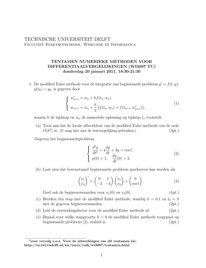
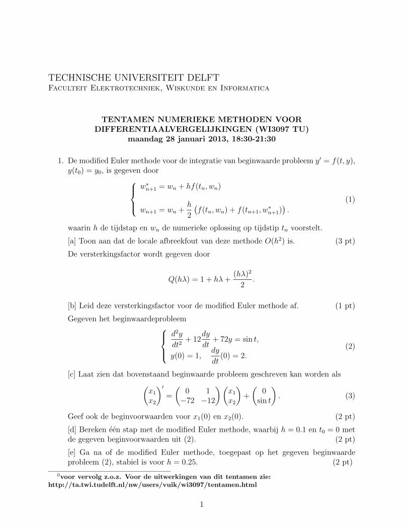
1. De modified Euler methode voor de integratie van beginwaarde probleem y′ = f(t, y),y(t0) = y0, is gegeven door
w∗n+1 = wn + hf(tn, wn)
wn+1 = wn +h
2
(f(tn, wn) + f(tn+1, w
∗n+1)
),
(1)
waarin h de tijdstap en wn de numerieke oplossing op tijdstip tn voorstelt.
(a) Toon aan dat de locale afbreekfout van de modified Euler methode van de ordeO(h2) is. (U mag hier niet de testvergelijking gebruiken.) (3pt.)
Gegeven het beginwaardeprobleemd2y
dt2+ 4
dy
dt+ 3y = cos t,
y(0) = 1,dy
dt(0) = 2.
(2)
(b) Laat zien dat bovenstaand beginwaarde probleem geschreven kan worden als(x1
x2
)′
=
(0 1−3 −4
) (x1
x2
)+
(0
cos t
). (3)
Geef ook de beginvoorwaarden voor x1(0) en x2(0). (1pt.)
(c) Bereken een stap met de modified Euler methode, waarbij h = 0.1 en t0 = 0met de gegeven beginvoorwaarden. (2pt.)
(d) Leid de versterkingsfactor voor de modified Euler methode af. (2pt.)
(e) Bepaal voor welke stapgrootte h > 0 de modified Euler methode toegepast opbeginwaarde probleem (2), stabiel is. (2pt.)
0voor vervolg z.o.z. Voor de uitwerkingen van dit tentamen zie:http://ta.twi.tudelft.nl/nw/users/vuik/wi3097/tentamen.html
1
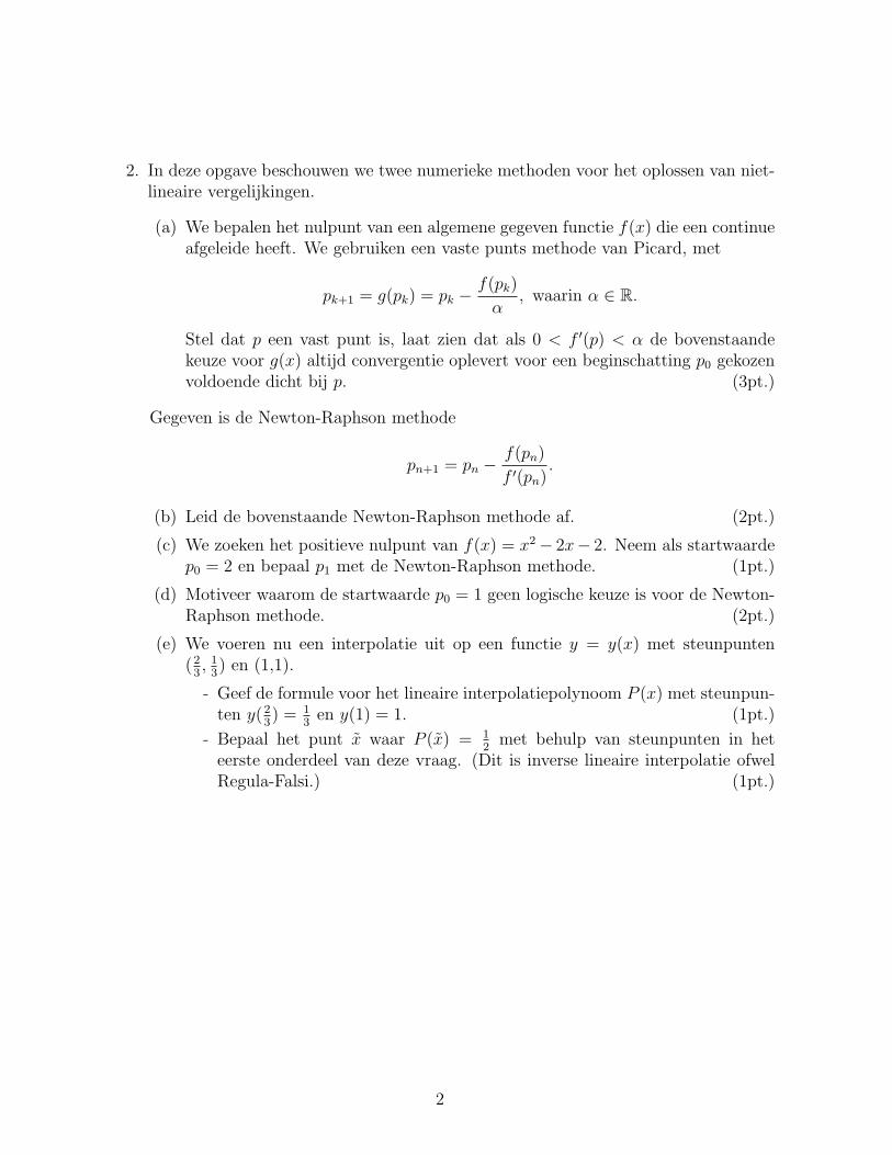
2. In deze opgave beschouwen we twee numerieke methoden voor het oplossen van niet-lineaire vergelijkingen.
(a) We bepalen het nulpunt van een algemene gegeven functie f(x) die een continueafgeleide heeft. We gebruiken een vaste punts methode van Picard, met
pk+1 = g(pk) = pk −f(pk)
α, waarin α ∈ R.
Stel dat p een vast punt is, laat zien dat als 0 < f ′(p) < α de bovenstaandekeuze voor g(x) altijd convergentie oplevert voor een beginschatting p0 gekozenvoldoende dicht bij p. (3pt.)
Gegeven is de Newton-Raphson methode
pn+1 = pn −f(pn)
f ′(pn).
(b) Leid de bovenstaande Newton-Raphson methode af. (2pt.)
(c) We zoeken het positieve nulpunt van f(x) = x2− 2x− 2. Neem als startwaardep0 = 2 en bepaal p1 met de Newton-Raphson methode. (1pt.)
(d) Motiveer waarom de startwaarde p0 = 1 geen logische keuze is voor de Newton-Raphson methode. (2pt.)
(e) We voeren nu een interpolatie uit op een functie y = y(x) met steunpunten(2
3, 1
3) en (1,1).
- Geef de formule voor het lineaire interpolatiepolynoom P (x) met steunpun-ten y(2
3) = 1
3en y(1) = 1. (1pt.)
- Bepaal het punt x waar P (x) = 12
met behulp van steunpunten in heteerste onderdeel van deze vraag. (Dit is inverse lineaire interpolatie ofwelRegula-Falsi.) (1pt.)
2
TECHNISCHE UNIVERSITEIT DELFTFaculteit Elektrotechniek, Wiskunde en Informatica
TENTAMEN NUMERIEKE METHODEN VOORDIFFERENTIAALVERGELIJKINGEN (WI3097 TU)
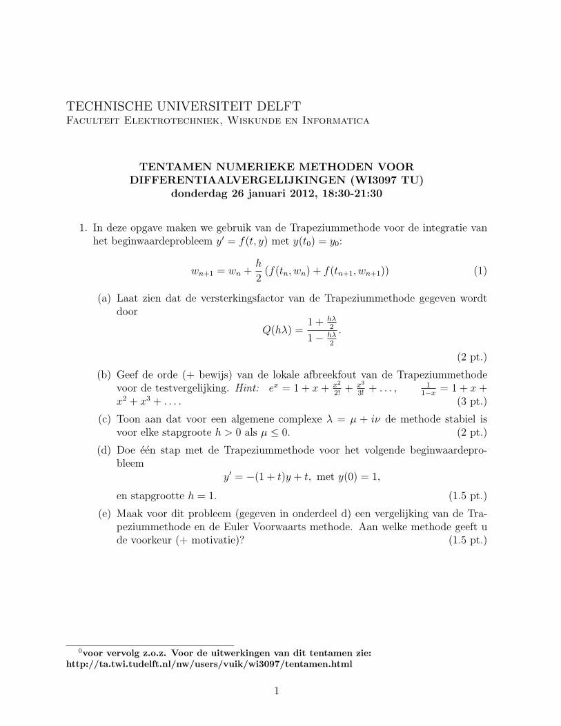
donderdag 26 januari 2012, 18:30-21:30
1. In deze opgave maken we gebruik van de Trapeziummethode voor de integratie vanhet beginwaardeprobleem y′ = f(t, y) met y(t0) = y0:
wn+1 = wn +h
2(f(tn, wn) + f(tn+1, wn+1)) (1)
(a) Laat zien dat de versterkingsfactor van de Trapeziummethode gegeven wordtdoor
Q(hλ) =1 + hλ
2
1− hλ2
.
(2 pt.)
(b) Geef de orde (+ bewijs) van de lokale afbreekfout van de Trapeziummethodevoor de testvergelijking. Hint: ex = 1 + x + x2
2!+ x3
3!+ . . . , 1
1−x= 1 + x +
x2 + x3 + . . . . (3 pt.)
(c) Toon aan dat voor een algemene complexe λ = µ + iν de methode stabiel isvoor elke stapgroote h > 0 als µ ≤ 0. (2 pt.)
(d) Doe een stap met de Trapeziummethode voor het volgende beginwaardepro-bleem
y′ = −(1 + t)y + t, met y(0) = 1,
en stapgrootte h = 1. (1.5 pt.)
(e) Maak voor dit probleem (gegeven in onderdeel d) een vergelijking van de Tra-peziummethode en de Euler Voorwaarts methode. Aan welke methode geeft ude voorkeur (+ motivatie)? (1.5 pt.)
0voor vervolg z.o.z. Voor de uitwerkingen van dit tentamen zie:http://ta.twi.tudelft.nl/nw/users/vuik/wi3097/tentamen.html
1
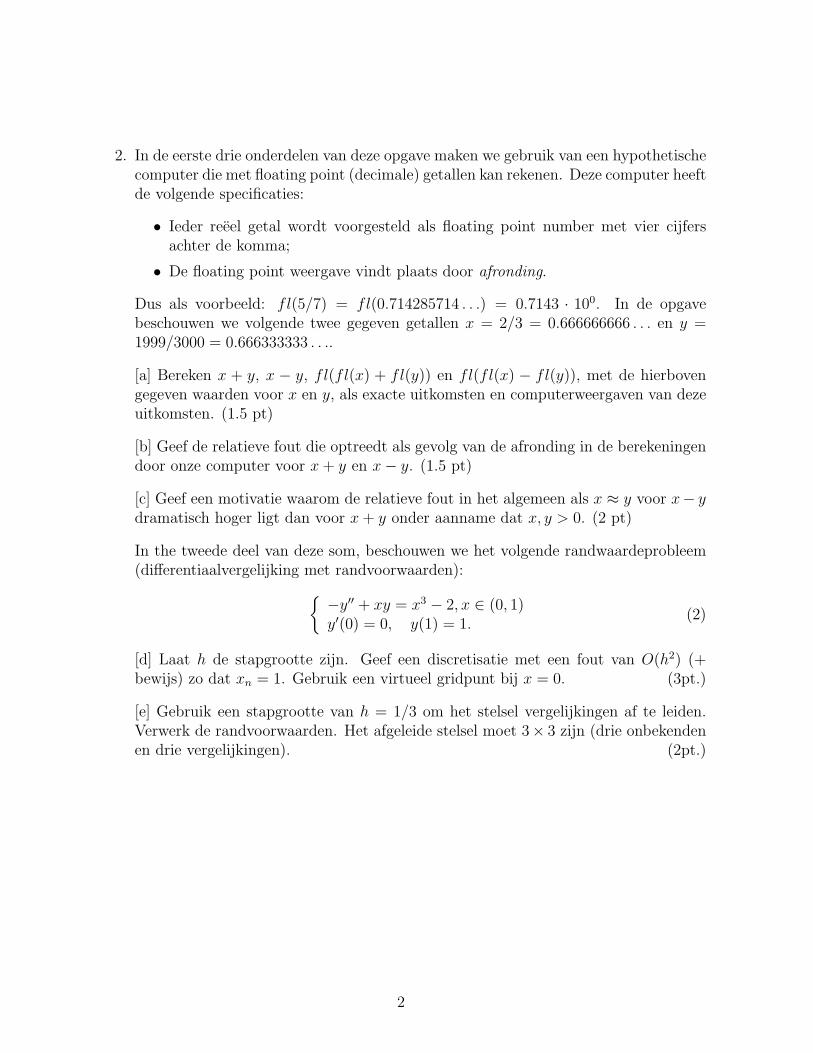
2. In de eerste drie onderdelen van deze opgave maken we gebruik van een hypothetischecomputer die met floating point (decimale) getallen kan rekenen. Deze computer heeftde volgende specificaties:
• Ieder reeel getal wordt voorgesteld als floating point number met vier cijfersachter de komma;
• De floating point weergave vindt plaats door afronding.
Dus als voorbeeld: fl(5/7) = fl(0.714285714 . . .) = 0.7143 · 100. In de opgavebeschouwen we volgende twee gegeven getallen x = 2/3 = 0.666666666 . . . en y =1999/3000 = 0.666333333 . . ..
[a] Bereken x + y, x − y, fl(fl(x) + fl(y)) en fl(fl(x) − fl(y)), met de hierbovengegeven waarden voor x en y, als exacte uitkomsten en computerweergaven van dezeuitkomsten. (1.5 pt)
[b] Geef de relatieve fout die optreedt als gevolg van de afronding in de berekeningendoor onze computer voor x + y en x− y. (1.5 pt)
[c] Geef een motivatie waarom de relatieve fout in het algemeen als x ≈ y voor x− ydramatisch hoger ligt dan voor x + y onder aanname dat x, y > 0. (2 pt)
In the tweede deel van deze som, beschouwen we het volgende randwaardeprobleem(differentiaalvergelijking met randvoorwaarden):{
−y′′ + xy = x3 − 2, x ∈ (0, 1)y′(0) = 0, y(1) = 1.
(2)
[d] Laat h de stapgrootte zijn. Geef een discretisatie met een fout van O(h2) (+bewijs) zo dat xn = 1. Gebruik een virtueel gridpunt bij x = 0. (3pt.)
[e] Gebruik een stapgrootte van h = 1/3 om het stelsel vergelijkingen af te leiden.Verwerk de randvoorwaarden. Het afgeleide stelsel moet 3× 3 zijn (drie onbekendenen drie vergelijkingen). (2pt.)
2
TECHNISCHE UNIVERSITEIT DELFTFaculteit Elektrotechniek, Wiskunde en Informatica
TENTAMEN NUMERIEKE METHODEN VOORDIFFERENTIAALVERGELIJKINGEN (WI3097 TU)
maandag 28 januari 2013, 18:30-21:30
1. De modified Euler methode voor de integratie van beginwaarde probleem y′ = f(t, y),y(t0) = y0, is gegeven door
w∗n+1 = wn + hf(tn, wn)
wn+1 = wn +h
2
(f(tn, wn) + f(tn+1, w
∗n+1)
).
(1)
waarin h de tijdstap en wn de numerieke oplossing op tijdstip tn voorstelt.
[a] Toon aan dat de locale afbreekfout van deze methode O(h2) is. (3 pt)
De versterkingsfactor wordt gegeven door
Q(hλ) = 1 + hλ+(hλ)2
2.
[b] Leid deze versterkingsfactor voor de modified Euler methode af. (1 pt)
Gegeven het beginwaardeprobleemd2y
dt2+ 12
dy
dt+ 72y = sin t,
y(0) = 1,dy
dt(0) = 2.
(2)
[c] Laat zien dat bovenstaand beginwaarde probleem geschreven kan worden als(x1x2
)′=
(0 1−72 −12
)(x1x2
)+
(0
sin t
). (3)
Geef ook de beginvoorwaarden voor x1(0) en x2(0). (2 pt)
[d] Bereken een stap met de modified Euler methode, waarbij h = 0.1 en t0 = 0 metde gegeven beginvoorwaarden uit (2). (2 pt)
[e] Ga na of de modified Euler methode, toegepast op het gegeven beginwaardeprobleem (2), stabiel is voor h = 0.25. (2 pt)
0voor vervolg z.o.z. Voor de uitwerkingen van dit tentamen zie:http://ta.twi.tudelft.nl/nw/users/vuik/wi3097/tentamen.html
1
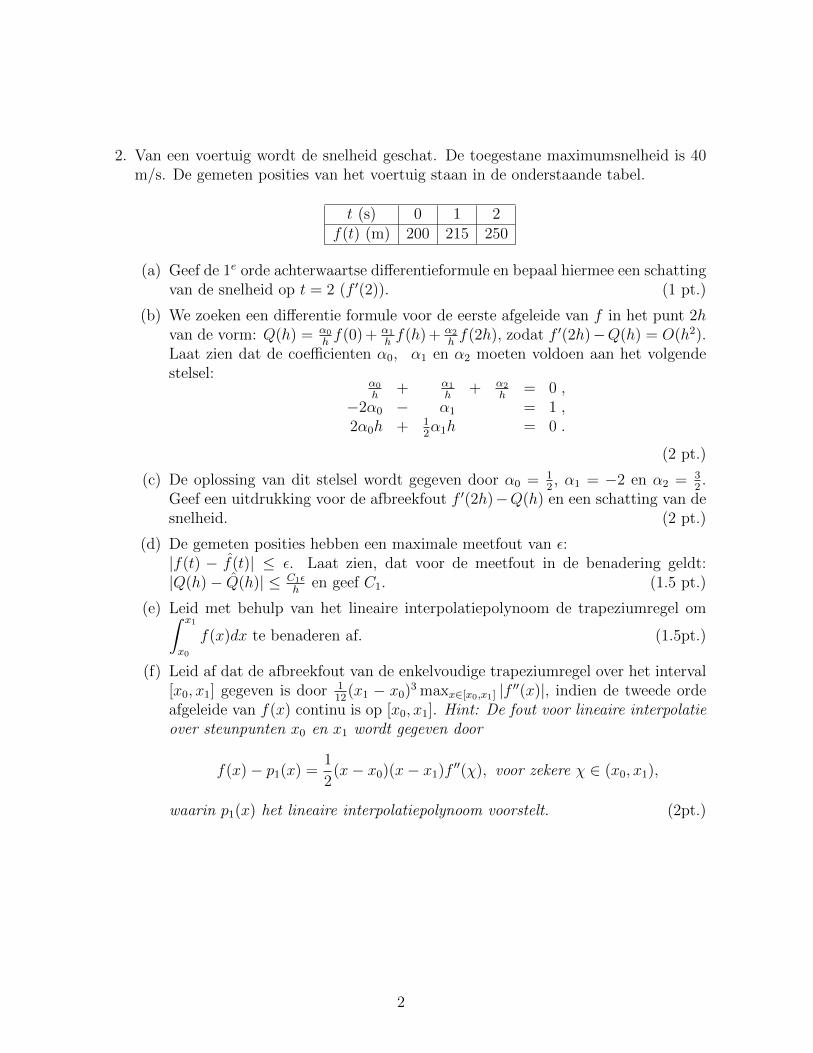
2. Van een voertuig wordt de snelheid geschat. De toegestane maximumsnelheid is 40m/s. De gemeten posities van het voertuig staan in de onderstaande tabel.
t (s) 0 1 2f(t) (m) 200 215 250
(a) Geef de 1e orde achterwaartse differentieformule en bepaal hiermee een schattingvan de snelheid op t = 2 (f ′(2)). (1 pt.)
(b) We zoeken een differentie formule voor de eerste afgeleide van f in het punt 2hvan de vorm: Q(h) = α0
hf(0) + α1
hf(h) + α2
hf(2h), zodat f ′(2h)−Q(h) = O(h2).
Laat zien dat de coefficienten α0, α1 en α2 moeten voldoen aan het volgendestelsel:
α0
h+ α1
h+ α2
h= 0 ,
−2α0 − α1 = 1 ,2α0h + 1
2α1h = 0 .
(2 pt.)
(c) De oplossing van dit stelsel wordt gegeven door α0 = 12, α1 = −2 en α2 = 3
2.
Geef een uitdrukking voor de afbreekfout f ′(2h)−Q(h) en een schatting van desnelheid. (2 pt.)
(d) De gemeten posities hebben een maximale meetfout van ε:|f(t) − f(t)| ≤ ε. Laat zien, dat voor de meetfout in de benadering geldt:|Q(h)− Q(h)| ≤ C1ε
hen geef C1. (1.5 pt.)
(e) Leid met behulp van het lineaire interpolatiepolynoom de trapeziumregel om∫ x1
x0
f(x)dx te benaderen af. (1.5pt.)
(f) Leid af dat de afbreekfout van de enkelvoudige trapeziumregel over het interval[x0, x1] gegeven is door 1
12(x1 − x0)3 maxx∈[x0,x1] |f ′′(x)|, indien de tweede orde
afgeleide van f(x) continu is op [x0, x1]. Hint: De fout voor lineaire interpolatieover steunpunten x0 en x1 wordt gegeven door
f(x)− p1(x) =1
2(x− x0)(x− x1)f ′′(χ), voor zekere χ ∈ (x0, x1),
waarin p1(x) het lineaire interpolatiepolynoom voorstelt. (2pt.)
2
TECHNISCHE UNIVERSITEIT DELFTFaculteit Elektrotechniek, Wiskunde en Informatica
TENTAMEN NUMERIEKE METHODEN VOORDIFFERENTIAALVERGELIJKINGEN (WI3097 TU)
donderdag 5 juli 2012, 18:30-21:30
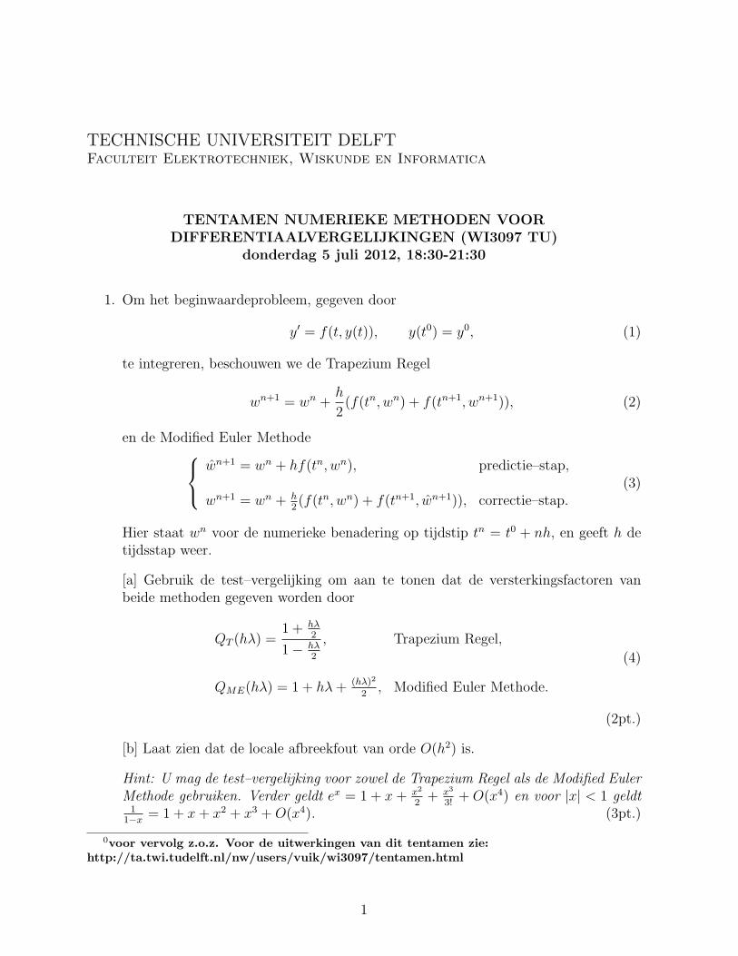
1. Om het beginwaardeprobleem, gegeven door
y′ = f(t, y(t)), y(t0) = y0, (1)
te integreren, beschouwen we de Trapezium Regel
wn+1 = wn +h
2(f(tn, wn) + f(tn+1, wn+1)), (2)
en de Modified Euler Methodewn+1 = wn + hf(tn, wn), predictie–stap,
wn+1 = wn + h2(f(tn, wn) + f(tn+1, wn+1)), correctie–stap.
(3)
Hier staat wn voor de numerieke benadering op tijdstip tn = t0 + nh, en geeft h detijdsstap weer.
[a] Gebruik de test–vergelijking om aan te tonen dat de versterkingsfactoren vanbeide methoden gegeven worden door
QT (hλ) =1 + hλ
2
1− hλ2
, Trapezium Regel,
QME(hλ) = 1 + hλ + (hλ)2
2, Modified Euler Methode.
(4)
(2pt.)
[b] Laat zien dat de locale afbreekfout van orde O(h2) is.
Hint: U mag de test–vergelijking voor zowel de Trapezium Regel als de Modified EulerMethode gebruiken. Verder geldt ex = 1 + x + x2
2+ x3
3!+ O(x4) en voor |x| < 1 geldt
11−x
= 1 + x + x2 + x3 + O(x4). (3pt.)
0voor vervolg z.o.z. Voor de uitwerkingen van dit tentamen zie:http://ta.twi.tudelft.nl/nw/users/vuik/wi3097/tentamen.html
1
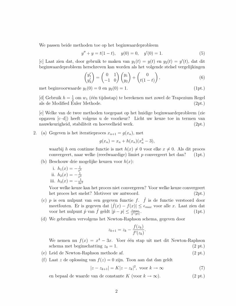
We passen beide methoden toe op het beginwaardeprobleem
y′′ + y = t(1− t), y(0) = 0, y′(0) = 1. (5)
[c] Laat zien dat, door gebruik te maken van y1(t) = y(t) en y2(t) = y′(t), dat ditbeginwaardeprobleem herschreven kan worden als het volgende stelsel vergelijkingen(
y′1
y′2
)=
(0 1−1 0
) (y1
y2
)+
(0
t(1− t)
), (6)
met beginvoorwaarde y1(0) = 0 en y2(0) = 1. (1pt.)
[d] Gebruik h = 12
om w1 (een tijdsstap) te berekenen met zowel de Trapezium Regelals de Modified Euler Methode. (2pt.)
[e] Welke van de twee methoden toegepast op het huidige beginwaardeprobleem (zieopgaven [c–d]) heeft volgens u de voorkeur? Licht uw keuze toe in termen vannauwkeurigheid, stabiliteit en hoeveelheid werk. (2pt.)
2. (a) Gegeven is het iteratieproces xn+1 = g(xn), met
g(xn) = xn + h(xn)(x3n − 3),
waarbij h een continue functie is met h(x) 6= 0 voor elke x 6= 0. Als dit procesconvergeert, naar welke (reeelwaardige) limiet p convergeert het dan? (1pt.)
(b) Beschouw drie mogelijke keuzen voor h(x):
i. h1(x) = − 1x4
ii. h2(x) = − 1x2
iii. h3(x) = − 13x2
Voor welke keuze kan het proces niet convergeren? Voor welke keuze convergeerthet proces het snelst? Motiveer uw antwoord. (2pt.)
(c) p is een nulpunt van een gegeven functie f . f is de functie verstoord doormeetfouten. Er is gegeven dat |f(x) − f(x)| ≤ εmax voor alle x. Laat zien datvoor het nulpunt p van f geldt |p− p| ≤ εmax
|f ′(p)| . (1pt.)
(d) We gebruiken vervolgens het Newton-Raphson schema, gegeven door
zk+1 = zk −f(zk)
f ′(zk).
We nemen nu f(x) = x4 − 3x. Voer een stap uit met dit Newton-Raphsonschema met beginschatting z0 = 1. (2 pt.)
(e) Leid de Newton-Raphson methode af. (2 pt.)
(f) Laat z de oplossing van f(z) = 0 zijn. Toon aan dat dan geldt
|z − zk+1| = K|z − zk|2, voor k →∞ (7)
en bepaal de waarde van de constante K (voor k →∞). (2 pt.)
2
TECHNISCHE UNIVERSITEIT DELFTFaculteit Elektrotechniek, Wiskunde en Informatica
TENTAMEN NUMERIEKE METHODEN VOORDIFFERENTIAALVERGELIJKINGEN (WI3097 TU)
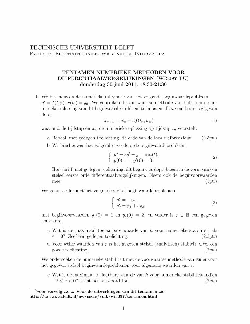
donderdag 30 juni 2011, 18:30-21:30
1. We beschouwen de numerieke integratie van het volgende beginwaardeprobleemy′ = f(t, y), y(t0) = y0. We gebruiken de voorwaartse methode van Euler om de nu-merieke oplossing van dit beginwaardeprobleem te bepalen. Deze methode is gegevendoor
wn+1 = wn + hf(tn, wn), (1)
waarin h de tijdstap en wn de numerieke oplossing op tijdstip tn voorstelt.
a Bepaal, met gedegen toelichting, de orde van de locale afbreekfout. (2.5pt.)
b We beschouwen het volgende tweede orde beginwaardeprobleem{y′′ + εy′ + y = sin(t),y(0) = 1, y′(0) = 0.
(2)
Herschrijf, met gedegen toelichting, dit beginwaardeprobleem in de vorm van eenstelsel eerste orde differentiaalvergelijkingen. Neem ook de beginvoorwaardenmee. (1pt.)
We gaan verder met het volgende stelsel beginwaardeproblemen{y′
1 = −y2,y′
2 = y1 + εy2,(3)
met beginvoorwaarden y1(0) = 1 en y2(0) = 2, en verder is ε ∈ R een gegevenconstante.
c Wat is de maximaal toelaatbare waarde van h voor numerieke stabiliteit alsε = 0? Geef een gedegen toelichting. (2.5pt.)
d Voor welke waarden van ε is het gegeven stelsel (analytisch) stabiel? Geef eengoede toelichting. (2pt.)
We onderzoeken de numerieke stabiliteit met de voorwaartse methode van Euler voorhet gegeven stelsel beginwaardeproblemen voor algemene waarden van ε.
e Wat is de maximaal toelaatbare waarde van h voor numerieke stabiliteit indien−2 ≤ ε < 0? Licht het antwoord toe. (2pt.)
0voor vervolg z.o.z. Voor de uitwerkingen van dit tentamen zie:http://ta.twi.tudelft.nl/nw/users/vuik/wi3097/tentamen.html
1
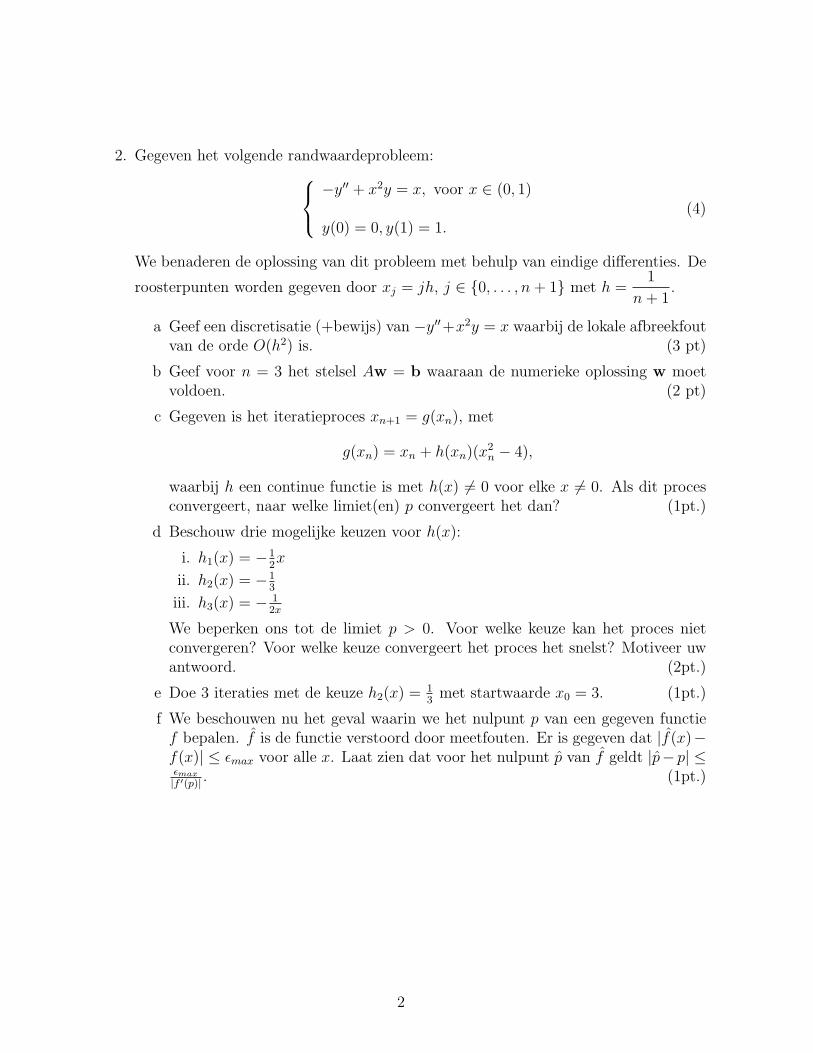
2. Gegeven het volgende randwaardeprobleem:−y′′ + x2y = x, voor x ∈ (0, 1)
y(0) = 0, y(1) = 1.(4)
We benaderen de oplossing van dit probleem met behulp van eindige differenties. De
roosterpunten worden gegeven door xj = jh, j ∈ {0, . . . , n + 1} met h =1
n + 1.
a Geef een discretisatie (+bewijs) van −y′′+x2y = x waarbij de lokale afbreekfoutvan de orde O(h2) is. (3 pt)
b Geef voor n = 3 het stelsel Aw = b waaraan de numerieke oplossing w moetvoldoen. (2 pt)
c Gegeven is het iteratieproces xn+1 = g(xn), met
g(xn) = xn + h(xn)(x2n − 4),
waarbij h een continue functie is met h(x) 6= 0 voor elke x 6= 0. Als dit procesconvergeert, naar welke limiet(en) p convergeert het dan? (1pt.)
d Beschouw drie mogelijke keuzen voor h(x):
i. h1(x) = −12x
ii. h2(x) = −13
iii. h3(x) = − 12x
We beperken ons tot de limiet p > 0. Voor welke keuze kan het proces nietconvergeren? Voor welke keuze convergeert het proces het snelst? Motiveer uwantwoord. (2pt.)
e Doe 3 iteraties met de keuze h2(x) = 13
met startwaarde x0 = 3. (1pt.)
f We beschouwen nu het geval waarin we het nulpunt p van een gegeven functief bepalen. f is de functie verstoord door meetfouten. Er is gegeven dat |f(x)−f(x)| ≤ εmax voor alle x. Laat zien dat voor het nulpunt p van f geldt |p− p| ≤εmax
|f ′(p)| . (1pt.)
2
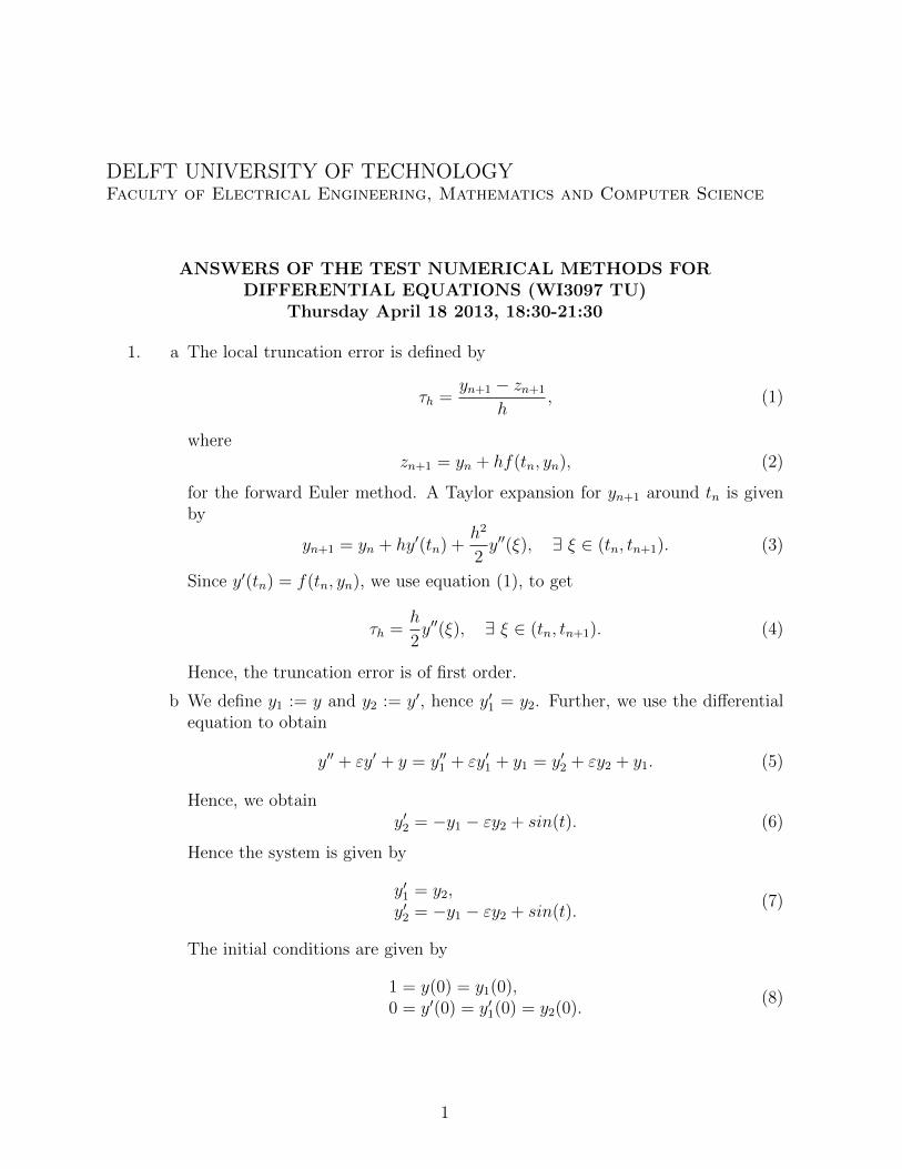
DELFT UNIVERSITY OF TECHNOLOGYFaculty of Electrical Engineering, Mathematics and Computer Science
ANSWERS OF THE TEST NUMERICAL METHODS FORDIFFERENTIAL EQUATIONS (WI3097 TU)
Thursday April 18 2013, 18:30-21:30
1. a The local truncation error is defined by
τh =yn+1 − zn+1
h, (1)
wherezn+1 = yn + hf(tn, yn), (2)
for the forward Euler method. A Taylor expansion for yn+1 around tn is givenby
yn+1 = yn + hy′(tn) +h2
2y′′(ξ), ∃ ξ ∈ (tn, tn+1). (3)
Since y′(tn) = f(tn, yn), we use equation (1), to get
τh =h
2y′′(ξ), ∃ ξ ∈ (tn, tn+1). (4)
Hence, the truncation error is of first order.
b We define y1 := y and y2 := y′, hence y′1 = y2. Further, we use the differentialequation to obtain
y′′ + εy′ + y = y′′1 + εy′1 + y1 = y′2 + εy2 + y1. (5)
Hence, we obtainy′2 = −y1 − εy2 + sin(t). (6)
Hence the system is given by
y′1 = y2,y′2 = −y1 − εy2 + sin(t).
(7)
The initial conditions are given by
1 = y(0) = y1(0),0 = y′(0) = y′1(0) = y2(0).
(8)
1
c First, we use the test equation, y′ = λy, to analyze numerical stability. Forforward Euler, we obtain
wn+1 = wn + hλwn = Q(hλ)wn, (9)
hence the amplification factor becomes
Q(hλ) = 1 + hλ. (10)
The numerical solution is stable if and only if |Q(hλ)| ≤ 1. Next, we deal withthe case ε = 0, to obtain the following system(
y′1y′2
)=
(0 −11 0
)(y1y2
). (11)
This system gives the following eigenvalues λ1,2 = ±i, where i is the imaginaryunit. Hence, the amplification factor is given by
Q(hλ) = 1± hi. (12)
Then, it is immediately clear that |Q(hλ)| > 1 for all h > 0. Hence, we concludethat the forward Euler method is never stable if ε = 0.
d From Assignment 1.c., we know that if ε = 0, the eigenvalues of the system arepurely imaginary. This implies that the system is analytically (zero) stable ifε = 0.
Nonzero values of ε give the following system(y′1y′2
)=
(0 −11 ε
)(y1y2
). (13)
then we get the following eigenvalues λ1,2 = ε2± 1
2
√ε2 − 4 (real-valued), if
ε2 − 4 ≥ 0 and λ = ε2± i
2
√4− ε2 (nonreal-valued) if ε2 − 4 < 0. Hence,
we consider two cases: real-valued and nonreal-valued eigenvalues.
Real-valued eigenvaluesIn this case |ε| ≥ 2, and 0 ≤ ε2 − 4 < ε2, and hence the real-valued eigenvalueshave the same sign, which is determined by the sign of ε. Hence, if ε ≤ −2,then, the system is stable. Furthermore, if ε ≥ 2, then, the system is unstable.
Nonreal-valued eigenvaluesIn this case |ε| < 2. The system is analytically unstable if and only if the realpart of the eigenvalues is positive. Further, the real part of the eigenvalues ispositive if and only if ε > 0. Hence, the system is analytically unstable if andonly if ε > 0. Hence, the system is stable if and only if (−2 <)ε ≤ 0.
From these arguments, it follows that the system is stable if and only if ε ≤ 0.
2
e Since currently the discriminant, ε2−4, is negative, the eigenvalues are nonreal.Substitution into the amplification factor yields
Q(hλ) = 1 +ε
2h± ih
2
√4− ε2. (14)
Hence, numerical stability is warranted if
|Q(hλ)|2 = (1 +ε
2h)2 +
h2
4(4− ε2) ≤ 1. (15)
Hence for stability, we have
1 + εh+ε2h2
4+ h2 − ε2h2
4= 1 + hε+ h2 ≤ 1. (16)
Since h > 0, we obtain the following stability criterion
h ≤ −ε = |ε|. (17)
If ε = −2, then both eigenvalues are real-valued and given by λ1,2 = −1. Forthis case, we obtain Q(λh) = 1 − h, and stability is warranted if and only if−1 ≤ Q(hλ) ≤ 1, hence h ≤ 2(= |ε|).
We conclude that for −2 ≤ ε < 0, we have a numerically stable solution if andonly if h ≤ |ε|.
2. a First we check that y(x) = x2 satisfies the boundary conditions. It immediatelyfollows that y(0) = 0 and using y′(x) = 2x, gives y′(1) = 2, and hence theboundary conditions are satisfied. Further, substitution of y = x2, using y′′(x) =2, gives
−y′′ + y′ + y = −2 + 2x+ x2, (18)
which is equal to the right-hand side of the differential equation and hencey(x) = x2 satisfies the boundary value problem (the differential equation andthe boundary conditions).
b Let xj = jh, xn = 1, hence h = 1n. We use a Taylor Series to express the relation
between the differences formulae and the derivatives. Using the convention that
3
yj = y(xj), gives
−yj+1 − 2yj + yj−1h2
+yj+1 − yj−1
2h+ yj =
−yj + hy′(xj) + h2
2y′′(xj) + h3
3!y′′′(xj) + h4
4!y′′′′(xj) +O(h5)− 2yj
h2−
yj − hy′(xj) + h2
2y′′(xj)− h3
3!y′′′(xj) + h4
4!y′′′′(xj) +O(h5)
h2+
yj + hy′(xj) + h2
2y′′(xj) + h3
3!y′′′(xj) +O(h4)
2h−
yj − hy′(xj) + h2
2y′′(xj)− h3
3!y′′′(xj) +O(h4)
2h+ yj =
−y′′(xj) + y′(xj) + y(xj) +h2
12(y′′′′(xj) + 2y′′′(xj)) +O(h3).
(19)
Hence the local trunction error for the discretization in the interior gives a orderO(h2), where minimal third–order derivatives are involved. Further, using avirtual gridnode at xn+1 = 1 + h, gives
yn+1 − yn−12h
=y(1) + hy′(1) + h2
2y′′(1) + h3
3!y′′′(1) +O(h4)
2h−
y(1)− hy′(1) + h2
2y′′(1)− h3
3!y′′′(1) +O(h4)
2h= y′(1) +
h2
6y′′′(1) +O(h3) =
2 +h2
6y′′′(1) +O(h3).
(20)Hence, also for the differencing at x = 1, a local truncation error of O(h2) isobtained with derivatives of minimal third order. Hence all difference formulaegive a (local) truncation error of order O(h2). Neglecting the truncation errors,and setting f(x) = x2 + 2x− 2, gives the following finite difference approach forthe numerical approximation wj:
−wj−1 + 2wj − wj+1
h2+wj+1 − wj−1
2h+ wj = f(xj), j = 1 . . . n. (21)
The above equation can be simplified to
−(1
h2+
1
2h)wj−1 +(1+
2
h2)wj +(− 1
h2+
1
2h)wj+1 = f(xj), j = 1 . . . n. (22)
4
Using the boundary condition w0 = 0, gives for j = 0:
(1 +2
h2)w1 + (− 1
h2+
1
2h)w2 = f(x1). (23)
For j = n, we substitute
wn+1 − wn−1
2h= 2⇔ wn+1 = wn−1 + 4h, (24)
to obtain for j = n
− 2
h2wn−1 + (1 +
2
h2)wn = f(xj) +
4
h− 2. (25)
Herewith, we got a discretization with local truncation errors of O(h2).
c In the previous assignment, we saw that all truncation errors are of order O(h2)with derivatives of minimal third order. Since y(x) = x2 is the (only) solutionto the boundary value problem considered currently, we see that all p–th or-der derivatives y(p)(x) = 0, for p ≥ 3, and hence all truncation errors are zero.Therefore, for the present boundary value problem, the current finite differencesapproach gives the exact solution to the boundary value problem (hence the dif-ference between the exact solution and the numerical approximation vanishes).
d The forward difference formula, Q(h), to approximate y′(0) is given by
Q(h) =y(h)− y(0)
h. (26)
For h = 0.25 and h = 0.5 from the tabular values, we, respectively, getQ(0.25) = 0.252 and Q(0.5) = 0.5. Note that the tildes indicate that we usedthe approximate values for y(x) from Table 1.
e i Let y(xj), and y(xj), respectively, represent the approximate values andexact values, and let Q(h) denote the differencing executed with the ap-proximate values for y, then
|Q(h)− Q(h)| = |y(h)− y(0)
h− y(h)− y(0)
h| = |y(h)− y(h)|
h≤
ε
h=
0.0005
h.
(27)
(Note that this gives an upperbound |Q(h)− Q(h)| ≤ 0.002.)
ii The truncation error is given by
y′(0)− y(h)− y(0)
h= y′(0)−
y(0) + hy′(0) + h2
2y′′(0) +O(h3)− y(0)
h=
−h2y′′(0) +O(h2).
(28)Hence the truncation error is of order O(h).
5
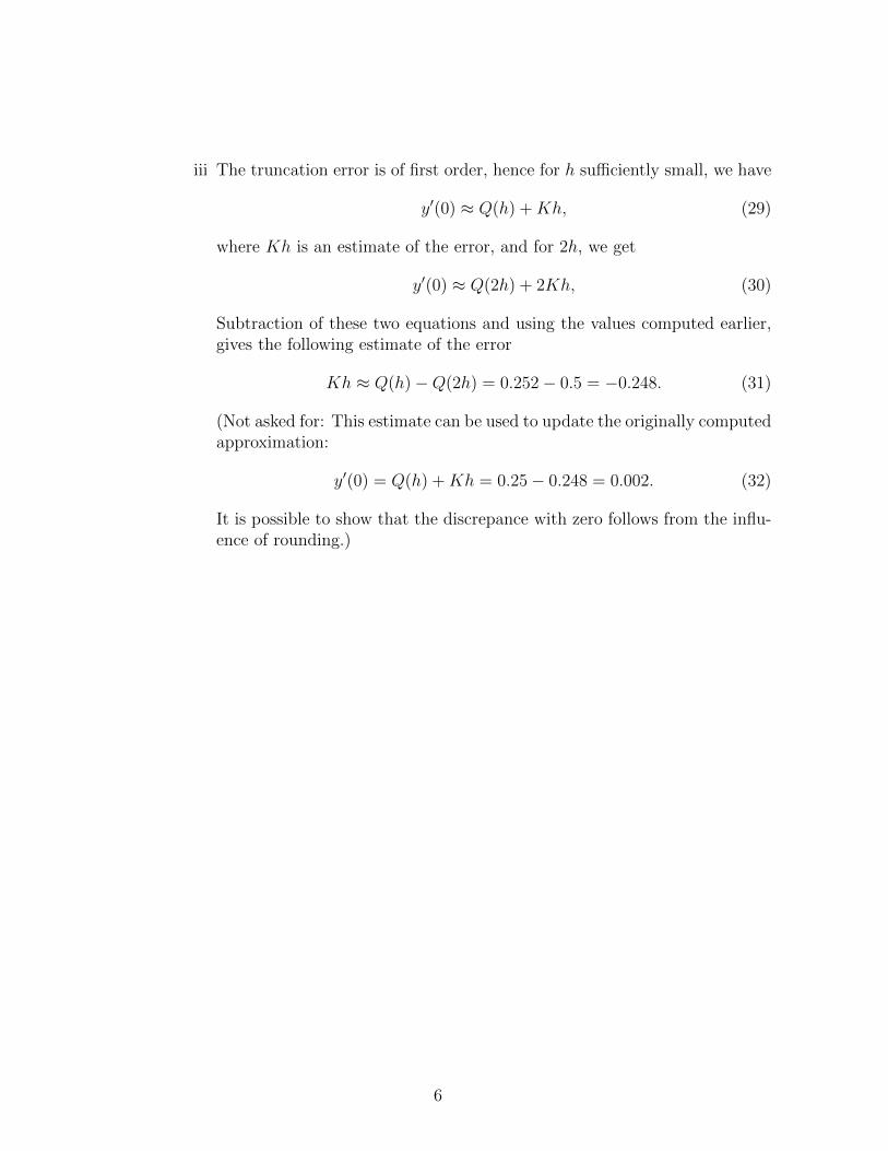
iii The truncation error is of first order, hence for h sufficiently small, we have
y′(0) ≈ Q(h) +Kh, (29)
where Kh is an estimate of the error, and for 2h, we get
y′(0) ≈ Q(2h) + 2Kh, (30)
Subtraction of these two equations and using the values computed earlier,gives the following estimate of the error
Kh ≈ Q(h)−Q(2h) = 0.252− 0.5 = −0.248. (31)
(Not asked for: This estimate can be used to update the originally computedapproximation:
y′(0) = Q(h) +Kh = 0.25− 0.248 = 0.002. (32)
It is possible to show that the discrepance with zero follows from the influ-ence of rounding.)
6
DELFT UNIVERSITY OF TECHNOLOGYFaculty of Electrical Engineering, Mathematics and Computer Science
ANSWERS OF THE TEST NUMERICAL METHODS FORDIFFERENTIAL EQUATIONS (WI3097 TU)
Thursday April 14 2011, 18:30-21:30
1. We consider the following method:
yn+1 = yn + h (αf(tn, yn) + βf(tn−1, yn−1)) . (1)
(a) The local truncation error is given by
τn+1 =yn+1 − zn+1
h,
where yn+1 is the exact solution at time tn+1 and zn+1 is the numerical method(1) applied to yn−1 and yn. We will need the following Taylor expansions:
yn+1 = yn + hy′n +h2
2y′′n +O(h3),
y′n−1 = f(tn−1, yn−1) = y′n − hy′′n +O(h2).
We then have for zn+1 :
zn+1 = yn + h(α + β)y′n − h2βy′′n +O(h3).
Subtracting this from yn+1 and dividing by h we have the local truncation erroris:
τn+1 = (1− (α + β))y′n + h
(1
2+ β
)y′′n +O(h2).
Since
α =3
2, β = −1
2
we obtain τn+1 = O(h2).
(b) Substituting the relation yj = [Q(hλ)]yj−1 and the test equation y′ = λy =f(t, y) in (1) gives the following:
[Q(hλ)]2yn−1 = Q(hλ)yn−1 + h
(3
2λQ(hλ)yn−1 −
1
2λyn−1
).
This can be rewritten as
[Q(hλ)]2 −Q(hλ)
(1 +
3
2hλ
)+
1
2hλ = 0.
1
We therefore have that
Q1(hλ) =1
2
1 +3
2hλ +
√(3
2hλ
)2
+ hλ + 1
(2)
Q2(hλ) =1
2
1 +3
2hλ−
√(3
2hλ
)2
+ hλ + 1
(3)
(c) Since the discriminant of(
32hλ
)2+hλ+1 is negative the value of
(32hλ
)2+hλ+1
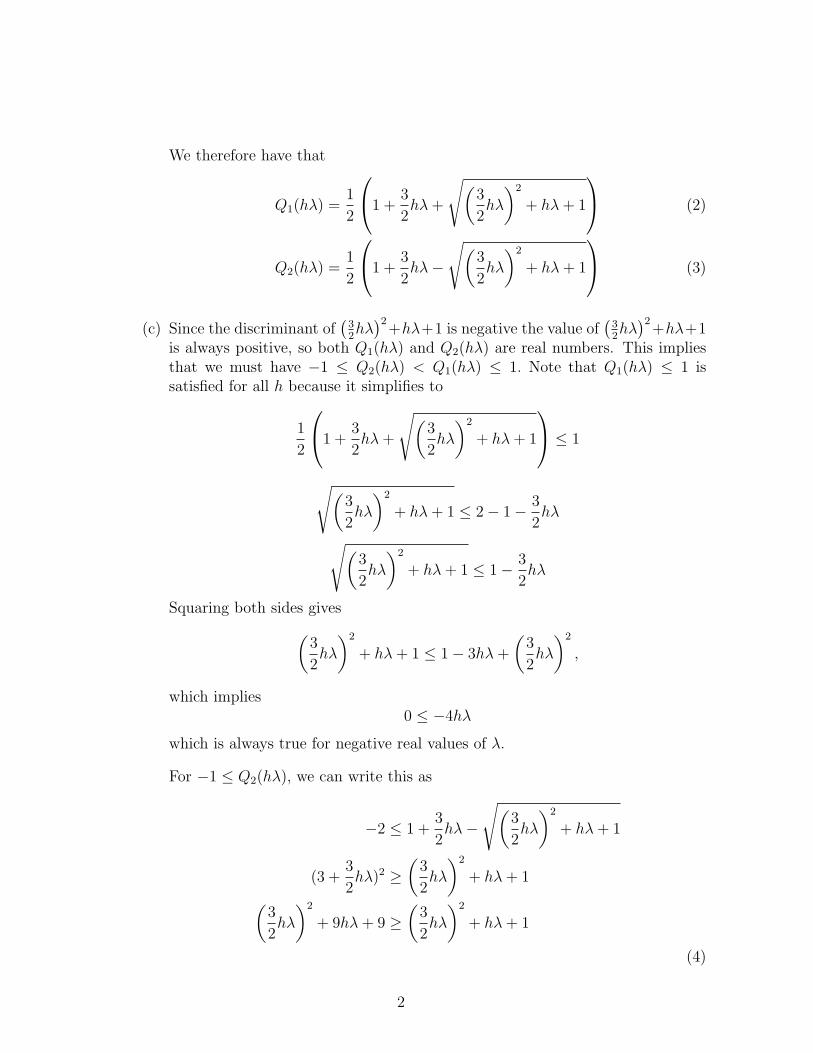
is always positive, so both Q1(hλ) and Q2(hλ) are real numbers. This impliesthat we must have −1 ≤ Q2(hλ) < Q1(hλ) ≤ 1. Note that Q1(hλ) ≤ 1 issatisfied for all h because it simplifies to
1
2
1 +3
2hλ +
√(3
2hλ
)2
+ hλ + 1
≤ 1
√(3
2hλ
)2
+ hλ + 1 ≤ 2− 1− 3
2hλ√(
3
2hλ
)2
+ hλ + 1 ≤ 1− 3
2hλ
Squaring both sides gives(3
2hλ
)2
+ hλ + 1 ≤ 1− 3hλ +
(3
2hλ
)2
,
which implies0 ≤ −4hλ
which is always true for negative real values of λ.
For −1 ≤ Q2(hλ), we can write this as
−2 ≤ 1 +3
2hλ−
√(3
2hλ
)2
+ hλ + 1
(3 +3
2hλ)2 ≥
(3
2hλ
)2
+ hλ + 1(3
2hλ
)2
+ 9hλ + 9 ≥(
3
2hλ
)2
+ hλ + 1
(4)
2
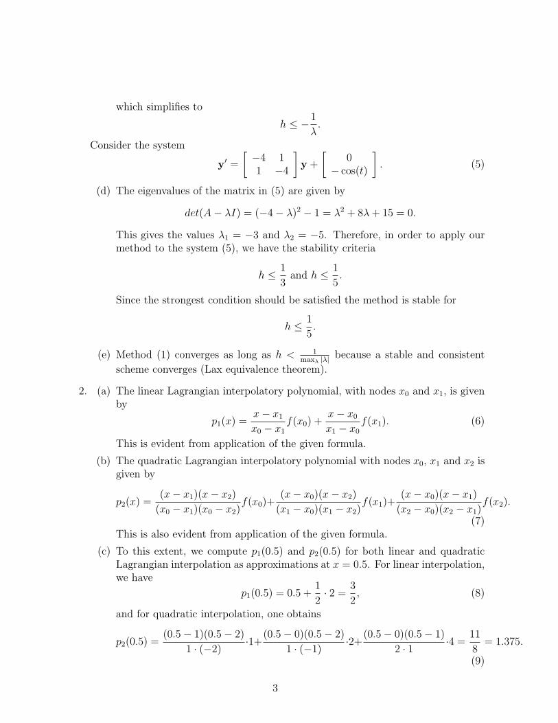
which simplifies to
h ≤ −1
λ.
Consider the system
y′ =
[−4 11 −4
]y +
[0
− cos(t)
]. (5)
(d) The eigenvalues of the matrix in (5) are given by
det(A− λI) = (−4− λ)2 − 1 = λ2 + 8λ + 15 = 0.
This gives the values λ1 = −3 and λ2 = −5. Therefore, in order to apply ourmethod to the system (5), we have the stability criteria
h ≤ 1
3and h ≤ 1
5.
Since the strongest condition should be satisfied the method is stable for
h ≤ 1
5.
(e) Method (1) converges as long as h < 1maxλ |λ| because a stable and consistent
scheme converges (Lax equivalence theorem).
2. (a) The linear Lagrangian interpolatory polynomial, with nodes x0 and x1, is givenby
p1(x) =x− x1
x0 − x1
f(x0) +x− x0
x1 − x0
f(x1). (6)
This is evident from application of the given formula.
(b) The quadratic Lagrangian interpolatory polynomial with nodes x0, x1 and x2 isgiven by
p2(x) =(x− x1)(x− x2)
(x0 − x1)(x0 − x2)f(x0)+
(x− x0)(x− x2)
(x1 − x0)(x1 − x2)f(x1)+
(x− x0)(x− x1)
(x2 − x0)(x2 − x1)f(x2).
(7)This is also evident from application of the given formula.
(c) To this extent, we compute p1(0.5) and p2(0.5) for both linear and quadraticLagrangian interpolation as approximations at x = 0.5. For linear interpolation,we have
p1(0.5) = 0.5 +1
2· 2 =
3
2, (8)
and for quadratic interpolation, one obtains
p2(0.5) =(0.5− 1)(0.5− 2)
1 · (−2)·1+
(0.5− 0)(0.5− 2)
1 · (−1)·2+
(0.5− 0)(0.5− 1)
2 · 1·4 =
11
8= 1.375.
(9)
3
x x10
x
y
(x ,f(x ))0 0
(x ,f(x ))1 1
2e
uncertainty region
uncertainty region
uncertainty region
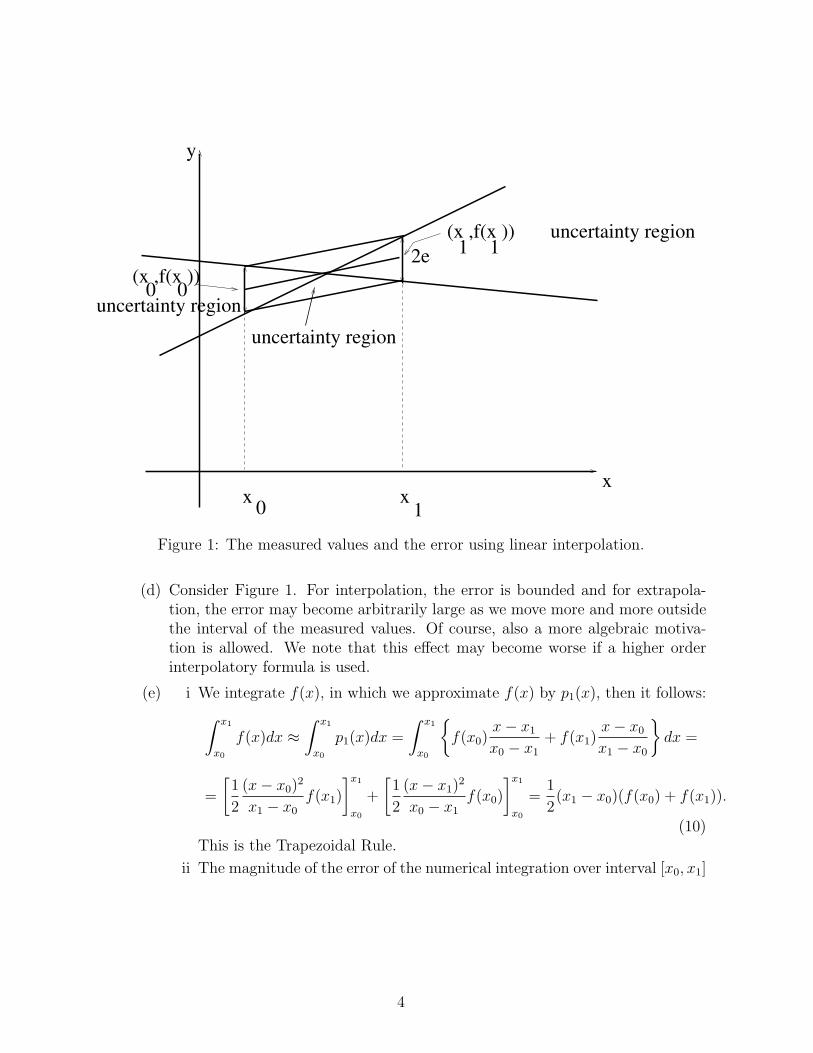
Figure 1: The measured values and the error using linear interpolation.
(d) Consider Figure 1. For interpolation, the error is bounded and for extrapola-tion, the error may become arbitrarily large as we move more and more outsidethe interval of the measured values. Of course, also a more algebraic motiva-tion is allowed. We note that this effect may become worse if a higher orderinterpolatory formula is used.
(e) i We integrate f(x), in which we approximate f(x) by p1(x), then it follows:∫ x1
x0
f(x)dx ≈∫ x1
x0
p1(x)dx =
∫ x1
x0
{f(x0)
x− x1
x0 − x1
+ f(x1)x− x0
x1 − x0
}dx =
=
[1
2
(x− x0)2
x1 − x0
f(x1)
]x1
x0
+
[1
2
(x− x1)2
x0 − x1
f(x0)
]x1
x0
=1
2(x1 − x0)(f(x0) + f(x1)).
(10)This is the Trapezoidal Rule.
ii The magnitude of the error of the numerical integration over interval [x0, x1]
4
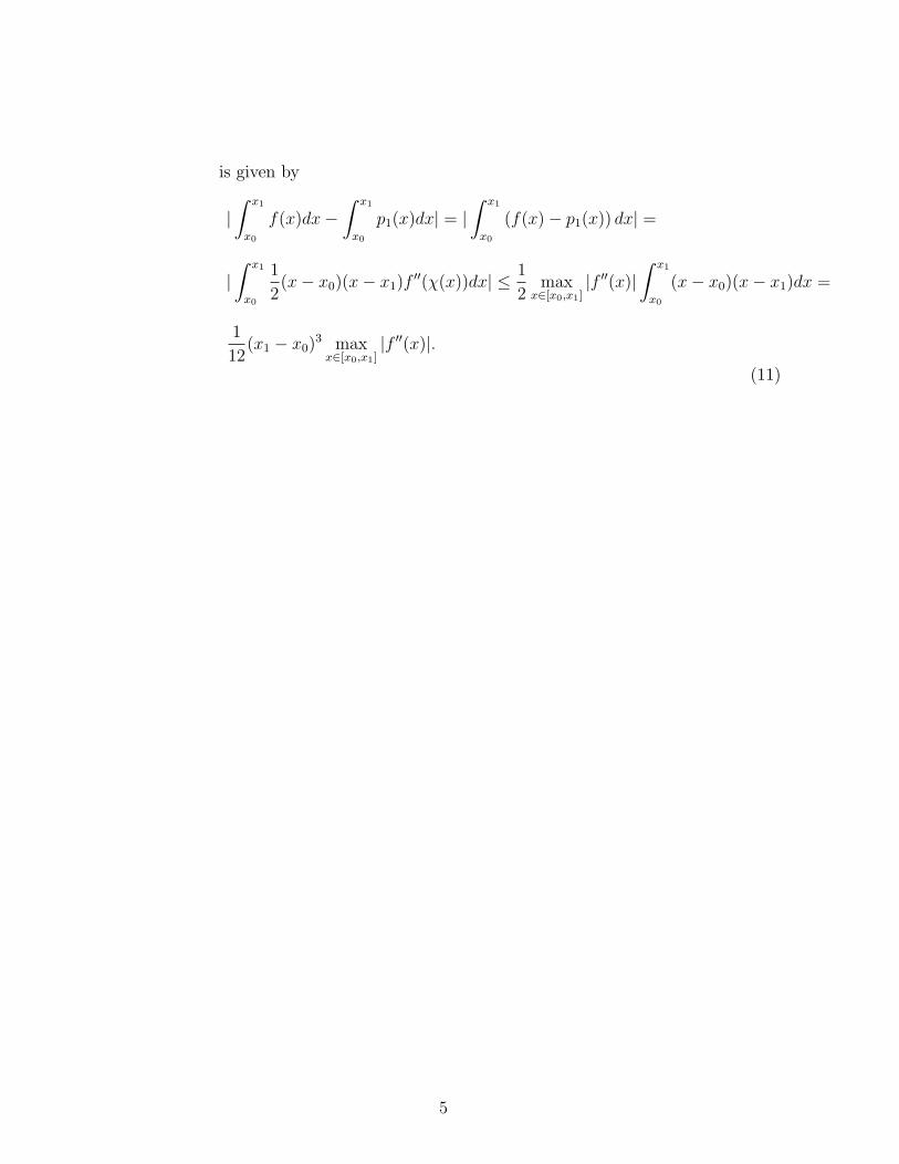
is given by
|∫ x1
x0
f(x)dx−∫ x1
x0
p1(x)dx| = |∫ x1
x0
(f(x)− p1(x)) dx| =
|∫ x1
x0
1
2(x− x0)(x− x1)f
′′(χ(x))dx| ≤ 1
2max
x∈[x0,x1]|f ′′(x)|
∫ x1
x0
(x− x0)(x− x1)dx =
1
12(x1 − x0)
3 maxx∈[x0,x1]
|f ′′(x)|.
(11)
5
DELFT UNIVERSITY OF TECHNOLOGYFaculty of Electrical Engineering, Mathematics and Computer Science
ANSWERS OF THE TEST NUMERICAL METHODS FORDIFFERENTIAL EQUATIONS (WI3097 TU)
Thursday April 19 2012, 18:30-21:30
1.
a The local truncation error is defined as
τn+1(h) =yn+1 − zn+1
h, (1)
where zn+1 is given by
zn+1 = yn + h (a1f(tn, yn) + a2f(tn + h, yn + hf(tn, yn)) . (2)
A Taylor expansion of f around (tn, yn) yields
f(tn+h, yn+hf(tn, yn)) = f(tn, yn)+h∂f
∂t(tn, yn)+hf(tn, yn)
∂f
∂y(tn, yn)+O(h2). (3)
This is substituted into equation (2) to obtain
zn+1 = yn+h
(a1f(tn, yn) + a2
[f(tn, yn) + h
∂f
∂t(tn, yn) + hf(tn, yn)
∂f
∂y(tn, yn)
])+O(h3).
(4)A Taylor series for y(x) around tn gives for yn+1
yn+1 = y(tn + h) = yn + hy′(tn) +h2
2y′′(tn) + O(h3). (5)
From the differential equation we know that:
y′(tn) = f(tn, yn) (6)
From the Chain Rule of Differentiation, we derive
y′′(tn) =df(tn, yn)
dt=
∂f(tn, yn)
∂t+
∂f(tn, yn)
∂yy′(tn) (7)
after substitution of the differential equation one obtains:
y′′(tn) =∂f(tn, yn)
∂t+
∂f(tn, yn)
∂yf(tn, yn) (8)
Equations (5) and (4) are substituted into relation (1) to obtain
τn+1(h) = f(tn, yn)(1− (a1 + a2)) + h
(∂f
∂t+ f
∂f
∂y
) (1
2− a2
)+ O(h2) (9)
Hence
1
(a) a1 + a2 = 1 implies τn+1(h) = O(h);
(b) a1 + a2 = 1 and a2 = 1/2, that is, a1 = a2 = 1/2, gives τn+1(h) = O(h2).
b The test equation is given byy′ = λy. (10)
Application of the predictor step to the test equation gives
w∗n+1 = wn + hλwn = (1 + hλ)wn. (11)
The corrector step yields
wn+1 = wn + h (a1λwn + a2λ(1 + hλ)wn) = (1 + (a1 + a2)hλ + a2h2λ2)wn. (12)
Hence the amplification factor is given by
Q(hλ) = 1 + (a1 + a2)hλ + a2h2λ2. (13)
c Let λ < 0 (so λ is real), then, for stability, the amplification factor must satisfy
−1 ≤ Q(hλ) ≤ 1, (14)
from the previous assignment, we have
−1 ≤ 1 + (a1 + a2)hλ + a2(hλ)2 ≤ 1 ⇔ −2 ≤ (a1 + a2)hλ + a2(hλ)2 ≤ 0. (15)
First, we consider the left inequality:
a2(hλ)2 + (a1 + a2)hλ + 2 ≥ 0 (16)
For hλ = 0, the above inequality is satisfied, further the discriminant is given by(a1 + a2)
2 − 8a2 < 0. Here the last inequality follows from the given hypothesis.Hence the left inequality in relation (15) is always satisfied. Next we consider theright hand inequality of relation (15)
a2(hλ)2 + (a1 + a2)hλ ≤ 0. (17)
This relation is rearranged into
a2(hλ)2 ≤ −(a1 + a2)hλ, (18)
hence
a2|hλ|2 ≤ (a1 + a2)|hλ| ⇔ |hλ| ≤ a1 + a2
a2
, a2 6= 0. (19)
This results into the following condition for stability
h ≤ a1 + a2
a2|λ|, a2 6= 0. (20)
2
d The Jacobian, J , is given by
J =
∂f1
∂y1
∂f1
∂y2
∂f2
∂y1
∂f2
∂y2
. (21)
Since f1(y1, y2) = −y1y2 and f2(y1, y2) = y1y2 − y2, we obtain
J =
(−y2 −y1
y2 y1 − 1
). (22)
Substitution of the initial values y1(0) = 1 and y2(0) = 2, gives
J =
(−2 −12 0
). (23)
e The eigenvalues of the Jacobian at y1(0) = y2(0) = 1 are given by λ1,2 = 1 ± i. Forour case, we have
Q(hλ) = −1 + hλ + 1/2(hλ)2. (24)
Since our eigenvalues are not real valued, it is required for stability that
|Q(hλ)| ≤ 1. (25)
Since the eigenvalues are complex conjugates, we can proceed with one of the eigen-values, say λ = −1 + i with λ2 = −2i to obtain
Q(hλ) = 1 + h(−1 + i) + 1/2h2(−2i) (26)
Substitution of h = 1 shows that Q(hλ) = 0. This implies that |Q(hλ)| = 0 ≤ 1 sothe method is stable.
2. a Given v(x) = x(2 − x), then v′′(x) = −2, and hence −v′′ + v = 2 + x(2 − x)follows by simple addition. Further, v(0) = 0 and v′(x) = 2 − 2x and hencev′(1) = 0. Hence the differential equation, as well as the boundary conditionsare satisfied.
b Let vj = v(xj), and let xn = 1, hence h = 1/n, then
vj−1 = v(xj − h) = vj − hv′(xj) + h2/2v′′(xj)− h3/3!v′′′(xj) + h4/4!v′′′′(xj) + O(h5);
vj+1 = v(xj + h) = vj + hv′(xj) + h2/2v′′(xj) + h3/3!v′′′(xj) + h4/4!v′′′′(xj) + O(h5).(27)
From the above expression, it can be seen that
v′′(xj) =vj−1 − 2vj + vj+1
h2+
h2
12v′′′′(xj) + O(h3), (28)
3
and hence the error is O(h2). This gives the following discretization
−wj−1 + 2wj − wj+1
h2+ wj = 2 + xj(2− xj), for j = 1 . . . n, (29)
where xj = jh and wj ≈ vj as the numerical (finite difference) solution underneglecting the error. Further, we use a virtual gridnode near x = 1, xn+1 = 1+h,with
0 = v′(1) =vn+1 − vn−1
2h− h2
3v′′′(1) + O(h3), (30)
hence the error is O(h2). Neglecting the error, and substitution into the dis-cretization equation j = n, gives
−2wn−1 + 2wn
h2+ wn = 3. (31)
Division by 2 to make the discretization symmetric, gives
−wn−1 + wn
h2+
1
2wn =
3
2. (32)
The boundary condition at x = 0, gives
2w1 − w2
h2+ w1 = 2 + h(2− h).. (33)
c For j = 1, we get, using h = 1/3,
18w1 − 9w2 + w1 = 2 + 1/3 ∗ 5/3 = 23/9. (34)
For j = 2, we obtain
−9w1 + 18w2 − 9w3 + w2 = 26/9. (35)
For j = 3 = n, we use w4 = w2, which gives
−9w2 + 9w3 + 1/2w3 = 3/2. (36)
Hence, the system of equations is19w1 − 9w2 = 23/9,
−9w1 + 19w2 − 9w3 = 26/9,
−9w2 + 19/2w3 = 3/2.
(37)
d The exact solution is given by v(x) = x(2−x), and hence all derivatives of orderthree and larger are zero. Further, the error is determined by the derivatives ofthird order and larger. This implies that the error is zero.
4
e To this extent, we consider the determination of the zeros of the following systemof equations
F1(v1, v2) = 18v1 − 9v2 + v21 − 20
9,
F2(v1, v2) = −9v1 + 18v2 + v22 − 20
9.
We consider (vk1 , v
k2) as the kth estimate of the successive approximations. Lin-
earization around the estimate (vk1 , v
k2) gives the following Newton method:
∂(F1, F2)
∂(v1, v2)(vk
1 , vk2)
vk+11 − vk
1
vk+12 − vk
2
= −F (vk1 , v
k2), (38)
where F (v1, v2) = [F1(v1, v2) F2(v1, v2)]T , and
∂(F1, F2)
∂(v1, v2)(vk
1 , vk2) =
∂F1
∂v1(vk
1 , vk2)
∂F1
∂v2(vk
1 , vk2)
∂F2
∂v1(vk
1 , vk2)
∂F2
∂v2(vk
1 , vk2)
=
18 + 2vk1 −9
−9 18 + 2vk2
,
(39)is the Jacobian matrix. Using v0
1 = v02 = 0, we get18 −9
−9 18
v11 − v0
1
v12 − v0
2
=
20/9
20/9
. (40)
The solution is given by v11 − v0
1 = 20/81 = v12 − v0
2, and hence v11 = v1
2 = 20/81.
5
DELFT UNIVERSITY OF TECHNOLOGYFaculty of Electrical Engineering, Mathematics and Computer Science
ANSWERS OF THE TEST NUMERICAL METHODS FORDIFFERENTIAL EQUATIONS (WI3097 TU)
Thursday August 25 2011, 18:30-21:30
1. (a) The local truncation error is given by
τn+1(h) =yn+1 − zn+1
h. (1)
Here we obtain yn+1 by a Taylor expansion around tn:
yn+1 = yn + hy′(tn) +h2
2y′′(tn) + O(h3). (2)
For zn+1, we obtain, after substitution of the predictor step for z∗n+1 into thecorrector step
zn+1 = yn + h ((1− θ)f(tn, yn) + θf(tn + h, yn + hf(tn, yn))) (3)
After a Taylor expansion of f(tn+h, yn+hf(tn, yn)) around (tn, yn) one obtains:
zn+1 = yn+h
((1− θ)f(tn, yn) + θ(f(tn, yn) + h(
∂f(tn, yn)
∂t+ f(tn, yn)
∂f(tn, yn)
∂y)) + O(h2)
).
(4)From the differential equation we know that:
y′(tn) = f(tn, yn) (5)
From the Chain Rule of Differentiation, we derive
y′′(tn) =df(tn, yn)
dt=
∂f(tn, yn)
∂t+
∂f(tn, yn)
∂yy′(tn) (6)
after substitution of the differential equation one obtains:
y′′(tn) =∂f(tn, yn)
∂t+
∂f(tn, yn)
∂yf(tn, yn) (7)
This implies that zn+1 = yn + hy′(tn) + θh2y′′(tn). Subsequently, it follows that
yn+1 − zn+1 = O(h2), and, hence τn+1(h) =O(h2)
h= O(h) for 0 ≤ θ ≤ 1, (8)
yn+1 − zn+1 = O(h3), and, hence τn+1(h) =O(h3)
h= O(h2) for θ =
1
2. (9)
1
(b) Consider the test equation y′ = λy, then, herewith, one obtains
w∗n+1 = wn + hλwn = (1 + hλ)wn,
wn+1 = wn + h((1− θ)λwn + θλw∗n+1) =
= wn + h((1− θ)λwn + θλ(wn + hλwn)) = (1 + hλ + θ(hλ)2)wn.(10)
Hence the amplification factor is given by
Q(hλ) = 1 + hλ + θ(hλ)2. (11)
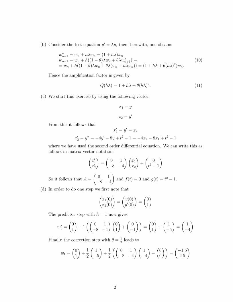
(c) We start this exercise by using the following vector:
x1 = y
x2 = y′
From this it follows thatx′1 = y′ = x2
x′2 = y′′ = −4y′ − 8y + t2 − 1 = −4x2 − 8x1 + t2 − 1
where we have used the second order differential equation. We can write this asfollows in matrix-vector notation:(
x′1x′2
)=
(0 1−8 −4
) (x1
x2
)+
(0
t2 − 1
)
So it follows that A =
(0 1−8 −4
)and f(t) = 0 and g(t) = t2 − 1.
(d) In order to do one step we first note that(x1(0)x2(0)
)=
(y(0)y′(0)
)=
(01
)The predictor step with h = 1 now gives:
w∗1 =
(01
)+ 1
((0 1−8 −4
) (01
)+
(0−1
))=
(01
)+
(1−5
)=
(1−4
)Finally the correction step with θ = 1
2leads to
w1 =
(01
)+
1
2
(1−5
)+
1
2
((0 1−8 −4
) (1−4
)+
(00
))=
(−1.52.5
)
2
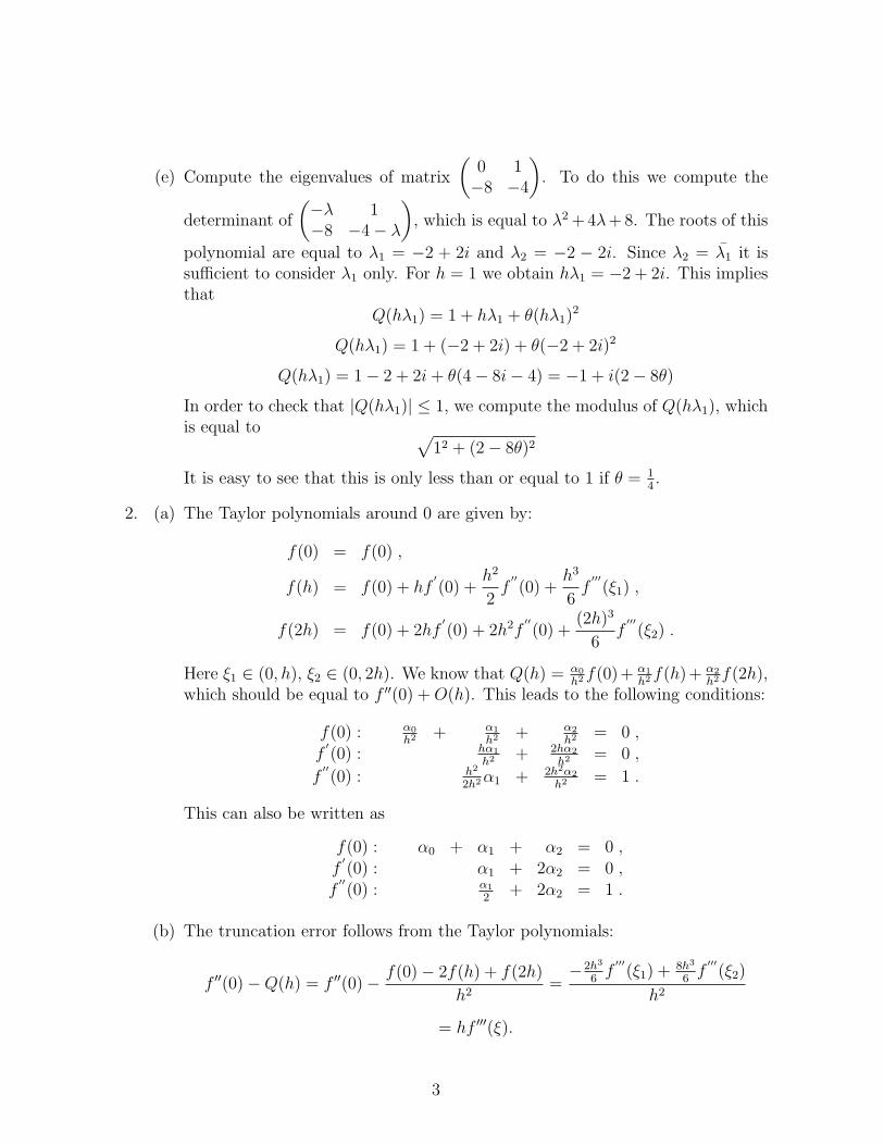
(e) Compute the eigenvalues of matrix
(0 1−8 −4
). To do this we compute the
determinant of
(−λ 1−8 −4− λ
), which is equal to λ2 +4λ+8. The roots of this
polynomial are equal to λ1 = −2 + 2i and λ2 = −2 − 2i. Since λ2 = λ1 it issufficient to consider λ1 only. For h = 1 we obtain hλ1 = −2 + 2i. This impliesthat
Q(hλ1) = 1 + hλ1 + θ(hλ1)2
Q(hλ1) = 1 + (−2 + 2i) + θ(−2 + 2i)2
Q(hλ1) = 1− 2 + 2i + θ(4− 8i− 4) = −1 + i(2− 8θ)
In order to check that |Q(hλ1)| ≤ 1, we compute the modulus of Q(hλ1), whichis equal to √
12 + (2− 8θ)2
It is easy to see that this is only less than or equal to 1 if θ = 14.
2. (a) The Taylor polynomials around 0 are given by:
f(0) = f(0) ,
f(h) = f(0) + hf′(0) +
h2
2f
′′(0) +
h3
6f
′′′(ξ1) ,
f(2h) = f(0) + 2hf′(0) + 2h2f
′′(0) +
(2h)3
6f
′′′(ξ2) .
Here ξ1 ∈ (0, h), ξ2 ∈ (0, 2h). We know that Q(h) = α0
h2 f(0)+ α1
h2 f(h)+ α2
h2 f(2h),which should be equal to f ′′(0) + O(h). This leads to the following conditions:
f(0) : α0
h2 + α1
h2 + α2
h2 = 0 ,f
′(0) : hα1
h2 + 2hα2
h2 = 0 ,
f′′(0) : h2
2h2 α1 + 2h2α2
h2 = 1 .
This can also be written as
f(0) : α0 + α1 + α2 = 0 ,f
′(0) : α1 + 2α2 = 0 ,
f′′(0) : α1
2+ 2α2 = 1 .
(b) The truncation error follows from the Taylor polynomials:
f ′′(0)−Q(h) = f ′′(0)− f(0)− 2f(h) + f(2h)
h2=−2h3
6f
′′′(ξ1) + 8h3
6f
′′′(ξ2)
h2
= hf ′′′(ξ).
3

(c) Note thatf ′′(0)−Q(h) = Kh (12)
f ′′(0)−Q(h
2) = K(
h
2) (13)
Subtraction gives:
Q(h
2)−Q(h) = Kh−K
h
2= K(
h
2). (14)
We choose h = 12. Then Q(h) = Q(1
2) = 0−2×0.1250+1
0.25= 3 and Q(h
2) = Q(1
4) =
0−2×0.0156+0.1250( 14)2
= 1.5008. Combining (13) and (14) shows that
f ′′(0)−Q(1
4) = Q(
1
4)−Q(
1
2) = −1.4992
(d) To estimate the rounding error we note that
|Q(h)− Q(h)| = |(f(0)− f(0))− 2(f(h)− f(h)) + (f(2h)− f(2h))
h2|
≤ |f(0)− f(0)|+ 2|f(h)− f(h)|+ |f(2h)− f(2h)|h2
≤ 4ε
h2,
so C1 = 4. Since only 4 digits are given the rounding error is: ε = 0.00005.
(e) The total error is bounded by
|f ′′(0)− Q(h)| = |f ′′(0)−Q(h) + Q(h)− Q(h)|
≤ |f ′′(0)−Q(h)|+ |Q(h)− Q(h)|
≤ 6h +4ε
h2= g(h)
This is minimal for hopt, for which g′(hopt) = 0. Note that g′(h) = 6− 8εh3 . This
implies that h3opt = 4ε
3, so hopt = (4ε
3)
13 ≈ 0.0405.
4
DELFT UNIVERSITY OF TECHNOLOGYFaculty of Electrical Engineering, Mathematics and Computer Science
ANSWERS OF THE TEST NUMERICAL METHODS FORDIFFERENTIAL EQUATIONS (WI3097 TU)
Thursday August 30 2012, 18:30-21:30
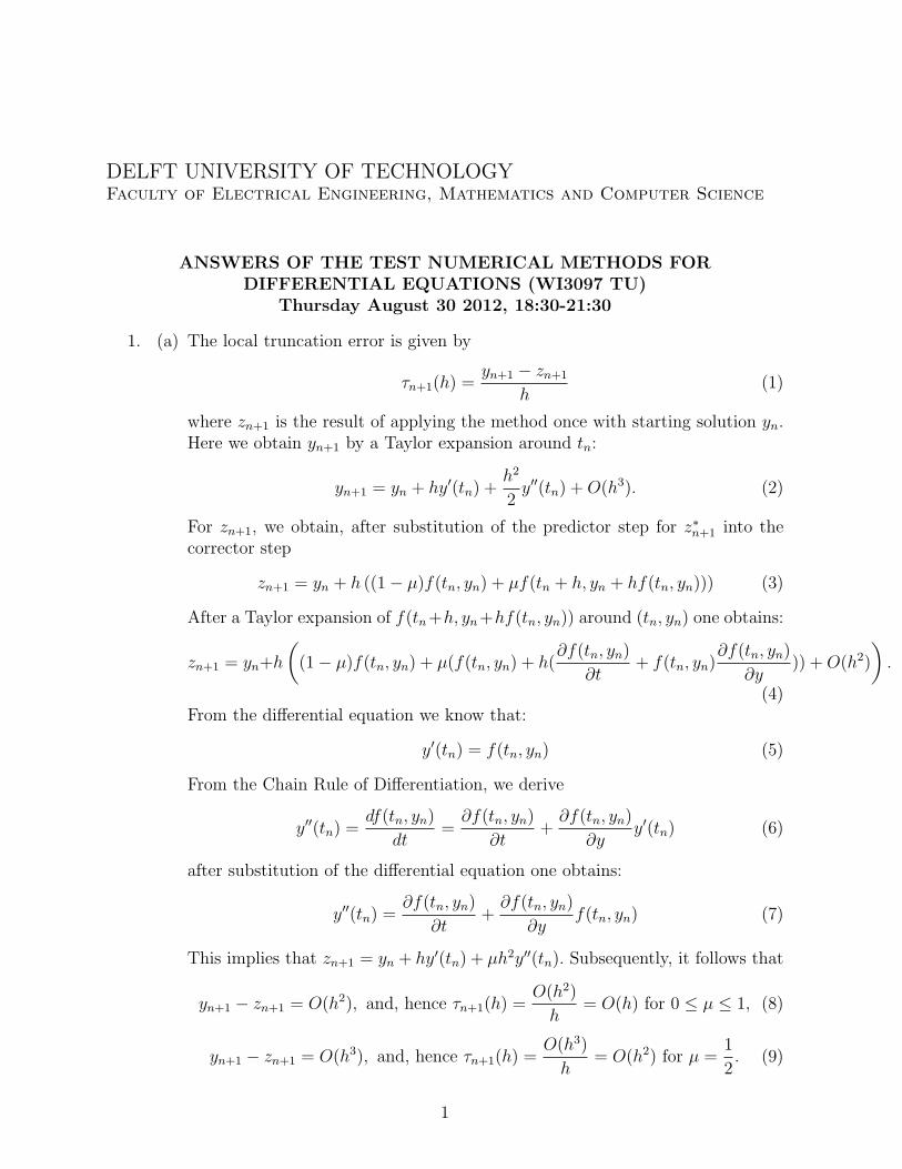
1. (a) The local truncation error is given by
τn+1(h) =yn+1 − zn+1
h(1)
where zn+1 is the result of applying the method once with starting solution yn.Here we obtain yn+1 by a Taylor expansion around tn:
yn+1 = yn + hy′(tn) +h2
2y′′(tn) + O(h3). (2)
For zn+1, we obtain, after substitution of the predictor step for z∗n+1 into thecorrector step
zn+1 = yn + h ((1− µ)f(tn, yn) + µf(tn + h, yn + hf(tn, yn))) (3)
After a Taylor expansion of f(tn+h, yn+hf(tn, yn)) around (tn, yn) one obtains:
zn+1 = yn+h
((1− µ)f(tn, yn) + µ(f(tn, yn) + h(
∂f(tn, yn)
∂t+ f(tn, yn)
∂f(tn, yn)
∂y)) + O(h2)
).
(4)From the differential equation we know that:
y′(tn) = f(tn, yn) (5)
From the Chain Rule of Differentiation, we derive
y′′(tn) =df(tn, yn)
dt=
∂f(tn, yn)
∂t+
∂f(tn, yn)
∂yy′(tn) (6)
after substitution of the differential equation one obtains:
y′′(tn) =∂f(tn, yn)
∂t+
∂f(tn, yn)
∂yf(tn, yn) (7)
This implies that zn+1 = yn + hy′(tn) + µh2y′′(tn). Subsequently, it follows that
yn+1 − zn+1 = O(h2), and, hence τn+1(h) =O(h2)
h= O(h) for 0 ≤ µ ≤ 1, (8)
yn+1 − zn+1 = O(h3), and, hence τn+1(h) =O(h3)
h= O(h2) for µ =
1
2. (9)
1
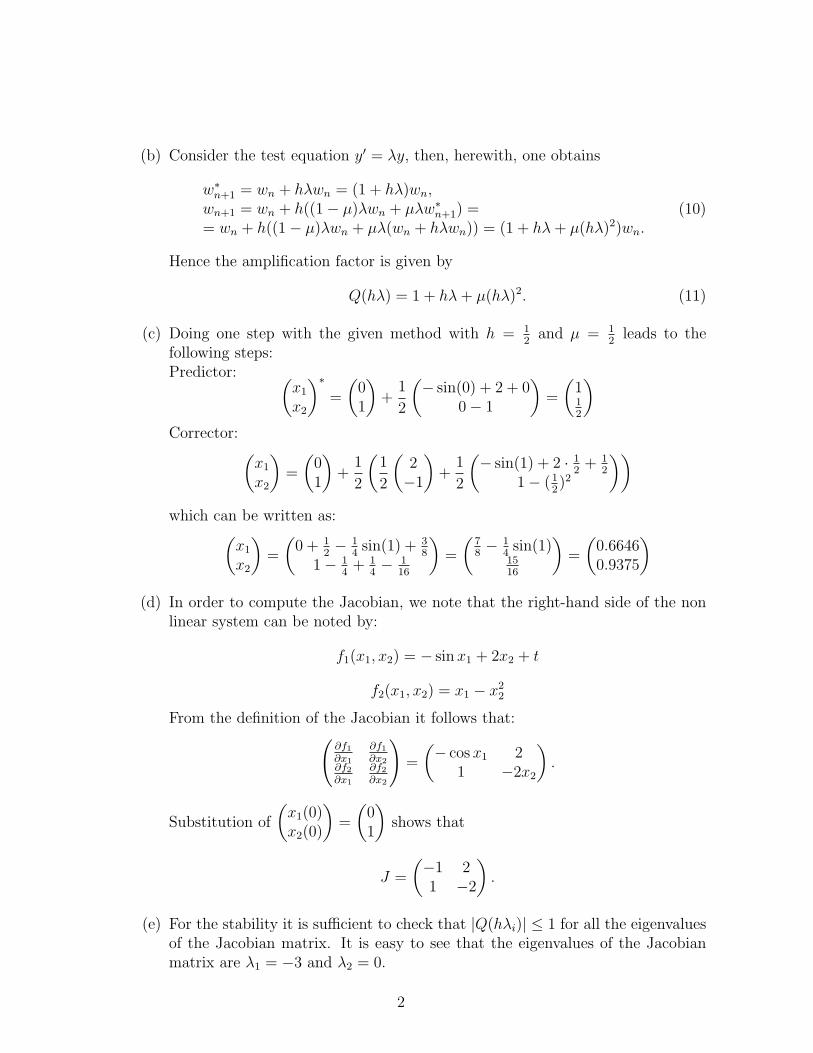
(b) Consider the test equation y′ = λy, then, herewith, one obtains
w∗n+1 = wn + hλwn = (1 + hλ)wn,
wn+1 = wn + h((1− µ)λwn + µλw∗n+1) =
= wn + h((1− µ)λwn + µλ(wn + hλwn)) = (1 + hλ + µ(hλ)2)wn.(10)
Hence the amplification factor is given by
Q(hλ) = 1 + hλ + µ(hλ)2. (11)
(c) Doing one step with the given method with h = 12
and µ = 12
leads to thefollowing steps:Predictor: (
x1
x2
)∗
=
(01
)+
1
2
(− sin(0) + 2 + 0
0− 1
)=
(112
)Corrector: (
x1
x2
)=
(01
)+
1
2
(1
2
(2−1
)+
1
2
(− sin(1) + 2 · 1
2+ 1
2
1− (12)2
))which can be written as:(
x1
x2
)=
(0 + 1
2− 1
4sin(1) + 3
8
1− 14
+ 14− 1
16
)=
(78− 1
4sin(1)
1516
)=
(0.66460.9375
)(d) In order to compute the Jacobian, we note that the right-hand side of the non
linear system can be noted by:
f1(x1, x2) = − sin x1 + 2x2 + t
f2(x1, x2) = x1 − x22
From the definition of the Jacobian it follows that:(∂f1
∂x1
∂f1
∂x2∂f2
∂x1
∂f2
∂x2
)=
(− cos x1 2
1 −2x2
).
Substitution of
(x1(0)x2(0)
)=
(01
)shows that
J =
(−1 21 −2
).
(e) For the stability it is sufficient to check that |Q(hλi)| ≤ 1 for all the eigenvaluesof the Jacobian matrix. It is easy to see that the eigenvalues of the Jacobianmatrix are λ1 = −3 and λ2 = 0.
2
For the choice µ = 0 we note that the method is equal to the Euler Forwardmethod. For real eigenvalues the Euler Forward method is stable if h ≤ −2
λ.
Since λ1 = −3 and λ2 = 0 we know that the method is stable if h ≤ −2−3
= 23
(another option is to derive the values of h such that |Q(hλi)| ≤ 1 by using thedescription of Q(hλ))
For the choice µ = 12
we use the expression
Q(hλ) = 1 + hλ +1
2(hλ)2
For λ2 = 0 it appears that Q(hλ2) = 1 so the inequality is satisfied for all h.For λ1 = −3 we have to check the following inequalities:
−1 ≤ 1− 3h +9
2h2 ≤ 1
For the left-hand inequality we arrive at
0 ≤ 9
2h2 − 3h + 2
It appears that the discriminant 9−4 · 92·2 is negative, so there are no real roots
which implies that the inequality is satisfied for all h.
For the right-hand inequality we get
−3h +9
2h2 ≤ 0
9
2h2 ≤ 3h
so
h ≤ 2
3
(another option is to see that for µ = 12
the method is equal to the modifiedEuler method, and remember that this method is stable for real eigenvalues ifh ≤ −2
λ)
2. (a) Taylor’s Theorem (or here the Mean Value Theorem) gives for a zeroth orderapproximation around xj:
f(x) = f(xj) + (x− xj)f′(ξ(x)), (12)
for a ξ(x) ∈ (xj, x) if x > xj. Then we consider the interval [xj, xj+1) and useTaylor’s Theorem around xj in the integration to get∫ xj+1
xj
f(x)dx =
∫ xj+1
xj
f(xj)+(x−xj)f′(ξ(x))dx = hf(xj)+
∫ xj+1
xj
(x−xj)f′(ξ(x))dx.
(13)
3
Hence we get
|∫ xj+1
xj
f(x)dx−∫ xj+1
xj
f(xj)| = |∫ xj+1
xj
(x− xj)f′(ξ(x))dx|. (14)
Taking the maximum value of f ′ over the interval [xj, xj+1], yields
|∫ xj+1
xj
(x−xj)f′(ξ(x))dx| ≤ max
x∈[xj ,xj+1]|f ′(x)|
∫ xj+1
xj
(x−xj)dx =h2
2max
x∈[xj ,xj+1]|f ′(x)|.
(15)By combining relations (14) and (15), we proved that
|∫ xj+1
xj
f(x)dx−∫ xj+1
xj
f(xj)| ≤h2
2max
x∈[xj ,xj+1]|f ′(x)|. (16)
Next, we deal with the entire interval [a, b], then
|∫ b
a
f(x)dx− hn∑
j=1
f(xj)| = |n∑
j=1
(∫ xj+1
xj
f(x)dx− hf(xj)
)|. (17)
We use the Triangle Inequality to get
|n∑
j=1
(∫ xj+1
xj
f(x)dx− hf(xj)
)| ≤
n∑j=1
|∫ xj+1
xj
f(x)dx− hf(xj)|. (18)
From relation (16), it follows that
n∑j=1
|∫ xj+1
xj
f(x)dx− hf(xj)|. ≤h2
2
n∑j=1
maxx∈[xj ,xj+1]
|f ′(x)|. (19)
Since maxx∈([a,b] |f ′(x)| ≥ maxx∈([xj ,xj+1] |f ′(x)|, ∀j ∈ {1, . . . , n}, we get
h2
2
n∑j=1
maxx∈[xj ,xj+1]
|f ′(x)| ≤ h2
2· n · max
x∈[a,b]|f ′(x)|. (20)
Since xn+1 = a + nh = b, we have nh = b − a and hence the above inequalitygives
h2
2
n∑j=1
maxx∈[xj ,xj+1]
|f ′(x)| ≤ h2
2· n · max
x∈[a,b]|f ′(x)| =
h
2(b− a) max
x∈[a,b]|f ′(x)|. (21)
Hence the global error can be estimated from above by
|∫ b
a
f(x)dx− hn∑
j=1
f(xj)| ≤h
2(b− a) max
x∈[a,b]|f ′(x)|. (22)
4
(b) Incorporating the first–order derivative in Taylor’s Theorem (linearization) gives
f(x) = f(xj) + (x− xj)f′(xj) +
(x− xj)2
2f ′′(ξ(x)), (23)
for a ξ(x) ∈ (xj, x) if x > xj. We start integrating over the interval [xj, xj+1] toget∫ xj+1
xj
f(x)dx =
∫ xj+1
xj
f(xj) + (x− xj)f′(xj) +
(x− xj)2
2f ′′(ξ(x))dx =
hf(xj) +h2
2f ′(xj) +
∫ xj+1
xj
(x− xj)2
2f ′′(ξ(x))dx.
(24)
Hence, we obtain
|∫ xj+1
xj
f(x)dx− (hf(xj) +h2
2f ′(xj))| = |
∫ xj+1
xj
(x− xj)2
2f ′′(ξ(x))dx| ≤
maxx∈[xj ,xj+1]
|f ′′(x)|∫ xj+1
xj
(x− xj)2
2=
h3
6max
x∈[xj ,xj+1]|f ′′(x)|.
(25)Analogously to the previous assignment, we get
|E1| = |∫ b
a
f(x)dx−n∑
j=1
(hf(xj) +
h2
2f ′(xj)
)| = |
n∑j=1
(∫ xj+1
xj
f(x)dx−(
hf(xj) +h2
2f ′(xj)
))| ≤
n∑j=1
|
(∫ xj+1
xj
f(x)dx−(
hf(xj) +h2
2f ′(xj)
))| ≤ h3
6
n∑j=1
maxx∈[xj ,xj+1]
|f ′′(x)| ≤
h3
6· n · max
x∈[a,b]|f ′′(x)| =
h2
6(b− a) max
x∈[a,b]|f ′′(x)|.
(26)
Hence∫ b
af(x)dx ≈
∑nj=1 h(f(xj) + h
2f ′(xj)) = T1 where the global error is
estimated from above by the above expression.
(c) Upon considering the interval (0, 1) with h = 12, we use x1 = 0 and x2 = 1
2
(n = 2). Then, we get∫ 1
0
x2dx ≈ h(f(x1)+f(x2)+h
2(f ′(x1)+f ′(x2)) =
1
2(0+(
1
2)2+
1
4(0+2 · 1
2)) =
1
4.
(27)The exact answer is given by 1
3, hence the error is 1
12. To check our result, we
use the upper bound of the error given in relation (26):
h2
6(b− a) max
x∈[a,b]|f ′′(x)| =
1
6· (1
2)2 · 1 · 2 =
1
12. (28)
5
Note that here it was used that the second–order derivative of x2 is given by 2.Hence our the error that we found using the exact solution does not exceed theupper bound from relation (26), and hence our result makes sense.
(d) T1 is the approximation of the integral obtained by the use the first order deriva-tives, hence T2 is the analogon with the first and second order derivatives, hence
T2 =
n∑j=1
(∫ xj+1
xj
f(xj) + (x− xj)f′(xj) +
(x− xj)2
2f ′′(xj)dx
)=
n∑j=1
(∫ xj+1
xj
f(xj) + (x− xj)f′(xj)dx
)+
n∑j=1
∫ xj+1
xj
(x− xj)2
2f ′′(xj)dx
= T1 +n∑
j=1
∫ xj+1
xj
(x− xj)2
2f ′′(xj)dx = T1 +
h3
3!
n∑j=1
f ′′(xj).
(29)
The last step follows from evaluation of the integral. Hence we demonstratedthat
T2 = T1 +h3
3!
n∑j=1
f ′′(xj). (30)
Further, the local error is found by using Taylor’s Theorem over the interval[xj, xj+1] to get
|∫ xj+1
xj
f(x)dx−
(∫ xj+1
xj
f(xj) + . . . +(x− xj)
2
2!f ′′(xj)dx
)| =
|∫ xj+1
xj
(x− xj)3
3!f ′′′(ξ(x))dx| ≤ max
x∈[xj ,xj+1]|f ′′′(x)|
∫ xj+1
xj
(x− xj)3
3!dx =
h4
4!max
x∈[xj ,xj+1]|f ′′′(x)|.
(31)
Here, the last step follows from evaluation of the integral. A summation proce-dure over all intervals, similar to assignment 2.a., gives the global error bound:
|E2| = |∫ b
a
f(x)dx− T2| ≤h4
4!
n∑j=1
maxx∈[xj ,xj+1]
|f ′′′(x)| ≤
h4
4!· n · max
x∈[a,b]|f ′′′(x)| =
h3(b− a)
4!maxx∈[a,b]
|f ′′′(x)|.
(32)
6
(e) Let T2 and T2, respectively, be the approximation of∫ b
af(x)dx using the exact
and available values of f and its derivatives. Then, we have
T2 =n∑
j=1
∫ xj+1
xj
f(xj) + . . . +(x− xj)
2
2!f ′′(xj)dx =
n∑j=1
(hf(xj) +
h2
2f ′(xj) +
h3
3!f ′′(xj)
)=
hn∑
j=1
f(xj) +h2
2
n∑j=1
f ′(xj) +h3
3!
n∑j=1
f ′′(xj).
(33)
For T2, we similarly have
T2 = hn∑
j=1
f(xj) +h2
2
n∑j=1
f ′(xj) +h3
3!
n∑j=1
f ′′(xj). (34)
Subtraction of the above two equations, taking the absolute value, and usingthe Triangle Inequality, gives
|T2 − T2| ≤
hn∑
j=1
|f(xj)− f(xj)|+h2
2
n∑j=1
|f ′(xj)− f ′(xj)|+h3
3!
n∑j=1
|f ′′(xj)− f ′′(xj)|,
(35)Using |f (k)(xj)− f (k)(xj)| ≤ ε for all k and j, and nh = b− a, gives
|T2 − T2| ≤ h · n · ε +h2
2· n · ε +
h3
3!· n · ε =
(b− a)ε
(1 +
h
2+
h2
3!
)= (b− a)ε
3∑k=1
hk−1
k!.
.
(36)
7
DELFT UNIVERSITY OF TECHNOLOGYFaculty of Electrical Engineering, Mathematics and Computer Science
ANSWERS OF THE TEST NUMERICAL METHODS FORDIFFERENTIAL EQUATIONS (WI3097 TU)
Thursday January 20 2011, 18:30-21:30
1. (a) The local truncation error is given by
τn+1(h) =yn+1 − zn+1
h, (1)
in which we determine yn+1 by the use of Taylor expansions around tn:
yn+1 = yn + hy′(tn) +h2
2y′′(tn) + O(h3). (2)
We bear in mind that
y′(tn) = f(tn, yn)
y′′(tn) =df(tn, yn)
dt=
∂f(tn, yn)
∂t+
∂f(tn, yn)
∂yy′(tn) =
∂f(tn, yn)
∂t+
∂f(tn, yn)
∂yf(tn, yn).
(3)
Hence
yn+1 = yn + hy′(tn) +h2
2
(
∂f(tn, yn)
∂t+
∂f(tn, yn)
∂yf(tn, yn)
)
+ O(h3). (4)
After substitution of the predictor z∗n+1 = yn +hf(tn, yn) into the corrector, andafter using a Taylor expansion around (tn, yn), we obtain for zn+1
zn+1 = yn + h2
(f(tn, yn) + f(tn + h, yn + hf(tn, yn))) =
yn +h
2
(
f(tn, yn) + f(tn, yn) + h(∂f(tn, yn)
∂t+ f(tn, yn)
∂f(tn, yn)
∂y) + O(h2)
)
.
(5)Herewith, one obtains
yn+1 − zn+1 = O(h3), and hence τn+1(h) =O(h3)
h= O(h2). (6)
1
(b) Let x1 = y and x2 = y′, then y′′ = x′
2, and hence
x′
2 + 4x2 + 3x1 = cos(t),x2 = x′
1.(7)
We write this asx′
1 = x2,
x′
2 = −3x1 − 4x2 + cos(t).(8)
Finally, this is represented in the following matrix-vector form:(
x1
x2
)
′
=
(
0 1−3 −4
) (
x1
x2
)
+
(
0cos(t)
)
. (9)
In which, we have the following matrix A =
(
0 1−3 −4
)
and f =
(
0cos(t)
)
.
The initial conditions are defined by
(
x1(0)x2(0)
)
=
(
12
)
.
(c) Application of the Modified Euler method to the system x′ = Ax + f , gives
w∗
1 = w0 + h(
Aw0 + f0
)
,
w1 = w0 + h2
(
Aw0 + f0 + Aw∗
1 + f1
)
.(10)
With the initial condition w0 =
(
12
)
and h = 0.1, this gives the following result
for the predictor
w∗
1 =
(
12
)
+1
10
((
0 1−3 −4
) (
12
)
+
(
01
))
=
(
6/51
)
. (11)
The corrector is calculated as follows
w1 =
(
12
)
+ 120
((
0 1−3 −4
) (
12
)
+
(
01
)
+
(
0 1−3 −4
) (
6/51
)
+
(
0cos( 1
10)
))
=
=
(
1.15001.1698
)
(12)
(d) Consider the test equation y′ = λy, then one gets
w∗
n+1 = wn + hλwn = (1 + hλ)wn,
wn+1 = wn +h
2(λwn + λw∗
n+1) =
= wn +h
2(λwn + λ(wn + hλwn)) = (1 + hλ +
(hλ)2
2)wn.
(13)
Hence the amplification factor is given by
Q(hλ) = 1 + hλ +(hλ)2
2. (14)
2
(e) First, we determine the eigenvalues of the matrix A. Subsequently, the eigenval-ues are substituted into the amplification factor. The eigenvalues of the matrixA are given by λ1 = −1 and λ2 = −3. We first check the amplification factorof λ1 = −1:
−1 ≤ 1 − h +1
2h2 ≤ 1 (15)
The first inequality leads to
0 ≤ 2 − h +1
2h2
Since the discriminant of this equation is equal to 1−4∗ 12∗2 = −3 the inequality
always holds. The second inequality leads to
−h +1
2h2 ≤ 0
so1
2h2 ≤ h
which impliesh ≤ 2
Now we check the amplification factor of λ2 = −3:
−1 ≤ 1 − 3h +1
29h2 ≤ 1 (16)
The first inequality leads to
0 ≤ 2 − 3h +1
29h2
Since the discriminant of this equation is equal to 9 − 4 ∗ 92∗ 2 = −27 the
inequality always holds. The second inequality leads to
−3h +9
2h2 ≤ 0
so3
2h2 ≤ h
which implies
h ≤2
3
So the modified Euler method is stable if h ≤ 23.
3
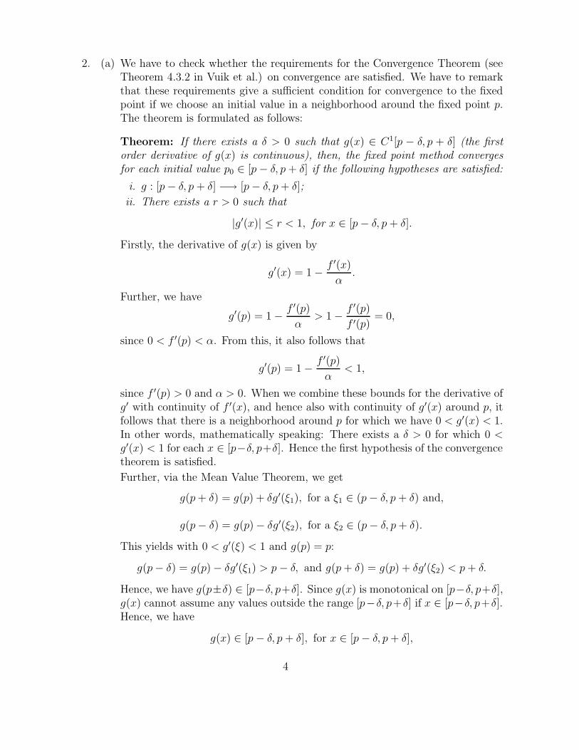
2. (a) We have to check whether the requirements for the Convergence Theorem (seeTheorem 4.3.2 in Vuik et al.) on convergence are satisfied. We have to remarkthat these requirements give a sufficient condition for convergence to the fixedpoint if we choose an initial value in a neighborhood around the fixed point p.The theorem is formulated as follows:
Theorem: If there exists a δ > 0 such that g(x) ∈ C1[p − δ, p + δ] (the firstorder derivative of g(x) is continuous), then, the fixed point method convergesfor each initial value p0 ∈ [p − δ, p + δ] if the following hypotheses are satisfied:
i. g : [p − δ, p + δ] −→ [p − δ, p + δ];
ii. There exists a r > 0 such that
|g′(x)| ≤ r < 1, for x ∈ [p − δ, p + δ].
Firstly, the derivative of g(x) is given by
g′(x) = 1 −f ′(x)
α.
Further, we have
g′(p) = 1 −f ′(p)
α> 1 −
f ′(p)
f ′(p)= 0,
since 0 < f ′(p) < α. From this, it also follows that
g′(p) = 1 −f ′(p)
α< 1,
since f ′(p) > 0 and α > 0. When we combine these bounds for the derivative ofg′ with continuity of f ′(x), and hence also with continuity of g′(x) around p, itfollows that there is a neighborhood around p for which we have 0 < g′(x) < 1.In other words, mathematically speaking: There exists a δ > 0 for which 0 <
g′(x) < 1 for each x ∈ [p−δ, p+δ]. Hence the first hypothesis of the convergencetheorem is satisfied.
Further, via the Mean Value Theorem, we get
g(p + δ) = g(p) + δg′(ξ1), for a ξ1 ∈ (p − δ, p + δ) and,
g(p − δ) = g(p) − δg′(ξ2), for a ξ2 ∈ (p − δ, p + δ).
This yields with 0 < g′(ξ) < 1 and g(p) = p:
g(p − δ) = g(p) − δg′(ξ1) > p − δ, and g(p + δ) = g(p) + δg′(ξ2) < p + δ.
Hence, we have g(p±δ) ∈ [p−δ, p+δ]. Since g(x) is monotonical on [p−δ, p+δ],g(x) cannot assume any values outside the range [p−δ, p+δ] if x ∈ [p−δ, p+δ].Hence, we have
g(x) ∈ [p − δ, p + δ], for x ∈ [p − δ, p + δ],
4
which is equivalent to the second hypothesis. This all sustains convergence ifthe initial guess is chosen within a neighborhood around the fixed point p.
(b) The method of Newton-Raphson is based on linearization around the iterate pn.This is given by
L(x) = f(pn) + (x − pn)f ′(pn). (17)
Next, we determine pn+1 such that L(pn+1) = 0, that is
f(pn) + (pn+1 − pn)f ′(pn) = 0 ⇔ pn+1 = pn −f(pn)
f ′(pn), f ′(pn) 6= 0. (18)
This result can also be proved graphically, see book, chapter 4.
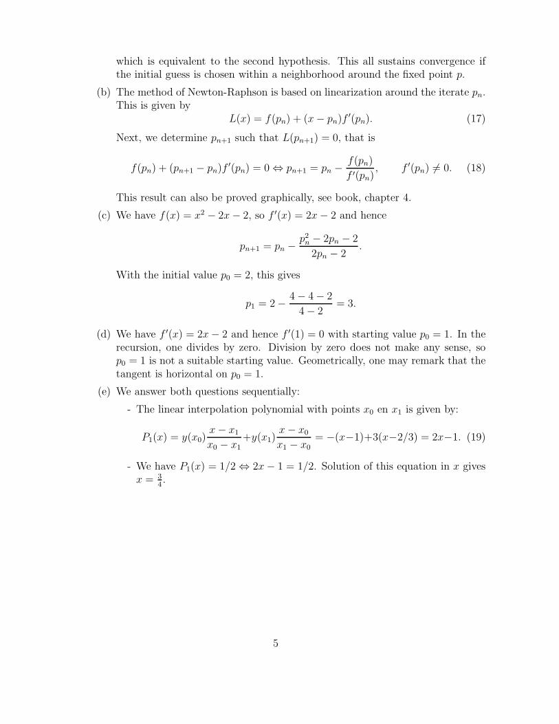
(c) We have f(x) = x2 − 2x − 2, so f ′(x) = 2x − 2 and hence
pn+1 = pn −p2
n − 2pn − 2
2pn − 2.
With the initial value p0 = 2, this gives
p1 = 2 −4 − 4 − 2
4 − 2= 3.
(d) We have f ′(x) = 2x − 2 and hence f ′(1) = 0 with starting value p0 = 1. In therecursion, one divides by zero. Division by zero does not make any sense, sop0 = 1 is not a suitable starting value. Geometrically, one may remark that thetangent is horizontal on p0 = 1.
(e) We answer both questions sequentially:
- The linear interpolation polynomial with points x0 en x1 is given by:
P1(x) = y(x0)x − x1
x0 − x1+y(x1)
x − x0
x1 − x0= −(x−1)+3(x−2/3) = 2x−1. (19)
- We have P1(x) = 1/2 ⇔ 2x − 1 = 1/2. Solution of this equation in x givesx = 3
4.
5
DELFT UNIVERSITY OF TECHNOLOGYFaculty of Electrical Engineering, Mathematics and Computer Science
ANSWERS OF THE TEST NUMERICAL METHODS FORDIFFERENTIAL EQUATIONS (WI3097 TU)
Thursday January 26 2012, 18:30-21:30
1. (a) The amplification factor can be derived as follows. Consider the test equationy′ = λy. Application of the trapezoidal rule to this equation gives:
wj+1 = wj +h
2(λwj + λwj+1) (1)
Rearranging of wj+1 and wj in (1) yields(1− h
2λ
)wj+1 =
(1 +
h
2λ
)wj.
It now follows that
wj+1 =1 + h
2λ
1− h2λ
wj,
and thus
Q(hλ) =1 + h
2λ
1− h2λ
.
(b) The definition of the local truncation error is
τj+1 =yj+1 −Q(hλ)yj
h.
The exact solution of the test equation is given by
yj+1 = ehλyj.
Combination of these results shows that the local truncation error of the testequation is determined by the difference between the exponential function andthe amplification factor Q(hλ)
τj+1 =ehλ −Q(hλ)
hyj. (2)
The difference between the exponential function and amplification factor can becomputed as follows. The Taylor series of ehλ with known point 0 is:
ehλ = 1 + λh +(λh)2
2+O(h3). (3)
1

The Taylor series of 11−h
2λ
with known point 0 is:
1
1− h2λ
= 1 +1
2hλ +
1
4h2λ2 +O(h3). (4)
With (4) it follows that1+h
2λ
1−h2λ
is equal to
1 + h2λ
1− h2λ
= 1 + hλ +1
2(hλ)2 +O(h3). (5)
In order to determine ehλ − Q(hλ), we subtract (5) from (3). Now it followsthat
ehλ −Q(hλ) = O(h3). (6)
The local truncation error can be found by substituting (6) into (2), which leadsto
τj+1 = O(h2).
(c) The trapezoidal rule is stable if
|1 + h2λ|
|1− h2λ|≤ 1.
Using the complex valued λ = µ + iν it appears that the condition is equal to:
|1 + h2(µ + iν)|
|1− h2(µ + iν)|
≤ 1
This is equivalent with √(1 + h
2µ)2 + (h
2ν)2√
(1− h2µ)2 + (h
2ν)2
≤ 1
Since µ ≤ 0 it easily follows that√(1 +
h
2µ)2 + (
h
2ν)2 ≤
√(1− h
2µ)2 + (
h
2ν)2
which implies that|1 + h
2λ|
|1− h2λ|≤ 1.
and the method is stable.
2
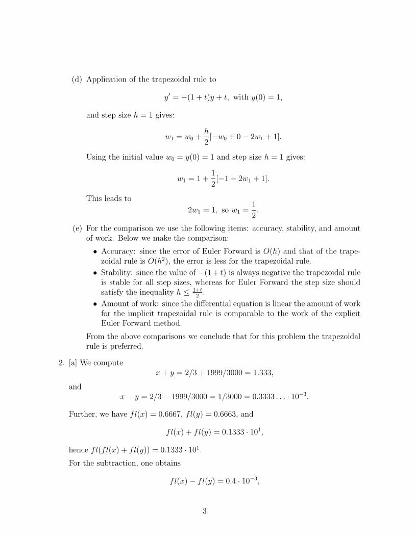
(d) Application of the trapezoidal rule to
y′ = −(1 + t)y + t, with y(0) = 1,
and step size h = 1 gives:
w1 = w0 +h
2[−w0 + 0− 2w1 + 1].
Using the initial value w0 = y(0) = 1 and step size h = 1 gives:
w1 = 1 +1
2[−1− 2w1 + 1].
This leads to
2w1 = 1, so w1 =1
2.
(e) For the comparison we use the following items: accuracy, stability, and amountof work. Below we make the comparison:
• Accuracy: since the error of Euler Forward is O(h) and that of the trape-zoidal rule is O(h2), the error is less for the trapezoidal rule.
• Stability: since the value of −(1+ t) is always negative the trapezoidal ruleis stable for all step sizes, whereas for Euler Forward the step size shouldsatisfy the inequality h ≤ 1+t
2.
• Amount of work: since the differential equation is linear the amount of workfor the implicit trapezoidal rule is comparable to the work of the explicitEuler Forward method.
From the above comparisons we conclude that for this problem the trapezoidalrule is preferred.
2. [a] We computex + y = 2/3 + 1999/3000 = 1.333,
andx− y = 2/3− 1999/3000 = 1/3000 = 0.3333 . . . · 10−3.
Further, we have fl(x) = 0.6667, fl(y) = 0.6663, and
fl(x) + fl(y) = 0.1333 · 101,
hence fl(fl(x) + fl(y)) = 0.1333 · 101.
For the subtraction, one obtains
fl(x)− fl(y) = 0.4 · 10−3,
3
and hencefl(fl(x)− fl(y)) = fl(0.4 · 10−3) = 0.4000 · 10−3.
[b] After the addition, the relative error is given by
|0.1333 · 101 − 1.333
0.1333 · 101| = 0,
and after the subtraction, one gets
|0.4000 · 10−3 − 0.3333 . . . · 10−3
0.3333 . . . · 10−3| = 0.2.
[c] The relative error due to subtraction of two positive numbers is divided by thedifference between these numbers. If this difference gets arbitrarily small, then therelative error gets arbitrarily large for a given absolute error.
[d] Using central differences for the second order derivative at a node xj = jh, gives
y′′(xj) ≈yj+1 − 2yj + yj−1
h2=: Q(h). (7)
Here yj := y(xj). Next, we will prove that this approximation is second order ac-curate, that is |y′′(xj) − Q(h)| = O(h2). Using Taylor’s Theorem around x = xj,gives
yj+1 = y(xj + h) = y(xj) + hy′(xj) + h2
2y′′(xj) + h3
3!y′′′(xj) + h4
4!y′′′′(η+),
yj−1 = y(xj − h) = y(xj)− hy′(xj) + h2
2y′′(xj)− h3
3!y′′′(xj) + h4
4!y′′′′(η−).
(8)
Here, η+ and η− are numbers within the intervals (xj, xj+1) and (xj−1, xj), respec-tively. Substitution of these expressions into Q(h) gives |y′′(xj) − Q(h)| = O(h2).Therewith, we obtain the following discretization formula for the internal grid nodes:
−wj−1 + 2wj − wj+1
h2+ xjwj = x3
j − 2. (9)
Here wj represents the numerical approximation of the solution yj. To deal with theboundary x = 0, we use a virtual node at x = −h, and we define y−1 := y(−h).Then, using central differences at x = 0 gives
0 = y′(0) ≈ y1 − y−1
2h=: Qb(h). (10)
4
Using Taylor’s Theorem, gives
Qb(h) =
y(0) + hy′(0) + h2
2y′′(0) + h3
3!y′′′(η+)− (y(0)− hy′(0) + h2
2y′′(0)− h3
3!y′′′(η−))
2h=
y′(0) + O(h2).(11)
Again, we get an error of O(h2).
With respect to the numerical approximation at the virtual node, we get
w1 − w−1
2h= 0 ⇔ w−1 = w1. (12)
The discretization at x = 0 is given by
−w−1 + 2w0 − w1
h2= −2. (13)
Substitution of equation (12) into the above equation, yields
2w0 − 2w1
h2= −2. (14)
Subsequently, we consider the boundary x = 1. To this extent, we consider itsneighboring point xn−1, here substitution of the boundary condition wn = y(1) =yn = 1 into equation (9), gives
−wn−2 + 2wn−1
h2+ xn−1wn−1 = x3
n−1 − 2 +1
h2= (1− h)3 − 2 +
1
h2. (15)
This concludes our discretization of the boundary conditions. In order to get asymmetric discretization matrix, one divides equation (14) by 2.
[e] Next, we use h = 1/3, then, from equations (9, 14, 15), one obtains the followingsystem
9w0 − 9w1 = −1
−9w0 + 1813w1 − 9w2 = −53
27
−9w1 + 1823w2 = 197
27.
(16)
5
DELFT UNIVERSITY OF TECHNOLOGYFaculty of Electrical Engineering, Mathematics and Computer Science
ANSWERS OF THE TEST NUMERICAL METHODS FORDIFFERENTIAL EQUATIONS (WI3097 TU)
Monday January 28 2013, 18:30-21:30
1. [a] The local truncation error is given by
τn+1(h) =yn+1 − zn+1
h, (1)
where zn+1 is computed by one step of the method starting from yn, and we determineyn+1 by the use of a Taylor Series around tn:
yn+1 = yn + hy′(tn) +h2
2y′′(tn) +O(h3). (2)
We realize that
y′(tn) = f(tn, yn)
y′′(tn) =df(tn, yn)
dt=∂f(tn, yn)
∂t+∂f(tn, yn)
∂yy′(tn) =
=∂f(tn, yn)
∂t+∂f(tn, yn)
∂yf(tn, yn).
(3)
Hence, this gives
yn+1 = yn + hy′(tn) +h2
2
(∂f(tn, yn)
∂t+∂f(tn, yn)
∂yf(tn, yn)
)+O(h3). (4)
For zn+1, after substitution of the predictor–step for z∗n+1 into the corrector–step, andusing the Taylor Series around (tn, yn)
zn+1 = yn + h2
(f(tn, yn) + f(tn + h, yn + hf(tn, yn))) =
yn +h
2
(f(tn, yn) + f(tn, yn) + h(
∂f(tn, yn)
∂t+ f(tn, yn)
∂f(tn, yn)
∂y) +O(h2)
).
(5)
Then, it follows that
yn+1 − zn+1 = O(h3), and hence τn+1(h) =O(h3)
h= O(h2). (6)
1
[b] Consider the test–equation y′ = λy, then it follows that
w∗n+1 = wn + hλwn = (1 + hλ)wn,
wn+1 = wn +h
2(λwn + λw∗n+1) =
= wn +h
2(λwn + λ(wn + hλwn)) = (1 + hλ+
(hλ)2
2)wn.
(7)
Hence the amplification factor is given by
Q(hλ) = 1 + hλ+(hλ)2
2. (8)
[c] Let x1 = y and x2 = y′, then it follows that y′′ = x′2, and hence we get
x′2 + 12x2 + 72x1 = sin(t),x2 = x′1.
(9)
This expression is written as
x′1 = x2,x′2 = −72x1 − 12x2 + sin(t).
(10)
Finally, we get the following matrix–form:(x1x2
)′=
(0 1−72 −12
)(x1x2
)+
(0
sin(t)
). (11)
Here, we have A =
(0 1−72 −12
)and f =
(0
sin(t)
). The initial conditions are given
by
(x1(0)x2(0)
)=
(12
).
[d] The Modified Euler Method, applied to the system x′ = Ax+ f , gives
w∗1 = w0 + h(Aw0 + f
0
),
w1 = w0 + h2
(Aw0 + f
0+ Aw∗1 + f
1
).
(12)
With the initial condition and h = 0.1, this gives
w∗1 =
(12
)+
1
10
((0 1−72 −12
)(12
)+
(00
))=
(1.2−7.6
). (13)
Then, the correction–step is given by
w1 =
(12
)+ 1
20
((0 1−72 −12
)(12
)+
(00
)+
(0 1−72 −12
)(1.2−7.6
)+
(0
sin( 110
)
))=
=
(0.72
−2.55501
)(14)
2

[e] To this extent, we determine the eigenvalues of the matrix A. Subsequently, theseeigenvalues are substituted into the amplification factor. The eigenvalues of A aregiven by −6± 6i. Using h = 0.25, it follows that
Q(hλ) = 1+hλ+1
2h2λ2 = 1+
1
4(−6+6i)+
1
32(−6+6i)2 = 1− 3
2+
3
2i− 72
32i = −1
2− 3
4i.
(15)Herewith, it follows that |Q(hλ)|2 = 1
4+ 9
16= 13
16< 1. Hence for h = 0.25, it follows
that the method applied to the given system is stable. Note that this conclusionholds for both the eigenvalues of A since they are complex conjugates.
2. (a) The first order backward difference formula for the first derivative is given by
f ′(t) ≈ f(t)− f(t− h)
h.
Using t = 2, and h = 1 the approximation of the velocity is
f(2)− f(1)
1= 250− 215 = 35 (m/s).
(b) Taylor polynomials are:
f(0) = f(2h)− 2hf′(2h) + 2h2f
′′(2h)− (2h)3
6f
′′′(ξ0) ,
f(h) = f(2h)− hf ′(2h) +
h2
2f
′′(2h)− h3
6f
′′′(ξ1) ,
f(2h) = f(2h).
We know that Q(h) = α0
hf(0) + α1
hf(h) + α2
hf(2h), which should be equal to
f ′(2h) +O(h2). This leads to the following conditions:
α0
h+ α1
h+ α2
h= 0 ,
−2α0 − α1 = 1 ,2α0h + 1
2α1h = 0 .
(c) The truncation error follows from the Taylor polynomials:
f ′(2h)−Q(h) = f ′(2h)−f(0)− 4f(h) + 3f(2h)
2h=
8h3
6f
′′′(ξ0)− 4(h
3
6f
′′′(ξ1))
2h=
1
3h2f ′′′(ξ).
Using the new formula with h = 1 we obtain the estimate:
f(0)− 4f(1) + 3f(2)
2=
200− 4× 215 + 3× 250
2= 45 (m/s).
Note that the estimated velocity of the vehicle is larger than the maximumspeed of 40 (m/s).
3
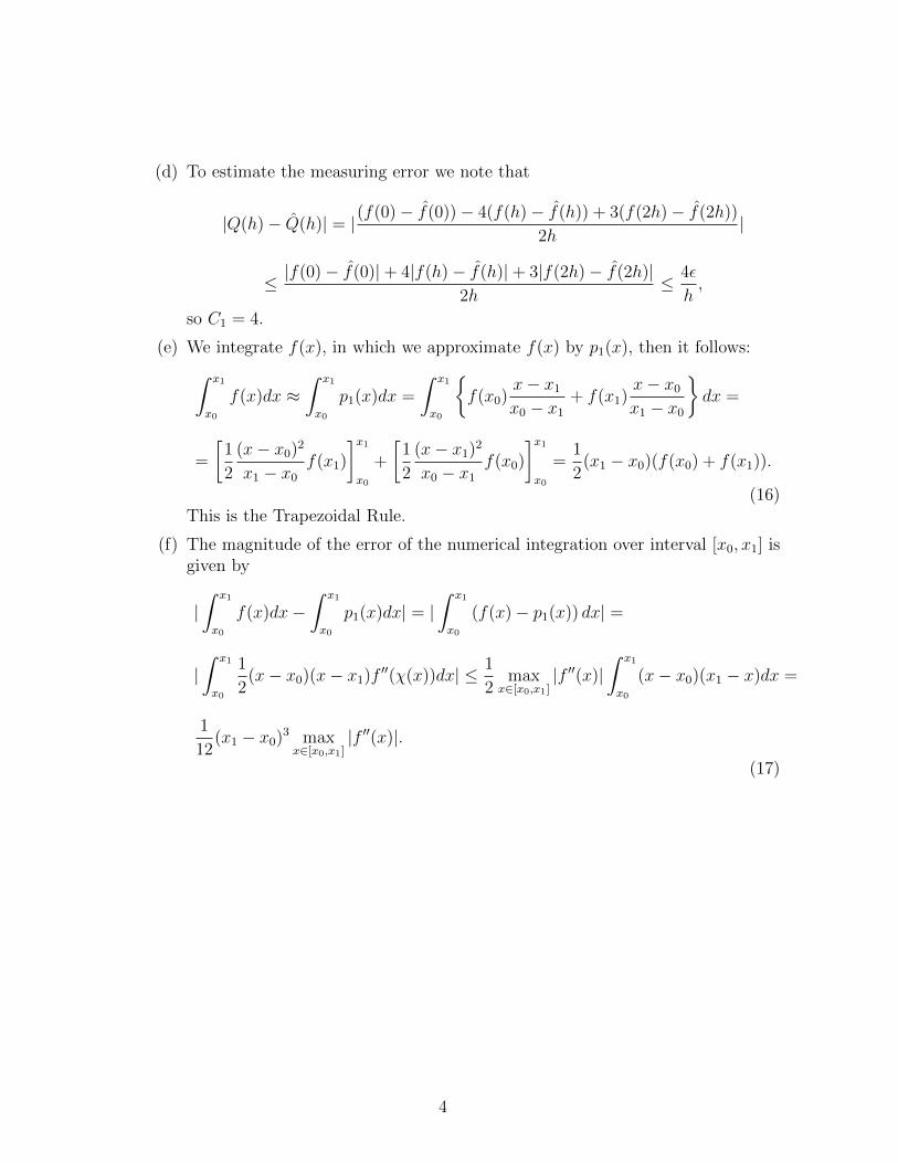
(d) To estimate the measuring error we note that
|Q(h)− Q(h)| = |(f(0)− f(0))− 4(f(h)− f(h)) + 3(f(2h)− f(2h))
2h|
≤ |f(0)− f(0)|+ 4|f(h)− f(h)|+ 3|f(2h)− f(2h)|2h
≤ 4ε
h,
so C1 = 4.
(e) We integrate f(x), in which we approximate f(x) by p1(x), then it follows:∫ x1
x0
f(x)dx ≈∫ x1
x0
p1(x)dx =
∫ x1
x0
{f(x0)
x− x1x0 − x1
+ f(x1)x− x0x1 − x0
}dx =
=
[1
2
(x− x0)2
x1 − x0f(x1)
]x1x0
+
[1
2
(x− x1)2
x0 − x1f(x0)
]x1x0
=1
2(x1 − x0)(f(x0) + f(x1)).
(16)This is the Trapezoidal Rule.
(f) The magnitude of the error of the numerical integration over interval [x0, x1] isgiven by
|∫ x1
x0
f(x)dx−∫ x1
x0
p1(x)dx| = |∫ x1
x0
(f(x)− p1(x)) dx| =
|∫ x1
x0
1
2(x− x0)(x− x1)f ′′(χ(x))dx| ≤ 1
2max
x∈[x0,x1]|f ′′(x)|
∫ x1
x0
(x− x0)(x1 − x)dx =
1
12(x1 − x0)3 max
x∈[x0,x1]|f ′′(x)|.
(17)
4
DELFT UNIVERSITY OF TECHNOLOGYFaculty of Electrical Engineering, Mathematics and Computer Science
ANSWERS OF THE TEST NUMERICAL METHODS FORDIFFERENTIAL EQUATIONS (WI3097 TU)
Thursday July 5 2012, 18:30-21:30
1. [a] The test–equation is given by y′ = λy, and we bear in mind that the amplificationfactor is defined by
Q(hλ) =wn+1
wn. (1)
Then for the Trapezoidal Rule, we get
wn+1 = wn +h
2(λwn + λwn+1) = wn +
hλ
2(wn + wn+1). (2)
The above equation is rewritten as
wn+1(1− hλ
2) = wn(1 +
hλ
2). (3)
Then, using the definition of the amplification factor, we immediately have
QT (hλ) =1 + hλ
2
1− hλ2
. (4)
The Modified Euler Method is treated analogously, to get
wn+1 = wn + hλwn, predictor
wn+1 = wn + h2(λwn + λwn+1), corrector.
(5)
Combining the predictor and corrector, gives
wn+1 = wn +hλ
2(wn + wn + hλwn) = wn(1 + hλ +
(hλ)2
2). (6)
Finally, the definition of the amplification factor implies that
QME(hλ) = 1 + hλ +(hλ)2
2. (7)
[b] The local truncation error is defined by
τn+1(h) =yn+1 − zn+1
h, (8)
1
where yn+1 and zn+1, respectively, denote the exact solution and the numerical ap-proximation at time tn+1 under using yn. Since, we use the test–equation to estimatethe local truncation error, we get
zn+1 = Q(hλ)yn. (9)
The exact solution to the test–equation at time tn+1 is expressed in terms of yn by
yn+1 = yneλh. (10)
Substitution into the definition of the local truncation error, gives
τn+1(h) =yn
h(ehλ −Q(hλ)) =
yn
h(1 + hλ +
(hλ)2
2+
(hλ)3
3!+ O(h4)−Q(hλ)), (11)
where we used the Taylor expansion of the exponential around 0. For the TrapezoidalRule, we have
QT (hλ) =1 + hλ
2
1− hλ2
= (1 +hλ
2)(1 +
hλ
2+ (
hλ
2)2 + (
hλ
2)3 + O(h4)) =
1 + hλ +(hλ)2
2+
(hλ)3
4+ O(h4).
(12)
Using equation (11), we get after some rearrangements
τn+1(h) = −ynλ3h2
12+ O(h3) = O(h2). (13)
The Modified Euler Method is treated similarly with
QME(hλ) = 1 + hλ +(hλ)2
2, (14)
to give via equation (11)
τn+1(h) =ynλ3h2
6+ O(h3) = O(h2). (15)
[c] Let y1 = y and let y2 = y′1, then y′2 = y′′1 = y′′. Hence we have
y′1 = y2, y′2 = −y1 + t(1− t). (16)
The two equations are linear and therewith, one can rewrite this system using amatrix representation: (
y′1y′2
)=
(0 1−1 0
) (y1
y2
)+
(0
t(1− t)
), (17)
2
Further, we have y1(0) = y(0) = 0 and y2(0) = y′(0) = 1.
[d] We use h = 12, and let
A =
(0 1−1 0
), w1 =
(w1
1
w12
), y0 =
(01
), (18)
where the subscript stands for the component, whereas the superscript denotes thetime–index. The Trapezoidal Rule gives
w1 = y0 +h
2(Ay0 + Aw1 +
(014
)). (19)
This gives
(I − h
2A)w1 = (I +
h
2A)y0 +
h
2
(014
). (20)
Substitution of h = 12, gives the following linear system(
1 −14
14
1
)w1 =
(141716
). (21)
This system is solved by
w1 =
3368
1617
(22)
Next, we treat the Modified Euler Method. First, we carry out the prediction step
w1 = y0 + hAy0 =
(01
)+
1
2
(10
)=
12
1
. (23)
Subsequently, we perform the corrector step
w1 = y0 +h
2
(Ay0 + Aw1 +
(014
)). (24)
Using h = 12, gives
w1 =
(01
)+
1
4
((10
)+
(1−1
2
)+
(014
))=
12
1516
. (25)
[e] The local truncation errors for both methods are approximated by
τTn+1(h) = −ynλ3h2
12, τEM
n+1 (h) =ynλ3h2
6. (26)
3
From these equations, it can be seen that the errors have the same order, althoughthe error from the Trapezoidal Rule is about twice as small as the one from theModified Euler Method in the limit for h → 0.
With regard to stability, the eigenvalues of A in the present initial value problem,are given by λ = ±i. Herewith, the following amplification factors are obtained:
QT (h) =1 + ±ih
2
1− ±ih2
, QME(h) = 1± ih− 1
2h2. (27)
This gives the following moduli
|QT (h)| = 1, |QME(h)| =√
(1− h2
2)2 + h2 =
√1 +
h4
4> 1. (28)
Hence the Trapezoidal Rule is neutrally stable, whereas the Modified Euler Methodis unstable.
The workload is smaller for the Modified Euler Method, since no linear system needsto be solved. Although the solution of the linear system may require considerablecomputation time if A is a very large matrix, the issue is not very important for thepresent case.
Therefore, the Trapezoidal Rule is to be preferred for the present system since thesystem is just a two-by-two set of equations.
2. (a) The iteration process is a fixed point method. If the process converges we have:limn→∞ xn = p. Using this in the iteration process yields:
limn→∞
xn+1 = limn→∞
[xn + h(xn)(x3n − 3)]
Since h is a continuous function one obtains:
p = p + h(p)(p3 − 3)
soh(p)(p3 − 3) = 0.
Since h(x) 6= 0 for each x 6= 0 it follows that p3 − 3 = 0 and thus p = 313 .
(b) The convergence of a fixed point method xn+1 = g(xn) is determined by g′(p).If |g′(p)| < 1 the method converges, whereas if |g′(p)| > 1 the method diverges.For all choices we compute the first derivative in p. For the first method weelaborate all steps. For the other methods we only give the final result. For h1
we have g1(x) = x− x3−3x4 . The first derivative is:
g′1(x) = 1− 3x2 · x4 − (x3 − 3) · 4x3
(x4)2
4

Substitution of p yields:
g′1(p) = 1− 3p6 − (p3 − 3) · 4p3
p8.
Since p = 313 the final term cancels:
g′1(p) = 1− 3p6
p8= 1− 3
13 = −0.4422.
This implies that the method is convergent with convergence factor 0.4422.
For the second method we have:
g′2(p) = 1− 3p4 − (p3 − 3) · 2pp4
= 1− 3p4
p4= −2
Thus the method diverges.
For the third method we have:
g′3(p) = 1− 9p4 − (p3 − 3) · 6p9p4
= 1− 9p4
9p4= 0
Thus the method is convergent with convergence factor 0.
Concluding we note that the third method is the fastest.
(c) To estimate the error in p we first approximate the function f in the neighboor-hood of p by the first order Taylor polynomial:
P1(x) = f(p) + (x− p)f ′(p) = (x− p)f ′(p).
Due to the measurement errors we know that
(x− p)f ′(p)− εmax ≤ P1(x) ≤ (x− p)f ′(p) + εmax.
This implies that the perturbed root p is bounded by the roots of (x−p)f ′(p)−εmax and (x− p)f ′(p) + εmax, which leads to
p− εmax
|f ′(p)|≤ p ≤ p +
εmax
|f ′(p)|.
(d) Using the Newton-Raphson iteration method
zk+1 = zk −f(zk)
f ′(zk)
for f(x) = x4 − 3x we have to compute f ′(x). It easily follows that f ′(x) =4x3−3. Substituting this together with the initial guess z0 = 1 into the definitionof the Newton-Raphson method leads to:
z1 = z0 −f(z0)
f ′(z0)= z0 −
z40 − 3z0
4z30 − 3
= 1− 1− 3
4− 3= 3.
5
(e) The Newton-Raphson iteration method can be derived using a graph of a func-tion, in which the zero of the tangent at zk on f(x) defines zk+1. We consider alinearization of f(x) around zk:
L(x) := f(zk) + (x− zk)f′(zk),
and determine its zero, that is L(zk+1) = 0, this gives
zk+1 = zk −f(zk)
f ′(zk), provided that f ′(zk) 6= 0,
�
(f) We consider a Taylor polynomial around zk, to express z
0 = f(z) = f(zk) + (z − zk)f′(zk) +
(z − zk)2
2f ′′(ξk), (29)
for some ξk between z and zk. Note that this form gives the exact representation.Subsequently, we consider the Newton-Raphson approximation
0 = L(zk+1) = f(zk) + (zk+1 − zk)f′(zk). (30)
Subtraction of these two above equations gives
zk+1 − z =(zk − z)2
2
f ′′(ξk)
f ′(zk), provided that f ′(zk) 6= 0, (31)
and hence
|zk+1 − z| = (zk − z)2
2|f′′(ξk)
f ′(zk)|, provided that f ′(zk) 6= 0, (32)
Note that f ′′(x) = 12x2 and z = 313 . Using zk → z, ξk → z as k → ∞
and continuity of f(x) up to at least the second derivative, we arrive at K =
| f ′′(z)2∗f ′(z)
| = | 12z2
2(4z3−3)| ≈ 1.3867. �
6

DELFT UNIVERSITY OF TECHNOLOGYFaculty of Electrical Engineering, Mathematics and Computer Science
ANSWERS OF THE TEST NUMERICAL METHODS FORDIFFERENTIAL EQUATIONS (WI3097 TU)
Thursday June 30 2011, 18:30-21:30
1. a The local truncation error is defined by
τh =yn+1 − zn+1
h, (1)
wherezn+1 = yn + hf(tn, yn), (2)
for the forward Euler method. A Taylor expansion for yn+1 around tn is givenby
yn+1 = yn + hy′(tn) +h2
2y′′(ξ), ∃ ξ ∈ (tn, tn+1). (3)
Since y′(tn) = f(tn, yn), we use equation (1), to get
τh =h
2y′′(ξ), ∃ ξ ∈ (tn, tn+1). (4)
Hence, the truncation error is of first order.
b We define y1 := y and y2 := y′, hence y′1 = y2. Further, we use the differentialequation to obtain
y′′ + εy′ + y = y′′1 + εy′1 + y1 = y′2 + εy2 + y1. (5)
Hence, we obtainy′2 = −y1 − εy2 + sin(t). (6)
Hence the system is given by
y′1 = y2,y′2 = −y1 − εy2 + sin(t).
(7)
The initial conditions are given by
1 = y(0) = y1(0),0 = y′(0) = y′1(0) = y2(0).
(8)
1

c First, we use the test equation, y′ = λy, to analyze numerical stability. Forforward Euler, we obtain
wn+1 = wn + hλwn = Q(hλ)wn, (9)
hence the amplification factor becomes
Q(hλ) = 1 + hλ. (10)
The numerical solution is stable if and only if |Q(hλ)| ≤ 1. Next, we deal withthe case ε = 0, to obtain the following system(
y′1y′2
)=
(0 −11 0
) (y1
y2
). (11)
This system gives the following eigenvalues λ1,2 = ±i, where i is the imaginaryunit. Hence, the amplification factor is given by
Q(hλ) = 1± hi. (12)
Then, it is immediately clear that |Q(hλ)| > 1 for all h > 0. Hence, we concludethat the forward Euler method is never stable if ε = 0.
d From Assignment 1.c., we know that if ε = 0, the eigenvalues of the system arepurely imaginary. This implies that the system is analytically (zero) stable ifε = 0.
Nonzero values of ε give the following system(y′1y′2
)=
(0 −11 ε
) (y1
y2
). (13)
then we get the following eigenvalues λ1,2 = ε2± 1
2
√ε2 − 4 (real-valued), if
ε2 − 4 ≥ 0 and λ = ε2± i
2
√4− ε2 (nonreal-valued) if ε2 − 4 < 0. Hence,
we consider two cases: real-valued and nonreal-valued eigenvalues.
Real-valued eigenvaluesIn this case |ε| ≥ 2, and 0 ≤ ε2 − 4 < ε2, and hence the real-valued eigenvalueshave the same sign, which is determined by the sign of ε. Hence, if ε ≤ −2,then, the system is stable. Furthermore, if ε ≥ 2, then, the system is unstable.
Nonreal-valued eigenvaluesIn this case |ε| < 2. The system is analytically unstable if and only if the realpart of the eigenvalues is positive. Further, the real part of the eigenvalues ispositive if and only if ε > 0. Hence, the system is analytically unstable if andonly if ε > 0. Hence, the system is stable if and only if (−2 <)ε ≤ 0.
From these arguments, it follows that the system is stable if and only if ε ≤ 0.
2
e Since currently the discriminant, ε2−4, is negative, the eigenvalues are nonreal.Substitution into the amplification factor yields
Q(hλ) = 1 +ε
2h± ih
2
√4− ε2. (14)
Hence, numerical stability is warranted if
|Q(hλ)|2 = (1 +ε
2h)2 +
h2
4(4− ε2) ≤ 1. (15)
Hence for stability, we have
1 + εh +ε2h2
4+ h2 − ε2h2
4= 1 + hε + h2 ≤ 1. (16)
Since h > 0, we obtain the following stability criterion
h ≤ −ε = |ε|. (17)
If ε = −2, then both eigenvalues are real-valued and given by λ1,2 = −1. Forthis case, we obtain Q(λh) = 1 − h, and stability is warranted if and only if−1 ≤ Q(hλ) ≤ 1, hence h ≤ 2(= |ε|.
We conclude that for −2 ≤ ε < 0, we have a numerically stable solution if andonly if h ≤ |ε|.
2. a After discretization by the use of finite differences one obtains
−wi−1 + 2wi − wi+1
h2+ x2
i wi = xi. (18)
The truncation error is defined by
ei =−yi−1 + 2yi − yi+1
h2+ x2
i yi − xi. (19)
Taylor series of yi−1 and yi+1 around xi, gives
yi+1 = yi + hy′(xi) +h2
2!y′′(xi) +
h3
3!y′′′(xi) +
h4
4!y′′′′(xi) + O(h5),
yi−1 = yi − hy′(xi) +h2
2!y′′(xi)−
h3
3!y′′′(xi) +
h4
4!y′′′′(xi)−O(h5),
(20)
Substitution of the above expressions into the definition of the truncation errorgives
εi = −y′′(xi) + O(h2) + x2i y(xi)− xi. (21)
Using the differential equation −y′′ + x2y = x finally gives
εi = O(h2). (22)
3
b For this case we have h = 0.25, for the points j ∈ {1, 2, 3}, the discretizationwith w0 = 0 and w4 = 1:
32w1 − 16w2 +1
16w1 =
1
4,
−16w1 + 32w2 − 16w3 +1
4w2 =
1
2,
−16w2 + 32w3 +9
16w3 =
3
4+ 16.
(23)
Hence in matrix-vector form:32.0625 −16 0−16 32.25 −160 −16 32.5625
w1
w2
w3
=
0.250.5
16.75
(24)
c The iteration process is a fixed point method. If the process converges we have:limn→∞ xn = p. Using this in the iteration process yields:
limn→∞
xn+1 = limn→∞
[xn + h(xn)(x2n − 4)]
Since h is a continuous function one obtains:
p = p + h(p)(p2 − 4)
soh(p)(p2 − 4) = 0.
Since h(x) 6= 0 for each x 6= 0 it follows that p2 − 4 = 0 and thus there are twolimits p = −2 and p = 2.
d The convergence of a fixed point method xn+1 = g(xn) is determined by g′(p).If |g′(p)| < 1 the method converges, whereas if |g′(p)| > 1 the method diverges ifp0 6= p. For all choices we compute the first derivative in p. For the first methodwe elaborate all steps. For the other methods we only give the final result. Forh1 we have g1(x) = x− 1
2x(x2 − 4) = 3x− 1
2x3. The first derivative is:
g′1(x) = 3− 3
2x2
Substitution of p = 2 yields:
g′1(2) = 3− 3
24 = 3− 6 = −3.
Since |g′1(2)| = 3 > 1 this method is divergent.
For the second method we have:
g2(x) = x− 1
3(x2 − 4)
4
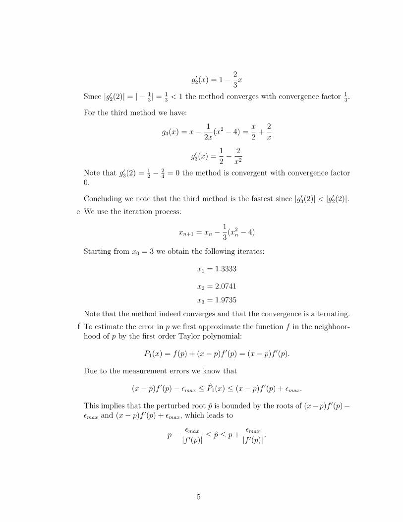
g′2(x) = 1− 2
3x
Since |g′2(2)| = | − 13| = 1
3< 1 the method converges with convergence factor 1
3.
For the third method we have:
g3(x) = x− 1
2x(x2 − 4) =
x
2+
2
x
g′3(x) =1
2− 2
x2
Note that g′3(2) = 12− 2
4= 0 the method is convergent with convergence factor
0.
Concluding we note that the third method is the fastest since |g′3(2)| < |g′2(2)|.e We use the iteration process:
xn+1 = xn −1
3(x2
n − 4)
Starting from x0 = 3 we obtain the following iterates:
x1 = 1.3333
x2 = 2.0741
x3 = 1.9735
Note that the method indeed converges and that the convergence is alternating.
f To estimate the error in p we first approximate the function f in the neighboor-hood of p by the first order Taylor polynomial:
P1(x) = f(p) + (x− p)f ′(p) = (x− p)f ′(p).
Due to the measurement errors we know that
(x− p)f ′(p)− εmax ≤ P1(x) ≤ (x− p)f ′(p) + εmax.
This implies that the perturbed root p is bounded by the roots of (x−p)f ′(p)−εmax and (x− p)f ′(p) + εmax, which leads to
p− εmax
|f ′(p)|≤ p ≤ p +
εmax
|f ′(p)|.
5