Numerieke analyse van de spannings- envervormingstoestand in het femur met behulp van demethode der eindige elementenBrekelmans, W.A.M.; Poort, H.W.

Published: 01/01/1971

Document VersionPublisher’s PDF, also known as Version of Record (includes final page, issue and volume numbers)

Please check the document version of this publication:

• A submitted manuscript is the author's version of the article upon submission and before peer-review. There can be important differencesbetween the submitted version and the official published version of record. People interested in the research are advised to contact theauthor for the final version of the publication, or visit the DOI to the publisher's website.• The final author version and the galley proof are versions of the publication after peer review.• The final published version features the final layout of the paper including the volume, issue and page numbers.

Link to publication

Citation for published version (APA):Brekelmans, W. A. M., & Poort, H. W. (1971). Numerieke analyse van de spannings- en vervormingstoestand inhet femur met behulp van de methode der eindige elementen. (DCT rapporten; Vol. 1971.027A). Eindhoven:Technische Hogeschool Eindhoven.

General rightsCopyright and moral rights for the publications made accessible in the public portal are retained by the authors and/or other copyright ownersand it is a condition of accessing publications that users recognise and abide by the legal requirements associated with these rights.

• Users may download and print one copy of any publication from the public portal for the purpose of private study or research. • You may not further distribute the material or use it for any profit-making activity or commercial gain • You may freely distribute the URL identifying the publication in the public portal ?

Take down policyIf you believe that this document breaches copyright please contact us providing details, and we will remove access to the work immediatelyand investigate your claim.

Download date: 15. Jun. 2018

Contents

List of symbols

Literature

Summary

1. Introduction

2. Principle of the method

3. The element method as a tool

4. Numerical results

5. Comparison of the results obtained when us~ng a more

advanced type of element

6. Alteration of the geometry

7. Conclusion and acknowledgements

Appendix

-------------

2

5

6

10

11

19

29

35

37

38

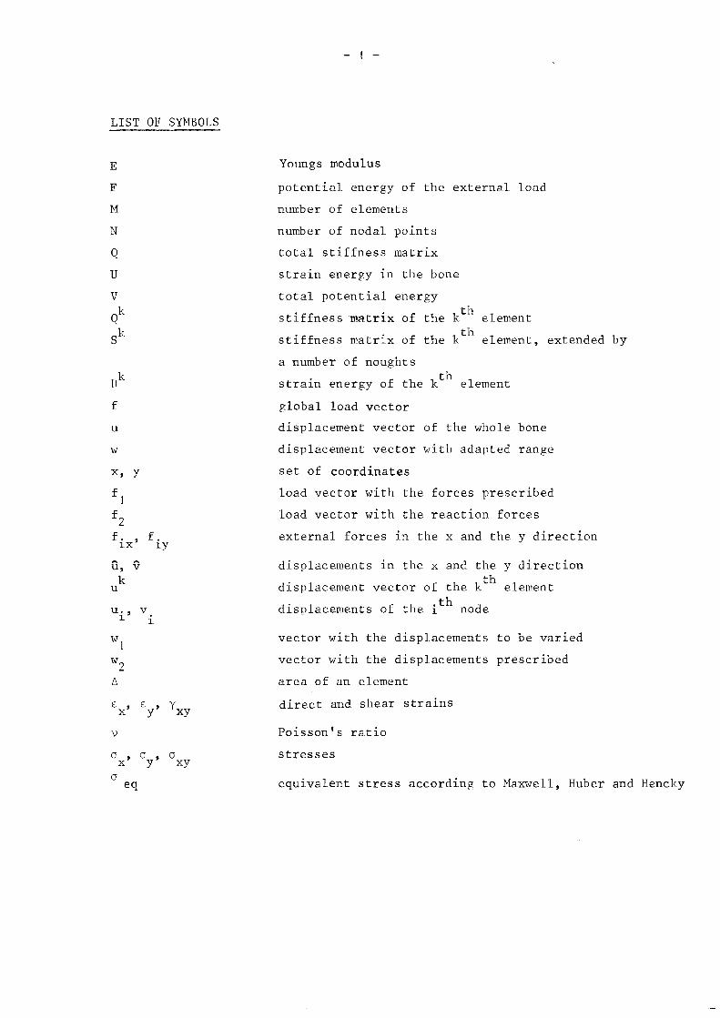
LIST OF SYMBOLS

E

F

M

N

Uk

f

u

w

x, Y

fl

f2

f., f.~x ~y

n, vk

u

u i ' v~

wIw

2to

v

o , 0 , 0x y xy

oeq

- I -

Youngs modulus

potential energy of the external load

nu~ber of elements

number of nodal points

total stiffness matrix

strain energy in the bone

total potential energy

stiffness matrix of the kth

element

stiffness matrix of the kth

element, extended by

a number of noughtsth

strain energy of the k element

global load vector

displacement vector of the whole bone

displacement vector with adapted range

set of coordinates

load vector with the forces prescribed

load vector with the reaction forces

external forces in the x and the y direction

displacements in the x and the y direction

displacement vector of the kth

element

displacements of the i th node

vector with the displacements to be varied

vector with the displacements prescribed

area of an element

direct and shear strains

Poisson's ratio

stresses

equivalent stress according to Maxwell, Huber and Hencky

- 2 -

Literature

I. BlaiIT1ont, P.

Contribution a l'etude biomechanique du femur humain.

Acta Orthopaedica Belgica,

34 (1968), pp. 665 - 844.

2. Currey, J.D.

The mechanical consequences of variation ~n the mineral content of bone.

Journal of Biomechanics,

2 (1969), pp. 1 - 11.

3. Evans, F.G. and LebO'\!, H.

Regional differences in some of the physical properties of the human femur.

Journal of Applied Physiology,

3 (1951), pp. 563 - 572.

4. Frocht, M.M.

Photoelasticity

J. Wiley & Sons, New York, 1957.

5. Halleux, P.

Un paradoxe de la resistance mecanique de l'os humain.

Universite Libre de Bruxelles,

seminair d'analyse des contraintes no. I, 1968

6. Eoland, 1. and Bell, K.

Finite element methods in stress analysis.

The Technical University of Norway,

Trondheim, Noruay, 1969.

7. Janssen, J.D.

Numerieke Hethoden.

Technische Hogeschool Eindhoven

Collegedictaat, 1970

8. }'~och,·J.c.Laws of bone architecture.

A.merican Journal of AnatoTI'Y,

21 (1917), ?p. 177 - 298.

- 3 -

9 . Kummer, B.

Photoelastic studies on the functional structure of bone.

Folia Biotheoretica,

6 (1966), pp. 31 - 40

10. Kummer, B.

Eine vereinfachte Methode zur Darstellung von Spannungstrajectorien,

gleichzeitig ein Hodellversuch fur die Ausrichtung und Dichtverteilung

der Spongiosa in den Celenkenden der Rohrenknochen.

Zeitschrift fur Anatomische Entwicklungsgeschichte,

II? (1956), pp. 223 - 234.

II. Hilch, E.

Photoelastic studies of bone form.

Journal of Bone and Joint Surgery,

22 (1940), pp. 621 - 626.

12. Pauwels, F.

Gesammelte Abhandlungen zur funktionellen Pillatomie des Bewegungsapparates.

Springer-Verlag, Berlin, Heidelberg,

Nev,7 York, 1965

I 3. P_yd e 11, N. 1'1.

Forces acting on the femoral head-prosthesis.

Goteborg, 1966.

14. Seldin, E.n. and Hirsch, C.

Factors affecting the determination of the physical properties of femoral

cortical bone.

Acta Orthopaedica Scandinavica,

37 (1966), pp. 29 - 48

15. Mather Sher~ood, B.

The effect of variation ~n specific gravity and as1] content on the mecha­

nical properties of human compact bone.

Journal of Biomechanics,

1 (1968), pp. 207 - 210.

16. Smith, J.H. and Halmsley, R.

Factors affecting the elasticity of bone.

American Journal of Anatomy,

93 (1959), pp. 503 - 523

- l] -

17. Timoshenko, S. and Goodier, J.N.

Theory of elasticity.

Hc Graw-Hill Book Company Inc.,

New York, Toronto, London, 1951

18. Visser, H.

The finite element method in deformation and heat conduction problems.

Proefschrift Technische Eogeschool Delft, 1968.

19. Holf, H.

Spannungsoptik

Springer-Verlag, Berlin, Gottingen.

Heidelberg, 1961.

20. VJolff, J.

Das Gesetz der Transformati.on der Knochen.

Eirschwald, Berlin, 1892.

21. Zienkiewicz, (1. C. and Cheung) Y. K.

The finite element method in structural and continuum mechanics,

He Graw-nill, London, 1967

- 5 -

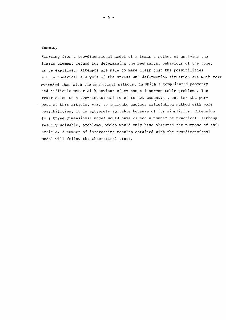
Summary

Starting from a two-dimensional model of a femur a method of applying the

finite element method for determining the mechanical behaviour of the bone,

is be explained. Attempts are made to make clear that the possibilities

with a numerical analysis of the stress and deformation situation are much more

extended than with the analytical methods, in which a complicated geometry

and difficult material behaviour often cause insurmountable problems. The

restriction to a two-dimensional model is not essential, but for the pur-

pose of this article, viz. to indicate another calculation method with more

possibilities, it is extremely suitable because of its simplicity. Fxtension

to a three-dimensional model would have caused a number of practical, although

readily solvable, problems, which would only have obscured the purpose of this

article. A number of interesting results obtained with the two-dimensional

model will follow the theoretical start.

- 6 -

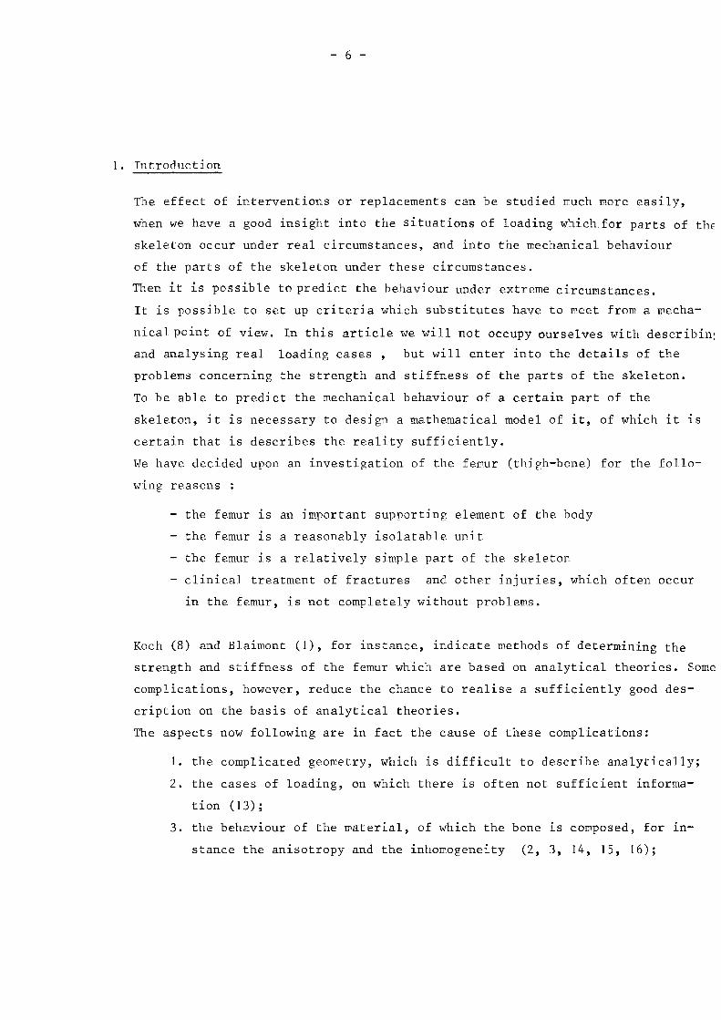
1. Introduction

The effect of interventions or replacements can be studied much more easily,

when we have a good insight into the situations of loading which for parts of thE

skeleton occur under real circumstances, and into the mechanical behaviour

of the parts of the skeleton under these circumstances.

Then it is possible to predict the behaviour under extreme circumstances.

It is possible to set up criteria which substitutes have to meet from a mecha­

nicalpoint of view. In this article we will not occupy ourselves with describin:

and analysing real loading cases, but will enter into the details of the

problems concerning the strength and stiffness of the parts of the skeleton.

To be able to predict the mechanical behaviour of a certain part of the

skeleton, it 1S necessary to design a mathematical model of it, of which it 1S

certain that 1S describes the reality suffjciently.

We have decided upon an investigation of the femur (thigh-bone) for the follo­

wing reasons :

- the femur 1S an important supporting element of the body

- the femur 1S a reasonably isolatable unit

- the femur 1S a relatively simple part of the skeleton

- clinical treatment of fractures and other injuries, which often occur

in the femur, is not completely without problems.

Koch (8) and Blaimont (1), for instance, indicate methods of determining the

strength and stiffness of the femur which are based on analytical theories. Some

complications, however, reduce the chance to realise a sufficiently good des­

cription on the basis of analytical theories.

The aspects now following are in fact the cause of these complications:

1. the complicated geometry, which is difficult to describe analytically;

2. the cases of loading, on which there is often not sufficient informa­

tion (13);

3. the behaviour of the material, of which the bone is c.omposed, for 1n­

stanc.e the anisotropy and the inhomogeneity (2, 3, 14, 15, 16);

- 7 -

Procedures, tuned to a computer, especially the finite element method

(6, 7, 18, 21), abbreviated to the element method, offer considerably

more chance of success.

In this method the object to be investigated is divided into a large number of

small parts, which often have a very simple boundary, two-dimensional for

instance triangles or rectangles, three-dimensional for instance tetrahedrons

or prisms. The mechanical features of such an element are less complex than

for the object as a whole, with its arbitrary geometry.

By joining the elements in the right way, statements can be made about the

mechanical features of the whole object. The result of such a calculation

method will exist of numerical data for:

1. the displacements

2. the strains

3. the stresses

Complicated material behaviour or a complicated geometry do not cause essential

difficulties, provided there is sufficient information on these phenomena. At

the moment, however, we would like to rid ourselves from all this, as the main

purpose of this article is to indicate the way of working with and the possibi­

lities of the element method. We intend to do this on the basis of a two-dimen­

sional,plane, homogeneous and isotropic model of a femur in static cases of

loading.

In principle such a two-dimensional model is identical with the model used with

photo-elastic research (9, 10, 11, 12), on the understanding, however, that the

element method gives much more information than photo-elastic research. Photo­

elasticity supplies isoclinics, with which the principal stress directions can

be constructed and fringes, the lines along which the differences between the

principal stresses are constant.

- 8 -

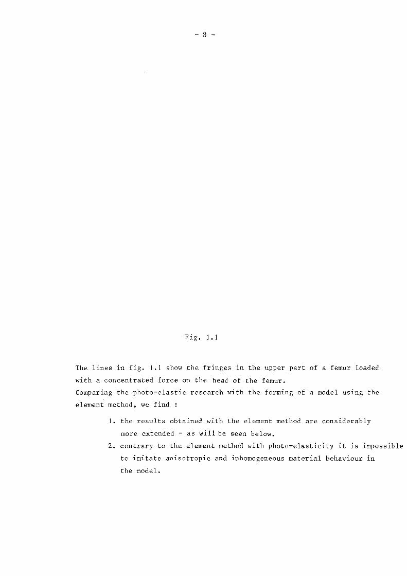
Fig. I.I

The lines in fig. 1.1 show the fringes in the upper part of a femur loaded

with a concentrated force on the head of the femur.

Comparing the photo-elastic research with the forming of a mndel uSlng the

element method, we find :

I. the results obtained with the element method are considerably

more extended - as will be seen below.

2. contrary to the element method with photo-elasticity it lS impossible

to imitate anisotropic and inhomogeneous material behaviour in

the model.

- 9 -

3. 1n the element model it is not difficult to create any

arbitrary load.

4. the change-over to a three-dimensional model does not cause any

difficulties with the element method. The photo-elastic research

becomes very complicated when applied to a spatial model. With

the latter there are the same limitations as with the two-dimen­

sional research.

5. the obtaining and handling of results is much less time-consuminf

in the case of the element method, provided adequate general

calculation programmes are available, than in the case of photo­

elastic research.

- 10 -

2. Principle of the method

The central starting-point for a numerical analysis of the stress and deforma­

tion situation of the bone, with the help of the element method, is "the prin­

ciple of minimum potential energy" (17, 18). If we define:

U: the strain energy, accumulated in the bone as a result of the ex­

ternal load, expressed in the displacements;

F: the potential energy of the load, i.e. the sum of the negative

product of each force acting on the bone, with the labour absorbing

component of the displacement of the point of application.;

v = u + F: the potential energy

the principle of the m~n~mum potential energy can then be formulated as

follows:

~len we have at our disposal a number of different displacement fields

for a certain problem, which are all compatible and fulfil the geo­

metrical boundary conditions, then that solution is to be preferred,

that minimizes the expression for the potential energy with respect

to "neighbouring" admissible displacement fields, because this solu­

tion best meets reality.

The choice ~s realised by claiming that the variation of the potential energy

~s zero,

oV = 0

for all admissible variations of the displacement field.

(2. 1)

In the following chapter it will be indicated in what way the principle can

lead to a usable method. It has to be realised that as an example for explaininl

the method we have made only a very limited choice from a great range of possi­

bilities, namely a way of working with the element method for a two-dimensional

model and using a very simple element.

- 11 -

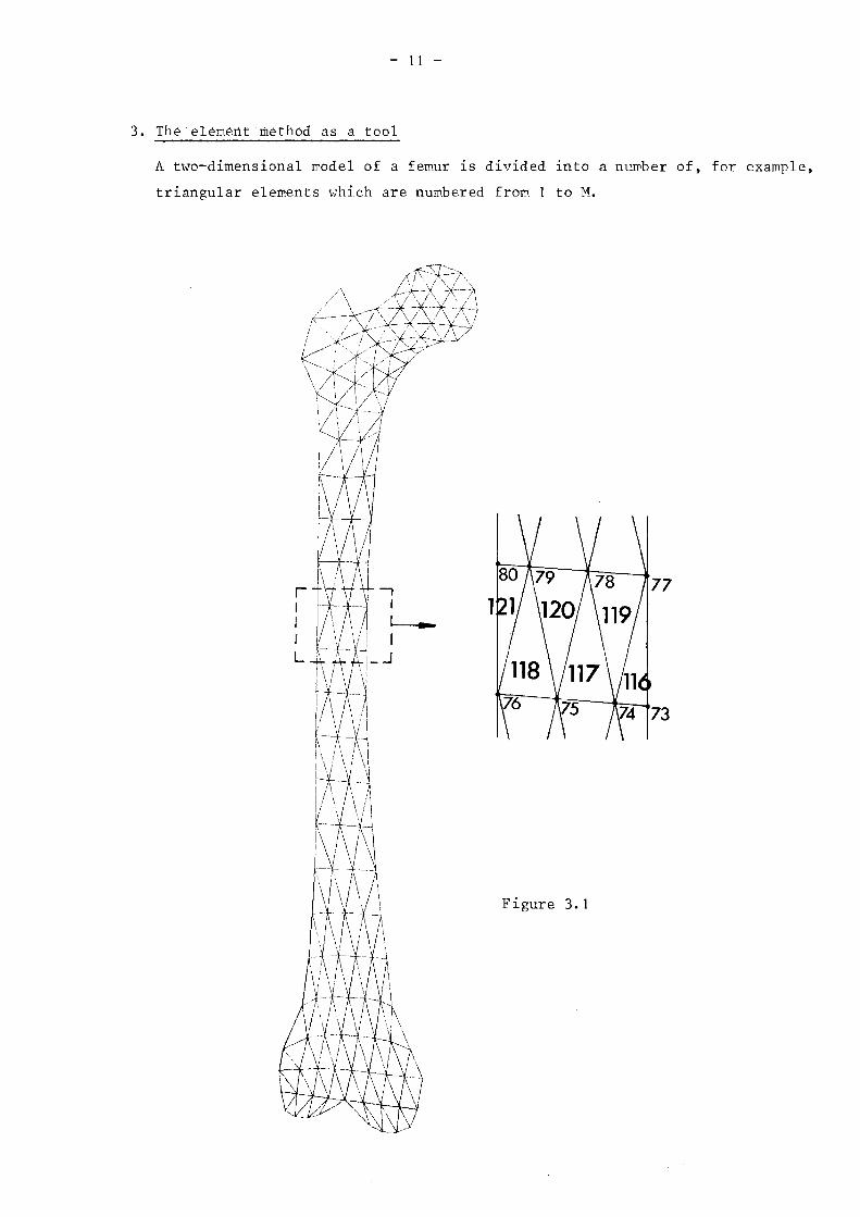
3. The element method as a tool

A two-dimensional model of a femur is divided into a number of, for example,

triangular elements which are numbered from 1 to M.

Figure 3. 1

- 12 -

All nodes, the angular points of the elements, are numbered from 1 to N.

Fig. 3.1 exemplifies such a division with M = 224 and N = 146.

We indicate the displacements ~n an arbitrary point of the bone ~n the x

and y direction respectively, by G and v. The displac2ments will depend among

other things on the coordinates of that point, and for that reason they will

be a function of x and y in this plane model. The still unknown displacement

field can be indicated by

u(x,y)

v(x,y)

(3.1)

(~.2)

In the continuous theories the displacements are described as a function of the

coordinates. On the other hand, the behaviour in an element model is charac­

terized by a concrete number of magnitudes, the nodal-point displacements.

Within each element a displacement field 1S assumed that is dependent on and

consistent with the displacements of the nodes pertaining to the element con­

sidered. Fig. 3.2 shows an arbitrary element (with number k). At the nodes we

have not mentioned the global numbers from the range 1 to N, but we have used

a local numbering: 1,2 and 3.

- 13 -

The total deformation situation of this element k has to be characterized

by the nodal point displacements, which we place in a vector uk

'ku = (u

1(3.3)

Note: as regards the vector notation we have used and the matrix notation we

are going to use, we refer the reader to the appendix.

With this element it is usual to choose an interpolation function for the dis­

placement field, which is linear in the coordinates: x and y. Naturally this

is an approximation of reality, which will be all the better, the finer the

distribution of the elewents 1S made.

The advantage of this choice 1S that along the boundaries the continuity betweer

two elements is also guaranteed in a deforwed situation. We can write the de­

formation field of this element:

with:

u(x,y)

v(x,y)

(3.4)

(3.5)

PI(x,y)I2t:. [ (3.6)

In formula (3.6) t:. is the area of the element concerned. P2

(x,y) and P3 (x,y)

can be found by exchanging cyclically the indices in formula (3.6). Starting

from the two-dimensional theory of elasticity with plane stress situation suita­

ble for this model, we can express the strain energy, Uk, stored in this element,

in the still unknown components of vector uk and in the reometrical and physica:

features of this element. If we restrict ourselves to a homoreneous, isotropic

and linear material behaviour and to a constant thickness, we have:

s 2 + s 2 + 2vs s + (I-v)x Y x Y

'Y 2} dxdyxy(3.7)

The restrictions are not essential at all, but they simplify the formulation

considerably.

- 14 -

For the direct and shear strains

auE axx

avE

'oyy

au + ovYxy = oxay

E and y we have:y xy

0.8)

(3.9)

(3.10)

Substitution of (3.4) and (3.5) ln these strain terms gives the following

results:

(3.11 )

EY

(3.12)

Yxy ;6, [u 1 . (x3 - x2) + u2 . (x 1 - x3) + u3 . (x2 - xl) +

vI • (Y2 - Y3) + v 2 • (Y3

- Y1) + v 3 • (Y 1 - Y2)J

(3.13)

It is evident that the direct and shear strains are constant for an element,

which is the result of the displacement field assumed.

Substitution of (3.11), (3.12) and (3.13) in (3.7) and further elaborationkresults in a quadratic formula expressed in the components of vector U , and

h f . h .. . kt ere ore, uSlng t e matrlx notatlon, we can wrlte U as

Uk _ I 'k Qk k

- 2 U U

The matrix of coefficients qk, which can simply be taken symmetrically,

Qk = Qk , is called the stiffness matrix of element k.

(3.14)

- 15 -

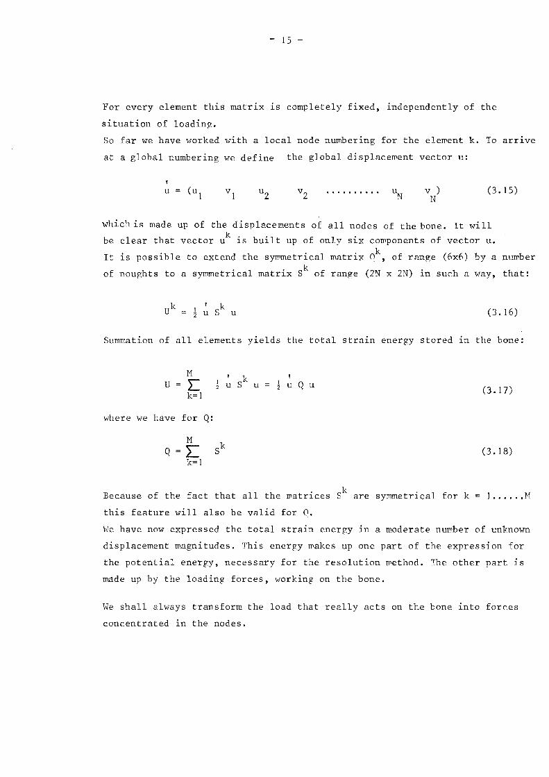
For every element this matrix 1S completely fixed~ independently of the

situation of loading.

So far we have worked with a local node nuwbering for the elewent k. To arr1ve

at a global numbering we define the global displacement vector u:

uN

v )N

(3.15)

which is made up of the displacements of all nodes of the bone. It will

be clear that vector uk is built up of only six components of vector u.

It is possible to extend the sywmetrical matrix ok, of range (6x6) by a number

of noughts to a sywmetrical matrix Sk of range (2N x 2N) in such a way, that:

(3.16)

Summation of all elements yields the total strain energy stored 1n the bone:

H , kU L u S u u Q u

k=1

where we have for Q:

HSkQ L

k=1

(3.17)

(3.18)

1•••••• MBecause of the fact that all the watrices sk are symmetrical for k

this feature will also be valid for Q.

We have now expressed the total strain energy 1n a moderate number of unknown

displacement magnitudes. This energy wakes up one part of the expression for

the potential energy, necessary for the resolution wethod. The other part is

wBde up by the loading forces, working on the bone.

We shall always transform the load that really acts on the bone into forces

concentrated in the nodes.

- 16 -

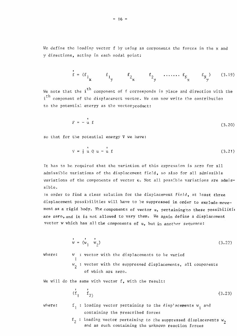
We define the loading vector f by us~ng as components the forces ~n the x and

y directions, acting in each nodal point:

f ••••••• f:N

x(3.19)

h h .th f f dId d' . . h hWe note t at t e ~ component 0 correspon s ~n p ace an ~rect~on w~t t e

ith

component of the displacement vector. We can now write the contribution

to the potential energy as the vectorproduct:

F - u f(3.20)

so that for the potential energy V we have:

V ! u Q u - u f (3.21 )

It has to be required that the variation of this express~on is zero for all

admissible variations of the displacement field, so also for all admissible

variations of the components of vector u. Not all possible variations are admis­

sible.

In order to find a clear solution for the displacement field, at least three

displacement possibilities will have to be suppressed in order to exclude,move­

ment as a rigid body. The components of vector u, perta1n1ng to these possibilitiE

are zero, and it is not allowed to vary them. We again define a displacement

vector w which has all the components of u, but in another sequence:

w (3.22)

vector with the displacements to be variedwhere: w1

w2

vector with the suppressed displacements, all components

of which are zero.

We will do the same with vector f, with the result:

(3.23)

where: f1

: loading vector pertaining to the displacements WI and

containing the prescribed forces

f 2 loading vector perta1n~ng to the suppressed displacements w2

and as such containing the unknown reaction forces

- 17 -

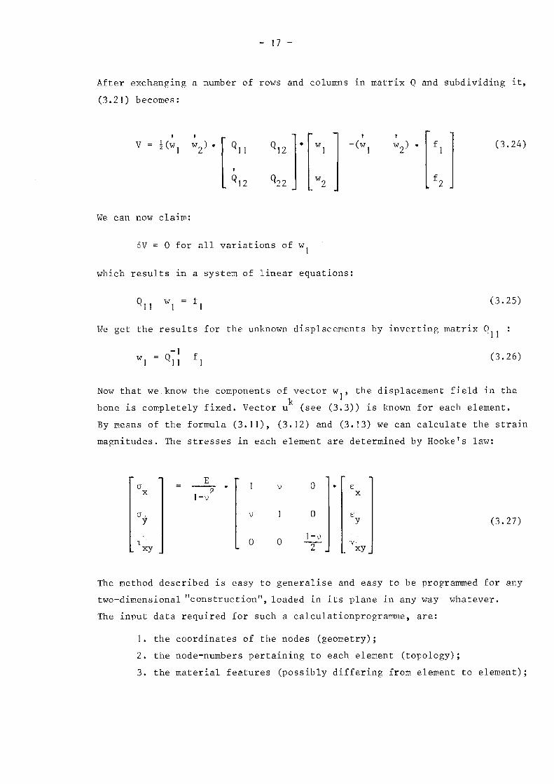
After exchanging a number of rows and columns ~n matrix Q and subdividing it,

(3.21) becomes:

v,

-(wI

(3.24 )

We can now claim:

6V 0 for all variations of wI

which results ~n a system of linear equations:

(3.25)

We get the results for the unknown displacements by inverting matrix QII :

(3.26)

Now that we know the components of vector wI' the displacement field in the

bone is completely fixed. Vector uk (see (3.3)) is known for each element.

By means of the formula (3. II), (3.12) and (3.13) we can calculate the strain

magnitudes. The stresses in each element are determined by Hooke's law:

E0° --2 . v E:

X I-v x

0, v 0 E:Y Y (3.27)

0 0Ie-v

T -"1- Yxyxy ~

The method described is easy to generalise and easy to be programmed for any

two-dimensional "construction", loaded in its plane in any way whatever.

The input data required for such a calculationprograro~e, are:

I. the coordinates of the nodes (geometry);

2. the node-numbers pertaining to each element (topology);

3. the material features (possibly differing from element to element);

- 18 -

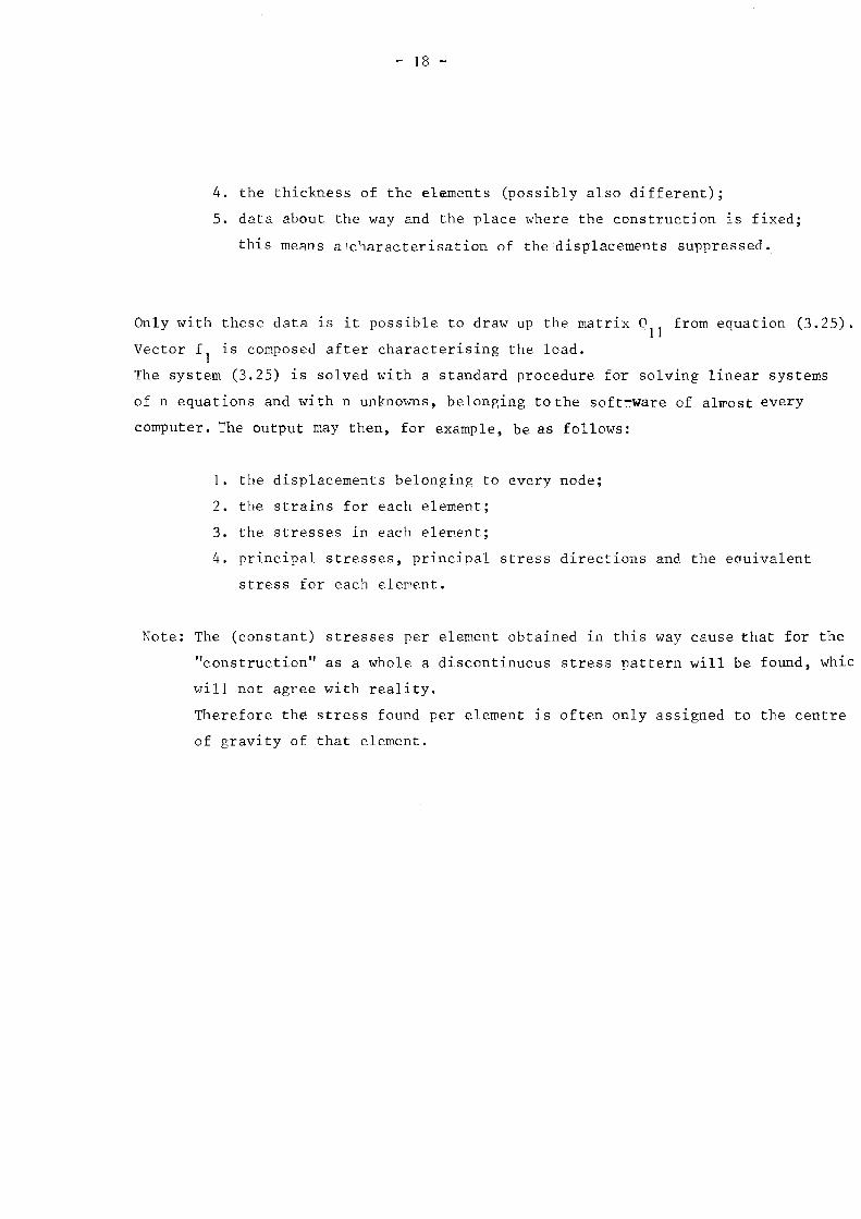
4. the thickness of the elements (possibly also different);

5. data about the way and the place where the construction is fixed;

this means aicharacterisation of the displacements suppressed.

Only with these data is it possible to draw up the matrix all from equation (3.25).

Vector f1

is composed after characterising the load.

The system (3.25) is solved with a standard procedure for solving linear systems

of n equations and with n unknowns, belonging tothe soft~are of alwost every

computer. The output may then, for example, be as follows:

1. the displacements belonging to every node;

2. the strains for each element;

3. the stresses in each element;

4. principal stresses, principal stress directions and the eauivalent

stress for each element.

Note: The (constant) stresses per element obtained in this way cause that for the

"construction" as a whole a discontinuous stress pattern will be found, whic

will not agree with reality.

Therefore the stress found per element ~s often only assigned to the centre

of gravity of that element.

- 19 -

4. Numerical results

A two-dimensional model of a femur with an external geometry as g~ven by Koch (8)

will be analysed ~n two different loading cases:

A. A loading as used by Koch, v~z. a force acting on the head of the femur

with a line of action, which is connection line from the centre

of the head to the middle between the condylis medialis and the condylis

lateralis.

B. A load as indicated by Rydell (13) v~z. a force acting on the head of the

femur directed to the centre of the head with a point of application within

area on the head, indicated by Rydell; and a force acting on the trochan­

ter major in a direction also indicated by Rydell, the direction of

the resultant of the abductor muscle forces.

Because of the linearity of the theory the magnitude of the force is not imDortant

in loading case A. In loading case B, only the ratio of the two forces is impor­

tant.

In both loading cases the same fixation was.e.s.tablished. We assume the bone to be

clamped along the whole bottom. This means that a prescribed value equal to zero

is assumed for the displacements of all poin:ts of the boundary.of the condylis

medialis and the condylis lateralis.

Fig. 4.1 shows the loading cases to be analysed.

y

lOOON

A

x

Fig. 4.1

y

1200N

B

x

- 20 -

Although not essential for the method we make th

following restrictions:

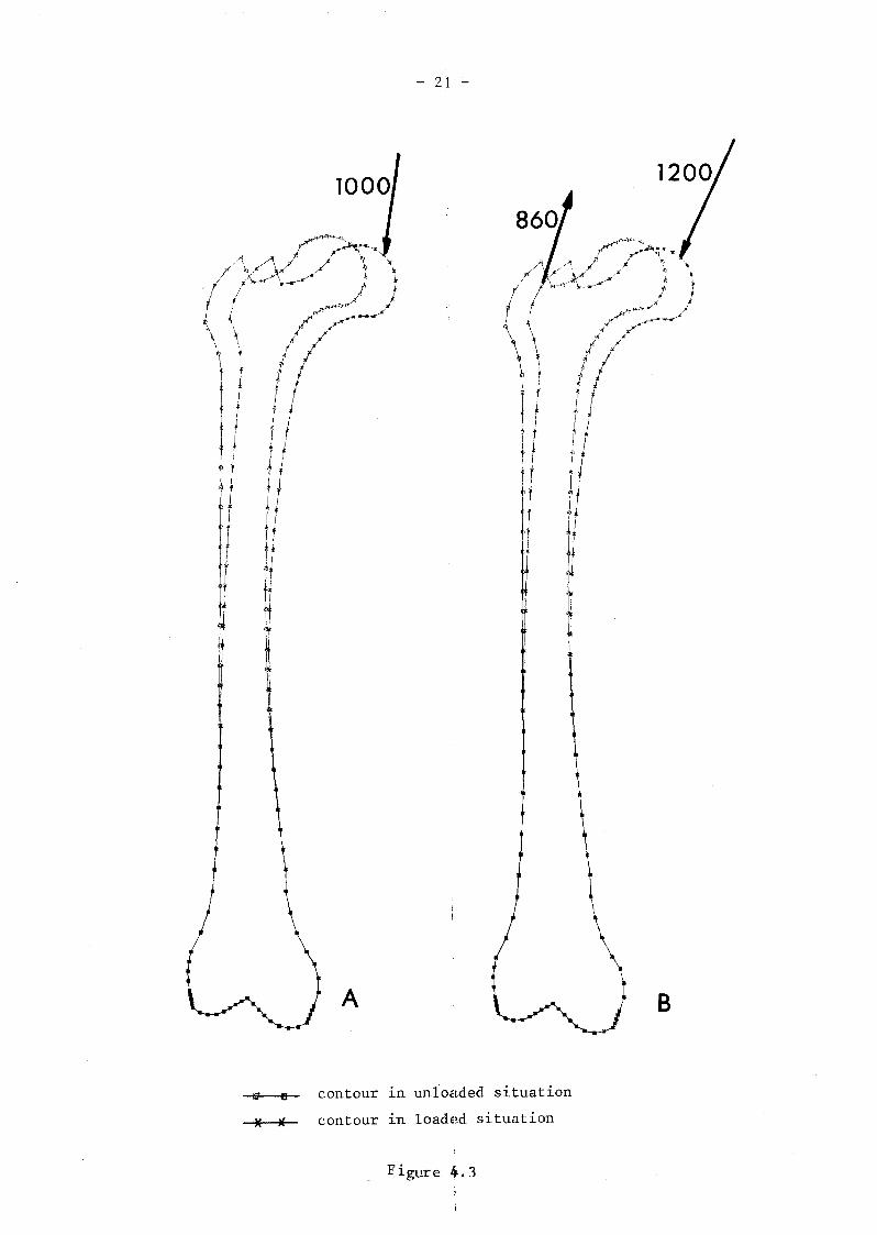
The enlargement factor used for the displace­

ments was 5.

It appears that the displacement fields for tl

two loading cases hardly differ.

1. At this moment we suppose the material to be

homogeneous, isotropic and linear with

F 2.104

N/mm2

v = 0.37

2. We assume the thickness of the model to be co:

stant. The numerical value we give this thick

ness is not important, because of the fact tho

the results to be obtained for the displace­

ments, strains and stresses, are inversely pr,

portional to the thickness because of the lin

arity of the theory.

We have chosen:

t = 10 m.m

1 : 2.5

1': 0.5

- scale for external outline

scale for displacements

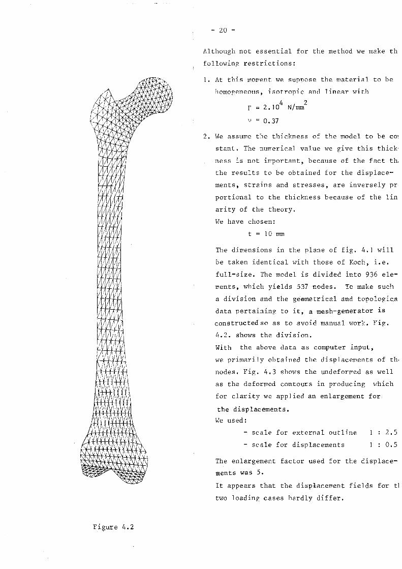
The dimensions 1n the plane of fig. 4.1 will

be taken identical with those of Koch, i.e.

full-size. The model is divided into 936 ele­

ments, which yields 537 nodes. To make such

a division and the ge<llmetrical and topologica

data pertaining to it, a mesh-generator is:

constructedso as to avoid manual work. Fig.

4.2. shows the division.

With the above data as computer input,

we primarily obtained the displacements of tho

nodes. Fig. 4.3 shows the undeformed as well

as the deformed contours in producing which

for clarity we applied an enlargement fori

the displacements.

We used:

Figure 4.2

- 21 -

A B

E1 B contour in unlo~lded situation

X 1( contour in loadE~d situation

Figure 4.3

- 22 -

86~.. /»9 '1h{~>~l0; / \5') ' .... )/ /j "

/ ~() //'5 \y.;>. /) _~./

/ \ ( /~;.;;rI /,..~ f-..,JI ,/ /10I I /-7-

10---\ I (/~/-151~-\ \ I /ld-2020~\\ \ . I. i j.!/)-25

II ' ,IiIIfIIi 1'1'/111'11 ,I

1111

,/:

I1I1IIII( !,

/,

1111

- 25II \!

\20111/1111 \

\1-201511

/ \\ \-15

101I \\-10

V \5) \\5O~.J \

\A

!iI

I~ I ! B

'-/ ~/

0y

o

~-~ ./ A'---_ .. -~

<~)r-!:-10<, I"~(, " 5'I; '\~ \

//tR~/;1 )( I

/ //-\/ ..

/ \ ---I / F"~

/ / /-5~ ----- ( /1/~10.:>'\ \ I /10\" \ I I /;;L 15

5"\ \ I II J1 1\ ' II (~-20

i.

1

\, I 1

1

1,.1/ill I II i

III' If III !I' iI 1111-25

II 1)1,

1.11: 1'1/1,,I li I1\ [-25

II \\Ii! II15[ I '\

I \1"-20

II I\\\lCJ 1\\\ 1

\\ r 5

5~ I \\1\ \\-10

\ \\ \\(

\\-5

Figure 41. 4

- 23 -

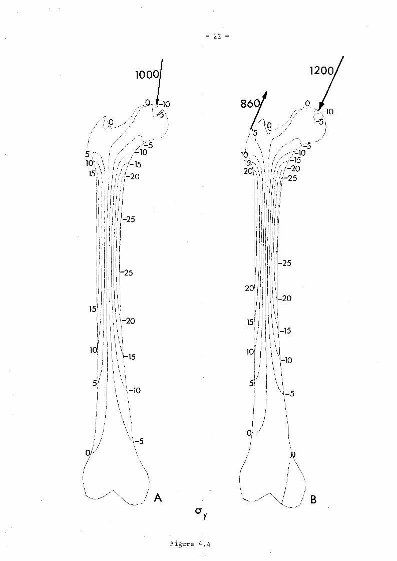
By means of a calculating machine we determine the strains and stresses ~n

each element from the displacements. We could represent these stresses in

table form or as numbers written in the elements in a figure such as fig. 4.2.

A better image shows for instance fig. 4.4,in which lines of constant stress

in y-direction, a , are arawn, being the most interesting stress magnitudey

for both loading cases in the shaft of the femur.

In order to draw such (continuous) lines, it is necessary that the stress field

~s continuous or that, if need be, it is made continuous artificially.

In our case we did this by assigning to each node the average value of the rele­

vant stress magnitudes in the elements lying around that node, and after that,

by choosing a linear stress field per element. This method may cause great de­

viations along the boundaries, expecially when the stress gradient is high in the

direction perpendicular to the boundary. The numbers appearing in fig. 4.4 show. • / 2the values of a on each l~ne ~n N mm •

y

We should set less value on the stresses in the surroundings of the points of

fixation as they are caused by the method of fixation of the bonel

From the uniform stress pattern in the shaft in both loading cases we conclude

that the loading case in that area is very closely related to ajsituation

of pure bending. It appears that in both loading cases the greatest value of ay

does not occur in the neck, but in the upper part of the shaft on the

medial side. I

At the point of application of the concellltxated forces we hardly find stress concenJ

trations, which from a physical point of view should occurthere under such condi-,

tions. When calculated by the element method, these stress concentrations fade

away more and more, according as the element pattern is less fine.

We will not pay any attention to this phenomenon, as a load in the shape of a

concentrated force is not in accordance with reality.

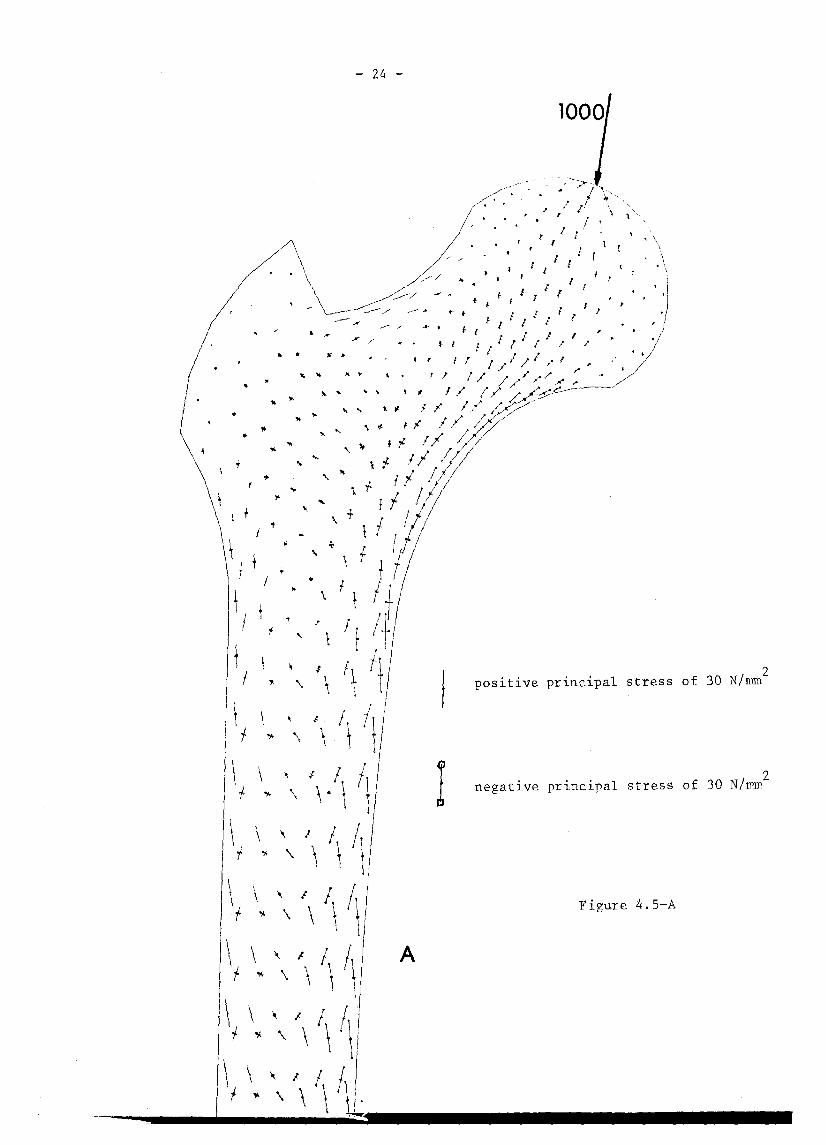
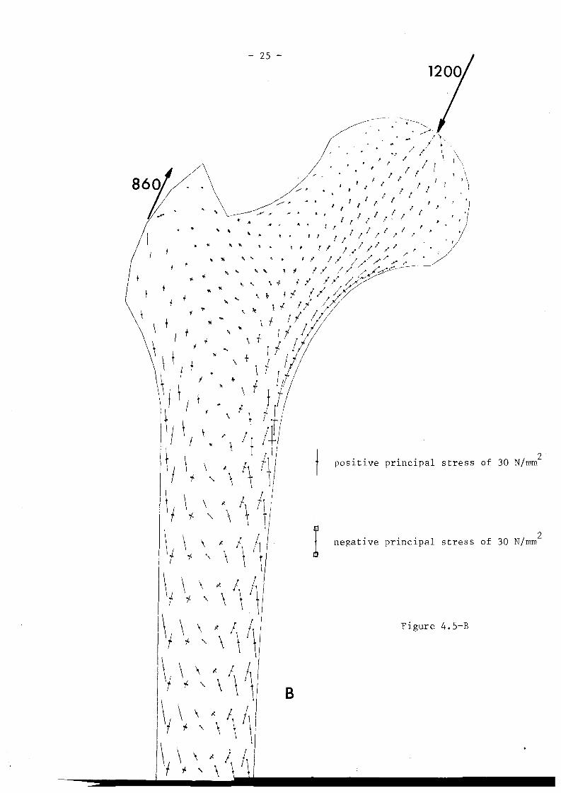
In order to g~ve the reader a picture of the total stress situation, we indica­

ted in fig. 4.5 the principal stresses and the accessory principal stress direc­

tions. However, for practical reasons, only the upper part of the bone is

shown.

- 24 -

Figure 4.5-A

positive principal stress of 30 N/mm2

negative principal stress of 30 N/mm2I

A

/\'\

"

/:<-~"- .. --'7/'--... ... ,.,:.,'

'. ," I Ii .. '." ' ". .' r ' \ "'"" • ' ! ! [' l \

// .• ' I ' .! I I ' \

// .' ( [l r \.. I '- ' __/ .' I I • \'-~ - -. ,"--~/ -- .""""" ''. -- -, ' . '-'/ ...... f ti'l' r I, ' " )

'" . . ' ,!" ' I I! .. '.. I,' (' , · ' .."". ' II I 1/_/• ! I .

.' ,. " . " /,," " ./.l " " '.1:1 / / /// .J'~/.. '.. "... ?¥,.. .,

II.. \" I I' / /-"c"• ' 1/ ,.-- ..' .' ,. ," 1 / ! /~~~..-

"' ,!' ff l/.~;ff+ " i of II ///

,. .. \.;. f I ;/\ t . " 1 f II

I ~ \ ,. »\ ._ \f /1

I \ I • • .' • fl f j I;\/ \ • \ \ f f'\ ; • '\ If IfI \ ~ f

1 "\ 1\ t\ \ ~ ! f If 'A,\\ \ t

\ \ ' I ! If 'A '\ \. \ 1

\t

\ ' I I If ' , \ \ \

\ \ ' I I !/ ' \ \ \ \

\ \ '\ I I If ~ \ \ \ \

\ \~ I I I/. , \ \ \\ \ ~ 1/1f ~ \ \ \ \1"

~

- 25 -

B

t positive principal stress of 30 N/mm2

I . .. 1 / 2negatlve prlnclpa stress of 30 N rom

Figure 4.5-B

- 26 -

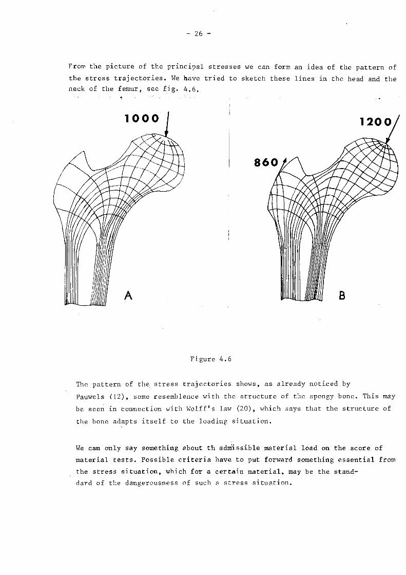
From the picture of the principal stresses we can form an idea of the pattern of

the stress trajectories. We have tried to sketch these lines in the head and the

neck of the femur, see fig. 4.6.

1000

B

Figure 4.6

The pattern of the stress trajectories shows, as already noticed by

Pauwels (12), some resemblence with the structure of the spongy bone. This may

be seen in connection with Wolff's law (20), which says that the structure of

the bone adapts itself to the loading situation.

We can only say something about th admissible material load on the score of

material tests. possible criteria have to put forward something essential from

the stress situation, which for a certain material. may be the stand-

dard of the dangerousness of such a stress situation.

- 27 -

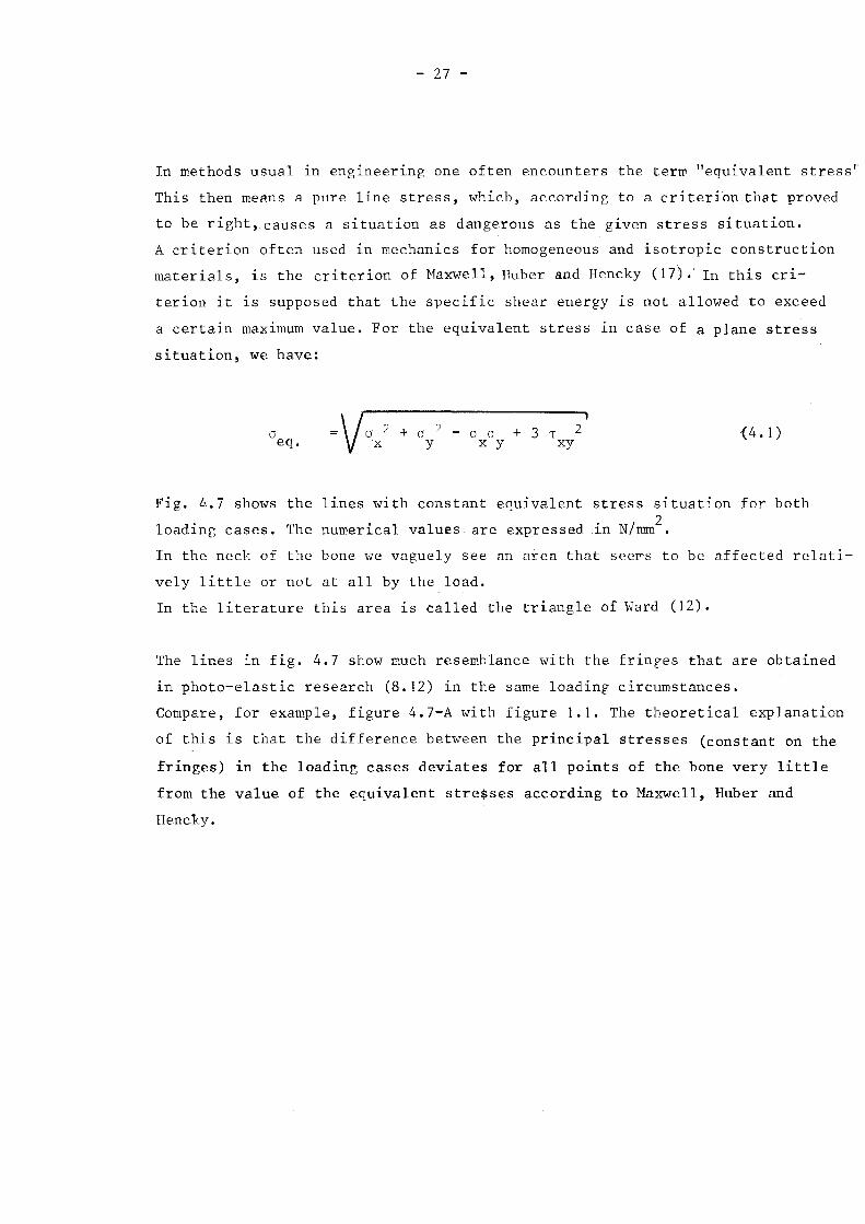
In methods usual in engineering one often encounters the term "equivalent stress"

This then means a pure line stress, which, according to a criterion that proved

to be right, causes a situation as dangerous as the given stress situation.

A criterion often used in mechanics for homogeneous and isotropic construction

materials, is the criterion of Maxwell, Huber and Hencky (17). In this cr~­

terion it is supposed that the specific shear energy is not allowed to exceed

a certain maximum value. For the equivalent stress in case of a plane stress'

situation, we have:

0­eq.

I

+ 3 T 2xy

(4.1)

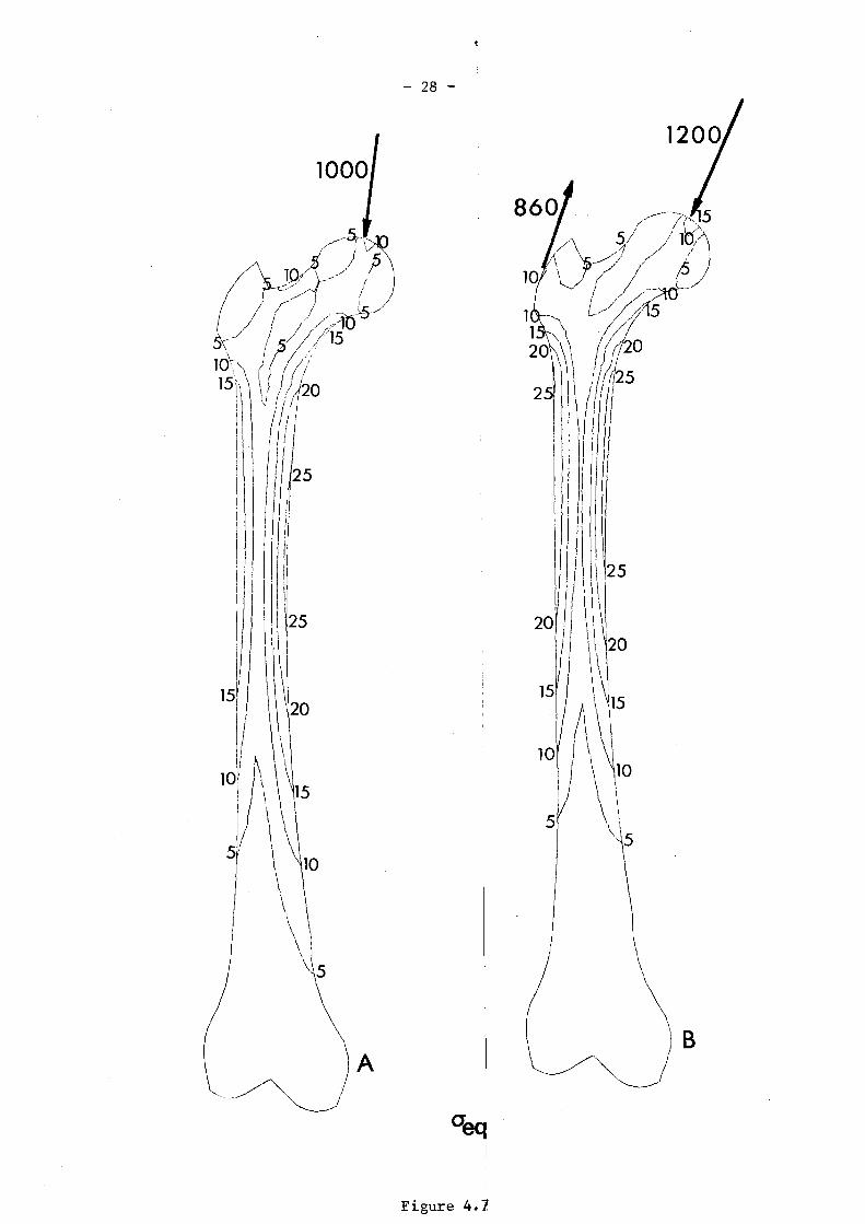
Fig. 4.7 shows the lines with constant equivalent stress situation for both

loading cases. The numerical values. are expressed in N/mm2

•

In the neck of the bone we vaguely see an area that see~s to be affected relati­

vely little or not at all by the load.

In the literature this area is called the triangle of Ward (12).

The lines in fig. 4.7 show much resemblance with the fringes that are obtained

in photo-elastic research (8.12) in the same loading circumstances.

Compare, for example, figure 4.7-A with figure 1.1. The theoretical explanation

of this is that the difference between the principal stresses (constant on the

fringes) in the loading cases deviates for all points of the bone very little

from the value of the equivalent stre$ses according to Maxwell, Huber and

Hencky.

- 28 -

.\ 125

\1120

\

5

iI I II \I 1125

1\

15/ I \\20

~ \

101

~\ \5V· \\

5 "\10

\\ i

\

\\5

f't\rJ!,j

/'/\ 0'/~!'15

1?J\~ ;!(j)/,1\ Ii/I 20

I IiiI I!

A

~~

I ~~IBI°eqI

Figure 4. ~

- 29 -

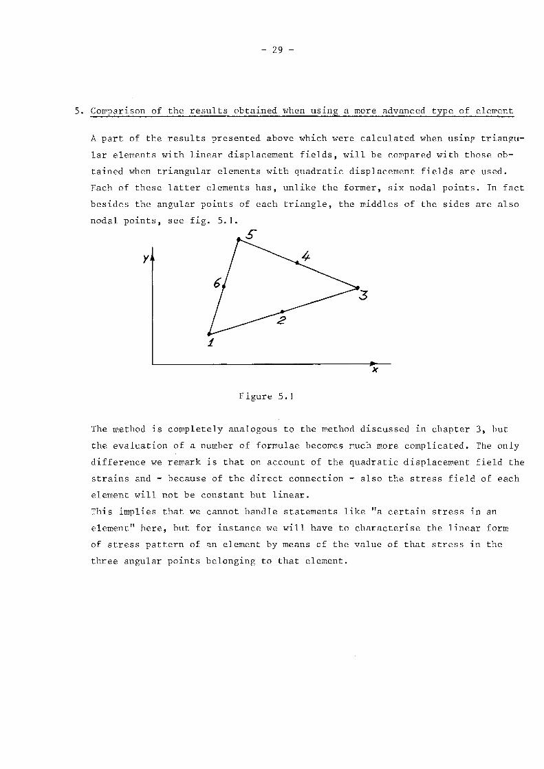
5. Comparison of the results obtained when using a more advanced type of element

A part of the results presented above which were calculated when uSlng triangu­

lar elements with linear displacement fields, will be compared with those ob­

tained when triangular elements with quadratic displacement fields are used.

Each of these latter elements has, unlike the former, six nodal points. In fact

besides the angular points of each triangle, the middles of the sides are also

nodal points, see fig. 5.1.

y

1

x

Figure 5.1

The method is completely analogous to the method discussed in chapter 3, but

the evaluation of a number of formulae becomes much more complicated. The only

difference we remark is that on account of the quadratic displacement field the

strains and - because of the direct connection - also the stress field of each

element will not be constant but linear.

This implies that we cannot handle statements like "a certain stress in an

element" here, but for instance we will have to characterise the linear form

of stress pattern of ~n element by means of the value of that stress in the

three angular points belonging to that element.

- 30 -

Just as in the case of calculations involving the elements with three nodes,

a continuous stress field for the whole bone will not be found.

We find for each element separately in the angular points a certain value for

a stress magnitude. Because of this fact for a certain node where a number of

angular points meet will be found for the same stress magnitude a number of

different values.

A procedure often followed then is to take the average of these values and to

consider the result as the final result of that stress magnitude in that node.

The continuous stress field needed for drawing lines of constant stress, is then

created by choosing the stress field Iwithin each element linear by considering

exclusively the average values of the stress 1n the angular points of each ele­

ment and by neglecting completely the values 1n the middles of the sides.

In addition to the method described above a number of other procedures can be

designed to obtain a continuous stress field. We will not go further into this

matter. The deviations that we introduce in this way will be considerably smaller

than in the case of the element with three nodes, introduced in chapter 4.

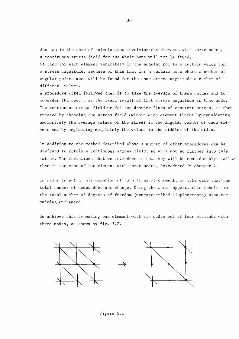
In order to get a fair equation of both types of element, we take care that the

total number of nodes does not change. Using the same support, this results 1n

the total number of degrees of freedom (non-prescribed displacements) also re­

maining unchanged.

We achieve this by making one element with six nodes out of four elements with

three nodes, as shown by fig. 5.2.

Figure 5.2

- 31 -

For the element with three nodes we have:

loading case A V - 0.43 Nm

loading case B V - 0.48 Nm

For the element with six nodes, we have

loading case A V - 0.50 Nm

loading case B V - 0.58 Nm

(5. ])v

Because of the fact that in loading case A only

2 and ~n case B only 4 components of f] differ fron

zero, we can calculate the numerical value of

V simply by hand, provided the nodal point

displacements are kno~~.

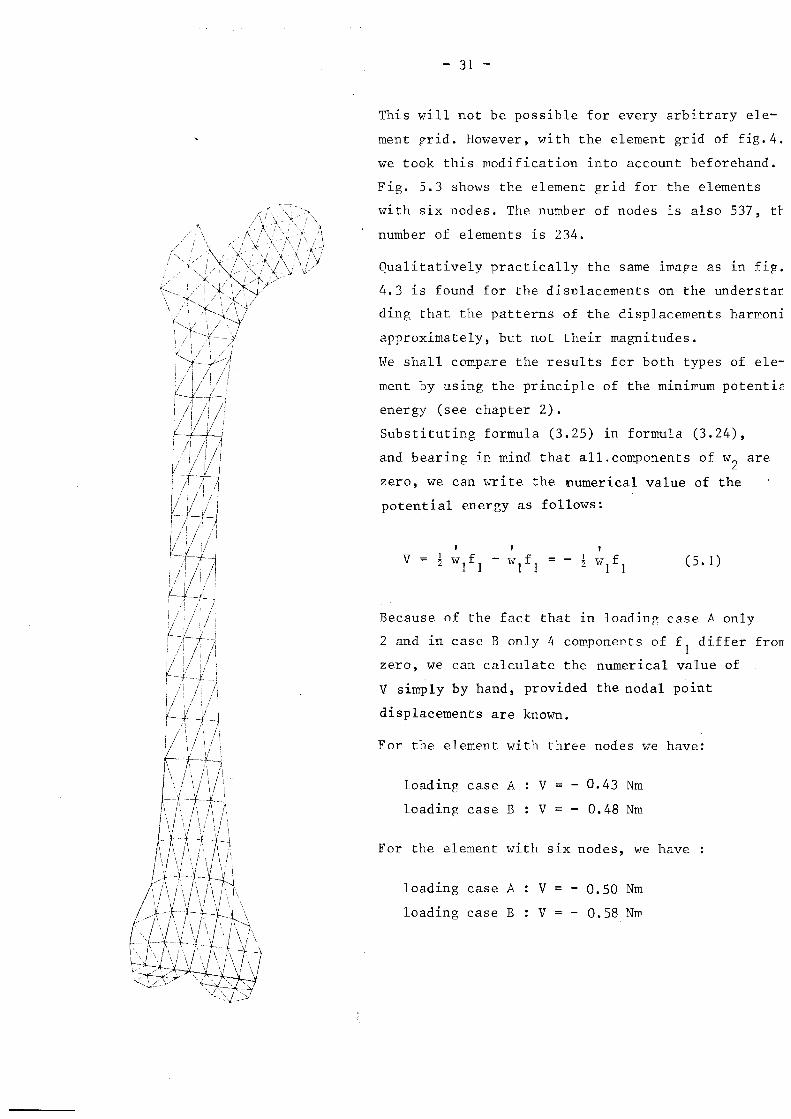
Qualitatively practically the same ~mave as in fiV.

4.3 is found for the displacements on the understan

ding that the patterns of the displacements harmoni

approximately, but not their mBgnitudes.

We shall compare the results for both types of ele­

ment by using the principle of the minimum potenti~

energy (see chapter 2).

Substituting formula (3.25) in formula (3.24),

and bearing in mind that all components of w2 are

zero, we can write the numerical value of the

potential energy as follows:

This will not be possible for every arbitrary ele­

ment grid. However, with the element grid of fig.4.

we took this modification into account beforehand.

Fig. 5.3 shows the element grid for the elements

with s~x nodes. The number of nodes is also 537, tr

number of elements is 234.

- 32 -

In the case of a calculation with the six~hode element for both loading

cases the potential energy 1S much smaller than in the case of the three­

node element. On the score of our ambition to reach a minimum value of the

potential energy, we can conclude that, seen as a whole, the reality is

described better when using the element with six nodes.

Viewed locally, however, we cannot say anything about the quality of the re­

sults found with both types of element. These assertions are confirmed in the

literature, where the same conclusions on the basis of more t~chnical construc­

tions are made (6).

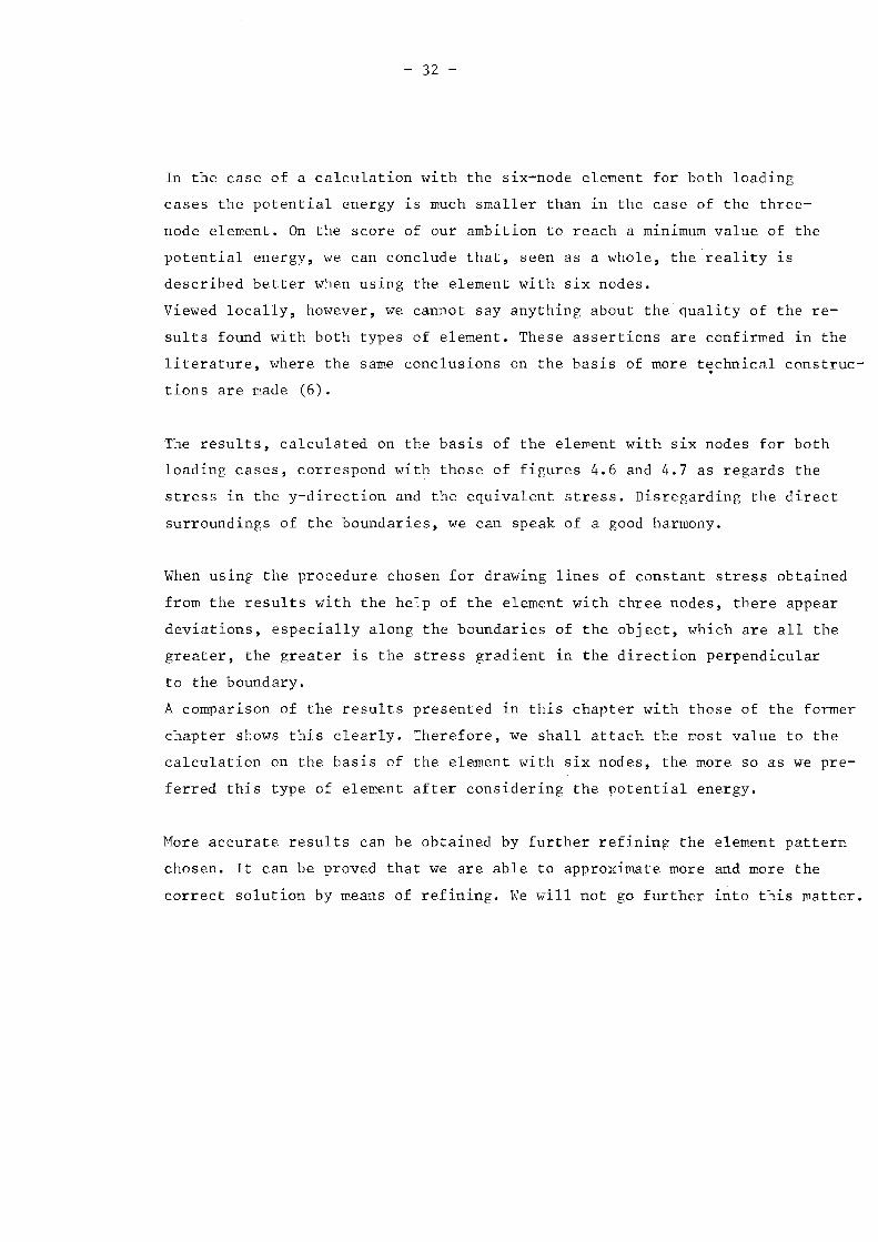
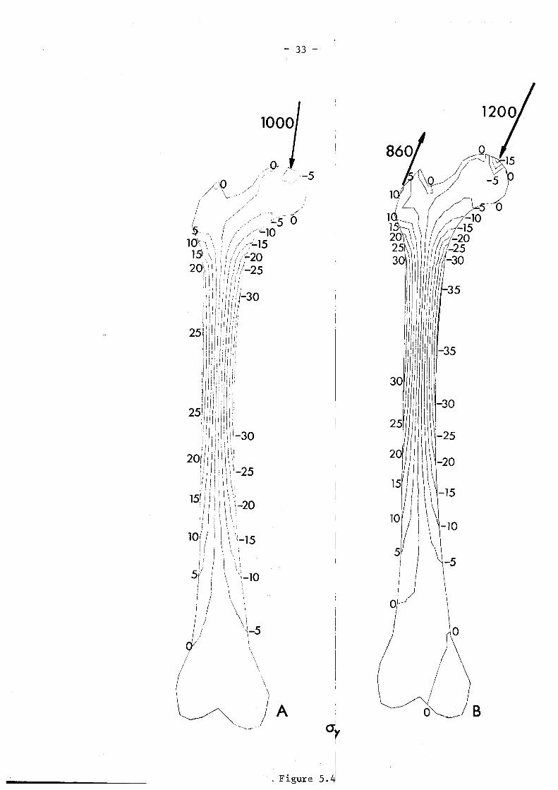
The results, calculated on the basis of the element with S1X nodes for both

loading cases, correspond with those of figures 4.6 and 4.7 as regards the

stress in the y-direction and the equivalent stress. Disregarding the direct

surroundings of the boundaries, we can speak of a good harmony.

When uS1ng the procedure chosen for drawing lines of constant stress obtained

from the results with the help of the element with three nodes, there appear

deviations, especially along the boundaries of the object, which are all the

greater, the greater is the stress gradient 1n the direction perpendicular

to the boundary.

A comparison of the results presented in this chapter with those of the former

chapter shows this clearly. Therefore, we shall attach the most value to the

calculation on the basis of the element with six nodes, the mnre so as we pre­

ferred this type of element after considering the potential energy.

More accurate results can be obtained by further refinin~ the element pattern

chosen. It can be proved that we are able to approximate more and more the

correct solution by means of refining. We will not go further into this matter.

- 33 -

\

\

\

\111-25

\~~~:\ ~-10

-5

0"'---- _J B,

0'rI

--5,Q.

/~:o //>

/ \~- /, ./

I ,::"'5 0$-- /;';:'10

10\-,\ /<--. '-151 I ! '

.i I I ,)1 i' Ii! ! / ...20201," !' / I1!-25

':1 \ I I ,I , / ,n

·:·11. '. III!, I I, ,i , ill:)::.I.i i I;I.! -30I " II 'I! \ i ill I f,

I, II, I', Iii I,I! IIi'I'i II JII'

251il.. 11 •.i'j'II' ..:'I!I' 'I" ,[!I,i 1

11/:

111!i, iii! 1,1

'11 11 1/1 11'\1'

•

1

1

,,1 1 ',.'.',1.. 11.,...•1 ,.,,!. I!I'II' ';1''r!ililli f

:I'lli'l' 11!II i.I.'!'III, 'I'25rd!lllil:

ill!II'!I[I',,11. 1

: 11,.'\Iii'; i 11ildl \!(\,,-30:;Ii, /111\::

201../1 1

1\\'"I["II ,1:\\-25", I I \ I'III I \ III ! ! \ \'.111 'I I \ :.

15,/ I /', 'i-20" \'I \ 'I:

lOU I \'~-15II \ \[I \ ;

I i \ \!1/ '5r \ \\-10I\,\I \ \I \

! \',I \ i

\L5!\\

\~ )A~---' /

.. Figure 5.41

- 34 ,-

\15

86Z-.... ,... .' ~\1/~.. 5" ~' lq:'.'is ' d

/ I i / ,

1/ : / .". O'-10 1-" / //1' ·/15

1Q., ", /.'."'2'0~

\ '!/1", '. '/ J

2 I. \ \. Ii. /.25\ I \ Iii '.

2~'\\ '.I/!':"I.:;)" I I "30

1"'1 I III/i.,\I!' II '"30r,'I, I'i ',.,!! ii/I

I' 'I "II''1',', Ifi,i!111 'I!II I! 1/'1,111111

1.

1

1

!I !'. I!" Iii,! 3511/1 Iii!111'1'1.1 .!Id'lii'l II iiji

1\1 I 'II1i'\lil Iiiif", I,Iii! I IIIi135iii: II [III'li!l\ '."1IIHI\ :\1\

301 /11'1\\,\\1.\11//1(' 1'\1

1\30

~II! I'llf I Iq

2 )111\'I J25,I{ I ,I!i Ii \\\1

2or" i;,1 I, "\120Ii \"

:1 I \ \1151 II' \ h5i! ,'I \'

i 1\ \\lOr) \ \\10

I ! \ \i ( "

5fJ\\5! \

I \, \I \I "I \I \

\\\

I BI( ,

"'~~/ ""'--..J~---~--

/'

'20

510'

15

/20

1/25

A

,10

IIliI

Iii!i;I'

'I:Ii

130

5

! \;

\ \:

1,'10I.

.s 10 5

101

Jil

Iii;I'

25.]1Ii

III'

201!i

\

',-

" I "1 '~i •

Figure 51.5

- 35 -

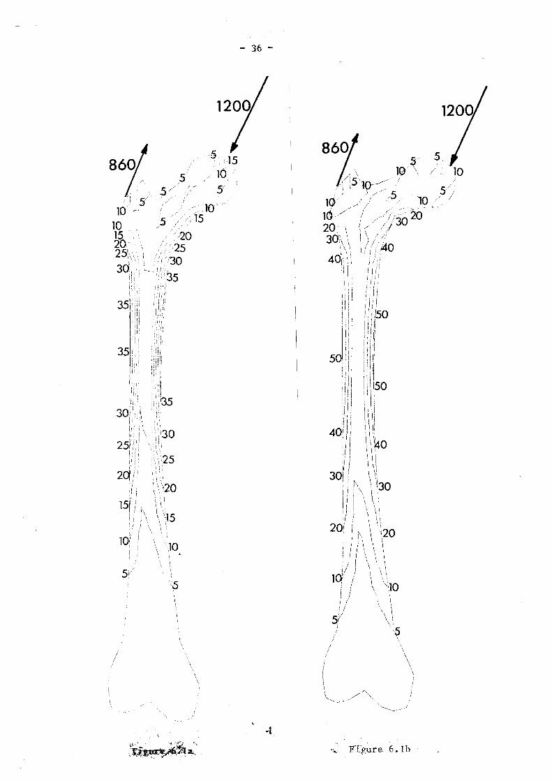
6. Alteration of the geometry

If we want to trace the influence of the size of the inclination angle or

the length of the neck on the loading situation, we will have to replace

only a very small portion of the numrers of the input data needed for the

calculation programmes. As a matter of fact, for an eleT'"'entpattern analo­

gous to fig. 5.3, exclusively the numbers of the coordinates of the nodes

in the neck and in the head of the femur, get a new numerical value. The in­

fluence on the eauivalent stress of this kind of alterat~ons is indicated

for t~.JO examples in figure 6. I. The load chosen is that accordinp- to

RydelL The figure has to re cOT'"'pared with fifo 5.5 for the saT'"'.e loading

case.

The influence of the alteration of the length of the neck on the stress

situation in loading case B is found to be very small. It appears clearly

that the diminution of the inclination angle has unfavourable consequences

for the stress situation in the bone, as fig. 6.1 shows.

Fig.

Fig.

6.la

6.1 b

bone with longer neck

bone with smaller inclination angle

- 36 .....

~'~

/,/,/'" '"

I

86%......... ..5 ; .. 10. 10 \. ! L

/151()_--- 5",'i' )5 '10

lQ' j- /2010/ //3020. \ I>:

0" , /3,\ \ 1/;.40\ \. 'I i !/.4at, i \ iji!

1.,,'\ 'I "I.iii!I 1",

;':, I (ii

1\,.1.. :. :.' .• j'~.'1 111 ; iiii iiiI,ii Ii! a:: II iiriii tll11Iii II! Iil. ,f,f[iii 1111\501i l, 1:[1

I! II .ill1..

11

il\'11\50ill IIII.flr i!i.\'1dI I \ Iiill \ \1

40:./ I. \.1\~OI I 1'1

ill \\\301 Ii' \ bo

1

1

.1

1

1

\" \ !1 \ \ \

I \ \\1./ I \ \\I I \\' I

201 j '~20i j i\ l (

iii \\ \ \' ! I \ \[I \ I,/ I \ \. \. I ' \.!

ldf

I \ \~i]QI / \ I. , \i / \

5(>' '

125

no

5

·"20; iII

\15\I!

5/

10i

2q/

'!15r

251I

P351·

i

35l!ii

I:,i

30r

8601/ .....•...

IS10 j,

10152025;3d

.:~\_~",\-:.;;1"--; .. '

\ti~f"'ta'"", 11·:- \ '\ "

.'" Yfgure 6. lb

- 37 -

7. Conclusion and acknowledgements

This contribution to the strain and stress analysis of a skeleton part is

based on the finite element method. We have tried to indicate that

this method is extremely suitable to analyse complicated constructions

like a femur.

Pe have explained the use of this method, vrhilst also the theoretical back­

grounds have been under discussion. A simple two-dimensional model of a

femur is elaborated. He have described the results of SOIT'e loadinp- cases ln

more than one way. Two types of eleIT'ent have been used and compared with

each other, whilst illustrating the possibilities and restrictions of the

element method.

It must be clear now that the anisotropic and inhomogenuous character of

the bone-material, the complicated geometry and the variety ln loading cases

do not cause in principle any difficulties when analysing with this method.

This article has been written ln cooperation with a biomechanical working

team. The participants in this team are: H.M. Berntsen and O.S. Ingwersen

(Diaconessenziekenhuis, Eindhoven); G. Chapchal, T.J.J.H. Slooff

L.t-t. D. Suda and H. Vister (Katholieke Universiteit, Nijmegen);

W.A.M. Brekelmans, J.D. Janssen, H.W. Poort, P.P.T.G. van Rens, A.J. Sanders,

L.B.M. Tomesen and S.D. Zorge (Technische Hogeschool, Eindhoven).

The purpose of the working-team is to carry out fundamental investip-ations

in the field of biomechanics viewed from various disciplines, as may appear

from the composition of the team.

The authors owe thanks to the participants of this teaIT'. for their useful co­

operation, which was a very great help in composing this article.

- 38 -

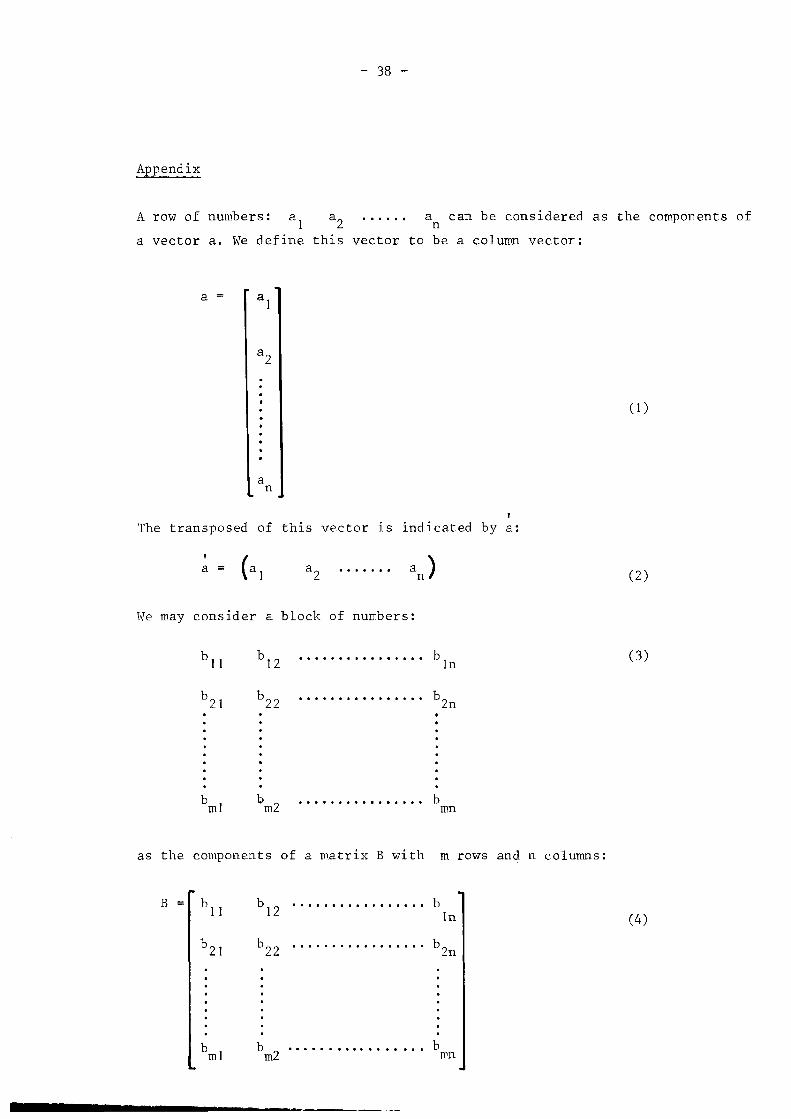
Appendix

A row of numbers: al

a2 .••••• an can be considered as the components of

a vector a. We define this vector to be a column vector:

a =

(I)

an

The transposed of this vector is indicated by a:

We may consider a block of numbers:

b l2 .•.....•...•.•.. bIn

bmn

as the components of a matrix B with m rows and n columns:

B bll

bl2

................. bIn

b21 b22

................. b2n

bmn

(2)

(3)

(4)

- 39 -

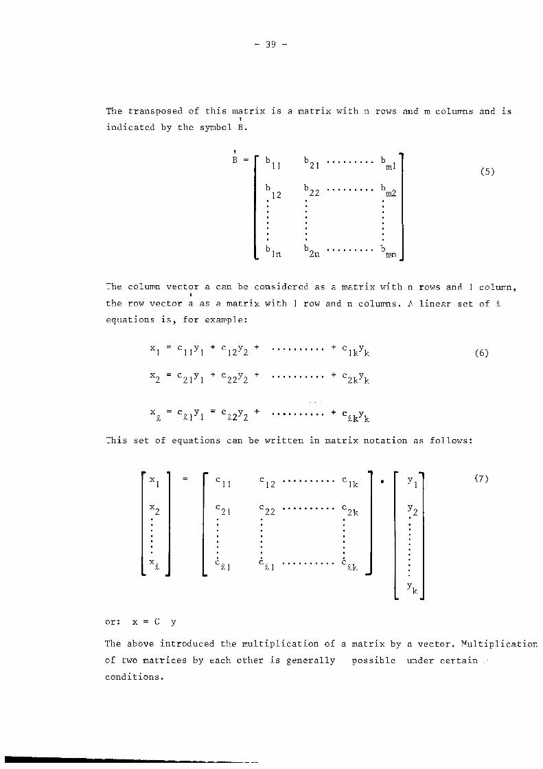
The transposed of this matrix 1S a matrix with n rows and m columns and 1SI

indicated by the symbol B.

B b II b21

......... bml

(5)

b b22 ......... bm212

b2n

. bmn

The column vector a can be considered as a matrix with n rows and I column,I

the row vector a as a matrix with I row and n columns. ~ linear set of 2

equations is, for example:

•••••••••• +(6)

This set of equations can be written in matrix notation as follows:

•

or: x = C Y

(7)

The above introduced the multiplication of a matrix by a vector. Multiplication

of two matrices by each other is generally

conditions.

possible under certain .

- 40 -

When we define:

a.. as the components of A with i1J

It •••••••••• k,

J ••••••••••• £

b .. as the components of B with 11J

••••••••••• m.

J ••••••••••• n

the matrix product AB is then defined under the condition that £ = m

This matrix product is also a matrix, C = AB with components to be calculated

as follows:

£c .. L a. b (9 )

1Jp=1

1p PJ

Matrix C has k rows and n columns. When for C applies that C AB, we can

easily prove that we also have:

,C

, ,B A (l0)

(11 )

An independent linear set of equations x = Cy, where the components of x

are considered to be known and where a solution is asked for y, is only

solvable in case the matrix C has as many rows as columns, in other words

1n case the number of equations is as, large as the number of the un­

knowns.

Then the s04ution can be written as follows:-1

y = C x

Here, C- I is the inverse of the matrix C. There exist all kinds of methods-I

of calculating C when C is known.

•