Master in de bio - ingenieurswetenschappen: Chemie en ... · iii Woord vooraf Deze masterproef kwam...

Faculteit Bio-ingenieurswetenschappen

Academiejaar 2015 – 2016

Heat and mass transfer modelling of auger reactors

Jelle Roegiers Promotor: Prof. dr. ir. Frederik Ronsse & Prof. dr. ir. Jan Pieters Tutor: Xiaogang Shi

Masterproef voorgedragen tot het behalen van de graad van Master in de bio-ingenieurswetenschappen: Chemie en bioprocestechnologie

ii

Copyrights

De auteur en promotoren geven de toelating deze scriptie voor consultatie beschikbaar te

stellen en delen ervan te kopiëren voor persoonlijk gebruik. Elk ander gebruik valt onder de

beperkingen van het auteursrecht, in het bijzonder met betrekking tot de verplichting

uitdrukkelijk de bron te vermelden bij aanhalen van resultaten uit deze scriptie.

The author and promotors give the permission to use this thesis for consultation and to copy

parts of it for personal use. Every other use is subject to copyright laws, more specifically the

source must be extensively specified when using results of this thesis.

Ghent, June 2016

iii

Woord vooraf

Deze masterproef kwam tot stand in het kader van het 2de masterjaar Bio-ingenieurswetenschappen:

Chemie en bioprocestechnologie en vormt het sluitstuk van mijn opleiding. Langs deze weg zou ik dan

ook graag een dankwoord richten tot alle personen die tot het goed einde van deze masterproef

hebben bijgedragen.

In de eerste plaats zou ik graag mijn promotoren Prof dr. Ir. Ronsse en Prof. dr. Ir. Pieters bedanken

voor de begeleiding en ondersteuning bij het opstellen van deze masterthesis. Wat ik bijzonder

apprecieerde was het feit dat ik altijd direct terecht kon met vragen of problemen.

Mijn dankwoord gaat ook uit naar mijn tutor Xiaogang Shi, die mij in het begin op het juiste pad heeft

geholpen en mij gedurende het hele traject heeft bijgestuurd waar nodig.

Tenslotte gaat mijn dank uit naar mijn ouders, die mij zowel financieel als moreel hebben gesteund

tijdens mijn opleiding. Ze hebben mij altijd aangemoedigd en in mij geloofd zodat ik deze opleiding tot

een goed einde kon brengen.

iv

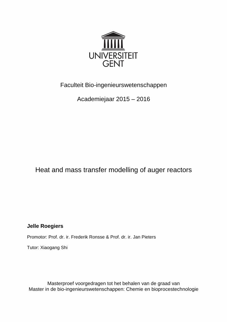
Abstract

Auger (or screw) reactors are tubular, continuous reactors in which solid reactants are transported by

means of a rotating screw and heat is transported along the tubular wall of the reactor. The screw

thereby fulfills two purposes: first, it mixes the solid material and second, it controls the residence time

of the solids in the reactor. Screw or auger reactors have been successfully applied in the gasification

and/or pyrolysis of coal and are currently being investigated for their use in biomass pyrolysis,

torrefaction and gasification.

One of the key questions regarding successful use of these type of reactors in commercial applications

of biomass conversion is whether they can be scaled up. Or put in other words, do they retain their

excellent heat and mass transfer properties in larger (commercial) scale with higher throughput? With

the use of Computional Fluid Dynamics (CFD), featuring an Euler-Euler model to simulate the granular

flow, the reaction kinetics, the heat transfer and mass transfer properties have been studied on a

bench scale reactor. By replicating the operating conditions and material properties, used in the

experimental setup, a comparison of the simulated data with the experimental data was made, which

showed that the present model was accurate in predicting hydrodynamics, particle residence time,

temperature distributions and product yields in this screw reactor..

Plots of the volume fraction and velocity profile indicated that the Euler-Euler model was capable to

represent a granular flow in a two phase system. This was also shown in results of residence time

distributions of the solid phase. Heat transfer properties were optimized to achieve good agreement

with the temperature profile of the experimental setup. Simulated results of the product yield implied

that a complex reaction scheme is required, since the solid product yield was underestimated by

roughly 15% in the present model. Finally, a sensitivity analysis illustrated that the biomass

temperature is sensitive towards the biomass moisture content, the rotating frequency and packing

limit.

The present modelling work is valuable in guiding the in-depth understanding of the thermochemical

performance of the screw reactor in processing biomass particles.

v

Samenvatting Schroefreactoren zijn tubulaire, continue reactoren waarin vast materiaal wordt getransporteerd door

rotatie van de schroef, waarbij warmtetransfer plaatsvindt doorheen de tubulaire wand van de reactor.

De schroef biedt twee voordelen: mixing van het vaste materiaal en controle van de verblijftijd in de

reactor. Door hun succesvolle toepassingen in vergassing en/of pyrolyse van steenkool, wordt

momenteel onderzoek verricht om schroefreactoren in te zetten voor pyrolyse, torrefactie en

vergassing van biomassa.

Voor toepassingen op commerciële schaal, moet onderzocht worden of schroefreactoren kunnen

worden opgeschaald en hierbij hun massa- en warmtetransfer eigenschappen behouden. Om deze

eigenschappen te onderzoeken, werd in deze thesis gebruik gemaakt van Computional Fluid Dynamics

(CFD), waarbij een Euler-Euler model geïncorporeerd werd om de granulaire flow in een schroefreactor

te beschrijven. Door het nabootsen van operationele condities en materiaaleigenschappen tijdens

experimenten met een laboschaal schroefreactor, konden de gesimuleerde resultaten vergeleken

worden met de experimentele resultaten.

Plots van de volume fractie en snelheidsprofiel gaven aan dat het Euler-Euler model in staat was om

de granulaire flow in een tweefasensysteem te simuleren. Een bijkomende bevestiging hiervan werd

gegeven door het vergelijken van verblijftijd distributies. De thermische eigenschappen van het

materiaal werden geoptimaliseerd zodat een goede, kwalitatieve overeenkomst werd bekomen met

het temperatuursprofiel van de experimentele data. De resultaten van productopbrengst wezen erop

dat in de toekomst een meer complex reactieschema zal moeten gebruikt worden, want het huidige

reactie schema overschatte de opbrengst van de gasfractie met 15%, ten koste van de opbrengst van

het vaste materiaal. Ten slotte werd een gevoeligheidsanalyse uitgevoerd, waarbij aangetoond werd

dat de biomassa temperatuur sterk gevoelig is voor veranderingen in het vochtgehalte van de

biomassa, de frequentie van de schroef en de packingslimiet van het materiaal.

Het model is een waardevolle tool om de thermochemische prestaties van een schroefreactor in detail

te kunnen bekijken en begrijpen.

vi

Table of Contents

1 Introduction ..................................................................................................................................... 3 2 Literature review ............................................................................................................................. 5

2.1 Biomass conversion processes ................................................................................................ 5 2.1.1 Biochemical ......................................................................................................................... 5 2.1.2 Thermochemical .................................................................................................................. 5

2.1.2.1 Combustion ................................................................................................................. 6 2.1.2.2 Gasification .................................................................................................................. 6 2.1.2.3 Pyrolysis ....................................................................................................................... 7

2.2 History of the auger reactor .................................................................................................. 12 2.3 Configuration of a screw reactor for pyrolysis ...................................................................... 13

2.3.1 Feed drum ......................................................................................................................... 13 2.3.2 Feed screw ......................................................................................................................... 15 2.3.3 Screw conveyor ................................................................................................................. 15 2.3.4 Condenser/afterburner ..................................................................................................... 16 2.3.5 Cooling ............................................................................................................................... 16 2.3.6 Effects of operating conditions ......................................................................................... 16

2.4 Numerical modelling of pyrolysis .......................................................................................... 19 2.4.1 Kinetic model ..................................................................................................................... 19

2.4.1.1 One-component mechanisms ................................................................................... 19 2.4.1.2 Multi-component mechanisms ................................................................................. 21

2.4.2 Hydrodynamic models ....................................................................................................... 21 3 Materials and methods ................................................................................................................. 25

3.1 Overall approach ................................................................................................................... 25 3.2 Screw rotation ....................................................................................................................... 26

3.2.1 Rotating reference frame .................................................................................................. 26 3.2.1.1 Fictitious forces ......................................................................................................... 26 3.2.1.2 Gravitational force ..................................................................................................... 27

3.2.2 Mesh motion ..................................................................................................................... 28 3.3 Kinetic theory of granular flow .............................................................................................. 29

3.3.1 Bulk viscosity ..................................................................................................................... 29 3.3.1.1 Volume fraction ......................................................................................................... 29 3.3.1.2 Particle diameter ....................................................................................................... 30 3.3.1.3 Radial distribution function ....................................................................................... 30 3.3.1.4 Coefficient of restitution ........................................................................................... 30 3.3.1.5 Granular temperature ............................................................................................... 30

3.3.2 Solid shear viscosity ........................................................................................................... 31 3.4 Numerical set-up ................................................................................................................... 31

3.4.1 Geometry ........................................................................................................................... 31 3.4.2 Mesh .................................................................................................................................. 33 3.4.3 Governing equations ......................................................................................................... 34

3.4.3.1 Conservation of mass ................................................................................................ 34 3.4.3.2 Conservation of momentum ..................................................................................... 34 3.4.3.3 Heat transfer ............................................................................................................. 36 3.4.3.4 Component transport equations ............................................................................... 38

3.4.4 Reaction kinetics ................................................................................................................ 38 3.4.5 Boundary conditions.......................................................................................................... 40 3.4.6 Phase properties ................................................................................................................ 40

vii

3.4.7 Solution methods .............................................................................................................. 41 3.5 Simulation procedures .......................................................................................................... 41

3.5.1 Granular flow pattern ........................................................................................................ 41 3.5.2 Residence time .................................................................................................................. 42 3.5.3 Temperature ...................................................................................................................... 42 3.5.4 Product yield ...................................................................................................................... 42 3.5.5 Sensitivity analysis ............................................................................................................. 43 3.5.6 Parameterisation ............................................................................................................... 43

4 Results and discussion ................................................................................................................... 47 4.1 Model Implementation in Ansys fluent ................................................................................. 47 4.2 Granular Flow Pattern ........................................................................................................... 47 4.3 Residence Time Distributions ................................................................................................ 50 4.4 Temperature .......................................................................................................................... 52 4.5 Product yield.......................................................................................................................... 54 4.6 Energy balance ...................................................................................................................... 56 4.7 Sensitivity analysis ................................................................................................................. 57 4.8 Future research ..................................................................................................................... 58

5 Conclusion ..................................................................................................................................... 59 6 References ..................................................................................................................................... 61 7 Addendum ..................................................................................................................................... 67

1

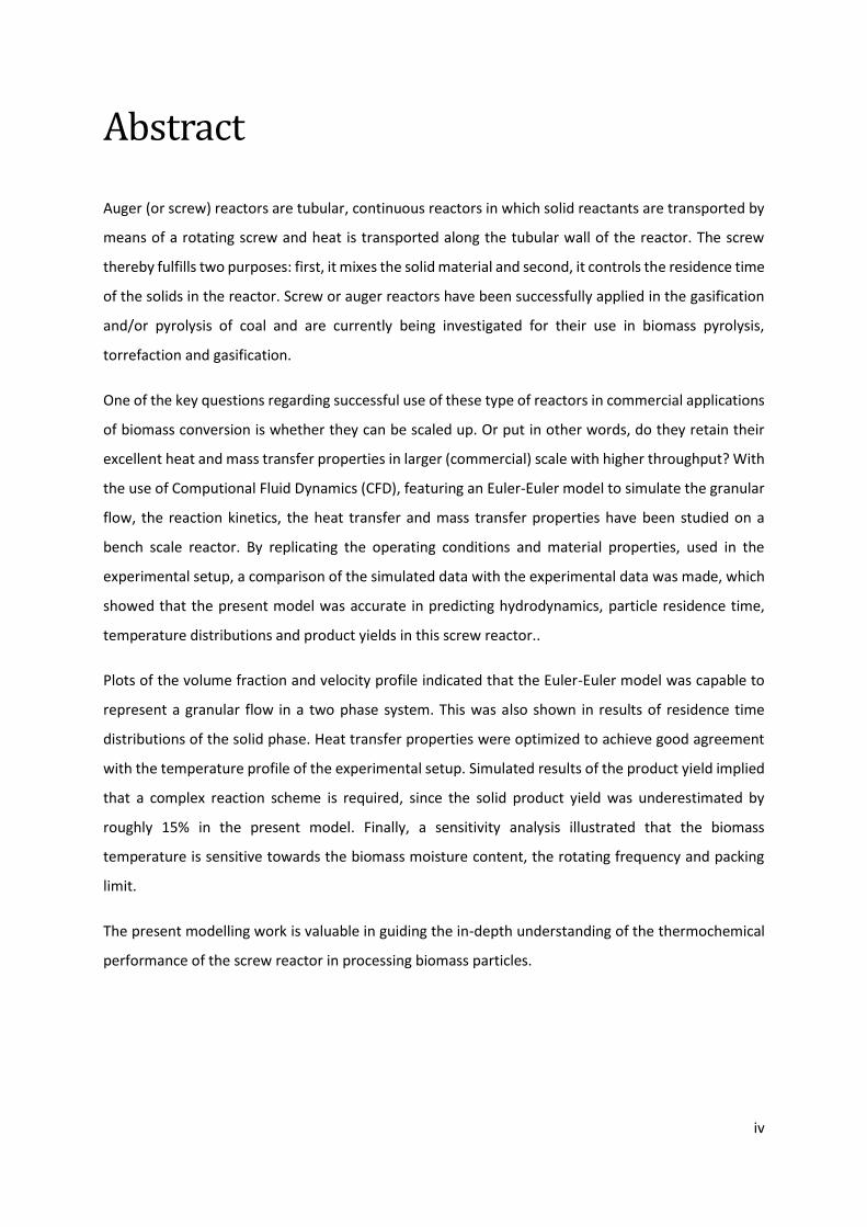
List of abbreviations

Description Unit

Abbreviations CAD Computer Aided Design CFD Computional Fluid Dynamics DEM Discrete Element Method ODE Ordinary Differential Equations PDE Partial Differential Equations RRF Rotating Reference Frame RTD Residence Time Distribution Greek letters 𝛼 Volume fraction (-) 𝛼𝑚𝑎𝑥 Packing limit (-) 𝛽 Interphase drag coefficient 𝑘𝑔/𝑚3/𝑠 𝜃 Granular temperature 𝑚²/𝑠² 𝜆 Thermal conductivity 𝑊/𝑚/𝐾 𝜇 Viscosity 𝑃𝑎 ∙ 𝑠 𝜌 Density 𝑘𝑔/𝑚³ �̿� Stress Tensor 𝑁/𝑚² 𝜔 Angular velocity 𝑟𝑎𝑑/𝑠 Symbols 𝑎 Acceleration 𝑚/𝑠² A Pre-exponential factor 1/𝑠 𝐶𝐷 Drag coefficient (-) 𝑐𝑝 Specific heat capacity 𝐽/𝑘𝑔/𝐾

𝑑𝑃 Particle diameter 𝑚 𝐸𝐴 Activiation energy 𝐽/𝑚𝑜𝑙 𝑒𝑠𝑠 Coefficient of restitution (-) F External body force 𝑁/𝑚³ g Gravitational acceleration 𝑚/𝑠² 𝑔0 Radial distribution function (-) h Heat transfer coefficient 𝑊/𝑚²/𝐾 𝐻 Specific enthalpy 𝐽/𝑘𝑔 J Diffusion flux 𝑘𝑔/𝑚/𝑠 k Reaction rate constant 1/𝑠 �̇� Specific mass transfer rate 𝑘𝑔/𝑚³/𝑠 Nu Nusselt number (-) p Pressure 𝑃𝑎 Pr Prandtl number (-) q Conductive heat flux 𝑊/𝑚²

2

𝑄 Heat exchange rate 𝐽/𝑚³/𝑠 r⃗ Radial position vector in rotating frame (-) 𝑅 Interaction coefficient between phases 𝑁/𝑚³ Re Reynolds number (-) 𝑆 Source term 𝑘𝑔/𝑚³/𝑠 T Temperature 𝐾 𝑣 Velocity 𝑚/𝑠 V Volume m³ Y Phase component (-)

3

1 Introduction

Today, fossil fuels are still the dominant energy source for the industrialized world. About 80% of all

primary energy is derived from fossil fuels: oil (33%), coal (27%) and natural gas (20%) (Shafiee and

Topal 2009, Hook and Tang 2013). Meeting the current energy consumption rates, the reserves for

coal are estimated to be depleted in 100-150 years. Gas and oil reserves are even more limited and

will be exhausted within approximately 30-40 years (Shafiee and Topal 2009). Furthermore, large

amounts of greenhouse gases, in particular CO2, are emitted from fossil fuel consumption causing the

climate to change tremendously. These fossil fuel concerns have caused a shift to renewable energy

sources. Solar, wind, hydro and geothermal energy can generate power and heat and contribute all

together for roughly 4% of the total primary energy (Hook and Tang 2013). However these technologies

don’t qualify if energy is required as a fuel for transportation or for the production of chemicals.

Conversion technologies for biomass and waste into useful energy (e.g. in the form of fuels) have been

widely studied in the last decade. It is estimated that the bioenergy captured by land plants each year

is roughly 3-4 times larger than the global energy demand (Guo 2015). A wide range of technologies

has already been investigated and deployed for the conversion of biomass into useful energy. The

benefit of using biomass as an energy source lies in the ability to take up the emitted CO2 from energy

consumption, through photosynthesis and in this way closing the carbon cycle.

Different biomass conversion processes will be discussed in Chapter 2, in particular thermochemical

conversion using pyrolysis. The development of biomass conversion technologies is often accompanied

by numerical efforts to model a specific process as a time-efficient and cost-reducing method. In this

master thesis, a relatively new concept for thermochemical biomass conversion, the auger reactor, is

studied in CFD software with the use of an Euler-Euler model to study the granular flow, heat transfer

and product yield. Chapter 2 includes a description of a typical auger reactor configuration for pyrolysis.

Furthermore , different kinetic-and hydrodynamic models are reviewed. In Chapter 3, the numerical

implementation and governing equations are discussed for the implementation of the Euler-Euler

model in CFD software. The results of the simulation are summarized and discussed in Chapter 4.

5

2 Literature review

2.1 Biomass conversion processes

A number of different processes can be used to convert biomass into useful forms of energy. The

choice of the deployed process is influenced by several factors: the type and availability of the

feedstock, environmental standards, economic factors and most importantly, the desired form of

energy. A brief overview of biomass conversion processes is presented. The conversion processes are

mainly divided into two dominant platforms: biochemical conversion and thermochemical conversion

(McKendry 2002a, McKendry 2002b).

2.1.1 Biochemical

Biochemical conversion is based on the use of microorganisms or enzymes combined with chemical

agents to convert biomass into gaseous or liquid products with a high energy content. Two main

processes can be distinguished: fermentation and anaerobic digestion. Fermentation is used on a large

scale to produce ethanol from sugar- and starch crops, and recently from lignocellulosic biomass.

Anaerobic digestion is the conversion of organic material into biogas, which is a mainly a mixture of

methane and carbon dioxide. This process is not the scope of this work, so no further details are given

here. McKendry expands further on this topic (McKendry 2002b).

2.1.2 Thermochemical

Thermochemical conversion involves the use of heat to decompose biomass and can be divided among

three major categories: combustion, pyrolysis and gasification. These processes and their final energy

products are illustrated in the flowchart shown in Fig. 1. Other thermochemical conversion processes

are hydrothermal upgrading (HTU) and liquefaction and are especially suitable for wet biomass

(McKendry 2002b).

6

Fig. 1 Main processes for thermochemical conversion of dry biomass (Bridgwater 2012)

2.1.2.1 Combustion

Burning the biomass in contact with air is the most straightforward method to convert the biochemical

energy stored in biomass into heat and indirectly into mechanical power and electricity. It is an efficient

process in that way, that it only requires a limited amount of preprocessing (e.g. drying). Combustion

of biomass produces hot gases at temperatures around 1100-1300 K using equipment such as stoves

or furnaces. However, biomass combustion is only feasible with a moisture content below 50%, so pre-

drying is often required. Moreover, preprocessing is usually desired to increase the bulk density of the

biomass for transport purposes. Because combustion is not able to provide a fuel, it is usually not the

most desired option in the industry (McKendry 2002b, Bridgwater 2003).

2.1.2.2 Gasification

Gasification is a complex process that converts biomass into a combustible gas mixture by partial

oxidation at high temperatures (1100-1200 K). Gasification can be conducted by various gasification

agents such as air, steam or oxygen. The product gases mainly consist of CO, H2, CH4 an CO2, often

referred to as “producer gas”. Syngas is the upgraded producer gas to a mixture of H2 and CO. Syngas

allows the production of methanol and hydrogen, which can be used as a potential fuel for

transportation. Other applications involve the synthesis of ethanol (mixed-alcohol synthesis) and the

synthesis of dimethyl ether (DME). The Fischer-Tropsch process can produce synthetic liquid fuels

(McKendry 2002b, Bridgwater 2003).

7

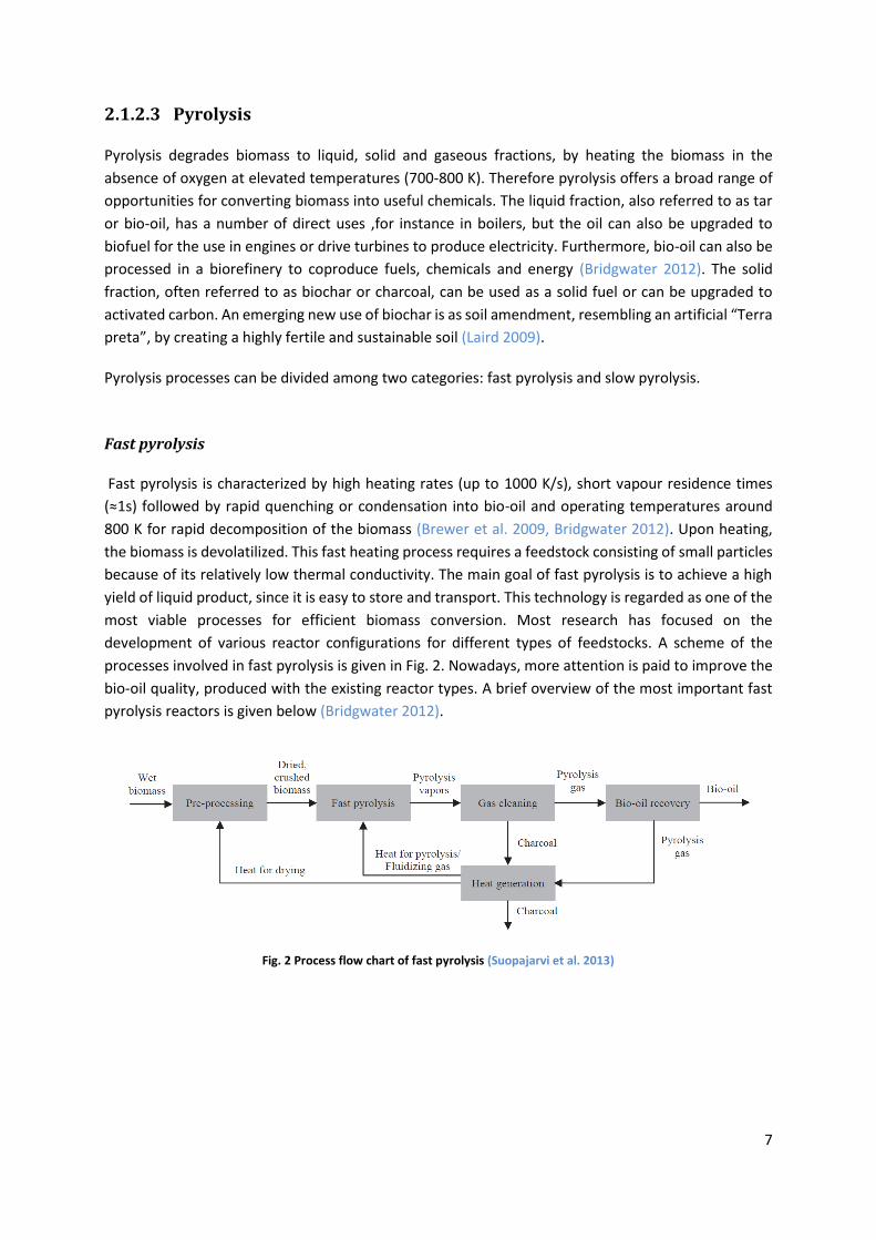
2.1.2.3 Pyrolysis

Pyrolysis degrades biomass to liquid, solid and gaseous fractions, by heating the biomass in the

absence of oxygen at elevated temperatures (700-800 K). Therefore pyrolysis offers a broad range of

opportunities for converting biomass into useful chemicals. The liquid fraction, also referred to as tar

or bio-oil, has a number of direct uses ,for instance in boilers, but the oil can also be upgraded to

biofuel for the use in engines or drive turbines to produce electricity. Furthermore, bio-oil can also be

processed in a biorefinery to coproduce fuels, chemicals and energy (Bridgwater 2012). The solid

fraction, often referred to as biochar or charcoal, can be used as a solid fuel or can be upgraded to

activated carbon. An emerging new use of biochar is as soil amendment, resembling an artificial “Terra

preta”, by creating a highly fertile and sustainable soil (Laird 2009).

Pyrolysis processes can be divided among two categories: fast pyrolysis and slow pyrolysis.

Fast pyrolysis

Fast pyrolysis is characterized by high heating rates (up to 1000 K/s), short vapour residence times

(≈1s) followed by rapid quenching or condensation into bio-oil and operating temperatures around

800 K for rapid decomposition of the biomass (Brewer et al. 2009, Bridgwater 2012). Upon heating,

the biomass is devolatilized. This fast heating process requires a feedstock consisting of small particles

because of its relatively low thermal conductivity. The main goal of fast pyrolysis is to achieve a high

yield of liquid product, since it is easy to store and transport. This technology is regarded as one of the

most viable processes for efficient biomass conversion. Most research has focused on the

development of various reactor configurations for different types of feedstocks. A scheme of the

processes involved in fast pyrolysis is given in Fig. 2. Nowadays, more attention is paid to improve the

bio-oil quality, produced with the existing reactor types. A brief overview of the most important fast

pyrolysis reactors is given below (Bridgwater 2012).

Fig. 2 Process flow chart of fast pyrolysis (Suopajarvi et al. 2013)

8

Bubbling fluidized bed

In bubbling fluidized beds (Fig. 3), pyrolysis is carried out in a fluidized bed of hot sand at low fluidizing

gas velocities, while biomass is constantly injected. It is a well understood technology that is simple in

construction and operation. Good temperature control is possible and efficient heat transfer is

achieved, dependent on the particle size and reactor scale. Reaction products are sent through

cyclones for separation of char, which can be combusted to provide the heat for pyrolysis or it can be

separated and exported. The vapours are cooled and separated as bio-oil. Fluidized bed reactors give

good performance with liquid yields up to 75 wt%, making them one of the most promising reactors

for biomass pyrolysis (Bridgwater 2003, Butler 2011, Bridgwater 2012). Dynamotive has built a

commercial plant, which operates 4 fluidized bed reactors with a total capacity of 8 tons/h. Agritherm

and Biomass Engineering Ltd also make use of this technology and can both process 200 kg biomass/h .

Fig. 3 Bubbling fluidized bed reactor (Bridgwater 2003)

Circulating fluidized bed

Circulating fluidized bed reactors (Fig. 4) are very similar to the bubbling fluidized bed reactors, except

that the residence time of the char is almost the same as for the gas. This reactor is operated at higher

gas velocities. Consequently, char and sand are carried out at the top. After separation of the vapours

(using a cyclone), the char is combusted in the presence of the sand to heat up the latter. Bio-oil is

obtained in a similar way as the bubbling fluidized bed. This process makes it possible to achieve high

throughput, but it is a more complex process due to complicated hydrodynamics (Bridgwater 2003,

Butler 2011, Bridgwater 2012). Ensyn has a commercial plant in Canada that produces bio-oil based on

forest residues with a capacity of 2,5 ton/h. The same company has recently built a plant in Brazil with

a capacity of 16,7 ton/h, with Eucalyptus as feedstock.

9

Fig. 4 Circulating fluidized bed reactor (Bridgwater 2003)

Rotating Cone

The rotating cone reactor (Fig. 5) is a relatively recent development, invented at the University of

Twente. The biomass introduced near the bottom of the rotating cone, is carried up the wall of the

rotating cone in a spiral motion due to the centrifugal force. Flash heating of the biomass can be

achieved by means of high heat transfer by the wall and heated sand. The advantage of this type of

reactor, is that no carrier gas is needed to transport the vapours and thereby reducing the operating

cost (Wagenaar 1994, Bridgwater 2003, Butler 2011, Bridgwater 2012).

Fig. 5 Rotating Cone Reactor (Bridgwater 2003)

10

Ablative pyrolyzer

The ablative reactor approaches flash pyrolysis with a totally different concept compared to the other

reactor configurations. The process is often compared to melting butter in a frying pan. Biomass is

pressed against a heated surface and is subsequently moved away mechanically, leaving a ‘molten

layer’. This layer can vaporize into a product similar to the products derived from other fast pyrolysis

reactors. The advantage of this configuration is that larger biomass particles can be used and no carrier

gas is required. A very compact reactor can be constructed (Peacocke and Bridgwater 1994, Butler

2011, Bridgwater 2012).

Other reactors

Many other reactor configurations exist for fast pyrolysis, such as microwave pyrolyzer, vacuum

pyrolyzer, fixed bed pyrolyzer and so on. Other types of reactors are usually less studied or are still in

early stages of development.

Slow pyrolysis

Slow pyrolysis is characterized by lower heating rates (10-30 K/min), longer solid residence times (5

min-12 h) and lower operating temperatures (≈700 K) compared to fast pyrolysis (Kambo and Dutta

2015). Generally, the reactor configurations are able to handle a larger solid particle size as well. The

operating conditions of slow pyrolysis cause a shift to a higher solid yield. In contrast to fast pyrolysis,

a liquid biofuel is not necessarily the desired end product, but rather charcoal. The gas produced during

slow pyrolysis is usually considered a by-product and can be used to provide the heat for the pyrolysis

process (Fig. 6) (Williams and Besler 1996, Suopajarvi et al. 2013). Only a limited amount of reactors,

applying slow pyrolysis, are reported in the literature, such as rotating drums, batch or continuous

retorts and screw conveyors. Most of these reactor types are only deployed as small scale installations

and just a few are active on commercial scale.

Fig. 6 Process flow chart of slow pyrolysis (Suopajarvi et al. 2013)

11

Auger reactor

Auger reactors, also known as screw reactors, were only recently investigated for their use in pyrolysis

processes (Fig. 7). Auger reactors can be used for both fast and slow pyrolysis. Despite the simple

design and operation, the mechanical mixing and granular flow are very complex and difficult to

examine and control. In this type of reactor, biomass is fed to a cylindrical tube and conveyed through

the heated reactor by rotation of a screw. The biomass is heated by maintaining a high temperature

at the cylindrical wall or in the case of fast pyrolysis, combined with heated sand. This principle of

heating and conveying of the biomass allows a continuous process. Rotation of the screw also ensures

efficient mixing of the biomass to enhance heat transfer among solids and the reactor wall. Another

advantage of the screw reactor is that it can be built very compact and in some cases even portable,

so the reactor might be used on the site where the biomass is abundantly available. In this way, the

bio-oil can be generated on-site and transported much more efficiently to a nearby biorefinery (Ingram

et al. 2008).

Fig. 7 Auger reactor (Brown 2009)

Torrefaction

Torrefaction is considered a mild form of slow pyrolysis, operating at temperatures of 500-600 K,

heating rates of 10-15 K/min and solid residence times between 30 min - 4 h (Kambo and Dutta 2015).

These less severe conditions have an influence on the product composition (higher H:C ratio and O:C

ratio) and usually result in a higher mass and energy yield of the solid product compared to slow

pyrolysis. Torrefaction is mainly applied for its logistic advantages towards transport, storage and

handling. The biomass has a higher hydrophobicity after torrefaction, making it less susceptible for

biological degradation and has a higher heating value (Nachenius 2015).

12

2.2 History of the auger reactor

The history of the screw reactor goes back as far as the beginning of the 20th century to mechanically

convey and process coal. Since then, the auger reactor has been studied and optimized for its current

use in applications such as drying, feeding, pyrolysis, extrusion…

The first report of the use of an auger reactor was described by Laucks 1927. Laucks investigated a

slow pyrolysis screw reactor for coal processing to produce a coke-like product, which was described

as a “smokeless fuel”. In theory the reactor was simply a heated tube with a screw inside. In practice,

a lot of problems were noted during operation of the system. These problems were attributed to the

high wall temperature compared to the low temperature of the screw shaft, causing the tar to deposit

on the cold shaft. Laucks suggested to transfer the heat using a hollow shaft to allow upscaling. In

1941, Woody investigated the commercial viability of slow pyrolysis of coal in a screw reactor, similar

to Laucks’ work (Woody 1941).

In the 1950’s, the Lurgi Company developed the Lurgi-Ruhrgas process for retorting finely crushed oil

shale to produce fuel with the use of an auger reactor. In contrast to earlier attempts, a better heat

transfer was achieved with the use of sand as a heat carrier. A commercial plant was built in

Dormhagen, Germany in 1958 based on this Lurgi-Ruhrgas process to produce ethylene using a

naphtha feed (Brown 2009). At the end of the 20th century, coal pyrolysis was deemed an inexpensive

alternative to post-combustion cleaning methods such as sulphur removal. A dual screw coal feeder

reactor was employed to pre-emptively desulfurize the coal via mild pyrolysis in a first step and

separating H2S using a calcium-based sorbent (Lin et al. 1997). Camp 1990 further discussed the use of

a twin screw by comparing the performance with a single screw reactor.

Increased awareness of fossil fuel depletion, has caused a shift to use renewable resources as a

feedstock for the auger reactor. The first known reference to the auger reactor for biomass pyrolysis

dates from 1969. The screw reactor was opted because of its continuous handling. No heat carrier was

used during the pyrolysis process, but heat transfer only occurred by the heated shell. The authors

state that this system would be problematic at a large scale (Lakshman et al. 1969). Brown 2009

reviewed the further development of different processes and wide range of renewable resources for

pyrolysis in an auger reactor.

Today, implementation of the auger reactor is widely studied at bench scale, but commercial

installations are already in use. The first commercial effort can be dated to beginning of the 21st century.

Renewable Oil International (ROI) developed an auger reactor for the use on a poultry farm to convert

animal waste to bio-oil, which could process 5 ton per day. In 2008, the KIT (Karlsruhe institute of

technology) Bioliq model comprises decentralized densification of biomass by pyrolysis, followed by

centralized gasification and Fischer-Tropsch synthesis. This process is based on the Lurgi-Ruhrgas

process, discussed before. During the process, a bioslurry (biochar and bio-oil) is produced in a twin

screw mixer reactor.

13

A pilot plant has been constructed in Germany with a capacity of 12 ton per day (Brown 2009). ARBI-

Tech, a joint-venture between Advance BioRefinery Inc. and Forespect Inc. developed an auger system

using a high density heat carrier. The units have a capacity of 1 ton per day, but a 50 ton per day unit

is already installed in Canada and currently tested for commercial use, so it will be operational soon.

Multiple other companies produce biochar for commercial purposes such as Sonnenerde in Austria,

Swiss Biochar and Verora in Switzerland. The auger reactors for all these companies were developed

by the German company Pyreg (Ronsse 2013).

2.3 Configuration of a screw reactor for pyrolysis

A general scheme of a screw reactor used for slow pyrolysis is described and shown in Fig. 8 (Ronsse

2013). The different parts of an experimental setup are briefly discussed, but this master thesis mainly

focuses on the screw conveyor.

Fig. 8 Experimental set-up of a screw reactor for biomass pyrolysis (Ronsse 2013)

2.3.1 Feed drum

The feed drum is a temporary storage for the feedstock before it is fed to the reactor and is used in

most reactor configurations for pyrolysis. Although the use of a feed drum seems straight forward, a

lot of problems start here. Feeding problems such as bridging, rathole formation and blockage can

occur due to an improper setup of the feed drum. Cohesion between particles plays a major role in

these problems. Cohesion depends on material properties such as size, shape and moisture content.

Different states of solid flow can be observed, depending on the cohesive force between the particles.

Particles can flow continuously from the bin to the screw if there is no significant interparticle cohesion

and so flow is easily driven by gravity and drag of the rotation screw. As the cohesive force increases,

14

a more stable network of particles is formed. The combined effect of the cohesive forces and the

perturbation of the screw rotation makes the mass flow less smooth and can even occur periodically.

When the cohesive force reaches a threshold value, the mass flow rate decreases drastically until it is

completely stopped. In this case a stable arch is formed, where particles encounter difficulties to flow

into the void and are therefore interrupting the mass flow to the screw (Hou et al. 2014).

The screw length within the feed drum is an important parameter related to the mass flow towards

the screw. With the increase of pitch number in the feed drum, the circulation zone of particles in the

drum increases, which means that there are more particles in motion (Fig. 9). This has two

consequences, first of all, the motion of particles inhibits the formation of stable arches and therefore

benefits the mass flow. Secondly, the motion of these particles requires energy. The larger the

circulation zones become, the more energy input is required to maintain this motion. Since the mass

flow rate reaches a steady state from a certain pitch number and the energy consumption keeps

increasing with pitch number, a suitable length can be selected to balance mass flow rate and energy

consumption (Hou et al. 2014).

Fig. 9 Velocity fields of mass flow for different pitch numbers P in a feed bin (blue= velocity field in hopper, green = velocity field in feed screw) (Hou et al. 2014)

15

The type of feed drum can also have an effect on the feeding characteristics. There are two types of

popular container designs: the bin and the hopper. The mass flow in a hopper is more likely to form a

stable arch and cause bridging compared to a bin. This is due to the fact that the sloped walls of the

hopper support a stable arch combined with large cohesive forces of the biomass. Furthermore, near

the outlet, particles have to flow, ‘squeezed’ so to say, through a small opening leading to the

formation of particle clusters which are again more likely to give aid to bridging. A bin or hopper can

be mechanically vibrated or agitated to improve mass flow.

2.3.2 Feed screw

At first, a smaller screw, called the feed screw, is used to introduce material in the screw reactor. This

is often applied in other reactors as well, e.g. fluidized bed reactors. Material from the feed drum

enters the feed screw and the mass flow is determined by the rotational frequency of the screw feeder.

In this way, the feed screw determines the mass flow through the screw conveyor. However, if the

frequency of the feed screw is too large compared to the screw reactor, the reactor will be overloaded

and consequently block. This must be avoided at any time, since it results in long reactor downtime in

order to remove this blockage. Additionally, the biomass feed can be preheated in the feed screw if

necessary. In case the biomass is not dried in advance, the water content of the feed can be removed

in this segment.

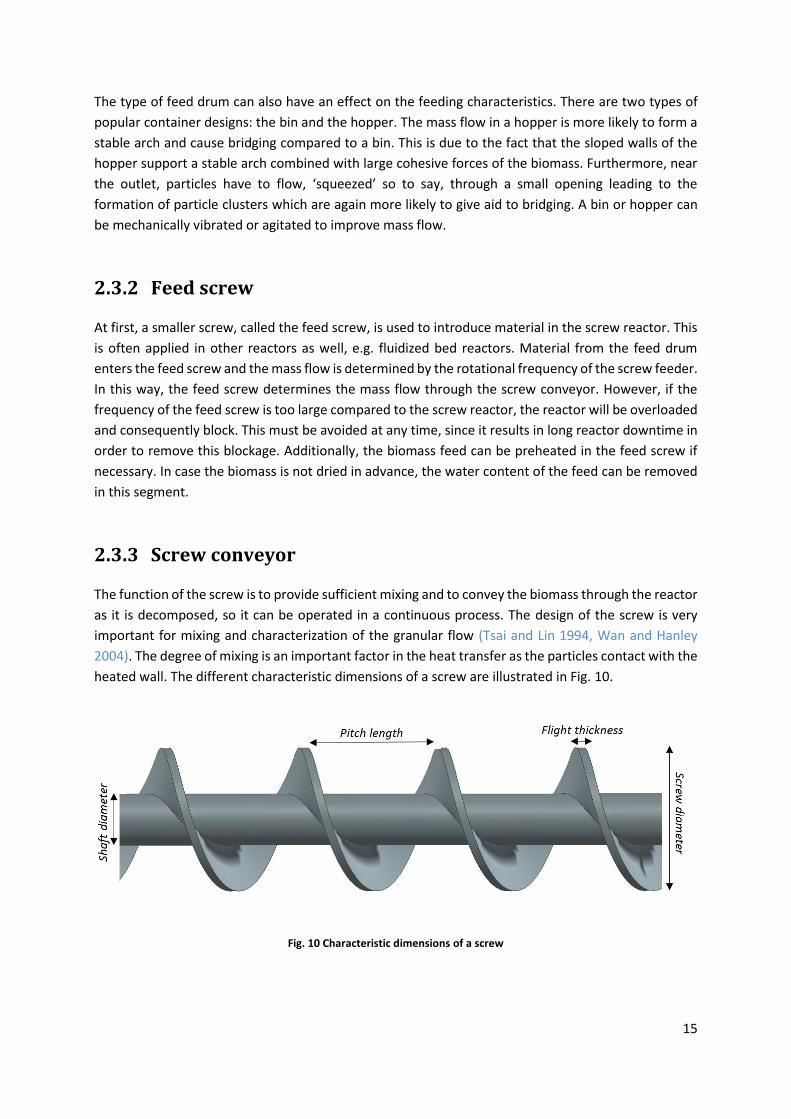
2.3.3 Screw conveyor

The function of the screw is to provide sufficient mixing and to convey the biomass through the reactor

as it is decomposed, so it can be operated in a continuous process. The design of the screw is very

important for mixing and characterization of the granular flow (Tsai and Lin 1994, Wan and Hanley

2004). The degree of mixing is an important factor in the heat transfer as the particles contact with the

heated wall. The different characteristic dimensions of a screw are illustrated in Fig. 10.

Fig. 10 Characteristic dimensions of a screw

16

One dimension not illustrated in Fig. 10, is the clearance. This is the radial distance between the flight

of the screw and the shell. Twin screws are also frequently used, because of their improved mixing and

reduced power consumption (Kingston and Heindel 2014). Kingston discusses the granular mixing in

double screw mixers.

To ensure that the reactor remains oxygen free, nitrogen is introduced at the inlet. Additionally,

product gases are swept from the reactor, so just a minimum amount of carrier gas is used compared

to fluidized bed reactors.

Heating occurs usually by keeping the shell at a constant temperature. In order to reach high biomass

temperatures near the shaft of the screw, good mixing is required. Several options can improve the

heating rate. For example, the screw itself can be a heating medium. In practice, preheated sand is

usually added to achieve higher heating rates, since it is mixed together with the biomass as it is

conveyed. But also steel or ceramic balls can be used as heat carrier (Bridgwater 2012).

2.3.4 Condenser/afterburner

Gases and vapours are swept by the inert gas and leave the reactor. The gases and vapours first pass

through a cyclone to separate the solid particles, which were dragged along. If bio-oil is a desired

product, the gases are sent to a condenser where bio-oil condenses and permanent gases leave the

condenser at the top. The permanent gases still have a relatively high calorific value and can be

combusted to (partially) provide the heat for pyrolysis. Usually, an additional external fuel source is

needed to generate enough heat. If only biochar is desired, the hot gases and vapours do not pass a

condenser, but are immediately combusted in the afterburner to provide enough heat for pyrolysis.

2.3.5 Cooling

Finally, the biochar requires cooling to prevent spontaneous ignition in contact with air. A cooling

screw can aid this process by improving cooling rates due to the high degree of mixing. The solids are

collected in a drum and ready for further applications.

2.3.6 Effects of operating conditions

One of the main operating parameters of a screw reactor is the rotating frequency. It can be expected

that particles have a shorter residence time in the reactor as the screw speed is increased, since the

particles get conveyed faster. Moreover, the variance of the residence time decreases with increasing

screw speed. The reason for this is quite simple: at higher rotational speed the solid residence time

decreases, reducing the time and possibility for particles to mix, resulting in a small variance (Tsai and

Lin 1994).

17

There are however some contradictions in this theory. Waje et al. 2007 reports that the higher screw

speed results in a higher degree of mixing. The reason for this can be explained on the basis of

differences in flow pattern at various rotational speeds. With increasing rotational speed, there are

more particles taken up and thrown over the shaft. This results in a backflow where particles meet the

next pitch, resulting in higher axial dispersion. This is illustrated in Fig. 11.

Fig. 11 Effects of rotational speed on the granular mixing in a horizontal screw conveyor, 600, 1000 and 1400 rpm respectively (Owen and Cleary 2009)

Fig. 11 indicates that the centrifugal force has a higher influence at higher rotational speed. At high

frequencies, more particles are thrown over the shaft. This way of axial mixing would result in higher

variance at higher rotational speed. A possible explanation for this contradiction is that the mixing is

not only dependent on the rotational speed, but also influenced by other parameters. It is possible

that with a higher degree of filling, it is more likely that particles are thrown over the shaft. The

cohesion between particles and adhesion with the wall and flights will also play a role. The influence

of the degree of filling is illustrated in Fig. 12.

Fig. 12 Effect of degree of filling on the granular flow in a horizontal screw conveyor, 30%, 50% and 70%

respectively (Owen and Cleary 2009)

The flow pattern will significantly change with volume fraction inside the reactor and therefore

influence the degree of mixing. At low volume fraction (30%), the particle mixing occurs mainly due to

a circulating flow in the same pitch. While the pitch moves forward, the particles are taken up to the

top of the flight. At the top, they avalanche back to the front and finally flow back to meet the flight

again to complete the cycle. Only a few particles are thrown over the shaft and end up in the pitch

behind the initial one. At a degree of filling of about 70%, there is no free space for avalanching. The

only possibility is to fall over the shaft, resulting in a large backflow and a high axial dispersion.

18

Experimental results in an single screw conveyor can confirm that the axial dispersion is indeed

dependent on the degree of filling (Nachenius et al. 2015).

High cohesive and adhesive forces can result in a larger amount of particles falling over the shaft.

(Sarkar and Wassgren 2010) reviewed the influence of cohesive particles and amount of filling on the

axial dispersion of particles in a DEM study (see section 2.4.2). It is stated that mixing is improved with

increased cohesion, but if it exceeds a limit of cohesion, the degree of mixing is significantly reduced

again.

The residence time distributions in twin screw conveyors has been extensively studied (Todd 1975,

Altomare and Ghossi 1986, Gao et al. 1999, Kumar et al. 2015). The flow pattern in twin screws differs

significantly from the pattern in single screw conveyor and the degree of mixing is usually higher for

twin screw conveyors for the same rotational speed (Camp 1990, Kingston and Heindel 2014).

Next to the rotational frequency, temperature and heating rate are major factors in pyrolysis. The

temperature and the vapour residence time determine the product yield and composition. In general,

it can be stated that low process temperature (<800 K) and long vapour residence time favour the

production of charcoal. High temperatures (>1000 K) and long residence times increase biomass

conversion to gas, and moderate temperatures (800 K) and short vapour residence time are desired

for a maximum liquid yield (Bridgwater 2012).

Operation at low temperature favours the yield of biochar, because the devolatilization of the biomass

occurs much slower, and dehydration and cross polymerization reactions are enhanced. If a high liquid

yield is desired, the solid residence time must be sufficiently long by operating at lower frequencies.

High temperatures and long vapour residence times decrease both char yield and liquid yield. At high

temperatures, the biomass decomposes in large amounts of gases, vapours and aerosols and therefore

the solid yield decreases. The long vapour residence time causes secondary pyrolytic reactions of the

tar. In this case, the tar vapour undergoes secondary cracking to produce more non-condensable gases,

which is usually not desired (Doolan et al. 1987). In addition, the presence of char improves secondary

cracking and secondary char formation. Secondary char formation occurs if heavy primary pyrolysis

fragments recombine with the char. These reactions are however inhibited by the light hydrocarbons

formed during secondary cracking, but also enhanced with an increased concentration of salts (Zaror

et al. 1985). In auger reactors, in which fast pyrolysis is applied, the bio-oil is the desired product. In

order to obtain a high liquid yield, the temperature must be high enough to volatilize the biomass, but

not too high to avoid secondary reactions. High heating rates and short vapour residence times

maximize the liquid yield. High heating rates can be achieved by adding heat carriers and sufficient

mixing of the heat carrier with the biomass while operating at relatively high rotating frequencies.

Moreover, increasing the flow rate of the sweep gas decreases the vapour residence time and avoids

secondary reactions (Brown and Brown 2012). The composition of the end products varies with

different operating conditions and is highly dependent on the type of feedstock. The bio-oil

composition after pyrolysis in auger reactors can be found in the literature (Ingram et al. 2008, Puy et

al. 2011, Pittman et al. 2012), but is out of scope of this work.

19

2.4 Numerical modelling of pyrolysis

Experimental investigation of pyrolysis is generally expensive due to costs for design, construction and

operation and also very time-consuming. Significant improvement of computational power allows

numerical modelling of biomass pyrolysis as a cost and time saving alternative. Moreover,

computational simulations provide a more detailed insight in the various aspects of pyrolysis processes

under different conditions. CFD (Computational Fluid Dynamics) modelling can be used to simulate the

mass flow in a pyrolysis reactor, coupled with a kinetic model to represent the reaction kinetics.

Modelling of pyrolysis requires a detailed knowledge of the complex mass flow of multiphase

hydrodynamics and insight in the reaction kinetics of pyrolysis.

2.4.1 Kinetic model

A kinetic scheme refers to different types of reactions that occur, during decomposition of biomass.

The most frequently used models are lumped models in which biomass is assumed to degrade in three

product classes: gas, tar and char. Several kinetic schemes have been reported in the literature for

primary pyrolysis of biomass as well as secondary reactions for volatile products. Distributed models

are an alternative to lumped models. In distributed models, a large number of parallel reactions is

considered with activation energies obtained from a Gaussian distribution function (Sharma et al.

2015).

2.4.1.1 One-component mechanisms

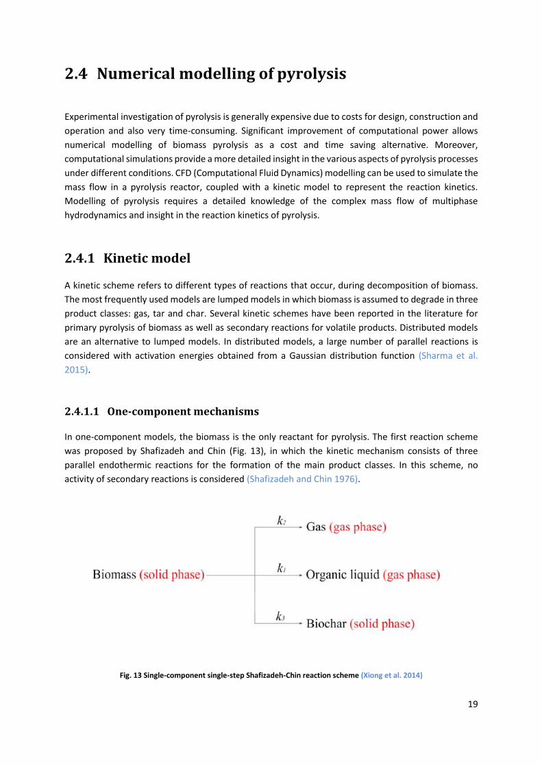
In one-component models, the biomass is the only reactant for pyrolysis. The first reaction scheme

was proposed by Shafizadeh and Chin (Fig. 13), in which the kinetic mechanism consists of three

parallel endothermic reactions for the formation of the main product classes. In this scheme, no

activity of secondary reactions is considered (Shafizadeh and Chin 1976).

Fig. 13 Single-component single-step Shafizadeh-Chin reaction scheme (Xiong et al. 2014)

20

The reaction rate constants (k1,k2,k3) are determined by using the Arrhenius law for temperature

dependency and thus include an activation energy and a pre-exponential factor. Determination of

these factors is based on experimental results. However, a large variey of kinetic constant calculations

is reported in the literature based on different experimental data. Three main categories are mostly

distinguised (Di Blasi 2008):

1. High temperature data (up to 1400K)

2. Low temperature data (below 700-800K) with low activation energy

3. Low temperature data (below 700-800K) with high activation energy

The differences in kinetic data in each category can be attributed to many factors. The biomass type

has a considerable influence. Biomass can differ in composition, but also in water content and ash

content. For example, ash constituents, especially potassium, sodium and calcium, act as catalysts and

favour char formation. Pretreatment of the biomass, such as washing with water or mild acid washing,

also introduces a significant modification in the biomass decomposition characteristics and usually

favours the liquid yield. Moreover, factors such as heating rate and particle size can drastically

influence the outcome. The use of thick particles clearly gives rise to heat and mass transfer limitations,

which are not considered in most kinetic models. Finally, secondary reactions can alter the product

compositon significantly, especially at high temperatures and sufficiently long vapour residence times.

(Di Blasi 2008).

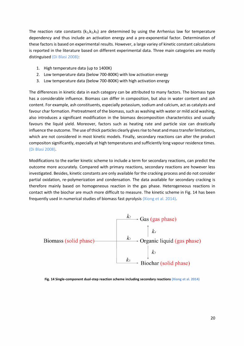
Modifications to the earlier kinetic scheme to include a term for secondary reactions, can predict the

outcome more accurately. Compared with primary reactions, secondary reactions are however less

investigated. Besides, kinetic constants are only available for the cracking process and do not consider

partial oxidation, re-polymerization and condensation. The data available for secondary cracking is

therefore mainly based on homogeneous reaction in the gas phase. Heterogeneous reactions in

contact with the biochar are much more difficult to measure. The kinetic scheme in Fig. 14 has been

frequently used in numerical studies of biomass fast pyrolysis (Xiong et al. 2014).

Fig. 14 Single-component dual-step reaction scheme including secondary reactions (Xiong et al. 2014)

21

2.4.1.2 Multi-component mechanisms

In multi-component reaction schemes, the biomass is not treated as one reactant, but regarded as a

composition of three major components: cellulose, hemicellulose and lignin. In this way, more

accurate results can be obtained compared to single component schemes, since the biomass

composition is now included in the reaction scheme. Hemicellulose is the least stable compound and

decomposes at 500-600 K. Cellulose decomposes at higher temperatures around 600-650 K. Lignin

degrades over a much wider range of temperatures due to its complex structure. It was analysed that

cellulose and hemicellulose produce mostly volatile products, while lignin accounts more for the

biochar production (Shafizadeh and Chin 1976, Sharma et al. 2015).

The same reaction schemes, as discussed in the one-component mechanisms, can be used for each

individual component, whether or not with secondary reactions included. Miller and Bellan proposed

a multistage model by modifying earlier developed reaction schemes of Broido and Bradbury (Fig. 15)

(Bradbury 1979, Miller and Bellan 1998).

Fig. 15 Multicomponent multistep reaction scheme (Xiong et al. 2014)

The first reaction, referred to as the initiation reaction, may be interpreted as the depolymerisation

step. No mass change is considered, but composition and physical properties, such as porosity, have

been changed during this step. The following reaction steps are two competitive first order reactions,

similar to the schemes discussed before. Miller and Bellan 1998 reported reaction rate constants for

this reaction scheme for each individual compound.

Another method is to assemble a reaction scheme by combining kinetic data of the different

components, each determined in different studies. The reaction schemes for each component are

usually more detailed and more complex to implement (Sharma et al. 2015).

2.4.2 Hydrodynamic models

An appropriate kinetic model is only sufficient if pyrolysis is studied on the particle level. In order to

study pyrolysis for a whole system, the reaction kinetics need to be coupled with transport phenomena.

CFD provides a useful tool, in which conservation laws and equations are employed to describe

complex fluid dynamics and has the ability to couple with kinetic models and heat transfer. The

literature reports various CFD models for biomass pyrolysis in which multiphase models are used.

22

Different types of multiphase models can be used to simulate biomass pyrolysis: Mixture model, Euler-

Lagrange model and Euler-Euler model.

An Euler-Lagrange model is a discrete element method (DEM) and has been studied for various

applications (Kruggel-Emden et al. 2006, Papadikis et al. 2008, Papadikis et al. 2009, Papadikis et al.

2010, Ren et al. 2012, Fang et al. 2013, Mahmoudi et al. 2014). In Euler-Lagrange models, the gas phase

is described according to an Eulerian formulation for mass and momentum, while the solid phase is

tracked by describing each particle and its interaction with the surrounding particles individually.

In an Euler-Euler model on the other hand, both phases are considered as interpenetrating continua

in an Eulerian framework. In other words, the solid phase is treated as a pseudo-fluid and its properties

are determined by the kinetic theory of granular flow. This model has been frequently used for the

simulation of fast pyrolysis in fluidized beds (Papadikis et al. 2008, Papadikis et al. 2009, Papadikis et

al. 2010, Xue et al. 2011, Mellin et al. 2013, Ozel et al. 2013, Xiong et al. 2013, Hua et al. 2015).

The mixture model is a simplified Euler-Euler model and is mostly used to simulate liquids or gases

containing a dispersed phase. In this model only one set of Navier-Stokes equations is solved for the

momentum of the mixture and transport equations prescribe the dispersed phase volume fractions.

This means that the velocity field of the mixture describes the dispersed phase based on a relative

velocity between the two phases in case of non-homogeneous multiphase flow. The mixture model is

not regarded as a suitable model to simulate dense granular flows.

Both Euler-Euler and Euler-Lagrange models are very promising for biomass pyrolysis simulations. The

Euler-Euler method is applicable for most systems, but is rather computationally intensive. The Euler-

Lagrange method is very efficient in a dilute system, since the computational demand of a simulation

increases with the amount of particles that are tracked. In screw reactors, the amount of particles is

very high, especially at high degrees of filling. Therefore, the Euler-Euler method is more suitable and

requires less computational capacity to simulate the granular flow.

As mentioned before, most of the numerical studies on biomass pyrolysis have been devoted to

common platforms, such as fluidized bed reactors. Studies on simulations of screw reactors are rather

limited. Besides, the focus of these studies is to investigate the granular flow under isothermal

conditions.

Owen and Cleary 2009 used a DEM-study to analyse the performance of a screw conveyor in terms of:

particle speed, mass flow rate, energy dissipation and power consumption (Owen and Cleary 2009).

The computational intensity of the Euler-Lagrange model was decreased by applying periodic

boundary conditions to a single pitch of the screw and by using coarse particles. The flow behaviour

was characterized at different screw inclination levels. A recirculatory flow of particles (avalanching-

effect) was observed for low levels of filling and a horizontal screw configuration. For higher degrees

of filling in combination with higher inclinations, a shearing flow in a bed of uniform depth was

observed, where particles were spread evenly across the flight surface. Increasing the inclination also

led to a higher energy input for the same mass flow and led to a progressively slower axial transport.

The predicted mass flow rate was in good agreement with the experimentally measured values.

Underestimations of the mass flow in some cases, were due to the fact that variations of particle

23

friction, irregular particle shapes and particle cohesion were not included. In this study, only an

isothermal flow was considered and the simplifications made to use Euler-Lagrange method inhibit the

inclusion of heat transfer and kinetics schemes in the model.

Sarkar and Wassgren 2010 studied the effect of cohesion on the granular flow. The particles are still

considered as perfect spheres, but the cohesive forces account for differences in particle size and

shape. Differences in axial flow were found to be more significant at low rotational frequencies due to

cohesion. At larger speeds, larger shear rates overcome particle bonding so that cohesive particles flow

in a manner similar to non-cohesive material. Hou et al. 2014 also stated that the solid flow is a function

of the rotational speed of the screw and the cohesive force between particles. A DEM-study is used to

analyse the flow behaviour in a screw feeder and in a feed bin (The latter has already been discussed

in section 2.3.6.)

Aramideh et al. 2015 discussed the numerical simulation of biomass fast pyrolysis in an auger reactor.

A 3D screw reactor model was designed in OpenFOAM to study the biomass residence time and

product yields. The length and the diameter of the reactor were 0,16m and 0,04m, respectively.

Biomass with a feed rate of 0,5 kg/h was injected continuously from the top inlet, while nitrogen with

a volume flow rate of 75 L/h was supplied from the left inlet, both at 300 K. The reactor wall was

maintained at a constant temperature of 850 K and the screw rotated at a speed of 60 rpm. An Euler-

Euler model, coupled with a multicomponent multistep kinetic model was used to simulate fast

pyrolysis. High temperatures, small particles (250-400 µm) and a very low solid volume fraction (Fig.

16) resulted in rapid conversion of the biomass.

Fig. 16 Spatial distributions of solid volume fraction and velocity (depicted by length of vector) in the auger reactor (Aramideh et al. 2015)

It can be concluded that Aramideh et al. 2015 successfully developed an Euler-Euler model which can

simulate the granular flow for a small reactor with a low degree of filling. Furthermore, the predicted

product yields from the fast pyrolysis agreed well with the experimental data.

24

In this master thesis, an Euler-Euler model is developed for torrefaction. The goal of this master thesis

is to study the different aspects of a screw reactor, such as temperature profile, granular flow pattern,

residence time distributions, product yields and the influence of different operating conditions.

Validation of the model could be achieved by replicating an existing screw reactor, situated at the

Faculty of Bioscience Engineering in Ghent, and comparison with the experimental results of Nachenius

et al. 2014-2015. In a first experiment, Nachenius et al. studied the residence time distribution of

coarse biomass particles. In second experiment, the temperature profile and product yields were

examined during continuous torrefaction processes. The results from these experiments were used to

calibrate the model. Successful calibration of the model parameters with experimental results also

allows to predict the performance of upscaled reactors.

25

3 Materials and methods

3.1 Overall approach

In this chapter, the theoretical background for the implementation of the Euler-Euler model in CFD

software is first discussed. The screw reactor configuration (Fig. 17), based on the dimensions of the

lab scale reactor at the Faculty of Bioscience Engineering in Ghent, is then constructed in specialized

software and imported in ANSYS Fluent 16.2 (CFD software). As Fig. 18 shows, the screw conveyor

consist of two sections to make the reactor more compact. In the model, the two screw sections are

implemented as one screw as a simplification. First, an isothermal flow has been simulated to study

the granular flow and residence time distributions. Subsequently, heat transfer and reaction kinetics

were added to investigate the temperature profile and product yields. The effect of different model

parameters was examined to calibrate the model with the experimental data. Finally, a sensitivity

analysis was conducted to study the effect of various operating parameters, physical properties and

model parameters. The governing equations used in these simulations are discussed in detail in this

chapter.

Fig. 17 Screw reactor at the Faculty of Bioscience Engineering, Ghent

26

3.2 Screw rotation

In an auger reactor, the biomass is conveyed by the rotation of the screw. Although rotation seems

straight forward, it is not obvious to implement it in CFD models. Generally, two main methods are

used to simulate rotation: a rotating reference frame and mesh rotation. Aramideh 2015 and Verclyte

2015 describe the use of a rotating reference frame (RRF). Both concepts are further explained.

3.2.1 Rotating reference frame

3.2.1.1 Fictitious forces

A RRF is a non-inertial reference frame that rotates relative to an inertial reference frame. All rotating

frames exhibit three fictitious forces: centrifugal force, Coriolis force and Euler force, which are not

observed in a stationary, inertial reference frame.

Fig. 18 Process flow diagram of the screw reactor

27

𝑎𝑐𝑒𝑛𝑡𝑟𝑖𝑓𝑢𝑔𝑎𝑙 = �⃗⃗⃗� 𝑥 (�⃗⃗⃗� 𝑥 r⃗) ( 1 )

𝑎𝑐𝑜𝑟𝑖𝑜𝑙𝑖𝑠 = −2ω⃗⃗⃗ 𝑥 �⃗� ( 2 )

𝑎𝐸𝑢𝑙𝑒𝑟 = −𝑑𝜔

𝑑𝑡𝑥 𝑟

( 3 )

3.2.1.2 Gravitational force

Compared to the magnitude of the fictitious forces in a RRF, gravity is still the dominant force in a

screw conveyor, so it is important that it is introduced correctly. The implementation of gravity is

illustrated in Fig. 19:

Fig. 19 Particle movement in a screw conveyor (side view) with gravitational vector plot (red vector)

28

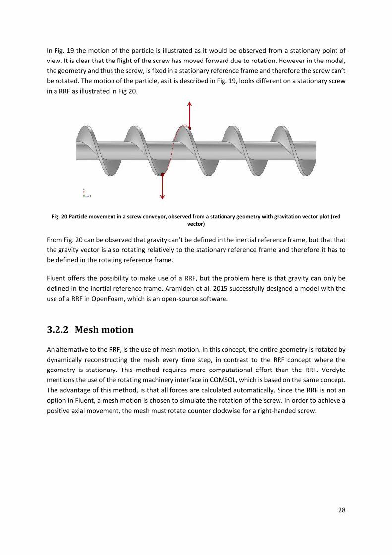
In Fig. 19 the motion of the particle is illustrated as it would be observed from a stationary point of

view. It is clear that the flight of the screw has moved forward due to rotation. However in the model,

the geometry and thus the screw, is fixed in a stationary reference frame and therefore the screw can’t

be rotated. The motion of the particle, as it is described in Fig. 19, looks different on a stationary screw

in a RRF as illustrated in Fig 20.

Fig. 20 Particle movement in a screw conveyor, observed from a stationary geometry with gravitation vector plot (red vector)

From Fig. 20 can be observed that gravity can’t be defined in the inertial reference frame, but that that

the gravity vector is also rotating relatively to the stationary reference frame and therefore it has to

be defined in the rotating reference frame.

Fluent offers the possibility to make use of a RRF, but the problem here is that gravity can only be

defined in the inertial reference frame. Aramideh et al. 2015 successfully designed a model with the

use of a RRF in OpenFoam, which is an open-source software.

3.2.2 Mesh motion

An alternative to the RRF, is the use of mesh motion. In this concept, the entire geometry is rotated by

dynamically reconstructing the mesh every time step, in contrast to the RRF concept where the

geometry is stationary. This method requires more computational effort than the RRF. Verclyte

mentions the use of the rotating machinery interface in COMSOL, which is based on the same concept.

The advantage of this method, is that all forces are calculated automatically. Since the RRF is not an

option in Fluent, a mesh motion is chosen to simulate the rotation of the screw. In order to achieve a

positive axial movement, the mesh must rotate counter clockwise for a right-handed screw.

29

3.3 Kinetic theory of granular flow

In gas-solid flows, high particle numbers (Euler-Lagrange method), can be smoothed out by using a

continuous phase (Euler-Euler method). The way a fluid flows, differs from the way granular particles

flow through the reactor. Thus, the properties of this continuous phase must be defined in a specific

way so that it behaves as granular flow. This is also known as the kinetic theory of granular flow

(Gidaspow 1994). The viscosity of a continuous phase is modified to make it look like a solid flow. The

total viscosity of the continuous phase that describes the solid phase is regarded as the sum two

independent viscosities: the bulk viscosity and the frictional viscosity.

3.3.1 Bulk viscosity

The bulk viscosity is the internal friction a ‘fluid’ experiences with the absence of shear stress and

accounts for the resistance of ‘fluid’ to compression and expansion. The calculation for the bulk

viscosity is based on (Lun et al. 1984, Hua et al. 2015):

With 𝛼 the volume fraction of the solid phase, 𝜌𝑠 [kg/m³] the solid density, 𝑑𝑃[m] the average particle

diameter, 𝑔0 [-] the radial distribution function, 𝑒𝑠𝑠 [-] the coefficient of restitution and 𝜃 [m²/s²] the

granular temperature. These variables are described in more detail in the next section.

3.3.1.1 Volume fraction

Since the particles are not discretized in an Euler-Euler model, the concentration of both phases in any

location within the modelled geometry is characterized by the volume fraction. The volume fraction is

defined by the distribution of phases and the size of the computational volume. In a system with n

phases, the volume of a phase 𝑖, 𝑉𝑖, at a certain time is defined as (ANSYS 2013):

𝑉𝑖 = ∫𝛼𝑖 𝑑𝑉

𝑉

( 5 )

And the sum of the volume fractions of all phases in a defined volume always equals 1. In this case:

𝛼𝑠𝑜𝑙𝑖𝑑 𝑝ℎ𝑎𝑠𝑒 + 𝛼𝑔𝑎𝑠 𝑝ℎ𝑎𝑠𝑒 = 1

( 6 )

In reality, the volume fraction of the solid phase can never equal 1, because the bulk viscosity will be

infinite. If particles are packed in a certain volume, there is always a void, which is then occupied by

𝜇𝑏 =4

3𝛼 𝜌𝑠𝑑𝑃𝑔0(1 + 𝑒𝑠𝑠)√

𝜃

𝜋

( 4 )

30

another phase, in this case the gas phase. Therefore, the volume fraction of the solid phase is limited

by a packing limit 𝛼𝑚𝑎𝑥.

3.3.1.2 Particle diameter

The feedstock typically used in biomass pyrolysis applications consists of a grinded material, such as

wood chips and varies strongly in shape and size. In numerical methods, a particle is usually considered

a perfect sphere. The diameter of such a particle can be an average value or represented by a

distribution function. A uniform particle diameter is less computationally intensive and is used in most

cases. Moreover, the biomass particle shrinks during pyrolysis. It is not possible to include shape

factors or shrinking, but the angle of internal friction (included in frictional viscosity equation (9)) can

be altered as a function of particle size and shape. An angle of internal friction of 45° for pine was

reported by Nachenius et al. 2015.

3.3.1.3 Radial distribution function

The radial distribution function is used to calculate a dimensionless particle-particle distance expressed

in terms of volume fraction. It certifies that the viscosity is increased to infinity if the volume fraction

equals the packing limit (Andersson 2012, ANSYS 2013):

𝑔0 = (1 − (

𝛼

𝛼𝑚𝑎𝑥 )1/3

)

−1

( 7 )

3.3.1.4 Coefficient of restitution

Whenever a particle collides with another particle, a part of the kinetic energy is lost either through

heat or deformation of the particle. The coefficient of restitution 𝑒𝑠𝑠 is the ratio of kinetic energy

before collision and after. The value of 𝑒𝑠𝑠 is usually around 0.9-0.99 for biomass (Hua et al. 2015).

3.3.1.5 Granular temperature

The granular temperature 𝜃 is defined as the mean square of particle velocity fluctuations. The

velocity fluctuations derive from collisions of particles. In a fluidized bed this parameter can have a

large influence on the solid bulk viscosity. In a screw reactor however, the velocity fluctuations �⃗� due

to particle interactions, are insignificant and therefore result in a low value for the granular

temperature (Andersson 2012, ANSYS 2013, Sun et al. 2014).

𝜃 =

1

3 ⟨�⃗�2⟩

( 8 )

31

3.3.2 Solid shear viscosity

The equations for solid shear viscosity are based on particle-particle interactions, arising from kinetic-

collisional stresses and shear stresses (Makkawi et al. 2006). At low solid volume fraction applications,

such as in a fluidized or a circulating bed, the particle-particle interactions are almost exclusively

determined by kinetic-collisional stresses, since the particles are diluted in the gas phase. However, for

a high solid fraction, the momentum transfer in the particulate phase becomes dominant over the

kinetic collisional stress, which is the case in screw conveyors. This means that long term contact and

multi-particle contact have a larger influence compared to collisions between particles causing

frictional stress (Bokkers 2004, Makkawi et al. 2006).

Fig. 21 Mechanisms of shear stresses (Andersson 2012)

The solid shear viscosity equation is described as (Schaeffer 1987):

𝜇𝑠 =10𝜌𝑠𝑑𝑃√𝜃𝜋

96𝛼(1 + 𝑒𝑠𝑠)𝑔0[1 +

4

5𝑔0𝛼(1 + 𝑒𝑠𝑠)]

2

+4

5𝛼𝜌𝑠𝑑𝑃𝑔0(1 + 𝑒𝑠𝑠)√

𝜃

𝜋+ 𝜇𝑠,𝑓𝑟𝑖𝑐

( 9 )

The first term describes the collisional viscosity, the second term the kinetic viscosity and the third

term the frictional viscosity and the summation of all terms makes up the solid shear viscosity. The

expression for the frictional viscosity is very complex and depends on the angle of internal friction and

the velocity field of the solid phase.

3.4 Numerical set-up

3.4.1 Geometry

The implementation of the geometry in the software was the first challenge to overcome. The design

of a screw is too complex to implement in the geometry interface of ANSYS. Consequently, SIEMENS

NX was used, a specialized program for computer aided design (CAD), to draw the screw. As mentioned

32

before, the dimensions of the screw (Table 1) were based on the lab scale reactor, situated at the

Faculty of Bioscience Engineering in Ghent (Nachenius et al. 2014, Nachenius et al. 2015), so the results

from the model can be compared with experimental results. Some of the experiments of Nachenius

were conducted on only 1 screw conveyor section, while in other experiments, the complete reactor

was deployed. Consequently, a screw geometry for 1 section and 2 sections was drawn.

The flights of the screw were drawn with the use of two right-handed helices. The helices were defined

by two parameters: the radius and the pitch. The flight thickness was set by the distance between the

two helices. Subsequently both helices were swept according to a predefined vector to form the flights.

The orientation of this vector determined the angle between the shaft and the flight. Subsequently,

the helices were united into one object. Finally the shaft was drawn and sewed on the flights to form

one solid object.

In CFD software, the partial differential equations (PDEs) are solved for the volume inside the reactor.

Therefore, the geometry was adjusted by constructing a solid cylinder with a diameter equal to the

inner shell diameter. By subtracting the screw from this solid cylinder, by a Boolean operation, the

volume in which the equations are solved, was constructed. This resulted in a radial clearance of 1mm

between shell and flight. The recommended radial clearance is usually 1.5 times larger than the

maximum particle size in order to prevent jamming. This means that particles should theoretically not

be larger than 0,7mm (Roberts 1999). The geometry was finally exported as a STEP-file to make it

compatible for import in ANSYS.

Dimension

Reactor length (1 screw section) 1,640 m Shell diameter 0,052 m Screw diameter 0,050 m Radial clearance 0,001 m Shaft diameter 0,018 m Pitch 0,046 m Flight thickness 0,003 m

Table 1 Screw dimensions

33

Fig. 22 Geometry of the screw (1.64m) in SIEMENS NX

3.4.2 Mesh

In order to solve the PDEs that govern fluid flow and heat transfer, the entire domain of the geometry

is fragmented into smaller subdomains, referred to as cells or elements. These cells usually consist of

tetrahedral or hexahedral elements. The collection of cells is called the mesh or grid. By solving the

PDEs in each of the cells and combining the solutions, the total solution over the whole domain can be

obtained. ANSYS Fluent provides a meshing interface equipped with an automated meshing program.

Meshing is a field that can be studied on its own because it is very complex and more importantly it

can have a large influence on the results. Specialized meshing software exists, such as Gambit or ICEM,

that provides the tools to mesh complex structures. Unfortunately, studying the features of meshing

in detail was not possible within the time frame of this work.

The automated meshing interface of Fluent was used to create a suitable mesh. The quality of the

mesh was checked with two quality factors: skewness and aspect ratio. Skewness compares the shape

of a cell relative to the shape of an optimal cell. Elements with a low skewness have the best quality.

The aspect ratio measures mesh quality by calculating the ratio of the longest edge length to the

shortest edge length. Cells with a ratio near 1 have the best quality. The element quality can be

increased by refining the grid. Especially for sharp edges, such as in the screw geometry, and small

spaces, a smaller minimum element size results in a higher element quality. On the other hand, when

the mesh is refined, the simulation time is significantly increased, since a set of PDEs needs to be solved

for each cell individually. Therefore, a grid is most often refined until the results from the simulation

become mesh independent. Further refinement of the mesh will only result in longer computational

time, but insignificant changes in the result. A grid size of 200 000 cells (for 1.68m reactor) was opted

for the model.

34

3.4.3 Governing equations

The governing equations are the equations that describe each phase in the system. By solving the

equations in each cell at a certain time step, a state-space representation of the system can be

generated.

3.4.3.1 Conservation of mass

The conservation of mass is based on a continuity equation for each phase, expressed as (ANSYS 2013,

Pieters and Verhoest 2013):

𝜕

𝜕𝑡(𝛼𝑖𝜌𝑖) + ∇(𝛼𝑖𝜌𝑖�⃗�𝑖) =∑(�̇�𝑗𝑖 − �̇�𝑖𝑗)

𝑛

𝑖=1

+ 𝑆𝑖

( 10 )

Where �̇�𝑗𝑖 represents the specific mass transfer rate from phase 𝑗 to phase 𝑖, and �̇�𝑖𝑗 the specific

mass transfer rate from phase 𝑖 to phase 𝑗. In reality, a gas is formed if biomass is pyrolyzed, which

means that there is a mass transfer from the solid phase to the gas phase. In this model, the term that

accounts for mass transfer between phases was first neglected, to simulate the cold granular flow ,

and later included for the pyrolysis reactions after adding the kinetic model. 𝑆𝑖 is the source term,

which is zero in this case, since there is no mass creation within the control volume. So for a cold

granular flow, the equations for both phases can be rewritten as:

𝜕

𝜕𝑡(𝛼𝑔𝜌𝑔) + ∇(𝛼𝑔𝜌𝑔�⃗�𝑔) = 0 (gas phase) ( 11 )

𝜕

𝜕𝑡(𝛼𝑠𝜌𝑠) + ∇(𝛼𝑠𝜌𝑠�⃗�𝑠) = 0 (solid phase) ( 12 )

3.4.3.2 Conservation of momentum

The conservation of momentum equation is based on the Navier-Stokes equations (ANSYS 2013,

Pieters and Verhoest 2013):

𝜕

𝜕𝑡(𝛼𝑖𝜌𝑖�⃗�𝑖) + ∇(𝛼𝑖𝜌𝑖�⃗�𝑖�⃗�𝑖) = −𝛼𝑖∇𝑝 + ∇τ̿ + 𝛼𝑖𝜌𝑖�⃗� +∑(�⃗⃗�𝑗𝑖 + �̇�𝑗𝑖�⃗�𝑗𝑖 − �̇�𝑖𝑗�⃗�𝑖𝑗)

𝑛

𝑖=1

+ �⃗�

( 13 )

Compared to the Navier-Stokes equations for momentum conservation for a single phase flow, an

additional term is included for momentum exchange between phases, were �⃗⃗�𝑗𝑖 is an interaction force

between the two phases and �⃗�𝑗𝑖 and �⃗�𝑖𝑗 are the interphase velocities. As discussed for the mass

35

conservation equation, mass transfer is not included in the cold flow model. The external volume force

�⃗� is the term that includes the forces induced by rotation of the volume.

The stress tensor τ̿ describes the stress forces and can be expressed in function of viscosity (ANSYS

2013):

τ̿ = 𝛼𝑔𝜇𝑔(∇�⃗�𝑔 + ∇�⃗�𝑔𝑇) −

2

3𝛼𝑔𝜇𝑔(∇�⃗�𝑔)𝐼 ̿ (gas phase) ( 14 )

τ̿ = 𝛼𝑠𝜇𝑠(∇�⃗�𝑠 + ∇�⃗�𝑠

𝑇) + 𝛼𝑠(𝜇𝑏 −

2

3𝜇𝑠)(∇�⃗�𝑠)𝐼 ̿ (solid phase) ( 15 )

For the gas phase, the viscosity 𝜇𝑔 is a constant. The stress forces for the solid phase are more complex

and are dependent on the solid bulk viscosity 𝜇𝑏 and the solid shear viscosity 𝜇𝑠, which were already

discussed in the kinetic theory of granular flow.

The interaction force �⃗⃗�𝑗𝑖 depends on friction, pressure, cohesion and other effects, and is subject to

the condition that �⃗⃗�𝑗𝑖 = − �⃗⃗�𝑖𝑗. The interaction term can be expressed as a function of relative velocity

between both phases:

�⃗⃗�𝑗𝑖 = 𝛽(�⃗�𝑗 − �⃗�𝑖)

( 16 )

Consequently, the equations for conservation of momentum for both phases can be rewritten as:

𝜕

𝜕𝑡(𝛼𝑔𝜌𝑔�⃗�𝑔) + ∇(𝛼𝑔𝜌𝑔𝑣𝑔�⃗�𝑔) = −𝛼𝑔∇𝑝 + ∇τ̿ + 𝛼𝑔𝜌𝑔�⃗� + 𝛽(�⃗�𝑠 − �⃗�𝑔) + �⃗� (gas phase) ( 17 )

𝜕

𝜕𝑡(𝛼𝑠𝜌𝑠�⃗�𝑠) + ∇(𝛼𝑠𝜌𝑠�⃗�𝑠�⃗�𝑠) = −𝛼𝑠∇𝑝 − ∇𝑝𝑠 + ∇τ̿ + 𝛼𝑠𝜌𝑠�⃗� + 𝛽(�⃗�𝑔 − �⃗�𝑠) + �⃗� (solid phase) ( 18 )

𝛽 is the solid-fluid exchange coefficient, also referred to as the drag coefficient in the literature. The

literature reports a wide range of experimental relations for this variable. In fluidized bed, the choice

of the drag coefficient relation has a major influence on the CFD simulation results. In fluidized bed

reactors used for pyrolysis, the biomass particles are suspended in or carried out of the reactor due to

high gas velocities, so the interaction between gas and particle is very important and well-studied. In

screw reactors however, momentum transfer between gas and particle is of less importance, since the

particles are not suspended in high gas velocity flows, but by rotation of the screw and interaction

between particles. The choice of the inter-phase drag model has a negligible influence on the outcome

of the screw reactor simulation and therefore it was opted to choose the frequently used Gidaspow

drag model (Gidaspow 1994).

36

𝛽 =

{

3

4𝐶𝐷𝛼𝑔𝛼𝑠𝜌𝑔|�⃗�𝑔 − �⃗�𝑠|

𝑑𝑝𝛼𝑔

−2.65

150𝛼𝑠(1 − 𝛼𝑔)𝜇𝑔

𝛼𝑔𝑑𝑝2 +

7

4

𝜌𝑔𝛼𝑠|�⃗�𝑔 − �⃗�𝑠|

𝑑𝑝

𝛼𝑔 ≥ 0.8

𝛼𝑔 < 0.8

( 19 )

where,

𝐶𝐷 = {

24

𝑅𝑒(1 + 0.15𝑅𝑒0.687)

0.44

𝑅𝑒 < 1000

𝑅𝑒 ≥ 1000

( 20 )

The relative Reynolds number is obtained from:

𝑅𝑒 =

𝜌𝑔𝑑𝑝|�⃗�𝑔 − �⃗�𝑠|

𝜇𝑔

( 21 )

The Gidaspow model is also frequently used in dense fluidized bed simulations, and therefore also

recommended in a simulation with a high volume fraction such as the screw reactor.

For the solid phase momentum equation, an extra term for the granular pressure is to be included,

which accounts for the momentum transfer due to particle-particle interaction. It is calculated

independently as (ANSYS 2013):

𝑝𝑠 = 𝜌𝑠𝛼𝑠𝜃(1 + 2𝛼𝑠𝑔0(1 + 𝑒𝑠𝑠))

( 22 )

The different parameters in this equation have already been extensively discussed in section 3.3. The

radial distribution function in this equation certifies that the packing limit is never surpassed by

increasing the particle pressure to infinity if 𝛼 = 𝛼𝑚𝑎𝑥.

3.4.3.3 Heat transfer

The energy conservation equation describes how the specific enthalpy H changes in time and space

and has basically the same structure as the other conservation equations.

𝜕

𝜕𝑡(𝛼𝑔𝜌𝑔𝐻𝑔) + ∇(𝛼𝑔𝜌𝑔�⃗�𝑔𝐻𝑔) = −𝛼𝑔

𝜕𝑝

𝜕𝑡+ ∇τ̿: ∇�⃗�𝑔 + ∇q⃗⃗𝑔 + 𝑄𝑔

(gas phase) ( 23 )

𝜕

𝜕𝑡(𝛼𝑠𝜌𝑠𝐻𝑠) + ∇(𝛼𝑠𝜌𝑠�⃗�𝑠𝐻𝑠) = −𝛼𝑠

𝜕𝑝

𝜕𝑡+ ∇τ̿: ∇�⃗�𝑠 + ∇q⃗⃗𝑠 + 𝑄𝑠 + 𝑆𝑠 (solid phase) ( 24 )

37

The change of enthalpy is expressed in terms of change in mechanical energy, the conductive heat flux

q⃗⃗ , and the rate of heat exchange between the two phases 𝑄. The enthalpy is defined as:

𝐻 = ∫𝑐𝑝𝑑𝑇 ( 25 )

With 𝑐𝑝 [J/kg/K] the specific heat capacity, which is different for both phases, at the pressure of the

gas phase. The conductive heat flux can be written as (Pieters and Verhoest 2013)

q⃗⃗ = 𝛼𝜆∇T ( 26 )

The rate of heat exchange between gas phase and biomass is function of temperature difference

between both phases:

𝑄𝑔 = h𝑔𝑠(T𝑠 − T𝑔) ( 27 )

𝑄𝑠 = h𝑔𝑠(T𝑔 − T𝑠) ( 28 )

The heat transfer coefficient h𝑔𝑠 is defined as (Gunn 1978):

h𝑔𝑠 =

6𝛼𝑔𝛼𝑠𝜆𝑔𝑁𝑢

𝑑𝑝2 ( 29 )

With Nu the Nusselt number, which is determined by the Gunn correlation for a granular flow as

(ANSYS 2013):

𝑁𝑢 = (7 − 10𝛼𝑔 + 5𝛼𝑔2)(1 + 0.7𝑅𝑒0.2𝑃𝑟1 3⁄ ) + (1.33 − 2.4𝛼𝑔 + 1.2𝛼𝑔

2)𝑅𝑒0.2𝑃𝑟1 3⁄ ( 30 )

The Nusselt number is generally used to characterize the heat flux from a solid to a fluid and is the

ratio of the convective to the conductive heat transfer across a particle surface.

And the Prandtl 𝑃𝑟 number for the gas phase:

𝑃𝑟 =𝑐𝑝,𝑔𝜇𝑔

𝜆𝑔 ( 31 )

38

The heat transfer coefficient between the wall of the reactor and both phases is automatically

determined by Fluent, based on velocity, temperature, turbulence, etc. (ANSYS 2013)

In the energy equation for the solid phase, there is also a source term 𝑆𝑠 included. This term can

account for the heat dissipated due to the endothermic pyrolysis reactions (or released in case of

exothermic reactions) and can thus be interpreted as reaction enthalpy.

3.4.3.4 Component transport equations

Fluent predicts the local mass fraction of each component 𝑌𝑖 with the solution of a convection-

diffusion equation, described as (ANSYS 2013):

𝜕

𝜕𝑡(𝜌𝑌𝑖) + ∇(𝜌�⃗�𝑌𝑖) = −∇ ∙ J𝑖⃗⃗⃗ + 𝑅𝑖 + 𝑆𝑖 ( 32 )

Where 𝑅𝑖 is the net rate of production of component 𝑖 and 𝑆𝑖 is the rate of creation from other sources

(e.g. direct transport between two phases), which is not included in this model. J𝑖⃗⃗⃗ is the diffusion flux

of component 𝑖 due to concentration gradients. However, convective transport will dominate over

diffusion of components in both phases for the screw reactor, so this term was neglected.

The net rate of production 𝑅𝑖 is a first order reaction term with reaction rate constants determined

by the Arrhenius expressions:

𝑘𝑗𝑖 = 𝐴𝑗𝑖𝑒

−𝐸𝑎,𝑗𝑖𝑅𝑇

( 33 )

𝑑𝑌𝑖

𝑑𝑡= 𝑘𝑗𝑖𝑌𝑗

( 34 )

with 𝐴𝑗𝑖 the pre-exponential factor for the reaction of component 𝑗 to component 𝑖 and 𝐸𝑎,𝑗𝑖 the

activation energy.

3.4.4 Reaction kinetics

The product yield of pyrolysis can be predicted by including reaction kinetics in the model. In this work,

the slow pyrolysis process was represented by the kinetic scheme of Shafizadeh and Chin (Fig. 13)

(Shafizadeh and Chin 1976). Four different components participate in this reaction scheme: unreacted

biomass, char, tar and gas. This means that the discrete phase is subdivided in biomass, char and bound

water, while the continuous phase is subdivided in tar, gas, vapour and nitrogen gas. The latter does

39

not participate in any reactions. Water (both in a bound state to the biomass as well as vapour) was

added to the model, i.e. its evaporation is added to the reaction kinetics because of its latent heat of

evaporation has a large impact on the overall heat balances and consequently, a large effect on the

temperature profile. Fluent distinguishes between homogeneous and heterogeneous reactions.

Homogeneous reactions involve conversion of components within the same phase. The conversion of

biomass to char is a homogeneous reaction within the discrete phase. Heterogeneous reactions involve

components of different phases. In this case, it concerned the reaction from biomass (discrete phase)

to gas and tar (continuous phase).

All reactions in the kinetic scheme were considered to be first order reactions with Arrhenius

parameters given in Table 2.

Table 2 Arrhenius parameters for the reaction scheme of Shafizadeh and Chin (Ratte et al. 2011) and for the bound water vaporization (Bates and Ghoniem 2014)

Reaction Pre-exponential factor (1/s) Activation energy (kJ/mol)

Biomass Char 4,426 x 107 106,5 Biomass Tar 2,475 x 108 112,7

Biomass Gas 8,607 x 105 88,6

Bound H20(l) H2O(g) 4,5 x 103 45,0

Additionally, a second reaction scheme, the multicomponent multistep kinetic scheme of Broido-

Bradbury (Fig. 15) was investigated. Unfortunately, due to complexity of the model, a limited time

frame and long simulation times, only a theoretical approach for this model was developed, at the

reaction temperature of 600K, which is the temperature of the present simulated experimental setup,

without CFD-simulations. However, the mean residence time and temperature progression of the

screw reactor model were accounted for in the theoretical calculation of the product yield. The

Arrhenius parameters of the Broido-Bradbury kinetic scheme are given in Table 3. The initial

composition of the dry biomass for cellulose, hemicellulose and lignin was 46%, 36% and 18%

respectively (Di Blasi 2008).

Table 3 Arrhenius parameters for the reaction scheme of Broido-Bradbury (Miller and Bellan 1998)

Reaction Pre-exponential factor (1/s)

Activation energy (kJ/mol)

Cellulose Active Cellulose 2,8 x 1019 2,424 x 105 Active Cellulose Tar 3,28 x 1014 1,965 x 105

Active Cellulose 0,35 Char + 0,65 Gas 1,3 x 1010 1,505 x 105

Hemicellulose Active Hemicellulose 2,1 x 1016 1,867 x 105

40

Active Hemicellulose Tar 8,75 x 1015 2,024 x 105 Active Hemicellulose 0,6 Char + 0,4 Gas 2,6 x 1011 1,457 x 105 Lignin Active Lignin 9,6 x 108 1,076 x 105

Active Lignin Tar 1,5 x 109 1,438 x 105 Active Lignin 0,75 Char + 0,25 Gas 7,7 x 106 1,114 x 105

Tar Gas 4,28 x 106 1,08 x 105

3.4.5 Boundary conditions

The boundary conditions describe the surrounding of the phases. The inlet condition is expressed as

mass flows for both phases. A wide range of solid mass flows was tested to compare various flow

patterns at different filling degrees. The slip velocity specification is either expressed as a slip velocity

ratio between both phases or a volume fraction of the granular phase. In the case of the screw reactor,

the slip velocity at the inlet does not influence the results in any way. Therefore a volume fraction was

opted for the slip velocity specification. The volume fraction at the inlet must never exceed the packing

limit or the solver will return a floating point error. The incoming biomass has an ambient temperature.

The outlet is defined as a pressure-outlet condition with 0 Pa relative pressure.

The screw wall was set as a moving wall, rotating at the same speed relative to the adjacent cell zone.

The wall of the tube is described by a moving wall, which rotates at the opposite direction as viewed

from the moving mesh. In other words, the wall remains stationary in the inertial reference frame. For

each wall condition, the shear condition of both phases is represented by a ‘no slip’ condition. This

results in a high shear between the solid particles and the wall. Alternatively, a specularity coefficient

could be set for the solid phase to interpolate between a slip and no-slip condition, but no data was

available for this. In the model, only the shell is heated by maintaining a constant wall temperature.

The screw had a no-heat flux boundary condition.

3.4.6 Phase properties

The phase properties are important input parameters to solve the governing equations. Part of the

solid phase properties has already been discussed in the kinetic theory of granular flow. The properties

of the gas phase on the other hand are straightforward and available via the Fluent material database.

The properties of both phases are determined by the components as volume- or mass weighted

averages. All phase properties are summarized in section 3.5, together with other parameters used in

the model.

41

3.4.7 Solution methods

In order to solve PDEs, such as the continuity equations, a suitable discretization method is first applied

to convert the differential equations to algebraic equations and approximate the variables at discrete

points in time and space.

Spatial discretization

The PDEs are first discretized in space to form ordinary differential equations (ODE). Fluent uses the

finite volume method. This technique consists of integrating the PDEs in each mesh cell. The discretized

equation is usually expressed in terms of face values. Since values are stored at the centre of each cell,

a proper scheme needs to be used to interpolate the centre value to a face value. A more detailed

description of spatial discretization and its interpolation schemes can be found in the Fluent Manual

(ANSYS 2013).

Temporal discretization

Total discretization is achieved by applying a temporal discretization to the ODE. Temporal

discretization can be treated explicitly or implicitly. The explicit method solves the state of a system at

the next timestep based on variables at the current state, while the implicit method solves the state

of a system based on both variables at the current state and the state at the next time step. The implicit

scheme is more stable and provides a more accurate solution, but comes with a higher computational

cost. The implicit method was used in this master thesis. Pressure-velocity coupling was achieved with

the “Phase SIMPLE coupled”-algorithm. This is a pressure based segregated solver. The solution

method is not discussed in further detail, since it is out of scope for this work. For details, the reader

is referred to ANSYS Fluent Theory Guide (ANSYS 2013).

3.5 Simulation procedures

3.5.1 Granular flow pattern

The charachteristics of the granular flow have a large impact on the degree of mixing and cosequently

the heat transfer and reaction kinetics. So it is important to check if the Euler-Euler model was fit to

represent a granular flow in a screw conveyor. A study on the flow pattern for an isothermal flow was

performed on a small reactor (0,2 m) to reduce simulation time. An important parameter that needed

to be investigated, was the packing limit, since it determines the degree of filling and consequently the

flow pattern. Biomass with a high packing limit will occupy a lower volume then biomass with a low

packing limit for the same weight. Nachenius et al. uses pine in his experiments with a bulk density of

155-165 kg/m³. The solid density of pine usually varies around a value of 500 kg/m³ (Nachenius et al.

2015). The value for the packing limit was initially choosen as the ratio of the bulk density and the solid

42

density of pine (𝛼𝑚𝑎𝑥 ≈ 0,32). Later, the packing limit was slightly altered to fit the model better with

the experimental data.

3.5.2 Residence time

The residence time of biomass in the reactor is an important aspect during the pyrolysis process, since

it significantly influences the product yield. The residence time distribution (RTD) is evaluated by

adding a third phase to the system with the exact same properties as the solid phase. A pulse injection

of this tracer phase can be measured as a mass flow at the outlet and translated to a residence time

distribution. This was done by injecting 10% of the present mass flow as a third phase during 0,5 s.

Consequently, this fraction is conveyed together with the biomass without altering the granular flow.

Technically, the system needs to be at steady-state when the injection occurs. To reduce simulation

time, the third phase was injected as soon as the first three pitches of the screw were filled with a solid

phase. In order to determine when the model reaches statistically steady-state the total solid mass

was monitored. The experiments of Nachenius for the residence time distributions were performed

on 1 screw conveyor section. Consequently the same screw reactor length (1.64 m) was used in the

model.

3.5.3 Temperature

The temperature profile is an important parameter for reactor design, because it shows when the

biomass reaches the desired temperature for pyrolysis or torrefaction. The temperature of the

biomass was controlled by the heated shell at a constant temperature of 600K and the heat of reaction.

The influence of the endothermic reactions can consequently be compared to the wall heat flux to

study the influence on the temperature. The temperature simulations were first conducted on the

complete screw reactor (2 sections). It was observed that the biomass temperature is already close to

the wall temperature at the end of the first section. Therefore, future simulations carried out on 1

screw reactor section to study the temperature profile, in order to reduce simulation time.

3.5.4 Product yield

The product yield was studied after optimisation of the parameters for the temperature profile. These

simulations were conducted on the complete reactor (2 sections) by measuring the components at the

outlet. The product yield, usually expressed in mass fractions, can be further used to calculate calorific

value of the final products. The theoretical calculation of the Broido-Bradbury kinetic scheme was

conducted in the reaction engineering interface of COMSOL Multiphysics 5.2.

43

3.5.5 Sensitivity analysis

A sensitivity analysis was performed on various parameters of the model to discover which parameters

can be used to fit the model data to the experimental data and to investigate the effect of different

operating conditions. A model with a reactor length of 0,5 m was used to reduce simulation time.

Subsequently, the sensitivity of difference parameters on the outlet temperature of the solid phase

was tested. It could be interesting to study the effect of various parameters on the product yield, but

unfortunately, longer reactor models are required to see an adequate change in mass fractions.

3.5.6 Parameterisation

The final parameterisation of the model is summarized below:

Table 4 Properties of biomass, char, tar, gas and nitrogen

Component properties Value/Equation

Density

𝝆𝒃𝒊𝒐𝒎𝒂𝒔𝒔 500 kg/m³ 𝝆𝒄𝒉𝒂𝒓 300 kg/m³

Heat Capacity 𝑪𝒑,𝒃𝒊𝒐𝒎𝒂𝒔𝒔 531,15 + 2,45 𝑇 𝐽/𝑘𝑔 𝐾 (Harada et al. 1998)

𝑪𝒑,𝒄𝒉𝒂𝒓 531,15 + 2,45 𝑇 𝐽/𝑘𝑔 𝐾 (Harada et al. 1998)

𝑪𝒑,𝒕𝒂𝒓 1162 + 0,961𝑇 𝐽/𝑘𝑔 𝐾 (Bates and Ghoniem 2014)

𝑪𝒑,𝒈𝒂𝒔 1162 + 0,961𝑇 𝐽/𝑘𝑔 𝐾 (Bates and Ghoniem 2014)

𝑪𝒑,𝑵𝟐 979 + 0,418𝑇 − 0,00118𝑇2 + 1,674 × 10−6𝑇3 − 7,256 ×10−10𝑇4 (ANSYS 2013)

Thermal Conductivity 𝝀𝒃𝒊𝒐𝒎𝒂𝒔𝒔 0,0481 + 0,0003𝑇 𝑊/𝑚 𝐾 (Koufopanos et al. 1989)

𝝀𝒄𝒉𝒂𝒓 0,071 𝑊/𝑚 𝐾 (Bates and Ghoniem 2014)

𝝀𝒕𝒂𝒓 25,77 × 10−3 𝑊/𝑚 𝐾 (Bates and Ghoniem 2014) 𝝀𝒈𝒂𝒔 25,77 × 10−3 𝑊/𝑚 𝐾 (Bates and Ghoniem 2014)

𝝀𝑵𝟐 0,0242 𝑊/𝑚 𝐾 (ANSYS 2013)

44

Table 5 Properties of phases and interaction terms between phases

Phase property Value/Calculation

Primary phase (Continuous)

Density 1,138 kg/m³ (ANSYS 2013)

Heat Capacity Mass-weighted mixing law of components Thermal conductivity Mass-weighted mixing law of components Viscosity 1,663× 10−5 Pa*s (ANSYS 2013)

Secondary phase (Discrete)

Density Volume − weighted mixing law of components

Heat Capacity Mass − weighted mixing law of components

Thermal conductivity Mass − weighted mixing law of components

Diameter 0,002 m Granular viscosity (Gidaspow 1994)

Granular bulk viscosity Eq. (4) (Lun et al. 1984)

Frictional viscosity Eq. (9) (Schaeffer 1987)

Angle of internal friction 45° Granular temperature Eq. (8) (ANSYS 2013)

Solids pressure Eq. (22) (Lun et al. 1984)

Radial distribution Eq. (7) (Lun et al. 1984)

Packing limit 0,30

Interaction terms

Drag Coefficient Eq. (19) (Gidaspow 1994)

Heat Transfer Eq. (29) (Gunn 1978)

Table 6 Boundary Conditions

Boundary Conditions Value

Inlet: Primary phase (Continuous)

Gas phase mass flowrate 3.6 × 10−6 kg/s (Nachenius et al. 2015) Solid phase temperature 300 K Mass fraction N2 of solid phase 1,00

Inlet: Secondary phase (Discrete) Solid phase mass flowrate 6,94 × 10−4 kg/s (Nachenius et al. 2015) Solid phase temperature 300 K

Moisture content 0,12 Mass fraction dry biomass of solid phase 0,88

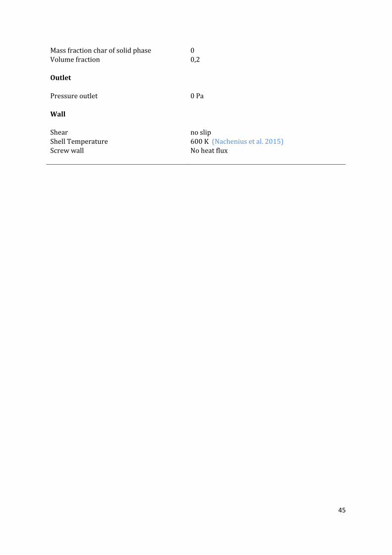
45

Mass fraction char of solid phase 0 Volume fraction 0,2 Outlet

Pressure outlet 0 Pa Wall Shear no slip

Shell Temperature 600 K (Nachenius et al. 2015) Screw wall No heat flux

47

4 Results and discussion

4.1 Model Implementation in Ansys fluent

A successful model implementation was achieved in Ansys fluent. It was important to maintain a stable

simulation progression without any errors or divergence problems. This was one of the main

challenges in the start-up phase of this model. A lot of trial & error procedures were carried out to find

the best spatial and temporal discretization schemes and solvers. Moreover, the time step size and the

number of iterations per time step had a major influence on the model stability. A smaller time step

size and a higher number of iterations per time step led to a high stability, but drastically increased the

simulation time. The largest time step size for a stable simulation progression was observed to be

0,002s with a maximum of 3 iterations per time step. Consequently, simulations times were between

14 hours and 20 days, depending on the reactor size (or better: mesh size) that was modelled. A

detailed guide for model implementation is described in Addendum.

4.2 Granular Flow Pattern

Fig. 23 Volume fraction of the solid phase (packing limit = 0,2)

48

Fig. 23 illustrates the volume fraction of the solid phase. The particles can be found on the bottom of

the reactor due to gravity, whilst conveyed by the rotating screw. In the red zone, the volume fraction

equals the packing limit, which means that the particles are packed and that they experience high

shear stresses (note: the packing limit is lower than the reported value of 0,30 (Table 5) and the present

packing limit in the model was set after calibrating with experimental data) . The solid phase is slightly

higher on the side of the leading flight because of the ‘no slip’-wall boundary condition in the model.

This phenomena can also be observed in the DEM-model of Owen and Cleary 2009 (Fig. 12) and more

importantly, in reality. However, the avalanching effect and the fact that particles are thrown over the

shaft, can’t be observed from this figure. Therefore the velocity vectors of the solid phase were studied.

Fig. 24 Velocity profile of the solid phase, illustrating the avalanching effect. a) High velocities highlighted by red vectors. b) Comparison with granular flow profile in DEM study (Owen and Cleary 2009)

b)

a)

49

In Fig. 24a velocity profile of the solid phase is plotted. The particles with high velocities are highlighted

by red vectors. The particles gain velocity at the top, while rolling down to the next flight. This indicates

that the present model, based on the Euler-Euler method combined with kinetic theory of granular

flow, can qualitatively predict the flow hydrodynamics of particles in the screw reactor. In Fig. 25a the

same vector plot is shown from the backside.

The red vectors are directed downwards, which shows that particles are thrown over the shaft and

gain velocity due to gravitational acceleration. The fact that these characteristics of a granular flow are

observed in the model, shows that the Euler-Euler model can predict the particle flow behaviour inside

the screw reactor with a continuous phase assumption for the solid phase in the model.

Fig. 25 Velocity profile of the solid phase, illustrating flow pattern at backside. a) High velocities highlighted by red vectors. b) Comparison with granular flow profile in DEM study (Owen and Cleary 2009)

b)

a)

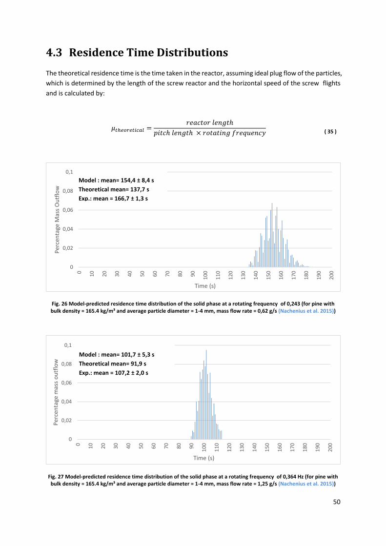
50

4.3 Residence Time Distributions

The theoretical residence time is the time taken in the reactor, assuming ideal plug flow of the particles,

which is determined by the length of the screw reactor and the horizontal speed of the screw flights

and is calculated by:

Fig. 26 Model-predicted residence time distribution of the solid phase at a rotating frequency of 0,243 (for pine with bulk density = 165.4 kg/m³ and average particle diameter = 1-4 mm, mass flow rate = 0,62 g/s (Nachenius et al. 2015))

Fig. 27 Model-predicted residence time distribution of the solid phase at a rotating frequency of 0,364 Hz (for pine with bulk density = 165.4 kg/m³ and average particle diameter = 1-4 mm, mass flow rate = 1,25 g/s (Nachenius et al. 2015))

𝜇𝑡ℎ𝑒𝑜𝑟𝑒𝑡𝑖𝑐𝑎𝑙 =𝑟𝑒𝑎𝑐𝑡𝑜𝑟 𝑙𝑒𝑛𝑔𝑡ℎ

𝑝𝑖𝑡𝑐ℎ 𝑙𝑒𝑛𝑔𝑡ℎ × 𝑟𝑜𝑡𝑎𝑡𝑖𝑛𝑔 𝑓𝑟𝑒𝑞𝑢𝑒𝑛𝑐𝑦

( 35 )

0

0,02

0,04

0,06

0,08

0,1

0

10

20

30

40

50

60

70

80

90

10

0

11

0

12

0

13

0

14

0

15

0

16

0

17

0

18

0

19

0

20

0

Per

cen

tage

Mas

s O

utf

low

Time (s)

Model : mean= 154,4 ± 8,4 s

Theoretical mean= 137,7 s

Exp.: mean = 166,7 ± 1,3 s

0

0,02

0,04

0,06

0,08

0,1

0

10

20

30

40

50

60

70

80

90

10

0

11

0

12

0

13

0

14

0

15

0

16

0

17

0

18

0

19

0

20

0

Per

cen

tage

mas

s o

utf

low

Time (s)

Model : mean= 101,7 ± 5,3 s


Exp.: mean = 107,2 ± 2,0 s

51

Fig. 26-28 show that the biomass residence time increases with decreasing rotating frequency, which

is reflected in both the experimental and model-predicted residence time distributions. At a rotating

frequency of 0,243 Hz, the solid phase had a mean residence time of 154,4 s (Fig. 26). When the screw

rotated twice as fast (0,486 Hz), the mean residence time was 78,9 s, half of the former residence time

(Fig .28). The modelled values for the mean residence times are situated between the theoretical value

and mean residence time from the experimental data, which indicates that the present model was

capable to predict the particle residence time inside screw reactor. Since the product yield in the screw

reactor was determined by the particle residence time and the temperature, the capability of

predicting the particle residence time in the model provides reliability in estimating the performance

of the screw reactor. However, the standard deviation of the distributions was much larger for the

model compared to the experimental data (Fig.26-28). Because the solid phase is represented by a

continuous phase in the model, the particles can ‘flow’ under the flights without physical restriction.

In reality particles can’t move under the flights if particle diameters exceed the height of the clearance.

Unfortunately, this effect cannot be incorporated in an Euler-Euler model. So due to friction with the

wall, particles move under the shaft, spreading the solid phase over multiple pitches. This explains the

larger variance on the residence time distributions and an increased variance with a larger mean

residence time. With a lower rotating frequency, the variance of particle residence time is larger, which

indicates that biomass particles experience heavier backmixing, and this is generally unfavourable for

the product characteristics.

0

0,02

0,04

0,06

0,08

0,1

0,12

0

10

20

30

40

50

60

70

80

90

10

0

11

0

12

0

13

0

14

0

15

0

16

0

17

0

18

0

19

0

20

0

Per

cen

tage

mas

s o

utf

low

Time (s)

Model : mean= 78,9 ± 4,9 s


Exp.: mean = 78,5 ± 0,8 s

Fig. 28 Model-predicted residence time distribution of the solid phase at a rotating frequency of 0,486 Hz (for pine with bulk density = 165.4 kg/m³ and average particle diameter = 1-4 mm, mass flow rate = 1,25 g/s (Nachenius et al. 2015))

52

4.4 Temperature

In order to determine when the model reaches statistically steady-state, the total solid mass is

monitored (Fig.29).

It can be seen in Fig. 29 that the total solid mass in the reactor initially increased linearly with a slope

equal to the mass inflow (red line). As time advanced, a deviation could be observed due to conversion

of solid mass to gasses and vapours. Around 120s the solid phase exited the reactor. Normally the

model would have reached steady-state at this point, but the total mass in the reactor slightly

decreases until it reaches a constant total mass around 250s. This means that the torrefaction reaction

and heat transfer require a longer time to achieve steady-state. At t=250s the temperature of the solid

phase was measured at different intervals near the screw of the reactor and compared with

experimental results (Fig.30).

Fig. 29 Total solid mass in the reactor model (1 section, 1,64m) as a function of time (rotating frequency= 0,292 Hz, biomass feed rate=2,48 kg/h, nitrogen feed rate = 8L/h, wall temperature= 600K)

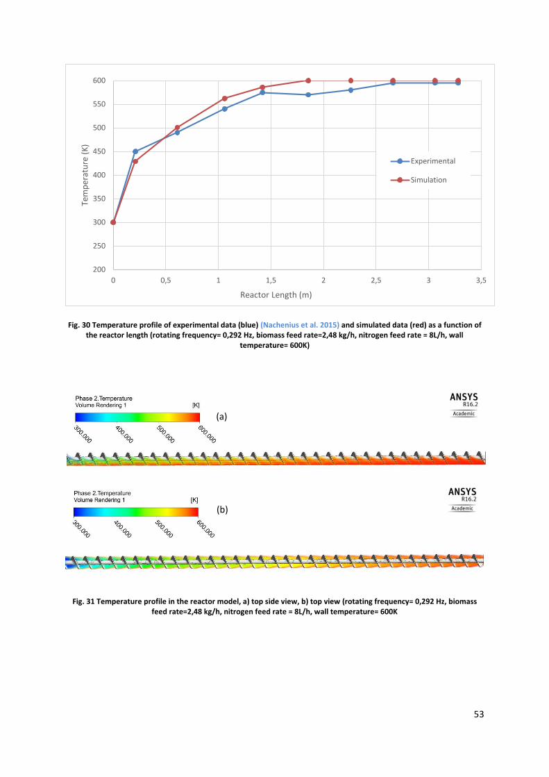
53

Fig. 30 Temperature profile of experimental data (blue) (Nachenius et al. 2015) and simulated data (red) as a function of the reactor length (rotating frequency= 0,292 Hz, biomass feed rate=2,48 kg/h, nitrogen feed rate = 8L/h, wall

temperature= 600K)

200

250

300

350

400

450

500

550

600

0 0,5 1 1,5 2 2,5 3 3,5

Tem

per

atu

re (

K)

Reactor Length (m)

Experimental

Simulation

Fig. 31 Temperature profile in the reactor model, a) top side view, b) top view (rotating frequency= 0,292 Hz, biomass feed rate=2,48 kg/h, nitrogen feed rate = 8L/h, wall temperature= 600K

(a)

(b)

54

The temperature of the biomass increases fast upon entering the reactor and is aligned with the

experimental data (Fig. 30-31). The heat of evaporation of the bound water in the biomass slows down

the temperature increase in the first part of the reactor. At the end of the first reactor section, the

temperature has reached a value of 590 K. As mentioned before, all experiments were conducted on

1 section to study the temperature profile. The temperature for the second section was extrapolated

to the wall temperature of 600K. A maximum deviation of 20 K is observed between the model results

and the experimental data in the first section. Deviation between the two curves is almost inevitable,

since the simulated temperature is strongly dependent on assumptions for the thermal conductivity,

the heat capacity, heat transfer coefficients, the packing limit and a correct implementation of the

granular flow, which determines the degree of mixing of the solid phase. Besides, the largest deviation

between two curves is observed at the end of the first reactor section. In the experimental setup, the

sections are intermittent by a connection part, where the off-gas is situated, resulting in a small

temperature drop. Since the model assumes both sections as one entity, this temperature drop is not

observed in the simulated data.

Generally, the simulated temperature-profile is in good qualitative agreement with the experimental

results, despite some quantitative differences between the model results and the experimental data.

As the product yield in the screw reactor was dependent on the particle residence time and the

temperature, the accuracy of the present model in predicting the temperature profile inside the screw

reactor provides reliability in estimating the performance of the screw reactor.

4.5 Product yield

The mass fraction of each component can only be measured for each phase individually. Nachenius et

al. 2015 reports the product yield as mass fraction of the dry biomass feed. In order to compare the

simulated product yield with the experimental product yield, the mass fraction per phase is converted

according:

In the model, the solid product yield is the summation of the biomass fraction and the char fraction,

while the liquid yield is the tar fraction and the gas yield is the mass fraction of the permanent gasses.

Table 7 compares the simulated mass fraction, as well as the theoretical approach with the Broido-

Bradbury kinetic scheme, with the experimental results.

𝑚𝑎𝑠𝑠 𝑓𝑟𝑎𝑐𝑡𝑖𝑜𝑛 (𝑑𝑟𝑦 𝑓𝑒𝑒𝑑 𝑏𝑎𝑠𝑖𝑠)(%) =

𝑚𝑎𝑠𝑠 𝑓𝑟𝑎𝑐𝑡𝑖𝑜𝑛 𝑝𝑒𝑟 𝑝ℎ𝑎𝑠𝑒 (%) × 𝑝ℎ𝑎𝑠𝑒 𝑚𝑎𝑠𝑠 𝑜𝑢𝑡𝑓𝑙𝑜𝑤 (𝑘𝑔/𝑠)

𝑏𝑖𝑜𝑚𝑎𝑠𝑠 𝑓𝑒𝑒𝑑 𝑟𝑎𝑡𝑒 (𝑘𝑔/𝑠) × (100 −𝑚𝑜𝑖𝑠𝑡𝑢𝑟𝑒 𝑐𝑜𝑛𝑡𝑒𝑛𝑡 (%))

( 36 )

55

Table 7 Comparison of the simulated product yield with experimental data (Nachenius et al. 2015) (rotating frequency= 0,292 Hz, biomass feed rate=2,48 kg/h, nitrogen feed rate = 8L/h, wall temperature= 600K)

Torrefaction is mainly used to produce solid product with enhanced physical properties (higher energy

density, better grindability, etc..). Therefore, the solid yield is the main parameter of interest in the

present simulation. Table 7 shows that the model predicts the solid yield with a relative error of about

15% compared to the experimental data. This error was acceptable considering the complex particle

hydrodynamics, heat transfer and torrefaction reactions simultaneously happening in the screw

reactor. The model overestimates the gas yield, at the expense of the solid yield. The predicted product

yield was largely determined by the particle residence time, temperature profile and the torrefaction

reactions inside the screw reactor. As mentioned above, the present model was capable to accurately

predict particle residence time and temperature profile inside the screw reactor.

Product yield Experiment (w%) Model (Kinetic scheme of Shafizadeh and Chin) (w%)

Theoretical (Kinetic scheme of Broido-Bradbury) (w%)

Solid yield 72 % 60,78 % 74,41 %

Liquid yield 22 % 23,33 % 6,72 %

Gas yield

5 % 15,89 % 18,86 %

0

0,2

0,4

0,6

0,8

1

1,2

0 0,5 1 1,5 2 2,5 3 3,5

Pro

du

ct Y

ield

(%

)

Reactor length (m)

Solid mass fraction

Liquid mass fraction

Gas mass fraction

Fig. 32 Mass fractions in function of reactor length (rotating frequency= 0,292 Hz, biomass feed rate=2,48 kg/h, nitrogen feed rate = 8L/h, wall temperature= 600K)

56

Therefore, discrepancy between the experimental data and the simulated data is mainly due to the

choice of kinetic scheme for the reaction kinetics. First of all, the kinetic scheme of Shafizadeh and Chin

is a general scheme for pyrolysis. In slow and fast pyrolysis, the gasses and tars are more abundant due

to more severe reaction conditions. The kinetic scheme of Shafizadeh and Chin and the related

Arrhenius parameters are possibly less suited for mild conditions of torrefaction processes. For

example, the activation energy for the reaction of biomass to gas is very low compared to the

activation energy for the reaction to tar. This results in a high conversion of biomass to gas at low

temperatures of torrection processes and possibly the overestimation over the gas yield. Additionally,

this kinetic scheme is a very simple representation of the reactions during torrefaction. Table 7

indicates that the more complex reaction scheme of Broido-Bradbury might be more suitable to

predict the product yield. Good results were achieved for the solid yield compared to the experimental

data. However, the results for the gas and tar yield should be reversed.

Fig.32 shows how the solid mass fraction decreases as it progresses towards the outlet, while gas and

liquid mass fraction increase. From the inlet to about 0,6m, no reaction takes place because the

temperature at that position in the reactor is not high enough yet. This part is mostly controlled by

evaporation of bound water. At 0,6 m, the temperature has reached a value of about 500 K (Fig. 30).

Devolatilization of the biomass results in a linear increase of the tar and gas mass fractions towards

the outlet, where the products are collected.

4.6 Energy balance

The product yield can be used to calculate the calorific value, if the higher heating values are known,

according to:

Consequently, the results obtained for the solids, tars and gasses are 10,97 kW, 4,03 kW and 1,83 kW.

The total heat input was calculated by integrating the heat flux over the reactor shell and had an

average value of 405 W. Therefore, the energy input of the process was much lower than the calorific

values of the products.

Important to note was that the latent heat for evaporation of the bound water consumed a large

portion of the total heat input. In order to evaporate the 12% moisture content of the biomass, a total

heat of 188 W was required, so 46,4 % of the total heat input.

𝐸𝑛𝑒𝑟𝑔𝑦 𝑜𝑢𝑡𝑝𝑢𝑡 𝑝𝑒𝑟 𝑢𝑛𝑖𝑡 𝑜𝑓 𝑡𝑖𝑚𝑒 (𝑊) =

𝑝𝑟𝑜𝑑𝑢𝑐𝑡 𝑦𝑖𝑒𝑙𝑑 (%)

100× 𝑑𝑟𝑦 𝑏𝑖𝑜𝑚𝑎𝑠𝑠 𝑓𝑒𝑒𝑑 𝑟𝑎𝑡𝑒 (

𝑘𝑔

𝑠) × 𝐻𝐻𝑉 (

𝐽

𝑘𝑔)

( 37 )

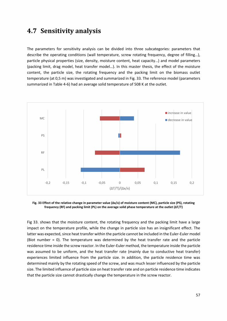
57

4.7 Sensitivity analysis

The parameters for sensitivity analysis can be divided into three subcategories: parameters that

describe the operating conditions (wall temperature, screw rotating frequency, degree of filling…),

particle physical properties (size, density, moisture content, heat capacity…) and model parameters

(packing limit, drag model, heat transfer model…). In this master thesis, the effect of the moisture

content, the particle size, the rotating frequency and the packing limit on the biomass outlet

temperature (at 0,5 m) was investigated and summarized in Fig. 33. The reference model (parameters

summarized in Table 4-6) had an average solid temperature of 508 K at the outlet.

Fig. 33 Effect of the relative change in parameter value (∆x/x) of moisture content (MC), particle size (PS), rotating frequency (RF) and packing limit (PL) on the average solid phase temperature at the outlet (∆T/T)

Fig 33. shows that the moisture content, the rotating frequency and the packing limit have a large

impact on the temperature profile, while the change in particle size has an insignificant effect. The

latter was expected, since heat transfer within the particle cannot be included in the Euler-Euler model

(Biot number = 0). The temperature was determined by the heat transfer rate and the particle

residence time inside the screw reactor. In the Euler-Euler method, the temperature inside the particle

was assumed to be uniform, and the heat transfer rate (mainly due to conductive heat transfer)

experiences limited influence from the particle size. In addition, the particle residence time was

determined mainly by the rotating speed of the screw, and was much lesser influenced by the particle

size. The limited influence of particle size on heat transfer rate and on particle residence time indicates

that the particle size cannot drastically change the temperature in the screw reactor.

-0,2 -0,15 -0,1 -0,05 0 0,05 0,1 0,15 0,2

PL

RF

PS

MC

(∆T/T)/(∆x/x)

increase in value

decrease in value

58

A decrease in temperature is observed with increased moisture content and vice-versa due to change

in latent heat of bound water evaporation. Higher rotating frequencies result in less contact time of

the biomass with the heated wall and consequently a lower temperature at the outlet. A longer solid

residence time shows the opposite. Finally, the temperature increases with a higher packing limit

because of the increased conductive heat flux. A change in the packing limit from the default value of

0,32 (see section 3.5.1) to a new value of 0,30 (Table 5) resulted in a better fit of the temperature

profile with the experimental data, while the change in volumetric degree of filling was insignificant.

4.8 Future research

First of all, there is a need for a more suitable reaction scheme to predict torrefaction product yields.

Either the Arrhenius parameters of the present reaction scheme need to be modified for mild reaction

conditions or a more complex reaction scheme needs to be implemented. The latter means that more

components and/or intermediate components need to be included in the model. This can lead to more

accurate results, but will require longer simulation times because of the increased number of

governing equations that need to be solved at each time step.

In this master thesis, only a limited amount of parameters was tested for their sensitivity towards

biomass temperature. Future work can focus on a more detailed investigation of model sensitivity

towards various operational conditions (wall temperature, screw rotating frequency, degree of

filling…), physical properties (size, density, moisture content, heat capacity…) and model parameters

(packing limit, drag model, heat transfer model…). In addition to the temperature, the effect of

different parameters on the product yield can be studied for example.

It would also be interesting to see if the present model is capable of predicting temperature profiles

and product yields for more severe reaction conditions, such as in slow or fast pyrolysis processes.

Since the reaction scheme is for pyrolysis reactions in general, the model might be able to predict the

product yields better for slow and fast pyrolysis. To achieve high temperatures for fast pyrolysis,

heated sand is usually added to the reactor. This can simply be done by including a second solid phase

in the model with the properties of sand.

The final challenge is to research if the model can be used to predict mass and heat transfer properties

in upscaled screw reactors and whether these reactors suffice to produce on commercial scale or not.

The independency of the particle size towards the heat and mass transfer in the model, is expected to

be one of the major limits of the Euler-Euler model. If the particles of the feedstock become larger, the

temperature of the particle cannot be assumed to be uniform anymore. Besides, mass transfer inside

the particle (mostly determined by diffusion in the pores) can drastically alter the reaction kinetics in

large particles.

Overall, the model is flexible and expendable for further research, but there are limitations that need

to be overcome.

59

5 Conclusion

A comprehensive CFD-model to simulate torrefaction in a screw reactor, based on a bench scale

experimental setup at Ghent University, was developed in Ansys fluent. An Euler-Euler model has been

successfully implemented to represent a multiphase system with a granular flow. Rotation of the screw

was achieved with the use of mesh motion.

Characterization of the granular flow shows similarities with flow patterns reported in the literature.

A velocity profile of the solid phase shows that particles avalanche from the top of a flight to the next

flight. At high degrees of filling, particles are thrown over the shaft. The residence time distributions

were in good agreement with theoretical and experimental mean residence times. Lower rotating

speed will result in higher variance for particle residence time, which is unfavourable for product

distribution.

The temperature progress is an important parameter for reactor design and needed careful attention

for correct implementation. The simulated temperature profile demonstrated at good fit with the

experimental data. A simple single component, single step reaction scheme was used to predict the

product yield at the reactor outlet. However, the model underestimated the solid yield. The need for

a more complex kinetic model, such as a multicomponent multistep kinetic model, could offer a

solution.

Results obtained from a sensitivity analysis and an energy balance clarified the importance of the

moisture content of the fresh biomass. Roughly half of the total heat input was used for evaporation.

Furthermore, the temperature was significantly altered by a change in packing limit and rotating

frequency, while the particle size had no effect. The latter is one of the limits of the Euler-Euler model,

since large particles can influence the mass transfer, heat transfer and reaction kinetics drastically.

Future work can further study the sensitivity of the model towards operational conditions, physical

properties and model parameters. Different kinetic schemes need to be investigated, in order to find

more suitable kinetic scheme for the mild conditions of torrefaction. Finally, the model can be used to

research whether the mass- and heat transfer properties are retained in upscaled reactors for

commercial use.

61

6 References

"http://www.biocharproducts.com/." Accesed on 18/04/16.

"http://www.pyne.co.uk/?_id=156." Accesed on 18/04/16.

"http://www.pyreg.de/." Accesed on 18/04/16.

"http://www.sonnenerde.at/index.php?route=common/page&id=1254." Accesed on 18/04/16.

"http://www.swiss-biochar.com/." Accesed on 18/04/16.

"http://www.verora.ch/page/de/verora-pflanzenkohle." Accesed on 18/04/16.

Altomare, R. E. and P. Ghossi (1986). "An Analysis of Residence Time Distribution Patterns in a Twin Screw Cooking Extruder." Biotechnology Progress 2(3): 157-163.

Andersson, B. (2012). Computational fluid dynamics for engineers. Cambridge ; New York, Cambridge University Press.

ANSYS (2013). "ANSYS Fluent Theory Guide."

Aramideh, S., Q. G. Xiong, S. C. Kong and R. C. Brown (2015). "Numerical simulation of biomass fast pyrolysis in an auger reactor." Fuel 156: 234-242.

Bates, R. B. and A. F. Ghoniem (2014). "Modeling kinetics-transport interactions during biomass torrefaction: The effects of temperature, particle size, and moisture content." Fuel 137: 216-229.

Bokkers, G. A. V. S. A., M., Kuipers, J.A.M. (2004). "Comparison of continuum models using the kinetic theory of granular flow with discrete particle models and experiments: extent of particle mixing induced by bubbles." Proceedings of Fluidization 11: 187-194.

Bradbury AGW, S. Y., Shafizadeh F. (1979). "Kinetic model for pyrolysis of celulose." Journal of Applied Polymer Science 23(11): 3271–3280.

Brewer, C. E., K. Schmidt-Rohr, J. A. Satrio and R. C. Brown (2009). "Characterization of Biochar from Fast Pyrolysis and Gasification Systems." Environmental Progress & Sustainable Energy 28(3): 386-396.

Bridgwater, A. V. (2003). "Renewable fuels and chemicals by thermal processing of biomass." Chemical Engineering Journal 91(2-3): 87-102.

Bridgwater, A. V. (2012). "Review of fast pyrolysis of biomass and product upgrading." Biomass & Bioenergy 38: 68-94.

Brown, J. N. (2009). "Development of a lab-scale auger reactor for biomass fast pyrolysis and process optimization using response surface methodology."

http://www.biocharproducts.com/

http://www.pyne.co.uk/?_id=156.

http://www.pyreg.de/

http://www.sonnenerde.at/index.php?route=common/page&id=1254.

http://www.swiss-biochar.com/

http://www.verora.ch/page/de/verora-pflanzenkohle.

62

Brown, J. N. and R. C. Brown (2012). "Process optimization of an auger pyrolyzer with heat carrier using response surface methodology." Bioresource Technology 103(1): 405-414.

Butler E., D. G., Meier D., McDonnell K. (2011). "A review of recent laboratory research and commercial developments in fast pyrolysis and upgrading." Renewable and Sustainable Energy Reviews 15: 4171-4186.

Camp, D. W. (1990). "Mild Coal Gasification - Screw Pyrolyzer Development and Design." Lawrence Livermore National Laboratory.

Di Blasi, C. (2008). "Modeling chemical and physical processes of wood and biomass pyrolysis." Progress in Energy and Combustion Science 34(1): 47-90.

Doolan, K. R., J. C. Mackie and R. J. Tyler (1987). "Coal Flash Pyrolysis - Secondary Cracking of Tar Vapors in the Range 870-2000 K." Fuel 66(4): 572-578.

Fang, M. M., K. Luo, S. L. Yang, K. Zhang and J. R. Fan (2013). "Computational Fluid Dynamics-Discrete Element Method Investigation of Solid Mixing Characteristics in an Internally Circulating Fluidized Bed." Industrial & Engineering Chemistry Research 52(22): 7556-7568.

Gao, J., G. C. Walsh, D. Bigio, R. M. Briber and M. D. Wetzel (1999). "Residence-time distribution model for twin-screw extruders." Aiche Journal 45(12): 2541-2549.

Gidaspow, D. (1994). Multiphase flow and fluidization : continuum and kinetic theory descriptions. Boston, Academic Press.

Gunn, D. J. (1978). "Transfer of Heat or Mass to Particles in Fixed and Fluidized-Beds." International Journal of Heat and Mass Transfer 21(4): 467-476.

Guo Mingxin, W. S., Jeremy Buhain (2015). "Bioenergy and biofuels: History, status, and perspective." Renewable and Sustainable Energy Reviews 42: 712-725.

Harada, T., T. Hata and S. Ishihara (1998). "Thermal constants of wood during the heating process measured with the laser flash method." Journal of Wood Science 44(6): 425-431.

Hook, M. and X. Tang (2013). "Depletion of fossil fuels and anthropogenic climate change-A review." Energy Policy 52: 797-809.

Hou, Q. F., K. J. Dong and A. B. Yu (2014). "DEM study of the flow of cohesive particles in a screw feeder." Powder Technology 256: 529-539.

Hua, L. N., H. Zhao, J. Li, J. W. Wang and Q. S. Zhu (2015). "Eulerian-Eulerian simulation of irregular particles in dense gas-solid fluidized beds." Powder Technology 284: 299-311.

Ingram, L., D. Mohan, M. Bricka, P. Steele, D. Strobel, D. Crocker, B. Mitchell, J. Mohammad, K. Cantrell and C. U. Pittman (2008). "Pyrolysis of wood and bark in an auger reactor: Physical properties and chemical analysis of the produced bio-oils." Energy & Fuels 22(1): 614-625.

Kambo, H. S. and A. Dutta (2015). "A comparative review of biochar and hydrochar in terms of production, physico-chemical properties and applications." Renewable & Sustainable Energy Reviews 45: 359-378.

63

Kingston, T. A. and T. J. Heindel (2014). "Granular mixing optimization and the influence of operating conditions in a double screw mixer." Powder Technology 266: 144-155.

Koufopanos, C. A., G. Maschio and A. Lucchesi (1989). "Kinetic Modeling of the Pyrolysis of Biomass and Biomass Components." Canadian Journal of Chemical Engineering 67(1): 75-84.

Kruggel-Emden, H., S. Wirtz, E. Simsek and V. Scherer (2006). "Modeling of granular flow and combined heat transfer in hoppers by the discrete element method (DEM)." Journal of Pressure Vessel Technology-Transactions of the Asme 128(3): 439-444.

Kumar, A., J. Vercruysse, V. Vanhoorne, M. Toiviainen, P. E. Panouillot, M. Juuti, C. Vervaet, J. P. Remon, K. V. Gernaey, T. De Beer and I. Nopens (2015). "Conceptual framework for model-based analysis of residence time distribution in twin-screw granulation." European Journal of Pharmaceutical Sciences 71: 25-34.

Laird D.A., B. R. C., Amonette J.E., Lehmann J. (2009). "Review of the pyrolysis platform for coproducing bio-oil and biochar." Biofuels, Bioproducts & Biorefining 3: 547–562.

Lakshman.Cm, B. Galor and Hoelsche.He (1969). "Production of Levoglucosan by Pyrolysis of Carbohydrates." Industrial & Engineering Chemistry Product Research and Development 8(3): 261-&.

Lin, L., S. J. Khang and T. C. Keener (1997). "Coal desulfurization by mild pyrolysis in a dual-auger coal feeder." Fuel Processing Technology 53(1-2): 15-29.

Lun, C. K. K., S. B. Savage, D. J. Jeffrey and N. Chepurniy (1984). "Kinetic Theories for Granular Flow - Inelastic Particles in Couette-Flow and Slightly Inelastic Particles in a General Flowfield." Journal of Fluid Mechanics 140(Mar): 223-256.

Mahmoudi, A. H., F. Hoffmann and B. Peters (2014). "Detailed numerical modeling of pyrolysis in a heterogeneous packed bed using XDEM." Journal of Analytical and Applied Pyrolysis 106: 9-20.

Makkawi, Y. T., P. C. Wright and R. Ocone (2006). "The effect of friction and inter-particle cohesive forces on the hydrodynamics of gas-solid flow: A comparative analysis of theoretical predictions and experiments." Powder Technology 163(1-2): 69-79.

McKendry, P. (2002a). "Energy production from biomass (Part 1): Overview of biomass." Bioresour Technol 83(1): 37-46.

McKendry, P. (2002b). "Energy production from biomass (Part 2): Conversion technologies." Bioresour Technol 83(1): 47-54.

Mellin, P., Q. L. Zhang, E. Kantarelis and W. H. Yang (2013). "An Euler-Euler approach to modeling biomass fast pyrolysis in fluidized-bed reactors - Focusing on the gas phase." Applied Thermal Engineering 58(1-2): 344-353.

Miller, R. S. and J. Bellan (1998). "Numerical simulation of vortex pyrolysis reactors for condensable tar production from biomass." Energy & Fuels 12(1): 25-40.

Nachenius, R. W., Kiel, J. H. A., Prins, W. (2015). "Torrefaction: upgrading biomass into high-quality solid bioenergy carriers." Biomass power for the world 6: 395 - 424.

64

Nachenius, R. W., T. A. van de Wardt, F. Ronsse and W. Prins (2014). "Torrefaction of Biomass in a Continuous Rotating Screw Reactor." Papers of the 22nd European Biomass Conference: Setting the Course for a Biobased Economy: 1018-1024.

Nachenius, R. W., T. A. van de Wardt, F. Ronsse and W. Prins (2015). "Residence time distributions of coarse biomass particles in a screw conveyor reactor." Fuel Processing Technology 130: 87-95.

Nachenius, R. W., T. A. van de Wardt, F. Ronsse and W. Prins (2015). "Torrefaction of pine in a bench-scale screw conveyor reactor." Biomass & Bioenergy 79: 96-104.

Owen, P. J. and P. W. Cleary (2009). "Prediction of screw conveyor performance using the Discrete Element Method (DEM)." Powder Technology 193(3): 274-288.

Ozel, A., P. Fede and O. Simonin (2013). "Development of filtered Euler-Euler two-phase model for circulating fluidised bed: High resolution simulation, formulation and a priori analyses." International Journal of Multiphase Flow 55: 43-63.

Papadikis, K., A. V. Bridgwater and S. Gu (2008). "CFD modelling of the fast pyrolysis of biomass in fluidised bed reactors, Part A: Eulerian computation of momentum transport in bubbling fluidised beds." Chemical Engineering Science 63(16): 4218-4227.

Papadikis, K., S. Gu and A. V. Bridgwater (2010). "Computational modelling of the impact of particle size to the heat transfer coefficient between biomass particles and a fluidised bed." Fuel Processing Technology 91(1): 68-79.

Papadikis, K., S. Gu, A. V. Bridgwater and H. Gerhauser (2009). "Application of CFD to model fast pyrolysis of biomass." Fuel Processing Technology 90(4): 504-512.

Peacocke, G. V. C. and A. V. Bridgwater (1994). "Ablative Plate Pyrolysis of Biomass for Liquids." Biomass & Bioenergy 7(1-6): 147-154.

Pieters, J. and N. Verhoest (2013). "Fyscia 4 : fysische transportverschijnselen."

Pittman, C. U., D. Mohan, A. Eseyin, Q. Li, L. Ingram, E. B. M. Hassan, B. Mitchell, H. Guo and P. H. Steele (2012). "Characterization of Bio-oils Produced from Fast Pyrolysis of Corn Stalks in an Auger Reactor." Energy & Fuels 26(6): 3816-3825.

Puy, N., R. Murillo, M. V. Navarro, J. M. Lopez, J. Rieradevall, G. Fowler, I. Aranguren, T. Garcia, J. Bartroli and A. M. Mastral (2011). "Valorisation of forestry waste by pyrolysis in an auger reactor." Waste Management 31(6): 1339-1349.

Ratte, J., E. Fardet, D. Mateos and J. S. Hery (2011). "Mathematical modelling of a continuous biomass torrefaction reactor: TORSPYD (TM) column." Biomass & Bioenergy 35(8): 3481-3495.

Ren, B., Y. J. Shao, W. Q. Zhong, B. S. Jin, Z. L. Yuan and Y. Lu (2012). "Investigation of mixing behaviors in a spouted bed with different density particles using discrete element method." Powder Technology 222: 85-94.

Roberts, A. W. (1999). "The influence of granular vortex motion on the volumetric performance of enclosed screw conveyors." Powder Technology 104(1): 56-67.

Ronsse, F. (2013). "Commercial biochar production and its certification." Interreg Conference.

65

Sarkar, A. and C. Wassgren (2010). "Continuous blending of cohesive granular material." Chemical Engineering Science 65(21): 5687-5698.

Schaeffer, D. G. (1987). "Instability in the evolution equations describing incompressible granular flow." Journal of Differential Equations 66(1): 19-50.

Shafiee, S. and E. Topal (2009). "When will fossil fuel reserves be diminished?" Energy Policy 37(1): 181-189.

Shafizadeh, F. and P. P. S. Chin (1976). "Thermal Deterioration of Wood." Abstracts of Papers of the American Chemical Society 172(Sep3): 37-37.

Sharma, A., V. Pareek and D. K. Zhang (2015). "Biomass pyrolysis-A review of modelling, process parameters and catalytic studies." Renewable & Sustainable Energy Reviews 50: 1081-1096.

Sun, L. Y., S. Y. Wang, H. Lu, G. D. Liu, H. L. Lu, Y. Liu and F. X. Zhao (2014). "Simulations of configurational and granular temperatures of particles using DEM in roller conveyor." Powder Technology 268: 436-445.

Suopajarvi, H., E. Pongracz and T. Fabritius (2013). "The potential of using biomass-based reducing agents in the blast furnace: A review of thermochemical conversion technologies and assessments related to sustainability." Renewable & Sustainable Energy Reviews 25: 511-528.

Todd, D. B. (1975). "Residence Time Distribution in Twin-Screw Extruders." Polymer Engineering and Science 15(6): 437-443.

Tsai, W. R. and C. I. Lin (1994). "On the Mixing of Granular-Materials in a Screw Feeder." Powder Technology 80(2): 119-126.

Wagenaar, B. M., W. Prins and W. P. M. Van Swaaij (1994). "Pyrolysis of biomass in the rotating cone reactor: Modelling and experimental justification." Chemical Engineering Science 49(24b): 5109-5126.

Waje, S. S., A. K. Patel, B. N. Thorat and A. S. Mujumdar (2007). "Study of residence time distribution in a pilot-scale screw conveyor dryer." Drying Technology 25(1-3): 249-259.

Wan, Y. K. and T. R. Hanley (2004). "Computational fluid dynamics simulation and redesign of a screw conveyor reactor." Applied Biochemistry and Biotechnology 113: 733-745.

Williams, P. T. and S. Besler (1996). "The influence of temperature and heating rate on the pyrolysis of biomass." Renewable Energy 7(3): 233-250.

Woody, G. V. (1941). "Production of coke as a domestic fuel source. The Hayes process for carbonizing coal at low temperatures." Industrial & Engineering Chemistry Research 33: 841-846.

Xiong, Q. G., S. Aramideh and S. C. Kong (2014). "Assessment of Devolatilization Schemes in Predicting Product Yields of Biomass Fast Pyrolysis." Environmental Progress & Sustainable Energy 33(3): 756-761.

Xiong, Q. G., S. C. Kong and A. Passalacqua (2013). "Development of a generalized numerical framework for simulating biomass fast pyrolysis in fluidized-bed reactors." Chemical Engineering Science 99: 305-313.

66

Xue, Q., T. J. Heindel and R. Fox (2011). "A CFD model for biomass fast pyrolysis in fluidized-bed reactors." Chemical Engineering Science 66(11): 2440-2452.

Zaror, C. A., I. S. Hutchings, D. L. Pyle, H. N. Stiles and R. Kandiyoti (1985). "Secondary Char Formation in the Catalytic Pyrolysis of Biomass." Fuel 64(7): 990-994.

67

7 Addendum

Guide for model implementation in Ansys Fluent

Introduction

This guide gives a detailed description of a step-by-step implementation of the model for the screw

reactor in Ansys Fluent 16.2. When fluent is started, the mesh is automatically imported from the

meshing interface into the modelling interface. If the mesh was not generated in the Ansys meshing

interface, a grid needs to be imported from an external source.

General

In the general setup menu, a transient model is selected, which is a time-dependent study. The gravity

is included by defining a gravitional accelaration in the negative x-direction (the direction depends on

how the geometry is constructed in the coordinate system).

68

Models

In order to simulate a two phase system with heat transfer and reaction kinetics, the multiphase model

is included for configuraton of the Euler-Euler model, the energy model represents the heat transfer

and the species transport is added to include reaction kinetics.

69

The Eulerian model is selected with 2 phases: the discrete phase and the continous phase. The implicit

formulation is selected for the best solution. The energy model is included by simply checking the box.

Reaction only takes place in the bulk, so only volumetric reactions are added. The phase properties are

defined by the continuous and discrete phase by default and are configurated later in the set-up.

Transport by diffusion is neglected in this model.

Materials

In the material set-up, the properties of the phases and their components are defined. Each phase is

represented by by a mixture of ‘species ’. The species, or better components, are added as a fluid, since

the Euler-Euler model consists of two continuous phases. The different properties of each component

are summarized in Table 4.

70

If the properties of all components are defined, the ‘mixtures’ can be composed, which are basically

the gas phase and the solid phase. The solid phase consists of the biomass, the char and the bound

water. The gas phase on the other hand consists of the permanent gasses, tars, water vapour and the

inert nitrogen gas. The reaction setup for the ‘mixtures’ can only be used for homogeneous reactions.

The reaction of biomass to char is implemented here with the associated Arrhenius parameters (Table

2). The properties of each phase are summarized in Table 5.

Phases

The phases set-up is used to associate each phase with its respective ‘mixture’. The primary phase is

the continuous phase by default, while the secondary phase is the phase that is modified by the kinetic

theory of granular flow.

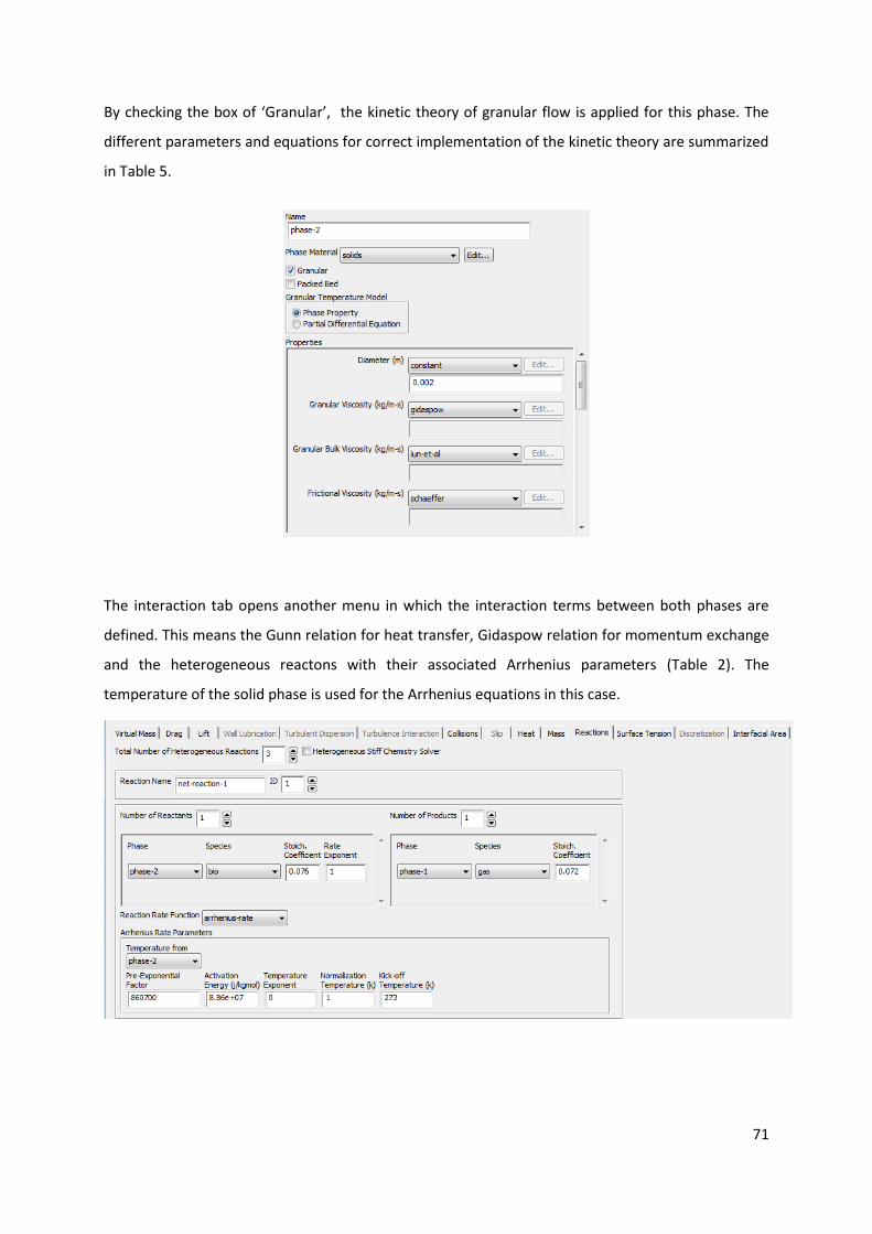
71

By checking the box of ‘Granular’, the kinetic theory of granular flow is applied for this phase. The

different parameters and equations for correct implementation of the kinetic theory are summarized

in Table 5.

The interaction tab opens another menu in which the interaction terms between both phases are

defined. This means the Gunn relation for heat transfer, Gidaspow relation for momentum exchange

and the heterogeneous reactons with their associated Arrhenius parameters (Table 2). The

temperature of the solid phase is used for the Arrhenius equations in this case.

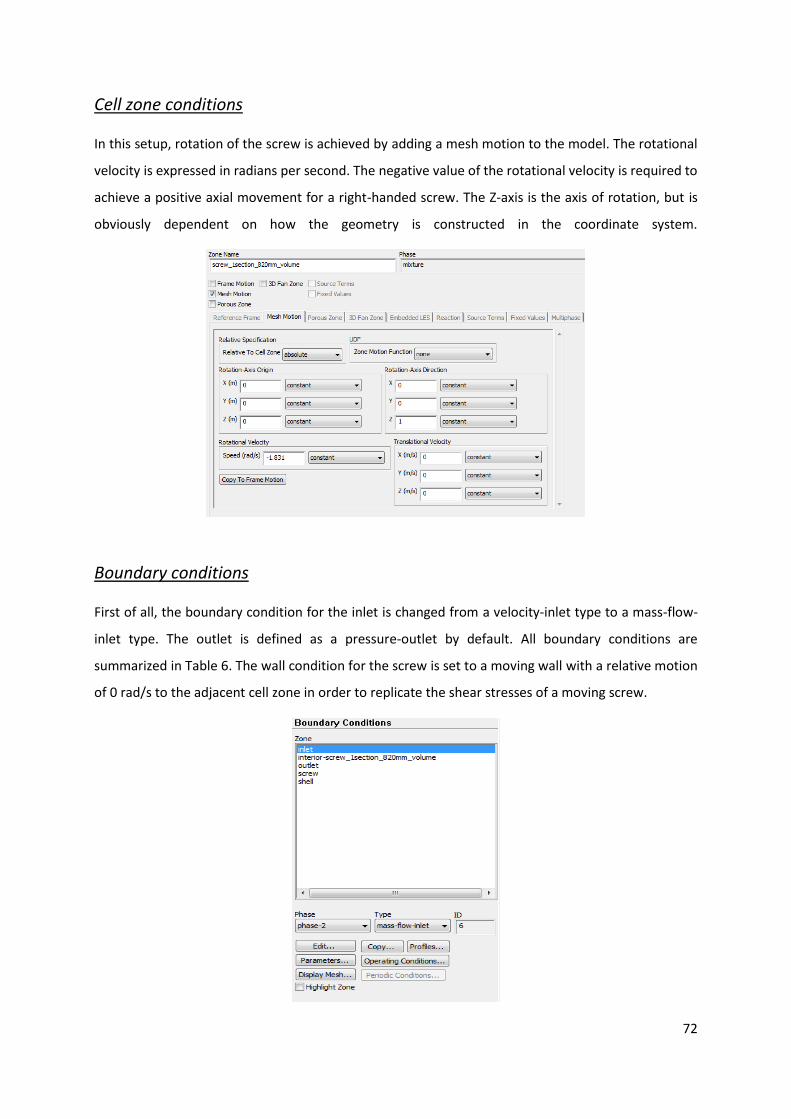
72

Cell zone conditions

In this setup, rotation of the screw is achieved by adding a mesh motion to the model. The rotational

velocity is expressed in radians per second. The negative value of the rotational velocity is required to

achieve a positive axial movement for a right-handed screw. The Z-axis is the axis of rotation, but is

obviously dependent on how the geometry is constructed in the coordinate system.

Boundary conditions

First of all, the boundary condition for the inlet is changed from a velocity-inlet type to a mass-flow-

inlet type. The outlet is defined as a pressure-outlet by default. All boundary conditions are

summarized in Table 6. The wall condition for the screw is set to a moving wall with a relative motion

of 0 rad/s to the adjacent cell zone in order to replicate the shear stresses of a moving screw.

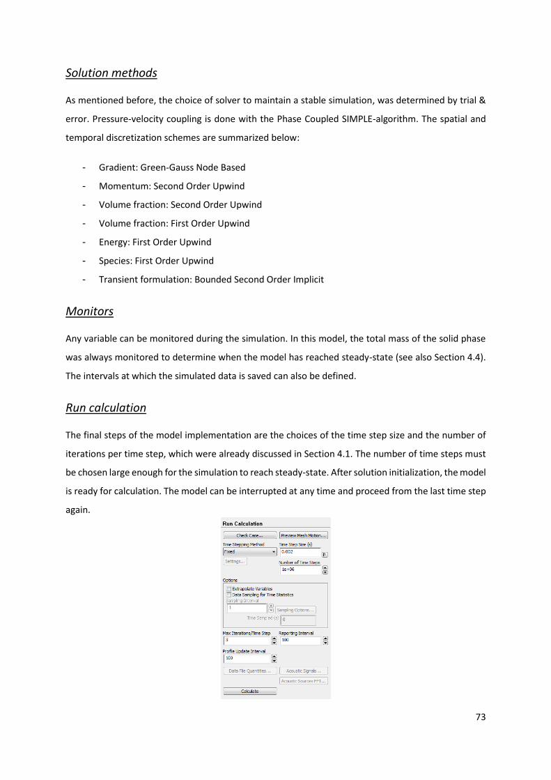
73

Solution methods

As mentioned before, the choice of solver to maintain a stable simulation, was determined by trial &

error. Pressure-velocity coupling is done with the Phase Coupled SIMPLE-algorithm. The spatial and

temporal discretization schemes are summarized below:

- Gradient: Green-Gauss Node Based

- Momentum: Second Order Upwind

- Volume fraction: Second Order Upwind

- Volume fraction: First Order Upwind

- Energy: First Order Upwind

- Species: First Order Upwind

- Transient formulation: Bounded Second Order Implicit

Monitors

Any variable can be monitored during the simulation. In this model, the total mass of the solid phase

was always monitored to determine when the model has reached steady-state (see also Section 4.4).

The intervals at which the simulated data is saved can also be defined.

Run calculation

The final steps of the model implementation are the choices of the time step size and the number of

iterations per time step, which were already discussed in Section 4.1. The number of time steps must

be chosen large enough for the simulation to reach steady-state. After solution initialization, the model

is ready for calculation. The model can be interrupted at any time and proceed from the last time step

again.

Master in de bio - ingenieurswetenschappen: Chemie en ... · iii Woord vooraf Deze masterproef kwam...

Documents

Transcript of Master in de bio - ingenieurswetenschappen: Chemie en ... · iii Woord vooraf Deze masterproef kwam...