A Koiter-Newton arclength method for buckling-sensitive ...
191
A Koiter-Newton arclength method for buckling-sensitive structures
Transcript of A Koiter-Newton arclength method for buckling-sensitive ...

A Koiter-Newton arclength method
for buckling-sensitive structures

A Koiter-Newton arclength method
for buckling-sensitive structures
Proefschrift
ter verkrijging van de graad van doctoraan de Technische Universiteit Delft,
op gezag van de Rector Magnificus Prof.dr.ir. K.C.A.M. Luyben,voorzitter van het College voor Promoties,
in het openbaar te verdedigen op vrijdag 19 july 2013 om 10.00 uur
door
Ke Liang
Bachelor of Aircraft Design Engineering,Northwestern Polytechnical University, Xi’an, China
geboren te Luoyang, China.
Dit proefschrift is goedgekeurd door de promotoren:Prof.dr. Z. Gurdal
Copromotor: Dr. M.M. Abdalla
Samenstelling promotiecommissie:
Rector Magnificus: voorzitterProf. dr. Z. Gurdal Technische Universiteit Delft, promotorDr. M.M. Abdalla Technische Universiteit Delft, copromotorProf. dr. ir. M.J.L. van Tooren Technische Universiteit DelftProf. dr. A.V. Metrikine Technische Universiteit DelftProf. dr. V.V. Toropov University of LeedsProf. dr. V.V. Vasiliev Russian Academy of SciencesProf. dr. Q. Sun Northwestern Polytechnical University
Keywords: Buckling/Imperfection/Geometric Nonlinearity/Path-following/Koiter-Newton Approach/Reduced Order Model/Finite Elements.
ISBN 978-94-6203-387-0
Copyright c©2013 by Ke Liang
All right reserved. No part of the material protected by the copyright notice maybe reproduced or utilised in any form or by any means, electronic or mechanical, in-cluding photocopying, recording or by any information storage and retrieval system,without the prior written permission by the author.
Printed by: Wohrmann Print Service, Zutphen, the Netherlands

Dedicated to my parents and Xiaxia

iv
Forewords
I have worked as a Ph.D. researcher in the Department of Aerospace Structuresand Computational Mechanics at Faculty of Aerospace Engineering, TUDelft fora period of three years. At the completion of this thesis, first, I would like tothank my promoter Prof.dr. Z. Gurdal who provided me with patient guidance andunflinching encouragement during my research. Even now, I remember the firstemail that I sent to him to apply to become, if possible, a guest Ph.D researcher inhis group and his warm response. Then, many thanks to my daily supervisor Dr.Mostafa Abdalla, who offered me constructive advices and timely critiques on mywork and also constantly encourage me to conduct my research independently.
I would also like to thank my supervisor Prof. Sun Qin in China. He taught mehow to become a researcher when I started my Ph.D study, and additionally he hascontinued to provide valuable support to me during my time abroad. I would liketo thank the China Scholarship Council, for giving me a one-year scholarship. Theresearch leading to these results has also received funding from the European Com-munitys Seventh Framework Programme ([FP7/2007-2013]) under grant agreementn0282522. Thank yous to my DESICOS project partners, Prof. Richard.Degenhardt(from DLR), Dr. Mark.W.Hilburger (from NASA) and the others, all of whom havegiven me many suggestions and advices, that have improved my research work.
Many thanks to Ir. Jan Hol, Dr. Roeland De Breuker, Dr. Martin Ruess andDr. Christos Kassapoglou, good partners for any project. Thanks to Laura, whogave me so much help on the administrative issues and kept me sane. I also wantto thank Miranda Aldham-Breary for teaching me a pure English and reviewingthe text carefully. Thanks to Ir. Daniel Peeters and Dr. Roeland De Breuker fortranslating some parts of my thesis into Dutch. My last, but not least thanks to allof my office colleagues. It has been a great pleasure working with so many helpfuland nice colleagues in the AeS group. During my studies at Delft, I have been verylucky to make many good friends. Thank you all for lighting up my life here.
Moreover, I thank all the committee members for kindly agreeing to devote timeand effort in judging and giving precious opinions to this thesis.
Finally, this thesis is specially dedicated to my parents and my love Xiaxia Shen fortheir unconditional love. Without their support, I could not have come this far.
v

vi
Summary
Thin-walled structures, when properly designed, possess a high strength-to-weightand stiffness-to-weight ratio, and therefore are used as the primary components insome weight critical structural applications, such as aerospace and marine engineer-ing. These structures are prone to be limited in their load carrying capability bybuckling, while staying in the linear elastic range of the material. Buckling of thin-walled structures is an inherently nonlinear phenomena. When the material stayswithin its linear elastic range, the source of the nonlinearity is purely geometric.Thus, the analysis of nonlinear response of structures, especially thin-walled struc-tures which are buckling sensitive, is important for determining their load carryingcapability. For this reason, structural geometric nonlinearities are increasingly takeninto account in engineering design. Nowadays, with the expanding computationalpower of modern computers nonlinear finite element analysis using commercial soft-ware is becoming the standard technique used to obtain the nonlinear response ofcomplex structures, however, the repeated analyses that are needed in the designphase are still computationally intensive, in terms of the computation time requiredto run large models, even for modern computers. For this reason, reduced ordertechniques that reduce the problem size are attractive whenever repetitive analysesare required, such as in design optimization.
Research on reduced order modeling of the nonlinear response of structures hasattracted much attention from researchers. Some analytic techniques constitute verypowerful tools for reducing the number of degrees of freedom (DOFs) in a nonlinearsystem, such as the Rayleigh-Ritz techniques and perturbation techniques. Thesetwo reduced basis techniques can be implemented in both analytical and numericalcontexts, and due to the modeling versatility of the finite element method (FEM),most researchers prefer to reconstruct them within the FEM context, referred toas reduction methods. There are two families of reduction methods which can berecognized. The first family consists the path-following reduction methods whichare based on some analytic techniques to reduce the number of DOFs in the fullmodel and are able to trace the entire nonlinear equilibrium path of structuresautomatically, while they may find difficulties in the presence of buckling. Koiterreduction methods belong to the second family, and they are very good at handlingthe buckling sensitive cases due to the use of Koiter’s classical initial postbucklingtheory, but the Koiter perturbation approach also limits the validity of these methodsto a small range around the bifurcation point. The focus of the research reported inthis thesis therefore is to find ways to synthesize the advantages of current reductionmethods and obtain a new reduced basis path-following approach.
In this thesis, a new approach called the Koiter-Newton (K-N) is presented for the
vii
viii
numerical solution of a class of elastic nonlinear structural analysis problems. Themethod combines ideas from Koiter’s initial post-buckling analysis and Newton arc-length methods to obtain an algorithm that is accurate over the entire equilibriumpath of structures and efficient in the presence of buckling and/or imperfectionsensitivity.
The proposed approach is performed in a step by step manner to trace the entireequilibrium path, as is commonly used in the classical Newton arc-length method.In every expansion step, the approach works by combining a prediction step usinga nonlinear reduced order model (ROM) based on Koiter’s initial postbuckling ex-pansion with a Newton arc-length correction procedure. This nonlinear predictionprovided by the reduced order model is much better compared to linear predictorsused by the classical Newton-Raphson method, thus allowing the algorithm to usefairly large step sizes.
The basic premise behind the proposed approach is the use of Koiter’s asymptoticexpansion from the beginning rather than using it only at the bifurcation point incontrast to the traditional Koiter approaches. In each asymptotic expansion, theforce space is reduced by the span of a set of perturbation loads that are chosen toexcite the possible buckling branches. According to the stability of the equilibriumpoint, at which the asymptotic expansion is applied, different ways for selectingthe perturbation loads are proposed. The proposed selection rules guarantee thatthe expansion step of the proposed approach can be applied at any point along theequilibrium path.
The proposed technique requires derivatives of the element load vectors with respectto the degrees of freedom up to the third order. This is two orders more than whatis traditionally needed for Newton’s method. To facilitate differentiation, nonlinearelements based on the element independent co-rotational frame are applied in theKoiter-Newton analysis. Automatic differentiation is used to find the derivatives ofthe co-rotational frame with respect to element degrees of freedom. In this way, fullnonlinear kinematics are taken into account when constructing the reduced ordermodel.
In some cases, the nonlinear in-plane rotations of structures can be neglected, al-though the rotations of the normals to the mid-surface are finite. In such cases,Von Karman kinematics, which ignore some nonlinear items in the Green’s stain-displacement relations, possess an acceptable accuracy compared with the full non-linear kinematics. Hence, the Koiter-Newton approach is also implemented basedon Von Karman kinematics to achieve a better computational efficiency.
Various numerical examples of beam and shell models are presented and used to
ix
evaluate the performance of the method. The Koiter-Newton analyses using the co-rotational kinematics and the Von Karman kinematics are accurate and more compu-tational efficient, compared with the results obtained using ABAQUS which adopts afull nonlinear analysis. The improved efficiency demonstrated by the Koiter-Newtontechnique will open the door to the direct use of detailed nonlinear finite elementmodels in the design optimization of next generation flight and launch vehicles.

x
Samenvatting
Dunwandige structuren hebben een hoge sterkte-gewicht en stijfheid-gewicht ver-houding als ze goed ontworpen zijn en worden daarom gebruikt als primaire con-structies in bepaalde gewicht-kritische toepassingen zoals lucht-en ruimtevaart ofzeevaart technologie. Deze structuren zijn beperkt in hun krachtdragende capaciteitdoor knik terwijl het materiaal nog in het linear-elastische bereik is. Knik van dun-wandige structuren is een inherent niet-lineair fenomeen. Als het materiaal binnenzijn lineair-elastische gebied blijft, is de bron van de niet-lineariteit puur geometrisch.De analyse van niet-lineaire structuren is dus belangrijk om hun krachtdragende ca-paciteit te berekenen, zeker bij dunwandige structuren, die knikgevoelig zijn. Dit isde reden dat er meer en meer rekening gehouden wordt met structureel geometrischeniet-lineariteit. Door de steeds toenemende rekenkracht van moderne computersworden niet-lineaire eindige elementen analyses tegenwoordig de standaardtechniekom de niet-lineaire respons van complexe structuren te berekenen. Echter, de ho-eveelheid analyses die nodig zijn in de ontwerpfase zijn erg rekenintensief voor grotestructuren en vragen dus veel tijd, zelfs op moderne computers. Hierdoor zijn lagere-orde technieken die de grootte van het probleem reduceren erg aantrekkelijk wanneermeerdere analyses nodig zijn, zoals in ontwerpoptimalisatie.
Het lagere-orde modelleren van de niet-lineaire respons van structuren is al vaakonderzocht. Sommige analytische technieken vormen erg krachtige manieren om hetaantal vrijheidsgraden in een niet-lineair systeem te reduceren, zoals Rayleigh-Ritzen perturbatietechnieken. Deze twee basistechnieken kunnen zowel in een analytis-che als in een numerieke context geımplementeerd worden, en door de flexibiliteitdie de eindige elementen methode biedt, verkiezen de meeste onderzoekers om ze teimplementeren in de eindige elementen context. Hieraan wordt gerefereerd als reduc-tiemethodes. Er kunnen twee soorten reductiemethodes onderscheiden worden. Deeerste soort bestaat uit de evenwichtspadtracerende reductiemethodes die gebaseerdzijn op analystische technieken om het aantal vrijheidsgraden in een volledig model tereduceren en in staat zijn om automatisch het volledige niet-lineaire evenwichtspadvan de structuur te bepalen, terwijl ze soms falen bij knikverschijnselen. Koiterreduceermethodes behoren tot de tweede soort en zijn erg goed in het berekenenvan knikgevoelige structuren door het gebruik van Koiter’s klassieke initiele post-knik theorie. Maar de Koiter perturbatiemethode limiteert de geldigheid van dezemethodes tot een kleine omgeving rond het vertakkingspunt. De focus van het on-derzoek in deze thesis ligt daarom op het vinden van manieren om de voordelenvan de huidige reduceermethodes te combineren en het vinden van een nieuwe even-wichtspadtracerende reductiemethode.
In deze thesis is een nieuwe methode voor het numeriek oplossen van een klasse
xi
xii
van niet-lineaire structurele analyse problemen geponeerd. Deze methode wordtKoiter-Newton (K-N) genoemd. De methode combineert ideen van Koiter’s initielepost-knik analyse en Newton’s booglengte methode om een algoritme te bekomendat accuraat is over het hele evenwichtspad van de structuren en efficient is als kniken/of imperfectiegevoeiligheid aanwezig zijn.
Het hele evenwichtspad wordt stap voor stap gereconstrueerd, zoals het gewoonlijkwordt gedaan in de klassieke Newton booglengte methode. Voor elke nieuwe stap iser een voorspellende stap, die gebruik maakt van het niet-lineaire lagere-orde modelgebaseerd op Koiter’s initiele post-knik expansie, en die gevolgd wordt door een New-ton booglengte correctie. Deze niet-lineaire voorspelling door het lagere-orde modelis veel beter vergeleken met lineaire voorspellers gebruikt in de klassieke Newton-Raphson methode en laat het algoritme dus toe een redelijk grote stapgrootte tegebruiken.
De basis van de voorgestelde methode is het gebruik van Koiter’s asymptotische ex-pansie van in het begin, dit in tegenstelling tot de klassieke Koiter methode waarbijhet enkel wordt gebruikt bij het vertakkingspunt. In iedere asymptotische expansie isde kracht-ruimte gereduceerd door een set van kleine krachten die mogelijk knikvor-men kunnen veroorzaken. Volgens de stabiliteit van het evenwichtspunt, waar deasymptotische expansie is toegepast, zijn er verschillende manieren voorgesteld omdie kleine krachten te selecteren. De voorgestelde selectieprocedures garanderen datde uitbreidingsstap van de voorgestelde methode toegepast kan worden op elk puntlangs het evenwichtspad.
De voorgestelde techniek heeft de eerste, tweede en derde afgeleides van de kracht-envectoren van elk elementent naar de vrijheidsgraden nodig. Dit zijn twee afgelei-des meer dan wat normaal nodig is voor Newton’s methode. Om de afleiding tevereenvoudigen zijn niet-lineaire elementen gebaseerd op het elementonafhankeli-jke meedraaiende referentiekader toegepast in de Koiter-Newton analyse. Om deafgeleides van het meedraaiende referentiekader naar de vrijheidsgraden te vinden isautomatische afleiding gebruikt. Op deze manier is rekening gehouden met volledigeniet-lineaire kinematica terwijl het lagere-orde model wordt opgesteld.
In bepaalde gevallen kunnen de niet-lineaire rotaties in het vlak van de structuurgenegeerd worden, ook al zijn de verdraaiingen van de loodrechten tot het midden-oppervlak eindig. In deze gevallen heeft de Von Krmn kinematica, die sommige niet-lineaire delen in de rekrelaties van Green negeert, een aanvaardbare nauwkeurigheid.Daarom is de Koiter-Newton methode ook gemplementeerd gebaseerd op de VonKrmn kinematica om een betere rekenefficintie te bereiken.
Verschillende numerieke voorbeelden van balk en schaal-modellen zijn beschreven en

xiii
gebruikt om de prestaties van de methode te evalueren. De Koiter-Newton analysedie gebruik maakt van de co-rotationele kinematica en de Von Krmn kinematica isnauwkeurig en efficinter qua rekentijd vergeleken met de resultaten van ABAQUSdie een volledige niet-lineaire analyse gebruikt. De verbeterde efficintie aangetoonddoor de Koiter-Newton techniek zal het mogelijk maken om direct gebruik te makenvan gedetailleerde niet-lineaire eindige elementen modellen in de optimalisatie vande volgende generatie vlieg- en lanceervoertuigen.

xiv
Contents
1 Introduction 1
1.1 Background and motivation . . . . . . . . . . . . . . . . . . . . . . . 1
1.2 Literature review . . . . . . . . . . . . . . . . . . . . . . . . . . . . . 5
1.2.1 Path-following techniques in buckling analysis . . . . . . . . . 5
1.2.2 Path-following reduction methods . . . . . . . . . . . . . . . 6
1.2.3 Koiter reduction methods . . . . . . . . . . . . . . . . . . . . 9
1.3 Thesis layout . . . . . . . . . . . . . . . . . . . . . . . . . . . . . . . 12
2 Koiter-Newton approach 15
2.1 Introduction . . . . . . . . . . . . . . . . . . . . . . . . . . . . . . . . 15
2.2 Construction of the reduced order model . . . . . . . . . . . . . . . . 16
2.2.1 Governing equations and asymptotic expansions . . . . . . . 17
2.2.2 Reduced order model . . . . . . . . . . . . . . . . . . . . . . . 20
2.3 Selection of the perturbation loads . . . . . . . . . . . . . . . . . . . 27
2.3.1 Expansion on the stable path . . . . . . . . . . . . . . . . . . 28
xv
xvi CONTENTS
2.3.2 Expansion on the unstable path . . . . . . . . . . . . . . . . . 29
2.4 Reduced order model with imperfections . . . . . . . . . . . . . . . . 32
2.4.1 Imperfection loads based on the sub-loads . . . . . . . . . . . 33
2.4.2 Independent imperfection loads . . . . . . . . . . . . . . . . . 34
2.5 Simulation of the reduced order model . . . . . . . . . . . . . . . . . 36
2.6 Koiter-Newton arclength method . . . . . . . . . . . . . . . . . . . . 38
2.6.1 Automated techniques . . . . . . . . . . . . . . . . . . . . . . 39
2.6.2 Computational costs . . . . . . . . . . . . . . . . . . . . . . . 40
2.7 Conclusions . . . . . . . . . . . . . . . . . . . . . . . . . . . . . . . . 42
3 Koiter-Newton analysis using co-rotational beam kinematics 43
3.1 Introduction . . . . . . . . . . . . . . . . . . . . . . . . . . . . . . . . 43
3.2 Co-rotational beam kinematics . . . . . . . . . . . . . . . . . . . . . 45
3.3 Equilibrium equations in a third order form . . . . . . . . . . . . . . 48
3.3.1 Strain energy of the co-rotational beam element . . . . . . . 48
3.3.2 Derivatives of the strain energy with respect to the local de-grees of freedom . . . . . . . . . . . . . . . . . . . . . . . . . 50
3.3.3 Derivatives of the local degrees of freedom with respect to theglobal degrees of freedom . . . . . . . . . . . . . . . . . . . . 51
3.4 Numerical results . . . . . . . . . . . . . . . . . . . . . . . . . . . . . 56
3.4.1 Three beam frame . . . . . . . . . . . . . . . . . . . . . . . . 57
3.4.2 Nonlinear beam examples . . . . . . . . . . . . . . . . . . . . 59
3.5 Conclusions . . . . . . . . . . . . . . . . . . . . . . . . . . . . . . . . 68
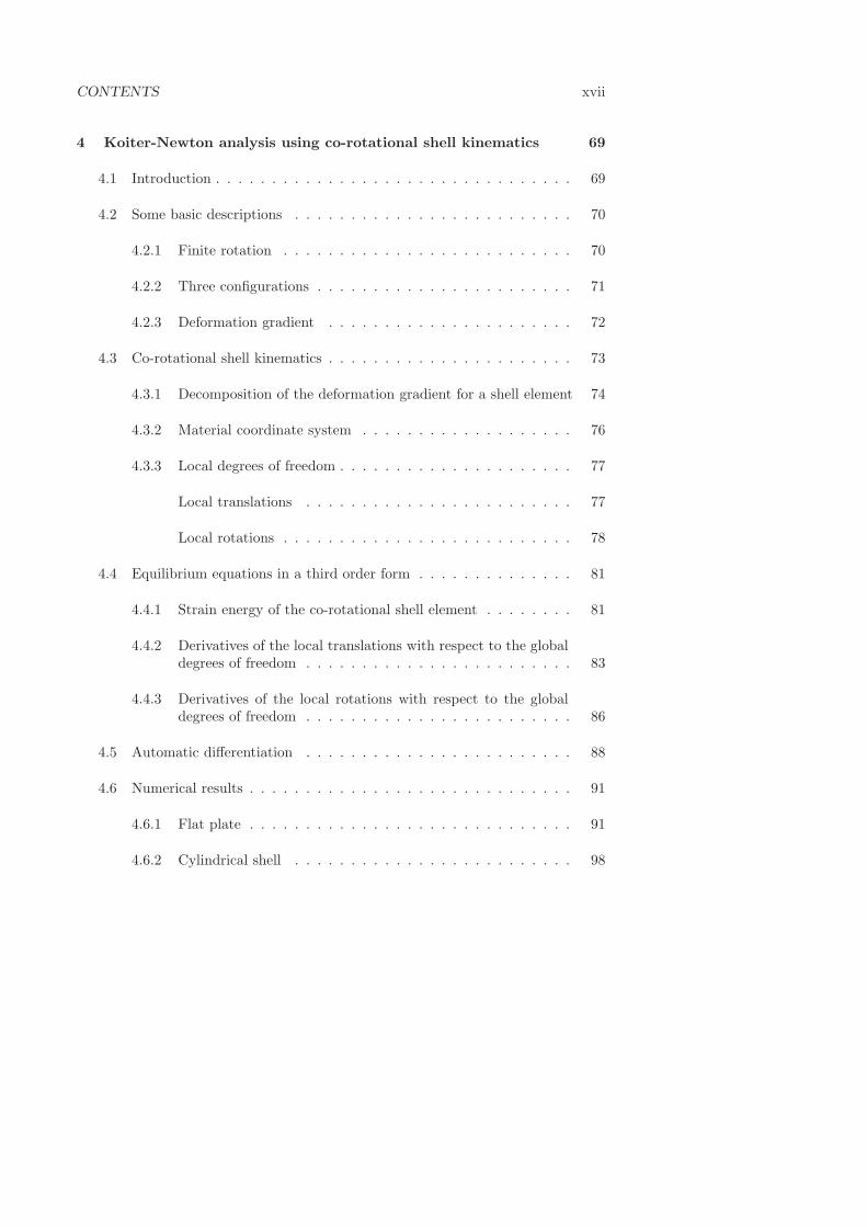
CONTENTS xvii
4 Koiter-Newton analysis using co-rotational shell kinematics 69
4.1 Introduction . . . . . . . . . . . . . . . . . . . . . . . . . . . . . . . . 69
4.2 Some basic descriptions . . . . . . . . . . . . . . . . . . . . . . . . . 70
4.2.1 Finite rotation . . . . . . . . . . . . . . . . . . . . . . . . . . 70
4.2.2 Three configurations . . . . . . . . . . . . . . . . . . . . . . . 71
4.2.3 Deformation gradient . . . . . . . . . . . . . . . . . . . . . . 72
4.3 Co-rotational shell kinematics . . . . . . . . . . . . . . . . . . . . . . 73
4.3.1 Decomposition of the deformation gradient for a shell element 74
4.3.2 Material coordinate system . . . . . . . . . . . . . . . . . . . 76
4.3.3 Local degrees of freedom . . . . . . . . . . . . . . . . . . . . . 77
Local translations . . . . . . . . . . . . . . . . . . . . . . . . 77
Local rotations . . . . . . . . . . . . . . . . . . . . . . . . . . 78
4.4 Equilibrium equations in a third order form . . . . . . . . . . . . . . 81
4.4.1 Strain energy of the co-rotational shell element . . . . . . . . 81
4.4.2 Derivatives of the local translations with respect to the globaldegrees of freedom . . . . . . . . . . . . . . . . . . . . . . . . 83
4.4.3 Derivatives of the local rotations with respect to the globaldegrees of freedom . . . . . . . . . . . . . . . . . . . . . . . . 86
4.5 Automatic differentiation . . . . . . . . . . . . . . . . . . . . . . . . 88
4.6 Numerical results . . . . . . . . . . . . . . . . . . . . . . . . . . . . . 91
4.6.1 Flat plate . . . . . . . . . . . . . . . . . . . . . . . . . . . . . 91
4.6.2 Cylindrical shell . . . . . . . . . . . . . . . . . . . . . . . . . 98
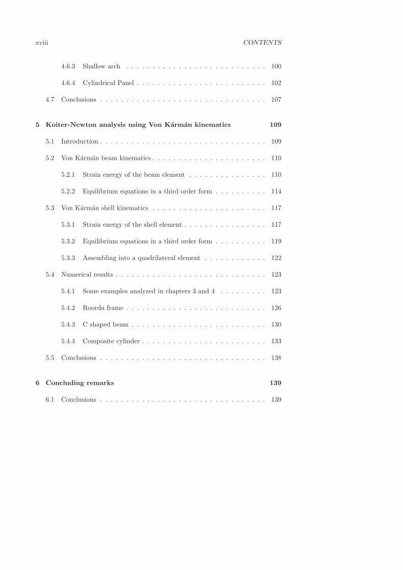
xviii CONTENTS
4.6.3 Shallow arch . . . . . . . . . . . . . . . . . . . . . . . . . . . 100
4.6.4 Cylindrical Panel . . . . . . . . . . . . . . . . . . . . . . . . . 102
4.7 Conclusions . . . . . . . . . . . . . . . . . . . . . . . . . . . . . . . . 107
5 Koiter-Newton analysis using Von Karman kinematics 109
5.1 Introduction . . . . . . . . . . . . . . . . . . . . . . . . . . . . . . . . 109
5.2 Von Karman beam kinematics . . . . . . . . . . . . . . . . . . . . . . 110
5.2.1 Strain energy of the beam element . . . . . . . . . . . . . . . 110
5.2.2 Equilibrium equations in a third order form . . . . . . . . . . 114
5.3 Von Karman shell kinematics . . . . . . . . . . . . . . . . . . . . . . 117
5.3.1 Strain energy of the shell element . . . . . . . . . . . . . . . . 117
5.3.2 Equilibrium equations in a third order form . . . . . . . . . . 119
5.3.3 Assembling into a quadrilateral element . . . . . . . . . . . . 122
5.4 Numerical results . . . . . . . . . . . . . . . . . . . . . . . . . . . . . 123
5.4.1 Some examples analyzed in chapters 3 and 4 . . . . . . . . . 123
5.4.2 Roorda frame . . . . . . . . . . . . . . . . . . . . . . . . . . . 126
5.4.3 C shaped beam . . . . . . . . . . . . . . . . . . . . . . . . . . 130
5.4.4 Composite cylinder . . . . . . . . . . . . . . . . . . . . . . . . 133
5.5 Conclusions . . . . . . . . . . . . . . . . . . . . . . . . . . . . . . . . 138
6 Concluding remarks 139
6.1 Conclusions . . . . . . . . . . . . . . . . . . . . . . . . . . . . . . . . 139

CONTENTS xix
6.2 Recommendations . . . . . . . . . . . . . . . . . . . . . . . . . . . . 142
Appendix A Linear shell element in a co-rotational frame 145
Bibliography 161

xx CONTENTS
List of Figures
1.1 Path-following strategy of the Koiter-Newton approach, comparedwith Newton methods . . . . . . . . . . . . . . . . . . . . . . . . . . 4
1.2 Basic characteristics of the proposed Koiter-Newton approach . . . . 4
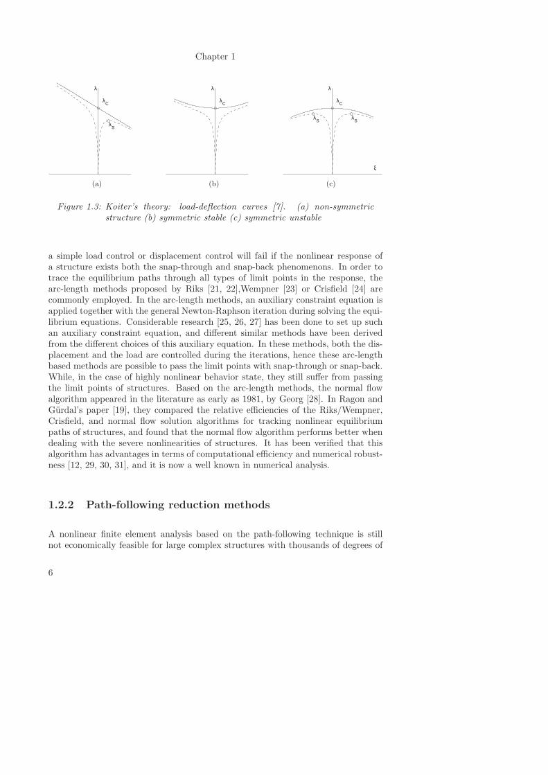
1.3 Koiter’s theory: load-deflection curves [7]. (a) non-symmetric struc-ture (b) symmetric stable (c) symmetric unstable . . . . . . . . . . . 6
2.1 Mapping from the displacement space to the force space . . . . . . . 17
2.2 Normal flow algorithm . . . . . . . . . . . . . . . . . . . . . . . . . . 37
2.3 Nonlinear response curve of structures . . . . . . . . . . . . . . . . . 40
2.4 Flow chart of the Koiter-Newton approach . . . . . . . . . . . . . . . 41
3.1 Sketch of the beam element in a co-rotational frame . . . . . . . . . 46
3.2 Position vectors of the two nodes in a beam element . . . . . . . . . 48
3.3 The three beam frame [7] . . . . . . . . . . . . . . . . . . . . . . . . 57
3.4 The first two buckling modes of the three beam frame . . . . . . . . 58
3.5 The first order displacement fields of the three beam frame . . . . . 58
xxi
xxii LIST OF FIGURES
3.6 The second order displacement fields of the three beam frame . . . . 59
3.7 Buckling response curves of the three beam frame . . . . . . . . . . . 60
3.8 Six nonlinear beams . . . . . . . . . . . . . . . . . . . . . . . . . . . 61
3.9 Response curves of six nonlinear beams . . . . . . . . . . . . . . . . 63
3.10 Response curves of the beam (b), multiple expansions . . . . . . . . 65
3.11 Response curves of the beam (c), multiple expansions . . . . . . . . 65
3.12 Response curves of the beam (d), multiple expansions . . . . . . . . 66
3.13 Bifurcation branches of the beam c . . . . . . . . . . . . . . . . . . . 67
4.1 Three configurations of the co-rotational shell element . . . . . . . . 72
4.2 Sketch of the polar decomposition of the deformation gradient . . . . 73
4.3 Sketch of the element coordinate systems . . . . . . . . . . . . . . . 74
4.4 Sketch of the element rotations . . . . . . . . . . . . . . . . . . . . . 79
4.5 The flat plate . . . . . . . . . . . . . . . . . . . . . . . . . . . . . . . 92
4.6 The first two buckling modes of the plate . . . . . . . . . . . . . . . 93
4.7 The first order displacement fields of the plate . . . . . . . . . . . . . 94
4.8 The buckling response of the perfect plate . . . . . . . . . . . . . . . 95
4.9 Response curves of the plat plate with imperfections . . . . . . . . . 96
4.10 Response curves of the plate for six different imperfection loads . . . 96
4.11 The cylindrical shell . . . . . . . . . . . . . . . . . . . . . . . . . . . 98
4.12 Response curves of the cylindrical shell . . . . . . . . . . . . . . . . . 99
4.13 Deformations of the cylindrical shell near the limit point . . . . . . . 99
LIST OF FIGURES xxiii
4.14 The shallow arch . . . . . . . . . . . . . . . . . . . . . . . . . . . . . 100
4.15 Response curves of the shallow arch . . . . . . . . . . . . . . . . . . 100
4.16 Deformations of the shallow arch near the limit point . . . . . . . . . 101
4.17 The cylindrical panel . . . . . . . . . . . . . . . . . . . . . . . . . . . 102
4.18 The first four buckling modes of the cylindrical panel . . . . . . . . . 103
4.19 Response curves of the perfect panel . . . . . . . . . . . . . . . . . . 104
4.20 Response curves of the cylindrical panel for ten different imperfectionloads . . . . . . . . . . . . . . . . . . . . . . . . . . . . . . . . . . . . 105
4.21 Comparison of the limit loads of the panel . . . . . . . . . . . . . . . 106
4.22 Deformations of the cylindrical panel near the limit point, imperfec-tion 0.1t . . . . . . . . . . . . . . . . . . . . . . . . . . . . . . . . . . 107
5.1 Two-node planar beam element [7] . . . . . . . . . . . . . . . . . . . 111
5.2 Three-node triangular element [7] . . . . . . . . . . . . . . . . . . . . 118
5.3 Quadrilateral element assembled by triangular elements . . . . . . . 123
5.4 Koiter-Newton analysis of the nonlinear beam (c) using Von Karmanand co-rotational kinematical model . . . . . . . . . . . . . . . . . . 124
5.5 Koiter-Newton analysis of the cylindrical shell using Von Karman andco-rotational kinematical model . . . . . . . . . . . . . . . . . . . . . 125
5.6 Koiter-Newton analysis of the shallow arch using Von Karman andco-rotational kinematical model . . . . . . . . . . . . . . . . . . . . . 125
5.7 Koiter-Newton analysis of the cylindrical panel using Von Karmanand co-rotational kinematical model . . . . . . . . . . . . . . . . . . 126
5.8 Roorda frame . . . . . . . . . . . . . . . . . . . . . . . . . . . . . . . 127
5.9 Comparison of the first buckling mode of the Roorda frame . . . . . 128
xxiv LIST OF FIGURES
5.10 The first order displacement fields of the Roorda frame . . . . . . . . 128
5.11 Response curves of the Roorda frame with imperfections . . . . . . . 129
5.12 C shaped beam . . . . . . . . . . . . . . . . . . . . . . . . . . . . . . 130
5.13 The first four buckling modes of the C shaped beam . . . . . . . . . 131
5.14 The first order displacement fields of the C shaped beam . . . . . . . 132
5.15 Response curves of the C shaped beam . . . . . . . . . . . . . . . . . 132
5.16 The composite cylinder . . . . . . . . . . . . . . . . . . . . . . . . . 133
5.17 The convergence study of the end shortening of the composite cylinder135
5.18 The convergence study of the first bifurcation load of the compositecylinder . . . . . . . . . . . . . . . . . . . . . . . . . . . . . . . . . . 136
5.19 Comparison of the first buckling mode of the composite cylinder . . 136
5.20 Response curves of the composite cylinder for different imperfectionloads . . . . . . . . . . . . . . . . . . . . . . . . . . . . . . . . . . . . 137
5.21 The knock-down factor curves of the composite cylinder . . . . . . . 138
A.1 The combination of the membrane (left) and bending (right) degreesof freedom in the triangle shell element [7] . . . . . . . . . . . . . . . 146
A.2 Quadrilateral element assembled by four triangular elements. . . . . 148
List of Tables
3.1 Comparison between the linear buckling load and the limit load . . . 64
3.2 Comparison of the computational cost in terms of number of linerFEM solutions . . . . . . . . . . . . . . . . . . . . . . . . . . . . . . 64
5.1 Comparison of computational times of the Roorda frame . . . . . . . 129
5.2 Material properties of each ply of the composite cylinder . . . . . . . 134
xxv

xxvi
Chapter 1
Introduction
1.1 Background and motivation
Nonlinear static analysis of structures is an essential step of the design of flightvehicles and is important for many practical situations, for example, it is crucial tocarry out a nonlinear static analysis when the displacements and/or rotations of astructure that is being designed are large. Even more important for flight vehiclesis the case where a structure, or some of its components, are prone to buckling.
Thin-walled structures which constitute the main structural components for the bod-ies of flight vehicles are prone to static buckling instabilities due to their favorablestrength-to-weight ratio together with their slenderness. The form of such struc-tures often makes buckling strength the key design criterion of a design process [1],and often, at the onset of buckling, the stress level remains much lower than theyield stress. In many cases, it is crucial to assess the load carrying capability of astructure at which buckling occurs as well as the behavior of the structure beyondthat buckling point. In addition, many shell type structures exhibit unstable post-buckling behavior and are highly sensitive to geometric or load imperfections [2, 3].In the presence of buckling, such structures may exhibit high out-of-plane displace-ments, compared to wall thickness, which cause geometrically nonlinear structuralresponses. Therefore, geometrically nonlinear analysis of new structures during thedesign process is essential for this class of structures to obtain realistic modeling ofthe engineered and product [4].
1
Chapter 1
In recent years, nonlinear structural analysis of static and dynamic problems hasbecome the focus of research efforts [5]. This is largely due to the emphasis placed bymanufactures and contractors on realistic modeling and accurate analysis of criticalstructures [6]. Traditionally, there have been two major approaches to this problem.One is to use the finite element (FE) method based incremental-iterative procedures.This is the most popular technique used in industrial and research applications.Nowadays, the size of the detailed finite element model used by customers andcompanies is steadily growing, and the nonlinearities of the structural behavior areincreasingly taken into account even in the early stages of the design. In spite ofrecent advances in computer hardware and the significant increases in the speed andcapacity of present-day computers, the repeated solution in time of large nonlinearsystem of equations stemming from a FE discretization to reproduce the nonlinearbehavior of a general structure is still a computationally heavy task [7, 8]. For thisreason, approach two which is an asymptotic method that can significantly reducethe number of degrees of freedom using some classical analytic or semi-analytictechniques has begun to attract more attention from researchers working in the fieldof nonlinear structural analysis.
Some analytic techniques, such as the Rayleigh-Ritz technique and the perturbationtechnique, can be used to reduce the number of degrees of freedom in an analy-sis. The deformation modes of various components are described in terms of simpleanalytic functions resulting in a small system of nonlinear equations to be solved.Moreover, exact bifurcation analysis is usually easy to perform including initial post-buckling analysis. Initial post-buckling analysis describes the behavior of the struc-ture in the immediate vicinity of the buckling point. As such it is invaluable inits ability to provide the analyst with a quick qualitative assessment of the post-buckling behavior of a structure. As to be expected, the semi-analytic approach isorders of magnitude faster than nonlinear finite element analysis. This is demon-strated by the following quote, taken from a recent design study: “The efficiencyof ...[semi-analytic] analysis methods and models permits global optimization of astiffened panel concept for less computer time than typically required for a singlenon-linear finite element analysis.” However, analytic or semi-analytic methods areonly applicable for simple geometries and more often than not simplified boundaryconditions and loading.
The challenge is to synthesize the best aspects of both approaches. It is desirableto discretize fairly general structures in a finite element environment while at thesame time greatly reducing the computational effort to make it viable for optimiza-tion purposes. In the nonlinear structural analysis, most of the reduction methodsthat have been proposed are hybrid procedures which combine contemporary finiteelement method and classical asymptotic method.
2
Introduction
In the recent years two main families of reduction methods implemented in a finiteelement environment have been recognized. The first family consists of reductionmethods that work in combination with path-following techniques. Through theupdating of the basis vectors and correcting the results these methods can be usedto trace the nonlinear structural equilibrium path automatically. The selection ofbasis vectors is critical and the accuracy of the method is sensitive to this selection.In addition, these methods often use path derivatives in the expansion, which causesdifficulties near the bifurcation points. For this reason these methods may not besuitable for handling some buckling sensitive cases.
Another family of reduction methods is based on Koiter’s celebrated initial post-buckling theory and numerically performs Koiter’s asymptotic expansion at the bi-furcation point. Recently, work at the Aerospace Structures group at Delft Univer-sity of Technology [7, 8] has focused on the development of this kind of physics-basedreduced order models. Several orders of magnitude reduction in model size is pos-sible using this approach. The method has been implemented in a finite elementenvironment and applied to moderately complex structures, unstiffened shells andstiffened panels, and is currently available in an open-loop format. The model isreduced and the validity of the reduced model is found only in a small range nearthe bifurcation point. There is no further link between the original finite elementmodel and the reduced order model. Thus, the range of validity of the approximatemodel needs to be assessed by comparing it to a full finite element analysis. Thissituation greatly limits the applicability of the new approach.
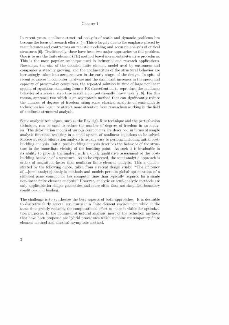
To achieve greater applicability, a combination of Koiter’s analysis and the Newtonarc-length method is proposed in this thesis [9]. In this Koiter-Newton approach, areduced order model (ROM) is constructed based on Koiter’s theory in every step,which is used to make an initial nonlinear prediction of the response of the struc-ture. Compared with traditional Newton methods which use the linear prediction,a larger step size can be achieved using the Koiter-Newton approach due to thisbetter nonlinear prediction provided by the ROM, see Fig. 1.1. In addition, thisnonlinear prediction can also detect and trace the buckling branch accurately in thepresence of buckling, as shown in Fig. 1.1. The exact unbalanced force residual atthe new predicted point is calculated using the full finite element model. Then in acorrector phase, this residual is driven to zero in a manner similar to that used intraditional Newton arc-length methods. This correction procedure can be presentedby the small red arrow in Fig. 1.1. As the solution proceeds to higher and higherload levels, the quality of the ROM are assessed, based on the norm of force residu-als, and if needed the ROM is updated to reflect changes in structural stiffness andload distribution. The proposed approach can trace the entire nonlinear equilibriumpath based on the reduction method automatically and will significantly improvethe efficiency of nonlinear static finite element analysis by incorporating informa-
3
Chapter 1
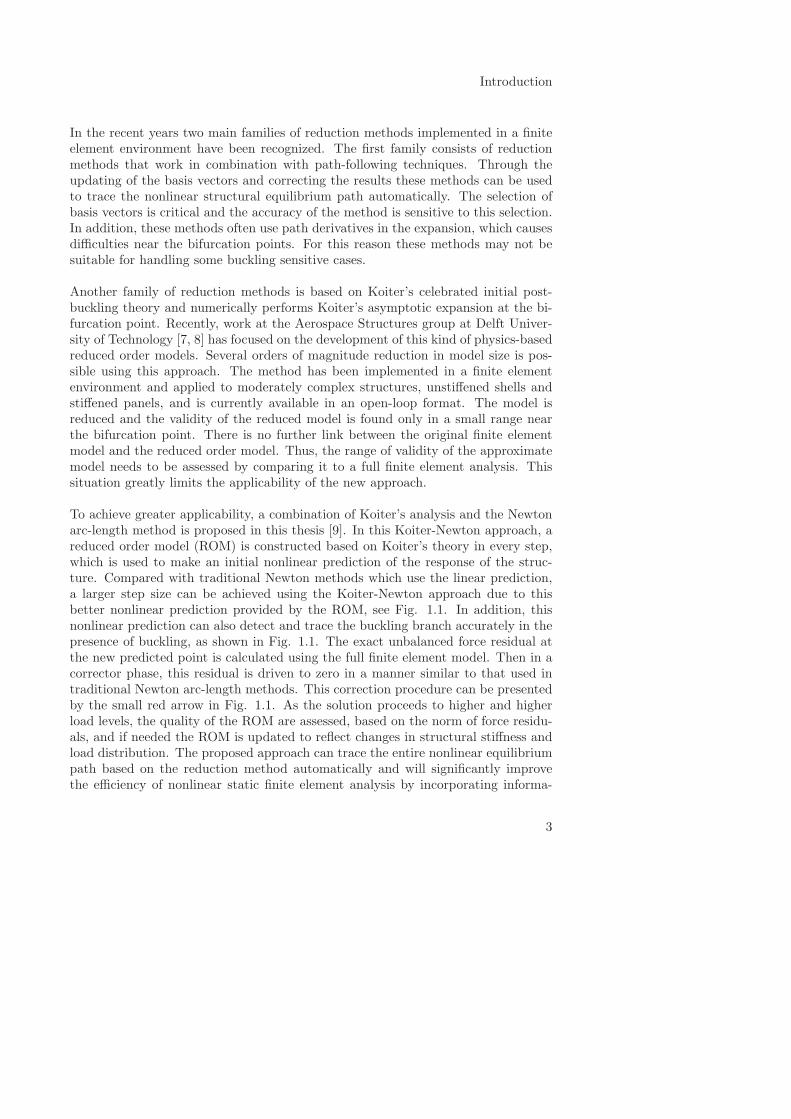
tion from Koiter’s analysis while retaining the complete generality usually associatedwith finite element modeling. This improved efficiency will open the door for thedirect use of detailed nonlinear finite element models in the design optimization ofnext generation flight and launch vehicles [10, 11]. The basic characteristics of thecurrent proposed Koiter-Newton approach are shown in Fig. 1.2.
f
u
Koiter-Newton method:
nonlinear predictions obtained from ROMs
Newton method: linear predictions
Detecting the buckling branch
Figure 1.1: Path-following strategy of the Koiter-Newton approach, comparedwith Newton methods
Koiter-Newton approach
Handle
buckling sensitive cases
Trace
the entire equilibrium pathSave
computational costs
Figure 1.2: Basic characteristics of the proposed Koiter-Newton approach
In recent years, a lot of effort has been made by several research groups to applyasymptotic techniques in finite element context for nonlinear structural analysis,and this will be discussed, along with some involved specific issues, in the followingsection. Based on this discussion, the research objectives for the present research
4
Introduction
will be formulated in the subsequent section.
1.2 Literature review
A brief review of the relevant literature of interest for the research presented in thisthesis work is presented in this section with the reduction methods for nonlinearstructural analysis forming the focal point of the discussion. The three main topicsdealt with in this section, are: path-following techniques in buckling analysis, path-following reduction methods and Koiter reduction methods. Comparison of thecurrent reduction methods is also discussed.
1.2.1 Path-following techniques in buckling analysis
It is necessary to obtain the nonlinear relationship between the applied loads and thestructural responses in engineering. Once the nonlinear response curve of a struc-ture is plotted, the buckling point can be easily achieved from the curve, and thenthe load carrying capability is gained. The buckling points in nonlinear structuralelasticity can be classified into limit points λc and bifurcation points λs [12], asshown in Fig. 1.3. For limit points, whether they belong to a snap-through type ora snap-back type [13], the path-following scheme to compute the regular equilibriumpoints successively on the equilibrium path are sufficient for the computational sta-bility analysis. For bifurcation points, a branch detection technique can be used forswitching into the postbuckling path of a structure [12].
To trace the equilibrium path and also obtain the buckling characteristics of a struc-ture, many researchers [14, 15] have tried to use some analytical techniques to dothe geometrically nonlinear analysis. While, for the structures with complicatedgeometries and boundary conditions, analytical methods face difficulties to gain thesolutions of these nonlinear system of equations. To solve these difficulties manynumerical solutions have been proposed for such nonlinear system of equations byresearchers [16, 17, 18]. Nowadays, nonlinear equilibrium equations of structuresare usually solved by using the traditional Newton-Raphson method together withan incremental/iterative solution technique [19, 20]. While, this method is com-putationally very expensive in the case of nonlinear analysis of the structures withcomplex and serious nonlinear behavior. In addition, the Newton-Raphson methodalways diverges when passing the limit points of a structure. The reason is that
5
Chapter 1
ξ
λC
λ
λS
(a)
ξ
λC
λ
(b)
λS
ξ
λC
λ
λS
(c)
Figure 1.3: Koiter’s theory: load-deflection curves [7]. (a) non-symmetricstructure (b) symmetric stable (c) symmetric unstable
a simple load control or displacement control will fail if the nonlinear response ofa structure exists both the snap-through and snap-back phenomenons. In order totrace the equilibrium paths through all types of limit points in the response, thearc-length methods proposed by Riks [21, 22],Wempner [23] or Crisfield [24] arecommonly employed. In the arc-length methods, an auxiliary constraint equation isapplied together with the general Newton-Raphson iteration during solving the equi-librium equations. Considerable research [25, 26, 27] has been done to set up suchan auxiliary constraint equation, and different similar methods have been derivedfrom the different choices of this auxiliary equation. In these methods, both the dis-placement and the load are controlled during the iterations, hence these arc-lengthbased methods are possible to pass the limit points with snap-through or snap-back.While, in the case of highly nonlinear behavior state, they still suffer from passingthe limit points of structures. Based on the arc-length methods, the normal flowalgorithm appeared in the literature as early as 1981, by Georg [28]. In Ragon andGurdal’s paper [19], they compared the relative efficiencies of the Riks/Wempner,Crisfield, and normal flow solution algorithms for tracking nonlinear equilibriumpaths of structures, and found that the normal flow algorithm performs better whendealing with the severe nonlinearities of structures. It has been verified that thisalgorithm has advantages in terms of computational efficiency and numerical robust-ness [12, 29, 30, 31], and it is now a well known in numerical analysis.
1.2.2 Path-following reduction methods
A nonlinear finite element analysis based on the path-following technique is stillnot economically feasible for large complex structures with thousands of degrees of
6
Introduction
freedom despite the capabilities of present day computers. Hence, the application ofa hybrid approach which can combines contemporary finite elements and classicalanalytic approximations has attracted more attentions [32, 33, 34, 35, 36]. Thetechniques for reducing the degrees of freedom in a FE environment are referredto as reduction methods. Such a global-local approach can preserve the modelingversatility inherent in the FE method and also reduce the number of degrees offreedom using some classic approximations [35].
As discussed in section 1.1, there are two main families of reduction methods. Thefirst family consists of reduction methods that work in combination with path-following techniques. Another family of reduction methods is based on Koiter’scelebrated initial post-buckling theory. In this subsection, the first family of reduc-tion methods, the path-following reduction methods, will be discussed. Throughupdating the reduced order model and correcting the results, these methods can beused to trace the nonlinear structural equilibrium path automatically.
Actually, a nonlinear system of equilibrium equations can be used to present thenonlinear response of a discretized structure. Then, a reduced nonlinear system ofequations with considerably fewer unknowns is constructed using some asymptotictechniques to replace the original equilibrium equations of the structure [37]. TheRayleigh-Ritz and perturbation techniques are two major asymptotic techniquesused to reduce the number of degrees of freedom in a nonlinear analysis. TheRayleigh-Ritz technique expresses the displacement using a linear combination ofglobal approximation functions or basis vectors, while the perturbation techniqueuses power series with respect to a certain parameter to express the displacement.According to the different asymptotic techniques adopted for reducing the number ofdegrees of freedom in the finite element model, the path-following reduction methodscan be classified as Rayleigh-Ritz reduced path-following methods [38, 39, 35, 40]and perturbation reduced path-following methods [41, 42].
As discussed above, in the Rayleigh-Ritz reduced path-following methods, the de-formation of a structure is presented by some known modes, such as basis vectors orglobal RayleighRitz approximation functions, and the number of these known modesis usually much smaller than the total number of degrees of freedom of the originalFE model [37]. Hence, the effectiveness of the reduction method depends largely onthe proper selection of these basis vectors such that their combination may give thecorrect deformation of the structure, and the ease with which they can be generatedwithout incurring a large amount of computational overhead. For this purpose, var-ious choices for approximation functions were proposed in the literature. Similar tothe modal superposition technique, Nagy [38] selected the first few buckling modesto represent the prebuckling nonlinear behavior of structures. The first linear andsubsequent nonlinear solution vectors at consecutive steps were adopted by Almroth
7
Chapter 1
et al. [39]. Noor et al. [35] chose a nonlinear solution and its path derivatives ofascending order commonly used in the static perturbation technique as the basisvectors. Recently Chan and Hsiao [40] have considered nonlinear solutions and thecorrection vectors generated during a nonlinear iteration step for this purpose. Intheir work, an implicit reduction technique is proposed where only the displacementcorrections are evaluated in the reduced system while the residual forces are cal-culated in the full system as usual, thus enabling the method to be applicable tomaterially and geometrically nonlinear problems. For Rayleigh-Ritz reduced path-following methods, the selection of basis vectors is crucial and the accuracy of thesemethods are very sensitive to this selection. In addition, the path derivatives [35]are often applied in the expansion as the basis vectors, and it will make the algo-rithm divergent near the bifurcation/limit points. Hence, these methods may notbe suitable for handling some buckling sensitive cases.
The perturbation reduced path-following methods are generated based on the ana-lytical perturbation techniques [43, 44, 45, 46, 47]. For these methods, the nonlinearbranch is expanded in the form of power series with respect to a path parameter.The principle of these methods is to determine some terms of the series by solvinga recursive set of linear problems which yields an approximate analytical represen-tation of the solution branch. A perturbation technique is also a good means touse to build up an efficient Ritz basis to be used in a Ritz reduction technique,as proposed and tested by Noor and Peters [35]. In order to settle the difficultyof computing more than the first few terms of the series, due to the growing com-plexity of the problems to be solved, Damil and Potier-Ferry [48, 49] have proposedan asymptotic-numerical method which permits one to compute a large number ofterms of a perturbation series using very classical programming techniques and littlecomputational time. They considered the bifurcation branches in their original al-gorithm [41] which is based on the asymptotic numerical method (ANM) and Padeapproximants by giving two choices for the control parameter a (Signorini expansionand bifurcation-type expansion). Based on this method, Azrar [50, 41] has obtainedthe post-buckling branch of elastic plates and shells. Cochenlin [42] has extendedit to any generic nonlinear solution branch, and showed that with a proper choiceof the perturbation parameter the series have a finite radius of convergence whichis not necessarily small. Based on Potier-Ferry’s works Boutyour [51] detected thebifurcation point using two manners. One manner is to analyze the poles of the Padeapproximants, and another one is to evaluate a bifurcation indicator which is welladapted to ANM along the computed solution branch. In addition, there are manyother very relevant possibilities for choices of path parameters, see Lopez [52] andespecially Mottaqi et al [53]. For the current perturbation reduced path-followingmethods, in the case of buckling, the expansion parameter needs to be changed totrace the buckling branches. Hence, it is not convenient for the current perturbationreduced path-following methods to achieve automations in the presence of buckling.
8
Introduction
1.2.3 Koiter reduction methods
The Koiter reduction methods are based on a specific perturbation technique, Koi-ter’s perturbation technique, to reduce the number of degrees of freedom in the finiteelement model. The main advantage of Koiter’s theory [43] is that it can provide aquick and accurate enough description of the buckling capability and also the ini-tial postbuckling behavior of a structure. The postbuckling coefficients obtained byKoiter perturbation expansion are used to describe the buckling characteristics ofthe structure. In addition, when the buckling loads are very close, the interactionsof these closely spaced buckling modes can be easily taken into account using Koiterperturbation method. Based on the closely spaced buckling modes and using thepostbuckling coefficients, a reduced nonlinear system of equations is constructed atthe bifurcation point to approximate the initial postbuckling path of the structure.For the imperfection analysis, the effect of geometrical imperfections can easily beintroduced and results in a force term that can be added to the already constructedreduced order model of the perfect structure.
For many yeas, Koiter’s theory has been regarded to be only suitable in analyticaland semi-analytical contexts, and many relevant work [54, 55, 56, 57, 58, 59, 60]has been done to obtain the stability behavior of a structure only for academic in-terest. Recently, considerable research efforts have been put into finding a properimplementation of Koiter’s work in an FE context [7, 8]. In the beginning, Gal-lagher [61] outlined some difficulties involved in the finite element implementationof Koiter’s perturbation approach. Obtaining the b coefficient with a good accu-racy and convergence is a key issue in the FE implementation. Many researchers[62, 63, 64, 65, 66, 67] have tried to find a suitable kinematic model that can beused to obtain good accuracy and convergence for the b coefficient. Antman [62] hasproposed a consistent kinematical model which shows an extremely fast convergencein the determination of the initial postbuckling coefficients. Later, a geometricallyexact beam based on Antman’s [62] kinematical model was proposed by Pacoste [64]to obtain an accurate b coefficient. In addition, a bad convergence of the b coef-ficient will cause a locking phenomena in the implementation of the perturbationapproach into the finite element context. This locking phenomena is due to the factthat the components of the in-plane displacement are interpolated to a lower degreethan the components of the out-of-plane [7]. This causes inaccurate calculation ofpostbuckling response and consequently it gives rise to an extremely slow conver-gence of the post-buckling curvature b. Olesen and Byskov [68, 69], and Poulsen andDamkilde [70] respectively used Lagrange multipliers and a local stress contributionto tackle this problem. Research done by Garcea [67] has shown that the elementsbased on the co-rotational (CR) formulation can settle these problems very well, andsome numerical examples of beam and shell models have been used to verify this
9
Chapter 1
viewpoint.
The Koiter reduction methods are based on Koiter’s perturbation technique andKoiter’s asymptotic expansion is used only once at the bifurcation point. Hence, theperturbation approach used in this research is valid asymptotically in the neighbor-hood of the starting point of the perturbation expansion. In most of the researchwork, the expansion of the displacement field is up to the second order which isoften enough to capture the initial postbuckling response of structures. Damil andPotier-Ferry [48] have tried to adopt higher order terms to increase the range ofvalidity of the perturbation expansion further. Increasing the order terms of thedisplacement should obtain a wider range of validity. Yet, the reduced order modelobtained by a single perturbation expansion still has a limited range of validity thatcannot be determined a priori.
Koiter’s theory is often used to handle problems characterized by bifurcation typebuckling. The Koiter reduction methods discussed above only consider bifurcationtype buckling. Problems with the limit type buckling, such as snap through andsnap back, were initially considered by Haftka et al. [71] and later by Carnoy [72]and Salerno et al. [73]. In their work, they assumed there is a bifurcation point ina fictitious perfect structure and an intrinsic imperfection is applied to predict thebehavior of the real structure. Using some numerical examples, it demonstrates thatthis approach worked well with some beam structures but not with the same level ofsuccess for the case of shell structures. In Carnoy’s [72] paper, some measures havebeen proposed to improve the application in shells.
The interactions of the closely spaced buckling modes may degrade the load carryingcapacity of a structure, and buckling modes being stable in isolation may exhibit anunstable postbuckling behavior and imperfection sensitivity when they are subjectto modal interaction, hence a multi mode study is very important in the bucklinganalysis. Thin-walled structures are the most classical engineering applications thatexhibit many close bifurcation points near the lowest critical load, and some re-search work has found that the number of closely spaced buckling modes is greaterif the structure is thinner. In the early time, Koiter [74, 75] considered the modalinteraction issue for continua in an analytical frame. Later on, many scholars, suchas Byskov and Hutchinso [76], Peek and Kheyrkhahan [77] and Salerno and Cas-ciaro [78] did some more detailed research into applying the closely spaced modescase in the perturbation approach. Lanzo and Garcea [79], Garcea and Casciaro[80], Salerno and Casciaro [78] and Garcea [81] used high continuity finite elements[82, 83] and Salerno’s perturbation expansion [78] to study the model interactionsand the worst imperfection shape [84, 85] in the buckling analysis. In Bilotta’s [86]work, shear deformability and composite plates were considered, and he found thatthe secondary bifurcation paths obtained using the perturbation approach matched
10
Introduction
very well with the results from a full model analysis based on a path-following ap-proach in the neighborhood of the bifurcation point. This conclusion was also drawnby Garcea [87]. Menken et al. [88, 89], Erp and Menken [90, 91] and Schreppersand Menken [92] used the expansion given by Byskov and Hutchinson [76] and useda spline finite-strip type element to explore the phenomenon of the modal interac-tion in folded plate type structures. Some research work [93, 94] has been doneon thin-walled structures, such as the isotropic cylindrical and spherical shells. Inaddition, Kouhia and Mikkola [95], Huang and Atluri [96], and Magnusson [97] usedthe perturbation approach carried out at any bifurcation point as a predictor for thepath following through any specific bifurcating branch.
In a general path-following analysis, only second order accuracy is needed to re-cover the elastic response vector and the tangent stiffness matrix [98]. While, theasymptotic approach used in reduction methods needs a fourth order expansion ofthe strain energy. It is usually complex and perhaps not possible to apply a fourthorder accurate strain model into the FE context. The co-rotational approach (CR)[99, 100] which is able to provide a fourth order accurate description of the ele-ment motion appears to be suitable to overcome this difficulty. The basic idea ofthe co-rotational description is to refer each element to a local frame which movestogether with the element, thus filtering its rigid motion. Initially, Garcea [67] re-searched to implement the Koiter’s asymptotic approach into nonlinear structuralFE models which are based on a co-rotational frame. Later, Eriksson and Pacoste[64] investigated the possibility of using co-rotational formulation. Recently, Zagari[98, 101] has presented a co-rotational formulation, suitable for a nonlinear, fourthorder accurate asymptotic postbuckling analysis of shell structures exploiting thethree dimensional finite rotations in his PhD thesis.
As discussed in the background and motivation section of this chapter, the bucklingand postbuckling behaviors of structures are strongly influenced by the prebucklingnonlinearity of such structures. While, in the literatures listed above, the prebucklingstate is often assumed to be linear in the Koiter reduction methods. Actually, thislinear assumption for the prebuckling state will often overestimate the buckling loadof an important class of engineering problems the prebuckling of which is obviousnonlinear. Therefore, the effect of prebuckling nonlinearity should be taken into ac-count in the buckling analysis. Much of the work on Koiter’s theory are based on thealternative procedure proposed by Budiansky and Hutchinson [102], which assumesthat the prebuckling is linear. Cohen [56] and Fitch [57], and later Arbocz and Hol[60, 103] derived the modifications necessary to make Budiansky and Hutchinson’swork [102] include prebuckling nonlinearity. Recently, Rahman [104, 105, 8], Zagari[67, 98] have made use of the derivations done by Arbocz and Hol [60, 103] within afinite element context to consider the nonlinearity of the prebuckling of a structure.In their work, first, a standard nonlinear analysis is performed to reach, as closely
11
Chapter 1
as possible, the critical point of a structure without encountering any negative di-agonal term in the system stiffness matrix to get a basic state, and then they applyKoiter’s asymptotic expansion at this basic state to obtain a more accurate initialpostbuckling response which considers the effect of the prebuckling nonlinearity ofa structure.
In general, Koiter reduction methods, which are based on Koiter’s initial postbuck-ling theory, give very easy handling of buckling/imperfection sensitive cases espe-cially if the structure has closely spaced buckling modes, however, these reductionmethods have some disadvantages. They experience difficulties when dealing withlimit point type buckling. Using general nonlinear finite elements it is very compli-cated to compute the fourth order derivatives needed for the asymptotic expansion.These reduction methods are only valid for a small range near the bifurcation pointdue to Koiter’s asymptotic expansion being used only once at the bifurcation point.The effect of the prebuckling nonlinearity of a structure can only be considered usinga general nonlinear finite element analysis in a full finite element model.
1.3 Thesis layout
This thesis is organized as follows.
The background and motivation of the present research together with a literaturesurvey for the selected areas of application is presented in chapter 1. Particularattention is paid to the comparison of the current reduction methods.
A new approach termed the Koiter-Newton is presented for the numerical solutionof a class of elastic nonlinear structural response problems in chapter 2. It is acombination of a reduction method inspired by Koiter’s post-buckling analysis andthe Newton arc-length method so that it is accurate over the entire equilibriumpath and it is also computationally efficient in the presence of buckling. The Koiter-Newton approach combines Koiter’s analysis as a predictor and the Newton arc-length method as a corrector. A detailed introduction of the reduction methodin one expansion step for this new approach will be given. Then, the selection ofperturbation loads is discussed, especially when the expansion step is applied on theunstable part of the equilibrium path. Next, the effect of the imperfection loadsis taken into account to get a load term that can be added to the already formedreduced order model for the perfect structure. After obtaining the reduced ordermodel, with and without the imperfections, a path-following technique called thenormal flow method is reviewed and used to simulate the ROM and obtain the
12
Introduction
response curve of the structure. Finally, an automated technique is applied to makethe proposed approach trace the entire nonlinear equilibrium path automatically,and the corresponding computational cost is counted.
Implementations of the Koiter-Newton approach into the beam and shell elementsbased on the co-rotational kinematics are presented in chapters 3 and 4. The deriva-tives of the co-rotational frame with respect to the element degrees of freedom arepresented, and the equilibrium equations of a third-order form at the expansionequilibrium point are obtained to construct the reduced order model. For the shellelement, three configurations during the deformation are defined to make the de-scription easier, and the nonlinear rotation matrix is used to describe the large/finiterotation accurately. Some numerical examples involving beams and shells are usedto evaluate the performance of the Koiter-Newton analysis using co-rotational kine-matics. The results are compared with results produced for the same problems usinga full nonlinear analysis (ABAQUS), with the same number of nodes and elements.
The Von Karman kinematical model is adopted in chapter 5 and used to achievethe Koiter-Newton approach. The Von Karman kinematics do not take into accountfully nonlinearities in the element, hence using them it is much faster and easierthan using co-rotational kinematics to obtain a fourth order expansion of the strainenergy. In the cases where the nonlinear in-plane rotations of the structure can beneglected, but the rotations of the normals to the mid-surface are finitely large, anacceptable accuracy of a nonlinear structural analysis can be obtained using the VonKarman kinematics. Some previous used numerical examples which have alreadybeen tested using co-rotational kinematics are used to evaluate the performance ofthe Koiter-Newton analysis using Von Karman kinematics, and some new exampleswhich need a very fine mesh are also analyzed in this chapter.
The conclusions drawn from the research discussed in this thesis are summarized inchapter 6.
13

Chapter 1
14
Chapter 2
Koiter-Newton approach
2.1 Introduction
The main aim of the research reported here is to find a new analytical approachto nonlinear structural problems with the presence of the buckling. As discussed inthe literature review section of the first chapter, current Koiter reduction methods,which are based on Koiter’s initial postbuckling theory and can handle the buck-ling/imperfection case very well, still have some main drawbacks as follows. Theyare not well suited to dealing with limit point type buckling and it is quite difficultto take into consideration prebuckling nonlinearity using these methods. In the tra-ditional Koiter’s theory, Koiter’s asymptotic expansion is carried out only once atthe bifurcation point, so the range of validity of these Koiter reduction methods isonly near the bifurcation point. In order to overcome these disadvantages, a new ap-proach called Koiter-Newton is presented here for the numerical solution of a classof elastic nonlinear structural analysis problems [9, 106]. This method combinesideas from Koiter’s initial postbuckling analysis and Newton arc-length methods toobtain an algorithm that is accurate over the entire equilibrium path and efficientin the presence of buckling and/or imperfection sensitivity.
The basic premise behind the method is to use Koiter’s asymptotic expansion fromthe beginning rather than using it only once at the bifurcation point. In everystep of the Koiter-Newton approach, a reduced order model (ROM) is constructedbased on Koiter’s initial post-buckling theory. This ROM is used to make an initialprediction of the response of the structure. At the new predicted point, the exact
15
Chapter 2
unbalanced force residual is calculated using the full finite element model. Then ina corrector step, this residual is driven to zero in a manner similar to that used inthe traditional Newton arc-length methods. As the solution proceeds to higher andhigher load levels, the quality of the ROM is assessed, based on the norm of forceresiduals, and if needed the ROM is updated to reflect changes in structural stiffnessand load distribution.
The proposed approach will significantly improve the efficiency of nonlinear staticfinite element analysis by incorporating information from Koiter’s analysis while re-taining the complete generality usually associated with finite element modeling. Thenumber of linear FEM systems of equations need to be solved is much less than thatfor the classical arc-length methods. This is due to the better prediction provided bythe nonlinear reduced order model compared to linear predictors especially withinthe nonlinear segments of the original response curve, thus allowing the algorithm touse fairly large step sizes. In addition, perturbation loads corresponding to bucklingmodes are considered in the reduced order model. The ROM provides a convenientand cheap way to assess imperfection sensitivity of a structure.
First, the construction of the reduced order model in one expansion step of theKoiter-Newton approach is presented using a functional notation. The selectionof the perturbation loads, especially when the expansion point is on the unstablepart of the equilibrium path, is then discussed. Next, the imperfection loads are alsotaken into account in the reduced order model to model the geometric imperfections,and the normal flow algorithm is introduced to simulate the reduced order model.Finally, the automated technique and the computational effort associated with theproposed approach are given.
2.2 Construction of the reduced order model
The essence of the reduction methods for nonlinear problems is to use the asymptotictechnique to replace the governing equations of the structure by a reduced system ofequations with considerably fewer unknowns. Here, the reduced system of equationsis just the reduced order model of the original model. Then, instead of solving alarge nonlinear finite element model, the nonlinear responses of the structure can beobtained by solving this reduced order model with much fewer degrees of freedom.So, the reduced order model is the most important part in a reduction method, andit determines the characteristics and functions of the method that will be used. Inthe present Koiter-Newton approach, the constructional way of reduced order modelis quite different from other reduction methods, which makes the present approach
16
Koiter-Newton approach
synthesizing the best aspects of the others.
This section is ordered as follows. First, the governing equations and their asymp-totic expansions are given at an known equilibrium point. The reduced order modelis then established at this equilibrium point to approximate the equilibrium equa-tions.
2.2.1 Governing equations and asymptotic expansions
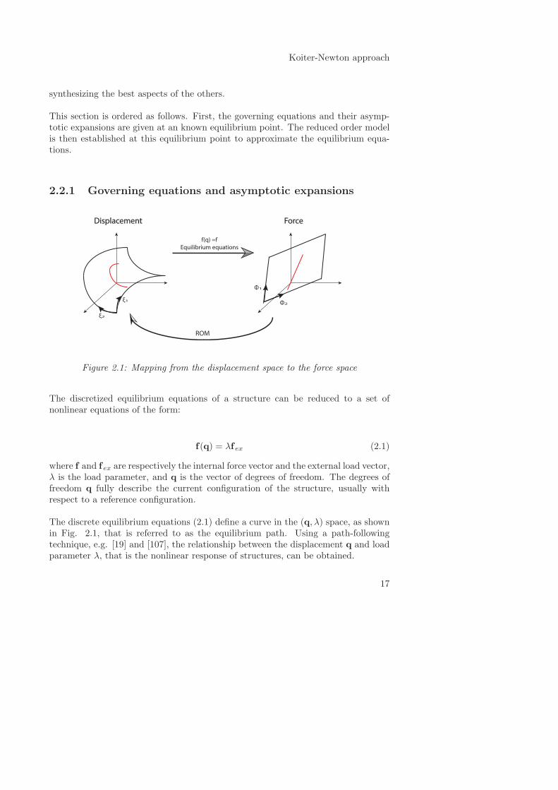
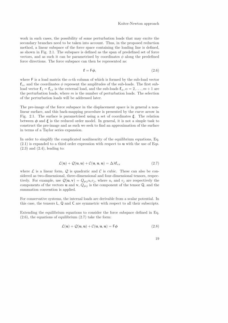
Displacement Force
f(q) =f
Equilibrium equations
ξ1
ξ2
Ф1
Ф2
ROM
Figure 2.1: Mapping from the displacement space to the force space
The discretized equilibrium equations of a structure can be reduced to a set ofnonlinear equations of the form:
f(q) = λfex (2.1)
where f and fex are respectively the internal force vector and the external load vector,λ is the load parameter, and q is the vector of degrees of freedom. The degrees offreedom q fully describe the current configuration of the structure, usually withrespect to a reference configuration.
The discrete equilibrium equations (2.1) define a curve in the (q, λ) space, as shownin Fig. 2.1, that is referred to as the equilibrium path. Using a path-followingtechnique, e.g. [19] and [107], the relationship between the displacement q and loadparameter λ, that is the nonlinear response of structures, can be obtained.
17
Chapter 2
In the proposed Koiter-Newton approach, a reduced order model is established toapproximate the equilibrium equations in the neighborhood of a known equilibriumstate (q0, λ0). The vector q0 describes the configuration at this equilibrium state,which we will refer to as the nominal configuration. Let q be the unknown displace-ment vector near this nominal state, it results in:
q = q0 ◦ u (2.2)
where u describes the current configuration with respect to the nominal configura-tion. The composition of q0 and u is not always a simple addition, and for beamsand shells where rotational degrees of freedom are used, the composition operationwill depend on the parametrization of rotations.
As discussed above, (q0, λ0) is the nominal equilibrium state, (q, λ) is the currentequilibrium state, and (u,∆λ) describes the current equilibrium state with respect tothe nominal equilibrium state. So, the load parameters should satisfy the followingrelation:
∆λ = λ− λ0 (2.3)
As an equilibrium state, the nominal state (q0, λ0) should also satisfy the equilibriumequations (2.1), leading to:
f(q0) = λ0fex (2.4)
According to Eq. (2.2), the equilibrium equations (2.1) can be rewritten as:
f(q0 ◦ u) = λfex (2.5)
The equilibrium equations (2.1) may be interpreted geometrically as a mappingfrom the displacement space to the force space, see the straight arrow in Fig. 2.1.Equivalently, we may think of the equilibrium path as the pre-image of the linef = λfex in the displacement space.
The proposed technique aims to be applicable for buckling sensitive structures. Inthe presence of buckling, multiple secondary equilibrium branches that intersectwith the primary path at the buckling, bifurcation, points exist. For the method to
18
Koiter-Newton approach
work in such cases, the possibility of some perturbation loads that may excite thesecondary branches need to be taken into account. Thus, in the proposed reductionmethod, a linear subspace of the force space containing the loading line is defined,as shown in Fig. 2.1. The subspace is defined as the span of predefined set of forcevectors, and as such it can be parametrised by coordinates φ along the predefinedforce directions. The force subspace can then be represented as:
f = Fφ, (2.6)
where F is a load matrix the α-th column of which is formed by the sub-load vectorfα, and the coordinates φ represent the amplitudes of the sub-loads. The first sub-load vector f1 = fex is the external load, and the sub-loads fα, α = 2, . . . ,m+ 1 arethe perturbation loads, where m is the number of perturbation loads. The selectionof the perturbation loads will be addressed later.
The pre-image of the force subspace in the displacement space is in general a non-linear surface, and this back-mapping procedure is presented by the curve arrow inFig. 2.1. The surface is parametrised using a set of coordinates ξ. The relationbetween φ and ξ is the reduced order model. In general, it is not a simple task toconstruct the pre-image and as such we seek to find an approximation of the surfacein terms of a Taylor series expansion.
In order to simplify the complicated nonlinearity of the equilibrium equations, Eq.(2.1) is expanded to a third order expression with respect to u with the use of Eqs.(2.3) and (2.4), leading to:
L(u) +Q(u,u) + C(u,u,u) = ∆λfex (2.7)
where L is a linear form, Q is quadratic and C is cubic. These can also be con-sidered as two-dimensional, three-dimensional and four-dimensional tensors, respec-tively. For example, use Q(u,v) = Qpijuivj , where ui and vj are respectively thecomponents of the vectors u and v, Qpij is the component of the tensor Q, and thesummation convention is applied.
For conservative systems, the internal loads are derivable from a scalar potential. Inthis case, the tensors L, Q and C are symmetric with respect to all their subscripts.
Extending the equilibrium equations to consider the force subspace defined in Eq.(2.6), the equations of equilibrium (2.7) take the form:
L(u) +Q(u,u) + C(u,u,u) = Fφ (2.8)
19
Chapter 2
2.2.2 Reduced order model
The solution for u of Eq. (2.8) lies, in general, on an m + 1 dimensional surfacewhere m is the number of perturbation loads. The numerical construction of such asurface would be computationally prohibitive. To circumvent this, an approximatesolution can be obtained using Taylor series expansion, which defines a nonlineardisplacement subspace in Fig. 2.1. This equilibrium surface is parametrised in termsof generalised displacements ξ, and the equilibrium displacement is expanded to thethird order with respect to ξ as follows:
u = uαξα + uαβξαξβ + uαβγξαξβξγ , (2.9)
where the greek subscripts vary over the range 1, 2, . . . ,m + 1, and the summationconvention is applied. The first order displacements uα define the tangent plane tothe equilibrium surface at the approximation point. The second order displacementsuαβ and third order displacements uαβγ describe the interactions among first andsecond order displacement fields, respectively.
The equilibrium surface may be parametrised with an infinite number of choices forξ. To fix the parameterization, we choose the vector ξ such that it is work conjugateto the load amplitudes φ, leading to:
(Fφ)tδu ≡ φtδξ (2.10)
Substituting the expansion of the displacement (2.9) into the left hand side of Eq.(2.10), it results in:
(Fφ)tδu = φtFt(uαδξα + uαβδξαξβ + uαβξαδξβ + ...)
= φpftp(uαδξα + uαβδξαξβ + uαβξαδξβ + ...)
= (f tpuα)φpδξα + (f tpuαβ)φpδξαξβ + (f tpuαβ)φpξαδξβ + ...
≡ φtδξ
(2.11)
In order to make the identical equation (2.11) tenable forever with respect to anyvalue of ξ, the coefficients of the various derivatives of ξ should satisfy the followingconstraint equations about the sub-loads and displacement fields, given by:
20
Koiter-Newton approach
f tαuβ = δαβf tαuβγ = 0f tαuβγδ = 0
(2.12)
where δαβ is the Kronecker delta. It means that the sub-loads fα are orthogonal toall the second and third order displacement fields(uβγ ,uβγδ).
Consistent with the displacement expansion (2.9), we assume the expansion for theload amplitudes φ to be:
φ = L(ξ) + Q(ξ, ξ) + C(ξ, ξ, ξ) (2.13)
where the L, Q and C are, still to be determined, linear, quadratic, and cubicforms. These three forms have the same characteristics with the forms of the L, Qand C in the equilibrium equations (2.7). The tensors L, Q and C should be theircorresponding matrix forms.
Introducing the displacement expansion (2.9) and the load expansion (2.13) into theequilibrium equations (2.8), and then regrouping it with respect to ξ, we obtain:
{L(uα)− FLα
}ξα +
{L(uαβ) +Q(uα,uβ)− FQαβ
}ξαβ+
{L(uαβγ) + (2/3) [Q(uαβ ,uγ) +Q(uβγ ,uα) +Q(uγα,uβ)] +
C(uα,uβ ,uγ)− FCαβγ
}ξαβγ
= 0
(2.14)
where the expressions Lα, Qαβ and Cαβγ represent the vector in the multiple di-
mensional tensors L, Q and C, respectively.
Equating the coefficients of the various powers of ξ to zero, three sets of linearequations are obtained as:
L(uα) = FLα (2.15)
L(uαβ) +Q(uα,uβ) = FQαβ (2.16)
21
Chapter 2
L(uαβγ) +2
3[Q(uαβ ,uγ) +Q(uβγ ,uα) +Q(uγα,uβ)] + C(uα,uβ ,uγ) = FCαβγ
(2.17)
Taking the first order term Eq. (2.15), together with the first equation of orthogo-nality constraints (2.12), we can write them together as:
{L(uα) = FLα
f tαuβ = δαβ(2.18)
In order to be convenient for the implementation of the finite element method, thenotations in Eq. (2.18) can be replaced by the FE notations:
{Ktuα = FLα
Ftuα = Eα(2.19)
where Kt = L is the tangent stiffness matrix at the approximation/nominal con-figuration. The vectors Eα are the unit basis vectors and are such that the α-thcomponent is one and all the other components are zero.
Rewriting above equations in a matrix form, we obtain a set of linear systems ofequations:
[Kt −F
−Ft 0
]{uα
Lα
}=
{0
−Eα
}(2.20)
In the same way, we combine the second order term Eq. (2.16) and the secondequation of orthogonality constraints (2.12), leading to:
{L(uαβ) +Q(uα,uβ) = FQαβ
f tαuβγ = 0(2.21)
Then, replacing the notations in Eq. (2.21) and rewriting them in a matrix form,we can obtain another set of linear systems of equations:
[Kt −F
−Ft 0
]{uαβ
Qαβ
}=
{−Q(uα,uβ)
0
}(2.22)
22
Koiter-Newton approach
The vector Lα in the tensor L and the vector Qαβ in the tensor Q can be achievedrespectively by Eqs. (2.20) and (2.22).
In order to simplify the algebra in constructing the reduced order model, the com-ponents of the tensors L and Q should be obtained from their vectors Lα andQαβ ,respectively.
We work on the components Lαβ of the tensor L firstly. Multipling the transposeof the first order displacement vector uβ on both sides of the first order term Eq.(2.15), we obtain:
utβL(uα) = ut
βFLα (2.23)
where the right hand side can be rewritten as:
utβFLα =
(Ftuβ
)tLα = Et
βLα = Lβα (2.24)
where the equation Ftuβ = Eβ exist referring to the first equation of the orthogonal-ity constraints (2.12), the unit basis vectors Eβ are such that the β-th componentis one and all the other components are zero.
Then, Eqs. (2.23) and (2.24) demonstrate that the components of the tensor L canbe calculated as follows:
Lβα = utβL(uα) (2.25)
where for conservative systems the tensors L is symmetric in all indices, hence thetensor L is also symmetric in all indices.
The components Qαβγ of the tensor Q can also be achieved in a similar way. Wemultiply the transpose of the first order displacement vector uγ on both sides of thesecond order term Eq. (2.16), leading to:
utγL(uαβ) + ut
γQ(uα,uβ) = utγFQαβ (2.26)
where the left hand side can be rewritten to be a more compact notation:
23
Chapter 2
utγL(uαβ) + ut
γQ(uα,uβ) = utαβL(uγ) + ut
γQ(uα,uβ)
=(Ftuαβ
)tLγ + ut
γQ(uα,uβ)
= utγQ(uα,uβ)
(2.27)
where the derivations is based on the assumption of conservative systems, henceutγL(uαβ) = ut
αβL(uγ). We have also used the facts that L(uγ) = FLγ from Eq.
(2.15) and Ftuαβ = 0 due to the second equation of the orthogonality constraints(2.12).
The right hand side of Eq. (2.26) can be expressed as:
utγFQαβ =
(Ftuγ
)tQαβ = Et
γQαβ = Qγαβ (2.28)
where Ftuγ = Eγ due to the first equation of the orthogonality constraints (2.12),and the unit basis vectors Eγ are such that the γ-th component is one and all theother components are zero.
Then, combining Eqs. (2.27) and (2.28), the components of the tensor Q can becalculated as follows:
Qγαβ = utγQ(uα,uβ) (2.29)
where tensor Q is also symmetric in all indices due to conservative systems.
In the third order term, the component of C can be obtained by the scalar multipli-cation of both sides of Eq. (2.17) with uδ, leading to:
utδL(uαβγ) + ut
δ
2
3[Q(uαβ ,uγ) +Q(uβγ ,uα) +Q(uγα,uβ)] +
utδC(uα,uβ ,uγ) =
(Ftuδ
)tCαβγ
(2.30)
where the subscript δ also runs from 1 to m + 1, and the first term utδL(uαβγ) is
represented as:
utδL(uαβγ) = ut
αβγL(uδ) =(Ftuαβγ
)tLδ = 0 (2.31)
where utδL(uαβγ) = ut
αβγL(uδ) is based on conservative systems, and Ftuαβγ = 0
comes from the third equation of the orthogonality constraints (2.12).
24
Koiter-Newton approach
The right hand side of Eq. (2.30) can be rewritten as the following form:
(Ftuδ
)tCαβγ = Et
δCαβγ = Cδαβγ (2.32)
where Ftuδ = Eδ due to the using of the first equation in orthogonality constraints(2.12), and the unit basis vectors Eδ are such that the δ-th component is one andall the other components are zero.
Then, substituting Eqs. (2.31) and (2.32) into Eq. (2.30), the expression of thecomponents of C can be written as:
utδ
2
3[Q(uαβ ,uγ) +Q(uβγ ,uα) +Q(uγα,uβ)] + ut
δC(uα,uβ ,uγ) = Cδαβγ (2.33)
A simpler expression for Cαβγδ may be obtained in the case of conservative systemswhere, L, Q, and C are symmetric in all indices. In this case, it results in:
Cαβγδ = C(uα,uβ ,uγ ,uδ)−2
3[ut
αβL(uδγ) + utβγL(uδα) + ut
γαL(uδβ)] (2.34)
At this point, the expressions of L, Q, C in Eq. (2.13) and the displacement vectorsuα, uαβ have been obtained. Actually, the expansion of load amplitudes of Eq.(2.13) is just the reduced order model at the approximation/nominal point, that is:
L(ξ) + Q(ξ, ξ) + C(ξ, ξ, ξ) = φ (2.35)
25
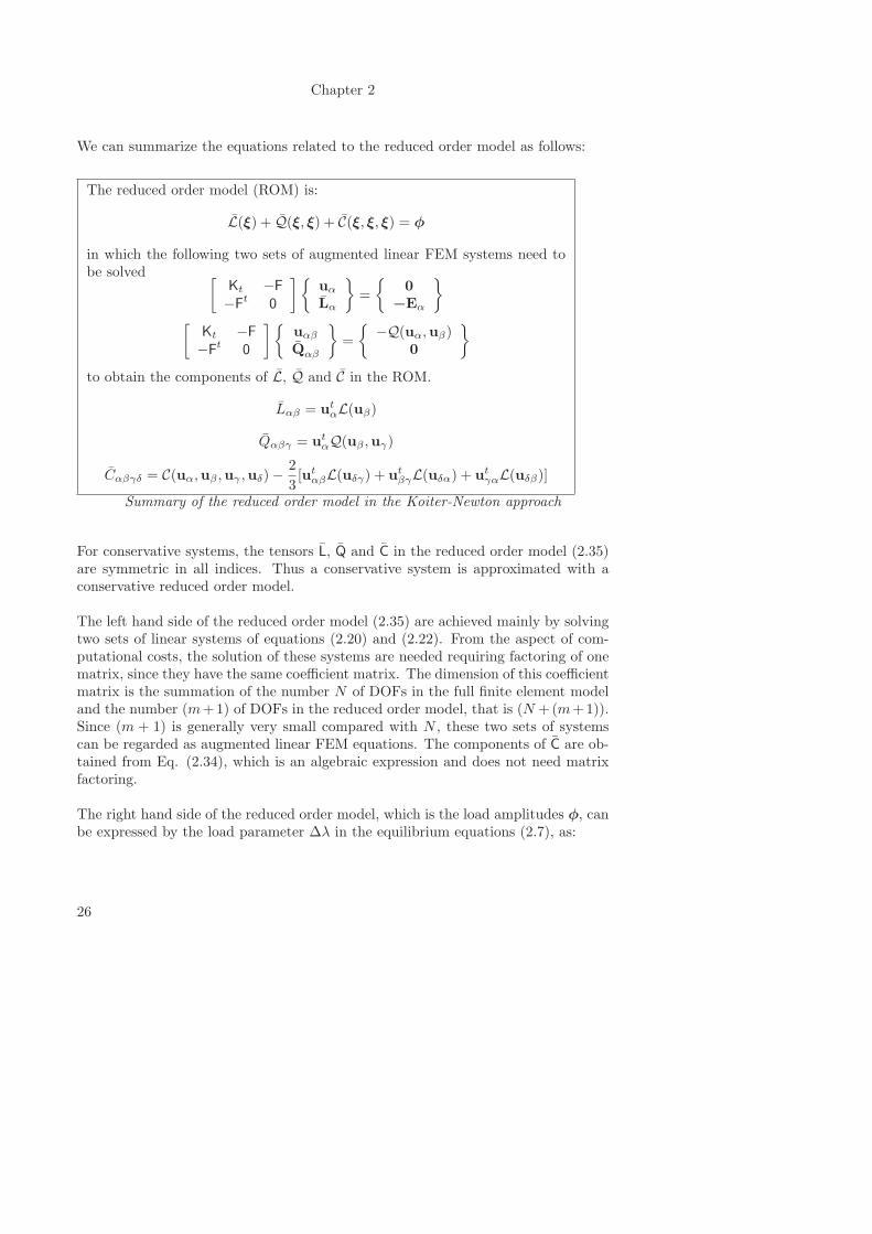
Chapter 2
We can summarize the equations related to the reduced order model as follows:
The reduced order model (ROM) is:
L(ξ) + Q(ξ, ξ) + C(ξ, ξ, ξ) = φ
in which the following two sets of augmented linear FEM systems need tobe solved [
Kt −F
−Ft
0
]{uα
Lα
}=
{0
−Eα
}
[Kt −F
−Ft
0
]{uαβ
Qαβ
}=
{−Q(uα,uβ)
0
}
to obtain the components of L, Q and C in the ROM.
Lαβ = utαL(uβ)
Qαβγ = utαQ(uβ ,uγ)
Cαβγδ = C(uα,uβ ,uγ ,uδ)−2
3[ut
αβL(uδγ) + utβγL(uδα) + ut
γαL(uδβ)]
Summary of the reduced order model in the Koiter-Newton approach
For conservative systems, the tensors L, Q and C in the reduced order model (2.35)are symmetric in all indices. Thus a conservative system is approximated with aconservative reduced order model.
The left hand side of the reduced order model (2.35) are achieved mainly by solvingtwo sets of linear systems of equations (2.20) and (2.22). From the aspect of com-putational costs, the solution of these systems are needed requiring factoring of onematrix, since they have the same coefficient matrix. The dimension of this coefficientmatrix is the summation of the number N of DOFs in the full finite element modeland the number (m+1) of DOFs in the reduced order model, that is (N +(m+1)).Since (m + 1) is generally very small compared with N , these two sets of systemscan be regarded as augmented linear FEM equations. The components of C are ob-tained from Eq. (2.34), which is an algebraic expression and does not need matrixfactoring.
The right hand side of the reduced order model, which is the load amplitudes φ, canbe expressed by the load parameter ∆λ in the equilibrium equations (2.7), as:
26
Koiter-Newton approach
φ = ∆λE1 (2.36)
where the unit basis vectors E1 are such that the 1-th component is one and allthe other components are zero. The dimension of the load amplitudes φ is m + 1.The first component ∆λ is the load parameter of the external load f1; The othercomponents are the load parameters of the perturbation loads fα, α = 2, . . . ,m+ 1and all are set equal to zero to simulate the response of the structure to actual loads.
If the buckling does not happen in the analysis, e.g. the stiffness of a structure isincreased with the increase of the load, only the external load and its correspondingload parameter ∆λ need to be considered and there will be only one degree of freedomin the reduced order model. Otherwise, the total number of degrees of freedom isrelated to the number m of closely-spaced buckling modes and will be m+ 1.
If the structure has many closely spaced buckling modes, buckling modes associ-ated with simultaneous or nearly simultaneous buckling loads, these closely spacedmodes will interact and influence the buckling characteristics of a structure. So,the selection of perturbation loads should also consider this case. As a simple rule,the buckling modes with buckling loads within 20% of the first buckling load areconsidered to be closely spaced modes and used to construct the perturbation loadswhich will be dicussed in the next section.
Having constructed the reduced order model (2.35), a path following technique maybe used to solve the reduced order model, and the relationship between the loadparameter ∆λ and displacement parameter ξ is obtained. In order to get the non-linear response (λ - q), the definitions λ = λ0 +∆λ and q = q0 ◦u are used and thedisplacement expansion is invoked:
u = u0 + uαξα + uαβξαξβ (2.37)
2.3 Selection of the perturbation loads
As discussed in the previous section, a linear subspace of the force space parametrizedby coordinates φ is defined as the span of predefined set of load vectors. In theproposed approach, the first load vector is always the external load fex, and theother load vectors are perturbation loads. The selection of these perturbation loadsis arbitrary within the restriction that the system matrix in Eqs. (2.20) and (2.22)is invertible.
27
Chapter 2
To make the proposed approach suitable for buckling-sensitive structures the Koiter-Newton approach is related to the traditional Koiter perturbation approach. Inspiredby Koiter perturbation approach, the perturbation loads should excite the bucklingbranches near the bifurcation points using knowledge of the buckling modes.
The basic premise behind the method is the use of Koiter’s asymptotic expansionfrom the beginning and at any point along the equilibrium path rather than using itonly at the bifurcation point. On the basis of the stability of the equilibrium pointat which the asymptotic expansion is applied, two cases need to be distinguished inthe selection of the perturbation loads related to the stable and unstable segmentsof the equilibrium path.
2.3.1 Expansion on the stable path
Case one is when the asymptotic expansion is applied on the stable part of theequilibrium path, which often happens in the prebuckling stage. In this case, thetangent stiffness matrix Kt = L is positive definite.
In Koiter’s work, the first order displacements are selected along the buckling modes.In the proposed approach, the primary path is also considered in the first order dis-placements. Our purpose is that when the expansion is applied near the bifurcationpoint, the first order displacements uα would be in the direction of the active buck-ling modes vα. To this end, the perturbation loads fα, α = 2, . . . ,m+1 are proposedas:
fα = Kgvϕ (2.38)
where vϕ, ϕ = 1, 2, . . . ,m are the closely-spaced linearized buckling modes; Kg is thegeometric stiffness matrix which can be calculated as follows:
Kg = −dKt
dλ= −
dKt
dq
dq
dλ(2.39)
where dKt/dq is the second order derivative of the internal force at the approximationpoint, that is 2Q. We assume q,λ can be determined by deriving the equilibriumequations, Eq. (2.1), with respect to λ to give:
Ktq,λ = fex (2.40)
Then, using the displacement q,λ obtained by solving Eq. (2.40), the final expression
28
Koiter-Newton approach
of the geometric matrix Kg will be:
Kg = −2Q(q,λ) (2.41)
In order to obtain the linearized buckling modes vϕ in Eq. (2.38), one linear bucklingeigenvalue problem at the approximation point needs to be solved as:
Ktv = µKgv (2.42)
where the scaler µ is the eigenvalue or buckling load parameter, and the vector v isthe buckling mode.
The eigenvalue problem (2.42) is solvable since the tangent stiffness matrix Kt isalways positive definite on the stable part of the equilibrium path.
If the expansion point is exactly at the bifurcation point, the condition f texvα = 0is satisfied. Moreover, the properties of eigenvalue problem (2.42) necessitate thatvtβKgvα = 0, α 6= β which can be written as f tβvα = 0, β > 1. These two conditions
indicate that vα is orthogonal to all forces except to fα. Hence we deduce thatuα = cαvα, no sum on α. This result guarantees that the present selection of forcesguarantees similar results near the bifurcation point to Koiter’s initial post-bucklingtheory.
2.3.2 Expansion on the unstable path
Case two is when the asymptotic expansion/approximation point is on the unstablepart of the equilibrium path, such as on the postbuckling path. In such cases,the tangent stiffness matrix is no longer positive definite and the above eigenvalueproblem (2.42) is unsolvable. To circumvent this problem a modified eigenvalueproblem needs to be constructed to find out the necessary modes.
In this case, two families of modes must be considered in the analysis. Family oneincludes the modes w which are already unstable, and the second family containsthe buckling prone modes v. Then, the total perturbation loads fα, α = 2, . . . ,m+1are composed of two sets of perturbation loads constructed by these two types ofmodes, respectively. It results in:
29
Chapter 2
{f2, ..., fα, ..., fm+1} ={f1, ..., fβ , ..., fma
, f1, ..., fγ , ..., fmb
}(2.43)
where fβ , β = 1, . . . ,ma are the perturbation loads related to already unstable modes
and ma is the number, fγ , γ = 1, . . . ,mb are the perturbation loads related tobuckling prone modes and mb is the number. The relationship m = ma + mb issatisfied.
Already Unstable Modes
For the modes that are already unstable, we can split the tangent stiffness into twoparts, the material stiffness Km and the stress stiffness Kσ, as follows:
Kt = Km + Kσ (2.44)
Then, the eigenvalue problem based on these two matrices can be constructed asEq. (2.45). Because the material matrix is always positive definite at any point, thiseigenvalue problem is solvable at all times, given by:
Kσw = µKmw (2.45)
where µ is the eigenvalue and w is the eigenvector or mode. Among all the modes,wβ , β = 1, 2, . . . ,ma are the already unstable modes. The selection criterion is thatthe mode w, the eigenvalue µ of which satisfies the inequation (1+ µ) ≤ 0, is alreadyunstable. The reason is as follows. Multiply the modes w and wt on both sides ofEq. (2.44), thus after some straightforward algebra it leads to:
wtKtw = wtKmw +wtKσw = wtKmw(1 +wtKσw
wtKmw) = wtKmw(1 + µ) (2.46)
where wtKσw/wtKmw = µ comes from Eq. (2.45).
Eq. (2.46) demonstrates that the tangent matrix will be not positive definite, thatis wtKtw ≤ 0, only if µ satisfies (1 + µ) ≤ 0.
The perturbation loads fβ , β = 1, 2, . . . ,ma which are related to the already unstablemodes are constructed as follows:
30
Koiter-Newton approach
fβ = Kmwβ (2.47)
Buckling Prone Modes
At the unstable equilibrium point of the equilibrium path, excepting the alreadyunstable modes w, the modes v that might go unstable are also important. The per-turbation loads which are constructed by these modes can excite buckling brancheswhich may occur later along the equilibrium path. In order to make Eq. (2.42) solv-able at the unstable equilibrium point, the eigenvalue problem based on the tangentstiffness and the geometric stiffness to make it is restricted to stable modes renderingit solvable. Hence, an additional orthogonality constraint about the buckling modesv and the perturbation loads fβ related to the already unstable modes is added intothe former eigenvalue problem (2.42). It results in:
{Ktv = µKgv
ft
βv = 0(2.48)
where µ is the eigenvalue and v is the buckling prone mode. The closely spacedbuckling modes vγ , γ = 1, . . . ,mb are selected using the proposed simple rule.
After obtaining the buckling modes, perturbation loads related to these bucklingprone modes fγ can be constructed as follows:
fγ = Kgvγ (2.49)
31
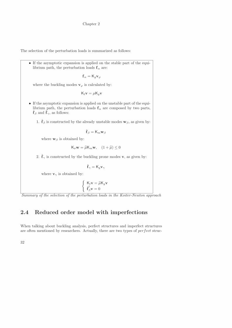
Chapter 2
The selection of the perturbation loads is summarized as follows:
• If the asymptotic expansion is applied on the stable part of the equi-librium path, the perturbation loads fα are:
fα = Kgvϕ
where the buckling modes vϕ is calculated by:
Ktv = µKgv
• If the asymptotic expansion is applied on the unstable part of the equi-librium path, the perturbation loads fα are composed by two parts,fβ and fγ , as follows:
1. fβ is constructed by the already unstable modes wβ , as given by:
fβ = Kmwβ
where wβ is obtained by:
Kσw = µKmw, (1 + µ) ≤ 0
2. fγ is constructed by the buckling prone modes v, as given by:
fγ = Kgvγ
where vγ is obtained by:
{Ktv = µKgv
ft
βv = 0
Summary of the selection of the perturbation loads in the Koiter-Newton approach
2.4 Reduced order model with imperfections
When talking about buckling analysis, perfect structures and imperfect structuresare often mentioned by researchers. Actually, there are two types of perfect struc-
32

Koiter-Newton approach
tures. One type refers to the exactly perfect structures, and another type to thenominal perfect structures. For the exactly perfect structures, e.g. the Eular col-umn and the flat plat under the axial compression, the structure is geometricalsymmetrical and the loading is not offset. In these cases, the buckling phenomenondoes not happen if there are no imperfection perturbations. In reality, these types ofstructures always have some small initial imperfections during the manufacture anduse. The nominal perfect cases mean that the structures do not exist any imperfec-tions but their geometries and loadings are not symmetrical. This type of structuresis very common in engineering, for instance, curved beams and panels under lat-eral loads or compression belong to this case. For the nominal perfect structures,the loading capability of a postbuckling is very sensitive to imperfections, thus animperfection analysis is very important in the buckling design of structures.
The reduced order model (2.35) in section 2.2 is only constructed for the perfectstructure. Now we will show how the behavior of the imperfect structure can bederived from the properties of the perfect structure [108]. Geometric imperfectionsare the most common imperfections used in the imperfection analysis. The de-formations caused by the initial imperfection loads can be used as the geometricimperfection. In the Koiter-Newton approach, imperfection loads are very conve-nient for implementing in the model. Here, two different ways of the implementationof imperfection loads are presented. The first way is based on the sub-loads, andthe second way is to use the independent imperfection loads.
2.4.1 Imperfection loads based on the sub-loads
We use the vector ∆f to indicate the imperfection loads applied on the discretefinite element model. It can be expressed as an approximate linear combination ofthe sub-loads fα, α = 1, . . . ,m + 1 mentioned in the multiple loading form of theequilibrium equations (2.8), which leads to:
∆f ≈ ∆λ1f1 +∆λ2f2 + ...+∆λαfα + ... (2.50)
where ∆λ ={∆λ1,∆λ2, ...,∆λα, ...
}, α = 1, . . . ,m+1 is the combination coefficient
vector which can also refer to as the imperfection coefficient vector, the sub-load f1is the external load fex, and the sub-loads fα, α = 2, . . . ,m+1 are the perturbationloads, wherem is the number of perturbation loads or closely spaced buckling modes.
Multiplying the first order displacement fields utα on both sides of Eq. (2.50) and
using the orthogonality constraints (2.12), these imperfection coefficients can be
33
Chapter 2
obtained by:
∆λα ≈ utα∆f (2.51)
Eq. (2.51) means that the imperfection coefficient ∆λα can be calculated by themultiplication of the corresponding displacement field ut
α and the imperfection load∆f .
The reduced order model (2.35) is constructed only for the perfect structure, thusits right hand side which is the load amplitude vector φ is defined to be such thatonly the first component is nonzero, see Eq. (2.36). If considering the imperfections,we can directly superpose the imperfection coefficient vector ∆λ on the right handside of the reduced order model, which results in:
L(ξ) + Q(ξ, ξ) + C(ξ, ξ, ξ) = φ+∆λ (2.52)
where the components, excluding the first one, of the right hand side vector are notall zeros, thus the effect of imperfections is considered in the reduced order model.
As the imperfection loads are implemented only in the right hand side of Eq. (2.52),the reduced order model is computed only once for the perfect structure and theeffect of various imperfections can be obtained afterwards with very little additionalcomputational cost for each imperfection pattern, which makes the Koiter-Newtonapproach to be much more efficient for imperfection analyses.
Then, the relation between the load parameter ∆λ and displacement parameter ξ
can be obtained by using a path following technique to solve the reduced order modelwith imperfections. Finally, after introducing it into the equations λ = λ0+∆λ,q =q0 ◦ u and Eq. (2.37), we get the nonlinear response (λ - q) of the structure withimperfections.
2.4.2 Independent imperfection loads
The implementation of imperfection loads introduced in subsection 2.4.1 will be in-valid when the buckling mode is orthogonal to the imperfection load vector ∆f .In this case, the corresponding first order displacement field may also be almost
34
Koiter-Newton approach
orthogonal to the imperfection load vector, which makes the corresponding imper-fection coefficients approach to zero according to Eq. (2.51). Another way for theimplementation of imperfection loads introduced in this subsection can overcomethis drawback and be more convenient for implementation.
Excluding the external loads fex applied on the structure, the independent imperfec-tion loads are also applied as some kind of external loads to model the imperfections.Hence, the differences after considering the imperfection loads start from the expan-sion of the equilibrium equations:
L(u) +Q(u,u) + C(u,u,u) = Fimφ (2.53)
where the load matrix Fim is different from F in Eq. (2.8). The α-th column of Fim
is also formed by the sub-load vector fα, however the sub-loads here are composedof three types of loads. The first sub-load vector f1 = fex is the external load;The sub-loads fα, α = 2, . . . , I + 1 are the independent imperfection loads, and I isnumber of imperfection loads; The sub-loads fα, α = I + 2, . . . ,m + I + 1 are theperturbation loads, where m is the number of perturbation loads or closely spacedbuckling modes.
Then, following the derivatives written in section 2.2.2, the reduced order modelwith the imperfection loads is given by:
L(ξ) + Q(ξ, ξ) + C(ξ, ξ, ξ) = φ (2.54)
where the reduced order model is a (m+I+1)th order nonlinear system of equations,φ here is the load amplitude vector considering the imperfection loads, which is a(m+ I + 1)× 1 vector.
The definition of the load amplitude vector φ is not the same as the definition inEq. (2.36). Consistent with the sub-loads, the components of φ also consist ofthree parts. The first part is φ1 = ∆λ, which is the load increment parameterof the external load fex; The second part contains the load parameters φα, α =2, . . . , I +1 of all the independent imperfection loads fα, α = 2, . . . , I +1; The thirdpart encompass the load parameters φα, α = I+2, . . . ,m+ I+1 of the perturbationloads fα, α = I + 2, . . . ,m + I + 1 and are all set equal to zero to simulate theresponse of the structure under actual loads.
For a given pattern of imperfection loads, the load parameters φα, α = 2, . . . , I + 1of the independent imperfection loads are fixed to be some certain values duringthe simulation of the reduced order model using a path following technique. For a
35
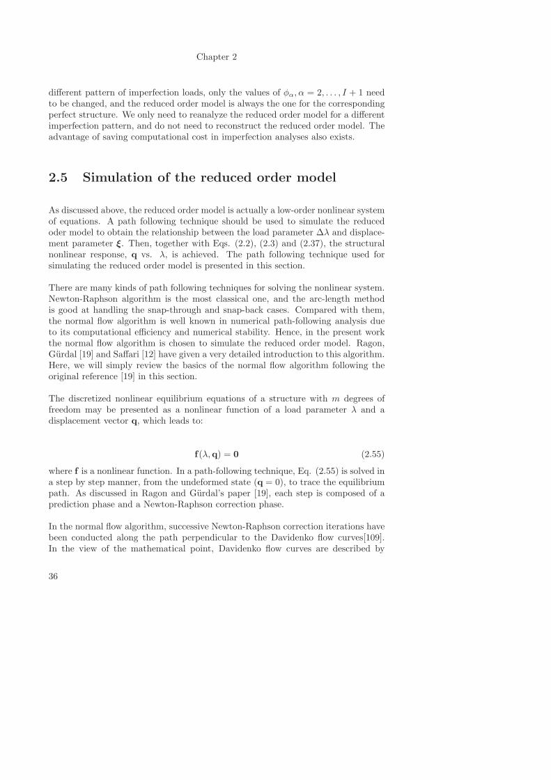
Chapter 2
different pattern of imperfection loads, only the values of φα, α = 2, . . . , I + 1 needto be changed, and the reduced order model is always the one for the correspondingperfect structure. We only need to reanalyze the reduced order model for a differentimperfection pattern, and do not need to reconstruct the reduced order model. Theadvantage of saving computational cost in imperfection analyses also exists.
2.5 Simulation of the reduced order model
As discussed above, the reduced order model is actually a low-order nonlinear systemof equations. A path following technique should be used to simulate the reducedoder model to obtain the relationship between the load parameter ∆λ and displace-ment parameter ξ. Then, together with Eqs. (2.2), (2.3) and (2.37), the structuralnonlinear response, q vs. λ, is achieved. The path following technique used forsimulating the reduced order model is presented in this section.
There are many kinds of path following techniques for solving the nonlinear system.Newton-Raphson algorithm is the most classical one, and the arc-length methodis good at handling the snap-through and snap-back cases. Compared with them,the normal flow algorithm is well known in numerical path-following analysis dueto its computational efficiency and numerical stability. Hence, in the present workthe normal flow algorithm is chosen to simulate the reduced order model. Ragon,Gurdal [19] and Saffari [12] have given a very detailed introduction to this algorithm.Here, we will simply review the basics of the normal flow algorithm following theoriginal reference [19] in this section.
The discretized nonlinear equilibrium equations of a structure with m degrees offreedom may be presented as a nonlinear function of a load parameter λ and adisplacement vector q, which leads to:
f(λ,q) = 0 (2.55)
where f is a nonlinear function. In a path-following technique, Eq. (2.55) is solved ina step by step manner, from the undeformed state (q = 0), to trace the equilibriumpath. As discussed in Ragon and Gurdal’s paper [19], each step is composed of aprediction phase and a Newton-Raphson correction phase.
In the normal flow algorithm, successive Newton-Raphson correction iterations havebeen conducted along the path perpendicular to the Davidenko flow curves[109].In the view of the mathematical point, Davidenko flow curves are described by
36
Koiter-Newton approach
considering a perturbation parameter η into the nonlinear system of equations, whichgoverns the problem as the following form:
f(λ,q) = η (2.56)
A family of response curves called Davidenko flow is obtained by changing the per-turbation parameter η and solving the nonlinear system of equations (2.56). In Fig.2.2, the dashed curves represent the Davidenko flow curves for a system with justone degree of freedom. As discussed above, to gain an acceptable convergence rate,the correction iterations for solving the problem are conducted along the path per-pendicular to the Davidenko flow curves. As shown in Fig. 2.2, for a given step, westart at a converged equilibrium point A, then a point B can be found using the di-rection of the tangent vector in an initial prediction phase. Finally, the normal flowalgorithm will converge to a new equilibrium point C along the path perpendicularto the Davidenko flow curves in a Newton-Raphson correction phase.
A
B
C
λ
q
Normal !ow iterations
Figure 2.2: Normal flow algorithm
To describe this correction phrase in detail, the ith iteration in the step (n+1) canbe presented as:
37
Chapter 2
[Df(si−1n+1)]∆s = −f(si−1
n+1)
c(sin+1) = 0
(2.57)
sin+1 = si−1n+1 +∆s, i = 1, 2, . . . (2.58)
and:
∆s = v −vtu
utuu (2.59)
where sin+1 = (λin+1,qin+1)
t is the solution of the ith iteration in the step (n + 1).The second equation in (2.57) is an auxiliary constraint equation which is the core ofthe normal flow algorithm. For different path-following techniques, this constraintequation is constructed in a different way to present a different correction strategy.[Df ] is a m × (m + 1) Jacobian matrix of the system (2.55). ∆s is an solutionincrement between the (i− 1)th iteration and the ith iteration. It can be seen thatthe number of solution increments in the first equation of system (2.57) is infinite,however a minimum solution ∆s, which is unique, can be obtained in the correctionphase of the normal flow algorithm using a particular solution v and a vector u.A particular solution v to system (2.57) can be obtained by selecting a constraintequation. A vector u is any vector in the kernel of [Df ], and it can be chose to bethe tangent vector s∗n which has already been obtained in each step.
In this way, after ∗th iteration, a new equilibrium point s∗n+1 on the equilibriumpath is obtained and a new step will begin from this known point.
2.6 Koiter-Newton arclength method
A traditional drawback of reduced order models is that they have a limited rangeof validity. The reduced order model(ROM) proposed in section 2.2 should havea wider range of validity than for example the use of path derivatives [35] as itaccounts for possible branching into quickly softening modes. Yet, it will still havesome limited range of validity that cannot be determined a priori.
38
Koiter-Newton approach
2.6.1 Automated techniques
In order to construct an efficient algorithm, analysis of the range of validity shouldbe automated. While the reduced order model was simulated using a path followingtechnique, the exact unbalanced force was calculated using the full finite elementmodel at the end of each solution step. The norm of the residual force was used tojudge whether the ROM was sufficiently accurate. The simulation of the reducedorder model was stopped when:
‖R‖
λ ‖fex‖> ε (2.60)
where, ε is a prespecified tolerance, λ is the current load parameter, and R is theunbalanced (residual) force and can be calculated as follows:
R = λfex − f (2.61)
where f is the current internal force.
A fully general and automatic procedure can be devised at this stage. Starting froma given equilibrium point, usually the undeformed configuration, a Koiter’s asymp-totic expansion is carried out and a ROM is constructed. Using the constructedROM, a path following technique is applied, and the solution of the ROM is usedto estimate the response of the full model, see Fig. 2.3. The ROM is used untilit is no longer valid according to Eq. (2.60). This is considered to be a predictorstep. A conventional Newton-based arc-length method can then be used to restorethe equilibrium of the full model in a corrector step. The new convergent point onthe equilibrium path, see Fig. 2.3, is denoted the expansion point for the next stepof the algorithm.
The flow chart for the Koiter-Newton approach can be seen in Fig. 2.4.
A few remarks about the advantages of the approach are in order.
• In the present approach, the reduced order model is based on Koiter’s initialpost-buckling theory, which can easily capture the buckling branches accu-rately, even for perfect structure. Branch detection can be checked for theROM easily leading to improved robustness without increased computationalcost. Conventional nonlinear FE methods, and many reduction methods that
39
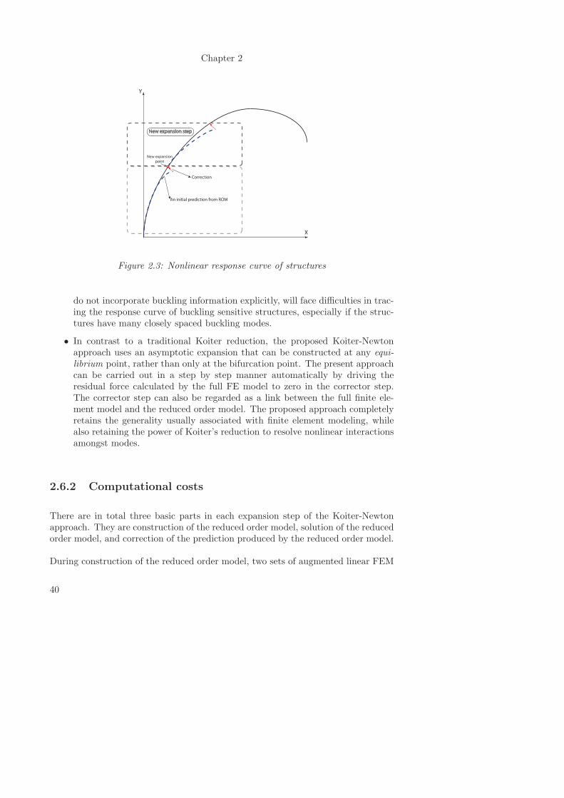
Chapter 2
Y
X
An initial prediction from ROM
Correction
New expansion
point
New expansion step
Figure 2.3: Nonlinear response curve of structures
do not incorporate buckling information explicitly, will face difficulties in trac-ing the response curve of buckling sensitive structures, especially if the struc-tures have many closely spaced buckling modes.
• In contrast to a traditional Koiter reduction, the proposed Koiter-Newtonapproach uses an asymptotic expansion that can be constructed at any equi-librium point, rather than only at the bifurcation point. The present approachcan be carried out in a step by step manner automatically by driving theresidual force calculated by the full FE model to zero in the corrector step.The corrector step can also be regarded as a link between the full finite ele-ment model and the reduced order model. The proposed approach completelyretains the generality usually associated with finite element modeling, whilealso retaining the power of Koiter’s reduction to resolve nonlinear interactionsamongst modes.
2.6.2 Computational costs
There are in total three basic parts in each expansion step of the Koiter-Newtonapproach. They are construction of the reduced order model, solution of the reducedorder model, and correction of the prediction produced by the reduced order model.
During construction of the reduced order model, two sets of augmented linear FEM
40
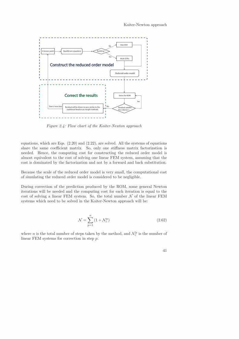
Koiter-Newton approach
Buckling ?A known point Equilibrium equations
One DOF
Multi DOFs
No
Yes
Reduced order model
Solve the ROM
Residual satis!es
the criterion ?
Residual will be driven to zero similar to the
traditional Newton arc-length methods
Construct the reduced order model
Correct the results
No
Yes
Start a new step
Figure 2.4: Flow chart of the Koiter-Newton approach
equations, which are Eqs. (2.20) and (2.22), are solved. All the systems of equationsshare the same coefficient matrix. So, only one stiffness matrix factorization isneeded. Hence, the computing cost for constructing the reduced order model isalmost equivalent to the cost of solving one linear FEM system, assuming that thecost is dominated by the factorization and not by a forward and back substitution.
Because the scale of the reduced order model is very small, the computational costof simulating the reduced order model is considered to be negligible.
During correction of the prediction produced by the ROM, some general Newtoniterations will be needed and the computing cost for each iteration is equal to thecost of solving a linear FEM system. So, the total number N of the linear FEMsystems which need to be solved in the Koiter-Newton approach will be:
N =n∑
p=1
(1 +N pc ) (2.62)
where n is the total number of steps taken by the method, and N pc is the number of
linear FEM systems for correction in step p.
41
Chapter 2
The better prediction provided by the reduced order model compared to linear pre-dictors which classical Newton methods usually use, allows the algorithm to usefairly large step sizes during K-N iterations.
Based on the discussion above, the proposed approach will significantly improve theefficiency of nonlinear static finite element analysis, especially for buckling sensitivestructures as will be demonstrated in the numerical examples of chapters 4 and 5.
2.7 Conclusions
A new approach denoted the Koiter-Newton is presented for the numerical solutionof a class of elastic nonlinear structural response problems. It is a combinationof a reduction method inspired by Koiter’s post-buckling analysis and the Newtonarc-length method which makes the method accurate over the entire nonlinear equi-librium path, and also computationally efficient in the presence of buckling; TheKoiter-Newton approach can also consider imperfections in a structure and do therequired imperfection analyses in a computationally economic manner; The com-putational costs of using the Koiter-Newton approach are summarized to show thehigh efficiency in the nonlinear structural analysis.
42
Chapter 3
Koiter-Newton analysis using
co-rotational beam
kinematics
3.1 Introduction
A structure usually undergoes a large motion in the presence of buckling, hencegeometrically nonlinear mechanics is usually employed in a buckling analysis [110].In Felippa’s book [111], geometrically nonlinear problems have been discussed indetail, hence we will simply review the basics of geometrically nonlinear mechanics,especially the co-rotational kinematics, following Felippa’s book in this section.
Currently, three Lagrangian kinematic descriptions that exist in the literature areused for finite element analysis of geometrically nonlinear structures [111, 112]: (1)total Lagrangian (TL) formulation, (2) updated Lagrangian (UL) formulation, and(3) co-rotational (CR) formulation. Among them, the CR formulation was the last tobe developed, and it has received considerable attention recently. In the beginning,the CR formulation was not designed to be implemented in a general finite elementfor the nonlinear analysis of structures, since the application of this formulation islimited by a priori kinematics assumptions. This assumption demands that the CRformulation can only be used in the case where the displacements and rotations maybe arbitrarily large, but the deformations must be small [111]. To make the CR
43
Chapter 3
formulation more widely applicable, the idea of multiple frames [113] was proposedfor the CR formulation. Instead of one CR frame for a whole structure, each elementof a structure is given one independent frame called a CR element frame. Thismodification helps to fulfill the above assumption, and it is achieved by making theelement deformational displacements and rotations small with respect to the CRelement frame. Even if the assumption is violated for a coarse mesh, we can refinethe mesh to make the element size small enough. Then, the domain of applicationfor the CR formulation is extended in the geometrically nonlinear structural analysis[114].
Instead of introducing new element formulations, the current popular way is toconstruct a systematic and efficient procedure to update the existing linear elementlibrary to take into consideration the nonlinear kinematics. One good choice forthis purpose is to use the element independent co-rotational frame [115, 116, 117,98]. In this CR frame, the element motion is split into two parts, a rigid partand a deformational part. The rigid part indicates the average motion of the CRframe which moves together with the element from the reference configuration tothe current configuration. The deformational part is the local motion within thisCR frame. As discussed above, this deformational part can be made small enoughby refining the mesh. The element strain energy is only related to the deformationalpart, hence some simplified kinematics, such as the linear kinematics, can be used inthe CR frame. It can be seen that the basic idea of the CR formulation is to extractthe deformational part of the total motion by purging the rigid part before theelement computations. It can be performed outside the standard element routinesand thus is independent of element type [111].
The basic procedure of the Koiter-Newton approach is presented in chapter 2 in de-tail, and for wide applicability in engineering, this approach should be implementedinto the finite element environment. According to the derivations given in chapter2, the expressions of the L, Q and C in the equilibrium equations (2.8) should beobtained to construct the reduced order model, and these expressions are relatedto the element formulations. In the present thesis, the co-rotational formulation isused for the FE implementation of the Koiter-Newton approach. The reasons are asfollows:
• the element independent co-rotational frame are more accurate for the largedisplacement and large rotation cases in the geometrically nonlinear analysis,by purging the rigid part from the total motion.
• the co-rotational formulation can address the accuracy and convergence prob-lems which often occurs in the implementation of Koiter perturbation approachinto the finite element context [67, 8].
44
Koiter-Newton’s analysis using co-rotational beam kinematics
• the proposed Koiter-Newton approach presented in Chapter 2 requires deriva-tives of the element load vectors with respect to degrees of freedom up to thethird order. This is two orders more than traditionally needed for Newton’smethod. Nonlinear elements based on the element independent co-rotationalframe can facilitate the differentiations. Automatic differentiation is used tofind the derivatives of the co-rotational frame with respect to element degreesof freedom. In this way, full nonlinear kinematics are taken into account whenconstructing the reduced order model.
• due to the element independent characteristic of the co-rotational frame, anytype of the linear elements in the current element library can be used for theKoiter-Newton approach, and the geometric nonlinearity is taken into accountby the derivatives of the local co-rotational frame with respect to the globalframe.
The Koiter-Newton approach using co-rotational beam kinematics is presented inthis chapter, and the focus of chapter 4 is the co-rotational shell kinematics. Therest of this chapter is organized as follows. The finite element implementation ofthe co-rotational beam kinematics is presented, then, the performance of the Koiter-Newton analysis is evaluated using some numerical examples of the beam model.
3.2 Co-rotational beam kinematics
In this section, we introduce the descriptions of the beam element in a co-rotationalframe, then based on it, the local and global degrees of freedom of the beam elementare given.
A simple co-rotational beam element using Kirchhoff theory is presented in Cr-isfield’s book [112]. Deformation of a 2-D beam element from the initial undeformedconfiguration, that is the initial reference configuration, to the current deformedconfiguration under the loading is shown in Fig. 3.1. The two nodes of the beamelement are denoted as a and b, and there are three degrees of freedom of each nodewhich are two translations u, v and one rotation θ. In Fig. 3.1, the coordinatesystem x − y is the global system, and the coordinate system ex − ey located onthe node a is the co-rotational system of element which moves together with theelement. The ex axis of the co-rotational system is always along the direction fromnode a to node b, and the ey axis is perpendicular to the ex axis in the 2D beamplane.
45
Chapter 3
0
ye
0
xea
dye
d
xe
x
y
θ∆
ˆaθ
aθ
x
θ
0θ
Figure 3.1: Sketch of the beam element in a co-rotational frame
Then, the global degrees of freedom of the beam element in the global coordinatesystem x− y are given as:
q = {ua, va, θa, ub, vb, θb}t
(3.1)
where the subscripts a and b are the node numbers.
When a large displacement or large rotation happens, most of the global degrees offreedom are caused by the rigid motion. Since the strain energy depends only onthe deformational part, the local degrees of freedom which cause the deformationcan be selected in the co-rotational frame, which results in:
q ={0, 0, θa, ub, 0, θb
}t
(3.2)
where, based on the definition of the local co-rotational coordinate system, the twolocal translations ua, va of node a and the local vertical translation vb of node bare zeros at all times during the deformation of the element. The local rotations θa
46
Koiter-Newton’s analysis using co-rotational beam kinematics
and θb can also be called local co-rotational slopes [112]. Hence, the local degrees offreedom q of the beam element can be reduced to:
q ={ub, θa, θb
}t
(3.3)
It can be seen from Fig. 3.1 that the global and local degrees of freedom of the beamelement should satisfy the following geometrical relations, given by:
ub = ln − l
θa = θa −∆θ = θa − (θ − θ0) = θa − θ + θ0θb = θb −∆θ = θb − (θ − θ0) = θb − θ + θ0
(3.4)
where the l and ln are the initial and current length of the beam element, respectively,θ is the angle between the current configuration of the beam and the x axis of theglobal coordinate system, θ0 is the angle between the initial configuration of thebeam and the x axis of the global coordinate system, and ∆θ is the angle betweenthe initial and current configuration of the beam.
We assume that the position vectors of the nodes a and b in the initial configurationare ra and rb ,respectively, and the position vectors of the nodes a and b in thecurrent configuration are da and db, respectively, see Fig. 3.2. Then, the currentlength ln of the beam element after the deformation can be expressed as:
l2n = l2 + 2(rb − ra)t(db − da) + (db − da)
t(db − da) (3.5)
Next, the strain of the beam element can be written as:
ε =ubl
=ln − l
l=
l2n − l2
l(ln + l)=
2(rb − ra)t(db − da) + (db − da)
t(db − da)
l(ln + l)(3.6)
The curvature of the beam element can be expressed as:
κ =θb − θa
l(3.7)
47
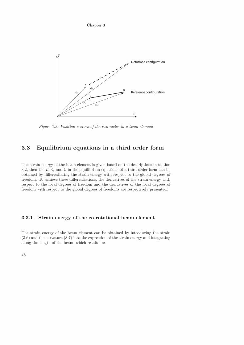
Chapter 3
b
a
b
a
rarb
da
db
y
x
Reference con�guration
Deformed con�guration
Figure 3.2: Position vectors of the two nodes in a beam element
3.3 Equilibrium equations in a third order form
The strain energy of the beam element is given based on the descriptions in section3.2, then the L, Q and C in the equilibrium equations of a third order form can beobtained by differentiating the strain energy with respect to the global degrees offreedom. To achieve these differentiations, the derivatives of the strain energy withrespect to the local degrees of freedom and the derivatives of the local degrees offreedom with respect to the global degrees of freedoms are respectively presented.
3.3.1 Strain energy of the co-rotational beam element
The strain energy of the beam element can be obtained by introducing the strain(3.6) and the curvature (3.7) into the expression of the strain energy and integratingalong the length of the beam, which results in:
48
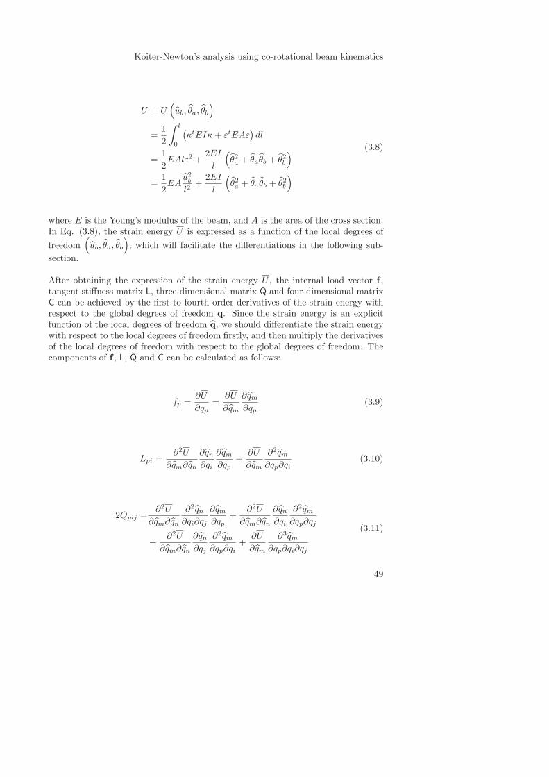
Koiter-Newton’s analysis using co-rotational beam kinematics
U = U(ub, θa, θb
)
=1
2
∫ l
0
(κtEIκ+ εtEAε
)dl
=1
2EAlε2 +
2EI
l
(θ2a + θaθb + θ2b
)
=1
2EA
u2bl2
+2EI
l
(θ2a + θaθb + θ2b
)
(3.8)
where E is the Young’s modulus of the beam, and A is the area of the cross section.In Eq. (3.8), the strain energy U is expressed as a function of the local degrees of
freedom(ub, θa, θb
), which will facilitate the differentiations in the following sub-
section.
After obtaining the expression of the strain energy U , the internal load vector f ,tangent stiffness matrix L, three-dimensional matrix Q and four-dimensional matrixC can be achieved by the first to fourth order derivatives of the strain energy withrespect to the global degrees of freedom q. Since the strain energy is an explicitfunction of the local degrees of freedom q, we should differentiate the strain energywith respect to the local degrees of freedom firstly, and then multiply the derivativesof the local degrees of freedom with respect to the global degrees of freedom. Thecomponents of f , L, Q and C can be calculated as follows:
fp =∂U
∂qp=
∂U
∂qm
∂qm∂qp
(3.9)
Lpi =∂2U
∂qm∂qn
∂qn∂qi
∂qm∂qp
+∂U
∂qm
∂2qm∂qp∂qi
(3.10)
2Qpij =∂2U
∂qm∂qn
∂2qn∂qi∂qj
∂qm∂qp
+∂2U
∂qm∂qn
∂qn∂qi
∂2qm∂qp∂qj
+∂2U
∂qm∂qn
∂qn∂qj
∂2qm∂qp∂qi
+∂U
∂qm
∂3qm∂qp∂qi∂qj
(3.11)
49
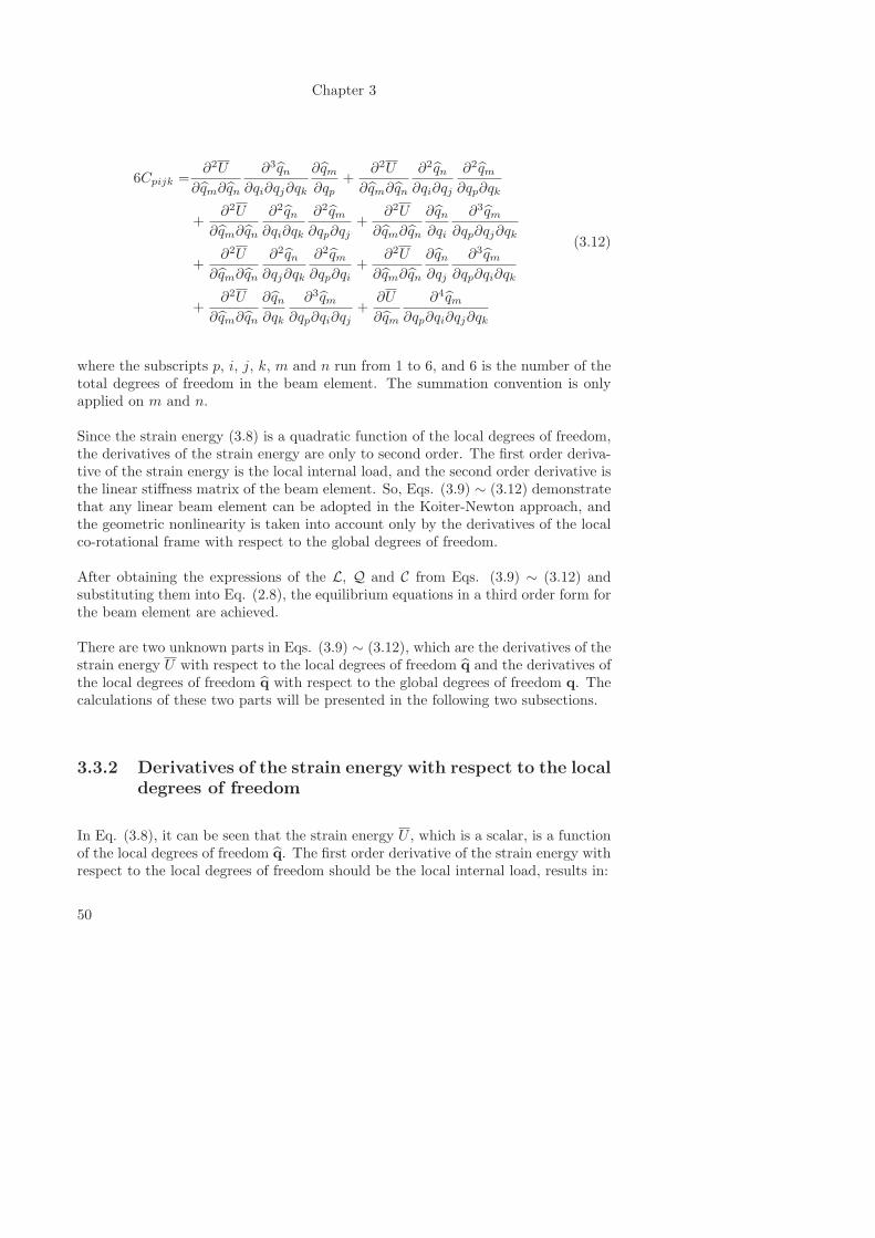
Chapter 3
6Cpijk =∂2U
∂qm∂qn
∂3qn∂qi∂qj∂qk
∂qm∂qp
+∂2U
∂qm∂qn
∂2qn∂qi∂qj
∂2qm∂qp∂qk
+∂2U
∂qm∂qn
∂2qn∂qi∂qk
∂2qm∂qp∂qj
+∂2U
∂qm∂qn
∂qn∂qi
∂3qm∂qp∂qj∂qk
+∂2U
∂qm∂qn
∂2qn∂qj∂qk
∂2qm∂qp∂qi
+∂2U
∂qm∂qn
∂qn∂qj
∂3qm∂qp∂qi∂qk
+∂2U
∂qm∂qn
∂qn∂qk
∂3qm∂qp∂qi∂qj
+∂U
∂qm
∂4qm∂qp∂qi∂qj∂qk
(3.12)
where the subscripts p, i, j, k, m and n run from 1 to 6, and 6 is the number of thetotal degrees of freedom in the beam element. The summation convention is onlyapplied on m and n.
Since the strain energy (3.8) is a quadratic function of the local degrees of freedom,the derivatives of the strain energy are only to second order. The first order deriva-tive of the strain energy is the local internal load, and the second order derivative isthe linear stiffness matrix of the beam element. So, Eqs. (3.9) ∼ (3.12) demonstratethat any linear beam element can be adopted in the Koiter-Newton approach, andthe geometric nonlinearity is taken into account only by the derivatives of the localco-rotational frame with respect to the global degrees of freedom.
After obtaining the expressions of the L, Q and C from Eqs. (3.9) ∼ (3.12) andsubstituting them into Eq. (2.8), the equilibrium equations in a third order form forthe beam element are achieved.
There are two unknown parts in Eqs. (3.9) ∼ (3.12), which are the derivatives of thestrain energy U with respect to the local degrees of freedom q and the derivatives ofthe local degrees of freedom q with respect to the global degrees of freedom q. Thecalculations of these two parts will be presented in the following two subsections.
3.3.2 Derivatives of the strain energy with respect to the local
degrees of freedom
In Eq. (3.8), it can be seen that the strain energy U , which is a scalar, is a functionof the local degrees of freedom q. The first order derivative of the strain energy withrespect to the local degrees of freedom should be the local internal load, results in:
50
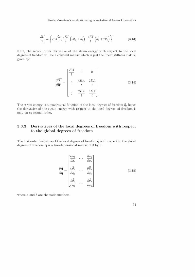
Koiter-Newton’s analysis using co-rotational beam kinematics
∂U
∂q=
{EA
ubl,2EI
l
(2θa + θb
),2EI
l
(θa + 2θb
)}t
(3.13)
Next, the second order derivative of the strain energy with respect to the localdegrees of freedom will be a constant matrix which is just the linear stiffness matrix,given by:
∂2U
∂q2=
EA
l0 0
04EA
l
2EA
l
02EA
l
4EA
l
(3.14)
The strain energy is a quadratical function of the local degrees of freedom q, hencethe derivative of the strain energy with respect to the local degrees of freedom isonly up to second order.
3.3.3 Derivatives of the local degrees of freedom with respect
to the global degrees of freedom
The first order derivative of the local degrees of freedom q with respect to the globaldegrees of freedom q is a two-dimensional matrix of 3 by 6:
∂q
∂q=
∂ub∂q1
· · ·∂ub∂q6
∂θa∂q1
· · ·∂θa∂q6
∂θb∂q1
· · ·∂θb∂q6
(3.15)
where a and b are the node numbers.
51
Chapter 3
In the same way, we can know that the second to fourth order derivatives of thelocal degrees of freedom with respect to the global degrees of freedom will be thethree-dimensional matrix of 3 by 6 by 6, the four-dimensional matrix of 3 by 6 by 6by 6 and the five-dimensional matrix of 3 by 6 by 6 by 6 by 6, the forms of whichare very complicated and are not listed here. Actually, these matrices are formedby three groups of derivatives, which are listed only to the second order as follows:
∂ub∂qi
=∂ln∂qi
;∂2ub∂qi∂qj
=∂2ln∂qi∂qj
; · · · (3.16)
∂θa∂qi
=
1, if i = 3
0, if i = 6
∂θ
∂qi, if i = others
;∂2θa∂qi∂qj
=
0, if i, j = 3, 6
∂2θ
∂qi∂qj, if i, j = others
(3.17)
∂θb∂qi
=
1, if i = 3
0, if i = 6
∂θ
∂qi, if i = others
;∂2θb∂qi∂qj
=
0, if i, j = 3, 6
∂2θ
∂qi∂qj, if i, j = others
(3.18)
where the subscripts i and j run from 1 to 6, and the fact of the geometrical relations(3.4) are used.
From Eqs. (3.16) to (3.18) it can be seen that the unknown terms are the derivativesof the current length ln and the rigid rotation θ with respect to the global degrees offreedom. The detailed calculations of these two unknown groups of derivatives willbe presented in the rest of this subsection.
Referring to Fig. 3.1, the following geometrical relation can be easily found in atriangle formed by the current configuration and the x axis, which results in:
{ln cos θ, ln sin θ} = {db − da} = ∆r(q) (3.19)
52
Koiter-Newton’s analysis using co-rotational beam kinematics
where the vector ∆r(q) is related to the global degrees of freedom {ua, va, ub, vb},and can be calculated by:
∆r(q) = {(x0b − x0a) + (ub − ua), (y0b − y0a) + (vb − va)} (3.20)
where (x0a, y0a) and (x0b, y0b) are respectively the coordinates of nodes a and b ofthe initial undeformed beam.
Differentiating Eq. (3.19) with respect to the global degrees of freedom, the followingequation can be obtained:
∂ln∂qi
(cos θ, sin θ) + ln (− sin θ, cos θ)∂θ
∂qi=
∆r(q)
∂qi(3.21)
where the subscript i runs from 1 to 6, and the right hand side of Eq. (3.21) can beobtained by differentiating Eq. (3.20), which leads to:
∆r(q)
∂qi=
(−1, 0) if i = 1
(0,−1) if i = 2
(1, 0) if i = 4
(0, 1) if i = 5
(0, 0) if i = 3, 6
(3.22)
Then, if both sides of Eq. (3.21) is multiplied by the vector (cos θ, sin θ)t, the first
order derivative of the current length ln of the beam element with respect to theglobal degrees of freedom can be obtained by:
∂ln∂qi
=∆r(q)
∂qi(cos θ, sin θ)
t(3.23)
Next, if both sides of Eq. (3.21) is multiplied by the vector (− sin θ, cos θ)t, the first
order derivative of the rigid rotation θ with respect to the global degrees of freedomcan be obtained by:
53
Chapter 3
ln∂θ
∂qi=
∆r(q)
∂qi(− sin θ, cos θ)
t(3.24)
In the same way, the other derivatives of the current length ln of the beam elementand the rigid rotation θ with respect to the global degrees of freedom can be achievedas follows (up to the fourth order):
∂2ln∂qi∂qj
= ln∂θ
∂qi
∂θ
∂qj
ln∂2θ
∂qi∂qj= −
(∂ln∂qi
∂θ
∂qj+∂ln∂qj
∂θ
∂qi
) (3.25)
∂3ln∂qi∂qj∂qk
=ln∂2θ
∂qi∂qj
∂θ
∂qk+ ln
∂2θ
∂qj∂qk
∂θ
∂qi+ ln
∂2θ
∂qk∂qi
∂θ
∂qj
+∂ln∂qi
∂θ
∂qj
∂θ
∂qk+∂ln∂qj
∂θ
∂qk
∂θ
∂qi+∂ln∂qk
∂θ
∂qi
∂θ
∂qj
ln∂3θ
∂pi∂pj∂pk=−
∂2ln∂qi∂qj
∂θ
∂qk−
∂2ln∂qj∂qk
∂θ
∂qi−
∂2ln∂qk∂qi
∂θ
∂qj
−∂ln∂qi
∂2θ
∂qj∂qk−∂ln∂qj
∂2θ
∂qk∂qi−∂ln∂qk
∂2θ
∂qi∂qj
+ ln∂θ
∂qi
∂θ
∂qj
∂θ
∂qk
(3.26)
54
Koiter-Newton’s analysis using co-rotational beam kinematics
∂4ln∂qi∂qj∂qk∂ql
=∂2ln∂qi∂qj
∂θ
∂qk
∂θ
∂ql+
∂2ln∂qj∂qk
∂θ
∂ql
∂θ
∂qi+
∂2ln∂qk∂ql
∂θ
∂qi
∂θ
∂qj
+∂2ln∂ql∂qi
∂θ
∂qj
∂θ
∂qk+
∂2ln∂qi∂qk
∂θ
∂qj
∂θ
∂ql+
∂2ln∂qj∂ql
∂θ
∂qi
∂θ
∂qk
+∂ln∂qi
∂2θ
∂qj∂qk
∂θ
∂ql+∂ln∂qi
∂2θ
∂qj∂ql
∂θ
∂qk+∂ln∂qi
∂2θ
∂qk∂ql
∂θ
∂qj
+∂ln∂qj
∂2θ
∂qi∂ql
∂θ
∂qk+∂ln∂qj
∂2θ
∂qk∂ql
∂θ
∂qi+∂ln∂qj
∂2θ
∂qi∂qk
∂θ
∂ql
+∂ln∂qk
∂2θ
∂qi∂ql
∂θ
∂qj+∂ln∂qk
∂2θ
∂qj∂ql
∂θ
∂qi+∂ln∂qk
∂2θ
∂qi∂qj
∂θ
∂ql
+∂ln∂ql
∂2θ
∂qi∂qk
∂θ
∂qj+∂ln∂ql
∂2θ
∂qj∂qk
∂θ
∂qi+∂ln∂ql
∂2θ
∂qi∂qj
∂θ
∂qk
+ ln∂3θ
∂qi∂qj∂qk
∂θ
∂ql+ ln
∂3θ
∂qi∂qj∂ql
∂θ
∂qk+ ln
∂3θ
∂qj∂qk∂ql
∂θ
∂qi
+ ln∂3θ
∂qi∂qk∂ql
∂θ
∂qj+ ln
∂2θ
∂qi∂qj
∂2θ
∂qk∂ql+ ln
∂2θ
∂qi∂ql
∂2θ
∂qj∂qk
+ ln∂2θ
∂qi∂qk
∂2θ
∂qj∂ql− ln
∂θ
∂qi
∂θ
∂qj
∂θ
∂qk
∂θ
∂ql
(3.27)
55
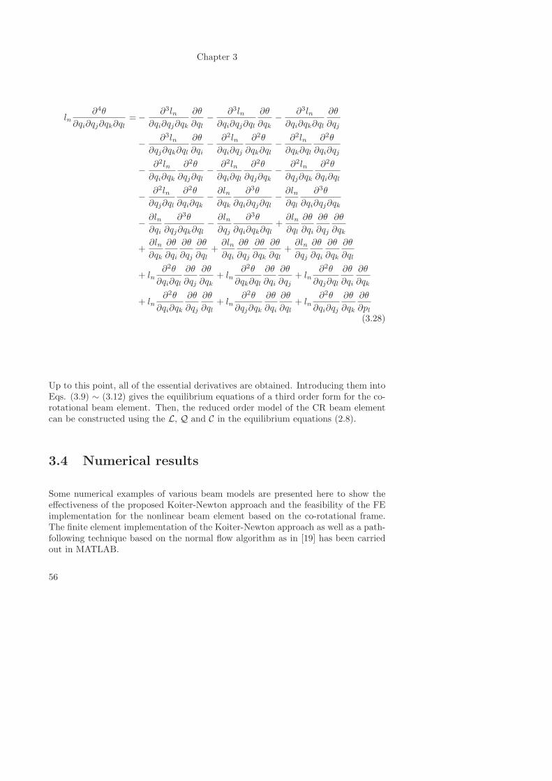
Chapter 3
ln∂4θ
∂qi∂qj∂qk∂ql=−
∂3ln∂qi∂qj∂qk
∂θ
∂ql−
∂3ln∂qi∂qj∂ql
∂θ
∂qk−
∂3ln∂qi∂qk∂ql
∂θ
∂qj
−∂3ln
∂qj∂qk∂ql
∂θ
∂qi−
∂2ln∂qi∂qj
∂2θ
∂qk∂ql−
∂2ln∂qk∂ql
∂2θ
∂qi∂qj
−∂2ln∂qi∂qk
∂2θ
∂qj∂ql−
∂2ln∂qi∂ql
∂2θ
∂qj∂qk−
∂2ln∂qj∂qk
∂2θ
∂qi∂ql
−∂2ln∂qj∂ql
∂2θ
∂qi∂qk−∂ln∂qk
∂3θ
∂qi∂qj∂ql−∂ln∂ql
∂3θ
∂qi∂qj∂qk
−∂ln∂qi
∂3θ
∂qj∂qk∂ql−∂ln∂qj
∂3θ
∂qi∂qk∂ql+∂ln∂ql
∂θ
∂qi
∂θ
∂qj
∂θ
∂qk
+∂ln∂qk
∂θ
∂qi
∂θ
∂qj
∂θ
∂ql+∂ln∂qi
∂θ
∂qj
∂θ
∂qk
∂θ
∂ql+∂ln∂qj
∂θ
∂qi
∂θ
∂qk
∂θ
∂ql
+ ln∂2θ
∂qi∂ql
∂θ
∂qj
∂θ
∂qk+ ln
∂2θ
∂qk∂ql
∂θ
∂qi
∂θ
∂qj+ ln
∂2θ
∂qj∂ql
∂θ
∂qi
∂θ
∂qk
+ ln∂2θ
∂qi∂qk
∂θ
∂qj
∂θ
∂ql+ ln
∂2θ
∂qj∂qk
∂θ
∂qi
∂θ
∂ql+ ln
∂2θ
∂qi∂qj
∂θ
∂qk
∂θ
∂pl(3.28)
Up to this point, all of the essential derivatives are obtained. Introducing them intoEqs. (3.9) ∼ (3.12) gives the equilibrium equations of a third order form for the co-rotational beam element. Then, the reduced order model of the CR beam elementcan be constructed using the L, Q and C in the equilibrium equations (2.8).
3.4 Numerical results
Some numerical examples of various beam models are presented here to show theeffectiveness of the proposed Koiter-Newton approach and the feasibility of the FEimplementation for the nonlinear beam element based on the co-rotational frame.The finite element implementation of the Koiter-Newton approach as well as a path-following technique based on the normal flow algorithm as in [19] has been carriedout in MATLAB.
56
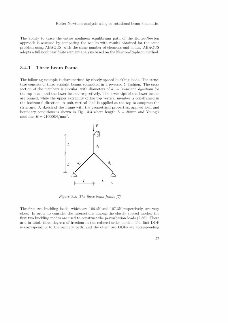
Koiter-Newton’s analysis using co-rotational beam kinematics
The ability to trace the entire nonlinear equilibrium path of the Koiter-Newtonapproach is assessed by comparing the results with results obtained for the sameproblem using ABAQUS, with the same number of elements and nodes. ABAQUSadopts a full nonlinear finite element analysis based on the Newton-Raphson method.
3.4.1 Three beam frame
The following example is characterized by closely spaced buckling loads. The struc-ture consists of three straight beams connected in a reversed Y fashion. The crosssection of the members is circular, with diameters of d1 = 3mm and d2=9mm forthe top beam and the lower beams, respectively. The lower tips of the lower beamsare pinned, while the upper extremity of the top vertical member is constrained inthe horizontal direction. A unit vertical load is applied at the top to compress thestructure. A sketch of the frame with the geometrical properties, applied load andboundary conditions is shown in Fig. 3.3 where length L = 30mm and Young’smodulus E = 210000N/mm2.
Figure 3.3: The three beam frame [7]
The first two buckling loads, which are 106.4N and 107.3N respectively, are veryclose. In order to consider the interactions among the closely spaced modes, thefirst two buckling modes are used to construct the perturbation loads (2.38). Thereare, in total, three degrees of freedom in the reduced order model. The first DOFis corresponding to the primary path, and the other two DOFs are corresponding
57
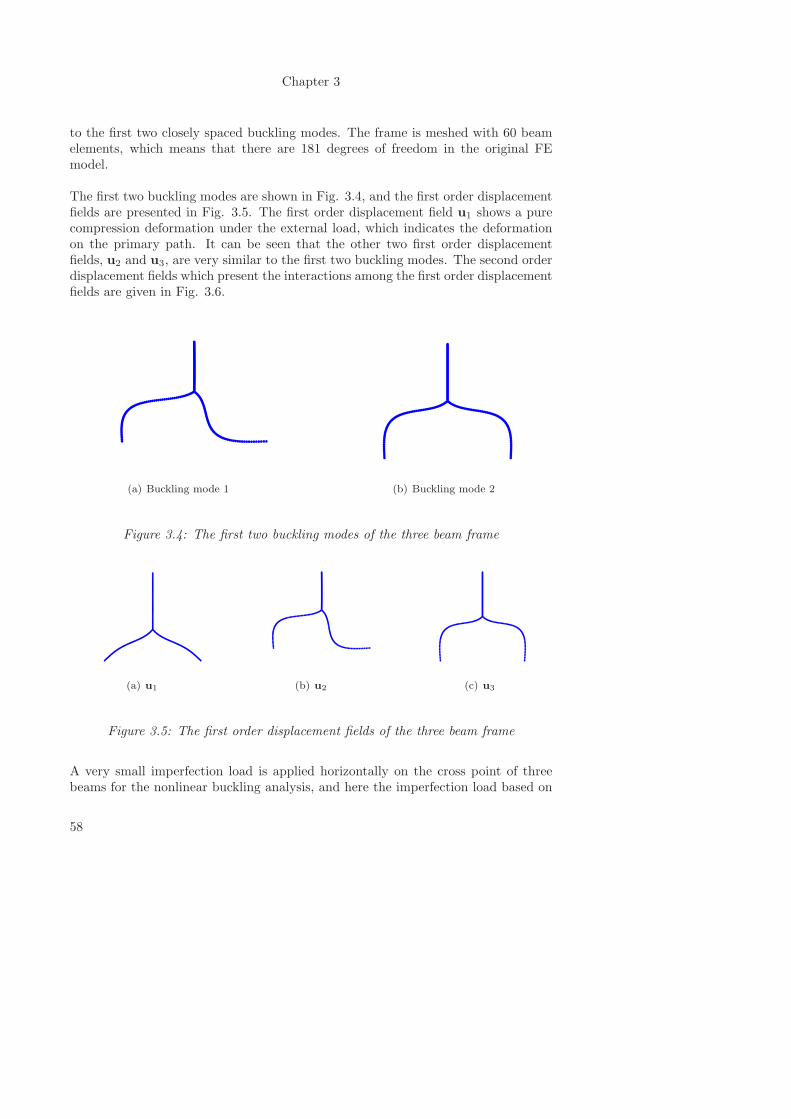
Chapter 3
to the first two closely spaced buckling modes. The frame is meshed with 60 beamelements, which means that there are 181 degrees of freedom in the original FEmodel.
The first two buckling modes are shown in Fig. 3.4, and the first order displacementfields are presented in Fig. 3.5. The first order displacement field u1 shows a purecompression deformation under the external load, which indicates the deformationon the primary path. It can be seen that the other two first order displacementfields, u2 and u3, are very similar to the first two buckling modes. The second orderdisplacement fields which present the interactions among the first order displacementfields are given in Fig. 3.6.
(a) Buckling mode 1 (b) Buckling mode 2
Figure 3.4: The first two buckling modes of the three beam frame
(a) u1 (b) u2 (c) u3
Figure 3.5: The first order displacement fields of the three beam frame
A very small imperfection load is applied horizontally on the cross point of threebeams for the nonlinear buckling analysis, and here the imperfection load based on
58
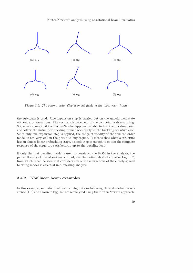
Koiter-Newton’s analysis using co-rotational beam kinematics
(a) u11 (b) u12 (c) u13
(d) u22 (e) u23 (f) u33
Figure 3.6: The second order displacement fields of the three beam frame
the sub-loads is used. One expansion step is carried out on the undeformed statewithout any corrections. The vertical displacement of the top point is shown in Fig.3.7, which shows that the Koiter-Newton approach is able to find the buckling pointand follow the initial postbuckling branch accurately in the buckling sensitive case.Since only one expansion step is applied, the range of validity of the reduced ordermodel is not very well in the post-buckling regime. It means that when a structurehas an almost linear prebuckling stage, a single step is enough to obtain the completeresponse of the structure satisfactorily up to the buckling load.
If only the first buckling mode is used to construct the ROM in the analysis, thepath-following of the algorithm will fail, see the dotted dashed curve in Fig. 3.7,from which it can be seen that consideration of the interactions of the closely spacedbuckling modes is essential in a buckling analysis.
3.4.2 Nonlinear beam examples
In this example, six individual beam configurations following those described in ref-erence [118] and shown in Fig. 3.8 are reanalyzed using the Koiter-Newton approach.
59
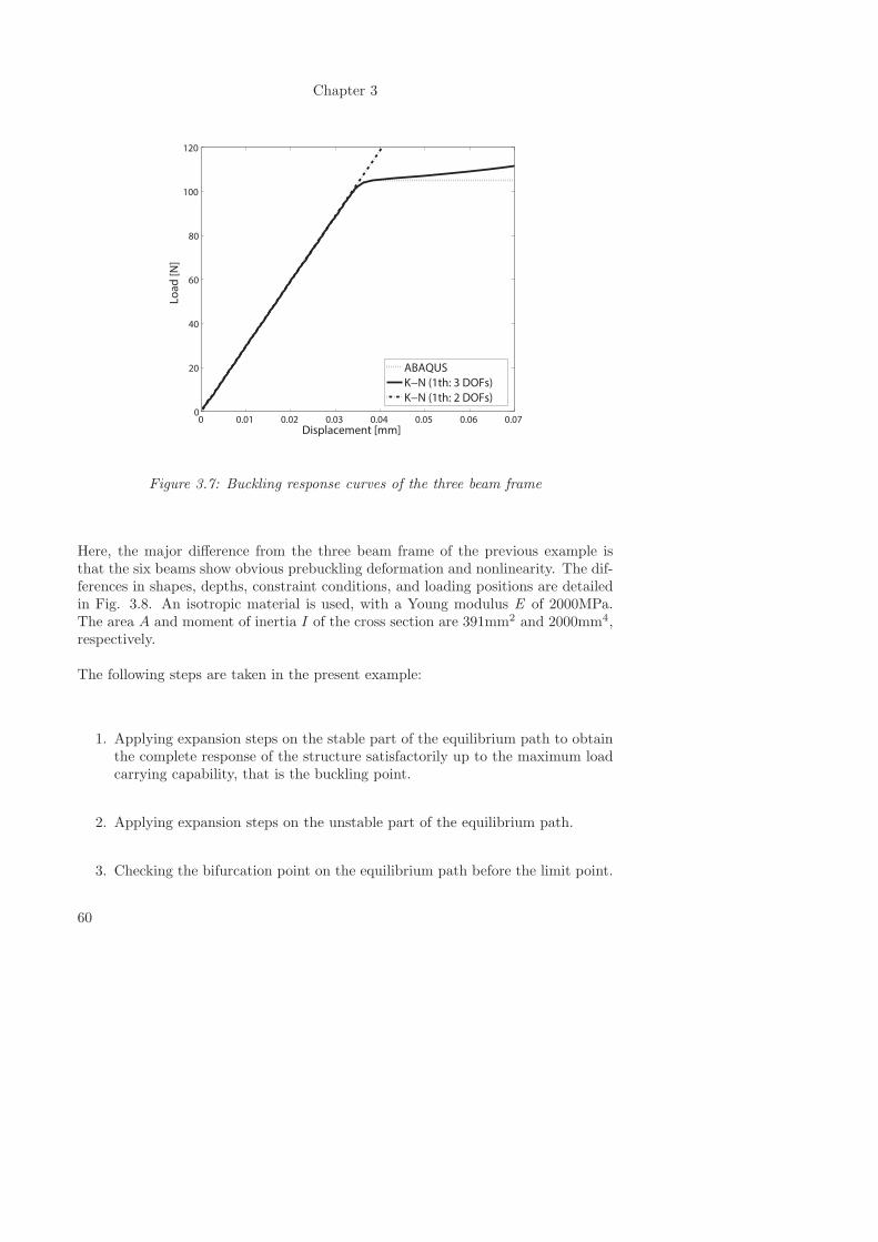
Chapter 3
0 0.01 0.02 0.03 0.04 0.05 0.06 0.070
20
40
60
80
100
120
Displacement [mm]
Lo
ad
[N
]
ABAQUS
K−N (1th: 3 DOFs)
K−N (1th: 2 DOFs)
Figure 3.7: Buckling response curves of the three beam frame
Here, the major difference from the three beam frame of the previous example isthat the six beams show obvious prebuckling deformation and nonlinearity. The dif-ferences in shapes, depths, constraint conditions, and loading positions are detailedin Fig. 3.8. An isotropic material is used, with a Young modulus E of 2000MPa.The area A and moment of inertia I of the cross section are 391mm2 and 2000mm4,respectively.
The following steps are taken in the present example:
1. Applying expansion steps on the stable part of the equilibrium path to obtainthe complete response of the structure satisfactorily up to the maximum loadcarrying capability, that is the buckling point.
2. Applying expansion steps on the unstable part of the equilibrium path.
3. Checking the bifurcation point on the equilibrium path before the limit point.
60
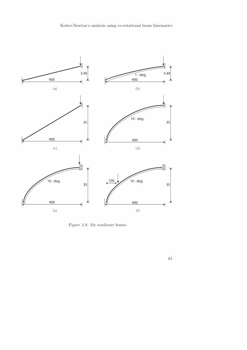
Koiter-Newton’s analysis using co-rotational beam kinematics
400
3.49
(a)
400
3.491 - deg.
(b)
400
35
(c)
400
3510 - deg.
(d)
400
3510 - deg.
(e)
400
3510 - deg.100
(f)
Figure 3.8: Six nonlinear beams
61
Chapter 3
Expansions on the stable equilibrium path
When the asymptotic expansion is applied on the stable part of the equilibriumpath, the first buckling load of these six beams is separated from the others, henceonly the first buckling mode is chosen and the number of degrees of freedom in thereduced order model is two. While, there are 63 degrees of freedom in the original FEmodel. The nonlinear response curves, vertical displacement at the loading positionvs. load, are shown in Fig. 3.9.
Due to the mild nonlinearity or load distribution in the prebuckling deformation,only one expansion step at the undeformed configuration is enough to obtain anaccurate buckling response, including the nonlinear prebuckling stage, limit loadand initial postbuckling stage for beams (a), (b), (c).
The prebuckling nonlinearity and the load distribution are very significant for beams(d), (e), (f), hence one single step from the beginning is not enough to capture theaccurate nonlinear response. In this case, the automated technique discussed in sec.2.6 for the path-following is adopted to correct the result and start a new expansionstep. In the end, 3, 3 and 4 steps are adopted for beams (d), (e), (f), respectively,to obtain an accurate nonlinear response and maximum load carrying capability foreach beam. The curves obtained for the different steps are plotted in Figs. 3.9(d)∼ 3.9(f).
The six beams all show limit point type buckling. From Table 3.4.2 it can be seenthat the limit loads of the beams are quite different from the linear buckling loadsobtained using the eigenvalue problem (2.42). This indicates that the nonlinearityof the prebuckling stage will greatly affect the structural buckling characteristics ofa beam.
Finally, the computational costs for the Koiter-Newton approach are compared tothose for using ABAQUS in Table 3.4.2. Tracing to the same equilibrium point onthe postbuckling path, a number of linear FEM systems need to be solved and anumber of solution steps are shown in Table 3.4.2. Due to the need for one single stepwithout a need for corrections for the first three beams, only one linear FEM systemfor constructing the reduced order model need to be solved. While, for the otherthree beams it is necessary to solve some additional systems for corrections. As canbe seen from Table 3.4.2, in addition to the total linear FEM system, the number ofsolution steps taken using the Koiter-Newton approach is also fewer than the numberof load steps used for the classical Newton method(ABAQUS), which indicated thata fairly larger step size can be adopted in the proposed Koiter-Newton approach dueto the better prediction obtained using the ROM. In general, it is obvious that the
62
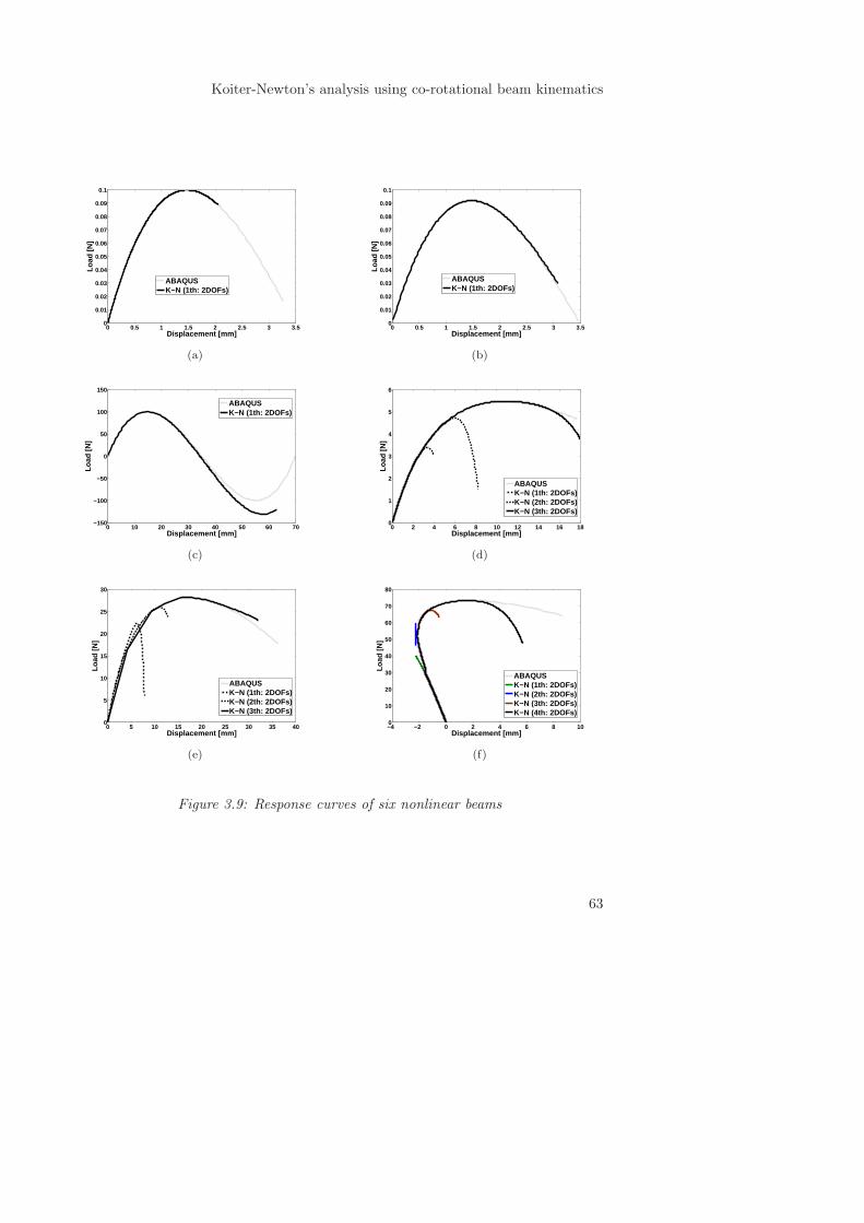
Koiter-Newton’s analysis using co-rotational beam kinematics
0 0.5 1 1.5 2 2.5 3 3.50
0.01
0.02
0.03
0.04
0.05
0.06
0.07
0.08
0.09
0.1
Displacement [mm]
Load
[N]
ABAQUSK−N (1th: 2DOFs)
(a)
0 0.5 1 1.5 2 2.5 3 3.50
0.01
0.02
0.03
0.04
0.05
0.06
0.07
0.08
0.09
0.1
Displacement [mm]
Load
[N]
ABAQUSK−N (1th: 2DOFs)
(b)
0 10 20 30 40 50 60 70−150
−100
−50
0
50
100
150
Displacement [mm]
Load
[N]
ABAQUSK−N (1th: 2DOFs)
(c)
0 2 4 6 8 10 12 14 16 180
1
2
3
4
5
6
Displacement [mm]
Load
[N]
ABAQUSK−N (1th: 2DOFs)K−N (2th: 2DOFs)K−N (3th: 2DOFs)
(d)
0 5 10 15 20 25 30 35 400
5
10
15
20
25
30
Displacement [mm]
Load
[N]
ABAQUSK−N (1th: 2DOFs)K−N (2th: 2DOFs)K−N (3th: 2DOFs)
(e)
−4 −2 0 2 4 6 8 100
10
20
30
40
50
60
70
80
Displacement [mm]
Load
[N]
ABAQUSK−N (1th: 2DOFs)K−N (2th: 2DOFs)K−N (3th: 2DOFs)K−N (4th: 2DOFs)
(f)
Figure 3.9: Response curves of six nonlinear beams
63
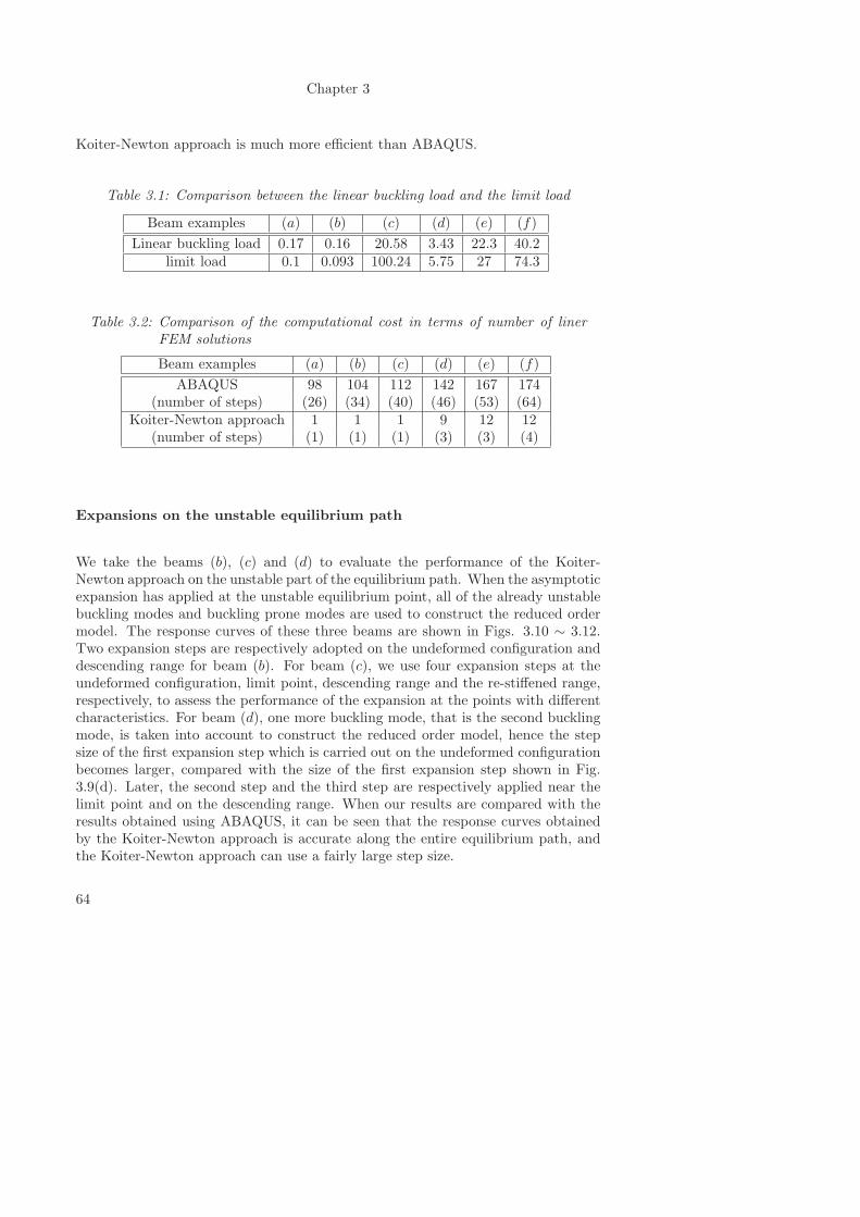
Chapter 3
Koiter-Newton approach is much more efficient than ABAQUS.
Table 3.1: Comparison between the linear buckling load and the limit load
Beam examples (a) (b) (c) (d) (e) (f)
Linear buckling load 0.17 0.16 20.58 3.43 22.3 40.2limit load 0.1 0.093 100.24 5.75 27 74.3
Table 3.2: Comparison of the computational cost in terms of number of linerFEM solutions
Beam examples (a) (b) (c) (d) (e) (f)
ABAQUS 98 104 112 142 167 174(number of steps) (26) (34) (40) (46) (53) (64)
Koiter-Newton approach 1 1 1 9 12 12(number of steps) (1) (1) (1) (3) (3) (4)
Expansions on the unstable equilibrium path
We take the beams (b), (c) and (d) to evaluate the performance of the Koiter-Newton approach on the unstable part of the equilibrium path. When the asymptoticexpansion has applied at the unstable equilibrium point, all of the already unstablebuckling modes and buckling prone modes are used to construct the reduced ordermodel. The response curves of these three beams are shown in Figs. 3.10 ∼ 3.12.Two expansion steps are respectively adopted on the undeformed configuration anddescending range for beam (b). For beam (c), we use four expansion steps at theundeformed configuration, limit point, descending range and the re-stiffened range,respectively, to assess the performance of the expansion at the points with differentcharacteristics. For beam (d), one more buckling mode, that is the second bucklingmode, is taken into account to construct the reduced order model, hence the stepsize of the first expansion step which is carried out on the undeformed configurationbecomes larger, compared with the size of the first expansion step shown in Fig.3.9(d). Later, the second step and the third step are respectively applied near thelimit point and on the descending range. When our results are compared with theresults obtained using ABAQUS, it can be seen that the response curves obtainedby the Koiter-Newton approach is accurate along the entire equilibrium path, andthe Koiter-Newton approach can use a fairly large step size.
64
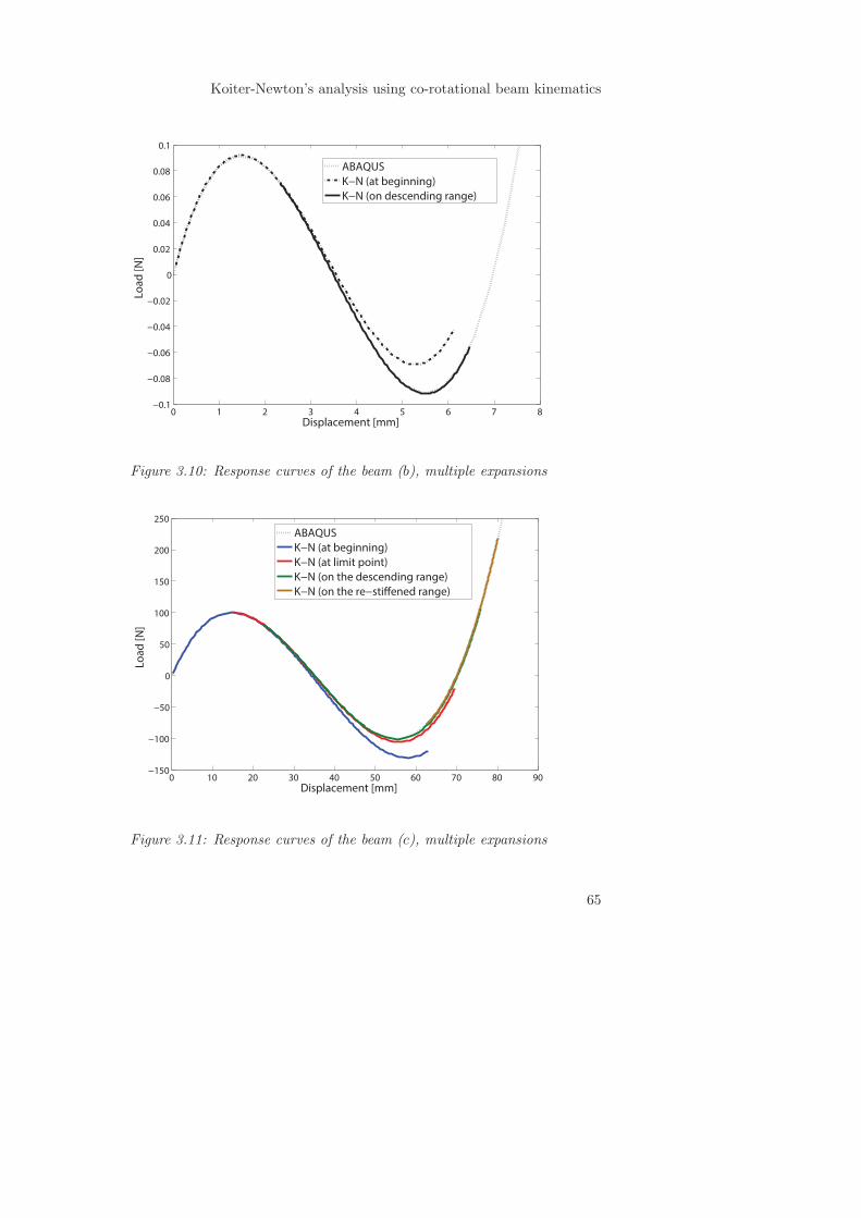
Koiter-Newton’s analysis using co-rotational beam kinematics
0 1 2 3 4 5 6 7 8−0.1
−0.08
−0.06
−0.04
−0.02
0
0.02
0.04
0.06
0.08
0.1
Displacement [mm]
Lo
ad
[N
]
ABAQUS
K−N (at beginning)
K−N (on descending range)
Figure 3.10: Response curves of the beam (b), multiple expansions
0 10 20 30 40 50 60 70 80 90−150
−100
−50
0
50
100
150
200
250
Displacement [mm]
Lo
ad
[N
]
ABAQUS
K−N (at beginning)
K−N (at limit point)
K−N (on the descending range)
K−N (on the re−sti"ened range)
Figure 3.11: Response curves of the beam (c), multiple expansions
65
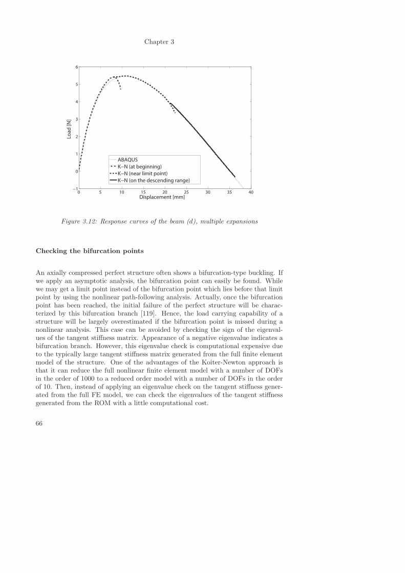
Chapter 3
0 5 10 15 20 25 30 35 40−1
0
1
2
3
4
5
6
Displacement [mm]
Lo
ad
[N
]
ABAQUS
K−N (at beginning)
K−N (near limit point)
K−N (on the descending range)
Figure 3.12: Response curves of the beam (d), multiple expansions
Checking the bifurcation points
An axially compressed perfect structure often shows a bifurcation-type buckling. Ifwe apply an asymptotic analysis, the bifurcation point can easily be found. Whilewe may get a limit point instead of the bifurcation point which lies before that limitpoint by using the nonlinear path-following analysis. Actually, once the bifurcationpoint has been reached, the initial failure of the perfect structure will be charac-terized by this bifurcation branch [119]. Hence, the load carrying capability of astructure will be largely overestimated if the bifurcation point is missed during anonlinear analysis. This case can be avoided by checking the sign of the eigenval-ues of the tangent stiffness matrix. Appearance of a negative eigenvalue indicates abifurcation branch. However, this eigenvalue check is computational expensive dueto the typically large tangent stiffness matrix generated from the full finite elementmodel of the structure. One of the advantages of the Koiter-Newton approach isthat it can reduce the full nonlinear finite element model with a number of DOFsin the order of 1000 to a reduced order model with a number of DOFs in the orderof 10. Then, instead of applying an eigenvalue check on the tangent stiffness gener-ated from the full FE model, we can check the eigenvalues of the tangent stiffnessgenerated from the ROM with a little computational cost.
66
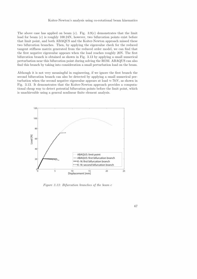
Koiter-Newton’s analysis using co-rotational beam kinematics
The above case has applied on beam (c). Fig. 3.9(c) demonstrates that the limitload for beam (c) is roughly 100.24N, however, two bifurcation points exist beforethat limit point, and both ABAQUS and the Koiter-Newton approach missed thesetwo bifurcation branches. Then, by applying the eigenvalue check for the reducedtangent stiffness matrix generated from the reduced order model, we can find thatthe first negative eigenvalue appears when the load reaches roughly 20N. The firstbifurcation branch is obtained as shown in Fig. 3.13 by applying a small numericalperturbation near this bifurcation point during solving the ROM. ABAQUS can alsofind this branch by taking into consideration a small perturbation load on the beam.
Although it is not very meaningful in engineering, if we ignore the first branch thesecond bifurcation branch can also be detected by applying a small numerical per-turbation when the second negative eigenvalue appears at load ≈ 70N , as shown inFig. 3.13. It demonstrates that the Koiter-Newton approach provides a computa-tional cheap way to detect potential bifurcation points before the limit point, whichis unachievable using a general nonlinear finite element analysis.
0 5 10 15 20 250
20
40
60
80
100
120
Displacement [mm]
Lo
ad
[N
]
ABAQUS: limit point
ABAQUS: !rst bifurcation branch
K−N: !rst bifurcation branch
K−N: second bifurcation branch
Figure 3.13: Bifurcation branches of the beam c
67
Chapter 3
3.5 Conclusions
In this chapter, the Koiter-Newton approach has been implemented in the beamelement based on the co-rotational frame. After differentiating the strain energyto the fourth order with respect to the global degrees of freedom, the equilibriumequations of a third order form is achieved. Then, the reduced order model of theco-rotational beam element is obtained according to the equilibrium equations.
Some numerical examples involving beams are used to evaluate the performanceof the Koiter-Newton approach. If prebuckling nonlinearity is mild, a single stepis enough to obtain the complete response of the structure satisfactorily up to themaximum load carrying capability, either by buckling or a limit point instability.More steps are needed for structures that show significant prebuckling deformation.A comparison of the results obtained using the Koiter-Newton approach with resultsobtained using ABAQUS, indicates that the Koiter-Newton approach is automatic,accurate, more efficient and less expensive to use.
68
Chapter 4
Koiter-Newton analysis using
co-rotational shell kinematics
4.1 Introduction
An FE implementation of the Koiter-Newton approach into a co-rotational beamkinematics was presented in chapter 3. In this chapter a more general application ofthe Koiter-Newton approach will be demonstrated by analyzing shell element basedon an element independent co-rotational frame. Compared to a two-dimensionalbeam element, a shell element is more complicated to describe due to its 3D largerotations. As discussed in Argyris’s paper [120], infinitesimal rotations in 2D spacemay be assigned a vectorial identity, however this can not be done for finite rotations.Argyris said that “commutativity, which is one of the three essential propertiesof a vector, is not satisfied for two or more finite rotations about arbitrary axesin space since the sequential order of their imposition determines in each case adifferent result and this non-commutativity of finite rotations is, however, not onlycharacteristic of truly large rotations but it holds even when second order effectshave to be considered”. A large body of work on 3D and finite rotation algebra forthe nonlinear analysis of shell structures can be found in the literature [121, 122,123, 124, 125].
The rest of this chapter is organized as follows. Some basic descriptions about theshell element are introduced. Then, co-rotational shell kinematics are presented.
69
Chapter 4
Next, the equilibrium equations of a third order form for the co-rotational shellelement are given, and the technique of automatic differentiations is introduced. Fi-nally, some numerical examples of shell structures are used to assess the performanceof the Koiter-Newton approach.
4.2 Some basic descriptions
In the case of the finite rotation, many rules are quite different from those in thecase of the infinitesimal rotation, hence a description of finite rotation is given inthis section. Three configurations of the shell element are introduced to make thedescription of the deformation concise, and the basic definition of the deformationgradient tensor is presented.
4.2.1 Finite rotation
In the Cartesian coordinate system, an arbitrary rotation ϑ = {ϕ, χ, ψ} can berepresented by a corresponding rotation matrix R. Then, after rotating a vector p
by ϑ, a new vector p′ can be obtained as [120]:
p′ = Rp (4.1)
where the rotation matrix R is an orthogonal matrix, and it is actually a nonlinearfunction of the rotation ϑ for the 3D finite rotation.
If a sequence of n successive rotations {ϑ1,ϑ2, ...,ϑn} is applied on the vector p,and the corresponding rotation matrices of them are {R1,R2, ...,Rn}, the final totalrotation matrix R of this sequence of rotations can be written as:
R = RnRn−1...R1 (4.2)
As mentioned above, the rotation matrix is a nonlinear function of the rotation ϑ
when the rotation is not infinitesimal, which leads to:
R = exp(ϑ)= I+ ϑ+
1
2!ϑ2 +
1
3!ϑ3 + . . . (4.3)
70
Koiter-Newton’s analysis using co-rotational shell kinematics
where the matrix I is a 3× 3 identity matrix, the operator exp ( ) means applying
an exponent operation on the matrix in the bracket, and the matrix ϑ is an anti-symmetric matrix formed by the three components of the rotation vector ϑ, whichresults in:
ϑ =
0 −ψ χψ 0 −ϕ−χ ϕ 0
(4.4)
Eq. (4.3) demonstrates that the rotation matrix can degenerate to the familiarinfinitesimal rotation matrix, given by:
R = I+ ϑ (4.5)
In the case of finite rotations, the derivatives of the rotation matrix R with respectto the three components of the rotation ϑ can be obtained by differentiating Eq.(4.3). In this procedure, the derivatives of the antisymmetric matrix ϑ with respectto these three components are calculated from Eq. (4.4), as follows:
∂ϑ
∂ϕ=
0 0 00 0 −10 1 0
;
∂ϑ
∂χ=
0 0 10 0 0−1 0 0
;
∂ϑ
∂ψ=
0 −1 01 0 00 0 0
(4.6)
4.2.2 Three configurations
To make the description of the co-rotational shell concise in later derivations, threeconfigurations during the deformation of the shell element are defined in this thesis,as shown in Fig. 4.1
These three configurations are called the reference configuration, nominal configu-ration and current configuration, respectively, and defined as follows:
• reference configuration: the initial undeformed configuration of the shell ele-ment is the reference configuration.
• nominal configuration: the last known configuration during the deformation ofthe shell element is the nominal configuration. In the beginning, the nominal
71
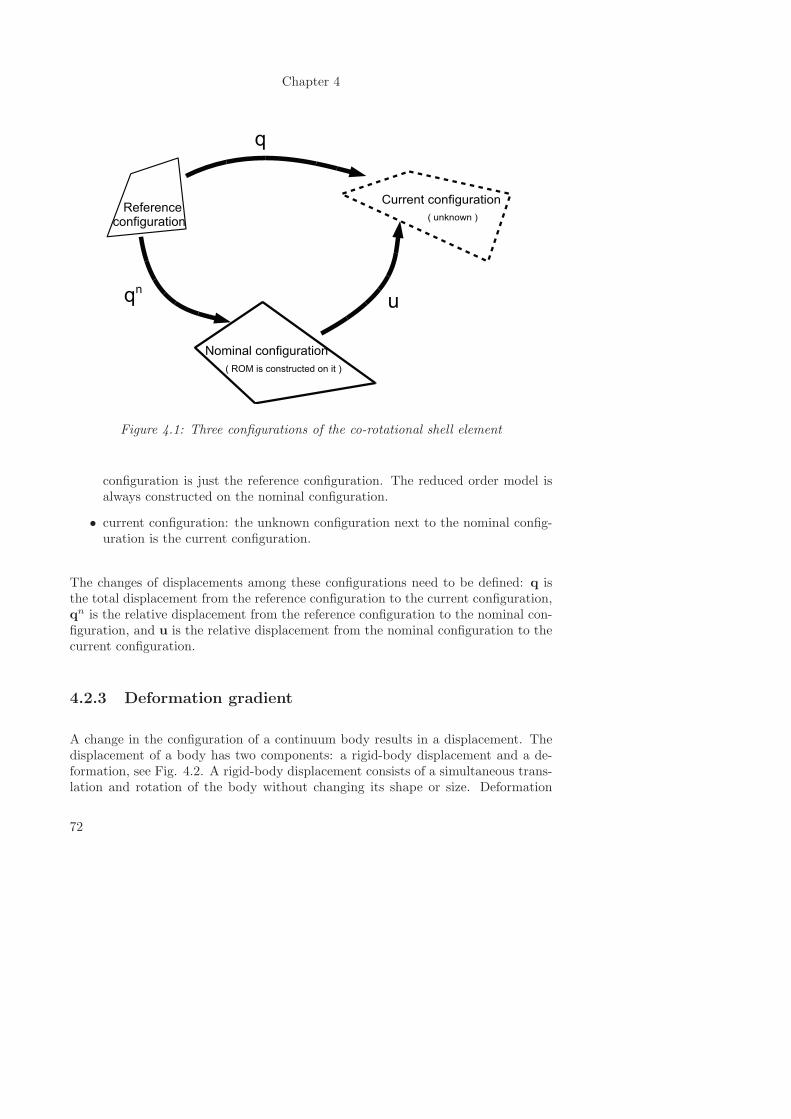
Chapter 4
Reference configuration
Nominal configuration
( ROM is constructed on it )
q
qn
u
Current configuration
( unknown )
Figure 4.1: Three configurations of the co-rotational shell element
configuration is just the reference configuration. The reduced order model isalways constructed on the nominal configuration.
• current configuration: the unknown configuration next to the nominal config-uration is the current configuration.
The changes of displacements among these configurations need to be defined: q isthe total displacement from the reference configuration to the current configuration,qn is the relative displacement from the reference configuration to the nominal con-figuration, and u is the relative displacement from the nominal configuration to thecurrent configuration.
4.2.3 Deformation gradient
A change in the configuration of a continuum body results in a displacement. Thedisplacement of a body has two components: a rigid-body displacement and a de-formation, see Fig. 4.2. A rigid-body displacement consists of a simultaneous trans-lation and rotation of the body without changing its shape or size. Deformation
72
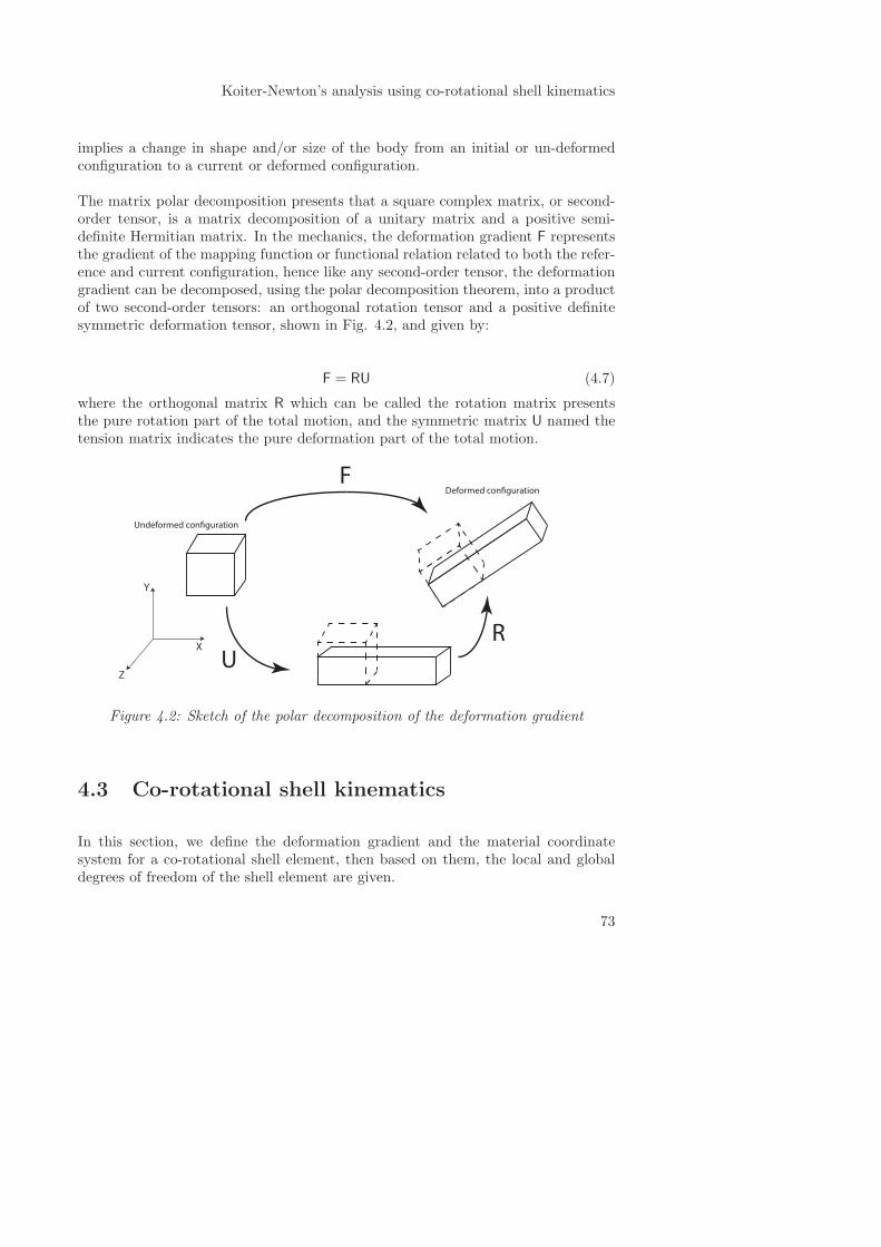
Koiter-Newton’s analysis using co-rotational shell kinematics
implies a change in shape and/or size of the body from an initial or un-deformedconfiguration to a current or deformed configuration.
The matrix polar decomposition presents that a square complex matrix, or second-order tensor, is a matrix decomposition of a unitary matrix and a positive semi-definite Hermitian matrix. In the mechanics, the deformation gradient F representsthe gradient of the mapping function or functional relation related to both the refer-ence and current configuration, hence like any second-order tensor, the deformationgradient can be decomposed, using the polar decomposition theorem, into a productof two second-order tensors: an orthogonal rotation tensor and a positive definitesymmetric deformation tensor, shown in Fig. 4.2, and given by:
F = RU (4.7)
where the orthogonal matrix R which can be called the rotation matrix presentsthe pure rotation part of the total motion, and the symmetric matrix U named thetension matrix indicates the pure deformation part of the total motion.
Z
X
Y
F
UR
Undeformed con!guration
Deformed con!guration
Figure 4.2: Sketch of the polar decomposition of the deformation gradient
4.3 Co-rotational shell kinematics
In this section, we define the deformation gradient and the material coordinatesystem for a co-rotational shell element, then based on them, the local and globaldegrees of freedom of the shell element are given.
73
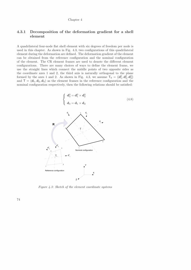
Chapter 4
4.3.1 Decomposition of the deformation gradient for a shell
element
A quadrilateral four-node flat shell element with six degrees of freedom per node isused in this chapter. As shown in Fig. 4.3, two configurations of this quadrilateralelement during the deformation are defined. The deformation gradient of the elementcan be obtained from the reference configuration and the nominal configurationof the element. The CR element frames are used to denote the different elementconfigurations. There are many choices of ways to define the element frame, weuse the straight lines which connect the middle points of two opposite sides asthe coordinate axes 1 and 2, the third axis is naturally orthogonal to the planeformed by the axes 1 and 2. As shown in Fig. 4.3, we assume T0 =
(d01,d
02,d
03
)
and T = (d1,d2,d3) as the element frames in the reference configuration and thenominal configuration respectively, then the following relations should be satisfied:
d03 = d0
1 × d02
d3 = d1 × d2
(4.8)
d0
1
d0
2
d0
3
d2
d3
d1
Y
X
Z
1
2
3
4
1
2
3
4
R
Reference configuration
Nominal configuration
T0
T
Figure 4.3: Sketch of the element coordinate systems
74
Koiter-Newton’s analysis using co-rotational shell kinematics
In order to find the deformation gradient, we assume that two arbitrary vectors, a0
and a, are located in the reference and nominal configurations respectively, and thatthey are in the same position relative to the element coordinate systems. Then, thedeformation gradient is just the mapping function related to these two vectors. Thetwo vectors, a0 and a, can be expressed as:
a0 = a1d01 + a2d
02 + a3d
03
a = a1d1 + a2d2 + a3d3
(4.9)
where the a1, a2, a3 are the components of the coordinates.
Based on Eq. (4.9), the vector a can be expressed by the vector a0:
a = {d1,d2,d3}{d01,d
02,d
03
}−1a0 (4.10)
According to the definition of the deformation gradient, the deformation gradient inthis case can be presented as:
F = {d1,d2,d3}{d01,d
02,d
03
}−1(4.11)
To obtain the symmetric matrix U which indicates the pure deformation part of theelement motion, we can multiply Ft on both sides of Eq. (4.7), which leads to:
FtF = FtRU = URtRU = UU (4.12)
where the fact that RtR = I is used.
After obtaining the matrix U, introducing it into Eq. (4.7) the rotation matrix R
can be achieved by:
R = FU−1 (4.13)
75
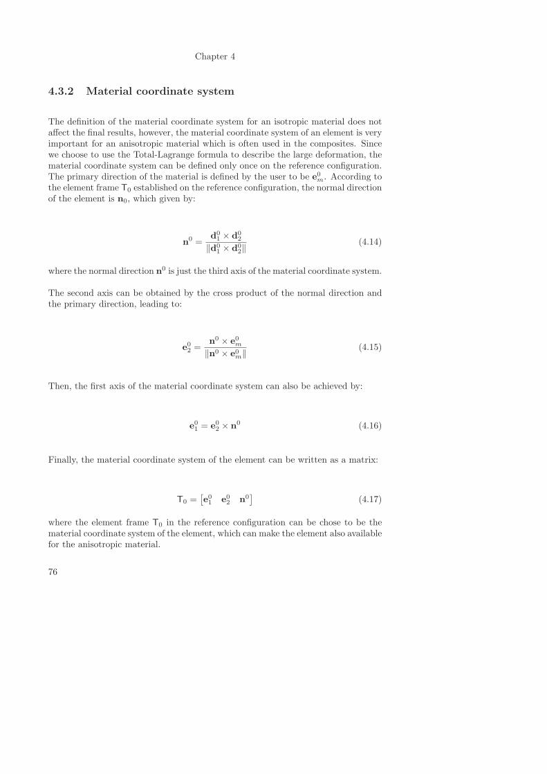
Chapter 4
4.3.2 Material coordinate system
The definition of the material coordinate system for an isotropic material does notaffect the final results, however, the material coordinate system of an element is veryimportant for an anisotropic material which is often used in the composites. Sincewe choose to use the Total-Lagrange formula to describe the large deformation, thematerial coordinate system can be defined only once on the reference configuration.The primary direction of the material is defined by the user to be e0m. According tothe element frame T0 established on the reference configuration, the normal directionof the element is n0, which given by:
n0 =d01 × d0
2
‖d01 × d0
2‖(4.14)
where the normal direction n0 is just the third axis of the material coordinate system.
The second axis can be obtained by the cross product of the normal direction andthe primary direction, leading to:
e02 =n0 × e0m
‖n0 × e0m‖(4.15)
Then, the first axis of the material coordinate system can also be achieved by:
e01 = e02 × n0 (4.16)
Finally, the material coordinate system of the element can be written as a matrix:
T0 =[e01 e02 n0
](4.17)
where the element frame T0 in the reference configuration can be chose to be thematerial coordinate system of the element, which can make the element also availablefor the anisotropic material.
76
Koiter-Newton’s analysis using co-rotational shell kinematics
4.3.3 Local degrees of freedom
The global and local degrees of freedom of this shell element are expressed by two24 by 1 vectors, q and q, respectively. The global degrees of freedom are the degreesof freedom under the global coordinate system Tg = (X,Y,Z) in Fig. 4.3, andthe local degrees of freedom are generated from the global degrees of freedom in aco-rotational shell frame.
For a convenient description, the global and local degrees of freedom are divided intotwo parts, the translation part and the rotation part. For each node a (a = 1, 2, 3, 4),the 3 by 1 vectors ua and θa denote the translation and rotation part of the globaldegrees of freedom, respectively, and ua and θa are the corresponding translationand rotation part of the local degrees of freedom, respectively. The local translationsua and the local rotations θa in the local DOFs are respectively presented in thefollowing two parts.
Local translations
We can assume a vector r0a under the global frame Tg to be the position vector of thenode a on the reference configuration in Fig. 4.3, and ua is a global translation ofthis vector from the reference configuration to the nominal configuration, hence theposition of the new vector on the nominal configuration is r0a+ua. Then, T
t(r0a+ua)is the local position of this new vector under the nominal frame T, which should beequal to:
Tt(r0a + ua) = Tt0r
0a + ua (4.18)
where Tt0r
0a is the local position of the initial vector r0a under the reference configu-
ration, and ua is the local translation.
The reference frame T0 and the nominal frame T satisfy the following relationship:
T = RT0 (4.19)
Substituting Eq. (4.19) into Eq. (4.18), the expression of the local translation ua isobtained:
77
Chapter 4
ua = Tt0R
tua + Tt0(R
t − I)T0Tt0r
0a (4.20)
where R is the rotation matrix, and r0a, a = 1, 2, 3, 4 is the position vector of eachnode in the initial undeformed configuration. We can choose T0 to be the materialcoordinate system defined in Eq. (4.17).
The local translations of each node are picked up from the local degrees of freedom,and are given by:
{q1, q2, q3, · · · , q7, q8, q9, · · · , q13, q14, q15, · · · , q19, q20, q21, · · · }t
(4.21)
According to Eq. (4.20), the three local translations of each node can be expressedas:
qiqi+1
qi+2
= Tt
0Rt
qiqi+1
qi+2
+ Tt
0
(Rt − I
)T0T
t0r
0(i+5)/6 (4.22)
where i = 1, 7, 13, 19, and qi, qi+1, qi+2 are the global translations for each node.
Local rotations
The local rotations in the local degrees of freedom are discussed as follows. To makethe description for the rotation part easier, three configurations were introduced insubsection 4.2.2. Based on these three configurations, the global degrees of freedomq can be divided into two parts, which are the relative displacement qn from thereference configuration to the nominal configuration and the relative displacementu from the nominal configuration to the current configuration, as given by:
q = qn ◦ u (4.23)
where as mentioned in Eq. (2.2) the composition ◦ is not a simple addition in thecase of finite rotations, and will depend on the parametrisation of rotations.
In Fig. 4.4, R is the average global rotation matrix for the shell element, and thefour nodes also possess their own global rotation matrix Ra, a = 1, 2, 3, 4. θa and
78
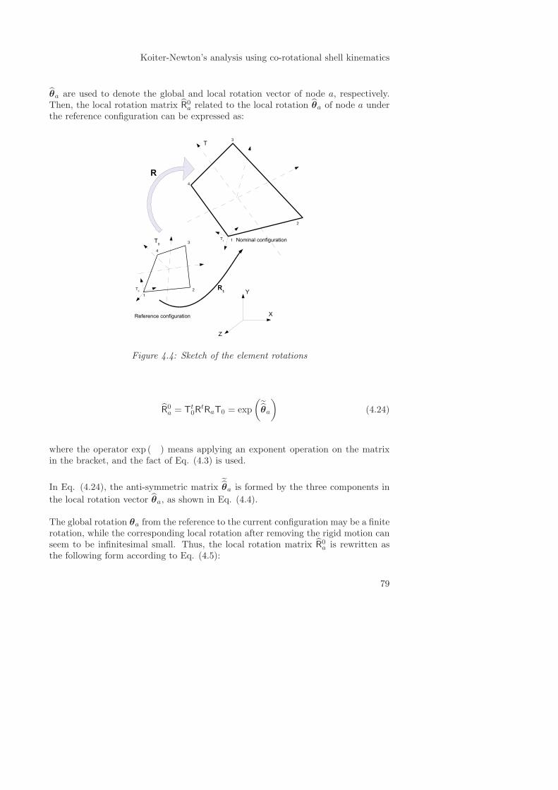
Koiter-Newton’s analysis using co-rotational shell kinematics
θa are used to denote the global and local rotation vector of node a, respectively.Then, the local rotation matrix R0
a related to the local rotation θa of node a underthe reference configuration can be expressed as:
T0
Y
X
Z
1
2
3
4
1
2
3
4
R
T
T0
T1
R1
Reference configuration
Nominal configuration
Figure 4.4: Sketch of the element rotations
R0a = Tt
0RtRaT0 = exp
(˜θa
)(4.24)
where the operator exp ( ) means applying an exponent operation on the matrixin the bracket, and the fact of Eq. (4.3) is used.
In Eq. (4.24), the anti-symmetric matrix˜θa is formed by the three components in
the local rotation vector θa, as shown in Eq. (4.4).
The global rotation θa from the reference to the current configuration may be a finiterotation, while the corresponding local rotation after removing the rigid motion canseem to be infinitesimal small. Thus, the local rotation matrix R0
a is rewritten asthe following form according to Eq. (4.5):
79
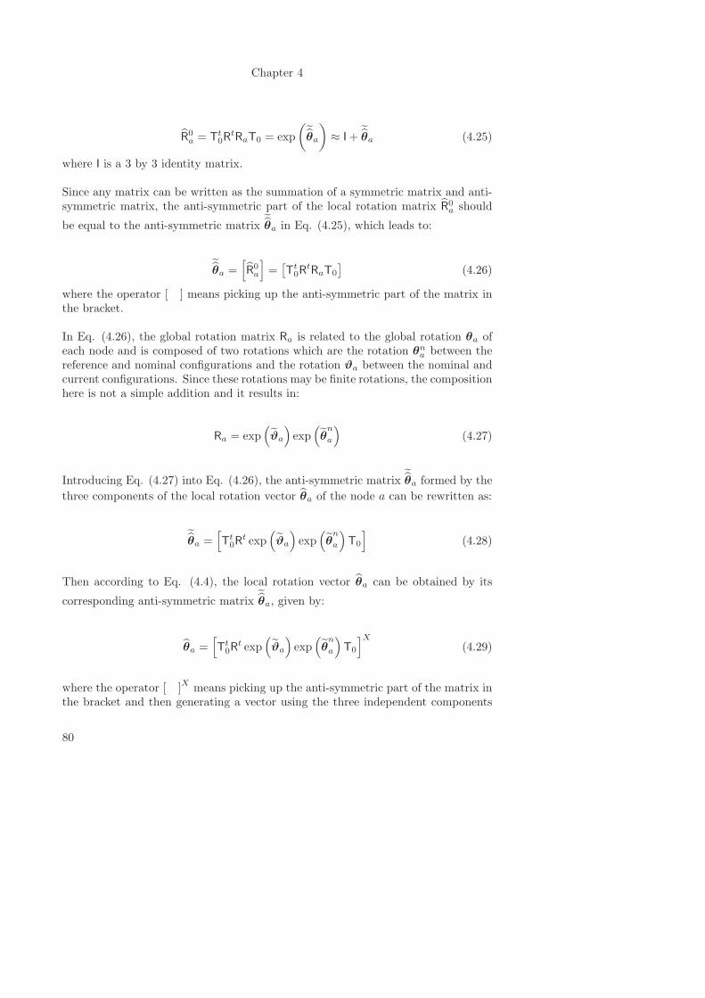
Chapter 4
R0a = Tt
0RtRaT0 = exp
(˜θa
)≈ I+
˜θa (4.25)
where I is a 3 by 3 identity matrix.
Since any matrix can be written as the summation of a symmetric matrix and anti-symmetric matrix, the anti-symmetric part of the local rotation matrix R0
a should
be equal to the anti-symmetric matrix˜θa in Eq. (4.25), which leads to:
˜θa =
[R0a
]=
[Tt0R
tRaT0
](4.26)
where the operator [ ] means picking up the anti-symmetric part of the matrix inthe bracket.
In Eq. (4.26), the global rotation matrix Ra is related to the global rotation θa ofeach node and is composed of two rotations which are the rotation θn
a between thereference and nominal configurations and the rotation ϑa between the nominal andcurrent configurations. Since these rotations may be finite rotations, the compositionhere is not a simple addition and it results in:
Ra = exp(ϑa
)exp
(θn
a
)(4.27)
Introducing Eq. (4.27) into Eq. (4.26), the anti-symmetric matrix˜θa formed by the
three components of the local rotation vector θa of the node a can be rewritten as:
˜θa =
[Tt0R
t exp(ϑa
)exp
(θn
a
)T0
](4.28)
Then according to Eq. (4.4), the local rotation vector θa can be obtained by its
corresponding anti-symmetric matrix˜θa, given by:
θa =[Tt0R
t exp(ϑa
)exp
(θn
a
)T0
]X(4.29)
where the operator [ ]X
means picking up the anti-symmetric part of the matrix inthe bracket and then generating a vector using the three independent components
80
Koiter-Newton’s analysis using co-rotational shell kinematics
of this anti-symmetric matrix.
4.4 Equilibrium equations in a third order form
The strain energy of the shell element in a co-rotational frame is obtained, then theL, Q and C in the equilibrium equations of a third order form can be obtained bydifferentiating the strain energy with respect to the global degrees of freedom. Toachieve these differentiations, the derivatives of the local degrees of freedom withrespect to the global degrees of freedoms are presented in detail.
4.4.1 Strain energy of the co-rotational shell element
In a co-rotational frame, the element strain energy only depends on the local degreesof freedom q which cause the deformational part of the total motion, given by:
U =1
2εtCε =
1
2qtKLq (4.30)
where the vector ε is the local strain of the element, the matrix C is the materialmatrix, and KL is the linear stiffness matrix of a quadrilateral element. In thepresent work, this quadrilateral element is formed by assembling four triangular flatelements and merging the middle node. The triangular flat element and the assemblytechnique are introduced in appendix A.
From Eq. (4.30), it can be seen that the element strain energy U is a quadraticfunction of the local degrees of freedom q, hence we can differentiate U up to thesecond order form, as follows:
∂U
∂q= KLq = f (4.31)
∂2U
∂q2= KL (4.32)
where the first and second order derivatives of the strain energy are the local internalload f and linear stiffness matrix KL, respectively.
81
Chapter 4
Substituting Eqs. (4.31) and (4.32) into Eqs. (3.9) ∼ (3.12), we can obtain the com-ponents of the internal load vector f , tangent stiffness matrix L, three-dimensionalmatrix Q and four-dimensional matrix C in the equilibrium equations (2.8) for theshell element, as follows:
fp =∂U
∂qp= f
∂qm∂qp
(4.33)
Lpi = KL∂qn∂qi
∂qm∂qp
+ f∂2qm∂qp∂qi
(4.34)
2Qpij =KL∂2qn∂qi∂qj
∂qm∂qp
+ KL∂qn∂qi
∂2qm∂qp∂qj
+ KL∂qn∂qj
∂2qm∂qp∂qi
+ f∂3qm
∂qp∂qi∂qj
(4.35)
6Cpijk =KL∂3qn
∂qi∂qj∂qk
∂qm∂qp
+ KL∂2qn∂qi∂qj
∂2qm∂qp∂qk
+ KL∂2qn∂qi∂qk
∂2qm∂qp∂qj
+ KL∂qn∂qi
∂3qm∂qp∂qj∂qk
+ KL∂2qn∂qj∂qk
∂2qm∂qp∂qi
+ KL∂qn∂qj
∂3qm∂qp∂qi∂qk
+ KL∂qn∂qk
∂3qm∂qp∂qi∂qj
+ f∂4qm
∂qp∂qi∂qj∂qk
(4.36)
where the subscripts p, i, j, k, m and n run from 1 to 24, and the summationconvention is applied on m and n.
In Eqs. (4.33) ∼ (4.36) the unknowns are the derivatives of the local degrees offreedoms q with respect to the global degrees of freedom q. Since the descriptionof the shell element is more complicated, we can split the local degrees of freedomq into two parts, translations and rotations, and then calculate the derivatives ofthese two parts respectively.
82
Koiter-Newton’s analysis using co-rotational shell kinematics
4.4.2 Derivatives of the local translations with respect to the
global degrees of freedom
The derivatives of the local translations (4.22) with respect to the global degreesof freedom are presented in this subsection. The first order derivative of the localtranslations with respect to the global degrees of freedom will be introduced below,and the second to forth order derivatives can be easily achieved in the same way.
The first order derivative of the local degrees of freedom q with respect to the global
degrees of freedom q is a 24× 24 matrix, the components of which are∂qi∂qj
. In this
subsection, we only list the components that are related to the local translations,which results in:
∂qi∂qj
∂qi+1
∂qj
∂qi+2
∂qj
= Tt0
∂Rt
∂qj
qiqi+1
qi+2
+Tt
0Rt0
∂
qiqi+1
qi+2
∂qj+Tt
0
∂Rt
∂qjT0T
t0r
0(i+5)/6 (4.37)
where i equals 1, 7, 13 and 19 respectively and j runs from 1 to 24 automaticallyfor each of i.
The term Rt0
∂
qiqi+1
qi+2
∂qjin Eq. (4.37) can be obtained as follows:
Rt0
∂
qiqi+1
qi+2
∂qj=
{1, 0, 0}t , if j = i
{0, 1, 0}t , if j = i+ 1
{0, 0, 1}t , if j = i+ 2
{0, 0, 0}t , if j = others
(4.38)
The component of the first derivative of the rotation matrix R with respect to the
83
Chapter 4
global degrees of freedom q, that is the∂Rt
∂qj, is calculated as follows.
First, we differentiate both sides of Eq. (4.7) with respect to the global degrees offreedom, and then multiply the transpose of the rotation matrix Rt on both sides,which results in:
Rt ∂F
∂qj= Rt ∂R
∂qjU+
∂U
∂qi(4.39)
where the fact of RtR = I is used, since the rotation matrix R is an orthogonalmatrix.
Any matrix can be written as a summation of a symmetric matrix and an anti-symmetric matrix. The derivatives of the symmetric matrix U is still a symmetricmatrix, which indicates that the anti-symmetric part of Eq. (4.39) is given by:
[Rt ∂R
∂qjU
]=
[Rt ∂F
∂qj
](4.40)
where the operator [ ] is used to pick up the anti-symmetric part of the matrix inthe bracket.
we use P to indicate the matrix Rt ∂F
∂qjin the right hand side of Eq. (4.40), that is:
P = Rt ∂F
∂qj(4.41)
where the term∂F
∂qjis achieved by differentiating Eq. (4.11), as given by:
∂F
∂qj=
{∂d1
∂qj,∂d2
∂qj,∂d3
∂qj
}{d01,d
02,d
03
}−1(4.42)
where the term
{∂d1
∂qj,∂d2
∂qj,∂d3
∂qj
}can be easily obtained by the geometry and
deformation relations.
84
Koiter-Newton’s analysis using co-rotational shell kinematics
The matrix Rt ∂R
∂qjin the left hand side of Eq. (4.40) is an anti-symmetric matrix,
and this conclusion is obtained by differentiating the equation RtR = I on both sides,which is given as:
∂Rt
∂qjR+ Rt ∂R
∂qj= 0 ⇒ Rt ∂R
∂qj= −
(Rt ∂R
∂qj
)t
(4.43)
Hence, The matrix Rt ∂R
∂qjcan be represented by a anti-symmetric matrix Sj , as:
Sj = Rt ∂R
∂qj=
0 s1j s2j−s1j 0 s3j−s2j −s3j 0
(4.44)
where s1j , s2j and s3j are the three independent components in this anti-symmetricmatrix Sj .
Any anti-symmetric matrix can be expressed by the three independent components,hence the independent components of the two anti-symmetric matrices in Eq. (4.40)should be equal, which leads to a linear system of equations:
U11 + U22 U23 −U13
U23 U11 + U33 U12
−U13 U12 U22 + U33
s1js2js3j
=
P12 − P21
P13 − P31
P23 − P32
(4.45)
where the U11, U22, U33, U12, U13 and U23 are the components of the symmetricmatrix U, and P12, P21, P13, P31, P23 and P32 are the components of the matrix P
defined in Eq. (4.41).
After solving this linear system of equations (4.45) and introducing the solutionvector {s1j , s2j , s3j} into Eq. (4.44), we can obtain the anti-symmetric matrix Sj .Then, according to Eq. (4.44), the component of the first derivative of the rotation
matrix with respect to the global degrees of freedom,∂Rt
∂qj, is achieved by:
∂Rt
∂qj= RSj (4.46)
85
Chapter 4
Finally, introducing Eqs. (4.38) and (4.46) into Eq. (4.37), the first order derivativeof the local translations with respect to the global degrees of freedom q is obtained.
4.4.3 Derivatives of the local rotations with respect to the
global degrees of freedom
Based on the expression of the local rotation, the derivatives of the local rotationwith respect to the global degrees of freedom can be achieved. From Eq. (4.29), it
can be seen that the local rotation vector θa is related to both the rotations andthe translations involved in the global rotation matrix R. Since the reduced ordermodel is constructed on the known nominal configuration, the relative displacementu between the nominal and current configurations should be set to be zero in thederivatives. Here, the first and second order derivatives of the local rotation withrespect to the global degrees of freedom are listed below, and the other high orderderivatives can be obtained in the same way.
The first order derivative of the local degrees of freedom q with respect to the global
degrees of freedom q is a 24 × 24 matrix, the components of which are∂qi∂qj
. The
components related to the local translations have already been obtained using Eq.(4.37). Here, we only list the components that are related to the local rotations,which results in:
∂qi∂qj
∂qi+1
∂qj
∂qi+2
∂qj
=
[Tt0
{Rt,j exp
(ϑ(i+2)/6
)+ Rt exp
(ϑ(i+2)/6
),j
}exp
(θn
(i+2)/6
)T0
]X
(4.47)
where the subscript i equals 4, 10, 16, 12 respectively to denote only the rotationcomponent, while j runs from 1 to 24.
In Eq. (4.47), the derivatives R,j of the element average rotation matrix with respectto the global degrees of freedom can be obtained by Eq. (4.46). The matrix operator
86
Koiter-Newton’s analysis using co-rotational shell kinematics
exp ( ) and its derivatives were introduced in subsection 4.2.1. When j runs from 1to 24 the two terms in the brace of the right hand side of Eq. (4.47) will not alwaysbe nonzeros. The following three cases should be considered.
1. If the value of j is related to the translations, only the first term Rt,j exp
(ϑ(i+2)/6
)
is nonzero due to the value of exp(ϑ(i+2)/6
),j
in the second term is equal to
zero.
2. If the value of j is related to the rotations and also equal to the current rotation
i, i + 1, i + 2, only the second term Rt exp(ϑ(i+2)/6
),j
is nonzero due to the
value of Rt,j in the first term is equal to zero.
3. If the value of j is equal to other values, both of the terms are zero.
The second order derivative of the local degrees of freedom q with respect to theglobal degrees of freedom q is a three dimensional 24× 24× 24 matrix, and we can
use∂2qi∂qj∂qk
to express its components. The components that are related to the local
rotations are:
∂2qi∂qj∂qk
∂2qi+1
∂qj∂qk
∂2qi+2
∂qj∂qk
=
Tt0
Rt,jk exp
(ϑ(i+2)/6
)
+ Rt,j exp
(ϑ(i+2)/6
),k
+ Rt,k exp
(ϑ(i+2)/6
),j
+ Rt exp(ϑ(i+2)/6
),jk
exp(θn
(i+2)/6
)T0
X
(4.48)
where the subscript i equals 4, 10, 16, 12 respectively to denote only the rotationcomponent, while j, k runs from 1 to 24. The second derivatives R,jk of the elementaverage rotation matrix with respect to the global degrees of freedom can be achievedin the same way as that used in Eq. (4.46).
In Eq. (4.48), five cases should be taken into account to check whether the fourterms in the brace of the right hand side of Eq. (4.48) are all zeros or not.
87
Chapter 4
1. If the values of j and k are related to the translations, only the first term
Rt,jk exp
(ϑ(i+2)/6
)is nonzero.
2. If the value of j is related to the translations and k is equal to the current
rotation i, i+ 1, i+ 2, only the second term Rt,j exp
(ϑ(i+2)/6
),k
is nonzero.
3. If the value of k is related to the translations and j is equal to the current
rotation i, i+ 1, i+ 2, only the third term Rt,k exp
(ϑ(i+2)/6
),jis nonzero.
4. If the values of j and k are all equal to the current rotation i, i+ 1, i+ 2, only
the fourth term Rt exp(ϑ(i+2)/6
),jk
is nonzero.
5. If the values of j and k are equal to other values, all of the four terms in thebrace are zero.
Up to this point, the derivatives of the local degrees of freedom with respect to theglobal degrees of freedom are obtained by combining both the translation part andthe rotation part. Introducing them into the Eqs. (4.33) ∼ (4.36), the equilibriumequations (2.8) of the shell element in a co-rotational frame are achieved. Then, thereduced order model of the CR shell element can be constructed using the L, Q andC in the equilibrium equations (2.8).
4.5 Automatic differentiation
From section 4.4, it can be seen that we need to obtain many high order, to fourthorder, differentiations for some variables. In order to make the codes more conciseand faster an automatic differentiation technology [126] is adopted in the Matlabcodes. In Tsukanov’s paper [126] the data structure and algorithms are developed forthe direct application of generalized Leibnitz rules to the numerical computation ofpartial derivatives in forward mode. The proposed data structure provides constanttime access to the partial derivatives, which accelerates the automatic differentiationcomputations. This automatic differentiation technique based on the generalizedLeibnitz rules can differentiate a composite function in a forward mode.
88
Koiter-Newton’s analysis using co-rotational shell kinematics
Firstly, we will simply review the basics of this technique following Tsukanov’s paper.A partial derivative of a product of two functions f(x) = u(x)v(x) is a linear combi-nation of products of partial derivatives of u and v with binomial coefficients. Thefunctions which need high order differentiations and appear in the current researchwork are products of multiple functions, which can also seem to be a combinationof some single products of two functions. Hence, in this section, a standard partialderivative of a product of two functions is given to show how the automatic differen-tiation technique works. Differentiating the equation f(x) = u(x)v(x) with respectto the variable x, it results in [126]:
∂|µ|f
∂xµ1
1 ∂xµ2
2 · · · ∂xµnn
=
µ1∑
α1=0
µ2∑
α2=0
· · ·
µn∑
αn=0
(µ1
α1
)(µ2
α2
)· · ·
(µn
αn
)
∗∂|α|u
∂xα1
1 ∂xα2
2 · · · ∂xαnn
∗∂|µ−α|v
∂xµ1−α1
1 ∂xµ2−α2
2 · · · ∂xµn−αnn
(4.49)
where |µ| =n∑
i=1
µi, 0 < |µ| ≤ m(m is the order of the highest derivative), and
|α| =n∑
i=1
αi. An additional multi-index α the elements of which serve as counters
of summation loops is used. In addition, each term in Eq. (4.49) is multiplied by
n binomial coefficient
(µi
αi
), i = 1, . . . , n. In this case, both the computation of
positions of partial derivatives given by multi-indices α and µ − α, and the com-
putation of the products of binomial coefficientsn∏
i=1
(µi
αi
)are considered in the
differentiation of the product includes.
Next, some examples are presented to show the application of the automatic differ-entiation technique used for the present research. As discussed in section 4.4, thereare at least four places where the automatic differentiation technique can be used,and we take these four main applications as examples.
• The first application is for the derivatives of the rotation matrix R with respectto the global degrees of freedom. These derivatives are achieved by differenti-ating both sides of Eq. (4.7), that is F = RU. According to Eq. (4.49) thesedifferentiations can be rewritten as:
89
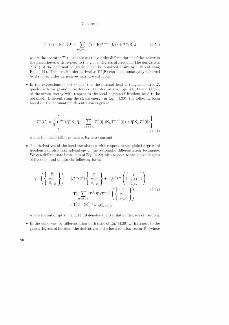
Chapter 4
T α(F) = RT α(U) +∑
0<β<α
{T β(R)T α−β(U)
}+ T α(R)U (4.50)
where the operator T α( ) expresses the α order differentiation of the matrix inthe parentheses with respect to the global degrees of freedom. The derivativesT α(F) of the deformation gradient can be obtained easily by differentiatingEq. (4.11). Then, each order derivative T α(R) can be automatically achievedby its lower order derivatives in a forward mode.
• In the expressions (4.33) ∼ (4.36) of the internal load f , tangent matrix L,quadratic form Q and cubic form C, the derivatives, Eqs. (4.31) and (4.32),of the strain energy with respect to the local degrees of freedom need to beobtained. Differentiating the strain energy in Eq. (4.30), the following formbased on the automatic differentiation is given:
T α(U) =1
2
T α(qt)KLq+
∑
0<β<α
T β(qt)KLTα−β(q) + qtKLT
α(q)
(4.51)
where the linear stiffness matrix KL is a constant.
• The derivatives of the local translations with respect to the global degrees offreedom can also take advantage of the automatic differentiation technique.We can differentiate both sides of Eq. (4.22) with respect to the global degreesof freedom, and obtain the following form:
T α
qiqi+1
qi+2
=Tt
0Tα(Rt)
qiqi+1
qi+2
+ Tt
0RtT α
qiqi+1
qi+2
+ Tt0
∑
0<β<α
T β(Rt)T α−β
qiqi+1
qi+2
+ Tt0T
α(Rt)T0T
t0r
0(i+5)/6
(4.52)
where the subscript i = 1, 7, 13, 19 denotes the translation degrees of freedom.
• In the same way, by differentiating both sides of Eq. (4.29) with respect to the
global degrees of freedom, the derivatives of the local rotation vector θa (where
90
Koiter-Newton’s analysis using co-rotational shell kinematics
a is equal to 1, 2, 3, 4 to denote the node number) with respect to the globaldegrees of freedom using the automatic differentiation technique are given by:
T α(θa) =
T
t0
T α(Rt) exp(ϑa
)+ RtT α(exp
(ϑa
))
+∑
0<β<α
T β(Rt)T α−β(exp(ϑa
))
exp(θn
a
)T0
X
(4.53)
where the term exp(θn
a
)is related to the rotation vector θ
n
a in the known
nominal configuration and is a constant for a given value of a.
4.6 Numerical results
In this section several reference problems of the shell models are considered usingthe Koiter-Newton approach. The imperfection analyses of the structures are alsopresented. The results are compared with results obtained using ABAQUS basedon a full nonlinear analysis, with the same number of elements and nodes.
4.6.1 Flat plate
The Koiter-Newton approach’s ability to handle a closely-spaced buckling modescase is well illustrated by the following shell example. This is a flat plate uniformlycompressed in the longitudinal direction. The constraint conditions are shown in Fig.4.5. The sides are a = 140mm and b = 100mm long, respectively, and the thicknessis 0.5mm. The elastic material properties are E = 70000N/mm2 and ν = 0.3. Theplate is meshed with 140 square shell elements.
The following steps are taken in the present example:
1. Some preparation work is done to construct the reduced order model: a linearbuckling analysis and the first and second order displacement fields.
2. A nonlinear analysis is applied for the perfect plate using the Koiter-Newtonapproach.
91
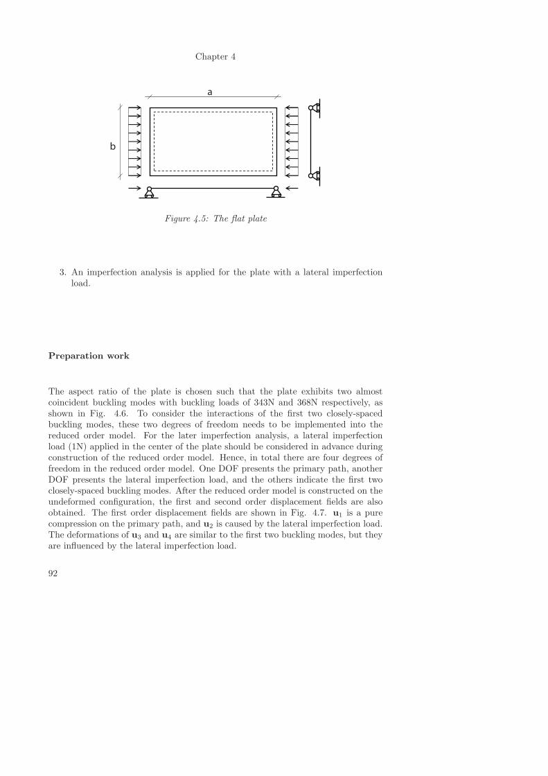
Chapter 4
a
b
Figure 4.5: The flat plate
3. An imperfection analysis is applied for the plate with a lateral imperfectionload.
Preparation work
The aspect ratio of the plate is chosen such that the plate exhibits two almostcoincident buckling modes with buckling loads of 343N and 368N respectively, asshown in Fig. 4.6. To consider the interactions of the first two closely-spacedbuckling modes, these two degrees of freedom needs to be implemented into thereduced order model. For the later imperfection analysis, a lateral imperfectionload (1N) applied in the center of the plate should be considered in advance duringconstruction of the reduced order model. Hence, in total there are four degrees offreedom in the reduced order model. One DOF presents the primary path, anotherDOF presents the lateral imperfection load, and the others indicate the first twoclosely-spaced buckling modes. After the reduced order model is constructed on theundeformed configuration, the first and second order displacement fields are alsoobtained. The first order displacement fields are shown in Fig. 4.7. u1 is a purecompression on the primary path, and u2 is caused by the lateral imperfection load.The deformations of u3 and u4 are similar to the first two buckling modes, but theyare influenced by the lateral imperfection load.
92
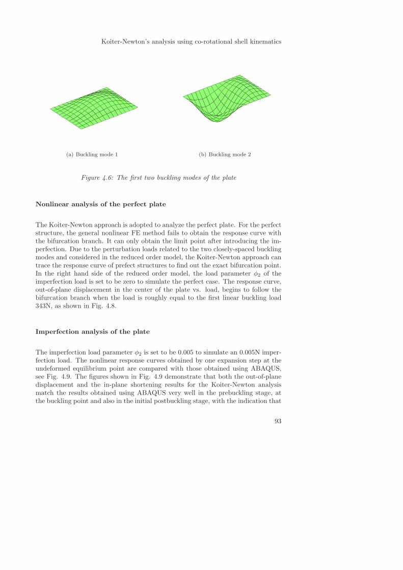
Koiter-Newton’s analysis using co-rotational shell kinematics
(a) Buckling mode 1 (b) Buckling mode 2
Figure 4.6: The first two buckling modes of the plate
Nonlinear analysis of the perfect plate
The Koiter-Newton approach is adopted to analyze the perfect plate. For the perfectstructure, the general nonlinear FE method fails to obtain the response curve withthe bifurcation branch. It can only obtain the limit point after introducing the im-perfection. Due to the perturbation loads related to the two closely-spaced bucklingmodes and considered in the reduced order model, the Koiter-Newton approach cantrace the response curve of prefect structures to find out the exact bifurcation point.In the right hand side of the reduced order model, the load parameter φ2 of theimperfection load is set to be zero to simulate the perfect case. The response curve,out-of-plane displacement in the center of the plate vs. load, begins to follow thebifurcation branch when the load is roughly equal to the first linear buckling load343N, as shown in Fig. 4.8.
Imperfection analysis of the plate
The imperfection load parameter φ2 is set to be 0.005 to simulate an 0.005N imper-fection load. The nonlinear response curves obtained by one expansion step at theundeformed equilibrium point are compared with those obtained using ABAQUS,see Fig. 4.9. The figures shown in Fig. 4.9 demonstrate that both the out-of-planedisplacement and the in-plane shortening results for the Koiter-Newton analysismatch the results obtained using ABAQUS very well in the prebuckling stage, atthe buckling point and also in the initial postbuckling stage, with the indication that
93
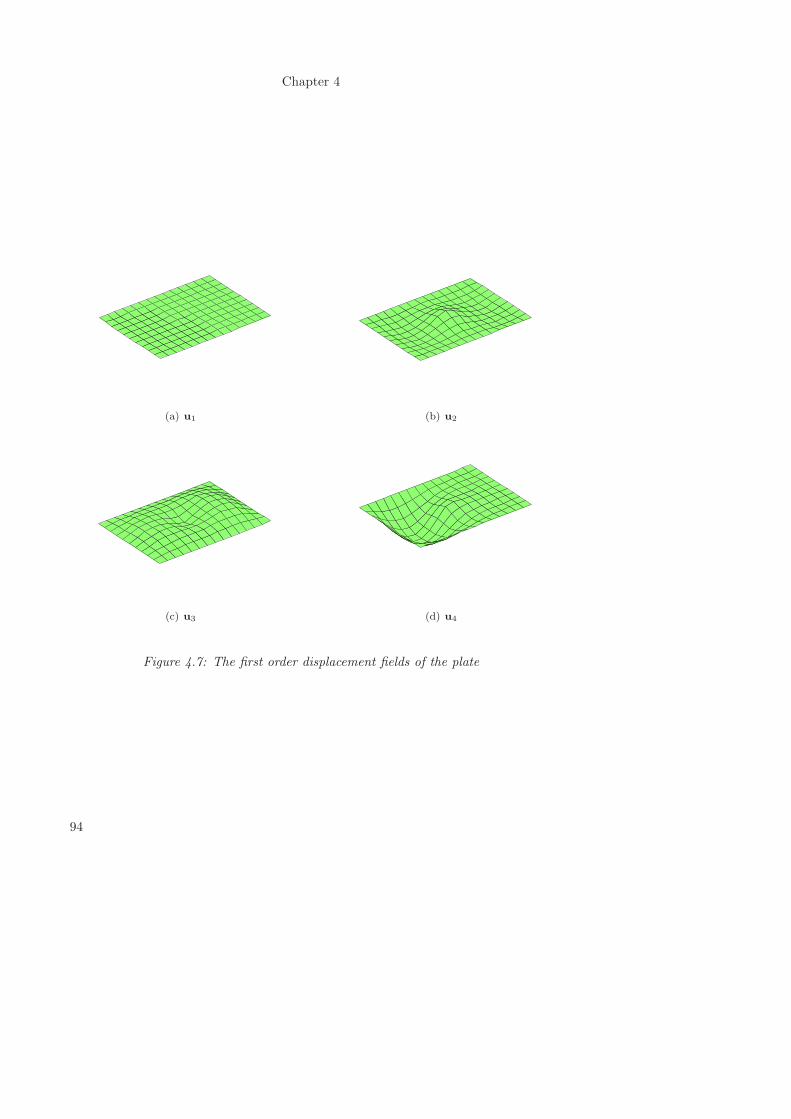
Chapter 4
(a) u1 (b) u2
(c) u3 (d) u4
Figure 4.7: The first order displacement fields of the plate
94
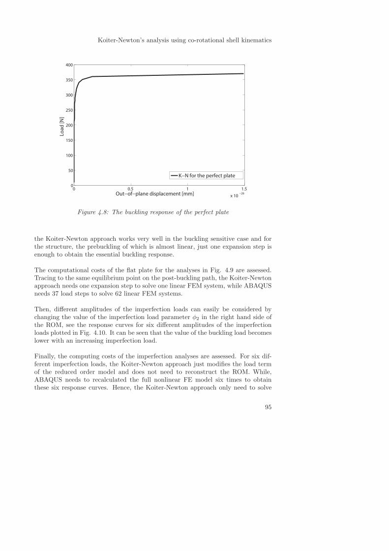
Koiter-Newton’s analysis using co-rotational shell kinematics
0 0.5 1 1.5
x 10−26
0
50
100
150
200
250
300
350
400
Out−of−plane displacement [mm]
Lo
ad
[N
]
K−N for the perfect plate
Figure 4.8: The buckling response of the perfect plate
the Koiter-Newton approach works very well in the buckling sensitive case and forthe structure, the prebuckling of which is almost linear, just one expansion step isenough to obtain the essential buckling response.
The computational costs of the flat plate for the analyses in Fig. 4.9 are assessed.Tracing to the same equilibrium point on the post-buckling path, the Koiter-Newtonapproach needs one expansion step to solve one linear FEM system, while ABAQUSneeds 37 load steps to solve 62 linear FEM systems.
Then, different amplitudes of the imperfection loads can easily be considered bychanging the value of the imperfection load parameter φ2 in the right hand side ofthe ROM, see the response curves for six different amplitudes of the imperfectionloads plotted in Fig. 4.10. It can be seen that the value of the buckling load becomeslower with an increasing imperfection load.
Finally, the computing costs of the imperfection analyses are assessed. For six dif-ferent imperfection loads, the Koiter-Newton approach just modifies the load termof the reduced order model and does not need to reconstruct the ROM. While,ABAQUS needs to recalculated the full nonlinear FE model six times to obtainthese six response curves. Hence, the Koiter-Newton approach only need to solve
95
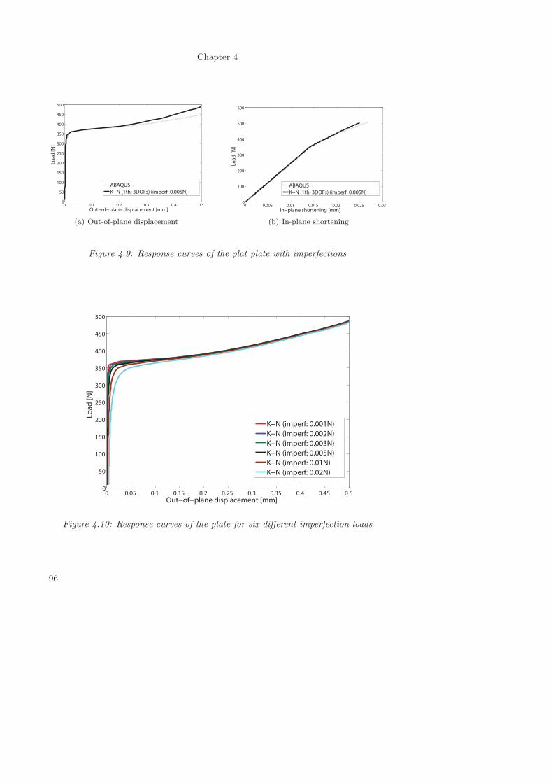
Chapter 4
0 0.1 0.2 0.3 0.4 0.50
50
100
150
200
250
300
350
400
450
500
Out−of−plane displacement [mm]
Lo
ad
[N
]
ABAQUS
K−N (1th: 3DOFs) (imperf: 0.005N)
(a) Out-of-plane displacement
0 0.005 0.01 0.015 0.02 0.025 0.030
100
200
300
400
500
600
In−plane shortening [mm]
Lo
ad
[N
]
ABAQUS
K−N (1th: 3DOFs) (imperf: 0.005N)
(b) In-plane shortening
Figure 4.9: Response curves of the plat plate with imperfections
0 0.05 0.1 0.15 0.2 0.25 0.3 0.35 0.4 0.45 0.50
50
100
150
200
250
300
350
400
450
500
Out−of−plane displacement [mm]
Lo
ad
[N
]
K−N (imperf: 0.001N)
K−N (imperf: 0.002N)
K−N (imperf: 0.003N)
K−N (imperf: 0.005N)
K−N (imperf: 0.01N)
K−N (imperf: 0.02N)
Figure 4.10: Response curves of the plate for six different imperfection loads
96

Koiter-Newton’s analysis using co-rotational shell kinematics
one linear FEM system to construct the reduced order model once, and the costs forsolving these six low-order ROMs can be neglected. While ABAQUS needs to solveapproximate 62 linear FEM systems for each imperfection case, that will be 372systems for all the six imperfection cases, thus it shows that the advantage of theKoiter-Newton approach in computational costs is more obvious in the imperfectionanalysis.
97
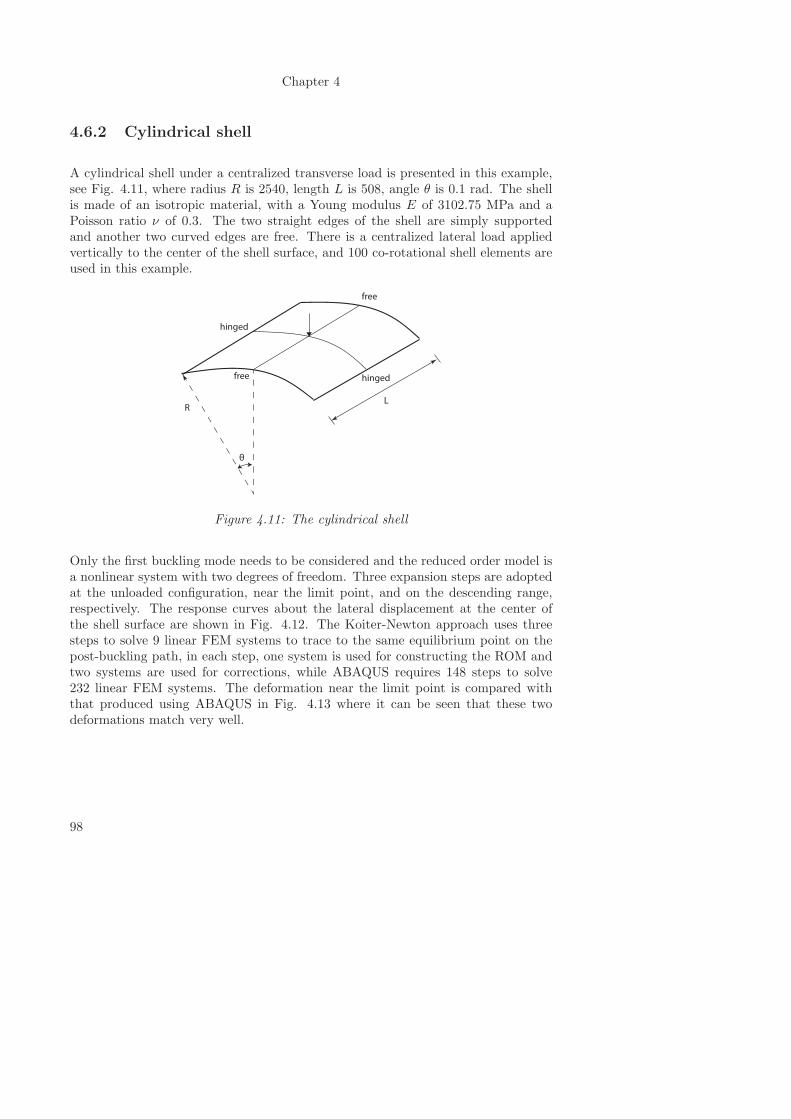
Chapter 4
4.6.2 Cylindrical shell
A cylindrical shell under a centralized transverse load is presented in this example,see Fig. 4.11, where radius R is 2540, length L is 508, angle θ is 0.1 rad. The shellis made of an isotropic material, with a Young modulus E of 3102.75 MPa and aPoisson ratio ν of 0.3. The two straight edges of the shell are simply supportedand another two curved edges are free. There is a centralized lateral load appliedvertically to the center of the shell surface, and 100 co-rotational shell elements areused in this example.
R
θ
L
free
free
hinged
hinged
Figure 4.11: The cylindrical shell
Only the first buckling mode needs to be considered and the reduced order model isa nonlinear system with two degrees of freedom. Three expansion steps are adoptedat the unloaded configuration, near the limit point, and on the descending range,respectively. The response curves about the lateral displacement at the center ofthe shell surface are shown in Fig. 4.12. The Koiter-Newton approach uses threesteps to solve 9 linear FEM systems to trace to the same equilibrium point on thepost-buckling path, in each step, one system is used for constructing the ROM andtwo systems are used for corrections, while ABAQUS requires 148 steps to solve232 linear FEM systems. The deformation near the limit point is compared withthat produced using ABAQUS in Fig. 4.13 where it can be seen that these twodeformations match very well.
98
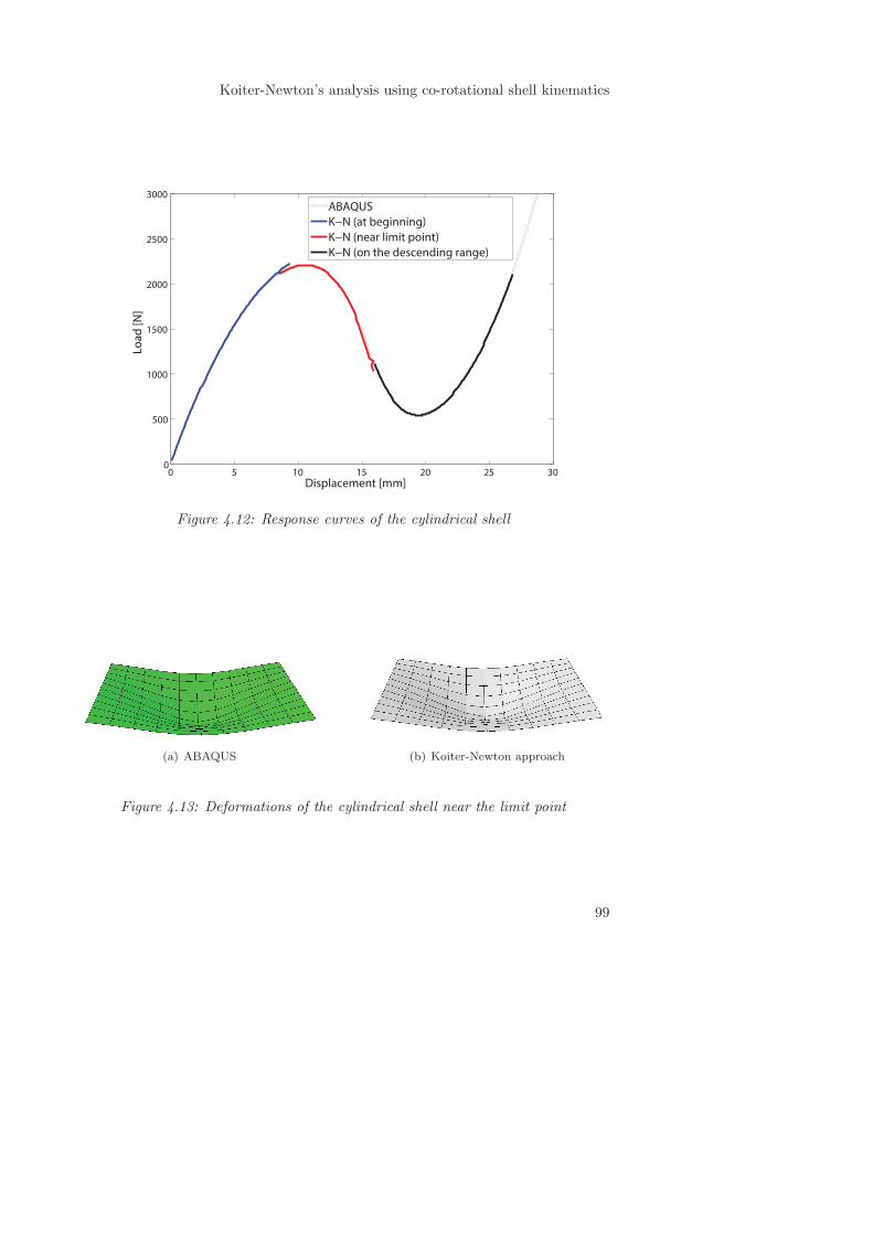
Koiter-Newton’s analysis using co-rotational shell kinematics
0 5 10 15 20 25 300
500
1000
1500
2000
2500
3000
Displacement [mm]
Lo
ad
[N
]
ABAQUS
K−N (at beginning)
K−N (near limit point)
K−N (on the descending range)
Figure 4.12: Response curves of the cylindrical shell
(a) ABAQUS (b) Koiter-Newton approach
Figure 4.13: Deformations of the cylindrical shell near the limit point
99
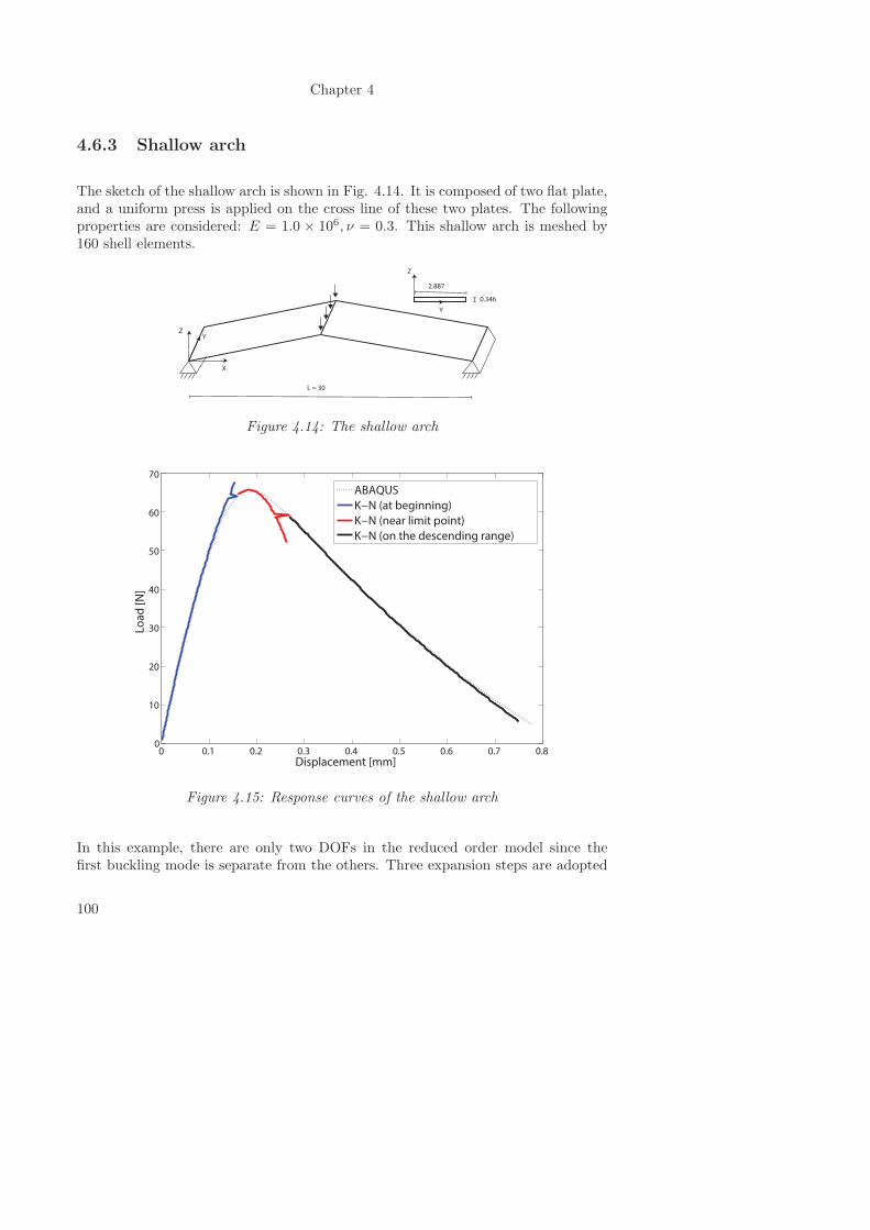
Chapter 4
4.6.3 Shallow arch
The sketch of the shallow arch is shown in Fig. 4.14. It is composed of two flat plate,and a uniform press is applied on the cross line of these two plates. The followingproperties are considered: E = 1.0 × 10⁶, ν = 0.3. This shallow arch is meshed by160 shell elements.
X
ZY
L = 30
Z
Y
2.887
0.346
Figure 4.14: The shallow arch
0 0.1 0.2 0.3 0.4 0.5 0.6 0.7 0.80
10
20
30
40
50
60
70
Displacement [mm]
Lo
ad
[N
]
ABAQUS
K−N (at beginning)
K−N (near limit point)
K−N (on the descending range)
Figure 4.15: Response curves of the shallow arch
In this example, there are only two DOFs in the reduced order model since thefirst buckling mode is separate from the others. Three expansion steps are adopted
100
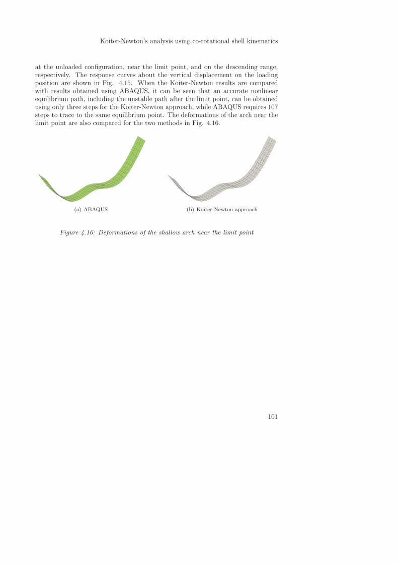
Koiter-Newton’s analysis using co-rotational shell kinematics
at the unloaded configuration, near the limit point, and on the descending range,respectively. The response curves about the vertical displacement on the loadingposition are shown in Fig. 4.15. When the Koiter-Newton results are comparedwith results obtained using ABAQUS, it can be seen that an accurate nonlinearequilibrium path, including the unstable path after the limit point, can be obtainedusing only three steps for the Koiter-Newton approach, while ABAQUS requires 107steps to trace to the same equilibrium point. The deformations of the arch near thelimit point are also compared for the two methods in Fig. 4.16.
(a) ABAQUS (b) Koiter-Newton approach
Figure 4.16: Deformations of the shallow arch near the limit point
101
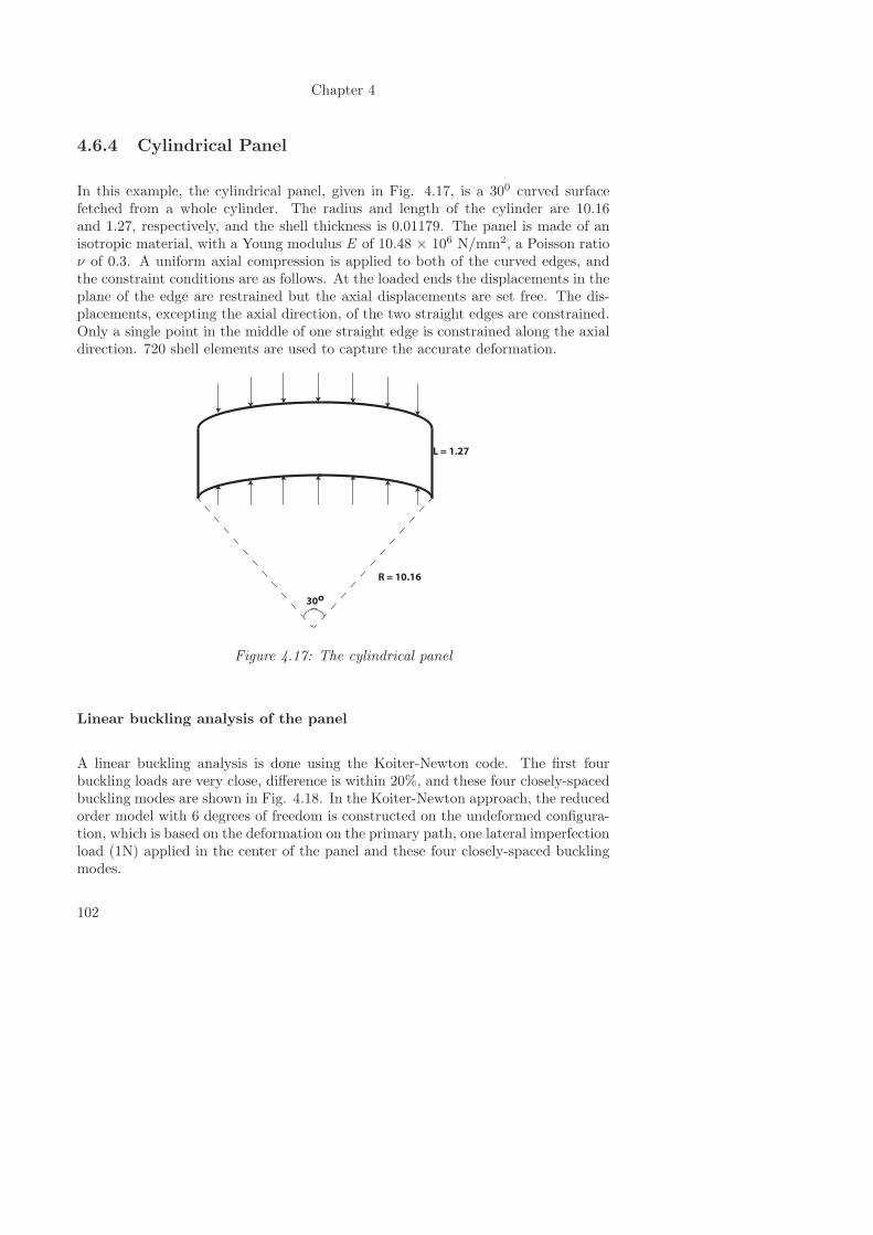
Chapter 4
4.6.4 Cylindrical Panel
In this example, the cylindrical panel, given in Fig. 4.17, is a 300 curved surfacefetched from a whole cylinder. The radius and length of the cylinder are 10.16and 1.27, respectively, and the shell thickness is 0.01179. The panel is made of anisotropic material, with a Young modulus E of 10.48 × 10⁶ N/mm2, a Poisson ratioν of 0.3. A uniform axial compression is applied to both of the curved edges, andthe constraint conditions are as follows. At the loaded ends the displacements in theplane of the edge are restrained but the axial displacements are set free. The dis-placements, excepting the axial direction, of the two straight edges are constrained.Only a single point in the middle of one straight edge is constrained along the axialdirection. 720 shell elements are used to capture the accurate deformation.
30o
L = 1.27
R = 10.16
Figure 4.17: The cylindrical panel
Linear buckling analysis of the panel
A linear buckling analysis is done using the Koiter-Newton code. The first fourbuckling loads are very close, difference is within 20%, and these four closely-spacedbuckling modes are shown in Fig. 4.18. In the Koiter-Newton approach, the reducedorder model with 6 degrees of freedom is constructed on the undeformed configura-tion, which is based on the deformation on the primary path, one lateral imperfectionload (1N) applied in the center of the panel and these four closely-spaced bucklingmodes.
102
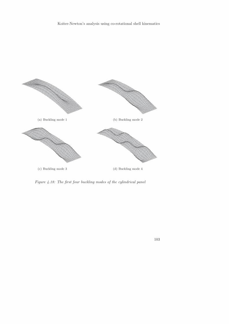
Koiter-Newton’s analysis using co-rotational shell kinematics
(a) Buckling mode 1 (b) Buckling mode 2
(c) Buckling mode 3 (d) Buckling mode 4
Figure 4.18: The first four buckling modes of the cylindrical panel
103
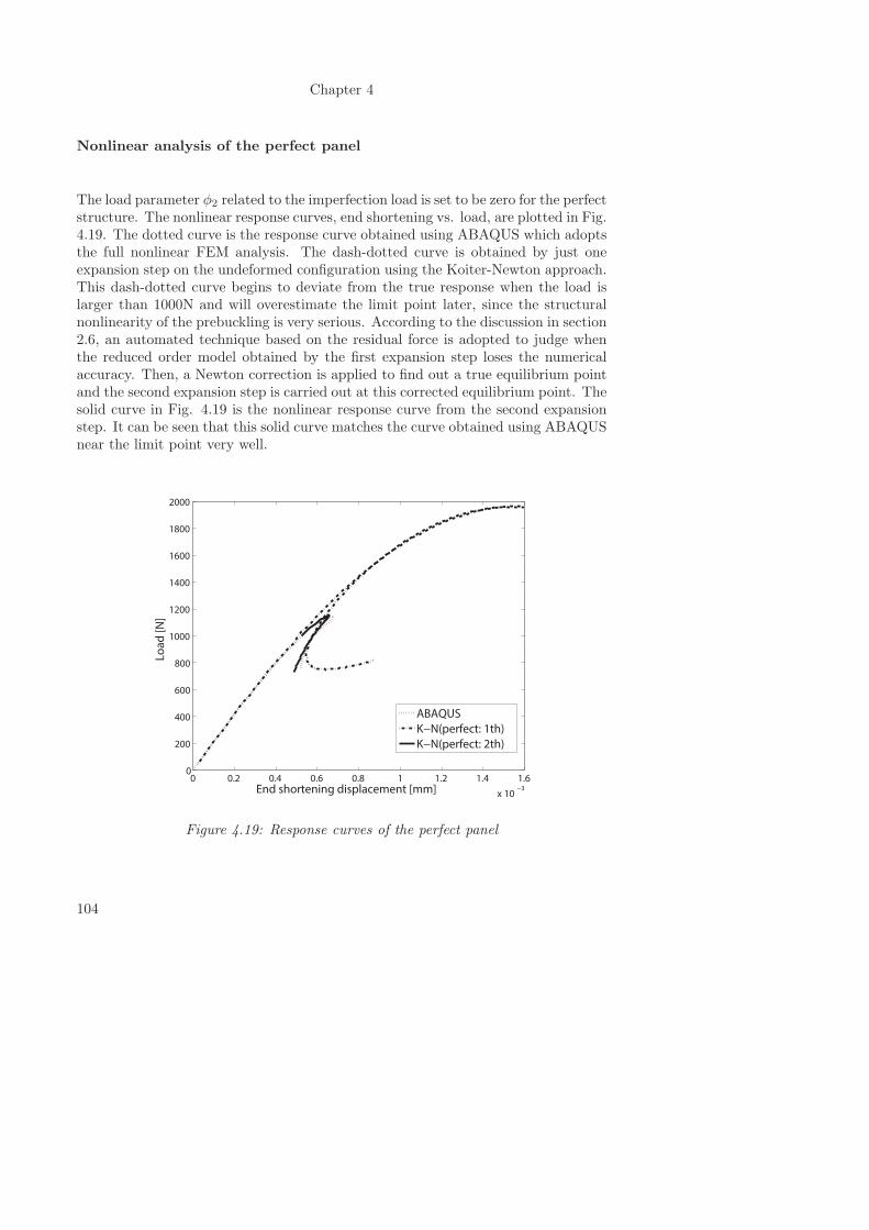
Chapter 4
Nonlinear analysis of the perfect panel
The load parameter φ2 related to the imperfection load is set to be zero for the perfectstructure. The nonlinear response curves, end shortening vs. load, are plotted in Fig.4.19. The dotted curve is the response curve obtained using ABAQUS which adoptsthe full nonlinear FEM analysis. The dash-dotted curve is obtained by just oneexpansion step on the undeformed configuration using the Koiter-Newton approach.This dash-dotted curve begins to deviate from the true response when the load islarger than 1000N and will overestimate the limit point later, since the structuralnonlinearity of the prebuckling is very serious. According to the discussion in section2.6, an automated technique based on the residual force is adopted to judge whenthe reduced order model obtained by the first expansion step loses the numericalaccuracy. Then, a Newton correction is applied to find out a true equilibrium pointand the second expansion step is carried out at this corrected equilibrium point. Thesolid curve in Fig. 4.19 is the nonlinear response curve from the second expansionstep. It can be seen that this solid curve matches the curve obtained using ABAQUSnear the limit point very well.
0 0.2 0.4 0.6 0.8 1 1.2 1.4 1.6
x 10−3
0
200
400
600
800
1000
1200
1400
1600
1800
2000
End shortening displacement [mm]
Lo
ad
[N
]
ABAQUS
K−N(perfect: 1th)
K−N(perfect: 2th)
Figure 4.19: Response curves of the perfect panel
104
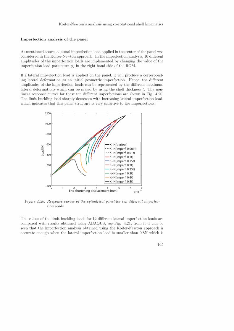
Koiter-Newton’s analysis using co-rotational shell kinematics
Imperfection analysis of the panel
As mentioned above, a lateral imperfection load applied in the center of the panel wasconsidered in the Koiter-Newton approach. In the imperfection analysis, 10 differentamplitudes of the imperfection loads are implemented by changing the value of theimperfection load parameter φ2 in the right hand side of the ROM.
If a lateral imperfection load is applied on the panel, it will produce a correspond-ing lateral deformation as an initial geometric imperfection. Hence, the differentamplitudes of the imperfection loads can be represented by the different maximumlateral deformations which can be scaled by using the shell thickness t. The non-linear response curves for these ten different imperfections are shown in Fig. 4.20.The limit buckling load sharply decreases with increasing lateral imperfection load,which indicates that this panel structure is very sensitive to the imperfections.
0 1 2 3 4 5 6 7 8
x 10−4
−200
0
200
400
600
800
1000
1200
End shortening displacement [mm]
Lo
ad
[N
]
K−N(perfect)
K−N(imperf: 0.001t)
K−N(imperf: 0.01t)
K−N(imperf: 0.1t)
K−N(imperf: 0.15t)
K−N(imperf: 0.2t)
K−N(imperf: 0.25t)
K−N(imperf: 0.3t)
K−N(imperf: 0.4t)
K−N(imperf: 0.5t)
Figure 4.20: Response curves of the cylindrical panel for ten different imperfec-tion loads
The values of the limit buckling loads for 12 different lateral imperfection loads arecompared with results obtained using ABAQUS, see Fig. 4.21, from it it can beseen that the imperfection analysis obtained using the Koiter-Newton approach isaccurate enough when the lateral imperfection load is smaller than 0.8N which is
105
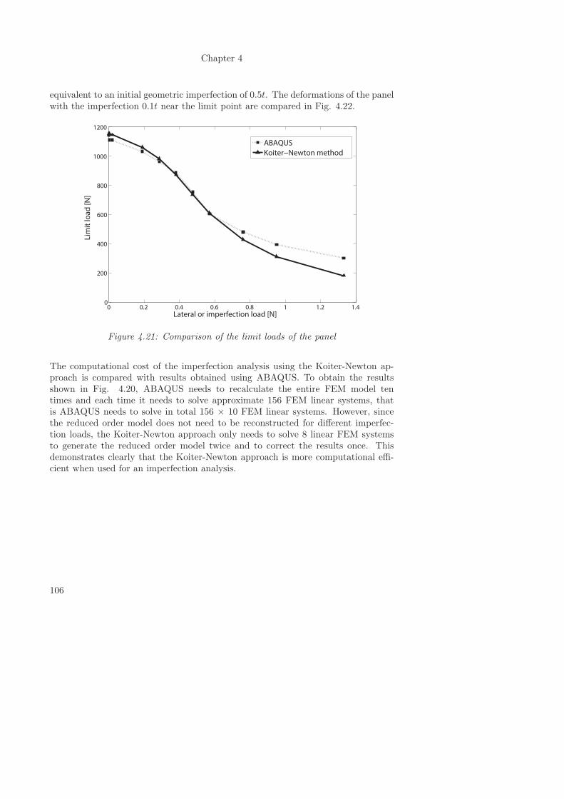
Chapter 4
equivalent to an initial geometric imperfection of 0.5t. The deformations of the panelwith the imperfection 0.1t near the limit point are compared in Fig. 4.22.
0 0.2 0.4 0.6 0.8 1 1.2 1.40
200
400
600
800
1000
1200
Lateral or imperfection load [N]
Lim
it lo
ad
[N
]
ABAQUS
Koiter−Newton method
Figure 4.21: Comparison of the limit loads of the panel
The computational cost of the imperfection analysis using the Koiter-Newton ap-proach is compared with results obtained using ABAQUS. To obtain the resultsshown in Fig. 4.20, ABAQUS needs to recalculate the entire FEM model tentimes and each time it needs to solve approximate 156 FEM linear systems, thatis ABAQUS needs to solve in total 156 × 10 FEM linear systems. However, sincethe reduced order model does not need to be reconstructed for different imperfec-tion loads, the Koiter-Newton approach only needs to solve 8 linear FEM systemsto generate the reduced order model twice and to correct the results once. Thisdemonstrates clearly that the Koiter-Newton approach is more computational effi-cient when used for an imperfection analysis.
106
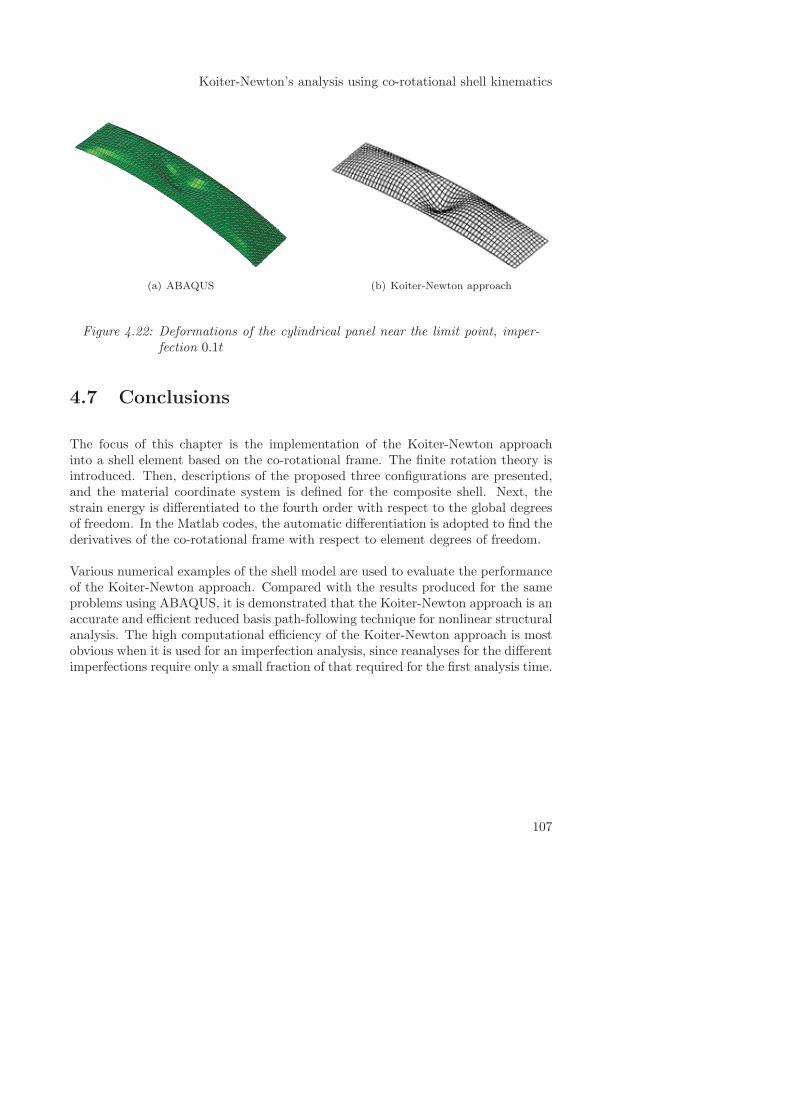
Koiter-Newton’s analysis using co-rotational shell kinematics
(a) ABAQUS (b) Koiter-Newton approach
Figure 4.22: Deformations of the cylindrical panel near the limit point, imper-fection 0.1t
4.7 Conclusions
The focus of this chapter is the implementation of the Koiter-Newton approachinto a shell element based on the co-rotational frame. The finite rotation theory isintroduced. Then, descriptions of the proposed three configurations are presented,and the material coordinate system is defined for the composite shell. Next, thestrain energy is differentiated to the fourth order with respect to the global degreesof freedom. In the Matlab codes, the automatic differentiation is adopted to find thederivatives of the co-rotational frame with respect to element degrees of freedom.
Various numerical examples of the shell model are used to evaluate the performanceof the Koiter-Newton approach. Compared with the results produced for the sameproblems using ABAQUS, it is demonstrated that the Koiter-Newton approach is anaccurate and efficient reduced basis path-following technique for nonlinear structuralanalysis. The high computational efficiency of the Koiter-Newton approach is mostobvious when it is used for an imperfection analysis, since reanalyses for the differentimperfections require only a small fraction of that required for the first analysis time.
107

Chapter 4
108
Chapter 5
Koiter-Newton analysis using
Von Karman kinematics
5.1 Introduction
The Koiter-Newton analyses using co-rotational kinematics were introduced in chap-ters 3 and 4. Achieving equilibrium equations of a third order form (2.8), especiallythe forms L, Q and C, is the main task of FE implementations. Elements in aco-rotational frame consider the fully geometric nonlinearities in the element, hencethe FE implementation is complicated and time consuming. In engineering, somestructures under the loading can neglect the nonlinear in-plane rotations while therotations of the normals to the mid-surface are finitely large. In this case, theVon Karman kinematics which ignore some nonlinear terms in the Green’s stain-displacement relations are also available in the analysis. The membrane part of vonKarman’s strain-displacement relationships for moderately large-deflection analysiscan be considered as a special case of the Green strain [112]. The expression of theVon Karman membrane strain for a plate is given by:
109
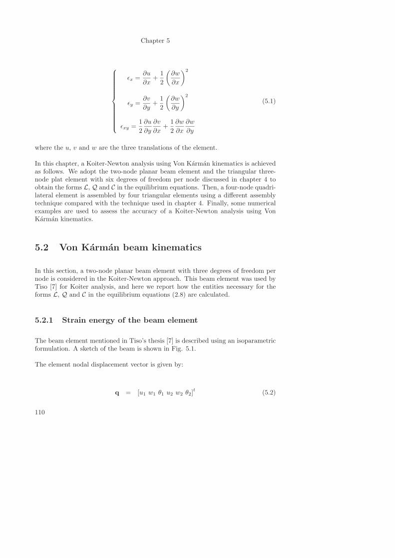
Chapter 5
ǫx =∂u
∂x+
1
2
(∂w
∂x
)2
ǫy =∂v
∂y+
1
2
(∂w
∂y
)2
ǫxy =1
2
∂u
∂y
∂v
∂x+
1
2
∂w
∂x
∂w
∂y
(5.1)
where the u, v and w are the three translations of the element.
In this chapter, a Koiter-Newton analysis using Von Karman kinematics is achievedas follows. We adopt the two-node planar beam element and the triangular three-node plat element with six degrees of freedom per node discussed in chapter 4 toobtain the forms L, Q and C in the equilibrium equations. Then, a four-node quadri-lateral element is assembled by four triangular elements using a different assemblytechnique compared with the technique used in chapter 4. Finally, some numericalexamples are used to assess the accuracy of a Koiter-Newton analysis using VonKarman kinematics.
5.2 Von Karman beam kinematics
In this section, a two-node planar beam element with three degrees of freedom pernode is considered in the Koiter-Newton approach. This beam element was used byTiso [7] for Koiter analysis, and here we report how the entities necessary for theforms L, Q and C in the equilibrium equations (2.8) are calculated.
5.2.1 Strain energy of the beam element
The beam element mentioned in Tiso’s thesis [7] is described using an isoparametricformulation. A sketch of the beam is shown in Fig. 5.1.
The element nodal displacement vector is given by:
q = [u1 w1 θ1 u2 w2 θ2]t
(5.2)
110
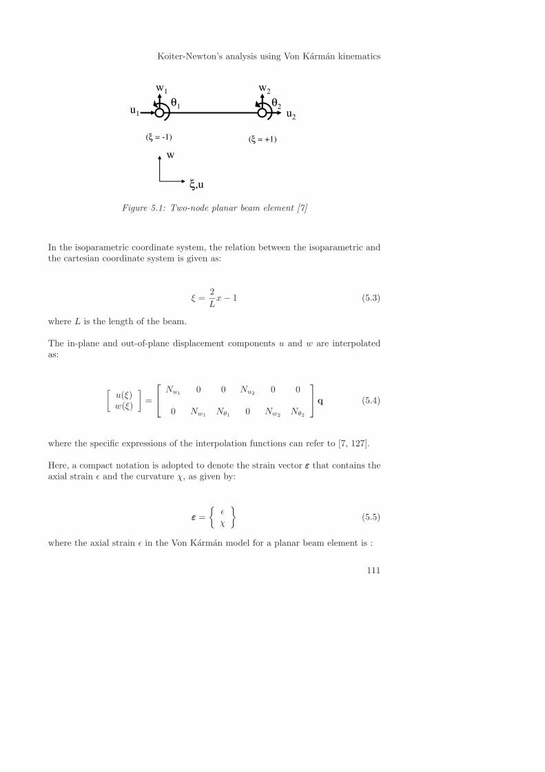
Koiter-Newton’s analysis using Von Karman kinematics
Figure 5.1: Two-node planar beam element [7]
In the isoparametric coordinate system, the relation between the isoparametric andthe cartesian coordinate system is given as:
ξ =2
Lx− 1 (5.3)
where L is the length of the beam.
The in-plane and out-of-plane displacement components u and w are interpolatedas:
[u(ξ)w(ξ)
]=
Nu1
0 0 Nu20 0
0 Nw1Nθ1 0 Nw2
Nθ2
q (5.4)
where the specific expressions of the interpolation functions can refer to [7, 127].
Here, a compact notation is adopted to denote the strain vector εεε that contains theaxial strain ǫ and the curvature χ, as given by:
εεε =
{ǫχ
}(5.5)
where the axial strain ǫ in the Von Karman model for a planar beam element is :
111
Chapter 5
ǫ =du
dx+
1
2
(dw
dx
)2
(5.6)
and the curvature χ is:
χ =d2w
dx2(5.7)
Introducing the displacements (5.4) into Eqs. (5.6) ∼ (5.7) and then into Eq. (5.5),the strain vector εεε is represented by the displacements. Then, the strain can bedivided into the linear part and the nonlinear part with respect to the displacements,resulting in:
εεε =
{ǫχ
}= εεεl + εεεnl (5.8)
where the linear part εεεl is:
εεεl =1
L
−u1 + u2
3
2ξw1 +
(−1
4L+
3
4Lξ
)θ1 −
3
2ξw2 +
(1
4L+
3
4Lξ
)θ2
(5.9)
and the nonlinear part εεεnl is:
εεεnl =1
2
6
5L2(w1 − w2)
2+
2
15(θ1 − θ2)
2+
1
5θ1θ2 +
1
5L(θ1 + θ2) (w1 − w2)
0
(5.10)
According to Eqs. (5.8) ∼ (5.10), the axial strain ǫ and the curvature χ are:
112
Koiter-Newton’s analysis using Von Karman kinematics
ǫ =1
L(−u1 + u2)
+1
2
[6
5L2(w1 − w2)
2+
2
15(θ1 − θ2)
2+
1
5θ1θ2 +
1
5L(θ1 + θ2) (w1 − w2)
]
(5.11)
χ =1
L
[3
2ξw1 +
(−1
4L+
3
4Lξ
)θ1 −
3
2ξw2 +
(1
4L+
3
4Lξ
)θ2
](5.12)
Eq. (5.12) demonstrates that the curvature χ is totally linear with respect to thedisplacements and only the axial strain ǫ contains some nonlinear terms. The linearpart of the strain vector only contributes to the linear stiffness matrix which is alwaysa constant matrix and does not contribute to the third or fourth order derivatives ofthe strain energy. Hence, here we only consider the axial strain ǫ (5.11) to calculatethe axial strain energy, and the bending part that results from the curvature χ canbe easily superposed. The axial strain energy U of a planar beam element is writtenas:
U =1
2EALǫ2 (5.13)
where E is the Young’s modulus of the beam, and A is the area of the cross section.In the rest of this section, we will only use the strain energy U caused by the nonlinearaxial strain ǫ for calculations.
The bending part of the linear stiffness matrix, which is generated by the curvatureχ, is a very familiar form, as given by:
113
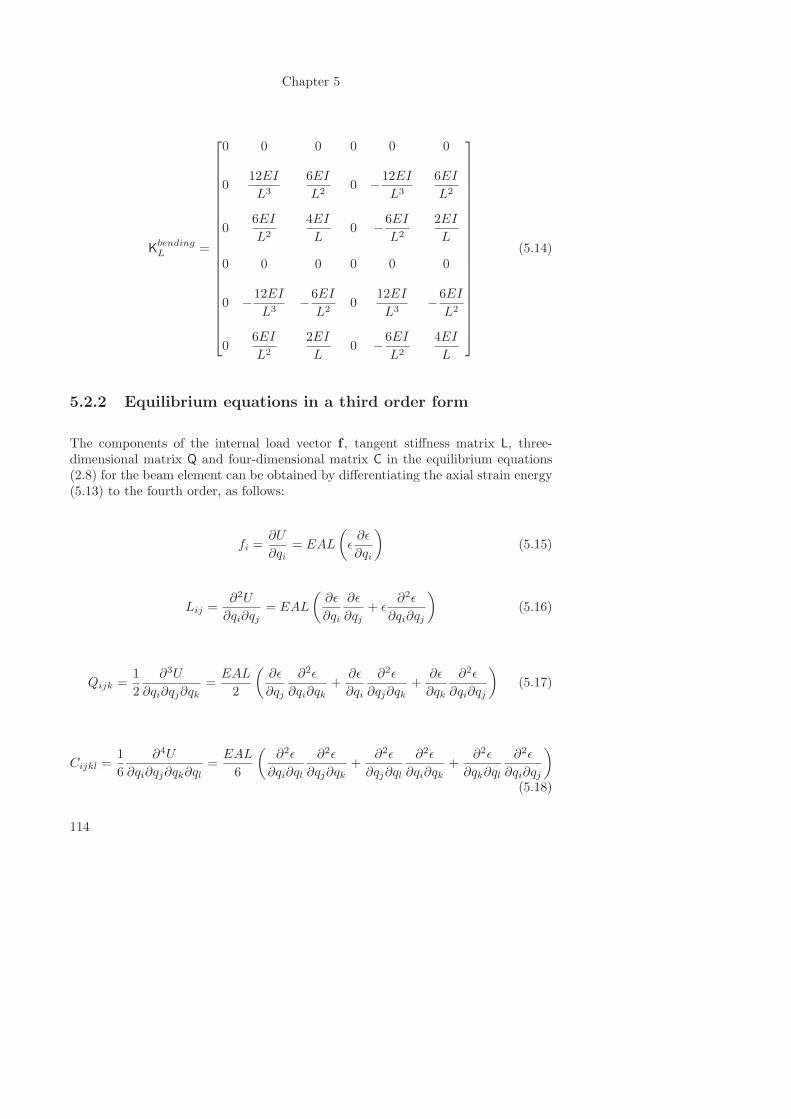
Chapter 5
KbendingL =
0 0 0 0 0 0
012EI
L3
6EI
L20 −
12EI
L3
6EI
L2
06EI
L2
4EI
L0 −
6EI
L2
2EI
L
0 0 0 0 0 0
0 −12EI
L3−6EI
L20
12EI
L3−6EI
L2
06EI
L2
2EI
L0 −
6EI
L2
4EI
L
(5.14)
5.2.2 Equilibrium equations in a third order form
The components of the internal load vector f , tangent stiffness matrix L, three-dimensional matrix Q and four-dimensional matrix C in the equilibrium equations(2.8) for the beam element can be obtained by differentiating the axial strain energy(5.13) to the fourth order, as follows:
fi =∂U
∂qi= EAL
(ǫ∂ǫ
∂qi
)(5.15)
Lij =∂2U
∂qi∂qj= EAL
(∂ǫ
∂qi
∂ǫ
∂qj+ ǫ
∂2ǫ
∂qi∂qj
)(5.16)
Qijk =1
2
∂3U
∂qi∂qj∂qk=EAL
2
(∂ǫ
∂qj
∂2ǫ
∂qi∂qk+
∂ǫ
∂qi
∂2ǫ
∂qj∂qk+
∂ǫ
∂qk
∂2ǫ
∂qi∂qj
)(5.17)
Cijkl =1
6
∂4U
∂qi∂qj∂qk∂ql=EAL
6
(∂2ǫ
∂qi∂ql
∂2ǫ
∂qj∂qk+
∂2ǫ
∂qj∂ql
∂2ǫ
∂qi∂qk+
∂2ǫ
∂qk∂ql
∂2ǫ
∂qi∂qj
)
(5.18)
114
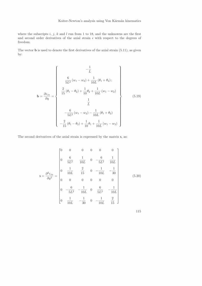
Koiter-Newton’s analysis using Von Karman kinematics
where the subscripts i, j, k and l run from 1 to 18, and the unknowns are the firstand second order derivatives of the axial strain ǫ with respect to the degrees offreedom.
The vector b is used to denote the first derivatives of the axial strain (5.11), as givenby:
b =∂ǫin∂q
=
−1
L
6
5L2(w1 − w2) +
1
10L(θ1 + θ2) ;
2
15(θ1 − θ2) +
1
10θ2 +
1
10L(w1 − w2)
1
L
−6
5L2(w1 − w2)−
1
10L(θ1 + θ2)
−2
15(θ1 − θ2) +
1
10θ1 +
1
10L(w1 − w2)
(5.19)
The second derivatives of the axial strain is expressed by the matrix s, as:
s =∂2ǫin∂q2
=
0 0 0 0 0 0
06
5L2
1
10L0 −
6
5L2
1
10L
01
10L
2
150 −
1
10L−
1
30
0 0 0 0 0 0
0 −6
5L2−
1
10L0
6
5L2−
1
10L
01
10L−
1
300 −
1
10L
2
15
(5.20)
115
Chapter 5
Then, Eqs. (5.15) ∼ (5.16) can be rewritten in a compact form by using the vectorb and the matrix s as:
f = EAL (ǫb) (5.21)
L = EAL(bbt + ǫs
)(5.22)
The three-dimensional matrix Q and four-dimensional matrix C are not directly andseparately used in the Koiter-Newton approach, and they are involved in three placesduring the derivations. The first one is Q(q) for calculating the geometric stiffnessmatrix Kg = −2Qq = −2Q(q) (refer to Eq. (2.41)), the second one is Q(uα,uβ)which is used to solve the linear system of equations (2.22) and achieve the Q in thereduced order model, and the third one is C(uα,uβ ,uγ ,uδ) which is in Eq. (2.34)to calculate the C in the reduced order model. These three terms are achieved asfollows:
• Q(q) can be achieved by the multiplication of the 3D matrix Q in Eq. (5.17)and the displacement vector q obtained by a linear static analysis, which resultsin a matrix:
Q(q) = Qijk qk =EAL
2
(∂ǫ
∂qj
∂2ǫ
∂qi∂qkqk +
∂ǫ
∂qi
∂2ǫ
∂qj∂qkqk +
∂ǫ
∂qkqk
∂2ǫ
∂qi∂qj
)
(5.23)where the summation convention is applied. A compact notation can be usedby using b and s:
Q(q) =EAL
2
(sqbt + bq
ts+ btqs
)(5.24)
• In the same way, Q(uα,uβ) which is obtained by multiplying two first orderdisplacement fields (uα and uβ) is written as:
Q(uα,uβ) =EAL
2
[(btuα)(suβ) + (btuβ)(suα) + (uαt
suβ)b]
(5.25)
• C(uα,uβ ,uγ ,uδ) is calculated by multiplying four first order displacementfields (uα, uβ , uγ and uδ), as given by:
116
Koiter-Newton’s analysis using Von Karman kinematics
C(uα,uβ ,uγ ,uδ) =EAL
6
(uαt
suδ)(
uβt
suγ)+(uβt
suδ)(
uαt
suγ)
+(uγt
suδ)(
uαt
suβ)
(5.26)If we introduce a new notation:
Dαβ = uαt
suβ (5.27)
Eq. (5.26) becomes a more compact form:
C(uα,uβ ,uγ ,uδ) =EAL
6[DαδDβγ +DβδDαγ +DγδDαβ ] (5.28)
At this point, the L, Q and C in the equilibrium equations (2.8) of a Von Karmanbeam element are all achieved.
5.3 Von Karman shell kinematics
In this section, we will use a four-node quadrilateral element which is assembled bytriangular elements based on Von Karman kinematics. The triangular three-nodeplat element with six degrees of freedom per node, adopted in chapter 4 and Tiso’sthesis [7], is used to obtain the forms L, Q and C in the equilibrium equations (2.8),then another assembly technique, which is different from the one used in chapter 4,is introduced due to the existence of the quadratic and cubic forms Q and C.
5.3.1 Strain energy of the shell element
Firstly, we will give a quick review on the basic description of the triangular element.A discussion of the linear part and some nonlinear terms of this element can be foundin appendix A and Tiso’s thesis [7].
As shown in Fig. 5.2, each node of the triangular element has six degrees of freedom,as given by qa:
qa ={ua va wa θxa
θyaθza
}, a = 1, 2, 3 (5.29)
117
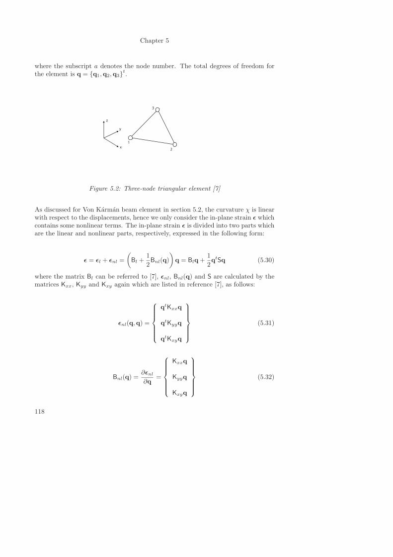
Chapter 5
where the subscript a denotes the node number. The total degrees of freedom forthe element is q = {q1,q2,q3}
t.
x
y
z
1
2
3
Figure 5.2: Three-node triangular element [7]
As discussed for Von Karman beam element in section 5.2, the curvature χ is linearwith respect to the displacements, hence we only consider the in-plane strain ǫ whichcontains some nonlinear terms. The in-plane strain ǫ is divided into two parts whichare the linear and nonlinear parts, respectively, expressed in the following form:
ǫ = ǫl + ǫnl =
(Bl +
1
2Bnl(q)
)q = Blq+
1
2qtSq (5.30)
where the matrix Bl can be referred to [7], ǫnl, Bnl(q) and S are calculated by thematrices Kxx, Kyy and Kxy again which are listed in reference [7], as follows:
ǫnl(q,q) =
qtKxxq
qtKyyq
qtKxyq
(5.31)
Bnl(q) =∂ǫnl∂q
=
Kxxq
Kyyq
Kxyq
(5.32)
118
Koiter-Newton’s analysis using Von Karman kinematics
S =∂2ǫnl∂q2
=
S(1, :, :) = Kxx
S(2, :, :) = Kyy
S(3, :, :) = Kxy
(5.33)
where S is a 3× 3× 3 matrix, and S(a, :, :) indicates the a-th 2D matrix in S.
Then, the in-plane resultant N is:
N = Am
(Bl +
1
2Bnl(q)
)q (5.34)
where Am is the in-plane part of the material matrix.
From Eq. (5.34), the nonlinear part Nnl of the in-plane stress is given by:
Nnl =1
2AmBnlq (5.35)
5.3.2 Equilibrium equations in a third order form
According to the strain in Eq. (5.30), the in-plane strain energy can be calculatedby:
Uin−plane =1
2AAmαβ
(ǫlα + ǫnlα)(ǫlβ + ǫnlβ
)(5.36)
where the subscripts α, β = 1, 2, 3 denote the addresses of components in the tensor,and the summation convention is applied, A is the element area.
The nonlinear part of the in-plane strain energy (5.36), which contributes to thequadratic and cubic forms in the equilibrium equations (2.8), is expressed by U :
U =1
2AAmαβ
(2ǫlαǫnlβ + ǫnlαǫnlβ
)(5.37)
In the rest of this section, we only consider the nonlinear part of the strain energy(5.37), since the linear part does not contribute to the high order differentiations. As
119
Chapter 5
presented for the Von Karman beam element in section 5.2, the components of theinternal load vector f , tangent stiffness matrix L, three-dimensional matrix Q andfour-dimensional matrix C in the equilibrium equations (2.8) for the shell element areall achieved by differentiating the strain energy (5.37) to the fourth order. Firstly,the components of the f and L are listed:
fi =∂U
∂qi=
1
2AAmαβ
2∂ǫlα∂qi
ǫnlβ+ 2
∂ǫnlβ∂qi
ǫlα
+∂ǫnlα∂qi
ǫnlβ +∂ǫnlβ∂qi
ǫnlα
(5.38)
Lij =∂2U
∂qi∂qj=
1
2AAmαβ
2∂ǫlα∂qi
∂ǫnlβ∂qj
+ 2∂ǫlα∂qj
∂ǫnlβ∂qi
+ 2∂2ǫnlβ∂qi∂qj
ǫlα
+2∂2ǫnlα∂qi∂qj
ǫnlβ +∂ǫnlα∂qi
∂ǫnlβ∂qj
(5.39)
where the subscripts i and j run from 1 to 18, and the summation convention isapplied on α and β.
Substituting Eqs. (5.30) ∼ (5.33) into Eq. (5.38) and Eq. (5.39), and together withEq. (5.34) and Eq. (5.35), the vector f and the matrix L can be calculated by acompact notation, as follows:
f = A(BtlNnl + 2Bt
nlN)
(5.40)
L = A{(
BtlBnl + Bt
nlBl + BtnlBnl
)+ (NxKxx +NyKyy +NxyKxy)
}(5.41)
where Nx, Ny and Nxy are the three components of the stress vector N.
As mentioned in subsection 5.2.2, we only need to calculate the expressions of Q(q),Q(uα,uβ) and C(uα,uβ ,uγ ,uδ) for the quadratic form Q and cubic form C. Thesethree terms are achieved as follows:
• The expression of Q can be easily obtained by differentiating the strain energy(5.37) to a third order with respect to the degrees of freedom. Multiplyingthe tensor Q by a displacement vector q, Q(q) is achieved and its expression
120
Koiter-Newton’s analysis using Von Karman kinematics
is very complicated. Hence, some notations are introduced to simplify thisexpression.
According to Eq. (5.32), the Bnl(q) related to the displacement q is given as:
Bnl(q) =∂ǫnl∂q
=
Kxxq
Kyyq
Kxyq
(5.42)
In Eq. (5.34), we assume a total matrix B related to the degrees of freedom q
to be:
B(q) = Bl +1
2Bnl(q) (5.43)
Then, the stress N(q) related to the displacement q results in:
N(q) = AmB(q)q (5.44)
Based on these notations (5.42) ∼ (5.44), Q(q) can be rewritten to be a com-pact form:
Q(q) =1
2A
{ (Btnl(q)AmB(q) + Bt(q)AmBnl(q)
)
+(NxKxx +NyKyy +NxyKxy
)}
(5.45)
where Nx, Ny and Nxy are the three components of the stress vector N(q).
• Another notation is introduced for calculating Q(uα,uβ), as given by:
N(uα,uβ) = AmB(uα)uβ (5.46)
where the stress N is related to the first order displacements, uα and uβ .
Then, in a similar way, Q(uα,uβ) is expressed by:
Q(uα,uβ) =1
2A(Btnl(uβ)N(uα) + Bt
nl(uα)N(uβ) + BtN(uα,uβ))
(5.47)
121
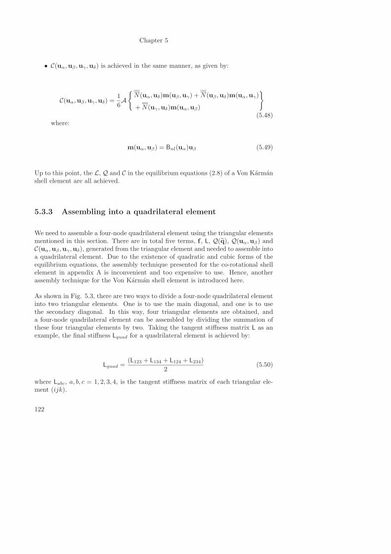
Chapter 5
• C(uα,uβ ,uγ ,uδ) is achieved in the same manner, as given by:
C(uα,uβ ,uγ ,uδ) =1
6A
{N(uα,uδ)m(uβ ,uγ) +N(uβ ,uδ)m(uα,uγ)
+N(uγ ,uδ)m(uα,uβ)
}
(5.48)where:
m(uα,uβ) = Bnl(uα)uβ (5.49)
Up to this point, the L, Q and C in the equilibrium equations (2.8) of a Von Karmanshell element are all achieved.
5.3.3 Assembling into a quadrilateral element
We need to assemble a four-node quadrilateral element using the triangular elementsmentioned in this section. There are in total five terms, f , L, Q(q), Q(uα,uβ) andC(uα,uβ ,uγ ,uδ), generated from the triangular element and needed to assemble intoa quadrilateral element. Due to the existence of quadratic and cubic forms of theequilibrium equations, the assembly technique presented for the co-rotational shellelement in appendix A is inconvenient and too expensive to use. Hence, anotherassembly technique for the Von Karman shell element is introduced here.
As shown in Fig. 5.3, there are two ways to divide a four-node quadrilateral elementinto two triangular elements. One is to use the main diagonal, and one is to usethe secondary diagonal. In this way, four triangular elements are obtained, anda four-node quadrilateral element can be assembled by dividing the summation ofthese four triangular elements by two. Taking the tangent stiffness matrix L as anexample, the final stiffness Lquad for a quadrilateral element is achieved by:
Lquad =(L123 + L134 + L124 + L234)
2(5.50)
where Labc, a, b, c = 1, 2, 3, 4, is the tangent stiffness matrix of each triangular ele-ment (ijk).
122
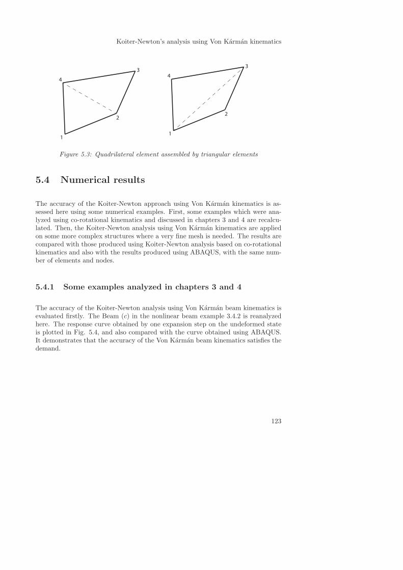
Koiter-Newton’s analysis using Von Karman kinematics
4
3
2
1
4
3
2
1
Figure 5.3: Quadrilateral element assembled by triangular elements
5.4 Numerical results
The accuracy of the Koiter-Newton approach using Von Karman kinematics is as-sessed here using some numerical examples. First, some examples which were ana-lyzed using co-rotational kinematics and discussed in chapters 3 and 4 are recalcu-lated. Then, the Koiter-Newton analysis using Von Karman kinematics are appliedon some more complex structures where a very fine mesh is needed. The results arecompared with those produced using Koiter-Newton analysis based on co-rotationalkinematics and also with the results produced using ABAQUS, with the same num-ber of elements and nodes.
5.4.1 Some examples analyzed in chapters 3 and 4
The accuracy of the Koiter-Newton analysis using Von Karman beam kinematics isevaluated firstly. The Beam (c) in the nonlinear beam example 3.4.2 is reanalyzedhere. The response curve obtained by one expansion step on the undeformed stateis plotted in Fig. 5.4, and also compared with the curve obtained using ABAQUS.It demonstrates that the accuracy of the Von Karman beam kinematics satisfies thedemand.
123
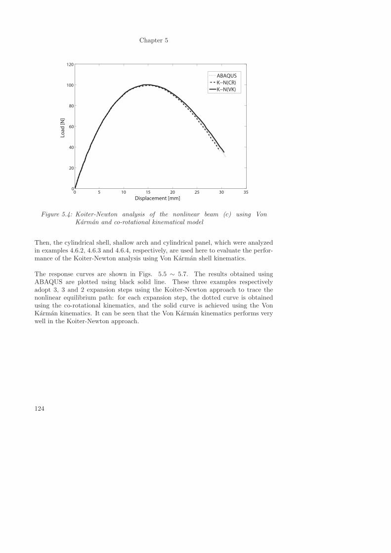
Chapter 5
0 5 10 15 20 25 30 350
20
40
60
80
100
120
Displacement [mm]
Lo
ad
[N
]
ABAQUS
K−N(CR)
K−N(VK)
Figure 5.4: Koiter-Newton analysis of the nonlinear beam (c) using VonKarman and co-rotational kinematical model
Then, the cylindrical shell, shallow arch and cylindrical panel, which were analyzedin examples 4.6.2, 4.6.3 and 4.6.4, respectively, are used here to evaluate the perfor-mance of the Koiter-Newton analysis using Von Karman shell kinematics.
The response curves are shown in Figs. 5.5 ∼ 5.7. The results obtained usingABAQUS are plotted using black solid line. These three examples respectivelyadopt 3, 3 and 2 expansion steps using the Koiter-Newton approach to trace thenonlinear equilibrium path: for each expansion step, the dotted curve is obtainedusing the co-rotational kinematics, and the solid curve is achieved using the VonKarman kinematics. It can be seen that the Von Karman kinematics performs verywell in the Koiter-Newton approach.
124
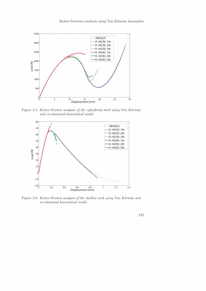
Koiter-Newton’s analysis using Von Karman kinematics
0 5 10 15 20 25 300
500
1000
1500
2000
2500
3000
3500
Displacement [mm]
Lo
ad
[N
]
ABAQUS
K−N(CR): 1th
K−N(CR): 2th
K−N(CR): 3th
K−N(VK): 1th
K−N(VK): 2th
K−N(VK): 3th
Figure 5.5: Koiter-Newton analysis of the cylindrical shell using Von Karmanand co-rotational kinematical model
0 0.2 0.4 0.6 0.8 1 1.2 1.4−20
−10
0
10
20
30
40
50
60
70
80
Displacement [mm]
Lo
ad
[N
]
ABAQUS
K−N(CR): 1th
K−N(CR): 2th
K−N(CR): 3th
K−N(VK): 1th
K−N(VK): 2th
K−N(VK): 3th
Figure 5.6: Koiter-Newton analysis of the shallow arch using Von Karman andco-rotational kinematical model
125
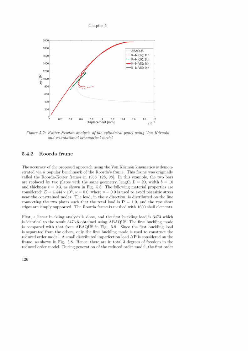
Chapter 5
0 0.2 0.4 0.6 0.8 1 1.2 1.4 1.6 1.8 2
x 10−3
0
200
400
600
800
1000
1200
1400
1600
1800
2000
Displacement [mm]
Lo
ad
[N
]
ABAQUS
K−N(CR): 1th
K−N(CR): 2th
K−N(VK): 1th
K−N(VK): 2th
Figure 5.7: Koiter-Newton analysis of the cylindrical panel using Von Karmanand co-rotational kinematical model
5.4.2 Roorda frame
The accuracy of the proposed approach using the Von Karman kinematics is demon-strated via a popular benchmark of the Roorda’s frame. This frame was originallycalled the Roorda-Koiter frames in 1956 [128, 98]. In this example, the two barsare replaced by two plates with the same geometry, length L = 20, width b = 10and thickness t = 0.3, as shown in Fig. 5.8. The following material properties areconsidered: E = 4.444× 10⁶, ν = 0.0, where ν = 0.0 is used to avoid parasitic stressnear the constrained nodes. The load, in the x direction, is distributed on the lineconnecting the two plates such that the total load is P = 1.0, and the two shortedges are simply supported. The Roorda frame is meshed with 1600 shell elements.
First, a linear buckling analysis is done, and the first buckling load is 3473 whichis identical to the result 3473.6 obtained using ABAQUS. The first buckling modeis compared with that from ABAQUS in Fig. 5.9. Since the first buckling loadis separated from the others, only the first buckling mode is used to construct thereduced order model. A small distributed imperfection load ∆P is considered on theframe, as shown in Fig. 5.8. Hence, there are in total 3 degrees of freedom in thereduced order model. During generation of the reduced order model, the first order
126
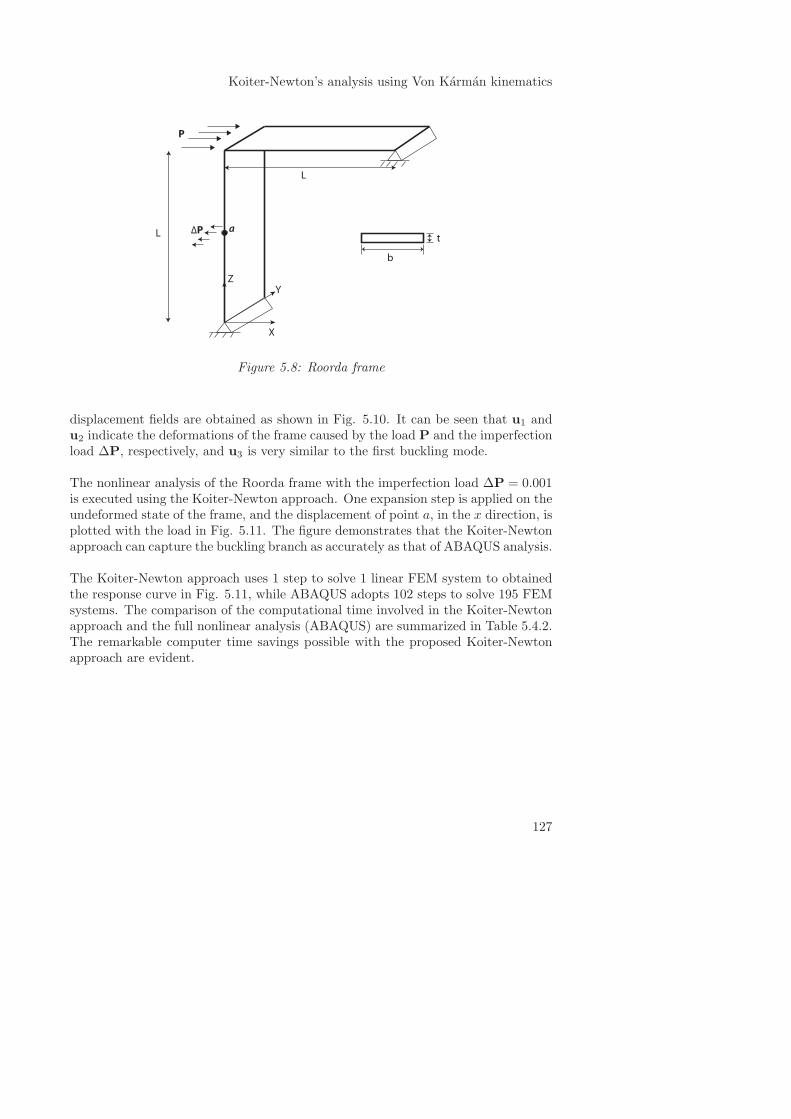
Koiter-Newton’s analysis using Von Karman kinematics
X
YZ
L
L
∆P
P
t
b
a
Figure 5.8: Roorda frame
displacement fields are obtained as shown in Fig. 5.10. It can be seen that u1 andu2 indicate the deformations of the frame caused by the load P and the imperfectionload ∆P, respectively, and u3 is very similar to the first buckling mode.
The nonlinear analysis of the Roorda frame with the imperfection load ∆P = 0.001is executed using the Koiter-Newton approach. One expansion step is applied on theundeformed state of the frame, and the displacement of point a, in the x direction, isplotted with the load in Fig. 5.11. The figure demonstrates that the Koiter-Newtonapproach can capture the buckling branch as accurately as that of ABAQUS analysis.
The Koiter-Newton approach uses 1 step to solve 1 linear FEM system to obtainedthe response curve in Fig. 5.11, while ABAQUS adopts 102 steps to solve 195 FEMsystems. The comparison of the computational time involved in the Koiter-Newtonapproach and the full nonlinear analysis (ABAQUS) are summarized in Table 5.4.2.The remarkable computer time savings possible with the proposed Koiter-Newtonapproach are evident.
127
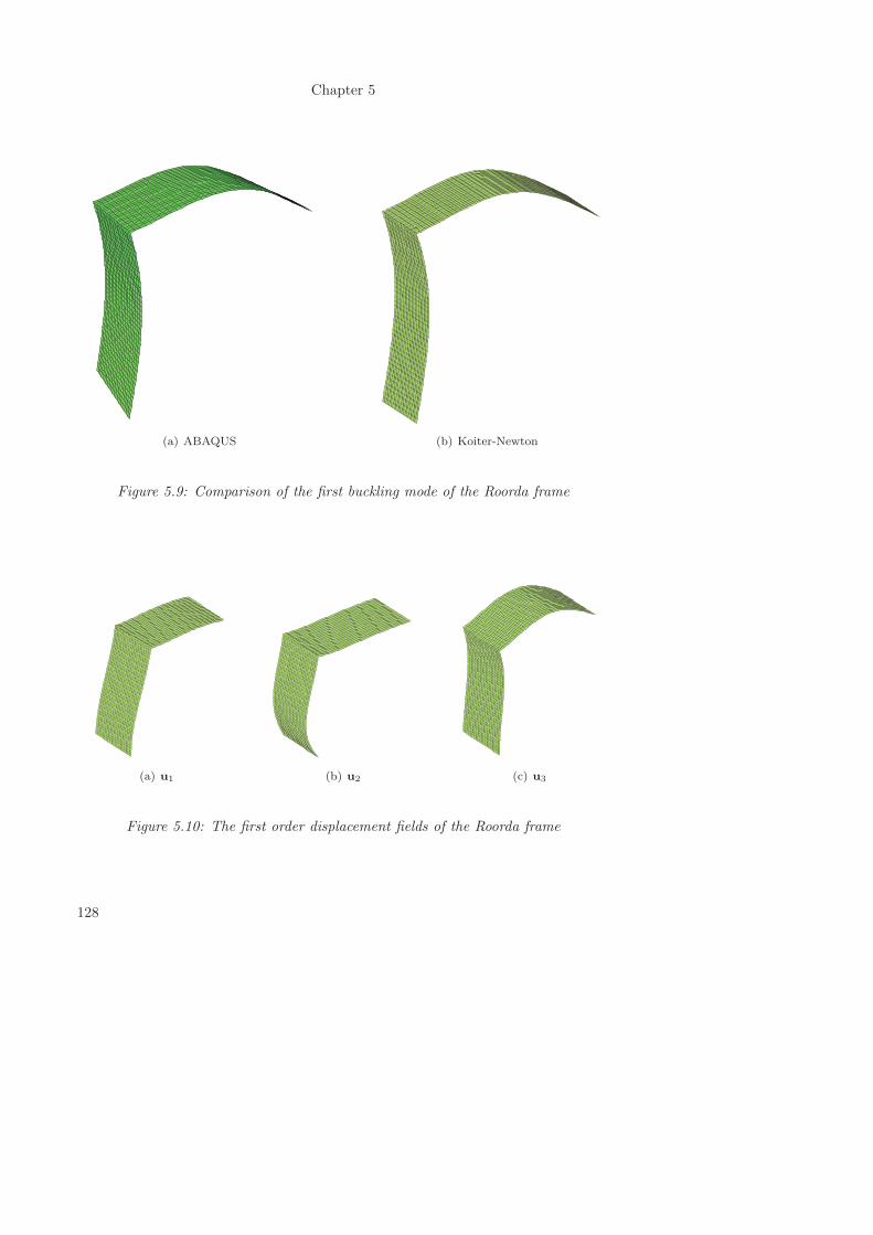
Chapter 5
(a) ABAQUS (b) Koiter-Newton
Figure 5.9: Comparison of the first buckling mode of the Roorda frame
(a) u1 (b) u2 (c) u3
Figure 5.10: The first order displacement fields of the Roorda frame
128
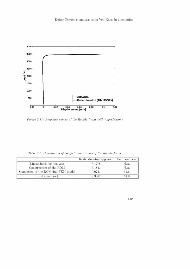
Koiter-Newton’s analysis using Von Karman kinematics
−0.02 0 0.02 0.04 0.06 0.08 0.1 0.120
500
1000
1500
2000
2500
3000
3500
4000
Displacement [mm]
Load
[N]
ABAQUSKoiter−Newton (1th: 3DOFs)
Figure 5.11: Response curves of the Roorda frame with imperfections
Table 5.1: Comparison of computational times of the Roorda frame
Koiter-Newton approach Full nonlinear
Linear buckling analysis 3.1278 N.A.Construction of the ROM 5.1843 N.A.
Simulation of the ROM/full FEM model 0.0241 54.8
Total time (sec) 8.3362 54.8
129
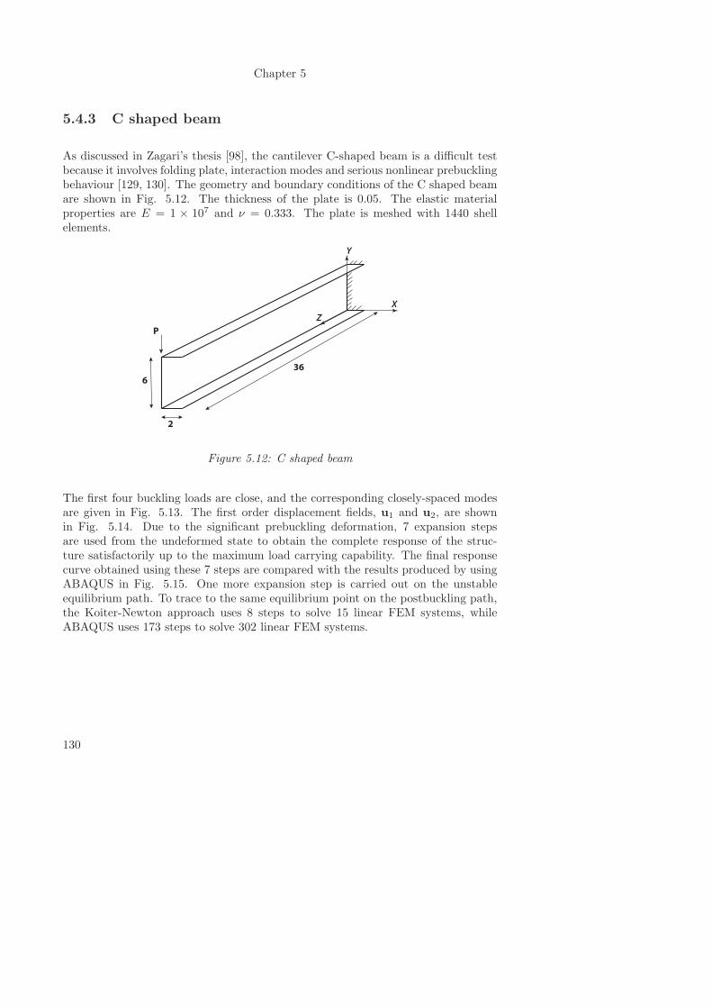
Chapter 5
5.4.3 C shaped beam
As discussed in Zagari’s thesis [98], the cantilever C-shaped beam is a difficult testbecause it involves folding plate, interaction modes and serious nonlinear prebucklingbehaviour [129, 130]. The geometry and boundary conditions of the C shaped beamare shown in Fig. 5.12. The thickness of the plate is 0.05. The elastic materialproperties are E = 1 × 10⁷ and ν = 0.333. The plate is meshed with 1440 shellelements.
6
36
2
X
Y
Z
P
Figure 5.12: C shaped beam
The first four buckling loads are close, and the corresponding closely-spaced modesare given in Fig. 5.13. The first order displacement fields, u1 and u2, are shownin Fig. 5.14. Due to the significant prebuckling deformation, 7 expansion stepsare used from the undeformed state to obtain the complete response of the struc-ture satisfactorily up to the maximum load carrying capability. The final responsecurve obtained using these 7 steps are compared with the results produced by usingABAQUS in Fig. 5.15. One more expansion step is carried out on the unstableequilibrium path. To trace to the same equilibrium point on the postbuckling path,the Koiter-Newton approach uses 8 steps to solve 15 linear FEM systems, whileABAQUS uses 173 steps to solve 302 linear FEM systems.
130
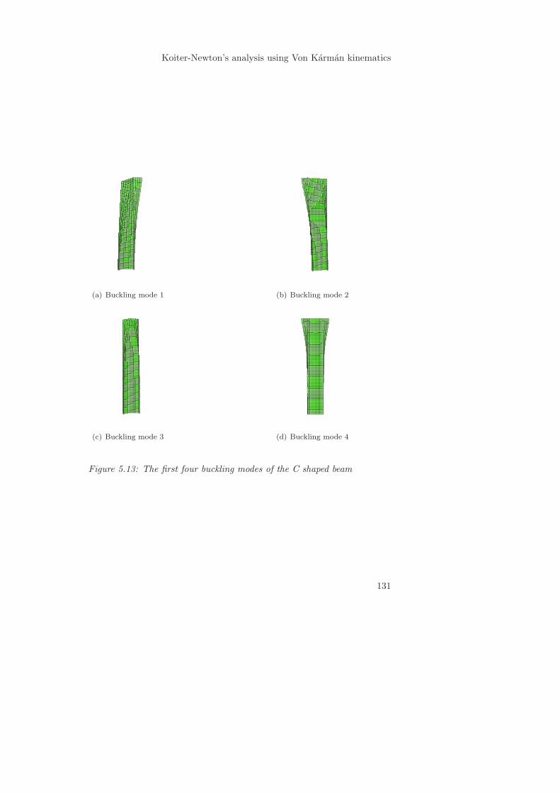
Koiter-Newton’s analysis using Von Karman kinematics
(a) Buckling mode 1 (b) Buckling mode 2
(c) Buckling mode 3 (d) Buckling mode 4
Figure 5.13: The first four buckling modes of the C shaped beam
131
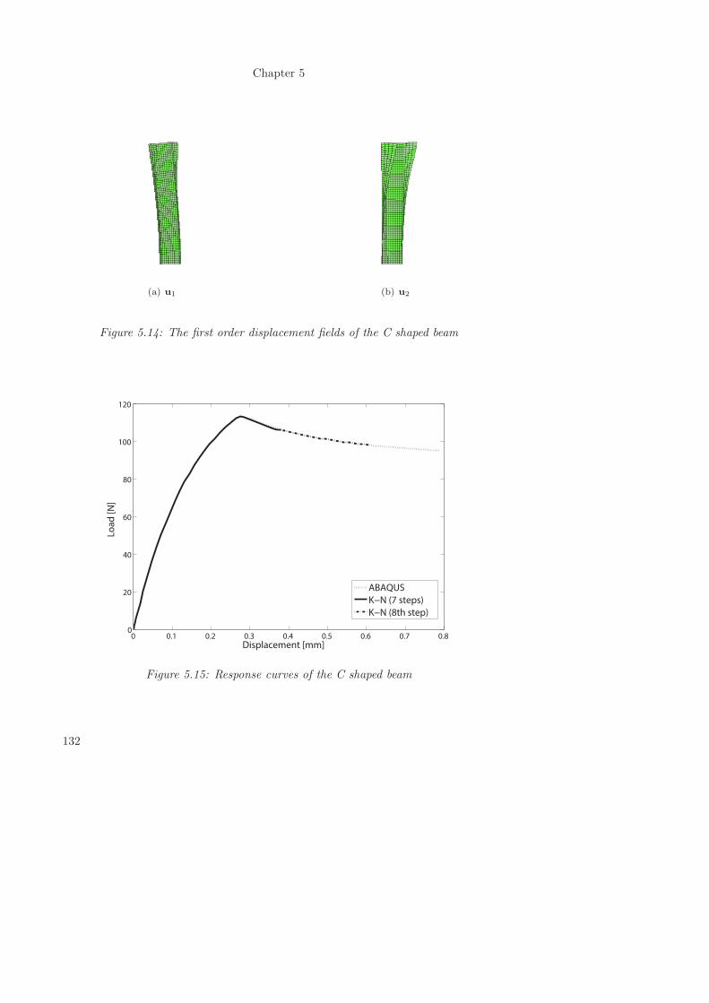
Chapter 5
(a) u1 (b) u2
Figure 5.14: The first order displacement fields of the C shaped beam
0 0.1 0.2 0.3 0.4 0.5 0.6 0.7 0.80
20
40
60
80
100
120
Displacement [mm]
Lo
ad
[N
]
ABAQUS
K−N (7 steps)
K−N (8th step)
Figure 5.15: Response curves of the C shaped beam
132
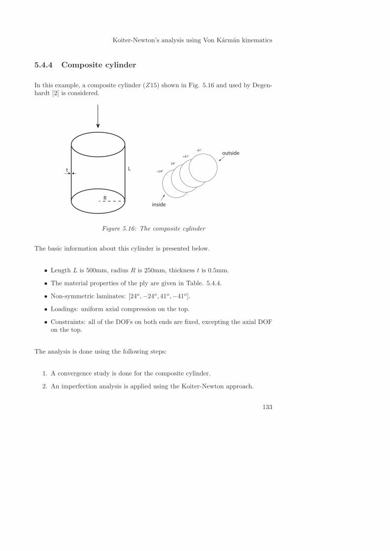
Koiter-Newton’s analysis using Von Karman kinematics
5.4.4 Composite cylinder
In this example, a composite cylinder (Z15) shown in Fig. 5.16 and used by Degen-hardt [2] is considered.
L
R
t
inside
outside
+240
-240
+410
-410
Figure 5.16: The composite cylinder
The basic information about this cylinder is presented below.
• Length L is 500mm, radius R is 250mm, thickness t is 0.5mm.
• The material properties of the ply are given in Table. 5.4.4.
• Non-symmetric laminates: [24o,−24o, 41o,−41o].
• Loadings: uniform axial compression on the top.
• Constraints: all of the DOFs on both ends are fixed, excepting the axial DOFon the top.
The analysis is done using the following steps:
1. A convergence study is done for the composite cylinder.
2. An imperfection analysis is applied using the Koiter-Newton approach.
133
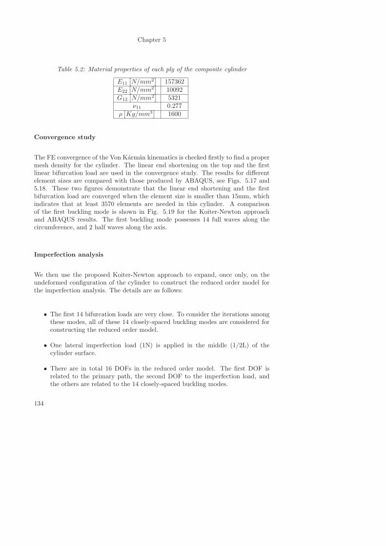
Chapter 5
Table 5.2: Material properties of each ply of the composite cylinder
E11
[N/mm2
]157362
E22
[N/mm2
]10092
G12
[N/mm2
]5321
ν11 0.277
ρ[Kg/mm3
]1600
Convergence study
The FE convergence of the Von Karman kinematics is checked firstly to find a propermesh density for the cylinder. The linear end shortening on the top and the firstlinear bifurcation load are used in the convergence study. The results for differentelement sizes are compared with those produced by ABAQUS, see Figs. 5.17 and5.18. These two figures demonstrate that the linear end shortening and the firstbifurcation load are converged when the element size is smaller than 15mm, whichindicates that at least 3570 elements are needed in this cylinder. A comparisonof the first buckling mode is shown in Fig. 5.19 for the Koiter-Newton approachand ABAQUS results. The first buckling mode possesses 14 full waves along thecircumference, and 2 half waves along the axis.
Imperfection analysis
We then use the proposed Koiter-Newton approach to expand, once only, on theundeformed configuration of the cylinder to construct the reduced order model forthe imperfection analysis. The details are as follows:
• The first 14 bifurcation loads are very close. To consider the iterations amongthese modes, all of these 14 closely-spaced buckling modes are considered forconstructing the reduced order model.
• One lateral imperfection load (1N) is applied in the middle (1/2L) of thecylinder surface.
• There are in total 16 DOFs in the reduced order model. The first DOF isrelated to the primary path, the second DOF to the imperfection load, andthe others are related to the 14 closely-spaced buckling modes.
134
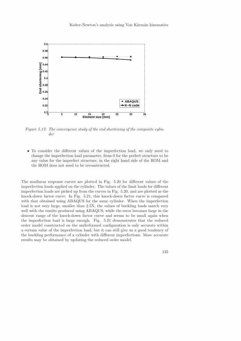
Koiter-Newton’s analysis using Von Karman kinematics
0 5 10 15 20 25 30 350.3
0.32
0.34
0.36
0.38
0.4
0.42
0.44
0.46
0.48
0.5
Element size [mm]
End
sho
rten
ing
[mm
]
ABAQUSK−N code
Figure 5.17: The convergence study of the end shortening of the composite cylin-der
• To consider the different values of the imperfection load, we only need tochange the imperfection load parameter, from 0 for the perfect structure to beany value for the imperfect structure, in the right hand side of the ROM andthe ROM does not need to be reconstructed.
The nonlinear response curves are plotted in Fig. 5.20 for different values of theimperfection loads applied on the cylinder. The values of the limit loads for differentimperfection loads are picked up from the curves in Fig. 5.20, and are plotted as theknock-down factor curve. In Fig. 5.21, this knock-down factor curve is comparedwith that obtained using ABAQUS for the same cylinder. When the imperfectionload is not very large, smaller than 2.5N, the values of buckling loads match verywell with the results produced using ABAQUS, while the error becomes large in thedescent range of the knock-down factor curve and seems to be small again whenthe imperfection load is large enough. Fig. 5.21 demonstrates that the reducedorder model constructed on the underformed configuration is only accurate withina certain value of the imperfection load, but it can still give us a good tendency ofthe buckling performance of a cylinder with different imperfections. More accurateresults may be obtained by updating the reduced order model.
135
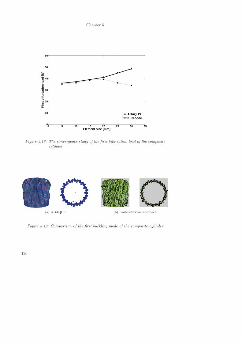
Chapter 5
0 5 10 15 20 25 30 350
10
20
30
40
50
60
Element size [mm]
Firs
t bifu
rcat
ion
load
[N]
ABAQUSK−N code
Figure 5.18: The convergence study of the first bifurcation load of the compositecylinder
(a) ABAQUS (b) Koiter-Newton approach
Figure 5.19: Comparison of the first buckling mode of the composite cylinder
136
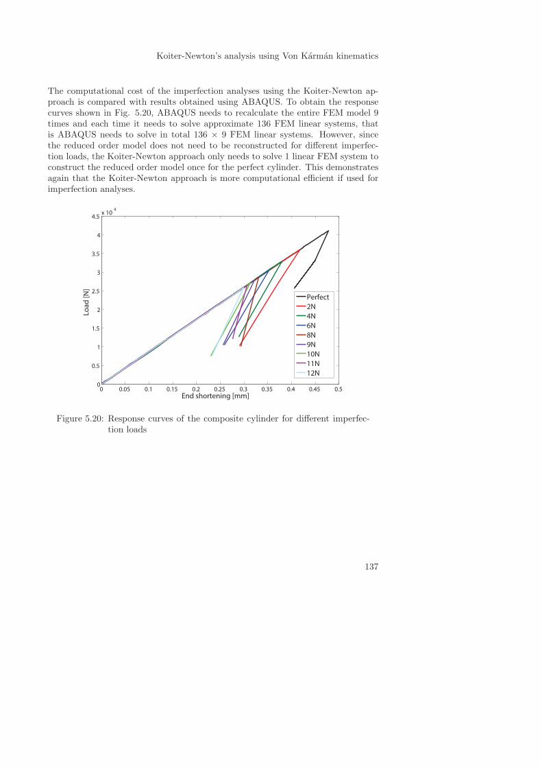
Koiter-Newton’s analysis using Von Karman kinematics
The computational cost of the imperfection analyses using the Koiter-Newton ap-proach is compared with results obtained using ABAQUS. To obtain the responsecurves shown in Fig. 5.20, ABAQUS needs to recalculate the entire FEM model 9times and each time it needs to solve approximate 136 FEM linear systems, thatis ABAQUS needs to solve in total 136 × 9 FEM linear systems. However, sincethe reduced order model does not need to be reconstructed for different imperfec-tion loads, the Koiter-Newton approach only needs to solve 1 linear FEM system toconstruct the reduced order model once for the perfect cylinder. This demonstratesagain that the Koiter-Newton approach is more computational efficient if used forimperfection analyses.
0 0.05 0.1 0.15 0.2 0.25 0.3 0.35 0.4 0.45 0.50
0.5
1
1.5
2
2.5
3
3.5
4
4.5x 10
4
End shortening [mm]
Lo
ad
[N
]
Perfect
2N
4N
6N
8N
9N
10N
11N
12N
Figure 5.20: Response curves of the composite cylinder for different imperfec-tion loads
137
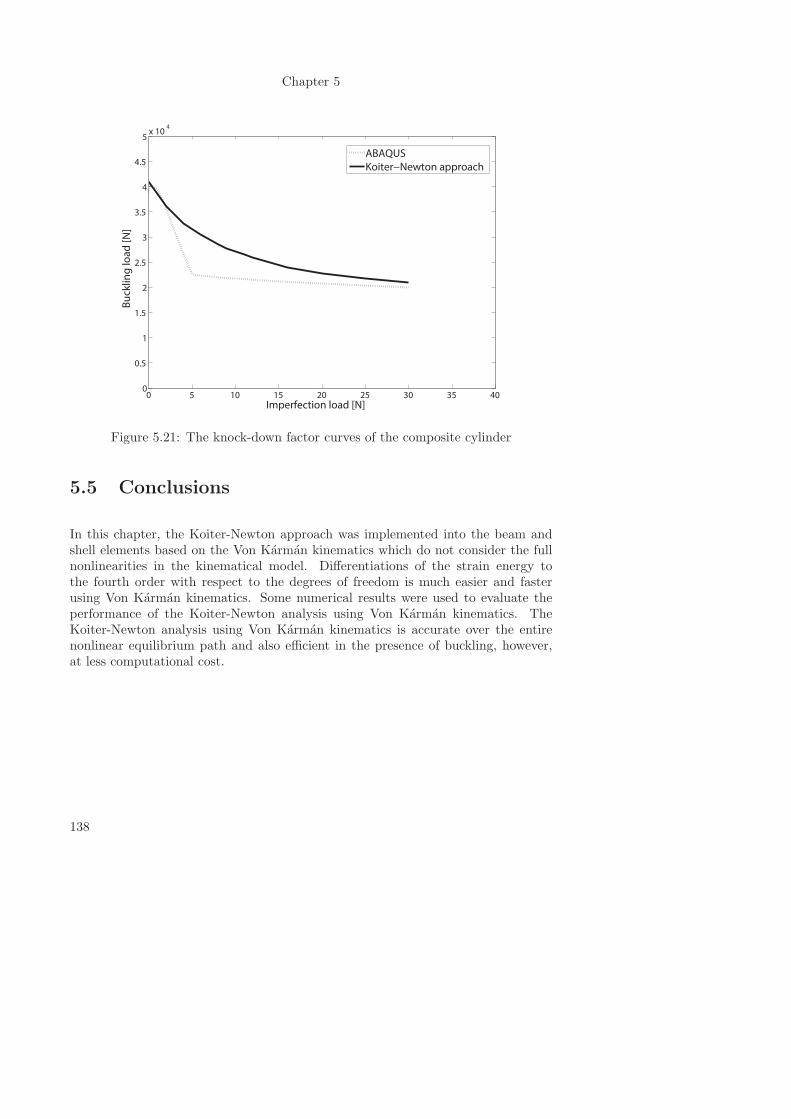
Chapter 5
0 5 10 15 20 25 30 35 400
0.5
1
1.5
2
2.5
3
3.5
4
4.5
5x 10
4
Imperfection load [N]
Bu
ckli
ng
loa
d [
N]
ABAQUS
Koiter−Newton approach
Figure 5.21: The knock-down factor curves of the composite cylinder
5.5 Conclusions
In this chapter, the Koiter-Newton approach was implemented into the beam andshell elements based on the Von Karman kinematics which do not consider the fullnonlinearities in the kinematical model. Differentiations of the strain energy tothe fourth order with respect to the degrees of freedom is much easier and fasterusing Von Karman kinematics. Some numerical results were used to evaluate theperformance of the Koiter-Newton analysis using Von Karman kinematics. TheKoiter-Newton analysis using Von Karman kinematics is accurate over the entirenonlinear equilibrium path and also efficient in the presence of buckling, however,at less computational cost.
138
Chapter 6
Concluding remarks
The nonlinear finite element method is the most frequently-used tool for the analysisof nonlinear response of structures. In spite of improvements in modern comput-ers, a full model nonlinear analysis can still be a computationally expensive task,especially in design optimization. The present research dealt with a finite elementbased perturbation method, the Koiter-Newton approach, for the geometrically non-linear analysis of structures. This new approach combines ideas from Koiter’s initialpost-buckling analysis and Newton arc-length methods to trace the entire nonlinearequilibrium path effectively using the reduced order model while retaining a goodaccuracy of the solution by the corrections.
The thesis is organized as follows. The background, motivation and literature revieware introduced in chapter 1. The new proposed Koiter-Newton approach is presentedin detail in chapter 2. The Koiter-Newton analyses using co-rotational beam andshell kinematics are given in chapters 3 and 4. Then, the Koiter-Newton analysis isalso achieved using Von Karman kinematics in chapter 5. Finally, some concludingremarks are discussed in the rest of this chapter.
6.1 Conclusions
The Koiter-Newton approach based on Koiter’s initial post-buckling theory andNewton arc-length methods are proposed for a class of elastic nonlinear structural
139
Chapter 6
analysis. In this approach Koiter’s asymptotic expansion can be applied from thebeginning, rather than only once at the bifurcation point, by the consideration ofthe primary equilibrium path in the displacement expansion. In the case of bucklingand/or imperfection sensitivity, this approach also works very well due to its use ofKoiter’s theory. (in chapter 2)
The Koiter-Newton approach can trace the entire nonlinear equilibrium path au-tomatically in a step by step manner using an idea taken from Newton arc-lengthmethods. In each expansion step, a reduced order model is constructed at a knownexpansion equilibrium point. Then a path-following technique is adopted to sim-ulate the ROM, and the solution is used as an initial prediction of the responseof the structure. At the same time, the quality of the ROM is assessed based onthe norm of the force residuals obtained using the full finite element model. If theresidual exceeds the accuracy tolerance, it demonstrates that the current ROM hasalready lost accuracy and then the residual force can be driven to zero using thetraditional Newton iterations in a corrector step. Up to this point, a whole stepin the Koiter-Newton approach is finished. In the next step an updated ROM canbe reconstructed at this corrected equilibrium point to reflect changes in structuralstiffness. (in chapter 2)
In the presence of buckling, multiple secondary equilibrium branches may intersectwith the primary path near the bifurcation points. Hence, the selection of theperturbation loads which should excite the secondary branches is very importantin the Koiter-Newton approach. If the expansion point is on the stable part ofthe equilibrium path, an eigenvalue problem based on the tangent stiffness Kt andthe geometric stiffness Kg is solved to obtain the buckling modes which can beused to construct the perturbation loads. This eigenvalue problem is unsolvableonce the expansion point is on the unstable path, due to the non-positive definitionof the tangent stiffness Kt. In this case, in order to capture buckling branchesaccurately, both the modes which are already unstable and the buckling modes whichare prone to further instability must be included in the calculation to obtain theperturbation loads. An eigenvalue problem based on the material stiffness and thestress stiffness can be adopted to obtain the already unstable modes. For the bucklingprone modes the eigenvalue problem, based on the tangent stiffness and the geometricstiffness required to make it, is restricted to stable modes rendering it solvable. Afterobtaining all the necessary modes, Koiter’s asymptotic expansion can be carried outat any point to trace the entire nonlinear equilibrium path automatically, includingthe unstable equilibrium path. (in chapter 2)
The Koiter-Newton approach significantly improves the efficiency of nonlinear staticfinite element analysis. In each step, we only need to factor the augmented FEstiffness matrix once to construct the reduced order model, and do several Newton
140
Concluding remarks
iterations in the full finite element model to correct the results. The fairly large stepsizes are possible because of the better nonlinear prediction provided by the ROMcompared to linear predictors used in Newton arc-length methods. (in chapter 2)
The proposed technique is based on Koiter’s theory and requires up to the third or-der derivatives of the element load vectors with respect to degrees of freedom whichis two orders more than the first order what is traditionally needed for Newton’smethod. To facilitate differentiation and also consider the full nonlinear kinemat-ics, nonlinear elements based on the element independent co-rotational frame areapplied. The implementation of the Koiter-Newton approach into the co-rotational(CR) beam kinematics is first presented. Then, the Koiter-Newton analysis is ex-tended with the co-rotational shell kinematics in greater detail. During the FEimplementation, the finite rotation theory is used and the descriptions of the pro-posed three configurations are introduced. The material coordinate system is alsodefined for the composite shell. The automatic differentiation is adopted to find thederivatives of the co-rotational frame with respect to element degrees of freedom inMatlab codes. (in chapters 3 and 4)
Von Karman kinematics, which ignore some nonlinear terms in the Green’s stain-displacement relations, do not consider the full nonlinear kinematics. In the caseswhere the nonlinear in-plane rotations of the structure can be neglected while therotations of the normals to the mid-surface are finitely large, Von Karman kinemat-ics are a good choice for the FE implementation due to the higher efficiency andacceptable accuracy. Hence, the Koiter-Newton approach is also implemented inthe beam and shell elements based on Von Karman kinematics, and the equilibriumequations of a third order form for Von Karman kinematics are achieved. (in chapter5)
Various numerical examples of beam and shell models are presented and used toevaluate the performance of the Koiter-Newton approach. The results are comparedwith results for the same problem obtained using ABAQUS based on a full nonlinearanalysis, and some conclusions about the application of this new proposed approachare summarized as follows: (in chapter 3, 4 and 5)
• If the prebuckling nonlinearity or load distribution is mild, a single step isenough to obtain the complete response of the structure satisfactorily up tothe maximum load carrying capability, either by buckling or a limit pointinstability. While more steps are needed for structures that show significantprebuckling deformation.
• The unstable equilibrium path can be obtained using the expansion steps onthe unstable equilibrium points. The use of the already unstable modes and
141
Chapter 6
the buckling prone modes to construct the reduced oder model is feasibleand efficient. In this way, the Koiter-Newton approach can trace the entirenonlinear equilibrium path of structures.
• For the cases where one or more bifurcation points lie before the limit point, thetraditional nonlinear path-following analysis (ABAQUS) usually misses thesebifurcation points and overestimates the load carrying capability of a structure.While, the Koiter-Newton approach can capture these possible bifurcationbranches at much less computational costs, using an eigenvalue check for thetangent matrix of the reduced order model.
• The Koiter-Newton analysis using Von Karman kinematics shows nearly thesame accuracy compared with that of co-rotational kinematics in some exam-ples. The efficiency advantages of using Von Karman kinematics is much moreobvious for structures which need a very fine mesh.
• The number of the FEM systems of equations that need to be solved us-ing the Koiter-Newton approach is compared with the number required usingABAQUS, with the same number of elements and nodes. To reach the sameequilibrium point on the nonlinear equilibrium path, the Koiter-Newton ap-proach is much computationally cheaper than ABAQUS as it requires fewermatrix factorizations and it uses a larger step size. In the imperfection analysis,the Koiter-Newton approach requires only a small fraction of the first analysistime, since the reduced order model does not need to be reconstructed for adifferent imperfection. The advantage of the proposed approach on the com-putational cost is much more obvious in imperfection analyses of a structure.
6.2 Recommendations
The following recommendations for future work are proposed.
1. In the current research, we only considered the geometric nonlinearity, in real-ity, the material may be in the plasticity range when the deformation is verylarge. Hence, material nonlinearity should also be taken into account in theKoiter-Newton approach for the buckling analysis.
2. We use the initial deformations caused by independent imperfection loads tomodel the geometric imperfections in the present work. Actually, the realisticgeometric imperfections obtained by measurements can also be implementedinto the proposed approach. In the reduced order model, the effect of geometric
142
Concluding remarks
imperfections is represented as a load term in the right hand side of the reducedorder model. Hence, for different imperfections the reduced order model needsnot be reconstructed, and the high computational efficiency in imperfectionanalyses also exists with the consideration of geometric imperfections.
3. The norm flow algorithm is used in the present work to simulate the nonlinearreduced order model. However, the path-following techniques which are basedon the Newton arc-length method will meet difficulties in the case when thereare lots of closely-spaced buckling modes around the first buckling load. Thereduced order model constructed in the proposed Koiter-Newton approachis actually a system of polynomial equations, hence we can try to use thepolynomial solver which is very numerically stable to obtain all the roots ofthe reduced order model and then plot the equilibrium path according to thesepoints.
4. Parallel computation can be introduced into the Koiter-Newton approach toimprove the efficiency of the algorithm. For example, we can divide the cylin-der into 3 or 4 parts to construct the reduced order model of each part simul-taneously, and then assemble them to get a total reduced order model for awhole cylinder. This may further improve the computational efficiency of theKoiter-Newton approach.
143

Appendix
144
Appendix A
Linear shell element in a
co-rotational frame
In a co-rotational frame, any type of linear shell elements can be used, since the geo-metric nonlinearity is taken into account by the derivatives of the local co-rotationalframe with respect to the global degrees of freedom. For the shell element, weadopt the four-node quadrilateral element obtained by assembling four triangularflat elements and merging the middle node. In this appendix, an introduction ofthe triangular flat element is presented, and then the construction of the four-nodequadrilateral element is introduced.
Triangular flat shell element with the drilling DOF
A triangular three-node flat shell element with six degrees of freedom per node (threetranslations and three rotations) is presented in this section. This element has beenimplemented by Tiso and Tanvir [7, 8] in the Matlab environment to achieve Koiter’sreduction methods, hence we will simply review the basics of this element followingTiso’s thesis in this section.
This element seems to be the combination of a membrane element and a bendingelement. Figure A.1 shows the combination of the degrees of freedom for the mem-brane and bending part. The drilling degree of freedom θz is also introduced in
145
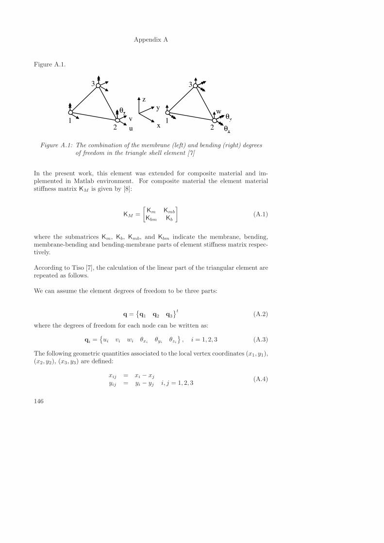
Appendix A
Figure A.1.
Figure A.1: The combination of the membrane (left) and bending (right) degreesof freedom in the triangle shell element [7]
In the present work, this element was extended for composite material and im-plemented in Matlab environment. For composite material the element materialstiffness matrix KM is given by [8]:
KM =
[Km Kmb
Kbm Kb
](A.1)
where the submatrices Km, Kb, Kmb, and Kbm indicate the membrane, bending,membrane-bending and bending-membrane parts of element stiffness matrix respec-tively.
According to Tiso [7], the calculation of the linear part of the triangular element arerepeated as follows.
We can assume the element degrees of freedom to be three parts:
q ={q1 q2 q3
}t(A.2)
where the degrees of freedom for each node can be written as:
qi ={ui vi wi θxi
θyiθzi
}, i = 1, 2, 3 (A.3)
The following geometric quantities associated to the local vertex coordinates (x1, y1),(x2, y2), (x3, y3) are defined:
xij = xi − xjyij = yi − yj i, j = 1, 2, 3
(A.4)
146
Linear shell element in a co-rotational frame
According to the geometric quantities, the element area A can be calculated as:
A =y21x13 − x21y13
2(A.5)
A triangular coordinate system (ζ1, ζ2, ζ3) is used, where the following relation holds:
ζ1 + ζ2 + ζ3 = 1 (A.6)
The isoparametric coordinates can be linked to the cartesian coordinates throughthe following transformation, given by:
1xy
=
1 1 1x1 x2 x3y1 y2 y3
ζ1ζ2ζ3
(A.7)
From Eq. (A.7) the link between the partial derivatives in the cartesian coordinatesand those in the isoparametric coordinates can be obtained as:
∂
∂x
∂
∂y
=
Tx
Ty
∂
∂ζ1
∂
∂ζ2
(A.8)
where the transform matrix Tx and Ty is defined as follows:
Tx =1
2A
[y23 y31 y12
](A.9)
Ty =1
2A
[x32 x13 x21
](A.10)
The in-plane strain components εεε of the strain model can be expressed as:
εεε =[ǫx ǫy ǫxy
]T(A.11)
The B matrix which gives the relationship of the in-plane strain and degrees offreedom is formed according to the formulation by Felippa [131]. The final result islisted here:
B = [B1 B2 B3] (A.12)
where
B1 =
y23 0 x32
0 x32[0]3×3
y23
y23 (y13 − y21)
6
x32 (x31 − x12)
6
(x31y13 − x12y21)
3
(A.13)
147
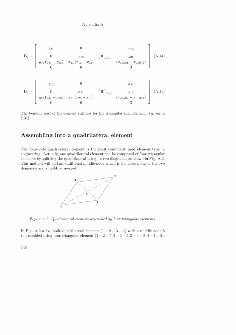
Appendix A
B2 =
y31 0 x13
0 x13[0]3×3
y31
y31 (y21 − y32)
6
x13 (x12 − x23)
6
(x12y21 − x23y32)
3
(A.14)
B3 =
y12 0 x21
0 x21[0]3×3
y12
y12 (y32 − y13)
6
x21 (x23 − x31)
6
(x23y32 − x31y13)
3
(A.15)
The bending part of the element stiffness for the triangular shell element is given in[131].
Assembling into a quadrilateral element
The four-node quadrilateral element is the most commonly used element type inengineering. Actually, one quadrilateral element can be composed of four triangularelements by splitting the quadrilateral using its two diagonals, as shown in Fig. A.2.This method will add an additional middle node which is the cross point of the twodiagonals and should be merged.
1
2
3
4
5
Figure A.2: Quadrilateral element assembled by four triangular elements.
In Fig. A.2 a five-node quadrilateral element (1 − 2 − 3 − 4) with a middle node 5is assembled using four triangular element (1− 2− 5, 2− 3− 5, 3− 4− 5, 4− 1− 5).
148
Linear shell element in a co-rotational frame
The 18× 18 linear stiffness matrices of these four triangular elements are calculatedand then be assembled into a 30 × 30 total stiffness matrix K. K can be split intofour submatrices according to the additional node 5, given by:
K =
[K24×24 K24×6
K6×24 K6×6
](A.16)
where the submatrices K24×24 and K6×6 are relative to nodes 1, 2, 3, 4 and node 5respectively, and submatrices K24×6 and K6×24 indicate the interaction items.
Then the corresponding equilibrium equations can be written in the form of matrix:
[K24×24 K24×6
K6×24 K6×6
]{u
u5
}=
{p
p5
}(A.17)
where the displacement and load consist of two parts, and the part without thesubscript is related to the nodes 1, 2, 3, 4 and the part with the subscript is relatedto node 5. Our aim is to merge the contribution of the middle node 5 and find outthe relation of the displacement u and load p which are only related to the fournodes 1, 2, 3, 4.
Since there is no load applying on the node 5, the fact p5 = 0 always exists and wecan use u to express u5 from the second equation of (A.17), leading to:
u5 = −K6×24u
K6×6(A.18)
If substituting Eq. (A.18) into the first equation of Eq. (A.17), the relation betweenu and p, which is just the stiffness matrix Kquad of the four-node quadrilateralelement, can be obtained by:
(K24×24 −
K24×6K6×24
K6×6
)u = p (A.19)
where
Kquad =
(K24×24 −
K24×6K6×24
K6×6
)(A.20)
149

150
Bibliography
[1] B. Vermeulen and M.J.L. van Tooren. Design case study for a comparativeperformance analysis of aerospace materials. Materials Design, 27(1):10–20,2006.
[2] R. Degenhardt, A. Kling, A. Bethge, J. Orf, L. Karger, R. Zimmermann,K. Rohwer, and A. Calvi. Investigations on imperfection sensitivity and de-duction of improved knock-down factors for unstiffened cfrp cylindrical shells.Composite Structures, 92(8):1939–1946, 2010.
[3] M.W. Hilburger and J.H. Starnes Jr. Buckling behavior of compression-loadedcomposite cylindrical shells with reinforced cutouts. International Journal ofNon-Linear Mechanics, 40(7):1005–1021, 2005.
[4] H. Ullah. Buckling of thin-walled cylindrical shells under axial compression. In-ternational Journal for Numerical Methods in Engineering, 79(11):1332–1353,2009.
[5] G.A. Maugin and A.V. Metrikine. Mechanics of Generalized Continua.Springer, 2010.
[6] C.A. Felippa and K.C. Park. Direct time integration methods in nonlinearstructural dynamics. In International Conference on Finite Elements in Non-linear Mechanics, 1978.
[7] P. Tiso. Finite Element Based Reduction Methods for Static and DynamicAnalysis of Thin-Walled Structures. PhD thesis, Delft University of Technol-ogy, 2006.
[8] T. Rahman. A Perturbation Approach for Geometrically Nonlinear StructuralAnalysis Using a General Purpose Finite Element Code. PhD thesis, DelftUniversity of Technology, 2009.
151
[9] K. Liang, M. Abdalla, Z. Gurdal, and Q. Sun. A koiter-newton approach fornonlinear structural analysis. In 3rd Aircraft Structural Design conference,Delft, the Netherlands, 2012.
[10] Valery V. Vasiliev. Advanced Mechanics of Composite Materials (Second Edi-tion): Chapter 8 - Optimal Composite Structures. Elsevier Ltd, 2007.
[11] A. Hirahara, R. Hino, F. Yoshida, and V.V. Toropov. Numerical optimizationof sheet metal forming process using new fracture criterion. InternationalJournal of Modern Physics B, 22:5692–5698, 2008.
[12] H. Saffari, M.J. Fadaee, M. ASCE, and R. Tabatabaei. Nonlinear analysisof space trusses using modified normal flow algorithm. Journal of StructuralEngineering, 134(6):998–1005, 2008.
[13] E. Ramm. Strategies for tracing the nonlinear response near limit points. In”Nonlinear finite element analysis in structural mechanics.” Proceedings of theEurope - US Workshop, Germany, July 28-31, Springer-Verlag Berlin, pages63–89, 1981.
[14] D.A. Pecknold, J. Ghaboussi, and T. J. Healey. snap-through and bifurcationin a simple structure. Journal of Engineering Mechanics, 111(7):909–922, 1985.
[15] D.S. Jagannathan, P. Christiano, and H.I. Epstein. Nonlinear analysis of retic-ulated space trusses. J. Struct. Div., 101(12):2641–2658, 1975.
[16] R. Levy and W.R. Spillers. Analysis of geometrically nonlinear structures. InProceedings of the 2nd Ed., Kluwer, Dordrecht, The Netherlands., 2003.
[17] M. Papadrakakis. Inelastic post-buckling analysis of trusses. Journal of Struc-tural Engineering, 109(9):2129–2147, 1983.
[18] G.E. Blandford. Large deformation analysis of inelastic space truss structures.Journal of Structural Engineering, 122(4):407–415, 1996.
[19] S.A. Ragon, Z. Gurdal, and L.T. Watson. A comparison of three algorithmsfor tracing nonlinear equilibrium paths of structural systems. InternationalJournal of Solids Structures, 139:689–698, 2002.
[20] W.E. Haisler and J.A. Stricklin. Development and evaluation of solution pro-cedures for geometrically nonlinear analysis. AIAA Journal, 10(3):164–172,1996.
[21] E. Riks. An incremental approach to the solution of snapping and bucklingproblems. International Journal of Solids and Structures, 15:524–551, 1979.
152
Bibliography
[22] E. Riks. Buckling analysis of elastic structures: A computational approach.Advances in Applied Mechanics, 34:1–76, 1997.
[23] G.A. Wempner. Discrete approximation related to nonlinear theories of solids.International Journal of Solids and Structures, 17:1581–1599, 1971.
[24] M.A. Crisfield. A fast incremental/iterative solution procedure that handlessnap-through. Computers & Structures, 13:55–62, 1981.
[25] B.W.R. Forde and S.F. Stiemer. Improved arc-length orthogonality methodsfor nonlinear finite element analysis. Computers & Structures, 27(5):625–630,1987.
[26] S.N. Al-Rasby. Solution techniques in nonlinear structural analysis. Computers& Structures, 40(4):985–993, 1991.
[27] M. Bashir-Ahmad and S. Xiao-zu. Arc-length technique for nonlinear finiteelement analysis. J. Zhejiang Univ., 5(5):618–628, 2004.
[28] K. Georg. Numerical integration of the davidenko equation. In Lecture Notesin Math. Springer, Berlin, 1981.
[29] L.T. Watson, M. Sosonkina, R.C. Melville, A.P. Morgan, and H.F. Walker.Algorithm 777: Hompack90: A suite of fortran 90 codes for globally con-vergent homotopy algorithms. ACM Transactions on Mathematical Software,23(4):514–549, 1997.
[30] I. Fried. Orthogonal trajectory accession to the nonlinear equilibrium curve.Computer Methods in Applied Mechanics and Engineering, 47:283–298, 1984.
[31] L.T. Watson, S.C. Billups, and A.P. Morgan. Algorithm 652: Hompack: Asuite of codes for globally convergent homotopy algorithms. ACM Transactionson Mathematical Software, 13(3):281–310, 1987.
[32] J.F. Besseling. Nonlinear analysis of structures by the finite element method asa supplement to a linear analysis. Comp. Meth. Appl. Mech. Engng, 3(2):173–194, 1974.
[33] B.O. Almroth, P. Stern, and F.A. Brogan. Automatic choice of global shapefunctions in structural analysis. AIAA Journal, 16(5):525–528, 1978.
[34] D.A. Nagy. Modal representation of geometrically nonlinear behavior by thefinite element method. Composite Structures, 10(4):683–688, 1979.
[35] A.K. Noor and J.M. Peters. Reduced basis technique for nonlinear analysis ofstructures. AIAA Journal, 18:455–462, 1980.
153
[36] A.K. Noor, C.M. Andersen, and J.M. Peters. Global-local approach for non-linear shell analysis. In Proc. 7th ASCE Conf. on Electronic Computation,Washington University, St. Louis, Missouri, August 6-8, pages 634–657, 1979.
[37] A.K. Noor. Recent advances in reduction methods for nonlinear problems.Computers & Structures, 13(1-3):31–44, 19801.
[38] D.A. Nagy and M. Konig. Geometrically nonlinear finite element behaviourusing buckling mode superposition. Computer Methods in Applied Mechanicsand Engineering, 19:447–484, 1979.
[39] B.O. Almroth, P. Stern, and F-A. Brogan. Automatic choice of globai shapefunctions in structural analysis. AIAA Journal, 16(5):525–528, 1978.
[40] A.S.L. Chan and KM. Hsiao. Nonlinear analysis using a reduced number ofvariables. Computer Methods in Applied Mechanics and Engineering, 52:899–913, 1985.
[41] B. Cochelin. A path-following technique via an asymptotic-numerical method.Computers & Structures, 53(5):1181–1192, 1994.
[42] B. Cochelin, N. Damil, and M. Potier-Ferry. Asymptotic-numerical methodsand pade approximants for non-linear elastic structures. International Journalfor Numerical Methods in Engineering, 37:1187–1213, 1994.
[43] W.T. Koiter. On the stability of the elastic equilibrium. PhD thesis, DelftUniversity of Technology, 1945.
[44] J.M.T. Thompson and A.C. Walker. The nonlinear perturbation analysis ofdiscrete structural systems. International Journal of Solids and Structures,4:151–168, 1968.
[45] R.H. Gallagher. Perburbation procedures in nonlinear finite element structuralanalysis. In Conf on Comp. Method in Nonlinear Mech., Austin, Texas, pages634–657, 1974.
[46] E. Riks. Some computational aspect of the stability analysis of nonlinearstructures. Computer Methods in Applied Mechanics and Engineering, 47:219–259, 1984.
[47] M. Jamal, H. Elasmar, and B. Braikat. Bifurcation indicators. Acta Mechanica,139:129–142, 2000.
[48] N. Damil and M. Potier-Ferry. A new method to compute perturbed bifurca-tions: application to the buckling of imperfect elastic structures. InternationalJournal of Engineering Science, 9:943–957, 1990.
154
Bibliography
[49] B. Cochelin, N. Damil, and M. Potier-Ferry. Asymptotic-numerical methodsand pade approximants for nonlinear elastic structures. International Journalfor Numerical Methods in Engineering, 37(7):1187–1213, 1994.
[50] L. Azrar, B. Cochelin, N. Damil, and M. Potier-Ferry. An asymptoticnumericalmethod to compute the postbuckling behaviour of elastic plates and shells.International Journal for Numerical Methods in Engineering, 36:1251–1277,1993.
[51] E.H. Boutyour, H. Zahrouni, M. Potier-Ferry, and M. Boudi. Bifurcationpoints and bifurcated branches by an asymptotic numerical method and padeapproximants. International Journal for Numerical Methods in Engineering,60(12):1987–2012, 2004.
[52] S. Lopez. An effective parametrization for asymptotic extrapolations. Com-puter Methods in Applied Mechanics and Engineering, 189(1):297–311, 2000.
[53] H. Mottaqui, B. Braikat, and N. Damil. Discussion about parameterizationin the asymptotic numerical method: Application to nonlinear elastic shells.Computer Methods in Applied Mechanics and Engineering, 199:1701–1709,2010.
[54] J.C. Amazigo, B. Budiansky, and G.F. Carrier. Asymptotic analysis of thebuckling of imperfect columns on nonlinear elastic foundations. InternationalJournal of Solids Structures, 6:1341–1356, 1970.
[55] B. Budiansky. Theory of buckling and postbuckling behavior of elastic struc-tures. Advances in Applied Mechanics, 14:1–65, 1974.
[56] G.A. Cohen. Effect of a nonlinear prebuckling state on the postbuckling behav-ior and imperfection sensitivity of elastic structures. AIAA Journal, 6:1616–1619, 1968.
[57] J.R. Fitch. The buckling and postbukling behavior of spherical caps underconcentrated loads. International Journal of Solids and Structures, 4:421–446,1968.
[58] N. Rizzi and A. Tatone. Symbolic manipulation in buckling and postbucklinganalysis. Computers & Structures, 21:691–700, 1985.
[59] D. Hui and I.H.Y. Du. Initial postbuckling behavior of imperfect, antisym-metric crossply cylindrical shells under torsion. Journal of Applied Mechanics,54:174–180, 1987.
[60] J. Arbocz and J.M.A.M. Hol. Koiters stability theory in a computer-aidedengineering (cae) environment. International Journal of Solids Structures,26:945–975, 1990.
155
[61] R.H. Gallagher. Perturbation procedures in nonlinear finite element structuralanalysis, in computational mechanics. In Lecture Notes in Mathematics. Vol.461, Springer Verlag, Berlin, 1975.
[62] S.S. Antman. Bifurcation problems in non-linearly elastic structures. AcademicPress, 1977.
[63] U. Eckstein, R.K. Jurcke, and W.B. Krtzig. Imperfection sensitivity of elasticstructures a numerical postbuckling approach. In In 8th International Con-ference on Structural Mechanics in Reactor Technology, Brussels, Belgium,August, pages 634–657, 1985.
[64] C. Pacoste and A. Eriksson. Beam elements in instability problems. ComputerMethods in Applied Mechanics and Engineering, 144:163–197, 1997.
[65] B. Wu and Z. Wang. A perturbation method for the determination of thebuckling strength of imperfection-sensitive structures. Computer Methods inApplied Mechanics and Engineering, 145:203–215, 1997.
[66] B. Geier. A method to compute koiters b-factor of anisotropic panels. Inter-national Journal of Non-Linear Mechanics, 37:699–707, 2002.
[67] G. Garcea, A. Madeo, G. Zagari, and R. Casciaro. Asymptotic postbucklingfem analysis using co-rotational formulation. International Journal of Solidsand Structures, 46:377–397, 2009.
[68] J.F. Olesen and E. Byskov. Accurate determination of asymptotic postbucklingstresses by the finite element method. Computers & Structures, 15:157–163,1982.
[69] E. Byskov. Smooth postbuckling stresses by a modified finite element method.International Journal for Numerical Methods in Engineering, 28:2877–2888,1989.
[70] P.N. Poulsen and L. Damkilde. Direct determination of asymptotic structuralpostbuckling behavior by the finite element method. International Journal forNumerical Methods in Engineering, 42:685–702, 1998.
[71] R.T. Haftka, R.H. Mallett, and W. Nachbar. Adaption of koiter’s methodto finite element analysis of snap-through buckling behavior. InternationalJournal of Solids and Structures, 7:1427–1445, 1971.
[72] E.G. Carnoy. Asymptotic study of the elastic postbuckling behavior of struc-tures by the finite element method. Computer Methods in Applied Mechanicsand Engineering, 29:147–173, 1981.
156
Bibliography
[73] G. Salerno, R. Casciaro, and A.D. Lanzo. Finite element asymptotic analysisof slender elastic structures: A simple approach. International Journal forNumerical Methods in Engineering, 35:1397–1426, 1992.
[74] W.T. Koiter and G.D.C. Kuiken. The interaction between local buckling andoverall buckling on the behavior of built-up columns. In Technical ReportWTHD-23, Delft University of Technology, Delft, The Netherlands, 1971.
[75] W.T. Koiter. General theory of mode interaction in stiffened plate and shellstructures. In Technical Report WTHD-91, Delft University of Technology,Delft, The Netherlands, 1976.
[76] E. Byskov and J.W. Hutchinson. Mode interaction in axially stiffened cylin-drical shells. AIAA Journal, 15:941–948, 1977.
[77] R. Peek and M. Kheyrkhahan. Postbuckling behavior and imperfection sensi-tivity of elastic structures by the lyapunov-schmidt-koiter approach. ComputerMethods in Applied Mechanics and Engineering, 108:261–279, 1993.
[78] G. Salerno and R. Casciaro. Mode jumping and attractive paths in multi-modeelastic buckling. International Journal for Numerical Methods in Engineering,40:833–861, 1997.
[79] A.D. Lanzo and G. Garceai. Koiter’s analysis of thin-walled structures bya finite element approach. International Journal for Numerical Methods inEngineering, 39:3007–3031, 1996.
[80] G. Garcea, R. Casciaro, G. Attanasio, and F. Giordano. Perturbation approachto elastic post-buckling analysis. Computers & Structures, 66:585–595, 1998.
[81] G. Garcea. Mixed formulation in koiter analysis of thin-walled beams. Com-puters & Structures, 190:3369–3399, 2001.
[82] A.D. Lanzo, G. Garcea, and R. Casciaro. Asymptotic post-buckling analysis ofrectangular plates by hc finite elements. International Journal for NumericalMethods in Engineering, 38:2325–2345, 1995.
[83] M. Aristodemo. A high-continuity finite element method for two-dimensionalelastic problems. Computers & Structures, 21:987–993, 1985.
[84] D. Ho. Buckling load of non-linear systems with multiple eigenvalues. Inter-national Journal of Solids Structures, 10:1315–1330, 1974.
[85] W.T. Koiter. Current trend in the theory of buckling. In In Buckling ofstructures, Proc. IUTAM Symp., Springer, Berlin, pages 1–13, 1976.
157
[86] A. Bilotta, A.D. Lanzo, and R. Casciaro. A finite element model for thekoiter nonlinear analysis of composite thin-walled structures. In In CongressECCOMAS 2000, Barcellona, 2000.
[87] G. Garcea, G.A. Trunfio, and R. Casicaro. Path-following analysis of thin-walled structures and comparison with asymptotic post-critical solutions. In-ternational Journal for Numerical Methods in Engineering, 55:73–100, 2002.
[88] C.M. Menken, G.M.A. Schreppers, W.J. Groot, and R. Petterson. Analyzingbuckling mode interactions in elastic structures using an asymptotic approach;theory and experiment. Computers & Structures, 64:473–480, 1997.
[89] C.M. Menken, R. Couhia, and W.J. Groot. An investigation into non-linearinteraction between buckling modes. Thin-walled structures, 19:129–145, 1994.
[90] G.M. van Erp and C.M. Menken. Initial post-buckling analysis with thefinitestrip method. Computers & Structures, 40(5):1193–1201, 1991.
[91] C.M. Menken and G.M. van Erp. The spline finite-strip method in the bucklinganalyses of thin walled structures. Communications in Applied NumericalMethods, 6:477–484, 1990.
[92] G.M.A. Schreppers and C.M. Menken. Mode-reduction applied to initial post-buckling behavior. In In DIANA computational mechanics: 1st internationalconference on computational mechanics, Delft, Netherlands, pages 287–296,1994.
[93] M. Kheyrkhahan and R. Peek. Postbuckling analysis and imperfection sensi-tivity of general shells by the finite element method. International Journal ofSolids and Structures, 36:2641–2681, 1999.
[94] E. Byskov. Mode interactions in structures - an overview. In In WCCM VIin conjunction with APCOM, Beijing, China, September, 2004.
[95] R. Kouhia and M. Mikkola. Tracing the equilibrium path beyond compoundcritical points. International Journal for Numerical Methods in Engineering,46:1049–1074, 1999.
[96] B.Z. Huang and S.N. Atluri. A simple method to follow post-buckling pathsin finite element analysis. Computers & Structures, 57:477–489, 1995.
[97] A. Magnusson. Treatment of bifurcation points with asymptotic expansion.Computers & structures, 77:475–484, 2000.
[98] G. Zagari. Koiter’s asymptotic numerical methods for shell structures using acorotational formulation. PhD thesis, Universita Della Calabria, 2009.
158
Bibliography
[99] C.C. Rankin and B.N. Omid. The use of projectors to improve finite elementperformance. Computers & Structures, 30(1-2):257–267, 1988.
[100] C.C. Rankin, F.A. Brogan, and E. Riks. Some computational tools for theanalysis of through cracks in stiffened fuselage shells. Computational Mechan-ics, 13(3):143–156, 1993.
[101] G. Zagari, A. Madeoa, R. Casciaro, S. de Mirandab, and F. Ubertini. Koi-ter analysis of folded structures using a corotational approach. InternationalJournal of Solids and Structures, 50(5):755–765, 2013.
[102] B. Budiansky and J.W. Hutchinson. Dynamic buckling of imperfection sen-sitive structures. In In Proceedings of the 11th IUTAM congress, pages636651.Springer-Verlag, Berlin/Gottingen/Heidelberg/Newyork, pages 636–651, 1964.
[103] J. Arbocz and J.M.A.M. Hol. Anilisa - computational module for koitersimperfection sensitivity theory. In Technical Report LR-582, Delft Universityof Technology, 1989.
[104] T. Rahman and E.L. Jansen. Finite element based initial post-buckling anal-ysis of shells of revolution. In In 49th AIAA/ASME/ASCE/AHS/ASC Struc-tures, Structural Dynamics and Materials Conference, Schaumburg, Illinois,2008.
[105] T. Rahman and E.L. Jansen. Finite element based multi-mode ini-tial post-buckling analysis of composite cylindrical shells. In In 50thAIAA/ASME/ASCE/AHS/ASC Structures, Structural Dynamics and Mate-rials Conference, 2009.
[106] K. Liang, M. Abdalla, and Z. Gurdal. A koiter-newton approach for tracingthe entire structural nonlinear equilibrium path. In International Conferenceon Computational Mechanics (CM13), Durham, UK, 2013.
[107] J.G. Teng and Y.F. Lou. Post-collapse bifurcation analysis of shells of revo-lution by the accumulated arc-length method. International Journal for Nu-merical Methods in Engineering, 40(13):2369–2383, 1997.
[108] K. Liang, M. Abdalla, and Z. Gurdal. Buckling imperfection-sensitivity analysis using a koiter-newton approach. In In 54thAIAA/ASME/ASCE/AHS/ASC Structures, Structural Dynamics and Mate-rials Conference, Boston, Massachusetts, US, 2013.
[109] E.L. Allgower and K. Georg. Homotopy methods for approximating severalsolutions to nonlinear systems of equations. In Numerical solution of highly
159
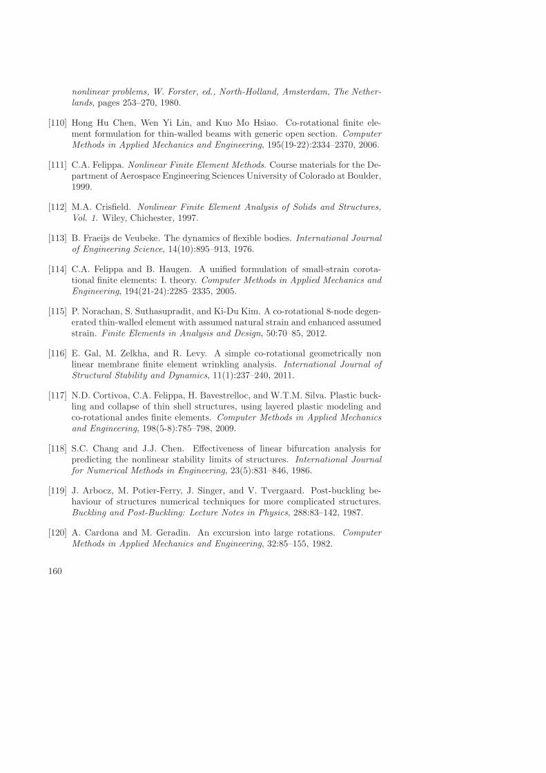
nonlinear problems, W. Forster, ed., North-Holland, Amsterdam, The Nether-lands, pages 253–270, 1980.
[110] Hong Hu Chen, Wen Yi Lin, and Kuo Mo Hsiao. Co-rotational finite ele-ment formulation for thin-walled beams with generic open section. ComputerMethods in Applied Mechanics and Engineering, 195(19-22):2334–2370, 2006.
[111] C.A. Felippa. Nonlinear Finite Element Methods. Course materials for the De-partment of Aerospace Engineering Sciences University of Colorado at Boulder,1999.
[112] M.A. Crisfield. Nonlinear Finite Element Analysis of Solids and Structures,Vol. 1. Wiley, Chichester, 1997.
[113] B. Fraeijs de Veubeke. The dynamics of flexible bodies. International Journalof Engineering Science, 14(10):895–913, 1976.
[114] C.A. Felippa and B. Haugen. A unified formulation of small-strain corota-tional finite elements: I. theory. Computer Methods in Applied Mechanics andEngineering, 194(21-24):2285–2335, 2005.
[115] P. Norachan, S. Suthasupradit, and Ki-Du Kim. A co-rotational 8-node degen-erated thin-walled element with assumed natural strain and enhanced assumedstrain. Finite Elements in Analysis and Design, 50:70–85, 2012.
[116] E. Gal, M. Zelkha, and R. Levy. A simple co-rotational geometrically nonlinear membrane finite element wrinkling analysis. International Journal ofStructural Stability and Dynamics, 11(1):237–240, 2011.
[117] N.D. Cortivoa, C.A. Felippa, H. Bavestrelloc, and W.T.M. Silva. Plastic buck-ling and collapse of thin shell structures, using layered plastic modeling andco-rotational andes finite elements. Computer Methods in Applied Mechanicsand Engineering, 198(5-8):785–798, 2009.
[118] S.C. Chang and J.J. Chen. Effectiveness of linear bifurcation analysis forpredicting the nonlinear stability limits of structures. International Journalfor Numerical Methods in Engineering, 23(5):831–846, 1986.
[119] J. Arbocz, M. Potier-Ferry, J. Singer, and V. Tvergaard. Post-buckling be-haviour of structures numerical techniques for more complicated structures.Buckling and Post-Buckling: Lecture Notes in Physics, 288:83–142, 1987.
[120] A. Cardona and M. Geradin. An excursion into large rotations. ComputerMethods in Applied Mechanics and Engineering, 32:85–155, 1982.
160
Bibliography
[121] A. Ibrahimbegovic, F. Frey, and Kozar. Computational aspects of vector-likeparametrization of three-dimensional finite rotations. International Journalfor Numerical Methods in Engineering, 38(21):3653–3673, 1995.
[122] Ibrahimbegovic. On the choice of finite rotation parameters. Computer Meth-ods in Applied Mechanics and Engineering, 149(1-4):49–71, 1997.
[123] M.R. Correa and D. Camotim. On the differentiation of the rodrigues for-mula and its significance for the vector-like parameterization of reissner-simobeam theory. International Journal for Numerical Methods in Engineering,55(9):1005–1032, 2002.
[124] M.R. Correa and D. Camotim. Work-conjugacy between rotation-dependentmoments and finite rotations. International Journal of Solids and Structures,40(11):2851–2873, 2003.
[125] A. Cardona and M. Geradin. Beam finite element non-linear theory withfinite rotations. International Journal for Numerical Methods in Engineering,26(11):2403–2438, 1988.
[126] I. Tsukanov and M. Hall. Data structure and algorithms for fast automaticdifferentiation. International Journal for Numerical Methods in Engineering,56:1949–1792, 2003.
[127] Robert D. Cook, David S. Malkus, Michael E. Plesha, and Robert J. Witt.Concepts and Applications of Finite Element Analysis, 4th Edition. Wiley,2001.
[128] I. Elishakoff, Y.W. Li, and J.H. Starnes Jr. Imperfection sensitivity due to theelastic moduli in the roorda-koiter frame. Chaos, Solitons Fractals, 7(8):1179–1186, 1996.
[129] A. Ibrahimbegovic. Stress resultant geometrically nonlinear shell theory withdrilling rotations: Part i. a consistent formulation. Computer Methods inApplied Mechanics and Engineering, 118(3-4):265–284, 1994.
[130] J. Chroscielewski, J. Makowski, and H. Stumpf. Genuinely resultant shell finiteelements accounting for geometric and material non-linearity. InternationalJournal for Numerical Methods in Engineering, 35(1):63–94, 1992.
[131] C.A. Felippa. A study of optimal membrane triangles with drilling freedoms.In Technical Report CU-CAS-03-02, Center for Aerospace Structures - Collegeof Engineering - University of Colorado, 2003.
161


Curriculum Vitae
Ke Liang was born on November 3th, 1984 in Luoyang, China. He enrolled inNorthwestern Polytechnical University of China after graduating from high school in2003. His major was aircraft designing and engineering. After obtaining a bachelor’sdegree with high honors, he was asked to enter the Ph.D program at NPU directly towork with Prof. Qin Sun. In October 2010, he came to the Netherlands to becomea Ph.D researcher in the Aerospace Structure group, at the faculty of AerospaceEngineering, Delft University of Technology. Under the guidance of Prof. ZaferGurdal and Dr. Mostafa Abdalla, he worked on reduction methods for the nonlinearanalysis of structures. The results of his Ph.D work are presented in this thesis.