Real-Time Radar SLAM - Uni DAS · 2017-11-21 · Real-Time Radar SLAM Markus Schoen∗, Markus Horn...

111. Workshop Fahrerassistenzsysteme und automatisiertes Fahren

Real-Time Radar SLAM

Markus Schoen∗, Markus Horn∗, Markus Hahn∗, Juergen Dickmann∗

Abstract: The Simultaneous Localization and Mapping (SLAM) problem is one of the key

problems on the way to autonomous driving. This paper provides a cost-efficient and robust

method with great accuracy in both localization and mapping. Therefore, a particle based

localization algorithm combined with 2D occupancy grid mapping is used. The algorithm uses

an odometer to obtain information about the vehicle movement and four radar sensors to get

a 360◦ coverage of the environment. The algorithm is evaluated on a dynamically changing

parking lot scenario and a driveway scenario. For each scenario, the algorithm is compared with

a highly accurate ground truth system. In certain situations, the algorithm achieves a RMS

error of less than 0.2 m. The results prove the performance of the algorithm.

Index Terms: Localization, Mapping, Occupancy Grid, Radar, SLAM

1 Introduction

This paper provides a Simultaneous Localization and Mapping (SLAM) algorithm [1]which builds a 2D occupancy grid map [2]. The algorithm uses radar sensors to capturethe environment and a particle based approach for localization [3]. Radar sensors arecheap and independent of weather conditions but lack in angular accuracy compared toLiDAR sensors. Therefore, the automotive industry uses radar sensors rather for obstacleavoidance applications like adaptive cruise control than localization algorithms. By usinga particle based approach for localization and a discrete 2D occupancy grid for mapping,the algorithm ensures high accuracy in both localization and mapping while keeping thecomputation time low to guarantee real-time processing.To evaluate the performance of the algorithm, two scenarios are processed. The firstscenario tests the algorithm in a dynamic parking lot situation. The parking space consistsof approximately a 150 m by 35 m area. The driven trajectory is approximately 400 mlong. The dataset consists of sequences at different time and weather conditions to show,that the algorithm is independent of changing environments. The second scenario teststhe algorithm in a driveway situation. This scenario demonstrates the strength of thealgorithm in static environments.The rest of this paper is organized as follows: Section 2 gives a short review of existingSLAM algorithms and points out differences to the proposed SLAM algorithm. Section 3describes the proposed real-time radar SLAM algorithm in detail. In Section 4, thealgorithm is evaluated on two scenarios. Section 5 gives a brief conclusion about thegained knowledge and an outlook for future work.

∗Daimler AG, Group Environment Perception, Ulm (e-mail: {markus.schoen, markus.h.horn,markus.hahn, juergen.dickmann}@daimler.com)

2 11. Workshop Fahrerassistenzsysteme und automatisiertes Fahren

2 Related Work

The SLAM problem has been a popular research topic in the past years since it is oneof the key problems on the way to autonomous driving. Durrant-Whyte et al. provide atutorial about the essential SLAM problem in [4] and recent advances in [5]. Beside ofthe same theoretical basis, SLAM realizations differ in the used map representation andlocalization algorithm.Feature based algorithms extract relevant information from raw sensor data and save themas landmarks in the map. Therefore, data storage is reduced but the extraction is oftenconnected with reduced robustness due to solving the data association problem. Since fea-ture extraction is common in image processing, feature based methods are commonly usedwith cameras [6]. An extension of feature based algorithms are graph based approaches.GraphSLAMs, first introduced by Thrun et al. [7], model relative landmark positions andvehicle movements as constraints to build a graph. The graph is optimized by minimizingthe least-square problem under given constraints. Since the optimization step is doneoffline, online localization results depend on the previously optimized map, which lead tohigh errors in dynamically changing environments. Grid based algorithms [8] work withraw sensor data and integrate them in a discrete map representation. This leads to ahigher level of detail due to the disappearance of the feature extractor and the associatedavoidable information loss. Downsides are higher data storage and computation costs.The first approaches to localize the vehicle pose simultaneously has been using an ex-tended kalman filter (EKF). EKF-SLAMs take the correlation between landmark andvehicle poses into account, but could diverge if any of the strong required assumptionsare violated. To respect the nonlinear process model and non-gaussian pose distribution,a particle filter can be used. FAST-SLAMs [9] use Rao-Blackwellisation and the associ-ated state space reduction to reduce the computation cost and make the particle basedapproach practical applicable.Existing SLAM algorithms often use sensors with high accuracy and low noise like LiDARsensors. Bruno et al. [10] introduce an extension of the established DP-SLAM [11]. Thealgorithm uses a particle filter for localization on a single map. The main difference to ouralgorithm is the map representation. Bruno et al. use a grid based map, where each cellstores the distance from the vehicle to a measurement, that lies inside the cell. The al-gorithm is very performant and simple to implement, but not designed for large outdoorenvironments due to the low accuracy in these situations. Zhao et al. [12] use LiDARsensors for large outdoor environments. The focus of the algorithm is achieving a highaccuracy and differ between static and dynamic objects. Therefore, the algorithm uses aclassification based on the motion history and the shape of the object, and a matchingalgorithm to correct the estimated pose. A separate loop closure algorithm ensures highaccuracy in cyclic situations. Radar sensors are recently recognized for localization [13]due to their advantages, especially their availability in contemporary vehicles. Schusteret al. [14] use a stream clustering algorithm to extract features from radar measurementsand incrementally update the map. The localization is done using FAST-SLAM with aspecially designed weight function with respect to the map representation. A radar basedGraphSLAM is introduced in [15]. Odometer measurements and landmarks are added tothe graph and stored in a R-tree data structure. A RANSAC is used to filter outliers andassign an unique identifier to each landmark. The graph optimization is done offline afterthe drive.


3 Real-Time Radar SLAM

The algorithm provides two outputs, the 2D occupancy grid map of the environmentand the estimated trajectory of the vehicle, including all estimated positions so far. Sec-tion 3.1 describes the idea of occupancy grid maps as a representation of the environment.Section 3.2 introduces the proposed method to localize the vehicle.

3.1 Map representation

The environment is represented by a 2D occupancy grid [18]. The idea is to equallydivide the space in independent cells m(x,y), where each cell has a probability P (m(x,y)) ofbeing occupied. Examples of occupancy grid maps are shown in Figure 3 and Figure 5.A dark color indicates a low occupancy probability while a light color indicates a highoccupancy probability. The medium gray indicates that the state of the cell is unknown,then the occupancy probability is P (m(x,y)) = 0.5. To integrate new measurements intothe map, the posterior probability needs to be calculated for each cell. By using a binaryBayes filter and the log-odd representation of the probabilities, the posterior probabilityis calculated to

L(m(x,y)(t)) = L(m(x,y)(t− 1))− L(m(x,y)(0)) + log

(P (m(x,y)(t)|Z1:t, X1:t)

1− P (m(x,y)(t)|Z1:t, X1:t)

)(1)

L(m(x,y)(0)) is the prior probability and set to zero. The term P (m(x,y)(t)|Z1:t, X1:t) iscalled inverse sensor model, a sensor specific probability to respect the influence of ameasurement on the grid cells. For radar sensors, the inverse sensor model is obtained asfollows: Cells, which are affected by the measurement relative to the normally distributeduncertainty, are updated with respect to the plausibility. The plausibility is calculatedbased on the range, amplitude and angle of the measurement. In contrast to the inversesensor model used for laser scanners, the update is done for each measurement in the sameangular range, not only for the furthermost measurement. All remaining Cells betweenthe uncertainty ellipse of the measurements and the sensor mounting position are assigneddecreasing occupancy.

3.2 Localization system

The localization system uses a particle based approach. A particle filter [3] approximatesthe recursive Bayesian filter, where the posterior distribution p(x(t)|z1:t,u1:t) is repre-sented by a finite set of particles X (t) = {x1(t), ...,xM(t)}. Each particle is a hypothesisof the current vehicle pose at time t

xk(t) = (Nk, Ek, ϕk)ᵀ (2)

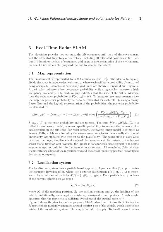
where Nk is the northing position, Ek the easting position and ϕk the heading of thevehicle. Additionally, a nonnegative weight wk is assigned to each particle. A high weightindicates, that the particle is a sufficient hypothesis of the current state x(t).Figure 1 shows the structure of the proposed SLAM algorithm. During the initializationM particles are randomly generated around the first pose of the vehicle, which is set to theorigin of the coordinate system. The map is initialized empty. To handle asynchronous


Sensor data

Initialization

Sensorbuffering

Correct poseestimation

Updateparticle poses

Collectmeasurements

Update map

Odometer

Radar

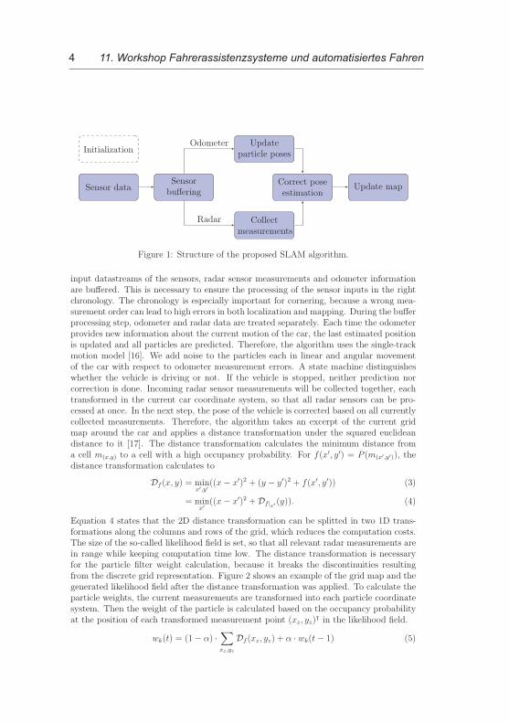
Figure 1: Structure of the proposed SLAM algorithm.

input datastreams of the sensors, radar sensor measurements and odometer informationare buffered. This is necessary to ensure the processing of the sensor inputs in the rightchronology. The chronology is especially important for cornering, because a wrong mea-surement order can lead to high errors in both localization and mapping. During the bufferprocessing step, odometer and radar data are treated separately. Each time the odometerprovides new information about the current motion of the car, the last estimated positionis updated and all particles are predicted. Therefore, the algorithm uses the single-trackmotion model [16]. We add noise to the particles each in linear and angular movementof the car with respect to odometer measurement errors. A state machine distinguisheswhether the vehicle is driving or not. If the vehicle is stopped, neither prediction norcorrection is done. Incoming radar sensor measurements will be collected together, eachtransformed in the current car coordinate system, so that all radar sensors can be pro-cessed at once. In the next step, the pose of the vehicle is corrected based on all currentlycollected measurements. Therefore, the algorithm takes an excerpt of the current gridmap around the car and applies a distance transformation under the squared euclideandistance to it [17]. The distance transformation calculates the minimum distance froma cell m(x,y) to a cell with a high occupancy probability. For f(x′, y′) = P (m(x′,y′)), thedistance transformation calculates to

Df (x, y) = minx′,y′

((x− x′)2 + (y − y′)2 + f(x′, y′)) (3)

= minx′

((x− x′)2 +Df |x′ (y)). (4)

Equation 4 states that the 2D distance transformation can be splitted in two 1D trans-formations along the columns and rows of the grid, which reduces the computation costs.The size of the so-called likelihood field is set, so that all relevant radar measurements arein range while keeping computation time low. The distance transformation is necessaryfor the particle filter weight calculation, because it breaks the discontinuities resultingfrom the discrete grid representation. Figure 2 shows an example of the grid map and thegenerated likelihood field after the distance transformation was applied. To calculate theparticle weights, the current measurements are transformed into each particle coordinatesystem. Then the weight of the particle is calculated based on the occupancy probabilityat the position of each transformed measurement point (xz, yz)

ᵀ in the likelihood field.

wk(t) = (1− α) ·∑xz ,yz

Df (xz, yz) + α · wk(t− 1) (5)


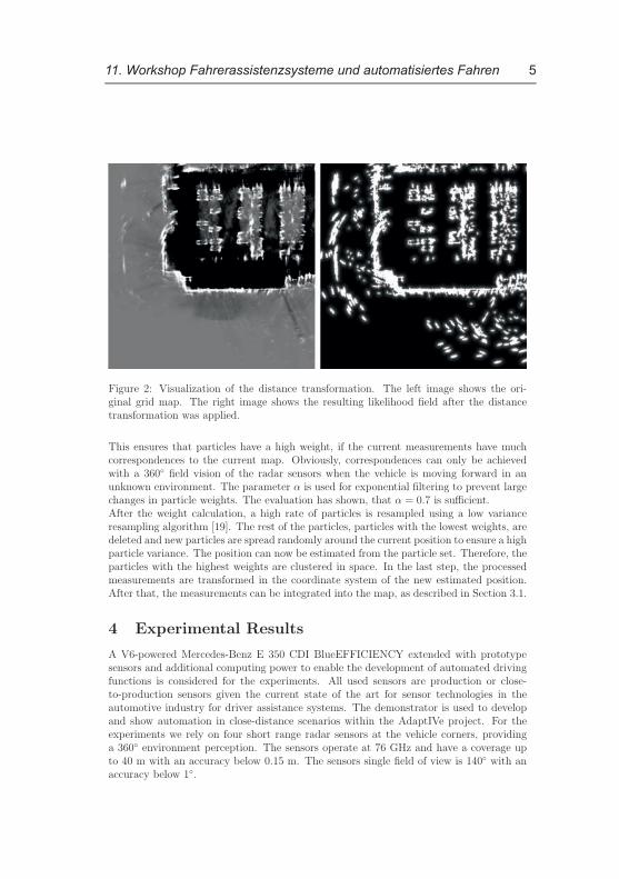
Figure 2: Visualization of the distance transformation. The left image shows the ori-ginal grid map. The right image shows the resulting likelihood field after the distancetransformation was applied.

This ensures that particles have a high weight, if the current measurements have muchcorrespondences to the current map. Obviously, correspondences can only be achievedwith a 360◦ field vision of the radar sensors when the vehicle is moving forward in anunknown environment. The parameter α is used for exponential filtering to prevent largechanges in particle weights. The evaluation has shown, that α = 0.7 is sufficient.After the weight calculation, a high rate of particles is resampled using a low varianceresampling algorithm [19]. The rest of the particles, particles with the lowest weights, aredeleted and new particles are spread randomly around the current position to ensure a highparticle variance. The position can now be estimated from the particle set. Therefore, theparticles with the highest weights are clustered in space. In the last step, the processedmeasurements are transformed in the coordinate system of the new estimated position.After that, the measurements can be integrated into the map, as described in Section 3.1.

4 Experimental Results

A V6-powered Mercedes-Benz E 350 CDI BlueEFFICIENCY extended with prototypesensors and additional computing power to enable the development of automated drivingfunctions is considered for the experiments. All used sensors are production or close-to-production sensors given the current state of the art for sensor technologies in theautomotive industry for driver assistance systems. The demonstrator is used to developand show automation in close-distance scenarios within the AdaptIVe project. For theexperiments we rely on four short range radar sensors at the vehicle corners, providinga 360◦ environment perception. The sensors operate at 76 GHz and have a coverage upto 40 m with an accuracy below 0.15 m. The sensors single field of view is 140◦ with anaccuracy below 1◦.


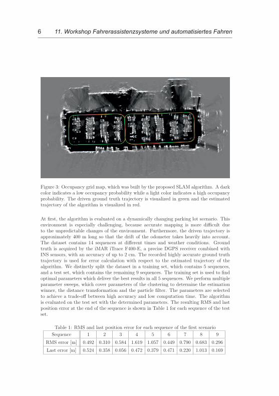
Figure 3: Occupancy grid map, which was built by the proposed SLAM algorithm. A darkcolor indicates a low occupancy probability while a light color indicates a high occupancyprobability. The driven ground truth trajectory is visualized in green and the estimatedtrajectory of the algorithm is visualized in red.

At first, the algorithm is evaluated on a dynamically changing parking lot scenario. Thisenvironment is especially challenging, because accurate mapping is more difficult dueto the unpredictable changes of the environment. Furthermore, the driven trajectory isapproximately 400 m long so that the drift of the odometer takes heavily into account.The dataset contains 14 sequences at different times and weather conditions. Groundtruth is acquired by the iMAR iTrace F400-E, a precise DGPS receiver combined withINS sensors, with an accuracy of up to 2 cm. The recorded highly accurate ground truthtrajectory is used for error calculation with respect to the estimated trajectory of thealgorithm. We distinctly split the dataset in a training set, which contains 5 sequences,and a test set, which contains the remaining 9 sequences. The training set is used to findoptimal parameters which deliver the best results in all 5 sequences. We perform multipleparameter sweeps, which cover parameters of the clustering to determine the estimationwinner, the distance transformation and the particle filter. The parameters are selectedto achieve a trade-off between high accuracy and low computation time. The algorithmis evaluated on the test set with the determined parameters. The resulting RMS and lastposition error at the end of the sequence is shown in Table 1 for each sequence of the testset.

Table 1: RMS and last position error for each sequence of the first scenario

Sequence 1 2 3 4 5 6 7 8 9

RMS error [m] 0.492 0.310 0.584 1.619 1.057 0.449 0.790 0.683 0.296

Last error [m] 0.524 0.358 0.056 0.472 0.379 0.471 0.220 1.013 0.169


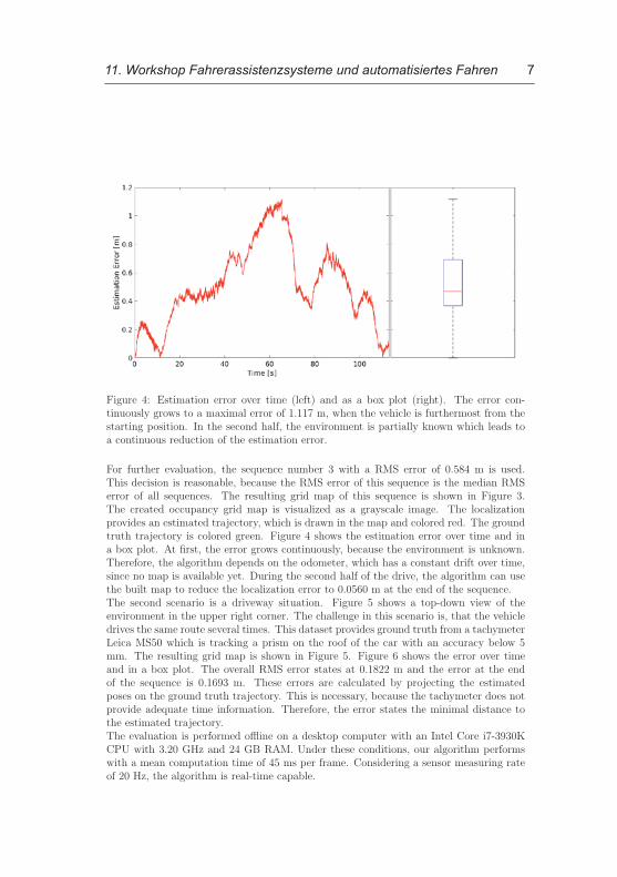
Figure 4: Estimation error over time (left) and as a box plot (right). The error con-tinuously grows to a maximal error of 1.117 m, when the vehicle is furthermost from thestarting position. In the second half, the environment is partially known which leads toa continuous reduction of the estimation error.

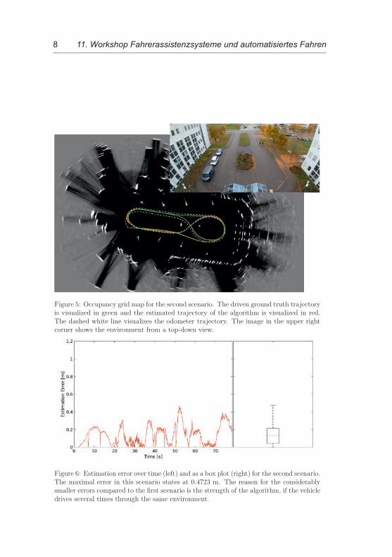
For further evaluation, the sequence number 3 with a RMS error of 0.584 m is used.This decision is reasonable, because the RMS error of this sequence is the median RMSerror of all sequences. The resulting grid map of this sequence is shown in Figure 3.The created occupancy grid map is visualized as a grayscale image. The localizationprovides an estimated trajectory, which is drawn in the map and colored red. The groundtruth trajectory is colored green. Figure 4 shows the estimation error over time and ina box plot. At first, the error grows continuously, because the environment is unknown.Therefore, the algorithm depends on the odometer, which has a constant drift over time,since no map is available yet. During the second half of the drive, the algorithm can usethe built map to reduce the localization error to 0.0560 m at the end of the sequence.The second scenario is a driveway situation. Figure 5 shows a top-down view of theenvironment in the upper right corner. The challenge in this scenario is, that the vehicledrives the same route several times. This dataset provides ground truth from a tachymeterLeica MS50 which is tracking a prism on the roof of the car with an accuracy below 5mm. The resulting grid map is shown in Figure 5. Figure 6 shows the error over timeand in a box plot. The overall RMS error states at 0.1822 m and the error at the endof the sequence is 0.1693 m. These errors are calculated by projecting the estimatedposes on the ground truth trajectory. This is necessary, because the tachymeter does notprovide adequate time information. Therefore, the error states the minimal distance tothe estimated trajectory.The evaluation is performed offline on a desktop computer with an Intel Core i7-3930KCPU with 3.20 GHz and 24 GB RAM. Under these conditions, our algorithm performswith a mean computation time of 45 ms per frame. Considering a sensor measuring rateof 20 Hz, the algorithm is real-time capable.


Figure 5: Occupancy grid map for the second scenario. The driven ground truth trajectoryis visualized in green and the estimated trajectory of the algorithm is visualized in red.The dashed white line visualizes the odometer trajectory. The image in the upper rightcorner shows the environment from a top-down view.

Figure 6: Estimation error over time (left) and as a box plot (right) for the second scenario.The maximal error in this scenario states at 0.4723 m. The reason for the considerablysmaller errors compared to the first scenario is the strength of the algorithm, if the vehicledrives several times through the same environment.


5 Conclusion

This paper provides a robust and cost-efficient method to solve the Simultaneous Local-ization and Mapping (SLAM) problem in real-time. The algorithm uses radar sensorsto perceive the environment and odometer measurements to get information about thevehicle movement. Both information are used to localize the vehicle using a particle filter,while simultaneously build a 2D occupancy grid map of the environment. Experimentalresults prove the high accuracy and real-time capability of the algorithm.Future work will concentrate on ways to compensate the oversaturation of the occupancygrid. The oversaturation occurs if the vehicle drives multiple times in the same environ-ment. The oversaturation leads to inconclusive object positions in the map, which cancause high localization and mapping errors.

6 Acknowledgement

The research leading to these results has received funding from the European Commis-sion Seventh Framework Programme (FP/2007-2013) under the project AdaptIVe, grantagreement number 610428. Responsibility for the information and views set out in thispublication lies entirely with the authors. The authors would like to thank all partnerswithin AdaptIVe for their cooperation and valuable contribution.

References

[1] LI, Jie; CHENG, Lei; WU, Huaiyu; XIONG, Ling; WANG, Dongmei. An overviewof the simultaneous localization and mapping on mobile robot. In: Modelling, Identi-fication & Control (ICMIC), 2012 Proceedings of International Conference on. IEEE,2012. S. 358-364.

[2] THRUN, Sebastian; BUCKEN, Arno. Integrating grid-based and topological mapsfor mobile robot navigation. In: Proceedings of the National Conference on ArtificialIntelligence. 1996. S. 944-951.

[3] DELLAERT, Frank; FOX, Dieter; BURGARD, Wolfram; THRUN, Sebastian. Montecarlo localization for mobile robots. In: Robotics and Automation, 1999. Proceedings.1999 IEEE International Conference on. IEEE, 1999. S. 1322-1328.

[4] DURRANT-WHYTE, Hugh; BAILEY, Tim. Simultaneous localization and mapping:part I. IEEE robotics & automation magazine, 2006, 13. Jg., Nr. 2, S. 99-110.

[5] BAILEY, Tim; DURRANT-WHYTE, Hugh. Simultaneous localization and mapping(SLAM): Part II. IEEE Robotics & Automation Magazine, 2006, 13. Jg., Nr. 3, S.108-117.

[6] ZIEGLER, Julius; LATEGAHN, Henning; SCHREIBER, Markus; KELLER, Chris-toph G.; KNOEPPEL, Carsten; HIPP, Jochen; HAUEIS, Martin; STILLER, Chris-toph. Video based localization for bertha. In: 2014 IEEE Intelligent Vehicles Sym-posium Proceedings. IEEE, 2014. S. 1231-1238.


[7] THRUN, Sebastian; MONTEMERLO, Michael. The graph SLAM algorithm withapplications to large-scale mapping of urban structures. The International Journal ofRobotics Research, 2006, 25. Jg., Nr. 5-6, S. 403-429.

[8] COLLEENS, Thomas; COLLEENS, J. J.; RYAN, Conor. Occupancy grid mapping:An empirical evaluation. In: Control & Automation, 2007. MED’07. MediterraneanConference on. IEEE, 2007. S. 1-6.

[9] MONTEMERLO, Michael; THRUN, Sebastian; KOLLER, Daphne; WEGBREIT,Ben. FastSLAM: A factored solution to the simultaneous localization and mappingproblem. In: Aaai/iaai. 2002. S. 593-598.

[10] STEUX, Bruno; EL HAMZAOUI, Oussama. tinySLAM: A SLAM algorithm inless than 200 lines C-language program. In: Control Automation Robotics & Vision(ICARCV), 2010 11th International Conference on. IEEE, 2010. S. 1975-1979.

[11] ELIAZAR, Austin; PARR, Ronald. DP-SLAM: Fast, robust simultaneous localiza-tion and mapping without predetermined landmarks. In: IJCAI. 2003. S. 1135-1142.

[12] ZHAO, Huijing; CHIBA, Masaki; SHIBASAKI, Ryosuke; SHAO, Xiaowei; CUI, Jin-shi; ZHA, Hongbin. SLAM in a dynamic large outdoor environment using a laserscanner. In: Robotics and Automation, 2008. ICRA 2008. IEEE International Confer-ence on. IEEE, 2008. S. 1455-1462.

[13] DICKMANN, Juergen; APPENRODT, Nils; BLOECHER, Hans-Ludwig; BRENK,C.; HACKBARTH, Thomas; HAHN, Markus; KLAPPSTEIN, Jens; MUNTZINGER,Marc; SAILER, Alfons. Radar contribution to highly automated driving. In: EuropeanRadar Conference (EuRAD), 2014 11th. IEEE, 2014. S. 412-415.

[14] SCHUSTER, Frank; WOERNER, Marcus; KELLER, Christoph; HAUEIS, Martin;CURIO, Cristobal. Robust localization based on radar signal clustering. In: IntelligentVehicles Symposium (IV), 2016 IEEE. IEEE, 2016. S. 839-844.

[15] SCHUSTER, Frank; KELLER, Chrisroph; RAPP, Matthias; HAUEIS, Martin;CURIO, Cristobal. Landmark based radar slam using graph optimization. In: In-telligent Transportation Systems (ITSC), 2016 IEEE 19th International Conferenceon. IEEE, 2016. S. 2559-2564.

[16] TAHERI, Saied. An investigation and design of slip control braking systems integ-rated with four-wheel steering. 1991. Doktorarbeit.

[17] FELZENSZWALB, Pedro; HUTTENLOCHER, Daniel. Distance transforms ofsampled functions. Cornell University, 2004.

[18] WERBER, Klaudius; RAPP, Matthias; KLAPPSTEIN, Jens; HAHN, Markus;DICKMANN, Juergen; DIETMAYER, Klaus; WALDSCHMIDT, Christian. Auto-motive radar gridmap representations. In: Microwaves for Intelligent Mobility (IC-MIM), 2015 IEEE MTT-S International Conference on. IEEE, 2015. S. 1-4.

[19] THRUN, Sebastian; BURGARD, Wolfram; FOX, Dieter. Probabilistic robotics. MITpress, 2005.

Real-Time Radar SLAM - Uni DAS · 2017-11-21 · Real-Time Radar SLAM Markus Schoen∗, Markus Horn...

Documents

Transcript of Real-Time Radar SLAM - Uni DAS · 2017-11-21 · Real-Time Radar SLAM Markus Schoen∗, Markus Horn...