Matthias Lesch Henri Moscovici Markus J. Pflaum
99
Connes–Chern character for manifolds with boundary and eta cochains Matthias Lesch Henri Moscovici Markus J. Pflaum Author address: MATHEMATISCHES I NSTITUT,UNIVERSIT ¨ AT BONN,ENDENICHER ALLEE 60, 53115 BONN,GERMANY E-mail address: [email protected], [email protected] URL: www.matthiaslesch.de, www.math.uni-bonn.de/people/lesch DEPARTMENT OF MATHEMATICS,THE OHIO STATE UNIVERSITY,COLUMBUS, OH 43210, USA E-mail address: [email protected] DEPARTMENT OF MATHEMATICS,UNIVERSITY OF COLORADO UCB 395, BOULDER, CO 80309, USA E-mail address: [email protected] URL: http://euclid.colorado.edu/∼pflaum
Transcript of Matthias Lesch Henri Moscovici Markus J. Pflaum

Connes–Chern character for manifolds with boundaryand eta cochains
Matthias Lesch
Henri Moscovici
Markus J. Pflaum
Author address:
MATHEMATISCHES INSTITUT, UNIVERSITAT BONN, ENDENICHER ALLEE 60,53115 BONN, GERMANY
E-mail address: [email protected], [email protected]
URL: www.matthiaslesch.de, www.math.uni-bonn.de/people/lesch
DEPARTMENT OF MATHEMATICS, THE OHIO STATE UNIVERSITY, COLUMBUS,OH 43210, USA
E-mail address: [email protected]
DEPARTMENT OF MATHEMATICS, UNIVERSITY OF COLORADO UCB 395,BOULDER, CO 80309, USA
E-mail address: [email protected]: http://euclid.colorado.edu/∼pflaum
Contents
List of Figures ix
Introduction 1
Chapter 1. Preliminaries 91.1. The general setup 91.2. Relative cyclic cohomology 101.3. The Chern character 121.4. Dirac operators and q-graded Clifford modules 131.5. The relative Connes–Chern character of a Dirac operator over a
manifold with boundary 151.6. Exact b-metrics and b-functions on cylinders 171.7. Global symbol calculus for pseudodifferential operators 191.8. Classical b-pseudodifferential operators 201.9. Indicial family 24
Chapter 2. The b-Analogue of the Entire Chern Character 252.1. The b-trace 252.2. The relative McKean–Singer formula and the APS Index Theorem 282.3. A formula for the b-trace 302.4. b-Clifford modules and b-Dirac operators 332.5. The b-JLO cochain 352.6. Cocycle and transgression formulæ for the even/odd b-Chern
character (without Clifford covariance) 362.7. Sketch of Proof of Theorem 2.11 39
Chapter 3. Heat Kernel and Resolvent Estimates 453.1. Basic resolvent and heat kernel estimates on general manifolds 453.2. Comparison results 523.3. Trace class estimates for the model heat kernel 553.4. Trace class estimates for the JLO integrand on manifolds with
cylindrical ends 583.5. Estimates for b-traces 593.6. Estimates for the components of the entire b-Chern character 60
Chapter 4. The Main Results 654.1. Asymptotic b-heat expansions 654.2. The Connes–Chern character of the relative Dirac class 694.3. Relative pairing formulæ and geometric consequences 754.4. Relation with the generalized APS pairing 82
v

vi CONTENTS
Bibliography 85
Subject Index 89
Notation Index 91
Abstract
We express the Connes-Chern character of the Dirac operator associated toa b-metric on a manifold with boundary in terms of a retracted cocycle in rela-tive cyclic cohomology, whose expression depends on a scaling/cut-off parameter.Blowing-up the metric one recovers the pair of characteristic currents that repre-sent the corresponding de Rham relative homology class, while the blow-downyields a relative cocycle whose expression involves higher eta cochains and theirb-analogues. The corresponding pairing formulæ with relative K-theory classescapture information about the boundary and allow to derive geometric conse-quences. As a by-product, we show that the generalized Atiyah-Patodi-Singerpairing introduced by Getzler and Wu is necessarily restricted to almost flat bun-dles.
2000 Mathematics Subject Classification. Primary 58Jxx, 46L80; Secondary 58B34, 46L87.Key words and phrases. Manifolds with boundary, b-calculus, noncommutative geometry, Connes–
Chern character, relative cyclic cohomology, η-invariant.M. L. was partially supported by the Hausdorff Center for Mathematics and by the Sonder-
forschungsbereich/Transregio 12 “Symmetries and Universality in Mesoscopic Systems” (Bochum–Duisburg/Essen–Koln–Warszawa).
H. M. was partially supported by the US National Science Foundation awards no. DMS-0245481and no. DMS-0652167.
M. J. P. was partially supported by the DFG.M. L. would like to thank the Department of Mathematics of the University of Colorado for hos-
pitality and support.Both H. M. and M. J. P. acknowledge with thanks the hospitality and support of the Hausdorff
Center for Mathematics.
vii

List of Figures
1.1 Compact manifoldMwith boundary 181.2 Interior of b–manifoldMwith cylindrical coordinates on the collar 18
3.1 Contour of integration for calculating e−tD2
from the resolvent. 483.2 Contour of integration if bottom of the essential spectrum of D2 is c. 493.3 The cut-off functions ϕ and ψ. 53
4.1 By homotopy invariance the signed sum of the four spectral flows addsup to 0. 78
ix

Introduction
LetM be a compact smoothm-dimensional manifold with boundary ∂M 6= ∅.Assuming that M possesses a Spinc structure, the fundamental class in the rel-ative K-homology group Km(M,∂M) can be realized analytically in terms of theDirac operator D (graded if m is even) associated to a riemannian metric on M.More precisely, according to [BDT89, §3], if De is a closed extension of D satisfy-ing the condition that either D∗eDe or DeD∗e has compact resolvent (e.g. both Dmin
and Dmax are such), then the bounded operator F = De(D∗eDe + 1)
−1/2 defines arelative Fredholm module over the pair of C∗-algebras
(C(M), C(∂M)
), hence an
element [D] ∈ Km(M,∂M). Moreover, by [BDT89, §4], the connecting homomor-phism maps [D] to the fundamental class [D∂] ∈ Km−1(∂M) corresponding to theDirac operator D∂ associated to the boundary restriction of the metric and of Spinc
structure.The map Index[D] : Km(M,∂M) → Z, defined by the pairing of K-theory
with the K-homology class of [D], can be expressed in cohomological terms bymeans of Connes’ Chern character with values in cyclic cohomology [CON85]. In-deed, the relative K-homology group Km(M,∂M), viewed as the Kasparov groupKKm
(C0(M \ ∂M);C
), can be realized as homotopy classes of Fredholm mod-
ules over the Frechet algebra J∞(∂M,M) of smooth functions on M vanishingto any order on ∂M; J∞(∂M,M) is a local C∗-algebra, H-unital and dense inC0(M \ ∂M) = f ∈ C(M) | f|∂M = 0. One can therefore define the Connes-Cherncharacter of [D] by restricting the operator F = De(D
∗eDe + 1)
−1/2, or directly D,to J∞(∂M,M) and regarding it as a finitely summable Fredholm module. Theresulting periodic cyclic cocycle corresponds, via the canonical isomorphism be-tween the periodic cyclic cohomology HP ev/odd
(J∞(∂M,M)
)and the de Rham
homology HdRev/odd(M \ ∂M;C) (cf. [BRPF08]), to the de Rham class of the current
(with arbitrary support) associated to the A-form of the riemannian metric. In fact,one can even recover the A-form itself out of local cocycle representatives for theConnes-Chern character, as in [COMO93, Remark 4, p. 119] or [COMO95, Re-mark II.1, p. 231]. However, the boundary ∂M remains conspicuously absent insuch representations.
It is the purpose of this paper to provide cocycle representatives for theConnes-Chern character of the fundamental K-homology class [D] ∈ Km(M,∂M)that capture and reflect geometric information about the boundary. Our point ofdeparture is Getzler’s construction [GET93A] of the Connes-Chern character of[D]. Cast in the propitious setting of Melrose’s b-calculus [MEL93], Getzler’s cocy-cle has however the disadvantage, from the viewpoint of its geometric functional-ity, of being realized not in the relative cyclic cohomology complex proper but inits entire extension. Entire cyclic cohomology [CON88] was devised primarily for
1
2 INTRODUCTION
handling infinite dimensional geometries and is less effective as a tool than ordi-nary cyclic cohomology when dealing with finite dimensional K-homology cycles.To remedy this drawback we undertook the task of producing cocycle realizationsfor the Connes-Chern character directly in the relative cyclic cohomology complexassociated to the pair of algebras
(C∞(M), C∞(∂M)
). This is achieved by adapt-
ing and implementing in the context of relative cyclic cohomology the retractionprocedure of [COMO93], which converts the entire Connes-Chern character intothe periodic one. The resulting cocycles automatically carry information about theboundary and this allows to derive geometric consequences.
It should be mentioned that the relative point of view in the framework ofcyclic cohomology was first exploited in [LMP09] to obtain cohomological ex-pressions for K-theory invariants associated to parametric pseudodifferential op-erators. It was subsequently employed by Moriyoshi and Piazza to establish aGodbillon-Vey index pairing for longitudinal Dirac operators on foliated bundles[MOPI11].
Here is a quick synopsis of the main results of the present paper. Throughoutthe paper, we fix an exact b-metric g on M, and denote by D the correspondingb-Dirac operator. We define for each t > 0 and any n ≥ m = dimM, n ≡ m (mod2), pairs of cochains( bchnt (D), chn+1t (D∂)
)resp.
( bchn
t (D), chn−1t (D∂))
(0.1)
over the pair of algebras(C∞(M), C∞(∂M)
), given by the following expressions:
bchnt (D) :=∑j≥0
bChn−2j(tD) + B bT/chn+1t (D),
chn+1t (D∂) :=∑j≥0
Chn−2j+1(tD∂) + BT/chn+2t (D∂),
bchn
t (D) := bchnt (D) + T/chnt (D∂) i∗.
(0.2)
In these formulæ, Ch•(D∂) stand for the components of the Jaffe-Lesniewski-Osterwalder cocycle [JLO88] representing the Connes-Chern character in entirecyclic cohomology, bCh•(D) denote the corresponding b-analogue (cf. (2.50)),while the cochains T/ch•t(D∂), resp. bT/ch•t(D) (see (4.20), are manufactured outof the canonical transgression formula as in [COMO93]; i : ∂M→M denotes theinclusion. One checks that
(b+ B)( bchnt (D)
)= chn+1t (D∂) i∗
(b+ B)( bch
n
t (D))= chn−1t (D∂) i∗,
(0.3)
which shows that the cochains (0.1) are cocycles in the relative total (b, B)-complexof (C∞(M), C∞(∂M)). Moreover, the class of this cocycle in periodic cyclic coho-mology is independent of t > 0 and of n = m+ 2k, k ∈ Z+. Furthermore, its limitas t→ 0 gives the pair of A currents corresponding to the b-manifold M, that is
(limt0 bchnt (D), lim
t0 chn+1t (D∂))=
(∫bM
A(b∇2g)∧ •,∫∂M
A(∇2g∂)∧ •). (0.4)
INTRODUCTION 3
The notation in the right hand side requires an explanation. With
A(b∇2g) = det
(b∇2g/4πi
sinh b∇2g/4πi
) 12
, A(∇2g∂) = det
(∇2g∂/4πi
sinh∇2g∂/4πi
) 12
, (0.5)
and∫
bM
: bΩm(M) → C denoting the b-integral of b-differential m-forms on
M associated to the trivialization of the normal bundle to ∂M underlying the b-structure, both terms in the right hand side of (0.4) are viewed as (b, B)-cochainsassociated to currents. More precisely, incorporating the 2πi factors which accountfor the conversion of the Chern character in cyclic homology into the Chern char-acter in de Rham cohomology, forM even dimensional this identification takes theform∫
bM
A(b∇2g)∧(f0, . . . , f2q
)=
1
(2πi)q(2q)!
∫bM
A(b∇2g)∧ f0 df1 ∧ . . .∧ f2q , (0.6)
respectively∫∂M
A(∇2g∂)∧(h0, . . . , h2q−1
)=
1
(2πi)q(2q− 1)!
∫∂M
A(∇2g∂)∧ h0 dh1 ∧ . . .∧ h2q−1. (0.7)
Finally (cf. Theorem 4.5 infra), the limit formula (0.4) implies that both(bchnt (D), chn+1t (D∂)
)and
(bch
n
t (D), chn−1t (D∂))
represent the Chern characterof the fundamental relative K-homology class [D] ∈ Km(M,∂M).
Under the assumption that KerD∂ = 0, we next prove (Theorem 4.6 infra) thatthe pair of retracted cochains
(bch
n
t (D), chn−1t (D∂))
has a limit as t → ∞. For neven, or equivalentlyM even dimensional, this limit has the expression
bchn∞(D) =
n/2∑j=0
κ2j(D) + B bT/chn+1∞ (D) + T/chn∞(D∂) i∗,
chn−1∞ (D∂) = BT/chn∞(D∂),
(0.8)
with the cochains κ•(D), occurring only when KerD 6= 0, given by
κ2j(D)(a0, . . . , a2j) = Str(ρH(a0)ωH(a1, a2) · · ·ωH(a2j−1, a2j)
); (0.9)
here H denotes the orthogonal projection onto KerD, and
ρH(a) := HaH , ωH(a, b) := ρH(ab) − ρH(a)ρH(b), for all a, b ∈ C∞(M).
WhenM is odd dimensional, the limit cocycle takes the similar form
bchn∞(D) = B bT/chn+1∞ (D) + T/chn∞(D∂) i∗ ,
chn−1∞ (D∂) = BT/chn∞(D∂).(0.10)
The absence of cochains of the form κ•(D∂) in the boundary component is due tothe assumption that KerD∂ = 0.
4 INTRODUCTION
The geometric implications become apparent when one inspects the ensuingpairing with K-theory classes. For M even dimensional, a class in Km(M,∂M)can be represented as a triple [E, F, h], where E, F are vector bundles over M,which we will identify with projections pE, pF ∈ MatN(C∞(M)), and h : [0, 1] →MatN(C∞(∂M)) is a smooth path of projections connecting their restrictions tothe boundary E∂ and F∂. For M odd dimensional, a representative of a class inKm(M,∂M) is a triple (U,V, h), where U,V : M → U(N) are unitaries and h is ahomotopy between their restrictions to the boundary U∂ and V∂. In both cases,the Chern character of [X, Y, h] ∈ Km(M,∂M) is represented by the relative cyclichomology cycle over the algebras
(C∞(M), C∞(∂M)
)ch•
([X, Y, h]
)=(
ch•(Y) − ch•(X) , −T/ch•(h)), (0.11)
where ch•, resp. T/ch• denote the components of the standard Chern character incyclic homology resp. of its canonical transgression (see Section 1.3).
The pairing⟨[D], [X, Y, h]
⟩∈ Z between the classes [D] ∈ Km(M,∂M) and
[X, Y, h] ∈ Km(M,∂M) acquires the cohomological expression⟨[D], [X,Y, h]
⟩=⟨( bch
n
t (D), chn−1t (D∂)), ch•[X, Y, h]
⟩=
=⟨∑j≥0
bChn−2j(tD) + B bT/chn+1t (D), ch•(Y) − ch•(X)⟩
+⟨
T/chnt (D∂), ch•(Y∂) − ch•(X∂)⟩
−⟨∑j≥0
Chn−2j−1(tD∂) + BT/chnt (D∂), T/ch•(h)⟩,
(0.12)
which holds for any t > 0. Letting t → 0 yields the local form of the pairingformula⟨
[D], [X, Y, h]⟩=
=
∫bM
A(b∇2g)∧(
ch•(Y) − ch•(X))−
∫∂M
A(∇2g∂)∧ T/ch•(h).(0.13)
It should be pointed out that (0.13) holds in complete generality, without requiringthe invertibility of D∂.
When M is even dimensional and D∂ is invertible, the equality between theabove limit and the limit as t→∞ yields, for any n = 2` ≥ m, the identity∑0≤k≤`
⟨κ2k(D), ch2k(pF) − ch2k(pE)
⟩+⟨B bT/chn+1∞ (D), chn(pF) − chn(pE)
⟩+
+⟨
T/chn∞(D∂), chn(pF∂) − chn(pE∂)⟩=
=
∫bM
A(b∇2g)∧(
ch•(pF) − ch•(pE))−
∫∂M
A(∇2g∂)∧ T/ch•(h)
+⟨BT/chn∞(D∂),T/chn−1(h)
⟩,
(0.14)
where
ch2k(p) =
tr0(p), for k = 0,
(−1)k (2k)!k! tr2k
((p− 1
2)⊗ p⊗2k
), for k > 0.
INTRODUCTION 5
Like the Atiyah-Patodi-Singer index formula [APS75], the equation (0.14) in-volves index and eta cochains, only of higher order. Moreover, the same typeof identity continues to hold in the odd dimensional case. Explicitly, it takes theform
(−1)n−12
(n−12
)!(⟨B bT/chn+1∞ (D), (V−1 ⊗ V)⊗n+1
2 − (U−1 ⊗U)⊗n+12
⟩+⟨
T/chn∞(D∂), (V−1∂ ⊗ V∂)
⊗n+12 − (U−1
∂ ⊗U∂)⊗n+1
2
⟩)=
=
∫bM
A(b∇2g)∧(
ch•(V) − ch•(U))−
∫∂M
A(∇2g∂)∧ T/ch•(h)
+⟨BT/chn∞(D∂),T/chn−1(h)
⟩.
(0.15)
The relationship between the relative pairing and the Atiyah-Patodi-Singer in-dex theorem can actually be made explicit, and leads to interesting geometric con-sequences. Indeed, under the necessary assumption that M is even dimensional,we show (cf. Theorem 4.12) that the above pairing can be expressed as follows:
〈[D], [E, F, h]〉 = IndAPS DF − IndAPS D
E + SF(h,D∂); (0.16)
here IndAPS stands for the APS-index, and SF(h,D∂) denotes the spectral flowalong the path of operators
(D+∂
)h(s); D+∂ is the restriction of c(dx)−1D∂ to the
positive half spinor bundle and c(dx) denotes Clifford multiplication by the in-ward normal vector. On applying the APS index formula [APS75, Eq. (4.3)], thepairing takes the explicit form
〈[D], [E, F, h]〉 =∫
bM
A(b∇2g)∧(
ch•(F) − ch•(E))
−(ξ(D+,F∂
∂ ) − ξ(D+,E∂∂ )
)+ SF(h,D∂),
(0.17)
where
ξ(D+,E∂∂ ) =
1
2
(η(D+,E∂
∂ ) + dim KerD+,E∂∂
). (0.18)
Comparing this expression with the local form of the pairing (0.13) leads to a gen-eralization of the APS odd-index formula [APS76, Prop. 6.2, Eq. (6.3)], from trivi-alized flat bundles to pairs of equivalent vector bundles in K-theory. Precisely (cf.Corollary 4.15), if E ′, F ′ are two such bundles on a closed odd dimensional spinmanifold N, and h is the homotopy implementing the equivalence of E ′ with F ′,then
ξ(DF′
g ′) − ξ(DE ′
g ′ ) =
∫N
A(∇2g ′)∧ T/ch•(h) + SF(h,Dg ′) , (0.19)
where Dg ′ denotes the Dirac operator associated to a riemannian metric g ′ on N;equivalently, ∫1
0
1
2
d
dt
(η(ph(t) Dg ′ ph(t))
)dt =
∫N
A(∇2g ′)∧ T/ch•(h) , (0.20)
where ph(t) is the path of projections joining E ′ and F ′, and the left hand side isthe natural extension of the real-valued index in [APS76, Eq. (6.1)].
Let us briefly comment on the main analytical challenges encountered in thecourse of proving the results outlined above. In order to compute the limit as
6 INTRODUCTION
t 0 of the Chern character, one needs to understand the asymptotic behavior ofexpressions of the form
b〈A0, A1, . . . , Ak〉√tD
:=
∫∆k
bTr(A0e
−σ0tD2
A1e−σ1tD
2
. . . Ake−σktD
2)dσ,
(0.21)
where ∆k denotes the standard simplex σ0 + . . .+ σk = 1, σj ≥ 0 and A0, . . . , Akare b-differential operators of order dj, j = 0, . . . , k; d :=
∑kj=0 dj denotes the sum
of their orders. The difficulty here is twofold. Firstly, the b-trace is a regularizedextension of the trace to b-pseudodifferential operators on the non-compact mani-foldM \∂M (recall that the b-metric degenerates at ∂M). Secondly, the expressioninside the b-trace involves a product of operators. The Schwartz kernel of theproduct A0e−σ0tD
2
A1e−σ1tD
2 · . . . · Ake−σktD2
does admit a pointwise asymptoticexpansion (see [WID79], [COMO90], [BLFO90]), namely(
A0e−σ0tD
2
A1e−σ1tD
2
· . . . ·Ake−σktD2)(p, p)
=:
n∑j=0
aj(A0, . . . , Ak,D)(p) tj−dimM−d
2 +Op(t(n+1−d−dimM)/2).
(0.22)
However, this asymptotic expansion is only locally uniform in p; it is not glob-ally uniform on the non-compact manifold M \ ∂M. A further complicationarises from the fact that the function aj(A0, . . . , Ak,D) is not necessarily inte-grable. Nevertheless, a partie finie-type regularized integral, which we denote by∫
bMaj(A0, . . . , Ak,D)dvol, does exist and we prove (cf. Theorem 4.3) that the cor-
responding b-trace admits an asymptotic expansion of the form
bTr(A0e
−σ0tD2
A1e−σ1tD
2
. . . Ake−σktD
2)
=
n∑j=0
∫bM
aj(A0, . . . , Ak,D)dvol tj−dimM−d
2 +
+O(( k∏j=1
σ−dj/2j
)t(n+1−d−dimM)/2
).
(0.23)
When D∂ is invertible and hence D is a Fredholm operator, we can also prove thefollowing estimate (cf. (3.72))
| b〈A0(I−H), ..., Ak(I−H)〉√tD|
≤ Cδ,εt−d/2−(dimM)/2−εe−tδ, for all 0 < t <∞, (0.24)
for any ε > 0 and any 0 < δ < inf specess D2. Here, specess denotes the essential
spectrum and H is the orthogonal projection onto KerD. This estimate allows usto compute the limit as t∞ and thus derive the formulæ (0.8) and (0.10).
A few words about the organization of the paper are now in order. Westart by recalling, in Chapter 1, some basic material on relative cyclic cohomol-ogy [LMP09], b-calculus [MEL93] and Dirac operators. In Section 2.1 we discussin detail the b-trace in the context of a manifold with cylindrical ends.
As a quick illustration of the usefulness of the relative cyclic cohomologicalapproach in the present context, we digress in Section 2.2 to establish an analogue
INTRODUCTION 7
of the well-known McKean–Singer formula for manifolds with boundary; we thenemploy it to recast in these terms Melrose’s proof of the Atiyah-Patodi-Singer in-dex theorem (cf. [MEL93, Introduction]).
In Section 2.3, refining an observation due to Loya [LOY05], we give an ef-fective formula for the b-trace, which will turn out to be a convenient technicaldevice.
After setting up the notation related to b-Clifford modules and b-Dirac opera-tors in Section 2.4, we revisit in the remainder of the chapter Getzler’s version ofthe relative entire Connes-Chern character in the setting of b-calculus [GET93A].
In Chapter 3 we prove some crucial estimates for the heat kernel of a b-Diracoperator, which are then applied in Section 3.6 to analyze the short and long timebehavior of the components of the b-analogue of the entire Chern character. Asa preparation more standard resolvent and heat kernel estimates are discussed inSection 3.1.
The final Chapter 4 contains our main results: Section 4.1 is devoted to asymp-totic expansions for the b-analogues of the Jaffe-Lesniewski-Osterwalder compo-nents. The retracted relative cocycle representing the Connes-Chern character inrelative cyclic cohomology is constructed in Section 4.2, where we also computethe expressions of its small and large scale limits.
Finally, Section 4.3 derives the ensuing pairing formulæ with the K-theory,establishes the connection with the Atiyah-Patodi-Singer index theorem, and dis-cusses the geometric consequences. The paper concludes with an explanatory note(Section 4.4) elucidating the relationship between the results presented here andthe prior work in this direction by Getzler [GET93A] and Wu [WU93], and clar-ifying why their generalized APS pairing is necessarily restricted to almost flatbundles.
Matthias Lesch, Henri Moscovici, Markus J. Pflaum

CHAPTER 1
Preliminaries
We start by recalling some basic material concerning relative cyclic cohomol-ogy, the Chern character and Dirac operators. Furthermore, for the convenience ofthe reader we provide in Sections 1.6–1.9 a quick synopsis of the fundamentals ofthe b-calculus for manifolds with boundaries due to Melrose. For further detailswe refer the reader to the monograph [MEL93] and the article [LOY05].
1.1. The general setup
Associated to a compact smooth manifold M with boundary ∂M, there is acommutative diagram of Frechet algebras with exact rows
0 // J∞(∂M,M) //
C∞(M)ρ //
Id
E∞(∂M,M) //
‖∂M
0
0 // J (∂M,M) // C∞(M) // C∞(∂M) // 0.
(1.1)
J (∂M,M) ⊂ C∞(M) is the closed ideal of smooth functions on M vanishing on∂M, J∞(∂M,M) ⊂ J (∂M,M) denotes the closed ideal of smooth functions onMvanishing up to infinite order on ∂M, and E∞(∂M,M) is the algebra of Whitneyfunctions over the subset ∂M ⊂M. More generally, for every closed subset X ⊂Mthe ideal J∞(X,M) ⊂ C∞(M) is defined as being
J∞(X,M) :=f ∈ C∞(M) | Df|X = 0 for every differential operator D onM
.
By Whitney’s extension theorem (cf. [MAL67, TOU72]), the algebra E∞(X,M) ofWhitney functions over X ⊂ M is naturally isomorphic to the quotient of C∞(M)by the closed ideal J∞(X,M); we take this as a definition of E∞(X,M). The rightvertical arrow in diagram (1.1) is given by the map
E∞(X,M)→ C∞(X), F 7→ F‖X := F+ J (X,M),
which is a surjection.Let us check that the Frechet algebra J∞ := J∞(∂M,M) is a local C∗-algebra.
First, by the multivariate Faa di Bruno formula [COSA96] the unitalization J∞,+of J∞ is seen to be closed under holomorphic calculus in the unitalization J+
of the algebra J := C0(M \ ∂M). Since J∞,+ is also dense in J+, it followsthat J∞ := J∞(∂M,M) is indeed a local C∗-algebra whose C∗-closure is theC∗-algebra J. Using this together with excision in K-homology (cf. for example[HIRO00]), one can easily check that the space of equivalence classes of Fred-holm modules over J∞ coincides naturally with the K-homology of the pair ofC∗-algebras
(C(M), C(∂M)
). Moreover, by [CON94, p. 298] one has the following
9
10 1. PRELIMINARIES
commutative diagramfinitely summable Fredholmmodules over J∞
ch• //
HP•(J∞)
K•(J) = KK•(J,C) // Hom(K•(J),C),
(1.2)
where the right vertical arrow is given by natural pairing between periodic cycliccohomology and K-theory, and the lower horizontal arrow by the pairing of K-theory with K-homology via the Fredholm index.
A Dirac, resp. a b-Dirac operator on M determines a Fredholm module overJ∞ and therefore a class in the K-homology of the pair
(C(M), C(∂M)
). In this
article, we are concerned with geometric representations of the Connes-Cherncharacter of such a class and of the ensuing pairing with the K-theory of the pair(C(M), C(∂M)
).
1.2. Relative cyclic cohomology
As in [LMP09], we associate to a short exact sequence of Frechet algebras
0 −→ J −→ A σ−→ B −→ 0, (1.3)
with A and B unital, a short exact sequence of mixed complexes
0 −→ (C•(B), b, B
)−→ (
C•(A), b, B)−→ (
Q•, b, B)−→ 0, (1.4)
whereC•(A) denotes the Hochschild cochain complex of a Frechet algebraA, b theHochschild coboundary, and B is the Connes coboundary (cf. [CON85, CON94]).Recall that the Hochschild cohomology of A is computed by the complex
(C•(A), b
),
the cyclic cohomology of A is the cohomology of the total complex(Tot•⊕BC•,•(A), b+ B
), where
BCp,q(A) =
Cq−p(A) :=
(A⊗q−p+1
)∗, for q ≥ p ≥ 0,
0, otherwise,
while the periodic cyclic cohomology of A is the cohomology of the total complex(Tot•⊕BC•,•per (A), b+ B
), where
BCp,qper (A) =
Cq−p(A) :=
(A⊗q−p+1
)∗, for q ≥ p,
0, else.
In [LMP09] we noted that the relative cohomology theories, or in other words thecohomologies of the quotient mixed complex
(Q•, b, B
), can be calculated from
a particular mixed complex quasi-isomorphic to Q•, namely from the direct summixed complex (
C•(A)⊕ C•+1(B), b, B),
where
b =
(b −σ∗
0 −b
), and B =
(B 00 −B
). (1.5)
In particular, the relative Hochschild cohomologyHH•(A,B) is computed by the com-plex
(C•(A)⊕C•+1(B), b
), the relative cyclic cohomologyHC•(A,B) by the complex
1.2. RELATIVE CYCLIC COHOMOLOGY 11(Tot•⊕BC•,•(A)⊕ Tot•+1⊕ BC•,•(B), b+ B
), and the relative periodic cyclic cohomology
HP•(A,B) by(Tot•⊕BC•,•per (A)⊕ Tot•+1⊕ BC•,•per (B), b+ B
).
Note that of course(Tot•⊕BC•,•(A)⊕ Tot•+1⊕ BC•,•(B), b+ B
)'(Tot•⊕BC•,•(A,B), b+ B
),
(1.6)
where BCp,q(A,B) := BCp,q(A)⊕ BCp,q+1(B).Dually to relative cyclic cohomology, one can define relative cyclic homology
theories. We will use these throughout this article as well, and in particular theirpairing with relative cyclic cohomology. For the convenience of the reader werecall their definition, referring to [LMP09] for more details. The short exact se-quence (1.3) gives rise to the following short exact sequence of homology mixedcomplexes
0→ (K•, b, B
)→ (C•(A), b, B
)→ (C•(B), b, B
)→ 0, (1.7)
where here b denotes the Hochschild boundary, and B the Connes boundary. Thekernel mixed complex K• is quasi-isomorphic to the direct sum mixed complex(
C•(A)⊕ C•+1(B), b, B),
where
b =
(b 0
−σ∗ −b
), and B =
(B 00 −B
). (1.8)
This implies that the relative cyclic homology HC•(A,B) is the homology of(Tot⊕• BC•,•(A,B), b + B
), where BCp,q(A,B) = BCp,q(A) ⊕ BCp,q+1(B).
Likewise, the relative periodic cyclic homology HP•(A,B) is the homology of(Tot
∏• BC
per•,•(A,B), b+ B
), where BCper
p,q(A,B) = BCperp,q(A)⊕ BCper
p,q+1(B).By [LMP09, Prop. 1.1], the relative cyclic (co)homology groups inherit a nat-
ural pairing〈−,−〉• : HC•(A,B)×HC•(A,B)→ C, (1.9)
which will be called the relative cyclic pairing, and which on chains and cochains isdefined by
〈−,−〉 :(BCp,q(A)⊕ BCp,q+1(B)
)×(BCp,q(A)⊕ BCp,q+1(B)
)→ C,((ϕ,ψ), (α,β)
)7→ 〈ϕ,α〉+ 〈ψ,β〉. (1.10)
This formula also describes the pairing between the relative periodic cyclic(co)homology groups.
Returning to diagram (1.1), we can now express the (periodic) cyclic cohomol-ogy of the pair
(C∞(M), E∞(∂M,M)
)resp. of the pair
(C∞(M), C∞(∂M)
)in terms
of the cyclic cohomology complexes of C∞(M) and E∞(∂M,M) resp. C∞(∂M). Wenote that the ideal J∞(∂M,M) is H-unital, since
(J∞(∂M,M)
)2= J∞(∂M,M)
(cf. [BRPF08]). Hence excision holds true for the ideal J∞(∂M,M), and any ofthe above cohomology theories of J∞(∂M,M) coincides with the correspondingrelative cohomology of the pair
(C∞(M), E∞(∂M,M)
). In particular, we have the
following chain of quasi-isomorphisms
Tot•⊕ BC•,•(J∞(∂M,M)
)∼qism Tot•⊕BC•,•
(C∞(M), E∞(∂M,M)
)∼qism
∼qism Tot•⊕ BC•,•(C∞(M))⊕ Tot•+1⊕ BC•,•(E∞(∂M,M)).(1.11)
12 1. PRELIMINARIES
Next recall from [BRPF08] that the map
Totk⊕ BC•,•per (C∞(M))→ Totk⊕BC•,•per (E∞(∂M,M)),
ψ 7→ ((E∞(∂M,M)
)⊗k+1 3 F0 ⊗ . . .⊗ Fk 7→ ψ(F0‖X ⊗ . . .⊗ Fk‖X
))between the periodic cyclic cochain complexes is a quasi-isomorphism. As a con-sequence of the Five Lemma one obtains quasi-isomorphisms
Tot•⊕ BC•,•per
(J∞(∂M,M)
)∼qism Tot•⊕BC•,•per
(C∞(M), E∞(∂M,M)
)∼qism
∼qism Tot•⊕ BC•,•per (C∞(M))⊕ Tot•+1⊕ BC•,•per (C∞(∂M)).(1.12)
In this paper we will mainly work with the relative complexes over the pairof algebras
(C∞(M), C∞(∂M)
), because its cycles carry geometric information
about the boundary, which is lost when considering only cycles over the idealJ∞(∂M,M). In this respect we note that periodic cyclic cohomology satisfies exci-sion by [CUQU93, CUQU94], hence in the notation of (1.3), HP•(J ) is canonicallyisomorphic to HP•(A,B).
1.3. The Chern character
For future reference, we recall the Chern character and its transgression incyclic homology, both in the even and in the odd case.
1.3.1. Even case. The Chern character of an idempotent e ∈ Mat∞(A) :=limN→∞ MatN(A) is the class in HP0(A) of the cycle given by the formula
ch•(e) := tr0(e) +∞∑k=1
(−1)k(2k)!
k!tr2k
((e−
1
2
)⊗ e⊗(2k)
), (1.13)
where for every j ∈ N the symbol e⊗j is an abbreviation for the j-fold tensor prod-uct e ⊗ · · · ⊗ e, and trj denotes the generalized trace map MatN(A)⊗j −→ A⊗j.
If (es)0≤s≤1 is a smooth path of idempotents, then the transgression formulareads
d
dsch•(es) = (b+ B)/ch•(es, (2es − 1)es); (1.14)
here the secondary Chern character /ch• is given by
/ch•(e, h) := ι(h) ch•(e), (1.15)
where the map ι(h) is defined by
ι(h)(a0 ⊗ a1 ⊗ . . .⊗ al)
=
l∑i=0
(−1)i(a0 ⊗ . . .⊗ ai ⊗ h⊗ ai+1 ⊗ . . .⊗ al).(1.16)
A relative K-theory class in K0(A,B) can be represented by a triple (p, q, h)with projections p, q ∈ MatN(A) and h : [0, 1] → MatN(B) a smooth path ofprojections with h(0) = σ(p), h(1) = σ(q) (cf. [HIRO00, Def. 4.3.3], see also[LMP09, Sec. 1.6]). The Chern character of (p, q, h) is represented by the relativecyclic cycle
ch•(p, q, h
)=(
ch•(q) − ch•(p) , −T/ch•(h)), (1.17)
1.4. DIRAC OPERATORS AND q-GRADED CLIFFORD MODULES 13
where
T/ch•(h) =∫10
/ch•(h(s), (2h(s) − 1)h(s)
)ds. (1.18)
That the r.h.s. of Eq. (1.17) is a relative cyclic cycle follows from the transgressionformula Eq. (1.14). From a secondary transgression formula [LMP09, (1.43)] onededuces that (1.17) indeed corresponds to the standard Chern character on K0(J )under excision.
1.3.2. Odd case. The odd case parallels the even case in many aspects. Givenan element g ∈ GL∞(A) := lim
N→∞ GLN(A), the odd Chern character is the follow-
ing normalized periodic cyclic cycle:
ch•(g) =
∞∑k=0
(−1)kk! tr2k+1((g−1 ⊗ g)⊗(k+1)
). (1.19)
If (gs)0≤s≤1 is a smooth path in GL∞(A), the transgression formula(cf. [GET93B, Prop. 3.3]) reads
d
dsch•(gs) = (b+ B) /ch•(gs, gs), (1.20)
where the secondary Chern character /ch• is defined by
/ch•(g, h) = tr0(g−1h)+ (1.21)
+
∞∑k=0
(−1)k+1k!
k∑j=0
tr2k+2((g−1 ⊗ g)⊗(j+1) ⊗ g−1h⊗ (g−1 ⊗ g)⊗(k−j)
).
A relative K-theory class in K1(A,B) can be represented by a triple (U,V, h),whereU,V ∈MatN(A) are unitaries and h : [0, 1]→MatN(B) is a path of unitariesjoining σ(U) and σ(V). Putting
T/ch•(h) =∫10
/ch•(hs, hs
)ds, (1.22)
the Chern character of (U,V, h) is represented by the relative cyclic cycle
ch•(U,V, h
)=(
ch•(V) − ch•(U) , −T/ch•(h)). (1.23)
Again the cycle property follows from the transgression formula Eq. (1.20) andwith the aid of a secondary transgression formula [LMP09, (1.15)] one showsthat (1.23) corresponds to the standard Chern character on K1(J ) under excision[LMP09, Thm. 1.7].
1.4. Dirac operators and q-graded Clifford modules
To treat both the even and the odd cases simultaneously we make use of theClifford supertrace (cf. e.g. [GET93A, Appendix]). Denote by C`q the complexClifford algebra on q generators, that is C`q is the universal C∗-algebra on unitarygenerators e1, ..., eq subject to the relations
ejek + ekej = −2δjk. (1.24)
Let H = H+ ⊕ H− be a Z2-graded Hilbert space with grading operator α. Weassume additionally that H is a Z2-graded right C`q-module. Denote by cr : H ⊗C`q → H the right C`q-action and define operators Ej : H → H for j = 1, · · · , q
14 1. PRELIMINARIES
by Ej := cr(− ⊗ej
). Then the Ej are unitary operators on H which anti-commute
with α.TheC∗-algebra L(H) of bounded linear operators onH is naturally Z2-graded,
too. For operators A,B ∈ L(H) of pure degree |A|, |B| the supercommutator is de-fined by
[A,B]Z2 := AB− (−1)|A||B|BA. (1.25)
Furthermore denote by LC`q(H) the supercommutant of C`q in H, that is LC`q(H)consists of those A ∈ L(H) for which [A,Ej]Z2 = 0, j = 1, ..., q. For K ∈ L1C`q(H) =A ∈ LC`q(H)
∣∣ A trace class
one defines the degree q Clifford supertrace
Strq(K) := (4π)−q/2 Tr(αE1 · ... · EqK). (1.26)
The following properties of Strq are straightforward to verify.
Lemma 1.1. For K,K1, K2 ∈ L1C`q(H), one has
(1) Strq K = 0, if |K|+ q is odd.(2) Strq vanishes on super-commutators: Strq([K1, K2]Z2) = 0.
Let (M,g) be a smooth riemannian manifold. Associated to it is the bundleC`(M) := C`(T∗M) of Clifford algebras. Its fiber over p ∈ M is given by theClifford algebra generated by elements of T∗pM subject to the relations
ξ · ζ+ ζ · ξ = −2g(ξ, ζ) for all ξ, ζ ∈ T∗pM. (1.27)
Definition 1.2 (cf. [GET93A, Sec. 5]). Let q be a natural number. By a degree qClifford module over M one then understands a Z2-graded complex vector bundleW →M together with a hermitian metric 〈−,−〉, a Clifford action c = cl : bT∗M⊗W → W, and an action cr : W ⊗ C`q → W such that both actions are graded andunitary and supercommute with each other. A Clifford superconnection on a degreeq Clifford moduleW overM is a superconnection
A : Ω•(M,W) := Γ∞(M;Λ•(T∗M)⊗W)→ Ω•(M,W)
which supercommutes with the action of C`q, satisfies[A, c(ω)
]Z2
= c(∇ω
)for allω ∈ Ω1(M),
and is metric in the sense that
〈Aξ, ζ〉+ 〈ξ,Aζ〉 = d 〈ξ, ζ〉 for all ξ, ζ ∈ Ω•(M,W).
Here, and in what follows,∇ denotes the Levi-Civita connection belonging to g.The Dirac operator associated to a degree q Clifford module W and a Clifford
superconnection A is defined as the differential operator
D := cl A : Γ∞(M;W)→ Γ∞(M;Λ•(T∗M)⊗W)→ Γ∞(M;W).
In this paper the term “Dirac operator” will always refer to the Dirac operatorassociated to a Clifford (super)connection in the above sense. Such Dirac operatorsare automatically formally self-adjoint. By a Dirac type operator we understand afirst order differential operator such that the principal symbol of its square is scalar(cf. [TAY96]).
1.5. RELATIVE CONNES–CHERN CHARACTER 15
1.4.1. The JLO cochain associated to a Dirac operator. Let M be a com-pact riemannian manifold without boundary and let D be a Dirac type oper-ator as described above. Since M is compact and since D is elliptic the heatoperator e−rD
2
, r > 0, is smoothing and hence for pseudodifferential operatorsA0, · · · , Ak ∈ Ψ∞(M,W) we put, following [GET93A, Sec. 2],
〈A0, · · · , Ak〉Dt :=
∫∆k
Strq(A0 e
−σ0D2t · · ·Ak e−σkD
2t)dσ
= Strq((A0, . . . , Ak)Dt
),
(1.28)
where
∆k :=σ = (σ0, ..., σk) ∈ Rk+1
∣∣ σj ≥ 0, σ0 + . . .+ σk = 1
(1.29)
denotes the standard k-simplex and
(A0, . . . , Ak)D :=
∫∆k
A0 e−σ0D
2
· · ·Ak e−σkD2
dσ. (1.30)
Furthermore, for smooth functions a0, . . . , ak ∈ C∞(M), one puts
Chk(D)(a0, · · · , ak) := 〈a0, [D, a1], · · · , [D, ak]〉, (1.31)
/chk(D,V)(a0, · · · , ak) :=∑0≤j≤k
(−1)j deg V 〈a0, [D, a1], · · · , [D, aj],V, [D, aj+1], · · · , [D, ak]〉. (1.32)
Ch•(D) is, up to a normalization factor depending on q, the JLO cocycle associatedto D. For a comparison with the standard non-Clifford covariant JLO cocycle seealso Section 2.6 below.
Now consider a family of Dirac operators, Dt, depending smoothly on a pa-rameter t. The operation /ch will mostly be used with V = Dt as a second argu-ment. Here Dt is considered of odd degree regardless of the value of q.
Ch•(Dt) then satisfies
bChk−1(Dt) + BChk+1(Dt) = 0 (1.33)
andd
dtChk(Dt) + b/chk−1(Dt, Dt) + B/chk+1(Dt, Dt) = 0. (1.34)
1.5. The relative Connes–Chern character of a Dirac operator over a manifoldwith boundary
In this section, M is a compact manifold with boundary, g0 is a riemannianmetric which is smooth up to the boundary, and W → M is a degree q Cliffordmodule. We choose a hermitian metric h onW together with a Clifford connectionwhich is unitary with respect to h. Let D = D(∇, g0) be the associated Dirac op-erator; we suppress the dependence on h from the notation. Then D is a denselydefined operator on the Hilbert spaceH of square-integrable sections ofW.
According to [BDT89, Prop. 3.1], as outlined in the introduction, D defines arelative Fredholm module over the pair of C∗-algebras
(C(M), C(∂M)
). Recall that
the relative Fredholm module is given by F = De(D∗eDe + 1)
−1/2, where De is aclosed extension of D such that either D∗eDe or DeD
∗e has compact resolvent (e.g.
both the closure Dmin = D and the “maximal extension” Dmax = (Dt)∗, which is
16 1. PRELIMINARIES
the adjoint of the formal adjoint, satisfy this condition), and that the K-homologyclass [F] does not depend on the particular choice of De (see [BDT89, Prop. 3.1]).Furthermore, [BDT89, §2] shows that over the C∗-algebra C0(M \ ∂M) of contin-uous functions vanishing at infinity, whose K-homology is by excision isomorphicto the relative K–homology group K•
(C(M), C(∂M)
), one has even more freedom
to choose closed extensions of D, and in particular the self-adjoint extension DAPSobtained by imposing APS boundary conditions yields the same K-homology classas [F] in K•
(C0(M \ ∂M)
).
It is well-known that DAPS has anm+-summable resolvent (cf. e.g. [GRSE95]).Moreover, multiplication by f ∈ J∞(∂M,M) preserves the domain of DAPS and[DAPS, f] = c(df) is bounded. Thus DAPS defines naturally an m+-summable Fred-holm module over the local C∗-algebra J∞(∂M,M) ⊂ C0(M \∂M). Since by exci-sion in K-homology K•
(C0(M\∂M)
)is naturally isomorphic to K•
(C(M), C(∂M)
),
one concludes that the class [F] of the relative Fredholm module coincides underthis isomorphism with the class [D] of the m+-summable Fredholm module overJ∞(∂M,M).
Let us now consider the Connes-Chern character of [D]. According to[COMO93], it can be represented by the truncated JLO-cocycle of the operatorD (with n ≥ m of the same parity asm):
chnt (D) =∑k≥0
Chn−2k(tD) + BT/chn+1t (D). (1.35)
Recall from [JLO88] that the JLO-cocycle is given by
Chk(D)(a0, . . . , ak) =∫∆k
Strq(a0e
−σ0D2
[D, a1] . . . [D, ak]e−σkD
2)dσ,
for a0, . . . , ak ∈ J∞(∂M,M).
(1.36)
Note that the cyclic cohomology class of chnt (D) is independent of t, and thatch•t is the Connes-Chern character as given in Diagram (1.2). To obtain theprecise form of the Connes-Chern character ch•t(D) ∈ HP•
(J∞(∂M,M)
)one
notes first that by [BRPF08] HP•(J∞(∂M,M)
)is isomorphic to the relative de
Rham cohomology group HdR• (M,∂M;C) and then one has to calculate the limit
limt0 chnt (D)(a0, . . . , ak). Since Chk is continuous with respect to the Frechettopology on J∞(∂M,M), and C∞c (M \ ∂M) is dense in J∞(∂M,M), it suffices toconsider the case where all aj in (1.36) have compact support in M \ ∂M. But inthat case one can use standard local heat kernel analysis or Getzler’s asymptoticcalculus as in [COMO90] or [BLFO90] to show that for n ≥ m and same parity asm
limt0
[chnt
]k(D)(a0, . . . , ak) =
∫M
ωD ∧ a0 da1 ∧ . . . dak. (1.37)
Here,[
chnt]k
denotes the component of chnt of degree k andωD is the local indexform of D. By Poincare duality the class of the current (1.37) in HdR
• (M,∂M) de-pends only on the absolute de Rham cohomology class of ωD in H•dR(M). By thetransgression formulæ this cohomology class is independent of∇ and g0.
Finally let g be an arbitrary smooth metric on the interior M = M \ ∂Mwhich does not necessarily extend to the boundary. Then we can still concludefrom the transgression formula that the absolute de Rham cohomology class in
1.6. EXACT B-METRICS AND B-FUNCTIONS ON CYLINDERS 17
H•dR(M) ∼= HdR(M \ ∂M) of the index form ωD of D(∇, g) represents the Connes-Chern character of [(D(∇, g0)].
Summing up and using Diagram (1.2), we obtain the following statement.
Proposition 1.3. LetM be a compact manifold with boundary and riemannian metric g0.Let W be a degree q Clifford module over M. For any choice of a hermitian metric h andunitary Clifford connection∇ onW the Dirac operator D = D(∇, g0) defines naturally aclass [D] ∈ Km(M \∂M). The Connes-Chern character of [D] is independent of the choiceof ∇ and g0. In particular the index map Index[D] : K
•(M,∂M) −→ Z, defined by thepairing with K-theory, is independent of∇ and g0.
Furthermore, for any smooth riemannian metric g in the interiorM =M \∂M thede Rham cohomology classωD(∇,g) represents the Connes-Chern character of D(∇, g0).
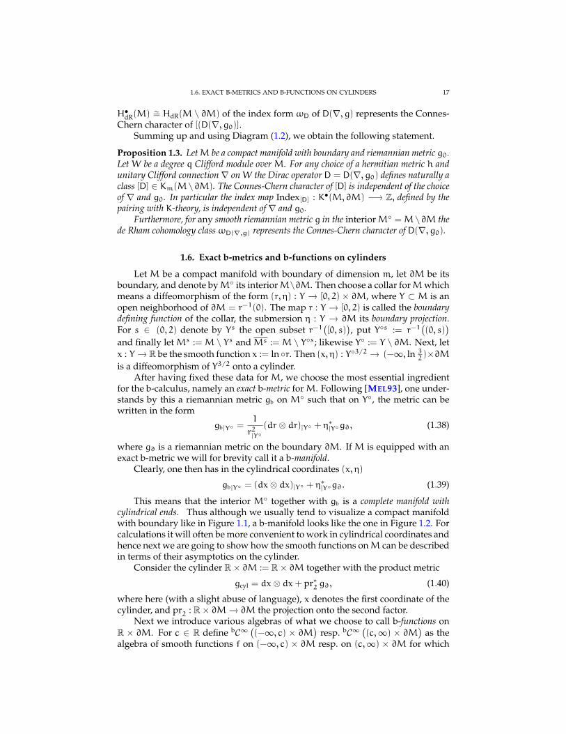
1.6. Exact b-metrics and b-functions on cylinders
Let M be a compact manifold with boundary of dimension m, let ∂M be itsboundary, and denote byM its interiorM\∂M. Then choose a collar forMwhichmeans a diffeomorphism of the form (r, η) : Y → [0, 2) × ∂M, where Y ⊂ M is anopen neighborhood of ∂M = r−1(0). The map r : Y → [0, 2) is called the boundarydefining function of the collar, the submersion η : Y → ∂M its boundary projection.For s ∈ (0, 2) denote by Ys the open subset r−1
([0, s)
), put Ys := r−1
((0, s)
)and finally let Ms :=M \ Ys and Ms :=M \ Ys; likewise Y := Y \ ∂M. Next, letx : Y → R be the smooth function x := ln r. Then (x, η) : Y3/2 → (−∞, ln 3
2)×∂M
is a diffeomorphism of Y3/2 onto a cylinder.After having fixed these data for M, we choose the most essential ingredient
for the b-calculus, namely an exact b-metric forM. Following [MEL93], one under-stands by this a riemannian metric gb on M such that on Y, the metric can bewritten in the form
gb|Y =1
r2|Y
(dr⊗ dr)|Y + η∗|Yg∂, (1.38)
where g∂ is a riemannian metric on the boundary ∂M. If M is equipped with anexact b-metric we will for brevity call it a b-manifold.
Clearly, one then has in the cylindrical coordinates (x, η)
gb|Y = (dx⊗ dx)|Y + η∗|Yg∂. (1.39)
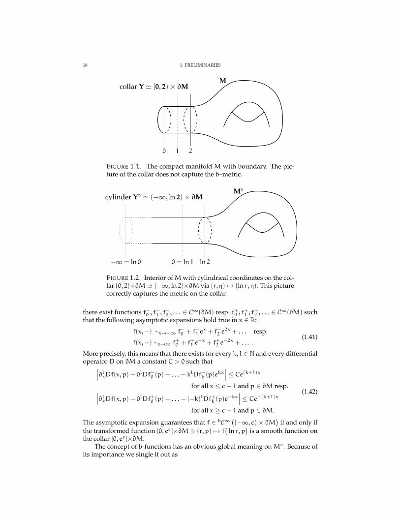
This means that the interior M together with gb is a complete manifold withcylindrical ends. Thus although we usually tend to visualize a compact manifoldwith boundary like in Figure 1.1, a b-manifold looks like the one in Figure 1.2. Forcalculations it will often be more convenient to work in cylindrical coordinates andhence next we are going to show how the smooth functions onM can be describedin terms of their asymptotics on the cylinder.
Consider the cylinder R× ∂M := R× ∂M together with the product metric
gcyl = dx⊗ dx+ pr∗2 g∂, (1.40)
where here (with a slight abuse of language), x denotes the first coordinate of thecylinder, and pr2 : R× ∂M→ ∂M the projection onto the second factor.
Next we introduce various algebras of what we choose to call b-functions onR × ∂M. For c ∈ R define bC∞ ((−∞, c) × ∂M) resp. bC∞ ((c,∞) × ∂M
)as the
algebra of smooth functions f on (−∞, c) × ∂M resp. on (c,∞) × ∂M for which
18 1. PRELIMINARIES
0 1 2
collar Y ' [0, 2)× ∂MM
FIGURE 1.1. The compact manifold M with boundary. The pic-ture of the collar does not capture the b–metric.
−∞ = ln 0 0 = ln 1 ln 2
cylinder Y ' (−∞, ln 2)× ∂MM
FIGURE 1.2. Interior ofMwith cylindrical coordinates on the col-lar (0, 2)×∂M ' (−∞, ln 2)×∂M via (r, η) 7→ (ln r, η). This picturecorrectly captures the metric on the collar.
there exist functions f−0 , f−1 , f
−2 , . . . ∈ C∞(∂M) resp. f+0 , f
+1 , f
+2 , . . . ∈ C∞(∂M) such
that the following asymptotic expansions hold true in x ∈ R:
f(x,−) ∼x→−∞ f−0 + f−1 ex + f−2 e
2x + . . . resp.
f(x,−) ∼x→∞ f+0 + f+1 e−x + f+2 e
−2x + . . . .(1.41)
More precisely, this means that there exists for every k, l ∈ N and every differentialoperator D on ∂M a constant C > 0 such that∣∣∣∂lxDf(x, p) − 0lDf−0 (p) − . . .− klDf−k (p)ekx∣∣∣ ≤ Ce(k+1)x
for all x ≤ c− 1 and p ∈ ∂M resp.∣∣∣∂lxDf(x, p) − 0lDf+0 (p) − . . .− (−k)lDf+k (p)e−kx
∣∣∣ ≤ Ce−(k+1)x
for all x ≥ c+ 1 and p ∈ ∂M.
(1.42)
The asymptotic expansion guarantees that f ∈ bC∞ ((−∞, c) × ∂M) if and only ifthe transformed function [0, ec[×∂M 3 (r, p) 7→ f
(ln r, p
)is a smooth function on
the collar [0, ec[×∂M.The concept of b-functions has an obvious global meaning on M. Because of
its importance we single it out as
1.7. GLOBAL SYMBOL CALCULUS FOR PSEUDODIFFERENTIAL OPERATORS 19
Proposition 1.4. A smooth function f ∈ C∞(M) extends to a smooth function on M ifand only if it is a b-function. In other words this means that the restriction map C∞(M) 3f 7→ f|M ∈ bC∞(M) is an isomorphism of algebras.
The claim is clear from the asymptotic expansions (1.42).The algebra bC∞ (R × ∂M) of b-functions on the full cylinder consists of all
smooth functions f on R× ∂M such that
f|(−∞,0)×∂M ∈ bC∞ ((−∞, 0)× ∂M) and f|(0,∞)×∂M ∈ bC∞ ((0,∞)× ∂M).
Next, we define the algebras of b-functions with compact support on the cylindri-cal ends by bC∞cpt
((−∞, c)× ∂M) :=
f ∈ bC∞ ((−∞, c)× ∂M) | f(x, p) = 0 for x ≥ c− ε, p ∈ ∂M and some ε > 0
resp. by bC∞cpt((c,∞)× ∂M
):=
f ∈ bC∞ ((c,∞)× ∂M)| f(x, p) = 0 for x ≤ c+ ε, p ∈ ∂M and some ε > 0
.
For sections in a vector bundle the notation Γ∞cpt((−∞, 0)×∂M;E) has the analogousmeaning.
The essential property of the thus defined algebras of b-functions is that thecoordinate system (x, η) : Y3/2 → (−∞, ln 3/2)× ∂M induces an isomorphism
(x, η)∗ : bC∞ ((−∞, ln 3/2)× ∂M)→ C∞(Y 32 ), (1.43)
which is defined by putting
(x, η)∗f :=
(Y32 3 p 7→ f(x(p), η(p)), if p /∈ ∂M,
f−0 (η(p)), if p ∈ ∂M.
),
for all f ∈ bC∞ ((−∞, ln 3/2) × ∂M). Under this isomorphism, bC∞cpt((−∞, 3/2) ×
∂M)
is mapped onto C∞cpt
(Y32
). In this article, we will use the isomorphism (x, η)∗
to obtain essential information about solutions of boundary value problems onMby transforming the problem to the cylinder over the boundary and then perform-ing computations there with b-functions on the cylinder.
The final class of b-functions used in this work is the algebra bS(R × ∂M
)of exponentially fast decreasing functions or b-Schwartz test functions on the cylinderdefined as the space of all smooth functions f ∈ C∞(R × ∂M) such that for alll, n ∈ N and all differential operators D ∈ Diff(∂M) there exists a Cl,D,n > 0 suchthat ∣∣∂lxDf(x, p)∣∣ ≤ Cl,D,Ne−n|x| for all x ∈ R and p ∈ ∂M. (1.44)
Obviously, (x, y)∗ maps bS(R×∂M
)∩ bC∞cpt
((−∞, ln 3/2)×∂M) onto the function
space J∞(∂M, Y 32 ) ∩ C∞cpt
(Y32
).
1.7. Global symbol calculus for pseudodifferential operators
In this section, we briefly recall the global symbol for pseudodifferential op-erators which was introduced by Widom in [WID80] (see also [FUKE88, PFL98]).We assume that (M0, g) is a riemannian manifold (without boundary), and thatπE : E → M0 and πF : F → M0 are smooth vector bundle carrying a hermitianmetric µE resp. µF. In later applications, M0 will be the interior of a given mani-fold with boundaryM.
20 1. PRELIMINARIES
Recall that there exists an open neighborhoodΩ0 of the diagonal inM0 ×M0
such that each two points p, q ∈ M0 can be joined by a unique geodesic. Let α0be a cut-off function for Ω0 which means a smooth map M0 ×M0 → [0, 1] whichhas support inΩ0 and is equal to 1 on a neighborhood of the diagonal. These datagive rise to the map
Φ :M×M→ TM, (p, q) 7→ α0(p, q) exp−1p (q) if (p, q) ∈ Ω0,
0 else,(1.45)
which is called a connection-induced linearization (cf. [FUKE88]). Next denote for(p, q) ∈ Ω0 by τEp,q : Ep → Eq the parallel transport in E along the geodesicjoining p and q. This gives rise to the map
τE : E×M→ E, (e, q) 7→ α0(πE(e), q)τEπE(e),q(e), if (πE(e), q) ∈ Ω0,0 else,
(1.46)
which is called a connection-induced local transport on E. (cf. [FUKE88]).Next let us define the symbol spaces Sm
(T∗M0;π
∗T∗ME
). For fixed m ∈ R
this space consists of all smooth sections a : T∗M0 → π∗T∗M0E such that in local
coordinates x : U→ RdimM0 of over U ⊂M0 open and vector bundle coordinates(x, η) : E|U → RdimM0+dimR E the following estimate holds true for each compactK ⊂ U and appropriate CK > 0 depending on K:∥∥∂αx∂βξ (η a)(ξ)∥∥ ≤ CK (1+ ‖T∗x(ξ)‖)m−|β| for all ξ ∈ T∗|KM0. (1.47)
Given a symbol a ∈ Sm(T∗M0;π
∗T∗MHom(E, F)
)one defines now a pseudodiffer-
ential operator Op(a) ∈ Ψm(M0;E, F) by(
Op(a)u)(p) :=
:=1
(2π)dimM
∫TpM0×T∗pM0
α0(p, exp v) e−i〈v,ξ〉 a(p, ξ)τE(u(exp v), p)dvdξ,
(1.48)
where u ∈ Γ∞cpt (E) and p ∈M0. Moreover, there is a quasi-inverse, the symbol mapσ : Ψm
(M0;E, F
)→ Sm(T∗M0;π∗T∗MHom(E, F)
)which is defined by
σ(A)(ξ)(e) := A(α0(p,−) τE(e,−) ei〈ξ,Φ(p,−)〉
)(π(ξ)
), (1.49)
where p ∈ M0, ξ ∈ T∗pM0, e ∈ Ep. It is a well-known result fromglobal symbol calculus (cf. [WID80, FUKE88, PFL98]) that the map Op mapsS−∞(T∗M0;π
∗T∗MHom(E, F)
)onto Ψ−∞(M0;E, F
)and that up to these spaces, Op
and σ are inverse to each other.
1.8. Classical b-pseudodifferential operators
Let us explain in the following the basics of the (small) calculus of b-pseudodifferential operators on a manifold with boundary M. In our presenta-tion, we lean on the approach [LOY05]. For more details on the original approachconfer [MEL93].
In this section, we assume that M carries a b-metric denoted by gb. Further-more, let πE : E → M and πF : F → M be two smooth hermitian vector bundles
1.8. CLASSICAL B-PSEUDODIFFERENTIAL OPERATORS 21
overM, and fix metric connections∇E and∇F. Then observe that by the SchwartzKernel Theorem there is an isomorphism between bounded linear maps
A : J∞(∂M,M;E)→ J∞(∂M,M; F ′
) ′and the strong dual J∞(∂(M ×M),M ×M;E F ′
) ′, where J∞(∂M,M;E):=
J∞(∂M,M) · C∞(M;E). This isomorphism is given by
A 7→ KA :=(J∞(∂M,M;E
)⊗J∞(∂M,M; F ′
)3 (u⊗ v) 7→ 〈Au, v〉), (1.50)
where we have used that
J∞(∂(M×M),M×M;E F ′)= J∞(∂M,M;E
)⊗J∞(∂M,M; F ′
)with ⊗ denoting the completed bornological tensor product. The b-volume formµb associated to gb gives rise to an embedding
M∞(∂M,M;E ′ ⊗ F)→ J∞(∂(M×M),M×M;E F ′
) ′,
k 7→ (u⊗ v 7→ ∫
M×M〈k(p, q), u(p)⊗ v(q)〉d
(µb ⊗ µb
)(p, q)
),
(1.51)
which we use implicitly throughout this work. In the formula for the embed-ding, 〈−,−〉 denotes the natural pairing of an element of a vector bundle withan element of the dual bundle over the same base point, u, v are elements ofJ∞(∂M,M;E
)and J∞(∂M,M; F ′
)respectively, and M∞(X,M;E) denotes for
X ⊂M closed the space of all sections u ∈ Γ∞(M \ X;E) such that in local coordi-nates (y, η) : π−1E (U)→ RdimM+dimE with U ⊂M open one has for every compactK ⊂ U, p ∈ K \ X, and α ∈ NdimM an estimate of the form∥∥∂αy(η u)(p)∥∥ ≤ C 1(
d(y(p), y(X ∩U)
))λ ,where C > 0 and λ > 0 depend only on the local coordinate system, K, and α. Thefundamental property ofM∞(X,M;E) is that
J∞(X,M) · M∞(X,M;E) ⊂ J∞(X,M;E).
Note that the vector bundle E (and likewise the vector bundle F) gives rise to apull-back vector bundle pr∗∂M E|∂M on the cylinder, where pr∂M : R× ∂M→ ∂Mis the canonical projection. This pull-back vector bundle will be denoted by E(resp. F), too. As further preparation we introduce two auxiliary functions ψ :M→ [0, 1] and ϕ :M→ [0, 1] onMwhich are smooth and satisfy suppψ ⊂⊂M1,ψ(p) = 1 for p ∈ M3/2, suppϕ ⊂⊂ Y1, and finally ϕ(p) = 1 for p ∈ Y1/2. Such apair of functions will be called a pair of auxiliary cut-off functions.
By a b-pseudodifferential operator of order m ∈ R we now understand a contin-uous operator A : J∞(∂M,M;E)→ J∞(∂M,M; F ′) ′ such that for one (and hencefor all) pair(s) of auxiliary cut-off functions the following is satisfied:
(bΨ1) The operator (1−ϕ)A(1−ϕ) is a compactly supported pseudodifferentialoperator of orderm in the interiorM.
(bΨ2) The operator ϕAψ is smoothing. Its integral kernel KϕAψ has support insuppϕ×M and lies in J∞(∂(M×M),M×M;E ′ F
).
(bΨ3) The operator ψAϕ is smoothing. Its integral kernel KψAϕ has support inM× suppϕ and lies in J∞(∂(M×M),M×M;E ′ F
).
22 1. PRELIMINARIES
(bΨ4) Consider the induced operator on the cylinder
A : bS(R× ∂M;E
)→ bS(R× ∂M; F
) ′,
u 7→ ((t, p) 7→ [
(1−ψ)A(1−ψ)((x, η)∗u
)]((x, η)−1(t, p)
)),
where bS(R × ∂M;E
):= bS(R)⊗C∞(∂M;E
). Denote by a := σ(A) ∈
Sm(T∗(R × ∂M);π∗Hom(E, F)
)the complete symbol of A defined by
Eq. (1.49) with respect to the product metric on R × ∂M. Then the fol-lowing conditions hold true:
(i) Let y denote local coordinates of ∂M, (y, ξ) the corresponding lo-cal coordinates of T∗∂M, and τ the cotangent variable of the cylin-der variable t ∈ R. Then the symbol a(t, τ, y, ξ) can be (uniquely)extended to an entire function in τ ∈ C such that uniformly in t,uniformly in a strip | Im τ| ≤ Rwith R > 0 and locally uniformly in y∥∥∥∂kt∂lτ∂αy∂βξ a∥∥∥ ≤ Ck,l,α,β (1+ |τ|+ ‖ξ‖)m−l−|β|
for l ∈ N, β ∈ NdimM−1.(ii) There exist symbols ak(τ, y, ξ) ∈ Sm
(C× T∗∂M;π∗Hom(E, F)
), k ∈
N, and rn(t, τ, y, ξ) ∈ Sm(R × C × T∗∂M);π∗Hom(E, F)
), n ∈ N,
which all are entire in τ and fulfill growth conditions as in (i) suchthat for every n ∈ N the following asymptotic expansion holds:
a(t, τ, y, ξ) =
n∑k=0
ektak(τ, y, ξ) + e(n+1)t rn(t, τ, y, ξ).
(iii) The Schwartz kernel KB
of the operator B := A − Op(a) with Op(a)defined by Eq. (1.48) can be represented in the form
KB(t, p, t ′, p ′) =
∫Rei(t−t
′)τ b(t, τ, p, p ′)dτ
with a symbol
b(t, τ, p, p ′) ∈ S−∞(T∗R× ∂M× ∂M;π∗Hom(E, F))
which is entire in τ and which for every m ∈ N, k, l ∈ N and everypair of differential operators Dp and D ′p ′ on ∂M (acting on the vari-able p resp. p ′) satisfies the following estimate uniformly in t, p, p ′
and uniformly in a strip | Im τ| ≤ Rwith R > 0∥∥∥∂kt∂lτDpD ′p ′ b∥∥∥ ≤ Cm,k,l,D,D ′ (1+ |τ|)m.
(iv) There exist symbols
bk(τ, p, p′) ∈ S−∞(C× ∂M× ∂M;π∗Hom(E, F)
),
for k ∈ N and symbols
rn(t, τ, p, p′) ∈ Sm
(R× C× ∂M× ∂M;π∗Hom(E, F)
),
for n ∈ N which all are entire in τ and fulfill growth conditions asin (iii) such that for every n ∈ N the following asymptotic expansion
1.8. CLASSICAL B-PSEUDODIFFERENTIAL OPERATORS 23
holds:
b(t, τ, p, p ′) =
n∑k=0
ekt bk(τ, p, p′) + e(n+1)t rn(t, τ, p, p
′).
If in addition to the above conditions the operators (1−ϕ)A(1−ϕ) and A are bothclassical pseudodifferential operators, then A is a classical b-pseudodifferentialoperator of order m. We denote the space of classical b-pseudodifferential oper-ators on (M,gb) of order m between E and F by bΨ
m(M;E, F), and put as usual
bΨ∞(M;E, F) :=
⋃m∈Z
bΨm(M;E, F). It is straightforward (though somewhat te-
dious) to check that bΨ∞(M;E) := bΨ
∞(M;E, E) even forms an algebra. Obvi-
ously, bΨ∞(M;E, F) contains as a natural subspace the space bDiff(M;E, F) of all
b-differential operators on M from E to F which means of all local classical b-pseudodifferential operators. The following is immediate to check.
Proposition 1.5. Let A ∈ bΨ∞(M;E, F
). Using the notation from above the following
propositions are then equivalent:(1) A ∈ bDiff
(M;E, F
).
(2) The operators (1 − ϕ)A(1 − ϕ) and A are differential operators, and both theoperators ϕAψ and ψAϕ vanish.
(3) The operator A acts as a differential operator over the interior, i.e. as a local op-erator on Γ∞(E|M). In addition, over the cylinder (−∞, 0)× ∂M the operatorA can be written locally in the form
A =∑
j+|α|≤ordA
aj,α∂αy∂jx, (1.52)
where aj,α ∈ bC∞((−∞, 0) × U), U ⊂ ∂M open and y : U → RdimM−1 arelocal coordinates of ∂M.
Over a cylinder (−∞, c)×Nwith c ∈ R andN a compact manifold, we some-times use the notation bΨ
∞cpt((−∞, c) × N;E, F
)to denote the space of all pseudo-
differential operators in bΨ∞(
(−∞, c) ×N;E, F)
having support in some cylinder(−∞, c− ε]×Nwith ε > 0. We also put
bDiffcpt((−∞, c)×N;E, F
):=
bDiff((−∞, c)×N;E, F
)∩ bΨ
∞cpt((−∞, c)×N;E, F
).
(1.53)
Note that in condition (bΨ4) above, the operator A is an element of the spacebΨ
∞cpt((−∞, 3/2)× ∂M;E, F
).
Throughout this work, we also need the b-versions of Sobolev-spaces. Theb-Sobolev space bH
m(M;E) is defined form ∈ N by
bHm(M,E) :=
u ∈ L2(M,E) | Du ∈ L2(M,E) for all D ∈ bDiff
m(M,E)
. (1.54)
For the definition of bHm(M,E) for arbitrary m ∈ R we refer the reader to
[MEL93]. The following result is straightforward.
Proposition 1.6. Let A ∈ bΨl(M;E, F) be a b-pseudodifferential operator. Then the
following holds true:
24 1. PRELIMINARIES
(1) A has a natural extension
A : bHm(M;E)→ bH
m−l(M; F), (1.55)
which we denote by the same symbol like the original operator.(2) The b-Sobolev-space bH
1(M,E) is the natural domain of any elliptic first order
b-pseudodifferential operator acting on sections of E.(3) If A has order l = 0, then A is bounded.
1.9. Indicial family
Assume A ∈ bΨm(M;E, F). Denote by A and a the induced operator and its
complete symbol on the cylinder R × ∂M as above in condition (bΨ4). Considerthe zeroth order term a0 in the asymptotic expansion (bΨ4)(ii) and put for τ ∈ C,u ∈ Γ∞(∂M;E) and p ∈ ∂MI(A)(τ)u(p) := Op
(a0(τ,−)
)u(p) = (1.56)
=1
(2π)dimM−1
∫Tp∂M×T∗p∂M
α0(p, exp v) e−i〈v,ξ〉 a0(τ, p, ξ) τE(u(exp v), p
)dvdξ,
where, as explained in Section 1.7, α0 :M×M→ [0, 1] is a cut-off function vanish-ing outside the injectivity radius and τE is a connection induced parallel transporton E. One thus obtains an entire family I(A) of pseudodifferential operators onthe boundary ∂Mwhich is called the indicial family of A. The indicial family playsa crucial role in deriving the Atiyah–Patodi–Singer index formula within the b-calculus (cf. [MEL93]).
CHAPTER 2
The b-Analogue of the Entire Chern Character
After discussing in Section 2.1 the b-trace in the context of a manifold withcylindrical ends, we digress in Section 2.2 to establish a cohomological analogueof the well-known McKean–Singer formula in the framework of relative cyclic co-homology for the pseudodifferential b-calculus, and then employ it to recast Mel-rose’s approach to the proof of the Atiyah–Patodi–Singer index theorem. In Sec-tion 2.3 we establish an effective formula for the b-trace, which will be used laterin the paper. The rest of this chapter is devoted to a reformulation of Getzler’s ver-sion of the entire Connes–Chern character in the setting of b-calculus, formulatedin terms of relative cyclic cohomology.
2.1. The b-trace
From now on we assume that M is a compact manifold with boundary, thatr : Y → [0, 2) is a boundary defining function, and that gb is an exact b-metric onM. These are the main ingredients of the b-calculus, which we will use in whatfollows (see Sections 1.6 to 1.9 for basic definitions and the monograph [MEL93]for further material on the b-calculus).
Before we can construct the b-analogue of the entire Chern character we haveto recall here however the definition of the b-trace (cf. [MEL93]), since this notionplays an essential role in our work. It will often be convenient to choose cylindricalcoordinates (see Figure 1.2 on page 18) (x, η) : Y → (−∞, ln 2) × ∂M over acollar Y ⊂ M with a boundary defining function r : Y → [0, 2) (see Section 1.6 fordetails and notation). When using these coordinates, we view the interiorM as amanifold with cylindrical ends, and have in this pictureM ∼= (−∞, 0]× ∂M ∪∂MM1. All explicit calculations will be done in cylindrical coordinates as explainedin the previous sections.
Let E be a smooth hermitian vector bundle over M. Whenever convenient,we will tacitly identify elements of Γ∞((−∞, 0] × ∂M;E
), the sections of E over
(−∞, 0] × ∂M, with Γ∞(∂M;E|∂M)–valued smooth functions on (−∞, 0], i.e. ele-ments of C∞((−∞, 0], Γ∞(∂M;E|∂M)
), in the obvious way; cf. Section 1.8. Accord-
ingly, we define for u ∈ Γ∞cpt((−∞, 0]×∂M;E
)the Fourier transform in the cylinder
variable, u(λ) ∈ Γ∞(∂M;E|∂E), by
u(λ, p) :=
∫∞−∞ e
−ixλu(x, p)dx. (2.1)
Now assume that A ∈ bΨ−∞
(M;E) is a smoothing b-pseudodifferential op-erator. In general, A is not trace class in the usual sense. However, since Ahas a smooth Schwartz kernel it is locally trace class, in the sense that ψAϕ istrace class for any pair of smooth functions ψ,ϕ : M → R having compact
25
26 2. THE B-ANALOGUE OF THE ENTIRE CHERN CHARACTER
support in M. Using the notation from Section 1.8, let A be the operator in-duced on the cylinder (−∞, 0] × ∂M. We define then an operator valued symbolA∂(x, λ) : Γ
∞(E|∂M)→ Γ∞(E|∂M) as follows: for v ∈ Γ∞(E|∂M) put(A∂(x, λ)v
)(p) :=
(e−ixλA
(ei·λ ⊗ v
))(x, p). (2.2)
For v ∈ Γ∞(E|∂M) we have (ei·λ ⊗ v)∧ = 2πδλ ⊗ v, hence for u ∈ Γ∞cpt((−∞, 0] ×
∂M;E)
one then obtains
(Au)(x, p) =
1
2π
∫∞−∞ e
ixλ(A∂(x, λ)u(λ,−)
)(p)dλ =
=1
2π
∫∞−∞∫∞−∞ e
i(x−x)λ(A∂(x, λ)u(x,−)
)(p)dx dλ.
(2.3)
We note in passing that A∂(x, λ) can also be constructed from the global symbola as A∂(x, λ) = Op
(a(x, λ,−)
)(cf. Sections 1.7 and 1.8). For the properties of a
see [LOY05, Sec. 2.2] and Section 1.8. In the small b-calculus a(x, λ,−) and henceA∂(x, λ) are entire in λwhile in the full b-calculus they are meromorphic [MEL93].In any case one has
A∂(x, λ) = I(A)(λ) +O(ex), x→ −∞, (2.4)
with a family I(A)(λ), λ ∈ R, of classical pseudodifferential operators on ∂M inthe parameter dependent calculus; cf. e.g. [LMP09, Sec. 2.1] for a brief summary ofthe parameter dependent calculus. It turns out that the operator valued functionλ ∈ R 7→ I(A)(λ) is exactly the indicial family of A as defined in Section 1.9. Thereason is that in terms of the global symbol a one has I(A)(λ) = Op
(a0(λ,−)
),
where a0(λ,−) is the first term in the asymptotic expansion of a with respect tox→ −∞.
Denote by k(x, x), x, x ≥ 0, the L(L2(∂M;E|∂M))-valued kernel of A. In termsof A∂(x, λ) the kernel k(x, x) is given by
k(x, x) =1
2π
∫∞−∞ e
i(x−x)λA∂(x, λ)dλ. (2.5)
Hence, as R→∞ one has in view of (2.4)
Tr(A|x≥−R) =
= Tr(A|M1) +
∫0−R
Tr∂M(k(x, x)) dx
= Tr(A|M1) +1
2π
∫0−∞∫∞−∞ Tr∂M
(A∂(x, λ) − I(A)(λ)
)dλdx
+ R1
2π
∫∞−∞ Tr∂M
(I(A)(λ)
)dλ+O(e−R), R→∞.
(2.6)
The finite part of this expansion is called the b-trace of A:
bTr(A) := Tr(A|M1) +1
2π
∫0−∞∫∞−∞ Tr∂M
(A∂(x, λ) − I(A)(λ)
)dλdx. (2.7)
2.1. THE B-TRACE 27
HenceTr(A|x≥−R)
= bTr(A) + R1
2π
∫∞−∞ Tr∂M
(I(A)(λ)
)dλ+O(e−R), R→∞. (2.8)
Its name notwithstanding, the b-trace is not a trace. One has, however, the follow-ing crucial formula.
Proposition 2.1 ([MEL93, Prop. 5.9], [LOY05, Thm. 2.5]). Assume that A ∈bΨm
cl (M;E) and K ∈ bΨ−∞cl (M;E). Then
bTr(AK− KA) =−1
2πi
∫∞−∞ Tr∂M
(dI(A)(λ)dλ
I(K)(λ))dλ. (2.9)
PROOF IN A SPECIAL CASE. It is instructive to prove this in the special casethat A is a Dirac operator D. We will see in Section 2.4 below that on the cylinderD takes the form D = Γ d
dx+ D∂ and that I(D)(λ) = iΓλ+ D∂.
After choosing cut–off functions w.l.o.g. we may assume that K is supportedin the interior of the cylinder and given by
(Ku)(x) =1
2π
∫∞−∞ e
ixλk(x, λ)u(λ)dλ
=1
2π
∫∞−∞∫∞−∞ e
i(x−y)λk(x, λ)u(y)dydλ
(2.10)
with an operator valued symbol k(x, λ). Then
(DKu)(x) =1
2π
∫∞−∞ e
ixλ(iλΓ + D∂)k(x, λ)u(λ)dλ
+1
2π
∫∞−∞ e
ixλΓ∂xk(x, λ)u(λ)dλ.
(2.11)
Furthermore, since (Du)∧ =(iΓλ+ D∂)uwe have
(KD)u(x) =1
2π
∫∞−∞ e
ixλk(x, λ)(iλΓ + D∂)u(λ)dλ. (2.12)
Consequently
Tr∂M((DK− KD)(x, x)
)=1
2π
∫∞−∞ Tr∂M
(Γ∂xk(x, λ)
)dλ, (2.13)
and hence, since by assumption K is supported in (−∞, 0) × ∂M and taking (2.4)into account, we find∫0
−R
Tr∂M((DK− KD)(x, x)
)dx =
−1
2π
∫∞−∞ Tr∂M
(Γk(−R, λ)
)dλ (2.14)
R→∞−→ −1
2πi
∫∞−∞ Tr∂M
(dI(D)(λ)dλ
I(K, λ))dλ.
Eq. (2.8) immediately entails the following result.
Corollary 2.2. Let A ∈ bΨm
cl (M;E) be a classical b-pseudodifferential operator of orderm < dimM. If the indicial family I(A) vanishes, then A is trace class, and
Tr(A) = bTr(A).
28 2. THE B-ANALOGUE OF THE ENTIRE CHERN CHARACTER
2.2. The relative McKean–Singer formula and the APS Index Theorem
In the introduction to [MEL93], the author explained in detail his elegant ap-proach to the APS index theorem, based on the b-calculus. The relative cohomol-ogy point of view allows to make this approach even more appealing. Indeed, wewill show that the APS index can be obtained as the pairing between a natural rel-ative cyclic 0-cocycle, one of whose components is the b-trace, and a relative cyclic0-cycle constructed out of the heat kernel. This pairing leads in fact to a relativeversion of the McKean–Singer formula.
We start, a bit more abstractly, by considering an exact sequence of algebras
0 −→ J −→ A σ−→ B −→ 0; (2.15)
A,B are assumed to be unital, σ is assumed to be a unital homomorphism. Let τbe a hypertrace on J , i.e. τ satisfies
τ(xa) = τ(ax) for a ∈ A, x ∈ J . (2.16)
Let τ : A −→ C be a linear extension (regularization) of τ toA, which is not assumedto be tracial. Nevertheless, τ induces a cyclic 1-cocycle on B as follows:
µ(σ(a0), σ(a1)) := τ([a0, a1]). (2.17)
Because of Eq. (2.16), µ does indeed depend only on σ(a0), σ(a1). Moreover, thepair (τ, µ) is a relative cyclic cocycle. Namely, in the notation of (1.5), Eq. (2.17)translates into b(τ, µ) = 0.
The relevant example for this paper is the exact sequence
0 −→ bΨ−∞tr (M;E) −→ bΨ
−∞(M;E)+
I−→ S −→ 0, (2.18)
where M is a compact manifold with boundary equipped with an exact b-metric.The operator trace Tr on bΨ
−∞tr (M;E) = Ker I satisfies (2.16), and the b-trace bTr
provides its linear extension to bΨ−∞
(M;E)+.The indicial map I realizes the quotient algebra
S = bΨ−∞
(M;E)+/bΨ−∞tr (M;E)
as a subalgebra of the unitalized algebra S(R, Ψ−∞(∂M;E))+ of Schwartz functionswith values in the smoothing operators Ψ−∞(∂M;E) on the boundary. That S doesnot equal S(R, Ψ−∞(∂M;E))+ (which would be nicer and more intuitive here) hasto do with the fine print of the definition of the b–calculus which requires e.g.the analyticity of the indicial family. For our discussion here these details are notrelevant and hence we will not elaborate further on them.
Going back to the abstract sequence (2.15) assume now that the algebra A isrepresented as bounded operators on some Hilbert space H and that J ⊂ L1(H)consists of trace class operators. LetD be a self-adjoint unbounded operator affili-ated withA, i.e. bounded continuous functions ofD belong toA. Furthermore, weassume that we are in a graded (even) situation and denote the grading operatorby α. Finally we assume that D is a Fredholm operator and that the orthogonalprojection PKerD ∈ J .
We note that in the case of a Dirac operator D on the b-manifold M it is well-known that D is Fredholm if and only if the tangential operator D∂ (see Section 2.4and Eq. (3.30) below) is invertible.
2.2. THE RELATIVE MCKEAN–SINGER FORMULA AND THE APS INDEX THEOREM 29
Define
A0(t) := αDe− 12tD2 , (2.19)
A1(t) :=
∫∞t
De(t2−s)D2 ds. (2.20)
Since D is affiliated with A, Aj(t) ∈ A for t > 0 and j = 1, 2.
2.2.1. Case 1: e−tD2 ∈ J , for t > 0. Under this assumption Aj(t) ∈ J , for
t > 0. Moreover, e−tD2 ∈ Cλ0(J ) = C0(J )/((1− λ)C0(J)) defines naturally a class
in Hλ0(J ).
Lemma 2.3. The class of αe−tD2
in Hλ0(J) equals that of αPKerD. In particular, it isindependent of t.
PROOF. We calculate
b(A0 ⊗A1) = 2α∫∞t
D2e−sD2
ds
= 2α(e−tD
2
− PKerD),
(2.21)
proving that αe−tD2
and αPKerD are homologous.
As an immediate corollary one recovers the classical McKean–Singer formula.Indeed, since the trace τ defines a class in H0λ(J ) one finds
IndD = Tr(αPKerD) = 〈τ, αPKerD〉 = 〈τ, αe−tD2
〉 = Tr(αe−tD2
). (2.22)
2.2.2. Case 2: The general case. The heat operator e−tD2
gives a class inHλ0(A). The pairing of e−tD
2
with τ cannot be expected to be independent of tsince τ is not a trace. It is however a component of the relative cyclic 0-cocycle(τ, µ). Therefore, we are led to construct a relative cyclic homology class frome−tD
2
. By Eq. (1.8) the relative cyclic complex is given by
Cλn(A,B) := Cλn(A)⊕ Cλn+1(B), b :=
(b 0
−σ∗ −b
). (2.23)
From (2.21) we infer
σ(αe−tD2
) = σ(αe−tD2
− αPKerD) =1
2b(σ(A0)⊗ σ(A1)
), (2.24)
hence
b
(αe−tD
2
−12σ(A0)⊗ σ(A1)
)= 0, (2.25)
i.e. the pair EXPt(D) :=(αe−tD
2
,−12σ(A0)⊗ σ(A1)
)is a relative cyclic homology
class. Furthermore, since
b
(12A0 ⊗A10
)=
(α(e−tD
2
− PKerD)
−12σ(A0)⊗ σ(A1)
), (2.26)
the class of EXPt(D) in Hλ0(A,B) equals that of the pair (αPKerD, 0) which, viaexcision, corresponds to the class of αPKerD ∈ HP0(J ). We have thus proved thefollowing result.
30 2. THE B-ANALOGUE OF THE ENTIRE CHERN CHARACTER
Lemma 2.4. The class of the pair(αe−tD
2
,−12σ(A0) ⊗ σ(A1)
)in HCλ0(A,B) equals
that of (αPKerD, 0). In particular, it is independent of t.
Pairing with the relative 0-cocycle (τ, µ) we now obtain the following relativeversion of the McKean–Singer formula:
IndD = Tr(αPKerD) = 〈(τ, µ),(αe−tD
2
,−1
2σ(A0)⊗ σ(A1)
)〉
= τ(αe−tD2
) −1
2µ(σ(A0), σ(A1))
= τ(αe−tD2
) −1
2τ([A0, A1]).
(2.27)
Once known, this identity can also be derived quite directly. Indeed, since[A0, A1] = 2α
∫∞tD2e−sD
2
ds,
τ(αe−tD2
) −1
2τ([A0, A1]) = τ(αe
−tD2) − τ(α
∫∞t
D2e−sD2
ds)
= τ(αe−tD2
) +
∫∞t
d
dsτ(αe−sD
2)ds
= lims→∞ τ
(αe−sD
2).
(2.28)
Let us show that in the case of the Dirac operator on a b-manifold the secondsummand is nothing but the η-invariant of the tangential operator. Indeed, in acollar of the boundary D takes the form
D =
(0 − d
dx+A
ddx
+A 0
)=: Γ
d
dx+ D∂, D∂ =
(0 AA 0
).
Hence, one calculates using Proposition 2.1
1
2µ(I(A0, λ), I(A1, λ))
=−1
4πi
∫∞−∞ Tr∂M
(dI(A0, λ)dλ
I(A1, λ))dλ
=−1
4π
∫∞−∞ Tr∂M
(αΓ
∫∞t
(iλΓ + D∂)e−s(D2∂+λ
2) ds)dλ
=−1
4√π
∫∞t
1√s
Tr∂M((−A 0
0 −A
)e−sA
2)ds
=1
2√π
∫∞t
1√s
Tr∂M(Ae−sA
2)ds =:
1
2ηt(A).
(2.29)
Thus if D is Fredholm we have for each t > 0
IndD = bTr(αe−tD2
) −1
2ηt(A), (2.30)
and taking the limit as t 0 gives the APS index theorem in the b-setting.
2.3. A formula for the b-trace
In this section we give an explicit formula for the b-trace, based on an obser-vation of Loya [LOY05], which provides a convenient tool for subsequent compu-tations.
2.3. A FORMULA FOR THE B-TRACE 31
We first briefly review the Hadamard partie finie integral in the special case ofb-functions. Let f ∈ bC∞((−∞, 0]). From the asymptotic expansion (see Eq. (1.41))
f(x) ∼x→−∞ f−0 + f−1 ex + f−2 e
2x + .... (2.31)
we infer ∫0−R
f(x)dx = f−0 R+ c+O(e−R), R→ −∞. (2.32)
The partie finie integral of f is then defined to be the constant term in the asymptoticexpansion (2.32), i.e.∫0
−R
f(x)dx =: f−0 R+ Pf∫0−∞ f(x)dx+O(e
−R), R→ −∞. (2.33)
The definition of the partie finie integral has an obvious extension to b-functionson manifolds with cylindrical ends (see Section 1.6). Because of its importance, wesingle it out as a definition-proposition.
Definition and Proposition 2.5. Let M be a riemannian manifold with cylindricalends and M the (up to diffeomorphism) unique compact manifold with boundary havingM as its interior. For a function f ∈ bC∞(M) one has∫
x≥−Rf dvol =: c logR+
∫bM
f dvol +O(e−R) as R→∞.This means that
∫bMf dvol is the finite part in the asymptotic expansion of
∫x≥−R f dvol
as R → ∞. More generally, if ω ∈ bΩm(M) is a (top degree) b-differential form, i.e. aform whose coefficients are in bC∞(M), then
∫bMω is defined accordingly as the finite
part of∫x≥−Rω as R→∞.
In local coordinates y1, . . . , yn on ∂M, b-differential p–forms are sums ofterms of the form
ω = f(x, y)dx∧ dyi1 ∧ . . .∧ dyip−1+ g(x, y)dyj1 ∧ . . .∧ dyjp , (2.34)
where 1 ≤ i1 < . . . < ip−1 ≤ n, 1 ≤ j1 < . . . < jp ≤ n and f, g are b-smoothfunctions. Putting ι∗ω := g−0 (y)dyj1 ∧ . . .∧ dyjp (cf. (2.32)) extends to a pullbackι∗ : bΩp(M) → Ωp(∂M). It is easy to see that Stokes’ Theorem holds for
∫bM
andι: ∫
bM
dω =
∫∂M
ι∗ω. (2.35)
For a b-pseudodifferential operator A ∈ bΨ•cl(M;E) of order < −dimM the
b-trace is nothing but the partie finie integral of its kernel over the diagonal:
bTr(A) =∫
bM
trp(KA(p, p))dvol(p), (2.36)
where nowKA(·, ·) denotes the Schwartz kernel ofA and trp denotes the fiber traceon Ep.
Next we mention a useful formula for the partie finie integral in terms of aconvergent integral. By Eq. (1.42), the asymptotic expansion (2.31) may be differ-entiated, hence ∂xf = O(ex), x → −∞, is integrable and thus integration by parts
32 2. THE B-ANALOGUE OF THE ENTIRE CHERN CHARACTER
yields ∫0−R
f(x)dx = Rf(−R) −
∫0−R
x∂xf(x)dx
= Rf−0 −
∫0−∞ x∂xf(x)dx+O(Re
−R), R→ −∞. (2.37)
Hence
Pf∫0−∞ f(x)dx =
∫0−∞ x∂xf(x)dx, (2.38)
where the integrand on the right hand side is summable in the Lebesgue sense.Using the tools from the previous paragraphs, we can now prove the following
theorem about the representation of the b-trace as a trace of certain trace classoperators.
Proposition 2.6. Let M be a compact manifold with boundary and an exact b-metricgb. Fix a collar (r, η) : Y → [0, 2) × ∂M of the boundary ∂M as described in Sec-tion 1.6, and let (x, η) : Y1 → (−∞, 0] × ∂M denote the corresponding diffeomor-phism onto the cylinder (−∞, 0] × ∂M. Assume that A ∈ bΨ
∞cl (M;E) is a classical
b-pseudodifferential operator of order < −dimM, and that its kernel is supported withinthe cylinder (−∞, 0)× ∂M. Then x
[ddx, A]
is trace class and one has
bTr(A) = −Tr(x[ ddx,A])
=
= −
∫(−∞,0)×∂M x
d
dxtrx,q
(KA(x, q; x, q)
)dvol(x, q),
(2.39)
where KA denotes the Schwartz kernel of A.
PROOF. The condition on the support of A is necessary since the operators xand d
dxare only defined on the cylinder. However, Proposition 2.6 can be extended
to arbitrary A ∈ bΨ<− dimMcl (M;E) in a straightforward way: choose a pair of cut-
off functions ϕ,ψ ∈ C∞(M) with support within the cylinder (−∞, 0) × ∂M andsuch that ϕ(x) = 1 for x ≤ −2, ϕ(x) = 0, for x ≥ −3/2, ψ(x) = 1 for x ≤ −1and ψ(x) = 0 for x ≥ −1/2. Finally, choose a cut-off function χ ∈ C∞c (M \ ∂M)with compact support and χ(1 − ϕ) = 1 − ϕ. The definition of the b-trace thenimmediately shows that
bTr(ϕA) = bTr(ψϕA) = bTr(ϕAψ)
and hence
bTr(A) = bTr(ϕAψ) + Tr((1−ϕ)Aχ) =
= −Tr(x[d
dx,ϕAψ]) + Tr((1−ϕ)Aχ).
The fact that x[ ddx, A] is trace class follows by Prop. 2.2, since the indicial family of
the commutator [ ddx, A] vanishes. We provide two variants of proof for (2.39).
2.4. B-CLIFFORD MODULES AND B-DIRAC OPERATORS 33
1st Variant. From equations (2.36) and (2.38) we infer
bTr(A) =∫
b(−∞,0)×∂M trx,q(KA(x, q; x, q)
)dvol(x, q)
= −
∫(−∞,0)×∂M x
d
dxtrx,q
(KA(x, q; x, q)
)dvol(x, q).
(2.40)
This proves the second line of (2.39). The first line follows, since the kernel of[ ddx, A] is given by [ d
dx, KA](x, p;y, q) = ∂xKA(x, p;y, q) + ∂yKA(x, p;y, q) which
for x = y equals ddxKA(x, p; x, p), cf. Eq. (2.38).
2nd Variant. For <z > 0 the operator ezxA is trace class and the function
z 7→ Tr(ezxA) (2.41)
is holomorphic for <z > 0 and it extends meromorphically to <z > −1, 0 is asimple pole and the residue at 0 equals bTr(A) (cf. [LOY05]). Hence
bTr(A) =d
dzzTr(ezxA)
∣∣∣∣z=0
=d
dzTr([ ddx, ezx
]A
)∣∣∣∣z=0
=d
dzTr([ ddx, ezxA
]− ezx
[ ddx,A])∣∣∣∣
z=0
= −Tr(x[ ddx,A]),
(2.42)
since for <z > 0 the trace of the commutator Tr([ ddx, ezxA]), thanks to the decay of
ezx, does vanish. The last claim follows as above.
2.4. b-Clifford modules and b-Dirac operators
Let M be a compact manifold with boundary, r : Y → [0, 2) a boundary defin-ing function, and gb an exact b-metric on M, cf. Section 1.6. If an object is de-rived from a b-metric we indicate this notationally by giving it a b-decoration.This applies in particular to the various structures derived from the riemann-ian metric gb as described in Section 1.4, e.g. the (co)tangent bundles bTM, bT∗M,the Levi-Civita b-connection b∇ belonging to gb, the bundle of Clifford algebrasbC`(M) := C`(bT∗M), and the b-Clifford superconnection bA on a degree q b-Cliffordmodule W over M. For a discussion of bC∞(M) vs. C∞(M) we refer to Section1.6.
In the remainder of this article, we assume that a b-Clifford superconnectionis always of product form near the boundary. This means that over Ys for some swith 0 < s < 2 the superconnection has the form
bA|Ys = η∗∇∂ + η∗ω∂ ∧−,
where η : Y → ∂M is the boundary projection from Section 1.6, ∇∂ is a metricconnection on the restricted bundle W|∂M and ω∂ ∈ Ω•
(∂M;End
(W|∂M
)). Re-
call that the pull-back covariant derivative(η∗∇∂
)on W|Y is uniquely defined by
34 2. THE B-ANALOGUE OF THE ENTIRE CHERN CHARACTER
requiring for ξ ∈ Γ∞(Y;W) that(η∗∇∂
)Vξ =
r∂ξ∂r, if V = r ∂
∂r,
∇∂Vξ, if V = V η for some V ∈ Γ∞(∂M; T∂M).
Note that the b-metric on M and the metric structure on W give rise to theHilbert space H = L2(M;W) of square integrable sections of the b-Clifford mod-ule. By assumption, C`q acts on L2(M;W), hence by Eq. (1.26) one obtains a super-trace Strq : L1C`q
(L2(M;W)
)→ C. Similarly the b-trace gives rise to a b-supertrace
bStrq : bΨ<− dimMcl,C`q
(M;W
)−→ C,
bStrq(K) := (4π)−q/2 bTr(αE1 · ... · EqK).(2.43)
Here, bΨ•cl,C`q
(M;W
)denotes the space of classical b-pseudodifferential operators
which lie in the supercommutant of C`q inH, cf. (1.25) supra.Next consider the natural embedding T∗∂M → bT∗|∂MM. By the univer-
sal property of Clifford algebras one obtains an embedding of Clifford bundlesC`(∂M
)→ bC`
(bT∗|∂MM
). Moreover, the decomposition bT∗|∂MM = T∗M⊕R · r ∂
∂r
induced by gb even gives rise to a splitting bC`(
bT∗|∂MM) → C`
(∂M
). Let now
W → M be a degree q b-Clifford module over M. Then C`(∂M
)acts on W|∂M
via the embedding C`(∂M
)→ bC`
(bT∗|∂MM
). We denote the resulting left ac-
tion of the boundary Clifford bundle on W|∂M again by c. Moreover, the actionW|∂M ⊗ C`q → W|∂M extends to a right action cr
∂ : W|∂M ⊗ C`q+1 → W|∂M byputting
Ej = cr∂(w, ej) :=
cr(w, ej
), for w ∈Wp, p ∈ ∂M, j = 1, · · · , q,
−cl(drr, w), for w ∈Wp, p ∈ ∂M, j = q+ 1,
(2.44)
cf. the beginning of Section 1.4. It is now easy to check that W|∂M together with cand cr
∂ as Clifford actions becomes a degree q+ 1 Clifford-module over ∂M.Now we have the ingredients for the b-supertrace of a supercommutator:
Proposition 2.7 ([GET93A, Cor. 5.5]). Let D be a Dirac operator on a q-graded b-Clifford bundle W, and K ∈ bΨ
−∞cl,C`q
(M;W
). On ∂M put Eq+1 := −cl(dr
r) = −cl(dx).
ThenbStrq
([D, K]Z2
)=
1√π
∫∞−∞ Strq+1,∂M
(I(K, λ)
)dλ. (2.45)
We do not claim here that I(K, λ) commutes with Γ in the graded sense. Thisis not necessary for the definition of Strq+1,∂M.
Remark 2.8. Another consequence of the previous considerations which we singleout for future reference is the structure of a Dirac operator on a cylinder R × ∂M(cf. (1.40)). Since all structures are product, D takes the form
D = c(dx)d
dx+ D∂ =: Γ
( ddx
+A). (2.46)
Here Γ = c(dx) is Clifford multiplication by the normal vector ddx
and D∂ := ΓA isthe tangential operator. D∂ is a Dirac operator on the boundary. Moreover, one hasthe relations
Γ∗ = −Γ, Γ2 = −I, At = A, ΓA+AΓ = ΓD∂ + D∂Γ = 0. (2.47)
2.5. THE B-JLO COCHAIN 35
Now let u be a section of the Clifford bundleW over the cylinder R×M. Then
(Du)(x, p) =1
2π
∫∞−∞(c(dx)
d
dx+ D∂
)eixλu(λ, p)dλ =
=1
2π
∫∞−∞ e
ixλ(ic(dx)λ+ D∂
)u(λ, p)dλ.
(2.48)
By Eqs. (2.3) and (2.4) this proves the following:
Proposition 2.9. Let M be a compact manifold with boundary and let gb be an exactb-metric on M. Furthermore, let D be a Dirac operator on M. Then the indicial family ofD is given by I(D)(λ) = iλc(dx) + D∂.
2.5. The b-JLO cochain
The degree qClifford module approach outlined in Section 1.4 has advantageswhen dealing with manifolds with boundary, because the formulæ for the JLO-cocycle and its transgression (cf. (2.52), (2.53) below) become simpler. To make theconnection to the standard even and odd Chern character without Clifford action,from now on we will also consider ungraded Clifford modules without auxiliaryClifford right action. Therefore we assume that either
• we are in the graded case with q Clifford matrices E1, . . . , Eq where D isodd, and Strq denotes the Clifford trace defined in Section 1.4,
or• we are in the ungraded case, when there are no Clifford matrices and no
grading operator; this case can be conveniently dealt with by putting q =−1 (which is odd!), α = 1 and Strq := Tr = Tr(α·).
From now on, we assume that Dt, t ∈ (0,∞), is a family of self-adjoint differ-ential operators of the form Dt = f(t)D with D the Dirac operator of a q-gradedb-Clifford module W over the b-manifold M (q ≥ −1 according to the previousexplanation) with b-Clifford superconnection (W, bA) and f : (0,∞)→ R a smoothfunction. Dt are Dirac type operators in the sense of [TAY96].
Following Getzler [GET93A, Sec. 6], we define for A0, · · · , Ak ∈ bΨ∞cl (M,W)
(cf. Subsection 1.4.1)
b〈A0, · · · , Ak〉Dt :=
∫∆k
bStrq(A0 e
−σ0D2t · · ·Ak e−σkD
2t)dσ
= bStrq((A0, . . . , Ak)Dt
).
(2.49)
Put for a0, . . . , ak ∈ C∞(M)
bChk(D)(a0, · · · , ak) := b〈a0, [D, a1], · · · , [D, ak]〉, (2.50)
b/chk(D,V)(a0, · · · , ak) :=∑
0≤j≤k
(−1)j deg V b〈a0, [D, a1], · · · , [D, aj],V, [D, aj+1], · · · , [D, ak]〉.(2.51)
The operation b/ch will mostly be used with V = Dt as a second argument.Here Dt is considered of odd degree regardless of the value of q.
Remark 2.10. For q = 0, k even resp. q = −1, k odd bChk(D), b/chk(D, D) are the
b-analogues of the even and odd JLO Chern character and its transgression.
36 2. THE B-ANALOGUE OF THE ENTIRE CHERN CHARACTER
The following result is crucial for this paper. It is essentially due to Getzler[GET93A, Thm. 6.2], although the following version is not stated explicitly in hispaper.
Theorem 2.11. For q ≥ 0 we have the following two equations for bCh•(D) andb/ch(D, D):
b bChk−1(Dt) + B bChk+1(Dt) = Chk(D∂,t) i∗, (2.52)d
dtbChk(Dt) + bb/ch
k−1(Dt, Dt) + B
b/chk+1
(Dt, Dt) = −/chk(D∂,t, D∂,t) i∗.(2.53)
These formulæ will be repeatedly used in Section 4.2 and thereafter. For nota-tional convenience we will omit the symbol i∗ whenever the context makes clearthat this composition is required.
The theorem can be derived from [GET93A, Thm. 6.2] by introducing the formvalued expression
b〈〈A0, · · · , Ak〉〉 :=∫∆k
bStrq(A0 e
−σ0(i dDt+D2t) · · ·Ak e−σk(i dDt+D2t))dσ, (2.54)
and the combined Chern character Ch•G, defined as
ChkG (Dt)(a0, · · · , ak)
:= b〈〈a0, [Dt, a1], · · · , [Dt, ak]〉〉,a0, · · · , ak ∈ C∞(M). (2.55)
For this, Getzler proves
(−i d+ b+ B)Ch•G(Dt) = Ch•G(D∂,t) i∗. (2.56)
Remark 2.12. Note that in this paper we use self-adjoint Dirac operators whileGetzler uses skew-adjoint ones in [GET93A]. Accordingly, our Dirac operatorsdiffer by a factor −i from the Dirac operators in [GET93A]. This explains the ap-pearance of such i-factors in our formulæ , which are not present in [GET93A].
By carefully tracing all the signs and i–factors involved in the graded formvalued Clifford calculus, as well as due to the various conventions, it turns outthat separating (2.56) into its scalar and 1-form parts, using [GET93A, Lem. 2.5]
b〈〈A0, · · · , Ak〉〉 =
= b〈A0, · · · , Ak〉− ik∑j=0
b〈A0, · · · , Aj, dt∧ Dt, Aj+1, · · · , Ak〉,(2.57)
one obtains Eqs. (2.52) and (2.53).However, for completeness, we will give a more direct argument in Section
2.7, without using operator valued forms. The proof below follows the lines ofthe standard proof for the JLO-cocycle representing the Chern character of a θ-summable Fredholm module (cf. [JLO88], [GESZ89]).
2.6. Cocycle and transgression formulæ for the even/odd b-Chern character(without Clifford covariance)
Recall from Remark 2.10 that for q = 0 and k even resp. q = −1 and k oddbCh•(D) is the b-analogue of the even, resp. odd, JLO Chern character. We shallrelate the ungraded (q = −1) case to the graded case with q = 1.
2.6. COCYCLE AND TRANSGRESSION FORMULÆ 37
Starting with an ungraded Dirac operator Dt acting on the Hilbert space H,put
H := H⊕H, α :=
(1 00 −1
), Dt :=
(0 DtDt 0
). (2.58)
Then Dt is odd with respect to the grading operator α and it anti commutes with
E1 :=
(0 1−1 0
). (2.59)
Note thatDt = αE1
(Dt ⊗ I2
)(2.60)
with I2 being the 2× 2 identity matrix.
Proposition 2.13. Let Dt be ungraded (q = −1) and let Dt = αE1(Dt ⊗ I2) be theassociated 1–graded (q = 1) operator. Then for k odd
bChk(Dt) =1√π
bChk(Dt),
b/chk−1
(D,˙Dt) =
1√π
b/chk−1
(Dt, Dt).
(2.61)
Needless to say that these formulæ are valid as well for Ch• and /ch•.
PROOF. Using Proposition 2.7 we find for k odd:b〈a0, [Dt, a1], . . . , [Dt, ak]〉Dt= b〈(αE1)ka0, [Dt ⊗ I2, a1], . . . , [Dt ⊗ I2, ak]〉Dt⊗I2
=
∫∆k
1√4π
bTr((αE1)
k+1︸ ︷︷ ︸=1
a0e−σ0D
2t [Dt, a1] . . . [Dtak]e
−σkD2t ⊗ I2
)=
1√π
b〈a0, [Dt, a1], . . . , [Dt, ak]〉Dt .
(2.62)
The calculation for b/chk−1
(Dt,˙Dt) is completely analogous.
Now we are ready to translate (2.52) and (2.53) into formulæ for the standardeven and odd Chern character without Clifford action.
2.6.1. q = 0. A priori we are in the standard even situation without Cliffordright action. However, D∂ is viewed as C`1 covariant with respect to the Cliffordaction given by E1 = −Γ . On the boundary, Γ gives a natural identification of theeven and odd half spinor bundle and with respect to the splitting into half spinorbundles D takes the form:
D =
(0 −11 0
)︸ ︷︷ ︸
Γ
d
dx+
(0 AA 0
)︸ ︷︷ ︸
D∂
;(2.63)
A is an ungraded Dirac type operator acting on the positive half spinor bundle (itis the operator whose positive spectral projection gives the APS boundary condi-tion). In the notation of Eq. (2.58), we have D∂ = A, E1 = −Γ . Thus, Proposition2.13 and Theorem 2.11 give the following result.
38 2. THE B-ANALOGUE OF THE ENTIRE CHERN CHARACTER
Proposition 2.14. Let M be an even dimensional compact manifold with boundary withan exact b-metric and let Dt = f(t)D be as before. Writing D in a collar of the boundary(in cylindrical coordinates) in the form
D =:
(0 − d
dx+A
ddx
+A
), (2.64)
A is an ungraded Dirac type operator acting on the positive half spinor bundle restrictedto the boundary. Furthermore we have with At = f(t)A
b bChk−1(Dt) + B bChk+1(Dt) =1√π
Chk(At) i∗, (2.65)
d
dtbChk(Dt) + bb/ch
k−1(Dt, Dt) + B
b/chk+1
(Dt, Dt)
= −1√π
/chk(At, At) i∗.(2.66)
2.6.2. q = −1. Now let D be ungraded and put D, α, E1 as in Eqs. (2.58), (2.59),(2.60). Then by Proposition 2.13 we have
bChk(Dt)(a0, . . . , ak) =√π bChk(Dt)(a0, . . . , ak), (2.67)
b/chk(Dt, Dt)(a0, . . . , ak) =
√π b/ch
k(Dt,
˙Dt)(a0, . . . , ak). (2.68)
In the collar of the boundary, we write as usual D = Γ ddx
+ D∂, and thus
D =
(0 ΓΓ 0
)︸ ︷︷ ︸
=:Γ
d
dx+
(0 D∂D∂ 0
)︸ ︷︷ ︸
=:D∂
. (2.69)
D∂ is 2–graded with respect to
E1 =
(0 1−1 0
), E2 = −Γ =
(0 −Γ−Γ 0
). (2.70)
Note that
αE1E2 = −Γ ⊗ I2, D∂ = αE1(D∂ ⊗ I2). (2.71)
For even kwe have
Str2(a0e
−σ0D∂,t2
[D∂,t, a1] · . . . · [D∂,t, ak]e−σkD∂,t2)
=1
4πTr(αE1E2(αE1)
k(a0e
−σ0D2∂,t [D∂,t, a1] · . . . · [D∂,t, ak]e−σkD
2∂,t)⊗ I2
)=−
1
2πTr(Γa0e
−σ0D2∂,t [D∂,t, a1] · . . . · [D∂,t, ak]e−σkD
2∂,t).
(2.72)
With respect to the grading given by −iΓ we can now write
−1
2πTr(Γ ·)=
1
2πiStr0 . (2.73)
Together with (2.67) and (2.68) we have thus proved:
2.7. SKETCH OF PROOF OF THEOREM 2.11 39
Proposition 2.15. Let M be an odd dimensional compact manifold with boundary withan exact b-metric and let D be an ungraded Dirac operator. Writing D in a collar of theboundary (in cylindrical coordinates) in the form
D =: Γd
dx+ D∂, (2.74)
D∂ is a graded Dirac type operator with respect to the grading operator −iΓ . Furthermore,we have
b bChk−1(Dt) + B bChk+1(Dt) =1
2√πi
Chk(D∂) i∗, (2.75)
d
dtbChk(Dt) + bb/ch
k−1(Dt, Dt) + B
b/chk+1
(Dt, Dt)
= −1
2√πi
/chk(D∂t , D∂
t ) i∗.(2.76)
2.7. Sketch of Proof of Theorem 2.11
Recall that Theorem 2.11 is stated for q ≥ 0, hence in this section all Diracoperators will be q–graded with q ≥ 0.
Proposition 2.16. LetA0, . . . , Ak ∈ bΨ•cl,C`q
(M;W
). Assume that for all but one index
j0 the indicial family is independent of λ and commutes with the actions of E1, . . . , Eqand Eq+1 = −Γ (cf. Section 1.4). For the possible exception j0 we assume that Aj0 isproportional to Dt. Then
b〈A0, . . . , Ak〉 = (−1)ε b〈Ak, A0, . . . , Ak−1〉, (2.77)
where ε = |Ak|(|A0|+ . . .+ |Ak−1|).
b〈A0, . . . , Ak〉 =k∑j=0
b〈A0, . . . , Aj, 1, Aj+1, . . . , Ak〉
=
k∑j=0
(−1)εj b〈1,Aj, . . . , Ak, A0, . . . , Aj−1〉,
(2.78)
where εj = (|A0|+ . . .+ |Aj−1|)(|Aj|+ . . .+ |Ak|).For j < k
b〈A0, . . . , Aj−1, [D2, Aj], Aj+1, . . . , Ak〉
= b〈A0, . . . , Aj−2, Aj−1Aj, Aj+1, . . . , Ak〉
− b〈A0, . . . , Aj−1, AjAj+1, Aj+2, . . . , Ak〉.
(2.79)
Similarly, for j = kb〈A0, . . . , Ak−1, [D2, Ak]〉
= b〈A0, . . . , Ak−2, Ak−1Ak〉
− (−1)|Ak|(|A0|+...+|Ak−1|) b〈AkA0, . . . , Ak−1〉.
(2.80)
Note that these formulæ are the same as in Getzler-Szenes [GESZ89, Lemma2.2]. In particular there is no boundary term. The proof proceeds exactly as theproofs of [GET93A, Lemma 6.3] (1),(2), (4), and we omit the details. We only notethat one has to make heavy use of the following lemma in order to show the van-ishing of certain terms:
40 2. THE B-ANALOGUE OF THE ENTIRE CHERN CHARACTER
Lemma 2.17 (Berezin Lemma). Let K ∈ L1C`q(H) (cf. Section 1.4). Then for j < q
Tr(αE1 · . . . · EjK) = 0.
PROOF. If j + q is odd then moving α past E1 · . . . · EjK and using the traceproperty gives
Tr(αE1 · . . . · EjK) = −Tr(E1 · . . . · EjKα)= −Tr(αE1 · . . . · EjK) = 0.
(2.81)
If j + q is even then, since j < q, Eq anti commutes with αE1 · . . . · EjK and hencesimilarly
Tr(αE1 · . . . · EjK) = −Tr(E2qαE1 · . . . · EjK) = Tr(EqαE1 · . . . · EjKEq)= Tr(E2qαE1 · . . . · EjK) = −Tr(αE1 · . . . · EjK) = 0.
We will make repeated use of the equations (2.77)–(2.80). Now we can proceedas for a θ–summable Fredholm module. Following [GBVF01, p. 451] we startwith the supercommutator∫
∆k
bStrq([Dt, a0e
−σ0D2t [Dt, a1] . . . [Dt, ak]e
−σkD2t])dσ, (2.82)
with a0, . . . , ak ∈ bC∞(M). As in [GET93A, bottom of p. 37] one shows, usingProposition 2.7 and the fact that
∫∞−∞ e−λ2dλ =
√π, that this supercommutator
equals〈a0,∂, [D∂t , a1,∂], . . . , [D∂t , ak,∂]〉D∂t . (2.83)
It is important to note that here we are in the case q + 1, where the grading is theinduced grading on the boundary and Eq+1 = −Γ .
For convenience we will write D instead of Dt. Expanding the supercommu-tator (2.82) on the other hand gives
b〈[D, a0], . . . , [D, ak]〉
+
k∑j=1
(−1)j−1 b〈a0, [D, a1] . . . , [D, aj−1], [D2, aj], . . . , [D, ak]〉,(2.84)
where we have used [D2, aj] = [D, [D, aj]]Z2 .We can now calculate the effect of b and B on bCh.
B bChk+1(D)(a0, . . . , ak)
=
k∑j=0
(−1)kj b〈1, [D, aj], . . . , [D, ak], [D, a0], . . . , [D, aj−1]〉
=
k∑j=0
b〈[D, a0], . . . , [D, aj−1], 1, [D, aj], . . . , [D, ak]〉
= b〈[D, a0], . . . , [D, ak]〉,
(2.85)
where we used (2.78) twice. Thus, the first summand in (2.84) equalsB bChk+1(D)(a0, . . . , ak).
2.7. SKETCH OF PROOF OF THEOREM 2.11 41
Furthermore,
b bChk−1(D)(a0, . . . , ak)
= b〈a0a1, [D, a2], . . . , [D, ak]〉
+
k−1∑j=1
(−1)j b〈a0, . . . , [D, ajaj+1], . . . , [D, ak]〉
+ (−1)k b〈aka0, [D, a1], . . . , [D, ak−1]〉
= b〈a0a1, [D, a2], . . . , [D, ak]〉
− b〈a0, a1[D, a2], . . . , [D, ak]〉
+
k−2∑j=1
(−1)j
(b〈a0, [D, a1], . . . , [D, aj]aj+1, . . . , [D, ak]〉
− b〈a0, . . . , [D, aj], aj+1[D, aj+2], . . . , [D, ak]〉
)+ (−1)k−1 b〈a0, [D, a1], . . . , [D, ak−1]ak〉
+ (−1)k b〈aka0, [D, a1], . . . , [D, ak−1]〉
=
k∑j=1
(−1)j−1 b〈a0, [D, a1], . . . , [D2, aj], . . . , [D, ak]〉,
(2.86)
where we have used (2.79) and (2.80). The right hand side of (2.86) equals the sumin the second line of (2.84).
Summing up (2.82), (2.83), (2.84), (2.85), and (2.86) we arrive at Eq. (2.52).
For additional clarity, let us perform two direct checks, for small values of k.
Case 1: k = 0. In this case (2.84) equalsb〈[D, a0]〉 = b〈1, [D, a0]〉 = B bCh1(D)(a0), (2.87)
by (2.78) and we are done in this case.
Case 2: k = 1. Then (2.84) equalsb〈[D, a0], [D, a1]〉+ b〈a0, [D2, a1]〉. (2.88)
The first summand is B bCh2(a0, a1) and the second summand equals in view of(2.80)
b〈a0a1〉− b〈a1a0〉 = b bCh0(D)(a0, a1). (2.89)
2.7.1. The transgression formula. To prove the transgression formula weproceed analogously and start with the supercommutator
k∑j=0
(−1)j∫∆k+1
bStrq([Dt, a0e
−σ0D2t [Dt, a1] . . .
. . . [Dt, aj]e−σjD
2t De−σj+1D
2t . . . [Dt, ak]e
−σk+1D2t])dσ. (2.90)
42 2. THE B-ANALOGUE OF THE ENTIRE CHERN CHARACTER
We compute this supercommutator using Proposition 2.7. Note that by Propo-sition 2.9 I(Dt, λ) is proportional to iΓλ + D∂. The summand iΓλ contributes aterm proportional to
∫∞−∞ λe−λ2dλ = 0. The remaining summand gives, since∫∞
−∞ e−λ2dλ =√π,
k∑j=0
(−1)j〈a0,∂, [D∂t , a1,∂], . . . , [D∂t , aj,∂], D∂
t , . . . , [D∂t , ak,∂]〉
= /chk(D∂, D∂)(a0,∂, . . . , ak,∂).
(2.91)
Let us again emphasize that here we are in the case q+ 1, where the grading is theinduced grading on the boundary and Eq+1 = −Γ .
Next we expand the commutator (2.90). However, we will confine ourselvesto small k. The calculation is basically the same as in [GBVF01, p. 451]. The onlydifference is that on a closed manifold (2.90) is a priori 0 while here it coincideswith the transgressed Chern character on the boundary.
Case 1: k = 0. (2.90) expands to
b〈[Dt, a0], Dt]〉+ b〈a0, [Dt, Dt]〉. (2.92)
On the other hand
Bb/ch1(Dt, Dt)(a0) =
b/ch1(Dt, Dt)(1, a0)
= b〈1, Dt, [Dt, a0]〉− b〈1, [Dt, a0], Dt〉
= − b〈[Dt, a0], 1, Dt〉− b〈[Dt, a0], Dt, 1〉
= − b〈[Dt, a0], Dt]〉,
(2.93)
by (2.78). Moreover using the well–known formula
d
dte−σD
2t = −
∫σ0
e(σ−s)D2t [Dt, Dt]e
−sD2tds, (2.94)
we haved
dtbCh0(Dt)(a0) = − b〈a0, [Dt, Dt]〉, (2.95)
hence altogether
d
dtbCh0(Dt) + Bb/ch
1(Dt, Dt) = −/ch0(D∂t , D
∂
t ). (2.96)
Case 2: k = 1. To be on the safe side, we also look at an example in the oddcase. We will again make repeated use of the formulæ in Proposition 2.16 withoutfurther mentioning. Eq. (2.90) now expands to
b〈[Dt, a0], Dt, [Dt, a1]〉− b〈[Dt, a0], [Dt, a1], Dt〉
+ b〈a0, [Dt, Dt], [Dt, a1]〉+ b〈a0, [Dt, a1], [Dt, Dt]〉
− b〈a0, Dt, [D2t , a1]〉− b〈a0, [D2t , a1], Dt〉.
(2.97)
2.7. SKETCH OF PROOF OF THEOREM 2.11 43
On the other hand
Bb/ch2(Dt, Dt)(a0) =
b/ch2(Dt, Dt)(1, a0, a1) −
b/ch2(Dt, Dt)(1, a1, a0)
= b〈1, Dt, [Dt, a0], [Dt, a1]〉− b〈1, [Dt, a0], Dt, [Dt, a1]〉
+ b〈1, [Dt, a0], [Dt, a1], Dt〉− b〈1, Dt, [Dt, a1], [Dt, a0]〉
+ b〈1, [Dt, a1], Dt, [Dt, a0]〉− b〈1, [Dt, a1], [Dt, a0], Dt〉
= b〈[Dt, a0], [Dt, a1], 1, Dt〉+ b〈[Dt, a0], 1, [Dt, a1], Dt〉
+ b〈[Dt, a0], [Dt, a1], Dt, 1〉− b〈[Dt, a0], Dt, [Dt, a1], 1〉
− b〈[Dt, a0], Dt, 1, [Dt, a1]〉− b〈[Dt, a0], 1, Dt, [Dt, a1]〉
= b〈[Dt, a0], [Dt, a1], Dt〉− b〈[Dt, a0], Dt, [Dt, a1]〉,
(2.98)
which equals the negative of the first two summands of (2.97).Furthermore,
bb/ch0(Dt, Dt)(a0, a1) =
b/ch0(Dt, Dt)([a0, a1]) =
b〈[a0, a1], Dt〉. (2.99)
Applying (2.79) and (2.80) to the last two summands of (2.97) we findb〈a0, Dt, [D2t , a1]〉+ b〈a0, [D2t , a1], Dt〉
= b〈a0, Dta1〉− b〈a1a0, Dt〉+ b〈a0a1, Dt〉− b〈a0, a1Dt〉
= b〈a0, [Dt, a1]〉+ bb/ch0(Dt, Dt)(a0, a1),
(2.100)
hence adding Bb/ch2(Dt, Dt)(a0, a1) and bb/ch
0(Dt, Dt)(a0, a1) to the right hand
side of (2.97) we obtain
/ch1(D∂t , D∂
t )(a0,∂, a1,∂) + Bb/ch
2(Dt, Dt)(a0, a1) + b
b/ch0(Dt, Dt)(a0, a1)
= − b〈a0, [Dt, a1]〉+ b〈a0, [Dt, Dt], [Dt, a1]〉+ b〈a0, [Dt, a1], [Dt, Dt]〉
=−d
dtbCh1(Dt)(a0, a1)
(2.101)
in view of (2.94).With more effort but in a similar manner, the previous considerations can be
extended to arbitrary k, thus proving Eq. (2.53).

CHAPTER 3
Heat Kernel and Resolvent Estimates
This is the most technical chapter of the paper. It is devoted to prove somecrucial estimates for the heat kernel of a b-Dirac operator. These estimates will beused to analyze the short and long time behavior of the Chern character. Through-out this chapter we will mostly work in the cylindrical context.
For the convenience of the reader we start by summarizing some basic esti-mates for the resolvent and the heat operator associated to an elliptic operator.These estimates will then be applied in Section 3.2 to prove comparison results forthe heat kernel and JLO integrand of a Dirac operator on a general manifold withcylindrical ends to those of a corresponding Dirac operator on the model cylinder.In the remainder of the Chapter we will then prove short and large time estimatesfor the b-Chern character. This is in preparation for proving heat kernel asymp-totics in the b-setting in Section 4.1.
3.1. Basic resolvent and heat kernel estimates on general manifolds
During the whole sectionMwill be a riemannian manifold without boundaryand D0 : Γ∞(M;W) −→ Γ∞(M;W) will denote a first order formally self-adjointelliptic differential operator acting between sections of the hermitian vector bun-dle W. We assume that there exists a self-adjoint extension, D, of D0. E.g. if M iscomplete andD0 is of Dirac type thenD0 is essentially self-adjoint; ifM is the inte-rior of a compact manifold with boundary thenD can be obtained by imposing anappropriate boundary condition. For the following considerations it is irrelevantwhich self-adjoint extension is chosen. We just fix one.
3.1.1. Resolvent estimates. We fix an open sector Λ :=z ∈ C \ 0
∣∣ 0 < ε <arg z < 2π− ε
⊂ C \ R+ in the complex plane.
We introduce the following notation: for a function f : Λ→ C we write f(λ) =O(|λ|α+0), λ → ∞, λ ∈ Λ if for every δ > 0, λ0 ∈ Λ, there is a constant Cδ,λ0 suchthat |f(λ)| ≤ Cδ|λ|α+δ for λ ∈ Λ, |λ| ≥ |λ0|.
We write f(λ) = O(|λ|−∞), λ → ∞, λ ∈ Λ if f(λ) = O(|λ|−N) for every N; theO–constant may depend on N.
L2s(M;W) denotes the Hilbert space of sections ofW which are of Sobolev classs. The Sobolev norm of an element f ∈ L2s(M;W) is denoted by ‖f‖s. For a linearoperator T : L2s(M;W)→ L2t(M;W) its operator norm is denoted by ‖T‖s,t.
For an operator T in a Hilbert space H we denote by ‖T‖p the p–th Schattennorm. To avoid confusions the letter p will not be used for Sobolev orders. Notethat the operator norm of T inH coincides with ‖T‖∞.
45
46 3. HEAT KERNEL AND RESOLVENT ESTIMATES
Proposition 3.1. LetA,B ∈ Ψ•(M,W) be pseudodifferential operators of order a, bwithcompact support.1
1. If k > (dimM)/4 + a/2 then A(D2 − λ)−k, (D2 − λ)−kA are Hilbert–Schmidtoperators for λ 6∈ specD2 and we have
‖A(D2 − λ)−k‖2 = O(|λ|a/2+(dimM)/4−k+0), as λ→∞ in Λ. (3.1)
The same estimate holds for ‖(D2 − λ)−kA‖2.2. If k > (dimM + a + b)/2 then A(D2 − λ)−kB is of trace class for λ 6∈ specD2
and‖A(D2 − λ)−kB‖1 = O(|λ|(dimM+a+b)/2−k+0), as λ→∞ in Λ. (3.2)
3. Denote by π1, π2 : M ×M → M the projection onto the first resp. second factorand assume that π2(suppA) ∩ π1(suppB) = ∅. Then A(D2 − λ)−kB is a trace classoperator for any k ≥ 1 and
‖A(D2 − λ)−kB‖1 = O(|λ|−∞), as λ→∞ in Λ. (3.3)
PROOF. 1. Sobolev embedding and elliptic regularity implies that forf ∈ L2(M;W) the section A(D2 − λ)−kf is continuous. Moreover, for r >dimM/2, |λ| ≥ |λ0|, and x in the compact set suppA =: K
‖(A(D2 − λ)−kf
)(x)‖ ≤ C‖(D2 − λ)−kf‖a+r,K
≤ C‖(D2 + I)(a+r)/2(D2 − λ)−kf‖0≤ C|λ|−k+(a+r)/2‖f‖.
(3.4)
For the Schwartz–kernel this implies the estimate
supx∈suppA
∫M
‖A(D2 − λ)−k(x, y)‖2dvol(y) ≤ C|λ|−2k+a+r, (3.5)
and since A has compact support, integration over x yields
‖A(D2 − λ)−k‖22
≤∫
suppA
∫M
‖A(D2 − λ)−k(x, y)‖2dvol(x)dvol(y)
≤ C|λ|−2k+a+r,
(3.6)
proving the estimate (3.1). The estimate for (D2 − λ)−kA follows by taking theadjoint.
2. The second claim follows from the first one using the Holder inequality.3. To prove the third claim we choose cut–off functions ϕ,ψ ∈ C∞c (M) with
ϕ = 1 on π2(suppA), ψ = 1 on π1(suppB) and suppϕ ∩ suppψ = ∅.Then A(D2 − λ)−kB = Aϕ(D2 − λ)−kψB and ϕ(D2 − λ)−kψ is a smoothing
operator in the parameter dependent calculus (cf. Shubin [SHU01, Chap. II]). Hencefor any real numbers s, t,N we have
‖ϕ(D2 − λ)−kψ‖s,t ≤ C(s, t,N) |λ|−N, as λ→∞ in Λ. (3.7)
Since the Sobolev orders s, t are arbitrary this implies the claim.
1This means that their Schwartz kernels are compactly supported inM×M.
3.1. BASIC RESOLVENT AND HEAT KERNEL ESTIMATES ON GENERAL MANIFOLDS 47
Proposition 3.2. Let A ∈ Ψa(M,W) be a pseudodifferential operator with compact sup-port.
1. Let ϕ ∈ C∞(M) be a smooth function such that suppdϕ is compact, i.e. outsidea compact set ϕ is locally constant. Moreover suppose that suppϕ ∩ π1(suppA) = ∅.Then ϕ(D2 − λ)−kA is a trace class operator for any k ≥ 1 and the estimate (3.3) holdsfor ϕ(D2 − λ)−kA.
2. If k > (dimM+ a)/2 then A(D2 − λ)−k, (D2 − λ)−kA are trace class operatorsand the estimate (3.2) holds with B = I.
PROOF. From
(D2 − λ)ϕ(D2 − λ)−kA = [D2, ϕ](D2 − λ)−kA+ϕ(D2 − λ)−k+1A (3.8)
we infer since ϕA = 0
ϕ(D2 − λ)−kA
= (D2 − λ)−1
[D2, ϕ](D2 − λ)−kA, k = 1,
[D2, ϕ](D2 − λ)−kA+ϕ(D2 − λ)−k+1A, k > 1.
(3.9)
Applying Proposition 3.1.3 to the right hand side we inductively obtain the firstassertion.
To prove the second assertion we choose a cut–off function ϕ ∈ C∞c (M) withϕ = 1 on π1(suppA). Then we apply Proposition 3.1.2 to ϕ(D2 − λ)−kA and theproved first assertion to (1−ϕ)(D2 − λ)−kA to reach the conclusion.
For the following Proposition it is crucial that we are precise about domainsof operators:
Definition 3.3. By Diffd(M,W) we denote the space of differential operators oforder d acting on the sections ofW. Given a differential operatorA ∈ Diffa(M,W)we say that the commutator [D2, A] has compact support if
(1) A and At map the domain dom(Dk) into the domain dom(Dk−a) fork ≥ a and
(2) the differential expression [D2, A] has compact support.
The main example we have in mind is where D is a Dirac type operator on acomplete manifold and A is multiplication by a smooth function ϕ such that dϕhas compact support. Then [D2, ϕ] has compact support in the above sense.
Proposition 3.4. Let A ∈ Diffa(M,W) be a differential operator such that [D2, A] hascompact support and is of order ≤ a + 1. Then for k > dimM + a the commutator[A, (D2 − λ)−k] is trace class and
‖[A, (D2 − λ)−k]‖1 = O(|λ|(dimM+a−1)/2−k+0), as λ→∞ in Λ. (3.10)
PROOF. Note first that since A and At map dom(Dk) into dom(Dk−a) thecommutator [A, (D2 − λ)−k] is defined as a linear operator on L2(M;W) and wehave the identity
[A, (D2 − λ)−k] =
k∑j=1
(D2 − λ)−j[D2, A](D2 − λ)−k+j−1. (3.11)
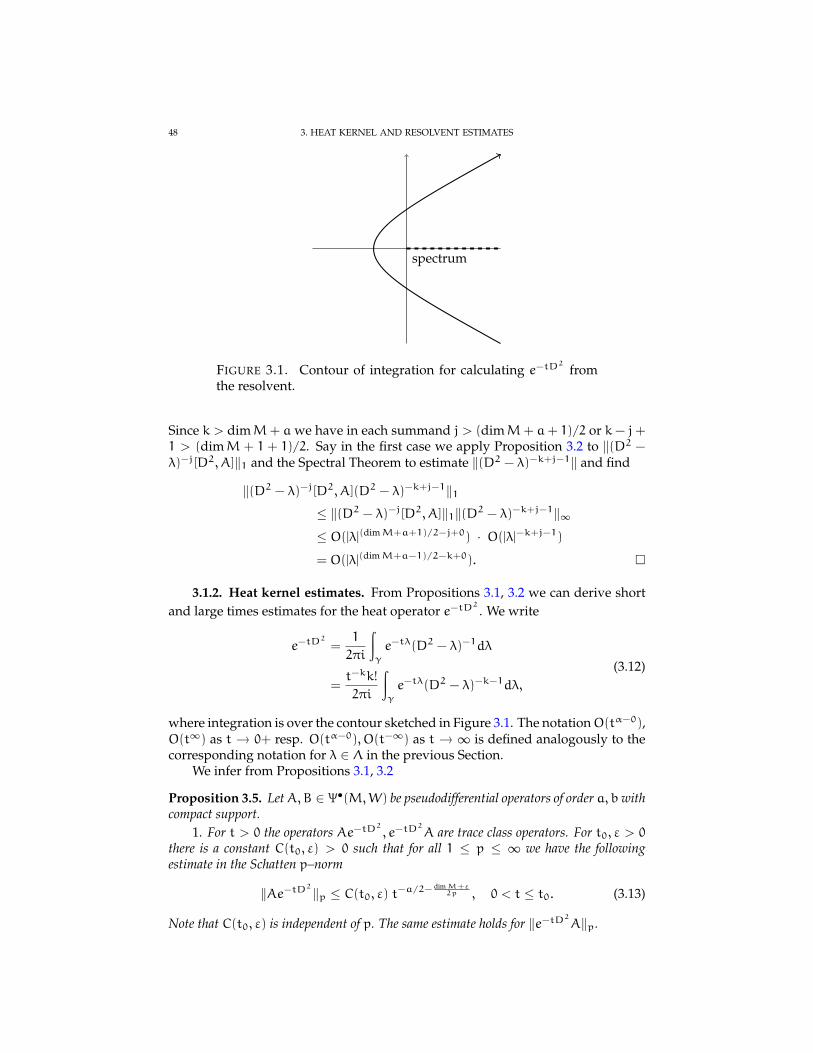
48 3. HEAT KERNEL AND RESOLVENT ESTIMATES
spectrum
FIGURE 3.1. Contour of integration for calculating e−tD2
fromthe resolvent.
Since k > dimM+ a we have in each summand j > (dimM+ a+ 1)/2 or k− j+1 > (dimM + 1 + 1)/2. Say in the first case we apply Proposition 3.2 to ‖(D2 −λ)−j[D2, A]‖1 and the Spectral Theorem to estimate ‖(D2 − λ)−k+j−1‖ and find
‖(D2 − λ)−j[D2, A](D2 − λ)−k+j−1‖1≤ ‖(D2 − λ)−j[D2, A]‖1‖(D2 − λ)−k+j−1‖∞≤ O(|λ|(dimM+a+1)/2−j+0) · O(|λ|−k+j−1)
= O(|λ|(dimM+a−1)/2−k+0).
3.1.2. Heat kernel estimates. From Propositions 3.1, 3.2 we can derive shortand large times estimates for the heat operator e−tD
2
. We write
e−tD2
=1
2πi
∫γ
e−tλ(D2 − λ)−1dλ
=t−kk!
2πi
∫γ
e−tλ(D2 − λ)−k−1dλ,
(3.12)
where integration is over the contour sketched in Figure 3.1. The notationO(tα−0),O(t∞) as t → 0+ resp. O(tα−0), O(t−∞) as t → ∞ is defined analogously to thecorresponding notation for λ ∈ Λ in the previous Section.
We infer from Propositions 3.1, 3.2
Proposition 3.5. LetA,B ∈ Ψ•(M,W) be pseudodifferential operators of order a, bwithcompact support.
1. For t > 0 the operators Ae−tD2
, e−tD2
A are trace class operators. For t0, ε > 0there is a constant C(t0, ε) > 0 such that for all 1 ≤ p ≤ ∞ we have the followingestimate in the Schatten p–norm
‖Ae−tD2
‖p ≤ C(t0, ε) t−a/2−dimM+ε2p , 0 < t ≤ t0. (3.13)
Note that C(t0, ε) is independent of p. The same estimate holds for ‖e−tD2A‖p.
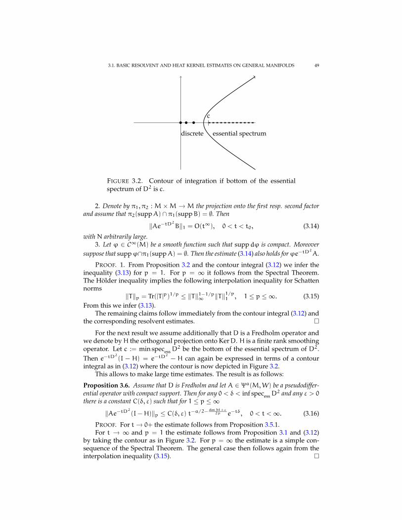
3.1. BASIC RESOLVENT AND HEAT KERNEL ESTIMATES ON GENERAL MANIFOLDS 49
c
essential spectrum
•
discrete
• •
FIGURE 3.2. Contour of integration if bottom of the essentialspectrum of D2 is c.
2. Denote by π1, π2 : M ×M → M the projection onto the first resp. second factorand assume that π2(suppA) ∩ π1(suppB) = ∅. Then
‖Ae−tD2
B‖1 = O(t∞), 0 < t < t0, (3.14)
with N arbitrarily large.3. Let ϕ ∈ C∞(M) be a smooth function such that suppdϕ is compact. Moreover
suppose that suppϕ∩π1(suppA) = ∅. Then the estimate (3.14) also holds forϕe−tD2
A.
PROOF. 1. From Proposition 3.2 and the contour integral (3.12) we infer theinequality (3.13) for p = 1. For p = ∞ it follows from the Spectral Theorem.The Holder inequality implies the following interpolation inequality for Schattennorms
‖T‖p = Tr(|T |p)1/p ≤ ‖T‖1−1/p∞ ‖T‖1/p1 , 1 ≤ p ≤∞. (3.15)From this we infer (3.13).
The remaining claims follow immediately from the contour integral (3.12) andthe corresponding resolvent estimates.
For the next result we assume additionally that D is a Fredholm operator andwe denote byH the orthogonal projection onto KerD. H is a finite rank smoothingoperator. Let c := min specessD
2 be the bottom of the essential spectrum of D2.Then e−tD
2
(I − H) = e−tD2
− H can again be expressed in terms of a contourintegral as in (3.12) where the contour is now depicted in Figure 3.2.
This allows to make large time estimates. The result is as follows:
Proposition 3.6. Assume that D is Fredholm and let A ∈ Ψa(M,W) be a pseudodiffer-ential operator with compact support. Then for any 0 < δ < inf specessD
2 and any ε > 0there is a constant C(δ, ε) such that for 1 ≤ p ≤∞
‖Ae−tD2
(I−H)‖p ≤ C(δ, ε) t−a/2−dimM+ε2p e−tδ, 0 < t <∞. (3.16)
PROOF. For t→ 0+ the estimate follows from Proposition 3.5.1.For t → ∞ and p = 1 the estimate follows from Proposition 3.1 and (3.12)
by taking the contour as in Figure 3.2. For p = ∞ the estimate is a simple con-sequence of the Spectral Theorem. The general case then follows again from theinterpolation inequality (3.15).
50 3. HEAT KERNEL AND RESOLVENT ESTIMATES
Finally we state the analogue of Proposition 3.4 for the heat kernel.
Proposition 3.7. Let A ∈ Diffa(M,W) be a differential operator such that [D2, A] hascompact support (in the sense of Definition 3.3) and is of order ≤ a+ 1.
Then for t > 0 the operator [A, e−tD2
] is of trace class. For t0, ε > 0 there is aconstant C(t0, ε) such that for all 1 ≤ p ≤ ∞ we have the following estimate in theSchatten p–norm
‖[A, e−tD2
]‖p ≤ C(t0, ε) t−a/2−dimM−1+ε
2p , 0 < t ≤ t0; (3.17)
C(t0, ε) is independent of p.If D is a Fredholm operator then for any 0 < δ < inf specessD
2 and any ε > 0 thereis a constant C(δ, ε) such that for 1 ≤ p ≤∞
‖[A, e−tD2
(I−H)]‖p ≤ C(δ, ε) t−a/2−dimM−1+ε
2p e−tδ, 0 < t <∞. (3.18)
PROOF. For p = 1 this follows from Proposition 3.4 and the contour integralrepresentation (3.12) by taking the contours as in Figure 3.1 for t → 0+ and asin Figure 3.2 in the Fredholm case as t → ∞. For p = ∞ the estimates are asimple consequence of the Spectral Theorem. The general case then follows fromthe interpolation inequality (3.15).
3.1.3. Estimates for the JLO integrand. Recall that we denote the standardk–simplex by ∆k :=
(σ0, ..., σk) ∈ Rk+1
∣∣ σj ≥ 0, σ0+ ...+σk = 1
. Furthermore,recall the notation (1.30).
Proposition 3.8. Let Aj ∈ Diffdj(M;W), j = 0, ..., k, be Ddj–bounded differentialoperators on of order dj on M; let d :=
∑kj=0 dj be the sum of their orders. Furthermore,
assume that suppAj0 is compact for at least one index j0.1. For t0, ε > 0 there is a constant C(t0, ε) such that for all σ = (σ0, ..., σk) ∈
∆k, σj > 0,
‖A0e−σ0tD2
A1 · . . . ·Ake−σktD2
‖1
≤ C(t0, ε)
(k∏j=0
σ−dj/2j
)t−d/2−(dimM)/2−ε, 0 < t ≤ t0.
(3.19)
In particular, if dj ≤ 1, j = 0, ..., k, then
‖(A0, ..., Ak)√tD‖ = O(t−d/2−(dimM)/2−0), t→ 0+ . (3.20)
2. Assume additionally thatD is Fredholm and denote byH the orthogonal projectiononto KerD. Then for ε > 0 and any 0 < δ < inf specessD
2 there is a constant C(δ, ε)such that for all σ ∈ ∆k, σj > 0
‖A0e−σ0tD2
(I−H)A1 · . . . ·Ake−σktD2
(I−H)‖1
≤ C(δ, ε)
(k∏j=0
σ−dj/2j
)t−d/2−(dimM)/2−εe−tδ, for all 0 < t <∞. (3.21)
In particular, dj ≤ 1, j = 0, ..., k, then
‖(A0(I−H), ..., Ak(I−H))√tD‖
= O(t−d/2−(dimM)/2−0e−tδ), for all 0 < t <∞. (3.22)
3.1. BASIC RESOLVENT AND HEAT KERNEL ESTIMATES ON GENERAL MANIFOLDS 51
PROOF. We first reduce the problem to the case that all Aj are compactly sup-ported. To this end choose ϕj0−1, ϕj0 ∈ C∞c (M) such that suppϕj0 ∩ supp(1 −ϕj0−1) = ∅ and such that ϕj0Aj0 = Aj0ϕj0 = Aj0 . Decompose Aj0−1 =Aj0−1ϕj0−1 +Aj0−1(1−ϕj0−1).
First we show that the estimates (3.19), (3.21) hold if we replace Aj0−1 byAj0−1(1−ϕj0−1):
Case 1. Proposition 3.5.3 gives
‖Aj0−1(1−ϕj0−1)e−σj0−1tD2
ϕj0‖1 ≤ Ct0σNj0−1tN, for σj0−1t ≤ t0. (3.23)
The operator norm of the other factors can be estimated using the Spectral Theo-rem, taking into account the Ddj -boundedness of Aj:
‖Aje−σjtD2
‖ ≤ Ct0(σjt)−dj/2, for σjt ≤ t0. (3.24)
Hence by the Holder inequality
‖A0e−σ0tD2
A1 · . . . ·Aj0−1(1−ϕj0−1)e−σj0−1tD2
·Ake−σktD2
‖1
≤ Ct0
(k∏j=0
σ−dj/2j
)t−
k∑j=0
dj+N
, 0 < t ≤ t0,(3.25)
which is even better than (3.19).Case 2 (D Fredholm). From (3.23), Proposition 3.6 and the fact thatH is a finite
rank operator with e−ξD2
H = Hwe infer
‖Aj0−1(1−ϕj0−1)e−σj0−1tD2
(I−H)ϕj0‖1≤ Cδe−σj0−1tδ, for all 0 < t <∞. (3.26)
To the other factors we apply Proposition 3.6 with p =∞:
‖Aje−σjtD2
(I−H)‖ ≤ Cδ(σjt)−dj/2e−σjtδ, 0 < t <∞. (3.27)
The Holder inequality combined with (3.26),(3.27) gives (3.21).Altogether we are left to consider A0, ..., Aj0−1ϕj0−1, Aj0 , ...Ak where now
Aj0−1ϕj0−1 and Aj0 are compactly supported. Continuing this way, also to theright of j0, it remains to treat the case where each Aj has compact support.
Case 1. We apply Holder’s inequality for Schatten norms and Proposition 3.5:
‖A0e−σ0tD2
A1 · . . . ·Ake−σktD2
‖1
≤k∏j=0
‖Aje−σjtD2
‖σ−1j
≤ C(t0, ε)k∏j=0
(σjt)−dj/2−
dimM+ε2
σj
≤ C(t0, ε)
(k∏j=0
σ−dj/2j
)t−d/2−
dimM+ε2 , 0 < t ≤ t0,
(3.28)
thanks to the fact that σ 7→ σ−dimM+ε
2σ is bounded as σ→ 0.
Case 2. If D is Fredholm we estimate
‖A0e−σ0tD2
(I−H)A1 · . . . ·Ake−σktD2
(I−H)‖1
52 3. HEAT KERNEL AND RESOLVENT ESTIMATES
using Holder as in (3.28) and apply Proposition 3.6 to the individual factors:
‖Aje−σjtD2
(I−H)‖σ−1j≤ Cδ(σjt)−dj/2−
dimM+ε2
σje−σjtδ, 0 < t <∞, (3.29)
to reach the conclusion.Finally we remark that the inequalities (3.20), (3.22) follow by integrating the
inequalities (3.19), (3.21) over the standard simplex ∆k. Note that∫∆k
(σ0 · . . . ·σk)
−1/2dσ <∞.
3.2. Comparison results
Let Mj, j = 1, 2, be complete riemannian manifolds with cylindrical ends,cf. Proposition 1.4. Assume thatM1 andM2 share a common cylinder component(−∞, 0]×Z. That is, ifMj = (−∞, 0]×Zj ∪Zj Xj, j = 1, 2, then Z is (after a suitableidentification) a common (union of) connected component(s) of Z1, Z2. A typicalexample will beM2 = R× Z.
Suppose that Dj are formally self-adjoint Dirac operators (cf. Section 1.4)on Mj, j = 1, 2 with D1|(−∞,0]×Z = D2|(−∞,0]×Z =: D = c(dx) d
dx+
D∂. The operators Dj are supposed to act on sections of the hermitian vec-tor bundles Wj such that W1|(−∞,0]×Z = W2|(−∞,0]×Z. As explained in Sec-tion 1.6, we identify Γ∞((−∞, c] × Z;W
), c ∈ R, with the completed ten-
sor product C∞((−∞, c])⊗Γ∞(Z;W) and accordingly bΓ∞cpt((−∞, c) × Z;W) with
bC∞cpt((−∞, c))⊗Γ∞(Z;W). We want to compare the resolvents and heat kernels of
Dj on the common cylinder (−∞, 0]× Z.To this end, we will make repeated use of Remark 2.8 without mentioning
it every time. There is an intimate relation between the spectrum, specD∂, of theboundary operator D∂ and the essential spectrum, specess D, ofD. We will only needthat
inf specess D2 = inf specD2∂. (3.30)
A proof of this can be found in [MUL94, Sec. 4]. Concerning notation, ‖T‖p standsfor the p-th Schatten norm of an operator T acting on a Hilbert space H unlessotherwise stated.
Proposition 3.9. 1. Fix an open sector Λ :=z ∈ C∗
∣∣ ε < arg z < 2π − ε⊂
C \ R+ where ε > 0. Then on (−∞, c] × Z, c < 0, the difference of the resolvents(D21 − λ)
−1 − (D22 − λ)−1, λ ∈ Λ, is trace class. Moreover, for N > 0 and λ0 ∈ Λ there
is a constant C(c,N, λ0) such that∥∥∥((D21 − λ)−1 − (D22 − λ)−1)|(−∞,c]×Z
∥∥∥1
≤ C(c,N, λ0) |λ|−N, for λ ∈ Λ, |λ| ≥ |λ0|. (3.31)
2. On (−∞, c]× Z, c < 0, the difference of the heat kernels(Dl1e
−tD21 − Dl2e−tD22
)|(−∞,c]×Z, l ∈ Z+, (3.32)
is trace class for t > 0. Moreover, forN, t0 > 0 there is a constant C(c, l,N, t0) such that∥∥∥(Dl1e−tD21 − Dl2e−tD22
)|(−∞,c]×Z
∥∥∥1≤ C(c, l,N, t0) tN, 0 < t ≤ t0. (3.33)
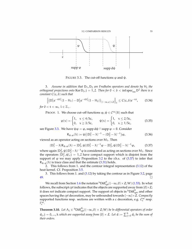
3.2. COMPARISON RESULTS 53
c
suppϕ suppdψ
ϕ ψ
FIGURE 3.3. The cut-off functions ϕ and ψ.
3. Assume in addition that D1,D2 are Fredholm operators and denote by Hj theorthogonal projections onto KerDj, j = 1, 2. Then for 0 < δ < inf specess D
2 there is aconstant C(c, δ) such that∥∥∥(Dl1e−tD21(I−H1) − Dl2e
−tD22(I−H2))|(−∞,c]×Z
∥∥∥1≤ C(c, δ)e−tδ, (3.34)
for 0 < t <∞, l ∈ Z+.
PROOF. 1. We choose cut–off functions ϕ,ψ ∈ C∞(R) such that
ϕ(x) =
1, x ≤ 4/5c,0, x ≥ 3/5c,
ψ(x) =
1, x ≤ 2/5c,0, x ≥ 1/5c,
(3.35)
see Figure 3.3. We have ψϕ = ϕ, suppdψ ∩ suppϕ = ∅. Consider
Rψ,ϕ(λ) := ψ((D21 − λ)
−1 − (D22 − λ)−1)ϕ, (3.36)
viewed as an operator acting on sections overM1. Then
(D21 − λ)Rψ,ϕ(λ) = [D21, ψ](D21 − λ)
−1ϕ− [D22, ψ](D22 − λ)
−1ϕ, (3.37)
where again [D22, ψ](D22−λ)
−1ϕ is considered as acting on sections overM1. Sincethe operators [D2j , ψ], j = 1, 2 have compact support which is disjoint from thesupport of ϕ we may apply Proposition 3.2 to the r.h.s. of (3.37) to infer thatRψ,ϕ(λ) is trace class and that the estimate (3.31) holds.
2. This follows from 1. and the contour integral representation (3.12) of theheat kernel. Cf. Proposition 3.5.
3. This follows from 1. and (3.12) by taking the contour as in Figure 3.2, page49.
We recall from Section 1.6 the notation bDiffa
cpt((−∞, 0)×Z;W) (1.53). In whatfollows, the subscript cpt indicates that the objects are supported away from 0×Z;it does not indicate compact support. The support of objects in bDiff
a
cpt, and otherspaces having the cpt decoration, may be unbounded towards −∞×Z. Compactlysupported functions resp. sections are written with a c decoration, e.g. C∞c resp.Γ∞c .
Theorem 3.10. Let Aj ∈ bDiffdjcpt((−∞, 0) × Z;W) be b–differential operators of order
dj, j = 0, ..., k which are supported away from 0 × Z. Let d :=∑kj=0 dj be the sum of
their orders.
54 3. HEAT KERNEL AND RESOLVENT ESTIMATES
1. For t0, N > 0 there is a constant C(t0, N) such that for all σ ∈ ∆k, σj > 0∥∥∥A0e−σ0tD21 · ... ·Al(e−σltD21 − e−σltD22)Al+1 · ... ·Ake−σktD21∥∥∥1
≤ C(t0, N)
(k∏
j=0,j6=l
σ−dj/2j
)(σlt)
N, 0 < t < t0. (3.38)
2. Assume in addition that D1,D2 are Fredholm operators and denote by Hj theorthogonal projections onto KerDj, j = 1, 2. Then for 0 < δ < inf specess D
2 and allσ ∈ ∆k, σj > 0,∥∥∥A0e−σ0tD21(I−H1) · ... ·Al(e−σltD21(I−H1) − e−σltD22(I−H2))Al+1 · ...
... ·Ake−σktD21(I−H1)
∥∥∥1
≤ C(δ)
(k∏
j=0,j 6=l
σ−dj/2j
)e−tδ, 0 < t <∞. (3.39)
Remark 3.11. With some more efforts one can show that the factors(∏kj=0 σ
−dj/2j
)on the right hand sides of the estimates (3.38), (3.39), and also
below in (3.63), (3.65) are obsolete. But since this is not needed for our purposeswe prefer a less cumbersome presentation.
PROOF. First note that by Proposition 1.6 the operator A(i+D)−a is boundedfor A ∈ bDiff
a
cpt((−∞, 0) × Z;W) and hence the Spectral Theorem implies that fort0 > 0 there is a C(t0) such that
‖Ae−tD2
‖∞ ≤ C(t0)t−a/2, 0 < t < t0. (3.40)
If D is Fredholm then for 0 < δ < inf specessD2 and t0 > 0 there is a C(t0, δ) such
that‖Ae−tD
2
(I−H)‖∞ ≤ C(δ)e−tδ, t0 < t <∞. (3.41)(3.40) and (3.41) together imply that for 0 < δ < inf specessD
2 there is a C(δ) suchthat
‖Ae−tD2
(I−H)‖∞ ≤ C(δ)t−a/2e−tδ, 0 < t <∞. (3.42)The first claim now follows from the second assertion of Theorem 3.9. Namely,
with some c < 0 such that suppAj ⊂ (−∞, c]× Zwe find∥∥∥A0e−σ0tD21 · ... ·Al(e−σltD21 − e−σltD22)Al+1 · ... ·Ake−σktD21∥∥∥1
≤
(k∏
j=0,j 6=l
‖Aje−σjtD21‖∞
) ∥∥Al(i+ D)−dl∥∥∞ ·
·∥∥∥((i+ D1)
dle−σltD21 − (i+ D2)
dle−σltD22)|(−∞,c]×Z
∥∥∥1
≤ C(t0, N)
(k∏
j=0,j 6=l
σ−dj/2j
)σNl t
N−d/2, 0 < t < t0.
(3.43)
Here we have used (3.40). Since σj < 1 an inequality which is valid for 0 < σjt < t0is certainly also valid for 0 < t < t0. Since N is arbitrary (3.43) proves the firstclaim.
3.3. TRACE CLASS ESTIMATES FOR THE MODEL HEAT KERNEL 55
2. Similarly, using the third assertion of Theorem 3.9 and (3.42)∥∥∥A0e−σ0tD21(I−H1) · ... ·Al(e−σltD21(I−H1) − e−σltD22(I−H2))Al+1 · ...... ·Ake−σktD
21(I−H1)
∥∥∥1
≤
(k∏
j=0,j 6=l
‖Aje−σjtD21(I−H1)‖∞
) ∥∥Al(i+ D)−dl∥∥∞·
·∥∥∥((i+ D1)
dle−σltD21(I−H1) − (i+ D2)
dle−σltD22(I−H2)
)|(−∞,c]×Z
∥∥∥1
≤ C(δ)
(k∏
j=0,j 6=l
σ−dj/2j
)t−d/2e−tδ.
(3.44)
Together with the proved short time estimate and the fact that the Hj are of finiterank and thus of trace class we reach the conclusion.
3.3. Trace class estimates for the model heat kernel
We consider the heat kernel of the Laplacian ∆R on the real line
kt(x, y) =1√4πt
e−(x−y)2/4t. (3.45)
By slight abuse of notation we will denote the operator of multiplication by IdRby X. We want to estimate the Schatten norms of eα|X|e−t∆Reβ|X|. Before we startwith this let us note for future reference:∫
Re−
z2
λt−βzdz =
√πλt eλβ
2t/4,∫Re−
z2
λt+β|z|dz ≤ 2
√πλt eλβ
2t/4,
β ∈ R; λ, t > 0. (3.46)
Furthermore, we will need the well-known Schur’s test:
Lemma 3.12 ([HASU78, Thm. 5.2]). Let K be an integral operator on a measure space(Ω,µ) with kernel k : Ω×Ω→ C. Assume that there are positive measurable functionsp, q : Ω→ (0,∞) such that∫
X
|k(x, y)|p(y)dµ(y) ≤ Cp q(x),∫X
|k(x, y)|q(x)dµ(x) ≤ Cq p(y).(3.47)
Then K is bounded in L2(Ω,µ) with ‖K‖ ≤√CpCq.
Now we can prove the following estimate.
Proposition 3.13. Let ∆R = − d2
dx2be the Laplacian on the real line. Then for α > β >
0, t > 0, l ∈ Z+, the integral operator e−α|X|(ddx
)le−t∆Reβ|X| with the (not everywhere
smooth) kernel1√4πt
e−α|x|∂lxe−(x−y)2/4t+β|y| (3.48)
56 3. HEAT KERNEL AND RESOLVENT ESTIMATES
is p-summable for 1 ≤ p ≤∞ and we have the estimate
‖e−α|X|( ddx
)le−t∆Reβ|X|‖p
≤(c1t
− l2− 12p + c2t
− 12p
)(α− β)−1/pe(α
2+β2)t, 0 < t <∞ (3.49)
with (computable) constants c1, c2 independent of α,β, p, t.
Remark 3.14. We are not striving to make these estimates optimal. We chose toformulate them in such a way that they are sufficient for our purposes and suchthat the proofs do not become too cumbersome.
PROOF. We will prove this estimate for p =∞ using Schur’s test Lemma 3.12and for p = 2 by estimating the L2-norm of the kernel. The case p = 1 will thenfollow from the semigroup property of the heat kernel. The result for general pfollows from the cases p = 1 and p =∞ and the interpolation inequality (3.15).
The case l ≥ 2 can easily be reduced to the case l ∈ 0, 1 in view of the identity
∂2kx e−t∆R = (−∆R)
ke−t∆R = ∂kt e−t∆R . (3.50)
The case p = ∞. We apply Schur’s test with p(x) = q(x) = 1. We will makefrequent use of (3.46) without explicitly mentioning it all the time.
1√4πt
∫Re−α|x|−(x−y)2/4t+β|y|dy
≤ 1√4πt
e−α|x|∫Re−z
2/4t+β|x|+β|z|dz
≤ e(β−α)|x|2eβ2t ≤ 2eβ
2t.
(3.51)
Reversing the roles of x and y one gets similarly
1√4πt
∫Reβ|y|−(x−y)2/4t−α|x|dx
≤ 1√4πt
eβ|y|∫Re−z
2/4t−α|y|+α|z|dz
≤ e(β−α)|y|2eα2t ≤ 2eα
2t.
(3.52)
This proves the result for l = 0 and p =∞. In the case l = 1 the integral
1√4πt
∫R
|x− y|
2te−α|x|−(x−y)2/4t+β|y|dy (3.53)
is estimated similarly.
The case p = 2. We estimate the L2-norm of the kernel on R× R by:
1
4πt
∫R
∫Re−2α|x|−
(x−y)2
2t+2β|y|dxdy
≤ 1
4πt
∫Re−2α|x|
∫Re−
z2
2t+2β|z|+2β|x|dzdx
≤ 1√2πt
∫Re−2(α−β)|x|e2β
2tdx
=1√2πt
1
α− βe2β
2t,
(3.54)
3.3. TRACE CLASS ESTIMATES FOR THE MODEL HEAT KERNEL 57
proving the result for l = 0 and p = 2. Again, the case l = 1 is similar.
The case p = 1. Put c = (α + β)/2. Then the semigroup property of the heatkernel gives
‖e−α|X|e−t∆Reβ|X|‖1≤ ‖e−α|X|e−t/2∆Rec|X|‖2‖e−c|X|e−t/2∆Reβ|X|‖2,
(3.55)
and using the proved case p = 2 gives the result for p = 1.
The previous Proposition and standard estimates for the heat kernel on closedmanifolds (cf. the Section 3.1) immediately give the following result for the heatkernel of the model Dirac operator on the cylinder.
Proposition 3.15. Let Z be a compact closed manifold and D = Γ(ddx
+ A)
a Diracoperator on the cylinder M = R × Z (cf. Remark 2.8). Furthermore, let Q ∈bDiff
q
cpt((−∞, 0) × Z;W) a b-differential operator of order q with support in somecylindrical end (−∞, c) × Z. Then for α > β > 0, t > 0 the integral operatore−α|X|Qe−tD
2
eβ|X| with kernel
1√4πt
e−α|x|Qxe−(x−y)2/4t+β|y|e−tA
2
(3.56)
is p-summable for 1 ≤ p ≤ ∞. Furthermore, for ε > 0, t0 > 0, there is a constantC(ε, t0), such that for 1 ≤ p ≤∞, 0 < t < t0, 0 < β < α
‖e−α|X|Qe−tD2
eβ|X|‖p ≤ C(ε, t0)(α− β)−1/pt−dimM+ε2p
−q2 . (3.57)
If in addition the operator A is invertible then for 0 < δ < inf specA2 and ε > 0 thereare constants Cj(δ, ε), j = 1, 2 such that for 1 ≤ p ≤∞, 0 < t <∞, 0 < β < α we havethe estimate
‖e−α|X|Qe−tD2
eβ|X|‖p
≤(C1(δ, ε)t
−q2 + C2(δ, ε)
)(α− β)−1/pt−
dimM+ε2p e(α
2+β2−δ)t. (3.58)
For the definition of bDiffq
cpt,bDiff
qsee Proposition 1.5 and Eq. (1.53).
PROOF. By Proposition 1.5 we may write Q as a sum of operators of the form
f(x, p)P( ddx
)l(3.59)
with• f ∈ bΓ∞cpt((−∞, c)× Z;EndW),• P ∈ Diffb−l(Z;W|Z) a differential operator of order b − l on Z which is
constant in x-direction.Note that e−α|X| commutes with f. Furthermore, f is uniformly bounded. Thus∥∥∥e−α|X|fP∂lxe−tD2eβ|X|∥∥∥
p≤ ‖f‖∞∥∥∥e−α|X|P∂lxe−tD2eβ|X|∥∥∥
p. (3.60)
Inside the p-norm is now a tensor product of operators
e−α|X|P∂lxe−tD2eβ|X| =
(e−α|X|∂lxe
−t∆Reβ|X|)⊗(Pe−tA
2). (3.61)
58 3. HEAT KERNEL AND RESOLVENT ESTIMATES
Since the p-norm of a tensor product is the product of the p-norms the claim fol-lows from Proposition 3.13 and standard elliptic estimates for the closed manifoldZ (Propositions 3.5, 3.6).
3.4. Trace class estimates for the JLO integrand on manifolds with cylindricalends
The heat kernel estimate for the Dirac operator on the model cylinder fromProposition 3.15 together with the comparison result in Section 3.2 will now beused to obtain trace class estimates for b-differential operators similar to the onein Proposition 3.8 if the indicial operator of at least one of the operatorsA0, . . . , Akvanishes. Let us mention here that in the following we will use the notation intro-duced in Subsection 1.4.1, in particular Eq. (1.30).
Proposition 3.16. LetM = (−∞, 0]×Z∪ZX, whereX is a compact manifold with bound-ary, be a complete manifold with cylindrical ends and let D be a Dirac operator on M. LetA0, ..., Ak ∈ bDiff(M;W) be b-differential operators of order d0, ..., dk;d :=
∑kj=0 dj.
Assume that for at least one index l ∈ 0, ..., k the indicial family of Al vanishes. Thenfor t > 0, σ ∈ ∆k the operator
A0e−σ0tD
2
A1 · . . . ·Ake−σktD2
(3.62)
is trace class. Furthermore, there are the following estimates:1. For t0 > 0, ε > 0 there is a constant C(t0, ε) such that for all σ = (σ0, ..., σk) ∈
∆k, σj > 0,
‖A0e−σ0tD2
A1 · . . . ·Ake−σktD2
‖1
≤ C(t0, ε)
(k∏j=0
σ−dj/2j
)t−d/2−(dimM)/2−ε, 0 < t ≤ t0.
(3.63)
In particular, if dj ≤ 1, j = 0, ..., k, then
‖(A0, ..., Ak)√tD‖ = O(t−d/2−(dimM)/2−0), t→ 0+ . (3.64)
2. Assume additionally that D is Fredholm and denote by H the orthogonal projectiononto KerD. Then for ε > 0 and any 0 < δ < inf specess D
2 there is a constant C(δ, ε)such that for all σ ∈ ∆k, σj > 0
‖A0e−σ0tD2
(I−H)A1 · . . . ·Ake−σktD2
(I−H)‖1
≤ C(δ, ε)
(k∏j=0
σ−dj/2j
)t−d/2−(dimM)/2−εe−tδ, for all 0 < t <∞. (3.65)
In particular, if dj ≤ 1, j = 0, ..., k, then
‖(A0(I−H), ..., Ak(I−H))√tD‖
≤ C(ε, δ) t−d/2−(dimM)/2−εe−tδ, for all 0 < t <∞. (3.66)
PROOF. We first reduce the problem to a problem on the cylinder (−∞, 0]×Z.WriteAj = A
(0)j +A
(1)j whereA(0)
j has compact support andA(1)j is supported
on (−∞, c]× Z for some c < 0.Then we split A0e−σ0tD
2
A1 · . . . ·Ake−σktD2
(resp. A0e−σ0tD2
(I−H)A1 · . . . ·Ake
−σktD2
(I−H)) into a sum of terms obtained by decomposingAj = A(0)j +A
(1)j .
3.5. ESTIMATES FOR B-TRACES 59
To the summands involving at least one term A(0)j we apply Proposition 3.8.
To the remaining summand involving only A(1)j we first apply the comparison
Theorem 3.10 with D1 = D and D2 = Γ ddx
+ D∂ = Γ(ddx
+ A), where D2 acts on
sections over the cylinder R× Z; cf. Remark 2.8.Hence it remains to prove the claim for the cylinderM = R×Zwhere eachAj
is supported on (−∞, c]× Z for some c < 0.For definiteness it is not a big loss of generality if we assume that the indicial
family ofA0 vanishes (I.e. l = 0). WriteA0 = e−|X|A0 withA0 ∈ bDiffd0cpt((−∞, 0)×
Z;W). Let β0, ..., βk+1 be real numbers with 1 ≥ β0 > β1 > ... > βk > βk+1 = 0.Let us assume that D is Fredholm and prove the claim 2. The proof of claim 1.
is similar and left to the reader. Holder’s inequality yields∥∥A0e−σ0tD2(I−H)A1 · ... ·Ake−σktD2(I−H)∥∥1≤ C
∥∥e−β0|X|A0e−σ0tD2(I−H)eβ1|X|∥∥σ−10
·
·k∏j=1
∥∥e−βj|X|Aje−σjtD2(I−H)eβj+1|X|∥∥σ−1j
. (3.67)
The individual factors are estimated by Proposition 3.15 and we obtain for 0 < t <∞:
... ≤k∏j=0
(C1,j(δ, ε, β)(tσj)
−dj/2 + C2,j(δ, ε, β))·
· t− dimM+ε2
σje(β2j+β
2j+1−δ)σjt
≤ C(δ, ε, β, γ)( k∏j=0
σ−dj/2j
)t−d/2−
dimM+ε2 e(2
∑β2j+γ−δ)t,
(3.68)
for any γ > 0. The γ > 0 is introduced to compensate t−d/2 as t → ∞. Since wemay choose 2
∑β2j + γ as small as we please, the claim is proved.
The remaining cases are treated similarly.
3.5. Estimates for b-traces
Now we come to the main result of this chapter.
Theorem 3.17. In the notation of Proposition 3.16 we now drop the assumption that theindicial family of one of the Al vanishes. Then the following estimates hold:
1. For ε > 0, t0 > 0 there is a constant C(ε, t0) such that for all σ = (σ0, ..., σk) ∈∆k, σj > 0,
bTr(A0e
−σ0tD2
A1 · . . . ·Ake−σktD2)
≤ C(ε, t0)
(k∏j=0
σ−dj/2−εj
)t−d/2−(dimM)/2−ε, 0 < t ≤ t0.
(3.69)
In particular,
| b〈A0, ..., Ak〉√tD| = O(t−d/2−(dimM)/2−ε), t→ 0+ . (3.70)
60 3. HEAT KERNEL AND RESOLVENT ESTIMATES
2. If D is Fredholm then for ε > 0 and any 0 < δ < inf specess D2 there is a constant
C(ε, δ) such that for all σ ∈ ∆k, σj > 0bTr(A0e
−σ0tD2
(I−H)A1 · . . . ·Ake−σktD2
(I−H))
≤ C(ε, δ)
(k∏j=0
σ−dj/2−εj
)t−d/2−(dimM)/2−εe−tδ, for all 0 < t <∞.
(3.71)
In particular,
| b〈A0(I−H), ..., Ak(I−H)〉√tD|
≤ Cδ,εt−d/2−(dimM)/2−εe−tδ, for all 0 < t <∞. (3.72)
PROOF. Arguing as in the proof of Proposition 3.16 we may assume that D isthe model Dirac operator and that A0, . . . , Ak ∈ bDiffcpt
((−∞, 0)× ∂M;W
).
By Proposition 2.6 we have
bTr(A0e
−σ0tD2
A1 · . . . ·Ake−σktD2)
= −
k∑j=0
Tr(xA0e
−σ0tD2
. . . [d
dx,Aj] . . . e
−σktD2). (3.73)
Although multiplication by x is not a b-differential operator it is easy to see thatProposition 3.16 still holds true for the summands on the right of (3.73). The reasonis that for any fixed ε > 0 the function xe−ε|x| is bounded. In fact any 0 < ε < 1will do since the coefficients of [ d
dx, Aj] are O(ex) as x→ −∞.
3.6. Estimates for the components of the entire b-Chern character
We continue to work in the setting of a complete riemannian manifold withcylindrical ends M, which is equivalent to a compact manifold with boundarywith an exact b-metric, cf. Section 1.6. Furthermore, let D be a Dirac operator onM.
3.6.1. Short time estimates.
Proposition 3.18. The Chern characters bChk and b/chk
defined in (2.50) and (2.51)satisfy the following estimates for k ∈ Z+:
bChk(tD)(a0, · · · , ak) = O(tk−dimM−0),
b/chk(tD,D)(a0, · · · , ak) = O(tk−dimM−0),
t→ 0+, (3.74)
for aj ∈ bC∞(M), j = 0, ..., k.In particular,
(1) limt→0+ bChk(tD) = 0 for k > dimM.
(2) The function t 7→ b/chk(tD,D)(a0, ..., ak) is integrable on [0, T ] for T > 0 and
k > dimM− 1.
PROOF. This follows immediately from Theorem 3.17.
3.6. ESTIMATES FOR THE COMPONENTS OF THE ENTIRE B-CHERN CHARACTER 61
3.6.2. Large time estimates. Unless otherwise said we assume in this Subsec-tion that D∂ is invertible. Then inf specess D
2 = inf specD2∂ > 0 (cf. Eq. (3.30))and hence D is a Fredholm operator. We denote by H the finite rank orthogonalprojection onto the kernel of D.
Lemma 3.19. Let Aj ∈ bDiff(M;W) be b-differential operators of order dj, j =
0, . . . , k;d :=k∑j=0
dj the total order. Furthermore let Hj = H or Hj = I −H, j = 0, ..., k
and assume that Hj = H for at least one index j. Then for each 0 < δ < inf specess D2∥∥∥A0H0e−σ0tD2A1H1e−σ1tD2 . . . AkHke−σktD2∥∥∥
1
≤ C(δ)( ∏l∈j1,...,jq
σ−dl/2l
)t−d/2e−(σj1+...+σjq)tδ, 0 < t <∞, (3.75)
where j1, ..., jq are those indices with Hj = I−H, d =∑l∈j1,...,jq dl.
PROOF. We pick an index lwith Hl = H. Then Holder’s inequality gives∥∥∥A0H0e−σ0tD2A1H1e−σ1tD2 . . . AkHke−σktD2∥∥∥1
≤∥∥AlHle−σltD2∥∥1 ∏
j6=l
∥∥AjHje−σjtD2∥∥∞. (3.76)
The individual factors are estimated as follows: if Hj = H then
‖AjHe−σjtD2
‖p ≤ ‖AjH‖p, for p ∈ 1,∞. (3.77)
If Hj = I − H then by the Spectral Theorem and Proposition 1.6 we have for 0 <δ < inf specess D
2
‖Aj(I−H)e−σjtD2
‖∞ ≤ C(δ,Aj)(σjt)−dj/2e−σjtδ, 0 < t <∞.
The next Lemma is extracted from the proof of [COMO93, Prop. 2].
Lemma 3.20. Let f : Rq+ → C be a (continuous) rapidly decreasing function of q ≤ nvariables. Then
limt→∞ t2q
∫∆n
f(t2σ1, ..., t2σq)dσ
=1
(n− q)!
∫Rq+f(u)du
(3.78)
PROOF. Changing variables uj = t2σj, j = 1, ..., q;uj = σj, j = q + 1, ..., n wefind
t2q∫∆n
f(t2σ1, ..., t2σj)dσ
=
∫t−2(u1+...+uq)+uq+1+...+un)≤1
f(u1, ..., uq)du
=
∫t2∆q
f(u1, ..., uq)
∫(1−t−2(u1+...+uq)
)∆n−q
du
=1
(n− q)!
∫t2∆q
(1− t−2(u1 + ...+ uq)
)n−qf(u)du.
(3.79)
62 3. HEAT KERNEL AND RESOLVENT ESTIMATES
By assumption f is rapidly decreasing, hence we may apply the Dominated Con-vergence Theorem to reach the conclusion.
3.6.3. Estimating the transgressed b-Chern character.
Proposition 3.21. For k ≥ 1 and a0, ..., ak ∈ bC∞(M) we have
b/chk(tD,D)(a0, ..., ak) =
O(t−2), k even ,O(t−3), k odd ,
t→∞. (3.80)
PROOF. /chk(tD,D)(a0, ..., ak) is a sum of terms of the form
T = b〈a0, [tD, a1], ..., [tD, ai−1],D, [tD, ai], ..., [tD, ak]〉tD. (3.81)
Writing A0 = a0, Aj = [D, aj], j = 1, ..., i − 1, Aj = [D, aj−1], j = i + 1, ..., k + 1,Ai := D we find
T = tk∑
Hj∈H,I−H
b〈A0H0, ..., Ak+1Hk+1〉tD, (3.82)
where the sum runs over all sequences H0, ..., Hk+1 with Hj ∈ H, I − H. SinceH[D, aj]H = 0,HD = DH = 0 (note Ai = D !) only terms containing no more than[k/2] + 1 copies of H can give a non-zero contribution.
Consider such a nonzero summand with at least one index j with Hj = H anddenote by q the number of indices l with Hl = I −H. Then q ≥ [k+1
2] + 1 and we
infer from Lemmas 3.19,3.20
tk b〈A0H0, ..., Ak+1Hk+1〉tD = O(tk−2q) =
O(t−2), k even,O(t−3), k odd .
(3.83)
We infer from Theorem 3.17 that the remaining summand with Hj = I − H for allj decays exponentially as t→∞ and we are done.
3.6.4. The limit as t→∞ of the b-Chern character. As in [COMO93] we put
ρH(A) := HAH, (3.84)
and
ωH(A,B) := ρH(AB) − ρH(A)ρH(B). (3.85)
Proposition 3.22. Let a0, ..., ak ∈ bC∞(M). If k is odd then
limt→∞ bChk(tD)(a0, ..., ak) = 0. (3.86)
If k = 2q is even then
limt→∞ bChk(tD)(a0, ..., a2q)
=(−1)q
q!Str(ρH(a0)ωH(a1, a2) . . .ωH(a2q−1, a2q)
)=: κ2q(D)(a0, . . . , a2q).
(3.87)
Of course, since H is of finite rank ρH(aj) andωH(aj, aj+1) are of trace class.
3.6. ESTIMATES FOR THE COMPONENTS OF THE ENTIRE B-CHERN CHARACTER 63
PROOF. As in the previous proof we abbreviate A0 = a0, Aj = [D, aj], j ≥ 1and decompose
b〈A0, A1, ..., Ak〉tD = tk∑
Hj∈H,I−H
b〈A0H0, ..., AkHk〉tD. (3.88)
Since H[D, aj]H = 0 only terms containing no more than [k/2] + 1 copies of H cangive a nonzero contribution.
The term containing no copy ofH decreases exponentially in view of Theorem3.17.
Consider a term containing q copies of I−H. If the number k+ 1−q of copiesof H is at least one but less than k/2 + 1, which is always the case if k is odd, thenq > k/2 and hence in view of Lemmas 3.19, 3.20
tk b〈A0H0, ..., AkHk〉tD = O(tk−2q) = O(t−1), t→∞. (3.89)
If n = 2q is even there is exactly one term containing k/2 + 1 copies of H,namely
t2q b〈A0H,A1(I−H), ..., A2qH〉tD
= t2q∫∆2q
Tr(γa0He
−σ0t2D2 [D, a1](I−H) · ... · e−σ2qt
2D2H)dσ.
(3.90)
The integrand depends only on the q = k/2 variables σ1, σ3, ..., σ2q−1 and so weinfer from Lemma 3.20 that the limit as t→∞ equals1
q!
∫Rq+
Tr(γa0H[D, a1]e
−u1D2
(I−H)[D, a2]H...e−u2q−1D
2
(I−H)[D, a2q]H)du.
(3.91)As in [COMO93, 2.2] one shows that this equals
(−1)q
q!Str(ρH(a0)ωH(a1, a2)...ωH(a2q−1, a2q)
).

CHAPTER 4
The Main Results
We are now in a position to establish the main results of this paper. Afterdiscussing in Section 4.1 asymptotic expansions for the b-analogues of the Jaffe-Lesniewski-Osterwalder components, we construct in Section 4.2 the retracted rel-ative cocycle representing the Connes–Chern character in relative cyclic cohomol-ogy and compute its small and large scale limits. Section 4.3 derives the ensuingpairing formula with the K-theory, and discusses the geometric consequences. Thefinal remark (Section 4.4) offers an explanation for the restrictive eta-pairing whichappears in the work of Getzler and Wu.
4.1. Asymptotic b-heat expansions
4.1.1. b-Heat expansion. Let M be a complete riemannian manifold withcylindrical ends and let D be a Dirac operator onM (cf. Remark 2.8, Section 1.6).
Let Q ∈ bDiffq(M;W) be an auxiliary b-differential operator of order q. It is
well-known (cf. e.g. [GIL95]) that the Schwartz-kernel of the operator Qe−tD2
hasa pointwise asymptotic expansion
(Qe−tD2
)(x, p; x, p) ∼t→0+∞∑j=0
aj(Q,D)(x, p) tj−dimM−q
2 . (4.1)
The problem is that in general neither Qe−tD2
is of trace class nor are the localheat invariants aj(Q,D) integrable over the manifold. Nevertheless we have thefollowing theorem, which has been used implicitly by Getzler [GET93A]. How-ever, we could not find a reference where the result is cleanly stated and proved.Therefore, we provide here a proof for the convenience of the reader.
Theorem 4.1. Under the previously stated assumptions the b-heat trace of Qe−tD2
hasthe following asymptotic expansion:
bTr(Qe−tD
2)∼t→0+
∞∑j=0
∫bM
trp(aj(Q,D)(p)
)dvol(p) t
j−dimM−q2 . (4.2)
The b-integral∫
bMwas defined in Section 2.3, cf. Definition-Proposition 2.5.
PROOF. We first write the operatorQ as a sumQ = Q(0) +Q(1) of differentialoperators with Q(0) ∈ bDiff
q
cpt((−∞, 0) × ∂M;W) and Q(1) a differential operator
supported in the interior. By standard elliptic theory ([GIL95]) Q(1)e−tD2
is traceclass and since the asymptotic expansion (4.1) is uniform on compact subsets ofMthe claim follows for Q(1) instead of Q.
So it remains to prove the claim for an operatorQ ∈ bDiffq
cpt((−∞, 0)×∂M;W);for convenience we write from now on againQ instead ofQ(0). Next we apply the
65
66 4. THE MAIN RESULTS
comparison Theorem 3.9 which allows us to assume thatM = R×∂M is the modelcylinder, D = c(dx) d
dx+D∂, andQ is supported on (−∞, c)× ∂M for some c > 0.
Furthermore, we may assume thatQ is of the form (3.59). Since the heat kernelof the model operator is explicitly known (cf. (3.45)) we have(
f(x, p)P∂lxe−tD2
)(x, p;y, q)
=1√4πt
(∂lxe
−(x−y)2/4t)(Pe−tA
2)(p, q), A := ΓD∂.
(4.3)
If l is odd then by induction one easily shows that this kernel vanishes on thediagonal and hence the b-trace bTr(Qe−tD
2
) as well as all local heat coefficientsvanish, proving the Theorem in this case. So let l = 2k be even. Then using (3.50)and since on the diagonal ∂kt e−t∆R(x, x) = ∂kt (4πt)
−1/2 =: ckt−1/2−k, we have(
f(x, p)P∂lxe−tD2
)(x, p; x, p)
= f(x, p)(Pe−tA
2)(p, p)ck t
−1/2−k
∼t→0+∞∑j=0
f(x, p)aj(P,A)(p)ck tj−dimM−q
2 .
(4.4)
Comparing with (4.1) we find for the heat coefficients aj(Q,D)
aj(Q,D)(x, p) = f(x, p)aj(P,A)(p)ck. (4.5)
Furthermore, we have using Theorem (2.6)
bTr(Qe−tD
2)=
∫0−∞∫∂M
trx,p(x∂xf(x, p)
(Pe−tA
2)(p, p)
)dvol∂M(p)dx. (4.6)(
Pe−tA2)(p, p) has an x-independent asymptotic expansion as t → 0+. Since
x∂xf(x, p) = O(e(1−δ)x), x → −∞, uniformly in p, we can plug the asymptoticexpansion (4.4) into (4.6) and use (4.5) to find
bTr(Qe−tD
2)∼t→0+
∞∑j=0
∫0−∞∫∂M
trx,p(x∂xf(x, p)aj(P,A)(p)
)dvol∂M(p)dx ck t
j−dimM−q2
∼t→0+∞∑j=0
∫b(−∞,0)×∂M trx,p
(aj(Q,D)(x, p)
)dvol(x, p) t
j−dimM−q2 .
The claim is proved.
4.1.2. The b-trace of the JLO integrand. To extend Theorem 4.1 to expres-sions of the form bTr
(A0e
−σ0tD2
A1e−σ1tD
2
...Ake−σktD
2)
we use a trick whichwas already applied successfully in the proof of the local index formula in non-commutative geometry [COMO95]. Namely, we successively commuteAje−σjtD
2
and control the remainder. We will need the estimates proved in Sections 3.4 and3.5.
We first need to introduce some notation (cf. [LES99, Lemma 4.2]). For a b-differential operator B ∈ bDiff(M;W) we put inductively
∇0DB := B, ∇j+1D B := [D2,∇jDB]. (4.7)
4.1. ASYMPTOTIC B-HEAT EXPANSIONS 67
Note that since D2 has scalar leading symbol we have ord(∇jDB) ≤ j+ ordB. Thefollowing formula can easily be shown by induction.
e−tD2
B =
n−1∑j=0
(−t)j
j!
(∇jDB
)e−tD
2
+
+(−t)n
(n− 1)!
∫10
(1− s)n−1e−stD2(∇nDB
)e−(1−s)tD2ds.
(4.8)
The identity (4.8) easily allows to prove the following statement about localheat invariants, cf. [WID79], [COMO90], [BLFO90]:
Proposition 4.2. LetA0, ..., Ak ∈ bDiff(M;W) of order d0, ..., dk;d :=∑kj=0 dj. Then
the Schwartz kernel of A0e−σ0tD2
A1e−σ1tD
2
...Ake−σktD
2
has a pointwise asymptoticexpansion(
A0e−σ0tD
2
A1e−σ1tD
2
...Ake−σktD
2)(p, p)
=∑
α∈Zk+,|α|≤n
(−t)|α|
α!σα10 (σ0 + σ1)
α2 ...(σ0 + ...+ σk−1)αk ·
·(A0∇α1D A1...∇αkD Ake
−tD2)(p, p) +Op(t
(n+1−d−dimM)/2),
=:
n∑j=0
aj(A0, ..., Ak,D)(p) tj−dimM−d
2 +Op(t(n+1−d−dimM)/2),
(4.9)
where d =k∑j=0
dj. The asymptotic expansion is locally uniformly in p. Furthermore, it is
uniform for σ ∈ ∆k.
Again we are facing the problem explained before Theorem 4.1. Still we willbe able to show that one obtains a correct formula by taking the b-trace on the leftand partie finie integrals on the right of (4.9):
Theorem 4.3. Under the assumptions of the previous Proposition 4.2 we have an asymp-totic expansion
bTr(A0e
−σ0tD2
A1e−σ1tD
2
...Ake−σktD
2)
=∑
α∈Zk+,|α|≤n
(−t)|α|
α!σα10 (σ0 + σ1)
α2 ...(σ0 + ...+ σk−1)αk ·
· bTr(A0∇α1D A1...∇αkD Ake
−tD2)+
+O(( k∏j=1
σ−dj/2j
)t(n+1−d−dimM)/2
),
=
n∑j=0
∫bM
aj(A0, ..., Ak,D)dvol tj−dimM−d
2 +
+O(( k∏j=1
σ−dj/2j
)t(n+1−d−dimM)/2
).
(4.10)
68 4. THE MAIN RESULTS
Remark 4.4. The O-constant in (4.10) is independent of σ ∈ ∆k. However, thefactor
(∏kj=1 σ
−dj/2j
)inside the O() causes some trouble because it is integrable
over the standard simplex ∆k only if d1, ..., dk ≤ 1. We do not claim that thisfactor is necessarily there. It might be an artifact of the inefficiency of our method.Cf. also Remarks 3.11, 3.14.
PROOF. The strategy of proof we present here can also be used to prove Propo-sition 4.2.
Again by the comparison Theorem 3.10 we may assume that D is the modelDirac operator and A0, ..., Ak ∈ bDiffcpt((−∞, 0)× ∂M;W).
Using Proposition 2.6 we have
bTr(A0e
−σ0tD2
A1...Ake−σktD
2)
= − bTr(x[ ddx,A0e
−σ0tD2
A1...Ake−σktD
2])= −
k∑j=0
Tr(xA0e
−σ0tD2
A1...[d
dx,Aj]...Ake
−σktD2).
(4.11)
[ ddx, Aj] is again in bDiffcpt((−∞, 0) × ∂M;W) and its indicial family vanishes.
Hence by Proposition 3.16 all summands on the right are of trace class. Cf. alsothe comment at the end of the proof of Theorem 3.17.
It therefore suffices to prove the claim for the summands on the right of (4.11),i.e. for Tr
(xA0e
−σ0tD2
A1...Ake−σktD
2)
where at least one of the Aj has vanishingindicial family.
Applying (4.8) to A1 we get
e−σ0tD2
A1 =
n−1∑j=0
(−σ0t)j
j!
(∇jDA1
)e−σ0tD
2
+ (4.12)
+(−σ0t)
n
(n− 1)!
∫10
(1− s)n−1e−sσ0tD2(∇nDA1
)e−(1−s)σ0tD
2
ds.
Therefore we need to estimate the expression
x(σ0t)n(1− s)n−1A0e
−sσ0tD2(∇nDA1
)e−(1−s)σ0tD
2
e−σ1tD2
...Ake−σktD
2
(4.13)
in the trace norm.If the index l for which the indicial family of Al vanishes is 0 we
write A0 as exA0 with A0 ∈ bDiffcpt((−∞, 0) × ∂M;W) and move xex un-der the trace to the right. This assures that Proposition 3.16 applies to(∇nDA1
)e−(1−s)σ0tD
2
e−σ1tD2
...Ake−σktD
2
xex.If l ≥ 1 we just move x under the trace to the right. After all w.l.o.g. we may
assume that l ≥ 1.
4.2. THE CONNES–CHERN CHARACTER OF THE RELATIVE DIRAC CLASS 69
Next we choose an integer β such that A0(D2 + I)−β has order ∈ 0, 1. ThenHolder’s inequality yields
(σ0t)n(1− s)n−1
∥∥∥A0(I+ D2)−βe−sσ0tD2
(I+ D2)β(∇nDA1
)e−(1−s)σ0tD
2
e−σ1tD2
...Ake−σktD
2
x∥∥∥1
≤ (σ0t)n(1− s)n−1(sσ0t)
−d0/2+β∥∥∥(I+ D2)β
(∇nDA1
)e−(1−s)σ0tD
2
e−σ1tD2
...Ake−σktD
2
x∥∥∥1
(4.14)
To the remaining trace we apply Proposition 3.16 and obtain
... ≤ σn0 tn(1− s)n−1(sσ0t)−d0/2+βC(t0, ε)((1− s)σ0
)−β−n/2−d1/2( k∏j=2
σ−dj/2j
)t−d/2+d0/2−dimM/2−ε−n/2−β
≤ C(t0, ε)s−1/2(1− s)n/2−1−β−d1/2σn−d0−d1
2
0
( k∏j=2
σ−dj/2j
)tn−d−dimM
2−ε.
(4.15)
If we choose n large enough the right hand side is integrable in s and we obtainthe desired estimate.
In the next step we apply (4.8) to e−(σ0+σ1)tD2
and A2. Continuing this waywe reach the conclusion after k steps.
4.2. The Connes–Chern character of the relative Dirac class
4.2.1. Retracted Connes–Chern character. In this section we assume that Dis a Dirac operator on a b-Clifford bundle W → M over the b-manifold M andDt = tD is a family of Dirac type operators. We now have all tools to applythe method of [COMO93] to convert the entire relative Connes-Chern character,which was constructed using the b-trace, into a finitely supported cocycle.
By integrating Eq. (2.53), one obtains for 0 < ε < t
bChk (εD) − bChk(tD) = b
∫tε
b/chk−1
(sD,D)ds
+ B
∫tε
b/chk+1
(sD,D)ds+
∫tε
/chk(sD∂,D∂) i∗ds.(4.16)
Ch•(D∂) satisfies the cocycle and transgression formulæ Eq. (1.33), (1.34). Integrat-ing these we obtain
Chk (εD∂) − Chk(tD∂) = b
∫tε
/chk−1(sD∂,D∂)ds
+ B
∫tε
/chk+1(sD∂,D∂)ds.(4.17)
70 4. THE MAIN RESULTS
By Proposition 3.18 (1), the limit ε 0 exists for k > dimM, and
limε0 bChk(εD) = 0,
limε0Chk−1(εD∂) = 0,
for all k > dimM. (4.18)
The second limit statement follows either from an obvious adaption of our calcu-lations to the ordinary trace or from [COMO93]. Hence one gets for k > dimM
− bChk(tD) = b bT/chk−1t (D) + B bT/chk+1t (D) + T/chkt (D∂) i∗,
−Chk−1(tD∂) = bT/chk−2t (D∂) + BT/chkt (D∂),(4.19)
where
bT/chkt (D) :=∫t0
/chk(sD,D)ds,
T/chk−1t (D∂) :=
∫t0
/chk−1(sD∂,D∂)ds.(4.20)
The above integrals exist in view of Proposition 3.18 (2) even for k ≥ dimM. FromEq. (4.17) and Theorem 2.11 we obtain for k ≥ dimM:
b(
bChk(tD) + B∫tε
b/chk+1
(sD,D)ds)
= −B bChk+2(εD) + Chk+1(εD∂) i∗ − b∫tε
/chk(sD∂,D∂)ds
−→ −bT/chkt (D∂) i∗, ε→ 0+ .
(4.21)
Thus
b(
bChk(tD) + B bT/chk+1t (D))= −bT/chkt (D∂) i∗,
b(
Chk−1(tD∂) + B bT/chkt (D∂))= 0,
k ≥ dimM. (4.22)
Following Connes-Moscovici [COMO93], we define for k ≥ dimM the Chern
characters bchkt (D), bchk(D) and chk−1t (D∂) by
bchkt (D) =∑j≥0
bChk−2j(tD) + B bT/chk+1t (D), (4.23)
chk−1t (D∂) =∑j≥0
Chk−2j−1(tD∂) + BT/chkt (D∂), (4.24)
bchk
t (D) = bchkt (D) + T/chkt (D∂) i∗. (4.25)
4.2. THE CONNES–CHERN CHARACTER OF THE RELATIVE DIRAC CLASS 71
Let us now compute (b+B) bch•t(D). Using Eq. (2.52) and Eq. (4.22) above, wewrite
b bchkt (D) + Bbchkt (D) =
=∑j≥1
(b bChk−2j(tD) + B bChk−2j+2(tD)
)+ b(
bChk(tD) + B bT/chk+1t (D))
=∑j≥1
Chk−2j+1(tD∂) i∗ − bT/chkt (D∂) i∗
=∑j≥0
Chk−2j−1(tD∂) i∗ − bT/chkt (D∂) i∗
= chk−1t (D∂) i∗ − BT/chkt (D∂) i∗ − bT/chkt (D∂) i∗
= chk+1t (D∂) i∗,
(4.26)
where the last equality follows from the second line of Eq. (4.19).In conclusion
(b+ B) bchkt (D) = chk+1t (D∂) i∗
(b+ B) bchk
t (D) = chk−1t (D∂) i∗.(4.27)
Denoting by b, B the relative Hochschild resp. Connes’ coboundaries, cf. Eq. (1.5),we thus infer
(b+ B)( bchkt (D), chk+1t (D∂)
)= 0,
(b+ B)( bch
k
t (D), chk−1t (D∂))= 0,
(4.28)
i.e. the pairs ( bchkt (D), chk+1t (D∂)) and ( bchk
t (D), chk−1t (D∂)) are relative cocyclesin the direct sum of total complexes
Totk⊕ BC•,•(C∞(M), C∞(∂M)) :=
:= Totk⊕ BC•,•(C∞(M))⊕ Totk+1⊕ BC•,•(C∞(∂M)).(4.29)
By Eq. (4.26) we have(bchkt (D) −
bchk
t (D), chk+1t (D∂) − chk−1t (D∂))
=(−T/chkt (D∂) i∗,−(b+ B)T/chkt (D∂)
)=(b+ B
)(0,T/chkt (D∂)
),
(4.30)
hence the two pairs differ only by a coboundary.Next let us compute
(bchk+2t (D), chk+3t (D∂)
)− S(
bchkt (D), chk+1t (D∂))
in theabove relative cochain complex. Using Eq. (4.19) one checks immediately that
bchk+2t (D) − bchkt (D) =bChk+2(tD) + B bT/chk+3t (D) − BT/chk+1t (D)
= − (b+ B)T/chk+1t (D) − T/chk+2t (D∂) i∗.From the second line of Eq. (4.19) (or from [COMO93, Sec. 2.1])
chk+3t (D∂) − chk+1t (D∂) = −(b+ B)T/chk+2t (D∂),
72 4. THE MAIN RESULTS
one thus gets ( bchk+2t (D), chk+3t (D∂))− S( bchkt (D), chk+1t (D∂)
)= (b+ B)
(− bT/chk+1t (D),T/chk+2t (D∂)
).
(4.31)
Hence, the relative cocycles(
bchk+2t (D), chk+3t (D∂))
and S(
bchkt (D), chk+1t (D∂))
are cohomologous. Similarly, one gets
bchkt (D) − chkτ(D) =
=∑j≥0
( bChk−2j(tD) − bChk−2j(τD))+ B
∫tτ
b/chk+1
(sD,D)ds
= − (b+ B)∑j≥0
∫tτ
b/chk−2j−1
(sD,D)ds−∑j≥0
∫tτ
/chk−2j(sD∂,D∂)ds,
resp.
chk+1t (D∂) − chk+1τ (D∂) = −(b+ B)∑j≥0
∫tτ
/chk−2j(sD∂,D∂)ds,
hence(
bchkt (D), chk+1t (D∂))
and(
bchkτ(D), chk+1τ (D∂))
are cohomologous in thetotal relative complex as well. Thus, we have proved (1)-(3) of the following result.
Theorem 4.5. (1) The pairs of retracted cochains(
bchkt (D), chk+1t (D∂)),(
bchk
t (D), chk−1t (D∂)), t > 0, t > 0, k ≥ m = dimM,k − m ∈ 2Z
are cocycles in the relative total complex Tot•⊕ BC•,•(C∞(M), C∞(∂M)).(2) They represent the same class inHCn(C∞(M), C∞(∂M)) which is independent
of t > 0.(3) They represent the same class in HP•(C∞(M), C∞(∂M)) which is independent
of k.(4) Denote by bωD,ωD∂ the local index forms of D resp. D∂ [BGV92, Thm. 4.1],
cf. Eq. (0.4), (0.5) and see Eq. (4.32) below. Then one has a pointwise limit
limt→0+
( bchk
t (D), chk−1t (D∂))=( ∫
bM
bωD ∧ •,∫∂M
ωD∂ ∧ •).
Moreover,(
bchk
t (D), chk−1t (D∂))
represents the Connes-Chern character of[D] ∈ KKm(C0(M);C) = Km(M,∂M).
The pointwise limit will be explained in the proof below. Up to normaliza-tion constants bωD is the A form A(b∇2g) and ωD∂ is the A form A(∇2g∂) on theboundary. Note also that ι∗ωD = ωD∂ .
PROOF. It remains to prove (4). So consider
a0, a1, . . . , aj ∈ bC∞(M).
Using Getzler’s asymptotic calculus (cf. [GET83], [COMO90, §3], and [BLFO90,Thm. 4.1]) one shows that the local heat invariants of
a0e−σ0tD
2
[D, a1]e−σ1tD
2
. . . [D, aj]e−σjtD
2
4.2. THE CONNES–CHERN CHARACTER OF THE RELATIVE DIRAC CLASS 73
(cf. Proposition 4.2) satisfy
tj∫∆j
strq,Wp(a0e
−σ0tD2
[D, a1]e−σ1tD
2
. . . [D, aj]e−σjtD
2)(p, p)dvolgb(p)
=1
j!
(bωD ∧ a0da1 · · ·∧ daj)|p+O(t1/2), t→ 0+ . (4.32)
Here strq,Wp denotes the fiber supertrace in Wp, q indicates the Clifford degreeof D, cf. Section 1.4, the factor 1
j! is the volume of the simplex ∆j. This statementholds locally on any riemannian manifold for any choice of a self-adjoint extensionof a Dirac operator. So it holds for D and accordingly for D∂.
From Theorem 4.3 and its well-known analogue for closed manifolds,cf. [COMO93, Sec. 4], we thus infer
limt→0+ bChj(tD)(a0, . . . , aj)
=1
j!
∫bM
bωD ∧ a0da1 · · ·∧ daj, a0, . . . , aj ∈ bC∞(M), (4.33)
resp.
limt→0+ Chj−1(tD∂)(a0, . . . , aj−1)
=1
(j− 1)!
∫∂M
ωD∂ ∧ a0da1 · · ·∧ daj−1, a0, . . . , aj−1 ∈ C∞(M). (4.34)
Furthermore, in view of (4.20) we have for k ≥ dimM− 1
limt→0+ bT/chk+1t (D)(a0, . . . , ak+1) = 0, a0, . . . , ak+1 ∈ bC∞(M),
limt→0+ T/chkt (D∂)(a0, . . . , ak) = 0, a0, . . . , ak ∈ C∞(M).
(4.35)
To interpret these limit results we briefly recall the relation between de Rhamcurrents and relative cyclic cohomology classes over (bC∞(M), C∞(M)), cf. also[LMP08, Sec. 2.2].
Given a de Rham current C of degree j then C defines naturally a cochainC ∈ Cj(bC∞(M)) by putting C(a0, . . . , aj) := 1
j! 〈C, a0da1 ∧ · · · ∧ daj〉. One has
bC = 0 and BC = ∂C, where ∂ is the codifferential. Because of this identificationwe will from now on omit the ∼ from the notation if no confusion is possible.
Given a closed b-differential form ω on M of even degree. By Cω we denotethe de Rham current
∫bMω∧−. There is a natural pullback ι∗ω at∞ (cf. Definition
and Proposition 2.5), which is a closed even degree form on ∂M. We now find
〈∂Cω, α〉 =∫
bM
ω∧ dα =
∫bM
d(ω∧ α) =
∫∂M
ι∗(ω∧ α) =
=
∫∂M
ι∗(ω)∧ ι∗(α) = 〈Cι∗ω, ι∗(α)〉.(4.36)
In view of Section 1.2 this means that the pair (Cω, Cι∗ω) is a relative deRham cycle or via the above mentioned identification between de Rham currentsand cochains that (Cω, Cι∗ω) is a relative cocycle in the relative total complexEq. (4.29).
74 4. THE MAIN RESULTS
If ω =∑j≥0ω2j with closed b-differential forms of degree 2j then the pair
(ω, ι∗ω) still gives rise to a relative cocycle of degree dimM in the relative totalcomplex. These considerations certainly apply to the even degree forms bωD,ωD∂
which satisfy ι∗(bω) = ωD∂ . The limit results (4.33), (4.34), (4.20) can then besummarized as
limt→0+
( bchk
t (D), chk−1t (D∂))=( ∫
bM
bωD ∧ •,∫∂M
ωD∂ ∧ •). (4.37)
The limit on left is understood pointwise for each component of pure degree.
Finally we need to relate(
bchk
t (D), chk−1t (D∂))
to the Chern character of [D] ∈Km(M,∂M). First recall from Eq. (1.11) that HP•
(C∞(M), C∞(∂M)
)is naturally
isomorphic to HP•(J∞(∂M,M)
). Under this isomorphism, the class of the pair(
bchk
t (D), chk−1t (D∂))
is mapped to bchk
t (D)|J∞(∂M,M), just because elements ofJ∞(∂M,M) vanish on ∂M. We note in passing that by (1.42) a smooth functionf on M lies in J∞(∂M,M) iff in cylindrical coordinates one has for all l, R andevery differential operator P on ∂M
∂lxDf(x, p) = O(eRx), x 7→ −∞.
In view of (4.32), the class of(
bchk
t (D), chk−1t (D∂))
in HP•(J∞(∂M,M)
)equals
that of CbωD. As explained in Section 1.5, HP•
(J∞(∂M,M)
)is naturally isomor-
phic to HdR• (M,∂M;C). Under this isomorphism, CbωD
corresponds to the relativede Rham cycle
(CbωD
, CωD∂
). Finally, note that under the Poincare duality isomor-
phismHdR• (M,∂M;C) ∼= H•dR(M\∂M;C), the relative de Rham cycle
(CbωD
, CωD∂
)is mapped onto the closed form bωD. This line of argument shows that the class of(
bchk
t (D), chk−1t (D∂))
depends only on the absolute de Rham cohomology class ofthe closed form bωD = c · A
(b∇2g
)on the open manifold M \ ∂M. The transgres-
sion formula in Chern–Weil theory shows that the (absolute) de Rham cohomologyclass of A
(∇2g)
is independent of the metric g on M. Thus the de Rham class ofbωD equals that of ωD = c · A
(∇2g0
)for any smooth metric g0. Choosing g0 to
be smooth up to the boundary we infer from Section 1.5 and Proposition 1.3 that
the class of(
bchk
t (D), chk−1t (D∂))
in HP•(C∞(M), C∞(∂M)
)∼= HP•
(J∞(∂M,M)
)equals that of the Connes-Chern character of [D].
4.2.2. The large time limit and higher η–invariants. Let us now assume thatthe boundary Dirac D∂ is invertible. In view of Proposition 3.21 and Proposition3.18 we can now, for k ≥ dimM, form the transgressed cochain
bT/chk∞(D)(a0, ..., ak) =
∫∞0
b/chk(sD,D)(a0, . . . , ak)ds, (4.38)
for a0, . . . , ak ∈ bC∞(M). In view of Eq. (2.98) we arrive at
B bT/chk+1∞ (D)(a0, ..., ak)
=
k∑j=0
(−1)j+1∫∞0
sk+1 b〈[D, a0], . . . , [D, aj],D, [D, aj+1], . . . , [D, ak]〉ds
4.3. RELATIVE PAIRING FORMULÆ AND GEOMETRIC CONSEQUENCES 75
=
k∑j=0
(−1)j+1∫∞0
sk+1∫∆k+1
bStrq([D, a0]e
−σ0s2D2 . . . (4.39)
[D, aj]e−σjs
2D2De−σj+1s2D2 . . . [D, ak]e
−σk+1s2D2)dσds.
Together with Proposition 3.22 we have proved the analogue of [COMO93,Thm. 1] in the relative setting:
Theorem 4.6. Let k ≥ dimM be of the same parity as q and assume that D∂ is invertible.Then the pair of retracted cochains
(bchkt (D), chk+1t (D∂)
), t > 0, has a limit as t → ∞.
For k = 2l even we have
bchk∞(D) =l∑j=0
κ2j(D) + B bT/chk+1∞ (D) ,
chk+1∞ (D∂) = BT/chk+2∞ (D∂) .
(4.40)
If k = 2l+ 1 is odd thenbchk∞(D) = B bT/chk+1∞ (D) ,
chk+1∞ (D∂) = BT/chk+2∞ (D∂) .(4.41)
4.3. Relative pairing formulæ and geometric consequences
Let us briefly recall some facts from the theory of boundary value problemsfor Dirac operators [BBWO93]. Given a Dirac operator D acting on sections of thebundleW on a compact riemannian manifold with boundary (M,g). In contrast tothe rest of the paper g is a ”true” riemannian metric, smooth and non-degenerateup to the boundary, and not a b-metric. We assume that all structures are productnear the boundary, that is there is a collar U = [0, ε) × ∂M of the boundary suchthat g|U = dx2 ⊕ g|∂M is a product metric. In particular the formulæ of Remark2.8 hold.
We assume furthermore that we are in the even situation. That is, D is oddwith respect to a Z2-grading. Then in a collar of the boundary D takes the form
D =
[0 D−
D+ 0
]=
[0 − d
dx+A+
ddx
+A+ 0
]= c(dx)
d
dx+ D∂. (4.42)
In the matrix notation we have identified W+ and W− via c(dx) and put A+ :=(c(dx)−1D∂
)|W+ . A+ is a first order self-adjoint elliptic differential operator.
Let P ∈ Ψ0(∂M;W+) be a pseudodifferential projection with P − 1[0,∞)(A+)
of order −1. Then we denote by DP the operator D acting on the domainu ∈
L21(M;W+)∣∣ P(u|∂M) = 0
.
DP is a Fredholm operator. The Agranovich–Dynin formula [BBWO93, Prop.21.4]
IndD+P − IndD+
Q = Ind(P,Q) =: Ind(P : ImQ −→ ImP
)(4.43)
expresses the difference of two such indices in terms of the relative index of thetwo projections P,Q.
Choosing for P the positive spectral projection P+(A+) = 1[0,∞)(A+) of A+
we obtain the APS index
IndAPS D+ = IndD+
P+(A+). (4.44)
76 4. THE MAIN RESULTS
We shortly comment on the relative index introduced above (cf. [ASS94],[BBWO93, Sec. 15], [BRLE01, Sec. 3]). Two orthogonal projections P,Q in a Hilbertspace are said to form a Fredholm pair if PQ : ImQ −→ ImP is a Fredholm opera-tor. The index of this Fredholm operator is then called the relative index, Ind(P,Q),of P and Q. It is easy to see that P,Q form a Fredholm pair if the difference P −Qis a compact operator. Furthermore, the relative index is additive
Ind(P, R) = Ind(P,Q) + Ind(Q,R) (4.45)
if P − Q or P − R is compact [BBWO93, Prop. 15.15], [ASS94, Thm. 3.4]. Ingeneral, just assuming that all three pairs (P,Q), (Q,R) and (Q,R) are Fredholm isnot sufficient for (4.45) to hold.
Sometimes the spectral flow of a path of self-adjoint operators can be ex-pressed as a relative index. The following proposition is a special case of [LES05,Thm. 3.6]:
Proposition 4.7. Let Ts = T0+Ts, 0 ≤ s ≤ 1, be a path of self-adjoint Fredholm operatorsin the Hilbert space H. Assume that Ts is a continuous family of bounded T0-compactoperators. Then the spectral flow of (Ts)0≤s≤1 is given by
SF(Ts)0≤s≤1 = − Ind(P+(T1), P+(T0)),
where P+(Ts) := 1[0,∞)(Ts).
Remark 4.8. If T0 is bounded then the condition of T0-compactness just meansthat the Ts are compact operators. If T0 is unbounded with compact resolvent thenany bounded operator is automatically T0-compact. The second case is the one ofrelevance for us.
In [LES05, Thm. 3.6] Proposition 4.7 is proved for Riesz continuous paths ofunbounded Fredholm operators. Since s 7→ Ts is continuous the map s 7→ T0 + Tsis automatically Riesz continuous [LES05, Prop. 3.2].
Note that our sign convention for the relative index differs from that of loc. cit.Therefore our formulation of Proposition 4.7 differs from [LES05, Thm. 3.6] by asign, too.
Proposition 4.9. Let (Ds)0≤s≤1 be a smooth family of self-adjoint Z2-graded (cf. (4.42))Dirac operators on a compact riemannian manifold with boundary. We assume that Ds isin product form near the boundary and that Ds = D0 +Φs with a bundle endomorphismΦs ∈ Γ∞(M;EndV). Then
IndAPS D+1 − IndAPS D
+0 = − SF(A+
s )0≤s≤1. (4.46)
Here, as explained above, A+s = (c(dx)−1D∂,s)|W+ .
PROOF. The family s 7→ Ds,APS is not necessarily continuous. The reason isthat if eigenvalues of A+
s cross 0 the family P+(A+s ) of APS projections jump.
However, since A+s − A+
0 is 0th order, the corresponding APS projectionsP+(A
+s ) all have the same leading symbol and hence P+(A+
s )−P+(A+s ′) is compact
for all s, s ′ ∈ [0, 1].Hence we can consider the family Ds,P+(A+
0), 0 ≤ s ≤ 1. Now the boundary
condition is fixed and thus s 7→ Ds,P+(A+0) is a graph continuous family of Fred-
holm operators [NIC95, BBFU98, BBLZ09]. Therefore, its index is independentof s.
4.3. RELATIVE PAIRING FORMULÆ AND GEOMETRIC CONSEQUENCES 77
Applying the Agranovich–Dynin formula (4.43) and Proposition 4.7 we find
IndAPS(D+1 ) = IndD+
1,P+(A+0)+ Ind
(P+(A
+1 ), P+(A
+0 ))
= IndD+0,P+(A+
0)+ Ind
(P+(A
+1 ), P+(A
+0 ))
(4.47)
= IndAPS D+0 − SF(A+
s )0≤s≤1.
Recall that a smooth idempotent p :M −→MatN(C) corresponds to a smoothvector bundle E ' Imp and using the Grassmann connection the twisted Diracoperator DE equals p(D⊗ IdN)p. To simplify notation we will write pDp for p(D⊗IdN)pwhenever confusions are unlikely.
We would like to extend Proposition 4.9 to families of twisted Dirac operatorsof the form Ds = psDps, where ps : M −→ MatN(C) is a family of orthogonalprojections.
The difficulty is that not only the leading symbol of Ds but even the Hilbertspace of sections, on which the operator acts, varies.
Proposition 4.10. Let D be a self-adjoint Z2-graded (cf. (4.42)) Dirac operator on a com-pact riemannian manifold with boundary M. Let ps : M −→ MatN(C) be a smoothfamily of orthogonal projections. Assume furthermore, that in a collar neighborhoodU = [0, ε) × ∂M of ∂M we have ps|U = p∂s , i.e. ps|U is independent of the normalvariable. Then
IndAPS p1D+p1 − IndAPS p0D
+p0 = − SF(psA+ps)0≤s≤1. (4.48)
PROOF. By a standard trick often used in operator K-theory [BLA86, Prop.4.3.3] we may choose a smooth path of unitaries u : M −→ MatN(C) such thatps = usp0u
∗s, u0 = IdN. Furthermore, we may assume that u|[0,ε)×∂M = u∂ is
also independent of the normal variable. Then psD+ps = us(p0u
∗sD
+usp0)u∗s
and(psD
+ps)
APS = us(p0u
∗sD
+usp0)
APSu∗s.
Since u∗sD+us = D+ + u∗sc(dus) Proposition 4.9 applies to the family
p0u∗sDusp0. Since the spectral flow is invariant under unitary conjugation we
reach the conclusion.
Definition 4.11. In the sequel we will write somewhat more suggestively and forbrevity SF(p·,D∂) instead of SF(psA+ps)0≤s≤1.
Theorem 4.12. Let M be a compact manifold with boundary and W a degree q Cliffordmodule on M. Let g be a smooth riemannian metric on M, h a hermitian metric and∇ a unitary Clifford connection on W. Assume that all structures are product near theboundary. Let D = D(∇, g) be the Dirac operator.
Let [p, q, γ] ∈ K0(M,∂M) be a relative K-cycle . That is p, q : M −→ MatN(C)are orthogonal projections and γ : [0, 1]× ∂M −→MatN(C) is a homotopy of orthogonalprojections with γ(0) = p∂, γ(1) = q∂. Then
〈[D], [p, q, γ]〉=− IndAPS pD
+p+ IndAPS qD+q+ SF(γ,D∂),
=
∫M
ωD(∇,g) ∧(ch•(q) − ch•(p)
)−
∫∂M
ωD∂(∇,g) ∧ T/ch•(h),
(4.49)
in particular the right hand side of (4.49) depends only on the relative K-theory class[p, q, γ] ∈ K0(M,∂M) and the degree q Clifford module W. It is independent of ∇ andg.
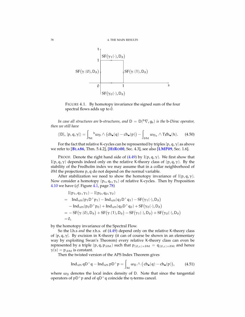
78 4. THE MAIN RESULTS
s
t
0 1
1
SF(γ·(1),D∂
)SF(γ·(0),D∂
)
SF(γ0(·),D∂
)
SF(γ1(·),D∂
)
FIGURE 4.1. By homotopy invariance the signed sum of the fourspectral flows adds up to 0.
In case all structures are b-structures, and D = D(b∇, gb) is the b-Dirac operator,then we still have
〈[D], [p, q, γ]〉 =∫
bM
bωD ∧(ch•(q) − ch•(p)
)−
∫∂M
ωD∂ ∧ T/ch•(h). (4.50)
For the fact that relativeK-cycles can be represented by triples [p, q, γ] as abovewe refer to [BLA86, Thm. 5.4.2], [HIRO00, Sec. 4.3], see also [LMP09, Sec. 1.6].
PROOF. Denote the right hand side of (4.49) by I(p, q, γ). We first show thatI(p, q, γ) depends indeed only on the relative K-theory class of (p, q, γ). By thestability of the Fredholm index we may assume that in a collar neighborhood of∂M the projections p, q do not depend on the normal variable.
After stabilization we need to show the homotopy invariance of I(p, q, γ).Now consider a homotopy (pt, qt, γt) of relative K-cycles. Then by Proposition4.10 we have (cf. Figure 4.1, page 78)
I(p1, q1, γ1) − I(p0, q0, γ0)
= IndAPS(p1D+p1) − IndAPS(q1D
+q1) − SF(γ1(·),D∂
)− IndAPS(p0D
+p0) + IndAPS(q0D+q0) + SF
(γ0(·),D∂
)= − SF
(γ·(0),D∂
)+ SF
(γ·(1),D∂
)− SF
(γ1(·),D∂
)+ SF
(γ0(·),D∂
)= 0,
by the homotopy invariance of the Spectral Flow.So the l.h.s and the r.h.s. of (4.49) depend only on the relative K-theory class
of [p, q, γ]. By excision in K-theory (it can of course be shown in an elementaryway by exploiting Swan’s Theorem) every relative K-theory class can even berepresented by a triple (p, q, p|∂M) such that p|[0,ε)×∂M = q|[0,ε)×∂M and henceγ(s) = p|∂M is constant.
Then the twisted version of the APS Index Theorem gives
IndAPS qD+q− IndAPS pD
+p =
∫M
ωD ∧(
ch•(q) − ch•(p)), (4.51)
where ωD denotes the local index density of D. Note that since the tangentialoperators of pD+p and of qD+q coincide the η-terms cancel.
4.3. RELATIVE PAIRING FORMULÆ AND GEOMETRIC CONSEQUENCES 79
As outlined in Section 1.5 (cf. also the proof of Theorem 4.5) the Connes-Cherncharacter of [D] inHP•
(J∞(∂M,M)
)' HdR
• (M\∂M;C) is represented by∫MωD.
By construction, the form ch•(q) − ch•(p) is compactly supported in M \ ∂M.Thus the right hand side of (4.51) equals the pairing 〈[D], [p, q, p|∂M]〉 and the firstequality in (4.49) is proved.
To prove the second equality in (4.49) we note that it represents the Poincareduality pairing between the de Rham cohomology class of ωD(∇,g) (note ι∗ωD =ωD∂ ) and the relative de Rham cohomology class of the pair of forms (ch•(q) −ch•(p),T/ch•(h)). Hence it depends only on the class [p, q, h] ∈ K0(M,∂M) andon [D]. In the situation above where p and q coincide in a collar of the boundaryit equals 〈[D], [p, q, γ]〉 and hence by homotopy invariance the claim is proved ingeneral up to Eq. (4.50).
For the proof of Eq. (4.50) note first that for a closed even b-differential formω the map (cf. Definition and Proposition 2.5)
Ωk(M)⊕Ωk−1(∂M)→ C, (η, τ) 7→ ∫bM
ω∧ η−
∫∂M
ι∗ω∧ τ
descends naturally to a linear form on HkdR(M,∂M;C). Hence the right hand sideof Eq. (4.50) is well-defined and depends only on the class of [p, q, h] ∈ K0(M,∂M).As before we may therefore specialize to (p, q, p|∂M) such that p|[0,ε)×∂M =q|[0,ε)×∂M. Then ch•(q) − ch•(p) has compact support in M \ ∂M and the re-maining claim follows from Theorem 4.5 (4).
We now proceed to express the pairing between relative K-theory classes andthe fundamental relative K-homology class in cohomological terms. We assumehere that we are in the b-setting.
Recall that a relative K-theory class in K0(M,∂M) is represented by a pair ofbundles (E, F) over M whose restrictions E∂, F∂ to ∂M are related by a homotopyh. We will explicitly write the formulæ in the even dimensional case and onlypoint out where the odd dimensional case is different.
The Chern character of [E, F, h] ∈ K0(M,∂M) is then represented by the rela-tive cyclic homology class
ch•([E, F, h]
)=(
ch•(pF) − ch•(pE) , −T/ch•(h)), (4.52)
cf. Eq. (1.17).By Theorem 4.5 we have for any t > 0⟨
[D], [E, F, h]⟩=⟨( bchnt (D), chn+1t (D∂)
), ch•([E, F, h])
⟩=⟨∑j≥0
bChn−2j(tD) + B bT/chn+1t (D), ch•(pF) − ch•(pE)⟩
−⟨∑j≥0
Chn−2j+1(tD∂) + BT/chn+2t (D∂), T/ch•(h)⟩.
(4.53)
Letting t 0 yields, again by Theorem 4.5, the local form of the pairing:⟨[D], [E, F, h]
⟩=
∫bM
ωD ∧(
ch•(pF) − ch•(pE))−
∫∂M
ωD∂(∂M)∧ T/ch•(h).(4.54)
80 4. THE MAIN RESULTS
If D∂ is invertible then, at the opposite end, letting t∞ gives in view of Theorem4.6 ⟨
[D], [E, F, h]⟩=⟨ ∑0≤k≤`
κ2k(D) + BbT/chn+1∞ (D), ch•(pF) − ch•(pE)⟩
−⟨BT/chn+2∞ (D∂),T/ch•(h)
⟩,
(4.55)
where 2` = n.By equating the above two limit expressions (4.54) and (4.55) one obtains the
following identity:
Corollary 4.13. Let n = 2` ≥ m and assume that D∂ is invertible. Then⟨κ0(D), pF − pE
⟩+
+∑1≤k≤`
(−1)k(2k)!
k!
⟨κ2k(D), (pF −
1
2)⊗ p⊗2kF − (pE −
1
2)⊗ p⊗2kE
⟩=
∫bM
ωD ∧(
ch•(pF) − ch•(pE))−
∫∂M
ωD∂ ∧ T/ch•(h)
− (−1)n/2n!
(n/2)!
⟨BbT/chn+1∞ (D), (pF −
1
2)⊗ p⊗nF − (pE −
1
2)⊗ p⊗nE
⟩+⟨BT/chn+2∞ (D∂),T/chn+1(h)
⟩.
The left hand side plays the role of a ‘higher’ relative index, while the righthand side contains local geometric terms and ‘higher’ eta cochains.
The pairing formula acquires a simpler form if one chooses special represen-tatives for the class [E, F, h]. For example, one can always assume that E∂ = F∂, inwhich case one obtains⟨
[D], [E, F, h0]⟩=⟨ ∑0≤k≤`
κ2k(D) + BbT/chn+1∞ (D), ch•(pF)⟩
−⟨ ∑0≤k≤`
κ2k(D) + BbT/chn+1∞ (D), ch•(pE)⟩.
(4.56)
Specializing even more, one can assume F = CN. Then the pairing formula be-comes⟨
[D], [E,CN, h0]⟩= −
⟨ ∑0≤k≤`
κ2k(D) + BbT/chn+1∞ (D), ch•(pE)⟩
+ N(dim KerD+ − dim KerD−).
(4.57)
On the other hand, applying Theorem 4.12⟨[D], [E,CN, h0]
⟩= − IndAPS(pED
+pE) +N IndAPSD+,
one obtains an index formula for the b-Dirac operator which is the direct analogueof Eq. (3.4) in [COMO93]:
Corollary 4.14. Let E be a vector bundle on M whose restriction to ∂M is trivial andassume D∂ to be invertible. Then for any n = 2` ≥ m
IndAPS(pED+pE) =
⟨ ∑0≤k≤`
κ2k(D) + BbT/chn+1∞ (D), ch•(pE)⟩. (4.58)
4.3. RELATIVE PAIRING FORMULÆ AND GEOMETRIC CONSEQUENCES 81
The expression IndAPS(pED+pE) is to be understood as follows: if p∂ED∂p
∂E is
invertible, then it is the Fredholm index of pED+pE. If pED+pE is not Fredholm,then chose a metric g smooth up to the boundary and construct on the Cliffordmodule of D the Dirac operator D to the riemannian metric g. Then, by Theo-rem. 4.5 the Connes-Chern characters of D and D coincide and thus⟨
[D], [E,CN, h0]⟩= − IndAPS pED
+pE +N IndAPS D
+.
As a by-product of the above considerations, we can now establish the follow-ing generalization of the Atiyah-Patodi-Singer odd-index theorem for trivializedflat bundles (comp. [APS76, Prop. 6.2, Eq. (6.3)]. An analogue for even dimen-sional manifolds has been subsequently established by Z. Xie [XIE11].
Corollary 4.15. Let N be a closed odd dimensional spin manifold, and let E ′, F ′ be twovector bundles which are equivalent in K-theory via a homotopy h. With Dg ′ denoting theDirac operator associated to a riemannian metric g ′ on N, one has
ξ(DF′
g ′) − ξ(DE ′
g ′ ) =
∫N
A(∇2g ′)∧ T/ch•(h) + SF(h,Dg ′) , (4.59)
or equivalently,∫10
1
2
d
dt
(η(ph(t) Dg ′ ph(t))
)dt =
∫N
A(∇2g ′)∧ T/ch•(h) , (4.60)
where ph(t)) is the path of projections joining E ′ and F ′.
PROOF. This follows from equating the local pairing (4.49) and the rela-tive APS index formula (0.17) after the following modifications. We recall thatEq. (4.49) holds in complete generality without invertibility hypothesis on D∂.First by passing to a multiple one can assume that N = ∂M. Then by addinga complement G ′ we can replace F ′ by a trivial bundle. Then both E ′ ⊕ G ′ andF ′ ⊕ G ′ extend to M. It remains to notice that both sides of the formula (4.59) areadditive.
The alternative formulation (4.60) follows immediately from the known rela-tion (see e.g. [KILE04, Lemma 3.4])
ξ(DF′
g ′) − ξ(DE ′
g ′ ) = SF(h,D∂) +∫10
1
2
d
dt
(η(ph(t) Dg ′ ph(t))
)dt.
In the odd dimensional case the pairing formulæ are similar, except that thecontribution from the kernel of D does not occur. Let (U,V, h) be a representativeof an odd relative K-theory class where U,V : M → U(N) are unitaries and h is ahomotopy between U∂M and V∂M. Then⟨
[D], [U,V, h]⟩=⟨B bT/chn+1∞ (D), chn(U) − chn(V)
⟩−⟨BT/chn+2∞ (D∂),T/chn+1(h)
⟩.
(4.61)
Choosing a representative of the class with U∂M = V∂M, the above formula sim-plifies to ⟨
[D], [U,V, h0]⟩=⟨B bT/chn+1∞ (D), chn(U) − chn(V)
⟩, (4.62)
and if moreover one takes V = Id, it reduces to⟨[D], [U, Id, h0]
⟩=⟨B bT/chn+1∞ (D), chn(U)
⟩. (4.63)
82 4. THE MAIN RESULTS
Finally, the equality between the local form of the pairing (4.54) and the ex-pression (4.61) gives the following odd analogue of Corollary 4.13.
Corollary 4.16. Let n ≥ m, both odd and assume that D∂ is invertible. Then⟨B bT/chn+1∞ (D), chn(U)
⟩−⟨B bT/chn+1∞ (D), chn(V)
⟩=
=
∫bM
A(b∇2g)∧(
ch•(U) − ch•(V))−
∫∂M
A(∇2g ′)∧ T/ch•(h)
−⟨BT/chn+2∞ (D∂),T/chn+1(h)
⟩.
4.4. Relation with the generalized APS pairing
Wu [WU93] showed that the full cochain η•(D∂) has a finite radius of con-vergence, proportional to the lowest eigenvalue of |D∂| (assumed to be invertible).Both Wu and Getzler [GET93A] proved, by different methods, the following gen-eralized Atiyah-Patodi-Singer index formula :
IndAPS DE =
∫bM
A(b∇2g)∧ ch•(pE) +⟨η•(D∂) i∗, ch•(pE)
⟩, (4.64)
for any vector bundle E = ImpE overMwhose restriction to the boundary satisfiesthe almost ∂-flatness condition ‖[D∂, r∂(pE)]‖ < λ1(|D∂|). Their result does providea decoupled index pairing, but only for those classes in Km(M,∂M) which can berepresented by pairs of almost ∂-flat bundles. Furthermore, if (E, F, h) is such atriple, on applying (4.64) and Theorem 4.12 one obtains
〈[D], [E, F, h]〉 =∫
bM
A(b∇2g)∧(
ch•(pF) − ch•(pE))
+⟨η•(D∂), i
∗( ch•(pF) − ch•(pE))⟩
+ SF(h,D∂),(4.65)
where SF(h,D∂) is an abbreviation for SF(h(s)A+h(s)
)0≤s≤1, cf. also Eq. (4.42). By
[WU93, Proof of Thm. 3.1],
(b+ B)η•(D∂) = −
∫∂M
A(∇2g ′)∧− .
At the formal level⟨η•(D∂) i∗, ch•(pF) − ch•(pE)
⟩=⟨η•(D∂), (b+ B)T/ch•(h)
⟩=⟨(b+ B)η•(D∂),T/ch•(h)
⟩= −
∫∂M
A(∇2g ′)∧ T/ch•(h).(4.66)
However, to ensure that the pairing⟨η•(D∂), (b + B)T/ch•(h)
⟩makes sense one
has to assume that ph(t) satisfy the same almost ∂-flatness condition. Then
Ker(ph(t)D∂ph(t)) = 0,
hence there is no spectral flow along the path.Thus, the total eta cochain disappears and (4.66) together with (4.65) just lead
to the known local pairing formula, cf. Eq. (4.49),
〈[D],[E, F, h]〉
=
∫bM
A(b∇2g)∧(
ch•(pF) − ch•(pE))−
∫∂M
A(∇2g ′)∧ T/ch•(h) .
4.4. RELATION WITH THE GENERALIZED APS PAIRING 83
The above considerations also show that the total eta cochain necessarily has afinite radius of convergence. If it was entire, then SF(h,D) = 0 for any h(t), whichis easy to disprove by a counterexample.

Bibliography
[APS75] M. F. ATIYAH, V. K. PATODI, and I. M. SINGER, Spectral asymmetry and Riemannian geome-try. I, Math. Proc. Cambridge Philos. Soc. 77 (1975), 43–69. MR 0397797 (53 #1655a) 5
[APS76] , Spectral asymmetry and Riemannian geometry. III, Math. Proc. Cambridge Philos. Soc.79 (1976), no. 1, 71–99. MR 0397799 (53 #1655c) 5, 81
[ASS94] J. AVRON, R. SEILER, and B. SIMON, The index of a pair of projections, J. Funct. Anal. 120(1994), no. 1, 220–237. MR 1262254 (95b:47012) 76
[BBFU98] B. BOOSS-BAVNBEK and K. FURUTANI, The Maslov index: a functional analytical definitionand the spectral flow formula, Tokyo J. Math. 21 (1998), no. 1, 1–34. MR 1630119 (99e:58172)76
[BBLZ09] B. BOOSS-BAVNBEK, M. LESCH, and C. ZHU, The Calderon projection:new definition and applications, J. Geom. Phys. 59 (2009), no. 7, 784–826.arXiv:0803.4160v1 [math.DG] , DOI: 10.1016/j.geomphys.2009.03.012,
http://dx.doi.org/10.1016/j.geomphys.2009.03.012, MR 2536846 76[BBWO93] B. BOOSS-BAVNBEK and K. P. WOJCIECHOWSKI, Elliptic boundary problems for Dirac op-
erators, Mathematics: Theory & Applications, Birkhauser Boston Inc., Boston, MA, 1993.MR 1233386 (94h:58168) 75, 76
[BDT89] P. BAUM, R. G. DOUGLAS, and M. E. TAYLOR, Cycles and relative cycles in analytic K-homology, J. Differential Geom. 30 (1989), no. 3, 761–804. MR 1021372 (91b:58244) 1, 15,16
[BGV92] N. BERLINE, E. GETZLER, and M. VERGNE, Heat kernels and Dirac operators, Grundlehrender Mathematischen Wissenschaften [Fundamental Principles of Mathematical Sciences],vol. 298, Springer-Verlag, Berlin, 1992. MR 1215720 (94e:58130) 72
[BLA86] B. BLACKADAR, K-theory for operator algebras, Mathematical Sciences Research InstitutePublications, vol. 5, Springer-Verlag, New York, 1986. MR 859867 (88g:46082) 77, 78
[BLFO90] J. BLOCK and J. FOX, Asymptotic pseudodifferential operators and index theory, Geometric andtopological invariants of elliptic operators (Brunswick, ME, 1988), Contemp. Math., vol.105, Amer. Math. Soc., Providence, RI, 1990, pp. 1–32. MR 1047274 (91e:58186) 6, 16, 67, 72
[BRLE01] J. BRUNING and M. LESCH, On boundary value problems for Dirac type operators. I. Regularityand self-adjointness, J. Funct. Anal. 185 (2001), no. 1, 1–62. arXiv:math/9905181 [math.FA],MR 1853751 (2002g:58034) 76
[BRPF08] J.-P. BRASSELET and M. J. PFLAUM, On the homology of algebras of Whitney functions oversubanalytic sets, Ann. of Math. (2) 167 (2008), no. 1, 1–52. MR 2373151 1, 11, 12, 16
[COMO90] A. CONNES and H. MOSCOVICI, Cyclic cohomology, the Novikov conjecture and hyperbolicgroups, Topology 29 (1990), no. 3, 345–388. MR 1066176 (92a:58137) 6, 16, 67, 72
[COMO93] , Transgression and the Chern character of finite-dimensional K-cycles, Comm. Math.Phys. 155 (1993), no. 1, 103–122. MR 1228528 (95a:46091) 1, 2, 16, 61, 62, 63, 69, 70, 71,73, 75, 80
[COMO95] A. CONNES and H. MOSCOVICI, The local index formula in noncommutative geometry, Geom.Funct. Anal. 5 (1995), no. 2, 174–243. MR 1334867 (96e:58149) 1, 66
[CON85] A. CONNES, Noncommutative differential geometry, Inst. Hautes Etudes Sci. Publ. Math. 62(1985), 257–360. MR 823176 (87i:58162) 1, 10
[CON88] , Entire cyclic cohomology of Banach algebras and characters of θ-summable Fredholm mod-ules, K-Theory 1 (1988), no. 6, 519–548. MR MR953915 (90c:46094) 1
[CON94] , Noncommutative geometry, Academic Press Inc., San Diego, CA, 1994. MR 1303779(95j:46063) 9, 10
[COSA96] G. M. CONSTANTINE and T. H. SAVITS, A multivariate Faa di Bruno formula with applications,Trans. Amer. Math. Soc. 348 (1996), no. 2, 503–520. MR 1325915 (96g:05008) 9
85
86 BIBLIOGRAPHY
[CUQU93] J. CUNTZ and D. QUILLEN, On excision in periodic cyclic cohomology, C. R. Acad. Sci. ParisSer. I Math. 317 (1993), no. 10, 917–922. MR 1249360 (94i:19002) 12
[CUQU94] , On excision in periodic cyclic cohomology. II. The general case, C. R. Acad. Sci. ParisSer. I Math. 318 (1994), no. 1, 11–12. MR 1260526 (94m:19001) 12
[FUKE88] S. A. FULLING and G. KENNEDY, The resolvent parametrix of the general elliptic linear differ-ential operator: a closed form for the intrinsic symbol, Trans. Amer. Math. Soc. 310 (1988), no. 2,583–617. MR 973171 (90b:58260) 19, 20
[GBVF01] J. M. GRACIA-BONDIA, J. C. VARILLY, and H. FIGUEROA, Elements of noncommutative ge-ometry, Birkhauser Advanced Texts: Basler Lehrbucher. [Birkhauser Advanced Texts: BaselTextbooks], Birkhauser Boston Inc., Boston, MA, 2001. MR 1789831 (2001h:58038) 40, 42
[GESZ89] E. GETZLER and A. SZENES, On the Chern character of a theta-summable Fredholm module, J.Funct. Anal. 84 (1989), no. 2, 343–357. MR 1001465 (91g:19007) 36, 39
[GET83] E. GETZLER, Pseudodifferential operators on supermanifolds and the Atiyah-Singer index theorem,Comm. Math. Phys. 92 (1983), no. 2, 163–178. MR 728863 (86a:58104) 72
[GET93A] , Cyclic homology and the Atiyah-Patodi-Singer index theorem, Index theory and opera-tor algebras (Boulder, CO, 1991), Contemp. Math., vol. 148, Amer. Math. Soc., Providence,RI, 1993, pp. 19–45. MR 1228498 (94j:58162) 1, 7, 13, 14, 15, 34, 35, 36, 39, 40, 65, 82
[GET93B] , The odd Chern character in cyclic homology and spectral flow, Topology 32 (1993), no. 3,489–507. MR 1231957 (95c:46118) 13
[GIL95] P. B. GILKEY, Invariance theory, the heat equation, and the Atiyah-Singer index theorem, seconded., Studies in Advanced Mathematics, CRC Press, Boca Raton, FL, 1995. MR 1396308(98b:58156) 65
[GRSE95] G. GRUBB and R. T. SEELEY, Weakly parametric pseudodifferential operators and Atiyah-Patodi-Singer boundary problems, Invent. Math. 121 (1995), no. 3, 481–529. MR 1353307 (96k:58216)16
[HASU78] P. R. HALMOS and V. S. SUNDER, Bounded integral operators on L2 spaces, Ergebnisse derMathematik und ihrer Grenzgebiete [Results in Mathematics and Related Areas], vol. 96,Springer-Verlag, Berlin, 1978. MR 517709 (80g:47036) 55
[HIRO00] N. HIGSON and J. ROE, Analytic K-homology, Oxford Mathematical Monographs, OxfordUniversity Press, Oxford, 2000, Oxford Science Publications. MR 1817560 (2002c:58036) 9,12, 78
[JLO88] A. JAFFE, A. LESNIEWSKI, and K. OSTERWALDER, Quantum K-theory. I. The Chern character,Comm. Math. Phys. 118 (1988), no. 1, 1–14. MR 954672 (90a:58170) 2, 16, 36
[KILE04] P. KIRK and M. LESCH, The η-invariant, Maslov index, and spectral flow for Dirac-type operatorson manifolds with boundary, Forum Math. 16 (2004), no. 4, 553–629. arXiv:math/0012123[math.DG], MR 2044028 (2005b:58029) 81
[LES99] M. LESCH, On the noncommutative residue for pseudodifferential operators with log-polyhomogeneous symbols, Ann. Global Anal. Geom. 17 (1999), no. 2, 151–187.arXiv:dg-ga/9708010, MR 1675408 (2000b:58050) 66
[LES05] , The uniqueness of the spectral flow on spaces of unbounded self-adjoint Fredholmoperators, Spectral geometry of manifolds with boundary and decomposition of mani-folds, Contemp. Math., vol. 366, Amer. Math. Soc., Providence, RI, 2005, pp. 193–224.arXiv:math/0401411 [math.FA], MR 2114489 (2005m:58049) 76
[LMP08] M. LESCH, H. MOSCOVICI, and M. J. PFLAUM, Regularized traces and K-theory invari-ants of parametric pseudodifferential operators, Traces in number theory, geometry andquantum fields, Aspects Math., E38, Friedr. Vieweg, Wiesbaden, 2008, pp. 161–177.www.matthiaslesch.de publications, MR 2427595 73
[LMP09] , Relative pairing in cyclic cohomology and divisor flows, J. K-Theory 3 (2009), no. 2,359–407. arXiv:math/0603500 [math.KT], MR 2496452 2, 6, 10, 11, 12, 13, 26, 78
[LOY05] P. LOYA, Dirac operators, boundary value problems, and the b-calculus, Spectral geometry ofmanifolds with boundary and decomposition of manifolds, Contemp. Math., vol. 366,Amer. Math. Soc., Providence, RI, 2005, pp. 241–280. MR 2114491 (2005k:58038) 7, 9, 20,26, 27, 30, 33
[MAL67] B. MALGRANGE, Ideals of differentiable functions, Tata Institute of Fundamental ResearchStudies in Mathematics, No. 3, Tata Institute of Fundamental Research, Bombay, 1967.MR 0212575 (35 #3446) 9
BIBLIOGRAPHY 87
[MEL93] R. B. MELROSE, The Atiyah-Patodi-Singer index theorem, Research Notes in Mathematics,vol. 4, A K Peters Ltd., Wellesley, MA, 1993. MR 1348401 (96g:58180) 1, 6, 7, 9, 17, 20, 23,24, 25, 26, 27, 28
[MOPI11] H. MORIYOSHI and P. PIAZZA, Relative pairings and the Atiyah–Patodi–Singer indexformula for the Godbillon–Vey cocycle, Noncommutative Geometry and Global Analy-sis, Contemp. Math., vol. 546, Amer. Math. Soc., Providence, RI, 2011, pp. 225–247.arXiv:math/0907.0173 2
[MUL94] W. MULLER, Eta invariants and manifolds with boundary, J. Differential Geom. 40 (1994), no. 2,311–377. MR 1293657 (96c:58165) 52
[NIC95] L. I. NICOLAESCU, The Maslov index, the spectral flow, and decompositions of manifolds, DukeMath. J. 80 (1995), no. 2, 485–533. MR 1369400 (96k:58208) 76
[PFL98] M. J. PFLAUM, The normal symbol on Riemannian manifolds, New York J. Math. 4 (1998),97–125 (electronic). MR 1640055 (99e:58181) 19, 20
[SHU01] M. A. SHUBIN, Pseudodifferential operators and spectral theory, second ed., Springer-Verlag,Berlin, 2001, Translated from the 1978 Russian original by Stig I. Andersson. MR 1852334(2002d:47073) 46
[TAY96] M. E. TAYLOR, Partial differential equations. II, Applied Mathematical Sciences, vol. 116,Springer-Verlag, New York, 1996, Qualitative studies of linear equations. MR 1395149(98b:35003) 14, 35
[TOU72] J.-C. TOUGERON, Ideaux de fonctions differentiables, Springer-Verlag, Berlin, 1972, Ergebnisseder Mathematik und ihrer Grenzgebiete, Band 71. MR 0440598 (55 #13472) 9
[WID79] H. WIDOM, Szego’s theorem and a complete symbolic calculus for pseudodifferential operators,Seminar on Singularities of Solutions of Linear Partial Differential Equations (Inst. Adv.Study, Princeton, N.J., 1977/78), Ann. of Math. Stud., vol. 91, Princeton Univ. Press, Prince-ton, N.J., 1979, pp. 261–283. MR 547022 (81b:58043) 6, 67
[WID80] , A complete symbolic calculus for pseudodifferential operators, Bull. Sci. Math. (2) 104(1980), no. 1, 19–63. MR 560744 (81m:58078) 19, 20
[WU93] F. WU, The Chern-Connes character for the Dirac operator on manifolds with boundary, K-Theory7 (1993), no. 2, 145–174. MR 1235286 (95f:58076) 7, 82
[XIE11] Z. XIE, Relative index pairing and odd index theorem for even dimensional manifolds, J. Funct.Anal. 260 (2011), no. 7, 2064–2085. MR 2756150 81

Subject Index
APS, 5, 7, 16, 28, 30, 37, 75–78, 81, 82
b-Clifford module, 33b-Clifford superconnection, 33b-function, 17, 19b-heat expansion, 65b-manifold, 17b-metric, 17, 20boundary defining function, 17boundary projection, 17b-pseudodifferential operator, 21b-trace, 26–28, 30–32, 34, 66, 67, 69
Chern character, 12–13secondary, 12
Clifford (super)connection, 14Clifford algebra
complex, 13Clifford module, 33
degree q, 14graded, 35ungraded, 35
Clifford superconnection, 33Clifford supertrace
degree q, 14Connes-Chern character, vii, 1, 2, 7, 10, 16, 17,
69, 72, 74, 79, 81Connes–Chern character
relative, 15cyclic (co)homology, 10
relative, 10, 11cylindrical ends, 17, 31
de Rham, 1, 3, 16, 73, 74, 79current, 73homology, 1
Dirac operator, 14Dirac type operator, 14domain, 16, 24, 47, 75
exact b-metric, 17excision, 9, 11–13, 16, 29, 78
finite part, see also partie finie
generalized trace map, 12
heat kernel, 16, 28, 45, 50, 55, 57, 66
Hochschild (co)homology, 10, 11, 71relative, 10
hypertrace, 28
indicial family, 24, 26, 27, 35integral
partie finie, see also partie finieinterpolation inequality, 49
JLO, 15, 16, 35, 36, 45, 58, 66
K-homology, 10, 16K-theory
relative, 12
local heat invariants, 67, 72
manifold with cylindrical ends, 17McKean–Singer formula, 29
relative, 28
pairing, 11, 21, 28, 75–82parameter dependent calculus, 46partie finie, 26, 31, 67periodic cyclic (co)homology, 10
relative, 11
regularization, 28relative
Connes–Chern character, 15cyclic (co)homology, 10, 11Fredholm module, 15Hochschild (co)homology, 10index, 76K-theory, 12McKean–Singer formula, 28periodic cyclic (co)homology, 11
Schatten class, 45Schur’s test, 55spectral flow, 76supercommutator, 14
tangential operator, 34trace
generalized trace map, 12transgression formula, 13, 41–43
secondary, 13
89

90 SUBJECT INDEX
Whitney functions, 9
Notation Index
Except a few standard notations, all symbols are explained at their first occurence.We recall a few very standard notations and then we provide an index to the usedsymbols.
N,Z,R,C Natural (including 0), integer, real and complex numbersR+ Nonnegative real numbers x ≥ 0Z+ Synonym for N
C(. . .), C∞(. . .) Continuous resp. smooth functionsC0(. . .), C∞0 (. . .) Ditto, vanishing at infinity (on locally compact space)Cc(. . .), C∞c (. . .) Ditto, compactly supported
Γ∞(M;E) Smooth sections of the vector bundle E overM, where Γ∞c , Γ∞0have the analogous meaning as for C∞.
GLN(A) Invertible N×Nmatrices with entries in AH Generic name for a Hilbert space
L(H) Algebra of bounded linear operators on the Hilbert spaceHL2(M;E) Square–integrable sections of the hermitian vector bundle EMatN(A) N×N–matrix algebra over the algebra A
spec(T) Spectrum of the linear operator Tspecess(T) Essential spectrum of the linear operator T
supp(f) Support of the distribution(al section) f
< −,− >, 11, 21C0(M \ ∂M), 16
A, 30, 34, 37, 57, 66A, 14
bC∞, 17–19, 23, 31, 33, 40, 60, 62, 72–74bCh, 2, 4, 35–43, 60, 62, 69–73, 79b/ch, 35–39, 42, 43, 60, 62, 69, 70, 72, 74bDiff, 23, 57, 58, 61, 65–67bDiffcpt, 23, 53, 54, 57, 59, 60, 65, 68bΓ∞cpt, 52, 57b∇, 2–5, 33, 72, 74, 78, 82bΨ, 21–25, 27, 28, 31, 32, 34, 35, 39bStr, 34–36, 40, 41, 75bT/ch, 2–5, 70–75, 81, 82bTr, 6, 26–28, 30–34, 37, 59, 60, 65–68
BCp,q(A), 10BCp,qper (A), 10
ch•(e), 12ch•(U, V, h), 13ch•(p, q, h), 12Ch, 2, 4, 15, 16, 36–39, 69–71, 73, 79/ch, 12, 13, 15, 36–39, 42, 43, 62, 69, 70, 72C`q, 13–14
De, 15D, 1–6, 14–17, 27, 28, 30, 34–43, 52–55, 57–63,
65–82∆R, 55Diff, 19, 47, 50, 57dom, 47
E∞(∂M,M), 9e⊗j, 12End, 33, 57, 76
F, 15[F], 16
91
92 NOTATION INDEX
GL∞(A),GLN(A), 13Γ , 27, 30, 34, 37–40, 42, 57, 59, 66
HC•(A,B), 10HH•(A,B), 10HP•(A,B), 10
IndAPS, 5, 75–78, 80–82Index[D], 1, 17
J , 9J∞, 9
Kj(A,B), 12K•(C(M), C(∂M)), 16
L(H), 14
MatN(A),Mat∞(A), 12
Pf∫
, 31, 32
SF, 5, 76–78, 81–83
Tot•⊕BC•,•(A), 10Tot•⊕BC•,•
per (A), 10trj, 12T/ch, 2–5, 12, 13, 16, 70–73, 75, 77–82