A HEURISTIC APPROACH TO UNIVERSITY COURSE TIMETABLING

UNIVERSITEIT GENT

FACULTEIT ECONOMIE EN BEDRIJFSKUNDE

ACADEMIEJAAR 2012 – 2013

A HEURISTIC APPROACH TO

UNIVERSITY COURSE TIMETABLING

Masterproef voorgedragen tot het bekomen van de graad van

Master of Science in de

Toegepaste Economische Wetenschappen: Handelsingenieur

Eline Verhees

onder leiding van

Prof. Dr. Broos Maenhout

iv

PERMISSION

Ondergetekende verklaart dat de inhoud van deze masterproef mag geraadpleegd

en/of gereproduceerd worden, mits bronvermelding.

Eline Verhees

v

I P REF A C E

This dissertation is the end piece of my five-year study Commercial Engineering: Operational

Management at the University of Ghent, Belgium.

It gave me the opportunity to dive into the world of complex optimization problems and the

countless ways to solve them. A subject of study that remained rather abstract during my education,

but that nevertheless always fascinated me. The timetabling problem in particular interested me as it

affects every single student in a university, but is often taken for granted.

Special thanks goes to my promoter Broos Maenhout with whom I could always discuss the

difficulties I encountered in an inspiring way. I would also like to thank Lieven Rigo for his useful tips

on implementing source code, Willem Lenaerts for his attentive reading of my text, and finally my

roommates for their love and support during the last intensive weeks.

Eline Verhees,

Gent, 17-12-2012

vi

I I IND EX

I Preface .............................................................................................................................................. v

II Index ................................................................................................................................................ vi

III List of Used Abbreviations ............................................................................................................... ix

IV List of Tables ..................................................................................................................................... x

V List of Figures .................................................................................................................................. xii

VI Nederlandse Samenvatting ........................................................................................................... xiii

1. Introduction ..................................................................................................................................... 1

2. The Importance of Timetabling ....................................................................................................... 2

2.1 Current Research & Organisations ......................................................................................... 5

3. General Framework of University Course Timetabling ................................................................... 6

3.1 What is Timetabling? ............................................................................................................. 6

3.2 Academic Timetabling ............................................................................................................ 6

3.2.1 Curriculum- / Student Enrolment- based Timetabling .................................................... 8

3.3 Problem Definition ................................................................................................................. 9

3.3.1 Combinatorial Optimization Problems ............................................................................ 9

3.3.2 Constraints..................................................................................................................... 10

3.3.3 NP-Hard Problems ......................................................................................................... 11

4. Methodology ................................................................................................................................. 13

5. International Timetabling Competition ......................................................................................... 14

5.1 International Timetabling Competition ............................................................................... 14

5.2 2003 Competition ................................................................................................................ 15

5.2.1 The Model...................................................................................................................... 15

5.2.2 Winning Entry ................................................................................................................ 17

5.3 2007 Competition ................................................................................................................ 17

5.3.1 The Model...................................................................................................................... 18

vii

5.3.2 Winning Entry ................................................................................................................ 19

6. Heuristics and Metaheuristics in UCT ........................................................................................... 20

6.1 Heuristics .............................................................................................................................. 20

6.1.1 Sequential Methods ...................................................................................................... 20

6.1.2 Cluster Methods ............................................................................................................ 21

6.1.3 Constraint-Based Approaches ....................................................................................... 21

6.2 Metaheuristics ..................................................................................................................... 22

6.3 Hybrid Algorithms ................................................................................................................ 24

7. The Algorithm ................................................................................................................................ 26

7.1 Variable Representation and Data Preprocessing ............................................................... 26

7.2 First Phase: Finding Feasibility ............................................................................................. 28

7.2.1 IH 1: Best Fit Heuristic and Variable Neighborhood Descent ........................................ 28

7.2.2 IH 2: Sequential Heuristic and VND ............................................................................... 32

7.2.3 IH 3: Dynamic Sequencing ............................................................................................. 33

7.2.4 Comparison of IH’s ........................................................................................................ 35

7.3 Second Phase: optimization ................................................................................................. 37

7.3.1 Hybrid Evolutionary Algorithm ...................................................................................... 37

7.3.2 The Population .............................................................................................................. 38

7.3.3 Selection Operator ........................................................................................................ 38

7.3.4 Mutation Operators ...................................................................................................... 39

7.3.5 Non-Linear Great Deluge Algorithm .............................................................................. 40

8. Test Design and Experimental Results .......................................................................................... 44

8.1 Local Search Parameter Testing ........................................................................................... 44

8.1.1 Neighborhoods .............................................................................................................. 44

8.1.2 Decay Rate Parameters ................................................................................................. 47

8.2 Population Parameter Testing ............................................................................................. 50

9. Results ........................................................................................................................................... 61

9.1 Final Algorithm ..................................................................................................................... 61

9.2 Results .................................................................................................................................. 63

9.3 Benchmarking ...................................................................................................................... 65

10. Conclusion ..................................................................................................................................... 66

viii

References ............................................................................................................................................. 67

Appendix ................................................................................................................................................ 73

Complete overview of Final obtained results................................................................................ 73

ix

I I I L IS T OF US ED A B B REV IA T IONS

CH Constructive Heuristic

COP Combinatorial Optimisation Problem

CSP Constraint Satisfaction Problem

EA Evolutionary Algorithm

GDA Great Deluge Algorithm

GA Genetic Algorithm

HC Hard Constraint

HCV Hard Constraint Violation

HEA Hybrid Evolutionary Algorithm

IH Initialization Heuristic

ILS Iterated Local Search

ITC International Timetabling Competition

LDF Largest Degree First

LS Local Search

LSDF Least Saturation Degree First

MR Mutation Random

MRR Mutation Rate Random

MRS Mutation Rate Smart

MS Mutation Smart

NLGDA Non-Linear Great Deluge Algorithm

OFV Objective Function Value

OR Operations Research

PATAT Practice And Theory of Automated Timetabling

RW Roulette Wheel

SA Simulated Annealing

SC Soft Constraint

SCV Soft Constraint Violation

TS Tabu Search

UCT(P) University Course Timetabling (Problem)

VND Variable Neighborhood Descent

x

I V L IS T OF TA B L ES

Table 1: Twenty Datasets of ITC 2003 (Chiardini Et Al., 2006) 17

Table 2: Hard Constraint Violations Constructive Heuristics Best Fit – Instance 1 29

Table 3: Hard Constraint Violations Constructive Heuristics Best Fit – Instance 4 30

Table 4: Hard Constraint Violations Sequential Constructive Heuristics – Instance 1 32

Table 5: Hard Constraint Violations Sequential Constructive Heuristics – Instance 4 32

Table 6: Hard Constraint Violations Constructive Heuristic Dynamic Sequencing – Instance 1 34

Table 7: Hard Constraint Violations Constructive Heuristic Dynamic Sequencing – Instance 4 34

Table 8: Performance of Initialization Heuristics for Creating Population – Instance 1 36

Table 9: Performance of Initialization Heuristics for Creating Population – Instance 4 36

Table 10: Initialization Heuristic 3 Tested on all Competition Instances 36

Table 11: Soft Constraint Violations of Different Neighborhood Combinations 45

Table 12: Assessment of Performance of Neighborhood One and Two 45

Table 13: Assessment of Performance of Neighborhood Four and Five 46

Table 14: Comparison of Performance of Best Neighborhood Combinations – 45 Seconds 47

Table 15: Comparison of Performance of Best Neighborhood Combinations – 500 Seconds 47

Table 16: Values of Water Level with Different Parameters 48

Table 17: Parameter Combination 1 50






xi











Table 33: Parameter Combination 17 – Instance 13 59

Table 34: Parameter Combination 18 – Instance 13 59

Table 35: Final Parameter Settings 59

Table 36: Comparison of Performance HEA with and without Neighborhood 5 62

Table 37: Separate Soft Constraint Violations HEA with and without Neighborhood 5 62

Table 38: Final Population Parameters 63

Table 39: Final Local Search Parameters 63

Table 40: Final Results Instances 1 - 10 63

Table 41: Final Results Instances 11 - 20 63

Table 42: Comparison Of Results with Official Competition Results 65

xii

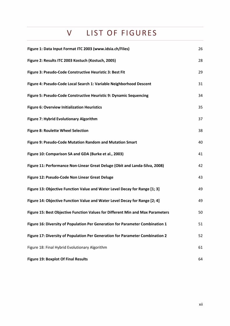
V L IS T OF F I GUR ES

Figure 1: Data Input Format ITC 2003 (www.idsia.ch/Files) 26

Figure 2: Results ITC 2003 Kostuch (Kostuch, 2005) 28

Figure 3: Pseudo-Code Constructive Heuristic 3: Best Fit 29

Figure 4: Pseudo-Code Local Search 1: Variable Neighborhood Descent 31

Figure 5: Pseudo-Code Constructive Heuristic 9: Dynamic Sequencing 34

Figure 6: Overview Initialization Heuristics 35

Figure 7: Hybrid Evolutionary Algorithm 37

Figure 8: Roulette Wheel Selection 38

Figure 9: Pseudo-Code Mutation Random and Mutation Smart 40

Figure 10: Comparison SA and GDA (Burke et al., 2003) 41

Figure 11: Performance Non-Linear Great Deluge (Obit and Landa-Silva, 2008) 42

Figure 12: Pseudo-Code Non Linear Great Deluge 43

Figure 13: Objective Function Value and Water Level Decay for Range [1; 3] 49

Figure 14: Objective Function Value and Water Level Decay for Range [2; 4] 49

Figure 15: Best Objective Function Values for Different Min and Max Parameters 50

Figure 16: Diversity of Population Per Generation for Parameter Combination 1 51

Figure 17: Diversity of Population Per Generation for Parameter Combination 2 52

Figure 18: Final Hybrid Evolutionary Algorithm 61

Figure 19: Boxplot Of Final Results 64

xiii

V I NED ERL A N D S E S A ME NV A T TING

EEN HEURISTISCHE BENADERING VAN

HET UNIVERSITAIR LESSENROOSTERPROBLEEM

Abstract

Het universitair lessenroosterprobleem (ULP)

is een combinatorisch optimalisatieprobleem

waarbij een set lessen moet ingepland

worden in tijdsloten en leslokalen. Hoewel

een degelijk lessenrooster enorm belangrijk

is voor het functioneren van een universiteit,

haar studenten en lesgevers is er nog geen

optimale oplossingstechniek gevonden.

In deze thesis test ik een hybride meta-

heuristische benadering aan de hand van de

benchmark datasets van de International

Timetabling Competition 2003. Het geteste

algoritme is een combinatie van een

aangepaste Great Deluge zoekmethode en

een incrementeel genetisch algoritme.

I. INTRODUCTIE

Sinds ongeveer vijftig jaar wordt er onderzoek

gedaan naar een automatische aanpak voor

het opstellen van een universitair

lessenrooster. Voordien werd dit handmatig

gedaan wat zeer veel man-werkdagen in

beslag nam en bovendien tot sterk inferieure

lessenroosters leidde vergeleken met een

automatische aanpak. Een degelijk

lessenrooster beïnvloedt in sterke mate het

reilen en zeilen van een universiteit, de

dagelijkse indeling van het leven van de

studenten, en van dat van de lesgevers.

Mede door het steeds groter worden van

universiteiten, door de uitbreiding van het

lessenpakket, en door de steeds vaker

toegekende mogelijkheid aan studenten om

hun curriculum zelf samen te stellen, is een

automatische aanpak van het

lessenroosterprobleem onmisbaar geworden.

In de volgende sectie geef ik een beknopte

beschrijving van het algemene

lessenroosterprobleem en van het specifieke

probleem waarvoor ik een algoritme

ontwikkeld heb. De sectie daarna geeft een

kort overzicht van de literatuur omtrent

bestaande oplossingsmethodes. Vervolgens

beschrijf ik het gebruikte algoritme, en

tenslotte geef ik de resultaten weer en de

daarop gebaseerde conclusie.

II. HET PROBLEEM

Het universitair lessenroosterprobleem maakt

deel uit van de grotere familie van timetabling

and scheduling problems. Roosters voor een

middelbare school of een universitaire

examenregeling, alsook bijvoorbeeld de

planning van arbeiders in een shiftensysteem

zijn in deze familie terug te vinden.

Uiteindelijk komt elke ULP neer op het

volgende:

Maak een combinatie van de volgende

elementen:

xiv

- Een set van lessen C = {c1, c2,…, cn}

met n het totaal aantal lessen.

- Een set van lesgevers P = {p1, p2, …,

pm} met m het totaal aantal lesgevers.

- Een set van lokalen R = {r1, r2, …, rk}

met k het totaal aantal lokalen.

- Een set van tijdsloten T = {t1, t2, …, th}

met h het totaal aantal tijdsloten.

op een dusdanige manier dat elke les C een

lesgever P, een lokaal R en een tijdsslot T

heeft toegewezen gekregen: C(P,R,T). Dit

probleem kan worden uitgebreid met sets van

eigenschappen van lokalen, sets van curricula,

of kan worden gereduceerd door de

toewijzing van lesgevers bijvoorbeeld niet in

te vullen.

International Timetabling Competition 2003

Het probleem dat ik in deze thesis aanpak was

het onderwerp van een internationale

competitie in 2003. De exacte

probleemstelling en alle andere benodigde

data kan gevonden worden op volgende

website: http://www.idsia.ch/Files/ttcomp20

02/oldindex.html

Twintig test instanties worden voorzien

waarbij lessen moeten worden ingepland in

een weekschema van 45 tijdsloten en een

bepaald aantal lokalen. Elk lokaal heeft

bepaalde eigenschappen en elke les vereist

gepland te worden in een lokaal met de juiste

eigenschappen. Het rooster is feasible als aan

volgende hard constraints voldaan wordt:

- HC 1: geen enkele student heeft meer

van één les op hetzelfde moment.

- HC 2: het lokaal is groot genoeg om

alle studenten van de geplande les

een plaats te geven en beschikt over

de eigenschappen die vereist zijn door

de les.

- HC 3: slecht een les is gepland per

lokaal per tijdslot.

Vervolgens wordt een kost aangerekend per

verbreking van de volgende soft constraints:

- SC 1: een student heeft een les in het

laatste tijdslot van de dag.

- SC 2: een student heeft meer dan

twee opeenvolgende lessen.

- SC 3: een student heeft slecht één les

per dag.

Dit probleem was het onderwerp van de ITC

2003. In 2007 en 2012 zijn er vergelijkbare

competities georganiseerd waarbij het

bestudeerde probleem telkens meer

elementen van een realistisch

lessenroosterprobleem kreeg. De datasets van

van de ITC 2003 worden sindsdien veelvuldig

als benchmark dataset gebruikt.

III. LITERATUUR

Er bestaan zeer veel methodes om het ULP

aan te pakken. Een vaak aangehaalde

onderverdeling van deze methodes is de

volgende: (1) sequential methods (2) cluster

methods (3) constraint-based methods en

tenslotte (4) metaheuristieken. Ik zal hier

enkel kort (1) en (4) bespreken. Voor een

volledige overzicht verwijs ik naar Burke en

Petrovic (2002).

(1) Sequential methods

Hierbij worden de lessen in een bepaalde

volgorde gezet alvorens ze in te plannen. Deze

volgorde wordt meestal bepaald op basis van

de moeilijkheid van een bepaald event om het

in te plannen. Deze ‘moeilijkheid’ kan

berekend worden aan de hand van

verschillende criteria. Sequencing wordt nog

steeds veelvuldig gebruikt, maar meestal als

onderdeel van een initialisatie heuristiek.

Namelijk om een eerste maal het tijdsschema

http://www.idsia.ch/Files/ttcomp20%2002/oldindex.html

http://www.idsia.ch/Files/ttcomp20%2002/oldindex.html

xv

in te vullen. Voorbeelden worden gevonden

in: Carter (1986), Burke (1998), Obit & Landa-

Silva (2011), Abdullah et al (2010), Kostuch,

2005.

(4) Metaheuristieken

Deze categorie van methodes is ongetwijfeld

de breedste en meest onderzochte. Een

metaheuristiek wordt niet ontwikkeld per

specifiek probleem, maar is toepasbaar op

vele complexe problemen, en volgt meestal

een logica waarvan men tot op de dag van

vandaag nog steeds niet helemaal zeker van is

hoe en waarom die soms wel en soms niet

werkt. De vijf belangrijkste metaheuristische

paradigma’s zijn (met vermelding van auteurs

die ze hebben toegepast op het ULP):

Genetische Algoritmes (Erben en Keppler,

1996; Lewis en Paechter, 2004), Ant Colony

Optimization (Socha et al., 2002; Malim et al.,

2006), Tabu Search (Burke et al., 2004; Di

Gaspero en Schaerf, 2001), Simulated

Annealing (Kostuch, 2005), Iterated Local

Search (Socha et al., 2002; Abdullah, 2007).

Naast deze vijf bestaan er nog andere

metaheuristieken, of variaties op de

voorgaande. Vooral methodes die

heuristieken en/of metaheuristieken

combineren, ook wel hybride algoritmes

genoemd worden het laatste decennium

onderzocht en lijken de beste resultaten te

geven.

IV. HET ALGORITME

De aanpak die ik gevolgd heb bestaat uit twee

fases. In de eerste fase (1) wordt een feasible

lessenrooster gecreëerd. Ik heb hiervoor drie

Initialisatie Heuristieken ontwikkeld, waarvan

de derde de best performerende bleek te zijn.

Deze plant lessen in het rooster volgens een

bepaalde volgorde. Het is dus een sequential

method. Per les wordt het aantal plaatsten

(zijnde een combinatie van een lokaal en een

tijdslot) waar die les mogelijk kan gepland

worden onthouden. De lessen met de minst

mogelijke plaatsen worden dan eerst

ingepland. De heuristiek is dynamisch

aangezien bij elke les die geplaatst wordt, het

aantal overgebleven plaatsen voor de andere

lessen herrekend wordt. Het grote voordeel

van deze heuristiek is dat hij onmiddellijk

feasible roosters creëert, en dat voor elk van

de twintig instanties van de competitie.

In fase twee wordt het lessenrooster

geoptimaliseerd door het aantal schendingen

van de soft constraints te verminderen. Dit

gebeurt aan de hand van een hybride

algoritme, namelijk een genetisch algoritme

met een steady-state populatie (2) die wordt

bewerkt door een van twee mutaties (4) en

een lokale zoekmethode (5).

Hybride Evolutionair Algoritme

De lokale zoekmethode is een niet-lineair

Great Deluge algoritme (vooreerst voorgesteld

door Dueck, 1993, en aangepast door Obit en

Landa-Silva, 2008). Per rondgang wordt op

basis van een Roulette Wheel selectie (3) één

rooster geselecteerd en vervolgens bewerkt

door (4) en (5) . Als het bekomen rooster

beter is dan het zwakste rooster in de

populatie dan vervangt het deze laatste, tenzij

het bekomen rooster meer dan 350 identieke

allocaties heeft in vergelijking met een rooster

in de populatie, dan wordt het beste van deze

twee geselecteerd (6) en (7). Indien het

gevonden rooster niet aan de populatie wordt

xvi

toegevoegd wordt het verwijderd (8). De ene

mutatie selecteert tussen nul en een bepaald

random aantal (maximum begrensd door de

mutation rate) van alle lessen en verplaatst

die lessen naar lege tijdsloten, of verwisselt ze

met een andere les. De tweede mutatie

selecteert tussen nul en een bepaald aantal

tijdslots (wederom begrensd door een

mutation rate), die een hoger dan gemiddelde

soft constraint kost hebben en verplaatst de

events in deze tijdsloten naar beschikbare

plaatsen. Bij beide mutaties wordt steeds

feasibility behouden. De zoekmethode werkt

met vier neighborhoods: N1 verplaats een

random event naar een lege plaats, N2

verplaats een random event dat een soft

constraint schendt naar een lege plaats , N3

verwisselt twee events, en N4 verplaatst een

event uit één van de vijf tijdsloten die op het

einde van de dag vallen naar een andere

plaats, niet op het einde van een dag. Bij elke

neighborhood wordt steeds gezorgd dat

feasibility behouden wordt.

V. RESULTATEN

Het algortime behaalt goede resultaten voor

elk van de twintig datasets van de competitie,

die de resultaten van de algoritmes die

achtste (Montemanni R., 2003) en negende

(Müller T., 2003) eindigden in de competitie

soms verbeteren, soms benaderen. De tabel

op pagina 66 toont mijn resultaten naast de

andere resultaten. Het nummer in de eerste rij

geeft de officiële ranking van de uiteindelijke

algoritmes weer. De waardes waarvoor mijn

algoritme beter scoorde zijn aangeduid in vet.

VI. CONCLUSIE EN RICHTLIJNEN

VOOR VERDER ONDERZOEK

De belangrijkste bevindingen van mijn

methode is de toevoeging van Neighborhood

5. Deze methode is nog niet uitgebreid

gebruikt en getest in de literatuur. Uit mijn

resultaten blijkt dat het een zeer krachtige

neighborhood is die de Objective Function

Value van dit specifieke probleem sterk kan

verbeteren. Verder bevestigt mijn algoritme

dat hybride methodes zeer goede resultaten

kunnen opleveren. Voor verder onderzoek

raad ik aan neighborhood 5 uitgebreider te

testen en toe te passen in andere algoritmes,

zoals bijvoorbeeld Very Large Neighborhood

Search of Variable Neighborhood Search, maar

uiteraard kan ze in elke lokale zoekmethode

geïmplementeerd worden.

1

1 . INTR OD UC TION

This thesis is a study of the process of automated timetabling and automated university course

timetabling in particular. Two respected researchers in this subject of study once said: “Everyone has

a story to tell about a timetable” (Burke and Ross, 1995, p. 9). And that is indeed true. Timetables are

indispensable in our modern society.

A good university timetable affects the life of students and teachers, as well as the quality of

education at the university. It is thus crucial for every university, small or big, to develop a

qualitative, balanced timetable. This is however no easy task. Even for relatively small universities the

problem has such an amount of variables, restrictions and preferences of students and teachers that

the complexity quickly increases. So, an automated approach emerges. It leads to substantially better

timetables compared to those made manually, and it significantly alleviates the work of the

university’s administration.

Research towards automation of timetabling has been conducted for several decades now, but an

optimal approach is still not found. In this light I attempted to develop an approach of my own and I

hope that my research and results can contribute to the on-going optimization of methods to

construct good, qualitative timetables. To find directions for my algorithm I studied the literature,

the winning submissions of two timetabling competitions and other papers that could lead me

towards interesting or promising methods.

The structure of this work is as follows: first I explain the importance of timetabling in general. Next I

give a framework of the university course timetabling and explain the problem and its variants in

detail. Thereafter the focus turns towards the International Timetabling Competition. This

competition is held every five years since 2003 and its subject has been widely used as a benchmark

problem by many researchers. The problem of the International Timetabling Competition of 2003 is

the problem for which also I attempted to develop an algorithm. After I explain the competition, I

give an overview of the literature and the existing methods to solve the university course timetabling

problem. In the next two sections I extensively explain the algorithm I developed, how I came to this

result, and the experimental testing of the parameters. In conclusion, I present my results and

compare them with the official results of the aforementioned competition. Lastly, I state my

conclusion, and suggest a possible direction for future research.

2

2 . T H E I MP ORTA NC E O F T IMETA B L I NG

A timetable is a plan of times at which certain events are scheduled to take place.

Timetabling is the action of placing events in a timetable.

Oxford Dictionary

Timetabling has long been recognized to be a very difficult problem. Timetables are used in an

extremely wide range of real-world situations. To name a few: hospitals, police departments,

factories, schools, airports, railways… It is obvious that timetables are essential to make our

community, our industries, and our daily life run smoothly. Without it employees wouldn’t know

when to come to work, airplanes wouldn’t know when to take of, or policemen wouldn’t know when

to patrol their neighborhood.

Generating a university course timetable is a very complex and time-consuming task every university

has to deal with, whether or not it is every year, or every semester. The complexity of this task comes

from the wide variety of courses most universities offer. These courses have to be timetabled, while

taking into account the preferences and skills of teachers, the choices of students, the availability and

suitability of classrooms, the educational policy of the university, the offered expectations of courses,

available budgets, …

However complex this task may be, it is absolutely necessary that every university, faculty or

department comes up with a feasible timetable. A timetable is feasible when it can be effectively

executed and when it meets the proposed requirements. This means that every course has to be

scheduled within a timeslot, located to a suitable classroom and assigned to a skilled teacher so that

every student who registered for a course has the ability to attend the lectures. Without a feasible

timetable not one university would succeed in its goals.

The importance of timetabling goes beyond this, as it is not only our goal to construct feasible

timetables, but to construct one which is as best as possible. Indeed, we try to optimize the

timetables, considering students’ and teachers’ preferences and educational quality. An optimal

timetable can make a big difference in a student’s or a teacher’s university life.

The previous paragraphs discuss the importance of timetabling in general. A more profound

understanding of the importance of university course timetabling can be reached by looking at the

different persons or groups who, on the one hand influence the construction of the university course

3

timetable, and on the other hand are equally affected by it. We call these persons or groups the

stakeholders of the timetable:

-The students: When thinking of a course timetable, the first thing that usually comes to mind are

the students. Students and the complete student body are the main influences on the construction of

the timetable. A course only has to be scheduled because of the simple fact that one or more

students chose to enrol themselves in this particular course. If not, the course would not have to be

scheduled. Another influence is the absolute size of the student body. The number of students who

enrol in a particular course, greatly influence the requirements that have to be met when scheduling

this course. More students in one course ask for a bigger classroom, or for a split of the course into

more groups, which in turn asks for more teaching hours and more classroom space, …

Another factor is the fact that students enrol in several different courses to form their curriculum,

which is a set of courses. Courses that are part of the same curriculum should not overlap. Originally

universities would compose different curricula and students could choose one of them. However,

lately there has been a trend of modularization which gives students the chance to compose their

own curriculum. Of course this trend makes it a lot more difficult to fulfil the requirement that

courses in the same curriculum shouldn’t overlap. This issue poses the choice of curriculum-based

timetabling or student enrolment-based timetabling (see infra p.9).

This also brings us to the ways students are affected by the timetable. When a student is enrolled in

two courses that have an overlap in the timetable, he or she will have to find a solution. This can be

dropping one of the courses or switching the followed lecture from week to week.

The last and least important way in which a timetable affects the student is the way in which it

complies with the student’s preferences. One might prefer not to have class on Friday afternoon or

not to have class five hours in a row, but if the timetable is scheduled like this, he or she will have no

choice but to obey the schedule.

-The teachers: This group influences the construction of the timetable by the contractual agreements

it has with the university. When the contract of a teacher stipulates that he or she does not work on

Wednesdays, the course that is taught by this teacher obviously cannot be scheduled on a

Wednesday. Although the physical requirements that are needed from a classroom are determined

by the intrinsic nature of the scheduled course and the size of the student body, as well as by the

teachers demands, I will mention it under this paragraph. When a teacher, the number of students or

4

a course itself requires the classroom to have certain physical elements, such as a laboratory or a

slide-projector, this of course influences the scheduling of the course.

The timetable affects teachers in the same way it affects students, namely that they will have to plan

their professional life as foreseen by the timetable. One difference of course is the fact that a teacher

cannot have two or more courses at the same time as he or she cannot teach in different locations in

one moment.

-The administration: The university’s educational policy, stipulated by the administration, can

influence the timetable in many ways. The administration can implement quality standards such as

‘lectures cannot be attended by more than forty students at a time’, or ‘students and teachers

should have a long break at least every three hours’, or ‘a classroom should be cleaned after every

lecture’ … In short, this group decides which minimum standards and requirements a timetable

should satisfy.

The construction of the timetable is also influenced by the cooperation between the

departments/faculties. The university can choose to have a centralized process of timetabling or a

decentralized process of timetabling. The latter will be strongly influenced by the degree of

cooperation between the different administrations, e.g.: one department can choose to make free

classrooms available to other departments.

It is now obvious that timetabling is a very complex task, influenced by many entities and decision

variables and affecting numerous stakeholders. In many universities this task is still done by hand,

using timetables of previous years and making small adjustments to them. This requires many

person-days of work and the solutions may be disappointing with respect to the different

stakeholders (Schaerf, 1999). Given the complexity of this task and given the fact that many

universities have to cope with a growth of their student body and with the trend of modularization, it

is not difficult to understand that an automated approach to timetabling is very desirable. This is why

there has been extensive research in this area for more than forty years. Overviews of previous

methods can be found in the following surveys (Burke et al. 1997; Burke and Petrovic 2002; Lewis

2008).

5

2.1 CURRENT RESEARCH & ORGANISATIONS

Since 1995 eight international conferences have been held on the Practice And Theory of Automated

Timetabling (PATAT)1. In 1996 a working group to complement these conferences was set up, the

EURO Working group on Automated Timetabling (WATT)2. The PATAT conference is now held every

two years and a WATT Workshop is held in alternate years as a special session of the conferences. In

2003 and 2007 an international timetabling competition (ITC) has been held with a price of 500

pounds and a ticket to the PATAT conference for the winning entry. These competitions were held

on the subject of University Course Timetabling (UCT) in 20033 and Examination Timetabling as well

as UCT, both curriculum-based and post-enrolment based timetabling in 20074. In 2012 a new

competition took place on the problem of high school timetabling.5 Apart from these organisations

many operations researchers and practitioners around the world study the problem and try to

improve the current automated solution approaches (See section 6 p.21-27).

1 http://www.asap.cs.nott.ac.uk/patat/patat-index.shtml

2 http://www.asap.cs.nott.ac.uk/watt/index.shtml

3 http://www.idsia.ch/Files/ttcomp2002

4 http://www.cs.qub.ac.uk/itc2007

5 http://www.utwente.nl/ctit/itc2011

6

3 . GENE RA L F RA MEW O R K OF UN I V ERS I T Y C OURS E T IMET A B L I NG

The previous section stressed the importance of timetabling and gave an introductory description of

the actual problem. This section will provide a more profound, technical description of timetabling

and more specifically of university course timetabling.

3.1 WHAT IS TIMETABLING?

University course timetabling is part of the bigger family of classic timetabling and scheduling

problems. The words schedule and timetable have slightly different meanings. Although a timetable

shows when every event should take place, it does not always indicate allocation of resources. A

schedule will normally contain all the special and time-based information necessary for a process to

be carried out. Thus, a schedule generally includes timeslots for every activity, assignments of

resources and work plans for personnel or machines. However, the use of these terms as if they were

synonymous is generally accepted in the literature (Müller, 2005).

A. Wren defines timetabling as follows:

“Timetabling is the allocation, subject to constraints, of given resources to objects (events, courses,

personnel) being placed in space-time, in such a way as to satisfy as nearly as possible a set of

desirable objectives.” (Wren, 1996, p. 3)

Timetabling arises in a very wide range of application domains, such as in education (scheduling

courses and exams in schools and universities), sport (scheduling games and tournaments), health

institutions (scheduling patients and personnel), transport (scheduling busses, trains and planes), and

many others.

3.2 ACADEMIC TIMETABLING

Academic timetabling refers to all timetabling problems that arise in an educational context. In the

literature many variations of the timetabling problem have been studied. They differ from each other

according to their type of institution (school or university), the type of events to be planned (courses

or exams) and the type of constraints. Schaerf (1999) classified these problems into three main

classes:

7

“School timetabling: The weekly scheduling for all the classes of a school, avoiding teachers meeting

two classes at the same time, and vice versa;

Course timetabling: The weekly scheduling for all the lectures of a set of university courses,

minimizing the overlaps of lectures of courses having common students;

Examination timetabling: The scheduling for the exams of a set of university courses, avoiding

overlap of exams of courses having common students, and spreading the exams for the students as

much as possible.” (Schaerf, 1999, p. 2)

The main difference between school and course timetabling is that university courses can have

students in common, while school classes are separated sets of students. If two or more courses

have students in common, they should not be scheduled at the same period. Additionally, in

universities a professor typically teaches only one subject, while school teachers usually teach more

than one course. Also, in the university problem availability and suitability of rooms plays a

significant role, whereas school classes often have their own classroom.

Examination timetabling is very similar to course timetabling. Some specific problems can even be

expressed both as a course or as an examination timetabling problem. However, there are some

widely-accepted differences. Examination timetabling has the following characteristics (which course

timetabling has not):

- “There is only one exam for each subject.

- The conflict condition is strict. We can accept that a student is forced to skip a lecture due

to overlapping, but not that a student skips an exam.

- The number of periods may vary, in contrast to course timetabling where it is fixed.

- There can be more than one exam per room.

- A certain exam can be spread over several rooms.” (Schaerf, 1999, p. 23-24)

These differences imply different constraints, which usually results in a less constrained problem

when comparing the two. Consequently course timetabling is often considered tougher than

examination timetabling (Kostuch, 2003).

Of course, the classification above is not strict. A specific problem of a school or university can have

certain characteristics or requirements so that it falls between two classes. For example, a school can

give much freedom to its students in choosing their sets of courses. This would make the problem

similar to a course timetabling problem. But the problem would still not have the typical and difficult

aspect of course timetabling where one course can be attended by more than two hundred students.

8

Also other classifications can be made. Burke and Petrovic (2002) suggest two main categories,

namely course timetabling and examination timetabling problems. Carter and Laporte (1997)

suggest a sub classification of the course timetabling problem, namely course scheduling, class-

teacher timetabling, student scheduling, teacher assignment, and classroom assignment.

Classifications can be made in many ways, but for me the one of Schaerf (1999) is the most clear and

logical.

Apart from these classification it needs to be said that there are numerous timetabling problems in

any class: “they differ from each other not only by the types of constraints which are to be taken into

account, but also by the density (or the scarcity) of the constraints; two problems of the same “size”,

with the same types of constraints may be very different from each other if one has many tight

constraints and the other has just a few. The solution methods may be quite different, so the

problems should be considered as different.” (de Werra, 1996, p.1)

In this work, I will focus on course timetabling, and I will use the term university course timetabling

(UCT) to avoid any confusion.

3.2.1 CURRICULUM- / STUDENT ENROLMENT- BASED TIMETABLING

One important distinction to be made is whether you will base your timetabling on curricula or on

student enrolments. Some universities choose to offer only certain curricula to their students. A

curriculum is a predetermined set of courses to which students can subscribe. Most European

universities work with curricula. In curriculum-based timetabling the objective is to schedule the

courses in such a way that there are no conflicts between two or more courses of the same

curriculum.

As opposed to curricula, universities can offer their students the choice of their own set of courses

out of all courses the university offers. In this case the timetable is constructed after student

enrolment, with the objective of trying to minimise the number of course conflicts among a possibly

large number of enrolments. Two courses that are chosen by the same student shouldn’t be

scheduled at the same time. This distinction will result in different models with different constraints

and objectives. In many real world situations, the construction of a timetable will actually involve a

combination of pre-enrolment and post-enrolment features and information. For example,

universities that offer curricula often also provide optional courses that students can freely choose as

an extension of their curriculum. In case of curriculum-based timetabling this will again increase the

number of conflicts between courses.

9

3.3 PROBLEM DEFINITION

Even though the UCT problem exists in many variations, every single problem boils down to this:

The goal is to combine the following elements

- A set of courses C = { c1, c2, … cn } with n the numbers of courses

- A set of teachers P = { p1, p2, … pm } with m the number of teachers

- A set of rooms R = { r1, r2, … rk } with k the number of rooms

- A set of timeslots T = { t11, t12, … tdh } with d the number of days and h the number of

timeslots per day

in such a way that every course C has assigned to it a teacher P, a room R and a timeslot T: C(P, R, T).

For example, course 5, taught by professor 2 in room 12 at timeslot 31 would be represented as ‘c5

(p2, r12, t31)’. This should result in a feasible timetable satisfying all the hard constraints and

minimizing the violation of soft constraints.

Depending on the specific characteristics of the problem the model can be extended with sets of

students, sets of features of the rooms, sets of courses or curricula; or it can be alleviated by

dropping the assignment of teachers, etcetera.

Basically, every UCT problem is a Combinatorial Optimization Problem (COP) that is constrained and

NP-hard. The following paragraphs will discuss these three characteristics.

3.3.1 COMBINATORIAL OPTIMIZATION PROBLEMS

“Operations Research (OR) is an interdisciplinary research area with links to Mathematics, Statistics,

Engineering, Business, Economics and Computer Science. The goal of OR is to find solutions for real-

world application problems. This is mostly done via the construction of a mathematical model, its

analysis with the scientific tools of the aforementioned subjects and the retranslation of the findings

back into real-world recommendations.” (Kostuch, 2003, p. 5) The landscape and the applications of

OR are extremely diverse. Ranging from problems with a low complexity, for which an optimal

solution can be found with a simple linear model and relatively low computational effort, to

problems with extremely high complexity, for which even the most sophisticated models need

immense computational effort to find just one good solution, let alone an optimal one. This wide

range of applications of course led to many subsets of OR-models, techniques and fields of research.

All these problems can be roughly divided into feasibility problems, where the goal is to find out

whether a solution exists that can be effectively applied or executed, i.e. that is feasible; and

10

optimality problems, where the goal is to find a feasible solution that has an optimal value for the

chosen objective function. Next, optimality problems are divided into those that deal with

continuous decision variables, and those that deal with discrete decision variables. The latter are the

combinatorial optimization problems.

Some well-known examples from COP are integer programming, the travelling salesman problem,

minimal spanning trees, shortest paths, graph colouring, job scheduling, and timetabling and

scheduling …

So all combinatorial optimization problems have the goal of finding a solution which is a combination

of a set of discrete variables that:

- respects all hard constraints

- minimizes/maximizes the value of the objective function

“The relation between the choices made in the discrete domain and the effects on the objective

function value are usually complex and not easy to trace. The discrete domain itself is usually huge

and very often curtailed by complicated restrictions. This means that COP’s are often very difficult to

solve even when employing sophisticated algorithms and hardware.” (Kostuch, 2003, p. 6).

3.3.2 CONSTRAINTS

Real-world problems always require the solution to meet certain preferences. These are expressed

by constraints. Constraints can be categorized in different ways. The distinction between hard and

soft constraints for UCT problems can be found in the literature.

Hard constraints are usually constraints that cannot be violated physically. This includes events that

cannot overlap in time, such as classes taught by the same professor or classes held in the same

room. However, sometimes hard constraints can in fact be physically possible, but are seen by the

university as too important to be violated. Therefore they are made hard. An example of this is a

professor who doesn’t work on certain days according to his contract. Only solutions that satisfy all

hard constraints are considered to be feasible.

Soft constraints are constraints that may be violated, although it would be better if they weren’t.

Therefore a penalty is given to the objective function every time a soft constraint is violated. These

penalties are proportional to the severity of violating the constraint. Soft constraints are often those

problems that are inevitably violated, meaning that if all these constraints were hard, it would be

impossible to find a feasible solution. An example of a soft constraint is a professor that prefers not

to work on Monday afternoon or no students having more than two consecutive courses.

11

Another interesting classification specific for the UCT problem has been made by Corne, Ross and

Fang (1995). They divided constraints into five categories:

- “Unary constraints: these constraints consider only one event. E.g.: ‘course a cannot be

scheduled on Fridays’ or ‘course b has to be scheduled in room c’.

- Binary constraints: these are pairs of constraints, such as ‘course a has to be scheduled

before course b’. Also event clash constraints belong in this category, such as ‘course a

cannot be scheduled in the same timeslot as course b’. These constraints are applicable

in almost every university. Also chains of binary constraints can be applied, such as

‘course a has to be scheduled before course b, which has to be scheduled before course c’.

- Capacity constraints: these constraints consider the capacity of classrooms. E.g.: ‘all events

have to be scheduled in classrooms with sufficient capacity’. Also constraints about other

features of rooms belong in this category

- Event spread constraints: these constraints consider spreading out events in order to reduce

students’ or teachers’ workload, or aggregating events to comply with university policy. Also

spreading of events in space is considered here, this can be important when students or

teachers have consecutive events in different classrooms; they need sufficient time to

move from one room to another.

- Agent constraints: these constraints concern the demands and preferences of all people

directly influenced by the timetable: teachers and students.

E.g.: ‘Professor x prefers to teach course a on a Wednesday afternoon’. “ (Corne, Ross and

Fang, 1995, p. 226)

Other classifications can be found in the literature. These can be useful to discuss different kinds and

types of constraints, but it is equally important to realize that almost every real-world problem is

different and will therefore have different constraints. Depending on the density and variety of the

constraints problems will vary widely in complexity.

3.3.3 NP-HARD PROBLEMS

Every problem has a certain level of complexity, meaning that it differs in how hard it is to be solved.

To formalize the notion of hardness the complexity theory has been developed. In this theory the

complexity of a problem is expressed as the complexity of the best possible algorithm for that

problem. This is usually expressed in the time it takes an algorithm to find a solution. The basis of

complexity theory is the realization that as the input size n of a problem increases the time to find

the optimal solution increases as well.

12

The class of P (polynomial) problems can be solved optimally in polynomial time. The growth in time

demand for finding an optimal solution is bounded by a polynomial expression in n.

For the class of NP (non-deterministic polynomial) problems a solution can be verified in polynomial

time by using a non-deterministic algorithm. However, when a currently known algorithm is applied

to an NP problem, the time to find a solution increases exponentially with the input size n. This

means that the problem cannot be solved in a deterministic way in a realistic and acceptable

timespan, as the time required to solve an even moderately sized problem increases extremely fast.

Therefore non-deterministic algorithms are usually applied to these problems, but unfortunately it is

not possible to know whether the solution found by the non-deterministic algorithm is optimal.

The class of NP-complete problems is a subset of the NP problems and can be seen as the ‘hardest’

NP problems.

Complexity theory usually deals with decision problems instead of optimization problems. However

by asking whether a certain problem is solvable for a specified objective function value, the two can

be easily translated into each other. An optimization problem stemming from an NP-complete

decision problem is called NP-hard.

The university course timetabling problem is an NP-hard problem. This means that a non-

deterministic algorithm will be needed to solve it to a predetermined ‘optimal’ value.

13

4 . METH OD O L OGY

The reader should now have a clear understanding of timetabling in general and academic

timetabling in specific as I discussed the basic variables and characteristics of the problem. In the

next section I will discuss the ITC of 2003 and 2007 more profoundly. Next I will give an overview of

existing methods and look at successful solution approaches to find directions for my own approach.

Thereafter I will tackle the problem of the ITC of 2003 by developing my own algorithm. The two

problems of the ITC are more or less similar, except for the fact that the 2007 problem is slightly

more constrained and therefore more complicated. The reason for selecting the problem of the 2003

competition is twofold. First, the fact that these problems were subject of an international

competition gives me the ability to benchmark my solution against other entries. Moreover, these

two problems were specifically designed to be appropriate for algorithm performance testing whilst

staying relatively close to real-world problems. Second, I will tackle the 2003 problem instead of 2007

because my ambition is not to find a solution for the most complicated, real-world simulating

problem, but to be creative in developing my own algorithm. So to clarify, the goal of this

dissertation is to develop a new algorithm for the problem of the ITC of 2003, which is a post-

enrolment based university course timetabling problem.

When I say ‘develop a new algorithm’, of course I do not mean develop a completely radically new

algorithm. Rather I will try to use different parts of existing algorithms and combine them in a way

that they haven’t been combined before. This will lead to a new algorithm, a new sequence of steps

that leads to a feasible and hopefully good timetable. As it is very difficult or almost impossible to

predict the performance of an algorithm I will not predefine certain objectives, such as the desire to

find an optimal timetable for the instances of the competition. Rather, my goal is to develop the

algorithm and analyse the results in a way that might be useful for future research.

All the data I will use for my experiments will come directly from the ITC competition. PATAT

provides twenty different sets of test instances, and every set consists of instances with variable

complexity. This will give me enough data to test my algorithm profoundly.

14

5 . INTERNA TI ONA L T IM ETA B L ING C OMP ETIT I ON

In this section I will describe the timetabling competitions of 2002 and 2007. First the organising

institutions are introduced. Next I explain the two problems and the competition rules in detail.

Finally I will shortly mention the winning papers. I incorporate the problem of 2007 so that the

difference with the problem of 2003 can be seen. This shows the directions where research in this

subject is going.

5.1 INTERNATIONAL TIMETABLING COMPETITION

The international timetabling competition has been brought to life by the EURO Working Group on

Automated Timetabling (EWG WATT) and the Practice and Theory of Automated Timetabling

(PATAT).

The EWG WATT is a working group of EURO, the Association of European Operational Research

societies. EURO is a non-profit organisation with the aim of promoting operational research

throughout Europe. Within the EURO network there are many working groups that specialize in

specific operations research topics. These are small groups of researchers for which EURO provides

an organisational framework. WATT is one of these groups. The researchers meet at least once a

year, give sessions in conferences, publish articles in journals, and organise conferences themselves.

In this way the working group provides a contact forum where members can exchange ideas,

experiences and research results, and support each other in their work. WATT organizes a workshop

every two years.

PATAT is an international series of conferences on the practice and theory of automated timetabling

held bi-annually as a forum for both researchers and practitioners of timetabling to exchange ideas.

The steering committee of the PATAT conferences consists of researchers from universities around

the world, many of whom are also member of the EWG WATT.

For the first time in 2002 these two organizations decided to start up a competition for automated

timetabling. The overall aim was to create better understanding between researchers and

practitioners by allowing emerging techniques to be trialed and tested on real-world models of

timetabling problems. Also, the organizers hoped that conclusions of the competition would further

stimulate debate and research in the field of timetabling and that the competition would establish a

15

widely accepted benchmark problem for the timetabling community. This goal has definitely been

achieved as the data sets of the competition are used frequently in many papers published during

the last decade.

5.2 2003 COMPETITION1

In 2003 the Metaheuristics Network was also one of the organizers of the competition. The

Metaheuristics Network2 was a project sponsored by the ‘Improving Human Potential’ program of

the European Community. The activities of the Metaheuristics Network, coordinated by Prof. Marco

Dorigo, started in September 2000 and were accomplished in August 2004.

To stimulate participation in the competition a prize of € 300 and a ticket to the 2004 PATAT

Conference was administered to the winner.

5.2.1 THE MODEL

The model used is a reduction of a real-world timetabling problem encountered at Napier University,

Edinburgh, UK. The problem consists of a set of n events E = {e1, …, en} to be scheduled in a set of 45

timeslots T = {t1, …, t45} (5 days in a week, 9 timeslots in a day), and a set of j rooms R = {r1, …, rj} in

which events can take place. Additionally, there is a set of students S who attend the events, and a

set of features F provided by the rooms and required by the events. Each room has a size and each

student attends a number of events. The model is thus post-enrolment based and not curriculum-

based. The following information comes directly from the competition’s website:

“A feasible timetable is one in which all events have been assigned a timeslot and a room so that the

following hard constraints (HC) are satisfied:

- no student attends more than one event at the same time (HC1);

- the room is big enough for all the attending students and satisfies all the features required by

the event (HC2);

- only one event takes place in each room at any timeslot (HC3).

1 All information can be found on: www.idsia.ch/Files/ttcomp2002

2 http://www.metaheuristics.net/index.php?main=1

http://www.cordis.lu/improving/home.html

http://iridia.ulb.ac.be/~mdorigo/

http://iridia.ulb.ac.be/~mdorigo/

16

In addition, a candidate timetable is penalized equally for each occurrence of the following soft

constraint (SC) violations:

- a student has a class in the last slot of the day (SC1);

- a student has more than two classes consecutively (SC2);

- a student has a single class on a day (SC3).

Infeasible timetables are worthless and are considered equally bad regardless of the actual level of

infeasibility or their level of soft constraint violations. The objective is to minimize the number of soft

constraints violations in a feasible timetable. Soft constraint violations are evaluated in the following

way:

- Count the number of occurrences of a student having just one class on a day (e.g. count

2 if a student has two days with only one class).

- Count the number of occurrences of a student having more than two classes consecutively

(3 consecutively scores 1, 4 consecutively scores 2, 5 consecutively scores 3, etc.). Classes

at the end of the day followed by classes at the beginning of the next day do not count as

consecutive.

- Count the number of occurrences of a student having a class in the last timeslot of the

day.

Twenty different sets of problem instances were provided for the competition. They are an extended

version of the instances proposed by Socha et al. (2002) and both are constructed by a generator

written by Ben Paechter. The instances have varying difficulty, but it is possible to find a feasible

solution for all of them within the given computer time. All the instances have at least one perfect

solution, that is a solution with no constraint violations, hard or soft, but it is unlikely to be found in

the given computer time. Table 1 on the next page shows the data of all twenty instances.

The algorithms submitted should run on a single processor machine. Participants have to benchmark

their machine with a program provided on the website. This program will indicate how much time

participants can run their algorithm on their machines. The same version (and fixed parameters) of

the algorithm should be used for all instances. “

17

Table 1: Twenty Datasets of ITC 2003 (Chiardini Et Al., 2006)

5.2.2 WINNING ENTRY

The winning paper was submitted by Philipp Kostuch of Oxford University, Department of Statistics.

The algorithm uses a three-phase approach. First an initial feasible solution is constructed while

trying to put the least possible events in the end-of-day timeslots. Next, the sequence of the formed

time-slots is changed in order to reduce the penalty score arising from the first two soft constraints,

using Simulated Annealing. Finally pairs of events in different timeslots are exchanged (if feasibility is

preserved) in order to further reduce the objective function, again using Simulated Annealing.

5.3 2007 COMPETITION1

In 2007 the second international timetabling competition was held. It built on the success of the first

competition, but more depth and complexity was introduced in order to move further into real-world

situations. The competition was composed of three tracks. Although there is much overlap, these

tracks represent distinct problems within the area of educational timetabling both from a research

and practical perspective. There were two tracks on course timetabling, curriculum-based and post

1 All information can be found on: http://www.cs.qub.ac.uk/itc2007

18

enrolment-based, and one on examination timetabling. To recall the difference between these

problems, see section 3.2, p. 8

This time a prize of £500 and a ticket to the 2008 PATAT Conference was awarded.

5.3.1 THE MODEL

I will discuss the post enrolment-based course timetabling track, as this is an extension of the model

used in the 2003 competition. The problem consists of the following: a set of events that are to be

scheduled into 45 timeslots (5 days of 9 hours each); a set of rooms in which events take place; a set

of students who attend the events; and a set of features satisfied by rooms and required by events.

Each student attends a number of events and each room has a size. This is exactly the same as in the

2003 competition described in section 5.2.1, p. 16 . In addition to this, some events can only be

assigned to certain timeslots, and some events will be required to occur before other events in the

timetable. So a feasible timetable is one where events have been assigned a timeslot and a room so

that the following hard constraints are satisfied:

- no student attends more than one event at the same time;

- the room is big enough for all the attending students and satisfies all the features required by

the event;

- only one event is put into each room in any timeslot;

- events are only assigned to timeslots that are pre-defined as available for those events;

- where specified, events are scheduled to occur in the correct order of the week.

Fourteen sets of problem instances are provided. The problem instances are set in such a way that it

might not always be possible to schedule all of the events into the timetable in the given time

without breaking some of the hard constraints. It will therefore be necessary for participants to not

place some events in the timetable (or remove them later) in order to ensure that no hard

constraints are being violated. These events will then be considered unplaced. This results in a

different evaluation of the submitted solutions. First, the hard constraints are considered. If any of

these are being violated then the solution will be disqualified. However, participants are allowed to

leave certain events unplaced. If there are events that are not assigned to the timetable, the distance

to feasibility is calculated. It is the total number of students that are required to attend each of the

unplaced events. The soft constraints and the penalties for the objective function value for breaking

the soft constraints are exactly the same as in the 2003 model.

A timetable’s quality is now reflected by two values: the distance to feasibility, and the number of

soft constraint violations. In order to compare two solutions, the following procedure is used: “First,

19

we will look at the solution’s Distance to Feasibility. The solution with the lowest value for this will be

the winner. If the two solutions are tied, we will then look at the number of soft constraint violations.

The winner will be the solution that has the lowest value here. “

5.3.2 WINNING ENTRY

The winning paper was submitted by Hadrien Cambazard, Emmanuel Hebrard, Barry O’Sullivan and

Alexandre Papadopoulos of the Cork Constraint Computation Centre. The approach was a local

search algorithm that was hybridized with a Constraint Programming approach. The paper with

description of this algorithm can be found in the references.

20

6 . H EURIS T IC S A ND META H E U RI S T I C S I N UC T

For about 50 years there has been research in finding methods to construct timetables, and for the

last 15 years-or-so there has been an increased interest in this field of research (MirHassani & Habibi,

2011) and especially in applying metaheuristics to it (Lewis, 2008). A wide variety of approaches can

be found in the literature and has been tested on real data sets. These approaches can be roughly

divided into four categories (Burke & Petrovic, 2002), (1) sequential methods, (2) cluster methods, (3)

constraint-based approaches, and (4) metaheuristics. The following paragraphs will give a short

description of each, as well as references to papers where they have been applied. It has to be noted

that of course these categories are not strict and methods and algorithms can fall in between two

categories or can be of a hybrid form.

6.1 HEURISTICS

6.1.1 SEQUENTIAL METHODS

When a sequential method is used to complete a timetable events are first ordered based on some

sequencing strategy and then scheduled into the timetable in that order, in such a way that no

events are in conflict with each other. The logical idea here is that events that are most difficult to

schedule will be considered first. Some well-known sequencing strategies are Largest Degree First,

Largest Weighted Degree First, Largest Coloured Degree First and Least Saturation First. A survey of

these sequencing strategies can be found in Carter (1986) or Burke and Petrovic (2002). Application

of these strategies was popular in the 1970’s and 80’s. Nowadays they can still be found in many

papers, where they are often used to construct initial solutions to be used in metaheuristics. (Obit &

Landa-Silva, 2011; Abdullah et al., 2010; Kostuch, 2005).

One widely-used and well-known heuristic based on the sequential method, is the graph-colouring

problem. Timetabling problems are represented as graphs where events are shown as vertices, while

conflicts between the events are represented by edges (de Werra, 1985). For example, if a student

has to attend two events there will be an edge between the vertices which represents this conflict. In

this way the construction of a conflict-free timetable can be modelled as a graph colouring problem.

Each time period in the timetable corresponds to a colour in the graph colouring problem and the

vertices of a graph are coloured in such a way so that no two vertices that are connected by an edge

21

are coloured by the same colour. A variety of graph colouring heuristics for constructing conflict-free

timetables can be found in Brelaz (1979). Although graph-colouring methods have been very useful,

they are, as a stand-alone method, absolutely not powerful enough to cope with the complexity of

today’s timetabling problems. Combined with other heuristics however they can be very valuable, as

is proven to us by Kostuch, the winner of the International Timetabling Competition of 2003 (see

supra p. 18). In his winning algorithm he used a sequential colouring algorithm to construct an initial

timetable. (Kostuch 2005)

6.1.2 CLUSTER METHODS

In cluster methods courses or events are subdivided into groups, ‘clusters’, in such a way that these

groups satisfy the hard constraints. Next the groups or clusters are assigned to timeslots while trying

to satisfy the soft constraints as much as possible. Different optimization techniques can be used to

schedule the groups of events into timeslots, an example of this can be found in Balakrishnan et al.,

1992. The main weakness of cluster methods is that the clusters of events are formed at the start of

the algorithm and remain the same throughout the execution. This inflexibility may well lead to a

poor quality timetable. (Burke & Petrovic, 2002).

The performance of these methods is again very poor compared to today’s state-of-the-art solutions.

However, clustering can still prove to be very useful when it is applied within a metaheuristic or

another solution procedure. In this case the clustering will be done with flexibility and allows the

researcher to analyze relationships between different groups of events and use them smartly.

6.1.3 CONSTRAINT-BASED APPROACHES

In a constraint-based approach a timetabling problem is modeled as a Constraint Satisfaction

Problem (CSP). A CSP consists of a set of variables (events or courses) to which values (rooms,

timeslots, teachers) have to be assigned while satisfying a number of constraints and minimizing an

objective function. Many combinatorial optimization problems, such as the timetabling problem can

be formulated as a CSP. (Brailsford, Potts, Smith, 1999).

Usually a number of rules is defined for assigning resources to events. When no rule is applicable to

the current partial solution a backtracking method is applied until a solution is found that satisfies all

constraints. With backtracking one or more events are removed from the partial solution so that the

heuristic can continue. Several backtracking strategies exist and they can be used in combination

with other heuristics. An example of backtracking can be found in Burke, Newall and Weare (1998).

22

In the International Timetabling Competition of 2007 both the winner and runner-up used a CSP

formulation and solver as part of their hybrid algorithm. (Cambazard et al., 2007; Atsuta et al., 2007)

This shows that constraint-based approaches can be very powerful.

6.2 METAHEURISTICS

The three approaches described above are all heuristic methods. “Although these heuristics show

great efficiency in constructing a timetabling solution quickly, the quality of the solution is often

inferior to that produced by metaheuristic or hybrid metaheuristic methods.” As stated before,

“nowadays these heuristics are normally used in the construction of initial solution(s) for

metaheuristic methods.” (Al-Betar & Khader, 2010, p. 4). While a heuristic method tries to find a

solution based on a systematic, logical, problem-specific approach, a metaheuristic goes beyond this.

The Metaheuristics Network, a European research project that was run between 2000 and 2004 (see

supra, p. 16) defines metaheuristics as follows: “A metaheuristic is a set of concepts that can be used

to define heuristic methods that can be applied to a wide set of different problems. In other words, a

metaheuristic can be seen as a general algorithmic framework which can be applied to different

optimization problems with relatively few modifications to make them adapted to a specific problem.

”Given these characteristics, and given the fact that timetabling problems can vary significantly

depending on their size, their constraints, the preferences of their institutions, … it seems that

metaheuristics are quite suitable in this problem domain (Lewis, 2008). It is generally agreed upon

that “the emergence of metaheuristics for solving difficult timetabling problems has been one of the

most notable accomplishments of the last two decades or even earlier” (Al-Betar & Khader, 2010, p.

4).

On their website the Metaheuristics Network states that there are five main metaheuristic

paradigms, namely (1) Evolutionary Algorithms (EA), (2) Ant-Colony Optimization, (3) Tabu search

(TS), (4) Simulated Annealing (SA), and (5) (Iterated) Local Search (ILS). Of course all five of these, and

other variants, have been numerously applied to the timetabling problem.

Different ways exist to classify metaheuristics: nature-inspired vs. non-nature inspired, dynamic vs.

static objective function, one vs. various neighborhood structures, memory usage vs. memore-less

methods, … But the most commonly way to classify metaheuristics is whether they are population-

based or local-search based (Blum & Roli, 2003).

Local search-based methods consider one solution at a time. The search-space around this solution

is explored iteratively, through the investigation of neighborhoods, and the solution is changed

23

whenever an improvement is found. The main strength of these methods is their ability of fine-

tuning the solution to an optimum fast and more structurally than population-based methods, the

main disadvantage is that they have a tendency to get stuck in a local optimum. This is mainly due to

the focus on exploitation rather than exploration, or in other words intensification rather than

diversification, which means that they move in one direction (i.e. towards the local optimum)

without performing a wider scan of the entire search space. Most local-search methods however try

to avoid getting stuck in local optima by using some kind of smart technique, such as accepting worse

solutions (SA, hill-climbing), keeping a list of prohibited moves (TS), … Although this improves the

performance it’s no guarantee for finding the optimal solution. Applications of local-search based

methods can be found in; Socha et al. (2002), this paper tackles a problem with small, large and

medium instances that has also been used in many papers as a benchmark dataset, with an Iterated

Local Search as part of a hybrid algorithm; Kostuch (2005) applies Simulated Annealing in a very

succesful way in the 2003 International Timetabling Competition; Abdullah et al. (2005) apply a Very

Large Neighborhood Search to the problem, and they conclude that their approach is most suitable

for smaller problems (i.e. the small and medium instances of Socha et al., 2002). A Tabu Search

approach can be found in Burke et al., (2004) or Di Gaspero and Schaerf (2001).

In 2002 Rossi-Doria et al. published a paper in which they ask an interesting question: “Is there one

kind of metaheuristic algorithm that performs significantly better than others?” The main goal of the

paper was to attempt an unbiased comparison of the performance of straightforward

implementations of five different metaheuristics. The authors conclude that Tabu Search and

Iterated Local Search show better results with respect to finding a feasible timetable, but when a

feasible solution is found, Simulated Annealing performed better in minimizing soft constraint

violations. Except for ILS, TS and SA, also Evolutionary Algorithm and Ant-Colony Optimization were

part of the comparison. Their overall conclusion was that there is no certain metaheuristic that

always outperforms the others. As UCTP’s can be very different according to their size and extent and

tightness of constraints, each solution approach, even with metaheuristics, should be at least

partially adjusted to the problem at hand.

One more local-search based method I would like to highlight is the relatively new Great Deluge

Algorithm (GDA). It was first proposed by Dueck (1993), and the underlying logic is very similar to

that of SA, but according to Dueck it often outperforms it. Applications of the GDA can be found in

Landa-Silva and Obit (2008) or McMullan et al. (2007)

Population-based methods consider many solutions at a time. During the execution of the algorithm,

existing solutions are recombined to obtain new ones. Unfortunately, the solutions obtained with

population-based methods are often of a poorer quality than those of local search-based methods as

24

they are worse at finding the exact optimal solution in the search space region to which the

algorithm converges (Fesanghary et al. 2008). The reason for this ‘weakness’ is that population-based

methods focus more on exploration or diversification rather than exploitation or intensification; they

explore the entire search space for solutions without searching for possible local improvements of

obtained solutions. Another drawback is that they often require more time compared to local-search

based methods. (Chiarandini et al. 2006). Applications of population-based methods can be found in;

Erben and Keppler (1996), this paper describes a purely Genetic Algorithm (GA) with a mutation and

crossover operator for a heavily constrained UCTP. Lewis and Paechter (2004) implement and

analyze the performance of four different crossover operators. They conclude that the crossovers are

not state-of-the-art and that the results could be significantly improved by implementing local

searches and/or smart mutations. Socha et al. (2002) developed a Min-Max Ant system, a modified

Ant Colony Optimization algorithm for the UCTP. Malim et al. (2006) apply three different Artificial

Immune System which show good results for relatively small problem instances.

6.3 HYBRID ALGORITHMS

In the light of the above, namely the different advantages and drawbacks of local-search versus

population-based methods, it seems reasonable to develop algorithms that use a combination of

these techniques through which the advantages of both can be fully exploited. In a paper of 2003

Blum and Roli explain this as follows: “In summary, population-based methods are better in

identifying promising areas in the search space, whereas trajectory methods are better in exploring

promising areas in the search space. Thus, metaheuristic hybrids that in some way manage to

combine the advantage of population-based methods with the strength of trajectory methods are

often very successful”. This is what, in the past decade-or-so many researchers have been doing, with

very promising results. Nowadays almost every solution approach developed is hybrid in at least

some way, and when ‘pure’ metaheuristics are studied for a certain problem, it is usually with the

goal to optimize them for later use in hybrid methods. The specific combination of local-search and

population-based methods is also referred to as Memetic Algorithms. The combination or

hybridization of different methods gives way to many research directions, which are being explored

by practitioners around the world. Applications of hybrid techniques can be found in: Abdullah et al.

(2010, 2007), Yang and Naseem Jat (2011), Chiarandini (2006), Fesanghary (2008), Landa-Silva and

Obit (2011) and Blum (2011).

25

As a final paragraph of this overview of methods used for the UCTP I would like to mention the

classifications of algorithms proposed by Lewis (2008). After a survey of the literature Lewis states

that most metaheuristic algorithms for timetabling fall into one of the three following categories:

- One-stage optimization algorithms: a satisfaction of both hard and soft constraints is

attempted simultaneously.

- Two-stage optimization algorithms: a satisfaction of soft constraints is attempted only

once a feasible timetable has been found.

- Algorithms that allow relaxations: violations of hard constraints are disallowed from the

outset by relaxing some other feature of the problem, and attempts are then made to try

to satisfy the soft constraints, whilst also giving consideration to the task of eliminating

these relaxations.

In the paper of Rossi-Doria et al. (2002) where a comparative study of the five basic metaheuristics is

done, the authors suggest, for future work to experiment with methods that split the search into two

phases. In the first phase feasibility is sought with appropriate heuristics, while in the second phase

soft constraint violations can be minimized while containing feasibility. So this paper, which was a

result of the cooperation of twelve experienced and eminent researchers, suggests that two-stage

optimization algorithms give way to promising results.

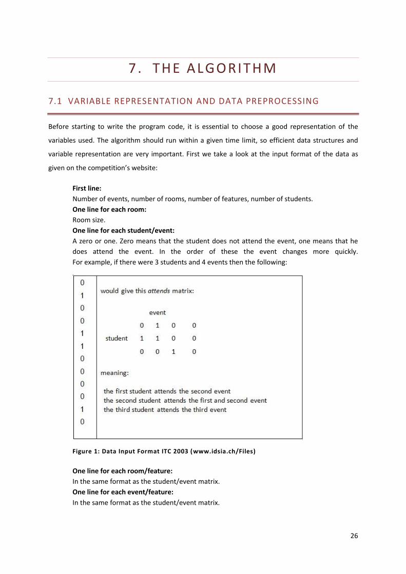
26

7 . TH E A L GO RITH M

7.1 VARIABLE REPRESENTATION AND DATA PREPROCESSING

Before starting to write the program code, it is essential to choose a good representation of the

variables used. The algorithm should run within a given time limit, so efficient data structures and

variable representation are very important. First we take a look at the input format of the data as

given on the competition’s website:

First line:

Number of events, number of rooms, number of features, number of students.

One line for each room:

Room size.

One line for each student/event:

A zero or one. Zero means that the student does not attend the event, one means that he

does attend the event. In the order of these the event changes more quickly.

For example, if there were 3 students and 4 events then the following:

Figure 1: Data Input Format ITC 2003 (www.idsia.ch/Files)

One line for each room/feature:

In the same format as the student/event matrix.

One line for each event/feature:

In the same format as the student/event matrix.

http://www.idsia.ch/Files

27

Based on this format I created five initial variables. Two arrays, one to save the total number of the

events, rooms, features and students, and one to save the size of the different rooms; and three

matrices, one student-event matrix, one room-feature matrix, and one event-feature matrix.

Because the program will be run on different instances with different sizes the matrices and the

room size array are created dynamically, based on the sizes given in the first array.

The information contained within these matrices can be processed into different matrices which

contain the same information in a more compact, easy-to-use way. To do this we take a look at the

problem’s constraints. HC1 says that no student can attend more than one event at the same time.

This means that two or more events that are taken by the same student cannot be scheduled in the

same timeslot. If we analyze the information given in the student-event matrix considering this hard

constraint, we can create an event-conflict matrix. This matrix of dimension events x events

indicates directly which events cannot be scheduled at the same time.

Next we look at HC2 which says that every event should be scheduled in a suitable room, meaning it

is big enough and has all required features available. For this constraint we can aggregate the

information given in the room size array, room-feature matrix, and event-feature matrix into an

event-room matrix, which directly indicates the suitable rooms per event. With this data

preprocessing the information of the instance is represented in these two matrices.

Before we start solving the problem, we can implement another data manipulation that can speed up

the algorithm. Given the event-room matrix we can check if there are events that can be held in only

one specific room. If there are such events, and if there are multiple events which have the same

room as their only option, we can use this information smartly. That is, events that have the same

room as their only option cannot be scheduled in the same timeslot, as this would give either a room

suitability conflict (HC2) or a room which is overbooked (HC3). Therefor we can update the event-

conflict matrix with this information (Kostuch, 2003).

The representation of the roster itself is a chromosome representation in the form of a two

dimensional matrix (rooms x timeslots) which has the value of the event scheduled in that room and

that timeslot, and a value of minus one if no event is scheduled. To speed up the algorithm and to

ensure flexibility when implementing different heuristics I also keep an event ID structure for every

event, which contains the day, hour and room in which that event is scheduled This enables the

algorithm to quickly find the location of an event in the roster. It is in fact another form of

chromosome representation. Additionally I use a student-chromosome of dimension students x

timeslot, which has the value of the event that a particular student has in that particular timeslot.

These last two matrices are kept to enable cheap evaluation and better constructive heuristics.

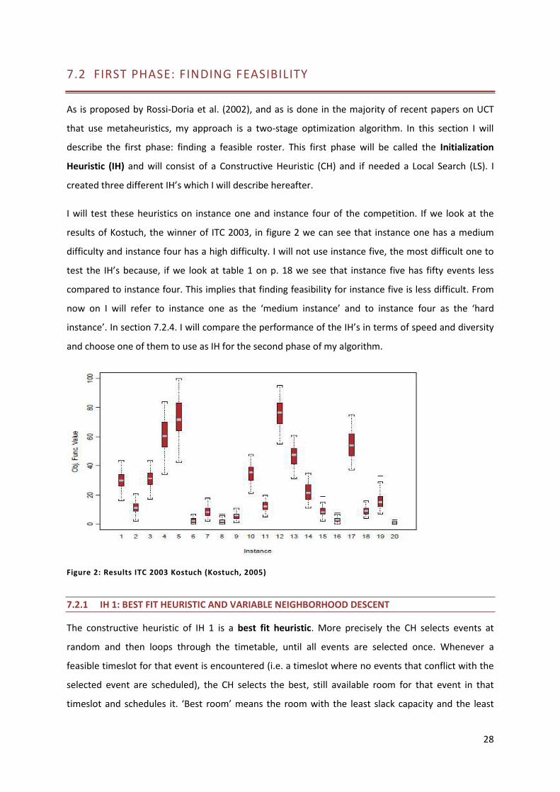
28

7.2 FIRST PHASE: FINDING FEASIBILITY

As is proposed by Rossi-Doria et al. (2002), and as is done in the majority of recent papers on UCT

that use metaheuristics, my approach is a two-stage optimization algorithm. In this section I will

describe the first phase: finding a feasible roster. This first phase will be called the Initialization

Heuristic (IH) and will consist of a Constructive Heuristic (CH) and if needed a Local Search (LS). I

created three different IH’s which I will describe hereafter.

I will test these heuristics on instance one and instance four of the competition. If we look at the

results of Kostuch, the winner of ITC 2003, in figure 2 we can see that instance one has a medium

difficulty and instance four has a high difficulty. I will not use instance five, the most difficult one to

test the IH’s because, if we look at table 1 on p. 18 we see that instance five has fifty events less

compared to instance four. This implies that finding feasibility for instance five is less difficult. From

now on I will refer to instance one as the ‘medium instance’ and to instance four as the ‘hard

instance’. In section 7.2.4. I will compare the performance of the IH’s in terms of speed and diversity

and choose one of them to use as IH for the second phase of my algorithm.

Figure 2: Results ITC 2003 Kostuch (Kostuch, 2005)

7.2.1 IH 1: BEST FIT HEURISTIC AND VARIABLE NEIGHBORHOOD DESCENT

The constructive heuristic of IH 1 is a best fit heuristic. More precisely the CH selects events at

random and then loops through the timetable, until all events are selected once. Whenever a

feasible timeslot for that event is encountered (i.e. a timeslot where no events that conflict with the

selected event are scheduled), the CH selects the best, still available room for that event in that

timeslot and schedules it. ‘Best room’ means the room with the least slack capacity and the least

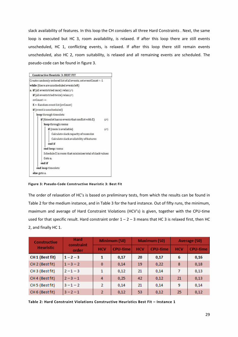
29

slack availability of features. In this loop the CH considers all three Hard Constraints . Next, the same

loop is executed but HC 3, room availability, is relaxed. If after this loop there are still events

unscheduled, HC 1, conflicting events, is relaxed. If after this loop there still remain events

unscheduled, also HC 2, room suitability, is relaxed and all remaining events are scheduled. The

pseudo-code can be found in figure 3.

Figure 3: Pseudo-Code Constructive Heuristic 3: Best Fit

The order of relaxation of HC’s is based on preliminary tests, from which the results can be found in

Table 2 for the medium instance, and in Table 3 for the hard instance. Out of fifty runs, the minimum,

maximum and average of Hard Constraint Violations (HCV’s) is given, together with the CPU-time

used for that specific result. Hard constraint order 1 – 2 – 3 means that HC 3 is relaxed first, then HC

2, and finally HC 1.

Table 2: Hard Constraint Violations Constructive Heuristics Best Fit – Instance 1

30

Table 3: Hard Constraint Violations Constructive Heuristics Best Fit – Instance 4

When HC 1 is relaxed first, the results are poorest. This makes sense once we analyze the hard

constraints. When two ‘conflicting events’ are scheduled at the same moment, and thus violating

HC1, the penalty arising from this is multiplied by the number of students taking both courses.

Whereas allocations that violate HC 2 (an event scheduled in an unsuited room) or HC 3 (an event

scheduled in an occupied room), the penalty for this is just one per violation, disregarding the

amount of students affected by it. The effect of which constraint is relaxed second is not so

significant. This can be understood by the fact that there are very few unscheduled events left,

usually between zero and five, after the heuristics executes the first two loops through all events

(where the first loop takes all HC’s into account, and the second loop drops one HC).

For the first initialization heuristic I decided to select CH 3 as constructive heuristic. Out of fifty runs,

the CH gives an average of seven HCV’s for the medium instance and an average of 64 HCV’s for the

hard instance. Remarkable in the results for the medium instance is that CH 2 constructs a feasible

timetable at once. CH 1, 2, 3, and 5 tend to do this from time to time. The CPU-times do not vary

significantly.

So an initial solution is created, and the LS can be applied to reach feasibility. This LS is a Variable

Neighborhood Descent (VND), as proposed by Hansen (1997), and is based on three facts:

- “A local minimum w.r.t. one neighborhood structure is not necessary so with another;

- A global minimum is a local minimum w.r.t. all possible neighborhoods;

- For many problems local minima w.r.t. one or several neighborhoods are relatively close

to each other.” (Hansen, 1997, p2)

These three facts can be used in a deterministic way to find feasibility. This is exactly what VND does.

During the search it scans different neighborhoods and selects the best move per neighborhood. If

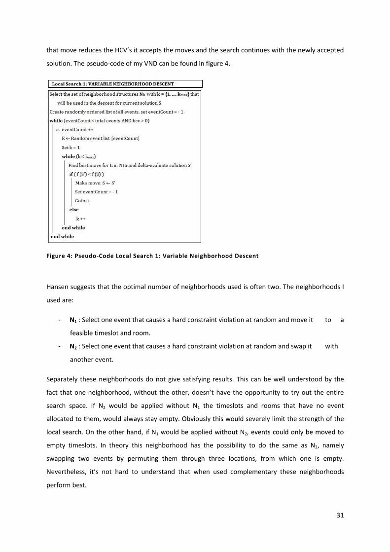
31

that move reduces the HCV’s it accepts the moves and the search continues with the newly accepted

solution. The pseudo-code of my VND can be found in figure 4.

Figure 4: Pseudo-Code Local Search 1: Variable Neighborhood Descent

Hansen suggests that the optimal number of neighborhoods used is often two. The neighborhoods I

used are:

- N1 : Select one event that causes a hard constraint violation at random and move it to a

feasible timeslot and room.

- N2 : Select one event that causes a hard constraint violation at random and swap it with

another event.

Separately these neighborhoods do not give satisfying results. This can be well understood by the

fact that one neighborhood, without the other, doesn’t have the opportunity to try out the entire

search space. If N2 would be applied without N1 the timeslots and rooms that have no event

allocated to them, would always stay empty. Obviously this would severely limit the strength of the

local search. On the other hand, if N1 would be applied without N2, events could only be moved to

empty timeslots. In theory this neighborhood has the possibility to do the same as N2, namely

swapping two events by permuting them through three locations, from which one is empty.

Nevertheless, it’s not hard to understand that when used complementary these neighborhoods

perform best.

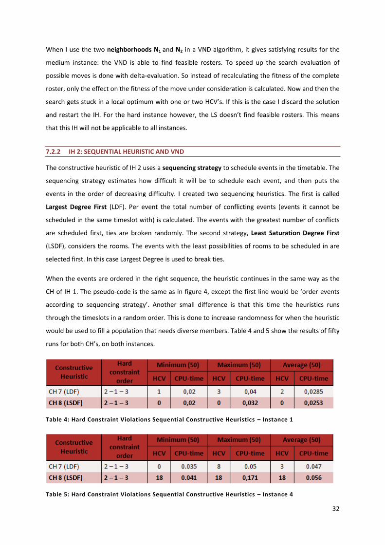
32

When I use the two neighborhoods N1 and N2 in a VND algorithm, it gives satisfying results for the

medium instance: the VND is able to find feasible rosters. To speed up the search evaluation of

possible moves is done with delta-evaluation. So instead of recalculating the fitness of the complete

roster, only the effect on the fitness of the move under consideration is calculated. Now and then the

search gets stuck in a local optimum with one or two HCV’s. If this is the case I discard the solution

and restart the IH. For the hard instance however, the LS doesn’t find feasible rosters. This means

that this IH will not be applicable to all instances.

7.2.2 IH 2: SEQUENTIAL HEURISTIC AND VND

The constructive heuristic of IH 2 uses a sequencing strategy to schedule events in the timetable. The

sequencing strategy estimates how difficult it will be to schedule each event, and then puts the

events in the order of decreasing difficulty. I created two sequencing heuristics. The first is called

Largest Degree First (LDF). Per event the total number of conflicting events (events it cannot be

scheduled in the same timeslot with) is calculated. The events with the greatest number of conflicts

are scheduled first, ties are broken randomly. The second strategy, Least Saturation Degree First

(LSDF), considers the rooms. The events with the least possibilities of rooms to be scheduled in are

selected first. In this case Largest Degree is used to break ties.

When the events are ordered in the right sequence, the heuristic continues in the same way as the

CH of IH 1. The pseudo-code is the same as in figure 4, except the first line would be ‘order events

according to sequencing strategy’. Another small difference is that this time the heuristics runs

through the timeslots in a random order. This is done to increase randomness for when the heuristic

would be used to fill a population that needs diverse members. Table 4 and 5 show the results of fifty

runs for both CH’s, on both instances.

Table 4: Hard Constraint Violations Sequential Constructive Heuristics – Instance 1

Table 5: Hard Constraint Violations Sequential Constructive Heuristics – Instance 4

33

We see that for the medium instance, CH 8 generates feasible timetables every time. CH 7 also gives

very good results with an average of two HCV’s.

For the hard instance results are different. CH 7 gives comparable results as for the medium instance,

but CH 8 always initializes timetables with eighteen HCV’s. The rosters are however different, which

can be concluded from their difference in soft constraint violations (SCV) or directly from calculating

the diversity between the constructed rosters (see infra section 7.2.4). The reason that there are

eighteen HCV’s every time is that the same three events are always scheduled last, as is dictated by

the sequencing strategy. And although the timetable is filled differently (because the order of

timeslots is chosen randomly), these three last events always cause eighteen HCV’s, from which

fifteen are caused by students having two events at the same time, and three are caused by a room

that has two events scheduled in it at the same time.

When these initial timetables are constructed, the same LS as for IH 1, namely VND, is applied to

them. This gives us two new IH’s: IH 2a consists of CH 7 followed by VND and IH 2b consists of CH 8

also followed by VND. Both of them can produce feasible rosters. Which one performs best will

become clear in section 7.2.4.

7.2.3 IH 3: DYNAMIC SEQUENCING

The last initialization heuristic consist of only a constructive heuristic. This CH is again based on a

sequential strategy. Compared to those described above, this strategy is slightly more complex, and

it is dynamic throughout its execution. This means that whenever an event is scheduled, the

sequencing order is recalculated. Another, slightly simpler example of a dynamic sequencing strategy

is Largest Coloured Degree First, where events with the greatest number of conflicting events that

have already been scheduled are scheduled first.

Our final CH was proposed by Arntzen and Løkketangen (2003), and also implemented by Lewis and

Paechter (2004). It orders events based on the total amount of places (a place being the combination

of a certain timeslot and room) it can possibly be scheduled in. Events with the least possibilities are

scheduled first, ties are broken randomly. The heuristic can be seen as an extended version of the

LSDF heuristic. The pseudo-code is shown in figure 5.

34

Figure 5: Pseudo-Code Constructive Heuristic 9: Dynamic Sequencing

Table 6 and 7 show the results of fifty runs. For every instance, it immediately generates feasible

timetables. Therefore no local search is needed, and this gives us the last initialization heuristic IH 3.

Occasionally it happens that an event ends up with an empty place list, so it cannot be scheduled. If

this is the case, I discard the solution and restart the IH. Remarkable is that this CH needs a lot more

CPU-time to create a timetable. This can be understood by the fact that it works dynamically and

thus needs a more time.

Table 6: Hard Constraint Violations Constructive Heuristic Dynamic Sequencing – Instance 1

Table 7: Hard Constraint Violations Constructive Heuristic Dynamic Sequencing – Instance 4

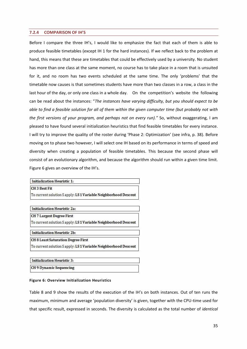
35

7.2.4 COMPARISON OF IH’S

Before I compare the three IH’s, I would like to emphasize the fact that each of them is able to

produce feasible timetables (except IH 1 for the hard instances). If we reflect back to the problem at

hand, this means that these are timetables that could be effectively used by a university. No student

has more than one class at the same moment, no course has to take place in a room that is unsuited

for it, and no room has two events scheduled at the same time. The only ‘problems’ that the

timetable now causes is that sometimes students have more than two classes in a row, a class in the

last hour of the day, or only one class in a whole day. On the competition’s website the following

can be read about the instances: “The instances have varying difficulty, but you should expect to be

able to find a feasible solution for all of them within the given computer time (but probably not with

the first versions of your program, and perhaps not on every run).” So, without exaggerating, I am

pleased to have found several initialization heuristics that find feasible timetables for every instance.

I will try to improve the quality of the roster during ‘Phase 2: Optimization’ (see infra, p. 38). Before

moving on to phase two however, I will select one IH based on its performance in terms of speed and

diversity when creating a population of feasible timetables. This because the second phase will

consist of an evolutionary algorithm, and because the algorithm should run within a given time limit.

Figure 6 gives an overview of the IH’s.

Figure 6: Overview Initialization Heuristics

Table 8 and 9 show the results of the execution of the IH’s on both instances. Out of ten runs the

maximum, minimum and average ‘population diversity’ is given, together with the CPU-time used for

that specific result, expressed in seconds. The diversity is calculated as the total number of identical

36

allocation between two rosters. So actually it indicates the ‘non-diversity’. The population diversity is

then calculated as the average of identical allocations between two rosters over the created

population. So for example, in table 8, 13 is the average population diversity of the most diverse

population out of ten populations created with IH 2b. The population size was set to twenty.

Table 8: Performance of Initialization Heuristics for Creating Population – Instance 1

Table 9: Performance of Initialization Heuristics for Creating Population – Instance 4

For the medium instance, IH 2b outperforms the others, in terms of diversity as well as speed. Speed

is important because the faster phase one is executed, the more time can be allocated to phase two:

optimization. For the hard instance IH 2a performs best. The rules of the ITC however, state that the

complete algorithm should be exactly the same for all instances, therefore I will use IH3 as

initialization heuristic for phase one. It’s performance in terms of speed comes second for both

instances, and the diversity in the population is definitely at an acceptable level. Table 10 shows the

results, in terms of SCV’s and cpu-time of a single execution of IH 3 on every instance of the problem.

A feasible timetable was found every time. With these results we can now confidently move on to

phase two.

Table 10: Initialization Heuristic 3 Tested on all Competition Instances

37

7.3 SECOND PHASE: OPTIMIZATION

As discussed in section 6 there are numerous methods to approach the timetabling problem. The

best results are currently obtained by hybrid algorithms, and thus my attempt to tackle the ITC 2003

problem instances will also be of a hybrid form. I will describe the methods that I tested and/or used

in the following sections. Test results to obtain the ideal composition of my algorithm , outcomes of

parameter fine-tuning, and other experimental results will be given in section 8: Test Design and

Experimental Results. The following sections are a pure theoretical description of the components of

the algorithm.

7.3.1 HYBRID EVOLUTIONARY ALGORITHM

A schematic overview of the complete algorithm are given in figure 7. As discussed before an initial

population is generated in phase one. Phase two begins by selecting one solution from the

population with a selection operator. Next a mutation operator and the Non-Linear Great Deluge

Algorithm (NLGDA) are applied to the solution. If the newly obtained timetable is better than the

worst timetable in the population it replaces it. The algorithm continues like this until the maximum

cpu-time is reached and then the best solution from the population is selected as the final result.

Figure 7: Hybrid Evolutionary Algorithm

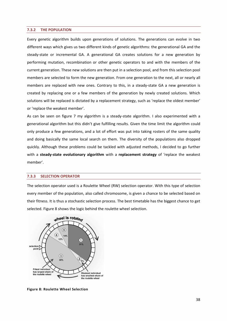
38

7.3.2 THE POPULATION

Every genetic algorithm builds upon generations of solutions. The generations can evolve in two

different ways which gives us two different kinds of genetic algorithms: the generational GA and the

steady-state or incremental GA. A generational GA creates solutions for a new generation by

performing mutation, recombination or other genetic operators to and with the members of the

current generation. These new solutions are then put in a selection pool, and from this selection pool

members are selected to form the new generation. From one generation to the next, all or nearly all

members are replaced with new ones. Contrary to this, in a steady-state GA a new generation is

created by replacing one or a few members of the generation by newly created solutions. Which

solutions will be replaced is dictated by a replacement strategy, such as ‘replace the oldest member’

or ‘replace the weakest member’.

As can be seen on figure 7 my algorithm is a steady-state algorithm. I also experimented with a

generational algorithm but this didn’t give fulfilling results. Given the time limit the algorithm could

only produce a few generations, and a lot of effort was put into taking rosters of the same quality

and doing basically the same local search on them. The diversity of the populations also dropped

quickly. Although these problems could be tackled with adjusted methods, I decided to go further

with a steady-state evolutionary algorithm with a replacement strategy of ‘replace the weakest

member’.

7.3.3 SELECTION OPERATOR

The selection operator used is a Roulette Wheel (RW) selection operator. With this type of selection

every member of the population, also called chromosome, is given a chance to be selected based on

their fitness. It is thus a stochastic selection process. The best timetable has the biggest chance to get

selected. Figure 8 shows the logic behind the roulette wheel selection.

Figure 8: Roulette Wheel Selection

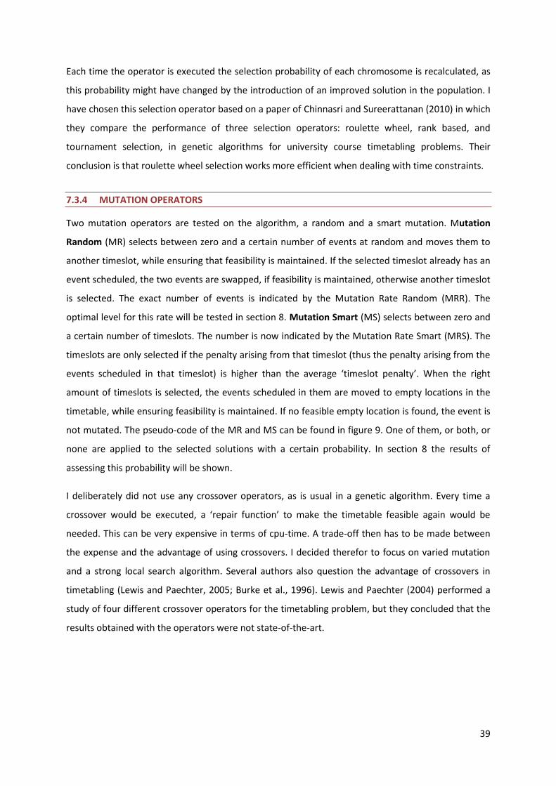
39

Each time the operator is executed the selection probability of each chromosome is recalculated, as

this probability might have changed by the introduction of an improved solution in the population. I

have chosen this selection operator based on a paper of Chinnasri and Sureerattanan (2010) in which

they compare the performance of three selection operators: roulette wheel, rank based, and

tournament selection, in genetic algorithms for university course timetabling problems. Their

conclusion is that roulette wheel selection works more efficient when dealing with time constraints.

7.3.4 MUTATION OPERATORS

Two mutation operators are tested on the algorithm, a random and a smart mutation. Mutation

Random (MR) selects between zero and a certain number of events at random and moves them to

another timeslot, while ensuring that feasibility is maintained. If the selected timeslot already has an

event scheduled, the two events are swapped, if feasibility is maintained, otherwise another timeslot

is selected. The exact number of events is indicated by the Mutation Rate Random (MRR). The

optimal level for this rate will be tested in section 8. Mutation Smart (MS) selects between zero and

a certain number of timeslots. The number is now indicated by the Mutation Rate Smart (MRS). The

timeslots are only selected if the penalty arising from that timeslot (thus the penalty arising from the

events scheduled in that timeslot) is higher than the average ‘timeslot penalty’. When the right

amount of timeslots is selected, the events scheduled in them are moved to empty locations in the

timetable, while ensuring feasibility is maintained. If no feasible empty location is found, the event is

not mutated. The pseudo-code of the MR and MS can be found in figure 9. One of them, or both, or

none are applied to the selected solutions with a certain probability. In section 8 the results of

assessing this probability will be shown.

I deliberately did not use any crossover operators, as is usual in a genetic algorithm. Every time a

crossover would be executed, a ‘repair function’ to make the timetable feasible again would be

needed. This can be very expensive in terms of cpu-time. A trade-off then has to be made between

the expense and the advantage of using crossovers. I decided therefor to focus on varied mutation

and a strong local search algorithm. Several authors also question the advantage of crossovers in

timetabling (Lewis and Paechter, 2005; Burke et al., 1996). Lewis and Paechter (2004) performed a

study of four different crossover operators for the timetabling problem, but they concluded that the

results obtained with the operators were not state-of-the-art.

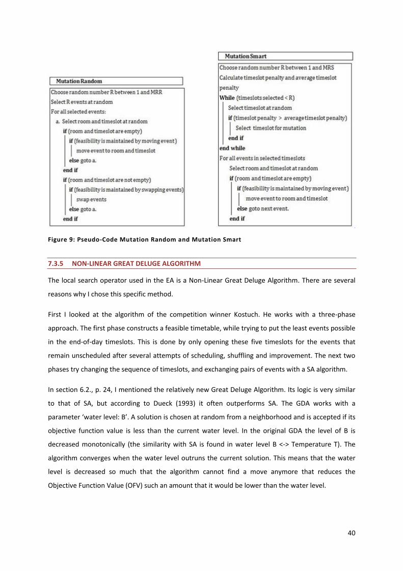
40

Figure 9: Pseudo-Code Mutation Random and Mutation Smart

7.3.5 NON-LINEAR GREAT DELUGE ALGORITHM

The local search operator used in the EA is a Non-Linear Great Deluge Algorithm. There are several

reasons why I chose this specific method.

First I looked at the algorithm of the competition winner Kostuch. He works with a three-phase

approach. The first phase constructs a feasible timetable, while trying to put the least events possible

in the end-of-day timeslots. This is done by only opening these five timeslots for the events that

remain unscheduled after several attempts of scheduling, shuffling and improvement. The next two

phases try changing the sequence of timeslots, and exchanging pairs of events with a SA algorithm.

In section 6.2., p. 24, I mentioned the relatively new Great Deluge Algorithm. Its logic is very similar

to that of SA, but according to Dueck (1993) it often outperforms SA. The GDA works with a

parameter ‘water level: B’. A solution is chosen at random from a neighborhood and is accepted if its

objective function value is less than the current water level. In the original GDA the level of B is

decreased monotonically (the similarity with SA is found in water level B <-> Temperature T). The

algorithm converges when the water level outruns the current solution. This means that the water

level is decreased so much that the algorithm cannot find a move anymore that reduces the

Objective Function Value (OFV) such an amount that it would be lower than the water level.

41

Burke et al. (2003) compare the performance of SA with GDA on the twenty test instances of the ITC

2003 datasets. To prevent premature convergence their algorithm also accepts solutions if their

objective function value is less than that of the current solution (the original GDA only accepts

solutions that are better than the water level). Generally their experiments show that the GDA gives

better results compared to SA. Figure 10 shows the results of SA (left side) and GDA on test instance

3 within a predefined time limit. The y-axis indicates the OFV, the x-axis indicates time and total

moves, both on another scale.

Figure 10: Comparison SA and GDA (Burke et al., 2003)

In 2008 a further improvement of the GDA used by Burke et al. was proposed by Obit and Landa-

Silva. Instead of a linear decay rate of the water level (i.e. the speed at which B decreases), as in the

algorithms of Dueck and Burke et al. (expression 1), they propose a non-linear decay rate of the

water level as shown in expression 2.

Linear decay rate: B = B - ∆B (1)

Non-linear decay rate: B = B x (exp-∂(rand[min, max])) + β (2)

The parameters in expression 2 control the speed and the shape of the water level decay rate.

Together they determine how fast the water level goes down. If it goes down really fast,

improvement is achieved quickly, but the chance of getting stuck in local optima also increases. The

results of fine-tuning the decay rate parameters will be described in the next section.

Another difference besides the non-linear decay rate, in the improved GDA of Obit and Landa-Silva, is

the fact that they allow the water level to go up when its value tends to outrun the objective function

value of the candidate solutions. The water level is then raised with a random number between Bmin

and Bmax. The authors suggest a range of [1,3] for these values.

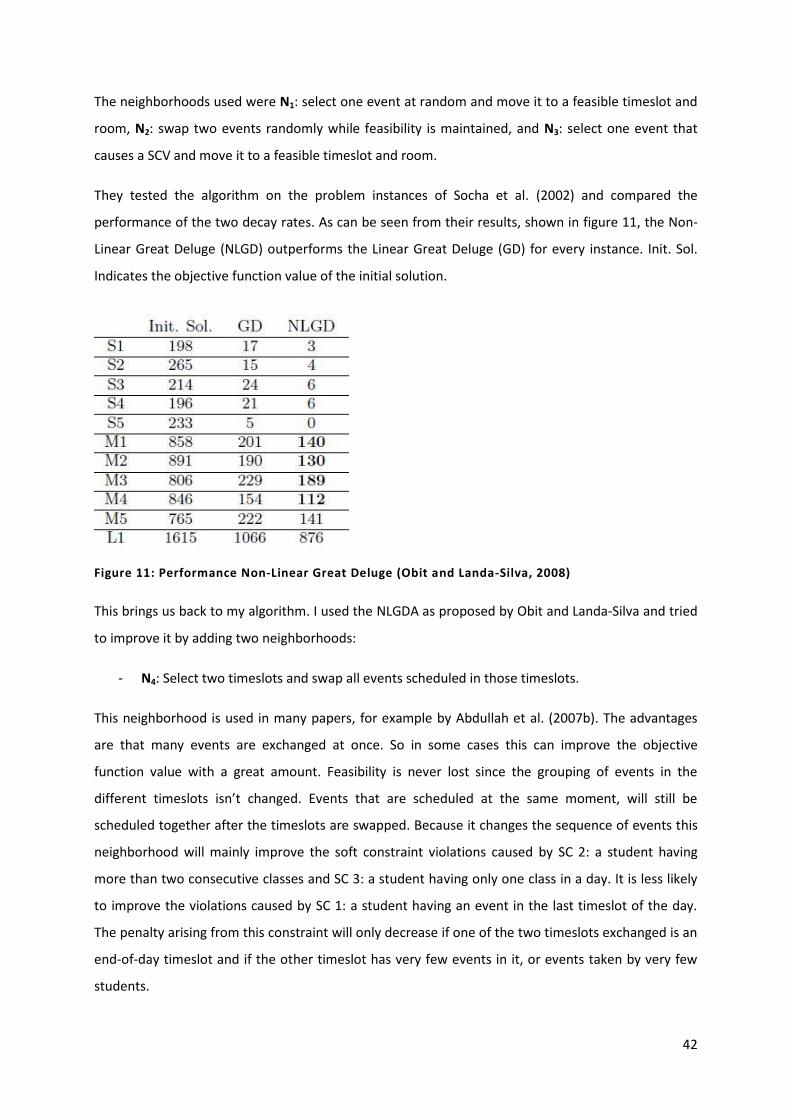
42

The neighborhoods used were N1: select one event at random and move it to a feasible timeslot and

room, N2: swap two events randomly while feasibility is maintained, and N3: select one event that

causes a SCV and move it to a feasible timeslot and room.

They tested the algorithm on the problem instances of Socha et al. (2002) and compared the

performance of the two decay rates. As can be seen from their results, shown in figure 11, the Non-

Linear Great Deluge (NLGD) outperforms the Linear Great Deluge (GD) for every instance. Init. Sol.

Indicates the objective function value of the initial solution.

Figure 11: Performance Non-Linear Great Deluge (Obit and Landa-Silva, 2008)

This brings us back to my algorithm. I used the NLGDA as proposed by Obit and Landa-Silva and tried

to improve it by adding two neighborhoods:

- N4: Select two timeslots and swap all events scheduled in those timeslots.

This n eighborhood is used in many papers, for example by Abdullah et al. (2007b). The advantages

are that many events are exchanged at once. So in some cases this can improve the objective

function value with a great amount. Feasibility is never lost since the grouping of events in the

different timeslots isn’t changed. Events that are scheduled at the same moment, will still be

scheduled together after the timeslots are swapped. Because it changes the sequence of events this

neighborhood will mainly improve the soft constraint violations caused by SC 2: a student having

more than two consecutive classes and SC 3: a student having only one class in a day. It is less likely

to improve the violations caused by SC 1: a student having an event in the last timeslot of the day.

The penalty arising from this constraint will only decrease if one of the two timeslots exchanged is an

end-of-day timeslot and if the other timeslot has very few events in it, or events taken by very few

students.

43

- N5: Select one event scheduled in an end-of-day timeslot and move it to a feasible room

and timeslot (that is not in the end of the day)

This neighborhood has not been extensively studied in the literature, or at least I didn’t find a paper

that describes it. The perfect solution of the timetabling problem at hand has no events scheduled in

any of the last timeslots. Therefor I wanted to test the effect of using a neighborhood that focuses on

clearing up these timeslots. Obviously this neighborhood mainly reduces violations of SC 1.

The effect of these two extra neighborhoods will be tested in the next section. The complete pseudo

code of the NLGDA is shown in figure 12.

Figure 12: Pseudo-Code Non Linear Great Deluge

44

8 . TES T D ES I GN A ND EX P ERIM E NTA L RES U L TS

In this section different variations of the eventual algorithm will be tested. First the parameters and

neighborhood use of the NLGDA, and once that is fine-tuned I will try to optimize the hybrid

evolutionary algorithm. Please note that the experiments with the parameters are not exhaustive.

Every parameter can be set to many different values, and moreover, combinations of various values

of parameters can give different results. The correlation between the values of the parameters are

usually not at all obvious or easy to trace. I therefore tried to test those values that seemed most

promising and most logical. During the tests I always stayed aware of the fact that my final algorithm

will have to be run within a given time limit. This time limit is indicated by a program that

benchmarks your computer1. The output in my case is shown beneath, so I can run my algorithm for

636 seconds.

This program is running, please wait

This program took 106 seconds to run on your machine

This means that you can run your algorithm on the instances provided for 636

seconds

Press return to continue

8.1 LOCAL SEARCH PARAMETER TESTING

8.1.1 NEIGHBORHOODS

As described in section 7.3.5., p. 43, I added two extra neighborhoods in addition to the three

neighborhoods proposed by Obit and Landa-Silva. To test the optimal combination of neighborhoods

I first ran the NLGDA ten times for each of the combinations shown in table 11. The runtime was 100

seconds. This is not particularly long, but in the light of the time limit this is definitely long enough. In

the eventual algorithm the runtime will most likely be much shorter. The left side of the table shows

the average and the minimum SCV out of ten runs. The search started each time from a feasible

1 This benchmark program can be downloaded from:

http://www.idsia.ch/Files/ttcomp2002/IC_Problem/node5.html

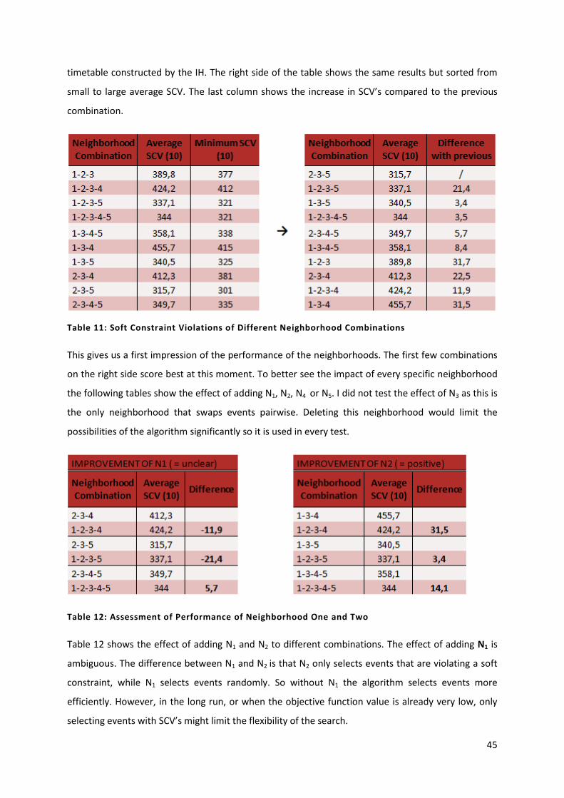
45

timetable constructed by the IH. The right side of the table shows the same results but sorted from

small to large average SCV. The last column shows the increase in SCV’s compared to the previous

combination.

Table 11: Soft Constraint Violations of Different Neighborhood Combinations

This gives us a first impression of the performance of the neighborhoods. The first few combinations

on the right side score best at this moment. To better see the impact of every specific neighborhood

the following tables show the effect of adding N1, N2, N4 or N5. I did not test the effect of N3 as this is

the only neighborhood that swaps events pairwise. Deleting this neighborhood would limit the

possibilities of the algorithm significantly so it is used in every test.

Table 12: Assessment of Performance of Neighborhood One and Two

Table 12 shows the effect of adding N1 and N2 to different combinations. The effect of adding N1 is

ambiguous. The difference between N1 and N2 is that N2 only selects events that are violating a soft

constraint, while N1 selects events randomly. So without N1 the algorithm selects events more

efficiently. However, in the long run, or when the objective function value is already very low, only

selecting events with SCV’s might limit the flexibility of the search.

46

The effect of N2 is overall positive. This can be understood by the fact that it increases the efficiency

of the search by selecting events with SCV’s every time. N1 and N2 are the only neighborhoods that

select events from all over the timetable and move them to an empty place. So, it will be best to use

at least one of them. The choice then obviously goes to N2. Whether we will also use N1 and thus

incorporate both of them will have to be decided based on further testing.

The outcomes of adding N4 and N5 (the neighborhoods I added to the original ones of Obit and

Landa-Silva) are shown in the table 13. Although the logic behind N4 seemed reasonable, this

neighborhood has a negative effect. I now assume that adding it slows down the search and thus

leads to inferior results. Taking a closer look at the output of the search shows why. If we look at

combination 1-2-3-4 we see that, for one run of 100 seconds, N4 finds only 59 moves that reduce the

OFV from the 3378 times it is selected. The other neighborhoods find 462, 547 and 668 moves out of

3232, 3244, and 3360 neighborhood selections respectively. This proves that N4 indeed slows down

the search. If we look back at table 11, we see that the fourth best combination is the one where all

neighborhoods are used. It is obvious now that this is only so because of the strength of N1, N2, N3,

and N5. N4 will thus not be used as a neighborhood in our search algorithm.

Table 13: Assessment of Performance of Neighborhood Four and Five

Finally we look at the effects of adding N5. The results are clearly positive. N5 focuses on emptying

the last timeslots. Since every event that is scheduled in an end-of-day timeslot causes a SCV

multiplied by the number of students taking the event, clearing up these timeslots pays off. Note that

N5 should always be used in combination with a neighborhood N1 or N2. If not, events would be

placed out of the end-of-day timeslots, but couldn’t be placed back in. This would cause the search to

get stuck in a local optimum very quickly.

47

So this leaves us with two possibilities: the combination 1-2-3-5 or 2-3-5. To test this I first ran each

of them fifty times, for 45 seconds. The results are shown in table 14. Combination 2-3-5 scores

slightly better, but the results are not really significant.

Table 14: Comparison of Performance of Best Neighborhood Combinations – 45 Seconds

Next I tested each combination five times, but now with a runtime of 500 seconds. I increased the

runtime to see the performance of the neighborhoods when the objective function value is already

relatively low. This is very important because the main goal is of course to get the objective function

value as low as possible.

Table 15: Comparison of Performance of Best Neighborhood Combinations – 500 Seconds

Now the difference between the two is even less. I therefor decide to use the second combination,

namely N1, N2, N3, and N5 for my final algorithm. The addition of N1 is certainly not negative, and

towards the end it will make the search trajectory more flexible.

Finally I checked if there was no skew in the selection of the neighborhoods during the search, as this

would seriously affect the outcomes and corrupt the results of the previous tests. Luckily this was not

the case. In a test were the runtime was set to 1000 and all neighborhoods were used the total times

of selection per n eighborhood was:

36.064 + 35.934 + 35.604 + 35.810 + 35.951 with a total of 179.363.

8.1.2 DECAY RATE PARAMETERS

All previous tests were executed with the same values for the parameters of the decay rate: B = B x

(exp-∂(rand[min, max])) + β. Β stands for the minimum expected objective function value. The twenty

instances of the ITC all have at least one perfect solution, so β is set to zero. The others were set to: 5

x 10^-9 for delta, 5.000.000 for min and 7.000.000 for max. The value of delta is proposed by Obit

and Landa-Silva for large instances. I will therefore keep delta at this value. For min and max they

propose to use 100.000 and 300.000, which is significantly lower than the values I used. In their

48

paper however they set the runtime of their algorithm to 6700 seconds for large instances which is

very high, and far above the maximum runtime for my complete algorithm. I therefore decided that

it would be best to set my min and max values a lot higher. This indeed increases the chance of

getting stuck in a local optimum. But, I will implement the search algorithm within an evolutionary

algorithm where the mutation operators are meant to escape from local optima. In the evolutionary

algorithm, the NLGDA will run a very short period every time it is executed. Therefore, to obtain good

results, the min and max values should be set sufficiently high so that significant improvement can be

reached within the runtime of each search. To make the decay rate expression less abstract I

calculated the outcomes of it for several parameters and several objective function values. The

values in table 16 indicate to which level the water level is decreased every time an improvement is

found.

Table 16: Values of Water Level with Different Parameters

So if we look at the upper right corner for instance, if an OFV is found that is below 300, let’s say 294,

then the water level decreases to a value somewhere between 293 and 296, let’s say 296. The next

search a move is accepted if the OFV of that move is less than 294 (the current OFV) or less than 296

(the current water level). If the move has an OFV of more than those values, it is not accepted, and

the water level is raised with a value between 1 and 3. Recall that the algorithm allows the water

level to go up with a value between Bmin and Bmax (see pseudo code p. 44). Obit and Landa-Silva

suggest a range of [1, 3], and I will also use these values. I also did some preliminary tests with a

range [2, 4]. The water level fluctuated much more than with [1, 3], but it didn’t lead to better

results. Figure 13 and 14 show the graphs of the search trajectory with range [1, 3] and [2, 4]

respectively. The x-axis shows the CPU-time in seconds. We can see that in the first graph the water

level gradually guides the OFV to lower levels, while in the second graphs the water level fluctuates

around the OFV and often drops below it. Only the first two seconds of the search are depicted, so

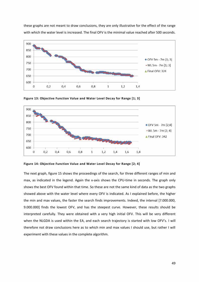
49

these graphs are not meant to draw conclusions, they are only illustrative for the effect of the range

with which the water level is increased. The final OFV is the minimal value reached after 500 seconds.

Figure 13: Objective Function Value and Water Level Decay for Range [1; 3]

Figure 14: Objective Function Value and Water Level Decay for Range [2; 4]

The next graph, figure 15 shows the proceedings of the search, for three different ranges of min and

max, as indicated in the legend. Again the x-axis shows the CPU-time in seconds. The graph only

shows the best OFV found within that time. So these are not the same kind of data as the two graphs

showed above with the water level where every OFV is indicated. As I explained before, the higher

the min and max values, the faster the search finds improvements. Indeed, the interval [7.000.000,

9.000.000] finds the lowest OFV, and has the steepest curve. However, these results should be

interpreted carefully. They were obtained with a very high initial OFV. This will be very different

when the NLGDA is used within the EA, and each search trajectory is started with low OFV’s. I will

therefore not draw conclusions here as to which min and max values I should use, but rather I will

experiment with these values in the complete algorithm.

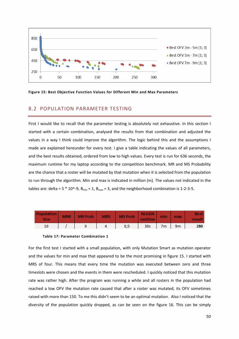
50

Figure 15: Best Objective Function Values for Different Min and Max Parameters

8.2 POPULATION PARAMETER TESTING

First I would like to recall that the parameter testing is absolutely not exhaustive. In this section I

started with a certain combination, analysed the results from that combination and adjusted the

values in a way I think could improve the algorithm. The logic behind this and the assumptions I

made are explained hereunder for every test. I give a table indicating the values of all parameters,

and the best results obtained, ordered from low to high values. Every test is run for 636 seconds, the

maximum runtime for my laptop according to the competition benchmark. MR and MS Probability

are the chance that a roster will be mutated by that mutation when it is selected from the population

to run through the algorithm. Min and max is indicated in million (m). The values not indicated in the

tables are: delta = 5 * 10^-9, Bmin = 1, Bmax = 3, and the n eighborhood combination is 1-2-3-5.

Table 17: Parameter Combination 1

For the first test I started with a small population, with only Mutation Smart as mutation operator

and the values for min and max that appeared to be the most promising in figure 15. I started with

MRS of four. This means that every time the mutation was executed between zero and three

timeslots were chosen and the events in them were rescheduled. I quickly noticed that this mutation

rate was rather high. After the program was running a while and all rosters in the population had

reached a low OFV the mutation rate caused that after a roster was mutated, its OFV sometimes

raised with more than 150. To me this didn’t seem to be an optimal mutation. Also I noticed that the

diversity of the population quickly dropped, as can be seen on the figure 16. This can be simply

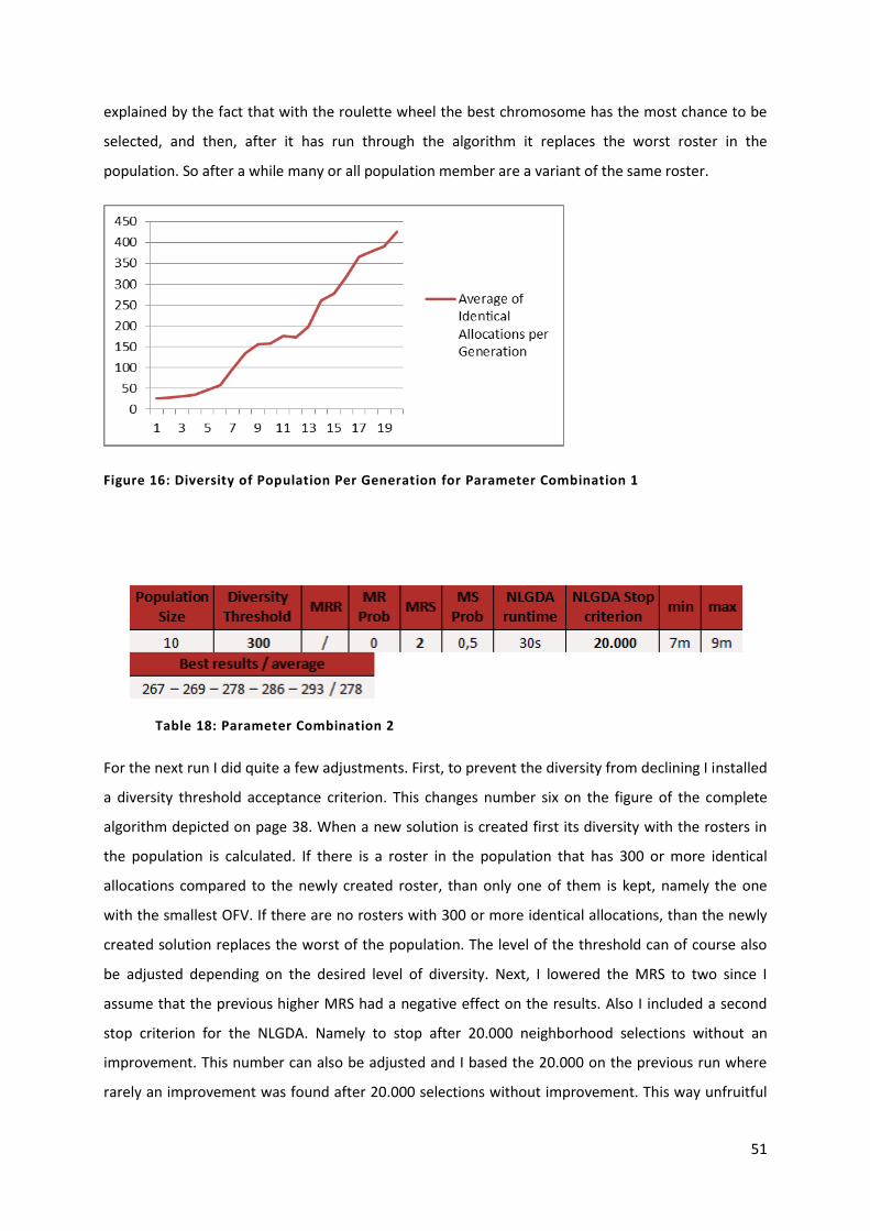
51

explained by the fact that with the roulette wheel the best chromosome has the most chance to be

selected, and then, after it has run through the algorithm it replaces the worst roster in the

population. So after a while many or all population member are a variant of the same roster.

Figure 16: Diversity of Population Per Generation for Parameter Combination 1


For the next run I did quite a few adjustments. First, to prevent the diversity from declining I installed

a diversity threshold acceptance criterion. This changes number six on the figure of the complete

algorithm depicted on page 38. When a new solution is created first its diversity with the rosters in

the population is calculated. If there is a roster in the population that has 300 or more identical

allocations compared to the newly created roster, than only one of them is kept, namely the one

with the smallest OFV. If there are no rosters with 300 or more identical allocations, than the newly

created solution replaces the worst of the population. The level of the threshold can of course also

be adjusted depending on the desired level of diversity. Next, I lowered the MRS to two since I

assume that the previous higher MRS had a negative effect on the results. Also I included a second

stop criterion for the NLGDA. Namely to stop after 20.000 neighborhood selections without an

improvement. This number can also be adjusted and I based the 20.000 on the previous run where

rarely an improvement was found after 20.000 selections without improvement. This way unfruitful

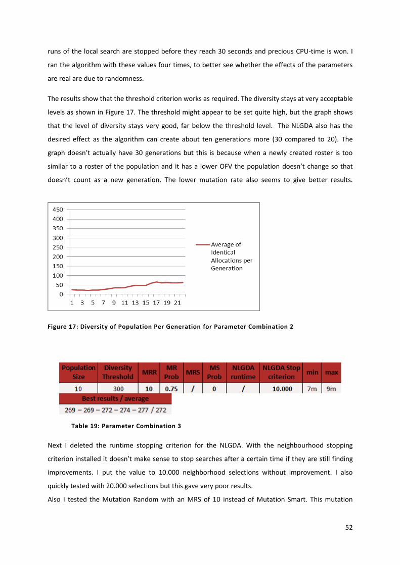
52

runs of the local search are stopped before they reach 30 seconds and precious CPU-time is won. I

ran the algorithm with these values four times, to better see whether the effects of the parameters

are real are due to randomness.

The results show that the threshold criterion works as required. The diversity stays at very acceptable

levels as shown in Figure 17. The threshold might appear to be set quite high, but the graph shows

that the level of diversity stays very good, far below the threshold level. The NLGDA also has the

desired effect as the algorithm can create about ten generations more (30 compared to 20). The

graph doesn’t actually have 30 generations but this is because when a newly created roster is too

similar to a roster of the population and it has a lower OFV the population doesn’t change so that

doesn’t count as a new generation. The lower mutation rate also seems to give better results.

Figure 17: Diversity of Population Per Generation for Parameter Combination 2


Next I deleted the runtime stopping criterion for the NLGDA. With the neighbourhood stopping

criterion installed it doesn’t make sense to stop searches after a certain time if they are still finding

improvements. I put the value to 10.000 neighborhood selections without improvement. I also

quickly tested with 20.000 selections but this gave very poor results.

Also I tested the Mutation Random with an MRS of 10 instead of Mutation Smart. This mutation

53

selects between zero and ten events and reschedules them. It is more levelled than Mutation Smart

as this last selects either zero or ten events (maximum one timeslots was selected with MRS 2 and

this usually has all rooms occupied so contains ten events). As the mutation will usually select less

events I used a mutation probability of 0.75.

The results are slightly better, but not significant. Due to the changed stopping criterion of the local

search, a lot more loops of the algorithm are executed. Although it didn’t lead to better results here,

this could be an advantage when other parameters are optimized.


Next, I increased the min and max values. As explained before this will cause that the search faster

finds improvement, but has a higher chance to get stuck in local optima. I kept the other parameters

unchanged to clearly see the results of the higher min and max values.

The results are visibly positive. With an average of twenty SCV’s less we can assume this is not due to

randomness. I would like to depict the effect of the higher min and max values on the local searches,

but this is not so easy. The search trajectory sometimes doesn’t find improvement at all, and in other

runs a lot. So depicting one or a few of all the executions of the NLGDA wouldn’t say very much, or

enable us to thoroughly analyse why the higher values lead to better results.

If I look at the different outputs I see that a newly created roster very often replaces the old version

of itself. This means that the rosters do not change a lot as they always exceed the diversity

threshold. I am not sure whether this has a negative effect on the results. In a way it’s normal that

they do not change a lot. Only when a mutation opens the way to significant improvements the

allocations will really differ. If the mutation changes some events in a way that only a small

improvement can be found, most likely not a high percentage of the allocations will change.

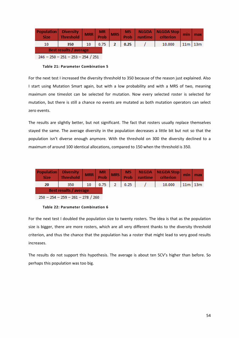
54


For the next test I increased the diversity threshold to 350 because of the reason just explained. Also

I start using Mutation Smart again, but with a low probability and with a MRS of two, meaning

maximum one timeslot can be selected for mutation. Now every selected roster is selected for

mutation, but there is still a chance no events are mutated as both mutation operators can select

zero events.

The results are slightly better, but not significant. The fact that rosters usually replace themselves

stayed the same. The average diversity in the population decreases a little bit but not so that the

population isn’t diverse enough anymore. With the threshold on 300 the diversity declined to a

maximum of around 100 identical allocations, compared to 150 when the threshold is 350.


For the next test I doubled the population size to twenty rosters. The idea is that as the population

size is bigger, there are more rosters, which are all very different thanks to the diversity threshold

criterion, and thus the chance that the population has a roster that might lead to very good results

increases.

The results do not support this hypothesis. The average is about ten SCV’s higher than before. So

perhaps this population was too big.

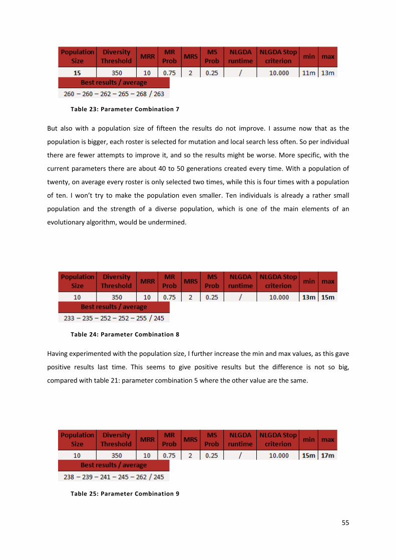
55


But also with a population size of fifteen the results do not improve. I assume now that as the

population is bigger, each roster is selected for mutation and local search less often. So per individual

there are fewer attempts to improve it, and so the results might be worse. More specific, with the

current parameters there are about 40 to 50 generations created every time. With a population of

twenty, on average every roster is only selected two times, while this is four times with a population

of ten. I won’t try to make the population even smaller. Ten individuals is already a rather small

population and the strength of a diverse population, which is one of the main elements of an

evolutionary algorithm, would be undermined.


Having experimented with the population size, I further increase the min and max values, as this gave

positive results last time. This seems to give positive results but the difference is not so big,

compared with table 21: parameter combination 5 where the other value are the same.


56

With even bigger min and max values the results stay more or less the same, so I assume that the

positive effect of raising those values has reached its maximum now.


For the next test I reset the min and max values to thirteen and fifteen million. From the outputs of

the local searches of the previous tests (combination eight) I saw that improvements were usually

found within 5.000 neighborhood selections, or even a lot less. More exactly, from 6.139

improvements made in the five runs together, only 65 were found after more than 5.000

neighborhood selections. So I now tested with a stop criterion of 5.000. This gives the algorithm the

chance to create a lot more generations, and thus every roster is selected more often to run through

the algorithm.

The results do not vary significantly, but they are definitely not worse. Recall the reason that I

assumed that testing with a bigger population didn’t pay off, namely that every roster is selected less

times to run through the algorithm. However, with this sharper stop criterion for the local search, a

lot more generations are created. About 100 compared to 50 before.



57

So, once more I tried to assess the effect of increasing the population size. Once with a stop criterion

of 5.000 and once with 3.000.

For 5.000 the results are definitely not better. For 3.000 they are more or less the same as the results

with a population of 10 and a stop criterion of 5.000. I will decide which parameters (population 10

and stop criterion 5.000 or population 20 and stop criterion 3.000) to use for my final algorithm

based on testing these two combinations on another instance of the competition (see infra, p. 60).


Finally I set up some last test runs to try to optimize the parameters of the mutation operators. First I

only used Mutation Random. I tried to increase the mutation rate quite a bit, to 20. So now between

zero and nineteen events are selected. I kept the mutation probability at 0,75 because the rate is

rather high.

The results do not really show an improvement. So I assume that the MRR was set too high.


Next I decreased the rate to fifteen. This also didn’t give better results. The average is significantly

decreased by the outlier 224. I assume this is due to a particularly good random seed and local

search proceedings, but is not the effect of the changed mutation parameters.

58


The higher mutation rates didn’t improve the outcomes so I tried to put the MRR relatively low. The

mutation probability was now set to one to counterbalance the really low mutation rate.

Again the results did not improve. I won’t try to test with Mutation Smart as the only mutation as this

is a rather inflexible mutation. The amount of events mutated is always zero, nine or ten, nineteen or

twenty, … So I do not expect this will yield good results.


I did one more test with both mutations where I lowered the MRR to six. But also this did not show

better results. My conclusion of the mutation rate testing is that the combination of both mutations

works best, with a higher probability for Mutation Random, and with MRR set to ten and MRS to two.

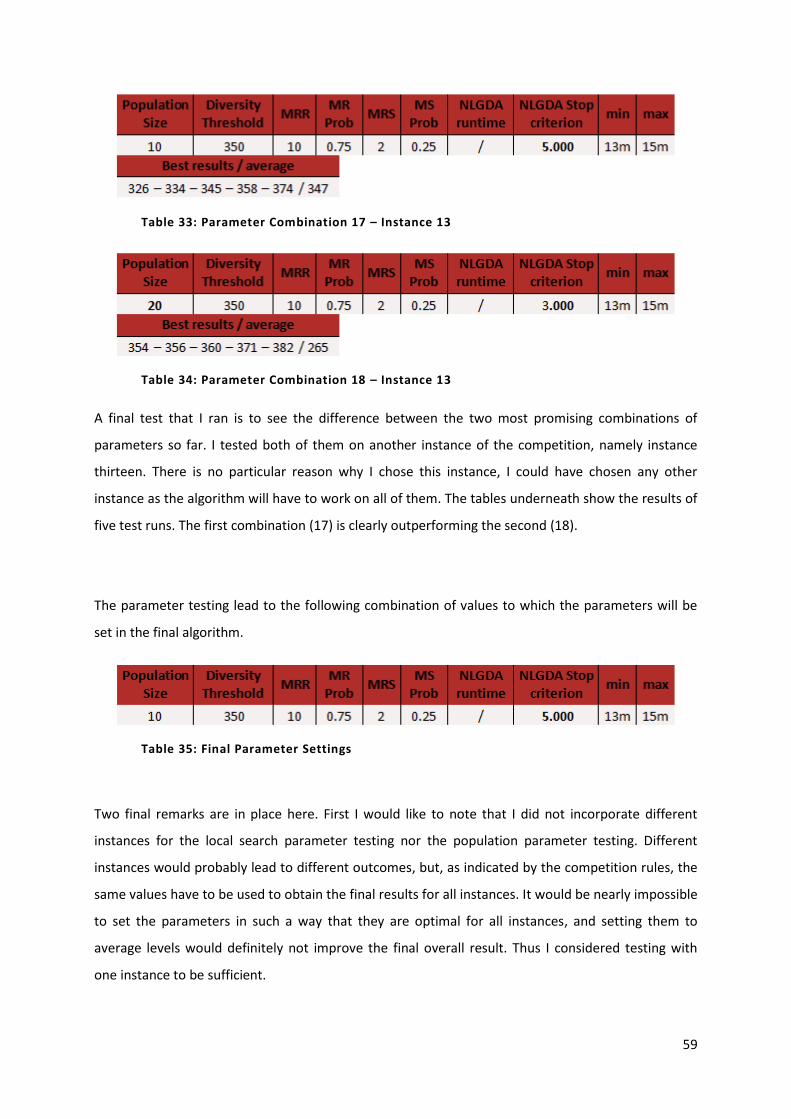
59

Table 33: Parameter Combination 17 – Instance 13

Table 34: Parameter Combination 18 – Instance 13

A final test that I ran is to see the difference between the two most promising combinations of

parameters so far. I tested both of them on another instance of the competition, namely instance

thirteen. There is no particular reason why I chose this instance, I could have chosen any other

instance as the algorithm will have to work on all of them. The tables underneath show the results of

five test runs. The first combination (17) is clearly outperforming the second (18).

The parameter testing lead to the following combination of values to which the parameters will be

set in the final algorithm.

Table 35: Final Parameter Settings

Two final remarks are in place here. First I would like to note that I did not incorporate different

instances for the local search parameter testing nor the population parameter testing. Different

instances would probably lead to different outcomes, but, as indicated by the competition rules, the

same values have to be used to obtain the final results for all instances. It would be nearly impossible

to set the parameters in such a way that they are optimal for all instances, and setting them to

average levels would definitely not improve the final overall result. Thus I considered testing with

one instance to be sufficient.

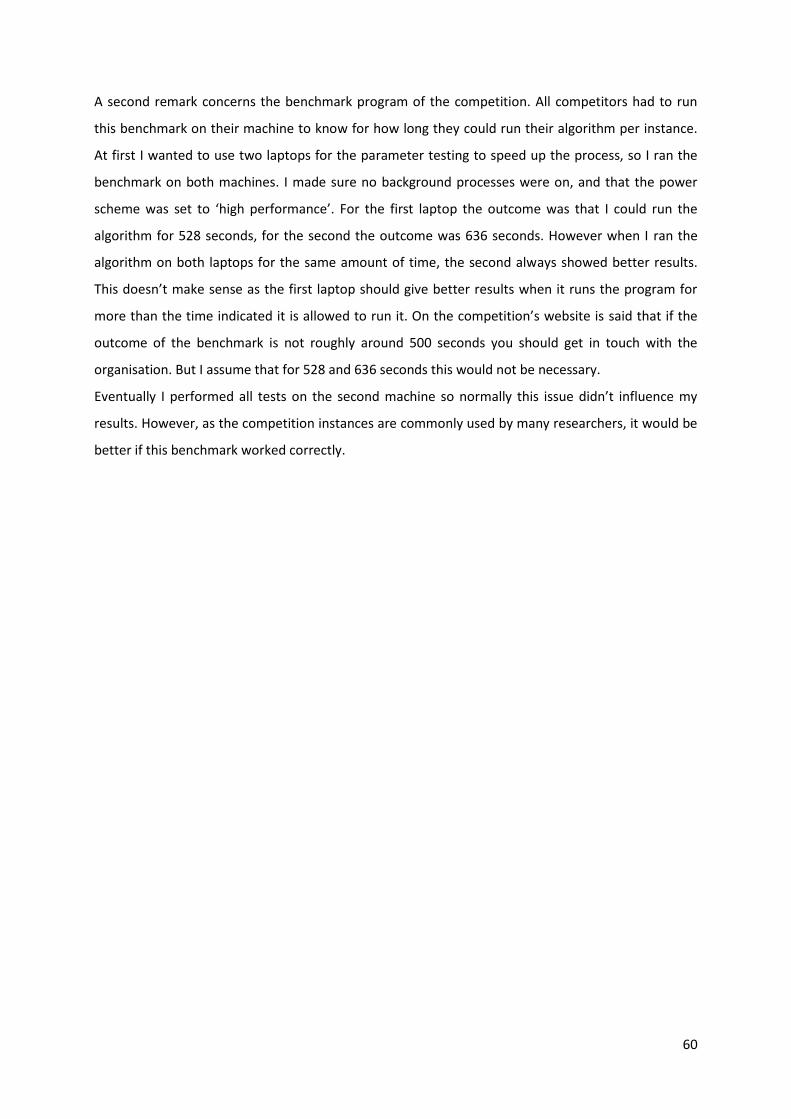
60

A second remark concerns the benchmark program of the competition. All competitors had to run

this benchmark on their machine to know for how long they could run their algorithm per instance.

At first I wanted to use two laptops for the parameter testing to speed up the process, so I ran the

benchmark on both machines. I made sure no background processes were on, and that the power

scheme was set to ‘high performance’. For the first laptop the outcome was that I could run the

algorithm for 528 seconds, for the second the outcome was 636 seconds. However when I ran the

algorithm on both laptops for the same amount of time, the second always showed better results.

This doesn’t make sense as the first laptop should give better results when it runs the program for

more than the time indicated it is allowed to run it. On the competition’s website is said that if the

outcome of the benchmark is not roughly around 500 seconds you should get in touch with the

organisation. But I assume that for 528 and 636 seconds this would not be necessary.

Eventually I performed all tests on the second machine so normally this issue didn’t influence my

results. However, as the competition instances are commonly used by many researchers, it would be

better if this benchmark worked correctly.

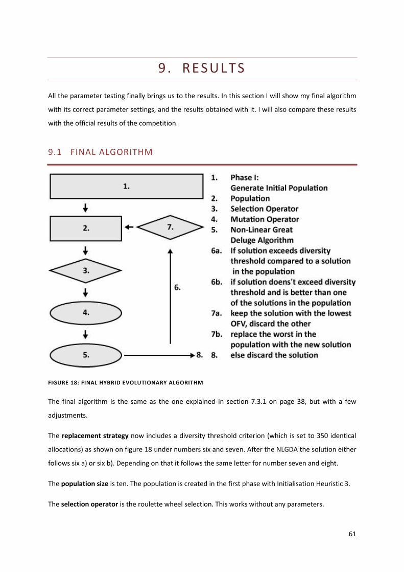
61

9 . RES UL TS

All the parameter testing finally brings us to the results. In this section I will show my final algorithm

with its correct parameter settings, and the results obtained with it. I will also compare these results

with the official results of the competition.

9.1 FINAL ALGORITHM

FIGURE 18: FINAL HYBRID EVOLUTIONARY ALGORITHM

The final algorithm is the same as the one explained in section 7.3.1 on page 38, but with a few

adjustments.

The replacement strategy now includes a diversity threshold criterion (which is set to 350 identical

allocations) as shown on figure 18 under numbers six and seven. After the NLGDA the solution either

follows six a) or six b). Depending on that it follows the same letter for number seven and eight.

The population size is ten. The population is created in the first phase with Initialisation Heuristic 3.

The selection operator is the roulette wheel selection. This works without any parameters.

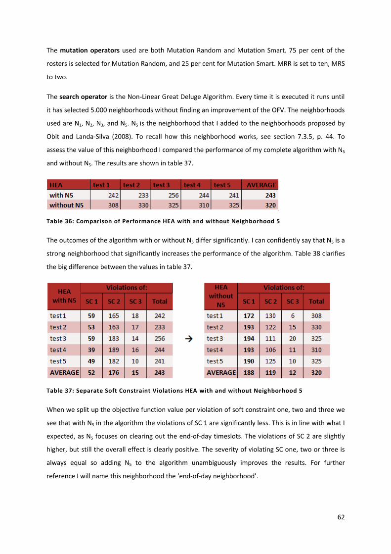
62

The mutation operators used are both Mutation Random and Mutation Smart. 75 per cent of the

rosters is selected for Mutation Random, and 25 per cent for Mutation Smart. MRR is set to ten, MRS

to two.

The search operator is the Non-Linear Great Deluge Algorithm. Every time it is executed it runs until

it has selected 5.000 neighborhoods without finding an improvement of the OFV. The neighborhoods

used are N1, N2, N3, and N5. N5 is the neighborhood that I added to the neighborhoods proposed by

Obit and Landa-Silva (2008). To recall how this neighborhood works, see section 7.3.5, p. 44. To

assess the value of this neighborhood I compared the performance of my complete algorithm with N5

and without N5. The results are shown in table 37.

Table 36: Comparison of Performance HEA with and without Neighborhood 5

The outcomes of the algorithm with or without N5 differ significantly. I can confidently say that N5 is a

strong neighborhood that significantly increases the performance of the algorithm. Table 38 clarifies

the big difference between the values in table 37.

Table 37: Separate Soft Constraint Violations HEA with and without Neighborhood 5

When we split up the objective function value per violation of soft constraint one, two and three we

see that with N5 in the algorithm the violations of SC 1 are significantly less. This is in line with what I

expected, as N5 focuses on clearing out the end-of-day timeslots. The violations of SC 2 are slightly

higher, but still the overall effect is clearly positive. The severity of violating SC one, two or three is

always equal so adding N5 to the algorithm unambiguously improves the results. For further

reference I will name this neighborhood the ‘end-of-day neighborhood’.

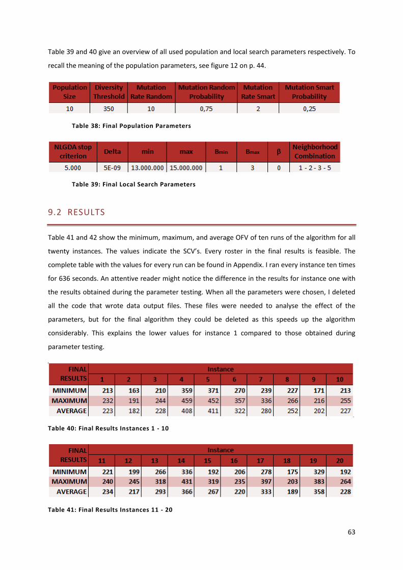
63

Table 39 and 40 give an overview of all used population and local search parameters respectively. To

recall the meaning of the population parameters, see figure 12 on p. 44.

Table 38: Final Population Parameters

Table 39: Final Local Search Parameters

9.2 RESULTS

Table 41 and 42 show the minimum, maximum, and average OFV of ten runs of the algorithm for all

twenty instances. The values indicate the SCV’s. Every roster in the final results is feasible. The

complete table with the values for every run can be found in Appendix. I ran every instance ten times

for 636 seconds. An attentive reader might notice the difference in the results for instance one with

the results obtained during the parameter testing. When all the parameters were chosen, I deleted

all the code that wrote data output files. These files were needed to analyse the effect of the

parameters, but for the final algorithm they could be deleted as this speeds up the algorithm

considerably. This explains the lower values for instance 1 compared to those obtained during

parameter testing.

Table 40: Final Results Instances 1 - 10

Table 41: Final Results Instances 11 - 20

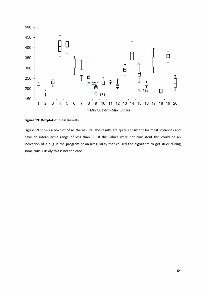
64

Figure 19: Boxplot of Final Results

Figure 19 shows a boxplot of all the results. The results are quite consistent for most instances and

have an interquartile range of less than 50. If the values were not consistent this could be an

indication of a bug in the program or an irregularity that caused the algorithm to get stuck during

some runs. Luckily this is not the case.

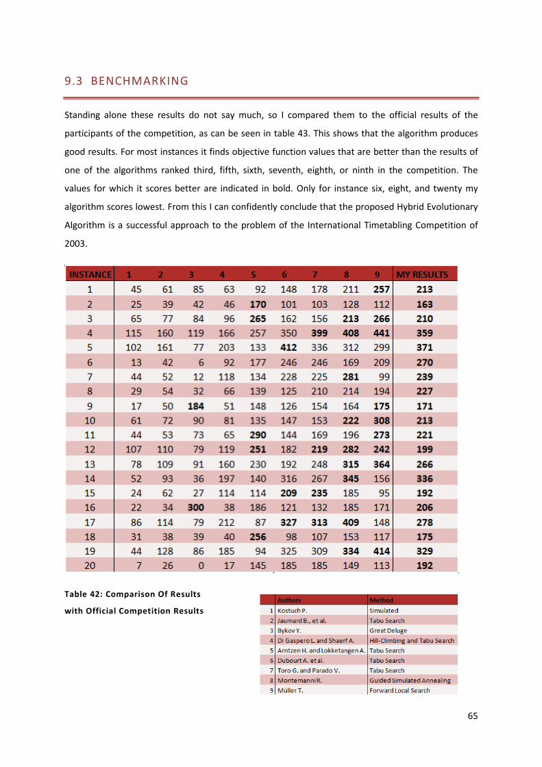
65

9.3 BENCHMARKING

Standing alone these results do not say much, so I compared them to the official results of the

participants of the competition, as can be seen in table 43. This shows that the algorithm produces

good results. For most instances it finds objective function values that are better than the results of

one of the algorithms ranked third, fifth, sixth, seventh, eighth, or ninth in the competition. The

values for which it scores better are indicated in bold. Only for instance six, eight, and twenty my

algorithm scores lowest. From this I can confidently conclude that the proposed Hybrid Evolutionary

Algorithm is a successful approach to the problem of the International Timetabling Competition of

2003.

Table 42: Comparison Of Results

with Official Competition Results

66

1 0 . C ONC L US ION

In this thesis I studied the university course timetabling problem on the basis of the International

Timetabling Competition of 2003. The university course timetabling problem is a combinatorial

optimization problem where courses have to be assigned to a suitable room and planned into a

weekly schedule of timeslots. A timetable strongly affects the life of students, teachers and other

university staff members as well as the quality of education at the university. It is therefore essential

for every institution to provide prime timetables that take into account the requirements for every

course, the educational policy of the university, and the preferences of students and teachers.

For several decades research has been done towards finding methods that are able to construct good

timetables. In 2003 the EURO Working group on Automated Timetabling (WATT) organized, together

with the Metaheuristics Network, an International Timetabling Competition (ITC 2003). The aim was

to create better understanding between researchers and practitioners by allowing emerging

techniques to be trialed and tested on real-world models of timetabling problems. Also, the

organizers hoped that conclusions of the competition would stimulate debate and research in the

field of timetabling. The subject problem of this competition has since been widely accepted as a

benchmark problem in the timetabling community. It is this problem that I extensively studied in this

thesis, and for which I have developed a method to solve it.

The university course timetabling problem is a problem with such a high complexity that it has to be

tackled with heuristic and metaheuristic approaches. Many solution methods have been proposed in

the literature but the ideal technique to find optimal timetables has not yet emerged. I hope that my

research can contribute to the on-going optimization of methods to solve the timetabling problem.

The algorithm I propose is a combination of an evolutionary algorithm with a non-linear great deluge

algorithm, it is thus a hybrid metaheuristic method. I tested the algorithm on the datasets of the

International Timetabling Competition of 2003. The results obtained can compete with the results

obtained by the algorithms that ended seventh, eighth, and ninth in the competition, and thus prove

that it is a good performing algorithm.

For future research I suggest to experiment with the end-of-day neighborhood proposed in this

thesis. It has not yet been extensively studied in literature, and comparison of the performance of

the algorithm with and without this neighborhood shows promising results.

67

REF E RENC ES

Abdullah, S., Burke, E. K., McCollum, B., 2007, A hybrid evolutionary approach to university course

timetabling, in CEC 2007, Congress on evolutionary computation 2007, Singapore, pp. 1764-

1768.

Abdullah, S., Burke, E. K., McCollum, B., 2007b, Using a randomized iterative improvement algorithm

with composite neighborhood structures for the university course timetabling problem., in

Operations Research/Computer Science Interfaces Series, vol. 39, pp. 153-169.

Abdullah, S., Turabich, H., McCollum, B., McMullan, P., 2010, A hybrid metaheuristic approach to the

university course timetabling problem, in Journal of Heuristics, vol. 18, Springer

Science+Business Media, pp. 1-23.

Al-Betar, M. A., Khader, A. T., 2010, A harmony search algorithm for university course timetabling, in

Annals of Operations Research, vol. 194, 2012, Springer Science+Business Media, pp. 3-31.

Arntzen, H., Løkketangen, A., 2003, A tabu search heuristic for a university timetabling problem, MIC

2003, Fifth Metaheuristic International Conference pp. 02-1 – 02-7.

Arntzen, H., Løkketangen, A., 2003, , A local search heuristic for a university timetabling problem, ITC

2003, <http://www.idsia.ch/Files/ttcomp2002/arntzen.pdf>

Atsuta, M., Nonobe, K., Ibaraki, T., 2007, ITC-2007 Track2: An Approach using General CSP Solver,

<http://www.cs.qub.ac.uk/itc2007/winner/bestcoursesolutio ns/Atsuta_et_al.pdf>

Balakrishnan, N., Lucena, A., Wong, R. T., 1992, Scheduling examinations to reduce second-order

conflicts, in Computers and Operations Research, vol. 19, pp. 353–361.

Blum, C., Roli, A., 2003, Metaheuristics in Combinatorial Optimization: Overview and Conceptual

Comparison, in ACM Computing Surveys, vol. 35, No. 3, 2003, pp. 268–308.

Blum, C., Puchinger, J., Raidl, G. R., Roli, A., 2011, Hybrid metaheuristics in combinatorial

optimization: a survey, in Applied soft computing, vol. 11, pp. 4135-4151.

Burke, E. K., Bykov, Y., Newall, J., Petrovic, S., 2003, a timepredefined approach to course

timetabling, in Yugoslav Journal of Operations Research, vol. 13(2), pp. 139-151.

http://www.cs.qub.ac.uk/itc2007/winner/bestcoursesolutio%20ns/Atsuta_et_al.pdf

68

Burke, E. K., Jackson, K., Kingston, J. H., & Weare, R., 1997, Automated university timetabling: The

state of the art, in The Computer Journal, vol. 40(9), pp. 565–571.

Burke, E. K., Kendall, G., Soubeiga, E., 2003, a tabu-search hyperheuristic for timetabling and

rosterting, in Journal of Heuristics, vol. 9, Kluwer Academic Publishers, pp. 451-470.

Burke, E. K., Marecek, J., Parkes, A. J., Rudóva, H., 2010, Decomposition, reformulation, and diving in

university course timetabling, in Journal of Computers & Operations Research, vol. 37, pp.

582-597.

Burke, E. K., Newall, J. P., Weare, R. F., 1996, A Memetic Algorithm for University Exam Timetabling,

in The Practice and Theory of Automated Timetabling I, Springer Lecture Notes in Computer

Science, vol. 1153, Springer-Verlag, pp. 241-250.

Burke, E. K., Newall, J. P., Weare, R. F., 1998. A simple heuristically guided search for the timetable

problem, International ICSC Symposium on Engineering of Intelligent Systems EIS’98, ICSC

Academic Press, New York, pp. 574–579.

Burke, E.K., Petrovic, S., 2002, Recent research directions in automated timetabling, in European

Journal of Operational Research, vol. 140(2), pp. 266-280.

Burke, E.K., Ross, P., 1995, Proceedings of the first International Conference on the Practice and

Theory of Automated Timetabling, in Lecture Notes in Computer Science, vol. 1153, Springer,

pp.1-384

Brailsford, S. C., Potts, C., N., Smith, B., M., 1999, Constraint satisfaction problems: Algorithms and

applications, in European Journal of Operational Research, vol. 119, pp. 557-581.

Brélaz, D. 1979, New methods to color the vertices of a graph, in Communications of the ACM, vol.

22(4), pp. 251– 256.

Bykov, Y., 2003, The description of the Algorithm for International Timetabling Competition, ITC

2003. <http://www.idsia.ch/Files/ttcomp2002/bykov.pdf>

Cambazard H., Hebrard, E., O’Sullivan, B., Papadopoulos A., 2007, Local search and constraint

programming for the post enrolment-based course timetabling problem, in Annals of

Operations Research, vol. 194, 2012, pp. 111-135.

69

Carter, M. W., Laporte, G., 1997, Recent developments in practical course timetabling, in Lecture

notes in computer scienc, vol. 1408. The practice and theory of automated timetabling, pp.

3–19.

Carter, M.W., 1986, A survey of practical applications of examination timetabling algorithms, in

Operations Research, vol. 34, pp. 193–202.

Chiarandini, M., Birattari, M., Socha, K., Rossi-Doria, O., 2006, An effective hybrid algorithm for

university course timetabling, in Journal of Scheduling, vol. 9(5), Springer Science+Business

Media, pp. 403-432.

Chinnasri, W., Sureerattanan, N., 2010, Comparison of Performance between Different Selection

Strategies on Genetic Algorithm with Course Timetabling Problem, in Advanced Management

Science (ICAMS), IEEE International Conference on General topics for Engineering, vol. 3, pp.

105-108.

Cordeau, J.-F., Jaumard, B., Morales, R., 2003, Efficient Timetabling with Tabu Search, ITC 2003,

<http://www.idsia.ch/Files/ttcomp2002/jaumard.pdf>

Corne, D., Ross, P., and Fang, H., 1995, Evolving timetables. in Lance C. Chambers, editor, The

Practical Handbook of Genetic Algorithms, vol. 1, CRC Press, pp. 219-276.

De Causmaecker, P., Demeester, P., Vanden Berghe, G., 2008, A decomposed metaheuristic approach

for a real-world university timetabling problem, in European Journal of Operational Research,

vol. 195, 2009, pp. 307–318.

de Werra, D., 1985, An Introduction to Timetabling, in European Journal of Operations Research, vol.

19, pp. 151-162.

de Werra, D., 1996, The Combinatorics of Timetabling, in European Journal of Operational Research,

vol. 96, pp. 504-513.

Di Gaspero, L., Schaerf, A., 2001, Tabu search techniques for examination timetabling, in E.K. Burke,

W. Erben (Eds.) Practice and theory of automated timetabling III: 3rd international

conference, Springer, pp. 104-116.

Di Gaspero, L., Schaerf, A., 2003, Timetabling Competition TTComp 2002: Solver Description, ITC

2003, <http://www.idsia.ch/Files/ttcomp2002/schaerf.pdf>

http://ieeexplore.ieee.org/xpl/mostRecentIssue.jsp?punumber=5547540

http://ieeexplore.ieee.org/xpl/mostRecentIssue.jsp?punumber=5547540

70

Dubourg, A., Laurent, B., Long, E., Salotti B., 2003, Algorithm description, ITC 2003,

<http://www.idsia.ch/Files/ttcomp2002/laurent.pdf>

Dueck, G., 1993, New optimization heuristics: The great deluge algorithm and the record-to-record

travel, in Journal of Computational Physics, vol. 104, pp. 86-92.

Erben, W., Keppler, J., 1996, A genetic algorithm solving a weekly course timetabling problem, in

Selected papers from the First International Conference on Practice and Theory of

Automated Timetabling, Springer-Verlag, London, pp. 198-211.

Fesanghary, M., Mahdavi, M., Minary-Jolandan, M., Alizadeh, Y., 2008, Hybridizing harmony search

algorithm with sequential quadratic programming for engineering optimization problems, in

Computer Methods in Applied Mechanics and Engineering, vol. 197(30-40), pp. 3080-3091.

Hansen, P., Mladenovic, N., 1997, Variable Neighborhood search, in Computer & Operations

Research, vol. 24 (11), Elsevier, pp. 1097-1100.

Kostuch, P. A., 2003, University course timetabling, Transfer Thesis, Oxford University, England, pp. 1-

67.

Kostuch, P., 2005, The university course timetabling problem with a three-phase approach, in E. K.

Burke, M. A. Trick (Eds.), Lecture notes in computer science, vol. 3616, Springer-Verlag, pp.

109-125.

Landa-Silva, D., Obit, J. H., 2008, Great deluge with non-linear decay rate for solving course

timetabling problems, in Proceedings of the 4th international IEEE conference on intelligent

systems (IS 2008), IEEE Press, New York, pp. 8.11-8.18.

Landa-Silva, D., Obit, J., H., 2011, Comparing hybrid constructive heuristics for university course

timetabling, in Proceedings of the VII ALIO–EURO – Workshop on Applied Combinatorial

Optimization, Porto, pp. 222-225.

Lewis, R., Paechter, B., 2004, New crossover operators for timetabling with evolutionary algorithms,

in A. Lofti (Ed.) The fifth international conference on recent advances in soft computing

RASC2004, Nottingham, pp. 189-194.

Lewis, R., Paechter, B., 2005, Application of the Grouping Genetic Algorithm to University Course

Timetabling, in Lecture Notes in Computer Science, vol. 3448, pp. 144-153.

71

Lewis, R., 2008, A survey of metaheuristic-based techniques for university timetabling problems, in

OR Spectrum, vol. 30, issue 1, pp. 167–190.

Malim, M. R., Khader, A. T., Mustafa, A., 2006, Artificial immune algorithms for university

timetabling, in E. K. Burke, H. Rudova (Eds.), Proceedings of the 6th international conference

on practice and theory of automated timetabling, pp. 234-245.

McMullan, P. J., Abdullah, S., Burke, E. K., McCollum, B, Parkes, A., J., 2007, An extended

implementation of the great deluge algorithm for course timetabling, in ICCS ’07:

Proceedings of the 7th international conference on computational science, Part I, Berlin

Springer, pp. 538-545.

Montemanni, R., 2003, Timetabling: Guided Simulated Annealing + Local Searches, ITC 2003,

<http://www.idsia.ch/Files/ttcomp2002/montemanni.pdf>

MirHassani, S., A., Habibi, F., 2011, Solution approaches to the course timetabling problem, in

Artificial Intelligence Review, Springer Science+Business Media, pp. 1-17.

Müller, T., 2005, Constraint-based timetabling, Ph.D. Thesis, KTIML MFF UK, pp. 13-14,

<http://muller.unitime.org/phd-thesis.pdf>

Müller, T., 2003, TTComp02: Algorithm Description, ITC 2003,

<http://www.idsia.ch/Files/ttcomp2002/muller.pdf>

Rossi-Doria, O., Samples, M., Birattari, M., Chiarandini, M., Dorigo, M., Gambardella, L., Knowles, J.,

Manfrin, M., Mastrolilli, M., Paechter, B., Paquette, L., Stültze, T., 2003, A comparison of the

performance of different metaheuristics on the timetabling problem, in E. K. Burke and P. De

Causmaecker, in Practice and Theory of Automated Timetabling, Springer lecture notes in

computer science, vol. 2740, pp. 329-351.

Schaerf, A., 1999. A survey of automated timetabling, in Artificial Intelligence Review, vol. 13 (2), pp.

87–127.

Socha, K., Knowles, J., Samples, M., 2002, A max-min ant system for the university course timetabling

problem., in Proceedings of the third international workshop on ant algorithms, ANTS 2002,

Springer lecture notes in computer science, vol. 2463, pp. 1-13.

Toro, G., Parada, V., 2003, The algorithm to solve the competition problem, ITC 2003,

<http://www.idsia.ch/Files/ttcomp2002/parada.pdf>

72

Wren, A., 1996, Scheduling, Timetabling and Rostering – A Special Relationship?, in the Practice and

Theory of Automated Timetabling, ed. E.K. Burke and P. Ross, Springer-Verlag, pp. 46-75.

Yang, S., Naseem Jat, S., 2011, Genetic algorithms with guided and local search strategies for

university course timetabling, in IEEE Transactions on systems, man, and cybernetics, part C:

applications and reviews, vol. 41, nr. 1, pp. 93-106.

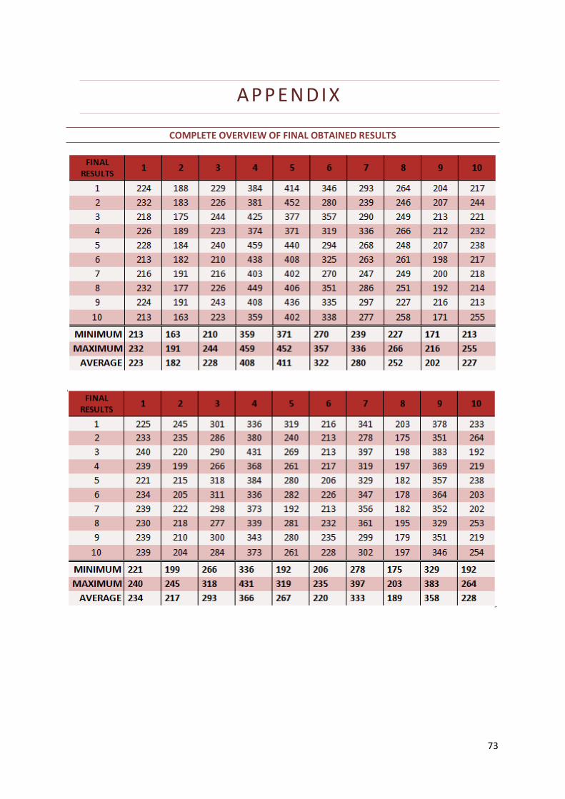
73

A P P END IX

COMPLETE OVERVIEW OF FINAL OBTAINED RESULTS

A HEURISTIC APPROACH TO UNIVERSITY COURSE TIMETABLING

Documents

Transcript of A HEURISTIC APPROACH TO UNIVERSITY COURSE TIMETABLING