
S CATTEROMETRY - Universiteit Utrecht
209
SCATTEROMETRY
Transcript of S CATTEROMETRY - Universiteit Utrecht

SCATTEROMETRY

CIP-GEGEVENS KONINKLIJKE BIBLIOTHEEK, DEN HAAG
Stoffelen, Ad
Scatterometry
Ad Stoffelen
Proefschrift Universiteit Utrecht. -Met lit. opg.-
Met samenvatting in het Nederlands.
ISBN 90-393-1708-9
Trefw.: meteorologie, satellietwaarnemingen

SCATTEROMETRY
DE SCATTEROMETER
(Met een samenvatting in het Nederlands)
Proefschrift
ter verkrijging van de graad van doctor aan de Universiteit Utrecht op gezag van de Rector
Magnificus Prof. Dr. H. O. Voorma, ingevolge het besluit van het College voor Promoties in
het openbaar te verdedigen op maandag 26 oktober 1998 des namiddags te 4.15 uur
door
Adrianus Cornelis Maria Stoffelen
geboren op 25 februari 1962, te Alphen (N.Br.)

Promotoren: Prof. Dr. Bert Holtslag, Universiteit Utrecht
Prof. Dr. David Anderson, University of Oxford
Prof. Dr. Ir. Arnold Heemink, Technische Universiteit Delft
The research described in this thesis has been carried out at the European Centre for
Medium-range Weather Forecasts (ECMWF) and the Royal Netherlands Meteorological
Institute (KNMI) with financial support from the European Space Agency (ESA) and the
Netherlands Remote Sensing Board (BCRS).
Winds at sea,
As wild as they can be,
Imagine the light,
That sees them bright.
Aan Karin,
Kees, Elma, Leon, en Rian

i
CONTENTS
SAMENVATTING
De Scatterometer ______________________________________________________vii
Overzicht____________________________________________________________ viii
CHAPTER I INTRODUCTION TO SCATTEROMETRY
1. The Need for Wind Data ____________________________________________ I-1
1.1. Atmospheric Flow____________________________________________________ I-1
1.2. Global Observing System______________________________________________ I-4
1.3. Data Assimilation ____________________________________________________ I-7
1.4. Weather and Wave Prediction__________________________________________ I-9
1.5. Climate____________________________________________________________ I-10
1.6. Ocean Modeling ____________________________________________________ I-10
2. Scatterometer Instruments __________________________________________ I-12
2.1. Normalized Radar Cross Section_______________________________________ I-12
2.2. SeaSat, NSCAT and SeaWinds ________________________________________ I-15
2.3. ERS Scatterometers and ASCAT ______________________________________ I-18
3. The Physics Behind Scatterometry ___________________________________ I-19
3.1. Electromagnetic Interaction of Microwaves With the Ocean Surface _________ I-20
3.2. The Ocean Topography ______________________________________________ I-21
3.3. From Capillary Waves to Winds _______________________________________ I-23
4. Aim and Overview of the Thesis _____________________________________ I-26
References _________________________________________________________ I-29
CHAPTER II MEASUREMENT SPACE AND INVERSION
ii
Abstract____________________________________________________________ II-1
1. Introduction _____________________________________________________ II-2
2. Visualization in Measurement Space _________________________________ II-4
2.1. Visualization of Anisotropy ___________________________________________ II-6
2.1.1. Validation of the Existence of a Solution Surface_______________________________ II-8
2.1.2. Estimation of B2_________________________________________________________ II-9
2.1.3. The Need for Higher Harmonics ___________________________________________ II-12
2.2. Visualization of the Triplet Distribution Along the Cone___________________ II-13
2.2.1. Upwind-Downwind Effect________________________________________________ II-14
2.3. Wind Speed Dependence ____________________________________________ II-16
2.4. Other Geophysical Dependencies______________________________________ II-16
3. Inversion _______________________________________________________ II-18
3.1. Measurement Space Transformation___________________________________ II-19
3.2. Quality Tests in the Transformed Space________________________________ II-22
4. Summary and Conclusions ________________________________________ II-23
Appendix A: The Prelaunch Transfer Function CMOD2___________________ II-25
Appendix B: Assumptions for B 1 Estimation ____________________________ II-26
Appendix C: Theoretical Derivation of the Inversion Procedure_____________ II-27
Appendix D: Estimation of the Triplet Scatter ___________________________ II-28
Acknowledgements _________________________________________________ II-28
References ________________________________________________________ II-29

iii
CHAPTER III ESTIMATION AND VALIDATION OF THE TRANSFER FUNCTION CMOD4
Abstract____________________________________________________________III-1
1. Introduction _____________________________________________________III-1
2. Estimation of the Transfer Function: Simulation Studies_________________III-2
2.1. Example 1: Tuning Simulations using Wind Components rather than Speed
and Direction ____________________________________________III-6
2.2. Example 2 :Tuning Simulations in Logarithmic Space _____________________III-7
3. Estimation of the Transfer Function: Real Data ________________________III-8
3.1. Data Selection ______________________________________________________III-8
3.2. Estimation ________________________________________________________III-10
4. Validation Procedure _____________________________________________III-12
4.1. Interpretation of σσ 0 Differences_______________________________________III-12
4.2. Simulation of the Effect of Noise on the Validation _______________________III-12
5. A Posteriori Verification __________________________________________III-13
5.1. Validation in σσ 0 Space ______________________________________________III-13
5.2. Validation against Winds ____________________________________________III-14
5.3. High Speed Comparisons ____________________________________________III-19
5.4. Wind Error Correlation_____________________________________________III-22
6. Summary and Conclusions ________________________________________III-24
Appendix A: Analytic Illustration of Curve-Fitting Complications___________III-27
A1. Example 1: Nonlinearity in the Transfer Function ________________________III-27
A2. Example 2: Bias Resulting from Proportional Errors _____________________III-29
Appendix B: The CMOD4 Model Formulation and Coefficients ____________III-30
Acknowledgements _________________________________________________III-31
References ________________________________________________________III-32
CHAPTER IV ERROR MODELING AND CALIBRATION USING TRIPLE COLLOCATION

iv
Abstract____________________________________________________________ IV-1
1. Introduction _____________________________________________________ IV-2
2. Observation Errors and Error Domain ________________________________ IV-3
3. Error Modeling and Calibration With Two Systems______________________ IV-8
4. Error Modeling and Calibration With Three Systems ____________________ IV-9
5. Higher-Order Calibration _________________________________________ IV-10
6. Calibration and Error Model Results ________________________________ IV-11
6.1. First-Order Calibration _____________________________________________ IV-12
6.2. Higher-Order Calibration ___________________________________________ IV-16
7. Conclusions_____________________________________________________ IV-18
7.1. Résumé___________________________________________________________ IV-18
7.2. Application _______________________________________________________ IV-19
Appendix A: Necessity of Error Modeling Before Calibration or Validation ___ IV-20
A1. Scatter Plots and Regression _________________________________________ IV-20
A2. Necessity of Error Modeling Before Calibration _________________________ IV-21
Appendix B: Pseudobias Through Nonlinear Transformation ______________ IV-23
Acknowledgements _________________________________________________ IV-23
References ________________________________________________________ IV-23
CHAPTER V AMBIGUITY REMOVAL AND ASSIMILATION OF SCATTEROMETER DATA

v
Abstract_____________________________________________________________V-1
1. Introduction ______________________________________________________V-2
2. Ambiguity Removal ________________________________________________V-4
2.1. Description of the Ambiguity Removal Procedure __________________________V-4
2.2. Examples of Ambiguity Removal Using PRESCAT_________________________V-7
3. Optimum Interpolation (OI) Assimilation______________________________V-12
3.1. The Analysis System_________________________________________________V-12
3.2. Analysis and Short-Range Impact ______________________________________V-15
3.3. Medium-Range Forecast Impact _______________________________________V-20
3.4. Validation of the OI Data Assimilation System ____________________________V-24
4. Variational Methods_______________________________________________V-26
5. Summary and Conclusions _________________________________________V-29
Acknowledgements __________________________________________________V-32
References _________________________________________________________V-32
CHAPTER VI OUTLOOK
1. Empirical Methodology ____________________________________________ VI-1
1.1. Using NWP fields ___________________________________________________ VI-1
1.2. Uncertainty and Non-linearity _________________________________________ VI-3
1.3. Backscatter Measurement Space _______________________________________ VI-4
2. Physics of Scatterometry ___________________________________________ VI-6
3. Impact of Scatterometers __________________________________________ VI-10
References ________________________________________________________ VI-11
APPENDIX

vi
A Simple Method for Calibration of a Scatterometer over the Ocean ___________A-1
Abstract ________________________________________________________________A-1
1. Introduction __________________________________________________________A-1
2. Method ______________________________________________________________A-4
3. Results_______________________________________________________________A-8
3.1. Ocean Calibration_________________________________________________________ A-8
3.2. Antenna Gain Variations __________________________________________________ A-10
3.3. Application _____________________________________________________________ A-12
4. Conclusions__________________________________________________________A-14
References _____________________________________________________________A-17
Acronyms __________________________________________________________A-19
Acknowledgments ___________________________________________________A-21
Curriculum Vitae____________________________________________________A-23

SAMENVATTING vii
SAMENVATTING
De Scatterometer
Een veelheid aan meteorologische metingen is dagelijks beschikbaar. De meeste van
deze waarnemingen bevinden zich echter boven land, en met name windwaarnemingen
boven de (Noord Atlantische) oceaan zijn schaars. Bij een westelijke luchtstroming is dit
een duidelijke beperking voor de weers- en golfverwachtingen ten behoeve van Nederland.
Juist dan is het gevaar voor bijvoorbeeld storm of overstroming het grootst. Ook in het
aardse klimaatsysteem speelt de wind aan het oppervlak een grote rol en is de belangrijkste
factor voor de aandrijving van de oceaancirculatie. De oceaancirculatie op zijn beurt is
cruciaal voor de verschijnselen die samenhangen met bijvoorbeeld El Niño. Dit proefschift
gaat over het scatterometer instrument dat vanuit de ruimte, zelfs onder een wolkendek,
nauwkeurige en betrouwbare informatie geeft over de wind aan het oceaanoppervlak met
een hoge mate van ruimtelijke consistentie.
Tijdens de tweede wereldoorlog werden radars aan boord van schepen veelvuldig
gebruikt voor de opsporing van vijandige vaartuigen. Hierbij werd vastgesteld dat de
detectie slechter werd naarmate de wind aan het zeeoppervlak groter was.
Proefondervindelijk was hiermee het principe van een wind scatterometer aangetoond. Al
snel ontwikkelde zich dan ook de idee de wind aan het zeeoppervlak te meten met behulp
van radar. Vanuit een vliegtuig of een satelliet word dan een microgolfbundel onder een
schuine hoek naar het zeeoppervlak gestuurd. De microgolfstraling, met gewoonlijk een
golflengte van enkele centimeters, wordt verstrooid aan het ruwe oppervlak, en een klein
gedeelte van de uitgezonden puls keert terug naar het detectorgedeelte van de scatterometer.
Het fysische fenomeen van belang voor de werking van de scatterometer is de
aanwezigheid van zogeheten capillaire gavitatiegolven op het zeeoppervlak. Deze golven
hebben een golflengte van enkele centimeters en reageren vrijwel instantaan op de sterkte
van de wind. De verstrooiing van microgolven is op zijn beurt weer sterk afhankelijk van de
amplitude van de capillaire golven. Bovendien blijken de capillaire golfjes over het
algemeen gericht in lijn met de windrichting. Aldus bestaat er een verband tussen de
hoeveelheid teruggestrooide energie en de windsterkte en -richting op enige hoogte. Een
scatterometer instrument wordt zo ontworpen dat uit diverse metingen van het
teruggestrooide vermogen, windsterkte en -richting afgeleid kunnen worden. Deze metingen
kunnen dan eenvoudig vergeleken worden met bestaande windgegevens van boeien, schepen
en weermodellen ter calibratie en validatie.
SAMENVATTINGviii
Overzicht
In de loop der jaren zijn scatterometer instrumenten aan boord van verscheidene
satellieten gelanceerd. De scatterometers op de ERS-1 en ERS-2 (“European Remote-
sensing Satellite”) hebben de langste staat van dienst en zijn sinds 1991 operationeel. Deze
scatterometers (die identiek zijn) hebben ieder drie antennes, waarmee het oceaanoppervlak
in drie verschillende richtingen bemeten wordt. Een punt op het aardoppervlak wordt eerst
door de naar voren gerichte bundel belicht, dan door de naar opzij gerichte bundel, en als
laatste door de naar achteren gerichte bundel. De drie metingen, verder kortweg aangeduid
als trits, kunnen tegen elkaar worden uitgezet, hetgeen resulteert in een ruimtelijk (3D)
plaatje. Door uitgekiende doorsneden te maken van deze ruimte kan de samenhang van de
drie metingen kwalitatief worden bestudeerd. De drie metingen blijken dan inderdaad een
sterke samenhang te vertonen die verklaard kan worden uit twee geofysische parameters. De
drie metingen liggen namelijk in het algemeen dichtbij een hoornvormig (2D) oppervlak. De
lengterichting van de hoorn blijkt voornamelijk te corresponderen met een variërende
windsterkte (of ruwheid van de zee), en de kortste omtrek van de hoorn met een variërende
windrichting (ofwel oriëntatie van de capillaire golfjes). De karakterisatie en modellering
van dit oppervlak heeft geleid tot een aanzienlijke verbetering in de interpretatie van de
scatterometer, zoals beschreven is in dit proefschrift.
Hierboven is een uiterst simplistisch beeld gegeven van de fysica die van belang is bij
de interpretatie van de scatterometer. Het eerste hoofdstuk van dit proefschrift beschrijft in
meer detail de fysische modellering van belang bij de interpretatie van de scatterometer
metingen. Ten eerste, de topografie van het zeeoppervlak is uitermate gecompliceerd en niet
nauwkeurig te beschrijven met eenvoudige mathematische vergelijkingen. De capillaire
golven hebben een andere fasesnelheid dan de langere golven en beide hebben hiermee een
ingewikkelde dynamische interactie. Bij hogere windsnelheid breken de golven en ontstaan
er schuimkoppen, hetgeen de fysische beschrijving verder compliceert. Ten tweede, de
interactie van een schuin invallende microgolfbundel met dit gecompliceerde oppervlak is
evenmin nauwkeurig te beschrijven. Zowel verstrooiing als reflectie kunnen een rol spelen.
Ten derde, over de relatie tussen de amplitude van de capillaire golven en de wind op enige
hoogte, laten we veronderstellen 10 m, is in de literatuur niet de overeenstemming tot in het
gewenste detail. Bij lage windsnelheid zouden de oppervlaktespanning of variaties in de
wind variabiliteit een rol kunnen spelen.
Gezien de fysische complexiteit, is het niet verwonderlijk dat voor de interpretatie van
scatterometer metingen statistische methoden hun opgang gevonden hebben. Dit proefschrift
gaat met name in op deze methoden, en geeft, aan de hand van vijf wetenschappelijke
publicaties, een tamelijk volledig beeld van de “state-of-the-art”, zoals die bereikt is met de

SAMENVATTING ix
ERS scatterometers (ERS-1 vanaf 17 juli 1991 en later ERS-2 vanaf 22 november 1995).
Het derde hoofdstuk behandelt de visualisatie van de gemeten tritsen in de 3D
meetruimte, de bepaling van de spreiding van de metingen rond het hoornvormige
oppervlak, en de schatting van de meest waarschijnlijke “werkelijke” (of ruisvrije) trits bij
het hoornvormige oppervlak gegeven de metingen en hun nauwkeurigheid (inversie). De
perceptie dat de metingen met grote waarschijnlijkheid dichtbij een hoornvormig oppervlak
liggen, vormt essentiële a priori informatie van belang voor de inversie. Een
inversieprocedure gestoeld op waarschijnlijkheidstheorie is afgeleid. Verder worden aan de
hand van de structuur van het hoornvormige oppervlak indicatoren bepaald, van belang voor
de kwaliteitscontrole, instrumentbewaking, en de verdere verwerking van de gegevens.
In de appendix wordt een methode besproken die beschrijft hoe, aan de hand van
geselecteerde windgegevens en een goed wind-microgolf verband, ofwel transfer functie, de
scatterometer verstrooiingsmetingen gecalibreerd kunnen worden boven de oceaan. Het
blijkt dat deze calibratie, die per antenne wordt uitgevoerd, uiterst nauwkeurig is, en,
wanneer toegepast, in de 3D meetruimte de verdeling van gemeten tritsen gemiddeld
dichterbij de door de transfer functie gemodelleerde hoorn brengt. Dit levert een verbetert
scatterometer wind product op. De methode was met name van groot belang voor de
validatie en calibratie van de ERS-2 scatterometer, voordat de instrumentele calibratie was
voltooid.
Met behulp van een set windgegevens uit een weermodel en hun geschatte
nauwkeurigheden, passend in locatie en tijd bij een set van scatterometer metingen en hun
geschatte nauwkeurigheden, kan met quasi-lineaire schattingstheorie (“Maximum
Likelihood Estimation”) de meest waarschijnlijke wind-microgolf transfer functie worden
afgeleid. De niet-lineariteit en onnauwkeurige formulering van de transfer functie, een niet-
uniforme verdeling van invoergegevens, en een inaccurate formulering van de geschatte
nauwkeurigheid kunnen hier een goed resultaat in de weg staan. Een nieuwe functie,
genoemd CMOD4, wordt afgeleid in hoofdstuk IV. Een eerste eis die gesteld wordt aan een
transfer functie, is dat het in de 3D meetruimte nauwkeurig bij de gemeten tritsen past.
Wanneer de “fit” optimaal is zal het gecombineerde effect van meetonnauwkeurigheid en
inversiefout kleiner zijn dan 0.5 m s−1 in de wind vector. CMOD4 blijkt binnen deze fout bij
de metingen te passen. Een tweede eis is, dat voor een onafhankelijke gegevensset, het
verschil tussen de geïnverteerde scatterometer wind en de bijpassende wind van
bijvoorbeeld een weermodel zo klein mogelijk is. In de praktijk blijkt dat deze tweede eis
impliciet volgt uit de eerste, maar ook dat de onnauwkeurigheid van de scatterometer wind
met name wordt bepaald door de associatie van een locatie op de hoorn met een wind
vector. De onnauwkeurigheid in de scatterometer wind kan dan ook goed beschreven
worden in het wind domein.

SAMENVATTINGx
In hoofdstuk V wordt dit laatste verder uitgewerkt, en wordt gestreefd naar een
gedetailleerde wind calibratie met behulp van in situ gegevens. Windgegevens bevatten
doorgaans een relatief grote onnauwkeurigheid. Het wordt aangetoond dat ijking of regressie
van zulke gegevens niet mogelijk is in een vergelijking van twee meetsystemen, tenzij de
nauwkeurigheid van één van de twee meetsystemen bekend is. In de praktijk is dit meestal
niet zo. Voor deze gevallen wordt een methode voorgesteld die uitgaat van de simultane
vergelijking van drie meetsystemen. In dit geval kan zowel de ijking als een foutenmodel
voor de drie meetsystemen worden opgelost. Toepassing van de methode laat zien dat de
scatterometer wind afgeleid met behulp van CMOD4 ruwweg 5 % te laag is, en de
oppervlaktewind van het gebruikte weermodel ongeveer 5 % te hoog.
Het hoornvormige oppervlak blijkt te bestaan uit twee nauw samenvallende laagjes.
Wanneer de wind een component heeft in de kijkrichting van de middelste microgolfbundel
wordt de ene hoorn beschreven, en wanneer de wind een component heeft tegengesteld
hieraan, de andere. Uit een trits metingen (met ruis) kan dus in het algemeen niet een unieke
windvector worden bepaald. Twee ongeveer tegengestelde oplossingen resulteren. Deze
dubbelzinnigheid in de windrichting kan in de praktijk worden opgelost door die oplossing
te kiezen die het dichtst bij een korte termijn weervoorspelling ligt. Daarna kunnen eisen
worden gesteld aan de ruimtelijke consistentie van het gevonden windvector veld. Zoals
beschreven in hoofdstuk V levert zo’n methode de goede oplossing in meer dan 99 % van de
gevallen. Zo kan een in het algemeen kwalitatief goed windproduct worden afgeleid uit de
ERS scatterometermetingen.
In het tweede gedeelte van hoofdstuk V wordt ingegaan op de assimilatie van
scatterometergegevens in weermodellen. Voor variationele gegevensassimilatie wordt een
methode voorgesteld, waarbij de dubbelzinnige scatterometerwinden worden geassimileerd,
en niet direct de terugstrooiingsmetingen. Dit vanwege het feit dat de onzekerheid in de
interpretatie van de scatterometer, het best is uit te drukken als een fout in de wind. De
projectie van deze fout op de microgolfmetingen is niet-lineair, en daarmee tamelijk moeilijk
te verwerken binnen de context van meteorologische variationele gegevensassimilatie.
Assimilatie van de dubbelzinnige wind daarentegen is tamelijk recht toe recht aan.
De scatterometermetingen leiden tot een duidelijk betere analyse en korte-termijn
voorspelling van het windveld boven zee. De bedekking is echter zodanig dat andere
windwaarnemingen nog lang een zeer welkome aanvulling zullen zijn. Nieuwe Amerikaanse
scatterometers met een grotere bedekking zijn in ontwikkeling (met name QuikSCAT en
SeaWinds). Vanwege hun andere geometrie en golflengte is echter eerst ontwikkelwerk
nodig om tot een gedegen interpretatie te komen. De in dit proefschrift beschreven
methodologie kan een belangrijke rol spelen in de interpretatie van de gegevens van deze
scatterometers. De volgende generatie Europese scatterometers (ASCAT genoemd) heeft een

SAMENVATTING xi
grote bedekking en de microgolflengte en meetgeometrie van de ERS scatterometers.
Hiermee zijn we op termijn verzekerd van een goed scatterometer wind product.

INTRODUCTION TO SCATTEROMETRY I-1
CHAPTER I
Introduction to Scatterometry
The scatterometer is an instrument that provides information on the wind over the
ocean near the surface, and scatterometry is the knowledge of extracting this information
from the instrument’s output. This thesis consists of a number of scientific publications on
scatterometry, and aims to provide a contemporary overview of the subject. Space-based
scatterometry has become of great benefit to meteorology and climate in the past years, and
the scientific work laid down here has contributed to this. This introductory chapter explains
the background of scatterometry and the structure of the thesis.
The first section of this chapter addresses atmospheric flow and the need for wind
observations for weather and wave prediction, and climate and ocean modeling. An
evaluation is given of the existing global meteorological observing system and data
assimilation capabilities in order to clarify the potential benefits of scatterometry. Next
section discusses past and future space-based scatterometers. Section 3 deals with the
complex physics of scatterometry and section 4 with how this is related to the empirical
approach that was followed for most studies in this thesis. An overview of the thesis
concludes this chapter.
1. The Need for Wind Data
1.1. Atmospheric Flow
In order to obtain the requirements for the meteorological observing system,
knowledge of atmospheric dynamics is essential. Phillips [1990] discusses in detail the
atmospheric flow in relation to the atmospheric analysis and forecasting problem.
Atmospheric dispersion processes make that small-scale uncertainties in the analysis
amplify and grow during a subsequent forecast. With the current meteorological observing
system the largest scales of atmospheric motion are well resolved. This results in a basic
weather prediction skill. Over the last decades improvements in data assimilation
methodology and observation processing (Lorenc [1986], Daley [1991], or Rabier et al
[1997]) have lead to a better analysis of the atmospheric flow and in improved weather
forecasts. Scales down to ~250 km are reasonably well analyzed. This threshold is largely
determined by the density of the current meteorological global observing system, as pointed
INTRODUCTION TO SCATTEROMETRYI-2
out in next section. Satellite data provide the potential to analyze yet smaller scales and
further improve weather and wave forecast skill, or climate and ocean modeling. The
atmospheric flow is determined by the wind field, but also by the mass or atmospheric
density field. It is shown below that wind observations are in particular useful on all scales
in the tropics, and elsewhere, to define the required smaller scales of atmospheric motion.
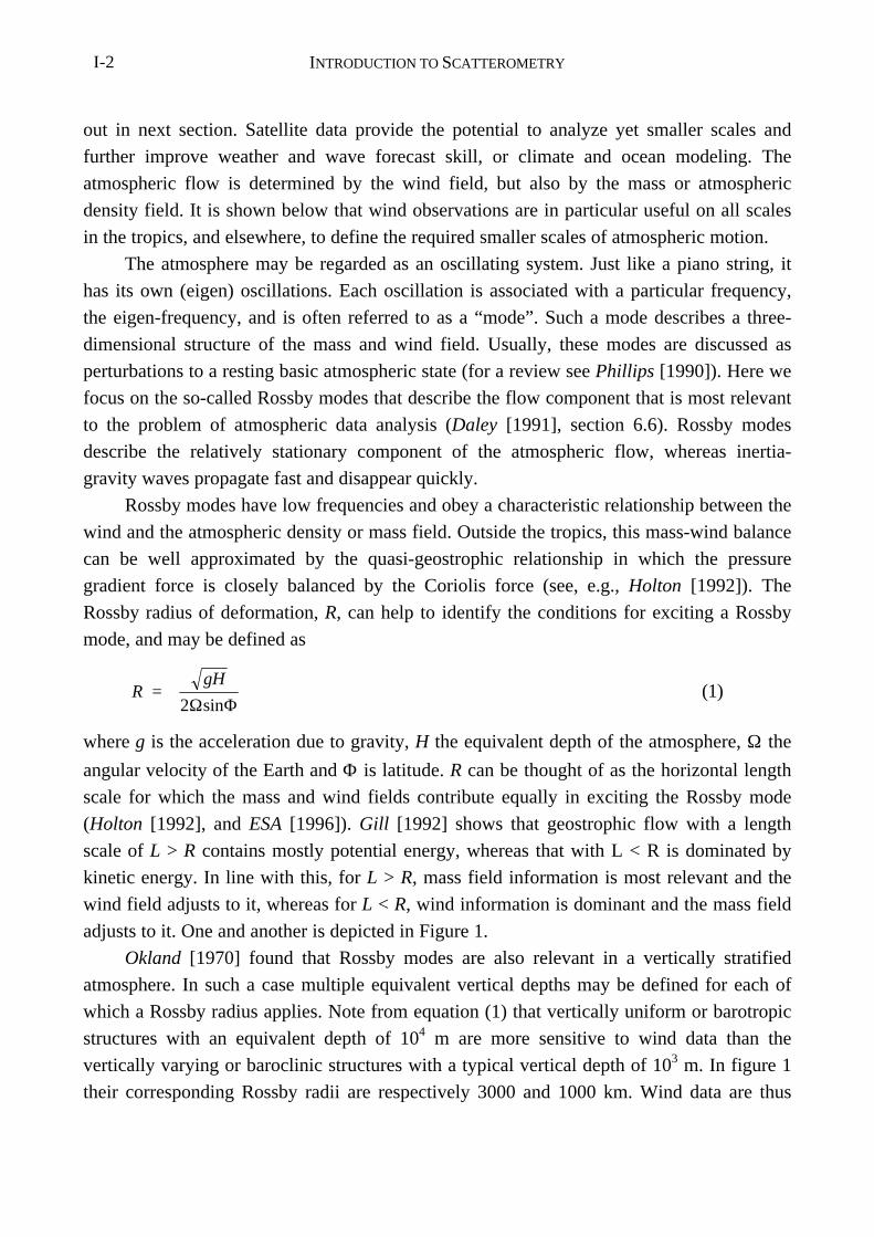
The atmosphere may be regarded as an oscillating system. Just like a piano string, it
has its own (eigen) oscillations. Each oscillation is associated with a particular frequency,
the eigen-frequency, and is often referred to as a “mode”. Such a mode describes a three-
dimensional structure of the mass and wind field. Usually, these modes are discussed as
perturbations to a resting basic atmospheric state (for a review see Phillips [1990]). Here we
focus on the so-called Rossby modes that describe the flow component that is most relevant
to the problem of atmospheric data analysis (Daley [1991], section 6.6). Rossby modes
describe the relatively stationary component of the atmospheric flow, whereas inertia-
gravity waves propagate fast and disappear quickly.
Rossby modes have low frequencies and obey a characteristic relationship between the
wind and the atmospheric density or mass field. Outside the tropics, this mass-wind balance
can be well approximated by the quasi-geostrophic relationship in which the pressure
gradient force is closely balanced by the Coriolis force (see, e.g., Holton [1992]). The
Rossby radius of deformation, R, can help to identify the conditions for exciting a Rossby
mode, and may be defined as
R = 2 sin
gH
Ω Φ(1)
where g is the acceleration due to gravity, H the equivalent depth of the atmosphere, Ω the
angular velocity of the Earth and Φ is latitude. R can be thought of as the horizontal length
scale for which the mass and wind fields contribute equally in exciting the Rossby mode
(Holton [1992], and ESA [1996]). Gill [1992] shows that geostrophic flow with a length
scale of L > R contains mostly potential energy, whereas that with L < R is dominated by
kinetic energy. In line with this, for L > R, mass field information is most relevant and the
wind field adjusts to it, whereas for L < R, wind information is dominant and the mass field
adjusts to it. One and another is depicted in Figure 1.
Okland [1970] found that Rossby modes are also relevant in a vertically stratified
atmosphere. In such a case multiple equivalent vertical depths may be defined for each of
which a Rossby radius applies. Note from equation (1) that vertically uniform or barotropic
structures with an equivalent depth of 104 m are more sensitive to wind data than the
vertically varying or baroclinic structures with a typical vertical depth of 103 m. In figure 1
their corresponding Rossby radii are respectively 3000 and 1000 km. Wind data are thus
INTRODUCTION TO SCATTEROMETRY I-3
relevant to determine the subsynoptic horizontal scales for particularly the larger vertical
depths, whereas mass data are important to define the larger synoptic scales.
To investigate the effect of small-scale wind information versus the effect of small-
scale mass information, Daley [1991] compares the geostrophic adjustment of a 8.5-km deep
midlatitude mass perturbation to the adjustment of a nondivergent wind perturbation of
similar energy and spatial scale. Almost all of the energy in the 400-km-scale mass
perturbation is carried away by inertia-gravity waves in a time frame of 6 hours, whereas,
over the same period, the similar-scale wind perturbation remains largely unchanged and is
quickly accompanied by a balanced mass field. This confirms that small-scale wind
information is most effective for analyzing the relevant component of the flow.
Figure 1 shows R for a latitude of 45°, and from equation (1) we note that R is latitude
dependent. With decreasing latitude, wind data will gain importance for the exciting of the
Rossby modes. As such, in the tropics the wind field will be the all-dominating factor for
the atmospheric flow [Gill, 1982].
Figure 1. Rossby radius of deformation for a latitude of 45° as a function of horizontal scale andequivalent depth. Along both axes some typical atmospheric phenomena are indicated. Open areasdenote the parameter range where the wind field dominates and in the gray area the mass fielddominates ((c) ESA, 1996). Wind data is particularly relevant at the smaller horizontal scales.
INTRODUCTION TO SCATTEROMETRYI-4
The above analysis of the atmospheric dynamics is relevant to define the observation
requirements for wind measurements. It turns out that outside the tropics the large-scale
component of the wind field may be derived from the atmospheric pressure and temperature
fields, but that elsewhere pressure or temperature observations alone are not sufficient to
describe the atmospheric flow. Wind measurements are necessary to define the circulation
on the subsynoptic scales and in the tropics.
1.2. Global Observing System
Since the beginning of weather prediction it has been recognized that a sound
meteorological observation network is a prerequisite to the success of such a system. The
Global Telecommunication System, GTS, has been set up to distribute observations of
relevant meteorological parameters in a timely manner. Conventionally, world-wide surface-
based observations of pressure, temperature, humidity, wind and other weather parameters
were communicated over the GTS, including balloon radiosondes that make vertical profiles
of temperature, humidity and wind, while ascending in the atmosphere. Latter observations
are an essential component of the Global Observing System, GOS (e.g., Kelly [1997]). Later
on, aircraft measurement systems were included. However, these conventional observation
types are not adequate to describe the atmospheric circulation in sufficient detail (see, e.g.,
ESA [1996], or Stoffelen [1993]). In Figure 2 a typical data coverage plot is shown for the
near-surface meteorological observations and the radiosondes. Over land, these observations
Figure 2. Above, the coverage of (a) stations measuring near surface variables (SYNOPS), and, onthe right, (b) stations releasing balloon radiosondes for atmospheric profiling, and (c) aircraftobservations. Large data sparse areas remain.
INTRODUCTION TO SCATTEROMETRY I-5
are mainly available over the densely populated and more developed areas. Over the oceans
much less observations are present, and those present, are close to the busiest sea and air
traffic routes. Especially over the oceans, extended data sparse regions remain. Therefore,
over the last two decades substantial effort has been devoted to the development of
complementary space-borne systems that provide meteorological information in these
otherwise data sparse regions.
The, in principle, simplest way to obtain information about the earth’s atmosphere
from Remote Sensing, RS, is by using so-called passive instruments. In this case the
Figure 2. Continued.
INTRODUCTION TO SCATTEROMETRYI-6
instrument on board the spacecraft will measure the microwave, infrared, visual or
ultraviolet electromagnetic (e.m.) radiation received from the Earth and its surrounding
atmosphere. Since the atmospheric transmission is temperature and humidity content
dependent, these so-called top-of-the-atmosphere radiances from sounding and imaging
instruments can provide, among other things, information on the three-dimensional
temperature and humidity structure of the troposphere and stratosphere. However, in section
1.1 it was argued that wind information is needed to describe the atmospheric flow in
sufficient detail.
By tracking cloud features or humidity structures on subsequent images taken by
passive instruments on geostationary satellites, one can get information on the atmospheric
flow. Geostationary satellites have fixed positions above the equator and as such currently
provide useful winds between latitudes of 50° south and north. However, it is often difficult
to accurately assign a height to the structures tracked. Alternatively, one can estimate the
wind speed over the ocean from passive microwave imagery. The emission of microwave
radiation from the ocean surface depends on the surface roughness, which in turn depends
on the near surface wind speed (see section 3.3). A drawback is that current wind algorithms
lack accuracy in cloudy areas and do not provide wind direction. So, although some wind
information may be obtained from passive instruments, their value for the analysis of the
atmospheric flow also has some limitations.
Active instruments emit e.m. radiation towards the Earth, and after absorption,
reflection or scattering by the Earth or its atmosphere, receive a small fraction of the emitted
power back. Since only a very small fraction of the emitted power is returned, active sensing
usually requires a powerful source and very sensitive detectors. An example of a potentially
very useful active instrument that would help resolve atmospheric dynamics, is a space-
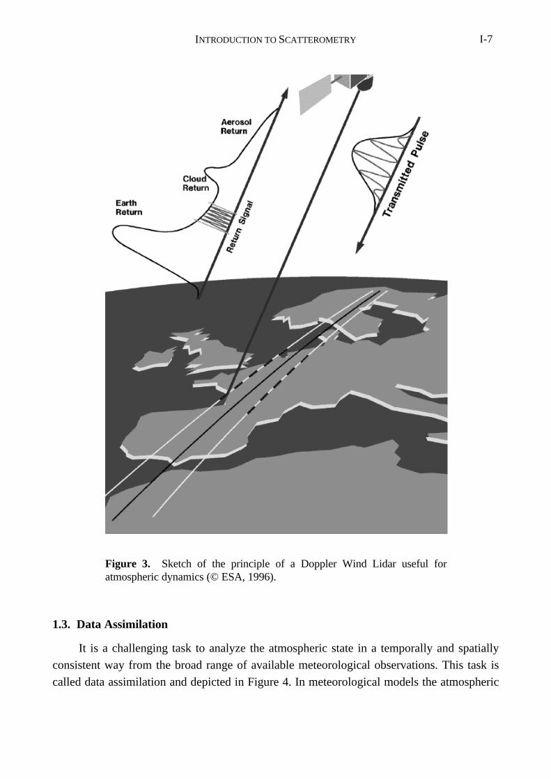
borne Doppler Wind Lidar, DWL, [ESA, 1996]. In Figure 3 a sketch is given of a DWL. A
DWL emits a laser pulse towards the Earth which is scattered in all directions by aerosol
particles in the atmosphere. A very small part of the aerosol scattered radiation will be
returned in the direction of the satellite and fall onto the DWL receiver. The movement of
the aerosol particles with respect to the laser in the direction along the laser beam, called
line of sight (LOS), will result in a so-called Doppler frequency shift, i.e., the frequency
difference between the emitted and backscattered radiation is proportional to this movement.
If one assumes that the particles move with the wind, then from the detection of the Doppler
shift one may infer the wind along the LOS. Since aerosol particles are abundant in the
troposphere and lower stratosphere, a DWL would be able to provide vertical profiles of the
wind vector. A DWL requires a powerful laser source and a very sensitive detector.
Nevertheless, well advanced programs exist for a DWL in space at ESA (ESA [1996]) and
NASA.
INTRODUCTION TO SCATTEROMETRY I-7
1.3. Data Assimilation
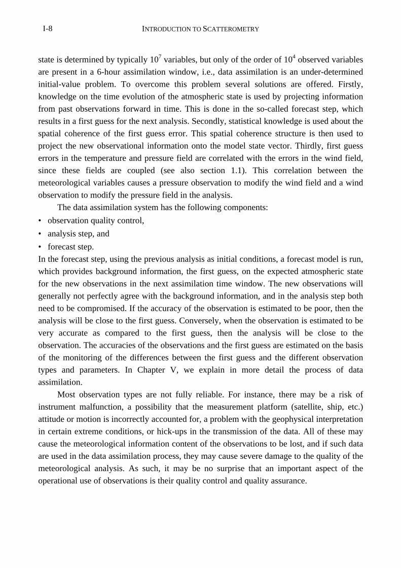
It is a challenging task to analyze the atmospheric state in a temporally and spatially
consistent way from the broad range of available meteorological observations. This task is
called data assimilation and depicted in Figure 4. In meteorological models the atmospheric
Figure 3. Sketch of the principle of a Doppler Wind Lidar useful foratmospheric dynamics (© ESA, 1996).
INTRODUCTION TO SCATTEROMETRYI-8
state is determined by typically 107 variables, but only of the order of 104 observed variables
are present in a 6-hour assimilation window, i.e., data assimilation is an under-determined
initial-value problem. To overcome this problem several solutions are offered. Firstly,
knowledge on the time evolution of the atmospheric state is used by projecting information
from past observations forward in time. This is done in the so-called forecast step, which
results in a first guess for the next analysis. Secondly, statistical knowledge is used about the
spatial coherence of the first guess error. This spatial coherence structure is then used to
project the new observational information onto the model state vector. Thirdly, first guess
errors in the temperature and pressure field are correlated with the errors in the wind field,
since these fields are coupled (see also section 1.1). This correlation between the
meteorological variables causes a pressure observation to modify the wind field and a wind
observation to modify the pressure field in the analysis.
The data assimilation system has the following components:
• observation quality control,
• analysis step, and
• forecast step.
In the forecast step, using the previous analysis as initial conditions, a forecast model is run,
which provides background information, the first guess, on the expected atmospheric state
for the new observations in the next assimilation time window. The new observations will
generally not perfectly agree with the background information, and in the analysis step both
need to be compromised. If the accuracy of the observation is estimated to be poor, then the
analysis will be close to the first guess. Conversely, when the observation is estimated to be
very accurate as compared to the first guess, then the analysis will be close to the
observation. The accuracies of the observations and the first guess are estimated on the basis
of the monitoring of the differences between the first guess and the different observation
types and parameters. In Chapter V, we explain in more detail the process of data
assimilation.
Most observation types are not fully reliable. For instance, there may be a risk of
instrument malfunction, a possibility that the measurement platform (satellite, ship, etc.)
attitude or motion is incorrectly accounted for, a problem with the geophysical interpretation
in certain extreme conditions, or hick-ups in the transmission of the data. All of these may
cause the meteorological information content of the observations to be lost, and if such data
are used in the data assimilation process, they may cause severe damage to the quality of the
meteorological analysis. As such, it may be no surprise that an important aspect of the
operational use of observations is their quality control and quality assurance.
INTRODUCTION TO SCATTEROMETRY I-9
1.4. Weather and Wave Prediction
The real-time analysis and forecast of the wind is relevant for various applications. For
example, ship and aircraft traffic may profit from wind information by saving fuel, and off-
shore activities by assessing and reducing risks. Moreover, a skillful forecast of extreme
wind events, usually associated with extreme waves and storm surges, is critical for these
activities, as well as for, for example, tourism or indeed sometimes for the population in a
broader sense (e.g., in case of severe storms or tropical cyclones). For the detection of
subsynoptic scale phenomena, such as polar lows, the required spatial and temporal
coverage is very large.
The availability of faster and more advanced computer systems, contributed to the fact
that Numerical Weather Prediction, NWP, has considerably improved its skill over the last
few decades. Naturally, improvements in the use of conventional observations, the use of
satellite data, and improvements in the forecast model, have also contributed to the skill
increase. The vastly expanding computer resources are spent to a large extent to improve the
meteorological analysis, but also to increase the sampling of the analysis and forecast fields.
Figure 4. Schematic of data assimilation. The vertical axis represents the atmospheric state and thehorizontal represents time.
INTRODUCTION TO SCATTEROMETRYI-10
An immediate effect of this increased sampling is that the surface topography is better
resolved, and thus the flow around mountains. Also other well-defined small scale forcing,
e.g. due to the land-sea mask, may result in a better forecast of the flow.
However, in more general terms, the resolution of a short range wind forecast is
determined by the density of the observational network, and is currently typically 250 km.
In the absence of a denser meteorological observation network, there is thus little scope to
better define the meso-scale flow. As such, scatterometer data are useful to fill in the data
sparse areas.
For the validation of NWP model parameterizations it is further useful to have high
resolution data for special cases, such as land-sea breezes or catabatic flow (e.g., mistral).
1.5. Climate
Near surface wind in the tropics is an essential variable of the climate system but
which is poorly defined. It determines momentum, heat, humidity, and carbondioxide gas
fluxes at the interface of the atmosphere and the ocean. Moreover, the tropical atmospheric
circulation (Hadley circulation) is of essential importance for predicting climate and climate
change. There are several indications (see, e.g., ESA [1996] or Kallberg [1997]) that the
Hadley circulation is ill-defined. Widely available and accurate near surface wind
observations would improve the situation to a substantial degree.
1.6. Ocean Modeling
The ocean is driven by atmospheric wind and heat exchange, and thus the output of an
ocean model is strongly related to the quality of the forcing input. Most important in this
respect are the air-sea momentum and latent heat fluxes that strongly depend on the wind in
the surface (air) layer. Ocean circulation models play an important role in the earth climate
system, and in the tropics for the seasonal forecasting of the El Niño southern oscillation.
Ocean wave models are most sensitive to the accurate definition of the air-sea momentum
flux.
For ocean modeling studies, NWP analyses may be used. As a refinement to these, re-
analyses can be made over longer periods in the past, where all available measurements are
used in the best possible way. This means that the observation requirements for NWP
generally cover those for climate or ocean circulation and wave prediction.
A currently available active instrument that is most useful to help analyze the
atmospheric flow is the scatterometer.
INTRODUCTION TO SCATTEROMETRY I-11
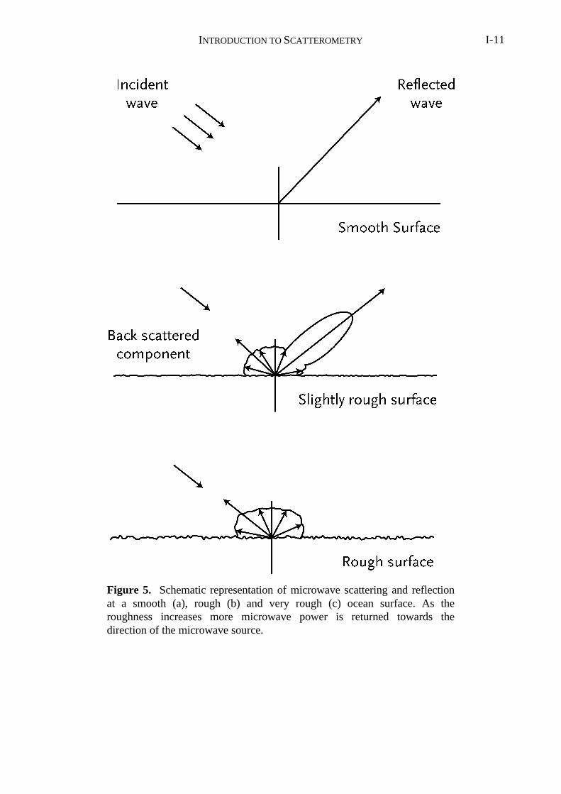
Figure 5. Schematic representation of microwave scattering and reflectionat a smooth (a), rough (b) and very rough (c) ocean surface. As theroughness increases more microwave power is returned towards thedirection of the microwave source.

INTRODUCTION TO SCATTEROMETRYI-12
2. Scatterometer Instruments
During the second world war, radar was much in use to detect and track hostile
vessels. It was noted that this detection was more and more hampered with increasing wind
speed. Naturally, the idea of measuring wind near the sea surface by using microwaves, i.e.,
scatterometry (e.g., Moore and Pierson [1967]), developed not much later. From an aircraft
or satellite a microwave beam is emitted to the ocean surface under an angle, as depicted in
Figure 5. This radiation, with a wavelength of some centimeters, will be scattered and
reflected on the rough ocean surface and a small part of the power emitted will be returned
to the detector of the scatterometer instrument.
2.1. Normalized Radar Cross Section
Suppose a point source emits a microwave pulse of power P T uniformly in all
directions in space. The power flux Φ T at a distance R from the source will then be Φ T =
P T / ( 4π R 2
). The antenna gain is defined as G = 4π / Ω, where Ω is the beam width in
steradians in which the emitted power is contained. For an emission uniform in all directions
G = 1, whereas for a narrow radar beam G >> 1, and the power flux becomes Φ T = G P T /
(4π R 2
). Figure 6 depicts radar backscattering.
Now suppose that microwave radiation hits a scatterer. Then the radar cross section is
defined as
σ = S
T
P
Φ(2)
where P S is the backscattered power by the target. The radar cross section depends on the
geometry of the target with respect to the incident microwaves and the dielectric constant of
the material of the scatterer. The power detected by the receiving antenna, let’s suppose it is
identical to the source antenna and of size A, is then P R = P S A / ( 4π R 2
) = G P T σ A
( 4π R 2
) -2. For a narrow beam rectangular antenna, i.e., L X by L Y, and a system without
losses, a relationship exists between the gain G and the antenna surface area A since Ω =
(λ / L X ).(λ / L Y ) = λ 2 / A. Thus A = λ
2 G / 4π.
A scatterometer has a footprint, F, of several tens of kilometers in diameter with
generally a large number of scattering elements in it. For such a distributed target one may
define a dimensionless microwave cross section per unit surface, often denoted “Normalized
Radar Cross Section” or NRCS and by convention written as σ 0 . We can now write:
( )P
P G
RF
F
R
2T = d
λ σ
43
0 2
4π ∫ (3)
INTRODUCTION TO SCATTEROMETRY I-13
In order to solve this integral one usually assumes that σ 0 does not vary over the area
of interest such that:
( )σ
π
λ0
2 =
43 4
2
R
G F
P
PR
T
(4)
However, in reality the roughness elements on the ocean surface will largely depend on the
local wind condition, which in turn exhibits large variability over a scatterometer footprint.
As the scattering mechanism does not linearly depend on the geophysical condition, the
geophysical variability within the footprint will contribute to σ 0 . This will be particularly
acute at low winds.
σ 0 is generally expressed in dB, i.e., as the value of 10 log ( σ
0 ).
The backscattered power turns out to be well correlated with the ocean near-surface
wind conditions, and empirical relationships exist that describe this correlation (see, e.g.,
Chapter III or Wentz [1984]). Scatterometer retrieved winds may be validated against winds
measured at conventional platforms (see, e.g., Chapter IV). The widely available and
validated scatterometer winds provide, even below cloud, accurate and spatially consistent
information on the near-surface atmospheric flow, and have as such become a relevant
Figure 6. Microwave scattering.
INTRODUCTION TO SCATTEROMETRYI-14
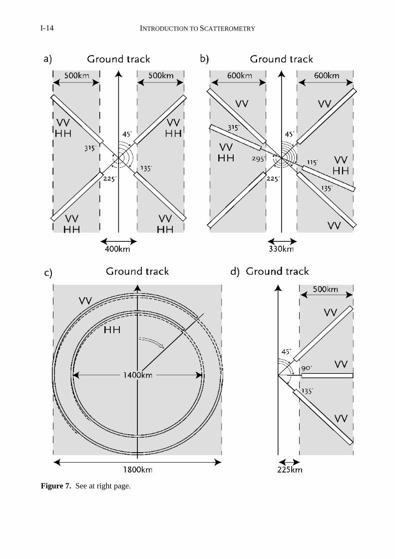
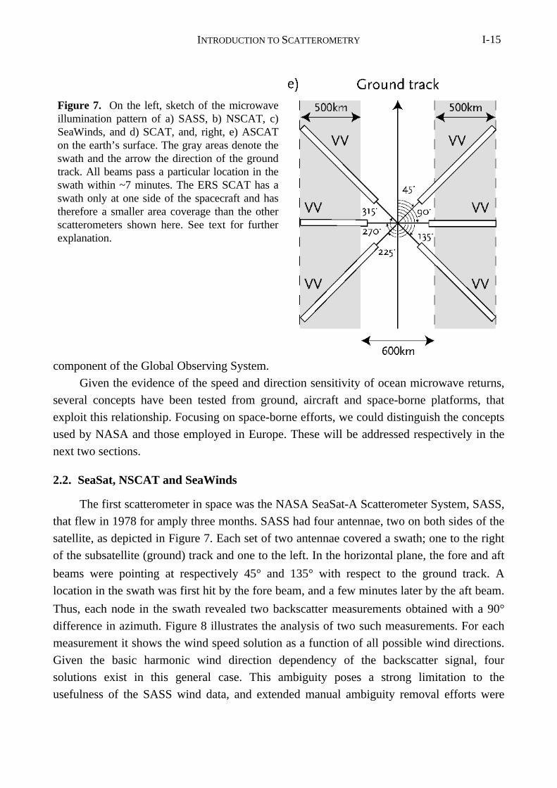
Figure 7. See at right page.
INTRODUCTION TO SCATTEROMETRY I-15
component of the Global Observing System.
Given the evidence of the speed and direction sensitivity of ocean microwave returns,
several concepts have been tested from ground, aircraft and space-borne platforms, that
exploit this relationship. Focusing on space-borne efforts, we could distinguish the concepts
used by NASA and those employed in Europe. These will be addressed respectively in the
next two sections.
2.2. SeaSat, NSCAT and SeaWinds
The first scatterometer in space was the NASA SeaSat-A Scatterometer System, SASS,
that flew in 1978 for amply three months. SASS had four antennae, two on both sides of the
satellite, as depicted in Figure 7. Each set of two antennae covered a swath; one to the right
of the subsatellite (ground) track and one to the left. In the horizontal plane, the fore and aft
beams were pointing at respectively 45° and 135° with respect to the ground track. A
location in the swath was first hit by the fore beam, and a few minutes later by the aft beam.
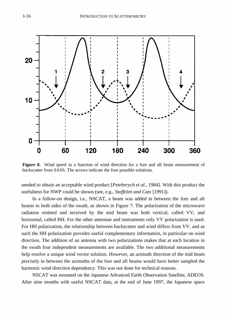
Thus, each node in the swath revealed two backscatter measurements obtained with a 90°difference in azimuth. Figure 8 illustrates the analysis of two such measurements. For each
measurement it shows the wind speed solution as a function of all possible wind directions.
Given the basic harmonic wind direction dependency of the backscatter signal, four
solutions exist in this general case. This ambiguity poses a strong limitation to the
usefulness of the SASS wind data, and extended manual ambiguity removal efforts were
Figure 7. On the left, sketch of the microwaveillumination pattern of a) SASS, b) NSCAT, c)SeaWinds, and d) SCAT, and, right, e) ASCATon the earth’s surface. The gray areas denote theswath and the arrow the direction of the groundtrack. All beams pass a particular location in theswath within ~7 minutes. The ERS SCAT has aswath only at one side of the spacecraft and hastherefore a smaller area coverage than the otherscatterometers shown here. See text for furtherexplanation.
INTRODUCTION TO SCATTEROMETRYI-16
needed to obtain an acceptable wind product [Peteherych et al., 1984]. With this product the
usefulness for NWP could be shown (see, e.g., Stoffelen and Cats [1991]).
In a follow-on design, i.e., NSCAT, a beam was added in between the fore and aft
beams to both sides of the swath, as shown in Figure 7. The polarization of the microwave
radiation emitted and received by the mid beam was both vertical, called VV, and
horizontal, called HH. For the other antennae and instruments only VV polarization is used.
For HH polarization, the relationship between backscatter and wind differs from VV, and as
such the HH polarization provides useful complementary information, in particular on wind
direction. The addition of an antenna with two polarizations makes that at each location in
the swath four independent measurements are available. The two additional measurements
help resolve a unique wind vector solution. However, an azimuth direction of the mid beam
precisely in between the azimuths of the fore and aft beams would have better sampled the
harmonic wind direction dependency. This was not done for technical reasons.
NSCAT was mounted on the Japanese Advanced Earth Observation Satellite, ADEOS.
After nine months with useful NSCAT data, at the end of June 1997, the Japanese space
Figure 8. Wind speed as a function of wind direction for a fore and aft beam measurement ofbackscatter from SASS. The arrows indicate the four possible solutions.
INTRODUCTION TO SCATTEROMETRY I-17
agency, NASDA, lost control of the ADEOS after a complete power loss. This dramatic
event has been a severe set-back for Earth Observation, and scatterometry in particular.
QuikSCAT, which is the next scatterometer to become operational, is planned on a
dedicated polar satellite, projected for launch in November 1998. QuikSCAT is the first
scanning scatterometer as depicted in Figure 7. A scanning scatterometer may accomodate a
broad swath. However, a disadvantage of such a concept is that at the extreme ends of the
swath, the earth surface is only illuminated from a single azimuth direction, Moreover, in
the middle of the swath, at the so-called subsatellite track, the ocean is only illuminated
from two exactly opposite directions. The limited azimuth sampling means that wind
direction can only be poorly resolved at these locations. Fortunately, the total QuikSCAT
swath width of 1800 km guarantees that the full wind vector can be determined accurately
over a large range across-the swath.
The record-fast QuikSCAT program was planned after the dramatic loss of NSCAT, in
order to fill the gap between the ADEOS-I and ADEOS-II missions. ADEOS-II will carry a
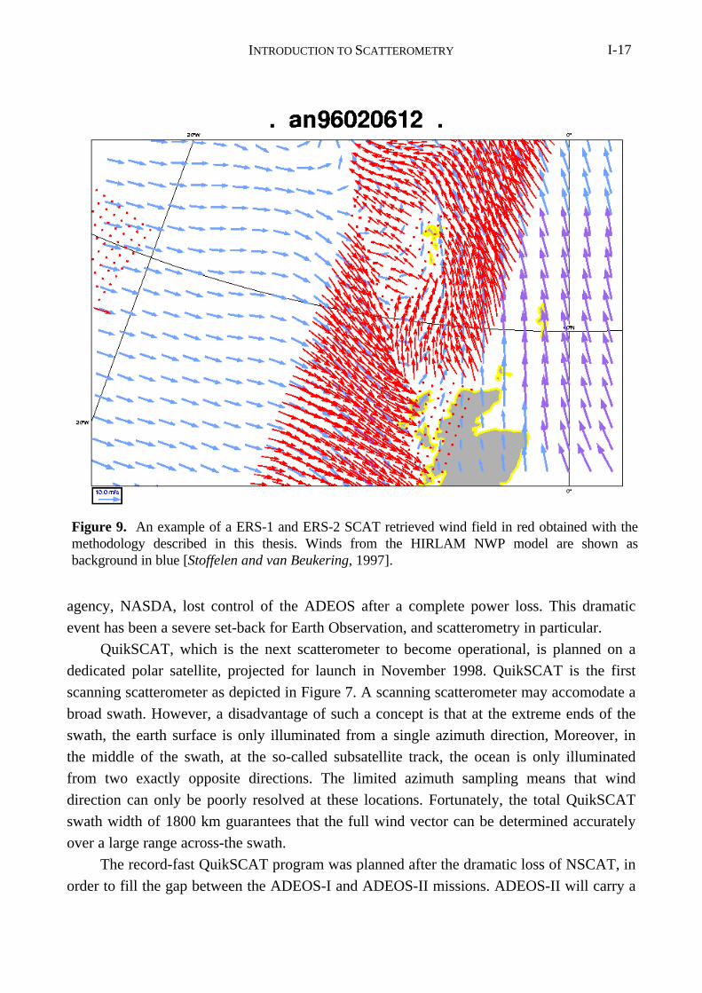
Figure 9. An example of a ERS-1 and ERS-2 SCAT retrieved wind field in red obtained with themethodology described in this thesis. Winds from the HIRLAM NWP model are shown asbackground in blue [Stoffelen and van Beukering, 1997].
INTRODUCTION TO SCATTEROMETRYI-18
scatterometer very similar to QuikSCAT, called SeaWinds, and is planned for launch in
early 2000.
SASS, NSCAT, QuikSCAT, and SeaWinds use a microwave wavelength of 2.1 cm
(14.6 GHz frequency; denoted Ku-band). This frequency is affected by atmospheric
attenuation due to cloud liquid water and rain. Furthermore, rain droplets hitting the ocean
surface distort the gravity-capillary waves, and may complicate the backscatter-wind
relationship. Latter effects become substantially smaller for a higher wavelength. To avoid
such effects and focus on reliable wind data below cloud, the ESA scatterometers on board
the ERS-1 and ERS-2 satellites, and the ASCAT scatterometer planned on the European
METOP satellite series use a wavelength of 5.7 cm (5.3 GHz frequency, denoted C-band).
2.3. ERS Scatterometers and ASCAT
The first ESA remote sensing satellite, ERS-1, was launched on 17 July 1991 into a
polar orbit of 800 km height. In 1995 the ERS-1 follow-on, ERS-2, was launched. The ERS-
1 and ERS-2 scatterometers, which are identical and denoted SCAT here, each have three
antennae, that illuminate the ocean surface from three different azimuth directions, as shown
in Figure 7. A point on the ocean surface will first be hit by the fore beam, then by the mid
beam and at last by the aft beam. In Chapter II of this thesis it is shown that this
measurement geometry generally results in two opposite wind vector solutions. In Chapter V
it is discussed how a unique wind vector solution may be selected from the two optional
ones. Chapter III describes the estimation of a backscatter-wind relationship for the
wavelength used by SCAT. The SCAT wind product has a high quality and shows small
scale meteorological structures, as shown in Figure 9.
A limitation of the SCAT is its coverage. In contrast to the NASA Ku-band
scatterometers, SCAT only views at one side of the subsatellite track. Moreover, the
microwave source is shared with a SAR instrument, so that the operation of SCAT is often
not possible in meteorologically interesting regions (e.g., in the Norwegian Sea). Although
with ERS-1 and ERS-2 two working SCAT and SAR instruments are in orbit at the moment,
for different reasons only the ERS-2 scatterometer is operated, and only part time (shared
mode with ERS-2 SAR). Certainly after the decline of NSCAT this is a regretful situation.
Tandem ERS-1 and ERS-2 SCAT numerical weather prediction impact experiments by
ECMWF [Le Meur, 1997] and KNMI [Stoffelen, 1997] have shown that two scatterometers
have more than twice the value of one.
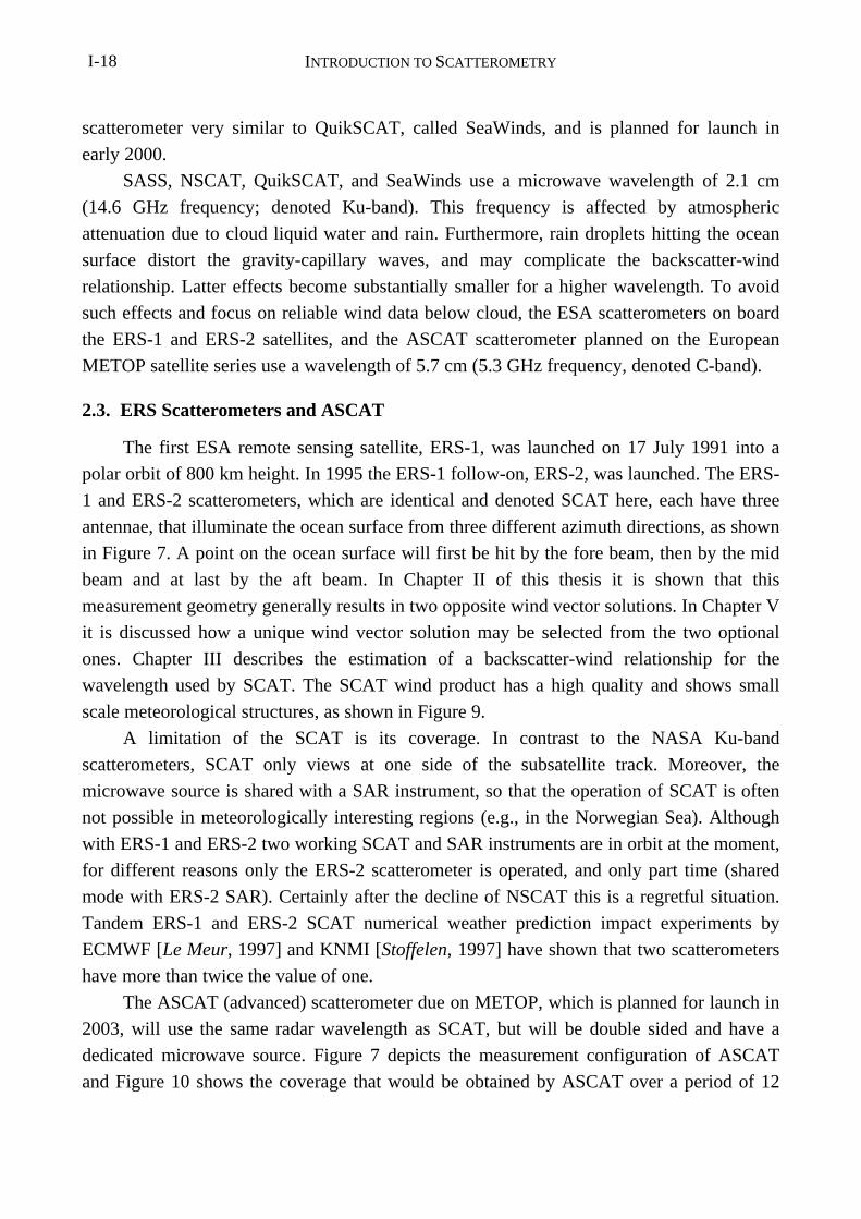
The ASCAT (advanced) scatterometer due on METOP, which is planned for launch in
2003, will use the same radar wavelength as SCAT, but will be double sided and have a
dedicated microwave source. Figure 7 depicts the measurement configuration of ASCAT
and Figure 10 shows the coverage that would be obtained by ASCAT over a period of 12
INTRODUCTION TO SCATTEROMETRY I-19
hours. The interpretation of ASCAT will benefit much from the knowledge gained during
the ERS missions. The extreme outer part of the ASCAT swath, however, corresponds to
microwave incidence angles that were not available in the SCAT swath, and may need
further investigation.
3. The Physics Behind Scatterometry
As already mentioned, scatterometry was developed heuristically. It was found
experimentally that the sensitivity to wind speed and direction describes well the changes in
backscatter over the ocean. In Chapters II and III of this thesis this is further confirmed and
it is found that within the measurement noise of the SCAT, which is as small as 0.2 dB, a
dependency on two geophysical parameters generally holds. When, in Chapters III and IV
wind speed and direction are taken to be the two geophysical parameters, then a
substantially larger uncertainty is introduced that amounts to a wind vector RMS error of
approximately 2.5 m s−1. However, such an error in a near surface wind observation is quite
acceptable.
In this section we will try to relate the empirical methodology followed in this thesis to
the current knowledge of the physics involved in scatterometry. It is important to realize that
in the approach followed in this thesis σ 0 is related to the wind at 10 meter height above the
ocean surface, simply because such measurements are widely available for validation. This
means that any effect that relates to the mean wind vector at 10 meter height is incorporated
Figure 10. The coverage after half a day expected from the ASCAT scatterometer on METOP tobe launched in 2002.
INTRODUCTION TO SCATTEROMETRYI-20
in the backscatter-to-wind relationship. As such, we will show that air stability, the
appearance of surface slicks, and the amplitude of gravity or longer ocean waves, depend to
some degree on the strength of the wind and may, to the same degree, be fitted by a
backscatter-to-wind transfer function.
Several attempts have been made to provide a theoretical framework in which all
aspects of scatterometry are tackled, e.g., Donelan and Pierson [1987] or Snoeij et al.
[1992]. Below we highlight some main aspects.
3.1. Electromagnetic Interaction of Microwaves With the Ocean Surface
The relevant physical phenomenon that is important for the working of the
scatterometer is the presence of the so-called gravity-capillary waves on the water surface.
Gravity-capillary waves have a wavelength of some centimeters and respond almost
instantaneously to the strength of the local wind [Plant, 1982]. Microwave scattering (see
Figure 5) strongly depends on the amplitude of the gravity-capillary waves. Furthermore, the
caps of these waves tend to align perpendicular to the local wind direction and thus the
ocean radar return is wind direction dependent.
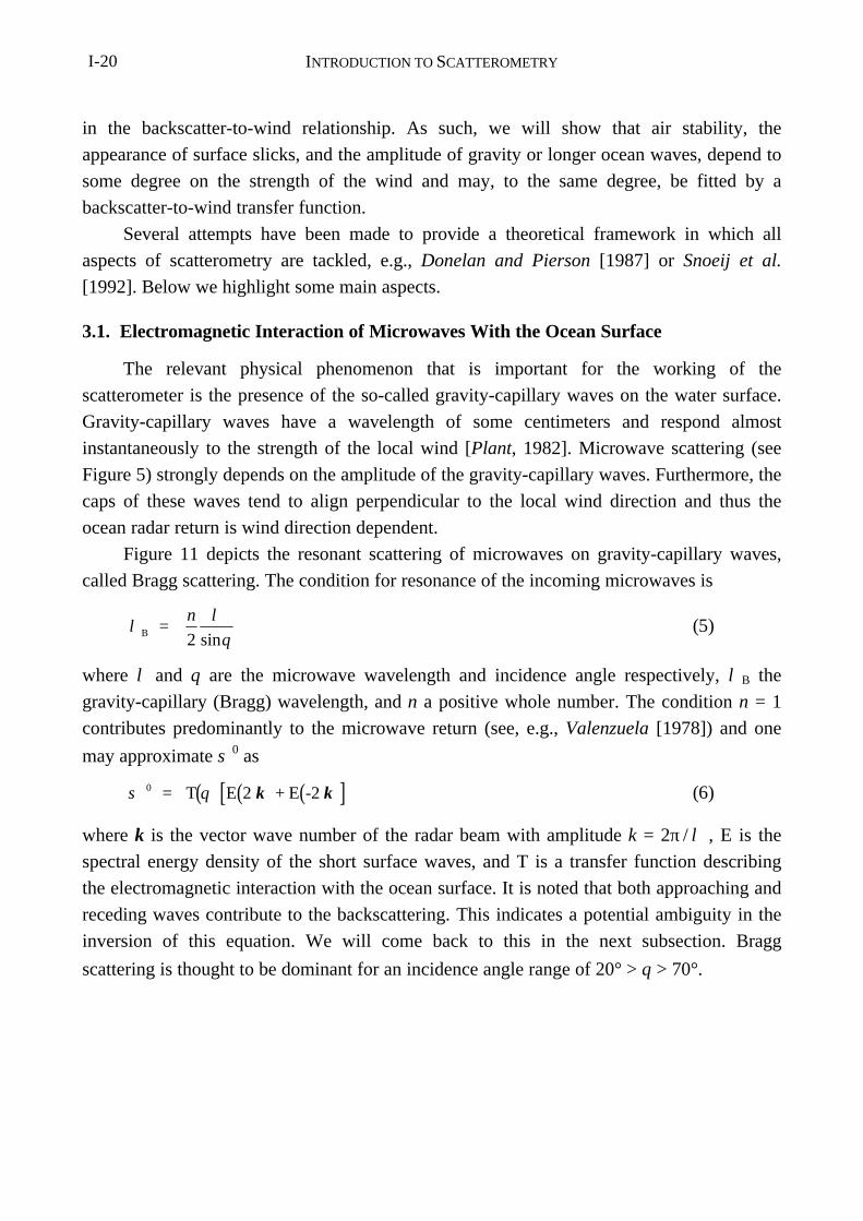
Figure 11 depicts the resonant scattering of microwaves on gravity-capillary waves,
called Bragg scattering. The condition for resonance of the incoming microwaves is
λλ
θB = n
2 sin(5)
where λ and θ are the microwave wavelength and incidence angle respectively, λ B the
gravity-capillary (Bragg) wavelength, and n a positive whole number. The condition n = 1
contributes predominantly to the microwave return (see, e.g., Valenzuela [1978]) and one
may approximate σ 0 as
( ) ( ) ( )[ ]σ θ = T E 2 + E -2 0 k k (6)
where k is the vector wave number of the radar beam with amplitude k = 2π / λ , E is the
spectral energy density of the short surface waves, and T is a transfer function describing
the electromagnetic interaction with the ocean surface. It is noted that both approaching and
receding waves contribute to the backscattering. This indicates a potential ambiguity in the
inversion of this equation. We will come back to this in the next subsection. Bragg
scattering is thought to be dominant for an incidence angle range of 20° > θ > 70°.

INTRODUCTION TO SCATTEROMETRY I-21
Specular reflection is another mechanism to get ocean microwave return. Facets of the
ocean that are normal to the incident microwaves will reflect the radiation back in the
direction of the radar antenna. For increasing incidence angles, the probability that a facet
has the appropriate orientation to contribute to specular reflection decreases, since the
steepness of ocean waves is limited. As such, this mechanism is thought to provide a non-
negligible contribution to σ 0 for incidence angles smaller than 30° [Stewart, 1985].
Several approximations exist that theoretically try to describe the interaction of e.m.
waves with the ocean surface (see, e.g., Snoeij et al., [1992]). However, for laboratory
experiments in a wave tank these different models show a dispersion of several dB, which is
large compared to the accuracy of the ERS scatterometer of 0.2 dB.
3.2. The Ocean Topography
The topography of a rough ocean surface is much more complicated and dynamic than
the relatively simple wave states that are usually generated in laboratory experiments, which
is further complicating a useful description of the interaction of a microwave beam with
such an ocean surface. Furthermore, the local interaction theories need to be extended in
order to provide a useful theory over a scatterometer footprint and take into account the sea
state variability.
Figure 11. Bragg scattering: A plan-parallel radar beam with wavelength λhits the rough ocean surface at incidence angle θ, where capillary gravitywaves with Bragg wavelength λB will cause microwave resonance.
INTRODUCTION TO SCATTEROMETRYI-22
At low wind speeds the wind direction and speed may vary considerably within the
scatterometer footprint. Locally, below a speed of roughly 2 m s−1, calm areas are present
where little or no backscatter occurs, perhaps further extended in the presence of natural
slicks that increase the water surface tension [Donelan and Pierson, 1987]. However, given
the variability of the wind within a footprint area of 50 km it is, even in the case of zero
mean vector wind, very unlikely that there are no patches with roughness in the footprint.
Likely, for low mean vector wind the patchiness or associated wind variability will
determine the amount of backscatter, and not the amplitude of the mean vector wind.
However, as the mean vector wind increases, the probability of a calm patch will quickly
decrease, and the mean microwave backscatter will increase. Also, natural slicks quickly
disappear as the wind speed increases, and as such the occurrence of these is correlated to
the amplitude of the mean vector wind over the footprint.
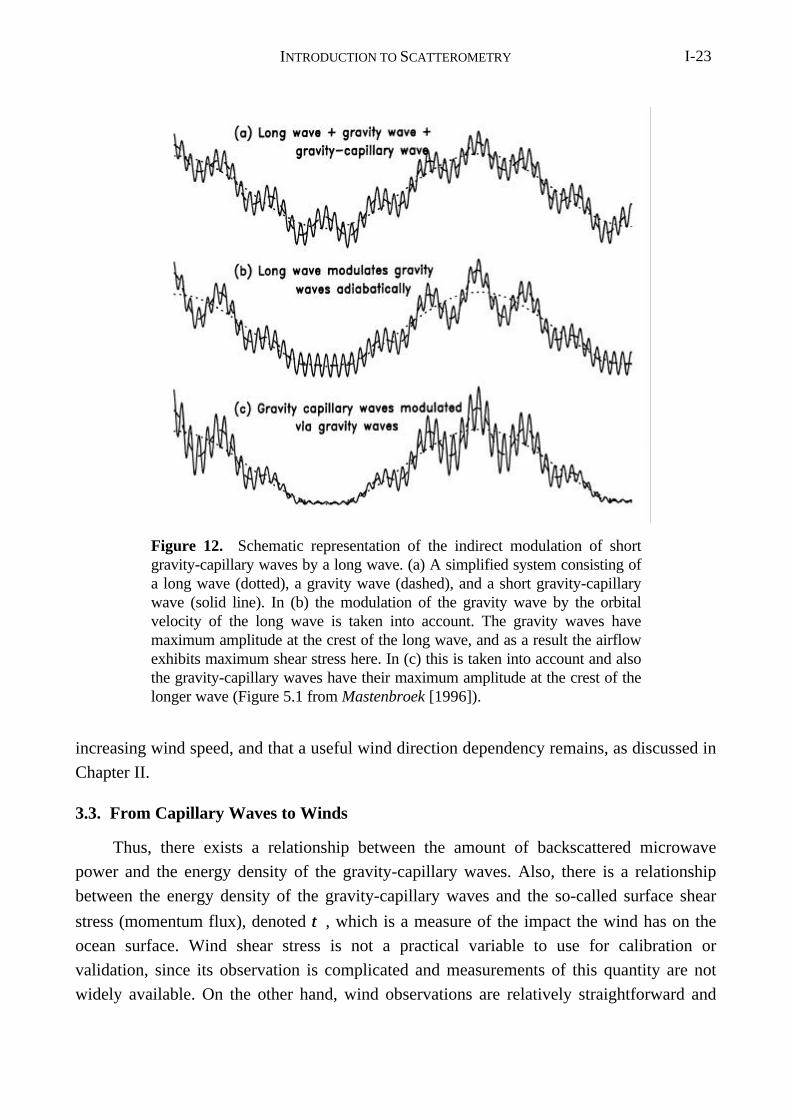
As the mean wind speed increases, gravity waves (decimetric) and longer waves
(metric or larger) will be formed. The gravity-capillary waves have a phase speed which is
different from that of the gravity and longer waves and all have a complicated dynamic
interaction as sketched in Figure 12 (from Mastenbroek, [1996]). The wind has maximum
impact close to the crest of the long wave, due to the presence here of gravity waves with
maximum amplitude. Since the gravity-capillary waves are in quasi-equilibrium with the
wind stress, they have also maximum amplitude at the long wave crest. Mastenbroek argues
that in turn the growth of the long waves is enhanced by these modulation mechanisms.
For moderate wind speed, waves will start to break and so-called white-caps will
occur. The breaking will generate gravity-capillary waves in addition to the wind generated
ones (see, e.g., Phillips [1977]). This hydrodynamic modulation will cause the energy
density of these waves to be different on the lee- and luffward side of the long waves. The
two terms on the right-hand side of equation (6) will then be different which may help
resolve approaching and receding waves. In fact, there is generally a distinguishable
difference in the backscatter level between upwind (approaching) and downwind (receding).
However, as shown in Chapter II, it turns out that with the three-antenna geometry of SCAT
or ASCAT, this difference does not lead to a possibility to discriminate between the upwind
and downwind solutions.
It is also shown in Chapter II that the upwind-downwind backscatter ratio shows a
strong dependence on incidence angle at around 35°. This may indicate the transition of a
regime where specular reflection plays a role, i.e., the lower incidence angles, to a regime
where it is negligible and Bragg scattering is fully dominating (see section 3.1).
At higher wind speeds wave breaking will further intensify, causing air bubbles, foam
and spray at the ocean surface, and a more and more complicated ocean topography.
Although theoretically not obvious, it is empirically found that σ 0 keeps increasing for
INTRODUCTION TO SCATTEROMETRY I-23
increasing wind speed, and that a useful wind direction dependency remains, as discussed in
Chapter II.
3.3. From Capillary Waves to Winds
Thus, there exists a relationship between the amount of backscattered microwave
power and the energy density of the gravity-capillary waves. Also, there is a relationship
between the energy density of the gravity-capillary waves and the so-called surface shear
stress (momentum flux), denoted ττ , which is a measure of the impact the wind has on the
ocean surface. Wind shear stress is not a practical variable to use for calibration or
validation, since its observation is complicated and measurements of this quantity are not
widely available. On the other hand, wind observations are relatively straightforward and
Figure 12. Schematic representation of the indirect modulation of shortgravity-capillary waves by a long wave. (a) A simplified system consisting ofa long wave (dotted), a gravity wave (dashed), and a short gravity-capillarywave (solid line). In (b) the modulation of the gravity wave by the orbitalvelocity of the long wave is taken into account. The gravity waves havemaximum amplitude at the crest of the long wave, and as a result the airflowexhibits maximum shear stress here. In (c) this is taken into account and alsothe gravity-capillary waves have their maximum amplitude at the crest of thelonger wave (Figure 5.1 from Mastenbroek [1996]).
INTRODUCTION TO SCATTEROMETRYI-24
widely available. The relationship between surface stress and wind at a reference height,
let’s say 10 m and referred to as U10 , is not without uncertainty, as will be discussed here.
Therefore, in order to find an empirical relationship, it appears favorable to correlate σ 0
with U10 rather than with the corresponding ττ computed from U10 with a nonlinear and
uncertain equation. Then, the uncertainties in the physics will be mainly in the wind-to-σ 0
transfer function, and not in the measurements used for validation or calibration. Obviously,
once a wind-to-σ 0 relationship is established one can also, with the geophysical
uncertainties involved, compute a stress-to-σ 0 relationship.
The following definition is widely used to relate ττ and U10 :
ττ = − ⟨u´w´⟩ = CD U10 U10 (7)
where ⟨u´w´⟩ is the ensemble average of the product of the horizontal and vertical wind
component fluctuations, and CD the so-called drag coefficient. In (7) it is assumed that the
directions of ττ and U10 are the same. This is a reasonable assumption in the so-called surface
layer where ττ is approximately constant with height (see, e.g., Holton [1992]). The surface
layer extends typically to a height of 30-50 m, but may be more shallow in low wind
conditions. The reference height of 10 m for wind observations is thus generally well within
the surface layer.
Using (7), CD has been investigated in many experimental campaigns over the last 20
years, and shows a large spread, i.e., 3⋅10−4 > CD > 5⋅10−3. Parameterizations of CD may
differ by 20 % or more (e.g., compare Smith et al. [1992], and Donelan et al. [1993]), but
commonly show an increase with increasing U10 . This increase will implicitly be
incorporated into an empirical wind-to-σ 0 transfer function.
Furthermore, atmospheric density effects, through temperature or humidity
fluctuations, may affect the drag. Therefore, it has been suggested to correct measured
winds to “equivalent neutral” winds [Liu and Tang, 1996] in the process of estimating a
transfer function or validating scatterometer winds. In this case, one assumes that the
scatterometer essentially measures τ, and by using neutral stability drag, denoted CDN, one
can relate this to a unique “equivalent neutral” wind, U10N , by using equation (7). This
scatterometer wind may then be compared to an independently obtained U10 , e.g. from an
anemometer, after multiplication of it by (CD/CDN)½ in order to obtain an “equivalent
neutral” wind. An example of such correction in the tropics is shown in Figure 13. It is clear
that stability is expected to be a function of wind speed.
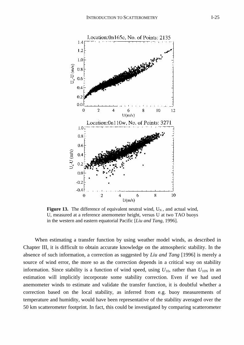
INTRODUCTION TO SCATTEROMETRY I-25
When estimating a transfer function by using weather model winds, as described in
Chapter III, it is difficult to obtain accurate knowledge on the atmospheric stability. In the
absence of such information, a correction as suggested by Liu and Tang [1996] is merely a
source of wind error, the more so as the correction depends in a critical way on stability
information. Since stability is a function of wind speed, using U10, rather than U10N in an
estimation will implicitly incorporate some stability correction. Even if we had used
anemometer winds to estimate and validate the transfer function, it is doubtful whether a
correction based on the local stability, as inferred from e.g. buoy measurements of
temperature and humidity, would have been representative of the stability averaged over the
50 km scatterometer footprint. In fact, this could be investigated by comparing scatterometer
Figure 13. The difference of equivalent neutral wind, UN , and actual wind,U, measured at a reference anemometer height, versus U at two TAO buoysin the western and eastern equatorial Pacific [Liu and Tang, 1996].
INTRODUCTION TO SCATTEROMETRYI-26
and buoy wind speed differences to the anticipated residual stability correction computed
from the buoy temperature and humidity information. Since this is not done yet, we did not
attempt stability correction of the validation wind data sets in this thesis.
When the wind picks up suddenly, the gravity-capillary waves at the ocean surface
start to grow immediately and gradually propagate their energy onto the longer waves. As
the longer waves grow and move in the direction of the wind, the surface stress will
gradually decrease. For a given wind speed, one could thus distinguish “young” and
“rough”, and, “developed” and “smooth” sea states, corresponding to relatively large and
small drag respectively. At 10 m s−1 Smith et al. [1992] and Donelan et al. [1993]
parameterizations show a large effect due to sea state, but which is different by a factor of
two. In contrast, Mastenbroek [1996] estimates the effect of a varying amplitude of the
longer waves on the mean surface roughness to be generally small, which suggests that the
sea state is generally not very important for the interpretation of scatterometer data. The
generally high accuracy of scatterometer winds, as described in Chapters III and IV, indeed
suggests that an additional parameter such as sea state is of secondary importance.
Nonetheless, we found that in 1-2% of cases, often very close to intense fronts or lows our
empirical two-parameter wind-to-backscatter transfer function provided a less good
description. A probable cause is that longer waves exist that are not in equilibrium (yet) with
the wind, i.e., what is called a confused sea state in Chapter IV. It is noted however, that
rain, air stability, or spatial processing effects may also be the cause.
4. Aim and Overview of the Thesis
The aim of this thesis is to provide an accurate interpretation of ERS scatterometer
winds for use in meteorological applications. It has become clear that a dependency of the
microwave backscatter on the near surface wind vector explains much of its variability.
Secondary geophysical effects may be investigated by correlating the residual errors to other
quantities, such as sub-footprint wind variability, sea state or air stability, as mentioned
earlier in this chapter. In line with the discussion in the previous paragraph on the prime
wind dependency, these secondary geophysical dependencies may be mixed with effects of
a statistical nature, and a careful analysis will be necessary to separate physics from
statistics.
Thus, it may not be a surprise that for the interpretation of scatterometer observations
statistical methods have been used to complement the physical knowledge. This thesis is
concerned with these, and gives, with the aid of scientific publications, a reasonably
complete overview of the state-of-the-art as achieved with the ERS scatterometer processing
(ERS-1 from 17 July 1991 and later ERS-2 from 22 November 1995).
A careful analysis of the accuracy of the data is often shown to be essential in order to
INTRODUCTION TO SCATTEROMETRY I-27
demonstrably improve the interpretation. What appears as residual error may be associated
to effects resulting from nonlinear transformation of random error, or a nonuniform
sampling of harmonic dependencies (e.g., in Chapters II, III, and IV, and the appendix). In
literature, such residuals of statistical origin are often erroneously assigned to physical
processes. Obviously, this leads to a wrong geophysical and statistical interpretation and
examples of this will be given, in particular in Chapter IV.
The triplet of SCAT measurements (see section 2.3) can be put in a 3D axes system,
where the measurement of each beam is represented along one of the three axes. By making
clever cross-sections through the 3D distribution of the triplets, the coherence in the
measurements may be investigated qualitatively. By doing so, the coherence of the
measurements is shown to be very strong and may be explained by two geophysical
parameters. The triplets are namely generally located near a conical (2D) surface (see Figure
1, Chapter II). It turns out that along the major axis of this cone mainly the wind speed (sea
surface roughness) varies, and the length of the minor axis is related to the wind direction
sensitivity (anisotropy of backscattering due to the orientation of the gravity-capillary
waves). The characterization and modeling of this surface gave rise to a considerable
improvement in the interpretation of the scatterometer, as is described in this thesis. The
visualization of the measured triplets in 3D measurement space, the scatter of triplets around
the cone, and the determination of the most likely “true” triplet on the cone, given the
measurements and their accuracy (inversion), will be addressed in Chapter II. The notion
that the triplets are with great probability close to a conical surface, is essential prior
information for the inversion. An inversion procedure based on probability theory is
derived. Given the position of a triplet with respect to the cone, indicators can be derived
that may be used for quality control, instrument monitoring, and the further processing.
In the appendix a method will be discussed that describes how, with the aid of
collocated and edited ocean wind data and an accurate microwave-wind transfer function
(CMOD4), the scatterometer may be calibrated. The calibration, performed for each antenna
separately, turns out to be very accurate and, when applied, gives a better match between the
measured triplets and the cone surface from CMOD4. This leads to a small improvement of
the scatterometer wind product.
From a collocation data set of weather model winds, backscatter measurements and
their estimated accuracies, a wind-to-σ 0 transfer function, called CMOD4, is derived with
Maximum Likelihood Estimation (MLE) as described in Chapter III. The nonlinearity and
inaccurate formulation of the transfer function, the nonuniformity of the distribution of data,
and the inaccurate formulation of the estimated data accuracies are shown to potentially lead
to substantial errors.
For the validation of the transfer function, the fit of the transfer function cone to the
INTRODUCTION TO SCATTEROMETRYI-28
distribution of measured backscatter triplets in the 3D measurement space is investigated
first. In case of an optimal fit, the combined effect of the measurement and inversion error
should correspond to less than 0.5 m s−1 in wind vector RMS. CMOD4 fits the data within
this amount of error, and as such the fit in measurement space contributes little to the
uncertainty of the inverted winds. The second validation concerns statistics of differences
between inverted scatterometer winds and collocated weather model or in situ winds. In
practice it turns out that a transfer function that provides a better fit in the 3D measurement
space, also shows (slightly) smaller RMS wind difference statistics. The accuracy of
scatterometer winds is mainly determined by the interpretation error, i.e., the assigning of a
unique wind speed and direction to a certain position on the cone surface. The uncertainty in
a scatterometer wind is thus best described in the wind domain.
Chapter IV further explores latter issue, and a detailed wind calibration is sought using
in situ, scatterometer and weather model winds. Wind observations are relatively noisy. It
will be illustrated that calibration or regression of such data is not possible when comparing
just two observation systems, unless the accuracy of one of the two systems is known. In
practice this is usually not the case. A method is proposed for the simultaneous calibration
and error modeling of three observation systems. By using triple collocation data, sufficient
statistical moments may be computed to perform this task. Application of the method shows
that scatterometer winds obtained with CMOD4 are roughly 5% low, whereas the surface
wind of the NCEP weather model appears roughly 5% high, with respect to ocean buoy
winds.
The cone surface consists of two closely overlapping sheaths. One sheath represents
conditions where the wind has a component in the direction of the pointing of the mid beam
(downwind), whereas the other sheath corresponds to winds with an opposite component
(upwind). From a (noisy) triplet, it will generally not be possible to determine a unique wind
vector, but two roughly opposite solutions are present (see also Eq. 6), one from the upwind
sheath and one from the downwind sheath. This ambiguity in wind direction can in practice
be solved by selecting the solution closest to a short range weather forecast. Furthermore,
constraints can be applied to increase the continuity of the resulting scatterometer wind
vector field. Such a method can provide the best wind solution in more than 99 % of the
cases, as described in Chapter V. As such, a scatterometer wind product with high quality
can be obtained from ERS.
Chapter V also deals with the assimilation of scatterometer winds in Numerical
Weather Prediction (NWP) models. The direct use of backscatter measurements in a
variational data assimilation system is shown to be cumbersome, whereas the assimilation of
ambiguous winds is effective. The reason is that the scatterometer observation error can be
easily expressed and dealt with in the wind components, but due to the nonlinearity of the
INTRODUCTION TO SCATTEROMETRY I-29
transfer function, is quite complex to account for in the backscatter domain.
References
Daley, R., Atmospheric data analysis, Cambridge atmosph. and space science series,
Cambridge University Press, 1991.
Donelan, M. A., and W. J. Pierson, Radar scattering and equilibrium ranges in wind-
generated waves with application to scatterometry, J. Geophys. Res., 92, 4971-5029. ,
1987
Donelan, M.A., F. W. Dobson, S. D. Smith, and R. J. Anderson, On the dependence of sea
surface roughness on wave development, J. Physical Oceanography, 23, 2143-2149,
1993.
ESA, The Nine Candidate Earth Explorer Missions - Atmospheric Dynamics Mission,
Special report published by the Eur. Space Agency, ESA SP-1196(4), ESTEC,
Noordwijk, the Netherlands, 1996.
Gill, A., Atmosphere-ocean dynamics, Academic Press, New York, 1982.
Holton, J. E., An introduction to dynamic meteorology, 3rd ed., Academic Press, New York,
511p., 1992.
Kelly, Graeme, Observation System Experiments at ECMWF, ECMWF Newsletter Summer
1997, ECMWF, Reading, England, 1997.
Mastenbroek, Kees, “Wind-Wave Interaction”, thesis at the Delft University of Technology,
Delft, the Netherlands, 12 December 1996.
Moore R.J. and W.J. Pierson, “Microwave determination of winds at sea”, Proc. IEEE, 67,
1504-1521, 1967.
Le Meur, Didier, Impact of ERS-1/ERS-2 scatterometer tandem on the ECMWF 3D Var
assimilation system, Proc. of the 3rd ERS Symposium - Space at the Service of our
Environment, Florence, 17-21 March 1997, Eur. Space Agency Special Publication,
ESA, Noordwijk, the Netherlands, 1997.
Lorenc, A., Analysis methods for numerical weather prediction, Quart. J. R. Meteor. Soc.,
112, 1177-1194, 1986.
Okland, H., On the adjustment toward balance in primitive equation weather prediction
models, Mon. Wea. Rev., 98, 271-279, 1970.
Peteherych, S., M. G. Wurtele, P. M. Woiceshyn, D. H. Boggs, and R. Atlas, First global
analysis of SEASAT scatterometer winds and potential for meteorological research,
NASA Conf. Publ. CP2303, 575-585 , 1984.
Phillips, N. A., Dispersion processes in large-scale weather prediction, Sixth IMO lecture,
WMO-No.700, 126 pp., 1990.
Phillips, O. M., The dynamics of the upper ocean, 2nd ed., Cambridge Un. Press, New
INTRODUCTION TO SCATTEROMETRYI-30
York, 366 pp., 1977.
Plant, W. J., A relation between wind stress and wave slope, J. Geophys. Res., 87(C), 1961-
1967, 1982
Rabier, F., J.-F. Mahfouf, M. Fisher, H. Järvinen, A. Simmons, E. Andersson, F. Bouttier,
P. Courtier, M. Hamrud, J. Haseler, A. Hollingsworth, L. Isaksen, E. Klinker, S.
Saarinen, C. Temperton, J.-N. Thépaut, P. Undén and D. Vasiljevic, The ECMWF
operational implementation of four-dimensional variational assimilation, ECMWF
Research Dept. Technical Memorandum No. 240, ECMWF, 1997.
Smith, S. D., R. J. Anderson, W. A. Oost, C. Kraan, N. Maat, J. DeCosmo, K. B. Katsaros,
K. L. Davidson, K. Bumke, L. Hasse, and H.M. Chadwick, Sea surface wind stress and
drag coefficients: the HEXOS results, Boundary Layer Meteor., 60, 109-142, 1992.
Snoeij, P., E. van Halsema, J. Vogelzang, S. Waas, S. Zechetto, H. Janssen, W. Oost, B.
Jähne, Ch. Calkoen, VIERS-1 Final Report Phase 3”, Project reports No. 92-24 for the
Dutch National Remote Sensing Board BCRS, BCRS Program Bureau, Delft, the
Netherlands, 1992.
Stewart, R. H., Methods of Satellite Oceanography, University of California Press, 1984.
Stoffelen, Ad, and Gerard Cats, The impact of SeaSat-A scatterometer data on high-
resolution analyses and forecasts: The development of the QEII storm, Mon. Wea. Rev.,
119, 2794-2802, 1991.
Stoffelen, Ad, Doppler wind lidar observations: NWP requirements, Proc. of 7th conference
on coherent laser microwave technology and applications, topical meeting held from
19-23 July 1993 in Paris, France, 1993.
Stoffelen, Ad, and Paul van Beukering, Improved backscatter processing and impact of
tandem ERS winds on HIRLAM, HIRLAM project report nr 31, IMET, Dublin, Ireland,
1997.
Valenzuela, G. R., Theories for the interaction of electromagnetic and ocean waves - a
review, Bound. Layer Meteor., 13, 612-685, 1978.
Wentz, F. J., S. Peteherych and L. A. Thomas, A model function for ocean radar cross
sections at 14.6 GHz, J. Geophys. Res., 89, 3689-3704, 1984.
MEASUREMENT SPACE AND INVERSION II-1
CHAPTER II
Scatterometer Data-Interpretation:
Measurement Space and Inversion*
Abstract. The geophysical interpretation of the radar measurements from the ERS-1
scatterometer, called σ 0, is considered. An important tool in the interpretation of the data is
the visualization of the triplets of radar backscatter in measurement space. For a given
position (or node) across the swath it is shown that the measured triplets of σ 0 are
distributed around a well-defined “conical” surface and hence that the signal largely
depends on just two geophysical parameters, which can be taken to be wind speed and
direction. In general, the scatter of triplets is comparable to the instrumental measurement
noise of 0.2 dB, which corresponds to an uncertainty in wind speed of only 0.5 m s-1. In
extreme meteorological conditions, a small number of anomalous triplets is found, but these
can be identified by their distance from the conical surface and flagged or rejected by our
quality control procedure.
The prelaunch transfer function developed by the European Space Agency (ESA),
denoted CMOD2, is shown to give a poor representation of the conical surface, with typical
errors an order of magnitude larger than instrumental noise. Its sensitivity to both wind
speed and direction needs revision in order to fit the backscatter characteristics, as
quantified in this paper. A fourth-order harmonic appeared essential to provide the particular
shape of the conical surface. The full specification of a new transfer function, known as
CMOD4, adopted by ESA since March 1993 has been derived by Stoffelen and Anderson
(Chapter III).
An inversion algorithm, based on Bayes' probability theorem, is developed that takes
account of the a priori known distribution of measured backscatter triplets in measurement
space, in contrast to previous inversion algorithms that have implicitly assumed a uniform
distribution. To keep the transfer function as simple as possible and to optimize the
inversion procedure, it is shown to be advantageous to operate in a transformed space: z =
( σ 0 ) 0.625. The conical surface on which the data lie consists of two closely overlapping
sheaths, which results, after the inversion, in two wind vector solutions of roughly opposite
* Based on:
Stoffelen, Ad and David Anderson, Scatterometer Data Interpretation: Measurement Space and inversion,
J. Atm. and Ocean Techn., 14(6), 1298-1313, 1997, © American Meteorological Society.
MEASUREMENT SPACE AND INVERSIONII-2
direction and almost equal probability. Visualization of this data surface shows clearly that
there is little possibility of removing the above directional ambiguity from backscatter data
alone: external information, for example, from a numerical weather forecast model is
needed to resolve the ambiguity. A wind direction skill parameter, useful in the ambiguity
removal, is introduced, based on the position of a measured triplet relative to the cone.
1. Introduction
The ERS-1 satellite was launched on 17 July 1991, into a polar orbit at about 800-km
height, carrying a C-band scatterometer with three independent antennas pointing in
directions of 45°, 90°, and 135° to the right of the satellite track. A site in the scatterometer
swath is illuminated three times, by the fore, mid and aft beams, respectively. The incidence
angle of the radar beam varies from 18° to 47° for the mid beam, and from 24° to 57° for the
fore and aft beams. The swath, approximately 500 km wide, is sampled every 25 km in both
the along-track and cross-track directions although the effective spatial resolution of the
instrument on the earth's surface, called the footprint, is approximately 50 km. Nineteen
across-track nodes exist, numbered from 1 at the inner swath to 19 at the outer swath. In the
first few months of the mission, the normalized radar backscatter cross section, denoted σ 0,
was calibrated by the European Space Agency (ESA) using transponders and radar returns
over the Amazon rain forest, while the European Centre for Medium-range Weather
Forecasts (ECMWF) provided real-time validation [Stoffelen and Anderson, 1995;
Appendix]. On February 24, 1992, the last engineering calibration on σ 0 was carried out.
The σ 0 measurement error K P, as computed by ESA, is generally around 0.2 dB or 5%. The
results in this paper mostly use collocated ERS-1 and ECMWF numerical weather
prediction (NWP) model data from after this date.
The prelaunch transfer function defined by ESA, denoted CMOD2 and given in
Appendix A, was derived from aircraft-mounted instrument data [Long, 1985]. In section 2,
CMOD2 is used to define cross sections through the three-dimensional (3D) measurement
space in which the backscatter values of the fore, mid, and aft beam are plotted along
separate axes. The distribution of measured triplets in these cross sections highlighted
several deficiencies of CMOD2. The full determination of the transfer function used by ESA
since March 1993, denoted CMOD4, is described in Stoffelen and Anderson [1997a;
Chapter III] although the need for a revised formulation is shown in this manuscript. For
comparison, the definition of CMOD4 is also given in Appendix B of Chapter III.
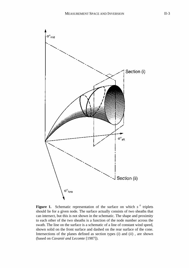
MEASUREMENT SPACE AND INVERSION II-3
Figure 1. Schematic representation of the surface on which σ 0 tripletsshould lie for a given node. The surface actually consists of two sheaths thatcan intersect, but this is not shown in the schematic. The shape and proximityto each other of the two sheaths is a function of the node number across theswath. The line on the surface is a schematic of a line of constant wind speed,shown solid on the front surface and dashed on the rear surface of the cone.Intersections of the planes defined as section types (i) and (ii) , are shown(based on Cavanié and Lecomte [1987]).
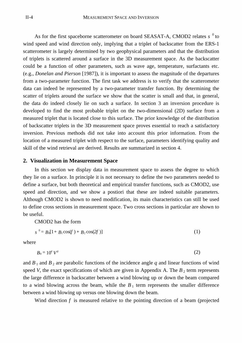
MEASUREMENT SPACE AND INVERSIONII-4
As for the first spaceborne scatterometer on board SEASAT-A, CMOD2 relates σ 0 to
wind speed and wind direction only, implying that a triplet of backscatter from the ERS-1
scatterometer is largely determined by two geophysical parameters and that the distribution
of triplets is scattered around a surface in the 3D measurement space. As the backscatter
could be a function of other parameters, such as wave age, temperature, surfactants etc.
(e.g., Donelan and Pierson [1987]), it is important to assess the magnitude of the departures
from a two-parameter function. The first task we address is to verify that the scatterometer
data can indeed be represented by a two-parameter transfer function. By determining the
scatter of triplets around the surface we show that the scatter is small and that, in general,
the data do indeed closely lie on such a surface. In section 3 an inversion procedure is
developed to find the most probable triplet on the two-dimensional (2D) surface from a
measured triplet that is located close to this surface. The prior knowledge of the distribution
of backscatter triplets in the 3D measurement space proves essential to reach a satisfactory
inversion. Previous methods did not take into account this prior information. From the
location of a measured triplet with respect to the surface, parameters identifying quality and
skill of the wind retrieval are derived. Results are summarized in section 4.
2. Visualization in Measurement Space
In this section we display data in measurement space to assess the degree to which
they lie on a surface. In principle it is not necessary to define the two parameters needed to
define a surface, but both theoretical and empirical transfer functions, such as CMOD2, use
speed and direction, and we show a postiori that these are indeed suitable parameters.
Although CMOD2 is shown to need modification, its main characteristics can still be used
to define cross sections in measurement space. Two cross sections in particular are shown to
be useful.
CMOD2 has the form
00 1 21σ φ φ= B + B + B 2[ cos( ) cos( )] (1)
where
0 10B = Vα γ (2)
and B 1 and B 2 are parabolic functions of the incidence angle θ and linear functions of wind
speed V, the exact specifications of which are given in Appendix A. The B 2 term represents
the large difference in backscatter between a wind blowing up or down the beam compared
to a wind blowing across the beam, while the B 1 term represents the smaller difference
between a wind blowing up versus one blowing down the beam.
Wind direction φ is measured relative to the pointing direction of a beam (projected
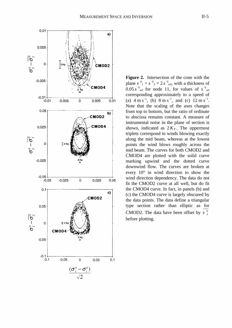
MEASUREMENT SPACE AND INVERSION II-5
Figure 2. Intersection of the cone with theplane σ 0
1 + σ 03 = 2 σ 0
ref, with a thickness of0.05 σ 0
ref for node 11, for values of σ 0ref
corresponding approximately to a speed of(a) 4 m s−1, (b) 8 m s−1, and (c) 12 m s−1.Note that the scaling of the axes changesfrom top to bottom, but the ratio of ordinateto abscissa remains constant. A measure ofinstrumental noise in the plane of section isshown, indicated as 2 K P . The uppermosttriplets correspond to winds blowing exactlyalong the mid beam, whereas at the lowestpoints the wind blows roughly across themid beam. The curves for both CMOD2 andCMOD4 are plotted with the solid curvemarking upwind and the dotted curvedownwind flow. The curves are broken atevery 10° in wind direction to show thewind direction dependency. The data do notfit the CMOD2 curve at all well, but do fitthe CMOD4 curve. In fact, in panels (b) and(c) the CMOD4 curve is largely obscured bythe data points. The data define a triangulartype section rather than elliptic as for
CMOD2. The data have been offset by σ 20
before plotting.
MEASUREMENT SPACE AND INVERSIONII-6
onto the horizontal plane), with φ = 0 corresponding to a wind blowing directly towards the
beam. Wind direction can also be defined with respect to the subsatellite track. To
distinguish which frame is being used we will use ϕ to indicate directions measured relative
to the satellite pointing direction and φ for directions relative to a beam.
According to the transfer function (1), a σ 0 triplet ( σ 0
1, σ 0
2, σ 0
3 ) can be written as
10
0 1 2
2 0 1 2
30
0 1 2
1 2 2
1 2
1 2 2
σ ϕ ϕ ϕ
σ ϕ ϕ
σ ϕ ϕ ϕ
= B + B + / + B
= B + B s - B
= B + B - / - B
0 * *
[ (sin cos ) sin ]
[ in cos ]
[ (sin cos ) sin ]
* (3)
where σ 01, σ 0
2, and σ 03 refer to the fore, mid, and aft beams, respectively. We have
assumed that the fore and aft beam incidence angles, and therefore their respective B 1 and
B 2 are identical. The values for the mid beam incidence angle are denoted B *1 and B
*2. For
a given node number, the parameters B 1, B 2, B *1, and B
*2 depend only on wind speed V.
Thus, at a given node (with known incidence angles for the three beams), the location of a
backscatter triplet in the 3D measurement space depends on only two free parameters, that
is, ( V, ϕ ). Consequently, (3) defines a surface in 3D σ 0 space for varying ( V, ϕ ) as shown
symbolically in Figure 1.
2.1. Visualization of Anisotropy
Sections through the cone were used to obtain quantitative information on the
geometry of the expected conical surface, in particular cross sections roughly normal to the
cone and cross sections along the main axis of the cone. From (2) and (3), it can be shown
that the vector length of the 3D backscatter vector σσ 0 = ( σ
01, σ
02, σ
03 ) depends mainly on
wind speed, whereas changes in wind direction mainly result in a different pointing
direction of the vector (which we denote anisotropy). Cross sections normal to the cone can
provide information on the dependence of the backscattering on wind direction, and those
along the cone axis can provide information on wind speed. CMOD2 will be used as a guide
to select appropriate cross sections. Although we show that CMOD2 needs to be revised, the
assumption that B 1 is small relative to B 2 still holds. We will later show that B 1 cannot be
ignored, but to aid the reader in the interpretation it is convenient, for now, to neglect B 1
and B *1 in (3) when
10
30
02 2 10σ σ α γ + B = V≈ × (4)
showing that a cross section where σ 01 + σ 0
3 = constant = 2σ 0ref corresponds to a section of
constant speed V. In such a cross section, denoted as type (i), we may write
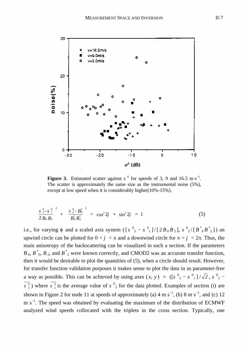
MEASUREMENT SPACE AND INVERSION II-7
230
10
0 2
220
0
0 2
2 2
22 2 1
σ σ σϕ ϕ
-
B B +
- B
B B = + =
*
* *
cos sin (5)
i.e., for varying ϕ and a scaled axis system ( [ σ 0
3 − σ 01 ] / [ 2 B 0 B 2 ], σ
02 / [ B
*0 B
*2 ] ) an
upwind circle can be plotted for 0 < ϕ < π and a downwind circle for π < ϕ < 2π. Thus, the
main anisotropy of the backscattering can be visualized in such a section. If the parameters
B 0, B *0, B 2, and B
*2 were known correctly, and CMOD2 was an accurate transfer function,
then it would be desirable to plot the quantities of (5), when a circle should result. However,
for transfer function validation purposes it makes sense to plot the data in as parameter-free
a way as possible. This can be achieved by using axes ( x, y ) = ([σ 03 − σ 0
1 ] / 2 , σ 02 −
σ 20 ) where σ 2
0 is the average value of σ 02 for the data plotted. Examples of section (i) are
shown in Figure 2 for node 11 at speeds of approximately (a) 4 m s−1, (b) 8 m s−1, and (c) 12
m s−1. The speed was obtained by evaluating the maximum of the distribution of ECMWF
analyzed wind speeds collocated with the triplets in the cross section. Typically, one
Figure 3. Estimated scatter against σ 0 for speeds of 3, 9 and 16.5 m s−1.The scatter is approximately the same size as the instrumental noise (5%),except at low speed when it is considerably higher(10%-15%).
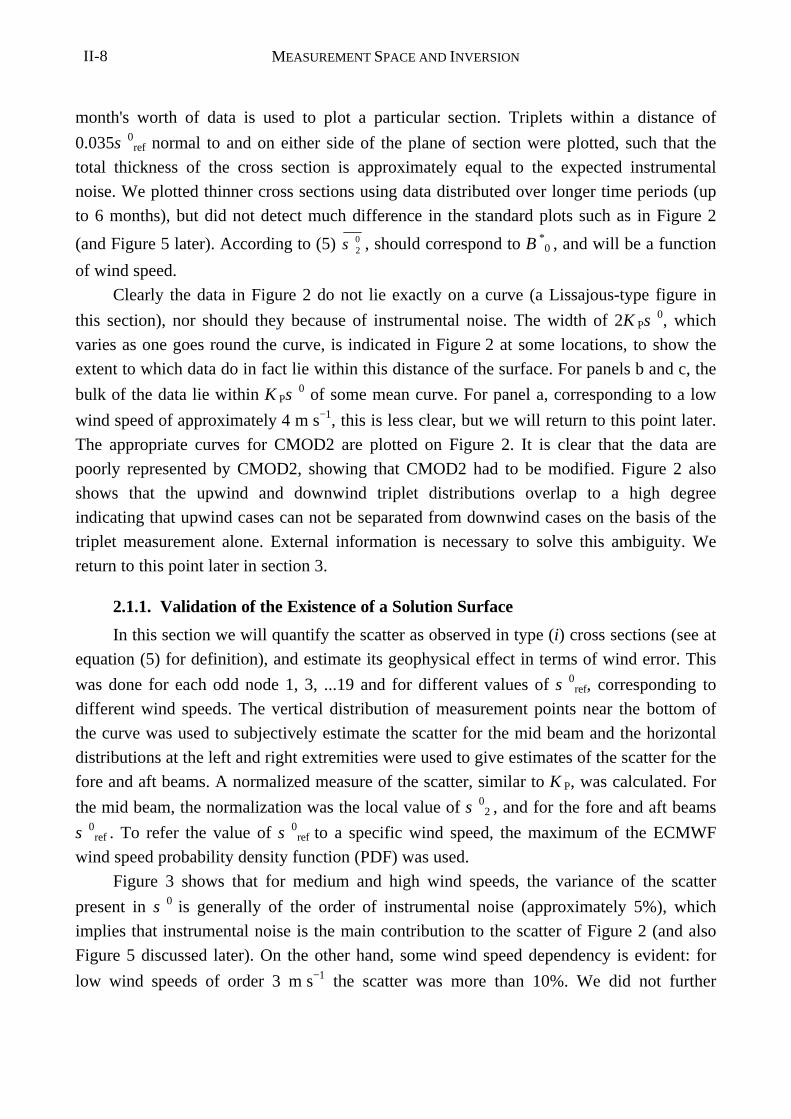
MEASUREMENT SPACE AND INVERSIONII-8
month's worth of data is used to plot a particular section. Triplets within a distance of
0.035σ 0ref normal to and on either side of the plane of section were plotted, such that the
total thickness of the cross section is approximately equal to the expected instrumental
noise. We plotted thinner cross sections using data distributed over longer time periods (up
to 6 months), but did not detect much difference in the standard plots such as in Figure 2
(and Figure 5 later). According to (5) σ 20 , should correspond to B
*0 , and will be a function
of wind speed.
Clearly the data in Figure 2 do not lie exactly on a curve (a Lissajous-type figure in
this section), nor should they because of instrumental noise. The width of 2K Pσ 0, which
varies as one goes round the curve, is indicated in Figure 2 at some locations, to show the
extent to which data do in fact lie within this distance of the surface. For panels b and c, the
bulk of the data lie within K Pσ 0 of some mean curve. For panel a, corresponding to a low
wind speed of approximately 4 m s−1, this is less clear, but we will return to this point later.
The appropriate curves for CMOD2 are plotted on Figure 2. It is clear that the data are
poorly represented by CMOD2, showing that CMOD2 had to be modified. Figure 2 also
shows that the upwind and downwind triplet distributions overlap to a high degree
indicating that upwind cases can not be separated from downwind cases on the basis of the
triplet measurement alone. External information is necessary to solve this ambiguity. We
return to this point later in section 3.
2.1.1. Validation of the Existence of a Solution Surface
In this section we will quantify the scatter as observed in type (i) cross sections (see at
equation (5) for definition), and estimate its geophysical effect in terms of wind error. This
was done for each odd node 1, 3, ...19 and for different values of σ 0ref, corresponding to
different wind speeds. The vertical distribution of measurement points near the bottom of
the curve was used to subjectively estimate the scatter for the mid beam and the horizontal
distributions at the left and right extremities were used to give estimates of the scatter for the
fore and aft beams. A normalized measure of the scatter, similar to K P, was calculated. For
the mid beam, the normalization was the local value of σ 02 , and for the fore and aft beams
σ 0ref . To refer the value of σ 0
ref to a specific wind speed, the maximum of the ECMWF
wind speed probability density function (PDF) was used.
Figure 3 shows that for medium and high wind speeds, the variance of the scatter
present in σ 0 is generally of the order of instrumental noise (approximately 5%), which
implies that instrumental noise is the main contribution to the scatter of Figure 2 (and also
Figure 5 discussed later). On the other hand, some wind speed dependency is evident: for
low wind speeds of order 3 m s−1 the scatter was more than 10%. We did not further
MEASUREMENT SPACE AND INVERSION II-9
investigate whether or not this could be accounted for from known geophysical effects,
since 10% at 3 m s−1 results only in a small wind error (approximately 0.3 m s−1).
To put the scatter into perspective, we simulated the average wind vector RMS error,
due to scatter in σ 0, to be approximately 0.5 m s−1 using CMOD4 as the transfer function.
As shown in Stoffelen and Anderson [1997a; Chapters III and IV], typical wind errors for
other observational systems are 3 m s−1 vector RMS. Therefore we may conclude that the
ERS-1 scatterometer is providing accurate σ 0 measurements, and that we may in general
regard the triplets as being scattered around a well-defined and relatively simple surface.
2.1.2. Estimation of B2
The provision of the cone surface to within 0.2 dB allows the unique possibility to
study characteristics of the transfer function in great detail. In aircraft and wave tank
experiments agreement to within 1 dB is considered satisfactory (see, e.g., Keller et al.
Figure 4. Estimated value of upwind-crosswind amplitude B 2 againstincidence angle θ for speeds of 3, 9, 12.5 and 16.5 m s−1. At higher speedsand incidence angles, B 2 saturates, but at lower speeds and incidence anglesit is speed dependent. The solid curve shows the CMOD2 relationship inwhich B 2 is independent of speed and does not fit the data well.
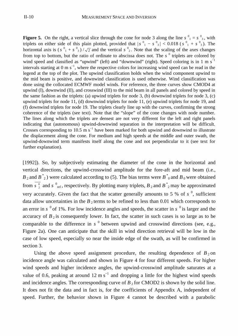
MEASUREMENT SPACE AND INVERSIONII-10
[1992]). So, by subjectively estimating the diameter of the cone in the horizontal and
vertical directions, the upwind-crosswind amplitude for the fore-aft and mid beam (i.e.,
B 2 and B *2 ) were calculated according to (5). The bias terms were B
*0 and B 0 were obtained
from σ 20 and σ 0
ref , respectively. By plotting many triplets, B 2 and B *2 may be approximated
very accurately. Given the fact that the scatter generally amounts to 5 % of σ 0, sufficient
data allow uncertainties in the B 2 terms to be refined to less than 0.01 which corresponds to
an error in σ 0 of 1%. For low incidence angles and speeds, the scatter in σ 0 is larger and the
accuracy of B 2 is consequently lower. In fact, the scatter in such cases is so large as to be
comparable to the difference in σ 0 between upwind and crosswind directions (see, e.g.,
Figure 2a). One can anticipate that the skill in wind direction retrieval will be low in the
case of low speed, especially so near the inside edge of the swath, as will be confirmed in
section 3.
Using the above speed assignment procedure, the resulting dependence of B 2 on
incidence angle was calculated and shown in Figure 4 for four different speeds. For higher
wind speeds and higher incidence angles, the upwind-crosswind amplitude saturates at a
value of 0.6, peaking at around 12 m s−1 and dropping a little for the highest wind speeds
and incidence angles. The corresponding curve of B 2 for CMOD2 is shown by the solid line.
It does not fit the data and in fact is, for the coefficients of Appendix A, independent of
speed. Further, the behavior shown in Figure 4 cannot be described with a parabolic
Figure 5. On the right, a vertical slice through the cone for node 3 along the line σ 01 = σ 0
3 , withtriplets on either side of this plain plotted, provided that | σ 0
1 − σ 03 | < 0.018 ( σ 0
1 + σ 03 ). The
horizontal axis is ( σ 01 + σ 0
3 ) / 2 and the vertical σ 02 . Note that the scaling of the axes changes
from top to bottom, but the ratio of ordinate to abscissa does not. The σ 0 triplets are colored bywind speed and classified as “upwind” (left) and “downwind” (right). Speed coloring is in 1 m s−1
intervals starting at 0 m s−1, where the respective colors for increasing wind speed can be read in thelegend at the top of the plot. The upwind classification holds when the wind component upwind tothe mid beam is positive, and downwind classification is used otherwise. Wind classification wasdone using the collocated ECMWF model winds. For reference, the three curves show CMOD4 atupwind (I), downwind (II), and crosswind (III) to the mid beam in all panels and colored by speed inthe same fashion as the triplets: (a) upwind triplets for node 3, (b) downwind triplets for node 3, (c)upwind triplets for node 11, (d) downwind triplets for node 11, (e) upwind triplets for node 19, and(f) downwind triplets for node 19. The triplets clearly line up with the curves, confirming the strongcoherence of the triplets (see text). Note that the “slope” of the cone changes with node number.The lines along which the triplets are densest are not very different for the left and right panelsindicating that (autonomous) upwind-downwind separation in the interpretation will be difficult.Crosses corresponding to 10.5 m s−1 have been marked for both upwind and downwind to illustratethe displacement along the cone. For medium and high speeds at the middle and outer swath, theupwind-downwind term manifests itself along the cone and not perpendicular to it (see text forfurther explanation).
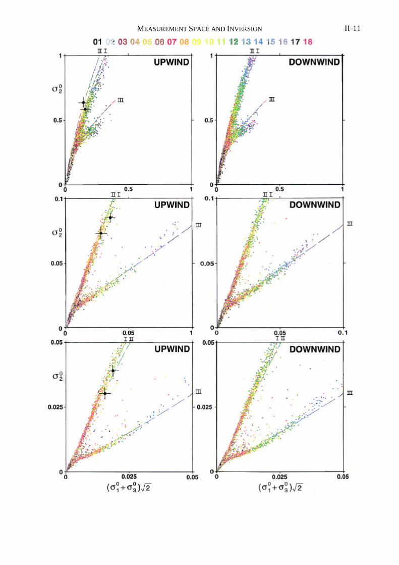
MEASUREMENT SPACE AND INVERSION II-11
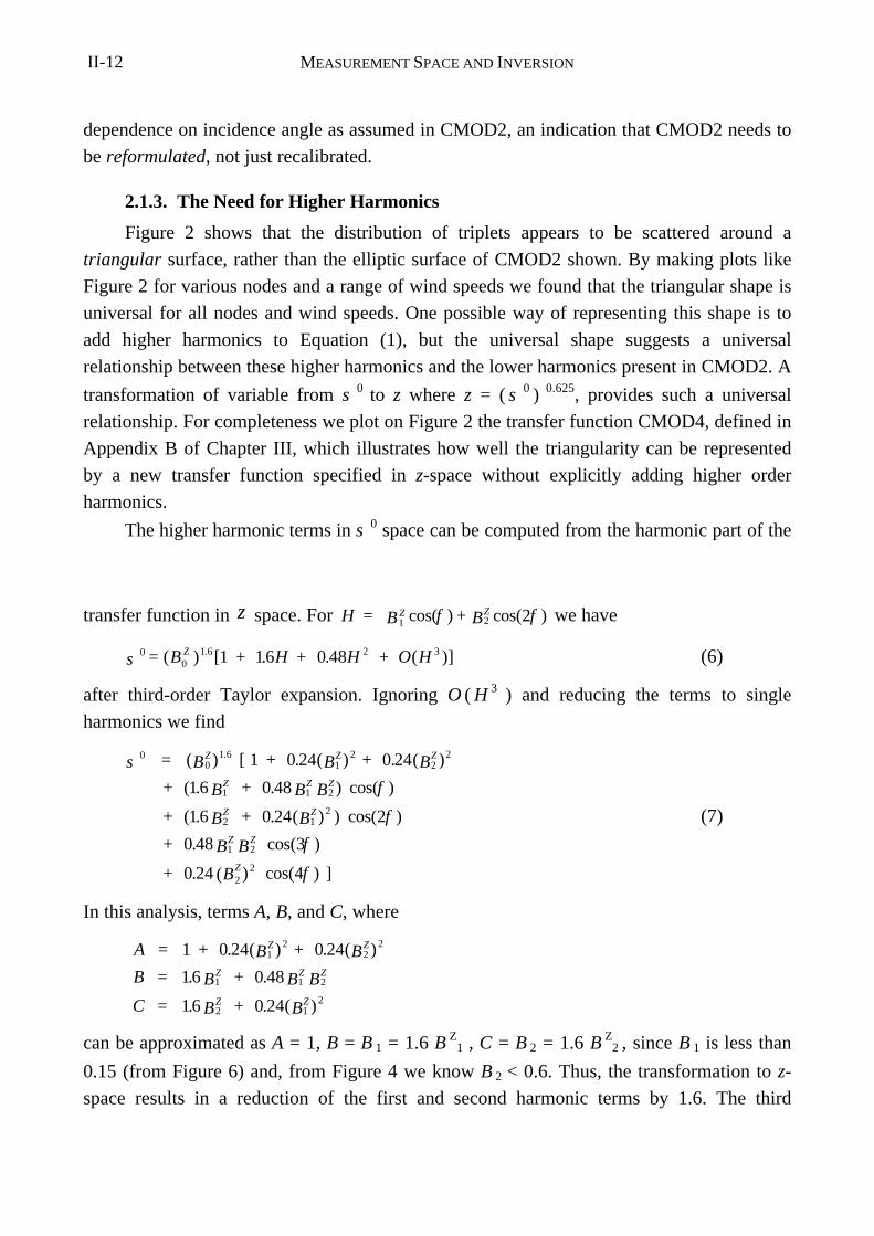
MEASUREMENT SPACE AND INVERSIONII-12
dependence on incidence angle as assumed in CMOD2, an indication that CMOD2 needs to
be reformulated, not just recalibrated.
2.1.3. The Need for Higher Harmonics
Figure 2 shows that the distribution of triplets appears to be scattered around a
triangular surface, rather than the elliptic surface of CMOD2 shown. By making plots like
Figure 2 for various nodes and a range of wind speeds we found that the triangular shape is
universal for all nodes and wind speeds. One possible way of representing this shape is to
add higher harmonics to Equation (1), but the universal shape suggests a universal
relationship between these higher harmonics and the lower harmonics present in CMOD2. A
transformation of variable from σ 0 to z where z = ( σ 0 ) 0.625, provides such a universal
relationship. For completeness we plot on Figure 2 the transfer function CMOD4, defined in
Appendix B of Chapter III, which illustrates how well the triangularity can be represented
by a new transfer function specified in z-space without explicitly adding higher order
harmonics.
The higher harmonic terms in σ 0 space can be computed from the harmonic part of the
transfer function in z space. For H = B + BZ Z1 2 2cos( ) cos( )φ φ we have
00
1 6 2 31 16 0 48σ = B + H + H + O HZ( ) [ . . ( )]. (6)
after third-order Taylor expansion. Ignoring O ( H 3
) and reducing the terms to single
harmonics we find
00
1 61
22
2
1 1 2
2 12
1 2
22
1 0 24 0 24
16 0 48
16 0 24 2
0 48 3
0 24 4
σφ
φ
φ
φ
= B + B + B
+ B + B B
+ B + B
+ B B
+ B
Z Z Z
Z Z Z
Z Z
Z Z
Z
( ) [ . ( ) . ( )
( . . ) cos( )
( . . ( ) ) cos( )
. cos( )
. ( ) cos( ) ]
.
(7)
In this analysis, terms A, B, and C, where
A = + B + B
B = B + B B
C = B + B
Z Z
Z Z Z
Z Z
1 0 24 0 24
16 0 48
16 0 24
12
22
1 1 2
2 12
. ( ) . ( )
. .
. . ( )
can be approximated as A = 1, B = B 1 = 1.6 B Z
1 , C = B 2 = 1.6 B Z2 , since B
1 is less than
0.15 (from Figure 6) and, from Figure 4 we know B 2 < 0.6. Thus, the transformation to z-
space results in a reduction of the first and second harmonic terms by 1.6. The third
MEASUREMENT SPACE AND INVERSION II-13
harmonic is very small, that is, 0.48 B Z1 B
Z2 ≤ 0.02. The fourth harmonic is the main cause
for the triangular cone shape. Although it is not large—that is 0.24 ( B Z
2 ) 2
≤ 0.04—it is
needed for an accurate representation of the shape of the conical surface.
2.2. Visualization of the Triplet Distribution Along the Cone
A second and independent cross section, denoted as type (ii), can be made for σ 01 =
σ 03. This equation is satisfied for:
I: ϕ = π/2, which is upwind to the mid beam pointing direction,
II: ϕ = 3π/2, which is downwind to the mid beam and
III: ϕ = − arcsin[ B 1 / ( 8 B 2 ) ], which is approximately at ϕ = 0 and ϕ = π , i.e.,
crosswind to the mid beam.
Figure 6. The value of B 1 , the upwind-downwind amplitude, versusincidence angle for different wind speed intervals, based on the average ofthe scatterometer and ECMWF wind speed. The three beams are shownseparately for each speed. At low incidence angles B 1 is small and negative,but has a marked speed dependence at higher incidence angles.
MEASUREMENT SPACE AND INVERSIONII-14
So, cross section (ii) should have data clustered along three lines corresponding to the wind
directions I, II, III above. If we plot y = σ 02 versus x = ( σ 01 + σ 0
3 ) / 2 then for CMOD2
I* *
II*
1* *
III* *
x
y =
B + B
B + B + B
x
y =
B - B
B - B + B
x
y =
B
B - B
0 1
0 1 2
0 1
0 2
0
0 2
2
1
2
1
2
1
( )
( )
( )
( )
( )
*
(8)
The x value for III (crosswind) is the average of I and II, while the value for III is smaller
than the y value for I and II by approximately δy = 2 B *0 B
*2 . The average of I, II and two
times III contains only the bias terms B 0, and B *
0 and defines for varying wind speed the
main axis of the cone. When B 1 is ignored, x depends only on B
0 , which in turn depends on
wind speed (Equation (2)). However, B 1 cannot be completely ignored as illustrated in
Figure 6. In I, y represents the upwind, in II the downwind, and in III the crosswind
backscatter of the mid beam.
In Figures 5a-f cross sections of type (ii) are shown for nodes 3, 11 and 19. The
diameter of the cone relative to the scatter normal to its surface is large for medium and high
speeds and for most node numbers, except for the first few at the inner swath. This ratio is a
good measure of the quality of the wind direction information in a triplet as will be
discussed further in section 3.
2.2.1. Upwind-Downwind Effect
In Figure 1 the upwind and downwind cones are sketched to overlap for illustration
purposes, while, in reality, for B 1 ≠ 0 they will be slightly separated. Figures 5a, 5c, and 5e
show triplets where the collocated ECMWF wind has a component toward the mid beam
(“upwind”), while Figures 5b, 5d, and 5f show triplets where the collocated ECMWF wind
has a component away from the mid beam (“downwind”). For reference, the full section
(showing I, II, and III) through the CMOD4 transfer function is also shown in each plot. The
location of “upwind” and “downwind” triplets is similar, confirming the inherent dual
ambiguity noted earlier. However, the collocated wind speeds are different for upwind and
downwind, that is, the “average” color at a certain location on the plot can be different for
upwind and downwind by up to 1.5 m s−1 at some nodes. This can be explained by (8). For a
fixed wind speed we note that the difference between I (upwind) and II (downwind) is ( ∆x,
∆y ) = ( 2 B 0 B
1 , 2 B *
0 B *
1 ), that is, a shift in both x and y directions. A small change in
wind speed will also change both x and y, that is, ( ∂x / ∂V, ∂y / ∂V ) = V −1
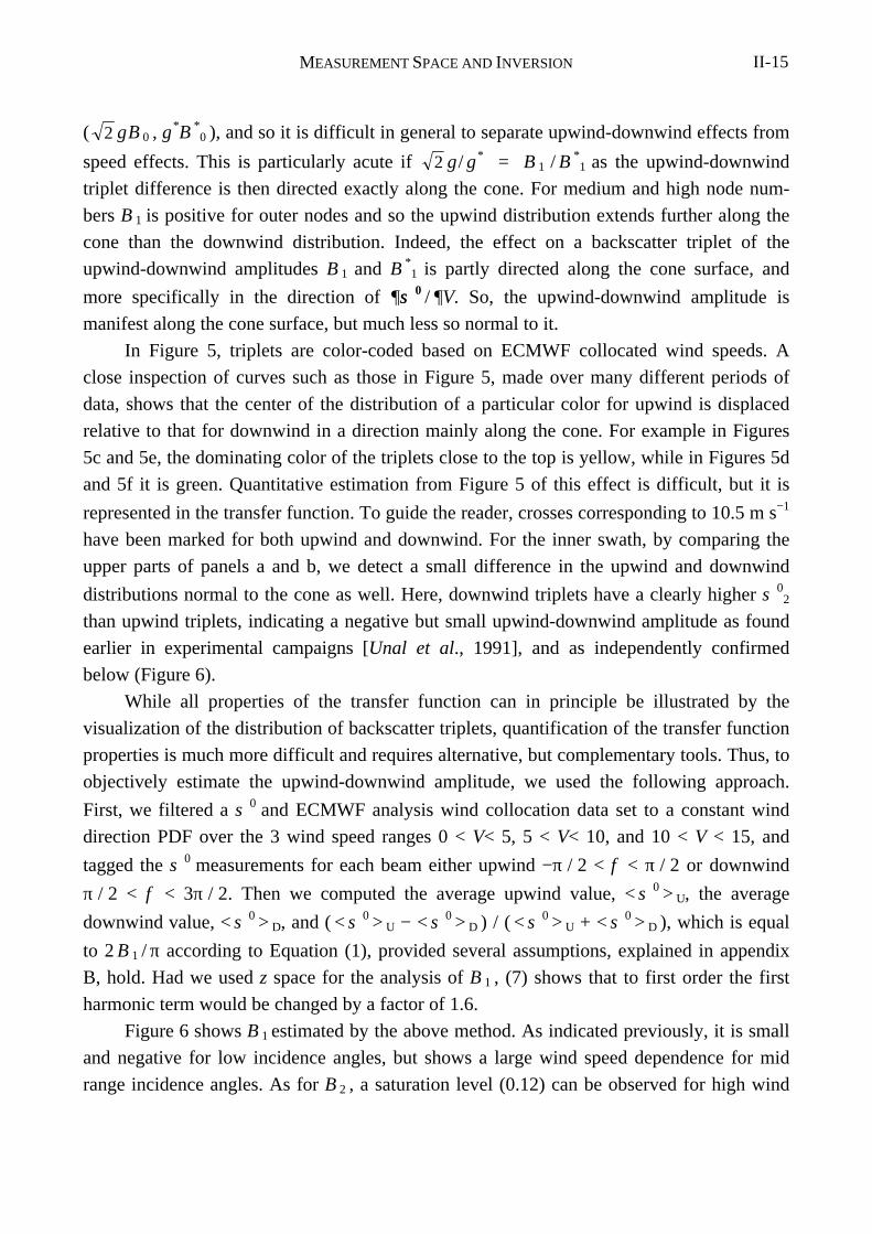
MEASUREMENT SPACE AND INVERSION II-15
( 2 γ B 0 , γ
*B *0 ), and so it is difficult in general to separate upwind-downwind effects from
speed effects. This is particularly acute if 2 γ / γ * = B
1 / B *
1 as the upwind-downwind
triplet difference is then directed exactly along the cone. For medium and high node num-
bers B 1 is positive for outer nodes and so the upwind distribution extends further along the
cone than the downwind distribution. Indeed, the effect on a backscatter triplet of the
upwind-downwind amplitudes B 1 and B *
1 is partly directed along the cone surface, and
more specifically in the direction of ∂σσ 0 / ∂V. So, the upwind-downwind amplitude is
manifest along the cone surface, but much less so normal to it.
In Figure 5, triplets are color-coded based on ECMWF collocated wind speeds. A
close inspection of curves such as those in Figure 5, made over many different periods of
data, shows that the center of the distribution of a particular color for upwind is displaced
relative to that for downwind in a direction mainly along the cone. For example in Figures
5c and 5e, the dominating color of the triplets close to the top is yellow, while in Figures 5d
and 5f it is green. Quantitative estimation from Figure 5 of this effect is difficult, but it is
represented in the transfer function. To guide the reader, crosses corresponding to 10.5 m s−1
have been marked for both upwind and downwind. For the inner swath, by comparing the
upper parts of panels a and b, we detect a small difference in the upwind and downwind
distributions normal to the cone as well. Here, downwind triplets have a clearly higher σ 02
than upwind triplets, indicating a negative but small upwind-downwind amplitude as found
earlier in experimental campaigns [Unal et al., 1991], and as independently confirmed
below (Figure 6).
While all properties of the transfer function can in principle be illustrated by the
visualization of the distribution of backscatter triplets, quantification of the transfer function
properties is much more difficult and requires alternative, but complementary tools. Thus, to
objectively estimate the upwind-downwind amplitude, we used the following approach.
First, we filtered a σ 0 and ECMWF analysis wind collocation data set to a constant wind
direction PDF over the 3 wind speed ranges 0 < V< 5, 5 < V< 10, and 10 < V < 15, and
tagged the σ 0 measurements for each beam either upwind −π / 2 < φ < π / 2 or downwind
π / 2 < φ < 3π / 2. Then we computed the average upwind value, < σ 0
> U, the average
downwind value, < σ 0
> D, and ( < σ 0
> U − < σ 0
> D ) / ( < σ 0
> U + < σ 0
> D ), which is equal
to 2 B 1 / π according to Equation (1), provided several assumptions, explained in appendix
B, hold. Had we used z space for the analysis of B 1 , (7) shows that to first order the first
harmonic term would be changed by a factor of 1.6.
Figure 6 shows B 1 estimated by the above method. As indicated previously, it is small
and negative for low incidence angles, but shows a large wind speed dependence for mid
range incidence angles. As for B 2 , a saturation level (0.12) can be observed for high wind
MEASUREMENT SPACE AND INVERSIONII-16
speeds and incidence angles, a behavior that cannot be described by the linear speed and
parabolic incidence angle dependency of CMOD2. In this section we have shown why the
form of CMOD2 had to be modified. Retuning parameters, but retaining the basic structure
of CMOD2 would not have been sufficient.
2.3. Wind Speed Dependence
In (1) the major speed dependence is in the B 0 term. From (4) one can estimate this
speed dependence by averaging σ 01 and σ 0
3 and comparing with the collocated ECMWF
wind speed. In Figure 7 we plot the joint distribution of log (V) estimated from the
scatterometer by this method and log (V) from ECMWF. We used log (V) in order to be able
to compute the optimal values of α and γ of (4) by linear regression. If we assume that both
estimates of the true wind contain the same amount of random error, then this joint
distribution should be symmetric around the 45° line. The distributions calculated for all
nodes using the log (V) dependence are in general not symmetric as illustrated in Figure 7
for node 17. When the log (V) dependence was modified to a log ( V + β (θ ) ) dependence,
the distributions became more symmetric, with the absolute value of β generally below 1
m s−1. A stronger modification of functionality, such as a V dependence gave unrealistic
distributions for the lower wind speeds, but a more symmetric distribution for high wind
speeds. This high wind speed asymmetry is not noticeable in Figure 7, but it was more
evident for nodes at the inner half of the swath. The transfer function dependency is
therefore best described by including the parameter β and a log-dependency for low wind
speeds and a V dependency for average and high speeds.
2.4. Other Geophysical Dependencies
By collocation of the σ 0 triplets to a geophysical parameter, sensitivity to it can be
studied. For example, for low wind speeds of order 3 m s−1 the σ 0 scatter increases to
approximately 15%, which is considerably larger than for the value for higher wind speeds.
It is possible that this increase is a result of geophysical effects, such as variations in sea
surface temperature, wind variability, or surface slick variations at a given wind speed (wind
speed dependent effects do not increase the scatter). The first dependency we tested used
cross section (ii) to investigate the sensitivity of the distribution of σ 0 triplets to sea surface
temperature (SST), in bins from 0°C to 10°C, 10°C to 20°C, 20°C to 30°C, and above 30°C,
for low wind speeds (less than 2 m s−1). If SST systematically influenced the backscatter,
then one would expect either that the distribution of triplets would shift in the 3D space,
dependent on SST, or that the density of the distribution would change. Neither of these
effects could be identified.
MEASUREMENT SPACE AND INVERSION II-17
On the other hand, there has been some evidence that SST gradients may have an
effect [Boehnke and Wismann, 1994] but we were unable to detect such a dependency. It is
likely that geophysical effects at low wind speeds will vary substantially on scales smaller
than the footprint size (50 km) but, by averaging the backscatter over an area the size of the
footprint, these effects are smoothed. However, it is difficult to find verification data of
wind, SST gradient and radar backscatter at one location with sufficient accuracy to
investigate this hypothesis rigorously.
Another relevant geophysical parameter is the sea ice extent. This is a dynamic
quantity, and it is therefore worthwhile to investigate whether measurement space can be
used to distinguish ocean scattering from ice scattering. It was found that the distribution of
Figure 7. Two-dimensional distribution in 10 log V, with V measured inmeters per second. The vertical axis is V, estimated from the fore and aftbeam measurements using Eq. (4), while the horizontal axis is the collocatedECMWF speed. Solid squares represent vertical averages over thedistribution and solid triangles, horizontal averages. Even though aregression on α and γ has been performed to optimize the distribution (seetext), the distribution is not symmetric around the 45° line. Data are for node17 from 30 September 1991 to 1 October 1991.
MEASUREMENT SPACE AND INVERSIONII-18
σ 0 triplets from ice is largely distinct from the open ocean distribution of triplets at the inner
and outer swath, and so ice and open ocean could be distinguished. At mid swath, however,
there is a considerable overlap in both distributions of σ 0 triplets and, for this case, time or
space continuity would have to be used to distinguish open sea from ice (e.g., Lecomte
[1993]).
3. Inversion
The 2D surface sketched in Figure 1, and shown more fully in Figures 2 and 5
describes the wind speed and direction dependence of the σ 0 triplet measurements. We will
formulate in this section an inversion procedure that seeks to find the most probable triplet
on the cone surface from a measured triplet that is located close to it. In earlier work the
inversion was generally based on minimization of the following maximum likelihood
estimator (MLE) for varying wind speed and direction (e.g., Graham et al [1989])
( )MLESDO S
N
=
∑i=
i i
i
-
1
32
0 0
0
σ σσ
(9)
where σ 0Oi is the measured (observed) value, σ 0
Si is the simulated value obtained from the
σ 0-to-wind transfer function for a trial value of the wind vector, and σ 0Ni is usually taken to
be either σ 0Oi or σ 0
Si. The index i indicates beam position: 1 = fore, 2 = mid, 3 = aft. Here,
SD( σ 0
Ni ) is a measure of the noise in σ 0 and has the form K Pi × σ 0
Ni, where K Pi is a
dimensionless constant (typically 0.05) whose value is determined by instrument noise.
(Strictly speaking, when assuming Gaussian errors, a term 2 ln [ SD(σ 0Ni ) ] should be added
to the right-hand side of (9) but this term is not significant and is not used in this paper.) The
minimization is done for each triplet of measured σ 0 values at each node.
The MLE minimization generally results in two local wind minima when the nor-
malization factor SD is equal to a constant, and generally four, but sometimes up to six,
when normalization is by the solution or the measurement [Graham et al., 1989]. The two
primary minima, corresponding to the two most likely solutions differ by approximately
180° in direction. The occurrence and location of the other minima frequently depend
strongly on the normalization, making one doubt their validity. We will show that the two
solutions describe the main ambiguity.
Normalization can be loosely thought of as a scaling of the axes of the 3D σ 0 space,
and provides a means of optimizing the way distances from the cone are penalized in this
space. We will show that the cost function of (9) is not optimal and suggest an
improvement, based on Bayes’ probability theorem and visualization in measurement space.
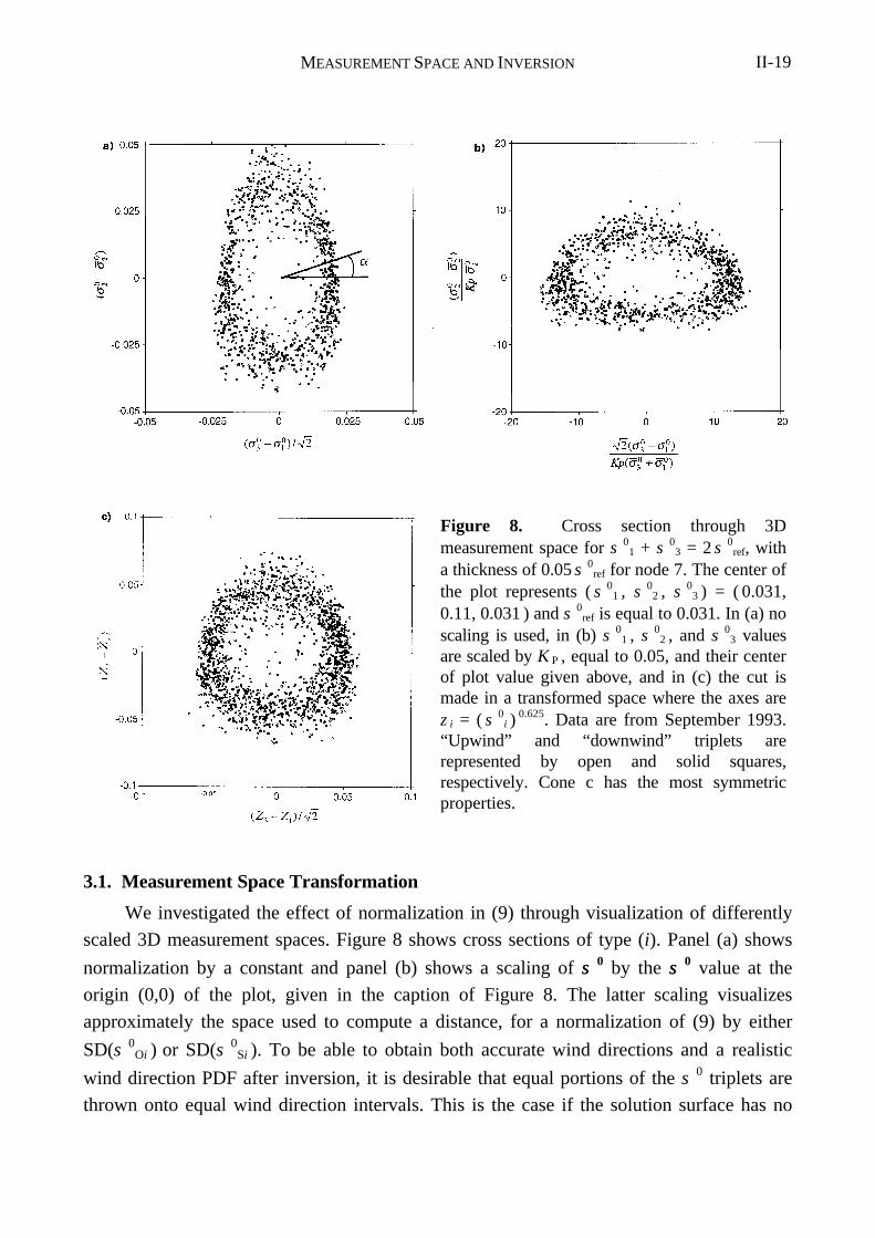
MEASUREMENT SPACE AND INVERSION II-19
3.1. Measurement Space Transformation
We investigated the effect of normalization in (9) through visualization of differently
scaled 3D measurement spaces. Figure 8 shows cross sections of type (i). Panel (a) shows
normalization by a constant and panel (b) shows a scaling of σσ 0 by the σσ 0 value at the
origin (0,0) of the plot, given in the caption of Figure 8. The latter scaling visualizes
approximately the space used to compute a distance, for a normalization of (9) by either
SD(σ 0Oi ) or SD(σ 0
Si ). To be able to obtain both accurate wind directions and a realistic
wind direction PDF after inversion, it is desirable that equal portions of the σ 0 triplets are
thrown onto equal wind direction intervals. This is the case if the solution surface has no
Figure 8. Cross section through 3Dmeasurement space for σ 0
1 + σ 03 = 2 σ 0
ref, witha thickness of 0.05 σ 0
ref for node 7. The center ofthe plot represents ( σ 0
1 , σ 02 , σ 0
3 ) = ( 0.031,0.11, 0.031 ) and σ 0
ref is equal to 0.031. In (a) noscaling is used, in (b) σ 0
1 , σ 02 , and σ 0
3 valuesare scaled by K P , equal to 0.05, and their centerof plot value given above, and in (c) the cut ismade in a transformed space where the axes arez i = ( σ 0
i ) 0.625. Data are from September 1993.
“Upwind” and “downwind” triplets arerepresented by open and solid squares,respectively. Cone c has the most symmetricproperties.
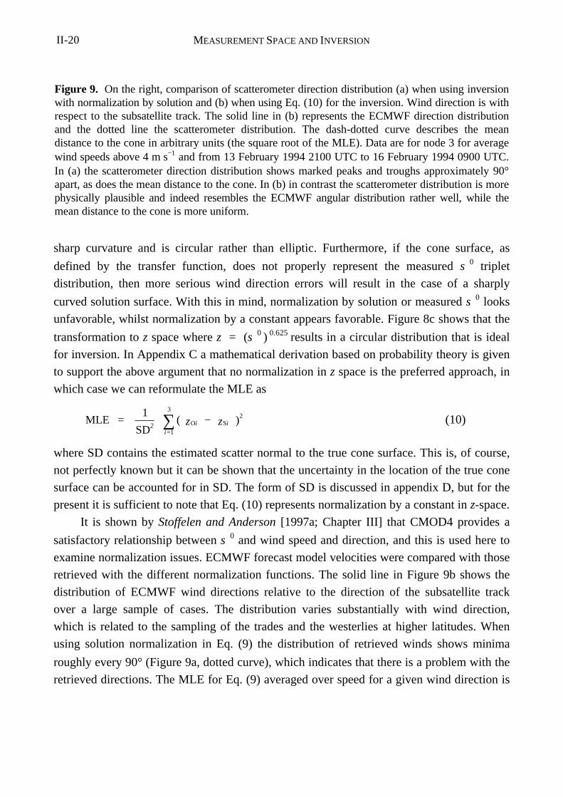
MEASUREMENT SPACE AND INVERSIONII-20
sharp curvature and is circular rather than elliptic. Furthermore, if the cone surface, as
defined by the transfer function, does not properly represent the measured σ 0 triplet
distribution, then more serious wind direction errors will result in the case of a sharply
curved solution surface. With this in mind, normalization by solution or measured σ 0 looks
unfavorable, whilst normalization by a constant appears favorable. Figure 8c shows that the
transformation to z space where z = (σ 0 )
0.625 results in a circular distribution that is ideal
for inversion. In Appendix C a mathematical derivation based on probability theory is given
to support the above argument that no normalization in z space is the preferred approach, in
which case we can reformulate the MLE as
MLESD
O S = z z 2 i i
i
1 2
1
3
( )−=∑ (10)
where SD contains the estimated scatter normal to the true cone surface. This is, of course,
not perfectly known but it can be shown that the uncertainty in the location of the true cone
surface can be accounted for in SD. The form of SD is discussed in appendix D, but for the
present it is sufficient to note that Eq. (10) represents normalization by a constant in z-space.
It is shown by Stoffelen and Anderson [1997a; Chapter III] that CMOD4 provides a
satisfactory relationship between σ 0 and wind speed and direction, and this is used here to
examine normalization issues. ECMWF forecast model velocities were compared with those
retrieved with the different normalization functions. The solid line in Figure 9b shows the
distribution of ECMWF wind directions relative to the direction of the subsatellite track
over a large sample of cases. The distribution varies substantially with wind direction,
which is related to the sampling of the trades and the westerlies at higher latitudes. When
using solution normalization in Eq. (9) the distribution of retrieved winds shows minima
roughly every 90° (Figure 9a, dotted curve), which indicates that there is a problem with the
retrieved directions. The MLE for Eq. (9) averaged over speed for a given wind direction is
Figure 9. On the right, comparison of scatterometer direction distribution (a) when using inversionwith normalization by solution and (b) when using Eq. (10) for the inversion. Wind direction is withrespect to the subsatellite track. The solid line in (b) represents the ECMWF direction distributionand the dotted line the scatterometer distribution. The dash-dotted curve describes the meandistance to the cone in arbitrary units (the square root of the MLE). Data are for node 3 for averagewind speeds above 4 m s−1 and from 13 February 1994 2100 UTC to 16 February 1994 0900 UTC.In (a) the scatterometer direction distribution shows marked peaks and troughs approximately 90°apart, as does the mean distance to the cone. In (b) in contrast the scatterometer distribution is morephysically plausible and indeed resembles the ECMWF angular distribution rather well, while themean distance to the cone is more uniform.
MEASUREMENT SPACE AND INVERSION II-21
Figure 9. Continued.
MEASUREMENT SPACE AND INVERSIONII-22
also shown in Figure 9a by the dot-dash curve. This shows that at the direction “gaps”, the
average MLE (dash-dotted) is relatively small; only points close to the cone surface can be
projected onto these directions, while points further from the surface are always projected
onto other directions. The distribution of retrieved directions (dotted) in Figure 9a, based on
solution normalization, and in Figure 9b, based on Eq. (10), are very different, but the latter
distribution is very similar to the independent reference distribution from ECMWF.
Moreover, in Figure 9b the average MLE (dash-dotted) is reasonably constant for all wind
directions, indicative of a constant probability. The improvement in direction accuracy when
using Eq. (10), rather than the other forms of MLE discussed, is most significant at the
inside swath, but present over the whole swath.
A synoptic consequence of the normalization by measurement or solution is a
granularity in the resulting wind field. Instead of winds turning smoothly with position, they
would all point in one direction and then jump abruptly to a new direction. (An example of
this is shown in Stoffelen and Anderson [1993]). With the constant normalization of Eq. (10)
this problem has been removed and the winds show no abrupt unmeteorological jumps in
direction.
Generally if points lie outside the cone then there will be two minima approximately
180° apart. The fact that two solutions exist emerges directly from the fact that the cone has
an upwind and a downwind sheath, as shown in Figures 2 and 5. There may be other
minima, but they are not likely to be meaningful and will correspond to large distances from
the cone—that is, large values of the MLE. On the other hand, points near the central axis of
the cone may have several solutions, all about the same distance from the surface and
therefore all equally probable, but not representative of the real wind direction.
As seen in Figures 2 and 5, the separation of the distribution of upwind and downwind
triplets is comparable to the σ 0 triplet scatter. If upwind and downwind were well separated
then one would have a good chance of distinguishing between the two possible wind
directions, on the basis of the σ 0 measurements alone, a procedure often called
“autonomous” ambiguity removal. However, Figures 2 and 5 show that in general the
sheaths are rather close, a consequence of which is that the two wind directions are almost
equally probable, so autonomous ambiguity removal is not very likely to succeed.
3.2. Quality Tests in the Transformed Space
Measurement space reveals a clear signature of a cone surface, and in the inversion
procedure we compute the distance of a measured triplet to this surface, which is a measure
of the quality (interpretability) of the measurement. On this basis we developed quality
control tests that just depend on the measured triplet values and not on external information
as is usually done. For quantitative use, we normalize the distance from the measurement
MEASUREMENT SPACE AND INVERSION II-23
point to the solution cone by an estimate of the triplet scatter to produce the normalized
distance d. (The exact definition and derivation of d are given in Appendix C.)
The minimum normalized distance (corresponding to the first solution) is denoted d 1.
The normalization is such that the expectation value of d 2
1 should be 1. A test has been
implemented to reject points for which d 1 is greater than 3, that is, to reject points lying
more than three standard deviations away from the cone (called the “3SD” test). The 3SD
distance typically amounts to a wind vector RMS error contribution of only 1.5 m s−1 and
represents a sensitive quality control test. Between 1% and 2% of triplets fail the 3SD test,
as one may expect. Generally they lie in areas of extreme meteorological conditions—that
is, within a distance of approximately 100 km of intense fronts or low pressure systems, or
close to tropical storms. We assume a confused sea state is present in these cases due to the
temporal variability of wind direction, fetch effects, or rain, but other effects like stability
are also possible candidates.
The probability information in d is used further to assign a quantitative skill index for
wind direction retrieval. For a given triplet we calculate a mean squared normalized distance
to the surface, averaged over all wind directions, denoted 2d , that increases going from the
cone center outwards. Each point is given a skill rating based on the minimum distance d 1
and the mean distance 2d . Specifically, the skill index is calculated from
( )I =
d - d
d ,
212
1 2
1 1
/
max( )(11)
According to this formula, directional skill will increase monotonically from the center of
the cone outward, reaching a maximum just outside the cone, and will then decrease for
points far outside the cone. This reflects the fact that for triplets near the center of the cone,
wind direction discrimination will be poor, whereas points at a similar distance outside the
cone may still provide valuable directional information. The test works well in that points at
the center of the cone have low skill ratings, while those near the cone have high skill
values. The directional skill increases as the cone opens up at increasing wind speeds.
4. Summary and Conclusions
The 3D σ 0 space visualization introduced in this paper is extremely useful in
considering the quality of the measured triplets, in designing the form of a suitable transfer
function, and in developing a wind inversion procedure. We verified the existence of a cone-
shaped surface in 3D σ 0 space and found the σσ 0 scatter perpendicular to the cone to be
close to measurement noise specification (approximately 5% or 0.2 dB), except at low wind
speeds and at the inside edge of the swath, implying that in general a two parameter transfer
MEASUREMENT SPACE AND INVERSIONII-24
function is sufficient to describe the σ 0 triplet distribution. Such a transfer function would
be able to describe the backscatter measurement coherence to within 0.2 dB, which is
exceptional. Usually a validation of backscatter data to within 1 dB is considered
appropriate ( See, e.g., Keller et al. [1992]). Therefore, we consider the ability of the
transfer function to fit the distribution of measured σ 0 triplets in the 3D σ 0 space as the
most important validation test. This is used extensively in Stoffelen and Anderson [1997a;
Chapter III].
In the cases where the scatter exceeds measurement noise, the deviation from the cone
surface may be related to geophysical parameters other than wind speed and direction. Such
a relation would not have a substantial effect on the global quality of the scatterometer wind
product, however, since the σ 0 scatter normal to the cone is small in terms of the error in the
derived wind. It might lead to a local improvement in cases where the quality control proce-
dure of section 3 rejects anomalous σ 0 triplets lying too far away from the cone (less than
2% of cases). This occurs in cases associated with extreme weather conditions, such as
within approximately 100 km of intense fronts, lows and tropical cyclones. Further research
is needed to investigate whether these anomalous triplets are caused by, for example, wave
effects, rapid changes in wind direction, or rain and whether they could be usefully included
in the transfer function.
Each point on the cone surface has a geophysical interpretation. Physically, the
extension of the cone in the 3D σ0 space is related to the amplitude of capillary ocean
waves, whereas the diameter of the cone is related to the anisotropy of backscattering of
radar waves from these centimeter-wavelength ocean waves. In the empirically derived
transfer functions these two parameters are assumed to be explicitly related to wind speed
and direction, an assumption justified by Stoffelen and Anderson [1997a; Chapters III and
IV]. The behavior of the bias term, the upwind-crosswind term, and the upwind-downwind
term of the empirical transfer function show important features that were not anticipated
before launch and so were not taken into account in the ESA prelaunch transfer function
CMOD2—for example, a nonlogarithmic wind speed dependency, saturation of the
harmonic terms for increasing wind speeds and incidence angles, and the necessity for
higher harmonic terms. The nonlogarithmic speed dependence as found by us for the ERS-1
scatterometer is confirmed by Keller et al. [1992], although their experiments were for a
much smaller footprint than for the ERS-1 scatterometer. The higher harmonic terms are,
however, not necessary in a slightly transformed space z = ( σ 0 ) 0.625, which has the further
advantage that the inversion procedure is done better. The transformation results in a fourth-
order harmonic of roughly 4% at maximum which agrees well with earlier aircraft
campaigns where 96% of the power was in the first two harmonics [Unal et al., 1991] at C
band and VV polarization. Although not yet theoretically supported, we would recommend
MEASUREMENT SPACE AND INVERSION II-25
using z space in the interpretation of ERS scatterometer measurements.
When we assume that a z triplet measurement originates from a “true” z triplet on the
cone surface, then the inversion problem is reduced to finding the most likely location of
this triplet on the cone surface. The curvature of the cone and the general distribution of
measured z triplets around the cone determines the optimal projection of a measured z triplet
onto the cone surface. We found an optimal and practical solution for the inversion problem
by making use of the symmetric geometry of the ERS-1 scatterometer. A less symmetric
geometry (such as the NSCAT or SeaWinds design developed by the National Aeronautical
and Space Administration (NASA)) would complicate the inversion problem. In earlier
inversion algorithms (see, e.g., Graham et al. [1989]), no account was taken of the prior
knowledge of the shape of the cone surface and the distribution of measured σ 0 triplets
around it.
The inversion process delivers two significant solutions in roughly opposite directions,
which is directly related to the fact that the “upwind” and “downwind” leaves of the cone in
3D σ 0 space are closely overlapping. The upwind-downwind amplitude B 1 is not zero, but
it results in a triplet distribution for upwind and downwind that mainly differs in a direction
along the cone. Ambiguity removal filters are needed to select a unique solution from the
two ambiguous wind vectors of similar strength and approximately opposite direction.
Directional accuracy, as measured by the position of a triplet relative to the cone surface,
can be quantified in a skill index that in turn can be used in ambiguity removal filters
[Stoffelen and Anderson, 1997b; Chapter V].
Appendix A: The Prelaunch Transfer Function CMOD2
The Prelaunch transfer function CMOD2 has the form
00 1 21 2σ φ φ= B + B + B[ cos( ) cos( )] (A1)
where
0 10B = Vα γ (A2)
and B 1 and B 2 are parabolic functions of the incidence angle θ in degrees and linear
functions of wind speed V in meters per second. The form of the coefficients is as follows.
α
γ
= C + C P + C P
= C ) + C P + C P
2
2
( ) ( ) ( )
( ) ( ) ( )
1 2 3
4 5 61
1
1 1 2 1 2
2 1 2 1 2
7 8 9 10 11 12
13 14 15 16 17 18B = C + C P + C P + C + C P + C P V
B = C + C P + C P + C + C P + C P V
[ ( ) ( ) ( ) ] [ ( ) ( ) ( ) ]
[ ( ) ( ) ( ) ] [ ( ) ( ) ( ) ]
where P 1 and P 2 are the first and second Legendre functions, given by
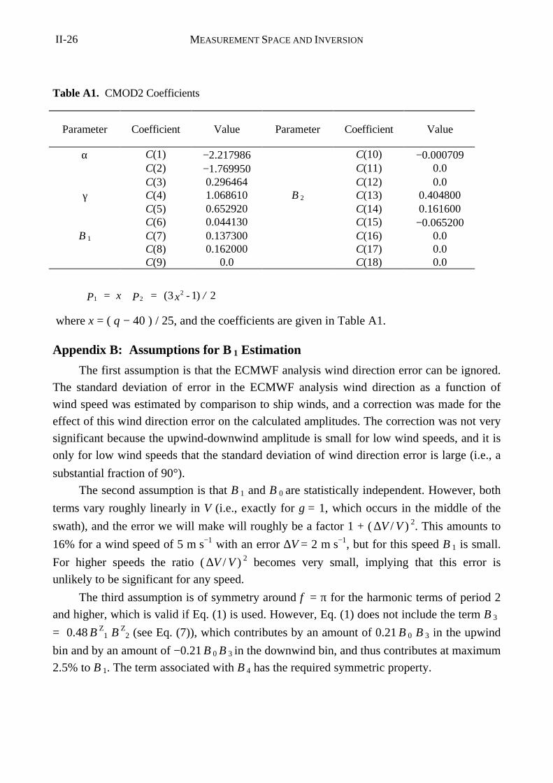
MEASUREMENT SPACE AND INVERSIONII-26
P = x P = x - /1 223 1 2( )
where x = ( θ − 40 ) / 25, and the coefficients are given in Table A1.
Appendix B: Assumptions for B 1 Estimation
The first assumption is that the ECMWF analysis wind direction error can be ignored.
The standard deviation of error in the ECMWF analysis wind direction as a function of
wind speed was estimated by comparison to ship winds, and a correction was made for the
effect of this wind direction error on the calculated amplitudes. The correction was not very
significant because the upwind-downwind amplitude is small for low wind speeds, and it is
only for low wind speeds that the standard deviation of wind direction error is large (i.e., a
substantial fraction of 90°).
The second assumption is that B 1 and B 0 are statistically independent. However, both
terms vary roughly linearly in V (i.e., exactly for γ = 1, which occurs in the middle of the
swath), and the error we will make will roughly be a factor 1 + ( ∆V / V ) 2. This amounts to
16% for a wind speed of 5 m s−1 with an error ∆V = 2 m s−1, but for this speed B 1 is small.
For higher speeds the ratio ( ∆V / V ) 2 becomes very small, implying that this error is
unlikely to be significant for any speed.
The third assumption is of symmetry around φ = π for the harmonic terms of period 2
and higher, which is valid if Eq. (1) is used. However, Eq. (1) does not include the term B 3
= 0.48 B Z
1 B Z
2 (see Eq. (7)), which contributes by an amount of 0.21 B 0 B 3 in the upwind
bin and by an amount of −0.21 B 0 B 3 in the downwind bin, and thus contributes at maximum
2.5% to B 1. The term associated with B 4 has the required symmetric property.
Table A1. CMOD2 Coefficients
Parameter Coefficient Value Parameter Coefficient Value
α C(1) −2.217986 C(10) −0.000709C(2) −1.769950 C(11) 0.0C(3) 0.296464 C(12) 0.0
γ C(4) 1.068610 B 2 C(13) 0.404800C(5) 0.652920 C(14) 0.161600C(6) 0.044130 C(15) −0.065200
B 1 C(7) 0.137300 C(16) 0.0C(8) 0.162000 C(17) 0.0C(9) 0.0 C(18) 0.0
MEASUREMENT SPACE AND INVERSION II-27
Appendix C: Theoretical Derivation of the Inversion Procedure
From a theoretical point of view, the maximum likelihood estimator (MLE) is not
optimal for this estimation problem involving a nonlinear surface. A nonquadratic
formulation of the MLE may be useful, but because of the complexity of the cone surface,
the derivation of this MLE is not easy. So, we sought an optimal practical solution by
transformation of σ 0 space on probabilistic grounds. Provided we have an accurate
mathematical description of the cone surface indicated by S , then given a measured vector
σσ 0O, we may be able to analyze the most probable value of the “true” vector σσ 0
T lying on
the cone surface. According to Bayes’ probability theorem we may write
p | = p | p / p ( ) ( ) ( ) ( )S O O S S O0 0 0 0 0 0σσ σσ σσ σσ σσ σσ
where p ( σσ 0
S | σσ 0
O ) is the conditional probability density for σσ 0S given a fixed σσ 0
O . This
equation can be maximized for varying σσ 0S. The a priori probability density p ( σσ
0O ) is a
constant in this process, since σσ 0O is given. The analysis equation requires a description of
p ( σσ 0
S ), the a priori probability density of having a “true” triplet somewhere in the 3D σ 0
space. Since we have assumed a perfect description of the cone surface, we have p ( σσ 0
S ) =
0 for σσ 0S ∉ S. Therefore, we only need to search trial values σσ 0
S ∈ S.. For convenience we
may assume
p = p | + p + , S
, S1 3( )
( ) ( )S
S S S S s
s
0
0
0σσσσ
σσ
α σ σ σ σ0 01
03
0
0
∈
∉
Here, α is a cylindrical angular variable in the range 0 ≤ α < 2π as depicted in Figure 8a (the
exact choice of the two parameters describing the surface is not significant at the moment,
but later we will use wind speed and direction), and ∫ p ( α | σ 0
S1 + σ 0S3 ) d α = 1. Given
the low scatter normal to the cone we can make the assumption that p ( σ 0
S1 + σ 0S3 ) is
constant, for σσ 0
S − σσ 0O close to or smaller than the scatter of triplets normal to the cone,
without any significant impact on the retrieved σσ 0T. Figure 8a shows a cross section through
3D measurement space, in the plane of the angular variable α . Given the distinct triangular
shape of the surface, the probability of finding a certain number of σ 0 triplets in an angular
sector ∆α depends on α , and therefore p ( α | σ 0
S1 + σ 0S3 ) is not constant.
Figure 8c shows the same cross section in z-space after the transformation. The data
now lie on a conical surface Σ = f ( S ), with an approximately uniform distribution in α .
Therefore, the assumption that p ( α ) is constant is appropriate in this space. We may
assume that the conditional probability density p ( z O | z ) is normal—that is, p ( z O | z ) =
N ( z, εε )—where N is a 3D normal distribution with mean z and standard deviation εε . The
MEASUREMENT SPACE AND INVERSIONII-28
assumption of normal error distribution was verified a posteriori by considering the
distribution of triplets over the different cross sections introduced in section 2 , but in z
space.
Appendix D: Estimation of the Triplet Scatter
In section 2.1.1, the scatter of σ 0 values around the cone surface was computed for the
three beams individually. In the inversion as of Eq. (10) not scatter values per beam are
needed but scatter of the vector z O around the cone. We derived the triplet scatter SD from
the results presented in section 2.1.1 for σ 0, assuming isotropic scatter, and represent it
analytically as
SD O = gi=
i0 6251 2
1
30 1 25. ( )
/
.∑
σ (D1)
Figure D1 shows the estimated isotropic scatter normal to the cone, ∆σ 0 /σσ 0, and the
functional form g, subjectively chosen to represent it, given by
g = +-
+V
+V
+V
h V0 02 145
271
5 1
2
5
22
2 3. ( )θ
(D2)
where θ 2 is the incidence angle of the mid beam measured in degrees, V is in meters per
second and h ( V ) represents an additional σσ 0 scatter contribution for winds above 15 m s−1
with the form
h = , V
+ V - / , V >
1 15
1 15 100 152
≤ ( )
For winds above 15 m s−1 it is unclear whether the σσ 0 scatter increases by the amount
specified in h. The factor h is introduced to account for the fact that the collocation data
base used for the derivation of the transfer function was rather sparse above speeds of 15
m s−1 and has been determined empirically to obtain a threshold below which the wind re-
trieval quality is not affected by the distance of the measured triplet to the cone.
Acknowledgments. It is a pleasure to acknowledge the constructive discussions we have
had with members of the ESA analysis team and with ECMWF staff and visitors, in
particular Evert Attema, Alf Long, Alain Cavanié, John Eyre, Peter Woiceshyn and Ross
Hofmann. Tony Hollingsworth and the anonymous reviewers provided useful comments on
the draft manuscript. The work was carried out at ECMWF under ESA contract
9097/90/NL/BI.
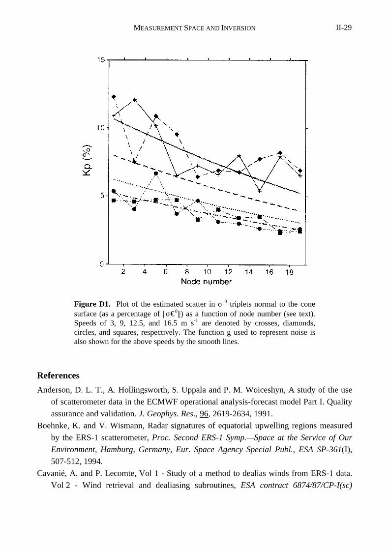
MEASUREMENT SPACE AND INVERSION II-29
References
Anderson, D. L. T., A. Hollingsworth, S. Uppala and P. M. Woiceshyn, A study of the use
of scatterometer data in the ECMWF operational analysis-forecast model Part I. Quality
assurance and validation. J. Geophys. Res., 96, 2619-2634, 1991.
Boehnke, K. and V. Wismann, Radar signatures of equatorial upwelling regions measured
by the ERS-1 scatterometer, Proc. Second ERS-1 Symp.—Space at the Service of Our
Environment, Hamburg, Germany, Eur. Space Agency Special Publ., ESA SP-361(I),
507-512, 1994.
Cavanié, A. and P. Lecomte, Vol 1 - Study of a method to dealias winds from ERS-1 data.
Vol 2 - Wind retrieval and dealiasing subroutines, ESA contract 6874/87/CP-I(sc)
Figure D1. Plot of the estimated scatter in σ 0 triplets normal to the conesurface (as a percentage of ||σ€0||) as a function of node number (see text).Speeds of 3, 9, 12.5, and 16.5 m s-1 are denoted by crosses, diamonds,circles, and squares, respectively. The function g used to represent noise isalso shown for the above speeds by the smooth lines.
MEASUREMENT SPACE AND INVERSIONII-30
report, ESA publications division, Noordwijk, the Netherlands, 1987.
Donelan, M. A. and W. J. Pierson Jr., Radar scattering and equilibrium ranges in wind-
generated waves with application to scatterometry, J. Geophys. Res., 92(C5), 4971-
5029, 1987.
Graham, R., D. Anderson, A. Hollingsworth and H. Böttger, Evaluation of ERS-1 wind
extraction and ambiguity removal algorithms: meteorological and statistical evaluation,
ECMWF report, ECMWF, Reading, England, 1989.
Keller, M. R., W. C. Keller and W. J. Plant, A wave tank study of the dependence of X-
band cross sections on wind speed and water temperature, J. Geophys. Res., 97(C4),
5771-5792, 1992.
Lecomte, P., Wind scatterometer processing requirements for ice detection, Document ER-
SA-ESA-SY-1122, Issue 2.1 (Available from ESRIN DPE/OM, Via Galileo Galilei 5, I-
00044, Frascati, Italy), 1993.
Long, A. E., Towards a C-Band radar sea echo model for the ERS-1 scatterometer,
Proceedings Conference on Spectral Signatures, Les Arcs, France, December 1984,
Eur. Space Agency Special Publ., ESA SP-247, 29-34, 1985.
Stoffelen, A. C. M. and D. L. T. Anderson, ERS-1 scatterometer data characteristics and
wind retrieval skill, Proceedings of the First ERS-1 Symposium, Cannes, France,
November 1992, Eur. Space Agency Special Publ., ESA SP-359, 41-47, 1993.
Stoffelen, A. C. M. and D. L. T. Anderson, The ECMWF contribution to the
characterisation, interpretation, calibration and validation of ERS-1 scatterometer
backscatter measurements and winds, and their use in numerical weather prediction
models, ESA contract 9097/90/NL/BI report, Eur. Centre for Medium-range Weather
Forecasts, Reading, England, 1995.
Stoffelen, A. C. M. and D. L. T. Anderson, Scatterometer data interpretation: Estimation
and validation of the transfer function CMOD4, J. Geophys. Res., 102(C3) , 5767-5780,
1997a.
Stoffelen, A. C. M. and D. L. T. Anderson, Ambiguity removal and assimilation of
scatterometer data, Q. J. Roy. Meteorol. Soc., 123, 491-518, 1997b.
Unal, C. M. H. P., P. Snoeij and P. J. F. Swart, The polarization-dependent relation between
radar backscatter from the ocean surface and surface wind vector at frequencies between
1 and 18 GHz, IEEE Trans. Geosci. Remote Sens., 29(4), 621, 1991.
ESTIMATION AND VALIDATION OF THE TRANSFER FUNCTION CMOD4 III-1
CHAPTER III
Scatterometer Data Interpretation: Estimation and Validation of the
Transfer Function CMOD4*
Abstract. In this paper we estimate the 18 coefficients of the CMOD4 σ 0-to-wind transfer
function using a Maximum Likelihood Estimation (MLE) method in order to improve the
prelaunch function. We show that a MLE method has to be used with caution when dealing
with a nonlinear relationship, or with measurement errors that depend on the measured
values. In the transfer function estimation it is crucial to use the components of the wind,
rather than wind speed and direction, to use σ 0 in logarithmic units rather than physical
ones, and to use well-sampled input data. In Stoffelen and Anderson [1997a; Chapter II], we
showed that the triplets of measured backscatter are very coherent, and, when plotted in a
three-dimensional measurement space, they lie on a well-defined conical surface. Here we
propose a strategy for validation of a transfer function, the first step of which is to test the
ability of a transfer function to fit this conical surface. We derive an objective measure to
compute the average fit of the transfer function surface to the distribution of measured σ 0
triplets. The transfer function CMOD4, derived in the first part of this paper, is shown to fit
the cone surface to within the observed scatter normal to the cone, i.e., within roughly 0.2
dB, equivalent to a root-mean-square wind vector error of ~0.5 m s−1. The second step in the
validation strategy is the verification of retrieved scatterometer winds at each position on the
cone surface. Scatterometer winds computed from CMOD4 compare better to the European
Centre for Medium-range Weather Forecasts model winds than real-time conventional
surface wind data (ship, buoy or island reports) with the root-mean-squared wind vector
difference typically 3.0 m s−1. This surprising result can be explained by the so-called
representativeness error. We further show that no significant spatial wind error correlation is
present in scatterometer data and therefore conclude that the ERS-1 scatterometer provides
winds useful for weather forecasting and climate studies.
1. Introduction
The ERS-1 satellite was launched on July 17, 1991, carrying a C-band scatterometer
*Based on:
Stoffelen, Ad , and David Anderson, Scatterometer Data Interpretation: Derivation of the Transfer Function
CMOD4, J. Geophys. Res., 102(C3) , 5767-5780, 1997, © American Geophysical Union.
ESTIMATION AND VALIDATION OF THE TRANSFER FUNCTION CMOD4III-2
providing at each node within the swath three radar backscatter measurements, called σ 0. In
Stoffelen and Anderson [1997a; Chapter II] the visualization of these radar backscatter
triplets in the three-dimensional (3D) measurement space was discussed. At each node
across the swath the distribution of measured backscatter triplets was shown to lie close to a
cone-shaped surface. The scatter of triplets normal to the surface is typically 0.2 dB, which
is comparable to the instrument noise. Furthermore, given the sensitivity of backscatter to
wind, this scatter is equivalent to an uncertainty in the wind domain of 0.5 m s−1 vector root-
mean-square (RMS). A backscatter-to-wind transfer function, as will be derived in this
paper, should be able to reproduce the conical surface and fit the distribution of backscatter
triplets to within 0.2 dB. It may be clear that this is a very stringent test for validation, since
an agreement of 1.0 dB between laboratory experiments and aircraft campaigns is
considered close [e.g., Keller et al, 1992]. In section 5 we will show that CMOD4 does
generally fit the distribution of measured backscatter triplets to within the required limit of
0.2 dB.
In Stoffelen and Anderson [1997a; Chapter II] described an accurate method to map a
measured triplet onto the cone surface, thereby providing the two coordinates of the surface.
CMOD4 uses the surface wind, i.e., wind speed and direction ( V, φ ), or alternatively the
wind components ( u, v ), to describe the geometry of the cone surface. A second validation
step, as discussed in section 5, is therefore to validate how well the two parameters are
related to the 10-m wind. Prior to the transfer function validation we discuss transfer
function estimation using a Maximum Likelihood Estimator (MLE) method.
The pre-launch transfer function CMOD2 relating σ 0 to wind speed V N and direction
φ N for neutral stability at 10-m height was discussed in Stoffelen and Anderson [1997a;
Chapter II], but for convenience we repeat it here.
0 = B + B + Bσ φ φ0 1 21 2[ cos( ) cos( )]N N (1)
where B 0 = 10 α V γN and B 1 and B 2 are linear functions of wind speed V N and parabolic
functions of the incidence angle θ and thus each contain six tunable coefficients. With α and
γ also parabolic functions of θ, containing three coefficients each, the total number of
tunable coefficients is 18. The parabolic incidence angle dependency is established by using
Legendre polynomials of order 0, 1, and 2 in x = (θ − 40)/25 withθ the radar beam
incidence angle measured in degrees, e.g., α = C 1 + C 2 x + C 3 (3x 2 − 1)/2. Stability effects
will be further ignored in this paper and in the above equations ( V N, φ N ) will be replaced
by (V, φ ). This is equivalent to assuming that stability is only wind speed dependent.
Stoffelen and Anderson [1997a; Chapter II] showed that the behavior of the bias term
B 0, the upwind-crosswind term B 2, and the upwind-downwind term B 1 of the empirical
ESTIMATION AND VALIDATION OF THE TRANSFER FUNCTION CMOD4 III-3
transfer function shows important features that are not represented in CMOD2. A
nonlogarithmic wind speed dependency, saturation of the harmonic terms for increasing
wind speeds and incidence angles, and the presence of higher harmonic terms in φ are the
most relevant. It was shown, however, that the higher harmonic terms, i.e., cos(3φ) and
cos(4φ), were unnecessary in a transformed space: z = ( σ 0 ) 0.625.
To accommodate these shortcomings of CMOD2, we propose a transfer function of the
form
z = B + B + Bz z z0 1 21 2[ cos( ) cos( )]φ φ (2)
with
0110z + LUT + f V +B = α θ γ β( ) ( ) (3)
where α and γ are formulated as in CMOD2, but whose values will be re-estimated in this
paper. LUT(θ) is computed from a comparison between the ERS-1 scatterometer σ 0 and σ 0
simulated from European Centre for Medium-range Weather Forecasts (ECMWF) analysis
winds [Stoffelen and Anderson, 1995] and is fixed. The parameter β has a parabolic
dependency on θ and is used to allow some flexibility in fitting σ 0 at low wind speeds,
while f 1(s) has the form recommended in Stoffelen and Anderson [1997a; Chapter II]
f s s
s
s
s
s1
10
10
10
3 2
10
10 5
5
( ) log
/ .
,
,
,
=−
≤< ≤>
−
− (4)
The form of B z1 is
1 1 2 3 4 2 5 0 61zB = a + a V + a + a V y - y ( )[ tanh( . ) . ] (5)
where a 1-a 4 are tunable coefficients and y = (θ − 31.25)/25. The tanh term describes the
saturation behaviour for increasing θ and V and the large sensitivity to θ around θ = 31.25°,
as discussed by Stoffelen and Anderson [1997a; Chapter II]. For the upwind-crosswind
amplitude we also tried to describe the saturation behaviour for increasing incidence angles
and wind speeds, using the following form for B z2
2 5 6 7 8 90 42 1zB = + a a + x a + V a + a + x V [ . ( )( )] tanh[ ( ) ] (6)
where x is as defined before, x = (θ − 40)/25. In this formulation, called CMOD4, there are
18 tunable coefficients. An MLE method will be used to determine these coefficients, as
was done for CMOD2 [Long, 1985].
The nonlinear nature of the σ 0-to-wind relationship and the fact that the error of the
radar measurements depends on the measured value complicate the estimation problem. In
section 2 we give examples using simulated data to provide guidance on how to modify the
ESTIMATION AND VALIDATION OF THE TRANSFER FUNCTION CMOD4III-4
MLE process to cope with these complications. In particular, we used the wind components,
rather than wind speed and direction, and σ 0 in logarithmic units, rather than physical ones,
in order to represent accurately the error characteristics of the measurements and minimize
the nonlinearities in the transfer function. We also consider how best to represent the error
in the wind data. In section 3 estimation with real data is discussed using well-sampled
collocated sets of ERS-1 scatterometer σ 0 and ECMWF numerical weather prediction
(NWP) model analysis winds. In section 4 it is shown that two apparently “obvious” a
posteriori checks on the quality of the transfer function are in fact not reliable indicators of
the quality at all. Specifically, in section 4.1 it is shown that simple direct comparisons of
measured σ 0 with σ 0 simulated from wind data are not a reliable indicator of a good transfer
function, while in section 4.2 it is shown that biases in retrieved wind speed are not
necessarily caused by an offset in the level of measurement of one system with respect to
the other but can result from different levels of noise in the two systems. In section 5, it is
shown preferable to adopt a two-step validation procedure, where verification of the
coherence of the σ 0 triplets in 3D measurement space and the validation of the wind vector
interpretation are done separately. Results are summarized in section 6.
2. Estimation of the Transfer Function: Simulation Studies
The problem is to find the best estimate of the coefficients relating a set of σ 0
measurements with collocated “ground truth” wind data, given estimates of both the ground
truth and σ 0 measurement errors. (The ground truth data should not be considered to be
error-free, although this is frequently done). The MLE procedure of Britt and Luecke [1973]
allows errors to be assigned to both σ 0 and the 'ground truth' wind, when seeking the best
fit. Long [1985] employed this procedure when determining the prelaunch transfer function
CMOD2. He used wind speed and direction measurements from research ships and buoys
participating in calibration and validation campaigns as the ground truth, while the σ 0 were
from airborne radars. Our data differ from Long's in that we used satellite σ 0 and 10-m
winds from the ECMWF analysis. It is important to use accurate estimates of the error
characteristics of both sets of information. The prelaunch specification for the σ 0 error was
10% and was therefore a proportional error. We used this as a starting point for our
simulations.
By verification of the ECMWF 6-hour wind forecast with conventional ship
observations, it was found that the standard deviation (SD) of the difference between the
observed and forecast wind components is rather independent of the magnitude of the wind.
In contrast, although the SD of the speed difference depends only weakly on wind speed, the
SD of the wind direction difference shows a strong variation with wind speed. So error
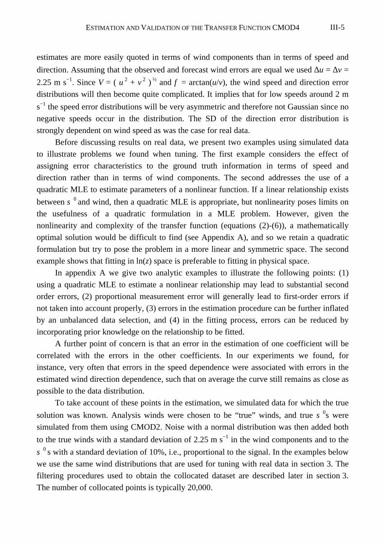
ESTIMATION AND VALIDATION OF THE TRANSFER FUNCTION CMOD4 III-5
estimates are more easily quoted in terms of wind components than in terms of speed and
direction. Assuming that the observed and forecast wind errors are equal we used ∆u = ∆v =
2.25 m s−1. Since V = ( u 2 + v 2 ) ½ and φ = arctan(u/v), the wind speed and direction error
distributions will then become quite complicated. It implies that for low speeds around 2 m
s−1 the speed error distributions will be very asymmetric and therefore not Gaussian since no
negative speeds occur in the distribution. The SD of the direction error distribution is
strongly dependent on wind speed as was the case for real data.
Before discussing results on real data, we present two examples using simulated data
to illustrate problems we found when tuning. The first example considers the effect of
assigning error characteristics to the ground truth information in terms of speed and
direction rather than in terms of wind components. The second addresses the use of a
quadratic MLE to estimate parameters of a nonlinear function. If a linear relationship exists
between σ 0 and wind, then a quadratic MLE is appropriate, but nonlinearity poses limits on
the usefulness of a quadratic formulation in a MLE problem. However, given the
nonlinearity and complexity of the transfer function (equations (2)-(6)), a mathematically
optimal solution would be difficult to find (see Appendix A), and so we retain a quadratic
formulation but try to pose the problem in a more linear and symmetric space. The second
example shows that fitting in ln(z) space is preferable to fitting in physical space.
In appendix A we give two analytic examples to illustrate the following points: (1)
using a quadratic MLE to estimate a nonlinear relationship may lead to substantial second
order errors, (2) proportional measurement error will generally lead to first-order errors if
not taken into account properly, (3) errors in the estimation procedure can be further inflated
by an unbalanced data selection, and (4) in the fitting process, errors can be reduced by
incorporating prior knowledge on the relationship to be fitted.
A further point of concern is that an error in the estimation of one coefficient will be
correlated with the errors in the other coefficients. In our experiments we found, for
instance, very often that errors in the speed dependence were associated with errors in the
estimated wind direction dependence, such that on average the curve still remains as close as
possible to the data distribution.
To take account of these points in the estimation, we simulated data for which the true
solution was known. Analysis winds were chosen to be “true” winds, and true σ 0s were
simulated from them using CMOD2. Noise with a normal distribution was then added both
to the true winds with a standard deviation of 2.25 m s−1 in the wind components and to the
σ 0 s with a standard deviation of 10%, i.e., proportional to the signal. In the examples below
we use the same wind distributions that are used for tuning with real data in section 3. The
filtering procedures used to obtain the collocated dataset are described later in section 3.
The number of collocated points is typically 20,000.
ESTIMATION AND VALIDATION OF THE TRANSFER FUNCTION CMOD4III-6
2.1. Example 1: Tuning Simulations using Wind Components rather than Speed and
Direction
The simulation will be most meaningful when the noise characteristics resemble the
noise that will be experienced in the real problem. For example, specification of the noise in
the wind as Gaussian and 20% in wind speed and 20° in direction for all wind velocities (as
was used by Long [1985] in deriving the CMOD2 model function, for example) will give
misleading simulations, since in reality such a noise specification is not a good
approximation. Since the statistical properties of errors in the components of the wind are
much simpler than the statistical properties of errors in wind speed and direction, it is more
advantageous to derive a transfer function using wind components rather than speed and
direction. To illustrate this, we compare the upwind-crosswind amplitude for two
simulations, differing only in that in one case we used wind speed and direction in the
objective function, and wind components in the other. The MLE software used is simular to
that used by Long [1985].
In case of using wind speed and direction we used
31
20 0
0
2 21
J = N
-
K + V -V
V +
-
i=
Ni Si
i
i Si i Si∑
σ σσ
φ φφ∆ ∆
(7)
where σ 0i is the (simulated) measured value, σ 0
Si = f( V Si, φ
Si ). V i and φ
i are ECMWF
analysis wind speed and direction respectively, and V Si and φ
Si are the estimated true wind
speed and direction respectively. The transfer function, f, has 18 coefficients and is defined
in (1). We used noise estimates of K = 0.1 for σ 0, ∆V = 2.6 m s−1 for wind speed, and ∆φ =
20° for wind direction. The number of measurements σ 0i collocated with ( V
i, φ i ) is
denoted N.
When using the wind components for the estimation, we used
41
20 0
0
2 2
2J = 1
N
-
K. + u - u + v - v
ui=
Ni Si
i
i Si i Si∑
σ σσ
( ) ( )
( )∆(8)
where u and v denote the components of the wind, and ∆u = 2.25 m s−1. In Figure 1 the
upwind-crosswind amplitude for CMOD2 is plotted for reference together with the tuned
values derived using speed and direction (J 3, dotted curve) and components (J 4, solid curve).
It is evident that neither gives the correct specification but estimation using wind
components gives a much closer fit to the “true” solution than using speed and direction.
ESTIMATION AND VALIDATION OF THE TRANSFER FUNCTION CMOD4 III-7
2.2. Example 2 :Tuning Simulations in Logarithmic Space
A further consideration is the consequence of proportional errors for MLE. The
expected value of the standard deviation of error in σ 0 is proportional to the true value of
σ 0. One way to accommodate this proportional error is to perform the estimation using σ 0
measured in dBs, rather than as a physical quantity. This has the obvious advantage that the
instrument error (Kp) is approximately constant at 10%, or 0.4 dB, but a further advantage is
that some of the nonlinear aspects of the transfer function are eliminated by posing it in ln(z)
rather than σ 0. A possible disadvantage is that the error distribution, which is by
approximation Gaussian in physical space [Stoffelen and Anderson, 1997a; Chapter II], will
Figure 1. Upwind-crosswind amplitude as a function of incidence anglederived using as input to the Britt-Luecke tuning algorithm speed anddirection (dotted curve) and wind components (solid curve). The “correct”solution is shown by the dashed curve. The wind speed is 10 m s−1. Thisshows that a more accurate form of the transfer function is obtained usingwind components than speed and direction, because the error can be moreaccurately specified in the former case. Neither using components nor speedand direction returns the correct answer however.
ESTIMATION AND VALIDATION OF THE TRANSFER FUNCTION CMOD4III-8
not be strictly so in logarithmic space.
Figure 2 shows the upwind-crosswind amplitude for two simulation cases differing
only in that the upper curve is obtained by MLE in physical space, whereas the lower curve
is obtained by MLE in logarithmic space for z where
51
2 2 2
2
1 10J =
N
z / zz
+ u u + v v
ui=
Ni Si i si i Si∑
− −log( ) ( ) ( )
∆ ∆(9)
The perceived back-scatter noise is ∆z = 0.25 dB and corresponds to K = 0.1. Not only is the
upwind-crosswind amplitude in error, but the bias term and upwind-downwind amplitude
are also significantly worse when estimation is made in physical space. Only the case using
wind components is tested as this was shown to be desirable in the previous example.
Experiments where we changed the backscatter error standard deviation to be Gaussian in
logarithmic space did not show any significant difference in the results (not shown),
indicating that the transformation of the error distribution from physical to logarithmic space
is not our first concern here.
In most experiments the upwind-crosswind amplitude was found to be very sensitive to
slight changes in the bias term, however, indicating that in reality we need a formulation for
the bias term which fits the data accurately as in CMOD4. Different, but reasonably uniform
wind distributions containing up to 20,000 points, gave slightly different answers after
convergence of the MLE procedure, but, in general, there was no dependence of the result
on initial conditions, and in most cases, 25 iterations were sufficient to converge to the
solution. At the time we made the simulations we were not yet able to accurately estimate
the noise level in either the wind components or in σ 0. In retrospect, both were a little too
high, the error in the wind components will later be shown to be ~1.5 m s−1 and the error in
σ 0 is close to 5% as shown in Stoffelen and Anderson [1997a; Chapter II]. These more
accurate estimates are used in the estimation with real data in next section, and as such
results better than those presented here in the simulations may be feasible.
3. Estimation of the Transfer Function: Real Data
3.1. Data Selection
Since the quality of the transfer function will be a function of the quality and
distribution of the data used to derive it, it is important to select a high-quality and
statistically well-conditioned input data set. As spatial correlation in the data introduces
local minima in solution space, input winds and σ 0 should be spatially decorrelated. So we
created data sets where the spatial separation was at least 300 km between one selected data
point and the next. Returns over ice and fractional ice were excluded by a sea surface
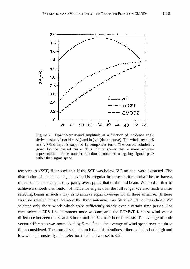
ESTIMATION AND VALIDATION OF THE TRANSFER FUNCTION CMOD4 III-9
temperature (SST) filter such that if the SST was below 6°C no data were extracted. The
distribution of incidence angles covered is irregular because the fore and aft beams have a
range of incidence angles only partly overlapping that of the mid beam. We used a filter to
achieve a smooth distribution of incidence angles over the full range. We also made a filter
selecting beams in such a way as to achieve equal coverage for all three antennae. (If there
were no relative biases between the three antennae this filter would be redundant.) We
selected only those winds which were sufficiently steady over a certain time period. For
each selected ERS-1 scatterometer node we compared the ECMWF forecast wind vector
difference between the 3- and 6-hour, and the 6- and 9-hour forecasts. The average of both
vector differences was normalized by 5 m s−1 plus the average of wind speed over the three
times considered. The normalization is such that this steadiness filter excludes both high and
low winds, if unsteady. The selection threshold was set to 0.2.
Figure 2. Upwind-crosswind amplitude as a function of incidence anglederived using σ 0 (solid curve) and ln ( z ) (dotted curve). The wind speed is 5m s−1. Wind input is supplied in component form. The correct solution isgiven by the dashed curve. This Figure shows that a more accuraterepresentation of the transfer function is obtained using log sigma spacerather than sigma space.
ESTIMATION AND VALIDATION OF THE TRANSFER FUNCTION CMOD4III-10
In addition, we tested the importance of time and space filtering. Normally, ERS-1
data with observation times differing by up to three hours from the analysis time were
selected. Bringing the time window down to two hours did not show any impact in our
initial experiments using CMOD2. With hindsight we would recommend using a short-range
forecast valid at observation time, called first guess at appropriate time (FGAT), rather than
the analysis winds, in which case time filtering becomes redundant [Stoffelen and Anderson,
1995]. The ECMWF analyses are believed to be more accurate in the Atlantic than, for
instance, in the southern hemisphere. However, we did not see any statistical difference in
surface wind speed verifications between those areas so we did not filter the data regionally
in deriving CMOD4.
If a reasonable transfer model already existed, then one could reject σ 0 data if the
triplet of measurements had too large a distance to the transfer function solution surface in
measurement space [ Stoffelen and Anderson, 1997a; Chapter II]. This filter has to be used
carefully since it could bias the MLE result towards the transfer function used for selection.
The filter was not used in deriving CMOD4.
3.2. Estimation
Our first attempts of tuning the transfer function parameters using (7) and the structure
of CMOD2 did not lead to an improved transfer function, but, as expected, the use of (9)
and the formulation of CMOD4 resulted in substantial progress. Further, in our revized
formulation (equations (2)-(6)) there are 18 coefficients to be determined. Our experience
with MLE for this problem is that, in general, more degrees of freedom lead to instability,
although this depends on how well the transfer function formulation can potentially fit the
data. Because of the nonlinearities in the transfer function relationship, our feeling is that
even a perfectly formulated function with too many degrees of freedom would show
aberrations after estimation. Therefore the diagnostics of the transfer function terms
described in Stoffelen and Anderson [1997a; Chapter II] were used here to select the transfer
function formulation.
Equation (9) was used in the estimations with real data, but with ∆z = 0.125 dB
reflecting a 5% error in σ 0. Several tests with transfer function formulations slightly
different from (2)-(6) were carried out, resulting in different values for J5 (equation (9)).
The lowest value found was 1.4, corresponding to CMOD4. Stoffelen and Anderson [1997a;
Chapter II] showed that noise in σ 0 increases at low wind speeds, but a noise formulation
taking this into account failed to give better results, probably as a result of the strong
nonlinearity in the transfer function for low wind speed.
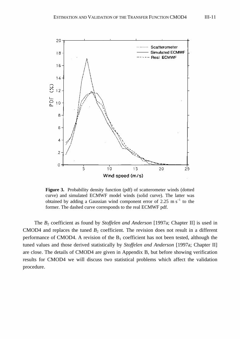
ESTIMATION AND VALIDATION OF THE TRANSFER FUNCTION CMOD4 III-11
The B2 coefficient as found by Stoffelen and Anderson [1997a; Chapter II] is used in
CMOD4 and replaces the tuned B2 coefficient. The revision does not result in a different
performance of CMOD4. A revision of the B1 coefficient has not been tested, although the
tuned values and those derived statistically by Stoffelen and Anderson [1997a; Chapter II]
are close. The details of CMOD4 are given in Appendix B, but before showing verification
results for CMOD4 we will discuss two statistical problems which affect the validation
procedure.
Figure 3. Probability density function (pdf) of scatterometer winds (dottedcurve) and simulated ECMWF model winds (solid curve). The latter wasobtained by adding a Gaussian wind component error of 2.25 m s−1 to theformer. The dashed curve corresponds to the real ECMWF pdf.
ESTIMATION AND VALIDATION OF THE TRANSFER FUNCTION CMOD4III-12
4. Validation Procedure
4.1. Interpretation of σσ 0 Differences
Differences between measured and simulated backscatter are caused by (1) noise or
scatter in σ 0, (2) errors in the ECMWF winds, and (3) errors in the transfer function. The
actual scatter of triplets around the cone surface corresponds to errors of only a few tenths
of a dB in σ 0, which roughly corresponds to a wind error variance of 0.5 m s−1 [Stoffelen
and Anderson, 1997a; Chapter II]. For comparison, the errors in the ECMWF analysis are
estimated to have a standard deviation of ~2.0 m s−1 in the components of the wind or ~3.0
m s−1 in vector RMS. The statistics of wind errors are best defined in terms of the
components of the wind as discussed in section 2. However, a symmetric error distribution
in the components (e.g. a normal distribution with a width of 2 m s−1) around a hypothetical
true state corresponds to “biased” and skew error distributions in σ 0 because of the
nonlinearity in the transfer function. Since this nonlinearity is wind speed and direction
dependent, the interpretation of the σ 0 differences and its average bias and variance is rather
complicated. For example, with an upwind-crosswind amplitude (B2) that may be as large as
0.6, we find that a large wind direction departure of, say, 90° may amount to a factor of 4 (6
dB) difference, while a smaller 20° departure may amount to around 2 dB. On the other
hand, because of the harmonic dependency of σ 0 on wind direction, a wind direction
departure of 90° can also result in a zero difference in σ 0. Equally, the nonlinear mappings
of wind component errors into speed errors and subsequently into σ 0 errors cause
asymmetric and wind dependent σ 0 error distributions. Thus in these σ 0 error distributions it
is difficult to separate the effect of the known errors in the ECMWF analysis winds from the
unknown errors of the transfer function.
4.2. Simulation of the Effect of Noise on the Validation
We simulated the effect of the noise of a wind-observing system on the wind speed
bias, computed when comparing against a reference observing system. The dotted line in
Figure 3 shows a scatterometer wind speed probability density function (PDF) which was
taken as a reference (“truth”). The scatterometer winds constituting the PDF were distorted
by a random Gaussian noise with zero mean and a standard deviation of 2.25 m s−1 in the
components of the wind. As a result the peak in the distorted PDF, represented by the solid
line, is shifted, and a wind speed bias of 0.5 m s−1 is created in the noisy system with respect
to the reference system. Further, the noisy winds are biased high at low speeds and biased
low at high speeds with respect to the true winds, due to the broadening of the PDF. The
ESTIMATION AND VALIDATION OF THE TRANSFER FUNCTION CMOD4 III-13
dashed line in Figure 3 shows the real ECMWF PDF. The resemblance of the dashed and
solid lines is remarkable. This shows that studies of bias, especially at high and low speeds,
can only be done after an analysis of the random wind error of both comparison systems.
Wind validation and error analysis are further discussed in section 5.2.
5. A Posteriori Verification
5.1. Validation in σσ 0 Space
A fundamental test of a transfer function is its ability to describe the cone surface to
within the measurement scatter. We therefore made several cross sections through 3D σ 0
space as defined by Stoffelen and Anderson [1997a; Chapter II] for the transfer functions we
computed. Measured σ 0 triplets and the transfer function CMOD4 were plotted for various
cross sections [Stoffelen and Anderson, 1995]. In general, CMOD4 fits the distribution of
σ 0 triplets very well. To have an objective score for the fit in σ 0 space, we compute for each
measured triplet the distance to the cone surface in z space as i=
i Siz - z1
32
1 2
∑
( )
/
, where z i and
z Si, (i =1, 2, 3) are the transformed fore, mid and aft beam measurements and cone values,
respectively. This distance is normalized by the standard deviation of the scatter we estimate
for this triplet [ Stoffelen and Anderson, 1997a; Chapter II] and given by
SD = z +-
+V
+V
+Vi=
i125 145
271
5 1
2
5
2
1 2
1
32
2 3./
∑
θ(10)
where θ i is the mid beam incidence angle in degrees and V the retrieved wind speed. For
speeds above 15 m s−1 a correction 1 15 1002+ (V - ) / is applied to SD. For CMOD4 the
average of this squared normalized distance versus node number, wind speed, and wind
direction is fairly constant. The square of the normalized distance to the cone is on average
1.7. For comparison, the corresponding value for CMOD2 is 4.0. A perfect transfer function
would ideally score roughly 1.0 considering the scatter of measured triplets normal to the
cone. The error variance of CMOD4 is therefore roughly 0.7, and smaller than the scatter,
so verifying the good fit of CMOD4 to the cone surface. Without exception we found a
positive correlation between the fits in σ 0 space and the minimum value of the objective
function J5, as defined in equation 9.
Spatial correlation of the normalized distance from the cone is evident on geographical
plots [Stoffelen and Anderson, 1995]. This may translate into spatially correlated errors in
the retrieved winds. However, Stoffelen and Anderson [1997a; Chapter II] showed that
measurement noise should result in a wind vector error of only ~ 0.5 m s−1 , which is small
ESTIMATION AND VALIDATION OF THE TRANSFER FUNCTION CMOD4III-14
compared to errors in the ECMWF analysis or other observational systems which are
typically 3 m s−1. Therefore we do not expect the spatial correlation in normalized distance
to lead to a substantial correlation of wind errors. The latter is discussed further in section
5.4.
5.2. Validation against Winds
In the above section we characterized the fit of CMOD4 to the distribution of σ 0
triplets in σ 0 space, which may be defined as the transfer function σ 0 error. For CMOD4
this error is smaller than the instrument error and should lead to only a small wind error.
CMOD4 assigns a geophysical interpretation to each location on the cone surface, i.e., a
wind speed and a wind direction. The error in this interpretation is best described as the
transfer function wind error and will be further discussed here. However, it will also be
shown that the use of CMOD2, which does not fit the cone surface very well, leads to large
systematic wind errors.
A statistical comparison between the ERS-1 wind speed retrieved using CMOD4 and
the ECMWF first guess is shown in Figure 4a for node 11 for a 3-day period. Similar
comparisons for the wind component along the mid beam and wind direction are given in
Figures 4b and c, respectively. These figures illustrate the good fit between ECMWF model
and scatterometer retrieved winds. For comparison, the corresponding plots for CMOD2 are
shown in Figure 5. An erroneous transfer function not only distorts the speed distribution
(Figure 5a), but also the angular distribution (Figure 5c), giving rise to the S-shaped
distribution for the wind component along the mid beam seen in Figure 5b. (The retrieval
procedure discussed in Stoffelen and Anderson [1997a; Chapter II] was used to derive the
winds in both Figures 4 and 5.) The ECMWF and CMOD4 direction distributions are not
uniform due to the nonuniform sampling of the trades and the westerlies in the extratropics.
Differences between the two PDFs arise because of errors in both ECMWF and CMOD4
inverted wind directions. The statistical problems, evident for CMOD2, occur in areas
where the transfer function cone is displaced with respect to the distribution of measured σ 0
triplets [see Stoffelen and Anderson, 1995]. At the locations where the CMOD2 cone
intersects with the distribution of σ 0 triplets, the probability that the corresponding wind
directions will be retrieved is increased, while in other directions that are more distant from
the measured σ 0 triplet distribution, there is much less probability. This effect is clearly seen
in Figure 5 and illustrates the importance of transfer function σ 0 error validation.
To put the comparisons with scatterometer data into perspective, histograms of
collocations of FGAT winds and automatic or non-automatic wind reports (SHIP) were also
made. The results are summarized in table 1. To have a favorable comparison for the

ESTIMATION AND VALIDATION OF THE TRANSFER FUNCTION CMOD4 III-15
Figure 4. Typical examples of (a) the ERS retrieved wind speed versus FGAT speed, (b) thecomponent along the mid beam of retrieved velocity versus the corresponding FGAT component,and (c) the distribution of wind direction measured relative to the satellite direction for ECMWF(solid curve) and retrieved directions (dotted curve). The transfer function CMOD4 was used,together with the inversion scheme described in Stoffelen and Anderson [1997a; Chapter II]. Dataare over the 3-day period February, 13-15, 1994 for node 11. Figures 4a and 4b show a good speedrelationship from 5 to 15 m s−1. Above 15 m s−1, it is difficult to reach a conclusion. Figure 4c showsthat the angular distributions are also similar.
ESTIMATION AND VALIDATION OF THE TRANSFER FUNCTION CMOD4III-16
conventional observations, we excluded conventional wind data more than 90° different
from the ECMWF wind direction. For scatterometer data the 180° wind direction ambiguity
is resolved by selecting the direction closest to FGAT. The difference statistics incorporate
not only wind error due to the observations but also the ECMWF model error, including an
error due to the extrapolation from the lowest model level (~30 m) to 10-m height, the
nominal height of ship and buoy wind reports. The representativeness error accounts for the
mismatch between the spatial and temporal scales that the observations represent and those
that the numerical weather prediction model, i.e. FGAT, represents.
“Automatic” SHIP reports include anemometer measurements from the NOAA buoys, the
North Sea buoys and some other fixed or moving platforms. “Nonautomatic” SHIP reports
often contain winds subjectively estimated from the local sea state (so-called Beaufort
estimates). The Beaufort estimates are of lower quality than the anemometer winds. As
illustrated in section 4.2, this may give rise to an artificial bias. In Table 1 we see that this
may indeed be the case since a positive correlation exists between bias and departure SD,
but other well-known factors may also be relevant for creating biases. For
example, surface wind should be reported at 10-m height but, in practice, height corrections
are either not made or are insufficient. Also, the ship's movement may be ignored or an
anemometer may be shielded from the free wind flow. When verifying the ECMWF first-
guess (FGAT) by (shallow-) island reports and buoy reports different, but generally lower,
biases were found. For these reports the departure wind component SD and observation
first-guess correlations are in most cases close to 3 m s−1 and 94%, respectively (not shown),
and their quality is similar to the automatic SHIP winds.
In table 1, the global statistics for retrieved scatterometer winds compared to the
ECMWF first guess for node 11 for the wind component along the mid beam show that the
highest correlation with the NWP model is for the scatterometer (0.97). Although the first
guess is taken from an experiment where SHIP winds were used, but scatterometer winds
were not, Table 1 indicates that the scatterometer winds agree better with the ECMWF
FGAT than any other real time available surface wind data set. This surprising result may be
explained by the representativeness error which will be close to 2 m s−1 for the conventional
data (see section 5.4). Conventional wind measurements are essentially local, whereas
scatterometer and NWP model winds both represent large areas ( ~50 km and ~200 km
respectively in diameter). The scatterometer wind speed bias is relatively small. This is not
surprising since CMOD4 has been tuned to the ECMWF model. However, in section 4.2 it
was shown that random error may result in a wind speed bias. This effect is seemingly
small, suggesting that FGAT and CMOD4 have a similar wind error SD of ~1.6 m s−1. So by
tuning to wind we are able to explain a large part of the backscatter signal in the case of
CMOD4. From the FGAT accuracy, we compute the wind component error SDs of the
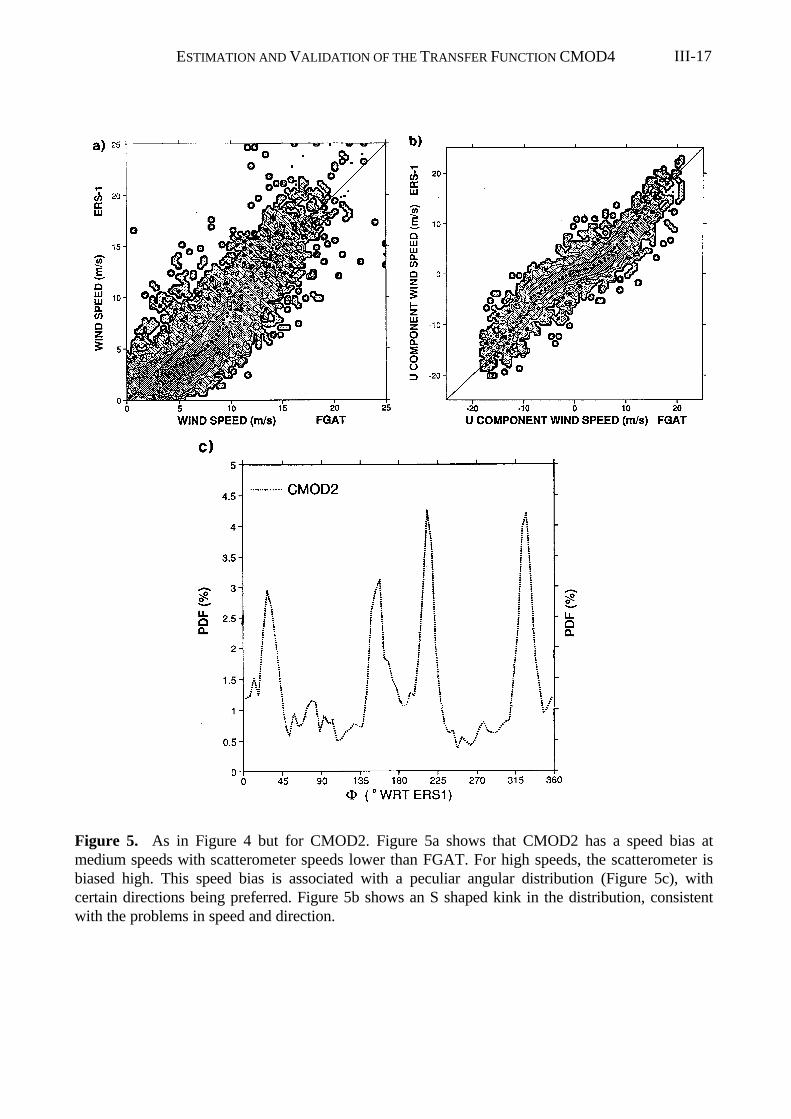
ESTIMATION AND VALIDATION OF THE TRANSFER FUNCTION CMOD4 III-17
Figure 5. As in Figure 4 but for CMOD2. Figure 5a shows that CMOD2 has a speed bias atmedium speeds with scatterometer speeds lower than FGAT. For high speeds, the scatterometer isbiased high. This speed bias is associated with a peculiar angular distribution (Figure 5c), withcertain directions being preferred. Figure 5b shows an S shaped kink in the distribution, consistentwith the problems in speed and direction.
ESTIMATION AND VALIDATION OF THE TRANSFER FUNCTION CMOD4III-18
“automatic” and “nonautomatic” ship winds to be 2.3 m s−1 and 3.1 m s−1, respectively.
Table 2 shows more detailed departure statistics of scatterometer minus ECMWF
forecast winds, separately for wind speed and direction, for each odd across-swath node.
The error, due to the smaller scale of representativeness of scatterometer data in comparison
with the NWP model, should not vary with node number. The ECMWF model error
contribution should also be the same for all nodes. However, there is a node-to-node
variation in the statistics, suggesting that the scatterometer observation error contribution
must be nonnegligible for at least some nodes.
We can see that the departure standard deviation (SD) for wind speed increases with
increasing node number, whereas for wind direction it decreases. The departure vector RMS
(i.e., the square root of the sum of the mean squared wind component differences) decreases
with increasing node number, however, indicating that the overall error of the scatterometer
system is smallest at far swath. The vector RMS error in the fifth column is slightly higher
than the one in the ninth column, because low wind speeds are the most accurate and
average speeds below 4 m s−1 are excluded in the fifth column. Due to differences in the
wind distribution, the statistics vary slightly between different seasons and latitudes.
However, the errors of both the ECMWF model and the scatterometer wind seem fairly
constant across the seasons and the globe. Surprisingly, the error characteristics of the
ECMWF model do not result in a substantially larger departure variance in the southern
hemisphere as compared to the northern hemisphere (not shown). This suggests that the
extrapolation error (projection from ~30 m to 10 m height), and not the error in the model
dynamics, dominates the total ECMWF model error in 10-m wind.
Table 1. The Standard Deviation (SD) and Correlation of the Wind Component Departures andthe Mean Wind Speed Departure for Nonautomatic Ship, Automatic Ship, and Scatterometer DataCompared to the ECMWF First Guess (FGAT).
SD u
(m s−1)
Correlation u Bias V
(m s−1)
Nonautomatic SHIPAutomatic SHIPScatterometer
3.52.82.2
0.930.950.97
1.41 0.73−0.2
SHIP data are for March 1993, mainly in the northern hemisphere, and scatterometer data areglobal for the period March 18, 1993 to March 28, 1993. The scatterometer statistics are for node11, for the wind component along the beam. Nodes 7 to 19 and the other component have verysimilar statistics (not shown).
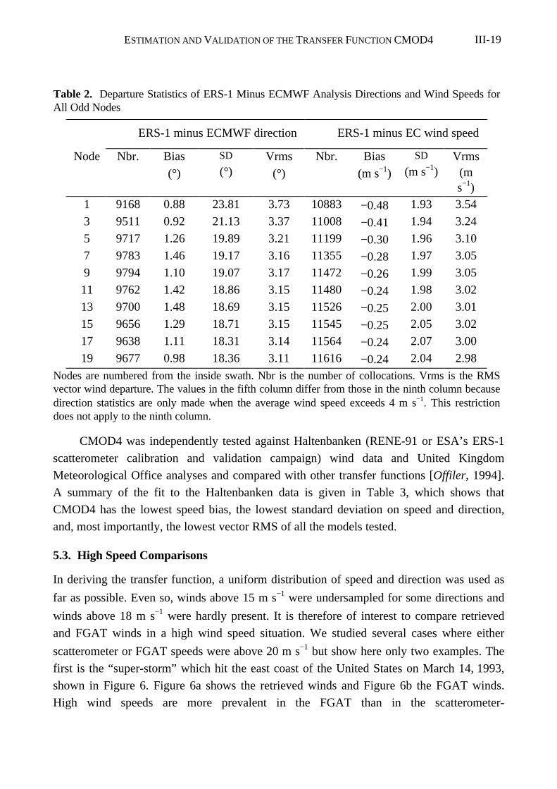
ESTIMATION AND VALIDATION OF THE TRANSFER FUNCTION CMOD4 III-19
CMOD4 was independently tested against Haltenbanken (RENE-91 or ESA’s ERS-1
scatterometer calibration and validation campaign) wind data and United Kingdom
Meteorological Office analyses and compared with other transfer functions [Offiler, 1994].
A summary of the fit to the Haltenbanken data is given in Table 3, which shows that
CMOD4 has the lowest speed bias, the lowest standard deviation on speed and direction,
and, most importantly, the lowest vector RMS of all the models tested.
5.3. High Speed Comparisons
In deriving the transfer function, a uniform distribution of speed and direction was used as
far as possible. Even so, winds above 15 m s−1 were undersampled for some directions and
winds above 18 m s−1 were hardly present. It is therefore of interest to compare retrieved
and FGAT winds in a high wind speed situation. We studied several cases where either
scatterometer or FGAT speeds were above 20 m s−1 but show here only two examples. The
first is the “super-storm” which hit the east coast of the United States on March 14, 1993,
shown in Figure 6. Figure 6a shows the retrieved winds and Figure 6b the FGAT winds.
High wind speeds are more prevalent in the FGAT than in the scatterometer-
Table 2. Departure Statistics of ERS-1 Minus ECMWF Analysis Directions and Wind Speeds forAll Odd Nodes
ERS-1 minus ECMWF direction ERS-1 minus EC wind speed
Node Nbr. Bias
(°)
SD
(°)Vrms
(°)
Nbr. Bias
(m s−1)
SD
(m s−1)Vrms
(ms−1)
1 9168 0.88 23.81 3.73 10883 −0.48 1.93 3.54
3 9511 0.92 21.13 3.37 11008 −0.41 1.94 3.24
5 9717 1.26 19.89 3.21 11199 −0.30 1.96 3.10
7 9783 1.46 19.17 3.16 11355 −0.28 1.97 3.05
9 9794 1.10 19.07 3.17 11472 −0.26 1.99 3.05
11 9762 1.42 18.86 3.15 11480 −0.24 1.98 3.02
13 9700 1.48 18.69 3.15 11526 −0.25 2.00 3.01
15 9656 1.29 18.71 3.15 11545 −0.25 2.05 3.02
17 9638 1.11 18.31 3.14 11564 −0.24 2.07 3.00
19 9677 0.98 18.36 3.11 11616 −0.24 2.04 2.98
Nodes are numbered from the inside swath. Nbr is the number of collocations. Vrms is the RMSvector wind departure. The values in the fifth column differ from those in the ninth column becausedirection statistics are only made when the average wind speed exceeds 4 m s−1. This restrictiondoes not apply to the ninth column.
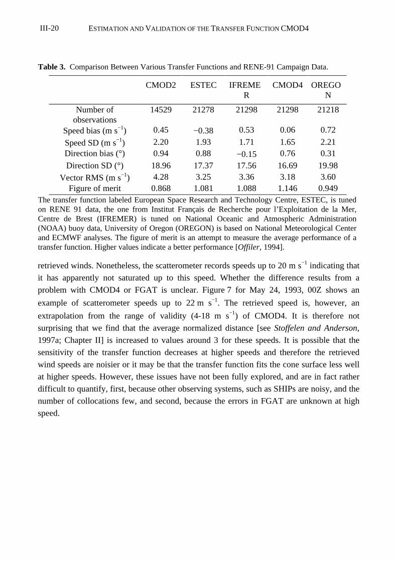
ESTIMATION AND VALIDATION OF THE TRANSFER FUNCTION CMOD4III-20
retrieved winds. Nonetheless, the scatterometer records speeds up to 20 m s−1 indicating that
it has apparently not saturated up to this speed. Whether the difference results from a
problem with CMOD4 or FGAT is unclear. Figure 7 for May 24, 1993, 00Z shows an
example of scatterometer speeds up to 22 m s−1. The retrieved speed is, however, an
extrapolation from the range of validity (4-18 m s−1) of CMOD4. It is therefore not
surprising that we find that the average normalized distance [see Stoffelen and Anderson,
1997a; Chapter II] is increased to values around 3 for these speeds. It is possible that the
sensitivity of the transfer function decreases at higher speeds and therefore the retrieved
wind speeds are noisier or it may be that the transfer function fits the cone surface less well
at higher speeds. However, these issues have not been fully explored, and are in fact rather
difficult to quantify, first, because other observing systems, such as SHIPs are noisy, and the
number of collocations few, and second, because the errors in FGAT are unknown at high
speed.
Table 3. Comparison Between Various Transfer Functions and RENE-91 Campaign Data.
CMOD2 ESTEC IFREMER
CMOD4 OREGON
Number ofobservations
14529 21278 21298 21298 21218
Speed bias (m s−1) 0.45 −0.38 0.53 0.06 0.72
Speed SD (m s−1) 2.20 1.93 1.71 1.65 2.21Direction bias (°) 0.94 0.88 −0.15 0.76 0.31
Direction SD (°) 18.96 17.37 17.56 16.69 19.98
Vector RMS (m s−1) 4.28 3.25 3.36 3.18 3.60Figure of merit 0.868 1.081 1.088 1.146 0.949
The transfer function labeled European Space Research and Technology Centre, ESTEC, is tunedon RENE 91 data, the one from Institut Français de Recherche pour l’Exploitation de la Mer,Centre de Brest (IFREMER) is tuned on National Oceanic and Atmospheric Administration(NOAA) buoy data, University of Oregon (OREGON) is based on National Meteorological Centerand ECMWF analyses. The figure of merit is an attempt to measure the average performance of atransfer function. Higher values indicate a better performance [Offiler, 1994].
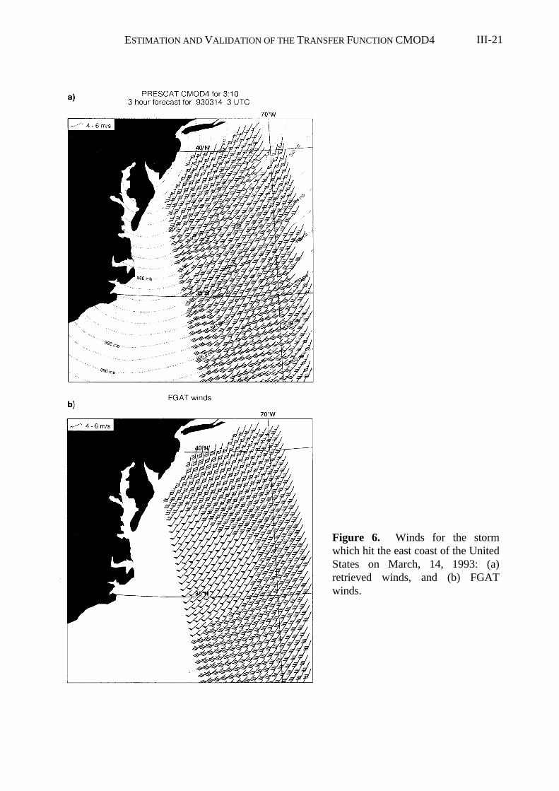
ESTIMATION AND VALIDATION OF THE TRANSFER FUNCTION CMOD4 III-21
Figure 6. Winds for the stormwhich hit the east coast of the UnitedStates on March, 14, 1993: (a)retrieved winds, and (b) FGATwinds.
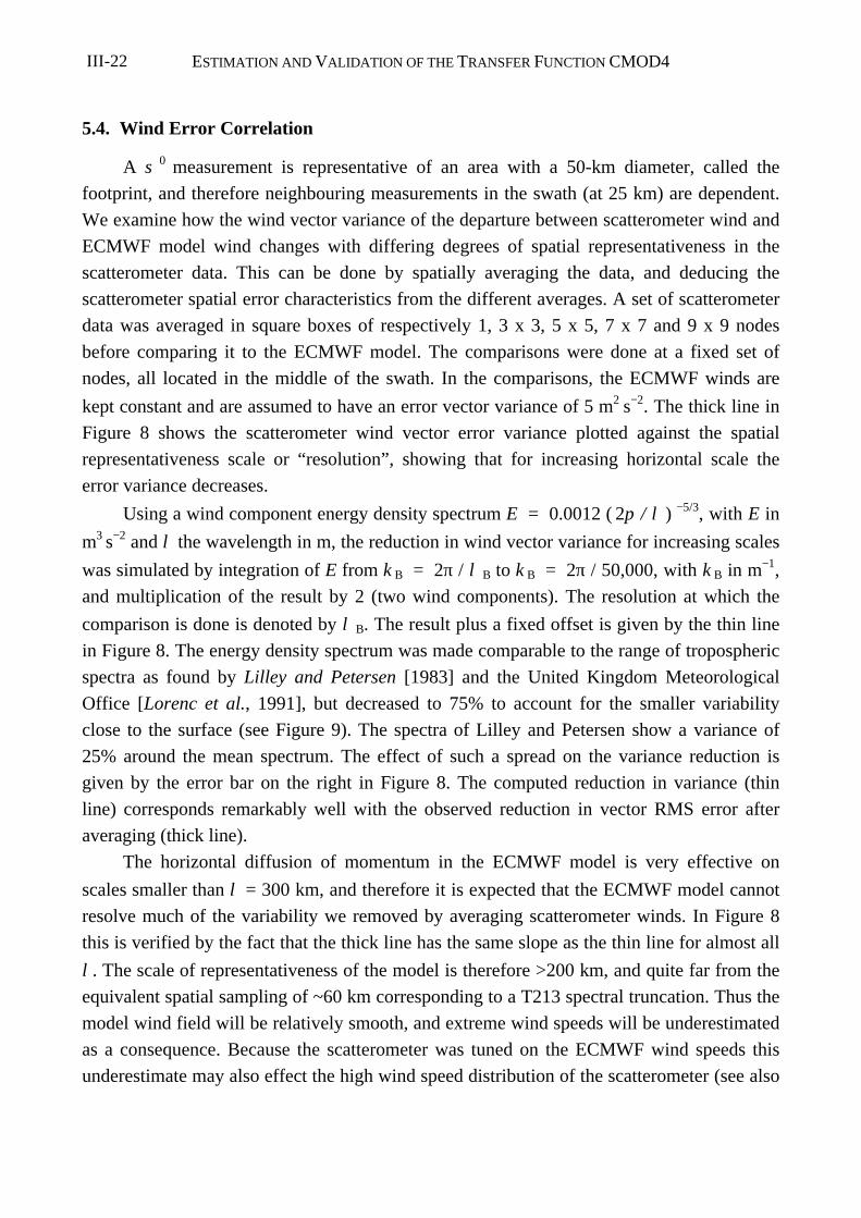
ESTIMATION AND VALIDATION OF THE TRANSFER FUNCTION CMOD4III-22
5.4. Wind Error Correlation
A σ 0 measurement is representative of an area with a 50-km diameter, called the
footprint, and therefore neighbouring measurements in the swath (at 25 km) are dependent.
We examine how the wind vector variance of the departure between scatterometer wind and
ECMWF model wind changes with differing degrees of spatial representativeness in the
scatterometer data. This can be done by spatially averaging the data, and deducing the
scatterometer spatial error characteristics from the different averages. A set of scatterometer
data was averaged in square boxes of respectively 1, 3 x 3, 5 x 5, 7 x 7 and 9 x 9 nodes
before comparing it to the ECMWF model. The comparisons were done at a fixed set of
nodes, all located in the middle of the swath. In the comparisons, the ECMWF winds are
kept constant and are assumed to have an error vector variance of 5 m2 s−2. The thick line in
Figure 8 shows the scatterometer wind vector error variance plotted against the spatial
representativeness scale or “resolution”, showing that for increasing horizontal scale the
error variance decreases.
Using a wind component energy density spectrum E = 0.0012 ( 2π / λ ) −5/3, with E in
m3 s−2 and λ the wavelength in m, the reduction in wind vector variance for increasing scales
was simulated by integration of E from k B = 2π / λ B to k B = 2π / 50,000, with k B in m−1,
and multiplication of the result by 2 (two wind components). The resolution at which the
comparison is done is denoted by λ B. The result plus a fixed offset is given by the thin line
in Figure 8. The energy density spectrum was made comparable to the range of tropospheric
spectra as found by Lilley and Petersen [1983] and the United Kingdom Meteorological
Office [Lorenc et al., 1991], but decreased to 75% to account for the smaller variability
close to the surface (see Figure 9). The spectra of Lilley and Petersen show a variance of
25% around the mean spectrum. The effect of such a spread on the variance reduction is
given by the error bar on the right in Figure 8. The computed reduction in variance (thin
line) corresponds remarkably well with the observed reduction in vector RMS error after
averaging (thick line).
The horizontal diffusion of momentum in the ECMWF model is very effective on
scales smaller than λ = 300 km, and therefore it is expected that the ECMWF model cannot
resolve much of the variability we removed by averaging scatterometer winds. In Figure 8
this is verified by the fact that the thick line has the same slope as the thin line for almost all
λ. The scale of representativeness of the model is therefore >200 km, and quite far from the
equivalent spatial sampling of ~60 km corresponding to a T213 spectral truncation. Thus the
model wind field will be relatively smooth, and extreme wind speeds will be underestimated
as a consequence. Because the scatterometer was tuned on the ECMWF wind speeds this
underestimate may also effect the high wind speed distribution of the scatterometer (see also
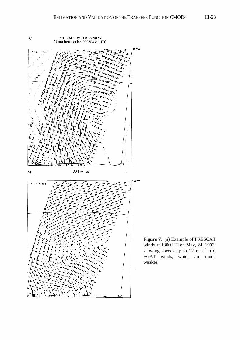
ESTIMATION AND VALIDATION OF THE TRANSFER FUNCTION CMOD4 III-23
Figure 7. (a) Example of PRESCATwinds at 1800 UT on May, 24, 1993,showing speeds up to 22 m s−1. (b)FGAT winds, which are muchweaker.
ESTIMATION AND VALIDATION OF THE TRANSFER FUNCTION CMOD4III-24
previous section).
The 25-km grid sampling and the 50-km footprint cause horizontal error correlation
between directly neighbouring scatterometer nodes. If the scatterometer winds had strongly
correlated spatial error beyond 50 km, we would expect from Figure 8 that at low λ the
reduction in variance would be less than that explained by the ( 2π / λ ) −5/3 spectrum (a flat
spectral response is expected in this case). We do not see significant signs of this and may
conclude that the horizontal error correlation in scatterometer winds is in general not
significant, which indicates that a transfer function dependency on spatially smooth
geophysical parameters other than wind (e.g. wave effects) is in general not likely to be
substantial. The sensitivity of the scatterometer to the wind vector is the main effect. Other
geophysical parameters should, however, be investigated for correlation with the remaining
departure errors in the more extreme or local conditions.
Global observation-minus-analysis departure statistics provide a good general
characterization of observation measurement error but fail to give a complete picture of the
usefulness of data. Numerous relevant and complicated synoptic weather patterns were
investigated in order to gain experience in dealing with the data. Stoffelen and Anderson
[1997b; Chapter V] showed and used some examples to illustrate the ambiguity removal
problem.
6. Summary and Conclusions
A transfer function, CMOD4, was developed which is able to fit the characteristics of
the σ 0-to-wind relationship observed from the ERS-1 scatterometer. The 18 coefficients of
the function were estimated with a maximum likelihood estimation (MLE) method. It was
necessary to have accurate estimates of the error characteristics of the winds and of the σ 0s
used in the estimation. For this purpose we used the components of the wind, rather than
wind speed and direction. Further, the logarithm of the backscatter was used in the
estimation, rather than σ 0 to partly take account of the nonlinear σ 0-to-wind relationship.
Before being used in the MLE, the σ 0 and wind data were filtered to obtain smooth
distributions and to avoid low-quality or correlated input data.
The validation of a transfer function by the “obvious” method of comparing the
simulated σ 0 with the measured value was shown to be rather complicated and more
sensitive to the quality of the comparison wind data than to the quality of the transfer
function under validation, since the nonlinear mapping of the wind errors in the σ 0 domain
dominate the σ 0 departures.
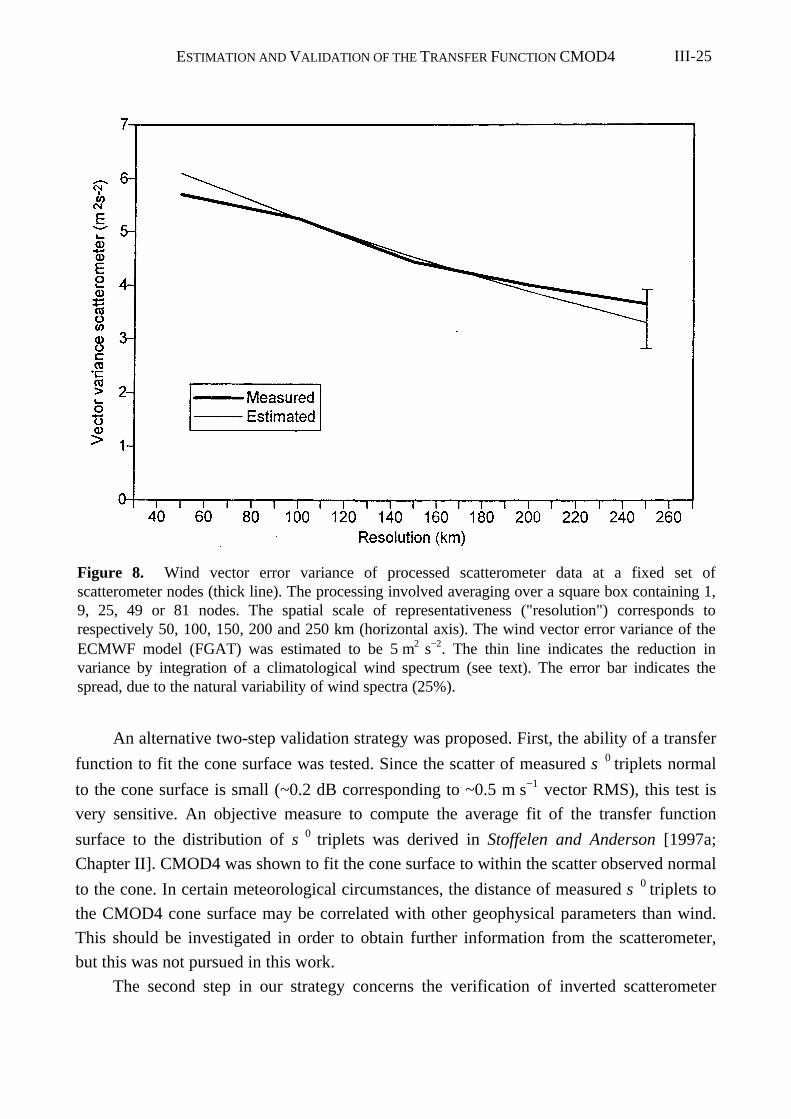
ESTIMATION AND VALIDATION OF THE TRANSFER FUNCTION CMOD4 III-25
An alternative two-step validation strategy was proposed. First, the ability of a transfer
function to fit the cone surface was tested. Since the scatter of measured σ 0 triplets normal
to the cone surface is small (~0.2 dB corresponding to ~0.5 m s−1 vector RMS), this test is
very sensitive. An objective measure to compute the average fit of the transfer function
surface to the distribution of σ 0 triplets was derived in Stoffelen and Anderson [1997a;
Chapter II]. CMOD4 was shown to fit the cone surface to within the scatter observed normal
to the cone. In certain meteorological circumstances, the distance of measured σ 0 triplets to
the CMOD4 cone surface may be correlated with other geophysical parameters than wind.
This should be investigated in order to obtain further information from the scatterometer,
but this was not pursued in this work.
The second step in our strategy concerns the verification of inverted scatterometer
Figure 8. Wind vector error variance of processed scatterometer data at a fixed set ofscatterometer nodes (thick line). The processing involved averaging over a square box containing 1,9, 25, 49 or 81 nodes. The spatial scale of representativeness ("resolution") corresponds torespectively 50, 100, 150, 200 and 250 km (horizontal axis). The wind vector error variance of theECMWF model (FGAT) was estimated to be 5 m2 s−2. The thin line indicates the reduction invariance by integration of a climatological wind spectrum (see text). The error bar indicates thespread, due to the natural variability of wind spectra (25%).
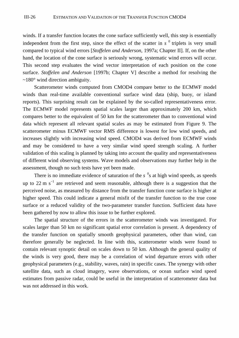
ESTIMATION AND VALIDATION OF THE TRANSFER FUNCTION CMOD4III-26
winds. If a transfer function locates the cone surface sufficiently well, this step is essentially
independent from the first step, since the effect of the scatter in σ 0 triplets is very small
compared to typical wind errors [Stoffelen and Anderson, 1997a; Chapter II]. If, on the other
hand, the location of the cone surface is seriously wrong, systematic wind errors will occur.
This second step evaluates the wind vector interpretation of each position on the cone
surface. Stoffelen and Anderson [1997b; Chapter V] describe a method for resolving the
~180° wind direction ambiguity.
Scatterometer winds computed from CMOD4 compare better to the ECMWF model
winds than real-time available conventional surface wind data (ship, buoy, or island
reports). This surprising result can be explained by the so-called representativeness error.
The ECMWF model represents spatial scales larger than approximately 200 km, which
compares better to the equivalent of 50 km for the scatterometer than to conventional wind
data which represent all relevant spatial scales as may be estimated from Figure 9. The
scatterometer minus ECMWF vector RMS difference is lowest for low wind speeds, and
increases slightly with increasing wind speed. CMOD4 was derived from ECMWF winds
and may be considered to have a very similar wind speed strength scaling. A further
validation of this scaling is planned by taking into account the quality and representativeness
of different wind observing systems. Wave models and observations may further help in the
assessment, though no such tests have yet been made.
There is no immediate evidence of saturation of the σ 0s at high wind speeds, as speeds
up to 22 m s−1 are retrieved and seem reasonable, although there is a suggestion that the
perceived noise, as measured by distance from the transfer function cone surface is higher at
higher speed. This could indicate a general misfit of the transfer function to the true cone
surface or a reduced validity of the two-parameter transfer function. Sufficient data have
been gathered by now to allow this issue to be further explored.
The spatial structure of the errors in the scatterometer winds was investigated. For
scales larger than 50 km no significant spatial error correlation is present. A dependency of
the transfer function on spatially smooth geophysical parameters, other than wind, can
therefore generally be neglected. In line with this, scatterometer winds were found to
contain relevant synoptic detail on scales down to 50 km. Although the general quality of
the winds is very good, there may be a correlation of wind departure errors with other
geophysical parameters (e.g., stability, waves, rain) in specific cases. The synergy with other
satellite data, such as cloud imagery, wave observations, or ocean surface wind speed
estimates from passive radar, could be useful in the interpretation of scatterometer data but
was not addressed in this work.
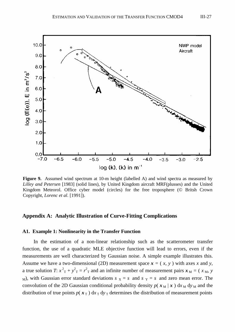
ESTIMATION AND VALIDATION OF THE TRANSFER FUNCTION CMOD4 III-27
Appendix A: Analytic Illustration of Curve-Fitting Complications
A1. Example 1: Nonlinearity in the Transfer Function
In the estimation of a non-linear relationship such as the scatterometer transfer
function, the use of a quadratic MLE objective function will lead to errors, even if the
measurements are well characterized by Gaussian noise. A simple example illustrates this.
Assume we have a two-dimensional (2D) measurement space x = ( x, y ) with axes x and y,
a true solution T: x 2T + y2
T = r2T and an infinite number of measurement pairs x M = ( x M, y
M), with Gaussian error standard deviations σ X = σ and σ Y = σ and zero mean error. The
convolution of the 2D Gaussian conditional probability density p( x M | x ) dx M dy M and the
distribution of true points p( x T ) dx T dy T determines the distribution of measurement points
Figure 9. Assumed wind spectrum at 10-m height (labelled A) and wind spectra as measured byLilley and Petersen [1983] (solid lines), by United Kingdom aircraft MRF(plusses) and the UnitedKingdom Meteorol. Office cyber model (circles) for the free troposphere (© Britsh CrownCopyright, Lorenc et al. [1991]).
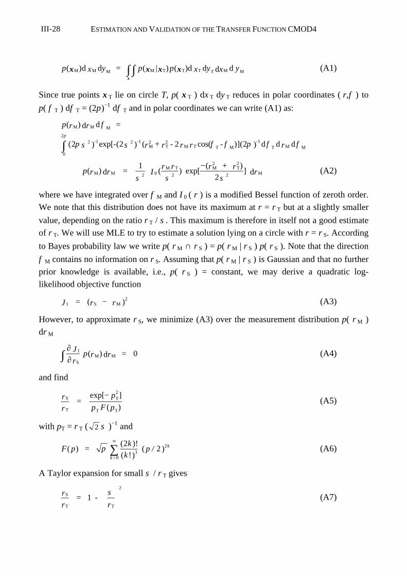
ESTIMATION AND VALIDATION OF THE TRANSFER FUNCTION CMOD4III-28
p x y = p p x y x y( ) ( | ) ( )M M M M T T T T M Md d d d d dx x x xx∫ ∫ (A1)
Since true points x T lie on circle T, p( x T ) dx T dy T reduces in polar coordinates ( r,φ ) to
p( φ T ) dφ T = (2π)−1 dφ T and in polar coordinates we can write (A1) as:
p r r =
- r + r - r r - r- - -
( )
( ) exp[ ( ) ( cos( )]( )
M M M
M T M T T M T M M
d d
d d d
φ
π σ σ φ φ π φ φπ
0
22 1 2 1 2 2 12 2 2 2∫
p r r = Ir r r + r r( ) ( ) exp[
( )]M M
M T M TMd d
1
22 0 2
2 2
2σ σ σ−
(A2)
where we have integrated over φ M and I 0 ( r ) is a modified Bessel function of zeroth order.
We note that this distribution does not have its maximum at r = r T but at a slightly smaller
value, depending on the ratio r T / σ. This maximum is therefore in itself not a good estimate
of r T. We will use MLE to try to estimate a solution lying on a circle with r = r S. According
to Bayes probability law we write p( r M ∩ r S ) = p( r M | r S ) p( r S ). Note that the direction
φ M contains no information on r S. Assuming that p( r M | r S ) is Gaussian and that no further
prior knowledge is available, i.e., p( r S ) = constant, we may derive a quadratic log-
likelihood objective function
12
J = r r( )S M− (A3)
However, to approximate r S, we minimize (A3) over the measurement distribution p( r M )
dr M
∂∂∫ 1 0J
r p r r =
SM Md( ) (A4)
and find
S
T
T
T T
r
r =
p
p F p
exp[ ]
( )
− 2
(A5)
with pT = r T ( 2 σ )−1 and
F p = k
k p / k
k=
( )( )!
( !)( )π
223
2
0
∞
∑ (A6)
A Taylor expansion for small σ / r T gives
S
T T
r
r = -
r1
2σ
(A7)
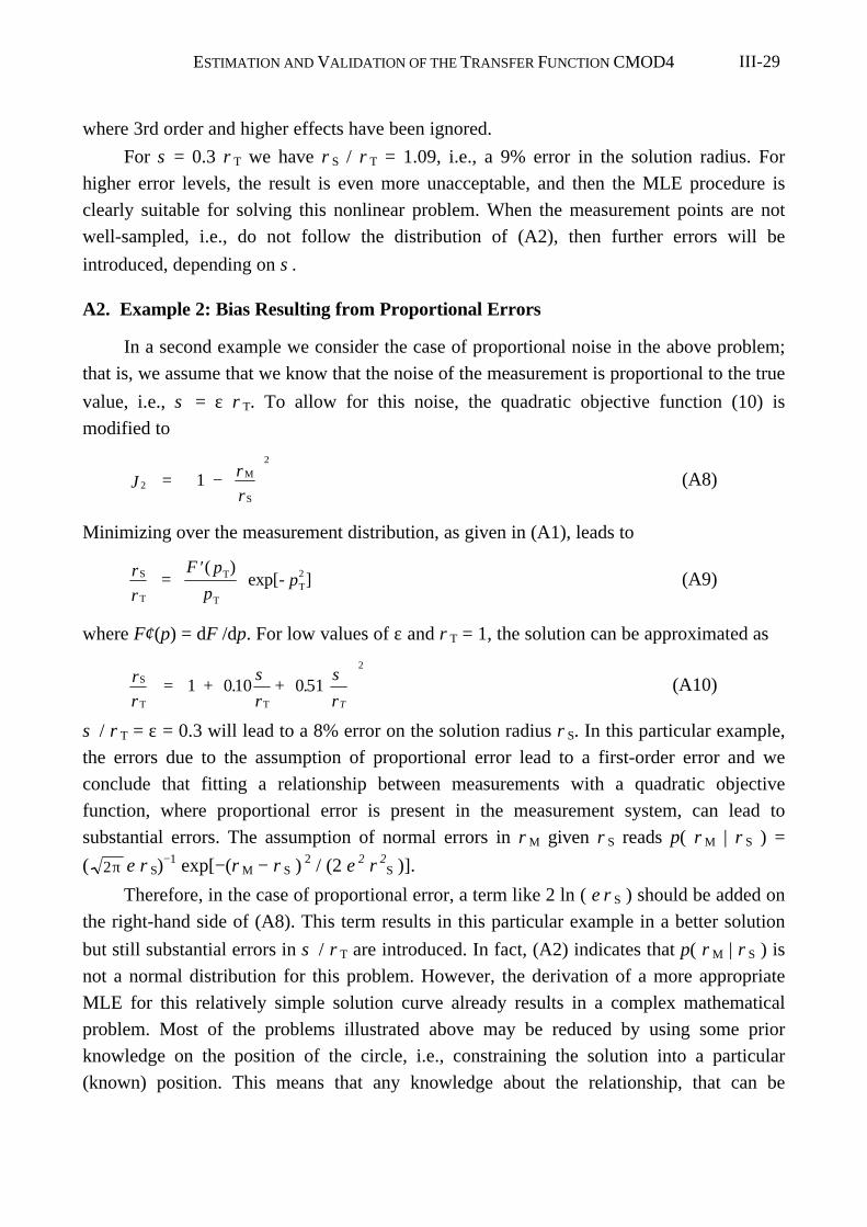
ESTIMATION AND VALIDATION OF THE TRANSFER FUNCTION CMOD4 III-29
where 3rd order and higher effects have been ignored.
For σ = 0.3 r T we have r S / r T = 1.09, i.e., a 9% error in the solution radius. For
higher error levels, the result is even more unacceptable, and then the MLE procedure is
clearly suitable for solving this nonlinear problem. When the measurement points are not
well-sampled, i.e., do not follow the distribution of (A2), then further errors will be
introduced, depending on σ.
A2. Example 2: Bias Resulting from Proportional Errors
In a second example we consider the case of proportional noise in the above problem;
that is, we assume that we know that the noise of the measurement is proportional to the true
value, i.e., σ = ε r T. To allow for this noise, the quadratic objective function (10) is
modified to
2
2
1J = r
r−
M
S
(A8)
Minimizing over the measurement distribution, as given in (A1), leads to
S
T
T
TT
r
r =
F p
p - p
′( )exp[ ]2 (A9)
where F′ (p) = dF /dp. For low values of ε and r T = 1, the solution can be approximated as
S
T T
r
r = +
r+
rT
1 010 0 512
. .σ σ
(A10)
σ / r T = ε = 0.3 will lead to a 8% error on the solution radius r S. In this particular example,
the errors due to the assumption of proportional error lead to a first-order error and we
conclude that fitting a relationship between measurements with a quadratic objective
function, where proportional error is present in the measurement system, can lead to
substantial errors. The assumption of normal errors in r M given r S reads p( r M | r S ) =
( 2π ε r S)−1 exp[−(r M − r S )
2 / (2 ε 2 r 2S )].
Therefore, in the case of proportional error, a term like 2 ln ( ε r S ) should be added on
the right-hand side of (A8). This term results in this particular example in a better solution
but still substantial errors in σ / r T are introduced. In fact, (A2) indicates that p( r M | r S ) is
not a normal distribution for this problem. However, the derivation of a more appropriate
MLE for this relatively simple solution curve already results in a complex mathematical
problem. Most of the problems illustrated above may be reduced by using some prior
knowledge on the position of the circle, i.e., constraining the solution into a particular
(known) position. This means that any knowledge about the relationship, that can be
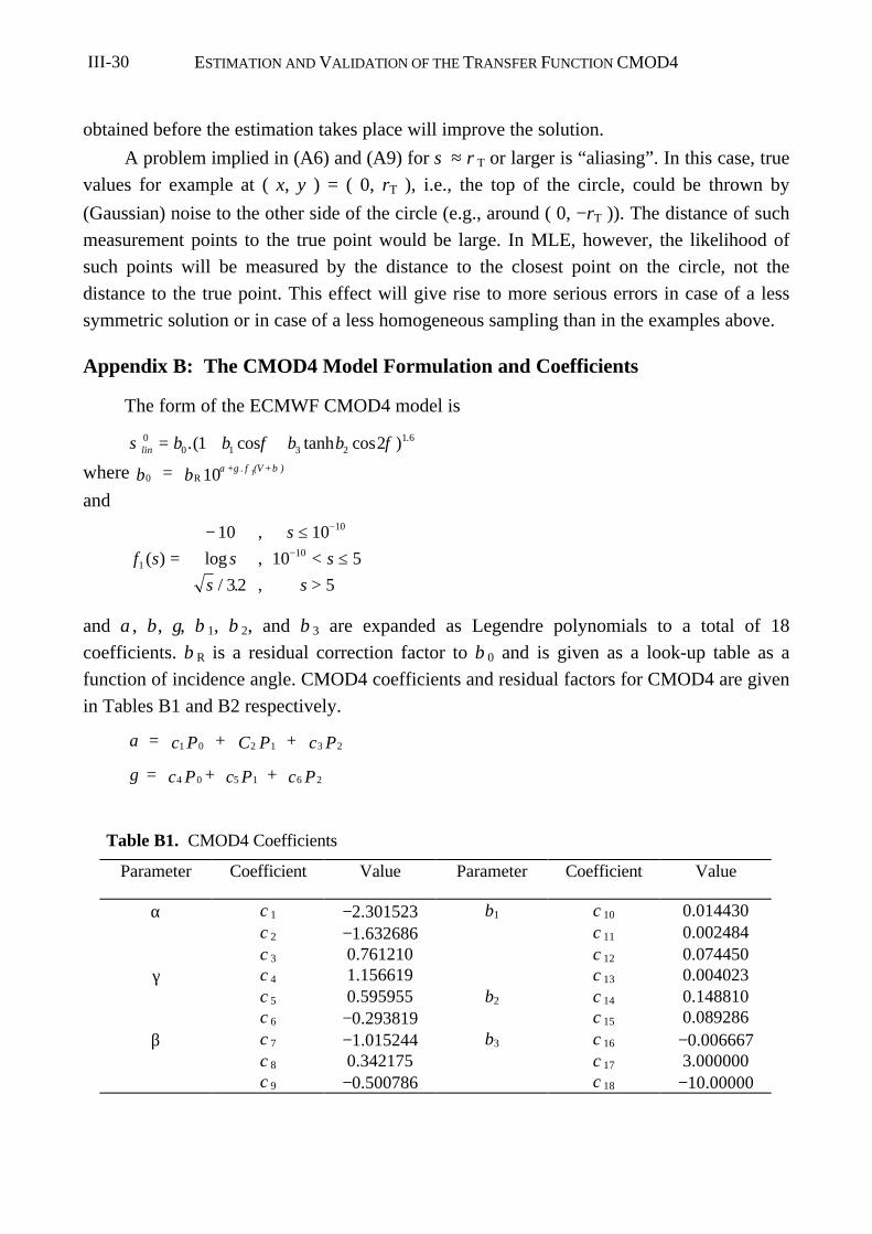
ESTIMATION AND VALIDATION OF THE TRANSFER FUNCTION CMOD4III-30
obtained before the estimation takes place will improve the solution.
A problem implied in (A6) and (A9) for σ ≈ r T or larger is “aliasing”. In this case, true
values for example at ( x, y ) = ( 0, rT ), i.e., the top of the circle, could be thrown by
(Gaussian) noise to the other side of the circle (e.g., around ( 0, −rT )). The distance of such
measurement points to the true point would be large. In MLE, however, the likelihood of
such points will be measured by the distance to the closest point on the circle, not the
distance to the true point. This effect will give rise to more serious errors in case of a less
symmetric solution or in case of a less homogeneous sampling than in the examples above.
Appendix B: The CMOD4 Model Formulation and Coefficients
The form of the ECMWF CMOD4 model is
σ φ φlin b b b b00 1 3 2
1 61 2= + +.( cos tanh cos ) .
where 0110b = b + . f (V + )
Rα γ β
and
f s s
s
s
s
s1
10
10
10
32
10
10 5
5
( ) log
/ .
,
,
,
=− ≤
< ≤>
−
−
and α, β, γ, b 1, b 2, and b 3 are expanded as Legendre polynomials to a total of 18
coefficients. b R is a residual correction factor to b 0 and is given as a look-up table as a
function of incidence angle. CMOD4 coefficients and residual factors for CMOD4 are given
in Tables B1 and B2 respectively.
α = c P + C P + c P1 0 2 1 3 2
γ = c P + c P + c P4 0 5 1 6 2
Table B1. CMOD4 Coefficients
Parameter Coefficient Value Parameter Coefficient Value
α c 1 −2.301523 b1 c 10 0.014430c 2 −1.632686 c 11 0.002484c 3 0.761210 c 12 0.074450
γ c 4 1.156619 c 13 0.004023c 5 0.595955 b2 c 14 0.148810c 6 −0.293819 c 15 0.089286
β c 7 −1.015244 b3 c 16 −0.006667c 8 0.342175 c 17 3.000000c 9 −0.500786 c 18 −10.00000
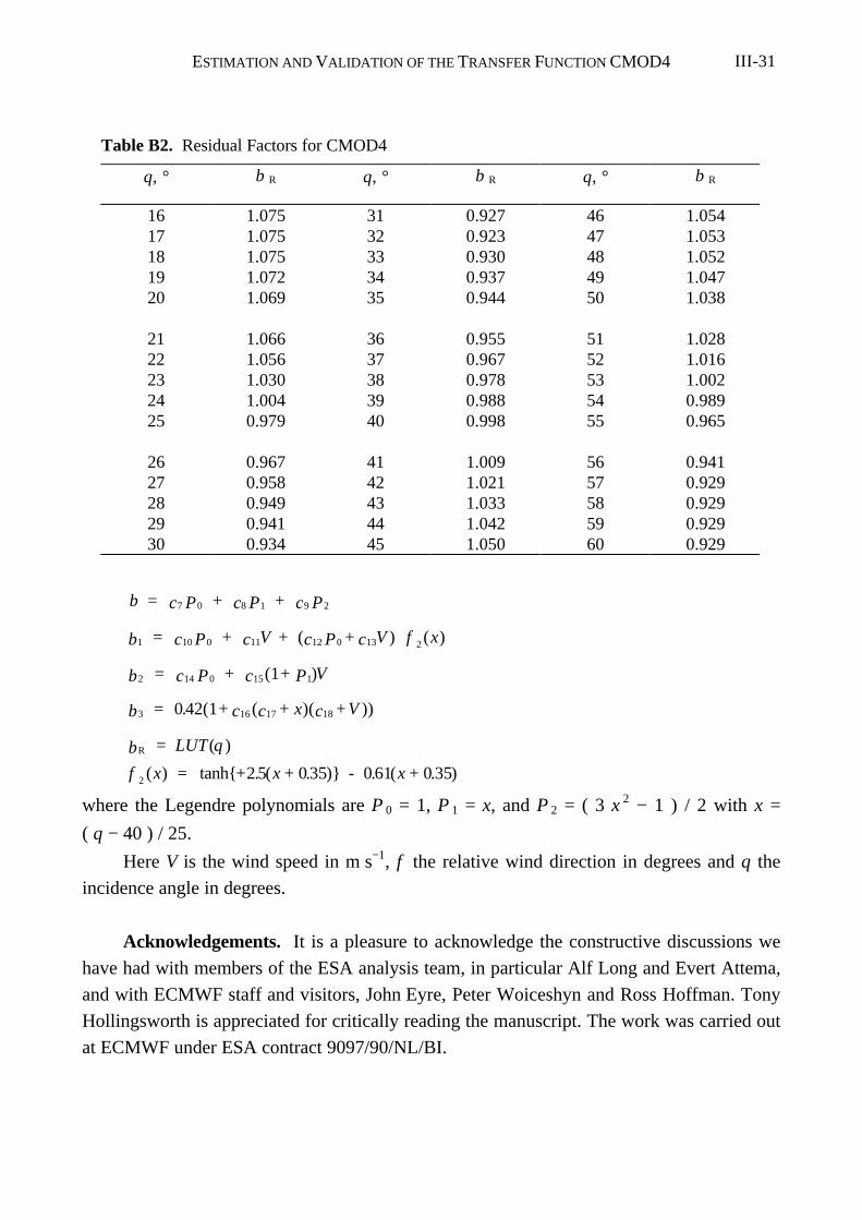
ESTIMATION AND VALIDATION OF THE TRANSFER FUNCTION CMOD4 III-31
β = c P + c P + c P7 0 8 1 9 2
1 10 0 11 12 0 13 2b = c P + c V + c P + c V f x( ) ( )
2 14 0 15 11b = c P + c + P V( )
3 16 17 180 42 1b = + c c + x c +V. ( ( )( ))
Rb = LUT( )θ
2 2 5 0 35 0 61 0 35f x = + x + - x +( ) tanh . ( . ) . ( . )
where the Legendre polynomials are P 0 = 1, P 1 = x, and P 2 = ( 3 x 2 − 1 ) / 2 with x =
( θ − 40 ) / 25.
Here V is the wind speed in m s−1, φ the relative wind direction in degrees and θ the
incidence angle in degrees.
Acknowledgements. It is a pleasure to acknowledge the constructive discussions we
have had with members of the ESA analysis team, in particular Alf Long and Evert Attema,
and with ECMWF staff and visitors, John Eyre, Peter Woiceshyn and Ross Hoffman. Tony
Hollingsworth is appreciated for critically reading the manuscript. The work was carried out
at ECMWF under ESA contract 9097/90/NL/BI.
Table B2. Residual Factors for CMOD4
θ, ° b R θ, ° b R θ, ° b R
16 1.075 31 0.927 46 1.05417 1.075 32 0.923 47 1.05318 1.075 33 0.930 48 1.05219 1.072 34 0.937 49 1.04720 1.069 35 0.944 50 1.038
21 1.066 36 0.955 51 1.02822 1.056 37 0.967 52 1.01623 1.030 38 0.978 53 1.00224 1.004 39 0.988 54 0.98925 0.979 40 0.998 55 0.965
26 0.967 41 1.009 56 0.94127 0.958 42 1.021 57 0.92928 0.949 43 1.033 58 0.92929 0.941 44 1.042 59 0.92930 0.934 45 1.050 60 0.929
ESTIMATION AND VALIDATION OF THE TRANSFER FUNCTION CMOD4III-32
References
Britt, H. I. and R. H. Luecke, The estimation of parameters in nonlinear, implicit models,
Technometrics, 15(2), 233-247, 1973.
Keller, M. R., W. C. Keller and W. J. Plant, A wave tank study of the dependence of X-
band cross sections on wind speed and water temperature. J. Geophys. Res., 97(C4),
5771-5792, 1992.
Lilley, D. K. and E. L. Petersen, Aircraft measurements of atmospheric kinetic energy
spectra, Tellus, Ser. A, 35, 379-382, 1983.
Long, A. E., Towards a C-Band radar sea echo model for the ERS-1 scatterometer, in
Proceedings of a Conference on Spectral Signatures, Les Arcs, France, Eur. Space
Agency Spec. Publ., ESA SP-247, 29-34, 1985.
Lorenc, A. C., R. J. Graham, I. Dharssi, B. Mcpherson, N. B. Ingleby and R.W. Lannon,
Study of preparation for the use of Doppler Wind Lidar information in meteorological
assimilation systems, Final report on ESA study contract 9063/90.HGE-I, published by
U. K. Meteorol. Office, Bracknell, England, 1991.
Offiler, D., The calibration of ERS-1 satellite scatterometer winds, J.Atmos.Oceanic
Technol., 11, 1002-1017, 1994.
Stoffelen, A. and D. Anderson, The ECMWF contribution to the characterisation,
interpretation, calibration and validation of ERS-1 scatterometer backscatter
measurements and winds, and their use in numerical weather prediction models, Final
report on ESA study contract 9097/90/NL/BI, published by Eur. Centre for Medium-
range Weather Forecasts, Reading, England, 1995.
Stoffelen, A. C. M. and D. L. T. Anderson, Scatterometer data interpretation: Measurement
space and inversion, J. Atmos. Oceanic Technol., 14(6), 1298-1313, 1997a.
Stoffelen, A. C. M. and D. L. T. Anderson, Ambiguity removal and assimilation of
scatterometer data, Q.J. Roy. Meteorolog. Soc., 123, 491-518, 1997b.

ESTIMATION AND VALIDATION OF THE TRANSFER FUNCTION CMOD4III-34
Figure 9. Assumed wind spectrum at 10-m height (labelled A) and wind spectra as measured byLilley and Petersen [1983] (solid lines), by United Kingdom aircraft MRF(plusses) and the UnitedKingdom Meteorol. Office cyber model (circles) for the free troposphere (© Britsh CrownCopyright, Lorenc et al. [1991]).
ERROR MODELING AND CALIBRATION USING TRIPLE COLLOCATION IV-1
CHAPTER IV
Toward the True Near-Surface Wind Speed:
Error Modeling and Calibration Using Triple Collocation*
Abstract. Wind is a very important geophysical variable to accurately measure. However, a
statistical phenomenon important for the validation or calibration of winds is the small
dynamic range relative to the typical measurement uncertainty, i.e., the generally small
signal-to-noise ratio. In such cases, pseudobiases may occur when standard validation or
calibration methods are applied, such as regression or bin-average analyses. Moreover,
nonlinear transformation of random error, for instance, between wind components and speed
and direction, may give rise to substantial pseudobiases. In fact, validation or calibration can
only be done properly when the full error characteristics of the data are known. In practice,
the problem is that prior knowledge on the error characteristics is seldom available. In this
paper we show that simultaneous error modeling and calibration can be achieved by using
triple collocations. This is a fundamental finding that is generally relevant to all geophysical
validation. To illustrate the statistical analysis using triple collocations, in situ, ERS
scatterometer, and forecast model winds are used. Wind component error analysis is shown
to be more convenient than wind speed and direction error analysis. The anemometer winds
from the National Oceanic and Atmospheric Administration (NOAA) buoys are shown to
have the largest error variance, followed by the scatterometer and the National Centers for
Environmental Prediction (NCEP) forecast model winds proved the most accurate. When
using the in situ winds as a reference, the scatterometer wind components are biased low by
~4%. The NCEP forecast model winds are found to be biased high by ~6%. After applying
a higher-order calibration procedure an improved ERS scatterometer wind retrieval is
proposed. The systematic and random error analysis is relevant for the use of near-surface
winds to compute fluxes of momentum, humidity, or heat or to drive ocean wave or
circulation models.
* Based on:
Stoffelen, Ad, Error modeling and calibration; towards the true surface wind speed , J. Geophys. Res., 103
(C4), 7755-7766, 1998, © American Geophysical Union.

ERROR MODELING AND CALIBRATION USING TRIPLE COLLOCATION IV-2
1. Introduction
Surface truth is very important for the computation of fluxes of momentum, humidity,
or heat, as these are relevant for climate studies on the seasonal scale (El Niño Southern
Oscillation) and the interannual scale. Ocean circulation models are driven by the near-
surface wind. Surface-based anemometer winds cover the spatial and temporal domains
poorly. On the other hand, meteorological analyses and scatterometers provide a wealth of
information, but an absolute calibration of these is lacking. In this paper we attempt to solve
this problem.
Wind errors are generally large, such that the signal-to-noise ratio (SNR) is not large
with respect to 1. In such cases, standard regression or bin-average (BA) analyses could
easily lead to pseudobias effects (see also Tolman [1998] or Freilich [1997]). It is shown in
this paper that only by using triple collocations and a profound error analysis such effects
may be avoided. We use a 1-month data set of triple collocations of anemometer winds from
the National Oceanic Atmospheric Administration (NOAA) buoys, ERS scatterometer
winds, and National Centers for Environmental Prediction (NCEP) forecast model winds in
a three-way comparison. Thus we readdress the wind calibration of CMOD4.
The current operational ERS scatterometer processing uses the transfer function
CMOD4 to derive winds from the backscatter measurements. Stoffelen [1998; Appendix]
discusses the effect of backscatter calibration on the wind processing. Both backscatter and
wind calibration may be performed over the ocean but in an almost independent way
[Stoffelen, 1998; Appendix]. This is not to say that the backscatter calibration has no effect
in the wind domain. For instance, following an onboard hardware problem in mid-1996, the
European Space Agency (ESA) switched to a redundant hardware module that slightly
affected the radar backscatter calibration. A bias of -0.2 m s-1 in the ESA “fast delivery” was
the known consequence. In mid-1997 this bias was corrected. The results in this paper apply
to ERS scatterometer winds processed from calibrated backscatter measurements using
CMOD4 [Stoffelen and Anderson, 1997a,b,c; Chapters II, III, and V].
CMOD4 was derived with a maximum likelihood estimation (MLE) procedure using
ERS measurements and European Centre for Medium-range Weather Forecasts (ECMWF)
analysis winds (operational winds in November 1991) as input [Stoffelen and Anderson,
1997 a, b, c; Chapters II, III and V]. Amongst some other proposals this transfer function
was verified against winds from the ESA-led Haltenbanken field campaign and winds from
the global forecast model of the United Kingdom Meteorological Office (UKMO) [Offiler,
1994] and selected as the preferable function. Winds from numerical weather prediction
(NWP) models are only a good reference when they in turn are calibrated against in situ
winds from conventional platforms. Also, in a calibration exercise it is important that a
ERROR MODELING AND CALIBRATION USING TRIPLE COLLOCATION IV-3
representative sample of the day-to-day weather events is present. With hindsight, the
Haltenbanken campaign was perhaps too limited in extent to guarantee this.
We study the error characteristics of in situ, scatterometer, and forecast model winds
in section 2. We discuss the selection of a measurement domain where the errors can be
described simply by a systematic and random part. Pseudobiases after nonlinear transforma-
tion of such errors are also discussed. The wind components rather than speed and direction
are shown to be the most convenient to provide an accurate description of observation
errors. Mean wind components of different measurement systems are generally close to each
other. Therefore we first focus on the first-order calibration, which is a multiplication factor
or scaling (a linear regression with zero bias term) that would for a particular true value t
provide calibrated measurements x with expectation value < x > = t . In section 3 it is
stated that without prior knowledge it is in the case of intercomparison of two noisy systems
not possible to resolve both the observation system error characteristics and the calibration.
In section 4 it is shown that with three noisy systems it is possible to calibrate two of the
systems with respect to the third and, at the same time, provide an error characterization for
all three systems. We have used the in situ winds as a reference and scaled the scatterometer
and forecast model winds to have the same average strength. In section 5 a higher-order, or
more detailed, calibration is considered. Section 6 provides the error model parameters and
calibration factors for the three collocation data sets. Section 7 discusses the implications of
this study for scatterometer data processing and wind data interpretation and application.
2. Observation Errors and Error Domain
In order to calibrate an observing system we need to have a good notion of what pa-
rameter we want to measure, i.e., what variable, but also on what temporal and spatial
scales. The variable that we deal with here is the vector wind at a height of 10 m above the
ocean surface. We ignore temporal effects and assume that all observing systems involved
represent the same temporal scale (10-min averages). We do not consider temporal averag-
ing of the buoy winds, since in our analysis this would not affect the calibrations and would
just reduce the random observation error of the buoys. In the spatial domain the in situ data
represent a local estimate and therefore include the wind variability on all scales. On the
other hand, the scatterometer with a footprint of 50 km does not measure the variability on
scales smaller than 50 km. The variability measured by an anemometer and not by the
scatterometer is more generally indicated as representativeness error [see, e.g., Lorenc,
1986].
For a detailed calibration a good notion of the accuracy of the observation systems is
necessary, that is, we need to know what may be called “the cloud of doubt” around the
measurement. The nature and amount of system error has to be taken into account. Usually,
ERROR MODELING AND CALIBRATION USING TRIPLE COLLOCATION IV-4
errors are classified as systematic (bias) or random (by their standard error (SE)). For most
observing systems one could distinguish detection errors and interpretation errors. The
detection error includes measurement accuracy and digitizing effects, whereas the interpre-
tation error is made when transforming the measurement(s) to the required variable(s).
For example, for buoys the detection error is determined by anemometer characteris-
tics and buoy motion. The interpretation error for anemometer winds has only to do with the
correction of the measurements to a height of 10 m and with the collocation time and space
window (see, e.g., Wilkerson and Earle [1990] for a more detailed discussion).
For the scatterometer the detection error is fairly small and expressed in vector wind
root-mean-square (RMS roughly 0.5 m s-1 [Stoffelen and Anderson, 1997 b, c; Chapters III
and V]. On the other hand, the interpretation error is larger and depends mainly on the
accuracy of CMOD4 since the inversion error is small. CMOD4 does contain effects for
instance of stability, surface slicks, and waves but only as far as they are correlated with the
area-averaged 10 m vector wind. However, backscatter effects that are not correlated with
the 10 m wind will contribute to the random error of CMOD4.
Although a weather forecast model wind is not a measurement, it may be treated as if
it was an observation, since it contains information from all tropospheric observations of
mass and wind that were assimilated in the past. Its error will be largely independent from
the errors of the current observations. The lowest model level is generally just below the top
of the surface layer, which is roughly at 50 m. In a postprocessing step, 10-m winds are
derived from model variables. Errors here are caused by errors in the model state (dynamics)
and by errors in the extrapolation module for the atmospheric boundary layer.
When trying to characterize measurement errors, it is practical to select a parameter
domain where the cloud of doubt is simple to describe. When it is symmetric, then first- and
second-order statistical moments may be sufficient to describe the errors. Although we need
not limit ourselves to these, for wind the two physical choices are either wind components (
u, v ) or wind speed and direction ( f, φ )A. These sets are nonlinearly related, and random
errors in the one domain may generate a serious pseudobias in the other domain, as will be
shown later.
One way to approach error characterization is to look in detail at the above error
sources. The anemometer characteristics for in situ winds will vary but will generally not be
the dominant error source. Interpretation errors, including height correction to 10 m and
platform motion correction errors, may be more substantial for the conventional winds.
Some components of it may be well characterized in the ( f, φ ) domain, while other
components are better characterized in the ( u, v ) domain. A major contribution to the
observation error for conventional winds when comparing to scatterometer data or forecast
model winds will be the spatial representativeness error. This part of the total observation
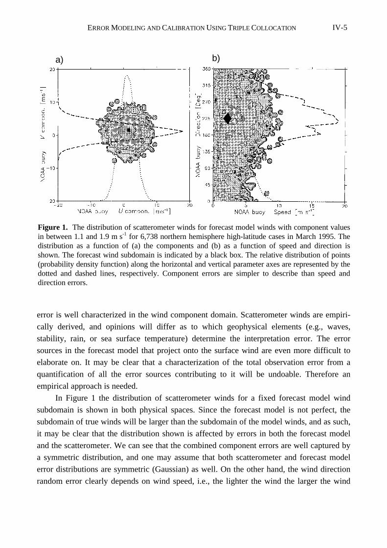
ERROR MODELING AND CALIBRATION USING TRIPLE COLLOCATION IV-5
error is well characterized in the wind component domain. Scatterometer winds are empiri-
cally derived, and opinions will differ as to which geophysical elements (e.g., waves,
stability, rain, or sea surface temperature) determine the interpretation error. The error
sources in the forecast model that project onto the surface wind are even more difficult to
elaborate on. It may be clear that a characterization of the total observation error from a
quantification of all the error sources contributing to it will be undoable. Therefore an
empirical approach is needed.
In Figure 1 the distribution of scatterometer winds for a fixed forecast model wind
subdomain is shown in both physical spaces. Since the forecast model is not perfect, the
subdomain of true winds will be larger than the subdomain of the model winds, and as such,
it may be clear that the distribution shown is affected by errors in both the forecast model
and the scatterometer. We can see that the combined component errors are well captured by
a symmetric distribution, and one may assume that both scatterometer and forecast model
error distributions are symmetric (Gaussian) as well. On the other hand, the wind direction
random error clearly depends on wind speed, i.e., the lighter the wind the larger the wind
a) b)
Figure 1. The distribution of scatterometer winds for forecast model winds with component valuesin between 1.1 and 1.9 m s-1 for 6,738 northern hemisphere high-latitude cases in March 1995. Thedistribution as a function of (a) the components and (b) as a function of speed and direction isshown. The forecast wind subdomain is indicated by a black box. The relative distribution of points(probability density function) along the horizontal and vertical parameter axes are represented by thedotted and dashed lines, respectively. Component errors are simpler to describe than speed anddirection errors.

ERROR MODELING AND CALIBRATION USING TRIPLE COLLOCATION IV-6
direction error. The wind speed error is not symmetrically distributed for light winds but
skew; that is, large positive errors are more likely than large negative errors [Hinton and
Wylie, 1985]. This is related to the fact that measured negative wind speeds cannot occur.
Moreover, the cloud of doubt in the ( f, φ )B space is quite complicated and cannot be
described by second-order statistics, whereas in ( u, v )C space the cloud of doubt seems
much simpler to describe. Therefore, as is common practice in meteorological data assimi-
lation, we define an error model in the wind components.
In practice, it is found that the random error on both the u and v components is similar,
as one may expect (see, e.g., Figure 1a). By verifying the error distributions at higher speeds
we found little evidence of a speed dependence of the component errors in the observation
systems studied (see, e.g., Figure 2). As such an error model with constant and normal
component errors appears appropriate. It implies for speed and direction that the expected
RMS wind speed difference < ( f X - f Y ) 2 >D of two noisy systems X and Y increases
monotonically with wind speed, and the wind direction RMS < ( φ X - φ Y ) 2 >E F increases
monotonically to a value of 104° for decreasing wind speed. Hinton and Wylie [1985] used
a truncated Gaussian error distribution that did not allow negative speeds, to correct for the
low-speed pseudobias. This procedure is rather unsatisfactory since it is not likely that the
true error distribution contains discontinuities. By assuming Gaussian error distributions in
the wind components the cutoff speed effect is naturally simulated, thereby avoiding an ad
hoc correction.
A good way to verify our approach is to simulate the wind speed and direction differ-
ence statistics with the error model we have obtained for the wind components. Figure 2
shows such a comparison (compare errors to Table 2). We can see that the average wind
speed difference (pseudobias) indeed varies as a function of wind speed and that it can be as
large as 1 m s-1 for realistic errors. The standard deviation of the wind speed difference and
the vector RMS difference go to a small value for low wind speed, as is observed for the
real data as well. The wind direction standard deviation increases for decreasing wind speed
and goes to a value of a hundred odd, as expected (random direction). Thus our error model
set up to describe the observed difference statistics in the wind components also qualita-
tively describes the observed difference statistics in wind speed and direction very well,
thereby confirming its adequacy. A quantitative validation of the error model can be made
when the wind component errors are known.
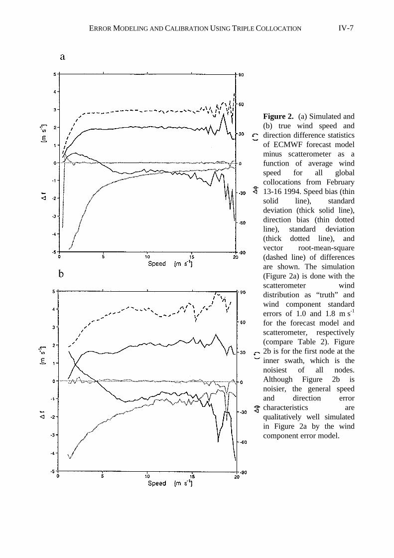
ERROR MODELING AND CALIBRATION USING TRIPLE COLLOCATION IV-7
Figure 2. (a) Simulated and(b) true wind speed anddirection difference statisticsof ECMWF forecast modelminus scatterometer as afunction of average windspeed for all globalcollocations from February13-16 1994. Speed bias (thinsolid line), standarddeviation (thick solid line),direction bias (thin dottedline), standard deviation(thick dotted line), andvector root-mean-square(dashed line) of differencesare shown. The simulation(Figure 2a) is done with thescatterometer winddistribution as “truth” andwind component standarderrors of 1.0 and 1.8 m s-1
for the forecast model andscatterometer, respectively(compare Table 2). Figure2b is for the first node at theinner swath, which is thenoisiest of all nodes.Although Figure 2b isnoisier, the general speedand direction errorcharacteristics arequalitatively well simulatedin Figure 2a by the windcomponent error model.
ERROR MODELING AND CALIBRATION USING TRIPLE COLLOCATION IV-8
3. Error Modeling and Calibration With Two Systems
Unfortunately, all observation systems contain error. This means that we cannot as-
sume that one measurement represents the true state and calibrate the other against it, as is
illustrated here. Assume we have a distribution of “true” states, indicated by the variable tG,
with expected variance < t 2 > = σ 2 , and two independent measurement systems X and Y,
indicated by the variables x and y with respective error variances of < ( t - x ) 2 > = ε 2X and
< ( t - y ) 2 > = ε 2Y. If the distribution of true values and the error distributions are normal,
one can show that for fixed xH the average of y does not lie at < y > = xI but at < y > = σ2 ( σ 2 + ε 2
X ) -1 x (see appendix A); that is for σ = 5 m s-1 and a typical wind error of ε X
= 2 Jm s-1 we find < y > = 0.84 xK, which implies a 1.6 m s-1 difference at 10 m s-1. So, for
unbiased Gaussian error distributions, computing the mean of y for a fixed subrange or bin
of x (bin-average analysis) does, in general, reveal a pseudobias that depends on the error
characteristics of system X.
Scatterometer data are often verified against buoy data, where the buoy data are as-
sumed to be “surface truth” [see, e.g., Rufenach, 1995]. However, the representativeness
error (see sections 1 and 4) for anemometer winds is substantial, and therefore this assump-
tion does not hold. As such, in this work the observation error of in situ winds will be
accounted for in the interpretation in order to be able to draw valid conclusions on the
scatterometer and forecast model bias.
A better assumption often used either implicitly (e.g., in “geometric mean” linear re-
gression) or explicitly is ε Y = ε X = ε , leading to the expectation < x 2 > = < y 2 > =
σ 2 + ε 2. Again, for σ = 5 m s-1 but now for the common wind errors of ε X = 3L m s-1 and
ε Y = 1 m s-1, M we find a ratio of total variances of < x 2 > < y 2 > -1 = 1.32, which would
lead after linear regression to the conclusion that system Y is biased low by 16% if system X
is assumed to be bias free. Thus the assumption may imply a 1.6 m s-1 pseudobias at 10 m s-1
for, in reality, unbiased Gaussian error distributions. The examples illustrate that when a
noisy system is used as a reference for calibration in a dual collocation, we will need to
know the error characteristics of that system. Further proof of this is given in Appendix A.
Another possibility of generating pseudobias is by nonlinear transformation. An unbi-
ased symmetric error distribution may then be transformed into a skew and biased error
distribution. For example, Gaussian errors on the wind components u and v for system XN
or YO will not correspond to Gaussian error distributions on wind speed f and direction φ.
Using the same notation and assumptions common to the previous two examples, we show
in Appendix B that < f X > = π / 2σ X, where σ 2X = σ 2 + ε 2
X, with σ the standard
deviation (SD) of the true wind component distributions, ε X the SE of system X, and where
the errors are assumed identical for the u and v componentsP. A similar expression can be
ERROR MODELING AND CALIBRATION USING TRIPLE COLLOCATION IV-9
derived for system YQ. The expected mean wind speed difference is approximated as < f X -
f Y > = π/ 2( σ X - σ Y ) ≈ π/ 2( ε 2X - ε 2
Y ) σ -1R. For example, the typical values of ( σ, ε
X, ε Y ) = ( 5, 3, 1 )S m s-1 will lead to an average wind speed bias of 0.4 m s-1. This is a
pseudobias since the error in the wind components is unbiased. One can show that the
pseudobias generally oscillates from positive to negative as a function of wind speed and is
largest in a relative sense for low speeds (as in Figure 2).
It may be clear from the above that it is desirable that the error characteristics of meas-
urement systems are well described, thereby avoiding pseudobias effects only caused by
inaccurate assumptions on the errors. Moreover, in order to provide a calibration and error
model of observing systems it is desirable that a domain is chosen where the errors are
simple to describe, preferably avoiding statistical moments of order higher than 2 (see
section 2). Also, in geophysical applications the use of data with complex error characteris-
tics may lead to biased results when the error characteristics are not properly accounted for.
Freilich [1997] and Tolman [1998] recognize the nonlinear effects described above
and the underdetermination of the dual collocation problem, but subsequently use assump-
tions on the statistical properties of the true or error distributions in order to close the
problem. Below it is shown that such assumptions are not needed in a three-way compari-
son.
4. Error Modeling and Calibration With Three Systems
In the previous section it was indicated that calibration of one noisy system against an-
other is not possible without fundamental assumptions on the noise characteristics of at least
one system. It was shown that these assumptions may lead to substantial pseudobias
problems. This is further elaborated in appendix A. Here a method is introduced to perform
calibration and error modeling using triple collocations. The method is quite general and is
introduced as such. Later on, the method is applied on in situ, scatterometer, and forecast
model wind components. Now suppose three measurement systems X, Y and Z measuring a
true variable t. Let us define
x = t + = < >
y = s t + = < >
z = s t + = < >
X X X
Y Y Y Y
Z Z Z Z
δ ε δ
δ ε δ
δ ε δ
,
( ) ,
( ) ,
2 2
2 2
2 2
(1)
with as before, σ 2 = < t 2 >, and now δ X , δ Y , Tand δ Z are the random observation errors
in the measurements xU, y, and z respectively. Here sYV and sZW are the calibration
(scaling) constants. We have assumed no bias such that < δ X > = < δ Y > = < δ Z > = 0X.
For marine winds this is valid to good approximation (see section 5), but otherwise, bias
ERROR MODELING AND CALIBRATION USING TRIPLE COLLOCATION IV-10
may be easily removed.
It is unlikely that the three systems represent the same spatial scales. Therefore we will
arbitrarily assume that observation systems XY and YZ can resolve smaller scales than
system ZAA by taking < δ X δ Y > = r 2BB. Here r 2 is the variance common to these
smaller scales and taken as part of the observation errors δ X and δ Y and t only
CCrepresents the spatial scales resolved by zDD. By definition r 2 is the correlated part of
the representativeness errors of X and Y. The choice for t to only resolve the coarsest scale
measurement allows the approximation < δ X t > = < δ Y t > = < δ Z t > = 0, that is, the
observation errors are assumed uncorrelated with tEE. Furthermore, since zFF does not
include the smaller scales, the observation error of system Z is independent of the errors of
X and Y, that is, < δ X δ Z > = < δ Z δ Y > = 0. The assumption that the wind component
errors of the different observation systems are uncorrelated, except for the representative-
ness error, is essential to determine the calibration. Now the calibration coefficients can be
derived from the different covariances
Y
Z2
y
s = < yz > < zx >
s = < yz > < xy > - r s >
−
−
1
1( )(2)
These coefficients can be used to create
GGy s y
z s z
Y
Z
*
*
=
=
−
−
1
1(3)
HHwhich are the calibrated data. Subsequently, all random error parameters of the observa-
tion systems X, Y, and Z can be resolved pairwise from the different covariances, as
illustrated in Appendix A by (A5)II. Here we used observation system XJJ as a reference
system. This preference can be easily altered by scaling all parameters to one of the other
systems.
So under the premise that we find an estimate for r 2KK we have found a way to per-
form a first-order calibration. In work by Stoffelen [1996] the spatial representativeness error
of the scatterometer with respect to the ECMWF model is estimated to be r 2 = 0.75 m2
s-2LL. We use this as a baseline assumption here as well. The sensitivity of the results to this
choice is discussed later on and shown to be small (section 6).
5. Higher-Order Calibration
After the first-order calibration the three systems should be largely unbiased. However,
in this section we consider a more detailed calibration of the systems by pairwise compari-
son. For the triple-collocated data the procedure is run comparing X and Y, Y and Z, and Z
and X so that consistency can be checked between the results.
ERROR MODELING AND CALIBRATION USING TRIPLE COLLOCATION IV-11
Now first consider X and Y. After obtaining ε X and ε YMM we decide which system is
the least noisy; for example, suppose ε X > ε YNN. Then system YOO may be convoluted
with a Gaussian distribution with width ε εX Y 2 2− PPto obtain a distribution (and a system Y’)
that has the same error properties as that of system X, i.e., ε’YQQ = ε XRR SS. In fact, since
they represent the same true distribution, the resulting distributions of XTT and Y’UU
should be identical in case of a large sample size. When dealing with winds, the errors of X
and Y may be matched for both components, such that either components or speed and
direction distributions should be identical. By comparing the cumulative distributions of
these two systems, f(x) and g(y’), that are monotonically increasing functions, we can easily
compute a mapping yµ = µ(y’)VV that results in identical distributions f(x) and g(yµWW).
The higher-order correction would then be µ(y) - y, which may be plotted versus y.
The higher-order calibration is only reliable when the errors of system X and Y are well
characterized by a normal distribution. However, if substantial errors of order higher than 2
would be present in either system X or Y, then the detailed bias computation method set out
above may provide large pseudobiases. When more than two systems are involved, such as
in our triple collocation data set, a consistency check between the different comparisons
may reveal such problems. In the extreme parts of the domain, where the error distributions
of either system are insufficiently sampled, further pseudobias effects may occur. To gain
confidence, the computed corrections may be verified by Monte Carlo simulation to test
such sampling problems.
6. Calibration and Error Model Results
In this section we describe the implementation of the method given earlier and show
the results of the calibration of scatterometer and forecast winds relative to the anemometer
winds. A 1-month data set kindly provided by NCEP from March 1995 with off-line
anemometer winds from the NOAA buoys corrected to 10-m height [Wilkerson and Earle,
1990] was used collocated with the ESA-processed ERS-1 scatterometer and NCEP forecast
model winds. The NCEP forecast wind is valid at the time and location of the buoy meas-
urement. All scatterometer data within 200 km and 3 hours of a buoy were selected and as a
result 40,091 triple collocations were available resulting from 1465 independent buoy
measurements.
The average wind components of the in situ, scatterometer, and forecast winds are very
close (within a few tenths of a m s-1). As such, the assumption just below (1) that the
systems have no absolute bias, i.e., < δ i > = 0 for i = ( X, Y, Z ) proves valid.
A quality control procedure is applied to exclude gross errors. An iterative scheme is
followed, where in each trial a calibrated (equation (3)) collocation triplet is rejected when
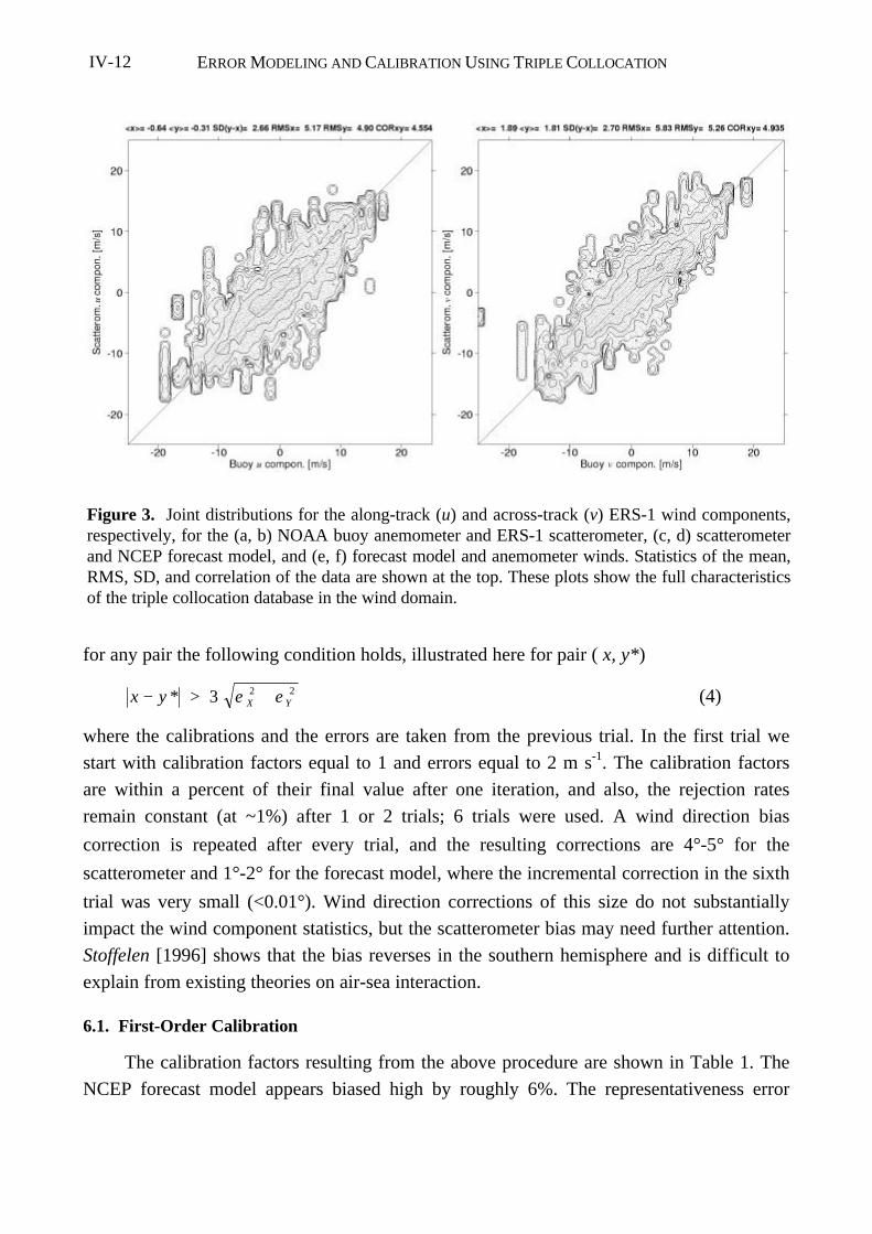
ERROR MODELING AND CALIBRATION USING TRIPLE COLLOCATION IV-12
for any pair the following condition holds, illustrated here for pair ( x, y*)
x y X Y− > +* 3 2 2ε ε (4)
where the calibrations and the errors are taken from the previous trial. In the first trial we
start with calibration factors equal to 1 and errors equal to 2 m s-1. The calibration factors
are within a percent of their final value after one iteration, and also, the rejection rates
remain constant (at ~1%) after 1 or 2 trials; 6 trials were used. A wind direction bias
correction is repeated after every trial, and the resulting corrections are 4°-5° for the
scatterometer and 1°-2° for the forecast model, where the incremental correction in the sixth
trial was very small (<0.01°). Wind direction corrections of this size do not substantially
impact the wind component statistics, but the scatterometer bias may need further attention.
Stoffelen [1996] shows that the bias reverses in the southern hemisphere and is difficult to
explain from existing theories on air-sea interaction.
6.1. First-Order Calibration
The calibration factors resulting from the above procedure are shown in Table 1. The
NCEP forecast model appears biased high by roughly 6%. The representativeness error
Figure 3. Joint distributions for the along-track (u) and across-track (v) ERS-1 wind components,respectively, for the (a, b) NOAA buoy anemometer and ERS-1 scatterometer, (c, d) scatterometerand NCEP forecast model, and (e, f) forecast model and anemometer winds. Statistics of the mean,RMS, SD, and correlation of the data are shown at the top. These plots show the full characteristicsof the triple collocation database in the wind domain.
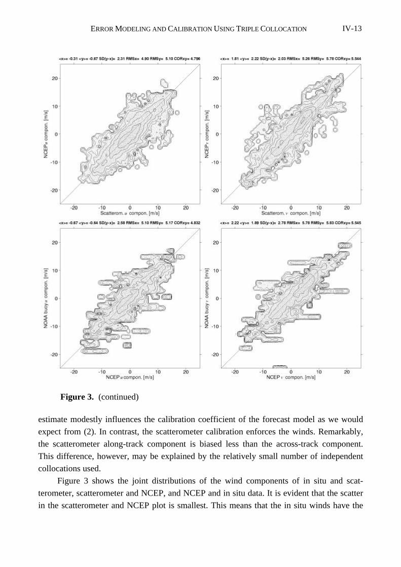
ERROR MODELING AND CALIBRATION USING TRIPLE COLLOCATION IV-13
estimate modestly influences the calibration coefficient of the forecast model as we would
expect from (2). In contrast, the scatterometer calibration enforces the winds. Remarkably,
the scatterometer along-track component is biased less than the across-track component.
This difference, however, may be explained by the relatively small number of independent
collocations used.
Figure 3 shows the joint distributions of the wind components of in situ and scat-
terometer, scatterometer and NCEP, and NCEP and in situ data. It is evident that the scatter
in the scatterometer and NCEP plot is smallest. This means that the in situ winds have the
Figure 3. (continued)

ERROR MODELING AND CALIBRATION USING TRIPLE COLLOCATION IV-14
largest error. The in situ and scatterometer plot shows the largest scatter, which indicates
that the NCEP winds are the most accurate. Table 2 shows the results of our random error
estimates from (A5) in Appendix A, which confirm our subjective analysis. The error
estimates for the u and v components are quite similar for NCEP and conventional winds,
but for the scatterometer the along-track component seems slightly worse than the across-
track component. Given the fact that the wind direction was predominantly across-track in
this data set, it may indicate some anisotropy in the scatterometer error distribution.
From a climatological wind spectrum one may estimate the representativeness error
variance of the conventional winds with respect to NCEP winds to be 2.1 m2 s-2 [Stoffelen,
1996]. As such, the (local) error of the in situ winds may be estimated as 1.41 m s-1 for the u
and 1.21 m s-1 for the v component. However, for many applications the local wind is not as
relevant as an area-averaged quantity such as provided by the scatterometer.
Since the scatterometer winds are not exactly collocated in space and time with the in
Table 1. Calibration Scaling Factors Against Buoy Winds for Wind Components From theScatterometer and Forecast Model for Different Representativeness Errors.
Component Scaling
u v r 2, m2 s-2
Scatterometer 0.97 0.95 allNCEP model 1.06 1.06 0.50NCEP model 1.06 1.07 0.75NCEP model 1.07 1.08 1.00
Here u is the along-track, and v is the across-track wind component; r 2 is the representativenesserror (due to scatterometer and model spatial resolution difference).
Table 2. Estimates of the Wind Component Standard Deviation of the True Distribution and theStandard Errors of the Buoy, Scatterometer, and Forecast Error Distributions.
Component, m s-1
u v
True variance 4.68 5.24In situ error 2.02 1.89
Scatterometer error 1.89 1.62NCEP error 1.11 1.15
Here u is the along-track and v the across-track wind component. The values are computed at thespatial representativeness of the forecast winds with r 2 = 0.75 m s-1 (see text).
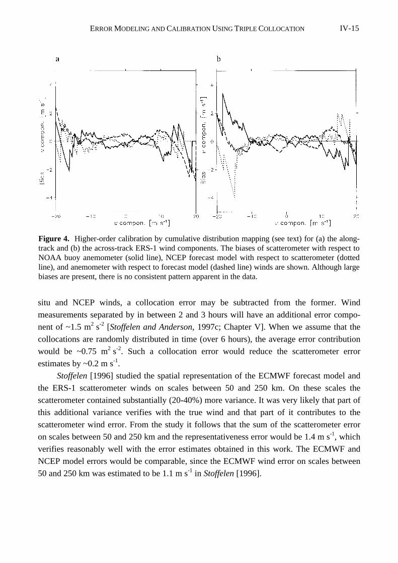
ERROR MODELING AND CALIBRATION USING TRIPLE COLLOCATION IV-15
situ and NCEP winds, a collocation error may be subtracted from the former. Wind
measurements separated by in between 2 and 3 hours will have an additional error compo-
nent of ~1.5 m2 s-2 [Stoffelen and Anderson, 1997c; Chapter V]. When we assume that the
collocations are randomly distributed in time (over 6 hours), the average error contribution
would be ~0.75 m2 s-2. Such a collocation error would reduce the scatterometer error
estimates by ~0.2 m s-1.
Stoffelen [1996] studied the spatial representation of the ECMWF forecast model and
the ERS-1 scatterometer winds on scales between 50 and 250 km. On these scales the
scatterometer contained substantially (20-40%) more variance. It was very likely that part of
this additional variance verifies with the true wind and that part of it contributes to the
scatterometer wind error. From the study it follows that the sum of the scatterometer error
on scales between 50 and 250 km and the representativeness error would be 1.4 m s-1, which
verifies reasonably well with the error estimates obtained in this work. The ECMWF and
NCEP model errors would be comparable, since the ECMWF wind error on scales between
50 and 250 km was estimated to be 1.1 m s-1 in Stoffelen [1996].
Figure 4. Higher-order calibration by cumulative distribution mapping (see text) for (a) the along-track and (b) the across-track ERS-1 wind components. The biases of scatterometer with respect toNOAA buoy anemometer (solid line), NCEP forecast model with respect to scatterometer (dottedline), and anemometer with respect to forecast model (dashed line) winds are shown. Although largebiases are present, there is no consistent pattern apparent in the data.

ERROR MODELING AND CALIBRATION USING TRIPLE COLLOCATION IV-16
6.2. Higher-Order Calibration
The higher-order calibration procedure of section 5 requires a convolution of the most
accurate system with a Gaussian error distribution with a width determined by the difference
in error variance of the two systems. Figure 4 shows the higher-order calibration by the
cumulative distribution mapping method. The wind component biases appear to be rather
random in nature. The smallest biases are generally present at small wind component values,
and the highest are present at high component speeds. This is due to the fact that the largest
number of data is present at low component speeds, and the lowest number is present at high
speeds. In other words, the higher the speeds the less accurate the results are. In an attempt
to fit the bias with a smooth function this would have to be taken into account, and changes
at the tail of the distribution should be kept small.
Inconsistency of the wind component biases between the calibration pairs is most no-
ticeable at the tail of the distributions; that is, for example, the bias of the in situ winds with
respect to the scatterometer is not equal to the sum of the biases of the conventional winds
with respect to NCEP and the bias of NCEP with respect to the scatterometer. Moreover, the
plot suggests that the scatterometer has a generally negative bias with respect to the
anemometer winds and NCEP for the along-track component. However, this effect is not
confirmed by the differences in mean value of the scatterometer along-track component.
Closer inspection reveals more (but smaller) inconsistencies. These indicate insufficient
sample size or higher-order statistical moments in the error distributions than those ac-
counted for.
The cloud of doubt is assumed to be Gaussian with a fixed standard error. However, in
reality, also higher-order moments may be relevant here. Furthermore, the standard error
may depend on the geophysical condition, for instance on stability, and we would need a
representative sample of all these conditions to perform the higher-order calibration
accurately. As such, the number of samples we need to determine the calibration and error
model may be quite large. Since there is no mechanism to remove the pseudobiases due to
sampling and higher-order moments, we believe that the methodology has to be used with
restraint.
Physically, one may expect systematic errors to scale with f and φ, rather than with u
and v. If the errors in u and v of systems X and Y are identical, then their f and φ distribu-
tions should ideally also be identical. The wind direction cumulative mapping also does not
result in substantial and consistent systematic effects, but for wind speed it does, as shown
in Figure 5. The scatterometer is biased high for high and very low wind speed and biased
low for moderate speeds with respect to the buoys. The NCEP model shows similar
differences with respect to the buoys but roughly half in size. However, at the very low
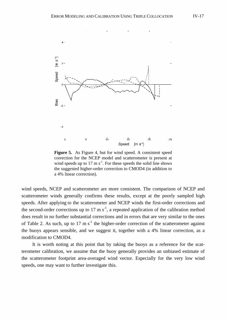
ERROR MODELING AND CALIBRATION USING TRIPLE COLLOCATION IV-17
wind speeds, NCEP and scatterometer are more consistent. The comparison of NCEP and
scatterometer winds generally confirms these results, except at the poorly sampled high
speeds. After applying to the scatterometer and NCEP winds the first-order corrections and
the second-order corrections up to 17 m s-1, a repeated application of the calibration method
does result in no further substantial corrections and in errors that are very similar to the ones
of Table 2. As such, up to 17 m s-1 the higher-order correction of the scatterometer against
the buoys appears sensible, and we suggest it, together with a 4% linear correction, as a
modification to CMOD4.
It is worth noting at this point that by taking the buoys as a reference for the scat-
terometer calibration, we assume that the buoy generally provides an unbiased estimate of
the scatterometer footprint area-averaged wind vector. Especially for the very low wind
speeds, one may want to further investigate this.
Figure 5. As Figure 4, but for wind speed. A consistent speedcorrection for the NCEP model and scatterometer is present atwind speeds up to 17 m s-1. For these speeds the solid line showsthe suggested higher-order correction to CMOD4 (in addition toa 4% linear correction).
ERROR MODELING AND CALIBRATION USING TRIPLE COLLOCATION IV-18
7. Conclusions
7.1. Résumé
In this paper, calibration and error modeling are discussed, and a methodology is pro-
vided to obtain the absolute calibration and accuracy of observing systems. In particular, the
focus is put on ocean surface wind speed (or stress) biases that are detrimental for the
computation of fluxes of momentum, humidity, and energy through the air-sea interface. An
improved ERS scatterometer wind processing is proposed.
It was demonstrated that the selection of a simple measurement domain where second-
order statistics are sufficient to describe the uncertainty of the measurements is preferred.
More specifically, we have shown that wind error modeling using component error distribu-
tions that are Gaussian and constant represents a simple method to describe the more
complex errors in speed and direction. We have shown that substantial pseudowind speed
biases can occur through the nonlinear transformation of unbiased wind component errors to
the wind speed and direction domain. In a direct wind speed calibration, where usually
unjustly symmetric error distributions are assumed, the pseudobiases would be taken out,
leading to biased wind components [see also Hinton and Wylie, 1985]. Wind component
error modeling as proposed here elegantly solves this problem.
In order to calibrate one observing system with respect to the other, one may use, ei-
ther explicitly or implicitly, a simplifying assumption on the errors of the two systems. For
instance, it is common practice to assume that the errors of two systems that are compared
are equal or to assume that one system is much more accurate (i.e., is “truth”) than the other.
Given our results in Table 2 and Figure 3, it is obvious that both of these choices would
have been crude for any of the observation systems dealt with in this paper. We have shown
that such assumptions may lead to substantial pseudobias effects. Furthermore, in Appendix
A it is shown that it is impossible to calibrate one noisy system against another without such
assumptions or other prior knowledge on the error characteristics of one or both systems.
For a proper calibration of an observing system a reference system is necessary and at
least one other observation system. Using triple collocations, a method to calibrate noisy
systems has been developed. Subsequently, in a pairwise comparison of the calibrated
observation systems the covariances were used to estimate the true variance resolved by
both systems and the error variance of the observations. To complement the linear calibra-
tion, a more refined bias estimation procedure was adopted.
We used the NOAA buoy anemometer winds as a reference, although they turned out
to be the least accurate amongst the scatterometer and NCEP forecast model winds. The
spatial representativeness error is the main reason for the low accuracy of the buoys in our
ERROR MODELING AND CALIBRATION USING TRIPLE COLLOCATION IV-19
triple comparison. One would expect this error to be of a random nature and not lead to
biases in the results. We found that the CMOD4-derived scatterometer wind components are
biased low by 4%. The NCEP forecast model appears to be very accurate but biased high by
6% for the period we examined (March 1995). In another study, using triple collocations of
the ECMWF forecast model, ERS scatterometer winds, and real-time available anemometer
winds, similar results were obtained [Stoffelen, 1996]. The higher-order scatterometer
calibration with respect to the buoys resulted in a correction additional to the 4% mentioned
above. The total correction is recommended for operational implementation in the ESA fast
delivery processing chain.
7.2. Application
Our statistical analysis on surface winds has direct implications in the area of data as-
similation in numerical weather prediction (NWP) models and in ocean circulation and
wave model forcing. However, the methodology may be applied for the interpretation of any
geophysical variable with a high variability on the smaller scales or high signal-to-noise
ratio. It provides a way to compare data with different amounts of noise or different spatial
and/or temporal resolution.
It is essential that NWP models assimilate unbiased data. It has been observed by
ECMWF that the scatterometer bias with respect to their forecast model (~10 %) had the
tendency to slow down the forecast winds in the analysis and subsequently fill in low-
pressure systems. This effect can be circumvented by a model wind correction to match the
mean observed wind [Roquet and Gaffard, 1995]. The 6% bias we found between the buoys
and the NCEP model may result from physical parameterizations that also control atmos-
pheric boundary layer humidity, depth, and temperature and that require careful tuning.
Such biases, when detected, are therefore not easily corrected, and a short-term solution
such as adopted by Roquet and Gaffard will be beneficial. However, in the long term the
forecast model bias correction should be replaced by forecast model improvements.
Roquet and Gaffard [1995] computed a bias correction in the wind speed domain,
rather than in the wind components. The wind components, however, are used for data
assimilation and should be unbiased. Figure 2 clearly shows that because of the nonlinear
transformation, unbiased component errors will lead to biased speeds and vice versa. It is
therefore essential to compute biases in the domain of the analysis variables, i.e., the wind
components [see also Le Meur et al., 1997]. For other analysis variables the same strategy
may be applied; that is, observations and forecast data are compared in that domain where
the errors are best described, and bias corrections are computed after the transformation of
the random errors to the analysis variable domain. For noisy data a careful statistical error
analysis as described in this work will be essential to arrive at an optimal bias correction and
ERROR MODELING AND CALIBRATION USING TRIPLE COLLOCATION IV-20
assimilation.
Wave models directly rely on NWP model winds. Here it was shown that NWP fore-
cast model winds are very accurate in describing the synoptic scale flow but may be biased.
However, since we quantified the bias, it is easily corrected for when the winds are used in
wave models. We note that it is more problematic to take account of the error in the forcing
since this error is nonlinearly related to the random wind error. Also, it is relevant to be
aware of the fact that a NWP model provides an area-averaged vector wind and that the
additional forcing due to the wind on the unresolved scales needs be parameterized.
Tropical wind analysis is very important for ocean circulation models and as such for
the study of the Earth's climate. In ocean circulation experiments, similar arguments apply
as in wave forecasting concerning the forcing problem. Stoffelen [1996] and Bryan et al.
[1995] noted a large directional inconsistency between scatterometer and ECMWF wind
direction at the equator. The tropical array of (TAO) buoys may provide a relevant data set
to enhance our knowledge on the utility of scatterometer and forecast winds in this area
using the methodology described here.
Appendix A: Necessity of Error Modeling Before Calibration or Validation
In this appendix the problem of calibration and validation of one noisy system with
respect to another one will be discussed. Usually, scatter plots are used to compare the data
followed by a regression analysis to compute a calibration coefficient or to validate the
system(s). First, the interpretation of scatter plots and associated regression and bin average
(BA) analyses are discussed, and it is illustrated that calibration or validation, without
knowing the error characteristics of one or both systems, can easily lead to pseudobiases. In
the second part it is shown that calibration or validation of one noisy system against another,
without knowing the error characteristics of the observing systems, is generally not possible.
A1. Scatter Plots and Regression
Usually, a scatter plot is used to determine the error characteristics of a measurement
system (see, for example, Figure 4). In this section we quantify the properties of the scatter
plot. If enough collocation data are available, then the density of points in the scatter plot is
proportional to the joint probability density of xFout! Schakeloptie-instructie niet
opgegeven. and yFout! Schakeloptie-instructie niet opgegeven. given by
p x, y = p x|t p y|t p t dt( ) ( ) ( ) ( )∫ (A1)
The integration is over the distribution of true states p( t )ZZ and over the distributions of
error. Here p( x | t )AAABBB is the conditional probability density ofCCC x given t, which
includes all measurement and error characteristics of the measurements x. (It is closely
ERROR MODELING AND CALIBRATION USING TRIPLE COLLOCATION IV-21
related to what was introduced as the cloud of doubt around observation x,DDD which
formally reads p( t | x )EEEFFF and where p( t | x )GGGHHH = p( x | t )IIIJJJ p( t ). ) We can
see that the joint distribution of xKKK and yLLL is not only determined by the error
characteristics of both systems but also by the distribution of true statesMMM. In the simple
case of unbiased Gaussian errors with standard error (SE) equal to ε X or ε Y and a Gaussian
true distribution with zero mean and RMS σNNN, the joint probability of x OOOand yPPP
can be written as
p x, y -+ x + + y - xy
+ + Y X
X Y X Y
( ) exp[( ) ( )
( )]
∝
2 2 2 2 2 2 2
2 2 2 2 2 22σ ε σ ε σ
σ ε σ ε ε ε (A2)
For given xQQQ the mean y value of this distribution does not lie at y = xRRR but at y = σ 2
( σ 2 + ε 2X ) -1 x. SSSSo, even for unbiased Gaussian error distributions, computing the
mean of yTTT for a fixed subrange or bin of xUUU (bin average) does, in general, reveal a
pseudobias that depends on the error characteristics of xVVV. This needs to be accounted
for in the interpretation, and therefore, when correcting for bin-average biases with respect
to a reference system, the error characteristics of that system, in this case ε X, need to be
known well.
For calibration or validation, often linear regression is used as a tool. For a well-
calibrated system and in the case of ε X = ε Y a geometric mean linear regression on the joint
distribution would indeed result in the line y = x, but in the more general case of ε X ≠ ε Y it
would result in y = ( σ 2 + ε 2Y ) ( σ 2 + ε 2X ) -1 x, where it would again result in a pseudo-
bias. When the error characteristics of x and y are known, a weighted fit may result in a
proper calibration. However, most often the errors are unknown.
A2. Necessity of Error Modeling Before Calibration
Then the question emerges; Is it possible to perform a calibration or validation of one
noisy system against the other without prior information on the error characteristics of one
or both of the systems? Below we illustrate that this is generally not possible.
Suppose we have a set of true states, indicated by variable t, measured by systems X
and Y resulting in measurements x and y. We define σ 2 = < t 2 >, where < > denotes the
expected mean,WWW and introduce the error model
x = t + = < >
y = t + = < >
X X X
Y Y Y
δ ε δ
δ ε δ
2 2
2 2(A3)
where x, y, and tXXX are as defined before and δ X and δ YYYY are the independent
observation errors on x and y respectively ZZZ, i.e., < δ X δ YAAAA > ≈ 0BBBB. The
observation errors are random and uncorrelated with tCCCC, i.e., < δ X t > ≈ 0DDDD and <
ERROR MODELING AND CALIBRATION USING TRIPLE COLLOCATION IV-22
δ YEEEE t > ≈ 0FFFF. For simplicity we have removed the true distribution’s mean and the
systematic errors, i.e., < t GGGG> = 0, < δ XHHHH > = 0, and < δ YIIII > = 0. We now find
< x > = +
< y > = +
< xy > =
X
Y
2 2 2
2 2 2
2
σ ε
σ ε
σ
(A4)
which are three equations with three unknowns that are easily resolved
X
Y
= < x > - < xy >
= < y > - < xy >
= < xy >
2 2
2 2
2
ε
ε
σ
(A5)
Thus from the covariances we can resolve the true variance and the standard errors of
systems X and Y.
Now suppose that one system is not calibrated, for example, we change (A3) to
x = t + = < >
y = s (t + ) = < >
X X X
Y Y Y Y
δ ε δ
δ ε δ
2 2
2 2(A6)
where sY is the calibration (scaling) constant. We now find
X*
X Y
Y*
Y Y Y Y
*Y
= < x > - < xy > = + - s
= < y > - < xy > = s + s s -
= < xy > = s
2 2 2 2
2 2 2 2 2
2 2
1
1
ε ε σ
ε ε σ
σ σ
( )
( ) (A7)
such that for ε*X
2JJJJ ≥ 0KKKK and ε*Y
2LLLL ≥ 0MMMMNNNN the transformed distribu-
tion of t* = ys tOOOO in combination with error model
* *X*
X*
X*
* *Y*
Y*
Y*
x = t + < > =
y = t + < > =
δ δ ε
δ δ ε
2 2
2 2(A8)
is statistically identical to the system defined in (A3). Consequently, one can show that
substituting the transformed quantitities defined in (A7-8) into (A2) rather than the real
quantities of (A3) leads to an identical joint distribution. As such, the calibration coefficient
cannot be resolved unambiguously without further information on the errors in this general
case.
This is due to the fact that we have three independent statistical variables, i.e., < x 2 >,
< y 2 >, and < xy >, and four unknowns that are s YPPPP, σ, ε X, and ε YQQQQRRRR, which
leaves one degree of freedom. The constraint that error variances are positive gives the
following values for the scaling constant s*Y in the case of sY = 1: -ε
2Y
SSSSTTTT ( σ 2 +
ε 2Y )
-1 ≤ s*YUUUU - 1 ≤ ε 2
X σ -2. Only the addition of an independent third system can
ERROR MODELING AND CALIBRATION USING TRIPLE COLLOCATION IV-23
help determine the unique and correct value of sY.
Appendix B: Pseudobias Through Nonlinear Transformation
A statistical problem that is relevant for considering the optimal error domain may oc-
cur through nonlinear transformation. This is easily shown for wind speed f VVVVthat
depends in a nonlinear manner on the wind components ( u, v ). As an alternative to Hinton
and Wylie [1985], we assume normal distributed errors on the wind components u and v for
measurement systems X WWWWand YXXXX, i.e., u X = N( u t, ε X ), v X = N( v t, ε X ), u Y
= N( u t, ε Y ), and v Y = N( v t, ε Y )YYYYZZZZ and, in addition, normal distributed true
components, u t = N( 0, σ ) and v t = N( 0, σ )AAAAABBBBB, where N( 0, σ€) indicates
the normal distribution with zero mean and standard deviation σ. The wind speed distribu-
tion of system X, p( f X ) df X , then becomes
p f df = f
-f
dfX XX
X
X
XX( ) exp[ ]
2
2
22σ σ (B1)
where σ 2
XCCCCCDDDDD = σ 2 + ε
2XEEEEE. A similar expression can be derived for system
YFFFFF. The expected mean value of f XGGGGGHHHHHIIIII will be < f X > = π / 2σ X , and < f X
- f Y > = π / 2( σ X - σ Y ) ≈ π / 2( ε 2X - ε 2
Y ) σ -1.JJJJJ Thus the difference in mean wind
speed is generally nonzero, and a pseudobias occurs, since the component error distributions
were not biased. More detailed analysis shows that the pseudobias results from the fact that
the wind speed error distribution is asymmetric in the case of symmetric wind component
error distributions, especially for low wind speeds. The magnitude of the pseudobias
depends on wind speed (see, e.g., Figure 2).
Acknowledgments. This work has been greatly stimulated by discussions in the ESA
ASCAT Science Advisory Group and in particular by discussions with Didier Le Meur from
ECMWF. Tsan Wang Yu from NCEP kindly provided me with the collocation data set and
is especially acknowledged.
References
Bryan, F. O., I. Wainer, and W. R. Holland, Sensitivity of the tropical Atlantic circulation to
specification of wind stress climatology, J. Geophys. Res., 24, 729-744, 1995.
Freilich, M. H., Validation of vector magnitude data sets: Effects of random component
errors, J. Atmos. Oceanic Technol., 14, 695-703, 1997 .
Hinton, B. B., and D. P. Wylie, A correction for the errors in ship reports of light wind, J.
Atmos. Oceanic Technol., 2, 353-356, 1985.

ERROR MODELING AND CALIBRATION USING TRIPLE COLLOCATION IV-24
Holton, J. R, An Introduction to Dynamic Meteorology, 2nd ed., Int. Geophys. Ser. - vol.
23, Academic, San Diego, Calif., 1979.
Le Meur, D., L. Isaksen, and A. Stoffelen, Wind calibration of the ERS scatterometer for
data assimilation purposes at ECMWF, paper presented at the Wind and Wave Valida-
tion Workshop, Comm. on Earth Obs. Satell., Eur. Space Agency, Noordwijk, Nether-
lands, June 3-5, 1997.
Lorenc, A. C., Analysis methods for numerical weather prediction, Q. J. R. Meteorol. Soc.,
112, 1177-1194, 1986.
Offiler, D., The calibration of ERS-1 satellite scatterometer winds, J. Atmos. and Oceanic
Technol., 11, 1002-1017, 1994.
Roquet, H. and C. Gaffard, Proposal for a new version of CMOD4, memorandum Forecast
Res. Dep., Eur. Centre Medium-range Weather Forecasts, Reading, UK.
Rufenach, C., A new relationship between radar cross-section and ocean surface wind speed
using ERS-1 scatterometer and buoy measurements, Int. J. Remote Sens., 16(18), 3629-
3647, 1995.
Stoffelen, A., Error modelling of scatterometer, in-situ, and ECMWF model winds: A
calibration refinement, Tech. rep. 193, R. Neth. Meteorol. Inst., de Bilt, Netherlands,
1996.
Stoffelen, A., A simple method for calibration of a scatterometer over the ocean, J. Atmos.
Oceanic Technol., in press, 1998.
Stoffelen, A., and D. Anderson, Scatterometer data interpretation: Measurement space and
inversion, J. Atmos. Oceanic Technol., 14(6), 1298-1313, 1997a.
Stoffelen, A., and D. Anderson, Scatterometer data interpretation: Estimation and validation
of the transfer function CMOD4, J. Geophys. Res., 102(C3) , 5767-5780, 1997b.
Stoffelen, A., and D. Anderson, Ambiguity removal and assimilation of scatterometer data,
Q. J. R. Meteorol. Soc., 123, 491-518, 1997c.
Tolman, H. L., Effects of observation errors in linear regression and bin-average analyses,
Q. J. R. Meteorol. Soc., 124, 897-917, 1998.
Wilkerson, J. C., and M. D. Earle, A study of differences between environmental reports by
ships in the voluntary observing program and measurements from buoys, J. Geophys.
Res., 95(C3), 3373-3385, 1990.
AMBIGUITY REMOVAL AND ASSIMILATION OF SCATTEROMETER DATA V-1
CHAPTER V
Ambiguity Removal and Assimilation of Scatterometer Data*
Abstract. The ERS-1 scatterometer has proved to be a source of high quality ocean surface
wind data, but a problem remains, namely the dual directional ambiguity of the solutions.
An ambiguity removal scheme, called PRESCAT, is described based on our experience (a)
that information on wind direction retrieval skill is an important input to ambiguity removal,
(b) that wind-vector filtering is beneficial compared to wind-direction filtering, and (c) that
meteorological forecast information already enables us to correctly remove 95% of all
ambiguities. The performance of the ambiguity filter is very good compared to other
operational ambiguity removal schemes. Furthermore, a statistical interpolation analysis
system called ‘buddy’ check is used effectively to identify and remove the few (approx.
0.1%) wrongly selected solutions.
Assimilation of scatterometer winds has a beneficial impact on analyses and short-
range forecasts, probably mainly from improvements on the sub-synoptic scales. On the
wider temporal and spatial scales, scatterometer winds were also found beneficial, but only
in the absence of satellite temperature soundings (SATEMs). In assimilation experiments in
which the latter were included, the scatterometer provided a neutral impact on the medium-
range forecast. Moreover, the conventional observations, including SATEMs, are shown to
have adverse effects on the surface-wind analysis. We believe that both the redundancy and
the adverse effects on the surface-wind field are explained by the rigid formulation of the 6-
hour-forecast error structure; the forecast error is assumed flow-independent, and
information on the special meteorological conditions in the atmospheric planetary boundary
layer is lacking. To make observational systems more useful and complementary for
numerical weather prediction the effects of the structure functions have to be investigated
more precisely. In an adaptive four-dimensional variational assimilation scheme the effect of
the assumptions on forecast-error structure will be less. We show that, in a variational
framework, scatterometer backscatter measurements are difficult to assimilate directly.
Instead, we derive and illustrate an alternative procedure to assimilate retrieved winds rather
than backscatter measurements.
*Based on:
Stoffelen, Ad, and David Anderson, Ambiguity Removal and Assimilation of Scatterometer Data, Q. J. R.
Meteorol. Soc., 123, 491-518, 1997.
AMBIGUITY REMOVAL AND ASSIMILATION OF SCATTEROMETER DATAV-2
1. Introduction
The European Space Agency’s remote-sensing satellite, ERS-1, was launched on 17
July 1991, carrying a C-band scatterometer. The satellite flies in a polar orbit at a height of
800 km. The scatterometer instrument (which is also mounted on ERS-2) has three
independent antennae pointing in a horizontal plane towards a direction of 45°, 90°, and
135° with respect to the satellite propagation, thus illuminating a site in the scatterometer’s
swath three times, by the fore, mid, and aft beam, respectively. The incidence angle of the
radar beam varies from 18° to 47° for the mid beam, and from 24° to 57° for the fore and aft
beams. The swath, approximately 500 km wide, is sampled every 25 km resulting in 19
measurement nodes across the swath; along the swath the sampling distance is also equal to
25 km. The nodes are not independent, however, and the effective spatial resolution of the
instrument on the earth’s surface (called the footprint) is approximately 50 km. At the
European Centre for Medium-range Weather Forecasts (ECMWF) a quality control
procedure has been implemented which can identify and reject anomalous triplets of
backscatter measurements [Stoffelen and Anderson, 1995; Chapter II]. It was also shown
that the scatterometer data can successfully be interpreted as measurements of the 10-m
wind vector. Through comparison with the ECMWF numerical weather-prediction (NWP)
model, scatterometer winds are found to be more accurate than conventional ocean surface
wind data, currently used in operational meteorology [Stoffelen and Anderson, 1995;
Chapter IV]. However, scatterometer winds have a dual ambiguity because there are two
wind solutions at each node on the earth’s surface. Several ambiguity removal schemes were
evaluated before the launch of ERS-1 [Graham et al., 1989], and a scheme called CREO
[Cavanié and Lecomte, 1987] was selected and implemented by the European Space Agency
(ESA). In this scheme two antiparallel fields from the two solutions at each node are built
up. For each field the number of cases in which the highest probability solution is chosen is
calculated. When this number is significantly higher for one of the fields than for the other,
then the field with the higher number is selected. This application of CREO is called
‘autonomous’ ambiguity removal. If autonomous ambiguity removal fails, or is not applied,
then a comparison is made between both antiparallel fields and a forecast of the surface
wind field; the field with the higher correlation selected. In section 2 we briefly discuss the
performance of this scheme when used with real data, and propose an alternative scheme,
based on the United Kingdom Meteorological Office (UKMO) scheme SLICE [Offiler,
1987], which improves the ambiguity removal skill.
Given the high quality of the retrieved scatterometer winds, it is important that they be
assimilated into numerical weather-prediction (NWP) models. Earlier assimilation
experiments with SEASAT scatterometer data in the T106 spectral resolution ECMWF
model had a neutral impact in both southern and northern hemispheres [Anderson et al.,
AMBIGUITY REMOVAL AND ASSIMILATION OF SCATTEROMETER DATA V-3
1991]. In the case of the rapidly developing QE-2 storm, the KNMI (Koninklijk Nederlands
Meteorologisch Instituut) limited area model (LAM) gave a forecast that was better than the
ECMWF model’s forecast [Stoffelen and Cats, 1991], and the use of SEASAT scatterometer
data had a further substantial and beneficial effect on the forecast. Preliminary tests with
ERS-1 scatterometer data in the ECMWF T106 model showed a neutral impact [Hoffman,
1993]. However, the quality of the SEASAT and the preliminary ERS-1 scatterometer data
used by Hoffman is substantially less than the current quality of the ERS-1 scatterometer
data. Assimilation experiments at the UK Meteorological Office showed that the ERS-1
scatterometer winds had a beneficial impact in a day-5 forecast in the southern hemisphere
[Bell, 1994]. Breivik et al. [1993] obtained a small beneficial effect in the Norwegian 50-km
resolution limited-area model.
For many years, ECMWF have been using a statistical interpolation scheme, otherwise
known as optimal interpolation or OI, to perform the analysis. To test whether the data can
be used to modify the ECMWF analyses using the current OI analysis scheme, various
experiments are done in which winds from the ERS scatterometer processing, inversion, and
ambiguity removal scheme, called PRESCAT, are assimilated into the ECMWF model
analysis. One of the periods selected is from 18 to 28 March; it is chosen so as to coincide
with a parallel study being conducted by the UK Meteorological Office [Bell, 1994].
Parallel assimilation experiments to assess the ‘redundancy’ between surface wind data
and NOAA/NESDIS (National Oceanographic and Atmospheric Administration/National
Environmental Satellite and Data Information System) processed TOVS (TIROS (Television
Infra-Red Operational Satellite) Operational Vertical Sounder) vertical temperature
soundings [Smith et al., 1979], called SATEM, are also discussed in section 3. Ten-day
forecasts from these assimilations were made and are compared with the verifying analyses
to test for impact of the scatterometer data on the forecast. Since scatterometer data had not
yet been used operationally at ECMWF, they can therefore be used to verify the operational
ECMWF surface wind analyses and forecasts, as is demonstrated in section 3.4.
In recent years variational assimilation schemes have become more mature, and at
ECMWF a scheme of this kind has been developed but, at the time of writing, has not yet
been implemented [Courtier et al., 1993]. It was anticipated that satellite measurements that
are indirectly related to NWP model variables, are best assimilated directly into such
schemes. In section 4, however, it is shown that this is not the case for scatterometer
measurements, and that it is more practicable to assimilate the ambiguous winds rather than
the scatterometer backscatter measurement values σ 0. The paper ends with a summary and
conclusions in section 5.
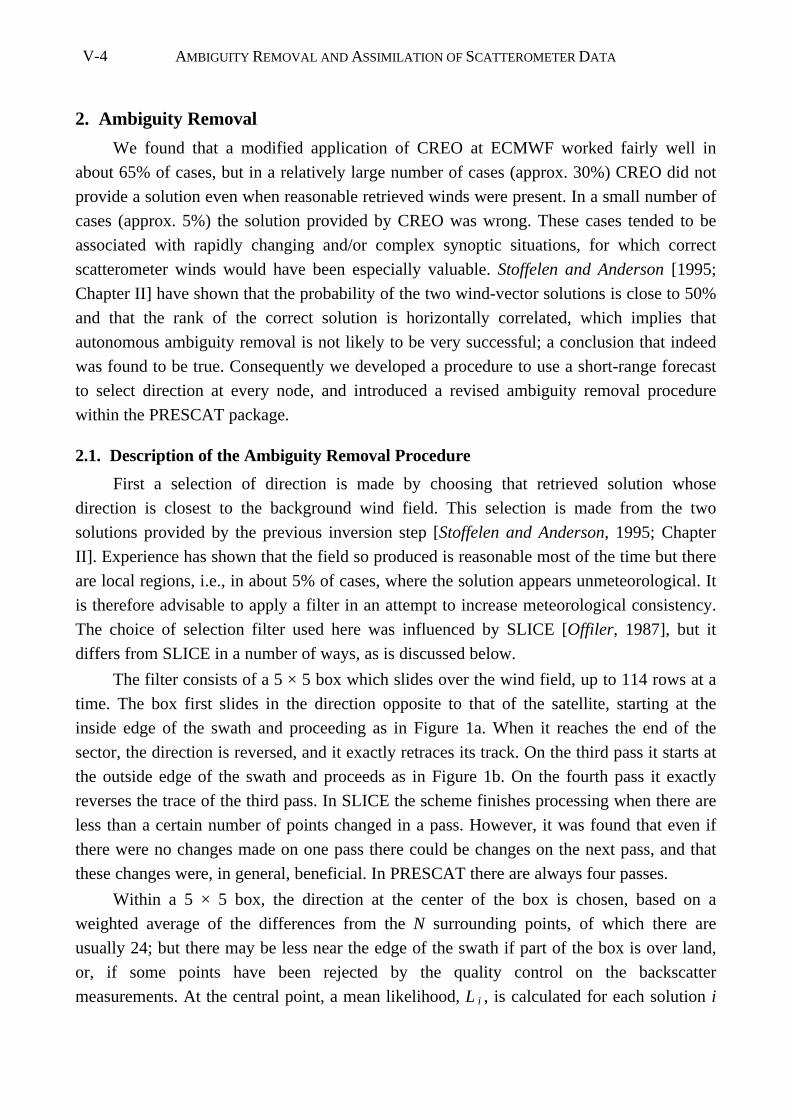
AMBIGUITY REMOVAL AND ASSIMILATION OF SCATTEROMETER DATAV-4
2. Ambiguity Removal
We found that a modified application of CREO at ECMWF worked fairly well in
about 65% of cases, but in a relatively large number of cases (approx. 30%) CREO did not
provide a solution even when reasonable retrieved winds were present. In a small number of
cases (approx. 5%) the solution provided by CREO was wrong. These cases tended to be
associated with rapidly changing and/or complex synoptic situations, for which correct
scatterometer winds would have been especially valuable. Stoffelen and Anderson [1995;
Chapter II] have shown that the probability of the two wind-vector solutions is close to 50%
and that the rank of the correct solution is horizontally correlated, which implies that
autonomous ambiguity removal is not likely to be very successful; a conclusion that indeed
was found to be true. Consequently we developed a procedure to use a short-range forecast
to select direction at every node, and introduced a revised ambiguity removal procedure
within the PRESCAT package.
2.1. Description of the Ambiguity Removal Procedure
First a selection of direction is made by choosing that retrieved solution whose
direction is closest to the background wind field. This selection is made from the two
solutions provided by the previous inversion step [Stoffelen and Anderson, 1995; Chapter
II]. Experience has shown that the field so produced is reasonable most of the time but there
are local regions, i.e., in about 5% of cases, where the solution appears unmeteorological. It
is therefore advisable to apply a filter in an attempt to increase meteorological consistency.
The choice of selection filter used here was influenced by SLICE [Offiler, 1987], but it
differs from SLICE in a number of ways, as is discussed below.
The filter consists of a 5 × 5 box which slides over the wind field, up to 114 rows at a
time. The box first slides in the direction opposite to that of the satellite, starting at the
inside edge of the swath and proceeding as in Figure 1a. When it reaches the end of the
sector, the direction is reversed, and it exactly retraces its track. On the third pass it starts at
the outside edge of the swath and proceeds as in Figure 1b. On the fourth pass it exactly
reverses the trace of the third pass. In SLICE the scheme finishes processing when there are
less than a certain number of points changed in a pass. However, it was found that even if
there were no changes made on one pass there could be changes on the next pass, and that
these changes were, in general, beneficial. In PRESCAT there are always four passes.
Within a 5 × 5 box, the direction at the center of the box is chosen, based on a
weighted average of the differences from the N surrounding points, of which there are
usually 24; but there may be less near the edge of the swath if part of the box is over land,
or, if some points have been rejected by the quality control on the backscatter
measurements. At the central point, a mean likelihood, L i , is calculated for each solution i
AMBIGUITY REMOVAL AND ASSIMILATION OF SCATTEROMETER DATA V-5
where
L
C u u v v q
Ni
j i j i jj
N
=− − + − −
=∑ exp[ . ( ) ( ) ]0 5 2 2 2
1 (1)
and the summation on j is over the N surrounding points in the box. The solution, i, with the
highest probability L i is then selected. The parameter q 2 should represent the wind
component variability within a box. Currently a value of q = 2.5 m s −1 is used. When a
lower value, 2.0 m s −1, was used, the filter was unable to influence neighboring points
sufficiently. In PRESCAT the computed likelihood of a solution depends on the wind vector
(Eq. (1)) rather than just direction as in SLICE, since we found several cases (near fronts)
where speed as much as direction indicated the consistency between neighboring points.
The parameter C j represents the confidence in the solution at node j. The initial value
of C is
CP A NN
=× ×
4(2)
where P is the scaled probability that the wind direction is within, say, 5° of the true
direction, A is the probability that the current solution is the correct one, and NN is the
number of nearest neighbors. A quantity I indicates the skill with which wind direction can
be resolved from the radar back-scatter measurements. P is derived from I, which in turn is
defined in Eq. (4.4) of Stoffelen and Anderson [1995; Chapter II]. As I can range from zero
to quite high values for high speeds and outer nodes, it is necessary to map it to the range 0
to 1 so as to use it as a probability index of skill. The mapping P = I ' ( 2 − I ′ ) where I ′ =
Figure 1. Schematic of the way that theambiguity removal filter slides along anascending orbit in (a) the first twoiterations and (b) the second twoiterations.
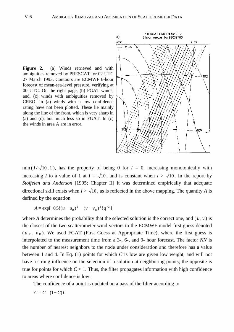
AMBIGUITY REMOVAL AND ASSIMILATION OF SCATTEROMETER DATAV-6
min ( I / 10 , 1 ), has the property of being 0 for I = 0, increasing monotonically with
increasing I to a value of 1 at I = 10 , and is constant when I > 10 . In the report by
Stoffelen and Anderson [1995; Chapter II] it was determined empirically that adequate
directional skill exists when I > 10 , as is reflected in the above mapping. The quantity A is
defined by the equation
A u u v v q= − − + − −exp[ . ( ) ( ) ]0 5 2 2 2B B
where A determines the probability that the selected solution is the correct one, and ( u, v ) is
the closest of the two scatterometer wind vectors to the ECMWF model first guess denoted
( u B , v B ). We used FGAT (First Guess at Appropriate Time), where the first guess is
interpolated to the measurement time from a 3-, 6-, and 9- hour forecast. The factor NN is
the number of nearest neighbors to the node under consideration and therefore has a value
between 1 and 4. In Eq. (1) points for which C is low are given low weight, and will not
have a strong influence on the selection of a solution at neighboring points; the opposite is
true for points for which C ≈ 1. Thus, the filter propagates information with high confidence
to areas where confidence is low.
The confidence of a point is updated on a pass of the filter according to
C C C L= + −( )1
Figure 2. (a) Winds retrieved and withambiguities removed by PRESCAT for 02 UTC27 March 1993. Contours are ECMWF 6-hourforecast of mean-sea-level pressure, verifying at00 UTC. On the right page, (b) FGAT winds,and, (c) winds with ambiguities removed byCREO. In (a) winds with a low confidencerating have not been plotted. These lie mainlyalong the line of the front, which is very sharp in(a) and (c), but much less so in FGAT. In (c)the winds in area A are in error.
a)
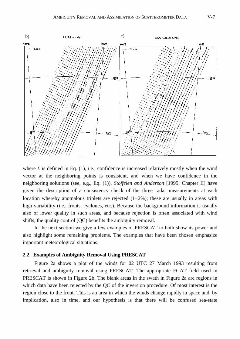
AMBIGUITY REMOVAL AND ASSIMILATION OF SCATTEROMETER DATA V-7
where L is defined in Eq. (1), i.e., confidence is increased relatively mostly when the wind
vector at the neighboring points is consistent, and when we have confidence in the
neighboring solutions (see, e.g., Eq. (1)). Stoffelen and Anderson [1995; Chapter II] have
given the description of a consistency check of the three radar measurements at each
location whereby anomalous triplets are rejected (1−2%); these are usually in areas with
high variability (i.e., fronts, cyclones, etc.). Because the background information is usually
also of lower quality in such areas, and because rejection is often associated with wind
shifts, the quality control (QC) benefits the ambiguity removal.
In the next section we give a few examples of PRESCAT to both show its power and
also highlight some remaining problems. The examples that have been chosen emphasize
important meteorological situations.
2.2. Examples of Ambiguity Removal Using PRESCAT
Figure 2a shows a plot of the winds for 02 UTC 27 March 1993 resulting from
retrieval and ambiguity removal using PRESCAT. The appropriate FGAT field used in
PRESCAT is shown in Figure 2b. The blank areas in the swath in Figure 2a are regions in
which data have been rejected by the QC of the inversion procedure. Of most interest is the
region close to the front. This is an area in which the winds change rapidly in space and, by
implication, also in time, and our hypothesis is that there will be confused sea-state
b) c)
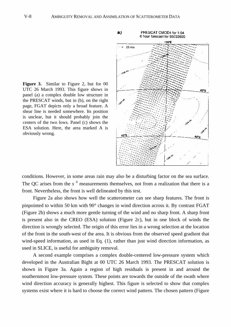
AMBIGUITY REMOVAL AND ASSIMILATION OF SCATTEROMETER DATAV-8
conditions. However, in some areas rain may also be a disturbing factor on the sea surface.
The QC arises from the σ 0 measurements themselves, not from a realization that there is a
front. Nevertheless, the front is well delineated by this test.
Figure 2a also shows how well the scatterometer can see sharp features. The front is
pinpointed to within 50 km with 90° changes in wind direction across it. By contrast FGAT
(Figure 2b) shows a much more gentle turning of the wind and no sharp front. A sharp front
is present also in the CREO (ESA) solution (Figure 2c), but in one block of winds the
direction is wrongly selected. The origin of this error lies in a wrong selection at the location
of the front in the south-west of the area. It is obvious from the observed speed gradient that
wind-speed information, as used in Eq. (1), rather than just wind direction information, as
used in SLICE, is useful for ambiguity removal.
A second example comprises a complex double-centered low-pressure system which
developed in the Australian Bight at 00 UTC 26 March 1993. The PRESCAT solution is
shown in Figure 3a. Again a region of high residuals is present in and around the
southernmost low-pressure system. These points are towards the outside of the swath where
wind direction accuracy is generally highest. This figure is selected to show that complex
systems exist where it is hard to choose the correct wind pattern. The chosen pattern (Figure
Figure 3. Similar to Figure 2, but for 00UTC 26 March 1993. This figure shows inpanel (a) a complex double low structure inthe PRESCAT winds, but in (b), on the rightpage, FGAT depicts only a broad feature. Ashear line is needed somewhere. Its positionis unclear, but it should probably join thecenters of the two lows. Panel (c) shows theESA solution. Here, the area marked A isobviously wrong.

AMBIGUITY REMOVAL AND ASSIMILATION OF SCATTEROMETER DATA V-9
3a) looks unmeteorological in the area east of the southernmost low because there are sharp
shear zones with a large shift in direction. A shear line is needed somewhere, probably
linking the centers of the two lows, rather than the one selected by PRESCAT. However, in
the forecast of surface pressure the southernmost low-pressure system and a wavelike
disturbance further to the north-east are present but shifted in position with respect to the
scatterometer-measured disturbance.
Part of the difficulty in ambiguity removal arises because the scatterometer can see
much smaller-scale features than are present in the FGAT winds (Figure 3b), which shows
only a smooth wind field. Finally, Figure 3c shows the CREO solution which is clearly
wrong in region A. Errors in PRESCAT can arise when the FGAT directions are roughly
along the direction of the wrong solution. In these cases the initially wrongly selected
solutions compare relatively well with FGAT and are assigned high confidence (Eq. (2)). If
the FGAT is close to 180° wrong for only a few isolated points, then the filter can correct
for this. If, however, the area of wrong solutions is large, then the filter is unable to make a
satisfactory correction. Errors also arise if the FGAT directions are nearly orthogonal to the
pseudo-streamline defined by the scatterometer. (The term pseudo-streamline is used rather
than streamline since the rank-1 and rank-2 directions are not exactly antiparallel.) Such
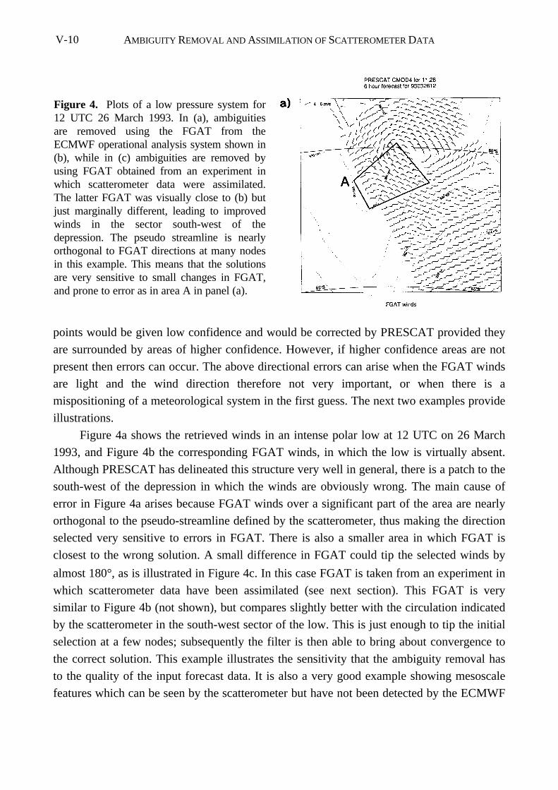
AMBIGUITY REMOVAL AND ASSIMILATION OF SCATTEROMETER DATAV-10
points would be given low confidence and would be corrected by PRESCAT provided they
are surrounded by areas of higher confidence. However, if higher confidence areas are not
present then errors can occur. The above directional errors can arise when the FGAT winds
are light and the wind direction therefore not very important, or when there is a
mispositioning of a meteorological system in the first guess. The next two examples provide
illustrations.
Figure 4a shows the retrieved winds in an intense polar low at 12 UTC on 26 March
1993, and Figure 4b the corresponding FGAT winds, in which the low is virtually absent.
Although PRESCAT has delineated this structure very well in general, there is a patch to the
south-west of the depression in which the winds are obviously wrong. The main cause of
error in Figure 4a arises because FGAT winds over a significant part of the area are nearly
orthogonal to the pseudo-streamline defined by the scatterometer, thus making the direction
selected very sensitive to errors in FGAT. There is also a smaller area in which FGAT is
closest to the wrong solution. A small difference in FGAT could tip the selected winds by
almost 180°, as is illustrated in Figure 4c. In this case FGAT is taken from an experiment in
which scatterometer data have been assimilated (see next section). This FGAT is very
similar to Figure 4b (not shown), but compares slightly better with the circulation indicated
by the scatterometer in the south-west sector of the low. This is just enough to tip the initial
selection at a few nodes; subsequently the filter is then able to bring about convergence to
the correct solution. This example illustrates the sensitivity that the ambiguity removal has
to the quality of the input forecast data. It is also a very good example showing mesoscale
features which can be seen by the scatterometer but have not been detected by the ECMWF
Figure 4. Plots of a low pressure system for12 UTC 26 March 1993. In (a), ambiguitiesare removed using the FGAT from theECMWF operational analysis system shown in(b), while in (c) ambiguities are removed byusing FGAT obtained from an experiment inwhich scatterometer data were assimilated.The latter FGAT was visually close to (b) butjust marginally different, leading to improvedwinds in the sector south-west of thedepression. The pseudo streamline is nearlyorthogonal to FGAT directions at many nodesin this example. This means that the solutionsare very sensitive to small changes in FGAT,and prone to error as in area A in panel (a).
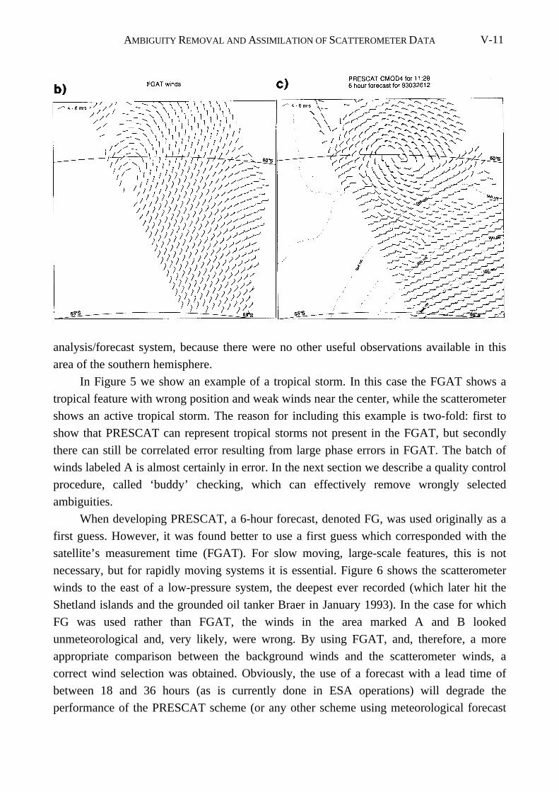
AMBIGUITY REMOVAL AND ASSIMILATION OF SCATTEROMETER DATA V-11
analysis/forecast system, because there were no other useful observations available in this
area of the southern hemisphere.
In Figure 5 we show an example of a tropical storm. In this case the FGAT shows a
tropical feature with wrong position and weak winds near the center, while the scatterometer
shows an active tropical storm. The reason for including this example is two-fold: first to
show that PRESCAT can represent tropical storms not present in the FGAT, but secondly
there can still be correlated error resulting from large phase errors in FGAT. The batch of
winds labeled A is almost certainly in error. In the next section we describe a quality control
procedure, called ‘buddy’ checking, which can effectively remove wrongly selected
ambiguities.
When developing PRESCAT, a 6-hour forecast, denoted FG, was used originally as a
first guess. However, it was found better to use a first guess which corresponded with the
satellite’s measurement time (FGAT). For slow moving, large-scale features, this is not
necessary, but for rapidly moving systems it is essential. Figure 6 shows the scatterometer
winds to the east of a low-pressure system, the deepest ever recorded (which later hit the
Shetland islands and the grounded oil tanker Braer in January 1993). In the case for which
FG was used rather than FGAT, the winds in the area marked A and B looked
unmeteorological and, very likely, were wrong. By using FGAT, and, therefore, a more
appropriate comparison between the background winds and the scatterometer winds, a
correct wind selection was obtained. Obviously, the use of a forecast with a lead time of
between 18 and 36 hours (as is currently done in ESA operations) will degrade the
performance of the PRESCAT scheme (or any other scheme using meteorological forecast
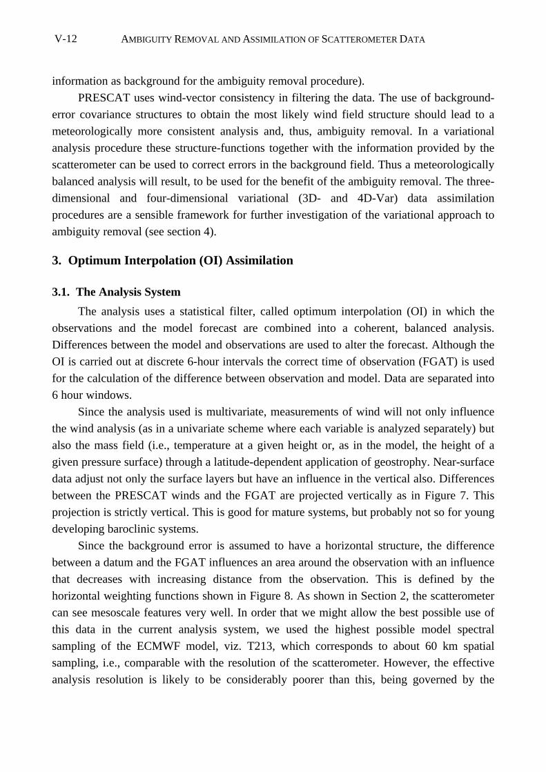
AMBIGUITY REMOVAL AND ASSIMILATION OF SCATTEROMETER DATAV-12
information as background for the ambiguity removal procedure).
PRESCAT uses wind-vector consistency in filtering the data. The use of background-
error covariance structures to obtain the most likely wind field structure should lead to a
meteorologically more consistent analysis and, thus, ambiguity removal. In a variational
analysis procedure these structure-functions together with the information provided by the
scatterometer can be used to correct errors in the background field. Thus a meteorologically
balanced analysis will result, to be used for the benefit of the ambiguity removal. The three-
dimensional and four-dimensional variational (3D- and 4D-Var) data assimilation
procedures are a sensible framework for further investigation of the variational approach to
ambiguity removal (see section 4).
3. Optimum Interpolation (OI) Assimilation
3.1. The Analysis System
The analysis uses a statistical filter, called optimum interpolation (OI) in which the
observations and the model forecast are combined into a coherent, balanced analysis.
Differences between the model and observations are used to alter the forecast. Although the
OI is carried out at discrete 6-hour intervals the correct time of observation (FGAT) is used
for the calculation of the difference between observation and model. Data are separated into
6 hour windows.
Since the analysis used is multivariate, measurements of wind will not only influence
the wind analysis (as in a univariate scheme where each variable is analyzed separately) but
also the mass field (i.e., temperature at a given height or, as in the model, the height of a
given pressure surface) through a latitude-dependent application of geostrophy. Near-surface
data adjust not only the surface layers but have an influence in the vertical also. Differences
between the PRESCAT winds and the FGAT are projected vertically as in Figure 7. This
projection is strictly vertical. This is good for mature systems, but probably not so for young
developing baroclinic systems.
Since the background error is assumed to have a horizontal structure, the difference
between a datum and the FGAT influences an area around the observation with an influence
that decreases with increasing distance from the observation. This is defined by the
horizontal weighting functions shown in Figure 8. As shown in Section 2, the scatterometer
can see mesoscale features very well. In order that we might allow the best possible use of
this data in the current analysis system, we used the highest possible model spectral
sampling of the ECMWF model, viz. T213, which corresponds to about 60 km spatial
sampling, i.e., comparable with the resolution of the scatterometer. However, the effective
analysis resolution is likely to be considerably poorer than this, being governed by the
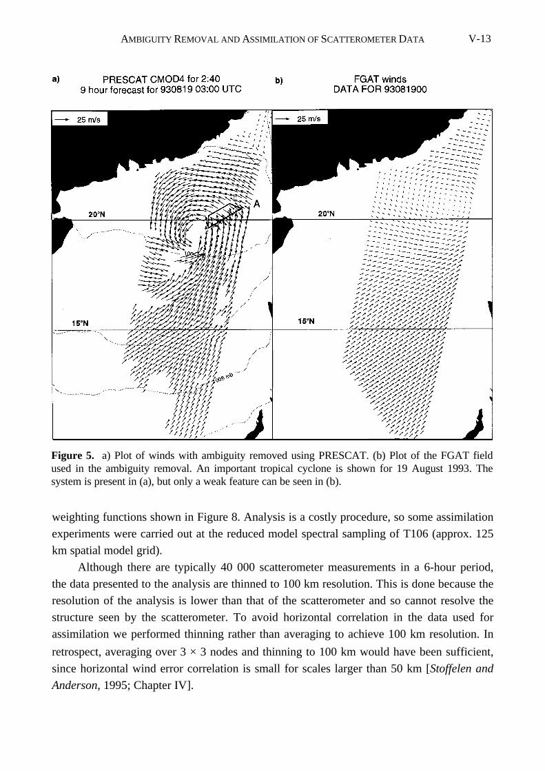
AMBIGUITY REMOVAL AND ASSIMILATION OF SCATTEROMETER DATA V-13
weighting functions shown in Figure 8. Analysis is a costly procedure, so some assimilation
experiments were carried out at the reduced model spectral sampling of T106 (approx. 125
km spatial model grid).
Although there are typically 40 000 scatterometer measurements in a 6-hour period,
the data presented to the analysis are thinned to 100 km resolution. This is done because the
resolution of the analysis is lower than that of the scatterometer and so cannot resolve the
structure seen by the scatterometer. To avoid horizontal correlation in the data used for
assimilation we performed thinning rather than averaging to achieve 100 km resolution. In
retrospect, averaging over 3 × 3 nodes and thinning to 100 km would have been sufficient,
since horizontal wind error correlation is small for scales larger than 50 km [Stoffelen and
Anderson, 1995; Chapter IV].
Figure 5. a) Plot of winds with ambiguity removed using PRESCAT. (b) Plot of the FGAT fieldused in the ambiguity removal. An important tropical cyclone is shown for 19 August 1993. Thesystem is present in (a), but only a weak feature can be seen in (b).
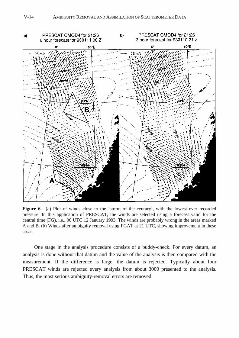
AMBIGUITY REMOVAL AND ASSIMILATION OF SCATTEROMETER DATAV-14
One stage in the analysis procedure consists of a buddy-check. For every datum, an
analysis is done without that datum and the value of the analysis is then compared with the
measurement. If the difference is large, the datum is rejected. Typically about four
PRESCAT winds are rejected every analysis from about 3000 presented to the analysis.
Thus, the most serious ambiguity-removal errors are removed.
Figure 6. (a) Plot of winds close to the ‘storm of the century’, with the lowest ever recordedpressure. In this application of PRESCAT, the winds are selected using a forecast valid for thecentral time (FG), i.e., 00 UTC 12 January 1993. The winds are probably wrong in the areas markedA and B. (b) Winds after ambiguity removal using FGAT at 21 UTC, showing improvement in theseareas.
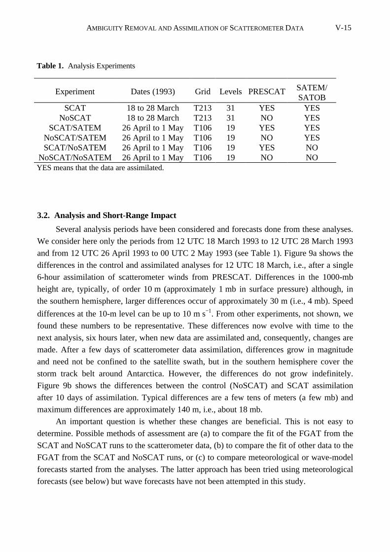
AMBIGUITY REMOVAL AND ASSIMILATION OF SCATTEROMETER DATA V-15
3.2. Analysis and Short-Range Impact
Several analysis periods have been considered and forecasts done from these analyses.
We consider here only the periods from 12 UTC 18 March 1993 to 12 UTC 28 March 1993
and from 12 UTC 26 April 1993 to 00 UTC 2 May 1993 (see Table 1). Figure 9a shows the
differences in the control and assimilated analyses for 12 UTC 18 March, i.e., after a single
6-hour assimilation of scatterometer winds from PRESCAT. Differences in the 1000-mb
height are, typically, of order 10 m (approximately 1 mb in surface pressure) although, in
the southern hemisphere, larger differences occur of approximately 30 m (i.e., 4 mb). Speed
differences at the 10-m level can be up to 10 m s−1. From other experiments, not shown, we
found these numbers to be representative. These differences now evolve with time to the
next analysis, six hours later, when new data are assimilated and, consequently, changes are
made. After a few days of scatterometer data assimilation, differences grow in magnitude
and need not be confined to the satellite swath, but in the southern hemisphere cover the
storm track belt around Antarctica. However, the differences do not grow indefinitely.
Figure 9b shows the differences between the control (NoSCAT) and SCAT assimilation
after 10 days of assimilation. Typical differences are a few tens of meters (a few mb) and
maximum differences are approximately 140 m, i.e., about 18 mb.
An important question is whether these changes are beneficial. This is not easy to
determine. Possible methods of assessment are (a) to compare the fit of the FGAT from the
SCAT and NoSCAT runs to the scatterometer data, (b) to compare the fit of other data to the
FGAT from the SCAT and NoSCAT runs, or (c) to compare meteorological or wave-model
forecasts started from the analyses. The latter approach has been tried using meteorological
forecasts (see below) but wave forecasts have not been attempted in this study.
Table 1. Analysis Experiments
Experiment Dates (1993) Grid Levels PRESCAT SATEM/SATOB
SCAT 18 to 28 March T213 31 YES YESNoSCAT 18 to 28 March T213 31 NO YES
SCAT/SATEM 26 April to 1 May T106 19 YES YESNoSCAT/SATEM 26 April to 1 May T106 19 NO YESSCAT/NoSATEM 26 April to 1 May T106 19 YES NO
NoSCAT/NoSATEM 26 April to 1 May T106 19 NO NOYES means that the data are assimilated.
AMBIGUITY REMOVAL AND ASSIMILATION OF SCATTEROMETER DATAV-16
As illustrated in Figures 2-5, the synoptic detail possessed by scatterometer data is
significantly greater than in the ECMWF model fields and, on a 100 km scale, scatterometer
errors are random rather than correlated [Stoffelen and Anderson, 1995; Chapters II and IV].
We do expect, therefore, an impact from scatterometer data on the smaller spatial scales
and, as a consequence, also on the shorter time scales. To measure the improvement on hese
scales in the ECMWF analysis/forecasting system, the same experiments have been verified
by direct comparison with observations. In Table 2 we show a comparison between
departure statistics of scatterometer minus FGAT winds for the experiment SCAT and the
control NoSCAT, averaged over twelve 6-hour windows near the end of the experiment.
Vector root-mean-square (RMS) departures are improved by approximately 5%. Because of
the polar orbit each location is generally sampled twice a day, therefore passes 6 hours apart
are generally well separated geographically and passes 12 hours apart fall in similar
geographical areas. The departure statistics are therefore a verification of information from
the scatterometer assimilated at least twelve hours earlier.
Figure 7. Vertical correlation function in the OI system used to extend surface wind increments inthe vertical: (a) mid latitudes; (b) tropics. Continuous line: non-divergent wind componentcovariance. Dotted line: divergent covariance (from Undén [1989]).
AMBIGUITY REMOVAL AND ASSIMILATION OF SCATTEROMETER DATA V-17
AMBIGUITY REMOVAL AND ASSIMILATION OF SCATTEROMETER DATAV-18
Table 2. Comparison of PRESCAT Winds With Experiment SCAT and NoSCAT
FGAT SCAT 930324:12, Twelve 6-hour steps
NodeNumber
(> 4 m s−1)Bias
(degrees)SD
(degrees)Number
all speedsBias
(m s−1)SD
(m s−1)Vector RMS
(m s−1)
1 10089 −0.41 31.15 13203 −0.61 1.77 3.923 10109 0.42 24.49 13398 −0.59 1.72 3.305 10137 0.73 21.90 13560 −0.48 1.72 3.107 10008 1.01 20.48 13627 −0.39 1.77 3.049 9849 1.13 19.76 13547 −0.30 1.81 3.05
11 9722 1.47 19.10 13462 −0.26 1.83 3.0413 9546 1.28 18.96 13291 −0.29 1.83 3.0215 9306 1.69 18.65 12986 −0.32 1.84 3.0117 9118 1.87 18.52 12680 −0.32 1.86 3.0219 8963 2.37 19.62 12316 −0.33 1.85 3.03
FGAT NoSCAT 930324:12, Twelve 6-hour steps
NodeNumber
(> 4 m s−1)Bias
(degrees)SD
(degrees)Number
all speedsBias
(m s−1)SD
(m s−1)Vector RMS
(m s−1)
1 10040 −0.89 32.14 13203 −0.64 1.88 4.063 10054 −0.11 25.75 13398 −0.61 1.83 3.465 10097 0.34 22.79 13560 −0.51 1.83 3.247 9971 0.80 21.47 13627 −0.42 1.87 3.199 9833 0.99 21.06 13547 −0.34 1.91 3.20
11 9743 1.37 20.60 13462 −0.30 1.94 3.2013 9564 1.40 20.48 13291 −0.33 1.93 3.1815 9310 1.70 20.08 12986 −0.36 1.93 3.1717 9078 1.94 19.91 12680 −0.36 1.95 3.1919 8941 2.33 20.59 12316 −0.37 1.94 3.20
For all nodes, the bias and SD of the FGAT and scatterometer wind differences and the vector RMSdifferences are smaller in SCAT than in NoSCAT, indicating that the SCAT FGAT has a betterquality.
AMBIGUITY REMOVAL AND ASSIMILATION OF SCATTEROMETER DATA V-19
Figure 9. Differencesbetween an analysis inwhich PRESCAT windsare assimilated (SCAT)and a control (NoSCAT)in which they are not used,(a) after the firstassimilation, (b) after 10days of assimilation. Fieldshown is the height of the1000-hPa surface. In (a)the contour interval is 2 m;in (b) 10 m. Impactincreases with time.
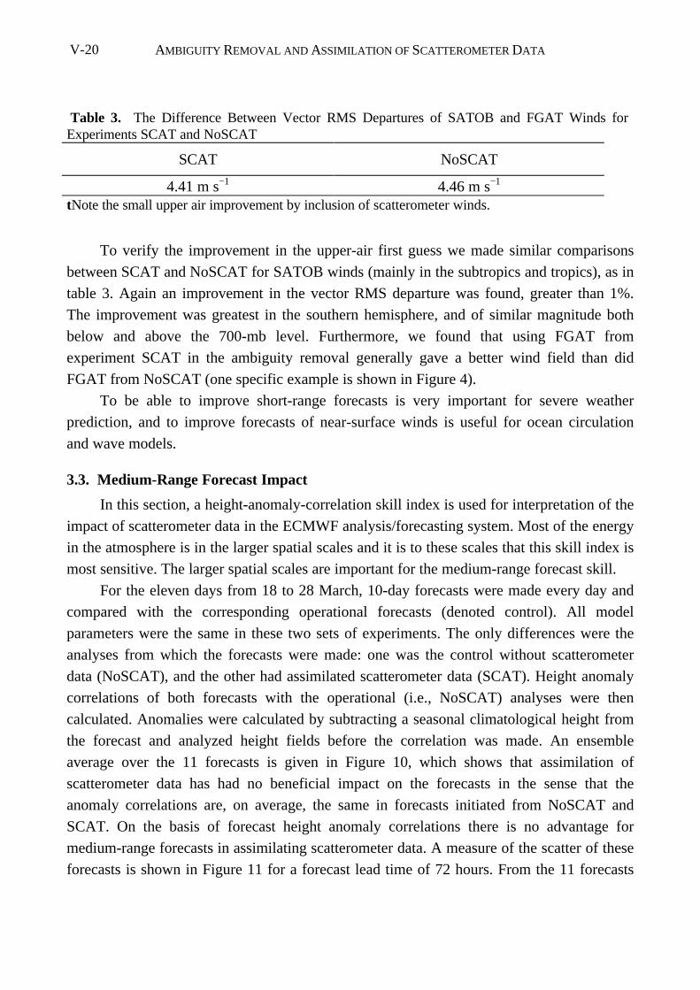
AMBIGUITY REMOVAL AND ASSIMILATION OF SCATTEROMETER DATAV-20
To verify the improvement in the upper-air first guess we made similar comparisons
between SCAT and NoSCAT for SATOB winds (mainly in the subtropics and tropics), as in
table 3. Again an improvement in the vector RMS departure was found, greater than 1%.
The improvement was greatest in the southern hemisphere, and of similar magnitude both
below and above the 700-mb level. Furthermore, we found that using FGAT from
experiment SCAT in the ambiguity removal generally gave a better wind field than did
FGAT from NoSCAT (one specific example is shown in Figure 4).
To be able to improve short-range forecasts is very important for severe weather
prediction, and to improve forecasts of near-surface winds is useful for ocean circulation
and wave models.
3.3. Medium-Range Forecast Impact
In this section, a height-anomaly-correlation skill index is used for interpretation of the
impact of scatterometer data in the ECMWF analysis/forecasting system. Most of the energy
in the atmosphere is in the larger spatial scales and it is to these scales that this skill index is
most sensitive. The larger spatial scales are important for the medium-range forecast skill.
For the eleven days from 18 to 28 March, 10-day forecasts were made every day and
compared with the corresponding operational forecasts (denoted control). All model
parameters were the same in these two sets of experiments. The only differences were the
analyses from which the forecasts were made: one was the control without scatterometer
data (NoSCAT), and the other had assimilated scatterometer data (SCAT). Height anomaly
correlations of both forecasts with the operational (i.e., NoSCAT) analyses were then
calculated. Anomalies were calculated by subtracting a seasonal climatological height from
the forecast and analyzed height fields before the correlation was made. An ensemble
average over the 11 forecasts is given in Figure 10, which shows that assimilation of
scatterometer data has had no beneficial impact on the forecasts in the sense that the
anomaly correlations are, on average, the same in forecasts initiated from NoSCAT and
SCAT. On the basis of forecast height anomaly correlations there is no advantage for
medium-range forecasts in assimilating scatterometer data. A measure of the scatter of these
forecasts is shown in Figure 11 for a forecast lead time of 72 hours. From the 11 forecasts
Table 3. The Difference Between Vector RMS Departures of SATOB and FGAT Winds forExperiments SCAT and NoSCAT
SCAT NoSCAT
4.41 m s−1 4.46 m s−1
tNote the small upper air improvement by inclusion of scatterometer winds.
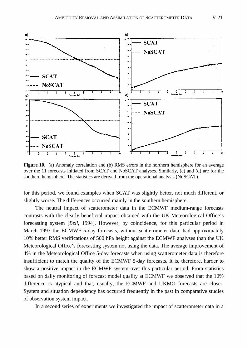
AMBIGUITY REMOVAL AND ASSIMILATION OF SCATTEROMETER DATA V-21
for this period, we found examples when SCAT was slightly better, not much different, or
slightly worse. The differences occurred mainly in the southern hemisphere.
The neutral impact of scatterometer data in the ECMWF medium-range forecasts
contrasts with the clearly beneficial impact obtained with the UK Meteorological Office’s
forecasting system [Bell, 1994]. However, by coincidence, for this particular period in
March 1993 the ECMWF 5-day forecasts, without scatterometer data, had approximately
10% better RMS verifications of 500 hPa height against the ECMWF analyses than the UK
Meteorological Office’s forecasting system not using the data. The average improvement of
4% in the Meteorological Office 5-day forecasts when using scatterometer data is therefore
insufficient to match the quality of the ECMWF 5-day forecasts. It is, therefore, harder to
show a positive impact in the ECMWF system over this particular period. From statistics
based on daily monitoring of forecast model quality at ECMWF we observed that the 10%
difference is atypical and that, usually, the ECMWF and UKMO forecasts are closer.
System and situation dependency has occurred frequently in the past in comparative studies
of observation system impact.
In a second series of experiments we investigated the impact of scatterometer data in a
Figure 10. (a) Anomaly correlation and (b) RMS errors in the northern hemisphere for an averageover the 11 forecasts initiated from SCAT and NoSCAT analyses. Similarly, (c) and (d) are for thesouthern hemisphere. The statistics are derived from the operational analysis (NoSCAT).
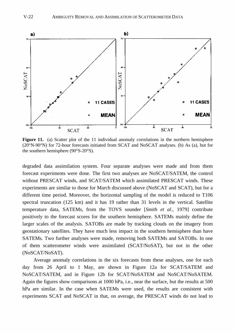
AMBIGUITY REMOVAL AND ASSIMILATION OF SCATTEROMETER DATAV-22
degraded data assimilation system. Four separate analyses were made and from them
forecast experiments were done. The first two analyses are NoSCAT/SATEM, the control
without PRESCAT winds, and SCAT/SATEM which assimilated PRESCAT winds. These
experiments are similar to those for March discussed above (NoSCAT and SCAT), but for a
different time period. Moreover, the horizontal sampling of the model is reduced to T106
spectral truncation (125 km) and it has 19 rather than 31 levels in the vertical. Satellite
temperature data, SATEMs, from the TOVS sounder [Smith et al., 1979] contribute
positively to the forecast scores for the southern hemisphere. SATEMs mainly define the
larger scales of the analysis. SATOBs are made by tracking clouds on the imagery from
geostationary satellites. They have much less impact in the southern hemisphere than have
SATEMs. Two further analyses were made, removing both SATEMs and SATOBs. In one
of them scatterometer winds were assimilated (SCAT/NoSAT), but not in the other
(NoSCAT/NoSAT).
Average anomaly correlations in the six forecasts from these analyses, one for each
day from 26 April to 1 May, are shown in Figure 12a for SCAT/SATEM and
NoSCAT/SATEM, and in Figure 12b for SCAT/NoSATEM and NoSCAT/NoSATEM.
Again the figures show comparisons at 1000 hPa, i.e., near the surface, but the results at 500
hPa are similar. In the case when SATEMs were used, the results are consistent with
experiments SCAT and NoSCAT in that, on average, the PRESCAT winds do not lead to
Figure 11. (a) Scatter plot of the 11 individual anomaly correlations in the northern hemisphere(20°N-90°N) for 72-hour forecasts initiated from SCAT and NoSCAT analyses. (b) As (a), but forthe southern hemisphere (90°S-20°S).
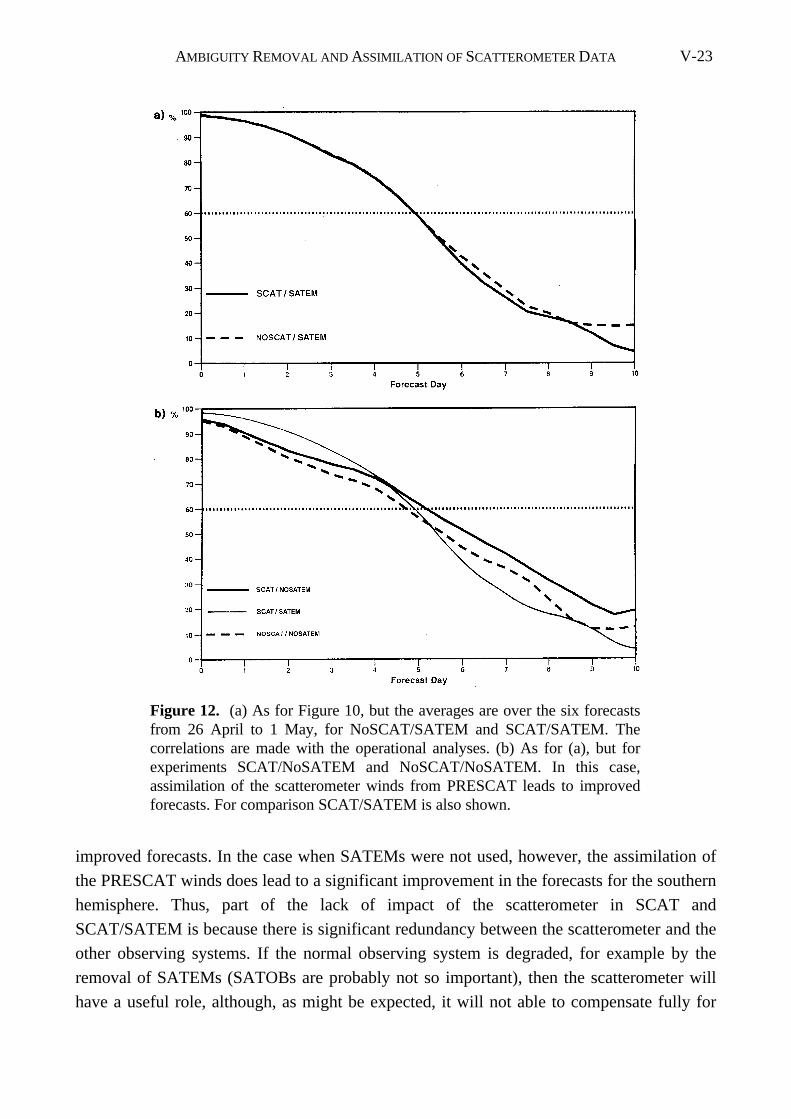
AMBIGUITY REMOVAL AND ASSIMILATION OF SCATTEROMETER DATA V-23
improved forecasts. In the case when SATEMs were not used, however, the assimilation of
the PRESCAT winds does lead to a significant improvement in the forecasts for the southern
hemisphere. Thus, part of the lack of impact of the scatterometer in SCAT and
SCAT/SATEM is because there is significant redundancy between the scatterometer and the
other observing systems. If the normal observing system is degraded, for example by the
removal of SATEMs (SATOBs are probably not so important), then the scatterometer will
have a useful role, although, as might be expected, it will not able to compensate fully for
Figure 12. (a) As for Figure 10, but the averages are over the six forecastsfrom 26 April to 1 May, for NoSCAT/SATEM and SCAT/SATEM. Thecorrelations are made with the operational analyses. (b) As for (a), but forexperiments SCAT/NoSATEM and NoSCAT/NoSATEM. In this case,assimilation of the scatterometer winds from PRESCAT leads to improvedforecasts. For comparison SCAT/SATEM is also shown.
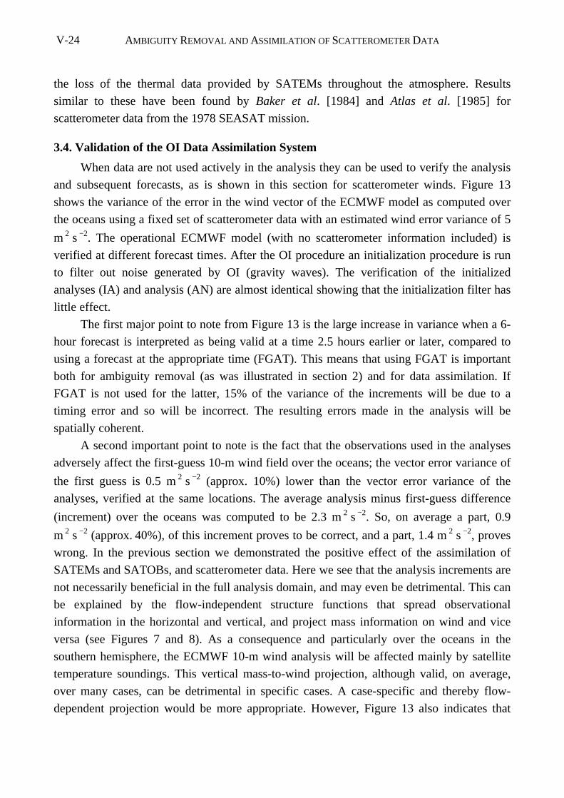
AMBIGUITY REMOVAL AND ASSIMILATION OF SCATTEROMETER DATAV-24
the loss of the thermal data provided by SATEMs throughout the atmosphere. Results
similar to these have been found by Baker et al. [1984] and Atlas et al. [1985] for
scatterometer data from the 1978 SEASAT mission.
3.4. Validation of the OI Data Assimilation System
When data are not used actively in the analysis they can be used to verify the analysis
and subsequent forecasts, as is shown in this section for scatterometer winds. Figure 13
shows the variance of the error in the wind vector of the ECMWF model as computed over
the oceans using a fixed set of scatterometer data with an estimated wind error variance of 5
m 2 s −2. The operational ECMWF model (with no scatterometer information included) is
verified at different forecast times. After the OI procedure an initialization procedure is run
to filter out noise generated by OI (gravity waves). The verification of the initialized
analyses (IA) and analysis (AN) are almost identical showing that the initialization filter has
little effect.
The first major point to note from Figure 13 is the large increase in variance when a 6-
hour forecast is interpreted as being valid at a time 2.5 hours earlier or later, compared to
using a forecast at the appropriate time (FGAT). This means that using FGAT is important
both for ambiguity removal (as was illustrated in section 2) and for data assimilation. If
FGAT is not used for the latter, 15% of the variance of the increments will be due to a
timing error and so will be incorrect. The resulting errors made in the analysis will be
spatially coherent.
A second important point to note is the fact that the observations used in the analyses
adversely affect the first-guess 10-m wind field over the oceans; the vector error variance of
the first guess is 0.5 m 2 s −2 (approx. 10%) lower than the vector error variance of the
analyses, verified at the same locations. The average analysis minus first-guess difference
(increment) over the oceans was computed to be 2.3 m 2 s −2. So, on average a part, 0.9
m 2 s −2 (approx. 40%), of this increment proves to be correct, and a part, 1.4 m 2 s −2, proves
wrong. In the previous section we demonstrated the positive effect of the assimilation of
SATEMs and SATOBs, and scatterometer data. Here we see that the analysis increments are
not necessarily beneficial in the full analysis domain, and may even be detrimental. This can
be explained by the flow-independent structure functions that spread observational
information in the horizontal and vertical, and project mass information on wind and vice
versa (see Figures 7 and 8). As a consequence and particularly over the oceans in the
southern hemisphere, the ECMWF 10-m wind analysis will be affected mainly by satellite
temperature soundings. This vertical mass-to-wind projection, although valid, on average,
over many cases, can be detrimental in specific cases. A case-specific and thereby flow-
dependent projection would be more appropriate. However, Figure 13 also indicates that
AMBIGUITY REMOVAL AND ASSIMILATION OF SCATTEROMETER DATA V-25
during the 6-hour forecast the 10-m winds are again properly balanced (baroclinically) with
the upper-air dynamics and become more realistic.
In section 3.3, we suggested that the analysis of scatterometer surface winds probably
also adversely affects the upper-air mass field for the same reason. As a result, the mass
corrections induced by the scatterometer would contradict the SATEM mass analysis-
increments. Conversely, surface wind increments induced by SATEMs will contradict
scatterometer wind information. It is, therefore, worthwhile that further investigation of
these effects be carried out to make observational systems more complementary.
Figure 13. Wind vector error variance of the ECMWF model at a fixed setof scatterometer nodes. The wind vector error variance of the scatterometerobservations was estimated to be 5 m 2 s −2. The solid line represents from leftto right the analysis, FG, and forecasts with different lead times (lead 0corresponds to the analysis and a lead time of 6 hours to the FG). Thesymbol Ο is the initialized analysis. For this set, the time difference betweenscatterometer observations and the corresponding field values is less than 1hour. The squares represent verification against another set of scatterometerwinds that are between 2 and 3 hours from the FG verification time; solidsquares FG and open squares FGAT.
AMBIGUITY REMOVAL AND ASSIMILATION OF SCATTEROMETER DATAV-26
Recent studies show that in a 4D-Var system baroclinic structures can be enforced by
assimilating surface (i.e., scatterometer) data [Thépaut et al., 1993], by using the time
trajectory of the forecast model. The fact that in a 6-hour forecast the surface balance is
restored, indicates that this is a promising technique which, potentially, can overcome a
weakness in 3D methods.
4. Variational Methods
A variational assimilation scheme [Le Dimet and Talagrand, 1986] consists in the
minimization of a cost function, i.e.,
ℑ = ℑ + ℑ + ℑO B C (3)
where ℑ O is a weighted quadratic term which measures the differences between the
estimated control variables and the observations, and ℑ B is a quadratic term measuring the
difference between the estimated control variables and the background field. ℑ C is a small
term expressing physical constraints on the atmospheric state. The term ℑ O describes the
observation error characteristics of all observations and is the sum of the contributions of
each individual observation. For each node the scatterometer penalty function, denoted
ℑ OSCAT, will be ambiguous where two penalty minima will exist corresponding to the two
solutions resulting from the inversion. Furthermore, it was shown by Stoffelen and Anderson
[1995; Chapter IV] that the total observation error of the unambiguous wind is well
characterized by a normal distribution around the true wind components with a standard
deviation of error of around 1.7 m s−1. In this way the observation error characteristics are
well defined in the wind domain. We will show in this section that the representation of the
total observation error in the σσ 0 domain is much more complex due to the highly nonlinear
relationship between σσ 0 and wind, and conclude that it is therefore more practical to define
ℑ OSCAT in the wind domain. At the end of the section we discuss the ambiguity in ℑ O
SCAT
and show that the meteorological balance constraints incorporated in the ℑ B term result
implicitly in a beneficial ambiguity removal of scatterometer data in 3D-Var.
Stoffelen and Anderson [1995; Chapter II] showed that σσ 0O for each node depends,
essentially, on two parameters. Consequently the distribution of σσ 0O triplets in the 3D
measurement space is located around a 2D surface, which is cone shaped. The scatter of
triplets around this cone surface is close to the instrument accuracy (5%). In the wind
domain such an error corresponds to a 0.5 m s−1 vector RMS error, i.e., it is very small.
Following Lorenc [1988], we may specify the contribution of scatterometer data to the
cost function in the form
ℑ = −OSCAT
O2 ln ( | )p σσ 0 V (4)
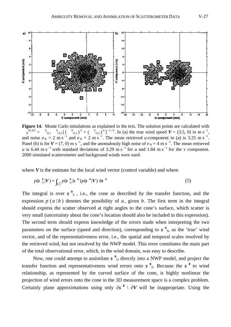
AMBIGUITY REMOVAL AND ASSIMILATION OF SCATTEROMETER DATA V-27
where V is the estimate for the local wind vector (control variable) and where
p p p( | ) ( | ) ( | )σσ σσ σσ σσ σσσσO O d
S
0 0 0 0 00
V V= ∫ (5)
The integral is over σσ 0S , i.e., the cone as described by the transfer function, and the
expression p ( α | β ) denotes the possibility of α, given β. The first term in the integral
should express the scatter observed at right angles to the cone’s surface, which scatter is
very small (uncertainty about the cone’s location should also be included in this expression).
The second term should express knowledge of the errors made when interpreting the two
parameters on the surface (speed and direction), corresponding to σσ 0S, as the ‘true’ wind
vector, and of the representativeness error, i.e., the spatial and temporal scales resolved by
the retrieved wind, but not resolved by the NWP model. This error constitutes the main part
of the total observational error, which, in the wind domain, was easy to describe.
Now, one could attempt to assimilate σσ 0O directly into a NWP model, and project the
transfer function and representativeness wind errors onto σσ 0S. Because the σσ 0 to wind
relationship, as represented by the curved surface of the cone, is highly nonlinear the
projection of wind errors onto the cone in the 3D measurement space is a complex problem.
Certainly plane approximations using only ∂σσ 0 \ ∂V will be inappropriate. Using the
Figure 14. Monte Carlo simulations as explained in the text. The solution points are calculated withℑ O
SCAT = ℑ S
O,1 ℑ S
O,2 [ ( ℑ S
O,1 ) 4 + ( ℑ
SO,2 )
4 ]
−1 / 4. In (a) the true wind speed V = (3.5, 0) in m s −1,and noise ε R = 2 m s −1 and ε B = 2 m s −1. The mean retrieved u-component in (a) is 3.25 m s −1.Panel (b) is for V = (7, 0) m s −1, and the anomalously high noise of ε B = 4 m s −1. The mean retrievedu is 6.44 m s −1 with standard deviations of 3.29 m s −1 for u and 1.84 m s −1 for the v component.2000 simulated scatterometer and background winds were used.
AMBIGUITY REMOVAL AND ASSIMILATION OF SCATTEROMETER DATAV-28
curvature, i.e., ∂ 2σσ 0 \ ∂V 2, should be better, although still not perfect, and will certainly
result in an algorithm of substantial mathematical complexity and computational cost.
Moreover, in an attempt to strive for mathematical elegance, one might forget that the
uncertainties regarding our knowledge of ∂ 2σσ 0 \ ∂V 2 may be a limiting factor.
Alternatively, one could try to formulate the problem in terms of wind. For this
purpose, we would have to make some approximations concerning Eq. (5). As mentioned
above, we can identify accurately the most likely ‘true’ position of a measured σ 0 triplet on
the cone’s surface, and this inversion only results in a small contribution to the overall wind
error of scatterometer winds, and so may be neglected. Therefore, replacing p( σσ 0
O | σσ
0S ) by
p( σσ 0
R | σσ
0S ), with σσ 0
R as derived from the inversion, we have a valid approximation. The
retrieval has multiple solutions σσ 0R,i
because of the 180° ambiguity, and therefore the first
term in the integral will be a sum of p ( σσ 0
R,i | σσ
0S ) / n, with i = 1, ..., n, the solution index
where n = 2. Stoffelen and Anderson [1995; Chapter II] found that the two solutions have
almost equal probability and therefore we have assumed no skill in the distinction of the
different σσ 0R,i
, i.e., all solutions have probability 1 / n.
The neglect of σσ 0 measurement errors in 3D σσ 0-space allows a further replacement of
p ( σσ 0
R,i | σσ
0S ) with a Kronecker delta function of the form δ ( σσ
0R,i
− σσ 0
S ). After integration
and using the transfer function to map σσ 0R,i
onto the retrieved winds VR,i , Eq. (5) reduces to
p p p( | ) ( | ) / ( | ) /, ,σσ O R R0 V V V V V= +1 22 2
As such, the formulation of the problem in wind space only needs a proper characterization
of the sum of transfer-function error and the representativeness error in wind space. We may
assume that
p p N( | ) ( | ) ( , )V V V V VA A A R= = εε
for an unambiguous scatterometer wind VA , i.e., normally distributed around the
components of VA with error εε R . Similarly, for the ambiguous solutions we may write
p N N( | ) ( , ) / ( , ) /, ,σσ εεO R R R R0 V V V= +1 22 2ε
From Eq. (4) we can derive the scatterometer cost function, which will not be quadratic,
particularly when
V VR R R, ,1 2− ≤ εε
Moreover, in these cases we find only one minimum at V = 0.
An alternative analytic formulation can be found, that describes a conditional
functionality in terms of the penalty function ℑ OSCAT
AMBIGUITY REMOVAL AND ASSIMILATION OF SCATTEROMETER DATA V-29
ℑ =
∏∑
OSCAT
K
K
ii
ii
P2
2
1
(6)
where P = 4; K i = [ ℑ S
O,i ( VR,i ) ]
P, and ℑ S
O,i characterizes the estimated scatterometer wind
error for one single solution, and is considered to be quadratic, as before. For low wind
speeds this ℑ OSCAT cost function also has two minima located at VR,1 and VR,2
, and a
quadratic dependency on V in almost the entire speed domain, except close to V − VR,1 = V −VR,2
. Therefore, this formulation has more symmetry around its minima. For P < 4 we have
a weaker gradient towards the minima, or in other words, exact ambiguity removal will be
less of a constraint and intermediate solutions will be more likely. This is also the case for
the cost function that was derived in the previous paragraph. From our experience with
ambiguity removal we believe that a strong constraint for ambiguity removal is more
appropriate; but this could be tested further.
To investigate the statistical consequence of the cost-function formulation, we
performed Monte Carlo simulations. The terms VR,1 and VR,2 (= −VR,1 ), and a background
wind VB , we simulated for a given V using respectively a Gaussian wind-component error
εε R for the scatterometer, and εε B for the background wind (in fact εε B characterizes the
accuracy of all available information, except the observation under investigation). Figure
14a shows a result when minimizing Eq. (3) with the above scatterometer cost function, for
2000 trials. Ambiguity removal is generally successful for a speed as low as 3.5 m s−1.
Figure 14b shows the distribution of solutions for 2000 simulations, but in this case ε B = 4
m s−1 and V = 7 m s−1. As expected, it can be seen that ambiguity removal is less successful
with reduced supporting background information. The statistical difference between the two
proposed cost functions is marginal and, therefore, because of its more symmetric and
quadratic behavior the functionality in Eq. (6) may be more desirable to use in a
minimization. With this equation, we have arrived at a practical and accurate solution for the
variational assimilation of scatterometer observations.
Preliminary results with a 3D-Var analysis system show that ambiguity removal is
done accurately, and a large-scale compromise is easily found in complicated situations, as
illustrated in Figure 15 (see also Stoffelen et al [1993]).
5. Summary and Conclusions
We have developed an ambiguity-removal scheme, called PRESCAT, as an alternative
to CREO and SLICE, based on the following guidelines,
(i) that information on wind-direction retrieval skill is an important input to ambiguity
removal,
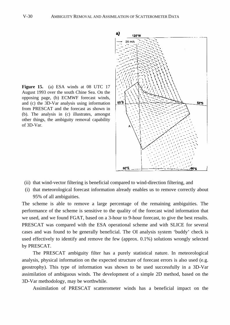
AMBIGUITY REMOVAL AND ASSIMILATION OF SCATTEROMETER DATAV-30
(ii) that wind-vector filtering is beneficial compared to wind-direction filtering, and
(i) that meteorological forecast information already enables us to remove correctly about
95% of all ambiguities.
The scheme is able to remove a large percentage of the remaining ambiguities. The
performance of the scheme is sensitive to the quality of the forecast wind information that
we used, and we found FGAT, based on a 3-hour to 9-hour forecast, to give the best results.
PRESCAT was compared with the ESA operational scheme and with SLICE for several
cases and was found to be generally beneficial. The OI analysis system ‘buddy’ check is
used effectively to identify and remove the few (approx. 0.1%) solutions wrongly selected
by PRESCAT.
The PRESCAT ambiguity filter has a purely statistical nature. In meteorological
analysis, physical information on the expected structure of forecast errors is also used (e.g.
geostrophy). This type of information was shown to be used successfully in a 3D-Var
assimilation of ambiguous winds. The development of a simple 2D method, based on the
3D-Var methodology, may be worthwhile.
Assimilation of PRESCAT scatterometer winds has a beneficial impact on the
Figure 15. (a) ESA winds at 08 UTC 17August 1993 over the south Chine Sea. On theopposing page, (b) ECMWF forecast winds,and (c) the 3D-Var analysis using informationfrom PRESCAT and the forecast as shown in(b). The analysis in (c) illustrates, amongstother things, the ambiguity removal capabilityof 3D-Var.
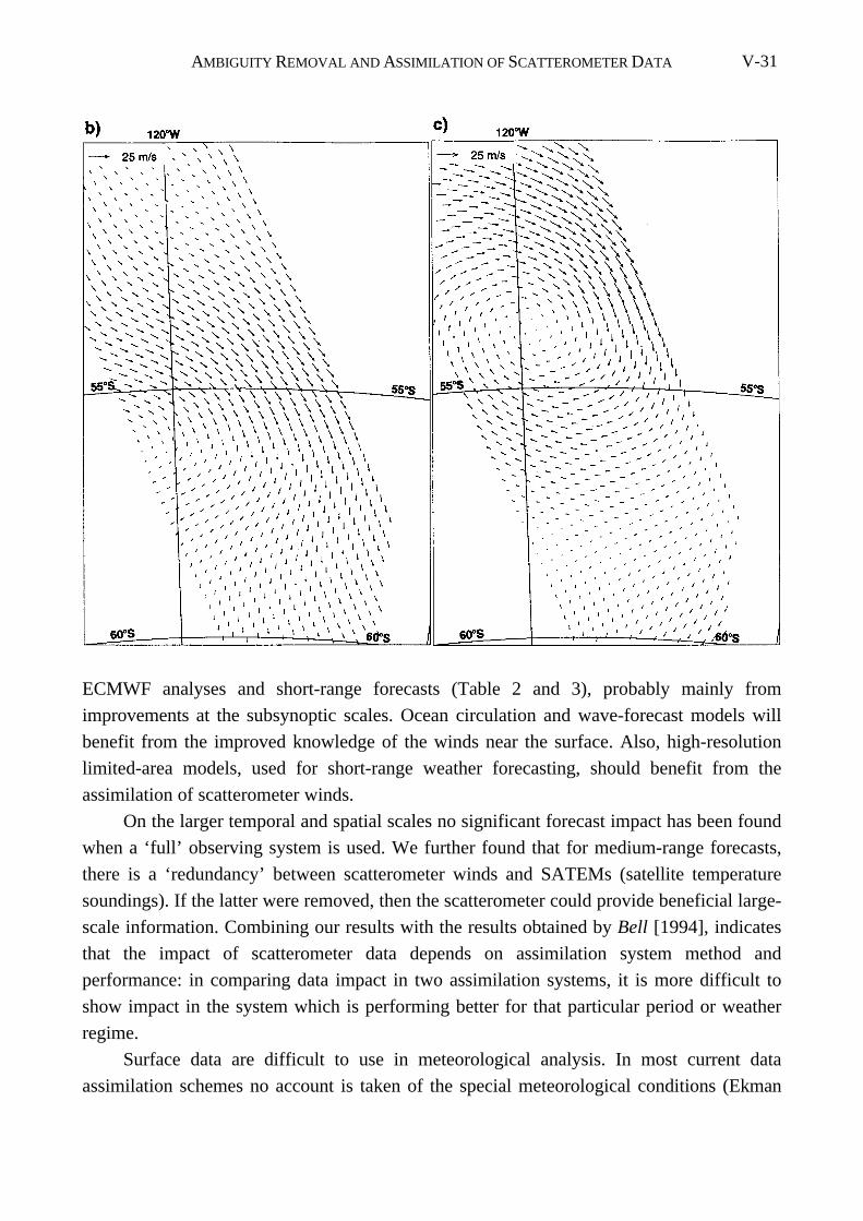
AMBIGUITY REMOVAL AND ASSIMILATION OF SCATTEROMETER DATA V-31
ECMWF analyses and short-range forecasts (Table 2 and 3), probably mainly from
improvements at the subsynoptic scales. Ocean circulation and wave-forecast models will
benefit from the improved knowledge of the winds near the surface. Also, high-resolution
limited-area models, used for short-range weather forecasting, should benefit from the
assimilation of scatterometer winds.
On the larger temporal and spatial scales no significant forecast impact has been found
when a ‘full’ observing system is used. We further found that for medium-range forecasts,
there is a ‘redundancy’ between scatterometer winds and SATEMs (satellite temperature
soundings). If the latter were removed, then the scatterometer could provide beneficial large-
scale information. Combining our results with the results obtained by Bell [1994], indicates
that the impact of scatterometer data depends on assimilation system method and
performance: in comparing data impact in two assimilation systems, it is more difficult to
show impact in the system which is performing better for that particular period or weather
regime.
Surface data are difficult to use in meteorological analysis. In most current data
assimilation schemes no account is taken of the special meteorological conditions (Ekman
AMBIGUITY REMOVAL AND ASSIMILATION OF SCATTEROMETER DATAV-32
spiral) in the planetary boundary layer (PBL). Further, the structure functions are defined in
a climatological sense and do not take into account the fact that the structure of error in the
first guess will depend on meteorological conditions. The spatial structures used to update
the background to fit e.g. surface observations will therefore partly be inappropriate to
change the upper-air background field and, conversely, upper-air observations may have
adverse effects on the surface analysis. In particular, it was shown that the global ECMWF
analysis of surface wind is of a quality slightly lower than the first-guess winds, as
measured by scatterometer data. When scatterometer data are used they oppose such
increment structures that deteriorate the surface wind forecasts. Further investigations are
needed to make the different observational systems more complementary and useful.
The above is a weakness also in 3D-Var, but in a 4D-Var assimilation scheme the
sensitivity of the time trajectory of the forecast model to external forcing will mainly
determine the structure of change in the model owing to an observation at a particular time
and location. This will make the 4D-Var analysis meteorologically better balanced than its
3D equivalent and should lead to a more beneficial modification of upper-air fields in
response to changes in the PBL.
In addition we showed that scatterometer backscatter measurements are difficult to
assimilate directly, and we derived and illustrated a procedure for the assimilation of
ambiguous winds.
Acknowledgments. It is a pleasure to acknowledge the constructive discussions we
have had with members of the ESA analysis team and with ECMWF staff and visitors.
Catherine Gaffard implemented the scatterometer processing in IFS under EUMETSAT
funding. The other work was carried out at ECMWF under ESA contract 9097/90/NL/BI.
Two anonymous reviewers helped by providing useful comments.
References
Anderson, D. L. T., A. Hollingsworth, S. Uppala and P. M. Woiceshyn, A study of the use
of scatterometer data in the ECMWF operational analysis - forecast model Part II: Data
impact, J. Geophys. Res., 96, 2635-2647, 1991.
Atlas, R. , E. Kalnay and M. Halem, Impact of Satellite Temperature Sounding and Wind
Data on Numerical Weather Prediction, Optical Engineering, 24(2), 341-346, 1985.
Baker W. E. , R. Atlas, E. Kalnay, M. Halem, P. M. Woiceshyn, Peteherych S. and D.
Edelmann, Large scale analysis and forecasting experiments with wind data from
SEASAT-A scatterometer, J. Geophys Res., 89, 4927-4936, 1984.
Bell, R. S., Operational use of ERS-1 products in the Meteorological Office, Proc. Second
ERS-1 Symp.—Space at the Service of Our Environment, Hamburg, Germany, Eur.
Space Agency Special Publ., ESA SP-361(I), 195-200, ESA, Noordwijk, the
AMBIGUITY REMOVAL AND ASSIMILATION OF SCATTEROMETER DATA V-33
Netherlands, 1994.
Breivik, L.-A., Assimilation of ERS-1 scatterometer wind information in a limited area
model, DNMI Technical Report No.104, DNMI, Oslo, Norway, 1993.
Cavanié, A. and P. Lecomte, Vol 1 - Study of a method to dealias winds from ERS-1 data.
Vol 2 - Wind retrieval and dealiasing subroutines, ESA contract 6874/87/CP-I(sc)
report, ESA publications division, Noordwijk, the Netherlands, 1987.
Courtier, P., E. Andersson, W. Heckley, G. Kelly, J. Pailleux, F. Rabier, J.-N. Thépaut, P.
Undén, D. Vasiljevic, C. Cardinale, J. Eyre, M. Hamrud, J. Haseler, A. Hollingsworth,
A. McNally, and A. Stoffelen, Variational assimilation at ECMWF, ECMWF Res. Dept.
Techn. Memo 194, ECMWF, Reading, England, 1993.
Graham, R., D. Anderson, A. Hollingsworth and H. Böttger, Evaluation of ERS-1 wind
extraction and ambiguity removal algorithms: meteorological and statistical evaluation,
ECMWF report, ECMWF, Reading, England, 1989.
Hoffman, R. N., A preliminary study of the impact of C-band scatterometer wind data on
global scale numerical weather prediction, J. Geophys. Res., 98 (C6), 10233-10244,1993.
Le Dimet, F-X. and O. Talagrand, Variational algorithms for analysis and assimilation of
meteorological observations, Tellus, 38A, 97-110,1986.
Lönnberg, P. and D. Shaw, ECMWF data assimilation scientific documentation, ECMWF
Res. Manual 1, 2nd revised ed., ECMWF, Reading , England, 1987.
Lorenc, A. C., Optimal non-linear objective analysis, Q. J. R. Meteorol. Soc., 114, 205-240,
1988.
Offiler, D., ERS-1 wind retrieval algorithms, U. K. Meteorol. O. 19 Branch Memorandum
No 86, Meteorological Office, Bracknell, England, 1987.
Smith, W. L. , H. M. Woolf, C. M. Hayden, D. Q. Wark and L. M. McMillin, The Tiros-N
operational vertical sounder, Bul. Am. Meteorol. Soc., 60, 1177-1187, 1979.
Stoffelen, A. , and D. Anderson, The ECMWF contribution to the characterization,
interpretation, calibration and validation of ERS-1 scatterometer backscatter
measurements and their use in numerical weather prediction models’, ESA contract
9097/90/NL/BI report, Eur. Centre for Medium-range Weather Forecasts, Reading,
England, 1995.
Stoffelen, A. C. M. and G. J. Cats, The impact of SEASAT-A scatterometer data on high-
resolution analyses and forecasts: The development of the QEII storm, Mon. Wea. Rev.,
119, 2794-2802, 1991.
Stoffelen, A. C. M., C. Gaffard and D. Anderson, ERS-1 scatterometer data assimilation,
Proc. Second ERS-1 Symp.—Space at the Service of Our Environment, Hamburg,

AMBIGUITY REMOVAL AND ASSIMILATION OF SCATTEROMETER DATAV-34
Germany, Eur. Space Agency Special Publ., ESA SP-361, ESA, Noordwijk, the
Netherlands, 1994.
Thépaut, J-N., R. N. Hoffman and P. Courtier, Interactions of dynamics and observations in
a four-dimensional variational system, Mon. Weather Rev., 121(12), 3393-3414, 1993.
Undén P., Tropical data assimilation and analyses of divergence, Mon. Weather Rev., 117,
2495-2517, 1989.

AMBIGUITY REMOVAL AND ASSIMILATION OF SCATTEROMETER DATA V-35
OUTLOOK VI-1
CHAPTER VI
Outlook
During the life time of the ERS scatterometers the usefulness of scatterometry has
become established. In the concluding sections of the previous chapters of this thesis many
conclusions have already been drawn and prospects been given on scatterometry. In this last
chapter a brief and more general outlook is provided, focusing on the applied methodology
and the future of scatterometry.
1. Empirical Methodology
For the interpretation of scatterometer observations, statistical methods are used to take
account of the uncertainty in the measurements and to deal with the limited physical
knowledge on scatterometry. This thesis concerns these methods, and gives, with the aid of
scientific publications, an overview of the state-of-the-art as achieved with ERS
scatterometer processing (ERS-1 from 17 July 1991 and later ERS-2 from 22 November
1995). Many aspects of the work may be useful in other disciplines as well; some of these
are highlighted below.
1.1. Using NWP fields
An important asset of this work is the use of output from a Numerical Weather
Prediction, NWP, data-assimilation system as the basic material for comparison with the
scatterometer measurements and for the development of an empirical transfer function
relating radar measurements to wind fields. The use of data-assimilation fields offers many
advantages in the validation and calibration of a new data source [Hollingsworth et al, 1986,
and Hollingsworth, 1989]. The main point is that for every meteorological observation, there
is an equivalent model value. Collocation with other observation data sources often leads to
a very serious data reduction. For instance, the ERS scatterometer produces almost a million
nodes per 2.5 days, scattered over the worlds oceans. On the other hand, if we put one buoy
at the equator for comparison purposes, measuring continuously in time, and allow a
collocation radius of 50 km, then it would take on average the same 2.5 days to obtain one
collocation with the scatterometer. The accuracy of our tuning, calibration or validation
results is proportional to the square root of the number of independent collocations, in
principle at least. A striking example of the power of the number of collocations in this
OUTLOOKVI-2
thesis is the backscatter ocean calibration. Within a period of a week the data from the ERS-
2 scatterometer could be used, while radar calibration over the rain forest and by
transponders took several months. The data abundance furthermore enables that the
complete spectrum of possible meteorological conditions may be validated against the
model in a relatively short time frame. Moreover, when using data-assimilation fields for
validation, the spatial (wavelength) or temporal (frequency) characteristics of the
measurements can be easily compared to those of the collocated model equivalents,
providing essential information on how these data sources complement each other. At last
we note that observations from space often represent a spatial average. NWP model
equivalents also represent a spatial average that is usually suitable for comparison, while in
situ measurement are often taken at a single point in space. Differences in spatial
representativeness are often not taken into account in data analysis (e.g., Rufenach [1998]),
potentially leading to large interpretation errors (Chapter IV).
This does certainly not mean that in situ data are useless for the calibration or
validation of new observation types. The data-assimilation fields are based on all past and
current meteorological observations of many kinds, and represent a best-effort analysis of
the meteorological conditions. However, the data-assimilation fields also rely on discretized
and filtered equations of motion, interacting with physical processes that are parameterized.
As such, the NWP model used in data assimilation has an effect on the data-assimilation
fields. To control possible systematic effects, most NWP centers monitor their data-
assimilation fields rigorously against in situ and other meteorological measurements, both in
real time and off line. These observations are thus indispensable to recover in particular the
systematic error characteristics of the data-assimilation fields, and help improve NWP
models. As a matter of fact, each in situ measurement has a NWP model equivalent, and the
in situ data are used very effectively to characterize the model errors. In the above example
of the buoy at the equator, if we compared its measurements hourly to the model, we would
obtain sixty collocations in 2.5 days. We conclude that data assimilation is a very powerful
tool for algorithm tuning, calibration and validation of new observing systems, provided that
the data-assimilation fields are in turn validated against reference observations (see also,
e.g., Eyre et al [1993]).
For instance, as ozone is now being included in NWP models, the new observation
systems measuring ozone may be very effectively characterized and exploited through data
assimilation (see also Stoffelen [1998]).
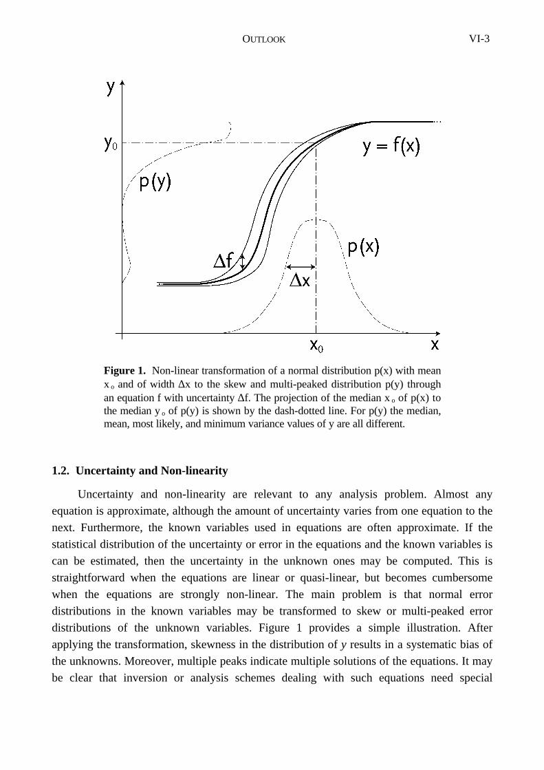
OUTLOOK VI-3
1.2. Uncertainty and Non-linearity
Uncertainty and non-linearity are relevant to any analysis problem. Almost any
equation is approximate, although the amount of uncertainty varies from one equation to the
next. Furthermore, the known variables used in equations are often approximate. If the
statistical distribution of the uncertainty or error in the equations and the known variables is
can be estimated, then the uncertainty in the unknown ones may be computed. This is
straightforward when the equations are linear or quasi-linear, but becomes cumbersome
when the equations are strongly non-linear. The main problem is that normal error
distributions in the known variables may be transformed to skew or multi-peaked error
distributions of the unknown variables. Figure 1 provides a simple illustration. After
applying the transformation, skewness in the distribution of y results in a systematic bias of
the unknowns. Moreover, multiple peaks indicate multiple solutions of the equations. It may
be clear that inversion or analysis schemes dealing with such equations need special
Figure 1. Non-linear transformation of a normal distribution p(x) with meanx o and of width ∆x to the skew and multi-peaked distribution p(y) throughan equation f with uncertainty ∆f. The projection of the median x o of p(x) tothe median y o of p(y) is shown by the dash-dotted line. For p(y) the median,mean, most likely, and minimum variance values of y are all different.
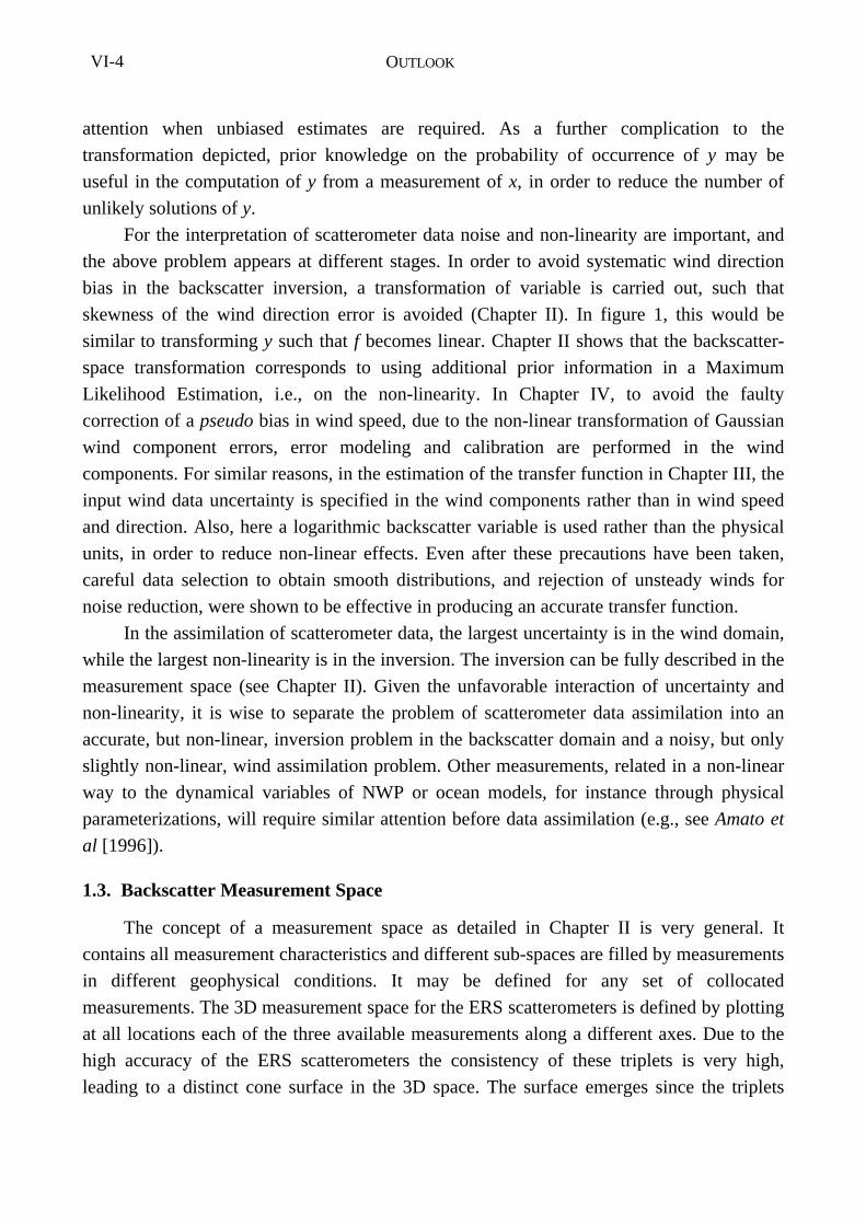
OUTLOOKVI-4
attention when unbiased estimates are required. As a further complication to the
transformation depicted, prior knowledge on the probability of occurrence of y may be
useful in the computation of y from a measurement of x, in order to reduce the number of
unlikely solutions of y.
For the interpretation of scatterometer data noise and non-linearity are important, and
the above problem appears at different stages. In order to avoid systematic wind direction
bias in the backscatter inversion, a transformation of variable is carried out, such that
skewness of the wind direction error is avoided (Chapter II). In figure 1, this would be
similar to transforming y such that f becomes linear. Chapter II shows that the backscatter-
space transformation corresponds to using additional prior information in a Maximum
Likelihood Estimation, i.e., on the non-linearity. In Chapter IV, to avoid the faulty
correction of a pseudo bias in wind speed, due to the non-linear transformation of Gaussian
wind component errors, error modeling and calibration are performed in the wind
components. For similar reasons, in the estimation of the transfer function in Chapter III, the
input wind data uncertainty is specified in the wind components rather than in wind speed
and direction. Also, here a logarithmic backscatter variable is used rather than the physical
units, in order to reduce non-linear effects. Even after these precautions have been taken,
careful data selection to obtain smooth distributions, and rejection of unsteady winds for
noise reduction, were shown to be effective in producing an accurate transfer function.
In the assimilation of scatterometer data, the largest uncertainty is in the wind domain,
while the largest non-linearity is in the inversion. The inversion can be fully described in the
measurement space (see Chapter II). Given the unfavorable interaction of uncertainty and
non-linearity, it is wise to separate the problem of scatterometer data assimilation into an
accurate, but non-linear, inversion problem in the backscatter domain and a noisy, but only
slightly non-linear, wind assimilation problem. Other measurements, related in a non-linear
way to the dynamical variables of NWP or ocean models, for instance through physical
parameterizations, will require similar attention before data assimilation (e.g., see Amato et
al [1996]).
1.3. Backscatter Measurement Space
The concept of a measurement space as detailed in Chapter II is very general. It
contains all measurement characteristics and different sub-spaces are filled by measurements
in different geophysical conditions. It may be defined for any set of collocated
measurements. The 3D measurement space for the ERS scatterometers is defined by plotting
at all locations each of the three available measurements along a different axes. Due to the
high accuracy of the ERS scatterometers the consistency of these triplets is very high,
leading to a distinct cone surface in the 3D space. The surface emerges since the triplets
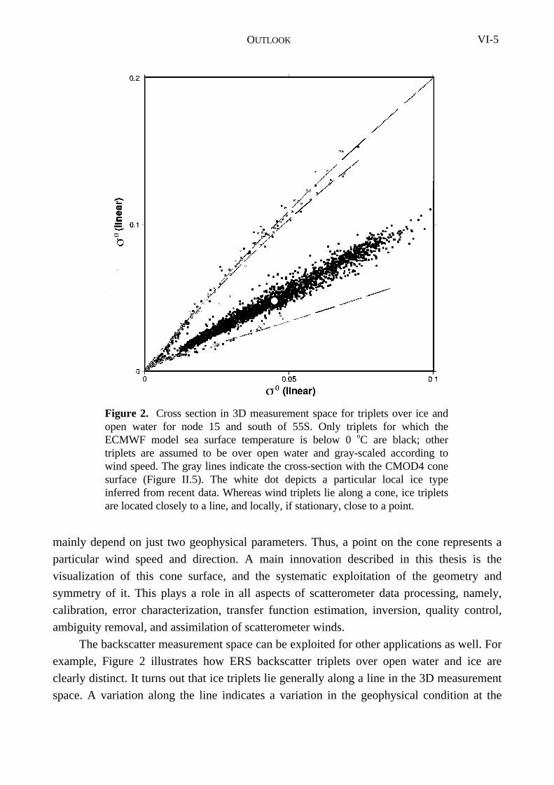
OUTLOOK VI-5
mainly depend on just two geophysical parameters. Thus, a point on the cone represents a
particular wind speed and direction. A main innovation described in this thesis is the
visualization of this cone surface, and the systematic exploitation of the geometry and
symmetry of it. This plays a role in all aspects of scatterometer data processing, namely,
calibration, error characterization, transfer function estimation, inversion, quality control,
ambiguity removal, and assimilation of scatterometer winds.
The backscatter measurement space can be exploited for other applications as well. For
example, Figure 2 illustrates how ERS backscatter triplets over open water and ice are
clearly distinct. It turns out that ice triplets lie generally along a line in the 3D measurement
space. A variation along the line indicates a variation in the geophysical condition at the
Figure 2. Cross section in 3D measurement space for triplets over ice andopen water for node 15 and south of 55S. Only triplets for which theECMWF model sea surface temperature is below 0 oC are black; othertriplets are assumed to be over open water and gray-scaled according towind speed. The gray lines indicate the cross-section with the CMOD4 conesurface (Figure II.5). The white dot depicts a particular local ice typeinferred from recent data. Whereas wind triplets lie along a cone, ice tripletsare located closely to a line, and locally, if stationary, close to a point.
OUTLOOKVI-6
surface, where several studies document that the aging of ice changes its structure [Gohin,
1995]. Thus, from a measured triplet one could infer the ice age by taking the most likely
(closest) point on this line, and from the distance of the measurement to the line, normalized
by the usual scatter of triplets around the line, one can infer the ice probability.
Subsequently, keeping an ice history over a few days and using the fact that the ice structure
is normally stationary over such a period, high probabilities of ice occurrence are limited to
a small area around a single point in the 3D measurement space. Then, by using ice
likelihood and wind likelihood (Chapter II) one may discriminate ice measurements from
wind measurements on a node-by-node basis. This has the practical advantage that
scatterometer winds close to the ice edge can be used. It illustrates that the concept of
measurement space may prove useful for the application of the ERS scatterometer over sea
ice. Sensitivity to swell or rain or the inspection of differences in land surface characteristics
may similarly be investigated in the backscatter measurement space.
For the interpretation or Quality Control over the ocean of NSCAT or
QuikSCAT/SeaWinds, the concept of a measurement space can be applied also. Chapter II
shows that in case of ERS strong changes in curvature of the cone surface as a function of
wind direction generate systematic wind direction errors after inversion, and that by a slight
transformation of measurement space these effects can be avoided. Figa and Stoffelen
[1998] show that the NSCAT 4D measurement space can also be transformed in order to
reduce the variation of curvature with wind direction, as illustrated in Figure 3. Work is
ongoing to demonstrate its effect on the wind retrieval. Also, at Ku-band rain modifies the
distribution of backscatter data in the measurement space, and it will be useful to try and
find the rain subspace. The rain characteristics may result in a rejection or even improved
interpretation of Ku-band backscatter data in case of rain. Taking into account the
developments described in this thesis and the similar developments ongoing for NSCAT, an
effort should be made to arrive at an accurate interpretation of the QuikSCAT and SeaWinds
scatterometers, which will become operational very soon, in order to be ready to assimilate
the data in NWP models. Undoubtedly, a measurement space analysis will be of benefit to
characterize many other observation systems as well.
2. Physics of Scatterometry
The accuracy of the ERS scatterometers (0.2 dB) and the visualization of the 3D
measurement space made it possible to learn about the geophysical signature of ocean radar
scattering from space and, through CMOD4, provide an accurate description of the cone
surface. In laboratory and field experiments with in situ and aircraft equipment an accuracy
of 1 dB is typical (Chapter II, Janssen et al [1998]). 1 dB corresponds to a factor of 1.25.
The well-defined cone surface leads to a better definition of the upwind-crosswind
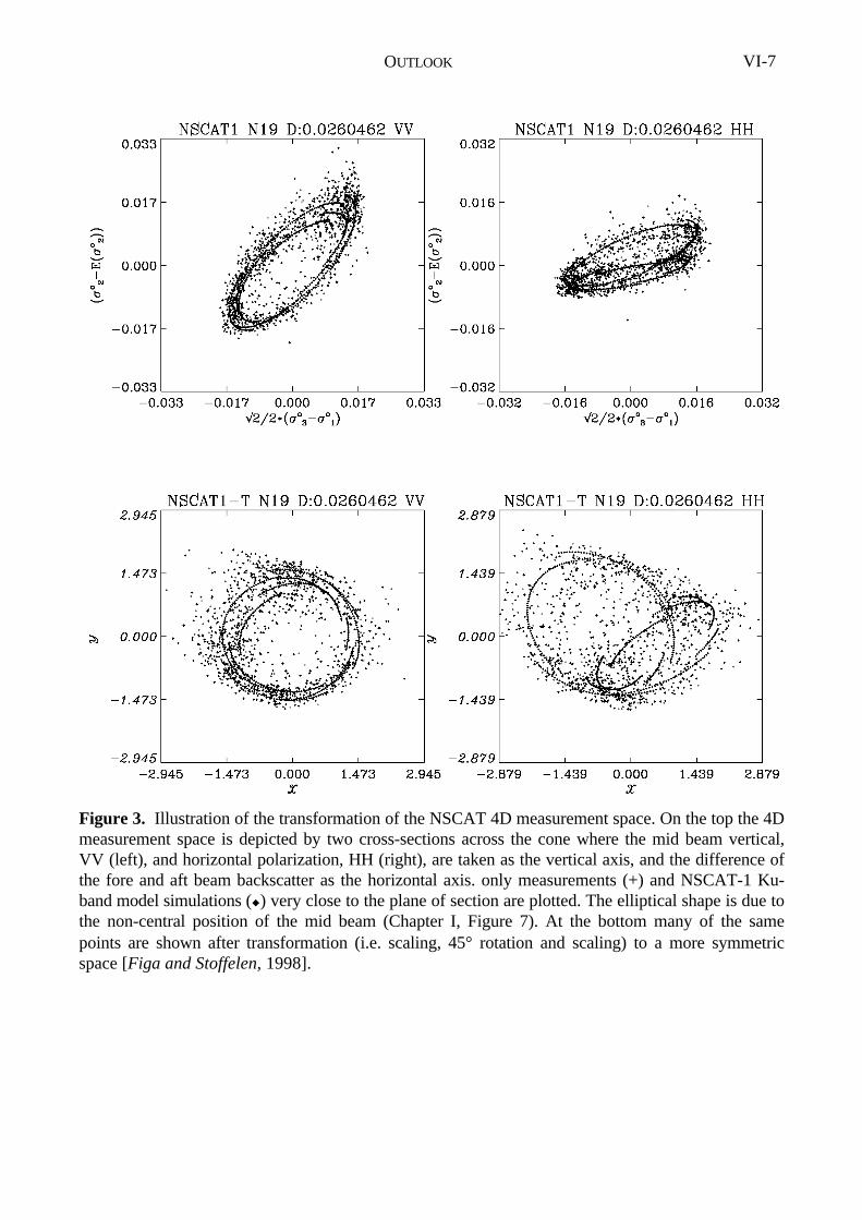
OUTLOOK VI-7
Figure 3. Illustration of the transformation of the NSCAT 4D measurement space. On the top the 4Dmeasurement space is depicted by two cross-sections across the cone where the mid beam vertical,VV (left), and horizontal polarization, HH (right), are taken as the vertical axis, and the difference ofthe fore and aft beam backscatter as the horizontal axis. only measurements (+) and NSCAT-1 Ku-band model simulations (u) very close to the plane of section are plotted. The elliptical shape is due tothe non-central position of the mid beam (Chapter I, Figure 7). At the bottom many of the samepoints are shown after transformation (i.e. scaling, 45° rotation and scaling) to a more symmetricspace [Figa and Stoffelen, 1998].
OUTLOOKVI-8
backscatter ratio. At low wind speeds this ratio is smaller compared to that found in aircraft
campaigns, due to the smoothing effect of the variability of wind direction and speed in the
large ERS scatterometer footprint. In this respect, CMOD4 should not be valid for a SAR
with a much smaller footprint. The saturation seen at high wind speeds corresponds to the
results seen from scatterometers on aircraft [Carswell et al, 1998]. What also becomes
immediately clear from the cone surface is that higher-order harmonics are required to
describe its geometry. That the observed geometric effects are small, is shown by the fact
that a fourth-order harmonic of just 4 % is sufficient to describe the asymmetric cone shape
(Chapter II). Nontheless, it is shown in Chapter II that this higher harmonic has a
pronounced effect on the wind direction retrieval. Physically-based models are not
sufficiently advanced to explain the incidence angle dependence of the upwind-crosswind
ratio, nor the behavior of the upwind-downwind ratio, nor the small effects observed in the
higher harmonics [Janssen et al, 1998].
The upwind-downwind backscatter ratio is more difficult to estimate from the cone
surface, but it can be well estimated from NWP model and scatterometer collocation
statistics. It turns out that the upwind-downwind coefficient goes up to 15 %, but that its
effect on the cone surface geometry is small. Instead, it has a systematic and pronounced
effect on the retrieved wind vector, i.e., up to 1.5 m s-1 in wind speed and a few degrees in
wind direction (Chapter II). Physically, one could argue that the increased backscatter when
looking upwind may be compensated by a slightly higher wind speed at downwind. This
would indicate that the 180 degree ambiguity seen with the ERS scatterometers is basic and
independent of, for example, the viewing geometry.
In the inversion, the most likely triplet on the CMOD4 cone surface is sought. Any
point on the cone surface corresponds to a particular retrieved wind vector. Ignoring the
ambiguity removal problem, one could thus map the retrieved wind vector on a collocated
set of calibration wind data. The wind calibration, addressed in Chapter IV, is thus largely
independent from the backscatter calibration, as detailed in Appendix A. In Chapter IV we
point out that the wind calibration is delicate and can only be properly done in a three-way
comparison. An issue of concern is the difficulty to accumulate extreme wind cases.
Carswell et al [1998] provides evidence of a large underestimation of extreme wind speeds
in tropical cyclones due to a large degradation in wind sensitivity of the ERS scatterometer
above 25 m s-1. A question remains whether the cyclone dynamics cause particular sea state
effects, influencing the amount and isotropy of the ocean backscatter. Extreme wind events
in the southern hemisphere, usually of larger scale, may provide more evidence, as well as
scatterometer measurements in different (parts of) tropical cyclones, subject to different sea
states.
There is no doubt that a scatterometer can measure at low wind speeds, but one may
OUTLOOK VI-9
disagree on what it actually measures. For a zero mean vector wind over a footprint of 50
km, it is very unlikely that the ocean surface is flat everywhere. Within the 50 km footprint
there will be wind variability, causing ocean surface gravity-capillary waves and
backscatter. In fact, in extremely light wind conditions, the scatterometer backscatter will be
proportional to the wind variability. By oversampling with backscatter measurements, one
may be able to improve their geophysical interpretation and infer both the mean and the
variability of the wind vector in such conditions.
Long waves, the presence of slicks, or atmospheric stability may affect the backscatter.
However, as stated in Chapter I, these effects partially depend on wind speed and as such
are modeled through CMOD4. Furthermore, physical parameterizations that take these
effects into account are uncertain and do not mutually agree very well. Thirdly, local
measurements of for example stability may not be suitable for a stability correction over the
large scatterometer footprint. In order to avoid problems due to these uncertainties, we
decided to relate the true 10-m vector wind to the ERS backscatter, rather than the 10-m
wind corrected for, e.g., atmospheric stability. This approach has proven to be successful.
In fact, the empirical methodology put forward in this thesis can be naturally extended
in order to incorporate the second-order geophysical effects mentioned above. Geophysical
conditions that affect the cone geometry are expected to result in an increased distance to
the CMOD4 cone. Chapter IV discusses a quality control procedure that rejects 1 % of
extreme geophysical conditions when the backscatter triplets are not close to the cone. Here,
one may think of more isotropic scattering conditions due to effects of waves or maybe rain.
In such cases the measured triplets will be located within the cone. Thus, these physical
effects may be easily visualized and identified by the methodology presented in this thesis,
provided collocated information indicating such conditions is available. Other second-order
geophysical effects, such as stability, do not alter the backscatter anisotropy, but rather the
backscatter amplitude through a modification of the surface stress. As such, these effects do
not result in an increased distance to the cone, but in a larger wind error. The correlation of
the wind error with data containing information on these effects may be empirically
investigated. Since these effects are second-order, pseudo correlations, due to the statistical
processing, need to be taken care of (see also Chapter IV). In summary, the empirical
methodology followed in this thesis provides a controlled framework to investigate the
physics of radar backscattering.
OUTLOOKVI-10
3. Impact of Scatterometers
A wealth of meteorological observations is available daily. However, most of these
observations are above land; above the ocean accurate wind observations are sparse. In a
strong westerly circulation this poses a main limitation to the weather forecasting capability
in western Europe. Especially here the risk of storm and flooding damage is largest. Wind
observations are furthermore relevant for the modeling of the atmospheric circulation in the
tropics. Near-surface winds determine the forcing of the ocean circulation, which in turn
plays a key role in the seasonal forecasting of the weather and in the earth climate system.
Scatterometer instruments now deliver many accurate and reliable surface winds with a high
spatial consistency, even below cloud, that prove to be useful for weather forecasting and
climate applications.
The ERS scatterometer measurements lead to a better analysis and weather forecast
over the oceans [Isaksen, 1998, Andrews and Bell, 1998] and increased data coverage is
shown to further enhance the impact [Le Meur, 1997, Stoffelen and Beukering, 1997]. The
ERS satellites are polar, which implies that they will pass along most locations twice a day.
However, doing so, they still leave large data gaps over the oceans.
The NSCAT scatterometer developed by NASA, that has recently operated for nine
months on ADEOS-I, had a three times larger coverage than ERS-1 or ERS-2. For
QuikSCAT, planned on a dedicated platform for late 1998, and SeaWinds, planned on
ADEOS-II for early 2000, the same applies. However, because of its different microwave
wavelength and instrument geometry, development work is necessary to arrive at an
accurate interpretation and quality control of the NASA scatterometers. Nonetheless, it is
anticipated that in most of the 1800 km broad QuikSCAT or SeaWinds swaths, accurate
wind vector data can be retrieved. Then, the methodology of variational ambiguity removal
and wind assimilation as presented in Chapter V may be applied for NSCAT, QuikSCAT
and SeaWinds as well. In particular the last two instruments will be crucial for providing
continuity of scatterometer winds over the first years of the third millennium.
ASCAT, which is planned on METOP/EPS in 2003 has a coverage similar to NSCAT,
with the geometry and microwave wavelength of the ERS scatterometers. With this, the
availability of an accurate and reliable scatterometer wind product is ensured on the longer
term.
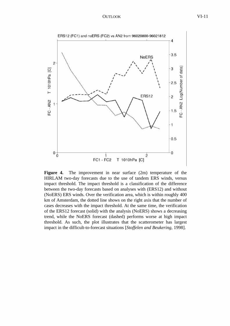
OUTLOOK VI-11
Figure 4. The improvement in near surface (2m) temperature of theHIRLAM two-day forecasts due to the use of tandem ERS winds, versusimpact threshold. The impact threshold is a classification of the differencebetween the two-day forecasts based on analyses with (ERS12) and without(NoERS) ERS winds. Over the verification area, which is within roughly 400km of Amsterdam, the dotted line shows on the right axis that the number ofcases decreases with the impact threshold. At the same time, the verificationof the ERS12 forecast (solid) with the analysis (NoERS) shows a decreasingtrend, while the NoERS forecast (dashed) performs worse at high impactthreshold. As such, the plot illustrates that the scatterometer has largestimpact in the difficult-to-forecast situations [Stoffelen and Beukering, 1998].
OUTLOOKVI-12
References
Amato, U., I de Feis, and C. Serio, Linearization pseudo-noise and its effect on the retrieval
of atmospheric state from infra-red spectral radiances, Geophys. Res. Lett., 23, 2565-
2568, 1996.
Andrews, P. L., and R. S. Bell, Optimizing the United Kingdom Meteorological Office data
assimilation for ERS-1 scatterometer winds, Mon. Weath. Rev., 126 (3), 736-746, 1998.
Carswell, J. R., W. J. Donnelly, P.S. Chang, and R.E. McIntosh, Ocean surface winds:
satellite and aircraft scatterometer measurements of Hurricane Fran, Proc. of the Ninth
Conference on Satellite Meteorology and Oceanography, Paris, France, 25-29 May
1998, Eumetsat, Darmstadt, Germany, 1998.
Eyre, J. R., G. Kelly, A. P. McNally, E. Andersson, Assimilation of TOVS radiances
through one-dimensional variational analysis, Quart. J. Royal Meteor. Soc., 119, 1427-
1463, 1993.
Figa, Julia., and Ad Stoffelen, “Towards an improved Ku-band scatterometer wind product”,
Paper prepared for the Workshop on Emerging Scatterometer Applications - From
Research to Operations -, to be held in ESTEC, Noordwijk, The Netherlands, 5-7
October 1998, 1998.
Gohin, F., Some active and passive microwave signatures of Antarctic sea ice from mid-
winter to spring 1991, Int. J. Remote Sensing, 16 (11), 2031-2054, 1995.
Hollingsworth, A., D. B. Shaw, P. Lönnberg, L. Illari, K. Arpe, A. J. Simmons, Monitoring
of observation and analysis quality by a data assimilation system, Mon. Weath. Rev.,
114, 861-879, 1986.
Hollingsworth, A., The role of four-dimensional assimilation in the quality control,
interpretation, and synthesis of climate data, Oceanic Circulation Models: Combining
OUTLOOK VI-13
Data and Dynamics, pp. 303-343, Ed. J. Willebrands and D. Anderson, Kluwer
Academic Publishers, 1989.
Isaksen, Lars, Impact of ERS -scatterometer wind data on ECMWF’s analysis and forecasts
of tropical cyclones, Paper prepared for the Workshop on Emerging Scatterometer
Applications - From Research to Operations -, to be held in ESTEC, Noordwijk, The
Netherlands, 5-7 October 1998, 1998.
Janssen, P. A. E. M., H. Wallbrink, C. J. Calkoen, D. Van Halsema, W. A. Oost, and P.
Snoeij, VIERS-1 scatterometer model, J. Geophys. Res., 103 (C4), 7807-7831, 1998.
Le Meur, Didier, Impact of ERS-1/ERS-2 scatterometer tandem on the ECMWF 3D Var
assimilation system, Proc. of the 3rd ERS Symposium - Space at the Service of our
Environment, Florence, 17-21 March 1997, Eur. Space Agency Special Publication,
ESA, Noordwijk, the Netherlands, 1997.
Rufenach, Clifford L., ERS-1 scatterometer measurements - Part II: An algorithm for ocean-
surface wind retrieval including light winds, IEEE Transactions on Geoscience and
Remote Sensing, 36 (2), 623-635, 1998.
Stoffelen, Ad, and Paul van Beukering, Improved backscatter processing and impact of
tandem ERS winds on HIRLAM, HIRLAM project report nr 31, IMET, Dublin, Ireland,
1997.
Stoffelen, Ad (editor), Satellite Ozone Data Assimilation, 1st Annual Contract Report to the
European Union, EU 4th Framework project by ECMWF, KNMI, Météo France, RAL,
UK Meteo. Office, Un. of Cambridge, and DAO, report available from KNMI, de Bilt,
the Netherlands, 1998.
A SIMPLE METHOD FOR CALIBRATION OF A SCATTEROMETER OVER THE OCEAN A-1
APPENDIX
A Simple Method for Calibration of a Scatterometer over the Ocean*
Abstract. The absolute calibration of the backscatter signal of a scatterometer is essential
for the retrieval of optimum quality geophysical products. The European Space Agency,
ESA, targeted a specification of 0.2 dB for the accuracy of the European Remote-sensing
Satellite, ERS, scatterometers. A radiometric error of this amount leads to a wind speed
error of roughly 0.25 m s-1. An interbeam bias of the same amount may lead to notable wind
direction effects. In this paper a method is discussed to obtain an accurate calibration of a
scatterometer over the ocean using an accurate backscatter-to-wind transfer function and
collocated winds from a numerical weather prediction model. The method is estimated to be
accurate to a precision of 0.1 dB. It can be used for instrument monitoring and application
of the calibration results has a demonstrable and beneficial impact on the wind inversion.
1. Introduction
It is not simple to obtain an accurate absolute calibration for a scatterometer. For the
calibration of the European Remote-sensing Satellite (ERS) scatterometers [Attema, 1991]
the European Space Agency, ESA, planned to perform the absolute calibration by a
controlled radar return to the scatterometer from transponders when these are illuminated by
one of the three scatterometer radar beams. In addition, an interbeam comparison was
planned over the rain forest where the radar cross section is known to be very stable and
rather time independent. Furthermore, the incidence angle response is known to be smooth
over the rain forest. At first, the two techniques resulted in an inconsistent calibration. It was
at this point that the ocean calibration method as described here in section 2 proved very
useful. It helped detect an interpretation problem of the results obtained with the
transponders. After solving the initial problems the three calibration methods are giving
results that lie within the ESA specifications for the radiometric accuracy of the ERS
scatterometers, which is 0.2 dB [Guignard et al., 1992, Stoffelen and Anderson, 1995, p. 8].
The ocean calibration method is still used for instrument monitoring purposes. The
main advantage of the ocean calibration with respect to the other two methods is the much
* Based on:
Stoffelen, A., A simple method for calibration of a scatterometer over the ocean, J. Atmos. Ocean. Technol.,
in press, 1998, © American Meteorological Society.
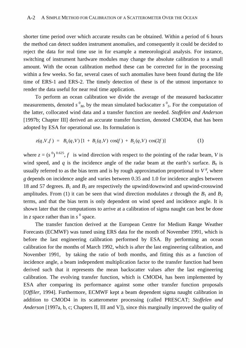
A SIMPLE METHOD FOR CALIBRATION OF A SCATTEROMETER OVER THE OCEANA-2
shorter time period over which accurate results can be obtained. Within a period of 6 hours
the method can detect sudden instrument anomalies, and consequently it could be decided to
reject the data for real time use in for example a meteorological analysis. For instance,
switching of instrument hardware modules may change the absolute calibration to a small
amount. With the ocean calibration method these can be corrected for in the processing
within a few weeks. So far, several cases of such anomalies have been found during the life
time of ERS-1 and ERS-2. The timely detection of these is of the utmost importance to
render the data useful for near real time application.
To perform an ocean calibration we divide the average of the measured backscatter
measurements, denoted σ0M, by the mean simulated backscatter σ0
S. For the computation of
the latter, collocated wind data and a transfer function are needed. Stoffelen and Anderson
[1997b; Chapter III] derived an accurate transfer function, denoted CMOD4, that has been
adopted by ESA for operational use. Its formulation is
z V B V B V B V( , , ) cos cosθ φ θ θ φ θ φ = ( , ) [ + ( , ) ( ) + ( , ) ( )]0 1 21 2 (1)
where z = (σ0) 0.625, φ is wind direction with respect to the pointing of the radar beam, V is
wind speed, and θ is the incidence angle of the radar beam at the earth’s surface. B0 is
usually referred to as the bias term and is by rough approximation proportional to V γ, where
γ depends on incidence angle and varies between 0.35 and 1.0 for incidence angles between
18 and 57 degrees. B1 and B2 are respectively the upwind/downwind and upwind-crosswind
amplitudes. From (1) it can be seen that wind direction modulates z through the B1 and B2
terms, and that the bias term is only dependent on wind speed and incidence angle. It is
shown later that the computations to arrive at a calibration of sigma naught can best be done
in z space rather than in σ0 space.
The transfer function derived at the European Centre for Medium Range Weather
Forecasts (ECMWF) was tuned using ERS data for the month of November 1991, which is
before the last engineering calibration performed by ESA. By performing an ocean
calibration for the months of March 1992, which is after the last engineering calibration, and
November 1991, by taking the ratio of both months, and fitting this as a function of
incidence angle, a beam independent multiplication factor to the transfer function had been
derived such that it represents the mean backscatter values after the last engineering
calibration. The evolving transfer function, which is CMOD4, has been implemented by
ESA after comparing its performance against some other transfer function proposals
[Offiler, 1994]. Furthermore, ECMWF kept a beam dependent sigma naught calibration in
addition to CMOD4 in its scatterometer processing (called PRESCAT; Stoffelen and
Anderson [1997a, b, c; Chapters II, III and V]), since this marginally improved the quality of

A SIMPLE METHOD FOR CALIBRATION OF A SCATTEROMETER OVER THE OCEAN A-3
the retrieved winds. Although a beam independent transfer function is preferred, in this
paper we denote, for convenience of notation, the combination of CMOD4 and March ‘92
ocean calibration as CMODEC. By using CMODEC, the “ocean” calibration procedure has
for long been an integral part of the PRESCAT ERS scatterometer data processing. In the
ESA processing CMOD4 is used, not CMODEC.
The calibration consists in a multiplication of the bias term with a beam and incidence
angle dependent constant. The ERS scatterometer backscatter measurements are organized
in 19 nodes across the swath. For each of these 19 nodes the triplet of incidence angles for
the fore, mid and aft beam is more or less fixed along the track. We use for each node and
beam the average value of the incidence angle. As such a calibration results in 19 x 3 = 51
calibration constants.
V and φ need be available at any location where the scatterometer makes a
measurement in order to obtain a quick procedure. Such a widely available wind data source
is provided by a global Numerical Weather Prediction (NWP) model and we used the
ECMWF model winds in our study. As such, changes in the mean ECMWF wind speed will
change the mean sigma naught simulated using CMOD4 and ECMWF winds, since wind
speed is the prime geophysical sensitivity of the backscatter signal over the ocean.
Fortunately, forecast model wind error characteristics are monitored routinely by e.g.
ECMWF and are also documented in special studies (e.g., Stoffelen [1998; Chapter IV]).
For each of the 19 nodes the triplet distribution of measurements from the fore, mid
and aft beams can be plotted in a three dimensional measurement space, where each beam is
represented by one axes. Stoffelen and Anderson [1997a; Chapter II] explored the coherence
of the ERS triplet backscatter measurements by visualization of the 3D measurement space,
and found that the data are generally distributed along a well-defined and conical (2D)
surface. The two parameters describing the surface most likely express the mean amplitude
and direction of the relevant gravity capillary waves at the water surface. Using this concept,
the sigma naught calibration procedure should seek for a bias correction that moves the
CMOD4 cone surface towards that surface in the measurement domain at which the density
of measured ERS-1 (or ERS-2) scatterometer triplets is largest, in order to bring model and
measurements as close together as possible, and thereby improve the wind inversion.
In section 2 the ocean calibration method is described in detail and both the effects of
errors in the transfer function and the wind data are addressed. Section 3 presents the results
of our method, whereas in section 4 a summary and conclusions are given. It is estimated
that the method is accurate to a radiometric precision of 0.1 dB when the precise calibration
of the transfer function and forecast model winds are given. It can be used for instrument
A SIMPLE METHOD FOR CALIBRATION OF A SCATTEROMETER OVER THE OCEANA-4
monitoring and application of the “ocean” calibration has a demonstrable and beneficial
impact on the wind inversion.
2. Method
In this section the ocean calibration procedure is described. For the method to work
accurately, the result should be independent of the geophysical conditions sampled by the
collocation data set used for the calibration. Using Bayes theorem, for the joint probability
density of the wind one may write
p(V ,φ ) = p(φ |V) p(V) (2)
where p(V) and p(φ |V) are the probability density function (pdf) of respectively wind speed
and, at a given speed, wind direction. When combining (1) and (2) we see that for a uniform
wind direction pdf, i.e., p(φ |V) = (2π)-1, the harmonic terms disappear when integrated over
φ. So, if we are able to achieve for the ocean calibration a collocation wind data set with
uniform wind direction distribution, then our results are independent of errors in the
harmonic terms of the transfer function, and insensitive to uncertainty in wind direction.
When we now also integrate over V, the expected average backscatter becomes
z B V( ) ( , )θ θ= 0 (3)
i.e., identical to the average value of the bias term. By computing the right-hand-side from
CMOD4 and the collocated model winds we would have a reference to compare the mean
measured backscatter against. As such, at each across-track node the application of Equation
(3) for the three beams defines the center of gravity of the cone in z space. When this center
of gravity matches for the measured and simulated triplets, then the inversion should work
best [Stoffelen and Anderson, 1997a; Chapter II].
Computation in σ 0 = z 1.6 (for Equation (1) we defined z = (σ 0 ) 0.625 ), using Taylor
expansion, causes an additional term to be added to the mean backscatter [Stoffelen and
Anderson, 1997a; Chapter II]
σ θ θ θ θ θ θ001 6
01 6
22
01 6
120 24 0 24( ) ( , ) . ( , ) ( , ) . ( , ) ( , ). . .= + +B V B V B V B V B V (4)
The right-most term is very small, since in this notation B1 ≤ 0.1. Since B2 ≤ 0.4, the mid
term on the right-hand-side may contribute up to 4%, but dependent on wind speed. B0 also
depends on wind speed, and as such the term with B2 may to a small extent interfere with
systematic changes in mean B0 due to changes in the wind speed level of the ECMWF
model. It may be clear to the reader that the interference of the harmonic terms in the ocean
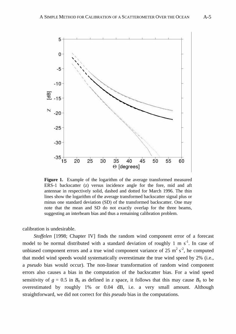
A SIMPLE METHOD FOR CALIBRATION OF A SCATTEROMETER OVER THE OCEAN A-5
calibration is undesirable.
Stoffelen [1998; Chapter IV] finds the random wind component error of a forecast
model to be normal distributed with a standard deviation of roughly 1 m s-1. In case of
unbiased component errors and a true wind component variance of 25 m2 s-2, he computed
that model wind speeds would systematically overestimate the true wind speed by 2% (i.e.,
a pseudo bias would occur). The non-linear transformation of random wind component
errors also causes a bias in the computation of the backscatter bias. For a wind speed
sensitivity of γ = 0.5 in B0 as defined in z space, it follows that this may cause B0 to be
overestimated by roughly 1% or 0.04 dB, i.e. a very small amount. Although
straightforward, we did not correct for this pseudo bias in the computations.
Figure 1. Example of the logarithm of the average transformed measuredERS-1 backscatter (z) versus incidence angle for the fore, mid and aftantennae in respectively solid, dashed and dotted for March 1996. The thinlines show the logarithm of the average transformed backscatter signal plus orminus one standard deviation (SD) of the transformed backscatter. One maynote that the mean and SD do not exactly overlap for the three beams,suggesting an interbeam bias and thus a remaining calibration problem.

A SIMPLE METHOD FOR CALIBRATION OF A SCATTEROMETER OVER THE OCEANA-6
The scatter of measured triplets around the cone is roughly 5% and is assumed to have
a normal distribution around the true σ0 with zero mean. In z space the distribution is
therefore slightly skew and it is relevant to estimate the effect of this on the ocean
calibration. Taylor expansion of σ0 [1 + δ ] in z space shows that
z O= − +( ) [ . ( ) ].σ δ δ 0 0 625 2 41 012 (5)
Based on this result we conclude that the measurement noise is not a motivation for either
computation in z or σ0 space, since for an expected standard deviation δ of 5% the δ terms
between square brackets only amount to roughly 0.0003.
Polar satellites sample the trades and the westerlies in a systematic manner. This
results in a modulation by more than a factor of two of p(φ |V) over the worlds oceans for
medium and high wind speeds. For low wind speeds the modulation is much less, as is
shown later. Freilich et al. [1998] assume p(φ |V) to be independent of wind speed, which to
our experience is not valid. The wind direction distribution becomes increasingly uniform
going from high to moderate, to low wind speed. The assumption of an invariant p(φ |V) for
varying V, introduces additional uncertainty in the results. A way to remove the wind
direction modulation for all wind speeds without this approximation, is to first determine
p(φ |V) for a given data set, and subsequently in a second pass remove randomly a fraction
of the data such that the resulting p(φ |V) becomes as uniform as possible. Then Equations
(3) and (4) can be used for the ocean calibration, without unnecessary assumptions on
p(φ |V) as in Freilich et al.
In Freilich et al. [1998] the wind direction distribution of the collocated winds is used
to compute the mean contribution from the harmonic terms of the transfer function.
However, this direction distribution is affected by the error in the wind direction of the
collocated data, and thereby somewhat smoothed. As a consequence, the estimated
contribution from the harmonic terms will be underestimated. We filtered wind directions by
using collocated ECMWF winds. We assume here that a uniform ECMWF wind direction
distribution corresponds to a uniform “true” wind direction distribution, and verify this later.
After the filtering to a uniform p(φ |V) as proposed here, the contribution of the harmonic
terms to the mean backscatter becomes negligible and its uncertainty unimportant.
After some testing, speeds were binned in 4 m s-1 intervals, i.e. 0-4 m s-1, 4-8 m s-1, up
to 36-40 m s-1, and directions in 5 degree intervals. After the first pass over the data, for
each speed interval the direction bin with the least points is searched for and in each bin the
fraction to keep is computed as the ratio of this minimum and the actual number of points in
the bin. In order to keep some points in the most data sparse areas of the wind domain, the
minimum is bound to values higher than 5 in case of a month of data.
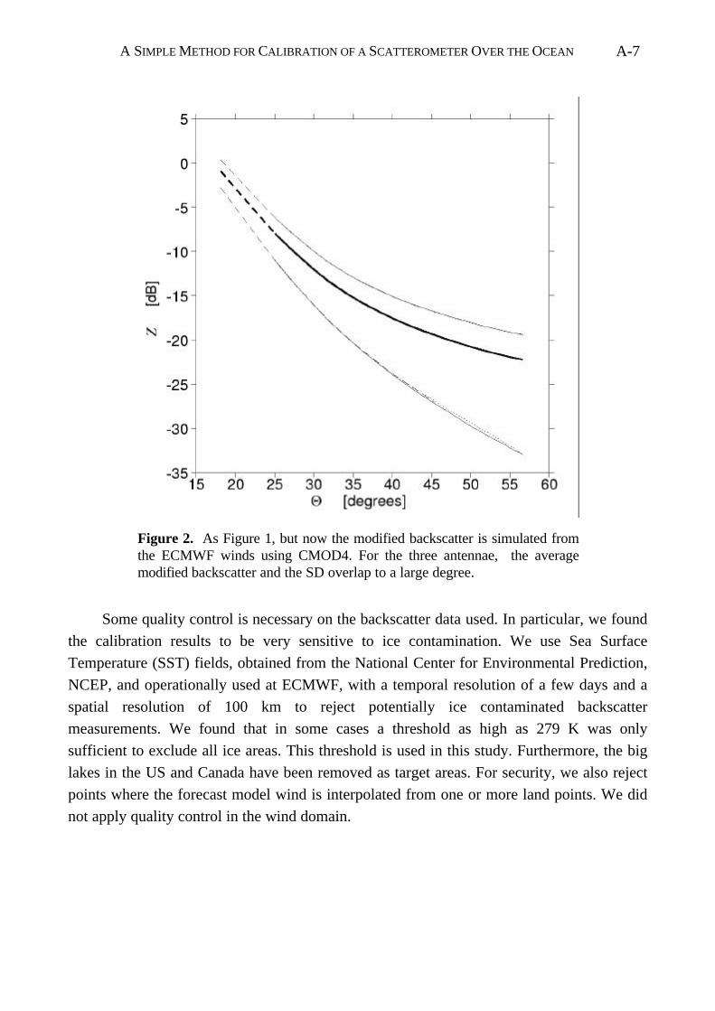
A SIMPLE METHOD FOR CALIBRATION OF A SCATTEROMETER OVER THE OCEAN A-7
Some quality control is necessary on the backscatter data used. In particular, we found
the calibration results to be very sensitive to ice contamination. We use Sea Surface
Temperature (SST) fields, obtained from the National Center for Environmental Prediction,
NCEP, and operationally used at ECMWF, with a temporal resolution of a few days and a
spatial resolution of 100 km to reject potentially ice contaminated backscatter
measurements. We found that in some cases a threshold as high as 279 K was only
sufficient to exclude all ice areas. This threshold is used in this study. Furthermore, the big
lakes in the US and Canada have been removed as target areas. For security, we also reject
points where the forecast model wind is interpolated from one or more land points. We did
not apply quality control in the wind domain.
Figure 2. As Figure 1, but now the modified backscatter is simulated fromthe ECMWF winds using CMOD4. For the three antennae, the averagemodified backscatter and the SD overlap to a large degree.
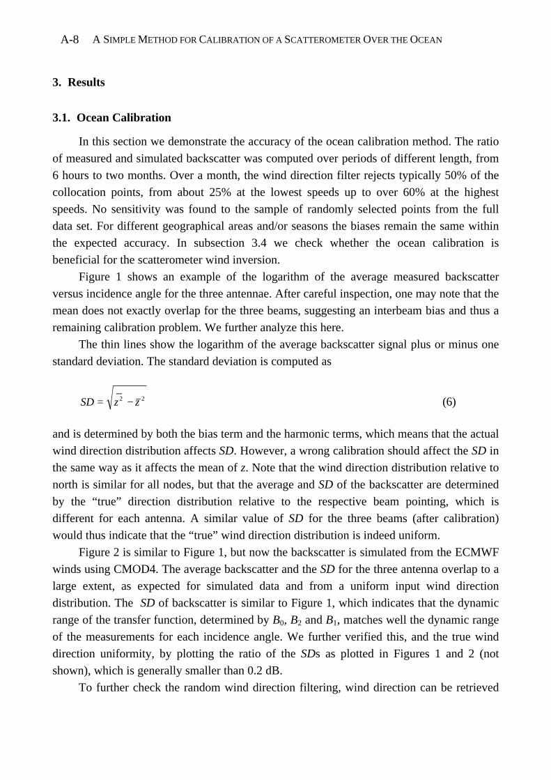
A SIMPLE METHOD FOR CALIBRATION OF A SCATTEROMETER OVER THE OCEANA-8
3. Results
3.1. Ocean Calibration
In this section we demonstrate the accuracy of the ocean calibration method. The ratio
of measured and simulated backscatter was computed over periods of different length, from
6 hours to two months. Over a month, the wind direction filter rejects typically 50% of the
collocation points, from about 25% at the lowest speeds up to over 60% at the highest
speeds. No sensitivity was found to the sample of randomly selected points from the full
data set. For different geographical areas and/or seasons the biases remain the same within
the expected accuracy. In subsection 3.4 we check whether the ocean calibration is
beneficial for the scatterometer wind inversion.
Figure 1 shows an example of the logarithm of the average measured backscatter
versus incidence angle for the three antennae. After careful inspection, one may note that the
mean does not exactly overlap for the three beams, suggesting an interbeam bias and thus a
remaining calibration problem. We further analyze this here.
The thin lines show the logarithm of the average backscatter signal plus or minus one
standard deviation. The standard deviation is computed as
SD z z= −2 2_
(6)
and is determined by both the bias term and the harmonic terms, which means that the actual
wind direction distribution affects SD. However, a wrong calibration should affect the SD in
the same way as it affects the mean of z. Note that the wind direction distribution relative to
north is similar for all nodes, but that the average and SD of the backscatter are determined
by the “true” direction distribution relative to the respective beam pointing, which is
different for each antenna. A similar value of SD for the three beams (after calibration)
would thus indicate that the “true” wind direction distribution is indeed uniform.
Figure 2 is similar to Figure 1, but now the backscatter is simulated from the ECMWF
winds using CMOD4. The average backscatter and the SD for the three antenna overlap to a
large extent, as expected for simulated data and from a uniform input wind direction
distribution. The SD of backscatter is similar to Figure 1, which indicates that the dynamic
range of the transfer function, determined by B0, B2 and B1, matches well the dynamic range
of the measurements for each incidence angle. We further verified this, and the true wind
direction uniformity, by plotting the ratio of the SDs as plotted in Figures 1 and 2 (not
shown), which is generally smaller than 0.2 dB.
To further check the random wind direction filtering, wind direction can be retrieved
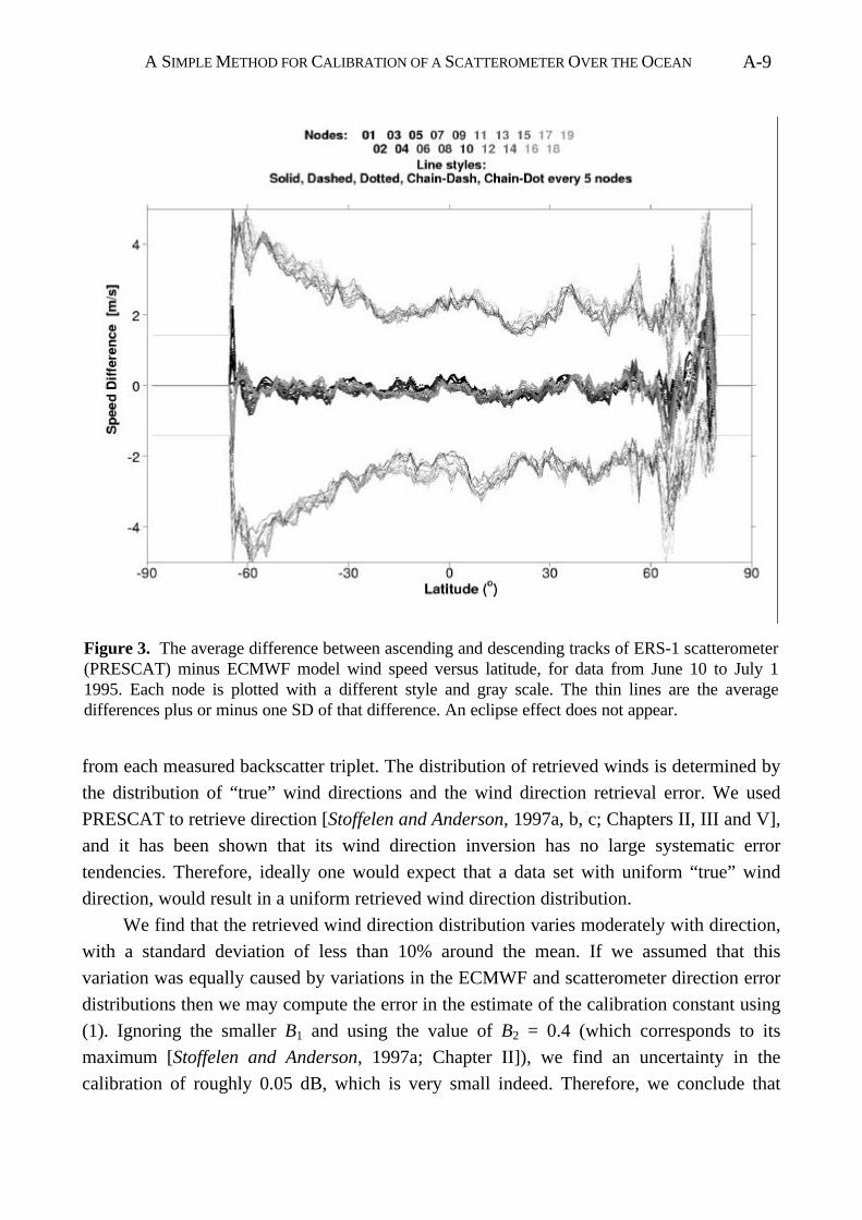
A SIMPLE METHOD FOR CALIBRATION OF A SCATTEROMETER OVER THE OCEAN A-9
from each measured backscatter triplet. The distribution of retrieved winds is determined by
the distribution of “true” wind directions and the wind direction retrieval error. We used
PRESCAT to retrieve direction [Stoffelen and Anderson, 1997a, b, c; Chapters II, III and V],
and it has been shown that its wind direction inversion has no large systematic error
tendencies. Therefore, ideally one would expect that a data set with uniform “true” wind
direction, would result in a uniform retrieved wind direction distribution.
We find that the retrieved wind direction distribution varies moderately with direction,
with a standard deviation of less than 10% around the mean. If we assumed that this
variation was equally caused by variations in the ECMWF and scatterometer direction error
distributions then we may compute the error in the estimate of the calibration constant using
(1). Ignoring the smaller B1 and using the value of B2 = 0.4 (which corresponds to its
maximum [Stoffelen and Anderson, 1997a; Chapter II]), we find an uncertainty in the
calibration of roughly 0.05 dB, which is very small indeed. Therefore, we conclude that
Figure 3. The average difference between ascending and descending tracks of ERS-1 scatterometer(PRESCAT) minus ECMWF model wind speed versus latitude, for data from June 10 to July 11995. Each node is plotted with a different style and gray scale. The thin lines are the averagedifferences plus or minus one SD of that difference. An eclipse effect does not appear.
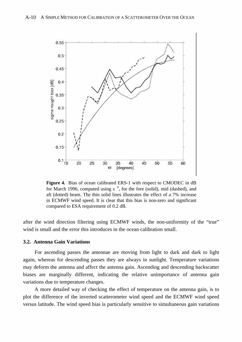
A SIMPLE METHOD FOR CALIBRATION OF A SCATTEROMETER OVER THE OCEANA-10
after the wind direction filtering using ECMWF winds, the non-uniformity of the “true”
wind is small and the error this introduces in the ocean calibration small.
3.2. Antenna Gain Variations
For ascending passes the antennae are moving from light to dark and dark to light
again, whereas for descending passes they are always in sunlight. Temperature variations
may deform the antenna and affect the antenna gain. Ascending and descending backscatter
biases are marginally different, indicating the relative unimportance of antenna gain
variations due to temperature changes.
A more detailed way of checking the effect of temperature on the antenna gain, is to
plot the difference of the inverted scatterometer wind speed and the ECMWF wind speed
versus latitude. The wind speed bias is particularly sensitive to simultaneous gain variations
Figure 4. Bias of ocean calibrated ERS-1 with respect to CMODEC in dBfor March 1996, computed using σ 0, for the fore (solid), mid (dashed), andaft (dotted) beam. The thin solid lines illustrates the effect of a 7% increasein ECMWF wind speed. It is clear that this bias is non-zero and significantcompared to ESA requirement of 0.2 dB.
A SIMPLE METHOD FOR CALIBRATION OF A SCATTEROMETER OVER THE OCEAN A-11
on the fore and aft antenna, and relatively insensitive to changes of the mid antenna gain
[Stoffelen and Anderson, 1997a; Chapter II]. Geophysical changes at the earth surface
associated with sunset or sunrise, that affect the 10m wind speed do occur not at the same
latitude than where the antennae see sunrise or sunset. Furthermore, as a function of latitude
the geophysical changes are expected to be smoother than the antenna gain effects.
For all data from 10-30 December 1995 and for all 19 nodes individually, the wind
speed bias versus latitude was computed, separately for ascending and descending orbits.
Subsequently, the difference of the bias at ascending and descending passes was computed
in order to highlight the eclipse effect and eliminate latitude-dependent statistical and
ECMWF model bias effects. The computations were repeated for the last 20 days of June
1995. It was found that the ascending minus descending wind speed bias difference versus
latitude does not vary much (Figure 3). This confirms in more detail the relative
unimportance of antenna gain variations along the orbit.
Figure 5. As Figure 4, but here the ECMWF wind speed was multiplied bya factor 0.93 before the backscatter simulation. Now the backscatter ratiovaries around -0.04 dB, and is small everywhere.

A SIMPLE METHOD FOR CALIBRATION OF A SCATTEROMETER OVER THE OCEANA-12
3.3. Application
When PRESCAT was implemented at ECMWF, it was decided to implement the beam
dependent ocean calibration (from March `92) as in CMODEC, because it resulted in a
slightly better wind retrieval. However, the calibration coefficients were derived using
Equation (4) rather than (3).
Figure 4 shows the bias in dB of ocean calibrated ERS-1 backscatter with respect to
CMODEC for March `96, using Equation (3). It is clear that this bias is non-zero. No
engineering changes have been detected from March `92 to March `96 in the backscatter
data, but the mean ECMWF wind speed has been increased. The increased ECMWF wind
speeds will give rise to increased backscatter as simulated by CMODEC. As a consequence,
the ratio of the mean measured and simulated σ0’s for March ‘96 will be smaller than for
March ‘92 (zero) as verified in Figure 4. The thin solid curve gives the sensitivity of the
backscatter (in B0) to a 7% increase of wind speed at 8 m s-1, which corresponds very well
with the general trend observed in the calibration curves of the three beams.
The ECMWF model near surface wind speed is sensitive to the boundary layer
parameterization scheme. Latter is subject to re-evaluation, for instance to solve problems
with boundary layer humidity or cloud, and as such the level of ECMWF wind speed may
change from one forecast model software cycle to the next. Stoffelen [1996] estimates the
average speed level of ECMWF in 1996 to be roughly 10% larger than the average ERS
scatterometer speed level. The 7% increase of the ECMWF wind speed between March ‘92
and March ‘96 is consistent with the scatterometer over model wind speed ratio of 1.10. It
may be concluded that in March ‘92 the same ratio was roughly 1.03, which in retrospect
verifies reasonably well with our experience (see, e.g., Stoffelen and Anderson [1997b;
Chapter III], for departure statistics). Figure 5 is similar to Figure 4, but here the ECMWF
wind speed was multiplied by a factor of 0.93 before the backscatter simulation. Now the
backscatter ratio varies around -0.04 dB, and is small everywhere. Thus, for a proper use of
ECMWF winds for the ocean calibration the wind speed has to be adjusted to the level of
the ECMWF model in November (or March) 1992, to which CMOD4 had been tuned.
The (independent) problem of wind calibration of the scatterometer and ECMWF
model to for example the buoy network is discussed by Stoffelen [1998; Chapter IV]. He
compares NCEP model and scatterometer winds to in situ wind measurements. Latter are
used to calibrate the two former wind data sources. A conclusion from the analysis is that
scatterometer wind speeds are biased low by ~4% with respect to the buoys. It is found here
that after the ocean calibration the node to node fluctuation of the wind speed bias is less
than before (see at the end of this section). However, the effect is small and the backscatter
calibration refinement suggested here has little impact on the overall wind calibration (and
vice versa).
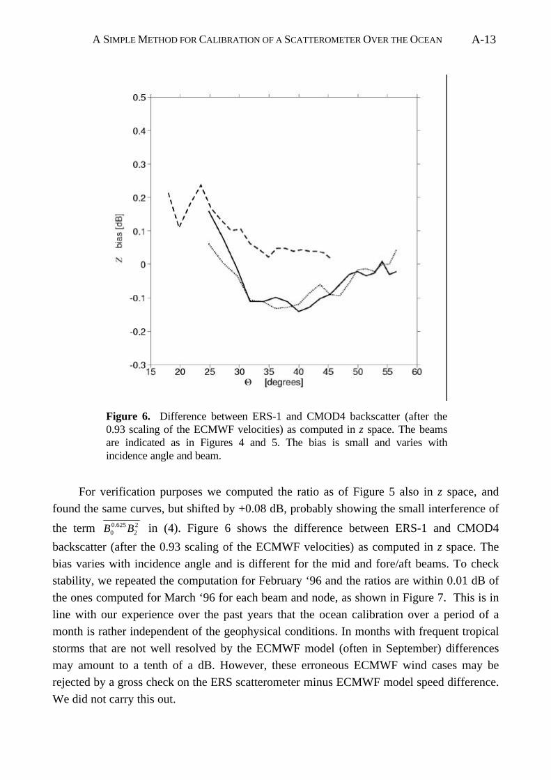
A SIMPLE METHOD FOR CALIBRATION OF A SCATTEROMETER OVER THE OCEAN A-13
For verification purposes we computed the ratio as of Figure 5 also in z space, and
found the same curves, but shifted by +0.08 dB, probably showing the small interference of
the term B B00 625
22. in (4). Figure 6 shows the difference between ERS-1 and CMOD4
backscatter (after the 0.93 scaling of the ECMWF velocities) as computed in z space. The
bias varies with incidence angle and is different for the mid and fore/aft beams. To check
stability, we repeated the computation for February ‘96 and the ratios are within 0.01 dB of
the ones computed for March ‘96 for each beam and node, as shown in Figure 7. This is in
line with our experience over the past years that the ocean calibration over a period of a
month is rather independent of the geophysical conditions. In months with frequent tropical
storms that are not well resolved by the ECMWF model (often in September) differences
may amount to a tenth of a dB. However, these erroneous ECMWF wind cases may be
rejected by a gross check on the ERS scatterometer minus ECMWF model speed difference.
We did not carry this out.
Figure 6. Difference between ERS-1 and CMOD4 backscatter (after the0.93 scaling of the ECMWF velocities) as computed in z space. The beamsare indicated as in Figures 4 and 5. The bias is small and varies withincidence angle and beam.
A SIMPLE METHOD FOR CALIBRATION OF A SCATTEROMETER OVER THE OCEANA-14
The difference in Figure 6 is within the ERS scatterometer specifications for
radiometric accuracy (0.2 dB), but it is still interesting to evaluate its effect on the wind
retrieval. An improvement in the fit of the ERS-1 measurements with the CMOD4 cone
should be particularly visible through a decreased average distance to the cone. Because the
normalized distance to the cone [Stoffelen and Anderson, 1997a; Chapter II] is reasonably
independent of wind speed, the average of it at each node is a good reflection of the overall
fit of triplets to the cone. Table 1 shows the normalized distance to the cone after and before
the backscatter bias correction. For all nodes the distance to the cone has decreased, even at
the outer nodes where the correction is fairly small. On average the distance to the cone has
decreased by 7%. As can be seen from Table 1, the correction has little effect on the
backscatter triplet quality control, as the number of data is similar with or without bias
correction.
A mid beam bias mostly affects the wind direction retrieval accuracy at low and
moderate speeds and not so much the speed retrieval. Table 1 shows the SD of the ECMWF
minus retrieved scatterometer wind direction for all speeds. As expected, the largest
improvement is found at the inner nodes where the mid beam bias is largest.
The fore and aft beam have very similar backscatter biases. This combination of fore
and aft beam bias will mostly effect wind speed bias, and not so much wind direction.
Indeed, the wind speed bias with respect to the ECMWF model winds is less variable from
node to node after the bias correction than before.
4. Conclusions
The method of ocean calibration is briefly explained and it is motivated that
application of the procedure in z space rather than σ 0 space gives the most accurate estimate
of the difference between the center of gravity of the transfer function cone and the center of
gravity of the distribution of measured triplets. As a consequence, application of it in the
processing of scatterometer data improves the geophysical product. The method is shown to
be stable in time and may be applied for monitoring purposes, as has been done for more
than 5 years now at ECMWF.
Land targets are also in use to determine the scatterometer calibration. The ESA rain
forest calibration corresponds with the ocean calibration procedure to within the specified
instrument precision of 0.2 dB. However, the stability of the land targets to an accuracy of
0.1 dB over all seasons is difficult to be assured of. Also, ESA employed transponders for
absolute calibration. However, the relatively infrequent overpass over the transponders and
the absolute accuracy of these, makes an absolute calibration on this basis only a tedious
procedure. The consistent combination of several methods is probably the best guarantee for
a good absolute scatterometer backscatter calibration.
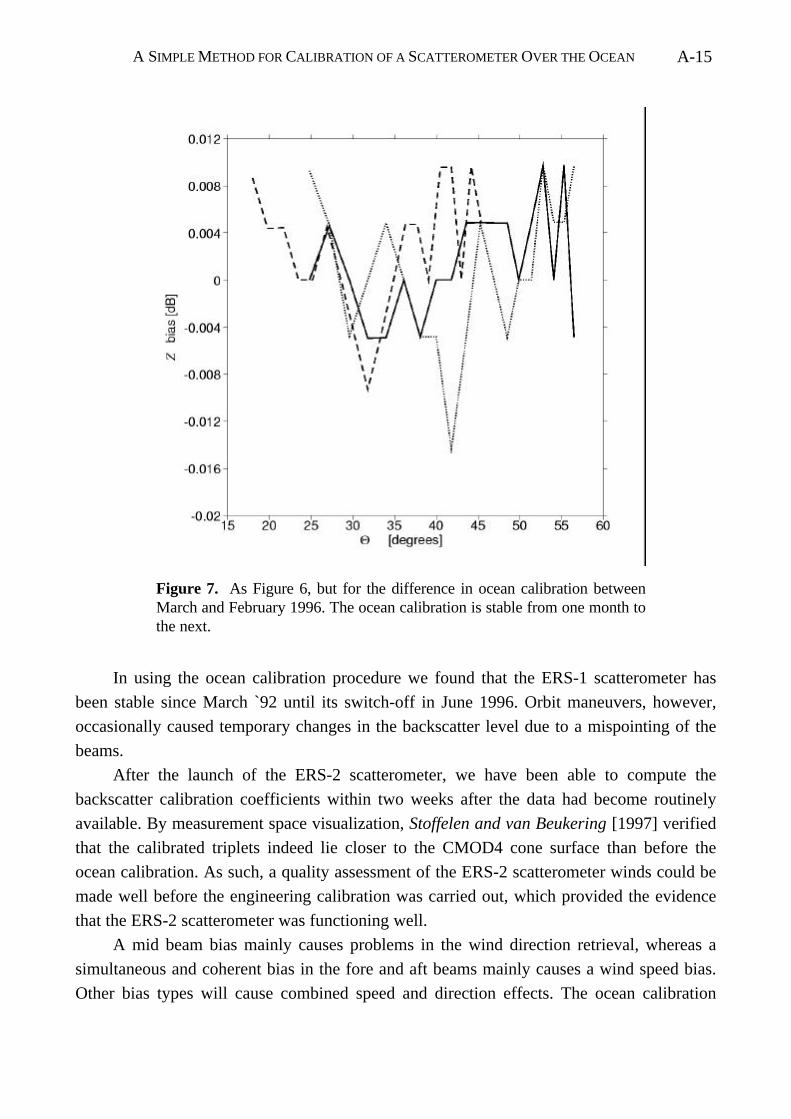
A SIMPLE METHOD FOR CALIBRATION OF A SCATTEROMETER OVER THE OCEAN A-15
In using the ocean calibration procedure we found that the ERS-1 scatterometer has
been stable since March `92 until its switch-off in June 1996. Orbit maneuvers, however,
occasionally caused temporary changes in the backscatter level due to a mispointing of the
beams.
After the launch of the ERS-2 scatterometer, we have been able to compute the
backscatter calibration coefficients within two weeks after the data had become routinely
available. By measurement space visualization, Stoffelen and van Beukering [1997] verified
that the calibrated triplets indeed lie closer to the CMOD4 cone surface than before the
ocean calibration. As such, a quality assessment of the ERS-2 scatterometer winds could be
made well before the engineering calibration was carried out, which provided the evidence
that the ERS-2 scatterometer was functioning well.
A mid beam bias mainly causes problems in the wind direction retrieval, whereas a
simultaneous and coherent bias in the fore and aft beams mainly causes a wind speed bias.
Other bias types will cause combined speed and direction effects. The ocean calibration
Figure 7. As Figure 6, but for the difference in ocean calibration betweenMarch and February 1996. The ocean calibration is stable from one month tothe next.
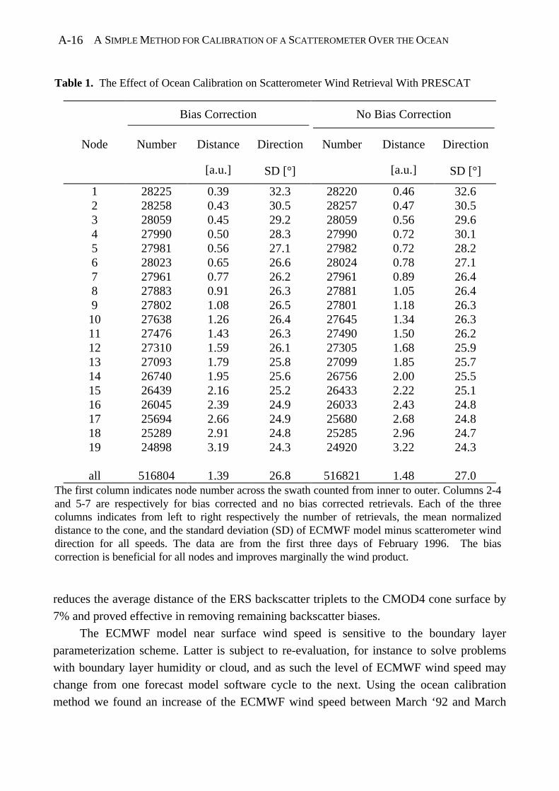
A SIMPLE METHOD FOR CALIBRATION OF A SCATTEROMETER OVER THE OCEANA-16
reduces the average distance of the ERS backscatter triplets to the CMOD4 cone surface by
7% and proved effective in removing remaining backscatter biases.
The ECMWF model near surface wind speed is sensitive to the boundary layer
parameterization scheme. Latter is subject to re-evaluation, for instance to solve problems
with boundary layer humidity or cloud, and as such the level of ECMWF wind speed may
change from one forecast model software cycle to the next. Using the ocean calibration
method we found an increase of the ECMWF wind speed between March ‘92 and March
Table 1. The Effect of Ocean Calibration on Scatterometer Wind Retrieval With PRESCAT
Bias Correction No Bias Correction
Node Number Distance Direction Number Distance Direction
[a.u.] SD [°] [a.u.] SD [°]
1 28225 0.39 32.3 28220 0.46 32.62 28258 0.43 30.5 28257 0.47 30.53 28059 0.45 29.2 28059 0.56 29.64 27990 0.50 28.3 27990 0.72 30.15 27981 0.56 27.1 27982 0.72 28.26 28023 0.65 26.6 28024 0.78 27.17 27961 0.77 26.2 27961 0.89 26.48 27883 0.91 26.3 27881 1.05 26.49 27802 1.08 26.5 27801 1.18 26.310 27638 1.26 26.4 27645 1.34 26.311 27476 1.43 26.3 27490 1.50 26.212 27310 1.59 26.1 27305 1.68 25.913 27093 1.79 25.8 27099 1.85 25.714 26740 1.95 25.6 26756 2.00 25.515 26439 2.16 25.2 26433 2.22 25.116 26045 2.39 24.9 26033 2.43 24.817 25694 2.66 24.9 25680 2.68 24.818 25289 2.91 24.8 25285 2.96 24.719 24898 3.19 24.3 24920 3.22 24.3
all 516804 1.39 26.8 516821 1.48 27.0The first column indicates node number across the swath counted from inner to outer. Columns 2-4and 5-7 are respectively for bias corrected and no bias corrected retrievals. Each of the threecolumns indicates from left to right respectively the number of retrievals, the mean normalizeddistance to the cone, and the standard deviation (SD) of ECMWF model minus scatterometer winddirection for all speeds. The data are from the first three days of February 1996. The biascorrection is beneficial for all nodes and improves marginally the wind product.
A SIMPLE METHOD FOR CALIBRATION OF A SCATTEROMETER OVER THE OCEAN A-17
‘96 of 7 %. This is consistent with the results of dedicated wind calibration studies. After
the ocean calibration the node to node fluctuation of the wind speed bias is less than before,
and for some nodes the wind direction retrieval is improved. However, the backscatter
calibration refinement suggested here has little impact on the overall wind calibration.
For the scatterometer processing we recommend correction of the backscatter biases
between scatterometer measurements and CMOD4 for e.g. March ‘96 and thereafter a
monitoring of the backscatter bias with respect to this. At the same time, checking of
departure statistics of surface wind from one forecast model cycle to the next is necessary as
an independent way to check speed level changes.
Acknowledgments
The work described in this paper profited much from the discussions in the ASCAT
SAG and in an earlier stage in the ERS analysis team. The comments of ECMWF staff, and
in particular Dave Anderson and Didier Lemeur, motivated me to refine the procedure. The
three reviewers of this manuscript are acknowledged for their constructive remarks.
References
Attema, E. W. P., The Active Microwave Instrument on board the ERS-1 satellite, Proc.
IEEE., 79, pp.791-799, 1991.
Freilich, M. H., Hongbo Qi and R. S. Dunbar, Scatterometer Beam-Balancing Using Open-
Ocean Backscatter Measurements, J. of Atmos. and Ocean. Technol., in press, 1998.
Guignard, J-P. et al., AMI Performances, Proc. of the ERS-1 commissioning phase mid-term
review held at ESA/ESTEC from 24-25 September 1991, ESA publishing division,
ESTEC, Noordwijk, the Netherlands, 1992.
Offiler, D., The calibration of ERS-1 satellite scatterometer winds, J. of Atmos. and Ocean.
Technol., 11, 1002-1017, 1994.
Stoffelen, Ad, Error modeling of scatterometer, in situ, and ECMWF model winds; a
calibration refinement, Tech. Rep. 193, KNMI, de Bilt, the Netherlands, 1996.
Stoffelen, Ad, Error modeling and calibration; towards the true surface wind speed , J.
Geophys. Res., 103 (C4), 7755-7766, 1998.
Stoffelen, Ad and David Anderson, Scatterometer Data Interpretation: Measurement Space
and inversion, J. Atm. and Ocean Techn., 14(6), 1298-1313, 1997a.
Stoffelen, Ad , and David Anderson, Scatterometer Data Interpretation: Derivation of the

A SIMPLE METHOD FOR CALIBRATION OF A SCATTEROMETER OVER THE OCEANA-18
Transfer Function CMOD4, J. Geoph. Res., 102(C3), 5767-5780, 1997b.
Stoffelen, Ad, and David Anderson, Ambiguity Removal and Assimilation of Scatterometer
Data, Q. J. R. Meteorol. Soc., 123, 491-518, 1997c.
Stoffelen, Ad, and Paul van Beukering, Implementation of Improved ERS Scatterometer
Data Processing and its impact on HIRLAM Short Range Weather Forecasts, Techn.
Report No. 31, BCRS project report, BCRS, Delft, Netherlands, 1997.

APPENDIX A-19
Acronyms
2D 2-Dimensional
3D 3-Dimensional
4D 4-Dimensional
3D-VAR 3D Variational meteorological spatial data analysis scheme
4D-VAR 4D Variational meteorological spatial and temporal data analysis scheme
ADEOS Advanced Earth Observation Satellite launched by Japan in 1996
ASCAT Advanced Scatterometer proposed for METOP/EPS
BCRS “BeleidsCommissie” Remote Sensing
BUFR Binary Universal Format Representation; code for meteorological data
CMOD2 Pre-launch transfer function for the C-band ERS scatterometer
CMOD4 Scatterometer transfer function for the C-band ERS scatterometer
CMODEC CMOD4, including an ocean calibration
CREO ESA’s ERS scatterometer ambiguity removal
DNMI The Norwegian Meteorological Institute
DWL Doppler Wind Lidar
ECMWF European Centre for Medium-range Weather Forecasts
ESA European Space Agency
e.m. electromagnetic
EPS European Polar System
ERS European Remote-sensing Satellite
ESA European Space Agency
EUMETSAT European Meteorological Satellite agency
FDP Fast Delivery Product
FG First Guess
FGAT First Guess at Appropriate Time
GOS Global Observing System
GTS meteorological Global Telecommunication System
HIRLAM High Resolution Limited Area Model
KNMI Royal Netherlands Meteorological Institute
LOS Line of Sight
LUT Look-Up Table of sigma naught calibration coefficients
MLE Maximum Likelihood Estimator
APPENDIX A-20
METOP Meteorological Operational Polar satellite series, proposed by EUMETSAT
NASA National Aeronautics and Space Agency (US)
NASDA National Aeronautics and Space Development Agency (Japan)
NCEP National Center for Environmental Prediction (US)
NESDIS National Environmental Satellite and Data Information System (US)
NOAA National Oceanographic and Atmospheric Administration (US)
NSCAT NASA Scatterometer on board ADEOS-I
NWP Numerical Weather Prediction
OI Optimal (statistical) Interpolation; meteorological data analysis method
PBL Planetary Boundary Layer
PRESCAT Pre-processor of Scatterometer data before meteorological assimilation
QC Quality Control
QuikSCAT Scanning scatterometer system to be launched on a dedicated platform inNovember 1998
RMS Root-Mean-Squared
RS Remote Sensing
SAR Synthetic Aperture Radar
SASS SEASAT-A Scatterometer System
SATEM NOAA/NESDIS TOVS vertical sounding
SCAT Scatterometer on board the ERS-1 and ERS-2 satellites.
SeaSat Sea state Satellite launched by NASA in 1978
SeaWinds Scanning scatterometer system on ADEOS-II
SD Standard Deviation
SLICE 2D modal wind direction filter for ambiguity removal by UKMO
SODA Studies for Ozone Data Assimilation (EU project)
T106 Truncation of model spectral sampling at wave number 106 (120 km grid)
T213 Truncation of model spectral sampling at wave number 213 (60 km grid)
TAO Tropical Array Of (buoys)
TIROS Television Infra-Red Operational Satellite
TOVS TIROS Operational Vertical Sounder
UKMO Meteorological Office of the United Kingdom
UTC Universal Time Coordinate
UU Universiteit Utrecht
UWI Acronym for the scatterometer BUFR product disseminated over the GTS
APPENDIX A-19
Acronyms
2D 2-Dimensional
3D 3-Dimensional
4D 4-Dimensional
3D-VAR 3D Variational meteorological spatial data analysis scheme
4D-VAR 4D Variational meteorological spatial and temporal data analysis scheme
ADEOS Advanced Earth Observation Satellite launched by Japan in 1996
ASCAT Advanced Scatterometer proposed for METOP/EPS
BCRS “BeleidsCommissie” Remote Sensing
BUFR Binary Universal Format Representation; code for meteorological data
CMOD2 Pre-launch transfer function for the C-band ERS scatterometer
CMOD4 Scatterometer transfer function for the C-band ERS scatterometer
CMODEC CMOD4, including an ocean calibration
CREO ESA’s ERS scatterometer ambiguity removal
DNMI The Norwegian Meteorological Institute
DWL Doppler Wind Lidar
ECMWF European Centre for Medium-range Weather Forecasts
ESA European Space Agency
e.m. electromagnetic
EPS European Polar System
ERS European Remote-sensing Satellite
ESA European Space Agency
EUMETSAT European Meteorological Satellite agency
FDP Fast Delivery Product
FG First Guess
FGAT First Guess at Appropriate Time
GOS Global Observing System
GTS meteorological Global Telecommunication System
HIRLAM High Resolution Limited Area Model
KNMI Royal Netherlands Meteorological Institute
LOS Line of Sight
LUT Look-Up Table of sigma naught calibration coefficients
MLE Maximum Likelihood Estimator

APPENDIX A-20
METOP Meteorological Operational Polar satellite series, proposed by EUMETSAT
NASA National Aeronautics and Space Agency (US)
NASDA National Aeronautics and Space Development Agency (Japan)
NCEP National Center for Environmental Prediction (US)
NESDIS National Environmental Satellite and Data Information System (US)
NOAA National Oceanographic and Atmospheric Administration (US)
NSCAT NASA Scatterometer on board ADEOS-I
NWP Numerical Weather Prediction
OI Optimal (statistical) Interpolation; meteorological data analysis method
PBL Planetary Boundary Layer
PRESCAT Pre-processor of Scatterometer data before meteorological assimilation
QC Quality Control
QuikSCAT Scanning scatterometer system to be launched on a dedicated platform inNovember 1998
RMS Root-Mean-Squared
RS Remote Sensing
SAR Synthetic Aperture Radar
SASS SEASAT-A Scatterometer System
SATEM NOAA/NESDIS TOVS vertical sounding
SCAT Scatterometer on board the ERS-1 and ERS-2 satellites.
SeaSat Sea state Satellite launched by NASA in 1978
SeaWinds Scanning scatterometer system on ADEOS-II
SD Standard Deviation
SLICE 2D modal wind direction filter for ambiguity removal by UKMO
SODA Studies for Ozone Data Assimilation (EU project)
T106 Truncation of model spectral sampling at wave number 106 (120 km grid)
T213 Truncation of model spectral sampling at wave number 213 (60 km grid)
TAO Tropical Array Of (buoys)
TIROS Television Infra-Red Operational Satellite
TOVS TIROS Operational Vertical Sounder
UKMO Meteorological Office of the United Kingdom
UTC Universal Time Coordinate
UU Universiteit Utrecht
UWI Acronym for the scatterometer BUFR product disseminated over the GTS
APPENDIX A-21
Acknowledgments
The work as described in this thesis would not have taken place without the continuing
support of my wife Karin. She made it possible for me to spend so much time on science,
while she had a busy job managing family life, removals, and birth and breastfeading
counseling. While preparing this literary infant, Kees, Elma, Leon and Rian were the four
other infants that took my care and affection.
David Anderson contributed substantially to the quality of the papers produced. His
unfailing impetus to question my ideas and improve on the written texts has been invaluable,
and I am very grateful for this. Tony Hollingsworth provided great support by fully
entrusting me the improvement of the scatterometer processing and by reviewing the
material. John Eyre led me to derive the mathematical framework supporting the ideas I had
put forward. The valuable time and effort that Bert Holtslag, Arnold Heemink, and the other
members of the committee have spend on the thesis is much appreciated. The hand of Rob
Hine and Birgit van Diemen in many drawings provides the thesis its current appearance.
Wiebe Oost provided the photograph on the cover.
The ESA analysis and experimenters teams bundled the knowledge on microwave-
ocean interaction within Europe, and provided a very stimulating atmosphere. In particular
Alf Long, who has a long career in the field, helped me with his knowledge, software, and
ideas. Evert Attema often joined in our discussions, which I found to be very helpful.
Besides the acknowledgments here and in Chapters II-V, many other people contributed by
providing a constructive scientific atmosphere.
It is a pleasure to see that the developments on scatterometer data interpretation
described here and originally supported by ESA, are now being supported by many other
institutes, amongst which the BCRS and EUMETSAT, and active co-operation takes place
on an international level, for instance with the NASA on QuikSCAT/SeaWinds. This is of
great importance for an optimal use of these costly space-based observations.
Almost four years I shared office and worked with Gerard Cats, whose clear analytical
explanations much helped me to understand the meteorological analysis problem.
Nowadays, Julia Figa shares my office until it is definitely broken down. At ECMWF my
work was often interrupted by Tony McNally, Laurant Phalippou, and Bernd Becker, but in
a pleasant and relaxing way. Here, Hervé Roquet, Catherine Gaffard, Didier Le Meur, and
more recently Lars Isaksen carried forward the developments initiated by me. During the 11
years of attachment to KNMI and ECMWF, I could easily fill a page with names of people
that help, or have helped, to provide a nice social and effective professional atmosphere. All

APPENDIX A-22
of you are gratefully honoured. The running, volley, and soccer were appreciated
interruptions from a busy job, and the many colleagues at ECMWF and KNMI that joined
me in these activities are acknowledged. I must have forgotten many people.

APPENDIX A-23
Curriculum Vitae
Born in Alphen en Riel on 25 February 1962 as a farmers son, I have spent many
thousands of hours outdoors exposed to the variable Dutch weather. This probably explains
my great interest in meteorology. After completing the Atheneum B education at the St.
Odulphuslyceum in Tilburg, I studied from 1980 to 1987 at the Technical University of
Eindhoven, where I became Ir in Physics. Fortunately, at the time when I studied in
Eindhoven, the curriculum was nominally 5 years and there were many opportunities to
train in both practical and theoretical skills. In the last 11 years my scope has been changed
from solid states to fluid dynamics and my interest in meteorology has been satisfied during
my work at KNMI and ECMWF. Besides scatterometry, I am since 7 years involved in the
preparation of an ESA Doppler Wind Lidar mission, and more recently as project leader in
ozone data assimilation (SODA European Union project). As a member of the
ESA/EUMETSAT ASCAT Science Advisory Group, the ESA Atmospheric Dynamics
Mission Advisory Group, the QuikSCAT science team, the ESA Radar Technical Advisory
Group and as co-ordinator of the HIRLAM satellite data activities I am well involved in the
development of Remote Sensing applications for the benefit of meteorology.

Stellingen
behorende bij het proefschrift “Scatterometry”
Ad Stoffelen
1 Augustus 1998
I. De scatterometer is een nauwkeurige windmeter (dit proefschrift).
II. De driedimensionale meetruimte van de ERS scatterometers zoals gedefinieerd in dit
proefschrift, én de sterke coherentie van de metingen in deze ruimte, vormen een
verfrissend en cruciaal gegeven van belang bij alle facetten in de interpretatie van de
radar verstrooingsmetingen (dit proefschrift).
III. Correcties voor o.a. stabiliteit, golftoestand, en oppervlakte-actieve stoffen (z.g. slicks)
op de wind-radar transfer functie zijn in het algemeen van secundair belang. Een reden
is dat deze effecten in hoge mate correleren met de windsnelheid en als zodanig
impliciet zijn opgenomen in het empirische CMOD4. Bovendien is in de meeste
gevallen en voor enkele van deze parameters geen adequate a priori informatie
voorhanden, zodat dan een eventueel windonafhankelijk effect niet gecorrigeerd kan
worden (dit proefschrift).
IV. Gegevensassimilatie in een mondiaal weermodel is een krachtig middel voor de
calibratie en validatie van in situ, satelliet-, en weermodel-gegevens (dit proefschrift).
V. Niet alleen een notie van het verband tussen meting en relevante geofysische
grootheden is van belang bij de interpretatie van metingen, maar ook een goede notie
van de nauwkeurigheid van de meting, de nauwkeurigheid van het geofysische
verband, en de ruimte- en tijdschalen die de meting én de geofysische parameters
beschrijven (dit proefschrift).

VI. Elke natuurwetenschappelijke uitspraak zou gepaard moeten gaan met een analyse van
zijn nauwkeurigheid. Een recursieve toepassing van deze stelling is echter heilloos.
VII. De inhomogeniteit van en schaarste in het wereldwijde meteorologische
waarnemingsnetwerk zijn de belangrijkste beperkingen voor een nauwkeurige
voorspelling van het weer. Met name windwaarnemingen in de troposfeer zijn nodig
voor een verbeterde beschrijving van de atmosferische circulatie (dit proefschrift).
VIII. Een prijspolitiek voor aardobservatiegegevens ondermijnt het potentiële gebruik ervan
in de maatschappij, en is daarom niet kosten besparend.
IX. De illusie van kennis is schadelijker dan onwetendheid.
X. In tegenstelling tot dat wat gepropageerd wordt door veel media, is de functie van de
vrouwelijke borst voornamelijk gericht op het pasgeboren kind.
XI. Het ouderschap is ook een respectabele baan.