
Matthijs Douze INRIA Grenobledouze/enseignement/cours_n7.pdf · 16/1/2015, page 2 About... Matthijs...
132
16/1/2015, page 1 Image indexing and retrieval Matthijs Douze INRIA Grenoble
Transcript of Matthijs Douze INRIA Grenobledouze/enseignement/cours_n7.pdf · 16/1/2015, page 2 About... Matthijs...
16/1/2015, page 1
Image indexing and retrieval
Matthijs Douze
INRIA Grenoble
16/1/2015, page 2
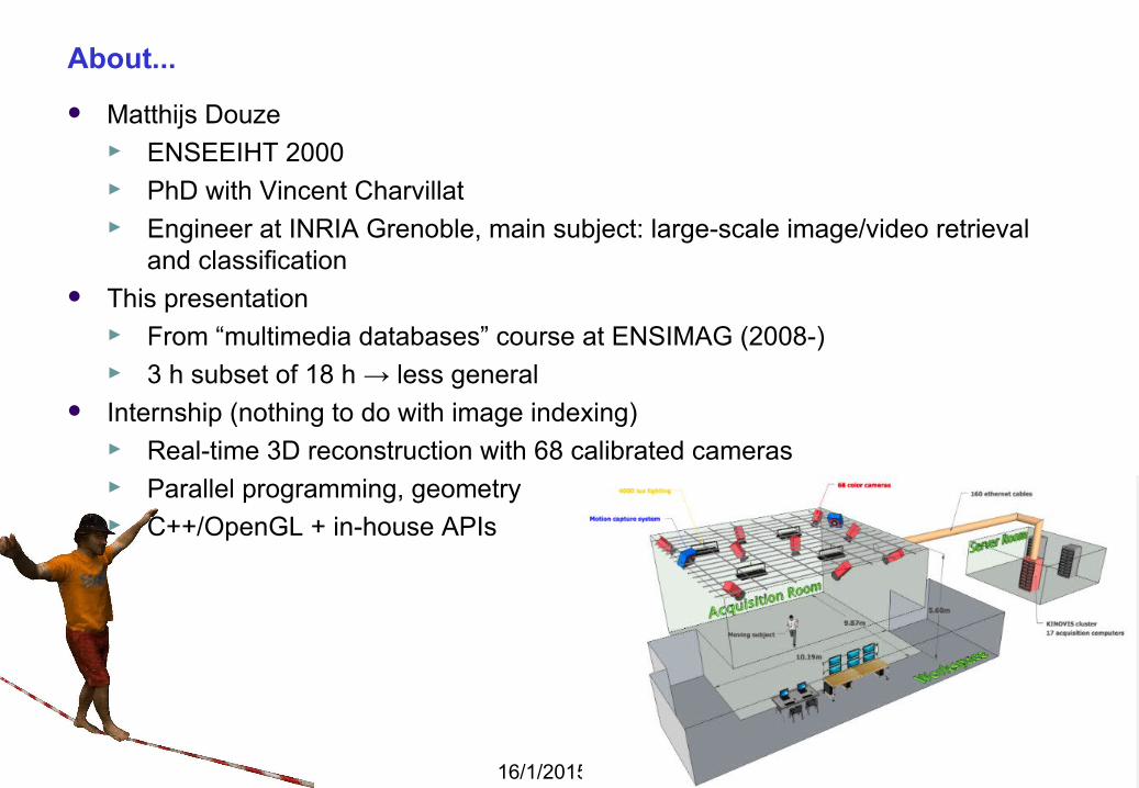
About...
Matthijs Douze► ENSEEIHT 2000► PhD with Vincent Charvillat► Engineer at INRIA Grenoble, main subject: large-scale image/video retrieval
and classification This presentation
► From “multimedia databases” course at ENSIMAG (2008-)► 3 h subset of 18 h → less general
Internship (nothing to do with image indexing)► Real-time 3D reconstruction with 68 calibrated cameras► Parallel programming, geometry► C++/OpenGL + in-house APIs

16/1/2015, page 3
Outline
Problem statement Extracting local image descriptors Indexing by image matching Bag-of-words and the inverted file Local descriptor aggregation Nearest neighbor search (low dimension) Nearest neighbor search (high dimension) Results

16/1/2015, page 4
1. Problem statement
16/1/2015, page 5
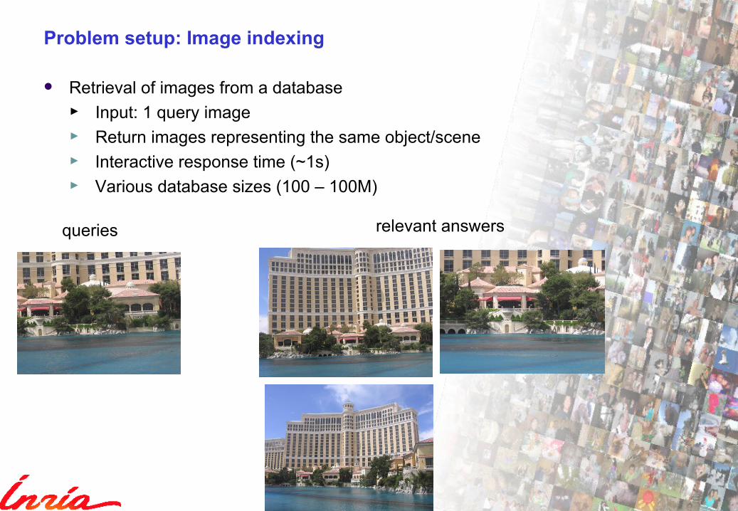
Problem setup: Image indexing
Retrieval of images from a database► Input: 1 query image► Return images representing the same object/scene► Interactive response time (~1s)► Various database sizes (100 – 100M)
queries relevant answers
16/1/2015, page 6
Types of object recognition
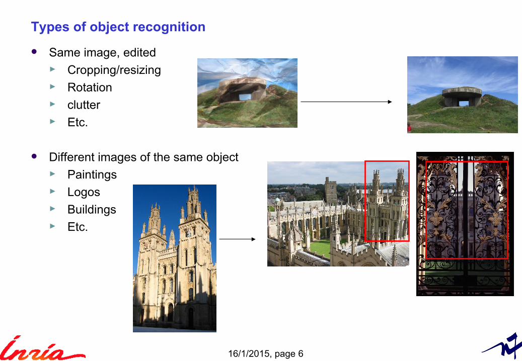
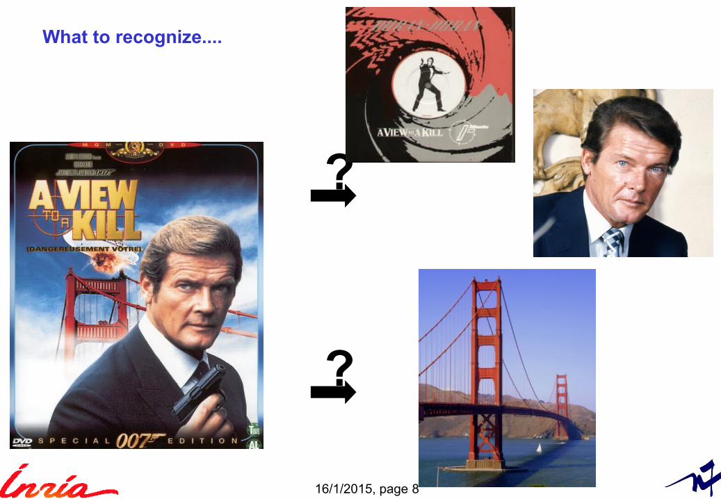
Same image, edited► Cropping/resizing► Rotation► clutter► Etc.
Different images of the same object► Paintings► Logos► Buildings► Etc.
16/1/2015, page 7
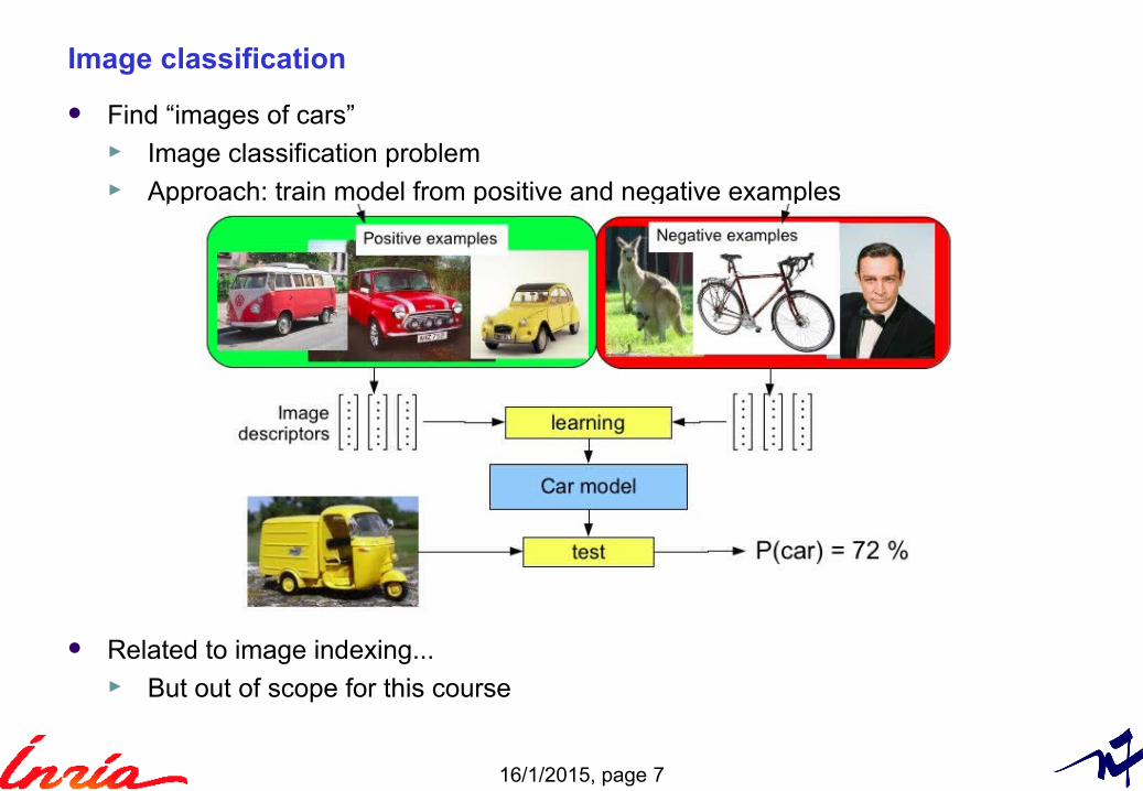
Image classification
Find “images of cars”► Image classification problem► Approach: train model from positive and negative examples
Related to image indexing... ► But out of scope for this course
16/1/2015, page 8
What to recognize....
?
?
16/1/2015, page 9
Applications
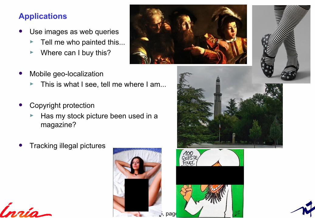
Use images as web queries► Tell me who painted this...► Where can I buy this?
Mobile geo-localization
► This is what I see, tell me where I am...
Copyright protection► Has my stock picture been used in a
magazine?
Tracking illegal pictures
16/1/2015, page 10
Commercial image databases
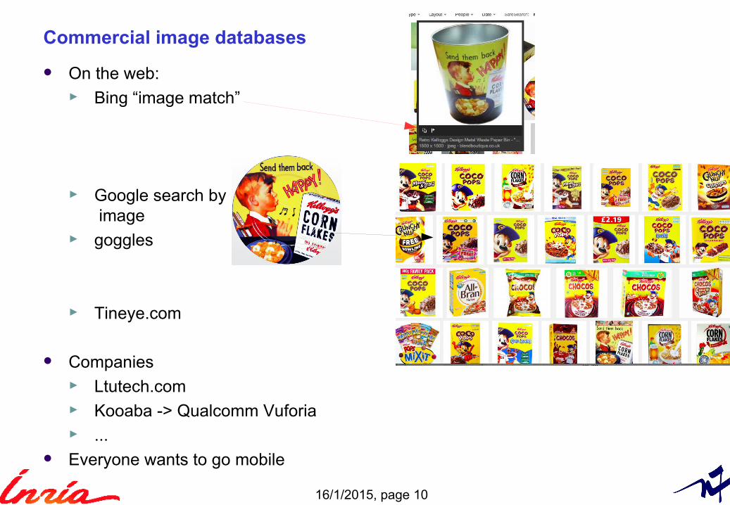
On the web:► Bing “image match”
► Google search by image
► goggles
► Tineye.com
Companies► Ltutech.com► Kooaba -> Qualcomm Vuforia► ...
Everyone wants to go mobile
16/1/2015, page 11
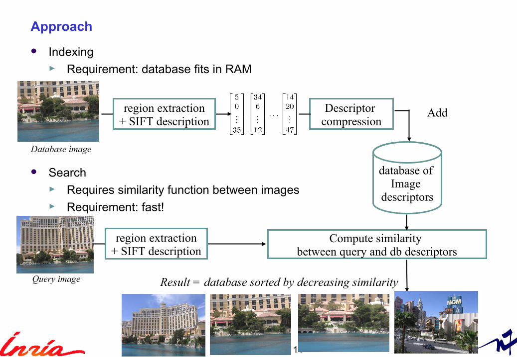
Approach
Indexing► Requirement: database fits in RAM
Search► Requires similarity function between images► Requirement: fast!
region extraction + SIFT description
Descriptor compression
Database image
database of Image
descriptors
region extraction + SIFT description
Query image
Add
Compute similarity between query and db descriptors
Result = database sorted by decreasing similarity
16/1/2015, page 12
2. Extracting local image descriptors
16/1/2015, page 13
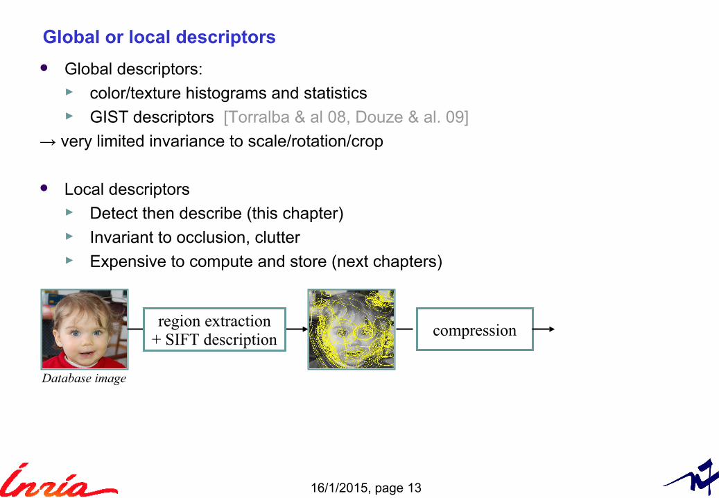
Global or local descriptors
Global descriptors:► color/texture histograms and statistics► GIST descriptors [Torralba & al 08, Douze & al. 09]
→ very limited invariance to scale/rotation/crop
Local descriptors► Detect then describe (this chapter)► Invariant to occlusion, clutter ► Expensive to compute and store (next chapters)
region extraction + SIFT description
compression
Database image
16/1/2015, page 14
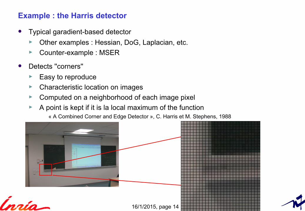
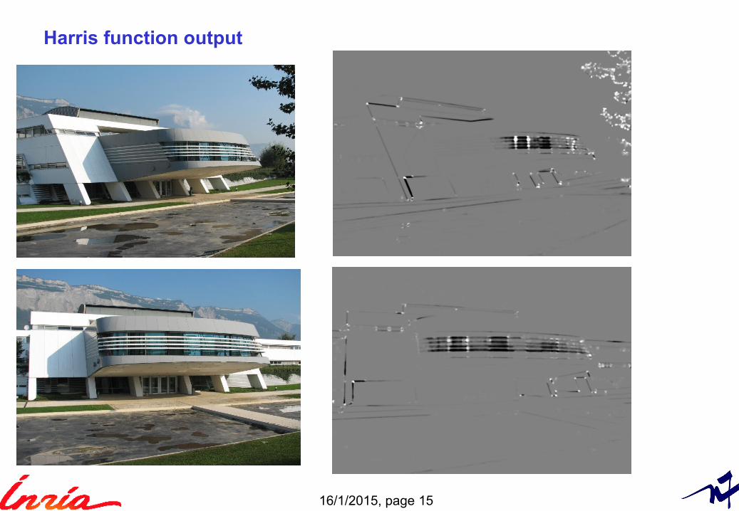
Example : the Harris detector
Typical garadient-based detector► Other examples : Hessian, DoG, Laplacian, etc.► Counter-example : MSER
Detects ''corners''► Easy to reproduce► Characteristic location on images► Computed on a neighborhood of each image pixel► A point is kept if it is la local maximum of the function
« A Combined Corner and Edge Detector », C. Harris et M. Stephens, 1988
16/1/2015, page 15
Harris function output
16/1/2015, page 16
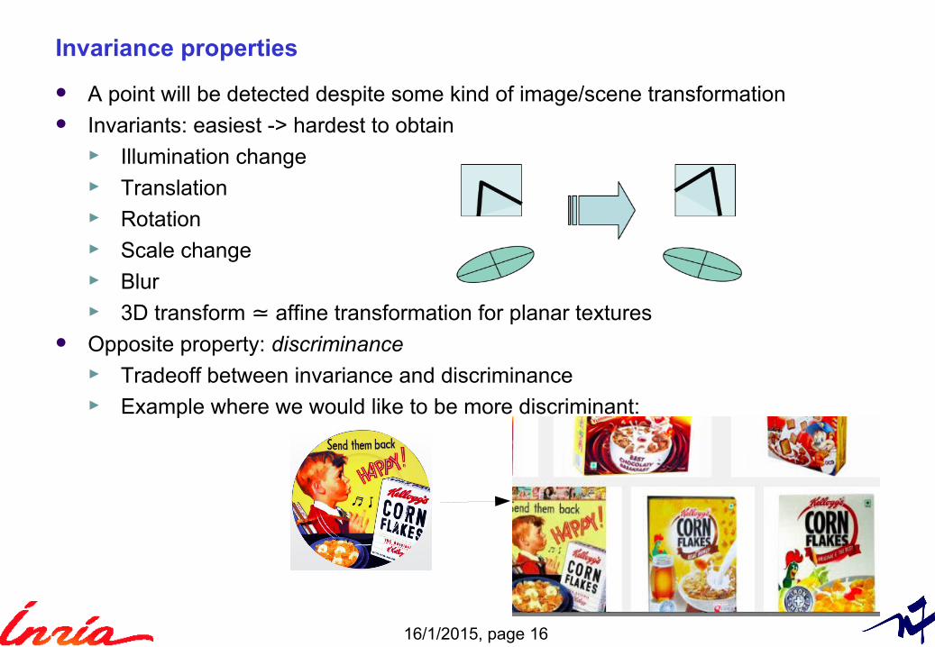
Invariance properties
A point will be detected despite some kind of image/scene transformation Invariants: easiest -> hardest to obtain
► Illumination change► Translation► Rotation► Scale change► Blur► 3D transform ≃ affine transformation for planar textures
Opposite property: discriminance► Tradeoff between invariance and discriminance► Example where we would like to be more discriminant:
16/1/2015, page 17
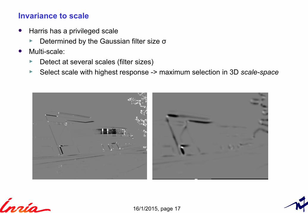
Invariance to scale
Harris has a privileged scale► Determined by the Gaussian filter size σ
Multi-scale:► Detect at several scales (filter sizes)► Select scale with highest response -> maximum selection in 3D scale-space
16/1/2015, page 18
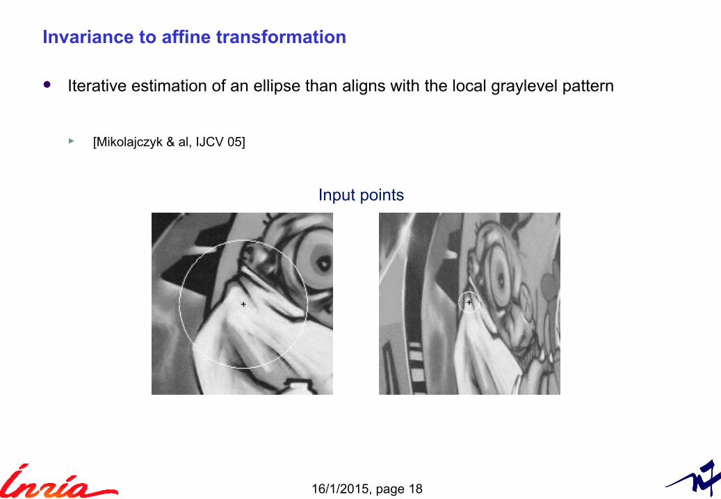
Invariance to affine transformation
Iterative estimation of an ellipse than aligns with the local graylevel pattern
► [Mikolajczyk & al, IJCV 05]
Input points
16/1/2015, page 19
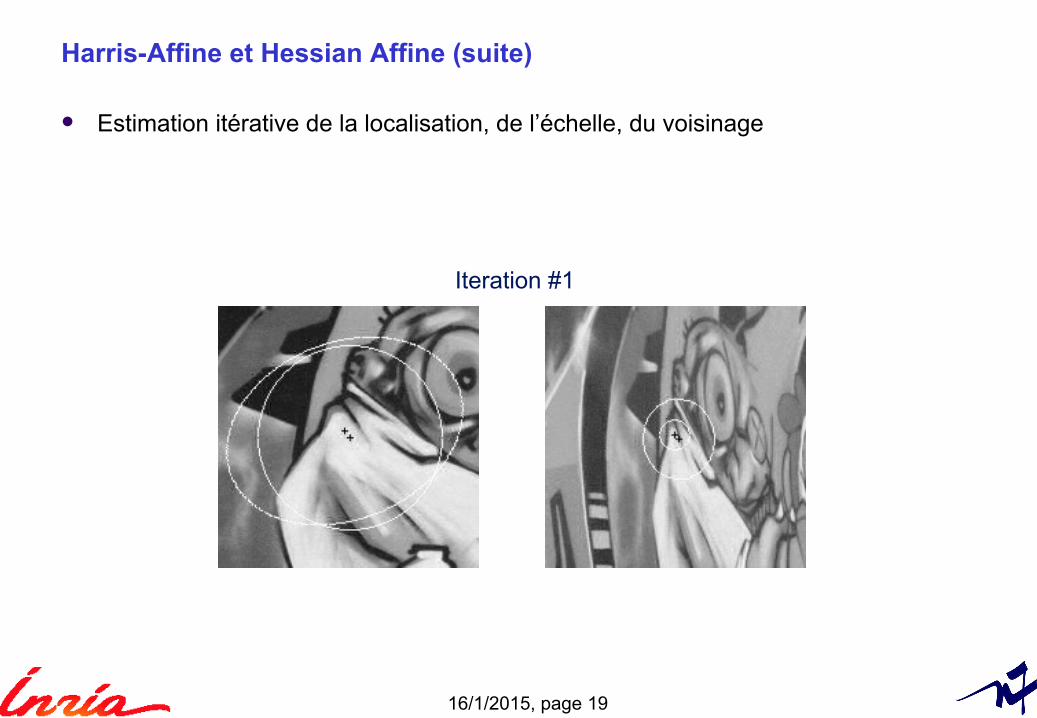
Harris-Affine et Hessian Affine (suite)
Estimation itérative de la localisation, de l’échelle, du voisinage
Iteration #1

16/1/2015, page 20
Harris-Affine et Hessian Affine (suite)
Estimation itérative de la localisation, de l’échelle, du voisinage
Iteration #2
16/1/2015, page 21
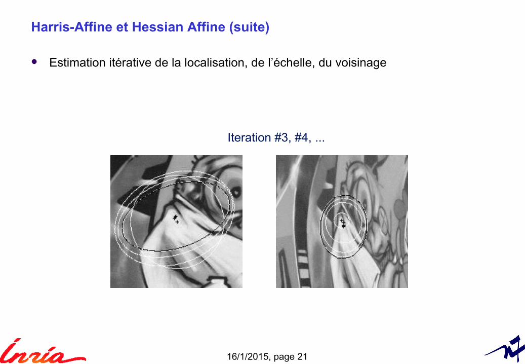
Harris-Affine et Hessian Affine (suite)
Estimation itérative de la localisation, de l’échelle, du voisinage
Iteration #3, #4, ...
16/1/2015, page 22
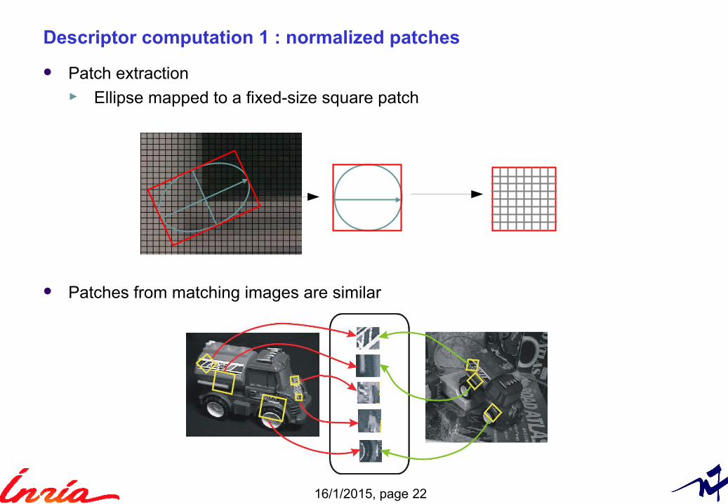
Descriptor computation 1 : normalized patches
Patch extraction► Ellipse mapped to a fixed-size square patch
Patches from matching images are similar
16/1/2015, page 23
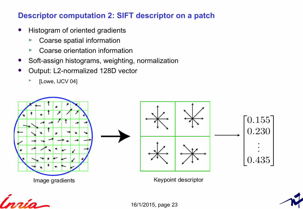
Descriptor computation 2: SIFT descriptor on a patch
Histogram of oriented gradients► Coarse spatial information ► Coarse orientation information
Soft-assign histograms, weighting, normalization Output: L2-normalized 128D vector
► [Lowe, IJCV 04]
16/1/2015, page 24
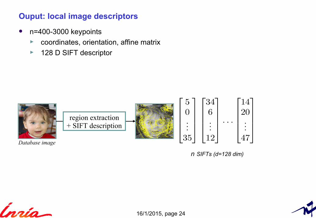
Ouput: local image descriptors
n=400-3000 keypoints► coordinates, orientation, affine matrix► 128 D SIFT descriptor
region extraction + SIFT description
Database image
n SIFTs (d=128 dim)
16/1/2015, page 25
3. Indexing by image matching
16/1/2015, page 26
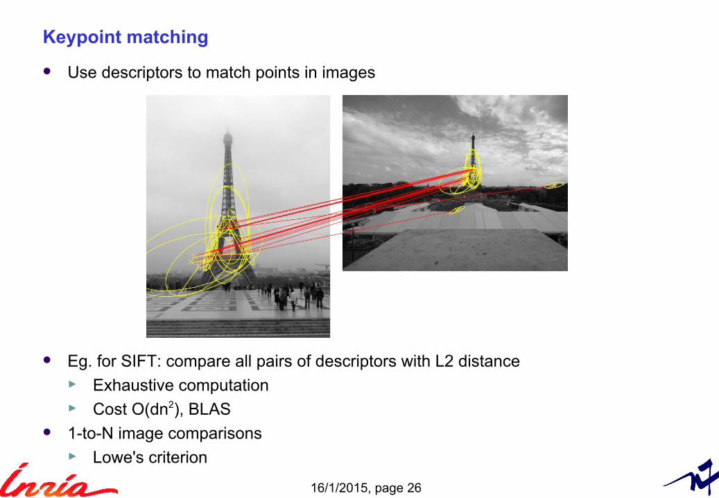
Keypoint matching
Use descriptors to match points in images
Eg. for SIFT: compare all pairs of descriptors with L2 distance► Exhaustive computation► Cost O(dn2), BLAS
1-to-N image comparisons► Lowe's criterion
16/1/2015, page 27
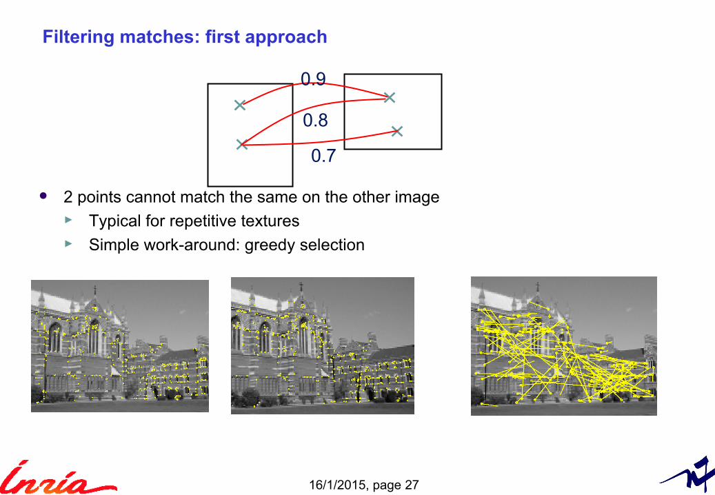
Filtering matches: first approach
2 points cannot match the same on the other image► Typical for repetitive textures► Simple work-around: greedy selection
0.9
0.8
0.7
16/1/2015, page 28
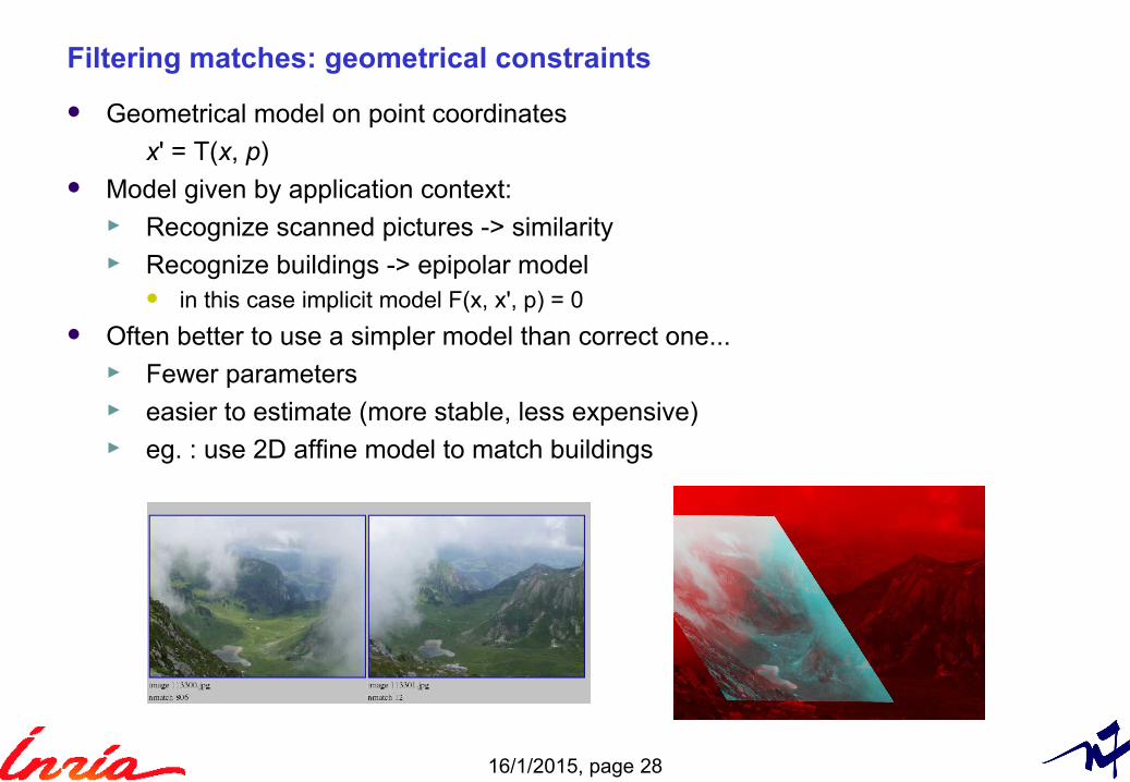
Filtering matches: geometrical constraints
Geometrical model on point coordinates
x' = T(x, p) Model given by application context:
► Recognize scanned pictures -> similarity► Recognize buildings -> epipolar model
in this case implicit model F(x, x', p) = 0
Often better to use a simpler model than correct one...► Fewer parameters► easier to estimate (more stable, less expensive)► eg. : use 2D affine model to match buildings
16/1/2015, page 29
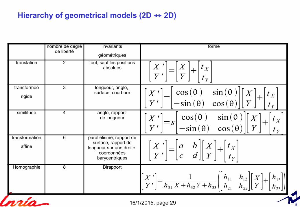
Hierarchy of geometrical models (2D ↔ 2D)
nombre de degréde liberté
invariants
géométriques
forme
translation 2 tout, sauf les positionsabsolues
transformée
rigide
3 longueur, angle, surface, courbure
similitude 4 angle, rapport de longueur
transformation
affine
6 parallélisme, rapport desurface, rapport de
longueur sur une droite,coordonnées
barycentriques
Homographie 8 Birapport
[ X 'Y ' ]=[a b
c d ] [ XY ][ t X
tY ][ X 'Y ' ]=s [ cos sin
−sin cos ][ XY ][ t X
tY ][ X 'Y ' ]=[ cos sin
−sin cos ] [ XY ][t X
tY ][ X 'Y ' ]=[XY ][ t X
tY]
[ X 'Y ' ]= 1
h31 X h32 Y h33 [h11 h12
h21 h22] [ X
Y ][h13
h23]
16/1/2015, page 30
Filtering matches: estimating model parameters
Estimate model parameters p robustly► Input: descriptor matches (many outliers)► Output: subset correct matches + model parameters
Robust estimation► RANSAC► Hough transform (low-dim models)
16/1/2015, page 31
Compute image similarity from keypoint matches
Basic: number of matching points between the two images Per-match weightings:
► descriptor distances► Geometrical matching error
Per-database image score normalization► number of keypoints► model likelihood
In practice: usable for ~10 images...
16/1/2015, page 32
4. Bag-of-words and the inverted file
16/1/2015, page 33
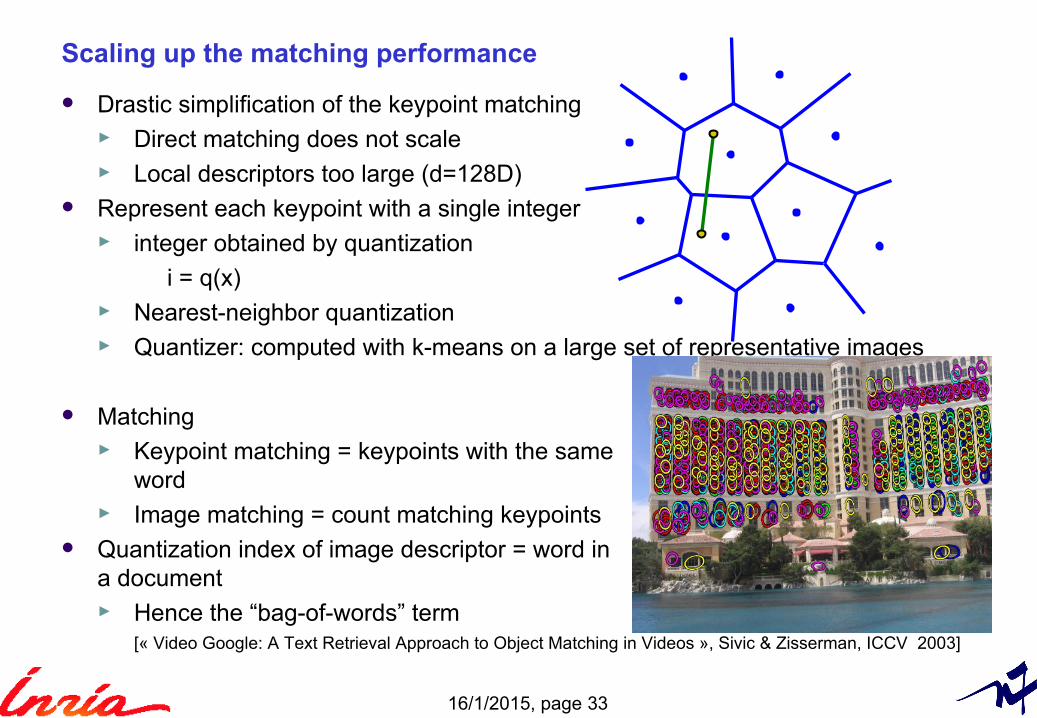
Scaling up the matching performance
Drastic simplification of the keypoint matching► Direct matching does not scale► Local descriptors too large (d=128D)
Represent each keypoint with a single integer► integer obtained by quantization
i = q(x)► Nearest-neighbor quantization► Quantizer: computed with k-means on a large set of representative images
Matching► Keypoint matching = keypoints with the same
word► Image matching = count matching keypoints
Quantization index of image descriptor = word in a document► Hence the “bag-of-words” term
[« Video Google: A Text Retrieval Approach to Object Matching in Videos », Sivic & Zisserman, ICCV 2003]
16/1/2015, page 34
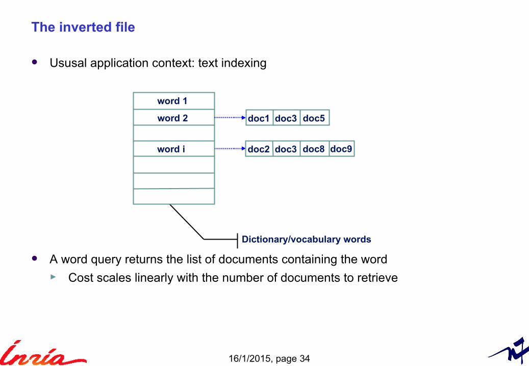
The inverted file
Ususal application context: text indexing
A word query returns the list of documents containing the word► Cost scales linearly with the number of documents to retrieve
word 1
Dictionary/vocabulary words
word 2
word i doc2 doc3 doc8 doc9
doc1 doc3 doc5
16/1/2015, page 35
Searching in text documents (1)
Vector model► Given a dictionary of size k► A text document is represented by a vector f=(f1,…,fi,…fk) ∈ ℝk
► Each dimension corresponds to a dictionary word► fi = frequency of the word in the document
In practice, non-discriminant words are removed from the dictionary► “the”, “a”, “is”, “them”, etc, are not discriminant enough (stop words)
Vectors are sparse ► The dictionary large wrt. Number of words used in document
16/1/2015, page 36
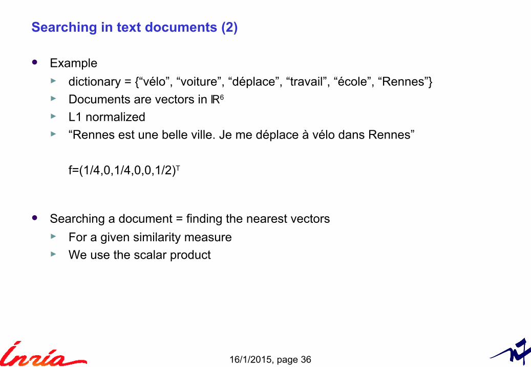
Searching in text documents (2)
Example► dictionary = {“vélo”, “voiture”, “déplace”, “travail”, “école”, “Rennes”} ► Documents are vectors in ℝ6
► L1 normalized► “Rennes est une belle ville. Je me déplace à vélo dans Rennes”
f=(1/4,0,1/4,0,0,1/2)T
Searching a document = finding the nearest vectors► For a given similarity measure► We use the scalar product
16/1/2015, page 37
1 0 0 0 5 0 0 0
0 0 1 0 0 0 2 0
0 0 0 0 0 0 1 1
y1
y2
y3
2
3
y2 1
y1 1
y2 5
y1 2
y3 1
y3 1
0 2 0 0 3 0 0 0q
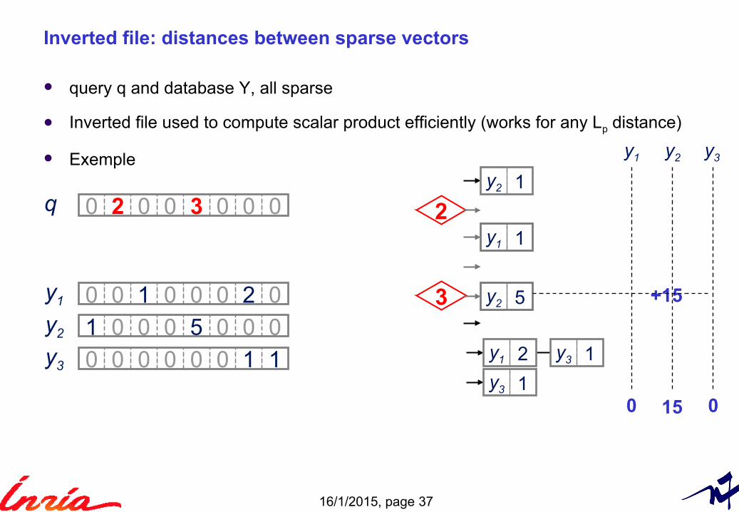
Inverted file: distances between sparse vectors
query q and database Y, all sparse
Inverted file used to compute scalar product efficiently (works for any Lp distance)
Exemple y1 y2 y3
+15
15 00
16/1/2015, page 38
Cost of searching in an inverted file
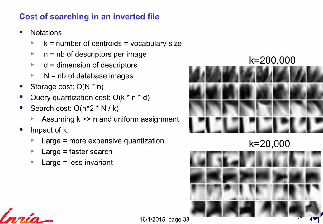
Notations► k = number of centroids = vocabulary size► n = nb of descriptors per image► d = dimension of descriptors► N = nb of database images
Storage cost: O(N * n) Query quantization cost: O(k * n * d) Search cost: O(n^2 * N / k)
► Assuming k >> n and uniform assignment Impact of k:
► Large = more expensive quantization ► Large = faster search► Large = less invariant
k=200,000
k=20,000
16/1/2015, page 39
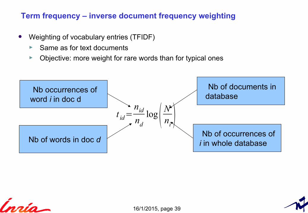
Term frequency – inverse document frequency weighting
Weighting of vocabulary entries (TFIDF) ► Same as for text documents► Objective: more weight for rare words than for typical ones
t id=nid
nd
log( Nni)
Nb occurrences ofword i in doc d
Nb of words in doc d
Nb of documents indatabase
Nb of occurrences ofi in whole database
16/1/2015, page 40
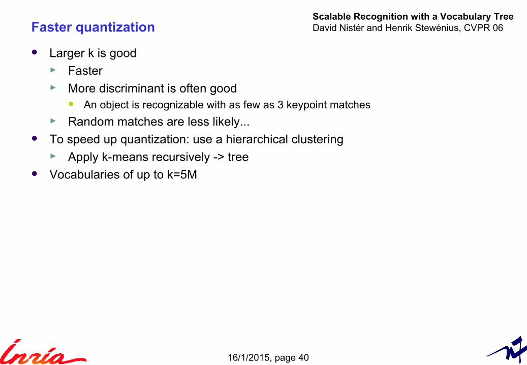
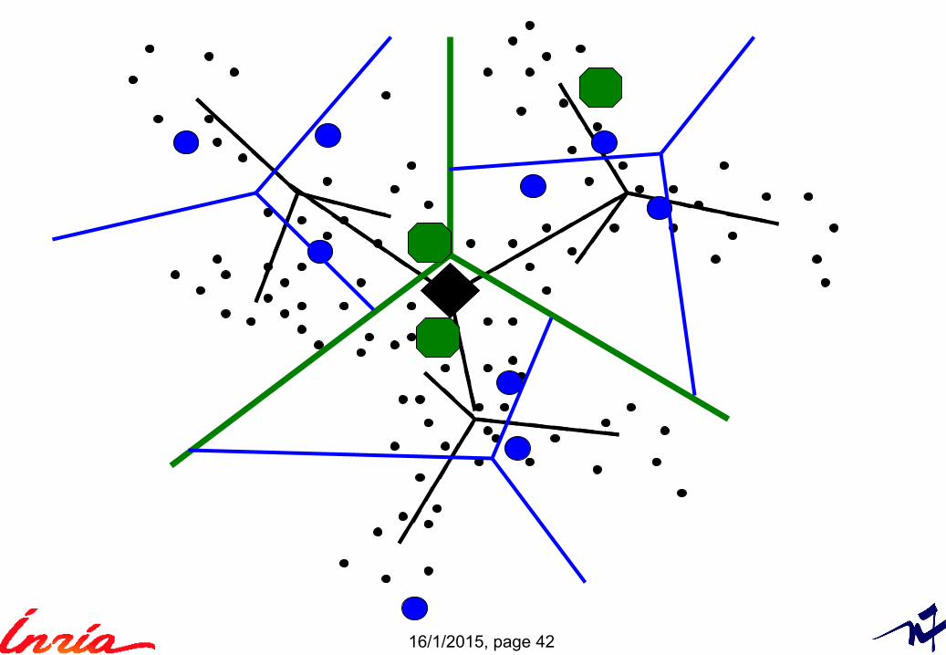
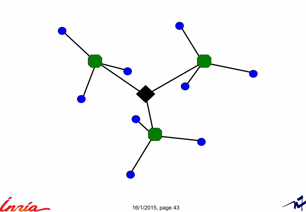
Faster quantization
Larger k is good► Faster► More discriminant is often good
An object is recognizable with as few as 3 keypoint matches► Random matches are less likely...
To speed up quantization: use a hierarchical clustering► Apply k-means recursively -> tree
Vocabularies of up to k=5M
Scalable Recognition with a Vocabulary Tree David Nistér and Henrik Stewénius, CVPR 06
16/1/2015, page 41
16/1/2015, page 42
16/1/2015, page 43
16/1/2015, page 44
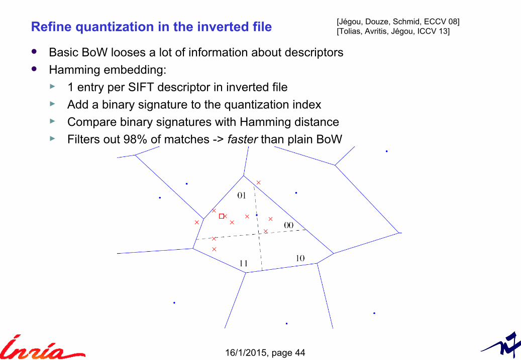
Refine quantization in the inverted file
Basic BoW looses a lot of information about descriptors Hamming embedding:
► 1 entry per SIFT descriptor in inverted file► Add a binary signature to the quantization index► Compare binary signatures with Hamming distance► Filters out 98% of matches -> faster than plain BoW
[Jégou, Douze, Schmid, ECCV 08][Tolias, Avritis, Jégou, ICCV 13]
16/1/2015, page 45
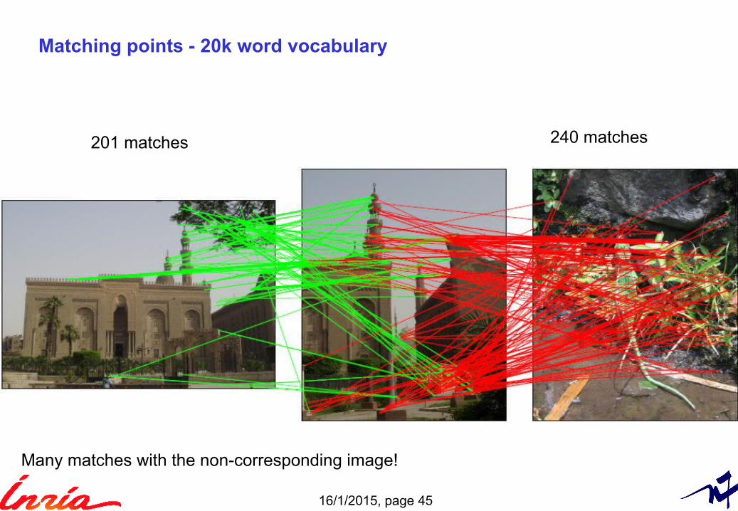
Matching points - 20k word vocabulary
201 matches 240 matches
Many matches with the non-corresponding image!
16/1/2015, page 46
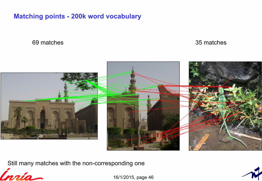
Matching points - 200k word vocabulary
69 matches 35 matches
Still many matches with the non-corresponding one
16/1/2015, page 47
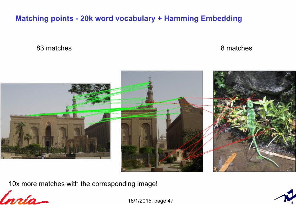
Matching points - 20k word vocabulary + Hamming Embedding
83 matches 8 matches
10x more matches with the corresponding image!
16/1/2015, page 48
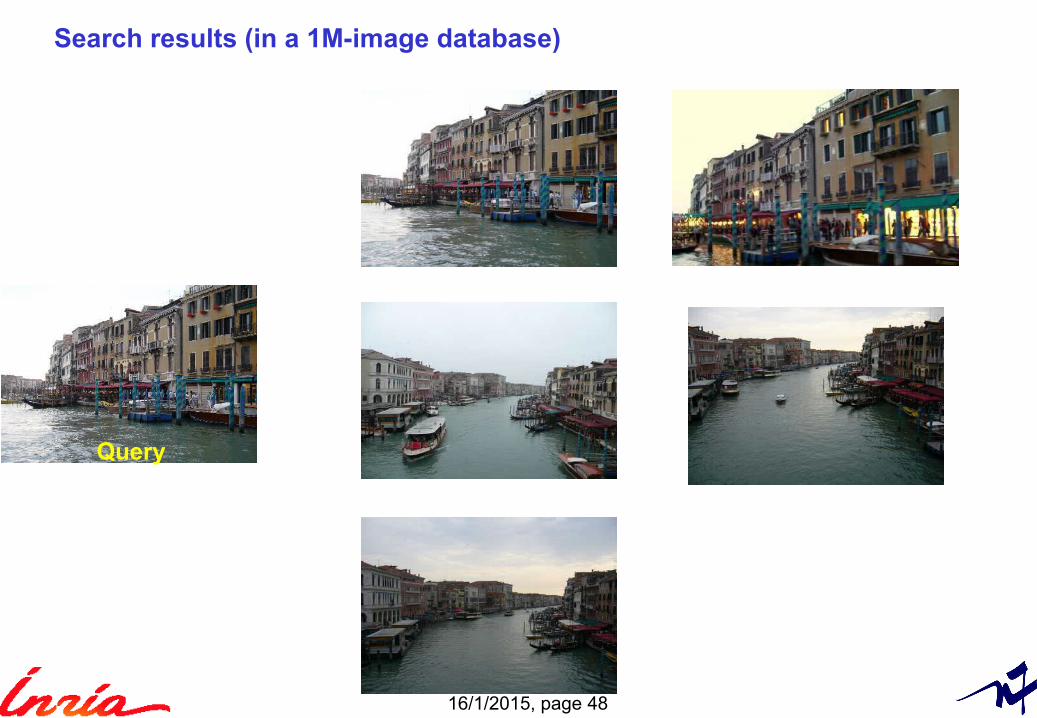
Search results (in a 1M-image database)
Query
16/1/2015, page 49
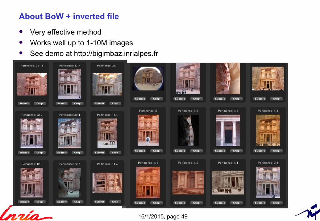
About BoW + inverted file
Very effective method Works well up to 1-10M images See demo at http://bigimbaz.inrialpes.fr
16/1/2015, page 50
5. Local descriptor aggregation
16/1/2015, page 51
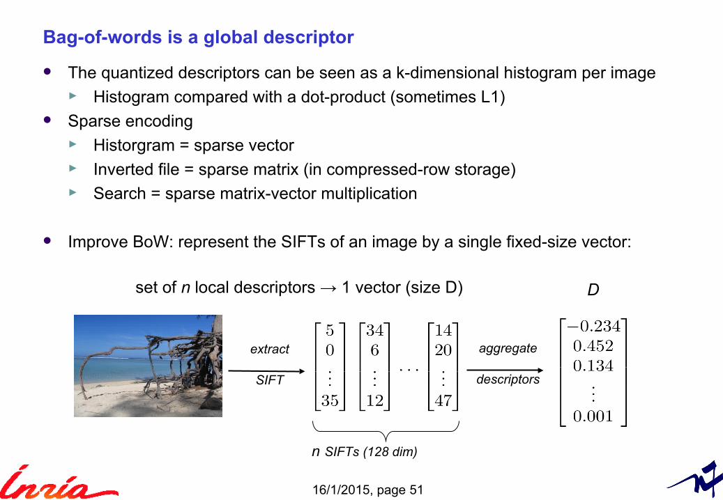
Bag-of-words is a global descriptor
The quantized descriptors can be seen as a k-dimensional histogram per image► Histogram compared with a dot-product (sometimes L1)
Sparse encoding► Historgram = sparse vector► Inverted file = sparse matrix (in compressed-row storage)► Search = sparse matrix-vector multiplication
Improve BoW: represent the SIFTs of an image by a single fixed-size vector:
set of n local descriptors → 1 vector (size D)
extract
SIFT
aggregate
descriptors
D
n SIFTs (128 dim)
16/1/2015, page 52
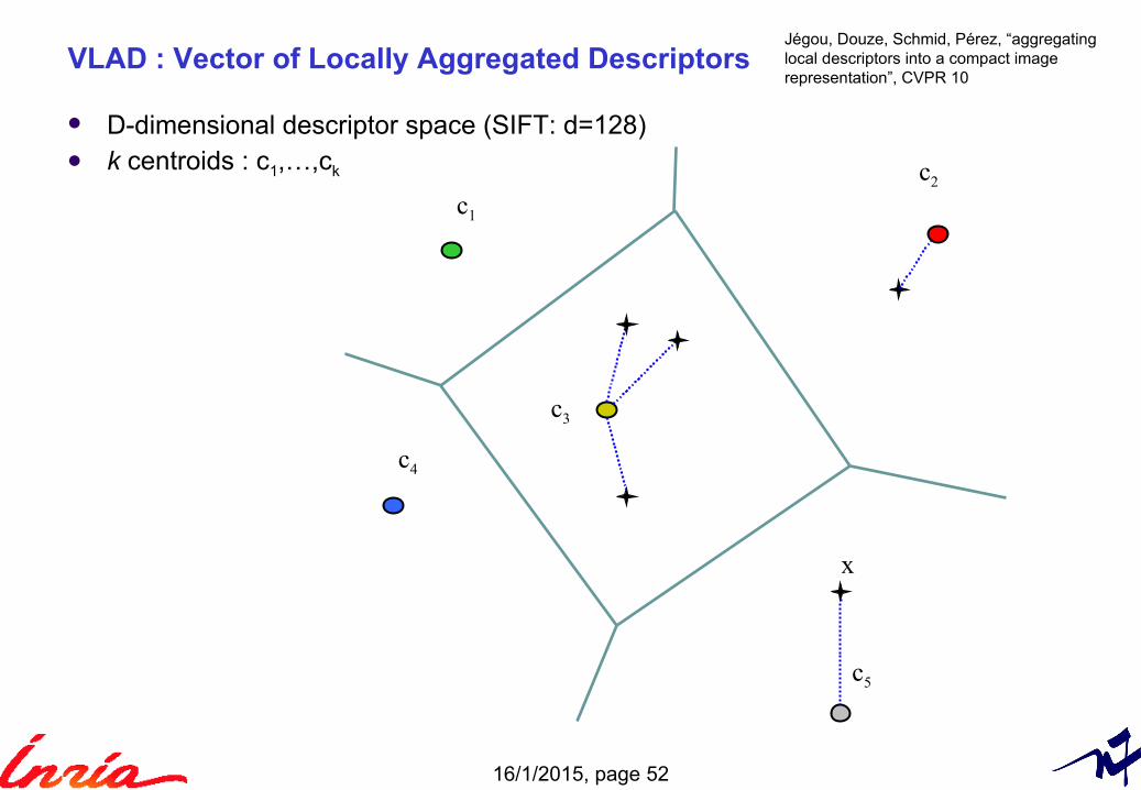
VLAD : Vector of Locally Aggregated Descriptors
c3
x
c1
c4
c2
c5
D-dimensional descriptor space (SIFT: d=128) k centroids : c1,…,ck
Jégou, Douze, Schmid, Pérez, “aggregatinglocal descriptors into a compact imagerepresentation”, CVPR 10
16/1/2015, page 53
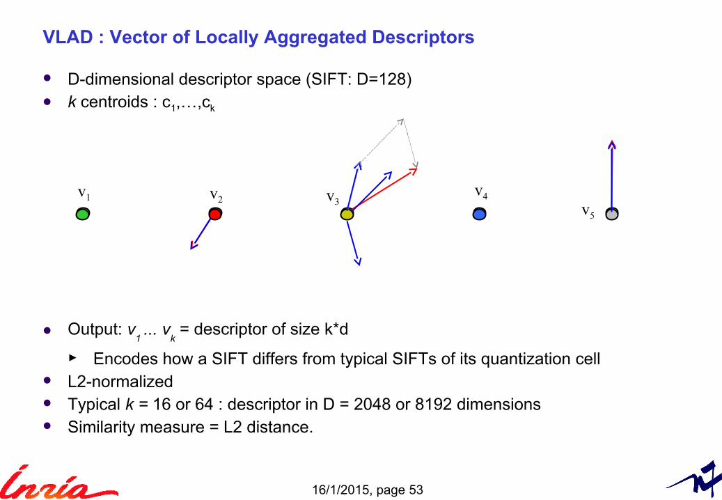
VLAD : Vector of Locally Aggregated Descriptors
v1 v2 v3v4
v5
D-dimensional descriptor space (SIFT: D=128) k centroids : c1,…,ck
Output: v1 ... v
k = descriptor of size k*d
► Encodes how a SIFT differs from typical SIFTs of its quantization cell L2-normalized Typical k = 16 or 64 : descriptor in D = 2048 or 8192 dimensions Similarity measure = L2 distance.
16/1/2015, page 54
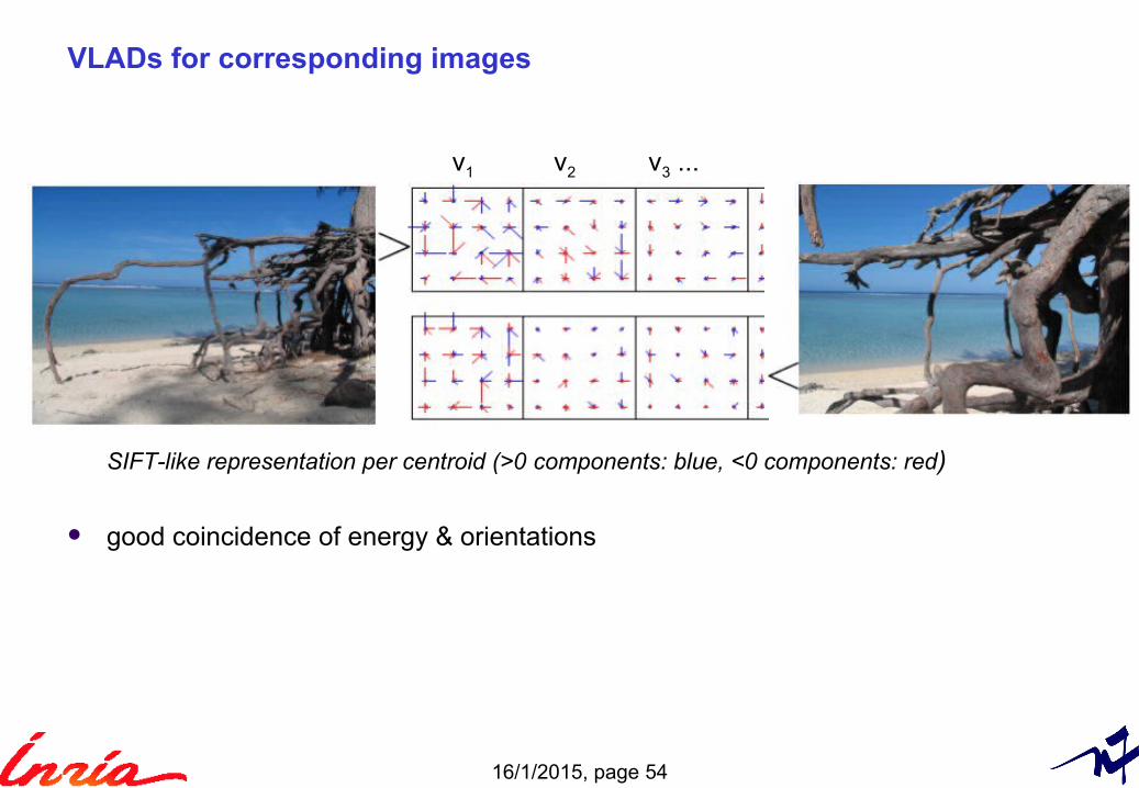
VLADs for corresponding images
SIFT-like representation per centroid (>0 components: blue, <0 components: red)
good coincidence of energy & orientations
v1 v2 v3 ...
16/1/2015, page 55
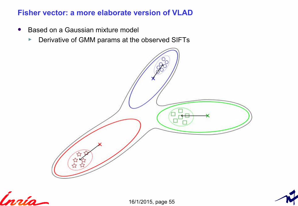
Fisher vector: a more elaborate version of VLAD
“Fisher kernels on visual vocabularies for image Categorization”. Perronnin & Dance, CVPR 2007
Based on a Gaussian mixture model► Derivative of GMM params at the observed SIFTs
16/1/2015, page 56
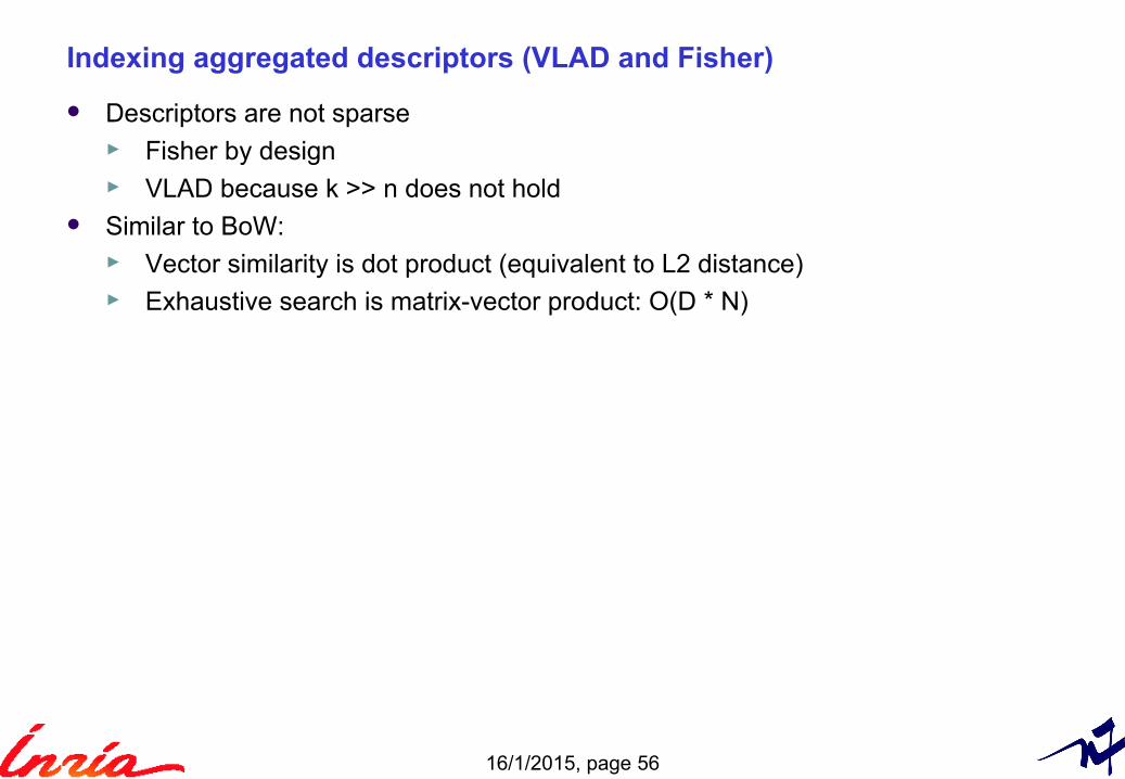
Indexing aggregated descriptors (VLAD and Fisher)
Descriptors are not sparse► Fisher by design► VLAD because k >> n does not hold
Similar to BoW:► Vector similarity is dot product (equivalent to L2 distance)► Exhaustive search is matrix-vector product: O(D * N)
16/1/2015, page 57
6. Nearest-neighbor search (low dimension)
16/1/2015, page 58
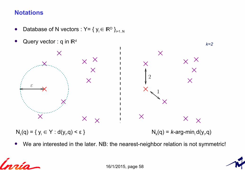
Notations
Database of N vectors : Y= { yi ∈ ℝD }i=1..N
Query vector : q in ℝd
We are interested in the later. NB: the nearest-neighbor relation is not symmetric!
k=2
Nε(q) = { yi ∈ Y : d(yi,q) < ε } Nk(q) = k-arg-mini d(yi,q)
16/1/2015, page 59
Preliminary: finding the k nearest neighbors given computed distances
Pour Nk(q), il faut de plus trouver effectuer l’opération k-arg-mini d(q,yi)
Exemple: on veut 3-argmin {1,3,9,4,6,2,10,5}► Méthode naïve 1: trier ces distances → O(n log n)► Méthode naïve 2: maintenir un tableau des k-plus petits éléments, mis à jour
pour chaque nouvelle distance considérée → O(n k)
Intuitivement, on peut faire mieux…
16/1/2015, page 60
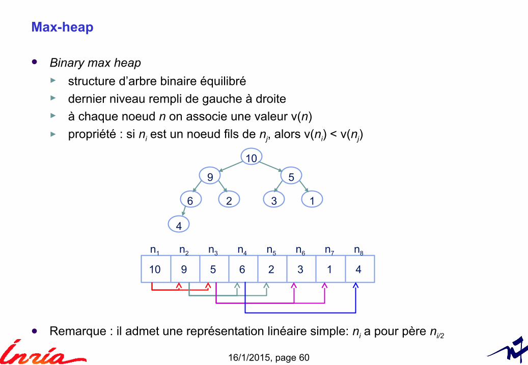
Max-heap
Binary max heap► structure d’arbre binaire équilibré► dernier niveau rempli de gauche à droite► à chaque noeud n on associe une valeur v(n)► propriété : si ni est un noeud fils de nj, alors v(ni) < v(nj)
Remarque : il admet une représentation linéaire simple: ni a pour père ni/2
10
9 5
6 2 3 1
4
n1
10
n2
9
n3
5
n4
6
n5
2
n6
3
n7
1
n8
4
16/1/2015, page 61
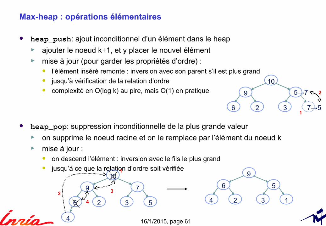
Max-heap : opérations élémentaires
heap_push: ajout inconditionnel d’un élément dans le heap ► ajouter le noeud k+1, et y placer le nouvel élément► mise à jour (pour garder les propriétés d’ordre) :
l’élément inséré remonte : inversion avec son parent s’il est plus grand jusqu’à vérification de la relation d’ordre complexité en O(log k) au pire, mais O(1) en pratique
heap_pop: suppression inconditionnelle de la plus grande valeur► on supprime le noeud racine et on le remplace par l’élément du noeud k► mise à jour :
on descend l’élément : inversion avec le fils le plus grand jusqu’à ce que la relation d’ordre soit vérifiée
10
9 7
6 2 3 5
4
10
9 5→7
6 2 3 7→5
1
2 3
4
9
6 5
4 2 3 1
1
2
16/1/2015, page 62
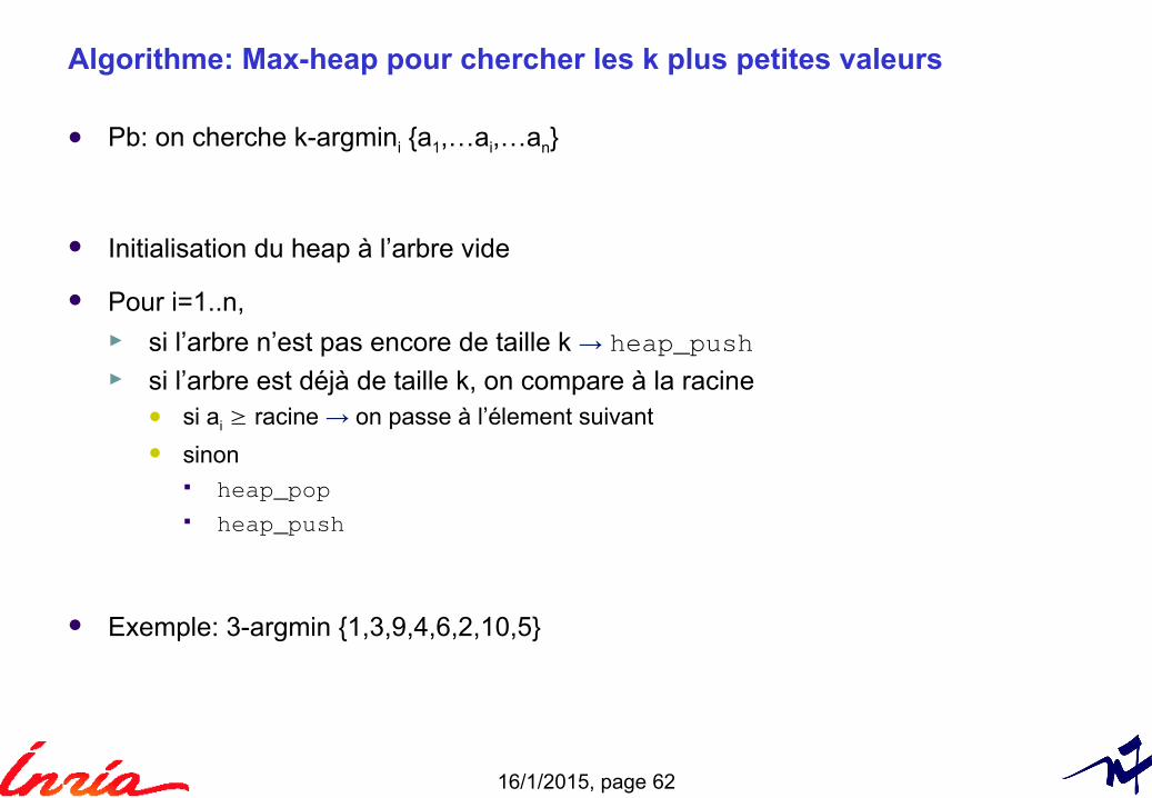
Algorithme: Max-heap pour chercher les k plus petites valeurs
Pb: on cherche k-argmini {a1,…ai,…an}
Initialisation du heap à l’arbre vide
Pour i=1..n, ► si l’arbre n’est pas encore de taille k → heap_push► si l’arbre est déjà de taille k, on compare à la racine
si ai ≥ racine → on passe à l’élement suivant
sinon heap_pop heap_push
Exemple: 3-argmin {1,3,9,4,6,2,10,5}
16/1/2015, page 63
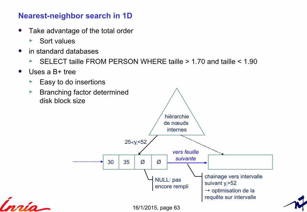
Nearest-neighbor search in 1D
Take advantage of the total order► Sort values
in standard databases► SELECT taille FROM PERSON WHERE taille > 1.70 and taille < 1.90
Uses a B+ tree ► Easy to do insertions► Branching factor determined
disk block size
vers feuillesuivante
30 35 Ø
NULL: pasencore rempli
hiérarchiede nœuds
internes
chainage vers intervallesuivant yi>52→ optimisation de larequête sur intervalle
25<yi<52
Ø
16/1/2015, page 64
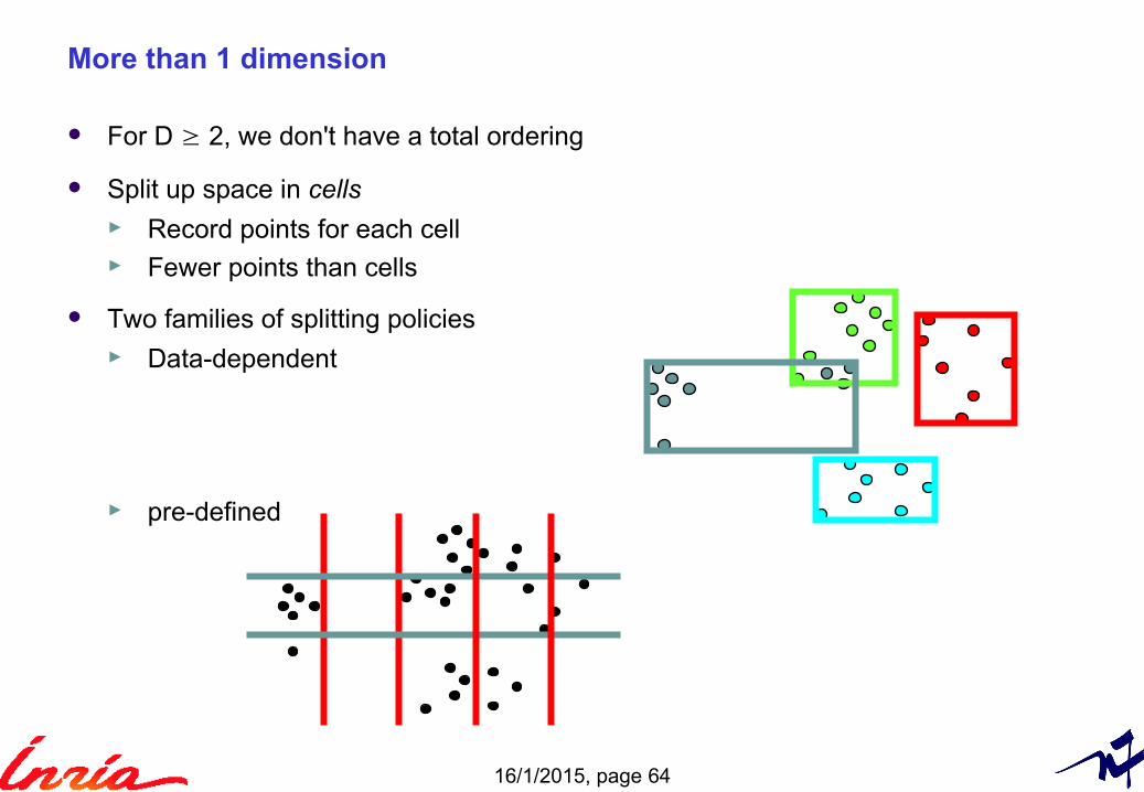
More than 1 dimension
For D ≥ 2, we don't have a total ordering
Split up space in cells ► Record points for each cell► Fewer points than cells
Two families of splitting policies► Data-dependent
► pre-defined
16/1/2015, page 65
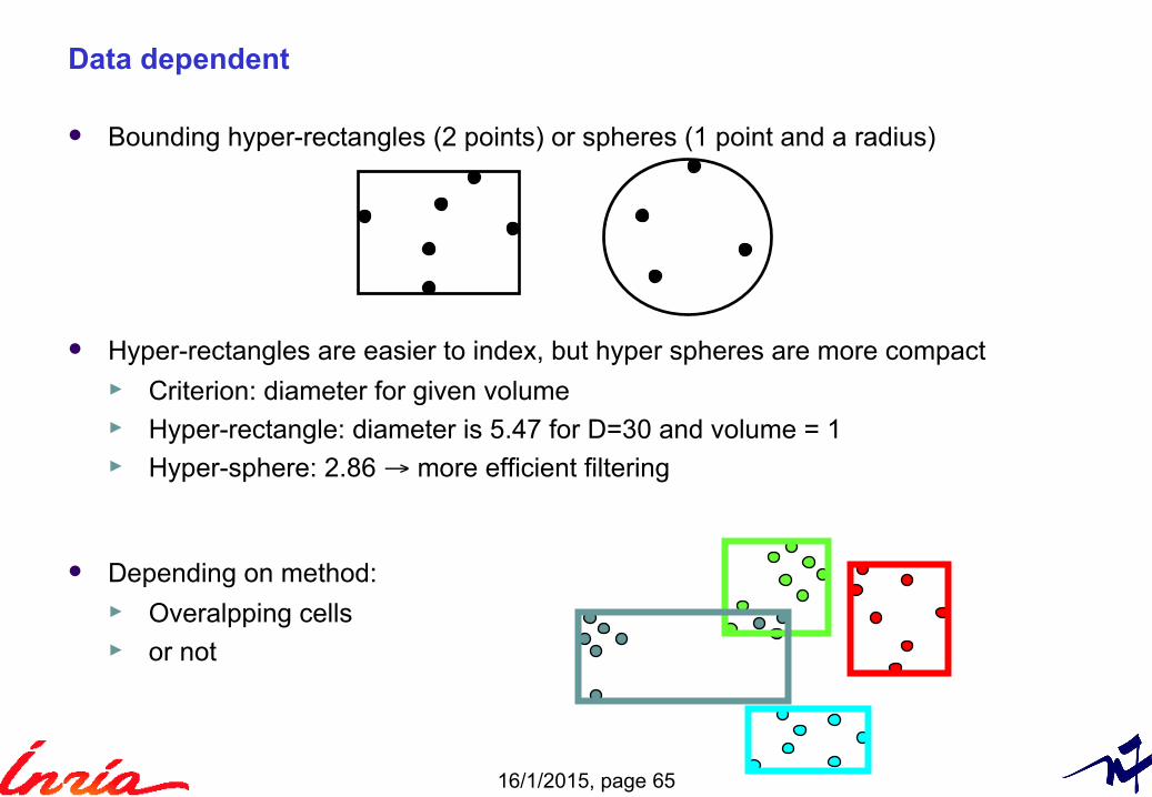
Data dependent
Bounding hyper-rectangles (2 points) or spheres (1 point and a radius)
Hyper-rectangles are easier to index, but hyper spheres are more compact► Criterion: diameter for given volume► Hyper-rectangle: diameter is 5.47 for D=30 and volume = 1► Hyper-sphere: 2.86 → more efficient filtering
Depending on method:► Overalpping cells ► or not
16/1/2015, page 66
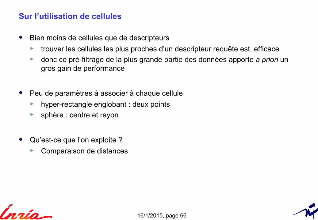
Sur l’utilisation de cellules
Bien moins de cellules que de descripteurs► trouver les cellules les plus proches d’un descripteur requête est efficace► donc ce pré-filtrage de la plus grande partie des données apporte a priori un
gros gain de performance
Peu de paramètres à associer à chaque cellule► hyper-rectangle englobant : deux points► sphère : centre et rayon
Qu’est-ce que l’on exploite ?► Comparaison de distances
16/1/2015, page 67
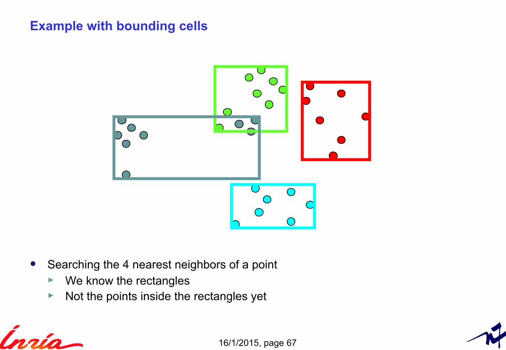
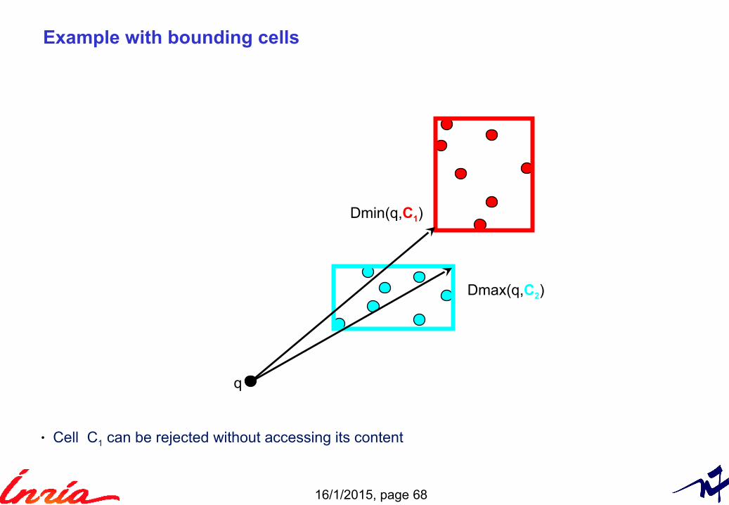
Example with bounding cells
Searching the 4 nearest neighbors of a point► We know the rectangles► Not the points inside the rectangles yet
16/1/2015, page 68
Example with bounding cells
q
Dmin(q,C1)
Dmax(q,C2)
• Cell C1 can be rejected without accessing its content
16/1/2015, page 69
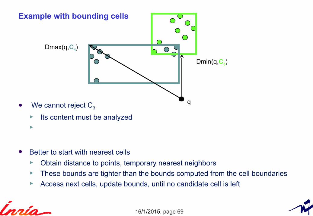
Example with bounding cells
q
Dmin(q,C3)
Dmax(q,C4)
We cannot reject C3
► Its content must be analyzed ►
Better to start with nearest cells► Obtain distance to points, temporary nearest neighbors► These bounds are tighter than the bounds computed from the cell boundaries► Access next cells, update bounds, until no candidate cell is left
16/1/2015, page 70
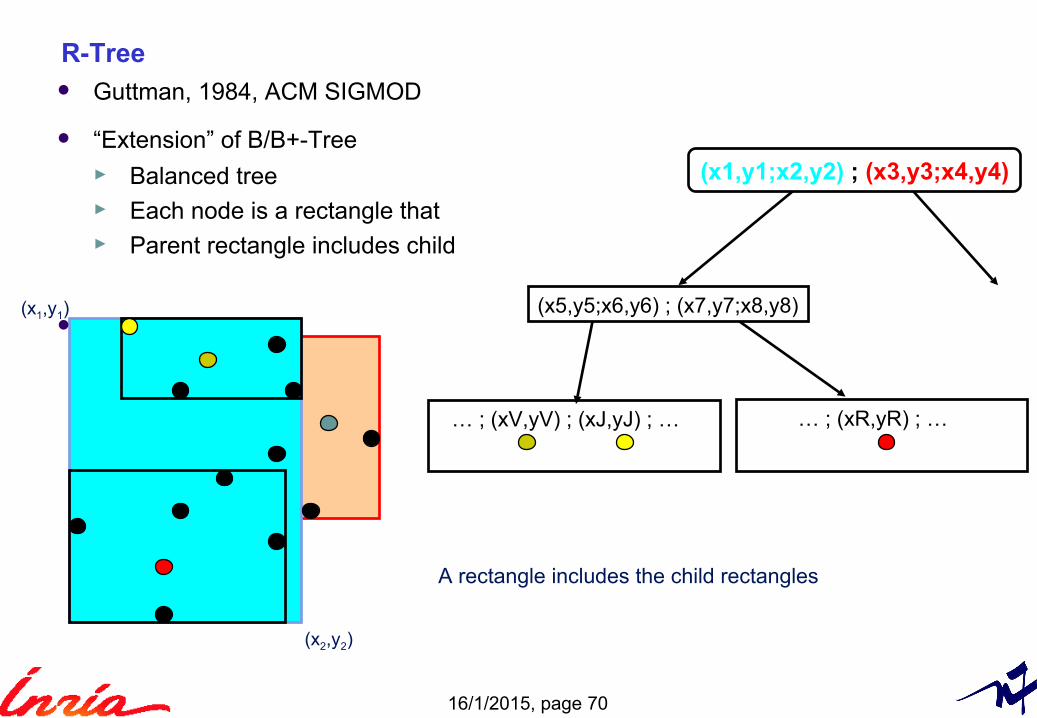
R-Tree
(x1,y1;x2,y2) ; (x3,y3;x4,y4)
(x5,y5;x6,y6) ; (x7,y7;x8,y8)
… ; (xV,yV) ; (xJ,yJ) ; … … ; (xR,yR) ; …
A rectangle includes the child rectangles
(x1,y1)
(x2,y2)
Guttman, 1984, ACM SIGMOD
“Extension” of B/B+-Tree ► Balanced tree► Each node is a rectangle that► Parent rectangle includes child
16/1/2015, page 71
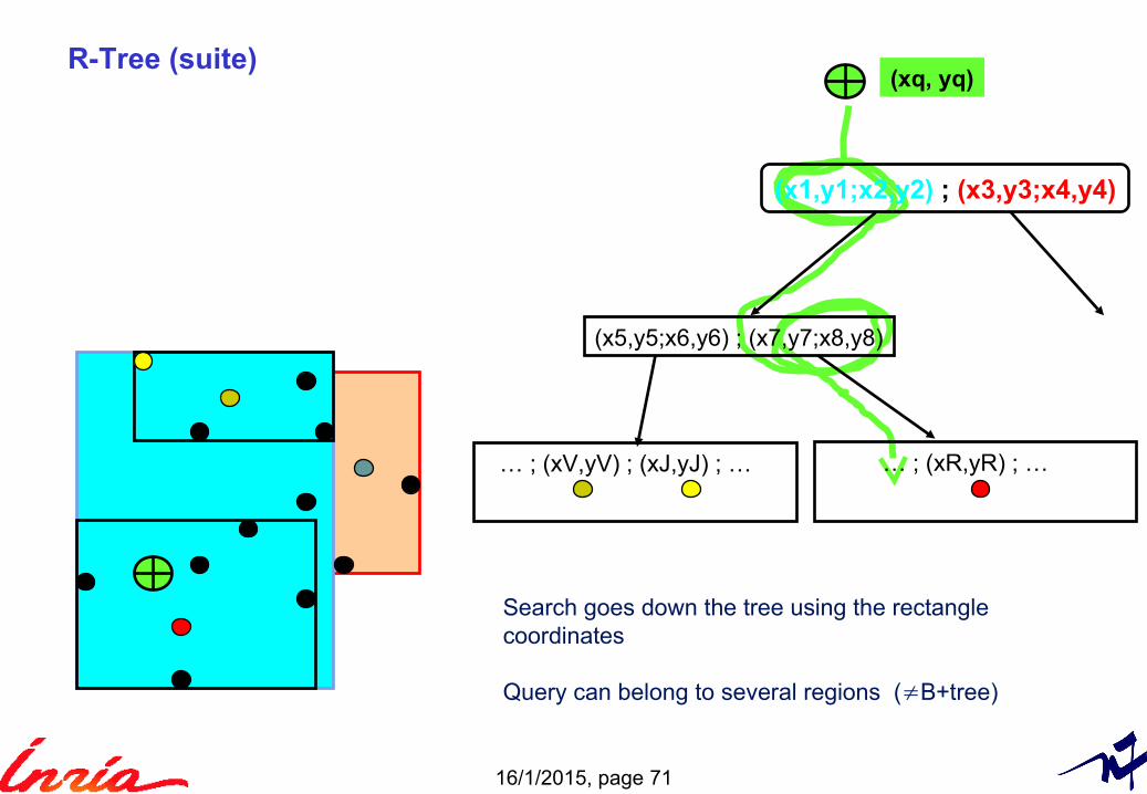
R-Tree (suite)
(x1,y1;x2,y2) ; (x3,y3;x4,y4)
(x5,y5;x6,y6) ; (x7,y7;x8,y8)
… ; (xV,yV) ; (xJ,yJ) ; …
Search goes down the tree using the rectanglecoordinates
Query can belong to several regions (≠B+tree)
… ; (xR,yR) ; …
(xq, yq)
16/1/2015, page 72
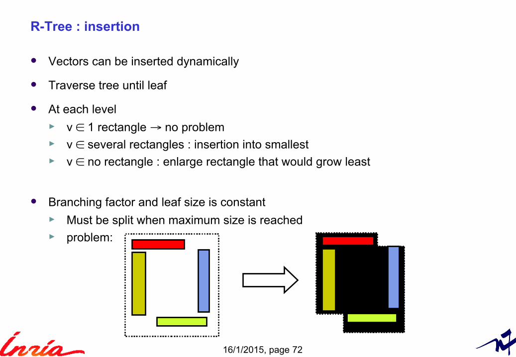
R-Tree : insertion
Vectors can be inserted dynamically
Traverse tree until leaf
At each level ► v ∈ 1 rectangle → no problem► v ∈ several rectangles : insertion into smallest► v ∈ no rectangle : enlarge rectangle that would grow least
Branching factor and leaf size is constant► Must be split when maximum size is reached ► problem:
16/1/2015, page 73
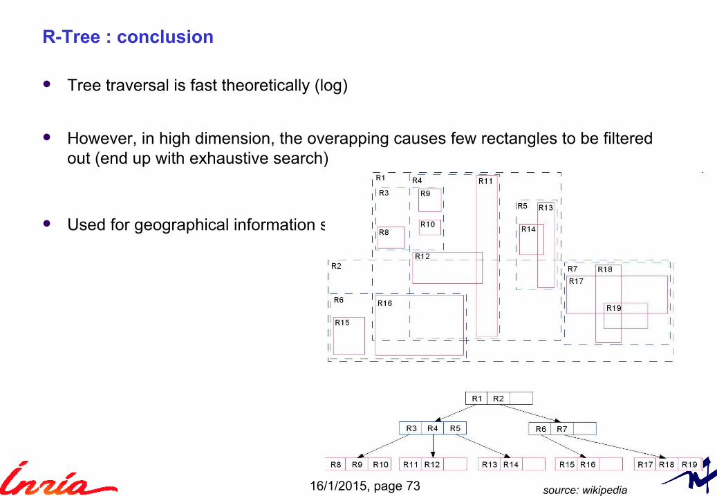
R-Tree : conclusion
Tree traversal is fast theoretically (log)
However, in high dimension, the overapping causes few rectangles to be filteredout (end up with exhaustive search)
Used for geographical information systems (2D)
source: wikipedia
16/1/2015, page 74
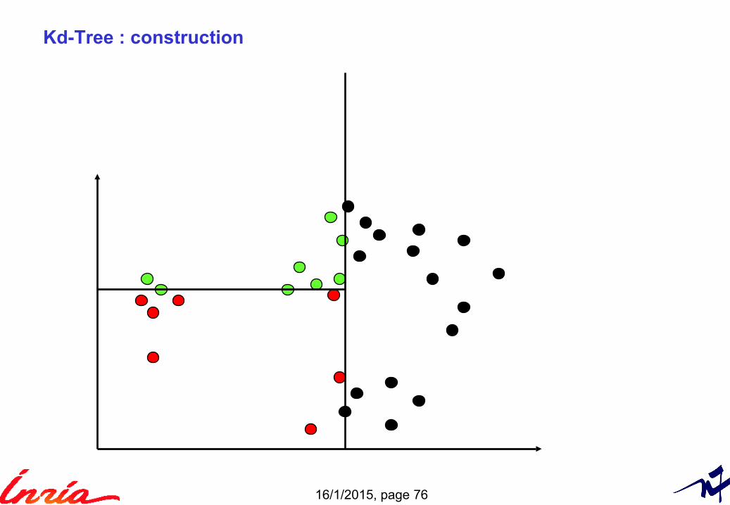
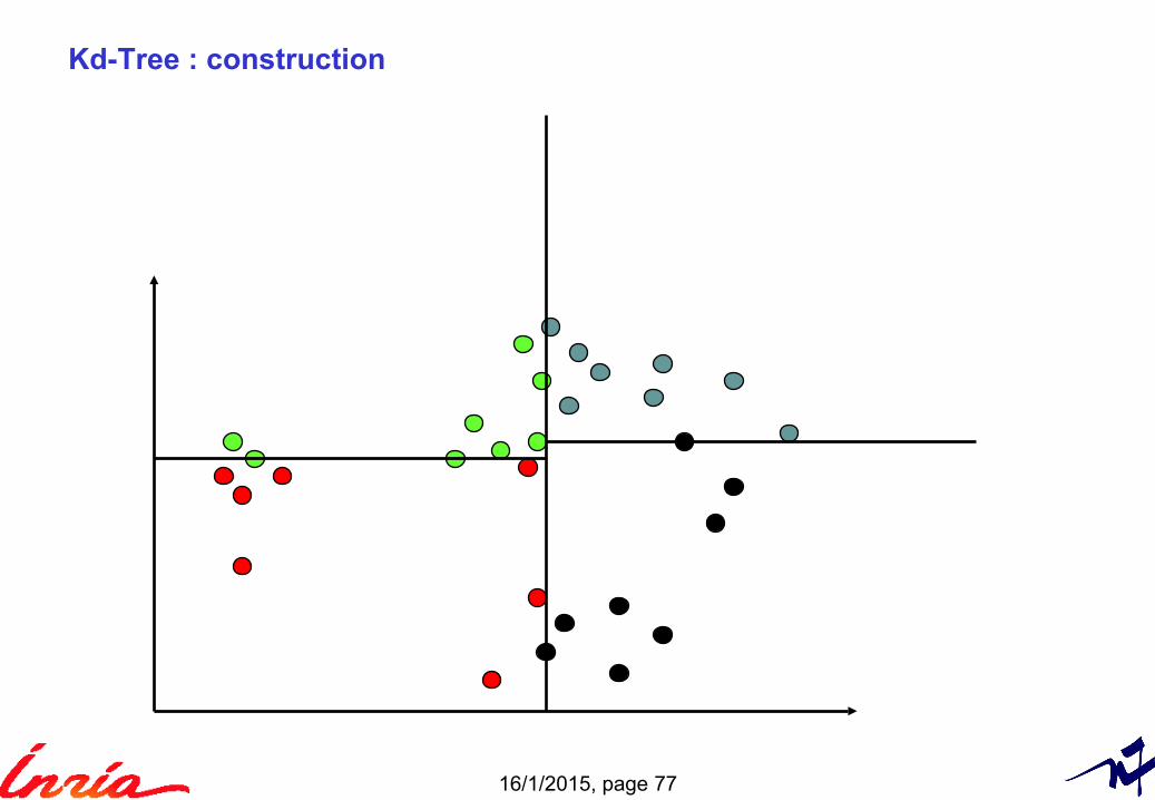
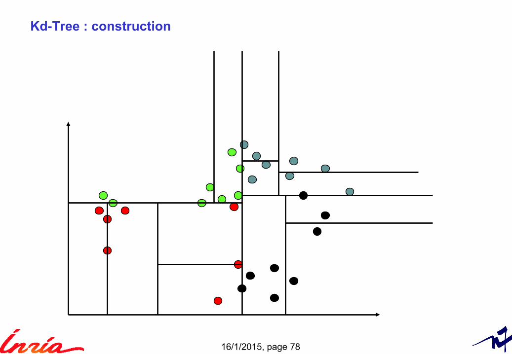
Kd-Tree
Binary tree
Popular technique to partition the space of vectors (non-overlapping cells)
Recursive splitting with hyper-planes► Axis-aligned ► Choice of axis: axis with highest variance► Splitting offset = median value of the points on the axis
Variants► Choice of axis► Tree arity ► Not axis aligned...
16/1/2015, page 75
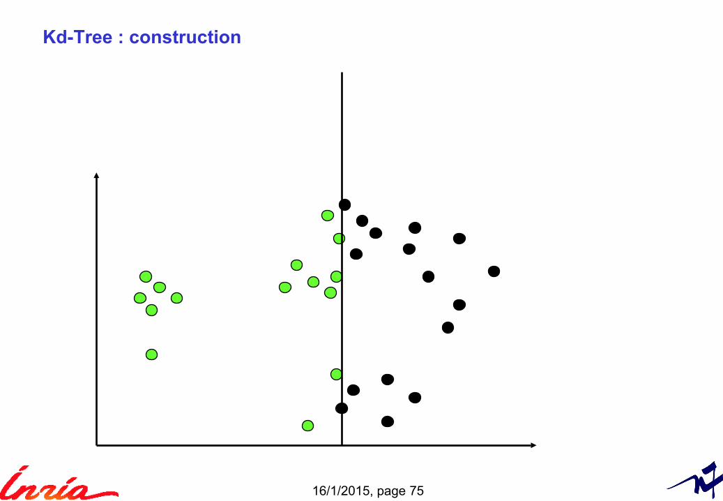
Kd-Tree : construction
16/1/2015, page 76
Kd-Tree : construction
16/1/2015, page 77
Kd-Tree : construction
16/1/2015, page 78
Kd-Tree : construction
16/1/2015, page 79
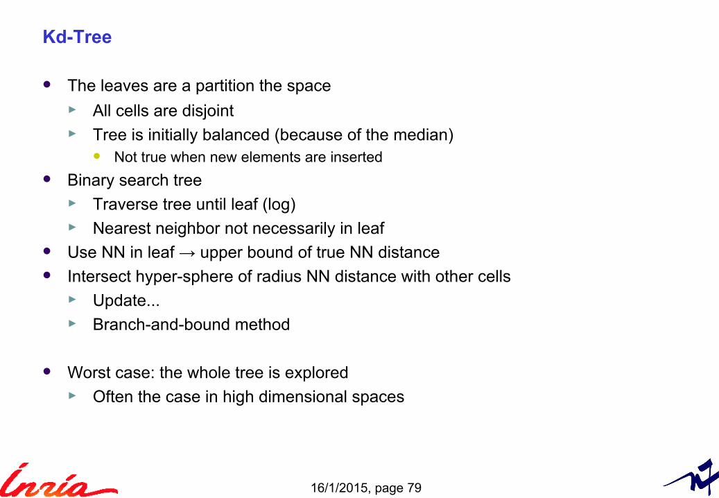
Kd-Tree
The leaves are a partition the space ► All cells are disjoint► Tree is initially balanced (because of the median)
Not true when new elements are inserted
Binary search tree ► Traverse tree until leaf (log)► Nearest neighbor not necessarily in leaf
Use NN in leaf → upper bound of true NN distance Intersect hyper-sphere of radius NN distance with other cells
► Update...► Branch-and-bound method
Worst case: the whole tree is explored► Often the case in high dimensional spaces
16/1/2015, page 80
7. Nearest-neighbor search (high dimension)
16/1/2015, page 81
The dimension curse
Methods that work in low dimensions are not effective in high dimensions... Due to a few counter-intuitive properies:
► Vanishing variance► Empty space► Proximity to boundaries
16/1/2015, page 82
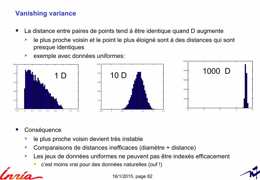
Vanishing variance
La distance entre paires de points tend à être identique quand D augmente► le plus proche voisin et le point le plus éloigné sont à des distances qui sont
presque identiques► exemple avec données uniformes:
Conséquence► le plus proche voisin devient très instable► Comparaisons de distances inefficaces (diamètre + distance)► Les jeux de données uniformes ne peuvent pas être indexés efficacement
c’est moins vrai pour des données naturelles (ouf !)
1 D 10 D 1000 D
16/1/2015, page 83
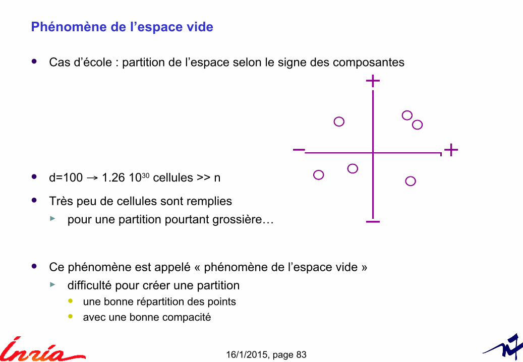
Phénomène de l’espace vide
Cas d’école : partition de l’espace selon le signe des composantes
d=100 → 1.26 1030 cellules >> n
Très peu de cellules sont remplies► pour une partition pourtant grossière…
Ce phénomène est appelé « phénomène de l’espace vide »► difficulté pour créer une partition
une bonne répartition des points avec une bonne compacité
16/1/2015, page 84
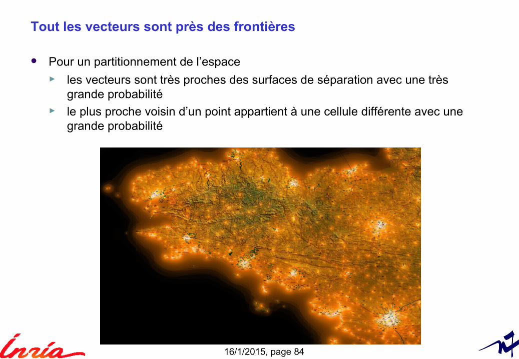
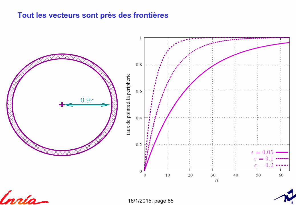
Tout les vecteurs sont près des frontières
Pour un partitionnement de l’espace► les vecteurs sont très proches des surfaces de séparation avec une très
grande probabilité► le plus proche voisin d’un point appartient à une cellule différente avec une
grande probabilité
16/1/2015, page 85
Tout les vecteurs sont près des frontières
16/1/2015, page 86
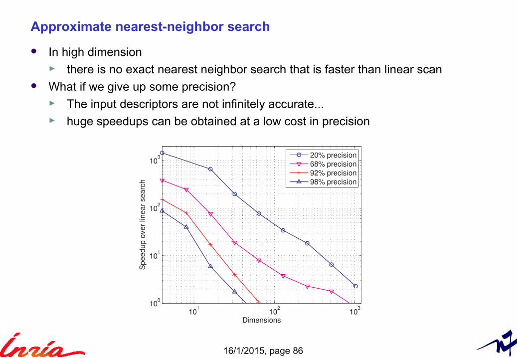
Approximate nearest-neighbor search
In high dimension► there is no exact nearest neighbor search that is faster than linear scan
What if we give up some precision?► The input descriptors are not infinitely accurate...► huge speedups can be obtained at a low cost in precision
16/1/2015, page 87
PCA: dimensionality reduction
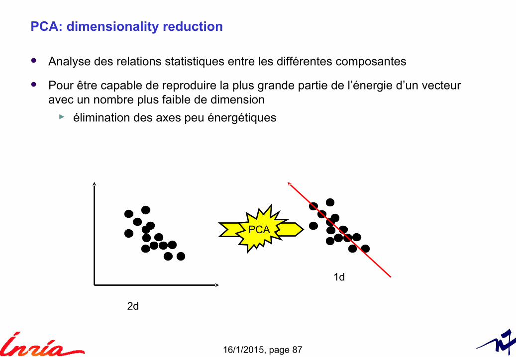
Analyse des relations statistiques entre les différentes composantes
Pour être capable de reproduire la plus grande partie de l’énergie d’un vecteuravec un nombre plus faible de dimension
► élimination des axes peu énergétiques
2d
1d
PCA
16/1/2015, page 88
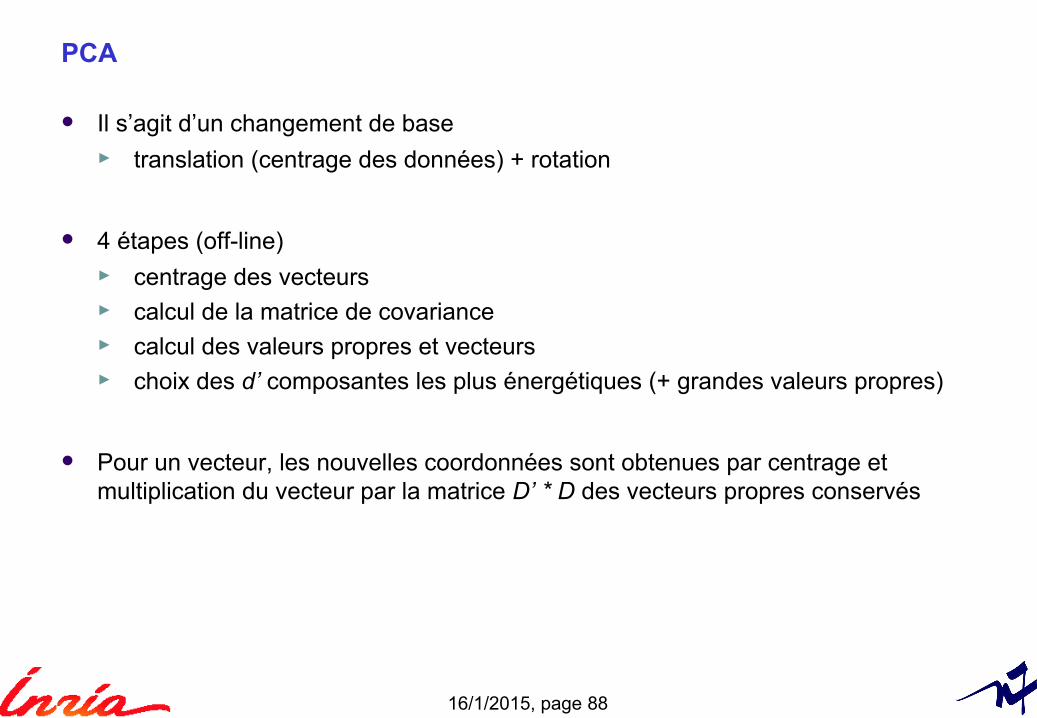
PCA
Il s’agit d’un changement de base► translation (centrage des données) + rotation
4 étapes (off-line)► centrage des vecteurs► calcul de la matrice de covariance► calcul des valeurs propres et vecteurs ► choix des d’ composantes les plus énergétiques (+ grandes valeurs propres)
Pour un vecteur, les nouvelles coordonnées sont obtenues par centrage etmultiplication du vecteur par la matrice D’ * D des vecteurs propres conservés
16/1/2015, page 89
Adaptation of low-dimensional indexing methods: FLANN
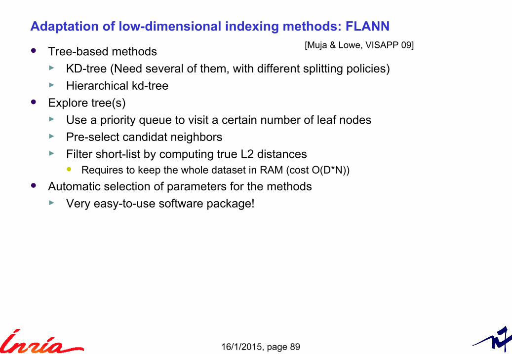
Tree-based methods► KD-tree (Need several of them, with different splitting policies)► Hierarchical kd-tree
Explore tree(s)► Use a priority queue to visit a certain number of leaf nodes ► Pre-select candidat neighbors ► Filter short-list by computing true L2 distances
Requires to keep the whole dataset in RAM (cost O(D*N))
Automatic selection of parameters for the methods► Very easy-to-use software package!
[Muja & Lowe, VISAPP 09]
16/1/2015, page 90
Indexing algorithm: searching with quantization
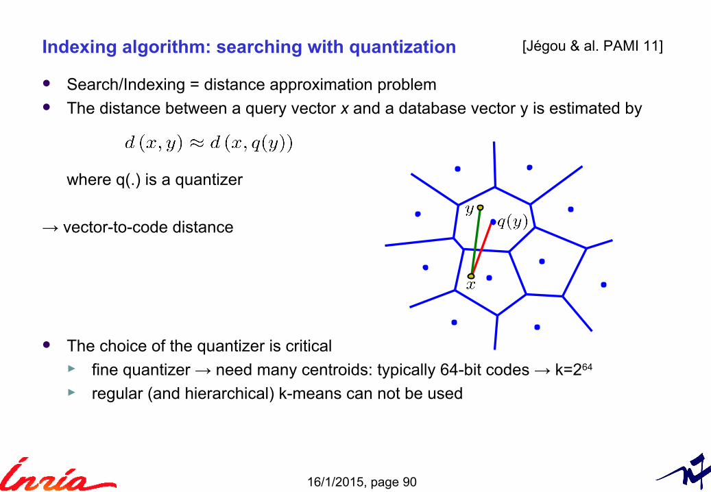
Search/Indexing = distance approximation problem The distance between a query vector x and a database vector y is estimated by
where q(.) is a quantizer
→ vector-to-code distance
The choice of the quantizer is critical► fine quantizer → need many centroids: typically 64-bit codes → k=264
► regular (and hierarchical) k-means can not be used
[Jégou & al. PAMI 11]
16/1/2015, page 91
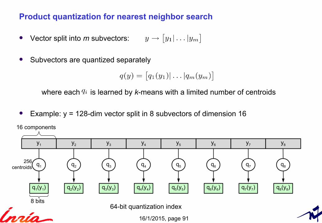
Vector split into m subvectors:
Subvectors are quantized separately
where each is learned by k-means with a limited number of centroids
Example: y = 128-dim vector split in 8 subvectors of dimension 16
Product quantization for nearest neighbor search
8 bits
16 components
⇒ 64-bit quantization index
y1 y2 y3 y4 y5 y6 y7 y8
q1 q2 q3 q4 q5 q6 q7 q8
q1(y1) q2(y2) q3(y3) q4(y4) q5(y5) q6(y6) q7(y7) q8(y8)
256centroids

16/1/2015, page 92
Vector split into m subvectors:
Subvectors are quantized separately
where each is learned by k-means with a limited number of centroids
Example: y = 128-dim vector split in 8 subvectors of dimension 16
Product quantization for nearest neighbor search
8 bits
16 components
⇒ 64-bit quantization index
y1 y2 y3 y4 y5 y6 y7 y8
q1 q2 q3 q4 q5 q6 q7 q8
q1(y1) q2(y2) q3(y3) q4(y4) q5(y5) q6(y6) q7(y7) q8(y8)
256centroids
16/1/2015, page 93
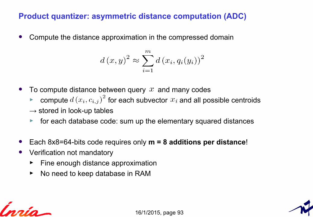
Product quantizer: asymmetric distance computation (ADC)
Compute the distance approximation in the compressed domain
To compute distance between query and many codes► compute for each subvector and all possible centroids
→ stored in look-up tables ► for each database code: sum up the elementary squared distances
Each 8x8=64-bits code requires only m = 8 additions per distance! Verification not mandatory
► Fine enough distance approximation► No need to keep database in RAM
16/1/2015, page 94
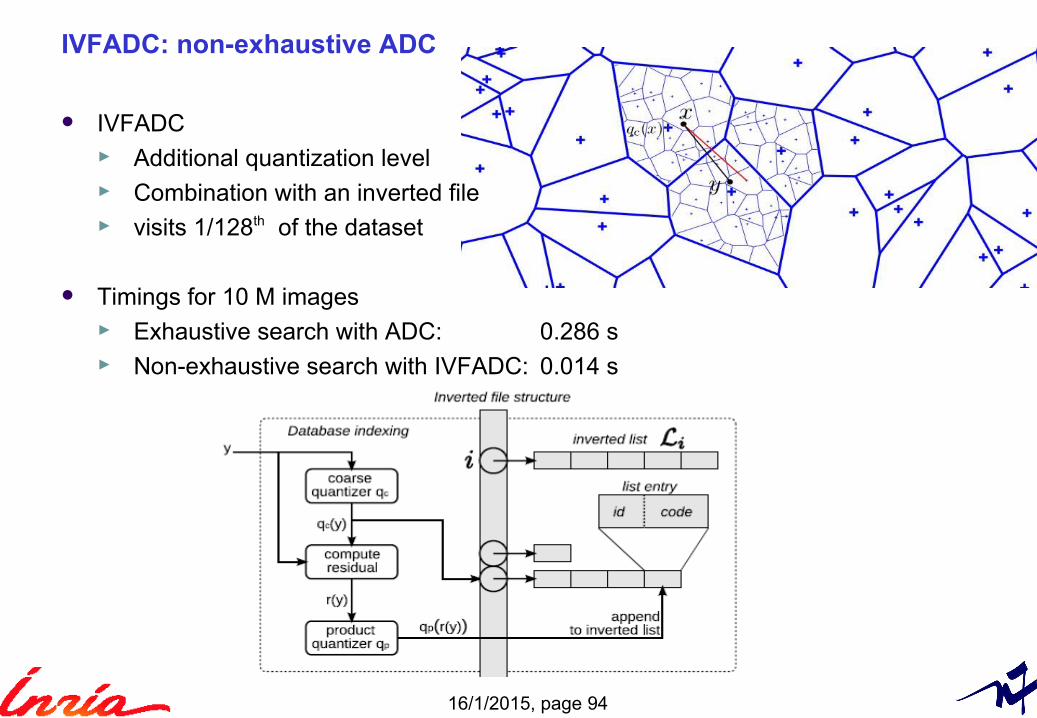
IVFADC: non-exhaustive ADC
IVFADC► Additional quantization level► Combination with an inverted file ► visits 1/128th of the dataset
Timings for 10 M images► Exhaustive search with ADC: 0.286 s► Non-exhaustive search with IVFADC: 0.014 s
16/1/2015, page 95
Conclusion
Product quantization performance► Can index 1B images at ► 20 bytes per image
Extensions ► Include temporal component for video [Douze & al. ECCV 2010]
► More quantization levels [Jégou & al. ICASSP 11] [Babenko & Lempistsky CVPR 11]

16/1/2015, page 96
8. Results
16/1/2015, page 97
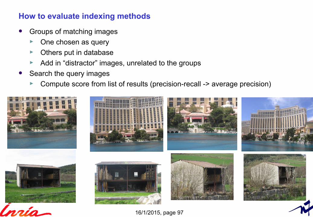
How to evaluate indexing methods
Groups of matching images► One chosen as query► Others put in database► Add in “distractor” images, unrelated to the groups
Search the query images► Compute score from list of results (precision-recall -> average precision)
16/1/2015, page 98
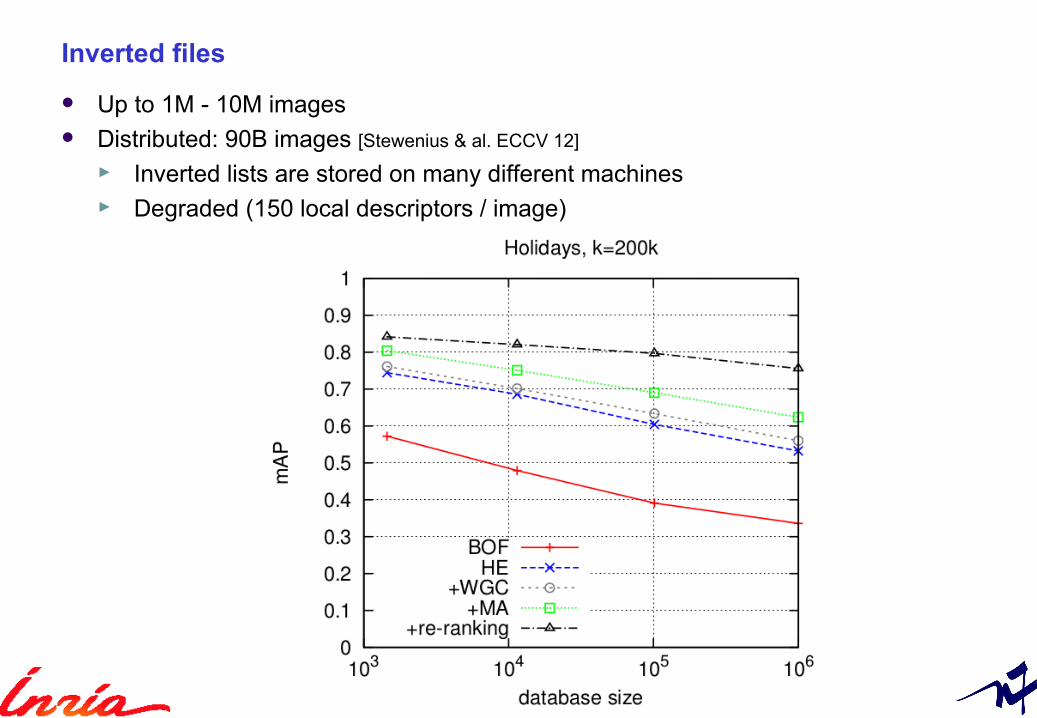
Inverted files
Up to 1M - 10M images Distributed: 90B images [Stewenius & al. ECCV 12]
► Inverted lists are stored on many different machines► Degraded (150 local descriptors / image)
16/1/2015, page 99
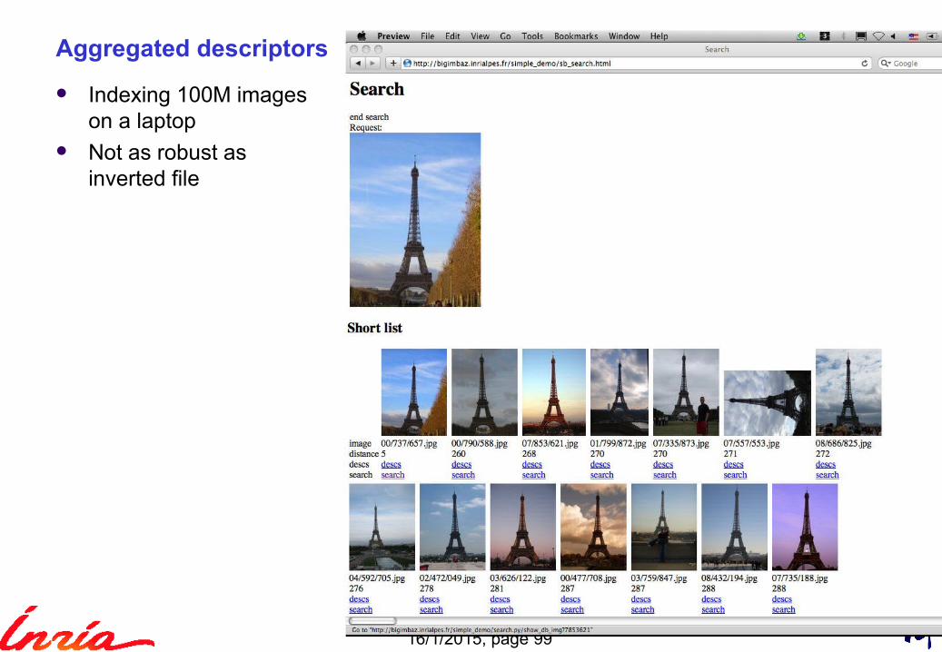
Aggregated descriptors
Indexing 100M imageson a laptop
Not as robust asinverted file
16/1/2015, page 100
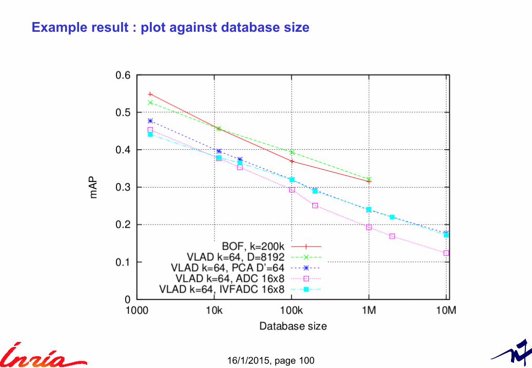
Example result : plot against database size
16/1/2015, page 101
Conclusion
Very active field Choose operating point
► Database size vs. performance Software packages
► For descriptor computation: OpenCV, VLFeat, etc.► Product quantization: inverted multi-index► Hamming Embedding: Yael

16/1/2015, page 102
END

16/1/2015, page 103
Outline
Problem statement Extracting local image descriptors Indexing by image matching Bag-of-words and the inverted file Local descriptor aggregation Nearest neighbor search (low dimension) Nearest neighbor search (high dimension) Results

16/1/2015, page 104
Outline
Problem statement Extracting local image descriptors Indexing by image matching Bag-of-words and the inverted file Local descriptor aggregation Nearest neighbor search (low dimension) Nearest neighbor search (high dimension) Results

16/1/2015, page 105
Outline
Problem statement Extracting local image descriptors Indexing by image matching Bag-of-words and the inverted file Local descriptor aggregation Nearest neighbor search (low dimension) Nearest neighbor search (high dimension) Results
16/1/2015, page 106
Outline
Problem statement Extracting local image descriptors Indexing by image matching Bag-of-words and the inverted file Local descriptor aggregation Nearest neighbor search (low dimension) Nearest neighbor search (high dimension) Results

16/1/2015, page 107
Outline
Problem statement Extracting local image descriptors Indexing by image matching Bag-of-words and the inverted file Local descriptor aggregation Nearest neighbor search (low dimension) Nearest neighbor search (high dimension) Results
16/1/2015, page 108
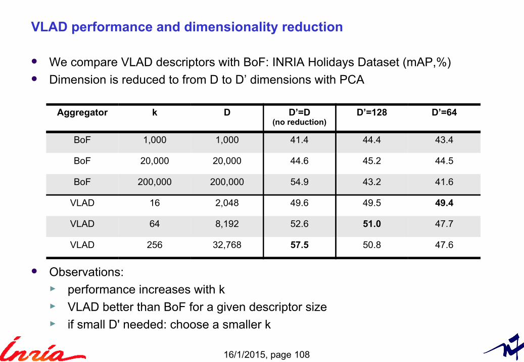
VLAD performance and dimensionality reduction
We compare VLAD descriptors with BoF: INRIA Holidays Dataset (mAP,%) Dimension is reduced to from D to D’ dimensions with PCA
Observations:► performance increases with k► VLAD better than BoF for a given descriptor size► if small D' needed: choose a smaller k
Aggregator k D D’=D(no reduction)
D’=128 D’=64
BoF 1,000 1,000 41.4 44.4 43.4
BoF 20,000 20,000 44.6 45.2 44.5
BoF 200,000 200,000 54.9 43.2 41.6
VLAD 16 2,048 49.6 49.5 49.4
VLAD 64 8,192 52.6 51.0 47.7
VLAD 256 32,768 57.5 50.8 47.6
16/1/2015, page 109
Outline
Image description with VLAD
Indexing with the product quantizer
Porting to mobile devices
Video indexing
16/1/2015, page 110
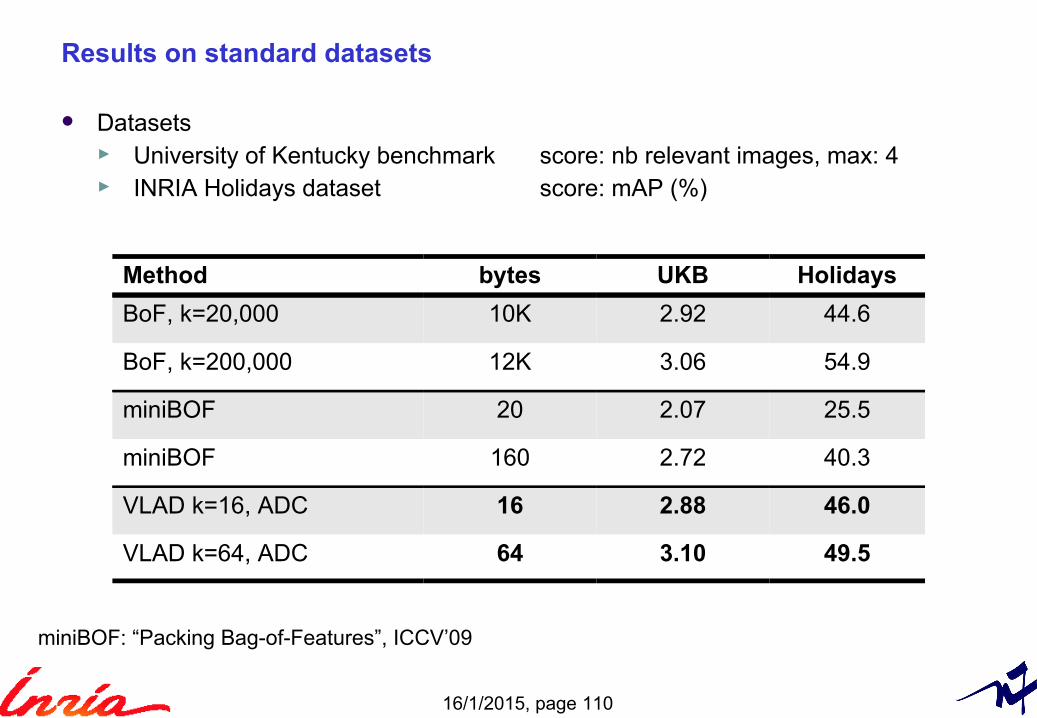
Results on standard datasets
Datasets► University of Kentucky benchmark score: nb relevant images, max: 4 ► INRIA Holidays dataset score: mAP (%)
Method bytes UKB Holidays
BoF, k=20,000 10K 2.92 44.6
BoF, k=200,000 12K 3.06 54.9
miniBOF 20 2.07 25.5
miniBOF 160 2.72 40.3
VLAD k=16, ADC 16 2.88 46.0
VLAD k=64, ADC 64 3.10 49.5
miniBOF: “Packing Bag-of-Features”, ICCV’09
16/1/2015, page 111
IVFADC: non-exhaustive ADC
IVFADC► Additional quantization level► Combination with an inverted file ► visits 1/128th of the dataset
Timings for 10 M images► Exhaustive search with ADC: 0.286 s► Non-exhaustive search with IVFADC: 0.014 s
16/1/2015, page 112
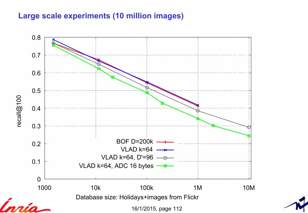
Large scale experiments (10 million images)
0
0.1
0.2
0.3
0.4
0.5
0.6
0.7
0.8
1000 10k 100k 1M 10M
reca
ll@10
0
Database size: Holidays+images from Flickr
BOF D=200kVLAD k=64
VLAD k=64, D'=96VLAD k=64, ADC 16 bytes
16/1/2015, page 113
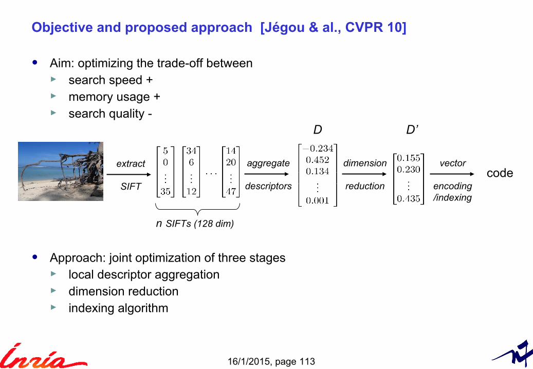
Objective and proposed approach [Jégou & al., CVPR 10]
• Aim: optimizing the trade-off between► search speed +► memory usage +► search quality -
• Approach: joint optimization of three stages► local descriptor aggregation► dimension reduction► indexing algorithm
extract
SIFT
aggregate
descriptors
dimension
reduction
vector
encoding/indexing
D
code
D’
n SIFTs (128 dim)
16/1/2015, page 114
Aggregation of local descriptors
Problem: represent an image by a single fixed-size vector:
set of n local descriptors → 1 vector
Indexing:► similarity = distance between aggregated description vectors (preferably L2)► search = (approximate) nearest-neighbor search in descriptor space
Most popular idea: BoF representation [Sivic & Zisserman 03]► sparse vector► highly dimensional
→ dimensionality reduction harms precision a lot
Alternative: Fisher Kernels [Perronnin et al 07]► non sparse vector► excellent results with a small vector dimensionality
→ VLAD is in the spirit of this representation
16/1/2015, page 115
Outline
Image description with VLAD
Indexing with the product quantizer
Porting to mobile devices
Video indexing
16/1/2015, page 116
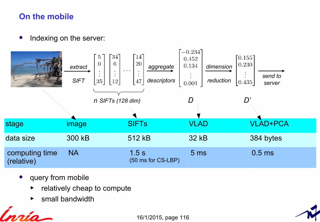
On the mobile
Indexing on the server:
query from mobile ► relatively cheap to compute► small bandwidth
extract
SIFT
aggregate
descriptors
dimension
reductionsend toserver
D D’n SIFTs (128 dim)
stage image SIFTs VLAD VLAD+PCA
data size 300 kB 512 kB 32 kB 384 bytes
computing time(relative)
NA 1.5 s (50 ms for CS-LBP)
5 ms 0.5 ms
16/1/2015, page 117
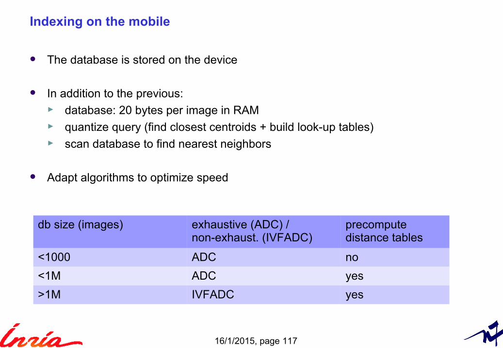
Indexing on the mobile
The database is stored on the device
In addition to the previous:► database: 20 bytes per image in RAM► quantize query (find closest centroids + build look-up tables)► scan database to find nearest neighbors
Adapt algorithms to optimize speed
db size (images) exhaustive (ADC) /non-exhaust. (IVFADC)
precomputedistance tables
<1000 ADC no
<1M ADC yes
>1M IVFADC yes
16/1/2015, page 118
Outline
Image description with VLAD
Indexing with the product quantizer
Porting to mobile devices
Video indexing
16/1/2015, page 119
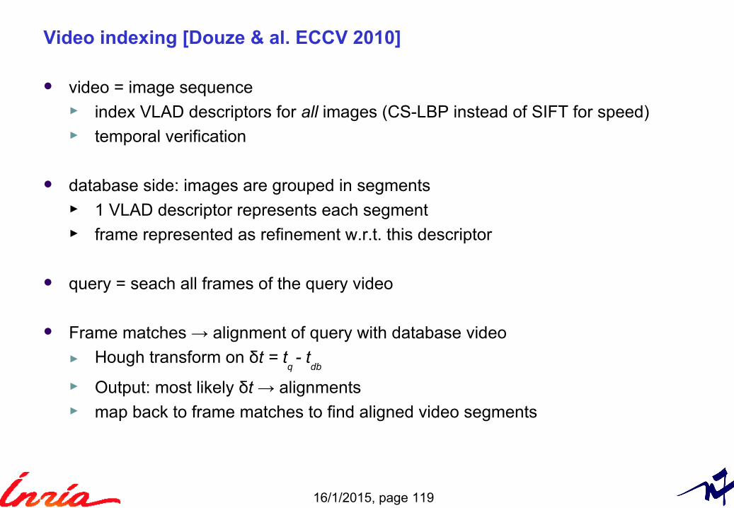
Video indexing [Douze & al. ECCV 2010]
video = image sequence► index VLAD descriptors for all images (CS-LBP instead of SIFT for speed)► temporal verification
database side: images are grouped in segments► 1 VLAD descriptor represents each segment► frame represented as refinement w.r.t. this descriptor
query = seach all frames of the query video
Frame matches → alignment of query with database video
► Hough transform on δt = tq - t
db
► Output: most likely δt → alignments► map back to frame matches to find aligned video segments
16/1/2015, page 120
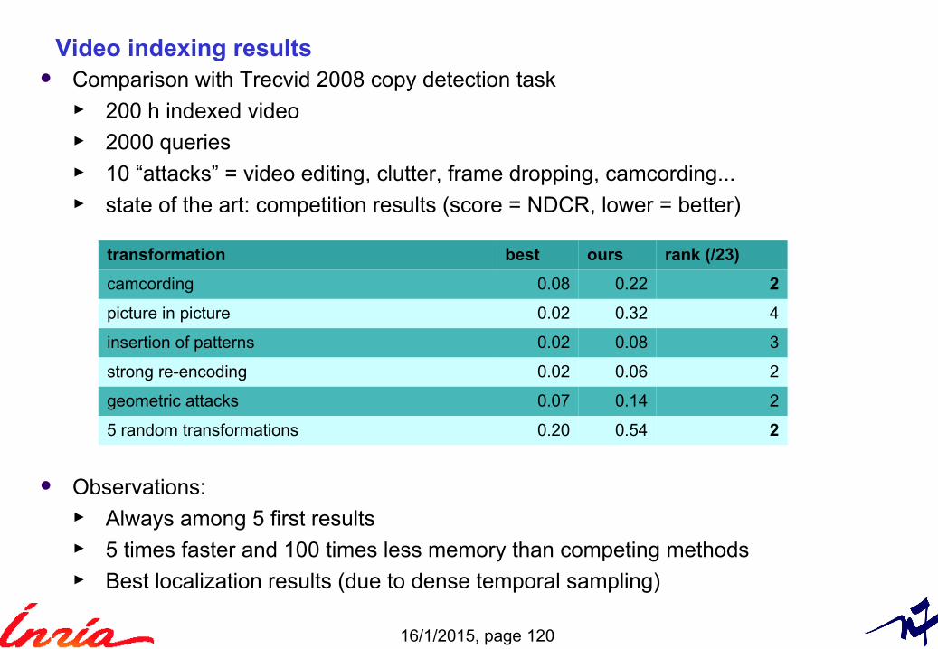
Video indexing results Comparison with Trecvid 2008 copy detection task
► 200 h indexed video ► 2000 queries► 10 “attacks” = video editing, clutter, frame dropping, camcording...► state of the art: competition results (score = NDCR, lower = better)
Observations:► Always among 5 first results► 5 times faster and 100 times less memory than competing methods► Best localization results (due to dense temporal sampling)
transformation best ours rank (/23)
camcording 0.08 0.22 2
picture in picture 0.02 0.32 4
insertion of patterns 0.02 0.08 3
strong re-encoding 0.02 0.06 2
geometric attacks 0.07 0.14 2
5 random transformations 0.20 0.54 2
16/1/2015, page 121
Conclusion
VLAD: compact & discriminative image descriptor► aggregation of SIFT, CS-LBP, SURF (ongoing),...
Product Quantizer: generic indexing method with nearest-neighbor search function► works with local descriptors and GIST, audio features (ongoing)...
Standard image and datasets► Holidays (different viewpoints)► Copydays (copyright attacks)
Compatible with mobile applications: ► compact descriptor, cheap to compute
Code for VLAD and Product quantizer at http://www.irisa.fr/texmex/people/jegou/src.php
Demo!

END
16/1/2015, page 123
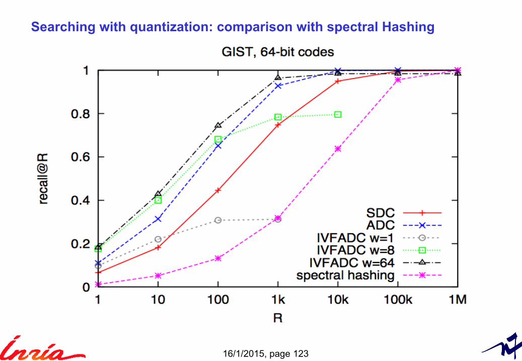
Searching with quantization: comparison with spectral Hashing
*** Put Only ADC ***
16/1/2015, page 124
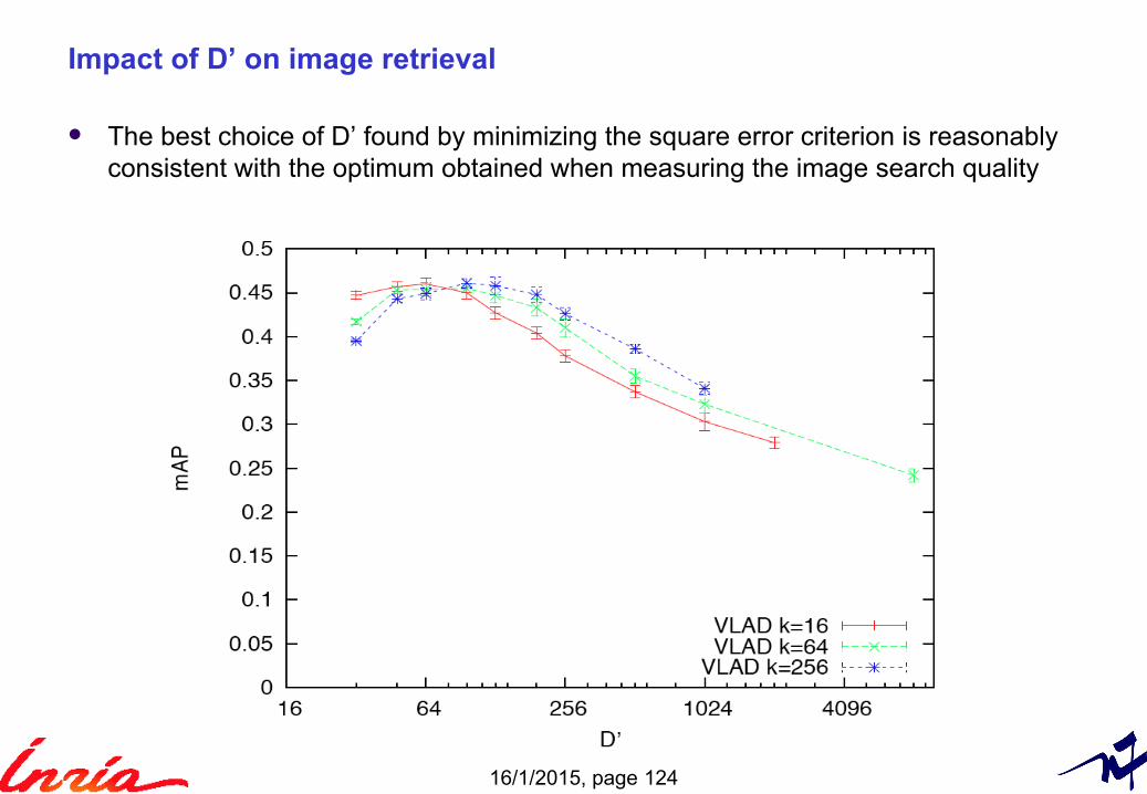
Impact of D’ on image retrieval
The best choice of D’ found by minimizing the square error criterion is reasonablyconsistent with the optimum obtained when measuring the image search quality
16/1/2015, page 125
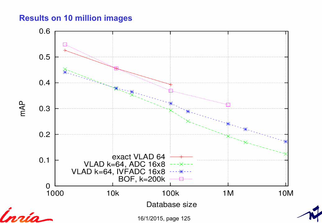
Results on 10 million images
16/1/2015, page 126
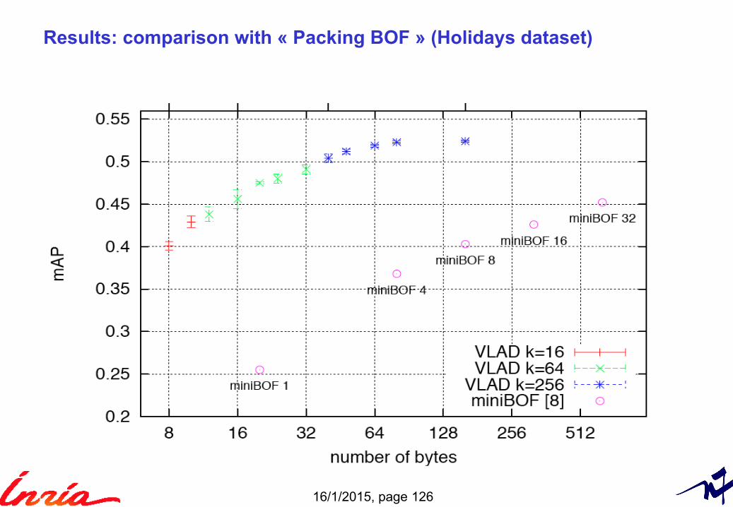
Results: comparison with « Packing BOF » (Holidays dataset)
16/1/2015, page 127
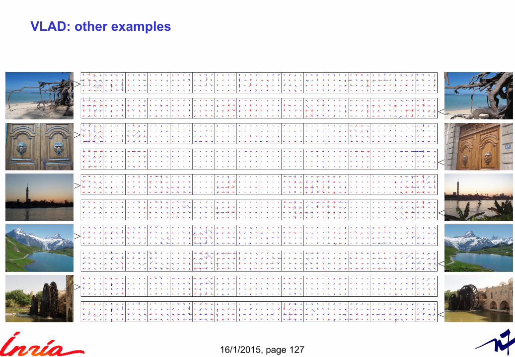
VLAD: other examples
16/1/2015, page 128
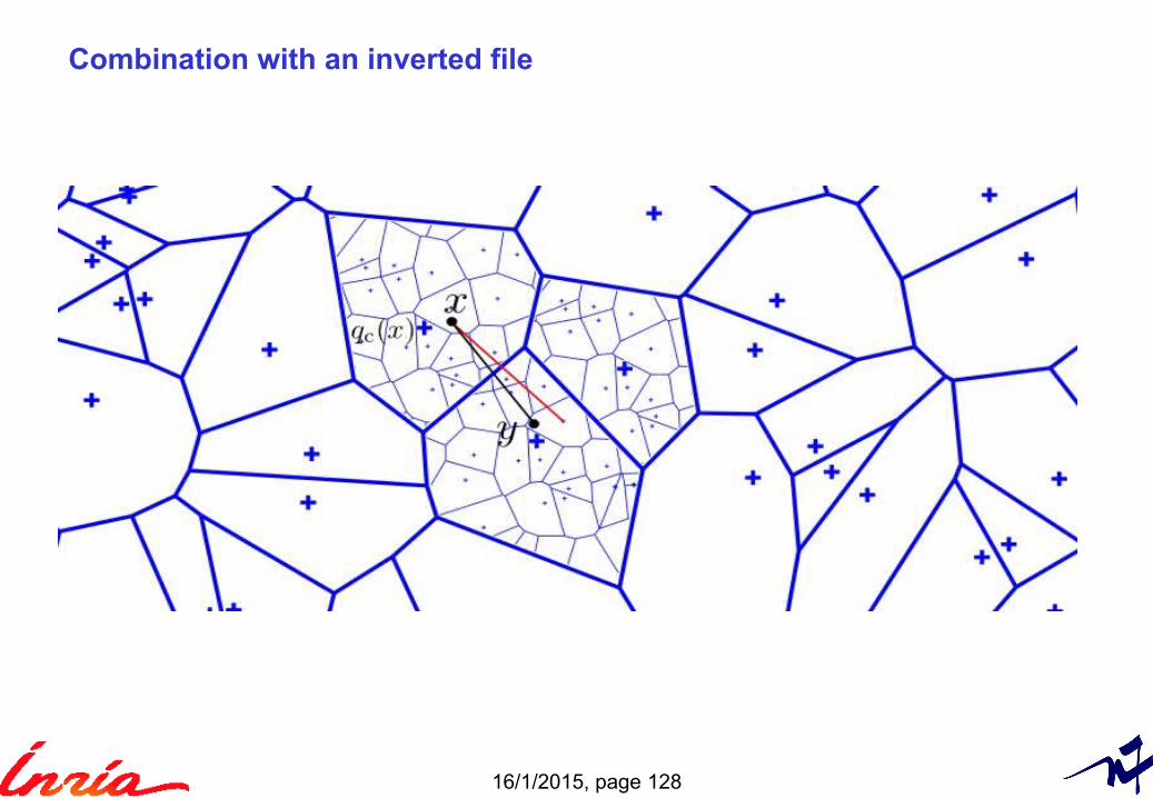
Combination with an inverted file
16/1/2015, page 129
Related work on large scale image search Global descriptors:
► GIST descriptors with Spectral Hashing or similar techniques [Torralba & al 08]
→ very limited invariance to scale/rotation/crop: use local descriptors
Bag-of-features [Sivic & Zisserman 03]► Large (hierarchical) vocabularies [Nister Stewenius 06]► Improved descriptor representation [Jégou et al 08, Philbin et al 08]► Geometry used in index [Jégou et al 08, Perdoc’h et al 09]► Query expansion [Chum et al 07]
→ memory tractable for a few million images only
Efficiency improved by ► Min-hash and Geometrical min-hash [Chum et al. 07-09]► compressing the BoF representation [Jégou et al. 09]
→ But still hundreds of bytes are required to obtain a “reasonable quality”

16/1/2015, page 130
1. Problem statement
16/1/2015, page 131
Include geometry in the inverted file
Problem statement Extracting local image descriptors Indexing by image matching Bag-of-words and the inverted file Local descriptor aggregation Nearest neighbor search (low dimension) Nearest neighbor search (high dimension) Results
16/1/2015, page 132
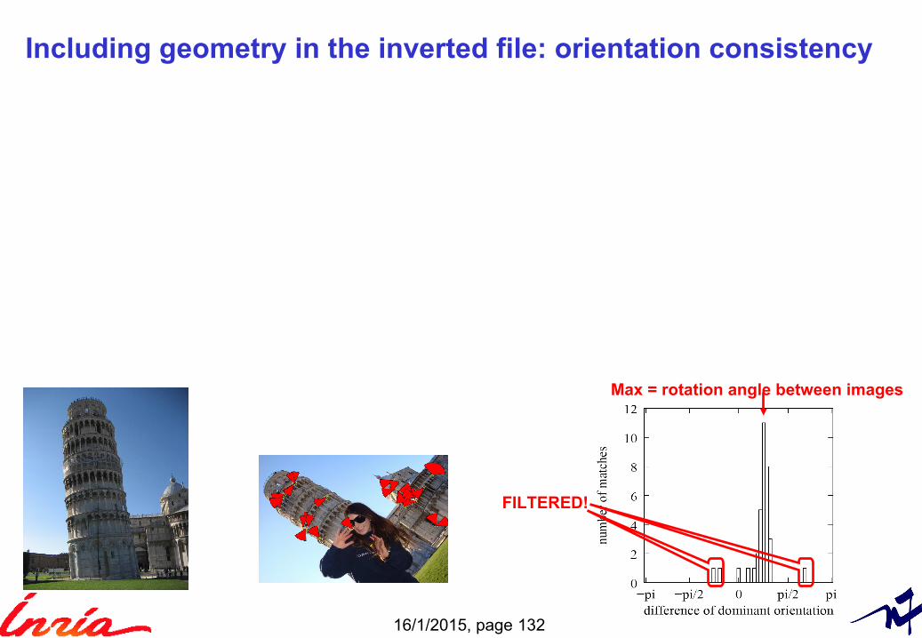
Max = rotation angle between images
Including geometry in the inverted file: orientation consistency
FILTERED!