14 juni 2016

Hoe goed is mijn kansverwachting? –

Inleiding op “verificatie”

Jan Verkade

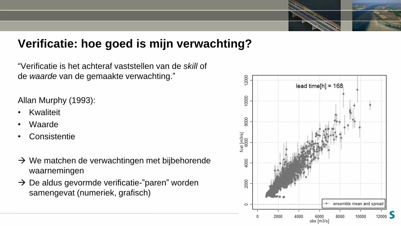
Verificatie: hoe goed is mijn verwachting?

“Verificatie is het achteraf vaststellen van de skill of

de waarde van de gemaakte verwachting.”

Allan Murphy (1993):

• Kwaliteit

• Waarde

• Consistentie

We matchen de verwachtingen met bijbehorende

waarnemingen

De aldus gevormde verificatie-”paren” worden

samengevat (numeriek, grafisch)

Redenen voor verificatie

1. Bestuurlijk/management:

Onderbouwen van de rationale (bijv. voor maken van verwachtingen, voor investeren in

nieuwe techniek, nieuw model etc)

2. Wetenschappelijk:

Waar kan ik verwachtingen verbeteren?

3. Economisch nut

Wat is de waarde voor de eindgebruiker?

(Jolliffe and Stephenson, 2012; Brier & Allen, 1951; Stanski et al., 1989)

Kwaliteit versus waarde van verwachtingen

• Kwaliteit: grote overeenkomst tussen verwachtingen en waarnemingen

• Waarde: eindgebruiker kan betere beslissing nemen

Klassiek voorbeeld: verwachting van zonnige dag boven de Sahara

• Kwaliteit?

• Waarde?

http://upload.wikimedia.org/wikipedia/commons/3/35/Dunes.jpg

Source: Bertrand Devouard / Florence Devouard

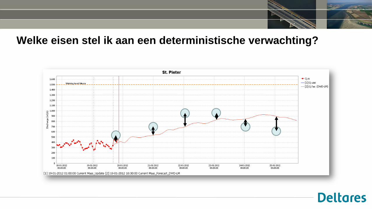
Welke eisen stel ik aan een deterministische verwachting?

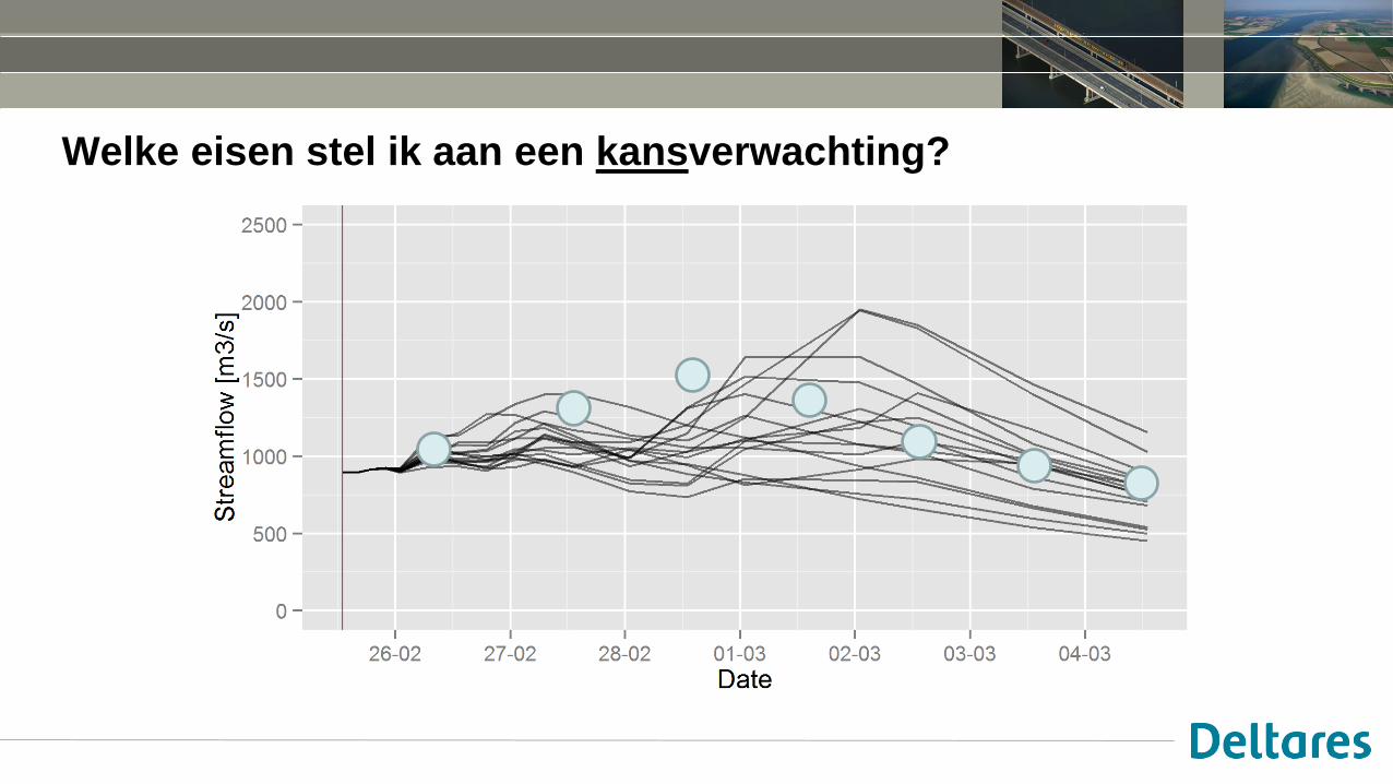
Welke eisen stel ik aan een kansverwachting?

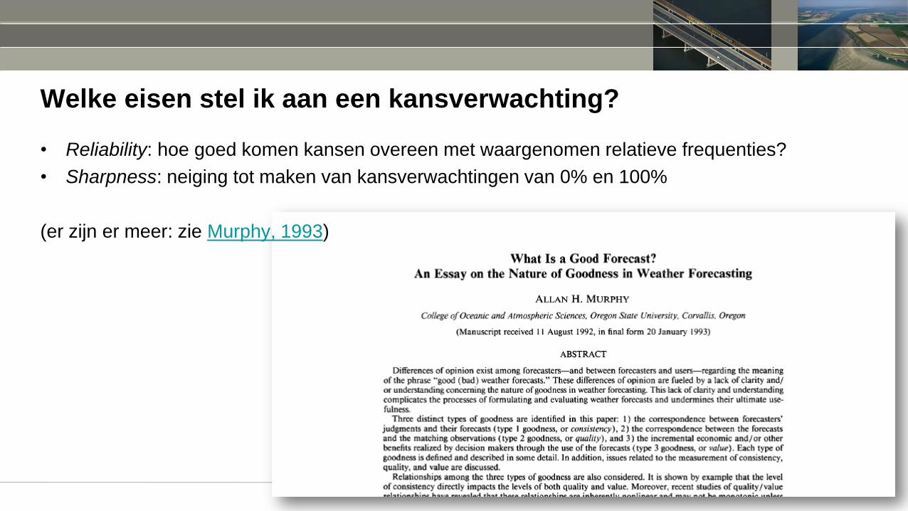
Welke eisen stel ik aan een kansverwachting?

• Reliability: hoe goed komen kansen overeen met waargenomen relatieve frequenties?

• Sharpness: neiging tot maken van kansverwachtingen van 0% en 100%

(er zijn er meer: zie Murphy, 1993)

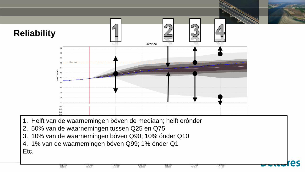
Reliability

1. Helft van de waarnemingen bóven de mediaan; helft erónder

2. 50% van de waarnemingen tussen Q25 en Q75

3. 10% van de waarnemingen bóven Q90; 10% ónder Q10

4. 1% van de waarnemingen bóven Q99; 1% ónder Q1

Etc.

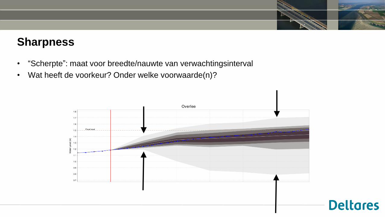
Sharpness

• “Scherpte”: maat voor breedte/nauwte van verwachtingsinterval

• Wat heeft de voorkeur? Onder welke voorwaarde(n)?

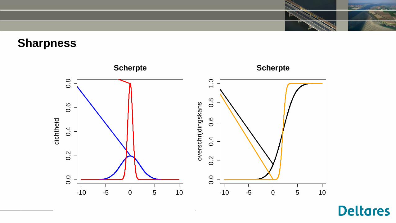
Sharpness

-10 -5 0 5 10

0.0

0.2

0.4

0.6

0.8

Scherpte

dic

hth

eid

-10 -5 0 5 10

0.0

0.2

0.4

0.6

0.8

1.0

Scherpte

ove

rsch

rijd

ing

ska

ns

Verification: (possible) approach

• Qualitative: “Eyeball verification”: take a look at forecasts and observations

• Summary metrics:

• Graphical verification measures

• Numerical: metrics and skill scores

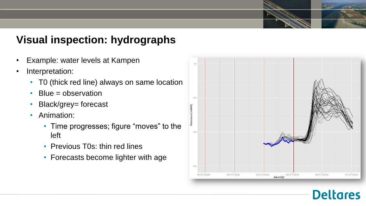
Visual inspection: hydrographs

• Example: water levels at Kampen

• Interpretation:

• T0 (thick red line) always on same location

• Blue = observation

• Black/grey= forecast

• Animation:

• Time progresses; figure “moves” to the

left

• Previous T0s: thin red lines

• Forecasts become lighter with age

Visual inspection: hydrographs

• What do you notice? Think of…

• Initial conditions

• Bias

• Spread

• Reliability

Kampen: https://youtu.be/Px_zQsyQJhk

Ramspolbrug: https://youtu.be/R-7klljaOlo

Nijkerkersluis West: https://youtu.be/p8qBDQMj6Bo

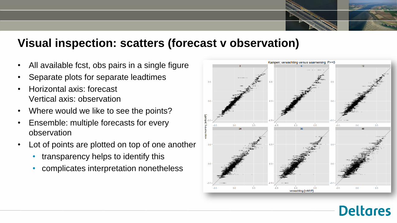
Visual inspection: scatters (forecast v observation)

• All available fcst, obs pairs in a single figure

• Separate plots for separate leadtimes

• Horizontal axis: forecast

Vertical axis: observation

• Where would we like to see the points?

• Ensemble: multiple forecasts for every

observation

• Lot of points are plotted on top of one another

• transparency helps to identify this

• complicates interpretation nonetheless

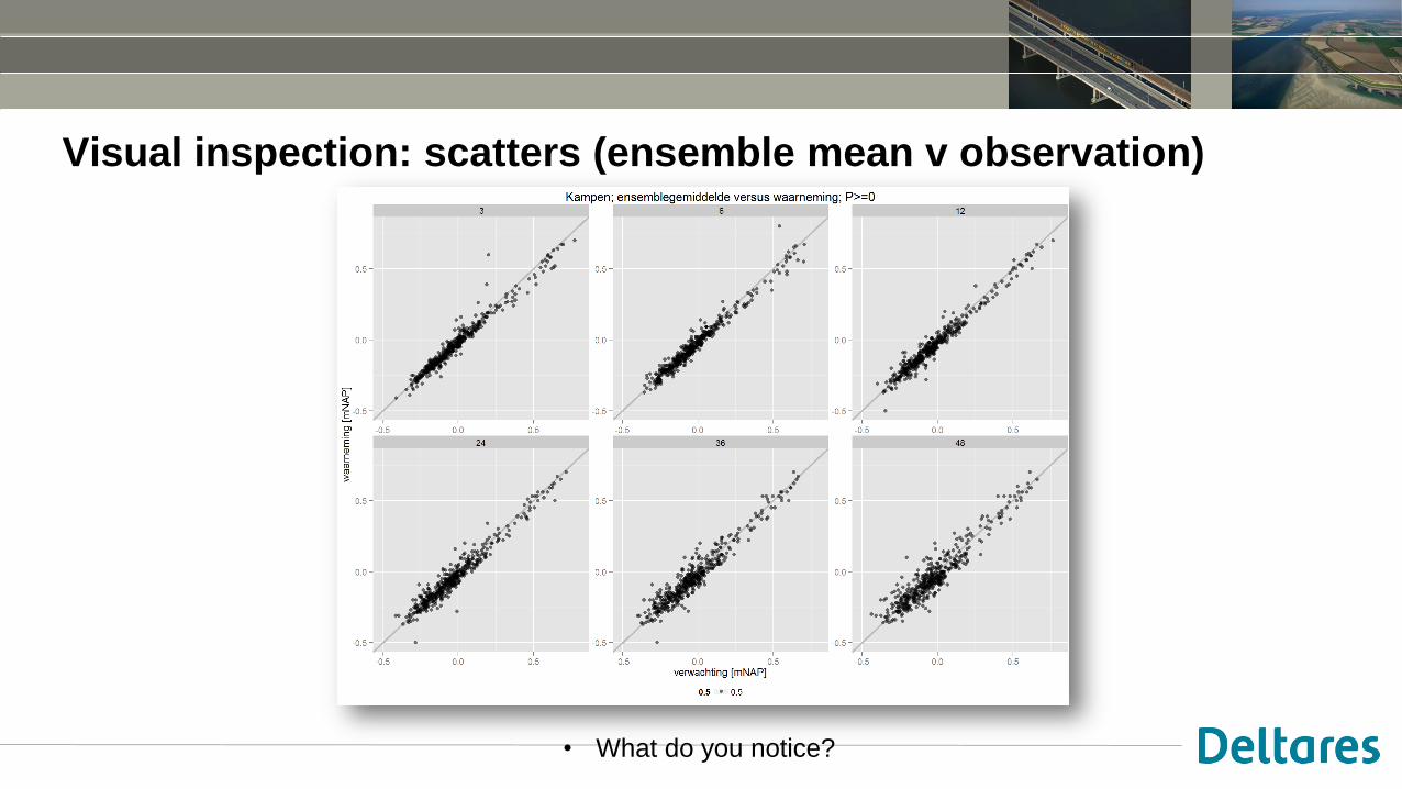
Visual inspection: scatters (ensemble mean v observation)

• What do you notice?

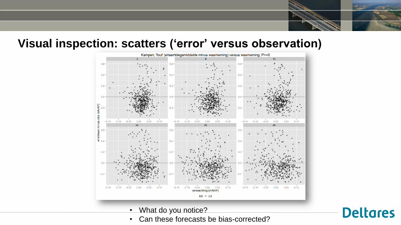
Visual inspection: scatters (‘error’ versus observation)

• What do you notice?

• Can these forecasts be bias-corrected?

Verification: (possible) approach

• Qualitative: “Eyeball verification”: take a look at forecasts and observations

• Summary metrics:

• Graphical verification measures

• Numerical: metrics and skill scores

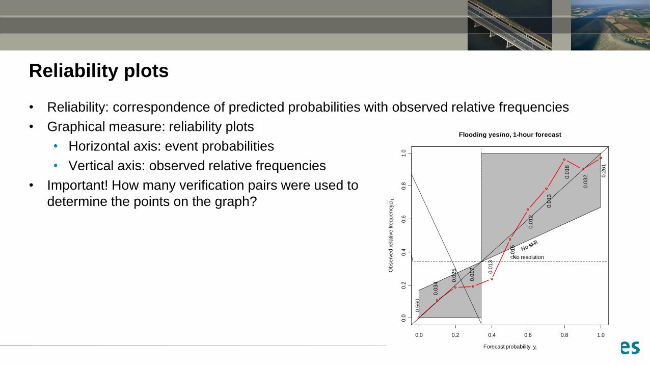
Reliability plots

• Reliability: correspondence of predicted probabilities with observed relative frequencies

• Graphical measure: reliability plots

• Horizontal axis: event probabilities

• Vertical axis: observed relative frequencies

• Important! How many verification pairs were used to

determine the points on the graph?

0.0 0.2 0.4 0.6 0.8 1.0

0.0

0.2

0.4

0.6

0.8

1.0

Forecast probability, yi

Ob

se

rve

d r

ela

tive

fre

qu

en

cy, o

1

No skill

0.5

60

0.0

34 0

.02

5

0.0

17

0.0

13

0.0

15

0.0

12

0.0

13

0.0

18

0.0

32 0

.26

1

Flooding yes/no, 1-hour forecast

No resolution

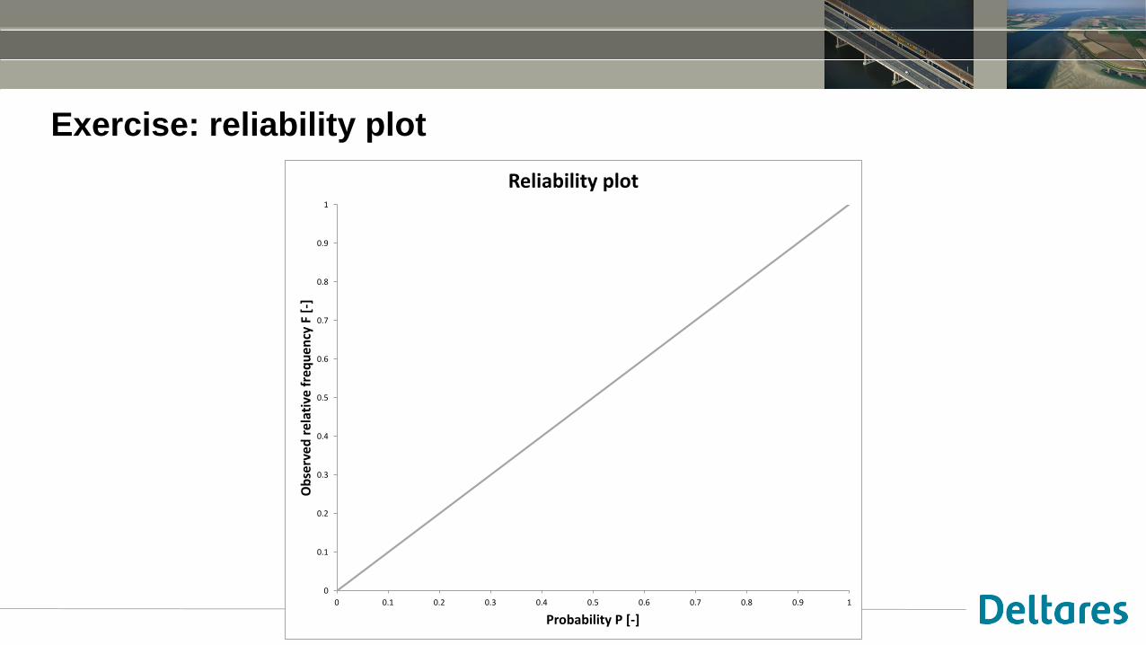
Exercise: reliability plot

0

0.1

0.2

0.3

0.4

0.5

0.6

0.7

0.8

0.9

1

0 0.1 0.2 0.3 0.4 0.5 0.6 0.7 0.8 0.9 1

Ob

serv

ed

re

lati

ve f

req

ue

ncy

F [

-]

Probability P [-]

Reliability plot

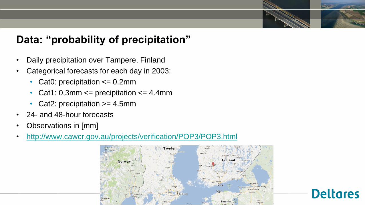
Data: “probability of precipitation”

• Daily precipitation over Tampere, Finland

• Categorical forecasts for each day in 2003:

• Cat0: precipitation <= 0.2mm

• Cat1: 0.3mm <= precipitation <= 4.4mm

• Cat2: precipitation >= 4.5mm

• 24- and 48-hour forecasts

• Observations in [mm]

• http://www.cawcr.gov.au/projects/verification/POP3/POP3.html

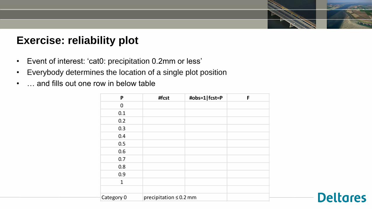
Exercise: reliability plot

• Event of interest: ‘cat0: precipitation 0.2mm or less’

• Everybody determines the location of a single plot position

• … and fills out one row in below table

P #fcst #obs=1|fcst=P F

0

0.1

0.2

0.3

0.4

0.5

0.6

0.7

0.8

0.9

1

Category 0 precipitation ≤ 0.2 mm

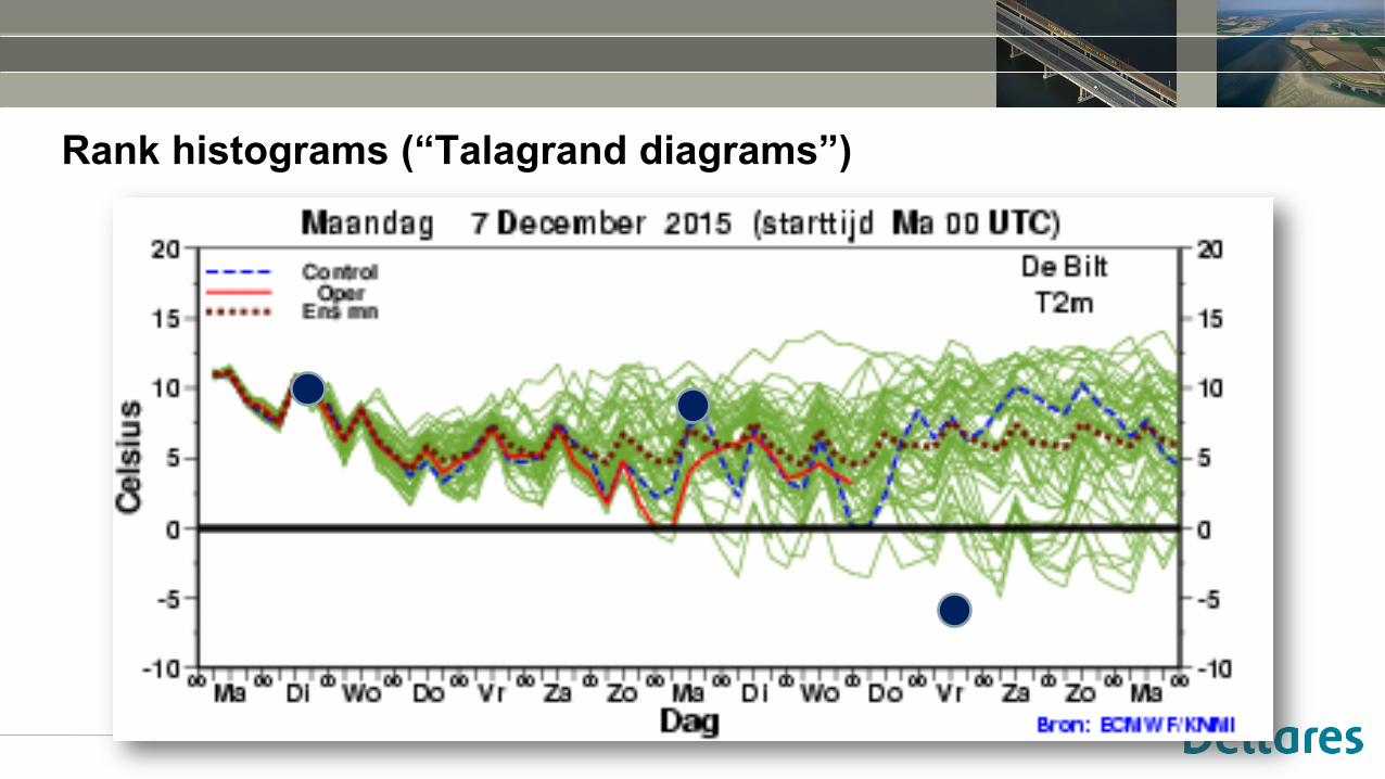
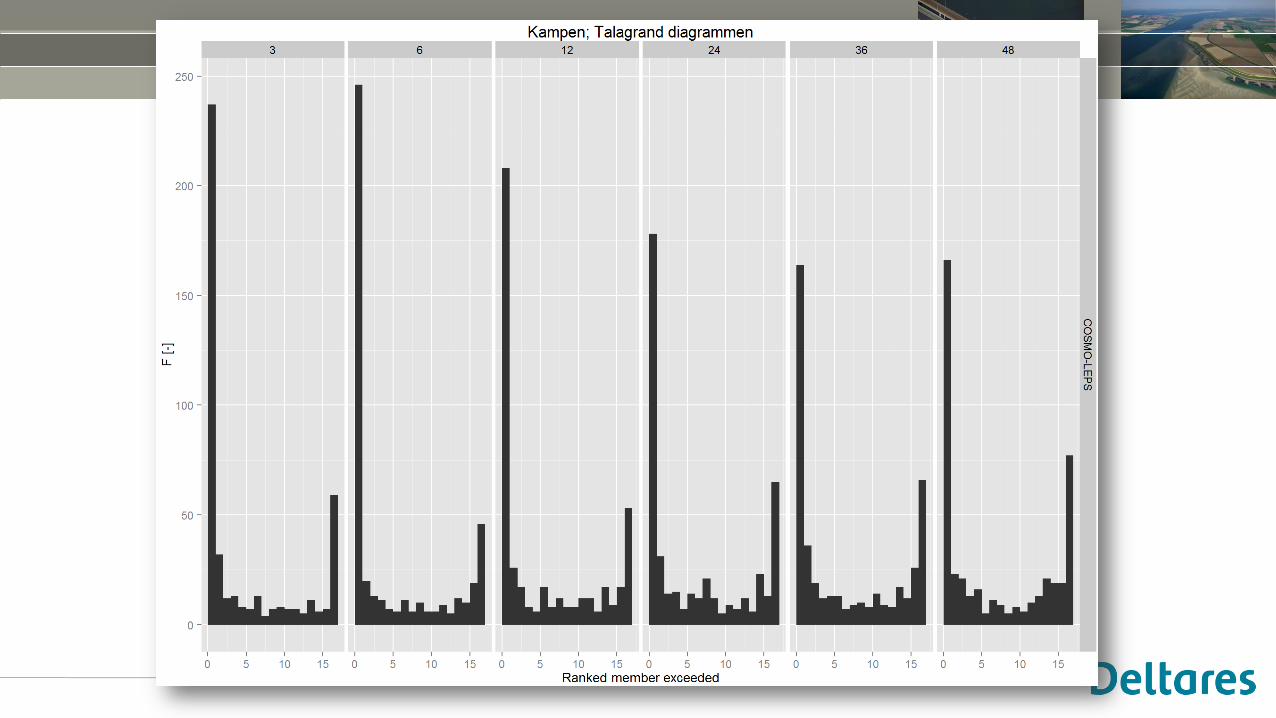
Rank histograms (“Talagrand diagrams”)

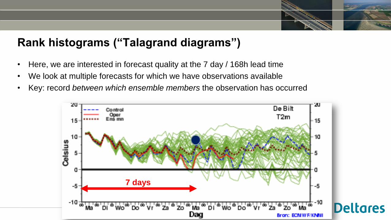
Rank histograms (“Talagrand diagrams”)

• Here, we are interested in forecast quality at the 7 day / 168h lead time

• We look at multiple forecasts for which we have observations available

• Key: record between which ensemble members the observation has occurred

7 days

forecast 1

0

5

10

15

20

25

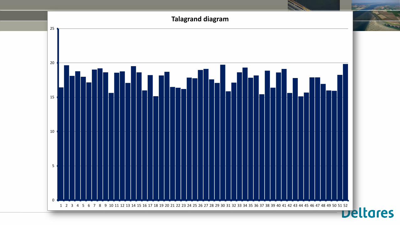
1 2 3 4 5 6 7 8 9 10 11 12 13 14 15 16 17 18 19 20 21 22 23 24 25 26 27 28 29 30 31 32 33 34 35 36 37 38 39 40 41 42 43 44 45 46 47 48 49 50 51 52

Talagrand diagram

forecast 3

forecast 4

forecast 2

0

5

10

15

20

25

1 2 3 4 5 6 7 8 9 10 11 12 13 14 15 16 17 18 19 20 21 22 23 24 25 26 27 28 29 30 31 32 33 34 35 36 37 38 39 40 41 42 43 44 45 46 47 48 49 50 51 52

Talagrand diagram

Verification: (possible) approach

• Qualitative: “Eyeball verification”: take a look at forecasts and observations

• Summary metrics:

• Graphical verification measures

• Numerical: metrics and skill scores

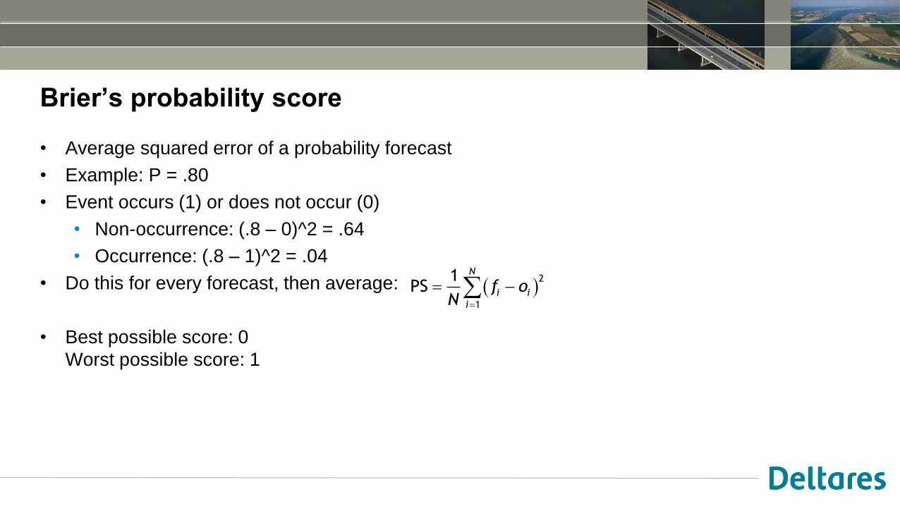
Brier’s probability score

• Average squared error of a probability forecast

• Example: P = .80

• Event occurs (1) or does not occur (0)

• Non-occurrence: (.8 – 0)^2 = .64

• Occurrence: (.8 – 1)^2 = .04

• Do this for every forecast, then average:

• Best possible score: 0

Worst possible score: 1

2

1

1PS

N

i i

i

f oN

Scores v skill

14 juni 2016

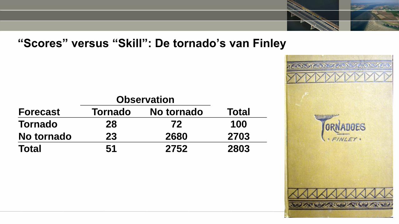
“Scores” versus “Skill”: De tornado’s van Finley

Observation

Forecast Tornado No tornado Total

Tornado 28 72 100

No tornado 23 2680 2703

Total 51 2752 2803

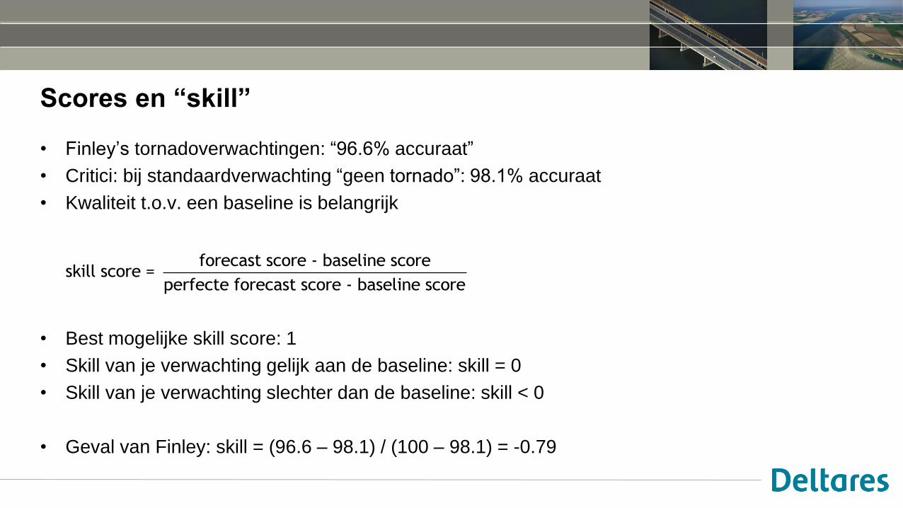
Scores en “skill”

• Finley’s tornadoverwachtingen: “96.6% accuraat”

• Critici: bij standaardverwachting “geen tornado”: 98.1% accuraat

• Kwaliteit t.o.v. een baseline is belangrijk

• Best mogelijke skill score: 1

• Skill van je verwachting gelijk aan de baseline: skill = 0

• Skill van je verwachting slechter dan de baseline: skill < 0

• Geval van Finley: skill = (96.6 – 98.1) / (100 – 98.1) = -0.79

forecast score - baseline scoreskill score =

perfecte forecast score - baseline score

De “contingency table” en afgeleide metrics

14 juni 2016

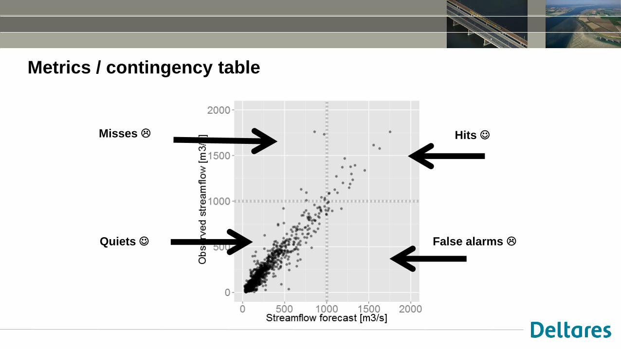
Metrics / contingency table

Hits

Quiets

Misses

False alarms

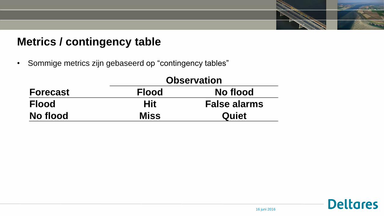
Metrics / contingency table

• Sommige metrics zijn gebaseerd op “contingency tables”

16 juni 2016

Observation

Forecast Flood No flood

Flood Hit False alarms

No flood Miss Quiet

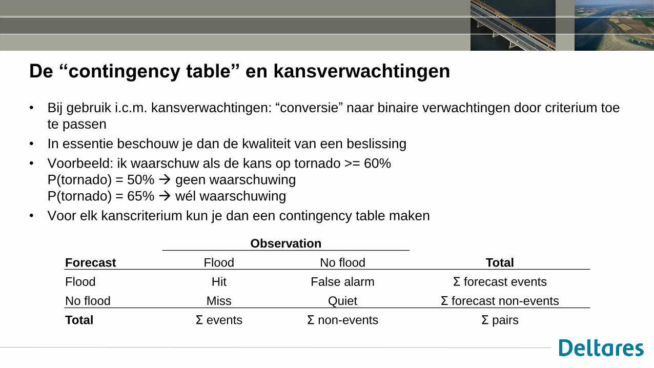
De “contingency table” en kansverwachtingen

• Bij gebruik i.c.m. kansverwachtingen: “conversie” naar binaire verwachtingen door criterium toe

te passen

• In essentie beschouw je dan de kwaliteit van een beslissing

• Voorbeeld: ik waarschuw als de kans op tornado >= 60%

P(tornado) = 50% geen waarschuwing

P(tornado) = 65% wél waarschuwing

• Voor elk kanscriterium kun je dan een contingency table maken

Observation

Forecast Flood No flood Total

Flood Hit False alarm Σ forecast events

No flood Miss Quiet Σ forecast non-events

Total Σ events Σ non-events Σ pairs

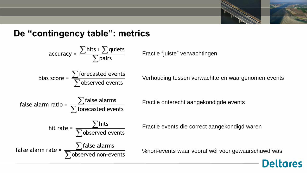
De “contingency table”: metrics

Fractie “juiste” verwachtingen

Verhouding tussen verwachtte en waargenomen events

Fractie onterecht aangekondigde events

Fractie events die correct aangekondigd waren

%non-events waar vooraf wél voor gewaarschuwd was

hitshit rate =

observed events

false alarmsfalse alarm rate =

observed non-events

false alarmsfalse alarm ratio =

forecasted events

forecasted eventsbias score =

observed events

hits quietsaccuracy =

pairs

Beschikbare verificatie-software

14 juni 2016

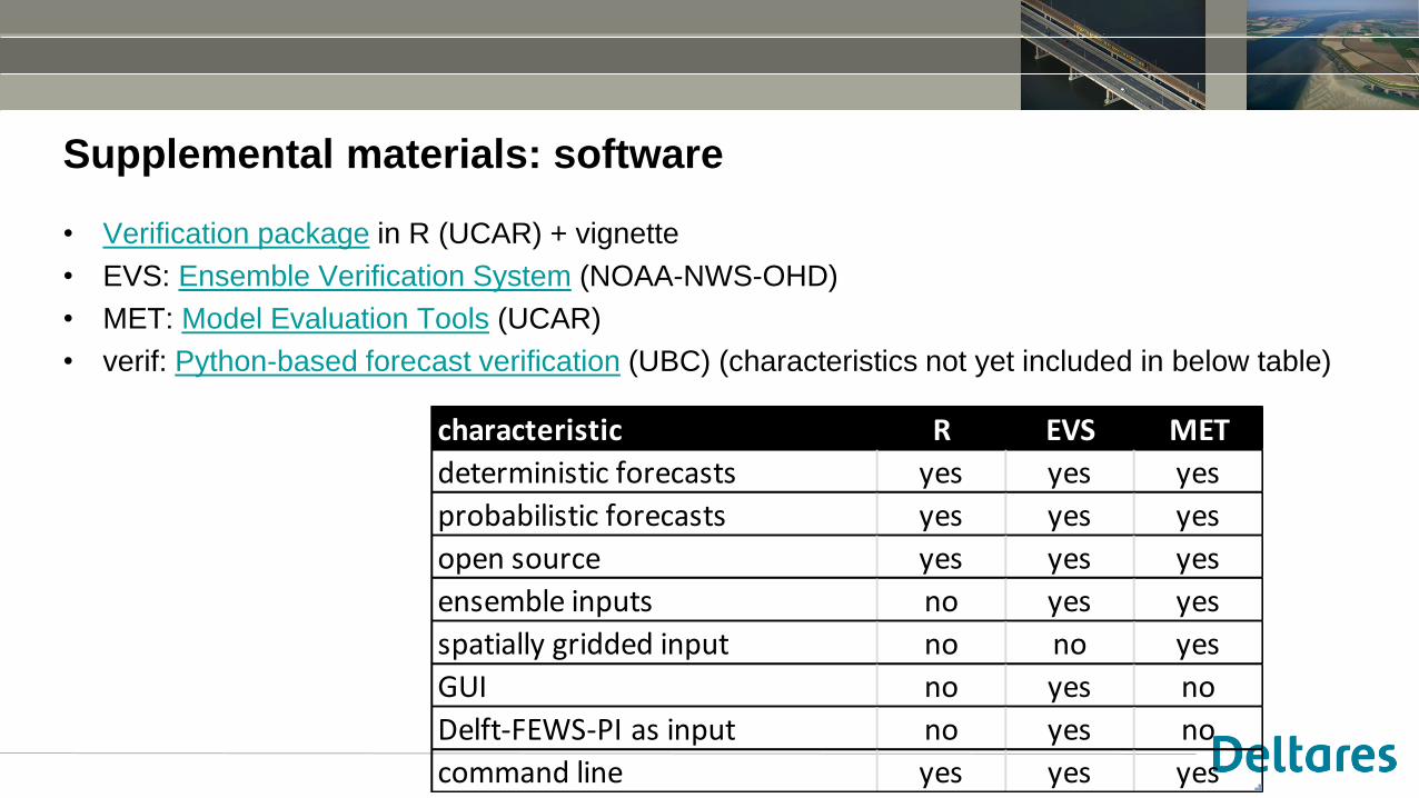
Supplemental materials: software

• Verification package in R (UCAR) + vignette

• EVS: Ensemble Verification System (NOAA-NWS-OHD)

• MET: Model Evaluation Tools (UCAR)

• verif: Python-based forecast verification (UBC) (characteristics not yet included in below table)

characteristic R EVS MET

deterministic forecasts yes yes yes

probabilistic forecasts yes yes yes

open source yes yes yes

ensemble inputs no yes yes

spatially gridded input no no yes

GUI no yes no

Delft-FEWS-PI as input no yes no

command line yes yes yes

Afronding

14 juni 2016

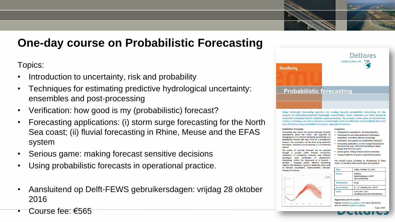
One-day course on Probabilistic Forecasting

Topics:

• Introduction to uncertainty, risk and probability

• Techniques for estimating predictive hydrological uncertainty:

ensembles and post-processing

• Verification: how good is my (probabilistic) forecast?

• Forecasting applications: (i) storm surge forecasting for the North

Sea coast; (ii) fluvial forecasting in Rhine, Meuse and the EFAS

system

• Serious game: making forecast sensitive decisions

• Using probabilistic forecasts in operational practice.

• Aansluitend op Delft-FEWS gebruikersdagen: vrijdag 28 oktober

2016

• Course fee: €565

Jan Verkade

jan.verkade@deltares.nl, +31 6 5161 6107

Dank voor uw aandacht!