
VEL TECH HIGH TECH Dr. RANGARAJAN Dr. SAKUNTHALA ...
61
VEL TECH HIGH TECH Dr. RANGARAJAN Dr. SAKUNTHALA ENGINEERING COLLEGE DEPARTMENT OF BIOTECHNOLOGY BT6701 BIOINFORMATICS AND COMPUTATIONAL BIOLOGY VEL TECH HIGH TECH Dr. RANGARAJAN Dr. SAKUNTHALA ENGINEERING COLLEGE 1 UNIT I DIFFERENT NETWORK TOPOLOGY WITH ILLUSTRATION. TOPOLOGY The term topology, or more specifically, network topology, refers to the arrangement or physical layout of computers, cables, and other components on the network. "Topology" is the standard term that most network professionals use when they refer to the network's basic design “Network topology is the study of the arrangement or mapping of the elements of a network, especi ally the physical (real) and logical (virtual) interconnections between nodes”. Classification of network topologies There are also three basic categories of network topologies: Physical topologies Signal topologies Logical topologies a) Physical topologies The mapping of the nodes of a network and the physical connections between them – i.e., the layout of wiring, cables, the locations of nodes, and the interconnections between the nodes and the cabling or wiring system is known as physical topologies. Classification of physical topologies Bus Star Mesh Tree Hybrid-network topologies b) Signal topology The mapping of the actual connections between the nodes of a network, as evidenced by the path that the signals take when propagating between the nodes. c) Logical topology The mapping of the apparent connections between the nodes of a network, as evidenced by the path that data appears to take when traveling between the nodes. TOPOLOGIES BUS STAR RING MESH TREE HYBRID
Transcript of VEL TECH HIGH TECH Dr. RANGARAJAN Dr. SAKUNTHALA ...
VEL TECH HIGH TECH Dr. RANGARAJAN Dr. SAKUNTHALA ENGINEERING COLLEGE
DEPARTMENT OF BIOTECHNOLOGY
BT6701 BIOINFORMATICS AND COMPUTATIONAL BIOLOGY
VEL TECH HIGH TECH Dr. RANGARAJAN Dr. SAKUNTHALA ENGINEERING COLLEGE
1
UNIT I
DIFFERENT NETWORK TOPOLOGY WITH ILLUSTRATION.
TOPOLOGY
The term topology, or more specifically, network topology, refers to the arrangement or physical layout of
computers, cables, and other components on the network. "Topology" is the standard term that most network
professionals use when they refer to the network's basic design
“Network topology is the study of the arrangement or mapping of the elements of a network, especially the
physical (real) and logical (virtual) interconnections between nodes”.
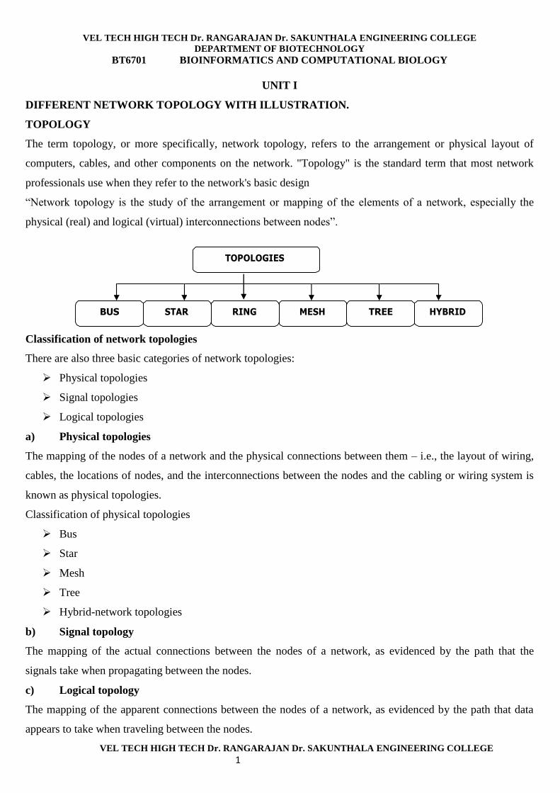
Classification of network topologies
There are also three basic categories of network topologies:
Physical topologies
Signal topologies
Logical topologies
a) Physical topologies
The mapping of the nodes of a network and the physical connections between them – i.e., the layout of wiring,
cables, the locations of nodes, and the interconnections between the nodes and the cabling or wiring system is
known as physical topologies.
Classification of physical topologies
Bus
Star
Mesh
Tree
Hybrid-network topologies
b) Signal topology
The mapping of the actual connections between the nodes of a network, as evidenced by the path that the
signals take when propagating between the nodes.
c) Logical topology
The mapping of the apparent connections between the nodes of a network, as evidenced by the path that data
appears to take when traveling between the nodes.
TOPOLOGIES
BUS STAR RING MESH TREE HYBRID
VEL TECH HIGH TECH Dr. RANGARAJAN Dr. SAKUNTHALA ENGINEERING COLLEGE
DEPARTMENT OF BIOTECHNOLOGY
BT6701 BIOINFORMATICS AND COMPUTATIONAL BIOLOGY
VEL TECH HIGH TECH Dr. RANGARAJAN Dr. SAKUNTHALA ENGINEERING COLLEGE
2
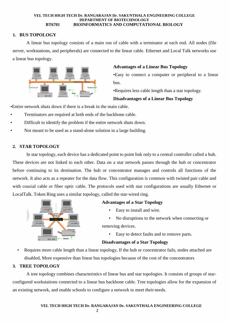
1. BUS TOPOLOGY
A linear bus topology consists of a main run of cable with a terminator at each end. All nodes (file
server, workstations, and peripherals) are connected to the linear cable. Ethernet and Local Talk networks use
a linear bus topology.
Advantages of a Linear Bus Topology
•Easy to connect a computer or peripheral to a linear
bus.
•Requires less cable length than a star topology.
Disadvantages of a Linear Bus Topology
•Entire network shuts down if there is a break in the main cable.
• Terminators are required at both ends of the backbone cable.
• Difficult to identify the problem if the entire network shuts down.
• Not meant to be used as a stand-alone solution in a large building.
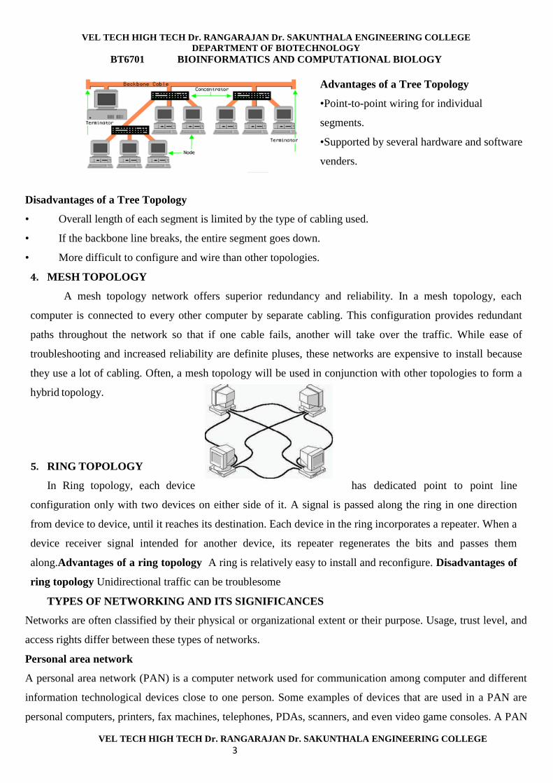
2. STAR TOPOLOGY
In star topology, each device has a dedicated point to point link only to a central controller called a hub.
These devices are not linked to each other. Data on a star network passes through the hub or concentrator
before continuing to its destination. The hub or concentrator manages and controls all functions of the
network. It also acts as a repeater for the data flow. This configuration is common with twisted pair cable and
with coaxial cable or fiber optic cable. The protocols used with star configurations are usually Ethernet or
LocalTalk. Token Ring uses a similar topology, called the star-wired ring.
Advantages of a Star Topology
• Easy to install and wire.
• No disruptions to the network when connecting or
removing devices.
• Easy to detect faults and to remove parts.
Disadvantages of a Star Topology
• Requires more cable length than a linear topology, If the hub or concentrator fails, nodes attached are
disabled, More expensive than linear bus topologies because of the cost of the concentrators
3. TREE TOPOLOGY
A tree topology combines characteristics of linear bus and star topologies. It consists of groups of star-
configured workstations connected to a linear bus backbone cable. Tree topologies allow for the expansion of
an existing network, and enable schools to configure a network to meet their needs.
VEL TECH HIGH TECH Dr. RANGARAJAN Dr. SAKUNTHALA ENGINEERING COLLEGE
DEPARTMENT OF BIOTECHNOLOGY
BT6701 BIOINFORMATICS AND COMPUTATIONAL BIOLOGY
VEL TECH HIGH TECH Dr. RANGARAJAN Dr. SAKUNTHALA ENGINEERING COLLEGE
3
Advantages of a Tree Topology
•Point-to-point wiring for individual
segments.
•Supported by several hardware and software
venders.
Disadvantages of a Tree Topology
• Overall length of each segment is limited by the type of cabling used.
• If the backbone line breaks, the entire segment goes down.
• More difficult to configure and wire than other topologies.
4. MESH TOPOLOGY
A mesh topology network offers superior redundancy and reliability. In a mesh topology, each
computer is connected to every other computer by separate cabling. This configuration provides redundant
paths throughout the network so that if one cable fails, another will take over the traffic. While ease of
troubleshooting and increased reliability are definite pluses, these networks are expensive to install because
they use a lot of cabling. Often, a mesh topology will be used in conjunction with other topologies to form a
hybrid topology.
5. RING TOPOLOGY
In Ring topology, each device has dedicated point to point line
configuration only with two devices on either side of it. A signal is passed along the ring in one direction
from device to device, until it reaches its destination. Each device in the ring incorporates a repeater. When a
device receiver signal intended for another device, its repeater regenerates the bits and passes them
along.Advantages of a ring topology A ring is relatively easy to install and reconfigure. Disadvantages of
ring topology Unidirectional traffic can be troublesome
TYPES OF NETWORKING AND ITS SIGNIFICANCES
Networks are often classified by their physical or organizational extent or their purpose. Usage, trust level, and
access rights differ between these types of networks.
Personal area network
A personal area network (PAN) is a computer network used for communication among computer and different
information technological devices close to one person. Some examples of devices that are used in a PAN are
personal computers, printers, fax machines, telephones, PDAs, scanners, and even video game consoles. A PAN
VEL TECH HIGH TECH Dr. RANGARAJAN Dr. SAKUNTHALA ENGINEERING COLLEGE
DEPARTMENT OF BIOTECHNOLOGY
BT6701 BIOINFORMATICS AND COMPUTATIONAL BIOLOGY
VEL TECH HIGH TECH Dr. RANGARAJAN Dr. SAKUNTHALA ENGINEERING COLLEGE
4
may include wired and wireless devices. The reach of a PAN typically extends to 10 meters.[11]
A wired PAN is
usually constructed with USB and Firewire connections while technologies such as Bluetooth and infrared
communication typically form a wireless PAN.
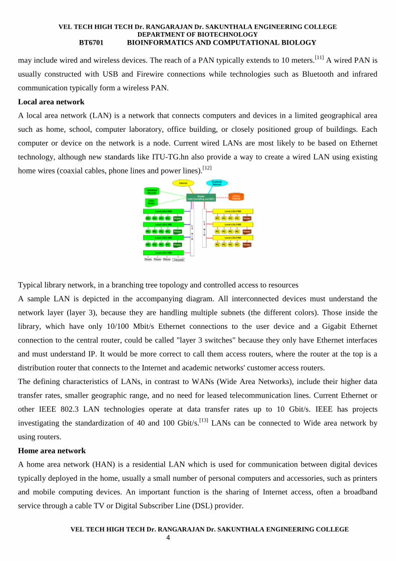
Local area network
A local area network (LAN) is a network that connects computers and devices in a limited geographical area
such as home, school, computer laboratory, office building, or closely positioned group of buildings. Each
computer or device on the network is a node. Current wired LANs are most likely to be based on Ethernet
technology, although new standards like ITU-TG.hn also provide a way to create a wired LAN using existing
home wires (coaxial cables, phone lines and power lines).[12]
Typical library network, in a branching tree topology and controlled access to resources
A sample LAN is depicted in the accompanying diagram. All interconnected devices must understand the
network layer (layer 3), because they are handling multiple subnets (the different colors). Those inside the
library, which have only 10/100 Mbit/s Ethernet connections to the user device and a Gigabit Ethernet
connection to the central router, could be called "layer 3 switches" because they only have Ethernet interfaces
and must understand IP. It would be more correct to call them access routers, where the router at the top is a
distribution router that connects to the Internet and academic networks' customer access routers.
The defining characteristics of LANs, in contrast to WANs (Wide Area Networks), include their higher data
transfer rates, smaller geographic range, and no need for leased telecommunication lines. Current Ethernet or
other IEEE 802.3 LAN technologies operate at data transfer rates up to 10 Gbit/s. IEEE has projects
investigating the standardization of 40 and 100 Gbit/s.[13]
LANs can be connected to Wide area network by
using routers.
Home area network
A home area network (HAN) is a residential LAN which is used for communication between digital devices
typically deployed in the home, usually a small number of personal computers and accessories, such as printers
and mobile computing devices. An important function is the sharing of Internet access, often a broadband
service through a cable TV or Digital Subscriber Line (DSL) provider.
VEL TECH HIGH TECH Dr. RANGARAJAN Dr. SAKUNTHALA ENGINEERING COLLEGE
DEPARTMENT OF BIOTECHNOLOGY
BT6701 BIOINFORMATICS AND COMPUTATIONAL BIOLOGY
VEL TECH HIGH TECH Dr. RANGARAJAN Dr. SAKUNTHALA ENGINEERING COLLEGE
5
Storage area network
A storage area network (SAN) is a dedicated network that provides access to consolidated, block level data
storage. SANs are primarily used to make storage devices, such as disk arrays, tape libraries, and optical
jukeboxes, accessible to servers so that the devices appear like locally attached devices to the operating system.
A SAN typically has its own network of storage devices that are generally not accessible through the local area
network by other devices. The cost and complexity of SANs dropped in the early 2000s to levels allowing wider
adoption across both enterprise and small to medium sized business environments.
Campus area network
A campus area network (CAN) is a computer network made up of an interconnection of LANs within a limited
geographical area. The networking equipment (switches, routers) and transmission media (optical fiber, copper
plant, Cat5 cabling etc.) are almost entirely owned (by the campus tenant / owner: an enterprise, university,
government etc.).
In the case of a university campus-based campus network, the network is likely to link a variety of campus
buildings including, for example, academic colleges or departments, the university library, and student
residence halls.
Backbone network
A backbone network is part of a computer network infrastructure that interconnects various pieces of network,
providing a path for the exchange of information between different LANs or subnetworks. A backbone can tie
together diverse networks in the same building, in different buildings in a campus environment, or over wide
areas. Normally, the backbone's capacity is greater than that of the networks connected to it.
A large corporation which has many locations may have a backbone network that ties all of these locations
together, for example, if a server cluster needs to be accessed by different departments of a company which are
located at different geographical locations. The equipment which ties these departments together constitute the
network backbone. Network performance management including network congestion are critical parameters
taken into account when designing a network backbone.
A specific case of a backbone network is the Internet backbone, which is the set of wide-area network
connections and core routers that interconnect all networks connected to the Internet.
Metropolitan area network
A Metropolitan area network (MAN) is a large computer network that usually spans a city or a large campus.
VEL TECH HIGH TECH Dr. RANGARAJAN Dr. SAKUNTHALA ENGINEERING COLLEGE
DEPARTMENT OF BIOTECHNOLOGY
BT6701 BIOINFORMATICS AND COMPUTATIONAL BIOLOGY
VEL TECH HIGH TECH Dr. RANGARAJAN Dr. SAKUNTHALA ENGINEERING COLLEGE
6
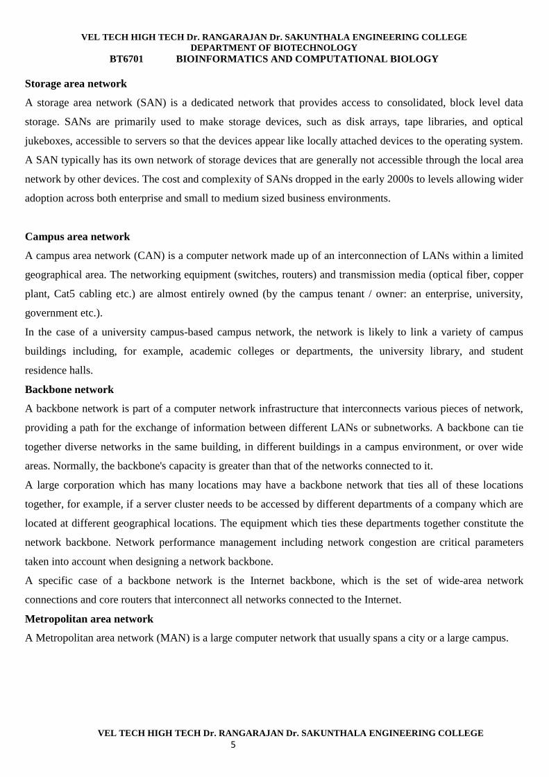
Sample EPN made of Frame relay WAN connections and dialup remote access.
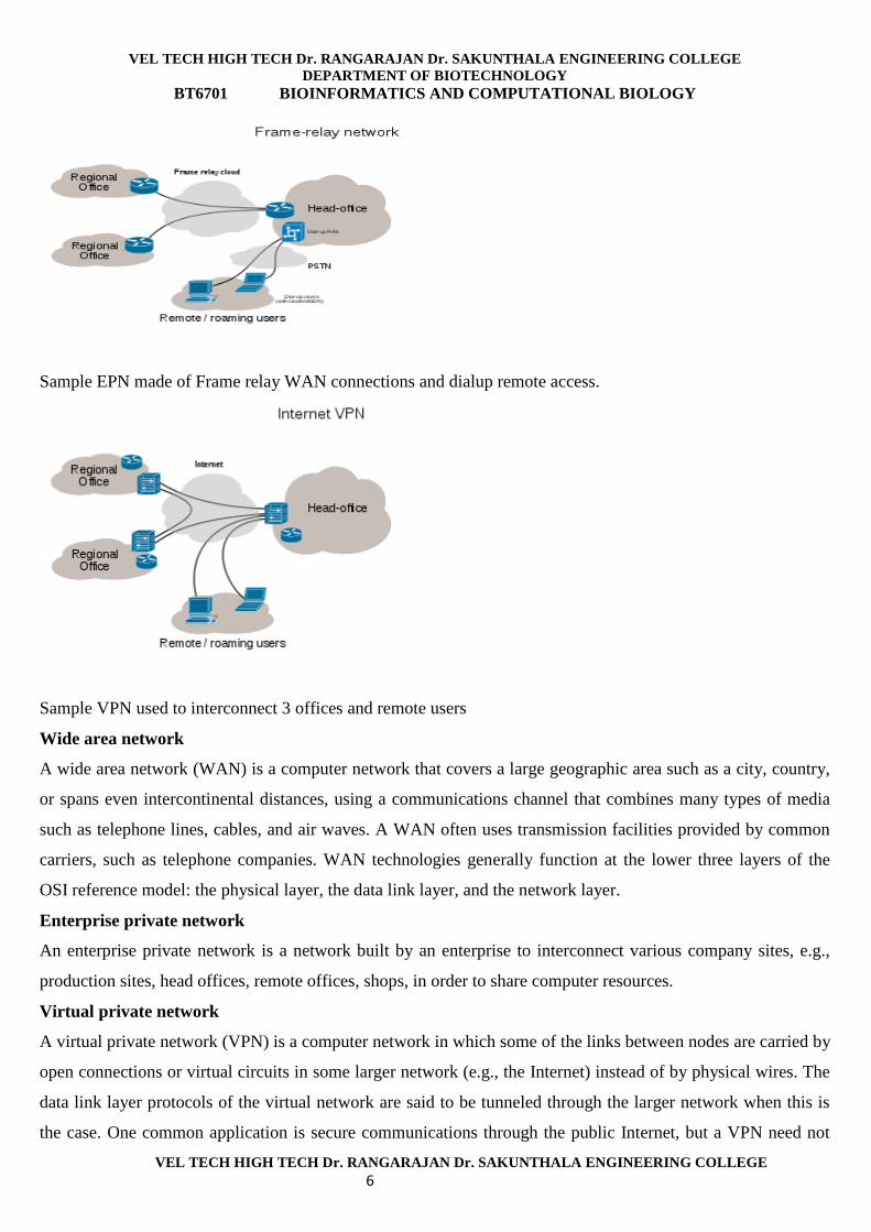
Sample VPN used to interconnect 3 offices and remote users
Wide area network
A wide area network (WAN) is a computer network that covers a large geographic area such as a city, country,
or spans even intercontinental distances, using a communications channel that combines many types of media
such as telephone lines, cables, and air waves. A WAN often uses transmission facilities provided by common
carriers, such as telephone companies. WAN technologies generally function at the lower three layers of the
OSI reference model: the physical layer, the data link layer, and the network layer.
Enterprise private network
An enterprise private network is a network built by an enterprise to interconnect various company sites, e.g.,
production sites, head offices, remote offices, shops, in order to share computer resources.
Virtual private network
A virtual private network (VPN) is a computer network in which some of the links between nodes are carried by
open connections or virtual circuits in some larger network (e.g., the Internet) instead of by physical wires. The
data link layer protocols of the virtual network are said to be tunneled through the larger network when this is
the case. One common application is secure communications through the public Internet, but a VPN need not
VEL TECH HIGH TECH Dr. RANGARAJAN Dr. SAKUNTHALA ENGINEERING COLLEGE
DEPARTMENT OF BIOTECHNOLOGY
BT6701 BIOINFORMATICS AND COMPUTATIONAL BIOLOGY
VEL TECH HIGH TECH Dr. RANGARAJAN Dr. SAKUNTHALA ENGINEERING COLLEGE
7
have explicit security features, such as authentication or content encryption. VPNs, for example, can be used to
separate the traffic of different user communities over an underlying network with strong security features.
VPN may have best-effort performance, or may have a defined service level agreement (SLA) between the
VPN customer and the VPN service provider. Generally, a VPN has a topology more complex than point-to-
point.
Internetwork
An internetwork is the connection of multiple computer networks via a common routing technology using
routers. The Internet is an aggregation of many connected internetworks spanning the Earth.
Organizational scope
Networks are typically managed by organizations which own them. According to the owner's point of view,
networks are seen as intranets or extranets. A special case of network is the Internet, which has no single owner
but a distinct status when seen by an organizational entity – that of permitting virtually unlimited global
connectivity for a great multitude of purposes.
UNIX, ITS COMMANDS AND ADVANTAGES OVER OTHER OS.
The UNIX has become quite popular since its inception in 1969, running on machines of varying
processing power from microprocessors to mainframes.
The system is divided in two.
The first part consists of programs and services that have made the UNIX system environment
so popular; it is readily apparent to users, including such programs as the shell, mail, text
processing packages, and source code control systems.
The second part consists of the operating system that supports these programs and services.
UNIX ARCHITECTURE
The high level architecture of the UNIX system is depicted below;
The hardware at the centre of the diagram provides the operating system with basic services. The
hardware at the centre provides the OS with several services. The OS interacts directly with the
hardware, providing common services to the programs and insulating them from hardware
idiosyncrasies.
The operating system is commonly called the system kernel, which is isolated from user programs. As
the programs are independent of the underlying hardware, it is easy to move them between UNIX
systems running on different hardware.
Programs such as shell and editors (ed and vi) in the outer layers interact with kernel by invoking to a
well defined set of system calls.
VEL TECH HIGH TECH Dr. RANGARAJAN Dr. SAKUNTHALA ENGINEERING COLLEGE
DEPARTMENT OF BIOTECHNOLOGY
BT6701 BIOINFORMATICS AND COMPUTATIONAL BIOLOGY
VEL TECH HIGH TECH Dr. RANGARAJAN Dr. SAKUNTHALA ENGINEERING COLLEGE
8
The system calls instruct the kernel to do various operations for the calling program and exchange
data between the kernel and the program. Several programs shown in the figure are in standard system
configurations and are known as commands.
Private user programs also exist in this layer as indicated by the programs such as a.out, the standard
name for executable files produced by the C compiler.
FEATURES OF UNIX SYSTEM
Some high-level features of the UNIX system are
The file system,
The processing environment, and
The building block primitives
THE FILE SYSTEM
The UNIX file system is characterized by
A hierarchical structure
Consistent treatment of file data
The ability to create and delete files
Dynamic growth of files
The protection of file data
The treatment of peripheral devices (such as terminal and tape units) as files
BASIC UNIX COMMANDS
1. WHO:
This command is used to display all the user’s who are currently logged on to the system.
Syntax: $who
2. who am i:
This is used to display the current user Syntax: $whoami
3. log name:
This is used to confirm the login name. Syntax: $logname
4. pwd:
This will display the current working directory. Syntax: $pwd
5. echo:
This is used to display the text typed from the keyboard. Syntax: $echo<text>
TELNET
TELNET is an abbreviation for Terminal Network. TELNET enables the establishment of a
VEL TECH HIGH TECH Dr. RANGARAJAN Dr. SAKUNTHALA ENGINEERING COLLEGE
DEPARTMENT OF BIOTECHNOLOGY
BT6701 BIOINFORMATICS AND COMPUTATIONAL BIOLOGY
VEL TECH HIGH TECH Dr. RANGARAJAN Dr. SAKUNTHALA ENGINEERING COLLEGE
9
connection to a remote system in such a way that the local terminal appears to be a terminal at the
remote system.
TELNET is a general purpose client-server program.
Briefly, TELNET is a program that allows the user to log into another computer on the internet as a
user on that system. With TELNET, a user can log into a server to access information stored on it.
For example, all public databases such as GenBank, EMBL and PDB all work on the principle of
TELNET only.
File Transfer Protocol (FTP)
File Transfer Protocol (FTP) is a standard mechanism provided by TCP/IP for copying a file from one
host to another. Transferring files from one computer to another is one of the most common tasks expected
from a networking or internetworking environment.
FTP differs from other client-server applications in that it establishes two connections between the
hosts.
One connection is used for data transfer; and the other for control information (commands and
responses), making FTP more efficient.
The client has three components
The user interface
The client control process and
The client data transfer process.
The server has two components;
The server control process
The server data transfer process
The control connection remains connected during the entire interactive FTP session. The data
connection is opened and then closed for each file transferred.
It opens each time commands that involved transferring files are used, and it closes when the file is
transferred.
The two FTP connections are
Control
Data
HYPERTEXT TRANSFER PROTOCOL (HTTP)
The HTTP is a protocol used mainly to access data on the WWW.
The protocol transfers data in the form of plain text, hypertext, audio, and video and so on.
VEL TECH HIGH TECH Dr. RANGARAJAN Dr. SAKUNTHALA ENGINEERING COLLEGE
DEPARTMENT OF BIOTECHNOLOGY
BT6701 BIOINFORMATICS AND COMPUTATIONAL BIOLOGY
VEL TECH HIGH TECH Dr. RANGARAJAN Dr. SAKUNTHALA ENGINEERING COLLEGE
10
It is highly efficient as it allows its use in a hypertext environment where there are rapid jumps from
one document to another.
HTTP functions like a combination of FTP and SMTP.
BIOLOGICAL DATABASES
A database is a collection of data stored in a standardized format, designed to be shared by multiple users.
Databases provide the long term memory of computer operations; take on variety of names, depending on
their structures, contents, use and amount of data they contain.
Databases are efficiently electronic filing cabinets, a convenient and efficient method of storing vast
amounts of information.
Databases range from the
o nature of information being stored and
o On the manner of data storage.
CLASSIFICATION OF DATABASES
PRIMARY SEQUENCE DATABASES
SECONDARY DATABASES
COMPOSITE DATABASES
PRIMARY SEQUENCE DATABASES
In the early 1980’s, sequence information started to become more abundant in the scientific literature
due the invention of the DNA and protein sequencing tools and development in molecular biology. Realizing
this impact, several laboratories started developing and storing these biological sequences in central
repositories (Data ware house) leading to the birth of primary databases.
The most important primary databases are
For nucleic acid;
o EMBL(European Molecular Biology Laboratory)
o GenBank
o DDBJ(DNA DataBank of Japan)
For proteins sequence databases;
o PIR(Protein Information Resources)
o MIPS
o SWISS-PROT
o TrEMBL
o NRL-3D
VEL TECH HIGH TECH Dr. RANGARAJAN Dr. SAKUNTHALA ENGINEERING COLLEGE
DEPARTMENT OF BIOTECHNOLOGY
BT6701 BIOINFORMATICS AND COMPUTATIONAL BIOLOGY
VEL TECH HIGH TECH Dr. RANGARAJAN Dr. SAKUNTHALA ENGINEERING COLLEGE
11
NUCLEIC ACID SEQUENCE DATABASES
The principal DNA sequence databases are GenBank(USA), EMBL(European Molecular Biology
Laboratory-Europe) and DDBJ (Japan), which exchange data on a daily basis to ensure
comprehensive coverage at each of the sites
EMBL, the nucleotide sequence database from the European Bioinformatics Institute(EBI), includes
sequences both from
o direct author submissions and
o genome sequence groups, and
o from scientific literature and
o Patent applications.
Information can be retrieved from EMBL using SRS Sequence Retrieval System; this links the
principal DNA and protein sequence databases with motif, structure, mapping and other specialized
databases
EMBL also has links with MEDLINE.
EMBL can be searched with query sequences via EBI’s web interfaces to the BLAST and FastA
programs
DDBJ
DDBJ is the DNA Data Bank of Japan, began in 1986 as a collaborators with EMBL and GenBank.
The database is produced, maintained and distributed at the National Institute of Genetics.
GenBank
GenBank, the DNA database from the NCBI, incorporates sequences from publicly available sources,
primarily from direct author submissions and large-scale sequencing projects.
GenBank is split into 17 divisions (till 2005) for it convenience such as;
o PRI Primate
o ROD Rodent
o MAM Other mammalian
o SYN Synthetic
o HTG High throughput genomic sequences
Information can be retrieved from GenBank using the Entrez integrated retrieval system
Entrez combines data from the principal DNA and protein sequence databases with information from
genome maps and protein structures.
Additional information on the sequences can be accessed via the MEDLINE , which provides
abstracts from the original published articles.
VEL TECH HIGH TECH Dr. RANGARAJAN Dr. SAKUNTHALA ENGINEERING COLLEGE
DEPARTMENT OF BIOTECHNOLOGY
BT6701 BIOINFORMATICS AND COMPUTATIONAL BIOLOGY
VEL TECH HIGH TECH Dr. RANGARAJAN Dr. SAKUNTHALA ENGINEERING COLLEGE
12
STRUCTURE OF GENBANK ENTRIES
GenBank entries include sequence files, indices created on various database fields and information
derived from the database.
The below figure depicts a GenBank entry;
In the below figure, keywords includes LOCUS, DEFINITION, ACCESSION, NID, SOURCE,
REFERENCE, FEATURES, BASE COUNT and ORIGIN
The LOCUS keyword introduces a short label for the entry that may suggest the function of the
sequence(1593 bp DNA linear VRL, where 1593 bp is the length of linear DNA from Viral source),
the line summarizes the number of bases, source of DNA, and date of submission
The DEFINITION line contains concise definition of the sequence(Canine parvovirus, VP-2 gene,
complete cds)
Following this is , the ACCESSION line gives the accession number(AY742949)
The KEYWORDS line introduces a list of short phrases, assigned by the author, describing gene
products and other relevant information about the entry (Here, VP-2 gene of CPV, Viral coat protein).
The SOURCE record provides the information on the fecal sample from which the data have been
derived.
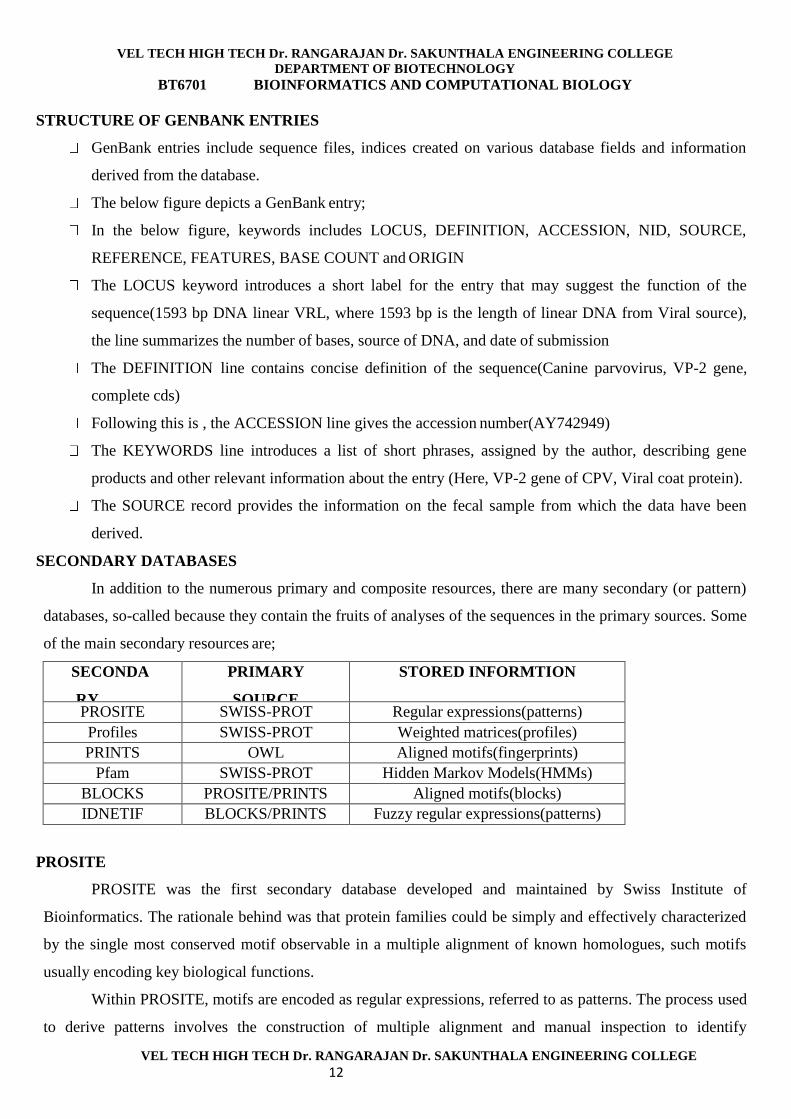
SECONDARY DATABASES
In addition to the numerous primary and composite resources, there are many secondary (or pattern)
databases, so-called because they contain the fruits of analyses of the sequences in the primary sources. Some
of the main secondary resources are;
SECONDA
RY
DATABAS
E
PRIMARY
SOURCE
STORED INFORMTION
PROSITE SWISS-PROT Regular expressions(patterns)
Profiles SWISS-PROT Weighted matrices(profiles)
PRINTS OWL Aligned motifs(fingerprints)
Pfam SWISS-PROT Hidden Markov Models(HMMs)
BLOCKS PROSITE/PRINTS Aligned motifs(blocks)
IDNETIF
Y
BLOCKS/PRINTS Fuzzy regular expressions(patterns)
PROSITE
PROSITE was the first secondary database developed and maintained by Swiss Institute of
Bioinformatics. The rationale behind was that protein families could be simply and effectively characterized
by the single most conserved motif observable in a multiple alignment of known homologues, such motifs
usually encoding key biological functions.
Within PROSITE, motifs are encoded as regular expressions, referred to as patterns. The process used
to derive patterns involves the construction of multiple alignment and manual inspection to identify
VEL TECH HIGH TECH Dr. RANGARAJAN Dr. SAKUNTHALA ENGINEERING COLLEGE
DEPARTMENT OF BIOTECHNOLOGY
BT6701 BIOINFORMATICS AND COMPUTATIONAL BIOLOGY
VEL TECH HIGH TECH Dr. RANGARAJAN Dr. SAKUNTHALA ENGINEERING COLLEGE
13
conserved regions. Sequence information within individual motifs is reduced to single consensus expressions
and the resulting seed patterns are used to search SWISS-PROT. Results are checked manually to determine
how well the patterns are performed.
STRUCTURE CLASSIFICATION DATABASES
Many proteins share structural similarities, reflecting common evolutionary origins. The evolutionary
process involves substitutions, insertions and deletions in amino acid sequences. For distantly related
proteins, such changes can be extensive, yielding folds in which the numbers and orientations of secondary
structures vary considerably. Two classification schemes are
SCOP (Structural Classification of Proteins)
CATH (Class, Architecture, Topology, Homology)
PDBsum-a different structural information database
SCOP
The SCOP (Structural Classification of Proteins) database maintained by the MRC laboratory of
Molecular Biology and Centre for Protein Engineering.
The database describes the structural and evolutionary relationships between proteins of known
structure.
As current automatic structure comparison tools cannot reliably identify all such relationships, SCOP
has been constructed using a combination of manual inspection and automated methods.
SCOP classification is based on hierarchy reflecting their structural and evolutionary relatedness.
Within the hierarchy there are many levels, but principally these describe the family, super family and
fold.
Family – Proteins are clustered into families with clear evolutionary relationships if they have
sequence identities ≥30%. But this is not absolute measure, as it is possible to infer common descent
from similar structures and functions in the absence of significant sequence identity.
Super family- Proteins are placed in superfamilies when, in spite of low identity, their structural and
functional characteristics suggest a common evolutionary origin.
Fold – Proteins are classed as having a common fold if they have same secondary structures in the
same arrangement and same topology.
CATH
The CATH (Class, Architecture, Topology, and Homology) database is a hierarchical domain
classification of protein structures maintained at UCL. The resource is largely derived using automatic
methods assisted by manual inspection. Different categories within the classification are identified by means
VEL TECH HIGH TECH Dr. RANGARAJAN Dr. SAKUNTHALA ENGINEERING COLLEGE
DEPARTMENT OF BIOTECHNOLOGY
BT6701 BIOINFORMATICS AND COMPUTATIONAL BIOLOGY
VEL TECH HIGH TECH Dr. RANGARAJAN Dr. SAKUNTHALA ENGINEERING COLLEGE
14
of both unique numbers and descriptive names. Such a numbering scheme allows efficient computational
manipulation of data. There are five levels within the hierarchy;
Class
Architecture
Topology
Homology
Sequence
CATH is accessible for keyword interrogation via UCL’s Biomolecular Structure and Modeling unit
web server.
FSSP
FSSP (Fold classification based on the structure-structure alignment of proteins and families of
structurally similar proteins) is based on the structural alignment of pairwise combinations of proteins in the
PDB. Alignments and classification are done automatically and are updated continuosly by the DALI search
engine. The FSSP database presents a continuously updated structural classification of three dimensional
protein folds. It is derived using an automatic structure comparison program (DALI)
MMDB
NCBI’s macromolecular 3D structure database is called MMDB or molecular modelling database.
It is also known as the NCBI structure division. It was designed to archive structural data from PDB as well
as biomolecules generated by electron microscopy. MMDB is linked to the rest of the NCBI’s databases.
PDBsum
PDBsum is a web-base compendium structural information database maintained at UCL. PDBsum
provides summaries and analyses of all structures in the PDB. Each summary gives an at-a- glance overview
of the contents of a PDB entry in terms of resolution and R-factor, number of protein chains, ligands, metal
ions, secondary structures, folds and ligand interactions. This compendium is helpful for retrieving 1D
(sequence), 2D (motifs) and 3D (structure) information’s on the proteins.
DALI
The DALI or Distance mAtrix aLIgnment server is a network used to compare three dimensional
protein structures.The query sequence coordinates are compared against those in the protein data bank.A
multiple alignment of structural neighbours is the output. The DALI serveris useful to compare 3D structures
where similarities are not detectable by comparing sequences direcly. The comparison uses Max Sprout
program to generate backbone and side-chain co-ordinates.
VEL TECH HIGH TECH Dr. RANGARAJAN Dr. SAKUNTHALA ENGINEERING COLLEGE
DEPARTMENT OF BIOTECHNOLOGY
BT6701 BIOINFORMATICS AND COMPUTATIONAL BIOLOGY
VEL TECH HIGH TECH Dr. RANGARAJAN Dr. SAKUNTHALA ENGINEERING COLLEGE
15
UNIT II
DOT BLOT matrix
Dot plots
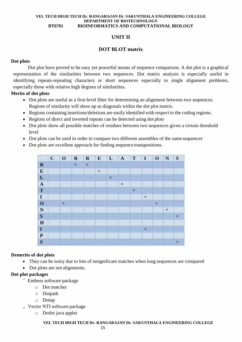
Dot plot have proved to be easy yet powerful means of sequence comparison. A dot plot is a graphical
representation of the similarities between two sequences. Dot matrix analysis is especially useful in
identifying repeats-repeating characters or short sequences especially to single alignment problems,
especially those with relative high degrees of similarities.
Merits of dot plots
Dot plots are useful as a first-level filter for determining an alignment between two sequences.
Regions of similarity will show up as diagonals within the dot plot matrix.
Regions containing insertions/deletions are easily identified with respect to the coding regions.
Regions of direct and inverted repeats can be detected using dot plots
Dot plots show all possible matches of residues between two sequences given a certain threshold
level
Dot plots can be used in order to compare two different assembles of the same sequences
Dot plots are excellent approach for finding sequence transpositions.
C O R R E L A T I O N S
R × ×
E ×
L ×
A ×
T ×
I ×
O × ×
N ×
S ×
H
I ×
P
S ×
Demerits of dot plots
They can be noisy due to lots of insignificant matches when long sequences are compared
Dot plots are not alignments.
Dot plot packages
Emboss software package
o Dot matcher
o Dotpath
o Dotup
Vector NTI software package
o Dotlet java applet
VEL TECH HIGH TECH Dr. RANGARAJAN Dr. SAKUNTHALA ENGINEERING COLLEGE
DEPARTMENT OF BIOTECHNOLOGY
BT6701 BIOINFORMATICS AND COMPUTATIONAL BIOLOGY
VEL TECH HIGH TECH Dr. RANGARAJAN Dr. SAKUNTHALA ENGINEERING COLLEGE
16
o Dotter
GCG software package
o Compare
o Dotplot
PAM & BLOSUM
Scoring matrices-Definition
A scoring matrix gives the score for aligning two amino acids (match or mismatch) in a pairwise
alignment. A scoring matrix can be considered a measure of the evolutionary change. The most widely used
matrices are PAMs and BLOSUMs. Both calculates substitution frequencies between amino acids, and both
are derived from known protein alignments
Substitution matrices algorithms
Scoring matrices are also known as substitution matrices. These are the tools that are extensively used
to model mutations in sequences. The most common method of creating a substitution matrix in the case of the
amino acids is to observe the actual substitution rates among the various amino acid residues in the nature.
The score is favourable if the substitution is observed frequently. On the other hand, the alignment for a pair
residues is penalized if the substitution is not observed frequently.
The score using this rule looks only at the degree of identical nature of the residues. It does not show
how similar those proteins are with respect to their structure and function. Thus to make amino acid
alignment and scoring more significant, matrices are developed that score mutation among amino acids with
similar physiochemical properties
Types of scoring models
There are two popular scoring models for protein sequences;
PAM (Point accepted mutation)
BLOSUM (BlOcks Substitution Matrix)
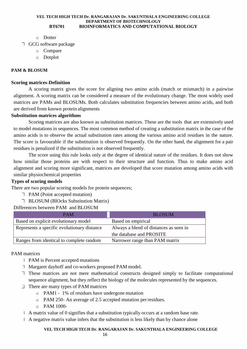
Differences between PAM and BLOSUM
PAM BLOSUM
Based on explicit evolutionary model Based on empirical
Represents a specific evolutionary distance Always a blend of distances as seen in
the database and PROSITE
Ranges from identical to complete random Narrower range than PAM matrix
PAM matrices
PAM is Percent accepted mutations
Margaret dayhoff and co-workers proposed PAM model.
These matrices are not mere mathematical constructs designed simply to facilitate computational
sequence alignment, but they reflect the biology of the molecules represented by the sequences.
There are many types of PAM matrices
o PAM1 - 1% of residues have undergone mutation
o PAM 250- An average of 2.5 accepted mutation per residues.
o PAM 1000-
A matrix value of 0 signifies that a substitution typically occurs at a random base rate.
A negative matrix value infers that the substitution is less likely than by chance alone
VEL TECH HIGH TECH Dr. RANGARAJAN Dr. SAKUNTHALA ENGINEERING COLLEGE
DEPARTMENT OF BIOTECHNOLOGY
BT6701 BIOINFORMATICS AND COMPUTATIONAL BIOLOGY
VEL TECH HIGH TECH Dr. RANGARAJAN Dr. SAKUNTHALA ENGINEERING COLLEGE
17
A positive matrix value means that substitution occurs more often than suggested by chance.
Creation of PAM matrix
Step 1 : Construct multiple sequence alignment between sequences with high similarity
Step 2 : Construct phylogenetic tree to show the order of various substitutions
Step 3 : Compute relative mutability (mi,j) for each amino acid
Step 4 : Compute relative mutability divided by the total number of mutations and multiplied by the
frequency of amino acid and a scaling factor of 100.
Step 5 : Compute substitution tally
Step 6 : Calculate the probability(M i,j) for each pair of amino acid Mi,j=
mjAi,j∑(i)Ai,j
Step 7 : Compute mutation probability Mi,j divided by the frequency of occurence of fi of the residue
(i)and then calculate Ri,j by taking the log of the resulting value for each entry of the PAM matrix. This is
repeated to compute values for non-diagonal entries in the PAM matrix.
Step 8 : Diagonal enteries in the PAM matrices are computed by taking Mi,j= 1-mj and then following
step 6.
Multiple Sequence Alignment
A multiple sequence alignment of three or more biological sequence, generally protein or DNA. MSA
is a tool to determine levels of homology and phylogeny, hence from the members of globally related
sequence. Visual depictions illustrates point mutation, insertions or deletions that appear as a gaps in one or
more sequences in the sequence alignment. MSA is used to assess sequence conservation of protein domains,
tertiary and secondary structures.
MSA is time consuming to handle manually when more than three biological sequences are
compared. Hence, computational algorithms are used to analyze alignments.
Tools for MSA
HMM
BLOCKS-HMM profile library
CDD-Conserved Domain Database
Pfam-Profile HMM library
PRINTS-Protein Fingerprints from SP/TrEMBL
PROSITE- A dictionary of protein motifs
AMAS-Analyze Multiple Aligned Sequences
ClustalW-General purpose MSA tool
DIALIGN-Local MSA
Musca-MSA
CINEMA-Colour Interactive Editor for Multiple Alignment
MEME/MAST-Search motifs and then query it against the database
MultiAlin-MSA with hierarchical clustering
Types of MSA
Global MSA
Local MSA
Multiple Sequence Alignment require sophisticated methodologies than pairwise alignments. Most
MSA’s program uses heuristic methods rather than global optimization.
VEL TECH HIGH TECH Dr. RANGARAJAN Dr. SAKUNTHALA ENGINEERING COLLEGE
DEPARTMENT OF BIOTECHNOLOGY
BT6701 BIOINFORMATICS AND COMPUTATIONAL BIOLOGY
VEL TECH HIGH TECH Dr. RANGARAJAN Dr. SAKUNTHALA ENGINEERING COLLEGE
18
Methods for MSA
Dynamic programming
Sum of pair method
Progressive alignment
Iterative methods
Hidden Markov Models
Genetic Algorithms
Automated tools (Macaw, Meme etc)
Dynamic programming
Refer Dynamic programming (Needlemann-wunsch algorithm and Smith-watermann
algorithm)
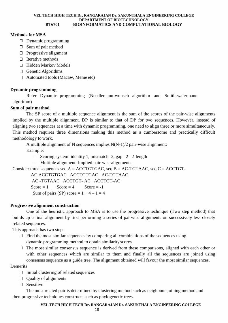
Sum of pair method
The SP score of a multiple sequence alignment is the sum of the scores of the pair-wise alignments
implied by the multiple alignment. DP is similar to that of DP for two sequences. However, instead of
aligning two sequences at a time with dynamic programming, one need to align three or more simultaneously.
This method requires three dimensions making this method as a cumbersome and practically difficult
methodology to work.
A multiple alignment of N sequences implies N(N-1)/2 pair-wise alignment:
Example:
– Scoring system: identity 1, mismatch -2, gap –2 –2 length
– Multiple alignment: Implied pair-wise alignments:
Consider three sequences seq A = ACCTGTGAC, seq B = AC-TGTAAC, seq C = ACCTGT-
AC ACCTGTGAC ACCTGTGAC AC-TGTAAC
AC -TGTAAC ACCTGT- AC ACCTGT-AC
Score = 1 Score = 4 Score = -1
Sum of pairs (SP) score = 1 + 4 – 1 = 4
Progressive alignment construction
One of the heuristic approach to MSA is to use the progressive technique (Two step method) that
builds up a final alignment by first performing a series of pairwise alignments on successively less closely
related sequences.
This approach has two steps
Find the most similar sequences by comparing all combinations of the sequences using
dynamic programming method to obtain similarity scores.
The most similar consensus sequence is derived from these comparisons, aligned with each other or
with other sequences which are similar to them and finally all the sequences are joined using
consensus sequence as a guide tree. The alignment obtained will favour the most similar sequences.
Demerits
Initial clustering of related sequences
Quality of alignments
Sensitive
The most related pair is determined by clustering method such as neighbour-joining method and
then progressive techniques constructs such as phylogenetic trees.
VEL TECH HIGH TECH Dr. RANGARAJAN Dr. SAKUNTHALA ENGINEERING COLLEGE
DEPARTMENT OF BIOTECHNOLOGY
BT6701 BIOINFORMATICS AND COMPUTATIONAL BIOLOGY
VEL TECH HIGH TECH Dr. RANGARAJAN Dr. SAKUNTHALA ENGINEERING COLLEGE
19
Examples of progressive alignments are
Clustal – It is widely used MSA alignment tool. It has two main variation
o Clustal X
o Clustal W
T-Coffee
Pile up-UPGMA (Unweighted Pair Group Method with Arithmetic Mean)
Iterative methods
A set of method to produce MSA’s while reducing the errors inherent in progressive methods are
classified as iterative because they work similar to progressive methods but repeatedly realign the initial
sequences as well as adding new sequences to the growing MSA
Examples for Iterative methods are
MUSCLE
CHAOS/DIALIGN
PRRN/PRPP
Hidden Markov Models
HMMs are probabilistic models that can assign likelihoods to all possible combinations of gaps,
matches and mismatches to determine the most likely MSA or set of possible MSAs.
HMMs produce highest-scoring output generating the best optimal alignment which is of biological
significance producing both local and global alignments. HMMs are dynamic as they are probabilistic.
Examples of HMMs
Viterbi algorithm - align the growing MSA to the next
POA-Partial Order Algorithm- HMM based
SAM-Sequence Alignment and Modelling Package
Genetic algorithm
Genetic algorithm is a dynamic and an iterative process continues indefinitely based on evolutionary
principles wherein a particular function or definition that best fits the constraints of an environment survives
to the next generation, and the other functions are eliminated. This method works by breaking a series of
possible MSAs into fragments and repeatedly rearranging those fragments with introduction of gaps at varying
positions.
Examples of Genetic algorithm
SAGA-Sequence Alignment by Genetic Algorithm
MSASA-Multiple Sequence Alignment by Simulated Annealing
Applications of Multiple Sequence Alignment
The principal applications of MSA are as follows;
Alignment of amino and nucleotide sequences
Searching for sequences
PCR primer design
Needleman –Wunsch algorithm (Global alignment)
The most basic algorithm to align two sequences was developed by S.A. Needleman and C.D.Wunsch (1970, J.
Mol. Biol. 48:443). The algorithm is a simple and beautiful way to find an alignment that maximizes a
particular score.
The initial steps of the algorithm are reminiscent of the dot plot. The first step is to place the two sequences
along the margins of a matrix
VEL TECH HIGH TECH Dr. RANGARAJAN Dr. SAKUNTHALA ENGINEERING COLLEGE
DEPARTMENT OF BIOTECHNOLOGY
BT6701 BIOINFORMATICS AND COMPUTATIONAL BIOLOGY
VEL TECH HIGH TECH Dr. RANGARAJAN Dr. SAKUNTHALA ENGINEERING COLLEGE
20
The introduction of a gap (either by an insertion or a deletion - an indel) in either sequence would correspond to
moving either above or below the main diagonal. To find the best route, Needleman and Wunsch suggested that
you modify the matrix to represent this idea of tracing different pathways through the matrix. However, you
want to include all possible pathways and from among these choose only that one which is best (in the sense of
maximizing some score). Their method consists of two passes through the matrix. The first pass traces a score
for all possible routes and moves right to left, bottom to top. Once the score for all possible routes are found, the
maximum can be chosen (it will be somewhere on the topmost row or leftmost column) and a second pass can
be carried out, this time running left to right, top to bottom to find that alignment that gives the maximum score.
The following is an example of global sequence alignment using Needleman/Wunsch techniques. For
this example, the two sequences to be globally aligned are
G A A T T C A G T T A (sequence #1) G G
A T C G A (sequence #2)
So M = 11 and N = 7 (the length of sequence #1 and sequence #2, respectively)
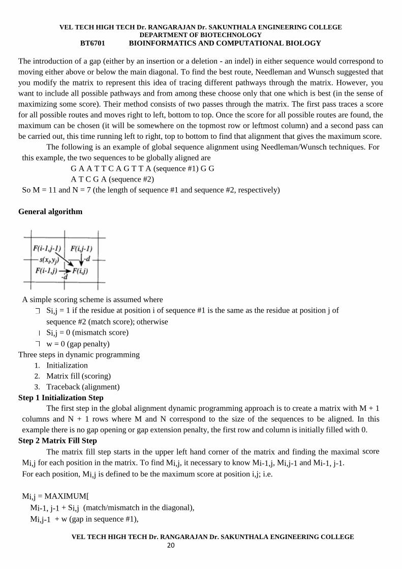
General algorithm
A simple scoring scheme is assumed where
Si,j = 1 if the residue at position i of sequence #1 is the same as the residue at position j of
sequence #2 (match score); otherwise
Si,j = 0 (mismatch score)
w = 0 (gap penalty)
Three steps in dynamic programming
1. Initialization
2. Matrix fill (scoring)
3. Traceback (alignment)
Step 1 Initialization Step
The first step in the global alignment dynamic programming approach is to create a matrix with M + 1
columns and N + 1 rows where M and N correspond to the size of the sequences to be aligned. In this
example there is no gap opening or gap extension penalty, the first row and column is initially filled with 0.
Step 2 Matrix Fill Step
The matrix fill step starts in the upper left hand corner of the matrix and finding the maximal score
Mi,j for each position in the matrix. To find Mi,j, it necessary to know Mi-1,j, Mi,j-1 and Mi-1, j-1.
For each position, Mi,j is defined to be the maximum score at position i,j; i.e.
Mi,j = MAXIMUM[
Mi-1, j-1 + Si,j (match/mismatch in the diagonal),
Mi,j-1 + w (gap in sequence #1),
VEL TECH HIGH TECH Dr. RANGARAJAN Dr. SAKUNTHALA ENGINEERING COLLEGE
DEPARTMENT OF BIOTECHNOLOGY
BT6701 BIOINFORMATICS AND COMPUTATIONAL BIOLOGY
VEL TECH HIGH TECH Dr. RANGARAJAN Dr. SAKUNTHALA ENGINEERING COLLEGE
21
Mi-1,j + w (gap in sequence #2)]
Since the first residue in both sequences is a G, S1,1 = 1, and by the assumptions stated at the
beginning, w = 0. Thus, M1,1 = MAX[M0,0 + 1, M1, 0 + 0, M0,1 + 0] = MAX [1, 0, 0] = 1.
A value of 1 is then placed in position 1,1 of the scoring matrix.
Use the algorithm, fill the column and rows. For example, at row 1 and column 1, both the bases are
guanine(G), the assigned value of maximum of 1(match), 0(horizontal gap) or 0 (vertical gap).
Similarly now let's look at column 2. The location at row 2 will be assigned the value of the maximum
of 1(mismatch), 1(horizontal gap) or 1 (vertical gap). So its value is 1.
At the position column 2 row 3, there is an A in both sequences. Thus, its value will be the maximum
of 2(match), 1 (horizontal gap), 1 (vertical gap) so its value is 2.
Moving along to position colum 2 row 4, its value will be the maximum of 1 (mismatch), 1
(horizontal gap), 2 (vertical gap) so its value is 2.
Note that for all of the remaining positions except the last one in column 2, the choices for the value
will be the exact same as in row 4 since there are no matches. The final row will contain the value 2
since it is the maximum of 2 (match), 1 (horizontal gap) and 2(vertical gap).
Step 3 Traceback Step
After the matrix fill step, the maximum alignment score for the two test sequences is 6.
The traceback step determines the actual alignment(s) that result in the maximum score.
The traceback step begins in the M,J position in the matrix, i.e. the position that leads to the maximal
score. In this case, there is a 6 in that location.
Traceback takes the current cell and looks to the neighbour cells that could be direct predecessor. This
means it looks to the neighbour cells (to its left, to above and to the diagonal neighbour) that could be
direct predecessors of the cell in consideration. Each neighbour determines a gap, match or a
mismatch.
o Neighbour to the left (gap in sequence #2),
o The diagonal neighbour (match/mismatch), and
o The neighbour above it (gap in sequence #1).
The algorithm for traceback chooses as the next cell in the sequence one of the possible predecessors.
VEL TECH HIGH TECH Dr. RANGARAJAN Dr. SAKUNTHALA ENGINEERING COLLEGE
DEPARTMENT OF BIOTECHNOLOGY
BT6701 BIOINFORMATICS AND COMPUTATIONAL BIOLOGY
VEL TECH HIGH TECH Dr. RANGARAJAN Dr. SAKUNTHALA ENGINEERING COLLEGE
22
UNIT III
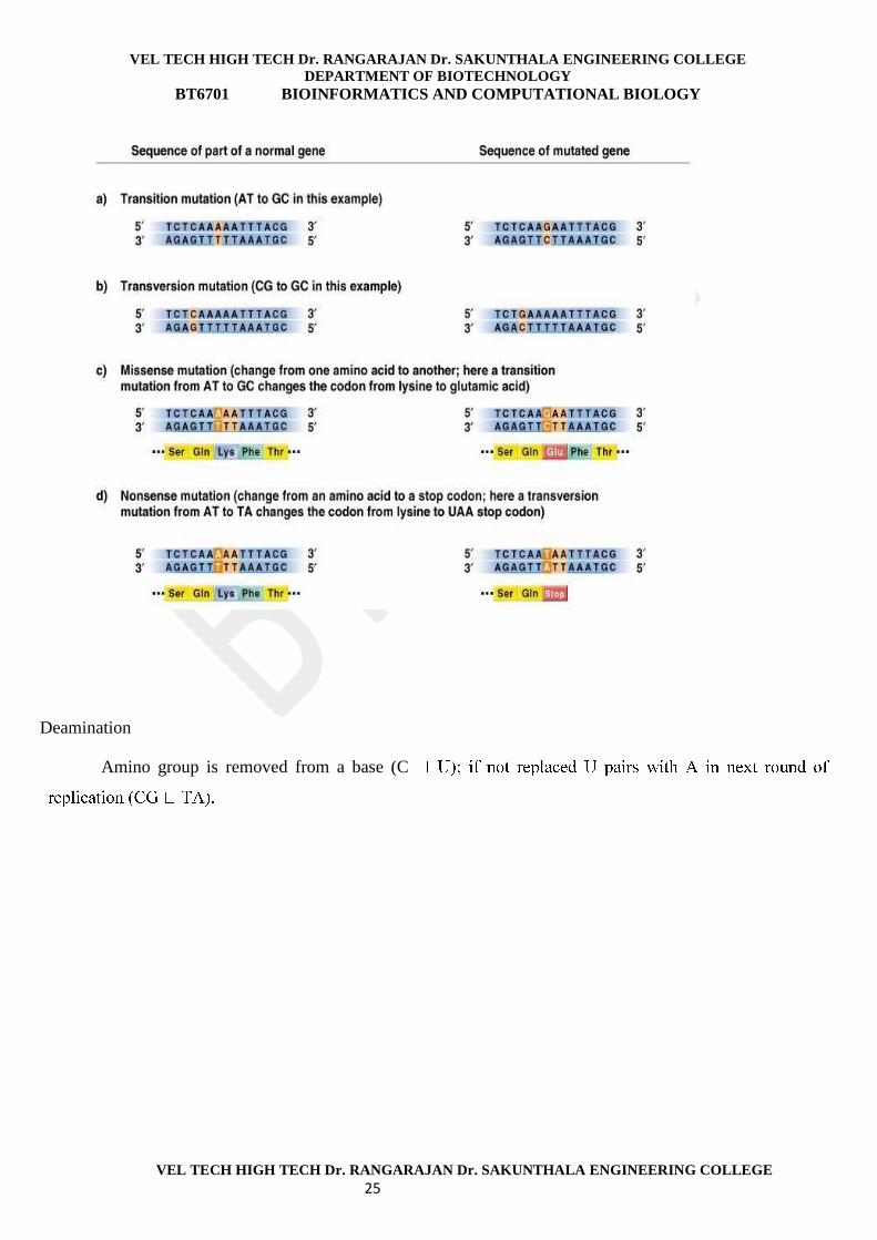
MUTATIONS
Any change in the DNA sequence of an organism is a mutation. Mutations are the source of the altered
versions of genes that provide the raw material for evolution. Most mutations have no effect on the organism,
especially among the eukaryotes, because a large portion of the DNA is not in genes and thus does not affect
the organism’s phenotype. Of the mutations that do affect the phenotype, the most common effect of
mutations is lethality, because most genes are necessary for life. There are various types of mutations such as
Point mutation
Insertion mutation
Deletion mutation
Frameshift mutation
Types of mutations in ORFs: Nonsense mutation
Base pair substitution results in a stop codon (and shorter polypeptide). Example: Hb-β McKees Rock.
Normal beta-globin is 146 amino acids long. In this mutation, codon 145 UAU (codes for tyrosine) is mutated
to UAA (stop). The final protein is thus 143 amino acids long. The clinical effect is to cause overproduction
of red blood cells, resulting in thick blood subject to abnormal clotting and bleeding.
Non synonymous/missense mutation
Base pair substitution results in substitution of a different amino acid. Example: HbS, sickle cell
hemoglobin, is a change in the beta-globin gene, where a GAG codon is converted to GUG. GAG codes for
glutamic acid, which is a hydrophilic amino acid that carries a -1 charge, and GUG codes for valine, a
hydrophobic amino acid. This amino acid is on the surface of the globin molecule, exposed to water. Under
low oxygen conditions, valine’s affinity for hydrophobic environments causes the hemoglobin to crystallize
out of solution.
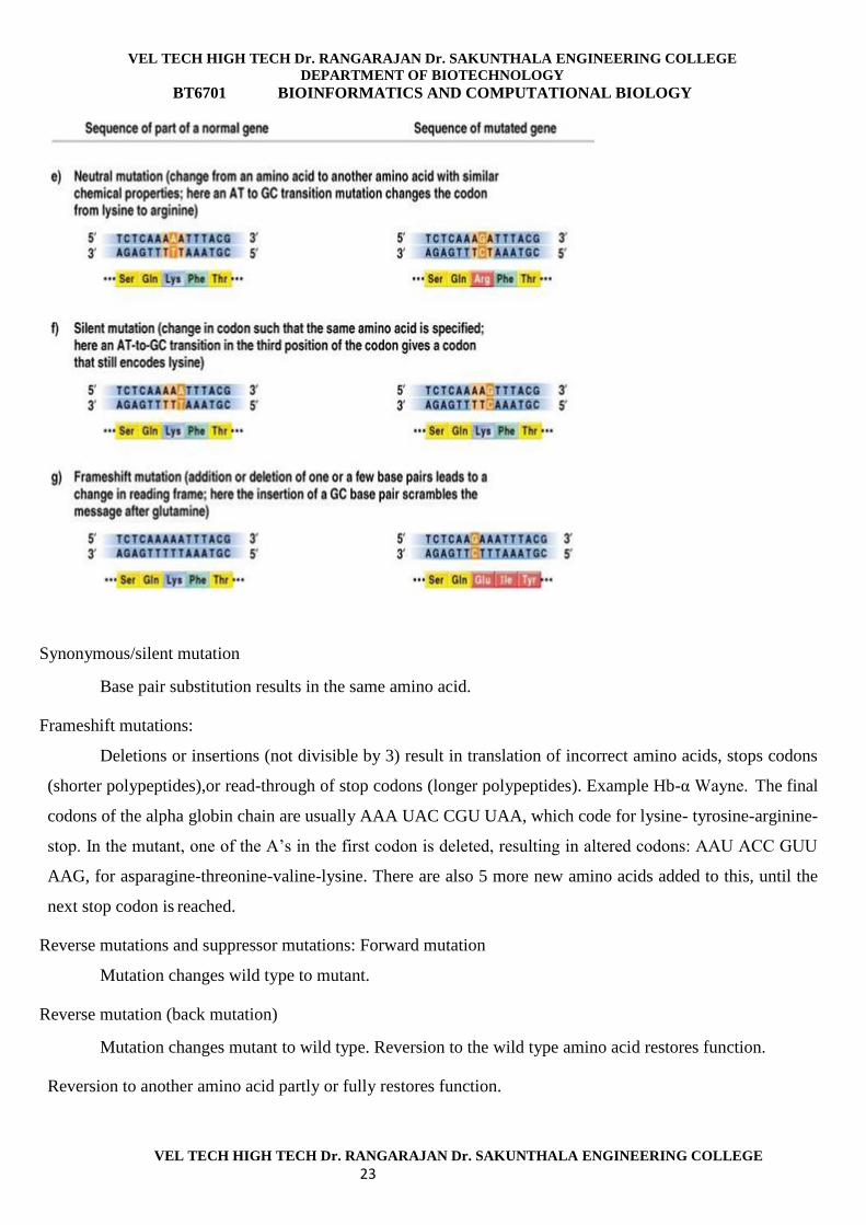
Neutral nonsynonymous mutation
Base pair substitution results in substitution of an amino acid with similar chemical properties (protein
function is not altered).
VEL TECH HIGH TECH Dr. RANGARAJAN Dr. SAKUNTHALA ENGINEERING COLLEGE
DEPARTMENT OF BIOTECHNOLOGY
BT6701 BIOINFORMATICS AND COMPUTATIONAL BIOLOGY
VEL TECH HIGH TECH Dr. RANGARAJAN Dr. SAKUNTHALA ENGINEERING COLLEGE
23
Synonymous/silent mutation
Base pair substitution results in the same amino acid.
Frameshift mutations:
Deletions or insertions (not divisible by 3) result in translation of incorrect amino acids, stops codons
(shorter polypeptides),or read-through of stop codons (longer polypeptides). Example Hb-α Wayne. The final
codons of the alpha globin chain are usually AAA UAC CGU UAA, which code for lysine- tyrosine-arginine-
stop. In the mutant, one of the A’s in the first codon is deleted, resulting in altered codons: AAU ACC GUU
AAG, for asparagine-threonine-valine-lysine. There are also 5 more new amino acids added to this, until the
next stop codon is reached.
Reverse mutations and suppressor mutations: Forward mutation
Mutation changes wild type to mutant.
Reverse mutation (back mutation)
Mutation changes mutant to wild type. Reversion to the wild type amino acid restores function.
Reversion to another amino acid partly or fully restores function.
VEL TECH HIGH TECH Dr. RANGARAJAN Dr. SAKUNTHALA ENGINEERING COLLEGE
DEPARTMENT OF BIOTECHNOLOGY
BT6701 BIOINFORMATICS AND COMPUTATIONAL BIOLOGY
VEL TECH HIGH TECH Dr. RANGARAJAN Dr. SAKUNTHALA ENGINEERING COLLEGE
24
Suppressor mutation
Occur at sites different from the original mutation and mask or compensate for the initial mutation
without reversing it.
• Intragenic suppressors occur on the same codon; e.g., nearby addition restores a deletion
• Intergenic suppressors occur on a different gene.
Spontaneous and induced mutations: Spontaneous mutations
Spontaneous mutations can occur at any point of the cell cycle. Movement of transposons (mobile
genetic elements; see chapter 20) causes spontaneous mutations. Mutation rate = ~10-4 to 10-6
mutations/gene/generation Rates vary by lineage, and many spontaneous errors are repaired. Different types of
spontaneous mutations include;
Wobble pairing
Insertions and Deletions
Deamination and Depurination (Mutations by spontaneous chemical changes)
Depurination
Common; A or G are removed and replaced with a random base.
VEL TECH HIGH TECH Dr. RANGARAJAN Dr. SAKUNTHALA ENGINEERING COLLEGE
DEPARTMENT OF BIOTECHNOLOGY
BT6701 BIOINFORMATICS AND COMPUTATIONAL BIOLOGY
VEL TECH HIGH TECH Dr. RANGARAJAN Dr. SAKUNTHALA ENGINEERING COLLEGE
25
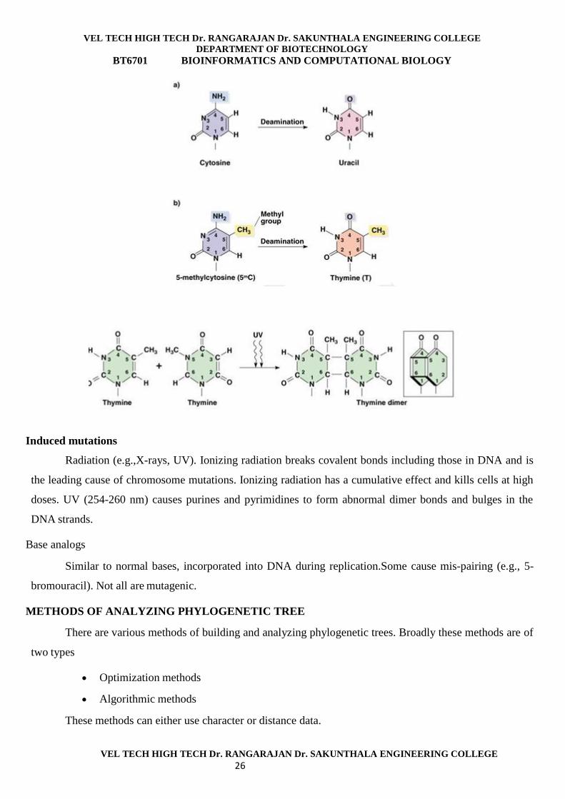
Deamination
Amino group is removed from a base (C
VEL TECH HIGH TECH Dr. RANGARAJAN Dr. SAKUNTHALA ENGINEERING COLLEGE
DEPARTMENT OF BIOTECHNOLOGY
BT6701 BIOINFORMATICS AND COMPUTATIONAL BIOLOGY
VEL TECH HIGH TECH Dr. RANGARAJAN Dr. SAKUNTHALA ENGINEERING COLLEGE
26
Induced mutations
Radiation (e.g.,X-rays, UV). Ionizing radiation breaks covalent bonds including those in DNA and is
the leading cause of chromosome mutations. Ionizing radiation has a cumulative effect and kills cells at high
doses. UV (254-260 nm) causes purines and pyrimidines to form abnormal dimer bonds and bulges in the
DNA strands.
Base analogs
Similar to normal bases, incorporated into DNA during replication.Some cause mis-pairing (e.g., 5-
bromouracil). Not all are mutagenic.
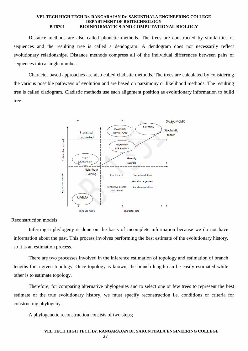
METHODS OF ANALYZING PHYLOGENETIC TREE
There are various methods of building and analyzing phylogenetic trees. Broadly these methods are of
two types
Optimization methods
Algorithmic methods
These methods can either use character or distance data.
VEL TECH HIGH TECH Dr. RANGARAJAN Dr. SAKUNTHALA ENGINEERING COLLEGE
DEPARTMENT OF BIOTECHNOLOGY
BT6701 BIOINFORMATICS AND COMPUTATIONAL BIOLOGY
VEL TECH HIGH TECH Dr. RANGARAJAN Dr. SAKUNTHALA ENGINEERING COLLEGE
27
Distance methods are also called phonetic methods. The trees are constructed by similarities of
sequences and the resulting tree is called a dendogram. A dendogram does not necessarily reflect
evolutionary relationships. Distance methods compress all of the individual differences between pairs of
sequences into a single number.
Character based approaches are also called cladistic methods. The trees are calculated by considering
the various possible pathways of evolution and are based on parsimony or likelihood methods. The resulting
tree is called cladogram. Cladistic methods use each alignment position as evolutionary information to build
tree.
Reconstruction models
Inferring a phylogeny is done on the basis of incomplete information because we do not have
information about the past. This process involves performing the best estimate of the evolutionary history,
so it is an estimation process.
There are two processes involved in the inference estimation of topology and estimation of branch
lengths for a given topology. Once topology is known, the branch length can be easily estimated while
other is to estimate topology.
Therefore, for comparing alternative phylogenies and to select one or few trees to represent the best
estimate of the true evolutionary history, we must specify reconstruction i.e. conditions or criteria for
constructing phylogeny.
A phylogenetic reconstruction consists of two steps;
VEL TECH HIGH TECH Dr. RANGARAJAN Dr. SAKUNTHALA ENGINEERING COLLEGE
DEPARTMENT OF BIOTECHNOLOGY
BT6701 BIOINFORMATICS AND COMPUTATIONAL BIOLOGY
VEL TECH HIGH TECH Dr. RANGARAJAN Dr. SAKUNTHALA ENGINEERING COLLEGE
28
1. Defining an optimally criterion or objective function
This step assigns a value to a tree and is subsequently used for comparing other trees.
2. Developing specific algorithms
These steps are used to develop an algorithm to compute the objective function values. This helps to
identify the tree or a set of trees that have the best values according to this criterion.
There are two approaches to phylogenetic reconstructions such as;
Evolutionary distance method
Character state method
Evolutionary distance method
In evolutionary distance method or distance matrix method, all possible pairs of sequences are aligned
to determine when pairs are the most similar or closely related. These alignments provide a measure of the
genetic distance between the sequences. These distance measurements are then used to predict the
evolutionary relationships.
There are various distance matrix algorithms such as
UPGMA
WPGMA
Neighbouring-joining
Fitch-Morgalish
UPGMA
The clustering procedure called UPGMA stands for Unweighted Pair Group Method using Arithmetic
averages. The method is simple and intuitively appealing. It works by clustering the sequences, at each stage
amalgamating two clusters and at the same time creating a new node on a tree. The tree can be imagined as
being assembled upwards, each node being added above the others, and the edge lengths being determined by
the difference in heights of the nodes at the top and bottom of the edge.
The distance between two clusters i and j is given by dij is the average distance between pairs of
sequences from each clusters.
UPGMA assumes that the rates of evolution are the same among different lineages
• In general, should not use this method for phylogenetic tree reconstruction (unless believe
assumption)
VEL TECH HIGH TECH Dr. RANGARAJAN Dr. SAKUNTHALA ENGINEERING COLLEGE
DEPARTMENT OF BIOTECHNOLOGY
BT6701 BIOINFORMATICS AND COMPUTATIONAL BIOLOGY
VEL TECH HIGH TECH Dr. RANGARAJAN Dr. SAKUNTHALA ENGINEERING COLLEGE
29
• Produces a rooted tree
WPGMA
Weighted Pair Group Method using Arithmetic mean, the clusters are weighted according to their
size. So that the candidate taxon K is equivalent in weighting to all previous taxa in the cluster.
Neighbour Joining (NJ)
NJ is a clustering method related to UPGMA that is able to solve problems similar to distance matrix
algorithms such as UPGMA. These algorithms are computationally fast and doesn’t make the assumption of
additivity. It begins by choosing the two most closely related sequences and then adding the next most distant
sequence as a third branch by the tree.
NJ Algorithm
Step 1: Let – (Almost) “average” distance to other nodes
Step 2: Choose i and j for which Mij – ui –uj is smallest
– Look for nodes that are close to each other, and far from everything else
– Turns out minimizing this is minimizing sum of branch lengths
Step 3: Define a new cluster (i, j), with a corresponding node in the tree
Distance from i and j to node (i,j):
di, (i,j) = 0.5(Mij + ui-uj)
dj, (i,j) = 0.5(Mij +uj-ui)
Step 4: Compute distance between new cluster and all other clusters:
M(ij)k = (Mik+Mjk – Mij)/2
Step 5: Delete i and j from matrix and replace by (i, j) Step
6: Continue until only 2 leaves remain Advantages
Fastest tree building method
Uses empirical substitution methods
Disadvantages
Tests only a single tree
VEL TECH HIGH TECH Dr. RANGARAJAN Dr. SAKUNTHALA ENGINEERING COLLEGE
DEPARTMENT OF BIOTECHNOLOGY
BT6701 BIOINFORMATICS AND COMPUTATIONAL BIOLOGY
VEL TECH HIGH TECH Dr. RANGARAJAN Dr. SAKUNTHALA ENGINEERING COLLEGE
30
Doesn’t consider intermediate
Distance matrices are derived in such a way that each mismatch between two sequences adds to the
distance, and each identity substracts from the distance. Scoring matrices include values for all possible
substitutions.
Transitions and tranversion substitution models are general time reversible models.
MOLECULAR CLOCK HYPOTHESIS
For any given macromolecule (a protein or DNA sequence) the rate of evolution is approximately
constant over time in all evolutionary lineages (Zuckerkandl and Pauling 1965 in Wen-Hsiung Li 1997).
Converts measures of genetic distance between sequences into estimates of the time at which the lineages
diverged (Welch and Bromham 2005).
Relevant mutations
Species differ in the characteristics, also called characters. These characters may be observable and
measurable for all the individuals. These characters are considered as properties. For examples, among
mammals, they can be classified based on a particular morphological character, or by a molecular character
(Gene duplication).
Any character can be used to classify species and reconstruct a phylogenetic tree. These characters are
mainly due to mutations. If a species depends on a character for its continued survival, that character will not
change as any mutations of it will be eliminated and such characters are considered essential. The differences
or similarities are essential characters are very relevant to the construction of the general shape of
phylogenetic tree, but they can’t be used to determine the relative lengths of lines within the tree.
Irrelevant mutations
Changes in non-essential characters are effected by mutations which are referred to as irrevalent. The
rate of change of irrevalent mutations should be uniform among species that are closely related. Eg. In case of
amino acids, there are 64 codons, so mutation in the third codon is almost considered as irrelevant. The DNA
can mutate at this stage/site and the resulting protein doesn’t change. Mutations as a measure of time
The probability p(t) that the character has some value at the beginning of a time interval of length t as
it does at the end. The probability q(t) that the character has one value at the beginning of a time interval of
length t but a different value at the end of the interval.
Suppose there are m different possible alternate values, and suppose that the mutation rate is r
mutations per unit time interval, then,
VEL TECH HIGH TECH Dr. RANGARAJAN Dr. SAKUNTHALA ENGINEERING COLLEGE
DEPARTMENT OF BIOTECHNOLOGY
BT6701 BIOINFORMATICS AND COMPUTATIONAL BIOLOGY
VEL TECH HIGH TECH Dr. RANGARAJAN Dr. SAKUNTHALA ENGINEERING COLLEGE
31
When t=0 p(0) = 1 (Mutation is there)
q(0) = 0 (As there is no mutation in no time)
When t approaches infinity p(t) and q(t) approaches 1/m, which literally means that in the long run,
each of the m alternative values are equally probable. Suppose there are n different characters, not just one.
Then the expected number of characters E(t) is given by
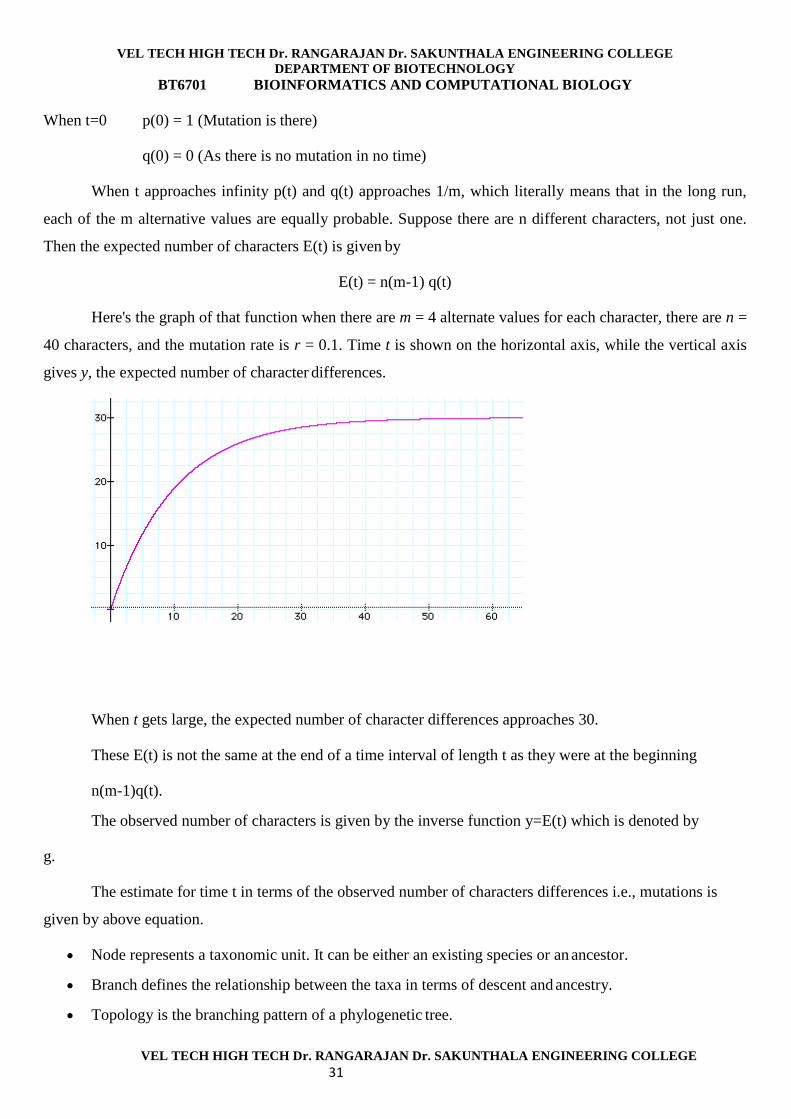
E(t) = n(m-1) q(t)
Here's the graph of that function when there are m = 4 alternate values for each character, there are n =
40 characters, and the mutation rate is r = 0.1. Time t is shown on the horizontal axis, while the vertical axis
gives y, the expected number of character differences.
When t gets large, the expected number of character differences approaches 30.
These E(t) is not the same at the end of a time interval of length t as they were at the beginning
n(m-1)q(t).
The observed number of characters is given by the inverse function y=E(t) which is denoted by
g.
The estimate for time t in terms of the observed number of characters differences i.e., mutations is
given by above equation.
Node represents a taxonomic unit. It can be either an existing species or an ancestor.
Branch defines the relationship between the taxa in terms of descent and ancestry.
Topology is the branching pattern of a phylogenetic tree.
VEL TECH HIGH TECH Dr. RANGARAJAN Dr. SAKUNTHALA ENGINEERING COLLEGE
DEPARTMENT OF BIOTECHNOLOGY
BT6701 BIOINFORMATICS AND COMPUTATIONAL BIOLOGY
VEL TECH HIGH TECH Dr. RANGARAJAN Dr. SAKUNTHALA ENGINEERING COLLEGE
32
Branch length is a very significant part of the phylogenetic tree. It represents the number of changes
that have occurred in a branch.
Distance scale is a scale chosen to represent the number of differences between organisms or
sequences.
Characters define the units upon which analysis is made. Eg. Amino acids, nucleotides etc.
Bootstrap is a method for assessing the statistical significance of a particular node on the phylogenetic
tree. It is arrived by randomly resampling subsets of the data.
Monophyl etic refers to a group of taxa that have a single origin on a tree i.e., all taxa descend from a
common ancestor.
Polyphyletic is a group of taxa that have multiple origins on a tree ie they arose twice in evolution.
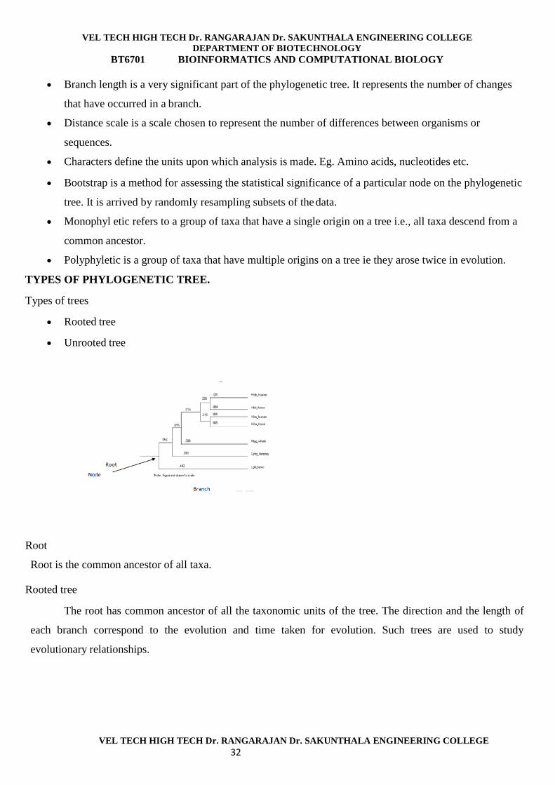
TYPES OF PHYLOGENETIC TREE.
Types of trees
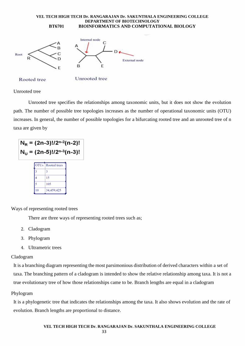
Rooted tree
Unrooted tree
Root
Root is the common ancestor of all taxa.
Rooted tree
The root has common ancestor of all the taxonomic units of the tree. The direction and the length of
each branch correspond to the evolution and time taken for evolution. Such trees are used to study
evolutionary relationships.
VEL TECH HIGH TECH Dr. RANGARAJAN Dr. SAKUNTHALA ENGINEERING COLLEGE
DEPARTMENT OF BIOTECHNOLOGY
BT6701 BIOINFORMATICS AND COMPUTATIONAL BIOLOGY
VEL TECH HIGH TECH Dr. RANGARAJAN Dr. SAKUNTHALA ENGINEERING COLLEGE
33
Unrooted tree
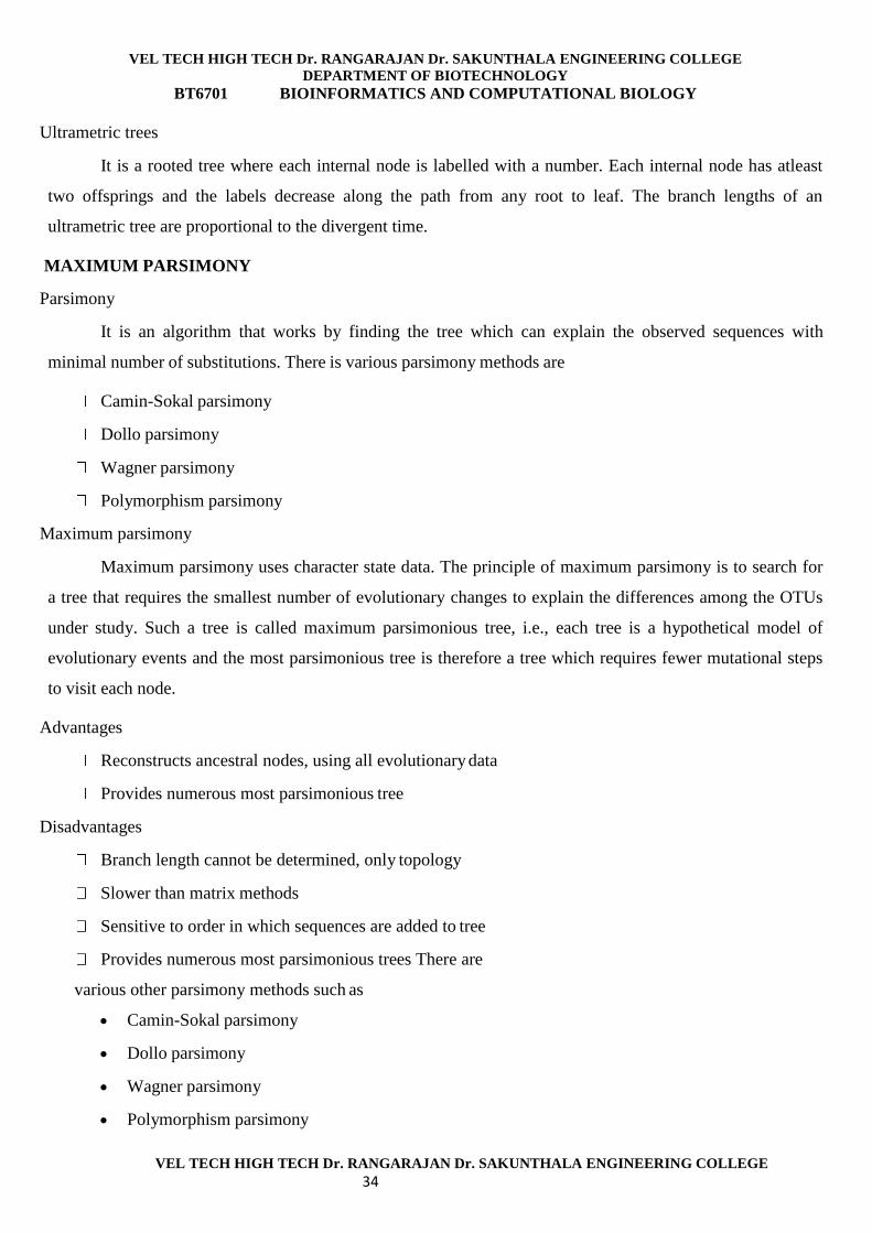
Unrooted tree specifies the relationships among taxonomic units, but it does not show the evolution
path. The number of possible tree topologies increases as the number of operational taxonomic units (OTU)
increases. In general, the number of possible topologies for a bifurcating rooted tree and an unrooted tree of n
taxa are given by
Ways of representing rooted trees
There are three ways of representing rooted trees such as;
2. Cladogram
3. Phylogram
4. Ultrametric trees
Cladogram
It is a branching diagram representing the most parsimonious distribution of derived characters within a set of
taxa. The branching pattern of a cladogram is intended to show the relative relationship among taxa. It is not a
true evolutionary tree of how those relationships came to be. Branch lengths are equal in a cladogram
Phylogram
It is a phylogenetic tree that indicates the relationships among the taxa. It also shows evolution and the rate of
evolution. Branch lengths are proportional to distance.
VEL TECH HIGH TECH Dr. RANGARAJAN Dr. SAKUNTHALA ENGINEERING COLLEGE
DEPARTMENT OF BIOTECHNOLOGY
BT6701 BIOINFORMATICS AND COMPUTATIONAL BIOLOGY
VEL TECH HIGH TECH Dr. RANGARAJAN Dr. SAKUNTHALA ENGINEERING COLLEGE
34
Ultrametric trees
It is a rooted tree where each internal node is labelled with a number. Each internal node has atleast
two offsprings and the labels decrease along the path from any root to leaf. The branch lengths of an
ultrametric tree are proportional to the divergent time.
MAXIMUM PARSIMONY
Parsimony
It is an algorithm that works by finding the tree which can explain the observed sequences with
minimal number of substitutions. There is various parsimony methods are
Camin-Sokal parsimony
Dollo parsimony
Wagner parsimony
Polymorphism parsimony
Maximum parsimony
Maximum parsimony uses character state data. The principle of maximum parsimony is to search for
a tree that requires the smallest number of evolutionary changes to explain the differences among the OTUs
under study. Such a tree is called maximum parsimonious tree, i.e., each tree is a hypothetical model of
evolutionary events and the most parsimonious tree is therefore a tree which requires fewer mutational steps
to visit each node.
Advantages
Reconstructs ancestral nodes, using all evolutionary data
Provides numerous most parsimonious tree
Disadvantages
Branch length cannot be determined, only topology
Slower than matrix methods
Sensitive to order in which sequences are added to tree
Provides numerous most parsimonious trees There are
various other parsimony methods such as
Camin-Sokal parsimony
Dollo parsimony
Wagner parsimony
Polymorphism parsimony
VEL TECH HIGH TECH Dr. RANGARAJAN Dr. SAKUNTHALA ENGINEERING COLLEGE
DEPARTMENT OF BIOTECHNOLOGY
BT6701 BIOINFORMATICS AND COMPUTATIONAL BIOLOGY
VEL TECH HIGH TECH Dr. RANGARAJAN Dr. SAKUNTHALA ENGINEERING COLLEGE
35
Felsenstein
Camin-Sokal parsimony
The main assumption of Camin-Sokal parsimony is that the ancestral state is defined as 0 i.e., at one
time an allele does not exist, and at a later time it does exist. Camin-sokal further assumes that loss of the
allele does not occur. It is therefore probably more appropriate for use with morphologic traits rather than
molecular marker data.
Dollo parsimony
Dollo parsimony assumes 0 as an ancestral state. It assumes that 1→0» 0→1, but that both are rare
over the evolutionary time scale being studied.
Wagner parsimony
Wagner parsimony assumes that ancestral states are unknown, and that roughly equal rates of
substitutions occur in either direction. This assumption is probably not valid for most molecular marker
methods. With marker data for both Wagner and Dollo parsimony tree should be compared. Branches
that are seen in both trees are likely to be robust, because they appear regardless of which set of assumptions
used.
Felsenstein
Felsenstein model is the one in which polymorphism can be retained in the population, thus
effectively allowing what looks like 0→1 if the 1 allele becomes fixed at some later time. In this model,
mutation from 1→0 is more likely than loss of an allele and the probability of 0→1 is essentially negligible.
Maximum likelihood
Maximum likelihood is a well established statistical method. The first application of this method to tree
construction was made by Cavall-Sforza and Edwards using gene frequency data. Later, Felsenstein
developed maximum likelihood for amino acid and nucleic acid sequence data.
In their simplest form, they begin by listing all possible models, and then calculating the probability
that each model would generate the data actually observed. The model with the highest probability of
generating the observed data is chosen as the best model.
Advantages
Reconstruct ancestral nodes, using all datas
Generates branch lengths
Generates statistical estimate of significance of each branch
Disadvantages
Very slow
Time required increases roughly with the fourth power of the number of sequences with small number
of sequences.
VEL TECH HIGH TECH Dr. RANGARAJAN Dr. SAKUNTHALA ENGINEERING COLLEGE
DEPARTMENT OF BIOTECHNOLOGY
BT6701 BIOINFORMATICS AND COMPUTATIONAL BIOLOGY
VEL TECH HIGH TECH Dr. RANGARAJAN Dr. SAKUNTHALA ENGINEERING COLLEGE
36
UNIT IV
HIDDEN MARKOV MODELS
A first order discrete HMM is a stochastic (randomly determined) generative model for time series
defined by a finite set of s of states, a discrete alphabet A of symbols, a probability transition matrix T= tij
and a probability emission matrix E = eix.
The system randomly evolves from state to state while emitting symbols from the alphabet. When the
system is in state i, it has the probability tij of moving from state i to state j and a probability eix of emitting
symbol X. Thus HMM can be visualized by imaging that two different dice are associated with each state;
An emission die
A transition die
The essential first order markov assumptions is that the emission and transition depends on the current
state only and not on the past. Only the symbols emitted by the system are observable, not the underlying
random walk between states; hence “hidden”. The random walks can be viewed as hidden or latent variables
underlying the observation.
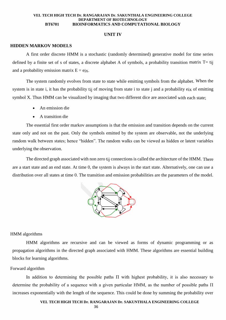
The directed graph associated with non zero tij connections is called the architecture of the HMM. There
are a start state and an end state. At time 0, the system is always in the start state. Alternatively, one can use a
distribution over all states at time 0. The transition and emission probabilities are the parameters of the model.
HMM algorithms
HMM algorithms are recursive and can be viewed as forms of dynamic programming or as
propagation algorithms in the directed graph associated with HMM. These algorithms are essential building
blocks for learning algorithms.
Forward algorithm
In addition to determining the possible paths П with highest probability, it is also necessary to
determine the probability of a sequence with a given particular HMM, as the number of possible paths П
increases exponentially with the length of the sequence. This could be done by summing the probability over
VEL TECH HIGH TECH Dr. RANGARAJAN Dr. SAKUNTHALA ENGINEERING COLLEGE
DEPARTMENT OF BIOTECHNOLOGY
BT6701 BIOINFORMATICS AND COMPUTATIONAL BIOLOGY
VEL TECH HIGH TECH Dr. RANGARAJAN Dr. SAKUNTHALA ENGINEERING COLLEGE
37
all the possible paths. This assumes path with significant probability П. The steps are similar to viterbi
algorithm, but we are replacing maximization steps with sums. This is called forward algorithm.
The quantity corresponding to viterbi algorithm Vk(i) in the forward algorithm is
fk(i)=P(x.....xi, Пi=k)
Which is the probability of the observed sequence upto and including xi (Пi=k). The recursion equation
is
fl (i+1) = el (xi+1) ∑ fk(i) akl
k
Viterbi algorithm
Viterbi algorithm is a dynamic programming algorithm used to find the most probable path through,
the HMM is calculated recursively. If Vk(i) is the probability of the most probable path ending in the state K
with observation I is known for all the states K, then for the next observation xi+1while in the state l
multiplied by the maximum over all the previous states K.
Vl(i+1)=el (xi+1) max [ Vk(i)akl]
k
HMM programs
HMMER
SAM
HMMPro
ProDoM
PROSITE
Interpro
NEURAL NETWORKS
It is claimed that the human central nervous system is comprised of about 1,3x10¹⁰ neurons and that
about 1x10¹⁰ of them takes place in the brain. At any time, some of these neurons are firing and the power
dissipation due this electrical activity is estimated to be in the order of 10 watts.
Monitoring the activity in the brain has shown that, even when asleep, 5x10⁷ nerve impulses per second are
being relayed back and forth between the brain and other parts of the body. This rate is increased significantly
when awake.
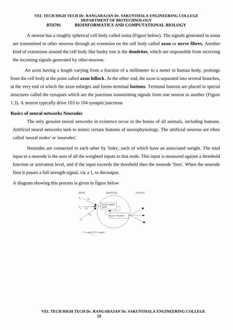
VEL TECH HIGH TECH Dr. RANGARAJAN Dr. SAKUNTHALA ENGINEERING COLLEGE
DEPARTMENT OF BIOTECHNOLOGY
BT6701 BIOINFORMATICS AND COMPUTATIONAL BIOLOGY
VEL TECH HIGH TECH Dr. RANGARAJAN Dr. SAKUNTHALA ENGINEERING COLLEGE
38
A neuron has a roughly spherical cell body called soma (Figure below). The signals generated in soma
are transmitted to other neurons through an extension on the cell body called axon or nerve fibres. Another
kind of extensions around the cell body like bushy tree is the dendrites, which are responsible from receiving
the incoming signals generated by other neurons.
An axon having a length varying from a fraction of a millimeter to a meter in human body, prolongs
from the cell body at the point called axon hillock. At the other end, the axon is separated into several branches,
at the very end of which the axon enlarges and forms terminal buttons. Terminal buttons are placed in special
structures called the synapses which are the junctions transmitting signals from one neuron to another (Figure
1.3). A neuron typically drive 103 to 104 synaptic junctions
Basics of neural networks Neurodes
The only genuine neural networks in existence occur in the brains of all animals, including humans.
Artificial neural networks seek to mimic certain features of neurophysiology. The artificial neurons are often
called 'neural nodes' or 'neurodes'.
Neurodes are connected to each other by 'links', each of which have an associated weight. The total
input to a neurode is the sum of all the weighted inputs to that node. This input is measured against a threshold
function or activation level, and if the input exceeds the threshold then the neurode 'fires'. When the neurode
fires it passes a full strength signal, viz a 1, to the output.
A diagram showing this process is given in figure below
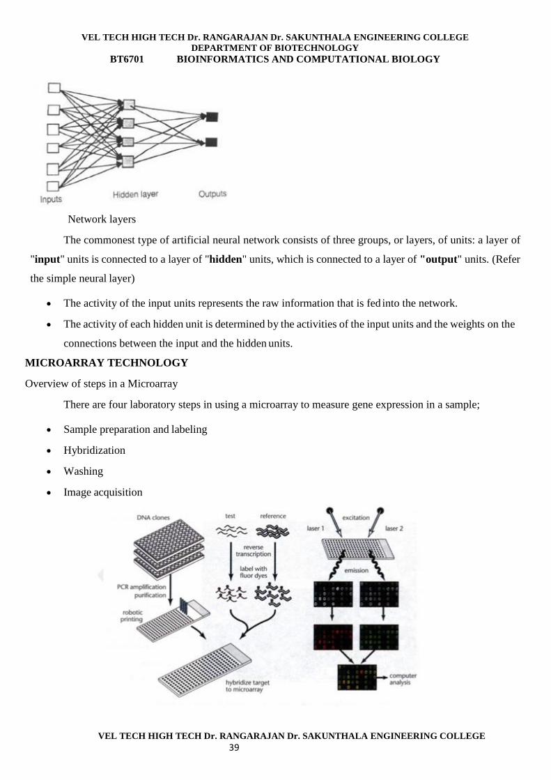
VEL TECH HIGH TECH Dr. RANGARAJAN Dr. SAKUNTHALA ENGINEERING COLLEGE
DEPARTMENT OF BIOTECHNOLOGY
BT6701 BIOINFORMATICS AND COMPUTATIONAL BIOLOGY
VEL TECH HIGH TECH Dr. RANGARAJAN Dr. SAKUNTHALA ENGINEERING COLLEGE
39
Network layers
The commonest type of artificial neural network consists of three groups, or layers, of units: a layer of
"input" units is connected to a layer of "hidden" units, which is connected to a layer of "output" units. (Refer
the simple neural layer)
The activity of the input units represents the raw information that is fed into the network.
The activity of each hidden unit is determined by the activities of the input units and the weights on the
connections between the input and the hidden units.
MICROARRAY TECHNOLOGY
Overview of steps in a Microarray
There are four laboratory steps in using a microarray to measure gene expression in a sample;
Sample preparation and labeling
Hybridization
Washing
Image acquisition
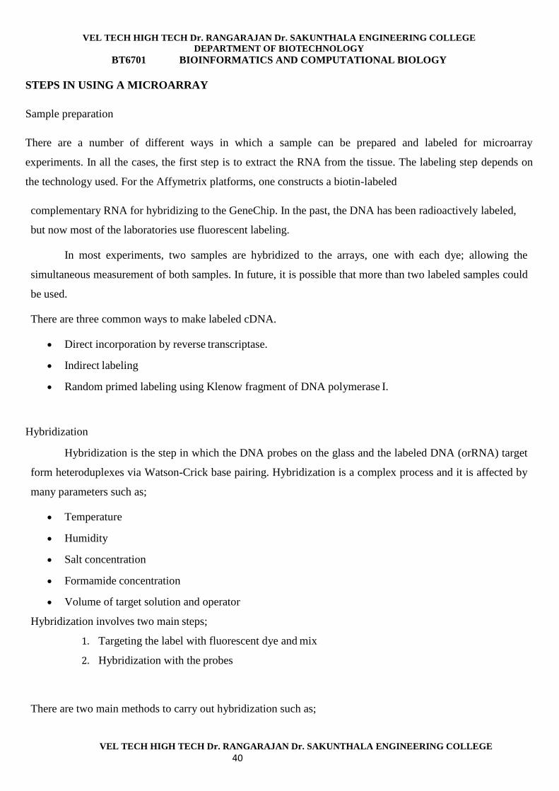
VEL TECH HIGH TECH Dr. RANGARAJAN Dr. SAKUNTHALA ENGINEERING COLLEGE
DEPARTMENT OF BIOTECHNOLOGY
BT6701 BIOINFORMATICS AND COMPUTATIONAL BIOLOGY
VEL TECH HIGH TECH Dr. RANGARAJAN Dr. SAKUNTHALA ENGINEERING COLLEGE
40
STEPS IN USING A MICROARRAY
Sample preparation
There are a number of different ways in which a sample can be prepared and labeled for microarray
experiments. In all the cases, the first step is to extract the RNA from the tissue. The labeling step depends on
the technology used. For the Affymetrix platforms, one constructs a biotin-labeled
complementary RNA for hybridizing to the GeneChip. In the past, the DNA has been radioactively labeled,
but now most of the laboratories use fluorescent labeling.
In most experiments, two samples are hybridized to the arrays, one with each dye; allowing the
simultaneous measurement of both samples. In future, it is possible that more than two labeled samples could
be used.
There are three common ways to make labeled cDNA.
Direct incorporation by reverse transcriptase.
Indirect labeling
Random primed labeling using Klenow fragment of DNA polymerase I.
Hybridization
Hybridization is the step in which the DNA probes on the glass and the labeled DNA (orRNA) target
form heteroduplexes via Watson-Crick base pairing. Hybridization is a complex process and it is affected by
many parameters such as;
Temperature
Humidity
Salt concentration
Formamide concentration
Volume of target solution and operator
Hybridization involves two main steps;
1. Targeting the label with fluorescent dye and mix
2. Hybridization with the probes
There are two main methods to carry out hybridization such as;
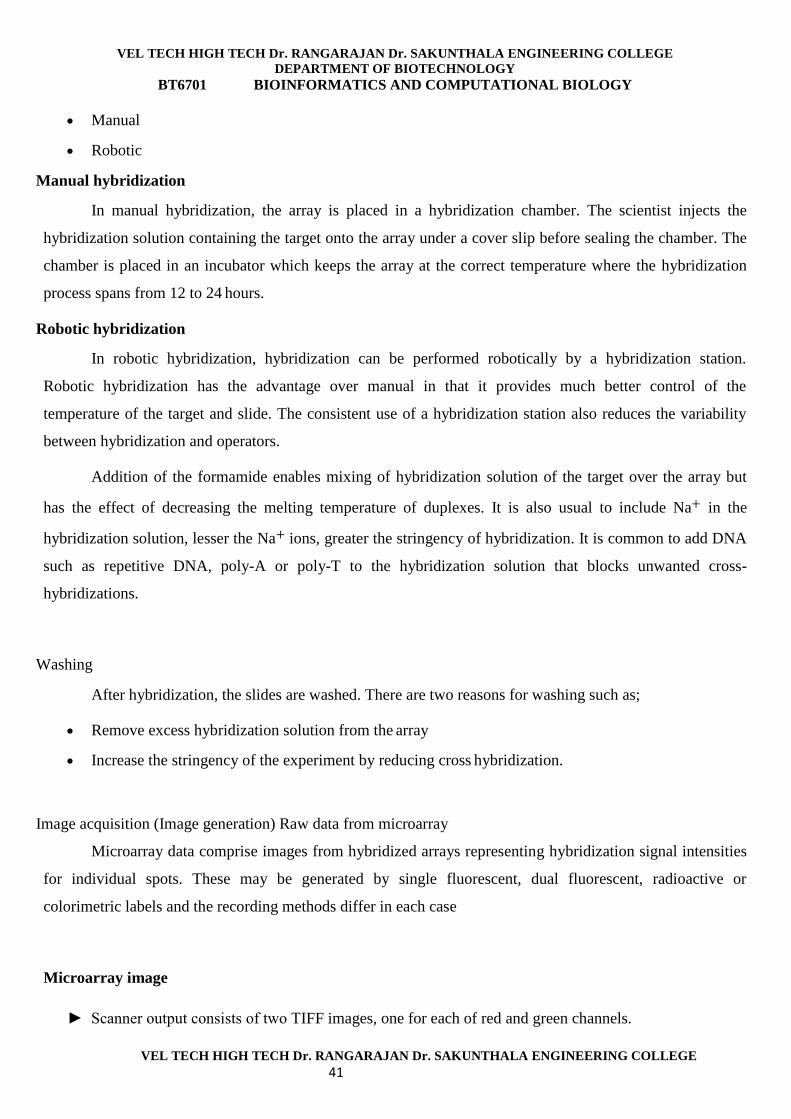
VEL TECH HIGH TECH Dr. RANGARAJAN Dr. SAKUNTHALA ENGINEERING COLLEGE
DEPARTMENT OF BIOTECHNOLOGY
BT6701 BIOINFORMATICS AND COMPUTATIONAL BIOLOGY
VEL TECH HIGH TECH Dr. RANGARAJAN Dr. SAKUNTHALA ENGINEERING COLLEGE
41
Manual
Robotic
Manual hybridization
In manual hybridization, the array is placed in a hybridization chamber. The scientist injects the
hybridization solution containing the target onto the array under a cover slip before sealing the chamber. The
chamber is placed in an incubator which keeps the array at the correct temperature where the hybridization
process spans from 12 to 24 hours.
Robotic hybridization
In robotic hybridization, hybridization can be performed robotically by a hybridization station.
Robotic hybridization has the advantage over manual in that it provides much better control of the
temperature of the target and slide. The consistent use of a hybridization station also reduces the variability
between hybridization and operators.
Addition of the formamide enables mixing of hybridization solution of the target over the array but
has the effect of decreasing the melting temperature of duplexes. It is also usual to include Na+ in the
hybridization solution, lesser the Na+ ions, greater the stringency of hybridization. It is common to add DNA
such as repetitive DNA, poly-A or poly-T to the hybridization solution that blocks unwanted cross-
hybridizations.
Washing
After hybridization, the slides are washed. There are two reasons for washing such as;
Remove excess hybridization solution from the array
Increase the stringency of the experiment by reducing cross hybridization.
Image acquisition (Image generation) Raw data from microarray
Microarray data comprise images from hybridized arrays representing hybridization signal intensities
for individual spots. These may be generated by single fluorescent, dual fluorescent, radioactive or
colorimetric labels and the recording methods differ in each case
Microarray image
► Scanner output consists of two TIFF images, one for each of red and green channels.
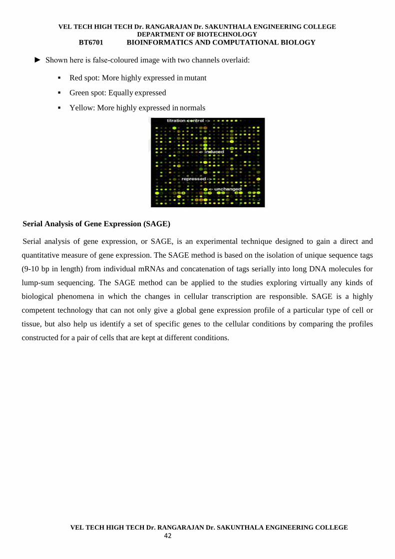
VEL TECH HIGH TECH Dr. RANGARAJAN Dr. SAKUNTHALA ENGINEERING COLLEGE
DEPARTMENT OF BIOTECHNOLOGY
BT6701 BIOINFORMATICS AND COMPUTATIONAL BIOLOGY
VEL TECH HIGH TECH Dr. RANGARAJAN Dr. SAKUNTHALA ENGINEERING COLLEGE
42
► Shown here is false-coloured image with two channels overlaid:
Red spot: More highly expressed in mutant
Green spot: Equally expressed
Yellow: More highly expressed in normals
Serial Analysis of Gene Expression (SAGE)
Serial analysis of gene expression, or SAGE, is an experimental technique designed to gain a direct and
quantitative measure of gene expression. The SAGE method is based on the isolation of unique sequence tags
(9-10 bp in length) from individual mRNAs and concatenation of tags serially into long DNA molecules for
lump-sum sequencing. The SAGE method can be applied to the studies exploring virtually any kinds of
biological phenomena in which the changes in cellular transcription are responsible. SAGE is a highly
competent technology that can not only give a global gene expression profile of a particular type of cell or
tissue, but also help us identify a set of specific genes to the cellular conditions by comparing the profiles
constructed for a pair of cells that are kept at different conditions.
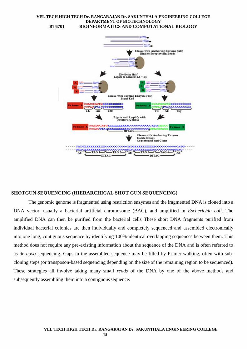
VEL TECH HIGH TECH Dr. RANGARAJAN Dr. SAKUNTHALA ENGINEERING COLLEGE
DEPARTMENT OF BIOTECHNOLOGY
BT6701 BIOINFORMATICS AND COMPUTATIONAL BIOLOGY
VEL TECH HIGH TECH Dr. RANGARAJAN Dr. SAKUNTHALA ENGINEERING COLLEGE
43
SHOTGUN SEQUENCING (HIERARCHICAL SHOT GUN SEQUENCING)
The genomic genome is fragmented using restriction enzymes and the fragmented DNA is cloned into a
DNA vector, usually a bacterial artificial chromosome (BAC), and amplified in Escherichia coli. The
amplified DNA can then be purified from the bacterial cells These short DNA fragments purified from
individual bacterial colonies are then individually and completely sequenced and assembled electronically
into one long, contiguous sequence by identifying 100%-identical overlapping sequences between them. This
method does not require any pre-existing information about the sequence of the DNA and is often referred to
as de novo sequencing. Gaps in the assembled sequence may be filled by Primer walking, often with sub-
cloning steps (or transposon-based sequencing depending on the size of the remaining region to be sequenced).
These strategies all involve taking many small reads of the DNA by one of the above methods and
subsequently assembling them into a contiguous sequence.
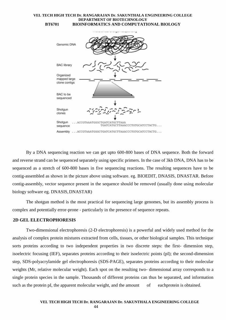
VEL TECH HIGH TECH Dr. RANGARAJAN Dr. SAKUNTHALA ENGINEERING COLLEGE
DEPARTMENT OF BIOTECHNOLOGY
BT6701 BIOINFORMATICS AND COMPUTATIONAL BIOLOGY
VEL TECH HIGH TECH Dr. RANGARAJAN Dr. SAKUNTHALA ENGINEERING COLLEGE
44
By a DNA sequencing reaction we can get upto 600-800 bases of DNA sequence. Both the forward
and reverse strand can be sequenced separately using specific primers. In the case of 3kb DNA, DNA has to be
sequenced as a stretch of 600-800 bases in five sequencing reactions. The resulting sequences have to be
contig-assembled as shown in the picture above using software. eg. BIOEDIT, DNASIS, DNASTAR. Before
contig-assembly, vector sequence present in the sequence should be removed (usually done using molecular
biology software eg. DNASIS, DNASTAR)
The shotgun method is the most practical for sequencing large genomes, but its assembly process is
complex and potentially error-prone - particularly in the presence of sequence repeats.
2D GEL ELECTROPHORESIS
Two-dimensional electrophoresis (2-D electrophoresis) is a powerful and widely used method for the
analysis of complex protein mixtures extracted from cells, tissues, or other biological samples. This technique
sorts proteins according to two independent properties in two discrete steps: the first- dimension step,
isoelectric focusing (IEF), separates proteins according to their isoelectric points (pI); the second-dimension
step, SDS-polyacrylamide gel electrophoresis (SDS-PAGE), separates proteins according to their molecular
weights (Mr, relative molecular weight). Each spot on the resulting two- dimensional array corresponds to a
single protein species in the sample. Thousands of different proteins can thus be separated, and information
such as the protein pI, the apparent molecular weight, and the amount of eachprotein is obtained.
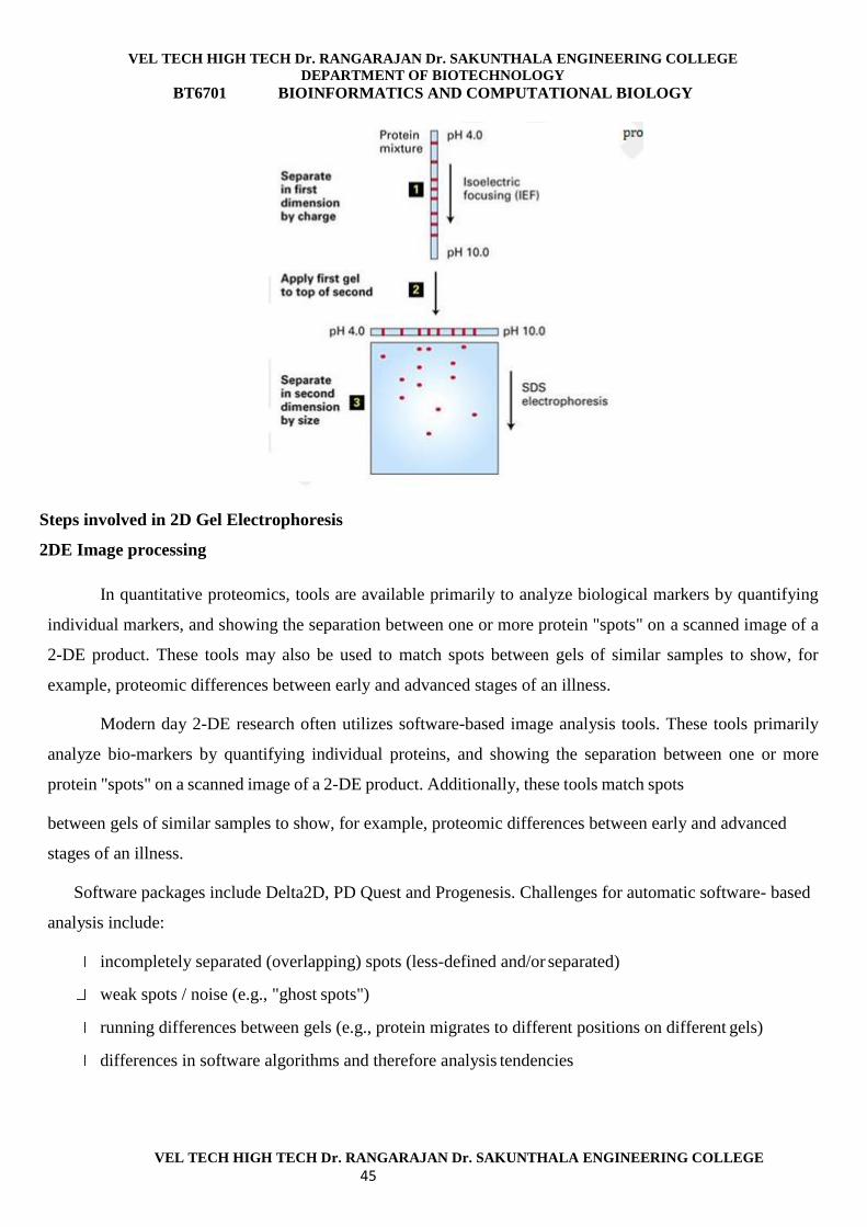
VEL TECH HIGH TECH Dr. RANGARAJAN Dr. SAKUNTHALA ENGINEERING COLLEGE
DEPARTMENT OF BIOTECHNOLOGY
BT6701 BIOINFORMATICS AND COMPUTATIONAL BIOLOGY
VEL TECH HIGH TECH Dr. RANGARAJAN Dr. SAKUNTHALA ENGINEERING COLLEGE
45
Steps involved in 2D Gel Electrophoresis
2DE Image processing
In quantitative proteomics, tools are available primarily to analyze biological markers by quantifying
individual markers, and showing the separation between one or more protein "spots" on a scanned image of a
2-DE product. These tools may also be used to match spots between gels of similar samples to show, for
example, proteomic differences between early and advanced stages of an illness.
Modern day 2-DE research often utilizes software-based image analysis tools. These tools primarily
analyze bio-markers by quantifying individual proteins, and showing the separation between one or more
protein "spots" on a scanned image of a 2-DE product. Additionally, these tools match spots
between gels of similar samples to show, for example, proteomic differences between early and advanced
stages of an illness.
Software packages include Delta2D, PD Quest and Progenesis. Challenges for automatic software- based
analysis include:
incompletely separated (overlapping) spots (less-defined and/or separated)
weak spots / noise (e.g., "ghost spots")
running differences between gels (e.g., protein migrates to different positions on different gels)
differences in software algorithms and therefore analysis tendencies

VEL TECH HIGH TECH Dr. RANGARAJAN Dr. SAKUNTHALA ENGINEERING COLLEGE
DEPARTMENT OF BIOTECHNOLOGY
BT6701 BIOINFORMATICS AND COMPUTATIONAL BIOLOGY
VEL TECH HIGH TECH Dr. RANGARAJAN Dr. SAKUNTHALA ENGINEERING COLLEGE
46
Modern software packages include advanced features, such as image warping, to try to compensate for
running differences between gels, and the generation of picking lists for the automated in-gel digestion of
protein spots, leading to the identification of the proteins by mass spectrometry. However, as noted above, 2-
DE automated image analysis technology has not been perfected - a fact which keeps manual visual analysis
as the "gold standard" for validation.
Advantages and disadvantages of 2D-PAGE.
The main advantage of using 2D-PAGE is the large mass range and the sheer amount of proteins that
can be analysed at any one time. 2D-PAGE is particularly good for looking at proteins within the mass range
of 20 - 250 kDa and pI of 3 - 11. Proteins of particular pI and mass, can be focused on by using narrow range
pH isoelectric focusing strips and the percentage of acrylamide used in the 2nd dimension PAGE gel,
respectively. If sufficient sample is present on the gel (>300 µg of total protein) then proteins can be excised
from the gel, subjected to in-gel proteolysis and analysed by mass spectrometry.
VEL TECH HIGH TECH Dr. RANGARAJAN Dr. SAKUNTHALA ENGINEERING COLLEGE
DEPARTMENT OF BIOTECHNOLOGY
BT6701 BIOINFORMATICS AND COMPUTATIONAL BIOLOGY
VEL TECH HIGH TECH Dr. RANGARAJAN Dr. SAKUNTHALA ENGINEERING COLLEGE
47
UNIT V
PERL
Perl is a high-level, general-purpose, interpreted, dynamic programming language. Perl was originally
developed by Larry Wall in 1987 as a general-purpose Unix scripting language to make report processing
easier. Since then, it has undergone many changes and revisions and become widely popular amongst
programmers. Larry Wall continues to oversee development of the core language. Perl borrows features from
other programming languages including C, shell scripting (sh), AWK, and sed. The language provides powerful
text processing facilities without the arbitrary data length limits of many contemporary Unix tools, facilitating
easy manipulation of text files. Perl gained widespread popularity in the late 1990s as a CGI scripting language,
in part due to its parsing abilities.
CREATING THE PROGRAM
A Perl program consists of an ordinary text file containing a series of Perl statements. Statements are written in
what looks like an amalgam of C, UNIX shell script, and English. In fact, that's pretty much what it is.
Perl code can be quite free-flowing. The broad syntactic rules governing where a statement starts and ends are
• Leading spaces on a line are ignored. You can start a Perl statement anywhere you want: at the
beginning of the line, indented for clarity (recommended) or even right-justified (definitely frowned on because
the code would be difficult to understand) if you like.
• Statements are terminated with a semicolon.
• Spaces, tabs, and blank lines outside of strings are irrelevant-one space is as good as a hundred. That
means you can split statements over several lines for clarity. A string is basically a series of characters enclosed
in quotes.
• Here's Our first uninspired Perl statement hello1.pl: print("Hello World\n");
NUMERIC AND STRING LITERALS
All computer programs use data in some way. Some use it to personalize the program. For example, a mail
program might need to remember your name so that it can greet you upon starting. Another program-say one
that searches your hard disk for files-might remember your last search parameters in case you want to perform
the same search twice. Perl uses four types of literals. Here is a quick glimpse at them:
VEL TECH HIGH TECH Dr. RANGARAJAN Dr. SAKUNTHALA ENGINEERING COLLEGE
DEPARTMENT OF BIOTECHNOLOGY
BT6701 BIOINFORMATICS AND COMPUTATIONAL BIOLOGY
VEL TECH HIGH TECH Dr. RANGARAJAN Dr. SAKUNTHALA ENGINEERING COLLEGE
48
• Numbers - This is the most basic data type.
• Strings - A string is a series of characters that are handled as one unit.
• Arrays - An array is a series of numbers and strings handled as a unit. You can also think of an array as a
list.
• Associative Arrays - This is the most complicated data type. Think of it as a list in which every value
has an associated lookup item.
NUMERIC LITERALS
Numeric literals are frequently used. They represent a number that your program will need to work with. Most
of the time you will use numbers in base ten-the base that everyone uses. However, Perl will also let you use
base 8 (octal) or base 16 (hexadecimal).
Note: For those of you who are not familiar with non-decimal numbering systems, here is a short explanation.
In decimal notation-or base ten- when you see the value 15 it signifies (1 *
10) + 5 or 1510. The subscript indicates which base is being used.
In octal notation-or base eight-when you see the value 15 it signifies (1 * 8) + 5 or 1310.
In hexadecimal notation-or base 16-when you see the value 15 it signifies (1 * 16) + 5 or 2110. Base 16 needs
an extra six characters in addition to 0 to 9 so that each position can have a total of 16 values. The letters A-F
are used to represent 11-16. So the value BD16 is equal to (B16 * 16) + D16 or (1110 * 16) + 1310 which is
17610.Perl is the Swiss Army chainsaw of programming languages: powerful and adaptable. It was first
developed by Larry Wall, a linguist working as a systems administrator for NASA in the late 1980s, as a way to
make report processing easier. Since then, it has moved into a several other areas: automating system
administration, acting as glue between different computer systems, web programming, bioinformatics, data
munging, and even application development.
Why did Perl become so popular when the Web came along? Two reasons: First, most of what is being done on
the Web happens with text, and is best done with a language that's designed for text processing. More
importantly, Perl was appreciably better than the alternatives at the time when people needed something to use.
C is complex and can produce security problems (especially with untrusted data), Tcl can be awkward, and
Python didn't really have a foothold.
VEL TECH HIGH TECH Dr. RANGARAJAN Dr. SAKUNTHALA ENGINEERING COLLEGE
DEPARTMENT OF BIOTECHNOLOGY
BT6701 BIOINFORMATICS AND COMPUTATIONAL BIOLOGY
VEL TECH HIGH TECH Dr. RANGARAJAN Dr. SAKUNTHALA ENGINEERING COLLEGE
49
It also didn't hurt that Perl is a friendly language. It plays well with your personal programming style. The Perl
slogan is "There's more than one way to do it," and that lends itself well to large and small problems alike. Even
more so, Perl is very portable and widespread -- it's available pre-installed almost everywhere -- and of course
there are thousands of freely-distributable libraries available from the CPAN.
In this first part of our series, you'll learn a few basics about Perl and see a small sample program.
A Word About Operating Systems
This series assumes that you're using a Unix or Unix-like operating system (Mac OS X and Cygwin qualify)
and that you have the perl binary available at /usr/bin/perl. It's OK if you're running Windows through
ActivePerl or Strawberry Perl; most Perl code is platform-independent.
Functions and Statements
Perl has a rich library of built-in functions. They're the verbs of Perl, the commands that the interpreter runs.
You can see a list of all the built-in functions in the perlfunc man page (perldoc perlfunc, from the command
line). Almost all functions can take a list of commma-separated parameters.
The print function is one of the most frequently used parts of Perl. You use it to display things on the screen or
to send information to a file. It takes a list of things to output as its parameters.
print "This is a single statement.";
print "Look, ", "a ", "list!";
A Perl program consists of statements, each of which ends with a semicolon. Statements don't need to be on
separate lines; there may be multiple statements on one line. You can also split a single statement across
multiple lines.
print "This is "; print "two statements.\n";
print "But this ", "is only one statement.\n";
Wait a minute though. What's the difference between say and print? What's this \n in the print statements?
The say function behaves just like the print function, except that it appends a newline at the end of its
arguments. It prints all of its arguments, and then a newline character. Always. No exceptions. print, on the
VEL TECH HIGH TECH Dr. RANGARAJAN Dr. SAKUNTHALA ENGINEERING COLLEGE
DEPARTMENT OF BIOTECHNOLOGY
BT6701 BIOINFORMATICS AND COMPUTATIONAL BIOLOGY
VEL TECH HIGH TECH Dr. RANGARAJAN Dr. SAKUNTHALA ENGINEERING COLLEGE
50
other hand, only prints what you see explicitly in these examples. If you want a newline, you have to add it
yourself with the special character escape sequence \n.
use feature ':5.10';
say "This is a single statement.";
say "Look, ", "a ", "list!";
Why do both exist? Why would you use one over the other? Usually, most "display something" statements need
the newline. It's common enough that say is a good default choice. Occasionally you need a little bit more
control over your output, so print is the option.
Note that say is two characters shorter than print. This is an important design principle for Perl -- common
things should be easy and simple
Table Perl Escape Sequences
Escape Sequences Description or Character
\b Backspace
\e Escape
\f Form Feed
\n Newline
\r Carriage Return
\t Tab
\v Vertical Tab
\$ Dollar Sign
\@ Ampersand
\0nnn Any Octal byte
\xnn Any Hexadecimal byte
\cn Any Control character
\l Change the next character to lowercase
VEL TECH HIGH TECH Dr. RANGARAJAN Dr. SAKUNTHALA ENGINEERING COLLEGE
DEPARTMENT OF BIOTECHNOLOGY
BT6701 BIOINFORMATICS AND COMPUTATIONAL BIOLOGY
VEL TECH HIGH TECH Dr. RANGARAJAN Dr. SAKUNTHALA ENGINEERING COLLEGE
51
\u Change the next character to uppercase
\L Change the following characters to
lowercase until a \E
sequence is encountered.
Note that you need to use an
uppercase E here, lowercase
will not work.
\Q Quote meta-characters as literals.
\U Change the following characters
to uppercase until a \E
sequence is encountered. Note that you
need to use an uppercase E
here, lowercase will not work.
\E Terminate the \L, \Q,
or \U sequence.
Variables
If functions are Perl's verbs, then variables are its nouns. Perl has three types of variables: scalars, arrays, and
hashes. Think of them as things, lists, and dictionaries respectively. In Perl, all variable names consist of a
punctuation character, a letter or underscore, and one or more alphanumeric characters or underscores.
Scalars are single things. This might be a number or a string. The name of a scalar begins with a dollar sign,
such as $i or $abacus. Assign a value to a scalar by telling Perl what it equals:
my $i = 5;
my $pie_flavor = 'apple';
my $constitution1776 = "We the People, etc.";
You don't need to specify whether a scalar is a number or a string. It doesn't matter, because when Perl needs to
treat a scalar as a string, it does; when it needs to treat it as a number, it does. The conversion happens
automatically. (This is different from many other languages, where strings and numbers are two separate data
types.)
VEL TECH HIGH TECH Dr. RANGARAJAN Dr. SAKUNTHALA ENGINEERING COLLEGE
DEPARTMENT OF BIOTECHNOLOGY
BT6701 BIOINFORMATICS AND COMPUTATIONAL BIOLOGY
VEL TECH HIGH TECH Dr. RANGARAJAN Dr. SAKUNTHALA ENGINEERING COLLEGE
52
If you use a double-quoted string, Perl will insert the value of any scalar variables you name in the string. This
is often useful to fill in strings on the fly:
use feature ':5.10';
my $apple_count = 5;
my $count_report = "There are $apple_count apples.";
say "The report is: $count_report";
The final output from this code is The report is: There are 5 apples..
You can manipulate numbers in Perl with the usual mathematical operations: addition, multiplication, division,
and subtraction. (The multiplication and division operators in Perl use the * and / symbols, by the way.)
my $a = 5;
my $b = $a + 10; # $b is now equal to 15.
my $c = $b * 10; # $c is now equal to 150.
$a = $a - 1; # $a is now 4, and algebra teachers are cringing.
That's all well and good, but what's this strange my, and why does it appear with some assignments and not
others? The my operator tells Perl that you're declaring a new variable. That is, you promise Perl that you
deliberately want to use a scalar, array, or hash of a specific name in your program. This is important for two
reasons. First, it helps Perl help you protect against typos; it's embarrassing to discover that you've accidentally
mistyped a variable name and spent an hour looking for a bug. Second, it helps you write larger programs,
where variables used in one part of the code don't accidentally affect variables used elsewhere.
You can also use special operators like ++, --, +=, -=, /= and *=. These manipulate a scalar's value without
needing two elements in an equation. Some people like them, some don't. I like the fact that they can make code
clearer.
my $a = 5;
$a++; # $a is now 6; we added 1 to it.
$a += 10; # Now it's 16; we added 10.
$a /= 2; # And divided it by 2, so it's 8.
VEL TECH HIGH TECH Dr. RANGARAJAN Dr. SAKUNTHALA ENGINEERING COLLEGE
DEPARTMENT OF BIOTECHNOLOGY
BT6701 BIOINFORMATICS AND COMPUTATIONAL BIOLOGY
VEL TECH HIGH TECH Dr. RANGARAJAN Dr. SAKUNTHALA ENGINEERING COLLEGE
53
Strings in Perl don't have quite as much flexibility. About the only basic operator that you can use on strings is
concatenation, which is a ten dollar way of saying "put together." The concatenation operator is the period.
Concatenation and addition are two different things:
my $a = "8"; # Note the quotes. $a is a string.
my $b = $a + "1"; # "1" is a string too.
my $c = $a . "1"; # But $b and $c have different values!
Remember that Perl converts strings to numbers transparently whenever necessary, so to get the value of $b, the
Perl interpreter converted the two strings "8" and "1" to numbers, then added them. The value of $b is the
number 9. However, $c used concatenation, so its value is the string "81".
Remember, the plus sign adds numbers and the period puts strings together. If you add things that aren't
numbers, Perl will try its best to do what you've told it to do, and will convert those non-numbers to numbers
with the best of its ability.
Arrays are lists of scalars. Array names begin with @. You define arrays by listing their contents in parentheses,
separated by commas:
my @lotto_numbers = (1, 2, 3, 4, 5, 6); # Hey, it could happen.
my @months = ("July", "August", "September");
You retrieve the contents of an array by an index, sort of like "Hey, give me the first month of the year."
Indexes in Perl start from zero. (Why not 1? Because. It's a computer thing.) To retrieve the elements of an
array, you replace the @ sign with a $ sign, and follow that with the index position of the element you want. (It
begins with a dollar sign because you're getting a scalar value.) You can also modify it in place, just like any
other scalar.
use feature ':5.10';
my @months = ("July", "August", "September");
say $months[0]; # This prints "July".
$months[2] = "Smarch"; # We just renamed September!
If an array value doesn't exist, Perl will create it for you when you assign to it.
my @winter_months = ("December", "January");
VEL TECH HIGH TECH Dr. RANGARAJAN Dr. SAKUNTHALA ENGINEERING COLLEGE
DEPARTMENT OF BIOTECHNOLOGY
BT6701 BIOINFORMATICS AND COMPUTATIONAL BIOLOGY
VEL TECH HIGH TECH Dr. RANGARAJAN Dr. SAKUNTHALA ENGINEERING COLLEGE
54
$winter_months[2] = "February";
Arrays always return their contents in the same order; if you go through @months from beginning to end, no
matter how many times you do it, you'll get back July, August, and September in that order. If you want to find
the number of elements of an array, assign the array to a scalar.
use feature ':5.10';
my @months = ("July", "August", "September");
my $month_count = @months;
say $month_count; # This prints 3.
my @autumn_months; # no elements
my $autumn_count = @autumn_months;
say $autumn_count; # this prints 0
Some programming languages call hashes "dictionaries". That's what they are: a term and a definition. More
precisely, they contain keys and values. Each key in a hash has one and only one corresponding value. The
name of a hash begins with a percentage sign, like %parents. You define hashes by comma-separated pairs of
key and value, like so:
my %days_in_month = ( "July" => 31, "August" => 31, "September" => 30 );
You can fetch any value from a hash by referring to $hashname{key}, or modify it in place just like any other
scalar.
say $days_in_month{September}; # 30, of course.
$days_in_month{February} = 29; # It's a leap year.
To see what keys are in a hash, use the keys function with the name of the hash. This returns a list containing all
of the keys in the hash. The list isn't always in the same order, though; while you can count on @months always
to return July, August, September in that order, keys %days_in_month might return them in any order
whatsoever.
my @month_list = keys %days_in_month;
# @month_list is now ('July', 'September', 'August', 'February')!
VEL TECH HIGH TECH Dr. RANGARAJAN Dr. SAKUNTHALA ENGINEERING COLLEGE
DEPARTMENT OF BIOTECHNOLOGY
BT6701 BIOINFORMATICS AND COMPUTATIONAL BIOLOGY
VEL TECH HIGH TECH Dr. RANGARAJAN Dr. SAKUNTHALA ENGINEERING COLLEGE
55
The three types of variables have three separate namespaces. That means that $abacus and @abacus are two
different variables, and $abacus[0] (the first element of @abacus) is not the same as $abacus{0} (the value in
%abacus that has the key 0).
Comments
Some of the code samples from the previous section contained code comments. These are useful for explaining
what a particular piece of code does, and vital for any piece of code you plan to modify, enhance, fix, or just
look at again. (That is to say, comments are important.)
Anything in a line of Perl code that follows a # sign is a comment, unless that # sign appears in a string.)
use feature ':5.10';
say "Hello world!"; # That's more like it.
# This entire line is a comment.
Loops
Almost every program ever written uses a loop of some kind. Loops allow you run a particular piece of code
over and over again. This is part of a general concept in programming called flow control.
Perl has several different functions that are useful for flow control, the most basic of which is for. When you use
the for function, you specify a variable to use as the loop index, and a list of values to loop over. Inside a pair of
curly brackets, you put any code you want to run during the loop:
use feature ':5.10';
for my $i (1, 2, 3, 4, 5) {
say $i;
}
This loop prints the numbers 1 through 5, each on a separate line. (It's not very useful; you're might think "Why
not just write say 1, 2, 3, 4, 5;?". This is because say adds only one newline, at the end of its list of arguments.)
A handy shortcut for defining loop values is the range operator .., which specifies a range of numbers. You can
write (1, 2, 3, 4, 5) as (1 .. 5) instead. You can also use arrays and scalars in your loop list. Try this code and see
what happens:
VEL TECH HIGH TECH Dr. RANGARAJAN Dr. SAKUNTHALA ENGINEERING COLLEGE
DEPARTMENT OF BIOTECHNOLOGY
BT6701 BIOINFORMATICS AND COMPUTATIONAL BIOLOGY
VEL TECH HIGH TECH Dr. RANGARAJAN Dr. SAKUNTHALA ENGINEERING COLLEGE
56
use feature ':5.10';
my @one_to_ten = (1 .. 10);
my $top_limit = 25;
for my $i (@one_to_ten, 15, 20 .. $top_limit) {
say $i;
}
Of course, again you could write say @one_to_ten, 15, 20 .. $top_limit;
The items in your loop list don't have to be numbers; you can use strings just as easily. If the hash %month_has
contains names of months and the number of days in each month, you can use the keys function to step through
them.
use feature ':5.10';
for my $i (keys %month_has) {
say "$i has $month_has{$i} days.";
}
for my $marx ('Groucho', 'Harpo', 'Zeppo', 'Karl') {
say "$marx is my favorite Marx brother.";
}
The Miracle of Compound Interest
You now know enough about Perl -- variables, print/say, and for() -- to write a small, useful program. Everyone
loves money, so the first sample program is a compound-interest calculator. It will print a (somewhat) nicely
formatted table showing the value of an investment over a number of years. (You can see the program at
compound_interest.pl)
The single most complex line in the program is:
my $interest = int( ( $apr / 100 ) * $nest_egg * 100 ) / 100;
VEL TECH HIGH TECH Dr. RANGARAJAN Dr. SAKUNTHALA ENGINEERING COLLEGE
DEPARTMENT OF BIOTECHNOLOGY
BT6701 BIOINFORMATICS AND COMPUTATIONAL BIOLOGY
VEL TECH HIGH TECH Dr. RANGARAJAN Dr. SAKUNTHALA ENGINEERING COLLEGE
57
$apr / 100 is the interest rate, and ($apr / 100) * $nest_egg is the amount of interest earned in one year. This line
uses the int() function, which returns the integer value of a scalar (its value after any stripping off any fractional
part). We use int() here because when you multiply, for example, 10925 by 9.25%, the result is 1010.5625,
which we must round off to 1010.56. To do this, we multiply by 100, yielding 101056.25, use int() to throw
away the leftover fraction, yielding 101056, and then divide by 100 again, so that the final result is 1010.56. Try
stepping through this statement yourself to see just how we end up with the correct result, rounded to cents.
Play Around!
At this point you have some basic knowledge of Perl syntax and a few simple toys to play with. Try writing
some simple programs with them. Here are two suggestions, one simple and the other a little more complex:
A word frequency counter. How often does each word show up in an array of words? Print out a report.
(Hint: Use a hash to count of the number of appearances of each word.)
Given a month and the day of the week that's the first of that month, print a calendar for the month.
Shell script
A shell script is just a text file containing a sequence of shell commands Example
$ cat testscript
#!/bin/sh
echo Here is a long listing of the current directory ls -l
Scalar data
A single number or string, depending on context
References to scalars always begin with $
Variable names may contain characters, numbers and underscores
Assignment is done using the = operator
Examples:
o $pi = 3.14159;
o $color = ’red’;
VEL TECH HIGH TECH Dr. RANGARAJAN Dr. SAKUNTHALA ENGINEERING COLLEGE
DEPARTMENT OF BIOTECHNOLOGY
BT6701 BIOINFORMATICS AND COMPUTATIONAL BIOLOGY
VEL TECH HIGH TECH Dr. RANGARAJAN Dr. SAKUNTHALA ENGINEERING COLLEGE
58
o $old_color = ”was $color before”;
o $host = `hostname`; # command substitution #
Strings
Sequences of characters
• No end of string character as in C
• Single-quoted (note: ’, not ̀ )
• Example
o $x = ”dog”; print ’bob $x’; # displays bob $x
What are arrays or ordered lists?
Arrays or Ordered lists of scalar data items, indexed by an integer, variable starts with a @. There is a
separate namespace for scalar and array variables. Arrays are subscripted using square brackets, where
indexing begins at 0. The (scalar) variable $#arry is the highest assigned index of the array @arry. Arrays
need not be declared; they come into existence when used.
Array functions Example
1:
push/pop
– Add/remove an element to/from the end of an array
– Either a scalar or a list can be added
Code
push (@a, $b); # same as @a = (@a, $b);
@x = (1,2);
push (@a, @x); # same as @a = (@a, 1, 2);
$c = pop (@a); # returns and removes last element of @a
Example2:
shift/unshift
VEL TECH HIGH TECH Dr. RANGARAJAN Dr. SAKUNTHALA ENGINEERING COLLEGE
DEPARTMENT OF BIOTECHNOLOGY
BT6701 BIOINFORMATICS AND COMPUTATIONAL BIOLOGY
VEL TECH HIGH TECH Dr. RANGARAJAN Dr. SAKUNTHALA ENGINEERING COLLEGE
59
– Add/remove element(s) at the beginning of a list
– Either a scalar or a list can be added
Code
unshift (@a, $b); # same as @a = ($b, @a);
$c = shift (@a); # returns and removes first element
# of @a
Associative arrays or Hashes?
An array indexed by arbitrary scalars (not necessarily integers) –Index values are called keys
o Associative array variable names begin with a %
o Subscripted using curly braces {}
o Elements have no particular order
String operators?
o Concatenation: .
”hello”. ”world”# the same as “helloworld””
o Repetition: x
fred”x 3 # same as ”fredfredfred” ”Bob”x
(1+1) # same as ”BobBob”
(3+2) x 4 # same as ”5”x 4 or 5555# (note auto-conversion
# of 5 to”5”)
o “Postfix”form: –In an expression, $j first used, and afterwards incremented
$j++; # the same as $j = $j + 1$j--; # the same as $j = $j -1
o “Prefix”form: –In an expression, $j first incremented, and then used in the expression
++$j; # the same as $j = $j + 1--$j; # the same as $j = $j -1
Data types used in PERL language?
Scalar −Scalars are simple variables. They are preceded by a dollar sign ($). A scalar is a number, a
string, or a reference. A reference is actually an address of a variable, which we will see in the
VEL TECH HIGH TECH Dr. RANGARAJAN Dr. SAKUNTHALA ENGINEERING COLLEGE
DEPARTMENT OF BIOTECHNOLOGY
BT6701 BIOINFORMATICS AND COMPUTATIONAL BIOLOGY
VEL TECH HIGH TECH Dr. RANGARAJAN Dr. SAKUNTHALA ENGINEERING COLLEGE
60
upcoming chapters.
Arrays −Arrays are ordered lists of scalars that you access with a numeric index which starts with 0.
They are preceded by an "at" sign (@).
Hashes −Hashes are unordered sets of key/value pairs that you access using the keys as subscripts.
They are preceded by a percent sign (%).
Write a code to reverse complement a DNA to RNA?
#!/usr/bin/perl-w
# Calculating the reverse complement of strand of DNA
# The DNA
$DNA =ACGGGAGGACGGGAAAATTACTACGGCATTAGC’;
# Print the DNA onto the screen
print "Here is the starting DNA:\n\n"; print "$DNA\n\n";
# Make a new copy of the DNA
$revcom= reverse $DNA;
# See the text for a discussion of tr///
$revcom=~ tr/ACGTacgt/TGCAtgca/;
# Print the reverse complement DNA onto the screen print "Here is the
reverse complement DNA:\n\n"; print "$revcom\n";
exit;
Write a Perl code how to transcribe DNA to RNA?
#!/usr/bin/perl-w
# Transcribing DNA into RNA
# The DNA
$DNA =’ACGGGAGGACGGGAAAATTACTACGGCATTAGC’;
# Print the DNA onto the screen

VEL TECH HIGH TECH Dr. RANGARAJAN Dr. SAKUNTHALA ENGINEERING COLLEGE
DEPARTMENT OF BIOTECHNOLOGY
BT6701 BIOINFORMATICS AND COMPUTATIONAL BIOLOGY
VEL TECH HIGH TECH Dr. RANGARAJAN Dr. SAKUNTHALA ENGINEERING COLLEGE
61
print "Here is the starting DNA:\n\n";
print "$DNA\n\n";# Transcribe the DNA to RNA by substituting
# all T’s with U’s.
$RNA = $DNA;
$RNA =~ s/T/U/g;
# Print the RNA onto the screen
print "Here is the result of transcribing the DNA to
RNA:\n\n";
print "$RNA\n";
# Exit the program.