ocw.mit.edu · 2020-01-04 · ˇ model2 = pylab.polyfit(xVals, yVals, 2) pylab.plot(xVals,...
51
Transcript of ocw.mit.edu · 2020-01-04 · ˇ model2 = pylab.polyfit(xVals, yVals, 2) pylab.plot(xVals,...
������������ ��������������������
� � � �������
����������������� ����� �� � ��������������������� ����� �
�
������������� �� �
� ����������������������������������������������������
� ���������������������� ����������������������!����������"�������#$�����%� ��%���&�������������'�(��
� )����������������� ���"��*����%�����+�#�!������&������##� ���+��� �#�������*�������� ������������%���&�$����
� ,���$������&��������$#���"������(���+���� #� ����+������!�% ����������*��- .����/���#���!�����������*��������%����������+����#������+���$����
!����"��������� ��
������������� �� ��

� 0�&����%���&�������!����������������#$����+�����#����&�� ��!�#������� ���(���������+�����+�����������%���&�$��� ���(�� �1�+1�2 ����1��3����#���4�������1�2 ����1�����5�� ������������%����������+��������#$�(�&�� ���� 6����#����&�� ����7���#����+�����������$#�������������!�����������+�����������������#���&��*�8��*��#���*������*������������������� �������������(���������������%���������������������9�����3����#��8�+������*������������!��������#� ���#��:#�����!�������*���#� ����������+����*�������
��#�������$���� %�����&!��� �'
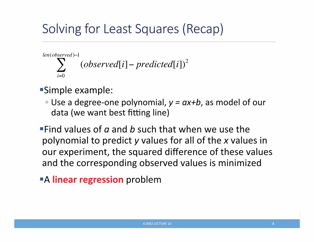
len(observed )−1
∑ (observed[i]− predicted[i])2
i=0
������������� �� ;�
� ,�������������<�- ��������(���1�������*������!���������!�����������+�� �������4��������%�����'�(�����5�
� =����&�� ����+���������� #��������������� ����������*���������������#����&�� ���+��������+�������&�� ������� ������������!������2 �������3����#���+�������&�� �����������#�����������(��%���&���&�� ������������9���
� >�������������������%����
��#�������$���� %�����&!��� �'
len(observed )−1
∑ (observed[i]− predicted[i])2
i=0
������������� �� ?�

��
%�
(������)��"�������#��&����������� �'
• ��������+����������%���������#���%��������������%*�������������1%����#��
• .��(������� �+�#�������������#�!����������(����+������ �+�#���������&�� ���+������%A�#$&��+ �#$���
• ,���$�(������*��������������� �+�#�!����"�B��������C!� �$��*� ����#������B%�/��C�
• �����������(����������%�����������������������
• ���(�������9�������(�����������������
������������� �� @�

*���)��� ���������&!��� �'
������������� �� ��
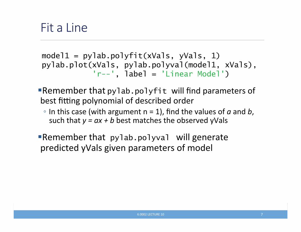
� �����%��������pylab.polyfit ���������������������+�%�����'�(����*��������+����#��%���������- .�������#����4�������( �������D� 5!���������&�� ����+��������!�� #������������������%�������#���������%���&���*E����
� �����%���������pylab.polyval �����(�������������#����*E����(�&���������������+�������
(���$� ��
model1 = pylab.polyfit(xVals, yVals, 1) pylab.plot(xVals, pylab.polyval(model1, xVals), 'r--', label = ’Linear Model')
������������� �� F�

(���$� ��
������������� �� G�

$��+����,��-�)��.����������� ��
model2 = pylab.polyfit(xVals, yVals, 2) pylab.plot(xVals, pylab.polyval(model2, xVals), 'r--', label = 'Quadratic Model')
������������� �� H�
2) l2

/���0��*���������"���1�2���( ��
������������� �� ��

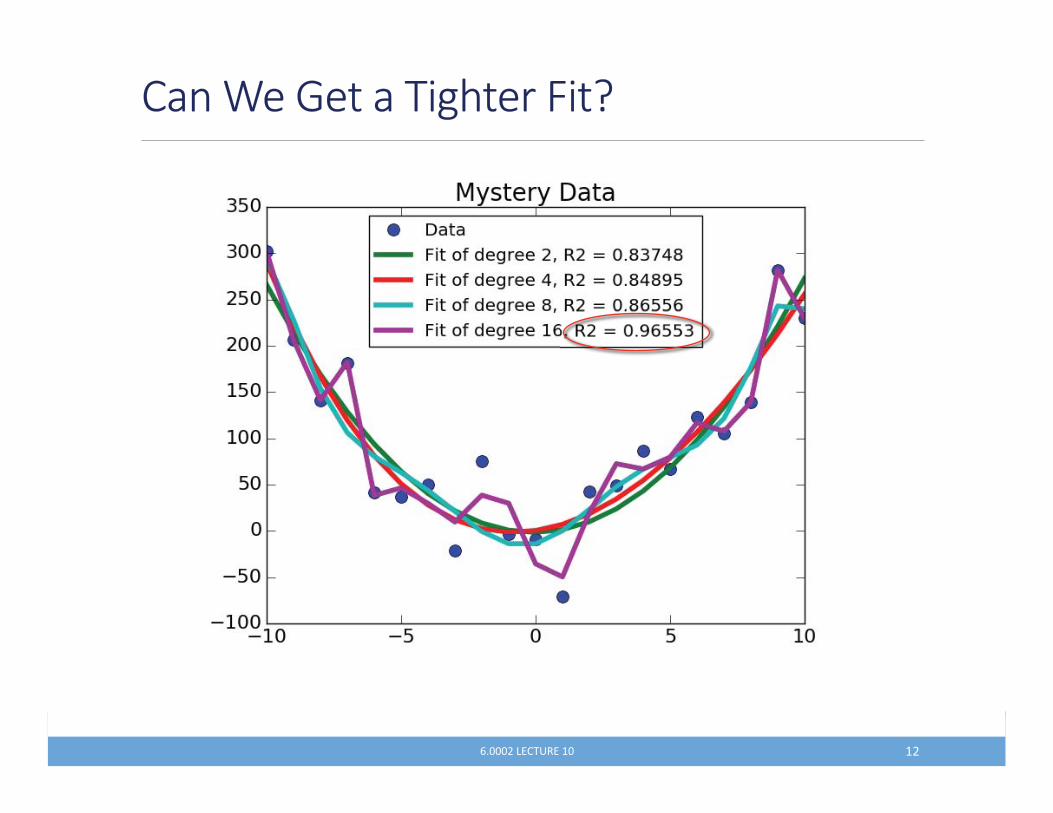
� ������+������*��'�(���(�������������*�������������������I�- J���������(�&�� ����%�/�����I�
� K����� ���������� �������I�- .���%���#���+���������+����$���4��(�!�������$#�������(����������������+������5!����4#��:#������+����������$��5�(�&��� ����#�������� ����+�����$(��������+��������������
- .������#����!������������������(�������&�� �������B%�/��C����
���3���������)����(� �4
������������� �� �
�����������$������
E����%����*�������� ���������
L������������ ����&�� ���6�������������#����&�� ���μ ���������+����� ����&�� ���
���3���������)����(� �4
������������� �� ��
� ���"����"����������� �������������*�(����8������� ������A ��� ������������ �������I�- ��������!�����������"�8���*�% ����������������������#�I�
� K���� �� �������������#���������(������������������- ��(�!�����������$����+������$# ����������������(�
� K���� ����"�������#$�����%� ��� �1�+1������������- ��(�!������#������������#�������+��������(��������+��#�������������������
- ��(�!������#�������3�#���+������������������$����- ��(�!������#������� �#�����+�������#$���
� >�(���������������� �����%�����+�����������(��
3),�3��1��������� ��
������������� �� ;�

� ��A�#���*��+������$#��� �����������M ��#���+��� ��+����(��&���$����������4��(��K����*N������5�
� 6���$����+�#�������+�������+���+���%���������
� J���(���+�������1%�����(���#��
��0#0��������,����,����5�6�"�� �
������������� �� ?�
Images of particle trajectory, load-bearing arch, football pass center of mass diagram © sources unknown. All rights reserved.This content is excluded from out Creative Commons license. For more information, see https://ocw.mit.edu/help/faq-fair-use/.
-�7��,����,����3��������� ��
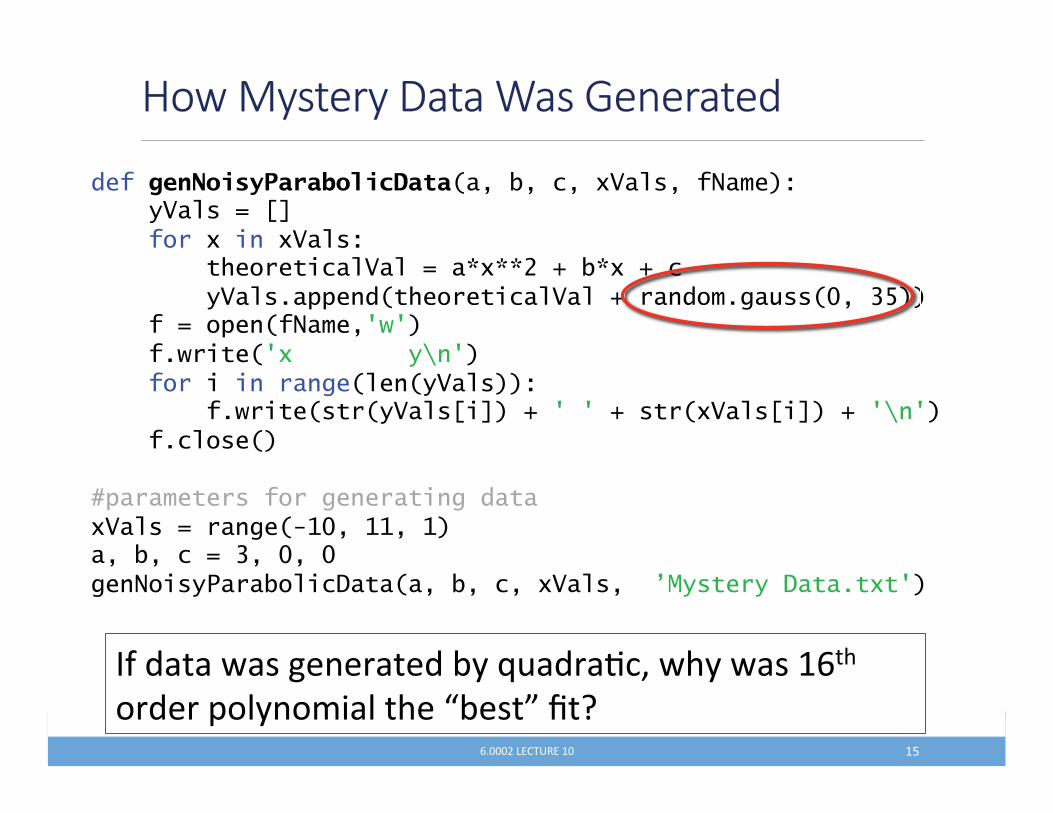
def genNoisyParabolicData(a, b, c, xVals, fName): yVals = [] for x in xVals: theoreticalVal = a*x**2 + b*x + c yVals.append(theoreticalVal + random.gauss(0, 35)) f = open(fName,'w') f.write('x y\n') for i in range(len(yVals)): f.write(str(yVals[i]) + ' ' + str(xVals[i]) + '\n') f.close() #parameters for generating data xVals = range(-10, 11, 1) a, b, c = 3, 0, 0 genNoisyParabolicData(a, b, c, xVals, ’Mystery Data.txt')
������������� �� @�
.+����������(���������%*�2 ����$#!���*����� �������������*�����������B%���C���I�
x + c + random.gauss(0, 35))

$��+��$��8����7����� �� ��
degrees = (2, 4, 8, 16) random.seed(0) xVals1, yVals1 = getData('Dataset 1.txt') models1 = genFits(xVals1, yVals1, degrees) testFits(models1, degrees, xVals1, yVals1, 'DataSet 1.txt') pylab.figure() xVals2, yVals2 = getData('Dataset 2.txt') models2 = genFits(xVals2, yVals2, degrees) testFits(models2, degrees, xVals2, yVals2, 'DataSet 2.txt')
������������� �� ��
ggenFits(models1testFits('
ggenFits(models2testFits(
(������������� �9
������������� �� F�
(������������� �:
������������� �� G�
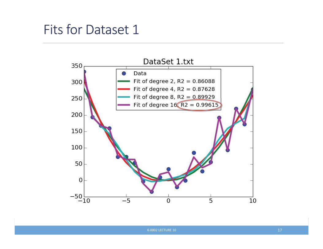
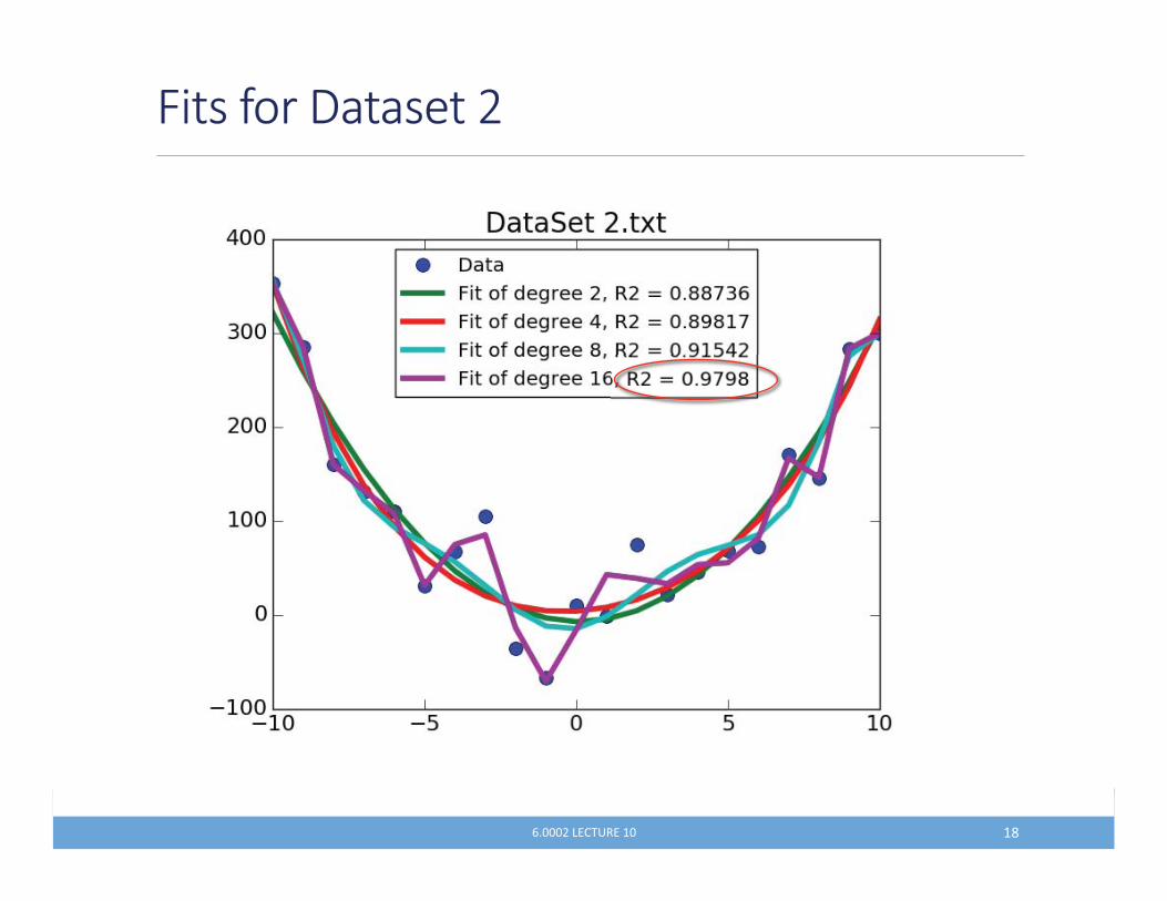
� BO���C��'�(�����������$��������� �����*�������+���%�������������!�� �����"�������������(��������� ���(���������������*������I�� �����������������(�#�����+�����������(�������- K���������������������+�����������������+�������#�����������������
- ,������������(�����������#�����*�#����$���+�����(����������!�� �������� �����������
� ��������������������"��������������������(���������%*�������������#����- ���� ��������+������������(����������������(�- 6���$�����+�#������ �������3������+��#���- E������������������������ �&�*���
� .�������������!��������������������(�������9��
-������������9;������)�����( ��
������������� �� H�
� 0��������������� ���(������������!���������������������������������������- �����������+���J������� ���������#���������+���J���������- �����������+���J�����������������#���������+���J������� �
� ����#�����$�(����������%�����(���������������(�������
� >�%�/�������#�$����+�(�������9�%����*�������������(�������
������<��� ��
������������� �� ���

�������� ��
pylab.figure() testFits(models1, degrees, xVals2, yVals2, 'DataSet 2/Model 1') pylab.figure() testFits(models2, degrees, xVals1, yVals1, 'DataSet 1/Model 2')
������������� �� � �
s1,S
s2, s2,
s2, s1, s1,
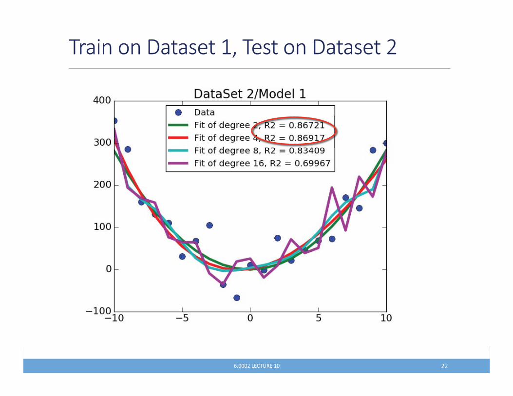
�������������9���������������� �:
������������� �� ���
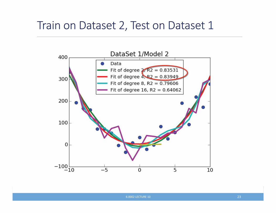
�������������:���������������� �9
������������� �� �;�
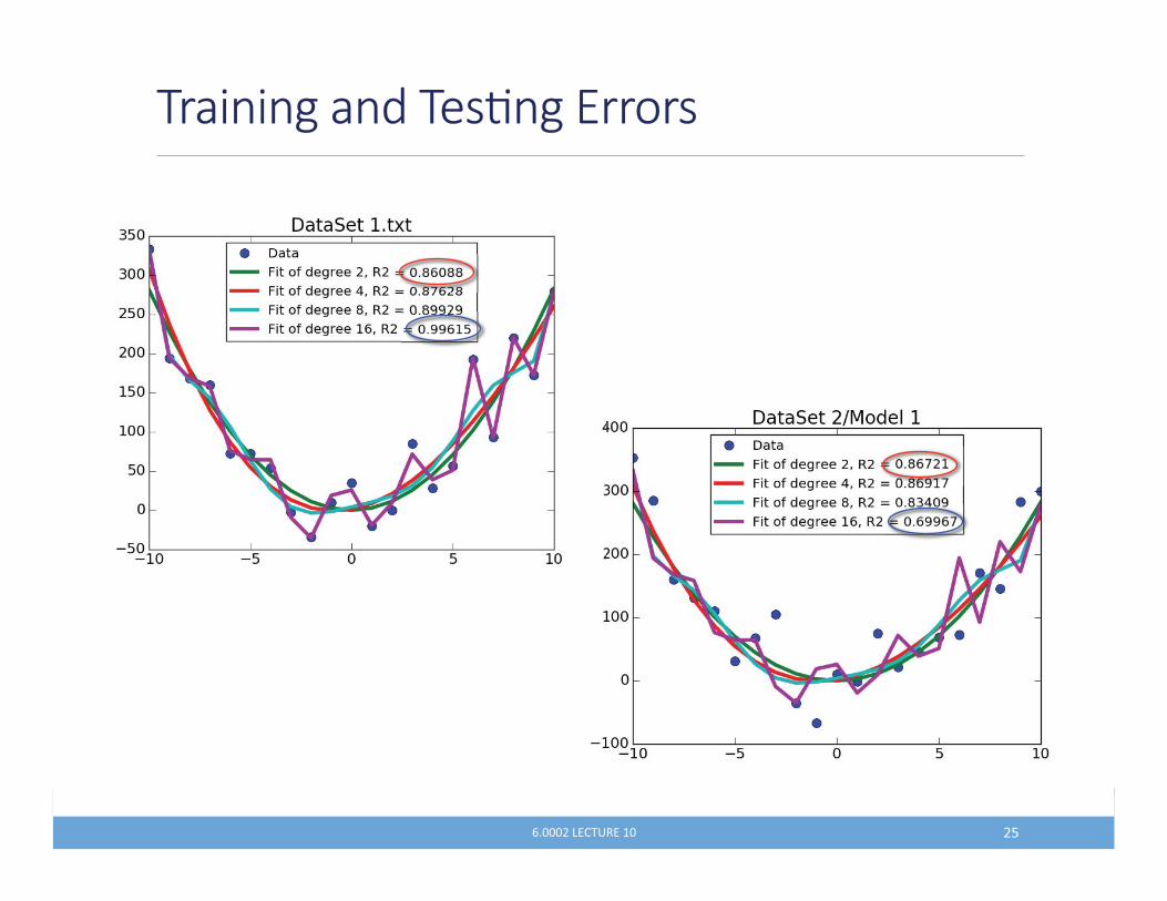
� P���#������������%������������ �%���!�%��������������������"��*����%���������������?������������*�������4���"�����������#� ���*����������!�������3����#��������&�� ���������/*������5!�% ��#�������*����� ����������
� ���������+��&����'�(�������������
� �������������+�������*��������������������(�����!������*���������#��������������������#������Q�% ���������(����������������!���������$�(��������#�������������������������%����
������<��0� ��
������������� �� �?�
������������0��� ���� ��
������������� �� �@�
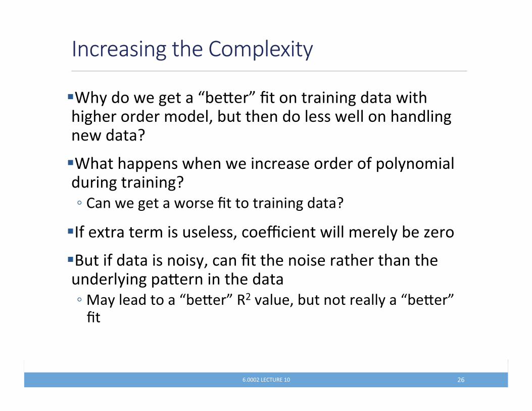
� ��*�������(�����B%�/��C��������������(�������������(���������������!�% ������������������������������(���������I�
� �����������������������#�������������+����*�������� ���(��������(I�- ������(������������������������(�����I�
� .+��������������� ������!�#��:#���������������*�%��9����
� O ���+�������������*!�#�������������������������������� �����*��(���/����������������- ��*�����������B%�/��C����&�� �!�% �����������*���B%�/��C����
����������)���������� �,
������������� �� ���
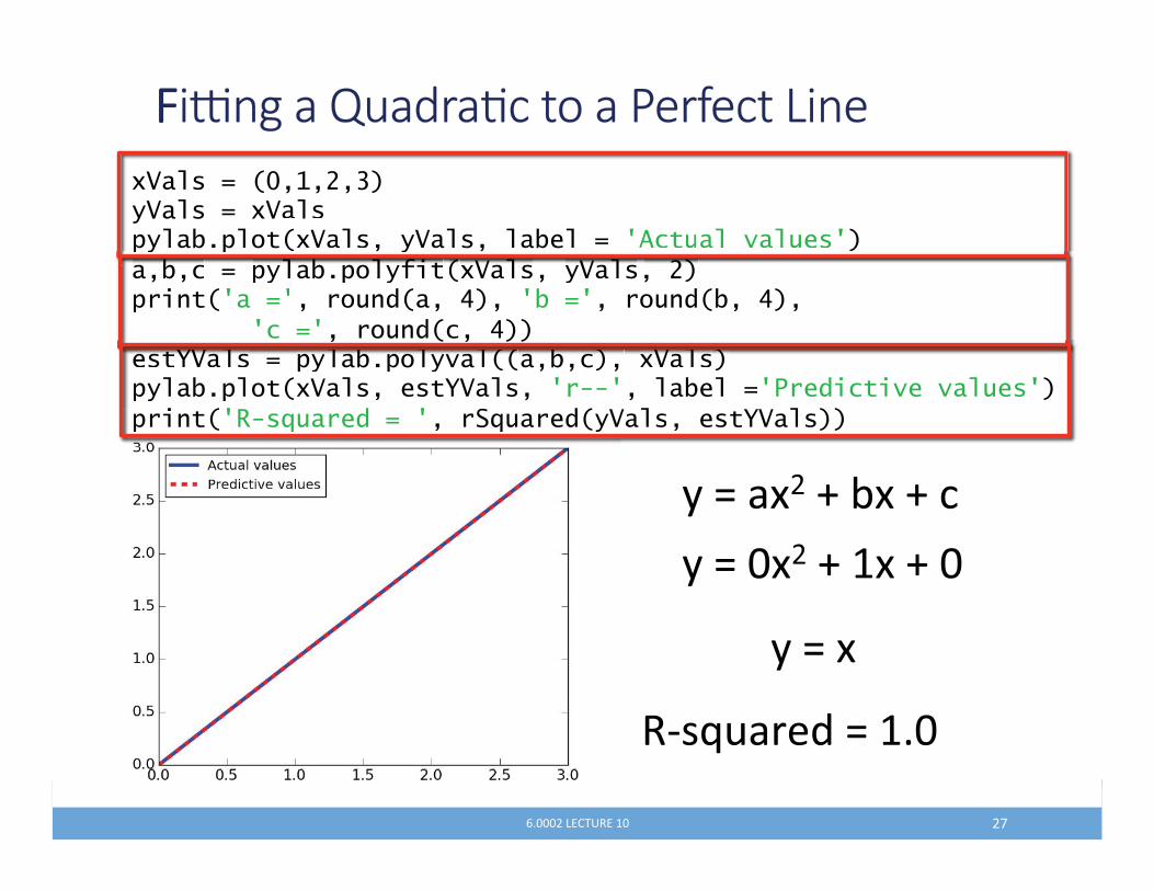
((=����/���0������6�������$� ��
������������� �� �F�
xVals = (0,1,2,3) yVals = xVals pylab.plot(xVals, yVals, label = 'Actual values') a,b,c = pylab.polyfit(xVals, yVals, 2) print('a =', round(a, 4), 'b =', round(b, 4), 'c =', round(c, 4)) estYVals = pylab.polyval((a,b,c), xVals) pylab.plot(xVals, estYVals, 'r--', label ='Predictive values') print('R-squared = ', rSquared(yVals, estYVals))
*�D�����R�%��R�#�*�D�����R� ��R���
*�D���
�1�2 �����D� ���
xVals = (0,1,2,3) yVals = xValspylab.plot(xVals, yVals, label = 'Actual values') py p , y ,a,b,c = pylab.polyfit(xVals, yVals, 2) print('a =', round(a, 4), 'b =', round(b, 4), 'c =', round(c, 4))
a b c pylab polyfit(xVals yVals 2)
estYVals = pylab.polyval((a,b,c), xVals) pylab.plot(xVals, estYVals, 'r--', label ='Predictive values') i (print(' d ''R-squared = ', S drSquared(( ValsyV , estYVals))
estYVals pylab polyval((a b c) xVals), ( , ))

6������*���)���6��������� ������� ��
������������� �� �G�
xVals = xVals + (20,) yVals = xVals pylab.plot(xVals, yVals, label = 'Actual values') estYVals = pylab.polyval((a,b,c), xVals) pylab.plot(xVals, estYVals, 'r--', label = 'Predictive values') print('R-squared = ', rSquared(yVals, estYVals))
(20,)
�1�2 �����D� ���

������� ��������������� ��� ��
������������� �� �H�
xVals = (0,1,2,3) yVals = (0,1,2,3.1) pylab.plot(xVals, yVals, label = 'Actual values') model = pylab.polyfit(xVals, yVals, 2) print(model) estYVals = pylab.polyval(model, xVals) pylab.plot(xVals, estYVals, 'r--', label = 'Predicted values') print('R-squared = ', rSquared(yVals, estYVals))
�1�2 �����D���HHH?�
*�D�����R�%��R�#�*�D����@���R��H@@��R����@�
,3) ,3.1) als yV

6������*���)���6��������� ������� ��
������������� �� ;��
xVals = xVals + (20,) yVals = xVals estYVals = pylab.polyval(model, xVals) print('R-squared = ', rSquared(yVals, estYVals)) pylab.figure() pylab.plot(xVals, estYVals)
�1�2 �����D���F����
(20,)
� ������D��*��%����*��4�E���!�*E���!� 5�
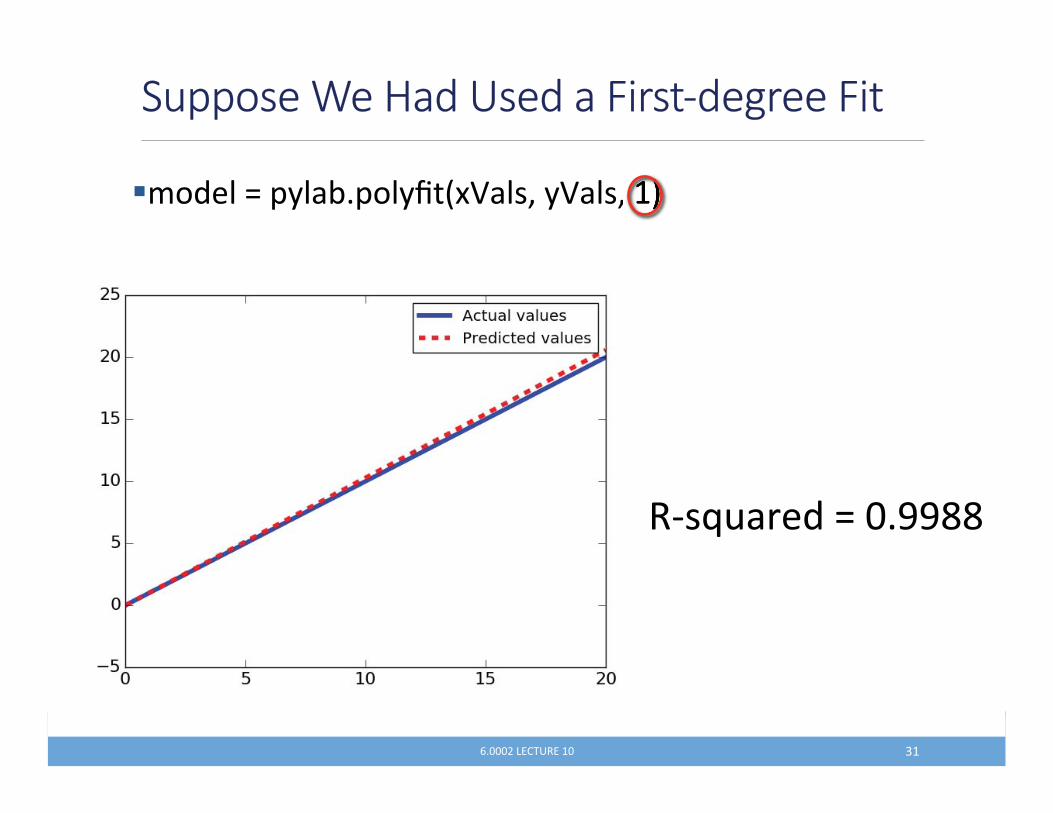
�������3��-��������(���.�������( ��
������������� �� ; �
�1�2 �����D���HHGG�
� 6����#$&���%����*��+���������������� #��%�/����������#�������������
��������>���������������������>� ��
������������� �� ;��
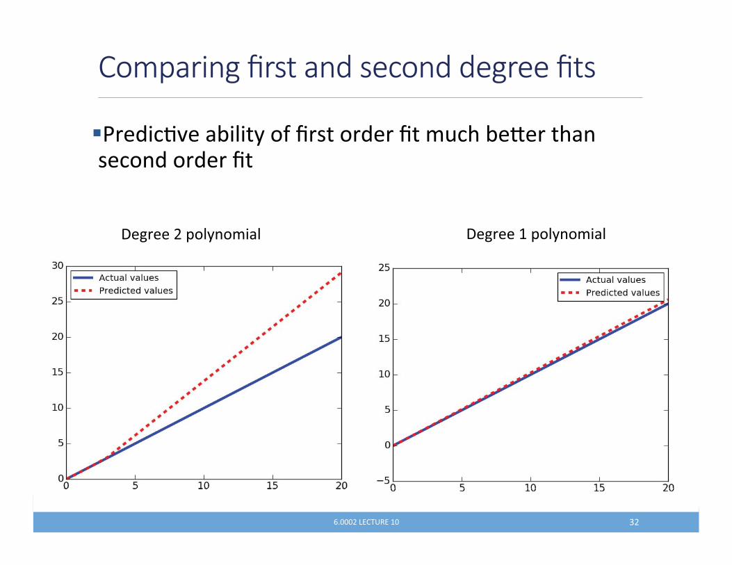
J�(���������*������� J�(���� ����*�������
� ������(�����&���*1#�����������������������&���'�(���������������(������
� .�#��������������"��+�����������������"�������*���������������#� ������������������(�����
� S�����������������#������(������� :#�����*�#��������������������������%�����- >��������������������������������������������%���#���*�����%���#�
- B�&��*����(���� ���%�������������������������%��!�% �������������C�8�>�%�������������
�)���8��-��������� ��
������������� �� ;;�

� .���%���#���+������*������#$�(��������+������!�#�����(�(�����������#�����#����- =�������������������������������(������- ����������������������#�������&�� ��- .�#�������������+������������������- ��$� �� �$������������������%�(���������#�����
1������(��7�)��������� �,
������������� �� ;?�

!�����������3)����3�� ���� ��
������������� �� ;@�
T ����$#����$(�����
O �������%���K��"��
����������%����&�������*��������(!��������� ���( ���� ��
������������ �$�����#������$#��������+������(�
,�� ������%�%�*������3������������������3��������(�������+������
O
�
���&�� ���9���������#�����#����8�����%�������#�����%���"���������������!�� #�������%�������������(��������&����(���������

� ����#����1&�����$������ �������( ��������#���#���+�������#��������*�
� .+��������������!� ������&�1���1� ��#�����&�����$���
� .+������������(����� (�!� ���"1+����#�����&�����$��������������1������1�������(�&�����$���
�������3�����+��-#��� �����)��� �,
������������� �� ;��
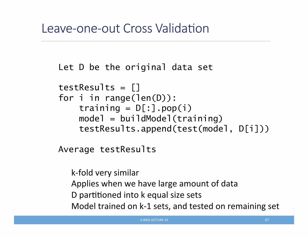
$�#�.���.����������<��0� ��
Let D be the original data set testResults = [] for i in range(len(D)): training = D[:].pop(i) model = buildModel(training) testResults.append(test(model, D[i])) Average testResults �����
"1+����&��*���������>�����������������&�����(����� ����+������J����$$����������"��2 �����9������������������������"1 �����!�����������������������(�����
������������� �� ;F�
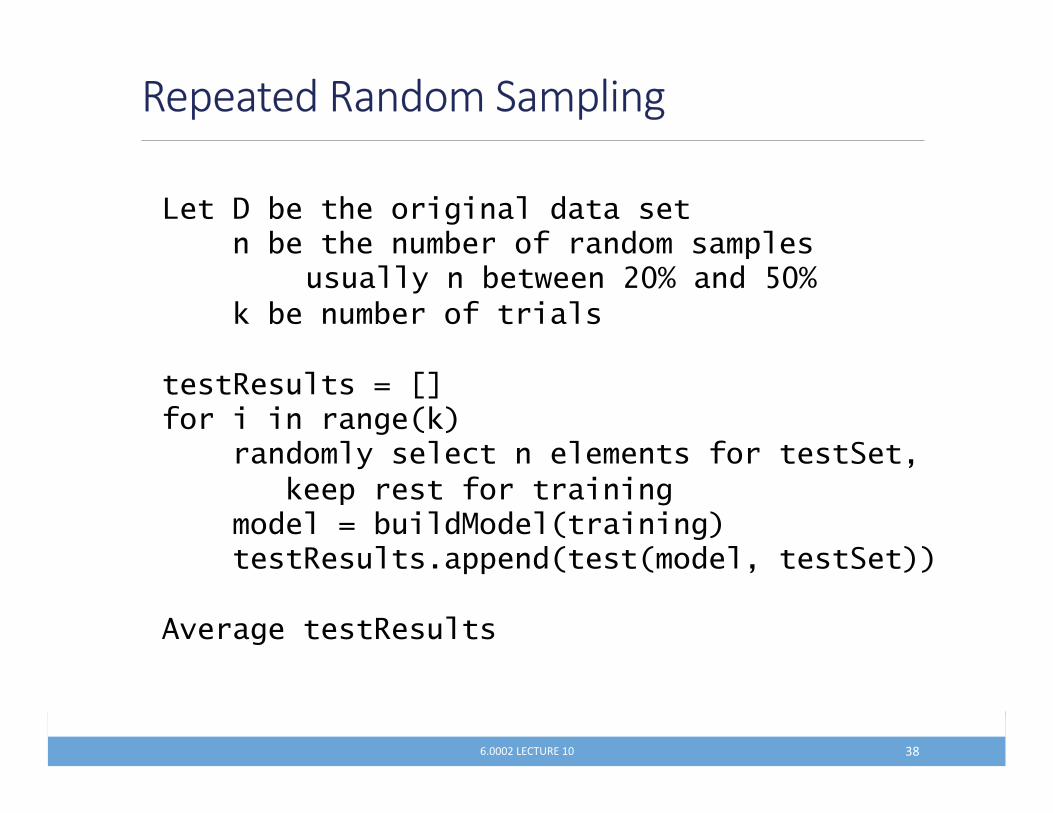
!�������!����� ���� ��
Let D be the original data set n be the number of random samples usually n between 20% and 50%
k be number of trials testResults = [] for i in range(k) randomly select n elements for testSet, keep rest for training model = buildModel(training) testResults.append(test(model, testSet)) Average testResults �����
������������� �� ;G�
� ��"<������������������������*���(���������� ������������,��&������+���� H� ����� (���� @�
� 0���������+�����#��*������������������
� �������*���&���������������+���$����- =�����#���������������*����%��������- ���������������+��+������- ����������������+�- ��#�����1�2 ������������������
� �������������1�2 �����+�����#���������������*�
*�� ������������������1,�?� ��
������������� �� ;H�

*�1�������� ��
class tempDatum(object): def __init__(self, s): info = s.split(',') self.high = float(info[1]) self.year = int(info[2][0:4]) def getHigh(self): return self.high def getYear(self): return self.year
������������� �� ?��

!����� �
def getTempData(): inFile = open('temperatures.csv') data = [] for l in inFile: data.append(tempDatum(l)) return data
������������� �� ? �

������� ��
def getYearlyMeans(data): years = {} for d in data: try: years[d.getYear()].append(d.getHigh()) except: years[d.getYear()] = [d.getHigh()] for y in years: years[y] = sum(years[y])/len(years[y]) return years
������������� �� ?��
�������6������ �
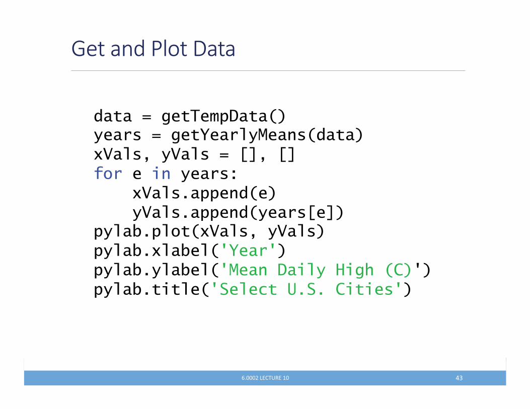
data = getTempData() years = getYearlyMeans(data) xVals, yVals = [], [] for e in years: xVals.append(e) yVals.append(years[e]) pylab.plot(xVals, yVals) pylab.xlabel('Year') pylab.ylabel('Mean Daily High (C)') pylab.title('Select U.S. Cities')
������������� �� ?;�
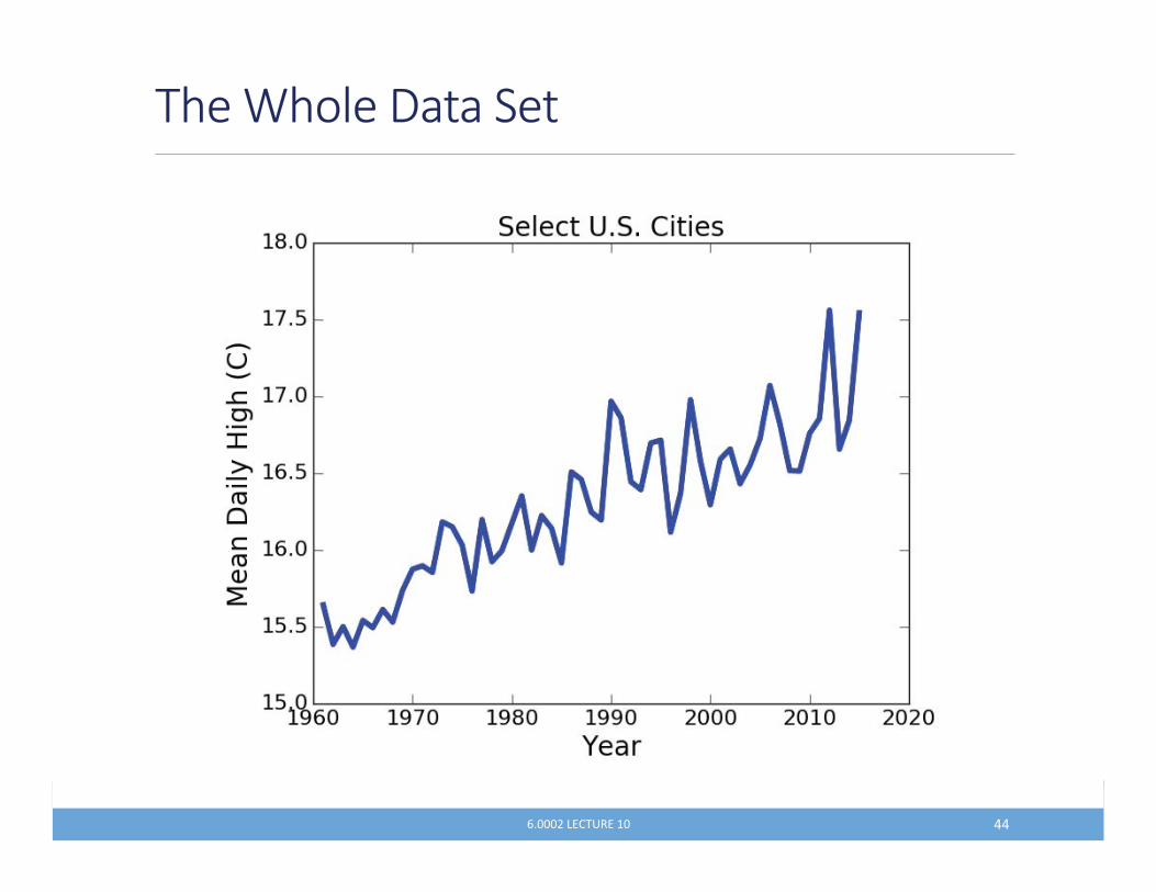
�)��3)������� � ��
������������� �� ??�
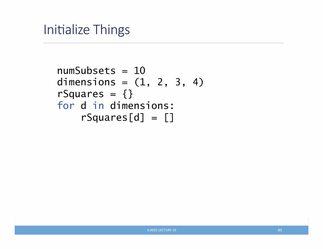
��0�@���)�� ��
numSubsets = 10 dimensions = (1, 2, 3, 4) rSquares = {} for d in dimensions: rSquares[d] = []
������������� �� ?@�

������ �
def splitData(xVals, yVals): toTrain = random.sample(range(len(xVals)), len(xVals)//2) trainX, trainY, testX, testY = [],[],[],[] for i in range(len(xVals)): if i in toTrain: trainX.append(xVals[i]) trainY.append(yVals[i]) else: testX.append(xVals[i]) testY.append(yVals[i]) return trainX, trainY, testX, testY
������������� �� ?��
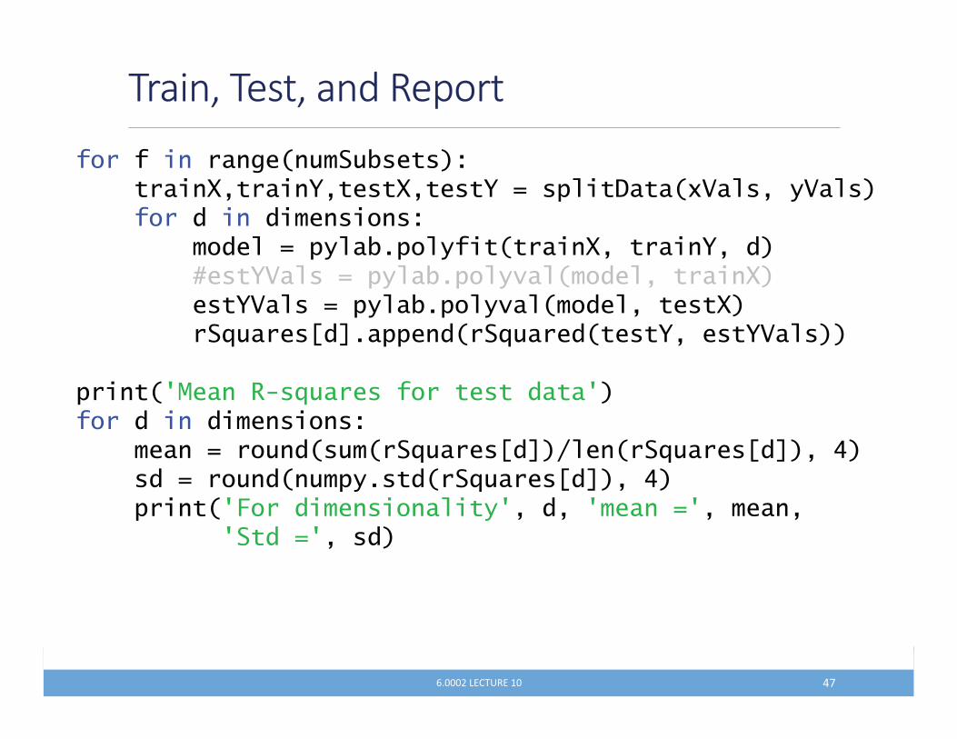
��������������!���� ��
for f in range(numSubsets): trainX,trainY,testX,testY = splitData(xVals, yVals) for d in dimensions: model = pylab.polyfit(trainX, trainY, d) #estYVals = pylab.polyval(model, trainX) estYVals = pylab.polyval(model, testX) rSquares[d].append(rSquared(testY, estYVals)) print('Mean R-squares for test data') for d in dimensions: mean = round(sum(rSquares[d])/len(rSquares[d]), 4) sd = round(numpy.std(rSquares[d]), 4) print('For dimensionality', d, 'mean =', mean, 'Std =', sd)
������������� �� ?F�
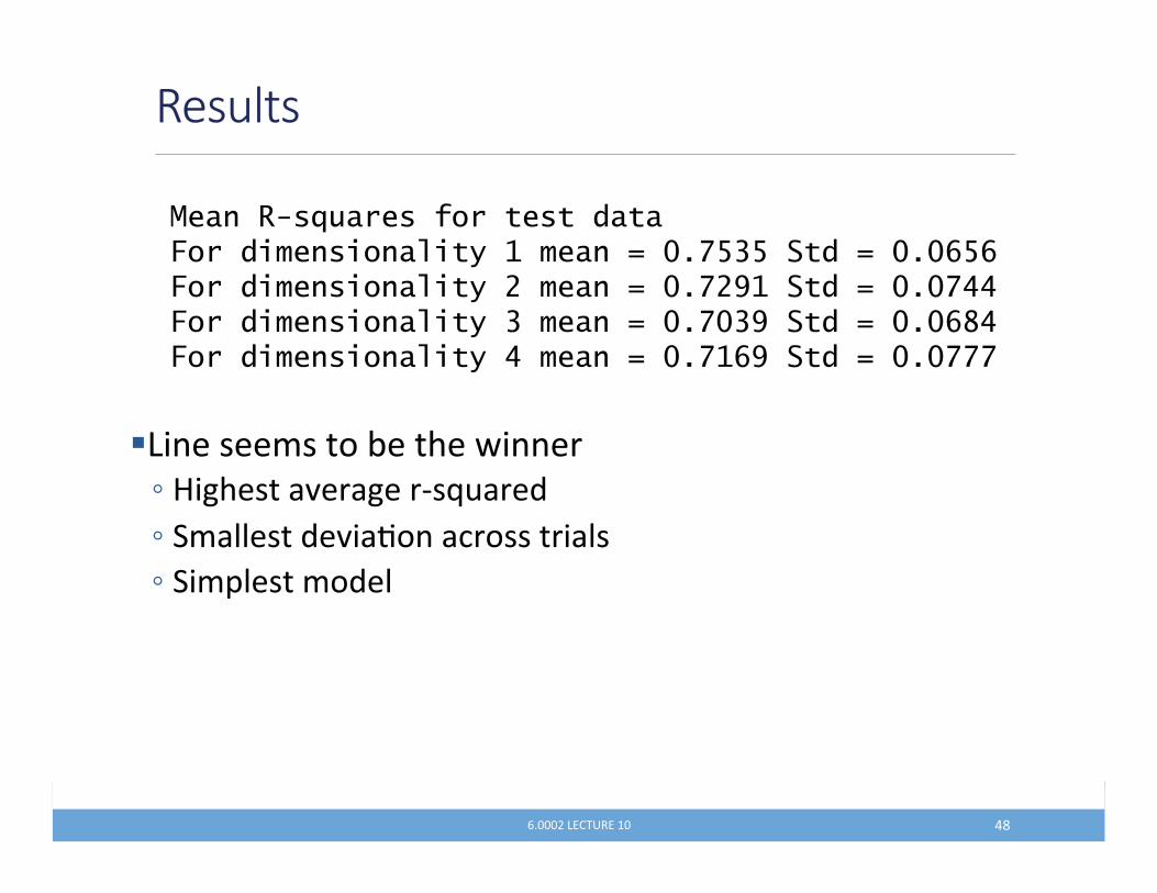
� ��������������%�������������- K�(������&���(���1�2 �����- ,����������&��$����#������������- ,��������������
!����� ��
Mean R-squares for test data For dimensionality 1 mean = 0.7535 Std = 0.0656 For dimensionality 2 mean = 0.7291 Std = 0.0744 For dimensionality 3 mean = 0.7039 Std = 0.0684 For dimensionality 4 mean = 0.7169 Std = 0.0777
������������� �� ?G�
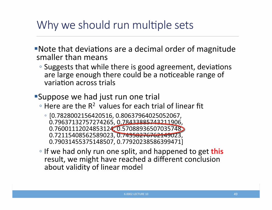
� P�����������&��$������������#������������+���(��� ����������������������- , ((�������������������������(�����(�������!���&��$�����������(����� (��������#� ���%������$#��%������(���+�&����$����#������������
� , �������������A ���� ������������- K����������������&�� ���+�����#���������+�����������- U��FG�G��� @�?��@ �!���G��;FH�?��@�@���F!���FH�;F ;�F@F�F?��@!���FG?;;GG@F?;� H��!���F��� ���?G@; �?!���@F�GGH;�@�F�;@F?G!���F� @?�G@��@GH��;!���F?;@G�F�F�� ?H��;!���FH�; ?@@;F@ ?G@�F!���FFH���;G@G�;HH?F V�
- .+�����������*�� �����������!�����������������(���������� ��!������(�����&�����#��������3������#��#� ������%� ��&������*��+��������������
3),�7���)������������0������� ��
������������� �� ?H�
@!���FG?;;GG@F?;� H��!�?!���@F�GGH;�@�F�;@F?G!�;! ��F?;@G�F�F�� ?H��;!
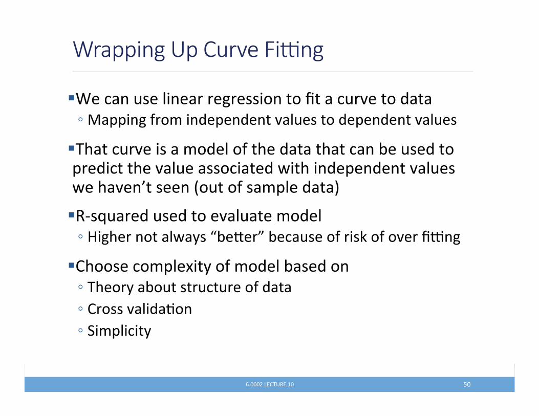
� ���#��� ������������(����������������# �&����������- ������(�+����������������&�� ����������������&�� ���
� ����# �&��������������+���������������#���%�� ������������#������&�� ������#�����������������������&�� ��������&��N�������4� ���+������������5�
� �1�2 ����� ��������&�� ����������- K�(������������*��B%�/��C�%�#� ����+����"��+��&����'�(�
� ������#��������*��+�������%��������- ����*��%� ����� #� ����+������- �����&�����$���- ,�����#��*�
3������������#��(=� ��
������������� �� @��
MIT OpenCourseWarehttps://ocw.mit.edu
6.0002 Introduction to Computational Thinking and Data ScienceFall 2016
For information about citing these materials or our Terms of Use, visit: https://ocw.mit.edu/terms.