
Multiband optical ux density and polarization ...
26
MNRAS 000, 1–26 (2019) Preprint 12 December 2019 Compiled using MNRAS L A T E X style file v3.0 Multiband optical flux density and polarization microvariability study of optically bright blazars Magdalena Pasierb, 1 ? Arti Goyal, 1 † Michal Ostrowski, 1 Lukasz Stawarz, 1 Paul J. Wiita, 2 Gopal-Krishna, 3 ,4 Valeri M. Larionov, 5 ,6 Daria A. Morozova, 5 Ryosuke Itoh, 7 Fahri Alicavus, 8 Ahmet Erdem, 8 Santosh Joshi, 3 Staszek Zola 1 ,9 Georgy A. Borman, 10 Tatiana S. Grishina, 5 Evgenia N. Kopatskaya, 5 Elena G. Larionova, 5 Sergey S. Savchenko, 5 Anna A. Nikiforova, 5 ,6 Yulia V. Troitskaya, 5 Ivan S. Troitsky, 5 Hiroshi Akitaya, 11 Miho Kawabata, 12 ,11 Tatsuya Nakaoka 11 1 Astronomical Observatory of the Jagiellonian University, ul. Orla 171, 30-244 Krak´ ow, Poland 2 Department of Physics, The College of New Jersey, 2000 Pennington Rd., Ewing, NJ 08628-0718, USA 3 Aryabhatta Research Institute of Observational Sciences (ARIES), Manora Peak, Nainital 263002, India 4 UM-DAE Centre for Excellence in Basic Sciences, Univ. of Mumbai, Mumbai-400098, India 5 Astronomical Institute of St. Petersburg State University, Petrodvorets 198504, Russia 6 196140, Pulkovskoye chaussee 65, Saint-Petersburg, Russia 7 Bisei Astronomical Observatory, 1723-70 Ookura, Bisei-cho, Ibara, Okayama 714-1411, Japan 8 Department of Physics, Faculty of Arts and Sciences, Canakkale Onsekiz Mart University, Canakkale TR-17100, Turkey 9 Mt. Suhora Observatory, Pedagogical University, ul. Podchorazych 2, Krak´ow 30-084, Poland 10 Astrophysical Observatory, P/O Nauchny, Crimea, 298409, Russia 11 Hiroshima Astrophysical Science Center, Hiroshima University, Higashi-Hiroshima, Hiroshima 739-8526, Japan 12 Department of Astronomy, Kyoto University, Kitashirakawa-Oiwakecho, Sakyo-ku, Kyoto 606-8502, Japan Accepted XXX. Received YYY; in original form ZZZ ABSTRACT We present the results of flux density, spectral index, and polarization intra-night monitoring studies of a sample of eight optically bright blazars, carried out by em- ploying several small to moderate aperture (0.4 m to 1.5 m diameter) telescopes fitted with CCDs and polarimeters located in Europe, India, and Japan. The duty cycle of flux variability for the targets is found to be ∼ 45 percent, similar to that reported in earlier studies. The computed two-point spectral indices are found to be between 0.65 to 1.87 for our sample, comprised of low- and intermediate frequency peaked blazars, with one exception; they are also found to be statistically variable for about half the instances where ‘confirmed’ variability is detected in flux density. In the analysis of the spectral evolution of the targets on hourly timescale, a counter-clockwise loop (soft-lagging) is noted in the flux–spectral index plane on two occasions, and in one case a clear spectral flattening with the decreasing flux is observed. In our data set, we also observe a variety of flux–polarization degree variability patterns, including instances with a relatively straightforward anti-correlation, correlation, or counter- clockwise looping. These changes are typically reflected in the flux–polarization angle plane: the anti-correlation between the flux and polarization degree is accompanied by an anti-correlation between the polarization angle and flux, while the counter- clockwise flux–PD looping behaviour is accompanied by a clockwise looping in the flux–polarization angle representation. We discuss our findings in the framework of the internal shock scenario for blazar sources. Key words: radiation mechanisms: non-thermal — galaxies: active — polarization — galaxies: jets — galaxies: individual: 0109+224, 3C 66A, S5 0716+714, OJ 287, 3C 279, PG 1553+113, CTA 102, and 3C 454.3. © 2019 The Authors arXiv:1912.05505v1 [astro-ph.HE] 11 Dec 2019
Transcript of Multiband optical ux density and polarization ...

MNRAS 000, 1–26 (2019) Preprint 12 December 2019 Compiled using MNRAS LATEX style file v3.0
Multiband optical flux density and polarizationmicrovariability study of optically bright blazars
Magdalena Pasierb,1? Arti Goyal,1† Micha l Ostrowski,1 Lukasz Stawarz,1
Paul J. Wiita,2 Gopal-Krishna,3,4 Valeri M. Larionov,5,6 Daria A. Morozova,5
Ryosuke Itoh,7 Fahri Alicavus,8 Ahmet Erdem,8 Santosh Joshi,3 Staszek Zola1,9
Georgy A. Borman,10 Tatiana S. Grishina,5 Evgenia N. Kopatskaya,5
Elena G. Larionova,5 Sergey S. Savchenko,5 Anna A. Nikiforova,5,6
Yulia V. Troitskaya,5 Ivan S. Troitsky,5 Hiroshi Akitaya,11 Miho Kawabata,12,11
Tatsuya Nakaoka111Astronomical Observatory of the Jagiellonian University, ul. Orla 171, 30-244 Krakow, Poland2Department of Physics, The College of New Jersey, 2000 Pennington Rd., Ewing, NJ 08628-0718, USA3Aryabhatta Research Institute of Observational Sciences (ARIES), Manora Peak, Nainital 263002, India4UM-DAE Centre for Excellence in Basic Sciences, Univ. of Mumbai, Mumbai-400098, India5Astronomical Institute of St. Petersburg State University, Petrodvorets 198504, Russia6196140, Pulkovskoye chaussee 65, Saint-Petersburg, Russia7Bisei Astronomical Observatory, 1723-70 Ookura, Bisei-cho, Ibara, Okayama 714-1411, Japan8Department of Physics, Faculty of Arts and Sciences, Canakkale Onsekiz Mart University, Canakkale TR-17100, Turkey9Mt. Suhora Observatory, Pedagogical University, ul. Podchorazych 2, Krakow 30-084, Poland10Astrophysical Observatory, P/O Nauchny, Crimea, 298409, Russia11Hiroshima Astrophysical Science Center, Hiroshima University, Higashi-Hiroshima, Hiroshima 739-8526, Japan12Department of Astronomy, Kyoto University, Kitashirakawa-Oiwakecho, Sakyo-ku, Kyoto 606-8502, Japan
Accepted XXX. Received YYY; in original form ZZZ
ABSTRACT
We present the results of flux density, spectral index, and polarization intra-nightmonitoring studies of a sample of eight optically bright blazars, carried out by em-ploying several small to moderate aperture (0.4 m to 1.5 m diameter) telescopes fittedwith CCDs and polarimeters located in Europe, India, and Japan. The duty cycle offlux variability for the targets is found to be ∼ 45 percent, similar to that reported inearlier studies. The computed two-point spectral indices are found to be between 0.65to 1.87 for our sample, comprised of low- and intermediate frequency peaked blazars,with one exception; they are also found to be statistically variable for about half theinstances where ‘confirmed’ variability is detected in flux density. In the analysis ofthe spectral evolution of the targets on hourly timescale, a counter-clockwise loop(soft-lagging) is noted in the flux–spectral index plane on two occasions, and in onecase a clear spectral flattening with the decreasing flux is observed. In our data set,we also observe a variety of flux–polarization degree variability patterns, includinginstances with a relatively straightforward anti-correlation, correlation, or counter-clockwise looping. These changes are typically reflected in the flux–polarization angleplane: the anti-correlation between the flux and polarization degree is accompaniedby an anti-correlation between the polarization angle and flux, while the counter-clockwise flux–PD looping behaviour is accompanied by a clockwise looping in theflux–polarization angle representation. We discuss our findings in the framework ofthe internal shock scenario for blazar sources.
Key words: radiation mechanisms: non-thermal — galaxies: active — polarization —galaxies: jets — galaxies: individual: 0109+224, 3C 66A, S5 0716+714, OJ 287, 3C 279,PG 1553+113, CTA 102, and 3C 454.3.
? E-mail: [email protected] (MP) † E-mail: [email protected] (AG)
© 2019 The Authors
arX
iv:1
912.
0550
5v1
[as
tro-
ph.H
E]
11
Dec
201
9

2 M. Pasierb et al.
1 INTRODUCTION
Characterized by large flux density and polarization vari-ability, blazars form a major class of active galactic nu-clei (AGN), for which the total radiative output is dom-inated by magnetized, relativistic plasma outflows — jets— launched from the center of massive elliptical galaxies(e.g., Urry & Padovani 1995; Padovani et al. 2017). Theblazar family includes flat-spectrum radio-loud quasars (FS-RQs) and BL Lacertae objects (BL Lacs), the former ofwhich have prominent emission lines in their optical spec-tra while the latter have very weak or undetectable lines.A blazar broadband spectral energy distribution (SED) iscomposed of two peaks: (1) a low energy segment rangingfrom radio to optical frequencies (sometimes extending upto X-rays in case of BL Lac objects) which is unequivo-cally attributed to synchrotron radiation of charged parti-cles accelerated up to TeV energies; and (2) a high energysegment ranging from optical/X-rays up to GeV/TeV γ−rayfrequencies which is attributed to inverse-Compton (IC) ra-diation of the seed photons produced locally (SynchrotronSelf-Compton; SSC) or externally (External Compton; EC)to the jet plasma within the leptonic emission scenarios(e.g., Madejski & Sikora 2016, and references therein). Al-ternatively, in ‘hadronic’ scenarios for emission, the higher-frequency radiation peak is believed to originate from pro-tons accelerated to 'PeV–EeV energies which could produceγ-rays via either direct synchrotron process, or meson decayand synchrotron emission by the secondaries produced inproton-photon interactions (e.g., Bottcher et al. 2013).
Depending on the timescales over which the flux den-sity variations were seen, the blazar variability is conven-tionally divided into long-term (years to months), short-term (months to weeks) and intra-night/day variability(INV/IDV) or microvariability (e.g., Wagner & Witzel 1995;Ghosh et al. 2000). While the long-term variability easilycan be reconciled within the standard paradigms of blazaremission models with modestly Doppler boosted relativisticjets (δ ∼10–20; Maraschi et al. 1992; Abdo et al. 2011b,a),sub-hour variability, especially at γ−ray energies, could beaccounted for only with extremely large δ’s (>30-50; Aharo-nian et al. 2007; Begelman et al. 2008) or with non-standardinterpretations (i.e., a synchrotron origin of the γ−ray flarein FSRQ 3C 279; Ackermann et al. 2016). Efficient energydissipation is needed to ensure flux density variations onthe smallest spatial scales and while there is no consensuson the main energy dissipation mechanism, the most favoredcandidates include plasma instabilities which lead to the for-mation of shocks and turbulence in the jet flow (e.g., Spadaet al. 2001; Agudo et al. 2011), or alternatively, an annihila-tion of magnetic field lines of opposite polarity transferringenergy from the field to the particles at the magnetic recon-nection sites (Sironi et al. 2015). Alternatively, many rapidflux density variations could be explained by geometrical ef-fects involving small changes in the direction of motion ofthe jet plasma (Gopal-Krishna & Wiita 1992; Camenzind &Krockenberger 1992; Meyer 2018).
The evolution of colour or the spectral index, α, (F(ν)∝ ν−α where ν is the radiation frequency and F(ν) is theflux density provides an insight into the particle distribu-tion giving rise to the observed flux density and its variabil-ity. In particular, at the synchrotron frequencies, within the
MNRAS 000, 1–26 (2019)
Flux density, spectral index, and polarization blazar microvariability 3
simplest scenario of single-zone emission models with homo-geneous magnetic field distributions, clear patterns betweenthe spectral index and the total intensity are predicted, i.e.,a “spectral hysteresis”, depending on the relative lengths ofthe radiative cooling timescale and the escape timescale ofthe accelerated particles from the emission zone (e.g., Kirket al. 1998). A significant fraction of long-term multibandflux monitoring studies have revealed bluer–when–brightertrends for BL Lac objects but frequently redder–when–brighter trends for FSRQs (Gu et al. 2006; Osterman Meyeret al. 2009; Rani et al. 2010; Hao et al. 2010; Ikejiri et al.2011; Bonning et al. 2012; Sandrinelli et al. 2014; Meng et al.2018; Li et al. 2018; Gupta et al. 2019) while ‘achromatic’flux variability (no colour evolution, Gaur et al. 2019; Bon-ning et al. 2012; Stalin et al. 2006), and erratic patterns(Wierzcholska et al. 2015) have also been reported. It hasbeen argued that particles accelerated to higher energiesare injected at the emission zone before being cooled ra-diatively in BL Lac sources leading to their overall SEDsbeing bluer-when-brighter; however, the ‘redder’ and morevariable jet-component can overwhelm the ‘bluer’ contribu-tion from the accretion disc, leading to redder-when-brightertrends for FSRQ type sources (Gu et al. 2006). Achromaticvariability is often ascribed to changes in the Doppler boost-ing factor (δ) as each frequency notes the same special rel-ativistic multiplication of flux (Gaur et al. 2012). However,erratic colour trends together with the opposite behaviours,i.e., redder–when–brighter changes for BL Lacs (Gu & Ai2011) and bluer–when–brighter trends for FSRQs (Wu et al.2011), indicate that more complex scenarios, presumably in-volving the dominance of the relative contributions of theDoppler boosted jet emission component and the accretiondisc component, respectively, are particularly relevant forblazars with peak synchrotron frequencies in the range of1013−15 Hz (low-frequency peaked blazars; Isler et al. 2017;Gopal-Krishna et al. 2019).
Polarization variability, i.e., changes in the polarizationdegree (PD) and/or the electric vector polarization angle(χ) is yet another diagnostic to probe emission scenarios.The PD is a measure of the structure of the magnetic fieldand the χ traces the direction of the projected magneticfield (being perpendicular to it) on the sky. For the simplecase of a single emission zone, the maximum PD is ≈70%for a power-law distribution of elections with energy index≈2 and uniform pitch angle distribution, immersed in a uni-form magnetic field (Rybicki & Lightman 1986). Blazars of-ten show ∼1–30% PDs at optical frequencies (Mead et al.1990; Ikejiri et al. 2011; Jermak et al. 2016; Angelakis et al.2016), indicating highly ordered magnetic fields at the emis-sion sites in some cases. Moreover, the abrupt rotation ofχ observed during outbursts has been taken as a signatureof shocks in the jet (Marscher & Gear 1985; Jorstad et al.2007; Marscher et al. 2008; Hughes et al. 2011; Saito et al.2015). Indeed, statistically significant correlations betweenswings of χ and γ−rays flares have been noted (Blinov et al.2016). However, the distributions of Q and U Stokes inten-sities in the (Q, U) plane often indicate a random-walk typeof behaviour, suggesting that many emission regions withdifferent magnetic field orientations contribute to the aggre-gate emission over longer monitoring periods (Moore et al.1982; Villforth et al. 2010; Gupta et al. 2019). Therefore,strictly simultaneous polarization monitoring, coupled with
flux monitoring at a few frequencies, is an important steptowards understanding the physical processes in blazar jets.
Only a handful of studies have probed the colourand polarization evolutions of blazars on microvariabilitytimescales. In particular, Stalin et al. (2006) showed thatBL Lacertae exhibited ‘bluer–when–brighter’ trends whileS5 0716+714 showed achromatic trends during intra-nightmonitoring sessions carried out in 1996 and 2000–2001. ForBL Lac alone, bluer–when–brighter trends on intra-nighttimescales have often been observed during different moni-toring campaigns (1999-2001; Papadakis et al. 2003), (2012-2016; Meng et al. 2017) and (2014-2016; Gaur et al. 2017).For the blazar S5 0716+714, Dai et al. (2013) noted bluer–when–brighter trends during the intra-night monitoring car-ried out in 2004–2011 while Zhang et al. (2018) showedthat the blazar exhibited both achromatic and bluer–when–brighter trends during the monitoring session carried out in2013–2016. As for polarization variations, the blazar popu-lation in general shows significantly variable polarization onintra-night timescales if the PD is found to be more than5% (Villforth et al. 2009). A highly polarized (PD∼50%)microflare was observed for the blazar S5 0716+714 duringthe Whole Earth Blazar Telescope campaign carried out in2014 (Bhatta et al. 2015). An orphan flare in polarized fluxdensity was observed for the blazar CTA 102 (Itoh et al.2013). Intense variability in total flux density, polarized fluxdensity, and χ was noted for BL Lacertae while the blazarPKS 1424+240 remained steady during the study by Covinoet al. (2015). In this context, the present study aims to ex-pand efforts to probe physical conditions on microvariabilitytimescales through systematic multiband flux and polariza-tion monitoring for a well-defined sample of blazars withwell-known microvariability properties.
Here we present the results of our monitoring campaignto characterize the flux (B, V, R, and I band), colour (orspectral index), and polarization microvariability for a sam-ple of eight bright blazars, each observed for a continuousmonitoring duration of ≥3 hours using several telescopes fit-ted with charge-coupled devices (CCDs) and polarimeters.Our aim was to obtain strictly simultaneous observationsin flux and polarization by coordinated monitoring betweentwo observatories, one serving as a photometer for flux mon-itoring while the other was equipped with a polarimeter toobtain PD and χ. However, our observations were severelylimited by weather conditions and despite several attemptsat coordinated monitoring, we could obtain strictly simul-taneous data only on a few occasions. The data presentedin this study were obtained in the years 2014 to 2017. InSections 2 and 3, we describe the sample selection anddata gathering, reduction and generation of differential lightcurves (DLCs). Section 4 describes the methodology for es-timation of variability parameters. Results are given in Sec-tions 5 with Section 6 listing the conclusions of the study.
2 SAMPLE SELECTION
The blazars monitored in the study are chosen from thesample of Goyal et al. (2013b) aside from the addition ofCTA 102 (Itoh et al. 2013), based on their established mi-crovariability properties. We briefly recall here the selectioncriteria for our monitoring. The source must: (i) be persis-
MNRAS 000, 1–26 (2019)
4 M. Pasierb et al.
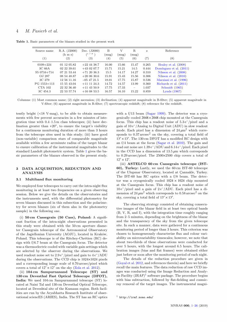
Table 1. Basic parameters of the blazars studied in the present work
Source name R.A. (J2000) Dec. (J2000) B V R z Reference(h m s) (◦ ′ ′′ ) (mag) (mag) (mag)
(1) (2) (3) (4) (5) (6) (7) (8)
0109+224 01 12 05.82 +22 44 38.7 16.00 15.66 15.47 0.265 Healey et al. (2008)
3C 66A 02 22 39.61 +43 02 07.7 15.71 15.21 14.5 0.444 Domınguez et al. (2011)
S5 0716+714 07 21 53.44 +71 20 36.3 15.5 14.17 14.27 0.310 Nilsson et al. (2008)OJ 287 08 54 48.87 +20 06 30.6 15.91 15.43 15.56 0.306 Nilsson et al. (2010)
3C 279 12 56 11.16 −05 47 21.5 18.01 17.75 15.87 0.536 Marziani et al. (1996)PG 1553+113 15 55 43.04 +11 11 24.3 14.72 14.57 13.99 0.360 Richards et al. (2011)
CTA 102 22 32 36.40 +11 43 50.9 17.75 17.33 – 1.037 Schmidt (1965)
3C 454.3 22 53 57.74 +16 08 53.5 16.57 16.10 15.22 0.859 Lynds (1967)
Columns: (1) Most common name; (2) right ascension; (3) declination; (4) apparent magnitude in B-filter; (5) apparent magnitude in
V-filter; (6) apparent magnitude in R-filter; (7) spectroscopic redshift; (8) reference for the redshift.
tently bright (<18 V-mag), to be able to obtain measure-ments with few percent accuracies in a few minutes of inte-gration time with 0.4–1.5 m class telescopes; (ii) have dec-lination greater than +20◦, to ensure the target’s visibilityfor a continuous monitoring duration of more than 3 hoursfrom the telescope sites used in this study; (iii) have good(non-variable) comparison stars of comparable magnitudeavailable within a few arcminute radius of the target blazarto ensure calibration of the instrumental magnitudes to thestandard Landolt photometric system. Table 1 gives the ba-sic parameters of the blazars observed in the present study.
3 DATA ACQUISITION, REDUCTION ANDANALYSIS
3.1 Multiband flux monitoring
We employed four telescopes to carry out the intra-night fluxmonitoring in at least two frequencies on a given observingsession. Below we give the details on the observatories andthe instruments used, with the differential photometry forseven blazars discussed in this subsection and the polarime-try for seven blazars (six of them also in the photometrysample) in the following one.
(i) 50 cm Cassegrain (50 Cass), Poland: A signifi-cant fraction of the intra-night observations presented inthis study were obtained with the 50 cm aperture diame-ter Cassegrain telescope of the Astronomical Observatoryof the Jagiellonian University (AOJU), located in Krakow,Poland. This telescope is of the Ritchey-Chretien (RC) de-sign with f/6.7 beam at the Cassegrain focus. The detectorwas a thermoelectric cooled with variable gain settings whichare selected by the observer during the observations. Weused readout noise set to 2.9 e−/pixel and gain to 4 e−/ADUduring the observations. The CCD chip is 1024×1024 pixelsand a corresponding image scale of 0.70 arcsec/pixel whichcovers a total of 12′ × 12′ on the sky (Zola et al. 2012).
(ii) 104 cm Sampurnanand Telescope (ST) and130 cm Devesthal Fast Optical Telescope (DFOT),India: We used 104 cm Sampurnanand telescope (ST) lo-cated at Naini Tal and 130 cm Devesthal Optical Telescope,located at Deveshtal site of the Kumaun region. Both facil-ities are run by the Aryabhatta Research Institute of obser-vational sciencES (ARIES), India. The ST has an RC optics
with a f/13 beam (Sagar 1999). The detector was a cryo-genically cooled 2048×2048 chip mounted at the Cassegrainfocus. This chip has a readout noise of 5.3 e−/pixel and again of 10 e−/Analog to Digital Unit (ADU) in slow readoutmode. Each pixel has a dimension of 24 µm2 which corre-sponds to 0.37 arcsec2 on the sky, covering a total field of13′ × 13′. The 130 cm DFOT has a modified RC design withan f/4 beam at the focus (Sagar et al. 2010). The gain andread out noise are 1.39 e−/ADU and 6.14 e−/pixel. Each pixelin the CCD has a dimension of 13.5 µm which correspondsto 0.29 arcsec/pixel. The 2500×2500 chip covers a total of12′ × 12′.
(iii) ASTELCO 60 cm Cassegrain telescope (IST-60), Turkey: Lastly, we used the 60 cm IST-60 telescopeof the Ulupınar Observatory, located at Cannakle, Turkey.The IST-60 has RC optics with a f/8 beam. The detec-tor was a cryogenically cooled 1024 × 1024 chip mountedat the Cassegrain focus. This chip has a readout noise of10 e−/pixel and a gain of 2 e−/ADU. Each pixel has a di-mension of 24 µm2 which corresponds to 0.58 arcsec2 on thesky, covering a total field of 13′ × 13′.
The observing strategy consisted of obtaining consecu-tive images of the blazar field in at least two optical bands(B, V, R, and I), with the integration time roughly rangingfrom 2–5 minutes, depending on the brightness of the blazarand the transparency of the sky from the given telescopesite. In such a manner, data were gathered for a continuousmonitoring period of longer than 3 hours. This criterion waschosen to homogeneously characterize flux and colour vari-ability on microvariability timescales; however, we note thatabout two-thirds of these observations were conducted forover 5 hours, with the longest around 6.5 hours. The cali-bration images (bias and flat frames) were obtained eitherjust before or soon after the monitoring period of each night.
The details of the reduction procedure are given in(Goyal et al. 2012, and references therein) and here we brieflyrecall the main features. The data reduction of raw CCD im-ages was conducted using the Image Reduction and Analy-sis Facility (IRAF)1 software package. The procedure beginswith bias subtraction, followed by flat-fielding and cosmic-ray removal of the target images. The instrumental magni-
1 http://iraf.noao.edu/
MNRAS 000, 1–26 (2019)
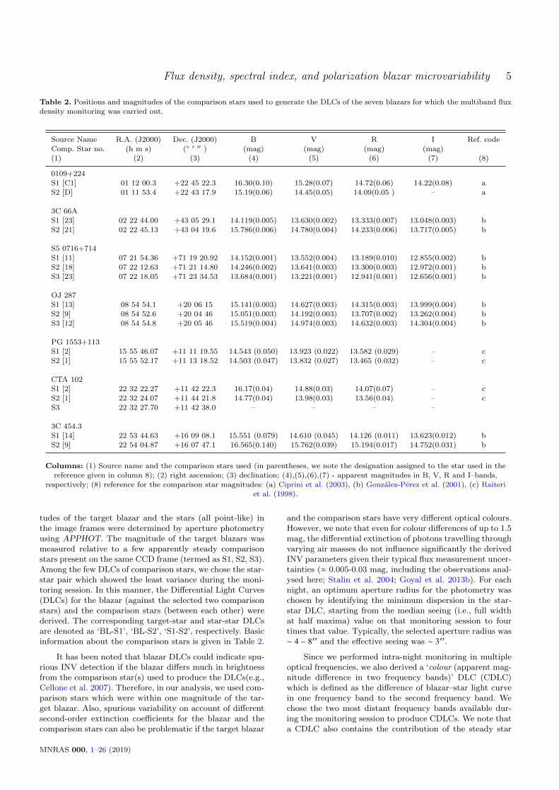
Flux density, spectral index, and polarization blazar microvariability 5
Table 2. Positions and magnitudes of the comparison stars used to generate the DLCs of the seven blazars for which the multiband fluxdensity monitoring was carried out.
Source Name R.A. (J2000) Dec. (J2000) B V R I Ref. codeComp. Star no. (h m s) (◦ ′ ′′ ) (mag) (mag) (mag) (mag)
(1) (2) (3) (4) (5) (6) (7) (8)
0109+224
S1 [C1] 01 12 00.3 +22 45 22.3 16.30(0.10) 15.28(0.07) 14.72(0.06) 14.22(0.08) a
S2 [D] 01 11 53.4 +22 43 17.9 15.19(0.06) 14.45(0.05) 14.09(0.05 ) – a
3C 66A
S1 [23] 02 22 44.00 +43 05 29.1 14.119(0.005) 13.630(0.002) 13.333(0.007) 13.048(0.003) bS2 [21] 02 22 45.13 +43 04 19.6 15.786(0.006) 14.780(0.004) 14.233(0.006) 13.717(0.005) b
S5 0716+714S1 [11] 07 21 54.36 +71 19 20.92 14.152(0.001) 13.552(0.004) 13.189(0.010) 12.855(0.002) b
S2 [18] 07 22 12.63 +71 21 14.80 14.246(0.002) 13.641(0.003) 13.300(0.003) 12.972(0.001) b
S3 [23] 07 22 18.05 +71 23 34.53 13.684(0.001) 13.221(0.001) 12.941(0.001) 12.656(0.001) b
OJ 287S1 [13] 08 54 54.1 +20 06 15 15.141(0.003) 14.627(0.003) 14.315(0.003) 13.999(0.004) b
S2 [9] 08 54 52.6 +20 04 46 15.051(0.003) 14.192(0.003) 13.707(0.002) 13.262(0.004) b
S3 [12] 08 54 54.8 +20 05 46 15.519(0.004) 14.974(0.003) 14.632(0.003) 14.304(0.004) b
PG 1553+113
S1 [2] 15 55 46.07 +11 11 19.55 14.543 (0.050) 13.923 (0.022) 13.582 (0.029) – cS2 [1] 15 55 52.17 +11 13 18.52 14.503 (0.047) 13.832 (0.027) 13.465 (0.032) – c
CTA 102S1 [2] 22 32 22.27 +11 42 22.3 16.17(0.04) 14.88(0.03) 14.07(0.07) – c
S2 [1] 22 32 24.07 +11 44 21.8 14.77(0.04) 13.98(0.03) 13.56(0.04) – c
S3 22 32 27.70 +11 42 38.0 – – – –
3C 454.3S1 [14] 22 53 44.63 +16 09 08.1 15.551 (0.079) 14.610 (0.045) 14.126 (0.011) 13.623(0.012) b
S2 [9] 22 54 04.87 +16 07 47.1 16.565(0.140) 15.762(0.039) 15.194(0.017) 14.752(0.031) b
Columns: (1) Source name and the comparison stars used (in parentheses, we note the designation assigned to the star used in the
reference given in column 8); (2) right ascension; (3) declination; (4),(5),(6),(7) - apparent magnitudes in B, V, R and I–bands,respectively; (8) reference for the comparison star magnitudes: (a) Ciprini et al. (2003), (b) Gonzalez-Perez et al. (2001), (c) Raiteri
et al. (1998).
tudes of the target blazar and the stars (all point-like) inthe image frames were determined by aperture photometryusing APPHOT. The magnitude of the target blazars wasmeasured relative to a few apparently steady comparisonstars present on the same CCD frame (termed as S1, S2, S3).Among the few DLCs of comparison stars, we chose the star-star pair which showed the least variance during the moni-toring session. In this manner, the Differential Light Curves(DLCs) for the blazar (against the selected two comparisonstars) and the comparison stars (between each other) werederived. The corresponding target-star and star-star DLCsare denoted as ‘BL-S1’, ‘BL-S2’, ‘S1-S2’, respectively. Basicinformation about the comparison stars is given in Table 2.
It has been noted that blazar DLCs could indicate spu-rious INV detection if the blazar differs much in brightnessfrom the comparison star(s) used to produce the DLCs(e.g.,Cellone et al. 2007). Therefore, in our analysis, we used com-parison stars which were within one magnitude of the tar-get blazar. Also, spurious variability on account of differentsecond-order extinction coefficients for the blazar and thecomparison stars can also be problematic if the target blazar
and the comparison stars have very different optical colours.However, we note that even for colour differences of up to 1.5mag, the differential extinction of photons travelling throughvarying air masses do not influence significantly the derivedINV parameters given their typical flux measurement uncer-tainties (' 0.005-0.03 mag, including the observations anal-ysed here; Stalin et al. 2004; Goyal et al. 2013b). For eachnight, an optimum aperture radius for the photometry waschosen by identifying the minimum dispersion in the star-star DLC, starting from the median seeing (i.e., full widthat half maxima) value on that monitoring session to fourtimes that value. Typically, the selected aperture radius was∼ 4 − 8′′ and the effective seeing was ∼ 3′′.
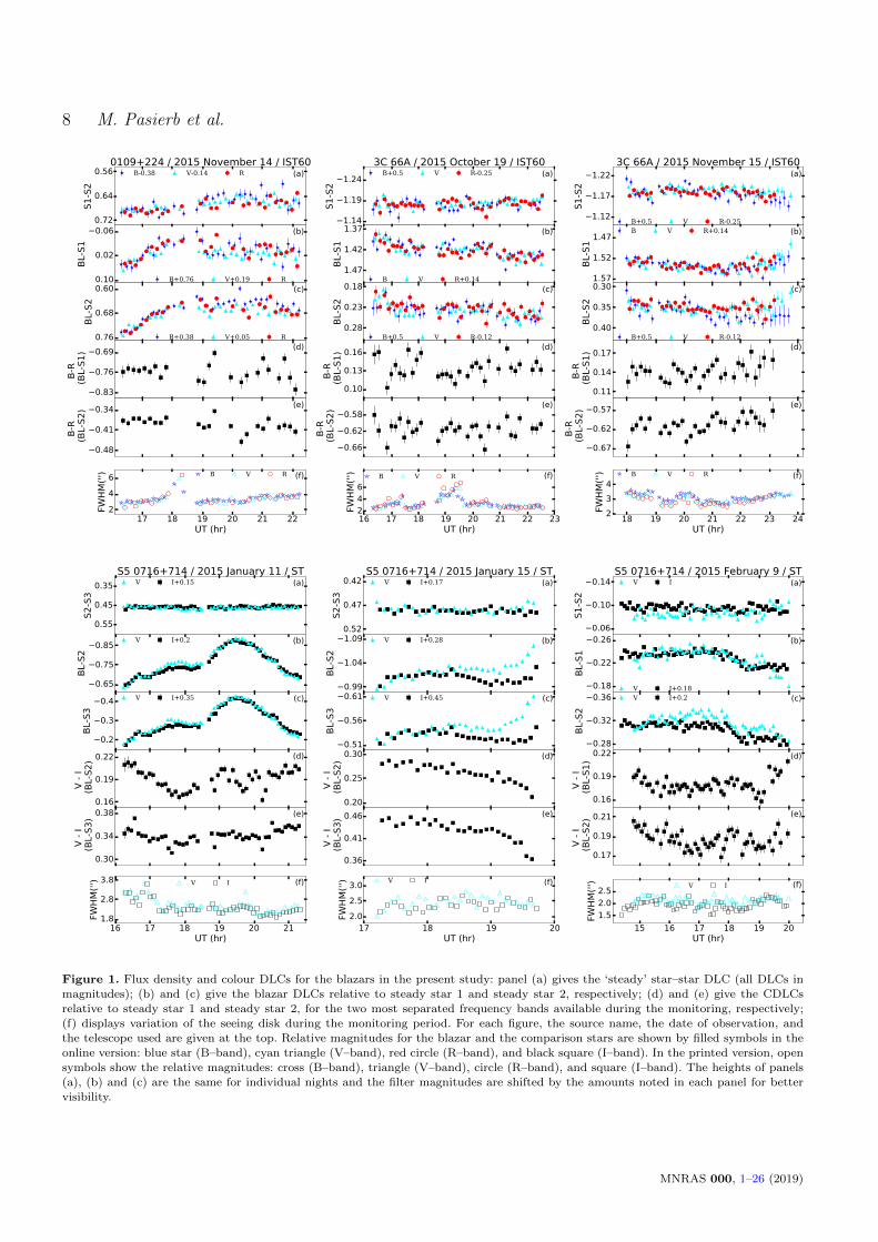
Since we performed intra-night monitoring in multipleoptical frequencies, we also derived a ‘colour (apparent mag-nitude difference in two frequency bands)’ DLC (CDLC)which is defined as the difference of blazar–star light curvein one frequency band to the second frequency band. Wechose the two most distant frequency bands available dur-ing the monitoring session to produce CDLCs. We note thata CDLC also contains the contribution of the steady star
MNRAS 000, 1–26 (2019)
6 M. Pasierb et al.
colour (Table 2) and hence the blazar colour could be ob-tained by subtracting the colour of the steady star concerned(Table 2). Finally, we computed the two-point spectral in-dex, αν2
ν1 , which is related to colour(ν1, ν2) by
αν2ν1 =
0.4 × colour(ν1, ν2) − log10(F(0, ν1)/F(0, ν2))log10(ν1/ν2)
(1)
where ν1 and ν2 refer to central frequencies of the passbandswhile F(0, ν1) and F(0, ν2) refer to zero point magnitude fluxesof the frequency bands. For the photometric system systemused in our observations, these are 4063 Jy, 3636 Jy, 3064 Jy,and 2635 Jy for the B, V, R, and I-bands, respectively (Glass1999). The statistical error on αν2
ν1 was derived using thestandard error propagation formula (Bevington & Robinson2003).
Our entire intra-night data are summarized in Table 3,and the newly acquired DLCs are shown in Figure 1. Ad-ditionally, we also searched for the presence of colour mi-crovariability in CDLCs using the F−test and the signif-icance criterion adopted for flux microvariability detection(see Section 4.1). Table 4 provides the summary of colour mi-crovariability for the CDLCs in our monitoring, along withthe ‘mean’ differential colour and two-point spectral indexof the blazar on a given session.
3.2 Summary of polarization monitoring
We employed three other telescopes to carry out the intra-night polarization monitoring for the sample. Below we givekey information on these observatories and instruments.
(i) 150 cm Kanata, Japan: A portion of our polariza-tion microvariability light curves come from monitoring us-ing the 150 cm Kanata telescope, run by Higashi–HiroshimaObservatory, Japan. We used Hiroshima One–shot Wide–field Polarimeter (HOWPol; Kawabata et al. 2008) whichis installed at the Nasmyth focus of the telescope. The po-larimetric observations were performed using the CousinsRc-filter.
(ii) 70 cm AZT-8+ST7, Russia: We used the 70 cmAZT-8+ST7 telescope of Crimean Astrophysical Observa-tory, located at Nauchnij, Russia for a large number of po-larimetric measurements. The observations were carried outin R-band (Larionov et al. 2013, 2016).
(iii) 40 cm LX-200, Russia: Lastly, we used the 40 cmLX-200 telescope of St. Petersburg State University, locatedat St. Petersburg, Russia for a comparable number of ob-servations. The observations were carried out in white-band(Larionov et al. 2013, 2016).
Our observing strategy consisted of obtaining successiveimages at four position angles of the half-wave plate, of 0◦,45◦, 22.5◦, and 67.5◦, for a continuous monitoring durationlasting for more than 3 hours. The calibration images, bias,and flat-frames were obtained either just before or soon afterthe target observations. In addition, un-polarized and highlypolarized standard stars were observed to set the instrumen-tal polarization and the position angle of the instrument.The observations were conducted using R-band at Kanataand AZT-8+ST7 and white light at LX-200. The details ofdata reduction from AZT-8+ST7 and LX-200 telescopes aregiven in Larionov et al. (2008, 2013, 2016).
For the Kanata data, the pre-processing (bias subtrac-tion and flat-fielding) of the images were carried out usingstandard procedures in IRAF. The flux of the target in eachhalf-wave plate combination was gathered using the aper-ture photometry in the APPHOT package. This enables themeasurement of PD and χ for the target while the totalintensity was computed using differential photometry usingthe comparison star on the same CCD frame. The polarizersplits the radiation into two parts, with orthogonal electricfield components which are denoted as ‘ordinary’, Io) and‘extra-ordinary’ Ie, images. The fluxes of Io and Ie imagesare thus obtained for the blazar and the comparison star us-ing a circular aperture that is roughly 2–3 times larger thanthe median seeing disc on the given night. The fractionallinear polarization (PD) is computed following the method-ology given by Wang et al. (2015):
PD =√
Q2 +U2 (2)
where, Q and U are the Stokes parameters which are deter-mined from:
Q =1 −
√(Ie/Io)0.0deg(Ie/Io)45.0deg
1 +√(Ie/Io)0.0deg(Ie/Io)45.0deg
, U =1 −
√(Ie/Io)22.5deg(Ie/Io)67.5deg
1 +√(Ie/Io)22.5deg(Ie/Io)67.5deg
, (3)
where Ie(0.0deg), Ie(45.0deg), Ie(22.5deg), Ie(67.5deg), Io(0.0deg),Io(45.0deg), Io(22.5deg), and Io(67.5deg) are the fluxes of the extra-ordinary and ordinary image components for the HWP com-binations at 0.0, 45.0, 22.5, and 67.5 deg., respectively. Theelectric vector polarization angle is
χ =12
arctan(U
Q
). (4)
Statistical errors on Q and U are obtained following standarderror propagation (Bevington & Robinson 2003) and assum-ing Poisson statistics, meaning δIe =
√Ie and δIo =
√Io, etc.,
for each HWP combination. Table 5 presents the polariza-tion data on all 30 monitoring sessions while Figure 2 showsthe light curves for which more than 10 data points, withoutany large gaps, were available for a monitoring session.
4 ANALYSIS OF INTRA-NIGHT LIGHTCURVES
4.1 Determination of microvariability parametersin the DLCs
Following Goyal et al. (2013b), we used the F−test for assign-ing the INV detection significance. The F−statistic comparesthe observed variance Vobs to the expected variance Vexp. Thenull hypothesis of no variability is rejected when the ratio
Fαν =VobsVexp
=Vt−s〈η2 σ2
t−s〉, (5)
exceeds a critical value for a chosen significance level α, fora given number of degrees of freedom (DOF) ν; here Vt−s isthe variance of the ‘target-star’ DLC, 〈σ2
t−s〉 is the mean ofthe squares of the (formal) rms errors of the individual data
MNRAS 000, 1–26 (2019)
Flux density, spectral index, and polarization blazar microvariability 7
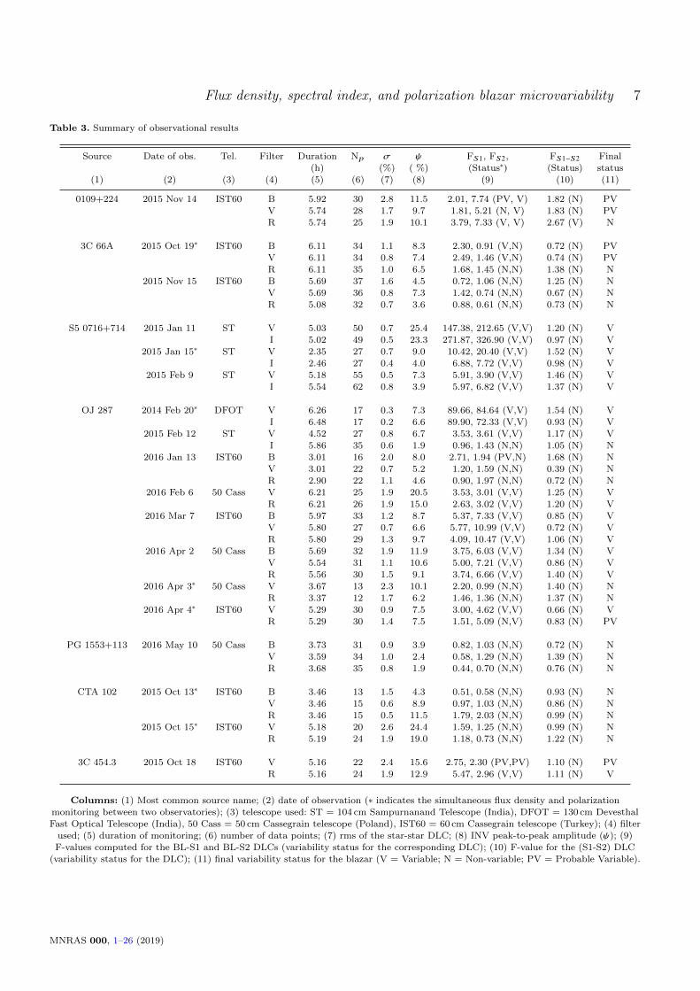
Table 3. Summary of observational results
Source Date of obs. Tel. Filter Duration Np σ ψ FS1, FS2, FS1−S2 Final(h) (%) ( %) (Status∗) (Status) status
(1) (2) (3) (4) (5) (6) (7) (8) (9) (10) (11)
0109+224 2015 Nov 14 IST60 B 5.92 30 2.8 11.5 2.01, 7.74 (PV, V) 1.82 (N) PV
V 5.74 28 1.7 9.7 1.81, 5.21 (N, V) 1.83 (N) PV
R 5.74 25 1.9 10.1 3.79, 7.33 (V, V) 2.67 (V) N
3C 66A 2015 Oct 19∗ IST60 B 6.11 34 1.1 8.3 2.30, 0.91 (V,N) 0.72 (N) PVV 6.11 34 0.8 7.4 2.49, 1.46 (V,N) 0.74 (N) PV
R 6.11 35 1.0 6.5 1.68, 1.45 (N,N) 1.38 (N) N
2015 Nov 15 IST60 B 5.69 37 1.6 4.5 0.72, 1.06 (N,N) 1.25 (N) NV 5.69 36 0.8 7.3 1.42, 0.74 (N,N) 0.67 (N) N
R 5.08 32 0.7 3.6 0.88, 0.61 (N,N) 0.73 (N) N
S5 0716+714 2015 Jan 11 ST V 5.03 50 0.7 25.4 147.38, 212.65 (V,V) 1.20 (N) V
I 5.02 49 0.5 23.3 271.87, 326.90 (V,V) 0.97 (N) V
2015 Jan 15∗ ST V 2.35 27 0.7 9.0 10.42, 20.40 (V,V) 1.52 (N) VI 2.46 27 0.4 4.0 6.88, 7.72 (V,V) 0.98 (N) V
2015 Feb 9 ST V 5.18 55 0.5 7.3 5.91, 3.90 (V,V) 1.46 (N) V
I 5.54 62 0.8 3.9 5.97, 6.82 (V,V) 1.37 (N) V
OJ 287 2014 Feb 20∗ DFOT V 6.26 17 0.3 7.3 89.66, 84.64 (V,V) 1.54 (N) VI 6.48 17 0.2 6.6 89.90, 72.33 (V,V) 0.93 (N) V
2015 Feb 12 ST V 4.52 27 0.8 6.7 3.53, 3.61 (V,V) 1.17 (N) V
I 5.86 35 0.6 1.9 0.96, 1.43 (N,N) 1.05 (N) N2016 Jan 13 IST60 B 3.01 16 2.0 8.0 2.71, 1.94 (PV,N) 1.68 (N) N
V 3.01 22 0.7 5.2 1.20, 1.59 (N,N) 0.39 (N) N
R 2.90 22 1.1 4.6 0.90, 1.97 (N,N) 0.72 (N) N2016 Feb 6 50 Cass V 6.21 25 1.9 20.5 3.53, 3.01 (V,V) 1.25 (N) V
R 6.21 26 1.9 15.0 2.63, 3.02 (V,V) 1.20 (N) V
2016 Mar 7 IST60 B 5.97 33 1.2 8.7 5.37, 7.33 (V,V) 0.85 (N) VV 5.80 27 0.7 6.6 5.77, 10.99 (V,V) 0.72 (N) V
R 5.80 29 1.3 9.7 4.09, 10.47 (V,V) 1.06 (N) V
2016 Apr 2 50 Cass B 5.69 32 1.9 11.9 3.75, 6.03 (V,V) 1.34 (N) VV 5.54 31 1.1 10.6 5.00, 7.21 (V,V) 0.86 (N) V
R 5.56 30 1.5 9.1 3.74, 6.66 (V,V) 1.40 (N) V
2016 Apr 3∗ 50 Cass V 3.67 13 2.3 10.1 2.20, 0.99 (N,N) 1.40 (N) NR 3.37 12 1.7 6.2 1.46, 1.36 (N,N) 1.37 (N) N
2016 Apr 4∗ IST60 V 5.29 30 0.9 7.5 3.00, 4.62 (V,V) 0.66 (N) VR 5.29 30 1.4 7.5 1.51, 5.09 (N,V) 0.83 (N) PV
PG 1553+113 2016 May 10 50 Cass B 3.73 31 0.9 3.9 0.82, 1.03 (N,N) 0.72 (N) NV 3.59 34 1.0 2.4 0.58, 1.29 (N,N) 1.39 (N) N
R 3.68 35 0.8 1.9 0.44, 0.70 (N,N) 0.76 (N) N
CTA 102 2015 Oct 13∗ IST60 B 3.46 13 1.5 4.3 0.51, 0.58 (N,N) 0.93 (N) N
V 3.46 15 0.6 8.9 0.97, 1.03 (N,N) 0.86 (N) NR 3.46 15 0.5 11.5 1.79, 2.03 (N,N) 0.99 (N) N
2015 Oct 15∗ IST60 V 5.18 20 2.6 24.4 1.59, 1.25 (N,N) 0.99 (N) NR 5.19 24 1.9 19.0 1.18, 0.73 (N,N) 1.22 (N) N
3C 454.3 2015 Oct 18 IST60 V 5.16 22 2.4 15.6 2.75, 2.30 (PV,PV) 1.10 (N) PV
R 5.16 24 1.9 12.9 5.47, 2.96 (V,V) 1.11 (N) V
Columns: (1) Most common source name; (2) date of observation (∗ indicates the simultaneous flux density and polarizationmonitoring between two observatories); (3) telescope used: ST = 104 cm Sampurnanand Telescope (India), DFOT = 130 cm Devesthal
Fast Optical Telescope (India), 50 Cass = 50 cm Cassegrain telescope (Poland), IST60 = 60 cm Cassegrain telescope (Turkey); (4) filter
used; (5) duration of monitoring; (6) number of data points; (7) rms of the star-star DLC; (8) INV peak-to-peak amplitude (ψ); (9)F-values computed for the BL-S1 and BL-S2 DLCs (variability status for the corresponding DLC); (10) F-value for the (S1-S2) DLC
(variability status for the DLC); (11) final variability status for the blazar (V = Variable; N = Non-variable; PV = Probable Variable).
MNRAS 000, 1–26 (2019)
8 M. Pasierb et al.
0.72
0.64
0.56
S1
-S2
(a)0109+224 / 2015 November 14 / IST60
B-0.38 V-0.14 R
0.10
0.02
0.06
BL-
S1
(b)
B+0.76 V+0.19 R
0.76
0.68
0.60
BL-
S2
(c)
B+0.38 V+0.05 R
0.83
0.76
0.69
B-R
(
BL-
S1
)
(d)
0.48
0.41
0.34
B-R
(
BL-
S2
)
(e)
17 18 19 20 21 22UT (hr)
2
4
6
FWH
M('
') (f)B V R
1.14
1.19
1.24
S1
-S2
(a)3C 66A / 2015 October 19 / IST60
B+0.5 V R-0.25
1.47
1.42
1.37
BL-
S1
(b)
B V R+0.14
0.28
0.23
0.18
BL-
S2
(c)
B+0.5 V R-0.12
0.10
0.13
0.16
B-R
(
BL-
S1
)(d)
0.66
0.62
0.58
B-R
(
BL-
S2
)
(e)
16 17 18 19 20 21 22 23UT (hr)
246
FWH
M('
') (f)B V R
1.12
1.17
1.22
S1
-S2
(a)3C 66A / 2015 November 15 / IST60
B+0.5 V R-0.25
1.57
1.52
1.47
BL-
S1
(b)B V R+0.14
0.40
0.35
0.30
BL-
S2
(c)
B+0.5 V R-0.12
0.11
0.14
0.17
B-R
(
BL-
S1
)
(d)
0.67
0.62
0.57
B-R
(
BL-
S2
)
(e)
18 19 20 21 22 23 24UT (hr)
2
3
4
FWH
M('
') (f)B V R
0.55
0.45
0.35
S2
-S3
(a)S5 0716+714 / 2015 January 11 / ST
V I+0.15
0.65
0.75
0.85
BL-
S2
(b)V I+0.2
0.2
0.3
0.4
BL-
S3
(c)V I+0.35
0.16
0.19
0.22
V -
I
(B
L-S2
)
(d)
0.30
0.34
0.38
V -
I
(B
L-S3)
(e)
16 17 18 19 20 21UT (hr)
1.8
2.8
3.8
FWH
M('
') (f)V I
0.52
0.47
0.42
S2
-S3
(a)S5 0716+714 / 2015 January 15 / ST
V I+0.17
0.99
1.04
1.09
BL-
S2
(b)V I+0.28
0.51
0.56
0.61
BL-
S3
(c)V I+0.45
0.20
0.25
0.30
V -
I
(B
L-S2
)
(d)
0.36
0.41
0.46
V -
I
(B
L-S3)
(e)
17 18 19 20UT (hr)
2.0
2.5
3.0
FWH
M('
') (f)V I
0.06
0.10
0.14S1
-S2
(a)S5 0716+714 / 2015 February 9 / ST
V I
0.18
0.22
0.26
BL-
S1
(b)
V I+0.18
0.28
0.32
0.36
BL-
S2
(c)V I+0.2
0.16
0.19
0.22
V -
I
(B
L-S1
)
(d)
0.17
0.19
0.21
V -
I
(B
L-S2)
(e)
15 16 17 18 19 20UT (hr)
1.5
2.0
2.5
FWH
M('
') (f)V I
Figure 1. Flux density and colour DLCs for the blazars in the present study: panel (a) gives the ‘steady’ star–star DLC (all DLCs in
magnitudes); (b) and (c) give the blazar DLCs relative to steady star 1 and steady star 2, respectively; (d) and (e) give the CDLCsrelative to steady star 1 and steady star 2, for the two most separated frequency bands available during the monitoring, respectively;
(f) displays variation of the seeing disk during the monitoring period. For each figure, the source name, the date of observation, andthe telescope used are given at the top. Relative magnitudes for the blazar and the comparison stars are shown by filled symbols in theonline version: blue star (B–band), cyan triangle (V–band), red circle (R–band), and black square (I–band). In the printed version, opensymbols show the relative magnitudes: cross (B–band), triangle (V–band), circle (R–band), and square (I–band). The heights of panels
(a), (b) and (c) are the same for individual nights and the filter magnitudes are shifted by the amounts noted in each panel for bettervisibility.
MNRAS 000, 1–26 (2019)

Flux density, spectral index, and polarization blazar microvariability 9
0.33
0.37
0.41
S1
-S3
(a)OJ 287 / 2014 February 20 / DFOT
V I+0.06
0.40
0.36
0.32
BL-
S1
(b)V I+0.48
0.05
0.01
0.03
BL-
S3
(c)V I+0.43
0.47
0.48
0.49
V -
I
(B
L-S1
)
(d)
0.41
0.42
0.43
0.44
V -
I
(B
L-S3
)
(e)
14 15 16 17 18 19 20 21UT (hr)
2.0
2.6
3.2
FWH
M('
') (f)V I
0.26
0.30
0.34
S1
-S3
(a)OJ 287 / 2015 February 12 / ST
V+0.08 I
0.13
0.09
0.05
BL-
S1
(b)V-0.25 I
0.14
0.18
0.22
BL-
S3
(c)
V-0.17 I
0.20
0.25
0.30
V -
I
(B
L-S1
)(d)
0.12
0.17
0.22
V -
I
(B
L-S3
)
(e)
15 16 17 18 19 20 21 22UT (hr)
1.8
2.3
2.8
FWH
M('
') (f)V I
0.45
0.40
0.35
S1
-S2
(a)OJ 287 / 2016 January 13 / IST60
B+0.3 V R-0.17
0.05
0.00
0.05
BL-
S1
(b)B V R+0.15
0.50
0.45
0.40
BL-
S2
(c)B+0.35 V R
0.09
0.13
0.17
B -
R
(B
L-S1
)
(d)
0.40
0.36
0.32
B -
R
(B
L-S2
)
(e)
19 20 21UT (hr)
2.53.54.5
FWH
M('
') (f)B V R
0.50
0.35
0.20
S1
-S2
(a)OJ 287 / 2016 February 6 / 50 Cass
V R-0.2
0.67
0.52
0.37
BL-
S1
(b)V R+0.18
1.07
0.92
0.77
BL-
S2
(c)V R-0.03
0.07
0.17
0.27
V -
R
(B
L-S1
)
(d)
0.13
0.03
0.07
V -
R
(B
L-S2)
(e)
18 19 20 21 22 23 24 25UT (hr)
1.8
2.8
3.8
FWH
M('
') (f)V R
0.45
0.40
0.35
S1
-S2
(a)OJ 287 / 2016 March 7 / IST60B+0.31 V R-0.19
0.52
0.57
0.62
BL-
S1
(b)B V-0.02 R+0.12
0.08
0.13
0.18
BL-
S2
(c)B+0.35 V R-0.04
0.06
0.10
0.14
B -
R
(B
L-S1
)
(d)
0.44
0.40
0.36
B -
R
(B
L-S2)
(e)
16 17 18 19 20 21 22UT (hr)
345
FWH
M('
') (f)B V R
0.43
0.35
0.27S1
-S2
(a)OJ 287 / 2016 April 2 / 50 Cass
B+0.25 V R-0.2
0.00
0.08
0.16
BL-
S1
(b)
B V R+0.14
0.44
0.36
0.28
BL-
S2
(c)
B+0.3 V+0.05 R
0.08
0.13
0.18
B -
R
(B
L-S1
)
(d)
0.36
0.31
0.26
B -
R
(B
L-S2)
(e)
18 19 20 21 22 23 24UT (hr)
1.5
2.5
3.5
FWH
M('
') (f)B V R
Figure 1 (Cont.).
points in the ‘target-star’ DLC. We note that one-way Anal-ysis of Variance (ANOVA; De Diego 2010, see also, De Diego2014 for the enhanced F−test which requires usage of multi-ple star-star DLCs) could also be used to test for microvari-ability and has some advantages; however, a robust imple-mentation of this approach requires a sufficiently large num-ber of data points (>30). Since our aim was to study colourevolution along with polarization on intra-night timescales,
the number of data points in a single optical band rarely sat-isfied this condition. Therefore, we use the F−test to assignthe INV detection in the DLCs. Since this method requiresflux density or magnitude estimates along with their errorestimates, it is important to determine the photometric er-rors accurately. As emphasized in several independent stud-ies, the photometric errors returned by APPHOT are sig-nificantly underestimated (by factors of η = 1.3–1.7; Gopal-
MNRAS 000, 1–26 (2019)

10 M. Pasierb et al.
0.63
0.56
0.49
S1
-S2
(a)OJ 287 / 2016 April 3 / 50 Cass
V+0.2 R
0.06
0.13
0.20
BL-
S1
(b)
V-0.15 R
0.50
0.43
0.36
BL-
S2
(c)V+0.05 R
0.08
0.18
0.28
V -
R
(B
L-S1
)
(d)
0.10
0.05
0.00
V -
R
(B
L-S2
)
(e)
19 20 21 22UT (hr)
1.5
2.0
2.5
FWH
M('
') (f)V R
0.45
0.41
0.37
S1
-S2
(a)OJ 287 / 2016 April 4 / IST60V R-0.18
0.12
0.16
0.20
BL-
S1
(b)V R+0.15
0.32
0.28
0.24
BL-
S2
(c)V R-0.03
0.10
0.15
0.20
V -
R
(B
L-S1
)(d)
0.06
0.03
0.00
V -
R
(B
L-S2
)
(e)
16 17 18 19 20 21UT (hr)
2.7
3.1
3.5
FWH
M('
') (f)V R
0.14
0.10
0.06
S1
-S2
(a)PG 1553+113 / 2016 May 10 / 50 Cass
B+0.05 V+0.03 R
0.36
0.32
0.28
BL-
S1
(b)B+0.25 V+0.05 R
0.48
0.44
0.40
BL-
S2
(c)B+0.3 V+0.07 R
0.28
0.25
0.22
B -
R
(B
L-S1
)
(d)
0.34
0.30
0.26
B -
R
(B
L-S2
)
(e)
21 22 23 24UT (hr)
1.42.23.0
FWH
M('
') (f)B V R
1.00
0.92
0.84
S1
-S2
(a)CTA 102 / 2015 October 13 / IST60
B-0.55 V R+0.4
1.82
1.74
1.66
BL-
S1
(b)B+0.8 V R-0.45
2.76
2.68
2.60
BL-
S2
(c)B+0.25 V R-0.06
1.35
1.25
1.15
B-R
(
BL-
S1
)
(d)
0.4
0.3
0.2
B-R
(
BL-
S2)
(e)
15 16 17 18 19UT (hr)
2.5
4.0
5.5
FWH
M('
') (f)B V R
1.1
1.3
1.5
S1
-S3
(a)CTA 102 / 2015 October 15 / IST60
V R+0.25
2.2
2.0
1.8
BL-
S1
(b)
V R-0.55
1.0
0.8
0.6
BL-
S3
(c)
V R-0.27
0.65
0.50
0.35
V-R
(
BL-
S1
)
(d)
0.40
0.25
0.10
V-R
(
BL-
S3)
(e)
16 17 18 19 20 21UT (hr)
3.0
4.5
6.0
FWH
M('
') (f)V R
1.05
1.15
1.25S1
-S2
(a)3C 454.3 / 2015 October 18 / IST60
V R
0.95
0.85
0.75
BL-
S1
(b)V R-0.1
0.15
0.25
0.35
BL-
S2
(c)V R-0.1
0.18
0.13
0.08
V-R
(
BL-
S1
)
(d)
0.18
0.12
0.06
V-R
(
BL-
S2)
(e)
15 16 17 18 19 20 21UT (hr)
2.5
3.5
4.5
FWH
M('
') (f)V R
Figure 1 (Cont.).
Krishna et al. 1995; Garcia et al. 1999; Stalin et al. 2004;Bachev et al. 2005; Zhang et al. 2018). Goyal et al. (2013a)obtained η =1.54±0.05, using 262 steady star-star DLCs andinvolving intra-night observations with three different tele-scopes located in India. Thus, η =1.54 has been used in thepresent analysis to scale up the photometric magnitude er-rors returned by IRAF.
The significance level set for a given test determines the
expected number of false positives, which is an indicator ofthe robustness of the test. We have chosen two significancelevels, α = 0.01 and 0.05, corresponding to p−values of & 0.99and & 0.95, respectively. Since the smaller the value of α is,the less likely it is for the variability to occur by chance, thus,a genuine INV detection is claimed, i.e., a ‘variable’ designa-tion (V) is assigned, if the computed statistic value is abovethe critical value corresponding to p > 0.99 (i.e., α = 0.01)
MNRAS 000, 1–26 (2019)

Flux density, spectral index, and polarization blazar microvariability 11
Table 4. Colour microvariability results
Source Date of obs. Tel. Np Filters colour αν2ν1 Fcc (status∗)
(1) (2) (3) (4) (5) (6) (7) (8)
0109+224 2015 Nov 14 IST60 23 B–R −0.76±0.03, −0.39±0.02 1.11±0.06 1.34, 1.58 (N, N)
3C 66A 2015 Oct 19 IST60 31 B–R 0.14±0.02, −0.62±0.02 1.51±0.04 1.02, 0.85 (N, N)2015 Nov 15 IST60 31 B–R 0.14±0.01, −0.61±0.02 1.53±0.04 0.68, 1.15 (N, N)
S5 0716+714 2015 Jan 11† ST 48 V–I 0.19±0.01, 0.34±0.01 1.33±0.03 3.47, 3.77 (V, V)
2015 Jan 15† ST 26 V–I 0.26±0.02, 0.43±0.02 1.53±0.05 8.03, 17.31 (V, V)
2015 Feb 9† ST 54 V–I 0.18±0.01, 0.19±0.01 1.28±0.02 1.62, 1.30 (PV, N)
OJ 287 2014 Feb 20† DFOT 16 V–I 0.48±0.01, 0.42±0.01 1.87±0.02 5.14, 8.83 (V, V)
2015 Feb 12† ST 27 V–I 0.25±0.02, 0.17±0.02 1.27±0.04 2.77, 3.61 (V, V)2016 Jan 13 IST60 13 B–R 0.14±0.02, −0.36±0.02 1.62± 0.04 0.88, 0.92 (N, N)
2016 Feb 6† 50 Cass 24 V–R 0.16±0.04, −0.04±0.03 1.55±0.18 0.96, 0.76 (N, N)
2016 Mar 7† IST60 29 B–R 0.11±0.02, −0.39±0.02 1.55±0.04 1.48, 161 (N, N)
2016 Apr 2† 50 Cass 30 B–R 0.13±0.02, −0.31±0.02 1.67±0.04 0.81, 1.41 (N, N)2016 Apr 3 50 Cass 12 V–R 0.14±0.04, −0.06±0.02 1.43±0.14 2.04, 0.81 (N, N)
2016 Apr 4† IST60 29 V–R 0.15±0.02, −0.03±0.02 1.55±0.08 0.61, 0.93 (N, N)PG 1553+113 2016 May 10 50 Cass 30 B–R −0.25±0.01, −0.31±0.02 1.01±0.03 0.51, 0.97 (N, N)
CTA 102 2015 Oct 13 IST60 13 B–R −1.26±0.05, −0.32±0.05 1.37±0.12 1.33, 1.29 (N, N)
2015 Oct 15 IST60 19 V–R −0.51±0.09 −0.25±0.07 0.65±0.51 1.78, 1.04 (N, N)
3C 454.3 2015 Oct 18† IST60 21 V–R −0.13±0.02, −0.12±0.03 1.22±0.13 0.80, 0.69 (N,N)
Columns: (1) Most common source name; (2) date of the observation/monitoring; (3) telescope used; (4) number of data points; (5)filters used for colour estimation; (6) computed mean value (colour index) for both CDLCs; (7) spectral index; (8) F-values computed
for the BL-S1 and BL-S2 CDLCs (variability status for the corresponding CDLC).∗ V = Variable; N = Non-variable; PV = Probable Variable. † blazar showed confirmed INV in at least one frequency band.
for a given degree of freedom (ν = Np − 1, where Np standsfor the number of data points in a given DLC). We assigna ‘probable variable’ designation (PV) when the computedtest statistic value is found to be between the critical valuesat α = 0.01 and 0.05; otherwise, a ‘non-variable’ (N) designa-tion is assigned to a DLC, though of course variability couldstill be present but at a lower level of significance. All thethree DLCs, i.e., BL−S1, BL−S2, and S1−S2, are subjectedto the F−test analysis. In a few cases, the microvariabilitystatus was different for the two blazar-star DLCs, and thisindicated a small amplitude variation of one or the othercomparison stars was likely to be present. Since such smallamplitude variations in star-star DLCs are difficult to ascer-tain, we conservatively only ascribed a “V” status if bothblazar-star DLCs gave a “V” status; otherwise, we quotea“PV” or “N” status if the star-star DLC itself turned tobe variable. Table 3 summarizes the analysis results for theseven blazars (except 3C 279) for which the multiband fluxdensity monitoring was carried out.
Following Romero et al. (1999) the peak-to-peak mi-crovariability amplitude was calculated as
ψ =
√(Dmax − Dmin)2 − 2σ2 , (6)
with Dmin/max denoting the minimum/maximum in the DLC
of the source, and σ2 = η2 〈σ2i 〉 where η = 1.54 (Goyal et al.
2013a) and σi is the nominal error associated with each datapoint.
The microvariability duty cycle (DC) was computed ac-cording to
DC = 100%
∑nj=1 Nj (1/∆tj )∑nj=1(1/∆tj )
, (7)
where ∆tj = ∆tj, obs (1+ z)−1 is the duration of the monitoring
session of a source on the jth night, corrected for the cosmo-logical redshift z, and Nj is set equal to 1 if microvariabilitywas detected, and otherwise to 0 (Stalin et al. 2004). Thisestimate is essentially the ratio of the number of nights asource is found to be variable to the total number of nightsit was monitored; ∆tj is used to weight to the monitoringduration for the evaluation of DC. We compute the DC us-ing intra-night light curves in V-filter because it was thepassband used for monitoring all the nights in this study.The computed microvariability DC for the light curves inV-band, consisting of 18 nights on 7 blazar sources, is 45%(55% if PV cases are also included).
We have performed a sanity check by computing thenumber of ‘Type 1 errors’, or the false positives, for ourdata set. A false positive arises due the rejection of a truenull hypothesis by a test, when applied to a non-varyingDLC and is solely dependent on the α value set for the testand the number of DLCs. We note that for our data set con-sisting of 18 steady star-star DLCs in V-filter, the means ofthe expected numbers of false positives are ' 0.2 and ' 1 forα = 0.01 and 0.05, respectively. Since the distribution of falsepositives is expectedly binomial, for α = 0.01 the number offalse positives should in fact be scattered between 0 and 2,and for most of the cases around ' 0.3 ± 0.5. Similarly, withα = 0.05, the number of false positives should lie between0 and 5, and should largely cluster at ' 1 ± 1. Meanwhile,the observed numbers of false positives reported by the ap-plication of the F−test (see column 10 of Table 3) is 0 forα = 0.01 and 0 for α = 0.05 (V-filter). The good agreementbetween the expected and the observed numbers of false pos-itives provides validation for our analysis procedure.
MNRAS 000, 1–26 (2019)
12 M. Pasierb et al.
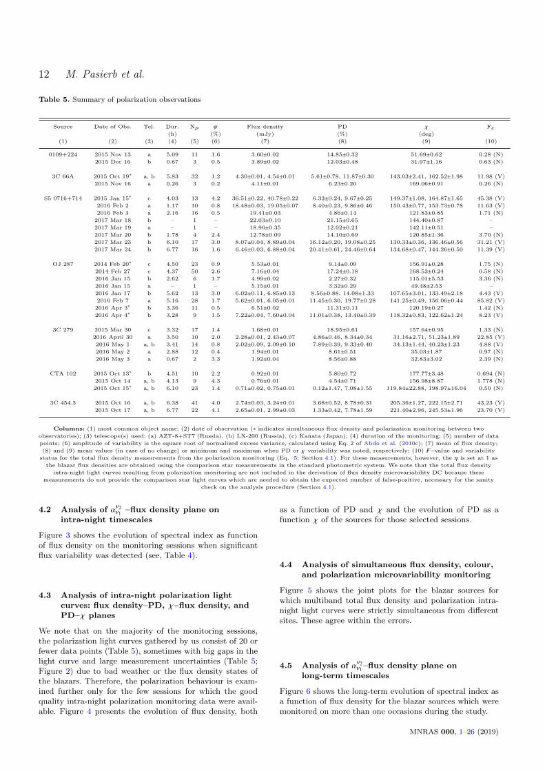
Table 5. Summary of polarization observations
Source Date of Obs. Tel. Dur. Np ψ Flux density PD χ Fc
(h) (%) (mJy) (%) (deg)
(1) (2) (3) (4) (5) (6) (7) (8) (9) (10)
0109+224 2015 Nov 13 a 5.09 11 1.6 3.60±0.02 14.85±0.32 51.69±0.62 0.28 (N)
2015 Dec 16 b 0.67 3 0.5 3.89±0.02 12.03±0.48 31.97±1.16 0.63 (N)
3C 66A 2015 Oct 19∗ a, b 5.83 32 1.2 4.30±0.01, 4.54±0.01 5.61±0.78, 11.87±0.30 143.03±2.41, 162.52±1.98 11.98 (V)
2015 Nov 16 a 0.26 3 0.2 4.11±0.01 6.23±0.20 169.06±0.91 0.26 (N)
S5 0716+714 2015 Jan 15∗ c 4.03 13 4.2 36.51±0.22, 40.78±0.22 6.33±0.24, 9.67±0.25 149.37±1.08, 164.87±1.65 45.38 (V)
2016 Feb 2 a 1.17 10 0.8 18.48±0.03, 19.05±0.07 8.40±0.23, 9.86±0.46 150.43±0.77, 153.73±0.78 11.63 (V)
2016 Feb 3 a 2.16 16 0.5 19.41±0.03 4.86±0.14 121.83±0.85 1.71 (N)
2017 Mar 18 b – 1 – 22.03±0.10 21.15±0.65 144.40±0.87 –
2017 Mar 19 a – 1 – 18.96±0.35 12.02±0.21 142.11±0.51 –
2017 Mar 20 b 1.78 4 2.4 12.78±0.09 14.10±0.69 120.85±1.36 3.70 (N)
2017 Mar 23 b 6.10 17 3.0 8.07±0.04, 8.89±0.04 16.12±0.20, 19.08±0.25 130.33±0.36, 136.46±0.56 31.21 (V)
2017 Mar 24 b 6.77 16 1.6 6.46±0.03, 6.88±0.04 20.41±0.61, 24.46±0.64 134.68±0.47, 144.26±0.50 11.39 (V)
OJ 287 2014 Feb 20∗ c 4.50 23 0.9 5.53±0.01 9.14±0.09 156.91±0.28 1.75 (N)
2014 Feb 27 c 4.37 50 2.6 7.16±0.04 17.24±0.18 168.53±0.24 0.58 (N)
2016 Jan 15 b 2.62 6 1.7 4.99±0.02 2.27±0.32 115.01±5.53 3.36 (N)
2016 Jan 15 a – 1 – 5.15±0.01 3.32±0.29 49.48±2.53 –
2016 Jan 17 b 5.62 13 3.0 6.02±0.11, 6.85±0.13 8.56±0.88, 14.08±1.33 107.65±3.01, 133.49±2.18 4.43 (V)
2016 Feb 7 a 5.16 28 1.7 5.62±0.01, 6.05±0.01 11.45±0.30, 19.77±0.28 141.25±0.49, 156.06±0.44 85.82 (V)
2016 Apr 3∗ b 3.36 11 0.5 6.51±0.02 11.31±0.11 120.19±0.27 1.42 (N)
2016 Apr 4∗ b 3.28 9 1.5 7.22±0.04, 7.60±0.04 11.01±0.38, 13.40±0.39 118.32±0.83, 122.62±1.24 8.23 (V)
3C 279 2015 Mar 30 c 3.32 17 1.4 1.68±0.01 18.95±0.61 157.64±0.95 1.33 (N)
2016 April 30 a 3.50 10 2.0 2.28±0.01, 2.43±0.07 4.86±0.46, 8.34±0.34 31.16±2.71, 51.23±1.89 22.85 (V)
2016 May 1 a, b 3.41 14 0.8 2.02±0.09, 2.09±0.10 7.89±0.39, 9.33±0.40 34.13±1.44, 40.23±1.23 4.88 (V)
2016 May 2 a 2.88 12 0.4 1.94±0.01 8.61±0.51 35.03±1.87 0.97 (N)
2016 May 3 a 0.67 2 3.3 1.92±0.04 8.56±0.88 32.83±3.02 2.39 (N)
CTA 102 2015 Oct 13∗ b 4.51 10 2.2 0.92±0.01 5.80±0.72 177.77±3.48 0.694 (N)
2015 Oct 14 a, b 4.13 9 4.3 0.76±0.01 4.54±0.71 156.98±8.87 1.778 (N)
2015 Oct 15∗ a, b 6.10 23 1.4 0.71±0.02, 0.75±0.01 0.12±1.47, 7.08±1.55 119.84±22.88, 198.97±16.04 0.50 (N)
3C 454.3 2015 Oct 16 a, b 6.38 41 4.0 2.74±0.03, 3.24±0.01 3.68±0.52, 8.78±0.31 205.36±1.27, 222.15±2.71 43.23 (V)
2015 Oct 17 a, b 6.77 22 4.1 2.65±0.01, 2.99±0.03 1.33±0.42, 7.78±1.59 221.40±2.96, 245.53±1.96 23.70 (V)
Columns: (1) most common object name; (2) date of observation (∗ indicates simultaneous flux density and polarization monitoring between two
observatories); (3) telescope(s) used: (a) AZT-8+ST7 (Russia), (b) LX-200 (Russia), (c) Kanata (Japan); (4) duration of the monitoring; (5) number of data
points; (6) amplitude of variability is the square root of normalized excess variance, calculated using Eq. 2 of Abdo et al. (2010c); (7) mean of flux density;
(8) and (9) mean values (in case of no change) or minimum and maximum when PD or χ variability was noted, respectively; (10) F−value and variability
status for the total flux density measurements from the polarization monitoring (Eq. 5; Section 4.1). For these measurements, however, the η is set at 1 as
the blazar flux densities are obtained using the comparison star measurements in the standard photometric system. We note that the total flux density
intra-night light curves resulting from polarization monitoring are not included in the derivation of flux density microvariability DC because these
measurements do not provide the comparison star light curves which are needed to obtain the expected number of false-positive, necessary for the sanity
check on the analysis procedure (Section 4.1).
4.2 Analysis of αν2ν1 –flux density plane on
intra-night timescales
Figure 3 shows the evolution of spectral index as functionof flux density on the monitoring sessions when significantflux variability was detected (see, Table 4).
4.3 Analysis of intra-night polarization lightcurves: flux density–PD, χ−flux density, andPD–χ planes
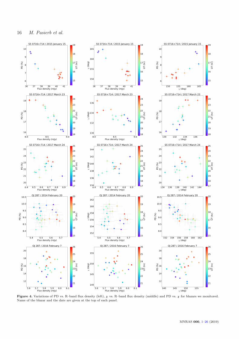
We note that on the majority of the monitoring sessions,the polarization light curves gathered by us consist of 20 orfewer data points (Table 5), sometimes with big gaps in thelight curve and large measurement uncertainties (Table 5;Figure 2) due to bad weather or the flux density states ofthe blazars. Therefore, the polarization behaviour is exam-ined further only for the few sessions for which the goodquality intra-night polarization monitoring data were avail-able. Figure 4 presents the evolution of flux density, both
as a function of PD and χ and the evolution of PD as afunction χ of the sources for those selected sessions.
4.4 Analysis of simultaneous flux density, colour,and polarization microvariability monitoring
Figure 5 shows the joint plots for the blazar sources forwhich multiband total flux density and polarization intra-night light curves were strictly simultaneous from differentsites. These agree within the errors.
4.5 Analysis of αν2ν1 –flux density plane on
long-term timescales
Figure 6 shows the long-term evolution of spectral index asa function of flux density for the blazar sources which weremonitored on more than one occasions during the study.
MNRAS 000, 1–26 (2019)
Flux density, spectral index, and polarization blazar microvariability 13
3.5
3.6
3.7
Flux d
ensi
ty(m
Jy)
(a)0109+224 / 2015 November 13 / AZT-8+ST7
13
15
17
PD
(%
)
(b)
19 20 21 22 23 24 25UT (hr)
46
51
56
χ (
deg)
(c)
4.3
4.4
4.5
Flux d
ensi
ty(m
Jy)
(a)3C 66A / 2015 October 19 / AZT-8+ST7 - LX-200
6
9
12
PD
(%
)
(b)
20 21 22 23 24 25 26UT (hr)
145
155
165χ (
deg)
(c)
36
39
42
Flux d
ensi
ty(m
Jy)
(a)S5 0716+714 / 2015 January 15 / Kanata
6
8
10
PD
(%
)
(b)
15 16 17 18 19UT (hr)
147
157
167
χ (
deg)
(c)
18.4
18.8
19.2
Flux d
ensi
ty(m
Jy)
(a)S5 0716+714 / 2016 February 2 / AZT-8+ST7
8.2
9.0
9.8
PD
(%
)
(b)
20 21UT (hr)
150
152
154
χ (
deg)
(c)
19.1
19.5
19.9
Flux d
ensi
ty(m
Jy)
(a)S5 0716+714 / 2016 February 3 / AZT-8+ST7
4.0
5.5
7.0
PD
(%
)
(b)
23 24 25UT (hr)
105
125
145
χ (
deg)
(c)
8.1
8.5
8.9
Flux d
ensi
ty(m
Jy)
(a)S5 0716+714 / 2017 March 23 / LX-200
16.0
17.5
19.0
PD
(%
)
(b)
18 19 20 21 22 23 24UT (hr)
130
133
136
χ (
deg)
(c)
6.40
6.65
6.90
Flux d
ensi
ty(m
Jy)
(a)S5 0716+714 / 2017 March 24 / LX-200
20
22
24
PD
(%
)
(b)
17 18 19 20 21 22 23 24 25UT (hr)
135
140
145
χ (
deg)
(c)
5.40
5.55
5.70
Flux d
ensi
ty(m
Jy)
(a)OJ 287 / 2014 February 20 / Kanata
8
9
10
PD
(%
)
(b)
15 16 17 18 19 20UT (hr)
152
157
162
χ (
deg)
(c)
6.5
7.0
7.5
8.0
Flux d
ensi
ty(m
Jy)
(a)OJ 287 / 2014 February 27 / Kanata
14
18
22
PD
(%
)
(b)
15 16 17 18 19UT (hr)
162
169
176
χ (
deg)
(c)
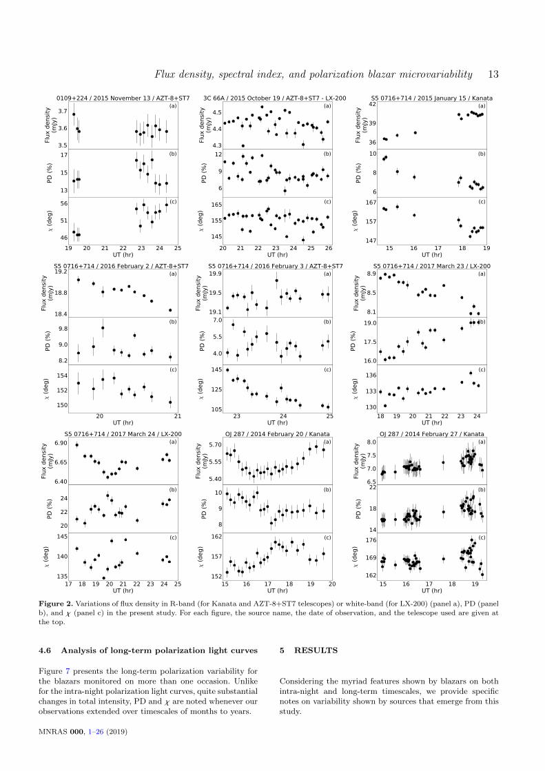
Figure 2. Variations of flux density in R-band (for Kanata and AZT-8+ST7 telescopes) or white-band (for LX-200) (panel a), PD (panelb), and χ (panel c) in the present study. For each figure, the source name, the date of observation, and the telescope used are given atthe top.
4.6 Analysis of long-term polarization light curves
Figure 7 presents the long-term polarization variability forthe blazars monitored on more than one occasion. Unlikefor the intra-night polarization light curves, quite substantialchanges in total intensity, PD and χ are noted whenever ourobservations extended over timescales of months to years.
5 RESULTS
Considering the myriad features shown by blazars on bothintra-night and long-term timescales, we provide specificnotes on variability shown by sources that emerge from thisstudy.
MNRAS 000, 1–26 (2019)

14 M. Pasierb et al.
4.8
5.0
5.2
Flux d
ensi
ty(m
Jy)
(a)OJ 287 / 2016 January 15 / LX-200
0
2
4
PD
(%
)
(b)
0 1 2 3UT (hr)
60
110
160
χ (
deg)
(c)
6.0
6.4
6.8
Flux d
ensi
ty(m
Jy)
(a)OJ 287 / 2016 January 17 / LX-200
8
11
14
PD
(%
)
(b)
21 22 23 24 25 26 27UT (hr)
105
120
135χ (
deg)
(c)
5.6
5.8
6.0
Flux d
ensi
ty(m
Jy)
(a)OJ 287 / 2016 February 7 / AZT-8+ST7
12
16
20
PD
(%
)
(b)
21 22 23 24 25 26UT (hr)
140
148
156
χ (
deg)
(c)
6.4
6.5
6.6
Flux d
ensi
ty(m
Jy)
(a)OJ 287 / 2016 April 3 / LX-200
10.0
11.5
13.0
PD
(%
)
(b)
19 20 21 22 23UT (hr)
114
119
124
χ (
deg)
(c)
7.2
7.4
7.6
Flux d
ensi
ty(m
Jy)
(a)OJ 287 / 2016 April 4 / LX-200
11.0
12.5
14.0
PD
(%
)
(b)
19 20 21 22 23UT (hr)
118
121
124
χ (
deg)
(c)
1.5
1.7
1.9
Flux d
ensi
ty(m
Jy)
(a)3C 279 / 2015 March 30 / Kanata
13
18
23
PD
(%
)
(b)
15 16 17 18UT (hr)
145
155
165
χ (
deg)
(c)
2.27
2.35
2.43
Flux d
ensi
ty(m
Jy)
(a)3C 279 / 2016 April 30 / AZT-8+ST7
4.5
6.5
8.5
PD
(%
)
(b)
20 21 22 23UT (hr)
30
40
50
χ (
deg)
(c)
2.00
2.05
2.10
Flux d
ensi
ty(m
Jy)
(a)3C 279 / 2016 May 1 /AZT-8+ST7 - LX-200
7.5
8.5
9.5
PD
(%
)
(b)
20 21 22 23UT (hr)
34
38
42
χ (
deg)
(c)
1.85
1.95
2.05
Flux d
ensi
ty(m
Jy)
(a)3C 279 / 2016 May 2 / AZT-8+ST7
4
8
12
PD
(%
)
(b)
19 20 21 22UT (hr)
10
40
70
χ (
deg)
(c)
Figure 2 (Cont.).
(i) 0109+224: This is a intermediate-frequency peakedBL Lac object (Abdo et al. 2010b). We could gather the to-tal intensity data on one occasion (Table 3, Figure 1) andpolarization data on two occasions (Table 5, Figure 2). Theblazar appeared to show an apparent ≈10 percent amplitudevariability but was assigned a ‘probable variable’ status inthe B- and V-bands and a ‘non-variable’ status in R-bandbecause the star–star DLC itself turned out to be variable(Table 3). The polarization intra-night curve is shown only
for the monitoring conducted on 2015 November 13 (Fig-ure 2); as we could gather only three data points on 2015December 16. The PD remained stable at ≈13 percent withabout 20 deg change in polarization angle between the twooccasions (Table 5; Figure 7).
(ii) 3C 66A: This blazar is classified as an intermediate-frequency peaked BL Lac object (Abdo et al. 2010b). It wasmonitored on two nights in total intensity (Table 3, Figure 1)and two nights in polarized light (Table 5, Figure 2) where
MNRAS 000, 1–26 (2019)

Flux density, spectral index, and polarization blazar microvariability 15
0.83
0.90
0.97
Flux d
ensi
ty(m
Jy)
(a)CTA 102 / 2015 October 13 / LX-200
2
6
10
PD
(%
)
(b)
17 18 19 20 21UT (hr)
150
175
200
χ (
deg)
(c)
0.7
0.8
0.9
Flux d
ensi
ty(m
Jy)
(a)CTA 102 / 2015 October 14 / LX-200
0
5
10
PD
(%
)
(b)
19 20 21 22 23UT (hr)
100
160
220χ (
deg)
(c)
0.68
0.73
0.78
Flux d
ensi
ty(m
Jy)
(a)CTA 102 / 2015 October 15 / AZT-8+ST7 - LX-200
0
4
8
PD
(%
)
(b)
17 18 19 20 21 22 23UT (hr)
100
150
200
χ (
deg)
(c)
2.75
3.00
3.25
Flux d
ensi
ty(m
Jy)
(a)3C 454.3 / 2015 October 16 / AZT-8+ST7 - LX-200
4.0
6.5
9.0
PD
(%
)
(b)
17 18 19 20 21 22 23UT (hr)
205
215
225
χ (
deg)
(c)
2.6
2.8
3.0
Flux d
ensi
ty(m
Jy)
(a)3C 454.3 / 2015 October 17 / AZT-8+ST7 - LX-200
4.0
6.5
9.0
PD
(%
)
(b)
16 17 18 19 20 21 22 23UT (hr)
218
231
244
χ (
deg)
(c)
Figure 2 (Cont.).
38 40 42 44 46Flux density I (mJy)
1.25
1.30
1.35
1.40
αV I
S5 0716+714 / 2015 January 11 / ST
17
18
19
20
21
UT (
hr)
55 56 57Flux density I (mJy)
1.40
1.45
1.50
1.55
1.60
1.65
αV I
S5 0716+714 / 2015 January 15 / ST
18
19
UT (
hr)
26.8 27.0 27.2 27.4 27.6 27.8Flux density I (mJy)
1.24
1.26
1.28
1.30
1.32
αV I
S5 0716+714 / 2015 February 9 / ST
15
16
17
18
19
UT (
hr)
7.1 7.2 7.3 7.4 7.5 7.6Flux density I (mJy)
1.84
1.86
1.88
1.90
1.92
αV I
OJ 287 / 2014 February 20 / DFOT
15
16
17
18
19
20
UT (
hr)
5.92 5.96 6.00 6.04Flux density I (mJy)
1.15
1.20
1.25
1.30
1.35
αV I
OJ 287 / 2015 February 12 / ST
16
17
18
19
20
UT (
hr)
Figure 3. α vs. I-band flux density evolution for sessions when colour microvariability was detected (Table 4).
MNRAS 000, 1–26 (2019)
16 M. Pasierb et al.
36 37 38 39 40 41Flux density (mJy)
6
7
8
9
10
PD
(%
)
S5 0716+714 / 2015 January 15
15
16
17
18
19
UT (
hr)
36 37 38 39 40 41Flux density (mJy)
150
155
160
165
χ (
deg)
S5 0716+714 / 2015 January 15
15
16
17
18
19
UT (
hr)
150 155 160 165χ (deg)
6
7
8
9
10
PD
(%
)
S5 0716+714 / 2015 January 15
15
16
17
18
19
UT (
hr)
8.0 8.5 9.0Flux density (mJy)
16
17
18
19
PD
(%
)
S5 0716+714 / 2017 March 23
18
19
20
21
22
23
24
UT (
hr)
8.0 8.5 9.0Flux density (mJy)
130
132
134
136
χ (
deg)
S5 0716+714 / 2017 March 23
18
19
20
21
22
23
24
UT (
hr)
130 132 134 136χ (deg)
16
17
18
19
PD
(%
)
S5 0716+714 / 2017 March 23
18
19
20
21
22
23
24
UT (
hr)
6.4 6.5 6.6 6.7 6.8 6.9Flux density (mJy)
20
21
22
23
24
25
PD
(%
)
S5 0716+714 / 2017 March 24
17
18
19
20
21
22
23
24
25
UT (
hr)
6.4 6.5 6.6 6.7 6.8 6.9Flux density (mJy)
134
136
138
140
142
144
χ (
deg)
S5 0716+714 / 2017 March 24
17
18
19
20
21
22
23
24
25U
T (
hr)
134 136 138 140 142 144χ (deg)
20
21
22
23
24
25
PD
(%
)
S5 0716+714 / 2017 March 24
17
18
19
20
21
22
23
24
25
UT (
hr)
5.4 5.5 5.6 5.7Flux density (mJy)
8.0
8.5
9.0
9.5
10.0
10.5
PD
(%
)
OJ 287 / 2014 February 20
15
16
17
18
19
20
UT (
hr)
5.4 5.5 5.6 5.7Flux density (mJy)
152
154
156
158
160
162
χ (
deg)
OJ 287 / 2014 February 20
15
16
17
18
19
20
UT (
hr)
152 154 156 158 160 162χ (deg)
8.0
8.5
9.0
9.5
10.0
10.5
PD
(%
)
OJ 287 / 2014 February 20
15
16
17
18
19
20
UT (
hr)
5.6 5.7 5.8 5.9 6.0 6.1Flux density (mJy)
12
14
16
18
20
PD
(%
)
OJ 287 / 2016 February 7
21
22
23
24
25
26
UT (
hr)
5.6 5.7 5.8 5.9 6.0 6.1Flux density (mJy)
140
145
150
155
χ (
deg)
OJ 287 / 2016 February 7
21
22
23
24
25
26
UT (
hr)
140 145 150 155χ (deg)
12
14
16
18
20
PD
(%
)
OJ 287 / 2016 February 7
21
22
23
24
25
26
UT (
hr)
Figure 4. Variations of PD vs. R–band flux density (left), χ vs. R–band flux density (middle) and PD vs. χ for blazars we monitored.Name of the blazar and the date are given at the top of each panel.
MNRAS 000, 1–26 (2019)

Flux density, spectral index, and polarization blazar microvariability 17
2.7 2.8 2.9 3.0 3.1 3.2 3.3Flux density (mJy)
3
4
5
6
7
8
9
PD
(%
)
3C 454.3 / 2015 October 16
17
18
19
20
21
22
23
UT (
hr)
2.7 2.8 2.9 3.0 3.1 3.2 3.3Flux density (mJy)
205
210
215
220
225
χ (
deg)
3C 454.3 / 2015 October 16
17
18
19
20
21
22
23
UT (
hr)
205 210 215 220 225χ (deg)
3
4
5
6
7
8
9
PD
(%
)
3C 454.3 / 2015 October 16
17
18
19
20
21
22
23
UT (
hr)
2.6 2.7 2.8 2.9 3.0Flux density (mJy)
1
3
5
7
9
PD
(%
)
3C 454.3 / 2015 October 17
16
17
18
19
20
21
22
23
UT (
hr)
2.6 2.7 2.8 2.9 3.0Flux density (mJy)
220
230
240
250
χ (
deg)
3C 454.3 / 2015 October 17
16
17
18
19
20
21
22
23
UT (
hr)
220 230 240 250χ (deg)
1
3
5
7
9
PD
(%
)
3C 454.3 / 2015 October 17
16
17
18
19
20
21
22
23
UT (
hr)
Figure 4 (Cont.).
only mild variations in total intensity are detected with nochanges in PD or χ. Simultaneous monitoring in flux densityand polarization was successfully conducted on 2015 Octo-ber 19 (Figure 5). On longer timescales, the blazar showsno change in the spectral index (∼1.5) when the flux den-sity decreased by ≈ 10 percent in about one month (Table 4;Figure 6). 3C 66A’s PD ranges from ≈5 percent to over 10percent and χ fluctuates by ∼15 deg on the night of 2015October 19 (Table 5). Its flux density dropped by ≈7 per-cent between the two sessions, which were separated by 25days, while the PD and χ remain essentially steady duringthe latter observation, though we note it was limited to 3measurements (Figure 7).
(iii) S5 0716+714: This blazar is classified as anintermediate-frequency peaked BL Lac object (Abdo et al.2010b). The total intensity monitoring was carried out inV- and I-bands on three occasions where it exhibited per-sistently ‘confirmed’ variability in both bands (Table 3; Fig-ure 1). The ψ ranged between 3 to 25 percent on a givennight. Confirmed colour variability is noted on two nightswhile a ‘probable’ status is assigned for 2015 February 9(Table 4; top panels of Figure 3). Polarization monitoringwas carried out on eight nights with light curves presentedfor five occasions (Table 5; Figure 2). The flux density in theR-band shows ‘confirmed’ variations on four occasions, withchanges in PD of a few percent and in χ by a few degreesbeing noted (Table 5).
The two-point spectral index exhibits a clear counter-clockwise loop on 2015 January 11 (Figure 3). On 2015 Jan-uary 15, however, the spectral index seems to flatten as theflux density decreases (Figure 3). No clear pattern is noticedon 2015 February 9. In polarization data obtained on 2015January 15, a monotonic decrease in PD (10 percent to 3percent) with an increase in flux density (10 percent) and arotation of χ by 8 deg is noted (Figure 4). Exactly the oppo-
site trend is noted on 2017 March 24 where the PD increased(16 percent to 19 percent) as the flux density decreased by10 percent and χ rotated by 8 deg (Figure 4). However,no trend is discernible for PD–flux density, χ–flux densityor PD–χ plane for 2015 March 25 (Figure 4). Incidentally,2015 January 15 is also the night when simultaneous fluxdensity and polarization monitoring was available for theblazar for 1.5 hours (17.5 to 19 UT; Figure 5). During thistime, a nearly monotonic increase of flux density (5 percent)with a flattening of spectral index (1.6 to 1.45), decrease inPD (2 percent) and a stable χ (152 deg) is observed. Onlonger-term timescales, a steepening of the spectral index(1.28 to 1.53) with a 25 percent increase in flux density overfour days is recorded. The spectral index flattens back tothe initial value (1.3) with the flux density decreasing by 60percent over 25 days when it was last monitored by us (Fig-ure 6). The long-term polarization variability for the blazarshows a variable PD (6–20 percent) but a stable χ ≈155 deg(Figure 7).
(iv) OJ 287: This blazar is classified as low-frequencypeaked BL Lac object (Abdo et al. 2010a) and was mostfrequently observed during our monitoring programme (Ta-ble 3; Figure 1). It showed ‘confirmed’ microvariability onfour occasions in all the passbands (2014 February 20, 2016February 6, 2016 March 7, 2016 April 2) and on two occa-sions the results of microvariability detection in passbandswere different (2015 February 12 and 2016 April 4). Signif-icant colour variability was detected on 2014 February 20and 2015 February 12 (Table 4). We saw a mild hint ofa counter-clockwise loop in the spectral index–flux densityplane on 2014 February 20 (Figure 3), while no discernibletrend was seen on 2015 February 12 (Figure 3).
Polarization monitoring was carried out on seven occa-sions (Table 5; Figure 2). On 2014 February 20, along withthe previously mentioned hint of counter–clockwise loop in
MNRAS 000, 1–26 (2019)
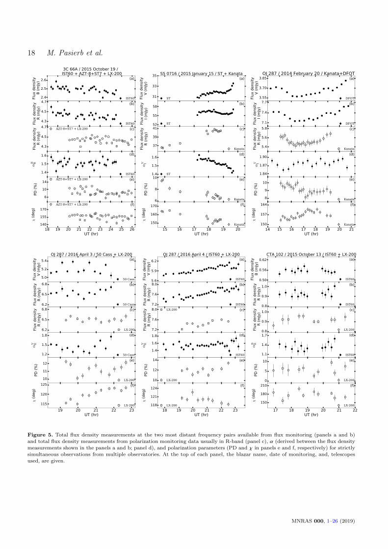
18 M. Pasierb et al.
2.4
2.5
2.6
Flux d
ensi
ty B
(m
Jy)
(a)
3C 66A / 2015 October 19 / IST60 + AZT-8+ST7 + LX-200
IST60
4.3
4.5
4.7
Flux d
ensi
ty R
(m
Jy)
(b)
IST60
4.3
4.5
4.7
Flux d
ensi
ty R
(m
Jy)
(c)AZT-8+ST7 + LX-200
1.4
1.5
1.6
αB R
(d)
IST60
6
10
14
PD
(%
)
(e)AZT-8+ST7 + LX-200
18 19 20 21 22 23 24 25 26UT (hr)
140
155
170
χ (
deg)
(f)AZT-8+ST7 + LX-200
31
33
35
Flux d
ensi
tyV
(m
Jy)
(a)S5 0716 / 2015 January 15 / ST + Kanata
ST
52
55
58
Flux d
ensi
tyI (m
Jy)
(b)
ST
37
39
41
Flux d
ensi
tyR
(m
Jy)
(c)
Kanata
1.4
1.5
1.6
αV I
(d)
ST
6
8
10
PD
(%
)
(e)
Kanata
15 16 17 18 19 20UT (hr)
150
160
170
χ (
deg)
(f)
Kanata
3.55
3.70
3.85
Flux d
ensi
ty V
(m
Jy)
(a)OJ 287 / 2014 February 20 / Kanata+DFOT
DFOT
7.1
7.4
7.7
Flux d
ensi
ty I (
mJy
)
(b)
DFOT
5.4
5.6
5.8
Flux d
ensi
ty R
(m
Jy)
(c)
Kanata
1.84
1.87
1.90
αV I
(d)
8
9
10
PD
(%
)
(e)
Kanata
14 15 16 17 18 19 20 21UT (hr)
150
157
164
χ (
deg)
(f)
Kanata
5.0
5.2
5.4
Flux d
ensi
tyV
(m
Jy)
(a)OJ 287 / 2016 April 3 / 50 Cass + LX-200
50 Cass
6.2
6.5
6.8
Flux d
ensi
tyR
(m
Jy)
(b)
50 Cass
6.2
6.5
6.8
Flux d
ensi
tyR
(m
Jy)
(c)
LX-200
1.2
1.5
1.8
αV R
(d)
50 Cass
10
11
12
PD
(%
)
(e)
LX-200
19 20 21 22 23UT (hr)
115
120
125
χ (
deg)
(f)
LX-200
5.6
5.9
6.2
Flux d
ensi
ty V
(m
Jy)
(a)OJ 287 / 2016 April 4 / IST60 + LX-200
IST60
7.2
7.6
8.0
Flux d
ensi
tyR
(m
Jy)
(b)
IST60
7.2
7.6
8.0
Flux d
ensi
tyR
(m
Jy)
(c)LX-200
1.4
1.6
1.8
αV R
(d)
IST60
10
12
14
PD
(%
)
(e)
LX-200
18 19 20 21 22 23UT (hr)
118
121
124
χ (
deg)
(f)
LX-200
0.50
0.56
0.62
Flux d
ensi
ty B
(m
Jy)
(a)CTA 102 / 2015 October 13 / IST60 + LX-200
IST60
0.8
0.9
1.0
Flux d
ensi
ty R
(m
Jy)
(b)
IST60
0.8
0.9
1.0
Flux d
ensi
ty R
(m
Jy)
(c)
LX-200
1.1
1.4
1.7
αB R
(d)
IST60
0
5
10
PD
(%
)
(e)
LX-200
17 18 19 20 21 22UT (hr)
150
180
210
χ (
deg)
(f)
LX-200
Figure 5. Total flux density measurements at the two most distant frequency pairs available from flux monitoring (panels a and b)and total flux density measurements from polarization monitoring data usually in R-band (panel c), α (derived between the flux density
measurements shown in the panels a and b; panel d), and polarization parameters (PD and χ in panels e and f, respectively) for strictlysimultaneous observations from multiple observatories. At the top of each panel, the blazar name, date of monitoring, and, telescopesused, are given.
MNRAS 000, 1–26 (2019)
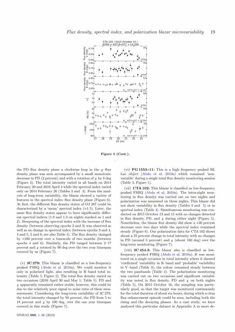
Flux density, spectral index, and polarization blazar microvariability 19
0.55
0.65
0.75
Flux d
ensi
ty V
(m
Jy)
(a)
CTA 102 / 2015 October 15 / IST60 + AZT-8+ST7 + LX-200
IST60
0.65
0.75
0.85
Flux d
ensi
tyR
(m
Jy)
(b)
IST60
0.65
0.75
0.85
Flux d
ensi
tyR
(m
Jy)
(c)
AZT-8+ST7 + LX-200
0
1
2
αV R
(d)
IST60
0
4
8
PD
(%
)
(e)
AZT-8+ST7 + LX-200
17 18 19 20 21 22 23UT (hr)
80
140
200
χ (
deg)
(f)
AZT-8+ST7 + LX-200
Figure 5 (Cont.).
.
the PD–flux density plane a clockwise loop in the χ–fluxdensity plane was seen accompanied by a small monotonicdecrease in PD (2 percent) and with a rotation of χ by 8 deg(Figure 4). The total intensity varied in all bands on 2014February 20 and 2016 April 4 while the spectral index variedonly on 2014 February 20 (Tables 3 and 4). From the anal-ysis of long-term variability, the blazar showed a variety offeatures in the spectral index–flux density plane (Figure 6).At first, the different flux density states of OJ 287 could becharacterized by a ‘mean’ spectral index (≈1.5). Later, thesame flux density states appear to have significantly differ-ent spectral indices (1.9 and 1.3 on nights marked as 1 and2). Steepening of the spectral index with the increase of fluxdensity (between observing epochs 2 and 3) was observed aswell as no change in spectral index (between epochs 3 and 4,4 and 5, 5 and 6; see also Table 4). The flux density changedby ≈100 percent over a timescale of two months (betweenepochs 4 and 6). Similarly, the PD ranged between 2–17percent and χ rotated by 90 deg over the two year timespancovered by us (Figure 7).
(v) 3C 279: This blazar is classified as a low-frequencypeaked FSRQ (Abdo et al. 2010a). We could monitor itonly in polarized light, also resulting in R–band total in-tensity (Table 5, Figure 2). The total flux density varied ontwo occasions (2016 April 30 and May 1; Table 5). PD andχ apparently remained rather stable; however, this could bedue to the relatively poor signal to noise ratio of these mea-surements. Considering the long-term variability of 3C 279,the total intensity changed by 50 percent, the PD from 5 to18 percent and χ by 100 deg, over the one year timespancovered in this study (Figure 7).
(vi) PG 1553+11: This is a high frequency peaked BLLac object (Abdo et al. 2010a) which remained ‘non-variable’ during a single total flux density monitoring session(Table 3, Figure 1).
(vii) CTA 102: This blazar is classified as low-frequencypeaked FSRQ (Abdo et al. 2010a). The intra-night mon-itoring in flux density was carried out on two nights andpolarization was measured on three nights. This blazar didnot show variability in flux density (Tables 3 and 5) or inspectral index (Table 4). Simultaneous monitoring was con-ducted on 2015 October 13 and 15 with no changes detectedin flux density, PD, and χ during either night (Figure 5).Nonetheless, the blazar flux density did show a ≈30 percentdecrease over two days while the spectral index remainedsteady (Figure 6). Our polarization data for CTA 102 showsabout a 25 percent change in total intensity with no changesin PD (around 5 percent) and χ (about 160 deg) over thelong-term monitoring (Figure 7).
(viii) 3C 454.3: This blazar also is classified as low-frequency peaked FSRQ (Abdo et al. 2010a). It was moni-tored on a single occasion in total intensity where it showed‘confirmed’ variability in R–band and ‘probable’ variabilityin V–band (Table 3); the colour remained steady betweenthe two passbands (Table 4). The polarization monitoringwas carried out on two occasions and significant variabil-ity was noted in flux density, PD and χ on both nights(Table 5). On 2015 October 16, the sampling was partic-ularly good, so that the target was monitored continuouslyfor the total duration of about six hours, during which a clearflux enhancement episode could be seen, including both therising and the decaying phases. As a case study, we haveanalysed this particular dataset in Appendix A in more de-
MNRAS 000, 1–26 (2019)
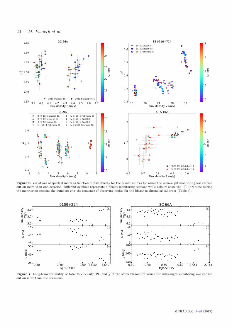
20 M. Pasierb et al.
3.9 4.0 4.1 4.2 4.3 4.4 4.5 4.6 4.7Flux density R (mJy)
1.35
1.40
1.45
1.50
1.55
1.60
1.65
αB R
2
1
3C 66A
2015 October 19 2015 November 15
21
22
23
24
UT (
hr)
16 20 24 28 32Flux density V (mJy)
1.2
1.3
1.4
1.5
1.6
αV I
1
2
3
S5 0716+7142015 January 11
2015 January 15
2015 February 09
15
16
17
18
19
UT (
hr)
2 3 4 5 6 7 8 9Flux density V (mJy)
1.1
1.4
1.7
2.0
α
1
2
34
5
6
7
8
OJ 287(B-R) 2016 January 13
(B-R) 2016 March 07
(B-R) 2016 April 02
(V-I) 2014 February 20
(V-R) 2016 February 06
(V-R) 2016 April 03
(V-R) 2016 April 04
(V-I) 2015 February 12
16
17
18
19
20
UT (
hr)
0.6 0.7 0.8 0.9 1.0Flux density R (mJy)
0
1
2α
1
2
CTA 102
(B-R) 2015 October 13
(V-R) 2015 October 1518
19
20
21
22
UT (
hr)
Figure 6. Variations of spectral index as function of flux density for the blazar sources for which the intra-night monitoring was carried
out on more than one occasion. Different symbols represents different monitoring sessions while colours show the UT (hr) time duringthe monitoring session; the numbers give the sequence of observing nights for the blazar in chronological order (Table 3).
3.5
3.7
3.9
Flux d
ensi
ty(m
Jy)
0109+224
11
14
17
PD
(%
)
0.30 0.40 0.50 MJD-57340
25
40
55
χ (
deg)
33.30 33.40
(a)
(b)
(c)
4.1
4.3
4.5
Flux d
ensi
ty(m
Jy)
3C 66A
5
10
15
PD
(%
)
0.30 0.40 0.50 0.60 MJD-57315
140
160
180
χ (
deg)
27.51 27.53
(a)
(b)
(c)
Figure 7. Long-term variability of total flux density, PD and χ of the seven blazars for which the intra-night monitoring was carried
out on more than one occasions.
MNRAS 000, 1–26 (2019)
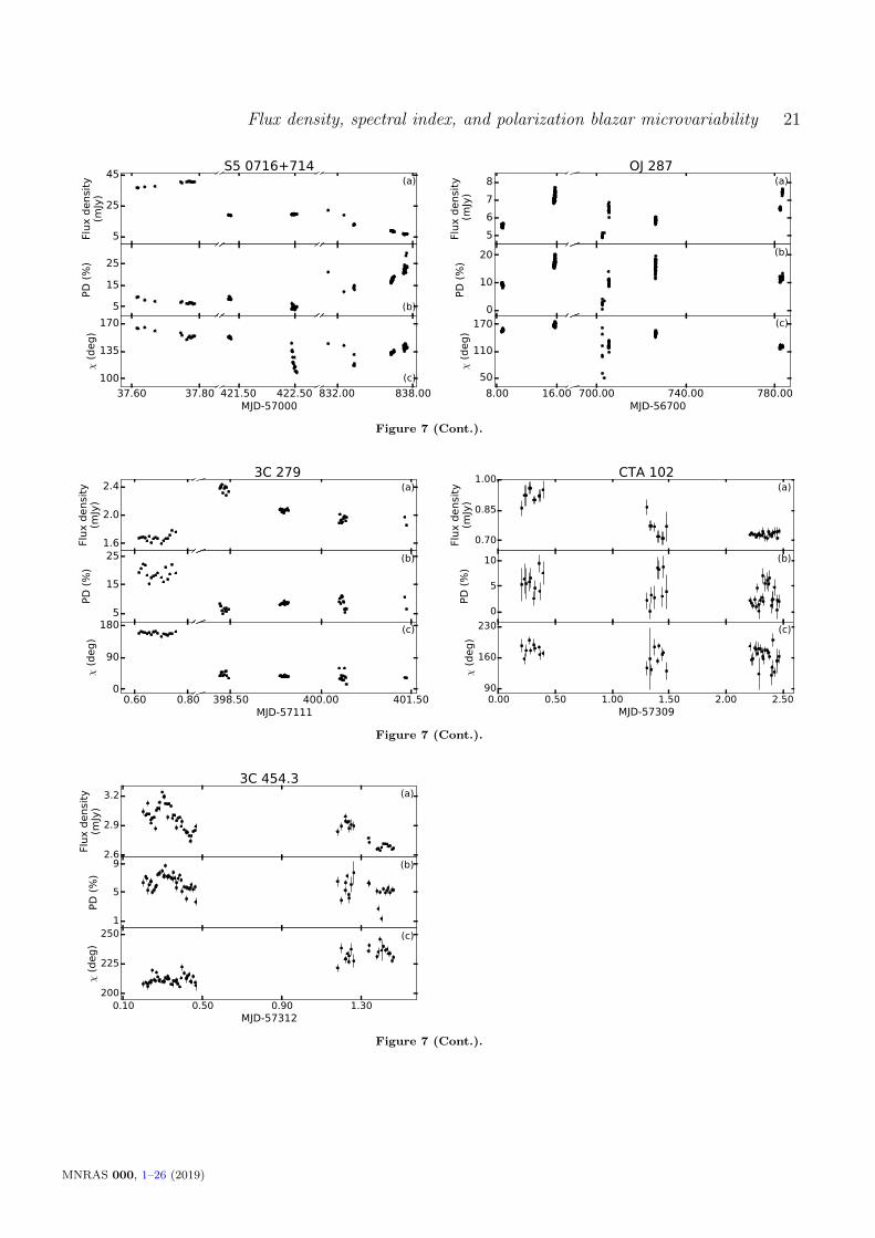
Flux density, spectral index, and polarization blazar microvariability 21
5
25
45
Flux d
ensi
ty(m
Jy)
S5 0716+714
5
15
25
PD
(%
)
37.60 37.80
100
135
170
χ (
deg)
421.50 422.50MJD-57000
832.00 838.00
(a)
(b)
(c)
5
6
7
8
Flux d
ensi
ty (
mJy
)
OJ 287
0
10
20
PD
(%
)
8.00 16.00
50
110
170
χ (
deg)
700.00 740.00 780.00MJD-56700
(a)
(b)
(c)
Figure 7 (Cont.).
1.6
2.0
2.4
Flux d
ensi
ty(m
Jy)
3C 279
5
15
25
PD
(%
)
0.60 0.800
90
180
χ (
deg)
398.50 400.00 401.50MJD-57111
(a)
(b)
(c)
0.70
0.85
1.00
Flux d
ensi
ty(m
Jy)
(a)CTA 102
0
5
10
PD
(%
)
(b)
0.00 0.50 1.00 1.50 2.00 2.50MJD-57309
90
160
230
χ (
deg)
(c)
Figure 7 (Cont.).
2.6
2.9
3.2
Flux d
ensi
ty(m
Jy)
(a)3C 454.3
1
5
9
PD
(%
)
(b)
0.10 0.50 0.90 1.30MJD-57312
200
225
250
χ (
deg)
(c)
Figure 7 (Cont.).
MNRAS 000, 1–26 (2019)

22 M. Pasierb et al.
tail, attempting to separate the “base emission component”from the “flaring emission component”. Unfortunately, noneof the multiband total intensity and polarization monitor-ing sessions overlapped. On 2015 October 16 a hint of anincrease in the PD as the flux density increases is noted inthe PD–flux density plane, while χ remains stable at ∼ 210deg (Figure 4). During the polarization monitoring carriedout on 2015 October 17, counter–clockwise loops in the PD–flux density and χ–flux density planes, respectively, seem tobe present, though no clear evolution in the PD–χ plane wasseen (Figure 4). Between those two consecutive nights thepolarization data show a 10 percent intensity change, butalso essentially constant PD (∼ 7 percent), along with a ∼30deg change in χ (Figure 7) .
6 DISCUSSION AND CONCLUSIONS
Microvariability in blazar sources has gathered special at-tention, partially because of the requirements of very effi-cient particle acceleration and very fast energy dissipationmechanisms necessary to produce it. Particularly challeng-ing are the high-amplitude flares with well-defined rise anddecay profiles which allows for size estimation of the emis-sion zone from flux density doubling arguments. As such,these timescales occasionally violate the shortest ‘charac-teristic’ variability timescale provided by the light-crossingtimescale (tlc) of the event horizon of the SMBH (∼15 minfor 108M�; Begelman et al. 1984, where tlc= rg/c = G M/c3
where rg is the gravitational radius, G is the gravitationalconstant, M is the mass of SMBH, and c is the speed oflight).
Nonetheless, variations on intra-night timescales mostoften constitute monotonic increases or decreases in inten-sity, indicating sizes > 1015 cm (R ∼ c δ tvar for δ =10 andtaking tvar= 5 hr from the typical length of the intra-nightmonitoring session) at least in the simple, and frequentlyemployed, single emission zone scenario. Such sizes couldthen be related to the distance of the dissipation site (r)from the central SMBH by R ' rθ j for a conical jet withan opening angle, θ j= θobs ∼ 1/Γ, where θobs is the anglebetween the jet axis and the observer’s lines of sight and Γis the jet Lorentz factor (Sikora et al. 1994). For the pop-ular internal shock scenario of particle acceleration, shellsof relativistic plasma, ejected intermittently from the cen-ter (with a larger dispersion in bulk velocity), collide witheach other at a characteristic distance r ∼ rg(Γ/10)2 (Spadaet al. 2001; Moderski et al. 2003). The flux variability onhourly timescales noted here would then be compatible withparticle acceleration by internal shocks. However, in such ascenario, a correlation between the flux and PD changes areexpected, because of a compression of the jet plasma withinitially tangled (by assumption) jet magnetic field at theshock front. Several observations for individual blazars on anight-to-night basis presented in the literature conforms tothis model, possibly with some minor modifications or addi-tions (e.g., Hagen-Thorn et al. 2008; Itoh et al. 2013; Covinoet al. 2015; Bhatta et al. 2016).
In our data set, we observe a variety of flux–PD vari-ability patterns, including clear instances with a relativelystraightforward anti-correlation (S5 0716+714 on 2015 Jan-uary 15 and 2017 March 23), correlation (3C 454 on 2015 Oc-
tober 16), counter-clockwise looping (OJ 287 on 2014 Febru-ary 20), but also instances with no obvious correlation pat-tern (S5 0716+714 on 2017 March 24, OJ 287 on 2016 Febru-ary 7, 3C 454 on 2015 October 17). It is, however, worth-while noting that whenever we see any order in the flux–PDchanges, it is reflected at the same time in the flux–χ plane,or equivalently the PD–χ plane (see Figure 4). In particular,the anti-correlation between the flux and PD seen clearly inS5 0716+714 on 2015 January 15 and 2017 March 23 areaccompanied by an anti-correlation between the polariza-tion angle χ and flux, while the counter-clockwise flux-PDlooping behaviour noted for OJ 287 on 2014 February 20is accompanied by a clockwise looping in the flux-χ repre-sentation (a similar pattern of variability to what has beennoticed for the blazar 3C 454.3 in Gopal-Krishna et al. 2019,based on the extensive observations reported by Gupta et al.2017). This piece of evidence seems to suggest that in or-der to fully understand the physics behind the intra-nightvariability of blazar sources, a three-dimensional parameterspace of a flux, polarization degree, and polarization anglehas to be considered. This still could possibly be reconciledwith the internal shock model, if one allows for example for achanges in the shock angle (i.e., the angle between the shocknormal and the line of sight) during the shock evolutionalong the outflow (see, e.g., the discussion in Bhatta et al.2015), and/or for a presence of a partly ordered magneticfield (e.g., in a form of a helical distortion flowing throughthe shock; see Perlman et al. 2011).
It should be emphasized, however, that the results of po-larization microvariability monitoring indicate variable PDand χ only on a few occasions (Table 5)). For about half ofthese instances, the quality of polarization measurements ispoor (low signal to noise ratio, too few data points, or biggaps in the light curve). Therefore, we give the mean valuesof total flux density, PD and χ for the monitoring sessionconsidered (Columns 4, 5, 6 of Table 5). The PD turns out tobe between 2 and 23% with a factor of few changes seen overthe timescale of days/months for a given blazar source. Themean χ also showed significant variability over days/monthstimescales during the monitoring campaign (Table 5, Fig-ure 2).
Our study using quasi-simultaneous B, V, R, and I-band intra-night light curves allowed us to estimate thetwo-point spectral index for several intra-night monitoringsessions (see Table 4). The mean α during our monitoringprogramme ranges from 0.68 up to 1.87. Moreover, out of10 cases where statistically significant flux microvariabilitywas detected (Table 3), ‘confirmed’ colour microvariabilitystatus is seen on four nights and a ‘probable’ variable sta-tus is assigned on one night (Table 4). This means that the‘colour’ is likely to be seen to vary on about half of theinstances when significant flux density microvariability isdetected in a sample, or, conversely, ‘achromatic’ flux mi-crovariability is expected on about half of the monitoringsessions, i.e., the colour microvariability DC is ≈50 percent.It is, however, important to note that ‘colour’ or spectralindex variability is a second order variation (as compared toflux density variations) and therefore is harder to detect dueto bigger statistical errors on spectral index measurementsarising solely from error propagation. Moreover, since weare severely limited by small number statistics in derivinga duty cycle (sample of 7 blazars monitored on 18 intra-
MNRAS 000, 1–26 (2019)
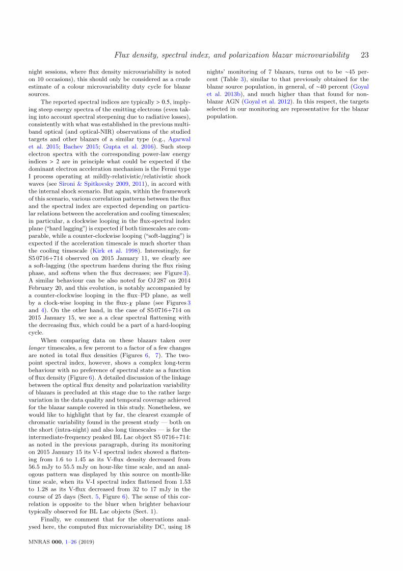
Flux density, spectral index, and polarization blazar microvariability 23
night sessions, where flux density microvariability is notedon 10 occasions), this should only be considered as a crudeestimate of a colour microvariability duty cycle for blazarsources.
The reported spectral indices are typically > 0.5, imply-ing steep energy spectra of the emitting electrons (even tak-ing into account spectral steepening due to radiative losses),consistently with what was established in the previous multi-band optical (and optical-NIR) observations of the studiedtargets and other blazars of a similar type (e.g., Agarwalet al. 2015; Bachev 2015; Gupta et al. 2016). Such steepelectron spectra with the corresponding power-law energyindices > 2 are in principle what could be expected if thedominant electron acceleration mechanism is the Fermi typeI process operating at mildly-relativistic/relativistic shockwaves (see Sironi & Spitkovsky 2009, 2011), in accord withthe internal shock scenario. But again, within the frameworkof this scenario, various correlation patterns between the fluxand the spectral index are expected depending on particu-lar relations between the acceleration and cooling timescales;in particular, a clockwise looping in the flux-spectral indexplane (“hard lagging”) is expected if both timescales are com-parable, while a counter-clockwise looping (“soft-lagging”) isexpected if the acceleration timescale is much shorter thanthe cooling timescale (Kirk et al. 1998). Interestingly, forS5 0716+714 observed on 2015 January 11, we clearly seea soft-lagging (the spectrum hardens during the flux risingphase, and softens when the flux decreases; see Figure 3).A similar behaviour can be also noted for OJ 287 on 2014February 20, and this evolution, is notably accompanied bya counter-clockwise looping in the flux–PD plane, as wellby a clock-wise looping in the flux-χ plane (see Figures 3and 4). On the other hand, in the case of S5 0716+714 on2015 January 15, we see a a clear spectral flattening withthe decreasing flux, which could be a part of a hard-loopingcycle.
When comparing data on these blazars taken overlonger timescales, a few percent to a factor of a few changesare noted in total flux densities (Figures 6, 7). The two-point spectral index, however, shows a complex long-termbehaviour with no preference of spectral state as a functionof flux density (Figure 6). A detailed discussion of the linkagebetween the optical flux density and polarization variabilityof blazars is precluded at this stage due to the rather largevariation in the data quality and temporal coverage achievedfor the blazar sample covered in this study. Nonetheless, wewould like to highlight that by far, the clearest example ofchromatic variability found in the present study — both onthe short (intra-night) and also long timescales — is for theintermediate-frequency peaked BL Lac object S5 0716+714:as noted in the previous paragraph, during its monitoringon 2015 January 15 its V-I spectral index showed a flatten-ing from 1.6 to 1.45 as its V-flux density decreased from56.5 mJy to 55.5 mJy on hour-like time scale, and an anal-ogous pattern was displayed by this source on month-liketime scale, when its V-I spectral index flattened from 1.53to 1.28 as its V-flux decreased from 32 to 17 mJy in thecourse of 25 days (Sect. 5, Figure 6). The sense of this cor-relation is opposite to the bluer when brighter behaviourtypically observed for BL Lac objects (Sect. 1).
Finally, we comment that for the observations anal-ysed here, the computed flux microvariability DC, using 18
nights’ monitoring of 7 blazars, turns out to be ∼45 per-cent (Table 3), similar to that previously obtained for theblazar source population, in general, of ∼40 percent (Goyalet al. 2013b), and much higher than that found for non-blazar AGN (Goyal et al. 2012). In this respect, the targetsselected in our monitoring are representative for the blazarpopulation.
MNRAS 000, 1–26 (2019)
24 M. Pasierb et al.
ACKNOWLEDGEMENTS
We thank the referee for providing constructive commentson the manuscript. We thank the staff of ARIES andKanata for carrying out some of the observations pre-sented in this study. AG acknowledges support from thePolish National Science Centre (NCN) through the grant2018/29/B/ST9/02298. LS acknowledges the support ofNCN via 2016/22/E/ST9/00061. SZ’s work is supported byNCN via 2018/29/B/ST9/01793. GK would like to thank In-dian National Science Academy for a Senior Scientist fellow-ship.The St. Petersburg University team acknowledges sup-port from Russian Science Foundation grant 17-12-01029.
REFERENCES
Abdo A. A., et al., 2010a, ApJ, 715, 429
Abdo A. A., et al., 2010b, ApJ, 716, 30
Abdo A. A., et al., 2010c, ApJ, 722, 520
Abdo A. A., et al., 2011a, ApJ, 727, 129
Abdo A. A., et al., 2011b, ApJ, 736, 131
Ackermann M., et al., 2016, ApJ, 824, L20
Agarwal A., et al., 2015, MNRAS, 451, 3882
Agudo I., et al., 2011, ApJ, 735, L10
Aharonian F., et al., 2007, ApJ, 664, L71
Angelakis E., et al., 2016, MNRAS, 463, 3365
Bachev R., 2015, MNRAS, 451, L21
Bachev R., Strigachev A., Semkov E., 2005, MNRAS, 358, 774
Begelman M. C., Blandford R. D., Rees M. J., 1984, Reviews ofModern Physics, 56, 255
Begelman M. C., Fabian A. C., Rees M. J., 2008, MNRAS, 384,L19
Bevington P. R., Robinson D. K., 2003, Data reduction and erroranalysis for the physical sciences. 3rd ed., by Philip R. Bev-
ington, and Keith D. Robinson. Boston, MA: McGraw-Hill,ISBN 0-07-247227-8, 2003
Bhatta G., et al., 2015, ApJ, 809, L27
Bhatta G., et al., 2016, ApJ, 832, 47
Blinov D., et al., 2016, MNRAS, 457, 2252
Bonning E., et al., 2012, ApJ, 756, 13
Bottcher M., Reimer A., Sweeney K., Prakash A., 2013, ApJ, 768,
54
Camenzind M., Krockenberger M., 1992, A&A, 255, 59
Cellone S. A., Romero G. E., Araudo A. T., 2007, MNRAS, 374,357
Ciprini S., Tosti G., Raiteri C. M., Villata M., Ibrahimov M. A.,Nucciarelli G., Lanteri L., 2003, A&A, 400, 487
Covino S., et al., 2015, A&A, 578, A68
Dai Y., Wu J., Zhu Z.-H., Zhou X., Ma J., Yuan Q., Wang L.,
2013, ApJS, 204, 22
De Diego J. A., 2010, AJ, 139, 1269
De Diego J. A., 2014, AJ, 148, 93
Domınguez A., et al., 2011, MNRAS, 410, 2556
Garcia A., Sodre L., Jablonski F. J., Terlevich R. J., 1999,
Monthly Notices of the Royal Astronomical Society, 309, 803
Gaur H., et al., 2012, MNRAS, 425, 3002
Gaur H., Gupta A., Bachev R., Strigachev A., Semkov E., WiitaP., Gu M., Ibryamov S., 2017, Galaxies, 5, 94
Gaur H., et al., 2019, MNRAS, 484, 5633
Ghosh K. K., Ramsey B. D., Sadun A. C., Soundararajaperumal
S., 2000, ApJS, 127, 11
Glass I. S., 1999, Handbook of Infrared Astronomy. CambridgeUniversity Press, Aug 13, 1999, page 63
Gonzalez-Perez J. N., Kidger M. R., Martın-Luis F., 2001, AJ,
122, 2055
Gopal-Krishna Wiita P. J., 1992, A&A, 259, 109
Gopal-Krishna Sagar R., Wiita P. J., 1995, MNRAS, 274, 701
Gopal-Krishna Britzen S., Wiita P., 2019, arXiv e-prints, p.
arXiv:1906.11339
Goyal A., Gopal-Krishna Wiita P. J., Anupama G. C., Sahu D. K.,
Sagar R., Joshi S., 2012, A&A, 544, A37
Goyal A., Mhaskey M., Gopal-Krishna Wiita P. J., Stalin C. S.,Sagar R., 2013a, Journal of Astrophysics and Astronomy, 34,
273
Goyal A., Gopal-Krishna Wiita P. J., Stalin C. S., Sagar R.,
2013b, MNRAS, 435, 1300
Gu M., Ai Y. L., 2011, Journal of Astrophysics and Astronomy,32, 87
Gu M. F., Lee C. U., Pak S., Yim H. S., Fletcher A. B., 2006,
A&A, 450, 39
Gupta A. C., et al., 2016, MNRAS, 458, 1127
Gupta A. C., et al., 2017, MNRAS, 472, 788
Gupta A. C., et al., 2019, AJ, 157, 95
Hagen-Thorn V. A., Larionov V. M., Jorstad S. G., Arkharov
A. A., Hagen-Thorn E. I., Efimova N. V., Larionova L. V.,Marscher A. P., 2008, ApJ, 672, 40
Hao J.-M., Wang B.-J., Jiang Z.-J., Dai B.-Z., 2010, Research in
Astronomy and Astrophysics, 10, 125
Healey S. E., et al., 2008, ApJS, 175, 97
Hughes P. A., Aller M. F., Aller H. D., 2011, ApJ, 735, 81
Ikejiri Y., et al., 2011, PASJ, 63, 639
Isler J. C., Urry C. M., Coppi P., Bailyn C., Brady M., MacPher-son E., Buxton M., Hasan I., 2017, ApJ, 844, 107
Itoh R., et al., 2013, ApJ, 768, L24
Jermak H., et al., 2016, MNRAS, 462, 4267
Jorstad S. G., et al., 2007, AJ, 134, 799
Jorstad S. G., et al., 2017, ApJ, 846, 98
Kawabata K. S., et al., 2008, in Ground-based and Air-
borne Instrumentation for Astronomy II. p. 70144L,
doi:10.1117/12.788569
Kirk J. G., Rieger F. M., Mastichiadis A., 1998, A&A, 333, 452
Larionov V. M., et al., 2008, A&A, 492, 389
Larionov V. M., et al., 2013, ApJ, 768, 40
Larionov V. M., et al., 2016, MNRAS, 461, 3047
Li X.-P., Luo Y.-H., Yang H.-T., Yang H.-Y., Yang C., Cai Y.,2018, Research in Astronomy and Astrophysics, 18, 150
Lynds C. R., 1967, ApJ, 147, 837
Madejski G. ., Sikora M., 2016, ARA&A, 54, 725
Maraschi L., Ghisellini G., Celotti A., 1992, ApJ, 397, L5
Marscher A. P., Gear W. K., 1985, ApJ, 298, 114
Marscher A. P., et al., 2008, Nature, 452, 966
Marziani P., Sulentic J. W., Dultzin-Hacyan D., Calvani M.,
Moles M., 1996, ApJS, 104, 37
Mead A. R. G., Ballard K. R., Brand P. W. J. L., Hough J. H.,Brindle C., Bailey J. A., 1990, A&AS, 83, 183
Meng N., Wu J., Webb J. R., Zhang X., Dai Y., 2017, MNRAS,
469, 3588
Meng N., Zhang X., Wu J., Ma J., Zhou X., 2018, ApJS, 237, 30
Meyer E. T., 2018, Nature Astronomy, 2, 32
Moderski R., Sikora M., B lazejowski M., 2003, A&A, 406, 855
Moore R. L., et al., 1982, ApJ, 260, 415
Nilsson K., Pursimo T., Sillanpaa A., Takalo L. O., Lindfors E.,
2008, A&A, 487, L29
Nilsson K., Takalo L. O., Lehto H. J., Sillanpaa A., 2010, A&A,516, A60
Osterman Meyer A., Miller H. R., Marshall K., Ryle W. T., Aller
H., Aller M., Balonek T., 2009, AJ, 138, 1902
Pacholczyk A. G., 1970, Radio astrophysics. Nonthermal pro-
cesses in galactic and extragalactic sources
Padovani P., et al., 2017, A&ARv, 25, 2
Papadakis I. E., Boumis P., Samaritakis V., Papamastorakis J.,2003, A&A, 397, 565
Perlman E. S., et al., 2011, ApJ, 743, 119
MNRAS 000, 1–26 (2019)
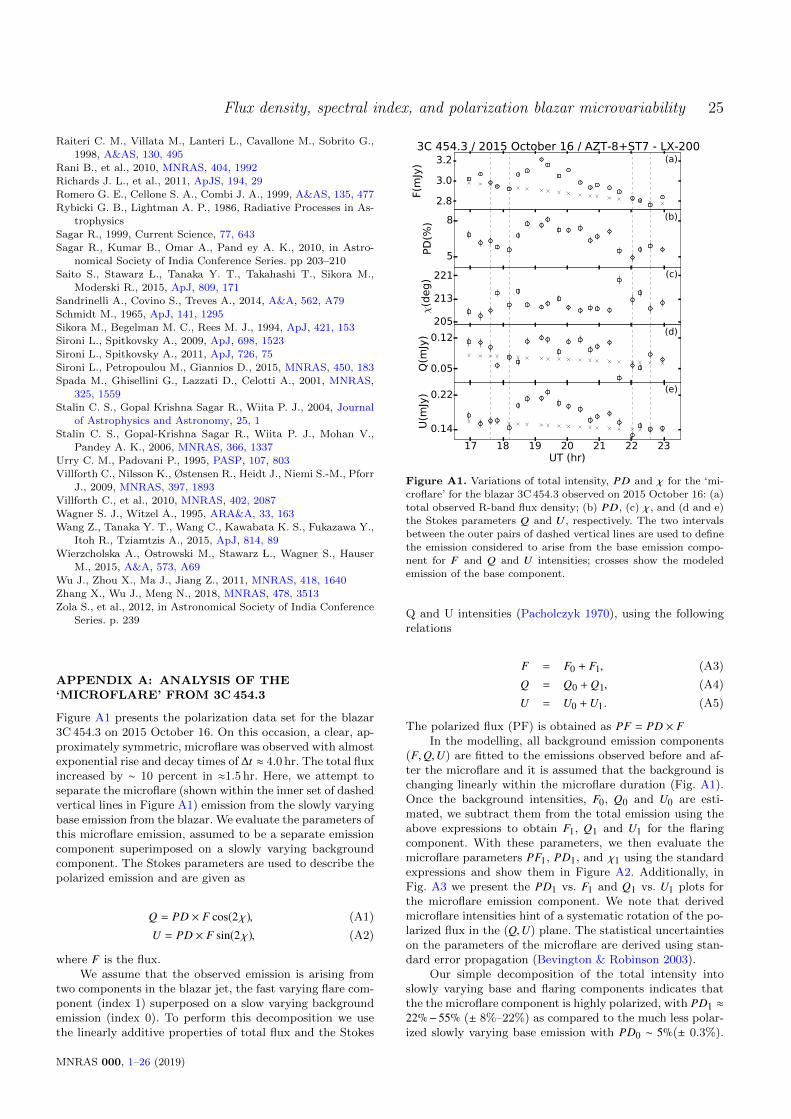
Flux density, spectral index, and polarization blazar microvariability 25
Raiteri C. M., Villata M., Lanteri L., Cavallone M., Sobrito G.,
1998, A&AS, 130, 495
Rani B., et al., 2010, MNRAS, 404, 1992
Richards J. L., et al., 2011, ApJS, 194, 29
Romero G. E., Cellone S. A., Combi J. A., 1999, A&AS, 135, 477
Rybicki G. B., Lightman A. P., 1986, Radiative Processes in As-
trophysics
Sagar R., 1999, Current Science, 77, 643
Sagar R., Kumar B., Omar A., Pand ey A. K., 2010, in Astro-
nomical Society of India Conference Series. pp 203–210
Saito S., Stawarz L., Tanaka Y. T., Takahashi T., Sikora M.,
Moderski R., 2015, ApJ, 809, 171
Sandrinelli A., Covino S., Treves A., 2014, A&A, 562, A79
Schmidt M., 1965, ApJ, 141, 1295
Sikora M., Begelman M. C., Rees M. J., 1994, ApJ, 421, 153
Sironi L., Spitkovsky A., 2009, ApJ, 698, 1523
Sironi L., Spitkovsky A., 2011, ApJ, 726, 75
Sironi L., Petropoulou M., Giannios D., 2015, MNRAS, 450, 183
Spada M., Ghisellini G., Lazzati D., Celotti A., 2001, MNRAS,
325, 1559
Stalin C. S., Gopal Krishna Sagar R., Wiita P. J., 2004, Journalof Astrophysics and Astronomy, 25, 1
Stalin C. S., Gopal-Krishna Sagar R., Wiita P. J., Mohan V.,
Pandey A. K., 2006, MNRAS, 366, 1337
Urry C. M., Padovani P., 1995, PASP, 107, 803
Villforth C., Nilsson K., Østensen R., Heidt J., Niemi S.-M., PforrJ., 2009, MNRAS, 397, 1893
Villforth C., et al., 2010, MNRAS, 402, 2087
Wagner S. J., Witzel A., 1995, ARA&A, 33, 163
Wang Z., Tanaka Y. T., Wang C., Kawabata K. S., Fukazawa Y.,
Itoh R., Tziamtzis A., 2015, ApJ, 814, 89
Wierzcholska A., Ostrowski M., Stawarz L., Wagner S., Hauser
M., 2015, A&A, 573, A69
Wu J., Zhou X., Ma J., Jiang Z., 2011, MNRAS, 418, 1640
Zhang X., Wu J., Meng N., 2018, MNRAS, 478, 3513
Zola S., et al., 2012, in Astronomical Society of India Conference
Series. p. 239
APPENDIX A: ANALYSIS OF THE‘MICROFLARE’ FROM 3C 454.3
Figure A1 presents the polarization data set for the blazar3C 454.3 on 2015 October 16. On this occasion, a clear, ap-proximately symmetric, microflare was observed with almostexponential rise and decay times of ∆t ≈ 4.0 hr. The total fluxincreased by ∼ 10 percent in ≈1.5 hr. Here, we attempt toseparate the microflare (shown within the inner set of dashedvertical lines in Figure A1) emission from the slowly varyingbase emission from the blazar. We evaluate the parameters ofthis microflare emission, assumed to be a separate emissioncomponent superimposed on a slowly varying backgroundcomponent. The Stokes parameters are used to describe thepolarized emission and are given as
Q = PD × F cos(2χ), (A1)
U = PD × F sin(2χ), (A2)
where F is the flux.We assume that the observed emission is arising from
two components in the blazar jet, the fast varying flare com-ponent (index 1) superposed on a slow varying backgroundemission (index 0). To perform this decomposition we usethe linearly additive properties of total flux and the Stokes
2.8
3.0
3.2
F(m
Jy)
(a)3C 454.3 / 2015 October 16 / AZT-8+ST7 - LX-200
5
8
PD
(%)
(b)
205
213
221
χ(d
eg) (c)
0.05
0.12
Q(m
Jy) (d)
17 18 19 20 21 22 23UT (hr)
0.14
0.22
U(m
Jy) (e)
Figure A1. Variations of total intensity, PD and χ for the ‘mi-croflare’ for the blazar 3C 454.3 observed on 2015 October 16: (a)
total observed R-band flux density; (b) PD, (c) χ, and (d and e)
the Stokes parameters Q and U, respectively. The two intervalsbetween the outer pairs of dashed vertical lines are used to define
the emission considered to arise from the base emission compo-
nent for F and Q and U intensities; crosses show the modeledemission of the base component.
Q and U intensities (Pacholczyk 1970), using the followingrelations
F = F0 + F1, (A3)
Q = Q0 +Q1, (A4)
U = U0 +U1. (A5)
The polarized flux (PF) is obtained as PF = PD × FIn the modelling, all background emission components
(F,Q,U) are fitted to the emissions observed before and af-ter the microflare and it is assumed that the background ischanging linearly within the microflare duration (Fig. A1).Once the background intensities, F0, Q0 and U0 are esti-mated, we subtract them from the total emission using theabove expressions to obtain F1, Q1 and U1 for the flaringcomponent. With these parameters, we then evaluate themicroflare parameters PF1, PD1, and χ1 using the standardexpressions and show them in Figure A2. Additionally, inFig. A3 we present the PD1 vs. F1 and Q1 vs. U1 plots forthe microflare emission component. We note that derivedmicroflare intensities hint of a systematic rotation of the po-larized flux in the (Q,U) plane. The statistical uncertaintieson the parameters of the microflare are derived using stan-dard error propagation (Bevington & Robinson 2003).
Our simple decomposition of the total intensity intoslowly varying base and flaring components indicates thatthe the microflare component is highly polarized, with PD1 ≈22%−55% (± 8%–22%) as compared to the much less polar-ized slowly varying base emission with PD0 ∼ 5%(± 0.3%).
MNRAS 000, 1–26 (2019)

26 M. Pasierb et al.
0.1
0.2
0.3
F1(m
Jy)
(a)3C 454.3 (microflare)
0.02
0.06
0.10
PF
1(m
Jy)
(b)
0
35
70
PD
1(%
)
(c)
18.5 19.0 19.5 20.0 20.5 21.0 21.5UT (hr)
40
0
40
χ1(d
eg)
(d)
Figure A2. The derived microflare (a) flux (F1), (b) polarized
flux (PF1) (c) polarization degree (PD1), (d) polarization angle(χ1); for comparison, PD0 and χ0 of the slowly varying base com-
ponent are presented with cross marks.
This implies the presence of a highly ordered magnetic fieldin the microflare emission region (Figure A2). The polariza-tion angle of the microflare component is χ1 ∼ 18◦ - 31◦ (±3-11◦), slightly different from the slowly varying base compo-nent with χ0 ∼ 31◦ (± 1◦). It is important to note that theseχ0 and χ1 are very different from the VLBI jet position angle(≈ −98±10◦; Jorstad et al. 2017). From inspection of Fig. A3,we note an indication of the microflare exhibiting loops inthe (PD, F) and (Q,U) planes. Therefore, the well-resolvedmicroflare shown by 3C 454.3 when polarization monitoringis available shows a highly polarized flare component, sim-ilar to that obtained for the blazar S5 0716+714 (PD ≈50percent; Bhatta et al. 2015). The spatial scale of the mi-croflare emitting region must be quite compact: smaller than∆t · c ≈ few × 1014 cm.
This paper has been typeset from a TEX/LATEX file prepared bythe author.
0.05 0.10 0.15 0.20 0.25 0.30F1 (mJy)
20
30
40
50
60
70
80
PD
1(%
)
(a)
3C 454.3 (microflare)
18.5
19.0
19.5
20.0
20.5
21.0
21.5
UT (
hr)
0.05 0.02 0.01 0.04 0.07Q1 (mJy)
0.00
0.03
0.06
0.09U
1 (
mJy
)(b)
3C 454.3 (microflare)
18.5
19.0
19.5
20.0
20.5
21.0
21.5
UT (
hr)
Figure A3. Evolution of the microflare in the: panel (a) (PD, F)
plane; panel (b) (Q,U) plane.
MNRAS 000, 1–26 (2019)