
Healing replicas in a software component replication...
95
André Nunes Gomes Alves Licenciado em Engenharia Informática Healing replicas in a software component replication system Dissertação para obtenção do Grau de Mestre em Engenharia Informática Orientador : Nuno Manuel Ribeiro Preguiça, Prof. Auxiliar, Universidade Nova de Lisboa : Presidente: Doutor João Baptista da Silva Araújo Junior Arguente: Doutor Carlos Baquero Moreno Vogal: Doutor Nuno Manuel Ribeiro Preguiça Novembro, 2013
Transcript of Healing replicas in a software component replication...
André Nunes Gomes Alves
Licenciado em Engenharia Informática
Healing replicas in a software componentreplication system
Dissertação para obtenção do Grau de Mestre emEngenharia Informática
Orientador : Nuno Manuel Ribeiro Preguiça, Prof. Auxiliar,Universidade Nova de Lisboa
:
Presidente: Doutor João Baptista da Silva Araújo Junior
Arguente: Doutor Carlos Baquero Moreno
Vogal: Doutor Nuno Manuel Ribeiro Preguiça
Novembro, 2013


iii
Healing replicas in a software component replication system
Copyright c© André Nunes Gomes Alves, Faculdade de Ciências e Tecnologia, Universi-dade Nova de Lisboa
A Faculdade de Ciências e Tecnologia e a Universidade Nova de Lisboa têm o direito,perpétuo e sem limites geográficos, de arquivar e publicar esta dissertação através de ex-emplares impressos reproduzidos em papel ou de forma digital, ou por qualquer outromeio conhecido ou que venha a ser inventado, e de a divulgar através de repositórioscientíficos e de admitir a sua cópia e distribuição com objectivos educacionais ou de in-vestigação, não comerciais, desde que seja dado crédito ao autor e editor.

iv

I dedicate my dissertation to those I love.To my father Aníbal, to my mother Fernanda, and to my
grandmother Antónia.A deep feeling of gratitude goes to them.

vi

Acknowledgements
I wish to thank those that have been present since the beginning of the course, as withoutacknowledging them this work would not be complete.
I would like to express my deepest gratitude to my supervisor, Professor Nuno Preguiça,for the opportunity given, for caring, and for all the guidance given.
I would like to acknowledge my colleges for being there in the bad times, and formaking good times happen. A special thanks goes to Fábio, Pedro, and João, for all thepatience and caring shown, for all the time spent together, and for all the discussions thatenlightened me.
I would like to express my deepest feelings of eternal gratitude towards my family,for creating all the conditions needed to complete my studies. To my father Aníbal, mymother Fernanda, and my grandmother Antónia, a special feeling of gratitude goes to allof you for always being there for me. I am, and forever will, be in debt with all of you,and I do not think that I will ever find a way to repay all the love given.
vii

viii
Abstract
Replication is a key technique for improving performance, availability and fault-tolerance of systems. Replicated systems exist in different settings – from large geo-replicated cloud systems, to replicated databases running in multi-core machines. Onefeature that it is often important is a mechanism to verify that replica contents continuein-sync, despite any problem that may occur – e.g. silent bugs that corrupt service state.
Traditional techniques for summarizing service state require that the internal servicestate is exactly the same after executing the same set of operation. However, for many ap-plications this does not occur, especially if operations are allowed to execute in differentorders or if different implementations are used in different replicas.
In this work we propose a new approach for summarizing and recovering the state ofa replicated service. Our approach is based on a novel data structure, Scalable CountingBloom Filter. This data structure combines the ideas in Counting Bloom Filters and Scal-able Bloom Filters to create a Bloom Filter variant that allow both delete operation andthe size of the structure to grow, thus adapting to size of any service state.
We propose an approach to use this data structure to summarize the state of a repli-cated service, while allowing concurrent operations to execute. We further propose astrategy to recover replicas in a replicated system and describe how to implement ourproposed solution in two in-memory databases: H2 and HSQL. The results of evaluationshow that our approach can compute the same summary when executing the same setof operation in both databases, thus allowing our solution to be used in diverse replica-tion scenarios. Results also show that additional work on performance optimization isnecessary to make our solution practical.
Keywords: component replication, fault-tolerance, performance, multi-core processor
ix

x
Resumo
A replicação é uma técnica fundamental para o melhoramento da performance, dispo-nibilidade e tolerância a faltas de sistemas. Os sistemas replicados variam na sua imple-mentação – desde sistemas geo-replicados na cloud, a bases de dados replicadas correndoem máquina multi-core. Uma característica que muitas vezes é importante possuíremé um mecanismo para verificar que o conteúdo de uma réplica continua sincronizado,mesmo na presença de faltas.
As técnicas tradicionais para sumarizar o estado de um serviço requerem que o seuestado interno seja exatamente o mesmo após este ter executado o mesmo bloco de ope-rações. Porém para muitas aplicações tal não acontece, particularmente no caso em queas operações pode ser executadas em diferentes ordens, ou quando replicas correm dife-rentes implementações.
Neste trabalho é proposta uma nova abordagem para sumarizar e recuperar o estadode um serviço replicado. Esta abordagem baseia-se numa nova estrutura de dados, Sca-lable Counting Bloom Filter que combina as ideas presentes nos Counting Bloom Filterse nos Scalable Bloom Filters, suportando operações de remoção e capacidade de esca-lar conforme as necessidades do serviço. Propõe-se o uso da estrutura para sumarizaro estado de um serviço replicado e uma estratégia para a recuperação de replicas paraserviços replicados, sendo descrita a forma como esta solução é implementada em duasbases de dados: H2 e HSQL. Os resultados da avaliação mostram que esta abordagem écapaz de gerar o mesmo sumário de estado quando são executados os mesmos blocos deoperações, permitindo que esta solução seja usada em diversos cenários de replicação.Contudo, a solução requer optimizações para que seja aplicável.
Palavras-chave: replicação de componentes, tolerância a faltas, desempenho, processa-dor multi-core
xi

xii
Contents
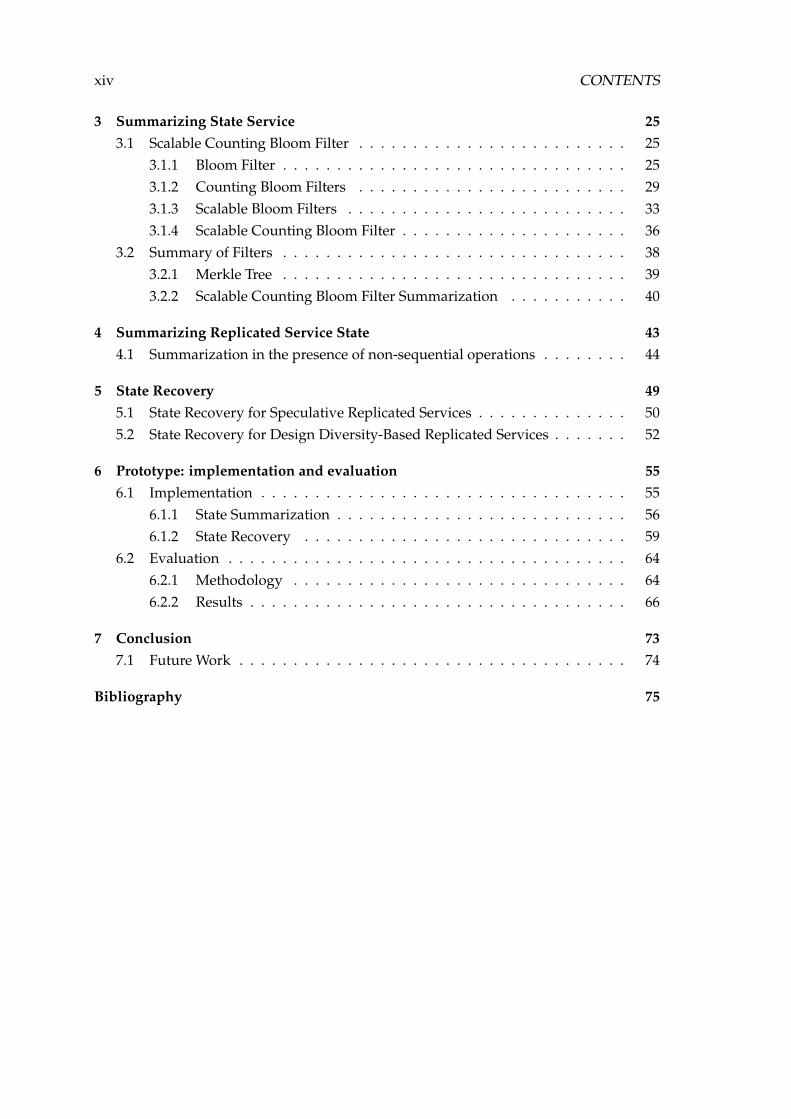
Contents xiii
List of Figures xv
List of Tables xvii
1 Introduction 1
1.1 Context . . . . . . . . . . . . . . . . . . . . . . . . . . . . . . . . . . . . . . . 1
1.2 Motivation . . . . . . . . . . . . . . . . . . . . . . . . . . . . . . . . . . . . . 2
1.3 Implemented Solution . . . . . . . . . . . . . . . . . . . . . . . . . . . . . . 2
1.4 Main Contributions . . . . . . . . . . . . . . . . . . . . . . . . . . . . . . . . 5
1.5 Organization . . . . . . . . . . . . . . . . . . . . . . . . . . . . . . . . . . . . 5
2 Related Work 7
2.1 Key Concepts . . . . . . . . . . . . . . . . . . . . . . . . . . . . . . . . . . . 7
2.1.1 State Machine . . . . . . . . . . . . . . . . . . . . . . . . . . . . . . . 7
2.1.2 State Machine Replication . . . . . . . . . . . . . . . . . . . . . . . . 7
2.1.3 Dependability . . . . . . . . . . . . . . . . . . . . . . . . . . . . . . . 8
2.1.4 Fault-tolerance . . . . . . . . . . . . . . . . . . . . . . . . . . . . . . 8
2.2 Techniques . . . . . . . . . . . . . . . . . . . . . . . . . . . . . . . . . . . . . 9
2.2.1 Proactive Recovery . . . . . . . . . . . . . . . . . . . . . . . . . . . . 9
2.2.2 Design Diversity . . . . . . . . . . . . . . . . . . . . . . . . . . . . . 9
2.2.3 Speculative Execution . . . . . . . . . . . . . . . . . . . . . . . . . . 10
2.3 Systems . . . . . . . . . . . . . . . . . . . . . . . . . . . . . . . . . . . . . . . 11
2.3.1 Systems for improved performance . . . . . . . . . . . . . . . . . . 11
2.3.2 Systems for improved fault tolerance . . . . . . . . . . . . . . . . . 15
2.4 Examples of replicated services . . . . . . . . . . . . . . . . . . . . . . . . . 21
2.4.1 Off-The-Shelf SQL Database Servers . . . . . . . . . . . . . . . . . . 21
xiii
xiv CONTENTS
3 Summarizing State Service 253.1 Scalable Counting Bloom Filter . . . . . . . . . . . . . . . . . . . . . . . . . 25
3.1.1 Bloom Filter . . . . . . . . . . . . . . . . . . . . . . . . . . . . . . . . 253.1.2 Counting Bloom Filters . . . . . . . . . . . . . . . . . . . . . . . . . 293.1.3 Scalable Bloom Filters . . . . . . . . . . . . . . . . . . . . . . . . . . 333.1.4 Scalable Counting Bloom Filter . . . . . . . . . . . . . . . . . . . . . 36
3.2 Summary of Filters . . . . . . . . . . . . . . . . . . . . . . . . . . . . . . . . 383.2.1 Merkle Tree . . . . . . . . . . . . . . . . . . . . . . . . . . . . . . . . 393.2.2 Scalable Counting Bloom Filter Summarization . . . . . . . . . . . 40
4 Summarizing Replicated Service State 434.1 Summarization in the presence of non-sequential operations . . . . . . . . 44
5 State Recovery 495.1 State Recovery for Speculative Replicated Services . . . . . . . . . . . . . . 505.2 State Recovery for Design Diversity-Based Replicated Services . . . . . . . 52
6 Prototype: implementation and evaluation 556.1 Implementation . . . . . . . . . . . . . . . . . . . . . . . . . . . . . . . . . . 55
6.1.1 State Summarization . . . . . . . . . . . . . . . . . . . . . . . . . . . 566.1.2 State Recovery . . . . . . . . . . . . . . . . . . . . . . . . . . . . . . 59
6.2 Evaluation . . . . . . . . . . . . . . . . . . . . . . . . . . . . . . . . . . . . . 646.2.1 Methodology . . . . . . . . . . . . . . . . . . . . . . . . . . . . . . . 646.2.2 Results . . . . . . . . . . . . . . . . . . . . . . . . . . . . . . . . . . . 66
7 Conclusion 737.1 Future Work . . . . . . . . . . . . . . . . . . . . . . . . . . . . . . . . . . . . 74
Bibliography 75
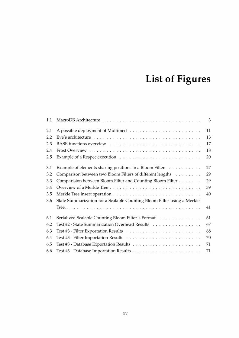
List of Figures
1.1 MacroDB Architecture . . . . . . . . . . . . . . . . . . . . . . . . . . . . . . 3
2.1 A possible deployment of Multimed . . . . . . . . . . . . . . . . . . . . . . 112.2 Eve’s architecture . . . . . . . . . . . . . . . . . . . . . . . . . . . . . . . . . 132.3 BASE functions overview . . . . . . . . . . . . . . . . . . . . . . . . . . . . 172.4 Frost Overview . . . . . . . . . . . . . . . . . . . . . . . . . . . . . . . . . . 182.5 Example of a Respec execution . . . . . . . . . . . . . . . . . . . . . . . . . 20
3.1 Example of elements sharing positions in a Bloom Filter. . . . . . . . . . . 273.2 Comparison between two Bloom Filters of different lengths . . . . . . . . 293.3 Comparision between Bloom Filter and Counting Bloom Filter . . . . . . . 293.4 Overview of a Merkle Tree . . . . . . . . . . . . . . . . . . . . . . . . . . . . 393.5 Merkle Tree insert operation . . . . . . . . . . . . . . . . . . . . . . . . . . . 403.6 State Summarization for a Scalable Counting Bloom Filter using a Merkle
Tree. . . . . . . . . . . . . . . . . . . . . . . . . . . . . . . . . . . . . . . . . . 41
6.1 Serialized Scalable Counting Bloom Filter’s Format . . . . . . . . . . . . . 616.2 Test #2 - State Summarization Overhead Results . . . . . . . . . . . . . . . 676.3 Test #3 - Filter Exportation Results . . . . . . . . . . . . . . . . . . . . . . . 686.4 Test #3 - Filter Importation Results . . . . . . . . . . . . . . . . . . . . . . . 706.5 Test #3 - Database Exportation Results . . . . . . . . . . . . . . . . . . . . . 716.6 Test #3 - Database Importation Results . . . . . . . . . . . . . . . . . . . . . 71
xv

xvi LIST OF FIGURES

List of Tables
2.1 Frost Plan of Action . . . . . . . . . . . . . . . . . . . . . . . . . . . . . . . . 18
xvii

xviii LIST OF TABLES
1Introduction
1.1 Context
Moore’s law states that transistor density on integrated circuits doubles about every twoyears [1, 2]. Until relatively recently, this implied a relation between the amount of tran-sistors in a chip and the processor’s performance. That’s because the additional transis-tors were mainly used to boost processor frequency and increase fast local memory. Allthis evolution was transparent to the software and the faster the hardware, the faster thesoftware would run.
However, beginning around the middle of last decade, increasing clock frequencystarted to hit a wall. As a result, as it was still possible to increase the number of tran-sistors in a chip, chipmakers start producing processors with multiple cores [3]. Thischanged the computational paradigm. From the perspective of the application these wereno longer seen as a single processor, but instead as complete independent processors.
The problem is that applications created with a decades old design — i.e., includinga single thread to execute a single thread of instructions — don’t benefit from additionalcores to do more work independently. Thus, these applications are unable to improveperformance solely on the basis of running on a multi-core processor. Ir order to exploitthe performance of these multi-core processors, reducing the time it takes applications toaccomplish a given task, the work has to be split into pieces, so that the processors canwork on them in parallel (multi-threading). This implies that the application needs to berewritten, and its work needs to be split into pieces suitable for multi-threading.
1
1. INTRODUCTION 1.2. Motivation
1.2 Motivation
In distributed systems, replication has been used to improve performance of systems.RepComp tries to explore a similar replication approach to improve the performance ofapplications running in multi-core systems without requiring application to be rewrit-ten. The intuition is that in single threaded applications, by keeping multiple replicas ofa given component, it might be possible to use the implementation with best performanceto run each operation more efficiently. In applications that have multiple threads, relyingon multiple replicas can improve performance by decreasing the contention among mul-tiple threads, as concurrent operations would run without any interaction in differentreplicas.
An alternative to multi-threading is to use state machine replication, more specificallycomponent replication [4], treating multi-core processors as distributed systems. Thusallowing for single-threaded applications to exploit multi-core processor performancewithout being rewritten.
Although component replication allows for applications to exploit the benefits of run-ning on multi-core processors, it also introduces a problem that needs addressing.
The problem with this technique is that in order for applications to be able to haveimproved throughput, with correct semantics, it is necessary to keep replicas synchro-nized. To this end, the system must include a replication algorithm to control the accessto the replicas and their update.
One important issue that arises is to guarantee that all replicas are kept consistent.The replication algorithm must guarantee this property. In some cases, the execution ofoperations in a given replica may be slow and the replica become stale (when comparedto others). In the presence of bugs, the state of a replica may become incorrect. To guar-antee that the system continues working correctly, it is necessary to detect and repair thissituation. This work focus on these problems in the context of RepComp project.
1.3 Implemented Solution
The RepComp project aims at exploring software component replication to improve per-formance and fault-tolerance of applications running in multi-core machines. The mainidea is to replace software components used by the application with macro-componentsthat include several replica of the same component specification — each replica may havethe same or a different implementation of the same interface (e.g., a set macro-componentmay be composed by a replica implemented with a tree and other replica implementedwith a hashtable).
MacroDB [5], an example of a Macro-Component [4], is a system aimed to improveDBMSs - specifically in-memory DBMSs - performance on multi-core processor plat-forms.
MacroDB is built as a middleware intended to be a transparent layer between clients
2
1. INTRODUCTION 1.3. Implemented Solution
Manager
PrimaryReplica Secondary
Replicas
MacroDB
Client Client Client Client
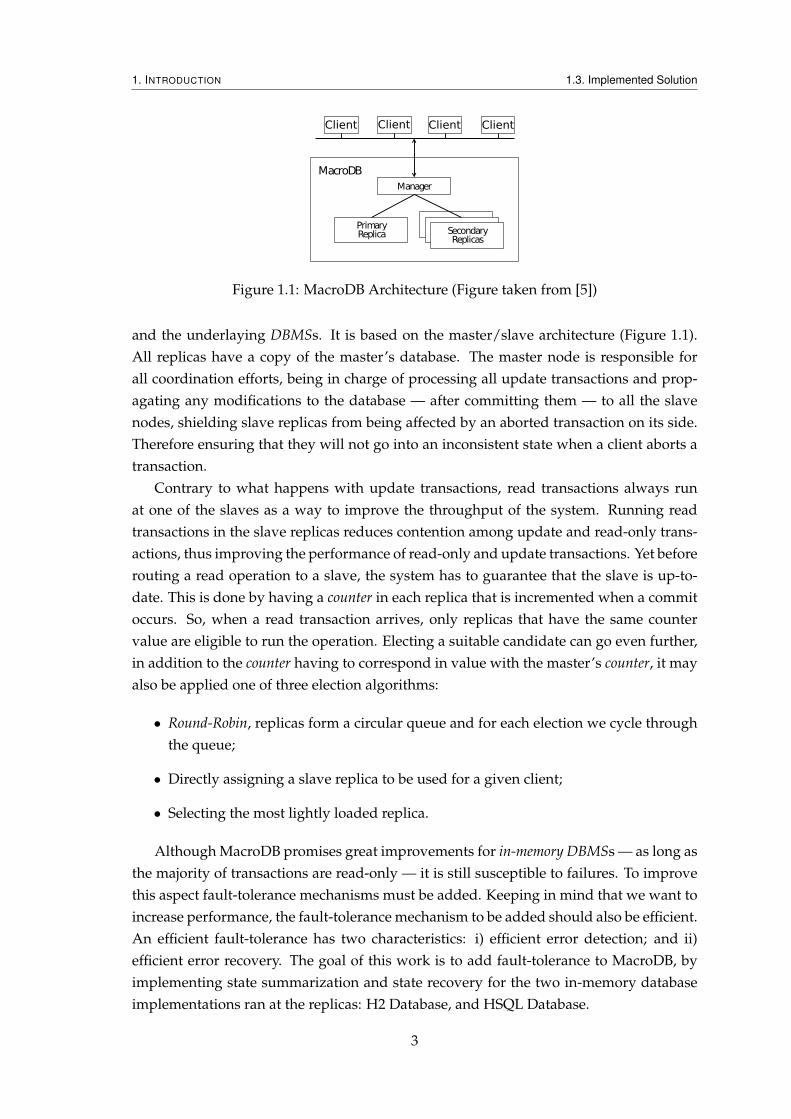
Figure 1.1: MacroDB Architecture (Figure taken from [5])
and the underlaying DBMSs. It is based on the master/slave architecture (Figure 1.1).All replicas have a copy of the master’s database. The master node is responsible forall coordination efforts, being in charge of processing all update transactions and prop-agating any modifications to the database — after committing them — to all the slavenodes, shielding slave replicas from being affected by an aborted transaction on its side.Therefore ensuring that they will not go into an inconsistent state when a client aborts atransaction.
Contrary to what happens with update transactions, read transactions always runat one of the slaves as a way to improve the throughput of the system. Running readtransactions in the slave replicas reduces contention among update and read-only trans-actions, thus improving the performance of read-only and update transactions. Yet beforerouting a read operation to a slave, the system has to guarantee that the slave is up-to-date. This is done by having a counter in each replica that is incremented when a commitoccurs. So, when a read transaction arrives, only replicas that have the same countervalue are eligible to run the operation. Electing a suitable candidate can go even further,in addition to the counter having to correspond in value with the master’s counter, it mayalso be applied one of three election algorithms:
• Round-Robin, replicas form a circular queue and for each election we cycle throughthe queue;
• Directly assigning a slave replica to be used for a given client;
• Selecting the most lightly loaded replica.
Although MacroDB promises great improvements for in-memory DBMSs — as long asthe majority of transactions are read-only — it is still susceptible to failures. To improvethis aspect fault-tolerance mechanisms must be added. Keeping in mind that we want toincrease performance, the fault-tolerance mechanism to be added should also be efficient.An efficient fault-tolerance has two characteristics: i) efficient error detection; and ii)efficient error recovery. The goal of this work is to add fault-tolerance to MacroDB, byimplementing state summarization and state recovery for the two in-memory databaseimplementations ran at the replicas: H2 Database, and HSQL Database.
3
1. INTRODUCTION 1.3. Implemented Solution
The goal of this work is to add fault-tolerance and healing of software componentreplicas to MacroDB. We now discuss the key ideas that were explored to achieve thisgoal.
If we assume a byzantine fault model for software components, to detect faults itis necessary to run operations in more than one node and compare the results beforereturning the final result to the client. In the context of RepComp, support for detectingthese faults have been developed. In this case, it is obvious that the state of a replica hasbecome incorrect. However, a replica may fail silently by getting internally corruptedbefore returning incorrect results.
This challenge is approached by creating a state summarization for the replica, in thecontext of this work, we implemented an abstraction of the internal state for the types ofreplicas used: H2 Database and HSQL Database.
The main idea here is to use Scalable Counting Bloom Filters to achieve the statesummarization. Integrating this structure with the databases we generate a token thatrepresents the internal state of the database that can be used by the replicated service toidentify divergent replicas by comparing their tokens.
Having a way for the internal state of the replica to be acquired is the first step in theprocess of adding support for fault-tolerance. After a replica has been marked as faulty,the system has to trigger the recovering process for the replica.
This process of recovering a replica is done by repairing the state of the replica, whichis done by replacing its state with the one from a known correct replica, hence the needfor the existence of mechanisms that allow a replica’s state to be exported, and to providea way for a faulty-replica to import a correct state.
Given that the state summarization token for both databases is based on the contentsof the that database’s tables, updating the state of the recovering replica can be done byrecreating those tables in the replica, which is done by recreating the data contained in thetables. Similarly to what was done for exporting and importing the state summarizationtoken, exporting the contents of the database is done by running specific functions alreadyoffered by the both databases’ interfaces.
These functions allow for the contents of the database, more concretely the tables andtheir respective data, to be exported to a file. The resulting file contains all the database’sschema, and all of the tables’ data in the form of sql inserts statements. The state of thereplica can then be brought up-to-date by parsing and executing the operations containedin the aforementioned file. Both databases provide functions that do this, these functionsreceive a file with sql statements, and executes them.
Although the replica’s tables have now been successfully brought up-to-date, thestructure used to summarize the state of the replica — Scalable Counting Bloom Filter— is still out-of-date, and it too needs to be brought up-to-date. This problem is ad-dressed by implementing functions in the replica’s that allow for its state to be exported,and for the state of a known correct replica to be imported. After the previous opera-tions has been completed, the next step to successfully recover the replica is to import the
4
1. INTRODUCTION 1.4. Main Contributions
Scalable Counting Bloom Filter from a known correct replica. The replicated service hasone of the correct replicas export its filter, and passes it to the recovering replica. Uponreceiving this filter, the recovering replica replaces its filter with the imported filter, andthe process of recovering the replica ends, as it as successfully been recovered.
1.4 Main Contributions
This works makes the following contributions:
• State summarization for H2;
• State summarization for HSQL;
• State recovery for H2;
• State recovery for HSQL.
1.5 Organization
The remaining document is organized as follows: the next chapter presents the currentsystems and techniques that in some way or another relate to the topic of this work.Chapter 3 explains how to summarize the state of a service, and Chapter 4 goes a stepfurther and details how can this be applied for replicated services. Then follows a Chap-ter that goes through the process of State Recovery. And the document ends with anevaluation of the developed work, and the final chapter is dedicated to making final re-marks and possible future improvements that can be made to this work.
5

1. INTRODUCTION 1.5. Organization
6
2Related Work
2.1 Key Concepts
We start by introducing some base general concepts before analyzing the current relatedwork.
2.1.1 State Machine
As defined by Fred B. Schneider: "A state machine consists of state variables, which encodeits state, and commands, which transform its state. Each command is implemented by adeterministic program; execution of the command is atomic with respect to other com-mands and modifies the state variables and/or produces some output. A client of thestate machine makes a request to execute a command. The request names a state machine,names the command to be performed, and contains any information needed by the com-mand. Output from request processing can be to an actuator (e.g., in a process-controlsystem), to some other peripheral device (e.g., a disk or terminal), or clients awaitingresponses from prior requests" [6].
2.1.2 State Machine Replication
State machine replication is the replication of a state machine. There are a couple of pro-prieties that the system must guarantee before state machine replication can be applied:
• Deterministic execution. If two replicas execute the same sequence of commandsin the same order, they must reach the same state and produce the same output [7].
7
2. RELATED WORK 2.1. Key Concepts
• Sequential execution. Before attempting to execute any further operation, thereplica needs to finish executing the current operation.
A system can implement state machine replication by executing the same sequenceof operations in all replicas. In this work, state machine replication is applied to therealm of multi-core processors, allowing for an improved performance [7, 4] and/or fault-tolerance [8, 9]. However, the solutions proposed in this thesis could be used in anycontext where state machine replication can be used and even in more general contextsthat use replicated state.
2.1.3 Dependability
"Dependability is an integrative concept that encompasses the following attributes: avail-ability: readiness for correct service; reliability: continuity of correct service; safety: ab-sence of catastrophic consequences on the user(s) and the environment; confidentiality:absence of unauthorized disclosure of information; integrity: absence of improper systemstate alterations; maintainability; ability to undergo repairs and modifications" [10].
In the context of this work, a system is considered to be dependable — provides de-pendability — if despite any faults, it continues behaving as expected.
2.1.4 Fault-tolerance
Fault-tolerance is one of several ways to attain dependability. Its purpose is to preservethe correct service operation despite any active fault.
The fault-tolerance mechanism is composed by two components:
• Error detection. Identifying when an error happens, in order to act upon.
• Error recovery. Recovery involves correcting the state of a faulty component. Thisconsists in reverting its state to a previously correct state and bringing its state up-to-date.
Throughout this work we’ll consider a replica to be faulty if it manifests one of thefollowing types of failure:
• Byzantine failures are arbitrary faults that occur during the execution. These faultsencompass both omission failures and commission failures. This type of failure ishard to detect due to the lack of manifestation, the components affected by thesefailures can keep executing normally while the system can not really mark them asfaulty.
• Fail-stop failures will halt the replica’s execution process instead of performing anerroneous state transformation that will be visible to other replicas [11].
These faults can have different origins — they can be caused by an error in the appli-cation’s code, deficient design, or be the result of a malicious attack.
8
2. RELATED WORK 2.2. Techniques
2.2 Techniques
This section introduces some basic techniques used in the systems discussed later.
2.2.1 Proactive Recovery
Proactive Recovery [12] provides improved dependability by taking preventative mea-sures against possible faulty replicas. Independently of their state, replicas are periodi-cally recovered, avoiding replicas to go into incoherent states. This is done because thereis anecdotal evidence that there is a correlation between the length of time a replica isrunning and the probability that it will fail [13]. The longer the replica runs, the higherthe probability of it failing.
When a replica undergoes the recovering process, it is rebooted and restarted. Usu-ally, the replica is initialized with an out-of-date correct state previously stored. Next,the replica is brought up-to-date, by having its state replaced with the correct state of thesystem. The correct state of the system can be determined by a majority vote among allreplicas. This is done by comparing the states of all replicas. The correct state is thentransfered to the new replica, which proceed executing as a system replica. After this laststep, the replica’s state is considered correct.
2.2.2 Design Diversity
Design diversity [9] is a technique to achieve fault tolerance [14]. The belief here is thathaving replicas yielding non-coincident errors will ease the job of detecting failures, asthis will avoid that replicas coincidently fail in the same operation. Ensuring that whenreplicas fail they do so with different errors allows the system to identify faulty replicas.
Another advantage of this system is that the aforementioned property not only en-sures that errors are detected, but also that most of the implementations will be able tosurvive that execution.
There are two variants of design diversity: diverse design diversity, and non-diversedesign diversity.
In the former type of design diversity each replica runs a different implementationof a common specification. This approach has the advantage of providing better fail-ure diversity, because each implementation is independently developed and will havetolerance for different errors. Because of this, it is also harder to integrate, as each imple-mentation may have its own way of presenting its internal state.
The latter, non-diverse design diversity, consists in using different versions of thesame implementation. This results in having almost identical tolerances for the sameerrors, thus having weaker failure diversity. The advantage of this variant is that asall implementations have a common code base, they will have nearly identical ways ofrepresenting their internal state, which allows for easier integration.
9
2. RELATED WORK 2.2. Techniques
2.2.3 Speculative Execution
Speculative execution is a general technique used to hide latency [15]. Rather than wait-ing for the results of a slow operation to arrive, the system may opt to work with a spec-ulated result — the result that it is expected to come from the previous operation — thusimproving the performance of the system by avoiding the time consumed waiting forresults.
The way speculation works is the following: on a replicated service an applicationinstead of waiting for a result of an operation to arrive, speculates what should be theoutcome of that operation. When the application creates a speculative result, it saves itscurrent state — by creating a checkpoint — and continues the execution process using thatresult.
When finally the response arrives, if the speculated result does not match it, the ap-plication needs to abort all operations for which that result was used, and needs to berecovered. This involves performing a rollback to the last available checkpoint, ensuringcorrectness of state before being brought up-to-date. Then, the application uses the cor-rect result to re-execute all the affected operations.
If the result received matches the speculated one, the application can discard the check-point created at the beginning of execution, and continue its execution process.
Speculative execution should only be used when the time wasted creating the check-point is smaller than the time that the system would have to wait for the correct result toarrive, and only when it is possible for the system to estimate the result of an operation.Otherwise speculative execution would be useless for the system, wasting its resourcesby creating unneeded checkpoints or by triggering recovery processes.
A byzantine fault-tolerant system’s client can improve its response time by applyingspeculative execution after receiving the first result, as in the normal case all replicas arecorrect and the first result equals the result that is obtained in the consensus process.
One thing that needs to be avoided is the externalization of speculative results, en-suring that the state associated with a speculative result is never committed, because byexternalizing the result of a speculative execution, the system would not be able to revertthe effect of that result.
An associated concept is the boundary of speculation. This boundary is what allowsthe system to control the repercussions of a bad speculation, by limiting the number ofoperations that are affected by a miscalculated result.
The larger the boundary allowed by the system, the higher the risk of having to takerecovery measures. This means that having large boundaries have higher costs for thesystem in the case of miscalculated results, as more operations are tainted by that result.The advantage of having large boundaries is that they allow for improved throughput,because more operations are allowed to use speculative results. On the other hand, ifthe system uses very small boundaries, speculative execution will not yield a great im-provement in throughput because there will be less speculative operations allowed to
10
2. RELATED WORK 2.3. Systems
take place. This also implies that the number of checkpoints that will be created is greaterand the number of state verifications that take place will also be greater, thus restrictingthe throughput of the system.
2.3 Systems
This section presents related work. Although our focus is on systems that rely on repli-cation in systems with multiple cores, we also present other relevant works. We start bypresenting systems that try to improve performance and later those that focus on fault-tolerance.
2.3.1 Systems for improved performance
The following systems were developed for improving performance. The first, Multimed [16],provides improved performance by treating multi-core processors as a distributed sys-tem. The second, Eve [17], provides support for multi-threading in state machine repli-cation systems. Lastly, Macro-Component [5, 18], exploits the performance differences ofvarious components, providing the best performance for all operations.
2.3.1.1 Multimed
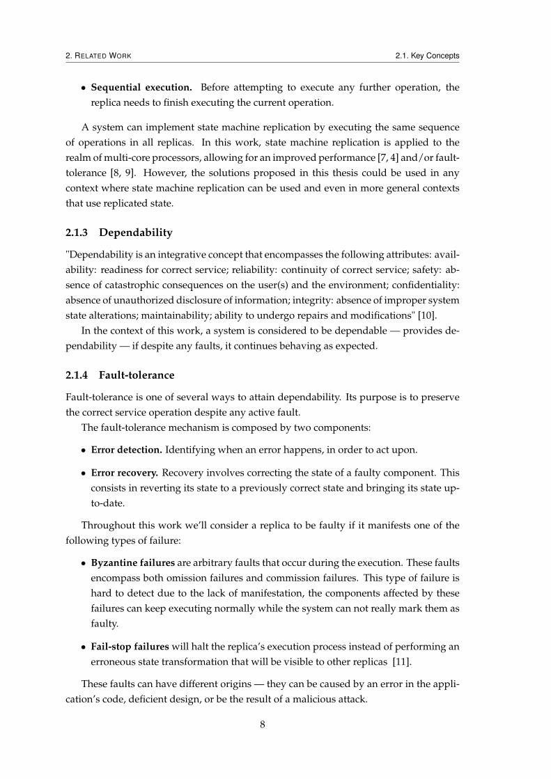
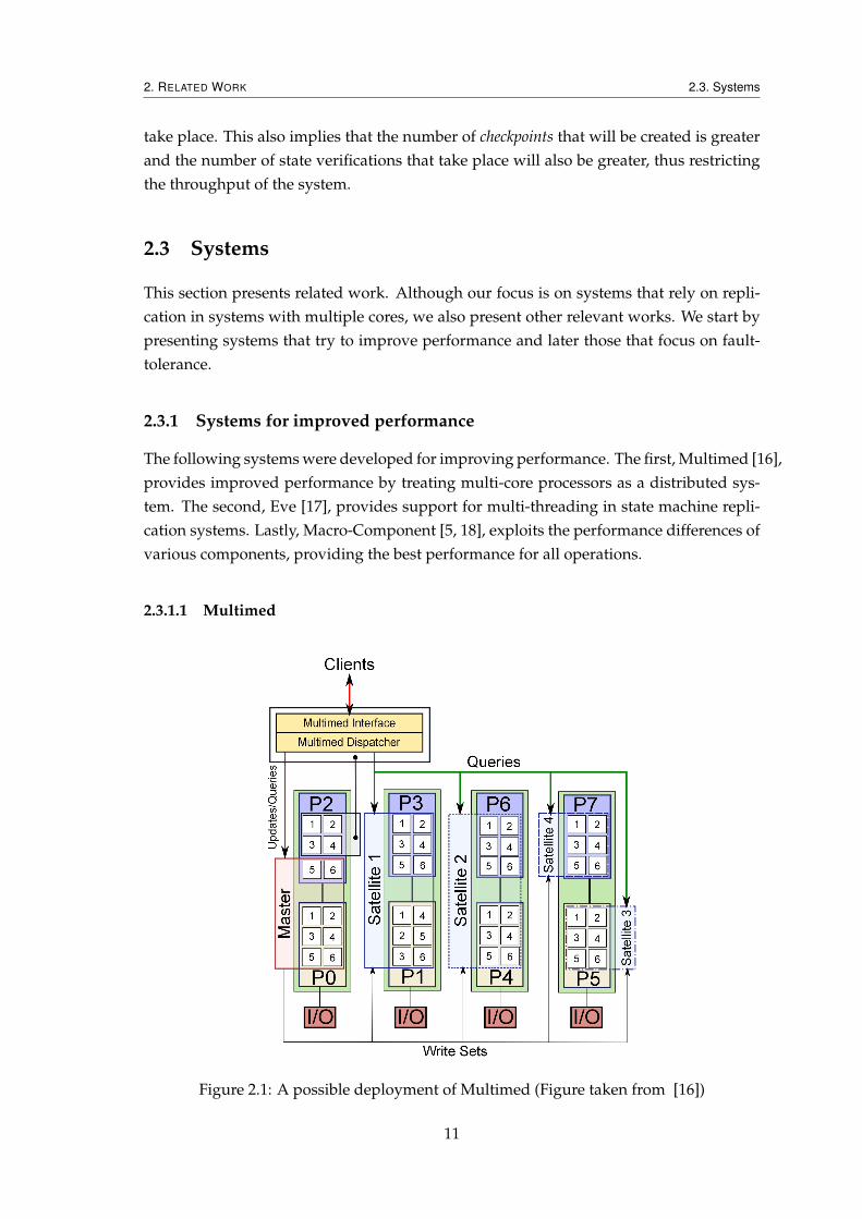
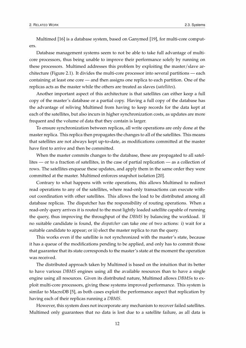
Figure 2.1: A possible deployment of Multimed (Figure taken from [16])
11
2. RELATED WORK 2.3. Systems
Multimed [16] is a database system, based on Ganymed [19], for multi-core comput-ers.
Database management systems seem to not be able to take full advantage of multi-core processors, thus being unable to improve their performance solely by running onthese processors. Multimed addresses this problem by exploiting the master/slave ar-chitecture (Figure 2.1). It divides the multi-core processor into several partitions — eachcontaining at least one core — and then assigns one replica to each partition. One of thereplicas acts as the master while the others are treated as slaves (satellites).
Another important aspect of this architecture is that satellites can either keep a fullcopy of the master’s database or a partial copy. Having a full copy of the database hasthe advantage of reliving Multimed from having to keep records for the data kept ateach of the satellites, but also incurs in higher synchronization costs, as updates are morefrequent and the volume of data that they contain is larger.
To ensure synchronization between replicas, all write operations are only done at themaster replica. This replica then propagates the changes to all of the satellites. This meansthat satellites are not always kept up-to-date, as modifications committed at the masterhave first to arrive and then be committed.
When the master commits changes to the database, these are propagated to all satel-lites — or to a fraction of satellites, in the case of partial replication — as a collection ofrows. The satellites enqueue these updates, and apply them in the same order they werecommitted at the master. Multimed enforces snapshot isolation [20].
Contrary to what happens with write operations, this allows Multimed to redirectread operations to any of the satellites, where read-only transactions can execute with-out coordination with other satellites. This allows the load to be distributed among alldatabase replicas. The dispatcher has the responsibility of routing operations. When aread-only query arrives it is routed to the most lightly loaded satellite capable of runningthe query, thus improving the throughput of the DBMS by balancing the workload. Ifno suitable candidate is found, the dispatcher can take one of two actions: i) wait for asuitable candidate to appear; or ii) elect the master replica to run the query.
This works even if the satellite is not synchronized with the master’s state, becauseit has a queue of the modifications pending to be applied, and only has to commit thosethat guarantee that its state corresponds to the master’s state at the moment the operationwas received.
The distributed approach taken by Multimed is based on the intuition that its betterto have various DBMS engines using all the available resources than to have a singleengine using all resources. Given its distributed nature, Multimed allows DBMSs to ex-ploit multi-core processors, giving these systems improved performance. This system issimilar to MacroDB [5], as both cases exploit the performance aspect that replication byhaving each of their replicas running a DBMS.
However, this system does not incorporate any mechanism to recover failed satellites.Multimed only guarantees that no data is lost due to a satellite failure, as all data is
12
2. RELATED WORK 2.3. Systems
durably committed by the master.
2.3.1.2 Eve
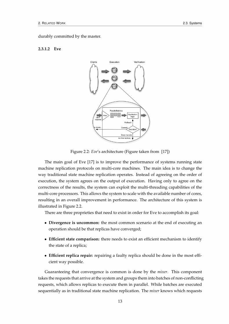
Figure 2.2: Eve’s architecture (Figure taken from [17])
The main goal of Eve [17] is to improve the performance of systems running statemachine replication protocols on multi-core machines. The main idea is to change theway traditional state machine replication operates. Instead of agreeing on the order ofexecution, the system agrees on the output of execution. Having only to agree on thecorrectness of the results, the system can exploit the multi-threading capabilities of themulti-core processors. This allows the system to scale with the available number of cores,resulting in an overall improvement in performance. The architecture of this system isillustrated in Figure 2.2.
There are three proprieties that need to exist in order for Eve to accomplish its goal:
• Divergence is uncommon: the most common scenario at the end of executing anoperation should be that replicas have converged;
• Efficient state comparison: there needs to exist an efficient mechanism to identifythe state of a replica;
• Efficient replica repair: repairing a faulty replica should be done in the most effi-cient way possible.
Guaranteeing that convergence is common is done by the mixer. This componenttakes the requests that arrive at the system and groups them into batches of non-conflictingrequests, which allows replicas to execute them in parallel. While batches are executedsequentially as in traditional state machine replication. The mixer knows which requests
13
2. RELATED WORK 2.3. Systems
will conflict by reading its configuration file. This file can be something as simple as alist of transactions used in the application, stating the tables they access and the type ofoperation that it is performed (read/write). Each replica can exploit multi-threading forthe execution of a batch-parallel request.
After executing a batch-parallel request, the results and the state of the replica are com-pared with the ones obtained by the other replicas. Instead of comparing the result andstate itself — as this would entail sending the whole result and state — only a token rep-resenting the replica’s state is sent. This token is the root-leaf of the merkle tree used by thereplica to store its objects. Using a merkle tree to generate a representation of the replica’sstate is challenging. For this to work the system must devise a way to ensure that eachreplica constructs its tree deterministically.
Eve overcomes this challenge by having each replica construct its tree only at the endof execution, before generating the token. The intuition here is that replicas that executedcorrectly should have the same objects to add to the tree, and by postponing the creationof the tree until the very last moment, they will construct the same tree.
If the state of the replicas is different — i.e., the tokens did not match — this meansthat some of the replicas have diverged. To identify which replicas diverged the systemruns a consensus algorithm with the collected tokens. If there are enough equal tokens,that means that this token corresponds to the correct result. All replicas whose state yielda different token are considered to have diverged, and need to be repaired.
Repairing a faulty replica involves undoing the operation that caused divergence, andbringing the replica to the correct state. A rollback is performed to undo the results ofthe operation, leaving the replica in a correct but out-of-date state. The rollback processis done by having the pointers of the merkle tree point to the original object. This ensuresthat the replica is in a previously correct state. The last step involves bringing the replicaup-to-date. This is done by sequentially re-executing the batch that caused divergence,in order to guarantee progress.
Some of the techniques used in Eve were applied in this thesis, namely the techniquesrelated to state summarization. The state summarization process implemented in ourprototype makes use of the efficient way that the merkle tree has for performing statesummarization. Although the merkle tree is not used in the same manner that it is usedin Eve to achieve state summarization of the replica, it still proved to be advantageous tointegrate this structure in the implemented state summarization process, as it provides amore efficient way for state summarization, in our case, for summarizing the state of thestructure used to achieve this, as described in subsequent chapters.
2.3.1.3 Macro-Component
The goal of Macro-Component [4] is to provide better performance or fault-tolerance overstandard components, doing so by applying diverse component replication. With Macro-Component, software components in a program are replaced by a Macro-Component that
14
2. RELATED WORK 2.3. Systems
includes several replicas of the same specification, typically with different implementa-tions.
The intuition behind Macro-Component is that no single implementation of a soft-ware specification yields the best results for every operation — i.e., a component that hasthe fastest results for some operations may have the slower results for other operations.This creates a dilemma for the programmer, forcing him to choose the component that isthe best fit for his application, thus sacrificing performance for some of the operations.This decision must be made by taking into account the expected workload for the appli-cation. The problem is that it is not always possible to know what will be the workload,as many applications vary their workload type throughout execution, and making thecorrect choice in these types of scenarios is impossible. Macro-Component removes thisdecision from the design processes, allowing the programmer to use the fastest methodfor any given operation.
For providing better fault-tolerance, Macro-Component can explore different compo-nent implementations to mask component bugs.
When a method is called on a Macro-Component, one of two paths is taken: i) ifthe method is expected to return results, a synchronous invocation model is used, con-currently calling the same method on all replicas — when configured to improve per-formance, the first result obtained is returned to the application; when configured toimprove fault-tolerance, the result is returned after being confirmed by more than onereplica; ii) in the case of the method not yielding any results, tt is known that the resultwill be ignored by the application, an asynchronous invocation model is used, concur-rently executing this method alongside the application’s thread, further improving thethroughput over standard components.
One limiting factor is the need for replica consistency. Although necessary, it neg-atively affects the system’s performance, as synchronization will reduce the amount ofparallelism that can take place. Macro-Component uses a variant of the master-slavescheme, that uses a master-rotating process. After executing a write operation, the cur-rent master is demoted to slave, and the first slave to complete all pending synchroniza-tion operations is elected as the new master. During this time, read operations are routedto the former-master. This forces a total execution order for write operations in all repli-cas, thus guaranteeing that they converge.
Macro-Component shows that replacing standard components with their Macro-Componentsiblings, yields improvements in performance, as this approach exploits the performancedifferences offered by the various implementations. The system includes no mechanismfor recovering replicas, which is the focus of this Msc work.
2.3.2 Systems for improved fault tolerance
The following systems were developed with dependability as their main goal. The first,N-Version programming [9], achieves this by using various implementations of the same
15
2. RELATED WORK 2.3. Systems
software specification, which will guarantee failure diversity. The second, BASE [8], usesabstraction to provide an improve byzantine fault tolerant system. The third, Frost [21],forces replicas to have complementary schedules in order for the application to be able toevade data-race bugs. Lastly, Respec [22], uses speculative execution and external deter-minism, to provide online deterministic replay for multi-core processors, which allowsthe system to improve its dependability.
2.3.2.1 N-Version Programming
N-Version programming [9] (NVP) is a technique that aims to improve a system’s faulttolerance mechanisms, thus improving dependability.
The main idea behind NVP is to force replicas to have non-coincident failures (failurediversity), allowing the system to detect faulty replicas by comparing their outputs ofexecution.
This is achieved by running N implementations of a given software specification.Running various implementations of the same specification guarantees that any errorsthat occur will be as diverse as possible. Having replicas yielding non-coincident errorsallows the system to detect faulty replicas, that are then to be recovered.
The system works as follows: the results of each execution are sent to a decisionalgorithm which, by consensus, derives the correct output of execution. The criteria usedto elect the correct result can be adjusted, favoring throughput or dependability. Thelarger the number of replicas that have to agree on the output of execution the slowerthe decision process, but gives the system better dependability. The lower the number,the higher the throughput of the system, at the cost of risking using incorrect results infuture executions.
Afterwards, the correct result can be used to derive which replicas went inconsistentduring execution. Replicas that yield incorrect results, are considered to be faulty, andneed to be repaired.
In order to successfully integrate this technique in a system, we need to guaranteea couple of things. Firstly, a clear software specification that states the behavior to beexpected throughout execution. This specification should leave no room for doubt. Sec-ondly, the system must have some mechanism to detect inconsistent replicas. And lastly,a mechanism capable of repairing faulty replicas. One example of a system that appliesthis technique is the Macro-Component [4], where different replicas are allowed to usedifferent implementations of the same software specification. This allows for an improve-ment in performance, as different implementations will outperform other implementa-tions for some operations.
16
2. RELATED WORK 2.3. Systems
executepropose_value/check_valueget_obj/put_objshutdown/restart
Client
BASEClient
BASEReplica
Conf.Wrapper
OriginalImplementation
invoke
BASEProtocol
modify
Figure 2.3: BASE functions overview (Figure taken from [8])
2.3.2.2 BASE
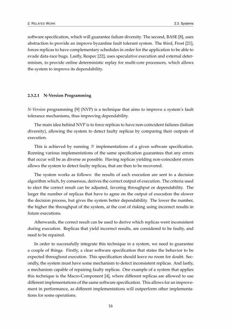
BASE [8] is a distributed replication system designed with the objective of providingimproved fault-tolerance, focusing mainly in byzantine faults. This system uses oppor-tunistic N-version programming to achieve those goals.
This system combines abstraction with a byzantine fault tolerance (BFT) library toimprove the system’s ability to mask software errors. The original PBFT library [23] haslimited use, as it requires that all replicas run the same implementation of a softwarespecification and that they update their state deterministically. Therefore, it can not tol-erate errors that cause all replicas to fail concurrently.
BASE solves this problems by implementing mechanisms that allow replicas to rundifferent implementations or non-deterministic implementations. The main concepts be-hind this system are the abstract specification, the abstract function and the conformance wrap-per. The abstract specification specifies the abstract state and the behavior of each operation,describing how these operations affect the state of the replica. The conformance wrapper isthe component that ensures that each implementation behaves accordingly to the abstractspecification. Finally, the abstract function is the component that allows to map from theconcrete state of each implementation to the abstract state, and vice-versa by implement-ing one of the inverse functions of the abstract function, thus allowing for a replica to berecovered. Figure 2.3 shows an overview of BASE’s functions.
With these components BASE is capable of reusing existing code. Different off-the-shelf implementations of a service can be used, as the conformance wrapper ensures thateach implementation behaves accordingly with the abstract specification, despite the factthat most implementations fail to conform with their own software specification (e.g.,many database management services exist, but they behave differently from each other).
This system also uses proactive recovery [12], rebooting replicas, restarting then froma clean state, and then bringing them up-to-date using an abstract state obtained by con-sensus from the other replicas. The aforementioned abstract state is created by identifiedthe core objects that represent the internal state of a replica. This means that indepen-dently of the replica’s implementation, there are concepts — in the form of objects — that
17
2. RELATED WORK 2.3. Systems
are transversal to all implementations, therefor providing the needed basis for creatingan abstract state that can be used by any implementation.
In this thesis, the idea of having an abstract state that could be used for summarizingthe internal state of a replica — independently of its implementation — was used. Thisallowed for different replicas to run different database implementations, while still pro-viding a way for comparing the internal state of two different implementations in orderto determine possible state divergences that might have occurred during operation. Ad-ditionally, the technique used to recover replicas used by BASE — proactive recovery —is also used in the implemented prototype. Recovering a replica that was deemed to befaulty is done by rebooting the replica, leaving the replica in a correct but out-of-datestate, and then using the correct state of any of the other replicas to bring the recoveringreplica up-to-date.
2.3.2.3 Frost
[Ep 0]
[Ep 1]
[Ep 2]
A
CPU 0
B
CPU 1
.
...
Epoch-parallel executionThread-parallel execution
CPU 5
[Ep 1]TIME
CPU 2[Ep 0]
CPU 3[Ep 0]
CPU 4
[Ep 1]A
B A
B
A
B
A
B
ckpt1
ckpt2
ckpt0
. .
.
.
....
Figure 2.4: Frost Overview (Figure taken from [21])
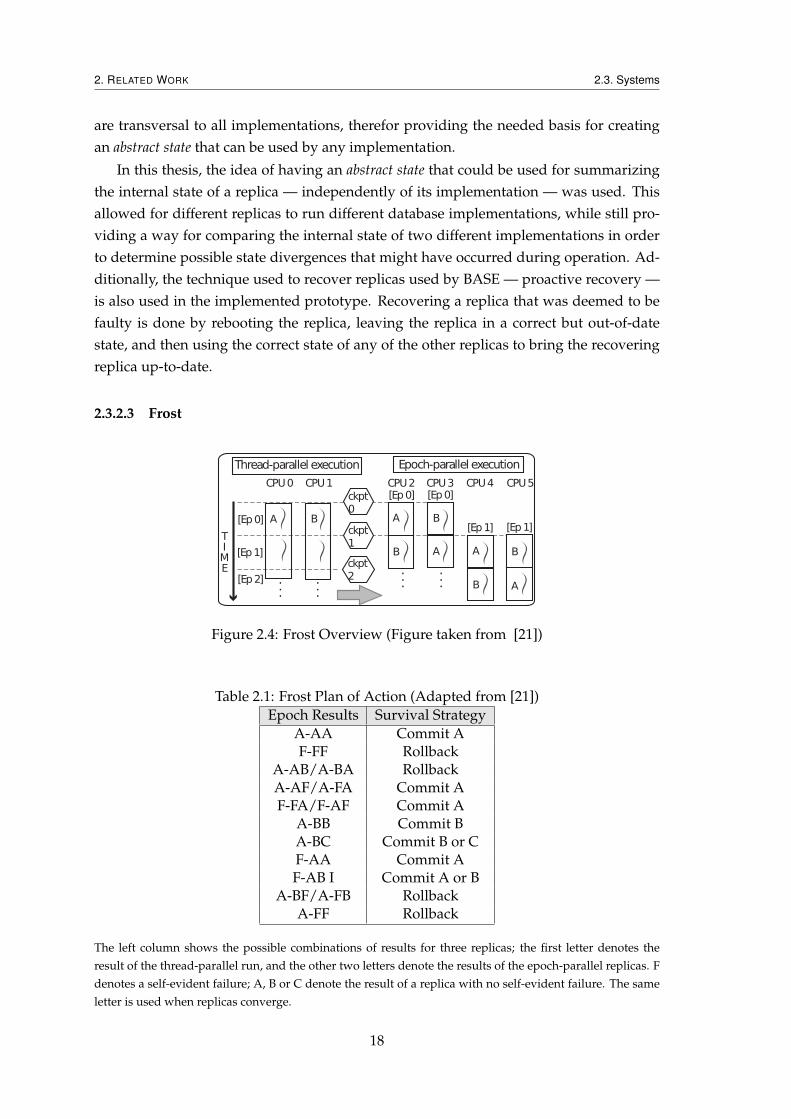
Table 2.1: Frost Plan of Action (Adapted from [21])Epoch Results Survival Strategy
A-AA Commit AF-FF Rollback
A-AB/A-BA RollbackA-AF/A-FA Commit AF-FA/F-AF Commit A
A-BB Commit BA-BC Commit B or CF-AA Commit AF-AB I Commit A or B
A-BF/A-FB RollbackA-FF Rollback
The left column shows the possible combinations of results for three replicas; the first letter denotes theresult of the thread-parallel run, and the other two letters denote the results of the epoch-parallel replicas. Fdenotes a self-evident failure; A, B or C denote the result of a replica with no self-evident failure. The sameletter is used when replicas converge.
18
2. RELATED WORK 2.3. Systems
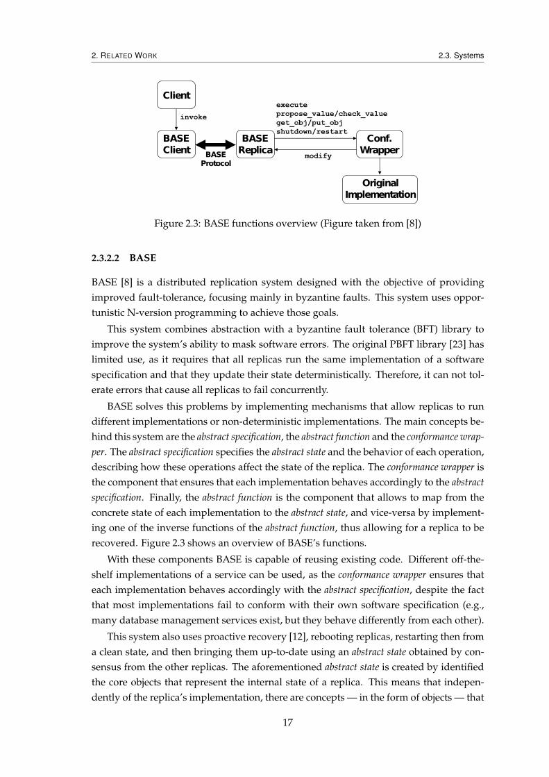
Data races are a common source for bugs in multi-threaded applications, creating theneed for mechanisms that are able to deal with such bugs. Frost [21] is a system that aimsat finding concurrency bugs in multi-threaded applications. The idea behind Frost is toforce the execution of complementary schedules.
Using complementary schedules tries to ensures that at least one of the replicas avoidsthe bug, by running the instructions that lead to that bug in a different order.
Frost achieves this by running each thread on its own processor, and with epoch-parallel execution — dividing the program execution in time-slices (epochs), and havingeach replica (epoch-parallel replica) run these epochs concurrently (see Figure 2.4).
This initial approach requires threads to run in a non-preemptively manner, makingthis solution only suitable for single-core processors, as this architecture allows Frost tocontrol the schedule used by the replicas.
In order to apply the same ideas to the realm of multi-core processors, Frost uses athird replica. The third replica runs its threads in parallel (thread-parallel replica), whichallows Frost to identify points during execution where system calls and synchronizationevents take place, and speculatively create checkpoints. The checkpoints are then used todivide the execution in synchronization-free regions (epochs), thus guaranteeing that onlya data-race can take place during an epoch.
The fault-tolerance mechanism works in two phases. In the first phase, Frost startsby checking if the replicas experienced self-evident failures. If they do not show signs ofself-evident failures, it looks for signs of failure by comparing their state at the end of theepoch, and the results yielded during that epoch.
After identifying that a race took place (i.e., a replica failed) and in order to survive ex-ecution, Frost chooses the survival strategy that is most likely to have at least one replicasurvive.
This is done by analyzing the results of the epochs, and depending on the results yieldby replicas it chooses the plan of action. As shown in Table 2.1, Frost may choose toperform a rollback, or to commit the results from a correct replica.
It decides to commit a result if all replicas converged, or if the combination of resultsallows for a correct result to be identified. If a epoch-parallel replica is chosen to be commit-ted, all subsequent epochs generated by the thread-parallel replica are invalid, and need tobe discarded. Then, the system starts new thread-parallel and epoch-parallel replicas usingthe committed state.
The rollback process occurs when no correct result can be identified. In this case,Frost may choose to generate additional replicas to further study the epoch that led to adivergence. The additional replicas are started from the checkpoint created at the beggingof the epoch, and their results will allow Frost to choose which replica to commit.
In order for replicas to continue their execution process, they must defer the outputof the previous epoch (speculative execution) — as Frost will not externalize any outputwithout it being committed. There is a trade-off between performance and dependability,as longer epochs provide better dependability, shorter epochs provide better performance.
19
2. RELATED WORK 2.3. Systems
Frost’s approach to data-race bug detection and survival can be applied to MacroDB [5].This would allow for the DBMSs used by MacroDB to have more relaxed locking mecha-nisms, while maintaining correctness of execution. By integrating the ideas behind Frostin the development of MacroDB’s fault-tolerance mechanism, the system would be ca-pable of detecting and surviving data-race bugs, thus further improving its resilience tofailures.
2.3.2.4 Respec
StartCheckpoint A
lock(q)unlock(q)
lock(q)unlock(q)
Checkpoint B
A
lock(q)unlock(q)
lock(q)unlock(q)
SysRead XLog X
Multi-threadedfork
Recorded Process Replayed Process
Epoch
1
Epoch
1’
O’ == O
B’==B?Delete Checkpoint A
Checkpoint C
SysWriteOLog O
C’==C?Commit O, Delete B
Log X
ReadLogXEpoch
2
Epoch
2’
Figure 2.5: Example of a Respec execution (Figure taken from [22])
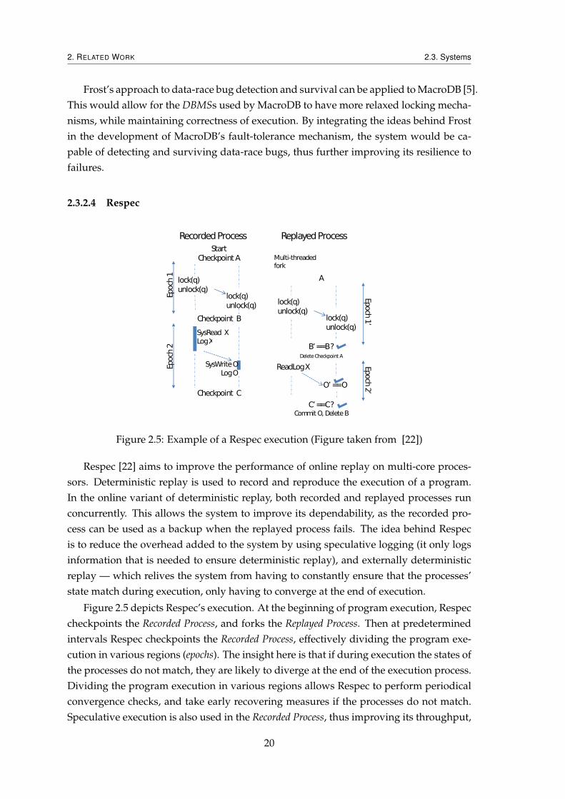
Respec [22] aims to improve the performance of online replay on multi-core proces-sors. Deterministic replay is used to record and reproduce the execution of a program.In the online variant of deterministic replay, both recorded and replayed processes runconcurrently. This allows the system to improve its dependability, as the recorded pro-cess can be used as a backup when the replayed process fails. The idea behind Respecis to reduce the overhead added to the system by using speculative logging (it only logsinformation that is needed to ensure deterministic replay), and externally deterministicreplay — which relives the system from having to constantly ensure that the processes’state match during execution, only having to converge at the end of execution.
Figure 2.5 depicts Respec’s execution. At the beginning of program execution, Respeccheckpoints the Recorded Process, and forks the Replayed Process. Then at predeterminedintervals Respec checkpoints the Recorded Process, effectively dividing the program exe-cution in various regions (epochs). The insight here is that if during execution the states ofthe processes do not match, they are likely to diverge at the end of the execution process.Dividing the program execution in various regions allows Respec to perform periodicalconvergence checks, and take early recovering measures if the processes do not match.Speculative execution is also used in the Recorded Process, thus improving its throughput,
20
2. RELATED WORK 2.4. Examples of replicated services
as it does not have to lock waiting for results in order to continue execution.
During an epoch, the Recorded Process logs its system calls. When the Replayed Processreaches a point during execution where a system call is made, instead of executing it,it emulates the system call using the logs created by the Recorded Process. This worksbecause the Recorded Process executes ahead of the Replayed Process, as it does not have toperform checks during each epoch.
Respec detects divergences — mis-speculations of race-free regions — in two ways.The first involves comparing the arguments passed to the system calls and the resultingoutput, allowing for an early recovery of the Replayed Process. The second method usedby Respec to detect divergences is to analyze the state of the processes’ at the end of theepoch, triggering the recovery process if they do not match.
The recovering process involves rolling back both processes to the beginning of theepoch, leaving them in the same correct state. Then, Respec optimistically re-executesthe problematic region, and performs the same checks as before. On repeated failure,in order to guarantee execution progress, Respec switches to the uniprocessor executionmodel — executing one thread at a time until both processes reach a system call. Afterthis, the processes’ state match and parallel execution can resume.
State machine replication systems can exploit the concepts behind Respec to improvetheir resilience to software errors. The replayed process can be used as a primary replica,and the recorded process as a secondary replica. Then the error detection process used inRespec, can be used as an efficient way to keep the state of both replicas synchronized. Inthe advent of a primary failure, the secondary replica can takeover the execution whilethe system recovers the faulty replica.
2.4 Examples of replicated services
This section discusses the challenges posed to integrate n-version programming withstate machine replication in database systems. Although the used techniques are a refine-ment of the techniques presented earlier, this work is particularly relevant to our workas we will address the problem of healing replicas in MacroDB [5], a macro-componentsystem that replicates in-memory database systems.
2.4.1 Off-The-Shelf SQL Database Servers
The poor dependability shown in off-the-shelf (OTS) SQL database servers [24, 25] isdue to the fact that they assume that only two kinds of errors can occur: fail-stop, andself-evident. Fail-stop errors are those that cause the software to crash, and self-evident er-rors are those that are externalized, for example, in the form of error messages. Thisassumption is not correct, as there are other kinds of errors that can affect the applica-tion’s behavior, and when they manifest themselves, the system will misbehave, as it isnot prepared to deal with them.
21
2. RELATED WORK 2.4. Examples of replicated services
One possible solution for improving dependability in OTS SQL database servers isto use active replication. Active replication consists in comparing the results throughoutexecution, in order to determine if some error took place. Comparing the results of eachexecution will determine the plan of action, if one replica shows a result that is inconsis-tent with the results obtained by the other replicas, we can assume that the replica hasfailed, and needs to be recovered. Recovering a faulty replica can be done by copyingthe state of a correct replica over the state of the faulty replica. But this approach willonly work if the majority of replicas executed correctly, allowing the consensus decisionalgorithm to infer what is the correct result. In the case of a majority of replicas failingwith the same incorrect result — thus misleading the decision algorithm into taking forcorrect an incorrect result — all the other replicas (including the replicas that had the cor-rect result) will be forced to converge to the state of a faulty replica. From this point on,the system state is incorrect, and all operations will yield incorrect results.
This means that the former solution is not enough to guarantee better dependability.The system needs to ensure that when replicas fail, they fail with errors as diverse as pos-sible. Failure diversity, more specifically design diversity, will ensure this property [9],avoiding replicas to have coincident failures. There are two types of design diversity:non-diverse, and diverse. The former is achieved by using evolving versions of the samedatabase product, has the advantage of being easier to integrate, but will not yield anysignificant advantage to the detection non-self-evident/non-crash failures, as versions ofthe same product will almost likely have coincident errors. The latter, consists in usingdifferent database products, and improves greatly the detection of non-self-evident/non-crash failures, but it is harder to integrate.
Applying diverse design diversity is more challenging for three main reasons:
• product-specific SQL dialects: each database may have its own implementation;
• missing/proprietary features: each database product may offer features that are notpresent in the others;
• replica consistency among all implementations.
It is possible to overcome the first challenge by doing on-the-fly translations of SQLstatements. The second can be partly solved in two distinct ways: i) using only the com-mon subset of features; or ii) trying to emulate some of the missing features (e.g., byrephrasing SQL statements). The third problem — replica consistency — can be solvedby applying the divide-and-conquer methodology, dividing the problem in two smallerones: detection, and recovery.
To identify a faulty replica the system can do one of two things: i) compare the re-sults of read operations, and verify if they match; or ii) verify the list of affected recordsafter write operations, and check if there are any differences between the replicas. Aftercomparing the state of the replicas, if the results diverged the system can then use itsfault-tolerance mechanism to mask the fault.
22
2. RELATED WORK 2.4. Examples of replicated services
The second problem — recovery — is done in two steps. The first step is to undo theoperation that left the replica inconsistent, rolling back the transaction to the last availablecheckpoint. The second step is to bring the replica to a consistent state, this can be doneby either re-executing the transaction — hoping that the new result is correct — or bycopying over the database contents of one of the correct replicas, thus ensuring that thereplica’s state is now consistent.
In this thesis similar problems had to be solved. The first, identifying replicas thathave become inconsistent during operation and need to undergo the recovering proce-dure follows a similar logic to the aforementioned one. Although, it is not verified ifthe list of affected records is the same for all replicas as this would entail sending resultsets for each operation, the state of the replicas is compared using a state summarizationstructure at each replica, and comparing the token that is generated by said structure, al-lowing for divergences of state to be detected. Additionally, the solution for recoveringan inconsistent replica implemented in this thesis follows the same line of thought de-scribed earlier. Where a replica that is deemed to have become inconsistent is recoveredin two steps. The first involving restarting the replica, leaving the replica in a correct butout-of-date state, and then bringing the state up-to-date by transfering the state from acorrect replica.
23

2. RELATED WORK 2.4. Examples of replicated services
24
3Summarizing State Service
This chapter explains how to achieve the summarization of state for a service. The firstsection presents the Scalable Counting Bloom Filter and all the process that took place tocreate this structure. The final section explains how to perform state summarization forthe Scalable Bloom Filter itself, which is crucial for the use of this structure to be able toefficiently summarize the state of a service.
3.1 Scalable Counting Bloom Filter
The goal for this section is to detail how the Scalable Counting Bloom Filter can be usedas a state summarization tool for a service.
3.1.1 Bloom Filter
The Bloom filter is a probabilistic data structure used to store a set of elements in a effi-cient way. The intuition behind this structure is that it is only needed to store a represen-tation of elements that are added, in order to be able to execute membership operations.This representation can be smaller than the size of the element, making this structureefficient.
The modus operandi behind this structure is to use a array of bits to store informationabout elements added to the set. When a new element is inserted in the Bloom filter, kpositions of the array are set to 1, effectively storing a representation of the element. Toverify if an element belongs to the Bloom filter, all of the k positions — that correspondto the representation of the element — of the array are checked in order to determine ifthey are all set to 1. If this is true, the element is said to belong to the filter, otherwise, it
25
3. SUMMARIZING STATE SERVICE 3.1. Scalable Counting Bloom Filter
not present in the filter.Depending on the desired false-probability rate set in the filter, the number of posi-
tions used in a the array to store the representation of an element varies. The larger thearray and the lower the false-probability rate, more positions will be used to represent anelement.
Although the false-probability rate can be controlled, there is another problem asso-ciated with the Bloom Filter’s approach to store elements. As elements are added to thefilter, the positions in the array of bits start to be all set to 1, which will have an impact inthe false-probability rate. In the extreme case where all of the bits get set to 1, checking formembership of any element will result in the filter claiming that the element is belongsto the set, when it does not. As we will later see, this is a problem related with the factthat the Bloom Filter can not expand beyond its initial size.
ρ = (1− e−k(n+0.5)/(m−1))k (3.1)
The probability of a false-positive — when the Bloom Filter falsely claims to have anelement, when in fact it has not — is given by the formula shown in Equation 3.1. Thisequation gives the false-probability ρ for a Bloom Filter of length m, that has n elements,and that uses k hash functions. This formula is only applicable for scenarios in which itis assumed that the aforementioned variables do not tend to infinity. In such case a morecomplex formula to calculate the false-positive probability ρ has to be used, which willnot be discussed.
The Bloom Filter offers the following operations: i) inserting elements; and ii) search-ing for elements (checking if an element belongs to the set).
Insert Operation
Data: x is the object key to insert into the Bloom filterFunction: insert(x)
for j : 1...k doi← hj(x);if Bi == 0 then
/* Bloom filter had zero bit at position i */Bi← 1;
endend
Algorithm 1: Bloom Filter insert function
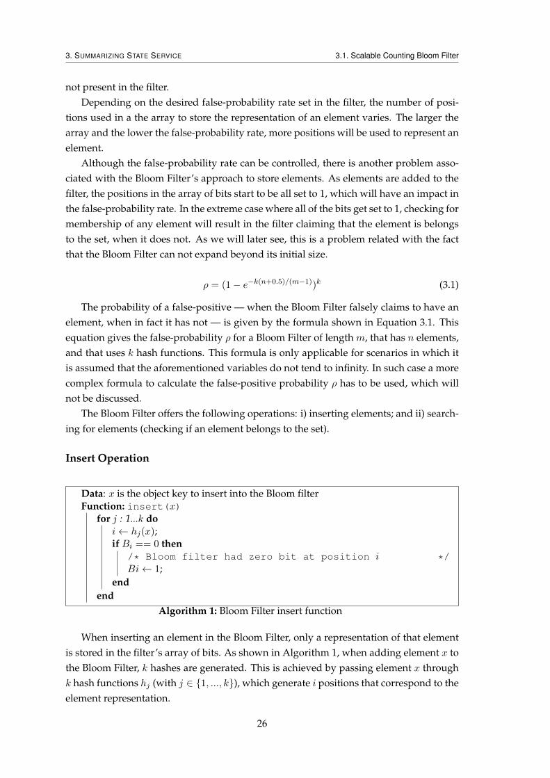
When inserting an element in the Bloom Filter, only a representation of that elementis stored in the filter’s array of bits. As shown in Algorithm 1, when adding element x tothe Bloom Filter, k hashes are generated. This is achieved by passing element x throughk hash functions hj (with j ∈ {1, ..., k}), which generate i positions that correspond to theelement representation.
26
3. SUMMARIZING STATE SERVICE 3.1. Scalable Counting Bloom Filter
Then the representation of element x is stored in the Bloom Filter by accessing itsarray of bits at each of the i positions and changing the corresponding values to one ifthey were set to zero. This effectively stores element x’s representation in the array, thussuccessfully completing the insert operation for that element.
Search Operation
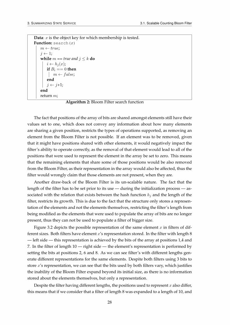
The search operation is similar to the insert operation, as shown by Algorithm 2. Whenchecking if element x belongs to the set, k hashes are generating by passing element xthrough k hash functions hj (where j ∈ 1...k). The resulting k hashes are then translatedto the i positions that represent the element in the array of bits. The values of thesei positions are then checked to see if they have been set to 1. If all positions are to 1,element x is considered to be present in the Bloom Filter with a false-probability rate of ρ.A false-positive occurs when the positions that correspond to element x’s representationhave all been set to 1 by the other members of the set, thus wrongly indicating to the filterthat x is a member.
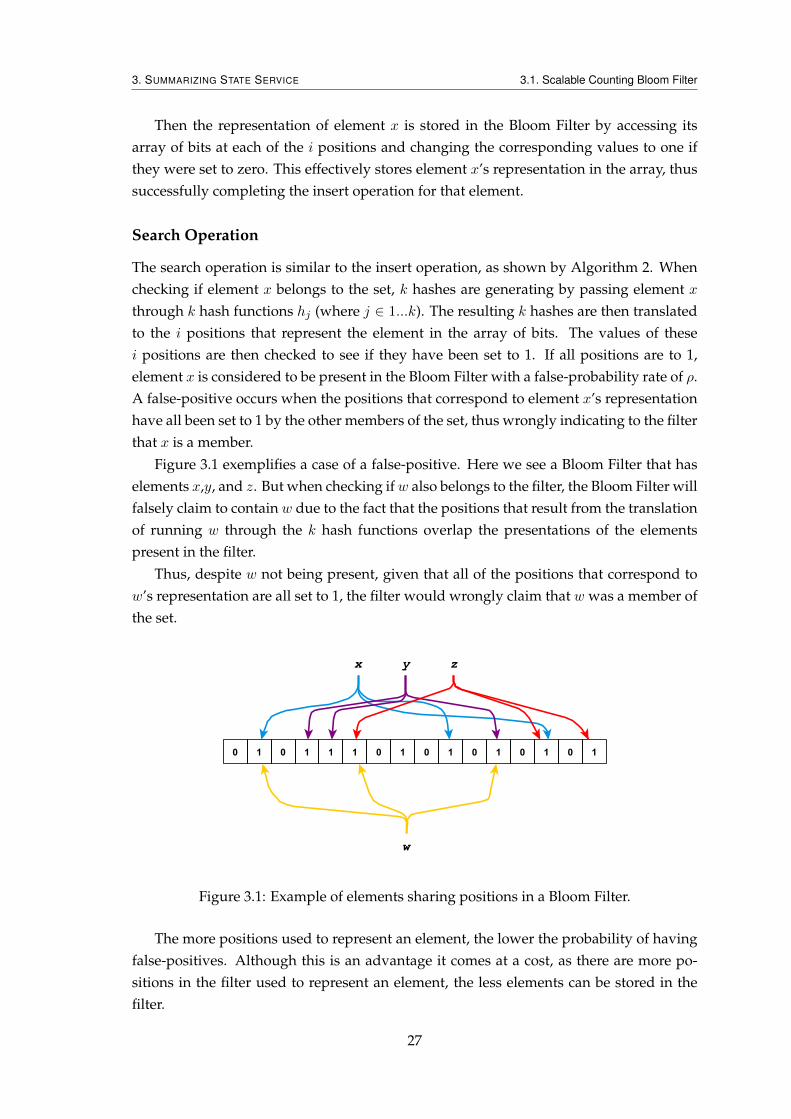
Figure 3.1 exemplifies a case of a false-positive. Here we see a Bloom Filter that haselements x,y, and z. But when checking ifw also belongs to the filter, the Bloom Filter willfalsely claim to contain w due to the fact that the positions that result from the translationof running w through the k hash functions overlap the presentations of the elementspresent in the filter.
Thus, despite w not being present, given that all of the positions that correspond tow’s representation are all set to 1, the filter would wrongly claim that w was a member ofthe set.
Figure 3.1: Example of elements sharing positions in a Bloom Filter.
The more positions used to represent an element, the lower the probability of havingfalse-positives. Although this is an advantage it comes at a cost, as there are more po-sitions in the filter used to represent an element, the less elements can be stored in thefilter.
27
3. SUMMARIZING STATE SERVICE 3.1. Scalable Counting Bloom Filter
Data: x is the object key for which membership is tested.Function: search(x)
m← true;j ← 1;while m == true and j ≤ k do
i← hj(x);if Bi == 0 then
m← false;endj ← j+1;
endreturn m;
Algorithm 2: Bloom Filter search function
The fact that positions of the array of bits are shared amongst elements still have theirvalues set to one, which does not convey any information about how many elementsare sharing a given position, restricts the types of operations supported, as removing anelement from the Bloom Filter is not possible. If an element was to be removed, giventhat it might have positions shared with other elements, it would negatively impact thefilter’s ability to operate correctly, as the removal of that element would lead to all of thepositions that were used to represent the element in the array be set to zero. This meansthat the remaining elements that share some of those positions would be also removedfrom the Bloom Filter, as their representation in the array would also be affected, thus thefilter would wrongly claim that those elements are not present, when they are.
Another draw-back of the Bloom Filter is its un-scalable nature. The fact that thelength of the filter has to be set prior to its use — during the initialization process — as-sociated with the relation that exists between the hash function hj and the length of thefilter, restricts its growth. This is due to the fact that the structure only stores a represen-tation of the elements and not the elements themselves, restricting the filter’s length frombeing modified as the elements that were used to populate the array of bits are no longerpresent, thus they can not be used to populate a filter of bigger size.
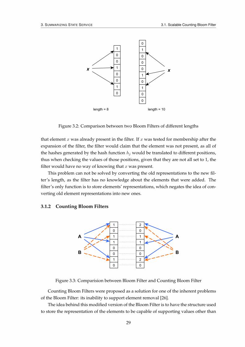
Figure 3.2 depicts the possible representation of the same element x in filters of dif-ferent sizes. Both filters have element x’s representation stored. In the filter with length 8— left side — this representation is achieved by the bits of the array at positions 1,4 and7. In the filter of length 10 — right side — the element’s representation is performed bysetting the bits at positions 2, 6 and 8. As we can see filter’s with different lengths gen-erate different representations for the same elements. Despite both filters using 3 bits tostore x’s representation, we can see that the bits used by both filters vary, which justifiesthe inability of the Bloom Filter expand beyond its initial size, as there is no informationstored about the elements themselves, but only a representation.
Despite the filter having different lengths, the positions used to represent x also differ,this means that if we consider that a filter of length 8 was expanded to a length of 10, and
28
3. SUMMARIZING STATE SERVICE 3.1. Scalable Counting Bloom Filter
Figure 3.2: Comparison between two Bloom Filters of different lengths
that element x was already present in the filter. If x was tested for membership after theexpansion of the filter, the filter would claim that the element was not present, as all ofthe hashes generated by the hash function hj would be translated to different positions,thus when checking the values of those positions, given that they are not all set to 1, thefilter would have no way of knowing that x was present.
This problem can not be solved by converting the old representations to the new fil-ter’s length, as the filter has no knowledge about the elements that were added. Thefilter’s only function is to store elements’ representations, which negates the idea of con-verting old element representations into new ones.
3.1.2 Counting Bloom Filters
Figure 3.3: Comparision between Bloom Filter and Counting Bloom Filter
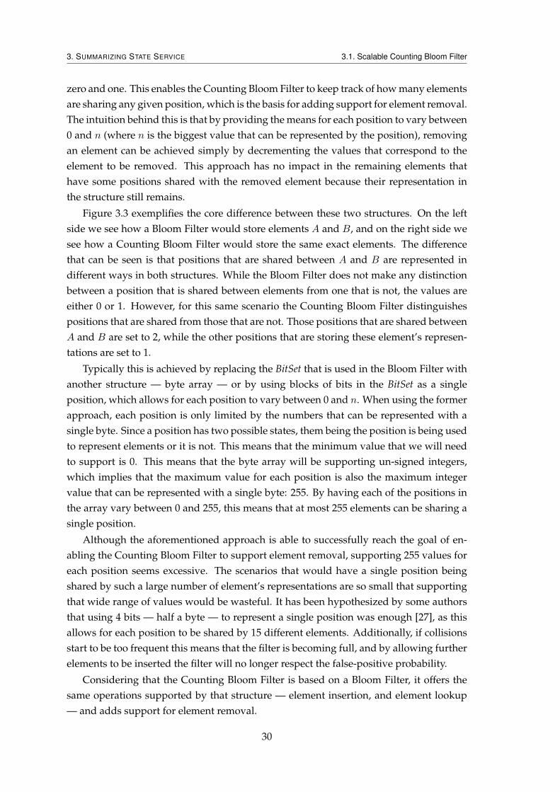
Counting Bloom Filters were proposed as a solution for one of the inherent problemsof the Bloom Filter: its inability to support element removal [26].
The idea behind this modified version of the Bloom Filter is to have the structure usedto store the representation of the elements to be capable of supporting values other than
29
3. SUMMARIZING STATE SERVICE 3.1. Scalable Counting Bloom Filter
zero and one. This enables the Counting Bloom Filter to keep track of how many elementsare sharing any given position, which is the basis for adding support for element removal.The intuition behind this is that by providing the means for each position to vary between0 and n (where n is the biggest value that can be represented by the position), removingan element can be achieved simply by decrementing the values that correspond to theelement to be removed. This approach has no impact in the remaining elements thathave some positions shared with the removed element because their representation inthe structure still remains.
Figure 3.3 exemplifies the core difference between these two structures. On the leftside we see how a Bloom Filter would store elements A and B, and on the right side wesee how a Counting Bloom Filter would store the same exact elements. The differencethat can be seen is that positions that are shared between A and B are represented indifferent ways in both structures. While the Bloom Filter does not make any distinctionbetween a position that is shared between elements from one that is not, the values areeither 0 or 1. However, for this same scenario the Counting Bloom Filter distinguishespositions that are shared from those that are not. Those positions that are shared betweenA and B are set to 2, while the other positions that are storing these element’s represen-tations are set to 1.
Typically this is achieved by replacing the BitSet that is used in the Bloom Filter withanother structure — byte array — or by using blocks of bits in the BitSet as a singleposition, which allows for each position to vary between 0 and n. When using the formerapproach, each position is only limited by the numbers that can be represented with asingle byte. Since a position has two possible states, them being the position is being usedto represent elements or it is not. This means that the minimum value that we will needto support is 0. This means that the byte array will be supporting un-signed integers,which implies that the maximum value for each position is also the maximum integervalue that can be represented with a single byte: 255. By having each of the positions inthe array vary between 0 and 255, this means that at most 255 elements can be sharing asingle position.
Although the aforementioned approach is able to successfully reach the goal of en-abling the Counting Bloom Filter to support element removal, supporting 255 values foreach position seems excessive. The scenarios that would have a single position beingshared by such a large number of element’s representations are so small that supportingthat wide range of values would be wasteful. It has been hypothesized by some authorsthat using 4 bits — half a byte — to represent a single position was enough [27], as thisallows for each position to be shared by 15 different elements. Additionally, if collisionsstart to be too frequent this means that the filter is becoming full, and by allowing furtherelements to be inserted the filter will no longer respect the false-positive probability.
Considering that the Counting Bloom Filter is based on a Bloom Filter, it offers thesame operations supported by that structure — element insertion, and element lookup— and adds support for element removal.
30
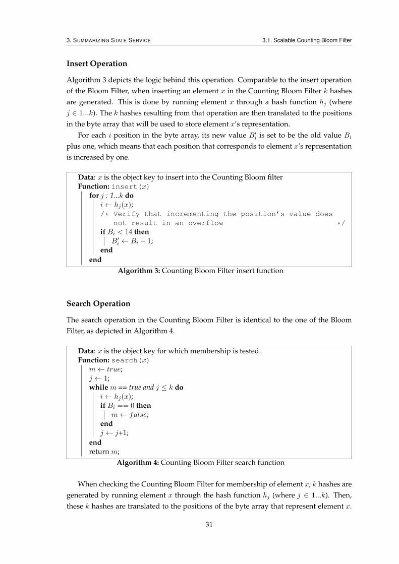
3. SUMMARIZING STATE SERVICE 3.1. Scalable Counting Bloom Filter
Insert Operation
Algorithm 3 depicts the logic behind this operation. Comparable to the insert operationof the Bloom Filter, when inserting an element x in the Counting Bloom Filter k hashesare generated. This is done by running element x through a hash function hj (wherej ∈ 1...k). The k hashes resulting from that operation are then translated to the positionsin the byte array that will be used to store element x’s representation.
For each i position in the byte array, its new value B′i is set to be the old value Bi
plus one, which means that each position that corresponds to element x’s representationis increased by one.
Data: x is the object key to insert into the Counting Bloom filterFunction: insert(x)
for j : 1...k doi← hj(x);/* Verify that incrementing the position’s value does
not result in an overflow */if Bi < 14 then
B′i ← Bi + 1;end
endAlgorithm 3: Counting Bloom Filter insert function
Search Operation
The search operation in the Counting Bloom Filter is identical to the one of the BloomFilter, as depicted in Algorithm 4.
Data: x is the object key for which membership is tested.Function: search(x)
m← true;j ← 1;while m == true and j ≤ k do
i← hj(x);if Bi == 0 then
m← false;endj ← j+1;
endreturn m;
Algorithm 4: Counting Bloom Filter search function
When checking the Counting Bloom Filter for membership of element x, k hashes aregenerated by running element x through the hash function hj (where j ∈ 1...k). Then,these k hashes are translated to the positions of the byte array that represent element x.
31
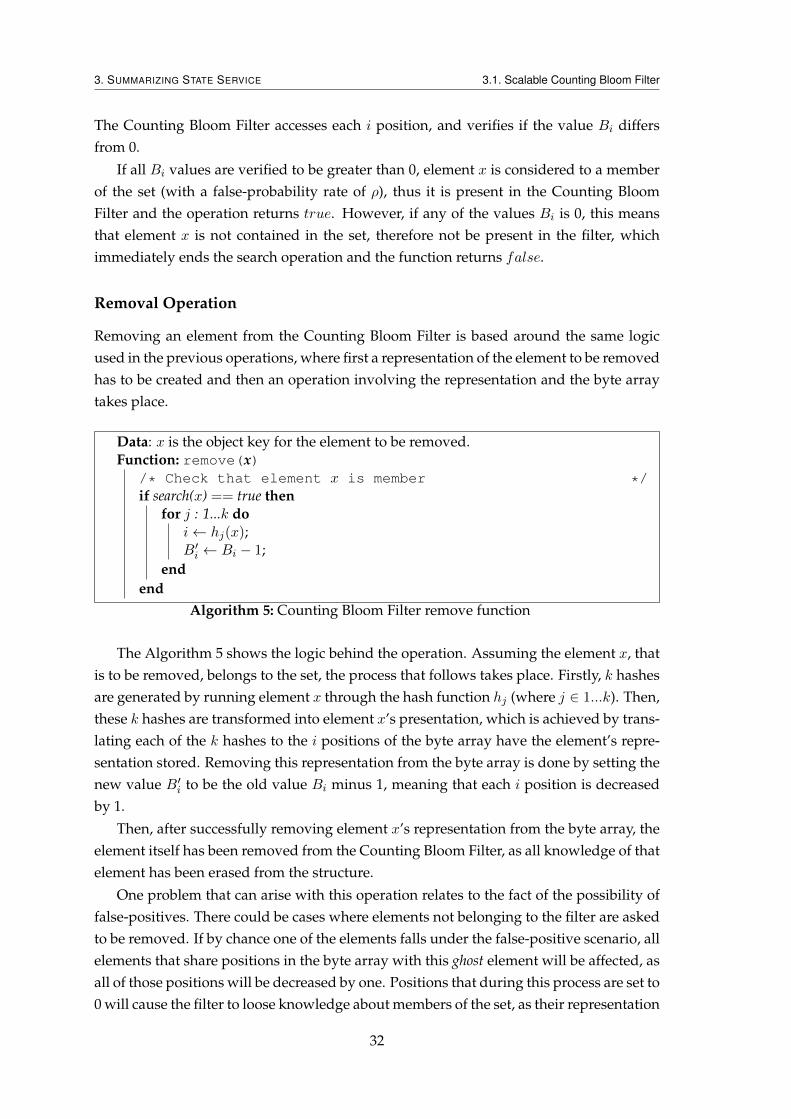
3. SUMMARIZING STATE SERVICE 3.1. Scalable Counting Bloom Filter
The Counting Bloom Filter accesses each i position, and verifies if the value Bi differsfrom 0.
If all Bi values are verified to be greater than 0, element x is considered to a memberof the set (with a false-probability rate of ρ), thus it is present in the Counting BloomFilter and the operation returns true. However, if any of the values Bi is 0, this meansthat element x is not contained in the set, therefore not be present in the filter, whichimmediately ends the search operation and the function returns false.
Removal Operation
Removing an element from the Counting Bloom Filter is based around the same logicused in the previous operations, where first a representation of the element to be removedhas to be created and then an operation involving the representation and the byte arraytakes place.
Data: x is the object key for the element to be removed.Function: remove(x)
/* Check that element x is member */if search(x) == true then
for j : 1...k doi← hj(x);B′i ← Bi − 1;
endend
Algorithm 5: Counting Bloom Filter remove function
The Algorithm 5 shows the logic behind the operation. Assuming the element x, thatis to be removed, belongs to the set, the process that follows takes place. Firstly, k hashesare generated by running element x through the hash function hj (where j ∈ 1...k). Then,these k hashes are transformed into element x’s presentation, which is achieved by trans-lating each of the k hashes to the i positions of the byte array have the element’s repre-sentation stored. Removing this representation from the byte array is done by setting thenew value B′i to be the old value Bi minus 1, meaning that each i position is decreasedby 1.
Then, after successfully removing element x’s representation from the byte array, theelement itself has been removed from the Counting Bloom Filter, as all knowledge of thatelement has been erased from the structure.
One problem that can arise with this operation relates to the fact of the possibility offalse-positives. There could be cases where elements not belonging to the filter are askedto be removed. If by chance one of the elements falls under the false-positive scenario, allelements that share positions in the byte array with this ghost element will be affected, asall of those positions will be decreased by one. Positions that during this process are set to0 will cause the filter to loose knowledge about members of the set, as their representation
32
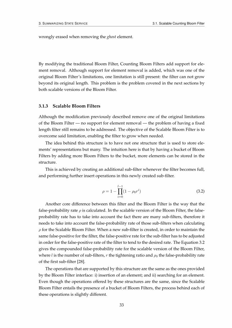
3. SUMMARIZING STATE SERVICE 3.1. Scalable Counting Bloom Filter
wrongly erased when removing the ghost element.
By modifying the traditional Bloom Filter, Counting Bloom Filters add support for ele-ment removal. Although support for element removal is added, which was one of theoriginal Bloom Filter’s limitations, one limitation is still present: the filter can not growbeyond its original length. This problem is the problem covered in the next sections byboth scalable versions of the Bloom Filter.
3.1.3 Scalable Bloom Filters
Although the modification previously described remove one of the original limitationsof the Bloom Filter — no support for element removal — the problem of having a fixedlength filter still remains to be addressed. The objective of the Scalable Bloom Filter is toovercome said limitation, enabling the filter to grow when needed.
The idea behind this structure is to have not one structure that is used to store ele-ments’ representations but many. The intuition here is that by having a bucket of BloomFilters by adding more Bloom Filters to the bucket, more elements can be stored in thestructure.
This is achieved by creating an additional sub-filter whenever the filter becomes full,and performing further insert operations in this newly created sub-filter.
ρ = 1−l−1∏i=0
(1− ρ0ri) (3.2)
Another core difference between this filter and the Bloom Filter is the way that thefalse-probability rate ρ is calculated. In the scalable version of the Bloom Filter, the false-probability rate has to take into account the fact there are many sub-filters, therefore itneeds to take into account the false-probability rate of those sub-filters when calculatingρ for the Scalable Bloom Filter. When a new sub-filter is created, in order to maintain thesame false-positive for the filter, the false-positive rate for the sub-filter has to be adjustedin order for the false-positive rate of the filter to tend to the desired rate. The Equation 3.2gives the compounded false-probability rate for the scalable version of the Bloom Filter,where l is the number of sub-filters, r the tightening ratio and ρ0 the false-probability rateof the first sub-filter [28].
The operations that are supported by this structure are the same as the ones providedby the Bloom Filter interface: i) insertion of an element; and ii) searching for an element.Even though the operations offered by these structures are the same, since the ScalableBloom Filter entails the presence of a bucket of Bloom Filters, the process behind each ofthese operations is slightly different.
33
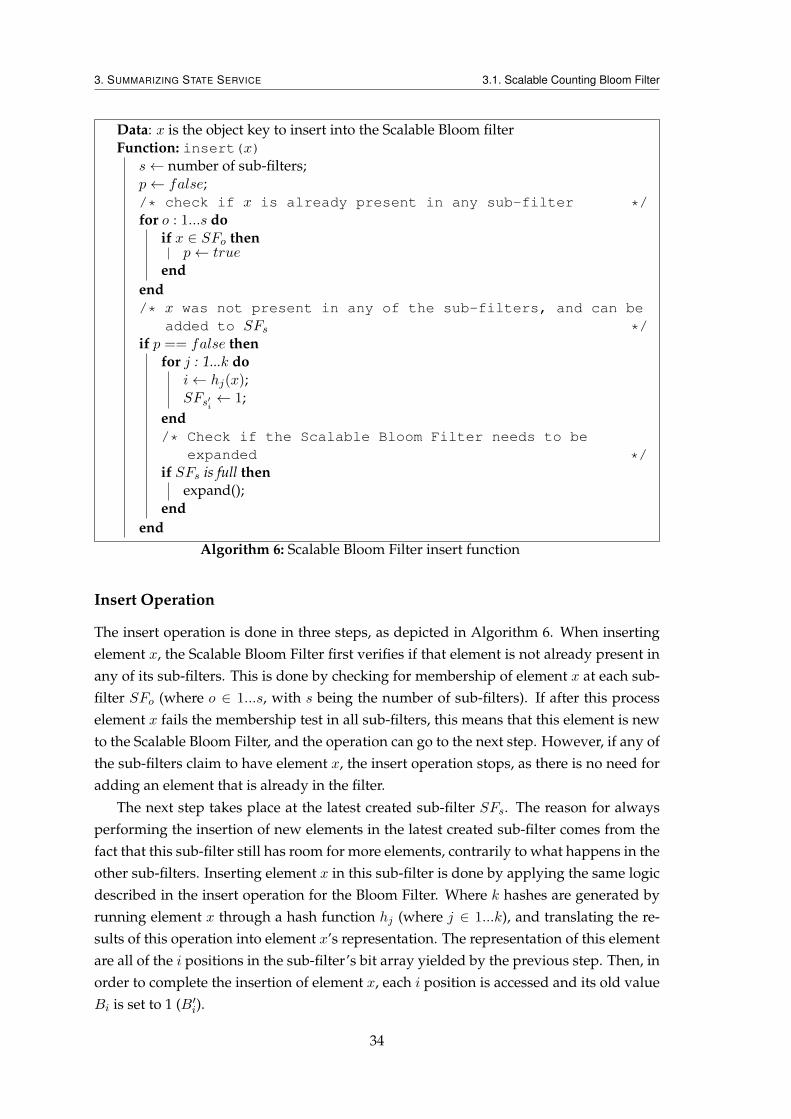
3. SUMMARIZING STATE SERVICE 3.1. Scalable Counting Bloom Filter
Data: x is the object key to insert into the Scalable Bloom filterFunction: insert(x)
s← number of sub-filters;p← false;/* check if x is already present in any sub-filter */for o : 1...s do
if x ∈ SFo thenp← true
endend/* x was not present in any of the sub-filters, and can be
added to SFs */if p == false then
for j : 1...k doi← hj(x);SFs′i
← 1;end/* Check if the Scalable Bloom Filter needs to be
expanded */if SFs is full then
expand();end
endAlgorithm 6: Scalable Bloom Filter insert function
Insert Operation
The insert operation is done in three steps, as depicted in Algorithm 6. When insertingelement x, the Scalable Bloom Filter first verifies if that element is not already present inany of its sub-filters. This is done by checking for membership of element x at each sub-filter SFo (where o ∈ 1...s, with s being the number of sub-filters). If after this processelement x fails the membership test in all sub-filters, this means that this element is newto the Scalable Bloom Filter, and the operation can go to the next step. However, if any ofthe sub-filters claim to have element x, the insert operation stops, as there is no need foradding an element that is already in the filter.
The next step takes place at the latest created sub-filter SFs. The reason for alwaysperforming the insertion of new elements in the latest created sub-filter comes from thefact that this sub-filter still has room for more elements, contrarily to what happens in theother sub-filters. Inserting element x in this sub-filter is done by applying the same logicdescribed in the insert operation for the Bloom Filter. Where k hashes are generated byrunning element x through a hash function hj (where j ∈ 1...k), and translating the re-sults of this operation into element x’s representation. The representation of this elementare all of the i positions in the sub-filter’s bit array yielded by the previous step. Then, inorder to complete the insertion of element x, each i position is accessed and its old valueBi is set to 1 (B′i).
34
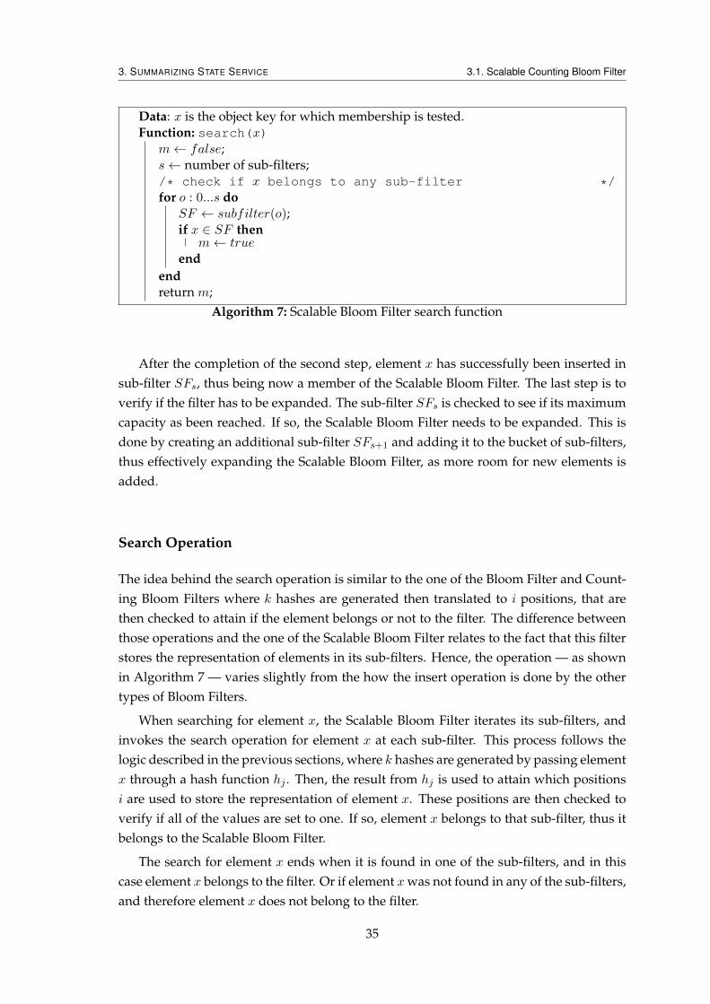
3. SUMMARIZING STATE SERVICE 3.1. Scalable Counting Bloom Filter
Data: x is the object key for which membership is tested.Function: search(x)
m← false;s← number of sub-filters;/* check if x belongs to any sub-filter */for o : 0...s do
SF ← subfilter(o);if x ∈ SF then
m← trueend
endreturn m;
Algorithm 7: Scalable Bloom Filter search function
After the completion of the second step, element x has successfully been inserted insub-filter SFs, thus being now a member of the Scalable Bloom Filter. The last step is toverify if the filter has to be expanded. The sub-filter SFs is checked to see if its maximumcapacity as been reached. If so, the Scalable Bloom Filter needs to be expanded. This isdone by creating an additional sub-filter SFs+1 and adding it to the bucket of sub-filters,thus effectively expanding the Scalable Bloom Filter, as more room for new elements isadded.
Search Operation
The idea behind the search operation is similar to the one of the Bloom Filter and Count-ing Bloom Filters where k hashes are generated then translated to i positions, that arethen checked to attain if the element belongs or not to the filter. The difference betweenthose operations and the one of the Scalable Bloom Filter relates to the fact that this filterstores the representation of elements in its sub-filters. Hence, the operation — as shownin Algorithm 7 — varies slightly from the how the insert operation is done by the othertypes of Bloom Filters.
When searching for element x, the Scalable Bloom Filter iterates its sub-filters, andinvokes the search operation for element x at each sub-filter. This process follows thelogic described in the previous sections, where k hashes are generated by passing elementx through a hash function hj . Then, the result from hj is used to attain which positionsi are used to store the representation of element x. These positions are then checked toverify if all of the values are set to one. If so, element x belongs to that sub-filter, thus itbelongs to the Scalable Bloom Filter.
The search for element x ends when it is found in one of the sub-filters, and in thiscase element x belongs to the filter. Or if element xwas not found in any of the sub-filters,and therefore element x does not belong to the filter.
35
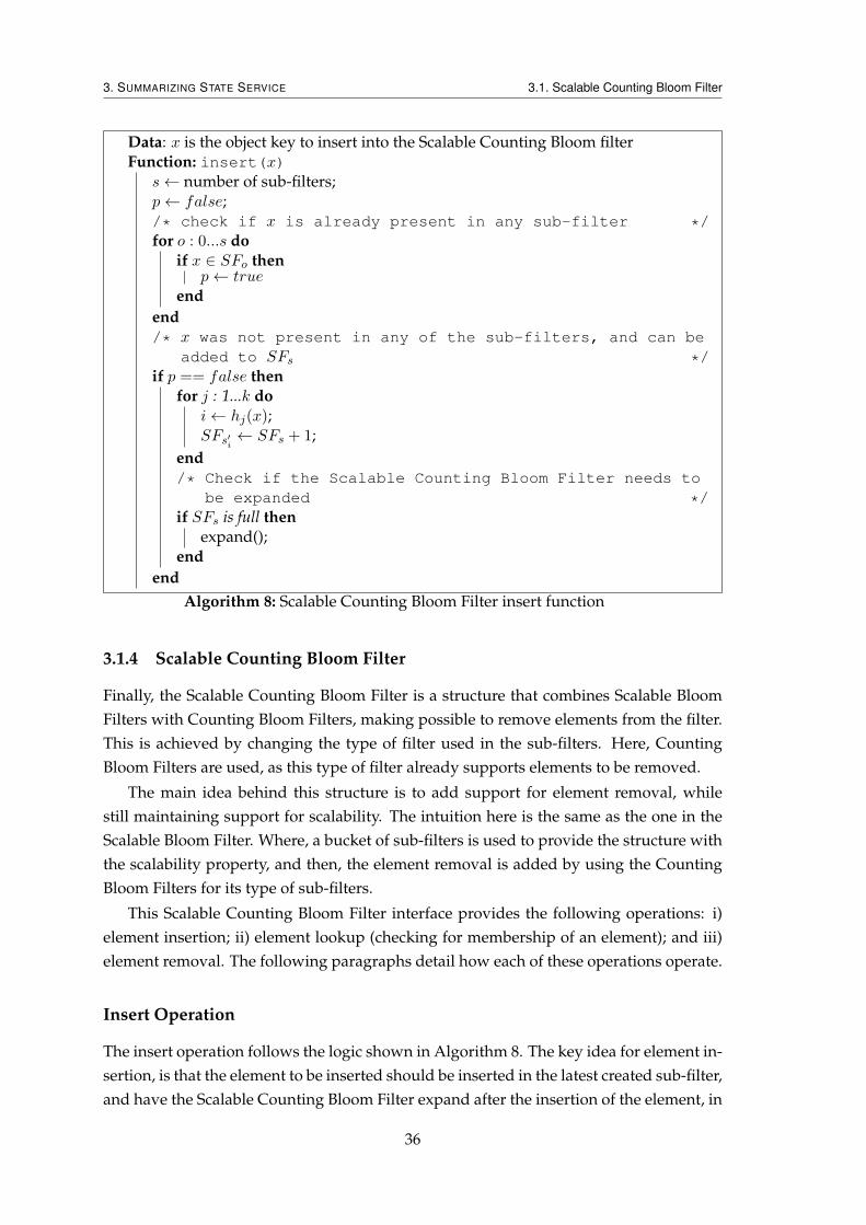
3. SUMMARIZING STATE SERVICE 3.1. Scalable Counting Bloom Filter
Data: x is the object key to insert into the Scalable Counting Bloom filterFunction: insert(x)
s← number of sub-filters;p← false;/* check if x is already present in any sub-filter */for o : 0...s do
if x ∈ SFo thenp← true
endend/* x was not present in any of the sub-filters, and can be
added to SFs */if p == false then
for j : 1...k doi← hj(x);SFs′i
← SFs + 1;end/* Check if the Scalable Counting Bloom Filter needs to
be expanded */if SFs is full then
expand();end
endAlgorithm 8: Scalable Counting Bloom Filter insert function
3.1.4 Scalable Counting Bloom Filter
Finally, the Scalable Counting Bloom Filter is a structure that combines Scalable BloomFilters with Counting Bloom Filters, making possible to remove elements from the filter.This is achieved by changing the type of filter used in the sub-filters. Here, CountingBloom Filters are used, as this type of filter already supports elements to be removed.
The main idea behind this structure is to add support for element removal, whilestill maintaining support for scalability. The intuition here is the same as the one in theScalable Bloom Filter. Where, a bucket of sub-filters is used to provide the structure withthe scalability property, and then, the element removal is added by using the CountingBloom Filters for its type of sub-filters.
This Scalable Counting Bloom Filter interface provides the following operations: i)element insertion; ii) element lookup (checking for membership of an element); and iii)element removal. The following paragraphs detail how each of these operations operate.
Insert Operation
The insert operation follows the logic shown in Algorithm 8. The key idea for element in-sertion, is that the element to be inserted should be inserted in the latest created sub-filter,and have the Scalable Counting Bloom Filter expand after the insertion of the element, in
36
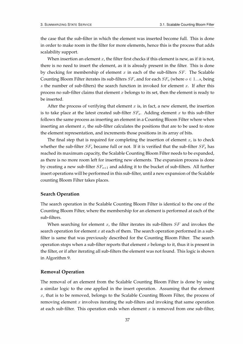
3. SUMMARIZING STATE SERVICE 3.1. Scalable Counting Bloom Filter
the case that the sub-filter in which the element was inserted become full. This is donein order to make room in the filter for more elements, hence this is the process that addsscalability support.
When insertion an element x, the filter first checks if this element is new, as if it is not,there is no need to insert the element, as it is already present in the filter. This is doneby checking for membership of element x in each of the sub-filters SF . The ScalableCounting Bloom Filter iterates its sub-filters SF , and for each SFo (where o ∈ 1...s, beings the number of sub-filters) the search function in invoked for element x. If after thisprocess no sub-filter claims that element x belongs to its set, then the element is ready tobe inserted.
After the process of verifying that element x is, in fact, a new element, the insertionis to take place at the latest created sub-filter SFs. Adding element x to this sub-filterfollows the same process as inserting an element in a Counting Bloom Filter where wheninserting an element x, the sub-filter calculates the positions that are to be used to storethe element representation, and increments those positions in its array of bits.
The final step that is required for completing the insertion of element x, is to checkwhether the sub-filter SFs became full or not. If it is verified that the sub-filter SFs hasreached its maximum capacity, the Scalable Counting Bloom Filter needs to be expanded,as there is no more room left for inserting new elements. The expansion process is doneby creating a new sub-filter SFs+1 and adding it to the bucket of sub-filters. All furtherinsert operations will be performed in this sub-filter, until a new expansion of the Scalablecounting Bloom Filter takes places.
Search Operation
The search operation in the Scalable Counting Bloom Filter is identical to the one of theCounting Bloom Filter, where the membership for an element is performed at each of thesub-filters.
When searching for element x, the filter iterates its sub-filters SF and invokes thesearch operation for element x at each of them. The search operation performed in a sub-filter is same that was previously described for the Counting Bloom Filter. The searchoperation stops when a sub-filter reports that element x belongs to it, thus it is present inthe filter, or if after iterating all sub-filters the element was not found. This logic is shownin Algorithm 9.
Removal Operation
The removal of an element from the Scalable Counting Bloom Filter is done by usinga similar logic to the one applied in the insert operation. Assuming that the elementx, that is to be removed, belongs to the Scalable Counting Bloom Filter, the process ofremoving element x involves iterating the sub-filters and invoking that same operationat each sub-filter. This operation ends when element x is removed from one sub-filter,
37
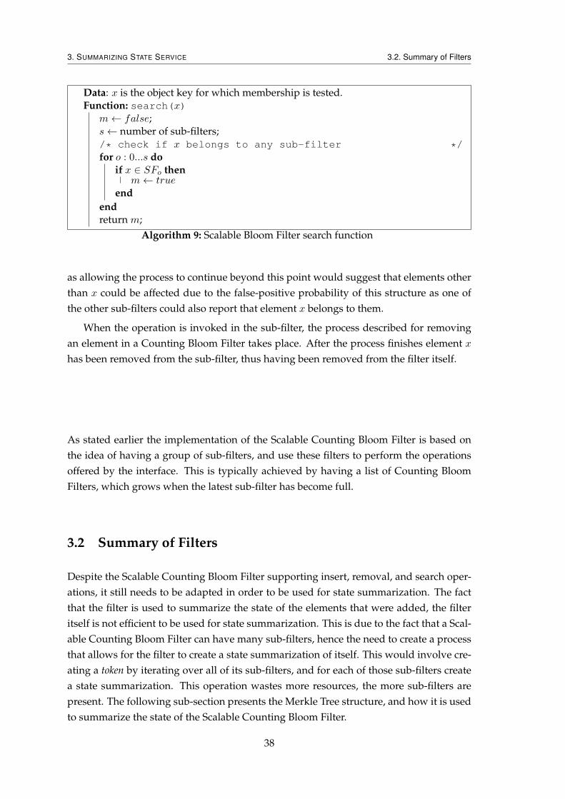
3. SUMMARIZING STATE SERVICE 3.2. Summary of Filters
Data: x is the object key for which membership is tested.Function: search(x)
m← false;s← number of sub-filters;/* check if x belongs to any sub-filter */for o : 0...s do
if x ∈ SFo thenm← true
endendreturn m;
Algorithm 9: Scalable Bloom Filter search function
as allowing the process to continue beyond this point would suggest that elements otherthan x could be affected due to the false-positive probability of this structure as one ofthe other sub-filters could also report that element x belongs to them.
When the operation is invoked in the sub-filter, the process described for removingan element in a Counting Bloom Filter takes place. After the process finishes element xhas been removed from the sub-filter, thus having been removed from the filter itself.
As stated earlier the implementation of the Scalable Counting Bloom Filter is based onthe idea of having a group of sub-filters, and use these filters to perform the operationsoffered by the interface. This is typically achieved by having a list of Counting BloomFilters, which grows when the latest sub-filter has become full.
3.2 Summary of Filters
Despite the Scalable Counting Bloom Filter supporting insert, removal, and search oper-ations, it still needs to be adapted in order to be used for state summarization. The factthat the filter is used to summarize the state of the elements that were added, the filteritself is not efficient to be used for state summarization. This is due to the fact that a Scal-able Counting Bloom Filter can have many sub-filters, hence the need to create a processthat allows for the filter to create a state summarization of itself. This would involve cre-ating a token by iterating over all of its sub-filters, and for each of those sub-filters createa state summarization. This operation wastes more resources, the more sub-filters arepresent. The following sub-section presents the Merkle Tree structure, and how it is usedto summarize the state of the Scalable Counting Bloom Filter.
38
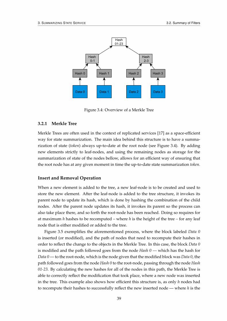
3. SUMMARIZING STATE SERVICE 3.2. Summary of Filters
Figure 3.4: Overview of a Merkle Tree
3.2.1 Merkle Tree
Merkle Trees are often used in the context of replicated services [17] as a space-efficientway for state summarization. The main idea behind this structure is to have a summa-rization of state (token) always up-to-date at the root node (see Figure 3.4). By addingnew elements strictly to leaf-nodes, and using the remaining nodes as storage for thesummarization of state of the nodes bellow, allows for an efficient way of ensuring thatthe root node has at any given moment in time the up-to-date state summarization token.
Insert and Removal Operation
When a new element is added to the tree, a new leaf-node is to be created and used tostore the new element. After the leaf-node is added to the tree structure, it invokes itsparent node to update its hash, which is done by hashing the combination of the childnodes. After the parent node updates its hash, it invokes its parent so the process canalso take place there, and so forth the root-node has been reached. Doing so requires forat maximum h hashes to be recomputed – where h is the height of the tree – for any leafnode that is either modified or added to the tree.
Figure 3.5 exemplifies the aforementioned process, where the block labeled Data 0is inserted (or modified), and the path of nodes that need to recompute their hashes inorder to reflect the change to the objects in the Merkle Tree. In this case, the block Data 0is modified and the path followed goes from the node Hash 0 — which has the hash forData 0 — to the root-node, which is the node given that the modified block was Data 0, thepath followed goes from the node Hash 0 to the root-node, passing through the node Hash01-23. By calculating the new hashes for all of the nodes in this path, the Merkle Tree isable to correctly reflect the modification that took place, where a new node was insertedin the tree. This example also shows how efficient this structure is, as only h nodes hadto recompute their hashes to successfully reflect the new inserted node — where h is the
39
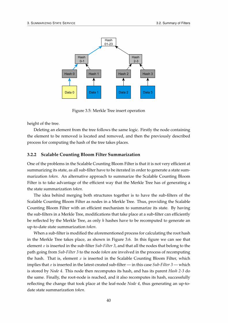
3. SUMMARIZING STATE SERVICE 3.2. Summary of Filters
Figure 3.5: Merkle Tree insert operation
height of the tree.Deleting an element from the tree follows the same logic. Firstly the node containing
the element to be removed is located and removed, and then the previously describedprocess for computing the hash of the tree takes places.
3.2.2 Scalable Counting Bloom Filter Summarization
One of the problems in the Scalable Counting Bloom Filter is that it is not very efficient atsummarizing its state, as all sub-filter have to be iterated in order to generate a state sum-marization token. An alternative approach to summarize the Scalable Counting BloomFilter is to take advantage of the efficient way that the Merkle Tree has of generating athe state summarization token.
The idea behind merging both structures together is to have the sub-filters of theScalable Counting Bloom Filter as nodes in a Merkle Tree. Thus, providing the ScalableCounting Bloom Filter with an efficient mechanism to summarize its state. By havingthe sub-filters in a Merkle Tree, modifications that take place at a sub-filter can efficientlybe reflected by the Merkle Tree, as only h hashes have to be recomputed to generate anup-to-date state summarization token.
When a sub-filter is modified the aforementioned process for calculating the root hashin the Merkle Tree takes place, as shown in Figure 3.6. In this figure we can see thatelement x is inserted in the sub-filter Sub-Filter 3, and that all the nodes that belong to thepath going from Sub-Filter 3 to the node token are involved in the process of recomputingthe hash. That is, element x is inserted in the Scalable Counting Bloom Filter, whichimplies that x is inserted in the latest created sub-filter — in this case Sub-Filter 3 — whichis stored by Node 4. This node then recomputes its hash, and has its parent Hash 2-3 dothe same. Finally, the root-node is reached, and it also recomputes its hash, successfullyreflecting the change that took place at the leaf-node Node 4, thus generating an up-to-date state summarization token.
40
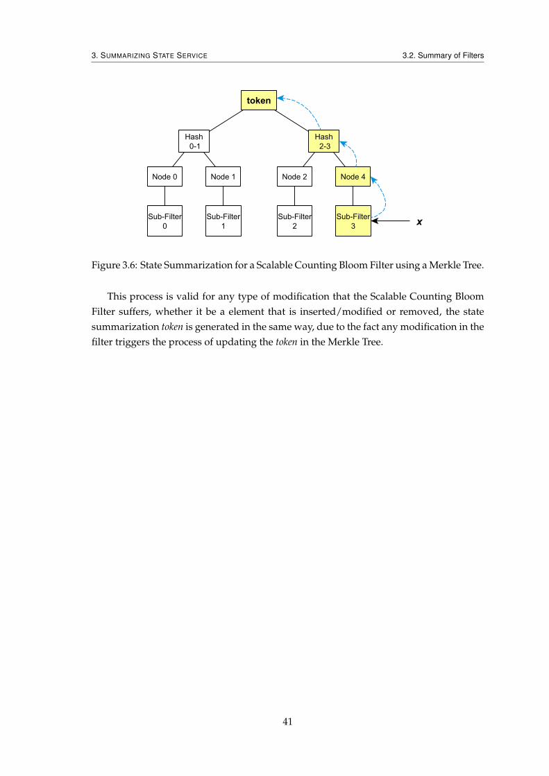
3. SUMMARIZING STATE SERVICE 3.2. Summary of Filters
Figure 3.6: State Summarization for a Scalable Counting Bloom Filter using a Merkle Tree.
This process is valid for any type of modification that the Scalable Counting BloomFilter suffers, whether it be a element that is inserted/modified or removed, the statesummarization token is generated in the same way, due to the fact any modification in thefilter triggers the process of updating the token in the Merkle Tree.
41

3. SUMMARIZING STATE SERVICE 3.2. Summary of Filters
42
4Summarizing Replicated Service
State
State summarization is usually achieved by building a Merkle Tree over the state of theservice. Using this summaries to compare replicas in a replicated services requires thatthe same Merkle Tree is built when replicas are in the same state. For services replicatedusing the state-machine model, it is reasonable to assume that the internal state of theservice will be the same, when ignoring pointers and considering state only. This mightbe no longer true if the service executes operations in different order, which may lead theinternal service to differ in different replicas. The same happens if different replica imple-mentations are used. To address this issue, some replicated services build Merkle Treesover the abstract state of the service, which must be exported. This is rather complex andmay lead to replicas generating different state summarization tokens even if they haveexecuted the same exact operations, as they are free to choose the order of execution forthe operations.
For those replicated services that ensure that replicas use a sequential order of exe-cution, the previously described techniques for state summarization can be used, as theyensure that a replicas that have not diverged from the others during operation will haveidentical state summarization tokens.
In this scenario the state of the replica can be summarized by using a Merkle Tree,which is an efficient structure for generating a state summarization token. When a replicaexecutes some operation, the objects that compose the internal state of the replica can beupdated in the Merkle Tree, triggering the state summarization process. In this processthe Merkle Tree computes the new hashes from the node that was affected to the root
43
4. SUMMARIZING REPLICATED SERVICE STATE 4.1. Summarization in the presence of non-sequential operations
node, thus updating the state summarization token that is stored at the root of the tree.The problem with using this structure to achieve state summarization is that the resultingsummarization of state is affected by how the tree itself evolves, the order by whichthe objects are added to the tree is also reflected by the summarization. This problemis solved in the Scalable Counting Bloom Filter by having the summarization of statebeing independent of the structure internal representation, in this structure this processreflects only the the objects that are inserted/removed, and not of the underlying internalstructures of the Scalable Counting Bloom Filter.
Likewise, the Scalable Counting Bloom Filter could also be used in this scenario.When a replica finishes executing an operation, the object modified by the operation inthe internal state need to be update in the filter. Here a distinction between three possi-ble types of modifications has to be made. If the object is removed from the replica, forexample, a database that erases a table row, the delete operation would be called at theScalable Counting Bloom Filter. The opposite logic would be used for a new object that isadded to the replica, where it would be added to the Scalable Counting Bloom Filter. Forupdate operations — an object that is already present in the replica that gets modified —the original object has to be also used by the filter. This is done in order to assure thatthe state summarization token generated correctly reflects the internal state of the replica.In this case the original object is first removed from the filter — by calling the removeoperation for that object — and only then the modified version of the object is inserted inthe filter.
After the aforementioned process for updating the objects in the Scalable CountingBloom Filter has been completed, the filter generates a state summarization token. Thistoken is generated by iterating the Scalable Counting Bloom Filter sub-filters, and for eachsub-filter an hash is generated. This hash corresponds to the summarization of state ofthe sub-filter, and it is typically generated by hashing the contents of the array of byteused by the sub-filter to keep track of the added elements. Then, all of the hashes arecombined, and hashed one more time. This last hashing process effectively generates anhash of the sub-filters’ hashes, thus creating a hash that is used by the Scalable CountingBloom Filter as the token that summarizes its state.
4.1 Summarization in the presence of non-sequential operations
The purpose of the previously described structures — Merkle Trees and Scalable Count-ing Bloom Filters — is to be used as an efficient way of representing the internal state ofa replica, by generating a token that reflects the elements encompassed in the structure.
Although these structures are able to achieve their goals in scenarios where the orderby which the elements are added is the same for all replicas, the same can not be guaran-teed when the order is not the same, albeit the need for an alternative solution to providea way for these structures to be used in a context where operations are non-sequential.
This results in these structures not being able to correctly summarize the state of the
44
4. SUMMARIZING REPLICATED SERVICE STATE 4.1. Summarization in the presence of non-sequential operations
service. Independently of the structure used, if replicas at the service have to executeoperation o1 ... on, if the order by which these operations are executed at the replicasvaries, the state summarization token may differ from replica to replica. As the operationsare reflected in the structures at different moments in time, and despite the fact that alloperations will eventually be reflected, the end result can be different
In the case of the Scalable Counting Bloom Filter, the aforementioned problem derivesfrom the fact that elements added in different orders may end up being stored at differentsub-filters. For example, if we consider a replicated service that has two replicas, and isto execute operation o1 and o2. If the Scalable Counting bloom Filter at each of thosereplicas is at verge of being expanded — they only support one more operation beforeneeding to expand — by executing the operations in a different order, this means that theoperations will be reflected in different sub-filters at the replicas. If replica ra executesoperation o1 and then o2, by having only room in its current version of the filter for oneoperation, before triggering the expansion of the filter, this signifies that the resultingstate from operation o1 is added to sub-filter sfi and the resulting state from operation o2to sub-filter sfi+ 1.
The opposite happens for the second replica rb, where operation o2 executed firstthan operation o1. In this case the resulting state of operation o2 is added to sub-filtersfi, whereas the resulting state of operation o1 is added to sfi+1. This results in a bothreplicas generating a different state summarization token, despite both having executedthe exact same operations.
Likewise, for Merkle Trees if replicas execute operations in a non-sequential way, thuselements are added in different order to the trees, this results in the possibility of havingdivergent state summarization tokens, despite having execute the same operations. Thisproblem is related with how the tree is internally represented, if the Merkle Tree is im-plemented by using a self-balancing tree, which typically perform some kind of noderotation when elements are added, the insertion order will affect the summarization ofstate, as different orders will trigger different rotations.
If we translate the aforementioned example to the context of Merkle Trees, where tworeplicas — ra and rb — execute operations o1 and o2 in a different order the former replicawill store operation o1 at, for example, node n1, and operation o2 at node n2. Whereasthe later replica will store operation o2 in node n1, and operation o1 in node n2. Aftercalculating the new state summarization token, by following the path that goes from thenew or modified nodes to the root-node of the tree, given that this path is different atreplica ra from replica rb, the token that is generated is necessarily different too.
The aforementioned scenarios pose a challenge, as both of these structures can notbe directly integrated in a replicated system’s replica to provide a way for state summa-rization in the presence of non-sequential operations. The goal for the remaining of thissection is to explain how the Scalable Counting Bloom Filter can be modified in orderto fit the context of summarizing the state of a replicated service that does not enforcesequential order of execution, more specifically it will be detailed how this is achieved in
45
4. SUMMARIZING REPLICATED SERVICE STATE 4.1. Summarization in the presence of non-sequential operations
the context of a replicated database service.
The challenge posed by non-sequential operations still stands in the context of repli-cated database services. This can be solved by enforcing mechanisms at the replicationservice itself, which purpose is to ensure that the aforementioned structures can be usedto summarize the internal state of a replica.
The idea is to have the replicated service allocate operations in blocks, ensuring thatthese operations are exactly the same for blocks of operations sent to any given replica. Byfollowing this approach we create a sense of a sequence of execution. The fact that eventhough these blocks of operations contain the same operations, they can still be execute indifferent order at the replicas. This second problem is solved by modifying the originalbehavior of the Scalable Counting Bloom Filter, restricting the filter from expanding inthe middle of a block of operations.
The intuition here is that by buffering a certain number of operations before theseare reflected in the state summarization structure — Scalable Counting Bloom Filter — itwill be possible to generate the same exact token despite the order by which the operationstook place was different. The buffering process requires for the same exact operations tobe buffered — the order by which this occurs does not matter. It is the responsibility of thereplicated service to ensure this. For example, in the case of a replicated database service,this can be achieved by ensuring that a certain number of transactions is performed atthe replicas before requesting new operations to be executed. Given that in this case it isexpected from the service to be always executing transactions, only a small dent in theperformance aspect takes place. As the time between a buffered block of transactionsbeing reflected by the filter, and a new one being formed should be small enough for theperformance hit be negligible.
By scheduling a certain number of transactions to take place before another blockcomes in, the Scalable Counting Bloom Filter can be used as a state summarization mech-anism as it will yield deterministic tokens for replicas that do not diverge during opera-tion. One problem that can be pointed to this solution is that during the buffering processsome transactions can result in a replica diverging from the others, and the replicatedservice only being able to identify this replica’s incorrect state after the completion ofthe execution of the block of transactions. This means that there will be resources beingwasted — executing further transactions — when the replica has already diverged.
Recalling the aforementioned example, where two replicas had two operations to ex-ecute, and by executing these operations in different order they generated different statesummarization tokens, due to the fact that the filter expanded at different operations inboth replicas. Where operation o1 triggered the expansion of the filter in replica ra, andoperation o2 triggered replica ra’s filter to expand. In principle, by restricting the mo-ments where replicas are allowed to expand the filters, the problem should be solved.Given that the replicated service already ensures that a block of operations contains theexact same operations, by restricting the moments where a filter is allowed to expand, theresulting token should be exactly the same. The idea here is that by only allowing a filter
46

4. SUMMARIZING REPLICATED SERVICE STATE 4.1. Summarization in the presence of non-sequential operations
to expand after a block of operations is reflected in the filter, the exact same operationsare added to the same sub-filter at any of the replica’s Scalable Counting Bloom Filters,despite the order by which the operations in a block are executed.
The reason behind choosing to use the Scalable Counting Bloom Filter over the MerkleTree to represent the state of the replica is that the filter grows deterministically, in thesense that the order by which elements are added does not influence the resulting token.Merkle Trees are typically implemented on top of a self-balancing tree (e.g., Red-BlackTree), and this restricts their applicability for summarizing the state of a replica in thepresence of non-sequential operations, resulting in replicas that execute the same exactoperations in different orders yielding different state summarization tokens, as the orderby which the resulting states from those operations are added to the tree will triggerdistinct rotations of the tree’s nodes.
By combining both approaches – Merkle Trees and Scalable Counting Bloom Filters –an efficient and accurate way of summarizing the internal state of the replica is created.Not only does the resulting structure grow deterministically throughout execution, but italso ensures that the generation of the state summarization token occurs efficiently, as theintegration of the Merkle Tree in the Scalable Counting Bloom Filter guarantees that thenumber of hashes that need to be computed is reduced.
47

4. SUMMARIZING REPLICATED SERVICE STATE 4.1. Summarization in the presence of non-sequential operations
48
5State Recovery
The previous section explained the process behind generating a token that summarizesthe state of a replicate service’s replica. In this section it is described how that same tokentriggers the process of recovering a faulty-replica, and how the recovery takes place.
Performing the recovery of a replica first requires the replicated service to be ableto identify those replicas that have become faulty, and therefore need to be recovered.This can be accomplished by applying the aforementioned concept of token describedin previous sections. The replicated service can then make use of this token in order toidentify replicas that have diverged during operation, by comparing the tokens that aregenerated by the replicas throughout their execution.
The following explanation assumes that the replicated service uses enough replicas,that allow for faulty-replicas to be identified by making use of the aforementioned token.That is, the number of replicas used allows for a consensus of what the correct value fortoken should be after operations are executed. If this is not guaranteed, a replicated ser-vice that makes use of only two replicas is not able to identify a faulty replica when theirtokens differ, as one of the following explanations could be given to justify the differenttokens generated by the replicas: i) both replicas have failed; ii) only one failed, but thereis not enough information to determine which of the replicas failed. Yet another prob-lem present itself in this scenario, even if both replicas generate the same token, they mayalso have both failed, and by not be able to identify this, the replicated service will beincorrect until the end of execution, as more operations are executed, the more the errorpropagates.
Algorithm 10 depicts how the replicated service identifies replicas that diverged dur-ing operation, thus have become faulty. Here, r replicas are to execute operation x. Afterall replicas execute x, a consensus algorithm is run. This allows the replicated service
49
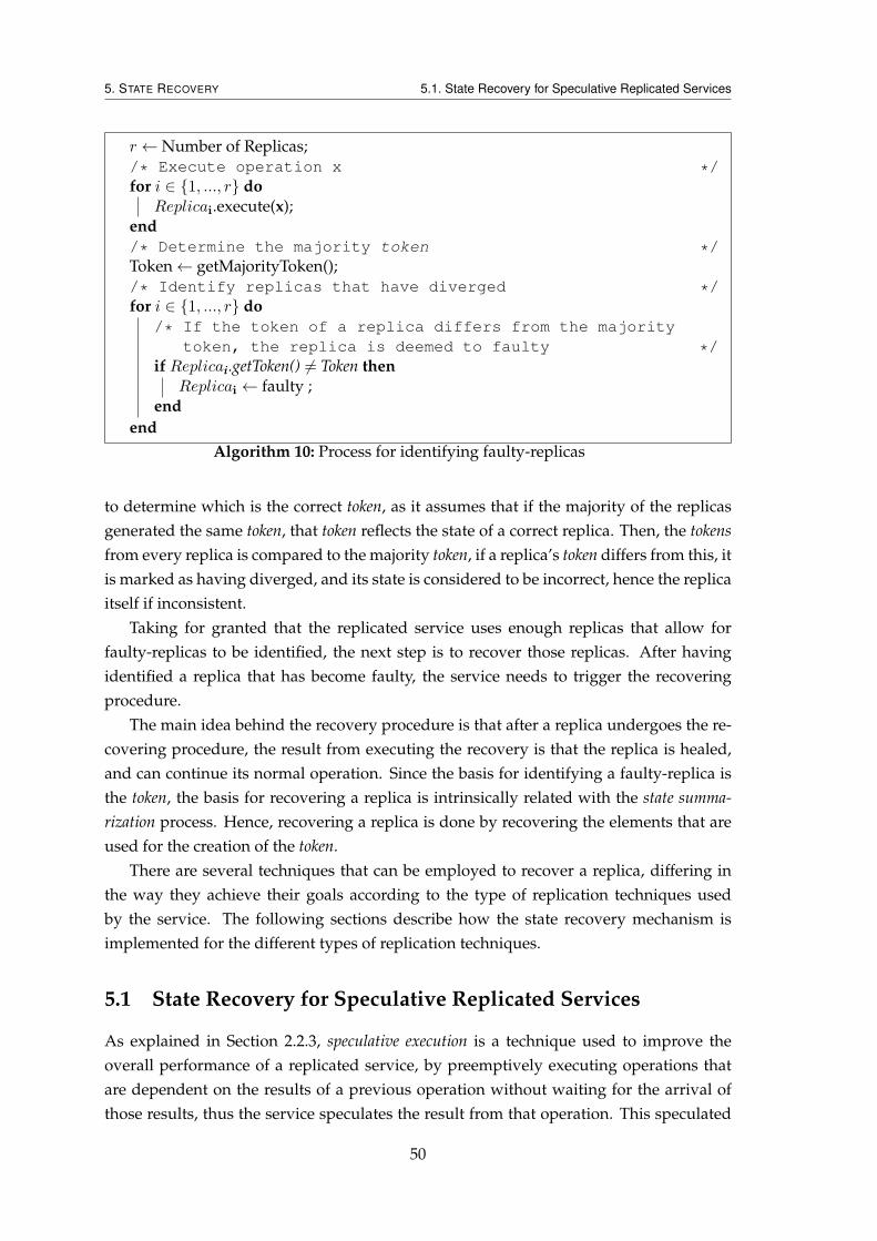
5. STATE RECOVERY 5.1. State Recovery for Speculative Replicated Services
r ← Number of Replicas;/* Execute operation x */for i ∈ {1, ..., r} do
Replicai.execute(x);end/* Determine the majority token */Token← getMajorityToken();/* Identify replicas that have diverged */for i ∈ {1, ..., r} do
/* If the token of a replica differs from the majoritytoken, the replica is deemed to faulty */
if Replicai.getToken() 6= Token thenReplicai ← faulty ;
endend
Algorithm 10: Process for identifying faulty-replicas
to determine which is the correct token, as it assumes that if the majority of the replicasgenerated the same token, that token reflects the state of a correct replica. Then, the tokensfrom every replica is compared to the majority token, if a replica’s token differs from this, itis marked as having diverged, and its state is considered to be incorrect, hence the replicaitself if inconsistent.
Taking for granted that the replicated service uses enough replicas that allow forfaulty-replicas to be identified, the next step is to recover those replicas. After havingidentified a replica that has become faulty, the service needs to trigger the recoveringprocedure.
The main idea behind the recovery procedure is that after a replica undergoes the re-covering procedure, the result from executing the recovery is that the replica is healed,and can continue its normal operation. Since the basis for identifying a faulty-replica isthe token, the basis for recovering a replica is intrinsically related with the state summa-rization process. Hence, recovering a replica is done by recovering the elements that areused for the creation of the token.
There are several techniques that can be employed to recover a replica, differing inthe way they achieve their goals according to the type of replication techniques usedby the service. The following sections describe how the state recovery mechanism isimplemented for the different types of replication techniques.
5.1 State Recovery for Speculative Replicated Services
As explained in Section 2.2.3, speculative execution is a technique used to improve theoverall performance of a replicated service, by preemptively executing operations thatare dependent on the results of a previous operation without waiting for the arrival ofthose results, thus the service speculates the result from that operation. This speculated
50
5. STATE RECOVERY 5.1. State Recovery for Speculative Replicated Services
result is then used by the replica to execute further operations, without needing to waitfor the real result of the operation to arrive.
This allows the replicated service to improve its performance, as the contention at thereplicas is reduced, by not having replica sit idle waiting for results of previous opera-tions to continue the execution of new operations, thus gaining performance.
The problem with this type of replication technique is the fact that if a speculatedresult does not match the real result, the state of the replica is affected, as the replicadiverges in state by having used an erroneous speculative result to execute other opera-tions.
For example, if the service speculatively executes operation o2 that depends of theresult of operation o1, and o1 fails to execute properly, o2 will also be affected. As theexecution of o2 took place on the basis that the speculative result was correct, thus bywrongly calculating this value to execute further operations — or simply by having di-verged during o1 — the replica state becomes faulty.
Traditionally, services based on speculative execution address this problem by creat-ing checkpoints throughout the replica’s lifetime. This allows the replica to have a fall-backpoint in time where its state was know to be correct, which enables the service to revertthe replica to previously known correct state in the case of a wrong speculative result.These checkpoints are created after the replicated service confirms that the result from thespeculative execution was correct, which translates in the state of the replica being cor-rect. This verification is done by confirming that the speculated result, used by the replicato execute further operations, matches the real result.
This checkpoint is then to be used by the replicated service to revert the replica to a cor-rect but out-of-date state if the replica diverges during operation. Divergences betweenreplicas’ states is done by applying any of the available state summarization techniques,and comparing that the summarization of state is identical across all replicas.
When the service identifies that a replica has diverged during operation, possibly dueto a wrongly speculated result, the replica uses the last available checkpoint to correct itsstate. At this point, the replica’s state is deemed to be correct but out-of-date. The nextstep in the state recovery process is to bring this replica’s state up-to-date. This is doneby executing the operations, that lead to a divergence in state, using the real result.
Although this approach effectively avoids running into another divergence related toanother wrong speculative result, it does not ensure that the replica’s state is correct, asthe replica might still diverge due to fail-stop/self-evident errors. If the replica’s statefails again to converge with the state of the remaining replicas, an alternative approachfor recovering its state is performed. This is done by applying the pro-active recoverytechnique, where the replica is restarted and rebooted, which ensures that the replica’sstate is blank. Then, the replica is brought up-to-date by transferring the state of a correctreplica, replacing its blank state, thus effectively recovering the replica.
In the above example, if the replica had created a checkpoint c0 before o1, the recoveryprocess for that service would rollback that replica’s state to that point in time (c0), as the
51
5. STATE RECOVERY 5.2. State Recovery for Design Diversity-Based Replicated Services
replica was known to be in a correct state, and discard all the operations that took placeafter o1. Then, the replica’s state can be brought up-to-date by replacing its state with thestate from a replica that has successfully completed the operations.
The reason behind the existence of the first method for recovering a replica’s state— reverting the replica to a previously known correct state and then re-executing in anon-speculative manner the block of operations that are pending — is due to the fact thatif this approach successfully recovers the state of the replica, less impact is felt on thereplicated service.
Given that a replicated services that applies speculative execution does so to reducecontention among replica, thus improving performance, it will favor a method for recov-ering replica’s state that has less impact — performance-wise — in its normal operation,even if this means that in some cases two different forms of state recovery are to be ex-ecuted to recover a fault-replica. The second approach — pro-active recovery — as agreater impact the service’s performance as the transference of state suggests that a cor-rect replica would have to waste resources exporting its state, before the faulty-replicawas successfully recovered.
5.2 State Recovery for Design Diversity-Based Replicated Ser-vices
There are two different types of design diversity: i) diverse; and ii) non-diverse. Althoughthe recovery of state in a service that applies diverse design diversity use the same logicbehind one that applies non-diverse design diversity, some implementation details differ,thus this type of diversity can be seen as a special case.
We start by describing the process of recovering a replica for a service that applies non-diverse design diversity and then detail the changes that need occur in order for the staterecovery mechanism to be applicable in the context of a replicated service that appliesdiverse design diversity.
Non-Diverse Design Diversity
In this context, given that all replicas present in the replicated service are identical, mean-ing that they all run the same software implementation, recovering a faulty-replica isdone by transferring the state of a correct replica to the faulty-replica, thus having itsstate coverage with the remaining replicas.
This requires for the presence of a state transference mechanism, which entail that thereplicas are to support the following operations: i) export their state; and ii) import thestate from another replica.
Exporting the state of a replica can be achieved by gathering the objects used bythe state summarization process to a general token that represents the current state ofa replica, and exporting said objects. The exportation of these objects can take various
52
5. STATE RECOVERY 5.2. State Recovery for Design Diversity-Based Replicated Services
forms: i) it may be a serialized version of the objects; or ii) the objects themselves. De-pending on the type of replicated service, opting for one approach over the other mayyield better results.
After the exportation of state completes, the result has to be transfered to the faulty-replica in order for it to be recovered. At this point, after the recovering replica receivesthis exported state, is replaces the correspondent objects with the ones from the importedstate. When the recovering replica finishes this process, its state is now considered tobe correct, as the objects used to create the state summarization token have all been re-placed with the ones from a known correct replicas, thus the replica is considered to haveterminated its recovery, and is now deemed to be correct.
Diverse Design Diversity
Although the aforementioned process works for the majority of cases, in order for it to beapplicable in the context of a replicated service that uses diverse design diversity, changeshave to be made to the mechanisms involved in the process of exporting and importingstates.
The challenge of recovering the state in this context comes from the fact that replicasare not all running the same software implementation. Despite the implementation run-ning in each replica obeying to the same software specification — independently of theway that the software is implemented, given the same inputs the outputs yielded are tobe the same — they differ in the way that they are implemented.
If before exporting and importing the state was achieved by exporting and importingthe objects used by the state summarization process to summarize the state of a replica,given that for this type of design diversity different replicas can be running different soft-ware implementations, there is a strong chance that the objects used in each implementa-tion vary, thus the exportation and importation of state has to be adapted to enable repli-cas running different implementations to be capable of importing and exporting statesamongst themselves.
This requires that in addition to the functions required for recovering the state in thenon-diverse design diversity scenario, for functions that translate implementation specificstates to an abstract state and vice-versa, which will enable the recovery of replicas run-ning different implementations.
For example, if we consider a replicated database service that runs two differentdatabases implementations: Ia and Ib. If a replica running implementation Ia becomesfaulty, and it is to be recovered with aid from implementation Ib, one possible abstractstate that Ib could export is the contents of the database itself. This would work as thecontents of the database are independent from the objects used by Ia and Ib to store thesecontents.
53

5. STATE RECOVERY 5.2. State Recovery for Design Diversity-Based Replicated Services
54
6Prototype: implementation and
evaluation
This section explains how the aforementioned concepts and techniques for summariza-tion of state and state recovery were applied to both H2 Database and HSQL Database. Weexplain how the state summarization and state recovery for both databases can be usedby a replicated service to improve its resilience to failures. We also perform a study of theoverhead added by the aforementioned mechanisms to the databases by comparing thetime it takes to execute a certain amount of operations in both modified (with the ScalableCounting Bloom Filter integrated) and un-modified versions of the databases.
6.1 Implementation
Here it is explained how the concepts and techniques described throughout the docu-ment were applied to H2 Database and HSQL Database.
Independently of the type of technique used by a replicated service, in order to im-prove its resilience to failures it needs to incorporate to major components: i) state sum-marization; and ii) state recovery. This means that the replicas of the replicated serviceneed to integrate the aforementioned components to provide the service with a way toidentify faulty-replicas and recover said replicas.
In the context of this work support for state summarization and state recovery areadded to the H2 Database and HSQL Database. The following sections describe the modi-fications that took place to achieve these goals, and what entails to use these implementedmechanisms by the replicated service.
55
6. PROTOTYPE: IMPLEMENTATION AND EVALUATION 6.1. Implementation
6.1.1 State Summarization
State summarization is what allows the replicated service to identify replicas that havediverged during operation, thus their state has become faulty and the replica needs to berecovered.
The process of summarizing the state of a replica is done by applying the techniquesdescribed in Chapter 3. By integrating a Scalable Bloom Filter, the state of the replicacan be summarized. But, as explained in earlier sections, not in all cases it is possible todirectly apply this structure, as the end result would not be the desired one. The mainreason for this is that many replicated services do not enforce a strict order of execution,which entails that despite replicas having the same operations to execute, they are free todo so in any order they see fit.
Chapter 4 provides a more elaborated way of achieving state summarization, that isalso applicable in scenarios in which the replica deals with un-ordered operations, whichis the basis for the solution that follows.
The first step in providing support for state summarization for any replica, is to firstanalyze the replica and identify what composes the state of the replica, which requiresidentifying the components of the replica that will be used to create its abstract state.
Given that the focus of this work is a replicated database service, and that support fordesign diversity is also an objective, identifying what composes the state of a H2 Databasereplica or a HSQL Database replica is not enough. Since the goal is to have replicas runningdifferent database implementations — the ones mentioned before — state summarizationhas to be a compromise between identifying what composes the state of a specific type ofreplica, and what the each type of replica has in common.
The state summarization begins by deciding what is the state that needs to be sum-marized. In a database service, the state consists of the data contents —- the internalstructures of the database can be left out of state summarization, as it would be possibleto locally verify if they are correct from the database contents. Thus, the contents of thetables of the database are used to compose a summary of the replica’s state, as the rowsof the tables are present in both H2 Database and HSQL Database.
This approach works despite the fact that the databases are implemented differently,because the values used to create the summary are the same for both implementations.By using the values of the operations — before they are converted to implementationspecific objects — it is guaranteed that the values used in the filter for both databases areidentical, therefor ensuring that the tokens generated through the replica’s life-cycle willbe the same in the absence of failures.
Next follows a explanation of how this was achieved for both H2 Database and HSQLDatabase
As aforementioned, the state summarization token is created by using the contents ofthe databases, more concretely, the values of each column of each rows that gets createdin a table. This means that the state summarization process needs to occur at the moment
56
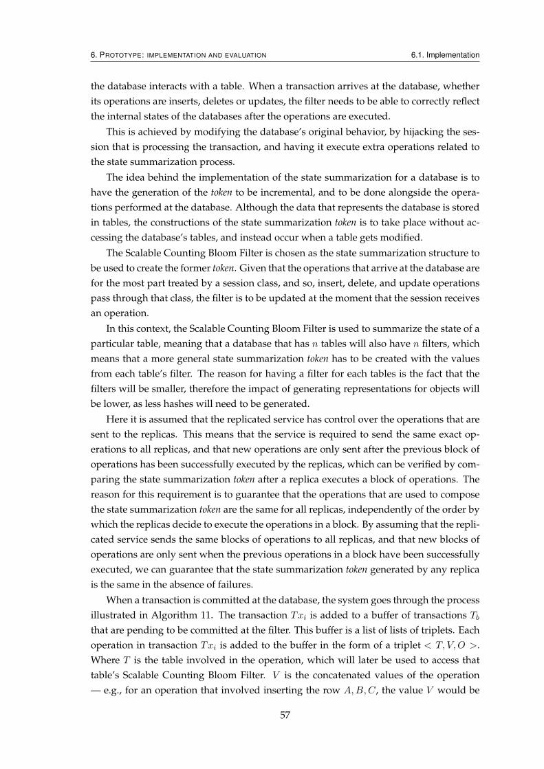
6. PROTOTYPE: IMPLEMENTATION AND EVALUATION 6.1. Implementation
the database interacts with a table. When a transaction arrives at the database, whetherits operations are inserts, deletes or updates, the filter needs to be able to correctly reflectthe internal states of the databases after the operations are executed.
This is achieved by modifying the database’s original behavior, by hijacking the ses-sion that is processing the transaction, and having it execute extra operations related tothe state summarization process.
The idea behind the implementation of the state summarization for a database is tohave the generation of the token to be incremental, and to be done alongside the opera-tions performed at the database. Although the data that represents the database is storedin tables, the constructions of the state summarization token is to take place without ac-cessing the database’s tables, and instead occur when a table gets modified.
The Scalable Counting Bloom Filter is chosen as the state summarization structure tobe used to create the former token. Given that the operations that arrive at the database arefor the most part treated by a session class, and so, insert, delete, and update operationspass through that class, the filter is to be updated at the moment that the session receivesan operation.
In this context, the Scalable Counting Bloom Filter is used to summarize the state of aparticular table, meaning that a database that has n tables will also have n filters, whichmeans that a more general state summarization token has to be created with the valuesfrom each table’s filter. The reason for having a filter for each tables is the fact that thefilters will be smaller, therefore the impact of generating representations for objects willbe lower, as less hashes will need to be generated.
Here it is assumed that the replicated service has control over the operations that aresent to the replicas. This means that the service is required to send the same exact op-erations to all replicas, and that new operations are only sent after the previous block ofoperations has been successfully executed by the replicas, which can be verified by com-paring the state summarization token after a replica executes a block of operations. Thereason for this requirement is to guarantee that the operations that are used to composethe state summarization token are the same for all replicas, independently of the order bywhich the replicas decide to execute the operations in a block. By assuming that the repli-cated service sends the same blocks of operations to all replicas, and that new blocks ofoperations are only sent when the previous operations in a block have been successfullyexecuted, we can guarantee that the state summarization token generated by any replicais the same in the absence of failures.
When a transaction is committed at the database, the system goes through the processillustrated in Algorithm 11. The transaction Txi is added to a buffer of transactions Tbthat are pending to be committed at the filter. This buffer is a list of lists of triplets. Eachoperation in transaction Txi is added to the buffer in the form of a triplet < T, V,O >.Where T is the table involved in the operation, which will later be used to access thattable’s Scalable Counting Bloom Filter. V is the concatenated values of the operation— e.g., for an operation that involved inserting the row A,B,C, the value V would be
57
6. PROTOTYPE: IMPLEMENTATION AND EVALUATION 6.1. Implementation
Tid ← Transaction Identifier;/* Mark Transaction Tid as committed by the Database */CTid
← 1;/* Add Transaction Tid to the buffer */B.add(Tid) ;Bs ← Buffer Size;ready ← true;/* Verify that all the transactions in a block have been
committed */while t ∈ {1, ..., Bs} and ready == true do
if Ct 6= 1 thenready ← false;
endt++;
endif ready == true then
for x ∈ {1, ..., Bs} dot← B.get(x) ;filter.add(t) ;
end/* Rotate C */C.rotate() ;/* Update Database’s state summarization token */Database.computeHash() ;
endAlgorithm 11: State Summarization Process
ABC — value that should be used in the filter. And O is the type of operation that wasperformed in the transaction, which is to be the operation performed at the filter.
After adding the necessary information to the buffer, the transaction Txi is marked ashave been committed by the database in a BitSet BSct. Using a BitSet for keeping trackof the transaction that have been committed by the database but that have not yet takenpart in the database’s state summarization token, allows for an efficient way for checkingwhich transactions have yet to be reflected by the state summarization structure.
The next step is to verify — after the transaction is executed by the replica — if thelatest block of buffered transactions — those that are waiting to be inserted in the filter —have all been marked as committed. If so, the buffer Tb is accessed, and a list of tripletsretrieved for each of the transactions that were pending to be added to the filter. Then,for each triplet in a list, the Scalable Counting Bloom Filter of the table T is accessed, andan operation of type O is performed with the value V . This process ends when all of theoperations have been reflected in their respective filters. At this point, the transactionshave successfully been added to the filters, therefore the buffer can discard them. Addi-tionally, the BitSet BSct is rotated, effectively discarding the information regarding thosetransactions, which restricts it size from going indefinitely. This is done by creating a
58
6. PROTOTYPE: IMPLEMENTATION AND EVALUATION 6.1. Implementation
new BitSet that contains all the values from the old BitSet except those that correspond tothe last block of transactions that where already reflected in the Scalable Counting BloomFilter.
At this stage the summarization of state in nearly completed, all the filters of themodified tables have now recomputed the tokens that summarize their state, and the onlyoperation that still needs to be made is for the general database’s token to be generated.This token is generated by concatenating all of the tokens of the database’s tables, andhashing that value. For each table T in the database, the Scalable Counting Bloom Filterof table T is accessed, its token retrieved, and concatenated with the remaining tokens.After iterating the tables, the concatenated value is passed through a hash function, thatgenerates the state summarization token for the database itself.
Although the state summarization token has been created, it still needs to be accessiblefrom the outside — replicated service — in order to be useful. As it is this same token thatallows the replicated service, more concretely its fault-tolerance mechanism, to identifyif a replica has diverged in state, therefore its faulty, and needs to undergo the recoveringprocedure.
This problem was approached by analyzing the interfaces for both databases, andidentifying those functions that could be used to retrieve the state summarization token.More specifically, our attention was drawn to the functions that provided access to themeta-data of the databases. The intuition here is that some of those functions would haveto access variables in the database in order to return some value, which opened the possi-bility of modifying the behavior of one of the functions to access the token, returning it tothe outside. Another advantage of this approach is that by using the functions offered bythe JDBC interface, it was guaranteed that it would be offered by both databases, avoid-ing the need to create a function in the replicated service to deal with the token retrieval.
One function that is offered by the JDBC interface, therefore being present for both H2database and HSQL database, is a function that allows to access the version of the database.Not only modifying this function does not change the normal behavior of the database,as it is not used in the context of this work, but it also fits the concept of version in areplicated service, as the version of a replica in this context can be seen as its currentstate, which is given by the state summarization token.
6.1.2 State Recovery
State recovery is the process of recovering a replica that the replicated service has identi-fied as being faulty.
The first step is for the replicated service to determine if a replica’s state has becomeinconsistent during operation, thus having become faulty, and needing to undergo therecovery process. The service achieves this by comparing the token that the replicas gen-erate after a certain amount of operations take place. This amount of operations corre-sponds to the size of the transaction buffer Tb mentioned in the previous section, as this
59
6. PROTOTYPE: IMPLEMENTATION AND EVALUATION 6.1. Implementation
allows for a more immediate identification of divergences betweens replicas. By check-ing the state of the replicas at the exact moment that a transaction block is reflect in therespective table filters, thus checking the token for the database state after this has beenupdated, allows for divergences between replicas to be promptly identified.
After the service identifies a replica that needs to be recovered, the state recovery pro-cess is triggered. Recovering the state of a replica in the context of a replicated databaseservice, where the replicas are databases — in this case, H2 databases and HSQL databases— consists in obtaining the state of a correct replica, and importing said state in the re-covering replica.
Given that the state of the replica includes Scalable Counting Bloom Filters for eachof the database’s tables, and that the token that is generated by the filter is based on thecontents of the tables, doing a full recovery of a replica can be divided in the followingoperations: i) exporting the filter from a correct replica; ii) dumping all of the tables’contents of the aforementioned replica; iii) importing the contents of the tables dumped;and iv) importing the previously exported filter in the recovering replica. Note that it isnecessary to import the filter from the correct replica, as re-creating an exactly equal filterwould require adding the information in the same order.
Exporting the filter
The filter exportation process takes place at a correct replica, ensuring that the recoveringreplica that will use this filter recreates its filter correctly, thus recovering successfully.This operation is divided in two parts: i) filter serialization; and ii) having the filter beaccessible from the outside-world.
The first part — filter serialization — is done by iterating all of a correct replica’stables, and for each of those tables invoke the filter exportation method. What this filterexportation method does, is to serialize the Scalable Counting Bloom Filter in a JSONobject. This JSON object contains not only the variables of the filter that are needed to re-initialize an identical Scalable Counting Bloom Filter, and all of the sub-filters and theirown variables.
Additionally, all of the resulting JSON objects that are created — one for each tableof the database — are paired with their corresponding table, generating a pair < T,F >,where T is the table’s name, and F is the JSON object that represents the Scalable Count-ing Bloom Filter of table T , after it has been converted to a string of text.
Figure 6.1 depicts the general structure of the aforementioned JSON object, after hav-ing been converted to a string of text.
The second step — making the serialized version of the filter accessible form the out-side — is achieved by using the string version of the JSON object that resulted from thefirst step, and inserting it a table Tf , which is by default accessible from the outside, giventhat it is a typical database table.
60
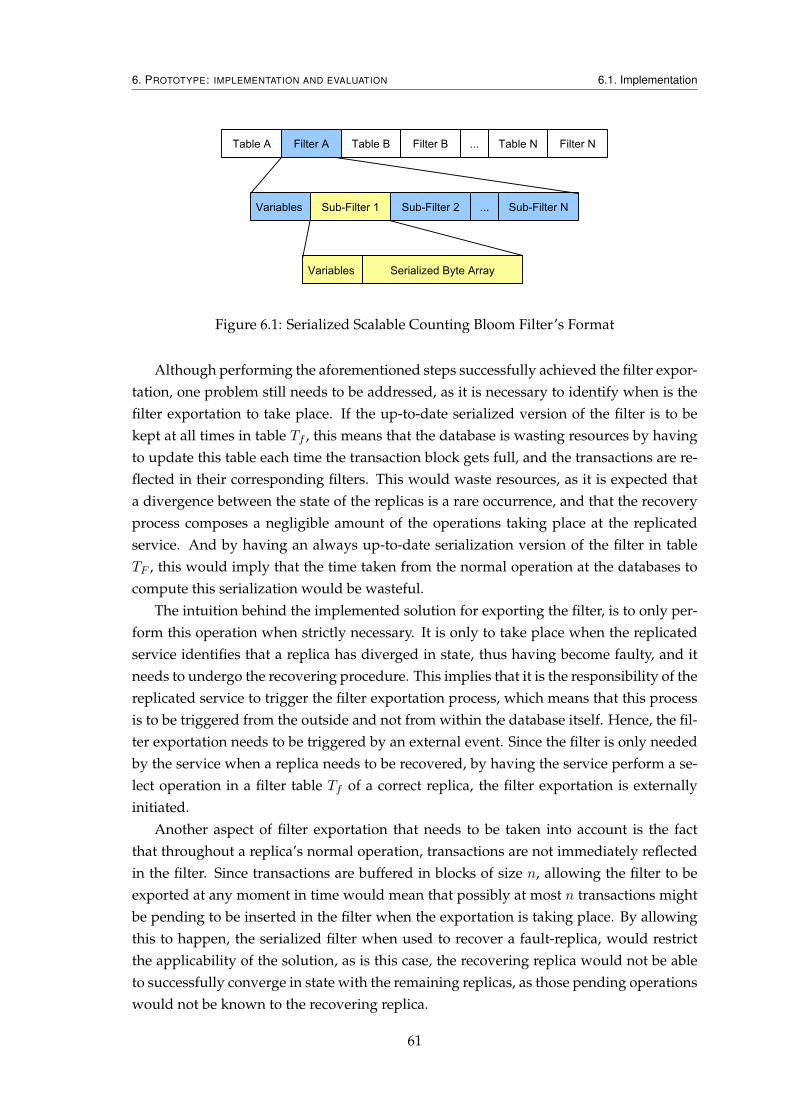
6. PROTOTYPE: IMPLEMENTATION AND EVALUATION 6.1. Implementation
Figure 6.1: Serialized Scalable Counting Bloom Filter’s Format
Although performing the aforementioned steps successfully achieved the filter expor-tation, one problem still needs to be addressed, as it is necessary to identify when is thefilter exportation to take place. If the up-to-date serialized version of the filter is to bekept at all times in table Tf , this means that the database is wasting resources by havingto update this table each time the transaction block gets full, and the transactions are re-flected in their corresponding filters. This would waste resources, as it is expected thata divergence between the state of the replicas is a rare occurrence, and that the recoveryprocess composes a negligible amount of the operations taking place at the replicatedservice. And by having an always up-to-date serialization version of the filter in tableTF , this would imply that the time taken from the normal operation at the databases tocompute this serialization would be wasteful.
The intuition behind the implemented solution for exporting the filter, is to only per-form this operation when strictly necessary. It is only to take place when the replicatedservice identifies that a replica has diverged in state, thus having become faulty, and itneeds to undergo the recovering procedure. This implies that it is the responsibility of thereplicated service to trigger the filter exportation process, which means that this processis to be triggered from the outside and not from within the database itself. Hence, the fil-ter exportation needs to be triggered by an external event. Since the filter is only neededby the service when a replica needs to be recovered, by having the service perform a se-lect operation in a filter table Tf of a correct replica, the filter exportation is externallyinitiated.
Another aspect of filter exportation that needs to be taken into account is the factthat throughout a replica’s normal operation, transactions are not immediately reflectedin the filter. Since transactions are buffered in blocks of size n, allowing the filter to beexported at any moment in time would mean that possibly at most n transactions mightbe pending to be inserted in the filter when the exportation is taking place. By allowingthis to happen, the serialized filter when used to recover a fault-replica, would restrictthe applicability of the solution, as is this case, the recovering replica would not be ableto successfully converge in state with the remaining replicas, as those pending operationswould not be known to the recovering replica.
61
6. PROTOTYPE: IMPLEMENTATION AND EVALUATION 6.1. Implementation
This problem is solved by restricting the moments that a replica can export its filter.Assuming that the replicated database service is constantly performing transactions, andtherefore the replica is constantly executing operations, the exportation of the filter canbe delayed until there are no transactions pending to be added to the filter. Or, in thecase where the replicated service is not expected to have to deal with constant opera-tions, dummy transactions could be created, forcing the buffer of transactions to get full,thus forcing the pending transactions to get added to their respective filters before theexportation process occurs.
Re-populating the tables of a recovering replica
Re-population of the database’s tables is done by dumping all of the contents of the tablesof a correct replica, and using this dump to populate the recovering replica’s database.
For the case of a replica running the H2 Database, the data in the tables is dumped to afile by using sql-native commands. The SCRIPT command offers a way for the databaseto create a file with the contents of the database. This file contains not only the necessarycommands needed to re-create the tables, but also the contents of each table. The datafor each table is represented for each row of a table as a sql insert statement insert sqlcommands that allow for the recreation of the tables and recreation of their contents.
For the other replica type — HSQL Database — used by the replicated service, theprocess of dumping the contents of the database is done by executing a Java programthat comes with the database. This program also provides the ability of exporting thecontents of a HSQL Database to a file. The structure of this file is identical to the filecreated by the H2 database, being composed by sql-commands that create the tables andthe contents of the tables that were present at the moment the export took place.
One problem that derives from both databases having different ways of exportingtheir contents to a file, is that the inverse process — importing contents from a file —is also different. This means that there is no direct way of using a file created by ah H2Database in an HSQL Database, and vice-versa. This problem can be solved by creatingabstract functions, whose job is to convert from a implementation specific file to anotherimplementation. These functions are to be created the replicated service itself, because itis only the service that has initial access to the files generated by the replicas. Then, afterconverting the file to fit the implementation of the replica that is being recovered, thereplicated service invokes the import function offered by the implementation, passingthe already converted file.
The process of re-populating the recovering replica’s database ends with the execu-tion of the sql commands of the exported file.
62
6. PROTOTYPE: IMPLEMENTATION AND EVALUATION 6.1. Implementation
Importing the filter
The last step in recovering a faulty-replica is the importation of the filter. This processtakes place at the recovering replica. Although, a serialized version of the filter has suc-cessfully been created at a correct replica, it still needs to be passed to the recoveringreplica, in order for this replica to re-create its filter. Given that all interactions with thereplicas are made using the JDBC interface, transferring the serialized version of the filterbetween a correct replica and the one being recovered has also to be achieved using thisinterface.
The idea behind the process of importing the serialized version of the filter is simi-lar to the process used in the replicated service for identifying faulty-replicas. Where aspecific table is accessed and the token that represents the replica’s state is retrieved bythe replicated service. The same is done when importing a filter. Where the replicatedservices accesses table Tf of a correct state replica, and it is the service’s responsibility topass this value to the recovering replica. Passing this serialized version of the filter to therecovering replica happens by using the JDBC interface, the filter is passed to the replicathrough its table Tf .
After the filter has been serialized and exported at a correct replica, it is inserted inthe recovering replica’s table Tf . Inserting this serialized version of the filter in table Tfraises another problem. Due to the fact that this insert operation is no different from otherinsert operations, if it was to be treated in the same way by the recovering replica, thiswould have this replica buffering this transaction, and going through the normal routineof later using the values from this transaction in its filter, hence this insert operation hasto be filtered. This is done by modifying the behavior of both databases, treating thistransaction as a special case. When a transaction arrives at the database, it is checked tosee if the affected table is Tf , and if so, it is to be treated differently. Upon identifying thatthe operation of that transaction is an insert operation in table Tf , a process for recreatingthe structure responsible for creating the replica’s state summarization token is triggered.
The process of recreating this structure is similar to the one that occurs when creatinga serialized version of the filter at the correct replica. The value that was inserted in tableTf is used to recreate the state summarization structure — the filter. This value is a stringof text that corresponds to the serialized version of a correct filter, having associated witheach table a Scalable Counting Bloom Filter. Recreating the structure is done by parsingthis value. Each of the table’s in the string is accessed and for each of them, it is invokedthe function that recreated the Scalable Counting Bloom Filter, passing to this function aserialized version of the Scalable Counting Bloom Filter of that table. This function thenrecreates the table’s Scalable Counting Bloom Filter by creating a new Scalable CountingBloom Filter, using as initialization parameters the variables’ values that were serialized.
Additionally, given that a Scalable Counting Bloom Filter entails the presence of sub-filters, they too need to be recreated. This process is identical to the aforementionedone. Where the Counting Bloom Filters — sub-filters — are initialized using the values
63
6. PROTOTYPE: IMPLEMENTATION AND EVALUATION 6.2. Evaluation
present in string of text. One small difference between these two processes, is that theCounting Bloom Filter has an array of bytes, which has itself been serialized. Thus, inorder to complete the recreation of the sub-filters, the serialized byte arrays also need tobe recreated, this is done by iterating the serialized version, and initialing a new bytearray with the corresponding correct values.
After all tables have recreated their Scalable Counting Bloom Filter, the recoveringreplica has now completed the recreation of the state summarization structure, and thereplica has been successfully recovered.
6.2 Evaluation
This section’s purpose is to analyze the implemented solution for both identifying a failedreplica, and for recovering a faulty-replica. Identifying the impact that the state summa-rization has on a database is done by comparing the time it takes for a database to executea certain amount of operations with the time that a modified version of the database takesto perform the same operations while also generating a state summarization token. Therecovery of a replica is analyzed in terms of the time it takes for a correct replica to exportis filter, and the database contents to a file, and the time that it takes for the recoveringreplica to recreate its filter, and to re-populate its database’s contents using the aforemen-tioned file.
This section is divided in three parts, the first details the methodology applied togather the relevant information to perform the tests described in the previous paragraph,the second part is dedicated to described the obtained results, and lastly, the third part, isdedicated to the analysis of the impact that adding support for state summarization andstate recovery has on both H2 Database and HSQL Database.
6.2.1 Methodology
This section describes the methodology applied to gather the data that is later used toperform an impact analysis of the implemented solution.
All of the tests described in this section were run multiple times, ensuring that theresults reflected the ordinary impact that solution has in the databases. These tests wererun in a Intel R© CoreTM i7-2630QM CPU @ 2.00 GHZ, with 4GB of RAM, running Mi-crosoft Windows 7 Professional, Java version 1.7, H2 Database version 1.3.170, and HSQLDatabase version 2.2.9. Additionally, the initial size for the Scalable Counting Bloom Fil-ters used in the tests had support for 1000 objects.
The objective for the tests was to collect data that would allow to determine: i) thecorrectness of the state summarization solution; ii) the overhead added by the state sum-marization process; and iii) the overhead of the recovery procedure.
64
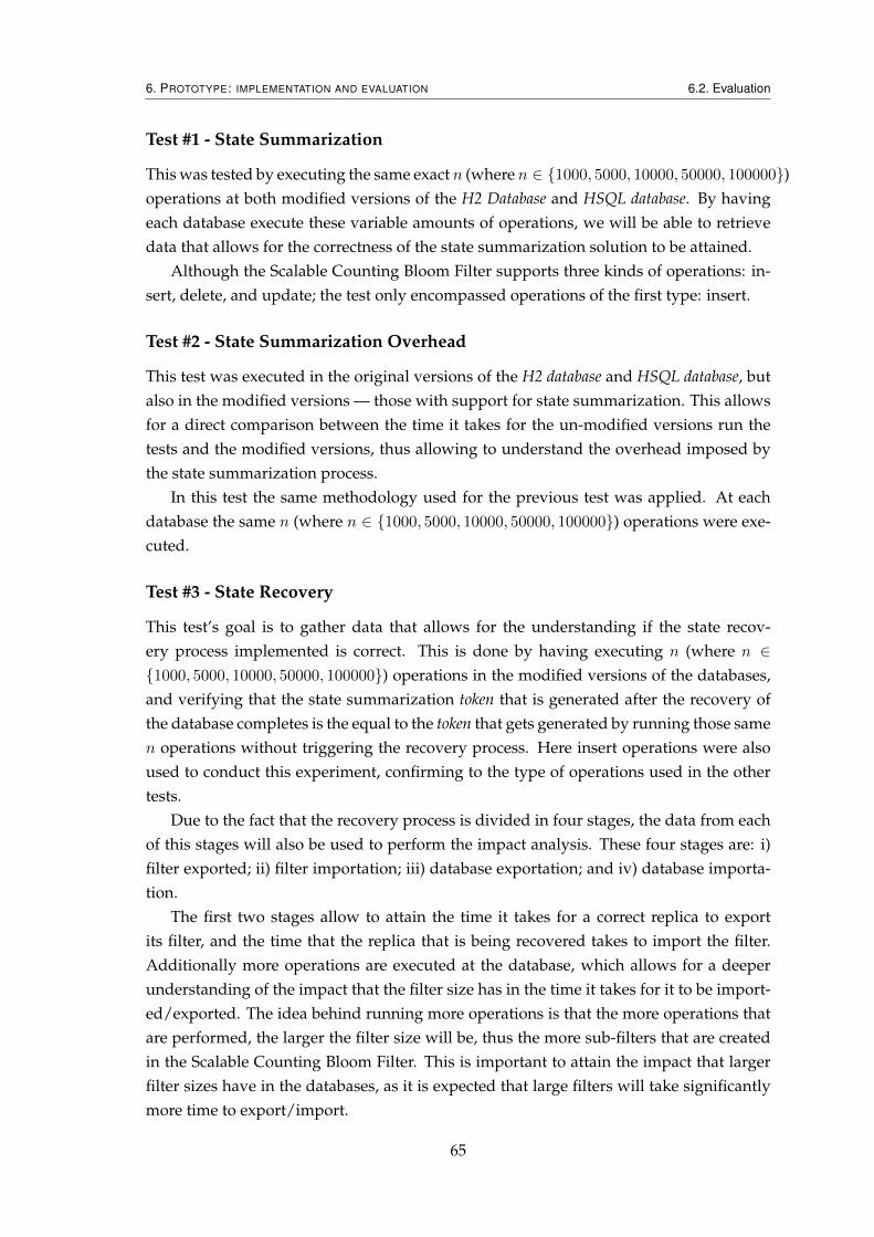
6. PROTOTYPE: IMPLEMENTATION AND EVALUATION 6.2. Evaluation
Test #1 - State Summarization
This was tested by executing the same exact n (where n ∈ {1000, 5000, 10000, 50000, 100000})operations at both modified versions of the H2 Database and HSQL database. By havingeach database execute these variable amounts of operations, we will be able to retrievedata that allows for the correctness of the state summarization solution to be attained.
Although the Scalable Counting Bloom Filter supports three kinds of operations: in-sert, delete, and update; the test only encompassed operations of the first type: insert.
Test #2 - State Summarization Overhead
This test was executed in the original versions of the H2 database and HSQL database, butalso in the modified versions — those with support for state summarization. This allowsfor a direct comparison between the time it takes for the un-modified versions run thetests and the modified versions, thus allowing to understand the overhead imposed bythe state summarization process.
In this test the same methodology used for the previous test was applied. At eachdatabase the same n (where n ∈ {1000, 5000, 10000, 50000, 100000}) operations were exe-cuted.
Test #3 - State Recovery
This test’s goal is to gather data that allows for the understanding if the state recov-ery process implemented is correct. This is done by having executing n (where n ∈{1000, 5000, 10000, 50000, 100000}) operations in the modified versions of the databases,and verifying that the state summarization token that is generated after the recovery ofthe database completes is the equal to the token that gets generated by running those samen operations without triggering the recovery process. Here insert operations were alsoused to conduct this experiment, confirming to the type of operations used in the othertests.
Due to the fact that the recovery process is divided in four stages, the data from eachof this stages will also be used to perform the impact analysis. These four stages are: i)filter exported; ii) filter importation; iii) database exportation; and iv) database importa-tion.
The first two stages allow to attain the time it takes for a correct replica to exportits filter, and the time that the replica that is being recovered takes to import the filter.Additionally more operations are executed at the database, which allows for a deeperunderstanding of the impact that the filter size has in the time it takes for it to be import-ed/exported. The idea behind running more operations is that the more operations thatare performed, the larger the filter size will be, thus the more sub-filters that are createdin the Scalable Counting Bloom Filter. This is important to attain the impact that largerfilter sizes have in the databases, as it is expected that large filters will take significantlymore time to export/import.
65
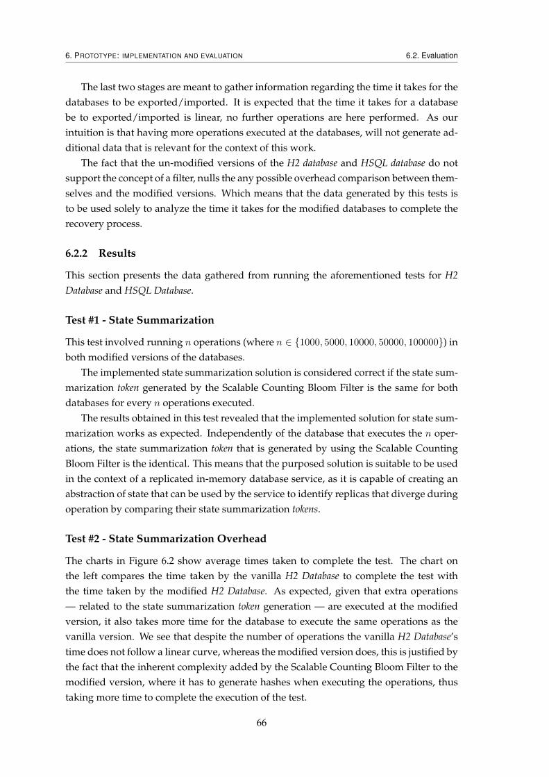
6. PROTOTYPE: IMPLEMENTATION AND EVALUATION 6.2. Evaluation
The last two stages are meant to gather information regarding the time it takes for thedatabases to be exported/imported. It is expected that the time it takes for a databasebe to exported/imported is linear, no further operations are here performed. As ourintuition is that having more operations executed at the databases, will not generate ad-ditional data that is relevant for the context of this work.
The fact that the un-modified versions of the H2 database and HSQL database do notsupport the concept of a filter, nulls the any possible overhead comparison between them-selves and the modified versions. Which means that the data generated by this tests isto be used solely to analyze the time it takes for the modified databases to complete therecovery process.
6.2.2 Results
This section presents the data gathered from running the aforementioned tests for H2Database and HSQL Database.
Test #1 - State Summarization
This test involved running n operations (where n ∈ {1000, 5000, 10000, 50000, 100000}) inboth modified versions of the databases.
The implemented state summarization solution is considered correct if the state sum-marization token generated by the Scalable Counting Bloom Filter is the same for bothdatabases for every n operations executed.
The results obtained in this test revealed that the implemented solution for state sum-marization works as expected. Independently of the database that executes the n oper-ations, the state summarization token that is generated by using the Scalable CountingBloom Filter is the identical. This means that the purposed solution is suitable to be usedin the context of a replicated in-memory database service, as it is capable of creating anabstraction of state that can be used by the service to identify replicas that diverge duringoperation by comparing their state summarization tokens.
Test #2 - State Summarization Overhead
The charts in Figure 6.2 show average times taken to complete the test. The chart onthe left compares the time taken by the vanilla H2 Database to complete the test withthe time taken by the modified H2 Database. As expected, given that extra operations— related to the state summarization token generation — are executed at the modifiedversion, it also takes more time for the database to execute the same operations as thevanilla version. We see that despite the number of operations the vanilla H2 Database’stime does not follow a linear curve, whereas the modified version does, this is justified bythe fact that the inherent complexity added by the Scalable Counting Bloom Filter to themodified version, where it has to generate hashes when executing the operations, thustaking more time to complete the execution of the test.
66
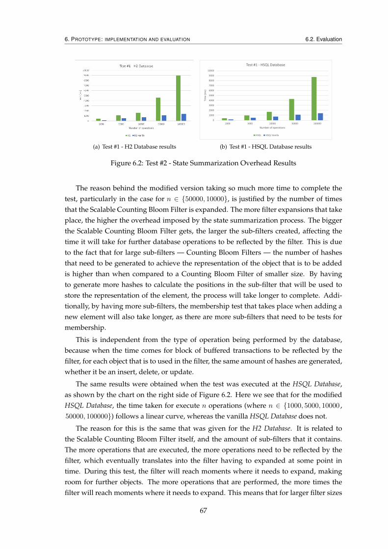
6. PROTOTYPE: IMPLEMENTATION AND EVALUATION 6.2. Evaluation
(a) Test #1 - H2 Database results
0
1000
2000
3000
4000
5000
6000
7000
8000
9000
10000
1000 5000 10000 50000 100000
Tim
e (
ms)
Number of operations
Test #1 - HSQL Database
HSQL HSQL Vanilla
(b) Test #1 - HSQL Database results
Figure 6.2: Test #2 - State Summarization Overhead Results
The reason behind the modified version taking so much more time to complete thetest, particularly in the case for n ∈ {50000, 10000}, is justified by the number of timesthat the Scalable Counting Bloom Filter is expanded. The more filter expansions that takeplace, the higher the overhead imposed by the state summarization process. The biggerthe Scalable Counting Bloom Filter gets, the larger the sub-filters created, affecting thetime it will take for further database operations to be reflected by the filter. This is dueto the fact that for large sub-filters — Counting Bloom Filters — the number of hashesthat need to be generated to achieve the representation of the object that is to be addedis higher than when compared to a Counting Bloom Filter of smaller size. By havingto generate more hashes to calculate the positions in the sub-filter that will be used tostore the representation of the element, the process will take longer to complete. Addi-tionally, by having more sub-filters, the membership test that takes place when adding anew element will also take longer, as there are more sub-filters that need to be tests formembership.
This is independent from the type of operation being performed by the database,because when the time comes for block of buffered transactions to be reflected by thefilter, for each object that is to used in the filter, the same amount of hashes are generated,whether it be an insert, delete, or update.
The same results were obtained when the test was executed at the HSQL Database,as shown by the chart on the right side of Figure 6.2. Here we see that for the modifiedHSQL Database, the time taken for execute n operations (where n ∈ {1000, 5000, 10000 ,50000, 100000}) follows a linear curve, whereas the vanilla HSQL Database does not.
The reason for this is the same that was given for the H2 Database. It is related tothe Scalable Counting Bloom Filter itself, and the amount of sub-filters that it contains.The more operations that are executed, the more operations need to be reflected by thefilter, which eventually translates into the filter having to expanded at some point intime. During this test, the filter will reach moments where it needs to expand, makingroom for further objects. The more operations that are performed, the more times thefilter will reach moments where it needs to expand. This means that for larger filter sizes
67
6. PROTOTYPE: IMPLEMENTATION AND EVALUATION 6.2. Evaluation
— which implies that there are more sub-filters — the number of hashes that needed tobe generated to reflect a database operation in the filter will be larger. Not only for theaddition of the operation itself, but also for the membership test, which is what allowsthe filter to correctly identify in which sub-filter is the element to be added.
Test #3 - State Recovery
The results from this test are segmented in four parts: i) filter exportation; ii) filter impor-tation; iii) database exportation; and iv) database importation;
Figure 6.3 shows the results for the first part of the test — filter exportation. As previ-ously stated, the filter exportation process is the process of creating a serialized version ofthe various Scalable Counting Bloom Filters present in the database. In the context of thistext this means that the database has to access its only table — the one used to execute theoperation — and export that filter. The process of exporting a Scalable Counting BloomFilter is essentially done by exporting its sub-filters and its variables, which means that itis expected that the more sub-filters that need to be exported — converted to a string rep-resentation — the more that it will take for the database to complete the filter exportationprocess.
0
100
200
300
400
500
600
700
800
1000 5000 10000 50000 100000
Tim
e (
ms)
Database size
Test #3 - Filter Exportation
H2 HSQL
Figure 6.3: Test #3 - Filter Exportation Results
The chart in the figure reflects exactly this. For n = 1000 it takes little to no time toperform the filter exportation, as here only one sub-filter exists in the Scalable CountingBloom Filter. As the value n grows, the number of expansions that occur at the ScalableCounting Bloom Filter increase, and for each expansion that occurs a new sub-filter iscreated. And, as expected, the time that is required to export the filter in this scenariosis much higher. In fact, the time difference between the exportation of a filter of sizen = 10000 and a filter of size n = 50000 is orders of magnitude higher, the same remainingtrue for the filter of size n = 100000. These results, for n = 50000 and n = 100000, seem
68
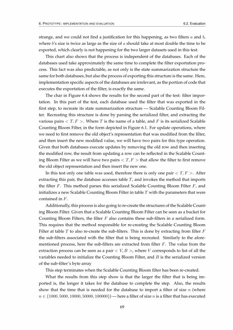
6. PROTOTYPE: IMPLEMENTATION AND EVALUATION 6.2. Evaluation
strange, and we could not find a justification for this happening, as two filters a and b,where b’s size is twice as large as the size of a should take at most double the time to beexported, which clearly is not happening for the two larger datasets used in this test.
This chart also shows that the process is independent of the databases. Each of thedatabases used take approximately the same time to complete the filter exportation pro-cess. This fact was also predictable, as not only is the state summarization structure thesame for both databases, but also the process of exporting this structure is the same. Here,implementation specific aspects of the databases are irrelevant, as the portion of code thatexecutes the exportation of the filter, is exactly the same.
The char in Figure 6.4 shows the results for the second part of the test: filter impor-tation. In this part of the test, each database used the filter that was exported in thefirst step, to recreate its state summarization structure — Scalable Counting Bloom Fil-ter. Recreating this structure is done by parsing the serialized filter, and extracting thevarious pairs < T,F >. Where T is the name of a table, and F is its serialized ScalableCounting Bloom Filter, in the form depicted in Figure 6.1. For update operations, wherewe need to first remove the old object’s representation that was modified from the filter,and then insert the new modified value, we will have two pairs for this type operation.Given that both databases execute updates by removing the old row and then insertingthe modified row, the result from updating a row can be reflected in the Scalable Count-ing Bloom Filter as we will have two pairs < T,F > that allow the filter to first removethe old object representation and then insert the new one.
In this test only one table was used, therefore there is only one pair < T,F >. Afterextracting this pair, the database accesses table T , and invokes the method that importsthe filter F . This method parses this serialized Scalable Counting Bloom Filter F , andinitializes a new Scalable Counting Bloom Filter in table T with the parameters that werecontained in F .
Additionally, this process is also going to re-create the structures of the Scalable Count-ing Bloom Filter. Given that a Scalable Counting Bloom Filter can be seen as a bucket forCounting Bloom Filters, the filter F also contains these sub-filters in a serialized form.This requires that the method responsible for re-creating the Scalable Counting BloomFilter at table T to also re-create the sub-filters. This is done by extracting from filter Fthe sub-filters associated with the filter that is being recreated. Similarly to the afore-mentioned process, here the sub-filters are extracted from filter F . The value from theextraction process can be seen as a pair < V,B >, where V corresponds to list of all thevariables needed to initialize the Counting Bloom Filter, and B is the serialized versionof the sub-filter’s byte array
This step terminates when the Scalable Counting Bloom filter has been re-created.
What the results from this step show is that the larger the filter that is being im-ported is, the longer it takes for the database to complete the step. Also, the resultsshow that the time that is needed for the database to import a filter of size n (wheren ∈ {1000, 5000, 10000, 50000, 100000}) — here a filter of size n is a filter that has executed
69
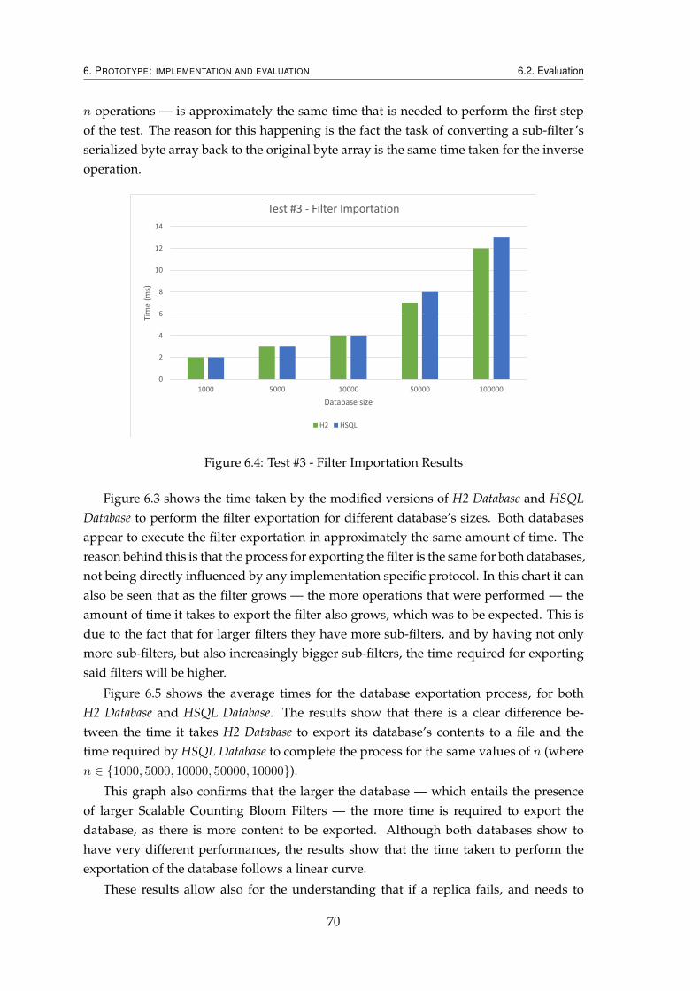
6. PROTOTYPE: IMPLEMENTATION AND EVALUATION 6.2. Evaluation
n operations — is approximately the same time that is needed to perform the first stepof the test. The reason for this happening is the fact the task of converting a sub-filter’sserialized byte array back to the original byte array is the same time taken for the inverseoperation.
0
2
4
6
8
10
12
14
1000 5000 10000 50000 100000
Tim
e (
ms)
Database size
Test #3 - Filter Importation
H2 HSQL
Figure 6.4: Test #3 - Filter Importation Results
Figure 6.3 shows the time taken by the modified versions of H2 Database and HSQLDatabase to perform the filter exportation for different database’s sizes. Both databasesappear to execute the filter exportation in approximately the same amount of time. Thereason behind this is that the process for exporting the filter is the same for both databases,not being directly influenced by any implementation specific protocol. In this chart it canalso be seen that as the filter grows — the more operations that were performed — theamount of time it takes to export the filter also grows, which was to be expected. This isdue to the fact that for larger filters they have more sub-filters, and by having not onlymore sub-filters, but also increasingly bigger sub-filters, the time required for exportingsaid filters will be higher.
Figure 6.5 shows the average times for the database exportation process, for bothH2 Database and HSQL Database. The results show that there is a clear difference be-tween the time it takes H2 Database to export its database’s contents to a file and thetime required by HSQL Database to complete the process for the same values of n (wheren ∈ {1000, 5000, 10000, 50000, 10000}).
This graph also confirms that the larger the database — which entails the presenceof larger Scalable Counting Bloom Filters — the more time is required to export thedatabase, as there is more content to be exported. Although both databases show tohave very different performances, the results show that the time taken to perform theexportation of the database follows a linear curve.
These results allow also for the understanding that if a replica fails, and needs to
70
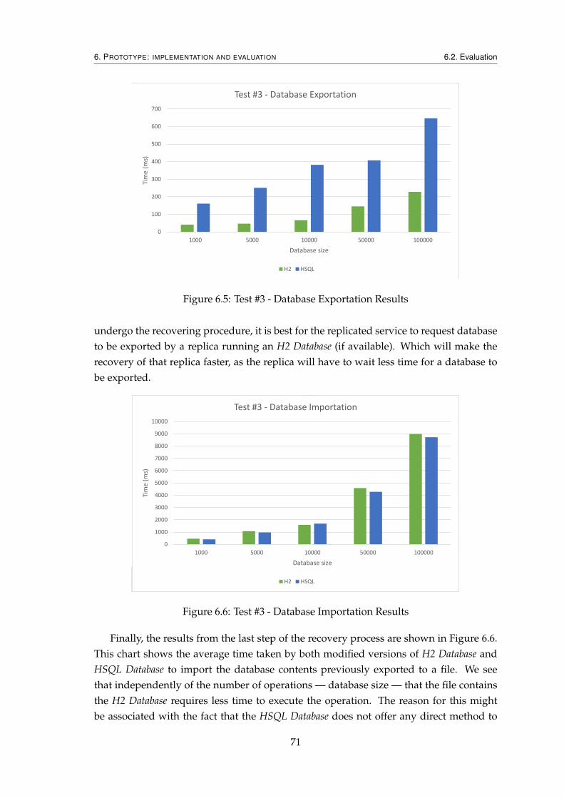
6. PROTOTYPE: IMPLEMENTATION AND EVALUATION 6.2. Evaluation
0
100
200
300
400
500
600
700
1000 5000 10000 50000 100000
Tim
e (
ms)
Database size
Test #3 - Database Exportation
H2 HSQL
Figure 6.5: Test #3 - Database Exportation Results
undergo the recovering procedure, it is best for the replicated service to request databaseto be exported by a replica running an H2 Database (if available). Which will make therecovery of that replica faster, as the replica will have to wait less time for a database tobe exported.
0
1000
2000
3000
4000
5000
6000
7000
8000
9000
1000 5000 100
Tim
e (
ms)
Number of
H2 H2 Van
Test #1 - HSQL Database
0
1000
2000
3000
4000
5000
6000
7000
8000
9000
10000
1000 5000 10000 50000 100000
Tim
e (
ms)
Database size
Test #3 - Database Importation
H2 HSQL
Figure 6.6: Test #3 - Database Importation Results
Finally, the results from the last step of the recovery process are shown in Figure 6.6.This chart shows the average time taken by both modified versions of H2 Database andHSQL Database to import the database contents previously exported to a file. We seethat independently of the number of operations — database size — that the file containsthe H2 Database requires less time to execute the operation. The reason for this mightbe associated with the fact that the HSQL Database does not offer any direct method to
71
6. PROTOTYPE: IMPLEMENTATION AND EVALUATION 6.2. Evaluation
execute a sql script, despite offering the opposite method, and the file had to be manuallyparsed in order to successfully execute each sql command present in the file.
Another aspect to note is that the time taken to complete this task, for each value of n(where n ∈ {1000, 5000, 10000, 50000, 100000}), is similar to the time obtained in Test #1.This is due to the fact that during this process the database will also be computing thestate summarization token, as these operations do not differ from any other operations,thus the database is not able to distinguish that in this case the state summarization pro-cess is not to take place. By computing the state summarization token during a databaseimportation, the database is effectively wasting resources, as the token generated will bereplaced when the filter is imported. In the final chapter, a possible improvement to thisprocess is suggested.
72
7Conclusion
This work presented a solution for summarizing the state of a database, and for perform-ing state recovering in case of failure, that can be used in the context of replicated services,allowing for a greater resilience to failures. The state summarization is achieved by us-ing Scalable Counting Bloom Filters, which provide a way for summarizing the state ofa replica, and by also using Merkle Trees, that provide an efficient way for summarizingthe filter itself.
By providing the mechanisms for the state of a database to be summarized, the repli-cated service can identify replicas that diverge during operation by comparing the statesummarization tokens of the replicas. Those replicas whose tokens do not match the ma-jority of the tokens can be marked by the replicated service as having diverged from theothers, thus having become faulty, and needing to undergo the recovery process (state re-covery). Our solution addresses a problem with current summarization techniques, suchas Merkle Trees — they work well only if the service maintains the exact same internalstate for the same data. In many situation this might not be the case — e.g. in Red-Blacktrees and other dynamic structures, the internal representation will vary depending onthe order by which operations were executed. The same problem occurs if different im-plementations are used in different replicas. To address this problem, the typical solutionis to compute the summary of the state based on an abstract state. However, this is rathercomplex or inefficient.
Our solution addresses this issue, as the summary depends directly on the servicestate. Although our solution also does not allow data to be added in a completely dif-ferent order, we propose a mechanism for allowing sets of operations to execute concur-rently without impacting the produced summary.
The recovery process is done in stages: i) exporting the filter of a correct replica; ii)
73
7. CONCLUSION
dumping the contents of the database; iii) importing said data dump to the replica thatis being recovered; and, finally, iv) recreating the filter of that replica by importing thepreviously exported filter. Effectively recovering the state of a faulty-replica, as bothits contents and its filter are identical to the ones present at a correct replica, after therecovery process completes.
We have implemented our solution in two in-memory databases — H2 Database andHSQL Database. We described the technical challenges we faced, and the rationale for thedecision taken. We have evaluated our solution experimentally — the reported resultsshow that the proposed approach correctly summarizes the state of the database in bothreplicas, reaching the same summary. Our approach has a non-negligible overhead thatmust be tackled before it can be used in practice.
7.1 Future Work
One characteristic that the implemented solution lacks is its inability to adapt the initialScalable Counting Bloom Filter size of the tables, which affects the performance of thestructure. It would be interesting to implement a mechanism to define for any giventable its initial filter size, as the current solution can lead to unnecessary filter expansionsdue to inappropriate filter sizes, which wastes system resources as all tables — big orsmall — will be forced to use the same filter size. By implementing the aforementionedmechanism tables that were expected to be small could be configured to have smallerfilter sizes, and the filters of bigger tables configured to have bigger sizes, thus restrictingthe occurrence of wasteful filter expansions.
Additionally, the recovering mechanism can still be further improved. The imple-mented solution first imports the contents of a correct state replica’s database, and thenit imports the filter of that replica. The problem here is that the replica does not differ theinsert operations in this process from other routine insert operations, which means thatit will go through the normal process of buffering transactions and computing the statesummarization token, effectively wasting resources, as the token generated here will bereplaced when the filter importation takes place. One possible solution to improve thisprocess is to stop the state summarization process during this process.
Another aspect of the recovery mechanism that can be improved is the filter expor-tation process. When a sub-filter is exported, its serialized representation can be cached,allowing future exportations to be faster, as this buffered representation will still be validuntil an operation is performed at its corresponding sub-filter.
Finally, the performance impact of the solution can also be improved. One possiblesolution to address the non-negligible impact that the current prototype has is to possibleexploit the capabilities of multi-core machines and use a background thread to update thefilter, while the main thread remains undisturbed.
74
Bibliography
[1] G. Moore. Excerpts from a conversation with Gordon Moore: Moore’s Law. [Accessed onJan. 31, 2013]. 2005.
[2] G. E. Moore. “Readings in computer architecture”. In: ed. by M. D. Hill, N. P.Jouppi, and G. S. Sohi. San Francisco, CA, USA: Morgan Kaufmann Publishers Inc.,2000. Chap. Cramming more components onto integrated circuits, pp. 56–59.
[3] D. Geer. “Industry Trends: Chip Makers Turn to Multicore Processors”. In: Com-puter 38.5 (May 2005), pp. 11–13.
[4] J. Soares, P. Mariano, J. Loureço, and N. Preguiça. “Improving Application Perfor-mance with Diverse Component Replication”. In: Submitted for publication.
[5] J. a. Soares, J. a. Lourenço, and N. Preguiça. “MacroDB: scaling database engines onmulticores”. In: Proceedings of the 19th international conference on Parallel Processing.Euro-Par’13. Aachen, Germany: Springer-Verlag, 2013, pp. 607–619.
[6] F. B. Schneider. “Implementing fault-tolerant services using the state machine ap-proach: a tutorial”. In: ACM Comput. Surv. 22.4 (Dec. 1990), pp. 299–319.
[7] P. J. Marandi, M. Primi, and F. Pedone. “High performance state-machine replica-tion”. In: Proceedings of the 2011 IEEE/IFIP 41st International Conference on DependableSystems&Networks. DSN ’11. Washington, DC, USA: IEEE Computer Society, 2011,pp. 454–465.
[8] M. Castro, R. Rodrigues, and B. Liskov. “BASE: Using abstraction to improve faulttolerance”. In: ACM Trans. Comput. Syst. 21.3 (Aug. 2003), pp. 236–269.
[9] A. Avizienis. “The N-Version Approach to Fault-Tolerant Software”. In: IEEE Trans.Softw. Eng. 11.12 (Dec. 1985), pp. 1491–1501.
[10] A. Avizienis, J.-C. Laprie, B. Randell, and Vytautas. “Fundamental Concepts of De-pendability”. In: (2000).
[11] F. B. Schneider. “Byzantine generals in action: implementing fail-stop processors”.In: ACM Trans. Comput. Syst. 2.2 (May 1984), pp. 145–154.
75
BIBLIOGRAPHY
[12] M. Castro and B. Liskov. “Proactive recovery in a Byzantine-fault-tolerant system”.In: Proceedings of the 4th conference on Symposium on Operating System Design & Im-plementation - Volume 4. OSDI’00. San Diego, California: USENIX Association, 2000,pp. 19–19.
[13] N. Kolettis and N. D. Fulton. “Software Rejuvenation: Analysis, Module and Appli-cations”. In: Proceedings of the Twenty-Fifth International Symposium on Fault-TolerantComputing. FTCS ’95. Washington, DC, USA: IEEE Computer Society, 1995, pp. 381–.
[14] J. P. J. Kelly, T. I. McVittie, and W. I. Yamamoto. “Implementing Design Diversityto Achieve Fault Tolerance”. In: IEEE Softw. 8.4 (July 1991), pp. 61–71.
[15] B. Wester, J. Cowling, E. B. Nightingale, P. M. Chen, J. Flinn, and B. Liskov. “Toler-ating latency in replicated state machines through client speculation”. In: Proceed-ings of the 6th USENIX symposium on Networked systems design and implementation.NSDI’09. Boston, Massachusetts: USENIX Association, 2009, pp. 245–260.
[16] T.-I. Salomie, I. E. Subasu, J. Giceva, and G. Alonso. “Database engines on multi-cores, why parallelize when you can distribute?” In: Proceedings of the sixth confer-ence on Computer systems. EuroSys ’11. Salzburg, Austria: ACM, 2011, pp. 17–30.
[17] M. Kapritsos, Y. Wang, V. Quema, A. Clement, L. Alvisi, and M. Dahlin. “All aboutEve: execute-verify replication for multi-core servers”. In: Proceedings of the 10thUSENIX conference on Operating Systems Design and Implementation. OSDI’12. Holly-wood, CA, USA: USENIX Association, 2012, pp. 237–250.
[18] J. Soares, J. Lourenço, and N. M. Preguiça. “Software Component Replication forImproved Fault-Tolerance: Can Multicore Processors Make It Work?” In: Proceed-ings of the 14th European Workshop on Dependable Computing (EWDC), LNCS 7869.2013, pp. 173–180.
[19] C. Plattner and G. Alonso. “Ganymed: scalable replication for transactional webapplications”. In: Proceedings of the 5th ACM/IFIP/USENIX international conferenceon Middleware. Middleware ’04. Toronto, Canada: Springer-Verlag New York, Inc.,2004, pp. 155–174.
[20] K. Daudjee and K. Salem. “Lazy database replication with snapshot isolation”. In:Proceedings of the 32nd international conference on Very large data bases. VLDB ’06.Seoul, Korea: VLDB Endowment, 2006, pp. 715–726.
[21] K. Veeraraghavan, P. M. Chen, J. Flinn, and S. Narayanasamy. “Detecting and sur-viving data races using complementary schedules”. In: Proceedings of the Twenty-Third ACM Symposium on Operating Systems Principles. SOSP ’11. Cascais, Portugal:ACM, 2011, pp. 369–384.
[22] D. Lee, B. Wester, K. Veeraraghavan, S. Narayanasamy, P. M. Chen, and J. Flinn.“Respec: efficient online multiprocessor replayvia speculation and external deter-minism”. In: SIGPLAN Not. 45.3 (Mar. 2010), pp. 77–90.
76
BIBLIOGRAPHY
[23] M. Castro and B. Liskov. “Practical Byzantine fault tolerance”. In: Proceedings ofthe third symposium on Operating systems design and implementation. OSDI ’99. NewOrleans, Louisiana, USA: USENIX Association, 1999, pp. 173–186.
[24] I. Gashi, P. Popov, and L. Strigini. “Fault Tolerance via Diversity for Off-the-ShelfProducts: A Study with SQL Database Servers”. In: IEEE Trans. Dependable Secur.Comput. 4.4 (Oct. 2007), pp. 280–294.
[25] I. Gashi, P. Popov, V. Stankovic, and L. Strigini. “On Designing Dependable Ser-vices with Diverse Off-the-Shelf SQL Servers”. In: Lecture Notes in Computer Sci-ence 3069 (2004). Ed. by R. Lemos, C. Gacek, and A. Romanovsky, pp. 191–214.
[26] F. Bonomi, M. Mitzenmacher, R. Panigrahy, S. Singh, and G. Varghese. “An Im-proved Construction for Counting Bloom Filters”. In: Algorithms – ESA 2006. Ed.by Y. Azar and T. Erlebach. Vol. 4168. Lecture Notes in Computer Science. SpringerBerlin Heidelberg, 2006, pp. 684–695.
[27] A. Broder and M. Mitzenmacher. “Network applications of bloom filters: A sur-vey”. In: Internet Mathematics 1.4 (2004), pp. 485–509.
[28] P. S. Almeida, C. Baquero, N. Preguiça, and D. Hutchison. “Scalable Bloom Filters”.In: Inf. Process. Lett. 101.6 (Mar. 2007), pp. 255–261.
77