FACULTY OF ECONOMICS AND BUSINESS …lib.ugent.be/fulltxt/RUG01/002/304/839/RUG01-002304839...Name...

UNIVERSITEIT GENT GHENT UNIVERSITY

FACULTEIT ECONOMIE EN BEDRIJFSKUNDE FACULTY OF ECONOMICS AND BUSINESS

ADMINISTRATION

ACADEMIC YEAR 2015 – 2016

THE EFFECT OF CAPACITY CONSTRAINTS IN SCOP SYSTEMS

PLANNING

Masterproef voorgedragen tot het bekomen van de graad van

Master’s Dissertation submitted to obtain the degree of

Master of Science in Business Economics Master of Science in Business Engineering

Hannes Ryheul

Under the guidance of

Prof. Tarik Aouam

III

PERMISSION

Ondergetekende verklaart dat de inhoud van deze masterproef mag geraadpleegd en/of

gereproduceerd worden, mits bronvermelding.

Naam student: Hannes Ryheul

PERMISSION

Undersigned declares that the contents of this master thesis may be consulted and / or

reproduced, provided the source is acknowledged.

Name student: Hannes Ryheul

IV

Nederlandse Samenvatting

Productiebedrijven moeten elke dag opnieuw beslissen hoeveel ze zullen produceren. Om deze

beslissing te nemen zijn er verschillende methodes ontworpen. Het is het doel van deze thesis om twee

van deze methodes te vergelijken en zo te bepalen welke het best presteert onder verschillende

omstandigheden. De eerste methode is gebaseerd op een lineair programma (LP). Een te optimaliseren

kostfunctie wordt geminimaliseerd, rekening houdend met enkele restricties. De tweede methodes is

gebaseerd op de ‘base stock’ (BS) methode. Voor elk product wordt een niveau bepaald. Iedere

periode wordt het verschil tussen dit niveau en de netto-stockpositie geproduceerd. Beide methodes

bepalen dus de dagelijkse productiehoeveelheden. Het doel van deze is kosten te minimaliseren en

terwijl een bepaald minimum serviceniveau te garanderen naar de klanten toe.

Om de twee methodes te kunnen vergelijken zal worden gebruik gemaakt ‘discrete event simulatie’.

Een fictieve supply chain zal worden gesimuleerd. Beide methodes zullen worden gebruikt om de

productiebeslissing te maken, op deze manier kunnen deze vergeleken worden. De chain bestaat uit

verschillende eindproducten die geproduceerd worden uit meerdere subassemblages. Bepaalde van

deze subassemblages zijn product specifiek, andere subassemblages worden gedeeld. Om de

invloeden van doorlooptijden te testen zullen verschillende simulaties gebeuren met verschillende

doorlooptijd structuren. Ook de variabiliteit van de vraag zal verschillen in verschillende simulaties om

de invloed hiervan te kunnen schatten. Uit de literatuurstudie blijkt dat de invloed van gelimiteerde

capaciteit slechts zelfden onderzocht was. Het is echter belangrijk dat dit gedaan wordt. Ten eerste

zijn realistische productiesystemen onderhevig aan capaciteitslimieten. Ten tweede kan dit onderzoek

helpen in het maken van investeringsbeslissingen (zal extra capaciteit leiden tot een daling van de

kosten?). Een procedure om deze capaciteitslimieten te introduceren in de simulaties wordt

geïntroduceerd. Uit de simulaties kunnen enkele belangrijke conclusies getrokken worden:

De base stock methode presteert veel beter dan de methode gebaseerd op een lineair programma.

Deze BS-methode is goedkoper onafhankelijk van variabiliteit van de vraag, doorlooptijd-structuur

of capaciteitslimieten. Tegelijkertijd behaalt de BS-methode een hogere Fill-Rate.

Het verkorten van de productietijd van gedeelde subassemblages leidt tot grote besparingen in

voorraadkosten.

De BS-methode is robuuster de LP-methode wanneer de capaciteit sterk gelimiteerd is. De base

stock methode kan het servicelevel nog garanderen als capaciteit zeer schaars is, het LP kan dit niet.

Ongeacht de methode, variabiliteit van de vraag of doorlooptijd-structuur. Het is optimaal dat de

capaciteit hoger is dan het 90%-punt (dit wil zeggen dat het systeem in 90% van dagen kan

produceren wat het zou produceren als capaciteit ongelimiteerd was).

V

Preface

I would like to thank a couple of people who have supported me in writing this thesis. First of all, I

would like to thank my promoter Prof. Dr. Tarik Aouam and his assistant Kunal Kumar for their

assistance and guidance in writing this paper. Furthermore, I would like to thank Liesbeth Fivez for

proofreading this thesis, and my parents for their support.

VI

Table of Contents

1 Introduction ..................................................................................................................................... 1

1.1 Motivation ............................................................................................................................... 1

1.2 Problem Definition .................................................................................................................. 4

1.3 Methodology ........................................................................................................................... 7

1.4 Outline ..................................................................................................................................... 7

2 Literature Review ............................................................................................................................ 9

2.1 Dealing With Uncertainty ........................................................................................................ 9

2.2 Planning Policies .................................................................................................................... 12

3 The Supply Chain Operations Planning Problem ........................................................................... 16

3.1 Definitions ............................................................................................................................. 16

3.2 Constraints ............................................................................................................................ 20

3.2.1 Material Constraints ...................................................................................................... 20

3.2.2 Resource Constraints ..................................................................................................... 21

3.2.3 The Impact of Lead Times .............................................................................................. 23

4 Base-Stock Policies ........................................................................................................................ 24

4.1 Pure Base-Stock Policies ........................................................................................................ 24

4.2 Modified Base-Stock Policies for Convergent Systems ......................................................... 26

4.3 Base-Stock Policies for Divergent Systems ............................................................................ 26

4.4 Synchronized Base-Stock Policies .......................................................................................... 28

5 Linear Programming Based Policies in a Rolling Schedule Context ............................................... 31

5.1 General .................................................................................................................................. 31

5.2 Rolling Horizon ...................................................................................................................... 35

6 Simulation Procedure to take Capacity into Account ................................................................... 36

6.1 General .................................................................................................................................. 36

6.1.1 Demand ......................................................................................................................... 36

6.1.2 Lead Times ..................................................................................................................... 37

6.1.3 Starting Conditions ........................................................................................................ 37

6.1.4 Number of Time Periods Simulated .............................................................................. 37

6.2 Linear Program ...................................................................................................................... 38

6.3 Base Stock .............................................................................................................................. 43

7 The Case Study .............................................................................................................................. 44

7.1 Description ............................................................................................................................ 44

7.2 Service level ........................................................................................................................... 45

VII

7.3 Demand ................................................................................................................................. 45

7.4 Lead time ............................................................................................................................... 45

7.5 Capacity ................................................................................................................................. 46

7.6 Cost structure ........................................................................................................................ 47

8 Analysis .......................................................................................................................................... 48

8.1 Performance of the Linear Programming Policy ................................................................... 48

8.1.1 No Capacity Limitations ................................................................................................. 48

8.1.2 Separately Capacitated Case ......................................................................................... 50

8.1.3 Common Capacity Restriction ....................................................................................... 54

8.1.4 The Influence of The Lead Time Structure .................................................................... 58

8.2 Base Stock Policy Performance ............................................................................................. 62


8.2.2 Common Capacity Restriction ....................................................................................... 64

8.3 Comparison Base Stock and Linear Program ......................................................................... 68


8.3.2 Limited Capacity ............................................................................................................ 70

9 Conclusions and Recommendations for Future Research ............................................................ 72

10 Bibliography .................................................................................................................................. I

VIII

List of abbreviations

BOM .................................................................................................................................. Bill of materials

LT ................................................................................................................................................Lead time

WIP ................................................................................................................................. Work in Progress

i.i.d. ............................................................................................. independent and identically distributed

cv ........................................................................................................................... coefficient of variation

LF ..................................................................................................................................... local forecasting

CF ........................................................................................................................collaborative forecasting

EOQ ................................................................................................................... Economic Order Quantity

POQ ..................................................................................................................... Periodic Order Quantity

BS .............................................................................................................................................. Base Stock

SBS ...................................................................................................................... Synchronized Base Stock

CTO ............................................................................................................................. Configure To Order

Avg ................................................................................................................................................. average

BO .............................................................................................................................................. Backorder

Inv ............................................................................................................................................... inventory

LP ....................................................................................................................................... linear program

IX

List of figures

Figure 1: A General Supply Chain (Chopra & Meindl, 2007, figure 1-2) .................................................. 1

Figure 2: terminology .............................................................................................................................. 3

Figure 3: BOM of a bicycle ....................................................................................................................... 5

Figure 4: bicycle production system ........................................................................................................ 5

Figure 5 Pure Base stock policy problem (2) illustration ....................................................................... 25

Figure 6 Pure Base stock policy problem (3) illustration ....................................................................... 25

Figure 7 net inventory distribution shift ............................................................................................... 34

Figure 8 supply chain restriction problem ............................................................................................. 39

Figure 9 Supply chain restriction problem: solution ............................................................................. 39

Figure 10 example of a simple supply chain.......................................................................................... 40

Figure 11 Example of a simple supply chain: with common restriction................................................ 42

Figure 12 The case study (Kok & Fransoo, 2002, figure 5) .................................................................... 44

Figure 13 Performance of the linear programming based policy without capacity limitations. (a) safety

stock; (b) average inventory cost; (c) average backorder cost; (d) average total cost; (e) fill-rate. ..... 48

Figure 14 Performance of the linear programming based policy in a system where each workstation

has a capacity limit. Common component has a long lead time (4 time periods). (a) safety stock; (b)

average inventory cost; (c) average backorder cost; (d) average total cost; (e) fill-rate. ..................... 50

Figure 15 Performance of the linear programming based policy in a system where each workstation

has a capacity limit. Common component has a short lead time (1 time period). (a) safety stock; (b)

average inventory cost; (c) average backorder cost; (d) average total cost; (e) fill-rate. ..................... 52

Figure 16 Performance of the linear programming based policy in a system where a capacity

limitation exists over multiple workstations. Common component has a long lead time (4 time

periods). (a) safety stock; (b) average inventory cost; (c) average backorder cost; (d) average total

cost; (e) fill-rate. .................................................................................................................................... 54

Figure 17 Performance of the linear programming based policy in a system where a capacity

limitation exists over multiple workstations. Common component has a short lead time (1 time

period). (a) safety stock; (b) average inventory cost; (c) average backorder cost; (d) average total

cost; (e) fill-rate ..................................................................................................................................... 56

Figure 18 Influence of the lead-time structure in a system where no capacity limitation exists. (a)

safety stock; (b) average inventory cost; (c) average backorder cost; (d) average total cost. ............. 58

Figure 19 Influence of the lead-time structure in a system where each workstation has a capacity

limit. (a) safety stock & limit = 99%; (b) average total cost & limit = 99%; (c) safety stock & limit =

95%; (d) average total cost & limit = 95%; (e) safety stock & limit = 90%; (f) average total cost & limit

= 90%. .................................................................................................................................................... 59

Figure 20 Influence of the lead-time structure in a system where a capacity limitation exists over

multiple workstations. (a) safety stock & limit = 99%; (b) average total cost & limit = 99%; (c) safety

stock & limit = 95%; (d) average total cost & limit = 95%; (e) safety stock & limit = 90%; (f) average

total cost & limit = 90%. ........................................................................................................................ 60

Figure 21 Performance of the Base Stock policy without capacity limitations. (a) Base Stock of end

product; (b) Base Stock of specific components; (c) average inventory cost; (d) average backorder

cost; (e) average total cost; (f) fill-rate. ................................................................................................. 62

Figure 22 Performance of the Base Stock policy in a system where a capacity limitation exists over

multiple workstations. Common component has a long lead time (4 time periods). (a) Base Stock of

end product; (b) Base Stock of specific components; (c) average inventory cost; (d) average backorder

cost; (e) average total cost; (f) fill-rate .................................................................................................. 64

X

Figure 23 Performance of the Base Stock policy in a system where a capacity limitation exists over

multiple workstations. Common component has a short lead time (1 time period). (a) Base Stock of

end product; (b) Base Stock of specific components; (c) average inventory cost; (d) average backorder

cost; (e) average total cost; (f) fill-rate .................................................................................................. 66

Figure 24 Comparison of LP policy and the SBS policy. No capacity limitations. Common component

with long lead time (4 time periods). (a) average inventory cost; (b) average back order cost; (c)

average total cost; (d) fill rate; (e) comparison of inventories (CV² = 0.25); (f) comparison of

inventories (CV² = 2). ............................................................................................................................. 68

Figure 25 Comparison of LP policy and the SBS policy. No capacity limitations. Common component

with short lead time (1 time period). (a) average inventory cost; (b) average back order cost; (c)

average total cost; (d) fill rate; (e) comparison of inventories (CV² = 0.25); (f) comparison of

inventories (CV² = 2). ............................................................................................................................. 69

Figure 26 Comparison of LP policy and the SBS policy. With capacity limitations. (a) limit = 99% & Lc=

4; (b) limit = 99% & Lc= 1; (c) limit = 95% & Lc= 4; (d) limit = 95% & Lc= 1; (e) limit = 90% & Lc= 4; (f)

limit = 90% & Lc= 1; ................................................................................................................................ 70

1

1 Introduction

1.1 Motivation Walking into a supermarket and picking the detergent you need of a shelf. Ordering new ink cartridges

for your printer and having it delivered at home. Streaming a movie on Netflix. These are all things we,

as consumers, do on a regular basis. In these transactions, customers usually only have contact with

one company, more particularly they only have contact with one department of that company.

However, in most cases, a whole network of different companies and different departments within

these companies are involved in the production and delivery of the goods. This network is what is

called a supply chain.

A supply chain can be defined as “all parties involved, directly or indirectly, in fulfilling a customer

request. The supply chain includes not only the manufacturer and suppliers but also transporters,

warehouses, retailers and even customers themselves. Within each organization, the supply chain

includes all functions involved in receiving and filling a customer request.” (Chopra & Meindl, 2007, p.

13).

A general a supply chain could look like this:

In a first stage, a manufacturer buys raw materials from a supplier. This manufacturer then transforms

these materials into a product fit for consumption. This product is then transported to a distributor,

who in turn sells it to retailers. These retailers make sure the product reaches the final stage in the

chain, the customer. Although it looks very simple, the reality is often more complex. First of all, there

may be multiple players in the different stages, or in some cases, certain stages might not even be in

the chain (by example buying vegetables from a local farmer who grows the vegetables and sells to

the customers directly). There are also other players that might be involved. Independ firms might be

used to transport the products from one place to another (from the manufacturer to the distributor

for example). If a customer orders a product from the retailer using their website, it also involves the

retailers’ website, a bank handling the financial transaction via internet banking and maybe an external

transporting firm is used to deliver the goods to the clients’ home.

Between the different players and stages in a supply chain flows occur. Generally, three types of flows

are distinguished (Chopra & Meindl, 2007):

Product or material flows

Supplier Manufacturer Distributor Retailer Customer

Figure 1: A General Supply Chain (Chopra & Meindl, 2007, figure 1-2)

2

Information flows

Money flows

In figure 1 it looks like there is only a flow from supplier to customer. In reality, however, these flows

often occur in both directions, or even skip stages. A retailer can by example notify a manufacturer of

an unexpected spike in sales (information flow). A distributor can send goods back to the manufacturer

if he is not satisfied with the quality of these goods (product flow). As said before, within each company

the supply chain is identified as the different departments involved in production and delivery of the

goods. This includes departments as customer service, distribution, and marketing but also finance,

operations, and R&D. Between these departments, the same three flows can occur (Chopra & Meindl,

2007).

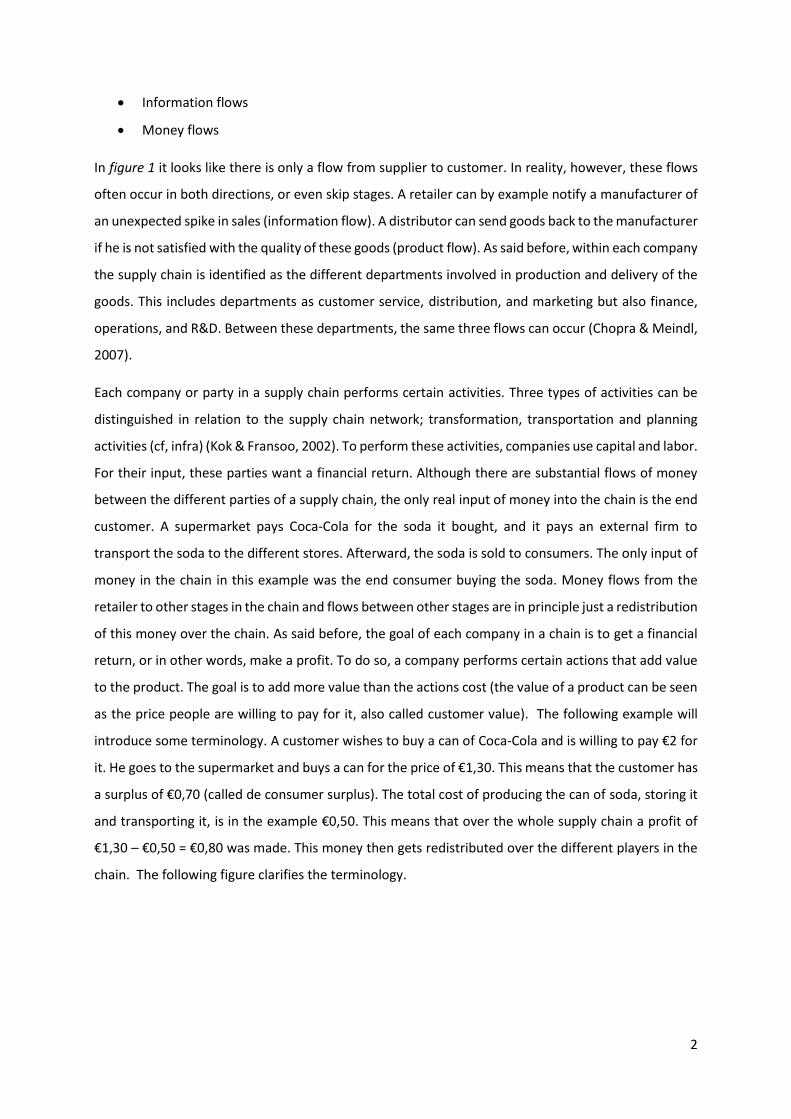
Each company or party in a supply chain performs certain activities. Three types of activities can be

distinguished in relation to the supply chain network; transformation, transportation and planning

activities (cf, infra) (Kok & Fransoo, 2002). To perform these activities, companies use capital and labor.

For their input, these parties want a financial return. Although there are substantial flows of money

between the different parties of a supply chain, the only real input of money into the chain is the end

customer. A supermarket pays Coca-Cola for the soda it bought, and it pays an external firm to

transport the soda to the different stores. Afterward, the soda is sold to consumers. The only input of

money in the chain in this example was the end consumer buying the soda. Money flows from the

retailer to other stages in the chain and flows between other stages are in principle just a redistribution

of this money over the chain. As said before, the goal of each company in a chain is to get a financial

return, or in other words, make a profit. To do so, a company performs certain actions that add value

to the product. The goal is to add more value than the actions cost (the value of a product can be seen

as the price people are willing to pay for it, also called customer value). The following example will

introduce some terminology. A customer wishes to buy a can of Coca-Cola and is willing to pay €2 for

it. He goes to the supermarket and buys a can for the price of €1,30. This means that the customer has

a surplus of €0,70 (called de consumer surplus). The total cost of producing the can of soda, storing it

and transporting it, is in the example €0,50. This means that over the whole supply chain a profit of

€1,30 – €0,50 = €0,80 was made. This money then gets redistributed over the different players in the

chain. The following figure clarifies the terminology.

3

It is clear that the value for each customer may differ. Not everybody will value a can of coke at €2.

Only people who value your product higher than or equal to the price will buy your product. That is

why a supply chain should focus on maximizing the total supply chain surplus (in most cases supply

chain profit and surplus are related, offering a product with higher customer value means more people

will buy your product, or it will allow you to ask a higher price). As the total supply chain profit is shared

over the whole supply chain, it is important that the different actors in the different stages take their

decisions in an effort to maximize the total supply chain profit, and not just try to maximize their own

profit. If every actor were to only focus on maximizing his own profit, it would have a negative influence

on the supply chain profit. Thus diminishing the total amount of money that can be distributed

throughout the chain (Chopra & Meindl, 2007).

The reasoning above shows why it is important to take decisions on a supply chain level. The decisions

have to be taken in such a way that they maximize the total supply chain surplus. These decisions

happen on different levels.

Design or strategic decisions in the long term

-By example location and number of stores

Planning decision on mid-term

-By example inventory policy, timing of marketing promotions

Day-to-day operational decisions

-By example assigning customer orders to machines.

The design of a supply chain should fit your strategy and market you want to serve. The design of the

chain will look very different for a company aiming at becoming a cost leader than for a company

aiming to serve a high-quality segment in that market. Once your chain is designed you can think about

the mid-term decisions. Are you going to do promotions? If yes, when, which type, on what products,

Figure 2: terminology

Price

Customer surplus

Supply Chain cost

Customer value

Supply Chain surplus

Supply chain profit

4

etcetera. Given long and mid-term decisions, day-to-day decisions can be taken. These decisions will

all influence the supply chain flows (product, information, and funds). Taking the right decisions will

greatly influence the success of the chain (Chopra & Meindl, 2007). An example can clarify this: Players

in a supply chain have to (among others) decide on their inventory policy. A good inventory policy can

have a significant impact on supply chain costs. Companies often hold safety stocks. This is to make

sure they can provide for their clients when an unexpected spike in demand happens. If all participants

in a chain decide to keep safety stock, then this will probably lead to a suboptimal solution. It is not

necessary that each stage keeps safety stock, to keep the following stage satisfied. In the end, the only

stage that has to be satisfied is the end customer. Rethinking safety stock policy with this in mind can

lead to significant savings on inventory cost and benefit every participant in the supply chain.

Companies like Walmart, Amazon and Dell have known great success because of the right decisions on

all three levels. Other companies have failed because they did not succeed in designing an appropriate

supply chain (Chopra & Meindl, 2007).

This is why it is important to research the influence of different decisions on the supply chain and its

profitability. Designing the right strategy is a very complex task. No two markets require the exact same

supply chain. Research on the different decisions and their impact can help managers think about their

situation, clarify different possibilities and it can help them make the right decisions. This is also the

goal of this dissertation. I wish to research the influence of different decisions on the overall

performance of the supply chain. A more detailed explanation follows in the next section.

1.2 Problem Definition The problem I wish to solve concerns the mid-term, planning decisions (production and inventory

policy), given a supply chain design. The following example will help to define the problem more

concretely.

Suppose that an entrepreneur starts a business in which he will produce and sell bicycles. To do so, he

starts by composing a bill of material (BOM). It is a list of all components and subcomponents of a

product. It can be represented through a ‘tree’. For a bicycle it might look something like this:

5

The figure above shows that a bike is assembled out of four subassemblies or components. These are

in their turn assembled out of other components (a wheel, in its turn, exist out of three different

components). The four subcomponents of ‘bicycle’ are called its children, and ‘bicycle’ is the parent of

the four subcomponents. ‘Wheels’ is then the parent of its three children and so on. It should be clear

that in reality, the BOM of a bike is much more complicated. It has much more subcomponents and

subassemblies, items might have multiple parent items, etcetera. For other more complicated

products, the BOM gets even larger and more complicated.

The BOM allows calculating how much pieces of each subcomponent are necessary for the production

of one end product. For example, each bicycle needs two wheels, and each wheel needs 28 spokes.

This means that per bicycle you need 56 spokes. The production system of the bicycles can be

represented as:

Figure 4: bicycle production system

Bicycle

Frame Saddle Brakes Wheels

Spokes Wheel Rim Tire

Figure 3: BOM of a bicycle

LT = 5

LT = 1

6

The squares represent workstation, the triangles represent stock and the arrows represent material

flows. The company buys the raw materials, when they arrive the materials go to the workstations

where they are transformed. When this is finished the materials go into stock. Here they wait until the

next workstation needs the products, where they get transformed again. This continues until the

product is finished. After which it is stored as a finished good and waits until it gets sold. When

something is ordered from an outside supplier, there are usually a couple of days waiting time until

the materials arrive. This is called procurement lead time. In the figure above the procurement lead

time for the first material is 5 days. Also, production and transportation take time. This means that

there are also internal lead times. In the example, the production of the first assembly takes one day.

In what follows the workstations and the related inventories will be represented using a single symbol.

Products leave the system through external demand. Naturally, there is external demand for end

products, but external demand for intermediate products is also a possibility. Two problems arise here:

In general, demand is unknown and variable.

The lead time offered to the customer is mostly much shorter than the time it takes to create

and assemble the product.

This means that companies have to forecast external demand. Forecasts are mostly based on historical

data (by example the average number of products sold each day in the past), expected market growth

and intuition of the forecaster. Also, the influence of promotions and competition can be taken into

account. However, forecasting is always prone to errors. Although on average 25 bikes are sold daily,

the actual number sold will be different and depend on variables that cannot be foreseen (by example;

an extra competitor enters the market or very bad weather causes the market to grow slower than

initially expected). Based on this forecast, the entrepreneur will have to decide on a production and

inventory policy. How will he decide which policy to choose? The goal of a supply chain is, as said

before, to maximize the supply chain surplus. The right policy will minimize inventory costs, while also

making sure a certain service towards the customers is obtained which will increase customer surplus.

The goal of this dissertation is to research the performance of a supply chain under different

circumstances of:

Demand variability

Lead times

Service level

Capacity utilization

I will research two different policies:

7

Base stock policies

Linear programming based policies.

Researching the performance of these policies under the different conditions can help managers to

make a better-informed decision about which policies to choose, and how it will affect their costs and

the supply chain surplus. Furthermore, the influence of capacity restriction is tested in this dissertation.

Oftentimes managers find themselves wondering if expanding capacity will result in significant savings.

Expanding capacity can by example lead to a decrease in necessary safety stock, the question is, will

this investment pay off? Under the different policies, the answer can be different. This research hopes

to shed some light on this matter; in this way, managers will hopefully be capable of taking better-

informed decisions.

1.3 Methodology In order to compare the different policies and the influence of the different circumstances discrete

event simulation is used. A supply chain, with multiple stages and multiple end-products, will be

simulated, taking into account inventory, lead times, production times, … Both control policies will be

applied under the different circumstances. Day to day demand will be simulated together with the

production decisions and its influence on inventories. This will be done for multiple time periods.

Material flow, inventory, and backlog under the different circumstances and policies will be studied,

and the overall performance of the supply chain will be assessed. The second goal of this dissertation

is to assess the influence of capacity limitations (in terms of the number of products that can be

produced per time period) on performance. To do this, simulations will be done ignoring the capacity

constraints. Later capacity restrictions will be included, using a new procedure, presented in this

dissertation. This will allow gaining insight into the actual influence of these constraints. Finally, the

results will be compared in order to draw conclusions that can help improve real life supply chain

decisions.

1.4 Outline In the next chapter (Literature Review) previous research related to the subject is discussed. In chapter

three the supply chain problem is discussed and translated into mathematical form. These variables

and formulas lie on the basis of the simulation. In chapters four and five, the base stock policy and the

linear program based policy are discussed. Both are translated into mathematical models. Then these

models are used as the basis for the simulations. Finally, I will compare these two policies using discrete

event simulation. The procedure of this will be discussed in detail in part 6. In chapter 7 The case study

is described that will be used to compare the performance of the different policies, under different

levels of demand uncertainty, machine capacity and Lead times. In chapter 8 the results are analyzed

8

and finally, in the last chapter conclusions are drawn and recommendations for future research are

given.

9

2 Literature Review

The literature review can roughly be divided into two parts. In the first part, it is discussed how a

company or chain of companies can deal with uncertainty from within and from outside of the system.

Secondly, different planning methods and models for material release, material production, and

material distribution are discussed.

2.1 Dealing with Uncertainty Mula, Poler, Garcia-Sabater, and lario (2006) and Galbraith (1973) define uncertainty as: “The

difference between the amount of information required to perform a task and the amount of

information already possessed” (Mula et al., 2006, p. 271). According to Ho (1989) uncertainty can be

caused by two different types of variables. Firstly, there is operating variables (uncertainty within the

system), secondly, there are environmental factors (uncertainty outside the system). Ho (1989)

investigated the impact of different operating variables on system nervousness (shocks due to

frequent rescheduling). The operating variables (Lot-sizing rules, the length of lead time, the planning

horizon, component commonality) have a significant impact on the system and affect the systems’

performance. Dynamic lot-sizing rules lead to a higher degree of system performance and nervousness.

Under uncertainty, the system will perform more poorly (Ho, 1989).

Mula et al. (2006) summarize different approaches to coping with uncertainty (by example: linear

programming, Markov decision processes, Monte Carlo techniques, Queuing theory, …).

C. Yano (1987) describes a model where Lead times are variable. Unsuspected events, (like machines

breaking down or suppliers being late) create the need for safety stock. C. Yano (1987) developed an

algorithm that minimizes inventory and backorder cost in case of stochastic lead times. In his model

safety time is added to the average lead time to compensate for this variability. According to Williams

and Whybark (1976) . Adding safety time is preferred to adding safety stock when the timing is

uncertain. The eventual model C. Yano (1987) comes up with is a difficult nonlinear program. The

implication of his model is the following: “If suppliers are perfectly reliable, then safety time is not

needed. But if suppliers are even slightly unreliable, then having fewer parts to assemble, and/or using

fewer suppliers to produce the same number of parts, may result in significant inventory savings and

shorter total lead times” (Yano, 1987, p. 380). However, in his research Yano made many assumptions

(like deterministic demand) that are not realistic. Hopp and Spearman (1993) worked on the same

subject as Yano. However, they also assumed deterministic demand.

Melnyk and Piper (1985) researched the ‘lead time error’ or the difference between planned and actual

lead time and its effect on performance, for different lot-sizing choices. They find that EOQ and POQ

10

(economic order quantity and period order quantity) may result in larger errors and worse delivery

performance.

In most research either demand is assumed variable and lead times known or the other way around.

In reality, however, both are oftentimes uncertain. Brennan and Gupta (1993) claim that these sort of

assumptions can lead to failure of an MRP system (or at least cause lower than expected results). “The

studies that have considered demand and/or supply factors can be grouped into three categories,

namely constant value of the factor, variable value of the factor, and uncertain value of the factor.”

(Brennan & Gupta, 1993, p.1689). Therefor Brennan and Gupta (1993) simulated an MRP production

system as realistically as possible, in a rolling horizon environment with different product structures

and different ways of deciding on the lot-size (lot-for-lot, EOQ, POQ, Wagner-Whitin, etcetera). They

concluded that given uncertainty in demand and lead times product structure influences cost

performance. Another conclusion is that when uncertainty exists EOQ outperforms al other lot sizing

models. Thirdly their results indicate that when lead time uncertainty rises, costs rise but the

uncertainty also has an influence on product structure, choice of the lot-sizing rule and the setup to

holding cost ratio and even demand variance. On the other hand, the variance of demand has no

influence on product structure, but it does interact with the lot-sizing choice.(Brennan & Gupta, 1993).

While Brennan and Gupta (1993) researched the impact of lead-time and demand uncertainty on

product structure (and other factors) E. Mohebbi and F. Choobineh (2005) researched the impact of

product structure (in particular component commonality) given demand and lead-time uncertainty.

Both uncertainty (in lead-time and demand) and commonality of components influence the

performance of assembly systems. If components are designed in a way that they can be used in

different products, it may increase production costs, but it won’t increase the number of units in stock.

The economies of scale can result in productivity gains and there will be cost savings in warehousing

and operations (Choobineh & E.Mohebbi, 2005) and (Bagchi & Gutierrez, 1992). In order to investigate

the impact of component commonality Choobineh and E.Mohebbi (2005) simulated an ATO (assembly-

to-order) environment. The characteristics were a rolling planning horizon, lot for lot sizing policy,

demand was random, planned lead time was one period for assembly, the planned procurement Lead

time was four periods, but the actual procurement lead time was random. The results of their research

are summarized below:

Firstly inventory, inventory costs, and backorders do not go down with more common components,

however, there is more on-time order delivery. Secondly, component commonality is more beneficial

in sectors where both demand and lead time uncertainty exist (Choobineh & E.Mohebbi, 2005). One

big limitation of this research is that Choobineh and E.Mohebbi (2005) do not take into account the

costs of designing and implementing a multi-functional common component.

11

Song, Yano, and Lerssrisuriya (2000) consider a situation where both supply lead time and Demand

quantity are unsure and random (but the demand happens only once, and it is known when). Song et

al. (2000) tried four heuristics to get the optimal value. Their research shows that the newsvendor-

heuristic proves to be very efficient at finding the optimal solution.

The paper of Bertrand and Rutten (1999) takes a different approach to uncertainty. What if the raw

material a company buys and uses as input in their assembly system varies a lot in quality (by example

input from the agricultural sector)? What if a company wants to minimize productions cost by using

the cheapest materials (but still ensuring a minimum quality)? What if demand for a certain product is

high but there are material shortages and long replenishment lead times? For these reasons (and

others) a company might want to change its assembly ‘recipe’ from time to time. Bertrand and Rutten

(1999) evaluate three planning procedures to deal with this kind of flexibility and uncertainty. For their

models, they assume short customer order lead time but long material replenishment lead time. The

first and optimal procedure “minimizes the expected value of the total alternative recipe costs over a

horizon that is equal to the material replenishment lead time.”(Bertrand & Rutten, 1999, p. 181). The

second procedure i.e. the deterministic planning procedure covers the complete material

replenishment lead time. Deterministic demand is set equal to the expected value of demand. This

version is suboptimal to the first one but easier to compute and thus more applicable in realistic

situations. The third and last procedure, i.e. the myopic procedure, uses only customer order

information (Bertrand & Rutten, 1999).

Aviv (2001) compared three different models. In the first model –which was called local forecasting

(LF) – each member of the supply chain made his own future demand forecast. In the second model –

collaborative forecasting (CF) – the forecasting information becomes central and every party has the

same information. The third model –only used as a benchmark – did not use any forecasts at all. The

first two cases took place in a rolling schedule context where forecasting information is periodically

updated. Aviv (2001) modeled his cases with only two players in the supply chain. Both parties with

their own inventory holding cost and cost per back ordered product. The research revealed that

collaborative forecasting performs 10% better in comparison to local forecasting and 20% better than

no forecasting at al. When the forecasting capabilities differ a lot across the supply chain, collaborative

forecasting has an even bigger impact (Aviv, 2001). These results are not surprising but another

conclusion from their research is this one: “ the absolute and the marginal benefits of CF are larger

when the lead times are smaller.” (Aviv, 2001, p. 1337). One would think that CF is more beneficial

when lead times are longer, but as it turns out initiatives aimed at reducing lead times and CF are

complementary (Aviv, 2001).

12

2.2 Planning Policies Clark and Scarf (1960) state that in a lot of papers lead time is assumed independent of the order/lot

size, however on many occasions this is not the case. In their paper Clark and Scarf (1960) research if

hard to implement theoretical mathematical models can be simplified for a multi-installation problem

without getting suboptimal solutions. They state that when you solve your problem to optimality for

each sub-installation, you get the optimal solution for the total multi-installation system. They find

that this is possible if the right assumptions are incorporated in the model. These assumptions are: (I)

there is only demand for end-products. (II) The cost of shipping one item from one station to another

is a linear function. (III) The holding and backorder costs for the end products are linear. The holding

and backorder costs for other products are functions of the inventory at that level and the inventory

at levels later in the system (but they can be zero). (IV) Each echelon backlogs excess demand. Even

when assumption (I) is relaxed Clark and Scarf (1960) find that their method gets the optimal solution,

although it is easier. However, assumption (II) and (III) are necessary for the simplification to give the

optimal solution (Clark & Scarf, 1960).

Agrawal and Cohen (2001) analyze the allocation of different components in an assembly system based

on a fair shares method. It is claimed the fair shares method is used in practice a lot, because “a heavy

mathematical program is very hard to implement in the context of a multiproduct assembly system

with many common components. Consequently, in practice, specific (albeit suboptimal) allocation

policies are used”(Agrawal & Cohen, 2001, p. 410). In their model, Agrawal and Cohen (2001) assume

demand for finished products is uncertain and resupply lead times for components differ. This policy

allocates components to orders of finished goods, without checking the availability of other required

components. The quantity is determined by the ratio of demand for that specific end product to total

demand of all orders. According to their research this fair shares makes it possible to predict what

effect component inventory level decisions have on the service level. Making this prediction while

using other models is harder. The second conclusion of their research was that in cases with a higher

degree of commonality, lower costs can be achieved (Agrawal & Cohen, 2001).

Schmidt and Nahmias (1985) considered an inventory system where one end product is assembled out

of two components, both are bought from external suppliers. There is no external demand for the two

components, only for the end product. The demand for the end products is assumed to be random.

Their results indicate that there is an optimal inventory level for both components, depending on the

lead time (Schmidt & Nahmias, 1985). Although the theory seems plausible at first, its assumptions

make it far from realistic.

Houtum, Inderfurth, and Zijm (1996) review the theories behind stochastic multi-echelon systems and

emphasize on materials coordination problems. The first thing stated is that centralized control of

13

multistage inventory systems is superior to a decentralized system cf. Forrester (1961). In their paper

Houtum et al. (1996) concentrate on a periodic review multi-echelon planning and control system.

However, they assume stationary conditions (which might not be realistic). They prove that multi-

echelon models are a good way to control materials flow in large production systems. However, the

conditions and assumption of their model can be considered too generalizing and thus unrealistic.

Hax and Meal (1973) describe a planning and scheduling policy for a system with multiple products,

and plants, and a varying demand pattern. They described four different levels of decision making,

each time on a lower hierarchy level or on a shorter term. The decisions made on a higher level are

considered constraints for the lower level. Although a decent framework for decision making, Hax and

Meal (1973) fail to implement uncertainty in their model. Gfrerer and Zäpfel (1995) added parameters

of uncertain demand. Future demand has an upper and a lower bound in their model. Meybodi and

Foote (1995) added uncertain demand and production failure (Mula et al., 2006).

Barbarosoğlu and Özgür (1999) developed a mixed integer mathematical model that addresses

production and distribution decisions. They then use a Lagrangian relaxation to split the production

and distribution problem. The model in itself functions like a decentralized system, but with a central

agent taking care of the information flow. The model looks good, but it seems that certain conditions

can make the model fail (however only slightly) (Barbarosoğlu & Özgür, 1999).

“The economic lot scheduling problem (ELSP) is the problem of accommodating cyclical production

patterns when several products are made in a single facility.”(Elmaghraby, 1978, p. 587). What if a

machine cannot produce enough components to fulfill demand, how should you minimize the cost of

the resulting schedule? This was the question Elmaghraby (1978) wanted to answer. “Two broad

categories of different approaches arise (I) analytical: achieve the optimum of a restricted version of

the original problem. (II) Heuristic approaches that achieve ‘good’ (and sometimes ‘very good’)

solutions of the original problem. In some sense, each category presents a penalty to be paid.”

(Elmaghraby, 1978, p. 587). Because parameters might be infeasible in a lot of these models

Elmaghraby (1978) adds a test for feasibility and a method on how to escape from infeasibility.

Another study on the ELSP was done by Raza and Akgunduz (2008). They compare different existing

solution algorithms and test them on two problems. They use the ELSP model of Dobson (1987) “which

uses the time-varying lot size approach. It has the following assumptions: (I) Items do not have any

precedence over each other. They compete for the same production facility. (II) Back-orders are not

allowed. (III) The production facility is assumed to be failure free and produce at perfect quality.” (Raza

& Akgunduz, 2008, p. 97). It is immediately clear that these assumptions might make the model

14

unrealistic. They propose different algorithms and the best performing one seems to be the ‘simulated

annealing’ method. (Raza & Akgunduz, 2008).

Song and Zipkin (2003) discuss stochastic models in assemble-to-order (ATO) systems with a focus on

pure base stock policies. “An ATO system is an efficient way to deliver a high level of product variety

to customers while maintaining reasonable times and costs.” (Song & Zipkin, 2003, p. 561). They

discuss one-period, multi-period and continuous time models. For one period models, a linear program

is given that minimizes the cost of inventory and the cost of orders lost, given some demand and supply

constraints. For the Multi-Period, Discrete-Time Models Song and Zipkin (2003) state that within one

time period the problem is the same as the first model. But when you link different periods, the end

state of the first period, is the beginning of the second, and that is where new problems arise. Lead

times for component replenishments complicate the equations, certainly when we get different lead

times for the different products (which is normally the case). Furthermore, lead times can be uncertain,

shortages and backorders can arise, but also excess inventory. Song and Zipkin (2003) propose several

different linear programs for different cases (where each time different assumptions are made) and

evaluate the performance of them all.

Because of the recent trend in the PC manufacturing industry where customers decide out of which

components their PC’s consist (An example of a PC manufacturer who does this very successfully is

Dell), researchers have been studying the field of Configure-to-Order (CTO) systems. In CTO systems

not only are back orders possible for end products, but also for the components (Cheng, Ettl, Lin, &

Yao, 2002). In other words, the optimization model where we assume there is only demand for the

end-products is wrong (in this case). In order to quantify the inventory-service tradeoff, Cheng et al.

(2002) develop a nonlinear optimization model. In this model, no finished goods inventory is kept, but

each component has its own inventory, and they all follow a base stock policy. An interesting result of

this research is that the cost savings because of the lower level of end-product-inventory are much

higher than the extra cost of component inventory that is needed in a CTO environment. Another

interesting result is that forecasting is significantly more accurate in a CTO environment. (Cheng et al.,

2002).

In their paper: ‘Planning Supply Chain Operations: Definition and Comparison of Planning Concepts’,

G.de Kok and J.Fransoo (2002) discuss different planning models. In particular, they discuss two

different types of policies/methods that decide on the daily produced amounts in a productions system.

The first one is a policy based on the optimization of a linear program. An objective function that sums

all costs of inventory and backorders is minimized. This minimization is subject to a set of constraints

such as the customer satisfaction rate. This model is made assuming a rolling schedule context, where

15

future demand is unknown and has to be forecast. The second policy investigated is the base stock

policy, where for each product in the chain an order-up-to-level is decided upon. Each time period the

produced amounts are based on the difference between this order-up-to-level and the inventory of

that product. Kok and Fransoo (2002) translate supply chains and their activities into mathematical

form. This mathematical expression of a supply chain is then used to research the performance of both

concepts using discrete event simulation.

The literature review reveals that a lot of different planning and production decision models have been

developed and tested on their performance under different circumstances of demand and lead time

variability, product structures, etcetera. However, to my knowledge the performance of these policies

under capacity restrictions has hardly been researched. In reality, all machines and production systems

have a maximum capacity, a maximum number of products produced per time period. Researching

how these policies perform under restricted capacity is important. Firstly, adding this factor to

simulations will make it more realistic. Secondly, researching the performance of supply chains under

capacity restrictions can help managers make investment decisions (will extra capacity lead to the

hoped performance improvement).

In this paper, two planning policies are compared, namely Base Stock policies and Linear Programming

based policies. The performance of supply chains controlled by these two policies has already been

researched by (Kok & Fransoo, 2002). This research will expand on theirs by adding capacity restrictions

to their models and testing the performance using simulations. In the next three chapters (chapters

three, four and five), the work of Kok and Fransoo (2002) is discussed in detail. The models and

formulas introduced by them form the basis of the simulations. In Chapter six it is discussed how these

models can be used to implement capacity restrictions in the simulations.

16

3 The Supply Chain Operations Planning Problem

In this part, the supply chain operations planning problem is introduced. In order to build the computer

simulation, the supply chain has to be described in a mathematical fashion. The variables needed to

do so are introduced in this chapter (variables describe goals of the supply chain, the status of

inventory, …). Secondly, the physical restrictions and constrictions, which every supply chain has to

meet (inventory cannot be negative for example), are discussed and translated into mathematical

form. These variables and formulas form the basis of the simulations. The simulations have to meet

these restrictions to be considered valid.

3.1 Definitions “The Supply Chain Operations Planning (SCOP) problem has the objective of coordinating the release

of materials and resources in the supply network in such a way that a certain customer service level is

met, at minimal cost” (Kok & Fransoo, 2002, p.1).

In the Supply Chain network three different activities can be distinguished:

Manufacturing activities: physically transform inputs into outputs.

Transportation activities: move goods from one place to another.

Planning activities: all administrative activities needed to enable manufacturing and

transportation.

“In order to solve the SCOP problem, it is essential that all activities their characteristics and their

relationships in a certain supply chain network are identified” (characteristics of manufacturing

activities are by example processing times, resource requirements,...) (Kok & Fransoo, 2002, p.2).

In the following paragraph, some symbols and variables relating to supply chain activities are

introduced. The same symbols are used by De Kok & Fransoo (2002).

Consider a supply network consisting of N items. For each item 𝑖, 𝑖 = 1,2, … 𝑁:

𝑎𝑖𝑗 number of items 𝑖 required to produce one item 𝑗, 𝑖 = 1,2, … , 𝑁 , 𝑗 = 1,2, … , 𝑁

(The matrix [𝑎𝑖𝑗] is another way of representing the Bill of Materials)

𝐸 {𝑖|𝑎𝑖𝑗 = 0, 𝑖 = 1,2, … , 𝑁, 𝑗 = 1,2, … , 𝑁}

𝐸 is the set of end-items; an end-item is not used in any other item. It is delivered to

the customers of the supply chain.

𝐼 {𝑖|∃ 1 ≤ 𝑗 ≤ 𝑁 𝑤𝑖𝑡ℎ 𝑎𝑖𝑗 > 0 𝑖 = 1,2, … , 𝑁}

𝐼 is the set of intermediate items. Each item that is used in another item in the supply

chain (by example in an assembly process) is in this set.

17

𝑉𝑖 {𝑗|𝑎𝑖𝑗 > 0 , 𝑗 = 1,2, … , 𝑁}

𝑉𝑖 is the set of successors of item 𝑖.

𝑊𝑖 {𝑗|𝑎𝑗𝑖 > 0, 𝑗 = 1,2, … , 𝑁}

𝑊𝑖 is the set of predecessors of 𝑖.

𝐷𝑖(𝑡) independent demand for item 𝑖 in period 𝑡.

Independent demand is generated by customers, it is usually unknown and must be

forecasted.

𝐺𝑖( 𝑡) dependent demand for item 𝑖 in period 𝑡.

(demand for item 𝑖 that is derived from demand for items in 𝐼 ∪ 𝐸)

𝑝𝑖(𝑡) quantity of item 𝑖 that becomes available at the start op period 𝑡.

(because of the transformation activity generating item 𝑖)

𝑟𝑖(𝑡) quantity of item 𝑖 released at the start of period t immediately after receipt of 𝑝𝑖(𝑡).

notice that {𝑟𝑖(𝑡)}are the set of decision variables, these are part of the outcome of

the SCOP problem.

𝐼𝑖(𝑡) physical inventory of item 𝑖 at the start of period 𝑡, immediately before receipt of

𝑝𝑖(𝑡)

𝐵𝑖(𝑡) backlog of item 𝑖 at the start of period 𝑡, immediately before receipt of 𝑝𝑖(𝑡).

𝐽𝑖(𝑡) net inventory of 𝑖, at the start of period 𝑡, immediately before receipt of 𝑝𝑖(𝑡)

𝐽𝑖(𝑡) = 𝐼𝑖(𝑡) – 𝐵𝑖(𝑡)

𝑃 Set of items 𝑖 with 𝐷𝑖(𝑡) > 0 for some 𝑡 ≥ 0

In order to manufacture and transport resources are necessary. The following set of variables takes

this into account:

𝐶𝑘𝑡 Amount of capacity available in units of time of resource 𝑘 in period 𝑡 ,

𝑘 = 1, … , 𝐾, 𝑡 ≥ 1.

With K the number of available resources.

𝑈𝑘 Set of items that can be processed on resource 𝑘.

𝑐𝑖 Time required to process one unit of item 𝑖 on its resource.

all symbols and definitions can be found in Kok and Fransoo (2002)

18

The decision variables related to the release of resources at the start of a period are given by the set

{𝑞𝑖(𝑡)}where 𝑞𝑖(𝑡) is defined as

𝑞𝑖(𝑡) Amount of item 𝑖 processed in period 𝑡, 𝑡 ≥ 0

Transformation and transportation activities take time. The time needed for a product 𝑖 to become

available is called the lead time of 𝑖. The lead time of a product consists of processing time and waiting

time (Kok & Fransoo, 2002).

𝐿𝑖 Lead time of product 𝑖.

throughput time between the time of the release of an order for item 𝑖 and time at

which the ordered items are available for usage in other items and/or delivery to

customers.

In this paper, it is assumed that 𝐿𝑖 is an integer number. This means that a product

cannot become available for further processing or sale in the middle of a time period.

The items 𝑖 released at the start of period 𝑡 are available for usage in period 𝑡 + 𝐿𝑖.

The goal of this paper is to compare different planning concepts in different situations and under

different conditions. The performance will be measured based on costs. Kok and Fransoo (2002)

defined as a cost function:

𝐶(𝑡) the cost incurred at the end of period t, t≥ 0

𝐶(𝑡) = ∑ ℎ𝑖𝐼𝑖(𝑡)

𝑁

𝑖=1

( 1 )

with

ℎ𝑖 value of item 𝑖, ∀𝑖

The cost function 𝐶(𝑡) represents the holding costs that occur in one specific time period. This

however does not represent the actual performance of the chain. To measure the actual performance,

the long-term average cost has to be calculated:

C average long- term cost

C = lim𝑡→∞

1

𝑡 ∑ 𝐶(𝑠)

𝑡

𝑠=1

19

( 2 )

This function only calculates average inventory costs. Also, backlog costs have to be taken into

account, to do so, the following functions are defined:

C’(t) cost incurred at the end of period 𝑡, 𝑡 ≥ 0, including backlog costs

𝐶′(𝑡) = ∑ ℎ𝑖𝐼𝑖(𝑡) + 𝜃ℎ𝑖𝐵𝑖(𝑡)

𝑁

𝑖=1

( 3 )

With

𝜃 = 𝛼

1−𝛼 , (𝑤𝑖𝑡ℎ 𝛼 𝑡ℎ𝑒 𝑠𝑒𝑟𝑣𝑖𝑐𝑒 𝑙𝑒𝑣𝑒𝑙 (𝑐𝑓𝑟 𝑖𝑛𝑓𝑟𝑎)) ( 4 )

The actual performance is measured using the average long-term cost:

𝐶′̅̅̅ = lim𝑡→∞

1

𝑡∑ 𝐶′(𝑠)

𝑡

𝑠=1

( 5 )

The backlog is included in the cost function for two reasons. Firstly, shortages of products lead to an

immediate loss of sales and unsatisfied customers. Customers that are unsatisfied are difficult to retain

and shortages can lead to big losses of sales in the future. Unsatisfied customers often file complaints

with the company, this then leads to extra costs because of complaint handling. When comparing the

supply chain performance, it is important to keep in mind that back orders lead to extra costs and to

take these into account. Secondly, capacity restrictions can influence average shortages. When backlog

costs are taken into account it will be possible to measure the influence of the different policies under

the different conditions on the shortages.

Shortages cost money, but shortages can be avoided by increasing the inventories of products. How

high should a company set these inventories? The actual answer depends on a lot of criteria. However,

the inventories are always set at a level high enough in order to assure a certain minimum service

towards the customer. This service level has to be defined for all items in P (all items with independent

demand). Generally, two different types of service levels are used (Kok & Fransoo, 2002):

𝛼𝑖 the non-stock out probability of product 𝑖, ∀𝑖 ∈ 𝑃

𝛼𝑖 = lim𝑡→∞

𝑃{𝐼𝑖(𝑡) > 0}, ∀ 𝑖 ∈ 𝑃 ( 6 )

𝛽𝑖 the fill rate of product 𝑖, ∀𝑖 ∈ 𝑃

20

𝛽𝑖 = lim𝑡→∞

1 −𝐸[(𝐼𝑖(𝑡)+𝑝𝑖(𝑡)−𝐷𝑖(𝑡))

+]−𝐸[(−𝐼𝑖(𝑡)−𝑝𝑖(𝑡))

+]

𝐸[𝐷𝑖(𝑡)], ∀i ∈ P ( 7 )

Each planning concept has the goal of solving the next problems (Kok & Fransoo, 2002):

Problem (𝑃𝛼):

Min C

s.t. 𝛼𝑖 (𝑃) ≥ 𝛼𝑖∗

Problem (𝑃𝛽):

Min C

s.t. 𝛽𝑖(𝑃) ≥ 𝛽𝑖∗

𝛼𝑖∗ and 𝛽𝑖

∗ are two variables endogenous to the SCOP problem. In practice these two are a strategic

decision made by higher management. These are considered a given for the Supply Chain Operations

Planning Problem. The actual values 𝛼𝑖 and 𝛽𝑖 are results of the planning system.

3.2 Constraints The BOM and the use of resources for manufacturing lead to a set of constraints (Kok & Fransoo, 2002).

In this paragraph, these constraints are discussed.

3.2.1 Material Constraints

The next set of constraints should be satisfied by any SCOP concept.

Given the definition of physical inventory and backlog:

𝐼𝑖(𝑡), 𝐵𝑖(𝑡) ≥ 0, 𝑡 ≥ 0, ∀𝑖 ( 8 )

It is clear that backlog only exists when physical inventory is zero:

𝐼𝑖(𝑡)𝐵𝑖(𝑡) = 0 , 𝑡 ≥ 0, ∀𝑖 ( 9 )

The net inventory is defined as:

𝐽𝑖(𝑡) = 𝐼𝑖(𝑡) − 𝐵𝑖(𝑡), 𝑡 ≥ 0, ∀𝑖 ( 10 )

The increase in backlog cannot exceed exogenous demand:

𝐵𝑖(𝑡 + 1) − 𝐵𝑖(𝑡) ≤ 𝐷𝑖(𝑡), ∀𝑖, 𝑡 ≥ 0 ( 11 )

This equation only makes sense if dependent demand is not back ordered. In this paper, the

assumption is made that dependent demand cannot be back ordered. Kok and Fransoo (2002) argue

that back ordering of dependent demand does not make sense. If you were to back order an item by

21

releasing more than available, physically you would only release all available material. The earliest

moment in time to resolve this back order would be the beginning of the next period. However, now

you have exact information about demand during that period and possibly better information about

future demand. So the decision to back order is not better than the decision to just release all

available material (Kok & Fransoo, 2002).

This has as a consequence that if a product 𝑖 has Di(t) = 0, ∀t, then there is no independent demand

for this product, and for this item applies:

𝐵𝑖(𝑡) = 0 ∀𝑡 ≥ 0 ( 12 )

Dependent demand 𝐺𝑖(𝑡) for item 𝑖, is generated by items in 𝑉𝑖. In order to calculate 𝐺𝑖(𝑡), the sum is

made of all released quantities of items in 𝑉𝑖 at the start of period 𝑡:

𝐺𝑖(𝑡) = ∑ 𝑎𝑖𝑗𝑟𝑗(𝑡), ∀𝑖 ∈ 𝐼

𝑗∈𝑉𝑖

( 13 )

As stated above dependent demand is not back ordered, so there must be sufficient inventory of 𝑖 to

start the manufacturing processes involved (Kok & Fransoo, 2002).

At the start of period 𝑡 the physical beginning inventory equals

𝑝𝑖(𝑡) + max (0, 𝐼𝑖(𝑡) − 𝐵𝑖(𝑡) ) ( 14 )

Consequentially:

𝐺𝑖(𝑡) ≤ 𝑝𝑖(𝑡) + max(0, 𝐼𝑖(𝑡) − 𝐵𝑖(𝑡)) , ∀𝑖, 𝑡 = 1, … , 𝑇 ( 15 )

All released quantities are assumed to be positive. In reality, this means that no returns are possible.

𝑟𝑖(𝑡) ≥ 0, ∀𝑖, 𝑡 = 1, … , 𝑇 ( 16 )

Given these definitions and constraints the next balancing constraint can be written:

𝐼𝑖(𝑡 + 1) − 𝐵𝑖(𝑡 + 1) = 𝐼𝑖(𝑡) − 𝐵𝑖(𝑡) − 𝐺𝑖(𝑡) − 𝐷𝑖(𝑡) + 𝑝𝑖(𝑡), ∀𝑖, 𝑡 = 0, … , 𝑇 ( 17 )

This constraint states that the net inventory (physical inventory minus backlog) in a period of a certain

product equals the net inventory of the previous period minus what was taken out of inventory

(independent and dependent demand) plus what is put in (because of the manufacturing activities).

(Kok & Fransoo, 2002).

3.2.2 Resource Constraints

Each supply chain is constrained by capacity. These constraints are represented through the next set

of constraints.

First of all, for all items that use the same resource or (𝑎𝑙𝑙 𝑖 ∈ 𝑈𝑘) applies

22

∑ 𝑐𝑖𝑟𝑖(𝑡) ≤ 𝐶𝑘𝑡+𝐿𝑖−1

𝑖∈𝑈𝑘

( 18 )

If a product is released in time period 𝑡 then it becomes available in 𝑡 + 𝐿𝑖 , which means it has to be

processed in 𝑡 + 𝐿𝑖 − 1. This constraint makes sure no more resources are released then can be

produced on resource K. However the constraint above is only necessary if it is required that resources

released in t, are produced in 𝑡 + 𝐿𝑖 − 1, or in other words if the decision is made that production

happens as late as possible with respect to the lead time (Kok & Fransoo, 2002). This constraint can be

relaxed (cf. infra).

Comparably the next constraints can be derived:

∑ 𝑐𝑖𝑞𝑖(𝑡) ≤ 𝐶𝑘𝑡

𝑖∈𝑈𝑘

( 19 )

And

∑ 𝑟𝑖(𝑠) ≥ ∑ 𝑞𝑖(𝑠)

𝑡

𝑠=1

𝑡

𝑠=1

( 20 )

This one makes sure that if a processing decision in a certain time period is made, the release decision

has also been made (this way the items are available) (Kok & Fransoo, 2002).

When a certain amount of product 𝑖 is released in period 𝑡, it becomes available in period 𝑡 + 𝐿𝑖 . This

means that in order for it to become available on time, it has to be produced in the periods 𝑡, … , 𝑡 +

𝐿𝑖 − 1. It follows that

∑ 𝑟𝑖(𝑠) ≤ ∑ 𝑞𝑖(𝑠)

𝑡+𝐿𝑖−1

𝑠=1

𝑡

𝑠=1

( 21 )

When equations 18 to 21 are combined:

∑ ∑ 𝑐𝑖𝑟𝑖(𝑠) ≤ ∑ 𝐶𝑘𝑠 , 𝑘 = 1 , … , 𝐾 𝑡 ≥ 1

𝑡+𝐿𝑖−1

𝑠=1𝑖∈𝑈𝑘

𝑡

𝑠=1

( 22 )

(Kok & Fransoo, 2002)

23

3.2.3 The Impact of Lead Times

Lead times allow describing the relationships between {𝑟𝑖(𝑡)}{𝑞𝑖(𝑡)}{𝑝𝑖(𝑡)}.

First, we have that

𝑝𝑖(𝑡) = 𝑞𝑖(𝑡 − 1) ( 23 )

This means that what is produced becomes available in the next time period. Within the constraints

described above this leads to flexibility about when products are actually manufactured. This can also

mean that products can become available earlier (this can be seen as favorable but keeping more in

inventory costs extra) (Kok & Fransoo, 2002).

In the following, the assumption is made that products only become available one lead time after being

released. This will make sure there is certainty about the availability of goods:

𝑝𝑖(𝑡) = 𝑟𝑖(𝑡 − 𝐿𝑖) ( 24 )

With this last constraint the balancing constraint can be rewritten:

𝐼𝑖(𝑡 + 1) − 𝐵𝑖(𝑡 + 1) =

𝐼𝑖(𝑡) − 𝐵𝑖(𝑡) − 𝐷𝑖(𝑡) − 𝐺𝑖(𝑡) + 𝑟𝑖(𝑡 − 𝐿𝑖), ∀𝑖, 𝑡 = 0, … , 𝑇 ( 25 )


In this chapter, the SCOP problem was discussed in a mathematical fashion. First, the necessary

variables were introduced. These variables represent the different activities of a supply chain or

describe the status of a supply chain. Next, the cost functions were introduced, that will measure the

performance of the supply chain. Thirdly, two different service level concepts were discussed. After

which the SCOP problem was introduced mathematically; minimizing costs, while attaining a minimum

service level. Finally, some constraints were introduced. Every supply chain is subject to these. For the

simulations to be considered correct, these are a necessary condition.

24

4 Base-Stock Policies

Above the general characteristics of a supply chain are discussed. In this chapter and the next chapter,

two planning policies are introduced. The goal of a planning policy is to decide on the amounts to

release and produce in each time period, for each product ({𝑟𝑖(𝑡)} and {𝑞𝑖(𝑡)} for t ≥ 0). Each

planning policy has its own characteristics, advantages and disadvantages. In this chapter the so called

“Base Stock Policy” is discussed. New variables and restrictions specific to these policies have to be

introduced. The variables and formulas introduced in this part are used in the simulations.

The following variables are at the basis of every base stock policy:

𝑂𝑖(𝑡) Cumulative amount of orders outstanding at start of period t

𝑋𝑖(𝑡) = 𝐽𝑖(𝑡), ∀𝑖 ∈ 𝐸 ( 26 )

𝑌𝑖(𝑡) = 𝑋𝑖(𝑡) + 𝑂𝑖(𝑡), ∀𝑖 ∈ 𝐸 ( 27 )

𝑋𝑖(𝑡) = 𝐽𝑖(𝑡) + ∑ 𝑌𝑗(𝑡), ∀𝑖 ∈ 𝐼

𝑗∈𝑉𝑖

( 28 )

𝑌𝑖(𝑡) = 𝑋𝑖(𝑡) + 𝑂𝑖(𝑡), ∀ 𝑖 ∈ 𝐼 ( 29 )

𝑋𝑖 is the echelon inventory stock and 𝑌𝑖 the echelon inventory position of 𝑖. 𝑌𝑖 represents the future

coverage of demand for item 𝑖 (Kok & Fransoo, 2002).

In the first part of this chapter, the very basic ‘pure base stock policy’ is discussed. A few problems will

arise with pure base stock policies, and expansions to the policy will be necessary. In part 4.2; 4.3 and

4.4 these expansions are discussed.

4.1 Pure Base-Stock Policies For each product 𝑖 a company decides on a base stock level:

𝑆𝑖 Base stock level van product 𝑖,

When using a pure base stock policy, the release decision is made like this:

𝑟𝑖(𝑡) = 𝑆𝑖 − 𝑌𝑖(𝑡) ( 30 )

Basically, the company decides on an order-up-to level (𝑆𝑖) for each product. Every time period net

inventory is checked in the number of products short is ordered (Kok & Fransoo, 2002).

In general, pure base stock policies lead to several problems:

(1) It does not take capacity constraints into account,

(2) It is possible that backlog exceeds exogenous demand, which would violate the constraints

defined above; consider the following example:

25

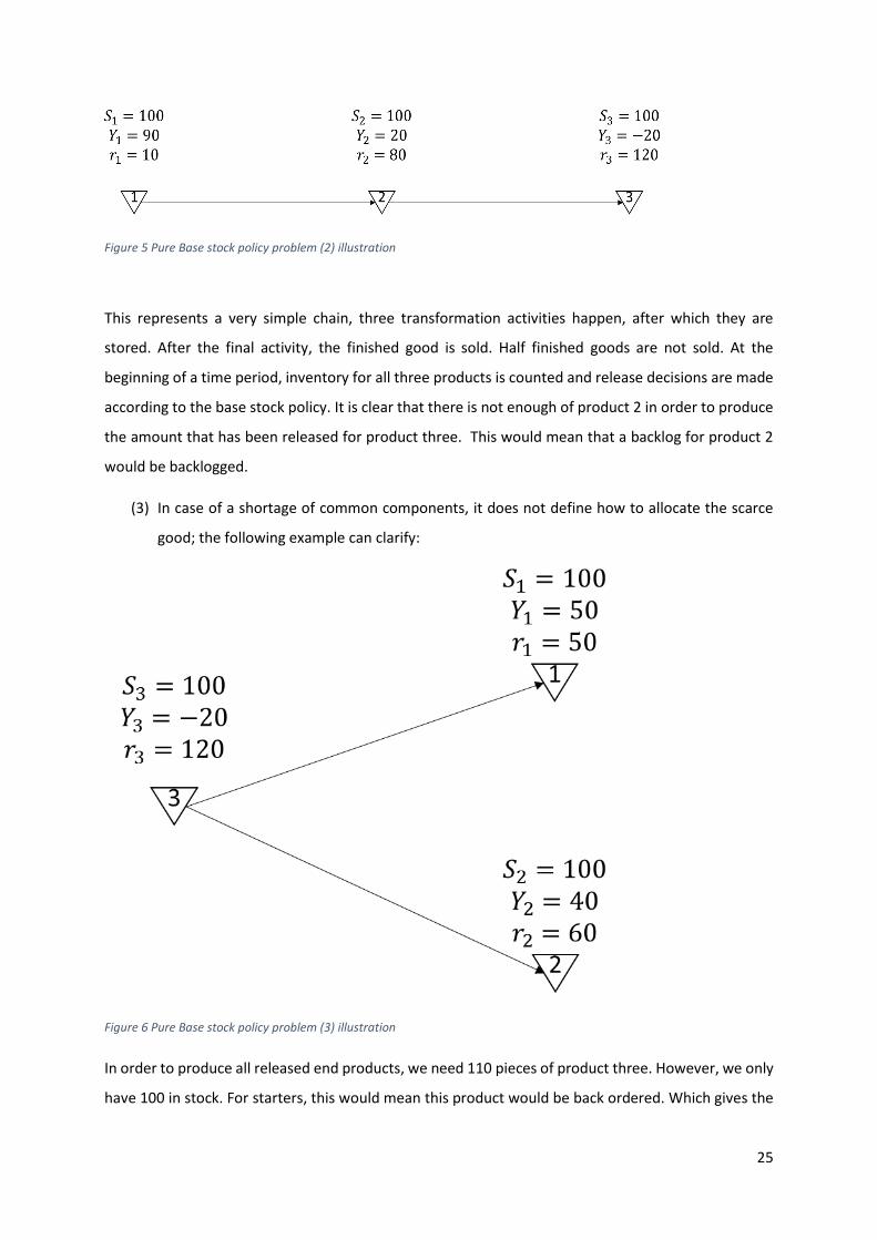
Figure 5 Pure Base stock policy problem (2) illustration

This represents a very simple chain, three transformation activities happen, after which they are

stored. After the final activity, the finished good is sold. Half finished goods are not sold. At the

beginning of a time period, inventory for all three products is counted and release decisions are made

according to the base stock policy. It is clear that there is not enough of product 2 in order to produce

the amount that has been released for product three. This would mean that a backlog for product 2

would be backlogged.

(3) In case of a shortage of common components, it does not define how to allocate the scarce

good; the following example can clarify:

Figure 6 Pure Base stock policy problem (3) illustration

In order to produce all released end products, we need 110 pieces of product three. However, we only

have 100 in stock. For starters, this would mean this product would be back ordered. Which gives the

26

same violation as described above. Secondly, the pure base stock policy does not define how to

allocate the 100 pieces of product 3 that we do have.

4.2 Modified Base-Stock Policies for Convergent Systems In order to solve the second problem (so we don’t release more than available), Kok and Fransoo (2002)

propose to modify the pure base stock policy. When releasing a product, we have to take into account

the availability of its predecessors. For now, a pure assembly system (There is one end product. Each

item has exactly one successor) is assumed. In this sort of system, it is easy to define cumulative lead

times:

𝐿𝑖 𝑐 = 𝐿𝑖, 𝑖 ∈ 𝐸 ( 31 )

𝐿𝑖𝑐 = 𝐿𝑖, +𝐿𝑠𝑢𝑐(𝑖), 𝑖 ∈ 𝐼 ( 32 )

In this case “𝑌𝑖(𝑡) represents the coverage by item 𝑖 of the end-product demand from the start of

period t until the start of period 𝑡 + 𝐿𝑖𝑐 just before releasing the item ordered at the start of period t.

For all items with a longer cumulative lead time, we know exactly their coverage of end-product

demand from the start of period t until the start of period 𝑡 + 𝐿𝑖𝑐. “ (Kok & Fransoo, 2002, p. 10)

𝑍𝑖𝑗(𝑡) coverage of end-product demand by item j from the start of period t

until the start of period 𝑡 + 𝐿𝑖𝑐 , 𝐿𝑗

𝑐 > 𝐿𝑖𝑐

Then the modified base stock policy can be defined as:

𝑟𝑖(𝑡) = 𝑚𝑎𝑥 (0 , 𝑚𝑖𝑛 {𝑆𝑖, min{𝑗|𝐿𝑗

𝑐 ≥𝐿𝑖𝑐}

{𝑍𝑖𝑗(𝑡)}} − 𝑌𝑖(𝑡)) ( 33 )

(Kok & Fransoo, 2002). Although the released quantity will no longer exceed the amount of materials

available, another problem remains. This new policy will only work if a product has maximum 1

successor. It does not tell us how to calculate 𝐿𝑖𝑐 if an item is used in multiple assemblies.

4.3 Base-Stock Policies for Divergent Systems A supply network is divergent when each item has one child, but may have multiple parents. There is

one root item (with a single supplier, with infinite material availability). If a child item is shared and the

cumulative orders for parent items exceed available stock, then parts of the available stock have to be

appointed to different parents. Diks and de Kok (1998) propose a balancing assumption to solve this.

The goal is to balance holding costs and backorder costs (both are assumed linear in the paper). In

order to go into further detail the following variables are introduced (in accordance with Kok and

Fransoo (2002)):

𝑝𝑖 penalty cost for item i, at the end of a period, 𝑖 ∈ 𝐸

27

𝑈𝑖 all items on the path of the root item(inclusive) to item i (exclusive), 𝑖 = 1,2, … , 𝑁

𝐸𝑖 Set of end products downstream of item i,

𝛼𝑘𝑖 non-stockout probability of 𝑘 ∈ 𝐸𝑖 under the optimal policy under the balance

assumption for the subtree of the divergent system with item 𝑖 as root item, 𝑖 =

1,2, … , 𝑁

It follows that:

𝐸𝑖 = {𝑖}, 𝑖 ∈ 𝐸 ( 34 )

𝐸𝑖 = ⋃ 𝐸𝑗 , 𝑖 ∈ 𝐼𝑗∈𝑉𝑖 ( 35 )

“Under the balance assumption, the optimal base stock level Si and optimal allocation policies satisfy

𝛼𝑘𝑖 = ( ∑ ℎ𝑚 + 𝑝𝑘

𝑚∈𝑈𝑖

) (ℎ𝑘 + ∑ ℎ𝑚 + 𝑝𝑘), ∀ 𝑘 ∈ 𝐸𝑖 , 𝑖 = 1,2, … , 𝑁

𝑚∈𝑈𝑘

⁄

( 36 )

From this, one can recursively compute the optimal 𝑆𝑖 and optimal allocation policies. However, this

turns out to be computationally infeasible for realistic instances” (Kok & Fransoo, 2002, p.34).

In order to make this problem computationally feasible (Diks & de Kok, 1999) assume linear allocation

functions:

𝑞𝑗 fraction of shortage allocated to item 𝑗

𝑋𝑡,𝑖 echelon stock of item 𝑖 at time 𝑡 immediately before allocation

𝐼𝑡,𝑗 amount of item 𝑖 allocated to 𝑗, 𝑗 ∈ 𝑉𝑖

A linear allocation rule:

𝐼𝑡,𝑗 = 𝑆𝑗 − 𝑞𝑗 ( ∑ 𝑆𝑚

𝑚∈𝑉𝑖

− 𝑋𝑡,𝑖)

+

( 37 )

In order to decide on the right 𝑞𝑗:

𝐷𝑘 demand per period of item 𝑘 ∈ 𝐸

28

𝜇𝑗 = ∑ 𝐸[𝐷𝑘]

𝑘∈𝐸𝑗

( 38 )

𝜎𝑗 = 𝜎( ∑ 𝐷𝑘)

𝑘∈𝐸𝑗

( 39 )

(Kok & Fransoo, 2002) find the following expression:

𝑞𝑗 = 𝜇𝑗

2

2 ∑ 𝜇𝑚2

𝑚∈𝑉𝑖

+ 𝜎𝑗

2

2 ∑ 𝜎𝑚2

𝑚∈𝑉𝑖

, 𝑗 ∈ 𝑉𝑖 , 𝑖 = 1,2, … , 𝑁

( 40 )

4.4 Synchronized Base-Stock Policies To summarize, in the beginning of the chapter pure base stock policies and the problems that arise

with this kind of policy were discussed. Subsequently, solutions to these problems were discussed. Of

course, in realistic instances, the problems will all arise in one chain. A supply chain normally is not

exclusively convergent or divergent. This means that the solutions above are not immediately

applicable in real life situations. Two new problems arise (Kok & Fransoo, 2002):

(1) The variable 𝑍𝑖𝑗(𝑡) cannot be defined since it is impossible to uniquely define 𝐿𝑖𝑐 in case of

multiple successors.

(2) In the case of a shortage, no procedure is defined for allocating shortage to successors in

general systems.

In order to solve the first problem de Kok and Visschers (1999) introduce a variable similar to 𝑍𝑖𝑗(𝑡),

and an allocation mechanism based on the one used for divergent systems.

Kok and Fransoo (2002) define:

𝐿𝑖𝑐 = 𝐿𝑖, 𝑖 ∈ 𝐸 ( 41 )

𝐿𝑖𝑐 = 𝐿𝑖 + max

𝑗∈𝑉𝑖

𝐿𝑗 , 𝑖 ∈ 𝐼. ( 42 )

𝑠 root node

𝑠 = arg (𝑚𝑎𝑥𝑖

𝐿𝑖𝑐) ( 43 )

By consequence:

𝐿𝑠𝑐 ≥ 𝐿𝑖

𝑐 , 𝑖 ∈ (𝐼 ∪ 𝐸) ( 44 )

The set 𝐶𝑖 is defined as follows:

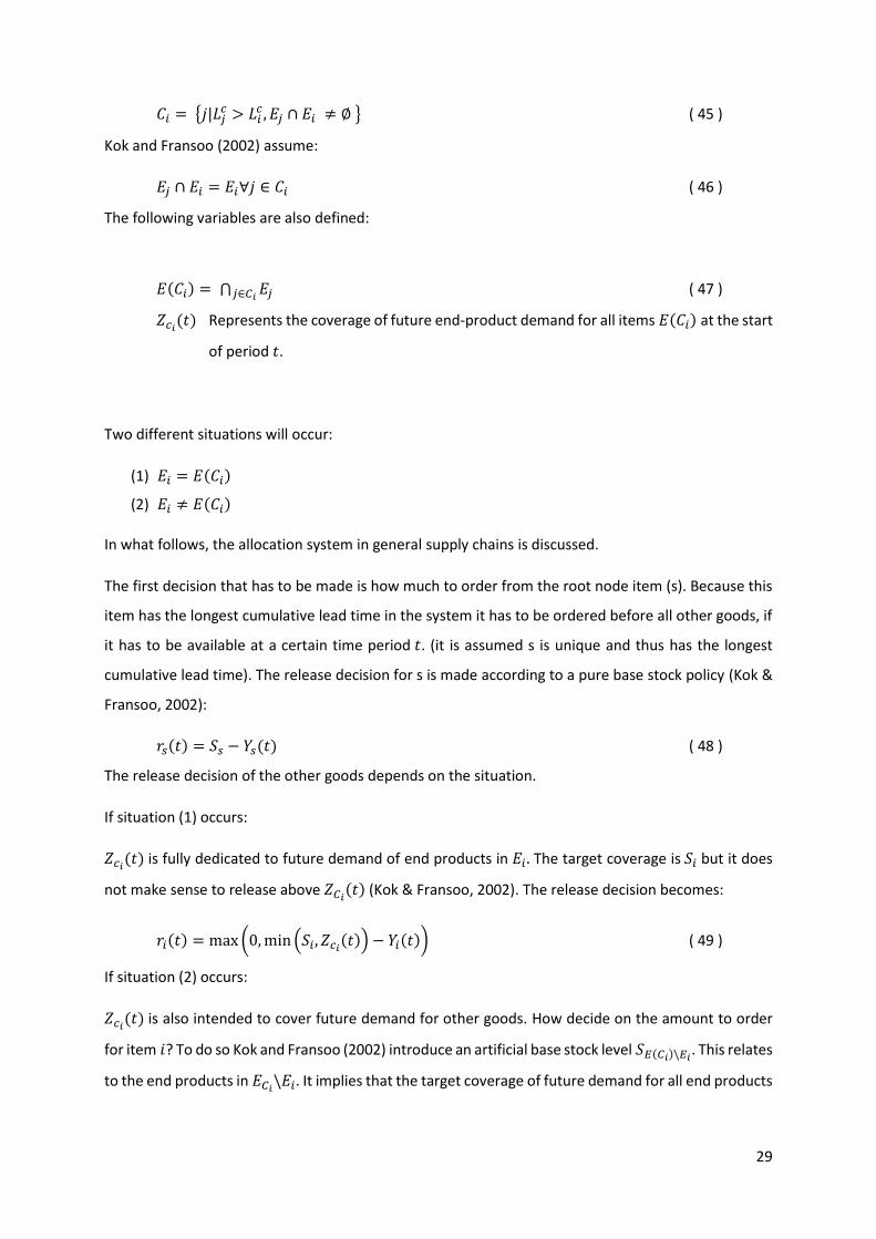
29

𝐶𝑖 = {𝑗|𝐿𝑗𝑐 > 𝐿𝑖

𝑐 , 𝐸𝑗 ∩ 𝐸𝑖 ≠ ∅ } ( 45 )

Kok and Fransoo (2002) assume:

𝐸𝑗 ∩ 𝐸𝑖 = 𝐸𝑖∀𝑗 ∈ 𝐶𝑖 ( 46 )

The following variables are also defined:

𝐸(𝐶𝑖) = ⋂ 𝐸𝑗𝑗∈𝐶𝑖 ( 47 )

𝑍𝑐𝑖(𝑡) Represents the coverage of future end-product demand for all items 𝐸(𝐶𝑖) at the start

of period 𝑡.

Two different situations will occur:

(1) 𝐸𝑖 = 𝐸(𝐶𝑖)

(2) 𝐸𝑖 ≠ 𝐸(𝐶𝑖)

In what follows, the allocation system in general supply chains is discussed.

The first decision that has to be made is how much to order from the root node item (s). Because this

item has the longest cumulative lead time in the system it has to be ordered before all other goods, if

it has to be available at a certain time period 𝑡. (it is assumed s is unique and thus has the longest

cumulative lead time). The release decision for s is made according to a pure base stock policy (Kok &

Fransoo, 2002):

𝑟𝑠(𝑡) = 𝑆𝑠 − 𝑌𝑠(𝑡) ( 48 )

The release decision of the other goods depends on the situation.

If situation (1) occurs:

𝑍𝑐𝑖(𝑡) is fully dedicated to future demand of end products in 𝐸𝑖. The target coverage is 𝑆𝑖 but it does

not make sense to release above 𝑍𝐶𝑖(𝑡) (Kok & Fransoo, 2002). The release decision becomes:

𝑟𝑖(𝑡) = max (0, min (𝑆𝑖, 𝑍𝑐𝑖(𝑡)) − 𝑌𝑖(𝑡)) ( 49 )

If situation (2) occurs:

𝑍𝑐𝑖(𝑡) is also intended to cover future demand for other goods. How decide on the amount to order

for item 𝑖? To do so Kok and Fransoo (2002) introduce an artificial base stock level 𝑆𝐸(𝐶𝑖)\𝐸𝑖. This relates

to the end products in 𝐸𝐶𝑖\𝐸𝑖. It implies that the target coverage of future demand for all end products

30

in 𝐸(𝐶𝑖) equals 𝑆𝑖 + 𝑆𝐸(𝐶𝑖)\𝐸𝑖. If 𝑍𝐶𝑖

(𝑡) is below this level, part of the deficit must me assigned. Kok

and Fransoo (2002) find the following release policy:

𝑟𝑖(𝑡) = max (0, 𝑆𝑖 − 𝑞𝑖 (𝑆𝑖 + 𝑆𝐸(𝐶𝑖)\𝐸𝑖− 𝑍𝐶𝑖

(𝑡))+

− 𝑌𝑖(𝑡)) ( 50 )

In this chapter, the first planning policy ‘Base Stock’ was described in detail. First, a pure base-stock

policy was discussed, quickly a few shortcomings became clear. In the following parts, modifications

on the pure base-stock policy are discussed that solve these problems. Finally, the ‘Synchronized Base-

Stock’ (SBS) policy is discussed. This policy is fit for most supply chains, and this is the one that will be

tested in the simulations. In the following chapter, a linear program based policy is introduced. This

policy has the same goal as the SBS: making production and release decisions. These two policies will

then be compared later in this dissertation.

31

5 Linear Programming Based Policies in a Rolling Schedule Context

In this part, the linear programming based allocation policy is discussed. It has the same goal as the

SBS: making production and release decisions. The linear program is discussed in part 5.1. This policy

takes place in a rolling schedule context, which is discussed in part 5.2.

5.1 General This policy is used in a rolling horizon situation. When the program is solved also release decisions for

future periods are made. These future time periods are of course not fixed, as they will be affected by

future events (more on this can be found below). When using the linear program, information about

future demand is needed. However, future demand is usually unknown. This means that demand has

to be forecasted (Kok & Fransoo, 2002). To take this into account, the following variables are

introduced:

�̂�𝑖(𝑡, 𝑡 + 𝑠) exogenous demand for item 𝑖 in period 𝑡 + 𝑠 as recorded at the start of

period 𝑡, 𝑡 ≥ 1, 𝑠 ≤ −𝑡 ∀𝑖

𝐺𝑖(𝑡, 𝑡 + 𝑠) endogenous demand for item 𝑖 in period 𝑡 + 𝑠 as recorded at the start of

period 𝑡, 𝑡 ≥ 1, 𝑠 ≤ −𝑡 ∀𝑖

�̂�𝑖(𝑡, 𝑡 + 𝑠) backlog of item 𝑖 released at the start of period 𝑡 + 𝑠 as recorded at the start

of period 𝑡, 𝑡 ≥ 1, 𝑠 ≤ −𝑡 ∀𝑖

�̂�𝑖(𝑡, 𝑡 + 𝑠) quantity of item 𝑖 released at the start of period 𝑡 + 𝑠 as recorded at the start

of period 𝑡, 𝑡 ≥ 1, 𝑠 ≤ −𝑡 ∀𝑖

�̂�𝑖(𝑡, 𝑡 + 𝑠) quantity of item 𝑖 processed at the start of period 𝑡 + 𝑠 as recorded at the

start of period 𝑡, 𝑡 ≥ 1, 𝑠 ≤ −𝑡 ∀𝑖

For 𝑠 ≥ 0, these variables represent forecasts made at the start of period t. For −𝑡 < 𝑠 < 0, these

variables represent actuals. To solve this problem, the assumption has to be made that there is a time

0, at which the state of the supply network is known. At this time, the linear program is solved for the

first time (Kok & Fransoo, 2002).

In chapter three, the general restrictions of every supply chain were discussed. When building a linear

program, these constraints have to be included:

32

𝐼𝑖(𝑡, 𝑡 + 𝑠 + 1) − �̂�𝑖(𝑡, 𝑡 + 𝑠 + 1)

= 𝐼𝑖(𝑡, 𝑡 + 𝑠) − �̂�𝑖(𝑡, 𝑡 + 𝑠) − ∑ 𝑎𝑖𝑗 �̂�𝑗(𝑡, 𝑡 + 𝑠)

𝑁

𝑗=1

− �̂�𝑖(𝑡, 𝑡 + 𝑠)

+ �̂�𝑖(𝑡, 𝑡 + 𝑠 − 𝐿𝑖), ∀𝑖, 𝑠 = 0, … , 𝑇 − 1

( 51 )

�̂�𝑖(𝑡, 𝑡 + 𝑠 − 1) − �̂�𝑖(𝑡, 𝑡 + 𝑠) ≤ �̂�𝑖(𝑡, 𝑡 + 𝑠), ∀𝑖, 𝑠 = 0, … , 𝑇 − 1 ( 52 )

∑ �̂�𝑖(𝑡, 𝑡 + 𝑤)

𝑠

𝑤=1−𝑡

≥ ∑ �̂�𝑖(𝑡, 𝑡 + 𝑤)

𝑠

𝑤=1−𝑡

, ∀𝑖, 𝑠 = 0, … , 𝑇 − 1

( 53 )

∑ �̂�𝑖(𝑡, 𝑡 + 𝑤)

𝑠

𝑤=1−𝑡

≤ ∑ �̂�𝑖(𝑡, 𝑡 + 𝑤)

𝑠+𝐿𝑖−1

𝑤=1−𝑡

, ∀𝑖, 𝑠 = 0, … , 𝑇 − 1

( 54 )

∑ 𝑐𝑖�̂�𝑖(𝑡, 𝑡 + 𝑠) ≤ 𝐶𝑘𝑡+𝑠

𝑖∈𝑈𝑘

, 𝑘 = 1, … , 𝐾, 𝑠 = 0, … , 𝑇 − 1

( 55 )

�̂�𝑖(𝑡, 𝑡 + 𝑠) ≥ 0, ∀𝑖, 𝑠 = 0, … , 𝑇 − 1 ( 56 )

�̂�𝑖(𝑡, 𝑡 + 𝑠) ≥ 0, ∀𝑖, 𝑠 = 0, … , 𝑇 − 1 ( 57 )

𝐼𝑖(𝑡, 𝑡 + 𝑠) ≥ 0 , ∀𝑖, 𝑠 = 0 , … , 𝑇 − 1 ( 58 )

�̂�𝑖(𝑡, 𝑡 + 𝑠) ≥ 0, ∀𝑖, 𝑠 = 0, … , 𝑇 − 1 ( 59 )


In a rolling schedule context, the decision variables ({𝑟𝑖(𝑡)}, {𝑞𝑖(𝑡)})are implemented. In the model

they are represented by:

𝑟𝑖(𝑡) = �̂�𝑖(𝑡, 𝑡), ∀𝑖, 𝑡 ≥ 1 ( 60 )

𝑞𝑖(𝑡) = �̂�𝑖(𝑡, 𝑡), ∀𝑖, 𝑡 ≥ 1 ( 61 )

Kok and Fransoo (2002) suggest two objective functions:

∑ (∑ ℎ𝑖𝐼𝑖(𝑡, 𝑡 + 𝑠)

𝑇

𝑠=1

+ ∑ 𝜃ℎ𝑖�̂�𝑖(𝑡, 𝑡 + 𝑠)

𝑠∈𝐸

)

𝑁

𝑖=1

( 62 )

33

And

∑ (∑ ℎ𝑖(𝐼𝑖(𝑡, 𝑡 + 𝑠) − 𝑣𝑖)+

𝑇

𝑠=1

+ ∑ 𝜃ℎ𝑖 (𝑣𝑖 − 𝐼𝑖(𝑡, 𝑡 + 𝑠))+

𝑠∈𝐸

)

𝑁

𝑖=1

( 63 )

With

𝑣𝑖 the safety stock of product 𝑖.

In the first objective function, the holding costs are predicted, and a term has been added to take costs

of back orders into account. This is to make sure a certain priority is given to satisfy exogenous demand

(without this, the optimal solution would be to not release or produce anything). However, solving

this to optimality does not make sure the correct service level is attained. Even changing 𝜃 and further

increasing it will not solve the problem. For a value of 𝜃 above a certain 𝜃0 the optimal solution will

not change (Kok & Fransoo, 2002, p. 26). In order to be able to control the service level in a better

fashion the second objective function and the variables 𝑣𝑖 are introduced. 𝑣𝑖 represents the safety

stock of product 𝑖. The higher the service level, the higher 𝑣𝑖 has to be set. In other words, the term 𝑣𝑖

makes sure a certain service level is attained (Kok & Fransoo, 2002). The two terms in the second

objective function make sure that any deviation from the safety stock is punished. This has as a

consequence that if for all end-items 𝐼𝑖(0) = 𝑣𝑖 ∀𝑖 ∈ 𝐸, the optimal solution will have the same value

for the decision variables ({�̂�𝑖(𝑡, 𝑡 + 𝑠)}, {�̂�𝑖(𝑡, 𝑡 + 𝑠)}) for each value of 𝑣𝑖 ∈ 𝐸. Proof of this can be

found in (Kok & Fransoo, 2002). If in the first time periods inventories are at 𝑣𝑖 than for a given demand

pattern in the next periods, the optimal solution will have the same release and processing decisions

(if we assume that backlogged demand has to be fulfilled and is not lost). If one were to plot out the

occurrence of net inventory positions, he would always get the same shape. Only the curve would shift,

depending on the safety stock levels. Imagine a company that sells one type of product and at the end

of each hour net inventory is recorded. After 10000 hours the results are plotted in the following curve:

34

Figure 7 net inventory distribution shift

In this example, the net inventory position follows a normal distribution (this is not necessarily the

case). The company notices that in 2369 out of the 10000 time periods net inventory was negative.

This means a non-stock out service level of 76%. What if the company aims at obtaining non-stock out

service level of 95%? The solution is increasing the safety stock. The reasoning above shows that

changing 𝑣𝑖 means that the shape of the curve won’t change but the curve will shift. An 𝛼∗ of 95%,

means the curve has to shift to the right until 95% of the case is higher than zero. The 5 percentile is

calculated. In this example we see that it is -133. This means that we need to increase 𝑣𝑖 with 133. (Kok

& Fransoo, 2002)

This last observation has as a consequence that “𝑝𝛼 and 𝑝𝛽 for the SCOP concept defined by the LP

constraints and the second objective function have a unique solution {𝑣𝑖}𝑖∈𝐸, where each 𝑣𝑖, 𝑖 ∈ 𝐸,

can be determined independent of all other 𝑣𝑗, 𝑗 ∈ 𝐸, 𝑗 ≠ 𝑖” (Kok & Fransoo, 2002, p.27).

To determine the optimal 𝑣𝑖 Kok and Fransoo (2002) propose the following procedure:

(1) Run a discrete event simulation is, with 𝑣𝑖 = 0, where each period the LP is solved with the

first objective function.

(2) Compute the empirical distribution of 𝐽𝑖(𝑡) − 𝑣𝑖 ≤ 𝑥, based on the simulation in (1).

Calculating the empirical distribution and afterwards the percentiles is time consuming. If the

simulation runs a high enough number of time periods, the actual distribution does not have

to be calculated. The net inventories can be saved in a list, and the percentiles can be easily

calculated.

(3) Compute 𝑣𝑖∗ such that the required service level is achieved.

(4) Run another simulation to compute 𝐶̅(𝑃).

35

However, the second objective function proposed by Kok and Fransoo (2002) causes another difficulty.

The first and the second term of the equation are only calculated when they are positive.

Consequentially, the function is no longer linear. This means the objective function has to be linearized.

To do so a slack variable was added:

𝑆𝐿𝐴𝐶𝐾̂𝑖(𝑡, 𝑡 + 𝑠) Indicates the difference between the net inventory and the Safety stock, for

item 𝑖 in period 𝑡 + 𝑠 as recorded at the start of period 𝑡, 𝑡 ≥ 1, 𝑠 ≤ −𝑡 ∀𝑖.

two constraints were added:

𝐼𝑖(𝑡, 𝑡 + 𝑠) − �̂�𝑖(𝑡, 𝑡 + 𝑠) + 𝑆𝐿𝐴𝐶𝐾̂𝑖(𝑡, 𝑡 + 𝑠) ≥ 𝑣𝑖 , ∀𝑖, 𝑠 = 0, … , 𝑇 − 1 ( 64 )

𝑆𝐿𝐴𝐶𝐾̂𝑖(𝑡, 𝑡 + 𝑠) ≥ 0, ∀𝑖, 𝑠 = 0, … , 𝑇 − 1 ( 65 )

The objective function was adjusted:

∑ (∑ ℎ𝑖𝐼𝑖(𝑡, 𝑡 + 𝑠)

𝑇

𝑠=1

+ ∑ 𝜃ℎ𝑖𝑆𝐿𝐴𝐶𝐾̂𝑖(𝑡, 𝑡 + 𝑠)

𝑠∈𝐸

)

𝑁

𝑖=1

( 66 )

This objective function represents the same thing as the second objective function proposed by (Kok

& Fransoo, 2002), but there is a small difference. In this equation, if inventory for a product 𝑖 is positive

but lower than the safety stock for that product, the calculated cost will be higher because both terms

in the equations will be positive. However, the optimal solution is no different than when the second

objective function would be used. Only the end value of the optimized function would differ but not

the values of the decision variables. This means that the optimal value for the objective function does

not represent the actual costs 𝐶(𝑃). These will have to be calculated afterwards.

5.2 Rolling Horizon The linear program is solved in a rolling horizon context. Essentially, every day you produce you need

to decide on the amount to release and to process that day. To decide on these amounts, the linear

program is solved to optimality, given a starting inventory and forecast of future demand. The linear

program will not only give the amount to produce and release for the current time period, but also for

future time periods. It can do this, because of the forecasts. If a 30-day demand forecast serves as an

input in the program, it will calculate the optimal amounts to produce and release for the following

thirty days. However, forecasts are always prone to error. If the forecast was wrong, it would be

illogical to follow the decisions of the linear program. That is why every time period the linear program

has to be resolved, with the new information.

36

6 Simulation Procedure to take Capacity into Account

Previously, the general supply chain problem was discussed. Then two decisions policies –

synchronized base stock & linear program – were discussed. In this section, the simulation procedure

that is followed to test the performance of the different planning methods under the different

conditions is introduced. The first part handles issues that arise in both cases. In the second part, the

simulation procedure for the linear program based policy is discussed. Finally, in the last part, the base

stock policy simulation procedure can be found.

6.1 General In order to compare both policies under the different circumstances, the conditions of demand and

lead time have to be the same.

6.1.1 Demand

As described above there are two types of demand. Internal and external demand. Internal demand

arises because a product is needed further downstream in the chain. External demand arises from

outside the chain; a customer who buys the product. Although there are exceptions, generally external

demand is unknown and has to be forecast based on history and market projections. A company might

know that on average it will sell x-amount of product each day, and how variable this number is. In

order to implement this in the simulation and make it more realistic, a random number generator is

used to simulate actual demand. Given a distribution and the right parameters (average, standard

deviation, …) this generates a sequence of random numbers that fit that distribution. Although the

actual demand in each period is unknown on beforehand, the input parameters are assumed to be

known to the players in the supply chain. A few problems arise with this approach. Random number

generators are mathematical tools. This means that they will generate numbers that are not realistic.

In this case, it is possible that the system generates sequences that contain decimal numbers and

negative numbers. For decimal numbers, rounding provides an easy solution. For the negative

numbers, a more complex approach is needed. An easy solution is every time a negative number is

generated it means no demand for that time period. However, one of the goals of this research is to

see what the influence is of demand variation. If this solution was applied in a high variation case it is

possible that the actual average demand would be higher than the average that was decided upon.

Another solution is needed. The following logarithm was followed:

Balance = 0

Get_demand():

Demand = randomNumber(average; standard deviation)

Balance = Balance + Demand

37

If Balance >= 0 : balance = 0

Return Maximum(Balance; 0)

This procedure uses a balance that is either zero or negative. If a negative number is generated, for

that period a demand of zero is assumed, and the balance is set at the negative number. In the next

period, the negative amount will be subtracted from the generated number. This way the average will

actually be what was decided upon. To prove this, multiple lists of random numbers have been

generated and the results confirm that this approach solves the problem. This then allows for better

comparisons between cases of different demand variation and allows assessing the influence of

demand variation.

6.1.2 Lead Times

When simulated, lead times will be assumed to be known and fixed. Different lead time structures will

be used, in order to assess the impact of lead times.

6.1.3 Starting Conditions

Another problem is the first period of the simulation. It is best to assume the whole system has been

up and running. In other words, there is inventory and there is work in progress. Starting inventories

are best set at the safety stock levels. It is more difficult for work in progress. If a product takes 5 time

periods to make, how much of it is finished in the first 5 time periods? It is impossible to look at the

production and release decisions of 5 periods earlier because this information is not yet available. In

order to solve this, assume that every period the average periodical demand (sum of external and

internal demand) is finished. This way, when actual processing and production decisions are available

(at the end of period five), the beginning inventory will be at a normal level. Lastly, it is also better not

to include the first time periods in the calculations. If you wish to calculate average inventory, do not

include the inventories in the first periods of the simulation. This warm-up period should be long

enough to overcome the influence of the ‘errors’ in the beginning. How long this warm-up period must

be, depends on the lead times and the number of time periods simulated.

6.1.4 Number of Time Periods Simulated

The actual number of time periods simulated should be long enough to make sure the influence of

outliers (by example because of random demand) is zero. The numbers calculated should represent

the actual values. The only way to know how many time periods are necessary is by running multiple

simulations with the same input and the same number of time periods. If the results differ, more time

periods are necessary. Secondly, the number of time periods has to be high enough so a long ‘warm-

up period’ (see 6.1.3) can be used.

38

6.2 Linear Program The goal is to see how a linear programming based planning policy performs under different conditions

of demand variability, lead times and of course see how capacity constraints influence this. The linear

program policy is based on the equations discussed in section 5.

Taking capacity constraints into account is not difficult in this case. Equation 55 is specifically designed

to take these into account. The difficulty lies in finding the correct height of the capacity Limitations.

To find these the following procedure was used:

1. Run a discrete event simulation without capacity restrictions and with safety stock equal to

zero.

2. Following the procedure described in section 5, calculate the safety stock

3. Rerun the simulation without capacity constraints but with safety stocks

4. Save the amount each machine produces each time period in a list (one list for each machine)

5. Sort the lists from small to large.

6. Calculate the percentiles you need for each machine

Now that you have the right height of the restrictions, the costs are calculated with this procedure:

7. Input the percentiles as maximum capacity for that machine and rerun the simulation without

safety stocks

8. Following the procedure in section 5, calculate the safety stock

9. Rerun the simulation with capacity constraint and safety stock to calculate the costs and

performance of the system.

A few remarks have to be made here. First of all, it would be more correct, theoretically to calculate

the distribution of the produced amounts (step 5 and 6). When this is done, the percentiles should be

calculated out of the distribution. However, this requires a lot of extra calculation time. With enough

time periods, the error made by using the method described above is negligible. Secondly, because

one of the goals is to see the influence of capacity limitations, it is important to calculate an array of

percentiles, from high percentiles to lower. This will give an idea about the performance of the system

in low utilization and high utilization cases. Finally, it is important to redo this exercise for each

different scenario and to recalculate the capacity percentiles for each scenario. Otherwise, it is not

possible to know if a low or a high utilization case is simulated.

The procedure described above works well for implementing restrictions for each machine individually

(e.g. the maximum amount a machine can produce per time period). However, it is also possible that

capacity restrictions exist over multiple machines. An example is people. Often employees can man

multiple workstations. But if an employee has to man one workstation, another station will be idle

39

because of this decision. This means that a tradeoff exists. The decision to produce one product means

that you cannot produce another at that same moment. The equations for the linear program allow

implementing capacity restrictions that exist over multiple machines. If this kind of capacity restriction

exists, it is difficult to simply use the procedure described above. It is not possible to calculate the

percentiles of the capacity used because this information is not available. Another procedure is

needed.

1. Add another machine in the simulation program that serves as an input to all machines that

are capacitated together.

2. Save the amount the machine produces each period in a list

3. Sort the list from small to large amounts

4. Calculate the percentiles you need

The following figure will clarify:

Figure 8 supply chain restriction problem

Four machines are depicted here. To produce one product on machine 1 you need one hour, on

machine 2 you need two man-hours and so on. This can be incorporated into the system using the

following adjustment:

Figure 9 Supply chain restriction problem: solution

40

Machine 5 is added and provides for all other machines. The lead time of machine 5 must then be set

to zero. Using the procedure described above it is possible to calculate how many man-hours if there

was no restriction in that sense. Using discrete event simulation, you can compile a list of how much

you need every time period, sort that list and calculate the percentiles. These percentiles can then be

used as maximum capacity parameters.

In order to clarify, a small example is provided. Imagine a supply chain manufacturing two end-

products, using two workstations. The inputs come from several suppliers; these inputs get

transformed in workstations 1 and 2, into two different end-products. When finished the products go

into inventory and eventually exit the system through sales. As can be seen on the picture the number

of man-hours needed to produce end-product two, is double of what is needed to produce end-

product one.

Figure 10 example of a simple supply chain

In the first case, the assumption is made that for both workstations specialized training is needed. In

other words, when an employee is trained to work on station one, he cannot be used to man station

two. It is clear that the amounts produced daily are constrained by the number of people trained to

work on a specific workstation. A manager in charge of the production decision can easily input this

information into the linear program discussed in section 5, and the optimal solution will show how

many people are needed to man each station. This manager can wonder what would happen if he had

less or more people available. He wishes to determine the influence of capacity restrictions on his

system. To do so the procedure discussed above can be used.

1. Run a first simulation where capacity is unlimited, and the safety stocks are set equal to zero.

2. Out of this first simulation, calculate the optimal safety stocks:

a. Every time period safe the net inventories (for product one and two) in a list

b. Sort the lists from small to large

c. Calculate the 5th percentiles (5th percentile if 𝛼∗ is 95%)

41

d. These percentiles are now the safety stocks (𝑣1 𝑎𝑛𝑑 𝑣2).

3. Rerun the simulation with capacity unlimited and the safety stocks equal to the 5th percentiles

4. Save the daily produced amounts by machine one and two in two different lists.

5. Sort these lists from small to large. The largest numbers in these lists show how much capacity

(in this case how many man-hours) is needed if the manager wants to be capable of producing

everything, every time period. However, investing so much is usually uneconomical. A large

part of the capacity would practically never be used. In how much man-hours to invest then?

6. To solve this question, take a look at the other numbers in the lists. Calculate the 99th, 95th,

90th, 85th and 80th percentile (and others if deemed necessary).

7. Set the 99th percentiles of both machines as maximum man-hours each day, set the safety

stocks to zero and rerun the simulation.

8. Repeat step two to calculate the safety stocks.

9. Rerun the simulation with the new safety stocks and capacity limitations to calculate costs.

10. Repeat steps 7 to 9 with the other percentiles as the maximum capacity.

11. Out of the calculations, a decent idea exists of the necessary capacity.

In reality, however, it is often the case that people can man multiple machines. In the example, this

would mean that the workstations are not separately restricted, but a capacity restriction exists over

both. It is clear that the total amount of product finished each day depends on the total number of

man-hours available. The tradeoff is also very clear if the manager decides to produce a unit of product

two, he loses two units of product one. Again, given the total number of man-hours available, the

person(s) responsible for the production decision could very easily just input the data into the linear

program. Solve it, and then find the optimal product mix. Again, the managers responsible can wonder

what the influence would be of increasing or decreasing capacity. The difference with the first example

is that the employees can now work both machines. Other characteristics of the chain are the same

(demand, lead time, ….). Again there is a need to determine the percentiles. One could argue that the

same method as above can be used. Eventually, two lists would be available with production

information for each machine. As maximum capacity, the production amounts of each time period are

summed up, and the percentiles are calculated out of this list. However, if the efficiencies of both

machines are different, this too would have to be taken into account, while calculating the percentiles.

Although it is not a big problem for this small example, it can be in realistic situations with multiple

machines or workstations that are constricted by the same resource. It is easier to program the supply

chain in the following way:

42

Figure 11 Example of a simple supply chain: with common restriction

With machine three providing the other two of man-hours, and the lead time of this equal to zero.

Now the same procedure as above can be followed. Only the capacity percentiles for machine three

have to be calculated, and this is the only machine that has to be restricted later. For machine three

you do not have to set any safety stocks. However, the inventory always needs to be “full” at the

beginning of every period.

1. Run the first simulation, with an unlimited capacity assumption, and the safety stocks are set

equal to zero. The production time for workstation three is equal to zero, it can immediately

provide to the other workstation.

2. Out of this first simulation calculate the optimal safety stocks:

a. Every time period safe the net inventory in a list (not for workstation three)

b. Sort the list from small to large

c. Calculate the 5th percentile (5th percentile if 𝛼∗ is 95%)

d. This percentile is now the safety stock

3. Rerun the simulation with capacity unlimited and safety stocks equal to the 5th percentile

4. Save the daily amounts produced by workstation three in a list.

5. Sort this list from small to large. The largest numbers in these lists show how much capacity

(in this case how many man-hours) is needed if the manager wants to be capable of producing

everything, every time period.

6. Calculate the 99th, 95th,90th ,85th and 80th percentile (and others if deemed necessary).

7. Set the 99th percentiles as the number of man hours in inventory every day, set the safety

stocks to zero and rerun the simulation.

8. Repeat step two to calculate the safety stocks

9. Rerun the simulation with safety stock and capacity constraint to calculate costs

10. Repeat steps 7 to 9 with the other percentiles as maximum capacity

11. Out of the calculations, a decent idea exists of the necessary capacity

43

6.3 Base Stock In this part, the simulation procedure of a supply chain controlled by a base stock policy (as described

in part four) is discussed. The procedure to find the right height of the restrictions is very similar to the

one used for a linear program.

1. Calculate base stocks (𝑆𝑖) for each product using formula 36.

2. Adjust base stocks if the alpha level is not met.

rules for adjusting:

if service level > 𝛼∗: decrease the safety stock level of only that product (not of products

upstream in the chain)

if service level < 𝛼∗: increase safety stock level of that product (not products upstream

in the chain). If this increase does not affect service level, then also increase the safety

stock of the products upstream.

3. Run a discrete event simulation.

4. Save the amount each machine produces each time period in a list (one list for each machine)

5. Sort the lists from small to large.

6. Calculate the percentiles for each machine.

7. Input the percentiles as maximum capacities for the respective machines and rerun the

simulation.

8. Check service levels and adjust if necessary

9. After adjusting rerun the simulation

10. Repeat steps 8 and 9 until the service level is equal to 𝛼∗

The procedure above is fitted for situations where machines are separately constrained. When a

situation arises where a restriction over multiple workstations exists another procedure has to be

followed. In this case, the same procedure as for the linear program has to be followed. An extra

workstation has to be added to the simulation that provides to all workstations that are restricted

together, and the lead time of the machine is then set to zero. The same procedure as above can then

be followed to assess the influence of capacity limitations. Save all the amounts produced each time

period on the extra workstation. Sort this list and calculate the percentiles. These then serve as

maximum capacities The starting inventory of this machine is set at the maximum capacity and every

time period it has to be reset at this level.

In this chapter, the simulation procedures to incorporate capacity limitations were discussed. In the

following chapter, a case study where these procedures are used is introduced.

44

7 The Case Study

Previously, the supply chain planning problem and two planning policies were discussed in detail. In

chapter 6 a procedure is introduced that allows implementing capacity limitations into simulations.

The goal of this paper is to test the performance of these planning policies under different

circumstances. In order to do this, a case is simulated. In this chapter, this case is described in detail.

This case has been used before and can be found in Kok and Fransoo (2002).

7.1 Description The following figure represents the case used:

Figure 12 The case study (Kok & Fransoo, 2002, figure 5)

The figure depicts a two stage system. In a first stage, inputs come into the system and get transformed

in workstation 5 to 11. The outputs of these workstations are subassemblies 5 to 11. In the following

stage, these seven subassemblies are assembled to make four different end products (products 1 to

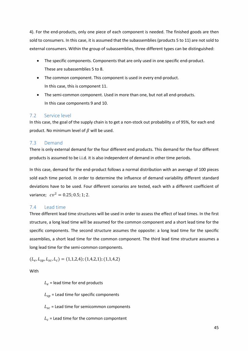
45

4). For the end-products, only one piece of each component is needed. The finished goods are then

sold to consumers. In this case, it is assumed that the subassemblies (products 5 to 11) are not sold to

external consumers. Within the group of subassemblies, three different types can be distinguished:

The specific components. Components that are only used in one specific end-product.

These are subassemblies 5 to 8.

The common component. This component is used in every end-product.

In this case, this is component 11.

The semi-common component. Used in more than one, but not all end-products.

In this case components 9 and 10.

7.2 Service level In this case, the goal of the supply chain is to get a non-stock out probability 𝛼 of 95%, for each end

product. No minimum level of 𝛽 will be used.

7.3 Demand There is only external demand for the four different end products. This demand for the four different

products is assumed to be i.i.d. it is also independent of demand in other time periods.

In this case, demand for the end-product follows a normal distribution with an average of 100 pieces

sold each time period. In order to determine the influence of demand variability different standard

deviations have to be used. Four different scenarios are tested, each with a different coefficient of

variance; 𝑐𝑣2 = 0.25; 0.5; 1; 2.

7.4 Lead time Three different lead time structures will be used in order to assess the effect of lead times. In the first

structure, a long lead time will be assumed for the common component and a short lead time for the

specific components. The second structure assumes the opposite: a long lead time for the specific

assemblies, a short lead time for the common component. The third lead time structure assumes a

long lead time for the semi-common components.

(𝐿𝑒 , 𝐿𝑠𝑝, 𝐿𝑠𝑐 , 𝐿𝑐) = (1,1,2,4); (1,4,2,1); (1,1,4,2)

With

𝐿𝑒 = lead time for end products

𝐿𝑠𝑝 = Lead time for specific components

𝐿𝑠𝑐 = Lead time for semicommon components

𝐿𝑐 = Lead time for the common compontent

46

In this case:

𝐿𝑖 = 𝐿𝑒 𝑓𝑜𝑟 𝑖 = 1,2,3,4

𝐿𝑖 = 𝐿𝑠𝑝 𝑓𝑜𝑟 𝑖 = 5 ,6,7,8

𝐿𝑖 = 𝐿𝑠𝑐 𝑓𝑜𝑟 𝑖 = 9,10

𝐿𝑖 = 𝐿𝑐 𝑓𝑜𝑟 𝑖 = 11

The combination of the different lead time structures with the different demand variability leads to 12

different situations.

7.5 Capacity To calculate the influence of capacity restriction on the performance of the system, the procedure

described in section 6 is used. The different percentiles used as maximum capacity are: 99%; 95%;

90%; 85%; 80%. The 99% case means that in 99% of the time periods the workstation will be capable

of delivering everything that would normally be asked of it if no capacity restriction existed. If the

capacity is restricted at 80%, in one out of 5 time periods, the machine will not be capable of producing

everything it would normally be asked to produce. These restrictions will be used for every

combination of lead time structure and demand variability.

When testing the linear program policy, three different case types are simulated:

No capacity restrictions.

In these cases, capacity is assumed unlimited. The different structures of demand variability

and lead time are implemented and the percentiles needed for capacity maximums are

calculated.

Separately capacitated.

Each workstation has a maximum amount of products it can produce each time period. This

maximum is based on the percentiles calculated in the no capacity restriction case with the

same demand variability and lead time structure.

Common capacity restriction.

In this last case, it is assumed that workstations one to four are restricted together. There is

an input these four use together that limits the total number of end products made each time

period.

When testing the base stock policy two different case types are simulated. The uncapacitated case and

the case where capacity is commonly restricted. The cases where the machines are assumed to be

separately capacitated is not simulated. The reason being that when separate capacitation is assumed,

47

the formulas in part four have to be adapted to take this into account. This is not the goal of this paper,

and would take us too far.

7.6 Cost structure To calculate the costs of the system, the following structure is used:

(ℎ𝑒 , ℎ𝑠𝑝, ℎ𝑠𝑐 , ℎ𝑐) = (100,10,30,50)

With

ℎ𝑒 = holding cost for end products

ℎ𝑠𝑝 = holding cost for the specific components

ℎ𝑠𝑐 = holding cost for the semicommon components

ℎ𝑐 = holding cost for the common component

In this case, this means:

ℎ𝑖 = ℎ𝑒 𝑓𝑜𝑟 𝑖 = 1,2,3,4

ℎ𝑖 = ℎ𝑠𝑝 𝑓𝑜𝑟 𝑖 = 5,6,7,8

ℎ𝑖 = ℎ𝑠𝑐 𝑓𝑜𝑟 𝑖 = 9,10

ℎ𝑖 = ℎ𝑐 𝑓𝑜𝑟 𝑖 = 11.

The cost for the backlog is calculated using formula 4. This gives a 𝜃 of 19. In other words, the cost of

backlog is 19 times the cost of a product in inventory. Backlog only exists for the four end-products.

The formulas and planning methods introduced in chapters three, four and five are now applied to

that case study introduced in this chapter. The procedure described in chapter six allows incorporating

capacity restrictions in the system. In the following chapter, the results of the simulations are described

and discussed.

48

8 Analysis

8.1 Performance of the Linear Programming Policy

8.1.1 No Capacity Limitations

Figure 13 Performance of the linear programming based policy without capacity limitations. (a) safety stock; (b) average inventory cost; (c) average back order cost; (d) average total cost; (e) fill-rate.

89%

90%

91%

92%

93%

94%

95%

96%

97%

98%

99%

0,25 0,5 1 2

Fill-

Rat

e

CV²

Lc = 4 Lc = 1 Lc = 2e

€-

€10 000,00

€20 000,00

€30 000,00

€40 000,00

€50 000,00

€60 000,00

0,25 0,5 1 2

Avg

BO

Co

st

CV²

Lc = 4 Lc = 1 Lc = 2c

€-

€50 000,00

€100 000,00

€150 000,00

€200 000,00

€250 000,00

€300 000,00

€350 000,00

€400 000,00

0,25 0,5 1 2

Avg

To

tal c

ost

CV²

Lc = 4 Lc = 1 Lc = 2d

€-

€50 000,00

€100 000,00

€150 000,00

€200 000,00

€250 000,00

€300 000,00

0,25 0,5 1 2

Avg

Inv

Co

stCV²

Lc = 4 Lc = 1 Lc = 2b

0

100

200

300

400

500

600

0,25 0,5 1 2

Safe

ty S

tock

CV²

Lc = 4 Lc = 1 Lc = 2a

49

In the first part, the performance of the linear program based policy is discussed. We start with the

performance under no capacity limitations.

On the graphs above, you can see four groups of bars. Grouped per variance of demand. In each group

the first bar signifies the case where the lead time is long for the common components and short for

the specific components. The second bar signifies the opposite (long lead time for specific, short lead

time for common components). The third bar shows the results for the cases where semi-common

components have a long lead time (see lead time structure part 7.4).

The upper left graph shows how high the safety stock of an end product has to be set in order to obtain

a 95% non-stock-out probability when no capacity restrictions exist. It has to be noted that under the

linear program based policy, safety stocks are only set for finished goods. Because of the symmetry of

the case, one can assume that the safety stocks for the end products are for all four equally high. This

is not necessarily the case, but the simulations confirmed this assumption. As expected, when demand

variability increases, the safety stock necessary to obtain the service level increases as well. Another

observation that can be made based on the graph is that when components that are commonly used

have a long lead time, a higher safety stock is needed to obtain the same service level. When the lead

time of the common components is shorter, safety stocks can go down. The reason lies in the fact that

when in a single time period, higher than average demand occurs for multiple products, the number

of the common components in stock decreases fast, and if this component has a long lead-time, it

takes a while until it is refilled. To buffer against this longer lead time the safety stocks of the end

products have to increase.

Graphs b, c, and d show the average daily inventory, back order and total costs associated with the

different lead time structures and demand variance. It is immediately clear that the costs follow the

same evolution as the safety stocks. If demand variance rises inventory and backorder costs rise too.

Inventory costs are higher when the lead time of the common component is longer. This is caused

partly by the higher necessary safety stocks. Reducing lead time of the common component can

positively influence the performance of the system as it reduces necessary safety stock, inventory costs

and backorder costs.

In graph e, the fill rate is depicted. The goal was attaining a minimum non-stock-out level. The

simulation was not subject to a minimum fill rate. It is clear that the fill rate decreases when demand

variance increases. Secondly, fill rate is generally higher when the common component has a short

lead time.

In the following part, capacity restrictions are introduced. Because it was clear from the previous that

the lead time of the common component greatly influences the costs, only the cases where the lead

time is long and short are discussed in detail.

50

8.1.2 Separately Capacitated Case

8.1.2.1 Common Component with Long Lead Time

Figure 14 Performance of the linear programming based policy in a system where each workstation has a capacity limit. The common component has a long lead time (4 time periods). (a) safety stock; (b) average inventory cost; (c) average back order cost; (d) average total cost; (e) fill-rate.

88%

90%

92%

94%

96%

98%

100% 99% 95% 90%

Fill-

Rat

e

Capacity Limitation

CV² = 0,25 CV² = 0,5

CV² = 1 CV² = 2

€150 000,00

€170 000,00

€190 000,00

€210 000,00

€230 000,00

€250 000,00

€270 000,00

€290 000,00

€310 000,00

100% 99% 95% 90%

Avg

Inv

Co

st

Capacity Limitation

CV² = 0,25 CV² = 0,5

CV² = 1 CV² = 2 b

€150 000,00

€200 000,00

€250 000,00

€300 000,00

€350 000,00

€400 000,00

100% 99% 95% 90%

Avg

To

tal C

ost

Capacity Limitation

CV² = 0,25 CV² = 0,5

CV² = 1 CV² = 2 d

€10 000,00

€20 000,00

€30 000,00

€40 000,00

€50 000,00

€60 000,00

€70 000,00

€80 000,00

€90 000,00

100% 99% 95% 90%

Avg

BO

Co

st

Capacity Limitation

CV² = 0,25 CV² = 0,5

CV² = 1 CV² = 2 c

200

300

400

500

600

700

800

100% 99% 95% 90%

Safe

ty S

tock

Capacity Limitation

CV² = 0,25 CV² = 0,5

CV² = 1 CV² = 2 a

e

51

In order to test the influence of capacity, the average demand was kept at the same height, while the

maximum amount produced daily was decreased. In the case without capacity limitation, the daily

produced amounts on each machine were saved and several percentiles of that list were calculated.

These percentiles then served as maximum capacities in later simulations. In the graphs above you can

see the horizontal axis ranges from 100% to 90%. These are the percentiles. 100% means no capacity

limitation. 90% means that the 90th percentile was used as maximum (this means that in 10% of time

periods the machines could not produce as much as it would have with unlimited capacity). This first

paragraph focusses on separately restricted machines (each machine has its own maximum capacity).

In graph a, the influence of capacity restriction on the safety stock necessary to obtain the 95% service-

level is depicted. As can be seen, the safety stocks are more or less stable until the 95% point, after

which a strong increase is necessary. This 95% point means that in 95% of the cases the machines are

capable of producing what would have been asked of it if capacity was unlimited. Inventory costs

follow a slightly different evolution (graph b). When capacity is restricted below 95%, a strong increase

in inventory cost happens (because of the increased safety stock). However, the simulations show that

this 95% point is optimal in terms of inventory costs. In other words, having more capacity has a

negative influence on the inventory policy. Backorder costs (graph c) seem to be fluctuating more

strongly. Generally, a high demand variance leads to higher BO costs, which also means a lower fill-

rate (graph e). In terms of total costs (graph d), it seems that some capacity limitation leads to a better

performance of the linear program. It seems that the optimal point is the 95% capacity limitation (this

means that each machine is capable of producing what it would produce under unlimited capacity in

95 percent of the time). In the case where demand variance is very low, capacity can even be lower.

It should be noted that situations, where capacity was restricted even further, were also simulated. In

these cases, safety stocks had to be set extremely high (above one hundred times average daily

demand). This can be explained. In the first time period, the inventories are assumed to be equal to

the safety stock. The extremely high inventories are the starting inventories that decline over the

number of time periods simulated. The capacity of the chain is too low, to rebuild the inventory. As a

solution, the system sets the starting inventory extremely high. This is confirmed by doing the same

simulation but doubling the number of time periods simulated. The safety stock, in this case, is much

higher (or the beginning inventory has to be much higher).

In the following part, the same simulations will be done, but with a different lead time structure. In

the next graphs lead time of the common component is assumed to be short, while the lead time for

the specific components is assumed to be longer (the opposite of what was simulated in this

paragraph).

52

8.1.2.2 Common Component with Short Lead Time

Figure 15 Performance of the linear programming based policy in a system where each workstation has a capacity limit. The common component has a short lead time (1 time period). (a) safety stock; (b) average inventory cost; (c) average back order cost; (d) average total cost; (e) fill-rate.

200

400

600

800

1000

1200

1400

100% 99% 95% 90% 85%

Safe

ty S

tock

Capacity Limitation

CV² = 0,25 CV² = 0,5

CV² = 1 CV² = 2 a

€100 000,00

€150 000,00

€200 000,00

€250 000,00

€300 000,00

€350 000,00

€400 000,00

100% 99% 95% 90% 85%

Avg

Inv

Co

st

Capacity Limitation

CV² = 0,25 CV² = 0,5

CV² = 1 CV² = 2 b

€100 000,00

€150 000,00

€200 000,00

€250 000,00

€300 000,00

€350 000,00

€400 000,00

€450 000,00

€500 000,00

100% 99% 95% 90% 85%

Avg

To

tal C

ost

Capacity limitation

CV² = 0,25 CV² = 0,5

CV² = 1 CV² = 2 d

€-

€20 000,00

€40 000,00

€60 000,00

€80 000,00

€100 000,00

€120 000,00

€140 000,00

€160 000,00

100% 99% 95% 90% 85%

Avg

BO

Co

st

Capacity Limitation

CV² = 0,25 CV² = 0,5

CV² = 1 CV² = 2 c

80%

85%

90%

95%

100%

100% 99% 95% 90% 85%

Fill-

rate

Capacity limitation

CV² = 0,25 CV² = 0,5

CV² = 1 CV² = 2 e

53

In the situation without capacity restrictions, safety stocks were smaller when the lead time of the

common component was shorter. This is still the case when capacity is limited (and the workstation

are separately restricted). In only two cases the safety stocks have to be higher when the lead time of

the common component is shorter (99% & CV²=2 and 95% and CV²=2), but it is only a small difference.

A second striking difference is that in the case where the common component had a long lead time,

capacity restriction below 90% was impossible, the service level could not be obtained. In this case, it

seems that the system is more robust. Although the increase in necessary safety stock is considerable,

if the capacity is below 90% it is still possible to obtain a 95% service level. When the capacity is below

85% it is no longer possible to do so. In this case (just like before) the necessary safety stock is stable

until the 95% point. When capacity is restricted further, large increases in safety stock are necessary.

A big difference with before is that capacity, in this case, can be restricted to 85%. Very large safety

stocks are necessary but the service level is attained (see graph a). In graph b, inventory costs are

depicted. It is clear that when capacity is more and more scarce, inventory costs rise. Starting from an

unlimited capacity situation and restricting capacity more and more, it can be seen that inventory costs

are stable as long as capacity is above 90%. Even less capacity will lead to very big increases in inventory

costs. Backorder costs are a different story (graph c). The backorder costs seem to be fluctuating more.

Certainly in the high demand variability case. The backorder costs increase dramatically when capacity

is constricted below 90%. Although the 95% non-stock-out service level is obtained, the fill rate is much

lower (79%) (graph e). All costs together one can conclude that capacity should certainly be above 90

percent (this means in 90% of the time periods, the workstations can produce what they would have

if capacity was unlimited). If capacity is lower, the cost increase is enormous. Although costs are higher

when demand variability is higher, there seems to be no influence on how strong the cost increase is

when less capacity is available (graph d). The actual point of optimal capacity is different when demand

variability is different. It seems that the higher the demand variability, the higher the optimal capacity.

In the following paragraph commonly used capacity is restricted. This means that a capacity restriction

exists over multiple machines. In this case, a capacity restriction exists over the four workstations that

produce the end-products. The paragraph is divided into two different parts, in the first part the lead

time of the common component is long, in the second part, the lead time of the common component

is assumed to be short. These two lead time structures represent both the least performing and best-

performing cases.

54

8.1.3 Common Capacity Restriction


Figure 16 Performance of the linear programming based policy in a system where a capacity limitation exists over multiple workstations. The common component has a long lead time (4 time periods). (a) safety stock; (b) average inventory cost; (c) average back order cost; (d) average total cost; (e) fill-rate.

300

350

400

450

500

550

600

650

700

100% 99% 95% 90%

Safe

ty S

tock

Capacity Limitation

CV² = 0,25 CV² = 0,5

CV² = 1 CV² = 2a

€170 000,00

€190 000,00

€210 000,00

€230 000,00

€250 000,00

€270 000,00

€290 000,00

€310 000,00

100% 99% 95% 90%

Avg

Inv

Co

st

Capacity Limitation

CV² = 0,25 CV² = 0,5

CV² = 1 CV² = 2b

€20 000,00

€30 000,00

€40 000,00

€50 000,00

€60 000,00

€70 000,00

100% 99% 95% 90%

Avg

BO

Co

st

Capacity limitation

CV² = 0,25 CV² = 0,5

CV² = 1 CV² = 2c

€200 000,00

€220 000,00

€240 000,00

€260 000,00

€280 000,00

€300 000,00

€320 000,00

€340 000,00

€360 000,00

€380 000,00

100% 99% 95% 90%

Avg

To

tal C

ost

Capacity Limitation

CV² = 0,25 CV² = 0,5

CV² = 1 CV² = 2d

91%

92%

93%

94%

95%

96%

97%

100% 99% 95% 90%

Fill

Rat

e

Capacity Limitation

CV² = 0,25 CV² = 0,5

CV² = 1 CV² = 2 e

55

These graphs depict a situation where workstations 1 to 4 all share a common resource that is limited.

On the horizontal axis’s the capacity limitation is depicted. The more to the left, the less capacity is

available. The 100% capacity point means that capacity is unlimited. The 95% capacity point means

that in 5% of the time periods, not enough resources are available. During the simulations, it seemed

impossible to restrict the capacity lower than the 90% point. The supply chain was incapable of

producing enough, to keep up with demand and assure a 95% service level.

In graph a, the necessary safety stock is depicted. It is clear that no matter the demand variance, the

necessary safety stock increases dramatically if capacity is restricted below the 95% point. If capacity

is lower than this point, extra investment will lead to a decrease in necessary safety stock. Given a

certain capacity, safety stock depends on demand variability. The higher the demand variability, the

more end- products have to be kept in inventory to assure the 95% non-stock-out probability. Naturally,

the inventory costs follow the same evolution. No matter the demand variance, if capacity is limited

below the 95% point, inventory costs increase strongly. Given a certain capacity, inventory costs

increase if demand variance is higher (graph b). No matter the demand variability it seems that the 95%

point is the optimal capacity point. Backorder costs, however, seem to follow a less predictable

evolution. The number of back orders goes down significantly in the high demand variance case when

capacity is limited to the 90% point. This is remarkable because it is not what one would expect. The

higher necessary safety stock to cope with the high variability and the limited capacity leads to a higher

fill rate (see graph e). Stock-outs still occur in 5% of the time periods, but the amount that is short is

much lower in comparison with the other cases. This decrease in back orders leads to a decrease in

total costs (graph d). For the high demand variability case, the optimal capacity point is at 90%.

Investing in more capacity will lead to a cost increase. However, when demand variability is lower,

more capacity is needed. In the other cases, the 95% point is optimal in terms of total costs.

In this paragraph, the analysis was done given that the lead time of the common component was long

(4 time-periods). In the following paragraph the same analysis is done, but on the cases where the lead

time of the common component is short (1 time-period).

56


Figure 17 Performance of the linear programming based policy in a system where a capacity limitation exists over multiple workstations. The common component has a short lead time (1 time period). (a) safety stock; (b) average inventory cost; (c) average back order cost; (d) average total cost; (e) fill-rate

250

300

350

400

450

500

550

600

100% 99% 95% 90% 85%

Safe

ty S

tock

Capicity limitation

CV² = 0,25 CV² = 0,5

CV² = 1 CV² = 2 a

€100 000,00

€120 000,00

€140 000,00

€160 000,00

€180 000,00

€200 000,00

€220 000,00

€240 000,00

100% 99% 95% 90% 85%

Avg

Inv

Co

st

Capacity Limitation

CV² = 0,25 CV² = 0,5

CV² = 1 CV² = 2 b

€10 000,00

€15 000,00

€20 000,00

€25 000,00

€30 000,00

€35 000,00

€40 000,00

€45 000,00

€50 000,00

€55 000,00

€60 000,00

100% 99% 95% 90% 85%

Avg

BO

Co

st

Capacity Limitation

CV² = 0,25 CV² = 0,5

CV² = 1 CV² = 2 c

€100 000,00

€120 000,00

€140 000,00

€160 000,00

€180 000,00

€200 000,00

€220 000,00

€240 000,00

€260 000,00

€280 000,00

€300 000,00

100% 99% 95% 90% 85%

Avg

To

tal C

ost

Capacity Limitation

CV² = 0,25 CV² = 0,5

CV² = 1 CV² = 2 d

92%

93%

94%

95%

96%

97%

98%

99%

100% 99% 95% 90% 85%

Fill

rate

Capacity Limitation

CV² = 0,25 CV² = 0,5

CV² = 1 CV² = 2 e

57

Necessary safety stock is generally lower when the lead time of the common component is shorter

(see 8.1.1 and 8.1.4). In this case, the same conclusions can be drawn; higher safety stocks are

necessary when variability of demand is higher and when capacity is scarcer (graph a). In graph b, the

average inventory costs per time period are depicted. Inventory costs remain stable when capacity

gets more and more scarce, certainly in the low variability cases. The lower the demand variability, the

lower the inventory costs. If demand variability is low, investing in extra capacity will probably not

influence the inventory cost much. But a bigger influence can be expected if demand variability is high

(graph b). Back orders are less stable and fluctuate strongly. It is important to remember that in all

case a 95% non-stock-out service level was obtained. The cause of the fluctuation is because of the

change in fill rate (graph e).

Everything together, the total costs are stable, although small savings can be made, by having the right

amount of capacity available. Finding ways to reduce demand variability will have a bigger influence

on costs.

It is clear the lead time of the common component largely influences the average inventory and

backorder costs. For that reason, this will be discussed in detail. In the following paragraph, the

influence of reducing lead time of the common component is discussed in three different cases of

capacity restrictions (no limitations, separately restricted workstations, workstations limited by a

common resource).

58

8.1.4 The Influence of The Lead Time Structure

In this first part, the influence of reducing lead time of the common component when no capacity

limitations exist is discussed.

8.1.4.1 Unconstrained Case

Figure 18 Influence of the lead-time structure in a system where no capacity limitation exists. (a) safety stock; (b) average inventory cost; (c) average back order cost; (d) average total cost.

It seems that no matter the demand variability, if the lead time of the common component increases,

so does necessary safety stock (graph a), average inventory costs (graph b), average back order cost

(graph c), and average total cost (graph d). It seems that investments in reducing common component

lead time greatly influence costs. It should be noted that when the lead time of the common

component was low, lead time of the specific component was high (see case study, part 7.4). This in

that changing lead times of a specific component will not influence costs as much.

0

100

200

300

400

500

600

0,25 0,5 1 2

Safe

ty S

tock

CV²

Lc = 1 Lc = 2 Lc = 4a

€-

€50 000,00

€100 000,00

€150 000,00

€200 000,00

€250 000,00

€300 000,00

0,25 0,5 1 2

Avg

Inv

Co

st

CV²

Lc = 1 Lc = 2 Lc = 4b

€-

€10 000,00

€20 000,00

€30 000,00

€40 000,00

€50 000,00

€60 000,00

0,25 0,5 1 2

Avg

BO

Co

st

CV²

Lc = 1 Lc = 2 Lc = 4c

€-

€50 000,00

€100 000,00

€150 000,00

€200 000,00

€250 000,00

€300 000,00

€350 000,00

0,25 0,5 1 2

Avg

To

tal C

ost

CV²

Lc = 1 Lc = 2 Lc = 4d

59

8.1.4.2 Separately Capacitated

Figure 19 Influence of the lead-time structure in a system where each workstation has a capacity limit. (a) safety stock & limit = 99%; (b) average total cost & limit = 99%; (c) safety stock & limit = 95%; (d) average total cost & limit = 95%; (e) safety stock & limit = 90%; (f) average total cost & limit = 90%.

0

100

200

300

400

500

600

0,25 0,5 1 2

Safe

ty S

tock

CV²

cap = 99%

Lc = 1 Lc = 2 Lc = 4a

€-

€50 000,00

€100 000,00

€150 000,00

€200 000,00

€250 000,00

€300 000,00

€350 000,00

0,25 0,5 1 2

Tota

l Co

sts

CV²

cap = 99%

Lc = 1 Lc = 2 Lc = 4b

€-

€50 000,00

€100 000,00

€150 000,00

€200 000,00

€250 000,00

€300 000,00

€350 000,00

€400 000,00

0,25 0,5 1 2

Safe

ty S

tock

CV²

Cap = 90 %

Lc = 1 Lc = 2 Lc = 4f

0

100

200

300

400

500

600

700

800

0,25 0,5 1 2

Safe

ty S

tock

CV²

cap = 90%

Lc = 1 Lc = 2 Lc = 4e

0

100

200

300

400

500

600

0,25 0,5 1 2

Safe

ty S

tock

CV²

Cap = 95%

Lc = 1 Lc = 2 Lc = 4c

€-

€50 000,00

€100 000,00

€150 000,00

€200 000,00

€250 000,00

€300 000,00

0,25 0,5 1 2

Tota

l Co

st

CV²

cap = 95 %

Lc = 1 Lc = 2 Lc = 4d

60

8.1.4.3 Commonly Restricted Capacity

Figure 20 Influence of the lead-time structure in a system where a capacity limitation exists over multiple workstations. (a) safety stock & limit = 99%; (b) average total cost & limit = 99%; (c) safety stock & limit = 95%; (d) average total cost & limit = 95%; (e) safety stock & limit = 90%; (f) average total cost & limit = 90%.

0

100

200

300

400

500

600

0,25 0,5 1 2

Safe

ty S

tock

CV²

cap = 99%

Lc = 1 Lc = 2 Lc = 4a

0

100

200

300

400

500

600

700

0,25 0,5 1 2

Safe

ty S

tock

CV²

cap = 90 %

Lc = 1 Lc = 2 Lc = 4e

€-

€50 000,00

€100 000,00

€150 000,00

€200 000,00

€250 000,00

€300 000,00

€350 000,00

€400 000,00

0,25 0,5 1 2

Safe

ty S

tock

CV²

cap = 90%

Lc = 1 Lc = 2 Lc = 4f

€-

€50 000,00

€100 000,00

€150 000,00

€200 000,00

€250 000,00

€300 000,00

€350 000,00

€400 000,00

0,25 0,5 1 2

Safe

ty S

tock

CV²

cap = 99%

Lc = 1 Lc = 2 Lc = 4b

0

100

200

300

400

500

600

0,25 0,5 1 2

Safe

ty S

tock

CV²

cap = 95%

Lc = 1 Lc = 2 Lc = 4c

€-

€50 000,00

€100 000,00

€150 000,00

€200 000,00

€250 000,00

€300 000,00

€350 000,00

€400 000,00

0,25 0,5 1 2

Tota

l Co

st

CV²

cap = 95%

Lc = 1 Lc = 2 Lc = 4d

61

In the first set of graphs, each workstation has its own maximum capacity. In the second set, a common

resource is used by workstation 1 to 4 that has a limited capacity. Graphs a and b depict the situation

where capacity is limited to the 99% point, in graphs c and d capacity is limited to 95% and in graphs e

and f capacity is limited to 90% (in both sets of graphs). The bars represent the respective lead times

of the common component. It is important to keep in mind that the lead-time structures described in

7.4 were used. Only the lead times of the common component are given in the graphs.

In the case of unlimited capacity, safety stocks had to go up when the lead time of the common

component increased. This is not necessarily the case when capacity is limited. In most cases, however,

this general trend can be seen. This means that reducing lead time on the common component has a

positive influence on necessary safety stock. It is important to note that while the lead time of the

common component decreased, lead time of the specific component increased. This means that the

lead time of the common component determines the safety stocks more than the lead time of specific

components. This finding is true, whether or not capacity is limited.

Total costs follow the same evolution in every case. The higher the common component lead time, the

higher the total cost. It does not matter, whether the demand variability is high or low, or whether

capacity is high or low, decreasing common component lead time leads to significant savings. This is

due to two reasons:

Reducing lead time on a component means that less of this component has to be held in stock.

The common component is the most expensive component in this case, so a big influence is

noticed.

When the common component is short, none of the end products can be produced. Although

component commonality has numerous advantages, it does imply a higher risk. To cope with

this higher risk, the safety stock of end products has to be higher to assure the 95% service

level. Keeping finished goods in stock is very costly, hence the increased total cost.

62

8.2 Base Stock Policy Performance


Figure 21 Performance of the Base Stock policy without capacity limitations. (a) Base Stock of end product; (b) Base Stock of specific components; (c) average inventory cost; (d) average back order cost; (e) average total cost; (f) fill-rate.

0

100

200

300

400

500

600

700

0,25 0,5 1 2

Bas

e St

ock

En

d-P

rod

uct

CV²

Lc = 4 Lc = 1 Lc = 2a

0

100

200

300

400

500

600

700

800

900

1000

0,25 0,5 1 2

Bas

e St

ock

Sp

ecif

ic C

om

po

nen

t

CV²

Lc = 4 Lc = 1 Lc = 2b

€-

€20 000,00

€40 000,00

€60 000,00

€80 000,00

€100 000,00

€120 000,00

€140 000,00

€160 000,00

0,25 0,5 1 2

Avg

Inv

Co

st

CV²

Lc = 4 Lc = 1 Lc = 2c

€-

€2 000,00

€4 000,00

€6 000,00

€8 000,00

€10 000,00

€12 000,00

€14 000,00

0,25 0,5 1 2

Avg

BO

Co

st

CV²

Lc = 4 Lc = 1 Lc = 2d

€-

€20 000,00

€40 000,00

€60 000,00

€80 000,00

€100 000,00

€120 000,00

€140 000,00

€160 000,00

0,25 0,5 1 2

Avg

To

tal C

ost

CV²

Lc = 4 Lc = 1 Lc = 2e

96,0%

96,5%

97,0%

97,5%

98,0%

98,5%

99,0%

99,5%

100,0%

0,25 0,5 1 2

Fill-

Rat

e

CV²

Lc = 4 Lc = 1 Lc = 2f

63

The height of the base stock level (𝑆𝑖) of a product under the base stock policy assumption is decided

upon using formula 36. This formula takes factors into account such as holding costs and penalty costs

of that item and its child items. For each product, a base stock level has to be calculated. The height of

the level includes a safety stock. This is the first big difference compared to the linear program where

safety stocks are decided upon by simulation. During the simulations it became clear that the base

stock level was not always high enough to assure a non-stock-out probability of 95%. When this

happened, the base stock levels of the end products were adjusted. This adjustment did not always

suffice. When this was the case, the base stock levels of the specific components were adjusted as

well. In graph a you can find the base stock level of the end products. It can be seen that they are

higher when demand variability increases. The base stock levels of the end products have to be higher

when lead times of the common and semi common components are high. When these lead times are

low (but lead time of the specific component is high), the base stock level of the end products lower.

To compensate however, the base stock level of the specific components has to increase. Furthermore,

the base stock levels of the specific components have to increase as demand variability rises (graph b).

In graphs c and d, the inventory and backlog costs in the unconstrained case are depicted. As the

variability of demand increases, it is necessary to increase inventory (higher base stock levels) to buffer.

Naturally, the inventory costs increase along with the order up to levels. Inventory costs are clearly

lower when the lead time of the common component is shorter. This is the same conclusion that was

drawn supply chain was controlled by the linear programming policy. Shorter common product lead

times, lead to lower base stock levels for both the end-products and the common component. These

are the two most expensive parts in this case. Reducing this lead time positively affects costs. As

variability rises, inventory (order up-to levels) has to increase, leading to fewer back-orders. Although

the difference looks very high on the graph, you have to keep in mind that the costs of backlog are

extremely high (19 times the costs of holding, the cost of one backlog is €1900). The actual backlog

decreases only a little. However, this evolution is opposite from what was noticed in the simulation

using the linear program. The overall performance of the system decreases when the demand

variability increases, the decrease in backlog costs is not enough to counter the increase in inventory

expenditures. The same influence of lead time structure can be seen as was noticed under the linear

program based policy. The longer the lead time of the common component, the higher the average

costs.

In the following paragraph capacity is limited. Workstations 1 to 4 use a common resource that is

limited. The graphs can be read in the same way as before. The 100% point on the x-axis means capacity

is unlimited. The more to the right, the less capacity is available. The 90% point means only in 90% of

the time periods the workstation can produce what it would have if capacity was unlimited.

64

8.2.2 Common Capacity Restriction


Figure 22 Performance of the Base Stock policy in a system where a capacity limitation exists over multiple workstations. The common component has a long lead time (4 time periods). (a) Base Stock of end product; (b) Base Stock of specific components; (c) average inventory cost; (d) average back order cost; (e) average total cost; (f) fill-rate

400

450

500

550

600

650

700

750

800

850

100% 99% 95% 90% 85% 80%

Bas

e St

ock

En

d P

rod

uct

Capacity Limitation

CV² = 0,25 CV² = 0,5

CV² = 1 CV² = 2a

400

450

500

550

600

650

700

750

800

850

100% 99% 95% 90% 85% 80%

Bas

e St

ock

Sp

ecif

ic C

om

po

nen

t

Capacity limitation

CV² = 0,25 CV² = 0,5

CV² = 1 CV² = 2 b

€55 000,00

€75 000,00

€95 000,00

€115 000,00

€135 000,00

€155 000,00

€175 000,00

Avg

Inv

Co

st

Capacity Limitation

CV² = 0,25 CV² = 0,5

CV² = 1 CV² = 2 c

€2 000,00

€4 000,00

€6 000,00

€8 000,00

€10 000,00

€12 000,00

€14 000,00

Avg

BO

Co

st

Capacity Limitation

CV² = 0,25 CV² = 0,5

CV² = 1 CV² = 2d

98,0%

98,2%

98,4%

98,6%

98,8%

99,0%

99,2%

99,4%

99,6%

99,8%

100% 99% 95% 90% 85% 80%

Fill-

rate

Capacity Limitation

CV² = 0,25 CV² = 0,5

CV² = 1 CV² = 2f

€60 000,00

€80 000,00

€100 000,00

€120 000,00

€140 000,00

€160 000,00

€180 000,00

Avg

To

tal C

ost

Capacity limitation

CV² = 0,25 CV² = 0,5

CV² = 1 CV² = 2e

65

In this first part, the focus lies on the cases where the common component has the longest lead time.

In the first graph, the increase in base stock levels of the end products is shown when capacity gets

more and more constricted. Of course, when less capacity is available, higher base stock levels are

necessary. It also seems that the increase in necessary base stock is higher when demand variability is

higher. In the case with the lowest variability, the base stock increased with 50 pieces when capacity

was restricted from 100% to 80%. In the high variability case, the base stock had to increase with 190

pieces. Only increasing the base stock levels of the end-products was, however, not enough to assure

the 95% non-stock-out probability. In order to do so, the base stock levels of the specific components

had to be adjusted as well. The results can be seen in graph b. The exact same evolution is noticed as

for the reorder levels of the end-products. As every end component needs one specific component,

this is normal. It has no use increasing the base stock level of the end products if not enough

components are in stock to assure that the end-products can be produced. On the other hand, it is

illogical to increase the reorder point of the specific components more, than the increase of the base

stock of the end products. The components would just remain in stock. Increasing the base stocks of

the other components was also a possibility. However, the simulations showed that this did not

influence the service level strongly. This means that when using a synchronized base stock policy,

specific component availability determines service level more strongly than the availability of

commonly used components.

Graphs c, d, and e show inventory costs, backorder costs, and total costs under capacity restrictions.

As expected, the inventory costs roughly follow the evolution of the of the base stock levels. If demand

variability is low, inventory costs remain stable when capacity decreases. However, if demand

variability is higher, inventory costs increase more strongly when capacity decreases. The backorder

costs fluctuate more. Interestingly, the backorder costs in the high demand variability case are lower,

compared to the cases where demand is less variable. The higher variability causes the base stock level

of each product to be higher. This increase leads to higher inventories. Although the non-stock-out

probability is still at 95%, the fill rate is much higher in comparison to the low demand variability cases.

In general, the total costs follow the expected pattern. They are stable, but when capacity is limited,

costs start to increase. The higher the demand variability the higher the costs and the stronger the cost

increase when less and less capacity is available.

In the following, the cases where the lead time of the common component is short are discussed. There

is still a common resource that workstations 1 to 4 use. Of this resource only a limited amount is

available.

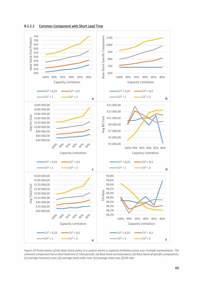
66


Figure 23 Performance of the Base Stock policy in a system where a capacity limitation exists over multiple workstations. The common component has a short lead time (1 time period). (a) Base Stock of end product; (b) Base Stock of specific components; (c) average inventory cost; (d) average back order cost; (e) average total cost; (f) fill-rate

300

350

400

450

500

550

600

650

700

750

100% 99% 95% 90% 85% 80%

Bas

e St

ock

En

d-P

rod

uct

Capacity Limitation

CV² = 0,25 CV² = 0,5

CV² = 1 CV² = 2 a

600

700

800

900

1000

1100

100% 99% 95% 90% 85% 80%Bas

e St

ock

Sp

ecif

ic C

om

po

nen

t

Capacity Limitation

CV² = 0,25 CV² = 0,5

CV² = 1 CV² = 2 b

€40 000,00

€60 000,00

€80 000,00

€100 000,00

€120 000,00

€140 000,00

€160 000,00

€180 000,00

€200 000,00

Avg

Inv

Co

st

Capacity Limitation

CV² = 0,25 CV² = 0,5

CV² = 1 CV² = 2 c

€3 000,00

€5 000,00

€7 000,00

€9 000,00

€11 000,00

€13 000,00

€15 000,00

100% 99% 95% 90% 85% 80%

Avg

BO

Co

st

Capacity Limitation

CV² = 0,25 CV² = 0,5

CV² = 1 CV² = 2 d

€50 000,00

€70 000,00

€90 000,00

€110 000,00

€130 000,00

€150 000,00

€170 000,00

€190 000,00

€210 000,00

Avg

To

tal C

ost

Capacity Limitation

CV² = 0,25 CV² = 0,5

CV² = 1 CV² = 2 e

98,0%

98,2%

98,4%

98,6%

98,8%

99,0%

99,2%

99,4%

99,6%

99,8%

100% 99% 95% 90% 85% 80%

Fill-

Rat

e

Capacity Limitation

CV² = 0,25 CV² = 0,5

CV² = 1 CV² = 2 f

67

The base stock levels of end products in the cases where the common component has short lead time,

follow the same pattern as in the cases with other lead time structures; the higher the demand

variability, the stronger the increase in base stock levels when capacity gets limited. However, these

base stock levels are lower in comparison with the other cases (see 8.2.1). In graph b, the base stock

levels of the specific component are depicted. The follow the same evolution but are higher in

comparison with the other lead time structures. In these cases, the lead time of the specific

components are the longest, logically the base stock levels of these have to be higher. On the other

hand, the lead time of the common components is very short, which positively influences the overall

costs. It can also be seen that, the higher the demand variability, the higher the increase of the base

stock levels when capacity is limited. The graphs c, d, and e show inventory, backlog and total costs

and how they are influenced by a base stock policy. As can be seen in the next graph, inventory costs

follow the same evolution as the base stock levels of the end-products. Backorder costs are much less

predictable. In total, the costs are higher when demand variability is higher. If a company faces high

demand variability extra capacity can positively affect average costs. This is still the case when demand

variability is low, but it will be much less effective (see graph e).

In the following paragraph, the performance of the base stock is compared with the performance of

the linear program. In the first part, a comparison is made where no capacity restriction was imposed.

Secondly, the comparison is made between both policies under the assumption that workstations 1 to

4 are restricted together.

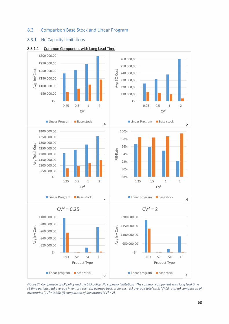
68

8.3 Comparison Base Stock and Linear Program



Figure 24 Comparison of LP policy and the SBS policy. No capacity limitations. The common component with long lead time (4 time periods). (a) average inventory cost; (b) average back order cost; (c) average total cost; (d) fill rate; (e) comparison of inventories (CV² = 0.25); (f) comparison of inventories (CV² = 2).

€-

€50 000,00

€100 000,00

€150 000,00

€200 000,00

€250 000,00

€300 000,00

0,25 0,5 1 2

Avg

In

v C

ost

CV²

Linear Program Base stocka

€-

€10 000,00

€20 000,00

€30 000,00

€40 000,00

€50 000,00

€60 000,00

0,25 0,5 1 2

Avg

BO

Co

stCV²

Linear Program Base stockb

€-

€50 000,00

€100 000,00

€150 000,00

€200 000,00

€250 000,00

€300 000,00

€350 000,00

€400 000,00

0,25 0,5 1 2

Avg

To

tal C

ost

CV²

Linear Program Base stockc

€-

€20 000,00

€40 000,00

€60 000,00

€80 000,00

€100 000,00

END SP SC C

Avg

Inv

Co

st

Product Type

CV² = 0,25

linear program base stocke

€-

€50 000,00

€100 000,00

€150 000,00

€200 000,00

END SP SC C

Avg

Inv

Co

st

Product Type

CV² = 2

linear program base stockf

88%

90%

92%

94%

96%

98%

100%

0,25 0,5 1 2

Fill-

Rat

e

CV²

linear program base stockd

69


Figure 25 Comparison of LP policy and the SBS policy. No capacity limitations. The common component with short lead time (1 time period). (a) average inventory cost; (b) average back order cost; (c) average total cost; (d) fill rate; (e) comparison of inventories (CV² = 0.25); (f) comparison of inventories (CV² = 2).

€-

€50 000,00

€100 000,00

€150 000,00

€200 000,00

€250 000,00

0,25 0,5 1 2

Avg

Inv

Co

st

CV²

Linear Program Base Stocka

€-

€10 000,00

€20 000,00

€30 000,00

€40 000,00

€50 000,00

€60 000,00

0,25 0,5 1 2

Avg

BO

Co

st

CV²

Linear Program Base Stockb

€-

€20 000,00

€40 000,00

€60 000,00

€80 000,00

€100 000,00

END SP SC C

Avg

Inv

Co

st

Product Type

CV² = 0.25

linear program base stocke

€-

€50 000,00

€100 000,00

€150 000,00

€200 000,00

€250 000,00

€300 000,00

0,25 0,5 1 2

Avg

To

tal C

ost

CV²

Linear Program Base Stockc

88%

90%

92%

94%

96%

98%

100%

0,25 0,5 1 2

Fill-

Rat

e

CV²

Linear Program Base Stockd

€-

€50 000,00

€100 000,00

€150 000,00

€200 000,00

END SP SC C

Avg

Inv

Co

st

Product Type

CV² = 2

linear program base stockf

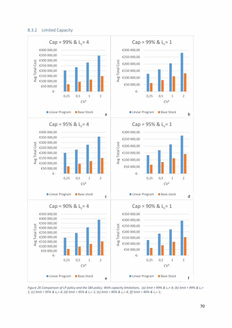
70

8.3.2 Limited Capacity

Figure 26 Comparison of LP policy and the SBS policy. With capacity limitations. (a) limit = 99% & Lc= 4; (b) limit = 99% & Lc= 1; (c) limit = 95% & Lc= 4; (d) limit = 95% & Lc= 1; (e) limit = 90% & Lc= 4; (f) limit = 90% & Lc= 1;

€-

€50 000,00

€100 000,00

€150 000,00

€200 000,00

€250 000,00

€300 000,00

€350 000,00

€400 000,00

0,25 0,5 1 2

Avg

To

tal C

ost

CV²

Cap = 95% & Lc= 4

Linear Program Base stockc

€-

€50 000,00

€100 000,00

€150 000,00

€200 000,00

€250 000,00

€300 000,00

0,25 0,5 1 2

Avg

To

tal C

ost

CV²

Cap = 95% & Lc= 1

Linear Program Base stockd

€-

€50 000,00

€100 000,00

€150 000,00

€200 000,00

€250 000,00

€300 000,00

€350 000,00

€400 000,00

0,25 0,5 1 2

Avg

To

tal C

ost

CV²

Cap = 99% & Lc= 4

Linear Program Base Stocka

€-

€50 000,00

€100 000,00

€150 000,00

€200 000,00

€250 000,00

€300 000,00

0,25 0,5 1 2

Avg

To

tal C

ost

CV²

Cap = 99% & Lc= 1

Linear Program Base Stockb

€-

€50 000,00

€100 000,00

€150 000,00

€200 000,00

€250 000,00

€300 000,00

€350 000,00

€400 000,00

€450 000,00

0,25 0,5 1 2

Avg

To

tal C

ost

CV²

Cap = 90% & Lc= 4

Linear Program Base Stocke

€-

€50 000,00

€100 000,00

€150 000,00

€200 000,00

€250 000,00

€300 000,00

€350 000,00

0,25 0,5 1 2

Avg

To

tal C

ost

CV²

Cap = 90% & Lc= 1

Linear Program Base Stockf

71

It is clear that the synchronized base stock policy outperforms the linear programming based policy in

every instance. When no capacity limitations assumed the synchronized base stock has lower inventory

and backorder costs while achieving a higher fill rate, no matter the demand variance. If we take a look

at the inventories we see that this is mainly caused by a lower end-product inventory in the

synchronized base stock case. In the low variability case the average end-product inventory when using

SBS is almost half of the average end-product inventory when using the linear program. When

variability is higher the difference in end-product inventory is still enormous. The inventories of other

products are also lower when using the SBS policy. Certainly when the lead time of the common

component is long. It seems that under the LP based policy large inventories of the common

component are needed (which is expensive). This is not necessary when the SBS policy is used.

When capacity restrictions are implemented, the same conclusion can be drawn; the linear program

based policy is far more expensive than the SBS policy. No matter the capacity limitation or lead time

structure.

Another striking result is that under the SBS policy, the supply chain was better capable of handling

limited capacity. When the planning decisions were made using the linear program, capacity could be

limited to 90% (or 85% if the lead time of the common component was short). Under the SBS policy,

however, capacity could be limited to 80% and the system could still obtain the 95% service level.

72

9 Conclusions and Recommendations for Future Research

In this paper, two different supply chain planning policies are compared through discrete event

simulation. The performance of both policies was tested under different circumstances of demand

variability and lead time structure. The literature review revealed that the influence of capacity

limitations on the systems’ performance was only rarely researched. For this reason, a procedure was

proposed that could implement capacity limitations in simulations. Two different types of capacity

limitations were researched. In the first type, every workstation had its own maximum capacity (i.e. a

maximum number of products each time period). In the second type, it was assumed that several

machines used the same resource, that was limited. In order to compare the performance of both

policies under the different circumstances, the problem was first described in mathematical form.

Later a simulation procedure necessary to include these capacity limitations was proposed. Finally, the

performance of both policies was tested using discrete event simulation on a fictitious case. Out of

these simulations, several conclusions can be drawn.

Firstly, the base stock policy outperforms the linear program based policy in every case. It is

much cheaper to make processing and release decisions using a synchronized base stock

policy. No matter the capacity limitations, lead time structure or demand variability, the SBS

policy outperformed the linear programming based policy every time. It assures the service

level at lower costs and even obtains a higher fill rate.

The second conclusion that can be drawn is that lead time structure has a big influence on

average holding costs. In this case, the influence of the commonly used component was

extremely high. Reducing common component lead times resulted in significant inventory and

back order savings under both policies. In most cases, it also allows reducing safety stocks.

Thirdly, the base stock policy is more robust when capacity becomes more and more limited.

When capacity is very scarce, the SBS will oftentimes still be capable of assuring the service

level. This is not the case for the LP-based policy.

Finally, under both policies, it is optimal to have the capacity at least at or above the 90% point

(this means that in 90% of the time periods the system is capable of producing what it would

have produced if capacity was unlimited). The actual optimal capacity usage depends on

various factors such as demand variability. Capacity investments seem to pay off the best when

demand variability is high.

The influence of the cost structure has not been researched in this paper. This is a limitation and should

be further investigated. Other assumptions were made for these simulations that are not always

realistic. Lead times were considered fixed and known. In reality, this is not always the case. Only end-

73

products could be bought by customers, oftentimes customers also buy parts or subassemblies (as a

replacement part for example). It was assumed no returns could happen. Relaxing these assumptions

will make the case more realistic and thus give further insight into the performance under both

policies.

It is clear that the linear program based policy does not perform well. One of the reasons can be that

it only calculates safety stocks for end-products, because of this more inventory is needed over the

whole system. Further research should go into the linear program, especially into the procedure that

decides on safety stocks and how high to set them for non-end products.

There are other planning policies (like Kanban) of which the performance was not researched.

Simulating Kanban and other policies may lead to new insights on their performance and help

managers decide on an appropriate policy.

Product structure can influence costs greatly. These two policies were only tested in one case.

Simulating the same policies in other product structures (more or less component commonality,

multiple stages, …) can lead to new insights.

In the case of the SBS policy, when the order-up-to-level did not suffice to assure a 95% non-stock-out

probability, the levels were adjusted manually. Although this policy already outperformed the LP-

based policy, it is not sure that these base-stock levels are the optimum. Other combinations of base

stock levels could exist that assure the service level, at a lower cost. Future research can focus on a

procedure that helps determine the optimal base – stock set.

I

10 Bibliography

Agrawal, N., & Cohen, M. A. (2001). Optimal Material Control in an Assembly System with Component Commonality. Naval Research Logistics, 48, 21.

Aviv, Y. (2001). The effect of collaborative forecasting on supply chain performance. Management Science, 47(10), 1326-1343.

Bagchi, U., & Gutierrez, G. (1992). Effect of increasing component commonality on service level and holding cost. Naval Research Logistics, 39(6), 815-847.

Barbarosoğlu, G., & Özgür, D. (1999). Hierarchical design of an integrated production and 2-echelon distribution system. European Journal of Operational Research, 118(3), 464-484.

Bertrand, J. W. M., & Rutten, W. G. M. M. (1999). Evaluation of three production planning procedures for the use of recipe flexibility. European Journal of Operational Research, 115(1), 179-194.

Brennan, L., & Gupta, S. M. (1993). A structured analysis of material requirements planning systems under combined demand and supply uncertainty. International Journal of Production Research, 31(7), 1689 - 1707.

Cheng, F., Ettl, M., Lin, G., & Yao, D. D. (2002). Inventory-service optimization in configure-to-order systems. Manufacturing & Service Operations Management, 4(2), 114-132.

Choobineh, F., & E.Mohebbi. (2005). The impact of component commonality in an assemble-to-order environment under supply and demand uncertainty. Omega, 33(6), 472-482.

Chopra, S., & Meindl, P. (2007). Supply chain management. Strategy, planning & operation Das Summa Summarum des Management (pp. 265-275): Springer.

Clark, A. J., & Scarf, H. (1960). Optimal policies for a multi-echelon inventory problem. Management Science, 6(4), 475-490.

de Kok, T. G., & Visschers, J. W. C. H. (1999). Analysis of assembly systems with service level constraints. International Journal of Production Economics, 59(1–3), 313-326. doi:http://dx.doi.org/10.1016/S0925-5273(98)00236-9

Diks, E. B., & de Kok, A. G. (1998). Optimal control of a divergent multi-echelon inventory system. European Journal of Operational Research, 111(1), 75-97. doi:http://dx.doi.org/10.1016/S0377-2217(97)00327-5

Diks, E. B., & de Kok, A. G. (1999). Computational results for the control of a divergent N-echelon inventory system. International Journal of Production Economics, 59(1–3), 327-336. doi:http://dx.doi.org/10.1016/S0925-5273(98)00023-1

Dobson, G. (1987). The economic lot-scheduling problem: achieving feasibility using time-varying lot sizes. Operations Research, 35(5), 764-771.

Elmaghraby, S. E. (1978). The economic lot scheduling problem (ELSP): review and extensions. Management Science, 24(6), 587-598.

Forrester, J. W. (1961). Industrial Dynamics: MIT Press, Cambridge,MA. Galbraith, J. (1973). Designing complex organizations: Addison-Wesley. Gfrerer, H., & Zäpfel, G. (1995). Hierarchical model for production planning in the case of uncertain

demand. European Journal of Operational Research, 86(1), 142-161. Hax, A. C., & Meal, H. C. (1973). Hierarchical integration of production planning and scheduling:

Citeseer. Ho, C.-J. (1989). Evaluating the impact of operating environments on MRP system nervousness.

International Journal of Production Research, 27(7), 1115-1135. Hopp, W. J., & Spearman, M. L. (1993). Setting Safety LeadTimes for purchased components in

Assembly Systems. IEE Transactions, 25(2), 2-11. Houtum, G. J. v., Inderfurth, K., & Zijm, W. H. M. (1996). Materials coordination in stochastic multi-

echelon systems. European Journal of Operational Research, 95(1), 1-23. Kok, T. G. d., & Fransoo, J. C. (2002). Planning Supply Chain Operations: Definition and Comparison of

Planning Concepts. Working Paper, 65.

http://dx.doi.org/10.1016/S0925-5273(98)00236-9

http://dx.doi.org/10.1016/S0377-2217(97)00327-5

http://dx.doi.org/10.1016/S0925-5273(98)00023-1

II

Melnyk, S. A., & Piper, C. J. (1985). Lead time errors in MRP: the lot-sizing effect. International Journal of Production Research, 23(2), 253-264.

Meybodi, M. Z., & Foote, B. L. (1995). Hierarchical production planning and scheduling with random demand and production failure. Annals of Operations Research, 59(1), 259-280.

Mula, J., Poler, R., Garcia-Sabater, J. P., & lario, F. C. (2006). Models for production planning under uncertainty: A review. International Journal of Production Economics, 103(1), 271-285.

Raza, A. S., & Akgunduz, A. (2008). A comparative study of heuristic algorithms on economic lot scheduling problem. Computers & Industrial Engineering, 55(1), 94-109.

Schmidt, C. P., & Nahmias, S. (1985). Optimal Policy for a Two-Stage Assembly System under Random Demand. Operations Research, 33(5), 1130-1145.

Song, J.-S., Yano, C. A., & Lerssrisuriya, P. (2000). Contract assembly: dealing with combined supply lead time and demand quantity uncertainty. Manufacturing & Service Operations Management, 2(3), 287-296.

Song, J.-S., & Zipkin, P. (2003). Supply chain operations: Assemble-to-order systems. Handbooks in operations research and management science, 11, 561-596.

Williams, J. G., & Whybark, D. C. (1976). Material Requirements Planning Under Uncertainty. Decision Sciences, 7(4), 595 - 606.

Yano, C. A. (1987). Stochastic Leadtimes in Two-Level Assembly Systems. IIE Trans, 19(4), 371-378.

FACULTY OF ECONOMICS AND BUSINESS …lib.ugent.be/fulltxt/RUG01/002/304/839/RUG01-002304839...Name...

Documents

Transcript of FACULTY OF ECONOMICS AND BUSINESS …lib.ugent.be/fulltxt/RUG01/002/304/839/RUG01-002304839...Name...