
Design Space Exploration of Stream-based Dataflow ...
266
Design Space Exploration of Stream-based Dataflow Architectures Methods and Tools Retargetable Mapping Architecture Instance Descriptions Application Performance Numbers Simulator A.C.J. Kienhuis
Transcript of Design Space Exploration of Stream-based Dataflow ...
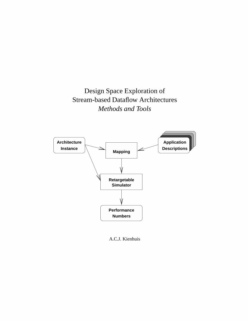
Design Space Exploration ofStream-based Dataflow Architectures
Methods and Tools
Retargetable
Mapping
Architecture
Instance Descriptions
Application
PerformanceNumbers
Simulator
A.C.J. Kienhuis
Design Space Exploration ofStream-based Dataflow Architectures
PROEFSCHRIFT
ter verkrijging van de graad van doctoraan de Technische Universiteit Delft,
op gezag van de Rector Magnificus prof.ir. K.F. Wakker,in het openbaar te verdedigen ten overstaan van een commissie,
door het College voor Promoties aangewezen,op vrijdag 29 Januari 1999 te 10:30 uur
door
Albert Carl Jan KIENHUIS
elektrotechnisch ingenieurgeboren te Vleuten.
Dit proefschrift is goedgekeurd door de promotor:Prof.dr.ir. P.M. Dewilde
Toegevoegd promotor: Dr.ir. E.F. Deprettere.
Samenstelling promotiecommissie:
Rector Magnificus, voorzitterProf.dr.ir. P.M. Dewilde, Technische Universiteit Delft, promotorDr.ir. E.F. Deprettere, Technische Universiteit Delft, toegevoegd promotorIr. K.A. Vissers, Philips Research EindhovenProf.dr.ir. J.L. van Meerbergen, Technische Universiteit EindhovenProf.Dr.-Ing. R. Ernst, Technische Universit¨at BraunschweigProf.dr. S. Vassiliadis, Technische Universiteit DelftProf.dr.ir. R.H.J.M. Otten, Technische Universiteit Delft
Ir. K.A. Vissers en Dr.ir. P. van der Wolf van Philips Research Eindhoven, hebben als begeleidersin belangrijke mate aan de totstandkoming van het proefschrift bijgedragen.
CIP-DATA KONINKLIJKE BIBLIOTHEEK, DEN HAAG
Kienhuis, Albert Carl Jan
Design Space Exploration of Stream-based Dataflow Architectures : Methods and ToolsAlbert Carl Jan Kienhuis. -Delft: Delft University of TechnologyThesis Technische Universiteit Delft. - With index, ref. - With summary in DutchISBN 90-5326-029-3Subject headings: IC-design; Data flow Computing; Systems Analysis
Copyright c 1999 by A.C.J. Kienhuis, Amsterdam, The Netherlands.All rights reserved. No part of the material protected by this copyright notice may be reproduced or utilized in any formor by any means, electronic or mechanical, including photocopying, recording or by any information storage and retrievalsystem, without permission from the author.
Printed in the Netherlands
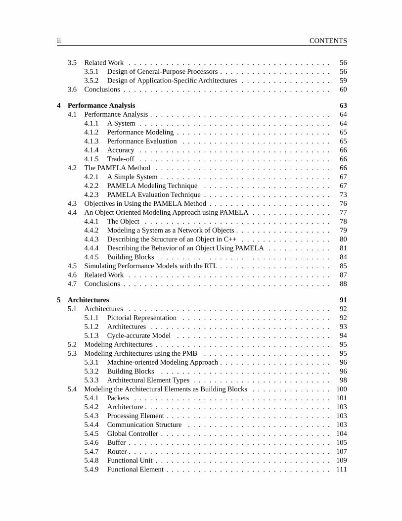
Contents
1 Introduction 11.1 Motivation . . . . . . . . . . . . . . . . . . . . . . . . . . . . . . . . . . . . . . . . 31.2 Video Signal Processing in a TV-set . . . . . . . . . . . . . . . . . . . . . . . . . . 3
1.2.1 TV-set . . . . . . . . . . . . . . . . . . . . . . . . . . . . . . . . . . . . . . 31.2.2 Video Processing Architectures in the TV of the Future . . . . . . . . . . . . 51.2.3 Stream-Based Dataflow Architecture . . . . . . . . . . . . . . . . . . . . . . 6
1.3 Design Space Exploration . . . . . . . . . . . . . . . . . . . . . . . . . . . . . . . . 81.4 Main Contributions of Thesis . . . . . . . . . . . . . . . . . . . . . . . . . . . . . . 91.5 Outline of the Thesis. . . . . . . . . . . . . . . . . . . . . . . . . . . . . . . . . . 11
2 Basic Definitions and Problem Statement 152.1 Stream-based Dataflow Architectures . . . . . . . . . . . . . . . . . . . . . . . . . 16
2.1.1 Definitions . . . . . . . . . . . . . . . . . . . . . . . . . . . . . . . . . . . 162.1.2 Structure . . . . . . . . . . . . . . . . . . . . . . . . . . . . . . . . . . . . 192.1.3 Behavior . . . . . . . . . . . . . . . . . . . . . . . . . . . . . . . . . . . . 22
2.2 The Class of Stream-based Dataflow Architectures . . . . . . . . . . . . . . . . . . 312.2.1 Architecture Template . . . . . . . . . . . . . . . . . . . . . . . . . . . . . 322.2.2 Design Space . . . . . . . . . . . . . . . . . . . . . . . . . . . . . . . . . . 32
2.3 The Designer’s Problem . . . . . . . . . . . . . . . . . . . . . . . . . . . . . . . . 322.3.1 Exploring the Design Space of Architectures . . . . . . . . . . . . . . . . . 332.3.2 Problems in Current Design Approaches . . . . . . . . . . . . . . . . . . . . 33
2.4 Related Work on Dataflow Architectures . . . . . . . . . . . . . . . . . . . . . . . . 342.4.1 Implementation Problems of Dataflow Architectures . . . . . . . . . . . . . 352.4.2 Other Dataflow Architectures . . . . . . . . . . . . . . . . . . . . . . . . . 352.4.3 Implementing Stream-based Dataflow Architectures . . . . . . . . . . . . . 36
2.5 Conclusions . . . . . . . . . . . . . . . . . . . . . . . . . . . . . . . . . . . . . . . 39
3 Solution Approach 433.1 The Evaluation of Alternative Architectures . . . . . . . . . . . . . . . . . . . . . . 44
3.1.1 Quantitative Data. . . . . . . . . . . . . . . . . . . . . . . . . . . . . . . . 443.1.2 The Y-chart Approach . . . . . . . . . . . . . . . . . . . . . . . . . . . . . 44
3.2 Design Space Exploration Using the Y-chart Approach . . . . . . . . . . . . . . . . 453.3 Requirements of the Y-chart Approach . . . . . . . . . . . . . . . . . . . . . . . . . 46
3.3.1 Performance Analysis . . . . . . . . . . . . . . . . . . . . . . . . . . . . . 473.3.2 Mapping . . . . . . . . . . . . . . . . . . . . . . . . . . . . . . . . . . . . 52
3.4 Development of a Y-chart Environment . . . . . . . . . . . . . . . . . . . . . . . . 55
i
ii CONTENTS
3.5 Related Work . . . . . . . . . . . . . . . . . . . . . . . . . . . . . . . . . . . . . . 563.5.1 Design of General-Purpose Processors . . . . . . . . . . . . . . . . . . . . . 563.5.2 Design of Application-Specific Architectures . . . . . . . . . . . . . . . . . 59
3.6 Conclusions . . . . . . . . . . . . . . . . . . . . . . . . . . . . . . . . . . . . . . . 60
4 Performance Analysis 634.1 Performance Analysis . . . . . . . . . . . . . . . . . . . . . . . . . . . . . . . . . . 64
4.1.1 A System . . . . . . . . . . . . . . . . . . . . . . . . . . . . . . . . . . . . 644.1.2 Performance Modeling . . . . . . . . . . . . . . . . . . . . . . . . . . . . . 654.1.3 Performance Evaluation . . . . . . . . . . . . . . . . . . . . . . . . . . . . 654.1.4 Accuracy . . . . . . . . . . . . . . . . . . . . . . . . . . . . . . . . . . . . 664.1.5 Trade-off . . . . . . . . . . . . . . . . . . . . . . . . . . . . . . . . . . . . 66
4.2 The PAMELA Method . . . . . . . . . . . . . . . . . . . . . . . . . . . . . . . . . 664.2.1 A Simple System . . . . . . . . . . . . . . . . . . . . . . . . . . . . . . . . 674.2.2 PAMELA Modeling Technique . . . . . . . . . . . . . . . . . . . . . . . . 674.2.3 PAMELA Evaluation Technique . . . . . . . . . . . . . . . . . . . . . . . . 73
4.3 Objectives in Using the PAMELA Method . . . . . . . . . . . . . . . . . . . . . . . 764.4 An Object Oriented Modeling Approach using PAMELA . . . . . . . . . . . . . . . 77
4.4.1 The Object . . . . . . . . . . . . . . . . . . . . . . . . . . . . . . . . . . . 784.4.2 Modeling a System as a Network of Objects . . . . . . . . . . . . . . . . . . 794.4.3 Describing the Structure of an Object in C++ . . . . . . . . . . . . . . . . . 804.4.4 Describing the Behavior of an Object Using PAMELA . . . . . . . . . . . . 814.4.5 Building Blocks . . . . . . . . . . . . . . . . . . . . . . . . . . . . . . . . 84
4.5 Simulating Performance Models with the RTL . . . . . . . . . . . . . . . . . . . . . 854.6 Related Work . . . . . . . . . . . . . . . . . . . . . . . . . . . . . . . . . . . . . . 874.7 Conclusions . . . . . . . . . . . . . . . . . . . . . . . . . . . . . . . . . . . . . . . 88
5 Architectures 915.1 Architectures . . . . . . . . . . . . . . . . . . . . . . . . . . . . . . . . . . . . . . 92
5.1.1 Pictorial Representation . . . . . . . . . . . . . . . . . . . . . . . . . . . . 925.1.2 Architectures . . . . . . . . . . . . . . . . . . . . . . . . . . . . . . . . . . 935.1.3 Cycle-accurate Model .. . . . . . . . . . . . . . . . . . . . . . . . . . . . 94
5.2 Modeling Architectures . . . . . . . . . . . . . . . . . . . . . . . . . . . . . . . . . 955.3 Modeling Architectures using the PMB . . . . . . . . . . . . . . . . . . . . . . . . 95
5.3.1 Machine-oriented Modeling Approach . . . . . . . . . . . . . . . . . . . . . 965.3.2 Building Blocks . . . . . . . . . . . . . . . . . . . . . . . . . . . . . . . . 965.3.3 Architectural Element Types . . . . . . . . . . . . . . . . . . . . . . . . . . 98
5.4 Modeling the Architectural Elements as Building Blocks . . . . . . . . . . . . . . . 1005.4.1 Packets . . . . . . . . . . . . . . . . . . . . . . . . . . . . . . . . . . . . . 1015.4.2 Architecture . . . . . . . . . . . . . . . . . . . . . . . . . . . . . . . . . . . 1035.4.3 Processing Element . . . . . . . . . . . . . . . . . . . . . . . . . . . . . . . 1035.4.4 Communication Structure . . . . . . . . . . . . . . . . . . . . . . . . . . . 1035.4.5 Global Controller . . . . . . . . . . . . . . . . . . . . . . . . . . . . . . . . 1045.4.6 Buffer . . . . . . . . . . . . . . . . . . . . . . . . . . . . . . . . . . . . . . 1055.4.7 Router . . . . . . . . . . . . . . . . . . . . . . . . . . . . . . . . . . . . . . 1075.4.8 Functional Unit . . . . . . . . . . . . . . . . . . . . . . . . . . . . . . . . . 1095.4.9 Functional Element . . . . . . . . . . . . . . . . . . . . . . . . . . . . . . . 111
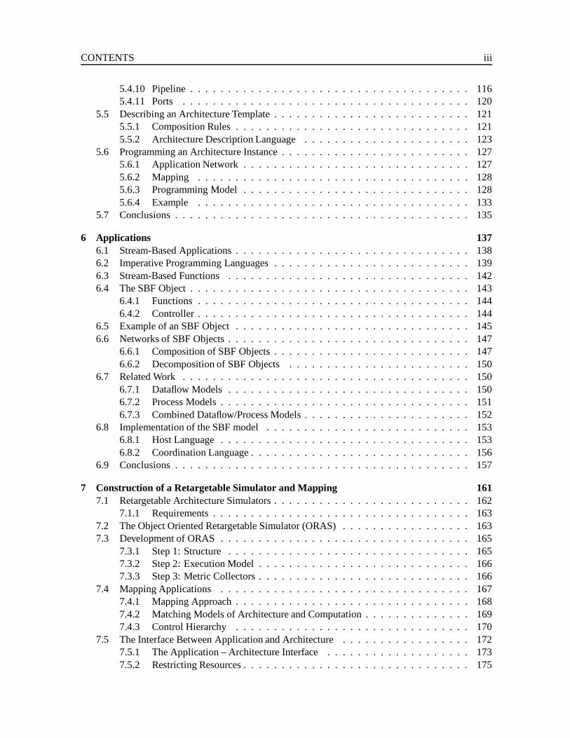
CONTENTS iii
5.4.10 Pipeline . . . . . . . . . . . . . . . . . . . . . . . . . . . . . . . . . . . . . 1165.4.11 Ports . . . . . . . . . . . . . . . . . . . . . . . . . . . . . . . . . . . . . . 120
5.5 Describing an Architecture Template . . . . . . . . . . . . . . . . . . . . . . . . . . 1215.5.1 Composition Rules . . .. . . . . . . . . . . . . . . . . . . . . . . . . . . . 1215.5.2 Architecture Description Language. . . . . . . . . . . . . . . . . . . . . . 123
5.6 Programming an Architecture Instance . . . . . . . . . . . . . . . . . . . . . . . . . 1275.6.1 Application Network . . . . . . . . . . . . . . . . . . . . . . . . . . . . . . 1275.6.2 Mapping . . . . . . . . . . . . . . . . . . . . . . . . . . . . . . . . . . . . 1285.6.3 Programming Model . . . . . . . . . . . . . . . . . . . . . . . . . . . . . . 1285.6.4 Example . . . . . . . . . . . . . . . . . . . . . . . . . . . . . . . . . . . . 133
5.7 Conclusions . . . . . . . . . . . . . . . . . . . . . . . . . . . . . . . . . . . . . . . 135
6 Applications 1376.1 Stream-Based Applications . . . . . . . . . . . . . . . . . . . . . . . . . . . . . . . 1386.2 Imperative Programming Languages. . . . . . . . . . . . . . . . . . . . . . . . . . 1396.3 Stream-Based Functions . . . . . . . . . . . . . . . . . . . . . . . . . . . . . . . . 1426.4 The SBF Object . . . . . . . . . . . . . . . . . . . . . . . . . . . . . . . . . . . . . 143
6.4.1 Functions . . . . . . . . . . . . . . . . . . . . . . . . . . . . . . . . . . . . 1446.4.2 Controller . . . . . . . . . . . . . . . . . . . . . . . . . . . . . . . . . . . . 144
6.5 Example of an SBF Object . . . . . . . . . . . . . . . . . . . . . . . . . . . . . . . 1456.6 Networks of SBF Objects . . . . . . . . . . . . . . . . . . . . . . . . . . . . . . . . 147
6.6.1 Composition of SBF Objects. . . . . . . . . . . . . . . . . . . . . . . . . . 1476.6.2 Decomposition of SBF Objects. . . . . . . . . . . . . . . . . . . . . . . . 150
6.7 Related Work . . . . . . . . . . . . . . . . . . . . . . . . . . . . . . . . . . . . . . 1506.7.1 Dataflow Models . . . . . . . . . . . . . . . . . . . . . . . . . . . . . . . . 1506.7.2 Process Models . . . . . . . . . . . . . . . . . . . . . . . . . . . . . . . . . 1516.7.3 Combined Dataflow/Process Models . . . . . . . . . . . . . . . . . . . . . . 152
6.8 Implementation of the SBF model . . . . . . . . . . . . . . . . . . . . . . . . . . . 1536.8.1 Host Language. . . . . . . . . . . . . . . . . . . . . . . . . . . . . . . . . 1536.8.2 Coordination Language .. . . . . . . . . . . . . . . . . . . . . . . . . . . . 156
6.9 Conclusions . . . . . . . . . . . . . . . . . . . . . . . . . . . . . . . . . . . . . . . 157
7 Construction of a Retargetable Simulator and Mapping 1617.1 Retargetable Architecture Simulators . . . . . . . . . . . . . . . . . . . . . . . . . . 162
7.1.1 Requirements . . . . . . . . . . . . . . . . . . . . . . . . . . . . . . . . . . 1637.2 The Object Oriented Retargetable Simulator (ORAS) . . . . . . . . . . . . . . . . . 1637.3 Development of ORAS . . . . . . . . . . . . . . . . . . . . . . . . . . . . . . . . . 165
7.3.1 Step 1: Structure . . . . . . . . . . . . . . . . . . . . . . . . . . . . . . . . 1657.3.2 Step 2: Execution Model . . . . . . . . . . . . . . . . . . . . . . . . . . . . 1667.3.3 Step 3: Metric Collectors . . . . . . . . . . . . . . . . . . . . . . . . . . . . 166
7.4 Mapping Applications . . . . . . . . . . . . . . . . . . . . . . . . . . . . . . . . . 1677.4.1 Mapping Approach . . . . . . . . . . . . . . . . . . . . . . . . . . . . . . . 1687.4.2 Matching Models of Architecture and Computation . . . . . . . . . . . . . . 1697.4.3 Control Hierarchy . . . . . . . . . . . . . . . . . . . . . . . . . . . . . . . 170
7.5 The Interface Between Application and Architecture . . . . . . . . . . . . . . . . . 1727.5.1 The Application – Architecture Interface . . . . . . . . . . . . . . . . . . . 1737.5.2 Restricting Resources . . . . . . . . . . . . . . . . . . . . . . . . . . . . . . 175
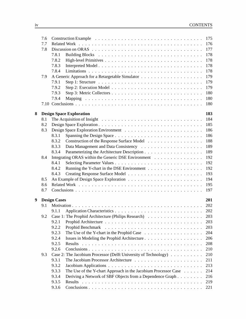
iv CONTENTS
7.6 Construction Example . . . . . . . . . . . . . . . . . . . . . . . . . . . . . . . . . 1757.7 Related Work . . . . . . . . . . . . . . . . . . . . . . . . . . . . . . . . . . . . . . 1767.8 Discussion on ORAS . . . . . . . . . . . . . . . . . . . . . . . . . . . . . . . . . . 177
7.8.1 Building Blocks . . . . . . . . . . . . . . . . . . . . . . . . . . . . . . . . 1787.8.2 High-level Primitives . . . . . . . . . . . . . . . . . . . . . . . . . . . . . . 1787.8.3 Interpreted Model . . . . . . . . . . . . . . . . . . . . . . . . . . . . . . . . 1787.8.4 Limitations . . . . . . . . . . . . . . . . . . . . . . . . . . . . . . . . . . . 178
7.9 A Generic Approach for a Retargetable Simulator . . . . . . . . . . . . . . . . . . . 1797.9.1 Step 1: Structure . . . . . . . . . . . . . . . . . . . . . . . . . . . . . . . . 1797.9.2 Step 2: Execution Model . . . . . . . . . . . . . . . . . . . . . . . . . . . . 1797.9.3 Step 3: Metric Collectors . . . . . . . . . . . . . . . . . . . . . . . . . . . . 1807.9.4 Mapping . . . . . . . . . . . . . . . . . . . . . . . . . . . . . . . . . . . . 180
7.10 Conclusions . . . . . . . . . . . . . . . . . . . . . . . . . . . . . . . . . . . . . . . 180
8 Design Space Exploration 1838.1 The Acquisition of Insight . . .. . . . . . . . . . . . . . . . . . . . . . . . . . . . 1848.2 Design Space Exploration . . . . . . . . . . . . . . . . . . . . . . . . . . . . . . . . 1858.3 Design Space Exploration Environment . . . . . . . . . . . . . . . . . . . . . . . . 186
8.3.1 Spanning the Design Space . . . . . . . . . . . . . . . . . . . . . . . . . . . 1868.3.2 Construction of the Response Surface Model. . . . . . . . . . . . . . . . . 1888.3.3 Data Management and Data Consistency . . . . . . . . . . . . . . . . . . . 1898.3.4 Parameterizing the Architecture Description . . . . . . . . . . . . . . . . . . 189
8.4 Integrating ORAS within the Generic DSE Environment . . . . . . . . . . . . . . . 1928.4.1 Selecting Parameter Values . . . . . . . . . . . . . . . . . . . . . . . . . . . 1928.4.2 Running the Y-chart in the DSE Environment. . . . . . . . . . . . . . . . . 1928.4.3 Creating Response Surface Model. . . . . . . . . . . . . . . . . . . . . . . 193
8.5 An Example of Design Space Exploration . . . . . . . . . . . . . . . . . . . . . . . 1948.6 Related Work . . . . . . . . . . . . . . . . . . . . . . . . . . . . . . . . . . . . . . 1958.7 Conclusions . . . . . . . . . . . . . . . . . . . . . . . . . . . . . . . . . . . . . . . 197
9 Design Cases 2019.1 Motivation . . . . . . . . . . . . . . . . . . . . . . . . . . . . . . . . . . . . . . . . 202
9.1.1 Application Characteristics . . . . . . . . . . . . . . . . . . . . . . . . . . . 2029.2 Case 1: The Prophid Architecture (Philips Research). . . . . . . . . . . . . . . . . 203
9.2.1 Prophid Architecture . .. . . . . . . . . . . . . . . . . . . . . . . . . . . . 2039.2.2 Prophid Benchmark . .. . . . . . . . . . . . . . . . . . . . . . . . . . . . 2039.2.3 The Use of the Y-chart in the Prophid Case .. . . . . . . . . . . . . . . . . 2049.2.4 Issues in Modeling the Prophid Architecture .. . . . . . . . . . . . . . . . . 2069.2.5 Results . . . . . . . . . . . . . . . . . . . . . . . . . . . . . . . . . . . . . 2089.2.6 Conclusions . . . . . . . . . . . . . . . . . . . . . . . . . . . . . . . . . . . 210
9.3 Case 2: The Jacobium Processor (Delft University of Technology). . . . . . . . . . 2109.3.1 The Jacobium Processor Architecture . . . . . . . . . . . . . . . . . . . . . 2119.3.2 Jacobium Applications . . . . . . . . . . . . . . . . . . . . . . . . . . . . . 2139.3.3 The Use of the Y-chart Approach in the Jacobium Processor Case . . . . . . 2149.3.4 Deriving a Network of SBF Objects from a Dependence Graph . . . . . . . . 2169.3.5 Results . . . . . . . . . . . . . . . . . . . . . . . . . . . . . . . . . . . . . 2199.3.6 Conclusions . . . . . . . . . . . . . . . . . . . . . . . . . . . . . . . . . . . 221
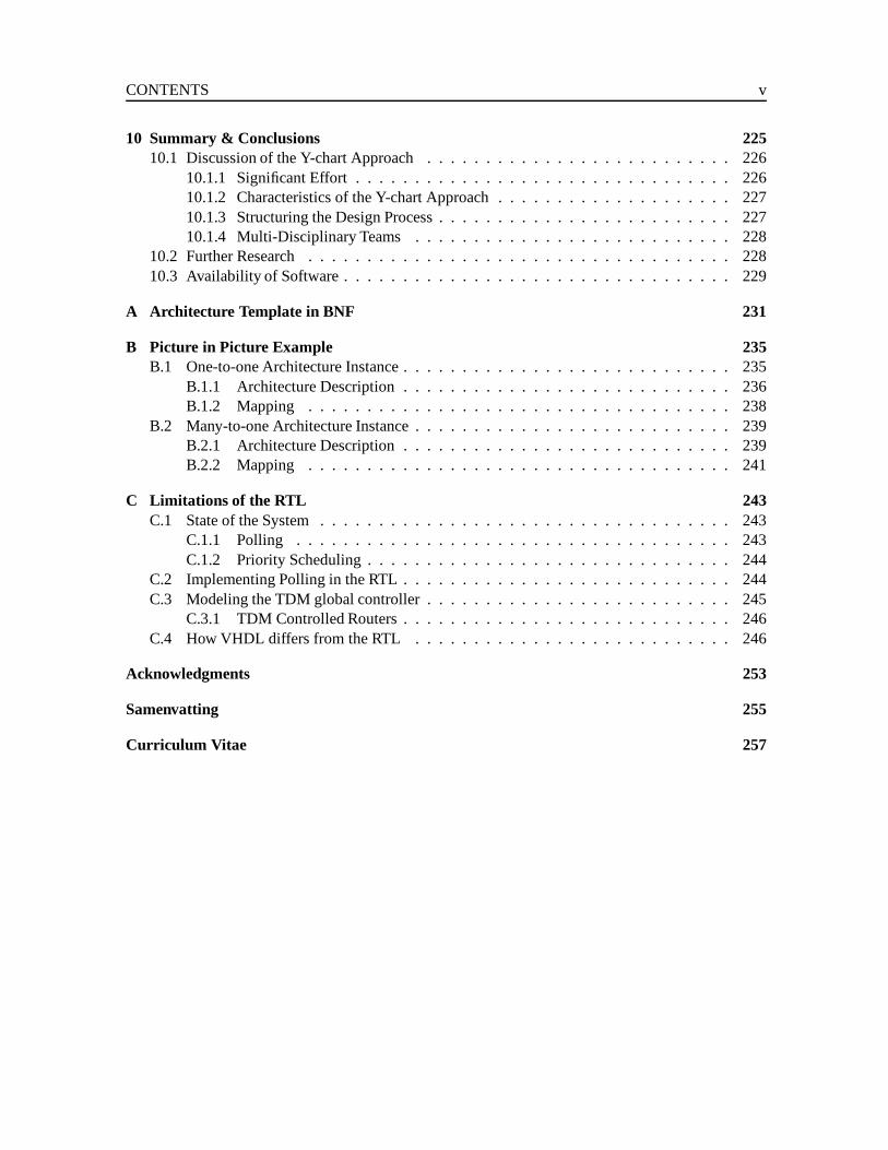
CONTENTS v
10 Summary & Conclusions 22510.1 Discussion of the Y-chart Approach . . . . . . . . . . . . . . . . . . . . . . . . . . 226
10.1.1 Significant Effort . . . . . . . . . . . . . . . . . . . . . . . . . . . . . . . . 22610.1.2 Characteristics of the Y-chart Approach . . . . . . . . . . . . . . . . . . . . 22710.1.3 Structuring the Design Process . . . . . . . . . . . . . . . . . . . . . . . . . 22710.1.4 Multi-Disciplinary Teams . . . . . . . . . . . . . . . . . . . . . . . . . . . 228
10.2 Further Research . . . . . . . . . . . . . . . . . . . . . . . . . . . . . . . . . . . . 22810.3 Availability of Software. . . . . . . . . . . . . . . . . . . . . . . . . . . . . . . . . 229
A Architecture Template in BNF 231
B Picture in Picture Example 235B.1 One-to-one Architecture Instance . . . . . . . . . . . . . . . . . . . . . . . . . . . . 235
B.1.1 Architecture Description . . . . . . . . . . . . . . . . . . . . . . . . . . . . 236B.1.2 Mapping . . . . . . . . . . . . . . . . . . . . . . . . . . . . . . . . . . . . 238
B.2 Many-to-one Architecture Instance . . . . . . . . . . . . . . . . . . . . . . . . . . . 239B.2.1 Architecture Description . . . . . . . . . . . . . . . . . . . . . . . . . . . . 239B.2.2 Mapping . . . . . . . . . . . . . . . . . . . . . . . . . . . . . . . . . . . . 241
C Limitations of the RTL 243C.1 State of the System . . . . . . . . . . . . . . . . . . . . . . . . . . . . . . . . . . . 243
C.1.1 Polling . . . . . . . . . . . . . . . . . . . . . . . . . . . . . . . . . . . . . 243C.1.2 Priority Scheduling . . . . . . . . . . . . . . . . . . . . . . . . . . . . . . . 244
C.2 Implementing Polling in the RTL. . . . . . . . . . . . . . . . . . . . . . . . . . . . 244C.3 Modeling the TDM global controller . . . . . . . . . . . . . . . . . . . . . . . . . . 245
C.3.1 TDM Controlled Routers . . . . . . . . . . . . . . . . . . . . . . . . . . . . 246C.4 How VHDL differs from the RTL . . . . . . . . . . . . . . . . . . . . . . . . . . . 246
Acknowledgments 253
Samenvatting 255
Curriculum Vitae 257
Chapter 1
Introduction
Contents
1.1 Motivation . . . . . . . . . . . . . . . . . . . . . . . . . . . . . . . . . . . . . . 3
1.2 Video Signal Processing in a TV-set . . . . . . . . . . . . . . . . . . . . . . . . 3
1.2.1 TV-set . . . . . . . . . . . . . . . . . . . . . . . . . . . . . . . . . . . . . 3
1.2.2 Video Processing Architectures in the TV of the Future . . . . . . . . . . . 5
1.2.3 Stream-Based Dataflow Architecture . . . . . . . . . . . . . . . . . . . . . 6
1.3 Design Space Exploration . . . . . . . . . . . . . . . . . . . . . . . . . . . . . . 8
1.4 Main Contributions of Thesis . . . . . . . . . . . . . . . . . . . . . . . . . . . . 9
1.5 Outline of the Thesis . . . . . . . . . . . . . . . . . . . . . . . . . . . . . . . . . 11
THE increasing digitalizationof information in text, speech, video, audio and graphics has resultedin a whole new variety of digital signal processing (DSP) applications like compression and
decompression, encryption, and all kinds of quality improvements [Negroponte, 1995]. A prerequisitefor making these signal processing applications available to the consumer market is their cost-effectiverealization into silicon. This leads to a demand for new application-specific architectures that areincreasinglyprogrammablei.e., architectures that can execute a set of applications instead of onlyone specific application. By reprogramming these architectures, they can execute other applicationswith the same resources, which makes these programmable architectures cost-effective. In the nearfuture, these architectures should find their way into consumer products like TV-sets, set-top boxes,multi-media terminals, and other multi-media products, as well as in wireless communication and lowcost radar systems.
The trend toward architectures that are more and more programmable represents, as argued by Leeand Messerschmitt [1998], the first major shift in electrical engineering since the transitions fromanalog to digital electronics and from vacuum tubes to semiconductors. However, general and struc-tured approaches are lacking for designing application-specific architectures that are sufficiently pro-grammable.
The current practice is to design application-specific architectures at a detailed level using hard-ware description languages like VHDL [1993] (Very high speed IC hardware description Language)or Verilog. A consequence of this approach is that designers work with very detailed descriptions ofarchitectures. The level of detail involved limits the design space of the architectures that they canexplore, which gives them little freedom to make trade-offs between programmability, utilization of
1
2 Introduction
resources, and silicon area. Because designers cannot make these trade-offs, designs end up underuti-lizing their resources and silicon area and are thus unnecessarily expensive, or they cannot satisfy theimposed design objectives.
The development of programmable architectures that execute widely different applications hasalready been being worked on for decades in the domain of general-purpose processors. These pro-cessors can execute a word-processing application or a spreadsheet application or can even simulatesome complex physical phenomenon, all on the same piece of silicon. Currently, these processors aredesigned by constructing performance models of processors at different levels of abstraction rangingfrom instruction level models to Register Transfer Level (RTL) models [Bose and Conte, 1998; Hen-nessy and Heinrich, 1996]. Theseperformance modelscan be evaluated to provide data for variousperformance metricsof a processor, like resource utilization and compute power while processing aworkload. A workload is typically a suite ofbenchmarks, i.e., a set of typical applications a proces-sor should execute. Measuring the performance of a processor deliversquantitativedata. This dataallows designers to explore the design space of processors at various levels of detail and to maketrade-offs at the different levels between, for example, the utilization of resources and performance ofprocessors. Moreover, quantitative data gives designers insight, at various levels of detail, into how tofurther improve architectures and serves as an objective basis for discussion of possible architectureimprovements.
The benchmark approach practiced in general-purpose processor architecture design leads tofinely tuned architectures targeted at particular markets. When the benchmark approach was initiallyintroduced at the beginning of the 1980s, it revolutionized general-purpose processor design, whichresulted in the development of RISC-style processors [Patterson, 1985]. These processor architectureswere smaller, faster, less expensive and easier to program than any conventional processor architectureof that time [Hennessy and Patterson, 1996].
General-purpose processors, although programmable, are not powerful enough to execute the dig-ital signal processing applications we are aiming at, as we will explain soon. Special application-specific architectures are therefore required that are nonetheless programmable to some extent. Thebenchmark approach used in the design of general-purpose processors is also useful in the design ofthe programmable application-specific architectures emerging now, as we show in this thesis. We willdevelop and implement in this thesis a benchmark approach, which we call the Y-chart approach, for aparticular class of programmable application-specific architecture calledStream-Based Dataflow Ar-chitecture. The benchmark approach we develop results in an environment in which designers are ableto perform design space exploration for the stream-based dataflow architecture at a level of abstractionthat is higher than that offered by standard hardware description languages.
In Section 1.1 of this chapter we explain further why programmable application-specific architec-tures will emerge for digital signal processing applications. Following this, in Section 1.2 we discussas an example the video signal processing architecture in a modern TV-set. Based on this example, weillustrate how the trend towards programmable architectures will affect the next generation of TV-setsand explain why general-purpose processors are not capable of providing the required performanceat acceptable cost. We focus on the stream-based dataflow architecture in TV-sets. In Section 1.3 weindicate how we are going to explore the design space of this architecture at a high level of abstraction.This chapter concludes with the statement of the main contributions of this thesis in Section 1.4 andthe further outline for the thesis in Section 1.5.

Introduction 3
1.1 Motivation
New advanced digital signal processing applications like signal compression and decompression, en-cryption, and all kinds of quality improvements become feasible on a single chip because the numberof transistors on a single die is still increasing, as predicted by Moore’s law. Digital signal pro-cessing applications involvereal-timeprocessing, which implies that these applications take in andproduce samples at a particular guaranteed rate, even under worst-case conditions. In addition, theseapplications are very demanding with respect tocomputational power, i.e., the number of operationsperformed in time, andbandwidth, i.e., the amount of data transported in time.
Architectures that realize the new applications cost-effectively in silicon must be able first of allto deliver enough processing power and bandwidth to execute the applications and secondly to satisfythe real-time requirements of the applications. The design of such new architecture configurations isbecoming an increasingly intricate process. Architectures are becoming increasingly programmableso that they can supportmulti-functionalproducts as well asmulti-standardproducts (like a mobiletelephone operational worldwide). In the design of these architectures, it is no longer the performanceof a single application that matters, but the performance of aset of applications. This impedes the de-sign of architectures that must satisfy all the given constraints such as real-time processing, utilizationof the resources, and programmability.
Before we look in more depth into the design problems of these new architectures, we illustratethe trend towards more programmable application-specific architectures by looking at the video signalprocessing architecture inside a modern television. In this domain, the need for architectures that canexecute a set of applications is clearly present.
1.2 Video Signal Processing in a TV-set
The trend towards devising new signal processing architectures that are programmable is clearly vis-ible in the domain of consumer market TV-sets, where the digital revolution started in the 1980s andearly 1990s. In this period, the signal processing architecture inside a TV-set moved from analogprocessing to digital processing, whereby analog functions were replaced by digital functions. Theall-digital TV architecture together with the expected continuation of transistor miniaturization in thesemiconductor industry has led to increased demand for new innovative signal processing architec-tures.
1.2.1 TV-set
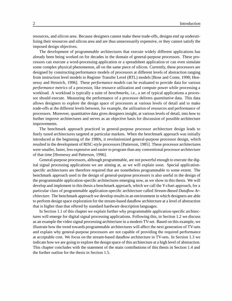
The signal path within a TV-set consists of three sections: afront-end and baseband processing sec-tion, avideo signal processing section, and adisplay section, as shown in Figure 1.1. The first sectiontransforms a TV-signal coming from an outside source like an aerial antenna into a signal that thedisplay section visualizes on a display device, for example a Cathode Ray Tube (CRT). In betweenthese two sections is an analog video signal processing section that makes a received signal suitablefor display.
As the video signal processing section evolves from being analog to fully digital, a whole range ofnew applications becomes available through digital signal processing. Examples of new digital appli-cations that improve the quality of images are luminance peaking [Jaspers and de With, 1997], noisereduction, and ghost image cancellation. Examples of complete new applications are picture reduc-tion (Picture in Picture), picture enlargement (Zoom) [Janssen et al., 1997], and motion compensated100Hz image conversions [de Haan et al., 1996].
4 1.2 Video Signal Processing in a TV-set
Cathode Ray Tube
Signal Processing
Front-end &BasebandProcessing
Video Display Device
Figure 1.1 . The signal path within a TV-set consists of three sections: a front-end andbaseband processing section, a video signal processing section, and a display section.
A TV-set must also be compatible with an increasing variety of standards. Signals containingcontent to be displayed may be delivered through many different sources, like cable TV, a satellitedish, a computer, video recorder (VCR), or a set-top box. Traditionally these formats have compliedwith conventional formats like NTSC (National Television System Committee), PAL (Phase Alternat-ing Line), or SECAM (Sequentiel `a Memoire), but increasingly often they are now also complyingwith emerging standards like various types of MPEG (Moving Picture Expert Group) and computerstandards like SVGA (Super Video Graphics Array).
The increasing demand for new digital applications by consumers and the need for TV-sets tocomply to different standards has made a more complex video signal processing section necessaryin TV-sets [Claasen, 1993]. The video signal processing section of a modern high-end TV-set isshown in Figure 1.2. Each of the applications shown has its own hardware processing unit, Whennew applications are added, new hardware units are incorporated into the video signal processingarchitecture to support them. Since the customer does not select all applications at the same time, thearchitecture uses these units uneconomically.
PAL
NTSC
SECAM
SVGA
MPEG
100Hz
PiP
TeleText
Graphics
NoiseReduction
Zoom
CancelGhost
Figure 1.2 . Video signal processing section of a modern high-end TV-set.
Because each hardware unit is dedicated to one particular application, it is not possible for appli-cations to share hardware units. However, if the hardware units were made less dedicated (which wediscuss later in this chapter), hardware units could be used to support more than one application. Theseprogrammable architectures of tomorrow could be reprogrammed to execute other applications with
Introduction 5
the same amount of resources, thus improving the utilization of silicon in implementing architectures.Thus, these architectures become cost effective for a set of applications.
1.2.2 Video Processing Architectures in the TV of the Future
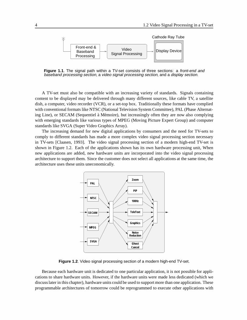
The architecture most likely to be found in the TV-set of tomorrow [Claasen, 1993] will look similarto the structure illustrated in Figure 1.3. This architecture is built around a programmable communi-cation network to which various elements connect. The video-in processor consists of several inputchannels. The video-out processor takes an output signal to the display section. A collection of pro-cessing elements (PEs) operate as hardware-accelerators, and a general purpose processor and a largehigh-bandwidth memory are present as well. The set of processing elements have their own controllerand operate very independently (but not completely) of the general-purpose processor.
ProcessorPurposeGeneral
VideoOut
Controller
PE 1 PE 2 PE 3
Weakly Programmable
VideoIn
Streams
Programmable Communication Network
High BandwidthMemory
Parallelism
Figure 1.3 . TV architecture of tomorrow.
The architecture in Figure 1.3 combines two architecture concepts: a general-purpose processorand the architecture enclosed by the dashed line. These two concepts are needed because of the largevariety of timing constraints present in a TV-set, as we will show. The general-purpose processorprocesses reactive tasks (e.g., a user pressing on the volume button on the remote control) and controltasks (e.g., controlling the menus displayed on the screen and their functions). The dedicated pro-cessing elements, on the other hand, execute data processing tasks, i.e., the digital signal processingapplications.
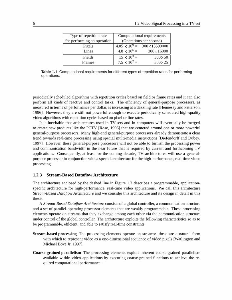
The large variations in timing constraints are caused by the structure of TV-signals. For example,a standard PAL video signal consists of a sequence of frames presented at a rate of 25 interlaced videoframesper second. Each frame consists of twofields: an even field containing the even video linesand an odd field containing the odd video lines. A field has 312 videolines, and each line consistsof 864 videopixels. Algorithms that operate on PAL video signals with different repetition periods –either pixels, lines, fields, or frames – result in very different computational requirements. Supposean algorithm consists of 300 RISC-like operations and operates periodically on pixels, lines, fields,or frames. The vastly different computational requirements are given in Table 1.1. An algorithmoperating at a field rate would perform 50�300, or 15,000 operations per second. An algorithmoperating at a pixel rate would perform 13.5M�300 operations per second, which is 4 Giga operationsper second.
A general-purpose processor (e.g., a RISC processor) is considered powerful enough to execute
6 1.2 Video Signal Processing in a TV-set
Type of repetition rate Computational requirementsfor performing an operation (Operations per second)
Pixels 4.05� 109 = 300�13500000Lines 4.8� 106 = 300�16000
Fields 15� 103 = 300�50Frames 7.5� 102 = 300�25
Table 1.1 . Computational requirements for different types of repetition rates for performingoperations.
periodically scheduled algorithms with repetition cycles based on field or frame rates and it can alsoperform all kinds of reactive and control tasks. The efficiency of general-purpose processors, asmeasured in terms of performance per dollar, is increasing at a dazzling rate [Hennessy and Patterson,1996]. However, they are still not powerful enough to execute periodically scheduled high-qualityvideo algorithms with repetition cycles based on pixel or line rates.
It is inevitable that architectures used in TV-sets and in computers will eventually be mergedto create new products like the PCTV [Rose, 1996] that are centered around one or more powerfulgeneral-purpose processors. Many high-end general-purpose processors already demonstrate a cleartrend towards real-time processing using special multi-media instructions [Diefendorff and Dubey,1997]. However, these general-purpose processors will not be able to furnish the processing powerand communication bandwidth in the near future that is required by current and forthcoming TVapplications. Consequently, at least for the coming decade, TV architectures will use a general-purpose processor in conjunction with a special architecture for the high-performance, real-time videoprocessing.
1.2.3 Stream-Based Dataflow Architecture
The architecture enclosed by the dashed line in Figure 1.3 describes a programmable, application-specific architecture for high-performance, real-time video applications. We call this architectureStream-Based Dataflow Architectureand we consider this architecture and its design in detail in thisthesis.
A Stream-Based Dataflow Architectureconsists of a global controller, a communication structureand a set of parallel-operating processor elements that are weakly programmable. These processingelements operate on streams that they exchange among each other via the communication structureunder control of the global controller. The architecture exploits the following characteristics so as tobe programmable, efficient, and able to satisfy real-time constraints.
Stream-based processingThe processing elements operate on streams: these are a natural formwith which to represent video as a one-dimensional sequence of video pixels [Watlington andMichael Bove Jr, 1997].
Coarse-grained parallelism The processing elements exploit inherent coarse-grained parallelismavailable within video applications by executing coarse-grained functions to achieve the re-quired computational performance.

Introduction 7
Weakly Programmable The processing elements implement a limited set of coarse-grained func-tions that provide the processing elements with the flexibility required to support a set of appli-cations.
The granularity of the functions implemented by the processing elements highly influences theefficiency of stream-based dataflow architectures. The granularity of the functions has two extremes,as illustrated in Figure 1.4.
At one end of the spectrum, there are Application Specific Integrated Circuits (ASICs). Here,each ASIC implements one video application like luminance peaking, noise reduction, or picturein picture. An ASIC can only execute one application very efficiently in terms of silicon use. Atthe other end of the spectrum are programmable domain specific architectures like the VSP [Visserset al., 1995] or Paddi [Chen, 1992]. These architectures use processing elements that implement smallsets of fine-grained functions like add, subtract, and compare. These fine-grained functions allowthe architectures to execute a wide range of video applications belonging to a specific applicationdomain while satisfying real-time constraints. However, in order to support this programmability,these architectures dedicate a substantial part of their silicon area to control and communication andless to the actual computation.
For some video applications a gap of a factor of ten to twenty is found in silicon efficiency betweenan ASIC solution and a programmable solution [Lippens et al., 1996, 1991]. If multiple applicationsexecute at the same time, a collection of ASICs results in the most efficient solution. However, for agiven set of applications of which only one or a few execute simultaneously, the efficiency is no longerthat high. In that case, a domain-specific programmable architecture is not efficient either, because itpossesses more flexibility than required, i.e., the architecture can execute more applications than arepresent in the set of applications. This surplus of programmability is present at the expense of extrasilicon.
Architectures
Programmability
Low
HighLow
High
SpecificIntegrated
Circuits (ASICs)
Efficiency
Dataflow ArchitecturesStream-based Programmable
Domain-SpecificApplication-
Coarse-grainedProcessing Elements Processing Elements
Fine-grained
Figure 1.4 . The relationship between granularity of the processing elements and the effi-ciency and programmability for high-performance, real-time signal processing applications.At one extreme of the spectrum, we find application-specific architectures that use verycoarse-grained processing elements. They are very efficient but cannot be programmed.At the other end of the spectrum, we find programmable domain-specific architectures thatuse very fine-grained processing elements. They are highly programmable but have a lowefficiency. Stream-based dataflow architectures result in the best balance between effi-ciency and programmability.
Lieverse et al. [1997] have investigated the relationship between the granularity of the process-ing elements and the efficiency and programmability of a stream-based dataflow architecture. For alimited set of applications, coarse-grained processing elements (i.e., processing elements implement-ing coarse-grained functions) result in the best balance between efficiency and programmability for
8 1.3 Design Space Exploration
high-performance, real-time signal processing applications. Therefore, we investigate stream-baseddataflow architectures that make use of coarse-grained processing elements.
1.3 Design Space Exploration
In the design of programmable application-specific architectures like the stream-based dataflow archi-tecture, a designer has to make many choices, like the granularity of the functions that the processingelements implement. Other choices include the number of processing elements to use or how muchbandwidth to allocate to the communication network. These and many more choices have an effecton the overall performance of architectures in terms of utilization of the resources and throughputof the various processing elements. Furthermore, because the architecture has to execute a set ofapplications, particular choices might be excellent for one application in the set, but bad for another.
Nevertheless, a designer has to make choices such that the performance of the architecture issatisfactory for the set of applications while being cost effective. To achieve this goal, a designer hasto maketrade-offs, i.e., weigh one choice against another and come to a compromise. A designer mustknow what the design space of architectures looks like in order to make trade-offs. He acquires thisknowledge byexploringhow a particular performance metric depends on a particular parameter.
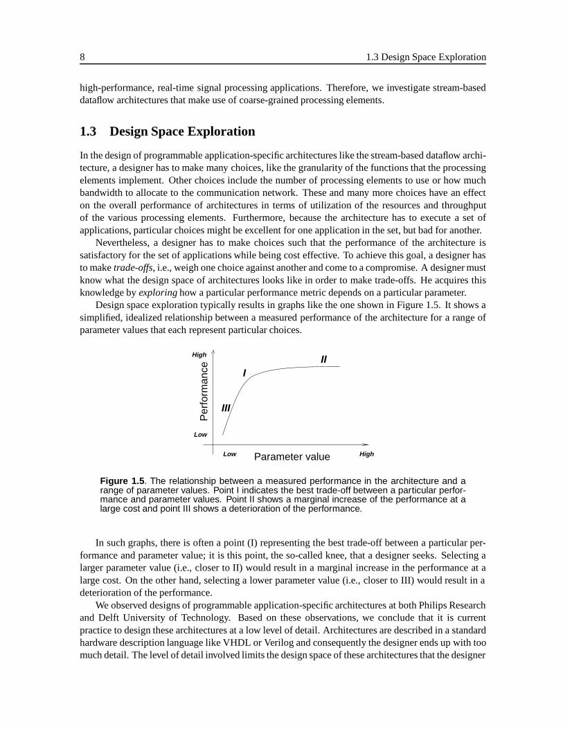
Design space exploration typically results in graphs like the one shown in Figure 1.5. It shows asimplified, idealized relationship between a measured performance of the architecture for a range ofparameter values that each represent particular choices.
III
III
Per
form
ance
High
Low
Low HighParameter value
Figure 1.5 . The relationship between a measured performance in the architecture and arange of parameter values. Point I indicates the best trade-off between a particular perfor-mance and parameter values. Point II shows a marginal increase of the performance at alarge cost and point III shows a deterioration of the performance.
In such graphs, there is often a point (I) representing the best trade-off between a particular per-formance and parameter value; it is this point, the so-called knee, that a designer seeks. Selecting alarger parameter value (i.e., closer to II) would result in a marginal increase in the performance at alarge cost. On the other hand, selecting a lower parameter value (i.e., closer to III) would result in adeterioration of the performance.
We observed designs of programmable application-specific architectures at both Philips Researchand Delft University of Technology. Based on these observations, we conclude that it is currentpractice to design these architectures at a low level of detail. Architectures are described in a standardhardware description language like VHDL or Verilog and consequently the designer ends up with toomuch detail. The level of detail involved limits the design space of these architectures that the designer
Introduction 9
can explore to look for better trade-offs. Therefore, a designer has difficulty finding a balance amongthe many choices present in architectures during the design process. This makes it hard to producearchitectures that are both cost effective and programmable enough to support a set of applications.
In this thesis we present a design approach called the “Y-chart approach” that overcomes thelimitations introduced by the low level of detail currently involved in the design of programmable ar-chitectures and which makes it possible to make better trade-offs in architectures. This approach leadsto an environment in which designers can first exercise architecture design, making design choices inarchitectures quantitative usingperformance analysis.
This involves the modeling of architectures to determine a performance model and the evaluationof this performance model to determine performance numbers, thus providing data for various per-formance metrics of a processor. In addition, by systematically changing design choices in a Y-chartenvironment, a designer should be able to systematically explore part of the design space of an ar-chitecture. This exploration provides the designer with the insight required for making the trade-offsnecessary for a good architecture for a given set of applications.
Performance analysis can take place at different levels of detail and designers should exploit thesedifferent levels to narrow down the design space of architectures in a stepwise fashion. A Y-chartenvironment is used in each step, but at different levels of detail. Therefore, when the modeling andevaluation of architectures is relatively inexpensive, a large part of the design space can be explored.By the time the modeling of an architecture as well as the evaluation of this model become expensive,the design space has been reduced considerably and it contains the interesting design points.
Applications
Retargetable
PerformanceNumbers
Design Space Exploration
Mapping
ArchitectureModeling Modeling
Simulator
(Chapter 5)
(Chapter 7)
(Chapter 6)
(Chapter 7)
(Chapter 8)
(Chapter 4)
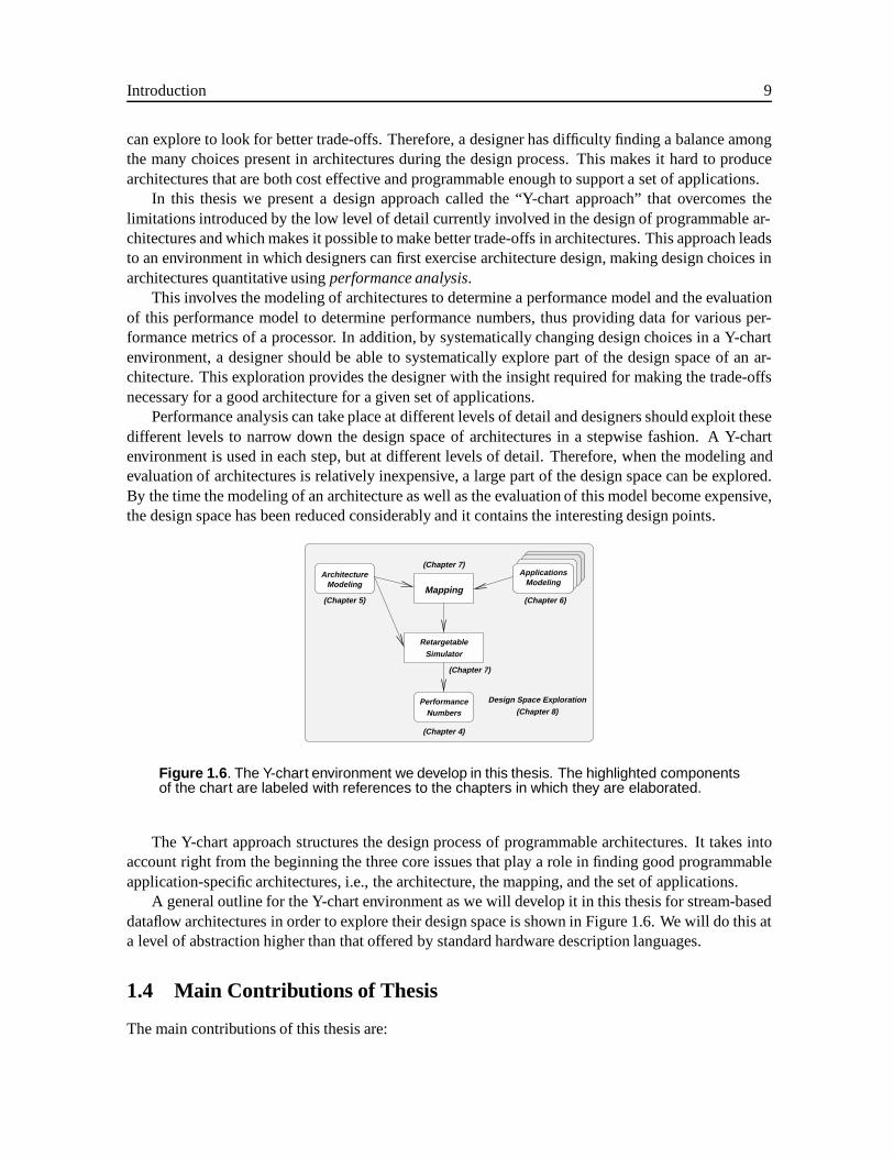
Figure 1.6 . The Y-chart environment we develop in this thesis. The highlighted componentsof the chart are labeled with references to the chapters in which they are elaborated.
The Y-chart approach structures the design process of programmable architectures. It takes intoaccount right from the beginning the three core issues that play a role in finding good programmableapplication-specific architectures, i.e., the architecture, the mapping, and the set of applications.
A general outline for the Y-chart environment as we will develop it in this thesis for stream-baseddataflow architectures in order to explore their design space is shown in Figure 1.6. We will do this ata level of abstraction higher than that offered by standard hardware description languages.
1.4 Main Contributions of Thesis
The main contributions of this thesis are:
10 1.4 Main Contributions of Thesis
Y-chart Approach The pivotal idea in this thesis is to provide a means with which the effect ofdesign choices on architectures can be quantified. This resulted in the formulation of the Y-chart approach, which quantifies design choices by measuring the performance.
We implemented the Y-chart approach in a Y-chart environment for the class of stream-baseddataflow architectures. This led to the following contributions:
Architecture Template for Stream-based Dataflow Architectures We present the stream-based dataflowarchitecture as a class of architectures. We show that all choices available within this class of ar-chitectures can be described by means of an architecture template that has a well defined designspace. We derive architecture instances from the architecture template.
Modeling Architectures in a Building Block Approach We use a high-level performance-modelingtool to render performance analysis at a high abstraction level. Using this method, we model thecomplete class of stream-based dataflow architectures while still obtaining cycle-accurate re-sults. We use object oriented programming techniques extensively together with the performance-modeling tool to construct building blocks. Using these building blocks, we construct exe-cutable architecture instances of the architecture template of stream-based dataflow architec-tures.
Stream-based Functions (SBF) ModelWe develop a new model of computation: the Stream-basedFunctions (SBF) Model. This model combines Kahn Process Networks [Kahn, 1974] with thea specialization of the Applicative State Transition (AST) Model proposed initially by Backus[1978]. The SBF model is well suited for describing digital signal processing applications atdifferent levels of granularity, ranging from fine-grained to coarse-grained. We also develop asimulator called SBFsim for the SBF model.
ORAS We develop the Object Oriented Retargetable Simulator (ORAS). Because ORAS is retar-getable, it can derive a full functional simulator for all feasible architectures from the class ofstream-based dataflow architectures. The derived simulator operates very fast in terms of realcomputer time while it also executes the correct functional behavior of an application. The ex-ecution speed is a prerequisite to performing an exploration of the design space of the class ofstream-based dataflow architectures in a limited amount of time.
Mapping Approach We introduce the notion of the model of architecture. Using this notion, we for-mulate a mapping approach in which we postulate that the model of computation should matchthe model of architecture of stream-based dataflow architectures. Only in this way is a smoothmapping possible. Moreover, it leads to an interface between applications and architecture. Thisinterface permits the execution of applications onto an architecture instance without its beingnecessary to modify the original application when mapping the application onto an architectureinstance.
Design Space ExplorationWe use a generic design space exploration environment to perform anexploration of stream-based dataflow architectures. We also formulate the problem of selectinga set of parameters that result in a particular architecture which satisfies the design objectivesfor a set of applications.
Different Design CasesWe use the Y-chart approach in two different design cases of programmablearchitectures. One design case is theProphidvideo-processor architecture [Leijten et al., 1997]

BIBLIOGRAPHY 11
for high-performance video applications and the other is theJacobiumprocessor architec-ture [Rijpkema et al., 1997] for array signal processing applications.
1.5 Outline of the Thesis
The organization of this thesis is as follows. We present the class of stream-based dataflow architec-tures in detail and formulate the main problem statement in Chapter 2. Our solution approach – theY-chart approach – is presented and discussed in Chapter 3. The chapters that follow each discuss aparticular aspect of the Y-chart environment for the class of stream-based dataflow architectures.
We explain what performance analysis entails in Chapter 4. We look into the aspects that de-termine the performance of a system, thus laying the foundation for performance analysis at a highlevel of abstraction. We use a high-level performance analysis method to carry out the performanceanalysis. Using this method, we set up an object oriented modeling approach leading to the notion ofbuilding blocks.
In Chapter 5, we look at how to model stream-based dataflow architectures using the buildingblocks discussed in Chapter 4. We construct the building blocks of the stream-based dataflow ar-chitecture in detail. We explain how we describe a class of architectures using a parser. Finally,we explain how to program stream-based dataflow architectures such that they execute a particularapplication.
To model applications, we introduce a new model of computation, calledStream-Based Functions(SBF). In Chapter 6, we explain what the SBF Model of computation comprises. We also explain howthe SBF Model is embedded in other well-established models of computations. How we implementedthis model of computation using C++ and Multi-threading is also described.
In Chapter 7 we combine aal these aspects to construct theObject oriented Retargetable Architec-ture Simulator(ORAS). We combine the work on architecture modeling presented in Chapter 5 withthe work on application modeling in Chapter 6 to construct a retargetable simulator that executes athigh speed. We also look in detail how we can easily map an application onto an architecture instance.
In Chapter 8 we explain what design space exploration (DSE) implies. We embed the ORASdeveloped in Chapter 7 in a generic design space exploration environment. We elaborate on thestatistical tools that the generic DSE environment uses to perform design space exploration efficiently.We also explain how we actually embed the ORAS in the generic DSE environment.
We investigate in Chapter 9 two cases in which a programmable architecture is developed and weuse in their design the Y-chart environment developed in this thesis. One case concerns the Prophidarchitecture for high-performance video application developed at Philips Research; the other concernsthe Jacobium architecture for a set of array signal processing applications developed at the DelftUniversity of Technology.
We conclude this thesis in Chapter 10 with our conclusions.
Bibliography
John Backus. Can programming be liberated from the von Neumann style? A functional style and itsalgebra of programs.Communications of the ACM, 21(8):613 – 641, 1978.
Pradip Bose and Thomas M. Conte. Performance analysis and its impact on design.IEEE Computer,31(5):41 – 49, 1998.
12 BIBLIOGRAPHY
D.C. Chen.Programmable Arithmetic Devices for High Speed Digital Signal Processing. PhD thesis,University of California at Berkeley, California, Department of Electrical Engineering and Com-puter Science, 1992.
T.A.C.M. Claasen. Technical and industrial challenges for signal processing in consumer electronics:A case study on TV applications. InProceedings of VLSI Signal Processing, VI, pages 3 – 11, 1993.
G. de Haan, J. Kettenis, and B. Deloore. IC for motion compensated 100hz TV, with smooth motionmovie-mode. InIEEE Transactions on Consumer Electronics, volume 42, pages 165 – 174, 1996.
Keith Diefendorff and Pradeep K. Dubey. How multimedia workloads will change processor design.IEEE Computer, 30(9):43 – 45, 1997.
John Hennessy and Mark Heinrich. Hardware/software codesign of processors: Concepts and ex-amples. In Giovanni De Micheli and Mariagiovanna Sami, editors,Hardware/Software Codesign,volume 310 ofSeries E: Applied Sciences, pages 29 – 44. NATO ASI Series, 1996.
John L. Hennessy and David A. Patterson.Computer Architectures: A QuantitativeApproach. MorganKaufmann Publishers, Inc., second edition, 1996.
Johan G.W.M. Janssen, Jeroen H. Stessen, and Peter H.N. de With. An advanced sampling rateconversion algorithm for video and graphics signals. InIEE Sixth International Conference onImage Processing and its Applications, Dublin, 1997.
Egbert G.T. Jaspers and Peter H.N. de With. A generic 2-D sharpness enhancement algorithm forluminance signals. InIEE Sixth InternationalConference on Image Processing and its Applications,Dublin, 1997.
Gilles Kahn. The semantics of a simple language for parallel programming. InProc. of the IFIPCongress 74. North-Holland Publishing Co., 1974.
Edward A. Lee and David G. Messerschmitt. Engineering and education for the future.IEEE Com-puter, 31(1):77 – 85, 1998.
Jeroen A.J. Leijten, Jef L. van Meerbergen, Adwin H. Timmer, and Jochen A.G. Jess. Prophid: Aheterogeneous multi-processor architecture for multimedia. InProceedings of ICCD’97, 1997.
P. Lieverse, E.F. Deprettere, A.C.J. Kienhuis, and E.A. de Kock. A clustering approach to exploregrain-sizes in the definition of weakly programmable processing elements. InProceedings of theIEEE Workshop on Signal Processing Systems, pages 107 – 120, De Montfort University, Leicester,UK, 1997.
Paul Lippens, Bart De Loore, Gerard de Haan, Piet Eeckhout, Henk Huijgen, Angelica Loning, BrianMcSweeney, Math Verstraelen, Bang Pham, and Jeroen Kettenis. A video signal processor formotion-compensated field-rate upconversion in consumer television.IEEE Journal of Solid-SateCircuits, 31(11):1762 – 1769, 1996.
P.E.R. Lippens, J.L. van Meerbergen, A. van der Werf, W.F.J. Verhaegh, B.T. McSweeney, J.O.Huisken, and O.P. McArdle. PHIDEO: A silicon compiler for high speed algorithms. InProc.EDAC, pages 436 – 441, 1991.
Nicholas Negroponte.Being Digital. Knopf, 1995.
BIBLIOGRAPHY 13
D.A. Patterson. Reduced instruction set computers.Comm. ACM, 28(1):8 – 21, 1985.
Edwin Rijpkema, Gerben Hekstra, Ed Deprettere, and Ju Ma. A strategy for determining a Jacobi spe-cific dataflow processor. InProceedings of 11th Int. Conference of Applications-specific Systems,Architectures and Processors (ASAP’97), pages 53 – 64, Zurich, Switzerland, 1997.
Frank Rose. The end of TV as we know it.FORTUNE, pages 58 – 68, 1996.
VHDL. IEEE Standard VHDL Language Reference Manual. IEEE Computer Service, 445 HoesLane, P.O. Box 1331, Piscataway, New Jersey, 08855-1331, 1993. IEEE Std 1076-1993.
K.A. Vissers, G. Essink, P.H.J. van Gerwen, P.J.M. Janssen, O. Popp, E. Riddersma, and J.M. Veen-drick. Algorithms and Parallel VLSI Architectures III, chapter Architecture and programming oftwo generations video signal processors, pages 167 – 178. Elsevier, 1995.
John A. Watlington and V. Michael Bove Jr. Stream-based computing and future television.SMPTEJournal, 106(4):217 – 224, 1997.

14 BIBLIOGRAPHY
Chapter 2
Basic Definitions and Problem Statement
Contents
2.1 Stream-based Dataflow Architectures . . . . . . . . . . . . . . . . . . . . . . . 16
2.1.1 Definitions . . . . . . . . . . . . . . . . . . . . . . . . . . . . . . . . . . 16
2.1.2 Structure . . . . . . . . . . . . . . . . . . . . . . . . . . . . . . . . . . . 19
2.1.3 Behavior . . . . . . . . . . . . . . . . . . . . . . . . . . . . . . . . . . . 22
2.2 The Class of Stream-based Dataflow Architectures . . . . . . . . . . . . . . . . 31
2.2.1 Architecture Template . . . . . . . . . . . . . . . . . . . . . . . . . . . . 32
2.2.2 Design Space . . . . . . . . . . . . . . . . . . . . . . . . . . . . . . . . . 32
2.3 The Designer’s Problem . . . . . . . . . . . . . . . . . . . . . . . . . . . . . . . 32
2.3.1 Exploring the Design Space of Architectures . . . . . . . . . . . . . . . . 33
2.3.2 Problems in Current Design Approaches . . . . . . . . . . . . . . . . . . . 33
2.4 Related Work on Dataflow Architectures . . . . . . . . . . . . . . . . . . . . . 34
2.4.1 Implementation Problems of Dataflow Architectures . . . . . . . . . . . . 35
2.4.2 Other Dataflow Architectures . . . . . . . . . . . . . . . . . . . . . . . . 35
2.4.3 Implementing Stream-based Dataflow Architectures . . . . . . . . . . . . 36
2.5 Conclusions . . . . . . . . . . . . . . . . . . . . . . . . . . . . . . . . . . . . . . 39
STREAM-BASED dataflow architectures were briefly introduced in the previous chapter. Weshowed that such architectures will be used for the high-performance video signal processing
section in the TV-sets of the near future. In this chapter, we look in more detail at the structure andbehavior of stream-based dataflow architectures.
Stream-based dataflow architectures are not one particular architecture, but rather a class of archi-tectures. This class is described using an architecture template to characterize the class in a parame-terized form. The architecture template has an associated design space and the design of architecturesbecomes the selection of parameter values representing a particular architecture within the designspace. The problem designers face, however, is how to select these parameter values. How do design-ers select these parameter values such that they result in architectures which satisfy the many designobjectives involved, such as real-time constraints, throughput of the architecture and the efficiency ofresources? At the same time, these architectures also need to be programmable enough that they canexecute a set of applications.
We start in Section 2.1 by defining what a stream-based dataflow architecture is. We introducedefinitions of terms to clarify what we understand in the context of this thesis by specific terms. We
15
16 2.1 Stream-based Dataflow Architectures
also describe the structure and behavior of stream-based dataflow architectures and introduce the manychoices present in both the structure and behavior of stream-based dataflow architectures. All thesechoices together characterize the class of stream-based dataflow architectures.
To describe the class of stream-based dataflow architectures, in Section 2.2 we introduce the archi-tecture template, which characterizes this class of architectures in a parameterized form. By assigningvalues to all parameters in the architecture template, we can derive a particular architecture instancethat makes up a design. This brings us in Section 2.3 to the goal of this thesis, which is to provide asystematic methodology for finding parameter values for an architecture template.
Dataflow architectures have already been around for many years in many different forms. Weconclude this chapter in Section 2.4 by presenting related work on dataflow architectures. We iden-tify known problems within dataflow architectures and indicate to what extent stream-based dataflowarchitectures exhibit these problems and how they cope with these problems.
2.1 Stream-based Dataflow Architectures
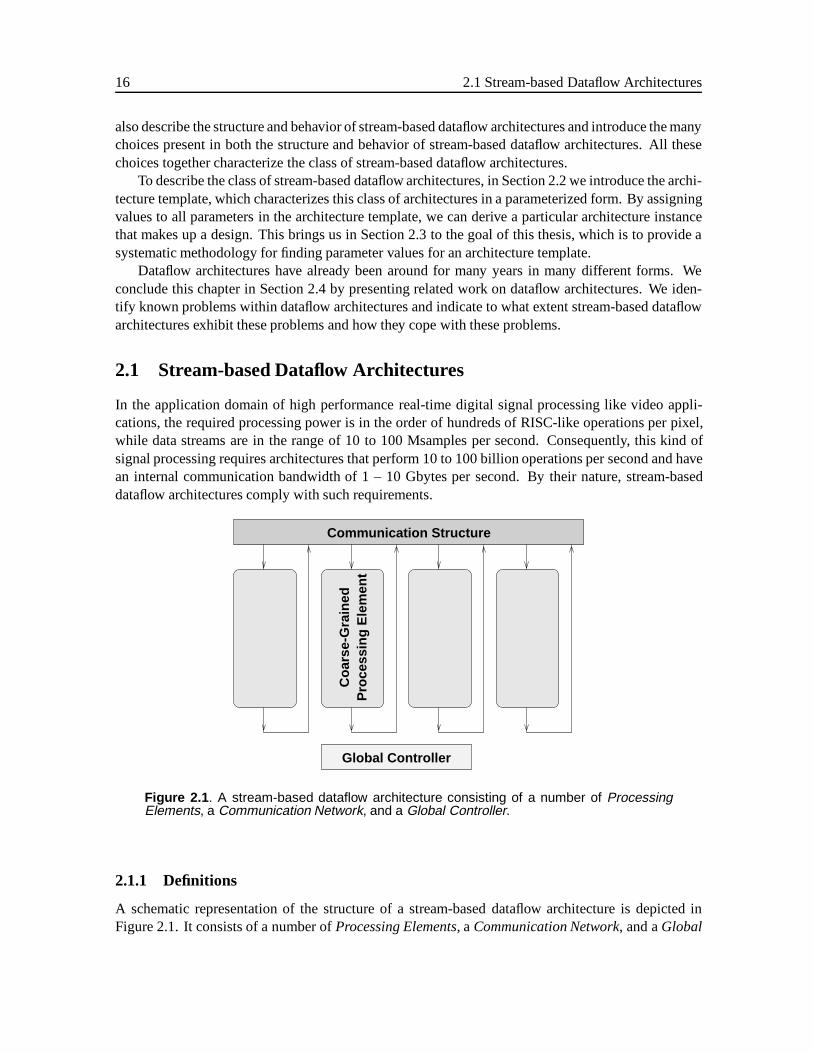
In the application domain of high performance real-time digital signal processing like video appli-cations, the required processing power is in the order of hundreds of RISC-like operations per pixel,while data streams are in the range of 10 to 100 Msamples per second. Consequently, this kind ofsignal processing requires architectures that perform 10 to 100 billion operations per second and havean internal communication bandwidth of 1 – 10 Gbytes per second. By their nature, stream-baseddataflow architectures comply with such requirements.
Pro
cess
ing
Ele
men
t
Global Controller
Communication Structure
Co
arse
-Gra
ined
Figure 2.1 . A stream-based dataflow architecture consisting of a number of ProcessingElements, a Communication Network, and a Global Controller.
2.1.1 Definitions
A schematic representation of the structure of a stream-based dataflow architecture is depicted inFigure 2.1. It consists of a number ofProcessing Elements, aCommunication Network, and aGlobal
Basic Definitions and Problem Statement 17
Controller. The processing elements operate concurrently on streams, which we define as
Definition 2.1. STREAM
A streamis a one-dimensional sequence of data items. 2
Unless stated differently, a data item represents a sample. In the case of video, a sample is typicallya video pixel and in the case of radar, a sample is typically an integer or fixed-point value. A streamcan be broken down into packets of finite length, resulting in a packet stream. We define a packet as
Definition 2.2. PACKET
A packetis a finite sequence of data items and is a concatenation of a header and a data part.2
In the architecture, a processing element executes a pre-selected function operating on one ormore streams and producing one or more output streams. The pre-selected function is one of a finite– typically, small – number of functions present in a processing element. These functions define thefunction repertoire of a processing element.
Definition 2.3. FUNCTION REPERTOIRE
Thefunction repertoireof a processing element describes a finite number of different pre-definedfunctions that the processing element can execute. 2
Each processing element has a function repertoire that typically, but not necessarily, differs fromthe function repertoire of every other processing element. The grain sizes of the functions of thefunction repertoire are a measure of their complexity.
Definition 2.4. GRAIN SIZE
A function has agrain sizeexpressed in terms of the equivalent number of representative RISC-like operations, likeAdd, Compare, andShift. RISC-like functions have a grain size of one, bydefinition. 2
The grain size provides a metric allowing us to quantify the complexity of functions. A functionwith a grain size of 100 is supposed to have an executable specification in terms of approximately 100RISC-like operations. [For more information on RISC instructions, see Appendix C of Hennessy andPatterson, 1996]. We say that functions with a grain size of one arefine-grained. Similarly, functionswith a grain size between 1 and 10 aremedium-grainedfunctions, and functions with a grain sizelarger than 10 arecoarse-grainedfunctions.
Although processing elements execute in parallel, each and every processing element executesonly one function from its function repertoire at a time. A processing element can switch at run-timebetween the functions of the function repertoire, which leads to the notion of weakly programmableprocessing elements.
Definition 2.5. WEAKLY PROGRAMMABLE PROCESSINGELEMENT
A weakly programmable processing elementcan switch at run-time between a fixed number ofpre-defined functions present in the function repertoire in such a way that only one function of thefunction repertoire is active at a time. 2
Although the processing elements can execute functions ranging from fine-grained to coarse-grained, the functions that it executes are typically coarse-grained, to balance best between pro-grammability and efficiency, as shown in Figure 1.4. When the granularity of functions increases,they become more dedicated and can, therefore, only be used to execute particular applications that
18 2.1 Stream-based Dataflow Architectures
belong to a set of applications. Consequently, coarse-grained functions are more specific than fine-grained functions used in fully programmable architectures. The weakly programmable processingelements and the grain size of the functions allow the architecture to provide just enough flexibility tosupport a set of applications. We assume that only one application is executed on the architecture at atime.
The global controller controls the flow of packets through the architecture. It contains aRoutingProgramwith which to control the flow. This routing program indicates which processing elementprocesses which stream, using which function from the function repertoire. By changing the routingprogram, we canreprogramthe architecture to execute another application.
We define stream-based dataflow architectures as follows:
Definition 2.6. STREAM-BASED DATAFLOW ARCHITECTURES
A Stream-based Dataflow Architectureconsists of a set of weakly programmable processing el-ements operating in parallel, a communication structure and a global controller. The processing ele-ments operate on packet streams that they exchange among themselves via the communication struc-ture controlled by the global controller. 2
Stream-based dataflow architectures have a particular hierarchical structure and a particular be-havior in time. We will now describe the structure and behavior of the architecture in more detail,whereby we make use of the terminology that Veen [1986] uses to describe dataflow architectures ingeneral.
We want to emphasize that the architecture concept shown in Figure 2.1 was proposed by Leijten,van Meerbergen, Timmer, and Jess [1997] and is further developed and discussed in greater detail inLeijten [1998].
Fq
Fp
Fu
nct
ion
al E
lem
ents
Ro
ute
rsOu
tpu
t B
uff
ers
Pro
cess
ing
Ele
men
t
Global Controller
Communication Structure
Un
itF
un
ctio
nal In
pu
t B
uff
ers
Co
arse
-Gra
ined
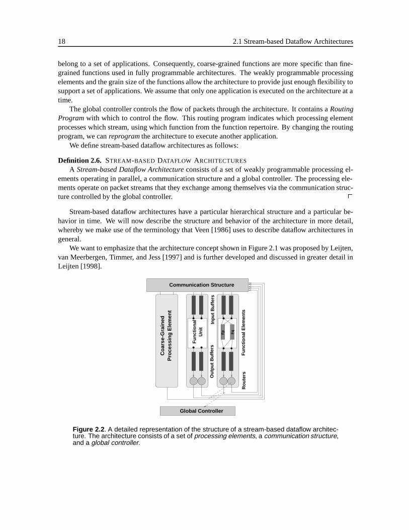
Figure 2.2 . A detailed representation of the structure of a stream-based dataflow architec-ture. The architecture consists of a set of processing elements, a communication structure,and a global controller.
Basic Definitions and Problem Statement 19
2.1.2 Structure
A stream-based dataflow architecture is given in Figure 2.2. The architecture consists of a set ofpro-cessing elements, acommunication structure, and aglobal controller. A processing element consistsof a number of input and outputbuffersandroutersand afunctional unit. The routers interact withthe global controller. The functional unit consists of a number offunctional elements(i.e., FEp andFEq). Each functional element executes a function and the functions of the functional elements makeup the function repertoire of a processing element. The communication structure interconnects theprocessing elements so they can communicate packet streams with each other under the control of theglobal controller.
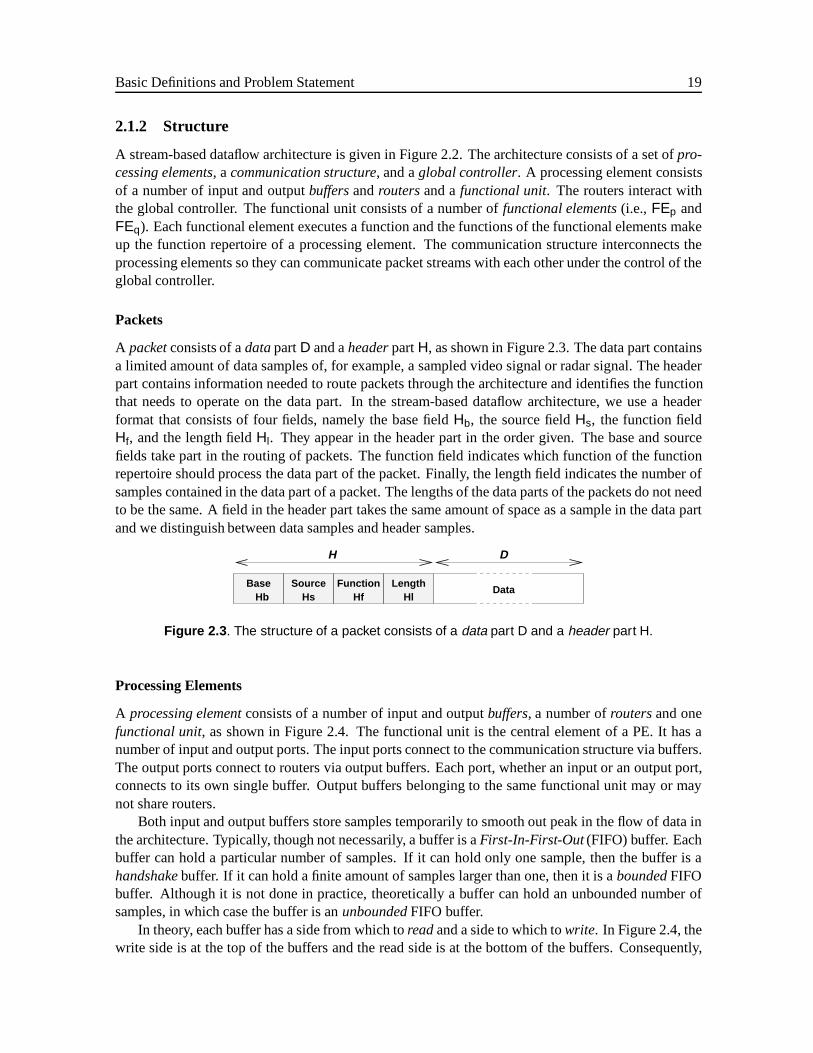
Packets
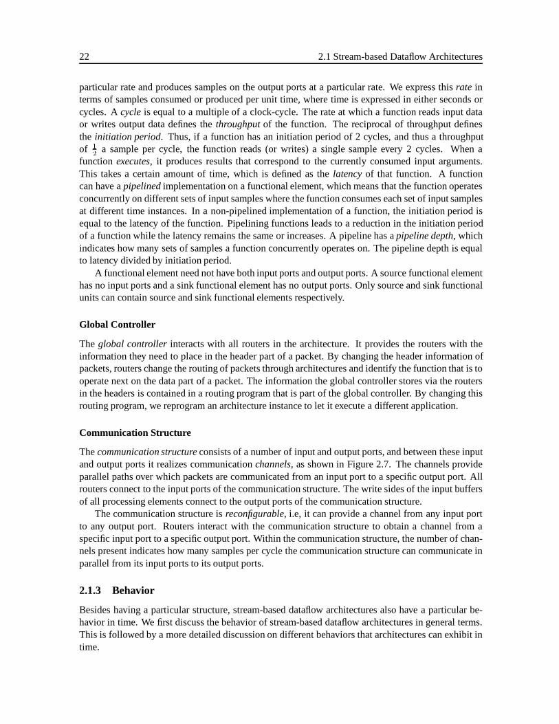
A packetconsists of adatapartD and aheaderpartH, as shown in Figure 2.3. The data part containsa limited amount of data samples of, for example, a sampled video signal or radar signal. The headerpart contains information needed to route packets through the architecture and identifies the functionthat needs to operate on the data part. In the stream-based dataflow architecture, we use a headerformat that consists of four fields, namely the base fieldHb, the source fieldHs, the function fieldHf, and the length fieldHl. They appear in the header part in the order given. The base and sourcefields take part in the routing of packets. The function field indicates which function of the functionrepertoire should process the data part of the packet. Finally, the length field indicates the number ofsamples contained in the data part of a packet. The lengths of the data parts of the packets do not needto be the same. A field in the header part takes the same amount of space as a sample in the data partand we distinguish between data samples and header samples.
BaseHb
Source Function LengthHf Hl
DataHs
H D
Figure 2.3 . The structure of a packet consists of a data part D and a header part H.
Processing Elements
A processing elementconsists of a number of input and outputbuffers, a number ofroutersand onefunctional unit, as shown in Figure 2.4. The functional unit is the central element of a PE. It has anumber of input and output ports. The input ports connect to the communication structure via buffers.The output ports connect to routers via output buffers. Each port, whether an input or an output port,connects to its own single buffer. Output buffers belonging to the same functional unit may or maynot share routers.
Both input and output buffers store samples temporarily to smooth out peak in the flow of data inthe architecture. Typically, though not necessarily, a buffer is aFirst-In-First-Out(FIFO) buffer. Eachbuffer can hold a particular number of samples. If it can hold only one sample, then the buffer is ahandshakebuffer. If it can hold a finite amount of samples larger than one, then it is aboundedFIFObuffer. Although it is not done in practice, theoretically a buffer can hold an unbounded number ofsamples, in which case the buffer is anunboundedFIFO buffer.
In theory, each buffer has a side from which toreadand a side to which towrite. In Figure 2.4, thewrite side is at the top of the buffers and the read side is at the bottom of the buffers. Consequently,

20 2.1 Stream-based Dataflow Architectures
Dir
ecti
on
of
the
Str
eam
Fun
ctio
nal
Uni
t
Output Buffers
Input Buffers
Input Ports
Output Ports
Routers
Figure 2.4 . A processing element consists of a number of input and output buffers, a num-ber of routers and one functional unit.
streams flow through the functional unit from top to bottom.Routers connect to the read side of output buffers and, via the communication structure, to the
input side of some input buffer. At run-time, the routers update the information in the four headerfields of a packet. This affects the routing of packets and the function operating on the data part ofa packet. Routers interact with the global controller to obtain this new header information. Besideschanging the header fields, the router also checks whether the communication structure provides apath to the correct input buffer. If such a path exists, the router uses it to transport a packet to its newdestination in the architecture.
There are two special kinds of PEs: a source PE and a sink PE. The source and sink processingelements interact with the external world of the architectures. A source processing element producespacket streams, whereas the sink processing element consumes packet streams. A regular PE connectsto the communication structure with both its inputs and its outputs. A source PE connects only withoutputs of the communication structure and a sink PE connects only with inputs to the communicationstructure.
Functional Units
A functional unitconsists of the setF of functional elements(FEs), alocal controller, and input andoutput ports, as shown in Figure 2.5. Functional Elements also have input and output ports, whichbind statically to the input and output ports of the functional unit. The setF specifies thefunctionrepertoireof a processing element.
F = fFE1; FE2; : : : ; FExg (2.1)
A functional unit switches between the functional elements at run-time. This switching takes placeunder the supervision of the local controller. Based on the value of the function fieldHf in the headerof a packet, the local controller resolves which functional element it should activate. Although pro-cessing elements, and thus also functional units, operate concurrently, inside a functional unit only asingle functional element is active at a time.
Basic Definitions and Problem Statement 21
ControllerLocal
FE0 FE1
Functional UnitInput Ports
Functional Unit
Binding
Output Ports
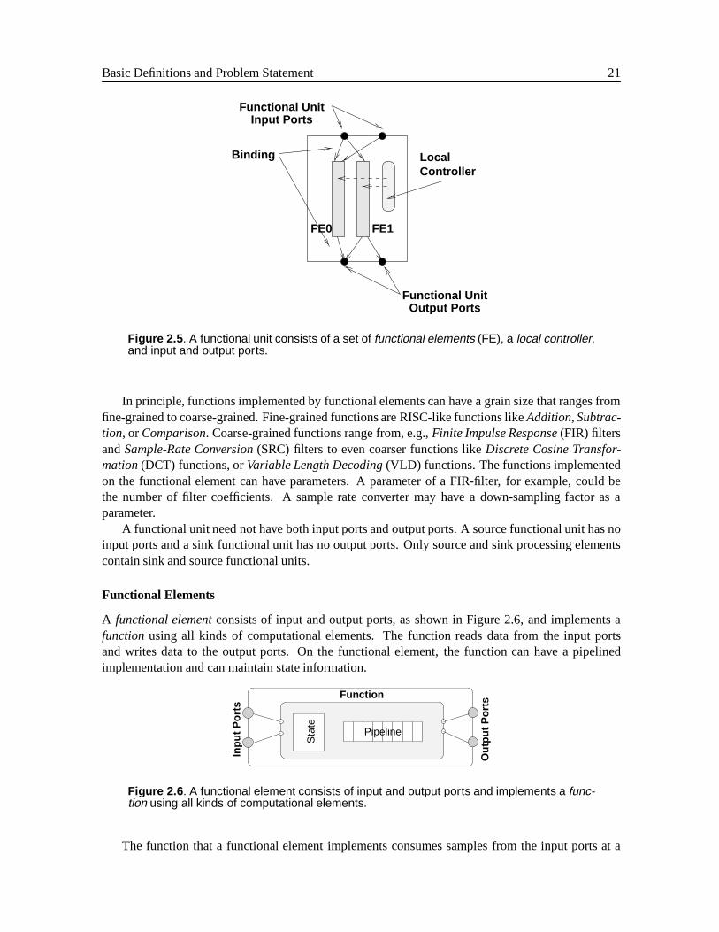
Figure 2.5 . A functional unit consists of a set of functional elements (FE), a local controller,and input and output ports.
In principle, functions implemented by functional elements can have a grain size that ranges fromfine-grained to coarse-grained. Fine-grained functions are RISC-like functions likeAddition,Subtrac-tion, orComparison. Coarse-grained functions range from, e.g.,Finite Impulse Response(FIR) filtersandSample-Rate Conversion(SRC) filters to even coarser functions likeDiscrete Cosine Transfor-mation(DCT) functions, orVariable Length Decoding(VLD) functions. The functions implementedon the functional element can have parameters. A parameter of a FIR-filter, for example, could bethe number of filter coefficients. A sample rate converter may have a down-sampling factor as aparameter.
A functional unit need not have both input ports and output ports. A source functional unit has noinput ports and a sink functional unit has no output ports. Only source and sink processing elementscontain sink and source functional units.
Functional Elements
A functional elementconsists of input and output ports, as shown in Figure 2.6, and implements afunctionusing all kinds of computational elements. The function reads data from the input portsand writes data to the output ports. On the functional element, the function can have a pipelinedimplementation and can maintain state information.
Sta
te
Function
Pipeline
Inp
ut
Po
rts
Ou
tpu
t P
ort
s
Figure 2.6 . A functional element consists of input and output ports and implements a func-tion using all kinds of computational elements.
The function that a functional element implements consumes samples from the input ports at a
22 2.1 Stream-based Dataflow Architectures
particular rate and produces samples on the output ports at a particular rate. We express thisrate interms of samples consumed or produced per unit time, where time is expressed in either seconds orcycles. Acycleis equal to a multiple of a clock-cycle. The rate at which a function reads input dataor writes output data defines thethroughputof the function. The reciprocal of throughput definesthe initiation period. Thus, if a function has an initiation period of 2 cycles, and thus a throughputof 1
2 a sample per cycle, the function reads (or writes) a single sample every 2 cycles. When afunction executes, it produces results that correspond to the currently consumed input arguments.This takes a certain amount of time, which is defined as thelatencyof that function. A functioncan have apipelinedimplementation on a functional element, which means that the function operatesconcurrently on different sets of input samples where the function consumes each set of input samplesat different time instances. In a non-pipelined implementation of a function, the initiation period isequal to the latency of the function. Pipelining functions leads to a reduction in the initiation periodof a function while the latency remains the same or increases. A pipeline has apipeline depth, whichindicates how many sets of samples a function concurrently operates on. The pipeline depth is equalto latency divided by initiation period.
A functional element need not have both input ports and output ports. A source functional elementhas no input ports and a sink functional element has no output ports. Only source and sink functionalunits can contain source and sink functional elements respectively.
Global Controller
The global controller interacts with all routers in the architecture. It provides the routers with theinformation they need to place in the header part of a packet. By changing the header information ofpackets, routers change the routing of packets through architectures and identify the function that is tooperate next on the data part of a packet. The information the global controller stores via the routersin the headers is contained in a routing program that is part of the global controller. By changing thisrouting program, we reprogram an architecture instance to let it execute a different application.
Communication Structure
Thecommunication structureconsists of a number of input and output ports, and between these inputand output ports it realizes communicationchannels, as shown in Figure 2.7. The channels provideparallel paths over which packets are communicated from an input port to a specific output port. Allrouters connect to the input ports of the communication structure. The write sides of the input buffersof all processing elements connect to the output ports of the communication structure.
The communication structure isreconfigurable, i.e, it can provide a channel from any input portto any output port. Routers interact with the communication structure to obtain a channel from aspecific input port to a specific output port. Within the communication structure, the number of chan-nels present indicates how many samples per cycle the communication structure can communicate inparallel from its input ports to its output ports.
2.1.3 Behavior
Besides having a particular structure, stream-based dataflow architectures also have a particular be-havior in time. We first discuss the behavior of stream-based dataflow architectures in general terms.This is followed by a more detailed discussion on different behaviors that architectures can exhibit intime.
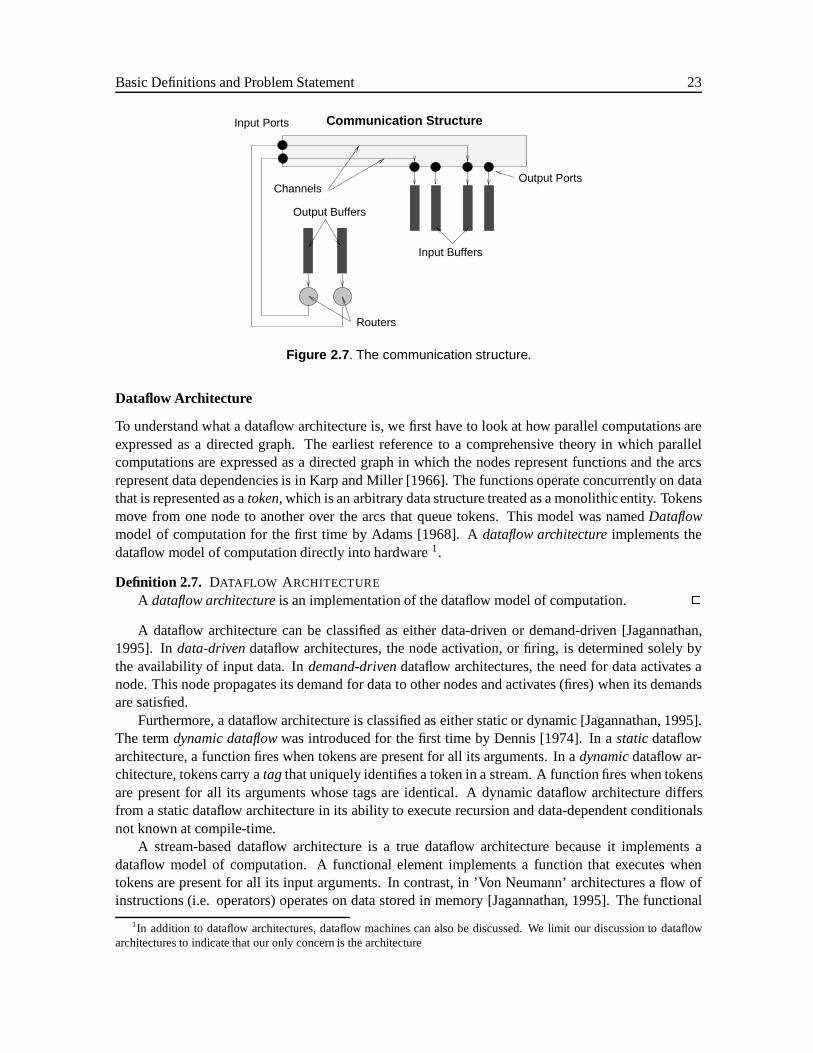
Basic Definitions and Problem Statement 23
Communication StructureInput Ports
ChannelsOutput Ports
Routers
Output Buffers
Input Buffers
Figure 2.7 . The communication structure.
Dataflow Architecture
To understand what a dataflow architecture is, we first have to look at how parallel computations areexpressed as a directed graph. The earliest reference to a comprehensive theory in which parallelcomputations are expressed as a directed graph in which the nodes represent functions and the arcsrepresent data dependencies is in Karp and Miller [1966]. The functions operate concurrently on datathat is represented as atoken, which is an arbitrary data structure treated as a monolithic entity. Tokensmove from one node to another over the arcs that queue tokens. This model was namedDataflowmodel of computation for the first time by Adams [1968]. Adataflow architectureimplements thedataflow model of computation directly into hardware1.
Definition 2.7. DATAFLOW ARCHITECTURE
A dataflow architectureis an implementation of the dataflow model of computation. 2
A dataflow architecture can be classified as either data-driven or demand-driven [Jagannathan,1995]. Indata-drivendataflow architectures, the node activation, or firing, is determined solely bythe availability of input data. Indemand-drivendataflow architectures, the need for data activates anode. This node propagates its demand for data to other nodes and activates (fires) when its demandsare satisfied.
Furthermore, a dataflow architecture is classified as either static or dynamic [Jagannathan, 1995].The termdynamic dataflowwas introduced for the first time by Dennis [1974]. In astaticdataflowarchitecture, a function fires when tokens are present for all its arguments. In adynamicdataflow ar-chitecture, tokens carry atag that uniquely identifies a token in a stream. A function fires when tokensare present for all its arguments whose tags are identical. A dynamic dataflow architecture differsfrom a static dataflow architecture in its ability to execute recursion and data-dependent conditionalsnot known at compile-time.
A stream-based dataflow architecture is a true dataflow architecture because it implements adataflow model of computation. A functional element implements a function that executes whentokens are present for all its input arguments. In contrast, in ’Von Neumann’ architectures a flow ofinstructions (i.e. operators) operates on data stored in memory [Jagannathan, 1995]. The functional
1In addition to dataflow architectures, dataflow machines can also be discussed. We limit our discussion to dataflowarchitectures to indicate that our only concern is the architecture
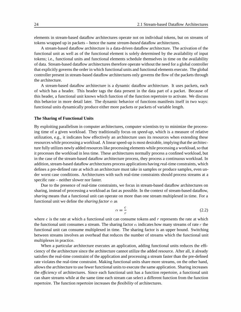
24 2.1 Stream-based Dataflow Architectures
elements in stream-based dataflow architectures operate not on individual tokens, but on streams oftokens wrapped up in packets – hence the namestream-baseddataflow architectures.
A stream-based dataflow architecture is a data-driven dataflow architecture. The activation of thefunctional unit as well as of the functional element is solely determined by the availability of inputtokens; i.e., functional units and functional elements schedule themselves in time on the availabilityof data. Stream-based dataflow architectures therefore operate without the need for a global controllerthat explicitly governs the order in which functional units and functional elements execute. The globalcontroller present in stream-based dataflow architectures only governs the flow of the packets throughthe architecture.
A stream-based dataflow architecture is a dynamic dataflow architecture. It uses packets, eachof which has a header. This header tags the data present in the data part of a packet. Because ofthis header, a functional unit knows which function of the function repertoire to activate. We discussthis behavior in more detail later. The dynamic behavior of functions manifests itself in two ways:functional units dynamically produce either more packets or packets of variable length.
The Sharing of Functional Units
By exploiting parallelism in computer architectures, computer scientists try to minimize the process-ing time of a given workload. They traditionally focus onspeed-up, which is a measure of relativeutilization, e.g., it indicates how effectively an architecture uses its resources when extending theseresources while processing a workload. A linear speed-up is most desirable, implying that the architec-ture fully utilizes newly added resources like processing elements while processing a workload, so thatit processes the workload in less time. These architectures normally process a confined workload, butin the case of the stream-based dataflow architecture process, they process a continuous workload. Inaddition, stream-based dataflow architectures process applications havingreal-time constraints, whichdefines a pre-defined rate at which an architecture must take in samples or produce samples, even un-der worst case conditions. Architectures with such real-time constraints should process streams at aspecific rate – neither slower nor faster.
Due to the presence of real-time constraints, we focus in stream-based dataflow architectures onsharing, instead of processing a workload as fast as possible. In the context of stream-based dataflow,sharingmeans that a functional unit can operate on more than one stream multiplexed in time. For afunctional unit we define thesharing factor� as
� =e
r(2.2)
wheree is the rate at which a functional unit can consume tokens andr represents the rate at whichthe functional unit consumes a stream. The sharing factor� indicates how many streams of rater thefunctional unit can consume multiplexed in time. The sharing factor is an upper bound. Switchingbetween streams involves an overhead that reduces the number of streams which the functional unitmultiplexes in practice.
When a particular architecture executes an application, adding functional units reduces the effi-ciency of the architecture since the architecture cannot utilize the added resource. After all, it alreadysatisfies the real-time constraint of the application and processing a stream faster than the pre-definedrate violates the real-time constraint. Making functional units share more streams, on the other hand,allows the architecture to use fewer functional units to execute the same application. Sharing increasestheefficiencyof architectures. Since each functional unit has a function repertoire, a functional unitcan share streams while at the same time each stream can select a different function from the functionrepertoire. The function repertoire increases theflexibility of architectures.
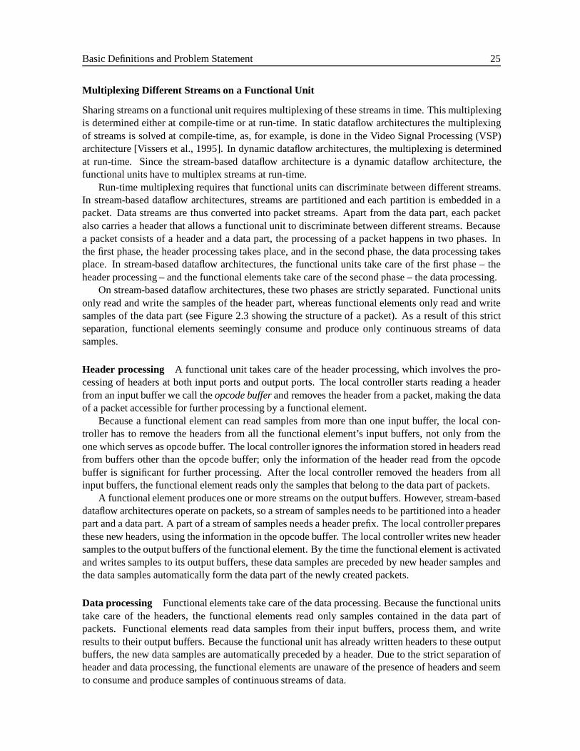
Basic Definitions and Problem Statement 25
Multiplexing Different Streams on a Functional Unit
Sharing streams on a functional unit requires multiplexing of these streams in time. This multiplexingis determined either at compile-time or at run-time. In static dataflow architectures the multiplexingof streams is solved at compile-time, as, for example, is done in the Video Signal Processing (VSP)architecture [Vissers et al., 1995]. In dynamic dataflow architectures, the multiplexing is determinedat run-time. Since the stream-based dataflow architecture is a dynamic dataflow architecture, thefunctional units have to multiplex streams at run-time.
Run-time multiplexing requires that functional units can discriminate between different streams.In stream-based dataflow architectures, streams are partitioned andeach partition is embedded in apacket. Data streams are thus converted into packet streams. Apart from the data part, each packetalso carries a header that allows a functional unit to discriminate between different streams. Becausea packet consists of a header and a data part, the processing of a packet happens in two phases. Inthe first phase, the header processing takes place, and in the second phase, the data processing takesplace. In stream-based dataflow architectures, the functional units take care of the first phase – theheader processing – and the functional elements take care of the second phase – the data processing.
On stream-based dataflow architectures, these two phases are strictly separated. Functional unitsonly read and write the samples of the header part, whereas functional elements only read and writesamples of the data part (see Figure 2.3 showing the structure of a packet). As a result of this strictseparation, functional elements seemingly consume and produce only continuous streams of datasamples.
Header processing A functional unit takes care of the header processing, which involves the pro-cessing of headers at both input ports and output ports. The local controller starts reading a headerfrom an input buffer we call theopcode bufferand removes the header from a packet, making the dataof a packet accessible for further processing by a functional element.
Because a functional element can read samples from more than one input buffer, the local con-troller has to remove the headers from all the functional element’s input buffers, not only from theone which serves as opcode buffer. The local controller ignores the information stored in headers readfrom buffers other than the opcode buffer; only the information of the header read from the opcodebuffer is significant for further processing. After the local controller removed the headers from allinput buffers, the functional element reads only the samples that belong to the data part of packets.
A functional element produces one or more streams on the output buffers. However, stream-baseddataflow architectures operate on packets, so a stream of samples needs to be partitioned into a headerpart and a data part. A part of a stream of samples needs a header prefix. The local controller preparesthese new headers, using the information in the opcode buffer. The local controller writes new headersamples to the output buffers of the functional element. By the time the functional element is activatedand writes samples to its output buffers, these data samples are preceded by new header samples andthe data samples automatically form the data part of the newly created packets.
Data processing Functional elements take care of the data processing. Because the functional unitstake care of the headers, the functional elements read only samples contained in the data part ofpackets. Functional elements read data samples from their input buffers, process them, and writeresults to their output buffers. Because the functional unit has already written headers to these outputbuffers, the new data samples are automatically preceded by a header. Due to the strict separation ofheader and data processing, the functional elements are unaware of the presence of headers and seemto consume and produce samples of continuous streams of data.
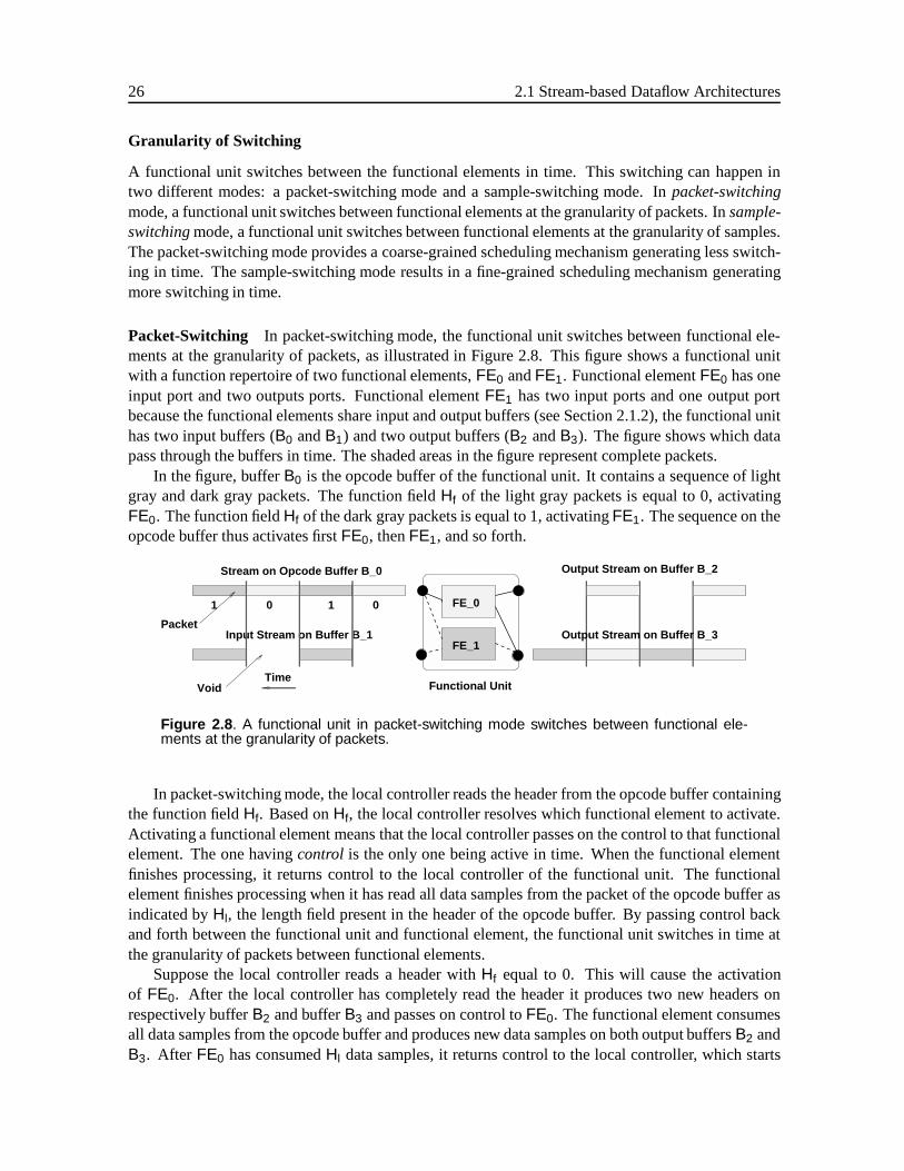
26 2.1 Stream-based Dataflow Architectures
Granularity of Switching
A functional unit switches between the functional elements in time. This switching can happen intwo different modes: a packet-switching mode and a sample-switching mode. Inpacket-switchingmode, a functional unit switches between functional elements at the granularity of packets. Insample-switchingmode, a functional unit switches between functional elements at the granularity of samples.The packet-switching mode provides a coarse-grained scheduling mechanism generating less switch-ing in time. The sample-switching mode results in a fine-grained scheduling mechanism generatingmore switching in time.
Packet-Switching In packet-switching mode, the functional unit switches between functional ele-ments at the granularity of packets, as illustrated in Figure 2.8. This figure shows a functional unitwith a function repertoire of two functional elements,FE0 andFE1. Functional elementFE0 has oneinput port and two outputs ports. Functional elementFE1 has two input ports and one output portbecause the functional elements share input and output buffers (see Section 2.1.2), the functional unithas two input buffers (B0 andB1) and two output buffers (B2 andB3). The figure shows which datapass through the buffers in time. The shaded areas in the figure represent complete packets.
In the figure, bufferB0 is the opcode buffer of the functional unit. It contains a sequence of lightgray and dark gray packets. The function fieldHf of the light gray packets is equal to 0, activatingFE0. The function fieldHf of the dark gray packets is equal to 1, activatingFE1. The sequence on theopcode buffer thus activates firstFE0, thenFE1, and so forth.
Input Stream on Buffer B_1
1 001
Stream on Opcode Buffer B_0
Packet
VoidTime
FE_1
FE_0
Functional Unit
Output Stream on Buffer B_2
Output Stream on Buffer B_3
Figure 2.8 . A functional unit in packet-switching mode switches between functional ele-ments at the granularity of packets.
In packet-switching mode, the local controller reads the header from the opcode buffer containingthe function fieldHf. Based onHf, the local controller resolves which functional element to activate.Activating a functional element means that the local controller passes on the control to that functionalelement. The one havingcontrol is the only one being active in time. When the functional elementfinishes processing, it returns control to the local controller of the functional unit. The functionalelement finishes processing when it has read all data samples from the packet of the opcode buffer asindicated byHl, the length field present in the header of the opcode buffer. By passing control backand forth between the functional unit and functional element, the functional unit switches in time atthe granularity of packets between functional elements.
Suppose the local controller reads a header withHf equal to 0. This will cause the activationof FE0. After the local controller has completely read the header it produces two new headers onrespectively bufferB2 and bufferB3 and passes on control toFE0. The functional element consumesall data samples from the opcode buffer and produces new data samples on both output buffersB2 andB3. After FE0 has consumedHl data samples, it returns control to the local controller, which starts
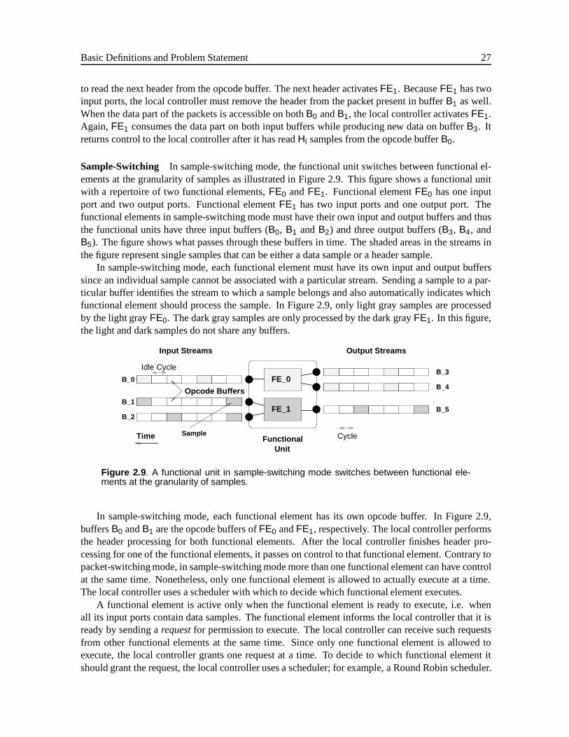
Basic Definitions and Problem Statement 27
to read the next header from the opcode buffer. The next header activatesFE1. BecauseFE1 has twoinput ports, the local controller must remove the header from the packet present in bufferB1 as well.When the data part of the packets is accessible on bothB0 andB1, the local controller activatesFE1.Again,FE1 consumes the data part on both input buffers while producing new data on bufferB3. Itreturns control to the local controller after it has readHl samples from the opcode bufferB0.
Sample-Switching In sample-switching mode, the functional unit switches between functional el-ements at the granularity of samples as illustrated in Figure 2.9. This figure shows a functional unitwith a repertoire of two functional elements,FE0 andFE1. Functional elementFE0 has one inputport and two output ports. Functional elementFE1 has two input ports and one output port. Thefunctional elements in sample-switching mode must have their own input and output buffers and thusthe functional units have three input buffers (B0, B1 andB2) and three output buffers (B3, B4, andB5). The figure shows what passes through these buffers in time. The shaded areas in the streams inthe figure represent single samples that can be either a data sample or a header sample.
In sample-switching mode, each functional element must have its own input and output bufferssince an individual sample cannot be associated with a particular stream. Sending a sample to a par-ticular buffer identifies the stream to which a sample belongs and also automatically indicates whichfunctional element should process the sample. In Figure 2.9, only light gray samples are processedby the light grayFE0. The dark gray samples are only processed by the dark grayFE1. In this figure,the light and dark samples do not share any buffers.
FE_1
FE_0B_3
B_4
B_5
B_0
B_1
B_2
SampleFunctional
Unit
Input Streams Output Streams
Time
Opcode Buffers
Cycle
Idle Cycle
Figure 2.9 . A functional unit in sample-switching mode switches between functional ele-ments at the granularity of samples.
In sample-switching mode, each functional element has its own opcode buffer. In Figure 2.9,buffersB0 andB1 are the opcode buffers ofFE0 andFE1, respectively. The local controller performsthe header processing for both functional elements. After the local controller finishes header pro-cessing for one of the functional elements, it passes on control to that functional element. Contrary topacket-switching mode, in sample-switching mode more than one functional element can have controlat the same time. Nonetheless, only one functional element is allowed to actually execute at a time.The local controller uses a scheduler with which to decide which functional element executes.
A functional element is active only when the functional element is ready to execute, i.e. whenall its input ports contain data samples. The functional element informs the local controller that it isready by sending arequestfor permission to execute. The local controller can receive such requestsfrom other functional elements at the same time. Since only one functional element is allowed toexecute, the local controller grants one request at a time. To decide to which functional element itshould grant the request, the local controller uses a scheduler; for example, a Round Robin scheduler.
28 2.1 Stream-based Dataflow Architectures
When agrantedfunctional element executes, it consumes the data samples from the input buffers andproduces samples on the output buffers. After a functional element has executed and its input buffersagain contain data samples, it makes a new request to the local controller. After allHl data sampleshave been read from the opcode buffer, a functional element returns control to the local controller ofthe functional element’s functional unit.
In Figure 2.9, we assume that bothFE0 andFE1 have control and read data samples from the inputbuffers.FE1 has all its input data available and requests the local controller to let it execute. The localcontroller grants the request ofFE1 to execute, which consumes the two samples from bufferB1 andB2, producing a new sample on bufferB5. Next, anidle cyclefollows, which means that none of thefunctional elements of the function repertoire can execute during that cycle. After the idle cycle, thenext cycle starts andFE0 reads samples and issues a request to the local controller to let it execute.The local controller grants this request, making sure only one functional element executes at a time.This process is repeated again and again.
Communication Structure
Within the communication structure, a number of channels are present to communicate packets inparallel from input ports to output ports. By changing the number of channels, the communicationstructure implements different communication mechanisms ranging from a simple bus structure up toa fully interconnected network structure like theswitch matrix[Vissers et al., 1995]. In the case ofa busstructure, the communication structure provides only a single channel. In the case of aswitchmatrix, the communication structure provides as many channels as needed such that all output bufferscan have a connection to input buffers at the same time. The bus structure and switch matrix structureboth represent extremes: any structure in between could serve as a communication structure.
The samples of packets are communicated over the communication structure using a particularprotocol. In stream-based dataflow architectures, two examples of protocols are a first-come-first-served protocol and a time-division-multiplexed protocol.
When the communication structure employs aFirst-Come-First-Served(FCFS) protocol, its chan-nels make up a pool of available channels. As soon as a router requires a channel for communication,it claims an available channel. The communication structure takes a channel from the pool and setsup a path from the input port that is connected to the router to the output port that is connected to theinput buffer of a processing element. The router claims the channel until it has completely transferreda packet to the input buffer. If all channels are in use and the communication structure cannot set up apath, the router has to wait until a channel becomes available.
When the communication structure employs atime division multiplexed(TDM) protocol, the ca-pacity of a channel is multiplexed in time. The bandwidth ofeach channel is divided intoN time slotsof x cycles. All the routers are pre-assigned a time slot on a channel that they can use to communicatesamples. The router receives the time slot even if it does not have to communicate samples at all. If arouter is given its time slot, a channel is set up from the input port connected to the router to the outputport connected to the input buffer of a processing element the router wants to communicate with. Therouter can communicate samples forx cycles. After thex cycles of the time slot have passed, thesame channel is set up for another router.
The TDM protocol guarantees that the communication capacity assigned to a router is a fraction ofthe channel capacity. This capacity is pre-assigned and routers might not use all the assigned capacityto transport samples. Although the FCFS protocol might be able to use the communication structuremore efficiently than the TDM protocol does, it is more difficult to determine whether the FCFS pro-tocol satisfies the real-time constraints of architectures, because it does not guarantee communication
Basic Definitions and Problem Statement 29
capacity in time.In the TDM protocol, routers communicate samples only in a specific time slot. This forces the
communication in architectures to take place in a particular rhythm. The global controller must informeach router when it can communicate. This results in large amount of control interaction between theglobal controller and the routers, which makes the global controller more complicated. In the FCFSprotocol, the routers themselves determine when to communicate samples and they do not interactwith the global controller. This leads to a simpler global controller.
Source/Sink Modes
The source and sink processing elements interact with systems external to the architecture. A sourceprocessing element produces packet streams, whereas a sink processing element consumes packetstreams.
The source processing element consists of a source functional unit and output buffers that connectto routers. A source functional unit wraps up an external stream of data samples (e.g. a TV-signal)into a packet stream. The functional unit writes headers to its output buffers followed by a certainamount of data samples (i.e. the packet lengthHl) from the external stream.
The sink processing element consists of a sink functional unit and input buffers. A sink functionalunit removes the headers from a packet stream, producing a continuous stream of data samples (e.g.an output TV-signal). The functional unit reads packets from its input buffers, removes the headersand writes the data samples into an external stream of data samples.
A source functional unit consumes an external stream at a particular rate while producing a packetstream at a particular rate. Within stream-based dataflow architectures, the source functional unit usestwo different modes to produce packet streams, namely a stream mode and a burst mode.
In stream mode, the source functional unit produces a packet stream at the same rate at which itconsumes the external stream. Inburst mode, the source functional unit produces a packet stream at ahigher rate than that at which it consumes the external stream. In this case, the source functional unitaccumulates samples until it can send out a packet at the higher rate.
In the stream mode, the source functional unit generates packets in a continuous stream, whereasin burst mode the source functional unit generates packets in bursts. Both modes are illustrated inFigure 2.10. Every black dot shown represents a data sample; every light gray dot, a header sample;and every square, a cycle. At the left-hand side are two external streams with a rate of 1 sample per 4cycles each. These streams are consumed by two source functional units that produce packet streamsin burst mode (i.e., the box at the top of Figure 2.10) and in stream mode (i.e., the box at the bottom ofFigure 2.10). In burst mode, the source functional unit produces a packet stream at a rate of 1 sampleper cycle. The source functional unit has packed the data samples closer together. The data of theexternal stream is preceded by 4 header samples. In stream-mode, the source functional unit producesa packet stream at a rate of 1 sample per 4 cycles, which is the same rate as the external stream. Again,the data samples are preceded by 4 header samples, of which only the last is still visible in the figure.
The mode in which a source functional unit operates affects the multiplexing of streams on func-tional units. The stream mode is used when functional units operate in sample-switching mode. InFigure 2.10, samples are produced in stream mode at a rate of 1 sample per 4 cycles. If a functionalunit has a throughput of 1, it can multiplex at maximum of four packet streamseach having a rate of1 sample per 4 cycles.
If the same functional unit were to operate in packet-switching mode, it would generate samples ata rate that is simply too slow. For every sample that the functional unit consumes, it has to wait 3 cyclesbefore it can read the next sample. However, when functional units operate in packet-switching mode,
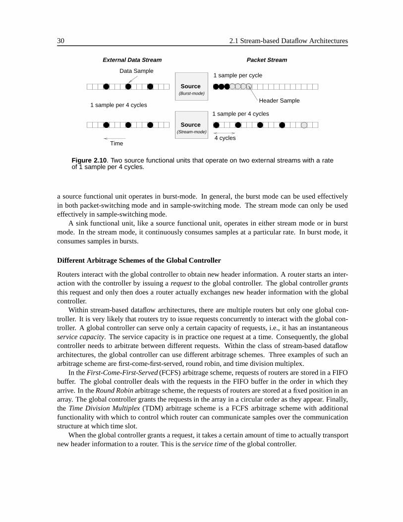
30 2.1 Stream-based Dataflow Architectures
Time
Source
Source
(Burst-mode)
(Stream-mode)
Data Sample
Header Sample
External Data Stream Packet Stream
1 sample per 4 cycles
1 sample per 4 cycles
1 sample per cycle
4 cycles
Figure 2.10 . Two source functional units that operate on two external streams with a rateof 1 sample per 4 cycles.
a source functional unit operates in burst-mode. In general, the burst mode can be used effectivelyin both packet-switching mode and in sample-switching mode. The stream mode can only be usedeffectively in sample-switching mode.
A sink functional unit, like a source functional unit, operates in either stream mode or in burstmode. In the stream mode, it continuously consumes samples at a particular rate. In burst mode, itconsumes samples in bursts.
Different Arbitrage Schemes of the Global Controller
Routers interact with the global controller to obtain new header information. A router starts an inter-action with the controller by issuing arequestto the global controller. The global controllergrantsthis request and only then does a router actually exchanges new header information with the globalcontroller.
Within stream-based dataflow architectures, there are multiple routers but only one global con-troller. It is very likely that routers try to issue requests concurrently to interact with the global con-troller. A global controller can serve only a certain capacity of requests, i.e., it has an instantaneousservice capacity. The service capacity is in practice one request at a time. Consequently, the globalcontroller needs to arbitrate between different requests. Within the class of stream-based dataflowarchitectures, the global controller can use different arbitrage schemes. Three examples of such anarbitrage scheme are first-come-first-served, round robin, and time division multiplex.
In theFirst-Come-First-Served(FCFS) arbitrage scheme, requests of routers are stored in a FIFObuffer. The global controller deals with the requests in the FIFO buffer in the order in which theyarrive. In theRound Robinarbitrage scheme, the requests of routers are stored at a fixed position in anarray. The global controller grants the requests in the array in a circular order as they appear. Finally,the Time Division Multiplex(TDM) arbitrage scheme is a FCFS arbitrage scheme with additionalfunctionality with which to control which router can communicate samples over the communicationstructure at which time slot.
When the global controller grants a request, it takes a certain amount of time to actually transportnew header information to a router. This is theservice timeof the global controller.
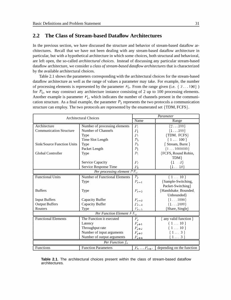
Basic Definitions and Problem Statement 31
2.2 The Class of Stream-based Dataflow Architectures
In the previous section, we have discussed the structure and behavior of stream-based dataflow ar-chitectures. Recall that we have not been dealing with any stream-based dataflow architecture inparticular, but with a hypothetical architecture in which some choices, both structural and behavioral,are left open, the so-calledarchitectural choices. Instead of discussing any particular stream-baseddataflow architecture, we consider aclass of stream-based dataflow architecturesthat is characterizedby the available architectural choices.
Table 2.1 shows the parameters corresponding with the architectural choices for the stream-baseddataflow architecture as well as the range of values a parameter may take. For example, the numberof processing elements is represented by the parameterP0. From the range given (i.e.f 2 : : :100g )for P0, we may construct any architecture instance consisting of 2 up to 100 processing elements.Another example is parameterP1, which indicates the number of channels present in the communi-cation structure. As a final example, the parameterP2 represents the two protocols a communicationstructure can employ. The two protocols are represented by the enumerated setfTDM;FCFSg.
ParameterArchitectural ChoicesName Range
Architecture Number of processing elementsP0 f2 : : :100gCommunication Structure Number of Channels P1 f1 : : :100g
Type P2 fTDM; FCFSgTime Slot Length P3 f 1 : : : 100g
Sink/Source Function Units Type P4 f Stream, BurstgPacket Length P5 f1 : : :1000000g
Global Controller Type P6 fFCFS;Round Robin;TDMg
Service Capacity P7 f1 : : :3gService Response Time P8 f1 : : :10g
Per processing elementPEx
Functional Units Number of Functional ElementsPx f 1 : : : 10gType Px+1 fSample-Switching;
Packet-SwitchinggBuffers Type Px+2 fHandshake;Bounded;
UnboundedgInput Buffers Capacity Buffer Px+3 f1 : : :1000gOutput Buffers Capacity Buffer Px+4 f1 : : :1000gRouters Type Px+5 fShare;Singleg
Per Function ElementFEy
Functional Elements The Function it executed Py f any valid functiongLatency Py+1 f 1 : : : 10gThroughput rate Py+2 f 1 : : : 10gNumber of input arguments Py+3 f 1 : : : 3 gNumber of output arguments Py+4 f 1 : : : 3 g
Per FunctionfnFunctions Function Parameters Pn : : :Pn+z depending on the function
Table 2.1 . The architectural choices present within the class of stream-based dataflowarchitectures.
32 2.3 The Designer’s Problem
2.2.1 Architecture Template
To describe the class of stream-based dataflow architectures, we introduce the notion of an architecturetemplate, which we define as
Definition 2.8. ARCHITECTURE TEMPLATE
An architecture templateis a specification of a class of architectures in a parameterized form.2
An architecture template represents a class of architectures by expressing the available architec-tural choices in terms of a parameter setP . A particular architecture within the class of architecturesis named an architecture instance, which is defined as
Definition 2.9. ARCHITECTURE INSTANCE
An architecture instance, or design, is the result of assigning values to all architectural choices,i.e., parameters of the architecture template. 2
2.2.2 Design Space
The set of architectural choices in Table 2.1 describes many different architecture instances of thestream-based dataflow architecture template. All these different instances together define thedesignspaceD of the class of stream-based dataflow architectures. For an architecture templateAT withparametersp0 : : : pn, the design spaceD is
D = P0 � P1 � � � � � Pn (2.3)
We can select a pointI in D by selecting for each parameterP0 toPn a particular valuep such that
I = (p0; p1; : : : ; pn) 2 D (2.4)
For this pointI we can derive an architecture instanceAI of AT
AT (I)! AI (2.5)
2.3 The Designer’s Problem
So far, we have considered the stream-based dataflow architecture template from the point of view ofstructure and behavior. Now we turn to the designer who needs to design architectures, and in partic-ular stream-based dataflow architectures, that can execute a set of applications. The designer has toproduce one or more architectures that satisfydesign objectivessuch as real-time constraints, through-put of the architecture, resource efficiency, and programmability. This list can easily be extended with,for example, power consumption and silicon area. We will confine ourselves to the design objectivesrelated to real-time constraints, throughput constraints, and utilization.
Definition 2.10. FEASIBLE DESIGN
A feasible designsatisfies all stated design objectives. 2
Thus the design problem a designer faces consists of selecting parameter values for an architecturetemplate such that a feasible design is found. This design task becomes increasingly difficult asarchitectures become more programmable. A design should satisfy the design objectives not only fora single application, but for a given set of applications.
A designer’s approach to constructing programmable applications-specific architectures, and inparticular, stream-based dataflow architectures, is what we consider in this thesis. The problem state-ment for which this thesis will provide a systematic methodology is:

Basic Definitions and Problem Statement 33
Central Problem Statement of this thesisGiven an architecture templateAT and its design spaceD, a set of applications, and thedesign objectives, provide a method to find parameter values of the architecture templatesuch that a feasible design results.
We discuss a feasible design and not an optimal design. The complexity of these architectures issuch that we simply do not know what an optimum might be. Nevertheless, of all possible feasibledesigns, a designer is interested in the design best satisfying the stated design objectives. When onefeasible design has a better utilization than that of other feasible designs, it is considered a betterdesign.
Design Objectives
Real-time ConstraintsThroughput ConstraintUtilizationSilicon Area CostPower ConsumptionProgrammability to Support a Set of Applications
Table 2.2 . Possible design objectives when finding an architecture for a set of applications.
2.3.1 Exploring the Design Space of Architectures
We observe that a design approach is not yet available for programmable architectures like stream-based dataflow architectures. As we will show, design approaches currently in use seem unable to helpdesigners in evaluating the consequences of architectural choices with respect to the design objectives.The level of detail introduced in current design approaches narrows down the design space that thedesigner can explore. As a result, a designer cannot make the trade-off between the many architecturalchoices shown in Table 2.1.
Because the designer cannot make the necessary trade-offs, the resulting design is eitherover-designedor under-designed. In the first case, a design under-utilizes its resources and it is thus a moreexpensive design than necessary; in the second case, the design cannot satisfy the imposed designobjectives.
2.3.2 Problems in Current Design Approaches
Designers typically start by sketching rough outlines of architectures on paper, which we callpaperarchitectures. Because it is difficult to evaluate particular architectural choices at this stage, designerstend to make qualitative statements about these paper architectures that lack a sound basis on whichto validate them. This makes designing feasible architectures an art rather than solid engineering.
Once designers have selected a particular paper design, they tend to fill in the detail of a design ina hardware description language like VHDL or Verilog. This design approach is sometimes referredto asGolden Point Design[Richards, 1994]. In this design approach, designers very quickly becomepreoccupied by details of the design. They do not thoroughly evaluate the consequences of decisionsat a high enough level. For example, the high level decision to use a particular kind of buffer of a
34 2.4 Related Work on Dataflow Architectures
certain size presumably has a far greater impact on the overall performance of a design than do thedetails of how a buffer communicates with a processing element.
As the description of the architecture becomes more detailed, it also becomes harder to changethe structure or behavior of the architecture. This makes it more difficult to try out other architecturalchoices. Since simulation becomes an increasingly important tool when more detail is added, anotherconsequence of a more detailed architecture is that the simulation speed drops dramatically, especiallyin the context of high performance video and radar applications. Consequently, only a few alternativescan be evaluated in a reasonable amount of time. An associated problem with adding more and moredetails is that many problems arise that were initially unforeseen. To solve these problems, designerstake ad-hoc decisions that can seriously affect the ability of architectures to satisfy their stated designobjectives.
Although designers develop programmable architectures, the development of the architecture isoften unrelated to the development of the set of applications. This further impedes making trade-offs on behalf of supporting a set of applications. It is therefore very much the question if the finalarchitecture is sufficiently programmable to execute the complete set of applications while satisfyingthe design objectives.
Another design approach is to transform digital signal processing applications in various steps ofrefinement into a particular architecture. This approach is used, for example, in thesystolic arraydesign community [H.T. Kung and Leiserson, 1978; H.T. Kung, 1982] and thewavefrontdesign com-munity [S.Y. Kung et al., 1982; S.Y. Kung, 1988]. Using all kinds of transformations like folding andpartitioning, the application is transformed into an architecture (see for example, figure 6.41 in S.Y.Kung [1988]). For a set of applications, this refinement method would lead to different optimal ar-chitectures for different applications. It lacks the ability to deal effectively with making trade-offs infavor of the set of applications.
Finally, the hardware/software codesign design approach relies on an architecture template todesign architectures. One application is partitioned into hardware and software parts that fit onto thisarchitecture template [De Micheli and Sami, 1996]. Nevertheless, the architecture template typicallyused in hardware/software codesign is too restrictive: it often consists of one or more co-processors, abus, and a programmable element like a CPU or a DSP. The architecture template is unable to handlethe demanding requirements of high-performance signal processing.
The Hardware/Software Codesign design approach lacks the ability to deal effectively with mak-ing trade-offs in favor of the set of applications. Only recently has the problem of executing a set ofmulti-media applications been addressed in the hardware/software codesign community (by Kalavadeand Subrahmanyam [1997]), albeit only for cyclo-static DSP applications.
2.4 Related Work on Dataflow Architectures
Work on dataflow architectures started in the early 1970s. It is Jack Dennis who is regarded as theoriginator of the concepts of dataflow architectures [Dennis and Misunas, 1975]. People working ondataflow architectures had great visions of plentiful computing power provided by powerful parallelarchitectures based on simple computing principles [Veen, 1986]. Dataflow architectures, especiallydynamic dataflow architecture (see Section 2.1.3), were researched intensively during the 1980s andthe early 1990s. During the 1980s, the now famous Manchester Dataflow Architecture was conceivedand implemented [Gurd et al., 1985]. It typifies the dynamic dataflow architectures of that time. TheManchester Dataflow Architecture was a general-purpose computer that used fine-grained, homoge-neous functional units (i.e., each functional unit executes the same set of functions). This makes it
Basic Definitions and Problem Statement 35
possible for the architecture to do load balancing of the functional units, giving speed-up that wasnearly linear.
2.4.1 Implementation Problems of Dataflow Architectures
In general, dynamic dataflow architectures, although very elegant conceptually, suffer from severe im-plementation problems. It was found to be impossible, as we will explain, to implement the dataflowmodel of computation efficiently in hardware [Veen, 1986]. Dynamic dataflow architectures exploitfine-grained functional elements, giving these architectures the most flexibility. This result, how-ever, in enormous communication requirements leading to special, bulky communication structures.Furthermore, dynamic dataflow architectures are able to execute recursion and data-dependent con-ditionals, causing parallelism to arise at run-time. This run-time parallelism disturbs the ordering ofthe tokens inside the architecture. To reorder these tokens at run-time, dynamic dataflow architecturesrequirematching units. These matching units are special hardware units that utilizetagsand a certainamount of associative memory to perform tag matching at run-time2. It is, however, very difficult toassess in advance how large this memory should be. In addition, matching units need to have someoverflow mechanisms, which can be very bulky [Gurd et al., 1985]. Another issue making the im-plementation of dynamic dataflow architectures difficult is the granularity of the data flowing aroundthe machine. This data is typically a single integer value, due to the fine-grained functions employed.Tagging these fine-grained tokens results in an enormous overhead. In addition, it is very difficult togenerate unique tags for all the tokens flowing through the architecture at the same time. Of all the im-plementation problems mentioned here, it is the implementation of matching units that has proven inthe end to be the Achilles heel of the implementation of dynamic dataflow architectures [Jagannathan,1995].
2.4.2 Other Dataflow Architectures
As research continued, it became increasingly clear that pure dynamic dataflow architectures, in par-ticular, fine-grained dataflow architectures, are not a viable option in the long term to become general-purpose computing architectures [Jagannathan, 1995]. Instead, research continued to focus moreon hybrid data-driven/control-driven architectures calledMultithreading Architecturesor dataflow ar-chitectures that are specialized for a particular application domain, calledDomain-specific DataflowArchitectures.
Multithreading architectures combine dataflow and von Neumann models of computation [Dennisand Gao, 1994]. These architectures hide the effects of both memory latency and synchronizationwaits by switching coarse-grained functions on a RISC-style processor. Examples of such hybridarchitectures are the Monsoon processor [Papadopoulos and Culler, 1990] and the Sparcle processorof the Alewife project [Agarwal et al., 1995].
Domain-specific architectures are specialized for a particular application domain. These architec-tures try to exploit characteristics of a particular domain, for example real-timevideo signal processing(VSP). VSP applications can be described in a very natural way using streams and dataflow models ofcomputation [Lee, 1992-1993; Jagannathan, 1995]. Dataflow architectures implement these dataflowmodels of computation directly into hardware. We discuss domain-specific dataflow architectures inmore detail in the next section. We thereby make a distinctionbetween static domain-specific dataflowarchitectures and dynamic domain-specific dataflow architectures.
2Architectures using these tags are calledtagged-token dataflow architectures. The Manchester Dataflow Architectureis such a tagged-token dataflow architecture.
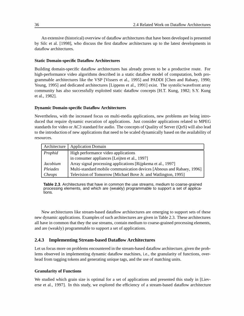
36 2.4 Related Work on Dataflow Architectures
An extensive (historical) overview of dataflow architectures that have been developed is presentedby Silc et al. [1998], who discuss the first dataflow architectures up to the latest developments indataflow architectures.
Static Domain-specific Dataflow Architectures
Building domain-specific dataflow architectures has already proven to be a productive route. Forhigh-performance video algorithms described in a static dataflow model of computation, both pro-grammable architectures like the VSP [Vissers et al., 1995] and PADDI [Chen and Rabaey, 1990;Yeung, 1995] and dedicated architectures [Lippens et al., 1991] exist. The systolic/wavefront arraycommunity has also successfully exploited static dataflow concepts [H.T. Kung, 1982; S.Y. Kunget al., 1982].
Dynamic Domain-specific Dataflow Architectures
Nevertheless, with the increased focus on multi-media applications, new problems are being intro-duced that require dynamic execution of applications. Just consider applications related to MPEGstandards for video or AC3 standard for audio. The concepts of Quality of Server (QoS) will also leadto the introduction of new applications that need to be scaled dynamically based on the availability ofresources.
Architecture Application Domain
Prophid High performance video applicationsin consumer appliances [Leijten et al., 1997]
Jacobium Array signal processing applications [Rijpkema et al., 1997]Pleiades Multi-standard mobile communication devices [Abnous and Rabaey, 1996]Cheops Television of Tomorrow [Michael Bove Jr. and Watlington, 1995]
Table 2.3 . Architectures that have in common the use streams, medium to coarse-grainedprocessing elements, and which are (weakly) programmable to support a set of applica-tions.
New architectures like stream-based dataflow architectures are emerging to support sets of thesenew dynamic applications. Examples of such architectures are given in Table 2.3. These architecturesall have in common that they the use streams, contain medium to coarse-grained processing elements,and are (weakly) programmable to support a set of applications.
2.4.3 Implementing Stream-based Dataflow Architectures
Let us focus more on problems encountered in the stream-based dataflow architecture, given the prob-lems observed in implementing dynamic dataflow machines, i.e., the granularity of functions, over-head from tagging tokens and generating unique tags, and the use of matching units.
Granularity of Functions
We studied which grain size is optimal for a set of applications and presented this study in [Liev-erse et al., 1997]. In this study, we explored the efficiency of a stream-based dataflow architecture
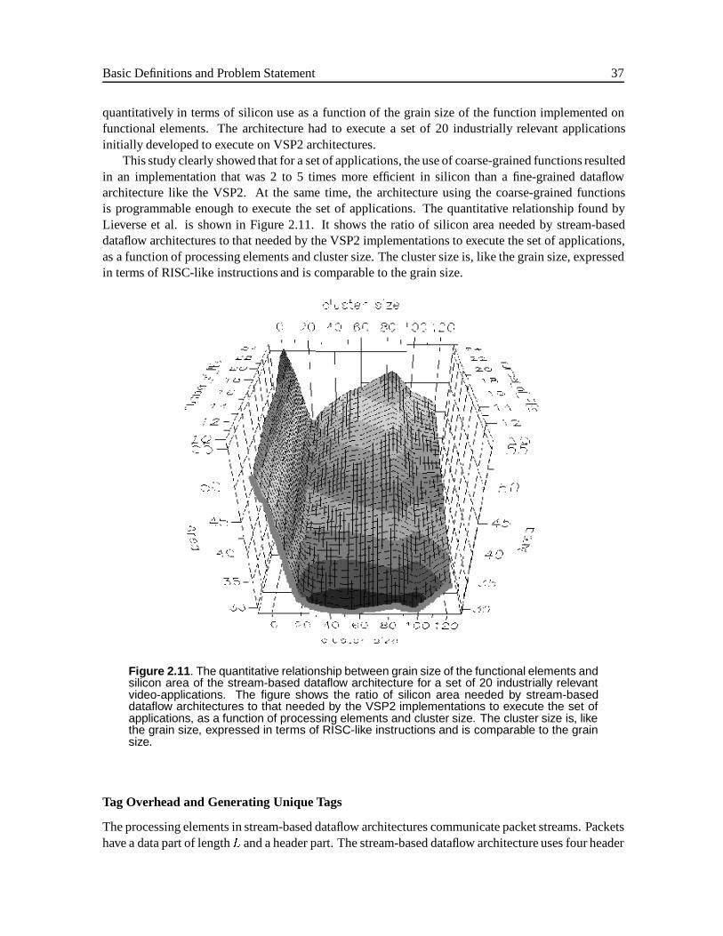
Basic Definitions and Problem Statement 37
quantitatively in terms of silicon use as a function of the grain size of the function implemented onfunctional elements. The architecture had to execute a set of 20 industrially relevant applicationsinitially developed to execute on VSP2 architectures.
This study clearly showed that for a set of applications, the use of coarse-grained functions resultedin an implementation that was 2 to 5 times more efficient in silicon than a fine-grained dataflowarchitecture like the VSP2. At the same time, the architecture using the coarse-grained functionsis programmable enough to execute the set of applications. The quantitative relationship found byLieverse et al. is shown in Figure 2.11. It shows the ratio of silicon area needed by stream-baseddataflow architectures to that needed by the VSP2 implementations to execute the set of applications,as a function of processing elements and cluster size. The cluster size is, like the grain size, expressedin terms of RISC-like instructions and is comparable to the grain size.
Figure 2.11 . The quantitative relationship between grain size of the functional elements andsilicon area of the stream-based dataflow architecture for a set of 20 industrially relevantvideo-applications. The figure shows the ratio of silicon area needed by stream-baseddataflow architectures to that needed by the VSP2 implementations to execute the set ofapplications, as a function of processing elements and cluster size. The cluster size is, likethe grain size, expressed in terms of RISC-like instructions and is comparable to the grainsize.
Tag Overhead and Generating Unique Tags
The processing elements in stream-based dataflow architectures communicate packet streams. Packetshave a data part of lengthL and a header part. The stream-based dataflow architecture uses four header

38 2.4 Related Work on Dataflow Architectures
samples to represent the header part. The header tags the data samples present in the data part. Bymaking a packet longer, we can spread the overhead introduced by the four header samples over moresamples: the longer the data part, the smaller the overhead per sample introduced by the header.
When a stream with a rate ofx samples/sec is broken down into a stream of packets with lengthL, the overhead introduced by the four header samples results in an effective rate of the samples as
x �1
1 + 4=L� 100% = Effective Rate (2.6)
In general, the longer the packet, the smaller the overhead of a header. A packet length of 100 to1000 is, for example, very common in video applications. A single video line takes approximately800 samples. When using packets of 1000, the overhead is less than 0.4%. However, very long packetsnegatively affect the switching of packet streams on a functional unit, which leads to large buffers:other packet streams have to wait longer before being processed by a functional unit. As packetsbecome longer, it becomes more difficult to reuse a functional unit. This reduces the programmabilityof functional units.
Stream-based dataflow architectures do not suffer that much from the unique tag problem. Thesearchitectures require fewer unique tags because of the use of packets and static routing of packetstreams. Furthermore, knowledge about the applications can be exploited to generate unique tags. Invideo, for example, there are strong relations between video frames.
Matching Units
Dynamic dataflow architectures require matching units to restore order in tokens streams. In principle,stream-based dataflow architectures also have to reorder packets at run-time. We illustrate this withthe example shown in Figure 2.12. It shows a functional unit in packet-switchingmode, with two inputports containing three functional elements (FE0, FE1, andFE2). Two input buffers connect to thesetwo input ports. The content of these two buffers is shown over time, with each gray area representinga packet. The number beneath each packet indicates to which functional element it belongs (i.e. it isthe value ofHf in the header). We do not show the output buffers in the figure. The example is thesame as the example shown in Figure 2.8 except that it contains one additional functional element, i.e.FE2 requires two input arguments.
The order of the packets in theOpcodeBuffer first causes the execution ofFE0, followed bythe execution ofFE1, which also consumes packets from bufferB1. The packet read from theOpcodebuffer after the execution ofFE1 again causesFE1 to execute. Input bufferB1, however,contains a packet belonging toFE2 and this situation causes adeadlock: the functional unit will neverbe able to execute functional elementFE1. In such a case, a matching unit has to reorder packets inboth buffers such that the packets presented to the functional unit belong to eitherFE1 or FE2. Thisprocedure prevents deadlock from occurring.
The sharing of input buffers between various functional elements causes the reordering problemin Figure 2.12. To solve this problem, the input buffers must not be shared, as is already required insample-switching mode. Although this is a solution for the reordering problem, it introduces as manyinputs buffers as there are input arguments for the functions of the function repertoire of a functionalunit, a result that might be undesirable.
Although sample-switching might solve the reordering problem through the introduction of morebuffers, it also leads to many more switches of the functional elements than occurs in packet-switchingmode. From work done on Multithreadingarchitectures [Dennis and Gao, 1994], we already know thatthis fast switching makes implementations of sample-switching functional units difficult. Conversely,
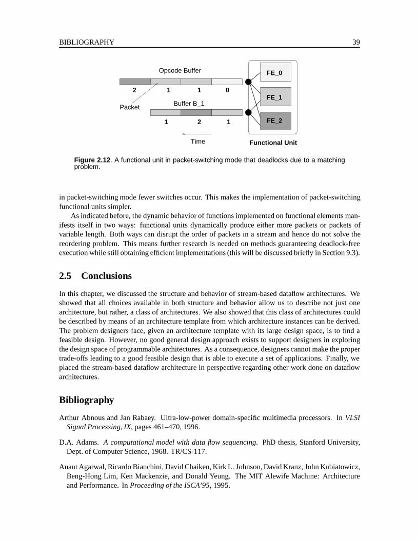
BIBLIOGRAPHY 39
FE_0
FE_1Buffer B_1
01
2 11
Functional Unit
FE_2
2 1
Time
Packet
Opcode Buffer
Figure 2.12 . A functional unit in packet-switching mode that deadlocks due to a matchingproblem.
in packet-switching mode fewer switches occur. This makes the implementation of packet-switchingfunctional units simpler.
As indicated before, the dynamic behavior of functions implemented on functional elements man-ifests itself in two ways: functional units dynamically produce either more packets or packets ofvariable length. Both ways can disrupt the order of packets in a stream and hence do not solve thereordering problem. This means further research is needed on methods guaranteeing deadlock-freeexecution while still obtaining efficient implementations (this will be discussed briefly in Section 9.3).
2.5 Conclusions
In this chapter, we discussed the structure and behavior of stream-based dataflow architectures. Weshowed that all choices available in both structure and behavior allow us to describe not just onearchitecture, but rather, a class of architectures. We also showed that this class of architectures couldbe described by means of an architecture template from which architecture instances can be derived.The problem designers face, given an architecture template with its large design space, is to find afeasible design. However, no good general design approach exists to support designers in exploringthe design space of programmable architectures. As a consequence, designers cannot make the propertrade-offs leading to a good feasible design that is able to execute a set of applications. Finally, weplaced the stream-based dataflow architecture in perspective regarding other work done on dataflowarchitectures.
Bibliography
Arthur Abnous and Jan Rabaey. Ultra-low-power domain-specific multimedia processors. InVLSISignal Processing, IX, pages 461–470, 1996.
D.A. Adams. A computational model with data flow sequencing. PhD thesis, Stanford University,Dept. of Computer Science, 1968. TR/CS-117.
Anant Agarwal, Ricardo Bianchini, David Chaiken, Kirk L. Johnson, David Kranz, John Kubiatowicz,Beng-Hong Lim, Ken Mackenzie, and Donald Yeung. The MIT Alewife Machine: Architectureand Performance. InProceeding of the ISCA’95, 1995.
40 BIBLIOGRAPHY
D.C. Chen and J.M. Rabaey. Paddi: Programmable arithmetic devices for digital signal processing.In Proceedings of VLSI Signal Processing, IV, pages 240 – 249, 1990.
Giovanni De Micheli and Mariagiovanna Sami.Hardware/Software Co-Design, volume 310 ofSeriesE: Applied Sciences. NATO ASI Series, 1996.
Jack B. Dennis and Guang R. Gao. Multithreaded architectures: principles, projects and issues. InRobert A. Iannucci, editor,Multithreaded Computer Architecture, A Summary of the State of theArt, chapter 1, pages 1–71. Kluwer Academic Publishers, 1994.
J.B. Dennis. First version of a data flow procedure language. InLecture Notes in Computer Science,volume 19. Springer-Verlag, 1974.
J.B. Dennis and D.P. Misunas. A preliminary architecture for a basic data flow architecture. InProceedings of the 2nd Annual Symposium on Computer Architectures, pages 126 – 132. IEEEPress, 1975.
J.R. Gurd, C.C. Kirkham, and I. Watson. The Manchester Prototype Dataflow Computer.Communi-cations of the ACM, 28(1):34 – 52, 1985.
John L. Hennessy and David A. Patterson.Computer Architectures: A QuantitativeApproach. MorganKaufmann Publishers, Inc., second edition, 1996.
H.T. Kung. Why systolic architectures?IEEE Computer, 15(1), 1982.
H.T. Kung and C.E. Leiserson. Systolic arrays (for VLSI). InSparse Matrix Symposium, pages 256 –282. SIAM, 1978.
R. Jagannathan. Dataflow models. In E.Y. Zomaya, editor,Parallel and Distributed ComputingHandbook. McGraw-Hill, 1995.
Asawaree Kalavade and P.A. Subrahmanyam. Hardware/software partioning for multi-function sys-tems. InProc. of ICCAD’97, pages 516 – 521, 1997.
R.M. Karp and R.E. Miller. Properties of a model for parallel computations: Determinacy, termina-tion, queueing.SIAM Journal on Applied Mathematics, 14(6):1390–1411, 1966.
Edward A. Lee. Design methodology for DSP. Technical Report 92-084, University of California atBerkeley, 1992-1993.
Jeroen Leijten.Real-Time Constrained Reconfigurable Communication between Embedded Proces-sors. PhD thesis, Eindhoven University of Technology, 1998.
Jeroen A.J. Leijten, Jef L. van Meerbergen, Adwin H. Timmer, and Jochen A.G. Jess. Prophid, adata-driven multi-processor architecture for high-performance DSP. InProc. ED&TC, 1997.
P. Lieverse, E.F. Deprettere, A.C.J. Kienhuis, and E.A. de Kock. A clustering approach to exploregrain-sizes in the definition of weakly programmable processing elements. InProceedings of theIEEE Workshop on Signal Processing Systems, pages 107 – 120, De Montfort University, Leicester,UK, 1997.
BIBLIOGRAPHY 41
P.E.R. Lippens, J.L. van Meerbergen, A. van der Werf, W.F.J. Verhaegh, B.T. McSweeney, J.O.Huisken, and O.P. McArdle. PHIDEO: A silicon compiler for high speed algorithms. InProc.EDAC, pages 436 – 441, 1991.
V. Michael Bove Jr. and John A Watlington. Cheops: A reconfigurable data-flow system for videoprocessing.IEEE Transactions on Circuits and Systems for Video Technology, 5(2), 1995.
G.M. Papadopoulos and D.E. Culler. Monsoon: an explicit token-store architecture. InProceedingsof of the 17th ISCA, pages 82 – 91, 1990.
Mark A. Richards. The rapid prototyping of application specific signal processors (RASSP) program:Overview and status. In5th International Workshop on Rapid System Prototyping, pages 1–6. IEEEComputer Society Press, 1994.
Edwin Rijpkema, Gerben Hekstra, Ed Deprettere, and Ju Ma. A strategy for determining a Jacobi spe-cific dataflow processor. InProceedings of 11th Int. Conference of Applications-specific Systems,Architectures and Processors (ASAP’97), pages 53 – 64, Zurich, Switzerland, 1997.
J. Silc, B. Robic, and T. Ungerer. Asynchrony in parallel computing: From dataflow to multithreading.Journal of Parallel and Distributed Computing Practices, 1998.
S.Y. Kung.VLSI Array Processors. Prentice Hall Information and System Sciences Series, 1988.
S.Y. Kung, K.S. Arun, R.J. Gal-Ezer, and D.V. Bhaskar Rao. Wavefront array processor: language,architecture, and applications.IEEE Transactions on Computers, Special Issue on Parallel andDistributed Computers, C-31(11):1054 – 1066, 1982.
Arthur H. Veen. Dataflow machine architecture.ACM Computing Surveys, 18(4):366–396, 1986.
K.A. Vissers, G. Essink, P.H.J. van Gerwen, P.J.M. Janssen, O. Popp, E. Riddersma, and J.M. Veen-drick. Algorithms and Parallel VLSI Architectures III, chapter Architecture and programming oftwo generations video signal processors, pages 167 – 178. Elsevier, 1995.
K.W. Yeung. A Data-Driven Multiprocessor Architecture for High Throughput Digital Signal Pro-cessing. PhD thesis, University of California at Berkeley, 1995.

42 BIBLIOGRAPHY
Chapter 3
Solution Approach
Contents
3.1 The Evaluation of Alternative Architectures . . . . . . . . . . . . . . . . . . . 44
3.1.1 Quantitative Data. . . . . . . . . . . . . . . . . . . . . . . . . . . . . . . 44
3.1.2 The Y-chart Approach . . . . . . . . . . . . . . . . . . . . . . . . . . . . 44
3.2 Design Space Exploration Using the Y-chart Approach . . . . . . . . . . . . . 45
3.3 Requirements of the Y-chart Approach . . . . . . . . . . . . . . . . . . . . . . 46
3.3.1 Performance Analysis . . . . . . . . . . . . . . . . . . . . . . . . . . . . 47
3.3.2 Mapping . . . . . . . . . . . . . . . . . . . . . . . . . . . . . . . . . . . 52
3.4 Development of a Y-chart Environment . . . . . . . . . . . . . . . . . . . . . . 55
3.5 Related Work . . . . . . . . . . . . . . . . . . . . . . . . . . . . . . . . . . . . 56
3.5.1 Design of General-Purpose Processors . . . . . . . . . . . . . . . . . . . . 56
3.5.2 Design of Application-Specific Architectures . . . . . . . . . . . . . . . . 59
3.6 Conclusions . . . . . . . . . . . . . . . . . . . . . . . . . . . . . . . . . . . . . . 60
THE architecture template of stream-based dataflow architectures offers many options to designersfor instantiating an architecture, as was explained in Chapter 2. So, how can designers explore
the design space of the architecture template to come to an architecture instance that satisfies his re-quirements? In this chapter, we discuss an approach in which designers can use performance modelsto make architectural choices. By evaluating the performance models of architecture instances, de-signers acquire performance numbers that provide them with quantitative data. They make justifiabledecisions based on this quantitative data.
The idea of using performance numbers to compare architecture instances leads to the Y-chartapproach presented in Section 3.1 in which the performance of architectures is analyzed for a givenset of applications. Using this approach, we explain in Section 3.2 how we can explore the designspace of the architecture template. The Y-chart approach consists of five components having theirown particular requirements. In Section 3.3, we consider the requirements for performance analy-sis an mapping. In this thesis, we development a Y-chart environment for the class of stream-baseddataflow architectures discussed in Chapter 2. In Section 3.4, we show each component of the Y-chartand briefly discuss what the issues are within each component. We finish this chapter in Section 3.5by looking at general-purpose processors. After all, designers have already been constructing pro-grammable architectures for decades. As it turns out, designers use a benchmark design approachwhich very much resembles the Y-chart approach.
43
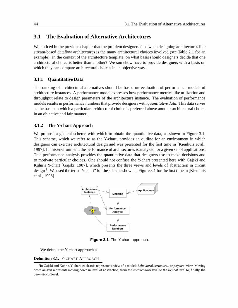
44 3.1 The Evaluation of Alternative Architectures
3.1 The Evaluation of Alternative Architectures
We noticed in the previous chapter that the problem designers face when designing architectures likestream-based dataflow architectures is the many architectural choices involved (see Table 2.1 for anexample). In the context of the architecture template, on what basis should designers decide that onearchitectural choice is better than another? We somehow have to provide designers with a basis onwhich they can compare architectural choices in an objective way.
3.1.1 Quantitative Data
The ranking of architectural alternatives should be based on evaluation of performance models ofarchitecture instances. A performance model expresses how performance metrics like utilization andthroughput relate to design parameters of the architecture instance. The evaluation of performancemodels results in performance numbers that provide designers withquantitative data. This data servesas the basis on which a particular architectural choice is preferred above another architectural choicein an objective and fair manner.
3.1.2 The Y-chart Approach
We propose a general scheme with which to obtain the quantitative data, as shown in Figure 3.1.This scheme, which we refer to as the Y-chart, provides an outline for an environment in whichdesigners can exercise architectural design and was presented for the first time in [Kienhuis et al.,1997]. In this environment, the performance of architectures is analyzed for a given set of applications.This performance analysis provides the quantitative data that designers use to make decisions andto motivate particular choices. One should not confuse the Y-chart presented here with Gajski andKuhn’s Y-chart [Gajski, 1987], which presents the three views and levels of abstraction in circuitdesign1. We used the term “Y-chart” for the scheme shown in Figure 3.1 for the first time in [Kienhuiset al., 1998].
AnalysisPerformance
Applications
PerformanceNumbers
Mapping
ArchitectureInstance
Figure 3.1 . The Y-chart approach.
We define the Y-chart approach as
Definition 3.1. Y-CHART APPROACH
1In Gajski and Kuhn’s Y-chart, each axis represents a view of a model:behavioral, structural, or physicalview. Movingdown an axis represents moving down in level of abstraction, from thearchitecturallevel to thelogical level to, finally, thegeometricallevel.
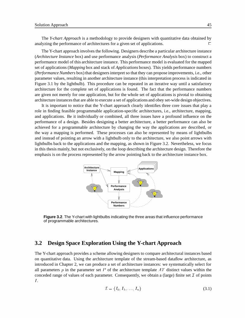
Solution Approach 45
TheY-chart Approachis a methodology to provide designers with quantitative data obtained byanalyzing the performance of architectures for a given set of applications. 2
The Y-chart approach involves the following. Designers describe a particular architecture instance(Architecture Instancebox) and use performance analysis (Performance Analysisbox) to construct aperformance model of this architecture instance. This performance model is evaluated for the mappedset of applications (Mappingbox and stack ofApplicationsboxes). This yields performance numbers(Performance Numbersbox) that designers interpret so that they can propose improvements, i.e., otherparameter values, resulting in another architecture instance (this interpretation process is indicated inFigure 3.1 by the lightbulb). This procedure can be repeated in an iterative way until a satisfactoryarchitecture for the complete set of applications is found. The fact that the performance numbersare given not merely for one application, but for the whole set of applications is pivotal to obtainingarchitecture instances that are able to execute a set of applicationsand obey set-wide design objectives.
It is important to notice that the Y-chart approach clearly identifies three core issues that play arole in finding feasible programmable application-specific architectures, i.e., architecture, mapping,and applications. Be it individually or combined, all three issues have a profound influence on theperformance of a design. Besides designing a better architecture, a better performance can also beachieved for a programmable architecture by changing the way the applications are described, orthe way a mapping is performed. These processes can also be represented by means of lightbulbsand instead of pointing an arrow with a lightbulb only to the architecture, we also point arrows withlightbulbs back to the applications and the mapping, as shown in Figure 3.2. Nevertheless, we focusin this thesis mainly, but not exclusively, on the loop describing the architecture design. Therefore theemphasis is on the process represented by the arrow pointing back to the architecture instance box.
Analysis
Performance
Applications
PerformanceNumbers
Mapping
ArchitectureInstance
Figure 3.2 . The Y-chart with lightbulbs indicating the three areas that influence performanceof programmable architectures.
3.2 Design Space Exploration Using the Y-chart Approach
The Y-chart approach provides a scheme allowing designers to compare architectural instances basedon quantitative data. Using the architecture template of the stream-based dataflow architecture, asintroduced in Chapter 2, we can produce a set of architecture instances: we systematically select forall parametersp in the parameter setP of the architecture templateAT distinct values within theconceded range of values of each parameter. Consequently, we obtain a (large) finite setI of pointsI .
I = fI0; I1; : : : ; Ing (3.1)
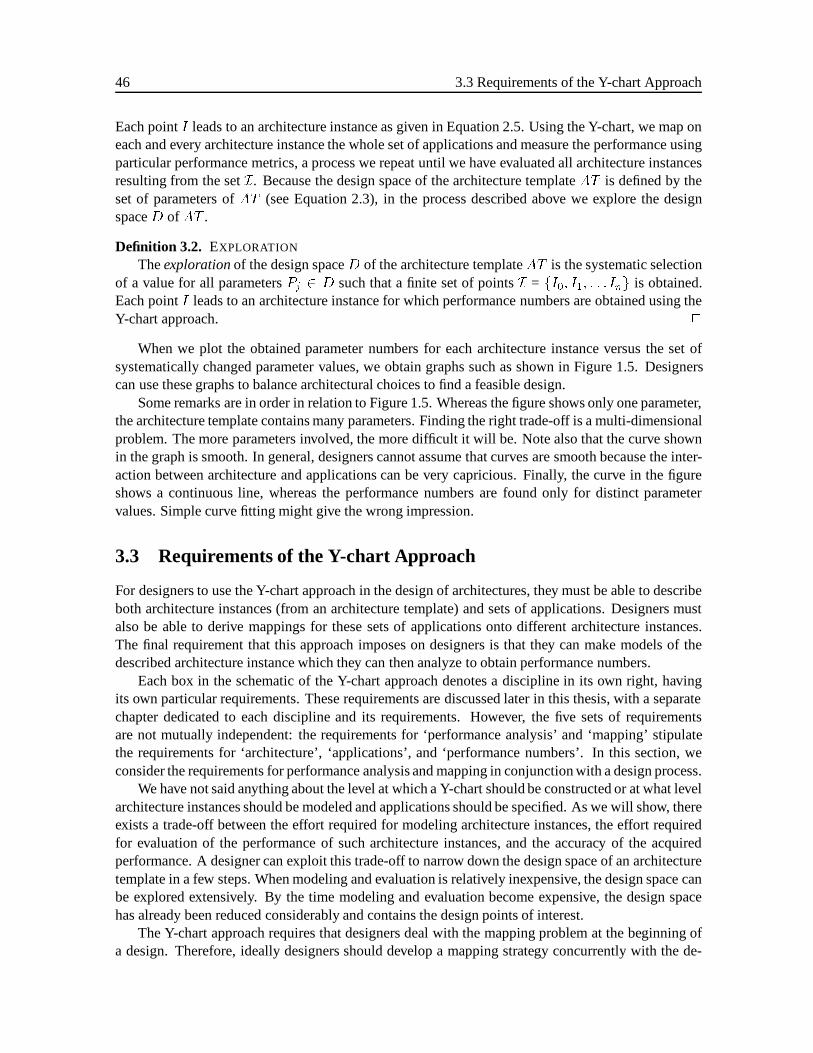
46 3.3 Requirements of the Y-chart Approach
Each pointI leads to an architecture instance as given in Equation 2.5. Using the Y-chart, we map oneach and every architecture instance the whole set of applications and measure the performance usingparticular performance metrics, a process we repeat until we have evaluated all architecture instancesresulting from the setI. Because the design space of the architecture templateAT is defined by theset of parameters ofAT (see Equation 2.3), in the process described above we explore the designspaceD of AT .
Definition 3.2. EXPLORATION
Theexplorationof the design spaceD of the architecture templateAT is the systematic selectionof a value for all parametersPj 2 D such that a finite set of pointsI = fI0; I1; : : : Ing is obtained.Each pointI leads to an architecture instance for which performance numbers are obtained using theY-chart approach. 2
When we plot the obtained parameter numbers for each architecture instance versus the set ofsystematically changed parameter values, we obtain graphs such as shown in Figure 1.5. Designerscan use these graphs to balance architectural choices to find a feasible design.
Some remarks are in order in relation to Figure 1.5. Whereas the figure shows only one parameter,the architecture template contains many parameters. Finding the right trade-off is a multi-dimensionalproblem. The more parameters involved, the more difficult it will be. Note also that the curve shownin the graph is smooth. In general, designers cannot assume that curves are smooth because the inter-action between architecture and applications can be very capricious. Finally, the curve in the figureshows a continuous line, whereas the performance numbers are found only for distinct parametervalues. Simple curve fitting might give the wrong impression.
3.3 Requirements of the Y-chart Approach
For designers to use the Y-chart approach in the design of architectures, they must be able to describeboth architecture instances (from an architecture template) and sets of applications. Designers mustalso be able to derive mappings for these sets of applications onto different architecture instances.The final requirement that this approach imposes on designers is that they can make models of thedescribed architecture instance which they can then analyze to obtain performance numbers.
Each box in the schematic of the Y-chart approach denotes a discipline in its own right, havingits own particular requirements. These requirements are discussed later in this thesis, with a separatechapter dedicated to each discipline and its requirements. However, the five sets of requirementsare not mutually independent: the requirements for ‘performance analysis’ and ‘mapping’ stipulatethe requirements for ‘architecture’, ‘applications’, and ‘performance numbers’. In this section, weconsider the requirements for performance analysis and mapping in conjunction with a design process.
We have not said anything about the level at which a Y-chart should be constructed or at what levelarchitecture instances should be modeled and applications should be specified. As we will show, thereexists a trade-off between the effort required for modeling architecture instances, the effort requiredfor evaluation of the performance of such architecture instances, and the accuracy of the acquiredperformance. A designer can exploit this trade-off to narrow down the design space of an architecturetemplate in a few steps. When modeling and evaluation is relatively inexpensive, the design space canbe explored extensively. By the time modeling and evaluation become expensive, the design spacehas already been reduced considerably and contains the design points of interest.
The Y-chart approach requires that designers deal with the mapping problem at the beginning ofa design. Therefore, ideally designers should develop a mapping strategy concurrently with the de-
Solution Approach 47
velopment of the architecture instance and the set of applications. We formulate a mapping approachwith which such mapping strategy can be developed for the stream-based dataflow architecture.
3.3.1 Performance Analysis
Performance analysis always involves three issues: amodeling effort, an evaluation effortand theaccuracyof the obtained results [Lavenberg, 1983; van Gemund, 1996]. We address each of these inmore detail in Chapter 4. Performance analysis can take place at different levels of detail, dependingon the trade-offs that are made between these three issues. Very accurate performance numbers canbe achieved, but at the expense of a lot of detailed modeling and long evaluation times. On the otherhand, performance numbers can be achieved in a short time with modest effort for modeling but at theexpense of loss of accuracy. We place the important relations between these three issues in perspectivein what we call theAbstraction Pyramid.
The Abstraction Pyramid
The abstraction pyramid (see Figure 3.3) describes the modeling of architectures at different levelsof abstraction in relation to the three issues in performance modeling. At the top of the pyramid is adesigner’s initial rough idea (shown as a lightbulb) for an architecture in the form of a ‘paper architec-ture’. The designer wants to realize this architecture in silicon. The bottom of the pyramid representsall possible feasible realizations; it thus represents the complete design space of the designer’s paperarchitecture. A discussion of the five main elements of the abstraction pyramid follows.
Cost of Modeling Moving down in the pyramid from top to bottom, a designer defines an increasingexpenditure of detail of an architecture using some modeling formalism. This process proceedsat the cost of an increasing amount of effort, as indicated on thecost of modelingaxis at theright-hand side of the pyramid. As a designer describes architectures in more detail, the numberof architectural choices (i.e. the number of parameters in the architecture template) increases,expanding the basis of the pyramid. Each new architectural choice, albeit at a lower level ofdetail, thus further broadens the design space of the architecture.
Opportunity to Change As the designer moves down and includes more detail using the modelingformalism, the architecture becomes increasingly more specific. Details added at a given levelinterfere with detail added at a higher level of abstraction. Due to this intertwining of detail, themore detailed models become, the more difficult it is to make changes in architectures. Thus,the opportunity to explore other architectures diminishes. This is indicated on theopportunityaxis at the left-hand side of the pyramid.
Level of Detail Lines intersecting the abstraction pyramid horizontally at different heights representarchitecture instances modeled at various levels of detail. At the highest level of abstraction,architectures are modeled usingback-of-the-envelope models. Models become more detailed asthe abstraction pyramid is descended. Theback-of-the-envelope modelsis followed byestima-tion models, abstract executable models, cycle-accurate models, and, finally, bysynthesizableVHDL models. This represents the lowest level at which designers can model architectures.
We use the termback-of-the-envelope modelfor simple mathematical relationships describingperformance metrics of an architecture instance under simple assumptions related to utilizationand data rates. Estimation models are more elaborated and sophisticated mathematical relation-ships to describe performance metrics. Neither model describes the correct functional behavior
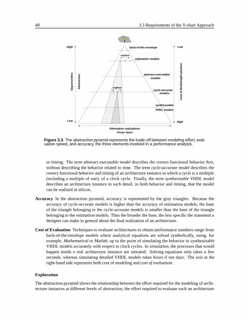
48 3.3 Requirements of the Y-chart Approach
Low
Alternative realizations
cycle-accuratemodels
explore
explore
High
HighLow
Design Space
estimation models
back-of-the-envelope
abstract executablemodels
Ab
stra
ctio
n
Op
po
rtu
nit
ies
Co
st o
f M
od
elin
g/E
valu
atio
n
synthesizable
VHDL models
Figure 3.3 . The abstraction pyramid represents the trade-off between modeling effort, eval-uation speed, and accuracy, the three elements involved in a performance analysis.
or timing. The termabstract executable modeldescribes the correct functional behavior first,without describing the behavior related to time. The termcycle-accurate modeldescribes thecorrect functional behavior and timing of an architecture instance in which a cycle is a multiple(including a multiple of one), of a clock cycle. Finally, the termsynthesizable VHDL modeldescribes an architecture instance in such detail, in both behavior and timing, that the modelcan be realized in silicon.
Accuracy In the abstraction pyramid, accuracy is represented by the gray triangles. Because theaccuracy of cycle-accurate models is higher than the accuracy of estimation models, the baseof the triangle belonging to the cycle-accurate models is smaller than the base of the trianglebelonging to the estimation models. Thus the broader the base, the less specific the statement adesigner can make in general about the final realization of an architecture.
Cost of Evaluation Techniques to evaluate architectures to obtain performance numbers range fromback-of-the-envelope models where analytical equations are solved symbolically, using, forexample,Mathematicalor Matlab, up to the point of simulating the behavior in synthesizableVHDL models accurately with respect to clock cycles. Insimulation, the processes that wouldhappen inside a real architecture instance are imitated. Solving equations only takes a fewseconds, whereas simulating detailed VHDL models takes hours if not days. The axis at theright-hand side represents both cost of modeling andcost of evaluation.
Exploration
The abstraction pyramid shows the relationship between the effort required for the modeling of archi-tecture instances at different levels of abstraction, the effort required to evaluate such an architecture
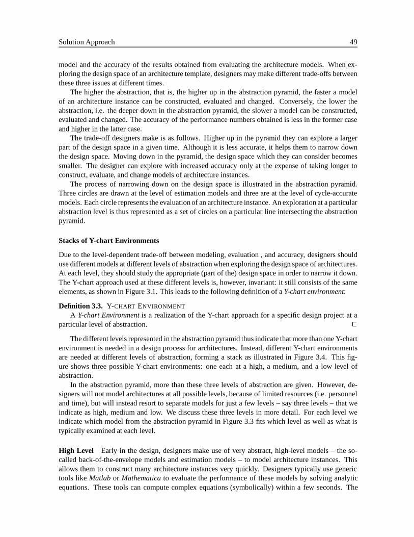
Solution Approach 49
model and the accuracy of the results obtained from evaluating the architecture models. When ex-ploring the design space of an architecture template, designers may make different trade-offs betweenthese three issues at different times.
The higher the abstraction, that is, the higher up in the abstraction pyramid, the faster a modelof an architecture instance can be constructed, evaluated and changed. Conversely, the lower theabstraction, i.e. the deeper down in the abstraction pyramid, the slower a model can be constructed,evaluated and changed. The accuracy of the performance numbers obtained is less in the former caseand higher in the latter case.
The trade-off designers make is as follows. Higher up in the pyramid they can explore a largerpart of the design space in a given time. Although it is less accurate, it helps them to narrow downthe design space. Moving down in the pyramid, the design space which they can consider becomessmaller. The designer can explore with increased accuracy only at the expense of taking longer toconstruct, evaluate, and change models of architecture instances.
The process of narrowing down on the design space is illustrated in the abstraction pyramid.Three circles are drawn at the level of estimation models and three are at the level of cycle-accuratemodels. Each circle represents the evaluationof an architecture instance. An exploration at a particularabstraction level is thus represented as a set of circles on a particular line intersecting the abstractionpyramid.
Stacks of Y-chart Environments
Due to the level-dependent trade-off between modeling, evaluation , and accuracy, designers shoulduse different models at different levels of abstraction when exploring the design space of architectures.At each level, they should study the appropriate (part of the) design space in order to narrow it down.The Y-chart approach used at these different levels is, however, invariant: it still consists of the sameelements, as shown in Figure 3.1. This leads to the following definition of aY-chart environment:
Definition 3.3. Y-CHART ENVIRONMENT
A Y-chart Environmentis a realization of the Y-chart approach for a specific design project at aparticular level of abstraction. 2
The different levels represented in the abstraction pyramid thus indicate that more than one Y-chartenvironment is needed in a design process for architectures. Instead, different Y-chart environmentsare needed at different levels of abstraction, forming a stack as illustrated in Figure 3.4. This fig-ure shows three possible Y-chart environments: one each at a high, a medium, and a low level ofabstraction.
In the abstraction pyramid, more than these three levels of abstraction are given. However, de-signers will not model architectures at all possible levels, because of limited resources (i.e. personneland time), but will instead resort to separate models for just a few levels – say three levels – that weindicate as high, medium and low. We discuss these three levels in more detail. For each level weindicate which model from the abstraction pyramid in Figure 3.3 fits which level as well as what istypically examined at each level.
High Level Early in the design, designers make use of very abstract, high-level models – the so-called back-of-the-envelope models and estimation models – to model architecture instances. Thisallows them to construct many architecture instances very quickly. Designers typically use generictools like Matlab or Mathematicato evaluate the performance of these models by solving analyticequations. These tools can compute complex equations (symbolically) within a few seconds. The
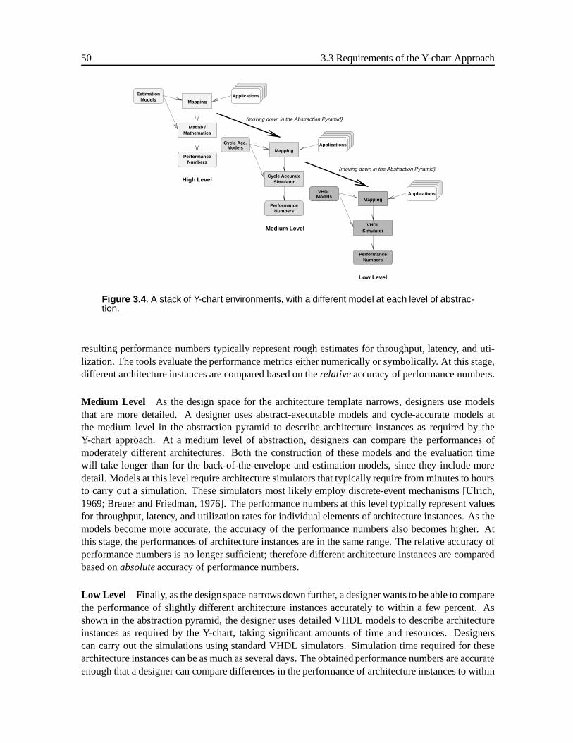
50 3.3 Requirements of the Y-chart Approach
High Level
Medium Level
Low Level
Applications
PerformanceNumbers
Applications
PerformanceNumbers
Applications
PerformanceNumbers
Mapping
Mapping
Mapping
VHDLSimulator
Cycle AccurateSimulator
Matlab /Mathematica
EstimationModels
Models
ModelsCycle Acc.
VHDL
(moving down in the Abstraction Pyramid}
(moving down in the Abstraction Pyramid}
Figure 3.4 . A stack of Y-chart environments, with a different model at each level of abstrac-tion.
resulting performance numbers typically represent rough estimates for throughput, latency, and uti-lization. The tools evaluate the performance metrics either numerically or symbolically. At this stage,different architecture instances are compared based on therelativeaccuracy of performance numbers.
Medium Level As the design space for the architecture template narrows, designers use modelsthat are more detailed. A designer uses abstract-executable models and cycle-accurate models atthe medium level in the abstraction pyramid to describe architecture instances as required by theY-chart approach. At a medium level of abstraction, designers can compare the performances ofmoderately different architectures. Both the construction of these models and the evaluation timewill take longer than for the back-of-the-envelope and estimation models, since they include moredetail. Models at this level require architecture simulators that typically require from minutes to hoursto carry out a simulation. These simulators most likely employ discrete-event mechanisms [Ulrich,1969; Breuer and Friedman, 1976]. The performance numbers at this level typically represent valuesfor throughput, latency, and utilization rates for individual elements of architecture instances. As themodels become more accurate, the accuracy of the performance numbers also becomes higher. Atthis stage, the performances of architecture instances are in the same range. The relative accuracy ofperformance numbers is no longer sufficient; therefore different architecture instances are comparedbased onabsoluteaccuracy of performance numbers.
Low Level Finally, as the design space narrows down further, a designer wants to be able to comparethe performance of slightly different architecture instances accurately to within a few percent. Asshown in the abstraction pyramid, the designer uses detailed VHDL models to describe architectureinstances as required by the Y-chart, taking significant amounts of time and resources. Designerscan carry out the simulations using standard VHDL simulators. Simulation time required for thesearchitecture instances can be as much as several days. The obtained performance numbers are accurateenough that a designer can compare differences in the performance of architecture instances to within
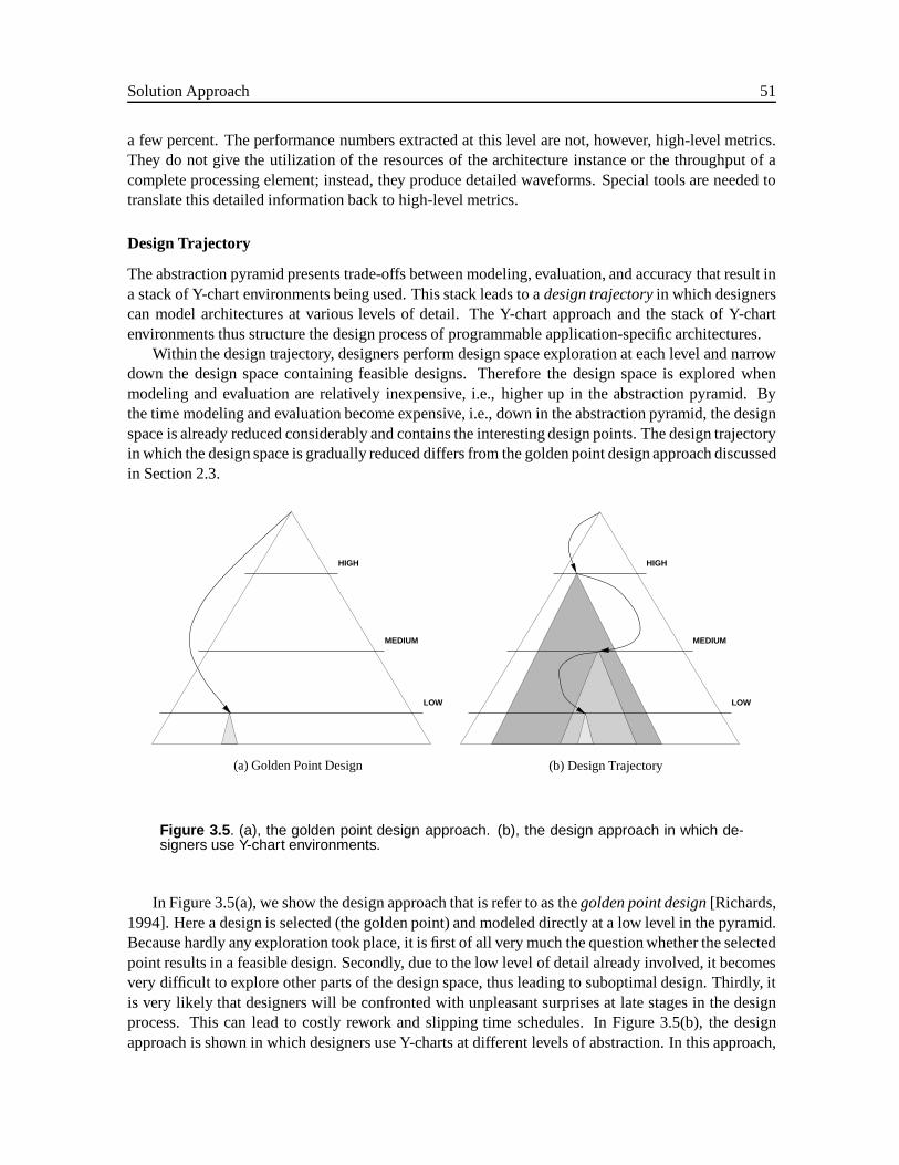
Solution Approach 51
a few percent. The performance numbers extracted at this level are not, however, high-level metrics.They do not give the utilization of the resources of the architecture instance or the throughput of acomplete processing element; instead, they produce detailed waveforms. Special tools are needed totranslate this detailed information back to high-level metrics.
Design Trajectory
The abstraction pyramid presents trade-offs between modeling, evaluation, and accuracy that result ina stack of Y-chart environments being used. This stack leads to adesign trajectoryin which designerscan model architectures at various levels of detail. The Y-chart approach and the stack of Y-chartenvironments thus structure the design process of programmable application-specific architectures.
Within the design trajectory, designers perform design space exploration at each level and narrowdown the design space containing feasible designs. Therefore the design space is explored whenmodeling and evaluation are relatively inexpensive, i.e., higher up in the abstraction pyramid. Bythe time modeling and evaluation become expensive, i.e., down in the abstraction pyramid, the designspace is already reduced considerably and contains the interesting design points. The design trajectoryin which the design space is gradually reduced differs from the golden point design approach discussedin Section 2.3.
HIGH
MEDIUM
LOW
(a) Golden Point Design
HIGH
MEDIUM
LOW
(b) Design Trajectory
Figure 3.5 . (a), the golden point design approach. (b), the design approach in which de-signers use Y-chart environments.
In Figure 3.5(a), we show the design approach that is refer to as thegolden point design[Richards,1994]. Here a design is selected (the golden point) and modeled directly at a low level in the pyramid.Because hardly any exploration took place, it is first of all very much the question whether the selectedpoint results in a feasible design. Secondly, due to the low level of detail already involved, it becomesvery difficult to explore other parts of the design space, thus leading to suboptimal design. Thirdly, itis very likely that designers will be confronted with unpleasant surprises at late stages in the designprocess. This can lead to costly rework and slipping time schedules. In Figure 3.5(b), the designapproach is shown in which designers use Y-charts at different levels of abstraction. In this approach,
52 3.3 Requirements of the Y-chart Approach
designers explore the design space of architectures at different levels of abstraction and graduallynarrow down the design space containing potential feasible designs.
3.3.2 Mapping
Mapping pertains to conditioning a programmable architecture instance such that it executes a partic-ular application. It leads to a program that causes execution of one application on the programmablearchitecture. Mapping involves assigning application functions to processing elements in architectureinstances that can execute these functions. It also involves mapping the communication that takesplace in applications onto communication structures in architecture instances.
We consider applications that have real-time requirements. When we map these applications ontoan architecture instance, we can look at mapping “in the small” and “in the large”. In mapping inthe large, we condition an architecture instance such that it executes applications under real-timeconstraints and we also ensure that the applications do not deadlock. In mapping in thesmall, weonly condition the architecture such that it executes applications. In this case, there is no guaranteewhatsoever that real-time constraints are satisfied or that an application will not deadlock. Mappingin the small is already a difficult problem and it is the problem that we address when we talk about“mapping”. Thus henceforth we mean “mapping in the small” when we say mapping2.
We discuss the basic idea that we used to make the mapping of applications as simple as possible,i.e., that applications and architecture do – somehow – naturally fit. When mapping is simple torealize, designers will experiment more with trying out different routing programs and will be able todevelop a mapping strategy concurrently with the architecture template.
Mapping Applications onto Architecture Instances
We assume that a natural fit exists if the model of computation used to specify applications matchesthe model of architecture used to specify architectures and if the data types used in the models aresimilar. This idea is shown in Figure 3.6. We first explain what a model of computation and model ofarchitecture are and then we show how this idea results in a mapping approach.
Architecture
Data Type
Application
Model of Architecture Model of Computation
Figure 3.6 . A smooth mapping from an application to an architecture only takes place if themodel of computation matches with the model of architecture and when a similar kind ofdata type is used in both models.
2Mapping is sometimes also referred to ascompilation
Solution Approach 53
Model of Computation
Applications are specified using some kind of formalism that has an underlying model of computation.We define a model of computation, inspired by [Lee and et al., 1994], as
Definition 3.4. MODEL OF COMPUTATION
A Model of Computationis a formal representation of the operational semantics of networks offunctional blocks describing computations. 2
So, the operation semantics of a model of computation governs how the functional blocks interactwith one another realizing computations. Many different models of computation already exist thathave specific properties. Different models have proven to be very effective in describing applica-tions in various application domains [Chang et al., 1997]. Some examples of well-known models ofcomputation areDataflow Models, Process Models, Finite State models, andImperative Models.
The dataflow model of computation and some forms of process models are well suited to describ-ing digital signal processing applications [Chang et al., 1997]. Therefore, we restrict ourselves in thisthesis to the use of these models. We discuss dataflow models and process models in more detail inChapter 6.
Model of Architecture
In analogy with a model of computation, we define the concept of model of architecture as
Definition 3.5. MODEL OF ARCHITECTURE
A Model of Architectureis a formal representation of the operational semantics of networks offunctional blocks describing architectures. 2
In this case, the functional blocks describe the behavior of architectural elements and the oper-ational semantics of a model of architecture governs how these functional blocks interact with oneanother. We described the model of architecture of stream-based dataflow architectures having par-ticular properties: these architecture are programmable and exploit parallelism and streams to satisfytough real-time constraints, computation requirements, and bandwidth requirements.
To describe the functional blocks, e.g. the basic elements of the stream-based dataflow architec-tures as well as their operational semantics, we develop a modeling approach in Chapter 4 based on ahigh-level performance modeling approach. In Chapter 5, we use this modeling approach to describeinstances of stream-based dataflow architectures.
Data Types
In both applications and architectures, data that is exchanged is organized in a particular way and hasparticular properties. These properties are described by adata type. Examples of simple data typesare integers, floats, or reals. More complex data types are streams of integers or matrices.
To realize a smooth mapping, the types used in the applications should match with the types usedin the architecture. If architectures use only streams of integers, the applications should also useonly streams of integers. Suppose an application uses only matrices whereas an architecture instanceon which we want to map the application uses only streams. Because the types do not match, wecan already say that we cannot map the application directly onto the architecture instance. We firsthave to express the matrices in terms of streams of integers. A stream of integers, however, has verydifferent properties from a matrix (e.g. a matrix is randomly accessible), having a profound influence
54 3.3 Requirements of the Y-chart Approach
on how the application should execute on the architecture (we look at this issues in more detail inChapter 6). Therefore, to obtain a smooth mapping of applications onto architectures the data in boththe applications and the architecture should useexactlythe same kind of data types.
This does not imply that applications cannot be specified using other data types than the ones usedin particular architectures. To realize a smooth mapping, however, a designer has to specify explicitlyhow the data types used in the application are transformed into data types used in the application.Thus, if an architecture uses only streams and an application uses matrices, a designer has to expressexplicitly how to transform these matrices into a stream of integers. We remark here that such a trans-formation can seriously affect in a negative way the performance of the application on an architectureinstance.
Natural Fit
Given an application that is described using a model of computation and an architecture instancethat is described using a model of architecture, when we say the application fitsnaturally onto thearchitecture instance, we mean that:
1. The architecture instance provides at least primitives similar to those used in the application.For example, the functions used in the application should also be found in the architectureinstance.
2. The operational semantics of the architecture instance at least matches the operational semanticsof the application. For example, when functional elements implement functions operating onstreams in a data-driven manner, then the functions in the application should behave in exactlythe same way.
3. The data types used in the application should match the data types used in the architectureinstance. For example, when an architecture instance transports only streams of samples, anapplication should also use only streams of samples.
For applications that need to be mapped onto instances of the stream-based dataflow architectures,this natural fit has as a consequence that functions used in the applications map to functions imple-mented by functional elements and that the edges representing communication map to combinationsof input and output buffers, routers, and the communication structure. The last consequence of a nat-ural fit is that applications operate on streams in a data-driven manner because stream-based dataflowarchitectures only operate on streams in a data-driven manner.
Mapping Approach
The mapping approach we use in this thesis is to have a model of computation and a model of ar-chitecture that fit naturally as illustrated in Figure 3.6. A consequence of this mapping approach isthat we have to introduce a new model of computation, which we call the Stream-Based FunctionsModel (SBF). We will present this model in Chapter 6. This model of computation matches the wayfunctional elements operate within the model of architecture of stream-based dataflow architectures.We demonstrate the mapping approach in detail in Chapter 7.
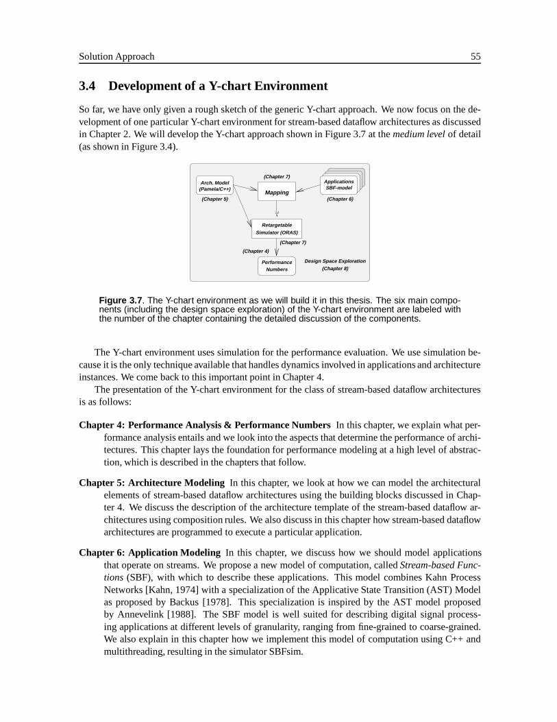
Solution Approach 55
3.4 Development of a Y-chart Environment
So far, we have only given a rough sketch of the generic Y-chart approach. We now focus on the de-velopment of one particular Y-chart environment for stream-based dataflow architectures as discussedin Chapter 2. We will develop the Y-chart approach shown in Figure 3.7 at themedium levelof detail(as shown in Figure 3.4).
Applications
RetargetableSimulator (ORAS)
PerformanceNumbers
SBF-model
Design Space Exploration
Mapping
Arch. Model(Pamela/C++)
(Chapter 5)
(Chapter 7)
(Chapter 6)
(Chapter 7)
(Chapter 8)
(Chapter 4)
Figure 3.7 . The Y-chart environment as we will build it in this thesis. The six main compo-nents (including the design space exploration) of the Y-chart environment are labeled withthe number of the chapter containing the detailed discussion of the components.
The Y-chart environment uses simulation for the performance evaluation. We use simulation be-cause it is the only technique available that handles dynamics involved in applications and architectureinstances. We come back to this important point in Chapter 4.
The presentation of the Y-chart environment for the class of stream-based dataflow architecturesis as follows:
Chapter 4: Performance Analysis & Performance Numbers In this chapter, we explain what per-formance analysis entails and we look into the aspects that determine the performance of archi-tectures. This chapter lays the foundation for performance modeling at a high level of abstrac-tion, which is described in the chapters that follow.
Chapter 5: Architecture Modeling In this chapter, we look at how we can model the architecturalelements of stream-based dataflow architectures using the building blocks discussed in Chap-ter 4. We discuss the description of the architecture template of the stream-based dataflow ar-chitectures using composition rules. We also discuss in this chapter how stream-based dataflowarchitectures are programmed to execute a particular application.
Chapter 6: Application Modeling In this chapter, we discuss how we should model applicationsthat operate on streams. We propose a new model of computation, calledStream-based Func-tions (SBF), with which to describe these applications. This model combines Kahn ProcessNetworks [Kahn, 1974] with a specialization of the Applicative State Transition (AST) Modelas proposed by Backus [1978]. This specialization is inspired by the AST model proposedby Annevelink [1988]. The SBF model is well suited for describing digital signal process-ing applications at different levels of granularity, ranging from fine-grained to coarse-grained.We also explain in this chapter how we implement this model of computation using C++ andmultithreading, resulting in the simulator SBFsim.
56 3.5 Related Work
Chapter 7: Retargetable Simulator & Mapping In this chapter, we combine the concepts presentedin the previous chapters together to construct theObject oriented Retargetable Architecture Sim-ulator (ORAS). We obtain the performance numbers of the architecture instance and we showthat the SBF model matches the functional elements of the stream-based dataflow architecture.
Chapter 8: Design Space ExplorationIn this chapter, we explain how we have embedded the Y-chart environment in a design management system calledNelsis[ten Bosch et al., 1991]. Theresulting design space exploration environment automatically constructs and systematicallyevaluates architecture instances, leading to the exploration of the design space of stream-baseddataflow architectures.
Chapter 9: Two Design CasesIn this chapter, we look at how we can use the Y-chart environmentin two design cases for different application domains.
3.5 Related Work
Programmable architectures have already been being developed for decades in the domain of general-purpose processor (GPP) design. In this domain, designers from Silicon Graphics, DEC, and Intel– to name a few – develop complex architectures calledinstruction-set processorsor microproces-sors. These processors execute a word-processor application as easily as a spreadsheet applicationor even simulate some complex physical phenomenon. Therefore, designers working in this domainknow what programmability implies in terms of (complex) trade-offs between hardware, software,and compilers.
A benchmark method is used in the design of general-purpose processors that can be cast into aparticular Y-chart environment. In this section, we first show that the design of GPPs fits into ourY-chart approach. This is followed by a discussion on related work on programmable application-specific architectures.
3.5.1 Design of General-Purpose Processors
In the beginning of the 1980s, revolutionary GPPs emerged that were called RISC microproces-sors [Patterson, 1985]. These processors were developed in a revolutionary way; namely, designersused extensive quantitative analysis of a suite ofbenchmarks, which is a set of applications. As aresult, these architectures were smaller, faster, cheaper and easier to program than conventional archi-tectures of that time. With the advent of the RISC microprocessors, the design of GPPs in generalbegan to swing away from focusing purely on hardware design. Designers started to focus more onthe quantitative analysis of difficulties encountered in architecture, mapping (or compiling), and theway benchmarks are written. Currently this quantitative approach is the de-facto development tech-nique for the design of general-purpose processors [Bose and Conte, 1998] (An excellent book on thequantitative design approach of RISC based processors is “Computer Architectures: A QuantitativeApproach” by Hennessy and Patterson [1996]).
We can cast the general-purpose processor architectures design approach in terms of our Y-chartapproach as presented in this chapter. For example, Hennessy and Heinrich [1996] developed theMIPS R4000 microprocessor using the Y-chart depicted in Figure 3.8. The benchmarks are specifiedin the C programming language. These benchmarks are known as the SPECmark programs [SPEC-marks, 1989]. Using a C-compiler, tuned especially to reflect the R4000 architecture, and a specialarchitecture simulator calledPixie, they evaluated the performance of the R4000. The performance
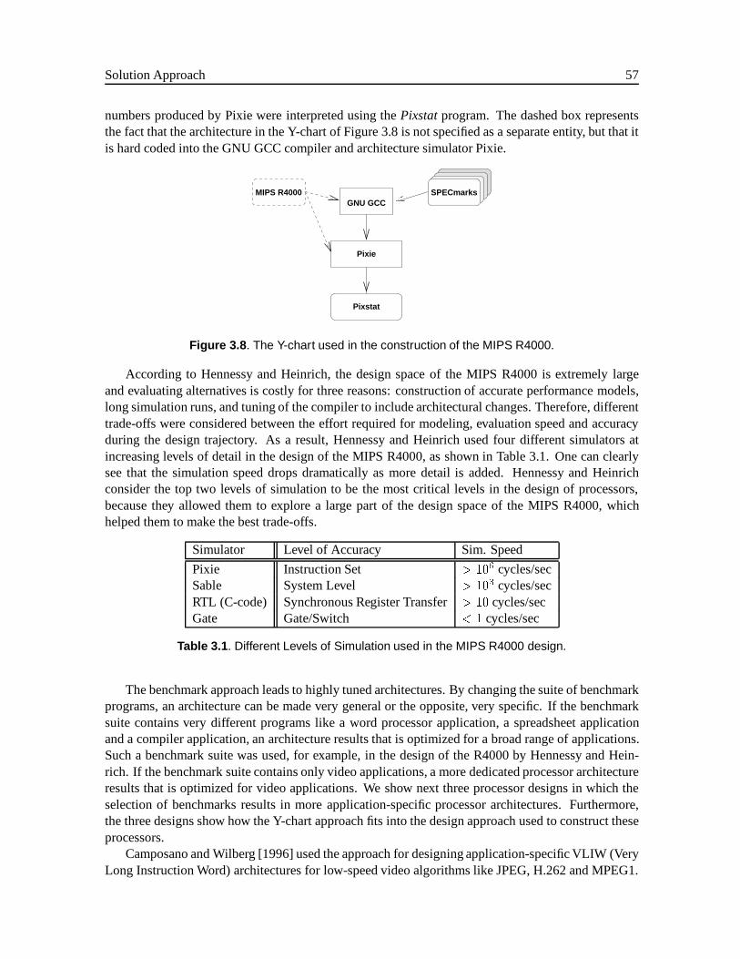
Solution Approach 57
numbers produced by Pixie were interpreted using thePixstatprogram. The dashed box representsthe fact that the architecture in the Y-chart of Figure 3.8 is not specified as a separate entity, but that itis hard coded into the GNU GCC compiler and architecture simulator Pixie.
Pixstat
GNU GCC
Pixie
SPECmarksMIPS R4000
Figure 3.8 . The Y-chart used in the construction of the MIPS R4000.
According to Hennessy and Heinrich, the design space of the MIPS R4000 is extremely largeand evaluating alternatives is costly for three reasons: construction of accurate performance models,long simulation runs, and tuning of the compiler to include architectural changes. Therefore, differenttrade-offs were considered between the effort required for modeling, evaluation speed and accuracyduring the design trajectory. As a result, Hennessy and Heinrich used four different simulators atincreasing levels of detail in the design of the MIPS R4000, as shown in Table 3.1. One can clearlysee that the simulation speed drops dramatically as more detail is added. Hennessy and Heinrichconsider the top two levels of simulation to be the most critical levels in the design of processors,because they allowed them to explore a large part of the design space of the MIPS R4000, whichhelped them to make the best trade-offs.
Simulator Level of Accuracy Sim. Speed
Pixie Instruction Set > 106 cycles/secSable System Level > 103 cycles/secRTL (C-code) Synchronous Register Transfer> 10 cycles/secGate Gate/Switch < 1 cycles/sec
Table 3.1 . Different Levels of Simulation used in the MIPS R4000 design.
The benchmark approach leads to highly tuned architectures. By changing the suite of benchmarkprograms, an architecture can be made very general or the opposite, very specific. If the benchmarksuite contains very different programs like a word processor application, a spreadsheet applicationand a compiler application, an architecture results that is optimized for a broad range of applications.Such a benchmark suite was used, for example, in the design of the R4000 by Hennessy and Hein-rich. If the benchmark suite contains only video applications, a more dedicated processor architectureresults that is optimized for video applications. We show next three processor designs in which theselection of benchmarks results in more application-specific processor architectures. Furthermore,the three designs show how the Y-chart approach fits into the design approach used to construct theseprocessors.
Camposano and Wilberg [1996] used the approach for designing application-specific VLIW (VeryLong Instruction Word) architectures for low-speed video algorithms like JPEG, H.262 and MPEG1.
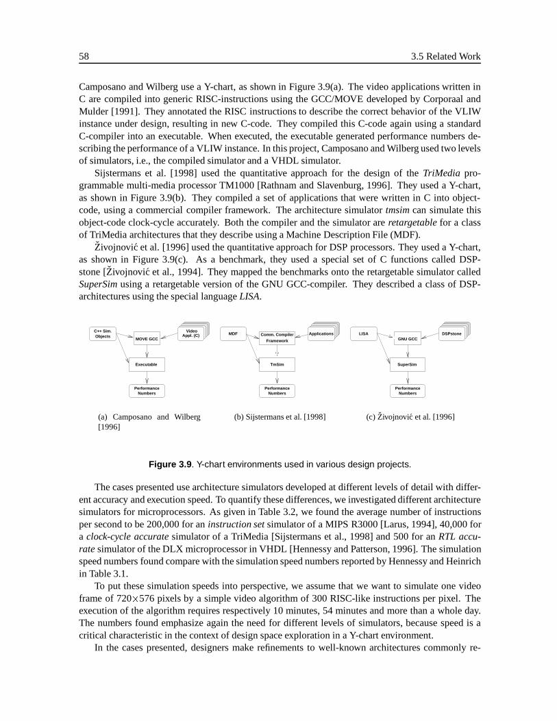
58 3.5 Related Work
Camposano and Wilberg use a Y-chart, as shown in Figure 3.9(a). The video applications written inC are compiled into generic RISC-instructions using the GCC/MOVE developed by Corporaal andMulder [1991]. They annotated the RISC instructions to describe the correct behavior of the VLIWinstance under design, resulting in new C-code. They compiled this C-code again using a standardC-compiler into an executable. When executed, the executable generated performance numbers de-scribing the performance of a VLIW instance. In this project, Camposano and Wilberg used two levelsof simulators, i.e., the compiled simulator and a VHDL simulator.
Sijstermans et al. [1998] used the quantitative approach for the design of theTriMedia pro-grammable multi-media processor TM1000 [Rathnam and Slavenburg, 1996]. They used a Y-chart,as shown in Figure 3.9(b). They compiled a set of applications that were written in C into object-code, using a commercial compiler framework. The architecture simulatortmsimcan simulate thisobject-code clock-cycle accurately. Both the compiler and the simulator areretargetablefor a classof TriMedia architectures that they describe using a Machine Description File (MDF).
Zivojnovic et al. [1996] used the quantitative approach for DSP processors. They used a Y-chart,as shown in Figure 3.9(c). As a benchmark, they used a special set of C functions called DSP-stone [Zivojnovic et al., 1994]. They mapped the benchmarks onto the retargetable simulator calledSuperSimusing a retargetable version of the GNU GCC-compiler. They described a class of DSP-architectures using the special languageLISA.
Executable
PerformanceNumbers
C++ Sim.Objects
MOVE GCCAppl. (C)
Video
(a) Camposano and Wilberg[1996]
PerformanceNumbers
MDF Applications
TmSim
Framework
Comm. Compiler
(b) Sijstermans et al. [1998]
GNU GCC
PerformanceNumbers
LISA DSPstone
SuperSim
(c) Zivojnovic et al. [1996]
Figure 3.9 . Y-chart environments used in various design projects.
The cases presented use architecture simulators developed at different levels of detail with differ-ent accuracy and execution speed. To quantify these differences, we investigated different architecturesimulators for microprocessors. As given in Table 3.2, we found the average number of instructionsper second to be 200,000 for aninstruction setsimulator of a MIPS R3000 [Larus, 1994], 40,000 fora clock-cycle accuratesimulator of a TriMedia [Sijstermans et al., 1998] and 500 for anRTL accu-ratesimulator of the DLX microprocessor in VHDL [Hennessy and Patterson, 1996]. The simulationspeed numbers found compare with the simulation speed numbers reported by Hennessy and Heinrichin Table 3.1.
To put these simulation speeds into perspective, we assume that we want to simulate one videoframe of 720�576 pixels by a simple video algorithm of 300 RISC-like instructions per pixel. Theexecution of the algorithm requires respectively 10 minutes, 54 minutes and more than a whole day.The numbers found emphasize again the need for different levels of simulators, because speed is acritical characteristic in the context of design space exploration in a Y-chart environment.
In the cases presented, designers make refinements to well-known architectures commonly re-
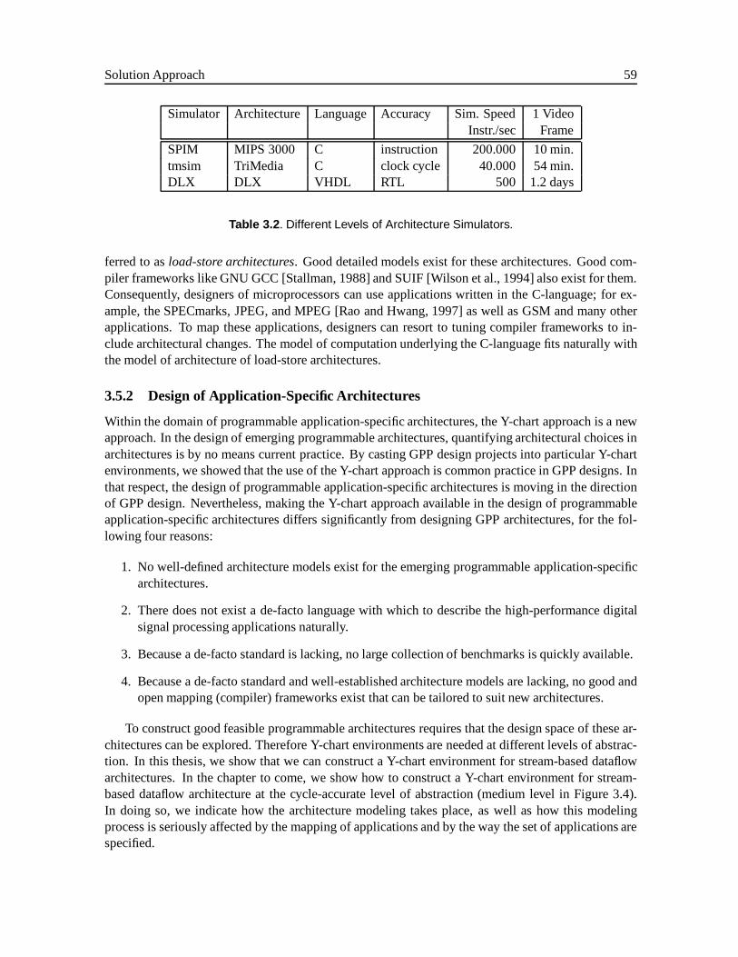
Solution Approach 59
Simulator Architecture Language Accuracy Sim. Speed 1 VideoInstr./sec Frame
SPIM MIPS 3000 C instruction 200.000 10 min.tmsim TriMedia C clock cycle 40.000 54 min.DLX DLX VHDL RTL 500 1.2 days
Table 3.2 . Different Levels of Architecture Simulators.
ferred to asload-store architectures. Good detailed models exist for these architectures. Good com-piler frameworks like GNU GCC [Stallman, 1988] and SUIF [Wilson et al., 1994] also exist for them.Consequently, designers of microprocessors can use applications written in the C-language; for ex-ample, the SPECmarks, JPEG, and MPEG [Rao and Hwang, 1997] as well as GSM and many otherapplications. To map these applications, designers can resort to tuning compiler frameworks to in-clude architectural changes. The model of computation underlying the C-language fits naturally withthe model of architecture of load-store architectures.
3.5.2 Design of Application-Specific Architectures
Within the domain of programmable application-specific architectures, the Y-chart approach is a newapproach. In the design of emerging programmable architectures, quantifying architectural choices inarchitectures is by no means current practice. By casting GPP design projects into particular Y-chartenvironments, we showed that the use of the Y-chart approach is common practice in GPP designs. Inthat respect, the design of programmable application-specific architectures is moving in the directionof GPP design. Nevertheless, making the Y-chart approach available in the design of programmableapplication-specific architectures differs significantly from designing GPP architectures, for the fol-lowing four reasons:
1. No well-defined architecture models exist for the emerging programmable application-specificarchitectures.
2. There does not exist a de-facto language with which to describe the high-performance digitalsignal processing applications naturally.
3. Because a de-facto standard is lacking, no large collection of benchmarks is quickly available.
4. Because a de-facto standard and well-established architecture models are lacking, no good andopen mapping (compiler) frameworks exist that can be tailored to suit new architectures.
To construct good feasible programmable architectures requires that the design space of these ar-chitectures can be explored. Therefore Y-chart environments are needed at different levels of abstrac-tion. In this thesis, we show that we can construct a Y-chart environment for stream-based dataflowarchitectures. In the chapter to come, we show how to construct a Y-chart environment for stream-based dataflow architecture at the cycle-accurate level of abstraction (medium level in Figure 3.4).In doing so, we indicate how the architecture modeling takes place, as well as how this modelingprocess is seriously affected by the mapping of applications and by the way the set of applications arespecified.
60 3.6 Conclusions
3.6 Conclusions
The Y-chart approach is the main idea presented in this chapter. It is a methodology in which designersuse quantitative data providing them with a sound basis on which to make decisions and motivateparticular design choices. The realization of the Y-chart approach for a specific design project at aparticular level of detail leads to a Y-chart environment. Within such an environment, we can performa design space exploration by systematically changing design choices.
The Y-chart approach uses performance analysis to obtain quantitative data. There is an importanttrade-off within performance analysis between the effort required for modeling, evaluation speed,and accuracy, which weillustrated in the abstraction pyramid. As a consequence of this trade-off,designers should use a stack of Y-chart environments, each at different levels of detail. Using thisstack, designers narrow down the design space of an architecture template in a stepwise fashion. Bythe time both modeling an architecture instance and evaluating this model become expensive, thedesign space is already reduced considerably and contains the interesting (feasible) designs.
The Y-chart approach takes into account the three core issues that play a role in finding goodprogrammable application-specific architectures. These are the architecture, the mapping, and the setof applications. Therefore attention for mapping is required from the very beginning. We formulatean approach that should result in a smooth mapping of an application onto architecture instances.
Bibliography
Jurgen Annevelink.HiFi, A Design Method for Implementing Signal Processing Algorithms on VLSIProcessor Arrays. PhD thesis, Delft University of Technology, 1988.
John Backus. Can programming be liberated from the von Neumann style? A functional style and itsalgebra of programs.Communications of the ACM, 21(8):613 – 641, 1978.
Pradip Bose and Thomas M. Conte. Performance analysis and its impact on design.IEEE Computer,31(5):41 – 49, 1998.
M.A. Breuer and A.D. Friedman.Diagnosis & Reliable Design of Digital Systems. Computer SciencePress, Woodland Hill, California, 1976.
R. Camposano and J. Wilberg. Embedded system design.Design Automation for Embedded Systems,1(1):5 – 50, 1996.
Wan-Teh Chang, Soonhoi Ha, and Edward A. Lee. Heterogeneous simulation - mixing discrete-eventmodels with dataflow.VLSI Signal Processing, 15(1/2):127 – 144, 1997.
H. Corporaal and H. Mulder. Move: A framework for high-performance processor design. InPro-ceedings of Supercomputing, pages 692 – 701, Albuquerque, 1991.
D. Gajski.Silicon Compilers. Addison-Wesley, 1987.
John Hennessy and Mark Heinrich. Hardware/software codesign of processors: Concepts and ex-amples. In Giovanni De Micheli and Mariagiovanna Sami, editors,Hardware/Software Codesign,volume 310 ofSeries E: Applied Sciences, pages 29 – 44. NATO ASI Series, 1996.
John L. Hennessy and David A. Patterson.Computer Architectures: A QuantitativeApproach. MorganKaufmann Publishers, Inc., second edition, 1996.
BIBLIOGRAPHY 61
Gilles Kahn. The semantics of a simple language for parallel programming. InProc. of the IFIPCongress 74. North-Holland Publishing Co., 1974.
B. Kienhuis, E. Deprettere, K.A. Vissers, and P. van der Wolf. An approach for quantitative analysis ofapplication-specific dataflow architectures. InProceedings of 11th Int. Conference of Applications-specific Systems, Architectures and Processors (ASAP’97), pages 338 – 349, Zurich, Switzerland,1997.
Bart Kienhuis, Ed Deprettere, Kees Vissers, and Pieter van der Wolf. The constructionof a retargetablesimulator for an architecture template. InProceedings of 6th Int. Workshop on Hardware/SoftwareCodesign, Seattle, Washington, 1998.
James Larus. SPIM, a MIPS r2000/3000 simulator. Available from the University of Wisconsin, 1994.
Stephen S. Lavenberg.Computer Performance Modeling Handbook. Acadamic Press, 1983.
Edward A. Lee and et al. An overview of the Ptolemy project. Technical report, University ofCalifornia at Berkeley, 1994.
D.A. Patterson. Reduced instruction set computers.Comm. ACM, 28(1):8 – 21, 1985.
R.K. Rao and J.J. Hwang.Techniques and Standards for Image, Video and Audio Coding. PrenticeHall, 1997.
S. Rathnam and G. Slavenburg. An architectural overview of the programmable multimedia processortm1. InProc. Compcon. IEEE CS press, 1996.
Mark A. Richards. The rapid prototyping of application specific signal processors (RASSP) program:Overview and status. In5th International Workshop on Rapid System Prototyping, pages 1–6. IEEEComputer Society Press, 1994.
F Sijstermans, E.J. Pol, B. Riemens, K Vissers, S. Rathnam, and G. Slavenburg. Design space explo-ration for future trimedia CPUs. InICASSP’98, 1998.
SPECmarks. Spec benchmark suite release 1.0, 1989.
R.M. Stallman.Using and Porting GNU CC. Free Software Foundation, Cambridge, MA, 1988.
K.O. ten Bosch, P. Bingley, and P. van der Wolf. Design flow management in the NELSIS CAD frame-work. In Proc. 28th ACM/IEEE Design Automation Conference, pages 711–716, San Francisco,1991.
E.G. Ulrich. Exclusive simulation of activity in digital networks.Communications of the ACM, 12(2):102 – 110, 1969.
Arjan. J.C. van Gemund.Performance Modeling of Parallel Systems. PhD thesis, Laboratory ofComputer Architecture and Digital Techniques, Delft University of Technology, 1996.
V. Zivojnovic, J. Martinez, C. Schl¨ager, and H. Meyr. DSPstone: A DSP-oriented benchmarkingmethodology. InProceedings of ICSPAT’94, Dallas, 1994.
Vojin Zivojnovic, Stefan Pees, Christian Schl¨ager, Markus Willems, Rainer Schoenen, and HeinrichMeyr. DSP Processor/Compiler Co-Design: A Quantitative Approach. InProc. ISSS, 1996.

62 BIBLIOGRAPHY
R. Wilson, R. French, C. Wilson, S. Amarasinghe, J. Anderson, S. Tjiang, S.-W. Liao, C.-W. Tseng,Hall M., Lam M., and J. Hennessy. SUIF: A parallelizing and optimizing research compiler. Tech-nical report, Stanford University, 1994. CSL-TR-94-620.
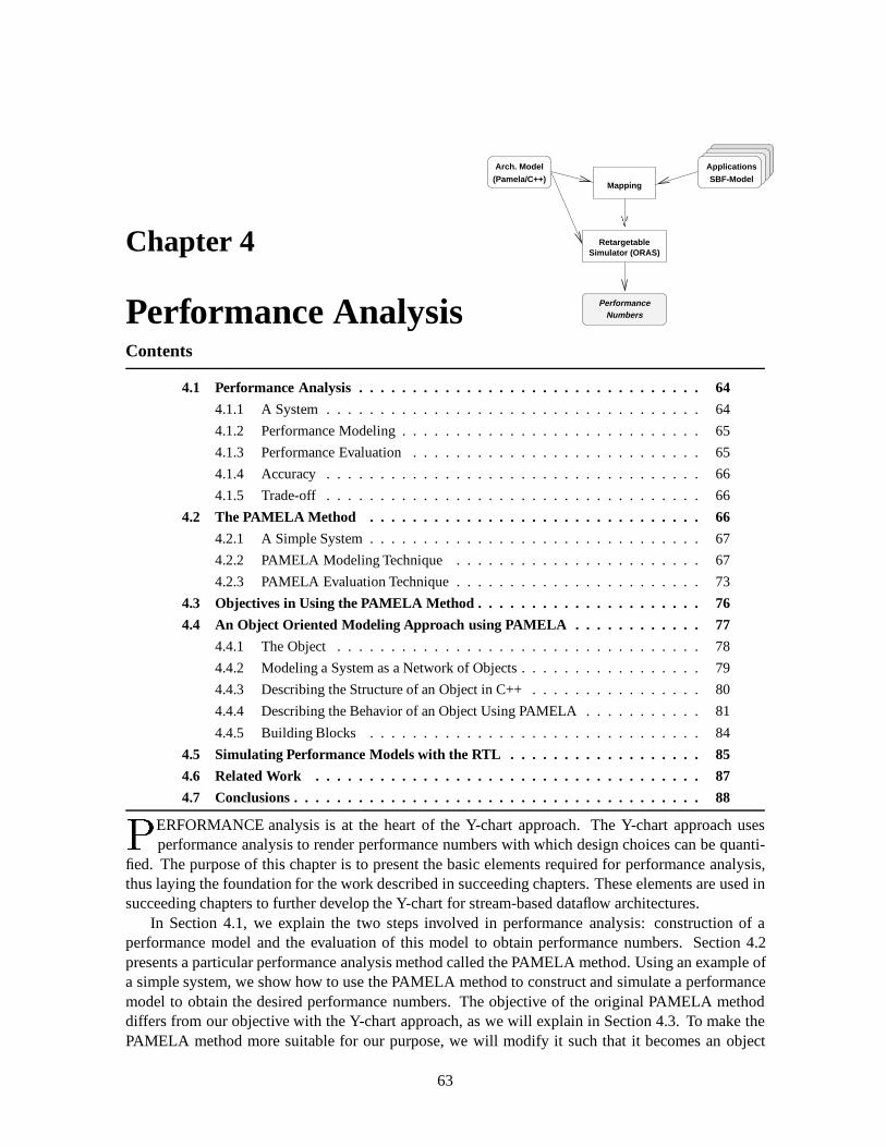
Chapter 4
Performance Analysis
RetargetableSimulator (ORAS)
Mapping
Applications
SBF-Model(Pamela/C++)
Arch. Model
PerformanceNumbers
Contents
4.1 Performance Analysis . . . . . . . . . . . . . . . . . . . . . . . . . . . . . . . . 64
4.1.1 A System . . . . . . . . . . . . . . . . . . . . . . . . . . . . . . . . . . . 64
4.1.2 Performance Modeling . . . . . . . . . . . . . . . . . . . . . . . . . . . . 65
4.1.3 Performance Evaluation . . . . . . . . . . . . . . . . . . . . . . . . . . . 65
4.1.4 Accuracy . . . . . . . . . . . . . . . . . . . . . . . . . . . . . . . . . . . 66
4.1.5 Trade-off . . . . . . . . . . . . . . . . . . . . . . . . . . . . . . . . . . . 66
4.2 The PAMELA Method . . . . . . . . . . . . . . . . . . . . . . . . . . . . . . . 66
4.2.1 A Simple System . . . . . . . . . . . . . . . . . . . . . . . . . . . . . . . 67
4.2.2 PAMELA Modeling Technique . . . . . . . . . . . . . . . . . . . . . . . 67
4.2.3 PAMELA Evaluation Technique . . . . . . . . . . . . . . . . . . . . . . . 73
4.3 Objectives in Using the PAMELA Method . . . . . . . . . . . . . . . . . . . . . 76
4.4 An Object Oriented Modeling Approach using PAMELA . . . . . . . . . . . . 77
4.4.1 The Object . . . . . . . . . . . . . . . . . . . . . . . . . . . . . . . . . . 78
4.4.2 Modeling a System as a Network of Objects . . . . . . . . . . . . . . . . . 79
4.4.3 Describing the Structure of an Object in C++ . . . . . . . . . . . . . . . . 80
4.4.4 Describing the Behavior of an Object Using PAMELA . . . . . . . . . . . 81
4.4.5 Building Blocks . . . . . . . . . . . . . . . . . . . . . . . . . . . . . . . 84
4.5 Simulating Performance Models with the RTL . . . . . . . . . . . . . . . . . . 85
4.6 Related Work . . . . . . . . . . . . . . . . . . . . . . . . . . . . . . . . . . . . 87
4.7 Conclusions . . . . . . . . . . . . . . . . . . . . . . . . . . . . . . . . . . . . . . 88
PERFORMANCE analysis is at the heart of the Y-chart approach. The Y-chart approach usesperformance analysis to render performance numbers with which design choices can be quanti-
fied. The purpose of this chapter is to present the basic elements required for performance analysis,thus laying the foundation for the work described in succeeding chapters. These elements are used insucceeding chapters to further develop the Y-chart for stream-based dataflow architectures.
In Section 4.1, we explain the two steps involved in performance analysis: construction of aperformance model and the evaluation of this model to obtain performance numbers. Section 4.2presents a particular performance analysis method called the PAMELA method. Using an example ofa simple system, we show how to use the PAMELA method to construct and simulate a performancemodel to obtain the desired performance numbers. The objective of the original PAMELA methoddiffers from our objective with the Y-chart approach, as we will explain in Section 4.3. To make thePAMELA method more suitable for our purpose, we will modify it such that it becomes an object
63
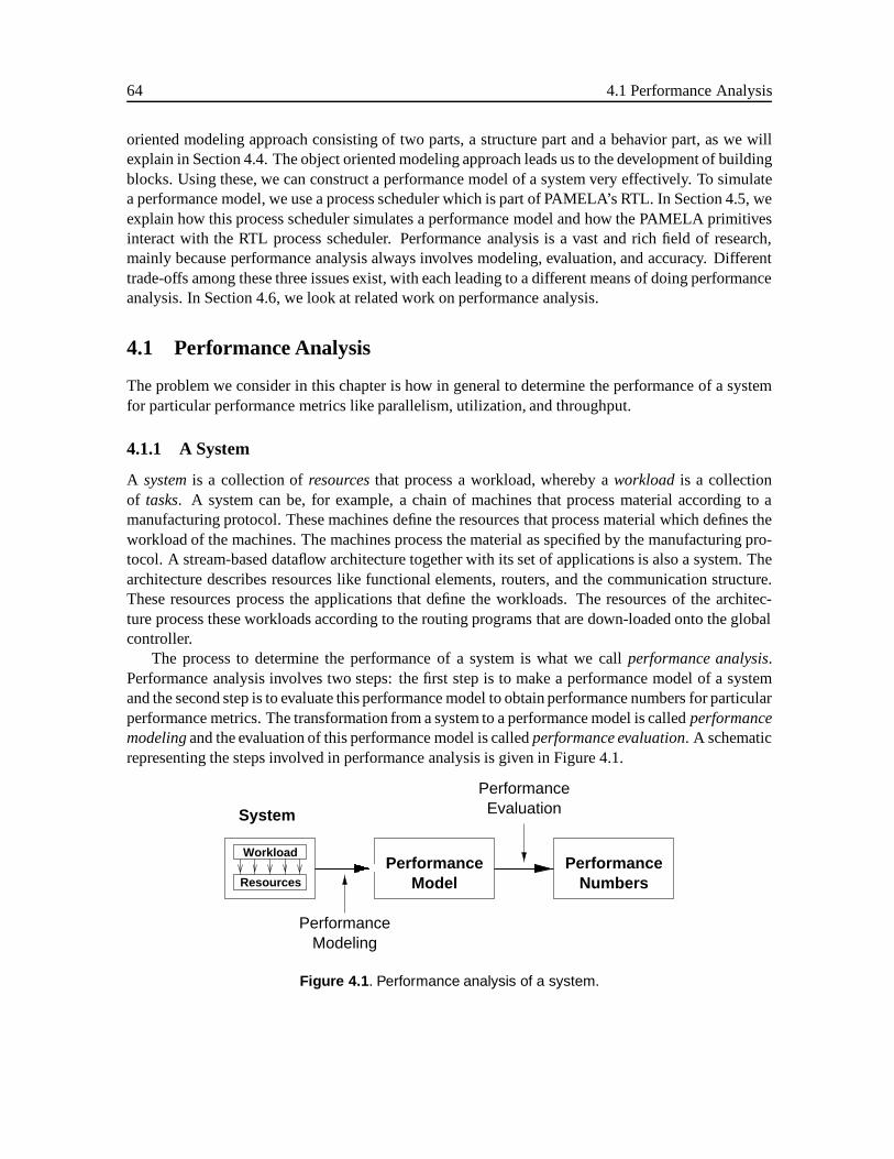
64 4.1 Performance Analysis
oriented modeling approach consisting of two parts, a structure part and a behavior part, as we willexplain in Section 4.4. The object oriented modeling approach leads us to the development of buildingblocks. Using these, we can construct a performance model of a system very effectively. To simulatea performance model, we use a process scheduler which is part of PAMELA’s RTL. In Section 4.5, weexplain how this process scheduler simulates a performance model and how the PAMELA primitivesinteract with the RTL process scheduler. Performance analysis is a vast and rich field of research,mainly because performance analysis always involves modeling, evaluation, and accuracy. Differenttrade-offs among these three issues exist, with each leading to a different means of doing performanceanalysis. In Section 4.6, we look at related work on performance analysis.
4.1 Performance Analysis
The problem we consider in this chapter is how in general to determine the performance of a systemfor particular performance metrics like parallelism, utilization, and throughput.
4.1.1 A System
A systemis a collection ofresourcesthat process a workload, whereby aworkload is a collectionof tasks. A system can be, for example, a chain of machines that process material according to amanufacturing protocol. These machines define the resources that process material which defines theworkload of the machines. The machines process the material as specified by the manufacturing pro-tocol. A stream-based dataflow architecture together with its set of applications is also a system. Thearchitecture describes resources like functional elements, routers, and the communication structure.These resources process the applications that define the workloads. The resources of the architec-ture process these workloads according to the routing programs that are down-loaded onto the globalcontroller.
The process to determine the performance of a system is what we callperformance analysis.Performance analysis involves two steps: the first step is to make a performance model of a systemand the second step is to evaluate this performance model to obtain performance numbers for particularperformance metrics. The transformation from a system to a performance model is calledperformancemodelingand the evaluation of this performance model is calledperformance evaluation. A schematicrepresenting the steps involved in performance analysis is given in Figure 4.1.
PerformanceModeling
EvaluationPerformance
PerformanceNumbers
PerformanceModel
System
Workload
Resources
Figure 4.1 . Performance analysis of a system.
Performance Analysis 65
4.1.2 Performance Modeling
In the performance-modeling step, we construct aperformance modelthat is an abstraction of thereal system it represents. This model captures only those aspects of the real system that determinethe performance of that system. To be able to model a system, we need to know what determines itsperformance. As argued by van Gemund [1996], only four aspects determine the performance ofanysystem. These four aspects define the four components of what we call the performance modelingbasis.
Definition 4.1. PERFORMANCEMODELING BASIS
ThePerformance Modeling Basis(PMB) consists of the four different components that determinethe performance of a system, namelycondition synchronization,mutual exclusion, execution timeandconditional control flow. 2
These components are as follows:
Condition Synchronization (CS): relates to data dependencies between tasks or to limited resources.
Mutual Exclusion (ME): relates to the fact that two or more tasks cannot operate overlapped in timeor that a resource cannot be used by more than one task at a time.
Execution Time (ET): relates to how long a task takes to execute or how long a resource is used.
Conditional Control Flow (CCF): relates to conditional selections at run-time between either tasksor resources.
Performance modeling thus means that we model a system by describing it in terms of the fourcomponents of the PMB. The first two aspects, condition synchronization and mutual exclusion, relateto synchronization between resources or tasks [Andrews and Schneider, 1983]. The other two aspects,execution time and conditional control flow, relate to the behavior of a single task or resource.
In the abstraction pyramid in Figure 3.3, we showed that performance modeling can happen atdifferent levels of abstraction. When the four components of the PMB are described in less detail, thedescription becomes more abstract (i.e. higher in the pyramid), and when they are described in moredetail, a description is less abstract (i.e. lower in the pyramid). In Chapter 5, we show how the fourcomponents of the PMB can describe architecture instances of the stream-based dataflow architecture.
4.1.3 Performance Evaluation
The performance evaluation step evaluates a performance model to obtain performance numbers forspecific performance metrics. Examples of performance metrics are the total time required by a systemto process a workload, the level of parallelism achieved in a system, the utilization of resources, andthe amount of data exchanged between tasks.
A performance model can be evaluated in many ways. It can be done in a symbolic way (aftertransforming the performance model to a time-domain representation) or via simulation. The back-of-the-envelope and estimations models presented in the abstraction pyramid are evaluated in a symbolicway. The abstract executable models, the cycle-accurate models and synthesizable models are evalu-ated using simulation.
66 4.2 The PAMELA Method
4.1.4 Accuracy
In the end, performance analysis yields performance numbers of a certainaccuracy. If the derivedvalue for a particular performance metric is equal toT 0 whereas the real performance of a system isequal toT , we say that the accuracy increases if the difference betweenT andT 0 becomes smaller.Thus, a higher accuracy indicates that the obtained performance numbers are closer to the real perfor-mance numbers. However, accuracy comes at a certain price. More accurate performance numbersare obtained at the expense of having to model a system in more detail and, typically, in having toevaluate it longer.
4.1.5 Trade-off
Performance analysis involves three issues: performance modeling, performance evaluation, and theaccuracy of the obtained results. A trade-off must be found between these three aspects, as we alreadyillustrated when discussing the abstraction pyramid in Figure 3.3.
The level of detail at which we model a system in the performance modeling step influences theaccuracy, as does the kind of evaluation technique used in the performance evaluation step. Nonethe-less, the accuracy of the modeling step and evaluation step cannot be considered separately. The levelof detail at which we describe a performance model influences the level of accuracy obtainable in theevaluation step.
4.2 The PAMELA Method
In this thesis, we make use of a high-level performance analysis method to analyze the performanceof architecture instances of stream-based dataflow architectures. This method is called the PAMELAmethod and was developed by van Gemund [1996] at Delft University of Technology.
The PAMELA method (PerformAnce ModEling LAnuage) includes the two techniques requiredto do performance analysis. It contains a technique for performance modeling and it contains a tech-nique for performance evaluation of a performance model. The modeling technique provides a simplelanguage in which to express performance models that can be evaluated either analytically or viasimulation. We will consider in this thesis only the simulation technique.
We present the PAMELA method on the basis of an example of a simple system. Using thisexample, we explain how to create a performance model for this system using the PAMELA modelingtechnique. Next, we evaluate this model using simulation and show how we can obtain performancenumbers. While working through the example, the main principles of the PAMELA method areexplained.
We first explain what the PAMELA performance modeling technique encompasses and introducea few simple primitives. These primitives allow us to describe a system using the four components ofthe PMB. Using these primitives and a pseudo-C language, we show how to construct a performancemodel for a simple system. After the modeling step, we evaluate the performance mode of the systemthrough simulation. Based on the results of the simulation, we show how we can acquire performancenumbers for specific performance metrics like total execution time, utilization, and parallelism. For amore in-depth discussion on the PAMELA method we refer to the work of van Gemund [1996].
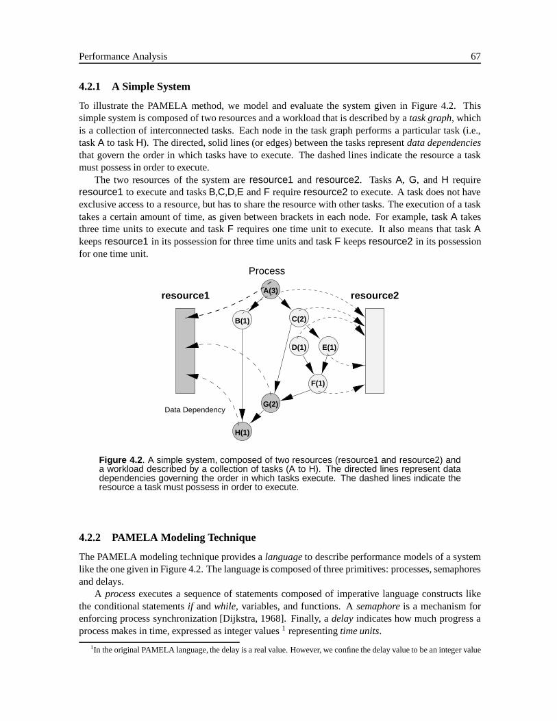
Performance Analysis 67
4.2.1 A Simple System
To illustrate the PAMELA method, we model and evaluate the system given in Figure 4.2. Thissimple system is composed of two resources and a workload that is described by atask graph, whichis a collection of interconnected tasks. Each node in the task graph performs a particular task (i.e.,taskA to taskH). The directed, solid lines (or edges) between the tasks representdata dependenciesthat govern the order in which tasks have to execute. The dashed lines indicate the resource a taskmust possess in order to execute.
The two resources of the system areresource1 and resource2. TasksA, G, andH requireresource1 to execute and tasksB,C,D,E andF requireresource2 to execute. A task does not haveexclusive access to a resource, but has to share the resource with other tasks. The execution of a tasktakes a certain amount of time, as given between brackets in each node. For example, taskA takesthree time units to execute and taskF requires one time unit to execute. It also means that taskAkeepsresource1 in its possession for three time units and taskF keepsresource2 in its possessionfor one time unit.
Process
Data Dependency
B(1)
A(3)
C(2)
E(1)D(1)
G(2)
H(1)
F(1)
resource1 resource2
Figure 4.2 . A simple system, composed of two resources (resource1 and resource2) anda workload described by a collection of tasks (A to H). The directed lines represent datadependencies governing the order in which tasks execute. The dashed lines indicate theresource a task must possess in order to execute.
4.2.2 PAMELA Modeling Technique
The PAMELA modeling technique provides alanguageto describe performance models of a systemlike the one given in Figure 4.2. The language is composed of three primitives: processes, semaphoresand delays.
A processexecutes a sequence of statements composed of imperative language constructs likethe conditional statementsif andwhile, variables, and functions. Asemaphoreis a mechanism forenforcing process synchronization [Dijkstra, 1968]. Finally, adelay indicates how much progress aprocess makes in time, expressed as integer values1 representingtime units.
1In the original PAMELA language, the delay is a real value. However, we confine the delay value to be an integer value
68 4.2 The PAMELA Method
A semaphore is a primitive that has an integer value. Processes manipulate this value using thePandV operators2. TheP operator decrements the value whereas theV operator increments the valueof a semaphore. When this value becomes zero using aP operator, the semaphore causes the processexecuting theP operator to block. Ablocked processstops executing its sequence of statements.A process remains blocked until another process executes theV operator, giving the semaphore anonzero value. This lifts the blocking condition and the blocked process can continue its sequence ofstatements.
Processes make progress autonomously in time using thedelayoperator and we refer to processesasactiveprimitives. Processes are hindered in their autonomous progress by semaphores. We refer tosemaphores aspassiveprimitives.
Modeling a System Using the PAMELA Modeling Technique
Using the primitives of the PAMELA language, we now describe the system given in Figure 4.2. Wedo not use the original PAMELA; instead we use apseudo Clanguage combined with the PAMELAprimitives. In the system, we only describe taskG and resources and dependencies related to this task.After we have indicated how to describe a complete performance model, we explain how the threePAMELA primitives describe the four components of the PMB, as required to make a performancemodel of a system.
Use of Symbols We describe programs in a pseudo C language. Those familiar with the C program-ming language should have no difficulties in understanding the code. The program sections we presentin this chapter and succeeding chapters contain only the minimal statements necessary to represent aparticular section of program. Initialization and declarations of variables are usually not presented. Inreferencing elements of programs, we use the following convention. Variables or functions to whichwe refer in a program are written asx andread , representing a variable and a function, respectively.Both special operators likeV or P and special program statements that we will introduce in this chap-ter are written using the bold face font. Finally, when we refer to names in figures, we write thesenames asA, for example, orresource1.
Modeling Approaches A system consists of resources and tasks. However, the PAMELA languageprovides processes, the active primitives and semaphores, and the passive primitives. This leads to twopossible modeling approaches [Kreutzer, 1986]: material-oriented modeling and machine-orientedmodeling. In theMaterial-oriented Modelingapproach, the tasks of a workload are modeled mainlyusing active primitives. In theMachine-oriented Modelingapproach, resources are mainly modeledusing active primitives. Which approach we should use very much depends on what we want toachieve with the constructed model. We come back to this important issue in Section 4.3, where wemotivate why we want to adapt the original PAMELA method to make it more appropriate for ourpurpose.
For the moment, we model the system given in Figure 4.2 using the material-oriented modelingapproach. We thus model each task as a process. We use semaphores to model data dependencies andresources. The delay primitive is used to indicate how long it takes to execute a task.
because we express delays in terms of number of cycles, and these are always represented as integer values (to be explainedfurther in Chapter 5).
2P is the first letter of the Dutch word “passeren,” which means “to pass”;V is the first letter of “vrijgeven,” the Dutchword for “to release” [Dijkstra, 1981].
Performance Analysis 69
Modeling Data Dependencies and ResourcesResources and data dependencies are modeled us-ing semaphores in the material-oriented modeling approach. When we look at taskG, we need tomodel its data dependencies with taskH, taskF, and taskC. We also have to model the relationshipwith resource1. These three data dependencies and the resource are described as semaphores inProgram 4.1.
Program 4.1. MODELING DATA DEPENDENCIES ANDRESOURCES
/* Data Dependencies */semaphore dependency_CG 0;semaphore dependency_FG 0;semaphore dependency_GH 0;
/* Resources */semaphore resource1 1;
In Program 4.1, we first show the three semaphores describing the data dependencies of taskGwith tasksC, F, andH. The value of each semaphore is initialized to zero. As a consequence, when aprocess uses theP operator on one of these semaphores, it will block. Suppose the process describingtaskG executes theP operator on semaphoredependency CG. As explained, the process will block.It remains blocked until the process describing taskC increments the semaphore using theV operator.This causes the value of semaphoredependency CGto become nonzero. Using the semaphore, taskC will always execute before taskG, and the semaphore thus implements a data dependency.
After describing the semaphores implementing the data dependencies, we show the semaphoreimplementingresource1. This semaphoreresource1 is initialized, in contrast to the data depen-dencies, to a nonzero value, and in particular, to the value of one. As such, a process using theP operator on this semaphore will not block. However, the next process using theP on the samesemaphore will block because the semaphore has acquired a zero value. As a consequence, only oneprocess can have exclusive access toresource1. When the first process uses theV operator, giving thesemaphore a nonzero value, it releases the resource so that the blocked process can obtain exclusiveaccess to the resource.
Modeling a Task TaskG in the system of Figure 4.2 has a data dependency with taskC and taskF. Consequently, TaskG can only execute after both dependencies with taskC and taskF have beensatisfied, i.e., after these tasks have already executed. Before taskG executes, it first needs to haveresource1 in its possession. After this is the case, then taskG executes, taking 2 time units. Thisis followed by releasing the resource and indicating to taskH that it is allowed to execute. Thissequence of events as explained so far is modeled – like any other task – using a process. For taskG,this process description is given in Program 4.2. It describes a sequence of statements enclosed by theword processand curly brackets. The statements between the curly brackets are executed one afterthe other. When the sequence comes to the end, i.e., at the last closing curly brackets, the sequencestarts all over again with the first statement after the wordprocessand the opening curly bracket.
In the process description in Program 4.2, we see that the sequence of statements consists of onlyP, V anddelay operators. When the process starts, it executes theP operator on the semaphore thatimplements the data dependency with taskC. Since this semaphoredependency CGis initialized toa value of zero, processG blocks. It remains blocked until the process modeling taskC executes aV operator on semaphoredependency CG. After the dependency with taskC is satisfied, processGexecutes theP operator on semaphoredependency FG, which models the data dependency with task
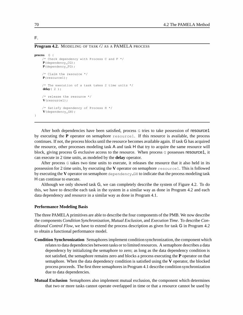
70 4.2 The PAMELA Method
F.
Program 4.2. MODELING OF TASKG AS A PAMELA PROCESS
process G {/* Check dependency with Process C and F */P(dependency_CG);P(dependency_FG);
/* Claim the resource */P(resource1);
/* The execution of a task takes 2 time units */delay( 2 );
/* release the resource */V(resource1);
/* Satisfy dependency of Process H */V(dependency_GH);
}
After both dependencies have been satisfied, processG tries to take possession ofresource1by executing theP operator on semaphoreresource1 . If this resource is available, the processcontinues. If not, the process blocks until the resource becomes available again. If taskG has acquiredthe resource, other processes modeling taskA and taskH that try to acquire the same resource willblock, giving processG exclusive access to the resource. When processG possessesresource1, itcan execute in 2 time units, as modeled by thedelayoperator.
After processG takes two time units to execute, it releases the resource that it also held in itspossession for 2 time units, by executing theV operator on semaphoreresource1 . This is followedby executing theV operator on semaphoredependency GHto indicate that the process modeling taskH can continue to execute.
Although we only showed taskG, we can completely describe the system of Figure 4.2. To dothis, we have to describe each task in the system in a similar way as done in Program 4.2 and eachdata dependency and resource in a similar way as done in Program 4.1.
Performance Modeling Basis
The three PAMELA primitives are able to describe the four components of the PMB. We now describethe componentsCondition Synchronization,Mutual Exclusion, andExecution Time. To describeCon-ditional Control Flow, we have to extend the process description as given for taskG in Program 4.2to obtain a functional performance model.
Condition Synchronization Semaphores implement conditionsynchronization, the component whichrelates to data dependencies between tasks or to limited resources. A semaphore describes a datadependency by initializing the semaphore to zero; as long as the data dependency condition isnot satisfied, the semaphore remains zero and blocks a process executing theP operator on thatsemaphore. When the data dependency condition is satisfied using theV operator, the blockedprocess proceeds. The first three semaphores in Program 4.1 describe condition synchronizationdue to data dependencies.
Mutual Exclusion Semaphores also implement mutual exclusion, the component which determinesthat two or more tasks cannot operate overlapped in time or that a resource cannot be used by

Performance Analysis 71
more than one task at a time. If a semaphore is initialized to the value of one, only one taskis allowed to access a resource at a time. The first task acquiring the resource by using thePoperator makes the semaphore zero, and all tasks trying to acquire the same resource will block.The semaphoreresource1 in Program 4.1 describes mutual exclusion of theresource1.
TaskG in the system shown in Figure 4.2 requires onlyresource1 in order to execute. Ingeneral, a task could require possession ofmultiple resourcesin order to execute. This multipleresource possession is modeled correctly byP andV operators.
Execution Time The delay primitive models the execution time, the component which determineshow long a task takes to execute or how long a resource is used. The integer value associatedwith thedelayoperator either indicates how many time units a task takes to execute or how longa resource is used. In Program 4.2, thedelayoperator shows that it takes taskG two time unitsto execute. Furthermore, sinceresource1 was claimed before and released after executing thedelayoperator, it is thus used by taskG for two time units. Note that we do not actually performa task.
Conditional Control Flow The sequence of imperative statements describes thecontrol flowof aprocess. A process has a conditional control flow when the sequence of statements consists ofconditional statements likeif andwhile. Conditional statements can affect control flow, basedon the evaluation of conditions at run-time.
In Program 4.3, we see part of a process description of a task. It describes a process that executesbased on the value of variablex . If the variablex has a value larger than 256, it takes the process sixtime units to execute, otherwise it takes the process two time units to execute.
Program 4.3. MODELING CONDITIONAL CONTROL FLOW
process {
/* Execution time of a Task */if ( x > 256 ) {
delay(6);} else {
delay(2);}
}
In the description of processG in Program 4.2 no variables are used; only relationships betweentasks and resources have been modeled. Nonetheless, as shown in Program 4.3, conditional con-trol flow requires data with which to resolve conditions at run-time. Put in other words, we need tohave afunctional performance model, which models besides the relationships between tasks and re-sources, also the correct functional behavior of a system. When only relationships between tasks andresources have been modeled, the model is also called anuninterpreted performance model, whereasa functional performance model is also called aninterpreted performance model[RASSP TaxonomyWorking Group (RTWG), 1998].
To describe the correct functional behavior of the system in Figure 4.2, we have to extend all thedescriptions of the processes modeling tasks in a way such as shown for taskG in Program 4.4. Thisprogram shows the process description given in Program 4.2, but also uses global and local variablesand a function. To illustrate conditional control flow, we also extended the process description of taskG as shown in Program 4.3.
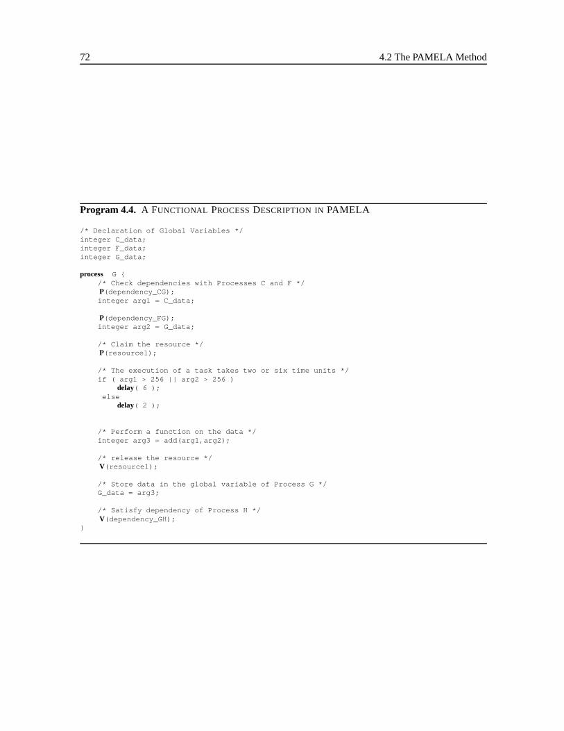
72 4.2 The PAMELA Method
Program 4.4. A FUNCTIONAL PROCESSDESCRIPTION INPAMELA
/* Declaration of Global Variables */integer C_data;integer F_data;integer G_data;
process G {/* Check dependencies with Processes C and F */P(dependency_CG);integer arg1 = C_data;
P(dependency_FG);integer arg2 = G_data;
/* Claim the resource */P(resource1);
/* The execution of a task takes two or six time units */if ( arg1 > 256 || arg2 > 256 )
delay( 6 );else
delay( 2 );
/* Perform a function on the data */integer arg3 = add(arg1,arg2);
/* release the resource */V(resource1);
/* Store data in the global variable of Process G */G_data = arg3;
/* Satisfy dependency of Process H */V(dependency_GH);
}
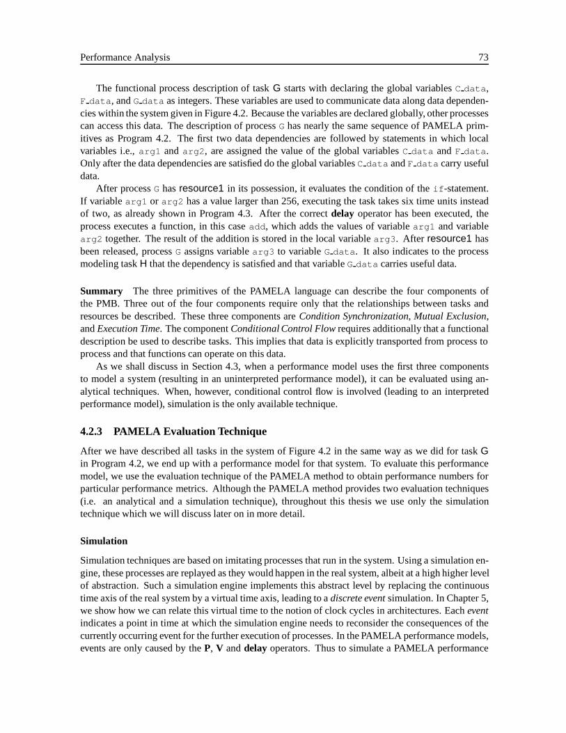
Performance Analysis 73
The functional process description of taskG starts with declaring the global variablesC data ,F data , andG data as integers. These variables are used to communicate data along data dependen-cies within the system given in Figure 4.2. Because the variables are declared globally, other processescan access this data. The description of processGhas nearly the same sequence of PAMELA prim-itives as Program 4.2. The first two data dependencies are followed by statements in which localvariables i.e.,arg1 andarg2 , are assigned the value of the global variablesC data andF data .Only after the data dependencies are satisfied do the global variablesC data andF data carry usefuldata.
After processG hasresource1 in its possession, it evaluates the condition of theif -statement.If variablearg1 or arg2 has a value larger than 256, executing the task takes six time units insteadof two, as already shown in Program 4.3. After the correctdelay operator has been executed, theprocess executes a function, in this caseadd , which adds the values of variablearg1 and variablearg2 together. The result of the addition is stored in the local variablearg3 . After resource1 hasbeen released, processG assigns variablearg3 to variableG data . It also indicates to the processmodeling taskH that the dependency is satisfied and that variableG data carries useful data.
Summary The three primitives of the PAMELA language can describe the four components ofthe PMB. Three out of the four components require only that the relationships between tasks andresources be described. These three components areCondition Synchronization, Mutual Exclusion,andExecution Time. The componentConditional Control Flowrequires additionally that a functionaldescription be used to describe tasks. This implies that data is explicitly transported from process toprocess and that functions can operate on this data.
As we shall discuss in Section 4.3, when a performance model uses the first three componentsto model a system (resulting in an uninterpreted performance model), it can be evaluated using an-alytical techniques. When, however, conditional control flow is involved (leading to an interpretedperformance model), simulation is the only available technique.
4.2.3 PAMELA Evaluation Technique
After we have described all tasks in the system of Figure 4.2 in the same way as we did for taskGin Program 4.2, we end up with a performance model for that system. To evaluate this performancemodel, we use the evaluation technique of the PAMELA method to obtain performance numbers forparticular performance metrics. Although the PAMELA method provides two evaluation techniques(i.e. an analytical and a simulation technique), throughout this thesis we use only the simulationtechnique which we will discuss later on in more detail.
Simulation
Simulation techniques are based on imitating processes that run in the system. Using a simulation en-gine, these processes are replayed as they would happen in the real system, albeit at a high higher levelof abstraction. Such a simulation engine implements this abstract level by replacing the continuoustime axis of the real system by a virtual time axis, leading to adiscrete eventsimulation. In Chapter 5,we show how we can relate this virtual time to the notion of clock cycles in architectures. Eacheventindicates a point in time at which the simulation engine needs to reconsider the consequences of thecurrently occurring event for the further execution of processes. In the PAMELA performance models,events are only caused by theP, V anddelay operators. Thus to simulate a PAMELA performance
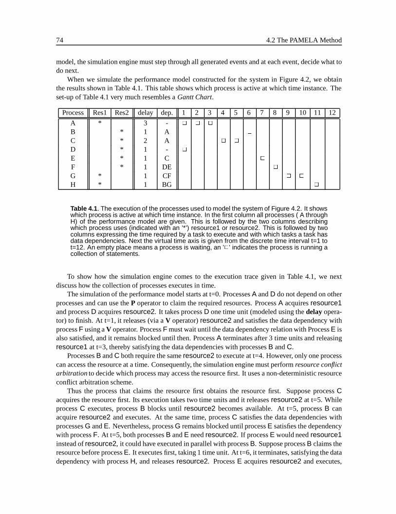
74 4.2 The PAMELA Method
model, the simulation engine must step through all generated events and at each event, decide what todo next.
When we simulate the performance model constructed for the system in Figure 4.2, we obtainthe results shown in Table 4.1. This table shows which process is active at which time instance. Theset-up of Table 4.1 very much resembles aGantt Chart.
Process Res1 Res2 delay dep. 1 2 3 4 5 6 7 8 9 10 11 12
A * 3 - 2 2 2
B * 1 A 2
C * 2 A 2 2
D * 1 - 2
E * 1 C 2
F * 1 DE 2
G * 1 CF 2 2
H * 1 BG 2
Table 4.1 . The execution of the processes used to model the system of Figure 4.2. It showswhich process is active at which time instance. In the first column all processes ( A throughH) of the performance model are given. This is followed by the two columns describingwhich process uses (indicated with an ’*’) resource1 or resource2. This is followed by twocolumns expressing the time required by a task to execute and with which tasks a task hasdata dependencies. Next the virtual time axis is given from the discrete time interval t=1 tot=12. An empty place means a process is waiting, an ’2’ indicates the process is running acollection of statements.
To show how the simulation engine comes to the execution trace given in Table 4.1, we nextdiscuss how the collection of processes executes in time.
The simulation of the performance model starts at t=0. ProcessesA andD do not depend on otherprocesses and can use theP operator to claim the required resources. ProcessA acquiresresource1and processD acquiresresource2. It takes processD one time unit (modeled using thedelayopera-tor) to finish. At t=1, it releases (via aV operator)resource2 and satisfies the data dependency withprocessF using aV operator. ProcessF must wait until the data dependency relation with ProcessE isalso satisfied, and it remains blocked until then. ProcessA terminates after 3 time units and releasingresource1 at t=3, thereby satisfying the data dependencies with processesB andC.
ProcessesB andC both require the sameresource2 to execute at t=4. However, only one processcan access the resource at a time. Consequently, the simulation engine must performresource conflictarbitration to decide which process may access the resource first. It uses a non-deterministic resourceconflict arbitration scheme.
Thus the process that claims the resource first obtains the resource first. Suppose processCacquires the resource first. Its execution takes two time units and it releasesresource2 at t=5. WhileprocessC executes, processB blocks until resource2 becomes available. At t=5, processB canacquireresource2 and executes. At the same time, processC satisfies the data dependencies withprocessesG andE. Nevertheless, processG remains blocked until processE satisfies the dependencywith processF. At t=5, both processesB andE needresource2. If processE would needresource1instead ofresource2, it could have executed in parallel with processB. Suppose processB claims theresource before processE. It executes first, taking 1 time unit. At t=6, it terminates, satisfying the datadependency with processH, and releasesresource2. ProcessE acquiresresource2 and executes,
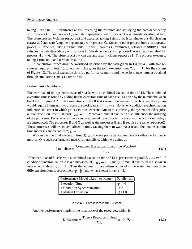
Performance Analysis 75
taking 1 time unit. It terminates at t=7, releasing the resource and satisfying the data dependencywith processF. For processF, the data dependency with processD was already satisfied at t=1.Therefore processF claimsresource2 and executes, taking 1 time unit. It terminates at t=8, releasingresource2 and satisfying the dependency with processG. Since no other process holdsresource1,processG executes, taking 2 time units. At t=10, processG terminates, releasesresource1, andsatisfies the data dependency with processH. The dependency with processB was already satisfied forprocessH at t=6. Therefore processH can execute after it claimsresource1. The process executes,taking 1 time unit, and terminates at t=11.
In conclusion, processing the workload described by the task-graph in Figure 4.2 with two re-sources requires in total 11 time units. This gives thetotal execution timeTend = 11 for the systemof Figure 4.2. The total execution time is a performance metric and the performance number obtainedthrough simulation equals 11 time units.
Performance Numbers
The workload of the system consists of 8 tasks with a combined execution time of 12. The combinedexecution time is found by adding up the execution time of each task, as given by the number betweenbrackets in Figure 4.2. If the executions of the 8 tasks were independent of each other, the systemwould require 3 time units to process the workload andTend = 3. However, condition synchronizationinfluences the order in which processes must execute. Due to this ordering, the system would requirea total execution time of at leastTend = 10. Moreover, mutual exclusion also influences the orderingof the processes. Because a resource can be accessed by only one process at a time, additional delaysare introduced. The processesB andC as well as the processesB andE require the sameresource2.These processes will be sequentialized in time, causing them to wait. As a result, the total executiontime increases and becomesTend = 11.
We can use the total execution timeTend to derive performance numbers for other performancemetrics. One such performance metric is parallelism, which we define as
Parallelism=Combined Execution Time of the Workload
Tend: (4.1)
If the workload of 8 tasks with a combined execution time of 12 is processed in parallel,Tend = 3. Ifcondition synchronization is taken intoaccount,Tend = 10. Finally, if mutual exclusion is also takeninto account, thenTend = 11. Thus the amount of parallelism achieved in the system in these threedifferent situations is respectively123 , 12
10 , and1211 , as shown in table 4.2.
Performance Model takes into accountParallelism
Execution Time 123 = 4
+ Condition Synchronization 1210 = 1.2
+ Mutual Exclusion 1211=1.09
Table 4.2 . Parallelism in the System.
Another performance metric is theutilizationof the resources, which is
Utilization=Time a Resource is Used
Tend� 100%: (4.2)
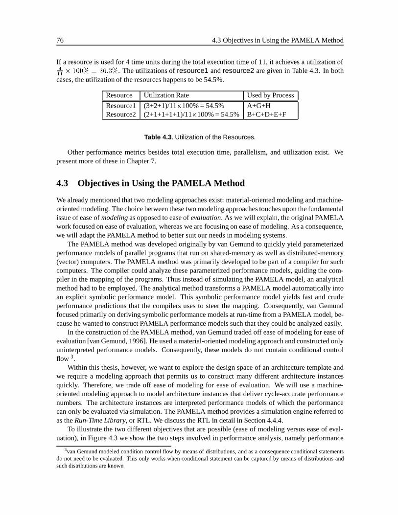
76 4.3 Objectives in Using the PAMELA Method
If a resource is used for 4 time units during the total execution time of 11, it achieves a utilization of411 � 100% = 36:3%. The utilizations ofresource1 andresource2 are given in Table 4.3. In bothcases, the utilization of the resources happens to be 54.5%.
Resource Utilization Rate Used by Process
Resource1 (3+2+1)/11�100% = 54.5% A+G+HResource2 (2+1+1+1+1)/11�100% = 54.5% B+C+D+E+F
Table 4.3 . Utilization of the Resources.
Other performance metrics besides total execution time, parallelism, and utilization exist. Wepresent more of these in Chapter 7.
4.3 Objectives in Using the PAMELA Method
We already mentioned that two modeling approaches exist: material-oriented modeling and machine-oriented modeling. The choice between these two modeling approaches touches upon the fundamentalissue of ease ofmodelingas opposed to ease ofevaluation. As we will explain, the original PAMELAwork focused on ease of evaluation, whereas we are focusing on ease of modeling. As a consequence,we will adapt the PAMELA method to better suit our needs in modeling systems.
The PAMELA method was developed originally by van Gemund to quickly yield parameterizedperformance models of parallel programs that run on shared-memory as well as distributed-memory(vector) computers. The PAMELA method was primarily developed to be part of a compiler for suchcomputers. The compiler could analyze these parameterized performance models, guiding the com-piler in the mapping of the programs. Thus instead of simulating the PAMELA model, an analyticalmethod had to be employed. The analytical method transforms a PAMELA model automatically intoan explicit symbolic performance model. This symbolic performance model yields fast and crudeperformance predictions that the compilers uses to steer the mapping. Consequently, van Gemundfocused primarily on deriving symbolic performance models at run-time from a PAMELA model, be-cause he wanted to construct PAMELA performance models such that they could be analyzed easily.
In the construction of the PAMELA method, van Gemund traded off ease of modeling for ease ofevaluation [van Gemund, 1996]. He used a material-oriented modeling approach and constructed onlyuninterpreted performance models. Consequently, these models do not contain conditional controlflow 3.
Within this thesis, however, we want to explore the design space of an architecture template andwe require a modeling approach that permits us to construct many different architecture instancesquickly. Therefore, we trade off ease of modeling for ease of evaluation. We will use a machine-oriented modeling approach to model architecture instances that deliver cycle-accurate performancenumbers. The architecture instances are interpreted performance models of which the performancecan only be evaluated via simulation. The PAMELA method provides a simulation engine referred toas theRun-Time Library, or RTL. We discuss the RTL in detail in Section 4.4.4.
To illustrate the two different objectives that are possible (ease of modeling versus ease of eval-uation), in Figure 4.3 we show the two steps involved in performance analysis, namely performance
3van Gemund modeled condition control flow by means of distributions, and as a consequence conditional statementsdo not need to be evaluated. This only works when conditional statement can be captured by means of distributions andsuch distributions are known
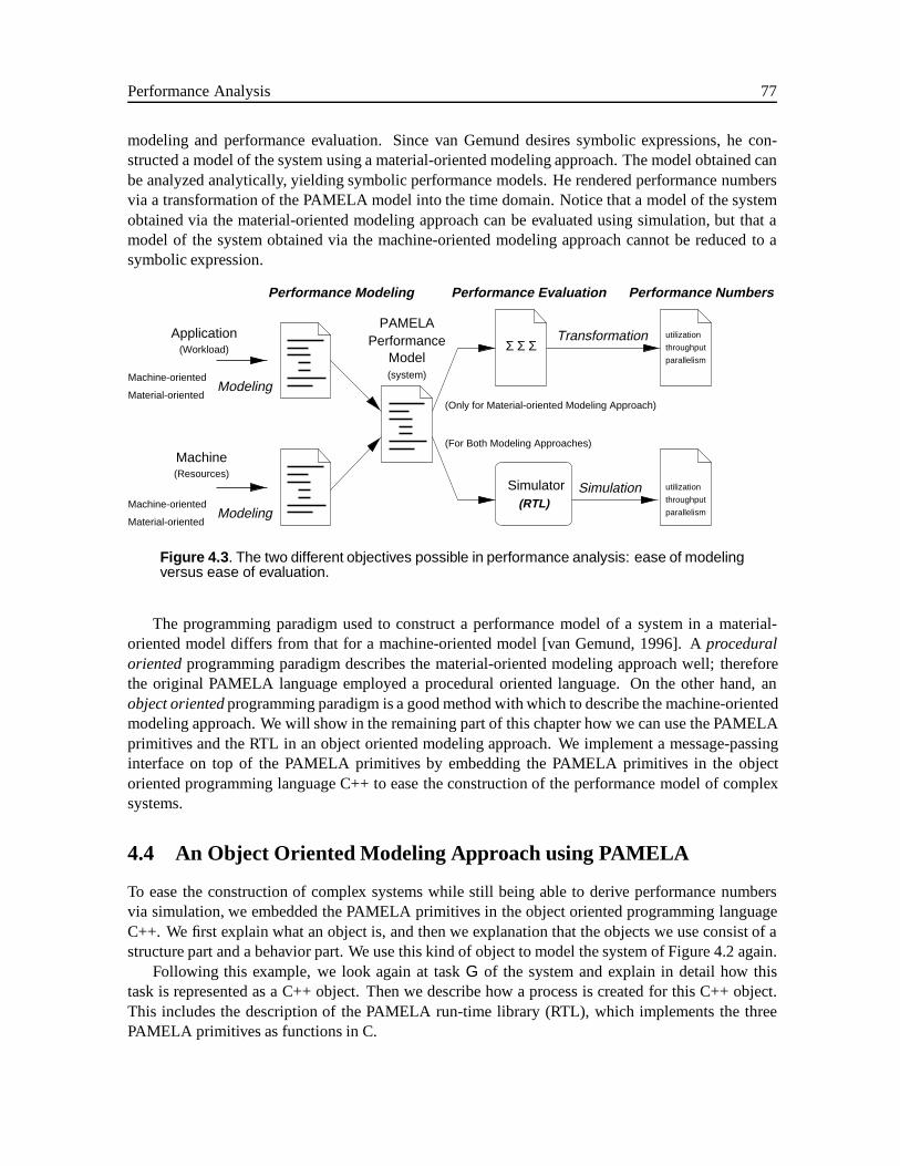
Performance Analysis 77
modeling and performance evaluation. Since van Gemund desires symbolic expressions, he con-structed a model of the system using a material-oriented modeling approach. The model obtained canbe analyzed analytically, yielding symbolic performance models. He rendered performance numbersvia a transformation of the PAMELA model into the time domain. Notice that a model of the systemobtained via the material-oriented modeling approach can be evaluated using simulation, but that amodel of the system obtained via the machine-oriented modeling approach cannot be reduced to asymbolic expression.
throughput
parallelism
utilization
throughput
parallelism
utilization
Machine(Resources)
(Workload)
ApplicationPAMELA
PerformanceModel(system)
Transformation
Simulator(RTL)
Simulation
Modeling
Modeling
Performance Modeling
Machine-oriented
Material-oriented
Machine-oriented
Material-oriented
(Only for Material-oriented Modeling Approach)
(For Both Modeling Approaches)
Performance Evaluation Performance Numbers
Σ Σ Σ
Figure 4.3 . The two different objectives possible in performance analysis: ease of modelingversus ease of evaluation.
The programming paradigm used to construct a performance model of a system in a material-oriented model differs from that for a machine-oriented model [van Gemund, 1996]. Aproceduralorientedprogramming paradigm describes the material-oriented modeling approach well; thereforethe original PAMELA language employed a procedural oriented language. On the other hand, anobject orientedprogramming paradigm is a good method with which to describe the machine-orientedmodeling approach. We will show in the remaining part of this chapter how we can use the PAMELAprimitives and the RTL in an object oriented modeling approach. We implement a message-passinginterface on top of the PAMELA primitives by embedding the PAMELA primitives in the objectoriented programming language C++ to ease the construction of the performance model of complexsystems.
4.4 An Object Oriented Modeling Approach using PAMELA
To ease the construction of complex systems while still being able to derive performance numbersvia simulation, we embedded the PAMELA primitives in the object oriented programming languageC++. We first explain what an object is, and then we explanation that the objects we use consist of astructure part and a behavior part. We use this kind of object to model the system of Figure 4.2 again.
Following this example, we look again at taskG of the system and explain in detail how thistask is represented as a C++ object. Then we describe how a process is created for this C++ object.This includes the description of the PAMELA run-time library (RTL), which implements the threePAMELA primitives as functions in C.
78 4.4 An Object Oriented Modeling Approach using PAMELA
4.4.1 The Object
The basic element of an object oriented programming language is the object. Anobjectconsists ofa data part as well as amethodspart that operates on the data part [Goldberg and Robson, 1983].The data part and the method part of an object, and thus the whole object, is defined using aclassdescription. Individual objects can beinstantiatedfrom such class description, which means that anobject is created taking up a certain amount of space. When an object is instantiated, a special method,theconstructor, is called. This constructor is called only once for each object at the time when theobject is instantiated.
The strength of objects is that they are well suited for use in constructing a (complex)struc-ture [Mellor and Johnson, 1997; Monroe et al., 1997; Kumar et al., 1994; Post et al., 1998] that isthe decomposition of a system into parts and relationships between those parts. In an object orientedprogramming language, a structure is hence constructed by interconnecting objects whereby each ob-ject can be composed of other interconnected objects. Within a structure, objects connect to otherobjects and only exchange information along these connections. An object exchanges informationwith other objects by invoking methods of those other objects. This way of exchanging information isreferred to as “message passing” [Goldberg and Robson, 1983]. The available methods of each objectthus defines for other objects which messages it can exchange; in other words it defines aninterface.Objects exchanging messages with another object remain completely unaware of what happens insidethis object, since it hides unnecessary information.
Besides describing the structure, we also have to describe the behavior of each object. Bybehaviorwe mean the function that the object describes in time. To describe the behavior of an object, wespecify a process that describes the input/output relations of that object in time. As we will seein Chapter 5, not every object is given a process. Recall that there is a distinction between activeprimitives, which are processes, and passive primitives, which are semaphores. An object that usesa process is called anactive objectand one that does not is called apassive object. A passive objectusesP andV operators in its methods, but no processes.
Connection with
Structure
Behavior
Object
other Objects
Figure 4.4 . The objects we construct have a structure part and a behavior part.
We use the object oriented programming language C++ [Stroustrup, 1991] to create an object.Although other object oriented programming languages like objective-C [The Stepstone Corporation,1989] or Java [Arnold and Gosling, 1996] could have been used, we use C++ for reasons of per-formance. The constructed objects in C++ have a structure part and a behavior part, as shown inFigure 4.4. The figure also shows the object connects with four objects, as indicated by the blackcircles. The object can only exchange information with the four objects to which it connects.
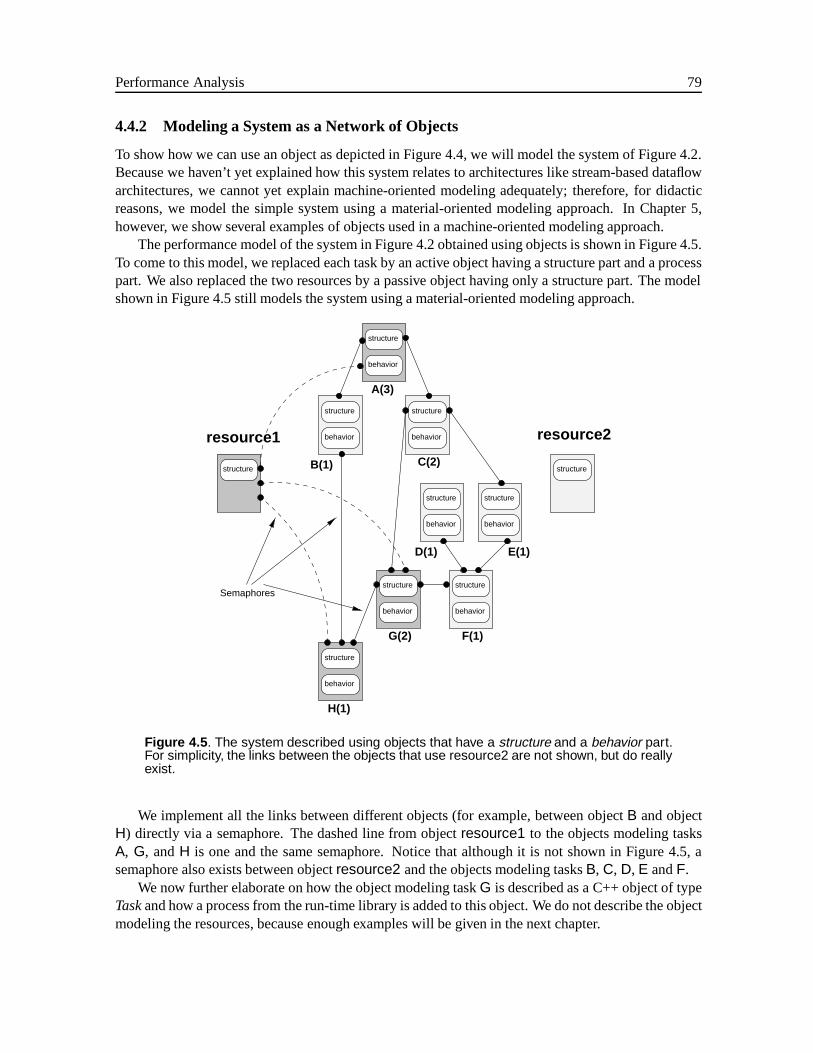
Performance Analysis 79
4.4.2 Modeling a System as a Network of Objects
To show how we can use an object as depicted in Figure 4.4, we will model the system of Figure 4.2.Because we haven’t yet explained how this system relates to architectures like stream-based dataflowarchitectures, we cannot yet explain machine-oriented modeling adequately; therefore, for didacticreasons, we model the simple system using a material-oriented modeling approach. In Chapter 5,however, we show several examples of objects used in a machine-oriented modeling approach.
The performance model of the system in Figure 4.2 obtained using objects is shown in Figure 4.5.To come to this model, we replaced each task by an active object having a structure part and a processpart. We also replaced the two resources by a passive object having only a structure part. The modelshown in Figure 4.5 still models the system using a material-oriented modeling approach.
structure
behavior
structure
behavior
F(1)G(2)
C(2)
A(3)
H(1)
B(1)
E(1)D(1)
structure
behavior
structure
behavior
structure
structure
behavior
structure
behavior
structure
behavior
structure
behavior
Semaphores
structure
resource1 resource2
Figure 4.5 . The system described using objects that have a structure and a behavior part.For simplicity, the links between the objects that use resource2 are not shown, but do reallyexist.
We implement all the links between different objects (for example, between objectB and objectH) directly via a semaphore. The dashed line from objectresource1 to the objects modeling tasksA, G, andH is one and the same semaphore. Notice that although it is not shown in Figure 4.5, asemaphore also exists between objectresource2 and the objects modeling tasksB, C, D, E andF.
We now further elaborate on how the object modeling taskG is described as a C++ object of typeTaskand how a process from the run-time library is added to this object. We do not describe the objectmodeling the resources, because enough examples will be given in the next chapter.
80 4.4 An Object Oriented Modeling Approach using PAMELA
4.4.3 Describing the Structure of an Object in C++
Before we can construct an objectTaskmodeling a task in the system of Figure 4.5, we need todescribe a class definition. In Program 4.5, we give the class description for the objectTask . In C++,a class definition always starts with the keywordClass.
Program 4.5. CLASS DEFINITION OF THETask OBJECT
class Task {/* Data Elements */semaphore in1;semaphore in2;semaphore out;semaphore resource;int delay;
/* Methods *//* Constructor */Task( semaphore, semaphore, semaphore, semaphore, int )
/* init Process */init_process(void);
}
Class Definition
Within this class description, an object is defined that consists of five data elements4 of which fourare semaphores and one is a single integer value. Three semaphores represent dependencies (in1 ,in2 , andout ) and one semaphore represents a resource (resource ). The integer delay valuedelay
indicates the time required by a task to execute.Within the same class description, two methods are defined for aTask object. Each method has
an implementation, which describes the function a method performs. One method is the construc-tor 5 of theTask object while the other method isinit process . The constructor method is calledwhen aTask object is instantiated from the class description. The constructor has a number of ar-guments that need to be provided when an object is created. In this case, the arguments include foursemaphores and an integer value. The constructor is used to set up the structure of an object, while theinit process method is used to create the behavior of an object. We describe first what happenswhen the constructor is called, followed by what happens when theinit process method is called.
Calling the Constructor
To instantiate an object representing taskG in the system of Figure 4.5, we call upon the C++ func-tion new, as given in Program 4.6. In creating theTask object, we pass on the semaphores alreadydescribed in Program 4.1 as arguments of the constructor. We also pass on the integer value 2, toindicate taskG takes two time units to execute.
4All the elements in the data part of the class definition are variables in C/C++. Therefore, semaphorein1 is a variable,as is the integerdelay
5In C++, methods are described using the:: notation. It should be read asclass::method , which describes theimplementation of a particular method of a class. The constructor method of a class always has the same name as the class.ThusTask::Task describes the implementation of the constructor of classTask .
Performance Analysis 81
Program 4.6. INSTANTIATE AN OBJECT REPRESENTING TASKG
new Task(dependency_CG, dependency_FG, dependency_GH, resource1, 2)
Executing thenew function causes the execution of the constructor, as shown in Program 4.7. Inthe constructor, the argumentsdep1 , dep2 , dep3 , res and, finally,task delay are assigned to thevariables declared in the data part of theTask object in Program 4.5. The value of variabledep1 isthus assigned to variablein1 . Because objectTask is created as shown in Program 4.6, argumentdep1 equals the semaphoredependency CGthat describes the dependency between taskC and taskG. Therefore variablein1 equals semaphoredependency CG.
Program 4.7. THE CONSTRUCTOR OFTask OBJECT
Task::Task(semaphore dep1, semaphore dep2, semaphore dep3, semaphore res, int task_delay){ // Constructor of a Process
in1 = dep1;in2 = dep2;out = dep3;resource = res;delay = task_delay;
}
4.4.4 Describing the Behavior of an Object Using PAMELA
We have shown how an object captures the structural elements in its data part, and in particular, fortaskG. Now we will look at how we can add a behavior part to the structure part of an object after wepresent the run-time library PAMELA.
Run-time Library (RTL)
The PAMELA language describes performance models using three primitives:processes, semaphoresanddelays. These three primitives have been implemented as C functions in the PAMELARun-TimeLibrary (RTL) [Nijweide, 1995]. The RTL is a simple, non-preemptivemultithreadingpackage. Itprovides the notion of parallelism in the sequential programming language C [Kernighan and Ritchie,1988]. The RTL implements aprocess scheduler, interleaving the parallel processes on a single CPU.It differs from many other multithreading packages [Open Software Foundation, 1995; Proven, 1995;Mueller, 1993], in that it uses the notion ofvirtual time.
The RTL implements processes aslightweight processes. Lightweight processes are implementedin the same address space [Finger, 1995], which makes communication of variables between processesvery simple and efficient. Each process has its ownthread-of-execution, and a thread has its owncontextof variables (state). Whenever the process scheduler switches a process on the CPU, it restoresthe context of the thread. This is calledcontext switching. The processes are called lightweightprocesses because the threads have a small or ‘light’ context6. This introduces only a small overheadand, consequently, the process scheduler can switch the context of processes quickly.
6This is in contrast toheavyweightprocesses used, for example, in the UNIX operating system. These processes havetheir own address space and require pipes to communicate variables with other processes. As such, these processes have abig or ‘heavy’ context, and context switching on a UNIX system requires more time than a context switch of a lightweightprocess.
82 4.4 An Object Oriented Modeling Approach using PAMELA
The complete RTL and its C functions are described in detail in [Nijweide, 1995]. We now discussthe function used to construct a process, the functions that implement the semaphore operatorsP andV and the function which implements thedelayoperator.
Process: The RTL describes a process as an ordinary C function called theprocess function. TheRTL creates an instance of a process function in memory. A process scheduler switches theseinstances of the process functions in time to give the appearance of their executing in parallel.A process is created via thepam fork statement. This statement requires three arguments: aname for identification purposes, a C function that is the process function, and an additionalargument. This additional argument is used by a process to initialize itself when it is created.
Semaphore operators:The RTL implements theP andV operators aspam P and pam V state-ments respectively. These statements operate on semaphores created via thepam alloc state-ment. This statement requires two arguments, namely a name for identification purposes and aninitialization value.
Delay operator: The RTL implements thedelayoperator as apam delaystatement. This statementmanipulates the time of a process. The operator requires a non-negative integer value.
The RTL provides more functions than just those mentioned above. We will wait, however, tointroduce these functions until they are used.
Creating a Process
All the tasks in Figure 4.2 are modeled using a process. We therefore need to create a process foreach object that models a task in the system-modeling example in Figure 4.5. Assume that we haveinstantiated an object for each task and stored links to other objects in the data part of these objects.In this example we do this using only semaphores.
A process is created for each object by calling the init process method, as shown for theTask
object in Program 4.8. This method causes the execution of thepam fork statement. As explainedwhen discussing the RTL-library, this invokes the creation of a process with the name “task ” thatexecutes the process functiontask function . The argumentthis is passed on to this process.In the C++ programming language thethis pointer represents the complete data part of an object.Therefore, thepam fork statement passes on the complete data structure of the object to the processfunctiontask function .
In the case of theTask object that models taskG, the data part of this object contains thesemaphores describing the data dependencies with tasksC, F andH. It also contains the semaphoredescribing theresource1.
Program 4.8. CREATING A PROCESS FOR ANOBJECT
Task::init_process( void ) { pam fork ("task",task function,this); }
A Process
The RTL creates a process from the process function by creating a unique instance in memory usingthe pam fork statement. In the case of theTask object, the RTL creates a process based on theprocess functiontask function , as shown in Program 4.9.
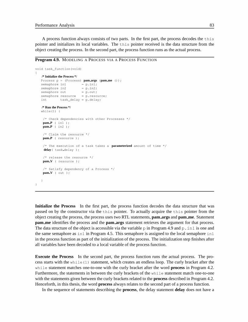
Performance Analysis 83
A process function always consists of two parts. In the first part, the process decodes thethis
pointer and initializes its local variables. Thethis pointer received is the data structure from theobject creating the process. In the second part, the process function runs as the actual process.
Program 4.9. MODELING A PROCESS VIA APROCESSFUNCTION
void task_function(void){
/* Initialize the Process */Process p = (Process) pam args ( pam me ());semaphore in1 = p.in1;semaphore in2 = p.in2;semaphore out = p.out;semaphore resource = p.resource;int task_delay = p.delay;
/* Run the Process */while(1) {
/* Check dependencies with other Processes */pam P ( in1 );pam P ( in2 );
/* Claim the resource */pam P ( resource );
/* The execution of a task takes a parameterized amount of time */delay( task delay );
/* release the resource */pam V ( resource );
/* Satisfy dependency of a Process */pam V ( out );
}}
Initialize the Process In the first part, the process function decodes the data structure that waspassed on by the constructor via thethis pointer. To actually acquire thethis pointer from theobject creating the process, the process uses two RTL statements,pam argsandpam me. Statementpam me identifies the process and thepam args statement retrieves the argument for that process.The data structure of the object is accessible via the variablep in Program 4.9 andp.in1 is one andthe same semaphore asin1 in Program 4.5. This semaphore is assigned to the local semaphorein1
in the process function as part of the initialization of the process. The initialization step finishes afterall variables have been decoded to a local variable of the process function.
Execute the Process In the second part, the process function runs the actual process. The pro-cess starts with thewhile(1) statement, which creates an endless loop. The curly bracket after thewhile statement matches one-to-one with the curly bracket after the wordprocessin Program 4.2.Furthermore, the statements in between the curly brackets of thewhile statement match one-to-onewith the statements given between the curly brackets related to theprocessdescribed in Program 4.2.Henceforth, in this thesis, the wordprocessalways relates to the second part of a process function.
In the sequence of statements describing theprocess, the delay statementdelay does not have a
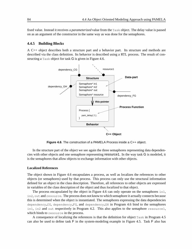
84 4.4 An Object Oriented Modeling Approach using PAMELA
fixed value. Instead it receives aparameterizedvalue from theTask object. The delay value is passedon as an argument of the constructor in the same way as was done for the semaphores.
4.4.5 Building Blocks
A C++ object describes both a structure part and a behavior part. Its structure and methods aredescribed via the class definition. Its behavior is described using a RTL process. The result of con-structing aTask object for taskG is given in Figure 4.6.
Semaphore* in1
pam_delay( 2 );
Semaphore* in2Semaphore* out
Semaphore* resource
}
Behavior
Structure
Process Function
this-pointer
C++ Object
dependency_FG
Process {
dependency_CG
dependency_GH
resource1
Data-part
Figure 4.6 . The construction of a PAMELA Process inside a C++ object.
In the structure part of the object we see again the three semaphores representing data dependen-cies with other objects and one semaphore representingresource1. In the way taskG is modeled, itis the semaphores that allow objects to exchange information with other objects.
Localized References
The object shown in Figure 4.6 encapsulates a process, as well as localizes the references to otherobjects (or semaphores) used by that process. This process can only use the structural informationdefined for an object in the class description. Therefore, all references to other objects are expressedin variables of the class description of the object and thuslocalizedto that object.
The process encapsulated by the object in Figure 4.6 can only operate on the semaphoresin1 ,in2 , out andresource . The process does not know to which semaphore it actually connects becausethis is determined when the object is instantiated. The semaphores expressing the data dependenciesdependency CG, dependency FG, anddependency GH in Program 4.6 bind to the semaphoresin1 , in2 and out respectively in Program 4.2. This also applies to the semaphoreresource1 ,which binds toresource in the process.
A consequence of localizing the references is that the definition for objectTask in Program 4.5can also be used to define taskF in the system-modeling example in Figure 4.5. TaskF also has
Performance Analysis 85
two input semaphores, one output semaphore, and one semaphore for a resource. By instantiating theobject as was done in Program 4.10, we obtain an object that models taskF.
Program 4.10. INSTANTIATE AN OBJECT REPRESENTING TASKF
new Task(dependency_DF, dependency_EF, dependency_FG, resource2, 1)
Note that we change the parameter value that describes the execution time of taskF in Pro-gram 4.10. Instead of taking two time units as we did for taskG, we now set the parameter valueto 1, which causes taskF to execute in one time unit.
By localizing the references of a process, we obtain objects representingBuilding Blocks. Thesebuilding blocks represent modular elements that are self-contained and parameterized. We define abuilding block as
Definition 4.2. BUILDING BLOCK
A building blockis a self-contained, parameterized object with a structure part and a behaviorpart. 2
That a building block isself-containedmeans that it can only exchange information with otherbuilding blocks to which references are present in the structural part. The exchange of informationtakes place using the “message passing” mechanism. Consequently, the internal structure of a build-ing block remains invisible to the other building blocks in a system, a key requirement in obtainingmodular elements.
There is a distinction between active objects and passive objects; a similar distinction exists forbuilding blocks. Anactive building blockuses one or moreprocessesto describe its behavior part. Apassive building blockuses only semaphores andpam P andpam V statements to describe its behav-ioral part. Thepam P andpam V statements are incorporated into methods of the building block andthese methods describe the behavioral part of the building block. We show several examples of activeand passive building blocks in Chapter 5, in which we use building blocks extensively to construct theperformance models of stream-based dataflow architectures by combining building blocks.
4.5 Simulating Performance Models with the RTL
We use simulation to obtain the performance number of a performance model for a system. PAMELA’sRTL provides not only processes, semaphores and delay statements, but also a process scheduler. Wenow explain how this process scheduler simulates a performance model and how the PAMELA prim-itives interact with the RTL process scheduler. We discuss the RTL in more detail, showing that theRTL has a very simple structure. This simple structure makes it possible to execute faster than withother kinds of discrete event simulators.
A process is said to berunnableif it is not in a blocking state. A process can attain a blockingstate only when executing apam P statement, and a process is taken out of this state via apam Vstatement. Each process has its own notion of time, represented by its owntime stamp. The value ofthis time stamp changes directly using apam delaystatement or indirectly using apam P statement.The time stamp is used by the process scheduler to order processes in time.
Although only one process can execute at a time, RTL implements aprocess schedulerthat sched-ules one process after the other, giving the impression that processes execute in parallel. The processscheduler uses two different queues to schedule processes. One queue, theRunnable Processes Queue
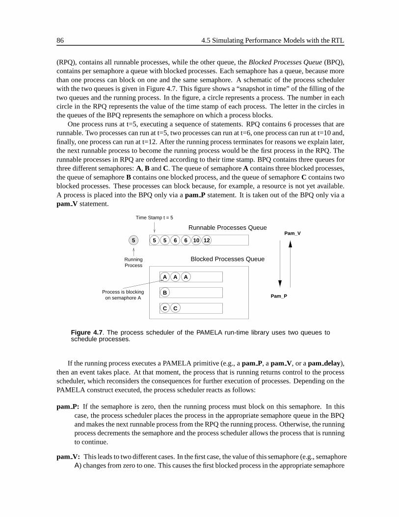
86 4.5 Simulating Performance Models with the RTL
(RPQ), contains all runnable processes, while the other queue, theBlocked Processes Queue(BPQ),contains per semaphore a queue with blocked processes. Each semaphore has a queue, because morethan one process can block on one and the same semaphore. A schematic of the process schedulerwith the two queues is given in Figure 4.7. This figure shows a “snapshot in time” of the filling of thetwo queues and the running process. In the figure, a circle represents a process. The number in eachcircle in the RPQ represents the value of the time stamp of each process. The letter in the circles inthe queues of the BPQ represents the semaphore on which a process blocks.
One process runs at t=5, executing a sequence of statements. RPQ contains 6 processes that arerunnable. Two processes can run at t=5, two processes can run at t=6, one process can run at t=10 and,finally, one process can run at t=12. After the running process terminates for reasons we explain later,the next runnable process to become the running process would be the first process in the RPQ. Therunnable processes in RPQ are ordered according to their time stamp. BPQ contains three queues forthree different semaphores:A, B andC. The queue of semaphoreA contains three blocked processes,the queue of semaphoreB contains one blocked process, and the queue of semaphoreC contains twoblocked processes. These processes can block because, for example, a resource is not yet available.A process is placed into the BPQ only via apam P statement. It is taken out of the BPQ only via apam V statement.
on semaphore AProcess is blocking
6 10 126555
RunningProcess
Runnable Processes Queue
Time Stamp t = 5
Pam_P
Pam_V
Blocked Processes Queue
A
B
A A
C C
Figure 4.7 . The process scheduler of the PAMELA run-time library uses two queues toschedule processes.
If the running process executes a PAMELA primitive (e.g., apam P, apam V, or apam delay),then an event takes place. At that moment, the process that is running returns control to the processscheduler, which reconsiders the consequences for further execution of processes. Depending on thePAMELA construct executed, the process scheduler reacts as follows:
pam P: If the semaphore is zero, then the running process must block on this semaphore. In thiscase, the process scheduler places the process in the appropriate semaphore queue in the BPQand makes the next runnable process from the RPQ the running process. Otherwise, the runningprocess decrements the semaphore and the process scheduler allows the process that is runningto continue.
pam V: This leads to two different cases. In the first case, the value of this semaphore (e.g., semaphoreA) changes from zero to one. This causes the first blocked process in the appropriate semaphore
Performance Analysis 87
queue in the BPQ to become runnable. The process scheduler makes this runnable process thenew running process. Before it does this, it puts the running process, which has a time stampt=5, back into the RPQ. The new running process is given the same time stamp as the runningprocess (t=5). In the second case, the running process increments a semaphore and the value ofthe semaphore becomes larger than one. In this case, the process scheduler allows the processthat is running to continue.
pam delay: This statement adds a certain amount of time to the time stamp of the running processand the process scheduler puts this process back into the RPQ. This process gets ordered inthe RPQ according to its new value of the time stamp. The process scheduler makes the nextrunnable process from the RPQ the running process.
The process scheduler of the RTL is anon-preemptivescheduler, which means that the processscheduler cannot preempt a running process in order to regain control. It must wait to regain controluntil the running process reaches a PAMELA construct that causes an event. Only then does theprocess scheduler get the control back from a process.
Note that the way processes get scheduled by the process scheduler results in a feasible schedule,which is not necessarily the fastest schedule. Processes are activated as soon as possible because theRTL implements a simple list-scheduler; however, this does not always result in the fastest sched-ule [De Micheli, 1994]. For an example, look at Table 4.1, which shows the scheduling of processesused to model the system of Figure 4.2. If taskB were not scheduled at t=6, but instead slightly later,it could execute in parallel with taskG without resource conflict. As a consequence, the resulting totalexecuting time in this case would beTend = 10 instead ofTend = 11.
4.6 Related Work
Traditionally,Queuing Theory[see, for example, Lazowska et al., 1984] has been used in performanceanalysis of computer designs. It can be used to describe a system in terms of servers and independentclients. These clients access the servers following a negative exponential distribution in time. Thestrength of queuing theory is that it derives a system’s steady state behavior analytically. This makesqueuing theory very useful for determining the capacity of servers. Queuing theory is, however, toorestrictive for our purpose because of its model. This model is not able to describe, for example,condition synchronization between various clients or conditional control flow.
Petri Nets[Petri, 1962; Jensen, 1991] were originally developed to study concurrency and to ana-lyze issues likeliveness, deadlockandstarvation[Ben-Ari, 1982], using analytical techniques. To usepetri nets for performance analysis requires the use ofTimed Petri Nets[Van der Aalst, 1992]. Thesepetri nets can be analyzed analytically in the time domain only under the assumption that transitiontakes place using a negative exponential delay. If the system constructed is ergodic, a Markov chaincan be constructed that can be analyzed analytically. However, instead of using analytical techniques,simulation can be used to derive the performance of a system [ASPT, 1994].
In contrast to queuing theory and petri nets,simulation toolslack an analytical basis. To ren-der performance numbers, simulation tools use simulation instead and typically employ event-basedsimulation techniques. Simulation tools are popular because they provide simple compositional con-structs to build large and complex models and they describe interpreted performance models well.Simulation tools use a textual or graphical representation to define a system. Many different simula-tion tools exist that are tailored to specific application domains. In the signal processing domain the
88 4.7 Conclusions
following tools (to name a few) are available: the Ptolemy system [in particular, the DE-domain, Bucket al., 1992], the Maisie environment [Bagradia, 1995] and the BoNES environment [Cadence, 1998].
Another tool that can be used for performance analysis is VHDL or Verilog. Although theselanguages were developed originally to describe and simulate hardware at a much lower level, i.e.,Register Transfer Level (RTL), a VHDL simulator is basically a parallel simulator using event simu-lation. In contrast to the previously discussed simulation tools, these languages are able to simulatesystems very accurately. Nonetheless, VHDL is also used for performance analysis on a higher levelof abstraction, as done, for example, by Rose and Shackleton [1997].
Standard programming languages like C [Kernighan and Ritchie, 1988] or C++ [Stroustrup, 1991]are used instead of simulation tools to construct performance models. These provide a high degree offreedom in constructing models of systems, but at the same time, they lack a systematic approach orwell defined simulation model. Furthermore, standard programming languages lack the notion of asimulation engine to handle parallel simulations.
The object oriented modeling approach that uses PAMELA to describe the behavior of each build-ing block as presented in this chapter is a very interesting approach for the following reason. The useof C++ gives us a large amount of freedom to model different architecture instances, as we will showin Chapter 5, where we discuss the modeling of stream-based dataflow architectures. The PAMELAprimitives provide high-level modeling primitives like semaphores, processes, and delays. This re-sults, as we will also see in Chapter 5, in compact descriptions when modeling the building blocks ofarchitecture instances. VHDL, for example, does not provide these high level primitives.
The PAMELA method gives accurate performance values using simulation. Other modeling ap-proaches can provide symbolic representations for performance numbers, but these representations arenot accurate enough since not all four components of the Performance Modeling Basis are included.For example, queuing theory cannot describe condition synchronization, whereas the analytical eval-uation technique of the PAMELA method cannot handle conditional control flow.
The RTL provides a very efficient simulation engine because of its simple structure. We wewill quantify the simulation speed in Chapter 7, when we discuss the construction of a retargetablesimulator for stream-based dataflow architectures. The execution model of the RTL is more restrictivethan the discrete simulation engines used in most simulation tools, but this results in fast simulation.
4.7 Conclusions
The Y-chart approach uses performance analysis to render performance numbers. In this chapter, wepresented the Performance Modeling Basis (PMB), which describes the four components determiningthe performance of a system. We presented the PAMELA method with which to carry out perfor-mance analysis. The method describes the four components of the PMB using only three high-levelprimitives: semaphores, processes and delays.
Our objective in light of Y-chart approach is to model architecture instances easily. To satisfythis objective, we had to modify the original PAMELA method from a procedural modeling approachto make it to an object oriented modeling approach. This led us to the definition of building blocks,which have a structure part and a behavior part. A system is easily constructed by simply combiningthese building blocks. The structure parts of building blocks use C++ whereas the behavior parts useprimitives of the PAMELA run-time library (RTL). The RTL is a simple multithreading package thatimplements semaphores, processes, and delays. The RTL also provides a process scheduler, allowingus to perform parallel simulations of a system constructed using building blocks.
BIBLIOGRAPHY 89
Bibliography
G.R. Andrews and F.B. Schneider. Concepts and notations for concurrent programming.ACM Com-puting Surveys, 15(1):4 – 43, 1983.
Ken Arnold and James Gosling.The Java Programming Language. Addison-Wesley, 1996.
ASPT. ExSpect 5.0 User Manual. Eindhoven University of Technology, Eindhoven, the Netherlands,1994.
Rajive Bagradia.Maisie User Manual. UCLA Parallel Computing Lab, 1995. Release 2.2.
M. Ben-Ari. Principles of Concurrent Programming. Prentice-Hall, 1982.
Joseph Buck, Soonhoi Ha, Edward A. Lee, and David G. Messerschmitt. Ptolemy: A framework forsimulating and prototyping heterogeneous systems.International Journal of Computer Simulation,1992. Special issue on Simulation Software Development.
Cadence. Bones 4.0. http://www.cadence.com, 1998.
Giovanni De Micheli. Synthesis and Optimization of Digital Circuits. McGraw-Hill InternationalEditions, 1994.
E.W. Dijkstra. Cooperating sequential processes. In F. Geunys, editor,Programming Languages,pages 43 – 112. Academic Press, 1968.
E.W. Dijkstra. Personal Communication, 1981.
Jonathan Finger. Lightweight tasks in C.Dr. Dobb’s Journal, pages 48 – 50, 1995.
Adele Goldberg and David Robson.Smalltalk-80, The Language and Its Implementation. Addison-Wesley Publishing Company, Xerox Palo Alto Research Center, 1983.
K. Jensen. Coloured petri nets: A high level language for system design and analysis. In K. Jensen andG. Rozenberg, editors,High-level Petri Nets: Theory and Application, pages 44 – 122. Springer-Verlag, 1991.
Brian W. Kernighan and Dennis M. Ritchie.The C Programming Language. Prentine Hall SoftwareSeries, second edition, 1988.
Wolfgang Kreutzer.System simulation, programming styles and languages. International ComputerScience Series. Addison-Wesley, 1986.
Sanjaya Kumar, Jamer H. Aylor, Barry W. Johmson, and Wm. A. Wulf. Object-oriented techniquesin hardware design.Computer, 27(6):64–70, 1994.
E.D. Lazowska, J. Zahorja, G. Graham, and K. Sevcik.Quantitative System Performance: ComputerSystem Analysis Using Queueing Network Models. Prentice-Hall, 1984.
Stephen J. Mellor and Ralph Johnson. Why explore object methods, patterns, and architectures?IEEESoftware, 14(1):27 – 30, 1997. Guest Editor’s Introduction.
Robert T. Monroe, Andrew Kompanek, Ralph Melton, and David Garlan. Architectural styles, designpatterns, and objects.IEEE Software, 14(1):43 – 52, 1997. Theme Issue.
90 BIBLIOGRAPHY
Frank Mueller. A library implementatio of POSIX threads under UNIX. InPro-ceedings of the USENIX Conference, pages 253–261, San Diego, CA, 1993.http://www.informatik.hu-berlin.de/ mueller/ .
Marc Nijweide. The pamela run-time library, version 1.3. Technical Report 1-68340-27(1995)06,Laboratory of Computer Architecture and Digital Techniques, Delft University of Technology,1995.http://dutepp0.et.tudelft.nl/ gemund/publications.html .
Open Software Foundation.OSF/DCE Application Development Guide, chapter Threads, pages 2–1to 2–24. Prentice Hall, 1995. release 1.1.
C.A. Petri.Kommunikation mit Automaten. PhD thesis, Institut f¨ur Instrumentelle Mathematik, Bonn,Germany, 1962.
Guido Post, Andrea Muller, and Rainer Schoenen. Object-oriented design of ATM switch hardwarein a telecommunication network simulation environment. InProceedings of GI/ITG/GMM Work-shop Methoden und Bescheibungssprachen zur Modellierung und Verifikation von Schaltungen undSystemen, Paderborn, 1998.
Christopher Proven. POSIX threads, 1995. WWW ref only.http://www.mit.edu:8001/people/proven/pthreads.html.
RASSP Taxonomy Working Group (RTWG). RASSP VHDL modeling terminology and taxonomy.http://rassp.scra.org/documents/taxonomy/taxonomy.html , 1998. Revision2.4.
Fred Rose and John Shackleton. Performance modeling of system architectures.VLSI Signal Pro-cessing, 15(1/2):97 – 110, 1997.
Bjarne Stroustrup.The C++ Programming Language. Addison-Wesley, 2nd edition, 1991.
The Stepstone Corporation.Objective-C Compiler v4.0. The Stepstone Corporation, 1989.
W.M.P. Van der Aalst.Interval Timed Coloured Petri Nets and their Analysis. PhD thesis, Dept. ofComputer Science and Mathematics, Eindhoven University of Technology, 1992.
Arjan. J.C. van Gemund.Performance Modeling of Parallel Systems. PhD thesis, Laboratory ofComputer Architecture and Digital Techniques, Delft University of Technology, 1996.
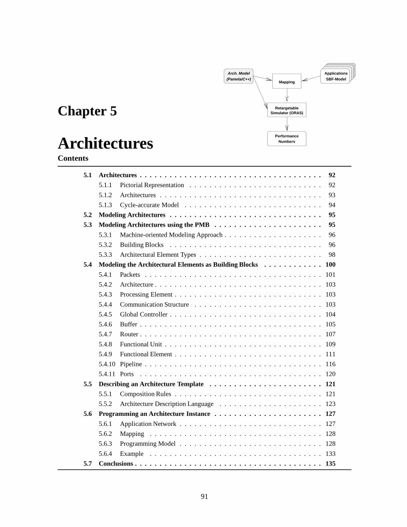
Chapter 5
Architectures
RetargetableSimulator (ORAS)
PerformanceNumbers
Mapping
Applications
SBF-Model
Arch. Model(Pamela/C++)
Contents
5.1 Architectures . . . . . . . . . . . . . . . . . . . . . . . . . . . . . . . . . . . . . 92
5.1.1 Pictorial Representation . . . . . . . . . . . . . . . . . . . . . . . . . . . 92
5.1.2 Architectures . . . . . . . . . . . . . . . . . . . . . . . . . . . . . . . . . 93
5.1.3 Cycle-accurate Model. . . . . . . . . . . . . . . . . . . . . . . . . . . . 94
5.2 Modeling Architectures . . . . . . . . . . . . . . . . . . . . . . . . . . . . . . . 95
5.3 Modeling Architectures using the PMB . . . . . . . . . . . . . . . . . . . . . . 95
5.3.1 Machine-oriented Modeling Approach . . . . . . . . . . . . . . . . . . . . 96
5.3.2 Building Blocks . . . . . . . . . . . . . . . . . . . . . . . . . . . . . . . 96
5.3.3 Architectural Element Types . . . . . . . . . . . . . . . . . . . . . . . . . 98
5.4 Modeling the Architectural Elements as Building Blocks . . . . . . . . . . . . 100
5.4.1 Packets . . . . . . . . . . . . . . . . . . . . . . . . . . . . . . . . . . . . 101
5.4.2 Architecture . . . . . . . . . . . . . . . . . . . . . . . . . . . . . . . . . . 103
5.4.3 Processing Element . . . . . . . . . . . . . . . . . . . . . . . . . . . . . . 103
5.4.4 Communication Structure . . . . . . . . . . . . . . . . . . . . . . . . . . 103
5.4.5 Global Controller . . . . . . . . . . . . . . . . . . . . . . . . . . . . . . . 104
5.4.6 Buffer . . . . . . . . . . . . . . . . . . . . . . . . . . . . . . . . . . . . . 105
5.4.7 Router . . . . . . . . . . . . . . . . . . . . . . . . . . . . . . . . . . . . . 107
5.4.8 Functional Unit . . . . . . . . . . . . . . . . . . . . . . . . . . . . . . . . 109
5.4.9 Functional Element . . . . . . . . . . . . . . . . . . . . . . . . . . . . . . 111
5.4.10 Pipeline . . . . . . . . . . . . . . . . . . . . . . . . . . . . . . . . . . . . 116
5.4.11 Ports . . . . . . . . . . . . . . . . . . . . . . . . . . . . . . . . . . . . . 120
5.5 Describing an Architecture Template . . . . . . . . . . . . . . . . . . . . . . . 121
5.5.1 Composition Rules. . . . . . . . . . . . . . . . . . . . . . . . . . . . . . 121
5.5.2 Architecture Description Language. . . . . . . . . . . . . . . . . . . . . 123
5.6 Programming an Architecture Instance . . . . . . . . . . . . . . . . . . . . . . 127
5.6.1 Application Network . . . . . . . . . . . . . . . . . . . . . . . . . . . . . 127
5.6.2 Mapping . . . . . . . . . . . . . . . . . . . . . . . . . . . . . . . . . . . 128
5.6.3 Programming Model . . . . . . . . . . . . . . . . . . . . . . . . . . . . . 128
5.6.4 Example . . . . . . . . . . . . . . . . . . . . . . . . . . . . . . . . . . . 133
5.7 Conclusions . . . . . . . . . . . . . . . . . . . . . . . . . . . . . . . . . . . . . . 135
91

92 5.1 Architectures
THE subject of this chapter is the modeling of architecture instances of the architecture templateof stream-based dataflow architectures that yield cycle-accurate performance numbers. In the
Y-chart approach, we must be able to derive architecture instances from an architecture template thatwe can evaluate to obtain performance numbers. As motivated using the abstraction pyramid shownin Figure 3.3, we want to model those architecture instances at a higher level of abstraction, i.e., werepresent only the details relevant to obtaining the performance of an architecture instance, suppress-ing irrelevant details. As motivated in Chapter 4, the Performance Modeling Basis (PMB) describesexactly those details relevant to describing the performance of a system. The PMB can be expressedusing only processes, semaphores and delays. In this chapter, we use these primitives together withthe concept of building blocks that was also introduced in Chapter 4 to describe architecture instancescycle-accurately. This way we model architectures at a level that is more abstract than that offered bystandard hardware description languages.
We start off in Section 5.1 with explaining what we consider an architecture to be; until now,we have given only pictorial representations of architectures. We also explain what we consider acycle-accurate model to be. Modeling an architecture in the context of the Y-chart approach impliesthat we need to derive an instance from the architecture template of stream-based dataflow architec-tures. In Section 5.2, we explain the four issues involved in this modeling process. In Section 5.3, weexplain how executable architecture instances are constructed from building blocks. We construct abuilding block for each architectural element of the architecture template of stream-based dataflow ar-chitectures and we construct executable models of architecture instances by combining these buildingblocks. Stream-based dataflow architectures are composed of many different architectural elements.In Section 5.4, we model each architectural element as a building block and describe in detail itsstructure and its behavior. We also show how only the three PAMELA primitives (semaphores, pro-cesses and delays) introduced in Chapter 4 are used to model the various architectural elements. Wedescribe an architecture template in Section 5.5, using composition rules. Stream-based dataflow ar-chitectures are programmable architectures. In Section 5.6, we explain the programming model ofstream-based dataflow architectures. We show how instances of the stream-based dataflow architec-ture are programmed for a particular application, leading to the routing program that is down-loadedonto the global controller. We conclude this chapter by presenting a comprehensive example in whichwe program a particular architecture instance for a particular application.
5.1 Architectures
So far, in our references to architectures, and especially stream-based dataflow architectures, we havedepended on our rather intuitive understanding of what an architecture might be. Since this chapter isabout modeling architectures, we begin by explaining what we consider an architecture to be.
5.1.1 Pictorial Representation
Architectures are normally represented in a pictorial way, using block diagrams. Theseblock diagramsdescribe a network consisting of boxes and lines connecting the boxes to each other. The boxes aregiven names related to the kind of functions they are supposed to perform. We have been presentingthe stream-based dataflow architecture in exactly this way, which is shown again in Figure 5.1. In thisfigure (which is the same as Figure 2.2, but shown again here for clarification), we gave names to theboxes to indicate their function in the architecture. We gave boxes the nameroutersto indicate that
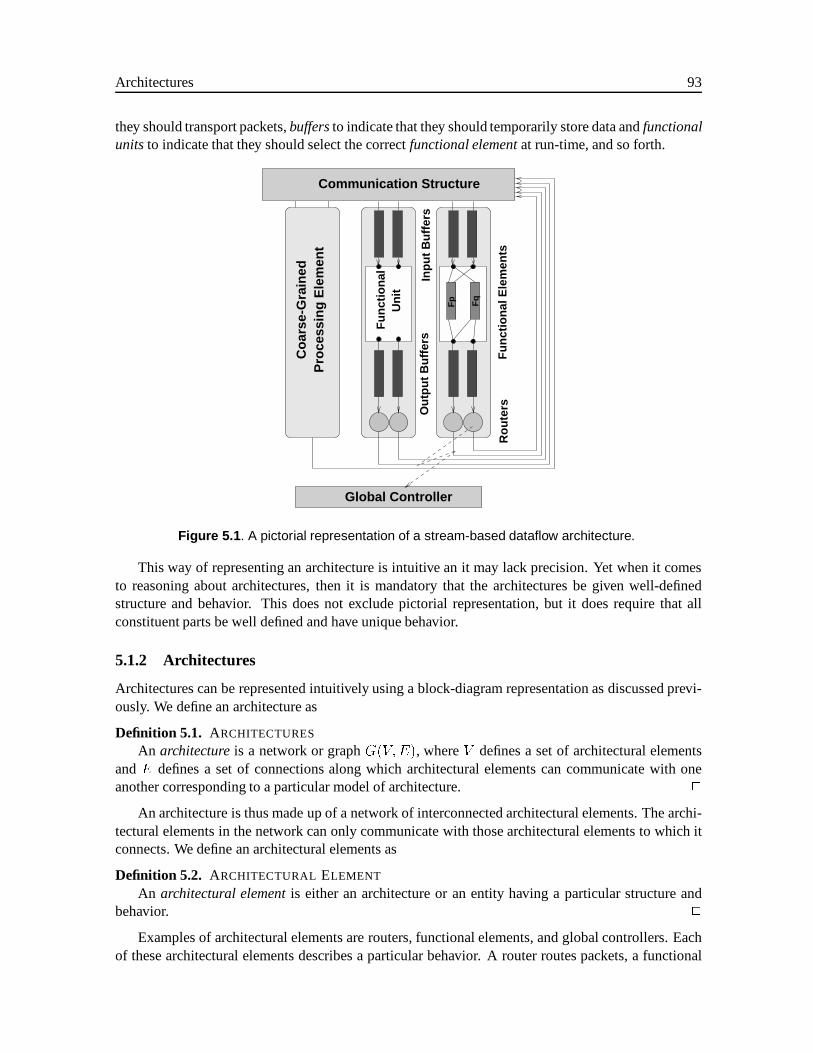
Architectures 93
they should transport packets,buffersto indicate that they should temporarily store data andfunctionalunitsto indicate that they should select the correctfunctional elementat run-time, and so forth.
Fq
Fp
Fu
nct
ion
al E
lem
ents
Ro
ute
rsOu
tpu
t B
uff
ers
Pro
cess
ing
Ele
men
t
Global Controller
Communication Structure
Un
itF
un
ctio
nal In
pu
t B
uff
ers
Co
arse
-Gra
ined
Figure 5.1 . A pictorial representation of a stream-based dataflow architecture.
This way of representing an architecture is intuitive an it may lack precision. Yet when it comesto reasoning about architectures, then it is mandatory that the architectures be given well-definedstructure and behavior. This does not exclude pictorial representation, but it does require that allconstituent parts be well defined and have unique behavior.
5.1.2 Architectures
Architectures can be represented intuitively using a block-diagram representation as discussed previ-ously. We define an architecture as
Definition 5.1. ARCHITECTURES
An architectureis a network or graphG(V;E), whereV defines a set of architectural elementsandE defines a set of connections along which architectural elements can communicate with oneanother corresponding to a particular model of architecture. 2
An architecture is thus made up of a network of interconnected architectural elements. The archi-tectural elements in the network can only communicate with those architectural elements to which itconnects. We define an architectural elements as
Definition 5.2. ARCHITECTURAL ELEMENT
An architectural elementis either an architecture or an entity having a particular structure andbehavior. 2
Examples of architectural elements are routers, functional elements, and global controllers. Eachof these architectural elements describes a particular behavior. A router routes packets, a functional
94 5.1 Architectures
element executes a particular function, and the global controller governs the flow of packets. Usingthese architectural elements, we can describe, for example, the stream-based dataflow architectureshown in Figure 5.1 as a network of architectural elements, giving the architecture a distinct structureand behavior in time.
Alternative Behaviors
Stream-based dataflow architectures describe a class of architectures within which architectural choicesare present. A communication structure, for example, can have either a FCFS or TDM behavior. Sim-ilarly, functional units can have a packet-switching or sample-switching behavior, or a buffer can havea handshake, a bounded FIFO, or an unbounded FIFO buffer behavior.
Given these choices, we look at architectural elements as having a particularpropertythat is real-ized using one or more behaviors. The property of a communication structure is that it communicatespackets from routers to input buffers, the property of a functional unit is that it selects the correctfunctional element at run-time, and the property of a buffer is that it stores data temporarily. Thisleads to the notion of architectural element types, which we define as
Definition 5.3. ARCHITECTURAL ELEMENT TYPE
An architectural element typedescribes the aggregated properties of an architectural element with-out implementing these properties using a particular behavior. 2
Therefore, if we use architectural element type ‘Buffer’ in an architecture, we indicate that it hasto store data temporarily, without specifying which behavior implements this property. We can stillchoose between a handshake behavior, a bounded FIFO behavior, and an unbounded FIFO behavior.
5.1.3 Cycle-accurate Model
An architectural element describes the behavior of a piece of hardware that it models. It describes thefunction of the hardware in time, in which time is divided into cycles that we define as
Definition 5.4. CYCLE
A cycleis multiple of a clock cycle as used in synchronous hardware. 2
The duration of a behavior of an architectural element can be expressed in cycles. Since anarchitectural element models a piece of hardware, it can only describe the behavior of the hardware itrepresents functionally correctly at the level of cycles. As such, an architectural element is a cycle-accurate model of the hardware. We define a cycle-accurate model to be
Definition 5.5. CYCLE-ACCURATE MODEL
A cycle-accurate modelis a model that describes the behavior of the actual hardware that it rep-resents correctly at time instances separated by cycles. 2
We use cycle-accurate models of hardware, e.g. the architectural elements, because it simplifiesthe description of the behavior of architectural elements significantly. We rely in this chapter onthe PMB presented in Chapter 4 to describe the architectural element cycle-accurately. The fourcomponents of the PMB can be expressed in terms of high-level primitives like processes, semaphores,and delays. These high-level primitives permit us to specify the behavior of architectural elements inless detail, as we will show in Section 5.4. Due to the abstract descriptions, a consequence is that thesimulation speed increases and that it become easier to modify the behavior of architectural elements.
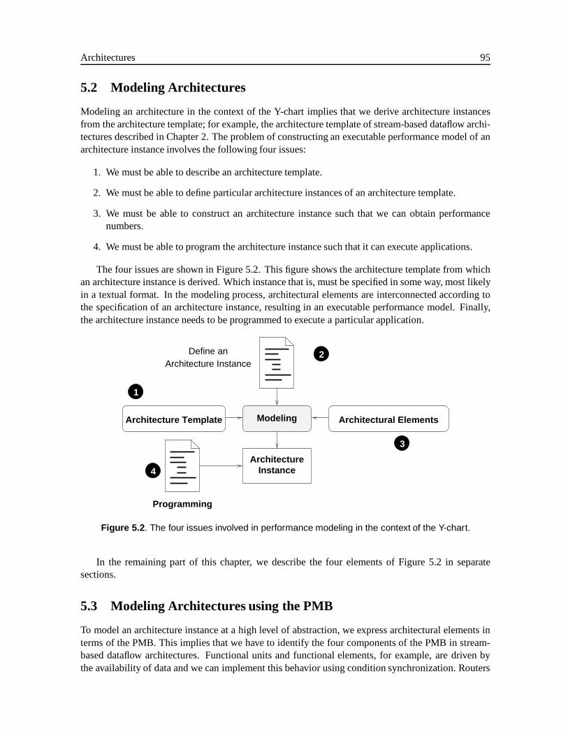
Architectures 95
5.2 Modeling Architectures
Modeling an architecture in the context of the Y-chart implies that we derive architecture instancesfrom the architecture template; for example, the architecture template of stream-based dataflow archi-tectures described in Chapter 2. The problem of constructing an executable performance model of anarchitecture instance involves the following four issues:
1. We must be able to describe an architecture template.
2. We must be able to define particular architecture instances of an architecture template.
3. We must be able to construct an architecture instance such that we can obtain performancenumbers.
4. We must be able to program the architecture instance such that it can execute applications.
The four issues are shown in Figure 5.2. This figure shows the architecture template from whichan architecture instance is derived. Which instance that is, must be specified in some way, most likelyin a textual format. In the modeling process, architectural elements are interconnected according tothe specification of an architecture instance, resulting in an executable performance model. Finally,the architecture instance needs to be programmed to execute a particular application.
Modeling
Define anArchitecture Instance
Architecture Template Architectural Elements
ArchitectureInstance
Programming
3
2
1
4
Figure 5.2 . The four issues involved in performance modeling in the context of the Y-chart.
In the remaining part of this chapter, we describe the four elements of Figure 5.2 in separatesections.
5.3 Modeling Architectures using the PMB
To model an architecture instance at a high level of abstraction, we express architectural elements interms of the PMB. This implies that we have to identify the four components of the PMB in stream-based dataflow architectures. Functional units and functional elements, for example, are driven bythe availability of data and we can implement this behavior using condition synchronization. Routers
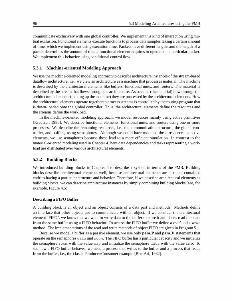
96 5.3 Modeling Architectures using the PMB
communicate exclusively with one global controller. We implement this kind of interaction using mu-tual exclusion. Functional elements execute functions to process data samples taking a certain amountof time, which we implement using execution time. Packets have different lengths and the length of apacket determines the amount of time a functional element requires to operate on a particular packet.We implement this behavior using conditional control flow.
5.3.1 Machine-oriented Modeling Approach
We use the machine-oriented modeling approach to describe architecture instances of the stream-baseddataflow architecture, i.e., we view an architecture as a machine that processes material. The machineis described by the architectural elements like buffers, functional units, and routers. The material isdescribed by the stream that flows through the architecture. As streams (the material) flow through thearchitectural elements (making up the machine) they are processed by the architectural elements. Howthe architectural elements operate together to process streams is controlled by the routing program thatis down-loaded onto the global controller. Thus, the architectural elements define the resources andthe streams define the workload.
In the machine-oriented modeling approach, we model resources mainly using active primitives[Kreutzer, 1986]. We describe functional elements, functional units, and routers using one or moreprocesses. We describe the remaining resources, i.e., the communication structure, the global con-troller, and buffers, using semaphores. Although we could have modeled these resources as activeelements, we use semaphores because these lead to a more efficient simulation. In contrast to thematerial-oriented modeling used in Chapter 4, here data dependencies and tasks representing a work-load are distributed over various architectural elements.
5.3.2 Building Blocks
We introduced building blocks in Chapter 4 to describe a system in terms of the PMB. Buildingblocks describe architectural elements well, because architectural elements are also self-containedentities having a particular structure and behavior. Therefore, if we describe architectural elements asbuilding blocks, we can describe architecture instances by simply combining building blocks (see, forexample, Figure 4.5).
Describing a FIFO Buffer
A building block is an object and an object consists of a data part and methods. Methods definean interface that other objects use to communicate with an object. If we consider the architecturalelement ‘FIFO’, we know that we want to write data to the buffer to store it and, later, read this datafrom the same buffer using a FIFO behavior. To access the FIFO buffer we define areadand awritemethod. The implementations of the read and write methods of object FIFO are given in Program 5.1.
Because we model a buffer as a passive element, we use onlypam P andpam V statements thatoperate on the semaphoresdata androom . The FIFO buffer has a particular capacity and we initializethe semaphoreroom with the valuecap and initialize the semaphoredata with the value zero. Tosee how a FIFO buffer behaves, we need a process that writes to the buffer and a process that readsfrom the buffer, i.e., the classic Producer/Consumer example [Ben-Ari, 1982].
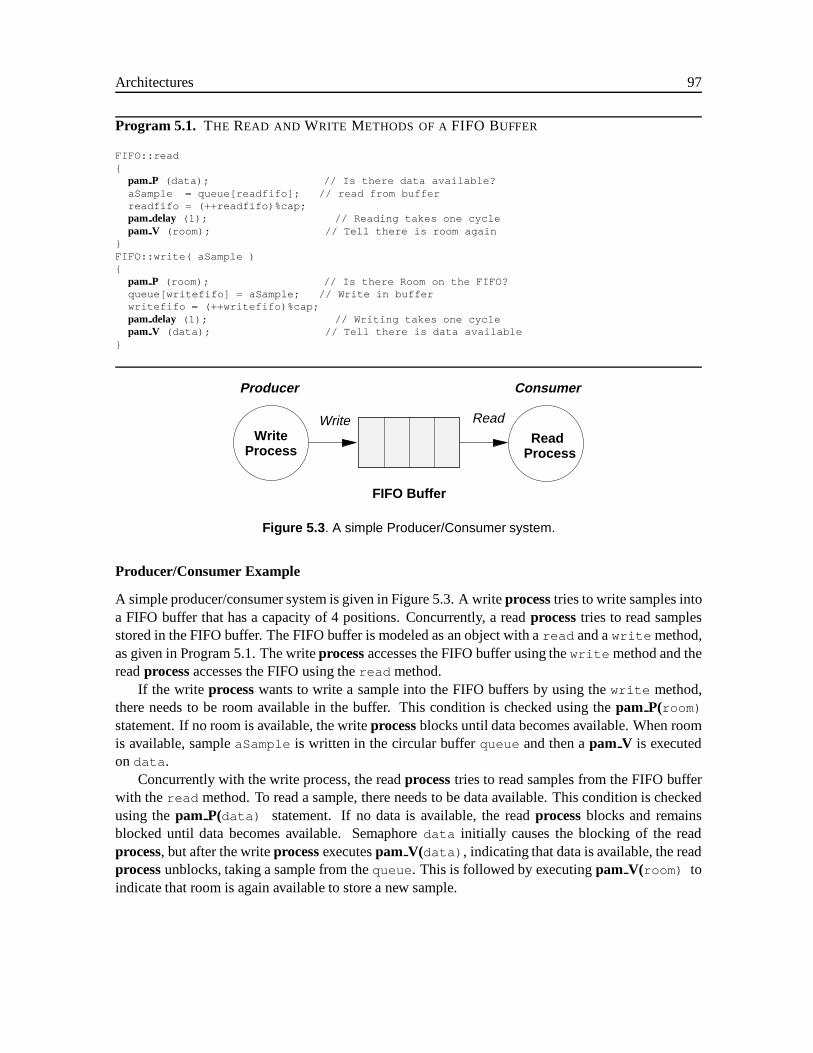
Architectures 97
Program 5.1. THE READ AND WRITE METHODS OF AFIFO BUFFER
FIFO::read{
pam P (data); // Is there data available?aSample = queue[readfifo]; // read from bufferreadfifo = (++readfifo)%cap;pam delay (1); // Reading takes one cyclepam V (room); // Tell there is room again
}FIFO::write( aSample ){
pam P (room); // Is there Room on the FIFO?queue[writefifo] = aSample; // Write in bufferwritefifo = (++writefifo)%cap;pam delay (1); // Writing takes one cyclepam V (data); // Tell there is data available
}
ReadWrite
FIFO Buffer
ReadWrite
Process Process
Producer Consumer
Figure 5.3 . A simple Producer/Consumer system.
Producer/Consumer Example
A simple producer/consumer system is given in Figure 5.3. A writeprocesstries to write samples intoa FIFO buffer that has a capacity of 4 positions. Concurrently, a readprocesstries to read samplesstored in the FIFO buffer. The FIFO buffer is modeled as an object with aread and awrite method,as given in Program 5.1. The writeprocessaccesses the FIFO buffer using thewrite method and thereadprocessaccesses the FIFO using theread method.
If the write processwants to write a sample into the FIFO buffers by using thewrite method,there needs to be room available in the buffer. This condition is checked using thepam P(room)
statement. If no room is available, the writeprocessblocks until data becomes available. When roomis available, sampleaSample is written in the circular bufferqueue and then apam V is executedon data .
Concurrently with the write process, the readprocesstries to read samples from the FIFO bufferwith theread method. To read a sample, there needs to be data available. This condition is checkedusing thepam P(data) statement. If no data is available, the readprocessblocks and remainsblocked until data becomes available. Semaphoredata initially causes the blocking of the readprocess, but after the writeprocessexecutespam V(data) , indicating that data is available, the readprocessunblocks, taking a sample from thequeue . This is followed by executingpam V(room) toindicate that room is again available to store a new sample.
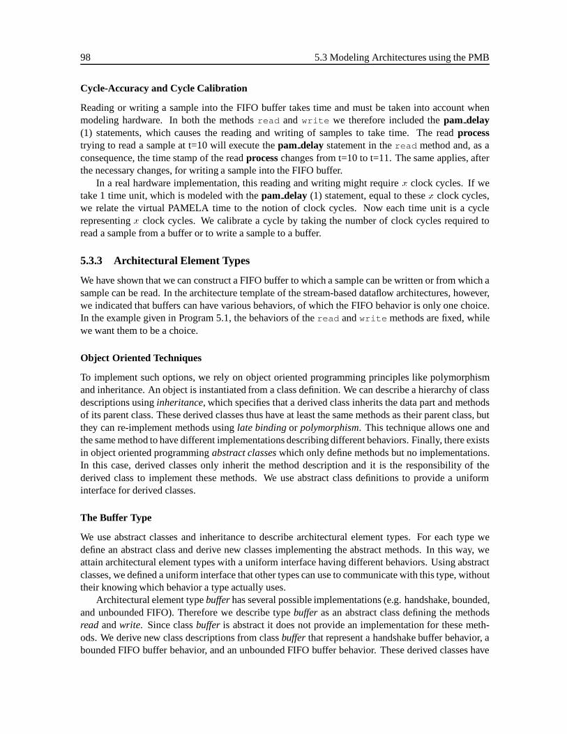
98 5.3 Modeling Architectures using the PMB
Cycle-Accuracy and Cycle Calibration
Reading or writing a sample into the FIFO buffer takes time and must be taken intoaccount whenmodeling hardware. In both the methodsread and write we therefore included thepam delay(1) statements, which causes the reading and writing of samples to take time. The readprocesstrying to read a sample at t=10 will execute thepam delay statement in theread method and, as aconsequence, the time stamp of the readprocesschanges from t=10 to t=11. The same applies, afterthe necessary changes, for writing a sample into the FIFO buffer.
In a real hardware implementation, this reading and writing might requirex clock cycles. If wetake 1 time unit, which is modeled with thepam delay (1) statement, equal to thesex clock cycles,we relate the virtual PAMELA time to the notion of clock cycles. Now each time unit is a cyclerepresentingx clock cycles. We calibrate a cycle by taking the number of clock cycles required toread a sample from a buffer or to write a sample to a buffer.
5.3.3 Architectural Element Types
We have shown that we can construct a FIFO buffer to which a sample can be written or from which asample can be read. In the architecture template of the stream-based dataflow architectures, however,we indicated that buffers can have various behaviors, of which the FIFO behavior is only one choice.In the example given in Program 5.1, the behaviors of theread andwrite methods are fixed, whilewe want them to be a choice.
Object Oriented Techniques
To implement such options, we rely on object oriented programming principles like polymorphismand inheritance. An object is instantiated from a class definition. We can describe a hierarchy of classdescriptions usinginheritance, which specifies that a derived class inherits the data part and methodsof its parent class. These derived classes thus have at least the same methods as their parent class, butthey can re-implement methods usinglate bindingor polymorphism. This technique allows one andthe same method to have different implementations describing different behaviors. Finally, there existsin object oriented programmingabstract classeswhich only define methods but no implementations.In this case, derived classes only inherit the method description and it is the responsibility of thederived class to implement these methods. We use abstract class definitions to provide a uniforminterface for derived classes.
The Buffer Type
We use abstract classes and inheritance to describe architectural element types. For each type wedefine an abstract class and derive new classes implementing the abstract methods. In this way, weattain architectural element types with a uniform interface having different behaviors. Using abstractclasses, we defined a uniform interface that other types can use to communicate with this type, withouttheir knowing which behavior a type actually uses.
Architectural element typebufferhas several possible implementations (e.g. handshake, bounded,and unbounded FIFO). Therefore we describe typebuffer as an abstract class defining the methodsread andwrite. Since classbuffer is abstract it does not provide an implementation for these meth-ods. We derive new class descriptions from classbufferthat represent a handshake buffer behavior, abounded FIFO buffer behavior, and an unbounded FIFO buffer behavior. These derived classes have
Architectures 99
ClassBuffer
Hand Shake
Bounded
UnboundedRead
Write
Abstract Class Derived Class
Provides the Interface Implements the Interface
FIFO
FIFO
Figure 5.4 . The buffer class defines the interface (e.g., the read and write methods) thatother classes implement.
the same two methodsreadandwrite from the buffer class via inheritance, but implement them dif-ferently, resulting in a different behavior. The handshake buffer, the bounded FIFO buffer, and theunbounded FIFO buffer implement the two methods using a single buffer position, a circular buffer,and a linked list, respectively.
The separation between the abstract classbuffer and the three derived classes is illustrated inFigure 5.4. Architectural element typebuffercan store data temporarily using the uniform interfacewhich consists of aread and awrite method. Nevertheless, typebuffer can store data using threedifferent behaviors.
For architectural elements that can have more than one behavior (see Table 2.1), we constructabstract classes as shown in Figure 5.5. For these abstract classes, we derived classes that provide theimplementation of the methods of the abstract classes. In Figure 5.5, we see again the architecturalelement typebuffer with its three implementations as described in Figure 5.4: handshake, boundedFIFO and unbounded FIFO. One architectural element type, the processing element, does not have animplementation. It represents a hierarchical architectural element that serves as acontainerfor otherelement types.
Revised Producer/consumer System
We have revised the way we model the producer/consumer system shown in Figure 5.3. In Figure 5.6,we show the producer/consumer system modeled using building blocks. It shows three building blocksof which two are processing elements (A andB) that exchange samples with each other via the FIFObuffer (FIFO Buffer). Processing elementA is the producer and processing elementB is the consumer.
The representation of the active building blocksA andB was already explained in Chapter 4. Notethat the structural part ofA andB contains references to the architectural element typeBuffer and notto a FIFO buffer. In theprocessdescription of processing elementA, theprocesswrites a sampleto theOut buffer. Inprocessdescription of Processing ElementB, theprocessreads a sample fromthe In buffer. In contrast to theprocessdescriptions given in Chapter 4, these processes start all overagain when they have written a sample to a buffer or when they have read a sample from a buffer.Thus, these processes read and write samplescontinuously; in other words, they operate on streams.
The representation of the passive building blockFIFObuffer does not encapsulate a process, butinstead uses methods to describe the behavior of the building block. The methodsread andwrite
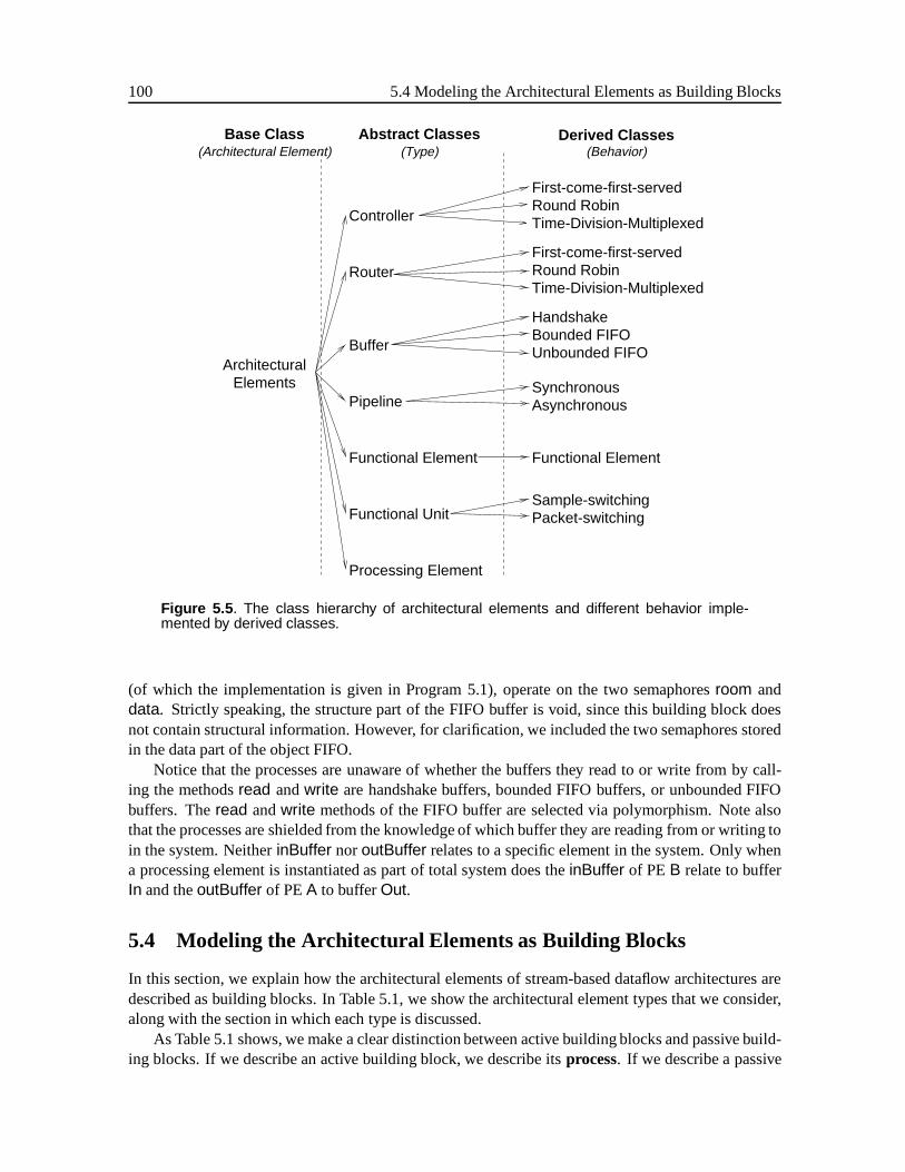
100 5.4 Modeling the Architectural Elements as Building Blocks
(Architectural Element) (Type) (Behavior)
Buffer
Pipeline
Functional Element
Handshake
SynchronousAsynchronous
Functional Unit Packet-switchingSample-switching
Processing Element
Functional Element
Controller
Router
ArchitecturalElements
Base Class Abstract Classes Derived Classes
First-come-first-servedRound Robin
First-come-first-servedRound RobinTime-Division-Multiplexed
Time-Division-Multiplexed
Bounded FIFOUnbounded FIFO
Figure 5.5 . The class hierarchy of architectural elements and different behavior imple-mented by derived classes.
(of which the implementation is given in Program 5.1), operate on the two semaphoresroom anddata. Strictly speaking, the structure part of the FIFO buffer is void, since this building block doesnot contain structural information. However, for clarification, we included the two semaphores storedin the data part of the object FIFO.
Notice that the processes are unaware of whether the buffers they read to or write from by call-ing the methodsread andwrite are handshake buffers, bounded FIFO buffers, or unbounded FIFObuffers. Theread andwrite methods of the FIFO buffer are selected via polymorphism. Note alsothat the processes are shielded from the knowledge of which buffer they are reading from or writing toin the system. NeitherinBuffer noroutBuffer relates to a specific element in the system. Only whena processing element is instantiated as part of total system does theinBuffer of PEB relate to bufferIn and theoutBuffer of PEA to bufferOut.
5.4 Modeling the Architectural Elements as Building Blocks
In this section, we explain how the architectural elements of stream-based dataflow architectures aredescribed as building blocks. In Table 5.1, we show the architectural element types that we consider,along with the section in which each type is discussed.
As Table 5.1 shows, we make a clear distinction between active building blocks and passive build-ing blocks. If we describe an active building block, we describe itsprocess. If we describe a passive
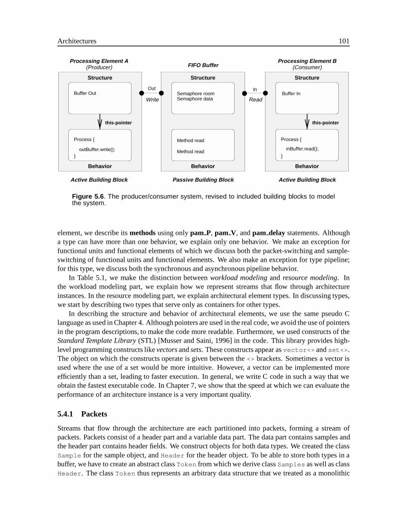
Architectures 101
Behavior
Structure
this-pointer
Process {
}
Out In
Passive Building Block Active Building BlockActive Building Block
Behavior
Structure
this-pointer
Process {
}
ReadWrite
Method read
Method read
Structure
Behavior
inBuffer.read();outBuffer.write();
Buffer Out Buffer InSemaphore roomSemaphore data
Processing Element BProcessing Element A(Producer) FIFO Buffer (Consumer)
Figure 5.6 . The producer/consumer system, revised to included building blocks to modelthe system.
element, we describe itsmethodsusing onlypam P, pam V, andpam delay statements. Althougha type can have more than one behavior, we explain only one behavior. We make an exception forfunctional units and functional elements of which we discuss both the packet-switching and sample-switching of functional units and functional elements. We also make an exception for type pipeline;for this type, we discuss both the synchronous and asynchronous pipeline behavior.
In Table 5.1, we make the distinction betweenworkload modelingand resource modeling. Inthe workload modeling part, we explain how we represent streams that flow through architectureinstances. In the resource modeling part, we explain architectural element types. In discussing types,we start by describing two types that serve only as containers for other types.
In describing the structure and behavior of architectural elements, we use the same pseudo Clanguage as used in Chapter 4. Although pointers are used in the real code, we avoid the use of pointersin the program descriptions, to make the code more readable. Furthermore, we used constructs of theStandard Template Library(STL) [Musser and Saini, 1996] in the code. This library provides high-level programming constructs likevectorsandsets. These constructs appear asvector<> andset<> .The object on which the constructs operate is given between the<> brackets. Sometimes a vector isused where the use of a set would be more intuitive. However, a vector can be implemented moreefficiently than a set, leading to faster execution. In general, we write C code in such a way that weobtain the fastest executable code. In Chapter 7, we show that the speed at which we can evaluate theperformance of an architecture instance is a very important quality.
5.4.1 Packets
Streams that flow through the architecture are each partitioned into packets, forming a stream ofpackets. Packets consist of a header part and a variable data part. The data part contains samples andthe header part contains header fields. We construct objects for both data types. We created the classSample for the sample object, andHeader for the header object. To be able to store both types in abuffer, we have to create an abstract classToken from which we derive classSamples as well as classHeader . The classToken thus represents an arbitrary data structure that we treated as a monolithic
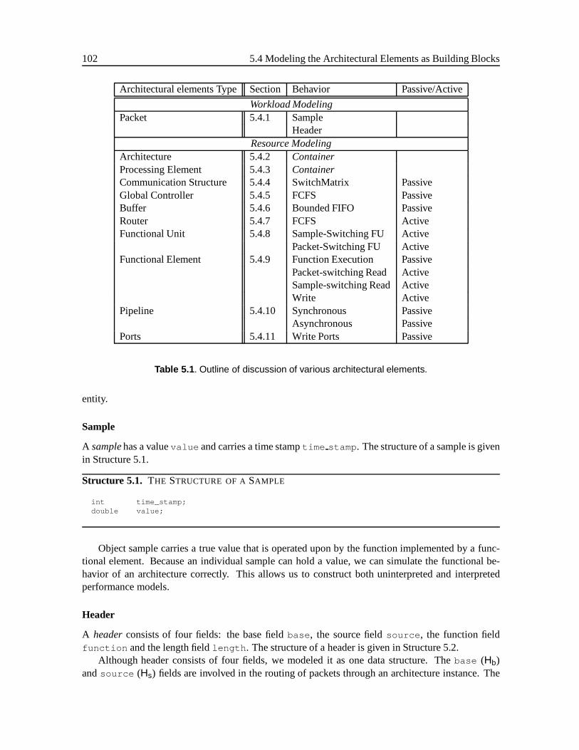
102 5.4 Modeling the Architectural Elements as Building Blocks
Architectural elements Type Section Behavior Passive/Active
Workload ModelingPacket 5.4.1 Sample
HeaderResource Modeling
Architecture 5.4.2 ContainerProcessing Element 5.4.3 ContainerCommunication Structure 5.4.4 SwitchMatrix PassiveGlobal Controller 5.4.5 FCFS PassiveBuffer 5.4.6 Bounded FIFO PassiveRouter 5.4.7 FCFS ActiveFunctional Unit 5.4.8 Sample-Switching FU Active
Packet-Switching FU ActiveFunctional Element 5.4.9 Function Execution Passive
Packet-switching Read ActiveSample-switching Read ActiveWrite Active
Pipeline 5.4.10 Synchronous PassiveAsynchronous Passive
Ports 5.4.11 Write Ports Passive
Table 5.1 . Outline of discussion of various architectural elements.
entity.
Sample
A samplehas a valuevalue and carries a time stamptime stamp . The structure of a sample is givenin Structure 5.1.
Structure 5.1. THE STRUCTURE OF ASAMPLE
int time_stamp;double value;
Object sample carries a true value that is operated upon by the function implemented by a func-tional element. Because an individual sample can hold a value, we can simulate the functional be-havior of an architecture correctly. This allows us to construct both uninterpreted and interpretedperformance models.
Header
A headerconsists of four fields: the base fieldbase , the source fieldsource , the function fieldfunction and the length fieldlength . The structure of a header is given in Structure 5.2.
Although header consists of four fields, we modeled it as one data structure. Thebase (Hb)andsource (Hs) fields are involved in the routing of packets through an architecture instance. The
Architectures 103
Structure 5.2. THE STRUCTURE OF AHEADER
int base;int source;int function;int length;
function field (Hf) stipulates which function of a functional unit should process the data part of apacket and, finally, thelength field (Hl) indicates the number of samples contained in the data partof the packet.
5.4.2 Architecture
Type architectureconsists of the following types: a communication structurecommunication , aglobal controllercontroller , and a set of processing elementsprocessingElements . The struc-ture of elementarchitectureis given in Structure 5.3.
Structure 5.3. THE STRUCTURE OFELEMENT ARCHITECTURE
GlobalController controller; /* structure */CommunicationStructure communication;set<ProcessingElement> processingElements;
Typearchitecturecaptures the top-level structure of a stream-based dataflow architecture (see, forexample, Figure 2.1). It does not describe a behavior, because it serves only as a container for othertypes.
5.4.3 Processing Element
Type processing element(PE) consists of a vector of input buffersinBuffers , a vector of outputbuffersoutBuffers , a vector of routersrouters and one functional unitfunctionalunit . Thestructure of elementprocessing elementis given in Structure 5.4.
Structure 5.4. THE STRUCTURE OFELEMENT PROCESSINGELEMENT
vector<Buffer> inBuffers; /* structure */FunctionalUnit functionalUnit;vector<Buffer> outBuffers;vector<Router> routers;
Typeprocessing elementdoes not describe a behavior, because it only serves as a container forother types. Two special kinds of PEs do exist: asource PEand asink PE. The source PE producespacket-streams and the sink PE consumes packet-streams.
5.4.4 Communication Structure
Typecommunication structurecontains the parametercapacity and the semaphorechannels . Thestructure of elementcommunication structureis given in Structure 5.5.
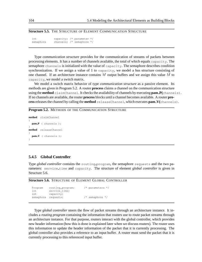
104 5.4 Modeling the Architectural Elements as Building Blocks
Structure 5.5. THE STRUCTURE OFELEMENT COMMUNICATION STRUCTURE
int capacity; /* parameter */semaphore channels; /* semaphore */
Type communication structureprovides for the communication of streams of packets betweenprocessing elements. It has a number of channels available, the total of which equalscapacity . Thesemaphorechannels is initialized with the value ofcapacity . The semaphore describes conditionsynchronization. If we assign a value of 1 tocapacity , we model a bus structure consisting ofone channel. If an architecture instance containsM output buffers and we assign this valueM tocapacity , we model a switch matrix.
We model a switch matrix behavior of typecommunication structureas a passive element. Itsmethods are given in Program 5.2. A routerprocessclaims a channel on the communication structureusing themethodclaimChannel . It checks the availabilityof channels by executingpam P(channels) .If no channels are available, the routerprocessblocks until a channel becomes available. A routerpro-cessreleases the channel by calling themethodreleaseChannel , which executespam V(channels) .
Program 5.2. METHODS OF THECOMMUNICATION STRUCTURE
method claimChannel{
pam P ( channels );}method releaseChannel{
pam V ( channels );}
5.4.5 Global Controller
Typeglobal controllercontains therouting program , the semaphorerequests and the two pa-rameters:service time and capacity . The structure of elementglobal controller is given inStructure 5.6.
Structure 5.6. STRUCTURE OFELEMENT GLOBAL CONTROLLER
Program routing_program; /* parameters */int service_time;int capacity;semaphore requests; /* semaphore */
Typeglobal controllersteers the flow of packet streams through an architecture instance. It in-cludes arouting programcontaining the information that routers use to route packet streams throughan architecture instance. For that purpose, routers interact with the global controller, which providesnew header information (how this is done is explained later when we discuss routers). The router usesthis information to update the header information of the packet that it is currently processing. Theglobal controller also provides a reference to an input buffer. A router must send the packet that it iscurrently processing to this referenced input buffer.
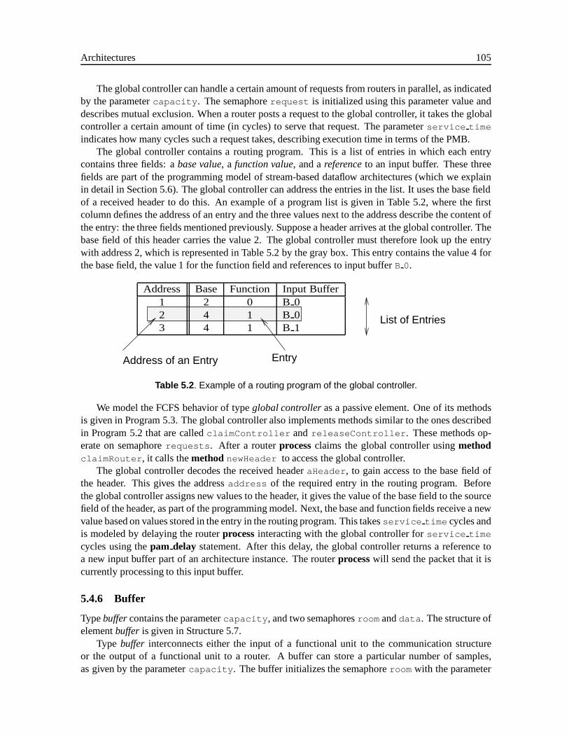
Architectures 105
The global controller can handle a certain amount of requests from routers in parallel, as indicatedby the parametercapacity . The semaphorerequest is initialized using this parameter value anddescribes mutual exclusion. When a router posts a request to the global controller, it takes the globalcontroller a certain amount of time (in cycles) to serve that request. The parameterservice time
indicates how many cycles such a request takes, describing execution time in terms of the PMB.The global controller contains a routing program. This is a list of entries in which each entry
contains three fields: abase value, a function value, and areferenceto an input buffer. These threefields are part of the programming model of stream-based dataflow architectures (which we explainin detail in Section 5.6). The global controller can address the entries in the list. It uses the base fieldof a received header to do this. An example of a program list is given in Table 5.2, where the firstcolumn defines the address of an entry and the three values next to the address describe the content ofthe entry: the three fields mentioned previously. Suppose a header arrives at the global controller. Thebase field of this header carries the value 2. The global controller must therefore look up the entrywith address 2, which is represented in Table 5.2 by the gray box. This entry contains the value 4 forthe base field, the value 1 for the function field and references to input bufferB 0.
Address Base Function Input Buffer1 2 0 B 02 4 1 B 03 4 1 B 1
Address of an Entry Entry
List of Entries
Table 5.2 . Example of a routing program of the global controller.
We model the FCFS behavior of typeglobal controlleras a passive element. One of its methodsis given in Program 5.3. The global controller also implements methods similar to the ones describedin Program 5.2 that are calledclaimController andreleaseController . These methods op-erate on semaphorerequests . After a routerprocessclaims the global controller usingmethodclaimRouter , it calls themethod newHeader to access the global controller.
The global controller decodes the received headeraHeader , to gain access to the base field ofthe header. This gives the addressaddress of the required entry in the routing program. Beforethe global controller assigns new values to the header, it gives the value of the base field to the sourcefield of the header, as part of the programming model. Next, the base and function fields receive a newvalue based on values stored in the entry in the routing program. This takesservice time cycles andis modeled by delaying the routerprocessinteracting with the global controller forservice time
cycles using thepam delay statement. After this delay, the global controller returns a reference toa new input buffer part of an architecture instance. The routerprocesswill send the packet that it iscurrently processing to this input buffer.
5.4.6 Buffer
Typebuffercontains the parametercapacity , and two semaphoresroom anddata . The structure ofelementbuffer is given in Structure 5.7.
Type buffer interconnects either the input of a functional unit to the communication structureor the output of a functional unit to a router. A buffer can store a particular number of samples,as given by the parametercapacity . The buffer initializes the semaphoreroom with the parameter

106 5.4 Modeling the Architectural Elements as Building Blocks
Program 5.3. GLOBAL CONTROLLER METHODS
method newHeader( aHeader )
// Get The Address from the Baseint address = aHeader.getBase();
// Assign the Base field to the Source FieldaHeader.setSource( aHeader.getBase() );
// Get New information from the ProgramaHeader.setBase( program[address].getBase() );aHeader.setFunction( program[address].getFunction() );
pam delay ( service_time );
// Determine new input Bufferinput_Buffer = program[address].getBuffer();return input_Buffer;
Structure 5.7. THE STRUCTURE OF ABUFFER
int capacity; /* parameter */semaphore room; /* semaphores */semaphore data;
capacity and initializes the semaphoredata with a zero value. Both semaphores describe conditionsynchronization.
We model the bounded FIFO behavior of typebufferas a passive element. Its methods are givenin Program 5.4. This program describes the implementation of themethod read and themethodwrite of a FIFO buffer (These two methods were also discussed in Section 5.3).
The bounded FIFO buffer uses aqueue to store tokens (vector<Token> ). When a routerpro-cessreads aToken 1 from a FIFO buffer using themethod read , the readmethod first executespam P(data) . If no Token is available, the router blocks, implementing a blocking read. It remainsblocked until new data becomes available. Otherwise, the readmethodcontinues by reading aToken
from the queuequeue . After the readmethodreads theToken , it executespam P(room) to indicatethat new room is available on the FIFO buffer.
When a routerprocesstries to write aToken into the FIFO buffer, it uses themethod write .Theprocessexecutespam P(room) . If no room is available in the FIFO buffer, the routerprocessblocks, implementing a blocking write. The routerprocessremains blocked until new room becomesavailable. Otherwise, theprocesscontinues by storing theToken in the queue. After theToken isstored, theprocessexecutespam V on semaphoredata , using the write method, to indicate that newdata is available on the FIFO buffer.
Before a routerprocesswrites to an input buffer, it must first have exclusive access to this buffer.For that purpose, the input buffers are extended with a semaphore that implements mutual exclusion.This semaphore is claimed and released in a similar way as used in the communication structure andglobal controller (described in Program 5.2).
1We sayToken , because it can be either aSample object or aHeader object
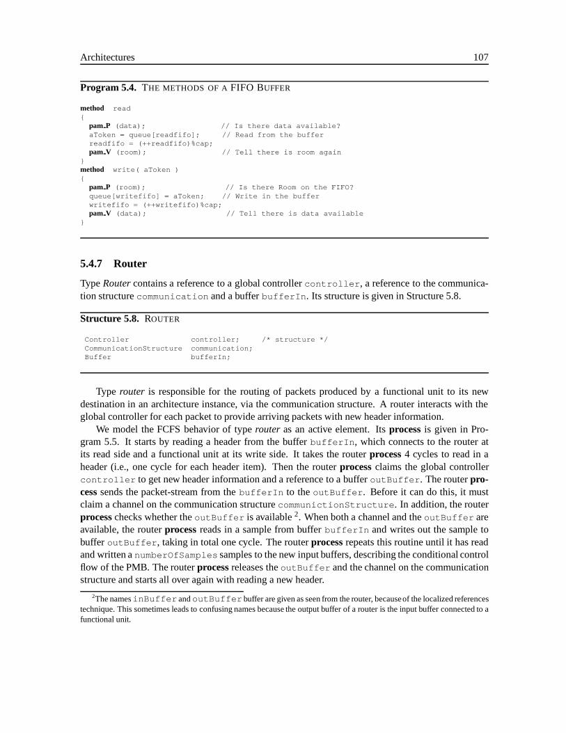
Architectures 107
Program 5.4. THE METHODS OF AFIFO BUFFER
method read{
pam P (data); // Is there data available?aToken = queue[readfifo]; // Read from the bufferreadfifo = (++readfifo)%cap;pam V (room); // Tell there is room again
}method write( aToken ){
pam P (room); // Is there Room on the FIFO?queue[writefifo] = aToken; // Write in the bufferwritefifo = (++writefifo)%cap;pam V (data); // Tell there is data available
}
5.4.7 Router
TypeRoutercontains a reference to a global controllercontroller , a reference to the communica-tion structurecommunication and a bufferbufferIn . Its structure is given in Structure 5.8.
Structure 5.8. ROUTER
Controller controller; /* structure */CommunicationStructure communication;Buffer bufferIn;
Type router is responsible for the routing of packets produced by a functional unit to its newdestination in an architecture instance, via the communication structure. A router interacts with theglobal controller for each packet to provide arriving packets with new header information.
We model the FCFS behavior of typerouter as an active element. Itsprocessis given in Pro-gram 5.5. It starts by reading a header from the bufferbufferIn , which connects to the router atits read side and a functional unit at its write side. It takes the routerprocess4 cycles to read in aheader (i.e., one cycle for each header item). Then the routerprocessclaims the global controllercontroller to get new header information and a reference to a bufferoutBuffer . The routerpro-cesssends the packet-stream from thebufferIn to theoutBuffer . Before it can do this, it mustclaim a channel on the communication structurecommunictionStructure . In addition, the routerprocesschecks whether theoutBuffer is available2. When both a channel and theoutBuffer areavailable, the routerprocessreads in a sample from bufferbufferIn and writes out the sample tobuffer outBuffer , taking in total one cycle. The routerprocessrepeats this routine until it has readand written anumberOfSamples samples to the new input buffers, describing the conditional controlflow of the PMB. The routerprocessreleases theoutBuffer and the channel on the communicationstructure and starts all over again with reading a new header.
2The namesinBuffer andoutBuffer buffer are given as seen from the router, becauseof the localized referencestechnique. This sometimes leads to confusing names because the output buffer of a router is the input buffer connected to afunctional unit.
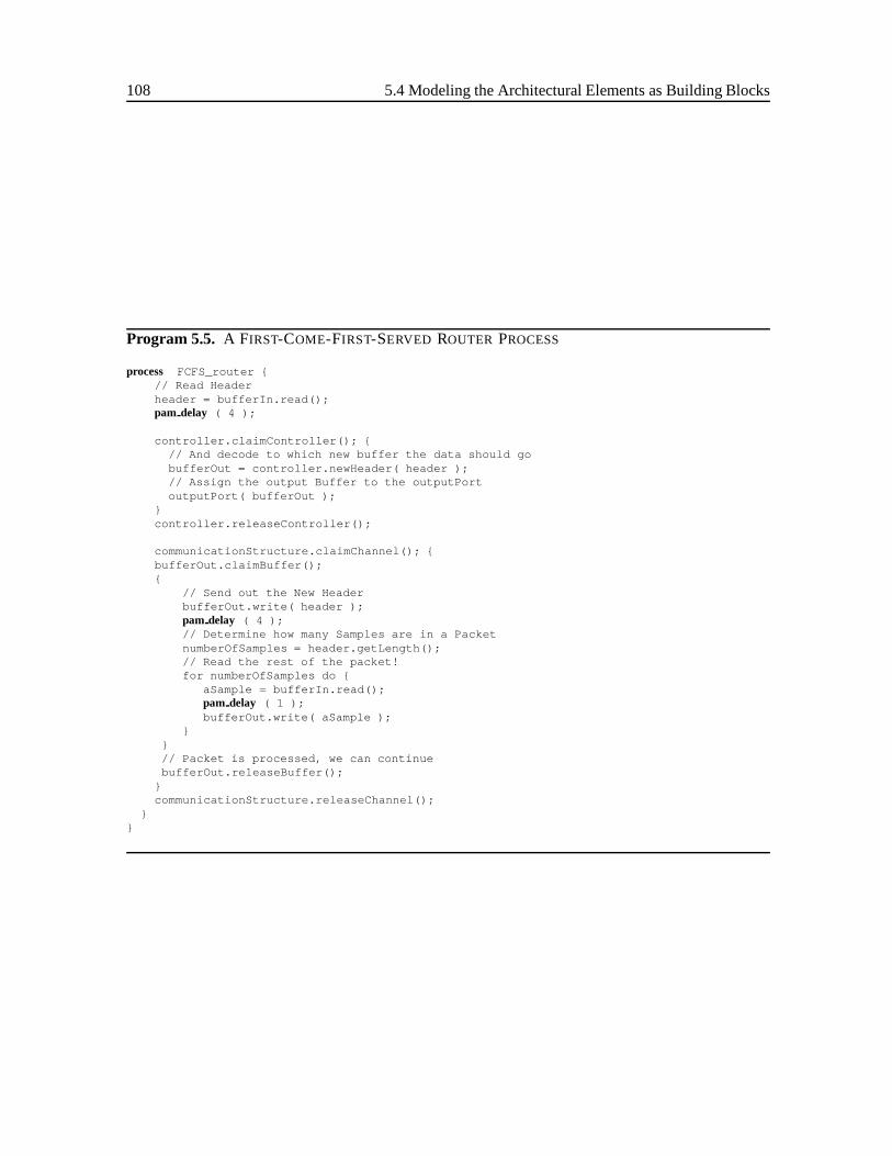
108 5.4 Modeling the Architectural Elements as Building Blocks
Program 5.5. A FIRST-COME-FIRST-SERVED ROUTER PROCESS
process FCFS_router {// Read Headerheader = bufferIn.read();pam delay ( 4 );
controller.claimController(); {// And decode to which new buffer the data should gobufferOut = controller.newHeader( header );// Assign the output Buffer to the outputPortoutputPort( bufferOut );
}controller.releaseController();
communicationStructure.claimChannel(); {bufferOut.claimBuffer();{
// Send out the New HeaderbufferOut.write( header );pam delay ( 4 );// Determine how many Samples are in a PacketnumberOfSamples = header.getLength();// Read the rest of the packet!for numberOfSamples do {
aSample = bufferIn.read();pam delay ( 1 );bufferOut.write( aSample );
}}// Packet is processed, we can continuebufferOut.releaseBuffer();
}communicationStructure.releaseChannel();
}}
Architectures 109
5.4.8 Functional Unit
TypeFunctional Unit(FU) consists of a vector of input portsinputPorts , a vector of output portsoutputPorts and a vector of functional elementsrepertoire . The structure of elementFunctionalUnit is given in Structure 5.9.
Structure 5.9. STRUCTURE OF A FUNCTIONAL UNIT
vector<ReadPort> inputPorts; /* structure */vector<WritePort> outputPorts;vector<FunctionalElement> repertoire;
TypeFU contains of a number of functional elements (FE) which defines the repertoireF (seeEquation 2.1). At run-time, the FU selects the correct FE to execute. Besides activating the correctFE, it also strips off headers from packets at input ports and prepares new headers on output ports.Two special kinds of FUs exist: asource FUand asink FU. A source FU does not have input ports.A sink FU does not have output ports. A source FU is exclusively part of a source PE, and a sink FU,of a sink PE.
We model the behavior of typeFE as an active element. The process describing the behavior isreferred to as the local controller of the FU. The local controller can describe two different behaviors:a packet-switching behavior where the local controller switches between FEs in between packets, anda sample-switching behavior where the local controller switches between FEs in between samples.
We are now going to discuss the behavior of the local controller for the packet-switchingprocessdescribed in Program 5.6 and the sample-switchingprocessdescribed in Program 5.7.
Packet-Switching
The packet-switchingprocessswitches between FEs on the boundaries of packets. In this mode, theFEs of the repertoire can share input and output buffers (or ports, because a buffer connects to a port)of a FU. A special port, theopcode port(which connects to the opcode buffer), is reserved for therun-time selection of the FE. The header arriving at the opcode port is used by the local controller toactivate a specific FE. The opcode port is always the first input port of a FU (i.e.inputPorts[0] ).We have explicitly named this port (and buffer) to emphasize its special role.
A model of a FU is depicted in Figure 5.7. The FU has two input ports and two output ports(represented by black circles in the figure). The repertoire of the FU consists of two FEs:FE0 andFE1. The FEs connect via their ports to the ports of the FU. This is called thebindingof the FE to theFU. In this mode, FEs always share the opcode port of the FU. In the example of Figure 5.7, the twoFEs also share an output port of the FU.
Theprocessrepresenting the local controller of the FU is represented as the white disc in Fig-ure 5.7. Although not shown explicitly in the figure, theprocessconnects to all input and output portsto strip off headers from read ports and prepares new headers on write ports. Theprocessactivates aFE using the semaphoresExecute andDone.
The packet-switchingprocessstarts by reading a header from theOpcodePort . It gets the correctfunction fieldfunc from the header viamethod getFunction . Next, theprocessselects from thevector repertoire the func -th FE. Theprocessstrips off the header from the input ports of thisFE and places new headers on the output ports of this FE. Next, theprocessactivates the FE fromthe repertoire by executingpam P(fe.execute) . This semaphore is connected to the functionalelementfe . This is directly followed by executingpam V(Done) , which causes theprocessto
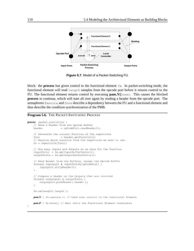
110 5.4 Modeling the Architectural Elements as Building Blocks
Functional Element 1
Functional Element 0
Opcode Port
Packet-SwitchingProcess
Input Ports Output Ports
Binding
execute done ControllerLocal
Figure 5.7 . Model of a Packet-Switching FU.
block: theprocesshas given control to the functional elementfe . In packet-switching mode, thefunctional element will readlength samples from the opcode port before it returns control to theFU. The functional element returns control by executingpam V(Done) . This causes the blockedprocessto continue, which will start all over again by reading a header from the opcode port. ThesemaphoresExecute andDone describe a dependency between the FU and a functional element andthus describe the condition synchronization of the PMB.
Program 5.6. THE PACKET-SWITCHING PROCESS
process packet_controller {// Read a Header from the Opcode Bufferheader = opCodePort.readHeader();
// Determine the correct function of the repertoirefunc = header.getFunction();// Resolve which function from the repertoire we want to usefe = repertoire[func];
// How many Inputs and Outputs do we have for the functioninputPorts = fe.getInputBufferVector();outputPorts = fe.getOutputBufferVector();
// Read Header from the Buffers, except the Opcode Bufferforeach inputport 2 inputPorts n{opCodePort} {
inputport.stripHeader();}
// Prepare a Header on the Outputs that are involvedforeach outputport 2 outputPorts {
outputport.pushHeader( header );}
fe.setLength( length );
pam V ( fe.execute ); // hand over control to the functional Element
pam P ( fe.done); // Wait until the Functional Element terminates}
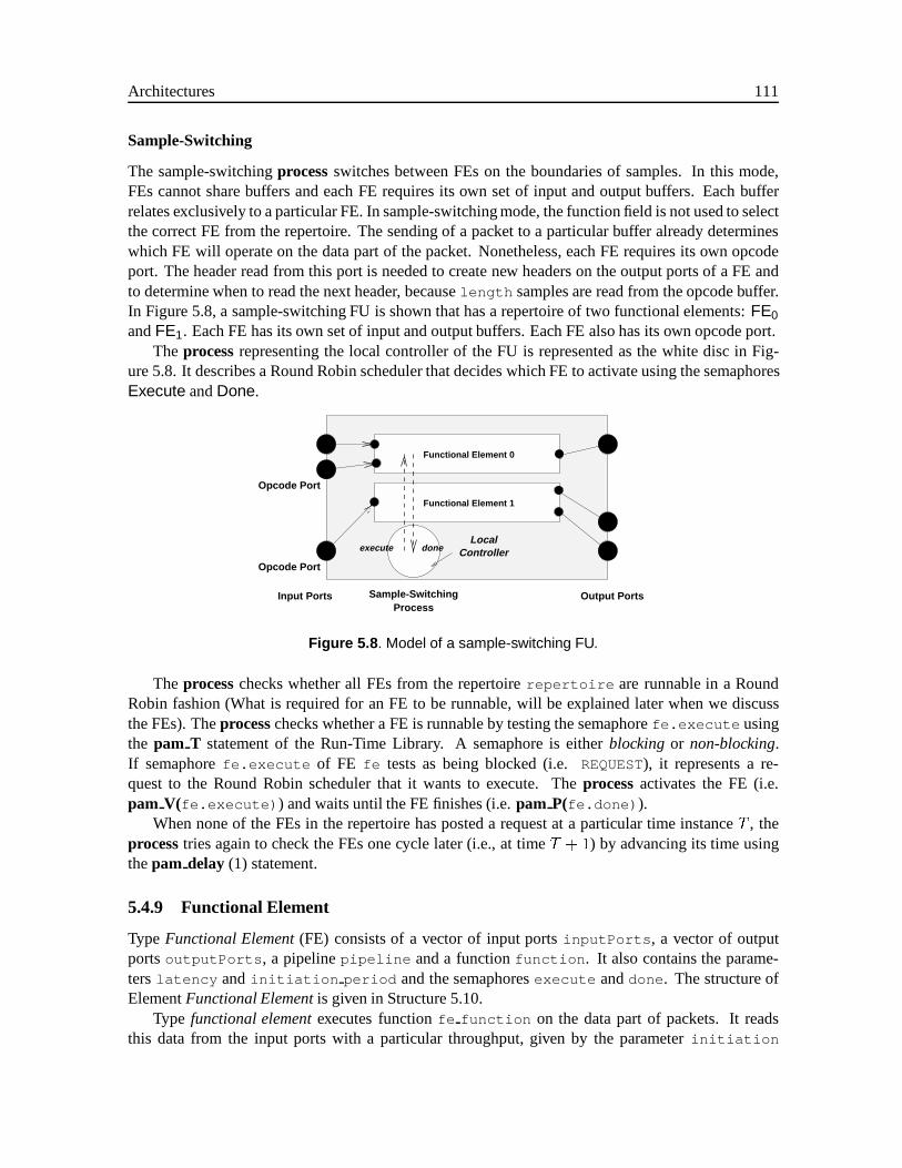
Architectures 111
Sample-Switching
The sample-switchingprocessswitches between FEs on the boundaries of samples. In this mode,FEs cannot share buffers and each FE requires its own set of input and output buffers. Each bufferrelates exclusively to a particular FE. In sample-switching mode, the function field is not used to selectthe correct FE from the repertoire. The sending of a packet to a particular buffer already determineswhich FE will operate on the data part of the packet. Nonetheless, each FE requires its own opcodeport. The header read from this port is needed to create new headers on the output ports of a FE andto determine when to read the next header, becauselength samples are read from the opcode buffer.In Figure 5.8, a sample-switching FU is shown that has a repertoire of two functional elements:FE0andFE1. Each FE has its own set of input and output buffers. Each FE also has its own opcode port.
Theprocessrepresenting the local controller of the FU is represented as the white disc in Fig-ure 5.8. It describes a Round Robin scheduler that decides which FE to activate using the semaphoresExecute andDone.
Functional Element 1
Functional Element 0
Sample-SwitchingProcess
Input Ports Output Ports
Opcode Port
Opcode Port
execute doneLocal
Controller
Figure 5.8 . Model of a sample-switching FU.
Theprocesschecks whether all FEs from the repertoirerepertoire are runnable in a RoundRobin fashion (What is required for an FE to be runnable, will be explained later when we discussthe FEs). Theprocesschecks whether a FE is runnable by testing the semaphorefe.execute usingthe pam T statement of the Run-Time Library. A semaphore is eitherblockingor non-blocking.If semaphorefe.execute of FE fe tests as being blocked (i.e.REQUEST), it represents a re-quest to the Round Robin scheduler that it wants to execute. Theprocessactivates the FE (i.e.pam V(fe.execute) ) and waits until the FE finishes (i.e.pam P(fe.done) ).
When none of the FEs in the repertoire has posted a request at a particular time instanceT , theprocesstries again to check the FEs one cycle later (i.e., at timeT + 1) by advancing its time usingthepam delay (1) statement.
5.4.9 Functional Element
Type Functional Element(FE) consists of a vector of input portsinputPorts , a vector of outputportsoutputPorts , a pipelinepipeline and a functionfunction . It also contains the parame-ters latency and initiation period and the semaphoresexecute anddone . The structure ofElementFunctional Elementis given in Structure 5.10.
Type functional elementexecutes functionfe function on the data part of packets. It readsthis data from the input ports with a particular throughput, given by the parameterinitiation

112 5.4 Modeling the Architectural Elements as Building Blocks
Program 5.7. SAMPLE SWITCHING FU PROCESS
process FUsample_controller {activate = false;// Check requests to execute from all FEs in the repertoireforeach fe 2 repertoire {
if ( pam T ( fe.execute ) == REQUEST ) {activate = true;pam V ( fe.execute ); // Grant the Requestpam P ( fe.done ); // Wait until FE terminates
}}if (activate == false) {
// No FE posted a request, advance// time by one cycle and try againpam delay (1);
}}
Structure 5.10. THE STRUCTURE OF AFUNCTIONAL ELEMENT
vector<ReadPort> inputPorts; /* Structure */vector<WritePort> outputPorts;Pipeline pipeline;Function fe_function;
int latency; /* Parameters */int initiation period;
semaphore execute; /* Semaphores */semaphore done;
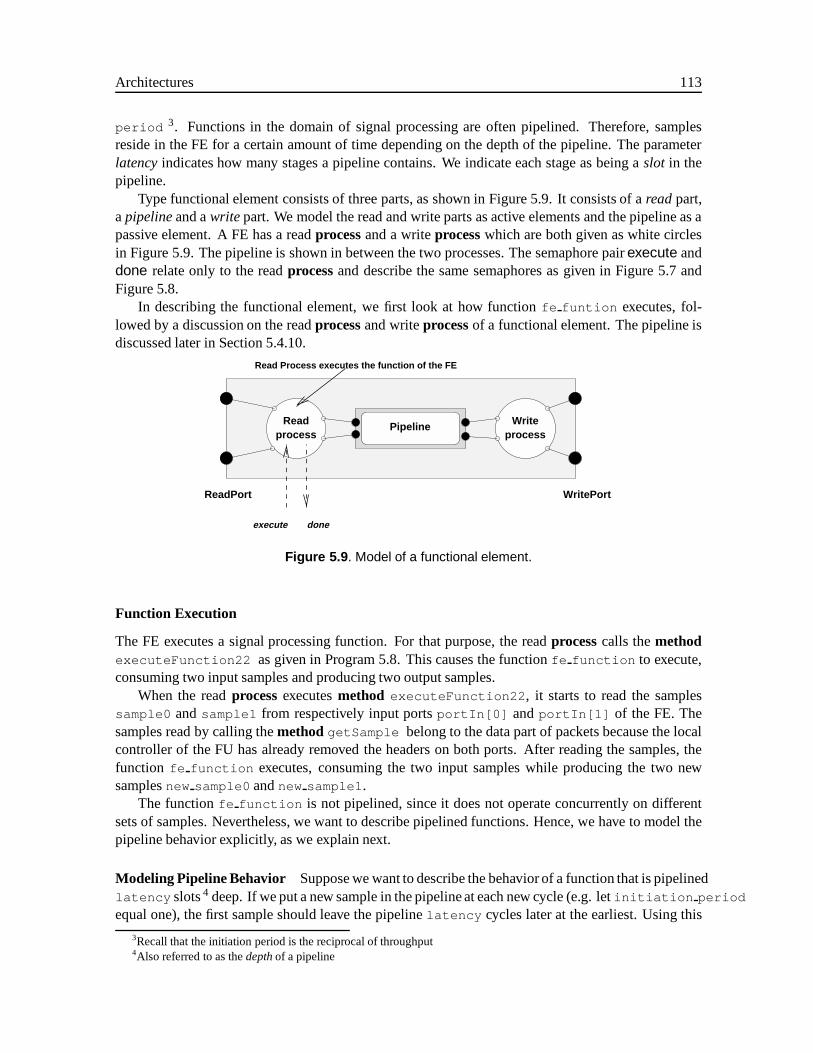
Architectures 113
period 3. Functions in the domain of signal processing are often pipelined. Therefore, samplesreside in the FE for a certain amount of time depending on the depth of the pipeline. The parameterlatencyindicates how many stages a pipeline contains. We indicate each stage as being aslot in thepipeline.
Type functional element consists of three parts, as shown in Figure 5.9. It consists of areadpart,apipelineand awrite part. We model the read and write parts as active elements and the pipeline as apassive element. A FE has a readprocessand a writeprocesswhich are both given as white circlesin Figure 5.9. The pipeline is shown in between the two processes. The semaphore pairexecute anddone relate only to the readprocessand describe the same semaphores as given in Figure 5.7 andFigure 5.8.
In describing the functional element, we first look at how functionfe funtion executes, fol-lowed by a discussion on the readprocessand writeprocessof a functional element. The pipeline isdiscussed later in Section 5.4.10.
WritePipelineReadprocess process
ReadPort WritePort
Read Process executes the function of the FE
execute done
Figure 5.9 . Model of a functional element.
Function Execution
The FE executes a signal processing function. For that purpose, the readprocesscalls themethodexecuteFunction22 as given in Program 5.8. This causes the functionfe function to execute,consuming two input samples and producing two output samples.
When the readprocessexecutesmethod executeFunction22 , it starts to read the samplessample0 andsample1 from respectively input portsportIn[0] andportIn[1] of the FE. Thesamples read by calling themethod getSample belong to the data part of packets because the localcontroller of the FU has already removed the headers on both ports. After reading the samples, thefunction fe function executes, consuming the two input samples while producing the two newsamplesnew sample0 andnew sample1 .
The functionfe function is not pipelined, since it does not operate concurrently on differentsets of samples. Nevertheless, we want to describe pipelined functions. Hence, we have to model thepipeline behavior explicitly, as we explain next.
Modeling Pipeline Behavior Suppose we want to describe the behavior of a function that is pipelinedlatency slots4 deep. If we put a new sample in the pipeline at each new cycle (e.g. letinitiation period
equal one), the first sample should leave the pipelinelatency cycles later at the earliest. Using this
3Recall that the initiation period is the reciprocal of throughput4Also referred to as thedepthof a pipeline
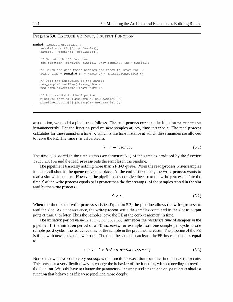
114 5.4 Modeling the Architectural Elements as Building Blocks
Program 5.8. EXECUTE A 2 INPUT, 2 OUTPUT FUNCTION
method executeFunction22 {sample0 = portIn[0].getSample();sample1 = portIn[1].getSample();
// Execute the FE-function(fe_function)(sample0, sample1, &new_sample0, &new_sample1);
// Calculate when these Samples are ready to leave the FEleave_time = pam time () + (latency * initiation period );
// Pass the Execution to the samplenew_sample0.setTime( leave_time );new_sample1.setTime( leave_time );
// Put results in the Pipelinepipeline_portIn[0].putSample( new_sample0 );pipeline_portIn[1].putSample( new_sample1 );
}
assumption, we model a pipeline as follows. The readprocessexecutes the functionfe function
instantaneously. Let the function produce new samples at, say, time instancet. The readprocesscalculates for these samples a timetl, which is the time instance at which these samples are allowedto leave the FE. The timetl is calculated as
tl = t + latency: (5.1)
The timetl is stored in the time stamp (see Structure 5.1) of the samples produced by the functionfe function and the readprocessputs the samples in the pipeline.
The pipeline is basically nothing more than a FIFO queue. When the readprocesswrites samplesin a slot, all slots in the queue move one place. At the end of the queue, the writeprocesswants toread a slot with samples. However, the pipeline does not give the slot to the writeprocessbefore thetime t0 of the writeprocessequals or is greater than the time stamptl of the samples stored in the slotread by the writeprocess.
t0 � tl (5.2)
When the time of the writeprocesssatisfies Equation 5.2, the pipeline allows the writeprocesstoread the slot. As a consequence, the writeprocesswrite the samples contained in the slot to outputports at timetl or later. Thus the samples leave the FE at the correct moment in time.
The initiation period valueinitiation period influences theresidence timeof samples in thepipeline. If the initiation period of a FE increases, for example from one sample per cycle to onesample per 2 cycles, the residence time of the sample in the pipeline increases. The pipeline of the FEis filled with new slots at a lower pace. The time the samples can leave the FE instead becomes equalto
t0 � t+ (initiation period � latency) (5.3)
Notice that we have completelyuncoupledthe function’s execution from the time it takes to execute.This provides a very flexible way to change the behavior of the function, without needing to rewritethe function. We only have to change the parameterslatency andinitiation period to obtain afunction that behaves as if it were pipelined more deeply.
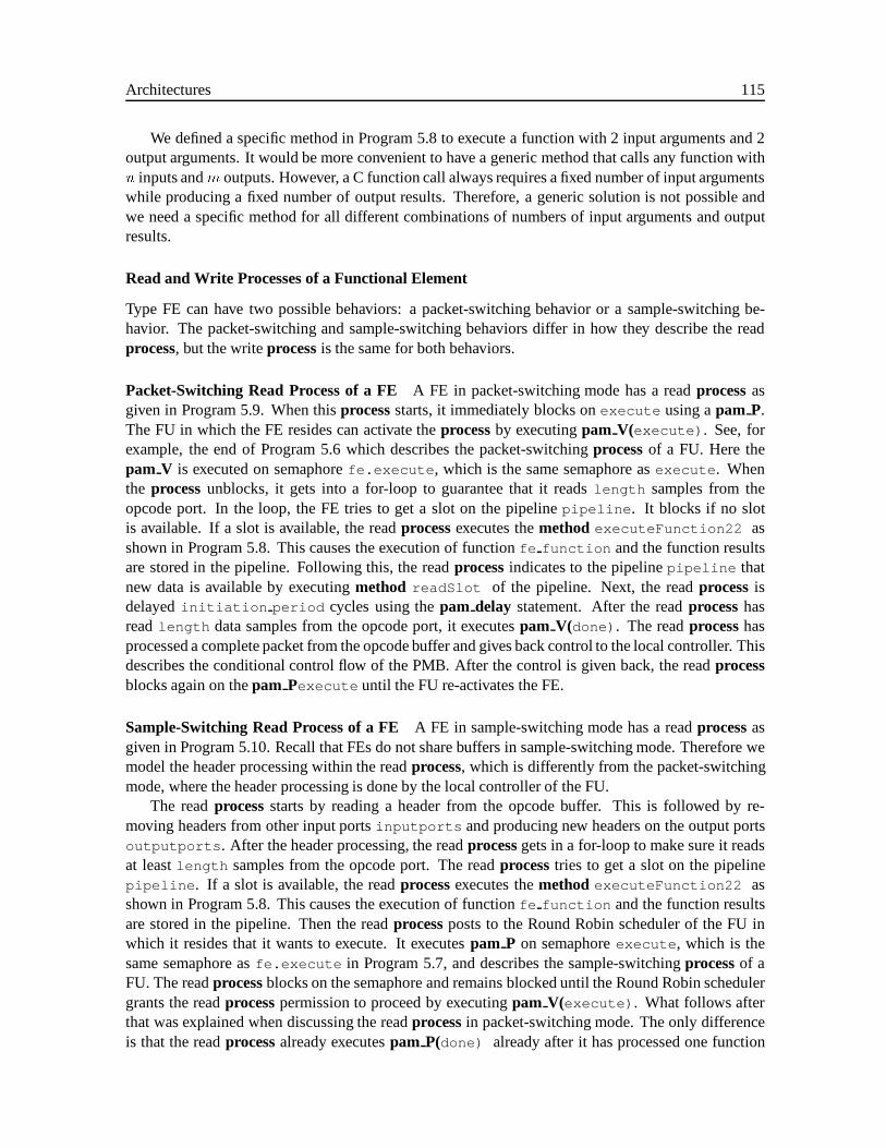
Architectures 115
We defined a specific method in Program 5.8 to execute a function with 2 input arguments and 2output arguments. It would be more convenient to have a generic method that calls any function withn inputs andm outputs. However, a C function call always requires a fixed number of input argumentswhile producing a fixed number of output results. Therefore, a generic solution is not possible andwe need a specific method for all different combinations of numbers of input arguments and outputresults.
Read and Write Processes of a Functional Element
Type FE can have two possible behaviors: a packet-switching behavior or a sample-switching be-havior. The packet-switching and sample-switching behaviors differ in how they describe the readprocess, but the writeprocessis the same for both behaviors.
Packet-Switching Read Process of a FE A FE in packet-switching mode has a readprocessasgiven in Program 5.9. When thisprocessstarts, it immediately blocks onexecute using apam P.The FU in which the FE resides can activate theprocessby executingpam V(execute) . See, forexample, the end of Program 5.6 which describes the packet-switchingprocessof a FU. Here thepam V is executed on semaphorefe.execute , which is the same semaphore asexecute . Whenthe processunblocks, it gets into a for-loop to guarantee that it readslength samples from theopcode port. In the loop, the FE tries to get a slot on the pipelinepipeline . It blocks if no slotis available. If a slot is available, the readprocessexecutes themethod executeFunction22 asshown in Program 5.8. This causes the execution of functionfe function and the function resultsare stored in the pipeline. Following this, the readprocessindicates to the pipelinepipeline thatnew data is available by executingmethod readSlot of the pipeline. Next, the readprocessisdelayedinitiation period cycles using thepam delay statement. After the readprocesshasreadlength data samples from the opcode port, it executespam V(done) . The readprocesshasprocessed a complete packet from the opcode buffer and gives back control to the local controller. Thisdescribes the conditional control flow of the PMB. After the control is given back, the readprocessblocks again on thepam Pexecute until the FU re-activates the FE.
Sample-Switching Read Process of a FEA FE in sample-switching mode has a readprocessasgiven in Program 5.10. Recall that FEs do not share buffers in sample-switching mode. Therefore wemodel the header processing within the readprocess, which is differently from the packet-switchingmode, where the header processing is done by the local controller of the FU.
The readprocessstarts by reading a header from the opcode buffer. This is followed by re-moving headers from other input portsinputports and producing new headers on the output portsoutputports . After the header processing, the readprocessgets in a for-loop to make sure it readsat leastlength samples from the opcode port. The readprocesstries to get a slot on the pipelinepipeline . If a slot is available, the readprocessexecutes themethod executeFunction22 asshown in Program 5.8. This causes the execution of functionfe function and the function resultsare stored in the pipeline. Then the readprocessposts to the Round Robin scheduler of the FU inwhich it resides that it wants to execute. It executespam P on semaphoreexecute , which is thesame semaphore asfe.execute in Program 5.7, and describes the sample-switchingprocessof aFU. The readprocessblocks on the semaphore and remains blocked until the Round Robin schedulergrants the readprocesspermission to proceed by executingpam V(execute) . What follows afterthat was explained when discussing the readprocessin packet-switching mode. The only differenceis that the readprocessalready executespam P(done) already after it has processed one function
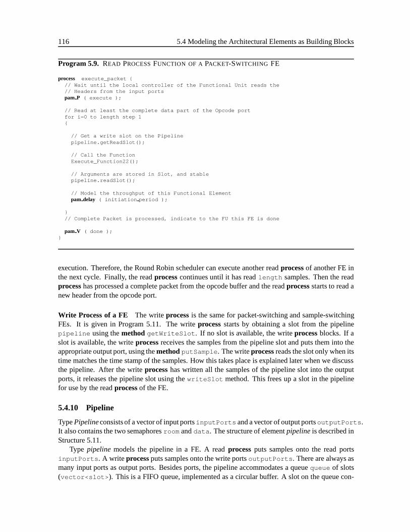
116 5.4 Modeling the Architectural Elements as Building Blocks
Program 5.9. READ PROCESSFUNCTION OF A PACKET-SWITCHING FE
process execute_packet {// Wait until the local controller of the Functional Unit reads the// Headers from the input portspam P ( execute );
// Read at least the complete data part of the Opcode portfor i=0 to length step 1{
// Get a write slot on the Pipelinepipeline.getReadSlot();
// Call the FunctionExecute_Function22();
// Arguments are stored in Slot, and stablepipeline.readSlot();
// Model the throughput of this Functional Elementpam delay ( initiation period );
}// Complete Packet is processed, indicate to the FU this FE is done
pam V ( done );}
execution. Therefore, the Round Robin scheduler can execute another readprocessof another FE inthe next cycle. Finally, the readprocesscontinues until it has readlength samples. Then the readprocesshas processed a complete packet from the opcode buffer and the readprocessstarts to read anew header from the opcode port.
Write Process of a FE The writeprocessis the same for packet-switching and sample-switchingFEs. It is given in Program 5.11. The writeprocessstarts by obtaining a slot from the pipelinepipeline using themethod getWriteSlot . If no slot is available, the writeprocessblocks. If aslot is available, the writeprocessreceives the samples from the pipeline slot and puts them into theappropriate output port, using themethodputSample . The writeprocessreads the slot only when itstime matches the time stamp of the samples. How this takes place is explained later when we discussthe pipeline. After the writeprocesshas written all the samples of the pipeline slot into the outputports, it releases the pipeline slot using thewriteSlot method. This frees up a slot in the pipelinefor use by the readprocessof the FE.
5.4.10 Pipeline
TypePipelineconsistsof a vector of input portsinputPorts and a vector of output portsoutputPorts .It also contains the two semaphoresroom anddata . The structure of elementpipelineis described inStructure 5.11.
Type pipeline models the pipeline in a FE. A readprocessputs samples onto the read portsinputPorts . A write processputs samples onto the write portsoutputPorts . There are always asmany input ports as output ports. Besides ports, the pipeline accommodates a queuequeue of slots(vector<slot> ). This is a FIFO queue, implemented as a circular buffer. A slot on the queue con-
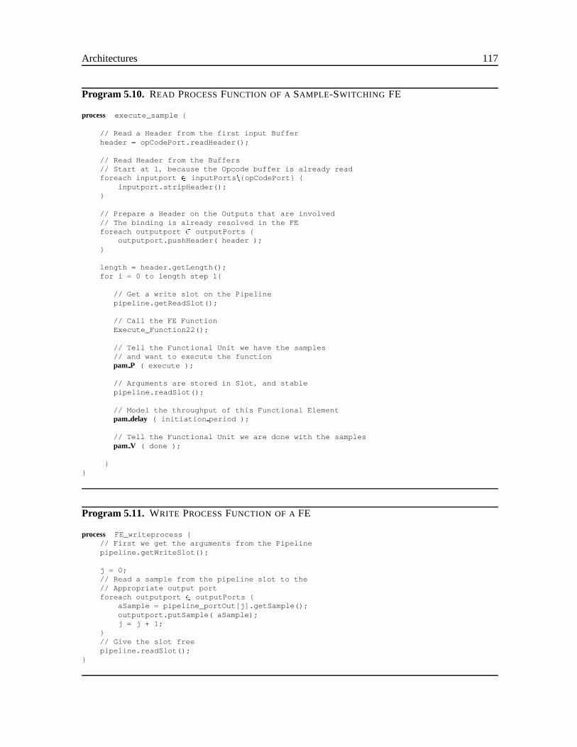
Architectures 117
Program 5.10. READ PROCESSFUNCTION OF A SAMPLE-SWITCHING FE
process execute_sample {
// Read a Header from the first input Bufferheader = opCodePort.readHeader();
// Read Header from the Buffers// Start at 1, because the Opcode buffer is already readforeach inputport 2 inputPorts n{opCodePort} {
inputport.stripHeader();}
// Prepare a Header on the Outputs that are involved// The binding is already resolved in the FEforeach outputport 2 outputPorts {
outputport.pushHeader( header );}
length = header.getLength();for i = 0 to length step 1{
// Get a write slot on the Pipelinepipeline.getReadSlot();
// Call the FE FunctionExecute_Function22();
// Tell the Functional Unit we have the samples// and want to execute the functionpam P ( execute );
// Arguments are stored in Slot, and stablepipeline.readSlot();
// Model the throughput of this Functional Elementpam delay ( initiation period );
// Tell the Functional Unit we are done with the samplespam V ( done );
}}
Program 5.11. WRITE PROCESSFUNCTION OF A FE
process FE_writeprocess {// First we get the arguments from the Pipelinepipeline.getWriteSlot();
j = 0;// Read a sample from the pipeline slot to the// Appropriate output portforeach outputport 2 outputPorts {
aSample = pipeline_portOut[j].getSample();outputport.putSample( aSample);j = j + 1;
}// Give the slot freepipeline.readSlot();
}
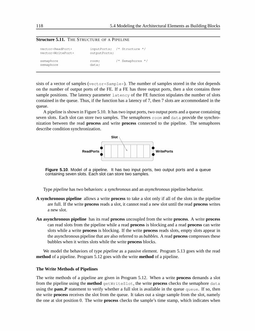
118 5.4 Modeling the Architectural Elements as Building Blocks
Structure 5.11. THE STRUCTURE OF APIPELINE
vector<ReadPort> inputPorts; /* Structure */vector<WritePort> outputPorts;
semaphore room; /* Semaphores */semaphore data;
sists of a vector of samples (vector<Sample> ). The number of samples stored in the slot dependson the number of output ports of the FE. If a FE has three output ports, then a slot contains threesample positions. The latency parameterlatency of the FE function stipulates the number of slotscontained in the queue. Thus, if the function has a latency of 7, then 7 slots are accommodated in thequeue.
A pipeline is shown in Figure 5.10. It has two input ports, two output ports and a queue containingseven slots. Each slot can store two samples. The semaphoresroom anddata provide the synchro-nization between the readprocessand writeprocessconnected to the pipeline. The semaphoresdescribe condition synchronization.
ReadPorts
Slot
WritePorts
Figure 5.10 . Model of a pipeline. It has two input ports, two output ports and a queuecontaining seven slots. Each slot can store two samples.
Typepipelinehas two behaviors: asynchronousand anasynchronouspipeline behavior.
A synchronous pipeline allows a writeprocessto take a slot only if all of the slots in the pipelineare full. If the writeprocessreads a slot, it cannot read a new slot until the readprocesswritesa new slot.
An asynchronous pipeline has its readprocessuncoupled from the writeprocess. A write processcan read slots from the pipeline while a readprocessis blocking and a readprocesscan writeslots while a writeprocessis blocking. If the writeprocessreads slots, empty slots appear inthe asynchronous pipeline that are also referred to asbubbles. A readprocesscompresses thesebubbles when it writes slots while the writeprocessblocks.
We model the behaviors of typepipelineas a passive element. Program 5.13 goes with the readmethod of a pipeline. Program 5.12 goes with the writemethod of a pipeline.
The Write Methods of Pipelines
The write methods of a pipeline are given in Program 5.12. When a writeprocessdemands a slotfrom the pipeline using themethod getWriteSlot , the writeprocesschecks the semaphoredata
using thepam P statement to verify whether a full slot is available in the queuequeue . If so, thenthe writeprocessreceives the slot from the queue. It takes out a singe sample from the slot, namelythe one at slot position 0. The writeprocesschecks the sample’s time stamp, which indicates when
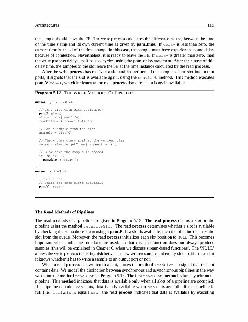
Architectures 119
the sample should leave the FE. The writeprocesscalculates the differencedelay between the timeof the time stamp and its own current time as given bypam time. If delay is less than zero, thecurrent time is ahead of the time stamp. In this case, the sample must have experienced some delaybecause of congestion. Nevertheless, it is ready to leave the FE. Ifdelay is greater than zero, thenthe writeprocessdelays itselfdelay cycles, using thepam delaystatement. After the elapse of thisdelay time, the samples of the slot leave the FE at the time instance calculated by the readprocess.
After the writeprocesshas received a slot and has written all the samples of the slot into outputports, it signals that the slot is available again, using thereadSlot method. This method executespam V(room) , which indicates to the readprocessthat a free slot is again available.
Program 5.12. THE WRITE METHODS OF PIPELINES
method getWriteSlot{
// Is a slot with data available?pam P (data);slot= queue[readfifo];readfifo = (++readfifo)%cap;
// Get a sample from the slotaSample = slot[0];
// Check time stamp against the current timedelay = aSample.getTime() - pam time () ;
// Slow down the sample if neededif (delay > 0) {
pam delay ( delay );}
}method writeSlot{
--full_slots;// There are free slots availablepam V (room);
}
The Read Methods of Pipelines
The read methods of a pipeline are given in Program 5.13. The readprocessclaims a slot on thepipeline using themethod getWriteSlot . The readprocessdetermines whether a slot is availableby checking the semaphoreroom using apam P. If a slot is available, then the pipeline receives theslot from the queue. Moreover, the readprocessinitializeseach slot position to NULL. This becomesimportant when multi-rate functions are used. In that case the function does not always producesamples (this will be explained in Chapter 6, when we discuss stream-based functions). The ‘NULL’allows the writeprocessto distinguish between a new written sample and empty slot positions, so thatit knows whether it has to write a sample to an output port or not.
When a readprocesshas written to a slot, it uses themethod readSlot to signal that the slotcontains data. We model the distinction between synchronous and asynchronous pipelines in the waywe define themethod readSlot in Program 5.13. The firstreadSlot method is for a synchronouspipeline. Thismethod indicates that data is available only when all slots of a pipeline are occupied.If a pipeline containscap slots, data is only available whencap slots are full. If the pipeline isfull (i.e. full slots equalscap ), the readprocessindicates that data is available by executing
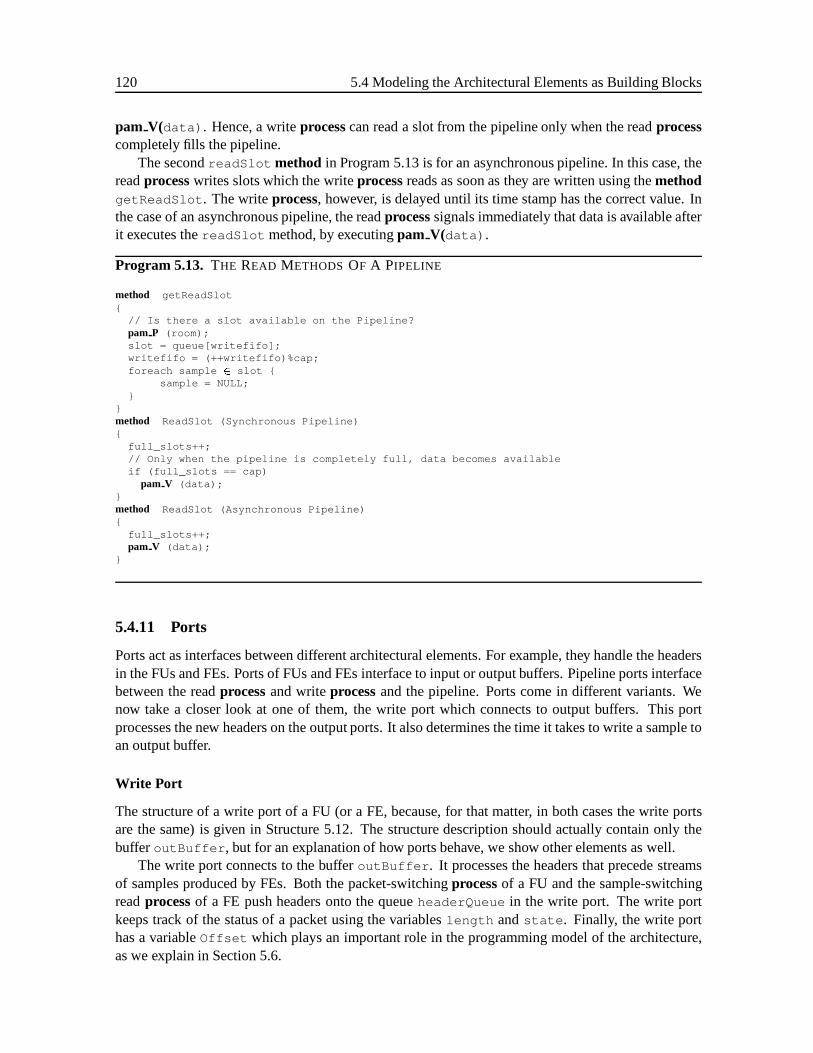
120 5.4 Modeling the Architectural Elements as Building Blocks
pam V(data) . Hence, a writeprocesscan read a slot from the pipeline only when the readprocesscompletely fills the pipeline.
The secondreadSlot method in Program 5.13 is for an asynchronous pipeline. In this case, thereadprocesswrites slots which the writeprocessreads as soon as they are written using themethodgetReadSlot . The writeprocess, however, is delayed until its time stamp has the correct value. Inthe case of an asynchronous pipeline, the readprocesssignals immediately that data is available afterit executes thereadSlot method, by executingpam V(data) .
Program 5.13. THE READ METHODS OF A PIPELINE
method getReadSlot{
// Is there a slot available on the Pipeline?pam P (room);slot = queue[writefifo];writefifo = (++writefifo)%cap;foreach sample 2 slot {
sample = NULL;}
}method ReadSlot (Synchronous Pipeline){
full_slots++;// Only when the pipeline is completely full, data becomes availableif (full_slots == cap)
pam V (data);}method ReadSlot (Asynchronous Pipeline){
full_slots++;pam V (data);
}
5.4.11 Ports
Ports act as interfaces between different architectural elements. For example, they handle the headersin the FUs and FEs. Ports of FUs and FEs interface to input or output buffers. Pipeline ports interfacebetween the readprocessand writeprocessand the pipeline. Ports come in different variants. Wenow take a closer look at one of them, the write port which connects to output buffers. This portprocesses the new headers on the output ports. It also determines the time it takes to write a sample toan output buffer.
Write Port
The structure of a write port of a FU (or a FE, because, for that matter, in both cases the write portsare the same) is given in Structure 5.12. The structure description should actually contain only thebufferoutBuffer , but for an explanation of how ports behave, we show other elements as well.
The write port connects to the bufferoutBuffer . It processes the headers that precede streamsof samples produced by FEs. Both the packet-switchingprocessof a FU and the sample-switchingreadprocessof a FE push headers onto the queueheaderQueue in the write port. The write portkeeps track of the status of a packet using the variableslength andstate . Finally, the write porthas a variableOffset which plays an important role in the programming model of the architecture,as we explain in Section 5.6.
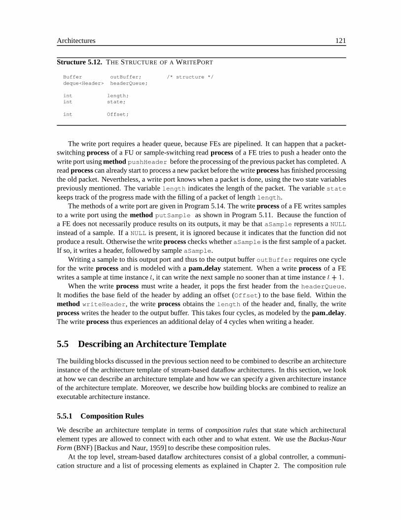
Architectures 121
Structure 5.12. THE STRUCTURE OF AWRITEPORT
Buffer outBuffer; /* structure */deque<Header> headerQueue;
int length;int state;
int Offset;
The write port requires a header queue, because FEs are pipelined. It can happen that a packet-switchingprocessof a FU or sample-switching readprocessof a FE tries to push a header onto thewrite port usingmethodpushHeader before the processing of the previous packet has completed. Areadprocesscan already start to process a new packet before the writeprocesshas finished processingthe old packet. Nevertheless, a write port knows when a packet is done, using the two state variablespreviously mentioned. The variablelength indicates the length of the packet. The variablestate
keeps track of the progress made with the filling of a packet of lengthlength .The methods of a write port are given in Program 5.14. The writeprocessof a FE writes samples
to a write port using themethod putSample as shown in Program 5.11. Because the function ofa FE does not necessarily produce results on its outputs, it may be thataSample represents aNULL
instead of a sample. If aNULL is present, it is ignored because it indicates that the function did notproduce a result. Otherwise the writeprocesschecks whetheraSample is the first sample of a packet.If so, it writes a header, followed by sampleaSample .
Writing a sample to this output port and thus to the output bufferoutBuffer requires one cyclefor the writeprocessand is modeled with apam delay statement. When a writeprocessof a FEwrites a sample at time instancet, it can write the next sample no sooner than at time instancet+ 1.
When the writeprocessmust write a header, it pops the first header from theheaderQueue .It modifies the base field of the header by adding an offset (Offset ) to the base field. Within themethod writeHeader , the writeprocessobtains thelength of the header and, finally, the writeprocesswrites the header to the output buffer. This takes four cycles, as modeled by thepam delay.The writeprocessthus experiences an additional delay of 4 cycles when writing a header.
5.5 Describing an Architecture Template
The building blocks discussed in the previous section need to be combined to describe an architectureinstance of the architecture template of stream-based dataflow architectures. In this section, we lookat how we can describe an architecture template and how we can specify a given architecture instanceof the architecture template. Moreover, we describe how building blocks are combined to realize anexecutable architecture instance.
5.5.1 Composition Rules
We describe an architecture template in terms ofcomposition rulesthat state which architecturalelement types are allowed to connect with each other and to what extent. We use theBackus-NaurForm (BNF) [Backus and Naur, 1959] to describe these composition rules.
At the top level, stream-based dataflow architectures consist of a global controller, a communi-cation structure and a list of processing elements as explained in Chapter 2. The composition rule
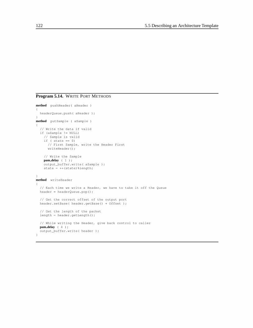
122 5.5 Describing an Architecture Template
Program 5.14. WRITE PORT METHODS
method pushHeader( aHeader ){
headerQueue.push( aHeader );}method putSample ( aSample ){
// Write the data if validif (aSample != NULL)
// Sample is validif ( state == 0)
// First Sample, write the Header FirstwriteHeader();
// Write the Samplepam delay ( 1 );output_buffer.write( aSample );state = ++(state)%length;
}method writeHeader{
// Each time we write a Header, we have to take it off the Queueheader = headerQueue.pop();
// Get the correct offset of the output portheader.setBase( header.getBase() + Offset );
// Get the length of the packetlength = header.getLength();
// While writing the Header, give back control to callerpam delay ( 4 );output_buffer.write( header );
}
Architectures 123
expressing this top-level structure is expressed in BNF as follows:
Architecture := Global Controller Communication Structure List Of Pes
Next, we further specify what a list of processing elements (PEs) implies. A list of processingelements should contain at least one or more processing elements. We express this requirement in arecursive way as follows:
List of Pes := PEj List of Pes PE
In this rule the “j” symbol indicates a choice: we can select this or (“j”) that. Thus, we selecteither a single PE (PE) or a list of PEs (List of Pes) that could again consist of a single PE or a listof PEs, and so forth. Different variants exist of a processing element. They can either be a regular PE,a source PE, or a sink PE. The composition rule describing the existence of these three types is statedin BNF as follows:
PE := Regular PEj Source PEj Sink PE
Recall that the “j” symbol indicates a choice. If we look further at these three variants, then wesee that each variant has its own set of requirements in terms of the functional unit type, the use ofinput and output buffers and the use of routers. The composition rule expressing these requirementsfor each of the three PE variants is as follows:
Regular PE := Input Buffers FU Output Buffers RoutersSource PE := Source FU Output Buffers RoutersSink PE := Input Buffers Sink FU
We can continue to construct composition rules until we have completely described the architec-ture template of stream-based dataflow architectures. We have done just that; the BNF rules describingthe complete architecture template of stream-based dataflow architectures are given in Appendix A.
5.5.2 Architecture Description Language
The composition rules used to describe the architecture template can also be used to define thegram-mar of a language. We use the BNF rules of Appendix A to define the grammar of theArchitectureDescription Language. We can use this language to describe architecture instances of the architecturetemplate.
To compare a textual description of an architecture instance with the grammar, we used the toolsFlex [Paxson, 1990] andBison[Donnelly and Stallman, 1992]. Flex breaks up the textual descriptioninto keywords and other identifiers. Bison matches these keywords and identifiers against the grammarof the language (i.e., the set of BNF rules given in Appendix A) and activates the approriate action ifa feasible composition rule is found.
124 5.5 Describing an Architecture Template
Creating a Building Block for an Architectural Element
We now consider the composition rules for architectural element typebufferand show how and whena parser creates a building block for this type. The composition rule expressing the three differentbehaviors of typebufferis:
Input Buffer := Bounded FIFOj Unbouned FIFOj HandShake
Now, if we look futher at the composition rule related toBounded FIFO , we find a compositionrule that looks as follows:
Bounded FIFO := INPUTBUFFER ’ f’ TYPE ’:’ FCFS ’(’ NUM ’)’ ’;’ ’ g’f
// Associated Action in C++Buffer* buffer = new FIFO( $7 );
g
In this composition rule, we introducekeywordslike INPUTBUFFER, TYPEandFCFS. The parseruses these keywords to decide where to break up a textual description defining a particular architectureinstance. It then tries to match these keywords with the defined set of BNF rules. If the parser findsa valid rule, like the one given forBounded FIFO , it activates the action associated with that rule,which is given between the curly brackets. We associated the action of creating a building block forthe FIFO buffer with the composition rule for theBounded FIFO , by instantiating an object of classFIFO using thenew statement.
In the instantiation of this object or building block, the parser passes along a parameter. In the caseof the FIFO buffer, the parser passes on the parameter representing the capacity of the FIFO buffer.The parameter is the seventh position in the composition rule ofBounded FIFO , which correspondswith theNUMfield describing a numerial value. This value is represented by$7 and is passed on tothe constructor of the FIFO buffer and bound to the parametercapacity (shown in Structure 5.7).
Specify an Architecture Instance
Using the architecture description language, we can specify one particular architecture instance ofthe stream-based dataflow architecture. As an example, in Figure 5.11 we show the architecturedescription of the architecture instance shown in Figure 5.12. We include the same terms (precededby the symbol “//” ) as used in Figure 5.12 in this architecture description.
In the first lines, we define a communication structure (Communication ) and a global controller(Controller ), followed by a list of processing elements (ProcessingElement ). The list consistsof three processing elements: a sink PE, a regular PE, and a source PE. For the regular PE we definethe input and output buffers (InputBuffer , OutputBuffer respectively), the routers (Router )and the functional unit (FunctionalUnit) . We also give the regular PE the nameFilter . Thefunctional unit of PEfilter consists of two functional elements (FunctionalElement ), namedLowPass andHighPass . The ports of the functional element bind to the ports of the functional unitin a particular way as described in the binding part (Input andOutput part).
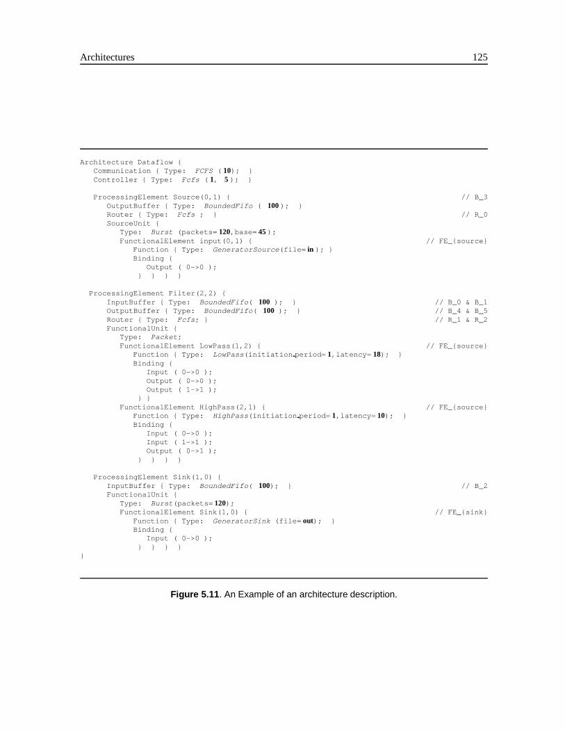
Architectures 125
Architecture Dataflow {Communication { Type: FCFS ( 10); }Controller { Type: Fcfs ( 1, 5 ); }
ProcessingElement Source(0,1) { // B_3OutputBuffer { Type: BoundedFifo ( 100); }Router { Type: Fcfs ; } // R_0SourceUnit {
Type: Burst (packets= 120,base= 45 );FunctionalElement input(0,1) { // FE_{source}
Function { Type: GeneratorSource (file= in ); }Binding {
Output ( 0->0 );} } } }
ProcessingElement Filter(2,2) {InputBuffer { Type: BoundedFifo ( 100 ); } // B_0 & B_1OutputBuffer { Type: BoundedFifo ( 100 ); } // B_4 & B_5Router { Type: Fcfs ; } // R_1 & R_2FunctionalUnit {
Type: Packet ;FunctionalElement LowPass(1,2) { // FE_{source}
Function { Type: LowPass (initiation period= 1,latency= 18); }Binding {
Input ( 0->0 );Output ( 0->0 );Output ( 1->1 );
} }FunctionalElement HighPass(2,1) { // FE_{source}
Function { Type: HighPass (initiation period= 1,latency= 10); }Binding {
Input ( 0->0 );Input ( 1->1 );Output ( 0->1 );
} } } }
ProcessingElement Sink(1,0) {InputBuffer { Type: BoundedFifo ( 100); } // B_2FunctionalUnit {
Type: Burst (packets= 120);FunctionalElement Sink(1,0) { // FE_{sink}
Function { Type: GeneratorSink (file= out); }Binding {
Input ( 0->0 );} } } }
}
Figure 5.11 . An Example of an architecture description.
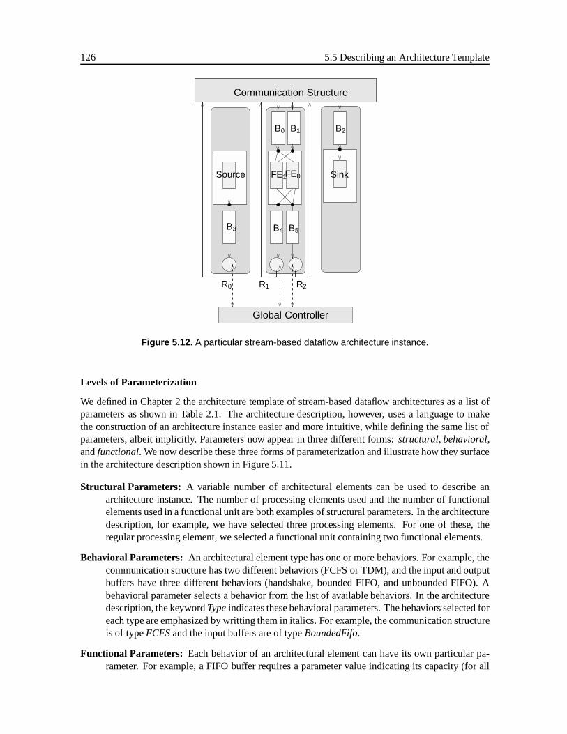
126 5.5 Describing an Architecture Template
R2
Communication Structure
Global Controller
B0 B1 B2
Source FE1FE0 Sink
B4 B5B3
R0 R1
Figure 5.12 . A particular stream-based dataflow architecture instance.
Levels of Parameterization
We defined in Chapter 2 the architecture template of stream-based dataflow architectures as a list ofparameters as shown in Table 2.1. The architecture description, however, uses a language to makethe construction of an architecture instance easier and more intuitive, while defining the same list ofparameters, albeit implicitly. Parameters now appear in three different forms:structural, behavioral,andfunctional. We now describe these three forms of parameterization and illustrate how they surfacein the architecture description shown in Figure 5.11.
Structural Parameters: A variable number of architectural elements can be used to describe anarchitecture instance. The number of processing elements used and the number of functionalelements used in a functional unit are both examples of structural parameters. In the architecturedescription, for example, we have selected three processing elements. For one of these, theregular processing element, we selected a functional unit containing two functional elements.
Behavioral Parameters: An architectural element type has one or more behaviors. For example, thecommunication structure has two different behaviors (FCFS or TDM), and the input and outputbuffers have three different behaviors (handshake, bounded FIFO, and unbounded FIFO). Abehavioral parameter selects a behavior from the list of available behaviors. In the architecturedescription, the keywordTypeindicates these behavioral parameters. The behaviors selected foreach type are emphasized by writting them in italics. For example, the communication structureis of typeFCFSand the input buffers are of typeBoundedFifo.
Functional Parameters: Each behavior of an architectural element can have its own particular pa-rameter. For example, a FIFO buffer requires a parameter value indicating its capacity (for all
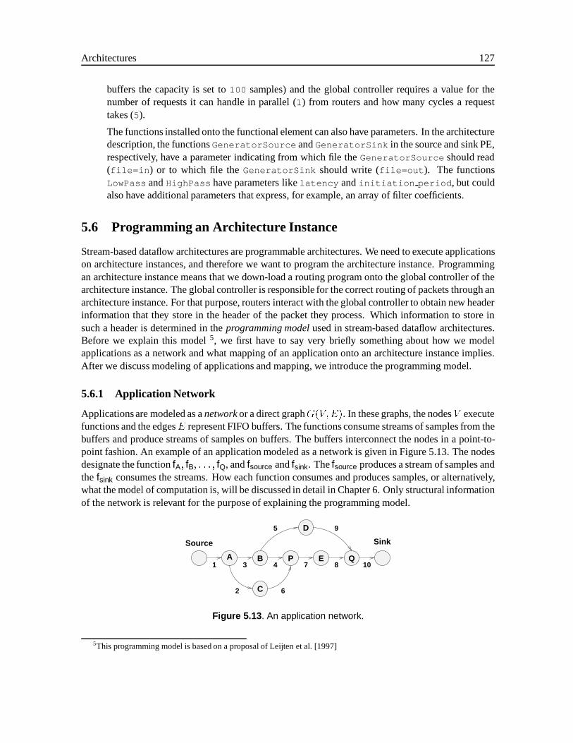
Architectures 127
buffers the capacity is set to100 samples) and the global controller requires a value for thenumber of requests it can handle in parallel (1) from routers and how many cycles a requesttakes (5).
The functions installed onto the functional element can also have parameters. In the architecturedescription, the functionsGeneratorSource andGeneratorSink in the source and sink PE,respectively, have a parameter indicating from which file theGeneratorSource should read(file=in ) or to which file theGeneratorSink should write (file=out ). The functionsLowPass andHighPass have parameters likelatency andinitiation period , but couldalso have additional parameters that express, for example, an array of filter coefficients.
5.6 Programming an Architecture Instance
Stream-based dataflow architectures are programmable architectures. We need to execute applicationson architecture instances, and therefore we want to program the architecture instance. Programmingan architecture instance means that we down-load a routing program onto the global controller of thearchitecture instance. The global controller is responsible for the correct routing of packets through anarchitecture instance. For that purpose, routers interact with the global controller to obtain new headerinformation that they store in the header of the packet they process. Which information to store insuch a header is determined in theprogramming modelused in stream-based dataflow architectures.Before we explain this model5, we first have to say very briefly something about how we modelapplications as a network and what mapping of an application onto an architecture instance implies.After we discuss modeling of applications and mapping, we introduce the programming model.
5.6.1 Application Network
Applicationsare modeled as anetworkor a direct graphG(V;E). In these graphs, the nodesV executefunctions and the edgesE represent FIFO buffers. The functions consume streams of samples from thebuffers and produce streams of samples on buffers. The buffers interconnect the nodes in a point-to-point fashion. An example of an application modeled as a network is given in Figure 5.13. The nodesdesignate the functionfA; fB; : : : ; fQ, andfsource andfsink. Thefsource produces a stream of samples andthe fsink consumes the streams. How each function consumes and produces samples, or alternatively,what the model of computation is, will be discussed in detail in Chapter 6. Only structural informationof the network is relevant for the purpose of explaining the programming model.
A B P E Q
C
D
Source Sink
1 3 4 7 8 10
2 6
5 9
Figure 5.13 . An application network.
5This programming model is based on a proposal of Leijten et al. [1997]
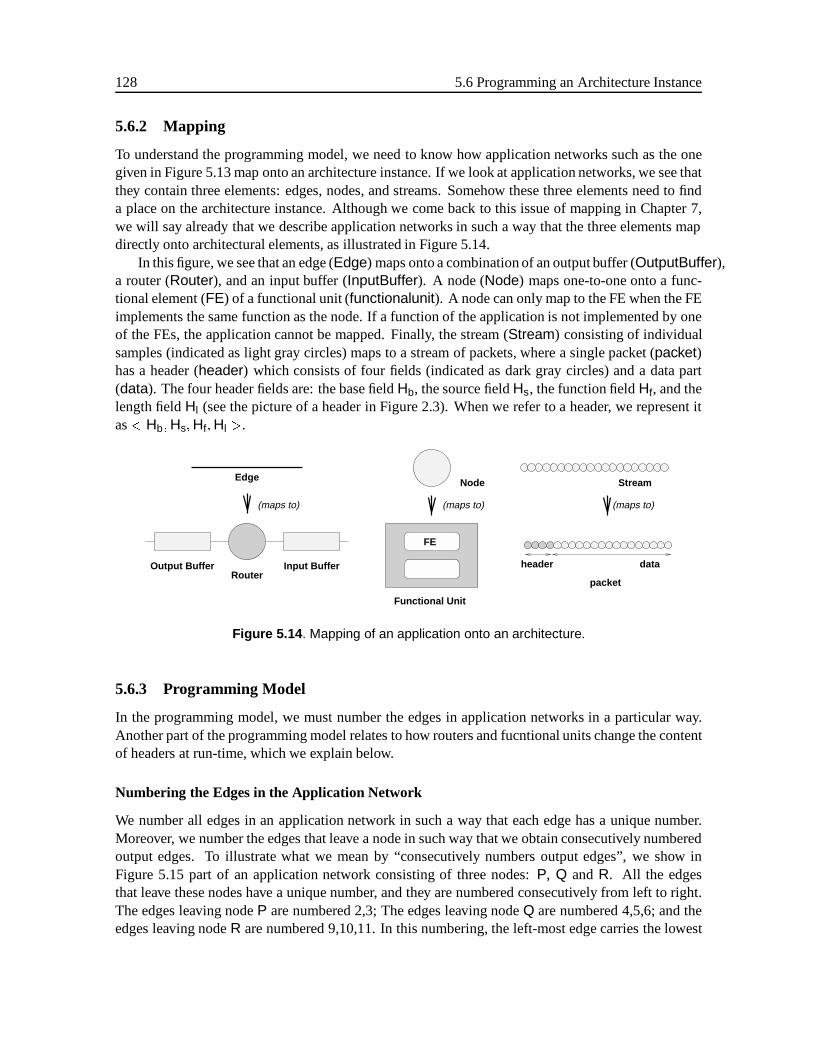
128 5.6 Programming an Architecture Instance
5.6.2 Mapping
To understand the programming model, we need to know how application networks such as the onegiven in Figure 5.13 map onto an architecture instance. If we look at application networks, we see thatthey contain three elements: edges, nodes, and streams. Somehow these three elements need to finda place on the architecture instance. Although we come back to this issue of mapping in Chapter 7,we will say already that we describe application networks in such a way that the three elements mapdirectly onto architectural elements, as illustrated in Figure 5.14.
In this figure, we see that an edge (Edge) maps onto a combination of an output buffer (OutputBuffer),a router (Router), and an input buffer (InputBuffer). A node (Node) maps one-to-one onto a func-tional element (FE) of a functional unit (functionalunit). A node can only map to the FE when the FEimplements the same function as the node. If a function of the application is not implemented by oneof the FEs, the application cannot be mapped. Finally, the stream (Stream) consisting of individualsamples (indicated as light gray circles) maps to a stream of packets, where a single packet (packet)has a header (header) which consists of four fields (indicated as dark gray circles) and a data part(data). The four header fields are: the base fieldHb, the source fieldHs, the function fieldHf, and thelength fieldHl (see the picture of a header in Figure 2.3). When we refer to a header, we represent itas< Hb;Hs;Hf;Hl >.
RouterInput BufferOutput Buffer
Edge
FE
(maps to) (maps to) (maps to)
Functional Unit
Node Stream
header
packet
data
Figure 5.14 . Mapping of an application onto an architecture.
5.6.3 Programming Model
In the programming model, we must number the edges in application networks in a particular way.Another part of the programming model relates to how routers and fucntional units change the contentof headers at run-time, which we explain below.
Numbering the Edges in the Application Network
We number all edges in an application network in such a way that each edge has a unique number.Moreover, we number the edges that leave a node in such way that we obtain consecutively numberedoutput edges. To illustrate what we mean by “consecutively numbers output edges”, we show inFigure 5.15 part of an application network consisting of three nodes:P, Q andR. All the edgesthat leave these nodes have a unique number, and they are numbered consecutively from left to right.The edges leaving nodeP are numbered 2,3; The edges leaving nodeQ are numbered 4,5,6; and theedges leaving nodeR are numbered 9,10,11. In this numbering, the left-most edge carries the lowest
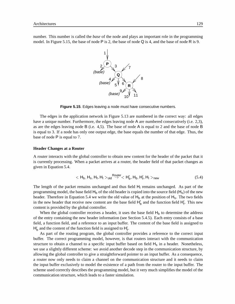
Architectures 129
number. This number is called thebaseof the node and plays an important role in the programmingmodel. In Figure 5.15, the base of nodeP is 2, the base of nodeQ is 4, and the base of nodeR is 9.
Q
P
R
1
8
2 3 7
64
5
9
10 11
(base)
(base)
(base)
Figure 5.15 . Edges leaving a node must have consecutive numbers.
The edges in the application network in Figure 5.13 are numbered in the correct way: all edgeshave a unique number. Furthermore, the edges leaving nodeA are numbered consecutively (i.e. 2,3),as are the edges leaving nodeB (i.e. 4,5). The base of nodeA is equal to 2 and the base of nodeBis equal to 3. If a node has only one output edge, the base equals the number of that edge. Thus, thebase of nodeP is equal to 7.
Header Changes at a Router
A router interacts with the global controller to obtain new content for the header of the packet that itis currently processing. When a packet arrives at a router, the header field of that packet changes asgiven in Equation 5.4.
< Hb;Hs;Hf;Hl >oldRouter! < H0
b;Hb;H0f;Hl >new (5.4)
The length of the packet remains unchanged and thus fieldHl remains unchanged. As part of theprogramming model, the base fieldHb of the old header is copied into the source field (Hs) of the newheader. Therefore in Equation 5.4 we write the old value ofHb at the position ofHs. The two fieldsin the new header that receive new content are the base fieldH0
b and the function fieldH0f. This new
content is provided by the global controller.When the global controller receives a header, it uses the base fieldHb to determine the address
of the entry containing the new header information (see Section 5.4.5). Each entry consists of a basefield, a function field, and a reference to an input buffer. The content of the base field is assigned toH0
b and the content of the function field is assigned toH0f.
As part of the routing program, the global controller provides a reference to the correct inputbuffer. The correct programming model, however, is that routers interact with the communicationstructure to obtain a channel to a specific input buffer based on fieldHs in a header. Nonetheless,we use a slightly different scheme: we avoid another decode step in the communication structure, byallowing the global controller to give a straightforward pointer to an input buffer. As a consequence,a router now only needs to claim a channel on the communication structure and it needs to claimthe input buffer exclusively to model the existence of a path from the router to the input buffer. Thescheme used correctly describes the programming model, but it very much simplifies the model of thecommunication structure, which leads to a faster simulation.
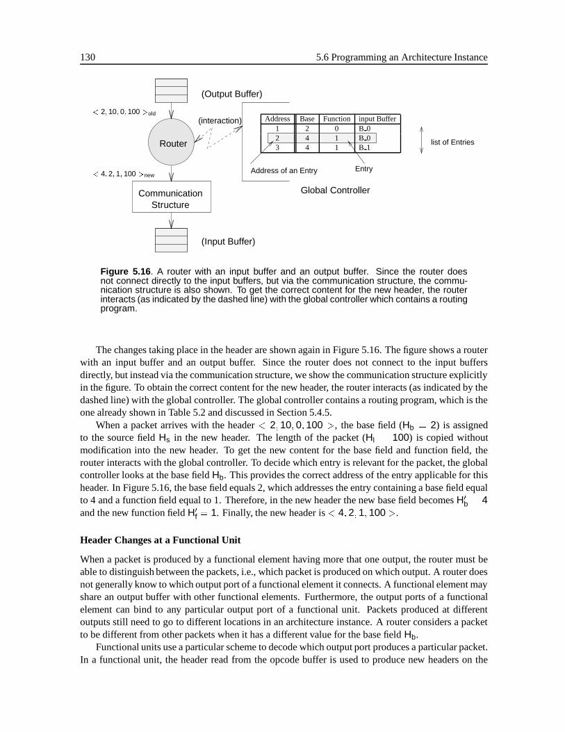
130 5.6 Programming an Architecture Instance
Address Base Function input Buffer1 2 0 B 02 4 1 B 03 4 1 B 1
list of Entries
Address of an Entry Entry
Global Controller
(Output Buffer)
(Input Buffer)
CommunicationStructure
Router
< 2; 10; 0; 100 >old
< 4; 2; 1; 100 >new
(interaction)
Figure 5.16 . A router with an input buffer and an output buffer. Since the router doesnot connect directly to the input buffers, but via the communication structure, the commu-nication structure is also shown. To get the correct content for the new header, the routerinteracts (as indicated by the dashed line) with the global controller which contains a routingprogram.
The changes taking place in the header are shown again in Figure 5.16. The figure shows a routerwith an input buffer and an output buffer. Since the router does not connect to the input buffersdirectly, but instead via the communication structure, we show the communication structure explicitlyin the figure. To obtain the correct content for the new header, the router interacts (as indicated by thedashed line) with the global controller. The global controller contains a routing program, which is theone already shown in Table 5.2 and discussed in Section 5.4.5.
When a packet arrives with the header< 2; 10; 0; 100 >, the base field (Hb = 2) is assignedto the source fieldHs in the new header. The length of the packet (Hl = 100) is copied withoutmodification into the new header. To get the new content for the base field and function field, therouter interacts with the global controller. To decide which entry is relevant for the packet, the globalcontroller looks at the base fieldHb. This provides the correct address of the entry applicable for thisheader. In Figure 5.16, the base field equals 2, which addresses the entry containing a base field equalto 4 and a function field equal to 1. Therefore, in the new header the new base field becomesH0
b = 4and the new function fieldH0
f = 1. Finally, the new header is< 4; 2; 1; 100 >.
Header Changes at a Functional Unit
When a packet is produced by a functional element having more that one output, the router must beable to distinguish between the packets, i.e., which packet is produced on which output. A router doesnot generally know to which output port of a functional element it connects. A functional element mayshare an output buffer with other functional elements. Furthermore, the output ports of a functionalelement can bind to any particular output port of a functional unit. Packets produced at differentoutputs still need to go to different locations in an architecture instance. A router considers a packetto be different from other packets when it has a different value for the base fieldHb.
Functional units use a particular scheme to decode which output port produces a particular packet.In a functional unit, the header read from the opcode buffer is used to produce new headers on the
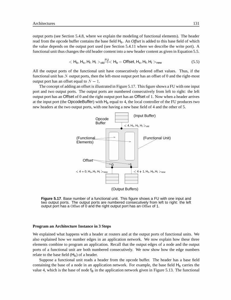
Architectures 131
output ports (see Section 5.4.8, where we explain the modeling of functional elements). The headerread from the opcode buffer contains the base fieldHb. An Offsetis added to this base field of whichthe value depends on the output port used (see Section 5.4.11 where we describe the write port). Afunctional unit thus changes the old header content into a new header content as given in Equation 5.5.
< Hb;Hs;Hf;Hl >oldFU!< Hb + Offset;Hs;Hf;Hl >new (5.5)
All the output ports of the functional unit have consecutively ordered offset values. Thus, if thefunctional unit hasN output ports, then the left-most output port has an offset of 0 and the right-mostoutput port has an offset equal toN � 1.
The concept of adding an offset is illustrated in Figure 5.17. This figure shows a FU with one inputport and two output ports. The output ports are numbered consecutively from left to right: the leftoutput port has anOffset of 0 and the right output port has anOffset of 1. Now when a header arrivesat the input port (theOpcodeBuffer) with Hb equal to 4, the local controller of the FU produces twonew headers at the two output ports, with one having a new base field of 4 and the other of 5.
< 4 + 1;Hs;Hf;Hl >new
0 1Offset
OpcodeBuffer
(Input Buffer)
(Output Buffers)
(Functional Unit)(FunctionalElements)
< 4;Hs;Hf;Hl >old
< 4 + 0;Hs;Hf;Hl >new
Figure 5.17 . Base number of a functional unit. This figure shows a FU with one input andtwo output ports. The output ports are numbered consecutively from left to right: the leftoutput port has a Offsetof 0 and the right output port has an Offsetof 1.
Program an Architecture Instance in 3 Steps
We explained what happens with a header at routers and at the output ports of functional units. Wealso explained how we number edges in an application network. We now explain how these threeelements combine to program an application. Recall that the output edges of a node and the outputports of a functional unit are both numbered consecutively. We now show how the edge numbersrelate to the base field (Hb) of a header.
Suppose a functional unit reads a header from the opcode buffer. The header has a base fieldcontaining the base of a node in an application network. For example, the base fieldHb carries thevalue 4, which is the base of nodefB in the application network given in Figure 5.13. The functional
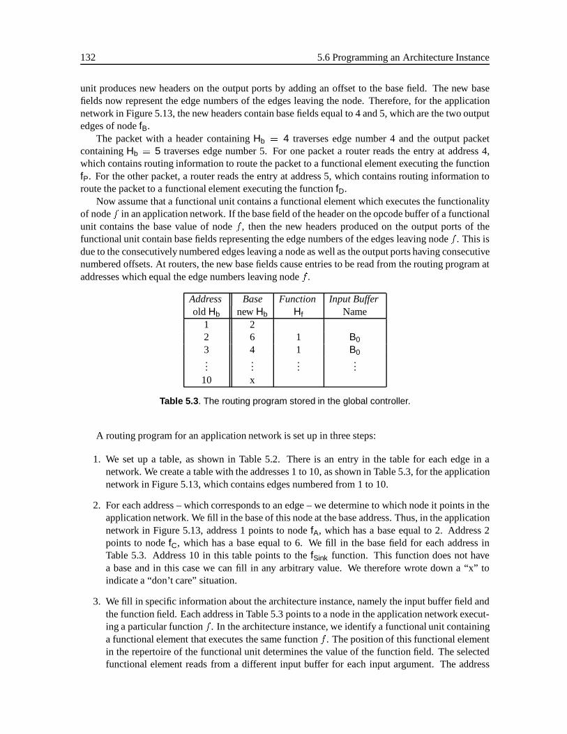
132 5.6 Programming an Architecture Instance
unit produces new headers on the output ports by adding an offset to the base field. The new basefields now represent the edge numbers of the edges leaving the node. Therefore, for the applicationnetwork in Figure 5.13, the new headers contain base fields equal to 4 and 5, which are the two outputedges of nodefB.
The packet with a header containingHb = 4 traverses edge number 4 and the output packetcontainingHb = 5 traverses edge number 5. For one packet a router reads the entry at address 4,which contains routing information to route the packet to a functional element executing the functionfP. For the other packet, a router reads the entry at address 5, which contains routing information toroute the packet to a functional element executing the functionfD.
Now assume that a functional unit contains a functional element which executes the functionalityof nodef in an application network. If the base field of the header on the opcode buffer of a functionalunit contains the base value of nodef , then the new headers produced on the output ports of thefunctional unit contain base fields representing the edge numbers of the edges leaving nodef . This isdue to the consecutively numbered edges leaving a node as well as the output ports having consecutivenumbered offsets. At routers, the new base fields cause entries to be read from the routing program ataddresses which equal the edge numbers leaving nodef .
Address Base Function Input Bufferold Hb newHb Hf Name
1 22 6 1 B0
3 4 1 B0...
......
...10 x
Table 5.3 . The routing program stored in the global controller.
A routing program for an application network is set up in three steps:
1. We set up a table, as shown in Table 5.2. There is an entry in the table for each edge in anetwork. We create a table with the addresses 1 to 10, as shown in Table 5.3, for the applicationnetwork in Figure 5.13, which contains edges numbered from 1 to 10.
2. For each address – which corresponds to an edge – we determine to which node it points in theapplication network. We fill in the base of this node at the base address. Thus, in the applicationnetwork in Figure 5.13, address 1 points to nodefA, which has a base equal to 2. Address 2points to nodefC, which has a base equal to 6. We fill in the base field for each address inTable 5.3. Address 10 in this table points to thefSink function. This function does not havea base and in this case we can fill in any arbitrary value. We therefore wrote down a “x” toindicate a “don’t care” situation.
3. We fill in specific information about the architecture instance, namely the input buffer field andthe function field. Each address in Table 5.3 points to a node in the application network execut-ing a particular functionf . In the architecture instance, we identify a functional unit containinga functional element that executes the same functionf . The position of this functional elementin the repertoire of the functional unit determines the value of the function field. The selectedfunctional element reads from a different input buffer for each input argument. The address
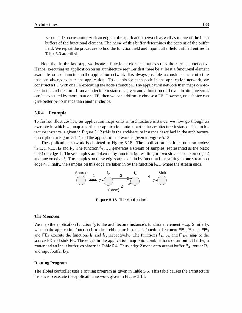
Architectures 133
we consider corresponds with an edge in the application network as well as to one of the inputbuffers of the functional element. The name of this buffer determines the content of the bufferfield. We repeat the procedure to find the function field and input buffer field until all entries inTable 5.3 are filled.
Note that in the last step, we locate a functional element that executes the correct functionf .Hence, executing an application on an architecture requires that there be at least a functional elementavailable for each function in the application network. It is always possible to construct an architecturethat can always execute the application. To do this for each node in the application network, weconstruct a FU with one FE executing the node’s function. The application network then mapsone-to-oneto the architecture. If an architecture instance is given and a function of the application networkcan be executed by more than one FE, then we can arbitrarily choose a FE. However, one choice cangive better performance than another choice.
5.6.4 Example
To further illustrate how an application maps onto an architecture instance, we now go though anexample in which we map a particular application onto a particular architecture instance. The archi-tecture instance is given in Figure 5.12 (this is the architecture instance described in the architecturedescription in Figure 5.11) and the application network is given in Figure 5.18.
The application network is depicted in Figure 5.18. The application has four function nodes:fSource, fSink, f0 andf1. The functionfSource generates a stream of samples (represented as the blackdots) on edge 1. These samples are taken in by functionf0, resulting in two streams: one on edge 2and one on edge 3. The samples on these edges are taken in by functionf1, resulting in one stream onedge 4. Finally, the samples on this edge are taken in by the functionfSink where the stream ends.
(base)
1 4Source f0 f1 Sink
3
2
Figure 5.18 . The Application.
The Mapping
We map the application functionf0 to the architecture instance’s functional elementFE0. Similarly,we map the application functionf1 to the architecture instance’s functional elementFE1. Hence,FE0andFE1 execute the functionsf0 and f1, respectively. The functionsfSource andFSink map to thesource FE and sink FE. The edges in the application map onto combinations of an output buffer, arouter and an input buffer, as shown in Table 5.4. Thus, edge 2 maps onto output bufferB4, routerR1
and input bufferB0.
Routing Program
The global controller uses a routing program as given in Table 5.5. This table causes the architectureinstance to execute the application network given in Figure 5.18.
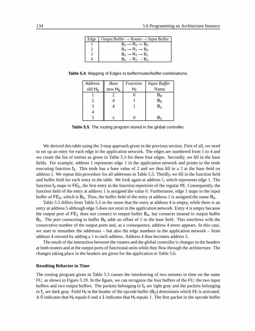
134 5.6 Programming an Architecture Instance
Edge Output Buffer! Router! Input Buffer1 B3 ! R0 ! B0
2 B4 ! R1 ! B0
3 B5 ! R2 ! B1
4 B5 ! R2 ! B2
Table 5.4 . Mapping of Edges to buffer/router/buffer combinations.
Address Base Function Input Bufferold Hb newHb Hf Name
1 2 0 B02 4 1 B0
3 4 1 B145 x 0 B2
Table 5.5 . The routing program stored in the global controller.
We derived this table using the 3-step approach given in the previous section. First of all, we needto set up an entry for each edge in the application network. The edges are numbered from 1 to 4 andwe create the list of entries as given in Table 5.3 for these four edges. Secondly, we fill in the basefields. For example, address 1 represents edge 1 in the application network and points to the nodeexecuting functionf0. This node has a base value of 2 and we thus fill in a 2 at the base field onaddress 1. We repeat this procedure for all addresses in Table 5.5. Thirdly, we fill in the function fieldand buffer field for each entry in the table. We look again at address 1, which represents edge 1. Thefunctionf0 maps toFE0, the first entry in the function repertoire of the regular PE. Consequently, thefunction field of the entry at address 1 is assigned the value 0. Furthermore, edge 1 maps to the inputbuffer of FE0, which isB0. Thus, the buffer field of the entry at address 1 is assigned the nameB0.
Table 5.3 differs from Table 5.5 in the sense that the entry at address 4 is empty, while there is anentry at address 5 although edge 5 does not exist in the application network. Entry 4 is empty becausethe output port ofFE1 does not connect to output bufferB4, but connects instead to output bufferB5. The port connecting to bufferB5 adds an offset of 1 to the base field. This interferes with theconsecutive number of the output ports and, as a consequence, address 4 never appears. In this case,we start to renumber the addresses – but also the edge numbers in the application network – fromaddress 4 onward by adding a 1 to each address. Address 4 thus becomes address 5.
The result of the interaction between the routers and the global controller is changes in the headersat both routers and at the output ports of functional units while they flow through the architecture. Thechanges taking place in the headers are given for the application in Table 5.6.
Resulting Behavior in Time
The routing program given in Table 5.5 causes the interleaving of two streams in time on the sameFU, as shown in Figure 5.19. In the figure, we can recognize the four buffers of the FU: the two inputbuffers and two output buffers. The packets belonging tof0 are light gray and the packets belongingto f1 are dark gray. FieldHf in the header of the opcode buffer (B0) determines which FE is activated.A 0 indicates thatHf equals 0 and a1 indicates thatHf equals 1. The first packet in the opcode buffer
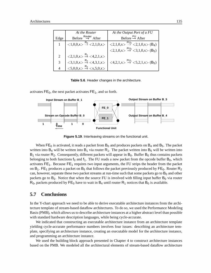
Architectures 135
At the Router At the Output Port of a FU
Edge BeforeRouter! After BeforeFU
! After
1 <1,0,0,x>R0! <2,1,0,x> <2,1,0,x>
FU0! <2,1,0,x> (B4)
<2,1,0,x>FU0! <3,1,0,x> (B5)
2 <2,1,0,x>R1! <4,2,1,x>
3 <3,1,0,x>R2! <4,3,1,x> <4,2,1,x>
FU1! <5,2,1,x> (B5)
4 <5,0,0,x>R2! <x,5,0,x>
Table 5.6 . Header changes in the architecture.
activatesFE0, the next packet activatesFE1, and so forth.
1 001
Stream on Opcode Buffer B_0
Input Stream on Buffer B_1
Time
FE_1
FE_0
Functional Unit
Output Stream on Buffer B_4
Output Stream on Buffer B_5
Figure 5.19 . Interleaving streams on the functional unit.
WhenFE0 is activated, it reads a packet fromB0 and produces packets onB4 andB5. The packetwritten intoB4 will be written intoB1 via routerR1. The packet written intoB5 will be written intoB1 via routerR2. Consequently, different packets will appear inB0. Buffer B0 thus contains packetsbelonging to both functionsf0 andf1. The FU reads a new packet from the opcode bufferB0, whichactivatesFE1. BecauseFE1 requires two input arguments, the FU strips the header from the packetonB1. FE1 produces a packet onB5 that follows the packet previously produced byFE0. RouterR2can, however, separate these two packet streams at run-time such that some packets go toB0 and otherpackets go toB2. Notice that when the source FU is involved with filling input bufferB0 via routerR0, packets produced byFE0 have to wait inB4 until routerR1 notices thatB0 is available.
5.7 Conclusions
In the Y-chart approach we need to be able to derive executable architecture instances from the archi-tecture template of stream-based dataflow architectures. To do so, we used the Performance ModelingBasis (PMB), which allows us to describe architecture instances at a higher abstract level than possiblewith standard hardware description languages, while being cycle-accurate.
We indicated that constructing an executable architecture instance from an architecture templateyielding cycle-accurate performance numbers involves four issues: describing an architecture tem-plate, specifying an architecture instance, creating an executable model for the architecture instance,and programming an architecture instance.
We used the building block approach presented in Chapter 4 to construct architecture instancesbased on the PMB. We modeled all the architectural elements of stream-based dataflow architecture
136 BIBLIOGRAPHY
as a building block at the abstract, cycle-accurate level. Furthermore, we showed the usefulness ofbuilding block and object oriented techniques like polymorphism and inheritance. These techniqueswere key to describing in a flexible way architectural elements having more than one behavior.
We showed that we use composition rules expressed in Backus-Naur Form (BNF) to define anarchitecture template. We modeled the architecture template of stream-based dataflow architecturesin Appendix A using BNF rules. We showed that BNF rules can also be used to define the grammarof an architecture description language. We used this language to describe a specific architectureinstance of the architecture template. We also showed how composition rules and building blockscombine such that a parser can automatically construct an executable architecture instance from anarchitecture description.
To provide an architecture instance with a workload, we need to program the architecture in-stances. We explained the programming model of stream-based dataflow architectures. This involvedour explaining how we model applications as networks and how we map these networks onto an archi-tecture instance. We also discussed a comprehensive example showing how we program a particulararchitecture instance for a particular application.
The generality of the architecture modeling approach presented in this chapter will be discussedin Chapter 7, where we use this approach to construct a retargetable architecture simulator for stream-based dataflow architectures.
Bibliography
John Backus and Peter Naur. The syntax and semantics of the proposed international algebraic lan-guage of the Zurich ACM-GAMM conference. InProceedings of the International Conference onInformation Processing (ICIP), Paris, 1959.
M. Ben-Ari. Principles of Concurrent Programming. Prentice-Hall, 1982.
Charles Donnelly and Richard Stallman.BISON, The YACC-compatible Parser Generator. The FreeSoftware Foundation, 1992. release 1.20.
Wolfgang Kreutzer.System simulation, programming styles and languages. International ComputerScience Series. Addison-Wesley, 1986.
Jeroen A.J. Leijten, Jef L. van Meerbergen, Adwin H. Timmer, and Jochen A.G. Jess. Prophid, adata-driven multi-processor architecture for high-performance DSP. InProc. ED&TC, 1997.
David R. Musser and Atul Saini.STL Tutorial and Reference Guide: C++ programmingwith standardtemplate library. Addison-Wesley Professional Computing Series, 1996.
Vern Paxson.Flex - fast lexical analyzer generator, 1990. Online manual pages of Flex.
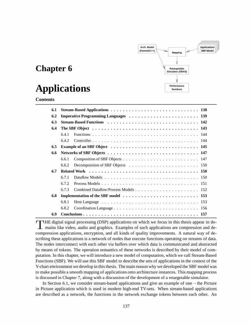
Chapter 6
Applications
RetargetableSimulator (ORAS)
PerformanceNumbers
Mapping(Pamela/C++)
Arch. Model ApplicationsSBF-Model
Contents
6.1 Stream-Based Applications . . . . . . . . . . . . . . . . . . . . . . . . . . . . . 138
6.2 Imperative Programming Languages . . . . . . . . . . . . . . . . . . . . . . . 139
6.3 Stream-Based Functions . . . . . . . . . . . . . . . . . . . . . . . . . . . . . . 142
6.4 The SBF Object . . . . . . . . . . . . . . . . . . . . . . . . . . . . . . . . . . . 143
6.4.1 Functions . . . . . . . . . . . . . . . . . . . . . . . . . . . . . . . . . . . 144
6.4.2 Controller . . . . . . . . . . . . . . . . . . . . . . . . . . . . . . . . . . . 144
6.5 Example of an SBF Object . . . . . . . . . . . . . . . . . . . . . . . . . . . . . 145
6.6 Networks of SBF Objects . . . . . . . . . . . . . . . . . . . . . . . . . . . . . . 147
6.6.1 Composition of SBF Objects .. . . . . . . . . . . . . . . . . . . . . . . . 147
6.6.2 Decomposition of SBF Objects. . . . . . . . . . . . . . . . . . . . . . . 150
6.7 Related Work . . . . . . . . . . . . . . . . . . . . . . . . . . . . . . . . . . . . 150
6.7.1 Dataflow Models . . . . . . . . . . . . . . . . . . . . . . . . . . . . . . . 150
6.7.2 Process Models . . . . . . . . . . . . . . . . . . . . . . . . . . . . . . . . 151
6.7.3 Combined Dataflow/Process Models . . . . . . . . . . . . . . . . . . . . . 152
6.8 Implementation of the SBF model . . . . . . . . . . . . . . . . . . . . . . . . . 153
6.8.1 Host Language. . . . . . . . . . . . . . . . . . . . . . . . . . . . . . . . 153
6.8.2 Coordination Language. . . . . . . . . . . . . . . . . . . . . . . . . . . . 156
6.9 Conclusions . . . . . . . . . . . . . . . . . . . . . . . . . . . . . . . . . . . . . . 157
THE digital signal processing (DSP) applications on which we focus in this thesis appear in do-mains like video, audio and graphics. Examples of such applications are compression and de-
compression applications, encryption, and all kinds of quality improvements. A natural way of de-scribing these applications is a network of nodes that execute functions operating on streams of data.The nodes interconnect with each other via buffers over which data is communicated and abstractedby means of tokens. The operation semantics of these networks is described by their model of com-putation. In this chapter, we will introduce a new model of computation, which we call Stream-BasedFunctions (SBF). We will use this SBF model to describe the sets of applications in the context of theY-chart environment we develop in this thesis. The main reason why we developed the SBF model wasto make possible a smooth mapping of applications onto architecture instances. This mapping processis discussed in Chapter 7, along with a discussion of the development of a retargetable simulator.
In Section 6.1, we consider stream-based applications and give an example of one – the Picturein Picture application which is used in modern high-end TV-sets. When stream-based applicationsare described as a network, the functions in the network exchange tokens between each other. An
137

138 6.1 Stream-Based Applications
important question is then what the token represents, and we investigate this problem in Section 6.2. InSections 6.3–6.3, we present stream-based dataflow functions model of computation. Many models ofcomputation already exist, like dataflow models, process models, and mixed dataflow/process models.In Section 6.7, we put the SBF model in perspective with respect to these models. We have constructedthe simulator SBFsim, for simulating networks of SBF objects. In Section 6.8, we explain how weconstructed this simulator using the programming language C++ and a multithreading package. Wealso show that we can reuse the building block approach (presented in Chapter 4) within the simulatorSBFsim.
6.1 Stream-Based Applications
We model DSP applications by means of a network, as already discussed in Chapter 5. We focusedthere only on the structural information of the network. In this chapter, we mainly focus on the modelof computation of such networks and the internals of each node in a network.
In a network describing a DSP application, the nodes describe functions that have a complexityranging from fine-grained to coarse-grained. Furthermore, the nodes execute concurrently, exchang-ing streams of tokens with each other via buffers. The buffers temporarily store the streams of tokenswithout changing the ordering of the tokens. We refer to applications that can be described in this wayas beingstream-based applications, and we define them as:
Definition 6.1. STREAM-BASED APPLICATION
A stream-based applicationis an application that can be described as a network or directed graphG(V;E), whereV defines a set of nodes executing functions on streams of data and whereE definesa set of buffers through which nodes exchange streams of data corresponding to a particular model ofcomputation. 2
A stream-based application describes astatic network, which means that nodes are not created ordestroyed during execution. Nodes within the network may produce and consume a variable amountof tokens while executing. As a consequence, the stream-based application may describe adynamicapplication, i.e., an application containing data-dependent conditionals that can only be resolved atrun-time.
Picture in Picture
An example of a stream-based video application is shown in Figure 6.1. It describes thePicturein Picture (PiP) algorithm, which reduces a picture to half its size in both horizontal and verticaldirections and places the reduced picture onto a full screen picture showing two images on a TVscreen [Janssen et al., 1997]. The Picture in Picture application is used in modern high-end televisions.
In the PiP example, aSource produces an infinite stream of video samples that are filtered byan N-tap Finite Impulse Response (FIR) filter. Then the stream is passed through a Sample-rateConverter (SRC) that performs a down-sampling of a factor two. Next, video images are transposed(Transpose), i.e., samples are re-ordered in such a way that two consecutive samples belong to twodifferent video lines. The stream then passes again through an N-tap FIR filter and a SRC, this timeto perform a vertical down-sampling of a factor two. The second transpose function performs a re-ordering on the stream that results such that consecutive samples now belong to the same video line.Finally, the sink consumes the samples.
In the example, the sample-rate converters have a fixed factor of two. In this case, each nodeknows exactly how many tokens to consume and produce while executing. The PiP algorithm thus
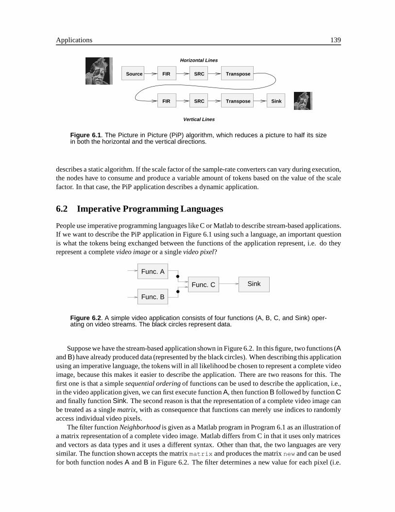
Applications 139
SinkTransposeSRCFIR
FIR SRC TransposeSource
Vertical Lines
Horizontal Lines
Figure 6.1 . The Picture in Picture (PiP) algorithm, which reduces a picture to half its sizein both the horizontal and the vertical directions.
describes a static algorithm. If the scale factor of the sample-rate converters can vary during execution,the nodes have to consume and produce a variable amount of tokens based on the value of the scalefactor. In that case, the PiP application describes a dynamic application.
6.2 Imperative Programming Languages
People use imperative programming languages like C or Matlab to describe stream-based applications.If we want to describe the PiP application in Figure 6.1 using such a language, an important questionis what the tokens being exchanged between the functions of the application represent, i.e. do theyrepresent a completevideo imageor a singlevideo pixel?
Func. A
Func. B
SinkFunc. C
Figure 6.2 . A simple video application consists of four functions (A, B, C, and Sink) oper-ating on video streams. The black circles represent data.
Suppose we have the stream-based applicationshown in Figure 6.2. In this figure, two functions (AandB) have already produced data (represented by the black circles). When describing this applicationusing an imperative language, the tokens will in all likelihood be chosen to represent a complete videoimage, because this makes it easier to describe the application. There are two reasons for this. Thefirst one is that a simplesequential orderingof functions can be used to describe the application, i.e.,in the video application given, we can first execute functionA, then functionB followed by functionCand finally functionSink. The second reason is that the representation of a complete video image canbe treated as a singlematrix, with as consequence that functions can merely use indices to randomlyaccess individual video pixels.
The filter functionNeighborhoodis given as a Matlab program in Program 6.1 as an illustration ofa matrix representation of a complete video image. Matlab differs from C in that it uses only matricesand vectors as data types and it uses a different syntax. Other than that, the two languages are verysimilar. The function shown accepts the matrixmatrix and produces the matrixnew and can be usedfor both function nodesA andB in Figure 6.2. The filter determines a new value for each pixel (i.e.
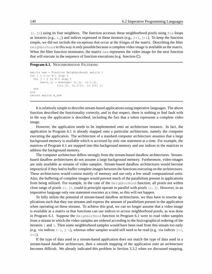
140 6.2 Imperative Programming Languages
(i,j) ) using its four neighbors. The function accesses these neighborhood pixels usingfor -loopsas iterators (e.g.,i ,j ) and indices expressed in these iterators (e.g.,i+1 , j+1 ). To keep the functionsimple, we did not include the exceptions that occur at the fringes of the matrix. Describing the filterneighborhood in this way isonlypossible because a complete video image is available as the matrix.When the filter function terminates, the matrixnew represents the video image for the next functionthat will execute in the sequence of function executions (e.g. functionC).
Program 6.1. NEIGHBORHOOD FILTERING
matrix new = Function NeighborHood( matrix )for i = 2 to N-1 step 1
for j = 2 to N-1 step 1new(i,j) = Average( (i,j), (i-1,j),
(i+1,j), (i,j-1), (i,j+1) );end
endreturn matrix A_new
It is relatively simple to describe stream-based applicationsusing imperative languages. The abovefunction described the functionality correctly, and in that respect, there is nothing to find fault within the way the application is described, including the fact that a token represents a complete videoimage.
However, the application needs to be implemented onto an architecture instance. In fact, theapplication in Program 6.1is already mapped onto a particular architecture, namely the computerexecuting the application. The architecture of a standard computer architecture assumes that a largebackground memory is available which is accessed by only one statement at a time. For example, thematrices of Program 6.1 are mapped into this background memory and use indices in the matrices toaddress the background memory.
The computer architecture differs strongly from the stream-based dataflow architectures. Stream-based dataflow architectures do not assume a large background memory. Furthermore, video-imagesare only available as streams of video samples. Stream-based dataflow architectures would becomeimpractical if they had to buffer complete images between the functions executing on the architectures.These architectures would consist mainly of memory and use only a few small computational units.Also, the buffering of complete images would prevent much of the parallelism present in applicationsfrom being utilized. For example, in the case of theNeighborHood function, all pixels not withinclose range of pixels(i,j) , could in principle operate in parallel with pixels(i,j) . However, in animperative language only one statement executes at a time, so this will not happen.
To fully utilize the potential of stream-based dataflow architectures, we thus have to rewrite ap-plications such that they use streams and express the amount of parallelism present in the applicationwhen operating on these streams. To achieve this goal, we can no longer assume that a video imageis available as a matrix ot that functions can use indices to access neighborhood pixels, as was donein Program 6.1. Suppose theNeighborHood function in Program 6.1 were to read video samplesfrom a stream in which the video samples are ordered according to the lexicographical ordering of theiteratorsi andj . Then some neighborhood samples would have been read from this stream too early(e.g. via indicesi-1 , j-1 ), whereas other samples would still need to be read (e.g. via indicesj+1 ,i+1 ).
If the type of data used in a stream-based application does not match the type of data used in astream-based dataflow architecture, then a smooth mapping of the application onto an architecturebecomes difficult. We already indicated this problem in Section 3.3.2 when we discussed mapping.
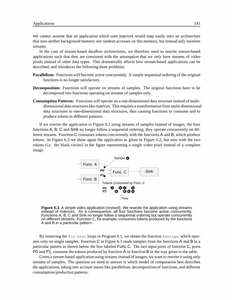
Applications 141
We cannot assume that an application which uses matrices would map easily onto an architecturethat uses neither background memory nor random accesses on this memory, but instead only involvesstreams.
In the case of stream-based dataflow architectures, we therefore need to rewrite stream-basedapplications such that they are consistent with the assumption that weonly have streams of videopixels instead of other data types. This dramatically affects how stream-based applications can bedescribed, and introduces the following three problems:
Parallelism: Functions will become active concurrently. A simple sequential ordering of the originalfunctions is no longer satisfactory.
Decomposition: Functions will operate on streams of samples. The original functions have to bedecomposed into functions operating on streams of samples only.
Consumption Patterns: Functions will operate on a one-dimensional data structure instead of multi-dimensional data structures like matrices. This requires a transformation from multi-dimensionaldata structures to one-dimensional data structures, thus causing functions to consume and toproduce tokens in different patterns.
If we rewrite the application in Figure 6.2 using streams of samples instead of images, the fourfunctionsA, B, C andSink no longer follow a sequential ordering; they operate concurrently on dif-ferent streams. FunctionC consumes tokens concurrently with the functionsA andB, which producetokens. In Figure 6.3 we show again the application as given in Figure 6.2, but now with the twotokens (i.e. the black circles) in the figure representing a single video pixel instead of a completeimage.
A AA
A
A
Tokens Consumed by Func. C
B BB B
Func. A
Func. B
SinkFunc. CP1P0
Time
P0P1
Sample
Figure 6.3 . A simple video application (revised). We rewrote the application using streamsinstead of matrices. As a consequence, all four functions become active concurrently.Functions A, B, C and Sink no longer follow a sequential ordering but operate concurrentlyon different streams. Function C, for example, consumes tokens produced by the functionsA and B in a particular pattern.
By removing thefor-next loops in Program 6.1, we obtain the functionAverage , which oper-ates only on single samples. FunctionC in Figure 6.3 reads samples from the functionsA andB in aparticular pattern as shown below the box labeledFunc:C. The two input ports of functionC, portsP0 andP1, consume the tokens produced by functionA or functionB in the way given in the table.
Given a stream-based application using streams instead of images, we want to rewrite it using onlystreams of samples. The question we need to answer is which model of computation best describesthe applications, taking into account issues like parallelism, decomposition of functions, and differentconsumption/production patterns.
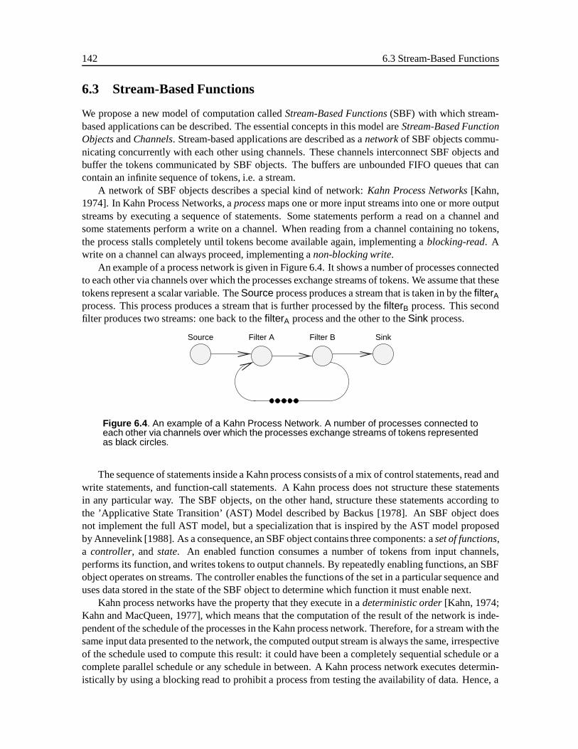
142 6.3 Stream-Based Functions
6.3 Stream-Based Functions
We propose a new model of computation calledStream-Based Functions(SBF) with which stream-based applications can be described. The essential concepts in this model areStream-Based FunctionObjectsandChannels. Stream-based applications are described as anetworkof SBF objects commu-nicating concurrently with each other using channels. These channels interconnect SBF objects andbuffer the tokens communicated by SBF objects. The buffers are unbounded FIFO queues that cancontain an infinite sequence of tokens, i.e. a stream.
A network of SBF objects describes a special kind of network:Kahn Process Networks[Kahn,1974]. In Kahn Process Networks, aprocessmaps one or more input streams into one or more outputstreams by executing a sequence of statements. Some statements perform a read on a channel andsome statements perform a write on a channel. When reading from a channel containing no tokens,the process stalls completely until tokens become available again, implementing ablocking-read. Awrite on a channel can always proceed, implementing anon-blocking write.
An example of a process network is given in Figure 6.4. It shows a number of processes connectedto each other via channels over which the processes exchange streams of tokens. We assume that thesetokens represent a scalar variable. TheSource process produces a stream that is taken in by thefilterAprocess. This process produces a stream that is further processed by thefilterB process. This secondfilter produces two streams: one back to thefilterA process and the other to theSink process.
SinkSource Filter A Filter B
Figure 6.4 . An example of a Kahn Process Network. A number of processes connected toeach other via channels over which the processes exchange streams of tokens representedas black circles.
The sequence of statements inside a Kahn process consists of a mix of control statements, read andwrite statements, and function-call statements. A Kahn process does not structure these statementsin any particular way. The SBF objects, on the other hand, structure these statements according tothe ’Applicative State Transition’ (AST) Model described by Backus [1978]. An SBF object doesnot implement the full AST model, but a specialization that is inspired by the AST model proposedby Annevelink [1988]. As a consequence, an SBF object contains three components: aset of functions,a controller, andstate. An enabled function consumes a number of tokens from input channels,performs its function, and writes tokens to output channels. By repeatedly enabling functions, an SBFobject operates on streams. The controller enables the functions of the set in a particular sequence anduses data stored in the state of the SBF object to determine which function it must enable next.
Kahn process networks have the property that they execute in adeterministic order[Kahn, 1974;Kahn and MacQueen, 1977], which means that the computation of the result of the network is inde-pendent of the schedule of the processes in the Kahn process network. Therefore, for a stream with thesame input data presented to the network, the computed output stream is always the same, irrespectiveof the schedule used to compute this result: it could have been a completely sequential schedule or acomplete parallel schedule or any schedule in between. A Kahn process network executes determin-istically by using a blocking read to prohibit a process from testing the availability of data. Hence, a
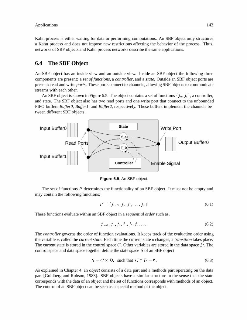
Applications 143
Kahn process is either waiting for data or performing computations. An SBF object only structuresa Kahn process and does not impose new restrictions affecting the behavior of the process. Thus,networks of SBF objects and Kahn process networks describe the same applications.
6.4 The SBF Object
An SBF object has an inside view and an outside view. Inside an SBF object the following threecomponents are present: aset of functions, a controller, and astate. Outside an SBF object ports arepresent: read and writeports. These ports connect to channels, allowing SBF objects to communicatestreams with each other.
An SBF object is shown in Figure 6.5. The object contains a set of functionsffa; fbg, a controller,and state. The SBF object also has two read ports and one write port that connect to the unboundedFIFO buffersBuffer0, Buffer1, andBuffer2, respectively. These buffers implement the channels be-tween different SBF objects.
Read Ports
Enable Signal
Output Buffer0
Write PortState
f_a
f_b
Input Buffer0
Input Buffer1Controller
Figure 6.5 . An SBF object.
The set of functionsP determines the functionality of an SBF object. It must not be empty andmay contain the following functions:
P = ffinit; fa; fb; : : : ; fxg: (6.1)
These functions evaluate within an SBF object in asequential ordersuch as,
finit; fa; fb; fa; fb; fa; : : : : (6.2)
Thecontrollergoverns the order of function evaluations. It keeps track of the evaluation order usingthe variablec, called thecurrent state. Each time the current statec changes, atransitiontakes place.The current state is stored in the control spaceC. Other variables are stored in the data spaceD. Thecontrol space and data space together define the state spaceS of an SBF object
S = C �D; such thatC \D = ;: (6.3)
As explained in Chapter 4, anobjectconsists of a data part and a methods part operating on the datapart [Goldberg and Robson, 1983]. SBF objects have a similar structure in the sense that the statecorresponds with the data of an object and the set of functions corresponds with methods of an object.The control of an SBF object can be seen as a special method of the object.
144 6.4 The SBF Object
6.4.1 Functions
For each functionf from the setP , there is a function call
f(x0; : : : ; xm; D) = (y0; : : : ; yn; D0); (6.4)
such that the functionf modifies the current data spaceD into the new data spaceD0 and the inputdatax0; : : : ; xm into the output datay0; : : : ; yn. A function call can either have no input data or nooutput data, in which case it describes asourceor asinkfunction respectively. A source function onlyproduces tokens and a sink function only consumes tokens. A function reads its input data from readports and writes its output data to write ports. It is statically determined on which read port or writeport a function operates.
When the controllerenablesa function, it reads input data from the input ports, performs thefunction and writes output data to output ports. The function reads all its input data using blockingreads. State variables are immediately available. A function can read only one token from an inputargument. Once a function has obtained all input data, it will not obtain any new inputs until it writesthe output data to the write ports and installs new state variables. During the evaluation of a function,the stateS cannot change and does not change. Consequently, a function operates without any sideeffects. When the enabled function has written all its output data, we say the function hasfired.
A function reads data from a read port using a blocking read. Therefore, if data is available, thefunction reads the data; otherwise it blocks. This causes a function to read its input datax0; : : : ; xmin a sequential order from the input ports. It first reads tokenx0, followed by tokenx1 and so forthuntil tokenxm has been read. The blocking read prohibits the testing of a read port on the availabilityof tokens. As a consequence, a function cannot have another behavior based on the results of testing acondition; thus it evaluates unconditionally: it is either waiting on a port or it is performing computa-tions. A function writes the output datay0; : : : ; yn to the appropriate write port using a non-blockingwrite, also in a sequential order.
6.4.2 Controller
The controller governs the enabling sequence of functions. It keeps track of this sequence in thecurrent state variablec. The controller moves from the current statec to another statec0 whenevera transition occurs. All obtainable states are described by the control spaceC. The control spaceis traversed as determined by thetransition function!, which associates the next statec0 with eachcurrent statec.
! : C �D ! C; !(c; d) = c0 (6.5)
To determine the next statec0, the transition function observes the control spaceC and the data spaceD. The controller cannot change the data space; it can only observe it. Although the controller isnot connected to any read or write port, the transition function describes dynamic behavior. Whendeciding what the next state will be, it observes the data spaceD affected only by the function ofP .
The transition function describes a path through the control space by going from the current stateto a new state. If both the data space and control space are observed to determine the next state, thetransition function describes infinitely many paths. Ateach new state, which path is started dependson the content ofD.
In a more restricted case, when the transition function observes only the control spaceC to deter-mine the next state, it always describes a single path to traverse the control space. Furthermore, if this
Applications 145
path is finite, the transition function determines a new statec which has previously been the currentstate, thus describing acycle. This cycle brings the state of the controller back into a previous state ina fixed number of transitions.
At each state, a specific function needs to be evaluated as determined by thebinding function�.This binding function associates a functionf from the setP with a particular control statec. Onlyone function can be associated with a state.
� : C ! P; �(c) = f (6.6)
Using the transition function! and the binding function�, the controller describes a sequence inwhich the functions of setP are enabled. A function becomes enabled and fires. This causes atransition to take place, and using! and� a new function is determined that is enabled the next time,leading up to the sequence described as follows:
finit�(!(S))�! fa
�(!(S))�! fb
�(!(S))�! : : : fx
�(!(S))�! : : : (6.7)
Thus an SBF object operates on streams by repeatedly enabling a function from the set of functionsP , which reads from a buffer and writes tokens to a buffer. We remark that only the functions usea blocking read. A transition, or alternatively the evaluation of the! and� functions, takes placeinstantaneously. This behavior described by an SBF object is referred to as aFire-and-Exit behavior.When we explain how we implement an SBF object, we explain why SBF objects describe suchbehavior.
The sequence given in Equation 6.7 results in a deterministic behavior of the SBF object. Thefunctions of setP all evaluate unconditionally because of the blocking read. They also observe onlyone read port at a time. For the same input sequence of tokens, functions evaluate in the same outputsequence. At the same time, the functions alter the data spaceD in a deterministic way, after all thefunctions have executed unconditionally. The transition function, which observes both the controlspace and the data space to resolve a new current state, also changes deterministically. Consequently,the complete SBF object describes a deterministic sequence.
When an SBF object is created, the controller needs to start at a particular statec. Within anSBF object, a specialinitialization functionfinit is available that initializes the stateC. This waythe variablec is set to a particular value. Within an SBF object, the first evaluated function is theinitialization function. It evaluates only once.
6.5 Example of an SBF Object
An example of an SBF object is given in Figure 6.6. The SBF object contains a set of functionsffa; fb; fcg, a controller, and a state containing the variablesc (the current state, being an element ofC) andx (a variable, being an element ofD).
Functionfa reads input data from the two read ports and writes output data to the write port.Functionfb reads the input data from the read port connected toBuffer0 and writes the output datato the write port. Functionfc does not have input data; it only writes output data to the write port. Allfunctions can change the data spaceD. However, only functionfa changes variablex in D and onlyfunctionfb reads variablex in D.
If function fa is enabled, it reads first one token fromBuffer0 and then one token fromBuffer1. IfBuffer0 does not contain any tokens, the complete SBF object blocks until a token becomes availablein Buffer0 even though data might already be available onBuffer1. When both tokens are available,
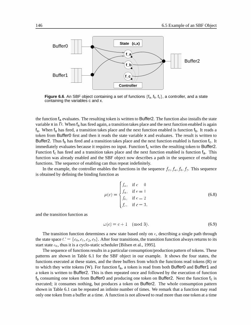
146 6.5 Example of an SBF Object
Controller
f_a
f_b
f_c
(c,x)State
Buffer1
Buffer0
Buffer2
Figure 6.6 . An SBF object containing a set of functions ffa; fb; fcg, a controller, and a statecontaining the variables c and x.
the functionfa evaluates. The resulting token is written toBuffer2. The function also installs the statevariablex inD. Whenfa has fired again, a transition takes place and the next function enabled is againfa. Whenfa has fired, a transition takes place and the next function enabled is functionfb. It reads atoken fromBuffer0 first and then it reads the state variablex and evaluates. The result is written toBuffer2. Thusfb has fired and a transition takes place and the next function enabled is functionfc. Itimmediately evaluates because it requires no input. Functionfc writes the resulting token toBuffer2.Functionfc has fired and a transition takes place and the next function enabled is functionfa. Thisfunction was already enabled and the SBF object now describes a path in the sequence of enablingfunctions. The sequence of enabling can thus repeat indefinitely.
In the example, the controller enables the functions in the sequencefa; fa; fb; fc. This sequenceis obtained by defining the binding function as
�(c) =
8>>>>><>>>>>:
fa; if c = 0
fa; if c = 1
fb; if c = 2
fc; if c = 3;
(6.8)
and the transition function as
!(c) = c+ 1 (mod 3): (6.9)
The transition function determines a new state based only onc, describing a single path throughthe state spaceC = fc0; c1; c2; c3g. After four transitions, the transition function always returns to itsstart statec0, thus it is a cyclo-static scheduler [Bilsen et al., 1995].
The sequence of functions results in a particular consumption/production pattern of tokens. Thesepatterns are shown in Table 6.1 for the SBF object in our example. It shows the four states, thefunctions executed at these states, and the three buffers from which the functions read tokens (R) orto which they write tokens (W). For functionfa, a token is read from bothBuffer0 andBuffer1 anda token is written toBuffer2. This is then repeated once and followed by the execution of functionfb consuming one token fromBuffer0 and producing one token onBuffer2. Next the functionfc isexecuted; it consumes nothing, but produces a token onBuffer2. The whole consumption patternshown in Table 6.1 can be repeated an infinite number of times. We remark that a function may readonly one token from a buffer at a time. A function is not allowed to read more than one token at a time
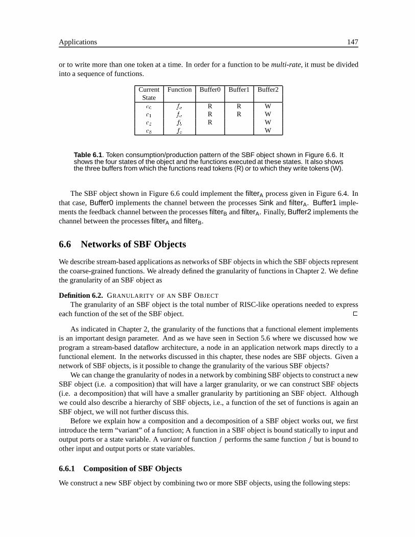
Applications 147
or to write more than one token at a time. In order for a function to bemulti-rate, it must be dividedinto a sequence of functions.
Current Function Buffer0 Buffer1 Buffer2Statec0 fa R R Wc1 fa R R Wc2 fb R Wc3 fc W
Table 6.1 . Token consumption/production pattern of the SBF object shown in Figure 6.6. Itshows the four states of the object and the functions executed at these states. It also showsthe three buffers from which the functions read tokens (R) or to which they write tokens (W).
The SBF object shown in Figure 6.6 could implement thefilterA process given in Figure 6.4. Inthat case,Buffer0 implements the channel between the processesSink andfilterA. Buffer1 imple-ments the feedback channel between the processesfilterB andfilterA. Finally,Buffer2 implements thechannel between the processesfilterA andfilterB.
6.6 Networks of SBF Objects
We describe stream-based applications as networks of SBF objects in which the SBF objects representthe coarse-grained functions. We already defined the granularity of functions in Chapter 2. We definethe granularity of an SBF object as
Definition 6.2. GRANULARITY OF AN SBF OBJECT
The granularity of an SBF object is the total number of RISC-like operations needed to expresseach function of the set of the SBF object. 2
As indicated in Chapter 2, the granularity of the functions that a functional element implementsis an important design parameter. And as we have seen in Section 5.6 where we discussed how weprogram a stream-based dataflow architecture, a node in an application network maps directly to afunctional element. In the networks discussed in this chapter, these nodes are SBF objects. Given anetwork of SBF objects, is it possible to change the granularity of the various SBF objects?
We can change the granularity of nodes in a network by combining SBF objects to construct a newSBF object (i.e. a composition) that will have a larger granularity, or we can construct SBF objects(i.e. a decomposition) that will have a smaller granularity by partitioning an SBF object. Althoughwe could also describe a hierarchy of SBF objects, i.e., a function of the set of functions is again anSBF object, we will not further discuss this.
Before we explain how a composition and a decomposition of a SBF object works out, we firstintroduce the term “variant” of a function; A function in a SBF object is bound statically to input andoutput ports or a state variable. Avariantof functionf performs the same functionf but is bound toother input and output ports or state variables.
6.6.1 Composition of SBF Objects
We construct a new SBF object by combining two or more SBF objects, using the following steps:
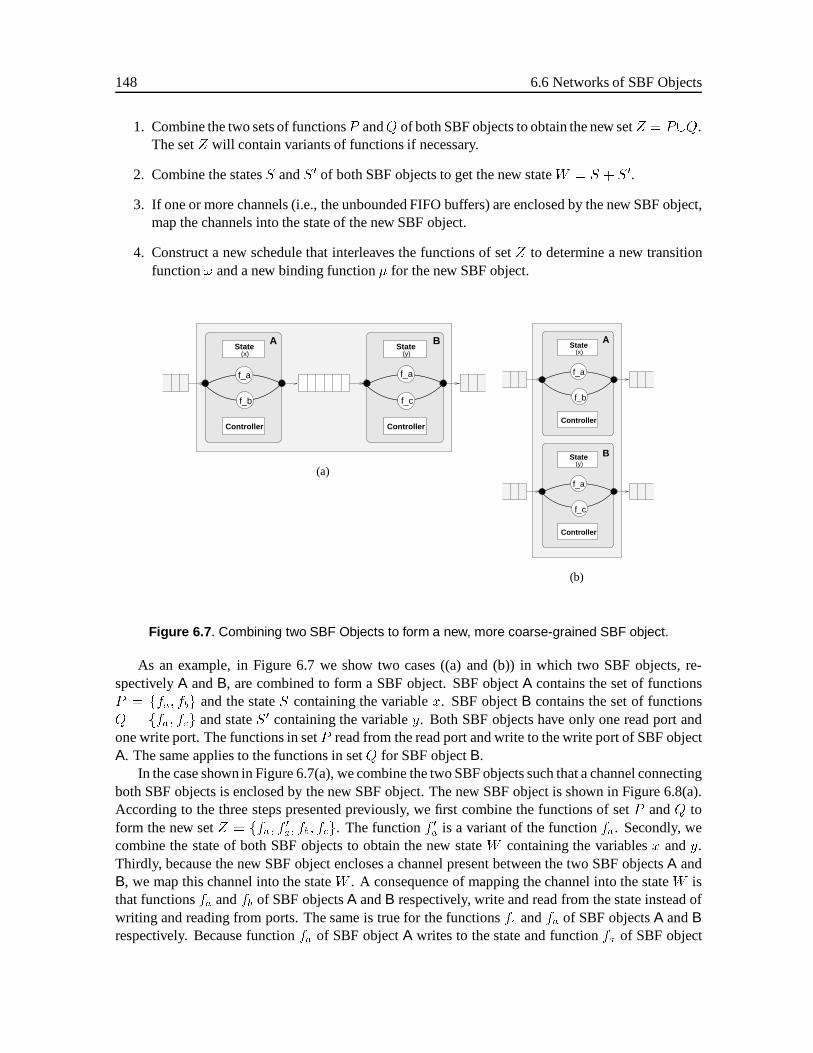
148 6.6 Networks of SBF Objects
1. Combine the two sets of functionsP andQ of both SBF objects to obtain the new setZ = P[Q.The setZ will contain variants of functions if necessary.
2. Combine the statesS andS 0 of both SBF objects to get the new stateW = S + S 0.
3. If one or more channels (i.e., the unbounded FIFO buffers) are enclosed by the new SBF object,map the channels into the state of the new SBF object.
4. Construct a new schedule that interleaves the functions of setZ to determine a new transitionfunction! and a new binding function� for the new SBF object.
f_af_a
(x) (y)
ControllerController
State StateA B
f_b f_c
(a)f_a
f_c
(y)
Controller
State B
A
f_a
f_b
(x)
Controller
State
(b)
Figure 6.7 . Combining two SBF Objects to form a new, more coarse-grained SBF object.
As an example, in Figure 6.7 we show two cases ((a) and (b)) in which two SBF objects, re-spectivelyA andB, are combined to form a SBF object. SBF objectA contains the set of functionsP = ffa; fbg and the stateS containing the variablex. SBF objectB contains the set of functionsQ = ffa; fcg and stateS 0 containing the variabley. Both SBF objects have only one read port andone write port. The functions in setP read from the read port and write to the write port of SBF objectA. The same applies to the functions in setQ for SBF objectB.
In the case shown in Figure 6.7(a), we combine the two SBF objects such that a channel connectingboth SBF objects is enclosed by the new SBF object. The new SBF object is shown in Figure 6.8(a).According to the three steps presented previously, we first combine the functions of setP andQ toform the new setZ = ffa; f
0a; fb; fcg. The functionf 0a is a variant of the functionfa. Secondly, we
combine the state of both SBF objects to obtain the new stateW containing the variablesx andy.Thirdly, because the new SBF object encloses a channel present between the two SBF objectsA andB, we map this channel into the stateW . A consequence of mapping the channel into the stateW isthat functionsfa andfb of SBF objectsA andB respectively, write and read from the state instead ofwriting and reading from ports. The same is true for the functionsfc andfa of SBF objectsA andBrespectively. Because functionfa of SBF objectA writes to the state and functionfa of SBF object
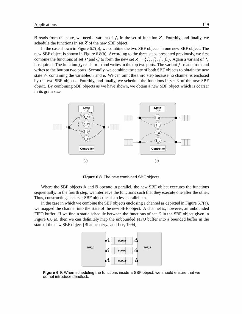
Applications 149
B reads from the state, we need a variant offa in the set of functionZ. Fourthly, and finally, weschedule the functions in setZ of the new SBF object.
In the case shown in Figure 6.7(b), we combine the two SBF objects in one new SBF object. Thenew SBF object is shown in Figure 6.8(b). According to the three steps presented previously, we firstcombine the functions of setP andQ to form the new setZ = ffa; f
0a; fb; fcg. Again a variant offa
is required. The functionfa reads from and writes to the top two ports. The variantf 0a reads from andwrites to the bottom two ports. Secondly, we combine the state of both SBF objects to obtain the newstateW containing the variablesx andy. We can omit the third step because no channel is enclosedby the two SBF objects. Fourthly, and finally, we schedule the functions in setZ of the new SBFobject. By combining SBF objects as we have shown, we obtain a new SBF object which is coarserin its grain size.
f_a
f_a’
f_b
f_c
(x,y)
Controller
State
(a)
(x,y)
f_a
f_c
f_b
f_a’
Controller
State
(b)
Figure 6.8 . The new combined SBF objects.
Where the SBF objectsA andB operate in parallel, the new SBF object executes the functionssequentially. In the fourth step, we interleave the functions such that they execute one after the other.Thus, constructing a coarser SBF object leads to less parallelism.
In the case in which we combine the SBF objects enclosing a channel as depicted in Figure 6.7(a),we mapped the channel into the state of the new SBF object. A channel is, however, an unboundedFIFO buffer. If we find a static schedule between the functions of setZ in the SBF object given inFigure 6.8(a), then we can definitely map the unbounded FIFO buffer into a bounded buffer in thestate of the new SBF object [Bhattacharyya and Lee, 1994].
3
2
1
1
2
3Buffer2
Buffer1
Buffer0
SBF_1SBF_0
Figure 6.9 . When scheduling the functions inside a SBF object, we should ensure that wedo not introduce deadlock.
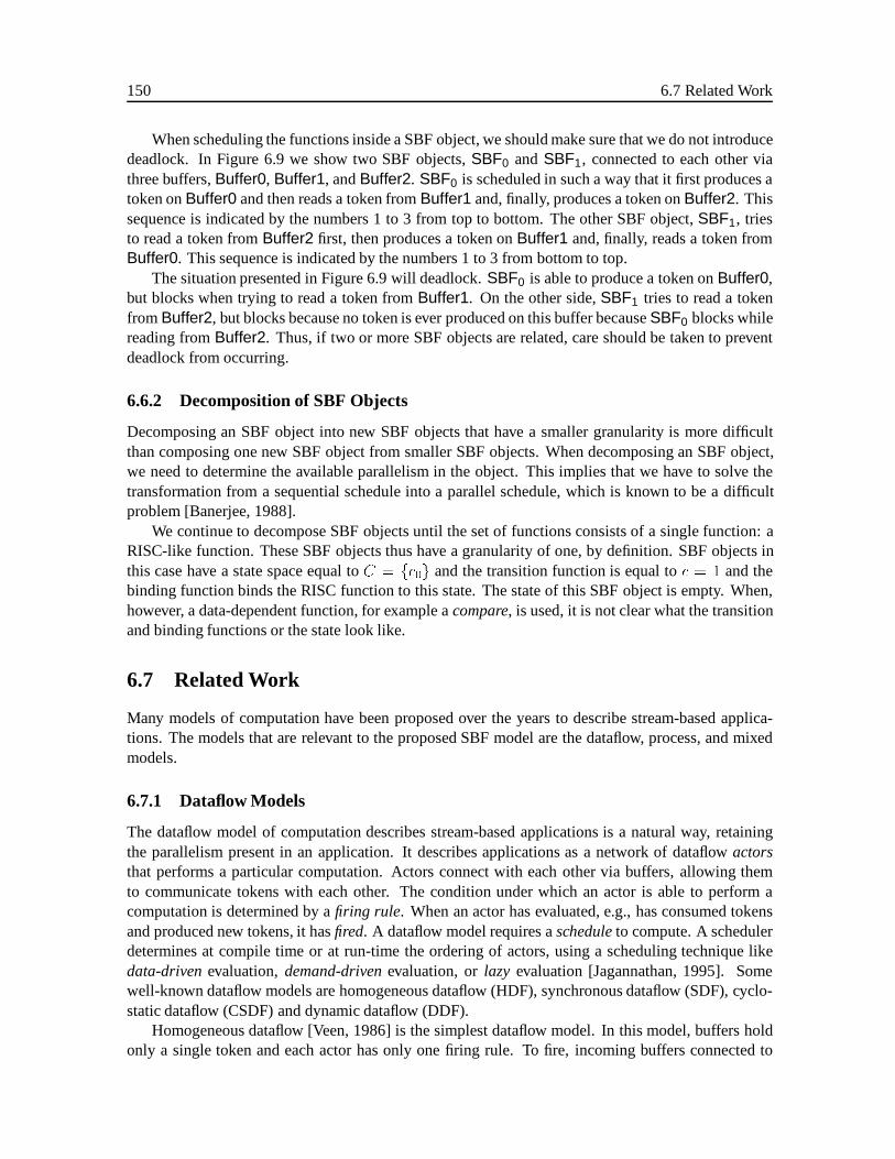
150 6.7 Related Work
When scheduling the functions inside a SBF object, we should make sure that we do not introducedeadlock. In Figure 6.9 we show two SBF objects,SBF0 andSBF1, connected to each other viathree buffers,Buffer0, Buffer1, andBuffer2. SBF0 is scheduled in such a way that it first produces atoken onBuffer0 and then reads a token fromBuffer1 and, finally, produces a token onBuffer2. Thissequence is indicated by the numbers 1 to 3 from top to bottom. The other SBF object,SBF1, triesto read a token fromBuffer2 first, then produces a token onBuffer1 and, finally, reads a token fromBuffer0. This sequence is indicated by the numbers 1 to 3 from bottom to top.
The situation presented in Figure 6.9 will deadlock.SBF0 is able to produce a token onBuffer0,but blocks when trying to read a token fromBuffer1. On the other side,SBF1 tries to read a tokenfrom Buffer2, but blocks because no token is ever produced on this buffer becauseSBF0 blocks whilereading fromBuffer2. Thus, if two or more SBF objects are related, care should be taken to preventdeadlock from occurring.
6.6.2 Decomposition of SBF Objects
Decomposing an SBF object into new SBF objects that have a smaller granularity is more difficultthan composing one new SBF object from smaller SBF objects. When decomposing an SBF object,we need to determine the available parallelism in the object. This implies that we have to solve thetransformation from a sequential schedule into a parallel schedule, which is known to be a difficultproblem [Banerjee, 1988].
We continue to decompose SBF objects until the set of functions consists of a single function: aRISC-like function. These SBF objects thus have a granularity of one, by definition. SBF objects inthis case have a state space equal toC = fc0g and the transition function is equal toc = 1 and thebinding function binds the RISC function to this state. The state of this SBF object is empty. When,however, a data-dependent function, for example acompare, is used, it is not clear what the transitionand binding functions or the state look like.
6.7 Related Work
Many models of computation have been proposed over the years to describe stream-based applica-tions. The models that are relevant to the proposed SBF model are the dataflow, process, and mixedmodels.
6.7.1 Dataflow Models
The dataflow model of computation describes stream-based applications is a natural way, retainingthe parallelism present in an application. It describes applications as a network of dataflowactorsthat performs a particular computation. Actors connect with each other via buffers, allowing themto communicate tokens with each other. The condition under which an actor is able to perform acomputation is determined by afiring rule. When an actor has evaluated, e.g., has consumed tokensand produced new tokens, it hasfired. A dataflow model requires ascheduleto compute. A schedulerdetermines at compile time or at run-time the ordering of actors, using a scheduling technique likedata-drivenevaluation,demand-drivenevaluation, orlazy evaluation [Jagannathan, 1995]. Somewell-known dataflow models are homogeneous dataflow (HDF), synchronous dataflow (SDF), cyclo-static dataflow (CSDF) and dynamic dataflow (DDF).
Homogeneous dataflow [Veen, 1986] is the simplest dataflow model. In this model, buffers holdonly a single token and each actor has only one firing rule. To fire, incoming buffers connected to
Applications 151
an actor must contain a token and all outcoming buffers must be empty. A feasible schedule alwaysexists and can be derived at compile time. This model cannot describe multi-rate behavior since abuffer can contain at most one token. HDF can describe static applications.
The synchronous dataflow model [Lee and Messerschmitt, 1987] is capable of describing multi-rate effects. In this model buffers are bounded FIFO buffers. Each actor still has one firing ruleand therefore the actors consume and produce a fixed pattern of tokens. The tokens consumed andproduced by all actors in a network can be expressed usingbalance equations. If a solution to thissystem of balance equations exists, a feasible schedule exists and can be found at compile time.The sizes of the buffers can also be determined at compile time. SDF can describe static multi-rateapplications.
The cyclo-static dataflow model [Bilsen et al., 1995] allows each actor to have one or more firingrules called upon in a known static order. This results in different consumption/production patternsof tokens, repeated infinitely many times. If a feasible schedule exists, it is found at compile time bysolving a system of balance equations. CSDF can describe cyclo-static multi-rate applications.
The dynamic dataflow model [Jagannathan, 1995] allows each actor to have a set of firing rulesthat are not ordered in any particular way. A specific function is bound to each rule of the set. Assoon as one of the rules in the set is satisfied, a valid firing is found and the function associated withthat rule is executed. This model can describe data-dependent consumption/production patterns and iscapable of describing dynamic applications. Since the rules are not ordered, non-deterministic effectsoccur. A typical example is the two-input merge function, which has two non-ordered firing-rules;the rule chosen first is unknown. The DDF model requires a run-time scheduler to evaluate. Be-cause a schedule cannot be found at compile-time owing to the Turing halting problem [Buck, 1993],the boundedness of the buffers cannot be calculated at compile time. DDF can describe dynamicapplications in a non-deterministic way.
A more restrictive DDF model is used in the Ptolemy system [Buck et al., 1992]. This modelalso allows each actor to have a set of firing rules, but they are ordered instead; one rule must followthe other. This model describes dynamic applications in a deterministic way. It requires a run-timescheduler to evaluate. This restrictive DDF model can describe dynamic applications in a deterministicway.
6.7.2 Process Models
Another way to describe stream-based applications is via process models. Process models describean application as a network of processes connected with each other via buffers. The buffers allowprocesses to communicate tokens with each other. Each process proceeds autonomously, i.e., it is notcontrolled by a global scheduler. A process interacts according to a particularprotocol with otherprocesses in a network. Two well-known process models with different protocols areKahn ProcessNetworks(see Section 6.3) andCommunicating Sequential Processes.
In Kahn process networks [Kahn, 1974; Kahn and MacQueen, 1977], buffers represent unboundedFIFO queues. These queues automatically buffer output of a process and allow processes, which runforever, to consume tokens from buffers at different rates. A process stores tokens on a buffer by usinga non-blocking write and reads tokens from a buffer with a blocking read. The blocking read prohibitstesting of ports on the availability of data; a process can only observe one port at a time. Hence aprocess is either waiting on a port or performing computations; therefore, Kahn process networksdescribe applications in a deterministic way.
In communicating sequential processes [Hoare, 1978, 1985], a buffer is a single place buffer. Ifone process puts a token into the buffer, it blocks until the process at the other end of the buffer
152 6.7 Related Work
removes the token from the buffer. It is possible to use unbounded FIFO buffers, but CSP must modelthem as a process. Within a CSP process which is intended to terminate, it is possible to test on theavailability of data and to select and perform a specific function based on the test results. Hence, theCSP model can describe applications in a non-deterministic way.
6.7.3 Combined Dataflow/Process Models
A combination of dataflow models and process models can also be used to describe stream-based ap-plications. Examples of combined dataflow/process models are theDataflow Process Networkmodeland theApplication State Transitionmodel. The former model combines the Kahn process networkmodel with dynamic dataflow, whereas the latter model combines CSP with dynamic dataflow.
In the dataflow process network model (DPN) [Lee and Parks, 1995; Parks, 1995], a single Kahnprocess contains a function and a set ofsequential firing rules. The process itself checks which firingrule applies, instead of some global scheduler doing this as in the dataflow models. The processchecks these rules in a sequential order with blocking reads (which is why this model usessequentialfiring rules). If a valid firing rule is found, the process fires the actor or function. At the moment theprocess fires the actor, all input arguments of the function are present and it evaluates instantaneously.Tokens are written to the output ports using a non-blocking write. After evaluating the function, theprocess checks the firing rules again until a valid firing is found.
In the Application State Transition Model (AST) [Kung, Annevelink, and Dewilde, 1984; Ann-evelink, 1988], a single CSP process contains a set of functions, whereby each function reads inputdata from specific read ports and writes data to specific write ports. When one function from the setis active, other functions are idle until it has evaluated. After a function evaluates, a control functionfc decides which function to evaluate next based on states and installs a new states0 [Held, 1996].Within the AST mode, the control function can read tokens from a special control port and use thesetokens to decide which function it should evaluate next. The CSP process used in the AST model isspecialized by forbidding the use of non-deterministic processes and by forbidding the use of sequen-tial compositions of processes. Because this model was inspired by the concept of the applicative statetransition model presented by Backus [1978], it is namedaccordingly.
When we compare the SBF model with other models discussed, we see that the SBF model de-scribes a combined dataflow/process model. It combines the Kahn process network model with thedynamic dataflow model. The SBF model differs from the DPN model by having a set of functionsinstead of a single function present in a process. Furthermore, the SBF model uses the notion of acontroller instead of a set of firing rules. As a consequence, when a function is activated within theSBF model, the function reads input data from input ports with a blocking read and writes data with anon-blocking write. The SBF model differs from the AST model in that it uses Kahn process networksinstead of CSP processes. A Kahn process runs forever, which is more consistent with the notion ofstreams. In addition, the Kahn model describes dynamic applications naturally in a deterministic way.In contrast, a CSP process typically terminates and describes a non-deterministic process [Hoare,1978]. Furthermore, the controller in a SBF model only observes the state of a SBF object to deter-mine the next state. Hence the controller does not have a direct connection to the world outside theSBF object using a control port, as it does in the AST model.
All three models presented distinguish between one or more functions and a control part. In ad-dition, the models describe a fire-and-exit behavior. Each time a function evaluates, the control partobserves that a transition took place. Such a transition leads to the clear sequence of function activa-tions as shown in Equation 6.7. However, a Kahn process is a free interleaving of control and functionstatements, as long as the sequence of statements uses blocking reads. In that case, a Kahn process
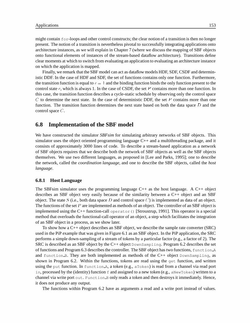
Applications 153
might containfor -loops and other control constructs; the clear notion of a transition is then no longerpresent. The notion of a transition is nevertheless pivotal to successfully integrating applications ontoarchitecture instances, as we will explain in Chapter 7 (where we discuss the mapping of SBF objectsonto functional elements of instances of the stream-based dataflow architecture). Transitions defineclear moments at which to switch from evaluating an application to evaluating an architecture instanceon which the application is mapped.
Finally, we remark that the SBF model can act as dataflow models HDF, SDF, CSDF and determin-istic DDF. In the case of HDF and SDF, the set of functions contains only one function. Furthermore,the transition function is equal toc = 1 and the binding function binds the only function present to thecontrol statec, which is always 1. In the case of CSDF, the setP contains more than one function. Inthis case, the transition function describes a cycle-static schedule by observing only the control spaceC to determine the next state. In the case of deterministic DDF, the setP contains more than onefunction. The transition function determines the next state based on both the data spaceD and thecontrol spaceC.
6.8 Implementation of the SBF model
We have constructed the simulatorSBFsimfor simulating arbitrary networks of SBF objects. Thissimulator uses the object oriented programming language C++ and a multithreading package, and itconsists of approximately 3000 lines of code. To describe a stream-based application as a networkof SBF objects requires that we describe both the network of SBF objects as well as the SBF objectsthemselves. We use two different languages, as proposed in [Lee and Parks, 1995]; one to describethe network, called thecoordination language, and one to describe the SBF objects, called thehostlanguage.
6.8.1 Host Language
The SBFsim simulator uses the programming language C++ as the host language. A C++ objectdescribes an SBF object very easily because of the similarity between a C++ object and an SBFobject. The stateS (i.e., both data spaceD and control spaceC) is implemented as data of an object.The functions of the setP are implemented as methods of an object. The controller of an SBF object isimplemented using the C++ function-calloperator() [Stroustrup, 1991]. This operator is a specialmethod that overloads the functional-call operator of an object, a step which facilitates the integrationof an SBF object in a process, as we show later.
To show how a C++ object describes an SBF object, we describe the sample rate converter (SRC)used in the PiP example that was given in Figure 6.1 as an SBF object. In the PiP application, the SRCperforms a simple down-sampling of a stream of tokens by a particular factor (e.g., a factor of 2). TheSRC is described as an SBF object by the C++ objectDownSampling . Program 6.2 describes the setof functions and Program 6.3 describes the controller. The SBF object has two functions,function A
and function B. They are both implemented as methods of the C++ objectDownSampling , asshown in Program 6.2. Within the functions, tokens are read using theget function, and writtenusing theput function. Infunction A, a token (e.g.,aToken ) is read from a channel via read portin , processed by the (identity) functionf and assigned to a new token (e.g.,aNewToken) written to achannel via write portout . Function B only reads a token and then destroys it immediately. Hence,it does not produce any output.
The functions within Program 6.2 have as arguments a read and a write port instead of values.
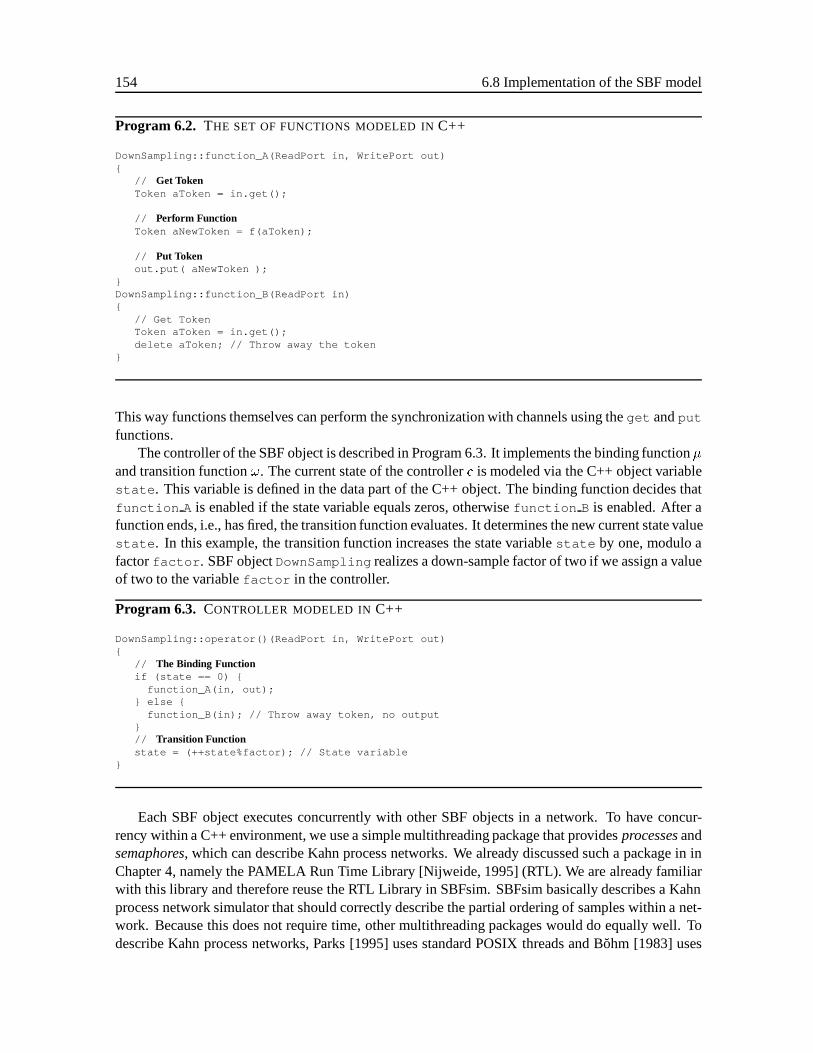
154 6.8 Implementation of the SBF model
Program 6.2. THE SET OF FUNCTIONS MODELED INC++
DownSampling::function_A(ReadPort in, WritePort out){
// Get TokenToken aToken = in.get();
// Perform FunctionToken aNewToken = f(aToken);
// Put Tokenout.put( aNewToken );
}DownSampling::function_B(ReadPort in){
// Get TokenToken aToken = in.get();delete aToken; // Throw away the token
}
This way functions themselves can perform the synchronization with channels using theget andput
functions.The controller of the SBF object is described in Program 6.3. It implements the binding function�
and transition function!. The current state of the controllerc is modeled via the C++ object variablestate . This variable is defined in the data part of the C++ object. The binding function decides thatfunction A is enabled if the state variable equals zeros, otherwisefunction B is enabled. After afunction ends, i.e., has fired, the transition function evaluates. It determines the new current state valuestate . In this example, the transition function increases the state variablestate by one, modulo afactorfactor . SBF objectDownSampling realizes a down-sample factor of two if we assign a valueof two to the variablefactor in the controller.
Program 6.3. CONTROLLER MODELED IN C++
DownSampling::operator()(ReadPort in, WritePort out){
// The Binding Functionif (state == 0) {
function_A(in, out);} else {
function_B(in); // Throw away token, no output}// Transition Functionstate = (++state%factor); // State variable
}
Each SBF object executes concurrently with other SBF objects in a network. To have concur-rency within a C++ environment, we use a simple multithreading package that providesprocessesandsemaphores, which can describe Kahn process networks. We already discussed such a package in inChapter 4, namely the PAMELA Run Time Library [Nijweide, 1995] (RTL). We are already familiarwith this library and therefore reuse the RTL Library in SBFsim. SBFsim basically describes a Kahnprocess network simulator that should correctly describe the partial ordering of samples within a net-work. Because this does not require time, other multithreading packages would do equally well. Todescribe Kahn process networks, Parks [1995] uses standard POSIX threads and B˘ohm [1983] uses
Applications 155
UNIX processes.Using the RTL, a process is created that we use to let an SBF object run concurrently with other
SBF objects. We use semaphores to implement FIFO buffers between the processes, as shown inProgram 5.1. The RTL implements a process scheduler that interleaves the execution of processes asexplained in Section 4.5. This gives the notion of SBF objects that execute concurrently.
Program 6.4. EXAMPLE OF PROCESS
// endless loopwhile(1){
(SBF object)(inPort 0, outPort 0);}
An example of a RTL process is given in Program 6.4. It describes a process that never terminates,because it contains an endless loop using thewhile(1) statement. Inside the loop, an SBF object iscalled as a function call with two arguments,inPort 0 andoutPort 0. These two arguments arerespectively the read port and write port connected to channels which are FIFO buffers that connectto other SBF objects within a network.
Building Blocks
The building blocks introduced in Chapter 4 are used again to describe a single SBF object. Thebehavioral part of a building block describes the process of an SBF object and could be the processdescription as given in Program 6.4. The structural part of the building block contains referencesto channels. For the SBF object described in Program 6.4, the structural part would thus containreferences to the channels via read portinPort 0 and write portoutPort 0.
The description given of the example of a system in Figure 4.5 describes a network of SBF objects,if we do not take resourceresource1 and resource2 into account. Each node in the network is abuilding block representing an SBF object and the edges between the nodes are unbounded FIFObuffers instead of semaphores. In this way, the network in Figure 4.5 describes an application as anetwork of SBF objects.
Fire-and-Exit Behavior
Each process defines a single thread-of-control that is passed on from the endless loop to the controllerof an SBF object via the function-call operator (this is shown in Program 6.3). Assuming that this isthe SBF objectDownSampling , then the binding function in the controller program gives the thread-of-control to eitherfunction A or function B. If, at any moment, one of the functions terminates(i.e., the function has fired), the function returns the thread-of-control to the controller, which executesthe transition function. This function updates the state of the SBF object. Finally, the thread-of-controlexits the controller and returns to the endless loop in Program 6.4 and the whole process described isrepeated another time.
The description in Program 6.4 shows clearly why an SBF object describes aFire-and-Exit be-havior. Recall the sequence that we presented in Equation 6.7, in which a function of the set fires anda transition takes place. Each time a functionfires, the transition function executes and the thread-of-controlexitsthe controller of the SBF object to return to the endless loop. Within the endless loop, wecan determine whether transition took place. As we will explain in Chapter 7, we use the notion of a

156 6.8 Implementation of the SBF model
(SBF Object)( .... ); (Transition)
Fire
Process
Exit
Figure 6.10 . Fire-and-Exit behavior.
transition to couple time to an SBF object. Each time a transition takes place, we execute apam delaystatement. Therefore, the execution of a function takes time.
Library of SBF Objects
We store SBF objects in alibrary to encourage reuse of previously defined SBF objects. Furthermore,we allow SBF objects to describe SBF objects in a parameterized form. Using the overloading ofthe function-call operator, an arbitrary SBF object with one input and one output can be used in Pro-gram 6.4. For that purpose, an SBF objectSBF Object is instantiated from the library. Notice that aprocess description as given in Program 6.4 describes a one-input, one-output function call. Thereforeseparate function descriptions are needed for other combinations of input and output arguments.
6.8.2 Coordination Language
The SBFsim simulator uses a dedicated coordination language that is implemented using aparsertorecognize a network description language1. This language describes the processes used in a networkand the connections between these processes. The parser also instantiates SBF objects from the libraryand places them onto the processes. Furthermore, it instantiates unbounded FIFOs for the channelsbetween SBF objects.
Program 6.5. NETWORK OFSBF OBJECTS
Program PictureInPicture {( x1 ) = Source<Source>( NULL );( x2 ) = FIR_H<FIR>( x1 );( x3 ) = SRC_H<DownSampling(factor=2)>( x2 );( x4 ) = Transpose_H<Transpose>( x3 );( x5 ) = FIR_V<FIR>( x4 );( x6 ) = SRC_V<DownSampling(factor=2)>( x5 );( x7 ) = Transpose_V<Transpose>( x6 );( NULL ) = Sink<Sink(stop=1000)>( x7 );
};
An example of a network description is given in Program 6.5. It describes the PiP applicationgiven in Figure 6.1. We create a process in the network description for each coarse-grained functionin the application. We created a process, for example, for the horizontal SRCSRCH that one inputx2 and one outputx3 . For each process, SBFsim creates a RTL process as described in Program 6.4.
1See Section 5.5, where we describe an architecture template, for more information about the use of a parser. In thatsection we also explain how the parser instantiates building blocks
Applications 157
SBFsim installs an SBF Object that is taken from a library on these processes, as described betweenthe “< >” brackets. For example, SBFsim installs on processSRCH the SBF objectDownSampling ,as described in Programs 6.2 and 6.3. An SBF object likeDownSampling can be parameterized.In the network description, we indicate that the SBF objects forSRCH andSRCV should perform adown-sampling of a factor of 2.
Each process in Program 6.5 has input and output arguments: on the left-hand side the outputarguments and on the right-hand side the input arguments. The source and sink processes have noinput and output arguments, respectively, as indicated by the keywordNULL. The channels betweenthe processes arex1 to x7 . In the example, SBFsim implements each channel as an unbounded FIFO.The sink process has the additional parameterstop=1000 , to indicate that it should stop executingafter it has read 1000 tokens. When the sink process stops, the whole network stops.
Although Kahn process networks require unbounded FIFOs, Parks [1995] discusses the construc-tion of Kahn networks using bounded FIFOs. He argues that the deterministic properties in a Kahnprocess networks are retained when bounded FIFOs are used. The use of bounded FIFOs requiresblocking writes to implement a write to a bounded channel. We constructed SBFsim such that it caninstantiate FIFO buffers of arbitrary (parameterized) capacity.
6.9 Conclusions
Within the Y-chart environment we want to map sets of applications onto architecture instances. Inthis chapter, we introduced the stream-based functions model of computation to describe the set ofapplications. The main reason why we developed the SBF model was to make a smooth mappingof applications onto architecture instances possible. The SBF model is a new model of computationsuitable for describing stream-based applications as a network of SBF objects.
We presented the SBF object and showed that it has a solid foundation in two well-known models:Kahn process networks and the AST model developed by Backus. The SBF model structures Kahnprocesses such that they consist of a set of functions, a controller and state. We call such a structuredKahn process an SBF object. SBF objects describe control (the controller) and dataflow (the set offunctions) in one and the same SBF object. This provides a high degree of flexibility when describing(complex) consumption/production patterns of tokens from streams. These consumption/productionpatterns result from transforming multi-dimensional data structures into one-dimensional streams.
SBF objects can describe fine-grained to very coarse-grained functions. As such, networks ofSBF objects describe applications at different levels of granularity. The granularity of the SBF objectsinfluences the granularity of the function executed by an functional element. The granularity of thesefunctions is an important design parameter in stream-based dataflow architectures. The granularityof SBF objects can be enlarged by combining them into a new SBF object or it can be reduced bydecomposing an SBF object into a set of new SBF objects.
We placed the SBF model of computation in the context of other relevant models of computa-tion. We considered dataflow models like homogeneous dataflow, synchronous dataflow, cyclo-staticdataflow, and dynamic dataflow. We also discussed process models like Kahn process networks andcommunicating sequential processes. Finally, we discussed models that combined dataflow/processmodels like the dataflow process network model and the application state transitionmodel. We showedthat the SBF model also describes a combined dataflow/process model.
Finally, we described the construction of SBFsim, a simulator that can simulate networks of SBFobjects. In the description of these networks, we made the distinction between the host language,in which we describe SBF objects, and the coordination language in which we describe the network
158 BIBLIOGRAPHY
of SBF objects. We showed that the SBF model of computation can be implemented very simplyusing C++ and a multithreading package. We also showed that we can reuse the building block ap-proach presented in Chapter 4 by representing each SBF object by a building block. The coordinationlanguage used in SBFsim is built using a parser that parses a network description language.
Bibliography
Jurgen Annevelink.HiFi, A Design Method for Implementing Signal Processing Algorithms on VLSIProcessor Arrays. PhD thesis, Delft University of Technology, 1988.
John Backus. Can programming be liberated from the von Neumann style? A functional style and itsalgebra of programs.Communications of the ACM, 21(8):613 – 641, 1978.
U. Banerjee.Dependence Analysis for Supercomputing. Kluwer Academic Publishers, 1988.
Shuvra S. Bhattacharyya and Edward A. Lee. Memory management for dataflow programming ofmultirate signal processing algorithms.IEEE Transactions on Signal Processing, 42(5), 1994.
G. Bilsen, M. Engels, R. Lauwereins, and J.A. Peperstraete. Cyclo-static data flow. InIEEE Interna-tional Conference ASSP, pages 3255 – 3258, 1995.
Joseph Buck, Soonhoi Ha, Edward A. Lee, and David G. Messerschmitt. Ptolemy: A framework forsimulating and prototyping heterogeneous systems.International Journal of Computer Simulation,1992. Special issue on Simulation Software Development.
J.T. Buck.Scheduling Dynamic Dataflow Graphs with Bounded Memory Using the Token Flow Model.PhD thesis, Dept. of EECS, University of California at Berkeley, 1993. Tech. Report UCB/ERL93/69.
A.P.W. Bohm.Dataflow Computation. Number 6 in CWI tract. Centrum voor Wiskunde en Informat-ica, Amsterdam, 1983. Dutch.
Adele Goldberg and David Robson.Smalltalk-80, The Language and Its Implementation. Addison-Wesley Publishing Company, Xerox Palo Alto Research Center, 1983.
Peter Held.Functional Design of Dataflow Networks. PhD thesis, Delft University of Technology,1996.
C.A.R. Hoare. Communicating sequential processes.Communications of the ACM, 21(8):666 – 677,1978.
C.A.R. Hoare.Communicating Sequential Processes. Prentice-Hall, 1985.
R. Jagannathan. Dataflow models. In E.Y. Zomaya, editor,Parallel and Distributed ComputingHandbook. McGraw-Hill, 1995.
Johan G.W.M. Janssen, Jeroen H. Stessen, and Peter H.N. de With. An advanced sampling rateconversion algorithm for video and graphics signals. InIEE Sixth International Conference onImage Processing and its Applications, Dublin, 1997.
Gilles Kahn. The semantics of a simple language for parallel programming. InProc. of the IFIPCongress 74. North-Holland Publishing Co., 1974.
BIBLIOGRAPHY 159
Gilles Kahn and David B. MacQueen. Coroutines and networks of parallel processes. InProc. of theIFIP Congress 77, pages 993 – 998. North-Holland Publishing Company Co., 1977.
S.Y. Kung, J. Annevelink, and P. Dewilde. Hierarchical iterative flowgraph integration for VLSI arrayprocessors. InProceedings University of Southern California (USC) Workshop on VLSI and SignalProcessing, 1984.
Edward A. Lee and David G. Messerschmitt. Synchronous data flow.Proc. IEEE, 75(9):1235 – 1245,1987.
Edward A. Lee and Thomas M. Parks. Dataflow process networks.Proceedings of the IEEE, 83(5):773–799, 1995.
Marc Nijweide. The pamela run-time library, version 1.3. Technical Report 1-68340-27(1995)06,Laboratory of Computer Architecture and Digital Techniques, Delft University of Technology,1995.http://dutepp0.et.tudelft.nl/ gemund/publications.html .
Tom Parks.Bounded Scheduling of Process Networks. PhD thesis, University of California at Berke-ley, 1995.
Bjarne Stroustrup.The C++ Programming Language. Addison-Wesley, 2nd edition, 1991.
Arthur H. Veen. Dataflow machine architecture.ACM Computing Surveys, 18(4):366–396, 1986.

160 BIBLIOGRAPHY
Chapter 7
Construction of a Retarget-able Simulator and Mapping
PerformanceNumbers
Applications
SBF-Model(Pamela/C++)
Arch. Model
RetargetableSimulator (ORAS)
Mapping
Contents
7.1 Retargetable Architecture Simulators . . . . . . . . . . . . . . . . . . . . . . . 162
7.1.1 Requirements . . . . . . . . . . . . . . . . . . . . . . . . . . . . . . . . . 163
7.2 The Object Oriented Retargetable Simulator (ORAS) . . . . . . . . . . . . . . 163
7.3 Development of ORAS . . . . . . . . . . . . . . . . . . . . . . . . . . . . . . . . 165
7.3.1 Step 1: Structure . . . . . . . . . . . . . . . . . . . . . . . . . . . . . . . 165
7.3.2 Step 2: Execution Model . . . . . . . . . . . . . . . . . . . . . . . . . . . 166
7.3.3 Step 3: Metric Collectors . . . . . . . . . . . . . . . . . . . . . . . . . . . 166
7.4 Mapping Applications . . . . . . . . . . . . . . . . . . . . . . . . . . . . . . . . 167
7.4.1 Mapping Approach . . . . . . . . . . . . . . . . . . . . . . . . . . . . . . 168
7.4.2 Matching Models of Architecture and Computation . . . . . . . . . . . . . 169
7.4.3 Control Hierarchy . . . . . . . . . . . . . . . . . . . . . . . . . . . . . . 170
7.5 The Interface Between Application and Architecture . . . . . . . . . . . . . . . 172
7.5.1 The Application – Architecture Interface . . . . . . . . . . . . . . . . . . 173
7.5.2 Restricting Resources . . . . . . . . . . . . . . . . . . . . . . . . . . . . . 175
7.6 Construction Example . . . . . . . . . . . . . . . . . . . . . . . . . . . . . . . . 175
7.7 Related Work . . . . . . . . . . . . . . . . . . . . . . . . . . . . . . . . . . . . 176
7.8 Discussion on ORAS . . . . . . . . . . . . . . . . . . . . . . . . . . . . . . . . . 177
7.8.1 Building Blocks . . . . . . . . . . . . . . . . . . . . . . . . . . . . . . . 178
7.8.2 High-level Primitives . . . . . . . . . . . . . . . . . . . . . . . . . . . . . 178
7.8.3 Interpreted Model . . . . . . . . . . . . . . . . . . . . . . . . . . . . . . . 178
7.8.4 Limitations . . . . . . . . . . . . . . . . . . . . . . . . . . . . . . . . . . 178
7.9 A Generic Approach for a Retargetable Simulator . . . . . . . . . . . . . . . . 179
7.9.1 Step 1: Structure . . . . . . . . . . . . . . . . . . . . . . . . . . . . . . . 179
7.9.2 Step 2: Execution Model . . . . . . . . . . . . . . . . . . . . . . . . . . . 179
7.9.3 Step 3: Metric Collectors . . . . . . . . . . . . . . . . . . . . . . . . . . . 180
7.9.4 Mapping . . . . . . . . . . . . . . . . . . . . . . . . . . . . . . . . . . . 180
7.10 Conclusions . . . . . . . . . . . . . . . . . . . . . . . . . . . . . . . . . . . . . . 180
161
162 7.1 Retargetable Architecture Simulators
THE use of the concepts presented in the previous chapters, for the construction of theObjectoriented Retargetable Architecture Simulator(ORAS) is what we discuss in this chapter. We
also discuss how applications map onto executable architecture instances that have been derived fromthe architecture template of stream-based dataflow architectures, using ORAS.
So far, we have discussed performance modeling techniques in Chapter 4 to model systems toacquire performance numbers. In Chapter 5, we used this modeling technique to construct executablearchitecture instances of stream-based dataflow models using building blocks. In Chapter 6 we ex-plained how we model applications using the stream-based function (SBF) models. In this chapter,we combine the concepts presented in the last three chapters to construct ORAS.
A retargetable simulator derives specific simulators for different architecture instances. It doesthis from an architecture template as we discuss in Section 7.1. The retargetable simulator ORAS ispresented in Section 7.2 and is followed in Section 7.3 by an explanation of the three steps involvedwithin ORAS. Being able to derive a simulator for an architecture instance is not all that is requiredto produce performance numbers; we must also map applications onto such an architecture instance.How applications, which are written as networks of SBF objects, map onto architecture instances isdiscussed in Section 7.4. The SBF model describes dynamic dataflow. The workload that an applica-tion represents may change, depending on the content of the stream that the application processes atrun-time. To reflect the correct dynamic workload on an architecture instance without much modifi-cations an architecture/application interface is needed, as we discuss in Section 7.5. In Section 7.6,we present an example that shows how ORAS constructs an architecture instance that executes thePicture in Picture (PiP) application (discussed in Chapter 6). We look at a one-to-one mapping and amany-to-one mapping of this application onto an architecture instance. In Section 7.7 we discuss re-lated work on constructing high-level retargetable architecture simulators. In Section 7.8 we evaluateORAS in the context of other architecture simulators. Finally, in Section 7.9, we reconsider the threesteps used in ORAS and show how they provide a generic outline for retargetable simulators for otherarchitecture templates.
7.1 Retargetable Architecture Simulators
To be able to execute architecture instances within the Y-chart environment, we need a retargetablearchitecture simulator for the architecture template of stream-based dataflow architectures. We define,inspired by [Marwedel and Goossens, 1995], a retargetable architecture simulator to be
Definition 7.1. RETARGETABLE ARCHITECTURESIMULATOR
A Retargetable Architecture Simulatoris a simulator that can simulate different architecture in-stances from an architecture template if an architecture description is provided for each architectureinstance. 2
In this chapter, we develop a retargetable simulator that derives a specific executable simulatorfor a specific architecture instance. We also discussed the development of the retargetable simulatorin [Kienhuis et al., 1998]. When we say a retargetable simulatorderivesa specific executable sim-ulator, we mean that the retargetable simulator instantiates a specific executable simulator in varioussteps. By executing such a derived simulator, we obtain the desired performance numbers for anarchitecture instance.

Construction of a Retargetable Simulator and Mapping 163
7.1.1 Requirements
The retargetable simulator that we develop for stream-based dataflow architectures needs to satisfy tothe requirements of retargetability, execution speed, andaccuracy.
Retargetability The retargetable architecture simulator must be capable of deriving simulators forall possible architecture instances of an architecture template. The parameters present in anarchitecture template of stream-based dataflow architectures clearly indicate the level of retar-getability required. We should exploit this confinement to obtain efficient retargetable simu-lators. Furthermore, the derived simulator should simulate valid instances of the architecturetemplate. We thus need to be able to verify whether an architecture instance is a valid one withrespect to the architecture template of stream-based dataflow architectures.
Execution SpeedThe retargetable simulator will be used in Chapter 8 to evaluate the performanceof architecture instances for the purpose of design space exploration. This leads to a veryimportant requirement for the derived simulators, namely their execution speed. In the end itis the execution speed that determines the number of instances which we can evaluate withina certain amount of time. This requirement is especially important in application domainslike video and radar that are very computationally intensive and involve a large amount ofcommunication. Providing support for retargetability introduces a certain amount of overheadin a simulator. Since this overhead reduces the simulation speed of the derived simulators, itshould be kept as small as possible.
Accuracy Here we study derived simulators that deliver cycle-accurate performance numbers. Thesesimulators must also be able to execute the dynamic behavior of both the architecture and theapplications. That is to say, the simulators must evaluate an interpreted performance model1.We provide such a model by mapping applications onto architecture instances and executingthe application on the architecture instance.
7.2 The Object Oriented Retargetable Simulator (ORAS)
We develop theObject Oriented Retargetable Simulator(ORAS), which derives a specific simulatorfor an architecture instance using the following three steps:
1. ORAS constructs the structure of an architecture instance from a textual architecture descrip-tion.
2. ORAS adds an execution model to the structure of the architecture instance to obtain an exe-cutable architecture instance.
3. ORAS instruments the executable architecture instance withmetric collectorsto measure andto extract performance numbers for selected performance metrics.
The three steps implemented in ORAS are shown in Figure 7.1. The first step concerns only thestructure of architecture instances. In this step, ORAS exploits object oriented principles to constructthe structure of architecture instances. It employs a parser that combines architectural elements, whichare modeled as building blocks, to construct the structure of a stream-based dataflow architecture
1See Chapter 4 where we explain what interpreted and uninterpreted performance models are
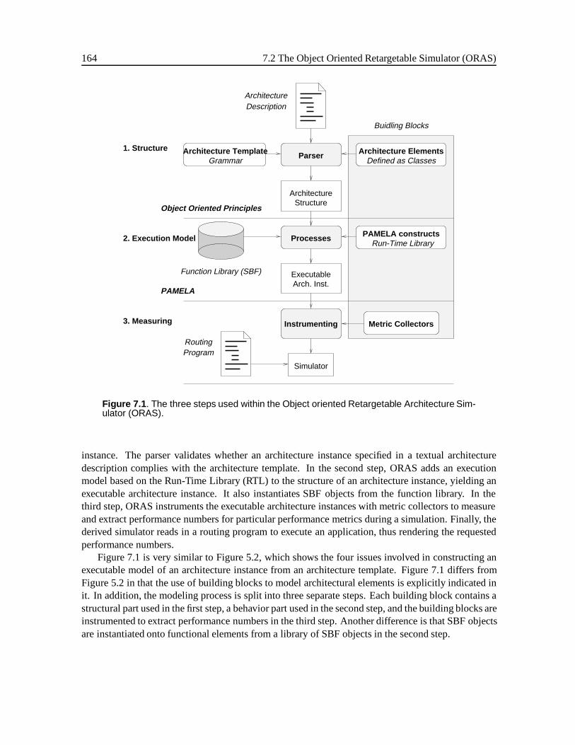
164 7.2 The Object Oriented Retargetable Simulator (ORAS)
Buidling Blocks
Architecture
Simulator
ExecutableArch. Inst.
Run-Time Library
Defined as ClassesGrammar
1. Structure
2. Execution Model
3. Measuring
Object Oriented Principles
PAMELA
Function Library (SBF)
DescriptionArchitecture
Parser
Processes
Instrumenting
Architecture Template Architecture Elements
PAMELA constructs
Metric Collectors
Structure
RoutingProgram
Figure 7.1 . The three steps used within the Object oriented Retargetable Architecture Sim-ulator (ORAS).
instance. The parser validates whether an architecture instance specified in a textual architecturedescription complies with the architecture template. In the second step, ORAS adds an executionmodel based on the Run-Time Library (RTL) to the structure of an architecture instance, yielding anexecutable architecture instance. It also instantiates SBF objects from the function library. In thethird step, ORAS instruments the executable architecture instances with metric collectors to measureand extract performance numbers for particular performance metrics during a simulation. Finally, thederived simulator reads in a routing program to execute an application, thus rendering the requestedperformance numbers.
Figure 7.1 is very similar to Figure 5.2, which shows the four issues involved in constructing anexecutable model of an architecture instance from an architecture template. Figure 7.1 differs fromFigure 5.2 in that the use of building blocks to model architectural elements is explicitly indicated init. In addition, the modeling process is split into three separate steps. Each building block contains astructural part used in the first step, a behavior part used in the second step, and the building blocks areinstrumented to extract performance numbers in the third step. Another difference is that SBF objectsare instantiated onto functional elements from a library of SBF objects in the second step.

Construction of a Retargetable Simulator and Mapping 165
7.3 Development of ORAS
In our development of ORAS, we focused primarily on constructing a retargetable architecture sim-ulator that executes fast while being cycle-accurate and capable of performing a functionally correctsimulation. We now elaborate on the three steps used in ORAS.
7.3.1 Step 1: Structure
The first step taken in ORAS concerns the construction of an architecture instance that is a feasibleinstance of the architecture template of the stream-based dataflow architecture. The construction ofsuch complex structures is easier if a programming language satisfies the following requirements:
Composition We defined an architecture to be a collection of interconnected architectural elementsas explained in Section 5.1. Each architectural element defines the constituent elements of anarchitecture instance and is modeled as a building block. We combine these building blocks toform larger hierarchical structures. For setting up the structure of an architecture instance, onlythe structural part of a building block is relevant.
Behaviors We introduced the notion of “architectural element type” to indicate that an architecturalelement has properties that can be implemented using more than one behavior. We describethe concept oftypesby means of abstract classes. When we construct an architecture usingonly types, we can still select various behaviors. This is illustrated in Figure 5.4), in which weshow the typeBufferdescribed as an abstract class with read and write methods. Three classesare derived from this abstract class, and they implement different behaviors, namely that of ahandshake buffer, a bounded FIFO buffer, and an unbounded FIFO buffer. For the stream-baseddataflow architecture we set up a class hierarchy (as shown in Figure 5.5) which shows theabstract classes describing architectural element types and the derived classes describing thevarious behaviors of the types.
Verification The architecture instance for which ORAS derives a simulator must comply with thearchitecture template of stream-based dataflow architecture. We explained in Section 5.5 howwe can specify an architecture template in terms of composition rules in BNF2. These rulesalso describe the grammar of an architecture description language.
ORAS uses a parser (i.e., Flex and Bison) to decompose a textual architecture description intoelements that the parser matches against the grammar of the architecture template. If a validrule is found, the parser activates the associated action; for example, instantiating an objectrepresenting a building block from the class hierarchy shown in Figure 5.5. The parser alsoresolves interconnections between objects, i.e., which object connects to which other object.
High-Level Constructs ORAS constructs the structure of architecture instances by combining ob-jects. To facilitate the combination of objects, ORAS adopts high-level programming constructslike vectors, lists, andmaps. These high-level constructs are part of the new standard in C++libraries called theStandard Template Library(STL) [Musser and Saini, 1996]. Because STL3
implements the high-level constructs using the C++ template mechanism [Stroustrup, 1991],the constructs are very efficient and introduce very little overhead. STL has proven to be a keytechnology for the effective and efficient development of ORAS.
2See appendix A for the BNF rules describing the composition rules of the architecture template of stream-based dataflowarchitectures
3Examples of STL constructs were shown when describing the various building blocks in Section 5.4
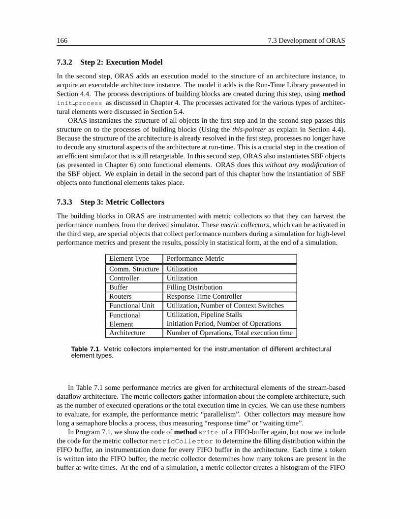
166 7.3 Development of ORAS
7.3.2 Step 2: Execution Model
In the second step, ORAS adds an execution model to the structure of an architecture instance, toacquire an executable architecture instance. The model it adds is the Run-Time Library presented inSection 4.4. The process descriptions of building blocks are created during this step, usingmethodinit process as discussed in Chapter 4. The processes activated for the various types of architec-tural elements were discussed in Section 5.4.
ORAS instantiates the structure of all objects in the first step and in the second step passes thisstructure on to the processes of building blocks (Using thethis-pointeras explain in Section 4.4).Because the structure of the architecture is already resolved in the first step, processes no longer haveto decode any structural aspects of the architecture at run-time. This is a crucial step in the creation ofan efficient simulator that is still retargetable. In this second step, ORAS also instantiates SBF objects(as presented in Chapter 6) onto functional elements. ORAS does thiswithout any modificationofthe SBF object. We explain in detail in the second part of this chapter how the instantiation of SBFobjects onto functional elements takes place.
7.3.3 Step 3: Metric Collectors
The building blocks in ORAS are instrumented with metric collectors so that they can harvest theperformance numbers from the derived simulator. Thesemetric collectors, which can be activated inthe third step, are special objects that collect performance numbers during a simulation for high-levelperformance metrics and present the results, possibly in statistical form, at the end of a simulation.
Element Type Performance Metric
Comm. Structure UtilizationController UtilizationBuffer Filling DistributionRouters Response Time ControllerFunctional Unit Utilization, Number of Context SwitchesFunctionalElement
Utilization, Pipeline StallsInitiation Period, Number of Operations
Architecture Number of Operations, Total execution time
Table 7.1 . Metric collectors implemented for the instrumentation of different architecturalelement types.
In Table 7.1 some performance metrics are given for architectural elements of the stream-baseddataflow architecture. The metric collectors gather information about the complete architecture, suchas the number of executed operations or the total execution time in cycles. We can use these numbersto evaluate, for example, the performance metric “parallelism”. Other collectors may measure howlong a semaphore blocks a process, thus measuring “response time” or “waiting time”.
In Program 7.1, we show the code ofmethodwrite of a FIFO-buffer again, but now we includethe code for the metric collectormetricCollector to determine the filling distribution within theFIFO buffer, an instrumentation done for every FIFO buffer in the architecture. Each time a tokenis written into the FIFO buffer, the metric collector determines how many tokens are present in thebuffer at write times. At the end of a simulation, a metric collector creates a histogram of the FIFO
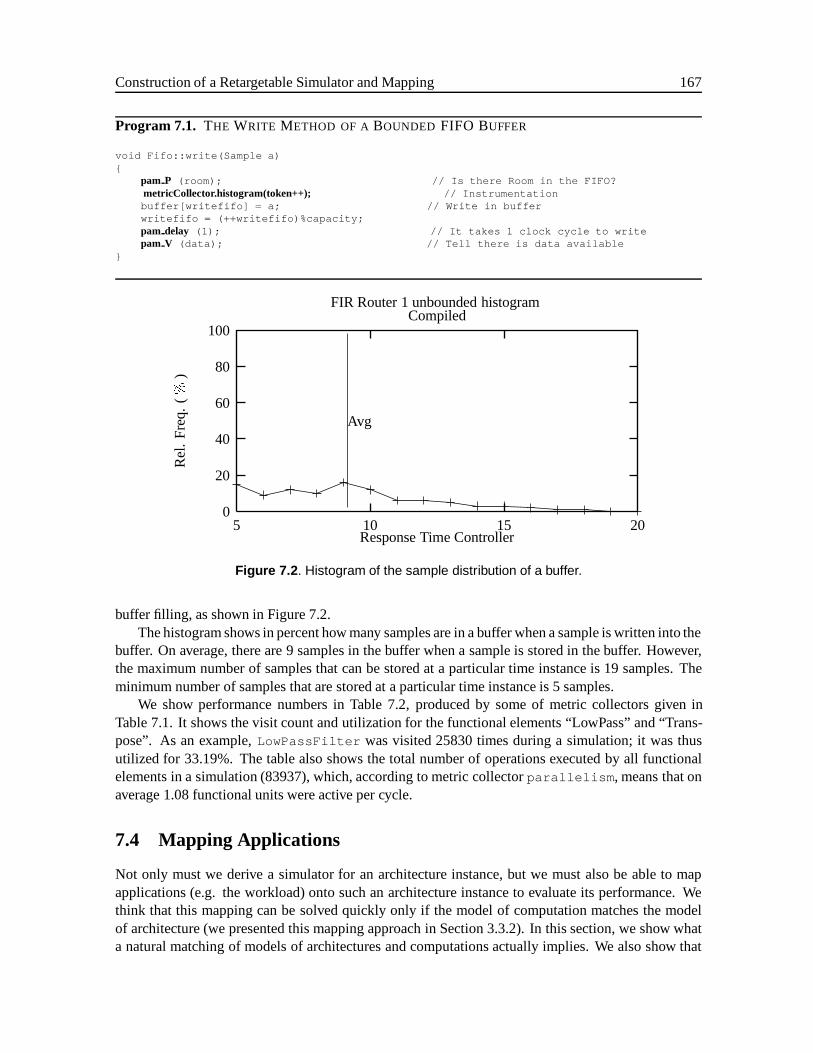
Construction of a Retargetable Simulator and Mapping 167
Program 7.1. THE WRITE METHOD OF A BOUNDED FIFO BUFFER
void Fifo::write(Sample a){
pam P (room); // Is there Room in the FIFO?metricCollector.histogram(token++); // Instrumentationbuffer[writefifo] = a; // Write in bufferwritefifo = (++writefifo)%capacity;pam delay (1); // It takes 1 clock cycle to writepam V (data); // Tell there is data available
}
Avg
CompiledFIR Router 1 unbounded histogram
Response Time Controller
Rel
.F
req.
(
%
)
2015105
100
80
60
40
20
0
Figure 7.2 . Histogram of the sample distribution of a buffer.
buffer filling, as shown in Figure 7.2.The histogram shows in percent how many samples are in a buffer when a sample is written into the
buffer. On average, there are 9 samples in the buffer when a sample is stored in the buffer. However,the maximum number of samples that can be stored at a particular time instance is 19 samples. Theminimum number of samples that are stored at a particular time instance is 5 samples.
We show performance numbers in Table 7.2, produced by some of metric collectors given inTable 7.1. It shows the visit count and utilization for the functional elements “LowPass” and “Trans-pose”. As an example,LowPassFilter was visited 25830 times during a simulation; it was thusutilized for 33.19%. The table also shows the total number of operations executed by all functionalelements in a simulation (83937), which, according to metric collectorparallelism , means that onaverage 1.08 functional units were active per cycle.
7.4 Mapping Applications
Not only must we derive a simulator for an architecture instance, but we must also be able to mapapplications (e.g. the workload) onto such an architecture instance to evaluate its performance. Wethink that this mapping can be solved quickly only if the model of computation matches the modelof architecture (we presented this mapping approach in Section 3.3.2). In this section, we show whata natural matching of models of architectures and computations actually implies. We also show that
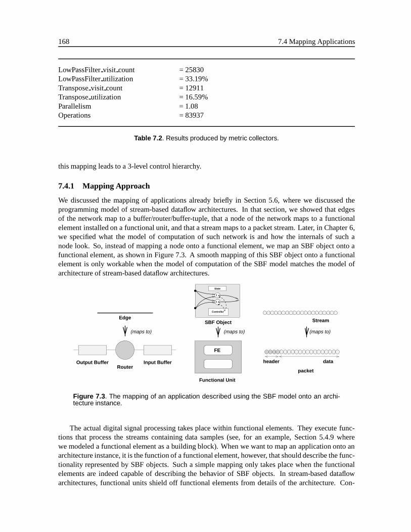
168 7.4 Mapping Applications
LowPassFiltervisit count = 25830LowPassFilterutilization = 33.19%Transposevisit count = 12911Transposeutilization = 16.59%Parallelism = 1.08Operations = 83937
Table 7.2 . Results produced by metric collectors.
this mapping leads to a 3-level control hierarchy.
7.4.1 Mapping Approach
We discussed the mapping of applications already briefly in Section 5.6, where we discussed theprogramming model of stream-based dataflow architectures. In that section, we showed that edgesof the network map to a buffer/router/buffer-tuple, that a node of the network maps to a functionalelement installed on a functional unit, and that a stream maps to a packet stream. Later, in Chapter 6,we specified what the model of computation of such network is and how the internals of such anode look. So, instead of mapping a node onto a functional element, we map an SBF object onto afunctional element, as shown in Figure 7.3. A smooth mapping of this SBF object onto a functionalelement is only workable when the model of computation of the SBF model matches the model ofarchitecture of stream-based dataflow architectures.
RouterInput BufferOutput Buffer
Edge
FE
(maps to) (maps to) (maps to)
Functional Unit
Stream
header
packet
data
SBF Object
State
f_a
f_b
Controller
Figure 7.3 . The mapping of an application described using the SBF model onto an archi-tecture instance.
The actual digital signal processing takes place within functional elements. They execute func-tions that process the streams containing data samples (see, for an example, Section 5.4.9 wherewe modeled a functional element as a building block). When we want to map an application onto anarchitecture instance, it is the function of a functional element, however, that should describe the func-tionality represented by SBF objects. Such a simple mapping only takes place when the functionalelements are indeed capable of describing the behavior of SBF objects. In stream-based dataflowarchitectures, functional units shield off functional elements from details of the architecture. Con-
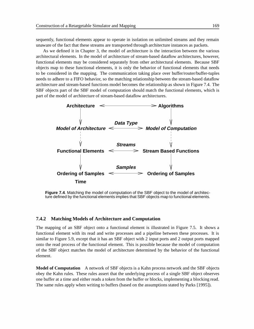
Construction of a Retargetable Simulator and Mapping 169
sequently, functional elements appear to operate in isolation on unlimited streams and they remainunaware of the fact that these streams are transported through architecture instances as packets.
As we defined it in Chapter 3, the model of architecture is the interaction between the variousarchitectural elements. In the model of architecture of stream-based dataflow architectures, however,functional elements may be considered separately from other architectural elements. Because SBFobjects map to these functional elements, it is only the behavior of functional elements that needsto be considered in the mapping. The communication taking place over buffer/router/buffer-tuplesneeds to adhere to a FIFO behavior, so the matching relationship between the stream-based dataflowarchitecture and stream-based functions model becomes the relationship as shown in Figure 7.4. TheSBF objects part of the SBF model of computation should match the functional elements, which ispart of the model of architecture of stream-based dataflow architectures.
Time
Functional Elements
Model of Architecture Model of Computation
Stream Based Functions
Architecture Algorithms
Data Type
Streams
SamplesOrdering of Samples Ordering of Samples
Figure 7.4 . Matching the model of computation of the SBF object to the model of architec-ture defined by the functional elements implies that SBF objects map to functional elements.
7.4.2 Matching Models of Architecture and Computation
The mapping of an SBF object onto a functional element is illustrated in Figure 7.5. It shows afunctional element with its read and write processes and a pipeline between these processes. It issimilar to Figure 5.9, except that it has an SBF object with 2 input ports and 2 output ports mappedonto the read process of the functional element. This is possible because the model of computationof the SBF object matches the model of architecture determined by the behavior of the functionalelement.
Model of Computation A network of SBF objects is a Kahn process network and the SBF objectsobey the Kahn rules. These rules assert that the underlying process of a single SBF object observesone buffer at a time and either reads a token from the buffer or blocks, implementing a blocking read.The same rules apply when writing to buffers (based on the assumptions stated by Parks [1995]).
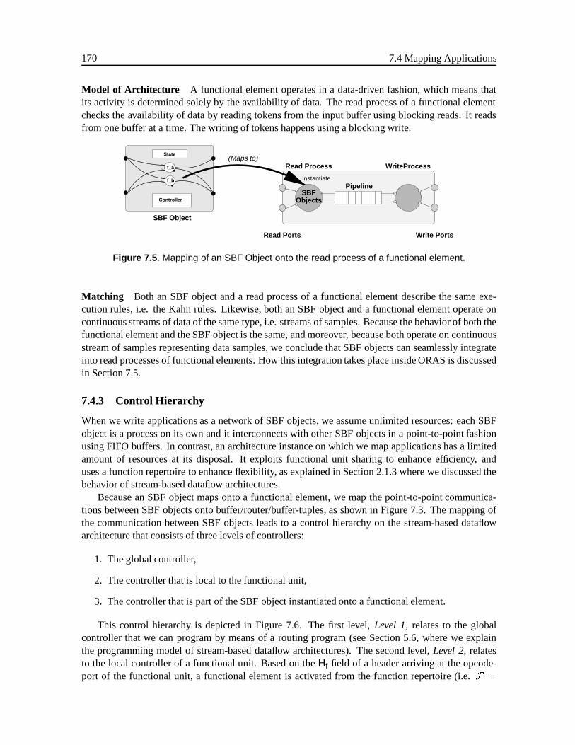
170 7.4 Mapping Applications
Model of Architecture A functional element operates in a data-driven fashion, which means thatits activity is determined solely by the availability of data. The read process of a functional elementchecks the availability of data by reading tokens from the input buffer using blocking reads. It readsfrom one buffer at a time. The writing of tokens happens using a blocking write.
State
f_a
f_b
Controller
Read Ports
Read Process WriteProcess
Write Ports
Pipeline
ObjectsSBF
SBF Object
(Maps to)
Instantiate
Figure 7.5 . Mapping of an SBF Object onto the read process of a functional element.
Matching Both an SBF object and a read process of a functional element describe the same exe-cution rules, i.e. the Kahn rules. Likewise, both an SBF object and a functional element operate oncontinuous streams of data of the same type, i.e. streams of samples. Because the behavior of both thefunctional element and the SBF object is the same, and moreover, because both operate on continuousstream of samples representing data samples, we conclude that SBF objects can seamlessly integrateinto read processes of functional elements. How this integration takes place inside ORAS is discussedin Section 7.5.
7.4.3 Control Hierarchy
When we write applications as a network of SBF objects, we assume unlimited resources: each SBFobject is a process on its own and it interconnects with other SBF objects in a point-to-point fashionusing FIFO buffers. In contrast, an architecture instance on which we map applications has a limitedamount of resources at its disposal. It exploits functional unit sharing to enhance efficiency, anduses a function repertoire to enhance flexibility, as explained in Section 2.1.3 where we discussed thebehavior of stream-based dataflow architectures.
Because an SBF object maps onto a functional element, we map the point-to-point communica-tions between SBF objects onto buffer/router/buffer-tuples, as shown in Figure 7.3. The mapping ofthe communication between SBF objects leads to a control hierarchy on the stream-based dataflowarchitecture that consists of three levels of controllers:
1. The global controller,
2. The controller that is local to the functional unit,
3. The controller that is part of the SBF object instantiated onto a functional element.
This control hierarchy is depicted in Figure 7.6. The first level,Level 1, relates to the globalcontroller that we can program by means of a routing program (see Section 5.6, where we explainthe programming model of stream-based dataflow architectures). The second level,Level 2, relatesto the local controller of a functional unit. Based on theHf field of a header arriving at the opcode-port of the functional unit, a functional element is activated from the function repertoire (i.e.F =

Construction of a Retargetable Simulator and Mapping 171
fF1;F2;F3;F4g) (see Section 5.4.8, where we modeled the local controller of a functional unit). In thefigure, the global controller has assigned a value toHf that relates to functional elementF1. An SBFobject is instantiated on each functional element and the third level,Level 3, relates to the controllerbeing part of that SBF object (see section 6.4, where we described the modeling of SBF objects).
The controllers at level 1 and level 2 only concern the communication between SBF objects and themultiplexing of streams. However, the controller at level 3 is completely determined from the givenapplication description. The control at level 3 is invariant with respect to the architecture instances.
Functional E
lements
F1 Length Data
Header
Level 3
Level 2
Level 1
ControlLevels
Local ControllerFunctional Unit
Selection FE, based on Header value
Global Controller
Opcode Buffer
(Run-Time)
Header filled by Global Controller(Run-Time)
F4F3
F2F1
Function Repertoire
Routing Program
State
f_a
f_b
Control
(Static)
(Static)
Figure 7.6 . Control Hierarchy in the stream-based dataflow architecture.
Level 1 The first level of control is at the global level where the global controller resides. The globalcontroller contains a routing program that describes the static routing of packets through anarchitecture instance. Routers interact with the global controller to receive this routing infor-mation (see Figure 5.16, where we showed how a router interacts with the global controller tochange the content of a header). By down-loading another routing program, we can establishanother flow of packets, causing the execution of another application.
Level 2 The second level of control is at the level of the functional units where the local controllerresides. The local controller of the functional unit selects and activates a functional elementat run-time from the function repertoireF of the functional unit, based on theHf field of the
172 7.5 The Interface Between Application and Architecture
header arriving on the opcode-buffer of the functional unit (in packet-switching mode). Thevalue ofHf is set at run-time by routers. The function repertoire, on the other hand, is staticallyresolved when an architecture instance is defined. For example, in the architecture descriptiongiven in Figure 5.11 we devised the regular processing elementFilter with a functional unitwith two functional elements, respectivelyLowPassandHighPass.
Level 3 The third level of control is at the level where SBF objects reside, which is internal to func-tional elements. The controller of an SBF object specifies the consumption/production patternof an SBF object, and thus of a functional element (see, for an example, Table 6.1, where weshow how the controller of an SBF object specifies the consumption/production pattern of theSBF object).
In the architecture description given in Figure 5.11 the functional elementLowPassinstantiatesSBF object “Lowpass” and functional elementHighPassinstantiates SBF object “Highpass”,both from the library of SBF objects. At this level, by selecting a particular SBF object forthe functional element to execute, we determine the grain size of a functional element, whichequals the granularity of an SBF object.
Modeling the Function Repertoire
We describe function repertoires as consisting of different functional elements. Not every functionalelement is going to become a piece of hardware on its own. In practice, we combine functionalelements into one piece of hardware. In the Jacobium case (which will be discussed in Section 9.3),we indicate how such a functional unit may look. Although we can construct a function repertoire ofvery different SBF objects, it is more logical to combine SBF objects that have more similar sets offunctions (as given by Equation 6.1).
7.5 The Interface Between Application and Architecture
The SBF model describes dynamic dataflow. The workload that an application represents may changedepending on the content of the stream(s) that the application processes at run-time. In the case ofvideo applications, the workload that results depends on the sequence of images being processed.MPEG [Rao and Hwang, 1997] algorithms typify such applications. Suppose such an applicationdescribes a dynamic workload and executes on a simulator derived by ORAS, as shown in Figure 7.7.The processing of the clown video-sequence results in a workload, for which the simulator deliversparticular performance numbers. If another sequence is chosen instead of the clown video sequence,then another workload results for which the simulator should deliver other performance numbers.Notice that the routing program – and thus the mapping – remains the same.
To have the simulator execute the correct dynamic workload without our having to make a largemodification to the original application description, we want to evaluate SBF objects functionallycorrectly at run-time in the context of architecture instances. This implies that SBF objects shouldaccess and process the data which flows through an architecture instance, simulating an interpretedperformance model of the architecture instance. Alternatively, SBF objects need anApplication –Architecture interface. An SBF object interacts on this interface with the data flowing through thearchitecture instance. Via the interface, the SBF object can access the data from the architectureinstance, process it, and put new results back into the architecture instance.
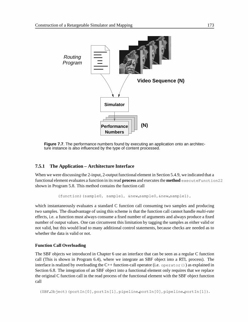
Construction of a Retargetable Simulator and Mapping 173
(N)
RoutingProgram
Video Sequence (N)
PerformanceNumbers
Simulator
Figure 7.7 . The performance numbers found by executing an application onto an architec-ture instance is also influenced by the type of content processed.
7.5.1 The Application – Architecture Interface
When we were discussing the 2-input, 2-output functional element in Section 5.4.9, we indicated that afunctional element evaluates a function in its readprocessand executes themethodexecuteFunction22
shown in Program 5.8. This method contains the function call
(function)(sample0, sample1, &new sample0,&new sample1),
which instantaneously evaluates a standard C function call consuming two samples and producingtwo samples. The disadvantage of using this scheme is that the function call cannot handlemulti-rateeffects, i.e. a function must always consume a fixed number of arguments and always produce a fixednumber of output values. One can circumvent this limitation by tagging the samples as either valid ornot valid, but this would lead to many additional control statements, because checks are needed as towhether the data is valid or not.
Function Call Overloading
The SBF objects we introduced in Chapter 6 use an interface that can be seen as a regular C functioncall (This is shown in Program 6.4), where we integrate an SBF object into a RTL process). Theinterface is realized by overloading the C++ function-call operator (i.e.operator() ) as explained inSection 6.8. The integration of an SBF object into a functional element only requires that we replacethe original C function call in the read process of the functional element with the SBF object functioncall
(SBF Object)(portIn[0],portIn[1],pipeline portIn[0],pipeline portIn[1]) :

174 7.5 The Interface Between Application and Architecture
The SBF object functional call accepts references to read and write ports, respectivelyportIn andpipeline portIn , whereas the original C function call accepts samples. This way, the controllerof the SBF object becomes responsible for the readprocessof the functional element that reads acorrect, but variable amount of tokens fromportIn and writes a correct, but variable amount oftokens topipeline port .
We show the revised program formethod executeFunction22 in Program 7.2. The readand write ports used in the architecture modeling are different from the read and write ports usedin the application modeling. In the architecture modeling, ports are involved in header processing,whereas in application modeling, headers do not exist. However, because of polymorphism, SBFobjects remain unaware of this difference. In Program 7.2, we pass on the input ports of the functionalelement (i.e.,portIn[] ) and the input ports of the pipeline (i.e.,pipeline portIn[] ) to the SBFobject.
Program 7.2. EXECUTE A 2-INPUT, 2-OUTPUT SBF OBJECT
method executeFunction22 {
// Execute the SBF Object// Pass on pointer to input and output, do not pass samples(SBF Object)(portIn[0],portIn[1],pipeline_portIn[0],pipeline_portIn[1]);
// Calculate when these Samples are ready to leave the FEleave_time = pam time () + (latency * initiation period );
// Pass the Execution to the samplepipeline_portIn[0].setTime( leave_time );pipeline_portIn[1].setTime( leave_time );
}
Passing Over the Thread-of-Control
As soon as the readprocessof a functional element passes the thread-of-control to the SBF object,the controller of the SBF object becomes responsible for the reading and writing of tokens. BecauseSBF objects have a fire-and-exit behavior (see Section 6.8, where we integrate an SBF object in a RTLprocess), the readprocessof the functional element always gets back the thread-of-control when afunction has fired. Notice that when the enabled function of the SBF object tries to read from an inputbuffer (e.g., via portIn[0]) and blocks, the readprocessof the functional element also blocks.
Augmenting SBF Objects with Time
Because the readprocessof the functional element always gets back the thread-of-control when afunction has fired, we can simply augment an SBF object with time by calling apam delay state-ment each time a transition (i.e., the firing of a function) takes place. We put apam delay state-ment in the endless loop in Program 6.4 following a call for the SBF object. In the context of theread process of a functional element, thepam delay statement must be replaced by thepam delay(initiation period ) statement shown in Program 5.9.
We use the architecture description that we gave in Figure 5.11 to illustrate how we define func-tional elements executing a function. In Figure 7.8, we describe one functional element on whichORAS will instantiate the SBF objectLowPass from the library of SBF objects. This SBF object hastwo parameters (i.e.,latency andinitiation period ) resulting in a pipelined implementation of
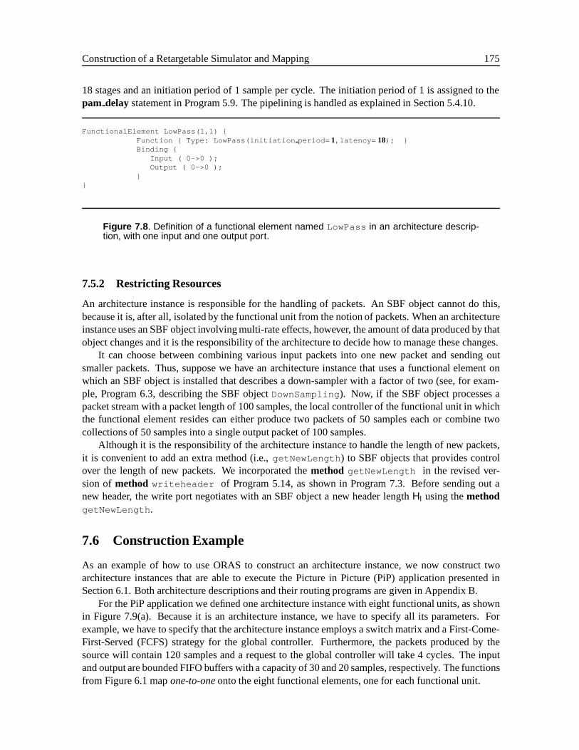
Construction of a Retargetable Simulator and Mapping 175
18 stages and an initiation period of 1 sample per cycle. The initiation period of 1 is assigned to thepam delaystatement in Program 5.9. The pipelining is handled as explained in Section 5.4.10.
FunctionalElement LowPass(1,1) {Function { Type: LowPass(initiation period= 1,latency= 18); }Binding {
Input ( 0->0 );Output ( 0->0 );
}}
Figure 7.8 . Definition of a functional element named LowPass in an architecture descrip-tion, with one input and one output port.
7.5.2 Restricting Resources
An architecture instance is responsible for the handling of packets. An SBF object cannot do this,because it is, after all, isolated by the functional unit from the notion of packets. When an architectureinstance uses an SBF object involving multi-rate effects, however, the amount of data produced by thatobject changes and it is the responsibility of the architecture to decide how to manage these changes.
It can choose between combining various input packets into one new packet and sending outsmaller packets. Thus, suppose we have an architecture instance that uses a functional element onwhich an SBF object is installed that describes a down-sampler with a factor of two (see, for exam-ple, Program 6.3, describing the SBF objectDownSampling ). Now, if the SBF object processes apacket stream with a packet length of 100 samples, the local controller of the functional unit in whichthe functional element resides can either produce two packets of 50 samples each or combine twocollections of 50 samples into a single output packet of 100 samples.
Although it is the responsibility of the architecture instance to handle the length of new packets,it is convenient to add an extra method (i.e.,getNewLength ) to SBF objects that provides controlover the length of new packets. We incorporated themethod getNewLength in the revised ver-sion of method writeheader of Program 5.14, as shown in Program 7.3. Before sending out anew header, the write port negotiates with an SBF object a new header lengthHl using themethodgetNewLength .
7.6 Construction Example
As an example of how to use ORAS to construct an architecture instance, we now construct twoarchitecture instances that are able to execute the Picture in Picture (PiP) application presented inSection 6.1. Both architecture descriptions and their routing programs are given in Appendix B.
For the PiP application we defined one architecture instance with eight functional units, as shownin Figure 7.9(a). Because it is an architecture instance, we have to specify all its parameters. Forexample, we have to specify that the architecture instance employs a switch matrix and a First-Come-First-Served (FCFS) strategy for the global controller. Furthermore, the packets produced by thesource will contain 120 samples and a request to the global controller will take 4 cycles. The inputand output are bounded FIFO buffers with a capacity of 30 and 20 samples, respectively. The functionsfrom Figure 6.1 mapone-to-oneonto the eight functional elements, one for each functional unit.
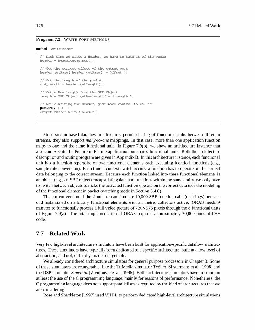
176 7.7 Related Work
Program 7.3. WRITE PORT METHODS
method writeHeader{
// Each time we write a Header, we have to take it of the Queueheader = headerQueue.pop();
// Get the correct offset of the output portheader.setBase( header.getBase() + Offset );
// Get the length of the packetold_length = header.getLength();
// Get a New length from the SBF Objectlength = SBF_Object.getNewLength( old_length );
// While writing the Header, give back control to callerpam delay ( 4 );output_buffer.write( header );
}
Since stream-based dataflow architectures permit sharing of functional units between differentstreams, they also supportmany-to-onemappings. In that case, more than one application functionmaps to one and the same functional unit. In Figure 7.9(b), we show an architecture instance thatalso can execute the Picture in Picture application but shares functional units. Both the architecturedescription and routing program are given in Appendix B. In this architecture instance, each functionalunit has a function repertoire of two functional elements each executing identical functions (e.g.,sample rate conversion). Each time a context switch occurs, a function has to operate on the correctdata belonging to the correct stream. Because each function linked into these functional elements isan object (e.g., an SBF object) encapsulating data and functions within the same entity, we only haveto switch between objects to make the activated function operate on the correct data (see the modelingof the functional element in packet-switching mode in Section 5.4.8).
The current version of the simulator can simulate 10,000 SBF function calls (or firings) per sec-ond instantiated on arbitrary functional elements with all metric collectors active. ORAS needs 9minutes to functionally process a full video picture of 720�576 pixels through the 8 functional unitsof Figure 7.9(a). The total implementation of ORAS required approximately 20,000 lines of C++code.
7.7 Related Work
Very few high-level architecture simulators have been built for application-specific dataflow architec-tures. These simulators have typically been dedicated to a specific architecture, built at a low level ofabstraction, and not, or hardly, made retargetable.
We already considered architecture simulators for general purpose processors in Chapter 3. Someof these simulators are retargetable, like the TriMedia simulatorTmSim[Sijstermans et al., 1998] andthe DSP simulatorSupersim[Zivojnovic et al., 1996]. Both architecture simulators have in commonat least the use of the C programming language, mainly for reasons of performance. Nonetheless, theC programming language does not support parallelism as required by the kind of architectures that weare considering.
Rose and Shackleton [1997] used VHDL to perform dedicated high-level architecture simulations
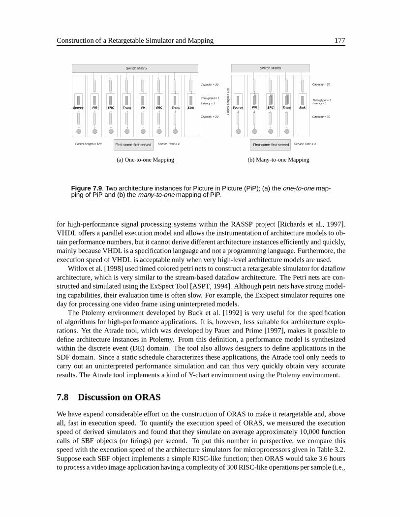
Construction of a Retargetable Simulator and Mapping 177
Switch Matrix
First-come-first-served
Capacity = 20
Capacity = 30
Throughput = 1
Latency = 1
SinkSource
Service Time = 4Packet Length = 120
FIR SRC Trans Fir SRC Trans
(a) One-to-one Mapping
Pac
ket L
engt
h =
120
Source FIR SRC Trans
Switch Matrix
First-come-first-served
Throughput = 1
Capacity = 20
Capacity = 30
Latency = 1
Sink
Service Time = 4
(b) Many-to-one Mapping
Figure 7.9 . Two architecture instances for Picture in Picture (PiP); (a) the one-to-one map-ping of PiP and (b) the many-to-one mapping of PiP.
for high-performance signal processing systems within the RASSP project [Richards et al., 1997].VHDL offers a parallel execution model and allows the instrumentation of architecture models to ob-tain performance numbers, but it cannot derive different architecture instances efficiently and quickly,mainly because VHDL is a specification language and not a programming language. Furthermore, theexecution speed of VHDL is acceptable only when very high-level architecture models are used.
Witlox et al. [1998] used timed colored petri nets to construct a retargetable simulator for dataflowarchitecture, which is very similar to the stream-based dataflow architecture. The Petri nets are con-structed and simulated using the ExSpect Tool [ASPT, 1994]. Although petri nets have strong model-ing capabilities, their evaluation time is often slow. For example, the ExSpect simulator requires oneday for processing one video frame using uninterpreted models.
The Ptolemy environment developed by Buck et al. [1992] is very useful for the specificationof algorithms for high-performance applications. It is, however, less suitable for architecture explo-rations. Yet the Atrade tool, which was developed by Pauer and Prime [1997], makes it possible todefine architecture instances in Ptolemy. From this definition, a performance model is synthesizedwithin the discrete event (DE) domain. The tool also allows designers to define applications in theSDF domain. Since a static schedule characterizes these applications, the Atrade tool only needs tocarry out an uninterpreted performance simulation and can thus very quickly obtain very accurateresults. The Atrade tool implements a kind of Y-chart environment using the Ptolemy environment.
7.8 Discussion on ORAS
We have expend considerable effort on the construction of ORAS to make it retargetable and, aboveall, fast in execution speed. To quantify the execution speed of ORAS, we measured the executionspeed of derived simulators and found that they simulate on average approximately 10,000 functioncalls of SBF objects (or firings) per second. To put this number in perspective, we compare thisspeed with the execution speed of the architecture simulators for microprocessors given in Table 3.2.Suppose each SBF object implements a simple RISC-like function; then ORAS would take 3.6 hoursto process a video image application having a complexity of 300 RISC-like operations per sample (i.e.,
178 7.8 Discussion on ORAS
per video pixel). Given the high level of retargetability, the complexity of the architecture instances,and the fact that it is an interpreted performance model, ORAS is a fast retargetable simulator.
ORAS is not limited, however, to the use of RISC-like functions, but permits the use of arbitrarycoarse-grained functions. We can still execute 10,000 function calls of SBF objects while describinga much more complex application, as shown in the Picture in Picture application example. In the PiPcase, the simulation speed ends up in the range of minutes and not hours (i.e., 9 minutes for a wholeframe), which clearly confirms that ORAS is a fast retargetable simulator.
7.8.1 Building Blocks
One reason why the execution speed of ORAS is high and at the same time still retargetable is that weused building blocks to construct the architecture.
The building block modeling technique developed in Chapter 5 allows us to describe every pos-sible architecture instance in the design space of a stream-based dataflow architecture. The use ofobjects and high-level construction primitives of the STL library makes it very simple to describecomplex architecture instances. Secondly, the building blocks separated the structure from the behav-ior. Because the structure of an architecture instance is resolved by the time processes are created, theprocesses no longer need to decode any structural aspects of the architecture at run-time.
7.8.2 High-level Primitives
Another reason why the execution speed of ORAS is high is that we used high-level primitives tomodel architectural elements and a very efficient simulation engine was available that can simulatevery fast structures using these high-level primitives.
The PAMELA method discussed in Chapter 4 provides 3 high-level primitives: processes, semaphores,and delays. These primitives allowed us to model architectural elements at a high level of abstractionin terms of the four components of the Performance Modeling Base. As a consequence, we move upin the abstraction pyramid shown in Figure 3.3, while simulating the performance of an architectureinstance cycle-accurately.
The three primitives can be simulated very efficiently using the RTL process scheduler. It requiresa minimal amount of sorting, compared to other simulation engines, because of its simple structure,as we explained in Section 4.5. In particular, we compare the RTL with a VHDL simulation engine inAppendix C.
7.8.3 Interpreted Model
In addition to being fast and retargetable, ORAS is also able to obtain cycle-accurate performancenumbers expressing the correct dynamic behavior of both the architecture and applications. ORASintegrates SBF objects seamlessly onto the functional elements of derived simulators, because of thearchitecture – application interface. This interface hardly introduces any overhead, while the derivedsimulator is able to execute an application functionally correctly.
7.8.4 Limitations
We conclude that with ORAS we have indeed succeeded in constructing a simulator that is fast andaccurate. The limitation of ORAS is that it is built for a specific architecture. Further, the RTLworks well for stream-based, data-driven kinds of architecture, but is inapplicable for control-oriented
Construction of a Retargetable Simulator and Mapping 179
architectures like load/store architectures. The RTL is less suited to describing low-level control likepolling, as we explain in Appendix C.
7.9 A Generic Approach for a Retargetable Simulator
In this chapter, we developed the retargetable simulator ORAS for stream-based dataflow architec-tures. In our opinion, the three-step approach shown in Figure 7.1 provides a generic outline for re-targetable simulators; therefore, we discuss each step used in ORAS and indicate the changes neededwhen a retargetable simulator is needed for another architecture template.
7.9.1 Step 1: Structure
In the first step, we need to distinguish the various architectural elements used in the architecture tem-plate. For each architectural element, we define a class describing the structure of the architecturalelement. If architectural elements have alternative behaviors, we will describe the architectural ele-ments as an architectural element type and describe this type as an abstract class. This procedure leadsto a class hierarchy similar to the one shown in Figure 5.5. Next, the structure of the architecture tem-plate is described in terms of composition rules in BNF, as explained in Section 5.5. The BNF rulesalso provide a grammar for an architecture description language. Based on this grammar, a parser canprocess architecture descriptions.
To come to the first step shown in Figure 7.1, we must replace the “architectural elements” withthe newly developed class hierarchy. Furthermore, we must replace the grammar of the architecturetemplate and use the newly devised architecture description language.
7.9.2 Step 2: Execution Model
In the second step, the retargetable simulator adds an execution model or simulation engine to thestructure. We can again use the RTL library as simulation engine and develop new process descriptionsfor each architectural element. We make a distinction between “active” and “passive” elements anddefine the correct methods and processes.
Given the limitation of the RTL as described in Appendix C, we could consider other simula-tion engines. These simulation engines furnish a more accurate execution model (i.e., lower in theabstraction pyramid) or an execution model that fits better with the architecture.
Gupta and Liao [1997] describe an execution model namedScenic. Their simulation engine useslightweight threads (like the RTL does) and C++, and implements the VHDL execution model. Aspointed out by Benders [1996], VHDL has severe problems with specifyingprocess control, excep-tionsandasynchronous communicationbetween concurrent entities while at the same time it is wellsuited to specifying low-level control. By integrating threads with a clock-cycle simulation engine,Gupta and Liao combined the power of threads to describe process behavior with the power of VHDLto describe low-level control. Post et al. [1998] have already shown how this simulation engine canbe used together with C++ to describe ATM switches for performance evaluation. Because C++ isused, this engine fits in very well with our building block approach. Unfortunately, no information isavailable on the execution speed of the simulations.
Koot et al. [1997] developed another simulation engine, namedTSS, that could also be considered.TSS is a tool developed at Philips Research for internal use. This is a very fast and modular clock-cycle-accurate simulation engine based on the C programming language. Although TSS can describeboth synchronous and asynchronous communication, it is particularly fast for the synchronous case.
180 7.10 Conclusions
If we use another simulation engine, then to come to the second step in Figure 7.1, we must changethe way we describe processes since each simulation engine provides other primitives. The approach,however, remains the same. We first build up the structure of an architecture instance and then add anexecution engine.
7.9.3 Step 3: Metric Collectors
In the third step, we instrument the executable architecture instance with metric collectors. The metriccollectors that we developed are generic and can be reused with little modification. To come to thethird step in Figure 7.1, we can reuse the metric collectors.
7.9.4 Mapping
A smooth mapping of applications onto an instance is only workable when the model of computationmatches the model of architecture. This implies that we need to investigate the architecture templateto determine its model of architecture. Using this information, we select the appropriate model ofcomputation to describe applications. If such a model does not exist, adjustments are needed in thearchitecture template or in the model of computation until a match is found. We remark that theclassification of models of architectures is not an area as well developed as that of the model ofcomputation.
7.10 Conclusions
In this chapter we discussed the construction of the Object Oriented Retargetable Architecture Simu-lator (ORAS). We also discussed the mapping of applications onto executable architecture instancesthat were derived by ORAS from the architecture template of stream-based dataflow architectures.
We showed that ORAS uses a three-step approach to derive executable architecture instances thatdeliver performance numbers. We showed how ORAS creates the structure of an architecture instancein the first step; it adds an execution model to the structure in the second step, making it possibleto describe the behavior of an architecture instance; and activates metric collectors to harvest theperformance numbers in the third step.
In Chapter 6, we developed the SFB Model and SBF objects. In this chapter, we showed thatapplications written as networks of SBF objects map indeed very smoothly onto architecture instances,because the model of computation matches the model of architecture. Functional elements use rulessimilar to the Kahn rules used in SBF objects; therefore, both SFB objects and functional elementsdescribe the same behavior. SBF objects thus map seamlessly onto functional elements. Because anSBF object maps to a functional element, the communication taking place between SBF objects overchannels map onto the buffer/router/buffer-tuples, which behave like FIFO buffers. We have showedthat this communication results in a 3-level control hierarchy.
The workload that SBF objects describe can change dynamically based on the content of streams.For an architecture instance to describe the correct workload without large modifications to the orig-inal application, SBF objects need to execute functionally correctly within the context of an archi-tecture instance. This requires an interface such that SBF objects can obtain data samples from anarchitecture instance, process them, and put new results back into the architecture instance. We haveshowed such an interface using function call overloading of the function operator in C++. The functionoverloading and the fact that SBF objects have a fire-and-exit behavior resulted in a simple interfaceallowing SBF objects to interact with functional elements.

BIBLIOGRAPHY 181
We showed an example in which ORAS derives an architecture instance that can execute thePicture in Picture application. We showed that ORAS handles a one-to-one mapping and a many-to-one mapping. We also discussed related work on high-level retargetable architecture simulators.
We compared the execution speed of ORAS with other architecture simulators. We found thatORAS is indeed a fast simulator, while still being a retargetable one. Simulators derived by ORASexecute 10,000 SBF object function calls (firings) per second. To process a complete video pictureof 720�576 pixels by the PiP application took 9 minutes. The reason why ORAS is fast and retar-getable is that it uses building blocks. Architecture instances adhering to the architecture templatecan be constructed by simply combining building blocks, using high-level programming constructs.Furthermore, building blocks separate structure from behavior. As a consequence, when a processis activated, all references between building blocks are already fixed and the process does not haveto decode any aspect of an architecture instance. In addition, the use of high-level primitives suchas processes, semaphores and delay allows us to describe the performance of architecture instancesat an abstract level, but still cycle-accurately. The process scheduler of the RTL can simulate thesehigh-level primitives very efficiently. The seamless integration of SBF objects onto functional ele-ments introduces very little overhead in the functionally correct execution of an application onto anarchitecture instance.
We also showed the limitations of ORAS. The main limitation is that it can only execute instancesof stream-based, data-driven architectures. It is less suitable for load/store architectures. We indicatedin Appendix C that the RTL is less suited for describing low-level control like polling.
Finally, we showed that the three steps used in ORAS provide a generic outline for other retar-getable simulators as well. We indicated the changes required in ORAS when a retargetable simulatormust be created for another architecture template.
Bibliography
ASPT. ExSpect 5.0 User Manual. Eindhoven University of Technology, Eindhoven, the Netherlands,1994.
Leon Benders.System Specification and Performance Analysis. PhD thesis, Eindhoven University ofTechnology, 1996.
Joseph Buck, Soonhoi Ha, Edward A. Lee, and David G. Messerschmitt. Ptolemy: A framework forsimulating and prototyping heterogeneous systems.International Journal of Computer Simulation,1992. Special issue on Simulation Software Development.
Rajesh K. Gupta and Stan Y. Liao. Using a programming language for digital system design.IEEEDesign & Test of Computers, 14(2):72 – 80, 1997.
Bart Kienhuis, Ed Deprettere, Kees Vissers, and Pieter van der Wolf. The constructionof a retargetablesimulator for an architecture template. InProceedings of 6th Int. Workshop on Hardware/SoftwareCodesign, Seattle, Washington, 1998.
Sjaak Koot, Arjan Versluys, and Pieter de Visser.TSS User Manual. Philips Research Laboratories,Eindhoven, 1997.
Peter Marwedel and Gert Goossens.Code Generation for Embedded Processors, chapter 1, pages 13– 31. Kluwer Academic Publishers, 1995.

182 BIBLIOGRAPHY
David R. Musser and Atul Saini.STL Tutorial and Reference Guide: C++ programmingwith standardtemplate library. Addison-Wesley Professional Computing Series, 1996.
Tom Parks.Bounded Scheduling of Process Networks. PhD thesis, University of California at Berke-ley, 1995.
Eric K. Pauer and Jonathan B. Prime. An architectural trade capability using the Ptolemy kernel. OnPtolemy Site http://ptolemy.eecs.berkeley.edu, 1997.
Guido Post, Andrea Muller, and Rainer Schoenen. Object-oriented design of ATM switch hardwarein a telecommunication network simulation environment. InProceedings of GI/ITG/GMM Work-shop Methoden und Bescheibungssprachen zur Modellierung und Verifikation von Schaltungen undSystemen, Paderborn, 1998.
R.K. Rao and J.J. Hwang.Techniques and Standards for Image, Video and Audio Coding. PrenticeHall, 1997.
Mark A. Richards, Anthony Gadient, Geoffrey A. Frank, and Randolph Harr. The RASSP program:Origin, concepts, and status: An introduction to the issue. InJournal of VLSI Signal Processing,volume 15, pages 7 – 28, 1997.
Fred Rose and John Shackleton. Performance modeling of system architectures.VLSI Signal Pro-cessing, 15(1/2):97 – 110, 1997.
F Sijstermans, E.J. Pol, B. Riemens, K Vissers, S. Rathnam, and G. Slavenburg. Design space explo-ration for future trimedia CPUs. InICASSP’98, 1998.
Bjarne Stroustrup.The C++ Programming Language. Addison-Wesley, 2nd edition, 1991.
Vojin Zivojnovic, Stefan Pees, Christian Schl¨ager, Markus Willems, Rainer Schoenen, and HeinrichMeyr. DSP Processor/Compiler Co-Design: A Quantitative Approach. InProc. ISSS, 1996.
B.R.T.M Witlox, P. van der Wolf, E.H.L Aarts, and W.M.P. van der Aalst. Performance analysis ofdataflow architectures using timed coloured petri nets. InProceedings of the 19th InternationalConference on Applications and Theory of Petri Nets, Lisabon, 1998.

Chapter 8
Design SpaceExploration
(Pamela/C++)Applications
RetargetableSimulator (ORAS)
PerformanceNumbers
SBF-model
Design Space Exploration
Mapping
Arch. Model
Contents
8.1 The Acquisition of Insight . . . . . . . . . . . . . . . . . . . . . . . . . . . . . . 184
8.2 Design Space Exploration . . . . . . . . . . . . . . . . . . . . . . . . . . . . . . 185
8.3 Design Space Exploration Environment . . . . . . . . . . . . . . . . . . . . . . 186
8.3.1 Spanning the Design Space . . . . . . . . . . . . . . . . . . . . . . . . . . 186
8.3.2 Construction of the Response Surface Model. . . . . . . . . . . . . . . . 188
8.3.3 Data Management and Data Consistency . . . . . . . . . . . . . . . . . . 189
8.3.4 Parameterizing the Architecture Description . . . . . . . . . . . . . . . . . 189
8.4 Integrating ORAS within the Generic DSE Environment . . . . . . . . . . . . 192
8.4.1 Selecting Parameter Values . . . . . . . . . . . . . . . . . . . . . . . . . . 192
8.4.2 Running the Y-chart in the DSE Environment. . . . . . . . . . . . . . . . 192
8.4.3 Creating Response Surface Model. . . . . . . . . . . . . . . . . . . . . . 193
8.5 An Example of Design Space Exploration . . . . . . . . . . . . . . . . . . . . . 194
8.6 Related Work . . . . . . . . . . . . . . . . . . . . . . . . . . . . . . . . . . . . 195
8.7 Conclusions . . . . . . . . . . . . . . . . . . . . . . . . . . . . . . . . . . . . . . 197
DESIGN Space exploration is the subject that we discuss in this chapter. A designer must knowwhat the design space of architectures looks like in order to make trade-offs related to the design.
The acquisition of this knowledge requires an exploration of the design space of architectures. In theprevious chapter we developed ORAS, which allows us to quantify the performance of an architectureinstance. We will now integrate ORAS in a generic Design Space Exploration (DSE) environment.This environment allows us to change parameters that are presented to ORAS in systematical andautomated way to generate different architecture instances. In this way, the environment makes itpossible for us to explore part of the design space of the architecture template of stream-based dataflowarchitectures automatically and systematically. At the end of an exploration, the environment presentsthe relationships between parameter values and performance values as a Response Surface Model(RSM). These RSMs enable designers to consider trade-offs in architectures.
We start in Section 8.1 by explaining what design space exploration is about, and we look at Re-sponse Surface Models that express the relationship between parameter values and performance met-rics. In Section 8.2, we present four problems that we have to solve in order to perform design spaceexploration. We make use of a generic design space exploration environment developed at PhilipsResearch to perform actual design space exploration. We describe this environment and we show in
183
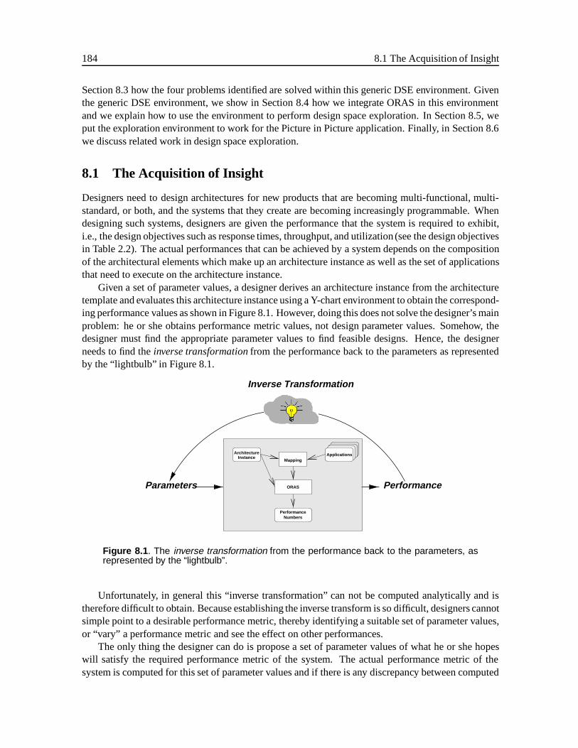
184 8.1 The Acquisition of Insight
Section 8.3 how the four problems identified are solved within this generic DSE environment. Giventhe generic DSE environment, we show in Section 8.4 how we integrate ORAS in this environmentand we explain how to use the environment to perform design space exploration. In Section 8.5, weput the exploration environment to work for the Picture in Picture application. Finally, in Section 8.6we discuss related work in design space exploration.
8.1 The Acquisition of Insight
Designers need to design architectures for new products that are becoming multi-functional, multi-standard, or both, and the systems that they create are becoming increasingly programmable. Whendesigning such systems, designers are given the performance that the system is required to exhibit,i.e., the design objectives such as response times, throughput, and utilization (see the design objectivesin Table 2.2). The actual performances that can be achieved by a system depends on the compositionof the architectural elements which make up an architecture instance as well as the set of applicationsthat need to execute on the architecture instance.
Given a set of parameter values, a designer derives an architecture instance from the architecturetemplate and evaluates this architecture instance using a Y-chart environment to obtain the correspond-ing performance values as shown in Figure 8.1. However, doing this does not solve the designer’s mainproblem: he or she obtains performance metric values, not design parameter values. Somehow, thedesigner must find the appropriate parameter values to find feasible designs. Hence, the designerneeds to find theinverse transformationfrom the performance back to the parameters as representedby the “lightbulb” in Figure 8.1.
Inverse Transformation
Applications
PerformanceNumbers
Mapping
ArchitectureInstance
ORASParameters Performance
Figure 8.1 . The inverse transformation from the performance back to the parameters, asrepresented by the “lightbulb”.
Unfortunately, in general this “inverse transformation” can not be computed analytically and istherefore difficult to obtain. Because establishing the inverse transform is so difficult, designers cannotsimple point to a desirable performance metric, thereby identifying a suitable set of parameter values,or “vary” a performance metric and see the effect on other performances.
The only thing the designer can do is propose a set of parameter values of what he or she hopeswill satisfy the required performance metric of the system. The actual performance metric of thesystem is computed for this set of parameter values and if there is any discrepancy between computed
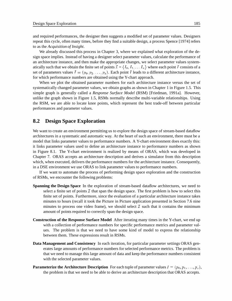
Design Space Exploration 185
and required performances, the designer then suggests a modified set of parameter values. Designersrepeat this cycle, often many times, before they find a suitable design, a process Spence [1974] refersto as theAcquisition of Insight.
We already discussed this process in Chapter 3, where we explained what exploration of the de-sign space implies. Instead of having a designer select parameter values, calculate the performance ofan architecture instance, and then make the appropriate changes, we select parameter values system-atically such that we obtain the finite set of pointsI = fI0; I1; : : : Ing where each pointI consists of aset of parameters valuesI = (p0; p1; : : : ; px). Each pointI leads to a different architecture instance,for which performance numbers are obtained using the Y-chart approach.
When we plot the obtained parameter numbers for each architecture instance versus the set ofsystematically changed parameter values, we obtain graphs as shown in Chapter 1 in Figure 1.5. Thissimple graph is generally called aResponse Surface Model(RSM) [Friedman, 1991a]. However,unlike the graph shown in Figure 1.5, RSMs normally describe multi-variable relationships. Usingthe RSM, we are able to locate knee points, which represent the best trade-off between particularperformances and parameter values.
8.2 Design Space Exploration
We want to create an environment permitting us to explore the design space of stream-based dataflowarchitectures in a systematic and automatic way. At the heart of such an environment, there must be amodel that links parameter values to performance numbers. A Y-chart environment does exactly this:it links parameter values used to define an architecture instance to performance numbers as shownin Figure 8.1. The Y-chart environment is realized by means of ORAS, which was developed inChapter 7. ORAS accepts an architecture description and derives a simulator from this descriptionwhich, when executed, delivers the performance numbers for the architecture instance. Consequently,in a DSE environment we use ORAS to link parameter values to performance numbers.
If we want to automate the process of performing design space exploration and the constructionof RSMs, we encounter the following problems:
Spanning the Design SpaceIn the exploration of stream-based dataflow architectures, we need toselect a finite set of pointsI that span the design space. The first problem is how to select thisfinite set of points. Furthermore, since the evaluation of a particular architecture instance takesminutes to hours (recall it took the Picture in Picture application presented in Section 7.6 nineminutes to process one video frame), we should selectI such that it contains the minimumamount of points required to correctly span the design space.
Construction of the Response Surface ModelAfter iterating many times in the Y-chart, we end upwith a collection of performance numbers for specific performance metrics and parameter val-ues. The problem is that we need to have some kind of model to express the relationshipbetween them. These expressions result in RSMs.
Data Management and ConsistencyIn each iteration, for particular parameter settings ORAS gen-erates large amounts of performance numbers for selected performance metrics. The problem isthat we need to manage this large amount of data and keep the performance numbers consistentwith the selected parameter values.
Parameterize the Architecture Description For each tuple of parameter valuesI = (p0; p1; : : : ; px),the problem is that we need to be able to derive an architecture description that ORAS accepts.
186 8.3 Design Space Exploration Environment
8.3 Design Space Exploration Environment
For the construction of the DSE environment, we have relied on the generic DSE environment de-veloped by Bingley and van der Linden [1994] at Philips Research. This environment combines adesign-data management tool with a set of tools for performing dynamic and statistical analysis of thecollected data. The generic DSE environment assumes that there is a black box that takes in a filecontaining a list of parameter values and subsequently delivers a file with performance numbers forspecific performance metrics, as shown in Figure 8.2.
PerformanceNumbers
Parameters
BlackBox
Generic DSE ToolValues
Figure 8.2 . The generic DSE environment.
To solve the first two problems mentioned in the previous section, i.e., spanning the design spaceand the construction of the RSMs, Bingley and van der Linden use mathematical theories developedwithin a specific area of statistics known as theDesign of Experiments(DOE). We now introduce themain concepts underlying DOE, without going into much detail. We explain the techniques used inthe generic DSE environment and review their relevance.
8.3.1 Spanning the Design Space
We already explained in Chapter 3 that the design space can be explored by selecting distinct valueswithin the range of values of each parameter systematically for all parametersp in the parameter setP . This results in the finite setI, which spans (part of) the design space; we say set thatI representsanexperiment. Careful planning of an experiment can save a great deal of time and effort, as we willshow.
If performance depends on just one parameter, the strategy used in an experiment is simple: mea-sure the performance at several different values of the parameter and fit a curve to the results. However,if there is more than one parameter involved, then the situation is somewhat more complicated. Tradi-tionally, what is done is based on the assumption that the parameters are independent variables, so thatthey can be taken into account one at a time. This approach does work, i.e., one gets an idea how thesystem responds to changes in the parameters, but it is not a reliable way to go about the investigation,because the parameters are not really independent of each other.
Design Of Experiments (DOE)
A better way to study the effects of parameter changes on a system is calledDesign of Experiments(DOE) or statistical experimental design. It is largely the result of work begun by an English statis-tician, Sir Ronald Fisher, in the 1920s and 1930s. He worked at an agricultural experimental station,and his job was to aid in the study of different fertilizers and such on the yields of different crops. Heintroduced and advanced the important concept offactorial design[Logothetis and Wynn, 1989]. The
Design Space Exploration 187
statistical techniques that he developed have been expanded, mainly due to Taguchi, and are in use inmany different industries.
In DOE, an experiment consists of a number oftrial runs. In each trial run the relationshipsbetween parameters, calledfactorsin DOE parlance, and the response from a model are determined.A reliable experimentis obtained when the response of a model can be determined accurately for twofactors even though other factors vary [Logothetis and Wynn, 1989].
Full Factorial Experiment
To obtain a reliable experiment, a model should be evaluated for distinct combinations of parametersin the setP , which determinesk factors. Thesek factors have ranges of conceded values and byselectingl distinct values, namedlevelsin DOE parlance, for each of them one achieves afull factorialexperiment. Such a reliable experiment would thus requireslk trial runs. The geometric interpretationof a full factorial experiment is that thek-dimensional design space is uniformly filled withlk points.
As an example, suppose we want to set up a full factorial experiment in which 7 parameters arechanged at 2 distinct levels. This would lead to
27 = 128 trial runs. (8.1)
The problem with a full factorial experiment is that the number of trial runs grows exponentiallywith the number of factors. Since each trial run corresponds with one evaluation round in the Y-chart, which takes minutes to hours of simulation time, the evaluating time of the experiment quicklybecomes exorbitantly large, making the method unsuitable in practice.
Fractional Factorial Experiment
Instead, afractional factorial experimentcan be performed, in which statistically techniques are usedto remove redundant trial runs. The result is a reliable experiment with almost the same amount ofinformation as with a full factorial experiment, but with fewer trial runs being required [Logothetisand Wynn, 1989].
In a fractional factorial experiment, a certain fractional subset of the full factorial set of experi-ments is carefully selected such that orthogonality is maintained among the various factors. Orthog-onality allows estimation of the average effects of factors without the risk that the results are beingdistorted by effects of other factors [Lochner and Matar, 1990]. Orthogonality thus allows for in-dependent estimation of responses from factors of the entire set of trial runs, resulting in reliableexperiments while dramatically reducing effort, expense, and time compared to full factorial experi-ments.
The fractional orthogonal subsets are derived usingorthogonal arrays[Bush, 1952] that describebasic combinatorial structures. In orthogonal arrays, the columns are mutually orthogonal; that is,for any pair of columns, all combinations of levels occur, and they occur an equal number of times.Therefore, orthogonal arrays provide a method for selecting an intelligent subset of the parameter,significantly reducing the number of trial runs required within an experiment.
Using orthogonal arrayOA8(27) [Owen, 1991], we repeat the full factorial experiment in which
we studied the 7 factors at 2-level as a fractional factorial experiment requiring only 8 trials. Thisis 1
16 th-fractional design of the full factorial design normally requiring 128 trials. This shows thata fractional factorial experiment indeed dramatically reduces the number of experiments, and thusevaluation time, allowing us to evaluate more architecture designs in less time.
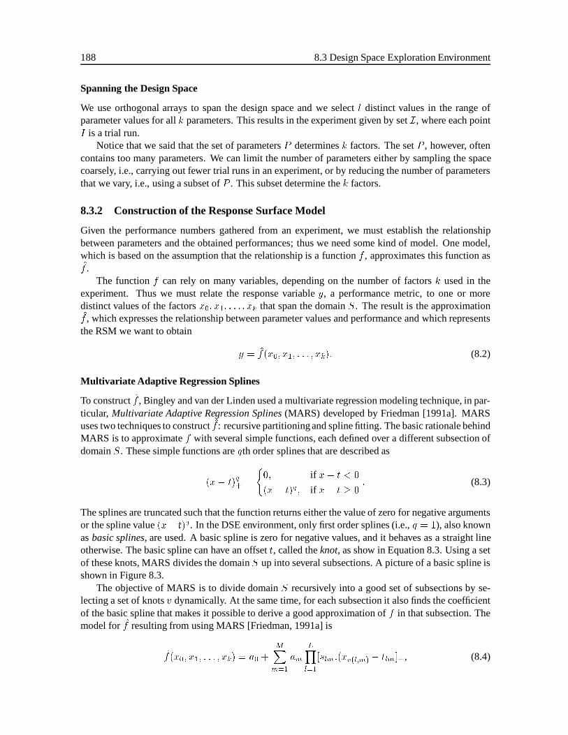
188 8.3 Design Space Exploration Environment
Spanning the Design Space
We use orthogonal arrays to span the design space and we selectl distinct values in the range ofparameter values for allk parameters. This results in the experiment given by setI, where each pointI is a trial run.
Notice that we said that the set of parametersP determinesk factors. The setP , however, oftencontains too many parameters. We can limit the number of parameters either by sampling the spacecoarsely, i.e., carrying out fewer trial runs in an experiment, or by reducing the number of parametersthat we vary, i.e., using a subset ofP . This subset determine thek factors.
8.3.2 Construction of the Response Surface Model
Given the performance numbers gathered from an experiment, we must establish the relationshipbetween parameters and the obtained performances; thus we need some kind of model. One model,which is based on the assumption that the relationship is a functionf , approximates this function asf .
The functionf can rely on many variables, depending on the number of factorsk used in theexperiment. Thus we must relate the response variabley, a performance metric, to one or moredistinct values of the factorsx0; x1; : : : ; xk that span the domainS. The result is the approximationf , which expresses the relationship between parameter values and performance and which representsthe RSM we want to obtain
y = f(x0; x1; : : : ; xk): (8.2)
Multivariate Adaptive Regression Splines
To constructf , Bingley and van der Linden used a multivariate regression modeling technique, in par-ticular, Multivariate Adaptive Regression Splines(MARS) developed by Friedman [1991a]. MARSuses two techniques to constructf : recursive partitioningand spline fitting. The basic rationale behindMARS is to approximatef with several simple functions, each defined over a different subsection ofdomainS. These simple functions areqth order splines that are described as
(x� t)q+ =
(0; if x� t < 0
(x� t)q; if x� t � 0: (8.3)
The splines are truncated such that the function returns either the value of zero for negative argumentsor the spline value(x� t)q. In the DSE environment, only first order splines (i.e.,q = 1), also knownasbasic splines, are used. A basic spline is zero for negative values, and it behaves as a straight lineotherwise. The basic spline can have an offsett, called theknot, as show in Equation 8.3. Using a setof these knots, MARS divides the domainS up into several subsections. A picture of a basic spline isshown in Figure 8.3.
The objective of MARS is to divide domainS recursively into a good set of subsections by se-lecting a set of knotsv dynamically. At the same time, for each subsection it also finds the coefficientof the basic spline that makes it possible to derive a good approximation off in that subsection. Themodel forf resulting from using MARS [Friedman, 1991a] is
f(x0; x1; : : : ; xk) = a0 +MXm=1
am
LYl=1
[slm:(xv(l;m) � tlm]+, (8.4)

Design Space Exploration 189
Y
t X
Figure 8.3 . A basic spline.
which is a summation ofM partial products ofL functions (i.e., basic splines) each expressed in oneparticular factork to account for univariate functionsf(xi) (i.e., l=1), bivariate functionsf(xi; xj)(i.e. l=2), or, in general, multi-variate functions (i.e.1 � l � L). The model also uses the functions that is either equal to +1 or -1. Thus, the functionf that is obtained is apiecewise linear modelexpressed in the parameters which were changed in the experiment, i.e., thek factors. Within thegeneric DSE environment the cross product is limited to be of maximal orderLmax = 2, i.e., bivariatefunctions.
To specify a RSM, which describes the relationship between parameters and a particular perfor-mance metric, we assume that the relationship is a functionf , which we approximate asf . We are,however, thoroughly aware that the relationship we want to describe does not need to be a function atall, but might be some wildly varying relationship. Therefore, when inspecting approximations likef , we should be careful when drawing conclusions. Nevertheless, the assumption that the relation isa function has proven to be very useful for the cases we have considered so far.
8.3.3 Data Management and Data Consistency
During DSE, we produce enormous amounts of data and we need to manage the consistencies betweenall this data. For each trial run of an experiment, performance numbers are created for performancemetrics for a particular set of parameter values. If we had used a simple file system, we would nothave preserved this kind of relationship. The generic DSE environment is therefore built on top ofthe Nelsisdesign data management tool developed by ten Bosch et al. [1991] at Delft Universityof Technology. The Nelsis system provides for the simple encapsulation and integration of designtools. It manages the large amount of data produced by the encapsulated tools and it preserves therelationships between the data offered to and produced by these tools.
Nelsis also has a visual interface as shown in Figure 8.4. The boxes in the figure represent toolsand the directed lines between boxes represent relationships between tools. The boxes together withthe lines define a particulardesign flowand the case shown by Figure 8.4 represents the design flowof the generic DSE environment. We explain the tool that each box represents in detail in Section 8.4.
The oval balloons connected to the lines represent design data that is exchanged between tools andmanaged by Nelsis. In Nelsis, a box can only execute when all its relationships with other boxes havebeen satisfied. Nelsis uses different colors for boxes and different thicknesses for lines to visualizethe status of a box, including whether it can execute or not.
8.3.4 Parameterizing the Architecture Description
Given a set of parameter values, we need to create different textual architecture descriptions. We usethe versatile scripting languagePerl [Wall and Schwartz, 1992] for that purpose. This very powerful
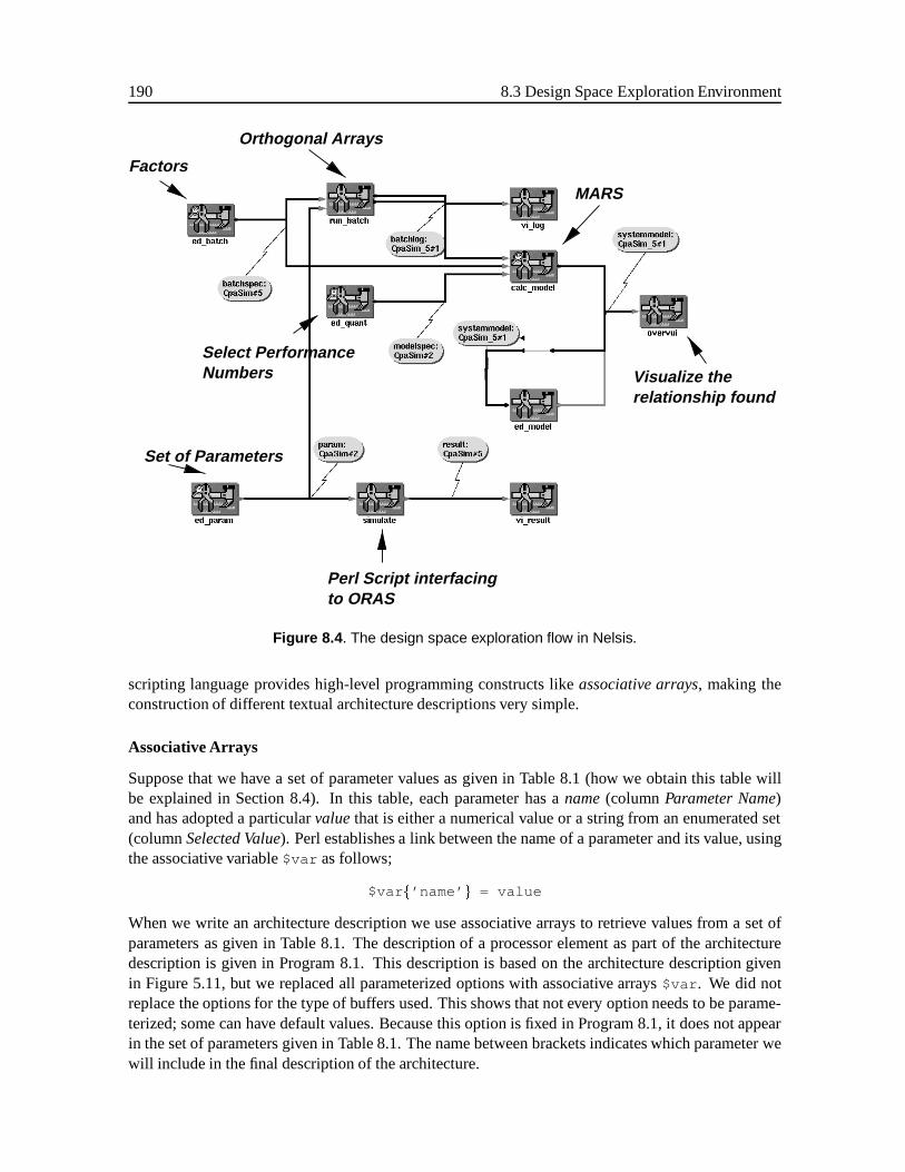
190 8.3 Design Space Exploration Environment
Orthogonal Arrays
MARS
Set of Parameters
Factors
Select Performance
Perl Script interfacing
Numbers
to ORAS
Visualize therelationship found
Figure 8.4 . The design space exploration flow in Nelsis.
scripting language provides high-level programming constructs likeassociative arrays, making theconstruction of different textual architecture descriptions very simple.
Associative Arrays
Suppose that we have a set of parameter values as given in Table 8.1 (how we obtain this table willbe explained in Section 8.4). In this table, each parameter has aname(columnParameter Name)and has adopted a particularvaluethat is either a numerical value or a string from an enumerated set(columnSelected Value). Perl establishes a link between the name of a parameter and its value, usingthe associative variable$var as follows;
$var f’name’ g = value
When we write an architecture description we use associative arrays to retrieve values from a set ofparameters as given in Table 8.1. The description of a processor element as part of the architecturedescription is given in Program 8.1. This description is based on the architecture description givenin Figure 5.11, but we replaced all parameterized options with associative arrays$var . We did notreplace the options for the type of buffers used. This shows that not every option needs to be parame-terized; some can have default values. Because this option is fixed in Program 8.1, it does not appearin the set of parameters given in Table 8.1. The name between brackets indicates which parameter wewill include in the final description of the architecture.
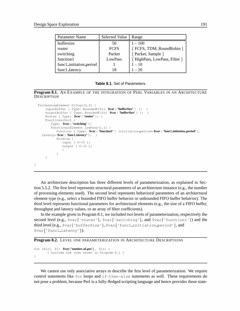
Design Space Exploration 191
Parameter Name Selected Value Range
buffersize 50 1 – 100router FCFS f FCFS, TDM, RoundRobingswitching Packet f Packet, Samplegfunction1 LowPass f HighPass, LowPass, Filtergfunc1 initiation period 1 1 – 10func1 latency 18 1 – 20
Table 8.1 . Set of Parameters.
Program 8.1. AN EXAMPLE OF THE INTEGRATION OFPERL VARIABLES IN AN ARCHITECTUREDESCRIPTION
ProcessingElement Filter(2,2) {InputBuffer { Type: BoundedFifo( $var { ’bufferSize’ } ); }OutputBuffer { Type: BoundedFifo( $var { ’bufferSize’ } ); }Router { Type: $var { ’router’ }; }FunctionalUnit {
Type: $var { ’switching’ };FunctionalElement LowPass(1,1) {
Function { Type: $var { ’function1’ } (initiation period= $var { ’func1 initiation period’ },latency= $var { ’func1 latency’ }; }
Binding {Input ( 0->0 );Output ( 0->0 );}
}}
}
An architecture description has three different levels of parameterization, as explained in Sec-tion 5.5.2. The first level represents structural parameters of an architecture instance (e.g., the numberof processing elements used). The second level represents behavioral parameters of an architecturalelement type (e.g., select a bounded FIFO buffer behavior or unbounded FIFO buffer behavior). Thethird level represents functional parameters for architectural elements (e.g., the size of a FIFO buffer,throughput and latency values, or an array of filter coefficients).
In the example given in Program 8.1, we included two levels of parameterization, respectively thesecond level (e.g.,$var f‘router’ g, $var f‘switching’ g, and$var f‘function1’ g) and thethird level (e.g.,$var f‘bufferSize’ g, $var f‘func1 initiation period’ g, and$var f‘func1 latency’ g).
Program 8.2. LEVEL ONE PARAMETERIZATION IN ARCHITECTUREDESCRIPTIONS
for ($i=1, $i< $varf’number of pes’g , $i++ ){ include the code shown in Program 8.1 }
}
We cannot use only associative arrays to describe the first level of parameterization. We requirecontrol statements likefor loops andif-then-else statements as well. These requirements donot pose a problem, because Perl is a fully-fledged scripting language and hence provides these state-
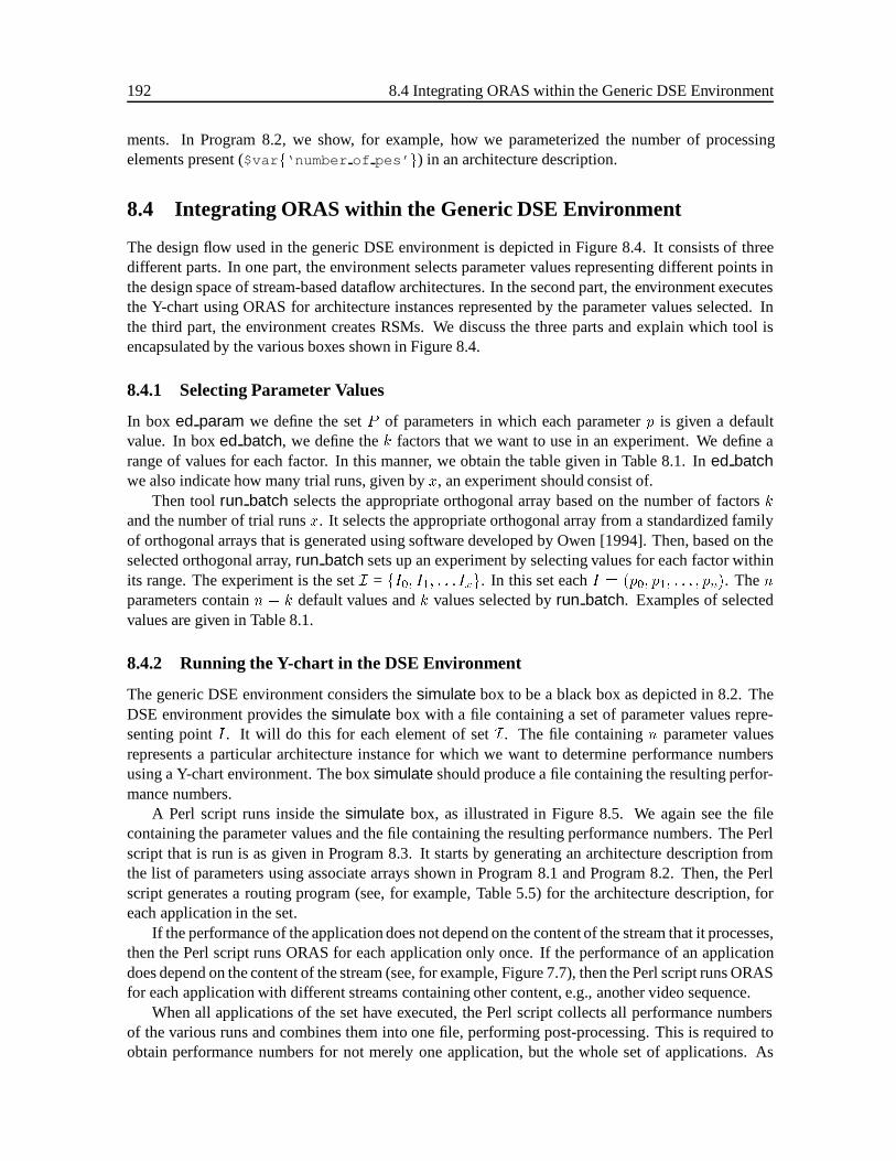
192 8.4 Integrating ORAS within the Generic DSE Environment
ments. In Program 8.2, we show, for example, how we parameterized the number of processingelements present ($var f‘number of pes’ g) in an architecture description.
8.4 Integrating ORAS within the Generic DSE Environment
The design flow used in the generic DSE environment is depicted in Figure 8.4. It consists of threedifferent parts. In one part, the environment selects parameter values representing different points inthe design space of stream-based dataflow architectures. In the second part, the environment executesthe Y-chart using ORAS for architecture instances represented by the parameter values selected. Inthe third part, the environment creates RSMs. We discuss the three parts and explain which tool isencapsulated by the various boxes shown in Figure 8.4.
8.4.1 Selecting Parameter Values
In box ed param we define the setP of parameters in which each parameterp is given a defaultvalue. In boxed batch, we define thek factors that we want to use in an experiment. We define arange of values for each factor. In this manner, we obtain the table given in Table 8.1. Ined batchwe also indicate how many trial runs, given byx, an experiment should consist of.
Then toolrun batch selects the appropriate orthogonal array based on the number of factorskand the number of trial runsx. It selects the appropriate orthogonal array from a standardized familyof orthogonal arrays that is generated using software developed by Owen [1994]. Then, based on theselected orthogonal array,run batch sets up an experiment by selecting values for each factor withinits range. The experiment is the setI = fI0; I1; : : : Ixg. In this set eachI = (p0; p1; : : : ; pn). Thenparameters containn � k default values andk values selected byrun batch. Examples of selectedvalues are given in Table 8.1.
8.4.2 Running the Y-chart in the DSE Environment
The generic DSE environment considers thesimulate box to be a black box as depicted in 8.2. TheDSE environment provides thesimulate box with a file containing a set of parameter values repre-senting pointI . It will do this for each element of setI. The file containingn parameter valuesrepresents a particular architecture instance for which we want to determine performance numbersusing a Y-chart environment. The boxsimulate should produce a file containing the resulting perfor-mance numbers.
A Perl script runs inside thesimulate box, as illustrated in Figure 8.5. We again see the filecontaining the parameter values and the file containing the resulting performance numbers. The Perlscript that is run is as given in Program 8.3. It starts by generating an architecture description fromthe list of parameters using associate arrays shown in Program 8.1 and Program 8.2. Then, the Perlscript generates a routing program (see, for example, Table 5.5) for the architecture description, foreach application in the set.
If the performance of the application does not depend on the content of the stream that it processes,then the Perl script runs ORAS for each application only once. If the performance of an applicationdoes depend on the content of the stream (see, for example, Figure 7.7), then the Perl script runs ORASfor each application with different streams containing other content, e.g., another video sequence.
When all applications of the set have executed, the Perl script collects all performance numbersof the various runs and combines them into one file, performing post-processing. This is required toobtain performance numbers for not merely one application, but the whole set of applications. As

Design Space Exploration 193
TextInput
ORAS
Script Language PERL
Text
Output
Results
Nelsis Box
Parameters
Architecture
Simulate
PerformanceNumbers
RoutingPrograms
Values
Description
Figure 8.5 . The realization of the simulate box, which interacts with the generic DSE en-vironment using an input file containing parameter values and an output file containingperformance numbers.
indicated in Chapter 3, this is essential to obtaining architecture instances that are able to execute aset of applications and obey set-wide design objectives.
Lastly, the Perl script writes out the performance numbers in the format of which an excerpt isshown in Table 7.2.
Program 8.3. PERL SCRIPT USED WITH THE GENERICDSE ENVIRONMENT
read File containing parameter values representing an architecture instancecreate the correct architecture description for the architecture instanceforeach application in the set
create correct routing programif application is a dynamic applications,
foreach stream with different contentexecute ORAS using the routing program and architecture description
elseexecute ORAS using the routing program and architecture description
endif combine found performance numbersperform post processing if needwrite File containing performance numbers
8.4.3 Creating Response Surface Model
All the performance numbers that are generated by thesimulate box are stored in a database whichis part of Nelsis. This database contains the performance numbers as well as the parameter valuesused to obtain these performance numbers. In boxed quant we can select a few performance met-rics, for which boxcalc model constructs the approximationf using the MARS model as given inEquation 8.4. Toolcalc model extracts the parameter values (p0; p1; : : : ; pn) from the database aswell as the performance numbery measured for the selected performance metric.Calc model usesthe software developed by Friedman [1991b] to construct the approximationf .
At last, theovervui box visualizes the approximationf as a 3-dimensional figure, as shown inFigure 8.6(a) and Figure 8.6(b). Notice that these 3-dimensional figures represent ak-dimensional
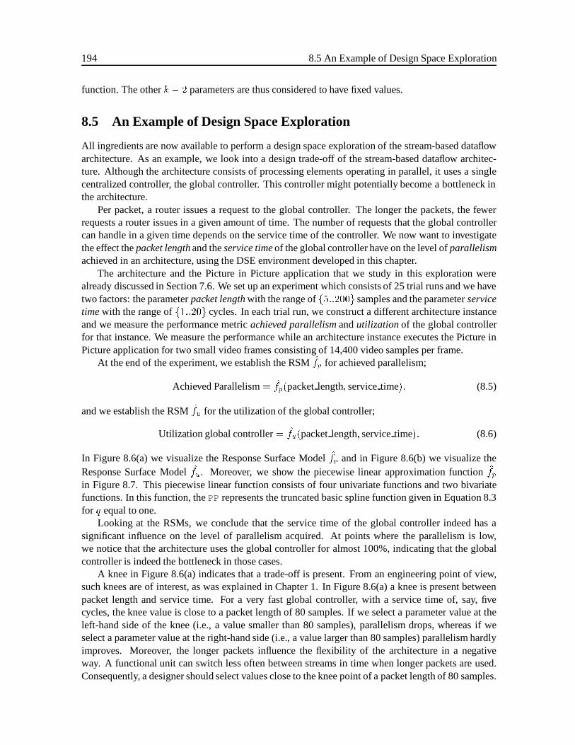
194 8.5 An Example of Design Space Exploration
function. The otherk � 2 parameters are thus considered to have fixed values.
8.5 An Example of Design Space Exploration
All ingredients are now available to perform a design space exploration of the stream-based dataflowarchitecture. As an example, we look into a design trade-off of the stream-based dataflow architec-ture. Although the architecture consists of processing elements operating in parallel, it uses a singlecentralized controller, the global controller. This controller might potentially become a bottleneck inthe architecture.
Per packet, a router issues a request to the global controller. The longer the packets, the fewerrequests a router issues in a given amount of time. The number of requests that the global controllercan handle in a given time depends on the service time of the controller. We now want to investigatethe effect thepacket lengthand theservice timeof the global controller have on the level ofparallelismachieved in an architecture, using the DSE environment developed in this chapter.
The architecture and the Picture in Picture application that we study in this exploration werealready discussed in Section 7.6. We set up an experiment which consists of 25 trial runs and we havetwo factors: the parameterpacket lengthwith the range off5::200g samples and the parameterservicetimewith the range off1::20g cycles. In each trial run, we construct a different architecture instanceand we measure the performance metricachieved parallelismandutilizationof the global controllerfor that instance. We measure the performance while an architecture instance executes the Picture inPicture application for two small video frames consisting of 14,400 video samples per frame.
At the end of the experiment, we establish the RSMfp for achieved parallelism;
Achieved Parallelism= fp(packetlength; servicetime); (8.5)
and we establish the RSMfu for the utilization of the global controller;
Utilization global controller= fu(packetlength; servicetime): (8.6)
In Figure 8.6(a) we visualize the Response Surface Modelfp and in Figure 8.6(b) we visualize theResponse Surface Modelfu. Moreover, we show the piecewise linear approximation functionfpin Figure 8.7. This piecewise linear function consists of four univariate functions and two bivariatefunctions. In this function, thePP represents the truncated basic spline function given in Equation 8.3for q equal to one.
Looking at the RSMs, we conclude that the service time of the global controller indeed has asignificant influence on the level of parallelism acquired. At points where the parallelism is low,we notice that the architecture uses the global controller for almost 100%, indicating that the globalcontroller is indeed the bottleneck in those cases.
A knee in Figure 8.6(a) indicates that a trade-off is present. From an engineering point of view,such knees are of interest, as was explained in Chapter 1. In Figure 8.6(a) a knee is present betweenpacket length and service time. For a very fast global controller, with a service time of, say, fivecycles, the knee value is close to a packet length of 80 samples. If we select a parameter value at theleft-hand side of the knee (i.e., a value smaller than 80 samples), parallelism drops, whereas if weselect a parameter value at the right-hand side (i.e., a value larger than 80 samples) parallelism hardlyimproves. Moreover, the longer packets influence the flexibility of the architecture in a negativeway. A functional unit can switch less often between streams in time when longer packets are used.Consequently, a designer should select values close to the knee point of a packet length of 80 samples.
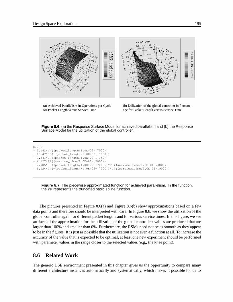
Design Space Exploration 195
(a) Achieved Parallelism in Operations per Cyclefor Packet Length versus Service Time
(b) Utilization of the global controller in Percent-age for Packet Length versus Service Time
Figure 8.6 . (a) the Response Surface Model for achieved parallelism and (b) the ResponseSurface Model for the utilization of the global controller.
8.786+ 1.142*PP((packet_length/1.0E+02-.7000))- 10.47*PP(-(packet_length/1.0E+02-.7000))- 2.541*PP((packet_length/1.0E+02-1.350))- 4.127*PP((service_time/1.0E+01-.5000))+ 2.905*PP((packet_length/1.0E+02-.7000))*PP((service_time/1.0E+01-.3000))+ 6.124*PP(-(packet_length/1.0E+02-.7000))*PP((service_time/1.0E+01-.9000))
Figure 8.7 . The piecewise approximated function for achieved parallelism. In the function,the PP represents the truncated basic spline function.
The pictures presented in Figure 8.6(a) and Figure 8.6(b) show approximations based on a fewdata points and therefore should be interpreted with care. In Figure 8.8, we show the utilization of theglobal controller again for different packet lengths and for various service times. In this figure, we seeartifacts of the approximation for the utilization of the global controller: values are produced that arelarger than 100% and smaller than 0%. Furthermore, the RSMs need not be as smooth as they appearto be in the figures. It is just as possible that the utilization is not even a function at all. To increase theaccuracy of the value that is expected to be optimal, at least one new experiment should be performedwith parameter values in the range closer to the selected values (e.g., the knee point).
8.6 Related Work
The generic DSE environment presented in this chapter gives us the opportunity to compare manydifferent architecture instances automatically and systematically, which makes it possible for us to
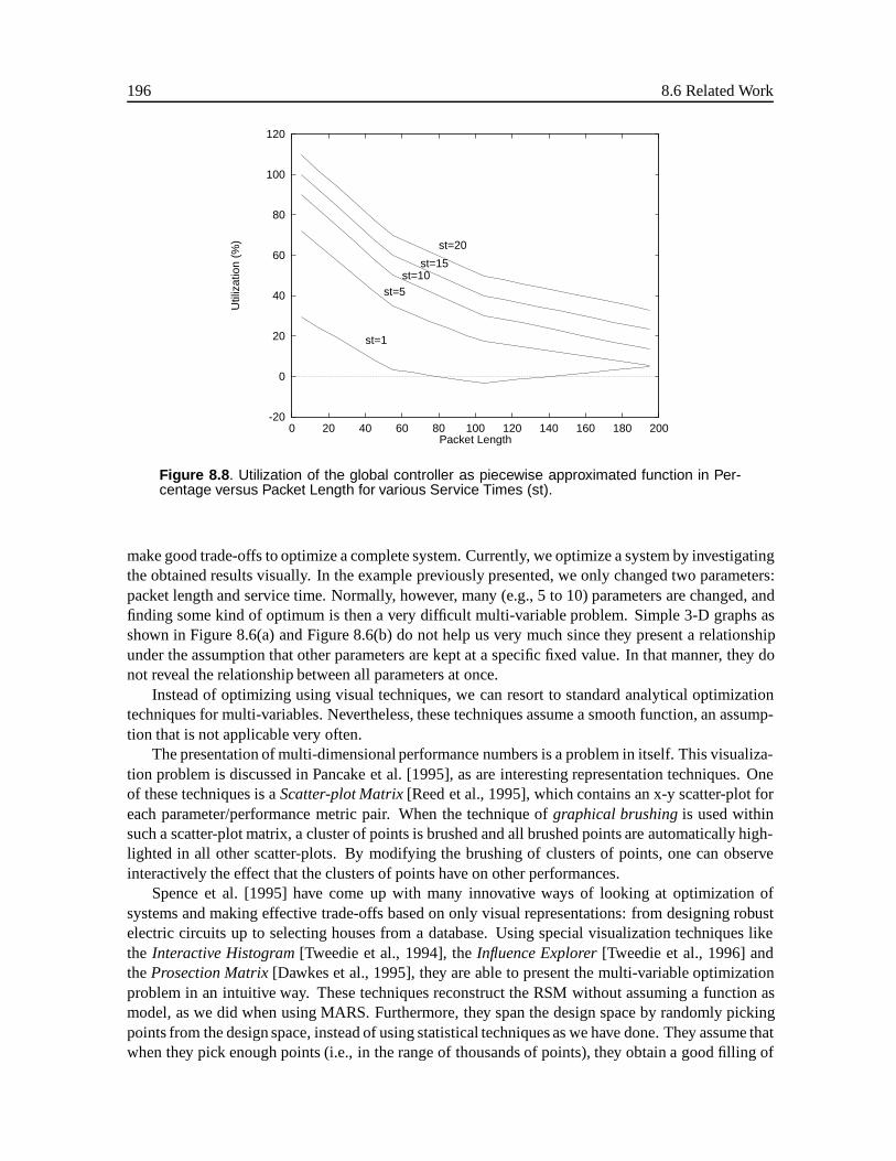
196 8.6 Related Work
-20
0
20
40
60
80
100
120
0 20 40 60 80 100 120 140 160 180 200
Util
izat
ion
(%)
Packet Length
st=1
st=5st=10
st=15
st=20
Figure 8.8 . Utilization of the global controller as piecewise approximated function in Per-centage versus Packet Length for various Service Times (st).
make good trade-offs to optimize a complete system. Currently, we optimize a system by investigatingthe obtained results visually. In the example previously presented, we only changed two parameters:packet length and service time. Normally, however, many (e.g., 5 to 10) parameters are changed, andfinding some kind of optimum is then a very difficult multi-variable problem. Simple 3-D graphs asshown in Figure 8.6(a) and Figure 8.6(b) do not help us very much since they present a relationshipunder the assumption that other parameters are kept at a specific fixed value. In that manner, they donot reveal the relationship between all parameters at once.
Instead of optimizing using visual techniques, we can resort to standard analytical optimizationtechniques for multi-variables. Nevertheless, these techniques assume a smooth function, an assump-tion that is not applicable very often.
The presentation of multi-dimensional performance numbers is a problem in itself. This visualiza-tion problem is discussed in Pancake et al. [1995], as are interesting representation techniques. Oneof these techniques is aScatter-plot Matrix[Reed et al., 1995], which contains an x-y scatter-plot foreach parameter/performance metric pair. When the technique ofgraphical brushingis used withinsuch a scatter-plot matrix, a cluster of points is brushed and all brushed points are automatically high-lighted in all other scatter-plots. By modifying the brushing of clusters of points, one can observeinteractively the effect that the clusters of points have on other performances.
Spence et al. [1995] have come up with many innovative ways of looking at optimization ofsystems and making effective trade-offs based on only visual representations: from designing robustelectric circuits up to selecting houses from a database. Using special visualization techniques likethe Interactive Histogram[Tweedie et al., 1994], theInfluence Explorer[Tweedie et al., 1996] andtheProsection Matrix[Dawkes et al., 1995], they are able to present the multi-variable optimizationproblem in an intuitive way. These techniques reconstruct the RSM without assuming a function asmodel, as we did when using MARS. Furthermore, they span the design space by randomly pickingpoints from the design space, instead of using statistical techniques as we have done. They assume thatwhen they pick enough points (i.e., in the range of thousands of points), they obtain a good filling of
Design Space Exploration 197
the design space. This involves many iterations in the Y-chart, each of which takes minutes to hoursto evaluate. The total evaluation time becomes exorbitantly large, making the present techniquesunattractive.
Teich et al. [1997] useGenetic Algorithmsto optimize architectures. This approach is more robustsince it does not demand smooth functions, as analytical techniques do. Also, the view presented inFigure 8.2 makes the optimization of architectures directly applicable for genetic algorithms. The setof parameters matches directly with the notion of the “gene”, the basic entity in genetic algorithms.However, genetic algorithms require many evaluations in order to reach an optimum. Since eachiteration in the Y-chart takes minutes to hours, the evaluation time becomes prohibitively large, makinggenetic algorithms unattractive.
8.7 Conclusions
In this chapter we have showed how we perform design space exploration of stream-based dataflowarchitectures systematically and automatically, using a Y-chart environment and a generic DSE envi-ronment. We explained that design space exploration involves finding the inverse transformation fromthe performance back to the parameters. Because this inverse is in general difficult to determine, weconstruct response surface models to help us do it. We used a generic DSE environment to performdesign space exploration.
To perform design space exploration, we had to carry out the following four steps: select pa-rameter values in the design space efficiently, construct the Response Surface Models, manage theenormous amounts of data produced in running an experiment, and describe architecture descriptionsin a parameterized way.
For the selection of parameter values in the design space, the generic DSE environment sets up anexperiment as a fractional factorial experiment. It employs orthogonal arrays to span a design spaceusing a minimal amount of trial runs; an important step since each execution of ORAS might takeminutes to hours.
The generic DSE environment uses a multivariate regression modeling technique called Multivari-ate Adaptive Regression Splines (MARS), to construct the RSMs. The generic DSE environment usesMARS to approximate the relationship between parameter values and a specific performance metricby f . This environment can visualizef , representing the RSM.
So that it can manage the large amount of data produced in experiments, the generic DSE envi-ronment is built on top of the Nelsis design data management tool. One task of this tool is to managethe storage and retrieval of data; its main function, however, is to manage the relationship betweendata offered to and produced by tools.
We used the versatile scripting language Perl to describe architecture descriptions in a parame-terized way. This very powerful scripting language provides high-level programming constructs likeassociative arrays, making the construction of different textual architecture descriptions very simple.Moreover, it acts like a UNIX shell script, which we use to activate various steps needed to evaluatean architecture instance for a set of applications using ORAS.
Using the generic DSE environment, we showed an example of design space exploration. Forthe Picture in Picture application, we set up an experiment in which we constructed 25 differentarchitecture instances and measured the achieved parallelism in the architecture instance as well asthe utilization of the global controller. We performed the exploration and showed the RSMfp forachieved parallelism and the RSMfu for the utilization of the global controller. The explorationshowed that the amount of achieved parallelism in the architecture instance very much depends on
198 BIBLIOGRAPHY
the relationship between the service time of the global controller and the packet length. Infp, weidentified a knee that represents a trade-off between the service time and packet length.
The RSMs presented are approximations. We showed the artifacts resulting from this approxima-tion and indicated clearly that these Response Surface Models need to be interpreted with care.
As last, we discussed related work on design space exploration.
Bibliography
Peter Bingley and Wim van der Linden. Application of framework technology in system simulationenvironments. InProceedings of the Seminar ‘Database Systems and Applications for the Nineties’.Delft University of Technology, 1994.
K.A. Bush. Orthogonal arrays of index unity.Annals of Mathematical Statistics, 23:426 – 434, 1952.
Huw Dawkes, Lisa Tweedie, and Bob Spence. VICKI - the visualisationconstruction kit. InAdvancedVisual Interfaces, Gubbio, Italy, 1995.
Jerome H. Friedman. Multivariate adaptive regression splines.Annals of Statistics, 19(1):1 – 141,1991a.
Jerome H. Friedman. Multivariate adaptive regression splines (MARS modeling) software. Softwarecan be obtained from http://stat.stanford.edu/software/software.html, 1991b. Version 3.5.
Robert H. Lochner and Joseph E. Matar.Designing for Quality: An introduction to the best of Taguchiand western methods of statistical experimental design. Chapman and Hall, 1990.
N. Logothetis and H.P. Wynn.Quality through design; experimental design, off-line quality controland Taguchi’s contributions, volume 7 ofOxford series on advanced manufacturing. Clarendon,Oxford, 1989.
Art Owen. Orthogonal arrays for computer experiments, integration, and visualization. Technicalreport, Dept. of Statistics, Stanford University, 1991.
Art Owen. Orthogonal array design software. Software can be obtained from:http://stat.stanford.edu/software/software.html, 1994.
Cherri M. Pancake, Margaret L. Simmons, and Jerry C. Yan. Guest editors’ introduction: Performanceevaluation tools for parallel and distributed systems.IEEE Computer, 28(11):16 – 20, 1995. ThemeFeature.
Daniel A. Reed, Keith A. Shields, Will H. Scullin, Luis F. Tavera, and Christopher L. Elford. Virtualreality and parallel systems performance analysis.IEEE Computer, 28(11):57 – 67, 1995.
R. Spence. MINNIE, a new direction in circuit design.Electronics Weekly, 1974. Issue 3.
R. Spence, L. Tweedie, H. Dawkes, and H Su. Visualisation for functional design. InProceedingsInformation Visualization’95, pages 4 – 10, 1995.
J. Teich, T. Blickle, and L. Thiele. An evolutionaryapproach to system-level synthesis. InProceedingsof the Fifth Int. Workshop on Hardware/Software Codesign, pages 167 – 171, 1997.
BIBLIOGRAPHY 199
K.O. ten Bosch, P. Bingley, and P. van der Wolf. Design flow management in the NELSIS CAD frame-work. In Proc. 28th ACM/IEEE Design Automation Conference, pages 711–716, San Francisco,1991.
Lisa Tweedie, Robert Spence, Huw Dawkes, and Hua Su. Externalising abstract mathematical models.In Proceedings of CHI’96, Vancouver, Canada, 1996. ACM Press.
Lisa Tweedie, Robert Spence, David Williams, and Ravinder Bhoghal. The attribute explorer. InVideo Proceedings and Conference Companion, CHI’94, pages 435 – 436, Boston, 1994. ACMPress.
Larry Wall and Randal L. Schwartz.Programming Perl. O’Reilly & Associates, Inc., 1992.

200 BIBLIOGRAPHY
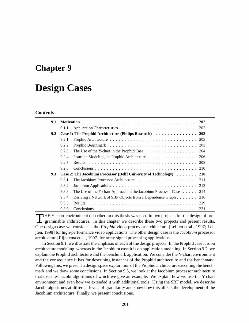
Chapter 9
Design Cases
Contents
9.1 Motivation . . . . . . . . . . . . . . . . . . . . . . . . . . . . . . . . . . . . . . 2029.1.1 Application Characteristics . . . . . . . . . . . . . . . . . . . . . . . . . . 202
9.2 Case 1: The Prophid Architecture (Philips Research) . . . . . . . . . . . . . . 2039.2.1 Prophid Architecture. . . . . . . . . . . . . . . . . . . . . . . . . . . . . 203
9.2.2 Prophid Benchmark. . . . . . . . . . . . . . . . . . . . . . . . . . . . . 203
9.2.3 The Use of the Y-chart in the Prophid Case. . . . . . . . . . . . . . . . . 204
9.2.4 Issues in Modeling the Prophid Architecture. . . . . . . . . . . . . . . . . 206
9.2.5 Results . . . . . . . . . . . . . . . . . . . . . . . . . . . . . . . . . . . . 208
9.2.6 Conclusions . . . . . . . . . . . . . . . . . . . . . . . . . . . . . . . . . . 210
9.3 Case 2: The Jacobium Processor (Delft University of Technology). . . . . . . 2109.3.1 The Jacobium Processor Architecture . . . . . . . . . . . . . . . . . . . . 211
9.3.2 Jacobium Applications . . . . . . . . . . . . . . . . . . . . . . . . . . . . 213
9.3.3 The Use of the Y-chart Approach in the Jacobium Processor Case . . . . . 214
9.3.4 Deriving a Network of SBF Objects from a Dependence Graph . . . . . . . 216
9.3.5 Results . . . . . . . . . . . . . . . . . . . . . . . . . . . . . . . . . . . . 219
9.3.6 Conclusions . . . . . . . . . . . . . . . . . . . . . . . . . . . . . . . . . . 221
THE Y-chart environment described in this thesis was used in two projects for the design of pro-grammable architectures. In this chapter we describe these two projects and present results.
One design case we consider is theProphidvideo-processor architecture [Leijten et al., 1997; Lei-jten, 1998] for high-performance video applications. The other design case is theJacobiumprocessorarchitecture [Rijpkema et al., 1997] for array signal processing applications.
In Section 9.1, we illustrate the emphasis ofeach of the design projects: In the Prophid case it is onarchitecture modeling, whereas in the Jacobium case it is on application modeling. In Section 9.2, weexplain the Prophid architecture and the benchmark application. We consider the Y-chart environmentand the consequence it has for describing instances of the Prophid architecture and the benchmark.Following this, we present a design space exploration of the Prophid architecture executing the bench-mark and we draw some conclusions. In Section 9.3, we look at the Jacobium processor architecturethat executes Jacobi algorithms of which we give an example. We explain how we use the Y-chartenvironment and even how we extended it with additional tools. Using the SBF model, we describeJacobi algorithms at different levels of granularity and show how this affects the development of theJacobium architecture. Finally, we present conclusions.
201
202 9.1 Motivation
9.1 Motivation
In this chapter, we discuss two different design cases of programmable architectures. Both archi-tectures are similar to stream-based dataflow architectures, but the applications belong to differentapplication domains. The purpose of this chapter is to show how the use of the Y-chart approach andY-chart environment effect real design cases. It also serve to shows that the techniques developed inthis thesis are indeed useful and capable of describing realistic design cases.
9.1.1 Application Characteristics
The Prophid and Jacobium architectures are similar to the stream-based dataflow architecture tem-plate presented in Chapter 2. For the Prophid architecture, this is not surprising since its architecturetemplate was in principle taken as model for the development of the class of stream-based dataflowarchitectures. The Jacobium architecture template is a result of further development of previous archi-tectures [van Dijk et al., 1993] and was inspired by developments in wireless communication archi-tectures [Jain, 1997]. The designers of the Jacobium architecture knew about the Prophid architectureand were influenced by it.
However, the two architectures execute applications with different characteristics. This becomesclear when we look at the dependence graphs (DG) of two applications. The DG representation ofvideo applications used in the Prophid case looks like a sequence of predominantly coarse-grainedoperators operating in a pipeline fashion. See, for example, the description of the Picture in Pic-ture application in Figure 6.1. In contrast, array signal processing applications used in the Jacobiumcase must exploit correlation of data received from, for example, various antennas. Therefore, theirDG representation consists of more fine-grained operators that are much more interrelated. See, forexample, the dependence graph in Figure 9.10.
Application Descriptions
The use of the Y-chart environment in both cases requires that applications be available and describedas networks of SBF objects. We experienced severe difficulties in finding realistic applications in boththe Prophid and the Jacobium case. If applications were specified at all, the specification was not inthe format of networks of SBF objects or in a format from which a networks of SBF objects can easilybe derived. The specifications were given in the C-programming language or in Matlab, using globalvariables and data structures of the wrong type (i.e. matrices or lines) and in such a way that they hidany form of parallelism, due to the inherent sequential ordering of the imperative languages (see formore information Chapter 6, where we explain how we model applications).
The acquisition of applications was somewhat less troublesome in the Jacobium case. In thatproject, the Jacobium processor executes algorithms which belong to the class of Jacobi-type algo-rithms [Golub and Loan, 1989]. For this class, many algorithms have already been specified as nested-loop programs. Moreover, tools are available that can help to manually transform these nested-loopprograms into the suitable format [Held, 1996], albeit with difficulty.
A consequence of not having a well-defined set of applications, especially in the Prophid case, isthat design space exploration is performed using one application instead of a set of applications. Syn-thetic application descriptions have been considered, but the derivation of realistic synthetic bench-marks is a complex problem in its own right [Dick et al., 1998].
We do not intend to give a complete description of the design cases and their results. Instead,we want to show that techniques developed in this thesis are indeed useful and capable of modeling
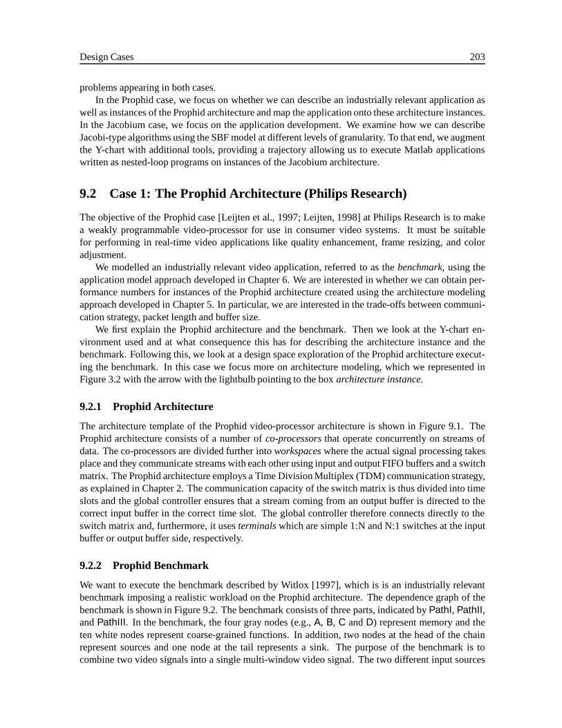
Design Cases 203
problems appearing in both cases.In the Prophid case, we focus on whether we can describe an industrially relevant application as
well as instances of the Prophid architecture and map the application onto these architecture instances.In the Jacobium case, we focus on the application development. We examine how we can describeJacobi-type algorithms using the SBF model at different levels of granularity. To that end, we augmentthe Y-chart with additional tools, providing a trajectory allowing us to execute Matlab applicationswritten as nested-loop programs on instances of the Jacobium architecture.
9.2 Case 1: The Prophid Architecture (Philips Research)
The objective of the Prophid case [Leijten et al., 1997; Leijten, 1998] at Philips Research is to makea weakly programmable video-processor for use in consumer video systems. It must be suitablefor performing in real-time video applications like quality enhancement, frame resizing, and coloradjustment.
We modelled an industrially relevant video application, referred to as thebenchmark, using theapplication model approach developed in Chapter 6. We are interested in whether we can obtain per-formance numbers for instances of the Prophid architecture created using the architecture modelingapproach developed in Chapter 5. In particular, we are interested in the trade-offs between communi-cation strategy, packet length and buffer size.
We first explain the Prophid architecture and the benchmark. Then we look at the Y-chart en-vironment used and at what consequence this has for describing the architecture instance and thebenchmark. Following this, we look at a design space exploration of the Prophid architecture execut-ing the benchmark. In this case we focus more on architecture modeling, which we represented inFigure 3.2 with the arrow with the lightbulb pointing to the boxarchitecture instance.
9.2.1 Prophid Architecture
The architecture template of the Prophid video-processor architecture is shown in Figure 9.1. TheProphid architecture consists of a number ofco-processorsthat operate concurrently on streams ofdata. The co-processors are divided further intoworkspaceswhere the actual signal processing takesplace and they communicate streams with each other using input and output FIFO buffers and a switchmatrix. The Prophid architecture employs a Time Division Multiplex (TDM) communication strategy,as explained in Chapter 2. The communication capacity of the switch matrix is thus divided into timeslots and the global controller ensures that a stream coming from an output buffer is directed to thecorrect input buffer in the correct time slot. The global controller therefore connects directly to theswitch matrix and, furthermore, it usesterminalswhich are simple 1:N and N:1 switches at the inputbuffer or output buffer side, respectively.
9.2.2 Prophid Benchmark
We want to execute the benchmark described by Witlox [1997], which is is an industrially relevantbenchmark imposing a realistic workload on the Prophid architecture. The dependence graph of thebenchmark is shown in Figure 9.2. The benchmark consists of three parts, indicated byPathI, PathII,andPathIII. In the benchmark, the four gray nodes (e.g.,A, B, C andD) represent memory and theten white nodes represent coarse-grained functions. In addition, two nodes at the head of the chainrepresent sources and one node at the tail represents a sink. The purpose of the benchmark is tocombine two video signals into a single multi-window video signal. The two different input sources
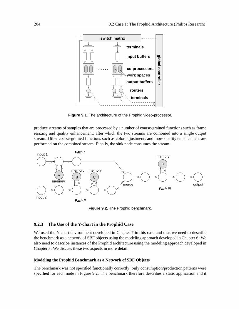
204 9.2 Case 1: The Prophid Architecture (Philips Research)
glo
bal co
ntro
ller
switch matrix
terminals
co-processors
routers
terminals
output buffers
input buffers
work spaces
Figure 9.1 . The architecture of the Prophid video-processor.
produce streams of samples that are processed by a number of coarse-grained functions such as frameresizing and quality enhancement, after which the two streams are combined into a single outputstream. Other coarse-grained functions such as color adjustments and more quality enhancement areperformed on the combined stream. Finally, the sink node consumes the stream.
input 2
input 1memory
output
memory memory
memorymerge
Path I
Path II
Path III
A B C
D
Figure 9.2 . The Prophid benchmark.
9.2.3 The Use of the Y-chart in the Prophid Case
We used the Y-chart environment developed in Chapter 7 in this case and thus we need to describethe benchmark as a network of SBF objects using the modeling approach developed in Chapter 6. Wealso need to describe instances of the Prophid architecture using the modeling approach developed inChapter 5. We discuss these two aspects in more detail.
Modeling the Prophid Benchmark as a Network of SBF Objects
The benchmark was not specified functionally correctly; only consumption/production patterns werespecified for each node in Figure 9.2. The benchmark therefore describes a static application and it
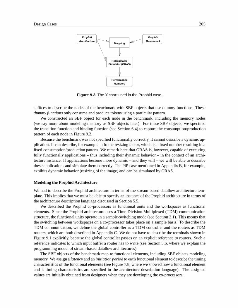
Design Cases 205
PerformanceNumbers
Mapping
RetargetableSimulator (ORAS)
ProphidArchitecture Benchmark
Prophid
Figure 9.3 . The Y-chart used in the Prophid case.
suffices to describe the nodes of the benchmark with SBF objects that use dummy functions. Thesedummy functionsonly consume and produce tokens using a particular pattern.
We constructed an SBF object for each node in the benchmark, including the memory nodes(we say more about modeling memory as SBF objects later). For these SBF objects, we specifiedthe transition function and binding function (see Section 6.4) to capture the consumption/productionpattern of each node in Figure 9.2.
Because the benchmark was not specified functionally correctly, it cannot describe a dynamic ap-plication. It can describe, for example, a frame resizing factor, which is a fixed number resulting in afixed consumption/production pattern. We remark here that ORAS is, however, capable of executingfully functionally applications – thus including their dynamic behavior – in the context of an archi-tecture instance. If applications become more dynamic – and they will – we will be able to describethese applications and simulate them correctly. The PiP case mentioned in Appendix B, for example,exhibits dynamic behavior (resizing of the image) and can be simulated by ORAS.
Modeling the Prophid Architecture
We had to describe the Prophid architecture in terms of the stream-based dataflow architecture tem-plate. This implies that we must be able to specify an instance of the Prophid architecture in terms ofthe architecture description language discussed in Section 5.5.
We described the Prophid co-processors as functional units and the workspaces as functionalelements. Since the Prophid architecture uses a Time Division Multiplexed (TDM) communicationstructure, the functional units operate in a sample-switching mode (see Section 2.1). This means thatthe switching between workspaces on a co-processor takes place on a sample basis. To describe theTDM communication, we define the global controller as a TDM controller and the routers as TDMrouters, which are both described in Appendix C. We do not have to describe the terminals shown inFigure 9.1 explicitly, because the global controller passes on an explicit reference to routers. Such areference indicates to which input buffer a router has to write (see Section 5.6, where we explain theprogramming model of stream-based dataflow architectures).
The SBF objects of the benchmark map to functional elements, including SBF objects modelingmemory. We assign alatencyand aninitiationperiodto each functional element to describe the timingcharacteristics of the functional elements (see Figure 7.8, where we showed how a functional elementand it timing characteristics are specified in the architecture description language). The assignedvalues are initially obtained from designers when they are developing the co-processors.
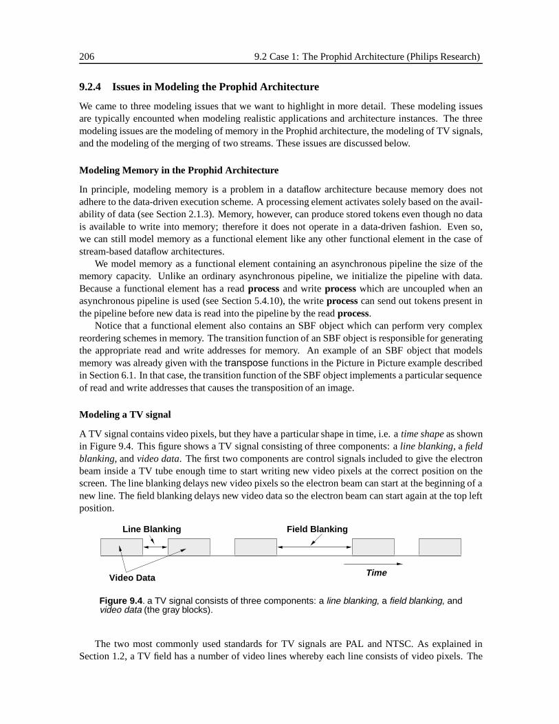
206 9.2 Case 1: The Prophid Architecture (Philips Research)
9.2.4 Issues in Modeling the Prophid Architecture
We came to three modeling issues that we want to highlight in more detail. These modeling issuesare typically encounted when modeling realistic applications and architecture instances. The threemodeling issues are the modeling of memory in the Prophid architecture, the modeling of TV signals,and the modeling of the merging of two streams. These issues are discussed below.
Modeling Memory in the Prophid Architecture
In principle, modeling memory is a problem in a dataflow architecture because memory does notadhere to the data-driven execution scheme. A processing element activates solely based on the avail-ability of data (see Section 2.1.3). Memory, however, can produce stored tokens even though no datais available to write into memory; therefore it does not operate in a data-driven fashion. Even so,we can still model memory as a functional element like any other functional element in the case ofstream-based dataflow architectures.
We model memory as a functional element containing an asynchronous pipeline the size of thememory capacity. Unlike an ordinary asynchronous pipeline, we initialize the pipeline with data.Because a functional element has a readprocessand writeprocesswhich are uncoupled when anasynchronous pipeline is used (see Section 5.4.10), the writeprocesscan send out tokens present inthe pipeline before new data is read into the pipeline by the readprocess.
Notice that a functional element also contains an SBF object which can perform very complexreordering schemes in memory. The transition function of an SBF object is responsible for generatingthe appropriate read and write addresses for memory. An example of an SBF object that modelsmemory was already given with thetranspose functions in the Picture in Picture example describedin Section 6.1. In that case, the transition function of the SBF object implements a particular sequenceof read and write addresses that causes the transposition of an image.
Modeling a TV signal
A TV signal contains video pixels, but they have a particular shape in time, i.e. atime shapeas shownin Figure 9.4. This figure shows a TV signal consisting of three components: aline blanking, afieldblanking, andvideo data. The first two components are control signals included to give the electronbeam inside a TV tube enough time to start writing new video pixels at the correct position on thescreen. The line blanking delays new video pixels so the electron beam can start at the beginning of anew line. The field blanking delays new video data so the electron beam can start again at the top leftposition.
Video Data Time
Field BlankingLine Blanking
Figure 9.4 . a TV signal consists of three components: a line blanking, a field blanking, andvideo data (the gray blocks).
The two most commonly used standards for TV signals are PAL and NTSC. As explained inSection 1.2, a TV field has a number of video lines whereby each line consists of video pixels. The
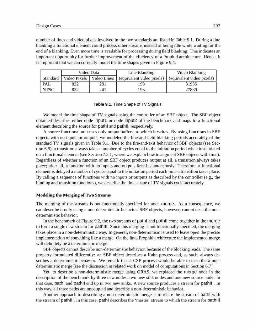
Design Cases 207
number of lines and video pixels involved in the two standards are listed in Table 9.1. During a lineblanking a functional element could process other streams instead of being idle while waiting for theend of a blanking. Even more time is available for processing during field blanking. This indicates animportant opportunity for further improvement of the efficiency of a Prophid architecture. Hence, itis important that we can correctly model the time shapes given in Figure 9.4.
Video Data Line Blanking Video BlankingStandard Video Pixels Video Lines (equivalent video pixels) (equivalent video pixels)PAL 832 281 193 31935NTSC 832 241 193 27839
Table 9.1 . Time Shape of TV Signals.
We model the time shape of TV signals using the controller of an SBF object. The SBF objectobtained describes either nodeinput1 or nodeinput2 of the benchmark and maps to a functionalelement describing the source forpathI andpathII, respectively.
A source functional unit uses only output buffers, to which it writes. By using functions in SBFobjects with no inputs or outputs, we modeled the line and field blanking periods accurately of thestandard TV signals given in Table 9.1. Due to the fire-and-exit behavior of SBF objects (see Sec-tion 6.8), a transition always takes a number of cycles equal to the initiation period when instantiatedon a functional element (see Section 7.5.1, where we explain how to augment SBF objects with time).Regardless of whether a function of an SBF object produces output at all, a transition always takesplace; after all, a function with no inputs and outputs fires instantaneously. Therefore, a functionalelement is delayed a number of cycles equal to the initiation periodeach time a transition takes place.By calling a sequence of functions with no inputs or outputs as described by the controller (e.g., thebinding and transition functions), we describe the time shape of TV signals cycle-accurately.
Modeling the Merging of Two Streams
The merging of the streams is not functionally specified for nodemerge. As a consequence, wecan describe it only using a non-deterministic behavior. SBF objects, however, cannot describe non-deterministic behavior.
In the benchmark of Figure 9.2, the two streams ofpathI andpathII come together in themergeto form a single new stream forpathIII. Since this merging is not functionally specified, the mergingtakes place in a non-deterministic way. In general, non-determinism is used to leave open the preciseimplementation of something like a merge. On the final Prophid architecture the implemented mergewill definitely be a deterministic merge.
SBF objects cannot describe non-deterministic behavior, because of the blocking reads. The sameproperty formulated differently: an SBF object describes a Kahn process and, as such, always de-scribes a deterministic behavior. We remark that a CSP process would be able to describe a non-deterministic merge (see the discussion in related work on model of computations in Section 6.7).
Yet, to describe a non-deterministic merge using ORAS, we replaced themerge node in thedescription of the benchmark by three new nodes: two new sink nodes and one new source node. Inthat case,pathI andpathII end up in two new sinks. A new source produces a stream forpathIII. Inthis way, all three paths are uncoupled and describe a non-deterministic behavior.
Another approach to describing a non-deterministic merge is to relate the stream ofpathI withthe stream ofpathIII. In this case,pathI describes the ‘master’ stream to which the stream forpathIII
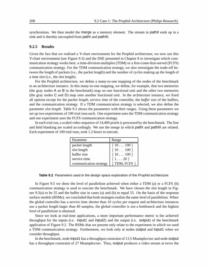
208 9.2 Case 1: The Prophid Architecture (Philips Research)
synchronizes. We then model themerge as a memory element. The stream inpathII ends up in asink and is thereby uncoupled frompathI andpathIII.
9.2.5 Results
Given the fact that we realized a Y-chart environment for the Prophid architecture, we now use thisY-chart environment (see Figure 9.3) and the DSE presented in Chapter 8 to investigate which com-munication strategy works best: a time-division-multiplex (TDM) or a first-come-first-served (FCFS)communication strategy. For the TDM communication strategy, we also investigate the trade-off be-tween the length of packets (i.e., the packet length) and the number of cycles making up the length ofa time slot (i.e., the slot length).
For the Prophid architecture, we define a many-to-one mapping of the nodes of the benchmarkto an architecture instance. In this many-to-one mapping, we define, for example, that two memories(the gray nodesA an B in the benchmark) map on one functional unit and the other two memories(the gray nodesC andD) map onto another functional unit. In the architecture instance, we fixedall options except for thepacket length, service timeof the controller, thebuffer sizeof the buffers,and the communication strategy. If a TDM communication strategy is selected, we also define theparameterslot length. Table 9.2 shows the parameters with their ranges. Using these parameters weset up two experiments of 100 trial runs each. One experiment uses the TDM communication strategyand one experiment uses the FCFS communication strategy.
In each trial run, a scaled video sequence of 14,400 pixels is processed by the benchmark. The lineand field blanking are scaled accordingly. We use the merge in whichpathI andpathIII are related.Each experiment of 100 trial runs, took 1.2 hours to execute.
Parameter Range
packet length f 10 : : : 100gslot length f 10 : : : 100gbuffer size f 10 : : : 100gservice time f 1 : : : 20gcommunication strategy f TDM, FCFSg
Table 9.2 . Parameters used in the design space exploration of the Prophid architecture.
In Figure 9.5 we show the level of parallelism achieved when either a TDM (a) or a FCFS (b)communication strategy is used to execute the benchmark. We have chosen the slot length in Fig-ure 9.5(a) to be 55 and the buffer size in cases (a) and (b) to equal 55. On the basis of the responsesurface models (RSMs), we concluded that both strategies realize the same level of parallelism. Whenthe global controller has a service time shorter than 10 cycles per request and architecture instancesuse a packet length larger than 40 samples, the global controller is not a bottleneck and the highestlevel of parallelism is obtained.
Since we look at real-time applications, a more important performance metric is the achievedthroughput for the inputs (i.e.input1 and input2) and the output (i.e.output) of the benchmarkapplication of Figure 9.2. The RSMs that we present only relate to the experiment in which we useda TDM communication strategy. Furthermore, we look only at nodesoutput and input1 when weconsider throughput.
In the benchmark, nodeinput1 has a throughput constraint of 13.5 Msamples/sec and nodeoutputhas a throughput constraint of 27 Msamples/sec. Thus,output produces a video stream at twice the
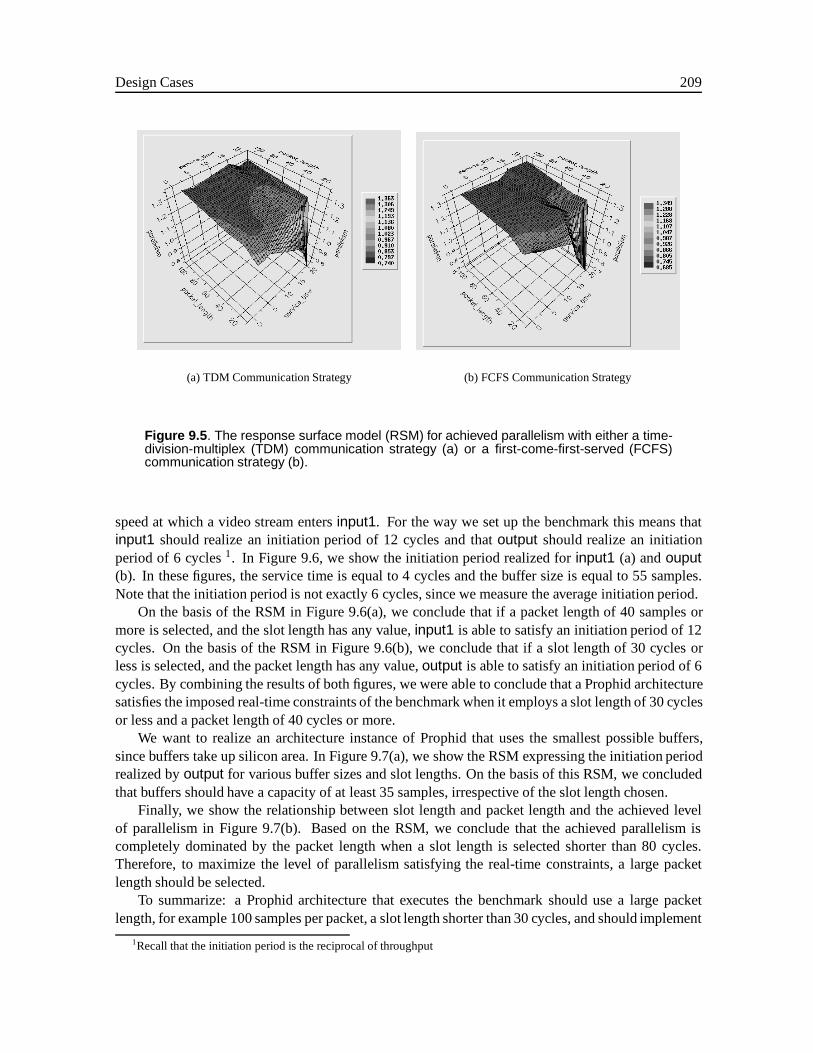
Design Cases 209
(a) TDM Communication Strategy (b) FCFS Communication Strategy
Figure 9.5 . The response surface model (RSM) for achieved parallelism with either a time-division-multiplex (TDM) communication strategy (a) or a first-come-first-served (FCFS)communication strategy (b).
speed at which a video stream entersinput1. For the way we set up the benchmark this means thatinput1 should realize an initiation period of 12 cycles and thatoutput should realize an initiationperiod of 6 cycles1. In Figure 9.6, we show the initiation period realized forinput1 (a) andouput(b). In these figures, the service time is equal to 4 cycles and the buffer size is equal to 55 samples.Note that the initiation period is not exactly 6 cycles, since we measure the average initiation period.
On the basis of the RSM in Figure 9.6(a), we conclude that if a packet length of 40 samples ormore is selected, and the slot length has any value,input1 is able to satisfy an initiation period of 12cycles. On the basis of the RSM in Figure 9.6(b), we conclude that if a slot length of 30 cycles orless is selected, and the packet length has any value,output is able to satisfy an initiation period of 6cycles. By combining the results of both figures, we were able to conclude that a Prophid architecturesatisfies the imposed real-time constraints of the benchmark when it employs a slot length of 30 cyclesor less and a packet length of 40 cycles or more.
We want to realize an architecture instance of Prophid that uses the smallest possible buffers,since buffers take up silicon area. In Figure 9.7(a), we show the RSM expressing the initiation periodrealized byoutput for various buffer sizes and slot lengths. On the basis of this RSM, we concludedthat buffers should have a capacity of at least 35 samples, irrespective of the slot length chosen.
Finally, we show the relationship between slot length and packet length and the achieved levelof parallelism in Figure 9.7(b). Based on the RSM, we conclude that the achieved parallelism iscompletely dominated by the packet length when a slot length is selected shorter than 80 cycles.Therefore, to maximize the level of parallelism satisfying the real-time constraints, a large packetlength should be selected.
To summarize: a Prophid architecture that executes the benchmark should use a large packetlength, for example 100 samples per packet, a slot length shorter than 30 cycles, and should implement
1Recall that the initiation period is the reciprocal of throughput
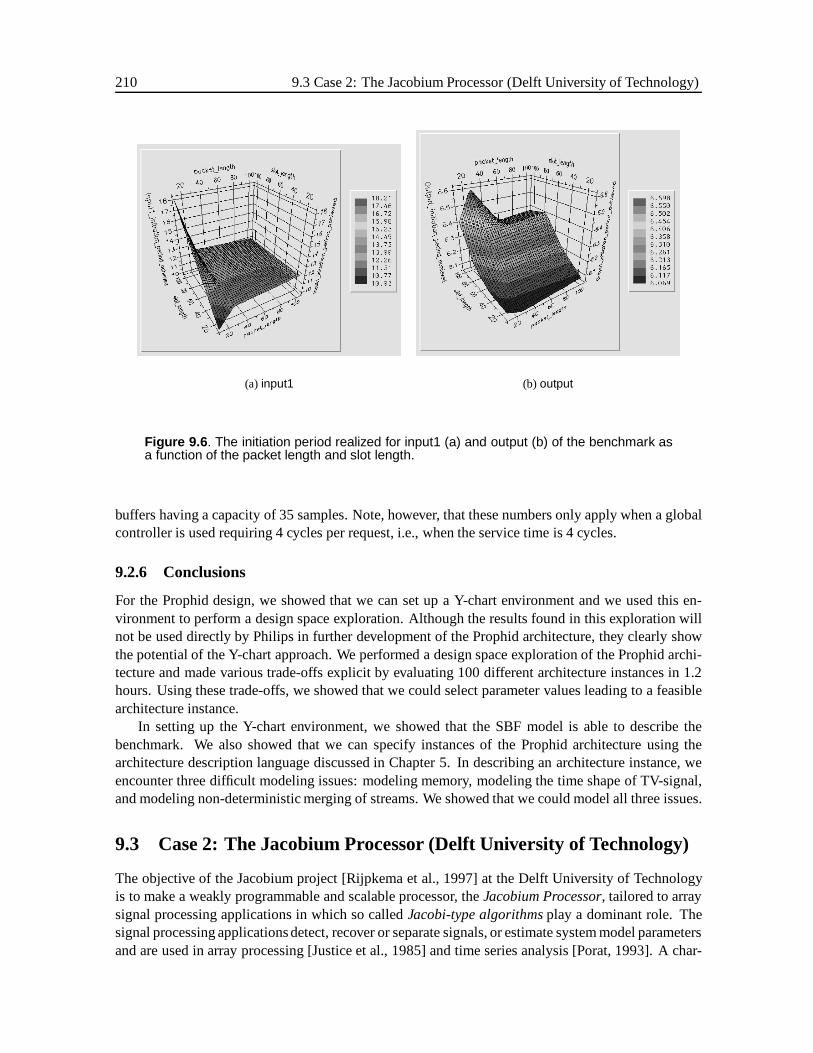
210 9.3 Case 2: The Jacobium Processor (Delft University of Technology)
(a) input1 (b) output
Figure 9.6 . The initiation period realized for input1 (a) and output (b) of the benchmark asa function of the packet length and slot length.
buffers having a capacity of 35 samples. Note, however, that these numbers only apply when a globalcontroller is used requiring 4 cycles per request, i.e., when the service time is 4 cycles.
9.2.6 Conclusions
For the Prophid design, we showed that we can set up a Y-chart environment and we used this en-vironment to perform a design space exploration. Although the results found in this exploration willnot be used directly by Philips in further development of the Prophid architecture, they clearly showthe potential of the Y-chart approach. We performed a design space exploration of the Prophid archi-tecture and made various trade-offs explicit by evaluating 100 different architecture instances in 1.2hours. Using these trade-offs, we showed that we could select parameter values leading to a feasiblearchitecture instance.
In setting up the Y-chart environment, we showed that the SBF model is able to describe thebenchmark. We also showed that we can specify instances of the Prophid architecture using thearchitecture description language discussed in Chapter 5. In describing an architecture instance, weencounter three difficult modeling issues: modeling memory, modeling the time shape of TV-signal,and modeling non-deterministic merging of streams. We showed that we could model all three issues.
9.3 Case 2: The Jacobium Processor (Delft University of Technology)
The objective of the Jacobium project [Rijpkema et al., 1997] at the Delft University of Technologyis to make a weakly programmable and scalable processor, theJacobium Processor, tailored to arraysignal processing applications in which so calledJacobi-type algorithmsplay a dominant role. Thesignal processing applicationsdetect, recover or separate signals, or estimate system model parametersand are used in array processing [Justice et al., 1985] and time series analysis [Porat, 1993]. A char-
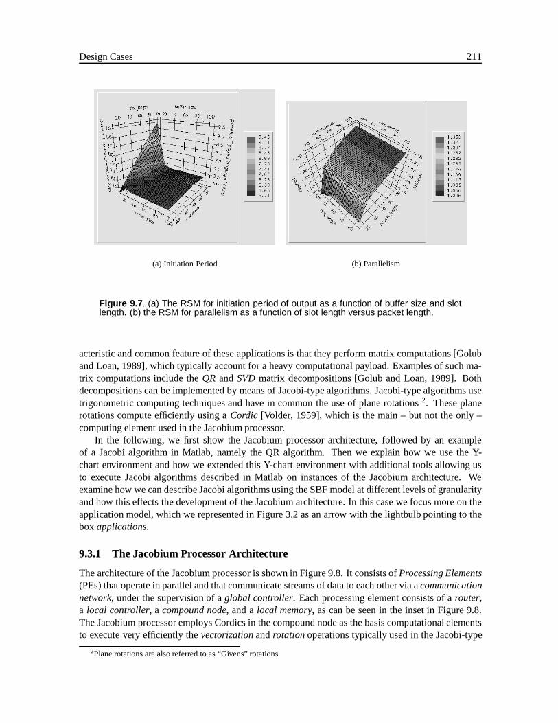
Design Cases 211
(a) Initiation Period (b) Parallelism
Figure 9.7 . (a) The RSM for initiation period of output as a function of buffer size and slotlength. (b) the RSM for parallelism as a function of slot length versus packet length.
acteristic and common feature of these applications is that they perform matrix computations [Goluband Loan, 1989], which typically account for a heavy computational payload. Examples of such ma-trix computations include theQR andSVDmatrix decompositions [Golub and Loan, 1989]. Bothdecompositions can be implemented by means of Jacobi-type algorithms. Jacobi-type algorithms usetrigonometric computing techniques and have in common the use of plane rotations2. These planerotations compute efficiently using aCordic [Volder, 1959], which is the main – but not the only –computing element used in the Jacobium processor.
In the following, we first show the Jacobium processor architecture, followed by an exampleof a Jacobi algorithm in Matlab, namely the QR algorithm. Then we explain how we use the Y-chart environment and how we extended this Y-chart environment with additional tools allowing usto execute Jacobi algorithms described in Matlab on instances of the Jacobium architecture. Weexamine how we can describe Jacobi algorithms using the SBF model at different levels of granularityand how this effects the development of the Jacobium architecture. In this case we focus more on theapplication model, which we represented in Figure 3.2 as an arrow with the lightbulb pointing to theboxapplications.
9.3.1 The Jacobium Processor Architecture
The architecture of the Jacobium processor is shown in Figure 9.8. It consists ofProcessing Elements(PEs) that operate in parallel and that communicate streams of data to each other via acommunicationnetwork, under the supervision of aglobal controller. Each processing element consists of arouter,a local controller, a compound node, and alocal memory, as can be seen in the inset in Figure 9.8.The Jacobium processor employs Cordics in the compound node as the basis computational elementsto execute very efficiently thevectorizationandrotationoperations typically used in the Jacobi-type
2Plane rotations are also referred to as “Givens” rotations
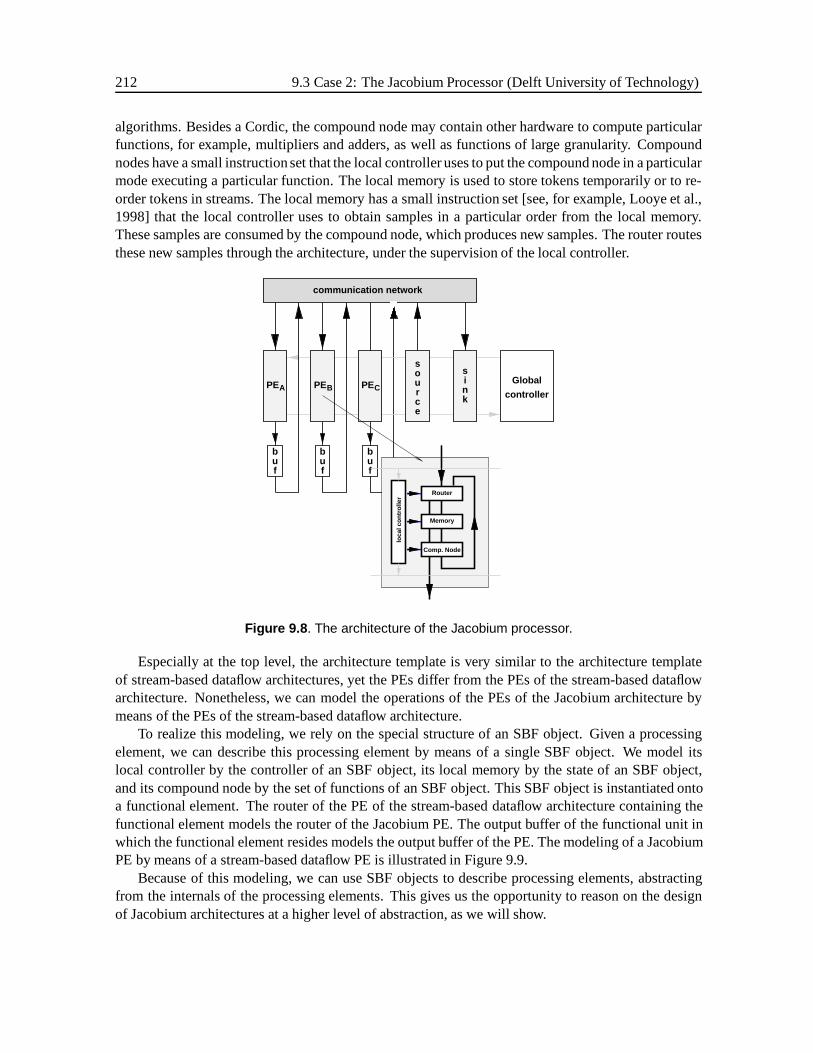
212 9.3 Case 2: The Jacobium Processor (Delft University of Technology)
algorithms. Besides a Cordic, the compound node may contain other hardware to compute particularfunctions, for example, multipliers and adders, as well as functions of large granularity. Compoundnodes have a small instructionset that the local controller uses to put the compound node in a particularmode executing a particular function. The local memory is used to store tokens temporarily or to re-order tokens in streams. The local memory has a small instruction set [see, for example, Looye et al.,1998] that the local controller uses to obtain samples in a particular order from the local memory.These samples are consumed by the compound node, which produces new samples. The router routesthese new samples through the architecture, under the supervision of the local controller.
ruos
ce
nk
is
uf
buf
buf
b
Router
Memory
Comp. Node
loca
l co
ntr
olle
r
communication network
Global
controllerPE PE PEA B C
Figure 9.8 . The architecture of the Jacobium processor.
Especially at the top level, the architecture template is very similar to the architecture templateof stream-based dataflow architectures, yet the PEs differ from the PEs of the stream-based dataflowarchitecture. Nonetheless, we can model the operations of the PEs of the Jacobium architecture bymeans of the PEs of the stream-based dataflow architecture.
To realize this modeling, we rely on the special structure of an SBF object. Given a processingelement, we can describe this processing element by means of a single SBF object. We model itslocal controller by the controller of an SBF object, its local memory by the state of an SBF object,and its compound node by the set of functions of an SBF object. This SBF object is instantiated ontoa functional element. The router of the PE of the stream-based dataflow architecture containing thefunctional element models the router of the Jacobium PE. The output buffer of the functional unit inwhich the functional element resides models the output buffer of the PE. The modeling of a JacobiumPE by means of a stream-based dataflow PE is illustrated in Figure 9.9.
Because of this modeling, we can use SBF objects to describe processing elements, abstractingfrom the internals of the processing elements. This gives us the opportunity to reason on the designof Jacobium architectures at a higher level of abstraction, as we will show.
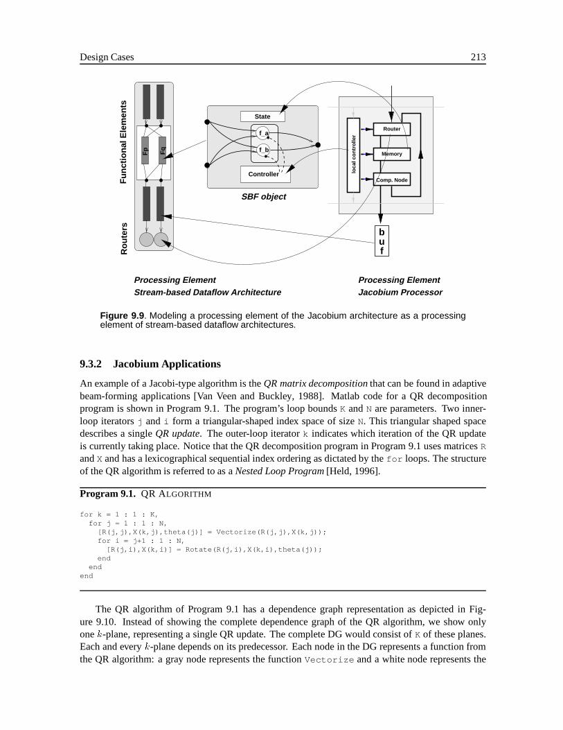
Design Cases 213
b
fu
Jacobium Processor
Fq
Fp
State
f_a
f_b
Controller
Router
Memory
Comp. Node
loca
l co
ntr
olle
r
Fu
nct
ion
al E
lem
ents
Ro
ute
rs
Stream-based Dataflow ArchitectureProcessing Element
SBF object
Processing Element
Figure 9.9 . Modeling a processing element of the Jacobium architecture as a processingelement of stream-based dataflow architectures.
9.3.2 Jacobium Applications
An example of a Jacobi-type algorithm is theQR matrix decompositionthat can be found in adaptivebeam-forming applications [Van Veen and Buckley, 1988]. Matlab code for a QR decompositionprogram is shown in Program 9.1. The program’s loop boundsK andN are parameters. Two inner-loop iteratorsj and i form a triangular-shaped index space of sizeN. This triangular shaped spacedescribes a singleQR update. The outer-loop iteratork indicates which iteration of the QR updateis currently taking place. Notice that the QR decomposition program in Program 9.1 uses matricesR
andX and has a lexicographical sequential index ordering as dictated by thefor loops. The structureof the QR algorithm is referred to as aNested Loop Program[Held, 1996].
Program 9.1. QR ALGORITHM
for k = 1 : 1 : K,for j = 1 : 1 : N,
[R(j,j),X(k,j),theta(j)] = Vectorize(R(j,j),X(k,j));for i = j+1 : 1 : N,
[R(j,i),X(k,i)] = Rotate(R(j,i),X(k,i),theta(j));end
endend
The QR algorithm of Program 9.1 has a dependence graph representation as depicted in Fig-ure 9.10. Instead of showing the complete dependence graph of the QR algorithm, we show onlyonek-plane, representing a single QR update. The complete DG would consist ofK of these planes.Each and everyk-plane depends on its predecessor. Each node in the DG represents a function fromthe QR algorithm: a gray node represents the functionVectorize and a white node represents the
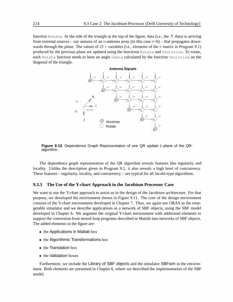
214 9.3 Case 2: The Jacobium Processor (Delft University of Technology)
functionRotate . At the side of the triangle at the top of the figure, data (i.e., theX data) is arrivingfrom external sources – say sensors of anN-antenna array (in this caseN=6) – that propagates down-wards through the plane. The values of 21r variables (i.e., elements of theR matrix in Program 9.1)produced by the previous plane are updated using the functionsRotate andVectorize . To rotate,eachRotate function needs to have an angletheta calculated by the functionVectorize on thediagonal of the triangle.
Antenna Signals
i
j
k
theta
VectorizeRotate
rk�1
xk
Figure 9.10 . Dependence Graph Representation of one QR update k-plane of the QR-algorithm.
The dependence graph representation of the QR algorithm reveals features like regularity andlocality. Unlike the description given in Program 9.1, it also reveals a high level of concurrency.These features – regularity, locality, and concurrency – are typical for all Jacobi-type algorithms.
9.3.3 The Use of the Y-chart Approach in the Jacobium Processor Case
We want to use the Y-chart approach to assist us in the design of the Jacobium architecture. For thatpurpose, we developed the environment shown in Figure 9.11. The core of the design environmentconsists of the Y-chart environment developed in Chapter 7. Thus, we again use ORAS as the retar-getable simulator and we describe applications as a network of SBF objects, using the SBF modeldeveloped in Chapter 6. We augment the original Y-chart environment with additional elements tosupport the conversion from nested loop programs described in Matlab into networks of SBF objects.The added elements in the figure are:
� theApplications in Matlab box
� theAlgorithmic Transformations box
� theTranslation box
� theValidation boxes
Furthermore, we include theLibrary of SBF objects and the simulatorSBFsim in the environ-ment. Both elements are presented in Chapter 6, where we described the implementation of the SBFmodel.
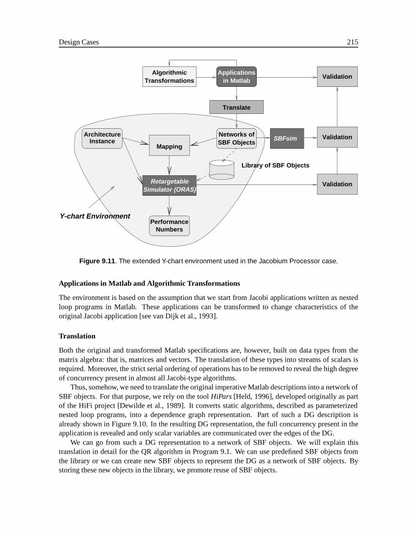
Design Cases 215
Translate
PerformanceNumbers
Networks of
TransformationsAlgorithmic
Validation
Validation
Validation
SBFsim
RetargetableSimulator (ORAS)
Applicationsin Matlab
ArchitectureInstance
Library of SBF Objects
SBF Objects
Y-chart Environment
Mapping
Figure 9.11 . The extended Y-chart environment used in the Jacobium Processor case.
Applications in Matlab and Algorithmic Transformations
The environment is based on the assumption that we start from Jacobi applications written as nestedloop programs in Matlab. These applications can be transformed to change characteristics of theoriginal Jacobi application [see van Dijk et al., 1993].
Translation
Both the original and transformed Matlab specifications are, however, built on data types from thematrix algebra: that is, matrices and vectors. The translation of these types into streams of scalars isrequired. Moreover, the strict serial ordering of operations has to be removed to reveal the high degreeof concurrency present in almost all Jacobi-type algorithms.
Thus, somehow, we need to translate the original imperative Matlab descriptions into a network ofSBF objects. For that purpose, we rely on the toolHiPars [Held, 1996], developed originally as partof the HiFi project [Dewilde et al., 1989]. It converts static algorithms, described as parameterizednested loop programs, into a dependence graph representation. Part of such a DG description isalready shown in Figure 9.10. In the resulting DG representation, the full concurrency present in theapplication is revealed and only scalar variables are communicated over the edges of the DG.
We can go from such a DG representation to a network of SBF objects. We will explain thistranslation in detail for the QR algorithm in Program 9.1. We can use predefined SBF objects fromthe library or we can create new SBF objects to represent the DG as a network of SBF objects. Bystoring these new objects in the library, we promote reuse of SBF objects.
216 9.3 Case 2: The Jacobium Processor (Delft University of Technology)
Validation
The translation of a Matlab program describing a nested loop program to a network of SFB objectsis not trivial and is not yet automated. For these reasons, we included a validation trajectory to checkwhether both the Matlab program and the SBF network have the same input/output behavior. Thuswe verify thetranslation steps by providing the same input data to both the Matlab applications andthe network of SBF objects and then comparing the output data.
We can map a network of SBF objects onto an architecture instance and use ORAS to obtain theperformance numbers. Because ORAS also performs a full functional simulation, we can also validatethe behavior at this level: ORAS should produce for the same input data the same output data as thatproduced by SBFsim or Matlab. This way we can check if the mapping was performed correctly.
9.3.4 Deriving a Network of SBF Objects from a Dependence Graph
We will show a very simple case in this section in which we express the QR algorithm of Program 9.1as a collection of different SBF objects, each with (very) different characteristics. We will use theextended Y-chart environment to provide feedback on the different SBF objects realized.
Using the HiPars tool, we attain a DG representation of a nested-loop Matlab program. We oughtto derive SBF objects from the DG representation that we can combine to model the original Matlabapplication as a network of SBF objects. This means, in the first place, that we have topartition theDG into smaller pieces, in which each piece makes up an SBF object with a particular set of functions.In the second place, for each identified SBF object we have to specify the controller functions, i.e.,the transition function and the binding function.
Partitioning a Dependence Graph
Given a singlek-plane of the QR algorithm as a DG representation, there are many ways we canconstruct a network of SBF objects executing the same QR application. Different partitions result indifferent grain sizes of the SBF objects, as was explained in Section 6.6. In Figure 9.12, we showthree different partitions,each leading to different SBF objects with different grain sizes. The numberof functions that an SBF object includes determines the grain size of that SBF object if we assumethat the functionsVectorize andRotate both requirex RISC-like operations.
We now illustrate three possible partitions (a, b, and c) to describe the samek-plane of the QRalgorithm. In specifying these partitions, we distinguishregionswhich describe a regular part of a DGcontaining the same kind of functions. Although two regions can describe the same function, they candiffer as to where functions get their data from and where they write output data to. In that case wehavevariantsof the same function (see Section 6.6).
case (a): In this partitioning, we assume thateach node of the DG defines an SBF object by it-self. This results in two SBF objects:SBFVectorize, containing the functionVectorize , andSBFRotate, containing the functionRotate . Since both SBF objects contain only one func-tion, the objects distinguish only one region. Both SBFVectorize and SBFRotate have a grainsize of1x. To cover the DG we would need 6 instances of SBFVectorize and 15 instances ofSBFRotate.
case (b): In this partitioning, we assume thateach horizontal chain of nodes (j-line) in the DG definesan SBF objectSBFline. SBFline contains two functions:Rotate andVectorize . Eachj-lineconsists of two regions: regionI and regionII. The functionVectorize is active in regionI,
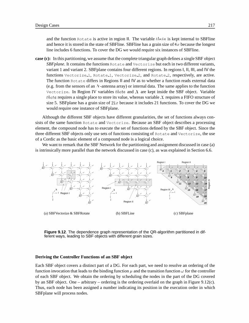
Design Cases 217
and the functionRotate is active in regionII. The variabletheta is kept internal to SBFlineand hence it is stored in the state of SBFline. SBFline has a grain size of6x because the longestline includes 6 functions. To cover the DG we would require six instances of SBFline.
case (c): In this partitioning,we assume that the complete triangular graph defines a single SBF objectSBFplane. It contains the functionsRotate andVectorize but each in two different variants,variant 1 and variant 2. SBFplane contains four different regions. In regionsI, II, III, andIV thefunctionsVectorize 1, Rotate 1, Vectorize 2, andRotate 2, respectively, are active.The functionRotate differs in RegionsII andIV as to whether a function reads external data(e.g. from the sensors of anN -antenna array) or internal data. The same applies to the functionVectorize . In Region IV variablestheta andX are kept inside the SBF object. Variabletheta requires a single place to store its value, whereas variableX requires a FIFO structure ofsize 5. SBFplane has a grain size of21x because it includes 21 functions. To cover the DG wewould require one instance of SBFplane.
Although the different SBF objects have different granularities, the set of functions always con-sists of the same functionRotate andVectorize . Because an SBF object describes a processingelement, the compound node has to execute the set of functions defined by the SBF object. Since thethree different SBF objects only use sets of functions consisting ofRotate andVectorize , the useof a Cordic as the basic element of a compound node is a logical choice.
We want to remark that the SBF Network for the partitioning and assignment discussed in case (a)is intrinsically more parallel than the network discussed in case (c), as was explained in Section 6.6.
j
ik
Region I
(a) SBFVectorize & SBFRotate
j
ik
Region II
Region I
(b) SBFLine
Region III
Region IIRegion I
Reg
ion
IV
j
ik
0 1 2
8 10
12 14
15 17
18 19
20
16
13
97
11
6
3 4 5
(c) SBFplane
Figure 9.12 . The dependence graph representation of the QR-algorithm partitioned in dif-ferent ways, leading to SBF objects with different grain sizes.
Deriving the Controller Functions of an SBF object
Each SBF object covers a distinct part of a DG. For each part, we need to resolve an ordering of thefunction invocation that leads to the binding function� and the transition function! for the controllerof each SBF object. We obtain the ordering by scheduling the nodes in the part of the DG coveredby an SBF object. One – arbitrary – ordering is the ordering overlaid on the graph in Figure 9.12(c).Thus, each node has been assigned a number indicating its position in the execution order in whichSBFplane will process nodes.
218 9.3 Case 2: The Jacobium Processor (Delft University of Technology)
Given the ordering of Figure 9.12(c), we can derive the binding functions� as
�(s) =
8>>>>><>>>>>:
Vectorize1; if s = 0
Rotate1; if s = 1; 2; 3; 4; 5
Vectorize2; if s = 6; 11; 15; 18; 20
Rotate2; if s = 7; 8; 9; 10; 12; 13; 14; 16; 17; 19
(9.1)
and the transition function! as
!(s) = s+ 1 (mod 20): (9.2)
The presented controller functions are defined for ak-plane DG havingN = 6. We could alsohave defined the controller functions in a parameterized form, expressed in parameterN .
Given the three possible partitions, we need to decide which partition results in the best architec-ture given the set of Jacobi-type algorithms. The SBF objects shown in Figure 9.12(a) can easily bereused since the functionsVectorize andRotate are used in most Jacobi-type algorithms. How-ever, the price that is paid for this reusability is a large amount of communication of single scalarvariables over the communication structure. The SBF objects presented in Figure 9.12(b) and Fig-ure 9.12(c) keep some variables internal, reducing the amount of data that needs to be transported.This increases the complexity of the local controller and may cause an increase in the amount of localmemory needed in a PE. As the SBF objects become more coarse-grained, tokens can very effectivelybe taken together into a packet, leading to a more efficient transportation of tokens. For example,theR values needed from a previous QR update are very effectively transported using packets. Inaddition, coarse-grained SBF objects can perform very complex operations, including the reorderingof data streams [Garcea, 1998].
Pipelining
The SBF objects described in Figure 9.12 are executed on a compound node. A compound node typi-cally uses a Cordic in the case of the Jacobium architecture. This Cordic is deeply pipelined [Hekstraand Deprettere, 1993] – 18 stages deep – to perform the trigonometric computations at a high through-put. Pipelining seriously affects the final performance of the Jacobium architecture, especially whenlong pipelines are used. The local data dependencies between nodes, as shown in the DGs of Jacobi-type algorithms, make it a very challenging task to obtain a high utilization of Jacobium architectureswhile maintaining a high throughput.
When we consider the Matlab description in Program 9.1, we notice that the functions are notpipelined at all. However, in the extended Y-chart environment they are, which makes it possible toobtain quick quantitative feedback on the utilization of an instance executed on a Jacobium architec-ture. By installing an SBF object (like the ones given in Figure 9.12) on a functional element (seeFigure 7.8) and specifying a particularinitiation period and latency, we can specify that the SBFobject have a pipelined behavior. Furthermore, different processing elements in the Jacobium archi-tecture can execute differentk planes. As a consequence, pipelining takes place inside PEs as well asbetween PEs.
By measuring the performance of an architecture instance, we can investigate the effect of thelevels of pipelining. When this is known, we can start to apply purposeful algorithmic transformationsto alter Matlab programs, for example to change the shape of the DGs such that a higher utilizationresults [van Dijk and Deprettere, 1995].
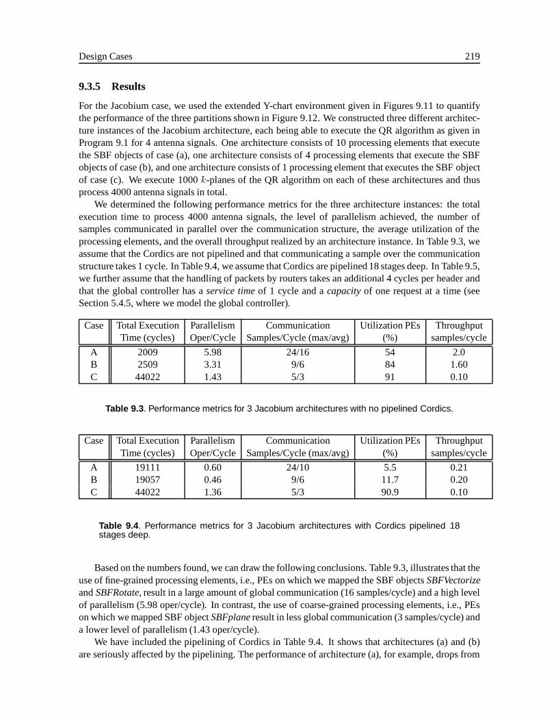
Design Cases 219
9.3.5 Results
For the Jacobium case, we used the extended Y-chart environment given in Figures 9.11 to quantifythe performance of the three partitions shown in Figure 9.12. We constructed three different architec-ture instances of the Jacobium architecture, each being able to execute the QR algorithm as given inProgram 9.1 for 4 antenna signals. One architecture consists of 10 processing elements that executethe SBF objects of case (a), one architecture consists of 4 processing elements that execute the SBFobjects of case (b), and one architecture consists of 1 processing element that executes the SBF objectof case (c). We execute 1000k-planes of the QR algorithm on each of these architectures and thusprocess 4000 antenna signals in total.
We determined the following performance metrics for the three architecture instances: the totalexecution time to process 4000 antenna signals, the level of parallelism achieved, the number ofsamples communicated in parallel over the communication structure, the average utilization of theprocessing elements, and the overall throughput realized by an architecture instance. In Table 9.3, weassume that the Cordics are not pipelined and that communicating a sample over the communicationstructure takes 1 cycle. In Table 9.4, we assume that Cordics are pipelined 18 stages deep. In Table 9.5,we further assume that the handling of packets by routers takes an additional 4 cycles per header andthat the global controller has aservice timeof 1 cycle and acapacityof one request at a time (seeSection 5.4.5, where we model the global controller).
Case Total Execution Parallelism Communication Utilization PEs ThroughputTime (cycles) Oper/Cycle Samples/Cycle (max/avg) (%) samples/cycle
A 2009 5.98 24/16 54 2.0B 2509 3.31 9/6 84 1.60C 44022 1.43 5/3 91 0.10
Table 9.3 . Performance metrics for 3 Jacobium architectures with no pipelined Cordics.
Case Total Execution Parallelism Communication Utilization PEs ThroughputTime (cycles) Oper/Cycle Samples/Cycle (max/avg) (%) samples/cycle
A 19111 0.60 24/10 5.5 0.21B 19057 0.46 9/6 11.7 0.20C 44022 1.36 5/3 90.9 0.10
Table 9.4 . Performance metrics for 3 Jacobium architectures with Cordics pipelined 18stages deep.
Based on the numbers found, we can draw the following conclusions. Table 9.3, illustrates that theuse of fine-grained processing elements, i.e., PEs on which we mapped the SBF objectsSBFVectorizeandSBFRotate, result in a large amount of global communication (16 samples/cycle) and a high levelof parallelism (5.98 oper/cycle). In contrast, the use of coarse-grained processing elements, i.e., PEson which we mapped SBF objectSBFplaneresult in less global communication (3 samples/cycle) anda lower level of parallelism (1.43 oper/cycle).
We have included the pipelining of Cordics in Table 9.4. It shows that architectures (a) and (b)are seriously affected by the pipelining. The performance of architecture (a), for example, drops from
220 9.3 Case 2: The Jacobium Processor (Delft University of Technology)
Case Total Execution Parallelism Communication Utilization PEs ThroughputTime (cycles) Oper/Cycle Samples/Cycle (max/avg) (%) samples/cycle
A 47326 0.25 17/11 2.4 0.08B 45241 0.19 9/6 4.9 0.09C 108944 0.55 5/2 36.7 0.04
Table 9.5 . Performance metrics for 3 Jacobium architectures with Cordics pipelined 18stages deep, with a global controller that has a service time of 1 cycle and a capacity ofone request at a time, and with routers that require an additional 4 cycles per header tohandle a packet.
5.98 to 0.60 operations per cycle. Architecture (c), on the other hand, is hardly affected by pipelining.Based on this table, we conclude that pipelining should not be neglected and that the extended Y-chartenvironment is useful and enables us to quickly investigate the effects of pipelining.
The results in Table 9.5 are based on the fact that communicating headers takes 4 cycles per headerand that one router at a time can access the global controller. This affects the overall performance ofall three architectures and the values for parallelism, utilization and throughput are about 60% lowerthan the values in Table 9.4. Although architecture (c) can use longer packets than architecture (a) or(b), its overall performance dropped 60%. Thus, packets longer that 21 samples are needed to reducethe influence of the headers. In absolute numbers, however, architectures (a) and (b) realize a higherthroughput, but architecture (c) uses its resources most efficiently.
We also performed a design space exploration of the Jacobium processor in which we lookedat architecture instances that useN coarse-grained processing elements to execute 1000k-planes ofthe QR algorithm. We mapped the SBF objectSBFplanethat processesM antenna signals on eachof these processing elements. We also changed the level of pipelining of the Cordics used in theprocessing elements and the size of the FIFO buffers. In the architecture instances, we assumed thatit takes 1 cycle to communicate a sample over the communication structure and that a header requiresan additional 4 cycles per packet. Table 9.6 shows the parameters of the exploration along with theirranges. We set up an experiment of 100 trial runs with these parameters. The experiment of 100 trialruns, took 50 minutes to execute. Notice that we did not include the packet length as parameter. Incase of the Jacobi-algorithms, it depends on the number of antenna signals (M ) used.
Parameter Range
Bufffer Size f 4 : : : 100gCordics (N ) f 1 : : : 7 gProblem Size (M ) f 4 : : : 12gPipeline Depth f 1 : : : 20g
Table 9.6 . Parameters used in the design space exploration of the Jacobium architecture.
Figures 9.13 shows the initiation period realized for a processing element (a) and the total execu-tion time required by an architecture instance to process 1000k planes (b) when a buffer size of 100and a pipeline depth of 18 are selected. The initiation period reported is not equal to the throughputreported in Table 9.3 to Table 9.5; it gives the throughput that an individual processing element canrealize. From figure (a), we concluded that processing elements operate with maximum throughput

Design Cases 221
(e.g. 1 sample/cycle) on a stream of samples when a small problem size is used (M � 7). Whena larger problem size is used, an architecture can maintain a throughput of 1 sample/cycle per pro-cessing element by using more processing elements. This works until a problem size larger than 9 isselected.
From figure (b), we concluded that when a small problem size is executed (e.g. 4� M � 7),adding extra processing elements is not efficient because the total execution time hardly decreases.When a large problem size is used (e.g.M � 8), additional processing elements are used moreefficiently, especially when between 3 and 5 processing elements. Using more that 6 extra processingelements hardly improves the total execution time.
(a) Initiation Period of Processing Element (b) Total Execution Time
Figure 9.13 . The response surface model for the initiation period achieved for one process-ing element (a) or the response surface model for total execution time required to process1000 k-planes (b) as a function of processing elements N and problem size M .
In Figure 9.14, we show the utilization of a processing element (a) and the achieved level of par-allelism of architecture instances for different levels of pipelining and buffer sizes. In both figures,the problem size is equal to 12 and the architecture instances use 4 processing elements. From figure(a), we concluded that the processing elements are used most efficiently when a buffer size of approx-imately 70 samples is used, irrespective of the level of pipelining. From figure (b), we conclude thatthe level of pipelining influences very much the level of parallelism realized. For a problem size of 12and 4 processing elements, the maximum level of parallelism is obtained when a pipeline depth of 5stages is used. Furthermore, the deeper the pipeline, the lower the level of parallelism.
9.3.6 Conclusions
The Jacobium project is still running, but we can draw the following preliminary conclusions regard-ing it. We were able to use the Y-chart environment developed in this thesis to model the architectureof the Jacobium processor in terms of the architecture template of stream-based dataflow architec-tures. We extended this Y-chart environment, which allowed us to execute applications written inMatlab as a network of SBF objects on an architecture instance and determine how these networks

222 BIBLIOGRAPHY
(a) Utilization (b) Parallelism
Figure 9.14 . The response surface model for utilization of a processing element (a) or theresponse surface model for realized level of parallelism (b) as a function of level of pipeliningand buffer sizes.
performed on architecture instances. We used the extended Y-chart to quantify characteristics of threedifferent partitions that executes one and the same QR algorithm, but with different granularity. Wealso quantified the effects of pipelining and global communication. For one partition, we performeda design space exploration and showed the we were able to derive relationships between architectureparameters and performance metrics.
Bibliography
P.M. Dewilde, A.A.J de Lange, A.J van der Hoeven, and E.F. Deprettere. HiFi: An object orientedsystem for the structural synthesis of signal processing algorithms and the VLSI compilation ofsignal-flow graphs. InIFIP Int. Workshop on Applied Formal Methods for Correct VLSI Design,1989.
Robert P. Dick, David L. Rhodes, and Wayne Wolf. TGFF: Task graphs for free. InProceedings of6th Int. Workshop on Hardware/Software Codesign, Seattle, Washington, 1998.
Giuseppe Garcea. Derivation of dataflow networks for a specific domain of applications. Master’sthesis, Delft University of Technology, Circuits & Systems Group, 1998.
G.H. Golub and C.F. Van Loan.Matrix Computations, (2nd ed.). John Hopkins University Press,1989.
Gerben J. Hekstra and Ed F. Deprettere. Floating point Cordic. InProceedings ARITH 11, pages130–137, Windsor, Ontario, 1993.
Peter Held.Functional Design of Dataflow Networks. PhD thesis, Delft University of Technology,1996.
BIBLIOGRAPHY 223
R. Jain. Personal Communication with Ed Deprettere, 1997.
J.H. Justice, N.L Owsley, J.L Jen, and A.C. Kak.Array Signal Processing. Prentice-Hall, 1985.
Jeroen Leijten.Real-Time Constrained Reconfigurable Communication between Embedded Proces-sors. PhD thesis, Eindhoven University of Technology, 1998.
Jeroen A.J. Leijten, Jef L. van Meerbergen, Adwin H. Timmer, and Jochen A.G. Jess. Prophid: Aheterogeneous multi-processor architecture for multimedia. InProceedings of ICCD’97, 1997.
A. Looye, G. Hekstra, and E. Deprettere. Multiport memory and floating point cordic pipeline inJacobium processing elements. InProceedings of the IEEE Workshop on Signal Processing Systems(SiPS’98), Boston, USA, 1998.
Boaz Porat.Digital Processing of Random Signals. Prentice-Hall, 1993.
Edwin Rijpkema, Gerben Hekstra, Ed Deprettere, and Ju Ma. A strategy for determining a Jacobi spe-cific dataflow processor. InProceedings of 11th Int. Conference of Applications-specific Systems,Architectures and Processors (ASAP’97), pages 53 – 64, Zurich, Switzerland, 1997.
H.W. van Dijk and E.F. Deprettere. Transformational reasoning on time-adaptive Jacobi type algo-rithms. In M. Moonen and B. De Moor, editors,SVD and Signal Processing, III, pages 277–286.Kluwer Academic Publishers, Dordrecht, 1995.
Hylke van Dijk, Gerben Hekstra, and Ed Deprettere. On the systematic exploration of the space ofJacobi algorithms. Technical Report ET/NT/Fact-2, Dept. Electrical Engineering, Delft Universityof Technology, 1993.
B. Van Veen and K. Buckley. Beam forming: A versatile approach to spatial filtering.IEEE ASSPMagazine, 5(2):4–24, 1988.
J.E. Volder. The Cordic trigonometric computing technique.IRE Trans. Electronic Computers, EC-8(3):330–340, 1959.
Bob Witlox. Performance analysis of dataflow architectures using petri nets. Master’s thesis, Eind-hoven University of Technology, Department of Mathematics and Computing Science, 1997.

224 BIBLIOGRAPHY
Chapter 10
Summary & Conclusions
THERE is a trend toward increasingly programmable application-specific architectures. Thesearchitectures are becoming increasingly programmable to support multi-functional and multi-
standard products. In the design of these architectures, it is no longer the performance of a singleapplication that matters, but the performance of a set of applications. We have observed that generaland structured approaches are lacking for the design of these increasingly programmable application-specific architectures.
We presented the stream-based dataflow architectures as an example of programmable application-specific architectures. We showed that this class of architectures fits into the category of dataflowarchitectures and that they represent interesting programmable architectures for high-performance,stream-based applications that are found in many multi-media applications.
In the design of stream-based dataflow architectures many architectural choices are involved, eachleading to a particular architecture with a specific behavior and performance. For designers, it be-comes increasingly complex to find feasible architectures, given the many choices involved and therequired programmability.
We structured the many design choices by means of an architecture template which describes aclass of architectures in a parameterized way and which has a well-defined design space. We con-sidered the central problem in this thesis to be to provide a method to help designers find parametervalues of the architecture template that result in a feasible design, given an architecture template, aset of applications, and design objectives like throughput and utilization as well as power and siliconarea.
The methodology that we presented in this thesis is the Y-chart approach shown in Figure 10.1.It is a methodology in which designers make decisions and motivate particular design choices basedon quantitative data. We showed that the Y-chart approach leads to a Y-chart environment whichallows designers to quantify design choices for a particular architecture. By using such a Y-chartenvironment and changing design choices in a systematic way, designers explore the design space of agiven architecture template for a set of applications. Furthermore, designers narrow down the designspace of an architecture template in a stepwise fashion by using a stack of Y-chart environments, eachat a different level of abstraction.
By exploring the design space at different abstraction levels, designers gain insight into the re-lationship between parameter values and the performance that is achieved. Based on this insight,designers make trade-offs between the many parameters leading to a feasible design. Therefore, theY-chart approach results in better-engineered architectures in less time. These engineered architec-tures satisfy the imposed design objectives for the complete set of applications. Moreover, they use
225
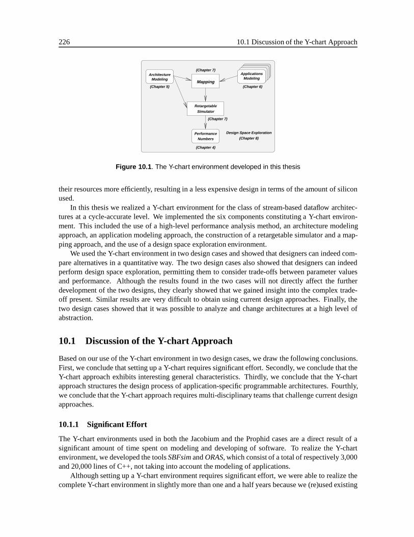
226 10.1 Discussion of the Y-chart Approach
Applications
Retargetable
PerformanceNumbers
Design Space Exploration
Mapping
ArchitectureModeling Modeling
Simulator
(Chapter 5)
(Chapter 7)
(Chapter 6)
(Chapter 7)
(Chapter 8)
(Chapter 4)
Figure 10.1 . The Y-chart environment developed in this thesis
their resources more efficiently, resulting in a less expensive design in terms of the amount of siliconused.
In this thesis we realized a Y-chart environment for the class of stream-based dataflow architec-tures at a cycle-accurate level. We implemented the six components constituting a Y-chart environ-ment. This included the use of a high-level performance analysis method, an architecture modelingapproach, an application modeling approach, the construction of a retargetable simulator and a map-ping approach, and the use of a design space exploration environment.
We used the Y-chart environment in two design cases and showed that designers can indeed com-pare alternatives in a quantitative way. The two design cases also showed that designers can indeedperform design space exploration, permitting them to consider trade-offs between parameter valuesand performance. Although the results found in the two cases will not directly affect the furtherdevelopment of the two designs, they clearly showed that we gained insight into the complex trade-off present. Similar results are very difficult to obtain using current design approaches. Finally, thetwo design cases showed that it was possible to analyze and change architectures at a high level ofabstraction.
10.1 Discussion of the Y-chart Approach
Based on our use of the Y-chart environment in two design cases, we draw the following conclusions.First, we conclude that setting up a Y-chart requires significant effort. Secondly, we conclude that theY-chart approach exhibits interesting general characteristics. Thirdly, we conclude that the Y-chartapproach structures the design process of application-specific programmable architectures. Fourthly,we conclude that the Y-chart approach requires multi-disciplinary teams that challenge current designapproaches.
10.1.1 Significant Effort
The Y-chart environments used in both the Jacobium and the Prophid cases are a direct result of asignificant amount of time spent on modeling and developing of software. To realize the Y-chartenvironment, we developed the toolsSBFsimandORAS, which consist of a total of respectively 3,000and 20,000 lines of C++, not taking into account the modeling of applications.
Although setting up a Y-chart environment requires significant effort, we were able to realize thecomplete Y-chart environment in slightly more than one and a half years because we (re)used existing
Summary & Conclusions 227
tools. We used the PAMELA Run-time Library, which provided us with high-level primitives thatmade it possible for us to model stream-based dataflow architectures at a high level of abstraction.Another existing tool that we used was the generic DSE environment. This environment took careof setting up experiments efficiently, data management, and visualization of results, e.g., drawing theresponse surface models.
10.1.2 Characteristics of the Y-chart Approach
We conclude that the Y-chart exhibits general characteristics that are invariant with respect to thearchitecture or application researched. We summarize the characteristics as:
1. The Y-chart approach permits designers to quantify architectural choices, providing a soundbasis on which design choices can be made.
2. The Y-chart approach permits designers to explore the design space of an architecture templatenot only for a single application, but for the whole set of applications.
3. The Y-chart approach allows designers to consider trade-offs and to balance between pro-grammability and efficiency, finding an architecture instance that obeys set-wide design ob-jectives.
4. The Y-chart approach takes into account the complete system – architecture, the set of applica-tions, and the mapping of these applications – thus optimizing the complete system instead ofonly the architecture.
5. The Y-chart approach is invariant for a specific level of detail at which designers need to specifyarchitecture instances when evaluating the architecture instance to render performance numbers.
6. The Y-chart approach requires that the architecture template be made explicit and thus thatarchitecture templates can be reused in other design projects.
10.1.3 Structuring the Design Process
We conclude that the Y-chart approach structures the design process of programmable application-specific architectures. It stipulates the requirements that need to be satisfied in order to performdesign space exploration of architectures.
In both the Jacobium and Prophid cases, we conclude that too much focus was placed on thearchitectural design. As a consequence, we experienced severe problems in obtaining specifications ofapplications in the appropriate format. The main reason these problems occurred was that developingapplications in the correct format was not an integral part of the design case of either the Prophid orthe Jacobium architectures.
In further development of programmable architectures, much more attention must be given to de-veloping applications in a suitable format, for example, by making the release of applications in theappropriate format a clear deliverable within design processes. The development of libraries contain-ing high-quality applications descriptions should be considered. This implies that applications shouldbe documented, well-structured (for example, by using code reviews), and released and maintainedover time by a person having the responsibility for particular applications.
A problem similar to the applications problem is mapping. Again, in both the Jacobium and theProphid cases, mapping was not addressed properly since it was not an integral part of the design case.
228 10.2 Further Research
The Y-chart approach, however, clearly states that designing programmable architectures requires thatthe architecture, the set of applications, and the mapping be addressed before any exploration takesplace.
The Y-chart approach has already made an impact within Philips Research. There are designprojects in which the Y-chart approach is used as the basis to structure the design process of newprogrammable architectures. In these design projects, the availability of benchmark applications andmapping were included from the beginning. In the near future, we expect that Y-chart environmentswill be realized for these design projects. For CPU design, and the Philips TriMedia processor inparticular, the exploration has already been performed. For hardware/software codesign that includesCPUs and coprocessors, exploration will soon take place.
10.1.4 Multi-Disciplinary Teams
As shown in Figure 10.1, the Y-chart approach consists of six components, each of which represents adiscipline on its own. The Y-chart approach brings these disciplines together from the very beginningof the design of a programmable architecture. Moreover, the Y-chart does not consider these disci-plines in isolation, but clearly indicates how the various disciplines depend on each other and howthey operate concurrently within the same design.
Setting up a Y-chart for a programmable architecture therefore requires that all six disciplines bemastered. This thesis shows that it is possible to integrate all these disciplines by constructing a Y-chart environment for stream-based dataflow architectures at the cycle-accurate level of abstraction.It also shows how one component representing a particular discipline influences the developmentof other components. For example, SBF Objects used in application modeling are designed in such away that they can seamlessly integrate with functional elements to realize fully functional simulations.Therefore, we combined architecture modeling with application modeling.
Currently, the design of new general purpose processors require very large multi-disciplinaryteams. It is not unusual in this area to have design teams of 100 to 300 people [Wilson, 1998] rep-resenting many different disciplines that interact with each other at different levels of abstraction atthe same time or at least at overlapping times. Managing these interactions is becoming increasinglyimportant and more difficult as designs become more complex [Hennessy and Heinrich, 1996]. Inaddition, less time is available for new designs because of time-to-market considerations. Similarobservations will apply to the use of the Y-chart. Therefore, we have to establish clearly defined inter-faces between the various components of a Y-chart environment as well as between components usedin a stack of Y-chart environments.
Finally, we remark that, in our opinion, the way application-specific programmable architecturesare designed should change radically. As pointed out above, the Y-chart approach combines dif-ferent disciplines. Therefore, to get the full benefit of the Y-chart approach, such that we obtainbetter-engineered architectures, tightly integrated multi-disciplinary teams are required instead of thedifferent teams of different disciplines as happens currently. An excellent example of how such tightlyintegrated multi-disciplinary teams should operate is described by Conklin [1996], who describes thedesign process of the DEC Alpha general purpose processor.
10.2 Further Research
We see many opportunities for further research, including:
Summary & Conclusions 229
More heterogeneous architecturesWe developed the Y-chart environment for stream-based dataflowarchitectures. An interesting line of research would be to investigate how techniques developedwithin this thesis can be used or be extended for more heterogeneous architectures that containboth dataflow and control concepts, possibly with different performance constraints (see, forexample, Figure 1.3). Lieverse et al. [1998] have already shown that such extentions are possi-ble. They used again the PAMELA run-time library for application modeling, but additionally,they used TSS (see Section 7.9) for architecture modeling.
Generalizing architecture modeling conceptsWe used the run-time library primitives and the build-ing block approach to construct architecture instances that perform simulations quickly and effi-ciently. However, the run-time library works very well for stream-based dataflow architectures,but lacks the capability to describepolling efficiently (as indicated in Appendix C). Furtherresearch could determine how the run-time library could be extended such that it can describepolling, while remaining fast and efficient. Some suggestions for this research were presentedin Section 7.9.
Presentation of multi-dimensional relationships The response surface models generated by the genericDSE environment presents 3-D graphs, while the response surface models actually representhigher-dimensional relationships. Further research could involve investigating how to presenthigher-dimensional relationships such that designers can more effectively make trade-offs. InSection 8.6, we already indicated thatscatter-plotsare an option.
Optimization Designers themselves inspect the Response Surface Models generated by the designspace exploration. Further research might involve replacing visual inspection by integratedoptimization tools within the generic DSE environment (i.e., replacing the “lightbulb” in Fig-ure 8.1). These optimization tools would have to find feasible architectures using a minimumnumber of iterations, since each iteration in a Y-chart environment generally takes a consider-able amount of time.
Use of the Y-chart approach in a real design by real designersThe Y-chart environment used inthe two cases proved the correctness of concept of the Y-chart approach. However, actualdesigners have not used it. Further research might include working with real designers usingY-chart environments and studying what kind of questions or difficulties arise at which levels.
Translation from Matlab to the SBF model In the Jacobium case, the translation from a Matlabapplication into a description in terms of the SBF model is not yet automated. Further researchcould be to automate the steps involved in the translation. This way a large pool of benchmarkapplications could easily be created, because many applications are already specified in Matlab.Rijpkema et al. [1998] have already identified the steps involved in automating this translationfor piecewise regular algorithms. The partition of applications (see, for example, Figure 9.12)should also be automated by providing tools that create the correct SBF objects for a givenpartition.
10.3 Availability of Software
The source code of the software developed in this thesis, i.e., SBFsim and ORAS are freely availablefor further use. The software can be obtained by accessing address.
http://cas.et.tudelft.nl/research/hse.html :
230 BIBLIOGRAPHY
Bibliography
Peter F. Conklin. Enrollment management: Managing the Alpha AXP program.IEEE Software, 13(4):53 – 64, 1996. Reprint from Digital Technical Journal, 1992.
John Hennessy and Mark Heinrich. Hardware/software codesign of processors: Concepts and ex-amples. In Giovanni De Micheli and Mariagiovanna Sami, editors,Hardware/Software Codesign,volume 310 ofSeries E: Applied Sciences, pages 29 – 44. NATO ASI Series, 1996.
Paul Lieverse, Pieter van der Wolf, Ed Deprettere, and Kees Vissers. Methodology for architectureexploration of heterogeneous systems. InProceedings of the ProRISC/IEEE Workshop on Circuits,Systems and Signal Processing, 1998.
Edwin Rijpkema, Bart Kienhuis, and Ed Deprettere. From piecewise regular algorithms to processnetworks. InProceedings of the ProRISC/IEEE Workshop on Circuits, Systems and Signal Pro-cessing, 1998.
Janet Wilson. Challenges and trends in processor design.IEEE Computer, 31(1):39 – 48, 1998.
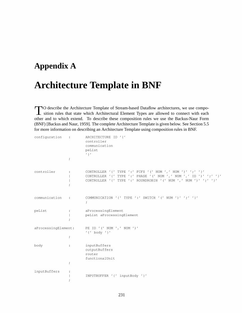
Appendix A
Architecture Template in BNF
TO describe the Architecture Template of Stream-based Dataflow architectures, we use compo-sition rules that state which Architectural Element Types are allowed to connect witheach
other and to which extend. To describe these composition rules we use the Backus-Naur Form(BNF) [Backus and Naur, 1959]. The complete Architecture Template is given below. See Section 5.5for more information on describing an Architecture Template using composition rules in BNF.
configuration : ARCHITECTURE ID ’{’controllercommunicationpeList’}’
;
controller : CONTROLLER ’{’ TYPE ’:’ FCFS ’(’ NUM ’,’ NUM ’)’ ’;’ ’}’| CONTROLLER ’{’ TYPE ’:’ PHASE ’(’ NUM ’,’ NUM ’,’ ID ’)’ ’;’ ’}’| CONTROLLER ’{’ TYPE ’:’ ROUNDROBIN ’(’ NUM ’,’ NUM ’)’ ’;’ ’}’;
communication : COMMUNICATION ’{’ TYPE ’:’ SWITCH ’(’ NUM ’)’ ’;’ ’}’;
peList : aProcessingElement| peList aProcessingElement;
aProcessingElement: PE ID ’(’ NUM ’,’ NUM ’)’’{’ body ’}’
;
body : inputBuffersoutputBuffersrouterfunctionalUnit
;
inputBuffers :| INPUTBUFFER ’{’ inputBody ’}’;
231
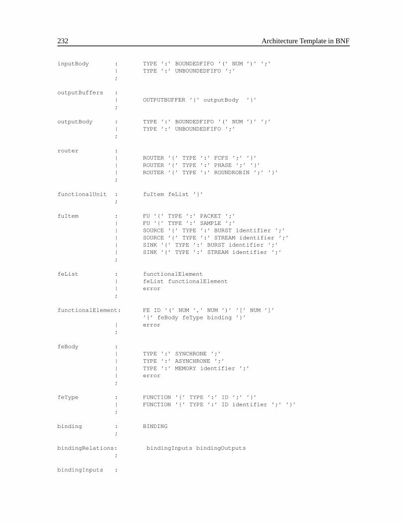
232 Architecture Template in BNF
inputBody : TYPE ’:’ BOUNDEDFIFO ’(’ NUM ’)’ ’;’| TYPE ’:’ UNBOUNDEDFIFO ’;’;
outputBuffers :| OUTPUTBUFFER ’{’ outputBody ’}’;
outputBody : TYPE ’:’ BOUNDEDFIFO ’(’ NUM ’)’ ’;’| TYPE ’:’ UNBOUNDEDFIFO ’;’;
router :| ROUTER ’{’ TYPE ’:’ FCFS ’;’ ’}’| ROUTER ’{’ TYPE ’:’ PHASE ’;’ ’}’| ROUTER ’{’ TYPE ’:’ ROUNDROBIN ’;’ ’}’;
functionalUnit : fuItem feList ’}’;
fuItem : FU ’{’ TYPE ’:’ PACKET ’;’| FU ’{’ TYPE ’:’ SAMPLE ’;’| SOURCE ’{’ TYPE ’:’ BURST identifier ’;’| SOURCE ’{’ TYPE ’:’ STREAM identifier ’;’| SINK ’{’ TYPE ’:’ BURST identifier ’;’| SINK ’{’ TYPE ’:’ STREAM identifier ’;’;
feList : functionalElement| feList functionalElement| error;
functionalElement: FE ID ’(’ NUM ’,’ NUM ’)’ ’[’ NUM ’]’’{’ feBody feType binding ’}’
| error;
feBody :| TYPE ’:’ SYNCHRONE ’;’| TYPE ’:’ ASYNCHRONE ’;’| TYPE ’:’ MEMORY identifier ’;’| error;
feType : FUNCTION ’{’ TYPE ’:’ ID ’;’ ’}’| FUNCTION ’{’ TYPE ’:’ ID identifier ’;’ ’}’;
binding : BINDING;
bindingRelations: bindingInputs bindingOutputs;
bindingInputs :
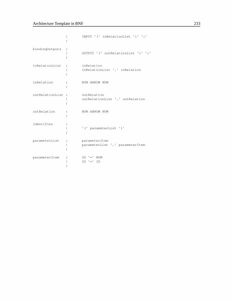
Architecture Template in BNF 233
| INPUT ’(’ inRelationList ’)’ ’;’;
bindingOutputs :| OUTPUT ’(’ outRelationList ’)’ ’;’;
inRelationList : inRelation| inRelationList ’,’ inRelation;
inRelation : NUM ARROW NUM;
outRelationList : outRelation| outRelationList ’,’ outRelation;
outRelation : NUM ARROW NUM;
identifier :| ’(’ parameterList ’)’;
parameterList : parameterItem| parameterList ’,’ parameterItem;
parameterItem : ID ’=’ NUM| ID ’=’ ID;

234 Architecture Template in BNF
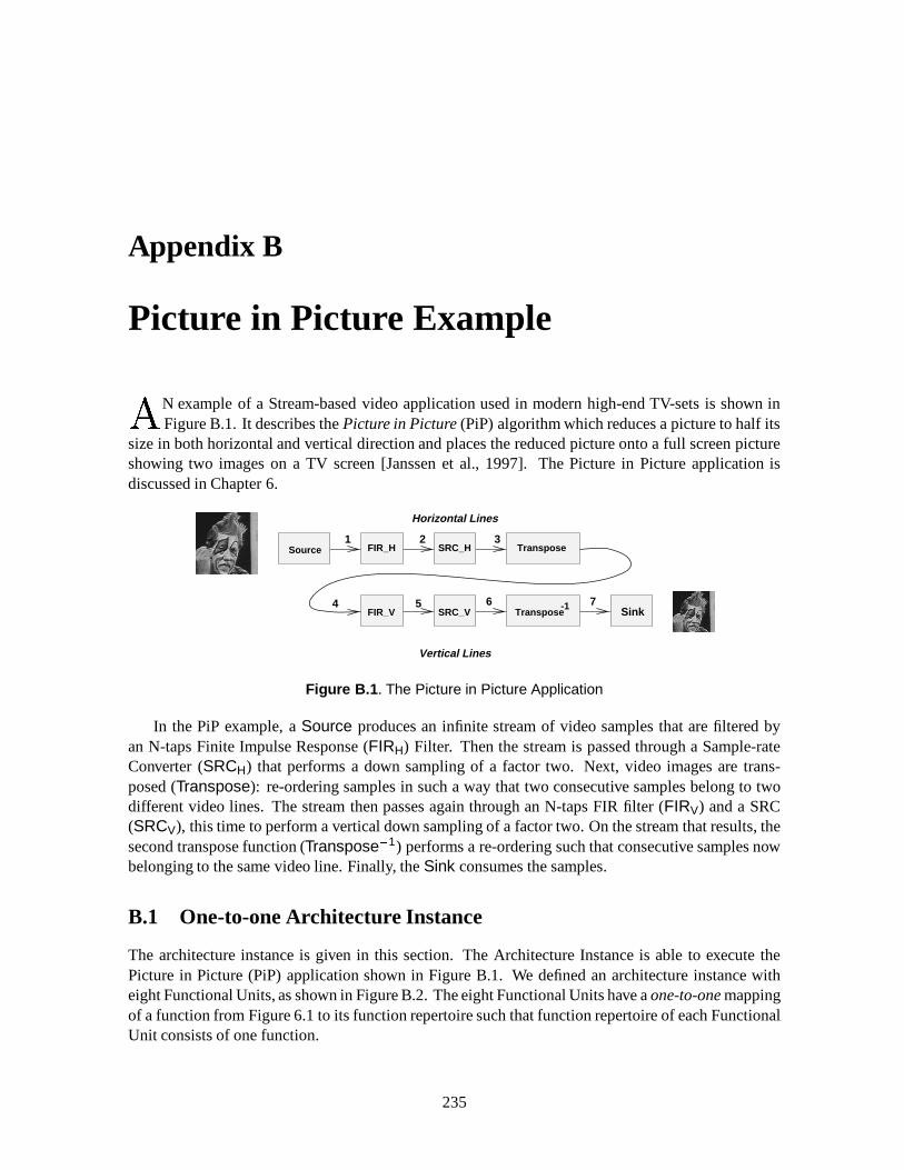
Appendix B
Picture in Picture Example
AN example of a Stream-based video application used in modern high-end TV-sets is shown inFigure B.1. It describes thePicture in Picture(PiP) algorithm which reduces a picture to half its
size in both horizontal and vertical direction and places the reduced picture onto a full screen pictureshowing two images on a TV screen [Janssen et al., 1997]. The Picture in Picture application isdiscussed in Chapter 6.
Sink
Vertical Lines
Horizontal Lines
1 2 3
4 5 6 7
Source FIR_H SRC_H
FIR_V SRC_V Transpose-1
Transpose
Figure B.1 . The Picture in Picture Application
In the PiP example, aSource produces an infinite stream of video samples that are filtered byan N-taps Finite Impulse Response (FIRH) Filter. Then the stream is passed through a Sample-rateConverter (SRCH) that performs a down sampling of a factor two. Next, video images are trans-posed (Transpose): re-ordering samples in such a way that two consecutive samples belong to twodifferent video lines. The stream then passes again through an N-taps FIR filter (FIRV) and a SRC(SRCV), this time to perform a vertical down sampling of a factor two. On the stream that results, thesecond transpose function (Transpose�1) performs a re-ordering such that consecutive samples nowbelonging to the same video line. Finally, theSink consumes the samples.
B.1 One-to-one Architecture Instance
The architecture instance is given in this section. The Architecture Instance is able to execute thePicture in Picture (PiP) application shown in Figure B.1. We defined an architecture instance witheight Functional Units, as shown in Figure B.2. The eight Functional Units have aone-to-onemappingof a function from Figure 6.1 to its function repertoire such that function repertoire of each FunctionalUnit consists of one function.
235
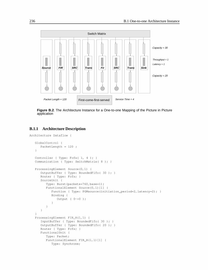
236 B.1 One-to-one Architecture Instance
Switch Matrix
First-come-first-served
Capacity = 20
Capacity = 30
Throughput = 1
Latency = 1
SinkSource
Service Time = 4Packet Length = 120
FIR SRC Trans Fir SRC Trans
Figure B.2 . The Architecture Instance for a One-to-one Mapping of the Picture in Pictureapplication
B.1.1 Architecture Description
Architecture Dataflow {
GlobalControl {PacketLength = 120 ;
}
Controller { Type: Fcfs( 1, 4 ); }Communication { Type: SwitchMatrix( 8 ); }
ProcessingElement Source(0,1) {OutputBuffer { Type: BoundedFifo( 30 ); }Router { Type: Fcfs; }SourceUnit {
Type: Burst(packets=760,base=1);FunctionalElement Source(0,1)[1] {
Function { Type: PGMsource(initiation_period=2,latency=2); }Binding {
Output ( 0->0 );}
}}
}ProcessingElement FIR_H(1,1) {
InputBuffer { Type: BoundedFifo( 30 ); }OutputBuffer { Type: BoundedFifo( 20 ); }Router { Type: Fcfs; }FunctionalUnit {
Type: Packet;FunctionalElement FIR_H(1,1)[1] {
Type: Synchrone;
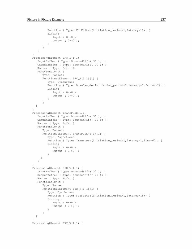
Picture in Picture Example 237
Function { Type: FirFilter(initiation_period=1,latency=18); }Binding {
Input ( 0->0 );Output ( 0->0 );
}}
}}ProcessingElement SRC_H(1,1) {
InputBuffer { Type: BoundedFifo( 30 ); }OutputBuffer { Type: BoundedFifo( 20 ); }Router { Type: Fcfs; }FunctionalUnit {
Type: Packet;FunctionalElement SRC_H(1,1)[1] {
Type: Synchrone;Function { Type: DownSample(initiation_period=1,latency=1,factor=2); }Binding {
Input ( 0->0 );Output ( 0->0 );
}}
}}ProcessingElement TRANSPOSE(1,1) {
InputBuffer { Type: BoundedFifo( 30 ); }OutputBuffer { Type: BoundedFifo( 20 ); }Router { Type: Fcfs; }FunctionalUnit {
Type: Packet;FunctionalElement TRANSPOSE(1,1)[1] {
Type: Asynchrone;Function { Type: Transpose(initiation_period=1,latency=1,line=60); }Binding {
Input ( 0->0 );Output ( 0->0 );
}}
}}ProcessingElement FIR_V(1,1) {
InputBuffer { Type: BoundedFifo( 30 ); }OutputBuffer { Type: BoundedFifo( 20 ); }Router { Type: Fcfs; }FunctionalUnit {
Type: Packet;FunctionalElement FIR_V(1,1)[1] {
Type: Synchrone;Function { Type: FirFilter(initiation_period=1,latency=18); }Binding {
Input ( 0->0 );Output ( 0->0 );
}}
}}ProcessingElement SRC_V(1,1) {
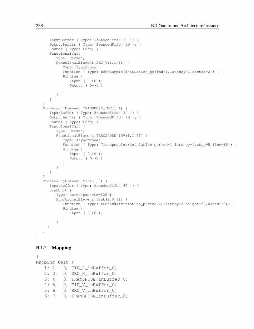
238 B.1 One-to-one Architecture Instance
InputBuffer { Type: BoundedFifo( 30 ); }OutputBuffer { Type: BoundedFifo( 20 ); }Router { Type: Fcfs; }FunctionalUnit {
Type: Packet;FunctionalElement SRC_V(1,1)[1] {
Type: Synchrone;Function { Type: DownSample(initiation_period=1,latency=1,factor=2); }Binding {
Input ( 0->0 );Output ( 0->0 );
}}
}}ProcessingElement TRANSPOSE_INV(1,1) {
InputBuffer { Type: BoundedFifo( 30 ); }OutputBuffer { Type: BoundedFifo( 20 ); }Router { Type: Fcfs; }FunctionalUnit {
Type: Packet;FunctionalElement TRANSPOSE_INV(1,1)[1] {
Type: Asynchrone;Function { Type: TransposeInv(initiation_period=1,latency=1,step=5,line=60); }Binding {
Input ( 0->0 );Output ( 0->0 );
}}
}}ProcessingElement Sink(1,0) {
InputBuffer { Type: BoundedFifo( 30 ); }SinkUnit {
Type: Burst(packets=120);FunctionalElement Sink(1,0)[1] {
Function { Type: PGMsink(initiation_period=2,latency=2,height=60,width=60); }Binding {
Input ( 0->0 );}
}}
}}
B.1.2 Mapping
}Mapping test {
1: 2, 0, FIR_H_inBuffer_0;2: 3, 0, SRC_H_inBuffer_0;3: 4, 0, TRANSPOSE_inBuffer_0;4: 5, 0, FIR_V_inBuffer_0;5: 6, 0, SRC_V_inBuffer_0;6: 7, 0, TRANSPOSE_inBuffer_0;
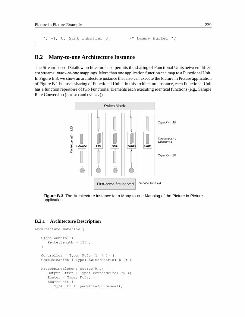
Picture in Picture Example 239
7: -1, 0, Sink_inBuffer_0; /* Dummy Buffer */}
B.2 Many-to-one Architecture Instance
The Stream-based Dataflow architecture also permits the sharing of Functional Units between differ-ent streams:many-to-onemappings. More than one application function can map to a Functional Unit.In Figure B.3, we show an architecture instance that also can execute the Picture in Picture applicationof Figure B.1 but uses sharing of Functional Units. In this architecture instance, each Functional Unithas a function repertoire of two Functional Elements each executing identical functions (e.g., SampleRate Conversion (SRCH) and (SRCV)).
Pac
ket L
engt
h =
120
Source FIR SRC Trans
Switch Matrix
First-come-first-served
Throughput = 1
Capacity = 20
Capacity = 30
Latency = 1
Sink
Service Time = 4
Figure B.3 . The Architecture Instance for a Many-to-one Mapping of the Picture in Pictureapplication
B.2.1 Architecture Description
Architecture Dataflow {
GlobalControl {PacketLength = 120 ;
}
Controller { Type: Fcfs( 1, 4 ); }Communication { Type: SwitchMatrix( 8 ); }
ProcessingElement Source(0,1) {OutputBuffer { Type: BoundedFifo( 30 ); }Router { Type: Fcfs; }SourceUnit {
Type: Burst(packets=760,base=1);
240 B.2 Many-to-one Architecture Instance
FunctionalElement Source(0,1)[1] {Function { Type: PGMsource(initiation_period=2,latency=2); }Binding {
Output ( 0->0 );}
}}
}ProcessingElement FIR(1,1) {
InputBuffer { Type: BoundedFifo( 30 ); }OutputBuffer { Type: BoundedFifo( 20 ); }Router { Type: Fcfs; }FunctionalUnit {
Type: Packet;FunctionalElement FIR_H(1,1)[1] {
Type: Synchrone;Function { Type: FirFilter(initiation_period=1,latency=18); }Binding {
Input ( 0->0 );Output ( 0->0 );
}}FunctionalElement FIR_V(1,1)[1] {
Type: Synchrone;Function { Type: FirFilter(initiation_period=1,latency=18); }Binding {
Input ( 0->0 );Output ( 0->0 );
}}
}}ProcessingElement SRC(1,1) {
InputBuffer { Type: BoundedFifo( 30 ); }OutputBuffer { Type: BoundedFifo( 20 ); }Router { Type: Fcfs; }FunctionalUnit {
Type: Packet;FunctionalElement SRC_H(1,1)[1] {
Type: Synchrone;Function { Type: DownSample(initiation_period=1,latency=1,factor=2); }Binding {
Input ( 0->0 );Output ( 0->0 );
}}FunctionalElement SRC_V(1,1)[1] {
Type: Synchrone;Function { Type: DownSample(initiation_period=1,latency=1,factor=2); }Binding {
Input ( 0->0 );Output ( 0->0 );
}}
}}ProcessingElement TRANSPOSE(1,1) {
BIBLIOGRAPHY 241
InputBuffer { Type: BoundedFifo( 30 ); }OutputBuffer { Type: BoundedFifo( 20 ); }Router { Type: Fcfs; }FunctionalUnit {
Type: Packet;FunctionalElement TRANSPOSE(1,1)[1] {
Type: Asynchrone;Function { Type: Transpose(initiation_period=1,latency=1,line=60); }Binding {
Input ( 0->0 );Output ( 0->0 );
}}
FunctionalElement TRANSPOSE_INV(1,1)[1] {Type: Asynchrone;Function { Type: Transpose(initiation_period=1,latency=1,step=5,line=60); }Binding {
Input ( 0->0 );Output ( 0->0 );
}}
}}ProcessingElement Sink(1,0) {
InputBuffer { Type: BoundedFifo( 30 ); }SinkUnit {
Type: Burst(packets=120);FunctionalElement Sink(1,0)[1] {
Function { Type: PGMsink(initiation_period=2,latency=2,height=60,width=60); }Binding {
Input ( 0->0 );}
}}
}}
B.2.2 Mapping
}Mapping test {
1: 2, 0, FIR_inBuffer_0;2: 3, 0, SRC_inBuffer_0;3: 4, 0, TRANSPOSE_inBuffer_0;4: 5, 1, FIR_inBuffer_0;5: 6, 1, SRC_inBuffer_0;6: 7, 1, TRANSPOSE_inBuffer_0;7: -1, 0, Sink_inBuffer_0; /* Dummy Buffer */
}
Bibliography
Johan G.W.M. Janssen, Jeroen H. Stessen, and Peter H.N. de With. An advanced sampling rate

242 BIBLIOGRAPHY
conversion algorithm for video and graphics signals. InIEE Sixth International Conference onImage Processing and its Applications, Dublin, 1997.
Appendix C
Limitations of the RTL
THE RTL describes asynchronous communication between processes very efficiently. It is, how-ever, less efficient when describing synchronouscommunication and control behavior likepolling,
which potentially limits the usability of the RTL. The reason why the RTL cannot describe pollingefficiently is that it lacks the notion of thestate of the system.
C.1 State of the System
When we use the RTL, we cannot determine the state of the system at a particular time instance. InFigure 4.7, the process shown is running at time instance t=5 and it observes the system while thereare still processes in the RPQ that need to execute at the same time. One of these processes couldchange the value of a variable at t=5. Hence, when the running process observes a variable in anotherprocess without making use ofpam P andpam V (i.e, when it does not explicitly synchronize withthat process), it is not able to determine whether the observed variable still holds the old value orwhether it has already acquired a new value.
C.1.1 Polling
When the notion of the state of the system is lacking, it is difficult to describepolling. In polling, aprocess checks a condition and performs a particular action based on this condition. When pollingis used, a process controls the progress of another process without synchronization. Therefore, oneprocess cannot make another process block.
The need for polling arises when we want to describe, for example, the time division multiplexedpolicy of the communication structure (see Section 2.1.3 where we explain the behavior of a TDMcommunication protocol). The communication structure divides the bandwidth of each channel intoN time slots ofx cycles. All routers are pre-assigned a time slot on a channel that they can use to senda packet or part of a packet to input buffers of functional units. The global controller is responsiblefor routers being enabled when their time slot is available.
To describe this enabling process, we model the global controller as an active element insteadof a passive element as is done in Program 5.3. The global controller could usepam V to activatethe appropriate routers for a time slot, but when it wants to reclaim control because the time slot hasfinished, it cannot simply usepam P. A router that is blocked, for example, because it wanted toread a token from an empty output buffer, also causes the global controller to block and the global
243
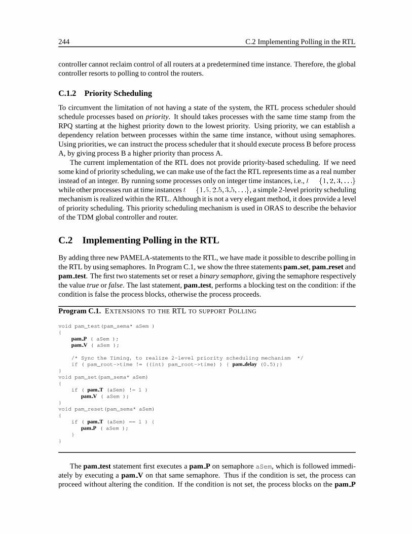
244 C.2 Implementing Polling in the RTL
controller cannot reclaim control of all routers at a predetermined time instance. Therefore, the globalcontroller resorts to polling to control the routers.
C.1.2 Priority Scheduling
To circumvent the limitation of not having a state of the system, the RTL process scheduler shouldschedule processes based onpriority. It should takes processes with the same time stamp from theRPQ starting at the highest priority down to the lowest priority. Using priority, we can establish adependency relation between processes within the same time instance, without using semaphores.Using priorities, we can instruct the process scheduler that it should execute process B before processA, by giving process B a higher priority than process A.
The current implementation of the RTL does not provide priority-based scheduling. If we needsome kind of priority scheduling, we can make use of the fact the RTL represents time as a real numberinstead of an integer. By running some processes only on integer time instances, i.e.,t = f1; 2; 3; : : :gwhile other processes run at time instancest = f1:5; 2:5; 3:5; : : :g, a simple 2-level priority schedulingmechanism is realized within the RTL. Although it is not a very elegant method, it does provide a levelof priority scheduling. This priority scheduling mechanism is used in ORAS to describe the behaviorof the TDM global controller and router.
C.2 Implementing Polling in the RTL
By adding three new PAMELA-statements to the RTL, we have made it possible to describe polling inthe RTL by using semaphores. In Program C.1, we show the three statementspam set, pam resetandpam test. The first two statements set or reset abinary semaphore, giving the semaphore respectivelythe valuetrueor false. The last statement,pam test, performs a blocking test on the condition: if thecondition is false the process blocks, otherwise the process proceeds.
Program C.1. EXTENSIONS TO THERTL TO SUPPORTPOLLING
void pam_test(pam_sema* aSem ){
pam P ( aSem );pam V ( aSem );
/* Sync the Timing, to realize 2-level priority scheduling mechanism */if ( pam_root->time != ((int) pam_root->time) ) { pam delay (0.5);}
}void pam_set(pam_sema* aSem){
if ( pam T (aSem) != 1 )pam V ( aSem );
}void pam_reset(pam_sema* aSem){
if ( pam T (aSem) == 1 ) {pam P ( aSem );
}}
Thepam test statement first executes apam P on semaphoreaSem, which is followed immedi-ately by executing apam V on that same semaphore. Thus if the condition is set, the process canproceed without altering the condition. If the condition is not set, the process blocks on thepam P
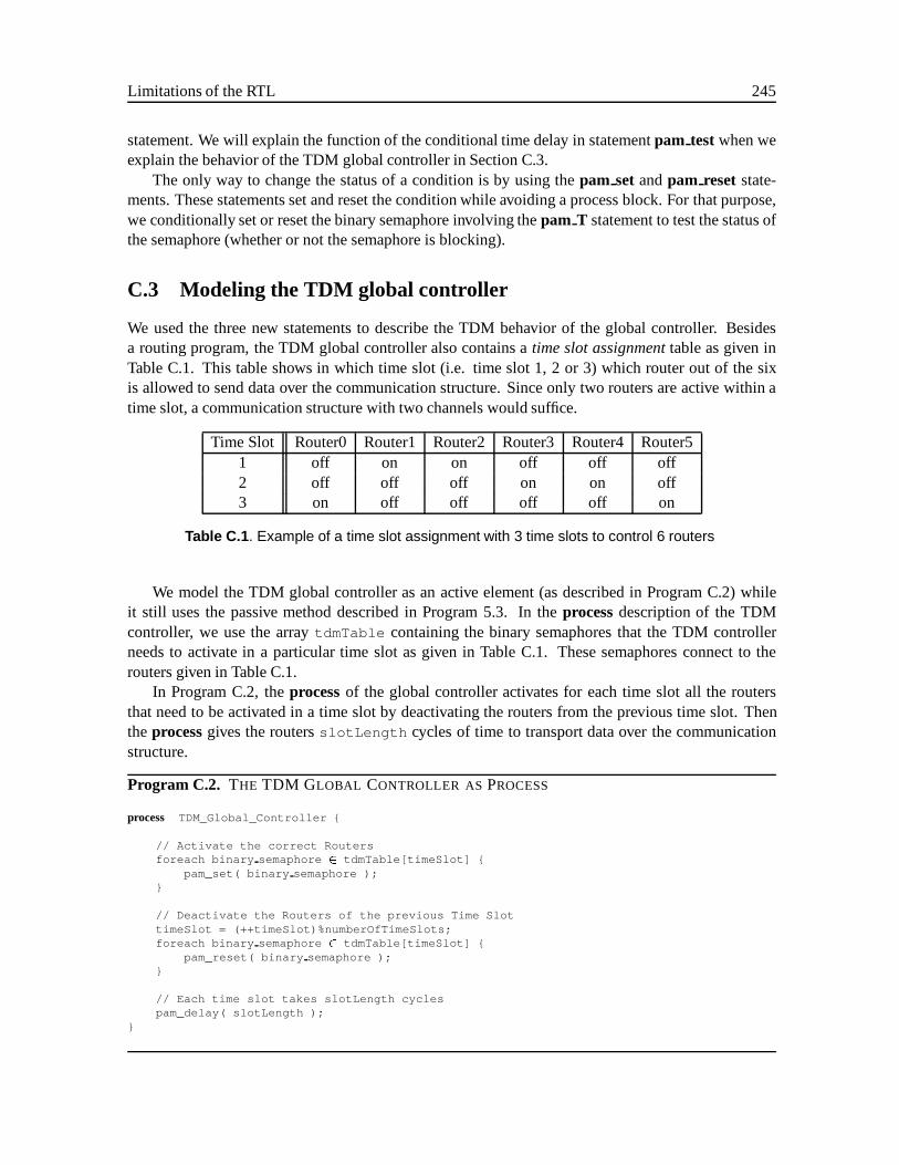
Limitations of the RTL 245
statement. We will explain the function of the conditional time delay in statementpam test when weexplain the behavior of the TDM global controller in Section C.3.
The only way to change the status of a condition is by using thepam setandpam reset state-ments. These statements set and reset the condition while avoiding a process block. For that purpose,we conditionally set or reset the binary semaphore involving thepam T statement to test the status ofthe semaphore (whether or not the semaphore is blocking).
C.3 Modeling the TDM global controller
We used the three new statements to describe the TDM behavior of the global controller. Besidesa routing program, the TDM global controller also contains atime slot assignmenttable as given inTable C.1. This table shows in which time slot (i.e. time slot 1, 2 or 3) which router out of the sixis allowed to send data over the communication structure. Since only two routers are active within atime slot, a communication structure with two channels would suffice.
Time Slot Router0 Router1 Router2 Router3 Router4 Router51 off on on off off off2 off off off on on off3 on off off off off on
Table C.1 . Example of a time slot assignment with 3 time slots to control 6 routers
We model the TDM global controller as an active element (as described in Program C.2) whileit still uses the passive method described in Program 5.3. In theprocessdescription of the TDMcontroller, we use the arraytdmTable containing the binary semaphores that the TDM controllerneeds to activate in a particular time slot as given in Table C.1. These semaphores connect to therouters given in Table C.1.
In Program C.2, theprocessof the global controller activates for each time slot all the routersthat need to be activated in a time slot by deactivating the routers from the previous time slot. Thentheprocessgives the routersslotLength cycles of time to transport data over the communicationstructure.
Program C.2. THE TDM GLOBAL CONTROLLER ASPROCESS
process TDM_Global_Controller {
// Activate the correct Routersforeach binary semaphore 2 tdmTable[timeSlot] {
pam_set( binary semaphore );}
// Deactivate the Routers of the previous Time SlottimeSlot = (++timeSlot)%numberOfTimeSlots;foreach binary semaphore 2 tdmTable[timeSlot] {
pam_reset( binary semaphore );}
// Each time slot takes slotLength cyclespam_delay( slotLength );
}
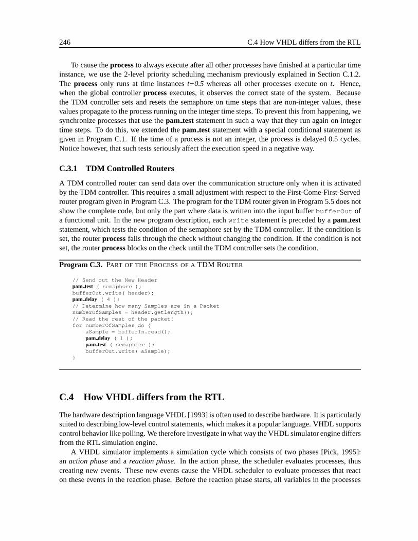
246 C.4 How VHDL differs from the RTL
To cause theprocessto always execute after all other processes have finished at a particular timeinstance, we use the 2-level priority scheduling mechanism previously explained in Section C.1.2.The processonly runs at time instancest+0.5 whereas all other processes execute ont. Hence,when the global controllerprocessexecutes, it observes the correct state of the system. Becausethe TDM controller sets and resets the semaphore on time steps that are non-integer values, thesevalues propagate to the process running on the integer time steps. To prevent this from happening, wesynchronize processes that use thepam test statement in such a way that they run again on integertime steps. To do this, we extended thepam test statement with a special conditional statement asgiven in Program C.1. If the time of a process is not an integer, the process is delayed 0.5 cycles.Notice however, that such tests seriously affect the execution speed in a negative way.
C.3.1 TDM Controlled Routers
A TDM controlled router can send data over the communication structure only when it is activatedby the TDM controller. This requires a small adjustment with respect to the First-Come-First-Servedrouter program given in Program C.3. The program for the TDM router given in Program 5.5 does notshow the complete code, but only the part where data is written into the input bufferbufferOut ofa functional unit. In the new program description, eachwrite statement is preceded by apam teststatement, which tests the condition of the semaphore set by the TDM controller. If the condition isset, the routerprocessfalls through the check without changing the condition. If the condition is notset, the routerprocessblocks on the check until the TDM controller sets the condition.
Program C.3. PART OF THE PROCESS OF ATDM ROUTER
// Send out the New Headerpam test ( semaphore );bufferOut.write( header);pam delay ( 4 );// Determine how many Samples are in a PacketnumberOfSamples = header.getlength();// Read the rest of the packet!for numberOfSamples do {
aSample = bufferIn.read();pam delay ( 1 );pam test ( semaphore );bufferOut.write( aSample);
}
C.4 How VHDL differs from the RTL
The hardware description language VHDL [1993] is often used to describe hardware. It is particularlysuited to describing low-level control statements, which makes it a popular language. VHDL supportscontrol behavior like polling. We therefore investigate in what way the VHDL simulator engine differsfrom the RTL simulation engine.
A VHDL simulator implements a simulation cycle which consists of two phases [Pick, 1995]:an action phaseand areaction phase. In the action phase, the scheduler evaluates processes, thuscreating new events. These new events cause the VHDL scheduler to evaluate processes that reacton these events in the reaction phase. Before the reaction phase starts, all variables in the processes
BIBLIOGRAPHY 247
have adopted new values reflecting the new state of the system. Hence, VHDL describes polling veryeffectively.
The VHDL simulation engine uses three different queues: atime-ordered queue, a signal-event-monitoringqueue, and aprocess-pending queue. The scheduler, which is part of the VHDL simulationengine, starts by evaluating processes with the same time-stamp in the time-ordered queue. Signalschange during the execution of processes, causing events on the event-monitoring queue. The sched-uler continues to evaluate processes until all processes with the same time-stamp have evaluated. Atthat time, all variables in the system have adopted new values reflecting the new state of the system.Next the VHDL scheduler wakes up processes that should react on events stored in the signal-event-monitoring queue. The awoken processes are stored in the process-pending queue. Next, the schedulerstarts the reaction phase by executing all processes in the process-pending queue. These processes ob-serve a system in which all variables reflect the new state of the system. Processes that execute in thesecond phase can cause new events to occur. Therefore the scheduler has to iterate a number of times,which is referred to as the VHDL�-mechanism [Pick, 1995]. After no more events take place and allprocesses have executed, the reaction phase has finished and a new simulation cycle starts.
A VHDL simulation engine must perform a large amount of bookkeeping and sorting to imple-ment the two-phase simulation cycle. This provides a large amount of flexibility, but at the expenseof a considerable amount of time being spent on these activities. The RTL scheduler, on the otherhand, executes a process as soon as an event (i.e. apam P, pam V, or pam delay) takes place, dra-matically reducing the amount of bookkeeping and sorting needed. As a consequence, although itis difficult to describe polling, the RTL has an excellent simulation speed compared to the speed ofVHDL simulations.
Bibliography
Joseph Pick. VHDL, Techniques, Experiments, and Caveats. Series on Computer Engineering.McGraw-Hill, 1995. pages 11 – 44.
VHDL. IEEE Standard VHDL Language Reference Manual. IEEE Computer Service, 445 HoesLane, P.O. Box 1331, Piscataway, New Jersey, 08855-1331, 1993. IEEE Std 1076-1993.
Index
abstract classes, 98abstract executable models, 47Abstraction Pyramid, 47accuracy, 66Acquisition of Insight, 185active building block, 85active object, 78active primitives, 68actors, 150Application – Architecture interface, 172Application State Transition, 152architectural choices, 31Architectural Element , 93Architectural Element Type, 94architecture
efficiency, 24flexibility, 24
Architecture Description Language, 123Architecture Instance, 32Architecture Template, 32Architectures, 93associative arrays, 190
back-of-the-envelope models, 47Backus-Naur Form, 121balance equations, 151bandwidth, 3base, 129basic splines, 188behavior, 78benchmark, 203benchmarks, 2binary semaphore, 244binding function, 145block diagrams, 92blocked process, 68Blocked Processes Queue, 86blocking-read, 142BNF, 121
bubbles, 118Building Block , 85burst mode, 29bus, 28
Channels, 142channels, 22class of stream-based dataflow architectures, 31Communicating Sequential Processes, 151communication network, 211communication structure, 22composition rules, 121, 231compound node, 211computational power, 3Condition Synchronization, 65, 70Conditional Control Flow, 65, 70container, 99context, 81context switching, 81coordination language, 153Cordic, 211current state, 143Cycle, 94cycle, 22, 145Cycle-Accurate Model, 94cycle-accurate models, 47Cyclo-static Dataflow, 151
data dependencies, 67data type, 53Dataflow Architecture, 23dataflow architecture
data-driven, 23demand-driven, 23dynamic, 23static, 23tag, 23
Dataflow Process Network, 152deadlock, 38
248
INDEX 249
design flow, 189design objectives, 32Design of Experiments, 186design space, 32design trajectory, 51deterministic order, 142discrete event, 73DOE, 186Domain-specific Dataflow Architectures, 35dummy functions, 205dynamic application, 138Dynamic Dataflow, 151
Enabled Function, 144estimation models, 47event, 73Execution Time, 65, 70experiment, 186Exploration , 46exploring, 8
factorial design, 186factors, 187Feasible Design, 32field blanking, 206Fire-and-Exit behavior, 145, 155fired, 150First-Come-First-Served, 28, 30First-In-First-Out, 19fractional factorial experiment, 187full factorial experiment, 187function execution, 22Function Firing, 144Function Repertoire, 17functional element, 21functional performance model, 71functional unit, 20
Gantt Chart, 74global controller, 22, 211Golden Point Design, 33golden point design, 51Grain Size, 17grain size
coarse-grained, 17fine-grained, 17medium-grained, 17
grammar, 123
grants, 30Granularity of an SBF Object , 147
HiPars, 215Homogeneous Dataflow, 150host language, 153
idle cycle, 28inheritance, 98initiation period, 22inverse transformation, 184
Jacobi-type algorithms, 210Jacobium Processor, 210
Kahn Process Network, 142, 151keywords, 124knot, 188
late binding, 98latency, 22levels, 187library, 156lightweight processes, 81line blanking, 206local controller, 211local memory, 211localized references, 84
Machine-oriented Modeling, 68Mapping
Many-to-One, 176One-to-One, 175
MARS, 188matching units, 35Material-oriented Modeling, 68metric collectors, 163, 166Model of Architecture , 53Model of Computation, 53multi-functional, 3multi-rate, 147, 173multi-standard, 3multiple resources possession, 71multithreading, 81Multithreading Architectures, 35Multivariate Adaptive Regression Splines, 188Mutual Exclusion, 65, 70
Nelsis, 189
250 INDEX
Nested Loop Program, 213network, 127non-blocking write, 142non-preemptive, 87
object, 78class description, 78constructor, 78data, 78implementation, 80instantiated, 78interface, 78methods, 78
object oriented, 77Object Oriented Retargetable Simulator, 163Offset, 131one-to-one, 133opcode buffer, 25ORAS, 163orthogonal arrays, 187over-designed, 33
Packet, 17packet, 19
data part, 19header part, 19
packet-switching, 26PAMELA Modeling, 67
delay, 67process, 67semaphore, 67time units, 67
paper architectures, 33Parameters
Behavioral, 126Functional, 126Structural, 126
partition, 216passive building block, 85passive object, 78passive primitives, 68performance analysis, 9, 64performance evaluation, 64performance metrics, 2performance model, 65performance modeling, 64
interpreted, 71
uninterpreted, 71Performance Modeling Basis, 65performance models, 2Perl, 189Petri Nets, 87Picture in Picture, 138, 235piecewise linear model, 189PiP, 138, 235pipeline depth, 22pipelined, 22polling, 243polymorphism, 98priority scheduling, 244Problem Statement, 33procedural oriented, 77process, 142process function, 82process scheduler, 81, 85processing element, 19Processing Elements, 211programmable, 1programming model, 127pseudo C, 68
QR matrix decomposition, 213QR update, 213quantitative, 2quantitative data, 44Queuing Theory, 87
r, 24rate, 22real-time, 3regions, 216reliable experiment, 187reprogram, 18request, 30residence time, 114resource conflict arbitration, 74resource modeling, 101resources, 64Response Surface Model, 185Retargetable Architecture Simulator, 162Round Robin, 30router, 211Routing Program, 18routing program, 104

INDEX 251
RSM, 185RTL, 81
delays, 81process, 81semaphores, 81
Run-Time Library, 76, 81runnable process, 85Runnable Processes Queue, 85
sample-switching, 26SBF object
controller, 142set of functions, 142state, 142
SBFsim, 153self-contained, 85sequential firing rules, 152sequential order, 143sequential ordering, 139service capacity, 30service time, 30set of applications, 3sharing, 24sharing factor, 24simulation tools, 87speed-up, 24Standard Template Library, 165state of the system, 243static network, 138Stream, 17stream mode, 29Stream-Based Application, 138Stream-Based Dataflow Architecture, 2Stream-based Dataflow Architectures, 18Stream-Based Function Objects, 142Stream-Based Functions, 142structure, 78switch matrix, 28Synchronous Dataflow, 151synthesizable VHDL models, 47system, 64
tagged-token dataflow architectures, 35tags, 35task graph, 67terminals, 203thread-of-execution, 81
throughput, 22Time Division Multiplex, 30time division multiplexed, 28time shape, 206time slot assignment, 245time stamp, 85token, 23total execution time, 75trade-offs, 8transition, 143transition function, 144trial runs, 187
under-designed, 33utilization, 75
Variant of a Function, 147variants, 216VHDL
action phase, 246queues, 247reaction phase, 246
Videofields, 5frames, 5lines, 5pixels, 5
video data, 206video signal processing, 35
Weakly Programmable Processing Element,17
workload, 64workload modeling, 101workspaces, 203
Y-chartstack, 49
Y-chart Approach , 44Y-chart Environment , 49

252 INDEX
Acknowledgments
ThisPh.D. thesis is theresult of research conducted mainly at PhilipsResearch Laboratories in Eind-hoven. As a Ph.D. student from the group Circuits & Systems at Delft University of Technology, Iconsidered it aprivilegeto work in thisinspiring research institute. I wasexposed to both industriallyrelevant problemsand to an excellent academic environment.
For thisopportunity I am indebted to many people. I want to thank my promotor Patrick Dewildefor giving me the opportunity to pursue a Ph.D. within the group Circuits & Systems, an excellentgroup of which I am aproud member. I also want to thank Eric van Utteren en Cees Niessen, who, asgroup leadersof thegroup VLSI Design Automation and Testing, gavemetheopportunity to work intheir group. Finally, thepartial support of PhilipsResearch and theMinistry of Economic affairs, theNetherlands, ishereby greatly acknowledged.
I was able to work within a team that consisted of people of which I have learned at lot: EdDeprettere, Kees Vissers and Pieter van der Wolf. I want to thank Ed Deprettere for his support ascopromotor and his relentless enthusiasm to learn and understand new things; Kees Vissers for hisopen mind, his insights, and his standards in research; and Pieter van der Wolf for structuring mywork and keeping me with both feet on the ground. I enjoyed working with the three of them andwant to thank them for being excellent mentors.
During my promotion, I had theopportunity to interact with many peoplethat I want to acknowl-edge. There were from many groups, both from Delf t and Philips Research. First of all I want tothank all personsof thegroup Circuits& Systemswith whom I have worked and in particular I wantto thank Paul Lieverse and Daniel van Loenen from Delft, and GiuseppeGarcea from the Universityof Florence, Italy, who all have done agreat job during their Masters assignment. I want to thankNeil Smith from UC Berkeley for his extensions to SBFsim and I want to thank Edwin Rijpkemafor the discussions we had on the Jacobium Project. I also want to thank Arjan van Gemund fromthe CARDIT group for his help on the use of PAMELA and the PAMELA Run-time Library. FromPhilipsResearch, I want to thank my colleaguesand in particular Gerben Essink, Erwin deKock, andWim Smits. I also want to
thank the people involved in the Prophid project: Jeroen Leijten, Adwin Timmer, and Jef vanMeerbergen. Peter Bingely and Wim van der Linden helped me with the generic DSE environment,and I want to thank them for their help. I also want to thank Andre van der Avoird for the manydiscussions we had on our work and about working at Philips Research. I also want to thank LaurelBeecher for editing my thesis.
I want to acknowledgethe fellow Ph.D. studentsat Philipswith whom I have shared room 4.085:Hansvan Gageldonk, Paul Lieverse, Bob Witlox, Robert Arendsen, and Ramon Clout.
253

254 INDEX
Finally, I want to thank my family and my friends for supporting me in my Ph.D. and for contin-uously showing interest in my work. Special thanks are for my wife-to-be Karien, who supported meall those years, in particular, by reading work I had written and by showing understanding when againsome deadline had to be met.
Bart Kienhuis,26 November 1998,Amsterdam.
Samenvatting
Er is momenteel een trend waarneembaar dat applicatie specifieke architecturen steeds meer pro-grammeerbaar worden, om multifunctionele en multistandaard produkten te kunnen ondersteunen.Het kenmerk van deze nieuwe architecturen is dat ze een set van applicaties kunnen ondersteunenin plaats van ´een enkele applicatie. We hebben echter ondervonden dat goede, algemeen toepasbareontwerp methoden niet voorhanden zijn voor dit soort architecturen.
Als voorbeeld van z’n programmeerbare architectuur, laten wij in dit proefschrift destroomgebaseerde dataflow architectuurzien. Deze architectuur past in de categorie van dataflow archi-tecturen en is zeer geschikt voor stroom gebaseerde, hoge prestatie applicaties die gevonden wordenin bijvoorbeeld real-time multimedia toepassingen.
Bij het ontwerp van deze stroom gebaseerde dataflow architecturen moeten erg veel keuzen gemaaktworden, waarbij elke keuze leidt tot een andere architectuur, met een eigen specifiek gedrag enprestatie. Nu wordt het voor ontwerpers steeds moeilijker om die keuzen te maken zodat de steedscomplexer wordende architectuur nog voldoet aan alle ontwerp eisen, waaronder programeerbaarheid.
Wij hebben de vele ontwerp keuzen gestructureerd met behulp van eenarchitectuur template.Deze beschrijft de totale klasse van stroom gebaseerde architecturen met behulp van parameters enheeft dus een duidelijk begrensde ontwerp ruimte. De probleem stelling van dit proefschrift is omeen methode te ontwikkelen die ontwerpers helpt bij het vinden van de parameter waarden van eenarchitectuur template, zodanig dat een haalbare architectuur gevonden wordt in de ontwerp ruimte.Een haalbare architectuur voldoet aan de opgelegde ontwerp eisen waaronder: doorzet en utilisatie,maar ook gebruikt vermogen en silicium oppervlakte.
In dit proefschrift presenteren wij als methodiek deY-chart aanpak, waarmee ontwerpers keuzenkunnen kwantificeren. De Y-chart aanpak genereert een objectieve basis voor het motiveren en makenvan keuzen. De Y-chart aanpak leidt tot eenY-chart omgevingen wij presenteren in dit proefschriftz’n Y-chart omgeving voor de klasse van stroom gebaseerde dataflow architecturen. Een Y-chartomgeving bestaat uit 6 componenten en elke component wordt besproken. Zo bespreken we een hoogniveau methode waarmee prestatie analyse gedaan kan worden, een architectuur modelerings aanpak,een applicatie modelerings aanpak, een aanpak voor het construeren van een retargetable simulator,en een aanpak om applicaties af te beelden op een specifiek instantie van de architectuur template.Tenslotte bespreken we ook hoe we de ontwerp ruimte van architecturen op een systematische manierkunnen exploreren.
We hebben de ontwikkelde Y-chart omgeving gebruikt in twee ontwerp cases. Daaruit blijkt dat deY-chart omgeving inderdaad ontwerp keuzen kwantificeert. Bovendien laten de twee ontwerp caseszien dan we de ontwerp ruimte van architecturen snel kunnen exploreren, op een hoog niveau vanabstractie. De getallen die gepresenteerd worden, zullen niet direct tot de verdere ontwikkeling vande twee architecturen leiden, maar geven wel duidelijk aan waartoe de methode in staat is. Het geeftontwerpers inzicht in de vele complexe afwegingen tussen parameter waarden en prestatie getallen dieaanwezig zijn in dit soort programmeerbare architecturen. Soortgelijke resultaten zijnzeer moeilijk
255

256 INDEX
te verkrijgen met de hedendaagse ontwerp methodes; en als ze te verkrijgen zijn heeft dat veel meerontwerp- en simulatie tijd gekost.
Curriculum Vitae
Bart Kienhuis was born on August 9, 1968 in Vleuten, The Netherlands. After finishing his HAVOdegree at the “St Gregorius” Community School in 1986, he received his VWO degree from Commu-nity School “De Klop” in 1987. In that same year, he started his study Electrical Engineering at DelftUniversity of Technology. As a student from the Circuits & Systems group, he did his M.Sc thesis ontheHiPars compiler that converts nested loop programs into parallel programs. After he graduatedin 1994, he started to work towards his Ph.D., again as a student of the Circuits & Systems groupand spent almost all of his research time at Philips Research Laboratories in Eindhoven, working on ajoint project.
From February 1st, 1999, Bart has accepted a Post-Doc position at UC Berkeley within the groupof Professor Edward A. Lee.
257

EDDDDand Submicron Technology
IDD EM SIDelft Institute of Microelectronics