Design and Modeling of High Performance Permanent Magnet ...
236
Design and Modeling of High Performance Permanent Magnet Synchronous Machines Martin van der Geest
Transcript of Design and Modeling of High Performance Permanent Magnet ...

Design and Modeling of High PerformancePermanent Magnet Synchronous Machines
Martin van der Geest
Design and Modeling of High Perform
ance Permanent M
agnet Synchronous Machines


Design and Modeling of High PerformancePermanent Magnet Synchronous Machines
Proefschriftter verkrijging van de graad van doctor
aan de Technische Universiteit Delft,op gezag van de Rector Magnificus prof. ir. K.C.A.M. Luyben;
voorzitter van het College voor Promoties,in het openbaar te verdedigen op
vrijdag 27 november 2015 om 10:00 uur
door
Martin VAN DER GEEST
elektrotechnisch ingenieur,Technische Universiteit Delft, Nederland,
geboren te Rijpwetering, Nederland

Dit proefschrift is goedgekeurd door depromotor: Prof. dr. eng. J.A. Ferreira encopromotor: Dr. ir. H. Polinder
Samenstelling promotiecommissie bestaat uit:Rector magnificus, voorzitterpromotor: Prof. dr. eng. J.A. Ferreiracopromotor: Dr. ir. H. Polinder
onafhankelijke leden:Prof. dr. B.C. Mecrow Newcastle University, United KingdomProf. dr. C. Gerada University of Nottingham, United KingdomProf. dr. ir. J. Hellendoorn Technische Universiteit DelftProf. dr. ir. M. Zeman Technische Universiteit Delft
Overig lid:Dr. M. Gerber Aeronamic B.V.
The research leading to these results has received funding from the European Union’s SeventhFramework Programme (FP7/2007-2013) for the Clean Sky Joint Technology Initiative under grantagreement CSJU-GAM-SGO-2008-001.
Printed by: Gildeprint
ISBN: 978-94-6233-158-7
Copyright © 2015 by Martin van der Geest


Contents
Summary ix
Samenvatting xiii
Glossary xvii
1 Introduction 11.1 Motivation . . . . . . . . . . . . . . . . . . . . . . . . . . . . . . . . . . . . . . . . . . . 21.2 Objectives . . . . . . . . . . . . . . . . . . . . . . . . . . . . . . . . . . . . . . . . . . . 3
1.2.1 Project objective . . . . . . . . . . . . . . . . . . . . . . . . . . . . . . . . . . . 31.2.2 Thesis objectives . . . . . . . . . . . . . . . . . . . . . . . . . . . . . . . . . . . 4
1.3 Outline and approach . . . . . . . . . . . . . . . . . . . . . . . . . . . . . . . . . . . . 4
2 Machine selection and design with automated optimization 72.1 Introduction . . . . . . . . . . . . . . . . . . . . . . . . . . . . . . . . . . . . . . . . . . 82.2 Optimization and modeling strategy . . . . . . . . . . . . . . . . . . . . . . . . . . . . 10
2.2.1 Machine analysis . . . . . . . . . . . . . . . . . . . . . . . . . . . . . . . . . . . 102.2.2 Particle Swarm Optimization . . . . . . . . . . . . . . . . . . . . . . . . . . . . 122.2.3 Additional remarks . . . . . . . . . . . . . . . . . . . . . . . . . . . . . . . . . . 14
2.3 Optimization example 1 . . . . . . . . . . . . . . . . . . . . . . . . . . . . . . . . . . . 152.3.1 The PM machines considered . . . . . . . . . . . . . . . . . . . . . . . . . . . 162.3.2 Optimization targets, assumptions and search space . . . . . . . . . . . . . . 172.3.3 Optimization results . . . . . . . . . . . . . . . . . . . . . . . . . . . . . . . . . 18
2.4 Optimization example 2: A first look at the S/G problem . . . . . . . . . . . . . . . . 212.4.1 Target specifications . . . . . . . . . . . . . . . . . . . . . . . . . . . . . . . . . 212.4.2 Machine optimization . . . . . . . . . . . . . . . . . . . . . . . . . . . . . . . . 222.4.3 Optimization results . . . . . . . . . . . . . . . . . . . . . . . . . . . . . . . . . 24
2.5 Conclusion . . . . . . . . . . . . . . . . . . . . . . . . . . . . . . . . . . . . . . . . . . . 31
3 Efficient finite element based rotor eddy current loss calculation 333.1 Introduction . . . . . . . . . . . . . . . . . . . . . . . . . . . . . . . . . . . . . . . . . . 343.2 Proposed modeling method . . . . . . . . . . . . . . . . . . . . . . . . . . . . . . . . . 353.3 2D calculation performance . . . . . . . . . . . . . . . . . . . . . . . . . . . . . . . . . 37
3.3.1 Baseline machine . . . . . . . . . . . . . . . . . . . . . . . . . . . . . . . . . . . 383.3.2 Space-harmonic losses only . . . . . . . . . . . . . . . . . . . . . . . . . . . . . 383.3.3 Space-harmonic losses and shielding . . . . . . . . . . . . . . . . . . . . . . . 413.3.4 Solid back-iron . . . . . . . . . . . . . . . . . . . . . . . . . . . . . . . . . . . . 423.3.5 Slotting losses . . . . . . . . . . . . . . . . . . . . . . . . . . . . . . . . . . . . . 423.3.6 Slotting losses with shielding . . . . . . . . . . . . . . . . . . . . . . . . . . . . 43
v

Contents
3.3.7 Strong stator saturation . . . . . . . . . . . . . . . . . . . . . . . . . . . . . . . 433.3.8 Low magnet span . . . . . . . . . . . . . . . . . . . . . . . . . . . . . . . . . . . 443.3.9 Distributed windings . . . . . . . . . . . . . . . . . . . . . . . . . . . . . . . . . 443.3.10 Tangential magnet segmentation . . . . . . . . . . . . . . . . . . . . . . . . . . 45
3.4 3D calculation performance . . . . . . . . . . . . . . . . . . . . . . . . . . . . . . . . . 463.4.1 Loss calculation . . . . . . . . . . . . . . . . . . . . . . . . . . . . . . . . . . . . 463.4.2 Inductance limited currents . . . . . . . . . . . . . . . . . . . . . . . . . . . . . 493.4.3 Effect of magnet segmentation . . . . . . . . . . . . . . . . . . . . . . . . . . . 513.4.4 Alternate winding layouts . . . . . . . . . . . . . . . . . . . . . . . . . . . . . . 52
3.5 Conclusion . . . . . . . . . . . . . . . . . . . . . . . . . . . . . . . . . . . . . . . . . . . 54
4 AC winding losses in high-speed PM machines 574.1 Introduction . . . . . . . . . . . . . . . . . . . . . . . . . . . . . . . . . . . . . . . . . . 584.2 Current sharing analysis . . . . . . . . . . . . . . . . . . . . . . . . . . . . . . . . . . . 59
4.2.1 Overview . . . . . . . . . . . . . . . . . . . . . . . . . . . . . . . . . . . . . . . . 594.2.2 Problem elaboration . . . . . . . . . . . . . . . . . . . . . . . . . . . . . . . . . 604.2.3 Model development . . . . . . . . . . . . . . . . . . . . . . . . . . . . . . . . . 624.2.4 Experimental validation . . . . . . . . . . . . . . . . . . . . . . . . . . . . . . . 654.2.5 Effect of strand twisting . . . . . . . . . . . . . . . . . . . . . . . . . . . . . . . 69
4.3 Loss reduction techniques . . . . . . . . . . . . . . . . . . . . . . . . . . . . . . . . . . 734.3.1 Background . . . . . . . . . . . . . . . . . . . . . . . . . . . . . . . . . . . . . . 734.3.2 Example machine . . . . . . . . . . . . . . . . . . . . . . . . . . . . . . . . . . . 744.3.3 Analytical models . . . . . . . . . . . . . . . . . . . . . . . . . . . . . . . . . . . 744.3.4 Loss reduction mechanisms . . . . . . . . . . . . . . . . . . . . . . . . . . . . 764.3.5 All methods combined . . . . . . . . . . . . . . . . . . . . . . . . . . . . . . . . 84
4.4 Conclusion . . . . . . . . . . . . . . . . . . . . . . . . . . . . . . . . . . . . . . . . . . . 86
5 Inter-turn faults – modeling, detection and consequences 895.1 Introduction . . . . . . . . . . . . . . . . . . . . . . . . . . . . . . . . . . . . . . . . . . 90
5.1.1 Modeling of short circuits . . . . . . . . . . . . . . . . . . . . . . . . . . . . . . 915.1.2 Fault detection . . . . . . . . . . . . . . . . . . . . . . . . . . . . . . . . . . . . 915.1.3 Fault mitigation . . . . . . . . . . . . . . . . . . . . . . . . . . . . . . . . . . . . 92
5.2 Modeling of short circuit faults . . . . . . . . . . . . . . . . . . . . . . . . . . . . . . . 925.2.1 Machine . . . . . . . . . . . . . . . . . . . . . . . . . . . . . . . . . . . . . . . . 925.2.2 Circuit . . . . . . . . . . . . . . . . . . . . . . . . . . . . . . . . . . . . . . . . . 935.2.3 Time-harmonic model . . . . . . . . . . . . . . . . . . . . . . . . . . . . . . . . 955.2.4 Transient models . . . . . . . . . . . . . . . . . . . . . . . . . . . . . . . . . . . 96
5.3 Analysis of short circuit faults . . . . . . . . . . . . . . . . . . . . . . . . . . . . . . . . 975.3.1 Parametric exploration . . . . . . . . . . . . . . . . . . . . . . . . . . . . . . . . 975.3.2 Number of parallel strands . . . . . . . . . . . . . . . . . . . . . . . . . . . . . 1035.3.3 Closed loop drive model . . . . . . . . . . . . . . . . . . . . . . . . . . . . . . . 105
5.4 Turn-level short circuit current measurement . . . . . . . . . . . . . . . . . . . . . . 1075.4.1 Test setup . . . . . . . . . . . . . . . . . . . . . . . . . . . . . . . . . . . . . . . 107
vi
5.4.2 Results . . . . . . . . . . . . . . . . . . . . . . . . . . . . . . . . . . . . . . . . . 1085.5 Consequences of short circuit faults . . . . . . . . . . . . . . . . . . . . . . . . . . . . 110
5.5.1 Test setup . . . . . . . . . . . . . . . . . . . . . . . . . . . . . . . . . . . . . . . 1105.5.2 Results . . . . . . . . . . . . . . . . . . . . . . . . . . . . . . . . . . . . . . . . . 111
5.6 Fault detector: concept . . . . . . . . . . . . . . . . . . . . . . . . . . . . . . . . . . . 1145.6.1 Detector description . . . . . . . . . . . . . . . . . . . . . . . . . . . . . . . . . 1145.6.2 Basic operation . . . . . . . . . . . . . . . . . . . . . . . . . . . . . . . . . . . . 1155.6.3 Low pass filter tuning . . . . . . . . . . . . . . . . . . . . . . . . . . . . . . . . 1175.6.4 Fault detection performance versus short circuit position . . . . . . . . . . . 1175.6.5 Open circuit faults . . . . . . . . . . . . . . . . . . . . . . . . . . . . . . . . . . 1185.6.6 Other faults . . . . . . . . . . . . . . . . . . . . . . . . . . . . . . . . . . . . . . 119
5.7 Fault detector: experimental validation . . . . . . . . . . . . . . . . . . . . . . . . . . 1215.7.1 Test on the prototype machine . . . . . . . . . . . . . . . . . . . . . . . . . . . 1215.7.2 Test on the industrial machine . . . . . . . . . . . . . . . . . . . . . . . . . . . 123
5.8 Conclusion . . . . . . . . . . . . . . . . . . . . . . . . . . . . . . . . . . . . . . . . . . . 127
6 Analysis of additional losses due to PWM induced current ripple 1296.1 Introduction . . . . . . . . . . . . . . . . . . . . . . . . . . . . . . . . . . . . . . . . . . 1306.2 System model . . . . . . . . . . . . . . . . . . . . . . . . . . . . . . . . . . . . . . . . . 131
6.2.1 Introduction . . . . . . . . . . . . . . . . . . . . . . . . . . . . . . . . . . . . . . 1316.2.2 Current ripple . . . . . . . . . . . . . . . . . . . . . . . . . . . . . . . . . . . . . 131
6.3 Stator lamination losses . . . . . . . . . . . . . . . . . . . . . . . . . . . . . . . . . . . 1346.4 Winding losses . . . . . . . . . . . . . . . . . . . . . . . . . . . . . . . . . . . . . . . . . 135
6.4.1 Current imbalance . . . . . . . . . . . . . . . . . . . . . . . . . . . . . . . . . . 1356.4.2 Induced losses (classical proximity effect) . . . . . . . . . . . . . . . . . . . . 136
6.5 Rotor eddy current losses . . . . . . . . . . . . . . . . . . . . . . . . . . . . . . . . . . 1376.6 Conclusion . . . . . . . . . . . . . . . . . . . . . . . . . . . . . . . . . . . . . . . . . . . 139
7 Design and testing of the prototype permanent magnet starter/generator 1417.1 Introduction . . . . . . . . . . . . . . . . . . . . . . . . . . . . . . . . . . . . . . . . . . 1427.2 Design considerations . . . . . . . . . . . . . . . . . . . . . . . . . . . . . . . . . . . . 143
7.2.1 Requirements . . . . . . . . . . . . . . . . . . . . . . . . . . . . . . . . . . . . . 1437.2.2 Inverter considerations . . . . . . . . . . . . . . . . . . . . . . . . . . . . . . . 1457.2.3 Machine considerations . . . . . . . . . . . . . . . . . . . . . . . . . . . . . . . 146
7.3 Detailed electromagnetic design . . . . . . . . . . . . . . . . . . . . . . . . . . . . . . 1497.3.1 Winding considerations . . . . . . . . . . . . . . . . . . . . . . . . . . . . . . . 1497.3.2 Rotor eddy current losses . . . . . . . . . . . . . . . . . . . . . . . . . . . . . . 1507.3.3 Demagnetization check . . . . . . . . . . . . . . . . . . . . . . . . . . . . . . . 1527.3.4 Realization . . . . . . . . . . . . . . . . . . . . . . . . . . . . . . . . . . . . . . . 152
7.4 Testing . . . . . . . . . . . . . . . . . . . . . . . . . . . . . . . . . . . . . . . . . . . . . 1547.4.1 Basic performance . . . . . . . . . . . . . . . . . . . . . . . . . . . . . . . . . . 1547.4.2 Saturation performance . . . . . . . . . . . . . . . . . . . . . . . . . . . . . . . 1547.4.3 Starting performance . . . . . . . . . . . . . . . . . . . . . . . . . . . . . . . . 155
vii

Contents
7.5 Conclusion . . . . . . . . . . . . . . . . . . . . . . . . . . . . . . . . . . . . . . . . . . . 156
8 Power density limits and design trends of high-speed permanent magnet synchronousmachines 1578.1 Introduction . . . . . . . . . . . . . . . . . . . . . . . . . . . . . . . . . . . . . . . . . . 1588.2 Optimization approach . . . . . . . . . . . . . . . . . . . . . . . . . . . . . . . . . . . 160
8.2.1 Choice of main target and independent variables . . . . . . . . . . . . . . . . 1608.2.2 Implementation . . . . . . . . . . . . . . . . . . . . . . . . . . . . . . . . . . . . 160
8.3 Modeling, assumptions & material properties . . . . . . . . . . . . . . . . . . . . . . 1638.3.1 Electrical domain . . . . . . . . . . . . . . . . . . . . . . . . . . . . . . . . . . . 1638.3.2 Mechanical domain . . . . . . . . . . . . . . . . . . . . . . . . . . . . . . . . . 1648.3.3 Thermal domain . . . . . . . . . . . . . . . . . . . . . . . . . . . . . . . . . . . 1648.3.4 Optimization . . . . . . . . . . . . . . . . . . . . . . . . . . . . . . . . . . . . . 166
8.4 Results . . . . . . . . . . . . . . . . . . . . . . . . . . . . . . . . . . . . . . . . . . . . . 1668.4.1 Individual fronts . . . . . . . . . . . . . . . . . . . . . . . . . . . . . . . . . . . 1668.4.2 Specific power density . . . . . . . . . . . . . . . . . . . . . . . . . . . . . . . . 1678.4.3 Detailed results – interface level . . . . . . . . . . . . . . . . . . . . . . . . . . 1688.4.4 Detailed results – machine level . . . . . . . . . . . . . . . . . . . . . . . . . . 1748.4.5 Lower temperature constraints . . . . . . . . . . . . . . . . . . . . . . . . . . . 177
8.5 Discussion . . . . . . . . . . . . . . . . . . . . . . . . . . . . . . . . . . . . . . . . . . . 1788.5.1 Literature comparison . . . . . . . . . . . . . . . . . . . . . . . . . . . . . . . . 1788.5.2 Thermal sensitivity analysis . . . . . . . . . . . . . . . . . . . . . . . . . . . . . 179
8.6 Conclusion . . . . . . . . . . . . . . . . . . . . . . . . . . . . . . . . . . . . . . . . . . . 180
9 Conclusion 183
A Thermal model 189A.1 Introduction . . . . . . . . . . . . . . . . . . . . . . . . . . . . . . . . . . . . . . . . . . 189A.2 Model description . . . . . . . . . . . . . . . . . . . . . . . . . . . . . . . . . . . . . . 190
A.2.1 Heat conduction in solid parts . . . . . . . . . . . . . . . . . . . . . . . . . . . 190A.2.2 Application of boundary conditions . . . . . . . . . . . . . . . . . . . . . . . . 191A.2.3 Special nodes . . . . . . . . . . . . . . . . . . . . . . . . . . . . . . . . . . . . . 191
A.3 FEM validation . . . . . . . . . . . . . . . . . . . . . . . . . . . . . . . . . . . . . . . . 192A.3.1 2D validation . . . . . . . . . . . . . . . . . . . . . . . . . . . . . . . . . . . . . 192A.3.2 3D validation . . . . . . . . . . . . . . . . . . . . . . . . . . . . . . . . . . . . . 193
References 198
Acknowledgements 211
List of publications 213
Biography 215
viii
Summary
The electrification of aerospace transportation calls for a wide range of challenging electricalmachines. Those machines often have very high rotational speeds, wide operating ranges interms of torque and speed, high safety requirements, and they should interface well with both theinverter and mechanical surroundings. At the same time, both the mass and the development andproduction cost should be kept at a minimum. To meet those expectations, analysis and designtools are required that are flexible, accurate and fast, and can be used at both an abstract systemlevel and a very specific detail level. Typical tools include analytical or finite element analysis(FEA), combined with various optimization strategies.
The goal of this thesis is to propose and demonstrate new design and analysis methods for highperformance electrical machines. Throughout this thesis, the design process of a brushlesspermanent magnet (PM) starter/generator (S/G) for aerospace applications serves as a centraltheme. The basic behavior and modeling methods of the selected machine topology, a surfacemounted PM (SPM) machine with retaining sleeve, are well known, but to successfully meet theconflicting S/G requirements, a range of advanced topics needs to be investigated. In particular:
• An optimization method is needed to examine and compare machine layouts and ultimatelyobtain a satisfactory candidate machine.
• A computationally efficient rotor eddy current loss calculation method is needed for usewith the optimization method.
• To obtain a safe system, all aspects of turn-to-turn short circuit faults, which includesdetection, propagation and mitigation, need to be researched.
• To achieve a high power densities, a high electrical frequencies is needed. This requires astudy into AC losses in the windings.
• The machine will be driven by an inverter and the interaction between them needs to beaccounted for. This includes sizing considerations as well as parasitic loss effects.
Although this thesis exclusively considers PM machines, the proposed methods and approachescan be applied to a much broader range of machine types. Finally, the earlier chapters focus moreon the modeling and optimization methods, with a shift in the later chapters to the insights thatare obtained by using the models.
OptimizationA first step is to develop a suitable optimization strategy. A variety of multi-objective particleswarm optimization (PSO) is used together with FEA to analyze the performance of the electricalmachines. When using FEA in this way, one should carefully select the necessary simulation stepsto bring the calculation time down to manageable levels. If this is done properly, the use of FEAoffers many benefits, because many electromagnetic effects that affect machine performancecan be included with great ease for a wide variety of machines, thereby shifting the designer
ix
Summary
effort from developing and validating the models, to actual machine design problems. In turn,multi-objective optimization algorithms are an effective means to gain insight into complexdesign problems, because they can reveal trends that are not always evident at the start, especiallywith multiple highly conflicting targets. The first chapter discusses all of those aspects.
Rotor eddy current lossesNext, the calculation of rotor eddy current losses is discussed. Computing those losses becomescomplex when the induced currents are (partially) inductance limited. A custom FEA approach isemployed to reduce the time needed for those calculations, best suited for SPM machines. In thisapproach, a conventional 2D or 3D FE model of a full machine is first solved in a number of staticsteps. The results from this step are used to compute torque and torque ripple, iron losses andwinding proximity losses. The tangential airgap H-field is then extracted and applied to a FE modelcontaining only the rotor geometry, which is solved with a time-dependent simulation. Thissecond model has fewer degrees of freedom and may be solved with linear material properties,providing time gains up to one order of magnitude, particularly in heavily saturated machines.This approach is used in 2D during optimization and in 3D during post-processing steps.
Winding AC lossesIn high-speed high-performance machines, the winding design requires special attention, be-cause the high electrical frequency can lead to significant AC losses. Moreover, fewer but thickerturns are needed to obtain a given back emf, leading to even higher induced losses. Litz wirecan reduce those losses, but has a somewhat poorer fill factor and thermal ratings. As an al-ternative, parallel strands of conventional solid magnet wire may be used. The use of parallelstrands potentially creates an unbalanced current distribution across the strands. FE modelswith individual strands are needed to analyze this effect, but these are numerically cumbersome(2D) or simply infeasible (3D). This thesis shows that with the inductance matrix, obtained frommultiple FE models with single strands, the current imbalance can be predicted correctly over awide frequency range, as demonstrated by experiments. Using those models, the effectiveness ofa single twist is demonstrated and design rules for using parallel strands are established.
Short circuit faultsFault behavior is an important aspect in aerospace machines. Internal turn-to-turn short circuitsare particularly dangerous due to the extremely high local loss densities. If the machine cannot bede-excited or stopped, as with the S/G, this failure can become catastrophic. A commonly usedapproach to avoid such a catastrophic failure is to design the machine with a 1-pu inductance.This allows a machine to be safely short-circuited at its terminals after detection of a fault,which should reduce internal short circuit currents to nominal values. This thesis considersthe effectiveness of this approach, as well as methods to detect the fault in the first place. Theadvantages and disadvantages of using parallel strands with regards to safety are highlighted.Additionally, experiments are performed with the proposed fault detector, showing the ability todetect short circuits across 0.4% of the winding. Practical limits of the proposed detector are alsodiscussed.
x

PWM induced lossesHigh performance machines are often driven by a non-filtered switching inverter. This leadsto a high frequency ripple in the phase currents, which in turn induces additional losses in theentire machine. In this short-chapter, the dependency of the iron, rotor and winding losses onthe switching frequency and dc-link voltage is explored.
Starter/generator designUsing the knowledge and models from the previous chapters, the actual S/G is designed. Thespecific machine has to deliver a starting torque of approximately five times the generator torque.This rules out the possibility of using a 1 pu inductance, from both the machine and invertersizing perspective, and a 0.25 pu inductance is used instead. The designed machine is constructedand tested, showing expected performance in all areas and demonstrating that a brushless PMS/G can be realized.
Power density limitsFinally, after demonstrating the correctness of the FE models, the optimization method is used todetermine quantitative specific power density limits and trends of surface mounted PM machines,as function of rotor surface speed, power level and cooling scenario. The strong dependency oncooling effort, even stronger than rotor surface speed, is highlighted. Underlying trends in designvariables and machine parameters are also shown and discussed. This allows the results to alsobe used as starting or reference point for new designs.
xi


Samenvatting
De elektrificatie van de luchtvaart vraagt om een breed scala aan uiteenlopende elektrischemachines. Deze machines hebben vaak een hoog nominaal toerental, een groot werkgebied quakoppel en snelheid, moeten voldoen aan strenge veiligheidseisen, in een beperkte ruimte passenen aangestuurd kunnen worden door een zo klein mogelijke omvormer. Tegelijkertijd moeten demassa en de ontwikkel- en productiekosten zo laag mogelijk zijn. Om aan deze verwachtingente kunnen voldoen, zijn ontwerptools nodig die flexibel, precies en snel zijn; en in eenvoudigingezet kunnen worden op zowel een abstract systeemniveau als een zeer laag detailniveau.Gangbare tools zijn analytische of eindige-elementen-analyse (FEA), in combinatie met allerleioptimalisatiemethodes.
Het doel van dit proefschrift is het voorstellen en demonstreren van nieuwe ontwerp- en analyse-methodes voor hoog presterende elektrische machines. Het ontwerpproces van een borstellozepermanent-magneet (PM) starter/generator (S/G) voor luchtvaartoepassingen vormt hierbij eenrode draad. De basale eigenschappen en modelleringsmethodes van het gekozen machinetype,een PM machine met oppervlaktemagneten en bandage (SPM), zijn algemene kennis, maar omsuccesvol aan alle conflicterende S/G-eisen te voldoen, moet een aantal specifieke onderwerpennader onderzocht worden. Dit omvat onder andere:
• Een optimalisatiemethode om machinetypes te onderzoeken en vergelijken, en uiteinde-lijke een kandidaat-machine te selecteren.
• Een efficiënte methode voor het berekenen van rotorwerverstroomverliezen voor gebruikbinnen de optimalisatiemethode.
• Om een veilig systeem te verkrijgen moeten alle aspecten van windingsluitingen onderzochtworden. Dit bestaat uit detectie, propagatie en tegenmaatregelen.
• Een hoge elektrische frequentie is nodig om een hoge vermogensdichtheid te verkrijgen.Hierdoor is een onderzoek naar wervelstroomverliezen in de wikkeling nodig.
• De interactie tussen de omvormer en de machine, zowel qua dimensionering als parasitaireverliezen.
Alhoewel in dit proefschrift uitsluitend PM-machines aan bod komen, zijn veel van de voorge-stelde methodes en aanpakken toepasbaar op een veel groter aantal machinetypes. Tenslottezullen de eerdere hoofdstukken zich met name richten op modelvorming, terwijl in de laterehoofdstukken de aandacht verschuift naar de inzichten die verkregen worden door het gebruikvan de modellen.
OptimalisatieEen eerste stap is het ontwikkelen van een geschikte optimalisatie-aanpak. Een versie van multi-objective particle swarm optimalisatie (PSO) wordt gebruikt, in combinatie met 2D FEA voorhet bepalen van de machineprestaties. Wanneer FEA op deze manier wordt gebruikt moeten de
xiii

Samenvatting
benodigde simulatiestappen zorgvuldig gekozen worden om de rekentijd laag te houden. Indiendit correct is gedaan, biedt het gebruik van FEA veel voordelen, omdat veel elektromagnetischeeffecten die invloed hebben op de machineprestaties eenvoudig meegenomen kunnen wordenvoor een grote verscheidenheid aan machines. Hierdoor kan de ontwerper meer tijd bestedenaan het daadwerkelijke ontwerpprobleem, in plaats van het opstellen en valideren van modellen.Multi-objective optimalisatie is op zijn beurt een manier om inzicht te krijgen in complexeontwerpproblemen, omdat hiermee trends gevonden kunnen worden die niet eenvoudig vallen tevoorspellen, zeker wanneer meerdere sterk conflicterende doelen worden gebruikt. Dit hoofdstukbepreekt al deze zaken.
RotorwervelstroomverliezenVervolgens wordt de berekening van rotorwervelstroomverliezen besproken. Het berekenen vandeze verliezen wordt complex wanneer de geïnduceerde stromen (deels) inductief begrensd zijn.Een aangepaste FEA-aanpak, met name geschikt voor SPM-machines, wordt gebruikt om dezeberekening te versnellen. In de voorgestelde aanpak wordt eerst een conventioneel FE-modelvan een volledige machine opgelost met een aantal rotor-posities. Deze resultaten worden eerstgebruikt voor de berekening van het koppel, de ijzerverliezen en de wisselstroomverliezen in hetkoper. Voor de rotorverliezen wordt de tangentiële component van het magnetisch veld in deluchtspleet als randvoorwaarde toegepast op een tweede FE-model van alleen de rotor, waarmeeeen tijdsafhankelijke berekening wordt uitgevoerd. Dit tweede model heeft minder onbekendenen kan opgelost worden met lineaire materiaaleigenschappen, waardoor een tijdsbesparing totéén ordegrote verkregen kan worden, in het bijzonder in zwaar verzadigde machines. Dezeaanpak wordt in 2D toegepast tijdens de optimalisaties en in 3D tijdens nabewerkingsstappen.
Wisselstroomverliezen in de wikkelingIn elektrische machines met een hoge draaisnelheid heeft het ontwerp van de wikkeling extraaandacht nodig, doordat de hoge elektrische frequentie tot significante geïnduceerde verliezenkan leiden in het koper. Daarbij zijn minder maar dikkere windingen nodig om een gegeven emk teverkrijgen, wat de situatie verergert. Met behulp van Litze-draad kunnen deze verliezen verlaagdworden, maar Litze-draad heeft een wat lagere vulgraad en slechtere thermische prestaties danmassief draad. Een alternatief is het gebruik van meerdere massieve draden in parallel. Dit kanechter leiden tot een ongelijke verdeling van de opgedrukte stroom over de draden. FE-modellenmet afzonderlijk gemodelleerde draden kunnen dit effect simuleren, maar zijn numeriek zwaar(2D) of zelf onhaalbaar (3D). Dit proefschrift laat met simulaties en experimenten zien dat met deinductantiematrix op draad-niveau, verkregen uit meerdere FE-modellen met steeds één draad,de stroomverdeling correct voorspeld kan worden over een breed frequentiebereik. Met dezemethode worden de effectiviteit van één draaiing van een bundel draden per machine-lengtegedemonstreerd en ontwerpregels voor het gebruik van parallelle draden opgesteld.
WindingsluitingenHet gedrag bij fouten is een belangrijke eigenschap voor machines in luchtvaarttoepassingen.Windingsluitingen zijn bijzonder gevaarlijk door de potentieel zeer hoge lokale verliezen. Als demachine niet mechanisch kan worden gestopt of elektrisch uitgeschakeld, zoals bij de beoogdeS/G, kan deze fout catastrofale gevolgen hebben. Een veel gebruikte aanpak om dit te voorkomen
xiv

is de machine te ontwerpen met een inductantie van 1 pu. Hierdoor kan een machine veiligworden kortgesloten aan de klemmen na de detectie van een windingsluiting, en wordt dekortsluitstroom idealiter gelijk aan de nominale stroom. Dit proefschrift analyseert de effectiviteitvan deze methode en presenteert een manier om sluitingen te kunnen detecteren. Ook komende gevolgen van het gebruik van parallelle draden voor de veiligheid komen aan bod. Verderworden experimenten uitgevoerd met de voorgestelde foutdetector, waarbij wordt aangetoonddat sluitingen over 0.4% van een spoel gedetecteerd kunnen worden. Tenslotte worden praktischelimieten van de detector besproken.
PWM-geïnduceerde verliezenElektrische machines in veeleisende toepassingen worden vaak aangestuurd met een omvormer,meestal zonder filter. Dit leidt tot een hoogfrequente rimpelstroom in de fasestromen, die totparasitaire verliezen in de gehele machine kan leiden. In dit korte hoofdstuk wordt de afhanke-lijkheid van de ijzer-, rotor- en koperverliezen van de schakelfrequentie en tussenkringspanningverkend.
Starter/generator-ontwerpMet de modellen en opgedane kennis uit de vorige hoofdstukken, kan nu de daadwerkelijkeS/G ontworpen worden. De toepassing vraag om een startkoppel ongeveer vijf maal groter danhet generatorkoppel. Dit sluit het gebruik van een 1 pu inductantie uit, zowel qua machine-als omvormerontwerp, en een inductantie van 0.25 pu wordt in plaats daarvan gebruikt. Deontworpen machine wordt gebouwd en getest, waarbij de gemeten eigenschappen overeenkomenmet de voorspelde eigenschappen. Dit laat zien dat een borstelloze PM S/G haalbaar is.
VermogensdichtheidslimietenNadat de juistheid van de modellen is aangetoond wordt de optimalisatiemethode gebruikt omde vermogensdichtheidslimieten en achterliggende trends van SPM machines te kwantificerenals functie van rotor-omtreksnelheid, vermogensniveau en koelmethode. De vermogensdichtheidblijk nog sterker afhankelijk van de koelmethode dan de omtreksnelheid. De bijbehorendetrends in de ontwerpparameters en machine-eigenschappen worden ook getoond en besproken.Hierdoor kunnen de resultaten ook gebruikt worden als start- of referentiepunt voor nieuweontwerpen.
xv


Glossary
CF carbon fiber
CW concentrated winding
d direct axis
DW distributed winding
FE(M) finite element (method/model)
FSM flux switching machine
GA genetic algorithm
i current (A)
IPM interior permanent magnet (machine)
LEM/N lumped element model/network
MVP magnetic vector potential
PI proportional-integral
PLL phase locked loop
PM permanent magnet
PMSM PM synchronous machine
POF Pareto optimal front
PSO particle swarm optimization
pu per-unit
PWM pulse width modulation
q quadrature axis
slots per pole per phase
RMS root mean square
S/G starter/generator
SPM surface mounted permanent magnet (machine)
TE totally enclosed
u voltage (also: you, not µ)
x scalar number
x vector
X matrix
θ tangential component in cylindrical systems
λ linked flux (Wb)
thermal conductivity (W/(m·K))
µr relative permeability
xvii

Glossary
ρ resistivity (Ωm)
σ conductivity (S/m)
ω angular frequency (rad/s)
xviii

CHAPTER 1
Introduction
Electrical machines have been in commercial use for over 150 years. Obviously, machine designshave changed over this period, but the changes in the way machines were analyzed and designedare perhaps even larger. Initially using empirical approaches, then slowing shifting into moremathematics based methods, and with the onset of cheap computing power, a rise in use ofnumerical methods. At the same time, the economical situation changed, with varying relativeprices of raw materials, energy and labor. These two trends together changed the goals andintentions of a machine design. Historically, the limited understanding or modeling capabilitiestogether with cheap materials led to low risk designs, but as the accuracy of the models increases,designs can be increasingly optimized.
This leads to the current design situation for high performance application-specific machines,such as those found in transportation applications, but also in e.g. high-speed turbine-basedgeneration systems. In those applications, the market imposes requirements on the machinedesign that are non-existent in classic machine applications:
• Close integration in a larger system. While machines have always intrinsically been part oflarger systems, the interface with those systems could be neglected or strongly simplified.In high-performance systems, the system integration imposes strict requirements on e.g.weight, dimensions, operational speed ranges, inductance and efficiency.
• A trend towards higher frequencies. Historically the grid imposed a working frequencyof 50 or 60 Hz (and an associated maximum rotational speed), allowing many ac losssources, such as winding or rotor eddy current losses, to be neglected or analyzed in asimplified fashion. In high-speed applications frequencies above 1 kHz are not uncommon,necessitating a careful analysis of those effects as well.
• Shorter and more flexible development process. For standard industrial applications onemay use off-the-shelf machines, selected from a wide range of standardized machine typesand having predictable lead times. Unfortunately, such machines are often unsuitable forhigh performance applications and a custom machine needs to be designed. However, the
1

1. Introduction
development cost and time are often limited, with little room for later revisions. Moreover,the specifications may not be fully fixed –or understood– at the start of a project and maychange as insights are gained, necessitating additional development cycles. Ultimately, thisdevelopment climate calls for a fast and flexible design and analysis strategy, while stillhaving sufficient accuracy to avoid the need for a redesign.
• Fault-tolerance and reliability. In certain applications, including aerospace, automotiveand off-shore wind energy, a high reliability is necessary. If this is to be obtained throughcomponent level redundancy, additional constraints are placed on the machine design.
• Cost. The emphasis on low cost, whether that are acquisition or operation costs, seemsstronger than ever. This limits for instance the selection of materials or constrains thegeometric design to enable a simple manufacturing process (‘design for manufacturability’).This too places additional constraints on the machine design.
To successfully design a machine with full consideration of those requirements, an integraldesign approach is needed where both the system level machine design and more detailed lossmechanisms receive attention. This thesis proposes such an approach. As a result, there is noextreme emphasis on one specific topic. Instead, the various aspects needed to design a feasibleprototype machine are discussed separately in the chapters.
The contributions of this thesis cover a comparatively wide range of topics. In particular, thereare contributions on the efficient usage of 2D and 3D FEA to calculate rotor eddy current lossesand current sharing between parallel strands; on the consequences and detection of turn-levelshort circuit faults; on the determination of machine design trends; and on the design trade-offsand considerations for a high-speed permanent magnet starter/generator machine. An implicitcontribution is the demonstration that through effective modeling, a wide range of topics can beaddressed in a short time frame, yet with a high level of detail.
1.1 Motivation
The work in this thesis is ultimately driven by the desire to replace brushed dc starter/generator(S/G) machines in helicopter applications with a brushless counterpart. Brushed dc machines,although simple to control, require periodic brush inspection and maintenance, as well as me-chanical torque dampers to handle the starting torque impulse. Brushless machines are typicallylighter than dc machines, but at the cost of a most likely heavier inverter unit and increasedcontrol complexity. Nonetheless, the promise of reduced maintenance requirements warranted aresearch project on the feasibility of brushless starter/generators.
2

1.2 – Objectives
1.2 Objectives
1.2.1 Project objective
The primary objective of the research project is defined as follows:
Design a surface mounted PM machine starter/generator meeting thespecifications summarized in Table 1.1.
To fully appreciate the trade-offs that follow from the specifications, a few calculations need to bemade. The maximum generator mode torque is about 4 Nm; five times less than the minimumstarting torque. To obtain good starting performance, one may be tempted to design a largemachine with high flux densities, but this reduces the high-speed generator performance. Inaddition, the machine needs to be fail-safe. This will be achieved by designing the machine tobe able to withstand a three phase short circuit, which in turn is achieved by using an adequatecooling system and per-unit phase inductance (a common approach often described in literature).However, minimizing the short circuit losses implies using a large inductance together withlow excitation flux densities, which directly opposes the starting requirement. Hence, all majoroperating modes are expected to oppose each other, necessitating a careful machine design.
The original requirements included a dc-link voltage of 28 V. At peak starting power, the resultingdc supply current would be in the order of 1000 A. For the machine, currents of similar magnitudewere to be expected. However, early design studies indicated that this approach was infeasible forthe entire drive system, and the dc-link voltage was increased to 270 V.
Although the specifications do not specifically prescribe a surface mounted PMSM, this machinetopology was chosen as it is suitable for high speed operation and it is believed that it offers thehighest power density. Whether or not the latter is fully correct is irrelevant to this thesis, sincethe application and machine type only serve as an example problem in many of the following
Table 1.1 Summarized Starter/Generator requirements
Property Requirement
Generator power 5 kW
Nominal speed 24,000 RPM
Generator speed 50–100 %
Generator efficiency > 93%
Starting torque >20 Nm, for 60 s
Safety level fail-safe
DC-link voltageOriginal: 28 V
Modified: 270 V
3

1. Introduction
analyses. In fact, many of the models and approaches to be proposed could equally well havebeen applied to e.g. an induction machine.
1.2.2 Thesis objectives
The specifications, together with the choice for a PM machine, present a number of additionalproblems. The initially very low dc link voltage implied that very few turns per coil will benecessary. Together with an electrical frequency of at least 400 Hz (in the case of one pole pair),high skin and proximity losses in the windings were to be expected. Using litz wire, a well knownsolution to those effects, was not desirable due to the somewhat poorer fill factor and thermalperformance, amongst other reasons. Therefore, the aim was to still use conventional solid roundenameled copper wire, leading to the objective
Determine the suitability of solid enameled wires in low voltage high-speed machines.
Next, the specifications call for a fail-safe design. As described above, this is achieved by applyinga terminal level short circuit to the machine after the detection of internal faults. This leads totwo research objectives:
Can a terminal level short circuit sufficiently reduce inter-turn short circuit currents?
and
Propose a fault detection concept suitable for stand-alone operation.
1.3 Outline and approach
The steps needed to fulfill the objectives are partially independent and are covered in individualchapters. Each of those chapters is mostly self-contained, having separate introduction, modeling& results, and conclusion sections; and can be read largely independent of the other chapters.
The S/G serves as a central theme in most chapters, but the specifications are often modified.This was necessary due to the confidentiality of the original specifications, but also to emphasizespecific loss mechanisms. Nevertheless, most chapters are sufficiently broad to be useful beyondthe specific S/G application.
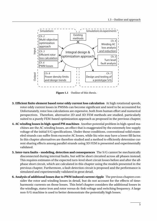
Figure 1.1 schematically shows the steps (chapters) that are taken to address the objectives. Inmore detail, they are:
2. Machine selection and design with automated optimization To design a machine that satis-factorily meets the set of conflicting starting, generating and safety requirements, a multi-objective optimization method is deemed necessary. Hence, this chapter presents anddescribes such a method. Additionally, it takes a preliminary look at the S/G design problem.
4
1.3 – Outline and approach
Simulations & experimentsSimulations
Integral design &optimization approach
Ch. 7Design and testing of
a prototype S/G
Ch. 8Power density limitsand design trends
Ch. 4Winding AC loss analysis
and reduction
Existingmethods
Ch. 3Ecient rotorloss calculation
Ch. 2Multi-objectiveoptimization approach
Ch. 5Turn level
fault analysis
Inpu
tO
utpu
t
Ch. 6PWM losses
Figure 1.1 Outline of this thesis.
3. Efficient finite element based rotor eddy current loss calculation At high rotational speeds,rotor eddy current losses in PMSMs can become significant and need to be accounted for.Unfortunately, rotor loss calculations are expensive, both from human effort and numericalperspectives. Therefore, alternative 2D and 3D FEM methods are studied, particularlysuited to a purely FEM-based optimization approach as proposed in the previous chapter.
4. AC winding losses in high-speed PM machines Another potential problem in high-speed ma-chines are the AC winding losses, an effect that is exaggerated by the extremely low supplyvoltage of the initial S/G specifications. Under those conditions, conventional solid enam-eled strands can suffer from excessive AC losses, while litz wire may have a lower fill factor.In this chapter alternatives are therefore studied and a method to efficiently determine cur-rent sharing effects among parallel strands using 3D FEM is presented and experimentallyvalidated.
5. Inter-turn faults – modeling, detection and consequences The S/G cannot be mechanicallydisconnected during internal faults, but will be short circuited across all phases instead.This requires estimates of the expected turn-level short circuit losses before and after the all-phase short circuit, which are calculated in this chapter using the models presented in theprevious chapter. Furthermore, a fault detection circuit is proposed and the performance issimulated and experimentally validated in great detail.
6. Analysis of additional losses due to PWM induced current ripple The previous chapters con-sider the rotor and winding losses in detail, but do not account for the effects of time-harmonic currents on those losses. This brief chapter considers the additional losses inthe windings, stator iron and rotor versus dc-link voltage and switching frequency. A largenon-S/G machine is used to better demonstrate the potentially high losses.
5

1. Introduction
7. Design and testing of a prototype permanent magnet starter/generator This chapter startswith an overview of existing S/G research. Then, using the optimization approach, modelsand knowledge gained in the previous chapters, the tradeoffs following from the specifica-tions are analyzed and discussed. The relation between the machine design and the basicinverter rating are also considered. A final candidate machine suitable for manufacturing isdesigned. After manufacturing, the electromagnetic performance of the machine is testedto confirm the models used in this thesis.
8. Power density limits and design trends of high-speed PMSMs The final chapter looks beyondthe S/G application and determines power density limits and trends of PMSMs, by usingthe optimization method at a large scale. This chapter can be used both as a reference whenperforming such a study, or as a reference on the limits of PMSMs and associated designtrends.
Finally, one appendix provides background information:
A. Thermal model This appendix presents the thermal model used in several of the main chap-ters.
6

CHAPTER 2
Machine selection and design with automatedoptimization
The rising demand for machines with high a technological and economical performancecalls for an automated design and optimization strategy. Due to the continuous reductionof computing costs, the possibilities in this area are continuously increasing. This chapterproposes such a method, based on particle swarm optimization combined with finite-elementbased machine analysis. After discussing the basic modeling and optimization approach, twoexamples are provided, demonstrating the basic steps applicable to any optimization problemas well as a number of involved post-processing steps.
Based on
• M. van der Geest, H. Polinder, J. A. Ferreira, and D. Zeilstra, “Optimization and com-parison of electrical machines using particle swarm optimization,” in 20th Int. Conf.Elec. Machines (ICEM), 2012, pp. 1380–1386; and
• M. van der Geest, H. Polinder, J. A. Ferreira, and D. Zeilstra, “Machine selection andinitial design of an aerospace starter/generator,” in IEEE Int. Electric Machines DrivesConf. (IEMDC), 2013, pp. 196–203.
7

2. Machine selection and design with automated optimization
2.1 Introduction
Selecting an electrical machine for a given application usually starts with choosing a certainmachine type, such as a switched reluctance machine or a PM machine, based on qualitativearguments. Due to the distinct differences between various machine types, this approach usuallysuffices. Once the machine type has been fixed, the specific machine configuration has to bechosen. Especially with PM machines many variations exist in terms of flux direction, windinglayout or magnet placement. Qualitative arguments may then no longer suffice to make a properselection and the differences need to be quantified. Furthermore, to ensure a fair comparisonbetween the various machines, each design should be optimized for the specific application athand.
Quantifying the performance of each machine variation requires models to estimate the perfor-mance. Analytical models are often used for this purpose and although these can be evaluatedvery fast, they cannot accurately or easily take into account complex geometric shapes or non-linear effects. Also, separate models may be required for different machine variations, requiringthe designer to spend precious time on creating those. Of course those disadvantages can beovercome by using FEA, shifting the required time from human to computer, but this creates otherproblems, such as a potential loss of insight and possibly very long calculation times. Nonetheless,hardware and software technologies have evolved to a point where the latter approach can beused.
The early attempts to use FEA in an electrical machine optimization process usually combinemultiple goals in a single target with a weighted sum and use a limited number of variables. In[1, 2] induction machines are optimized for a single target with a genetic algorithm (GA), whiledeterministic algorithms were used for this purpose in [3]. However, the long calculation timeslimited the use to individual machines, optimized for a single task.
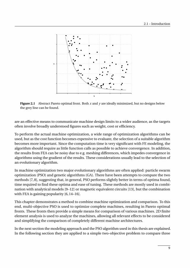
With the increase of computer speeds it became feasible to optimize entire machines, sometimesfor multiple targets. Other physical domains can also be included, such as the thermal [4] ormechanical [5] domains. The latter is especially relevant at higher rotational speeds, where thestresses in the rotor can reach the material limits or dynamic behavior prevents operation atcertain speeds. Optimizing for multiple targets is sometimes (still) achieved with a weighted sum,but this requires an a priori decision on the relative importance of all targets and thereby hidesthe trade-off between the optimization targets from the user. Several optimization trails withdiffering weights are then necessary to gain insight in the design problem. Referring to such anapproach as ‘multi-objective’ may even be considered as misleading. If instead the concept ofPareto optimality is used, the trade-off between all targets can be visualized after the optimizationand the user can make a more informed decision on the final design space for a new machine [6].Figure 2.1 shows an abstracted Pareto optimal front, which demonstrates that in the presence ofconflicting targets, no single optimal design exists. Instead, an infinite number of optimal designsexist, each with a different trade-off between the targets. For electrical machines, x and y couldfor instance be losses and mass, among many other parameters. Lastly, Pareto optimal fronts also
8
2.1 – Introduction
x
y
Figure 2.1 Abstract Pareto optimal front. Both x and y are ideally minimized, but no designs belowthe grey line can be found.
are an effective means to communicate machine design limits to a wider audience, as the targetsoften involve broadly understood figures such as weight, cost or efficiency.
To perform the actual machine optimization, a wide range of optimization algorithms can beused, but as the cost function becomes expensive to evaluate, the selection of a suitable algorithmbecomes more important. Since the computation time is very significant with FE modeling, thealgorithm should require as little function calls as possible to achieve convergence. In addition,the results from FEA can be noisy due to e.g. meshing differences, which impedes convergence inalgorithms using the gradient of the results. These considerations usually lead to the selection ofan evolutionary algorithm.
In machine optimization two major evolutionary algorithms are often applied: particle swarmoptimization (PSO) and genetic algorithms (GA). There have been attempts to compare the twomethods [7, 8], suggesting that, in general, PSO performs slightly better in terms of optima found,time required to find these optima and ease of tuning. These methods are mostly used in combi-nation with analytical models [9–12] or magnetic equivalent circuits [13], but the combinationwith FEA is gaining popularity [6, 14–16].
This chapter demonstrates a method to combine machine optimization and comparison. To thisend, multi-objective PSO is used to optimize complete machines, resulting in Pareto optimalfronts. These fronts then provide a simple means for comparison of various machines. 2D finiteelement analysis is used to analyze the machines, allowing all relevant effects to be consideredand simplifying the comparison of completely different machine architectures.
In the next section the modeling approach and the PSO algorithm used in this thesis are explained.In the following section they are applied to a simple two-objective problem to compare three
9

2. Machine selection and design with automated optimization
PM machines and introduce the concept to the reader, while the fourth section presents a moreinvolved example with four objectives.
2.2 Optimization and modeling strategy
Any engineering related optimization approach consists of two parts: models to describe theproblem and an algorithm to perform the actual optimization. The models used here are all basedon 2D FE computations, which allows a simple comparison of completely different machineswithout the need for separate analytical models. Nonlinearity can also be taken into account,which is essential to obtain realistic results. The optimization algorithm used here is PSO. Thisalgorithm was selected because it is gradient free, simple to implement and tune, and potentiallyrequires very few function calls [7, 8].
2.2.1 Machine analysis
The numerical machine analysis is performed by a combination of MATLAB to create and postpro-cess the FE models and COMSOL Multiphysics to solve the FE models. To save time a minimumnumber of preferably static simulations is executed and the machine characteristics are obtainedby postprocessing the results. The analysis of a single machine consists of the following baselinesteps:
• Compute the linked flux shape, magnitude and offset position. Four static simulationsprovide the linked flux at 24 points in time due to symmetry between the phases [17],allowing the back-emf to be computed up to the 12th harmonic. The phase order is alsodetermined in this step. To obtain the linked flux from the 2D FE model, the averagemagnetic vector potential tangential to the winding path is used:
λdom = 1
Adom
ÏAz dA (2.1)
where λdom is the flux linked with a given domain, Adom the area of that domain and Az thez-component of the magnetic vector potential.
• Compute the inductances. The computation is based on a change in linked flux due to anapplied current:
L = λI −λ0
I(2.2)
where λI and λ0 are the linked flux with and without current I , respectively. This allowssaturation due to the magnets to be taken into account. If necessary, more involved induc-tance definitions could be used, such as a current dependent inductance or dq inductances(versus current if necessary).
10

2.2 – Optimization and modeling strategy
• Iteratively determine the phase current needed to obtain the desired torque and thencompute that torque including the torque ripple, using a filtered Maxwell stress tensormethod [18]. This method offers a better accuracy for a given mesh size than a directapplication of the Maxwell stress tensor in COMSOL, saving computational time.
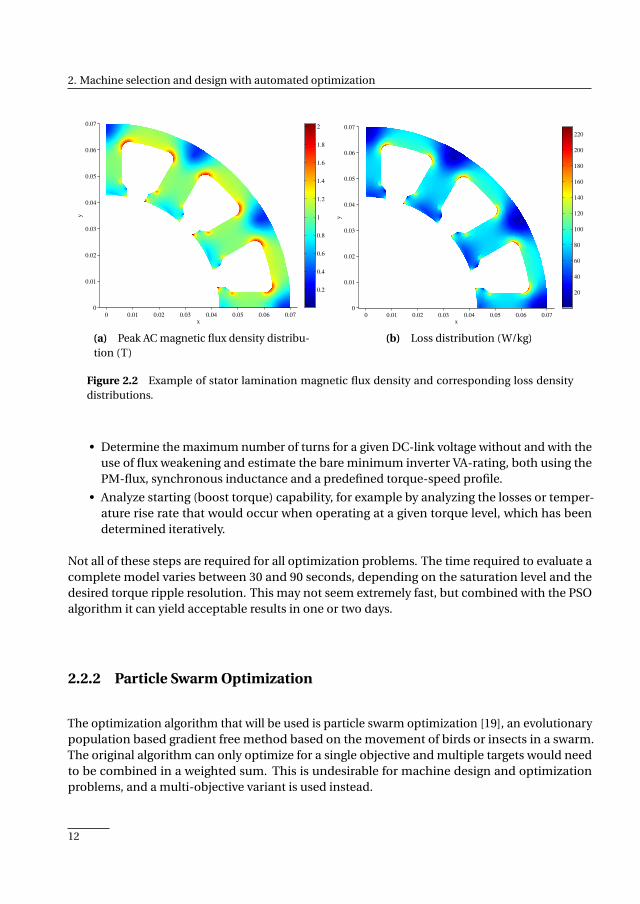
• Compute the mass (of the stack and end-windings), copper losses (in the stack and end-windigs) and iron losses. The iron losses are computed by using manufacturer data toobtain an equation for the specific loss density of the form
P = kh f αBβ+ke f 2B 2 (2.3)
where P is the specific power density, f the frequency and B the peak flux density; and kh ,α,β and ke are material dependent constants. With this equation, the loss density distributionis computed from the AC flux density distribution throughout the entire stator, therebycorrectly taking local high flux densities into account. An example of such a distribution isshown in Figure 2.2.
• Compute the rotor eddy current losses. The induced currents are computed with
Jz,i nd =σd Az
d t. (2.4)
It is assumed that the magnet pieces are electrically insulated from each other. In 2D models,this implies that within each magnet piece, the total z-current must be zero (otherwise, anaxial electric field would build up inside the magnet). This is specifically enforced in themodels by subtracting the average induced current density from the locally induced currentdensity for each individual magnet piece:
Jz =σd Az
d t−
Ïmagnet
σd Az
d tdA. (2.5)
To compute d Az /d t a transient (‘time-stepping’) simulation is necessarily used if interac-tion between the eddy currents and the inducing stator field (i.e. shielding) can occur. Suchsimulations are expensive, particularly with heavily saturated iron parts, and a modifiedFEA-based method is used; see Chapter 3 for more details. If the eddy currents are known tobe purely resistance limited over the entire design space, d Az /d t may simply be obtainedfrom the static solutions used to compute the torque. Lastly, if laminations are present inthe rotor, the lamination losses are computed as for the stator.
Additional problem dependent steps may also be taken, including:
• Compute the static or transient machine temperatures. See appendix A for details.
• Determine the worst case magnet operating point to estimate the risk of demagnetization.
• Compute the steady state short circuit performance (particularly the rotor losses) using atransient simulation with linear material properties. The short circuit repels the flux fromthe stator, warranting the use of linear material properties.
11
2. Machine selection and design with automated optimization
x
y
0 0.01 0.02 0.03 0.04 0.05 0.06 0.070
0.01
0.02
0.03
0.04
0.05
0.06
0.07
0.2
0.4
0.6
0.8
1
1.2
1.4
1.6
1.8
2
(a) Peak AC magnetic flux density distribu-tion (T)
x
y
0 0.01 0.02 0.03 0.04 0.05 0.06 0.070
0.01
0.02
0.03
0.04
0.05
0.06
0.07
20
40
60
80
100
120
140
160
180
200
220
(b) Loss distribution (W/kg)
Figure 2.2 Example of stator lamination magnetic flux density and corresponding loss densitydistributions.
• Determine the maximum number of turns for a given DC-link voltage without and with theuse of flux weakening and estimate the bare minimum inverter VA-rating, both using thePM-flux, synchronous inductance and a predefined torque-speed profile.
• Analyze starting (boost torque) capability, for example by analyzing the losses or temper-ature rise rate that would occur when operating at a given torque level, which has beendetermined iteratively.
Not all of these steps are required for all optimization problems. The time required to evaluate acomplete model varies between 30 and 90 seconds, depending on the saturation level and thedesired torque ripple resolution. This may not seem extremely fast, but combined with the PSOalgorithm it can yield acceptable results in one or two days.
2.2.2 Particle Swarm Optimization
The optimization algorithm that will be used is particle swarm optimization [19], an evolutionarypopulation based gradient free method based on the movement of birds or insects in a swarm.The original algorithm can only optimize for a single objective and multiple targets would needto be combined in a weighted sum. This is undesirable for machine design and optimizationproblems, and a multi-objective variant is used instead.
12

2.2 – Optimization and modeling strategy
Single-objective PSO
The following equations define the basic algorithm:
vn = mvn−1 + c1r1(xpbest −xn−1)+ c2r2(xg best −xn−1) (2.6)
xn = xn−1 +vn , (2.7)
where v and x are vectors holding the velocity and position for a given particle, n is the iterationstep, m, c1 and c2 are weights and r1 and r2 are vectors with random numbers on [0,1]. The lengthof all vectors equals the number of variables. The vectors xpbest and xg best hold the vectors of thepersonal and global best positions in the search space known so far, for respectively each particleand the entire swarm, and should be updated after every iteration if better results are obtained.All values are initialized randomly.
In words, the equations resemble the movement of particles (originally fish, bees, birds, etc.searching for food) through a higher dimensional problem space. The direction each membermoves in depends on three factors, each with its own scaling parameter:
• their current velocity combined with a mass; mvn−1,
• a tendency to move to their own known best position; c1r1(xpbest −xn−1),
• a tendency to move to the best position known to the group; c2r2(xg best −xn−1).
Particles with a high m(-ass) and low c1,2 show highly explorative behavior, while the oppositeproperties may lead to an early convergence. These three parameters are the main tuning pa-rameters of the algorithm. Lastly, the number of particles has to be chosen. Fortunately, theperformance does not depend strongly on this [8] and in most optimizations in this thesis, 20–30particles are used.
Multi-objective PSO
The specific algorithm used here is modified to work with multiple targets simultaneously [7],which allows the Pareto optimal fronts to be computed. This is accomplished by storing all Paretooptimal solutions in a repository and picking the global best target randomly from this repository.The personal best of each particle is updated if a Pareto optimal design is found. If both thecurrent and new designs are Pareto-optimal, the new design gets accepted with 50% possibility.After performing different optimization runs, the results can be compared by simply comparingthe repositories. The major downside of this approach compared to single-objective optimizationis that a larger part of the optimization space is considered so that more time is required to obtainthe optimal designs. However, the ability to obtain a Pareto optimal front is deemed to outweighthe increased optimization time.
Certain parts of the solution space, such as extremely inefficient or heavy designs, will not beof interest. To prevent unnecessary exploration of these regions, the global target is confined tointeresting parts of the solution space. Note that all results from particles that were successfully
13
2. Machine selection and design with automated optimization
evaluated and are Pareto optimal are kept in the repository, since they possibly yield insight intothe design problem. Further note that selecting a too narrow solution space for the global besttarget will reduce the true multi-objective nature of the optimization. For such local searches,alternative algorithms may offer better performance.
Handling boundary conditions
The original PSO formulation does not constrain the optimization variables. However, in mostengineering applications there are restrictions on practically all parameters, and it becomesnecessary to limit the search space. In addition, certain combinations of parameters, whereeach parameter individually is within the outer search boundaries, can still lead to geometricallyinfeasible designs (e.g. negative lengths, disappearing slots) that cannot be evaluated, furtherreducing the search space. Hence, an approach to keep particles inside the allowed and feasibleparts of the search space is therefore required.
In many optimization strategies, constraints are implemented through a penalty on the functionoutput if the function input is outside the feasible search space. Since this still requires thecost function to be evaluated, it cannot be used with FE based machine optimization. Anotherapproach is to place particles that would fall outside the search space, back on the border of thesearch space. Several variations of this approach have been proposed, such as speed reduction,variable clipping or reflecting [15, 20].
For inner infeasible regions those boundary handling methods become more complex, becauseoften multiple approaches exist to move a particle back in the feasible region. For example, ifthe outer radius is fixed and all radial thicknesses are variable, the shaft inner diameter couldbecome negative. This can be resolved by modifying any of the parameters, or a combination ofthem, which requires a complex decision strategy. To avoid this, an approach is used where thevelocity of particles that would drift into an inner infeasible part of the search space is reduceduntil they become feasible again. Practise shows that this allows particles to get sufficiently closeto the boundaries of the search space.
It should be noted though that the number and size of inner infeasible regions should and canbe avoided by a proper specification of the geometry, because this generally allows a fasterconvergence [16]. For example, it is better to specify the relative than the absolute magnet span,because the latter, combined with the rotor radius, excludes a part of the search space.
2.2.3 Additional remarks
This section discusses a few additional practical aspects related to performing multi-objectivemachine optimization.
When creating a model to be used within an optimization approach, a balance needs to befound between accuracy, execution speed, ease of creation, and level of detail. Doing so requires
14
2.3 – Optimization example 1
a clear picture of the total problem, so that one can determine the amount of modeling andcalculation time spent on a given aspect. Unfortunately, the required insights are often notavailable at the start of a new research project, and can only be obtained through several iterationsof optimization and postprocessing. Hence, it is important to not consider the optimization andmodeling approach as a static object.
Next, it is recommended to always include ‘sensibility checks’ in machine analysis code whereeasily possible and stop when such an error is encountered. This includes for instance checkingthe input to a model against the assumptions used in that model; checking the convergence of anyiterative solver; or checking for nonsensical values such as negative losses or unbalanced currents.To further find setup or user errors in an early stage of e.g. an optimization, it is important todisplay intermediate results, such as average torque, various losses, current density or inductance,during the analysis of a model. This allows an analysis or optimization run to be stopped andcorrected to prevent a waste of time. In other words, an optimization process that only shows‘running. . . ’ for three days, is poor practice.
The results of numerically expensive calculations and any derived values should be stored, evenif they are not directly used in the optimization targets. After an optimization, those results canreveal related design trends (see also Chapter 8); they may be used to correct for errors foundafter the optimization is executed; or they can help in the selection of final candidate machines,where differences in secondary variables can be a deciding factor when all primary performancetargets are met.
2.3 Optimization example 1
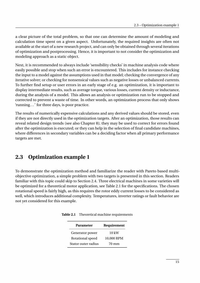
To demonstrate the optimization method and familiarize the reader with Pareto based multi-objective optimization, a simple problem with two targets is presented in this section. Readersfamiliar with this topic could skip to Section 2.4. Three electrical machines in some varieties willbe optimized for a theoretical motor application, see Table 2.1 for the specifications. The chosenrotational speed is fairly high, as this requires the rotor eddy current losses to be considered aswell, which introduces additional complexity. Temperatures, inverter ratings or fault behavior arenot yet considered for this example.
Table 2.1 Theoretical machine requirements
Parameter Requirement
Generator power 10 kW
Rotational speed 10,000 RPM
Stator outer radius 70 mm
15

2. Machine selection and design with automated optimization
(a) (b) (c)
Figure 2.3 Three machine types: (a) Surface mounted magnets with retaining sleeve; (b) Buried(interior) magnets; (c) Flux switching machine.
2.3.1 The PM machines considered
Three interior rotor PM machines will be considered, some in slightly different combinations.These are:
• Surface mounted magnet machine (SPM, Figure 2.3(a)) with an Inconel retaining sleeve,
• Buried magnet machine (IPM, Figure 2.3(b)),
• Flux switching machine (FSM, Figure 2.3(c)) with:
. 12 slots, 10 rotor teeth and
. 12 slots, 14 rotor teeth.
Exploratory studies have been performed for the SPM machine on appropriate slot/pole com-binations, leading to the selection of a 15 slot, 10 pole concentrated non-overlapping windinglayout (one coil per tooth). This specific combination has the benefits of tooth-coil windings(short end-windings, easy manufacturing, potentially high fill factor), but, compared to othernon-overlapping winding layouts, a fairly clean space harmonic spectrum and therefore lowrotor losses, an important design aspect in higher speed machines. For this reason a machinewith an Inconel retaining sleeve was considered. Note that, compared to the often used 12/10combination, the 15/10 combination has a slightly lower winding factor and a potentially highertorque ripple [21].
The IPM machine is often quoted for its robustness, because the magnets are both mechanicallyand magnetically protected by the laminations containing them. Compared to SPM machines,IPM machines are better suited for flux-weakening operation due to the reluctance torque theyexhibit [22] and the tendency for higher per-unit inductances. For the IPM a 15/10 slot/polecombination will be optimized too. Note that to fully exploit the reluctance torque, a distributedwinding should be used, but for the sake of comparison, only tooth-coil winding layouts are used.
16
2.3 – Optimization example 1
Flux switching machines received a lot of attention in the past ten years and they are beingconsidered for many applications [23]. They have a robust rotor suitable for high-speed operation,and compared with regular rotor-mounted PM machines they possess a potentially higher powerdensity [24, 25]. A very common stator/rotor teeth combination is 12/10, which for three phasewinding schemes is the layout with the minimum number of teeth that still provides a balancedforce and back-emf [26]. Note that in FSMs every rotor tooth resembles a pole pair to the stator,so that the electrical frequency in the stator of a 1210 FSM is twice that of a 1210 SPM, potentiallyleading to increased iron losses.
2.3.2 Optimization targets, assumptions and search space
The machines will be compared in terms of efficiency and weight. These objectives apply to manyapplications and by using only two Pareto targets the fronts can be presented as 2D plots, whichaids comprehensibility when printed.
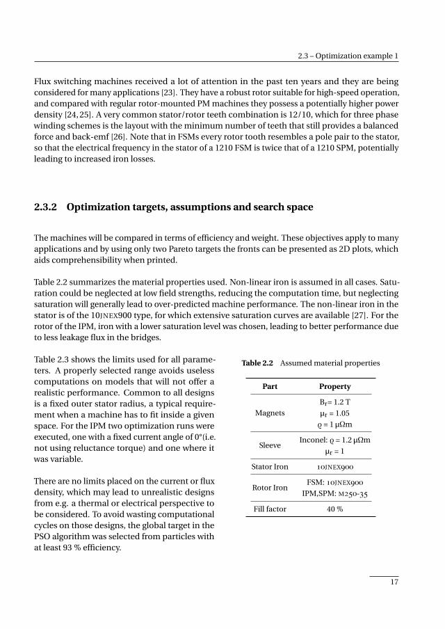
Table 2.2 summarizes the material properties used. Non-linear iron is assumed in all cases. Satu-ration could be neglected at low field strengths, reducing the computation time, but neglectingsaturation will generally lead to over-predicted machine performance. The non-linear iron in thestator is of the 10JNEX900 type, for which extensive saturation curves are available [27]. For therotor of the IPM, iron with a lower saturation level was chosen, leading to better performance dueto less leakage flux in the bridges.
Table 2.2 Assumed material properties
Part Property
Magnets
Br= 1.2 T
µr = 1.05
ρ = 1 µΩm
SleeveInconel: ρ = 1.2 µΩm
µr = 1
Stator Iron 10JNEX900
Rotor IronFSM: 10JNEX900
IPM,SPM: M250-35
Fill factor 40 %
Table 2.3 shows the limits used for all parame-ters. A properly selected range avoids uselesscomputations on models that will not offer arealistic performance. Common to all designsis a fixed outer stator radius, a typical require-ment when a machine has to fit inside a givenspace. For the IPM two optimization runs wereexecuted, one with a fixed current angle of 0°(i.e.not using reluctance torque) and one where itwas variable.
There are no limits placed on the current or fluxdensity, which may lead to unrealistic designsfrom e.g. a thermal or electrical perspective tobe considered. To avoid wasting computationalcycles on those designs, the global target in thePSO algorithm was selected from particles withat least 93 % efficiency.
17
2. Machine selection and design with automated optimization
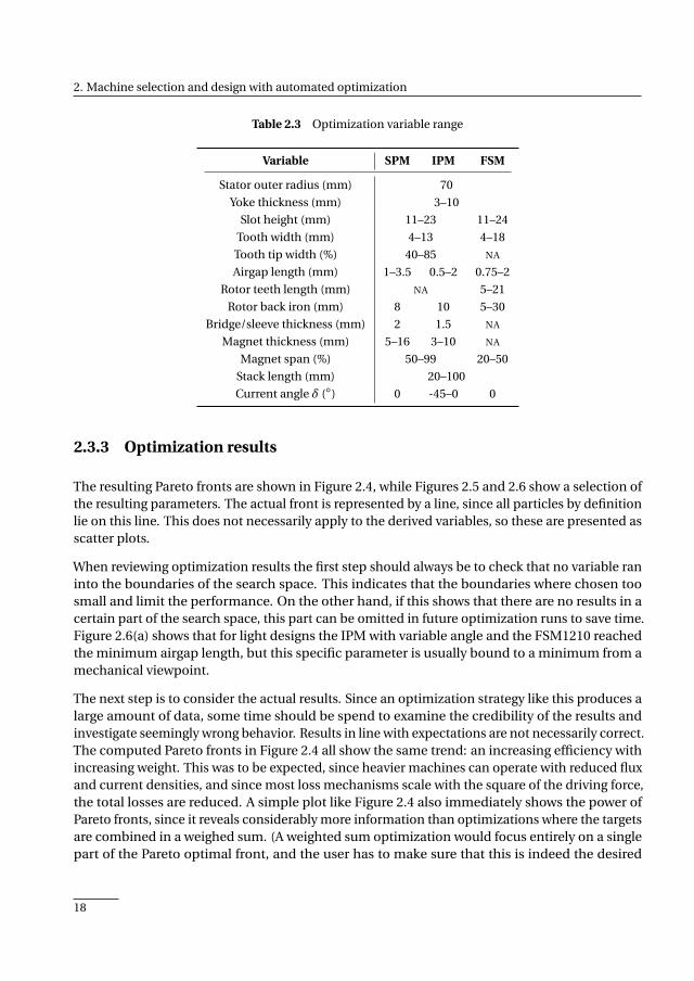
Table 2.3 Optimization variable range
Variable SPM IPM FSM
Stator outer radius (mm) 70
Yoke thickness (mm) 3–10
Slot height (mm) 11–23 11–24
Tooth width (mm) 4–13 4–18
Tooth tip width (%) 40–85 NA
Airgap length (mm) 1–3.5 0.5–2 0.75–2
Rotor teeth length (mm) NA 5–21
Rotor back iron (mm) 8 10 5–30
Bridge/sleeve thickness (mm) 2 1.5 NA
Magnet thickness (mm) 5–16 3–10 NA
Magnet span (%) 50–99 20–50
Stack length (mm) 20–100
Current angle δ () 0 -45–0 0
2.3.3 Optimization results
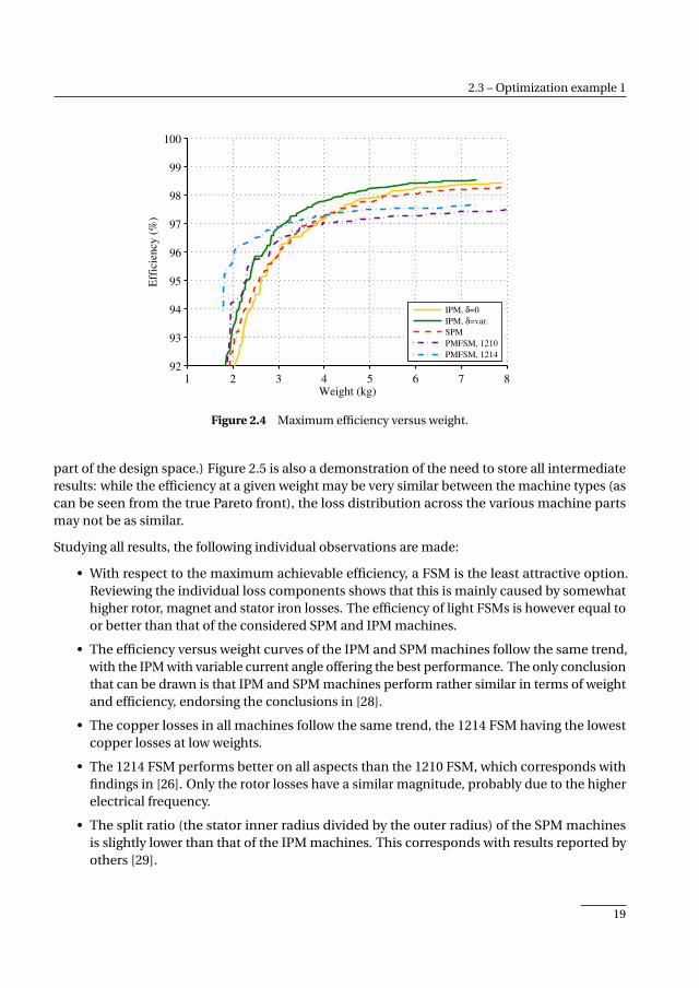
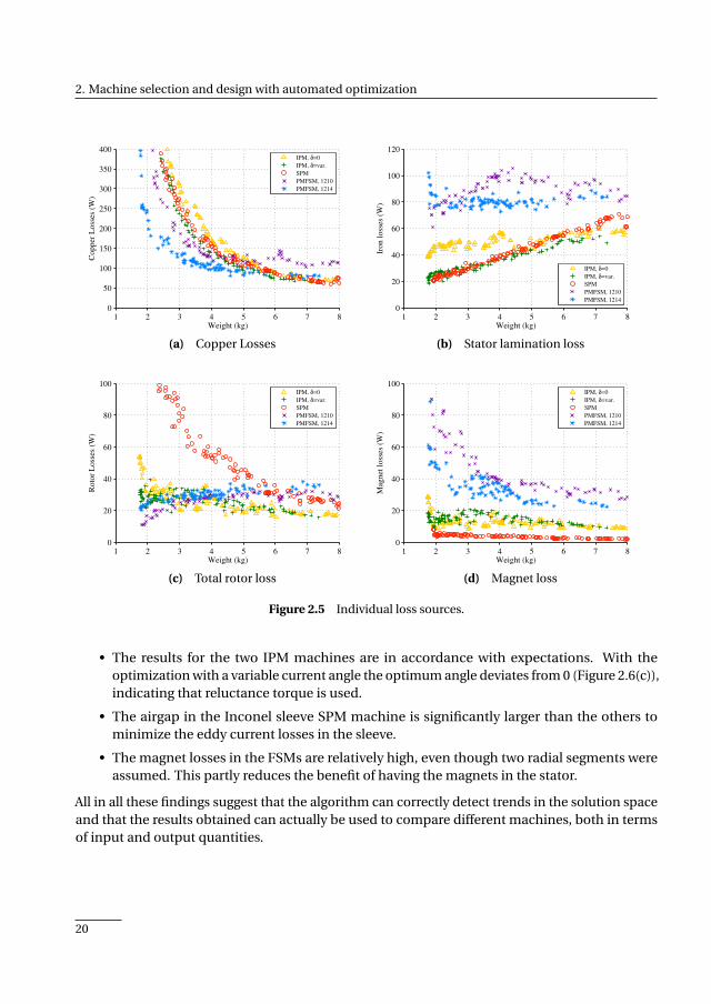
The resulting Pareto fronts are shown in Figure 2.4, while Figures 2.5 and 2.6 show a selection ofthe resulting parameters. The actual front is represented by a line, since all particles by definitionlie on this line. This does not necessarily apply to the derived variables, so these are presented asscatter plots.
When reviewing optimization results the first step should always be to check that no variable raninto the boundaries of the search space. This indicates that the boundaries where chosen toosmall and limit the performance. On the other hand, if this shows that there are no results in acertain part of the search space, this part can be omitted in future optimization runs to save time.Figure 2.6(a) shows that for light designs the IPM with variable angle and the FSM1210 reachedthe minimum airgap length, but this specific parameter is usually bound to a minimum from amechanical viewpoint.
The next step is to consider the actual results. Since an optimization strategy like this produces alarge amount of data, some time should be spend to examine the credibility of the results andinvestigate seemingly wrong behavior. Results in line with expectations are not necessarily correct.The computed Pareto fronts in Figure 2.4 all show the same trend: an increasing efficiency withincreasing weight. This was to be expected, since heavier machines can operate with reduced fluxand current densities, and since most loss mechanisms scale with the square of the driving force,the total losses are reduced. A simple plot like Figure 2.4 also immediately shows the power ofPareto fronts, since it reveals considerably more information than optimizations where the targetsare combined in a weighed sum. (A weighted sum optimization would focus entirely on a singlepart of the Pareto optimal front, and the user has to make sure that this is indeed the desired
18
2.3 – Optimization example 1
1 2 3 4 5 6 7 892
93
94
95
96
97
98
99
100
Weight (kg)
Eff
icie
ncy
(%
)
IPM, δ=0
IPM, δ=var.
SPM
PMFSM, 1210
PMFSM, 1214
Figure 2.4 Maximum efficiency versus weight.
part of the design space.) Figure 2.5 is also a demonstration of the need to store all intermediateresults: while the efficiency at a given weight may be very similar between the machine types (ascan be seen from the true Pareto front), the loss distribution across the various machine partsmay not be as similar.
Studying all results, the following individual observations are made:
• With respect to the maximum achievable efficiency, a FSM is the least attractive option.Reviewing the individual loss components shows that this is mainly caused by somewhathigher rotor, magnet and stator iron losses. The efficiency of light FSMs is however equal toor better than that of the considered SPM and IPM machines.
• The efficiency versus weight curves of the IPM and SPM machines follow the same trend,with the IPM with variable current angle offering the best performance. The only conclusionthat can be drawn is that IPM and SPM machines perform rather similar in terms of weightand efficiency, endorsing the conclusions in [28].
• The copper losses in all machines follow the same trend, the 1214 FSM having the lowestcopper losses at low weights.
• The 1214 FSM performs better on all aspects than the 1210 FSM, which corresponds withfindings in [26]. Only the rotor losses have a similar magnitude, probably due to the higherelectrical frequency.
• The split ratio (the stator inner radius divided by the outer radius) of the SPM machinesis slightly lower than that of the IPM machines. This corresponds with results reported byothers [29].
19
2. Machine selection and design with automated optimization
1 2 3 4 5 6 7 80
50
100
150
200
250
300
350
400
Weight (kg)
Co
pp
er L
oss
es (
W)
IPM, δ=0
IPM, δ=var.
SPM
PMFSM, 1210
PMFSM, 1214
(a) Copper Losses
1 2 3 4 5 6 7 80
20
40
60
80
100
120
Weight (kg)
Iro
n l
oss
es (
W)
IPM, δ=0
IPM, δ=var.
SPM
PMFSM, 1210
PMFSM, 1214
(b) Stator lamination loss
1 2 3 4 5 6 7 80
20
40
60
80
100
Weight (kg)
Ro
tor
Lo
sses
(W
)
IPM, δ=0
IPM, δ=var.
SPM
PMFSM, 1210
PMFSM, 1214
(c) Total rotor loss
1 2 3 4 5 6 7 80
20
40
60
80
100
Weight (kg)
Mag
net
lo
sses
(W
)
IPM, δ=0
IPM, δ=var.
SPM
PMFSM, 1210
PMFSM, 1214
(d) Magnet loss
Figure 2.5 Individual loss sources.
• The results for the two IPM machines are in accordance with expectations. With theoptimization with a variable current angle the optimum angle deviates from 0 (Figure 2.6(c)),indicating that reluctance torque is used.
• The airgap in the Inconel sleeve SPM machine is significantly larger than the others tominimize the eddy current losses in the sleeve.
• The magnet losses in the FSMs are relatively high, even though two radial segments wereassumed. This partly reduces the benefit of having the magnets in the stator.
All in all these findings suggest that the algorithm can correctly detect trends in the solution spaceand that the results obtained can actually be used to compare different machines, both in termsof input and output quantities.
20
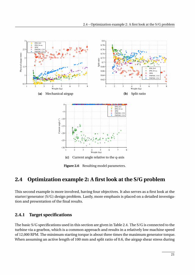
2.4 – Optimization example 2: A first look at the S/G problem
1 2 3 4 5 6 7 80.5
1
1.5
2
2.5
3
Weight (kg)
Ph
ysi
cal
airg
ap (
mm
)
IPM, δ=0
IPM, δ=var.
SPM
PMFSM, 1210
PMFSM, 1214
(a) Mechanical airgap
1 2 3 4 5 6 7 8
0.62
0.64
0.66
0.68
0.7
0.72
0.74
0.76
0.78
0.8
Weight (kg)
Sp
lit
rati
o
IPM, δ=0
IPM, δ=var.
SPM
PMFSM, 1210
PMFSM, 1214
(b) Split ratio
1 2 3 4 5 6 7 8−30
−25
−20
−15
−10
−5
0
Weight (kg)
Cu
rren
t an
gle
(°)
IPM, δ=0
IPM, δ=var.
SPM
PMFSM, 1210
PMFSM, 1214
(c) Current angle relative to the q-axis
Figure 2.6 Resulting model parameters.
2.4 Optimization example 2: A first look at the S/G problem
This second example is more involved, having four objectives. It also serves as a first look at thestarter/generator (S/G) design problem. Lastly, more emphasis is placed on a detailed investiga-tion and presentation of the final results.
2.4.1 Target specifications
The basic S/G specifications used in this section are given in Table 2.4. The S/G is connected to theturbine via a gearbox, which is a common approach and results in a relatively low machine speedof 12,000 RPM. The minimum starting torque is about three times the maximum generator torque.When assuming an active length of 100 mm and split ratio of 0.6, the airgap shear stress during
21
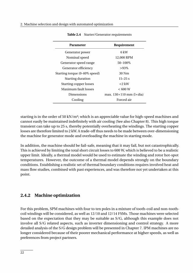
2. Machine selection and design with automated optimization
Table 2.4 Starter/Generator requirements
Parameter Requirement
Generator power 6 kW
Nominal speed 12,000 RPM
Generator speed range 50–100%
Generator efficiency >93%
Starting torque (0-40% speed) 30 Nm
Starting duration 15–25 s
Starting copper losses <2 kW
Maximum fault losses < 600 W
Dimensions max. 130×110 mm (l×dia)
Cooling Forced air
starting is in the order of 50 kN/m²; which is an appreciable value for high-speed machines andcannot easily be maintained indefinitely with air cooling (See also Chapter 8). This high torquetransient can take up to 25 s, thereby potentially overheating the windings. The starting copperlosses are therefore limited to 2 kW. A trade-off thus needs to be made between over-dimensioningthe machine for generator mode and overloading the machine in starting mode.
In addition, the machine should be fail-safe, meaning that it may fail, but not catastrophically.This is achieved by limiting the total short circuit losses to 600 W, which is believed to be a realisticupper limit. Ideally, a thermal model would be used to estimate the winding and rotor hot-spottemperatures. However, the outcome of a thermal model depends strongly on the boundaryconditions. Establishing a realistic set of thermal boundary conditions requires involved heat andmass flow studies, combined with past experiences, and was therefore not yet undertaken at thispoint.
2.4.2 Machine optimization
For this problem, SPM machines with four to ten poles in a mixture of tooth-coil and non-tooth-coil windings will be considered, as well as 12/10 and 12/14 FSMs. Those machines were selectedbased on the expectation that they may be suitable as S/G, although this example does notinvolve all S/G related aspects, such as inverter dimensioning and control strategy. A moredetailed analysis of the S/G design problem will be presented in Chapter 7. IPM machines are nolonger considered because of their poorer mechanical performance at higher speeds, as well aspreferences from project partners.
22

2.4 – Optimization example 2: A first look at the S/G problem
wt
wm
hag
tsy
hs
tm
wsh
(a)
tri
wt
hs
wm
hag
lrt
wrt
tsy
(b)
Figure 2.7 Optimization variables for the SPM (a) and FSM.
Description of the optimization approach
The analysis of each machine follows the same approach as the first example, but with theaddition of calculating the rotor, copper and iron losses during a three phase short circuit, aswell as the copper losses during starting. The iron and rotor losses are neglected during starting,both because they are expected to be low compared to the copper losses and their calculation isnumerically expensive.
Optimization settings
Figure 2.7 shows the machine geometries to be optimized, with all variables indicated. The rangeof the variables was wide enough to allow the PSO algorithm to consider any design that wouldnot lead to a degenerated (infeasible) geometry.
Four optimization objectives are used:
• Maximize generator mode efficiency
• Minimize mass
• Minimize 3 phase short circuit lossesThis objective ensures that the optimization progresses towards designs with acceptablefault losses. In case of a single phase short circuit, a three phase short circuit is applied bythe inverter to reduce the losses in the faulted phase due to the mutual coupling.
• Minimize copper losses during startingDuring starting, the frequency is still low and the copper losses are the main cause of losses.Minimizing these will prevent heat-up of the machine as well as limit the additional powerto be supplied by the inverter and source.
23
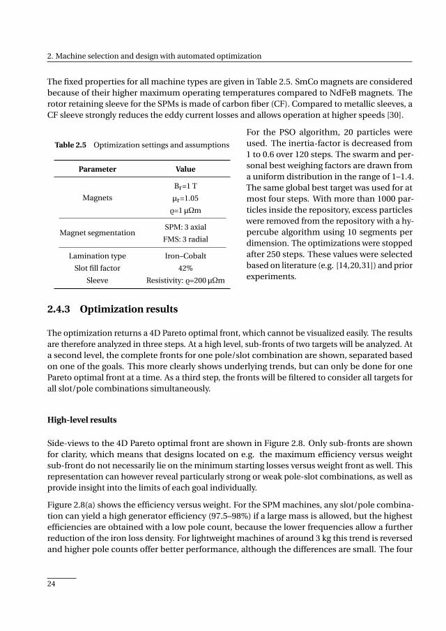
2. Machine selection and design with automated optimization
The fixed properties for all machine types are given in Table 2.5. SmCo magnets are consideredbecause of their higher maximum operating temperatures compared to NdFeB magnets. Therotor retaining sleeve for the SPMs is made of carbon fiber (CF). Compared to metallic sleeves, aCF sleeve strongly reduces the eddy current losses and allows operation at higher speeds [30].
Table 2.5 Optimization settings and assumptions
Parameter Value
Magnets
Br=1 T
µr=1.05
ρ=1 µΩm
Magnet segmentationSPM: 3 axial
FMS: 3 radial
Lamination type Iron–Cobalt
Slot fill factor 42%
Sleeve Resistivity: ρ=200 µΩm
For the PSO algorithm, 20 particles wereused. The inertia-factor is decreased from1 to 0.6 over 120 steps. The swarm and per-sonal best weighing factors are drawn froma uniform distribution in the range of 1–1.4.The same global best target was used for atmost four steps. With more than 1000 par-ticles inside the repository, excess particleswere removed from the repository with a hy-percube algorithm using 10 segments perdimension. The optimizations were stoppedafter 250 steps. These values were selectedbased on literature (e.g. [14,20,31]) and priorexperiments.
2.4.3 Optimization results
The optimization returns a 4D Pareto optimal front, which cannot be visualized easily. The resultsare therefore analyzed in three steps. At a high level, sub-fronts of two targets will be analyzed. Ata second level, the complete fronts for one pole/slot combination are shown, separated basedon one of the goals. This more clearly shows underlying trends, but can only be done for onePareto optimal front at a time. As a third step, the fronts will be filtered to consider all targets forall slot/pole combinations simultaneously.
High-level results
Side-views to the 4D Pareto optimal front are shown in Figure 2.8. Only sub-fronts are shownfor clarity, which means that designs located on e.g. the maximum efficiency versus weightsub-front do not necessarily lie on the minimum starting losses versus weight front as well. Thisrepresentation can however reveal particularly strong or weak pole-slot combinations, as well asprovide insight into the limits of each goal individually.
Figure 2.8(a) shows the efficiency versus weight. For the SPM machines, any slot/pole combina-tion can yield a high generator efficiency (97.5–98%) if a large mass is allowed, but the highestefficiencies are obtained with a low pole count, because the lower frequencies allow a furtherreduction of the iron loss density. For lightweight machines of around 3 kg this trend is reversedand higher pole counts offer better performance, although the differences are small. The four
24
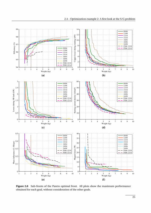
2.4 – Optimization example 2: A first look at the S/G problem
1 2 3 4 5 6 7 8 9 1094
95
96
97
98
99
Weight (kg)
Eff
icie
ncy
(%
)
09/06
12/08
12/10
15/10
18/04
18/06
24/08
FSM 12/10
FSM 12/14
(a)
1 2 3 4 5 6 7 8 9 100
2
4
6
8
10
12
14
Weight (kg)
Copper
loss
es d
uri
ng s
tart
ing (
kW
)
09/06
12/08
12/10
15/10
18/04
18/06
24/08
FSM 12/10
FSM 12/14
(b)
1 2 3 4 5 6 7 8 9 100
0.5
1
1.5
2
2.5
3
Weight (kg)
Loss
es d
uri
ng 3
Φ f
ault
(kW
)
09/06
12/08
12/10
15/10
18/04
18/06
24/08
FSM 12/10
FSM 12/14
(c)
1 2 3 4 5 6 7 8 9 100
10
20
30
40
50
60
Weight (kg)
Sta
rtin
g c
urr
ent
den
sity
(A
/mm
²)
09/06
12/08
12/10
15/10
18/04
18/06
24/08
FSM 12/10
FSM 12/14
(d)
1 2 3 4 5 6 7 8 9 100
0.1
0.2
0.3
0.4
0.5
Weight (kg)
Phas
e in
duct
ance
(L
−M
)(pu)
09/06
12/08
12/10
15/10
18/04
18/06
24/08
FSM 12/10
FSM 12/14
(e)
1 2 3 4 5 6 7 8 9 100
5
10
15
20
25
30
35
40
Weight (kg)
Mag
net
loss
es (
W)
09/06
12/08
12/10
15/10
18/04
18/06
24/08
FSM 12/10
FSM 12/14
(f )
Figure 2.8 Sub-fronts of the Pareto optimal front. All plots show the maximum performanceobtained for each goal, without consideration of the other goals.
25

2. Machine selection and design with automated optimization
pole distributed winding machine suffers from the heavy end-windings and is a poor choicefor lightweight machines. The same efficiency/weight arguments hold for the FSMs, only thehighest efficiency achievable is now about 96% due to the higher iron losses as result of the higherfrequency.
A high number of poles is beneficial for the starting performance of the machines, as shownin Figure 2.8(b). There is no apparent difference between distributed or concentrated windingmachines, apart from the 18/04 machine, which is again a poor choice. The FSM1214 is the lighteststarter-only machine, but from 5 kg onward the other machines offer similar performance. Whenalso considering the current density during starting (Figure 2.8(d)), an interesting observationcan be made: the FSM1214 has the lowest starting losses at low weight, but not the lowest currentdensity. This implies that the FSMs have less copper mass and that the winding will heat up moreduring starting. The current density at 3 kg is at least 30 A/mm², which will render air coolingineffective and increases the importance of thermal capacity. For machines above 5 kg the severityof this issue decreases.
Figure 2.8(e) shows the per-unit (pu) phase inductance, referred to nominal generator mode. TheFSM machines have a minimum inductance nearly twice that of the SPM machines. Moreover,the machines with q > 0.5 have somewhat lower inductances than the tooth-coil machines. Thistendency of non-tooth-coil winding machines towards lower inductances negatively affects thepossibility to limit the short circuit losses. The pu inductance links the machine design to theinverter design, since higher pu inductances require either a higher voltage rating (when usingid = 0) or current rating (when allowing flux weakening). In the latter case, the machine currentrating must also be increased.
It should be emphasized that these plots show the maximum achievable performance in oneparameter only, disregarding the performance on the other parameters. Machines that performfavorably in these plots may perform not so well when considering all parameters. This is espe-cially true for the fault losses, shown in Figure 2.8(c). Very low values, in the order of 100 W, can beobtained. These values are misleading however, as the next section will show that these designshave a very poor starting performance.
The magnet losses are shown in Figure 2.8(f). A clear separation between the concentrated anddistributed winding designs can be observed. With distributed windings, designs with almostzero magnet losses can be found, while machines with tooth-coil windings will always have somemagnet losses. This is simply the result of a richer space-harmonic content in the airgap of CWmachines. Finally, in line with the previous example, the FSM machines have higher magnetlosses than the SPM machines.
One particular front in detail
The fronts shown in Figure 2.8 are the 2D edges of the 4D front, which hides trends inside thefront. A more detailed view is obtained by plotting all particles of one front, with the particlesdivided in groups based on some parameter. This is done in Figure 2.9 for the 12/10 FSM, with
26

2.4 – Optimization example 2: A first look at the S/G problem
the individual particles marked based on starting losses. Figure 2.9(a) shows this division; thehorizontal bands are clearly visible. This same division is applied in Figures 2.9(b)–(f) as well,which immediately reveals design trends.
For example, designs with good starting performance, having starting copper losses less than500 W (green crosses), also have the highest fault losses and the lowest generator efficiency. Thatis, a good starter is a bad fail-safe generator. Also, good starter machines have the highest rotorlosses and the lowest per-unit inductance. The reasons behind this are simple: good startingperformance requires a high torque-per-current-density rating, which in turn requires highexcitation flux-densities in the machine. These are obtained with large magnet volumes and ashort airgap. This leads to high iron and rotor losses at high speed and thus a poor generatorperformance. At the same time, the high excitation flux yields a low per-unit inductance, which inturn gives large short circuit losses. This contradiction applies to all of the machines consideredhere.
Figure 2.9 further shows that there is no contradiction between efficient generator operationand fault losses. In fact, the most efficient designs generally have the lowest fault losses. Theexplanation is exactly opposite to the one given above: low fault losses require little PM flux, whichimplies small magnets and a long airgap. The low flux density then allows efficient generatoroperation, because the generator torque is small compared to the starting torque.
A low per-unit inductance improves the power factor during starting, allowing an inverter with alower current rating to be used. This means that the trade-off between starting and short circuitperformance for the machine is coupled to the inverter design. To arrive at the optimal completeS/G system, it will then be necessary to consider this interaction at an early design stage. Thisaspect will be discussed in more detail in Chapter 7.
Another observation from Figure 2.9 is that in the corners of the Pareto space, e.g. at very lowweights or with very low starting losses, the variation in secondary parameters is small. In otherwords, if obtaining the lowest possible starting losses is essential, the other parameters will befixed. This makes sense, because the extreme corners of the Pareto optimal fronts resembleregions where a single objective optimization would converge to. From an optimization algorithmperspective, finding those extremes can be challenging and it is sometimes used as a performancemeasure when comparing algorithms. However, for engineering applications those extremes arerarely relevant and it is not necessary to use an optimization algorithm that excels at finding theextremes.
In summary, adding fail-safety to a generator has little impact on the performance, while addingfail-safety to a starter machine does strongly impact the performance, because starting is consid-ered to be a transient overload condition.
27
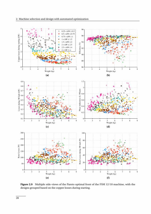
2. Machine selection and design with automated optimization
2 3 4 5 6 7 8 90
1
2
3
4
5
Weight (kg)
Co
pp
er l
oss
es d
uri
ng
sta
rtin
g (
kW
)
0.25 < kW ≤ 0.5
0.5 < kW ≤ 0.75
0.75 < kW ≤ 1
1 < kW ≤ 1.5
1.5 < kW ≤ 2
2 < kW ≤ 2.5
2.5 < kW ≤ 4
4 < kW ≤ ∞
(a)
2 3 4 5 6 7 8 986
88
90
92
94
96
98
Weight (kg)
Eff
icie
ncy
(%
)
(b)
2 3 4 5 6 7 8 90.1
0.2
0.3
0.4
0.5
0.6
0.7
0.8
0.9
Weight (kg)
Loss
es d
uri
ng 3
Φ f
ault
(kW
)
(c)
2 3 4 5 6 7 8 90
0.2
0.4
0.6
0.8
1
1.2
Weight (kg)
Ph
ase
ind
uct
ance
(L
−M
)(p
u)
(d)
2 3 4 5 6 7 8 90
50
100
150
200
250
300
Weight (kg)
Roto
r L
oss
es (
W)
(e)
2 3 4 5 6 7 8 90
20
40
60
80
100
Weight (kg)
Ro
tor
Lo
sses
du
rin
g 3
Φ f
ault
(W
)
(f )
Figure 2.9 Multiple side-views of the Pareto optimal front of the FSM 12/10 machine, with thedesigns grouped based on the copper losses during starting.
28

2.4 – Optimization example 2: A first look at the S/G problem
Table 2.6 Initial number of particles on the front, fraction of particles meeting individual criteriaand the fraction of particles meeting all criteria
TypeInitial
particles mas
s<9
kg
Pst
art<2
kW
93%<η
PSC
<600
W
Intersect
09/06 1196 98 43 96 25 2
12/08 972 98 46 99 23 5
12/10 1255 98 53 99 35 8
15/10 1366 99 51 100 18 3
18/04 1513 91 17 96 4 0
18/06 1343 96 30 99 22 0
24/08 1375 94 40 100 31 1
FSM 12/10 892 100 65 79 98 44
FSM 12/14 674 100 83 70 100 53
Considering all results
The previous section showed that a good starter machine has high fault losses and a poor generatorefficiency. In order to assess the feasibility of each slot/pole combination, all performance criteriahave to be considered simultaneously. To this end, constraints are set on the targets. The relativenumber of particles that meet all constraints is an indication of the feasibility of that specificdesign.
Table 2.6 shows the criteria that were used, the fraction of particles meeting each criterion indi-vidually and the fraction of particles meeting all criteria simultaneously. This way of representingthe results is far from perfect too, in the sense that much information is lost, but it does allow afast comparison of the individual machine types. For the FSM 12/10 machine the numbers in thetable can be directly related to Figure 2.9. For example, Figure 2.9(b) shows that there are designswith η< 93% and Table 2.6 indicates that 21% of the FSM 12/10 designs have an efficiency belowthat limit.
A few observations can be made from Table 2.6. First, both FSMs show considerably morepotential than the SPM machines, with about 50% of the front meeting all criteria. Of the SPMmachines, those with tooth-coil windings show some feasibility, while machines with distributedwindings lead to almost no feasible designs. The main reason lies in the ability to modify theper-unit inductance. With tooth-coil windings, the tooth-tips can be used to adjust the inductanceindependently from the back-emf (to some extent). Distributed windings do not offer this benefit.Since good starting performance requires a low per-unit inductance and low fault losses require a
29
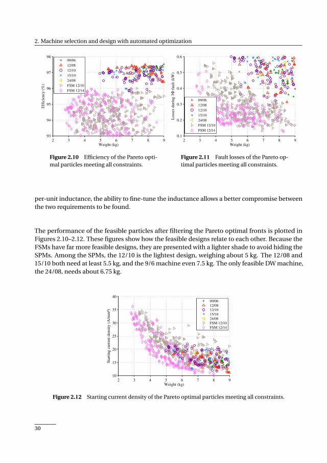
2. Machine selection and design with automated optimization
2 3 4 5 6 7 8 993
94
95
96
97
98
Weight (kg)
Eff
icie
ncy
(%
)
09/06
12/08
12/10
15/10
24/08
FSM 12/10
FSM 12/14
Figure 2.10 Efficiency of the Pareto opti-mal particles meeting all constraints.
2 3 4 5 6 7 8 90.1
0.2
0.3
0.4
0.5
0.6
Weight (kg)
Lo
sses
du
rin
g 3
Φ f
ault
(k
W)
09/06
12/08
12/10
15/10
24/08
FSM 12/10
FSM 12/14
Figure 2.11 Fault losses of the Pareto op-timal particles meeting all constraints.
per-unit inductance, the ability to fine-tune the inductance allows a better compromise betweenthe two requirements to be found.
The performance of the feasible particles after filtering the Pareto optimal fronts is plotted inFigures 2.10–2.12. These figures show how the feasible designs relate to each other. Because theFSMs have far more feasible designs, they are presented with a lighter shade to avoid hiding theSPMs. Among the SPMs, the 12/10 is the lightest design, weighing about 5 kg. The 12/08 and15/10 both need at least 5.5 kg, and the 9/6 machine even 7.5 kg. The only feasible DW machine,the 24/08, needs about 6.75 kg.
2 3 4 5 6 7 8 910
15
20
25
30
35
40
Weight (kg)
Sta
rtin
g c
urr
ent
den
sity
(A
/mm
²)
09/06
12/08
12/10
15/10
24/08
FSM 12/10
FSM 12/14
Figure 2.12 Starting current density of the Pareto optimal particles meeting all constraints.
30
2.5 – Conclusion
2.5 Conclusion
This chapter presented a method to optimize electrical machines using multi-objective particleswarm optimization combined with finite element based machine models. Using this method,greatly different machines can be optimized in an identical ( and thus fair) way, with little usereffort, and a high accuracy. The outcome of each optimization run, a Pareto optimal front, revealsimportant design trends and limits and allows different machine topologies and layouts to bequantitatively compared. A major benefit of a multi-objective optimization strategy is the insightgained in the designed problem, both at high and low levels, which makes the execution time–one to two days on standard computers– worthwhile.
Analyzing optimization results is an essential part of any optimization strategy; without it, anoptimization is not finished. This chapter described a number of possibilities to compare andpresent optimization results. The first step often consists of checking the results for obvious errorsand whether or not any variable consistently ran into any boundary. Next, to compare resultsat a global level, Pareto optimal fronts may be directly compared. Side-views to the front maybecome cluttered with more than two objectives, which can be overcome by using Pareto optimalsub-fronts, although this removes the ability to correlate different side-views. That is, it showsonly the most extreme designs possible. To study trends within a single Pareto optimal front, thefront can be divided based on a parameter of interest. Finally, as a trade-off between high levelcomparisons and a detailed per-front investigation, fronts can be filtered based designs havingdesirable properties. The fraction of designs meeting a set of criteria is a first indication of thesuitability of a given topology for the intended task.
The optimization method was demonstrated with two examples. In the first example five basicSPM, IPM and FSM machines were optimized for weight and efficiency, assuming a single oper-ating point. This demonstrated the basic correctness of the optimization method. The secondexample served as a first look at the starter/generator design problem, having two additionaltargets: starting copper losses and three phase short circuit losses. Nine FSM and SPM machinevariations were considered. Important observations are that mostly the requirements on bothlow starting and short circuit losses directly conflict; a fail-safe generator-only machine could beconstructed with little penalty. Furthermore, concentrated non-overlapping winding machines(q ≤ 0.5) allow a better fine-tuning of the phase inductance with respect to the linked magnetflux than distributed winding machines, which is essential to meet all design targets with a lowmachine weight. Lastly, FSMs offer lower copper losses than SPMs and in this respect lead tothe lightest S/G. However, they operate with higher current densities and the transient thermalbehavior may be worse. Also, they have large pu inductance values, which increases the minimuminverter VA-rating.
31


CHAPTER 3
Efficient finite element based rotor eddy current losscalculation
The rotor losses in tooth-coil winding machines cannot be neglected, particulary in high-speedmachines. At high frequencies the rotor losses may not be fully resistance limited, leading to acoupled eddy current problem. Although analytical models can solve those problems quickly,they are inflexible and problem dependent. This contradicts with the FE-based optimizationapproach, where flexibility with respect to machine types and geometries is highly desired.The losses can obviously be computed using the existing FE model of the machine, but this istime consuming, especially with saturated machine parts. Therefore, this chapter proposes analternate FE-based approach, using a transient simulation of only the rotor geometry withlinear material properties. The method is demonstrated in 2D and 3D, showing that bothwinding distribution and slotting harmonic losses can be correctly computed, even in thepresence of stator saturation or shielding effects in the rotor.
Based on
• M. van der Geest, H. Polinder, and J. A. Ferreira, “Efficient finite element based rotorloss calculation for permanent magnet synchronous machines,” in Int. Conf. ElectricalMachines (ICEM), 2014, pp. 1133–1138; and
• M. van der Geest, H. Polinder, and J. A. Ferreira, “Computationally efficient 3D FEMrotor eddy current loss calculation for permanent magnet synchronous machines,” inIEEE Int. Electric Machines Drives Conf. (IEMDC), 2015.
33

3. Efficient finite element based rotor eddy current loss calculation
3.1 Introduction
Rotor eddy current losses in permanent magnet machines can be one of the main electrical losssources, especially at high rotational speeds in combination with fractional pitch concentratednon-overlapping windings. In addition, the cooling capacity at the rotor is limited compared tothe stator. Therefore, obtaining an accurate estimation of the rotor losses and the effectivenessof any loss reduction method during the design stage of a machine is of great importance toprevent overheating of the constructed machine. Many rotor loss calculation methods have beenproposed [32], but most can be divided in three categories.
One extreme in rotor eddy current loss calculation are fully analytical methods [33–38]. Typically,the rotor geometry is simplified to a number of concentric shells or a rectilinear geometry, bound-ary conditions to account for the stator are imposed, and Maxwell’s equations are solved. Thismethod is very fast, and can account for shielding effects due to the eddy current reaction field,but fine geometric details or magnet segmentation cannot be included easily.
The other extreme in rotor loss calculation is transient finite element modeling. Any details ofinterest can be accounted for, although some, like axial magnet segmentation, require 3D models[39]. Obviously, the major penalty is the time required for these calculations.
In between those extremes are methods that combine FE and analytical aspects. The rotor lossescould for instance be computed with field distributions obtained from magnetic equivalentcircuits [40]. For increased accuracy, the rotor field distribution obtained from static FE solutionsmay be used to compute the magnet losses, under the assumption that the eddy currents do notinteract with the inducing field [41]. Magnet segmentation in all dimensions can also be includedin this way [42].
Another approach is to simplify FE simulations. If the effect of rotor eddy currents on the statorfield is not significant or of interest, static simulations of the complete machine may be used toobtain boundary conditions for models containing only the rotor geometry. The rotor-only modelmay be solved in the frequency domain for significant space-harmonics only, further saving time[43]. This concept can easily be extended to 3D [39, 44, 45].
In addition, a recent trend is to design electrical machines with a combination of automatedoptimization techniques and FEA, allowing one to arrive at very high performance machines,even for complex, multi-objective design tasks ([15, 46], Chapter 2). One optimization typicallyrequires the evaluation of thousands of design candidates. Therefore, a fast analysis of individualdesigns while maintaining a high degree of accuracy is essential. To minimize the computationalrequirements, transient simulations are preferably avoided [17]. Besides offering a low evaluationtime, the models should also be robust [46]. That is, they should compute correct values, even forunrealistic machine designs, as these may be considered during the optimization process.
Considering the above discussion, the ideal rotor loss calculation method should possess thefollowing properties:
34
3.2 – Proposed modeling method
• Flexibility: can account for arbitrary rotor shapes and machine types, without manualcustomizations for each new machine.
• Generality: can account for slotting and space-harmonic induced losses, and remainaccurate under stator saturation.
• Speed: requires few computational resources.
• Accuracy: Is as accurate as a full transient FE simulation.
• Shielding: accounts for shielding due to highly conductive rotor parts.
This chapter proposes and demonstrates a FE based rotor loss calculation method, using a rotor-only simulation with boundary conditions obtained from static solutions of the full machinemodel. Two-dimensional transient and three-dimensional transient and time-harmonic modelsare considered. Others have reported similar methods [43, 44], but did not demonstrate the limitsand capabilities of the method, or used a boundary condition that cannot account for strongshielding effects inside the rotor. This modeling approach is ideally suited to an automatedoptimization technique, where the full machine model (containing both the rotor and stator) isalso used to compute e.g. iron losses, torque and torque ripple.
The next section introduces the method and elaborates on some of the steps. The third and fourthsections compare, in respectively 2D and 3D, the accuracy and performance of the models to adirect solution of the full machine geometry, which serves in all cases as reference model. The lastsection draws the conclusions.
3.2 Proposed modeling method
The proposed modeling method consists of the following basic steps:
1. Solve a model of the full machine geometry, under the desired operating conditions overone electrical period in n static steps.
2. Extract the components of the H-field in the airgap tangential to the rotor surface asfunction of time and position. In the 2D case only Hθ is non-zero, in 3D Hz also needs to beextracted.
3. Analytically rotate the field(s) to the rotor reference frame.
4. With a model containing only the rotor geometry and airgap and having linear materialproperties, either
(a) perform a transient (or ‘time dependent’, or ‘time stepping’) simulation, with theH-field(s) directly applied as time-dependent surface current boundary condition.The losses can be directly obtained from the solution.
(b) decompose the airgap H-field into a set of spatial harmonics with associated frequen-cies, using a 1D and 2D Fourier transform for respectively the 2D and 3D models.Select the strongest harmonics based on a threshold with respect to the strongest
35
3. Efficient finite element based rotor eddy current loss calculation
harmonic, and for each harmonic solve a time-harmonic (complex frequency do-main) model. The eddy currents and subsequent losses can be obtained using thesuperposition principle.
The main advantage of the proposed method is that a simpler model is solved, having fewerdegrees of freedom and no need to account for a moving rotor. Additionally, the proposed methodalso allows optimization of the meshes used. If the eddy currents in the rotor have small skin-depths compared to the rotor dimensions, a fine mesh is needed to accurately represent the eddycurrents. In the proposed method, this fine mesh is only required in the rotor-only model. Thefull machine model can use a coarser rotor mesh, reducing the time required to solve the model.
The number of static steps n in step 1) that is used as input data poses an accuracy-speed trade-offthat is addressed in the next section. Furthermore, it is important that the lookup function usedas boundary condition has smooth spatial and temporal derivatives to speed up the transientsolver, but not so smooth that the loss calculation is affected. A mild low pass filter in space couldbe used to this end. Lastly, the location of the boundary condition in the airgap is not critical, inthis work it is placed at 70% of the mechanical airgap length, as seen from the rotor.
For the 2D models, both the full machine and rotor-only models use the quasi-static magneticvector potential formulation of Maxwell’s equations:
σd A
d t+∇× (
1
µ∇× A) = Jext (3.1)
where A is the magnetic vector potential and Jext an imposed current density, such as the phasecurrents. In 2D models only Az is non-zero and a poisson equation results. It would seemattractive to then directly use Az as a boundary condition instead of the magnetic field (which isthe derivative of Az ), but a later section will show that leads to an overestimation of the losses inthe presence of inductance limited eddy currents.
The transient rotor-only 3D models are also formulated using the quasi-static magnetic vectorpotential A. The time-harmonic models also include the scalar electric potential Ve , which isnecessary to account for magnet segmentation:
jωσA+∇× (1
µ∇× A)+σ∇Ve = Jext (3.2)
−∇· ( jωσA+σ∇Ve − Jext) = 0. (3.3)
Due to a limitation of the software used here (COMSOL Multiphysics) only time-harmonic modelscan use this mixed magnetic-electric formulation. Hence, the time-harmonic model can be seenas a means to avoid software limitations. Gauge fixing is enabled in all cases, which ensures aunique solution for the magnetic vector potential and helps to maintain a numerically correctconservation of current [47].
The time-harmonic approach, whether in 2D or 3D, brings an additional benefit: each of theharmonics is independent and can be solved without knowledge of the other harmonics, allowing
36
3.3 – 2D calculation performance
all harmonics to be solved in parallel in distributed computing environments, greatly acceleratingthe solution time (but not necessarily the total computational effort). In contrast, a transientmodel is sequential; solution of step n can only be started once step n −1 has completed.
With any FE analysis, mesh size is important. While modern computers have sufficient memoryto handle a fine mesh for 2D FE models without major problems or concerns, this is not yetalways the case for larger 3D problems. Still, the mesh should be fine enough to correctly captureall modeled phenomena. To ensure that the meshes for the models considered in this chapterwere fine enough, the mesh element sizes were varied to determine a maximum size needed toobtain results to within a few percent of those for a very fine mesh. In 2D, the linear systems aresolved with the UMFPACK solver [47], while in 3D either the direct PARDISO solver or iterativeFGMRES solver [47] are used, selecting the fastest of the two for every model. The timesteppingalgorithm for the transient models is the generalized-α method [47], with α = 0.75. Lastly, axialand circumferential (anti-) symmetry are used where possible both for the 2D and 3D cases.
3.3 2D calculation performance
This section demonstrates the performance of the method in 2D with a number of hypotheticalbenchmark machines, designed to emphasize the various rotor loss aspects. Concentrated non-overlapping windings are used in most cases, as the richer space-harmonic content induceshigher rotor losses.
The rotor losses are computed four times for each test case:
A. with an accurate transient simulation of the entire machine over one full electrical period,providing the baseline value for the rotor losses for comparison. A relative tolerance of 1%is used to control the stepsize of the transient solver algorithm.
B. with a fast transient simulation of the entire machine, to demonstrate the minimum timerequired to compute the rotor losses with reasonable accuracy using a full machine model.Half an electrical period is simulated to allow start-up transients to damp out. A relativetolerance of 2.5% is used.
C. with the proposed method over one full electrical period. A relative tolerance of 0.5% isused.
D. as with the proposed method, but using an Az boundary condition to demonstrate thelimits of this approach. A relative tolerance of 0.5% is used.
To summarize: the goal of this work is to find a method that approximates the rotor lossescomputed with an accurate FE transient simulation of the full machine model, yet requires lesstime. Whether the FE computed losses match the losses in an actual machine is beyond the scopeof this work, and no practical validation is therefore performed. Note that the time-harmonicmodel is not used in 2D. Generally, it was found to have less accuracy than the transient rotor-onlymodel, as will be shown for the 3D case.
37
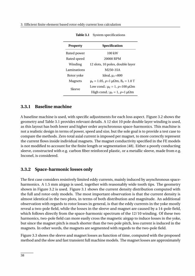
3. Efficient finite element based rotor eddy current loss calculation
Table 3.1 System specifications
Property Specification
Rated power 100 kW
Rated speed 20000 RPM
Winding 12 slots, 10 poles, double layer
Laminations M250-35A
Rotor yoke Ideal, µr =800
Magnets µr = 1.05, ρ=1 µΩm, Br = 1.0 T
SleeveLow cond.: µr = 1, ρ=100 µΩm
High cond.: µr = 1, ρ=1 µΩm
3.3.1 Baseline machine
A baseline machine is used, with specific adjustments for each loss aspect. Figure 3.2 shows thegeometry and Table 3.1 provides relevant details. A 12 slot 10 pole double layer winding is used,as this layout has both lower and higher order asynchronous space-harmonics. This machine isnot a realistic design in terms of power, speed and size, but the sole goal is to provide a test case tocompare the methods. Zero total axial current is imposed per magnet, to more correctly representthe current flows inside individual magnets. The magnet conductivity specified in the FE modelsis not modified to account for the finite length or segmentation [48]. Either a poorly conductingsleeve, constructed with e.g. carbon fiber reinforced plastic, or a metallic sleeve, made from e.g.Inconel, is considered.
3.3.2 Space-harmonic losses only
The first case considers resistively limited eddy currents, mainly induced by asynchronous space-harmonics. A 1.5 mm airgap is used, together with reasonably wide tooth tips. The geometryshown in Figure 3.2 is used. Figure 3.1 shows the current density distribution computed withthe full and rotor-only models. The most important observation is that the current density isalmost identical in the two plots, in terms of both distribution and magnitude. An additionalobservation with regards to rotor losses in general, is that the eddy currents in the yoke mostlyreveal a two-pole field, while the losses in the sleeve and magnet are caused by a 14-pole field,which follows directly from the space-harmonic spectrum of the 12/10 winding. Of these twoharmonics, two-pole field can more easily cross the magnetic airgap to induce losses in the yoke,but since the magnet pitch is much shorter than the two pole pitch, less current is induced in themagnets. In other words, the magnets are segmented with regards to the two-pole field.
Figure 3.3 shows the sleeve and magnet losses as function of time, computed with the proposedmethod and the slow and fast transient full machine models. The magnet losses are approximately
38
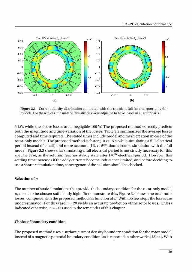
3.3 – 2D calculation performance
(a) (b)
Figure 3.1 Current density distribution computed with the transient full (a) and rotor-only (b)models. For these plots, the material resistivities were adjusted to have losses in all rotor parts.
5 kW, while the sleeve losses are a negligible 100 W. The proposed method correctly predictsboth the magnitude and time-variation of the losses. Table 3.2 summarizes the average lossescomputed and time required. The stated times include model and mesh creation in case of therotor-only models. The proposed method is faster (10 vs 15 s, while simulating a full electricalperiod instead of a half) and more accurate (1% vs 5%) than a coarse simulation with the fullmodel. Figure 3.3 shows that simulating a full electrical period is not strictly necessary for thisspecific case, as the solution reaches steady state after 1/6th electrical period. However, thissettling time increases if the eddy currents become inductance limited, and before deciding touse a shorter simulation time, convergence of the solution should be checked.
Selection of n
The number of static simulations that provide the boundary condition for the rotor-only model,n, needs to be chosen sufficiently high. To demonstrate this, Figure 3.4 shows the total rotorlosses, computed with the proposed method, as function of n. With too few steps the losses areunderestimated. For this case n = 20 yields an accurate prediction of the rotor losses. Unlessindicated otherwise, n = 24 is used in the remainder of this chapter.
Choice of boundary condition
The proposed method uses a surface current density boundary condition for the rotor model,instead of a magnetic potential boundary condition, as is reported in other works [43, 44]. With
39
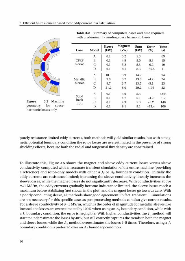
3. Efficient finite element based rotor eddy current loss calculation
Figure 3.2 Machinegeometry for space-harmonic losses only.
Table 3.2 Summary of computed losses and time required,with predominantly winding space harmonic losses
Case ModelSleeve(kW)
Magnets(kW)
Sum(kW)
Error(%)
Time(s)
CFRPsleeve
A 0.1 5.2 5.3 69B 0.1 4.9 5.0 -5.3 15C 0.1 5.2 5.3 -0.2 10D 0.1 8.1 8.3 +55.5 11
Metallicsleeve
A 10.3 3.9 14.2 94B 9.9 3.7 13.6 -4.2 24C 9.7 3.7 13.5 -5.1 23D 21.2 8.0 29.2 +105 23
Solidbackiron
A 0.1 5.0 5.3 6243B 0.1 4.7 5.1 -4.2 817C 0.1 4.9 5.3 +0.2 140D 0.1 8.1 9.1 +73.4 106
purely resistance limited eddy currents, both methods will yield similar results, but with a mag-netic potential boundary condition the rotor losses are overestimated in the presence of strongshielding effects, because both the radial and tangential flux density are constrained.
To illustrate this, Figure 3.5 shows the magnet and sleeve eddy current losses versus sleeveconductivity, computed with an accurate transient simulation of the entire machine (providinga reference) and rotor-only models with either a Js or Az boundary condition. Initially theeddy currents are resistance limited; increasing the sleeve conductivity linearly increases thesleeve losses, while the magnet losses do not significantly decrease. With conductivities aboveσ=1 MS/m, the eddy currents gradually become inductance limited, the sleeve losses reach amaximum before stabilizing (not shown in the plot) and the magnet losses go towards zero. Witha poorly conducting sleeve, all methods show good agreement. In fact, transient FE simulationsare not necessary for this specific case, as postprocessing methods can also give correct results.For a sleeve conductivity of σ=1 MS/m, which is the order of magnitude for metallic sleeves likeInconel, the losses are overestimated by 100% when using an Az boundary condition, while witha Js boundary condition, the error is negligible. With higher conductivities the Js method willstart to underestimate the losses by 40%, but still correctly captures the trends in both the magnetand sleeve losses, while the Az method overestimates the losses 4–5 times. Therefore, using a Js
boundary condition is preferred over an Az boundary condition.
40
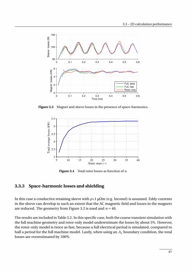
3.3 – 2D calculation performance
0 0.1 0.2 0.3 0.4 0.5 0.650
100
150
Sle
eve
lo
sse
s (
W)
0 0.1 0.2 0.3 0.4 0.5 0.60
2
4
6
Ma
gn
et
lo
sse
s (
kW
)
Time (ms)
Full, slow
Full, fast
Rotor only
Figure 3.3 Magnet and sleeve losses in the presence of space-harmonics.
5 10 15 20 25 30 35 403
3.5
4
4.5
5
5.5
Static steps (−)
Tota
l av
erag
e lo
sses
(kW
)
Figure 3.4 Total rotor losses as function of n.
3.3.3 Space-harmonic losses and shielding
In this case a conductive retaining sleeve with ρ=1 µΩm (e.g. Inconel) is assumed. Eddy-currentsin the sleeve can develop to such an extent that the AC magnetic field and losses in the magnetsare reduced. The geometry from Figure 3.2 is used and n = 40.
The results are included in Table 3.2. In this specific case, both the coarse transient simulation withthe full machine geometry and rotor-only model underestimate the losses by about 5%. However,the rotor-only model is twice as fast, because a full electrical period is simulated, compared tohalf a period for the full machine model. Lastly, when using an Az boundary condition, the totallosses are overestimated by 100%.
41

3. Efficient finite element based rotor eddy current loss calculation
0
10
20
30
40
50
Sle
eve
loss
es (
kW
)
104
105
106
1070
0.25
0.5
0.75
1
1.25
Sleeve conductivity (S/m)
Mag
net
lo
sses
(k
W)
Sleeve losses, full
Sleeve losses, Js
Sleeve losses, Az
Magnet losses, full
Magnet losses, Js
Magnet losses, Az
Figure 3.5 Magnet and sleeve losses as function of sleeve conductivity, computed with threedifferent models.
3.3.4 Solid back-iron
A solid rotor yoke brings significant mechanical and cost benefits, but is also susceptible toeddy current losses. Estimating whether a solid yoke can be used in a certain design requirescomputation of the yoke eddy current losses. The low skin-depth in the rotor yoke requires alocally dense mesh in FE calculations, increasing the time required to calculate the losses. Toestimate the consequences for the rotor loss calculation, the rotor yoke resistivity of the baselinedesign (Figure 3.2) is set to ρ=1 µΩm. The low-conductivity sleeve is assumed to maximize the AC-field inside the yoke and n = 24. The maximum mesh element size at the yoke-magnet interfaceis set to 0.4 mm.
The results are again summarized in Table 3.2. The yoke losses are computed as 238 W with theaccurate transient model of the full machine, while with the proposed method 215 W is computed,a 6% underestimation. The coarse transient full model overestimates the yoke losses by 25% andis 12 times slower than the rotor-only model. With an Az boundary condition, the yoke losses areoverestimated threefold. Also note that the magnet losses are slightly reduced compared to thebaseline case, due to shielding.
3.3.5 Slotting losses
Slotting or permeance variation induced losses are caused by a varying permeance experienced bythe magnets as they rotate past individual stator teeth. The extent of this effect strongly dependson the tooth tip shape and airgap length, with shorter airgaps and straight teeth increasing the
42

3.3 – 2D calculation performance
Figure 3.6 Machine ge-ometry with pronouncedslotting losses.
Table 3.3 Summary of computed losses and time requiredwith high slotting losses
Case ModelSleeve(kW)
Magnets(kW)
Sum(kW)
Error(%)
Time(s)
CFRPsleeve
A 0.2 35.7 35.9 441B 0.2 34.7 34.9 -2.6 128C 0.2 32.8 33.0 -7.9 36D 0.2 51.4 51.6 +43.9 36
Metallicsleeve
A 27.1 32.9 60.0 446B 26.0 31.9 57.9 -3.5 126C 23.3 28.1 51.4 -14.4 46D 32.4 51.0 83.4 +38.9 46
losses. Figure 3.6 shows the geometry used; a 0.4 mm airgap and 0.9 mm thick retaining sleeveare assumed, n = 40. To emphasize the slotting losses, zero stator current is specified.
In this case, the proposed method underestimates the losses by 8%, while the coarse full simu-lation underestimates the losses by only 3%. However, due to the short airgap the full machinemodel requires a dense mesh inside the airgap, increasing the required computation time. Thisdoes not apply to the rotor-only method, making it 6–7 times faster than the coarse full simulation.With an Az boundary condition the losses are overestimated by 44% in this case.
Aside from the differences between the calculation method, this example shows that the slottinglosses can be excessive, even in no-load. Compared to the baseline case (Table 3.2) under full load,the losses have increased over sixfold. This should be kept in mind when designing fractional slottooth-coil machines without tooth-tips.
3.3.6 Slotting losses with shielding
When a conducting sleeve is used with the ‘high slotting losses’ geometry, the proposed methodunderestimates the losses by 14% and the speed gain is decreased to about 6 times. Increas-ing n does not significantly reduce the error. With an Az boundary condition, the losses areoverestimated by 39%.
3.3.7 Strong stator saturation
Strong stator saturation can occur during a torque overload, but also in an optimization process,where unrealistic machine designs may need be evaluated. Transient simulations with heavily
43

3. Efficient finite element based rotor eddy current loss calculation
Figure 3.7 Machine ge-ometry for pronouncedstator saturation.
Table 3.4 Summary of computed losses and time requiredunder strong stator saturation
ModelSleeve(kW)
Magnets(kW)
Sum(kW)
Error(%)
Time(s)
A 0.2 15.2 15.4 1009B 0.2 14.2 14.4 -6.7 375C 0.2 12.8 13.0 -16.0 14D 0.4 23.4 23.9 +55.0 14
saturated machines require small time steps to prevent divergence of the solution, increasingthe time required. By performing a transient simulation with only the rotor and assuming linearmaterials, this problem is avoided.
To demonstrate the performance under heavy saturation, the yoke and teeth are made narrower,the stack length is halved and the output torque is doubled. Figure 3.7 shows the adjustedgeometry. For this case, the coarse transient simulation requires 375 s and underestimates thelosses by 7%. The proposed method requires only 14 s, but underestimates the losses by 16%.Given the roughly 25 times speed gain, this loss of accuracy is deemed acceptable.
3.3.8 Low magnet span
As part of an optimization process, very unrealistic designs need to be correctly evaluated. Oneextreme is a very low magnet pole span, as shown in Figure 3.8. The performance of the proposedmethod is in this case very similar to the initial case; a comparable error and approximatelytwice as fast as a course simulation with a full model. With an Az boundary the losses are stilloverestimated, although to a lesser extend due to the smaller magnets.
3.3.9 Distributed windings
Distributed integer pitch windings have a significantly cleaner airgap space-harmonic spectrumthan concentrated fractional pitch windings, which strongly reduces rotor losses. Correctlyaccounting for the eddy currents induced by the low amplitude asynchronous space-harmonicsrequires accurate transient solver settings, slowing down the solution process. In addition, thehigher number of teeth simply requires more mesh elements, further increasing the solving time.To estimate the performance of the proposed method under these circumstances, a distributedwinding machine with 36 slots and 6 poles (q = 2) is considered. The geometry is shown inFigure 3.9, the poorly conducting sleeve is assumed and n = 50.
44
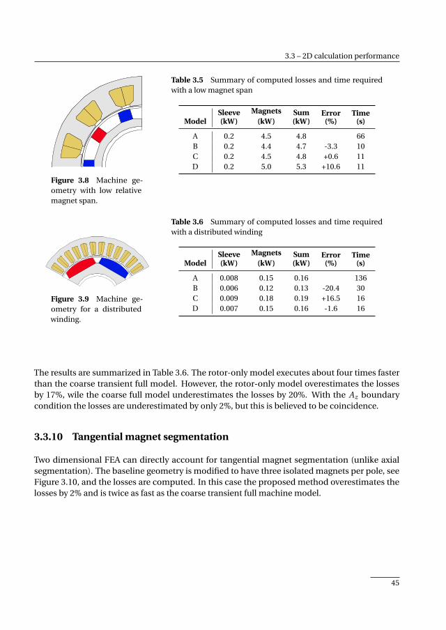
3.3 – 2D calculation performance
Figure 3.8 Machine ge-ometry with low relativemagnet span.
Table 3.5 Summary of computed losses and time requiredwith a low magnet span
ModelSleeve(kW)
Magnets(kW)
Sum(kW)
Error(%)
Time(s)
A 0.2 4.5 4.8 66B 0.2 4.4 4.7 -3.3 10C 0.2 4.5 4.8 +0.6 11D 0.2 5.0 5.3 +10.6 11
Figure 3.9 Machine ge-ometry for a distributedwinding.
Table 3.6 Summary of computed losses and time requiredwith a distributed winding
ModelSleeve(kW)
Magnets(kW)
Sum(kW)
Error(%)
Time(s)
A 0.008 0.15 0.16 136B 0.006 0.12 0.13 -20.4 30C 0.009 0.18 0.19 +16.5 16D 0.007 0.15 0.16 -1.6 16
The results are summarized in Table 3.6. The rotor-only model executes about four times fasterthan the coarse transient full model. However, the rotor-only model overestimates the lossesby 17%, wile the coarse full model underestimates the losses by 20%. With the Az boundarycondition the losses are underestimated by only 2%, but this is believed to be coincidence.
3.3.10 Tangential magnet segmentation
Two dimensional FEA can directly account for tangential magnet segmentation (unlike axialsegmentation). The baseline geometry is modified to have three isolated magnets per pole, seeFigure 3.10, and the losses are computed. In this case the proposed method overestimates thelosses by 2% and is twice as fast as the coarse transient full machine model.
45
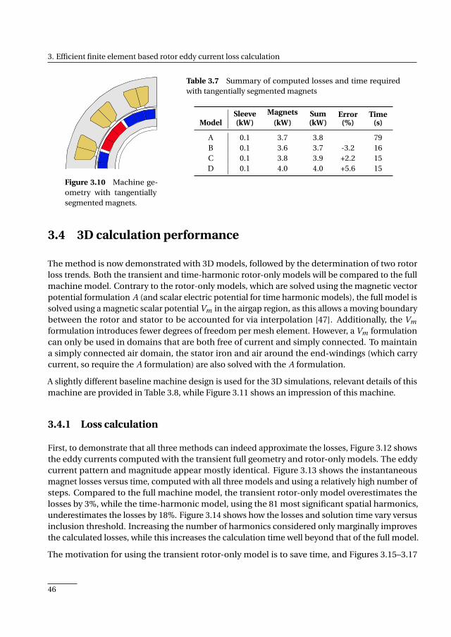
3. Efficient finite element based rotor eddy current loss calculation
Figure 3.10 Machine ge-ometry with tangentiallysegmented magnets.
Table 3.7 Summary of computed losses and time requiredwith tangentially segmented magnets
ModelSleeve(kW)
Magnets(kW)
Sum(kW)
Error(%)
Time(s)
A 0.1 3.7 3.8 79B 0.1 3.6 3.7 -3.2 16C 0.1 3.8 3.9 +2.2 15D 0.1 4.0 4.0 +5.6 15
3.4 3D calculation performance
The method is now demonstrated with 3D models, followed by the determination of two rotorloss trends. Both the transient and time-harmonic rotor-only models will be compared to the fullmachine model. Contrary to the rotor-only models, which are solved using the magnetic vectorpotential formulation A (and scalar electric potential for time harmonic models), the full model issolved using a magnetic scalar potential Vm in the airgap region, as this allows a moving boundarybetween the rotor and stator to be accounted for via interpolation [47]. Additionally, the Vm
formulation introduces fewer degrees of freedom per mesh element. However, a Vm formulationcan only be used in domains that are both free of current and simply connected. To maintaina simply connected air domain, the stator iron and air around the end-windings (which carrycurrent, so require the A formulation) are also solved with the A formulation.
A slightly different baseline machine design is used for the 3D simulations, relevant details of thismachine are provided in Table 3.8, while Figure 3.11 shows an impression of this machine.
3.4.1 Loss calculation
First, to demonstrate that all three methods can indeed approximate the losses, Figure 3.12 showsthe eddy currents computed with the transient full geometry and rotor-only models. The eddycurrent pattern and magnitude appear mostly identical. Figure 3.13 shows the instantaneousmagnet losses versus time, computed with all three models and using a relatively high number ofsteps. Compared to the full machine model, the transient rotor-only model overestimates thelosses by 3%, while the time-harmonic model, using the 81 most significant spatial harmonics,underestimates the losses by 18%. Figure 3.14 shows how the losses and solution time vary versusinclusion threshold. Increasing the number of harmonics considered only marginally improvesthe calculated losses, while this increases the calculation time well beyond that of the full model.
The motivation for using the transient rotor-only model is to save time, and Figures 3.15–3.17
46
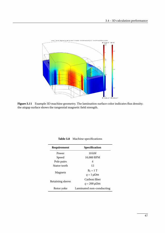
3.4 – 3D calculation performance
Figure 3.11 Example 3D machine geometry. The lamination surface color indicates flux density;the airgap surface shows the tangential magnetic field strength.
Table 3.8 Machine specifications
Requirement Specification
Power 10 kW
Speed 16,000 RPM
Pole pairs 4
Stator teeth 12
MagnetsBr = 1 T
ρ = 1 µΩm
Retaining sleeveCarbon fiber
ρ = 200 µΩm
Rotor yoke Laminated non-conducting
47
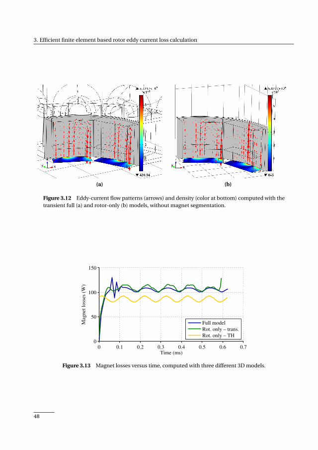
3. Efficient finite element based rotor eddy current loss calculation
(a) (b)
Figure 3.12 Eddy-current flow patterns (arrows) and density (color at bottom) computed with thetransient full (a) and rotor-only (b) models, without magnet segmentation.
0 0.1 0.2 0.3 0.4 0.5 0.6 0.70
50
100
150
Time (ms)
Mag
net
loss
es (
W)
Full model
Rot. only – trans.
Rot. only – TH
Figure 3.13 Magnet losses versus time, computed with three different 3D models.
48

3.4 – 3D calculation performance
80
85
90
95
100
Loss
es
5 10 15 20 25 30 35 40 450
2.5
5
7.5
10
Threshold (%)
Sol.
tim
e (
hr.
)
Losses
Sol. time
Figure 3.14 Solution time and losses versus harmonic inclusion threshold for the TH rotor-onlymodel.
100
150
200
250
Aver
age
mag
net
loss
es(W
)
20 30 40 50 60 70 80 90 1000
50
100
150
Simulated steps per electrical period
Solu
tion t
ime
(min
.)
Losses
Solution time
Figure 3.15 Computed losses and solution time for the full machine model.
elaborate on this. Figure 3.15 shows that 40 transients steps with the full model are needed tocalculate the losses to within 10% of the final value, taking about 50 minutes on a given computer.Next, Figure 3.16 shows that for the rotor-only model the number of time steps is more importantthan the number of static steps with the full model (which provide the boundary conditions).Twenty steps with the full model plus 75 steps with the rotor-only model are needed to obtainlosses to within 10% of the final value, taking in total 27 minutes on the same computer, as shownin Figure 3.17. Hence, the proposed approach is approximately two times faster than a directsolution of the full model.
3.4.2 Inductance limited currents
An important requirement of a rotor loss calculation method, is the ability to correctly account forshielding effects caused by inductance limited eddy currents. This allows the method to be used
49
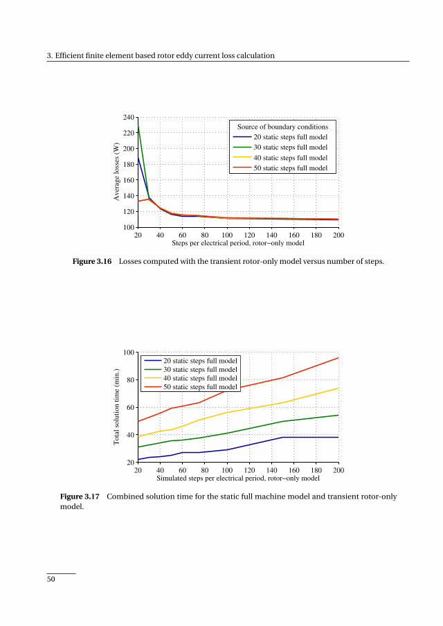
3. Efficient finite element based rotor eddy current loss calculation
20 40 60 80 100 120 140 160 180 200100
120
140
160
180
200
220
240
Steps per electrical period, rotor−only model
Av
erag
e lo
sses
(W
)
20 static steps full model
30 static steps full model
40 static steps full model
50 static steps full model
Source of boundary conditions
Figure 3.16 Losses computed with the transient rotor-only model versus number of steps.
20 40 60 80 100 120 140 160 180 20020
40
60
80
100
Simulated steps per electrical period, rotor−only model
To
tal
solu
tio
n t
ime
(min
.)
20 static steps full model
30 static steps full model
40 static steps full model
50 static steps full model
Figure 3.17 Combined solution time for the static full machine model and transient rotor-onlymodel.
50
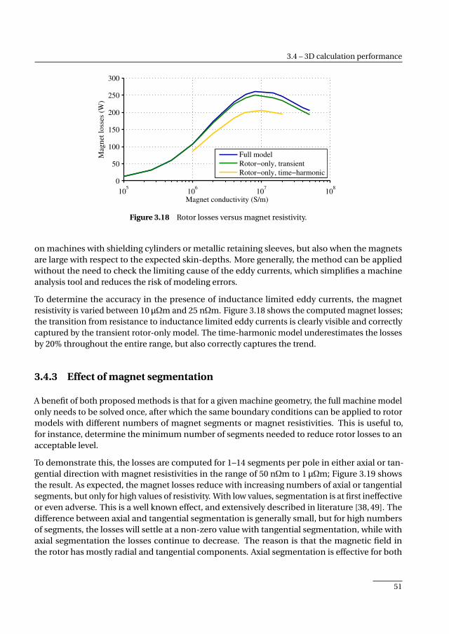
3.4 – 3D calculation performance
105
106
107
108
0
50
100
150
200
250
300
Magnet conductivity (S/m)
Mag
net
lo
sses
(W
)
Full model
Rotor−only, transient
Rotor−only, time−harmonic
Figure 3.18 Rotor losses versus magnet resistivity.
on machines with shielding cylinders or metallic retaining sleeves, but also when the magnetsare large with respect to the expected skin-depths. More generally, the method can be appliedwithout the need to check the limiting cause of the eddy currents, which simplifies a machineanalysis tool and reduces the risk of modeling errors.
To determine the accuracy in the presence of inductance limited eddy currents, the magnetresistivity is varied between 10 µΩm and 25 nΩm. Figure 3.18 shows the computed magnet losses;the transition from resistance to inductance limited eddy currents is clearly visible and correctlycaptured by the transient rotor-only model. The time-harmonic model underestimates the lossesby 20% throughout the entire range, but also correctly captures the trend.
3.4.3 Effect of magnet segmentation
A benefit of both proposed methods is that for a given machine geometry, the full machine modelonly needs to be solved once, after which the same boundary conditions can be applied to rotormodels with different numbers of magnet segments or magnet resistivities. This is useful to,for instance, determine the minimum number of segments needed to reduce rotor losses to anacceptable level.
To demonstrate this, the losses are computed for 1–14 segments per pole in either axial or tan-gential direction with magnet resistivities in the range of 50 nΩm to 1 µΩm; Figure 3.19 showsthe result. As expected, the magnet losses reduce with increasing numbers of axial or tangentialsegments, but only for high values of resistivity. With low values, segmentation is at first ineffectiveor even adverse. This is a well known effect, and extensively described in literature [38, 49]. Thedifference between axial and tangential segmentation is generally small, but for high numbersof segments, the losses will settle at a non-zero value with tangential segmentation, while withaxial segmentation the losses continue to decrease. The reason is that the magnetic field inthe rotor has mostly radial and tangential components. Axial segmentation is effective for both
51
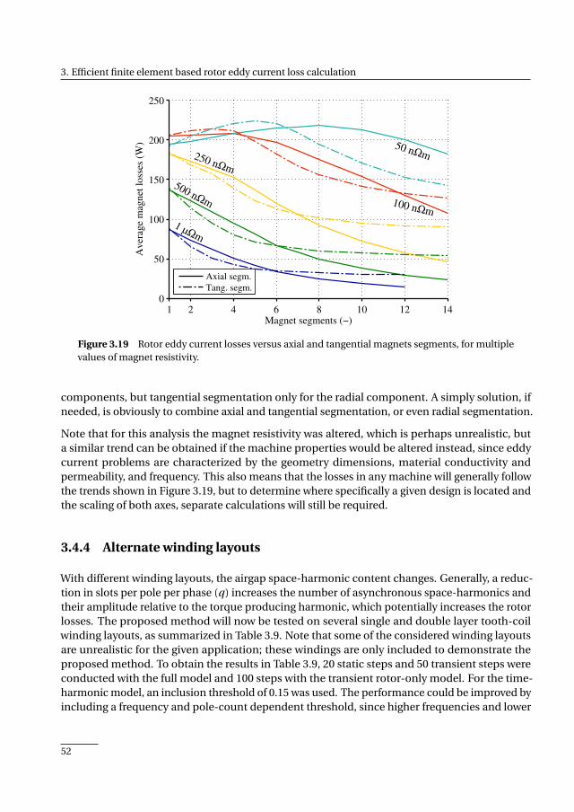
3. Efficient finite element based rotor eddy current loss calculation
1 2 4 6 8 10 12 140
50
100
150
200
250
Magnet segments (−)
Aver
age
mag
net
loss
es (
W)
1 µΩm
500 nΩm
250 nΩm
100 nΩm
50 nΩm
Axial segm.
Tang. segm.
Figure 3.19 Rotor eddy current losses versus axial and tangential magnets segments, for multiplevalues of magnet resistivity.
components, but tangential segmentation only for the radial component. A simply solution, ifneeded, is obviously to combine axial and tangential segmentation, or even radial segmentation.
Note that for this analysis the magnet resistivity was altered, which is perhaps unrealistic, buta similar trend can be obtained if the machine properties would be altered instead, since eddycurrent problems are characterized by the geometry dimensions, material conductivity andpermeability, and frequency. This also means that the losses in any machine will generally followthe trends shown in Figure 3.19, but to determine where specifically a given design is located andthe scaling of both axes, separate calculations will still be required.
3.4.4 Alternate winding layouts
With different winding layouts, the airgap space-harmonic content changes. Generally, a reduc-tion in slots per pole per phase (q) increases the number of asynchronous space-harmonics andtheir amplitude relative to the torque producing harmonic, which potentially increases the rotorlosses. The proposed method will now be tested on several single and double layer tooth-coilwinding layouts, as summarized in Table 3.9. Note that some of the considered winding layoutsare unrealistic for the given application; these windings are only included to demonstrate theproposed method. To obtain the results in Table 3.9, 20 static steps and 50 transient steps wereconducted with the full model and 100 steps with the transient rotor-only model. For the time-harmonic model, an inclusion threshold of 0.15 was used. The performance could be improved byincluding a frequency and pole-count dependent threshold, since higher frequencies and lower
52
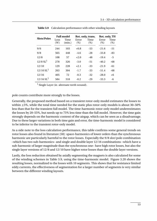
3.4 – 3D calculation performance
Table 3.9 Calculation performance with other winding layouts
Slots/PolesFull model Rot. only, trans. Rot. only, TH
Loss(W)
Time(min.)
Error(%)
Time(%)
Error(%)
Time(%)
9/6 244 103 +0.8 -53 -21.6 -51
9/8 565 448 -4.6 -28 -33.8 -83
12/8 108 57 +2.0 -48 -19.4 -5
12/8 SL1 278 326 -3.0 -51 -40.2 -68
12/10 129 228 +2.1 -33 -21.9 -61
12/10 SL1 263 304 -1.7 -33 -51.4 -68
12/16 405 72 -0.3 -32 -28.0 +6
12/16 SL1 584 318 -0.2 -29 -33.3 -6
1 Single Layer (ie. alternate teeth wound).
pole counts contribute more strongly to the losses.
Generally, the proposed method based on a transient rotor-only model estimates the losses towithin ±5%, while the total time needed for the static plus rotor-only models is about 30–50%less than that for the transient full model. The time-harmonic rotor-only model underestimatesthe losses by 20–55%, but needs up to 75% less time than the full model. However, the time gainstrongly depends on the harmonic content of the airgap, which can be seen as a disadvantage.Due to these larger variations in both time gain and error, the time-harmonic model is consideredto be inferior to the transient rotor-only model.
As a side note to the loss calculation performance, this table confirms some general trends onrotor losses also found in literature [50]: space-harmonics of lower orders than the synchronousharmonic are particularly harmful to the rotor losses. Especially the 9/8 slot/pole combination–which has two sub-harmonics– and single and double layer 12/16 combinations –which have asub-harmonic of larger magnitude than the synchronous one– have high rotor losses, but also thesingle layer versions of 12/8 and 12/10 have higher rotor losses than the double layer versions.
Lastly, the loss reduction obtained by axially segmenting the magnets is also calculated for someof the winding schemes in Table 3.9, using the time-harmonic model. Figure 3.20 shows theresulting losses, normalized to the losses with 10 segments. This shows that for resistance limitededdy currents, the effectiveness of segmentation for a larger number of segments is very similarbetween the different winding layouts.
53
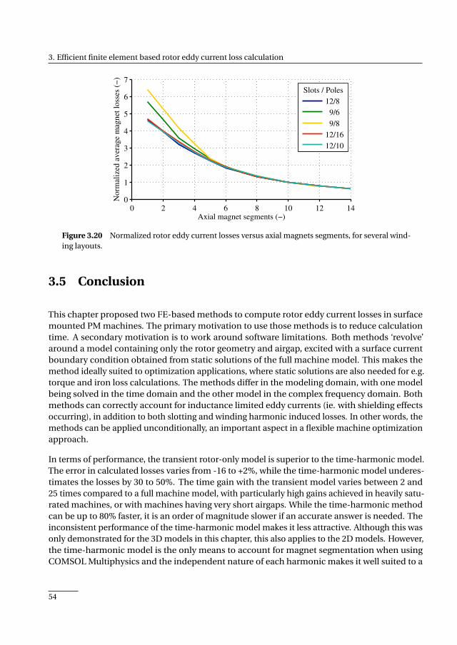
3. Efficient finite element based rotor eddy current loss calculation
0 2 4 6 8 10 12 140
1
2
3
4
5
6
7
Axial magnet segments (−)
Norm
aliz
ed a
ver
age
mag
net
lo
sses
(−
)
12/8
9/6
9/8
12/16
12/10
Slots / Poles
Figure 3.20 Normalized rotor eddy current losses versus axial magnets segments, for several wind-ing layouts.
3.5 Conclusion
This chapter proposed two FE-based methods to compute rotor eddy current losses in surfacemounted PM machines. The primary motivation to use those methods is to reduce calculationtime. A secondary motivation is to work around software limitations. Both methods ‘revolve’around a model containing only the rotor geometry and airgap, excited with a surface currentboundary condition obtained from static solutions of the full machine model. This makes themethod ideally suited to optimization applications, where static solutions are also needed for e.g.torque and iron loss calculations. The methods differ in the modeling domain, with one modelbeing solved in the time domain and the other model in the complex frequency domain. Bothmethods can correctly account for inductance limited eddy currents (ie. with shielding effectsoccurring), in addition to both slotting and winding harmonic induced losses. In other words, themethods can be applied unconditionally, an important aspect in a flexible machine optimizationapproach.
In terms of performance, the transient rotor-only model is superior to the time-harmonic model.The error in calculated losses varies from -16 to +2%, while the time-harmonic model underes-timates the losses by 30 to 50%. The time gain with the transient model varies between 2 and25 times compared to a full machine model, with particularly high gains achieved in heavily satu-rated machines, or with machines having very short airgaps. While the time-harmonic methodcan be up to 80% faster, it is an order of magnitude slower if an accurate answer is needed. Theinconsistent performance of the time-harmonic model makes it less attractive. Although this wasonly demonstrated for the 3D models in this chapter, this also applies to the 2D models. However,the time-harmonic model is the only means to account for magnet segmentation when usingCOMSOL Multiphysics and the independent nature of each harmonic makes it well suited to a
54

3.5 – Conclusion
parallel computing environment.
Using the proposed methods, the effect of magnet segmentation was demonstrated and commonwinding layouts were analyzed, confirming general trends also described in literature and showingthe general correctness of the methods.
55

CHAPTER 4
AC winding losses in high-speed PM machines
The electrical frequency in high-speed machines can easily exceed 1 kHz. As a result, few turnsper coil will be needed to obtain sufficient back-emf to interface with the inverter. In lowvoltage battery fed systems this effect is even more pronounced. Therefore, the cross-sectionalarea per turn increases, making the turns susceptible to eddy current losses. The high electricalfrequency enhances this problem. To reduce these additional losses, individual turns can beconstructed with multiple insulated strands and the placement of those strands in the slotscan be varied. However, analyzing suitable configurations is non-trivial, particularly with veryfew turns in non-square slots, while this is a necessary step in the design of a new machine.Hence, this chapter presents a modeling method to estimate the current distribution acrossparallel strands using simplified 3D FE models. After experimentally confirming the models, anumber of design guidelines with regards to strand placement are determined.
Based on
• M. van der Geest, H. Polinder, J. Ferreira, and D. Zeilstra, “Current sharing analysis ofparallel strands in low voltage high speed machines,” IEEE Trans. Ind. Electron., vol. 61,no. 6, pp. 3064–3070, Jun. 2014; and
• M. van der Geest, H. Polinder, J. A. Ferreira, and D. Zeilstra, “Stator winding proximityloss reduction techniques in high speed electrical machines,” in IEEE Int. ElectricMachines Drives Conf. (IEMDC), 2013, pp. 340–346.
57

4. AC winding losses in high-speed PM machines
4.1 Introduction
Obtaining a high slot fill factor is very desirable in any electrical machine, since it reduces both thecopper losses and thermal resistance, which ultimately increases the achievable power density[51,52]. However, measures against skin and proximity effects oppose a high fill factor. This appliesto measures such as using several thinner strands in parallel, optionally with twisting, or even litzwire [53], but also in very large machines with bar windings, where discrete displacements areused (Roebel winding) [54]. The fill factor is also reduced when strands close the slot opening areomitted, as they incur high losses due to leakage fields [53, 55–57], particularly at the frequenciespresent in high-speed machines. Therefore, such measures should only be applied to the extentnecessary to sufficiently reduce the winding AC losses. Hence, calculation of the AC losses, bothdue to unequal current sharing and proximity effects is necessary. This chapter starts with thecalculation of the losses due to unequal current sharing between parallel strands, as these lossesdominate in low voltage high-speed machines, followed by an overview of various loss mitigationmethods and their effectiveness.
Before commencing, a few words will be spent on terminology. All induced currents are the resultof a varying linked magnetic flux, but the associated losses can be separated in two groups basedon the source of the flux.
• First, additional losses in a strand due to a bulk AC current in that strand itself are referredto as skin effect losses. A ‘discrete’ skin effect occurs when using parallel strands, and thiswill be the topic of the next section.
• Secondly, additional losses in a strand due to an externally imposed field on that strandare typically called proximity losses. The source of the proximity losses is often dividedagain based on the cause, with small differences depending on the research topic. Whenanalyzing the performance with litz wires, which consist of twisted bundles of twistedstrands, a distinction is often made between strand-level and bundle-level losses, as thisallows modeling simplifications [58]. In regular electrical machines that have solid copperstrands, a distinction can be made between armature field proximity losses (either due toother turns of the same coil, or other phase coils) and excitation field proximity losses.
Excitation field induced losses are mainly a problem in slotless machines, since in such machinesthe windings are directly exposed to the field flux. Axial flux machines are often based on slotlessdesigns and a simple method to compute the field induced losses is presented in [59]. In high-speed machines without tooth tips these losses may also need to be considered [60], but thepresence of tooth tips can nearly diminish these losses. Proximity losses induced by the armaturefield are mainly the result of slot leakage flux. A high permeability material completely enclosinga winding, except for a small gap, enhances the field near that gap and proximity losses will occurat lower frequencies than in an identically shaped air core coil. This effect is clearly pointed out ine.g. [53, 55, 61]. Section 4.3 will discuss and compare methods to reduce both proximity lossesand bundle level skin effect losses.
58
4.2 – Current sharing analysis
4.2 Current sharing analysis
4.2.1 Overview
In low voltage high-speed machines, the necessarily low turn count and consequential large crosssection per turn further exacerbate the problems of induced winding losses [62]. Using parallelstrands wound straight through the slots does not solve the problem, because of unequal currentsharing and circulating currents [61, 63, 64]. In the extreme case, segmenting one solid turn into nisolated parallel strands, but connecting those strand together at the coil ends, will not reducethe losses at all. Similar problems can occur in high frequency magnetic components [65, 66].Displacing or twisting the conductors inside a slot can reduce the effects, but at the expense of areduced fill factor, and should therefore be used only when necessary.
To assess the necessity of twisting the strands and by how much, a model is required that canpredict the current imbalance. Conventionally, analyzing strand twisting is a topic within highfrequency transformer and inductor design. Analytical methods on simplified geometries areoften used to predict effective resistances and losses [58, 67–69]. Such methods also clearlydemonstrate that litz wire is only beneficial over a limited frequency range [70, 71]. A specificmodel where the effects of twisting the strands is considered is presented in [72], where theeffect on the resistance of the longitudinal magnetic field resulting from twisting the strandsis computed. To account for the losses in end-windings or other complex structures where ananalytical model is infeasible, FEA can provide a solution [65, 73, 74]. FEA is also used in [75],where the AC resistance of core-less planar windings is computed. In such a winding the copperis exposed to a significant magnetic field, increasing the AC loss density in the copper. Similarly,machines may have a large amount of leakage flux may exist inside the slots. Note that in themajority of the work on this topic, the litz wire is assumed to be ideal. That is, each strand carriesthe same net current.
In the field of machines little research exists on this topic, although one particular series of papersspecifically discusses this topic [63, 64, 76, 77]. In this work, fully analytical models are derivedto compute the magnetic field inside the slot, the current distribution and the induced losses.However, 3D effects related to the end-windings cannot be taken into account and while analyticalmethods are certainly faster than FE simulations, implementing the equations takes time andFEM verification is usually applied to confirm the equations. Also, the use of analytical modelsrequires expertise. For single case studies, it can then be attractive to accept the longer timerequired for FE simulations. When using FEA to compute the winding losses, both transientand time-harmonic calculations can be used, but if only the steady state solution is of interest,time-harmonic simulations can provide the same answer as a transient simulation in less time, asis demonstrated in [60] for the no-load eddy current losses.
The aim of this section is to compute the current distribution across parallel strands with fullaccount of the actual geometry. A simple method is proposed, based on the turn-level impedancematrix of the windings, which is extracted from 2D or 3D FE simulations, and basic circuit
59

4. AC winding losses in high-speed PM machines
Table 4.1 Machine specifications
Requirement Specification
Rated power 10 kW
Speed 32,000 RPM
RMS phase current 200 A
Pole pairs 5
Stator teeth 15
Stack length 50 mm
Turns/tooth 5
equations. Complex 3D models are avoided by simulating only individual strands and using thesuperposition principle, allowing otherwise too complex 3D structures to be modeled on desktopcomputers. A machine with concentrated non-overlapping windings serves as an example,although the method can also be applied to distributed windings. The only difficulty with thelatter type is the description of the end-winding shape.
4.2.2 Problem elaboration
Solid bars cannot be used as conductors in low voltage high frequency machines due to skin andproximity effects. As an alternative, regular circular wires connected in parallel may be used. Tomaintain a high fill factor, these strands are preferably wound straight (i.e. without twisting ordisplacements) around the teeth. Figure 4.1 shows four possibilities for such a winding, each hav-ing seven parallel strands and five turns of 1.5 mm diameter copper wire. More permutations arepossible, but the four depicted here are considered reasonably manufacturable. In the ’groupedstrands’ style, the parallel strands are wound one at a time and all turns of one strand physicallytouch each other, while with ’grouped turns’, all strands are wound simultaneously. In all casesthe fill factor is 51%.
To assess the performance of these winding configurations in terms of copper losses, they areanalyzed with transient 2D FEA. Table 4.1 summarizes the specifications of the machine used in allanalyses. The seven strands of each phase are connected in parallel and a total current is imposed.Table 4.2 reports the resulting steady-state strand currents. Large differences exist between thestrand currents; strands close to the slot-opening carry significant current in particular. Do notethat this table reports RMS currents; the vector sum of the currents will always equal the phasecurrent. At first sight these values may even seem erroneous and experiments will have to confirmthese results.
Also listed in Table 4.2 are the copper losses computed with the transient FE simulations and thecopper losses based on the strand currents only. The former includes all AC and DC losses, while
60
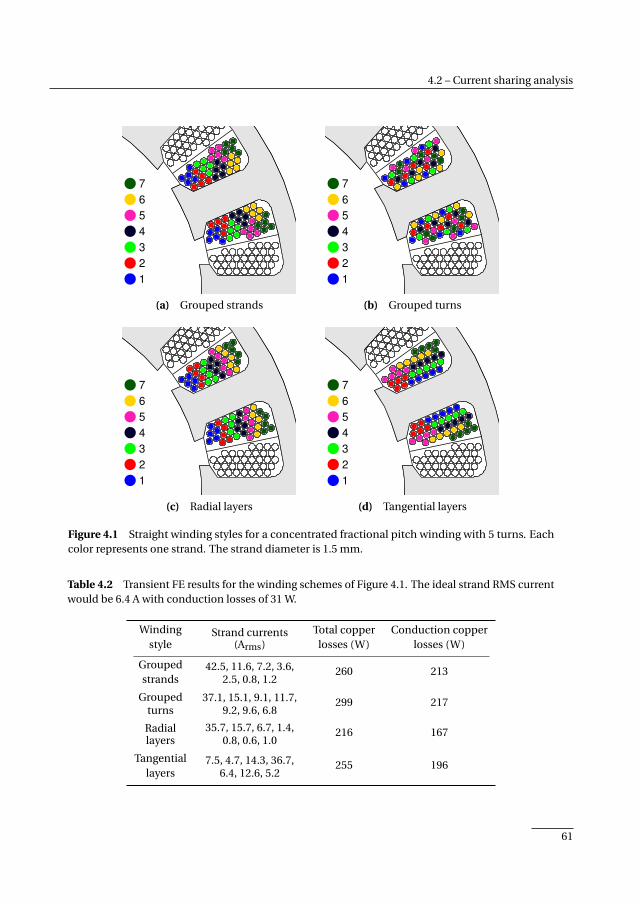
4.2 – Current sharing analysis
1
2
3
4
5
6
7
(a) Grouped strands
1
2
3
4
5
6
7
(b) Grouped turns
1
2
3
4
5
6
7
(c) Radial layers
1
2
3
4
5
6
7
(d) Tangential layers
Figure 4.1 Straight winding styles for a concentrated fractional pitch winding with 5 turns. Eachcolor represents one strand. The strand diameter is 1.5 mm.
Table 4.2 Transient FE results for the winding schemes of Figure 4.1. The ideal strand RMS currentwould be 6.4 A with conduction losses of 31 W.
Windingstyle
Strand currents(Arms)
Total copperlosses (W)
Conduction copperlosses (W)
Groupedstrands
42.5, 11.6, 7.2, 3.6,2.5, 0.8, 1.2
260 213
Groupedturns
37.1, 15.1, 9.1, 11.7,9.2, 9.6, 6.8
299 217
Radiallayers
35.7, 15.7, 6.7, 1.4,0.8, 0.6, 1.0
216 167
Tangentiallayers
7.5, 4.7, 14.3, 36.7,6.4, 12.6, 5.2
255 196
61
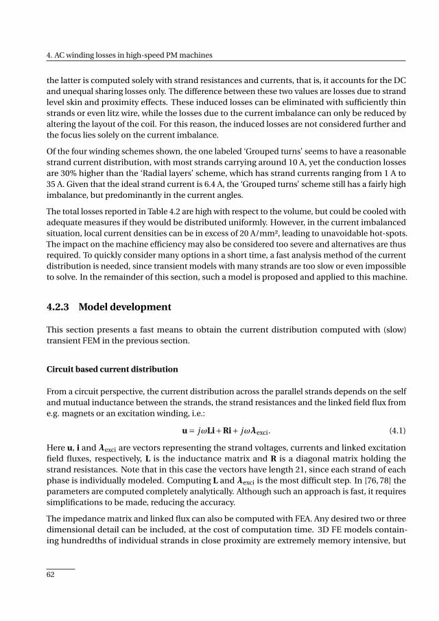
4. AC winding losses in high-speed PM machines
the latter is computed solely with strand resistances and currents, that is, it accounts for the DCand unequal sharing losses only. The difference between these two values are losses due to strandlevel skin and proximity effects. These induced losses can be eliminated with sufficiently thinstrands or even litz wire, while the losses due to the current imbalance can only be reduced byaltering the layout of the coil. For this reason, the induced losses are not considered further andthe focus lies solely on the current imbalance.
Of the four winding schemes shown, the one labeled ‘Grouped turns’ seems to have a reasonablestrand current distribution, with most strands carrying around 10 A, yet the conduction lossesare 30% higher than the ‘Radial layers’ scheme, which has strand currents ranging from 1 A to35 A. Given that the ideal strand current is 6.4 A, the ‘Grouped turns’ scheme still has a fairly highimbalance, but predominantly in the current angles.
The total losses reported in Table 4.2 are high with respect to the volume, but could be cooled withadequate measures if they would be distributed uniformly. However, in the current imbalancedsituation, local current densities can be in excess of 20 A/mm², leading to unavoidable hot-spots.The impact on the machine efficiency may also be considered too severe and alternatives are thusrequired. To quickly consider many options in a short time, a fast analysis method of the currentdistribution is needed, since transient models with many strands are too slow or even impossibleto solve. In the remainder of this section, such a model is proposed and applied to this machine.
4.2.3 Model development
This section presents a fast means to obtain the current distribution computed with (slow)transient FEM in the previous section.
Circuit based current distribution
From a circuit perspective, the current distribution across the parallel strands depends on the selfand mutual inductance between the strands, the strand resistances and the linked field flux frome.g. magnets or an excitation winding, i.e.:
u = jωLi+Ri+ jωλexci. (4.1)
Here u, i and λexci are vectors representing the strand voltages, currents and linked excitationfield fluxes, respectively, L is the inductance matrix and R is a diagonal matrix holding thestrand resistances. Note that in this case the vectors have length 21, since each strand of eachphase is individually modeled. Computing L and λexci is the most difficult step. In [76, 78] theparameters are computed completely analytically. Although such an approach is fast, it requiressimplifications to be made, reducing the accuracy.
The impedance matrix and linked flux can also be computed with FEA. Any desired two or threedimensional detail can be included, at the cost of computation time. 3D FE models contain-ing hundredths of individual strands in close proximity are extremely memory intensive, but
62
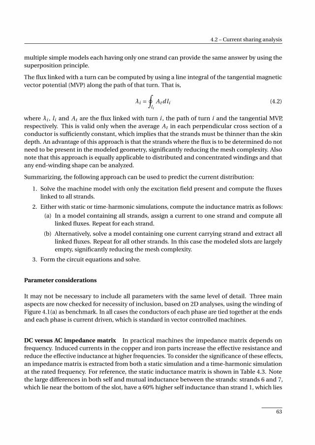
4.2 – Current sharing analysis
multiple simple models each having only one strand can provide the same answer by using thesuperposition principle.
The flux linked with a turn can be computed by using a line integral of the tangential magneticvector potential (MVP) along the path of that turn. That is,
λi =∮
li
At dli (4.2)
where λi , li and At are the flux linked with turn i , the path of turn i and the tangential MVP,respectively. This is valid only when the average At in each perpendicular cross section of aconductor is sufficiently constant, which implies that the strands must be thinner than the skindepth. An advantage of this approach is that the strands where the flux is to be determined do notneed to be present in the modeled geometry, significantly reducing the mesh complexity. Alsonote that this approach is equally applicable to distributed and concentrated windings and thatany end-winding shape can be analyzed.
Summarizing, the following approach can be used to predict the current distribution:
1. Solve the machine model with only the excitation field present and compute the fluxeslinked to all strands.
2. Either with static or time-harmonic simulations, compute the inductance matrix as follows:
(a) In a model containing all strands, assign a current to one strand and compute alllinked fluxes. Repeat for each strand.
(b) Alternatively, solve a model containing one current carrying strand and extract alllinked fluxes. Repeat for all other strands. In this case the modeled slots are largelyempty, significantly reducing the mesh complexity.
3. Form the circuit equations and solve.
Parameter considerations
It may not be necessary to include all parameters with the same level of detail. Three mainaspects are now checked for necessity of inclusion, based on 2D analyses, using the winding ofFigure 4.1(a) as benchmark. In all cases the conductors of each phase are tied together at the endsand each phase is current driven, which is standard in vector controlled machines.
DC versus AC impedance matrix In practical machines the impedance matrix depends onfrequency. Induced currents in the copper and iron parts increase the effective resistance andreduce the effective inductance at higher frequencies. To consider the significance of these effects,an impedance matrix is extracted from both a static simulation and a time-harmonic simulationat the rated frequency. For reference, the static inductance matrix is shown in Table 4.3. Notethe large differences in both self and mutual inductance between the strands: strands 6 and 7,which lie near the bottom of the slot, have a 60% higher self inductance than strand 1, which lies
63
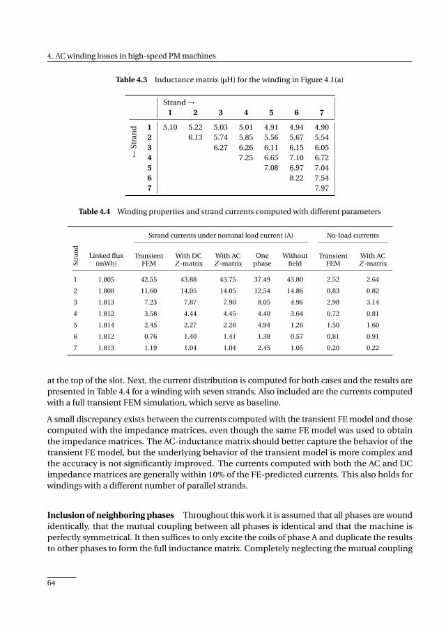
4. AC winding losses in high-speed PM machines
Table 4.3 Inductance matrix (µH) for the winding in Figure 4.1(a)
Strand →1 2 3 4 5 6 7
←St
ran
d 1 5.10 5.22 5.03 5.01 4.91 4.94 4.902 6.13 5.74 5.85 5.56 5.67 5.543 6.27 6.26 6.11 6.15 6.054 7.25 6.65 7.10 6.725 7.08 6.97 7.046 8.22 7.547 7.97
Table 4.4 Winding properties and strand currents computed with different parameters
Strand currents under nominal load current (A) No-load currents
Stra
nd
Linked flux(mWb)
TransientFEM
With DCZ -matrix
With ACZ -matrix
Onephase
Withoutfield
TransientFEM
With ACZ -matrix
1 1.805 42.55 43.88 43.75 37.49 43.80 2.52 2.64
2 1.808 11.60 14.05 14.05 12.54 14.86 0.83 0.82
3 1.813 7.23 7.87 7.90 8.05 4.96 2.98 3.14
4 1.812 3.58 4.44 4.45 4.40 3.64 0.72 0.81
5 1.814 2.45 2.27 2.28 4.94 1.28 1.50 1.60
6 1.812 0.76 1.40 1.41 1.38 0.57 0.81 0.91
7 1.813 1.19 1.04 1.04 2.45 1.05 0.20 0.22
at the top of the slot. Next, the current distribution is computed for both cases and the results arepresented in Table 4.4 for a winding with seven strands. Also included are the currents computedwith a full transient FEM simulation, which serve as baseline.
A small discrepancy exists between the currents computed with the transient FE model and thosecomputed with the impedance matrices, even though the same FE model was used to obtainthe impedance matrices. The AC-inductance matrix should better capture the behavior of thetransient FE model, but the underlying behavior of the transient model is more complex andthe accuracy is not significantly improved. The currents computed with both the AC and DCimpedance matrices are generally within 10% of the FE-predicted currents. This also holds forwindings with a different number of parallel strands.
Inclusion of neighboring phases Throughout this work it is assumed that all phases are woundidentically, that the mutual coupling between all phases is identical and that the machine isperfectly symmetrical. It then suffices to only excite the coils of phase A and duplicate the resultsto other phases to form the full inductance matrix. Completely neglecting the mutual coupling
64
4.2 – Current sharing analysis
between the phases could however further reduce the computation complexity.
To determine the feasibility of this assumption, the strand currents are computed based solely onthe circuit of a single phase coil and the results are also included in Table 4.4. The deviation fromthe FE results is in this case more severe and it is recommended to always solve the full systemincluding all phases.
Inclusion of excitation flux Although certainly relevant from a global circuit perspective, theeffect of the excitation flux may not be as relevant on the current distribution. More specifically, ifthe relative differences in inductance are larger than the relative differences in linked field flux,the linked flux simply induces a total voltage across the winding, without influencing the currentdistribution.
To verify this assumption, the current distribution is again computed, now setting the excitationflux to zero in the circuit equations, and the results are again given in Table 4.4. The predicteddistribution still agrees with the baseline FE results. This assumption is further supported by thelinked fluxes and self inductance; the variation in PM flux linked with the strands is only 0.5%(see Table 4.4) while the variation in self and mutual inductance between the strands is over 50%(Table 4.3).
This further implies that circulating currents will pose no problem. The last two columns ofTable 4.4 show the no-load strand currents and the magnitude is indeed insignificant comparedto the loaded currents. Also observe the close match between the transient FE and impedancebased results for this load case.
Summary of the proposed model
This section presented a simple modeling approach to determine the strand currents in the caseof parallel strands. Some conclusions are
• Basing the calculations on the DC or AC impedance matrix gives similar results.
• The mutual coupling between phases should be included for the highest accuracy. Ifthe phases are wound identically, the results can be copied between the phases and noadditional simulations are required.
• Field flux can be ignored. The variation in linked flux between the conductors is typicallyfar smaller than the variation in inductance. This also implies that there are no significantcirculating currents.
4.2.4 Experimental validation
The proposed method is now to be verified on a test stator. The previous section concluded thatthe field flux can be ignored, which implies that a stationary test setup without rotor is justified.
65

4. AC winding losses in high-speed PM machines
It was also concluded that in a three phase system, all phases should be considered in thecalculations. However, only one phase will be tested and modeled to minimize the experimentalcomplexity. Since this is an intrinsically one phase system and will be modeled as such, there areno consequences.
These considerations led to the creation of a stator with a single wound tooth. To this end, thewindings and short circuit rings were removed from a 50 mm long single phase shaded poleinduction machine stator with 0.65 mm thick laminations, and the stator was rewound withnine five-turn coils of 1.5 mm diameter copper, as depicted in Figure 4.2(a). A FE model of thissetup was created, with the strand assignment shown in Figure 4.2(b). A 3D model is depictedin Figure 4.2(c). Such a model is too complex to solve directly and 45 models with one currentcarrying turn were solved instead. In models with only one strand, computing an AC impedancematrix would not reflect the actual situation, since induced currents in other strands are notincluded. However, as shown in the previous section, the DC impedance matrix may be usedwithout penalty.
In the models with only one strand present, the mesh is coarser in the slots than it would be if allstrands are included, and as a result the accuracy is slightly reduced. A measure of the accuracyis the symmetry of the computed inductance matrix, which should be symmetrical. For thevalidation model, the average deviation between two symmetrical components is 0.01%, whichindicates that the numerical accuracy poses no problem.
The modeled inductances are frequency independent, while in reality inductance reduces athigh frequencies, or the winding even behaves capacitive due to parasitic capacitances. Hence,an error between the expected and measured current distribution is to be expected at highfrequencies. To estimate the frequency at which this deviation starts to occur, the impedance ofthe coils is measured with an impedance analyzer (HP 4294A with fixture 16047E). The lengthof the connection leads is 10 cm, which is negligible compared to the actual coil length. Thecurrent magnitude used in such a measurement will not saturate the iron, but since linear iron isassumed throughout all computations and measurements, this is acceptable. Figure 4.3 showsthe result of such a measurement where coil A was excited. Since each coil consists of the samenumber of turns and mutual coupling is never perfect, the self inductance will always have alarger magnitude than the mutual inductances. Although there is no definite region of constantinductance (which is not uncommon in machines), the measured inductance starts to reducenoticeably above 2 kHz and the predicted current distribution may start to deviate significantly.
Next, the actual current distribution is measured by exciting the parallel coils with a current andmeasuring the individual strand currents with current probes (Yokogawa 701929) and an oscillo-scope. The total current is measured as well and provides a reference for the relative magnitudeand phase of the individual strand currents. Figure 4.4 shows a schematic representation of thesetup. At the connection side the conductors were slightly separated to allow access of the probes,as shown in Figure 4.2(d). The effect of the parasitic impedance of the current probes (0.3 µH) andthe bends in the strands was found to be negligible. A total peak current of 8 A was used, keepingthe iron well out of saturation.
66
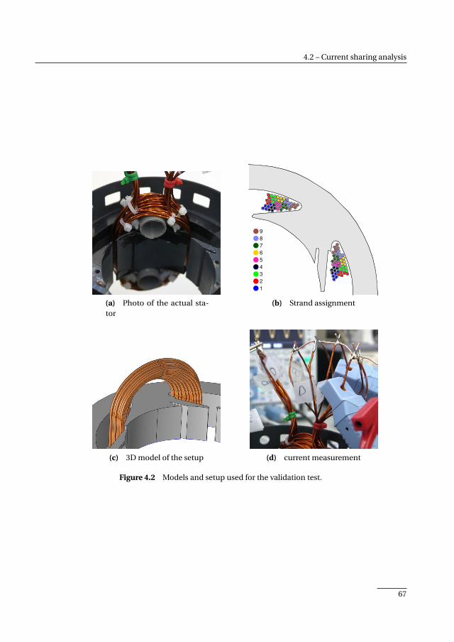
4.2 – Current sharing analysis
(a) Photo of the actual sta-tor
1
2
3
4
5
6
7
8
9
(b) Strand assignment
(c) 3D model of the setup (d) current measurement
Figure 4.2 Models and setup used for the validation test.
67
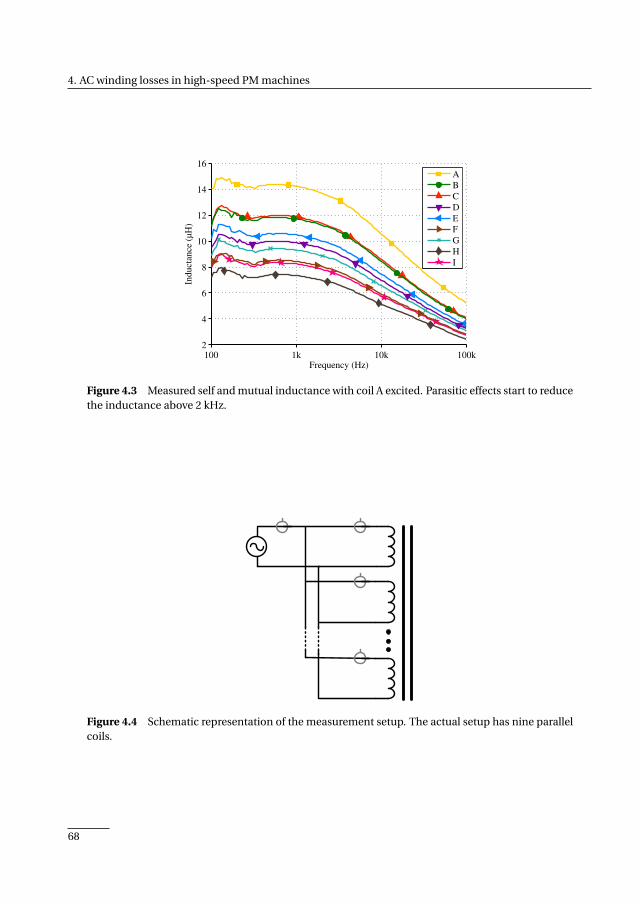
4. AC winding losses in high-speed PM machines
100 1k 10k 100k2
4
6
8
10
12
14
16
Frequency (Hz)
Induct
ance
(µH
)
A
B
C
D
E
F
G
H
I
Figure 4.3 Measured self and mutual inductance with coil A excited. Parasitic effects start to reducethe inductance above 2 kHz.
Figure 4.4 Schematic representation of the measurement setup. The actual setup has nine parallelcoils.
68
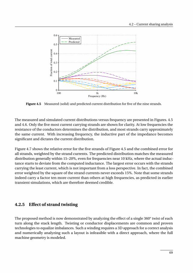
4.2 – Current sharing analysis
100 1k 10k0
0.1
0.2
0.3
0.4
0.5
0.6
Frequency (Hz)
Fra
ctio
n o
f to
tal
curr
ent
Measured
Predicted
Figure 4.5 Measured (solid) and predicted current distribution for five of the nine strands.
The measured and simulated current distributions versus frequency are presented in Figures. 4.5and 4.6. Only the five most current carrying strands are shown for clarity. At low frequencies theresistance of the conductors determines the distribution, and most strands carry approximatelythe same current. With increasing frequency, the inductive part of the impedance becomessignificant and dictates the current distribution.
Figure 4.7 shows the relative error for the five strands of Figure 4.5 and the combined error forall strands, weighted by the strand currents. The predicted distribution matches the measureddistribution generally within 15–20%, even for frequencies near 10 kHz, where the actual induc-tance starts to deviate from the computed inductance. The largest error occurs with the strandscarrying the least current, which is not important from a loss perspective. In fact, the combinederror weighted by the square of the strand currents never exceeds 15%. Note that some strandsindeed carry a factor ten more current than others at high frequencies, as predicted in earliertransient simulations, which are therefore deemed credible.
4.2.5 Effect of strand twisting
The proposed method is now demonstrated by analyzing the effect of a single 360° twist of eachturn along the stack length. Twisting or conductor displacements are common and proventechnologies to equalize imbalances. Such a winding requires a 3D approach for a correct analysisand numerically analyzing such a layout is infeasible with a direct approach, where the fullmachine geometry is modeled.
69
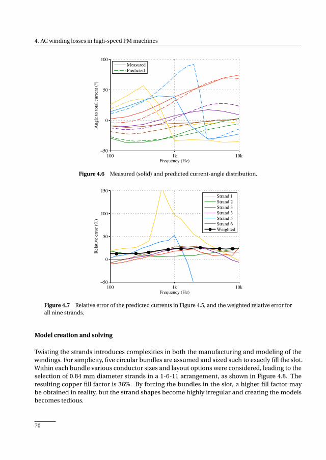
4. AC winding losses in high-speed PM machines
100 1k 10k−50
0
50
100
Frequency (Hz)
Angle
to t
ota
l cu
rren
t (°
)
Measured
Predicted
Figure 4.6 Measured (solid) and predicted current-angle distribution.
100 1k 10k−50
0
50
100
150
Frequency (Hz)
Rel
ativ
e er
ror
(%)
Strand 1
Strand 2
Strand 3
Strand 3
Strand 5
Strand 6
Weighted
Figure 4.7 Relative error of the predicted currents in Figure 4.5, and the weighted relative error forall nine strands.
Model creation and solving
Twisting the strands introduces complexities in both the manufacturing and modeling of thewindings. For simplicity, five circular bundles are assumed and sized such to exactly fill the slot.Within each bundle various conductor sizes and layout options were considered, leading to theselection of 0.84 mm diameter strands in a 1-6-11 arrangement, as shown in Figure 4.8. Theresulting copper fill factor is 36%. By forcing the bundles in the slot, a higher fill factor maybe obtained in reality, but the strand shapes become highly irregular and creating the modelsbecomes tedious.
70
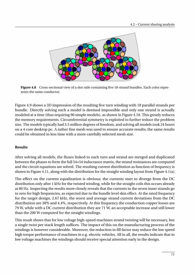
4.2 – Current sharing analysis
Figure 4.8 Cross-sectional view of a slot-side containing five 18-strand bundles. Each color repre-sents the same conductor.
Figure 4.9 shows a 3D impression of the resulting five turn winding with 18 parallel strands perbundle. Directly solving such a model is deemed impossible and only one strand is actuallymodeled at a time (thus requiring 90 simple models), as shown in Figure 4.10. This greatly reducesthe memory requirements. Circumferential symmetry is exploited to further reduce the problemsize. The models typically had 3.5 million degrees of freedom, and solving all models took 24 hourson a 4 core desktop pc. A rather fine mesh was used to ensure accurate results; the same resultscould be obtained in less time with a more carefully selected mesh size.
Results
After solving all models, the fluxes linked to each turn and strand are merged and duplicatedbetween the phases to form the full 54×54 inductance matrix, the strand resistances are computedand the circuit equations are solved. The resulting current distribution as function of frequency isshown in Figure 4.11, along with the distribution for the straight winding layout from Figure 4.1(a).
The effect on the current equalization is obvious; the currents start to diverge from the DCdistribution only after 1 kHz for the twisted winding, while for the straight coils this occurs alreadyat 80 Hz. Inspecting the results more closely reveals that the currents in the seven inner strands goto zero for high frequencies, as expected due to the bundle level skin effect. At the rated frequencyfor the target design, 2.67 kHz, the worst and average strand current deviations from the DCdistribution are 38% and 4.4%, respectively. At this frequency the conduction copper losses are79 W, while with a DC current distribution they are 71 W, an acceptable increase and still lowerthan the 200 W computed for the straight windings.
This result shows that for low voltage high-speed machines strand twisting will be necessary, buta single twist per stack length suffices. The impact of this on the manufacturing process of thewindings is however considerable. Moreover, the reduction in fill factor may reduce the low speedhigh torque performance of machines in e.g. electric vehicles. All in all, the results indicate that inlow voltage machines the windings should receive special attention early in the design.
71
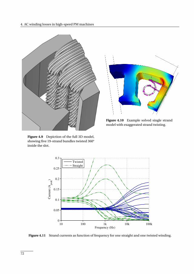
4. AC winding losses in high-speed PM machines
Figure 4.9 Depiction of the full 3D model,showing five 19-strand bundles twisted 360°inside the slot.
Figure 4.10 Example solved single strandmodel with exaggerated strand twisting.
10 100 1k 10k 100k0
0.05
0.1
0.15
0.2
0.25
0.3
Frequency (Hz)
Cu
rren
t (A
pea
k)
Twisted
Straight
Figure 4.11 Strand currents as function of frequency for one straight and one twisted winding.
72
4.3 – Loss reduction techniques
Additional observations
Having determined the 2D and 3D inductance matrices for both twisted and non-twisted windings,a few perhaps interesting observations can be made.
For a non-twisted layout, the self inductance of each coil increases for the machine consideredby some 20–22% due to the end-windings. The mutual inductance between parallel coils on thesame tooth increases slightly less; 18–20%. The mutual inductance between coils of neighboringphases increases by only 6–10%. As a result, the end-windings will act to equalize the currentdistribution across the strands. However, the extent of this effect is insignificant and cannotbe seen as a method to equalize the strand currents, unless an unrealistically short machine isconsidered.
4.3 Loss reduction techniques
The goal of this section is to summarize winding loss reduction methods and numerically comparethe benefits. The focus lies on small high-speed machines.
4.3.1 Background
The additional winding losses due to skin and proximity effects have been known since machinesare widely being used [79]. Various models to compute these losses have been proposed andapplied to show, for instance, the effects of segmentation [80], tooth tip shape [55], parallel strands[76], PWM [57], or the use of foil windings [81].
Using litz wire is a well known strategy from high frequency transformer design and is sometimesalso applied to machines. When using litz wire the number of strands and bundles still needs tobe determined. The individual strands should be no thicker than necessary as the effective copperarea decreases with decreasing strand diameter due to the space required for the insulation. Forhigh-frequency transformers approaches to determine the optimum are presented in [68, 82].High frequency magnetic components are mostly designed with no or small airgaps and, as aresult, have little leakage field inside the slot. The results obtained are then not directly applicableto machines.
Most examples found in literature concern single cases, obscuring the exact benefits and draw-backs of the measures. The aim of this section is to provide more insight into the problem ofeddy current loss reduction methods in high-speed PM machines by systematically analyzing theconsequences of using parallel strands, a reduced slot filling or slot size, or an increased fill factor.A high-speed fractional pitch concentrated non-overlapping winding machine is used as exampleand analyzed with 2D finite element (FE) analysis.
73

4. AC winding losses in high-speed PM machines
Table 4.5 Machine properties
Property Value
Rated power 10 kW
Rated speed 36,000 RPM
Poles 6
Turns/tooth 18
Copper losses 33 W (in-slot)
Iron losses 83 W
Dimensions
Outer radius: 70 mm
Yoke thickness: 12 mm
Slot height: 23 mm
Tooth width: 12.3 mm
Stack length: 41 mm
Tooth tip height: 1.2 mm
Tooth tip span: 75%
Figure 4.12 Cross section of the basic machine.
4.3.2 Example machine
This section presents the SPM machine that will be analyzed. Table 4.5 gives the basic specifica-tions and Figure 4.12 shows a cross section. The rotational speed and power level are those of e.g.an auxiliary generator for a gas turbine. The electrical frequency was deliberately chosen fairlyhigh (1.8 kHz) to enhance eddy current losses in the winding, but it is not unrealistically high.
The initial machine is assumed to have perfect litz wires, and the copper losses are computed witha fill factor of 30%. This gives rise to 33 W of copper losses inside the slots. Only the in-slot copperlosses are considered, because the magnetic field strength inside the slots is higher than in theend-windings, leading to far stronger pronounced loss effects [83]. In addition, the losses insidethe end-windings can be neglected compared to the in-slot part for longer machines, especiallyfor machines with tooth-coil windings.
The following sections aim to find design modifications that allow regular solid strands, placedinside the slots without twisting, to be used. This enables a cost reduction and an increased fillfactor.
4.3.3 Analytical models
The strand level AC copper losses can also be computed analytically, as is demonstrated in e.g.[55, 76]. The difficulty with analytical modeling is to obtain the distribution of the magnetic fieldinside the slots. FE modeling does not suffer from this drawback, but creating and solving models
74
4.3 – Loss reduction techniques
with a large number of strands inside the slots can take a long time. Also, rotor motion cannot beaccounted for with standard time-harmonic models, and transient or multiple specially preparedtime-harmonic models are required instead [60].
An intermediate solution is to use FE models with bulk strand domains to compute the magneticfield inside the slots and compute the AC copper losses afterwards. This allows a quick evaluationof the AC losses for various strand dimensions and slot fill styles. It also allows AC losses to beaccounted for in automated FE-based optimization strategies, where on the one hand the FEmodels should be as simple as possible, while on the other hand all loss mechanisms should betaken into account.
In the field of high-frequency magnetic components, much research exists on AC losses in wind-ings. The induced losses inside a strand subjected to an external magnetic field He are for instancegiven by [66]:
Pstr = ρl H 2Ds with Ds = 2πRe
αr I1(αr )
I0(αr )
(4.3)
where Pstr is the power in one strand, ρ the resistivity, l the length, H the peak of the magnetic
field, α= 1+ jp2ρ
pωµ, r the radius of the strand and I0 and I1 are modified Bessel functions.
To demonstrate the applicability of such an approach, the AC copper losses were computed witha FE model containing the individual strands and using eq. (4.3) together with a simpler FE model.Figure 4.13 shows a strand layout inside the slot along with the losses for each strand, computedin the two ways. A close match can be observed. The asymmetry between the slot sides is theresult of the selected load angle. The total analytically computed losses are 11% less than theFEM predicted losses. Although this is a close match, FEM will be used to calculated strand levelproximity losses throughout the rest of this chapter for maximum accuracy.
75

4. AC winding losses in high-speed PM machinesBlack: Analytical − Red: FEM
0.26
0.12
0.34
0.19
0.32
0.13
0.21
0.14
0.19
0.10
0.13
0.10
0.11
0.07
0.09
0.09
0.06
0.07
0.05
0.05
0.06
0.04
0.04
0.02
0.03
0.03
0.02
0.02
0.03
0.01
0.01
0.02
0.01
0.01
0.00
0.00
0.99
0.42
0.64
0.47
0.39
0.33
0.35
0.28
0.24
0.22
0.21
0.17
0.14
0.13
0.12
0.10
0.10
0.09
0.07
0.07
0.06
0.05
0.05
0.04
0.04
0.03
0.02
0.02
0.03
0.01
0.01
0.02
0.01
0.01
0.00
0.00
0.32
0.16
0.40
0.23
0.36
0.15
0.24
0.16
0.21
0.12
0.15
0.11
0.13
0.08
0.09
0.10
0.07
0.08
0.05
0.05
0.06
0.04
0.04
0.02
0.03
0.03
0.01
0.02
0.03
0.01
0.01
0.02
0.00
0.01
0.00
0.00
1.09
0.49
0.74
0.52
0.44
0.37
0.39
0.31
0.26
0.24
0.23
0.18
0.16
0.14
0.13
0.11
0.10
0.09
0.08
0.07
0.06
0.05
0.05
0.03
0.03
0.04
0.02
0.02
0.03
0.01
0.01
0.02
0.00
0.01
0.00
0.00
Figure 4.13 Individual average strand losses computed semi-analytically (top, black) and withtransient FEM (bottom, red). Total losses: FEM: 5.08 W, Analytical: 4.54 W.
4.3.4 Loss reduction mechanisms
This section considers the effects of the proposed loss reduction schemes.
Parallel strands
If the diameter of a single strand is close to the skin depth, employing several thinner strands inparallel may sufficiently reduce the additional losses. Two disadvantages of using parallel strandsare increased manufacturing complexity and an uneven current distribution across the stands.Advantages over pre-fabricated litz wire are a higher fill factor and reduced cost.
The uneven current sharing among the strands has two causes as pointed out in the previoussection: circulating currents, which are the result of imbalances in the linked field flux; and varia-tions in mutual coupling between the parallel strands, which depend on the winding geometryand cause the imposed current to distribute unevenly. For small machines the differences in theinductance matrix are greater than those in the linked field flux and circulating currents presentno significant problem. To minimize both effects, the impedance of all strands should be assimilar as possible, which can be achieved by placing each strand in various positions inside the
76
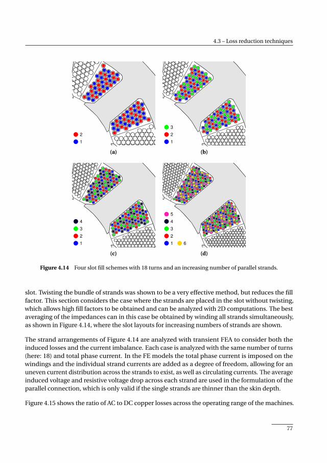
4.3 – Loss reduction techniques
1
2
(a)
1
2
3
(b)
1
2
3
4
(c)
1
2
3
4
5
6
(d)
Figure 4.14 Four slot fill schemes with 18 turns and an increasing number of parallel strands.
slot. Twisting the bundle of strands was shown to be a very effective method, but reduces the fillfactor. This section considers the case where the strands are placed in the slot without twisting,which allows high fill factors to be obtained and can be analyzed with 2D computations. The bestaveraging of the impedances can in this case be obtained by winding all strands simultaneously,as shown in Figure 4.14, where the slot layouts for increasing numbers of strands are shown.
The strand arrangements of Figure 4.14 are analyzed with transient FEA to consider both theinduced losses and the current imbalance. Each case is analyzed with the same number of turns(here: 18) and total phase current. In the FE models the total phase current is imposed on thewindings and the individual strand currents are added as a degree of freedom, allowing for anuneven current distribution across the strands to exist, as well as circulating currents. The averageinduced voltage and resistive voltage drop across each strand are used in the formulation of theparallel connection, which is only valid if the single strands are thinner than the skin depth.
Figure 4.15 shows the ratio of AC to DC copper losses across the operating range of the machines.
77
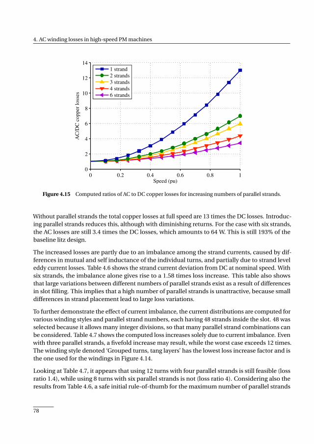
4. AC winding losses in high-speed PM machines
0 0.2 0.4 0.6 0.8 10
2
4
6
8
10
12
14
Speed (pu)
AC
/DC
copper
loss
es
1 strand
2 strands
3 strands
4 strands
6 strands
Figure 4.15 Computed ratios of AC to DC copper losses for increasing numbers of parallel strands.
Without parallel strands the total copper losses at full speed are 13 times the DC losses. Introduc-ing parallel strands reduces this, although with diminishing returns. For the case with six strands,the AC losses are still 3.4 times the DC losses, which amounts to 64 W. This is still 193% of thebaseline litz design.
The increased losses are partly due to an imbalance among the strand currents, caused by dif-ferences in mutual and self inductance of the individual turns, and partially due to strand leveleddy current losses. Table 4.6 shows the strand current deviation from DC at nominal speed. Withsix strands, the imbalance alone gives rise to a 1.58 times loss increase. This table also showsthat large variations between different numbers of parallel strands exist as a result of differencesin slot filling. This implies that a high number of parallel strands is unattractive, because smalldifferences in strand placement lead to large loss variations.
To further demonstrate the effect of current imbalance, the current distributions are computed forvarious winding styles and parallel strand numbers, each having 48 strands inside the slot. 48 wasselected because it allows many integer divisions, so that many parallel strand combinations canbe considered. Table 4.7 shows the computed loss increases solely due to current imbalance. Evenwith three parallel strands, a fivefold increase may result, while the worst case exceeds 12 times.The winding style denoted ‘Grouped turns, tang layers’ has the lowest loss increase factor and isthe one used for the windings in Figure 4.14.
Looking at Table 4.7, it appears that using 12 turns with four parallel strands is still feasible (lossratio 1.4), while using 8 turns with six parallel strands is not (loss ratio 4). Considering also theresults from Table 4.6, a safe initial rule-of-thumb for the maximum number of parallel strands
78

4.3 – Loss reduction techniques
Table 4.6 Relative strand current deviations from the ideal DC distribution and resulting lossincrease
Number ofstrands
Strand current deviationfrom ideal (%)
Additionallosses (%)
1 0 0
2 -2 +6 5
3 +103 -1 +30 126
4 +44 +3 +8 +22 45
5 +126 +45 -3 -3 +50 128
6 +2 +4 +33 +16 +4 +78 58
Table 4.7 Loss increase factors due to unbalanced currents for four winding schemes (all with 48strands per tooth).
filltype
Parallel strands
2 3 4 6 8 12 16 24 48
Grouped cond., random (Fig. 4.1(a)) 3.2 4.4 4.7 6.3 6.2 7.6 8.1 8.6 9.0
Grouped turns, random (4.1(b)) 2.9 5.0 7.1 9.8 8.7 10.0 10.6 10.8 9.0
Grouped turns, tang layers (4.14) 1.3 1.7 1.4 4.0 6.7 5.2 6.9 12.6 9.0
Grouped cond., tang layers (4.1(d)) 2.8 6.5 6.8 6.3 7.6 8.1 8.5 9.1 9.0
when not using equalization methods, would be to use at most half the number of turns asnumber of parallel strands.
Partially filled slots
With semi-closed slots, most leakage flux exists near the slot opening. In addition, a part of the PMflux also leaks close to the slot opening. By using only the rear side of the slot, the total losses maythen be reduced, despite a decrease in slot fill factor. Moreover, to maintain the same numberof turns, thinner strands will be required, further reducing the AC losses. For machines whichrequire transient high-torque operation, such as machines in electric vehicles, this measure maynot be attractive as the thermal capacity of the windings is reduced.
The main benefit of this solution is the reduction of the production cost, since less material isrequired, and regular round enameled wires and simple automatic winding techniques can beused.
The shape of the tooth tips greatly affects the field distribution near the slot opening and thereforealso the AC copper losses. The effect of the main tooth tip dimensions, the span and height, on
79
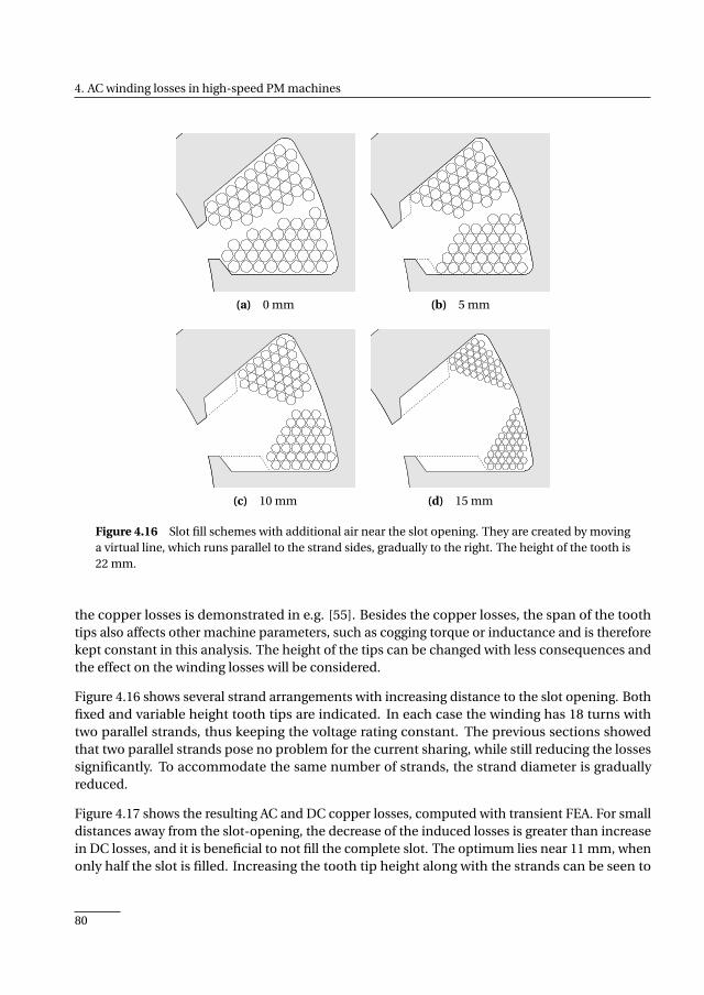
4. AC winding losses in high-speed PM machines
(a) 0 mm (b) 5 mm
(c) 10 mm (d) 15 mm
Figure 4.16 Slot fill schemes with additional air near the slot opening. They are created by movinga virtual line, which runs parallel to the strand sides, gradually to the right. The height of the tooth is22 mm.
the copper losses is demonstrated in e.g. [55]. Besides the copper losses, the span of the toothtips also affects other machine parameters, such as cogging torque or inductance and is thereforekept constant in this analysis. The height of the tips can be changed with less consequences andthe effect on the winding losses will be considered.
Figure 4.16 shows several strand arrangements with increasing distance to the slot opening. Bothfixed and variable height tooth tips are indicated. In each case the winding has 18 turns withtwo parallel strands, thus keeping the voltage rating constant. The previous sections showedthat two parallel strands pose no problem for the current sharing, while still reducing the lossessignificantly. To accommodate the same number of strands, the strand diameter is graduallyreduced.
Figure 4.17 shows the resulting AC and DC copper losses, computed with transient FEA. For smalldistances away from the slot-opening, the decrease of the induced losses is greater than increasein DC losses, and it is beneficial to not fill the complete slot. The optimum lies near 11 mm, whenonly half the slot is filled. Increasing the tooth tip height along with the strands can be seen to
80
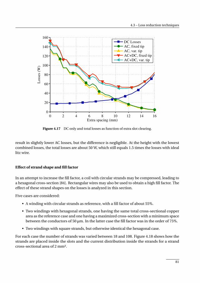
4.3 – Loss reduction techniques
0 2 4 6 8 10 12 14 160
20
40
60
80
100
120
140
160
Extra spacing (mm)
Loss
es (
W)
DC Losses
AC, fixed tip
AC, var. tip
AC+DC, fixed tip
AC+DC, var. tip
Figure 4.17 DC only and total losses as function of extra slot clearing.
result in slightly lower AC losses, but the difference is negligible. At the height with the lowestcombined losses, the total losses are about 50 W, which still equals 1.5 times the losses with ideallitz wire.
Effect of strand shape and fill factor
In an attempt to increase the fill factor, a coil with circular strands may be compressed, leading toa hexagonal cross-section [84]. Rectangular wires may also be used to obtain a high fill factor. Theeffect of these strand shapes on the losses is analyzed in this section.
Five cases are considered:
• A winding with circular strands as reference, with a fill factor of about 55%.
• Two windings with hexagonal strands, one having the same total cross-sectional copperarea as the reference case and one having a maximized cross-section with a minimum spacebetween the conductors of 50 µm. In the latter case the fill factor was in the order of 75%.
• Two windings with square strands, but otherwise identical the hexagonal case.
For each case the number of strands was varied between 18 and 108. Figure 4.18 shows how thestrands are placed inside the slots and the current distribution inside the strands for a strandcross-sectional area of 2 mm².
81
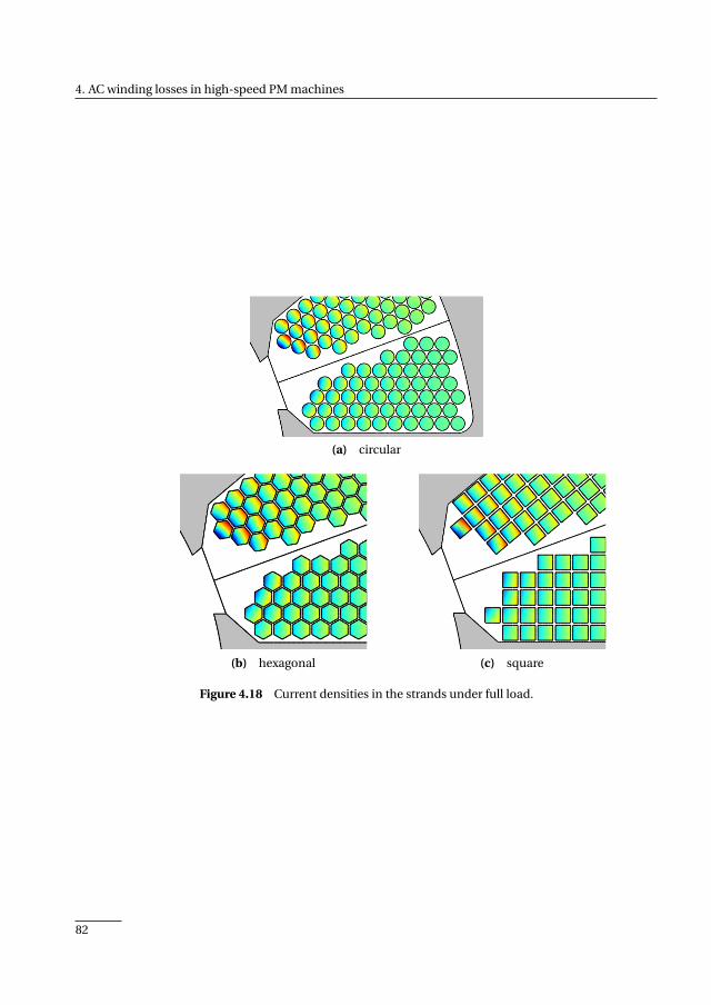
4. AC winding losses in high-speed PM machines
(a) circular
(b) hexagonal (c) square
Figure 4.18 Current densities in the strands under full load.
82
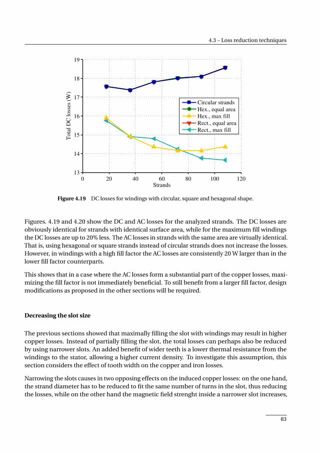
4.3 – Loss reduction techniques
0 20 40 60 80 100 12013
14
15
16
17
18
19
Strands
Tota
l D
C l
oss
es (
W)
Circular strands
Hex., equal area
Hex., max fill
Rect., equal area
Rect., max fill
Figure 4.19 DC losses for windings with circular, square and hexagonal shape.
Figures. 4.19 and 4.20 show the DC and AC losses for the analyzed strands. The DC losses areobviously identical for strands with identical surface area, while for the maximum fill windingsthe DC losses are up to 20% less. The AC losses in strands with the same area are virtually identical.That is, using hexagonal or square strands instead of circular strands does not increase the losses.However, in windings with a high fill factor the AC losses are consistently 20 W larger than in thelower fill factor counterparts.
This shows that in a case where the AC losses form a substantial part of the copper losses, maxi-mizing the fill factor is not immediately beneficial. To still benefit from a larger fill factor, designmodifications as proposed in the other sections will be required.
Decreasing the slot size
The previous sections showed that maximally filling the slot with windings may result in highercopper losses. Instead of partially filling the slot, the total losses can perhaps also be reducedby using narrower slots. An added benefit of wider teeth is a lower thermal resistance from thewindings to the stator, allowing a higher current density. To investigate this assumption, thissection considers the effect of tooth width on the copper and iron losses.
Narrowing the slots causes in two opposing effects on the induced copper losses: on the one hand,the strand diameter has to be reduced to fit the same number of turns in the slot, thus reducingthe losses, while on the other hand the magnetic field strenght inside a narrower slot increases,
83
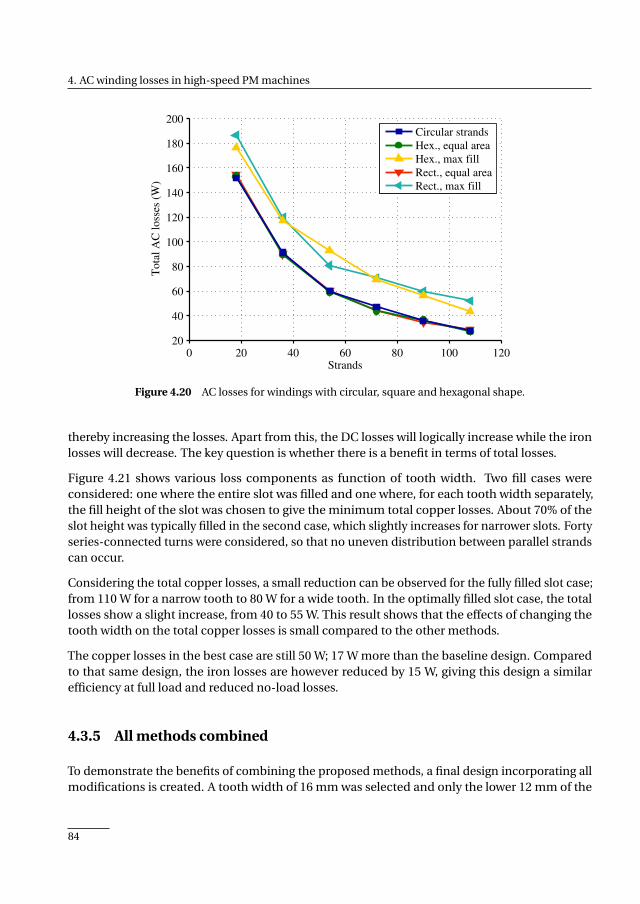
4. AC winding losses in high-speed PM machines
0 20 40 60 80 100 12020
40
60
80
100
120
140
160
180
200
Strands
To
tal
AC
lo
sses
(W
)
Circular strands
Hex., equal area
Hex., max fill
Rect., equal area
Rect., max fill
Figure 4.20 AC losses for windings with circular, square and hexagonal shape.
thereby increasing the losses. Apart from this, the DC losses will logically increase while the ironlosses will decrease. The key question is whether there is a benefit in terms of total losses.
Figure 4.21 shows various loss components as function of tooth width. Two fill cases wereconsidered: one where the entire slot was filled and one where, for each tooth width separately,the fill height of the slot was chosen to give the minimum total copper losses. About 70% of theslot height was typically filled in the second case, which slightly increases for narrower slots. Fortyseries-connected turns were considered, so that no uneven distribution between parallel strandscan occur.
Considering the total copper losses, a small reduction can be observed for the fully filled slot case;from 110 W for a narrow tooth to 80 W for a wide tooth. In the optimally filled slot case, the totallosses show a slight increase, from 40 to 55 W. This result shows that the effects of changing thetooth width on the total copper losses is small compared to the other methods.
The copper losses in the best case are still 50 W; 17 W more than the baseline design. Comparedto that same design, the iron losses are however reduced by 15 W, giving this design a similarefficiency at full load and reduced no-load losses.
4.3.5 All methods combined
To demonstrate the benefits of combining the proposed methods, a final design incorporating allmodifications is created. A tooth width of 16 mm was selected and only the lower 12 mm of the
84
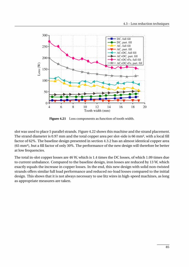
4.3 – Loss reduction techniques
4 6 8 10 12 14 16 18 200
50
100
150
200
250
300
Tooth width (mm)
Lo
ss (
W)
DC, full fill
DC, part. fill
AC, full fill
AC, part. fill
AC+DC, full fill
AC+DC, part. fill
AC+DC+Fe, full fill
AC+DC+Fe, part. fill
Figure 4.21 Loss components as function of tooth width.
slot was used to place 5 parallel strands. Figure 4.22 shows this machine and the strand placement.The strand diameter is 0.97 mm and the total copper area per slot-side is 66 mm², with a local fillfactor of 62%. The baseline design presented in section 4.3.2 has an almost identical copper area(65 mm²), but a fill factor of only 30%. The performance of the new design will therefore be betterat low frequencies.
The total in-slot copper losses are 46 W, which is 1.4 times the DC losses, of which 1.09 times dueto current unbalance. Compared to the baseline design, iron losses are reduced by 13 W, whichexactly equals the increase in copper losses. In the end, this new design with solid non-twistedstrands offers similar full load performance and reduced no-load losses compared to the initialdesign. This shows that it is not always necessary to use litz wires in high-speed machines, as longas appropriate measures are taken.
85
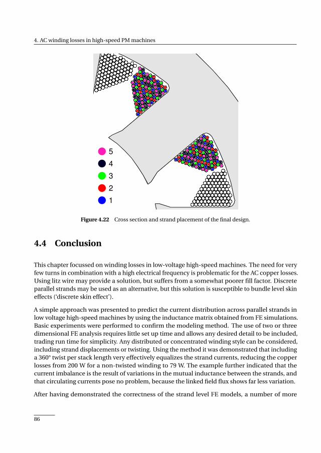
4. AC winding losses in high-speed PM machines
1
2
3
4
5
Figure 4.22 Cross section and strand placement of the final design.
4.4 Conclusion
This chapter focussed on winding losses in low-voltage high-speed machines. The need for veryfew turns in combination with a high electrical frequency is problematic for the AC copper losses.Using litz wire may provide a solution, but suffers from a somewhat poorer fill factor. Discreteparallel strands may be used as an alternative, but this solution is susceptible to bundle level skineffects (‘discrete skin effect’).
A simple approach was presented to predict the current distribution across parallel strands inlow voltage high-speed machines by using the inductance matrix obtained from FE simulations.Basic experiments were performed to confirm the modeling method. The use of two or threedimensional FE analysis requires little set up time and allows any desired detail to be included,trading run time for simplicity. Any distributed or concentrated winding style can be considered,including strand displacements or twisting. Using the method it was demonstrated that includinga 360° twist per stack length very effectively equalizes the strand currents, reducing the copperlosses from 200 W for a non-twisted winding to 79 W. The example further indicated that thecurrent imbalance is the result of variations in the mutual inductance between the strands, andthat circulating currents pose no problem, because the linked field flux shows far less variation.
After having demonstrated the correctness of the strand level FE models, a number of more
86

4.4 – Conclusion
general loss reduction methods were compared, starting from a baseline design using litz wire.Considered were the use of parallel strands, partially filling the slot and changing the tooth width.Of these, the most promising technique is to only partially fill the slots in radial direction. In theexample case, filling only the lower half of the slots limits the copper losses to 150% of those withideal litz wire. Although this is not interesting when a high efficiency is essential, this approachcan be cheaper and has a lower thermal resistivity from the winding core to the ambient thanlitz wire. When using parallel strands the best case losses were 193% of the ideal winding losses.However, compared to partially filling the slots, this approach gives a better total fill factor andhence a larger thermal capacity and lower DC losses, which are beneficial for sustained low-speedor transient operation modes. The benefits of this approach diminish for larger numbers ofparallel strands due to an increasing current imbalance across the strands. A rough rule of thumbto avoid problems with an uneven current distribution across non-twisted parallel strands, is tokeep the number of parallel strands below half the number of turns. For example, with ten turns,no more than five parallel strands should be used. Lastly, using wider teeth hardly changes thecopper losses, but does lower the iron losses and can bring a small benefit in this way.
Techniques to maximize the fill factor are of limited use if they are not combined with the othermethods considered here, because the increased strand area gives rise to more AC copper losses. Ifhowever all of the proposed methods are combined, a design results that has similar performanceas the baseline design with litz wires. This shows that solid copper strands, wound withouttwisting or displacements, can be used in high-speed machines.
Lastly, this chapter only considered the losses at the fundamental frequency, neglecting any time-harmonics in the phase currents. Considering that high-performance machines are commonlydriven by an inverter, the effect of time-harmonics should be given some consideration. This isfurther motivated by the results from Figure 4.11, which shows that even with twisted windings, thestrand currents start to diverge above a few kHz. Therefore, the consequences of time-harmonicsin the phase currents are given further consideration in Chapter 6.
87

CHAPTER 5
Inter-turn faults –modeling, detection and consequences
In fail-safe and fault-tolerant applications, a thorough understanding of all possible faults isnecessary to minimize the risk of those faults occurring. Some faults cannot be intrinsicallyavoided by proper design and additional measures are needed to reduce the consequences ifthose faults occur. Turn-to-turn or inter-turn short circuits in PM machines are an example ofsuch faults. Even though the use of heavy grade multi-layer insulation materials can reducethe likelihood of a turn-to-turn short circuit, this may not suffice and fault detection andmitigation systems will be needed.
This chapter is a detailed study of turn-to-turn faults. Starting with a modeling and analysissection, the consequences of various fault types and turn-turn combinations are considered.The fault currents, losses and other properties are computed for an idealized or completedrive system, allowing the severity of various faults to be compared. Next, a short series ofexperiments is performed to determine the failure mode and behavior of electrical coils. Finally,a fault detector concept is presented, demonstrated with the models from the earlier sections,and validated with lab experiments on two different machines.
Based on
• M. van der Geest, H. Polinder, J. A. Ferreira, A. Veltman, J. J. Wolmarans, and N. Tsiara,“Analysis and Neutral Voltage Based Detection of Inter-Turn Faults in High-SpeedPermanent Magnet Machines with Parallel Strands,” IEEE Trans. Ind. Electron., vol. 62,no. 6, pp. 3862–3873, Jun. 2015; and
• M. van der Geest, H. Polinder, and J. A. Ferreira, “Short-circuit faults in high-speedpm machines with parallel strands and coils,” in Int. Conf. Power Electron. MachinesDrives (PEMD), 2014; and
• M. van der Geest, H. Polinder, and J. A. Ferreira, “Experimental determination of statorwinding failure behavior,” in 16th European Conf. Power Electron. Appl. (EPE-ECCEEurope), 2014.
89
5. Inter-turn faults – modeling, detection and consequences
5.1 Introduction
Electrical drives in safety critical applications, such as those in automotive or aerospace systems,should exhibit a high system availability. One approach to achieve a high availability is to designfor a high reliability of the individual components that make up a system by using overrating.Examples are employing a higher grade winding insulation material than strictly necessary, orover-dimensioning the cooling system. In addition to, or as an alternative to overrating, a systemcan be made fault-tolerant. A fault-tolerant system can continue to (partially) function in thepresence of faults. To achieve this, possible failure modes are identified and the design is adaptedto handle such faults. Aerospace drive systems are a clear example of fault-tolerant systems. Inthese systems, both the electrical machine and the inverter can be implemented as multipleisolated and independent single or three phase subsystems [85–87]. By ensuring a completethermal, magnetic and electrical isolation between those systems, the failure of one subsystemdoes not affect other subsystems. Still, when a fault occurs, taking corrective actions can furtherreduce post fault risks such as fire hazards; improve performance, such as reducing torque rippleor power loss; or generally ensure a predictable post-fault state.
A particular problem with PM generators are short circuits, since the magnets cannot be disabled.Turn-to-turn (inter-turn) short circuits are especially dangerous, because the local short circuitcurrents can greatly exceed those caused by terminal short circuits [88], leading to rapid machinefailure. In many fault-tolerant drive systems inter-turn faults are dealt with by designing themachine to have a one per-unit inductance, leading to a terminal short circuit current equal to therated current. After the occurrence and detection of an inter-turn fault, the affected phase is shortcircuited at the terminals, ideally reducing the fault current to the nominal value [81, 86, 89, 90].An alternative approach is to not act after an inter-turn fault and relying on the design to reach asafe, non-functional steady state.
So, in the development of a fail-safe or fault-tolerant machine, a number of questions must beanswered:
• How large are the expected short circuit currents and how do they affect the total drivesystem?
• How does an unmitigated fault evolve? And, strongly related;
• How much time is available to detect a fault?
• How can faults be detected?
• How effectively can a terminal level short circuit suppress the local short circuit currents?
This chapter will address these topics. To this end, models will be created, partially based on themodeling method described and tested in Chapter 4, and used to estimate the fault currents andlosses for turn-to-turn faults in single strands, between parallel strands and between neighboringphase coils, with account of the position of the short circuit inside the slot. Contributions arethe level of detail that is considered and the fact that short circuits between parallel strands arealso considered. Next, experiments are performed on coils to determine basic failure behavior,
90
5.1 – Introduction
providing insight into the failure process of coils. Lastly, a novel fault detector is proposed, whichis simple enough for hardware implementation as an independent observer, but cannot locate oridentify faults. The detection concept is demonstrated with simulations and experiments. Theresults presented in this chapter will ultimately improve the understanding of (the detection of)turn level faults in electrical machines.
All of these items have been addressed in literature in one way or another. What now follows is anoverview of relevant work with regards to modeling, detection and mitigation of faults.
5.1.1 Modeling of short circuits
Short circuits at a turn level can be modeled in various ways, with a tradeoff between simplicityand level of detail. At the simplest level, the impedances of the healthy and faulty parts of thewinding are computed as a fraction of the total healthy impedance. Although this approach doesnot consider the effect of strand shape and position inside the slot, it can be used to quicklyestimate faulted machine performance. For a more detailed analysis, fully analytical methods[91–93], magnetic equivalent circuits [88, 94, 95], or finite element analysis (FEA) [96–98] can beused. Analytical models accounting for individual layered turns are described in [78,89], and showthat vertical strip layers can very effectively suppress fault currents, but are prone to proximityeffect losses. Ref. [76] presents a model to compute turn level windings properties with circularstrands, but does not compute fault behavior.
5.1.2 Fault detection
For the detection of short circuits, a large variety of systems has been proposed, differing incomplexity, sensitivity and fault identification abilities [99]. A somewhat older approach is tocompute the negative sequence component of the line currents for voltage fed machines, or thevoltages for current fed machines [100]. Instead of computing the negative sequence componentfrom the terminal quantities, the zero sequence component may be measured at the neutralpoint of the machine, which is simpler and slightly more sensitive [101–103]. Other frequencycomponents in the synchronous reference frame can also indicate faults, particulary for multi-phase machines[104]. Applying time-frequency or wavelet methods to the terminal quantitiesyields a more sensitive system, but is also computationally intense [105–107]. Nature inspiredmethods such as neural networks [108] or ant clustering [109] potentially offer high sensitivitywith limited complexity. Model based fault detection is yet another approach, but requiresextensive knowledge about the machine parameters [97, 110], although Kalman filtering canimprove performance[111].
Many detection methods are passive, using only existing terminal level voltages or currents todetermine the state of the machine. Such a method can be added to an existing drive system withfew modifications, but perhaps the major disadvantage is the dependency of the sensitivity onmotor speed. By injecting excitation signals, faults can be detected even at stand-still [112, 113],
91
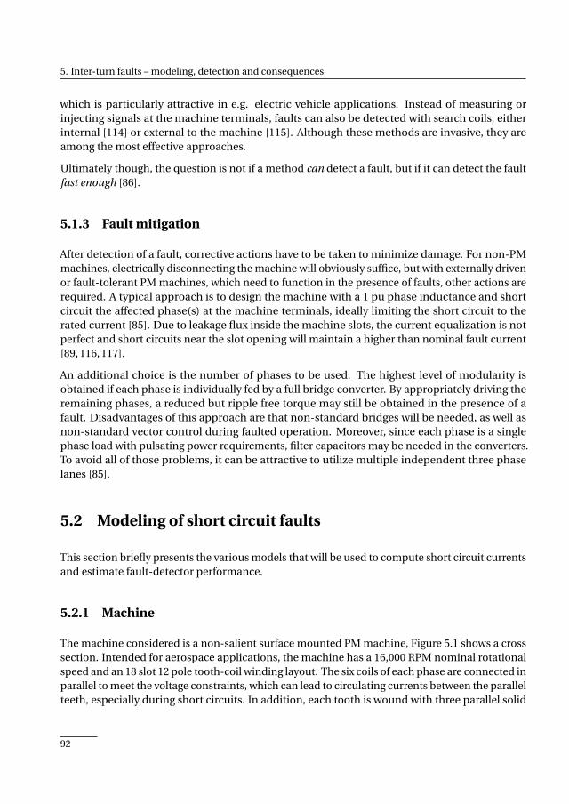
5. Inter-turn faults – modeling, detection and consequences
which is particularly attractive in e.g. electric vehicle applications. Instead of measuring orinjecting signals at the machine terminals, faults can also be detected with search coils, eitherinternal [114] or external to the machine [115]. Although these methods are invasive, they areamong the most effective approaches.
Ultimately though, the question is not if a method can detect a fault, but if it can detect the faultfast enough [86].
5.1.3 Fault mitigation
After detection of a fault, corrective actions have to be taken to minimize damage. For non-PMmachines, electrically disconnecting the machine will obviously suffice, but with externally drivenor fault-tolerant PM machines, which need to function in the presence of faults, other actions arerequired. A typical approach is to design the machine with a 1 pu phase inductance and shortcircuit the affected phase(s) at the machine terminals, ideally limiting the short circuit to therated current [85]. Due to leakage flux inside the machine slots, the current equalization is notperfect and short circuits near the slot opening will maintain a higher than nominal fault current[89, 116, 117].
An additional choice is the number of phases to be used. The highest level of modularity isobtained if each phase is individually fed by a full bridge converter. By appropriately driving theremaining phases, a reduced but ripple free torque may still be obtained in the presence of afault. Disadvantages of this approach are that non-standard bridges will be needed, as well asnon-standard vector control during faulted operation. Moreover, since each phase is a singlephase load with pulsating power requirements, filter capacitors may be needed in the converters.To avoid all of those problems, it can be attractive to utilize multiple independent three phaselanes [85].
5.2 Modeling of short circuit faults
This section briefly presents the various models that will be used to compute short circuit currentsand estimate fault-detector performance.
5.2.1 Machine
The machine considered is a non-salient surface mounted PM machine, Figure 5.1 shows a crosssection. Intended for aerospace applications, the machine has a 16,000 RPM nominal rotationalspeed and an 18 slot 12 pole tooth-coil winding layout. The six coils of each phase are connected inparallel to meet the voltage constraints, which can lead to circulating currents between the parallelteeth, especially during short circuits. In addition, each tooth is wound with three parallel solid
92
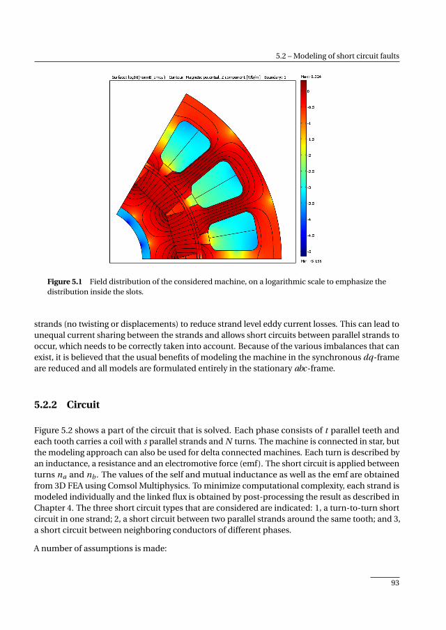
5.2 – Modeling of short circuit faults
Figure 5.1 Field distribution of the considered machine, on a logarithmic scale to emphasize thedistribution inside the slots.
strands (no twisting or displacements) to reduce strand level eddy current losses. This can lead tounequal current sharing between the strands and allows short circuits between parallel strands tooccur, which needs to be correctly taken into account. Because of the various imbalances that canexist, it is believed that the usual benefits of modeling the machine in the synchronous dq-frameare reduced and all models are formulated entirely in the stationary abc-frame.
5.2.2 Circuit
Figure 5.2 shows a part of the circuit that is solved. Each phase consists of t parallel teeth andeach tooth carries a coil with s parallel strands and N turns. The machine is connected in star, butthe modeling approach can also be used for delta connected machines. Each turn is described byan inductance, a resistance and an electromotive force (emf). The short circuit is applied betweenturns na and nb . The values of the self and mutual inductance as well as the emf are obtainedfrom 3D FEA using Comsol Multiphysics. To minimize computational complexity, each strand ismodeled individually and the linked flux is obtained by post-processing the result as described inChapter 4. The three short circuit types that are considered are indicated: 1, a turn-to-turn shortcircuit in one strand; 2, a short circuit between two parallel strands around the same tooth; and 3,a short circuit between neighboring conductors of different phases.
A number of assumptions is made:
93
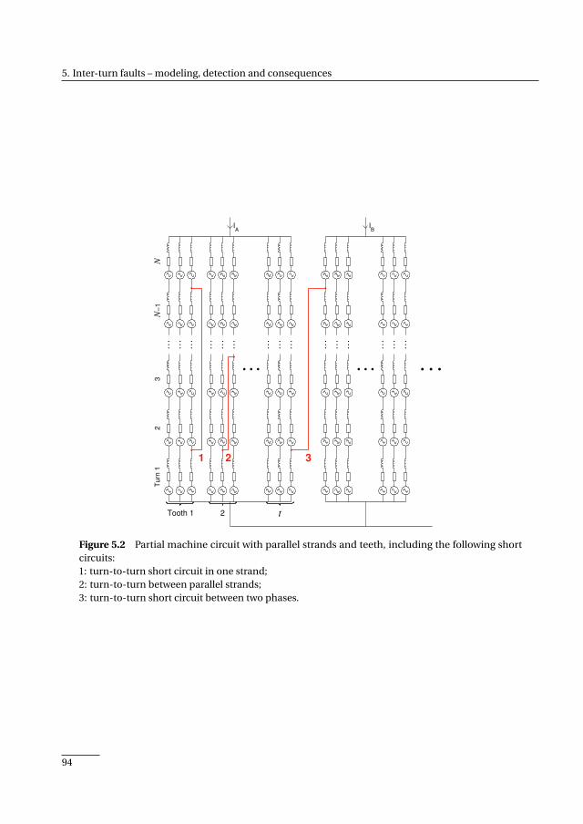
5. Inter-turn faults – modeling, detection and consequences
IA
IB
Tu
rn 1
23
N−
1N
Tooth 1 2 t
1 2 3
Figure 5.2 Partial machine circuit with parallel strands and teeth, including the following shortcircuits:1: turn-to-turn short circuit in one strand;2: turn-to-turn between parallel strands;3: turn-to-turn short circuit between two phases.
94

5.2 – Modeling of short circuit faults
1 2 3 4 5
67891011
12 13 14 15 16 17 18
192021222324
25 26 27 28 29 30
313233343536
37 38 39 40 41
42434445
46 47
4849
1 2 3 4 5
67891011
12 13 14 15 16 17
18192021222324
25 26 27 28 29 30
313233343536
37 38 39 40 41
424344
45 46 47
4849
Figure 5.3 Strand and turn locations inside the slot. Blue, red and green turns belong to strands 1,2 and 3, respectively.
• Only one simultaneous short circuit is considered.
• The external short circuit impedance is described by a resistance with value Rs (in additionto the turn resistance).
• The temperature (resistance) is held constant and fault propagation is not considered. Thisrepresents a short circuit immediately after it occurred.
• In the FE models, each turn is modeled as a closed loop. That is, the small diagonaldisplacements present in an actual winding are ignored.
• The short circuit is assumed to exist, without considering the cause.
• The number of parallel teeth, t , is 6, the number of parallel strands, s, is 3 and turns/toothN =49.
• The back-emf is sinusoidal.
• The iron is considered to be linear and constant inductance terms are used, based on thefact that a short circuit current opposes the inducing flux.
• Eddy current losses in the winding are ignored.
All combinations in terms of start turn and end turn of the fault will be considered. To this end,the turns are numbered as shown in Figure 5.3. In reality the exact position of each turn can varyby a few strand diameters, changing the short circuit properties, but this approach still allowstrends to be identified.
5.2.3 Time-harmonic model
Time-harmonic (frequency domain) models at the synchronous frequency with ideal currentsource excitation allow a quick estimation of the steady state currents and losses for all short
95
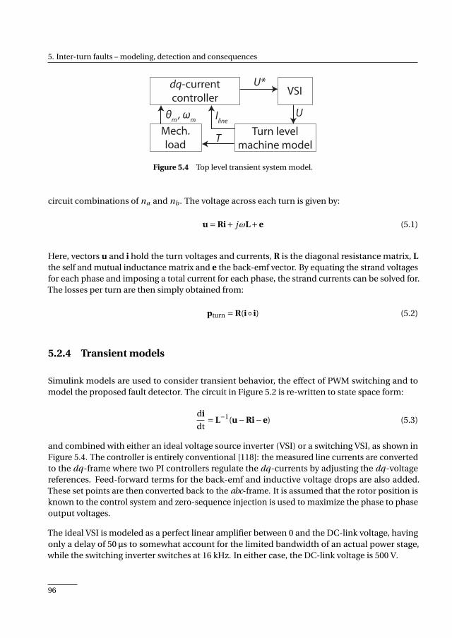
5. Inter-turn faults – modeling, detection and consequences
dq-currentcontroller
VSI
Turn levelmachine model
U*
UIlineθm , ωm
Mech.load T
Figure 5.4 Top level transient system model.
circuit combinations of na and nb . The voltage across each turn is given by:
u = Ri+ jωL+e (5.1)
Here, vectors u and i hold the turn voltages and currents, R is the diagonal resistance matrix, Lthe self and mutual inductance matrix and e the back-emf vector. By equating the strand voltagesfor each phase and imposing a total current for each phase, the strand currents can be solved for.The losses per turn are then simply obtained from:
pturn = R(i i) (5.2)
5.2.4 Transient models
Simulink models are used to consider transient behavior, the effect of PWM switching and tomodel the proposed fault detector. The circuit in Figure 5.2 is re-written to state space form:
di
dt= L−1(u−Ri−e) (5.3)
and combined with either an ideal voltage source inverter (VSI) or a switching VSI, as shown inFigure 5.4. The controller is entirely conventional [118]: the measured line currents are convertedto the dq-frame where two PI controllers regulate the dq-currents by adjusting the dq-voltagereferences. Feed-forward terms for the back-emf and inductive voltage drops are also added.These set points are then converted back to the abc-frame. It is assumed that the rotor position isknown to the control system and zero-sequence injection is used to maximize the phase to phaseoutput voltages.
The ideal VSI is modeled as a perfect linear amplifier between 0 and the DC-link voltage, havingonly a delay of 50 µs to somewhat account for the limited bandwidth of an actual power stage,while the switching inverter switches at 16 kHz. In either case, the DC-link voltage is 500 V.
96
5.3 – Analysis of short circuit faults
5.3 Analysis of short circuit faults
Now, the various short circuit cases will be compared in terms of severity and the time-harmonicand transient models are compared.
5.3.1 Parametric exploration
Three measures are relevant when considering the faulted copper losses. Firstly, the total lossesare important as they determine the expected braking torque and torque ripple (remember that ashort circuit is a single phase load, and as such will always cause a 100% torque ripple). Secondly,the maximum losses per turn are relevant because these relate to the localized temperature rise,which in turn determines the time available for detection of the fault. Lastly, if a terminal shortcircuit is used as safety measure in fault-tolerant or fail-safe applications, the per-turn lossesafter applying a terminal short circuit are relevant because they indicate how effectively the faultcurrent can be suppressed. These aspects will now be discussed individually for the three shortcircuit cases shown in Figure 5.2.
Single strand short circuit faults
A short circuit inside a single strand is indicated in Figure 5.2 by number 1 and is the most likelyturn-to-turn short circuit to occur in machines with one solid strand.
Figure 5.5(a) shows the total copper losses for this short circuit under nominal load and with aperfect short circuit (Rs = 0) for all combinations of na and nb , with the short circuit occurringin strand 1. Refer to Figure 5.3 for the turn and strand numbers. The diagonal in Figure 5.5(a),na = nb , indicates that only that turn is shorted. All turn combinations are shown, even though ashort circuit will most likely occur for turns directly adjacent to each other inside the slot.
In this example, the maximum total losses are 8 kW and occur for a difference of |na −nb | = 6,and are largely independent of the location of the short circuit along the length of the coil.With less turns involved, the turn resistance limits the fault current and a short circuit acrossmore turns leads to linearly increasing losses. For larger |na −nb |, the inductance becomes thelimiting impedance and both the short circuit current and total losses reduce due to the squaredrelationship between inductance and the number of shorted turns. As an indication, the singleturn impedance at the synchronous frequency is 6.8–8 mΩ + j3–5 mΩ.
Figure 5.5(b) shows the maximum losses per turn for all turn-to-turn combinations. For singleturn short circuits, the largest losses are in the range of 1.7—1.9 kW/turn, with current densitiesin the range of 0.8–1 kA/mm². The electrical position of the short circuit along the strand againhas little impact on the magnitude of the losses.
To emphasize these numbers, the initial temperature rise of the shorted turn is in the orderof several thousands K/s when assuming adiabatic heating. If a temporary 200 K increase is
97

5. Inter-turn faults – modeling, detection and consequences
na
nb
5 10 15 20 25 30 35 40 45
5
10
15
20
25
30
35
40
45
0
1
2
3
4
5
6
7
8
(a) Total losses (kW) under nominal load
na
nb
5 10 15 20 25 30 35 40 45
5
10
15
20
25
30
35
40
45
0
0.2
0.4
0.6
0.8
1
1.2
1.4
1.6
1.8
(b) Maximum per strand losses (kW) undernominal load
10
20
30
40
0
10
20
30
40
50
0
20
40
60
80
100
na
nb
Max
imu
m l
oss
es p
er t
urn
aft
er s
ho
rt−
circ
uit
(W
)
(c) Maximum per-turn losses (W) after mit-igation action (terminal short circuit)
Figure 5.5 Copper losses in the presence of a single strand turn-to-turn short circuit, versus startturn and end turn of the short circuit. The axis numbers refer to the turn numbers in Figure 5.3.
98

5.3 – Analysis of short circuit faults
acceptable, the available detection time is in the order of 100 ms, or 160 electrical periods. Thesenumbers clearly show that assuming a constant resistance will quickly overestimate the faultedlosses. However, the models are still useful to compare all short circuit cases and provide arough figure for the available detection time. It should be noted that this specific machine has afundamental frequency of 1600 Hz. Since the turn resistance limits the fault current with veryfew turns involved, the losses depend on the square of the frequency and in e.g. line-connectedmachines the temperature rise rate will be considerably lower.
These losses are partially so large because the healthy and shorted parts of the affected strandbehave as an autotransformer, with the healthy phase coils on the other five teeth acting as anexcitation source, in addition to the PM flux directly linked with the faulted tooth. Therefore, afew amperes from the healthy coils may induce several tens of amperes in the shorted strands,depending on which turns are affected. If the inverter is driving current into the machine, thiswill even further increase the losses. Note that with a short circuit across nearly all turns (from e.g.1 to 48 of 49) the losses in the shorted strands are nearly nominal as the inductance is leading inlimiting the fault current magnitude. The other teeth of the same phase will however be shortcircuited by the few remaining turns. Because the impedance of a single turn is far smaller thanthe impedance of an entire coil, the current is limited by the feeding coils. Hence, increasing thenumber of parallel machine sections increases the short circuit losses. With 1, 2, 3 or 4 sections,the losses are 2, 11, 29 and 55 W/turn, respectively. This should be kept in mind when machineswith a very large number of parallel sections are considered. One solution would be to drive eachsection from an individual inverter with independent current control.
Strand-to-strand short circuits
A strand-to-strand short circuit between parallel strands around one tooth is indicated in Fig-ure 5.2 by number 2. The fault current is driven by a voltage difference between the turns thatcome into contact; in an ideal machine, a short circuit between two strands at the same turn doesnot lead to any fault current. With this specific fault, the short circuit current forms a closed pathvia the terminals and is therefore limited by the resistance and leakage inductance of each turnencountered. As a result, a short circuit with a turn difference of e.g. five turns will lead to a largerfault current if it occurs between turns 1 and 6 than between turns 20 and 25. In the latter casethe total losses may be higher though, as more turns carry the fault current.
Figure 5.6(a) shows the total copper losses for all possible turn-turn combinations between thefirst two strands. Along the diagonal line na = nb –where the voltage difference between the turnswill be minimal– the losses are indeed near zero. When the difference in turn number |na −nb |increases, the fault losses increase as well, indicating that the short circuit current is still (partially)limited by ohmic resistance. The maximum losses are again in the order of 8 kW and occur for|na −nb | =10–13, but only near the electrical middle of the coil.
Figure 5.6(b) shows the maximum per-turn losses. Note the large differences to Figure 5.5(b).The largest loss is now 1 kW, about half that of a single strand short circuit, and only occurs for
99

5. Inter-turn faults – modeling, detection and consequences
na in strand 1
nb i
n s
trand 2
5 10 15 20 25 30 35 40 45
5
10
15
20
25
30
35
40
45
0
1
2
3
4
5
6
7
8
(a) Total losses (kW) under nominal load
na in strand 1
nb i
n s
tran
d 2
5 10 15 20 25 30 35 40 45
5
10
15
20
25
30
35
40
45
0
0.1
0.2
0.3
0.4
0.5
0.6
0.7
0.8
(b) Maximum per turn losses (kW) undernominal load
10
20
30
40
0
10
20
30
40
50
0
2
4
6
8
10
na in strand 1n
b in strand 2
Max
imum
loss
es p
er t
urn
aft
er s
hort
−ci
rcuit
(W
)
(c) Maximum per turn losses (W) after miti-gation action
Figure 5.6 Copper losses versus start turn and end turn of a short circuit between parallel strandsaround one tooth.
100
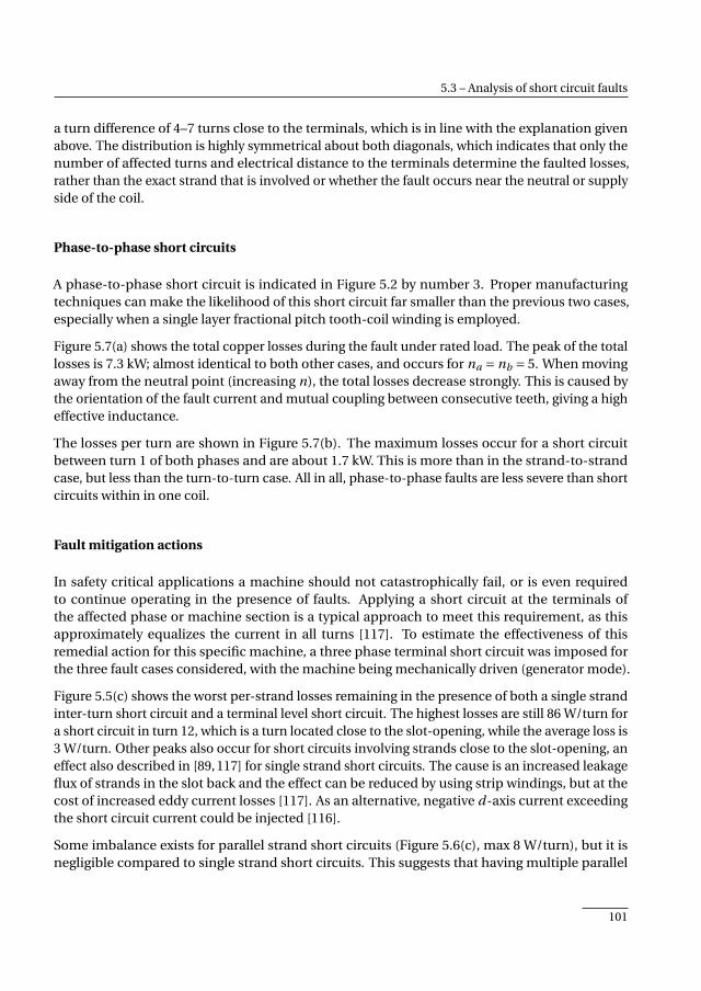
5.3 – Analysis of short circuit faults
a turn difference of 4–7 turns close to the terminals, which is in line with the explanation givenabove. The distribution is highly symmetrical about both diagonals, which indicates that only thenumber of affected turns and electrical distance to the terminals determine the faulted losses,rather than the exact strand that is involved or whether the fault occurs near the neutral or supplyside of the coil.
Phase-to-phase short circuits
A phase-to-phase short circuit is indicated in Figure 5.2 by number 3. Proper manufacturingtechniques can make the likelihood of this short circuit far smaller than the previous two cases,especially when a single layer fractional pitch tooth-coil winding is employed.
Figure 5.7(a) shows the total copper losses during the fault under rated load. The peak of the totallosses is 7.3 kW; almost identical to both other cases, and occurs for na = nb = 5. When movingaway from the neutral point (increasing n), the total losses decrease strongly. This is caused bythe orientation of the fault current and mutual coupling between consecutive teeth, giving a higheffective inductance.
The losses per turn are shown in Figure 5.7(b). The maximum losses occur for a short circuitbetween turn 1 of both phases and are about 1.7 kW. This is more than in the strand-to-strandcase, but less than the turn-to-turn case. All in all, phase-to-phase faults are less severe than shortcircuits within in one coil.
Fault mitigation actions
In safety critical applications a machine should not catastrophically fail, or is even requiredto continue operating in the presence of faults. Applying a short circuit at the terminals ofthe affected phase or machine section is a typical approach to meet this requirement, as thisapproximately equalizes the current in all turns [117]. To estimate the effectiveness of thisremedial action for this specific machine, a three phase terminal short circuit was imposed forthe three fault cases considered, with the machine being mechanically driven (generator mode).
Figure 5.5(c) shows the worst per-strand losses remaining in the presence of both a single strandinter-turn short circuit and a terminal level short circuit. The highest losses are still 86 W/turn fora short circuit in turn 12, which is a turn located close to the slot-opening, while the average loss is3 W/turn. Other peaks also occur for short circuits involving strands close to the slot-opening, aneffect also described in [89, 117] for single strand short circuits. The cause is an increased leakageflux of strands in the slot back and the effect can be reduced by using strip windings, but at thecost of increased eddy current losses [117]. As an alternative, negative d-axis current exceedingthe short circuit current could be injected [116].
Some imbalance exists for parallel strand short circuits (Figure 5.6(c), max 8 W/turn), but it isnegligible compared to single strand short circuits. This suggests that having multiple parallel
101
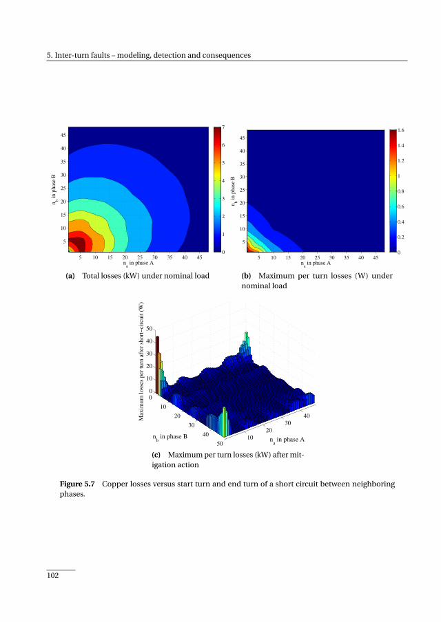
5. Inter-turn faults – modeling, detection and consequences
na in phase A
nb i
n p
has
e B
5 10 15 20 25 30 35 40 45
5
10
15
20
25
30
35
40
45
0
1
2
3
4
5
6
7
(a) Total losses (kW) under nominal load
na in phase A
nb i
n p
has
e B
5 10 15 20 25 30 35 40 45
5
10
15
20
25
30
35
40
45
0
0.2
0.4
0.6
0.8
1
1.2
1.4
1.6
(b) Maximum per turn losses (W) undernominal load
10
20
30
40
0
10
20
30
40
50
0
10
20
30
40
50
na in phase An
b in phase B
Max
imum
loss
es p
er t
urn
aft
er s
hort
−ci
rcuit
(W
)
(c) Maximum per turn losses (kW) after mit-igation action
Figure 5.7 Copper losses versus start turn and end turn of a short circuit between neighboringphases.
102
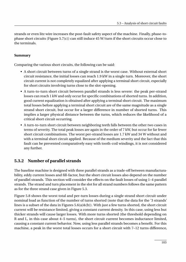
5.3 – Analysis of short circuit faults
strands or even litz wire increases the post-fault safety aspect of the machine. Finally, phase-to-phase short circuits (Figure 5.7(c)) can still induce 45 W/turn if the short circuits occur close tothe terminals.
Summary
Comparing the various short circuits, the following can be said:
• A short circuit between turns of a single strand is the worst case. Without external shortcircuit resistance, the initial losses can reach 1.9 kW in a single turn. Moreover, the shortcircuit current is not completely equalized after applying a terminal short circuit, especiallyfor short circuits involving turns close to the slot-opening.
• A turn-to-turn short circuit between parallel strands is less severe: the peak per-strandlosses can reach 1 kW and only occur for specific combinations of shorted turns. In addition,good current equalization is obtained after applying a terminal short circuit. The maximumtotal losses before applying a terminal short circuit are of the same magnitude as a singlestrand short circuit, but occur for a larger difference in number of shorted turns. Thisimplies a larger physical distance between the turns, which reduces the likelihood of acritical short circuit occurring.
• A turn-to-turn short circuit between neighboring teeth falls between the other two cases interms of severity. The total peak losses are again in the order of 7 kW, but occur for far fewershort circuit combinations. The worst per-strand losses are 1.7 kW and 34 W without andwith a terminal short circuit applied. Because of the medium severity and the fact that thisfault can be prevented comparatively easy with tooth-coil windings, it is not consideredany further.
5.3.2 Number of parallel strands
The baseline machine is designed with three parallel strands as a trade-off between manufactura-bility, eddy current losses and fill-factor, but the short circuit losses also depend on the numberof parallel strands. This section will consider the effects on the fault losses of using 1–4 parallelstrands. The strand and turn placement in the slot for all strand numbers follows the same patternas for the three strand case given in Figure 5.3.
Figure 5.8 shows the worst total and per-turn losses during a single strand short circuit undernominal load as function of the number of turns shorted (note that the data for the ’3 strands’lines is a subset of the data in Figures 5.6(a)&(b)). With just a few turns shorted, the short circuitcurrent will be resistance limited, giving a constant current density. In this case, using less butthicker strands will cause larger losses. With more turns shorted (the threshold depending onR and L, in this case about 4–5 turns), the short circuit current becomes inductance limited,causing a constant current behavior. Now, using less parallel strands becomes a benefit. For thismachine, a peak in the worst total losses occurs for a short circuit with 7–12 turns difference,
103
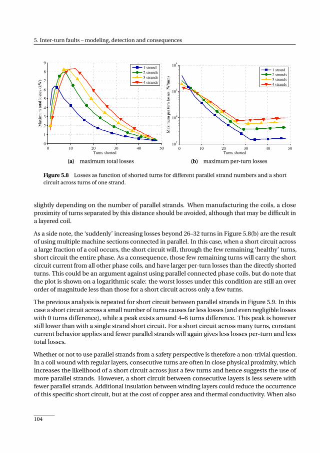
5. Inter-turn faults – modeling, detection and consequences
0 10 20 30 40 500
1
2
3
4
5
6
7
8
9
Turns shorted
Maxim
um
tota
l lo
sses
(kW
)
1 strand
2 strands
3 strands
4 strands
(a) maximum total losses
0 10 20 30 40 5010
1
102
103
104
Turns shorted
Max
imum
per
turn
loss
es (
W/t
urn
)
1 strand
2 strands
3 strands
4 strands
(b) maximum per-turn losses
Figure 5.8 Losses as function of shorted turns for different parallel strand numbers and a shortcircuit across turns of one strand.
slightly depending on the number of parallel strands. When manufacturing the coils, a closeproximity of turns separated by this distance should be avoided, although that may be difficult ina layered coil.
As a side note, the ‘suddenly’ increasing losses beyond 26–32 turns in Figure 5.8(b) are the resultof using multiple machine sections connected in parallel. In this case, when a short circuit acrossa large fraction of a coil occurs, the short circuit will, through the few remaining ‘healthy’ turns,short circuit the entire phase. As a consequence, those few remaining turns will carry the shortcircuit current from all other phase coils, and have larger per-turn losses than the directly shortedturns. This could be an argument against using parallel connected phase coils, but do note thatthe plot is shown on a logarithmic scale: the worst losses under this condition are still an overorder of magnitude less than those for a short circuit across only a few turns.
The previous analysis is repeated for short circuit between parallel strands in Figure 5.9. In thiscase a short circuit across a small number of turns causes far less losses (and even negligible losseswith 0 turns difference), while a peak exists around 4–6 turns difference. This peak is howeverstill lower than with a single strand short circuit. For a short circuit across many turns, constantcurrent behavior applies and fewer parallel strands will again gives less losses per-turn and lesstotal losses.
Whether or not to use parallel strands from a safety perspective is therefore a non-trivial question.In a coil wound with regular layers, consecutive turns are often in close physical proximity, whichincreases the likelihood of a short circuit across just a few turns and hence suggests the use ofmore parallel strands. However, a short circuit between consecutive layers is less severe withfewer parallel strands. Additional insulation between winding layers could reduce the occurrenceof this specific short circuit, but at the cost of copper area and thermal conductivity. When also
104
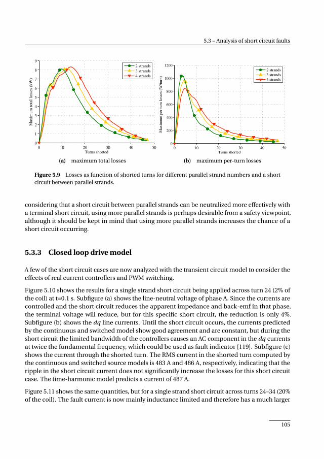
5.3 – Analysis of short circuit faults
0 10 20 30 40 500
1
2
3
4
5
6
7
8
9
Turns shorted
Maxim
um
tota
l lo
sses
(kW
)
2 strands
3 strands
4 strands
(a) maximum total losses
0 10 20 30 40 500
200
400
600
800
1000
1200
Turns shorted
Max
imu
m p
er t
urn
lo
sses
(W
/tu
rn)
2 strands
3 strands
4 strands
(b) maximum per-turn losses
Figure 5.9 Losses as function of shorted turns for different parallel strand numbers and a shortcircuit between parallel strands.
considering that a short circuit between parallel strands can be neutralized more effectively witha terminal short circuit, using more parallel strands is perhaps desirable from a safety viewpoint,although it should be kept in mind that using more parallel strands increases the chance of ashort circuit occurring.
5.3.3 Closed loop drive model
A few of the short circuit cases are now analyzed with the transient circuit model to consider theeffects of real current controllers and PWM switching.
Figure 5.10 shows the results for a single strand short circuit being applied across turn 24 (2% ofthe coil) at t=0.1 s. Subfigure (a) shows the line-neutral voltage of phase A. Since the currents arecontrolled and the short circuit reduces the apparent impedance and back-emf in that phase,the terminal voltage will reduce, but for this specific short circuit, the reduction is only 4%.Subfigure (b) shows the dq line currents. Until the short circuit occurs, the currents predictedby the continuous and switched model show good agreement and are constant, but during theshort circuit the limited bandwidth of the controllers causes an AC component in the dq currentsat twice the fundamental frequency, which could be used as fault indicator [119]. Subfigure (c)shows the current through the shorted turn. The RMS current in the shorted turn computed bythe continuous and switched source models is 483 A and 486 A, respectively, indicating that theripple in the short circuit current does not significantly increase the losses for this short circuitcase. The time-harmonic model predicts a current of 487 A.
Figure 5.11 shows the same quantities, but for a single strand short circuit across turns 24–34 (20%of the coil). The fault current is now mainly inductance limited and therefore has a much larger
105
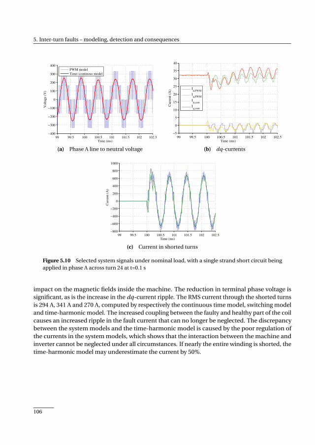
5. Inter-turn faults – modeling, detection and consequences
99 99.5 100 100.5 101 101.5 102 102.5−400
−300
−200
−100
0
100
200
300
400
Time (ms)
Vo
ltag
e (V
)
PWM model
Time−continous model
(a) Phase A line to neutral voltage
99 99.5 100 100.5 101 101.5 102 102.5−5
0
5
10
15
20
25
30
35
40
Time (ms)
Curr
ent
(A)
Id,PWM
Iq,PWM
Id,cont
Iq,cont
(b) dq-currents
99 99.5 100 100.5 101 101.5 102 102.5−800
−600
−400
−200
0
200
400
600
800
1000
Time (ms)
Cu
rren
t (A
)
(c) Current in shorted turns
Figure 5.10 Selected system signals under nominal load, with a single strand short circuit beingapplied in phase A across turn 24 at t=0.1 s
impact on the magnetic fields inside the machine. The reduction in terminal phase voltage issignificant, as is the increase in the dq-current ripple. The RMS current through the shorted turnsis 294 A, 341 A and 270 A, computed by respectively the continuous time model, switching modeland time-harmonic model. The increased coupling between the faulty and healthy part of the coilcauses an increased ripple in the fault current that can no longer be neglected. The discrepancybetween the system models and the time-harmonic model is caused by the poor regulation ofthe currents in the system models, which shows that the interaction between the machine andinverter cannot be neglected under all circumstances. If nearly the entire winding is shorted, thetime-harmonic model may underestimate the current by 50%.
106

5.4 – Turn-level short circuit current measurement
99 99.5 100 100.5 101 101.5 102 102.5−400
−300
−200
−100
0
100
200
300
400
Time (ms)
Vo
ltag
e (V
)
PWM model
Time−continous model
(a) Phase A line to neutral voltage
99 99.5 100 100.5 101 101.5 102 102.5−80
−60
−40
−20
0
20
40
60
80
100
Time (ms)
Curr
ent
(A)
Id,PWM
Iq,PWM
Id,cont
Iq,cont
(b) dq-currents
99 99.5 100 100.5 101 101.5 102 102.5−600
−400
−200
0
200
400
600
Time (ms)
Cu
rren
t (A
)
(c) Current in shorted turns
Figure 5.11 Selected system signals under nominal load, with a single strand short circuit beingapplied in phase A across turns 24–34 at t=0.1 s
5.4 Turn-level short circuit current measurement
Rudimentary experiments are now performed to validate part of the short circuit current calcula-tions.
5.4.1 Test setup
The prototype starter/generator (to be fully presented in Chapter 7) was equipped with twoadditional wires around two different teeth to mimic single turn short circuits. Due to the risksinvolved, this was preferred over modifying the actual winding. The wires have diameters of 1 mmand 2 mm diameter, with measured resistances of 8.7 mΩ and 4.6 mΩ, and represent smaller andlarger faults, respectively. The inductance of both turns is about 650 nH, approximately twice that
107
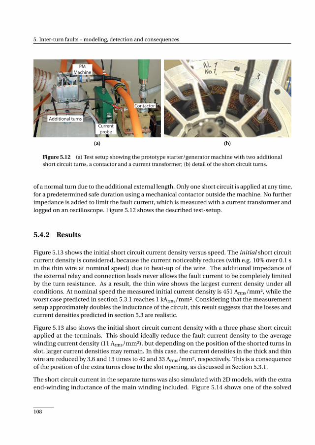
5. Inter-turn faults – modeling, detection and consequences
PM
Machine
Additional turns
Contactor
Current
probe
(a) (b)
Figure 5.12 (a) Test setup showing the prototype starter/generator machine with two additionalshort circuit turns, a contactor and a current transformer; (b) detail of the short circuit turns.
of a normal turn due to the additional external length. Only one short circuit is applied at any time,for a predetermined safe duration using a mechanical contactor outside the machine. No furtherimpedance is added to limit the fault current, which is measured with a current transformer andlogged on an oscilloscope. Figure 5.12 shows the described test-setup.
5.4.2 Results
Figure 5.13 shows the initial short circuit current density versus speed. The initial short circuitcurrent density is considered, because the current noticeably reduces (with e.g. 10% over 0.1 sin the thin wire at nominal speed) due to heat-up of the wire. The additional impedance ofthe external relay and connection leads never allows the fault current to be completely limitedby the turn resistance. As a result, the thin wire shows the largest current density under allconditions. At nominal speed the measured initial current density is 451 Arms/mm², while theworst case predicted in section 5.3.1 reaches 1 kArms/mm². Considering that the measurementsetup approximately doubles the inductance of the circuit, this result suggests that the losses andcurrent densities predicted in section 5.3 are realistic.
Figure 5.13 also shows the initial short circuit current density with a three phase short circuitapplied at the terminals. This should ideally reduce the fault current density to the averagewinding current density (11 Arms/mm²), but depending on the position of the shorted turns inslot, larger current densities may remain. In this case, the current densities in the thick and thinwire are reduced by 3.6 and 13 times to 40 and 33 Arms/mm², respectively. This is a consequenceof the position of the extra turns close to the slot opening, as discussed in Section 5.3.1.
The short circuit current in the separate turns was also simulated with 2D models, with the extraend-winding inductance of the main winding included. Figure 5.14 shows one of the solved
108
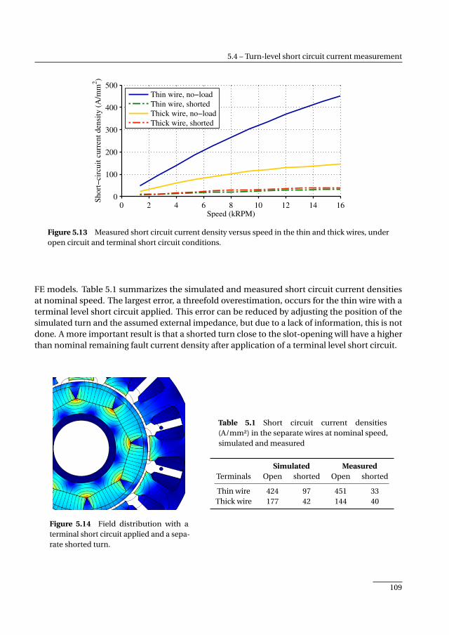
5.4 – Turn-level short circuit current measurement
0 2 4 6 8 10 12 14 160
100
200
300
400
500
Speed (kRPM)
Sh
ort
−ci
rcu
it c
urr
ent
den
sity
(A
/mm
2)
Thin wire, no−load
Thin wire, shorted
Thick wire, no−load
Thick wire, shorted
Figure 5.13 Measured short circuit current density versus speed in the thin and thick wires, underopen circuit and terminal short circuit conditions.
FE models. Table 5.1 summarizes the simulated and measured short circuit current densitiesat nominal speed. The largest error, a threefold overestimation, occurs for the thin wire with aterminal level short circuit applied. This error can be reduced by adjusting the position of thesimulated turn and the assumed external impedance, but due to a lack of information, this is notdone. A more important result is that a shorted turn close to the slot-opening will have a higherthan nominal remaining fault current density after application of a terminal level short circuit.
Figure 5.14 Field distribution with aterminal short circuit applied and a sepa-rate shorted turn.
Table 5.1 Short circuit current densities(A/mm²) in the separate wires at nominal speed,simulated and measured
Simulated MeasuredTerminals Open shorted Open shorted
Thin wire 424 97 451 33Thick wire 177 42 144 40
109
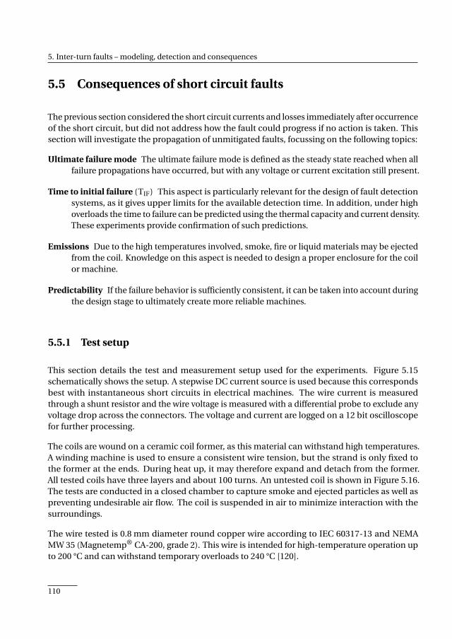
5. Inter-turn faults – modeling, detection and consequences
5.5 Consequences of short circuit faults
The previous section considered the short circuit currents and losses immediately after occurrenceof the short circuit, but did not address how the fault could progress if no action is taken. Thissection will investigate the propagation of unmitigated faults, focussing on the following topics:
Ultimate failure mode The ultimate failure mode is defined as the steady state reached when allfailure propagations have occurred, but with any voltage or current excitation still present.
Time to initial failure (TIF) This aspect is particularly relevant for the design of fault detectionsystems, as it gives upper limits for the available detection time. In addition, under highoverloads the time to failure can be predicted using the thermal capacity and current density.These experiments provide confirmation of such predictions.
Emissions Due to the high temperatures involved, smoke, fire or liquid materials may be ejectedfrom the coil. Knowledge on this aspect is needed to design a proper enclosure for the coilor machine.
Predictability If the failure behavior is sufficiently consistent, it can be taken into account duringthe design stage to ultimately create more reliable machines.
5.5.1 Test setup
This section details the test and measurement setup used for the experiments. Figure 5.15schematically shows the setup. A stepwise DC current source is used because this correspondsbest with instantaneous short circuits in electrical machines. The wire current is measuredthrough a shunt resistor and the wire voltage is measured with a differential probe to exclude anyvoltage drop across the connectors. The voltage and current are logged on a 12 bit oscilloscopefor further processing.
The coils are wound on a ceramic coil former, as this material can withstand high temperatures.A winding machine is used to ensure a consistent wire tension, but the strand is only fixed tothe former at the ends. During heat up, it may therefore expand and detach from the former.All tested coils have three layers and about 100 turns. An untested coil is shown in Figure 5.16.The tests are conducted in a closed chamber to capture smoke and ejected particles as well aspreventing undesirable air flow. The coil is suspended in air to minimize interaction with thesurroundings.
The wire tested is 0.8 mm diameter round copper wire according to IEC 60317-13 and NEMAMW 35 (Magnetemp® CA-200, grade 2). This wire is intended for high-temperature operation upto 200 °C and can withstand temporary overloads to 240 °C [120].
110
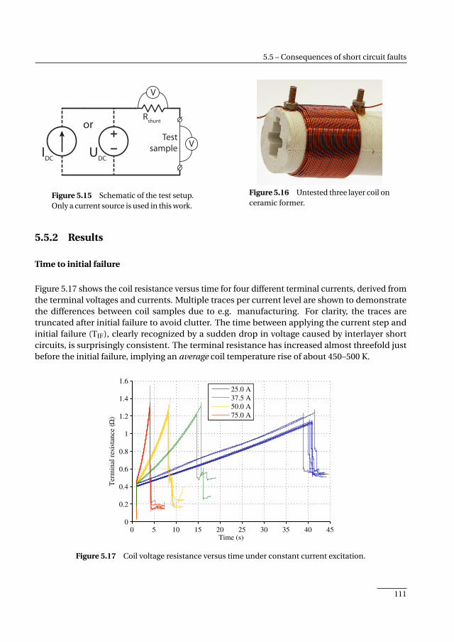
5.5 – Consequences of short circuit faults
IDC UDC
orTest
sample V
V
Rshunt
Figure 5.15 Schematic of the test setup.Only a current source is used in this work.
Figure 5.16 Untested three layer coil onceramic former.
5.5.2 Results
Time to initial failure
Figure 5.17 shows the coil resistance versus time for four different terminal currents, derived fromthe terminal voltages and currents. Multiple traces per current level are shown to demonstratethe differences between coil samples due to e.g. manufacturing. For clarity, the traces aretruncated after initial failure to avoid clutter. The time between applying the current step andinitial failure (TIF), clearly recognized by a sudden drop in voltage caused by interlayer shortcircuits, is surprisingly consistent. The terminal resistance has increased almost threefold justbefore the initial failure, implying an average coil temperature rise of about 450–500 K.
0 5 10 15 20 25 30 35 40 450
0.2
0.4
0.6
0.8
1
1.2
1.4
1.6
Time (s)
Term
inal
resi
stan
ce (
Ω)
25.0 A
37.5 A
50.0 A
75.0 A
Figure 5.17 Coil voltage resistance versus time under constant current excitation.
111
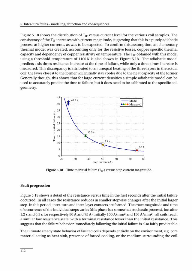
5. Inter-turn faults – modeling, detection and consequences
Figure 5.18 shows the distribution of TIF versus current level for the various coil samples. Theconsistency of the TIF increases with current magnitude, suggesting that this is a purely adiabaticprocess at higher currents, as was to be expected. To confirm this assumption, an elementarythermal model was created, accounting only for the resistive losses, copper specific thermalcapacity and dependency of copper resistivity on temperature. The TIF obtained with this modelusing a threshold temperature of 1100 K is also shown in Figure 5.18. The adiabatic modelpredicts a six times resistance increase at the time of failure, while only a three times increase ismeasured. This discrepancy is attributed to an unequal heating of the three layers in the actualcoil; the layer closest to the former will initially stay cooler due to the heat capacity of the former.Generally though, this shows that for large current densities a simple adiabatic model can beused to accurately predict the time to failure, but it does need to be calibrated to the specific coilgeometry.
20 30 40 50 60 70 800
5
10
15
20
25
30
35
40
45
Step current (A)
Tim
e to
init
ial
fail
ure
(s)
40.9 s
15.3 s
8.4 s
4.1 s
Model
Measured
Figure 5.18 Time to initial failure (TIF) versus step current magnitude.
Fault progression
Figure 5.19 shows a detail of the resistance versus time in the first seconds after the initial failureoccurred. In all cases the resistance reduces in smaller stepwise changes after the initial largerstep. In this period, inter-turn and inter-layer contacts are formed. The exact magnitude and timeof occurrence of the individual steps varies (this phase is a somewhat stochastic process), but after1.2 s and 0.3 s for respectively 50 A and 75 A (initially 100 A/mm² and 150 A/mm²), all coils reacha similar low resistance state, with a terminal resistance lower than the initial resistance. Thissuggests that the failure behavior immediately following the initial failure is also fairly predictable.
The ultimate steady state behavior of faulted coils depends entirely on the environment, e.g. corematerial acting as heat sink, presence of forced cooling, or the medium surrounding the coil.
112

5.5 – Consequences of short circuit faults
8 8.5 9 9.5 100
0.5
1
1.5
Time (s)
Resi
stance (
Ω)
(a) 50 A
4 4.1 4.2 4.3 4.4 4.50
0.5
1
1.5
Time (s)
Resi
stance (
Ω)
(b) 75 A
Figure 5.19 Coil resistance versus time immediately after initial failure. Different lines correspondto different coils.
Hence, the results on the steady state behavior presented here will only be an indication.
Figure 5.20(a) shows the coil resistance over a longer period of time for a terminal current of 25 A.All but one coil show similar behavior over the course of 6 minutes, with a sharp but repeatabledecrease in resistance after 250 s. It is suspected that this is related to insulation failure of thebottom layer, which is cooled via the coil former. Figure 5.20(a) shows the coil resistance for aterminal current of 50 A. At this current, one out of 6 coils failed to an open circuit after 36 s, whilethe other coils sustained this current for at least 90 s, when the test was stopped. With a terminalcurrent of 75 A, all samples failed to an open circuit within 10–17 s, typically with electrical arcsoccurring and liquid copper drops being ejected, potentially damaging the coil surroundings.Inspection of the samples showed that all failures occurred at the connection terminals, thus notproviding fully realistic data.
These results show that short circuits between the coil layers can reliably be formed at moderatecurrent densities, reducing the effective current density and allowing the coils to sustain largerterminal currents. Although the coils did repeatedly fail at 75 A, this failure occurred near theconnection terminals. To realistically determine the failure behavior after the initial failure forlarger initial current densities, more elaborate setups will be necessary, using e.g. magneticallyinduced currents.
The above results allow some predictions about fault progression in PM machines to be made.Short circuits in PM machines across few turns are typically resistance limited, allowing a maxi-mum current density to be determined, based on per-turn resistance and induced voltage, fromwhich the time to failure can be estimated. Machines with a high per-turn voltage will thereforeexhibit a faster failure process. As the fault spreads after the first failure, more turns (conductorarea) will carry the fault current and the current will become inductance limited (ie. the fault
113
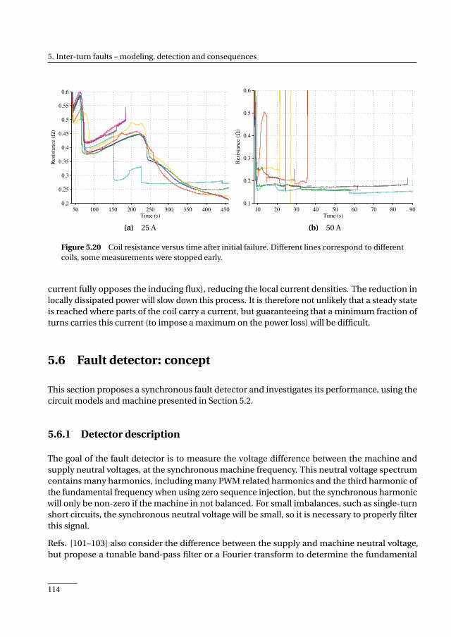
5. Inter-turn faults – modeling, detection and consequences
50 100 150 200 250 300 350 400 4500.2
0.25
0.3
0.35
0.4
0.45
0.5
0.55
0.6
Time (s)
Resi
stan
ce (
Ω)
(a) 25 A
10 20 30 40 50 60 70 80 900.1
0.2
0.3
0.4
0.5
0.6
Time (s)
Resi
stance (
Ω)
(b) 50 A
Figure 5.20 Coil resistance versus time after initial failure. Different lines correspond to differentcoils, some measurements were stopped early.
current fully opposes the inducing flux), reducing the local current densities. The reduction inlocally dissipated power will slow down this process. It is therefore not unlikely that a steady stateis reached where parts of the coil carry a current, but guaranteeing that a minimum fraction ofturns carries this current (to impose a maximum on the power loss) will be difficult.
5.6 Fault detector: concept
This section proposes a synchronous fault detector and investigates its performance, using thecircuit models and machine presented in Section 5.2.
5.6.1 Detector description
The goal of the fault detector is to measure the voltage difference between the machine andsupply neutral voltages, at the synchronous machine frequency. This neutral voltage spectrumcontains many harmonics, including many PWM related harmonics and the third harmonic ofthe fundamental frequency when using zero sequence injection, but the synchronous harmonicwill only be non-zero if the machine in not balanced. For small imbalances, such as single-turnshort circuits, the synchronous neutral voltage will be small, so it is necessary to properly filterthis signal.
Refs. [101–103] also consider the difference between the supply and machine neutral voltage,but propose a tunable band-pass filter or a Fourier transform to determine the fundamental
114
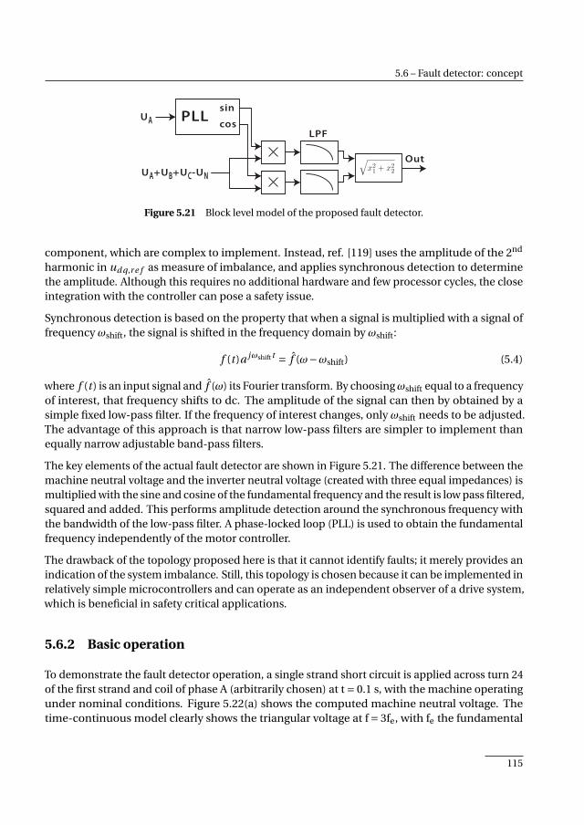
5.6 – Fault detector: concept
PLLsin
cos
Out
UA
UA+UB+UC-UN
LPF
Figure 5.21 Block level model of the proposed fault detector.
component, which are complex to implement. Instead, ref. [119] uses the amplitude of the 2nd
harmonic in ud q,r e f as measure of imbalance, and applies synchronous detection to determinethe amplitude. Although this requires no additional hardware and few processor cycles, the closeintegration with the controller can pose a safety issue.
Synchronous detection is based on the property that when a signal is multiplied with a signal offrequency ωshift, the signal is shifted in the frequency domain by ωshift:
f (t )a jωshiftt = f (ω−ωshift) (5.4)
where f (t ) is an input signal and f (ω) its Fourier transform. By choosingωshift equal to a frequencyof interest, that frequency shifts to dc. The amplitude of the signal can then by obtained by asimple fixed low-pass filter. If the frequency of interest changes, only ωshift needs to be adjusted.The advantage of this approach is that narrow low-pass filters are simpler to implement thanequally narrow adjustable band-pass filters.
The key elements of the actual fault detector are shown in Figure 5.21. The difference between themachine neutral voltage and the inverter neutral voltage (created with three equal impedances) ismultiplied with the sine and cosine of the fundamental frequency and the result is low pass filtered,squared and added. This performs amplitude detection around the synchronous frequency withthe bandwidth of the low-pass filter. A phase-locked loop (PLL) is used to obtain the fundamentalfrequency independently of the motor controller.
The drawback of the topology proposed here is that it cannot identify faults; it merely provides anindication of the system imbalance. Still, this topology is chosen because it can be implemented inrelatively simple microcontrollers and can operate as an independent observer of a drive system,which is beneficial in safety critical applications.
5.6.2 Basic operation
To demonstrate the fault detector operation, a single strand short circuit is applied across turn 24of the first strand and coil of phase A (arbitrarily chosen) at t = 0.1 s, with the machine operatingunder nominal conditions. Figure 5.22(a) shows the computed machine neutral voltage. Thetime-continuous model clearly shows the triangular voltage at f = 3fe, with fe the fundamental
115
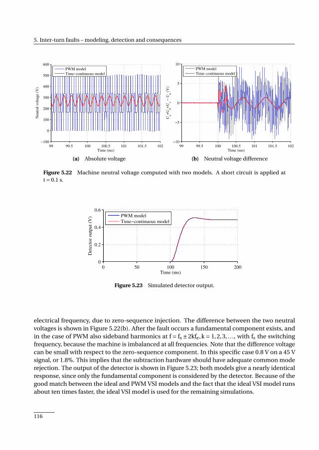
5. Inter-turn faults – modeling, detection and consequences
99 99.5 100 100.5 101 101.5 102−100
0
100
200
300
400
500
600
Time (ms)
Neu
tral
volt
age
(V)
PWM model
Time−continuous model
(a) Absolute voltage
99 99.5 100 100.5 101 101.5 102−10
−5
0
5
10
Time (ms)
Ua+
Ub+
Uc −
Un (
V)
PWM model
Time−continuous model
(b) Neutral voltage difference
Figure 5.22 Machine neutral voltage computed with two models. A short circuit is applied att = 0.1 s.
0 50 100 150 2000
0.2
0.4
0.6
Time (ms)
Det
ecto
r outp
ut
(V)
PWM model
Time−continuous model
Figure 5.23 Simulated detector output.
electrical frequency, due to zero-sequence injection. The difference between the two neutralvoltages is shown in Figure 5.22(b). After the fault occurs a fundamental component exists, andin the case of PWM also sideband harmonics at f = fs ±2kfe,k = 1,2,3, . . ., with fs the switchingfrequency, because the machine is imbalanced at all frequencies. Note that the difference voltagecan be small with respect to the zero-sequence component. In this specific case 0.8 V on a 45 Vsignal, or 1.8%. This implies that the subtraction hardware should have adequate common moderejection. The output of the detector is shown in Figure 5.23; both models give a nearly identicalresponse, since only the fundamental component is considered by the detector. Because of thegood match between the ideal and PWM VSI models and the fact that the ideal VSI model runsabout ten times faster, the ideal VSI model is used for the remaining simulations.
116
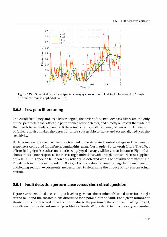
5.6 – Fault detector: concept
0 0.2 0.4 0.6 0.8 10
0.1
0.2
0.3
0.4
0.5
0.6
0.7
0.8
0.9
Time (s)
Dete
cto
r le
vel
(V)
2 Hz
5 Hz
10 Hz
20 Hz
Figure 5.24 Simulated detector output in a noisy system for multiple detector bandwidths. A singleturn short circuit is applied at t = 0.5 s.
5.6.3 Low pass filter tuning
The cutoff frequency and, to a lesser degree, the order of the two low pass filters are the onlycritical parameters that affect the performance of the detector, and directly represent the trade-offthat needs to be made for any fault detector: a high cutoff frequency allows a quick detectionof faults, but also makes the detection more susceptible to noise and essentially reduces thesensitivity.
To demonstrate this effect, white noise is added to the simulated neutral voltage and the detectorresponse is computed for different bandwidths, using fourth order Butterworth filters. The effectof interfering signals, such as unintended supply grid leakage, will be similar in nature. Figure 5.24shows the detector responses for increasing bandwidths with a single turn short circuit appliedat t = 0.5 s. This specific fault can only reliably be detected with a bandwidth of at most 5 Hz.The detection time is in the order of 0.25 s, which can already cause damage to the machine. Ina following section, experiments are performed to determine the impact of noise in an actualsystem.
5.6.4 Fault detection performance versus short circuit position
Figure 5.25 shows the detector output level range versus the number of shorted turns for a singlestrand fault and the shorted turns difference for a parallel strand fault. For a given number ofshorted turns, the detected imbalance varies due to the position of the short circuit along the coil,as indicated by the shaded areas of possible fault levels. With a short circuit across a given number
117
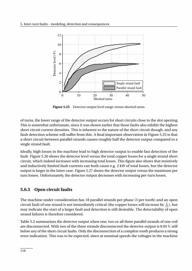
5. Inter-turn faults – modeling, detection and consequences
0 10 20 30 40 500
2
4
6
8
10
12
Shorted turns
Det
ecto
r le
vel
(V
)
Single strand fault
Parallel strand fault
Figure 5.25 Detector output level range versus shorted turns.
of turns, the lower range of the detector output occurs for short circuits close to the slot opening.This is somewhat unfortunate, since it was shown earlier that those faults also exhibit the highestshort circuit current densities. This is inherent to the nature of the short circuit though, and anyfault detection scheme will suffer from this. A final important observation in Figure 5.25 is thata short circuit between parallel strands causes roughly half the detector output compared to asingle strand fault.
Ideally, high losses in the machine lead to high detector output to enable fast detection of thefault. Figure 5.26 shows the detector level versus the total copper losses for a single strand shortcircuit, which indeed increases with increasing total losses. This figure also shows that resistivelyand inductively limited fault currents can both cause e.g. 2 kW of total losses, but the detectoroutput is larger in the latter case. Figure 5.27 shows the detector output versus the maximum perturn losses. Unfortunately, the detector output decreases with increasing per-turn losses.
5.6.5 Open circuit faults
The machine under consideration has 18 parallel strands per phase (3 per tooth) and an opencircuit fault of one strand is not immediately critical (the copper losses will increase by 1
17 ), butmay indicate the start of a larger fault and detection is still desirable. The detectability of openstrand failures is therefore considered.
Table 5.2 summarizes the detector output when one, two or all three parallel strands of one coilare disconnected. With two of the three strands disconnected the detector output is 0.05 V, stillbelow any of the short circuit faults. Only the disconnection of a complete tooth produces a strongerror indication. This was to be expected, since at nominal speeds the voltages in the machine
118
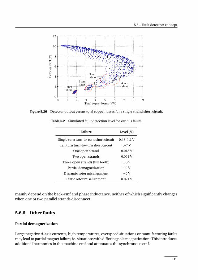
5.6 – Fault detector: concept
0 1 2 3 4 5 6 7 8 90
2
4
6
8
10
12
Total copper losses (kW)
Det
ecto
r le
vel
(V
)
1 turn short
2 turn short
3 turn short
4 turn short
Figure 5.26 Detector output versus total copper losses for a single strand short circuit.
Table 5.2 Simulated fault detection level for various faults
Failure Level (V)
Single turn turn-to-turn short circuit 0.48–1.2 V
Ten turn turn-to-turn short circuit 5–7 V
One open strand 0.013 V
Two open strands 0.051 V
Three open strands (full tooth) 1.5 V
Partial demagnetization ∼0 V
Dynamic rotor misalignment ∼0 V
Static rotor misalignment 0.021 V
mainly depend on the back-emf and phase inductance, neither of which significantly changeswhen one or two parallel strands disconnect.
5.6.6 Other faults
Partial demagnetization
Large negative d-axis currents, high temperatures, overspeed situations or manufacturing faultsmay lead to partial magnet failure, ie. situations with differing pole magnetization. This introducesadditional harmonics in the machine emf and attenuates the synchronous emf.
119
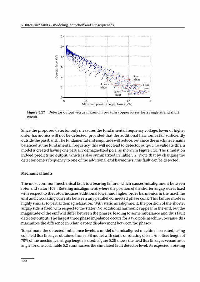
5. Inter-turn faults – modeling, detection and consequences
0 0.5 1 1.5 20
2
4
6
8
10
12
Maximum per−turn copper losses (kW)
Det
ecto
r le
vel
(V
)
1 turn short
2 turn short
3 turn short
4 turn short
Figure 5.27 Detector output versus maximum per turn copper losses for a single strand shortcircuit.
Since the proposed detector only measures the fundamental frequency voltage, lower or higherorder harmonics will not be detected, provided that the additional harmonics fall sufficientlyoutside the passband. The fundamental emf amplitude will reduce, but since the machine remainsbalanced at the fundamental frequency, this will not lead to detector output. To validate this, amodel is created having one partially demagnetized pole, as shown in Figure 5.28. The simulationindeed predicts no output, which is also summarized in Table 5.2. Note that by changing thedetector center frequency to one of the additional emf harmonics, this fault can be detected.
Mechanical faults
The most common mechanical fault is a bearing failure, which causes misalignment betweenrotor and stator [109]. Rotating misalignment, where the position of the shorter airgap side is fixedwith respect to the rotor, induces additional lower and higher order harmonics in the machineemf and circulating currents between any parallel connected phase coils. This failure mode ishighly similar to partial demagnetization. With static misalignment, the position of the shorterairgap side is fixed with respect to the stator. No additional harmonics appear in the emf, but themagnitude of the emf will differ between the phases, leading to some imbalance and thus faultdetector output. The largest three phase imbalance occurs for a two pole machine, because thismaximizes the difference in relative rotor displacement between the phases.
To estimate the detected imbalance levels, a model of a misaligned machine is created, usingcoil field flux linkages obtained from a FE model with static or rotating offset. An offset length of70% of the mechanical airgap length is used. Figure 5.28 shows the field flux linkages versus rotorangle for one coil. Table 5.2 summarizes the simulated fault detector level. As expected, rotating
120
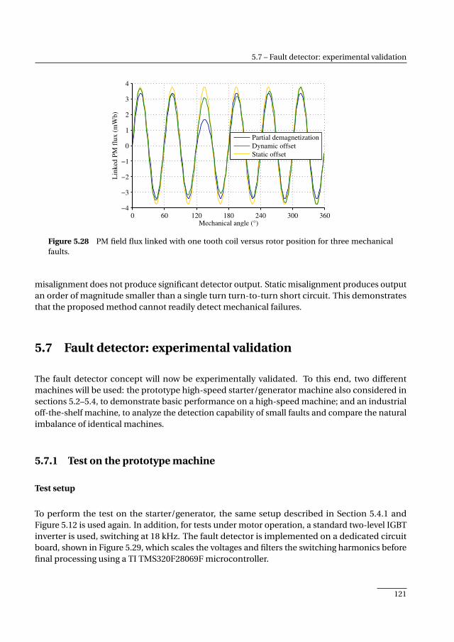
5.7 – Fault detector: experimental validation
0 60 120 180 240 300 360−4
−3
−2
−1
0
1
2
3
4
Mechanical angle (°)
Lin
ked
PM
flu
x (
mW
b)
Partial demagnetization
Dynamic offset
Static offset
Figure 5.28 PM field flux linked with one tooth coil versus rotor position for three mechanicalfaults.
misalignment does not produce significant detector output. Static misalignment produces outputan order of magnitude smaller than a single turn turn-to-turn short circuit. This demonstratesthat the proposed method cannot readily detect mechanical failures.
5.7 Fault detector: experimental validation
The fault detector concept will now be experimentally validated. To this end, two differentmachines will be used: the prototype high-speed starter/generator machine also considered insections 5.2–5.4, to demonstrate basic performance on a high-speed machine; and an industrialoff-the-shelf machine, to analyze the detection capability of small faults and compare the naturalimbalance of identical machines.
5.7.1 Test on the prototype machine
Test setup
To perform the test on the starter/generator, the same setup described in Section 5.4.1 andFigure 5.12 is used again. In addition, for tests under motor operation, a standard two-level IGBTinverter is used, switching at 18 kHz. The fault detector is implemented on a dedicated circuitboard, shown in Figure 5.29, which scales the voltages and filters the switching harmonics beforefinal processing using a TI TMS320F28069F microcontroller.
121
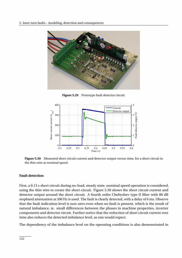
5. Inter-turn faults – modeling, detection and consequences
Figure 5.29 Prototype fault detector circuit.
0
100
200
300
400
Short
−ci
rcuit
curr
ent
(Arm
s)
0.2 0.25 0.3 0.35 0.4 0.45 0.5 0.55 0.60
1
2
3
4
Time (s)
Fau
lt d
etec
tor
outp
ut
(V)
Current
Detector output
Figure 5.30 Measured short circuit current and detector output versus time, for a short circuit inthe thin wire at nominal speed.
Fault detection
First, a 0.13 s short circuit during no-load, steady state, nominal speed operation is considered,using the thin wire to create the short circuit. Figure 5.30 shows the short circuit current anddetector output around the short circuit. A fourth order Chebyshev type II filter with 80 dBstopband attenuation at 500 Hz is used. The fault is clearly detected, with a delay of 6 ms. Observethat the fault indication level is non-zero even when no fault is present, which is the result ofnatural imbalance, ie. small differences between the phases in machine properties, invertercomponents and detector circuit. Further notice that the reduction of short circuit current overtime also reduces the detected imbalance level, as one would expect.
The dependency of the imbalance level on the operating conditions is also demonstrated in
122
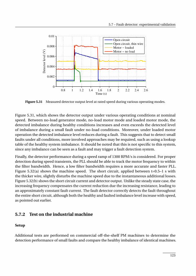
5.7 – Fault detector: experimental validation
0.8 1 1.2 1.4 1.6 1.8 2 2.2 2.4 2.60
0.002
0.004
0.006
0.008
0.01
Time (s)
Det
ecto
r le
vel
(V
)
Open circuit
Open circuit, thin wire
Motor − loaded
Motor − no load
Figure 5.31 Measured detector output level at rated speed during various operating modes.
Figure 5.31, which shows the detector output under various operating conditions at nominalspeed. Between no-load generator mode, no-load motor mode and loaded motor mode, thedetected imbalance during healthy conditions increases and even exceeds the detected levelof imbalance during a small fault under no-load conditions. Moreover, under loaded motoroperation the detected imbalance level reduces during a fault. This suggests that to detect smallfaults under all conditions, more involved approaches may be required, such as using a lookuptable of the healthy system imbalance. It should be noted that this is not specific to this system,since any imbalance can be seen as a fault and may trigger a fault detection system.
Finally, the detector performance during a speed ramp of 1300 RPM/s is considered. For properdetection during speed transients, the PLL should be able to track the motor frequency to withinthe filter bandwidth. Hence, a low filter bandwidth requires a more accurate and faster PLL.Figure 5.32(a) shows the machine speed. The short circuit, applied between t=0.5–1 s withthe thicker wire, slightly disturbs the machine speed due to the instantaneous additional losses.Figure 5.32(b) shows the short circuit current and detector output. Unlike the steady state case, theincreasing frequency compensates the current reduction due the increasing resistance, leading toan approximately constant fault current. The fault detector correctly detects the fault throughoutthe entire short circuit, although both the healthy and faulted imbalance level increase with speed,as pointed out earlier.
5.7.2 Test on the industrial machine
Setup
Additional tests are performed on commercial off-the-shelf PM machines to determine thedetection performance of small faults and compare the healthy imbalance of identical machines.
123
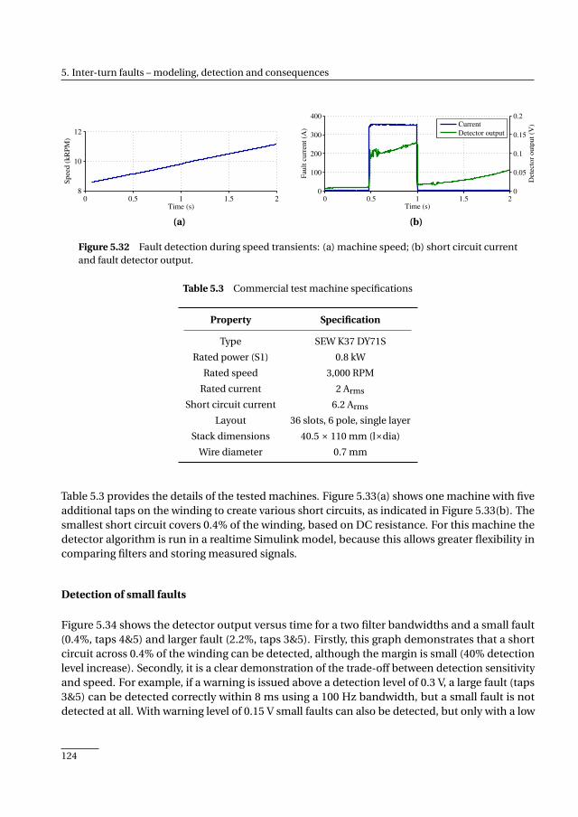
5. Inter-turn faults – modeling, detection and consequences
0 0.5 1 1.5 28
10
12
Time (s)
Spee
d (
kR
PM
)
(a)
0
100
200
300
400
Fau
lt c
urr
ent
(A)
0 0.5 1 1.5 20
0.05
0.1
0.15
0.2
Time (s)
Det
ecto
r outp
ut
(V)Current
Detector output
(b)
Figure 5.32 Fault detection during speed transients: (a) machine speed; (b) short circuit currentand fault detector output.
Table 5.3 Commercial test machine specifications
Property Specification
Type SEW K37 DY71S
Rated power (S1) 0.8 kW
Rated speed 3,000 RPM
Rated current 2 Arms
Short circuit current 6.2 Arms
Layout 36 slots, 6 pole, single layer
Stack dimensions 40.5 × 110 mm (l×dia)
Wire diameter 0.7 mm
Table 5.3 provides the details of the tested machines. Figure 5.33(a) shows one machine with fiveadditional taps on the winding to create various short circuits, as indicated in Figure 5.33(b). Thesmallest short circuit covers 0.4% of the winding, based on DC resistance. For this machine thedetector algorithm is run in a realtime Simulink model, because this allows greater flexibility incomparing filters and storing measured signals.
Detection of small faults
Figure 5.34 shows the detector output versus time for a two filter bandwidths and a small fault(0.4%, taps 4&5) and larger fault (2.2%, taps 3&5). Firstly, this graph demonstrates that a shortcircuit across 0.4% of the winding can be detected, although the margin is small (40% detectionlevel increase). Secondly, it is a clear demonstration of the trade-off between detection sensitivityand speed. For example, if a warning is issued above a detection level of 0.3 V, a large fault (taps3&5) can be detected correctly within 8 ms using a 100 Hz bandwidth, but a small fault is notdetected at all. With warning level of 0.15 V small faults can also be detected, but only with a low
124
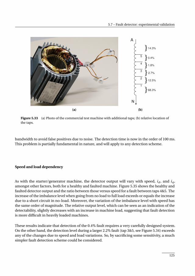
5.7 – Fault detector: experimental validation
(a)
1
2
3
4
5
0.4%
14.3%
1.8%
2.7%
12.5%
68.3%
A
B
C
N
(b)
Figure 5.33 (a) Photo of the commercial test machine with additional taps; (b) relative location ofthe taps.
bandwidth to avoid false positives due to noise. The detection time is now in the order of 100 ms.This problem is partially fundamental in nature, and will apply to any detection scheme.
Speed and load dependency
As with the starter/generator machine, the detector output will vary with speed, id , and iq ,amongst other factors, both for a healthy and faulted machine. Figure 5.35 shows the healthy andfaulted detector output and the ratio between those versus speed for a fault between taps 4&5. Theincrease of the imbalance level when going from no load to full load exceeds or equals the increasedue to a short circuit in no-load. Moreover, the variation of the imbalance level with speed hasthe same order of magnitude. The relative output level, which can be seen as an indication of thedetectability, slightly decreases with an increase in machine load, suggesting that fault detectionis more difficult in heavily loaded machines.
These results indicate that detection of the 0.4% fault requires a very carefully designed system.On the other hand, the detection level during a larger 2.2% fault (tap 3&5, see Figure 5.34) exceedsany of the changes due to speed and load variations. So, by sacrificing some sensitivity, a muchsimpler fault detection scheme could be considered.
125
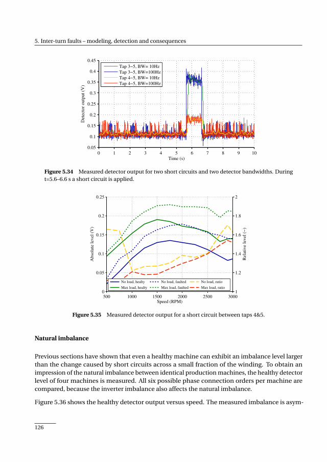
5. Inter-turn faults – modeling, detection and consequences
0 1 2 3 4 5 6 7 8 9 10
0.05
0.1
0.15
0.2
0.25
0.3
0.35
0.4
0.45
Time (s)
Det
ecto
r outp
ut
(V)
Tap 3−5, BW= 10Hz
Tap 3−5, BW=100Hz
Tap 4−5, BW= 10Hz
Tap 4−5, BW=100Hz
Figure 5.34 Measured detector output for two short circuits and two detector bandwidths. Duringt=5.6–6.6 s a short circuit is applied.
0
0.05
0.1
0.15
0.2
0.25
Abso
lute
lev
el (
V)
500 1000 1500 2000 2500 30001
1.2
1.4
1.6
1.8
2
Speed (RPM)
Rel
ativ
e le
vel
(−
)
No load, healty
Max load, healty
No load, faulted
Max load, faulted
No load, ratio
Max load, ratio
Figure 5.35 Measured detector output for a short circuit between taps 4&5.
Natural imbalance
Previous sections have shown that even a healthy machine can exhibit an imbalance level largerthan the change caused by short circuits across a small fraction of the winding. To obtain animpression of the natural imbalance between identical production machines, the healthy detectorlevel of four machines is measured. All six possible phase connection orders per machine arecompared, because the inverter imbalance also affects the natural imbalance.
Figure 5.36 shows the healthy detector output versus speed. The measured imbalance is asym-
126
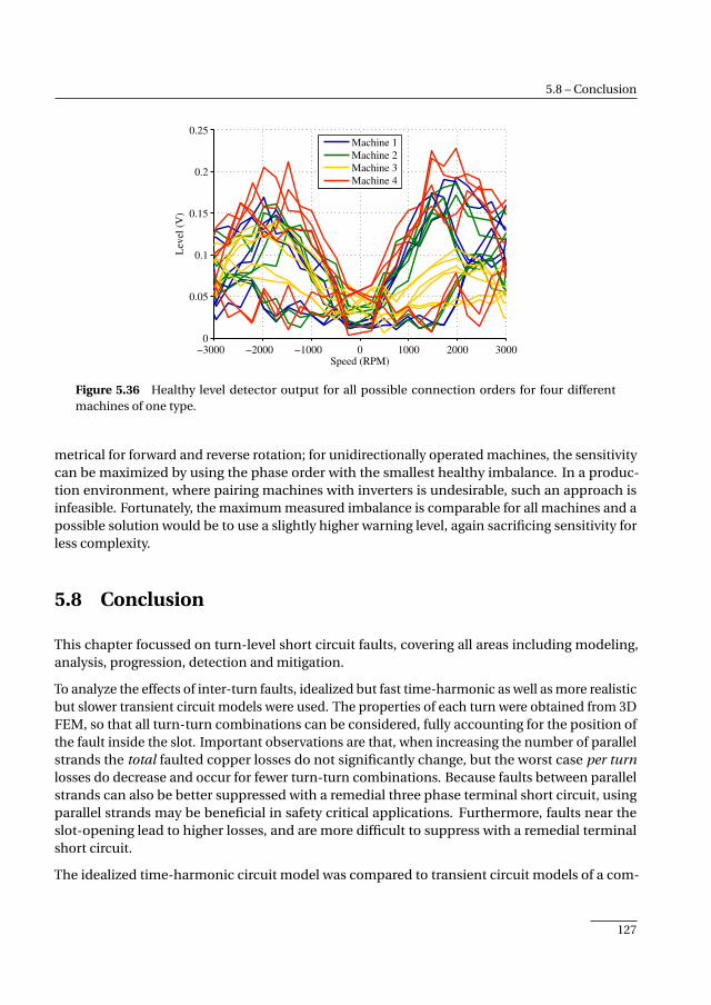
5.8 – Conclusion
−3000 −2000 −1000 0 1000 2000 30000
0.05
0.1
0.15
0.2
0.25
Speed (RPM)
Lev
el (
V)
Machine 1
Machine 2
Machine 3
Machine 4
Figure 5.36 Healthy level detector output for all possible connection orders for four differentmachines of one type.
metrical for forward and reverse rotation; for unidirectionally operated machines, the sensitivitycan be maximized by using the phase order with the smallest healthy imbalance. In a produc-tion environment, where pairing machines with inverters is undesirable, such an approach isinfeasible. Fortunately, the maximum measured imbalance is comparable for all machines and apossible solution would be to use a slightly higher warning level, again sacrificing sensitivity forless complexity.
5.8 Conclusion
This chapter focussed on turn-level short circuit faults, covering all areas including modeling,analysis, progression, detection and mitigation.
To analyze the effects of inter-turn faults, idealized but fast time-harmonic as well as more realisticbut slower transient circuit models were used. The properties of each turn were obtained from 3DFEM, so that all turn-turn combinations can be considered, fully accounting for the position ofthe fault inside the slot. Important observations are that, when increasing the number of parallelstrands the total faulted copper losses do not significantly change, but the worst case per turnlosses do decrease and occur for fewer turn-turn combinations. Because faults between parallelstrands can also be better suppressed with a remedial three phase terminal short circuit, usingparallel strands may be beneficial in safety critical applications. Furthermore, faults near theslot-opening lead to higher losses, and are more difficult to suppress with a remedial terminalshort circuit.
The idealized time-harmonic circuit model was compared to transient circuit models of a com-
127
5. Inter-turn faults – modeling, detection and consequences
plete closed loop drive system, using either an idealized VSI or switching VSI. It was found that forshort circuits across a small fraction of the winding, all models yield highly similar numbers. Thisshows that involved models are not necessary to estimate the worst case current densities. Withlarger parts of the winding short circuited, neglecting the limited bandwidth of actual currentregulators and the switching nature of real VSIs will cause an underestimation of the losses,although in practical cases this is unlikely to cause any issues.
A further observation is that single-turn short circuits remain resistance limited up to very highspeeds. This implies that turn-to-turn faults in high-speed machines can be more severe than inline frequency machines. Experiments on the starter-generator underline this, with measuredfault current densities up to 450 Arms/mm2, still partially being limited by the measurement setup.This highlights the need for a fast fault detection system in safety critical applications.
Brief experiments were performed to determine the basic failure behavior of coils in the presenceof unmitigated faults. Three layer dummy coils were subjected to a current step until steadystate breakdown was achieved. Important observations include that at moderate initial currentdensities, the inter-layer contacts formed due to failing insulation allow the coil to carry highercurrents for extended periods of time; and that at high current densities, a simple adiabaticthermal model can predict the time to initial breakdown.
Lastly, a fault detector is proposed that can provide an indication of the three phase system im-balance, based on synchronous detection of the machine and inverter neutral voltage difference.The main benefit is the simplicity of implementation. The concept was demonstrated on twodifferent machines, showing that short circuits across 0.4% of the winding can be detected with acarefully designed detector system. The design of this fault detector entails two tradeoffs: one, thedetection speed is fundamentally limited by noise; that is, detecting smaller faults requires moretime. Two, imbalances in practical systems cause fault detector output during healthy conditionsof a similar order of magnitude as small faults, leading to a tradeoff between a simple but lesssensitive system on the one hand, and a more involved and more sensitive detection system onthe other hand. These considerations apply to any fault detection system to some degree.
Concerning the detectability it is shown that short circuits between parallel strands are moredifficult to detect than single strand short circuits. In the case of parallel strands, open-circuitfaults are even more difficult to detect, but are also far less dangerous. Short circuits across agiven number of turns are more difficult to detect if they occur close to the slot-opening. This issomewhat unfortunate, as those faults also exhibit the highest losses. Mechanical faults or partialdemagnetization cannot be detected without changes to the proposed detector.
128
CHAPTER 6
Analysis of additional losses due to PWM inducedcurrent ripple
The previous chapters of this thesis occasionally considered the problem of matching a machineto an inverter, but considered only the primary aspect: relative inductance. The impact of thecurrent ripple caused by the pulse width modulated inverter output voltages was neglected.This brief chapter considers the impact of this current ripple on the rotor losses, iron losses andwinding losses. These losses are calculated for one machine, allowing their relative magnitudeto be compared. A different, larger machine is used instead of the S/G to better highlight thepotentially large losses.
Based on• M. van der Geest, H. Polinder, and J. A. Ferreira, “Influence of PWM switching frequency
on the losses in PM machines,” in Int. Conf. Electrical Machines (ICEM), 2014, pp.1243–1247.
129
6. Analysis of additional losses due to PWM induced current ripple
6.1 Introduction
Electrical machines are increasingly used in combination with an inverter due to obvious benefits,such as energy savings or improved dynamic behavior. One of the side effects of inverter drivenmachines is a high frequency current ripple, which induces additional losses in all parts of themachine. If these additional losses are neglected during the design stage, the machine may runwarmer or even fail in operation.
The magnitude of the current ripple depends on three factors: firstly, it is inversely proportionalto switching frequency, secondly, it is inversely proportional to the machine inductance and lastly,it is proportional to the dc-link voltage. When designing a complete drive system, at least somecare should taken to optimize these factors. Not only can this minimize the current ripple, it canalso reduce the total system size and/or inverter rating, ultimately saving cost.
The effect of the current ripple on the iron losses has received considerable attention in e.g. [121–124]. Compared to an ideal sinusoidal supply voltage, using a PWM power supply increases thelosses only marginally (10-20%) if the switching frequency and modulation index are sufficientlyhigh. At high modulation indexes but low switching frequencies, only a small loss increase ofabout 15% occurs, compared to high switching frequencies. With a decreasing modulation index,which implies an increase in dc-link voltage and current ripple, the additional iron losses at lowswitching frequencies can exceed 50%. This emphasizes the importance of a good match betweenthe machine voltage level and dc-link voltage. As a side note, although many models have beenproposed to accurately compute iron losses under various conditions, they are of limited usebecause a large spread in actual iron losses can exist, even between identical motors [125].
The high frequency current ripple also induces losses in the machine windings. In a machine withparallel strands (bundles) inside the coils, four components can be recognized (as explained inChapter 4): skin and proximity effects inside individual strands, and skin and proximity effectsbetween parallel strands [63, 126]. At the strand level, the skin-effect can be ignored if there aremany strands inside a slot, as the proximity effect will dominate. At bundle level, the variationsin (leakage) inductance between strands are often far greater than variations in linked magnetflux, and the proximity effect can be ignored instead. Due to these effects, the distribution of highfrequency currents in the strands and bundles, as well as the corresponding AC/DC loss ratio, canbe significantly worse than for the fundamental current component. In [57] up to 15% additionallosses are reported due to PWM switching. In [127] it is however demonstrated that the use of litzwire removes the dependency on switching frequency.
High frequency stator currents also create asynchronous airgap harmonics, which induce rotoreddy current losses. At lower frequencies the induced currents are resistively limited and thelosses depend on the square of both the frequency and field strength. At higher frequencies, theskin-effect provides shielding, limiting the loss increase [127, 128].
This chapter considers the additional losses as function of switching frequency with a case studyon a 500 kW machine (ie. not the starter/generator). Losses in the stator laminations, windings
130
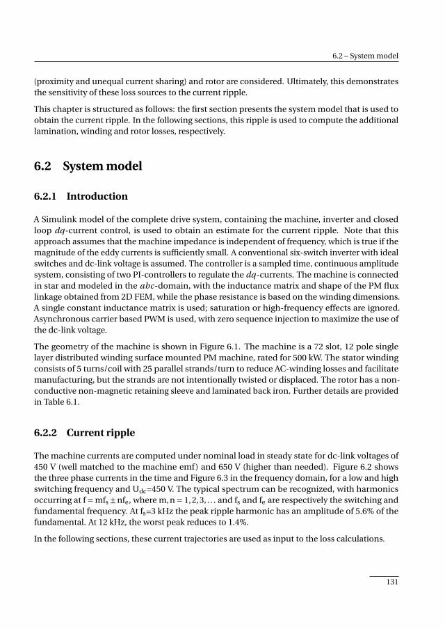
6.2 – System model
(proximity and unequal current sharing) and rotor are considered. Ultimately, this demonstratesthe sensitivity of these loss sources to the current ripple.
This chapter is structured as follows: the first section presents the system model that is used toobtain the current ripple. In the following sections, this ripple is used to compute the additionallamination, winding and rotor losses, respectively.
6.2 System model
6.2.1 Introduction
A Simulink model of the complete drive system, containing the machine, inverter and closedloop dq-current control, is used to obtain an estimate for the current ripple. Note that thisapproach assumes that the machine impedance is independent of frequency, which is true if themagnitude of the eddy currents is sufficiently small. A conventional six-switch inverter with idealswitches and dc-link voltage is assumed. The controller is a sampled time, continuous amplitudesystem, consisting of two PI-controllers to regulate the dq-currents. The machine is connectedin star and modeled in the abc-domain, with the inductance matrix and shape of the PM fluxlinkage obtained from 2D FEM, while the phase resistance is based on the winding dimensions.A single constant inductance matrix is used; saturation or high-frequency effects are ignored.Asynchronous carrier based PWM is used, with zero sequence injection to maximize the use ofthe dc-link voltage.
The geometry of the machine is shown in Figure 6.1. The machine is a 72 slot, 12 pole singlelayer distributed winding surface mounted PM machine, rated for 500 kW. The stator windingconsists of 5 turns/coil with 25 parallel strands/turn to reduce AC-winding losses and facilitatemanufacturing, but the strands are not intentionally twisted or displaced. The rotor has a non-conductive non-magnetic retaining sleeve and laminated back iron. Further details are providedin Table 6.1.
6.2.2 Current ripple
The machine currents are computed under nominal load in steady state for dc-link voltages of450 V (well matched to the machine emf) and 650 V (higher than needed). Figure 6.2 showsthe three phase currents in the time and Figure 6.3 in the frequency domain, for a low and highswitching frequency and Udc=450 V. The typical spectrum can be recognized, with harmonicsoccurring at f = mfs ±nfe, where m,n = 1,2,3, . . . and fs and fe are respectively the switching andfundamental frequency. At fs=3 kHz the peak ripple harmonic has an amplitude of 5.6% of thefundamental. At 12 kHz, the worst peak reduces to 1.4%.
In the following sections, these current trajectories are used as input to the loss calculations.
131
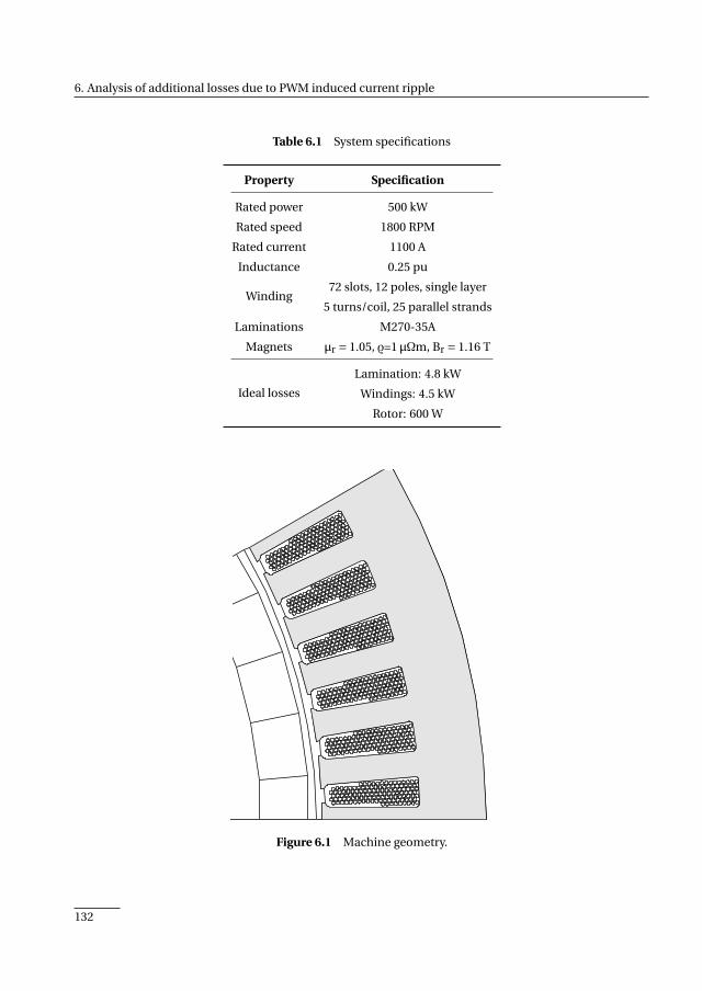
6. Analysis of additional losses due to PWM induced current ripple
Table 6.1 System specifications
Property Specification
Rated power 500 kW
Rated speed 1800 RPM
Rated current 1100 A
Inductance 0.25 pu
Winding72 slots, 12 poles, single layer
5 turns/coil, 25 parallel strands
Laminations M270-35A
Magnets µr = 1.05, ρ=1 µΩm, Br = 1.16 T
Ideal losses
Lamination: 4.8 kW
Windings: 4.5 kW
Rotor: 600 W
Figure 6.1 Machine geometry.
132

6.2 – System model
0 1 2 3 4 5−2000
−1500
−1000
−500
0
500
1000
1500
2000
Time (ms)
Curr
ent
(A)
Ia
Ib
Ic
(a)
0 1 2 3 4 5−2000
−1500
−1000
−500
0
500
1000
1500
2000
Time (ms)
Curr
ent
(A)
Ia
Ib
Ic
(b)
Figure 6.2 Phase currents with Udc=450 V: (a) fs=3 kHz; (b) fs=12 kHz.
0 5 10 15 201
10
100
1000
Frequency (kHz)
Curr
ent
mag
nit
ude
(Ap
eak)
(a)
0 5 10 15 201
10
100
1000
Frequency (kHz)
Curr
ent
mag
nit
ude
(Ap
eak)
(b)
Figure 6.3 Phase current spectra with Udc=450 V: (a) fs=3 kHz; (b) fs=12 kHz.
133
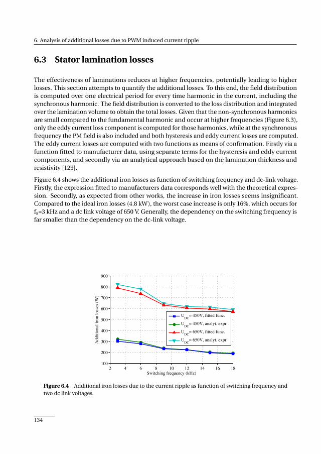
6. Analysis of additional losses due to PWM induced current ripple
6.3 Stator lamination losses
The effectiveness of laminations reduces at higher frequencies, potentially leading to higherlosses. This section attempts to quantify the additional losses. To this end, the field distributionis computed over one electrical period for every time harmonic in the current, including thesynchronous harmonic. The field distribution is converted to the loss distribution and integratedover the lamination volume to obtain the total losses. Given that the non-synchronous harmonicsare small compared to the fundamental harmonic and occur at higher frequencies (Figure 6.3),only the eddy current loss component is computed for those harmonics, while at the synchronousfrequency the PM field is also included and both hysteresis and eddy current losses are computed.The eddy current losses are computed with two functions as means of confirmation. Firstly via afunction fitted to manufacturer data, using separate terms for the hysteresis and eddy currentcomponents, and secondly via an analytical approach based on the lamination thickness andresistivity [129].
Figure 6.4 shows the additional iron losses as function of switching frequency and dc-link voltage.Firstly, the expression fitted to manufacturers data corresponds well with the theoretical expres-sion. Secondly, as expected from other works, the increase in iron losses seems insignificant.Compared to the ideal iron losses (4.8 kW), the worst case increase is only 16%, which occurs forfs=3 kHz and a dc link voltage of 650 V. Generally, the dependency on the switching frequency isfar smaller than the dependency on the dc-link voltage.
2 4 6 8 10 12 14 16 18100
200
300
400
500
600
700
800
900
Switching frequency (kHz)
Ad
dit
ion
al i
ron
lo
sses
(W
)
UDC
= 450V, fitted func.
UDC
= 450V, analyt. expr.
UDC
= 650V, fitted func.
UDC
= 650V, analyt. expr.
Figure 6.4 Additional iron losses due to the current ripple as function of switching frequency andtwo dc link voltages.
134
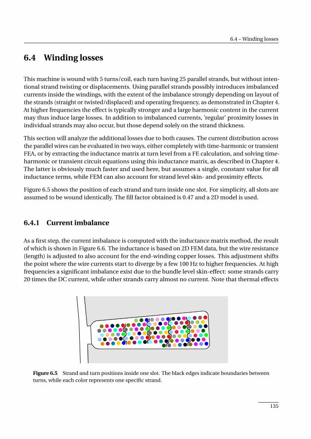
6.4 – Winding losses
6.4 Winding losses
This machine is wound with 5 turns/coil, each turn having 25 parallel strands, but without inten-tional strand twisting or displacements. Using parallel strands possibly introduces imbalancedcurrents inside the windings, with the extent of the imbalance strongly depending on layout ofthe strands (straight or twisted/displaced) and operating frequency, as demonstrated in Chapter 4.At higher frequencies the effect is typically stronger and a large harmonic content in the currentmay thus induce large losses. In addition to imbalanced currents, ’regular’ proximity losses inindividual strands may also occur, but those depend solely on the strand thickness.
This section will analyze the additional losses due to both causes. The current distribution acrossthe parallel wires can be evaluated in two ways, either completely with time-harmonic or transientFEA, or by extracting the inductance matrix at turn level from a FE calculation, and solving time-harmonic or transient circuit equations using this inductance matrix, as described in Chapter 4.The latter is obviously much faster and used here, but assumes a single, constant value for allinductance terms, while FEM can also account for strand level skin- and proximity effects.
Figure 6.5 shows the position of each strand and turn inside one slot. For simplicity, all slots areassumed to be wound identically. The fill factor obtained is 0.47 and a 2D model is used.
6.4.1 Current imbalance
As a first step, the current imbalance is computed with the inductance matrix method, the resultof which is shown in Figure 6.6. The inductance is based on 2D FEM data, but the wire resistance(length) is adjusted to also account for the end-winding copper losses. This adjustment shiftsthe point where the wire currents start to diverge by a few 100 Hz to higher frequencies. At highfrequencies a significant imbalance exist due to the bundle level skin-effect: some strands carry20 times the DC current, while other strands carry almost no current. Note that thermal effects
One color per strand, lines separate turns.
Figure 6.5 Strand and turn positions inside one slot. The black edges indicate boundaries betweenturns, while each color represents one specific strand.
135
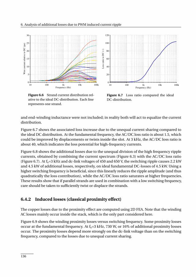
6. Analysis of additional losses due to PWM induced current ripple
10 100 1k 10k 100k0
5
10
15
20
25
30
Frequency (Hz)
Wir
e cu
rren
t re
lati
ve
to D
C (
pu
)
Figure 6.6 Strand current distribution rel-ative to the ideal DC-distribution. Each linerepresents one strand.
10 100 1k 10k 100k0
20
40
60
80
100
120
Frequency (Hz)
Lo
ss r
atio
to
DC
(−
)
Figure 6.7 Loss ratio compared the idealDC-distribution.
and end-winding inductance were not included; in reality both will act to equalize the currentdistribution.
Figure 6.7 shows the associated loss increase due to the unequal current sharing compared tothe ideal DC distribution. At the fundamental frequency, the AC/DC loss ratio is about 1.5, whichcould be improved by displacements or twists inside the slot. At 3 kHz, the AC/DC loss ratio isabout 40, which indicates the loss potential for high-frequency currents.
Figure 6.8 shows the additional losses due to the unequal division of the high frequency ripplecurrents, obtained by combining the current spectrum (Figure 6.3) with the AC/DC loss ratio(Figure 6.7). At fs=3 kHz and dc-link voltages of 450 and 650 V, the switching ripple causes 2.2 kWand 4.5 kW of additional losses, respectively, on ideal fundamental DC-losses of 4.5 kW. Using ahigher switching frequency is beneficial, since this linearly reduces the ripple amplitude (and thusquadratically the loss contribution), while the AC/DC loss ratio saturates at higher frequencies.These results show that if parallel strands are used in combination with a low switching frequency,care should be taken to sufficiently twist or displace the strands.
6.4.2 Induced losses (classical proximity effect)
The copper losses due to the proximity effect are computed using 2D FEA. Note that the windingAC losses mainly occur inside the stack, which is the only part considered here.
Figure 6.9 shows the winding proximity losses versus switching frequency. Some proximity lossesoccur at the fundamental frequency. At fs=3 kHz, 730 W, or 16% of additional proximity lossesoccur. The proximity losses depend more strongly on the dc-link voltage than on the switchingfrequency, compared to the losses due to unequal current sharing.
136
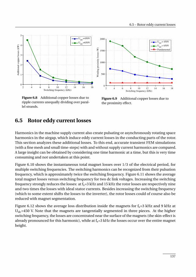
6.5 – Rotor eddy current losses
2 4 6 8 10 12 14 16 180
1
2
3
4
5
Switching frequency (kHz)
Addit
ional
copper
loss
es (
kW
)
UDC
=450V
UDC
=650V
Figure 6.8 Additional copper losses due toripple currents unequally dividing over paral-lel strands.
2 4 6 8 10 12 14 16 180
500
1000
1500
2000
Switching frequency (kHz)
Win
din
g p
roxim
ity l
oss
es (
W)
UDC
= 450V
UDC
= 650V
Fundamental
Figure 6.9 Additional copper losses due tothe proximity effect.
6.5 Rotor eddy current losses
Harmonics in the machine supply current also create pulsating or asynchronously rotating spaceharmonics in the airgap, which induce eddy current losses in the conducting parts of the rotor.This section analyzes these additional losses. To this end, accurate transient FEM simulations(with a fine mesh and small time-steps) with and without supply current harmonics are compared.A large insight can be obtained by considering one time harmonic at a time, but this is very timeconsuming and not undertaken at this point.
Figure 6.10 shows the instantaneous total magnet losses over 1/3 of the electrical period, formultiple switching frequencies. The switching harmonics can be recognized from their pulsationfrequency, which is approximately twice the switching frequency. Figure 6.11 shows the averagetotal magnet losses versus switching frequency for two dc link voltages. Increasing the switchingfrequency strongly reduces the losses: at fs=3 kHz and 15 kHz the rotor losses are respectively nineand two times the losses with ideal stator currents. Besides increasing the switching frequency(which to some extent shifts the losses to the inverter), the rotor losses could of course also bereduced with magnet segmentation.
Figure 6.12 shows the average loss distribution inside the magnets for fs=3 kHz and 9 kHz atUdc=450 V. Note that the magnets are tangentially segmented in three pieces. At the higherswitching frequency, the losses are concentrated near the surface of the magnets (the skin-effect isalready pronounced for this harmonic), while at fs=3 kHz the losses occur over the entire magnetheight.
137
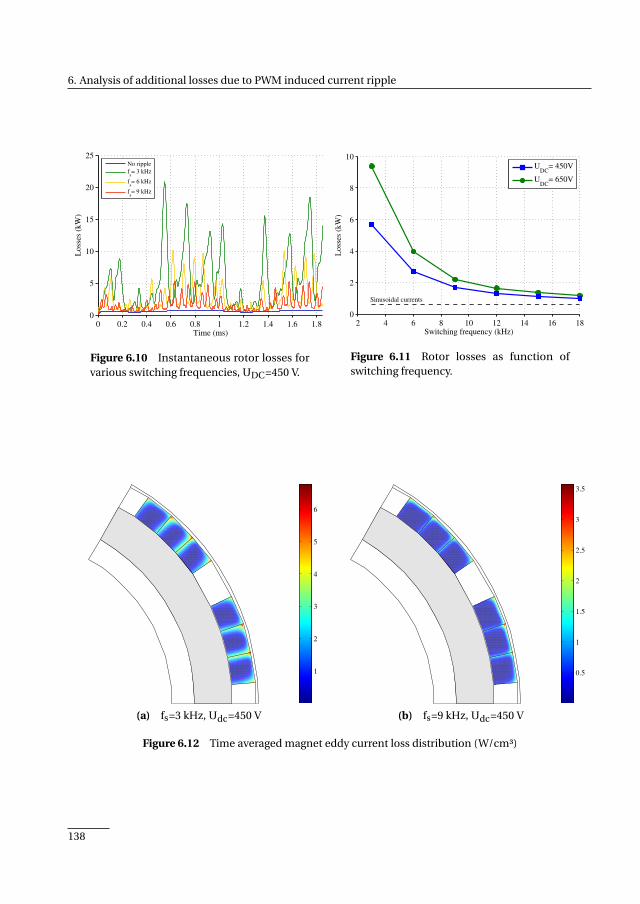
6. Analysis of additional losses due to PWM induced current ripple
0 0.2 0.4 0.6 0.8 1 1.2 1.4 1.6 1.80
5
10
15
20
25
Time (ms)
Loss
es (
kW
)
No ripple
fs= 3 kHz
fs= 6 kHz
fs= 9 kHz
Figure 6.10 Instantaneous rotor losses forvarious switching frequencies, UDC=450 V.
2 4 6 8 10 12 14 16 180
2
4
6
8
10
Switching frequency (kHz)L
oss
es (
kW
)
Sinusoidal currents
UDC
= 450V
UDC
= 650V
Figure 6.11 Rotor losses as function ofswitching frequency.
1
2
3
4
5
6
x 106
(a) fs=3 kHz, Udc=450 V
0.5
1
1.5
2
2.5
3
3.5
x 106
(b) fs=9 kHz, Udc=450 V
Figure 6.12 Time averaged magnet eddy current loss distribution (W/cm³)
138

6.6 – Conclusion
6.6 Conclusion
This chapter considered the additional iron, winding and rotor losses occurring in a PM machinedue to time harmonics in the phase currents. A range of switching frequencies and two dc linkvoltages were considered in a machine with a 0.25 pu inductance.
Based on literature, the increase in the stator lamination losses was expected to be small, whichwas confirmed. The largest increase obtained was 16%. Moreover, the additional iron lossesdepend much stronger on the dc-link voltage than the switching frequency. The rotor losseswere found to be the most sensitive to the switching frequency: compared to ideal sinusoidalsupply currents, the ripple at low switching frequencies causes a ninefold loss increase, while athigher switching frequencies the losses only double. The winding losses were analyzed separatelyfor proximity effect losses and unequal current sharing between parallel strands. The windingproximity losses due to the ripple currents depend more strongly on the dc-link voltage thanthe switching frequency, but always remain a fraction of the dc copper losses for the machineconsidered. However, unequal current sharing can cause significant AC/DC loss ratios, whichneeds attention when used in combination with a low switching frequency, although it can bevery effectively counteracted by increasing the switching frequency.
Comparing the different loss mechanisms, two groups can be identified. On the one side are theresistively limited eddy current losses –in this case the lamination and winding proximity losses–which barely depend on the switching frequency but strongly depend on the dc-link voltage. Onthe other side are the inductively limited eddy current losses –here the rotor and winding currentsharing losses– which depend strongly on both dc-link voltage and switching frequency. Thoseaspect have to be kept in mind when deciding on a (new) switching frequency for a new or givenmachine.
All in all, the results emphasize the importance of performing a system wide initial design ofa drive system, where upper and lower limits on the machine inductance, inverter switchingfrequency and system voltages are determined, to avoid excessive machine losses.
139


CHAPTER 7
Design and testing of the prototype permanentmagnet starter/generator
This chapter discusses the basic design of the prototype starter/generator (S/G) and experi-mentally validates the performance. After a brief overview of existing S/Gs, the impact of thestarting, generating and safety requirements on the machine and inverter sizing is discussed.Then, some detailed design aspects are described, such as the use of parallel wires and magnetsegmentation, using the models and results covered in detail in the earlier chapters. Finally,the machine is assembled and the basic functionalities are tested.
Based on
• M. van der Geest, H. Polinder, J. A. Ferreira, and D. Zeilstra, “Machine selection andinitial design of an aerospace starter/generator,” in IEEE Int. Electric Machines DrivesConf. (IEMDC), 2013, pp. 196–203; and
• M. van der Geest, H. Polinder, J. A. Ferreira, and D. Zeilstra, “Design and testing of ahigh-speed aerospace permanent magnet starter/generator,” in 3rd Int. Conf. ElectricalSystems Aircraft, Railway, Ship propulsion and Road Vehicles (ESARS), 2015.
141
7. Design and testing of the prototype permanent magnet starter/generator
7.1 Introduction
Large aerospace turbines are traditionally started with pneumatic motors, powered by bleed airfrom the auxiliary power unit. Electrical starters are used in smaller aircraft, where no bleedair may be available. An electrical generator is often connected in addition to the starter, tosupply power to the avionics and other on-board electronics. Combining these functions into astarter/generator (S/G) possibly saves weight and space, ultimately reducing the cost of owner-ship.
A combined S/G is not a new concept in aerospace applications though. Brushed DC machineshave been in use for decades at lower power levels [130]. The armature of these machines can beconnected directly to the DC-bus without power electronics and voltage control in generatingmode can be achieved with a straightforward DC-controller, leading to a very simple system. Themajor downside however, is the periodic maintenance that the brushes require. In addition, thesemachines have only a moderate power density and the uncontrolled torque transient duringturn-on may require special mechanical dampers. Therefore, to further reduce the operating costof an aircraft, brushless alternatives are sought.
The possibilities of using brushless machines as S/G has been explored before, especially in theautomotive industry, where much research exists on this topic. Since the mid 1990s virtually allmachines types have been or are being considered for use as a S/G. In [131] a switched reluctancemachine (SRM) is compared to an induction machine (IM), after dropping PM machines based onqualitative reasons. The IM generally performs better as a S/G. In [132] on the other hand, a SRMis developed and tested, resulting in system efficiencies of 80–90%. The described system uses adouble clutch system to spin up the SRM before connecting it to the engine, providing a torquepulse to overcome static friction without having to significantly increase machine size. SRMs arealso considered in [133]. A wound rotor synchronous machine was compared to an interior (orburied) PM machine (IPM) in [134]. Both machines have similar specific power densities, but theIPM has a higher efficiency. The benefits of an adjustable field, such as a better power factor andincreased safety, are also mentioned.
In automotive S/G research the main focus lies on PM machines, due to the potentially high powerdensity those machines offer. For automotive applications where the S/G is connected to maindrive engine, the operational shaft speed may vary over a 10:1 speed range, which is why usuallyIPMs are used. (Range extender combustion engines usually have a narrower operating speedrange, which slightly affects S/G design [135]). IPMs have a magnetically salient rotor, which,combined with properly dimensioned magnets, allows a theoretical infinite constant power speedrange [22, 136]. Examples of research on IPM S/Gs are [137–140]. PM flux switching machines(PMFSM) are also considered as S/G [141], but these have a salient stator and rotor (i.e. doublysalient), which, combined with high field strengths close to saturation, makes them prone totorque ripple. This is not desirable in automotive S/Gs from a comfort and noise perspectiveand a range of skewing methods is required to minimize the torque ripple [142]. Depending onthe available space, axial flux machines can be an attractive option. However, AF machines with
142
7.2 – Design considerations
iron-less stators have a very low inductance and electrical flux weakening is therefore ineffective.An alternative may be to use mechanical flux weakening [143].
Compared to automotive S/Gs, less research is published on brushless alternatives to the aerospaceDC S/G. In the research that exists, the main focus lies on SRMs, which are usually chosen dueto the very harsh environment and safety requirements [87, 144]. In older work from the early90s system efficiencies while generating of 80–85% are reported [145–147], which can be seenas a downside of this machine type. In [148] an embedded (incorporated in the turbine) SRM isdiscussed. Because the machine is embedded, the inner and outer radius were constrained and asegmented rotor is used, which provides a higher power density, but also presents manufacturingissues.
Wound rotor machines are also considered. Although their efficiency is perhaps less than that ofPM machines, the ability to control the field current allows unity power factor operation over awide speed range [149] or even the use of a simple bridge rectifier instead of a full inverter. Also,in case of faults the machine can be electrically switched off. A brushless exciter may be used toavoid brushes; the design, testing and control of such a machine are the topic in [150–152]. Awound-field doubly salient machine is presented as potential aerospace S/G in [153]. However,the doubly salient nature of this machine causes severe torque ripple. No comparison to othermachine types is made.
Recently, surface mounted PM machines have also been considered [154–156]. The simplemechanical structure of a surface mounted PM rotor allows operation up to very high speeds,offering significant power density improvements.
This chapter presents the implementation of a surface mounted permanent magnet (SPM) ma-chine for use as a S/G to fulfill the project specifications. For this specific application the startingtorque is approximately five times higher than the generator torque. Furthermore, the specifica-tion requires a fail-safe design, where failures during generator operation, such as short circuits,do not lead to catastrophic failure with any significant probability. Since the magnets cannot beswitched off, this is achieved by designing for a specific phase inductance together with adequatecooling capacity. However, the safety and high starting torque requirements directly oppose eachother and strongly affect both machine and inverter design, which is the topic of the first sectionof this chapter. The second section discusses the actual implementation of the machine, using themodels and conclusions from the earlier chapters, and the third section describes experimentaltests on the machine to validate the performance and models.
7.2 Design considerations
7.2.1 Requirements
Table 7.1 summarizes the main requirements. Note that this is (of course) a strong abstractionof the actual set of requirements, which in reality is far more verbose with regards to limits,
143
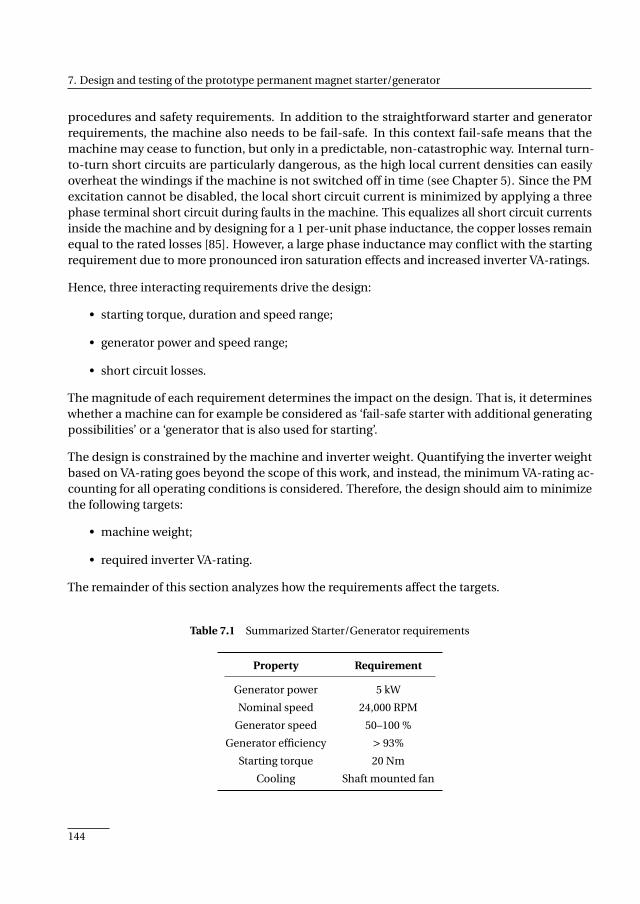
7. Design and testing of the prototype permanent magnet starter/generator
procedures and safety requirements. In addition to the straightforward starter and generatorrequirements, the machine also needs to be fail-safe. In this context fail-safe means that themachine may cease to function, but only in a predictable, non-catastrophic way. Internal turn-to-turn short circuits are particularly dangerous, as the high local current densities can easilyoverheat the windings if the machine is not switched off in time (see Chapter 5). Since the PMexcitation cannot be disabled, the local short circuit current is minimized by applying a threephase terminal short circuit during faults in the machine. This equalizes all short circuit currentsinside the machine and by designing for a 1 per-unit phase inductance, the copper losses remainequal to the rated losses [85]. However, a large phase inductance may conflict with the startingrequirement due to more pronounced iron saturation effects and increased inverter VA-ratings.
Hence, three interacting requirements drive the design:
• starting torque, duration and speed range;
• generator power and speed range;
• short circuit losses.
The magnitude of each requirement determines the impact on the design. That is, it determineswhether a machine can for example be considered as ‘fail-safe starter with additional generatingpossibilities’ or a ‘generator that is also used for starting’.
The design is constrained by the machine and inverter weight. Quantifying the inverter weightbased on VA-rating goes beyond the scope of this work, and instead, the minimum VA-rating ac-counting for all operating conditions is considered. Therefore, the design should aim to minimizethe following targets:
• machine weight;
• required inverter VA-rating.
The remainder of this section analyzes how the requirements affect the targets.
Table 7.1 Summarized Starter/Generator requirements
Property Requirement
Generator power 5 kW
Nominal speed 24,000 RPM
Generator speed 50–100 %
Generator efficiency > 93%
Starting torque 20 Nm
Cooling Shaft mounted fan
144

7.2 – Design considerations
0 0.2 0.4 0.6 0.8 1
1
1.5
2
2.5
3
3.5
Speed (pu)
Torq
ue
(pu)
Starter Generator
Ts
Tg,l
Tg,h
Figure 7.1 Definition of generic S/G torque speed curve.
7.2.2 Inverter considerations
To demonstrate the impact of the requirements on the system design, an abstract torque speedcurve is first defined in Figure 7.1. The machine operates as starter with constant torque Ts upto 50% speed and as a generator with constant power load between 50% and 100% speed. Thegenerator quantities at full speed serve as 1 pu base. The pu three phase short circuit current isIsc,pu. For convenience, the starting torque is normalized to the maximum generator torque:
Ts,rel =Ts
Tg,l(7.1)
Hence, for Ts,rel = 1 the starting torque requirement does not increase the machine or invertercurrent ratings, except from the thermal perspective in case of a shaft mounted fan. Lastly, themaximum losses that can be sustained indefinitely are set equal to the short circuit copper losses.
Next, the minimum theoretical inverter VA-rating is computed for different values of Ts,rel andIsc,pu, under the assumption that semiconductor devices with arbitrary ratings can be used. Thisrequires the dq-currents versus speed to be determined. The required q-axis current is definedby the torque-speed requirement, but the d-axis current can be chosen freely. In the followinganalysis, the d-axis current versus speed is chosen to either minimize the inverter VA-rating, or aszero.
Figure 7.2 shows the resulting minimum inverter rating versus short circuit current, normalizedto the nominal generator power. For large values of Ts,rel and low values of Isc,pu, the inverterrating rises sharply; a 1 pu short circuit current for the target machine would imply an inverter
145
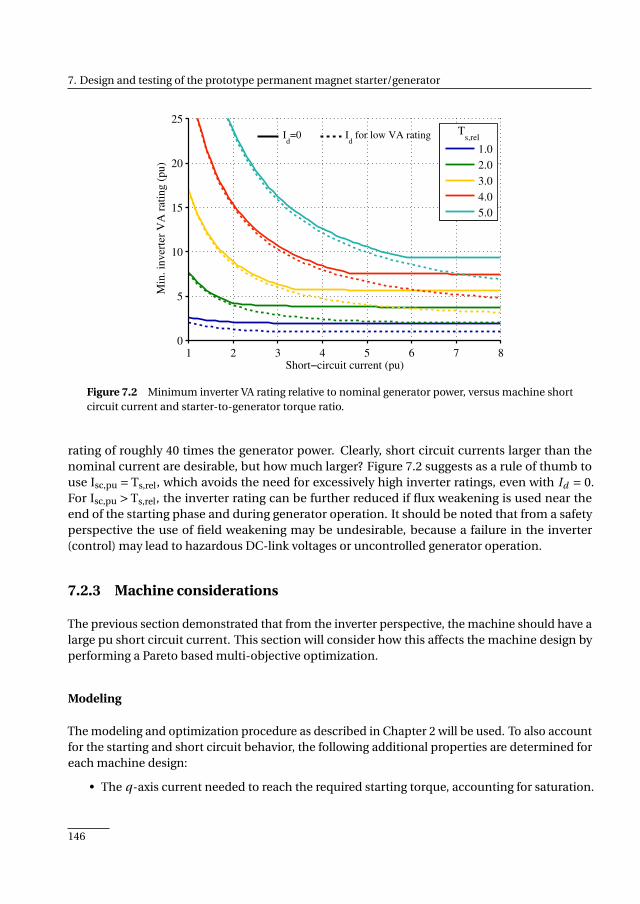
7. Design and testing of the prototype permanent magnet starter/generator
1 2 3 4 5 6 7 80
5
10
15
20
25
Short−circuit current (pu)
Min
. in
ver
ter
VA
rat
ing (
pu)
1.0
2.0
3.0
4.0
5.0
Ts,relI
d=0 I
d for low VA rating
Figure 7.2 Minimum inverter VA rating relative to nominal generator power, versus machine shortcircuit current and starter-to-generator torque ratio.
rating of roughly 40 times the generator power. Clearly, short circuit currents larger than thenominal current are desirable, but how much larger? Figure 7.2 suggests as a rule of thumb touse Isc,pu = Ts,rel, which avoids the need for excessively high inverter ratings, even with Id = 0.For Isc,pu > Ts,rel, the inverter rating can be further reduced if flux weakening is used near theend of the starting phase and during generator operation. It should be noted that from a safetyperspective the use of field weakening may be undesirable, because a failure in the inverter(control) may lead to hazardous DC-link voltages or uncontrolled generator operation.
7.2.3 Machine considerations
The previous section demonstrated that from the inverter perspective, the machine should have alarge pu short circuit current. This section will consider how this affects the machine design byperforming a Pareto based multi-objective optimization.
Modeling
The modeling and optimization procedure as described in Chapter 2 will be used. To also accountfor the starting and short circuit behavior, the following additional properties are determined foreach machine design:
• The q-axis current needed to reach the required starting torque, accounting for saturation.
146
7.2 – Design considerations
• The adiabatic temperature rise rate (K/s) during starting, to compare the starting perfor-mance of different machines. The adiabatic temperature rise is based solely on the copperlosses and weight, which may not be fully realistic, but avoids the need for more accuratethermal models.
• The copper, lamination and rotor losses during a three phase short circuit.
The optimization variables are the nine most important geometric dimensions, including stacklength, outer radius and airgap length. Further relevant assumptions are: a winding fill factorof 50%; 0.1 mm FeCo stator laminations (due to the high saturation flux density); magnets withBr=1 T; a carbon fiber retaining sleeve for low rotor losses and a 15 slot 10 pole concentratednon-overlapping winding layout.
The optimization targets were the following:
• minimize machine weight;
• maximize per-unit short circuit current;
• minimize short circuit losses;
• minimize starting temperature rise rate.
Note that the generator mode efficiency is not included as target; earlier exploratory optimizations(partially described in Chapter 2) indicated that when designing for both low fault losses andgood starting performance, acceptable generator performance will result, as will be shown hereas well. Further note that the S/G example optimization in Chapter 2 used the starting copperlosses as target, instead of temperature rise rate. Focussing on the copper losses favors FSMs,as those machines typically have lower copper losses than SPMs, but operate at higher currentdensities. Hence, when also accounting for the temperature rise rate, the benefits of FSMs reduce.
Lastly, to obtain the results in this section, 330 generations with 20 particles were used in two trailswith different starting conditions, so that in total over 13,000 machine designs were analyzed.
Optimization outcome
Figure 7.3 shows several side views to the Pareto optimal front, divided based on the startingtemperature rise rate, as indicated in Figure 7.3(a). Each point represents a machine designthat is optimal in some way in the 4D target space. Figure 7.3(a) clearly shows that a goodstarting performance requires a high short circuit current. For the specifications consideredhere, designing a machine with a 1 pu inductance is practically impossible, while with Isc,pu = 4,temperature rise rates below 2 K/s are possible. Figure 7.3(b) shows that machines with goodstarting performance (ie. yellow triangles) are heavy machines. This was to be expected, sincelarger machine have more copper mass to both carry the current and absorb the starting losses.
Figure 7.3(c) shows the short circuit losses versus Isc,pu. Unsurprisingly, increasing Isc,pu alsoincreases the short circuit losses, which conflicts with the fail-safe requirement of having low
147
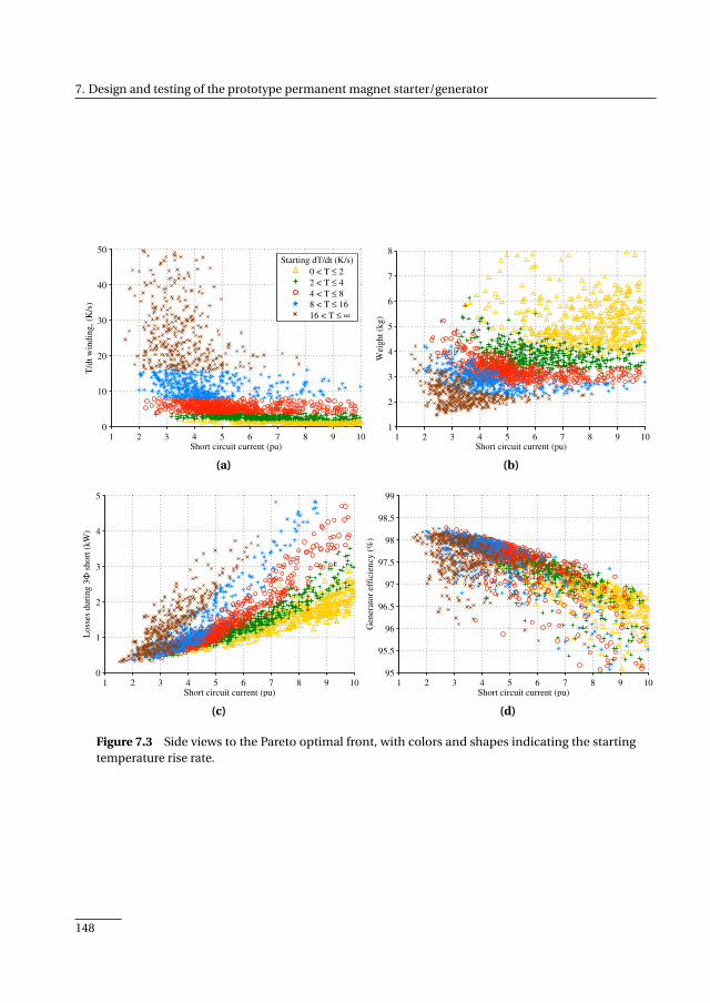
7. Design and testing of the prototype permanent magnet starter/generator
1 2 3 4 5 6 7 8 9 100
10
20
30
40
50
Short circuit current (pu)
T/d
t w
indin
g, (K
/s)
0 < T ≤ 2
2 < T ≤ 4
4 < T ≤ 8
8 < T ≤ 16
16 < T ≤ ∞
Starting dT/dt (K/s)
(a)
1 2 3 4 5 6 7 8 9 101
2
3
4
5
6
7
8
Short circuit current (pu)
Wei
ght
(kg)
(b)
1 2 3 4 5 6 7 8 9 100
1
2
3
4
5
Short circuit current (pu)
Loss
es d
uri
ng 3
Φ s
hort
(kW
)
(c)
1 2 3 4 5 6 7 8 9 1095
95.5
96
96.5
97
97.5
98
98.5
99
Short circuit current (pu)
Gen
erat
or
effi
cien
cy (
%)
(d)
Figure 7.3 Side views to the Pareto optimal front, with colors and shapes indicating the startingtemperature rise rate.
148
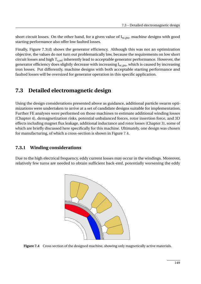
7.3 – Detailed electromagnetic design
short circuit losses. On the other hand, for a given value of Isc,pu, machine designs with goodstarting performance also offer low faulted losses.
Finally, Figure 7.3(d) shows the generator efficiency. Although this was not an optimizationobjective, the values do not turn out problematically low, because the requirements on low shortcircuit losses and high Ts,rel inherently lead to acceptable generator performance. However, thegenerator efficiency does slightly decrease with increasing Isc,pu, which is caused by increasingiron losses. Put differently, machine designs with both acceptable starting performance andfaulted losses will be oversized for generator operation in this specific application.
7.3 Detailed electromagnetic design
Using the design considerations presented above as guidance, additional particle swarm opti-mizations were undertaken to arrive at a set of candidate designs suitable for implementation.Further FE analyses were performed on those machines to estimate additional winding losses(Chapter 4), demagnetization risks, potential unbalanced forces, rotor insertion force, and 3Deffects including magnet flux leakage, additional inductance and rotor losses (Chapter 3), some ofwhich are briefly discussed here specifically for this machine. Ultimately, one design was chosenfor manufacturing, of which a cross-section is shown in Figure 7.4.
7.3.1 Winding considerations
Due to the high electrical frequency, eddy current losses may occur in the windings. Moreover,relatively few turns are needed to obtain sufficient back-emf, potentially worsening the eddy
Figure 7.4 Cross section of the designed machine, showing only magnetically active materials.
149
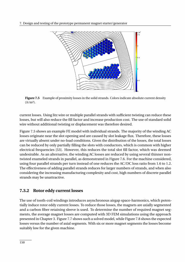
7. Design and testing of the prototype permanent magnet starter/generator
Figure 7.5 Example of proximity losses in the solid strands. Colors indicate absolute current density(A/m²).
current losses. Using litz wire or multiple parallel strands with sufficient twisting can reduce theselosses, but will also reduce the fill factor and increase production cost. The use of standard solidwire without additional twisting or displacement was therefore desired.
Figure 7.5 shows an example FE model with individual strands. The majority of the winding AClosses originate near the slot opening and are caused by slot leakage flux. Therefore, these lossesare virtually absent under no-load conditions. Given the distribution of the losses, the total lossescan be reduced by only partially filling the slots with conductors, which is common with higherelectrical frequencies [53]. However, this reduces the total slot fill factor, which was deemedundesirable. As an alternative, the winding AC losses are reduced by using several thinner non-twisted enameled strands in parallel, as demonstrated in Figure 7.6. For the machine considered,using four parallel strands per turn instead of one reduces the AC/DC loss ratio from 1.6 to 1.2.The effectiveness of adding parallel strands reduces for larger numbers of strands, and when alsoconsidering the increasing manufacturing complexity and cost, high numbers of discrete parallelstrands may be unattractive.
7.3.2 Rotor eddy current losses
The use of tooth-coil windings introduces asynchronous airgap space-harmonics, which poten-tially induce rotor eddy current losses. To reduce those losses, the magnets are axially segmentedand a carbon fiber retaining sleeve is used. To determine the number of required magnet seg-ments, the average magnet losses are computed with 3D FEM simulations using the approachpresented in Chapter 3. Figure 7.7 shows such a solved model, while Figure 7.8 shows the expectedlosses versus the number of axial segments. With six or more magnet segments the losses becomesuitably low for the given machine.
150
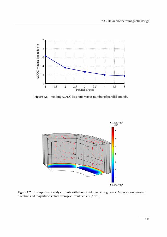
7.3 – Detailed electromagnetic design
1 1.5 2 2.5 3 3.5 4 4.5 51
1.2
1.4
1.6
1.8
2
Parallel strands
AC
/DC
win
din
g l
oss
rat
io (
−)
Figure 7.6 Winding AC/DC loss ratio versus number of parallel strands.
Figure 7.7 Example rotor eddy currents with three axial magnet segments. Arrows show currentdirection and magnitude, colors average current density (A/m²).
151
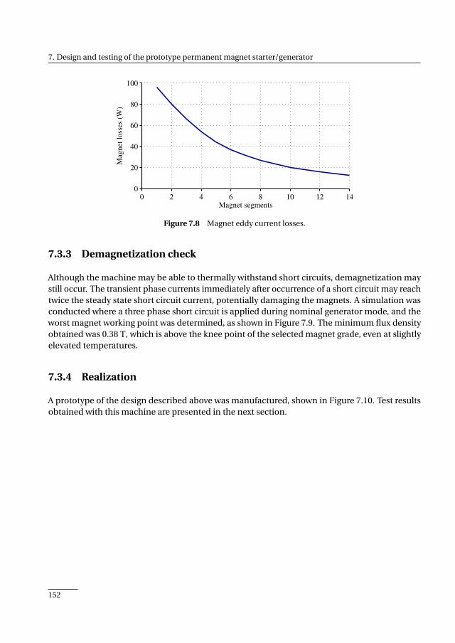
7. Design and testing of the prototype permanent magnet starter/generator
0 2 4 6 8 10 12 140
20
40
60
80
100
Magnet segments
Mag
net
lo
sses
(W
)
Figure 7.8 Magnet eddy current losses.
7.3.3 Demagnetization check
Although the machine may be able to thermally withstand short circuits, demagnetization maystill occur. The transient phase currents immediately after occurrence of a short circuit may reachtwice the steady state short circuit current, potentially damaging the magnets. A simulation wasconducted where a three phase short circuit is applied during nominal generator mode, and theworst magnet working point was determined, as shown in Figure 7.9. The minimum flux densityobtained was 0.38 T, which is above the knee point of the selected magnet grade, even at slightlyelevated temperatures.
7.3.4 Realization
A prototype of the design described above was manufactured, shown in Figure 7.10. Test resultsobtained with this machine are presented in the next section.
152
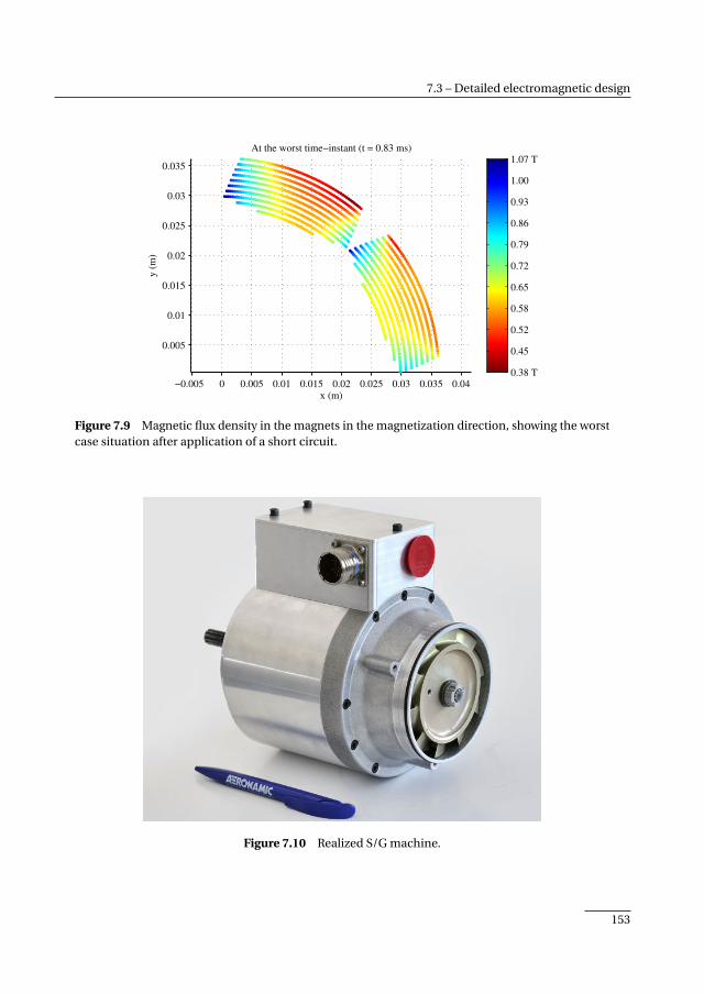
7.3 – Detailed electromagnetic design
−0.005 0 0.005 0.01 0.015 0.02 0.025 0.03 0.035 0.04
0.005
0.01
0.015
0.02
0.025
0.03
0.035
x (m)
At the worst time−instant (t = 0.83 ms)
y (
m)
1.07 T
1.00
0.93
0.86
0.79
0.72
0.65
0.58
0.52
0.45
0.38 T
Figure 7.9 Magnetic flux density in the magnets in the magnetization direction, showing the worstcase situation after application of a short circuit.
Figure 7.10 Realized S/G machine.
153
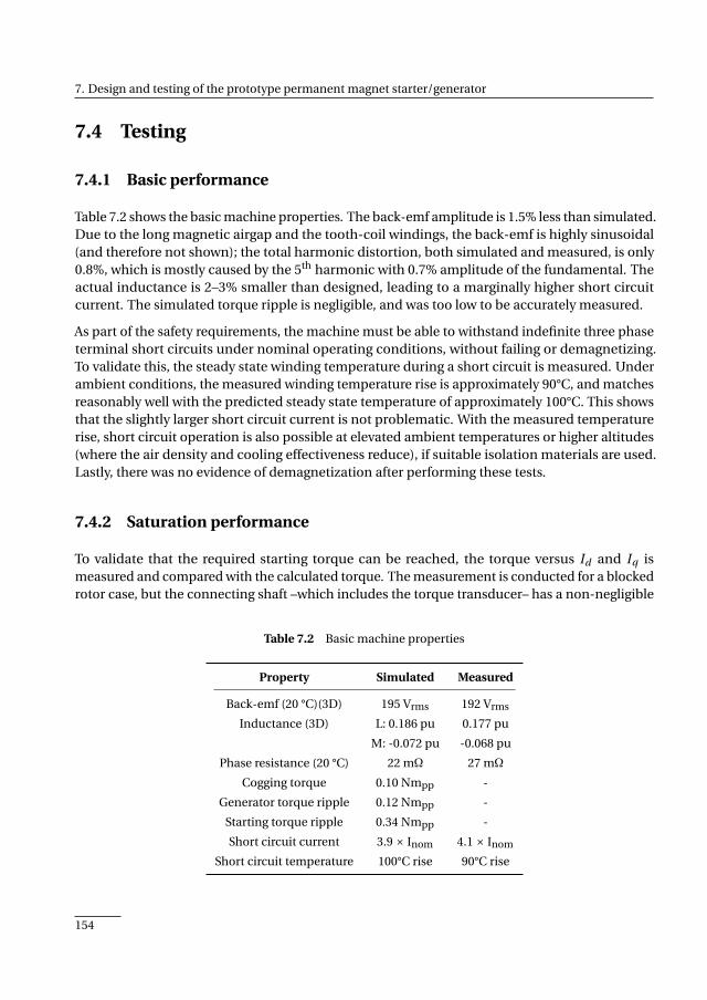
7. Design and testing of the prototype permanent magnet starter/generator
7.4 Testing
7.4.1 Basic performance
Table 7.2 shows the basic machine properties. The back-emf amplitude is 1.5% less than simulated.Due to the long magnetic airgap and the tooth-coil windings, the back-emf is highly sinusoidal(and therefore not shown); the total harmonic distortion, both simulated and measured, is only0.8%, which is mostly caused by the 5th harmonic with 0.7% amplitude of the fundamental. Theactual inductance is 2–3% smaller than designed, leading to a marginally higher short circuitcurrent. The simulated torque ripple is negligible, and was too low to be accurately measured.
As part of the safety requirements, the machine must be able to withstand indefinite three phaseterminal short circuits under nominal operating conditions, without failing or demagnetizing.To validate this, the steady state winding temperature during a short circuit is measured. Underambient conditions, the measured winding temperature rise is approximately 90°C, and matchesreasonably well with the predicted steady state temperature of approximately 100°C. This showsthat the slightly larger short circuit current is not problematic. With the measured temperaturerise, short circuit operation is also possible at elevated ambient temperatures or higher altitudes(where the air density and cooling effectiveness reduce), if suitable isolation materials are used.Lastly, there was no evidence of demagnetization after performing these tests.
7.4.2 Saturation performance
To validate that the required starting torque can be reached, the torque versus Id and Iq ismeasured and compared with the calculated torque. The measurement is conducted for a blockedrotor case, but the connecting shaft –which includes the torque transducer– has a non-negligible
Table 7.2 Basic machine properties
Property Simulated Measured
Back-emf (20 °C)(3D) 195 Vrms 192 Vrms
Inductance (3D) L: 0.186 pu 0.177 pu
M: -0.072 pu -0.068 pu
Phase resistance (20 °C) 22 mΩ 27 mΩ
Cogging torque 0.10 Nmpp -
Generator torque ripple 0.12 Nmpp -
Starting torque ripple 0.34 Nmpp -
Short circuit current 3.9 × Inom 4.1 × Inom
Short circuit temperature 100°C rise 90°C rise
154
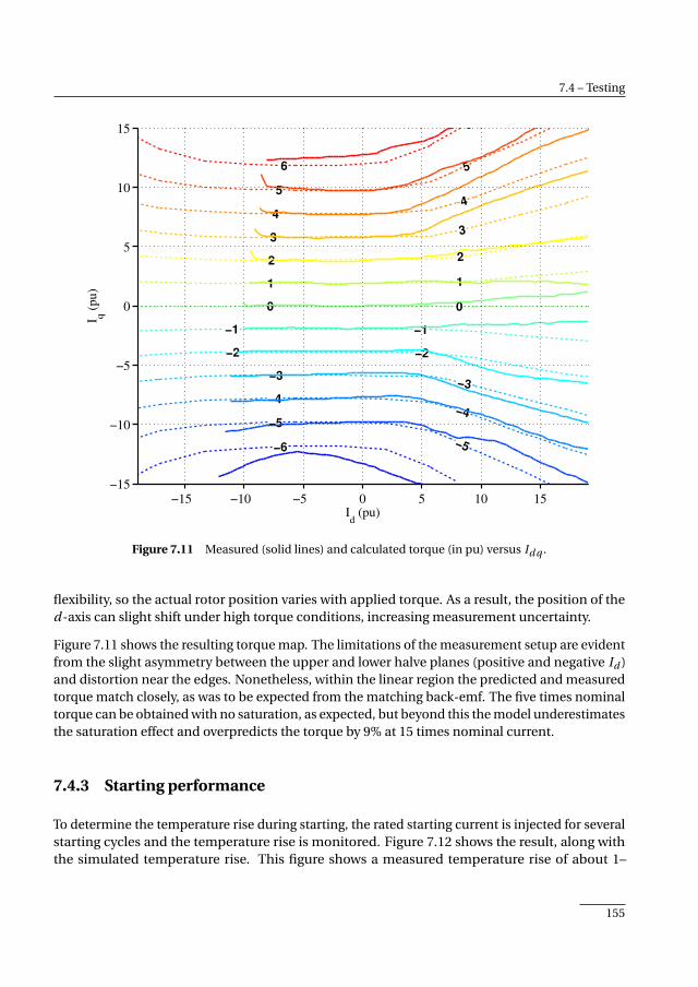
7.4 – Testing
−6
−6
−5
−5
−4−4
−3−3
−2 −2
−1 −1
0 0
1 1
2 2
33
4
4
5
56
6
Id (pu)
I q (
pu)
−15 −10 −5 0 5 10 15−15
−10
−5
0
5
10
15
Figure 7.11 Measured (solid lines) and calculated torque (in pu) versus Id q .
flexibility, so the actual rotor position varies with applied torque. As a result, the position of thed-axis can slight shift under high torque conditions, increasing measurement uncertainty.
Figure 7.11 shows the resulting torque map. The limitations of the measurement setup are evidentfrom the slight asymmetry between the upper and lower halve planes (positive and negative Id )and distortion near the edges. Nonetheless, within the linear region the predicted and measuredtorque match closely, as was to be expected from the matching back-emf. The five times nominaltorque can be obtained with no saturation, as expected, but beyond this the model underestimatesthe saturation effect and overpredicts the torque by 9% at 15 times nominal current.
7.4.3 Starting performance
To determine the temperature rise during starting, the rated starting current is injected for severalstarting cycles and the temperature rise is monitored. Figure 7.12 shows the result, along withthe simulated temperature rise. This figure shows a measured temperature rise of about 1–
155

7. Design and testing of the prototype permanent magnet starter/generator
0 2 4 6 8 100
50
100
150
200
Time (min.)
Coil
tem
per
ature
(°C
)
Measured
Thermal model
Figure 7.12 Measured and simulated winding temperature during repeated starting cycles.
1.5 K/s, which is sufficiently low to allow multiple repeated start attempts without overheating.Within each starting cycle the model overpredicts the temperature rise by about 10%, which isconsidered to be sufficiently accurate. The thermal model over-predicts the average temperaturerise after some time, because it partially neglects heat conduction to the machine’s surroundingsat standstill.
7.5 Conclusion
This chapter discussed the implementation of a surface mounted PM machine as an aerospacestarter/generator. Unique in this design is the five times larger starting torque than the maximumgenerator torque. Furthermore, the machine is required to be fail-safe, which is achieved bylimiting the short circuit current. However, a low short circuit current directly opposes the startingperformance, as it increases both the minimum inverter VA-rating and the temperature riseduring starting, and a compromise needs to be found. Ultimately, the implemented machine willbe over-dimensioned for the generator requirement, while still having only a limited safe startingduration.
Multidimensional particle swarm based optimization was again used to consider the importanttrade-offs that affect the machine design and find suitable candidate machines. Further detailedanalyses were performed, demonstrating the impact of rotor and winding eddy current lossesspecifically for this machine. A prototype was built and tested. The back-emf, inductance, shortcircuit current and temperature, and starting performance all show a good match to simulatedperformance, ultimately demonstrating that a surface mounted PM machine may be successfullyused as starter/generator. Additionally, the tests verify the outcome of the FE models usedthroughout this thesis.
156

CHAPTER 8
Power density limits and design trends of high-speedpermanent magnet synchronous machines
In the previous chapters, optimization methods were introduced and models were presentedand tested, eventually leading to the prototype starter/generator. In this final chapter, thosemodels and optimization methods are used at a large scale to determine more general butstill quantitative design trends and limits related to the specific power density of high-speedpermanent magnet machines. To this end, eighty individual optimizations are executed, cov-ering a range of rotor surface speeds, power levels and cooling systems. Afterwards, machinesare selected from each front and relevant performance criteria and properties are plotted,demonstrating various trends in machine design. This chapter may be used in two ways: as ademonstration of a method to find accurate yet generic design trends and limits; and as anactual overview of power density limits and the associated design trends.
Based on
• M. van der Geest, H. Polinder, J. A. Ferreira, and M. Christmann, “Power density limitsand design trends of high-speed permanent magnet synchronous machines,” IEEETrans. Transportation Electrification, vol. 1, no. 3, pp. 266–276, Oct. 2015; and
• M. van der Geest, H. Polinder, J. A. Ferreira, and M. Christmann, “Quantitative powerdensity limits of aerospace permanent magnet synchronous machines,” in More Elec-tric Aircraft Conference, 2015.
157
8. Power density limits and design trends of high-speed permanent magnet synchronous machines
8.1 Introduction
Electrical machines are inherently part of a larger system. They should therefore be designedtogether with the other parts of the system to arrive at a global optimum. This is particularlyimportant for aerospace systems, where a low system weight and volume are essential to obtaina competitive system. In the early design phase of new systems, many different concepts andconfigurations may be considered. It is usually infeasible to consider all possible options in detail,so a selection of the most promising systems to proceed with needs to be made. To facilitate thisearly selection, figures of merit or sufficiently accurate yet fast models are required for all majorsubcomponents in the system.
For electrical machines, many simple analytical scaling laws and rules of thumb exist, but thesecan only provide a rough initial guess for the machine size, which may be insufficient for thedesign of high performance systems [157]. For example, [158] uses very basic analytical equationsto establish a generic torque-per-volume parameter. This provides a high-level estimate ofmachine performance in this parameter, but may not offer the level of detail that is requiredfor early machine selection. Similar arguments apply to [159], where a more detailed sizingequation for volumetric power density is developed, but a detailed loss analysis is necessarilyomitted. Determining volumetric power density limits is the focus of [160]. However, the modelingand optimization methods have limitations, because the analytical models neglect saturationand rotor losses, while these effects are considered in the method proposed in this thesis. Themachines are loaded by a passive RL load, while an inverter drive would commonly be used inhigh performance applications today. Nonetheless, quantitative results for the volumetric powerdensity are presented and compared for a range of PM machine types. Ref. [161] determines speedlimits for electrical machines. To this end, analytical expressions are used to correlate mechanical,thermal and magnetic limits, providing a high level theoretical support of empirically obtainedpower-speed limits. Ref. [162] quantifies power limits of surface mounted permanent magnet(SPM) machines for five rotational speeds between 20–100 kRPM and a given set of mechanicaland thermal constraints. The emphasis lies on modeling however, and few underlying details ofthe five resulting machines are provided. A finite element based sizing approach for interior PMmachines with consideration of the magnetic and thermal domains is proposed in [163]. In atwo step process, a generic optimal machine cross-section is first created with PSO, which is thentransformed into a final design via a scaling exercise. Hence, manual interaction is still necessaryto obtain the final machine design. Most of these examples implicitly also illustrate that whendetermining limits of electrical machines, a balance needs to be found between generality andlevel of detail.
Another approach is to use a database with existing machine designs to identify trends and limits[164,165], but this approach has several drawbacks as well: very few comparable designs may exist(in terms of application, power and speed levels, design intent); or little specific data is publishedfor a given machine, such as constraints, dimensions, weight or used materials. Ultimately, aliterature study allows global limits such as power-speed curves to be identified, but an in-depthanalysis of underlying machine properties is generally not possible.
158
8.1 – Introduction
The desired level of detail and accuracy can be obtained with finite element analysis (FEA). Initself, FEA is an analysis method, but by combining FEA with optimization algorithms, it canbe part of a design method ([16, 166],Chapter 2). By using magnetic, thermal and mechanicalsimulations, all relevant performance data can be obtained, at the cost of computation time. Thiscomputational cost prohibits the direct application of FE-based optimization methods in an earlydesign stage.
This chapter attempts to bridge the gap between inaccurate scaling laws, underpopulateddatabases and time consuming FE-based optimizations, by filling a database with systemat-ically chosen and individually FE-based optimized machine designs. Advantages of this approachinclude that all machine properties –such as dimensions, losses or electrical parameters– areknown and that each resulting machine is optimized with identical targets, constraints and mate-rials. This allows both global trends such as power density, and underlying trends such as machinedimensions and performance, to be determined and quantified. The results can serve as a directstarting point for new designs, as a reference for comparison with existing designs, or as a meansto gain insight into fundamental design tradeoffs of surface mounted permanent magnet (SPM)machines.
In this work, the ultimate goal is to determine the maximum specific power density (kW/kg)of SPM machines, as function of four rotor surface speeds, five power levels and four coolingscenarios. For each of these 80 design points, an individual multi-objective FE-based optimizationis executed, with minimization of weight and peak winding temperature and maximization ofefficiency as objectives, and the machine geometry as variable. Qualitatively, the relation betweenthe specific power density and the main variables is well known. The contribution of this work isthe proposal and application of a method to quantify and present design trends and limits with avery high level of detail. A second contribution is the presentation of useful design relations andtrends that can be used as a starting point for new machine designs or gain general insight intosizing trends.
One major limitation of a design study as proposed here is validation of the results. Althoughthe underlying FE models used here have been successfully validated in the previous chapters,this does not imply that the trends determined here are also correct. Validation of the designtrends could for example be achieved by pursuing the same goal (ie. dependencies of specificpower density), but using a different optimization strategy and work flow. A simpler alternativewill be undertaken in this case though: the properties of the optimal designs obtained here arecompared with those from existing designs found in literature [161, 164].
This chapter is structured as follows: Section 8.2 explains and motivates the proposed optimiza-tion approach, while Section 8.3 briefly presents the models and assumptions used. Section 8.4presents and explains the results. Lastly, Section 8.5 discusses the results with a comparison toliterature values and a thermal sensitivity analysis.
159

8. Power density limits and design trends of high-speed permanent magnet synchronous machines
8.2 Optimization approach
8.2.1 Choice of main target and independent variables
The main goal of this work is to determine the dependency of specific power density on rotorsurface speed, power level and cooling effort. This is motivated by the following arguments:
• Specific power density is chosen because in aircraft, and particulary rotorcraft, low weightis essential to increase range and reduce operating costs.
• Constant rotor surface speeds of 25, 50, 100 and 200 m/s are considered. A constant surfacespeed is chosen over a constant rotational speed, because the former represents a roughlyconstant mechanical design effort. For example, a machine with vsurf=200 m/s will alwaysrequire detailed mechanical analysis, regardless of the rotational speed or rotor diameter. Inapplications where the rotational speed is imposed, the results from this work can be usedin two ways: with given surface and rotational speeds the rotor diameter can be estimatedand compared with a target design envelope. Alternatively, the results can be combinedwith gearbox data to compare direct drive systems to geared solutions.
• Power levels of 50, 100, 200, 500 and 1000 kW are considered. A small dependency of powerdensity on power level is expected and multiple levels are considered to confirm this.
• The achievable machine performance strongly depends on cooling intensity and a widerange of cooling options exist, ranging from passive convection cooling to complex liquidcooling with flow paths inside the magnetically active parts. This implies that the coolingsystem must be a parameter to obtain sufficiently generic results, but it also implies thatcooling solutions cannot easily be compared. Therefore, four cooling scenarios are defined,as will be described in a few pages.
8.2.2 Implementation
Due to the wide range of power, speed and cooling levels considered, properties such as optimalflux and current densities, pole count and dimensions will all vary between the considered cases.To ensure that each design in the database is indeed optimal, an individual multi-objectiveoptimization is executed for each design point. The variables in this optimization are the machinedimensions, while the targets are high efficiency, low winding temperature rise and low weight.
The result of each optimization is a Pareto optimal front (POF), which captures the fact in thepresence of conflicting targets, no single optimum exists ([16, 167],Chapter 2). In this study, eachof the 80 resulting three dimensional POFs shows the trade-off between weight, efficiency andwinding temperature for a given design point. These are considered local trade-offs, since theycorrespond to a single machine specification.
160
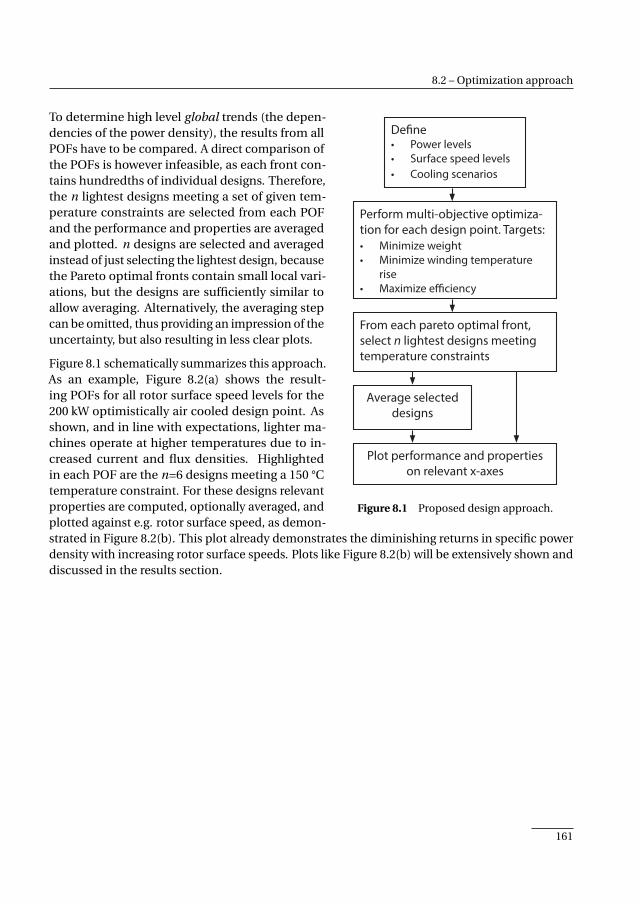
8.2 – Optimization approach
Define• Powerlevels• Surfacespeedlevels• Coolingscenarios
Performmulti-objectiveoptimiza-tionforeachdesignpoint.Targets:• Minimizeweight• Minimizewindingtemperature
rise• Maximizeefficiency
Fromeachparetooptimalfront,selectnlightestdesignsmeetingtemperatureconstraints
Averageselecteddesigns
Plotperformanceandpropertiesonrelevantx-axes
Figure 8.1 Proposed design approach.
To determine high level global trends (the depen-dencies of the power density), the results from allPOFs have to be compared. A direct comparison ofthe POFs is however infeasible, as each front con-tains hundredths of individual designs. Therefore,the n lightest designs meeting a set of given tem-perature constraints are selected from each POFand the performance and properties are averagedand plotted. n designs are selected and averagedinstead of just selecting the lightest design, becausethe Pareto optimal fronts contain small local vari-ations, but the designs are sufficiently similar toallow averaging. Alternatively, the averaging stepcan be omitted, thus providing an impression of theuncertainty, but also resulting in less clear plots.
Figure 8.1 schematically summarizes this approach.As an example, Figure 8.2(a) shows the result-ing POFs for all rotor surface speed levels for the200 kW optimistically air cooled design point. Asshown, and in line with expectations, lighter ma-chines operate at higher temperatures due to in-creased current and flux densities. Highlightedin each POF are the n=6 designs meeting a 150 °Ctemperature constraint. For these designs relevantproperties are computed, optionally averaged, andplotted against e.g. rotor surface speed, as demon-strated in Figure 8.2(b). This plot already demonstrates the diminishing returns in specific powerdensity with increasing rotor surface speeds. Plots like Figure 8.2(b) will be extensively shown anddiscussed in the results section.
161
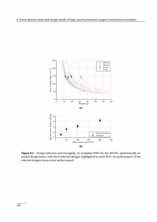
8. Power density limits and design trends of high-speed permanent magnet synchronous machines
0 20 40 60 80 100 120 1400
50
100
150
200
250
Weight (kg)
Max
. w
ind
ing
tem
p.
rise
(°C
)
200 m/s
100 m/s
50 m/s
25 m/s
(a)
0 50 100 150 200 2502
4
6
8
10
Rotor surface speed (m/s)
Sp
ecif
ic p
ow
er d
ensi
ty (
kW
/kg
)
Selected designs
Averaged
(b)
Figure 8.2 Design selection and averaging: (a) complete POFs for the 200 kW, optimistically aircooled design point, with the 6 selected designs highlighted in each POF; (b) performance of theselected designs versus rotor surface speed.
162

8.3 – Modeling, assumptions & material properties
8.3 Modeling, assumptions & material properties
This section describes all constants and assumptions, as well as the models used in the optimiza-tions.
8.3.1 Electrical domain
Assumptions
To keep the number of variables manageable, a number of assumptions must be made. With theemphasis on higher speed machines and high performance, SPM machines are considered. Athigh speeds SPM machines are more attractive than interior PM machines, because the latterrapidly require thicker magnetic bridges at higher speeds, which in turn requires more magnetmaterial to maintain sufficient airgap field strength [164, 168]. In addition, increasing surfacespeeds require increasing mechanical airgap lengths due to mechanical considerations, which inturn reduces the saliency ratio and with that, the benefits of interior PM machines.
Only concentrated non-overlapping windings are considered, because this offers the benefitsof short end-windings and simple manufacturing. With such windings, asynchronous space-harmonics can induce problematic rotor eddy current losses, especially at high speeds. Tominimize these losses, only windings from the 3 slot, 2 pole family (q=0.5) are chosen, as thesehave no space-harmonics below the synchronous harmonic and the first higher order harmonichas already twice the pole count of the synchronous harmonic. To further reduce rotor losses, acarbon fiber retaining sleeve is assumed, together with axial magnet segmentation in 8 pieces.
Lastly, (costly) iron-cobalt laminations are assumed, because they allow high flux saturation levels(2.4 T) and are available as thin sheets to reduce losses. Further material properties, constantsand variables are summarized in Table 8.1.
Modeling
Each machine is analyzed entirely with 2D FEA, allowing saturation, rotor eddy current losses andall geometric details to be accounted for. The basic machine properties and losses, such as linkedflux, inductance, torque ripple; and iron, copper and rotor losses are computed, as describedin Section 2.2.1. Note that losses, temperatures or current and flux densities are not explicitlyconstrained in this approach. Instead, by optimizing for a low temperature rise and selecting finaldesigns based on temperature, the optimal current and flux densities will result. This removes theneed for the user to specify ‘optimal’ current densities a priori. Next, because only 2D models areused, the machine performance may be overestimated for very short machines. To avoid this, aminimum axial stack length of 40 mm is used for all cases.
163

8. Power density limits and design trends of high-speed permanent magnet synchronous machines
Table 8.1 Relevant material properties
Stat./Rot.Lam.
Winding Magnets Retain.Sleeve
µr FeCo 1 1.05 1
Losses1 0.15 mm fill 50% ρ=1 µΩm ρ=100 µΩm
Br - - 1.2 T -
Density2 8120 5185 7500 1597
Therm.cond.3 29 / 0.7 1.2 / 195 7.5 / 2.5 0.77
1 Respectively sheet thickness, fill factor, resistivity2 In kg/m3; 3 In W/(m·K), in-plane / axial
8.3.2 Mechanical domain
At the considered rotor surface speeds, the mechanical design of the machines –consisting ofstatic stress analysis and rotor dynamic analysis– must be considered to some extend. Otherauthors suggest that the stress analysis is of primary concern for high power density designs [169].In this work, this is dealt with by using a fixed sleeve thickness of 2.5 mm for the carbon fibersleeve. At higher speeds this may be insufficient, but the results will show that at these speeds theoptimal magnetic airgap length increases, allowing thicker sleeves to be used if needed.
8.3.3 Thermal domain
Assumptions
A wide variety of cooling systems exists and quantifying a complete cooling system is difficult.Therefore, the following four cooling scenarios are defined:
• C1 – Pessimistic air cooling The machine is cooled only by ambient air forced through theairgap; the only heat exchange occurs in the airgap and around the end-windings. The statoryoke outside surface is assumed to be insulated. This case represents electrical machinesbuilt into large structures, where cooling from the machine outer periphery towards theenvironment is not possible (e.g. engine bays).
• C2 – Optimistic air cooling has increased flow rates compared to the previous case, as wellas forced cooling on the stator yoke outside surface.
• C3 – Liquid jacket, totally enclosed The stator outside is cooled by a liquid jacket. Themachine is closed, but air is circulated in the machine to transfer rotor heat to the stator.
• C4 – Liquid jacket & rotor air cooling Is similar to the previous case, but ambient air isforced through the airgap, although at lower rates than in the pessimistic air cooling case.
164
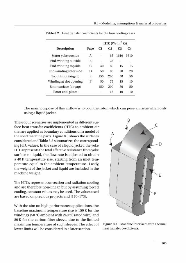
8.3 – Modeling, assumptions & material properties
Table 8.2 Heat transfer coefficients for the four cooling cases
HTC (W/(m2 K))
Description Face C1 C2 C3 C4
Stator yoke outside A - 65 1610 1610
End-winding outside B - 25 - -
End-winding topside C 40 80 15 15
End-winding rotor side D 50 80 20 20
Tooth front (airgap) E 150 200 50 50
Winding at slot opening F 50 75 15 10
Rotor surface (airgap) 150 200 50 50
Rotor end-plates - 15 10 10
The main purpose of this airflow is to cool the rotor, which can pose an issue when onlyusing a liquid jacket.
A
BC
D
E
F
Figure 8.3 Machine interfaces with thermalheat transfer coefficients.
These four scenarios are implemented as different sur-face heat transfer coefficients (HTC) to ambient airthat are applied as boundary conditions on a model ofthe solid machine parts. Figure 8.3 shows the surfacesconsidered and Table 8.2 summarizes the correspond-ing HTC values. In the case of a liquid jacket, the yokeHTC represents the total effective resistance from yokesurface to liquid, the flow rate is adjusted to obtaina 40 K temperature rise, starting from an inlet tem-perature equal to the ambient temperature. Lastly,the weight of the jacket and liquid are included in themachine weight.
The HTCs represent convection and radiation coolingand are therefore non-linear, but by assuming forcedcooling, constant values may be used. The values usedare based on previous projects and [170–173].
With the aim on high performance applications, thebaseline maximum temperature rise is 150 K for thewindings (50 °C ambient with 240 °C rated wire) and80 K for the carbon fiber sleeve, due to the limitedmaximum temperature of such sleeves. The effect oflower limits will be considered in a later section.
165

8. Power density limits and design trends of high-speed permanent magnet synchronous machines
Modeling
The temperatures are computed with a 3D lumped element network, which is faster than FEA,but still provides sufficient accuracy compared to FEA, given the uncertainty associated withtypical HTCs [170]. The use of a 3D model allows an axial temperature rise across the airgapor liquid jacket, as well as cooling of the end-windings, to be accounted for. Lastly, the lumpedelement network was validated with 3D FEM on a number of benchmark machines; the computedtemperatures were always within 10 K. See appendix A for more details on the thermal model.
8.3.4 Optimization
Particle swarm optimization (PSO) is used to determine the POF for each design point. PSO isa gradient free, heuristic optimization algorithm, used on electrical machine problems before[31, 174]. For each design point, 200 iterations with 20 particles are executed, so that ultimately320,000 machines have been analyzed to arrive at the final data set. Each optimization run takesabout 1–2 days using a workstation with a Xeon E5-1620 processor, analyzing 4000 machinedesigns in the process.
8.4 Results
The results are now discussed in four parts. First, all unfiltered and processed POFs are shown,serving as a bridge between the optimization results and more abstract trends. Then, the maingoal –specific power density– is discussed. Next, derived parameters for the same machines arepresented, split into parameters relevant at system level, such as efficiency or frequency, andthose only relevant to the machine designer, such as flux densities and loss distributions.
8.4.1 Individual fronts
Contrary to the procedure described in Section 8.2.2, the full POFs will now briefly be considered.This is done to demonstrate the amount of data that was generated and to underline the need forthe proposed additional processing steps to determine actual trends.
Figure 8.4 shows the efficiency versus weight side-view to the POF for the purely air cooledmachines. The typical behavior –increasing efficiency with weight– is visible for all machines.The most important observation is that the machine efficiency should not be a problem; a valueof 97% is easily obtainable for most machines. The general fronts for the liquid cooled machinesare very similar and hence not shown.
Figure 8.5 shows the winding temperature rise versus weight for the air cooled machines (theliquid cooled machines are again similar). Individual power levels can roughly be identified. The
166
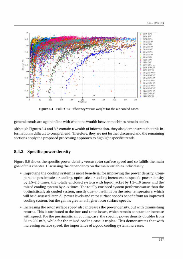
8.4 – Results
0 50 100 150 200 250 300 350 400 450 500
94
94.5
95
95.5
96
96.5
97
97.5
98
98.5
99
Weight (kg)
Eff
icie
ncy
(%
)
50 kW, 200 m/s
50 kW, 100 m/s
50 kW, 50 m/s
50 kW, 25 m/s
100 kW, 200 m/s
100 kW, 100 m/s
100 kW, 50 m/s
100 kW, 25 m/s
200 kW, 200 m/s
200 kW, 100 m/s
200 kW, 50 m/s
200 kW, 25 m/s
500 kW, 200 m/s
500 kW, 100 m/s
500 kW, 50 m/s
500 kW, 25 m/s
1 MW, 200 m/s
1 MW, 100 m/s
1 MW, 50 m/s
1 MW, 25 m/s
50 kW, 200 m/s, OA
50 kW, 100 m/s, OA
50 kW, 50 m/s, OA
50 kW, 25 m/s, OA
100 kW, 200 m/s, OA
100 kW, 100 m/s, OA
100 kW, 50 m/s, OA
100 kW, 25 m/s, OA
200 kW, 200 m/s, OA
200 kW, 100 m/s, OA
200 kW, 50 m/s, OA
200 kW, 25 m/s, OA
500 kW, 200 m/s, OA
500 kW, 100 m/s, OA
500 kW, 50 m/s, OA
500 kW, 25 m/s, OA
1 MW, 200 m/s, OA
1 MW, 100 m/s, OA
1 MW, 50 m/s, OA
1 MW, 25 m/s, OA
Figure 8.4 Full POFs: Efficiency versus weight for the air cooled cases.
general trends are again in line with what one would: heavier machines remain cooler.
Although Figures 8.4 and 8.5 contain a wealth of information, they also demonstrate that this in-formation is difficult to comprehend. Therefore, they are not further discussed and the remainingsections apply the proposed processing approach to highlight specific trends.
8.4.2 Specific power density
Figure 8.6 shows the specific power density versus rotor surface speed and so fulfills the maingoal of this chapter. Discussing the dependency on the main variables individually:
• Improving the cooling system is most beneficial for improving the power density. Com-pared to pessimistic air cooling, optimistic air cooling increases the specific power densityby 1.5–2.5 times, the totally enclosed system with liquid jacket by 1.2–1.6 times and themixed cooling system by 2–3 times. The totally enclosed system performs worse than theoptimistically air cooled system, mostly due to the limit on the rotor temperature, whichwill be discussed later. All power levels and rotor surface speeds benefit from an improvedcooling system, but the gain is greater at higher rotor surface speeds.
• Increasing the rotor surface speed also increases the power density, but with diminishingreturns. This is attributed to the iron and rotor losses, which remain constant or increasewith speed. For the pessimistic air cooling case, the specific power density doubles from25 to 200 m/s, while for the mixed cooling case it triples. This demonstrates that withincreasing surface speed, the importance of a good cooling system increases.
167
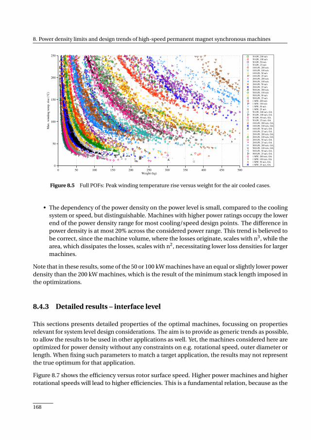
8. Power density limits and design trends of high-speed permanent magnet synchronous machines
0 50 100 150 200 250 300 350 400 450 500
0
50
100
150
200
250
Weight (kg)
Max
. w
ind
ing
tem
p.
rise
(°C
)
50 kW, 200 m/s
50 kW, 100 m/s
50 kW, 50 m/s
50 kW, 25 m/s
100 kW, 200 m/s
100 kW, 100 m/s
100 kW, 50 m/s
100 kW, 25 m/s
200 kW, 200 m/s
200 kW, 100 m/s
200 kW, 50 m/s
200 kW, 25 m/s
500 kW, 200 m/s
500 kW, 100 m/s
500 kW, 50 m/s
500 kW, 25 m/s
1 MW, 200 m/s
1 MW, 100 m/s
1 MW, 50 m/s
1 MW, 25 m/s
50 kW, 200 m/s, OA
50 kW, 100 m/s, OA
50 kW, 50 m/s, OA
50 kW, 25 m/s, OA
100 kW, 200 m/s, OA
100 kW, 100 m/s, OA
100 kW, 50 m/s, OA
100 kW, 25 m/s, OA
200 kW, 200 m/s, OA
200 kW, 100 m/s, OA
200 kW, 50 m/s, OA
200 kW, 25 m/s, OA
500 kW, 200 m/s, OA
500 kW, 100 m/s, OA
500 kW, 50 m/s, OA
500 kW, 25 m/s, OA
1 MW, 200 m/s, OA
1 MW, 100 m/s, OA
1 MW, 50 m/s, OA
1 MW, 25 m/s, OA
Figure 8.5 Full POFs: Peak winding temperature rise versus weight for the air cooled cases.
• The dependency of the power density on the power level is small, compared to the coolingsystem or speed, but distinguishable. Machines with higher power ratings occupy the lowerend of the power density range for most cooling/speed design points. The difference inpower density is at most 20% across the considered power range. This trend is believed tobe correct, since the machine volume, where the losses originate, scales with n3, while thearea, which dissipates the losses, scales with n2, necessitating lower loss densities for largermachines.
Note that in these results, some of the 50 or 100 kW machines have an equal or slightly lower powerdensity than the 200 kW machines, which is the result of the minimum stack length imposed inthe optimizations.
8.4.3 Detailed results – interface level
This sections presents detailed properties of the optimal machines, focussing on propertiesrelevant for system level design considerations. The aim is to provide as generic trends as possible,to allow the results to be used in other applications as well. Yet, the machines considered here areoptimized for power density without any constraints on e.g. rotational speed, outer diameter orlength. When fixing such parameters to match a target application, the results may not representthe true optimum for that application.
Figure 8.7 shows the efficiency versus rotor surface speed. Higher power machines and higherrotational speeds will lead to higher efficiencies. This is a fundamental relation, because as the
168
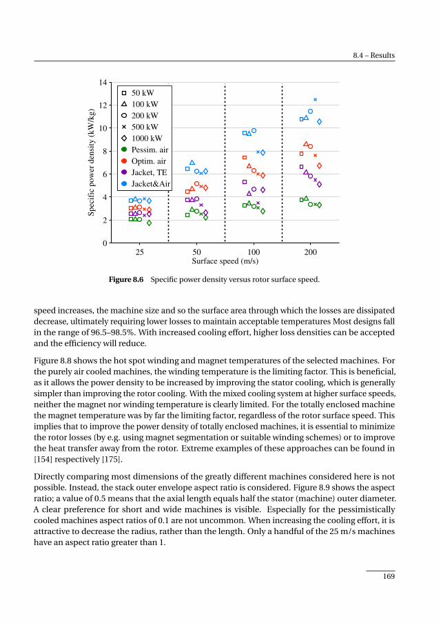
8.4 – Results
25 50 100 2000
2
4
6
8
10
12
14S
pec
ific
pow
er d
ensi
ty (
kW
/kg)
Surface speed (m/s)
50 kW
100 kW
200 kW
500 kW
1000 kW
Pessim. air
Optim. air
Jacket, TE
Jacket&Air
Figure 8.6 Specific power density versus rotor surface speed.
speed increases, the machine size and so the surface area through which the losses are dissipateddecrease, ultimately requiring lower losses to maintain acceptable temperatures Most designs fallin the range of 96.5–98.5%. With increased cooling effort, higher loss densities can be acceptedand the efficiency will reduce.
Figure 8.8 shows the hot spot winding and magnet temperatures of the selected machines. Forthe purely air cooled machines, the winding temperature is the limiting factor. This is beneficial,as it allows the power density to be increased by improving the stator cooling, which is generallysimpler than improving the rotor cooling. With the mixed cooling system at higher surface speeds,neither the magnet nor winding temperature is clearly limited. For the totally enclosed machinethe magnet temperature was by far the limiting factor, regardless of the rotor surface speed. Thisimplies that to improve the power density of totally enclosed machines, it is essential to minimizethe rotor losses (by e.g. using magnet segmentation or suitable winding schemes) or to improvethe heat transfer away from the rotor. Extreme examples of these approaches can be found in[154] respectively [175].
Directly comparing most dimensions of the greatly different machines considered here is notpossible. Instead, the stack outer envelope aspect ratio is considered. Figure 8.9 shows the aspectratio; a value of 0.5 means that the axial length equals half the stator (machine) outer diameter.A clear preference for short and wide machines is visible. Especially for the pessimisticallycooled machines aspect ratios of 0.1 are not uncommon. When increasing the cooling effort, it isattractive to decrease the radius, rather than the length. Only a handful of the 25 m/s machineshave an aspect ratio greater than 1.
169

8. Power density limits and design trends of high-speed permanent magnet synchronous machines
25 50 100 20095
95.5
96
96.5
97
97.5
98
98.5
Eff
icie
ncy
(%
)
Surface speed (m/s)
50 kW
100 kW
200 kW
500 kW
1000 kW
Pessim. air
Optim. air
Jacket, TE
Jacket&Air
Figure 8.7 Efficiency versus rotor surface speed.
25 50 100 20060
80
100
120
140
Max
. w
ind
ing
tem
p.
rise
(°C
)
Surface speed (m/s)
(a)
25 50 100 2000
20
40
60
80
Max
. m
agnet
tem
p. ri
se (
°C)
Surface speed (m/s)
(b)
Figure 8.8 Predicted maximum temperature: (a) winding; (b) magnets.
Figure 8.10(a) shows the mechanical airgap length. Note that the magnetic airgap is an addi-tional 2.5 mm longer due to the retaining sleeve. Most machine designs at vsurf=25 or 50 m/shave the minimum airgap of 1.5 mm specified in the optimizations. Hence, when performingoptimizations at those surface speeds using a fixed, low airgap length can yield satisfactory results.With increasing surface speed, the optimal airgap length increases. This is driven by the needto have a lower flux density in the iron at higher speeds and to maintain acceptable rotor eddycurrent losses, which would otherwise increase with frequency. A longer optimal airgap is alsobeneficial in several ways: it reduces windage losses and allows a thicker sleeve to be used if thisis mechanically necessary. Therefore, the fixed sleeve thickness used in this work does not leadto infeasible designs. In addition, a longer airgap alleviates the mechanical requirements. Todemonstrate this, Figure 8.10(b) shows the airgap length normalized to the rotor outer diameter,which accounts for the fact that shorter airgap lengths are more difficult to accurately maintain in
170
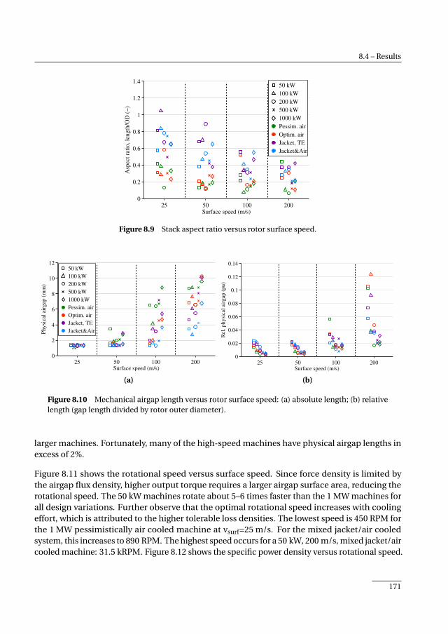
8.4 – Results
25 50 100 2000
0.2
0.4
0.6
0.8
1
1.2
1.4
Asp
ect
rati
o,
len
gth
/OD
(−
)
Surface speed (m/s)
50 kW
100 kW
200 kW
500 kW
1000 kW
Pessim. air
Optim. air
Jacket, TE
Jacket&Air
Figure 8.9 Stack aspect ratio versus rotor surface speed.
25 50 100 2000
2
4
6
8
10
12
Ph
ysi
cal
airg
ap (
mm
)
Surface speed (m/s)
50 kW
100 kW
200 kW
500 kW
1000 kW
Pessim. air
Optim. air
Jacket, TE
Jacket&Air
(a)
25 50 100 2000
0.02
0.04
0.06
0.08
0.1
0.12
0.14
Rel
. p
hy
sica
l ai
rgap
(p
u)
Surface speed (m/s)
(b)
Figure 8.10 Mechanical airgap length versus rotor surface speed: (a) absolute length; (b) relativelength (gap length divided by rotor outer diameter).
larger machines. Fortunately, many of the high-speed machines have physical airgap lengths inexcess of 2%.
Figure 8.11 shows the rotational speed versus surface speed. Since force density is limited bythe airgap flux density, higher output torque requires a larger airgap surface area, reducing therotational speed. The 50 kW machines rotate about 5–6 times faster than the 1 MW machines forall design variations. Further observe that the optimal rotational speed increases with coolingeffort, which is attributed to the higher tolerable loss densities. The lowest speed is 450 RPM forthe 1 MW pessimistically air cooled machine at vsurf=25 m/s. For the mixed jacket/air cooledsystem, this increases to 890 RPM. The highest speed occurs for a 50 kW, 200 m/s, mixed jacket/aircooled machine: 31.5 kRPM. Figure 8.12 shows the specific power density versus rotational speed.
171
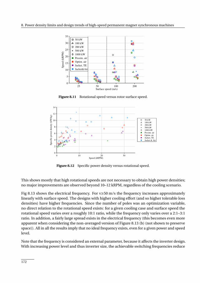
8. Power density limits and design trends of high-speed permanent magnet synchronous machines
25 50 100 2000
5
10
15
20
25
30
35
Spee
d (
kR
PM
)
Surface speed (m/s)
50 kW
100 kW
200 kW
500 kW
1000 kW
Pessim. air
Optim. air
Jacket, TE
Jacket&Air
Figure 8.11 Rotational speed versus rotor surface speed.
0 10 20 300
2
4
6
8
10
12
14
Speed (kRPM)
Sp
ecif
ic p
ow
er d
ensi
ty (
kW
/kg
)
50 kW
100 kW
200 kW
500 kW
1000 kW
Pessim. air
Optim. air
Jacket, TE
Jacket & Air
Figure 8.12 Specific power density versus rotational speed.
This shows mostly that high rotational speeds are not necessary to obtain high power densities;no major improvements are observed beyond 10–12 kRPM, regardless of the cooling scenario.
Fig 8.13 shows the electrical frequency. For v≥50 m/s the frequency increases approximatelylinearly with surface speed. The designs with higher cooling effort (and so higher tolerable lossdensities) have higher frequencies. Since the number of poles was an optimization variable,no direct relation to the rotational speed exists: for a given cooling case and surface speed therotational speed varies over a roughly 10:1 ratio, while the frequency only varies over a 2:1–3:1ratio. In addition, a fairly large spread exists in the electrical frequency (this becomes even moreapparent when considering the non-averaged version of Figure 8.13 (b) (not shown to preservespace)). All in all the results imply that no ideal frequency exists, even for a given power and speedlevel.
Note that the frequency is considered an external parameter, because it affects the inverter design.With increasing power level and thus inverter size, the achievable switching frequencies reduce
172
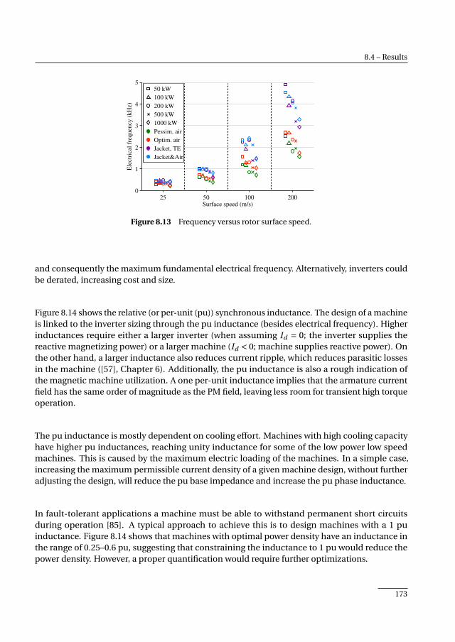
8.4 – Results
25 50 100 2000
1
2
3
4
5
Ele
ctri
cal
freq
uen
cy (
kH
z)
Surface speed (m/s)
50 kW
100 kW
200 kW
500 kW
1000 kW
Pessim. air
Optim. air
Jacket, TE
Jacket&Air
Figure 8.13 Frequency versus rotor surface speed.
and consequently the maximum fundamental electrical frequency. Alternatively, inverters couldbe derated, increasing cost and size.
Figure 8.14 shows the relative (or per-unit (pu)) synchronous inductance. The design of a machineis linked to the inverter sizing through the pu inductance (besides electrical frequency). Higherinductances require either a larger inverter (when assuming Id = 0; the inverter supplies thereactive magnetizing power) or a larger machine (Id < 0; machine supplies reactive power). Onthe other hand, a larger inductance also reduces current ripple, which reduces parasitic lossesin the machine ([57], Chapter 6). Additionally, the pu inductance is also a rough indication ofthe magnetic machine utilization. A one per-unit inductance implies that the armature currentfield has the same order of magnitude as the PM field, leaving less room for transient high torqueoperation.
The pu inductance is mostly dependent on cooling effort. Machines with high cooling capacityhave higher pu inductances, reaching unity inductance for some of the low power low speedmachines. This is caused by the maximum electric loading of the machines. In a simple case,increasing the maximum permissible current density of a given machine design, without furtheradjusting the design, will reduce the pu base impedance and increase the pu phase inductance.
In fault-tolerant applications a machine must be able to withstand permanent short circuitsduring operation [85]. A typical approach to achieve this is to design machines with a 1 puinductance. Figure 8.14 shows that machines with optimal power density have an inductance inthe range of 0.25–0.6 pu, suggesting that constraining the inductance to 1 pu would reduce thepower density. However, a proper quantification would require further optimizations.
173
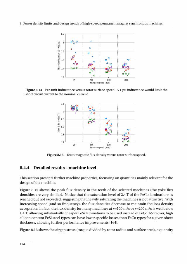
8. Power density limits and design trends of high-speed permanent magnet synchronous machines
25 50 100 2000.2
0.4
0.6
0.8
1
1.2
Ph
ase
ind
uct
ance
(L
−M
)(p
u)
Surface speed (m/s)
Figure 8.14 Per-unit inductance versus rotor surface speed. A 1 pu inductance would limit theshort circuit current to the nominal current.
25 50 100 2000.4
0.8
1.2
1.6
2
2.4
Max
B i
n t
eeth
(T
)
Surface speed (m/s)
Figure 8.15 Teeth magnetic flux density versus rotor surface speed.
8.4.4 Detailed results – machine level
This section presents further machine properties, focussing on quantities mainly relevant for thedesign of the machine.
Figure 8.15 shows the peak flux density in the teeth of the selected machines (the yoke fluxdensities are very similar). Notice that the saturation level of 2.4 T of the FeCo laminations isreached but not exceeded, suggesting that heavily saturating the machines is not attractive. Withincreasing speed (and so frequency), the flux densities decrease to maintain the loss densityacceptable. In fact, the flux density for many machines at v=100 m/s or v=200 m/s is well below1.4 T, allowing substantially cheaper FeSi laminations to be used instead of FeCo. Moreover, highsilicon content FeSi steel types can have lower specific losses than FeCo types for a given sheetthickness, allowing further performance improvements [164].
Figure 8.16 shows the airgap stress (torque divided by rotor radius and surface area), a quantity
174
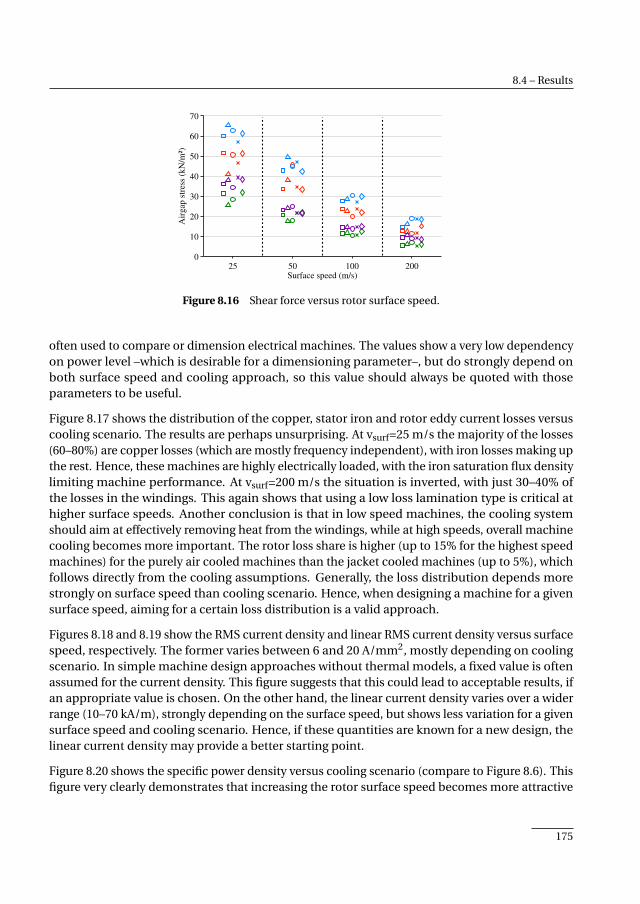
8.4 – Results
25 50 100 2000
10
20
30
40
50
60
70
Air
gap
str
ess
(kN
/m²)
Surface speed (m/s)
Figure 8.16 Shear force versus rotor surface speed.
often used to compare or dimension electrical machines. The values show a very low dependencyon power level –which is desirable for a dimensioning parameter–, but do strongly depend onboth surface speed and cooling approach, so this value should always be quoted with thoseparameters to be useful.
Figure 8.17 shows the distribution of the copper, stator iron and rotor eddy current losses versuscooling scenario. The results are perhaps unsurprising. At vsurf=25 m/s the majority of the losses(60–80%) are copper losses (which are mostly frequency independent), with iron losses making upthe rest. Hence, these machines are highly electrically loaded, with the iron saturation flux densitylimiting machine performance. At vsurf=200 m/s the situation is inverted, with just 30–40% ofthe losses in the windings. This again shows that using a low loss lamination type is critical athigher surface speeds. Another conclusion is that in low speed machines, the cooling systemshould aim at effectively removing heat from the windings, while at high speeds, overall machinecooling becomes more important. The rotor loss share is higher (up to 15% for the highest speedmachines) for the purely air cooled machines than the jacket cooled machines (up to 5%), whichfollows directly from the cooling assumptions. Generally, the loss distribution depends morestrongly on surface speed than cooling scenario. Hence, when designing a machine for a givensurface speed, aiming for a certain loss distribution is a valid approach.
Figures 8.18 and 8.19 show the RMS current density and linear RMS current density versus surfacespeed, respectively. The former varies between 6 and 20 A/mm2, mostly depending on coolingscenario. In simple machine design approaches without thermal models, a fixed value is oftenassumed for the current density. This figure suggests that this could lead to acceptable results, ifan appropriate value is chosen. On the other hand, the linear current density varies over a widerrange (10–70 kA/m), strongly depending on the surface speed, but shows less variation for a givensurface speed and cooling scenario. Hence, if these quantities are known for a new design, thelinear current density may provide a better starting point.
Figure 8.20 shows the specific power density versus cooling scenario (compare to Figure 8.6). Thisfigure very clearly demonstrates that increasing the rotor surface speed becomes more attractive
175

8. Power density limits and design trends of high-speed permanent magnet synchronous machines
Pessim. air Optim. air Jacket, TE Jacket&Air20
30
40
50
60
70
80
90
Copper
loss
es, sh
are
(%)
Cooling scenario
(a)
Pessim. air Optim. air Jacket, TE Jacket&Air10
20
30
40
50
60
70
Iron l
oss
es, sh
are
(%)
Cooling scenario
(b)
Pessim. air Optim. air Jacket, TE Jacket&Air0
5
10
15
20
25
Roto
r lo
sses
, sh
are
(%)
Cooling scenario
50 kW
100 kW
200 kW
500 kW
1000 kW
25 m/s
50 m/s
100 m/s
200 m/s
(c)
Figure 8.17 Distribution of the main electrical losses: (a) copper losses; (b) stator iron losses; (c)rotor losses.
176

8.4 – Results
25 50 100 2006
8
10
12
14
16
18
20
22
Cu
rren
t den
sity
(A
/mm
²)
Surface speed (m/s)
Figure 8.18 RMS current density versus ro-tor surface speed.
25 50 100 2000
10
20
30
40
50
60
70
Lin
ear
curr
ent
den
sity
(k
A/m
)
Surface speed (m/s)
Figure 8.19 Linear RMS current density ver-sus rotor surface speed.
Pessim. Air Opt. Air TE TE+Air0
2
4
6
8
10
12
14
Spec
ific
pow
er d
ensi
ty (
kW
/kg)
Cooling scenario
50 kW
100 kW
200 kW
500 kW
1000 kW
25 m/s
50 m/s
100 m/s
200 m/s
Figure 8.20 Specific power density versus cooling scenario (compare to Figure 8.6).
with better cooling: the power density doubles when increasing vsurf from 25 to 200 m/s for thepessimistically cooled machines, but more than triples for the intensively cooled machines.
8.4.5 Lower temperature constraints
The temperature constraints used in the previous section are based on the use of expensive,high performance materials. To investigate the impact of lower permissible temperature rises,Figure 8.21 shows the specific power density versus maximum winding and magnet temperature.The results are averaged over all power levels for this plot, because the power level has only asmall impact on power density. It appears that the specific power density follows an almost lineartrend with maximum temperature, in particular for the air-cooled machines. This was to beexpected, since for a given machine design, increasing the temperature rise by a factor f , requires
177
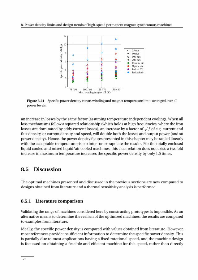
8. Power density limits and design trends of high-speed permanent magnet synchronous machines
75 / 50 100 / 60 125 / 70 150 / 800
2
4
6
8
10
12
Max. winding/magnet ∆T (K)
Sp
ecif
ic p
ow
er d
ensi
ty (
kW
/kg
)
25 m/s
50 m/s
100 m/s
200 m/s
Pessim. air
Optim. air
Jacket, TE
Jacket&air
Figure 8.21 Specific power density versus winding and magnet temperature limit, averaged over allpower levels.
an increase in losses by the same factor (assuming temperature independent cooling). When allloss mechanisms follow a squared relationship (which holds at high frequencies, where the ironlosses are dominated by eddy current losses), an increase by a factor of
√f of e.g. current and
flux density, or current density and speed, will double both the losses and output power (and sopower density). Hence, the power density figures presented in this chapter may be scaled linearlywith the acceptable temperature rise to inter- or extrapolate the results. For the totally enclosedliquid cooled and mixed liquid/air cooled machines, this clear relation does not exist; a twofoldincrease in maximum temperature increases the specific power density by only 1.5 times.
8.5 Discussion
The optimal machines presented and discussed in the previous sections are now compared todesigns obtained from literature and a thermal sensitivity analysis is performed.
8.5.1 Literature comparison
Validating the range of machines considered here by constructing prototypes is impossible. As analternative means to determine the realism of the optimized machines, the results are comparedto examples from literature.
Ideally, the specific power density is compared with values obtained from literature. However,most references provide insufficient information to determine the specific power density. Thisis partially due to most applications having a fixed rotational speed, and the machine designis focussed on obtaining a feasible and efficient machine for this speed, rather than directly
178
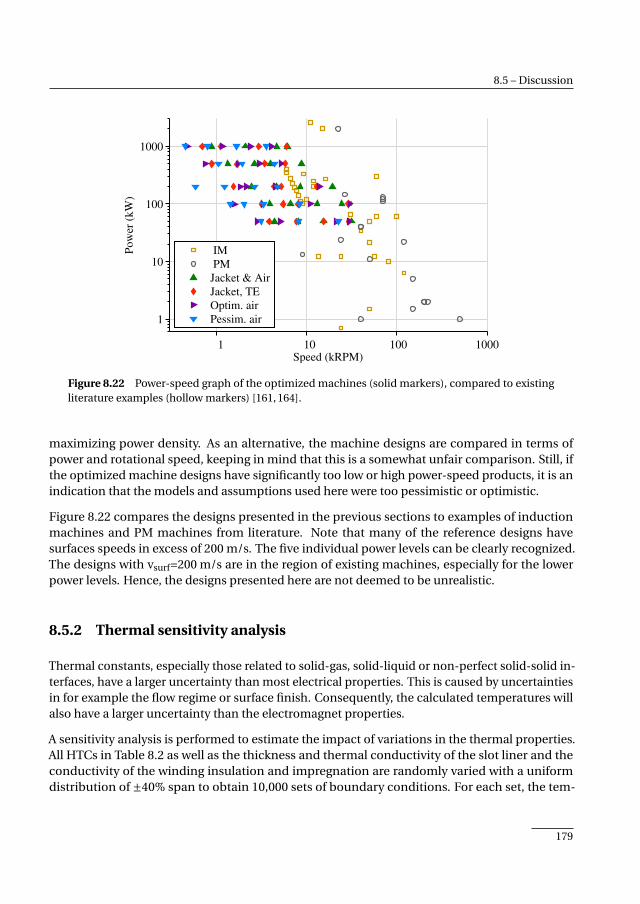
8.5 – Discussion
1 10 100 1000
1
10
100
1000
Speed (kRPM)
Pow
er (
kW
)
IM
PM
Jacket & Air
Jacket, TE
Optim. air
Pessim. air
Figure 8.22 Power-speed graph of the optimized machines (solid markers), compared to existingliterature examples (hollow markers) [161, 164].
maximizing power density. As an alternative, the machine designs are compared in terms ofpower and rotational speed, keeping in mind that this is a somewhat unfair comparison. Still, ifthe optimized machine designs have significantly too low or high power-speed products, it is anindication that the models and assumptions used here were too pessimistic or optimistic.
Figure 8.22 compares the designs presented in the previous sections to examples of inductionmachines and PM machines from literature. Note that many of the reference designs havesurfaces speeds in excess of 200 m/s. The five individual power levels can be clearly recognized.The designs with vsurf=200 m/s are in the region of existing machines, especially for the lowerpower levels. Hence, the designs presented here are not deemed to be unrealistic.
8.5.2 Thermal sensitivity analysis
Thermal constants, especially those related to solid-gas, solid-liquid or non-perfect solid-solid in-terfaces, have a larger uncertainty than most electrical properties. This is caused by uncertaintiesin for example the flow regime or surface finish. Consequently, the calculated temperatures willalso have a larger uncertainty than the electromagnet properties.
A sensitivity analysis is performed to estimate the impact of variations in the thermal properties.All HTCs in Table 8.2 as well as the thickness and thermal conductivity of the slot liner and theconductivity of the winding insulation and impregnation are randomly varied with a uniformdistribution of ±40% span to obtain 10,000 sets of boundary conditions. For each set, the tem-
179
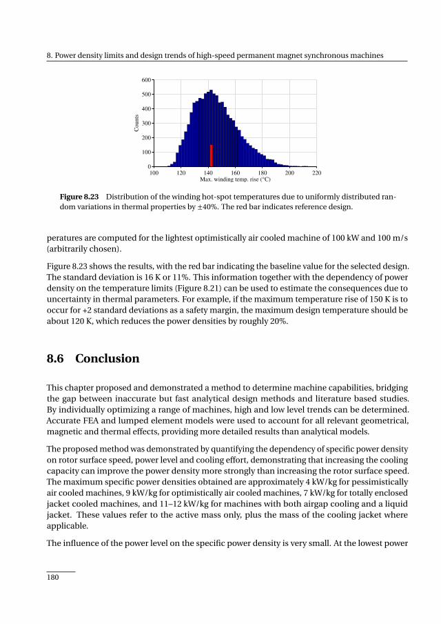
8. Power density limits and design trends of high-speed permanent magnet synchronous machines
100 120 140 160 180 200 2200
100
200
300
400
500
600
Max. winding temp. rise (°C)
Counts
Figure 8.23 Distribution of the winding hot-spot temperatures due to uniformly distributed ran-dom variations in thermal properties by ±40%. The red bar indicates reference design.
peratures are computed for the lightest optimistically air cooled machine of 100 kW and 100 m/s(arbitrarily chosen).
Figure 8.23 shows the results, with the red bar indicating the baseline value for the selected design.The standard deviation is 16 K or 11%. This information together with the dependency of powerdensity on the temperature limits (Figure 8.21) can be used to estimate the consequences due touncertainty in thermal parameters. For example, if the maximum temperature rise of 150 K is tooccur for +2 standard deviations as a safety margin, the maximum design temperature should beabout 120 K, which reduces the power densities by roughly 20%.
8.6 Conclusion
This chapter proposed and demonstrated a method to determine machine capabilities, bridgingthe gap between inaccurate but fast analytical design methods and literature based studies.By individually optimizing a range of machines, high and low level trends can be determined.Accurate FEA and lumped element models were used to account for all relevant geometrical,magnetic and thermal effects, providing more detailed results than analytical models.
The proposed method was demonstrated by quantifying the dependency of specific power densityon rotor surface speed, power level and cooling effort, demonstrating that increasing the coolingcapacity can improve the power density more strongly than increasing the rotor surface speed.The maximum specific power densities obtained are approximately 4 kW/kg for pessimisticallyair cooled machines, 9 kW/kg for optimistically air cooled machines, 7 kW/kg for totally enclosedjacket cooled machines, and 11–12 kW/kg for machines with both airgap cooling and a liquidjacket. These values refer to the active mass only, plus the mass of the cooling jacket whereapplicable.
The influence of the power level on the specific power density is very small. At the lowest power
180
8.6 – Conclusion
level of 50 kW, the constraint on the minimum stack length slightly limited the performance ofthese machines. For each surface speed and cooling scenario combination, peak power densitywas generally obtained for the 200 kW machines. At the highest power level of 1 MW the specificpower density marginally reduces, by about 10%. Compared to the impact of rotor surface speedor cooling effort, the specific power density could be considered to be independent of the powerlevel for the range considered in this work.
By further inspection of the results, it is shown amongst others that at high speeds the highsaturation flux density offered by FeCo laminations is not needed; that the optimal mechanicalairgap length increases up to 1 cm, allowing thicker retaining sleeves to be used or reducingwindage losses; and that the airgap stress or linear current densities are (indeed) good machinedimensioning parameters, but only if quoted together with cooling level and rotor surface speed.
Ultimately, using the results (and approach) presented here can be used at several levels: 1. as areference when performing a similar study for a different case; 2. as a reference work to determinethe capabilities of PMSMs for conceptual targets applications or comparisons with existing de-signs; and 3. as a starting point for new machine designs, using the basic dimensioning parametersgiven in Figures 8.16–8.19.
181

CHAPTER 9
Conclusion
The primary goal of the research project leading to this thesis was to provide a candidate de-sign for a prototype starter/generator. For the specific application, a balance had to be foundbetween weight, starting performance, short circuit losses and generator performance. Due tothe magnitude of the starting torque and the requirement for low short circuit losses, generatorperformance is of secondary importance and will generally be sufficient if the other requirementsare met. However, good starting performance directly opposes low fault losses and weight, whichare the main tradeoffs to be made. The faulted losses are strongly dependent on the per-unitphase inductance, which in turn determines a minimum inverter rating. Ultimately, a prototypemachine was designed and built having a short circuit current of 4 pu, which is roughly equalto the starting-to-generating torque ratio. Lower short circuit currents would sharply reduceboth machine and inverter feasibility. The prototype was tested, showing a good match betweensimulations and measurements. Afterwards, the prototype S/G (and associated power electronics)were successfully tested at the clients’ facilities. All in all this demonstrates that surface mountedPM machines may be successfully used as starter/generator.
However, before the final S/G design was established, several modeling and analysis steps werenecessary.
As a first step, a Pareto based multi-objective optimization strategy was developed, based on PSOand FEA. Such a tool serves two purposes: at first it helps to find machine designs that ‘optimally’meet the target specifications and allows various topologies to be compared. However, any realengineering problem has multiple –most likely conflicting– objectives and no single optimaldesign exists. The designer then has to decide on a specific compromise, but this requires insightinto the tradeoffs between the various targets. Gaining insight into a design problem is the secondpurpose of an optimization algorithm. When using an optimization algorithm it is extremelyimportant that the user and his audience become confident in the results, and can explain varioustrends that emerge. As a rule of thumb, one should maybe spent as much time checking theoutput of an optimization run as it took to set it up.
183
Conclusion
In the analysis and optimization of high-speed machines, rotor losses must be accounted for.If the eddy currents are expected to be inductance limited, calculating the inducing field andthe eddy currents becomes a coupled problem. This strongly increases the solution complexityregardless of the modeling approach. A FEM based method was proposed that fits well into theoptimization approach proposed earlier. By using a linear model of only the rotor geometry, themesh can have fewer elements; rotation does not need to be accounted for; and stator saturation,the most likely cause of saturation in SPM machines, does not have to be considered in a transientsimulation. All in all this leads to a speed gain of 2–20 times, depending on the machine operatingconditions, while still accurately estimating the losses even with pronounced shielding effects. Anadded benefit is that the method is flexible with regards to rotor shapes, due to the use of FEM.
The high-speed nature of the S/G also requires the additional winding losses to be considered.The initial starter/generator specification called for an extremely low voltage, requiring only a fewturns per tooth at most. Regular solid strands were to be used, optionally with discrete parallelstrands, and it is well known from literature that this may lead to strand level proximity effectsand bundle level skin effects. To accurately estimate the bundle level skin effect (unequal currentsharing), including 3D effects such as twisting and the end-windings, no adequate models werefound, so a simplified 3D FEM based method was developed and experimentally tested. Usingthe method, it was demonstrated that even a single twist over the machine length can increasethe frequency where current start to diverge by over an order of magnitude. Then, using thosemodels together with transient FEM models, the effects of various loss reduction mechanismswere compared, showing that by carefully using discrete non-twisted strands, performance similarto that of a winding made with an ideal but lower fill factor litz wire may be obtained.
A fourth and last important step was the analysis of turn level, or inter-turn, short circuit faults.This is a broad topic, including estimation of short circuit currents and losses, detection of thefault and post-fault operation. The strand based models from the previous chapter were used forthe short circuit calculations. Compared to most existing works, this offers a very high level ofdetail and easily allows the impact of using parallel strands to be considered. Trends describedin literature were confirmed, such as the increased fault losses for short circuits in turns locatedclose to the slot opening, even after applying a terminal level short circuit. Worst case faultcurrent densities approaching 1000 A/mm² were calculated, while in experiments values up to450 A/mm² were recorded, still limited by the measurement setup. Using parallel strands insafety critical applications brings both benefits and disadvantages. Major advantages include thereduced likelihood of high localized losses and the better fault current suppression by a terminallevel short circuit. A disadvantage is that the worst case total losses may be somewhat higher thanwith a single strand.
The potentially high fault current densities in high-speed machines stress the importance of afault detection system. In this thesis, a simple fault detection system is proposed, suitable forimplementation as an independent observer of a drive system. The system applies synchronousdetection at the fundamental frequency to the difference between the ideal inverter neutralvoltage and actual machine neutral voltage. As such, it provides an indication of the three phasesystem imbalance. The performance was characterized by simulations and measurements on two
184
totally different systems. With a careful system design, faults down to 0.4% of the winding canbe detected, albeit only at sufficiently high speeds. The strong dependency of the sensitivity onspeed is a disadvantage of the method. A second disadvantage is that no real system is perfectlybalanced. Changes in speed, id , iq or connection order will change the natural imbalance. Thesechanges may exceed the imbalance level caused by small faults, making the reliable detection ofsmall faults difficult. This fundamental limitation will affect any fault detection scheme, as everyimbalance can be seen as a fault.
After having confirmed the correctness of the machine models with the prototype machine, theywere applied one last time to determine power density limits for PMSMs versus rotor surfacespeed, power level and cooling system. An approach is proposed and demonstrated to find highlydetailed trends and limits from a set of carefully selected optimization runs. Main findings includethat increasing the cooling capacity can improve the power density more strongly than increasingthe rotor surface speed and that peak power densities beyond 10 kW/kg are possible with a mixedliquid/air cooling system. The method also confirms well known machine design trends, such asthe suitability of the linear current density as a design parameter. The fact that such trends andexpectations were not included in the optimization algorithms, partially confirms the modelingand optimization approach. Further confirmation was obtained by comparing the results to arange of designs from literature.
Contributions
Since the work in this thesis is motivated by a technical research project, the contributions canbe divided in two groups. First, the scientific contributions of this thesis can be summarized asfollows:
• The suitability of multi-objective optimization methods as a tool to systematically compareand select machine topologies was demonstrated. Additionally, such methods are a meansto gain insight into design problems.
• A finite element based rotor loss calculation method for surface mounted PM machine wasproposed. The method offers a speed improvement over a direct transient solution of a fullmachine model, without losing generality.
• A FE based method to estimate unbalanced current sharing effects between parallel strandswas proposed and demonstrated. With this method, individual strands can be accuratelyaccounted for with 3D FEA, using only very moderate computing resources.
• The short circuit losses for turn-to-turn faults were computed with full account of parallelstrands and the position of the strands in the slots. The findings suggest that using parallelstrands is beneficial in safety critical applications, because the peak per-turn losses areless than those with a single strand winding and because a better current equalization isobtained after applying an all-phase terminal short circuit.
185

Conclusion
• The potential dangers of turn-to-turn short circuits in high-speed machines were experi-mentally demonstrated, with measured current densities up to 450 A/mm² for a single turnshort circuit.
• A fault detector scheme aimed at a simple implementation was proposed and tested. Whenproperly adjusted, short circuit faults covering less than 1% of the winding can still bedetected.
• A large scale optimization approach to quantify limits and trends of electrical machineswas demonstrated.
• Power density limits and associated design trends were quantified.
Then, a number of engineering contributions can be identified:
• A surface mounted PM machine was successfully designed for a starter/generator applica-tion, meeting conflicting requirements for starting torque, generator efficiency, short circuitlosses and weight.
• Various winding AC loss reduction mechanisms were quantitatively compared, showingthat by carefully selecting the wire sizing and winding style, the use of litz wire can beavoided.
• Finally, all chapters together perhaps demonstrate that finite element modeling of electricalmachines has matured to a point that it may be used throughout the entire design cycleof electrical machines, varying from large scale exploratory optimization applications tohighly detailed parasitic loss analyses.
Recommendations
Although the methods proposed in this thesis were successfully used to design a prototypemachine, further improvements are possible:
• The optimization approach as presented in this thesis uses 2D estimations for the induc-tance and linked PM flux, because direct 3D calculations are too time consuming. In thedesign of the S/G, the value of the phase inductance is critical, because it determines boththe short circuit losses and inverter VA rating. An accurate and fast 3D estimate of thephase inductance will further reduce the design time, since no post-optimization 3D checksare required anymore. An important requirement of such an estimation method is that itshould be flexible with regards to the machine type and geometry, and be based on littleassumptions.
• While at an abstract level the design approach can be applied to any machine type, theanalysis time for a single model may become prohibitive. In practise, an analysis time inthe order of 1 minute per design allows one to obtain satisfactory results in a few days. Ifthe approach is to be used for other machine types, such as induction machines, modeling
186

simplifications may need to be investigated to obtain sufficiently fast, yet still accurateperformance estimates for those machines.
• In high speed machines, mechanical rotor dynamics and static forces cannot always befully neglected. A logical step would then be to include sufficiently accurate estimates ofthose properties in the modeling steps.
• While a fault detection and mitigation scheme are presented in this thesis and many otherscan be found in literature, it remains difficult to easily and reliably detect single turn faults,especially with higher turn counts. For high reliability applications, research into completelydifferent safety approaches may ultimately lead to a higher reliability than existing faultdetection methods.
187

APPENDIX A
Thermal model
This appendix briefly describes and demonstrates the thermal model used in the main part ofthis thesis.
A.1 Introduction
The maximum temperatures inside the various machine parts, along with material types used,ultimately determine the rating of the machine. Correctly predicting these temperatures is thusimport in the design stage if a high power density is the goal. This becomes even more importantin transiently loaded machines, partially because an increased cooling effort to ’correct’ forwrongly predicted temperatures after construction will be less effective than in the steady statecase.
A ‘classical’ thermal modeling method is the lumped element network. Such a model can yieldacceptable results and account for 3D heat flows, even with 10–20 nodes. At another end of themodeling spectrum is 3D FEA, which, although potentially very accurate, is computationallymore intense. Two-dimensional FEM is of limited use, because of axial heat flows occurring in e.g.the windings, shaft or cooling medium. This is obviously more pronounced in relatively shortmachines (‘pancake’ machines).
A problem with any thermal model is the determination of heat transfer coefficients between thesolid parts machine parts and the cooling medium (gas or liquid). Examples include the airgap,outer housing and end-winding regions. Moreover, small interface gaps, such as those betweenthe stator lamination and housing or the winding and slot wall, introduce additional uncertainty inthe model. Although an impression of expected values can be obtained from literature [170–172]or by using CFD (which is very computationally intensive)[176, 177], the actual values still dependstrongly on the material type and finishing, processing steps and assembly techniques. As a
189
A. Thermal model
result, thermal models will typically have greater uncertainties than e.g. electromagnetic models.Therefore, the use of ‘accurate’ FEA is questionable, especially during initial design stages.
In this work, a lumped element network is therefore employed, as it is believed to offer sufficientaccuracy at significant time savings. Different from some classical lumped element networkmodels, the network in this work is not simplified to a bare minimum number of nodes, as such asimplification is based on assumptions that reduce the generality. Instead, a grid-like networkof nodes, following the shape of the geometry is employed. It is believed that this approachultimately offers more flexibility.
The model only considers the heat conduction in the solid parts. This is perhaps not fully realistic,but for the purpose of comparing machines this approach can still suffice, provided that identicaland sufficiently realistic boundary conditions are used.
A.2 Model description
This section describes the various parts of the thermal model.
A.2.1 Heat conduction in solid parts
The thermal properties of solid materials are relatively well known and can be used directly todetermine the lumped thermal resistances. When determining these parameters, the machinegeometry is imaginarily divided in a grid of squares or a circular grid. Note that if the grid-size issmall compared to the geometry, a square grid can even accurately describe a circular geometry.To trade-off accuracy and speed, the node-density in many parts is a parameter. In addition to the(unavoidable) heat load, a heat capacity is also computed to allow useful transient computationsto be performed. The heat load may be made linearly temperature dependent, to account fore.g. temperature dependent copper losses. In addition, individual resistors may be set as non-linear resistors, using arbitrary equations involving any node-temperature available, so that e.g.non-linear passive convection can be included (although this feature is not used at this point).
In 2D models, only the in-stack cross sections of the stator and rotor are included. 3D modelingis not conceptually different than 2D modeling, but more time is needed to create, solve andvalidate the models. The 3D model consists of four separate regions:
• An in-stack stator part. Multiple stacked layers of the 2D network are used. The number oflayers can be varied as desired.
• An ’upstream’ end-winding part. This part is connected to the winding part of the in-stacknetwork. If an axial airflow with temperature gradient is imposed, this part is near theentrance.
• A ’downstream’ end-winding part. The network is a mirrored copy of the upstream part, butthe boundary conditions may differ.
190

A.2 – Model description
• An in-stack rotor part. Multiple stacked layers of the 2D network are used.
This network describes the solid, magnetically active part of the machine. Additional construc-tional or housing parts, such as a stator casing, end-plates, shaft and bearings, may be added tothe boundaries of the model as needed.
A.2.2 Application of boundary conditions
Boundary conditions are needed to fully specify a model. The following boundary conditions areavailable:
Insulation This is the default boundary condition that naturally results from a thermal networkif no further actions are taken.
Temperature source A hard temperature source may be specified, implying that the node tem-perature at this node is no longer an unknown.
Temperature source through Heat Transfer Coefficient In this case the node is connected to atemperature source through a constant resistor, its value depending on a given HTC andthe area of the node face.
To model an actual machine, the last boundary condition is typically used. To this end, individualtemperatures and HTC values are assigned to all surfaces subjected to a cooling medium; seeFigure 8.3 on page 165 and the associated table for an example. The values for the HTCs are inmany cases obtained from literature.
A.2.3 Special nodes
To enable a number of advanced modeling options, two special nodes are created:
• a temperature and heat flow dependent temperature source, and
• a temperature and heat flow dependent heat source.
Those nodes can be used to account for e.g. axial temperature rise of a coolant, or to couple rotorand stator side models that span a different tangential fraction of the machine (ie. practicallyall machine models, since the number of rotor magnets or bars rarely equals the number ofstator slots). In the latter case, a uni-directional transformer is used1, with a 1 : 1 ratio for thetemperature and a 1 : x ratio for the heatflow.
1remember that an ideal transformer can be modeled with back-to-back connected controlled voltage and currentsources.
191
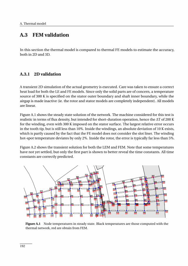
A. Thermal model
A.3 FEM validation
In this section the thermal model is compared to thermal FE models to estimate the accuracy,both in 2D and 3D.
A.3.1 2D validation
A transient 2D simulation of the actual geometry is executed. Care was taken to ensure a correctheat load for both the LE and FE models. Since only the solid parts are of concern, a temperaturesource of 300 K is specified on the stator outer boundary and shaft inner boundary, while theairgap is made inactive (ie. the rotor and stator models are completely independent). All modelsare linear.
Figure A.1 shows the steady state solution of the network. The machine considered for this test isrealistic in terms of flux density, but intended for short-duration operation, hence the ΔT of 200 Kfor the winding, even with 300 K imposed on the stator surface. The largest relative error occursin the tooth tip, but is still less than 10%. Inside the windings, an absolute deviation of 10 K exists,which is partly caused by the fact that the FE model does not consider the slot liner. The windinghot-spot temperature deviates by only 2%. Inside the rotor, the error is typically far less than 5%.
Figure A.2 shows the transient solution for both the LEM and FEM. Note that some temperatureshave not yet settled, but only the first part is shown to better reveal the time constants. All timeconstants are correctly predicted.
376NaN
376NaN
376379
376382
376NaN
376382
377383
377384
374376
378378381379383380
367367
371369373370375371
356353
359355360356362356
340336
341336342336342336
314312
300300
311311
310310
300300
313320
314320316320
308308
300300
312315314315
316316
308307
300300
312313
315314
317315
308307
300300312
313
315314317314
307307
300300313
313
315313318314
407407
446444
475472
494491
504500
400398
437433
464459
480475
489483
383379
412406
432425
445437
451443
352345
364356
372362
377367
379369
371371
366366
371371366
366
372371
366366
374372368
367
377376
377377
377376
377377
378377
378NaN
380378
380NaN
383378379
374
387383
383379
388383
388NaN
391387
391388
329328
318318
345344
356356
364364
329328
319319
345344
357356
364364
329329
319319
345344
357356
365364
330329
320320
330329
345344
346344
357356
358356
366364
366365
331329
332329
346344
347345
359357
360358
370368
374372
310310
307307
310310307
307
310310307
307
310310
306307
316315
316316
316316
317317
303303
300300
303303
300300
303303
300300
303303
300300
Figure A.1 Node temperatures in steady state. Black temperatures are those computed with thethermal network, red are obtain from FEM.
192

A.3 – FEM validation
0 50 100 150 200 250 300 350 400 450 500
250
300
350
400
450
500
550
Time (s)
T (
K)
Slot near middle
Front of tooth
Middle back magnet
Sleeve d−axis
Sleeve q−axis
Figure A.2 Several node temperatures as function of time. Solid lines: lumped element network;dashed lines: FEM.
A.3.2 3D validation
It is not uncommon that the end-windings are the hottest part of a machine and they should there-fore be considered in the thermal modeling process, requiring the use of 3D models. Moreover,axial temperature gradients in e.g. the forced cooling air also require a 3D model. The 2D modelfrom the previous section was therefore extended to 3D, which will be detailed in this section.The 3D network is created by stacking 2D layers and adding the end-windings; an impression ofthe resulting network is given in Figure A.3.
To validate the correctness of the model, an equivalent 3D FE model was created for comparison.Figure A.4 shows the solved FE model in the same orientation as the lumped element network. Toplace emphasis on the thermal model inside the solid parts rather than the boundary conditions,a simple constant temperature of 300 K was enforced on the stator outer surface and the rotorinner surface (identical to the 2D case). With both the FEM and LEM, anisotropic conductivitieswere set in the laminations and windings for the in-plane and axial conductivities (lamination:respectively 29 and 0.6 W/(m·K), windings: 2 and 195 W/(m·K)).
Surface plots like Figure A.4 cannot easily be made with the LEM. For comparison, the tempera-tures at several locations along the length of the machine are plotted instead in Figure A.6. Theworst absolute error in the winding is about 10 K, occurring at the back near the tooth/yokeintersection. This can possibly be explained by the fact that the slot rounding is not considered inthe LEM, while the slot liner is ignored in the FEM. The relative error in this point is 25%. However,
193
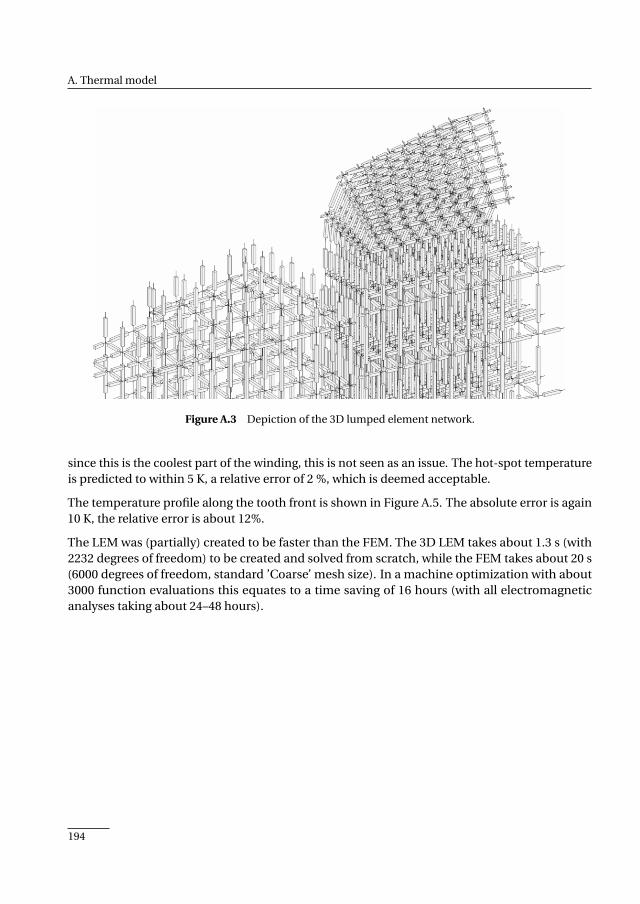
A. Thermal model
Figure A.3 Depiction of the 3D lumped element network.
since this is the coolest part of the winding, this is not seen as an issue. The hot-spot temperatureis predicted to within 5 K, a relative error of 2 %, which is deemed acceptable.
The temperature profile along the tooth front is shown in Figure A.5. The absolute error is again10 K, the relative error is about 12%.
The LEM was (partially) created to be faster than the FEM. The 3D LEM takes about 1.3 s (with2232 degrees of freedom) to be created and solved from scratch, while the FEM takes about 20 s(6000 degrees of freedom, standard ’Coarse’ mesh size). In a machine optimization with about3000 function evaluations this equates to a time saving of 16 hours (with all electromagneticanalyses taking about 24–48 hours).
194
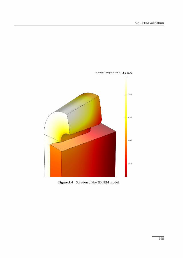
A.3 – FEM validation
Figure A.4 Solution of the 3D FEM model.
195

A. Thermal model
0 5 10 15 20 25 30 35 40
375
380
385
390
395
400
405
z (mm)
T (
K)
Figure A.5 Temperature profile along the middle front of the tooth. The dotted green line is theFEM result. In both models, the yoke outside surface was kept at 300 K.
196

A.3 – FEM validation
−30 −20 −10 0 10 20 30 40 50 60 70
530
531
532
533
534
535
536
Linelength (mm)
Tem
per
atu
re (
K)
In−StackDownstream EW Upstream EW
(a) Winding front, near slot opening
−30 −20 −10 0 10 20 30 40 50 60 70
350
360
370
380
390
400
410
420
430
Linelength (mm)
Tem
per
atu
re (
K)
In−StackDownstream EW Upstream EW
(b) Winding back, near slot middle
−20 −10 0 10 20 30 40 50 60
415
420
425
430
435
440
445
450
Linelength (mm)
Tem
per
atu
re (
K)
In−StackDownstream EW Upstream EW
(c) Winding front, near tooth
−20 −10 0 10 20 30 40 50 60
335
340
345
350
355
360
365
370
Linelength (mm)
Tem
per
atu
re (
K)
In−StackDownstream EW Upstream EW
(d) Winding back, near tooth
Figure A.6 Temperature at various locations inside the winding, along the path of the wires. Thedotted lines are the FEM result, the solid lines the LEM.
197

Bibliography
[1] S. Palko and T. Jokinen, “Optimisation of squirrel cage induction motors using finite element methodand genetic algorithms,” in Proc. Eighth Int. Electrical Machines and Drives Conf. (Conf. Publ. No. 444),1997, pp. 21–25.
[2] J. Lahteenmaki, “Optimisation of high-speed motors using a genetic algorithm,” in Proc. Eighth Int.Electrical Machines and Drives Conf. (Conf. Publ. No. 444), 1997, pp. 26–30.
[3] S. Williamson and C. I. McClay, “Optimization of the geometry of closed rotor slots for cage inductionmotors,” IEEE Trans. Ind. Appl., vol. 32, no. 3, pp. 560–568, 1996.
[4] J. Legranger, G. Friedrich, S. Vivier, and J. C. Mipo, “Combination of finite-element and analyticalmodels in the optimal multidomain design of machines: Application to an interior permanent-magnetstarter generator,” IEEE Trans. Ind. Appl., vol. 46, no. 1, pp. 232–239, 2010.
[5] J.-H. Seo, S.-M. Kim, and H.-K. Jung, “Rotor-design strategy of IPMSM for 42V integrated startergenerator,” IEEE Trans. Magn., vol. 46, no. 6, pp. 2458–2461, 2010.
[6] G. Pellegrino and F. Cupertino, “FEA-based multi-objective optimization of IPM motor design in-cluding rotor losses,” in Proc. IEEE Energy Conversion Congress and Exposition (ECCE), 2010, pp.3659–3666.
[7] C. A. C. Coello, G. T. Pulido, and M. S. Lechuga, “Handling multiple objectives with particle swarmoptimization,” IEEE Trans. Evol. Comput., vol. 8, no. 3, pp. 256–279, 2004.
[8] Y. Duan and R. G. Harley, “A novel method for multiobjective design and optimization of three phaseinduction machines,” IEEE Trans. Ind. Appl., vol. 47, no. 4, pp. 1707–1715, 2011.
[9] N. Bianchi and S. Bolognani, “Design optimisation of electric motors by genetic algorithms,” IEEProceedings -Electric Power Applications, vol. 145, no. 5, pp. 475–483, 1998.
[10] Y. Duan, R. G. Harley, and T. G. Habetler, “A useful multi-objective optimization design method for PMmotors considering nonlinear material properties,” in Proc. IEEE Energy Convers. Congr. and Expo.,2009, pp. 187–193.
[11] S. A. Semidey, Y. Duan, J. R. Mayor, R. G. Harley, and T. G. Habetler, “Optimal electromagnetic-thermo-mechanical integrated design candidate search and selection for surface-mount permanent-magnetmachines considering load profiles,” IEEE Trans. Ind. Appl., vol. 47, no. 6, pp. 2460–2468, Nov. 2011.
199
Bibliography
[12] A. Mahmoudi, S. Kahourzade, N. A. Rahim, and W. P. Hew, “Design, analysis, and prototyping of anaxial-flux permanent magnet motor based on genetic algorithm and finite-element analysis,” IEEETrans. Magn., vol. 49, no. 4, pp. 1479–1492, Apr. 2013.
[13] M. Rottach, C. Gerada, T. Hamiti, and P. W. Wheeler, “A computationally efficient design procedurefor actuator motors using magnetic reluctance-and thermal resistance network models,” in XXth Int.Conf. Electrical Machines (ICEM), Sep. 2012, pp. 2526–2532.
[14] R. Wrobel and P. H. Mellor, “Particle swarm optimisation for the design of brushless permanent magnetmachines,” in Conf. Rec. 41st IEEE IAS Annu. Meeting, vol. 4, 2006, pp. 1891–1897.
[15] F. Bittner and I. Hahn, “Kriging-assisted multi-objective particle swarm optimization of permanentmagnet synchronous machine for hybrid and electric cars,” in IEEE Int. Electric Machines Drives Conf.(IEMDC), 2013, pp. 15–22.
[16] P. Zhang et al., “Multi-objective tradeoffs in the design optimization of a brushless permanent magnetmachine with fractional-slot concentrated windings,” IEEE Trans. Ind. Appl., vol. 50, no. 5, pp. 3285–3294, Sep.-Oct. 2014.
[17] G. Sizov, D. Ionel, and N. Demerdash, “Modeling and parametric design of permanent magnet ACmachines using computationally efficient - finite element analysis,” IEEE Trans. Ind. Electron., vol. 59,no. 6, pp. 2403–2413, Jun 2012.
[18] M. Popescu, D. M. Ionel, T. J. E. Miller, S. J. Dellinger, and M. I. McGilp, “Improved finite elementcomputations of torque in brushless permanent magnet motors,” IEE Proc. Electric Power Appl., vol.152, no. 2, pp. 271–276, 2005.
[19] J. Kennedy and R. Eberhart, “Particle swarm optimization,” in Proc. Conf. IEEE Int Neural Networks,vol. 4, 1995, pp. 1942–1948.
[20] Y. del Valle, G. K. Venayagamoorthy, S. Mohagheghi, J.-C. Hernandez, and R. G. Harley, “Particle swarmoptimization: Basic concepts, variants and applications in power systems,” IEEE Trans. Evol. Comput.,vol. 12, no. 2, pp. 171–195, Apr. 2008.
[21] D. Ishak, Z. Q. Zhu, and D. Howe, “Comparison of PM brushless motors, having either all teeth oralternate teeth wound,” IEEE Trans. Energy Convers., vol. 21, no. 1, pp. 95–103, 2006.
[22] W. L. Soong and T. J. E. Miller, “Field-weakening performance of brushless synchronous AC motordrives,” IEE Proc. Electr. Power Appl., vol. 141, no. 6, pp. 331–340, 1994.
[23] Z. Q. Zhu and J. T. Chen, “Advanced flux-switching permanent magnet brushless machines,” IEEETrans. Magn., vol. 46, no. 6, pp. 1447–1453, 2010.
[24] A. S. Thomas, Z. Q. Zhu, and G. W. Jewell, “Comparison of flux switching and surface mountedpermanent magnet generators for high-speed applications,” IET Electrical Systems in Transportation,vol. 1, no. 3, pp. 111–116, 2011.
[25] Y. Pang et al., “Comparative study of flux-switching and interior permanent magnet machines,” inProc. ICEMS Electrical Machines and Systems Int. Conf, 2007, pp. 757–762.
[26] J. T. Chen, Z. Q. Zhu, A. S. Thomas, and D. Howe, “Optimal combination of stator and rotor polenumbers in flux-switching PM brushless AC machines,” in Proc. Int. Conf. Elect. Machines and SystemsICEMS, 2008, pp. 2905–2910.
[27] JFE electrical steel. [Online]. Available: http://www.jfe-steel.co.jp/en/products/electrical/index.html
200
[28] G. Pellegrino, A. Vagati, P. Guglielmi, and B. Boazzo, “Performance comparison between surfacemounted and interior PM motor drives for electric vehicle application,” IEEE Trans. Ind. Electron.,vol. 59, no. 2, pp. 803–811, Feb. 2012.
[29] D. Evans, Z. Azar, L. J. Wu, and Z. Q. Zhu, “Comparison of optimal design and performance of PMmachines having non-overlapping windings and different rotor topologies,” in Proc. IET Int. PowerElectron., Machines and Drives (PEMD), 2010, pp. 1–7.
[30] J. J. Wolmarans, M. van der Geest, H. Polinder, J. A. Ferreira, and D. Zeilstra, “Composite materials forlow loss rotor construction,” in IEEE Int. Elec. Mach. Drives Conf., 2011, pp. 295–299.
[31] L. dos Santos Coelho, L. Z. Barbosa, and L. Lebensztajn, “Multiobjective particle swarm approach forthe design of a brushless DC wheel motor,” IEEE Trans. Magn., vol. 46, no. 8, pp. 2994–2997, 2010.
[32] A. Jassal, H. Polinder, and J. A. Ferreira, “Literature survey of eddy-current loss analysis in rotatingelectrical machines,” IET Electric Power Appl., vol. 6, no. 9, pp. 743–752, Nov. 2012.
[33] F. Deng, “Commutation-caused eddy-current losses in permanent-magnet brushless DC motors,”IEEE Trans. Magn., vol. 33, no. 5, pp. 4310–4318, Sep. 1997.
[34] Z. Q. Zhu, K. Ng, N. Schofield, and D. Howe, “Improved analytical modelling of rotor eddy current lossin brushless machines equipped with surface-mounted permanent magnets,” IEE Elect. Power Appl.,vol. 151, no. 6, pp. 641–650, Nov. 2004.
[35] A. Jassal, H. Polinder, D. Lahaye, and J. A. Ferreira, “Comparison of analytical and finite elementcalculation of eddy-current losses in PM machines,” in Int. Conf. Elect. Machines (ICEM), Sep. 2010,pp. 1–7.
[36] L. J. Wu, Z. Q. Zhu, D. Staton, M. Popescu, and D. Hawkins, “Analytical model for predicting magnetloss of surface-mounted permanent magnet machines accounting for slotting effect and load,” IEEETrans. Magn., vol. 48, no. 1, pp. 107–117, Jan. 2012.
[37] J. Pyrhönen, H. Jussila, Y. Alexandrova, P. Rafajdus, and J. Nerg, “Harmonic loss calculation in rotorsurface permanent magnets—new analytic approach,” IEEE Trans. Magn., vol. 48, no. 8, pp. 2358–2366,Aug. 2012.
[38] F. Martin, M. E.-H. Zaïm, A. Tounzi, and N. Bernard, “Improved analytical determination of eddycurrent losses in surface mounted permanent magnets of synchronous machine,” IEEE Trans. Magn.,vol. 50, no. 6, pp. 1–9, Jun. 2014.
[39] K. Yamazaki and Y. Fukushima, “Effect of eddy-current loss reduction by magnet segmentation insynchronous motors with concentrated windings,” IEEE Trans. Ind. Appl., vol. 47, no. 2, pp. 779–788,Mar. 2011.
[40] A. R. Tariq, C. E. Nino-Baron, and E. G. Strangas, “Iron and magnet losses and torque calculation ofinterior permanent magnet synchronous machines using magnetic equivalent circuit,” IEEE Trans.Magn., vol. 46, no. 12, pp. 4073–4080, Dec. 2010.
[41] N. Schofield, K. Ng, Z. Q. Zhu, and D. Howe, “Parasitic rotor losses in a brushless permanent magnettraction machine,” in Int. Conf. Elect. Machines and Drives (Conf. Publ. No. 444), Sep. 1997, pp. 200–204.
[42] P. Zhang, G. Y. Sizov, J. He, D. M. Ionel, and N. A. O. Demerdash, “Calculation of magnet losses inconcentrated-winding permanent magnet synchronous machines using a computationally efficient -finite element method,” IEEE Trans. Ind. Appl., vol. 49, no. 99, pp. 2524–2532, Nov. 2013.
[43] F. Luise, A. Tessarolo, F. Agnolet, and M. Mezzarobba, “Use of time-harmonic FE analysis to computerotor eddy-current losses in synchronous machines subject to distorted stator currents,” in Int. Conf.Elect. Machines (ICEM), Sep. 2012, pp. 1503–1509.
201

Bibliography
[44] K. Yamazaki and Y. Kanou, “Rotor loss analysis of interior permanent magnet motors using combi-nation of 2-D and 3-D finite element method,” IEEE Trans. Magn., vol. 45, no. 3, pp. 1772–1775, Mar.2009.
[45] T. Okitsu, D. Matsuhashi, Y. Gao, and K. Muramatsu, “Coupled 2-d and 3-d eddy current analyses forevaluating eddy current loss of a permanent magnet in surface pm motors,” IEEE Trans. Magn., vol. 48,no. 11, pp. 3100–3103, Nov. 2012.
[46] P. Zhang et al., “Multi-objective tradeoffs in the design optimization of a brushless permanent magnetmachine with fractional-slot concentrated windings,” in Energy Conversion Congr. Expo. (ECCE), 2013,pp. 2842–2849.
[47] COMSOL Multiphysic Reference Manual, COMSOL AB, 2014.
[48] K. Yamazaki et al., “Reduction of magnet eddy-current loss in interior permanent-magnet motors withconcentrated windings,” IEEE Trans. Ind. Appl., vol. 46, no. 6, pp. 2434–2441, Nov 2010.
[49] M. Mirzaei, A. Binder, B. Funieru, and M. Susic, “Analytical calculations of induced eddy currentslosses in the magnets of surface mounted PM machines with consideration of circumferential andaxial segmentation effects,” IEEE Trans. Magn., vol. 48, no. 12, pp. 4831–4841, Dec. 2012.
[50] N. Bianchi, S. Bolognani, and E. Fornasiero, “An overview of rotor losses determination in three-phasefractional-slot pm machines,” IEEE Trans. Ind. Appl., vol. 46, no. 6, pp. 2338–2345, Nov. 2010.
[51] A. M. El-Refaie, “Fractional-slot concentrated-windings synchronous permanent magnet machines:Opportunities and challenges,” IEEE Trans. Ind. Electron., vol. 57, no. 1, pp. 107–121, Jan. 2010.
[52] D. G. Dorrell et al., “A review of the design issues and techniques for radial-flux brushless surfaceand internal rare-earth permanent-magnet motors,” IEEE Trans. Ind. Electron., vol. 58, no. 9, pp.3741–3757, Sep. 2011.
[53] G. J. Atkinson et al., “The analysis of losses in high-power fault-tolerant machines for aerospaceapplications,” IEEE Trans. Ind. Appl., vol. 42, no. 5, pp. 1162–1170, Sep.–Oct. 2006.
[54] M. Fujita et al., “Circulating currents in stator coils of large turbine generators and loss reduction,”IEEE Trans. Ind. Appl., vol. 45, no. 2, pp. 685–693, Mar.-Apr. 2009.
[55] L. J. Wu, Z. Q. Zhu, D. Staton, M. Popescu, and D. Hawkins, “Analytical model of eddy current loss inwindings of permanent-magnet machines accounting for load,” IEEE Trans. Magn., vol. 48, no. 7, pp.2138–2151, Jul. 2012.
[56] A. S. Thomas, Z. Q. Zhu, and G. W. Jewell, “Proximity loss study in high speed flux-switching permanentmagnet machine,” IEEE Trans. Magn., vol. 45, no. 10, pp. 4748–4751, Oct. 2009.
[57] S. Iwasaki et al., “Influence of PWM on the proximity loss in permanent-magnet brushless AC ma-chines,” IEEE Trans. Ind. Appl., vol. 45, no. 4, pp. 1359–1367, Jul.–Aug. 2009.
[58] J. A. Ferreira, “Improved analytical modeling of conductive losses in magnetic components,” IEEETrans. Power Electron., vol. 9, no. 1, pp. 127–131, Jan. 1994.
[59] R.-J. Wang and M. J. Kamper, “Calculation of eddy current loss in axial field permanent-magnetmachine with coreless stator,” IEEE Trans. Energy Convers., vol. 19, no. 3, pp. 532–538, Sep. 2004.
[60] A. Tessarolo, F. Agnolet, F. Luise, and M. Mezzarobba, “Use of time-harmonic finite-element analysisto compute stator winding eddy-current losses due to rotor motion in surface permanent-magnetmachines,” IEEE Trans. Energy Convers., vol. 27, no. 3, pp. 670–679, Sep. 2012.
202
[61] P. H. Mellor, R. Wrobel, and N. McNeill, “Investigation of proximity losses in a high speed brushlesspermanent magnet motor,” in Proc. Ind. Applications Conf. 41st IAS Annu. Meeting., vol. 3, Oct. 2006,pp. 1514–1518.
[62] T. Noguchi and T. Komori, “Eddy-current loss analysis of copper-bar windings of ultra high-speed PMmotor,” in 3rd Int. Conf. Electrical Systems Aircraft, Railway, Ship Propulsion Road Vehicles (ESARS),2015.
[63] P. B. Reddy, T. M. Jahns, and T. P. Bohn, “Transposition effects on bundle proximity losses in high-speedPM machines,” in IEEE Energy Convers. Congr. and Expo., Sep. 2009, pp. 1919–1926.
[64] P. B. Reddy and T. M. Jahns, “Analysis of bundle losses in high speed machines,” in Int. Power Electron.Conf., Jun. 2010, pp. 2181–2188.
[65] J. Sibue, J. Ferrieux, G. Meunier, and R. Periot, “Modeling of losses and current density distribution inconductors of a large air-gap transformer using homogenization and 3-D FEM,” IEEE Trans. Magn.,vol. 48, no. 2, pp. 763–766, Feb. 2012.
[66] H. Rossmanith, M. Doebroenti, M. Albach, and D. Exner, “Measurement and characterization of highfrequency losses in nonideal litz wires,” IEEE Trans. Power Electron., vol. 26, no. 11, pp. 3386–3394,Nov. 2011.
[67] P. L. Dowell, “Effects of eddy currents in transformer windings,” Proc. IEE, vol. 113, no. 8, pp. 1387–1394,Aug. 1966.
[68] R. P. Wojda and M. K. Kazimierczuk, “Analytical optimization of solid–round-wire windings,” IEEETrans. Ind. Electron., vol. 60, no. 3, pp. 1033–1041, Mar. 2013.
[69] J. Acero, R. Alonso, J. M. Burdio, L. A. Barragan, and D. Puyal, “Frequency-dependent resistance inlitz-wire planar windings for domestic induction heating appliances,” IEEE Trans. Power Electron.,vol. 21, no. 4, pp. 856–866, Jul. 2006.
[70] R. P. Wojda and M. K. Kazimierczuk, “Winding resistance of litz-wire and multi-strand inductors,” IETPower Electron., vol. 5, no. 2, pp. 257–268, Feb. 2012.
[71] M. Bartoli, N. Noferi, A. Reatti, and M. K. Kazimierczuk, “Modeling litz-wire winding losses in high-frequency power inductors,” in Proc. IEEE Power Electron. Spec. Conf., Baveno, Italy, vol. 2, Jun 1996,pp. 1690–1696 vol.2.
[72] A. W. Lotfi, P. M. Gradzki, and F. C. Lee, “Proximity effects in coils for high frequency power applications,”IEEE Trans. Magn., vol. 28, no. 5, pp. 2169–2171, Sep. 1992.
[73] R. Wrobel, A. Mlot, and P. H. Mellor, “Contribution of end-winding proximity losses to temperaturevariation in electromagnetic devices,” IEEE Trans. Ind. Electron., vol. 59, no. 2, pp. 848–857, Feb. 2012.
[74] C. R. Sullivan, “Computationally efficient winding loss calculation with multiple windings, arbitrarywaveforms, and two-dimensional or three-dimensional field geometry,” IEEE Trans. Power Electron.,vol. 16, no. 1, pp. 142–150, Jan. 2001.
[75] J. Acero, P. J. Hernandez, J. M. Burdio, R. Alonso, and L. A. Barragdan, “Simple resistance calculationin litz-wire planar windings for induction cooking appliances,” IEEE Trans. Magn., vol. 41, no. 4, pp.1280–1288, Apr. 2005.
[76] P. B. Reddy, T. M. Jahns, and T. P. Bohn, “Modeling and analysis of proximity losses in high-speedsurface permanent magnet machines with concentrated windings,” in IEEE Energy Convers. Congr.and Expo., Sep. 2010, pp. 996–1003.
203
Bibliography
[77] P. B. Reddy and T. M. Jahns, “Scalability investigation of proximity losses in fractional-slot concentratedwinding surface PM machines during high-speed operation,” in IEEE Energy Convers. Congr. andExpo., Sep. 2011, pp. 1670–1675.
[78] P. Arumugam, T. Hamiti, and C. Gerada, “Modeling of different winding configurations for fault-tolerant permanent magnet machines to restrain interturn short-circuit current,” IEEE Trans. EnergyConvers., vol. 27, no. 2, pp. 351–361, Jun. 2012.
[79] W. Rogowski, “Über zusätzliche kupferverluste, über die kritische kupferhöhe einer nut und über daskritische widerstandsverhältnis einer wechselstrommaschine,” Archiv für Elektrotechnik, vol. 2, no. 3,pp. 81–118, 1913.
[80] Y. Amara, P. Reghem, and G. Barakat, “Analytical prediction of eddy-current loss in armature windingsof permanent magnet brushless AC machines,” IEEE Trans. Magn., vol. 46, no. 8, pp. 3481–3484, Aug.2010.
[81] P. Arumugam, T. Hamiti, and C. Gerada, “Fault tolerant winding design — a compromise betweenlosses and fault tolerant capability,” in XXth Int. Conf. Elect. Machines, Sep. 2012, pp. 2559–2565.
[82] C. R. Sullivan, “Optimal choice for number of strands in a litz-wire transformer winding,” IEEE Trans.Power Electron., vol. 14, no. 2, pp. 283–291, Mar. 1999.
[83] H. Hämäläinen, J. Pyrhönen, and J. Nerg, “AC resistance factor in one-layer form-wound windingused in rotating electrical machines,” IEEE Trans. Magn., vol. 49, no. 6, pp. 2967–2973, 2013.
[84] A. G. Jack et al., “Permanent-magnet machines with powdered iron cores and prepressed windings,”IEEE Trans. Ind. Appl., vol. 36, no. 4, pp. 1077–1084, Jul.-Aug. 2000.
[85] J. W. Bennett, G. J. Atkinson, B. C. Mecrow, and D. J. Atkinson, “Fault-tolerant design considerationsand control strategies for aerospace drives,” IEEE Trans. Ind. Electron., vol. 59, no. 5, pp. 2049–2058,May 2012.
[86] A. M. El-Refaie, “Fault-tolerant permanent magnet machines: a review,” IET Electric Power Appl., vol. 5,no. 1, pp. 59–74, 2011.
[87] C. Wenping, B. C. Mecrow, G. J. Atkinson, J. W. Bennett, and D. J. Atkinson, “Overview of electricmotor technologies used for more electric aircraft (MEA),” IEEE Trans. Ind. Electron., vol. 59, no. 9, pp.3523–3531, Sep. 2012.
[88] C. Gerada, K. Bradley, and M. Summer, “Winding turn-to-turn faults in permanent magnet syn-chronous machine drives,” in Conf. Rec. 40th IEEE IAS Annu. Meeting, vol. 2, 2005, pp. 1029–1036.
[89] Z. Sun, J. Wang, D. Howe, and G. Jewell, “Analytical prediction of the short-circuit current in fault-tolerant permanent-magnet machines,” IEEE Trans. Ind. Electron., vol. 55, no. 12, pp. 4210–4217, Dec.2008.
[90] A. M. El-Refaie, M. R. Shah, and K. Huh, “High-power-density fault-tolerant PM generator for safety-critical applications,” IEEE Trans. Ind. Appl., vol. 50, no. 3, pp. 1717–1728, May 2014.
[91] R. M. Tallam, T. G. Habetler, and R. G. Harley, “Transient model for induction machines with statorwinding turn faults,” IEEE Trans. Ind. Appl., vol. 38, no. 3, pp. 632–637, May-Jun. 2002.
[92] L. Romeral, J. C. Urresty, J.-R. Riba Ruiz, and A. Garcia Espinosa, “Modeling of surface-mounted per-manent magnet synchronous motors with stator winding interturn faults,” IEEE Trans. Ind. Electron.,vol. 58, no. 5, pp. 1576–1585, May 2011.
204
[93] S. Nadarajan, S. Panda, A. Gupta, and B. Bhagnu, “Hybrid model for wound rotor synchronousgenerator to detect and diagnose turn-to-turn short circuit fault in stator windings,” IEEE Trans. Ind.Electron., vol. 62, no. 3, pp. 1888–1900, Mar. 2015.
[94] G. Y. Sizov, C.-C. Yeh, and N. A. O. Demerdash, “Magnetic equivalent circuit modeling of inductionmachines under stator and rotor fault conditions,” in Proc. Int. Elec. Machines Drives Conf. (IEMDC),2009, pp. 119–124.
[95] B.-G. Gu, J.-H. Choi, and I.-S. Jung, “Development and analysis of interturn short fault model ofPMSMs with series and parallel winding connections,” IEEE Trans. Power Electron., vol. 29, no. 4, pp.2016–2026, Apr. 2014.
[96] B. Vaseghi, N. Takorabet, and F. Meibody-Tabar, “Fault analysis and parameter identification ofpermanent-magnet motors by the finite-element method,” IEEE Trans. Magn., vol. 45, no. 9, pp.3290–3295, Sep. 2009.
[97] A. Sarikhani and O. A. Mohammed, “Inter-turn fault detection in PM synchronous machines byphysics-based back electromotive force estimation,” IEEE Trans. Ind. Electron., vol. 60, no. 8, pp.3472–3484, Aug. 2013.
[98] P. M. Tuohy, S. Djurovic, and A. C. Smith, “Finite element analysis of winding fault effects in a wound-rotor induction machine with experimental validation,” in Power Electron. Machines Drives Conf.(PEMD), 2012, pp. 1–6.
[99] A. Gandhi, T. Corrigan, and L. Parsa, “Recent advances in modeling and online detection of statorinterturn faults in electrical motors,” IEEE Trans. Ind. Electron., vol. 58, no. 5, pp. 1564–1575, May 2011.
[100] R. M. Tallam, T. G. Habetler, and R. G. Harley, “Stator winding turn-fault detection for closed-loopinduction motor drives,” IEEE Trans. Ind. Appl., vol. 39, no. 3, pp. 720–724, May-Jun. 2003.
[101] M. A. Cash, T. G. Habetler, and G. B. Kliman, “Insulation failure prediction in AC machines usingline-neutral voltages,” IEEE Trans. Ind. Appl., vol. 34, no. 6, pp. 1234–1239, Nov.-Dec. 1998.
[102] J. Urresty, J.-R. Riba Ruiz, and L. Romeral, “Diagnosis of interturn faults in PMSMs operating undernonstationary conditions by applying order tracking filtering,” IEEE Trans. Power Electron., vol. 28,no. 1, pp. 507–515, Jan. 2013.
[103] M. Christmann, “Error detection method for electrical motors having one or more star points,” EUPatent EP2 377 239 B1, Jul. 31, 2013.
[104] F. Immovilli, C. Bianchini, E. Lorenzani, A. Bellini, and E. Fornasiero, “Evaluation of combined refer-ence frame transformation for inter-turn fault detection in permanent magnet multi-phase machines,”IEEE Trans. Ind. Electron., vol. 62, no. 3, pp. 1912–1920, Mar. 2015.
[105] J. A. Rosero, L. Romeral, J. A. Ortega, and E. Rosero, “Short-circuit detection by means of empiricalmode decomposition and wigner–ville distribution for PMSM running under dynamic condition,”IEEE Trans. Ind. Electron., vol. 56, no. 11, pp. 4534–4547, Nov. 2009.
[106] A. G. Espinosa, J. A. Rosero, J. Cusido, L. Romeral, and J. A. Ortega, “Fault detection by means ofhilbert–huang transform of the stator current in a PMSM with demagnetization,” IEEE Trans. EnergyConvers., vol. 25, no. 2, pp. 312–318, Jun. 2010.
[107] J. Seshadrinath, B. Singh, and B. Panigrahi, “Incipient turn fault detection and condition monitoringof induction machine using analytical wavelet transform,” IEEE Trans. Ind. Appl., vol. 50, no. 3, pp.2235–2242, May 2014.
205
Bibliography
[108] Y. Nyanteh, C. Edrington, S. Srivastava, and D. Cartes, “Application of artificial intelligence to real-timefault detection in permanent-magnet synchronous machines,” IEEE Trans. Ind. Appl., vol. 49, no. 3,pp. 1205–1214, May 2013.
[109] A. Soualhi, G. Clerc, and H. Razik, “Detection and diagnosis of faults in induction motor using animproved artificial ant clustering technique,” IEEE Trans. Ind. Electron., vol. 60, no. 9, pp. 4053–4062,Sep. 2013.
[110] N. Leboeuf, T. Boileau, B. Nahid-Mobarakeh, G. Clerc, and F. Meibody-Tabar, “Real-time detection ofinterturn faults in PM drives using back-EMF estimation and residual analysis,” IEEE Trans. Ind. Appl.,vol. 47, no. 6, pp. 2402–2412, Nov.-Dec. 2011.
[111] B. Aubert, J. Regnier, S. Caux, and D. Alejo, “Kalman filter based indicator for on-line inter-turn short-circuits detection in permanent magnet synchronous generators,” IEEE Trans. Ind. Electron., vol. 62,no. 3, pp. 1921–1930, Mar. 2015.
[112] F. Briz, M. W. Degner, A. Zamarron, and J. M. Guerrero, “Online stator winding fault diagnosis ininverter-fed AC machines using high-frequency signal injection,” IEEE Trans. Ind. Appl., vol. 39, no. 4,pp. 1109–1117, Jul. 2003.
[113] J. Arellano-Padilla, M. Sumner, and C. Gerada, “Winding condition monitoring scheme for a perma-nent magnet machine using high-frequency injection,” IET Electric Power Appl., vol. 5, no. 1, pp. 89–99,Jan. 2011.
[114] Y. Da, X. Shi, and M. Krishnamurthy, “A new approach to fault diagnostics for permanent magnetsynchronous machines using electromagnetic signature analysis,” IEEE Trans. Power Electron., vol. 28,no. 8, pp. 4104–4112, Aug. 2013.
[115] H. Henao, C. Demian, and G.-A. Capolino, “A frequency-domain detection of stator winding faults ininduction machines using an external flux sensor,” IEEE Trans. Ind. Appl., vol. 39, no. 5, pp. 1272–1279,Sep. 2003.
[116] A. Mitcham, G. Antonopoulos, and J. J. A. Cullen, “Implications of shorted turn faults in bar woundPM machines,” IEE Proc. Elec. Power Appl., vol. 151, no. 6, pp. 651–657, Nov. 2004.
[117] P. Arumugam, T. Hamiti, C. Brunson, and C. Gerada, “Analysis of vertical strip wound fault-tolerantpermanent magnet synchronous machines,” IEEE Trans. Ind. Electron., vol. 61, no. 3, pp. 1158–1168,Mar. 2014.
[118] R. De Doncker, D. W. J. Pulle, and A. Veltman, Advanced Electrical Drives. Springer, 2011.
[119] T. Boileau, N. Leboeuf, B. Nahid-Mobarakeh, and F. Meibody-Tabar, “Synchronous demodulation ofcontrol voltages for stator interturn fault detection in PMSM,” IEEE Trans. Power Electron., vol. 28,no. 12, pp. 5647–5654, Dec. 2013.
[120] Magnetemp CA-200. Superior essex. [Online]. Available: http://superioressex.com/magnetwire.aspx?id=3698
[121] A. Boglietti, P. Ferraris, M. Lazzari, and M. Pastorelli, “Change of the iron losses with the switchingsupply frequency in soft magnetic materials supplied by PWM inverter,” IEEE Trans. Magn., vol. 31,no. 6, pp. 4250–4252, Nov. 1995.
[122] R. Liu, C. C. Mi, and D. W. Gao, “Modeling of eddy-current loss of electrical machines and transformersoperated by pulsewidth-modulated inverters,” IEEE Trans. Magn., vol. 44, no. 8, pp. 2021–2028, Aug.2008.
206

[123] A. Boglietti et al., “A general model to predict the iron losses in PWM inverter-fed induction motors,”IEEE Trans. Ind. Appl., vol. 46, no. 5, pp. 1882–1890, Sep. 2010.
[124] A. Krings, J. Soulard, and O. Wallmark, “Influence of PWM switching frequency and modulationindex on the iron losses and performance of slot-less permanent magnet motors,” in Int. Conf. Elec.Machines Syst. (ICEMS), Oct. 2013, pp. 474–479.
[125] P. A. Hargreaves, B. C. Mecrow, and R. Hall, “Calculation of iron loss in electrical generators usingfinite-element analysis,” IEEE Trans. Ind. Appl., vol. 48, no. 5, pp. 1460–1466, Sep.–Oct. 2012.
[126] P. Mellor, R. Wrobel, D. Salt, and A. Griffo, “Experimental and analytical determination of proximitylosses in a high-speed PM machine,” in Energy Convers. Congr. Expo. (ECCE), 2013, pp. 3504–3511.
[127] L. Schwager, A. Tüysüz, C. Zwyssig, and J. W. Kolar, “Modeling and comparison of machine andconverter losses for PWM and PAM in high-speed drives,” in Int. Conf. Elect. Machines (ICEM), Sep.2012, pp. 2441–2447.
[128] K. Yamazaki, T. Fukuoka, K. Akatsu, N. Nakao, and A. Ruderman, “Investigation of locked rotor test forestimation of magnet PWM carrier eddy current loss in synchronous machines,” IEEE Trans. Magn.,vol. 48, no. 11, pp. 3327–3330, Nov. 2012.
[129] G. Bertotti et al., “An improved estimation of iron losses in rotating electrical machines,” IEEE Trans.Magn., vol. 27, no. 6, pp. 5007–5009, Nov. 1991.
[130] V. B. Hart, “Starter-generator control system for a multijet airplane,” Trans. Amer. Inst. Elect. Engineers,vol. 67, no. 2, pp. 1316–1318, Jan. 1948.
[131] J. M. Miller, A. R. Gale, P. J. McCleer, F. Leonardi, and J. H. Lang, “Starter-alternator for hybrid electricvehicle: comparison of induction and variable reluctance machines and drives,” in Conf. Rec. 33rd
IEEE IAS Annu. Meeting, 1998, pp. 513–523.
[132] N. Schofield and S. Long, “Generator operation of a switched reluctance starter/generator at extendedspeeds,” IEEE Trans. Veh. Technol., vol. 58, no. 1, pp. 48–56, Jan. 2009.
[133] B. Fahimi, “A switched reluctance machine based starter/generator for more electric cars,” in IEEE Int.Elec. Mach. Drives Conf., 2001, pp. 73–78.
[134] G. Friedrich, “Experimental comparison between wound rotor and permanent magnet synchronousmachine for integrated starter generator applications,” in IEEE Energy Convers. Congr. Expo., Sep.2010, pp. 1731–1736.
[135] C.-F. Wang, M.-J. Jin, J.-X. Shen, and C. Yuan, “A permanent magnet integrated starter generator forelectric vehicle onboard range extender application,” IEEE Trans. Magn., vol. 48, no. 4, pp. 1625–1628,Apr. 2012.
[136] T. M. Jahns, G. B. Kliman, and T. W. Neumann, “Interior permanent-magnet synchronous motors foradjustable-speed drives,” IEEE Trans. Ind. Appl., vol. IA-22, no. 4, pp. 738–747, Jul. 1986.
[137] B.-H. Bae and S.-K. Sul, “Practical design criteria of interior permanent magnet synchronous motorfor 42V integrated starter-generator,” in IEEE Int. Electric Mach. Drives Conf., vol. 2, 2003, pp. 656–662.
[138] L. Chedot, G. Friedrich, J.-M. Biedinger, and P. Macret, “Integrated starter generator: The need for anoptimal design and control approach. application to a permanent magnet machine,” IEEE Trans. Ind.Appl., vol. 43, no. 2, pp. 551–559, 2007.
[139] L. Alberti et al., “IPM machine drive design and tests for an integrated starter–alternator application,”IEEE Trans. Ind. Appl., vol. 46, no. 3, pp. 993–1001, May-Jun. 2010.
207

Bibliography
[140] M. Morandin, A. Faggion, and S. Bolognani, “Integrated starter–alternator with sensorless ringed-polepm synchronous motor drive,” IEEE Trans. Ind. Appl., vol. 51, no. 2, pp. 1485–1493, Mar. 2015.
[141] Z. X. Fang, Y. Wang, J. X. Shen, and Z. W. Huang, “Design and analysis of a novel flux-switchingpermanent magnet integrated-starter-generator,” in IET Conf. Power Electron. Mach. Drives, Apr. 2008,pp. 106–110.
[142] W. Fei, P. C. K. Luk, J. X. Shen, B. Xia, and Y. Wang, “Permanent-magnet flux-switching integratedstarter generator with different rotor configurations for cogging torque and torque ripple mitigations,”IEEE Trans. Ind. Appl., vol. 47, no. 3, pp. 1247–1256, May-Jun. 2011.
[143] L. Del Ferraro, F. Caricchi, and F. G. Capponi, “Analysis and comparison of a speed-dependantand a torque-dependant mechanical device for wide constant power speed range in AFPMstarter/alternators,” IEEE Trans. Power Electron., vol. 21, no. 3, pp. 720–729, May 2006.
[144] J. Borg Bartolo and C. Gerada, “Design and modeling of a 45kW, switched reluctance starter-generatorfor a regional jet application,” in SAE Aerospace Syst. Techn. Conf., 2014.
[145] C. A. Ferreira, S. R. Jones, W. S. Heglund, and W. D. Jones, “Detailed design of a 30-kW switchedreluctance starter/generator system for a gas turbine engine application,” IEEE Trans. Ind. Appl.,vol. 31, no. 3, pp. 553–561, May-Jun. 1995.
[146] E. Richter and C. Ferreira, “Performance evaluation of a 250 kW switched reluctance starter generator,”in IEEE Ind. Appl. Conf, vol. 1, Oct. 1995, pp. 434–440 vol.1.
[147] S. R. MacMinn and W. D. Jones, “A very high speed switched-reluctance starter-generator for aircraftengine applications,” in IEEE Nat. Aerospace Electron. Conf. (NAECON), May 1989, pp. 1758–1764 vol.4.
[148] R. Hall, A. G. Jack, B. C. Mecrow, and A. J. Mitcham, “Design and initial testing of an outer rotating seg-mented rotor switched reluctance machine for an aero-engine shaft-line-embedded starter/generator,”in Proc. IEEE Int. Electric Mach. Drives Conf., 2005, pp. 1870–1877.
[149] G. Friedrich and A. Girardin, “Integrated starter generator,” IEEE Ind. Appl. Mag., vol. 15, no. 4, pp.26–34, Jul.–Aug. 2009.
[150] R. Wrobel et al., “Design study of a three-phase brushless exciter for aircraft starter/generator,” in Proc.IEEE Energy Convers. Congr. Expo., 2011, pp. 3998–4004.
[151] P. H. Mellor et al., “Design considerations for aircraft generator with start function,” in Power SystemsConference, 2008.
[152] A. Griffo, D. Drury, T. Sawata, and P. H. Mellor, “Sensorless starting of a wound-field synchronousstarter/generator for aerospace applications,” IEEE Trans. Ind. Electron., vol. 59, no. 9, pp. 3579–3587,Sep. 2012.
[153] Z. Chen, H. Wang, and Y. Yan, “A doubly salient starter/generator with two-section twisted-rotorstructure for potential future aerospace application,” IEEE Trans. Ind. Electron., vol. 59, no. 9, pp.3588–3595, Sep. 2012.
[154] M. Degano et al., “An optimized bi-directional, wide speed range electric starter-generator foraerospace application,” in 7th IET Int. Conf. Power Electron. Machines, Drives (PEMD), April 2014.
[155] P. Arumugam et al., “Comparative design analysis of permanent magnet rotor topologies for an aircraftstarter-generator,” in Int. Conf. Intelligent Energy Power Syst (IEPS), Jun. 2014, pp. 273–278.
[156] B. S. Bhangu and K. Rajashekara, “Electric starter generators: Their integration into gas turbineengines,” IEEE Ind. Appl. Mag., vol. 20, no. 2, pp. 14–22, Mar. 2014.
208

[157] N. Bianchi, D. Durello, and A. Fasolo, “Relationship between rotor losses and size of permanent-magnet machines,” IEEE Trans. Ind. Appl., vol. 49, no. 5, pp. 2015–2023, 2013.
[158] K. J. Binns and D. W. Shimmin, “Relationship between rated torque and size of permanent magnetmachines,” IEE Proc. - Electric Power Appl., vol. 143, no. 6, pp. 417–422, Nov 1996.
[159] S. Huang, J. Luo, F. Leonardi, and T. A. Lipo, “A general approach to sizing and power density equationsfor comparison of electrical machines,” IEEE Trans. Ind. Appl., vol. 34, no. 1, pp. 92–97, Jan. 1998.
[160] G. A. J. Amaratunga, P. P. Acarnley, and P. G. McLaren, “Optimum magnetic circuit configurations forpermanent magnet aerospace generators,” IEEE Trans. Aerosp. Electron. Syst., vol. AES-21, no. 2, pp.230–255, Mar. 1985.
[161] A. Borisavljevic, H. Polinder, and J. A. Ferreira, “On the speed limits of permanent-magnet machines,”IEEE Trans. Ind. Electron., vol. 57, no. 1, pp. 220–227, Jan. 2010.
[162] Z. Kolondzovski, A. Arkkio, J. Larjola, and P. Sallinen, “Power limits of high-speed permanent-magnetelectrical machines for compressor applications,” IEEE Trans. Energy Convers., vol. 26, no. 1, pp. 73–82,Mar. 2011.
[163] J. L. Baker, D. Drury, and P. H. Mellor, “Sizing of concentrated-wound permanent-magnet machinesusing thermal analysis,” in 7th IET Int. Conf. Power Electronics, Machines Drives (PEMD), Apr. 2014, pp.1–6.
[164] D. Gerada et al., “High-speed electrical machines: Technologies, trends, and developments,” IEEETrans. Ind. Electron., vol. 61, no. 6, pp. 2946–2959, Jun. 2014.
[165] A. Tenconi, S. Vaschetto, and A. Vigliani, “Electrical machines for high-speed applications: Designconsiderations and tradeoffs,” IEEE Trans. Ind. Electron., vol. 61, no. 6, pp. 3022–3029, Jun. 2014.
[166] F. Cupertino, G. Pellegrino, and C. Gerada, “Design of synchronous reluctance machines with multi-objective optimization algorithms,” IEEE Trans. Ind. Appl., vol. 50, no. 6, pp. 3617–3627, Nov.-Dec.2014.
[167] Y. Duan, Q. Sun, and D. M. Ionel, “Methods for studying the pareto-fronts in multi-objective designoptimization problems of electrical machines,” in Energy Convers. Congr. Expo. (ECCE), Sep. 2013, pp.5013–5018.
[168] A. Binder, T. Schneider, and M. Klohr, “Fixation of buried and surface-mounted magnets in high-speedpermanent-magnet synchronous machines,” IEEE Trans. Ind. Appl., vol. 42, no. 4, pp. 1031–1037, 2006.
[169] D. Gerada, A. Mebarki, N. L. Brown, K. J. Bradley, and C. Gerada, “Design aspects of high-speedhigh-power-density laminated-rotor induction machines,” IEEE Trans. Ind. Electron., vol. 58, no. 9, pp.4039–4047, Sep. 2011.
[170] A. Boglietti, A. Cavagnino, and D. Staton, “Determination of critical parameters in electrical machinethermal models,” IEEE Trans. Ind. Appl., vol. 44, no. 4, pp. 1150–1159, 2008.
[171] D. A. Staton and A. Cavagnino, “Convection heat transfer and flow calculations suitable for electricmachines thermal models,” IEEE Trans. Ind. Electron., vol. 55, no. 10, pp. 3509–3516, Oct. 2008.
[172] N. Simpson, R. Wrobel, and P. H. Mellor, “Estimation of equivalent thermal parameters of impregnatedelectrical windings,” IEEE Trans. Ind. Appl., vol. 49, no. 6, pp. 2505–2515, Nov. 2013.
[173] O. Maloberti et al., “Thermal modeling of a claw-pole electrical generator: Steady-state computationand identification of free and forced convection coefficients,” IEEE Trans. Ind. Appl., vol. 50, no. 1, pp.279–287, Jan. 2014.
209

Bibliography
[174] Y. Duan, R. G. Harley, and T. G. Habetler, “Comparison of particle swarm optimization and geneticalgorithm in the design of permanent magnet motors,” in Proc. 6th IEEE Int. Power Electron. andMotion Control Conf., 2009, pp. 822–825.
[175] B. C. Mecrow et al., “Design and testing of a four-phase fault-tolerant permanent-magnet machine foran engine fuel pump,” IEEE Trans. Energy Convers., vol. 19, no. 4, pp. 671–678, Dec. 2004.
[176] C. Jungreuthmayer et al., “A detailed heat and fluid flow analysis of an internal permanent magnetsynchronous machine by means of computational fluid dynamics,” IEEE Trans. Ind. Electron., vol. 59,no. 12, pp. 4568–4578, Dec. 2012.
[177] M. Tosetti, P. Maggiore, A. Cavagnino, and S. Vaschetto, “Conjugate heat transfer analysis of integratedbrushless generators for more electric engines,” IEEE Trans. Ind. Appl., vol. 50, no. 4, pp. 2467–2475,Jul. 2014.
210

Acknowledgements
The actual writing a of PhD thesis is something you do mostly alone, but all steps leading up tothis involve a lot of other people. Here, I would like to take the opportunity to thank those people.
First of all I want to thank my co-promotor Henk Polinder. He offered me the possibility to do thisPhD, and doing it with a great amount of freedom. His specific contributions to this thesis arehard to pinpoint, but his guidance during our weekly meetings has most certainly shaped it as awhole. More importantly, he was always available for questions and discussions, whether thosestayed on-topic or not.
Similarly I want to thank my promotor Braham Ferreira. Some may consider the monthly meetings’a waste of time’, but I definitely do not.
Next, I want to thank all people at Aeronamic, but especially Dennis Zeilstra and Sido Kermans,for handling the practical side of the project and asking the annoying questions I did not want toask myself; my thesis greatly benefitted from this! The same goes for Alte de Boer of the NLR, forhandling the more administrative aspects of the projects.
The ‘power-electronics-people’, Johan, Emile and Mark, should also be mentioned. A high perfor-mance machine needs high performance power electronics, and they made that happen and letme use it for my experiments, for which I am very grateful.
To all co-authors: thank you for your help, suggestions and corrections, or just insightful discus-sions! Without you, none of the papers would have materialized.
Colleagues, past and present, from the EPP and DCE&S groups: thank you for keeping the lifein the office more interesting and bearing my poor jokes. Maybe you won’t miss me, but I won’tforget you. This applies especially to my office mates, Anoop and Sílvio.
I also want to thank the lab managers, Rob, Harry, Chris, Joris, Kasper, for supporting or enduringmy sometimes strange or smelly experiments.
And finally, I want to thank my parents and sister for their continued support.
211

List of publications
Main papers:
• M. van der Geest, J. J. Wolmarans, H. Polinder, J. A. Ferreira, and D. Zeilstra, “Rotor losses in laminatedmagnets and an anisotropic carbon fiber sleeve,” in 6th IET Int. Conf. Power Electron. Machines Drives(PEMD), 2012.
• M. van der Geest, H. Polinder, J. A. Ferreira, and D. Zeilstra, “Optimization and comparison of electricalmachines using particle swarm optimization,” in 20th Int. Conf. Elec. Machines (ICEM), 2012, pp.1380–1386.
• M. van der Geest, H. Polinder, J. A. Ferreira, and D. Zeilstra, “Machine selection and initial design of anaerospace starter/generator,” in IEEE Int. Electric Machines Drives Conf. (IEMDC), 2013, pp. 196–203.
• M. van der Geest, H. Polinder, J. A. Ferreira, and D. Zeilstra, “Stator winding proximity loss reductiontechniques in high speed electrical machines,” in IEEE Int. Electric Machines Drives Conf. (IEMDC),2013, pp. 340–346.
• M. van der Geest, H. Polinder, J. Ferreira, and D. Zeilstra, “Current sharing analysis of parallel strandsin low voltage high speed machines,” IEEE Trans. Ind. Electron., vol. 61, no. 6, pp. 3064–3070, Jun.2014.
• M. van der Geest, H. Polinder, and J. A. Ferreira, “Efficient finite element based rotor loss calculationfor permanent magnet synchronous machines,” in Int. Conf. Electrical Machines (ICEM), 2014, pp.1133–1138.
• M. van der Geest, H. Polinder, and J. A. Ferreira, “Short-circuit faults in high-speed PM machines withparallel strands and coils,” in 7th Int. Conf. Power Electron. Machines Drives (PEMD), 2014.
• M. van der Geest, H. Polinder, and J. A. Ferreira, “Influence of PWM switching frequency on the lossesin PM machines,” in Int. Conf. Electrical Machines (ICEM), 2014, pp. 1243–1247.
• M. van der Geest, H. Polinder, and J. A. Ferreira, “Experimental determination of stator winding failurebehavior,” in 16th European Conf. Power Electron. Appl. (EPE-ECCE Europe), 2014.
• M. van der Geest, H. Polinder, J. A. Ferreira, and M. Christmann, “Quantitative power density limits ofaerospace permanent magnet synchronous machines,” in More Electric Aircraft Conference (MEA),Toulouse, 2015.
• M. van der Geest, H. Polinder, J. A. Ferreira, and D. Zeilstra, “Design and testing of a high-speedaerospace permanent magnet starter/generator,” in 3rd Int. Conf. Electrical Systems Aircraft, Railway,Ship propulsion and Road Vehicles (ESARS), 2015.
• M. van der Geest, H. Polinder, J. A. Ferreira, A. Veltman, J. J. Wolmarans, and N. Tsiara, “Analysis andNeutral Voltage Based Detection of Inter-Turn Faults in High-Speed Permanent Magnet Machineswith Parallel Strands,” IEEE Trans. Ind. Electron., vol. 62, no. 6, pp. 3862–3873, Jun. 2015.
• M. van der Geest, H. Polinder, J. A. Ferreira, and M. Christmann, “Power density limits and designtrends of high-speed permanent magnet synchronous machines,” IEEE Trans. Transportation Electri-fication, vol. 1, no. 3, pp. 266–276, Oct. 2015.
213

List of publications
• M. van der Geest, H. Polinder, and J. A. Ferreira, “Computationally efficient 3D FEM rotor eddy-currentloss calculation for permanent magnet synchronous machines,” in IEEE Int. Electric Machines DrivesConf. (IEMDC), 2015.
Co-authored:
• J. J. Wolmarans, M. van der Geest, H. Polinder, J. A. Ferreira, and D. Zeilstra, “Composite materials forlow loss rotor construction,” in IEEE Int. Elec. Mach. Drives Conf., 2011, pp. 295–299.
• J. J. Wolmarans, M. van der Geest, H. Polinder, J. A. Ferreira, and D. Zeilstra, “A low conductivitycomposite rotor for fractional pitch concentrated winding machines,” in IEEE Energy ConversionCongr. Expo. (ECCE), 2011, pp. 2536–2542.
• D. Papaoikonomou, M. van der Geest, and H. Polinder, “Comparison between induction and pmmachine for high speed starter-generator applications,” in 7th IET Int. Conf. Power Electronics,Machines Drives (PEMD), 2014.
214

Biography
Martin van der Geest was born in Rijpwetering, Netherlands, in 1987. He received the BSc andMSc (cum laude) degrees in Electrical Engineering and Electrical Power Engineering in 2009 and2011, respectively, from the Delft University of Technology, Delft, The Netherlands. From June2011 he pursued the PhD degree with the Electrical Power Processing group at the Delft Universityof Technology.His main research interests are the accurate and efficient modeling of electrical machines and theautomated optimization of those machines, as well as any related topics.
215