
clalllill 11.llllllllrl IICTITJTI IllPIWI ICCllllalll1...
12
clalllill 11.llllllllrl * IICTITJTI IllPIWI ICCllllalll1 AJIII EI7·87·138 U.Beho*, V.A.Zagreboov ONE·DIMENSIONAL RANDOM FIELD ISING MODEL AND DISCRETE STOCHASTIC MAPPINGS * Sektion Physik der Karl-Marx-Universitat leipzig, Karl-Marx-Platz, leipzig, 7010, DDR 1987
Transcript of clalllill 11.llllllllrl IICTITJTI IllPIWI ICCllllalll1...
clalllill 11llllllllrl
IICTITJTI IllPIWI
ICCllllalll1 AJIII
EI7middot87middot138
UBeho VAZagreboov
ONEmiddotDIMENSIONAL RANDOM FIELD
ISING MODEL
AND DISCRETE STOCHASTIC MAPPINGS
Sektion Physik der Karl-Marx-Universitat leipzig Karl-Marx-Platz leipzig 7010 DDR
1987
1 INTRODUCTION
In this paper we consider disorete stochastic mappings whioh appear when one studies the one-dimensional Ising ohain in a (frozen) random external magnetic field
N N
H=-JIss -LhS S-=plusmn1 S =0 JgtO (11)N h 1+1 n h h N+-1 bull
n~1 nd
These mappings are originatedegfrom the reduction of the problem of calculating the partition function for IV spins in the external field hll)1to the equivalent problem of only one spin in some auxiliary (local) random field governed by a probability distribushytion depending on the probability distribution of the external field as well as on the parameters of the system
To demonstrate the main idea we explain how the partition function of the Ising chain (11) can be oaloulated Acoording to the identity x
(12)I exp(J Sn5n+1+~nSJ = exp f- [A(~II)SM~+ B(en)] SplusmnI
where fo = (kJr1 T beeing the temperature and
(13)A(tn) = (2Jgtr1 ttl [Ch f (~n+J)chJ (ln-J)]
B Cn) = (2ten [4 ctt~On+J)cf1 (~h-J)] (14)
the partition function Ztv can be summed up step by step starting from the site 11 == 1 In the (N-1)-th step the partition funotion is obtained as
x Galam and Salinas III are incorreot at this point (see their formula (4)gt
~ c __
n ~ ~ I --JIVl ~ u- -t-_ ~ ~wD
to lliual bull1 0 rEKA
N- (15)Z =L exp f-[~NSN+L B(~h)J
N s _+- 111 N--
Thus the partition funotion of the whole system is reduced to that for one spin in the auxiliary field e which is defined by the
-- SN recursion formula
~n = -kn+ A(~11-1) == t (~11in-1) 1 ~n=D= 0 rt=12 N (16)
If ~ni~1iS a random field then (16) is nothing but a stoohastio equation (disorete stochastio mapping) whioh is the main objeot of our investigation and the main problem is to find the density
pC-C) of the probability m~asure fn(doc) of the auxiliary random field tn or its weak limits J-l for n 00
This probability density is useful for oaloulating physical observables For example from (15) we obtain the free energy density in the thermodynamic limit
N-1
f (1)) = - tm (~L B(~n) + (fgtN)poundn 2chJN) = (17) N oo 11=1
= tLm StN (d~) B(x) = - Sjt (dx) B (x) Noo
These equalities suppose some ergodio properties of the random sequence tJn~1 and convergence of tn(cl-c to the stationary measure t(dx) and hold with J-Pr = 1 egthe second term in the braoket tends to zero only with these restrictions second example is the magnetization per spin tn in the thermodynamio limit We conSider the expectation value for a spin on the site
k of the ohain Applying the reoursion procedure described above from both ends of the chain up to this site we obtain
k-1 lt)H = Z~1 exp [ L B(~h)]L Sk exp~(~k+k)SJJ)(
N 11=1 Skplusmn1 (la) k+1
X exp [~N B(~n)] t~ f-gt [Ek+ A(-azk)]
2
where t is governed by (16) 1ln is governed in a similar
way by a(1l_1=h-1+A(~I1) 1(N=hN 11= NN-1 J k+1 andi2k =A(iI2k) bull In the thermodynamio limit we obtain for the magnetishyzation (with the same restriotions as hold for (17) )
N
m(fraquo = Urn N-1 LltSkgtH =
N-+oo k=d tV (19)
= SfA (dx))yt (dif) ttf-gt [x+ A(1f)]
~imilarly one obtains for the Edwards-Anderson parameter ~poundA
the following N
(110)~EA=k N-1Lltsrgt = )f(Jx))jt(ctt) [thf-gt(oc+A(1j))]2 N+ 11-1 HN
The idea to reduoe the system with many degrees of freedom to a fiotitious one-partiole system in an auxiliary field substituting the influenoe of the surrounding is a common approach on the level of an approximation (eg the Bathe approximation) Only in the last few years this approach is u5ed to obtain exact results for a rather general class of Ising models 2-4 bull In the one-dimensional case this idea was applied as well to the random field as to the random exchange Ising model 5-9 bull Stochastic mappings like (16) are investigated only for uncorrelated driving fields a9 bull
In the present paper the previous results are generalized to a MarkOVian random magnetic field tIe construct the corresponding stoohastio mapping and investigate different limit cases for the transient probability of the driving process both for zero and nonshyzero temperatures It is shown that for T bull 0 all results oan be obtained in the frame of the standard theory of finite-state Markov chains The main results here concern the desoription of the essenshytial states and their dependence (besides on the Markovian parameter) on the paramet ers J I h and to Ihe mme approach is develolled for T gt 0 (an infinite-state Markov chain) including the evaluashytion of the fractal (Hausdorff) dimensionality of the supportdJ
S of the unique stationary measure peax) The dependenoe of S and df on J ft ho and the t-T phase diagram for to= 0 are also disoussed
The paper is organized as follows In ~eotion 2 the general properties of the disorete stoch~9tic mapping (16) are disoussed and the Chapman-Kolmogorov equation for the corresponding probability
3
density P~(X) is derived for a Markovian random external magnetic field In the following parts we consider only binary random external fields [ht=ftoth oltlgtOgtO)n1 bull In Sections J and 4 we consider the important case of zero temperature where the mapping (16) is piecewise-linear and the support of the statioshynary (invariant) meaSure consists of a finite set of points In Section 5 we consider the nonzero temperature case in which the support of the stationary measure has a fractal structure with a nonzero fractal (Hausdorff) dimension depending on the physical parameters of the system i~e possible changes in the support of the stationary probability measure are so drastic that we would like to call them phase transitions characterized by the fractal dimenshysion of the support as the order parameter
2 THE SJOCHASTIC MAliING
The properties of the stochastic mapping (16) depend obviously on the properties of the driving process iI1n1 bull For driving processes with continuous support of its probability denSity JPn(x)
the support of the measure ~n(dc) is also continuous However for driving prooesses with a disorete support of ftt(X) a drastic change of the structure of the support of JAn(dx) is possible Therefore we consider in the following as a model for the driVing
process the two-valued homogeneous stationary Lmrkov chain The properties of (16) are further determined by the behaviour
of the function A(~) given by (lJ) (cf Figl)
J Figl
The function A(x) for zero and nonzero temperatures-1 h
J x -
-- - -shy-J
Sinoe A(~) is monotonous and bounded (from below and above) we are not faced with the problem of intrinsic chaos which appears for discrete mappings with nonmonotonous A(c) (see eg Ref 10 ) For zero temperature the function A(c) is piecewise-linear whereas for nonzero temperature A(x) is infinitely many diffeshyrentiable As will be shown in the following Sections for the former case the support of the stationary ~easure ~(dx) consists
4
of a finite set of pOints whereas in the latter case it is an uncountable set of pOints which constitute a fractal
To calculate the probability density for the driven process ~nn~1 we remark that if the driving process is a first-
order Markov chain the driven one is of second order Therefore we introduce the vector ( ~It ~ It ) with the jOint probability densi ty Pn (ClZ) which is governed by a first-order Chapman-Kolmoshygorov equation (seeegRef 11 Ch V sect J ) From (16) we obtain
Plt(~~) jd~1Jdx T(azl~)Pn-lX~12I) E(x-~ -A (xraquo) (21)
where we introduced the tranSient probability density 1(~1~) for the driving Markov chain and its stationary distribution density f ([)
If we restrict ourself to an uncorrelated drivine provess then T(1poundlf)= p(il) and we obtain
(22)PIT (x) =5daz PIt(ClZ)=Jd-azJdxpCaz)Pttjx) F(x -~ -A (xraquo
which is nothing but the Chapman-Kolmogorov equation for the first-order Markov chain
In the opposite case of a constant fielditn= h (purely correshylated case) where T(~1Z) = 5 (12-72) and Plt1)=6(1Z- A) we obtain from (21)
Pn (~gtIt)= Jdc I Pn-1 (x~ft) 5 (x-it - A(-xIraquo) (2J )
with the fixed pOint solution
p(xI) = () (c-x(Iraquo) x= -h + A (c) (24 )
Thus we reduced the investieation of the model (11) to the study of the stochastic mapping (16) and finally to the Chapmanshy
Kolmogorov equation (21) for a driven Markov process f i1tn~1 The stationary solutions of (21) (fixed point probability densities p(~a2raquo give us a complete information about the thermodynamic
properties of the model (11) Hence our further strategy follows the MarkOV chain theory 11 and consists of two steps Firstly using the mapping (16) we describe the space of states of the Markov chain i ~nJ 1gt1 bull Secondly specifying the initial condi tions (distributions) we claSSify the states into essential (support) and
5
bull bull
inessential ones and using (21) we calculate the invariant (stashytionary) mea~ures which have this support
J ZERO TEMPERATURE AND ZERO MEAN 3XlEHlML FIELD
Jl poundbe Support
For zero temperature the function A which governs the mapping (16) is piecewise-linear
x lt JJ for Ixl~J (JI)ACx) c
XgtJJ
As a consequence for a finite-state driving process the mapping
(16) generates for a given J only a finite number of values
X xJ which constitute together with the possible values
of the driving process -ftJngt-1 the space of states of a finiteshy-state (lecond-order) Markov chain JJ Xi ~d
Assuming that the hh h~ -I can take only the val ues plusmn-It ~ gt 0 one shows straightforward that the can take
only the valuel
x(mplusmnJ)=mhplusmnJ and (J2)
x (mO)=mh OJ)
In both cases m = 0 1 2 bull has to be chosen such that
c t E -J J] U [-+J t-J] CJ4)
Thus the space of the states X as a function of J can be
found in Fig 2
x Fig2
The space of states X of the Markov chain (21) ash function of J for T = 0 and
o o lt 0( lt 1 Dashed lines
correspond to inessential
states
11- J
laquo)
Speoifying the transient probability density T in (21)
for the two-valued driving process by
T (~hZ) = 0( ( (T(+1f) +(1-0()5 (~-12) (35)
we can distinguish between essential and inessential states in dependence of the value of d
For 0lt0(lt 1 the c(mplusmnJ) are the essential states S which map exclusively into themselves For example for OltJ lt It) we have four essential states as can be seen in ~~e corresponding flow diagram 0shy
1-+1 -h-J h 11 Q 1 -h
-t+J ===tgt-t-J
Diagram 1 ~ Here --+ and ==igt denote the ~n of the mapping (1 6)
with realization -111= - and -It respectively The tx(mO) are the inessential states since there is a net outflow into
essential states This can be seen in the above diagram as well
as e g in the part of the diagram for I lt J lt 31t2 which contains these states
bull bullbull h-J I 4==J h+J
-2e ltl=I-n -o~ h 21 ~-h+J-h-J ~ bullbull Diagram 2
Thus in the limit n oo the probability that we find the system in the states ia(mO) vanishes and the support S oonsists
only of the states r(mplusmn J)j the number of which is 2i + 6 for j~2 lt J lt (~+1)2 -1 ~ 9-
Now it may be worthwhile to oonsider special Talues of ot
1
x
Obviously for 0( = 0 (homogeneous field cf (J5) ) the states X+= plusmn (h+J) for It =plusmn-h are trapping states corresponding- n
to the fixed point solutions (24) For d 1 (alternating field with period one cf (35) ) we
study different initial conditions I plusmn ~ and odd (even) number n of iterations which correspond to oOincidence (noncoincidence)
of the field on the site n under consideration with the initial ~ -tlone We denote the corresponding state by X ft~+J
As above we obtain from (16) - shy
~ + - -P J~+ x_ = - X+ -x_ - 11- for OoJlt1tz
xt x= =r -c -x = ft-J forfth~J~~ (J6)
X~ -X =ft l c~ = x = 0 J for ft J
It
o
--
Fig J
The space of states)( of the Markov chain (21) as function of J for T = 0 in the limit cases ol = 0 (solid lines) and d 1 (dashed lines)
J
see also FigJ From (J6) we see that for f~J we have at least two disconnected sets of essential states so that the mixing property is destroyed and the ergodicity of the corresponding Markov chain is broken For example in the case ft J we find the sets (x x ) and ( 0+ ) see also Diagram 2 These sets are disconnected because there is no possibility to arrive atc starting from x
8
J2 The Invariant Measure
For zero temperature the mapping (16) generates a finite-state (second-order) Markov chain the probablli ty density tJ (-c l) of whioh consists of a sum of 0 -functions with relative weights wJ located at the points f~L which constitute the space of states (cf (J2-4) ) Inserting
(J7)Ph (x O() = r 1Aftl) 0 (7- It) b (x- Xi) ~
into the Chapman-Ko1mogorov equation (21) and using (J5) we obtain
Zw(tl)Q (-Z--hJ S(x-x) = r o( Wt-1) a(-az+~)Hx+~-A (~))+ I if
1) (J8) + (-1-O()~ n- O(12-ftJ)b(x-4LJ-A CXJJ )
Baving in mind that the plusmnftd + A(xJ) are nothing but certain pOints of the support we may reorder the sum on the right-hand side of (J8) as
2 D w(h-i)o (n-k)~ (x-x) (J9) iJ~ Iltt d l
with
0lt ~J x~ = (ft Xr f (-~)) (J1 0)
Dmiddotmiddot= r1-C( LJ Xi J (ft XJ ( ) ) ij
o otherwise - (n) j (It) ( )Introduc~ng the vector 1U = l1lT we may rewrite J8 using
(J9) shortly as follows
Ui(It)= D Uj(tI-i) (Jll)
The invariant probability measure densities
p1t(X)=[ urt O(l-i)cr(~-XiJ (J12) I
where the W-r are the components of the fixed point vector of (J11) can be found by solving the linear equation
(-1- D) tj =- 0 (J13)
9
----
--two different fixed pOints corresponding to the trapping states
If the state space consists of only one connected set of essential ~ and~y cf Diagram 1
states the invariant measure is unique and should coincide with the For 0( == 1 the transition matrix D desoribes osoillations limit value
u = -ampm ort Ui (0) (J14) rt_ltgtltgt
for arbitrary ini tinl vector (distributton) w (0) ( see t e g Ref 11 )
The number of independent solutions of (JlJ) is equal to the number of disconnected sets of essential states These solutions can be found also from (J14) starting with different initial distribushytions with suppori on the corresponding subsets of connected essential states 1111
For example we first consider the case 0 lt J lt-12 bull hen the essential states as can be seen in Di~gram I are
2th~~ l(h+J-)(It-JJ(-i+J-ft)H-J-t)f= S x tiL (J15 )
The one-step tranSition matrix ]) according to (JlO) has the form
roo 0)DOo(ol (J16 )D= 0(0( 00( o 0 ~ r
Solving (JlJ) we obtain for 0 lt 0 1 the unique fixed point distribution
-- -1 ( y)T CJ17 )tV =~ (o(u
whioh oan also be obtained from (J14) observing that
0 r YY) (J18 )tm D rt i 0( 0( 0( 0lt tI oo 20(0(0lt0((
yen ~ 04
and starting from arbitrary initial Weights tj-CO) For d- 0 the statesit and~It become trapping and hve
the same weight For 0(-1 we have an osoillation between t2 and lt3 which
both oocur with the same weight For 0( =0 the transition matrix D becomes idempotent and has
)0
between ~2 and 23 bull Formally this corresponds to a fixed point - (0 12 12 0 )T bull remark that 11m DItsolution Ui We does not exist but D=D~ (n= 12 bullbullbull ) has two different eigenvectors (fixed points) (0 1 0 0)T and (0 0 1 0 )T
As a second example we consider the oase h lt J lt 36 It Here we should take into account also those states whioh are for Oltclaquo 1 inessent1al because part of them become essential for 0(= IThe full space of states oan be found in the Table From the seoond oolumn of this table we can obtain the elements of the transition matr1x ]) bull The matrix elements correspond1ng ta solid (brOken) lines are ~ (ot) bull Disconnected pOints oorrespond to zero matrix elements
For instance Damp-1== d ])1= ( and ])21= 0 bull In the next column one can find the weights of the corresponding invariant measure
As in the previous case one should distinguish the cases ct- 0 and ot = 0
For d -1 we have oscillations between the four pairs of states II( and lg t and 2-2 lt and ~12gt il-1 and ii1s but with different weights
For 0( = 1 we have in addi tion oscillations between lts and ~~O ~3 and ~4y which were former inessential Acoordingly
we have six independent formal fixed pOints of j) cf the Table The matrix D2M ( n = 12 bullbullbull ) has twelve different fixed points
4 ZERO TEMPERATURE AND NONZERO MEAN EXTERNAL FIELD
In this ohapter we shortly oonsider the case of a nonzero mean external field ie lhltM~1 takes now the values ltoplusmnJ ( -ho it gt 0 ) As in the previous case the mappine (1 6) generates a finite state (seoond order) Markov chain
Fig4
The space of states X of the Markov ohain (21) for nonshyzero mean external field ho = =h4 as fUnction of~ for
k -0 rrO
Ji-It T=O deglt co( L 1 Only the essenshy~ o tial states are shown
J I I t J o (1) (2)(3) It J
11
---------------------------------
-----
TABLE In Fig4 we present the dependence of the essential st~tes for Sta1A Mapping uJilshy o lt 0( lt 1 as a function of J for fo less than It namely
i zi n n+l 0 lt 0lt lt 1 0lt 0 0( 1 for 0 == 4 bull For this value of Ito the support shows a behaviour ---- ---- -------- similar to that for o 0 with the difference that the symmetry 1 (h+J h) 4 191 10 o with respect to = 0 is broken and that for 1 not too
2(1+2laquo) small the states are denser beoause the bifurcations at (1) (2) bullbullbull
2 (2h h ) o o o have a smaller period oompared with the zero mean case For1 and Oltclt~1 we find a completely different behaviouretaJ (Jh~ b) o o We first consoider the flow diagram for to and 2l- lt Jlt 2(ltjd)-
2(1+0lt)(1+20() (=12 ) 4 (J h) 0(2
o ()(l+ O() (1+2C(J Wa
5 (h h ) o o 10 J+ZhD00
0(6 (2hJ h) o------ 12 bull laquo) 2h 1~2(1+ 0lt) (1+ 2laquo) O2ho-middotmiddot 2(h-1) J~ 7 (-h+J h) o--~~-- lJ
2(1+ 0lt) (1+20pound)
a (-h+J -h) o o0( Diagram J------ 4
2(1+20() It Bhows that the only essentlJ tate S 32( J 10(~ ]1-20
9 (0 h ) o o t 1lj 121 anamplysis gives the resul t that these states are the14
only essential ones also for lt 10 bull Note that the space of 10 ( 0 -h ) o o essential states is the same both for stoohastic ( 0 lt 0( lt 1)
and periodic ( cent( = 1 ) external fields 5
11 (h~ h ) Wa o 15 This drastic reduction of the spaoe of states in dependence
12 (h~ -h) o on the mean value of the external field can also be found for117 6 nonzero temperature see belo
lJ (-2h+J -h) oW6 7 14 (-h-h) o o 119 15 (J -h ) o 5 THE I4APlING FOR NONZERO TEMPERATUREW4 w11
16 (-Jh+J -h) W o oJ 51 The Spaoe of the States and the Invariant Measure
17 (-2h -h ) o o o To desoribe the spaoe of states of the stochastio mapping (16) for nonzero temperature we introduoe the following notashy
18 (-h~ -h) WI 1--1 o tion We denote the result of the n-th iteration of the mapping (16) starting from the arbitrary initial value ~o=~ by
(51)X b6_lt 6~ lt1 f (t -J (hl1_~1 ( J (h~) )))
12 13
where tn) h~~ is a given realization of the binary driving process and 6 J 6 ~ is the corresponding sequenoe of signs It is clear that the space of states of the driven Markov process consists of all pOints which can be represented in this way
As for the zero temperature oase we call the sets of states which are invariant under the mapping (16) the sets of essential states Sinoe for nonzerc temperature J E COO OR 2) and oltoJ (ch) lt 1 the sets of essential states are given by im x ~JRbullbull 1he existence of these limits and their inshy
rL gtO 6Jmiddotmiddotit 1 -1(0
dependence of the starting pOint (f E IR are provided by the pro-J IIWperty 0cJ (xn) lt 1 see eg Ref bull We denote these limits
by S = lxa ~ where ~ oorresponds to an infinite realization 1 of the driving process
As a consequence of the independence of Xgt on the starting points if E IR one has (i) for the stochast1c~mapPing (16) the set 5 -= -c j is an attractor whose basin of attraotion is IR (11) for 0lt 0( lt -1 any two points x~ XG E S can be conshynected by the mapping (16) so that there are-no disconnected inshyvariant subsets in S Therefore the attractor S is a unique set of essential states (support) for the driven Markov prooess (16) for Tgt 0 and 0 lt 0 lt -1
We can construot the invariant measure for this process by iteration of the corresponding Chapman-Kolmogorov equation (21) start~ng from an arbitrary nontrivial probability density poCX~)4 on IR x l ft plusmn It bull Because the basin of attraotion of 5 is IR there exists a compact K =Klt Klt such that
) dP~(c~)= -1 bull tl~1 dP~ (C1) == Pt1(c~) dx d2 (52) K((l
Then by Prohorovs theorem 121 the sequence of probability measures fPIIt)~ is compact with respect to weak convergence ie there
are subsequences Pit It 1 such that for arbitrary ofof k
~ E C ( IR IR ) one has
(5J)trn 5clPltk (xgt~)~(x~)= JdP(X~)~(caz)ItIc OO
~ construotion (5J) the invariant measures tlk have the same support ooinciding with the attractor S which is the only set whioh is invariant with respeot to the mapping (16) (transitiT1ty)
14
This means that the measures (Jk are ergodic But on the same support there exists only one ergodic invariant measure IIJI ie the sequence tPI1 111 converges to the unique invariant probashybllity measure P
52 The Geometrical Structure of the Support and the Fractal Order Parameter
We now consider the geometrical structure of the attractor S on IR bull As it follows from 51 for the binary driving
process there is a one-to-one oorrespondence between the pOints ~ E S and the infinite sequencessect of + and - bull Therefore the cardinality of the set S is the continuum
Further by construction (51) the pOints of the support S are located in the interval [gt6- l6middot] where europlusmn= 611= + or Gh=--i bull As it follOWS from (51) the two pOints are the trapping states (fixed pOints) for 0( 0 the case the constant field (see Seotion 2) Thus in this limit the attractor reduces to two disjoint parts concentrated at the pOints
S+= ~+ and gt6- (cf 51 ) fo discuss the details we reshystriot ourselves in the following to the case of a zero mean random field Then one has (see Fig5)
plusmnX-It
(54)
For ci 1 (alternating external ield) the attractor S (see (51) ) also reduces to a two-point set I plusmn Cp where Xp XE+shy
( lt0 +- is the infinite alternating sequence starting with + ) or equtvalently the solution of the equation Xp= 1- (h- cp) But now S bull Cp 3- is a connected invariant set corresponding to an attractive orbit of the mapping (16) for c( bull 1 (cf Fig5)
As oan be seen from (51) (cf also Fig5) there are no states from S between the points
X+ G- = f C~X6-) and X_ 6 +=j(--xfi+) (55)- ~ - shy
Therefore the set S has a gap of the length
t = X+6--X_6~ = 2 CZk-c) (56)- shyAfter applying the mapping (16) this gap produces two gaps of the next generation whose end-points are (see Fig5)
15
-JC t = 1 (-ft~f(hjX~plusmn))lG ~
Fig5
The construction of the support (attractor) S and the origin of its fractal structure for mapping (16) and for its linearised version
(bold dashed lines) -x x For 010 1
(alternating field) ti reduces to an attracting orbit (dot-dashed lines)
ie S=i xXp)
-x-shy
In the same w83 one can construot the end-points of the gaps in the n-th generation as
(57)X6ntgtn_~JGP eurot =f (ftn j (-hpXit) ) This procedure allows one to construot all gaps in the attraotor S We call the finite sequenoe of n (different) signs ~ead and the infinite sequence of identical signs -tail- The two end-points of one of the gaps in the n-th generation can be represented bt two infinite sequenoes consisting of a head of n signs which differ only in the first sign and an infimiddotnite tail of signs opposite to the first one of the head
Bence the set of all end-points is obviously countable Qn the other hand it is dense in the support S in an arbitrary neighshybourhood of a point Xli Eo 5 one can find an end_point (an end-point is as closer to ~ - as longer its head is which coincides with the corresponding first signs of G ) Vice versa the set S is nowhere dense Therefore the ~pport S constitutes a Cantorshy-type-fractal 114 but in contrast to the Cantor set it has no simple self-similar structure
16
To elucidate the latter let us linearize the mapping (16) on the interval [-x rl-] substituting the function I (ftx)
by plusmnft + x (x~ft)x see Fig5 CLhen the above procedure (54-7) gives us instaad of S the standard Cantor set Ct with the larshygest gap equal to Ll (56) Now it is clear that S is nothing but a smooth deformation of and deviations of the support SCA from the Cantor set are due to the nonlinearity of the functionCA
A(x) see (16) and Fig5
Now we give a qualitative analysis of the Hausdorff (fractal) dimension 131 d dH (5) of the support S in dependence on the physical parameters of the system (11)
For the zero mean external random field we represent this deshypendence in Fig6 (the phase diagram) The condit1on b (-ft X(J-ft TgtOraquo) 0 (56) defines the boundary between two T
2J Fip6 kafn3
fhe phase diagram for the model) bgtO
(11) (zero mean external1~Oltdflt1 with fractal order parameter df bull~=O
dpound=1
1 1dJ~ 0bull dr 0 _~ ~ o Ito W
essentially different regions for fJgt 0 the support S has a fractal structure with Oltdf lt 1 whereas for 6 = 0 (and formally for 6lt 0 see (56) ) the support has no gap ie~= =~ To discuss the behavioUr of d as a function of (JftT) we use the approximation dr=lci (CA) whose accuracy depends on
H the accuracy of the linearized mapping considered above Because the Hausdorff dimension dH(CA) of the Cantor set Ct is well shy-known 14 one gets
for CitT) fl ( hC) ~ 01 d (J kT) =1 n 2
f xt for l (tT) b(hxraquoOil1- (58)
xgtt_h
17
The result (5S) establishes the phase diagram presented in Fig6 and gives a reason to consider fractal order parameter x bull
cI == ci (J- T) as a
For instance we obtained above that at T 0 the support S consists of a finite number of states (see Sections J and 4 )) ie clj(JltT=O)=O bull Therefore with T-tgtO one should obsershy
ve a transition of d] to zero (cf (5S) ) which is continuous in the gap region but should be discontinuous in the gapless one (see Fig6) On the other hand the function A (c) tends to zero for T __ 00 (cf (lJ) ) Then the support S reduces to the twoshy-point set i-Ait because for A(x) - 0 the first gap increashyses and its end-points converge to plusmnXil=plusmnJt (cf (56) and Fig5) Consequently dj(JhT-tgtoo) 0 and the border l1ne on the phase diagram shOUld behave for T -shy Cgto as it is presented in Fig6
Finally for a nonzero mean external random field f -itn = =ftoplusmnhJ we observe that for small ftogtO (fro -6 J) the fractal structure of the supports becomes nonsymmetric It contracts
)to the left end-point Xl and stretches near Xr (cf Fig7 while in the linear approximation the fractal structure is similar to that for ho 0 bull ror large hogtD (Itoraquo J) the first gap rapidshyly increases and the fractal structure approaches that in the linear approximation because the curvature of A (x) for xe Xl(x- 00 for Ao oo ) tends to zero Therefore in this case one can again utilize the approximation ct U (S)=d H (C 6 ) to evaluashyte the dimensionality of the support
6 CONCLUSIONS
The present paper is devoted to the study of the one-dimensional random field Ising model (RFIM) by the stoohastio mappings method We restrict ourselves to investigate the support S of the fixed pOints (or stationary) measure rather than calculating physical obsershyvables As it follows from above the knowledge of S and fI (dx) allows us to calCUlate the free-energy density (17) the magnetizashytion per site (19)and the Edwards-Anderson parameter (110) These calculations can be easily performed for TmiddotO (eg using Table ) but not so easy for lrgt 0 bull Starting from the Chapman-Kolmogorov
x VEry recently the fractal dimenSion of the RFIM was calculated 121avoiding this approximation bull The results support the phase
diagram in Fig6
18
h
xshyr I I I I I
- I t t t 11 I
-shy - I
x
Fig 7
The construction of the support (attractor) S and arising of its fractal structure for the mapping (16) with nonzero mean external fieldOlt~oltJ
equation (21) (for unoorrelated random field see Ref 8 ) we can do these calculations as a systematiC expansion in terms of the momenta lt~mgt of the stationary probability measure corresponding to the Markov chain driven by the external field see (J5) Then for zero mean external field we get for the Edwards-Anderson parashymeter susceptibility the following l
~itn~ T-O 0lt2) t EA= CgtO
(61)
where the divergence is exponential for 0 ltol -1 bull On the other hand the most instructuve information about
thermodynamics of the model is obviously contained in the behaViour of the support S including the phase transitions which we propose to characteri2le by theorder parameter d-r bull Simultaneously as it follows from Section 4 we have lim m(tD) = 0 for T 0 ( 15 ) k-plusmnOsee also Ref bull Therefore the phase transitions we discussed have no conneotion with the oontroversy oy the lower critioal dimenshysion of RFlM (partially settled in Refs 16-18 ) where the magneshy
tization is the order parameter AB it is shown above the local field in the one-dimensional
RFIN may have a very peculiar distribution with a nontrivial fractal dimensionality of its support The natural question is whether this is also charaoteristio of other simple models eg of mean-field ones In recent papers 1920 the mean-field RFIN is considered for an independent and identically distributed random external field From Ref 20 ~ection J it follows that in this case the distrishybution of the local magnetization only mimics that of the external
field
19
ACKNOWLEDGEMENT
One of the authors (UB) thanks the Laboratory of Theoret1ca1 Physics JINR for hospital1ty during visits when ~1n part of this research was done
REFERENCES
1 Galam S and Sal1na~ SR JPhys 1985 C18 p L4)9 2 Thomsen M Thorpe MF Choy TC and Sherr1ngton D PhysRev
1984 B)O p250 ) Thomsen M Thorpe MF Choy TC and Sherrington D PhysRev
1985 B31 p7)55
4 Thomsen M Thorpe MF Choy TC Sherr1ngton D and H-JSommers PhysRev B)J 19)1 1986
5 Derr1da D Vannimenus J and Pomeau Y JPhys 1978 Cll p4749 amp Bruinsma R and Aeppl1 G PhysRevLett 198J 50 p1494 7 Aeppli G and Bru1nsma R PhysLett 198J 97A p117 8 Gyorgy1 G and RVjan p JPhys 1984 C17 p4207 9 Normand JY Mehta ML and Orland H JPhys 1985 Al8 p621
10 SchUster HG Determ1nist1c Chaos (Phys1k-Verlag Ber11n 1985) 11 Doob JL Stochast1c Processes (John W11ey amp Sons New York 195)) 12 B1111ngsley p Convergence of Probab11ity Measure (John W11ey amp
Sons lew York 19amp8) 1) Cornfeld IP Fom1n SV and S1na1 YaG Ergod1c Theory
(Springer-Verlag BeIi1n 1982) 14 Mandelbrot BB The Fractal Geometry of Nature (Freeman San
Fransisco 1982) 15 Berretti ~ JStatPhys 1985 J8 p48J 16 Fisher DS Frohl1ch J and Spencer T JStatPhys 1984
J4 p86J 17 Imbrie JZ PhysRevLett 1984 5J p1747 18 Imbr1e JZ CommunMathPhys 1985 98 p145 19 Sal1nas SR and Wresz1nski WF JStatPhys 1985 41~299 20 Angelescu N and Zagrebnov VA JStatPhys 1985 41 p)2J 21 Szepfalusy P and Behn U ZtUr Phys1k 1981 B65 p331
Rece1ved by Pub11sh1ng Department on March 4 1981
20
DeH Y 3arpe6H08 BA EI7-87-138 OAHOMepHaA MOAenb MaHHra B cnY4aHHoM none H CTOXaCTH4eCKMe AHCKpeTHWC oT06paeHMA
OAHOMepHaR MOAenb MaHHra B cnY4aMHoM BHBWHeM none HccnBAOBaHa C no~~D CToxaCTH4eCKMX oT06paeHHH PaccMOTpeH cnY4aH laaMapaeHHOrol MapKOBCKOro BHBWHero nonR OaKaaaHo 4TO BCA HH$OpMaqMA 0 TepMOAHHaMM4eCKX CBOMCTBax MOAenM COAepwHTCR B HHBapMaHTHOM Mepe KOTopaR COOTBeTcTByeT HeKOTopaMY MapKoBCKOMY npoqeccy ynpaBnReMOMY BHeWHMH noneM H B 4aCTHOCTM B HOCMTeshyne S 3TOM MePW npH HyneBoM TeMnepaType S COAepwHT KOHe4Hoe 4Mcno T04eK a nPM HeHyneaoM ftBnfteTCA HexaOTM4eCKMM ICTpaHHWM aTTpaKTopOM C $paKTan~~ CTPYKTYpoM KaHTopaBCKoro THna nOKaaaHo 4TO $paKTanbHaR paaMepHOCTb dfHOCHTenft S HrpaeT ponb napaMeTpa nOpftAKa AnA AaHHoM MOAenM MccneAoBaHa aaBMCMMOCTb S H d f OT napaMeTpOB MOAenM H TeMnepaTYPW
Pa60Ta BwnonHeHa B na60paTopMH TeopeTH4ecKOM $HaMKH OMHM
CooampII_oca-o -CIInyTII ~ _eJIO Jlramp1111
Behn U Zagrebnov VA EI7-87-t38 One-Dimensional Random Field Ising Model and Discrete Stochastic Happings
The one-dimensional random field Ising model is studied using stochasmiddot tic mappings The case of a (frozen) Markovian external random field is considered We show that all information about thermodynamic properties of the model is contained in an invariant (stationary) measure corresponshyding to some Harkov process driven by the external field and particularly in the support S of this measure For zero temperature it contains a finite number of points but for nonzero ones it is a nonchaotic (strange) attracshytor with a Cantor-type fractal structure The fractal dimensionality df of S is proposed as an order parameter for the model The dependence of S and df on the model parameters and the temperature is studied in detail
The investigation has been performed at the laboratory of Theoretical Physics JINR
0iamIIofdIeloiDt IDiIIItuIe b NudIIIr a-dL0-1
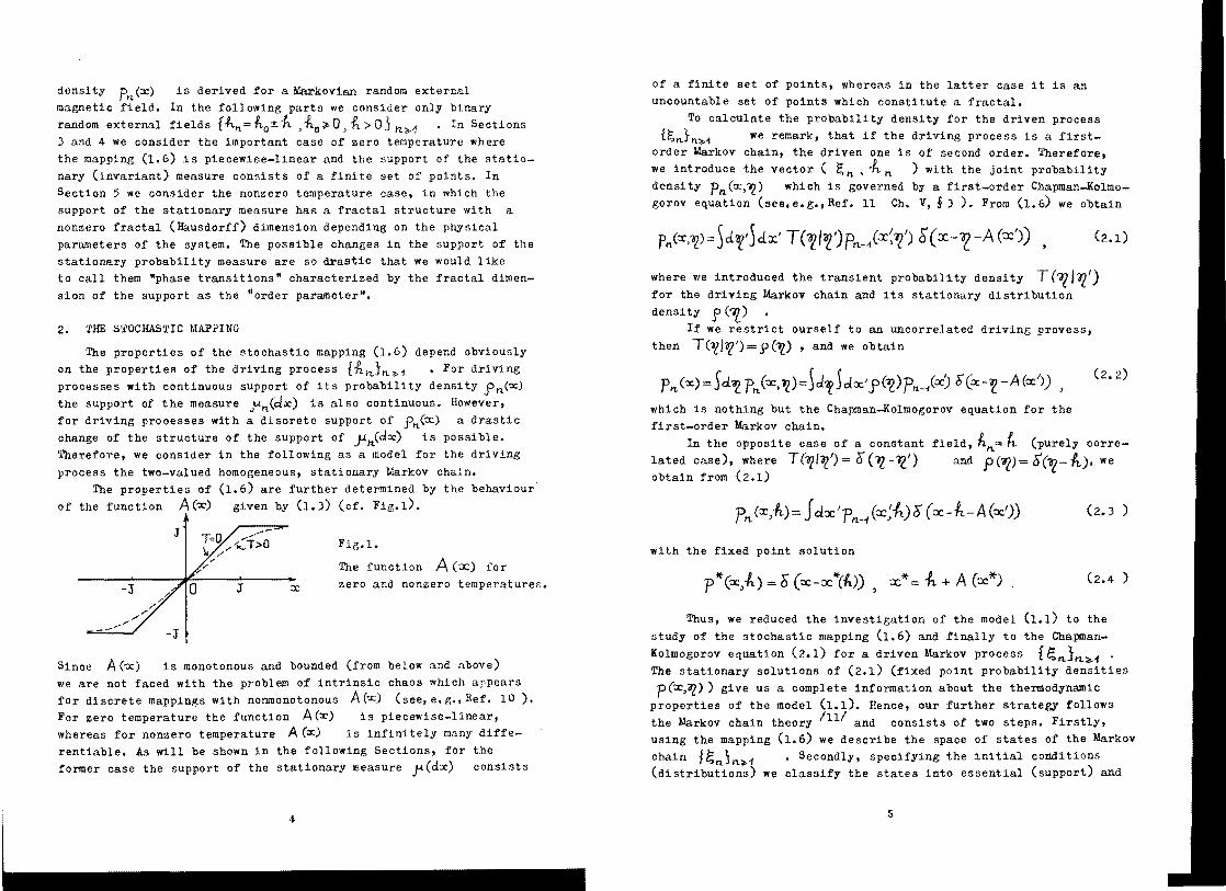
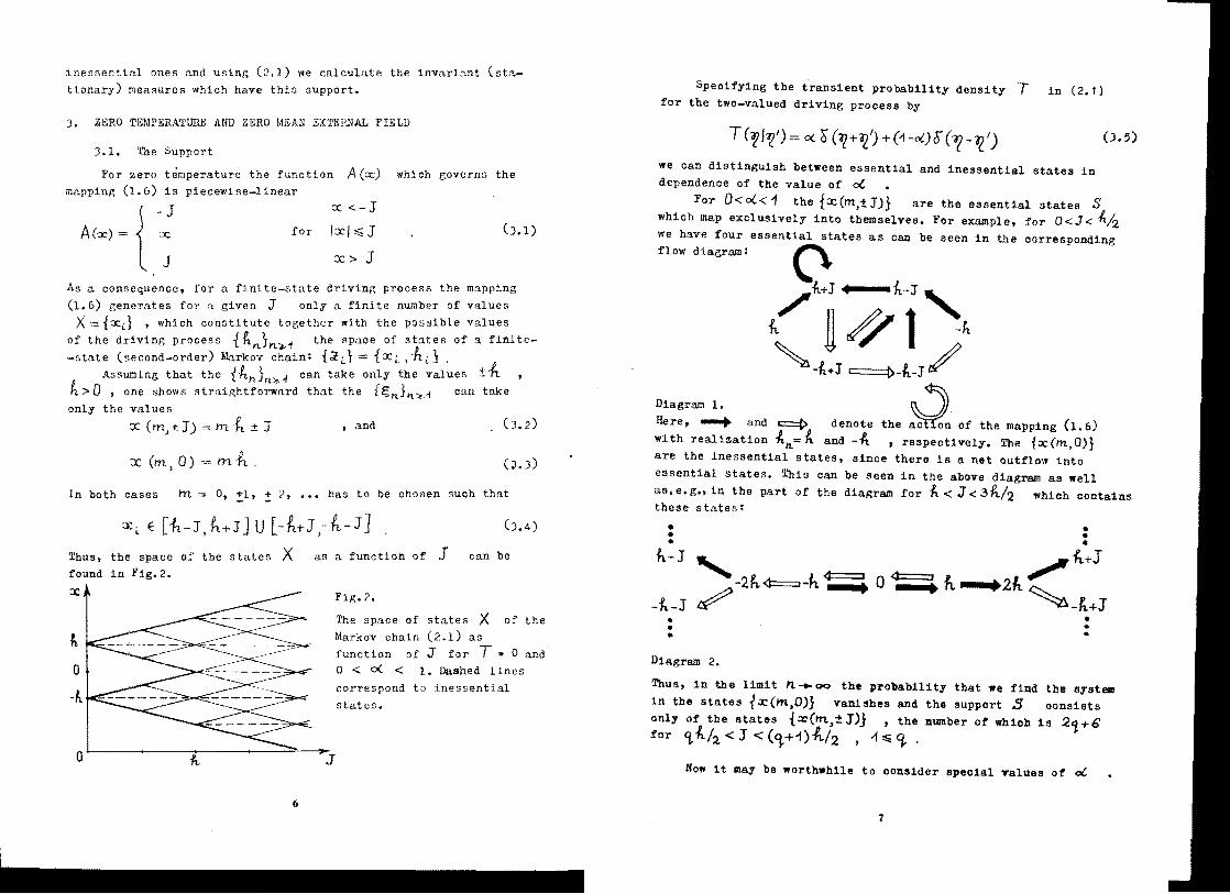
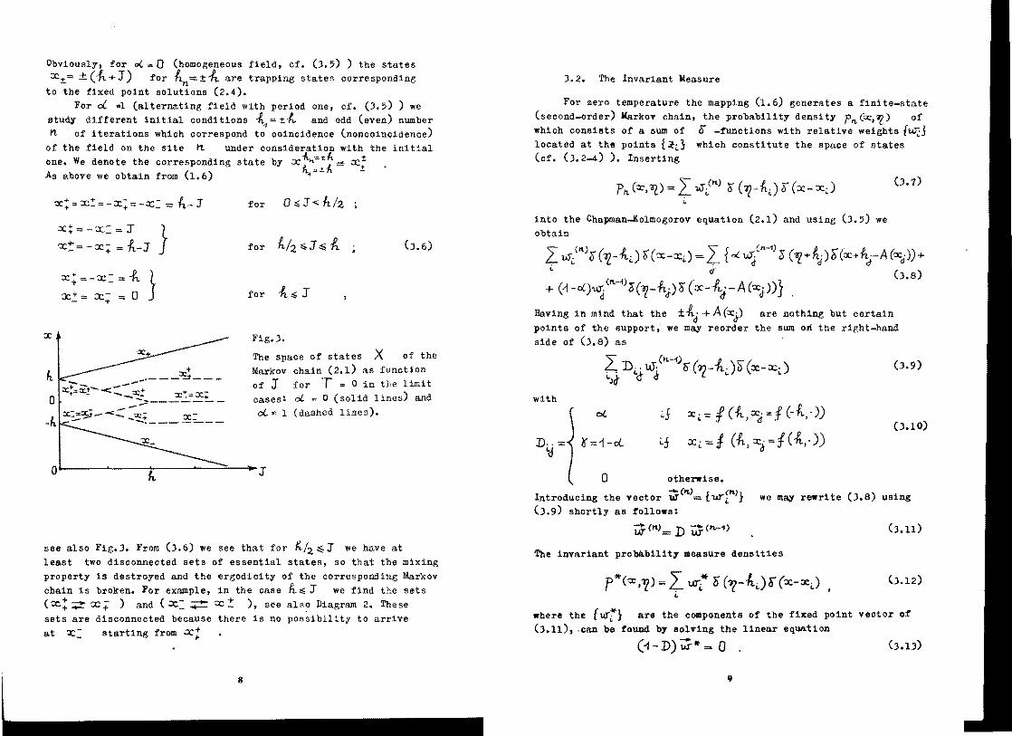
x
Obviously for 0( = 0 (homogeneous field cf (J5) ) the states X+= plusmn (h+J) for It =plusmn-h are trapping states corresponding- n
to the fixed point solutions (24) For d 1 (alternating field with period one cf (35) ) we
study different initial conditions I plusmn ~ and odd (even) number n of iterations which correspond to oOincidence (noncoincidence)
of the field on the site n under consideration with the initial ~ -tlone We denote the corresponding state by X ft~+J
As above we obtain from (16) - shy
~ + - -P J~+ x_ = - X+ -x_ - 11- for OoJlt1tz
xt x= =r -c -x = ft-J forfth~J~~ (J6)
X~ -X =ft l c~ = x = 0 J for ft J
It
o
--
Fig J
The space of states)( of the Markov chain (21) as function of J for T = 0 in the limit cases ol = 0 (solid lines) and d 1 (dashed lines)
J
see also FigJ From (J6) we see that for f~J we have at least two disconnected sets of essential states so that the mixing property is destroyed and the ergodicity of the corresponding Markov chain is broken For example in the case ft J we find the sets (x x ) and ( 0+ ) see also Diagram 2 These sets are disconnected because there is no possibility to arrive atc starting from x
8
J2 The Invariant Measure
For zero temperature the mapping (16) generates a finite-state (second-order) Markov chain the probablli ty density tJ (-c l) of whioh consists of a sum of 0 -functions with relative weights wJ located at the points f~L which constitute the space of states (cf (J2-4) ) Inserting
(J7)Ph (x O() = r 1Aftl) 0 (7- It) b (x- Xi) ~
into the Chapman-Ko1mogorov equation (21) and using (J5) we obtain
Zw(tl)Q (-Z--hJ S(x-x) = r o( Wt-1) a(-az+~)Hx+~-A (~))+ I if
1) (J8) + (-1-O()~ n- O(12-ftJ)b(x-4LJ-A CXJJ )
Baving in mind that the plusmnftd + A(xJ) are nothing but certain pOints of the support we may reorder the sum on the right-hand side of (J8) as
2 D w(h-i)o (n-k)~ (x-x) (J9) iJ~ Iltt d l
with
0lt ~J x~ = (ft Xr f (-~)) (J1 0)
Dmiddotmiddot= r1-C( LJ Xi J (ft XJ ( ) ) ij
o otherwise - (n) j (It) ( )Introduc~ng the vector 1U = l1lT we may rewrite J8 using
(J9) shortly as follows
Ui(It)= D Uj(tI-i) (Jll)
The invariant probability measure densities
p1t(X)=[ urt O(l-i)cr(~-XiJ (J12) I
where the W-r are the components of the fixed point vector of (J11) can be found by solving the linear equation
(-1- D) tj =- 0 (J13)
9
----
--two different fixed pOints corresponding to the trapping states
If the state space consists of only one connected set of essential ~ and~y cf Diagram 1
states the invariant measure is unique and should coincide with the For 0( == 1 the transition matrix D desoribes osoillations limit value
u = -ampm ort Ui (0) (J14) rt_ltgtltgt
for arbitrary ini tinl vector (distributton) w (0) ( see t e g Ref 11 )
The number of independent solutions of (JlJ) is equal to the number of disconnected sets of essential states These solutions can be found also from (J14) starting with different initial distribushytions with suppori on the corresponding subsets of connected essential states 1111
For example we first consider the case 0 lt J lt-12 bull hen the essential states as can be seen in Di~gram I are
2th~~ l(h+J-)(It-JJ(-i+J-ft)H-J-t)f= S x tiL (J15 )
The one-step tranSition matrix ]) according to (JlO) has the form
roo 0)DOo(ol (J16 )D= 0(0( 00( o 0 ~ r
Solving (JlJ) we obtain for 0 lt 0 1 the unique fixed point distribution
-- -1 ( y)T CJ17 )tV =~ (o(u
whioh oan also be obtained from (J14) observing that
0 r YY) (J18 )tm D rt i 0( 0( 0( 0lt tI oo 20(0(0lt0((
yen ~ 04
and starting from arbitrary initial Weights tj-CO) For d- 0 the statesit and~It become trapping and hve
the same weight For 0(-1 we have an osoillation between t2 and lt3 which
both oocur with the same weight For 0( =0 the transition matrix D becomes idempotent and has
)0
between ~2 and 23 bull Formally this corresponds to a fixed point - (0 12 12 0 )T bull remark that 11m DItsolution Ui We does not exist but D=D~ (n= 12 bullbullbull ) has two different eigenvectors (fixed points) (0 1 0 0)T and (0 0 1 0 )T
As a second example we consider the oase h lt J lt 36 It Here we should take into account also those states whioh are for Oltclaquo 1 inessent1al because part of them become essential for 0(= IThe full space of states oan be found in the Table From the seoond oolumn of this table we can obtain the elements of the transition matr1x ]) bull The matrix elements correspond1ng ta solid (brOken) lines are ~ (ot) bull Disconnected pOints oorrespond to zero matrix elements
For instance Damp-1== d ])1= ( and ])21= 0 bull In the next column one can find the weights of the corresponding invariant measure
As in the previous case one should distinguish the cases ct- 0 and ot = 0
For d -1 we have oscillations between the four pairs of states II( and lg t and 2-2 lt and ~12gt il-1 and ii1s but with different weights
For 0( = 1 we have in addi tion oscillations between lts and ~~O ~3 and ~4y which were former inessential Acoordingly
we have six independent formal fixed pOints of j) cf the Table The matrix D2M ( n = 12 bullbullbull ) has twelve different fixed points
4 ZERO TEMPERATURE AND NONZERO MEAN EXTERNAL FIELD
In this ohapter we shortly oonsider the case of a nonzero mean external field ie lhltM~1 takes now the values ltoplusmnJ ( -ho it gt 0 ) As in the previous case the mappine (1 6) generates a finite state (seoond order) Markov chain
Fig4
The space of states X of the Markov ohain (21) for nonshyzero mean external field ho = =h4 as fUnction of~ for
k -0 rrO
Ji-It T=O deglt co( L 1 Only the essenshy~ o tial states are shown
J I I t J o (1) (2)(3) It J
11
---------------------------------
-----
TABLE In Fig4 we present the dependence of the essential st~tes for Sta1A Mapping uJilshy o lt 0( lt 1 as a function of J for fo less than It namely
i zi n n+l 0 lt 0lt lt 1 0lt 0 0( 1 for 0 == 4 bull For this value of Ito the support shows a behaviour ---- ---- -------- similar to that for o 0 with the difference that the symmetry 1 (h+J h) 4 191 10 o with respect to = 0 is broken and that for 1 not too
2(1+2laquo) small the states are denser beoause the bifurcations at (1) (2) bullbullbull
2 (2h h ) o o o have a smaller period oompared with the zero mean case For1 and Oltclt~1 we find a completely different behaviouretaJ (Jh~ b) o o We first consoider the flow diagram for to and 2l- lt Jlt 2(ltjd)-
2(1+0lt)(1+20() (=12 ) 4 (J h) 0(2
o ()(l+ O() (1+2C(J Wa
5 (h h ) o o 10 J+ZhD00
0(6 (2hJ h) o------ 12 bull laquo) 2h 1~2(1+ 0lt) (1+ 2laquo) O2ho-middotmiddot 2(h-1) J~ 7 (-h+J h) o--~~-- lJ
2(1+ 0lt) (1+20pound)
a (-h+J -h) o o0( Diagram J------ 4
2(1+20() It Bhows that the only essentlJ tate S 32( J 10(~ ]1-20
9 (0 h ) o o t 1lj 121 anamplysis gives the resul t that these states are the14
only essential ones also for lt 10 bull Note that the space of 10 ( 0 -h ) o o essential states is the same both for stoohastic ( 0 lt 0( lt 1)
and periodic ( cent( = 1 ) external fields 5
11 (h~ h ) Wa o 15 This drastic reduction of the spaoe of states in dependence
12 (h~ -h) o on the mean value of the external field can also be found for117 6 nonzero temperature see belo
lJ (-2h+J -h) oW6 7 14 (-h-h) o o 119 15 (J -h ) o 5 THE I4APlING FOR NONZERO TEMPERATUREW4 w11
16 (-Jh+J -h) W o oJ 51 The Spaoe of the States and the Invariant Measure
17 (-2h -h ) o o o To desoribe the spaoe of states of the stochastio mapping (16) for nonzero temperature we introduoe the following notashy
18 (-h~ -h) WI 1--1 o tion We denote the result of the n-th iteration of the mapping (16) starting from the arbitrary initial value ~o=~ by
(51)X b6_lt 6~ lt1 f (t -J (hl1_~1 ( J (h~) )))
12 13
where tn) h~~ is a given realization of the binary driving process and 6 J 6 ~ is the corresponding sequenoe of signs It is clear that the space of states of the driven Markov process consists of all pOints which can be represented in this way
As for the zero temperature oase we call the sets of states which are invariant under the mapping (16) the sets of essential states Sinoe for nonzerc temperature J E COO OR 2) and oltoJ (ch) lt 1 the sets of essential states are given by im x ~JRbullbull 1he existence of these limits and their inshy
rL gtO 6Jmiddotmiddotit 1 -1(0
dependence of the starting pOint (f E IR are provided by the pro-J IIWperty 0cJ (xn) lt 1 see eg Ref bull We denote these limits
by S = lxa ~ where ~ oorresponds to an infinite realization 1 of the driving process
As a consequence of the independence of Xgt on the starting points if E IR one has (i) for the stochast1c~mapPing (16) the set 5 -= -c j is an attractor whose basin of attraotion is IR (11) for 0lt 0( lt -1 any two points x~ XG E S can be conshynected by the mapping (16) so that there are-no disconnected inshyvariant subsets in S Therefore the attractor S is a unique set of essential states (support) for the driven Markov prooess (16) for Tgt 0 and 0 lt 0 lt -1
We can construot the invariant measure for this process by iteration of the corresponding Chapman-Kolmogorov equation (21) start~ng from an arbitrary nontrivial probability density poCX~)4 on IR x l ft plusmn It bull Because the basin of attraotion of 5 is IR there exists a compact K =Klt Klt such that
) dP~(c~)= -1 bull tl~1 dP~ (C1) == Pt1(c~) dx d2 (52) K((l
Then by Prohorovs theorem 121 the sequence of probability measures fPIIt)~ is compact with respect to weak convergence ie there
are subsequences Pit It 1 such that for arbitrary ofof k
~ E C ( IR IR ) one has
(5J)trn 5clPltk (xgt~)~(x~)= JdP(X~)~(caz)ItIc OO
~ construotion (5J) the invariant measures tlk have the same support ooinciding with the attractor S which is the only set whioh is invariant with respeot to the mapping (16) (transitiT1ty)
14
This means that the measures (Jk are ergodic But on the same support there exists only one ergodic invariant measure IIJI ie the sequence tPI1 111 converges to the unique invariant probashybllity measure P
52 The Geometrical Structure of the Support and the Fractal Order Parameter
We now consider the geometrical structure of the attractor S on IR bull As it follows from 51 for the binary driving
process there is a one-to-one oorrespondence between the pOints ~ E S and the infinite sequencessect of + and - bull Therefore the cardinality of the set S is the continuum
Further by construction (51) the pOints of the support S are located in the interval [gt6- l6middot] where europlusmn= 611= + or Gh=--i bull As it follOWS from (51) the two pOints are the trapping states (fixed pOints) for 0( 0 the case the constant field (see Seotion 2) Thus in this limit the attractor reduces to two disjoint parts concentrated at the pOints
S+= ~+ and gt6- (cf 51 ) fo discuss the details we reshystriot ourselves in the following to the case of a zero mean random field Then one has (see Fig5)
plusmnX-It
(54)
For ci 1 (alternating external ield) the attractor S (see (51) ) also reduces to a two-point set I plusmn Cp where Xp XE+shy
( lt0 +- is the infinite alternating sequence starting with + ) or equtvalently the solution of the equation Xp= 1- (h- cp) But now S bull Cp 3- is a connected invariant set corresponding to an attractive orbit of the mapping (16) for c( bull 1 (cf Fig5)
As oan be seen from (51) (cf also Fig5) there are no states from S between the points
X+ G- = f C~X6-) and X_ 6 +=j(--xfi+) (55)- ~ - shy
Therefore the set S has a gap of the length
t = X+6--X_6~ = 2 CZk-c) (56)- shyAfter applying the mapping (16) this gap produces two gaps of the next generation whose end-points are (see Fig5)
15
-JC t = 1 (-ft~f(hjX~plusmn))lG ~
Fig5
The construction of the support (attractor) S and the origin of its fractal structure for mapping (16) and for its linearised version
(bold dashed lines) -x x For 010 1
(alternating field) ti reduces to an attracting orbit (dot-dashed lines)
ie S=i xXp)
-x-shy
In the same w83 one can construot the end-points of the gaps in the n-th generation as
(57)X6ntgtn_~JGP eurot =f (ftn j (-hpXit) ) This procedure allows one to construot all gaps in the attraotor S We call the finite sequenoe of n (different) signs ~ead and the infinite sequence of identical signs -tail- The two end-points of one of the gaps in the n-th generation can be represented bt two infinite sequenoes consisting of a head of n signs which differ only in the first sign and an infimiddotnite tail of signs opposite to the first one of the head
Bence the set of all end-points is obviously countable Qn the other hand it is dense in the support S in an arbitrary neighshybourhood of a point Xli Eo 5 one can find an end_point (an end-point is as closer to ~ - as longer its head is which coincides with the corresponding first signs of G ) Vice versa the set S is nowhere dense Therefore the ~pport S constitutes a Cantorshy-type-fractal 114 but in contrast to the Cantor set it has no simple self-similar structure
16
To elucidate the latter let us linearize the mapping (16) on the interval [-x rl-] substituting the function I (ftx)
by plusmnft + x (x~ft)x see Fig5 CLhen the above procedure (54-7) gives us instaad of S the standard Cantor set Ct with the larshygest gap equal to Ll (56) Now it is clear that S is nothing but a smooth deformation of and deviations of the support SCA from the Cantor set are due to the nonlinearity of the functionCA
A(x) see (16) and Fig5
Now we give a qualitative analysis of the Hausdorff (fractal) dimension 131 d dH (5) of the support S in dependence on the physical parameters of the system (11)
For the zero mean external random field we represent this deshypendence in Fig6 (the phase diagram) The condit1on b (-ft X(J-ft TgtOraquo) 0 (56) defines the boundary between two T
2J Fip6 kafn3
fhe phase diagram for the model) bgtO
(11) (zero mean external1~Oltdflt1 with fractal order parameter df bull~=O
dpound=1
1 1dJ~ 0bull dr 0 _~ ~ o Ito W
essentially different regions for fJgt 0 the support S has a fractal structure with Oltdf lt 1 whereas for 6 = 0 (and formally for 6lt 0 see (56) ) the support has no gap ie~= =~ To discuss the behavioUr of d as a function of (JftT) we use the approximation dr=lci (CA) whose accuracy depends on
H the accuracy of the linearized mapping considered above Because the Hausdorff dimension dH(CA) of the Cantor set Ct is well shy-known 14 one gets
for CitT) fl ( hC) ~ 01 d (J kT) =1 n 2
f xt for l (tT) b(hxraquoOil1- (58)
xgtt_h
17
The result (5S) establishes the phase diagram presented in Fig6 and gives a reason to consider fractal order parameter x bull
cI == ci (J- T) as a
For instance we obtained above that at T 0 the support S consists of a finite number of states (see Sections J and 4 )) ie clj(JltT=O)=O bull Therefore with T-tgtO one should obsershy
ve a transition of d] to zero (cf (5S) ) which is continuous in the gap region but should be discontinuous in the gapless one (see Fig6) On the other hand the function A (c) tends to zero for T __ 00 (cf (lJ) ) Then the support S reduces to the twoshy-point set i-Ait because for A(x) - 0 the first gap increashyses and its end-points converge to plusmnXil=plusmnJt (cf (56) and Fig5) Consequently dj(JhT-tgtoo) 0 and the border l1ne on the phase diagram shOUld behave for T -shy Cgto as it is presented in Fig6
Finally for a nonzero mean external random field f -itn = =ftoplusmnhJ we observe that for small ftogtO (fro -6 J) the fractal structure of the supports becomes nonsymmetric It contracts
)to the left end-point Xl and stretches near Xr (cf Fig7 while in the linear approximation the fractal structure is similar to that for ho 0 bull ror large hogtD (Itoraquo J) the first gap rapidshyly increases and the fractal structure approaches that in the linear approximation because the curvature of A (x) for xe Xl(x- 00 for Ao oo ) tends to zero Therefore in this case one can again utilize the approximation ct U (S)=d H (C 6 ) to evaluashyte the dimensionality of the support
6 CONCLUSIONS
The present paper is devoted to the study of the one-dimensional random field Ising model (RFIM) by the stoohastio mappings method We restrict ourselves to investigate the support S of the fixed pOints (or stationary) measure rather than calculating physical obsershyvables As it follows from above the knowledge of S and fI (dx) allows us to calCUlate the free-energy density (17) the magnetizashytion per site (19)and the Edwards-Anderson parameter (110) These calculations can be easily performed for TmiddotO (eg using Table ) but not so easy for lrgt 0 bull Starting from the Chapman-Kolmogorov
x VEry recently the fractal dimenSion of the RFIM was calculated 121avoiding this approximation bull The results support the phase
diagram in Fig6
18
h
xshyr I I I I I
- I t t t 11 I
-shy - I
x
Fig 7
The construction of the support (attractor) S and arising of its fractal structure for the mapping (16) with nonzero mean external fieldOlt~oltJ
equation (21) (for unoorrelated random field see Ref 8 ) we can do these calculations as a systematiC expansion in terms of the momenta lt~mgt of the stationary probability measure corresponding to the Markov chain driven by the external field see (J5) Then for zero mean external field we get for the Edwards-Anderson parashymeter susceptibility the following l
~itn~ T-O 0lt2) t EA= CgtO
(61)
where the divergence is exponential for 0 ltol -1 bull On the other hand the most instructuve information about
thermodynamics of the model is obviously contained in the behaViour of the support S including the phase transitions which we propose to characteri2le by theorder parameter d-r bull Simultaneously as it follows from Section 4 we have lim m(tD) = 0 for T 0 ( 15 ) k-plusmnOsee also Ref bull Therefore the phase transitions we discussed have no conneotion with the oontroversy oy the lower critioal dimenshysion of RFlM (partially settled in Refs 16-18 ) where the magneshy
tization is the order parameter AB it is shown above the local field in the one-dimensional
RFIN may have a very peculiar distribution with a nontrivial fractal dimensionality of its support The natural question is whether this is also charaoteristio of other simple models eg of mean-field ones In recent papers 1920 the mean-field RFIN is considered for an independent and identically distributed random external field From Ref 20 ~ection J it follows that in this case the distrishybution of the local magnetization only mimics that of the external
field
19
ACKNOWLEDGEMENT
One of the authors (UB) thanks the Laboratory of Theoret1ca1 Physics JINR for hospital1ty during visits when ~1n part of this research was done
REFERENCES
1 Galam S and Sal1na~ SR JPhys 1985 C18 p L4)9 2 Thomsen M Thorpe MF Choy TC and Sherr1ngton D PhysRev
1984 B)O p250 ) Thomsen M Thorpe MF Choy TC and Sherrington D PhysRev
1985 B31 p7)55
4 Thomsen M Thorpe MF Choy TC Sherr1ngton D and H-JSommers PhysRev B)J 19)1 1986
5 Derr1da D Vannimenus J and Pomeau Y JPhys 1978 Cll p4749 amp Bruinsma R and Aeppl1 G PhysRevLett 198J 50 p1494 7 Aeppli G and Bru1nsma R PhysLett 198J 97A p117 8 Gyorgy1 G and RVjan p JPhys 1984 C17 p4207 9 Normand JY Mehta ML and Orland H JPhys 1985 Al8 p621
10 SchUster HG Determ1nist1c Chaos (Phys1k-Verlag Ber11n 1985) 11 Doob JL Stochast1c Processes (John W11ey amp Sons New York 195)) 12 B1111ngsley p Convergence of Probab11ity Measure (John W11ey amp
Sons lew York 19amp8) 1) Cornfeld IP Fom1n SV and S1na1 YaG Ergod1c Theory
(Springer-Verlag BeIi1n 1982) 14 Mandelbrot BB The Fractal Geometry of Nature (Freeman San
Fransisco 1982) 15 Berretti ~ JStatPhys 1985 J8 p48J 16 Fisher DS Frohl1ch J and Spencer T JStatPhys 1984
J4 p86J 17 Imbrie JZ PhysRevLett 1984 5J p1747 18 Imbr1e JZ CommunMathPhys 1985 98 p145 19 Sal1nas SR and Wresz1nski WF JStatPhys 1985 41~299 20 Angelescu N and Zagrebnov VA JStatPhys 1985 41 p)2J 21 Szepfalusy P and Behn U ZtUr Phys1k 1981 B65 p331
Rece1ved by Pub11sh1ng Department on March 4 1981
20
DeH Y 3arpe6H08 BA EI7-87-138 OAHOMepHaA MOAenb MaHHra B cnY4aHHoM none H CTOXaCTH4eCKMe AHCKpeTHWC oT06paeHMA
OAHOMepHaR MOAenb MaHHra B cnY4aMHoM BHBWHeM none HccnBAOBaHa C no~~D CToxaCTH4eCKMX oT06paeHHH PaccMOTpeH cnY4aH laaMapaeHHOrol MapKOBCKOro BHBWHero nonR OaKaaaHo 4TO BCA HH$OpMaqMA 0 TepMOAHHaMM4eCKX CBOMCTBax MOAenM COAepwHTCR B HHBapMaHTHOM Mepe KOTopaR COOTBeTcTByeT HeKOTopaMY MapKoBCKOMY npoqeccy ynpaBnReMOMY BHeWHMH noneM H B 4aCTHOCTM B HOCMTeshyne S 3TOM MePW npH HyneBoM TeMnepaType S COAepwHT KOHe4Hoe 4Mcno T04eK a nPM HeHyneaoM ftBnfteTCA HexaOTM4eCKMM ICTpaHHWM aTTpaKTopOM C $paKTan~~ CTPYKTYpoM KaHTopaBCKoro THna nOKaaaHo 4TO $paKTanbHaR paaMepHOCTb dfHOCHTenft S HrpaeT ponb napaMeTpa nOpftAKa AnA AaHHoM MOAenM MccneAoBaHa aaBMCMMOCTb S H d f OT napaMeTpOB MOAenM H TeMnepaTYPW
Pa60Ta BwnonHeHa B na60paTopMH TeopeTH4ecKOM $HaMKH OMHM
CooampII_oca-o -CIInyTII ~ _eJIO Jlramp1111
Behn U Zagrebnov VA EI7-87-t38 One-Dimensional Random Field Ising Model and Discrete Stochastic Happings
The one-dimensional random field Ising model is studied using stochasmiddot tic mappings The case of a (frozen) Markovian external random field is considered We show that all information about thermodynamic properties of the model is contained in an invariant (stationary) measure corresponshyding to some Harkov process driven by the external field and particularly in the support S of this measure For zero temperature it contains a finite number of points but for nonzero ones it is a nonchaotic (strange) attracshytor with a Cantor-type fractal structure The fractal dimensionality df of S is proposed as an order parameter for the model The dependence of S and df on the model parameters and the temperature is studied in detail
The investigation has been performed at the laboratory of Theoretical Physics JINR
0iamIIofdIeloiDt IDiIIItuIe b NudIIIr a-dL0-1
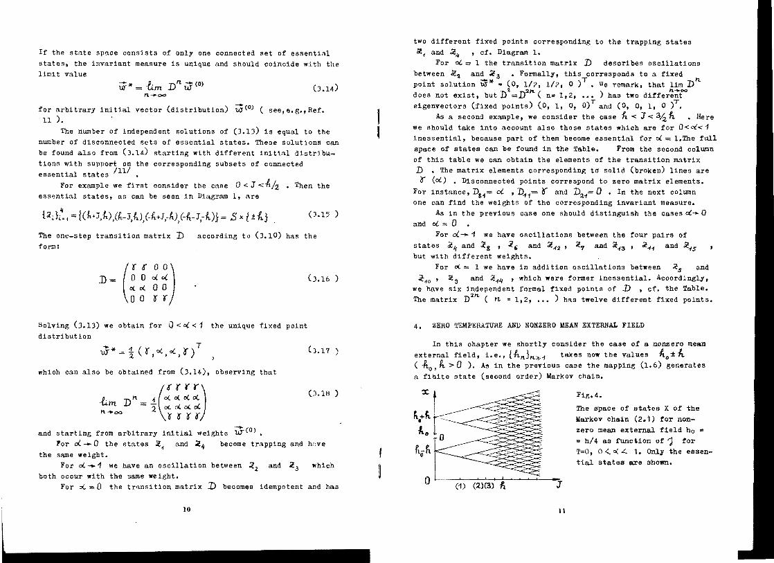
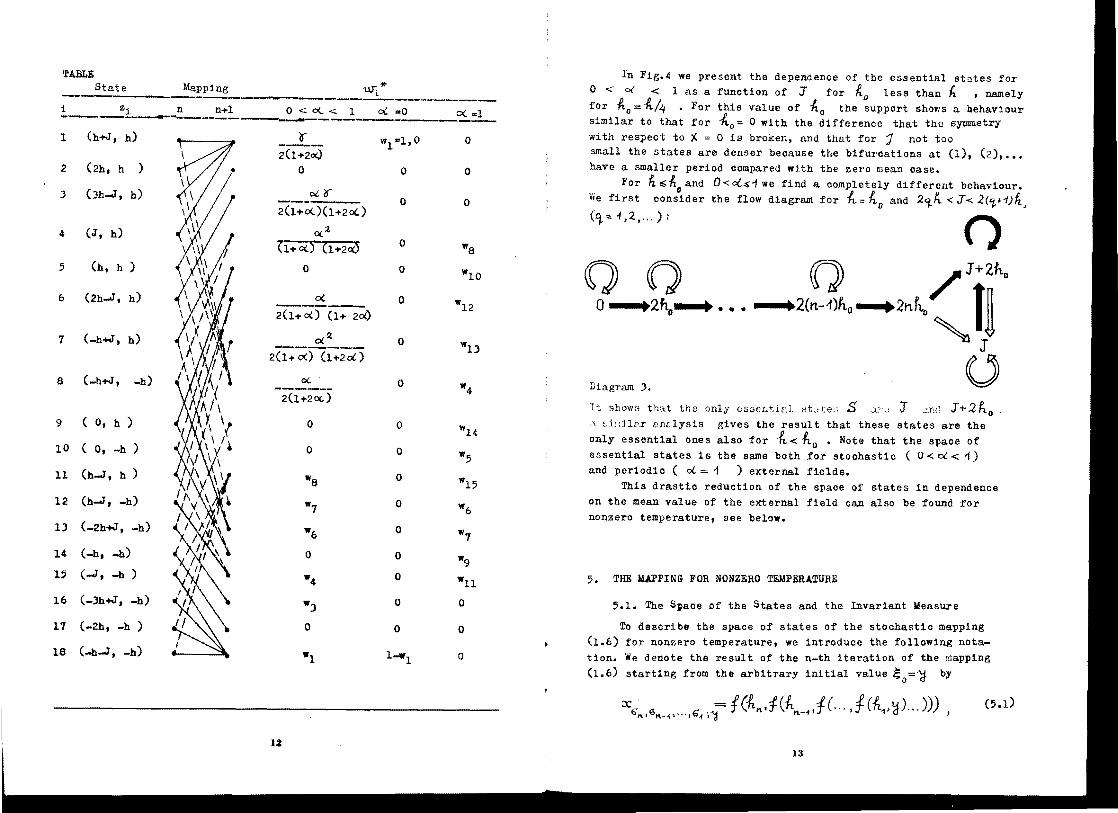
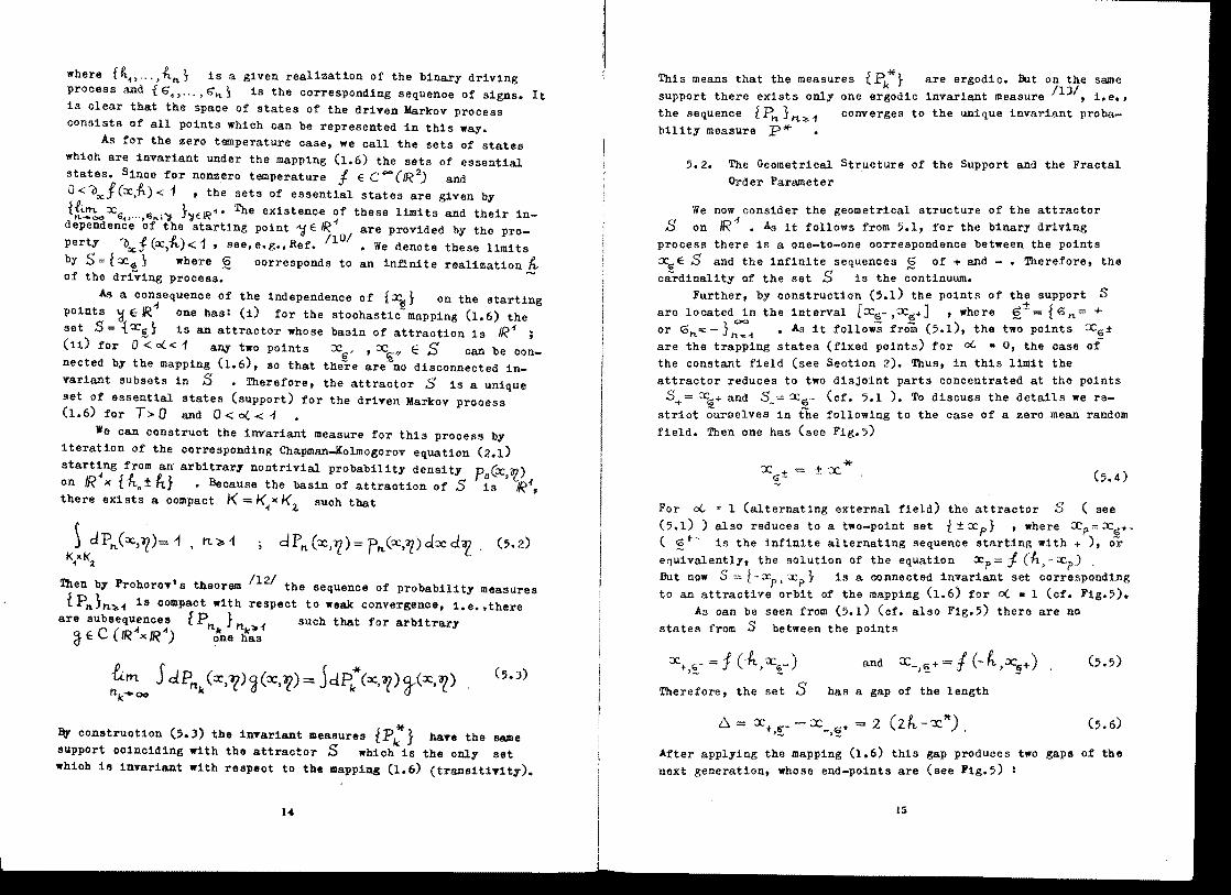
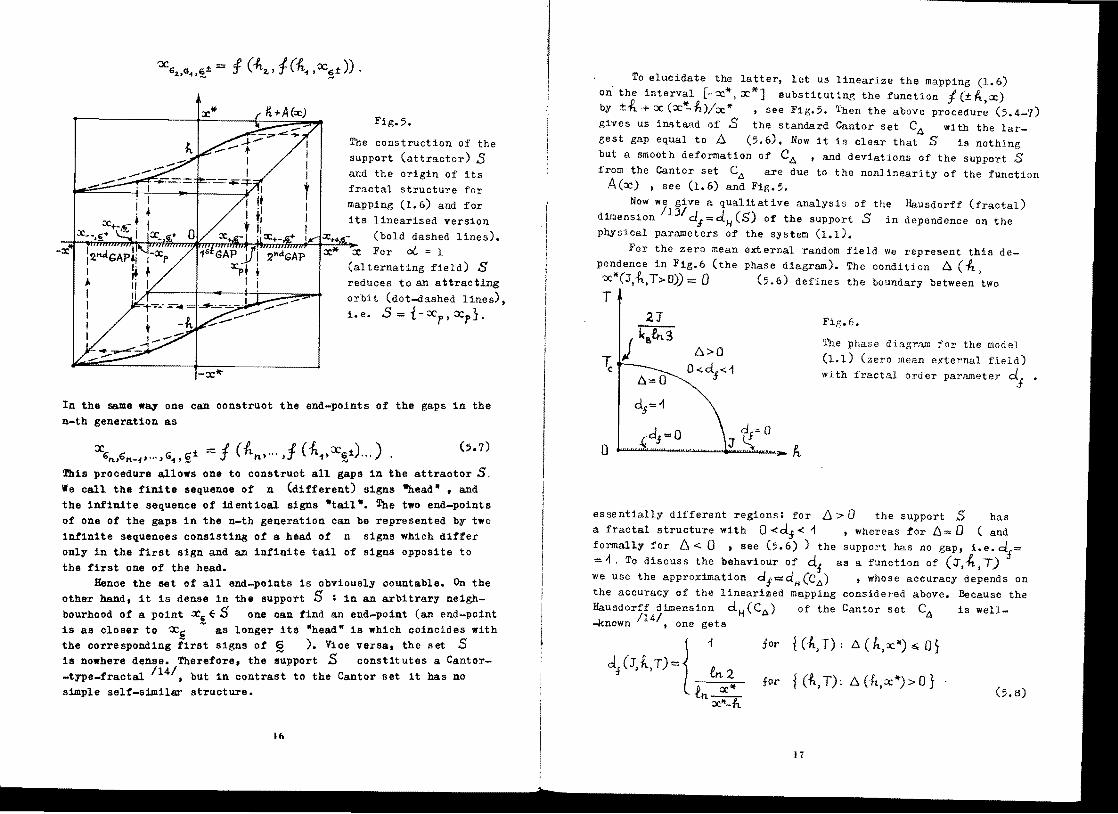
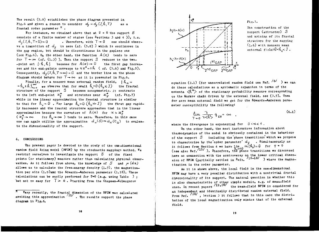