
VRIJE UNIVERSITEIT THE ZORA EQUA TION · VRIJE UNIVERSITEIT THE ZORA EQUA TION A CADEMISCH PR...
100
-
Upload
trankhuong -
Category
Documents
-
view
214 -
download
0
Transcript of VRIJE UNIVERSITEIT THE ZORA EQUA TION · VRIJE UNIVERSITEIT THE ZORA EQUA TION A CADEMISCH PR...
THE ZORA EQUATION
VRIJE UNIVERSITEIT
THE ZORA EQUATION
ACADEMISCH PROEFSCHRIFT
ter verkrijging van de graad van doctor aan
de Vrije Universiteit te Amsterdam,op gezag van de rector magni�cus
prof.dr E. Boeker,in het openbaar te verdedigen
ten overstaan van de promotiecommissievan de faculteit der scheikunde
op donderdag 18 januari 1996 te 15.45 uurin het hoofdgebouw van de universiteit, De Boelelaan 1105
door
Erik van Lenthe
geboren te Zwolle
Promotoren: prof.dr E.J. Baerends
prof.dr J.G. SnijdersReferent: prof.dr W.C. Nieuwpoort
Contents
1 Introduction and general overview 7
1.1 Introduction . . . . . . . . . . . . . . . . . . . . . . . . . . . . . . . . . . . . 7
1.2 Relativistic density functional theory . . . . . . . . . . . . . . . . . . . . . . 8
1.3 Overview of this thesis . . . . . . . . . . . . . . . . . . . . . . . . . . . . . . 10
2 Regular Expansions in Relativistic Mechanics 13
2.1 Classical Relativistic Mechanics and the Coulomb potential . . . . . . . . . . 13
2.2 Expansions in Relativistic Quantum Mechanics . . . . . . . . . . . . . . . . 14
2.2.1 Elimination of the small component . . . . . . . . . . . . . . . . . . . 14
2.2.2 The Foldy-Wouthuysen transformation . . . . . . . . . . . . . . . . . 18
2.2.3 Direct Perturbation Theory . . . . . . . . . . . . . . . . . . . . . . . 20
2.2.4 The Douglas-Kroll transformation . . . . . . . . . . . . . . . . . . . . 21
3 The ZORA Hamiltonian 23
3.1 Basic equations . . . . . . . . . . . . . . . . . . . . . . . . . . . . . . . . . . 23
3.2 Boundedness from below . . . . . . . . . . . . . . . . . . . . . . . . . . . . . 24
3.3 Total energy . . . . . . . . . . . . . . . . . . . . . . . . . . . . . . . . . . . . 26
3.4 Gauge invariance . . . . . . . . . . . . . . . . . . . . . . . . . . . . . . . . . 28
3.5 Molecular bond energies . . . . . . . . . . . . . . . . . . . . . . . . . . . . . 30
3.6 Magnetic �eld . . . . . . . . . . . . . . . . . . . . . . . . . . . . . . . . . . . 32
4 Exact relations between DIRAC and ZORA 35
4.1 Introduction . . . . . . . . . . . . . . . . . . . . . . . . . . . . . . . . . . . . 35
4.2 Exact solutions for hydrogen-like atoms . . . . . . . . . . . . . . . . . . . . . 35
4.2.1 First order perturbation . . . . . . . . . . . . . . . . . . . . . . . . . 36
4.2.2 Scalar relativistic equations . . . . . . . . . . . . . . . . . . . . . . . 37
4.3 One electron systems . . . . . . . . . . . . . . . . . . . . . . . . . . . . . . . 37
4.4 Two electron systems . . . . . . . . . . . . . . . . . . . . . . . . . . . . . . . 37
4.5 Results . . . . . . . . . . . . . . . . . . . . . . . . . . . . . . . . . . . . . . . 39
5 Numerical atomic calculations 43
5.1 Introduction . . . . . . . . . . . . . . . . . . . . . . . . . . . . . . . . . . . . 43
5.2 Selfconsistent calculations . . . . . . . . . . . . . . . . . . . . . . . . . . . . 44
5.2.1 Separation of the radial variable from angular and spin variables . . . 44
5.2.2 Basis set calculations . . . . . . . . . . . . . . . . . . . . . . . . . . . 45
5.3 All-electron calculations on U . . . . . . . . . . . . . . . . . . . . . . . . . . 45
5
6 CONTENTS
5.4 Valence-only calculations on Uranium using the Dirac core density . . . . . . 52
6 Implementation of ZORA 55
6.1 Implementation of ZORA in ADF . . . . . . . . . . . . . . . . . . . . . . . . 556.1.1 The frozen core approximation . . . . . . . . . . . . . . . . . . . . . . 56
6.2 Implementation of ZORA in ADF-BAND . . . . . . . . . . . . . . . . . . . . 58
6.3 Some remarks on the Pauli Hamiltonian . . . . . . . . . . . . . . . . . . . . 59
7 Molecular calculations 63
7.1 Scalar Relativistic calculations . . . . . . . . . . . . . . . . . . . . . . . . . . 637.2 Spin-orbit e�ects . . . . . . . . . . . . . . . . . . . . . . . . . . . . . . . . . 67
7.2.1 Open shell systems . . . . . . . . . . . . . . . . . . . . . . . . . . . . 677.2.2 Intermediate Coupling . . . . . . . . . . . . . . . . . . . . . . . . . . 69
7.2.3 Spin-orbit e�ects in atoms . . . . . . . . . . . . . . . . . . . . . . . . 707.3 Spin-orbit e�ects in closed shell molecules . . . . . . . . . . . . . . . . . . . 707.4 Conclusions . . . . . . . . . . . . . . . . . . . . . . . . . . . . . . . . . . . . 78
8 Elimination of the small component 79
8.1 Introduction . . . . . . . . . . . . . . . . . . . . . . . . . . . . . . . . . . . . 798.2 Solving the large component equation . . . . . . . . . . . . . . . . . . . . . . 80
8.3 (Dis-) advantages of the present method . . . . . . . . . . . . . . . . . . . . 818.4 Basis set selection and results . . . . . . . . . . . . . . . . . . . . . . . . . . 828.5 Conclusion . . . . . . . . . . . . . . . . . . . . . . . . . . . . . . . . . . . . . 84
9 The exact Foldy-Wouthuysen transformation 85
9.1 Introduction . . . . . . . . . . . . . . . . . . . . . . . . . . . . . . . . . . . . 859.2 The exact Foldy-Wouthuysen transformation . . . . . . . . . . . . . . . . . . 85
9.3 Iterative solution . . . . . . . . . . . . . . . . . . . . . . . . . . . . . . . . . 879.4 Numerical Test Results . . . . . . . . . . . . . . . . . . . . . . . . . . . . . . 889.5 Conclusions . . . . . . . . . . . . . . . . . . . . . . . . . . . . . . . . . . . . 90
Samenvatting 91
Summary 93
Dankwoord 95
Bibliography 97
Chapter 1
Introduction and general overview
1.1 Introduction
At present the standard description of the electromagnetic �eld and the motion of electronsis Quantum Electrodynamics (QED). Highly accurate QED calculations on small systems,
like the hydrogen and helium atom, are in very good agreement with highly accurate ex-periments. For larger systems accurate QED calculations are in general too expensive froma computational point of view. It is therefore convenient to approximate QED. Such anapproximation is the Dirac equation [1, 2]. This four-component equation can be solvedexactly for a hydrogen-like atom with a point charge [3, 4]. In many cases this equation
is further approximated, because it is still quite expensive to calculate. The standard ex-pansion gives in zeroth order the non-relativistic or Schr�odinger equation. This expansionis defective for Coulomb-like potentials. In this thesis a regular expansion is used, whichremains valid even for a Coulomb-like potential. This potential-dependent expansion, earlier
derived by Chang et al. [5] and Heully et al. [6], gives in zeroth order a regular approximated(ZORA) equation, which accounts for most of the relativistic e�ects. The ZORA equationwill be the main subject of this thesis.Since the nuclei have much larger masses than the electrons, we will use the Born-
Oppenheimer approximation. In this approximation the electronic problem is solved inthe external potential coming from �xed nuclei. Besides the kinematics, in many-electronsystems we also have to consider the electron-electron repulsion, which is often approxi-mated by the instantaneous Coulomb interaction 1=rij, where rij is the distance betweenthe electrons. Sometimes relativistic correction terms to the electron-electron repulsion are
used, like the Breit [7] or Gaunt [8] term. In so called ab initio calculations one often startsby solving the (Dirac-)Hartree-Fock equation. Afterwards one can use standard techniquesto take correlation e�ects into account. A di�erent standard method is density functionaltheory. In this thesis the Kohn-Sham approach to this theory is used (see next section).
For practical use one needs to have a good approximation for the density functional of theexchange-correlation energy. Successful approximations have been applied in non-relativisticcalculations. In this thesis we will use the same approximations for the exchange-correlationenergy in relativistic calculations.
Valence electrons are for a large part responsible for most of the chemical properties. Coreorbitals of an atom do not change much from one molecule to another. This is used in thefrozen core approximation, also used in this thesis, which can make the calculations cheaper,
7
8 CHAPTER 1. INTRODUCTION AND GENERAL OVERVIEW
without much loss of accuracy. A more severe approximation is the use of e�ective corepotentials (ECP). In this approximation valence electrons feel a parametrised e�ective corepotential, which for example also can take relativistic e�ects e�ectively into account.
Quantum chemistry is full of approximations. In this introduction I have only mentioned afew of them. Time will tell which approximations remain fruitful.
1.2 Relativistic density functional theory
In non-relativistic theory Hohenberg and Kohn [9] proved that in principal ground stateproperties, like the total energy, only depend on the ground state electron density of the
interacting many-electron system. The explicit dependence is generally not known and inpractice approximations are made. If one assumes that a minimum property of the energysimilar to the non-relativistic case is also valid in the relativistic case, one can also proofthe Hohenberg-Kohn theorem in the relativistic case [10, 11, 12]. However, this minimum
property of the energy is not proven rigorously [13]. In this section we will look more closelyat the minimum property of the energy used in this proof, without considering QED e�ects.The Dirac equation has besides positive total energy solutions, also negative energy solutions.The Dirac Hamiltonian HD for one electron moving in an external electrostatic potential Vcan be written as:
HD = Hsys + V (1.1)
where Hsys is the relativistic kinetic energy operator of the electron. In the one-electron case
the standard procedure is that the solution with the lowest possible positive energy is theground-state. In this case one can surround the Hamiltonian HD with projection operators�+
V [14, 15], which are the projection operators onto the positive energy states, to obtain theHamiltonian H+
D, which only has positive energy solutions:
H+
D = �+
VHD�+
V = �+
V (Hsys + V )�+
V (1.2)
The eigenstates of HD with positive energy are not altered due to the projection operatorsin H+
D , only the negative energy-states are removed. We now have a minimum principle for
the energy, which says that for any trial wavefunction T , with �+
VT 6= 0:
hT jH+
DjT i
hT j�+
V jT i
=hT j�+
V (Hsys + V )�+
V jT i
hT j�+
V jT i
� E0 (1.3)
where E0 is the energy of the ground state of H+
D. The projection operator �+
V depends onthe external potential V , which is clearly shown in an example of Hardekopf and Sucher [16].They solved the hydrogen-like system in the space of positive energy solutions of the freeparticle. They found that the energy is lower than the exact 1s ground state energy of the
hydrogen-like system. Heully et al. [15] have explained this by noting that the projectionoperator on the postive energy solutions of the Dirac equation for a given external poten-tial will introduce negative energy states in the case of another external potential (see alsothe standard textbook of Sakurai [17], x3.7). A related dependence on the external poten-
tial can also be found in the Foldy-Wouthuysen transformation [18], which decouples thefour-component Dirac equation in two two-component equations, one of which has only pos-itive energy eigenvalues and the other only negative ones. In the standard expansion in �2
1.2. RELATIVISTIC DENSITY FUNCTIONAL THEORY 9
(� � 1=137) of the Foldy-Wouthuysen transformed Dirac equation, non-trivial dependenceon the external potential starts to appear in �rst order, in the Darwin and spin-orbit term(see chapter 2).
In the �rst step of the Hohenberg-Kohn theorem one can prove a one-to-one correspondencebetween the external potential and the ground state wave function. We suppose a non-degenerate ground state, such that for a given external potential we only have one ground
state. The proof, that there is only one external potential (apart from an arbitrary constant)for a given ground state, is done by contradiction. Suppose we have the same ground stateji for two di�erent external potentials V1 and V2, which di�er more than a constant, notingthat the ground state of H+
D is also an eigenfunction of HD, thus:
H+
D(V1)ji = HD(V1)ji = (Hsys + V1)ji = E1ji (1.4)
H+
D(V2)ji = HD(V2)ji = (Hsys + V2)ji = E2ji (1.5)
In these equations we have used that the ground state of H+
D is also an eigenfunction of HD.Subtraction of these equations leads to:
(V1 � V2)ji = (E1 � E2)ji (1.6)
Since V1 and V2 are multiplicative operators, we must have V1� V2 = E1�E2, which meansthat V1 and V2 only di�er by a constant. This contradicts our assumption and the proofof the one-to-one correspondence between the external potential and the ground state wave
function is complete.Suppose we have j1
gi, the ground state of H+
D(V1), and j2
gi, the ground state of H+
D(V2),where V1 and V2 are arbitrary potentials, which di�er more than a constant. In the secondstep of the Hohenberg-Kohn theorem one wants to prove that these two di�erent normalised
ground state wave functions yield di�erent ground state densities. In the standard proof oneuses that the following minumum property of the energy is valid:
E1 = h1
gjHD(V1)j1
gi < h2
gjHD(V1)j2
gi (1.7)
For the non-relativistic Hamiltonian this is provided by the variational principle, for theDirac Hamiltonian this is not proven rigorously. On the other hand, we did not �nd acounter-example, which invalidates this inequality for the Dirac Hamiltonian. Problems will
de�nitely arise if one is not restricted to ground state wave functions, as we have seen in theexample of Hardekopf and Sucher [16]. According to the inequality 1.3 one can prove:
h1
gjHD(V1)j1
gi = h1
gjH+
D(V1)j1
gi �h2
gjH+
D(V1)j2
gi
h2gj�
+
V1j2
gi=h2
gj�+
V1(Hsys + V1)�
+
V1j2
gi
h2gj�
+
V1j2
gi(1.8)
If we assume inequality 1.7 is true the standard proof of the second step of the Hohenberg-
Kohn theorem is again by contradiction. Suppose j1
gi and j2
gi yield the same ground statedensity �. We then have:
E1 < h2
gjHD(V1)j2
gi = h2
gjHD(V2) + V1 � V2j2
gi = E2 +
Zd3x �(V1 � V2) (1.9)
Changing the role of V1 and V2 and adding the inequalities one obtains the contradiction:
E1 + E2 < E1 + E2 (1.10)
10 CHAPTER 1. INTRODUCTION AND GENERAL OVERVIEW
Thus our assumption was wrong and j1
gi and j2
gi should yield di�erent densities, which�nishes the proof of the one-to-one correspondence between ground state wave function anddensity. As said before this proof is only valid if inequality 1.7 is true. Essential in the proof
is that in the expectation values of the Hamiltonian in inequality 1.7, the terms containingthe external potential explicitly seperate out and only need the electron density. Due tothe complicated dependence on the external potential V1 this is not true for the term afterthe inequality in equation 1.8. It is possible that one can only derive rigorously minimal
properties for the energy in the relativistic case which have a non-trivial dependence on theexternal potential like in this inequality. Then it will be very hard to prove the Hohenberg-Kohn theorem for the Dirac equation, if it exists at all.
The many particle Dirac equation su�ers from the Brown-Ravenhall disease [19]. Forexample a system with two bound electrons is degenerate with a system, where one electronis in the negative energy continuum and one is in the very high positive energy continuum(continuum dissolution). In the non-interacting many-particle system the same one-particle
projection operator �+
V can be used as in the one-electron case, to avoid these problems.However, it will become more complicated for interacting electrons, where Hsys also containsthe electron-electron repulsion. In that case the projection operator �+
V is more di�cult toobtain [20, 21]. In this case one often expands the wavefunction in terms of single-particle
functions. To avoid continuum dissolution, one can use the positive energy solutions of thesingle-particle orbitals only, coming from for example a Dirac-Fock calculation. In eithercase the separation of the space of positive energy solutions and the space of negative energysolutions depends on the external potential. The question of the validity of the Hohenberg-Kohn theorem is not simpli�ed.
In the Kohn-Sham approach [22] of density functional theory one replaces the complicatedinteracting many-electron system with an e�ective non-interacting many-electron system,such that the non-interacting system has the same ground state electron density. In orderto solve the resulting Kohn-Sham equations one needs to know the e�ective (Kohn-Sham)
potential. In non-relativistic theory it is proven that there is a one-to-one correspondencebetween this e�ective potential and the exact ground-state density. One can then also showusing inequality 1.7 that the exchange-correlation part of the Kohn-Sham potential is thefunctional derivative of the exchange-correlation energy. In relativistic theory this can not
be proven rigorously. Of course, in the one-electron case for the Dirac equation, one Kohn-Sham potential is trivial, but the question concerning its uniqueness remains.In this thesis we will nevertheless use relativistic Kohn-Sham equations, with the sameapproximate density functionals for the exchange-correlation energy as were used in non-relativistic theory. These density functionals depend on the local density (LDA) or also on
density-gradients (GGC).
1.3 Overview of this thesis
In this thesis regular approximated relativistic equations are used in atomic and molecu-
lar calculations. In chapter 2 this regular expansion is obtained, using an expansion inE=(2c2 � V ) of the relativistic equation, which remains regular even for a Coulomb-likepotential. In that case the standard expansion in (E � V )=2c2 is defective. This potential-
1.3. OVERVIEW OF THIS THESIS 11
dependent expansion, earlier derived by Chang et al. [5] and Heully et al. [6], is used inrelativistic classical mechanics as well as in relativistic quantum mechanics. The zerothorder regular approximated (ZORA) equation obtained already accounts for most of the
relativistic e�ects.In the chapters 3 to 7 this ZORA Hamiltonian is further investigated. In chapter 3 it isshown that this Hamiltonian is bounded from below. There it is also shown that the ZORAequation is not gauge invariant, but that the scaled ZORA method almost completely solves
this problem. This method again can be approximated using the so called electrostatic shiftapproximation (ESA), which is an easy and accurate way to obtain energy di�erences. Inchapter 4 the exact solutions of the ZORA equation are given in the case of a hydrogen-likeatom. This is done by scaling of coordinates in the Dirac equation. The same scaling argu-
ments are used to obtain exact relations for one and two electron systems in more generalsystems. For the discrete part of the spectrum of the hydrogen-like atom it is shown therethat the scaled ZORA energies are exactly equal to the Dirac energies. Numerical atomiccalculations are done in chapter 5, showing the high accuracy of the ZORA method forvalence orbitals. The implementation of this method in molecular and in band structure
calculations is given in chapter 6. The results of molecular calculations on a number ofdiatomics is given in chapter 7, with an explicit treatment of the spinorbit operator. In thischapter a method is proposed for the calculation of the total energy of open shell systemsusing density functionals if spinorbit is present.
Chapter 8 and 9 show methods for solving the Dirac equation, using basis sets for the largecomponents only. In chapter 8 this is done using the standard method of eliminating thesmall component and requires a diagonalisation of a Hamiltonian for every occupied orbital.In chapter 9 the Dirac equation is solved by a new method. In the iterative procedure used, it
requires the evaluation of matrix elements of the Hamiltonian between the large componentsolutions of the previous cycle. In this chapter also a method was given for construction ofthe exact Foldy-Wouthuysen transformation, once one has the (large component) solutionto the Dirac equation.
12 CHAPTER 1. INTRODUCTION AND GENERAL OVERVIEW
This thesis is based on the following articles:
E. van Lenthe, E.J. Baerends, and J.G. Snijders.
J. Chem. Phys., 99:4597, 1993.Relativistic regular two-component Hamiltonians.
R. van Leeuwen, E. van Lenthe, E.J. Baerends, and J.G. Snijders.
J. Chem. Phys., 101:1272, 1994.Exact solutions of regular approximate relativistic wave equations for hydrogen-like atoms.
E. van Lenthe, E.J. Baerends, and J.G. Snijders.
J. Chem. Phys., 101:9783, 1994.Relativistic total energy using regular approximations.
A.J. Sadlej, J.G. Snijders, E. van Lenthe, and E.J. Baerends.J. Chem. Phys., 102:1758, 1995.
Four component regular relativistic Hamiltonians and the perturbational treatment of Dirac'sequation.
E. van Lenthe, E.J. Baerends, and J.G. Snijders.
(to be submitted).Spinorbit energy using regular approximations.
E. van Lenthe, R. van Leeuwen, E.J. Baerends, and J.G. Snijders.
in New Challenges in Computational Chemistry, Proceedings of the Symposium in honour of
W.C. Nieuwpoort (eds.) R. Broer, P.J.C. Aerts, and P.S. Bagus, Groningen U. P., Gronin-gen, page 93, 1994.Int. J. Quantum Chem.:accepted
Relativistic regular two-component Hamiltonians.
E. van Lenthe, E.J. Baerends, and J.G. Snijders.Chem. Phys. Lett., 236:235, 1995.Solving the Dirac equation, using the large component only, in a Dirac-type Slater orbital
basis set.
E. van Lenthe, E.J. Baerends, and J.G. Snijders.(submitted).
Construction of the Foldy-Wouthuysen transformation and solution of the Dirac equationusing large components only.
Chapter 2
Regular Expansions in Relativistic
Mechanics
In this chapter potential-dependent transforma-
tions are used to transform the four-component Dirac
Hamiltonian to e�ective two-component regular Ha-
miltonians. To zeroth order the expansions give
second order di�erential equations (just like the
Schr�odinger equation), which already contain the
most important relativistic e�ects, including spin-
orbit coupling. This potential-dependent expansion
is based on earlier work by Chang, P�elissier and Du-
rand [5] and of Heully et al. [6].
2.1 Classical Relativistic Me-
chanics and the Coulomb
potential
In this section the classical expression for the rela-
tivistic energy of a particle in a potential is expanded
in several ways, to prepare for similar expansions in
relativistic quantum mechanics. We will see that if
one expands the energy expression in c�1, as is usu-ally done, this will give rise to some problems if the
momentum of the particle is too large. For Coulomb-
like potentials there are always regions where this is
the case. A potential dependent expansion can be
found, which is well behaved even if the momentum
of the particle is large. This expansion will be consid-
ered after we have explained the shortcomings of the
c�1-expansion. Consider a particle that is moving ina potential V . In the special theory of relativity the
expression for the total energy W of the particle is:
W =
qm20c4 + p2c2 + V (2.1)
In this equation m0 is the rest-mass of the particle,
p its momentum and c the velocity of light. It is
convenient to de�ne the energy of a particle as:
E =W �m0c2 (2.2)
Equation 2.1 can be rewritten as:
E = m0c2
s1 +
p2
m20c2� 1
!+ V (2.3)
This equation can be expanded in p=(m0c), giving:
E = V +p2
2m0
�p4
8m30c2+ � � � (2.4)
where in second order the so called mass-velocity
term p4=(8m30c2) appears. The use of this expansion
is not justi�ed if p=(m0c) > 1, i.e. if the momentum
of the particle is too large, as has been stressed by
Farazdel and Smith [23]. If the potential is Coulomb-
like (V � �1=r), then there is always a region where
the potential is so negative that the momentum of
the particle p is larger than m0c, even if the en-
ergy E is small. However, another expansion can be
found, which is valid for Coulomb-like potentials over
all space, even if the momentum of the particle is at
times larger than m0c. The only restriction is that
the energy (a constant of the motion) is not too large,
jEj < (2m0c2 � V ), which in chemical applications is
always the case. At energies for which this inequality
would not apply other e�ects should be taken into ac-
count, like pair-creation. The expansion can be found
by �rst rewriting equation 2.3:
E =
qm20c4 + p2c2 �m0c
2 + V
=p2c2
m0c2 +pm20c4 + p2c2
+ V
=p2c2
2m0c2 +E � V+ V =
p2
2m0(1 +E�V2m0c2
)+ V
=p2c2
(2m0c2 � V )(1 + E2m0c2�V
)+ V (2.5)
13
14 CHAPTER 2. REGULAR EXPANSIONS IN RELATIVISTIC MECHANICS
The last two terms have been written down in or-
der to exhibit more clearly which expansions one can
make. The price to be paid to get rid of the root is
that the equation is now quadratic in the energy. The
equation has therefore an extraneous negative total
energy solution. By choosing a particular expansion
the spurious solution will be thrown away. Expand-
ing in (E � V )=(2m0c2) will give in zeroth order the
non-relativistic (NR) energy and in �rst order some-
thing we shall call the Pauli energy:
ENR = V +p2
2m0
(2.6)
EPauli = ENR ��ENR � V
2m0c2
�p2
2m0
= V +p2
2m0
�p4
8m30c2
(2.7)
Up to �rst order this gives the same expansion as
equation 2.4. It is obvious that this expansion is not
valid for r ! 0, where E � V > 2m0c2. A cor-
rect expansion can be found (for energies smaller than
2m0c2) by expanding in E=(2m0c
2�V ). In zeroth or-der this expansion gives, what we shall call the zeroth
order regular approximated (ZORA) energy:
Ezora =p2c2
2m0c2 � V+ V (2.8)
The E=(2m0c2 � V )-expansion is valid for Coulomb-
like potentials everywhere, whereas this is not true for
the (E�V )=(2m0c2)-expansion. Up to �rst order the
expansion in E=(m0c2 � V ) gives (�rst order regular
approximation (FORA)):
Efora = Ezora
�1�
p2c2
(2m0c2 � V )2
�
= V +(2m0c
2 � 2V )
(2m0c2 � V )2p2c2 �
p4c4
(2m0c2 � V )3(2.9)
We can make an even better approximation than this
�rst order expansion using a slightly di�erent form,
such that certain higher order terms are included. We
will call this the scaled ZORA energy:
Escaled =Ezora
1 + p2c2
(2m0c2�V )2(2.10)
After expansion of the numerator one can indeed see
that the �rst order result is obtained and that higher
order terms appear. This scaled ZORA energy turns
out to be su�ciently accurate in most cases and has
certain desirable properties in the case of a one elec-
tron ion in relativistic quantum mechanics. Even if
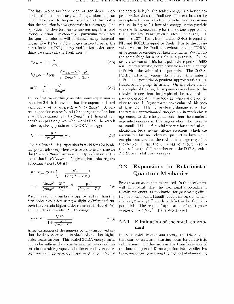
the energy is high, the scaled energy is a better ap-
proximation than the Pauli one. This can be seen for
example in the case of a free particle. In this case one
can see in �gure 2.1 how the energy of the particle
varies with momentum p for the various approxima-tions. The results are given in atomic units (m0 = 1
and c � 137). For a free particle ZORA is equal to
NR and FORA is equal to Pauli. Due to the mass-
velocity term the Pauli approximation (and FORA)
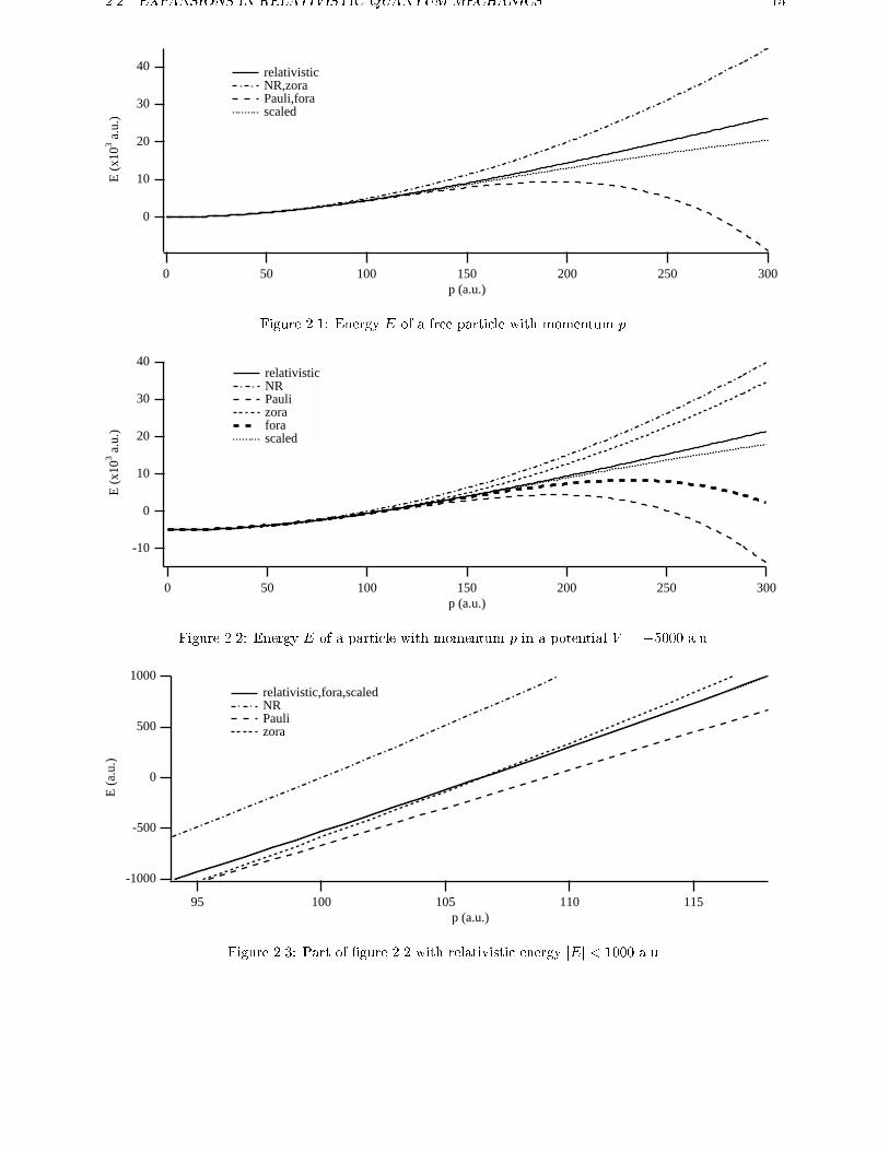
gives negative energies for high momenta. We can do
the same thing for a particle in a potential. In �g-
ure 2.2 we can see this for a potential equal to -5000
a.u. The relativistic, nonrelativistic and Pauli energy
shift with the value of the potential. The ZORA,
FORA and scaled energy do not have this uniform
shift. The potential-dependent approximations are
therefore not gauge invariant. On the other hand,
the graphs of this regular expansion are closer to the
relativistic one than the graphs of the standard ex-
pansion, especially if we look at relativistic energies
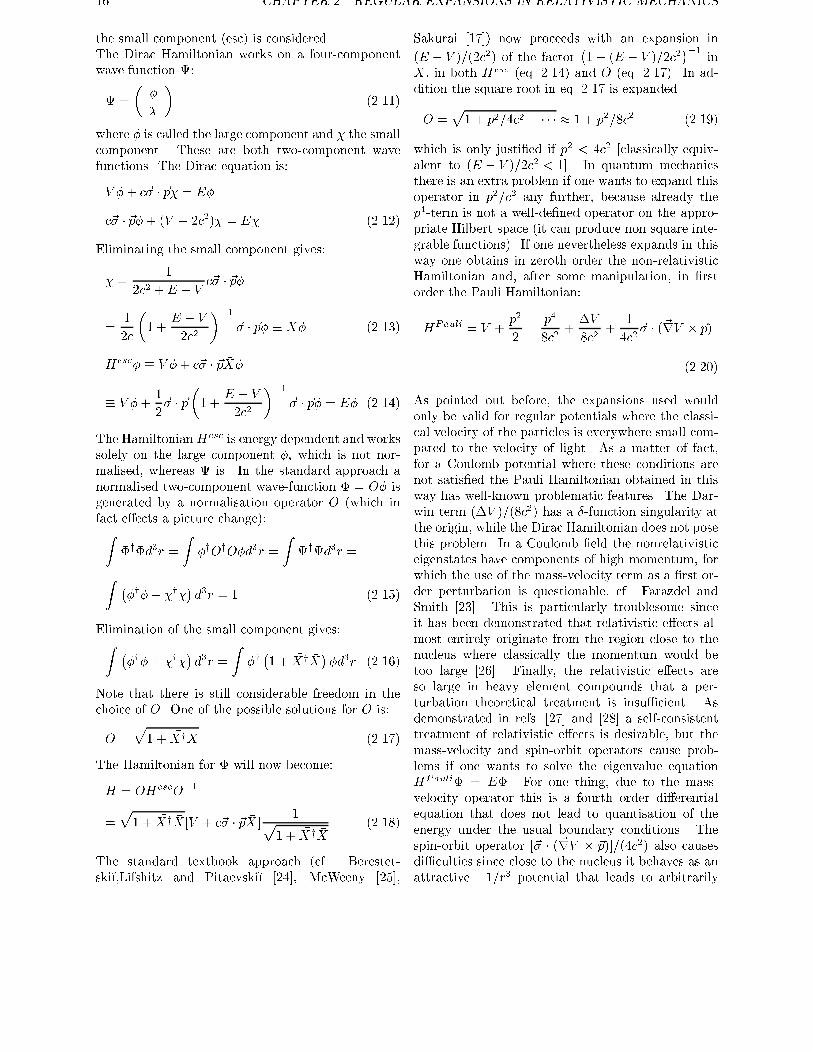
close to zero. In �gure 2.3 we have enlarged this part
of �gure 2.2. This �gure clearly demonstrates that
the regular approximated energies are in much closer
agreement to the relativistic ones than the standard
expanded energies in this region where the energies
are small. This is of special interest for chemical ap-
plications, because the valence electrons, which are
responsible for most chemical properties, have small
energies compared to the rest mass energy (m0c2) of
the electron. In fact the �gure has not enough resolu-
tion to show the di�erence between the FORA, scaled
ZORA and relativistic energies.
2.2 Expansions in Relativistic
Quantum Mechanics
From now on atomic units are used. In this section we
will demonstrate that the traditional approaches in
relativistic quantum mechanics for generating e�ec-
tive two-component Hamiltonians rely on the expan-
sion in (E � V )=2c2 which is defective for Coulomb
potentials. The result of application of the regular
expansion in E=(2c2 � V ) is also derived.
2.2.1 Elimination of the small compo-
nent
In the relativistic quantum theory, the Dirac equa-
tion can be used as a starting point for relativistic
calculations. In this section the transformation of
the four-component Dirac-equation into an e�ective
two-component form using the method of eliminating
2.2. EXPANSIONS IN RELATIVISTIC QUANTUM MECHANICS 15
40
30
20
10
0
E (
x103 a
.u.)
300250200150100500p (a.u.)
relativistic NR,zora Pauli,fora scaled
Figure 2.1: Energy E of a free particle with momentum p.
40
30
20
10
0
-10
E (
x103 a
.u.)
300250200150100500p (a.u.)
relativistic NR Pauli zora fora scaled
Figure 2.2: Energy E of a particle with momentum p in a potential V = �5000 a.u.
-1000
-500
0
500
1000
E (
a.u.
)
11511010510095p (a.u.)
relativistic,fora,scaled NR Pauli zora
Figure 2.3: Part of �gure 2.2 with relativistic energy jEj < 1000 a.u.
16 CHAPTER 2. REGULAR EXPANSIONS IN RELATIVISTIC MECHANICS
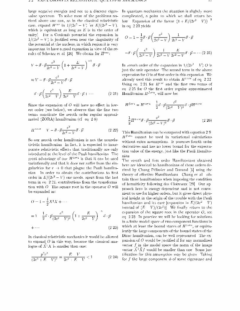
the small component (esc) is considered.
The Dirac Hamiltonian works on a four-component
wave function :
=
���
�(2.11)
where � is called the large component and � the small
component. These are both two-component wave
functions. The Dirac equation is:
V �+ c~� � ~p� = E�
c~� � ~p�+ (V � 2c2)� = E� (2.12)
Eliminating the small component gives:
� =1
2c2 +E � Vc~� � ~p�
=1
2c
�1 +
E � V
2c2
��1~� � ~p� � �X� (2.13)
Hesc� � V �+ c~� � ~p �X�
� V �+1
2~� � ~p
�1 +
E � V
2c2
��1~� � ~p� = E� (2.14)
The HamiltonianHesc is energy dependent and works
solely on the large component �, which is not nor-
malised, whereas is. In the standard approach a
normalised two-component wave-function � = O� is
generated by a normalisation operator O (which in
fact e�ects a picture change):Z�y�d3r =
Z�yOyO�d3r =
Zyd3r =
Z ��y�+ �y�
�d3r = 1 (2.15)
Elimination of the small component gives:Z ��y�+ �y�
�d3r =
Z�y�1 + �Xy �X
��d3r (2.16)
Note that there is still considerable freedom in the
choice of O. One of the possible solutions for O is:
O =p1 + �Xy �X (2.17)
The Hamiltonian for � will now become:
H = OHescO�1
=p1 + �Xy �X[V + c~� � ~p �X ]
1p1 + �Xy �X
(2.18)
The standard textbook approach (cf. Berestet-
ski��,Lifshitz and Pitaevski�� [24], McWeeny [25],
Sakurai [17]) now proceeds with an expansion in
(E � V )=(2c2) of the factor�1 + (E � V )=2c2
��1in
�X, in both Hesc (eq. 2.14) and O (eq. 2.17). In ad-
dition the square root in eq. 2.17 is expanded
O =p1 + p2=4c2 + � � � � 1 + p2=8c2 (2.19)
which is only justi�ed if p2 < 4c2 [classically equiv-
alent to (E � V )=2c2 < 1]. In quantum mechanics
there is an extra problem if one wants to expand this
operator in p2=c2 any further, because already the
p4-term is not a well-de�ned operator on the appro-
priate Hilbert space (it can produce non square inte-
grable functions). If one nevertheless expands in this
way one obtains in zeroth order the non-relativistic
Hamiltonian and, after some manipulation, in �rst
order the Pauli Hamiltonian:
HPauli = V +p2
2�
p4
8c2+�V
8c2+
1
4c2~� � (~rV � ~p)
(2.20)
As pointed out before, the expansions used would
only be valid for regular potentials where the classi-
cal velocity of the particles is everywhere small com-
pared to the velocity of light. As a matter of fact,
for a Coulomb potential where these conditions are
not satis�ed the Pauli Hamiltonian obtained in this
way has well-known problematic features. The Dar-
win term (�V )=(8c2) has a �-function singularity at
the origin, while the Dirac Hamiltonian does not pose
this problem. In a Coulomb �eld the nonrelativistic
eigenstates have components of high momentum, for
which the use of the mass-velocity term as a �rst or-
der perturbation is questionable, cf. Farazdel and
Smith [23]. This is particularly troublesome since
it has been demonstrated that relativistic e�ects al-
most entirely originate from the region close to the
nucleus where classically the momentum would be
too large [26]. Finally, the relativistic e�ects are
so large in heavy element compounds that a per-
turbation theoretical treatment is insu�cient. As
demonstrated in refs. [27] and [28] a self-consistent
treatment of relativistic e�ects is desirable, but the
mass-velocity and spin-orbit operators cause prob-
lems if one wants to solve the eigenvalue equation
HPauli� = E�. For one thing, due to the mass-
velocity operator this is a fourth order di�erential
equation that does not lead to quantisation of the
energy under the usual boundary conditions. The
spin-orbit operator [~� � (~rV � ~p)]=(4c2) also causes
di�culties since close to the nucleus it behaves as an
attractive �1=r3 potential that leads to arbitrarily
2.2. EXPANSIONS IN RELATIVISTIC QUANTUM MECHANICS 17
large negative energies and not to a discrete eigen-
value spectrum. To solve most of the problems no-
ticed above one can, as in the classical relativistic
case, expand Hesc in 1=(2c2 � V ) [or E=(2c2 � V ),which is equivalent as long as E is in the order of
unity]. For a Coulomb potential the expansion in
1=(2c2 � V ) is justi�ed even near the singularity of
the potential at the nucleus, in which region it is very
important to have a good expansion in view of the re-
sults of Schwarz et al. [26]. We obtain for Hesc:
V + ~� � ~pc2
2c2 � V
�1 +
E
2c2 � V
��1~� � ~p
� V + ~� � ~pc2
2c2 � V~� � ~p
�~� � ~p�
c2
2c2 � V
�E
2c2 � V~� � ~p+ � � � (2.21)
Since the expansion of O will have no e�ect in low-
est order (see below), we observe that the �rst two
terms constitute the zeroth order regular approxi-
mated (ZORA) hamiltonian (cf. eq. 2.8)
Hzora = V + ~� � ~pc2
2c2 � V~� � ~p (2.22)
So our zeroth order hamiltonian is not the nonrela-
tivistic hamiltonian. In fact, it is expected to incor-
porate relativistic e�ects that traditionally are only
introduced at the level of the Pauli hamiltonian. The
great advantage of our Hzora is that it can be used
variationally and that it does not su�er from the sin-
gularities for r ! 0 that plague the Pauli hamilto-
nian. In order to obtain the contributions to �rst
order in E=(2c2 � V ) one needs, apart from the last
term in eq. 2.21, contributions from the transforma-
tion with O. The square root in the operator O will
be expanded as:
O = 1 +1
2�Xy �X + � � �
= 1 +1
2~� � ~p
c2
(2c2 � V )2
�1 +
E
2c2 � V
��2~� � ~p
+ � � � (2.23)
In classical relativistic mechanics it would be allowed
to expand O in this way, because the classical ana-
logue of �Xy �X is smaller than one:
p2c2
(2c2 +E � V )2=
E � V
2c2 +E � V< 1 (2.24)
In quantum mechanics the situation is slightly more
complicated, a point to which we shall return be-
low. Expansion of the factor�1 +E=(2c2 � V )
��2in eq. 2.23 yields
O = 1 +1
2~� � ~p
�c2
2c2 � V
�1
2c2 � V~� � ~p
�~� � ~p�
c2
2c2 � V
�1
2c2 � V
E
2c2 � V~� � ~p+ � � � (2.25)
In zeroth order of the expansion in 1=(2c2 � V ) O is
just the unit operator. The second term in the above
expression for O is of �rst order in this expansion. We
already used this result to obtain Hzora of eq. 2.22.
Using eq. 2.21 for Hesc and the �rst two terms of
eq. 2.25 for O the �rst order regular approximated
Hamiltonian Hfora, will now be:
Hfora = Hzora �1
2~� � ~p
c2
(2c2 � V )2~� � ~pHzora
�1
2Hzora~� � ~p
c2
(2c2 � V )2~� � ~p (2.26)
This Hamiltonian can be compared with equation 2.9.
Hfora cannot be used in variational calculations
without extra assumptions. It posesses fourth order
derivatives and has no lower bound for the expecta-
tion value of the energy, just like the Pauli Hamilto-
nian.
The zeroth and �rst order Hamiltonians obtained
here are identical to hamiltonians of these orders de-
rived by Chang P�elissier and Durand [5] using the
theory of e�ective Hamiltonians. Chang et al. ob-
tain these hamiltonians when imposing the condition
of hermiticity following des Cloizeaux [29]. Our ap-
proach here is energy-dependent and is not conve-
nient to use for higher orders, but it gives direct phys-
ical insight in the origin of the trouble with the Pauli
hamiltonian and its cure [expansion in E=(2c2 � V )instead of (E � V )=(2c2)]. We �nally return to the
expansion of the square root in the operator O, seeeq. 2.23. In practice we will be looking for solutions
in a �nite model space of two-component functions in
which at least the bound states of Hzora, or equiva-
lently the large components of the bound states of the
Dirac hamiltonian, can be well represented. The ex-
pansion of O would be justi�ed if for any normalized
vector f in the model space the norm of the image
vector �Xy �Xf would be smaller than one. Some jus-
ti�cation for this assumption may be given. Taking
for f the large component � of some eigenstate and
18 CHAPTER 2. REGULAR EXPANSIONS IN RELATIVISTIC MECHANICS
using � = �X� the norm of �Xy �X� is seen to be just
the norm of �Xy�. Since
�Xy = c~� � ~p1
2c2 +E � V=
1
2c2 +E � Vc~� � ~p
�i(c~� � ~rV )
(2c2 +E � V )2(2.27)
we have, using eq. 2.14
�Xy� =E � V
2c2 +E � V�� i
(c~� � ~rV )(2c2 +E � V )2
� (2.28)
Since the factors in front of � and � are much smaller
than 1 everywhere except possibly very close to the
nucleus, the norm of �Xy� is expected to be small.
It is interesting to note that the quantum mechani-
cal e�ects, arising from the noncommuting of ~p and
V and leading to the second term in eq. 2.27, are
actually quite small.
2.2.2 The Foldy-Wouthuysen trans-
formation
The most straightforward way to generate an e�ective
two-component Hamiltonian would consist of �nding
a unitary transformation:
U =
0@ 1p
1+XyX
1p1+XyX
Xy
� 1p1+XXy
X 1p1+XXy
1A (2.29)
U�1 = U y
=
0@ 1p
1+XyX�Xy 1p
1+XXy
X 1p1+XyX
1p1+XXy
1A (2.30)
that brings the Dirac Hamiltonian HD:
HD =
�V c~� � ~p
c~� � ~p V � 2c2
�(2.31)
to block diagonal form. Foldy and Wouthuysen [18]
introduced a systematic procedure for decoupling the
large and small components to succesively higher or-
ders of c�2. In this section we closely follow the ap-
proach and notation of Kutzelnigg [30]. The trans-
formed Hamiltonian:
H = UHDU�1 (2.32)
is block-diagonal if:
�XV �Xc~� � ~pX + c~� � ~p+ (V � 2c2)X = 0 (2.33)
The upper-left part of the transformed Hamiltonian
is the Foldy-Wouthuysen Hamiltonian HFW :
HFW =1
p1 +XyX
�
(c~� � ~pX +Xyc~� � ~p� 2c2XyX + V +XyV X)�
1p1 +XyX
(2.34)
The same one-electron energies Ei as obtained from
the Dirac equation (only the positive part of the spec-
trum) result from the Foldy-Wouthuysen transformed
Dirac equation:
HFW�FWi = Ei�
FWi (2.35)
We now make the regular approximation for X :
(2c2 � V )X � c~� � ~p (2.36)
The transformed Dirac Hamiltonian will not be block
diagonal, but we will neglect this residual coupling.
The Foldy-Wouthuysen Hamiltonian is in this ap-
proximation:
1q1 + ~� � ~p c2
(2c2�V )2 ~� � ~p(~� � ~p
c2
2c2 � V~� � ~p+ V )�
1q1 + ~� � ~p c2
(2c2�V )2 ~� � ~p(2.37)
In this form this is not a practical approximation, be-
cause of the 1=p1 +XyX operator. In zeroth order
we will approximate it as the identity operator. The
Foldy-Wouthuysen Hamiltonian using this approxi-
mation will give the ZORA Hamiltonian, exactly the
same as in the previous section:
Hzora = ~� � ~pc2
2c2 � V~� � ~p+ V (2.38)
and we have the one-electron ZORA equation:
Hzora�zorai = Ezora
i �zorai (2.39)
If we would approximate the 1=p1 +XyX operator
as 1� 12XyX we will get the FORA Hamiltonian, like
in the previous section:
Hfora = Hzora �1
2~� � ~p
c2
(2c2 � V )2~� � ~pHzora
�1
2Hzora~� � ~p
c2
(2c2 � V )2~� � ~p (2.40)
The energy Ezorai will in general not be equal to the
Dirac energy. To improve this energy we will continue
2.2. EXPANSIONS IN RELATIVISTIC QUANTUM MECHANICS 19
as in �rst order perturbation theory, where the zeroth
order solution is put in the energy expression for the
�rst order. This will give for the FORA energy:
Eforai = Ezora
i �
(1� h�zorai j~� � ~p
c2
(2c2 � V )2~� � ~pj�zora
i i) (2.41)
We can proceed in a slightly di�erent way if we in-
troduce the following approximations:
1p1 +XyX
�i �1p
1 + h�ijXyX j�ii�i
(X�i)y(X�i) � h�ijXyX j�ii�
yi�i (2.42)
The di�erence is the way we approximate the
1=p1 +XyX operator. This has the advantage that
1=p1 +XyX�i is correct to �rst order rather than
zeroth order. The norm of X�i will be exact in the
approximation above. The improved energy, which
follows from these approximations, we will call the
scaled ZORA energy (see the resemblance with equa-
tion 2.10):
Escaledi =
Ezorai
1 + h�zorai j~� � ~p c2
(2c2�V )2~� � ~pj�zorai i
(2.43)
If h�zorai jXyX j�zora
i i << 1, which is true for
valence orbitals, the scaled ZORA energies are
very close to the FORA energies, which are seen
to represent the �rst term in the expansion of
(1 + h�zorai j~� � ~p c2
(2c2�V )2~� � ~pj�zorai i)�1. The scaling
procedure sums certain higher order contributions to
in�nite order.
Kutzelnigg [30] has stressed the problems con-
nected with the traditional procedure to obtain the
Foldy-Wouthuysen transformation, which are already
apparent from the lowest order (c�2) approximate
Hamiltonian (the Pauli Hamiltonian) obtained in the
FW method. We pause brie y to demonstrate that
part of the trouble is again caused by the neglect of
E�V with respect to 2c2 rather than E with respect
to 2c2 � V . Suppose the transformation U (equa-
tion 2.29) generates the desired two-component FW
wavefunction��
0
�= U
���
�(2.44)
so that
� =1
p1 +XyX
�+1
p1 +XyX
Xy�
0 = �1
p1 +XXy
X�+1
p1 +XXy
� (2.45)
The last line is an identity if X satis�es � = X�. Ifwe approximate X by expanding the energy depen-
dent �X for which � = �X� = (2c2 + E � V )�1c~� � ~p�in (E � V )=2c2, we obtain in lowest order X �(1=2c2)c~� � ~p and U becomes to order c�2:
U =
1� p2
8c2c~��~p2c2
� c~��~p2c2
1� p2
8c2
!(2.46)
This is precisely the traditional FW transformation
to order c�2 that leads to the much criticized Pauli
Hamiltonian. It is interesting to see what happens
if we follow, in order to arrive at an improved e�ec-
tive Hamiltonian, the same strategy as before and
avoid the erroneous expansion of (2c2 + E � V )�1
by expanding in E=(2c2�V ). This leads to insertingX � (2c2�V )�1c~� �~p in the expression for U . We also
have to expand the square root operatorp1 +XyX,
just like in the esc method. Following exactly the
same procedure of ordering the terms according to
the number of (2c2 � V ) factors in the denominator,
the transformation matrix U will now be:
U = (2.47) 1� 1
2~� � ~p c2
(2c2�V )2 ~� � ~p ~� � ~p c2c2�V
� c2c2�V ~� � ~p 1� 1
2c
2c2�V p2 c2c2�V
!
This transformation will give in zeroth and �rst or-
der exactly the same zero and �rst order (ZORA and
FORA) Hamiltonians as obtained before.
The density as well as other properties can be writ-
ten in terms of the Foldy-Wouthuysen transformed
wave functions, but one then needs the unitary ma-
trix 2.29. Denoting the components of the Dirac one-
electron spinor by i; i = 1::4, those of the trans-formed wavefunction � = U by �i; i = 1::4, (�3
and �4 are therefore zero), and the eigenstates of the
~r operator in the direct product space of spatial and
spinor coordinates by j~r; ii, we have
�D(~r) =Xi
jh~r; ijij2
6=Xi
jh~r; ij�ij2 = �FW (~r) (2.48)
The components of the transformed wavefunction
� = U along the j~r; ii are not identical to those
of , but only the components of � along the trans-
formed basis states U j~r; ii are: h~r; ijU yj�i = h~r; iji.This simply re ects the well known fact that a pic-
ture change e�ected by U requires that not only the
20 CHAPTER 2. REGULAR EXPANSIONS IN RELATIVISTIC MECHANICS
wavefunction is transformed but also the observables,
in this case ~r to U~rU y � ~q, in order that the physics
remains unaltered. The inverse transformation of the
operator ~r, Uy~rU , is called ~R. It is the operator thatdescribes, in the Dirac picture, the famous average
position or mass position rmass of the electron, see
Foldy and Wouthuysen [18] and Moss [31]. A clear
example of the di�erence we introduce by using �(~r)instead of �(~q) is provided by the nodes that are
present in the solutions �0 to eq. 3.2 and therefore in
the (orbital) density �zora(~r). Such nodes do not oc-
cur in �D(~r) since the nodes of the large component �do not coincide with those of the small component �.The e�ect of (neglect of) the picture change is prob-
ably small, but such e�ects are visible for core states,
as extensively discussed by Baerends et al. [32]. Al-
though the Dirac density is not j�(~r)j2 it could in
principle be calculated from �(~r), for instance by us-ing
���
�=
0@ 1p
1+XyX�Xy 1p
1+XXy
X 1p1+XyX
1p1+XXy
1A� �
0
�
(2.49)
and writing the Dirac electron density as,
�(~r) = �y(~r)�(~r) + �y(~r)�(~r) =
= (1
p1 +XyX
�(~r))y(1
p1 +XyX
�(~r))+
(X1
p1 +XyX
�(~r))y(X1
p1 +XyX
�(~r)) (2.50)
Note that one can not use the turn-over rule here. We
will however approximate the electron density by:
�zora(~r) = �zoray(~r)�zora(~r) (2.51)
which follows from the approximations of equa-
tion 2.42 that lead to the scaled energy. Here �zora
are the solutions of equation 3.2. So, apart from using
the approximate hamiltonian Hzora of eq. 3.2 we also
make two presumably small errors for the density. In
the �rst place the e�ect of the picture change is ig-
nored, meaning we use �y(~r)�(~r) instead of equation2.50. In the second place we neglect - consistent with
the order in which we work - the fact that the trans-
formation U that we e�ectively use is only correct to
order E=(2c2 � V ), so the small components are notcompletely annihilated by U , as they are assumed to
be in equations 2.49 and 2.50. Maybe this approxi-
mation is also most serious when the small component
is relatively large. Note that the second approxima-
tion, neglect of residual small components, would dis-
appear when more accurate transformations U would
be used, but the �rst approximation, exempli�ed by
the problem of the nodes, would not improve in that
case. It can only be remedied by making the correct
picture change for the position variable.
2.2.3 Direct Perturbation Theory
In this section we follow the approach of Sadlej and
Snijders et al. [33, 34], who have used regular ex-
pansions in the direct perturbation theory (DPT)
approach proposed by Rutkowski [35] and Kutzel-
nigg [36]. The approach starts by de�ning a 4-
component wave function , which has the same large
component � as the Dirac wave function, but has a
small component which is c times the small com-ponent � of the Dirac equation. To account for this
one has to modify the metric. The Dirac equation in
this approach is then written as:
HDPTD =
�V ~� � ~p~� � ~p �2V � 2
���
�
= E
�1 0
0 �2
���
�(2.52)
with � = � = 1=c. The normalisation of the 4-
component wave function in the modi�ed metric
is:
h�j�i + �2h j i = 1 (2.53)
The standard way of DPT is that all terms that in-
volve � and � (with � = �) are treated as a pertur-
bation. In the regular approximation one only treats
terms that involve � as a perurbation. In zeroth orderthis will give:�
V ~� � ~p~� � ~p �2V � 2
���0
0
�= E0
��0
0
�(2.54)
Elimination of the small component 0:
0 =1
2� �2V~� � ~p�0 (2.55)
gives:
(~� � ~p1
2� �2V~� � ~p+ V )�0 = E0�0 (2.56)
which is the ZORA equation, where the large com-
ponent �0 is equal to the ZORA wave function of
the previous section. This large component �0 is
normalised to one, as in the previous section. The
4-component wave function obtained we shall call
2.2. EXPANSIONS IN RELATIVISTIC QUANTUM MECHANICS 21
0. It is also possible to consider the approximate
4-component wave function as an approximation to
the Dirac wave function without approximating the
� dependent metric. This means that we still solve
the ZORA equation, but that the wave function, we
will call zora4 is normalised as:
h�zora4 j�zora4 i+ c�2h zora4 j zora4 i = 1 (2.57)
There is just a simple normalisation factor between
the functions 0 and zora4 :
zora4 =
1p1 + c�2h 0j 0i
0 =
1q1 + c�2h�0j~� � ~p 1
(2�c�2V )2~� � ~pj�0i
0 (2.58)
For the expectation value of an operator A we will
also use the new metric:
hAi =
hzora4 j
�1 0
0 c�1
�A
�1 0
0 c�1
�jzora
4 i (2.59)
If we apply this to the Dirac Hamiltonian HD itself,
remembering that:
HDPTD =
�1 0
0 c�1
�HD
�1 0
0 c�1
�(2.60)
we �nd for the improved energy:
Ezora�4scaled = hzora
4 jHDPTD jzora
4 i
=h0jHDPT
D j0i1 + c�2h 0j 0i
=E0
1 + c�2h�0j~� � ~p 1(2�c�2V )2
~� � ~pj�0i(2.61)
which is just the scaled ZORA energy of the previous
section if the potential is an external potential. This
rederivation of the scaled ZORA energy can be found
in the article of Sadlej and Snijders et al. [34]. The
electron density in this ZORA-4 approach is in view
of equation 2.57:
�zora4 (~r)
= �zoray4 (~r)�zora4 (~r) + �zoray4 (~r)�zora4 (~r) (2.62)
where:
�zora4 = c zora4 =c
2c2 � V~� � ~p�zora4 (2.63)
If the potential depends on the density, like in SCF
calculations, the ZORA-4 approach di�ers with re-
spect to the ZORA approach of the last section.
2.2.4 The Douglas-Kroll transforma-
tion
In this section we brie y say some words about an-
other successful method for approximating the Foldy-
Wouthuysen transformation, the so called Douglas-
Kroll transformation [37]. The starting point is the
free particle transformation, which can be obtained
exactly. If we make the approximation that the po-
tential V commutes with the operator X (V X =
XV ), equation 2.33 will give for X :
X �c~� � ~p
c2 +pc4 + p2c2
(2.64)
Using this approximation in the Foldy-Wouthuysen
Hamiltonian (see equation 2.34), again using that Vcommutes with X , we get:
HFW =pc4 + p2c2 � c2 + V (2.65)
which is the classical relativistic form of the energy
of a particle in a potential (see section 2.1). If the
potential is a constant (free particle case), this is the
exact Foldy-Wouthuysen transformation, because in
this case V and X commute. In general V and X will
not commute. Using an expansion method one can
take these e�ects to a certain order into account [37].
This expansion remains regular even for a Coulomb-
like potential. For atomic and molecular calculations
this method has been further developed by Hess [38].
In ordinary basis set programs one needs to evaluate
integrals in momentum space in order to calculate
rather complicated looking matrix elements. Prac-
tical implementations have been provided by Hess
and co-workers in ab-initio schemes [38, 39] and by
Knappe and R�osch [40] in a density-functional imple-
mentation. This method is now widely used in atomic
and molecular calculations.
22 CHAPTER 2. REGULAR EXPANSIONS IN RELATIVISTIC MECHANICS
Chapter 3
The ZORA Hamiltonian
3.1 Basic equations
In chapter 2 we have derived a regularized two-
component Hamiltonian by simply modifying the tra-
ditional esc, FW and DPT approaches so as to take
care of the radius of convergence of the employed ex-
pansions. The present simple approach becomes more
complicated for higher orders. It has been presented
in some detail in order to stress the important point
concerning the validity of the expansions to be used.
The Hamiltonian obtained has actually been derived
earlier by Chang, P�elissier and Durand [5] and Heully
et al. [6] will be denoted as the zeroth order regular
approximated (ZORA) Hamiltonian Hzora (we leave
aside the further regularisation of the kinetic energy
applied by Chang et al.). We will not study higher or-
der terms of the Hamiltonian but we note that Chang
et al. have derived and used high order terms in the
expansion of Hesc. Although our zero order hamil-
tonian is identical to the one obtained by Chang et
al., this does not hold for the higher orders since they
did not use the renormalisation operator O and ob-
tained non-hermitian higher orders. Our �rst order
regular approximated Hfora is actually identical to
the hermitian Des Cloizeaux H1 [5].
The ZORA e�ective Hamiltonian may be further
developed:
Hzora = V + ~� � ~pc2
2c2 � V~� � ~p
= V + ~pc2
2c2 � V~p+
c2
(2c2 � V )2~� � (~rV � ~p) (3.1)
One can now see that the spin-orbit splitting is al-
ready present in the zeroth order Hamiltonian. This
spin-orbit term is regular because of the (2c2 � V )�2
factor in it. It poses no problems in variational cal-
culations. The eigen-value equation:
Hzora�zora = (V + ~� � ~pc2
2c2 � V~� � ~p)�zora
= Ezora�zora (3.2)
is only a second order di�erential equation. The two-
component wave function �zora will now be referred
to as the ZORA wave function. In �rst order pertur-
bation calculations the FORA-energy Efora is:
Efora = Ezora�
(1� h�zoraj~� � ~pc2
(2c2 � V )2~� � ~pj�zorai) (3.3)
and the scaled ZORA energy, which sums certain
higher order contributions to in�nite order, is:
Escaled =Ezora
1 + h�zoraj~� � ~p c2
(2c2�V )2 ~� � ~pj�zorai
(3.4)
Because the Hamiltonian Hzora is energy-
independent and Hermitian the eigenfunctions be-
longing to di�erent eigenvalues Ezora are orthog-
onal. In the ZORA method the electron density
is the sum of the squared orbital wave functions
(two-component functions), whereas in the ZORA-
4 method (4-component functions) the small compo-
nent is taken into account (see section 2.2.3).
In quantum chemistry there are many situations
where the spin-orbit splitting is not important. One
can therefore be interested in a scalar relativis-
tic equation, which has the same symmetry as the
Schr�odinger equation. In refs. [41] and [42] such a
scalar relativistic equation (SR) was suggested and
applied to some atomic and solid state problems.
This equation is given by:
(V + ~pc2
2c2 +ESR � V~p)�SR = ESR�SR (3.5)
with orbital density:
�SR(~r) = �SRy(~r)�SR(~r) (3.6)
23
24 CHAPTER 3. THE ZORA HAMILTONIAN
The zeroth order regular approximate (ZORA) scalar
relativistic equation is obtained as the zeroth order
term in an expansion in E=(2c2�V ) of this equation:
HzoraSR �zora
SR � (V + ~pc2
2c2 � V~p)�zora
SR
= EzoraSR �zora
SR (3.7)
which is just the ZORA Hamiltonian (see equa-
tion 3.1) without spin-orbit coupling. The FORA
and scaled ZORA scalar relativistic energies can be
derived analoguous to the ones with spinorbit. In the
scalar relativistic case they are:
EforaSR = Ezora
SR �
(1� h�zoraSR j~p
c2
(2c2 � V )2~pj�zora
SR i) (3.8)
EscaledSR =
EzoraSR
1 + h�zoraSR j~p c2
(2c2�V )2 ~pj�zoraSR i
(3.9)
3.2 Boundedness from below
An important question is whether the eigenvalue
spectrum of the ZORA Hamiltonian is bounded from
below. We �rst brie y investigate this problem along
the lines of the analysis of Landau and Lifshitz [43]
for the nonrelativistic case, before we give a rigorous
proof that the ZORA eigenvalue spectrum is bounded
from below. We only consider potentials V for which
2c2 � V > 0 everywhere, so that the ZORA kinetic
energy operator T zora
T zora = ~� � ~pc2
2c2 � V~� � ~p (3.10)
is a positive operator. If the potential is bounded
from below by Vmin, then all the ZORA eigenvalues
Ezoran � Vmin, because the mean value of T zora � 0.
Now suppose the potential V is of the form:
V = �Z
rs(3.11)
near the origin. Consider a wave function localized
in some small region (of radius r0) around the origin.The uncertainty in the momentum of the particle is
then of order 1=r0 (uncertainty principle). The sum
of the mean values of the potential and kinetic energy
then is of the order:
�Z
rs0+
c2
r20(2c2 + Z
rs0
)(3.12)
For s < 1 this energy expression can not take arbi-
trarily large negative values. However, whereas in the
nonrelativistic case the energy is bounded from below
for s < 2 and conditionally so for s = 2 (depending
on the strength of the potential, cf. ref. [43], x35),the case s = 1 is already a special one for the ZORA
eigenvalue spectrum. Equation 3.12 suggests that for
s = 1, i.e. a Coulomb potential, the ZORA Hamil-
tonian will only be a bounded operator for Z < c.In fact, the condition Z < c for the strength of the
Coulomb potential is familiar from the Dirac equa-
tion. Analogous conditions for the potential in the
Dirac and the ZORA equation may perhaps be ex-
pected from the identical asymptotic behaviour for
r ! 0 for the regular solutions, which is r �1 in both
cases (see section 4.5). Here
=
r�2 �
Z2
c2(3.13)
and � is the usual relativistic quantum number. How-
ever, these arguments are qualitative.
Now a more detailed treatment of this important
question, that the ZORA eigenvalue spectrum is
bounded from below if Z < c s given. In chapter 4 it
will be shown, that the solutions of the zeroth order
of this two-component regular approximate (ZORA)
equation for hydrogen-like atoms are simply scaled
solutions of the large component of the Dirac wave
function for this problem. The eigenvalues are re-
lated in a similar way as (see eq. 4.9):
Ezora =2c2ED
2c2 +ED(3.14)
For Z < c the Dirac equation has eigenvalues below
�2c2 (negative energy continuum), between �c2 and0 (discrete spectrum) and above zero (positive energy
continuum). According to equation 3.14 these parts
of the Dirac spectrum are mapped onto the ZORA
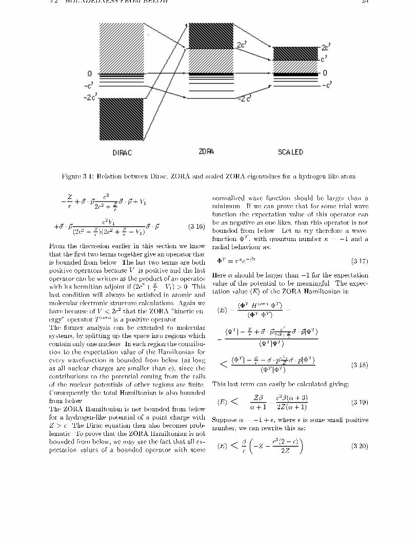
spectrum as follows (see �gure 3.1): the positive en-
ergy continuum (0,1) onto (0,2c2); the discrete part(�c2,0) onto (�2c2,0); the negative energy contin-
uum (�1,�2c2) onto (2c2,1). So all the eigenvalues
of the ZORA equation are larger than �2c2, whichmeans that for this potential the zeroth order regular
approximate Hamiltonian is bounded from below.
Now suppose the potential is given by:
V = �Z
r+ V1(r) (3.15)
where V1 is larger than zero everywhere. This V1 willusually be the mean repulsive potential of some elec-
tron density. We can divide the ZORA Hamiltonian
for this potential in operators, which are all bounded
from below:
Hzora = �Z
r+ V1 + ~� � ~p
c2
2c2 + Zr� V1
~� � ~p =
3.2. BOUNDEDNESS FROM BELOW 25
Figure 3.1: Relation between Dirac, ZORA and scaled ZORA eigenvalues for a hydrogen-like atom
= �Z
r+ ~� � ~p
c2
2c2 + Zr
~� � ~p+ V1
+~� � ~pc2V1
(2c2 + Zr)(2c2 + Z
r� V1)
~� � ~p (3.16)
From the discussion earlier in this section we know
that the �rst two terms together give an operator that
is bounded from below. The last two terms are both
positive operators because V1 is positive and the last
operator can be written as the product of an operator
with its hermitian adjoint if (2c2+ Zr�V1) > 0. This
last condition will always be satis�ed in atomic and
molecular electronic structure calculations. Again we
have because of V < 2c2 that the ZORA "kinetic en-
ergy" operator T zora is a positive operator.The former analysis can be extended to molecular
systems, by splitting up the space into regions which
contain only one nucleus. In each region the contribu-
tion to the expectation value of the Hamiltonian for
every wavefunction is bounded from below (as long
as all nuclear charges are smaller than c), since thecontributions to the potential coming from the tails
of the nuclear potentials of other regions are �nite.
Consequently the total Hamiltonian is also bounded
from below.
The ZORA Hamiltonian is not bounded from below
for a hydrogen-like potential of a point charge with
Z > c. The Dirac equation then also becomes prob-
lematic. To prove that the ZORA Hamiltonian is not
bounded from below, we may use the fact that all ex-
pectation values of a bounded operator with some
normalized wave function should be larger than a
minimum. If we can prove that for some trial wave
function the expectation value of this operator can
be as negative as one likes, than this operator is not
bounded from below. Let us try therefore a wave-
function �T , with quantum number � = �1 and a
radial behaviour as:
�T = r�e��r (3.17)
Here � should be larger than �1 for the expectationvalue of the potential to be meaningful. The expec-
tation value hEi of the ZORA Hamiltonian is:
hEi =h�T jHzoraj�T i
h�T j�T i=
=h�T j � Z
r+ ~� � ~p c2
2c2+Z
r
~� � ~pj�T i
h�T j�T i
<h�T j � Z
r+ ~� � ~p c
2rZ~� � ~pj�T i
h�T j�T i(3.18)
This last term can easily be calculated giving:
hEi< �Z�
�+ 1+c2�(� + 3)
2Z(�+ 1)(3.19)
Suppose � = �1 + �, where � is some small positivenumber, we can rewrite this as:
hEi<�
�
��Z +
c2(2 + �)
2Z
�(3.20)
26 CHAPTER 3. THE ZORA HAMILTONIAN
Here it can easily be seen that if Z > c we can choose� su�ciently small, so that the term between brackets
is negative. Now we still have the freedom to choose
� in such a way as to make the term on the right hand
side of the inequality as negative as one likes. This
proves that the operator is unbounded from below.
If we take the more physical point of view that the
nucleus is �nite, then the nuclear potential will not
have a singularity. The ZORA Hamiltonian in this
case is bounded from below if V < 2c2 everywhere,
because the potential is bounded from below and the
ZORA kinetic energy operator T zora is a positive op-erator.
3.3 Total energy
In this section we will derive an expression for the
total ZORA energy. We will use the results of sec-
tion 2.2.2 for the regular expansions in the Foldy-
Wouthuysen approach.
We can write the total energy of a many-electron sys-
tem in a density functional approach (without the in-
teraction energy of the nuclei), using the one-electron
orbitals of the Kohn-Sham independent particle for-
mulation of the theory, as:
EDiracTOT =
NXi=1
Z(�yi c~� � ~p�i + �yi c~� � ~p�i � 2c2�yi�i)
+
Z�VN +
1
2
Z Z�(1)�(2)
r12+ EXC [�] (3.21)
where:
� =
NXi=1
(�yi�i + �yi�i) (3.22)
The Kohn-Sham approach assumes that there exists
a model system of N non-interacting electrons mov-
ing in a local potential V (~r) which has the same den-sity as the exact interacting system. The one-electron
Kohn-Sham orbitals yield the non-interacting (Dirac)
kinetic energy and the above equation is essentially a
de�nition of EXC [�] which evidently, apart from the
exchange and correlation energies, also has to inco-
porate the di�erence between the true and the non-
interacting kinetic energies. For the electron-electron
repulsion the non-relativistic operator is used. Opti-
misation of the total energy yields the following one-
electron equations, which are the relativistic equiva-
lents of the Kohn-Sham equations:
c~� � ~p�i + V �i = Ei�i
c~� � ~p�i � 2c2�i + V �i = Ei�i (3.23)
where:
V (~r1) = VN (~r1) +
Z�(2)
r12d~r2 +
�EXC [�]
��(~r1)(3.24)
Using these one-electron equations in the expression
for the total energy, one obtains
ETOT =
NXi=1
Ei �1
2
Z Z�(1)�(2)
r12d1d2
+EXC [�]�Z�(1)
�EXC [�]
��(1)d1 (3.25)
We now wish to transform to a two-component for-
mulation by decoupling the large and small compo-
nents by way of a Foldy-Wouthuysen transformation.
Using a unitary matrix U (see [30] and section 2.2.2):
U =
0@ 1p
1+XyX
1p1+XyX
Xy
� 1p1+XXy
X 1p1+XXy
1A (3.26)
one can transform the Dirac-Hamiltonian HD to a
block-diagonal form if:
�XV �Xc~� � ~pX + c~� � ~p+ (V � 2c2)X = 0 (3.27)
We can express the large and small component � and
� of the Dirac wave function in terms of the Foldy-
Wouthuysen transformed wave function �FW as:���
�= U�1
��FW
0
�=
0@ 1p
1+XyX�FW
X 1p1+XyX
�FW
1A (3.28)
The same one-electron energies Ei as obtained in
eq.3.23 result from the Foldy-Wouthuysen trans-
formed Dirac-Kohn-Sham equation 2.35:
1p1 +XyX
�
(c~� � ~pX +Xyc~� � ~p� 2c2XyX + V +XyV X)�
1p1 +XyX
�FWi = Ei�
FWi (3.29)
The total energy may therefore also be written as:
EFWTOT =
NXi=1
Zd1(�FW
i )y1
p1 +XyX
�
(c~� � ~pX +Xyc~� � ~p� 2c2XyX + V +XyV X)�
3.3. TOTAL ENERGY 27
1p1 +XyX
�FWi �
1
2
Z Z�(1)�(2)
r12d1d2
+EXC [�]�Z�(1)
�EXC [�]
��(1)d1 (3.30)
where:
� =
NXi=1
[1
p1 +XyX
�FWi )y(
1p1 +XyX
�FWi )+
(X1
p1 +XyX
�FWi )y(X
1p1 +XyX
�FWi )] (3.31)
We will approximateX in the same way as before (see
section 2.2.2). The transformed Dirac Hamiltonian
will not be block diagonal, but we will neglect this
residual coupling.
X �c
2c2 � V~� � ~p (3.32)
together with the following approximations that lead
to the scaled ZORA energy:
1p1 +XyX
�i �1p
1 + h�ijXyX j�ii�i
(X�i)y(X�i) � h�ijXyX j�ii�
yi�i (3.33)
The norm of X�i will be exact in the approximation
above. Using these approximations the density can
be written as:
� =
NXi=1
�yi�i (3.34)
which is equivalent to a neglect of picture change.
A slightly di�erent approach is the ZORA-4 method
(see section 2.2.3), where we will use also a small
component for the density. The approximate Foldy-
Wouthuysen transformed Dirac equation now be-
comes an equation, which we shall call the scaled
ZORA equation:
~� � ~p c2
2c2�V ~� � ~p+ V
1 + h�ij~� � ~p c2
(2c2�V )2~� � ~pj�ii�i
= Escaledi �i (3.35)
which only di�ers from the ZORA equation:
(~� � ~pc2
2c2 � V~� � ~p+ V )�i = Ezora
i �i (3.36)
in the scaling factor in the denominator. The total
energy is:
EscaledTOT =
NXi=1
Escaledi �
1
2
Z Z�(1)�(2)
r12d1d2
+EXC [�]�Z�(1)
�EXC [�]
��(1)d1 (3.37)
Due to the approximations made, the one-electron
equations 3.35 are not variationally connected with
this total energy. In order to get total energy expres-
sions for the ZORA and FORA method we just have
to replace, in zeroth order, in the total energy expres-
sion the sum of scaled one-electron energies by the
sum of ZORA one-electron energies and in �rst or-
der by the sum of FORA (�rst order regular approx-
imate) one-electron energies. The ZORA-4 method
(see section 2.2.3) di�ers only in the way the electron
density is obtained.
To solve the scaled ZORA equation 3.35 we simply
have to solve the ZORA equation 3.36. The ZORA
and scaled ZORA eigenfunctions are the same. To
obtain the energy the ZORA energy is scaled (see
eq. 3.4):
Escaledi =
Ezorai
1 + h�ij~� � ~p c2
(2c2�V )2 ~� � ~pj�ii
=Ezorai
1 + h�ijXyX j�ii(3.38)
The FORA energy is de�ned as in equation 3.3:
Eforai = Ezora
i �
(1� h�ij~� � ~pc2
(2c2 � V )2~� � ~pj�ii) (3.39)
In chapter 4 we discuss the ZORA eigenvalues of the
hydrogen-like atoms, where the nucleus is a point
charge. There we found that those were exactly equal
to the Dirac energy, thus Escaled = ED. In this case
the scaled ZORA energy thus corrects completely for
the error in the ZORA one-electron energies. This
holds true in particular for the deep core levels, where
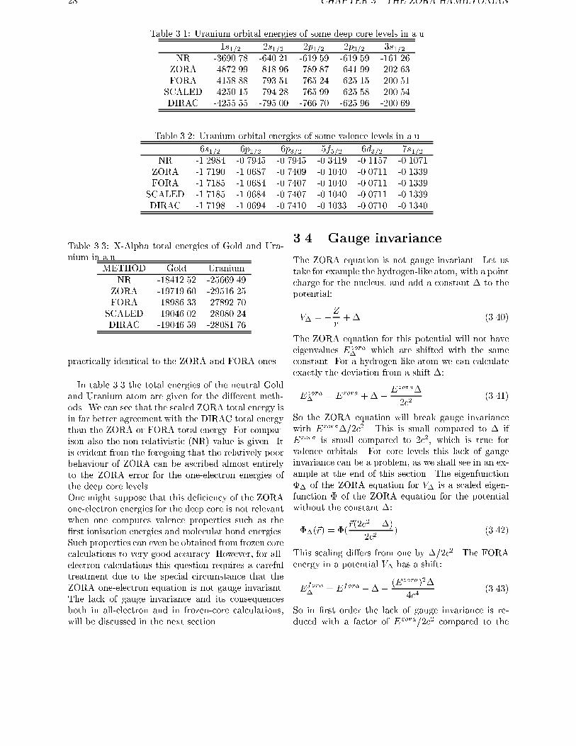
the error, being of order (Ezora)2=2c2, is largest, rel-atively and in an absolute sense.
In table 3.1 some of the core one-electron energies are
shown for the neutral Uranium atom using the X�approximation to the exchange-correlation potential
with � = 0:7. The scaled ZORA energies are now not
exact anymore. Still from the table we can see that
the scaled ZORA 1s1=2 orbital energy is much closer
to the Dirac energy than the ZORA or FORA orbital
energy. For the other core orbitals the improvement
of scaled ZORA over FORA, which is already rather
accurate, is smaller. For valence orbitals, which are
shown in table 3.2, the ZORA energies are quite close
to the Dirac energies and the scaled ZORA values are
28 CHAPTER 3. THE ZORA HAMILTONIAN
Table 3.1: Uranium orbital energies of some deep core levels in a.u.
1s1=2 2s1=2 2p1=2 2p3=2 3s1=2NR -3690.78 -640.21 -619.59 -619.59 -161.26
ZORA -4872.99 -818.96 -789.87 -641.99 -202.63
FORA -4158.88 -793.51 -765.24 -625.15 -200.51
SCALED -4250.15 -794.28 -765.99 -625.58 -200.54
DIRAC -4255.55 -795.00 -766.70 -625.96 -200.69
Table 3.2: Uranium orbital energies of some valence levels in a.u.
6s1=2 6p1=2 6p3=2 5f5=2 6d3=2 7s1=2NR -1.2984 -0.7945 -0.7945 -0.3419 -0.1157 -0.1071
ZORA -1.7190 -1.0687 -0.7409 -0.1040 -0.0711 -0.1339
FORA -1.7185 -1.0684 -0.7407 -0.1040 -0.0711 -0.1339
SCALED -1.7185 -1.0684 -0.7407 -0.1040 -0.0711 -0.1339
DIRAC -1.7198 -1.0694 -0.7410 -0.1033 -0.0710 -0.1340
Table 3.3: X-Alpha total energies of Gold and Ura-
nium in a.u.
METHOD Gold Uranium
NR -18412.52 -25669.49
ZORA -19719.60 -29516.25
FORA -18986.33 -27892.70
SCALED -19046.02 -28080.24
DIRAC -19046.59 -28081.76
practically identical to the ZORA and FORA ones.
In table 3.3 the total energies of the neutral Gold
and Uranium atom are given for the di�erent meth-
ods. We can see that the scaled ZORA total energy is
in far better agreement with the DIRAC total energy
than the ZORA or FORA total energy. For compar-
ison also the non-relativistic (NR) value is given. It
is evident from the foregoing that the relatively poor
behaviour of ZORA can be ascribed almost entirely
to the ZORA error for the one-electron energies of
the deep core levels.
One might suppose that this de�ciency of the ZORA
one-electron energies for the deep core is not relevant
when one computes valence properties such as the
�rst ionisation energies and molecular bond energies.
Such properties can even be obtained from frozen core
calculations to very good accuracy. However, for all-
electron calculations this question requires a careful
treatment due to the special circumstance that the
ZORA one-electron equation is not gauge invariant.
The lack of gauge invariance and its consequences
both in all-electron and in frozen-core calculations,
will be discussed in the next section.
3.4 Gauge invariance
The ZORA equation is not gauge invariant. Let us
take for example the hydrogen-like atom, with a point
charge for the nucleus, and add a constant � to the
potential:
V� = �Z
r+� (3.40)
The ZORA equation for this potential will not have
eigenvalues Ezora� which are shifted with the same
constant. For a hydrogen-like atom we can calculate
exactly the deviation from a shift �:
Ezora� = Ezora +��
Ezora�
2c2(3.41)
So the ZORA equation will break gauge invariance
with Ezora�=2c2. This is small compared to � if
Ezora is small compared to 2c2, which is true for
valence orbitals. For core levels this lack of gauge
invariance can be a problem, as we shall see in an ex-
ample at the end of this section. The eigenfunction
�� of the ZORA equation for V� is a scaled eigen-
function � of the ZORA equation for the potential
without the constant �:
��(~r) = �(~r(2c2 ��)
2c2) (3.42)
This scaling di�ers from one by �=2c2. The FORA
energy in a potential V� has a shift:
Efora� = Efora +��
(Ezora)2�
4c4(3.43)
So in �rst order the lack of gauge invariance is re-
duced with a factor of Ezora=2c2 compared to the
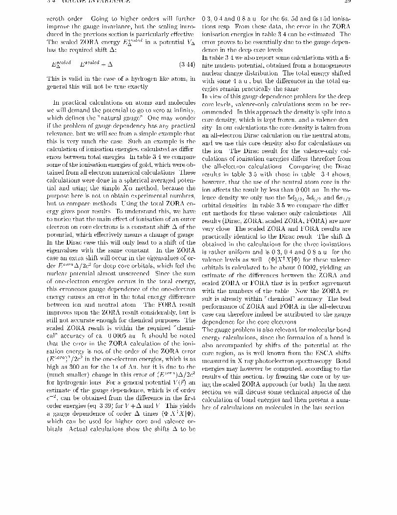
3.4. GAUGE INVARIANCE 29
zeroth order. Going to higher orders will further
improve the gauge invariance, but the scaling intro-
duced in the previous section is particularly e�ective.
The scaled ZORA energy Escaled� in a potential V�
has the required shift �:
Escaled� = Escaled +� (3.44)
This is valid in the case of a hydrogen-like atom, in
general this will not be true exactly.
In practical calculations on atoms and molecules
we will demand the potential to go to zero at in�nity,
which de�nes the "natural gauge". One may wonder
if the problem of gauge dependency has any practical
relevance, but we will see from a simple example that
this is very much the case. Such an example is the
calculation of ionisation energies, calculated as di�er-
ences between total energies. In table 3.4 we compare
some of the ionisation energies of gold, which were ob-
tained from all electron numerical calculations. These
calculations were done in a spherical averaged poten-
tial and using the simple X� method, because the
purpose here is not to obtain experimental numbers,
but to compare methods. Using the total ZORA en-
ergy gives poor results. To understand this, we have
to notice that the main e�ect of ionisation of an outer
electron on core electrons is a constant shift � of the
potential, which e�ectively means a change of gauge.
In the Dirac case this will only lead to a shift of the
eigenvalues with the same constant. In the ZORA
case an extra shift will occur in the eigenvalues of or-
der Ezora�=2c2 for deep core orbitals, which feel the
nuclear potential almost unscreened. Since the sum
of one-electron energies occurs in the total energy,
this erroneous gauge dependence of the one-electron
energy causes an error in the total energy di�erence
between ion and neutral atom. The FORA result
improves upon the ZORA result considerably, but is
still not accurate enough for chemical purposes. The
scaled ZORA result is within the required "chemi-
cal" accuracy of ca. 0.0005 au. It should be noted
that the error in the ZORA calculation of the ioni-
sation energy is not of the order of the ZORA error
(Ezora)2=2c2 in the one-electron energies, which is as
high as 300 au for the 1s of Au, but it is due to the
(much smaller) change in this error of (Ezora)�=2c2
for hydrogenic ions. For a general potential V (~r) anestimate of the gauge dependence, which is of order
c�2, can be obtained from the di�erence in the �rst
order energies (eq. 3.39) for V +� and V . This yieldsa gauge dependence of order � times h�jXyX j�i,which can be used for higher core and valence or-
bitals. Actual calculations show the shifts � to be
0.3, 0.4 and 0.8 a.u. for the 6s, 5d and 6s+5d ionisa-
tions resp. From these data, the error in the ZORA
ionisation energies in table 3.4 can be estimated. The
error proves to be essentially due to the gauge depen-
dence in the deep core levels.
In table 3.4 we also report some calculations with a �-
nite nucleus potential, obtained from a homogeneous
nuclear charge distribution. The total energy shifted
with some 4 a.u., but the di�erences in the total en-
ergies remain practically the same.
In view of this gauge dependence problem for the deep
core levels, valence-only calculations seem to be rec-
ommended. In this approach the density is split into a
core density, which is kept frozen, and a valence den-
sity. In our calculations the core density is taken from
an all-electron Dirac calculation on the neutral atom,
and we use this core density also for calculations on
the ion. The Dirac result for the valence-only cal-
culations of ionisation energies di�ers therefore from
the all-electron calculations. Comparing the Dirac
results in table 3.5 with those in table 3.4 shows,
however, that the use of the neutral atom core in the
ion a�ects the result by less than 0.001 au. In the va-
lence density we only use the 5d3=2, 5d5=2 and 6s1=2orbital densities. In table 3.5 we compare the di�er-
ent methods for these valence-only calculations. All
results (Dirac, ZORA, scaled ZORA, FORA) are now
very close. The scaled ZORA and FORA results are
practically identical to the Dirac result. The shift �
obtained in the calculations for the three ionisations
is rather uniform and is 0.3, 0.4 and 0.8 a.u. for the
valence levels as well. h�jXyX j�i for these valenceorbitals is calculated to be about 0.0002, yielding an
estimate of the di�erences between the ZORA and
scaled ZORA or FORA that is in perfect agreement
with the numbers of the table. Now the ZORA re-
sult is already within "chemical" accuracy. The bad
performance of ZORA and FORA in the all-electron
case can therefore indeed be attributed to the gauge
dependence for the core electrons.
The gauge problem is also relevant for molecular bond
energy calculations, since the formation of a bond is
also accompanied by shifts of the potential at the
core region, as is well known from the ESCA shifts
measured in X-ray photoelectron spectroscopy. Bond
energies may however be computed, according to the
results of this section, by freezing the core or by us-
ing the scaled ZORA approach (or both). In the next
section we will discuss some technical aspects of the
calculation of bond energies and then present a num-
ber of calculations on molecules in the last section.
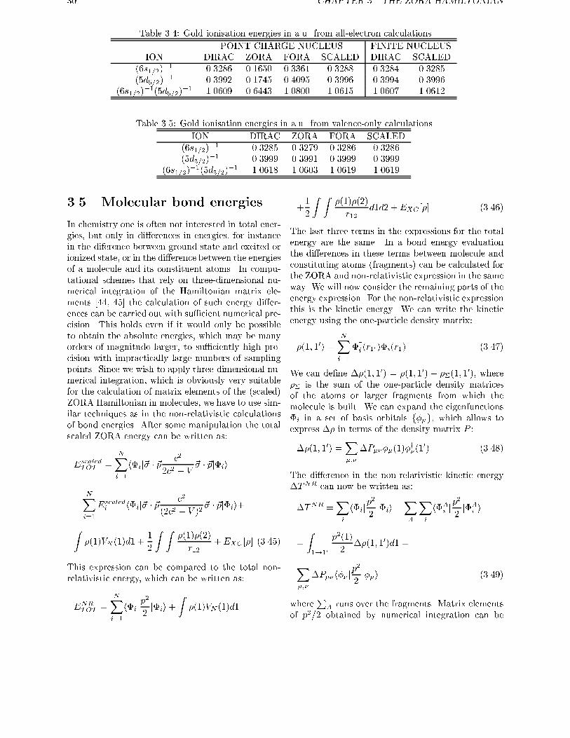
30 CHAPTER 3. THE ZORA HAMILTONIAN
Table 3.4: Gold ionisation energies in a.u. from all-electron calculations
POINT CHARGE NUCLEUS FINITE NUCLEUS
ION DIRAC ZORA FORA SCALED DIRAC SCALED
(6s1=2)�1 0.3286 0.1650 0.3361 0.3288 0.3284 0.3285
(5d5=2)�1 0.3992 0.1745 0.4095 0.3996 0.3994 0.3996
(6s1=2)�1(5d5=2)
�1 1.0609 0.6443 1.0800 1.0615 1.0607 1.0612
Table 3.5: Gold ionisation energies in a.u. from valence-only calculations.
ION DIRAC ZORA FORA SCALED
(6s1=2)�1 0.3285 0.3279 0.3286 0.3286
(5d5=2)�1 0.3999 0.3991 0.3999 0.3999
(6s1=2)�1(5d5=2)
�1 1.0618 1.0603 1.0619 1.0619
3.5 Molecular bond energies
In chemistry one is often not interested in total ener-
gies, but only in di�erences in energies, for instance
in the diference between ground state and excited or
ionized state, or in the di�erence between the energies
of a molecule and its constituent atoms. In compu-
tational schemes that rely on three-dimensional nu-
merical integration of the Hamiltonian matrix ele-
ments [44, 45] the calculation of such energy di�er-
ences can be carried out with su�cient numerical pre-
cision. This holds even if it would only be possible
to obtain the absolute energies, which may be many
orders of magnitude larger, to su�ciently high pre-
cision with impractically large numbers of sampling
points. Since we wish to apply three-dimensional nu-
merical integration, which is obviously very suitable
for the calculation of matrix elements of the (scaled)
ZORA Hamiltonian in molecules, we have to use sim-
ilar techniques as in the non-relativistic calculations
of bond energies. After some manipulation the total
scaled ZORA energy can be written as:
EscaledTOT =
NXi=1
h�ij~� � ~pc2
2c2 � V~� � ~pj�ii
�NXi=1
Escaledi h�ij~� � ~p
c2
(2c2 � V )2~� � ~pj�ii+
Z�(1)VN (1)d1 +
1
2
Z Z�(1)�(2)
r12+EXC [�] (3.45)
This expression can be compared to the total non-
relativistic energy, which can be written as:
ENRTOT =
NXi=1
h�ijp2
2j�ii+
Z�(1)VN (1)d1
+1
2
Z Z�(1)�(2)
r12d1d2 +EXC [�] (3.46)
The last three terms in the expressions for the total
energy are the same. In a bond energy evaluation
the di�erences in these terms between molecule and
constituting atoms (fragments) can be calculated for
the ZORA and non-relativistic expression in the same
way. We will now consider the remaining parts of the
energy expression. For the non-relativistic expression
this is the kinetic energy. We can write the kinetic
energy using the one-particle density matrix:
�(1; 10) =
NXi=1
�yi (r10 )�i(r1) (3.47)
We can de�ne ��(1; 10) = �(1; 10) � ��(1; 10), where
�� is the sum of the one-particle density matrices
of the atoms or larger fragments from which the
molecule is built. We can expand the eigenfunctions
�i in a set of basis orbitals f��g, which allows to
express �� in terms of the density matrix P :
��(1; 10) =X�;�
�P����(1)�y�(1
0) (3.48)
The di�erence in the non-relativistic kinetic energy
�TNR can now be written as:
�TNR =Xi
h�ijp2
2j�ii �
XA
Xi
h�Ai jp2
2j�A
i i
=
Z1!10
p2(1)
2��(1; 10)d1 =
X�;�
�P��h�� jp2
2j��i (3.49)
whereP
A runs over the fragments. Matrix elements
of p2=2 obtained by numerical integration can be
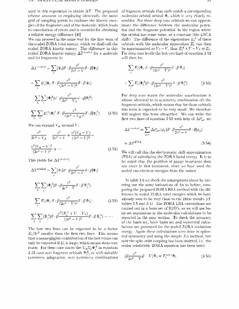
3.5. MOLECULAR BOND ENERGIES 31
used in this expression to obtain �T . The proposedscheme amounts to employing identically the same
grid of sampling points to evaluate the kinetic ener-
gies of the fragments and of the molecule, which leads
to cancellation of errors and is essential for obtaining
a reliable energy di�erence [46].
We can proceed in the same way for the �rst term of
the scaled ZORA total energy, which we shall call the
scaled ZORA kinetic energy. The di�erence in this
scaled ZORA kinetic energy �T scaled for a moleculeand its fragments is:
�T scaled =Xi
h�ij~� � ~pc2
2c2 � V~� � ~pj�ii
�Xi
Eih�ij~� � ~pc2
(2c2 � V )2~� � ~pj�ii
�XA
Xi
h�Ai j~� � ~p
c2
2c2 � VA~� � ~pj�A
i i+
XA
Xi
EAi h�
Ai j~� � ~p
c2
(2c2 � VA)2~� � ~pj�A
i i (3.50)
We can expand VA around V :
c2
2c2 � VA=
c2
2c2 � V+c2(VA � V )
(2c2 � V )2+
c2(VA � V )2
(2c2 � V )3+ � � � (3.51)
This yields for �T scaled:
�T scaled =Xi
h�ij~� � ~pc2
2c2 � V~� � ~pj�ii
�XA
Xj
h�Aj j~� � ~p
c2
2c2 � V~� � ~pj�A
j i
�Xi
Eih�ij~� � ~pc2
(2c2 � V )2~� � ~pj�ii+ (3.52)
XA
Xj
h�Aj j~� � ~p
c2(EAj + V � VA)
(2c2 � V )2~� � ~pj�A
j i+ � � �
The last two lines can be expected to be a factor
Ei=2c2 smaller than the �rst two lines. This means
that a nonnegligible contribution of the last terms can
only be expected if Ei is large, which means deep corestates. For deep core states the �A�j�
Aj in equation
3.52 runs over fragment orbitals �Aj , or with suitable
symmetry adaptation, over symmetry combinations
of fragment orbitals that each match a corresponding
molecular orbital orbital �i which it very closely re-
sembles. For these deep core orbitals we can approx-
imate the di�erence between the molecular poten-
tial and the fragment potential, in the region where
the orbital has some value, as a constant (the ESCA
shift). The di�erence of the eigenvalues EAi of these
orbitals with the molecular eigenvalues Ei can then
be approximated as VA�V , thus EAi +V �VA � Ei.
For deep core levels the last two lines of equation 3.52
will then be:
�Xi
Eih�ij~� � ~pc2
(2c2 � V )2~� � ~pj�ii
+Xi
Eih�Ai j~� � ~p
c2
(2c2 � V )2~� � ~pj�A
i i (3.53)
For deep core states the molecular wavefunction is
almost identical to (a symmetry combination of) the
fragment orbitals, which means that for those orbitals
this term is expected to be very small. We therefore
will neglect this term altogether. We can write the
�rst two lines of equation 3.52 with help of �P�� as:
�T scaled �X�;�
�P��h�� j~� � ~pc2
2c2 � V~� � ~pj��i
= �TESA (3.54)
We will call this the electrostatic shift approximation
(ESA) of calculating the ZORA bond energy. It is to
be noted that the problem of gauge invariance does
not enter in this treatment, since we have used the
scaled one-electron energies from the outset.
In table 3.6 we check the assumptions above by car-
rying out the same ionisations of Au as before, com-
paring the proposed ZORA ESA method with the dif-
ference in scaled ZORA total energies which we have
already seen to be very close to the Dirac results (cf.
tables 3.5 and 3.4). The ZORA ESA calculations are
carried out in a basis set of STO's, as we will use ba-
sis set expansions in the molecular calculations to be
reported in the next section. To check the accuracy
of the basis set, both basis set and numerical calcu-
lations are presented for the scaled ZORA ionisation
energy. Again these calculations were done in spher-
ical symmetry and using the simple X� method, but
now the spin-orbit coupling has been omitted, i.e. the
scalar relativistic ZORA equation has been used:
(~pc2
2c2 � V~p+ V )�i = Ezora
i �i (3.55)
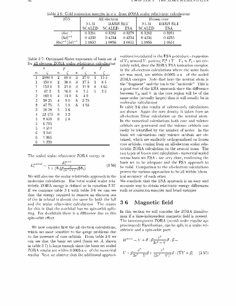
32 CHAPTER 3. THE ZORA HAMILTONIAN
Table 3.6: Gold ionisation energies in a.u. from ZORA scalar relativistic calculations
ION All electron Frozen core
NUM BASIS SET NUM BASIS SET
SCALED SCALED ESA SCALED ESA
(6s)�1 0.3281 0.3282 0.3278 0.3282 0.3281
(5d)�1 0.4230 0.4234 0.4234 0.4231 0.4235
(6s)�1(5d)�1 1.0853 1.0856 1.0851 1.0856 1.0854
Table 3.7: Optimized Slater exponents of basis set Afor all electron ZORA scalar relativistic calculations
s p d fn � n � n � n �
1 2000.0 2 60.0 3 27.0 4 15.5
1 450.0 2 36.0 3 17.5 4 8.5
1 152.0 3 21.0 4 11.9 4 4.65
1 87.2 3 16.0 4 7.5 5 2.5
2 100.0 4 13.0 5 4.9
2 38.25 4 9.0 5 2.75
3 47.75 5 5.8 5 1.55
3 20.38 5 3.6
4 12.475 6 3.2
4 8.859 6 1.8
5 6.795
5 4.514
6 3.141
6 1.965
6 1.239
The scaled scalar relativistic ZORA energy is:
Escaledi =
Ezorai
1 + h�ij~p c2
(2c2�V )2 ~pj�ii(3.56)
We will also use the scalar relativistic approach in the
molecular calculations. The total scaled scalar rela-
tivistic ZORA energy is de�ned as in equation 3.37.
If we compare table 3.4 with table 3.6 we can see
that the energy required to remove an electron out
of the 6s orbital is almost the same for both the full
and the scalar relativistic calculations. The reason
for this is that the s-orbital has no spin-orbit split-
ting. For d-orbitals there is a di�erence due to this
spin-orbit e�ect.
We now consider �rst the all electron calculations,
which are most sensitive to the gauge problems due
to the presence of core orbitals. From table 3.6 we
can see that the basis set used (basis set A, shownin table 3.7) is large enough since the basis set scaled
ZORA results are within 0.0005 a.u. of the numerical
results. Next we observe that the additional approxi-
mations introduced in the ESA procedure - expansion
of VA around V , putting EAi +V �VA � Ei - are cer-
tainly valid, since the ZORA ESA ionisation energies,
in the all-electron calculations where the same basis
set was used, are within 0.0005 a.u. of the scaled
ZORA energies. Note that here the neutral atom is
the "fragment" and the ion is the "molecule". This is
a good test of the ESA approach since the di�erence
between VA and V in the core region will be of the
same order (actually larger) than it will usually be in
molecular calculations.
In table 3.6 also results of valence-only calculations
are shown. Again the core density is taken from an
all-electron Dirac calculation on the neutral atom.
In the numerical calculations both core and valence
orbitals are generated and the valence orbitals can
easily be identi�ed by the number of nodes. In the
basis set calculations only valence orbitals are ob-
tained, which are explicitly orthogonalised on frozen
core orbitals, coming from an all-electron scalar rela-
tivistic ZORA calculation on the neutral atom. The
two types of frozen core calculation - numerical scaled
versus basis set ESA - are very close, con�rming the
basis set to be adequate and the ESA approach to
be valid. Comparison to the all-electron calculations
proves the various approaches to be all within 'chem-
ical accuracy' of each other.
We conclude that the ESA approach is an easy and
accurate way to obtain relativistic energy di�erences
such as ionisation energies and bond energies.
3.6 Magnetic �eld
In this section we will consider the ZORA Hamilto-
nian if a time-independent magnetic �eld is present.
The two-component ZORA (zeroth order regular ap-
proximated) Hamiltonian, can be split in a scalar rel-
ativistic and a spin-orbit part:
Hzora = V + ~� � ~pc2
2c2 � V~� � ~p =
V + ~pc2
2c2 � V~p+
c2
(2c2 � V )2~� � (~rV � ~p) (3.57)
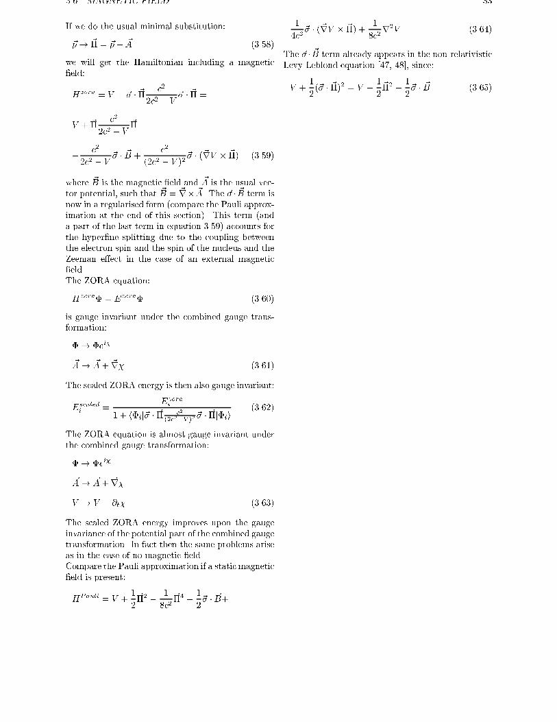
3.6. MAGNETIC FIELD 33
If we do the usual minimal substitution:
~p! ~� = ~p� ~A (3.58)
we will get the Hamiltonian including a magnetic
�eld:
Hzora = V + ~� � ~�c2
2c2 � V~� � ~� =
V + ~�c2
2c2 � V~�
�c2
2c2 � V~� � ~B +
c2
(2c2 � V )2~� � (~rV � ~�) (3.59)
where ~B is the magnetic �eld and ~A is the usual vec-
tor potential, such that ~B = ~r� ~A. The ~� � ~B term is
now in a regularised form (compare the Pauli approx-
imation at the end of this section). This term (and
a part of the last term in equation 3.59) accounts for
the hyper�ne splitting due to the coupling between
the electron spin and the spin of the nucleus and the
Zeeman e�ect in the case of an external magnetic
�eld.
The ZORA equation:
Hzora� = Ezora� (3.60)
is gauge invariant under the combined gauge trans-
formation:
�! �ei�
~A! ~A+ ~r� (3.61)
The scaled ZORA energy is then also gauge invariant:
Escaledi =
Ezorai
1 + h�ij~� � ~� c2
(2c2�V )2 ~� � ~�j�ii(3.62)
The ZORA equation is almost gauge invariant under
the combined gauge transformation:
�! �ei�
~A! ~A+ ~r�
V ! V � @t� (3.63)
The scaled ZORA energy improves upon the gauge
invariance of the potential part of the combined gauge
transformation. In fact then the same problems arise
as in the case of no magnetic �eld.
Compare the Pauli approximation if a static magnetic
�eld is present:
HPauli = V +1
2~�2 �
1
8c2~�4 �
1
2~� � ~B+
1
4c2~� � (~rV � ~�) +
1
8c2r2V (3.64)
The ~� � ~B term already appears in the non-relativistic
Levy-Leblond equation [47, 48], since:
V +1
2(~� � ~�)2 = V +
1
2~�2 �
1
2~� � ~B (3.65)
34 CHAPTER 3. THE ZORA HAMILTONIAN
Chapter 4
Exact relations between DIRAC and
ZORA
4.1 Introduction
One of the most important problems in quantum
mechanics, that can be solved exactly, is the prob-
lem of an electron moving in a Coulomb �eld. The
bound-state solutions of the Schr�odinger and Klein-
Gordon equation for hydrogen-like atoms were al-
ready obtained in the early days of quantum me-
chanics [49, 50]. For this system the solutions of the
Dirac equation are also known [3, 4], which is very
convenient when considering approximations. The
Schr�odinger equation may be considered to be the
zeroth order equation of the expansion in c�1 of theexact Foldy Wouthuysen transformed Dirac equation.
In this section we will give an exact relation between
the Dirac solutions and the solutions of the zeroth or-
der of the regular approximate (ZORA) equation in
the case of hydrogen-like atoms. Exact solutions of
these one electron systems are very useful as a start-
ing point for the calculations on more complex sys-
tems.
4.2 Exact
solutions for hydrogen-like
atoms
We are looking for hydrogen-like solutions of the ze-
roth order regular approximate (ZORA) equation in
a Coulomb potential of a point charge Z:
V = �Z
r(4.1)
The ZORA equation 3.2 is in this case:
(�Z
r+ ~� � ~p
c2
2c2 + Zr
~� � ~p)�zora(~r)
= Ezora�zora(~r) (4.2)
We can relate the solutions of the ZORA equation to
the well known solutions of the Dirac equation for this
problem. After elimination of the small component
the equation for the large component �D of the four-
component Dirac spinor is:
(�Z
r+ ~� � ~p
c2
2c2 +ED + Zr
~� � ~p)�D(~r)
= ED�D(~r) (4.3)
We can transform this equation to the ZORA equa-
tion by means of an energy-dependent scaling with �of the coordinate ~r:
~r 0 = �~r (4.4)
hence:
~� � ~p 0 =1
�~� � ~p (4.5)
After dividing by �, this transforms equation 4.3 into:
(�Z
r0+ ~� � ~p 0
c2
2c2+ED
�+ Z
r0
~� � ~p 0)�D(~r 0
�)
=ED
��D(
~r 0
�) (4.6)
De�ning the energy-dependent � by:
� =2c2 +ED
2c2(4.7)
one obtains:
(�Z
r0+ ~� � ~p 0
c2
2c2 + Zr0
~� � ~p 0)�D(~r 0
�)
=2c2ED
2c2 +ED�D(
~r 0
�) (4.8)
35
36 CHAPTER 4. EXACT RELATIONS BETWEEN DIRAC AND ZORA
Here one recognizes the one-particle ZORA equa-
tion 4.2. Thus for every solution of the Dirac-
equation with energy ED, we �nd a solution of the
ZORA equation with energy Ezora:
Ezora =2c2ED
2c2 +ED(4.9)
with corresponding eigenfunction �zora:
�zora(~r) = �D(~r
�) (4.10)
Thus the ZORA eigenfunctions are scaled Dirac large
components, in which the scaling factor depends on
the energy. The number of nodes in the ZORA eigen-
function is the same as in the large component of the
Dirac spinor, because only a scaling has been applied.
The derivation of the relativistic virial theorem [51]
was also done by scaling of coordinates. From this
theorem we can conclude, that the norm of the Dirac
large component, belonging to the discrete spectrum
in the case of a hydrogen-like atom, is related to its
eigenvalue as:
h�D j�Di =2c2 +ED
2c2(4.11)
This norm is the same as the energy-dependent � we
used to scale the Dirac equation.
4.2.1 First order perturbation
Having obtained the exact zeroth order result for the
case of hydrogen-like atoms, we will now obtain an
exact result for the �rst order. We can invert equa-
tion 4.9 to:
ED =2c2Ezora
2c2 �Ezora(4.12)
Expanding this in powers of c�2 gives:
ED = Ezora +(Ezora)2
2c2+ � � � (4.13)
In this section we will show that the scaled ZORA
energy is exactly equal to the Dirac energy and that
the FORA energy is just the Dirac energy expanded
in powers of c�2 up to �rst order:
Escaled = ED
Efora = Ezora +(Ezora)2
2c2(4.14)
In order to do this we need to know for the FORA
and scaled ZORA energy the expectation value of the
ZORA wavefunction with the following operator:
h�zoraj~� � ~pc2
(2c2 � V )2~� � ~pj�zorai (4.15)
We will prove the following relation for the dis-
crete part of the spectrum of Hzora in the case of
a hydrogen-like atom:
h�zoraj~� � ~pc2
(2c2 + Zr)2~� � ~pj�zorai = �
Ezora
2c2(4.16)
We de�ne a scaled eigenfunction of the ZORA Hamil-
tonian by:
��(~r) = �3
2�zora(�~r) (4.17)
Because of the prefactor �3
2 the scaled wavefunction
is also normalized. We de�ne the following energy
E�:
E� = h��jHzoraj��i (4.18)
Because �zora is an eigenvector of the discrete spec-
trum of Hzora, its eigenvalue Ezora is a stationary
value of the functional E� [52], thus:
dE�d�
j�=1 = 0 (4.19)
We can write:
E� =
Z�3�zoray(�~r)
�Zr
�zora(�~r)d~r+
Z�3�zoray(�~r)~� � ~p
c2
2c2 + Zr
~� � ~p�zora(�~r)d~r =
= �
Z�zoray(�~r)
�Z�r
�zora(�~r)d(�~r)+
�2Z
�zoray(�~r)~� � ~p�c2
2c2 + Z��r
~� � ~p��zora(�~r)d(�~r)
= �h�zoraj�Zrj�zorai+
�h�zoraj~� � ~pc2
2c2
�+ Z
r
~� � ~pj�zorai (4.20)
where ~� � ~p� = 1�~� � ~p. Now we can use equation 4.19,
which gives:
0 =dE�d�
j�=1 = h�zoraj�Zrj�zorai
+h�zoraj~� � ~pc2
2c2 + Zr
~� � ~pj�zorai+
2c2h�zoraj~� � ~pc2
(2c2 + Zr)2~� � ~pj�zorai =
Ezora + 2c2h�zoraj~� � ~pc2
(2c2 + Zr)2~� � ~pj�zorai(4.21)
4.3. ONE ELECTRON SYSTEMS 37
Thus:
h�zoraj~� � ~pc2
(2c2 + Zr)2~� � ~pj�zorai = �
Ezora
2c2(4.22)
Having obtained this result, we can now prove the
equations of 4.14 using equation 3.3 and 3.4 for the
de�nition of the FORA and scaled ZORA energy:
Escaled =Ezora
1 + h�zoraj~� � ~p c2
(2c2+Z
r)2~� � ~pj�zorai
=2c2Ezora
2c2 �Ezora= ED (4.23)
Efora = Ezora +(Ezora)2
2c2(4.24)
4.2.2 Scalar relativistic equations
In the case of a hydrogen-like atom all scaling argu-
ments of section 4.2 and 4.2.1 can be repeated for the
scalar relativistic (SR) equations. The SR equation
(see equation 3.5 for a hydrogen-like atom is given
by:
(V + ~pc2
2c2 +ESR + Zr
~p)�SR = ESR�SR (4.25)
and the zeroth order regular approximated SR equa-
tion is:
(V + ~pc2
2c2 + Zr
~p)�zoraSR = Ezora
SR �zoraSR (4.26)
For s-orbitals the SR equations are the same as the
equations including spin-orbit. Applying the argu-
ments of section 4.2 and 4.2.1 we get the following
relations between the eigenvalues and eigenfunctions
of the SR and ZORA SR equation in the case of a
hydrogen-like potential:
�zoraSR (~r) = �SR(
~r
�)
� =2c2 +ESR
2c2
EzoraSR =
2c2ESR
2c2 +ESR
EscaledSR = ESR
EforaSR = Ezora
SR +(Ezora
SR )2
2c2(4.27)
4.3 One electron systems
Scaling of one-electron equations can of course also
be done for a general potential. In that case the one-
electron Dirac equation for the large component in a
potential V (~r):
(V (~r) + ~� � ~pc2
2c2 +ED � V (~r)~� � ~p)�D(~r)
= ED�D(~r) (4.28)
becomes after scaling with � = (2c2 + ED)=(2c2) aZORA equation with a potential V 0(~r):
V 0(~r) =1
�V (
~r
�) (4.29)
which is in general di�erent from V (~r). The ZORA
eigenfunction is again a scaled Dirac large compo-
nent, like in the hydrogen-like atom case. An exam-
ple is the one-electron diatomic molecule. If one �nds
a solution to the Dirac equation for a certain distance
R between the atoms, one also has a solution to the
ZORA equation, but now for a distance �R between
the atoms. For a bound electron ED < 0, this means
a smaller distance. The situation may also be re-
versed. If one �nds a solution to the ZORA equation
one also has a solution to the Dirac equation, but for
a di�erent potential. The arguments of section 4.2.1
can only be used if V 0(~r) = V (~r). Thus in general
the scaled ZORA energy will not be exactly equal to
the Dirac energy.
4.4 Two electron systems
For helium-like ions we can derive some exact re-
lations in the case of the Dirac-Fock equations for
two electrons which have the same density and one-
electron energies, for example the ground state of he-
lium. In that case the exchange potential for these
electrons is just minus half the Coulomb potential VC .Suppose we have solved the Dirac-Fock equations for
such a system:
(�Z
r+1
2VC([�
D ];~r)+
~� � ~pc2
2c2 +ED + Zr� 1
2VC([�D];~r)
~� � ~p)�D(~r)
= ED�D(~r) (4.30)
and we know that the Coulomb-potential ful�ls the
simple scaling relation:
VC([�D];~r) = �VC([�
D1=�];�~r) (4.31)
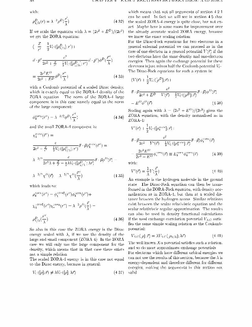
38 CHAPTER 4. EXACT RELATIONS BETWEEN DIRAC AND ZORA
with:
�D1=�(~r) = ��3�D(~r
�) (4.32)
If we scale the equation with � = (2c2 + ED)=(2c2)we get the ZORA equation:
(�Z
r0+1
2VC([�
D1=�]; r
0)+
~� � ~p 0c2
2c2 + Zr0� 1
2VC([�
D1=�
]; r0)~� � ~p 0)�D(
~r 0
�)
=2c2ED
2c2 +ED�D(
~r 0
�) (4.33)
with a Coulomb potential of a scaled Dirac density,
which is exactly equal to the ZORA-4 density of the
ZORA equation. The norm of the ZORA-4 large
component is in this case namely equal to the norm
of the large component:
�zora4 (~r 0) = ��3=2�D(~r 0
�) (4.34)
and the small ZORA-4 component is:
�zora4 (~r 0) =
c
2c2 + Zr0� 1
2VC([�
D1=�
]; r0)~� � ~p�zora4 (~r 0) =
��3=2c
2c2�+ Z~r� 1
2�VC([�
D1=�
];�~r)~� � ~p�D(~r) =
��3=2�D(~r) = ��3=2�D(~r 0
�) (4.35)
which leads to:
�zora4 (~r 0) = �zoray4 (~r 0)�zora4 (~r 0)+
�zoray4 (~r 0)�zora4 (~r 0) = ��3�D(~r
�) =
�D1=�(~r 0
�) (4.36)
So also in this case the ZORA energy is the Dirac
energy scaled with �, if we use the density of the
large and small component (ZORA-4). In the ZORA
case we will only use the large component for the
density, which means that in that case there exists
not a simple relation.
The scaled ZORA-4 energy is in this case not equal
to the Dirac energy, because in general:
VC([�];~r) 6= �VC([�];�~r) (4.37)
which means that not all arguments of section 4.2.1
can be used. In fact we will see in section 4.5 that
the scaled ZORA-4 energy is quite close, but not ex-
act. Maybe here is some room for improvement over
the already accurate scaled ZORA energy, because
we know the exact scaling relation.
For the Dirac-Fock equations for two electrons in a
general external potential we can proceed as in the
case of one electron in a general potential V (~r) if thetwo electrons have the same density and one-electron
energies. Then again the exchange potential for these
electrons is just minus half the Coulomb potential VC .The Dirac-Fock equations for such a system is:
(V (~r) +1
2VC([�
D ];~r)+
~� � ~pc2
2c2 +ED � V (~r)� 12VC([�D];~r)
~� � ~p)�D(~r)
= ED�D(~r) (4.38)
Scaling again with � = (2c2 + ED)=(2c2) gives theZORA equation, with the density normalised as in
ZORA-4:
V 0(~r) +1
2VC([�
zora4 ];~r)+
~� � ~pc2
2c2 � V 0(~r)� 12VC([�zora4 ];~r)
~� � ~p)�zora4 (~r)
=2c2ED
2c2 +ED�zora4 (~r) � Ezora
4 �zora4 (~r) (4.39)
with:
V 0(~r) =1
�V (
~r
�) (4.40)
An example is the hydrogen molecule in the ground
state. The Dirac-Fock equation can then be trans-
formed in the ZORA-Fock equation, with density nor-
malisation as in ZORA-4, but then at a scaled dis-
tance between the hydrogen atoms. Similar relations
exist between the scalar relativistic equation and the
scalar relativistic regular approximation. The results
can also be used in density functional calculations
if the used exchange-correlation potential VXC satis-
�es the same simple scaling relation as the Coulomb-
potential:
VXC([�];~r) = �VXC([�1=�];�~r) (4.41)
The well knownX� potential satis�es such a relation,
and so do most approximate exchange potentials.
For electrons which have di�erent orbital energies we
can not use the results of this section, because the � isenergy-dependent and therefore di�erent for di�erent
energies, making the arguments in this section not
valid.
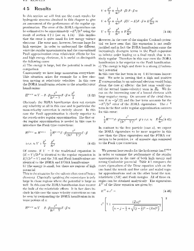
4.5. RESULTS 39
4.5 Results
In this section we will �rst use the exact results for
hydrogenic systems obtained in this chapter to give
an assessment of the performance of the regular ap-
proximation. The error of the ZORA eigenvalues can
be estimated to be approximately �E2=2c2 using theresult of section 4.2.1 (see eq. 4.14). This implies
that the error is quite small for low energy valence
electrons. The error may, however, become large for
high energies. In order to understand the di�erent
ways the regular approximation and the conventional
Pauli approximation treat relativistic e�ects for low
and high energy electrons, it is useful to distinguish
the following cases:
a) The energy is large, but the potential is small in
comparison.
Consequently we have large momentum everywhere.
This situation arises for example for a free elec-
tron moving at relativistic velocities. In this case
the ZORA hamiltonian reduces to the nonrelativistic
hamiltonian:
Hzora = V + ~� � ~pc2
2c2 � V~� � ~p =
p2
2(4.42)
Obviously the ZORA hamiltonian does not contain
any relativity at all in this case and in particular the
mass-velocity correction is entirely absent. In this
case the Pauli approximation is clearly superior to
the zeroth order regular approximation. The �rst or-
der regular approximation is needed in this case to
introduce the Pauli type corrections:
Hfora = Hzora �1
2Hzora~� � ~p
c2
(2c2 � V )2~� � ~p
+c:c: � V +p2
2�
p4
8c2(4.43)
Of course, if V = 0 the traditional expansion in
(E � V )=2c2 is identical to the regular expansion in
E=(2c2 � V ) and the NR and Pauli hamiltonians are
identical to the ZORA and FORA hamiltonians.
b) The energy is small, but there are regions of high
potential.
This is the situation for the valence electrons of heavy
elements. Classically speaking the momentum is only
large in those regions where the potential is large as
well. In this case the ZORA hamiltonian does recover
the bulk of the relativistic e�ects. It in fact does in-
clude in this case the mass-velocity corrections as can
be seen by reexpanding the ZORA hamiltonian in in-
verse powers of c:
Hzora = V + ~� � ~pc2
2c2 � V~� � ~p �
V +p2
2+
1
4c2~� � ~pV ~� � ~p �
V +p2
2+
1
4c2~� � ~p(V �E)~� � ~p+E
p2
4c2�
V +p2
2�
p4
8c2+E
p2
4c2(4.44)
However, in the case of the singular Coulomb poten-
tial we have seen that this expansion is not really
justi�ed and in fact the ZORA hamiltonian sums the
increasingly divergent terms in the Pauli expansion
to in�nite order leading to a �nal result that is en-
tirely regular. Therefore in this case even the ZORA
hamiltonian is far superior to the Pauli hamiltonian.
c) The energy is high and there is a strong (Coulom-
bic) potential.
In this case the last term in eq. 4.44 becomes impor-
tant. We note in passing that a high and positive
E corresponding to an unbound electron would bring
about the case a) e�ects: the last term would can-
cel the second (mass-velocity) term in ~H0. We fo-
cus on the interesting case of a bound electron with
large negative energy. On account of the virial theo-
rem E � �hp2=2i and the last term accounts for the
�E2=2c2 error of the ZORA eigenvalues. The c�2
term in the �rst order regular approximation corrects
for this error:
�1
2Hzora~� � ~p
c2
(2c2 � V )2~� � ~p+ c:c: � �E
p2
4c2(4.45)
In contrast to the free particle (case a), we expect
the ZORA eigenvalues to be more negative in this
case than the Dirac eigenvalues and the FORA cor-
rection to be positive, i.e. of opposite sign compared
to the Pauli type correction.
We present here results for the hydrogenic ion U91+
in order to examine the performance of the regular
approximation in the case of both high energy and
strong Coulombic potential. Table 4.1 compares the
exact eigenvalues of the Dirac equation with on the
one hand the zeroth and �rst order and scaled regu-
lar approximations and on the other hand the non-
relativistic (NR) and Pauli energies. All of these en-
ergies can be obtained analytically. The eigenvalues
ED of the Dirac equation are given by:
ED + c2 = (4.46)
c2
2641 + (Z�)2�
n� j � 12+q(j + 1
2)2 � (Z�)2
�2375� 1
2
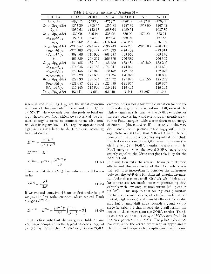
40 CHAPTER 4. EXACT RELATIONS BETWEEN DIRAC AND ZORA
Table 4.1: orbital energies of Uranium 91+
ORBITAL DIRAC ZORA FORA SCALED NR PAULI
1s1=2(1s) -4861.2 -5583.9 -4753.7 -4861.2 -4232.0 -4708.9
2s1=2; 2p1=2(2s) -1257.39 -1300.95 -1255.88 -1257.39 -1058.00 -1207.02
2p3=2 -1089.61 -1122.17 -1088.64 -1089.61 -1087.80
3s1=2; 3p1=2(3s) -539.09 -546.94 -538.98 -539.09 -470.22 -523.21
3p3=2; 3d3=2 -489.04 -495.49 -488.95 -489.04 -487.88
3d5=2 -476.262 -482.378 -476.183 -476.262 -476.109
4s1=2; 4p1=2(4s) -295.257 -297.597 -295.239 -295.257 -264.500 -288.715
4p3=2; 4d3=2 -274.408 -276.427 -274.393 -274.408 -273.814
4d5=2; 4f5=2 -268.966 -270.906 -268.952 -268.966 -268.846
4f7=2 -266.389 -268.292 -266.376 -266.389 -266.363
5s1=2; 5p1=2(5s) -185.485 -186.405 -185.480 -185.485 -169.280 -182.250
5p3=2; 5d3=2 -174.945 -175.763 -174.941 -174.945 -174.621
5d5=2; 5f5=2 -172.155 -172.948 -172.152 -172.155 -172.078
5f7=2; 5g7=2 -170.829 -171.609 -170.825 -170.829 -170.806
6s1=2; 6p1=2(6s) -127.093 -127.525 -127.092 -127.093 -117.556 -125.282
6p3=2; 6d3=2 -121.057 -121.449 -121.056 -121.057 -120.867
6d5=2; 6f5=2 -119.445 -119.826 -119.444 -119.445 -119.395
7s1=2; 7p1=2(7s) -92.441 -92.669 -92.440 -92.441 -86.367 -91.333
where n and � = �(j + 12) are the usual quantum
numbers of the particular orbital and � = 1=c �1=137:037. Here we only used the positive total en-
ergy eigenvalues, from which we subtracted the rest
mass energy in order to compare them with non-
relativistic eigenvalues. The regular approximated
eigenvalues are related to the Dirac ones according
to equation 4.9:
Ezora =2c2ED
2c2 +ED
Escaled = ED
Efora = Ezora +(Ezora)2
2c2(4.47)
The non-relativistic (NR) eigenvalues are well known
to be:
ENR = �Z2
2n2(4.48)
If we expand equation 4.5 up to �rst order in c�2
we get the �rst order energies, which we call Pauli
energies EPauli:
EPauli = ENR �(ENR)2
2c2
�4n
j + 12
� 3
�(4.49)
Let us �rst note that the energies in table 4.1 are
very large compared to the typical valence energy of
ca. 0.5 a.u.. Given the �E2=2c2 error in the ZORA
energies, this is not a favourable situation for the ze-
roth order regular approximation. Still, even at the
high energies of this example the ZORA energies for
the core-penetrating s and p orbitals are usually supe-rior to Pauli energies. This is true down to an energy
of 500 a.u. (the n = 3 shell). It is only in the very
deep core (note in particular the 1s1=2 with an en-
ergy close to 5000 a.u.) that ZORA starts to perform
poorly. In that case it becomes important to include
the �rst order corrections. Of course in all cases (in-
cluding 1s1=2) the FORA energies are superior to the
Pauli energies. Since the scaled ZORA energies are
exactly equal to the Dirac energies this is by far the
best method.
In connection with the relation between relativistic
e�ects and the singularity of the Coulomb poten-
tial [26], it is interesting to consider the di�erences
between the orbitals with di�erent angular momen-
tum belonging to one shell. Orbitals with high angu-
lar momentum are much less core penetrating than
orbitals with low angular momentum (cf. plots in
ref [26]). This implies that for d,f and g orbitals
the balance between case a) e�ects (relatively at po-
tential, high energy) and case b) e�ects (Coulombic
singularity) may shift more towards a), and we ob-
serve in table 4.1 that indeed the Pauli results are
better in those cases than the ZORA results. This is
in contrast to the superiority of ZORA over Pauli for
the core penetrating s levels. The p has hybrid be-
haviour: since the zeroth order regular approximate
Hamiltonian has spin-orbit coupling and has the same
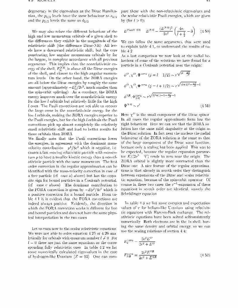
4.5. RESULTS 41
degeneracy in the eigenvalues as the Dirac Hamilto-
nian, the p1=2 levels have the same behaviour as s1=2and the p3=2 levels the same as d3=2.
We may also relate the di�erent behaviour of the
high and low momentum orbitals of a given shell to
the di�erences they exhibit in the magnitude of the
relativistic shift (the di�erence Dirac-NR). All lev-
els have a downward relativistic shift, but the core
penetrating low angular momentum orbitals by far
the largest, in complete accordance with all previous
arguments. This implies that the nonrelativistic en-
ergy of the shell, ENRn , is above all the Dirac energies
of the shell, and closest to the high angular momen-
tum levels. On the other hand, the ZORA energies
are all below the Dirac energies by roughly the same
amount (approximately �E2n=2c
2, much smaller than
the spin-orbit splitting). As a corollary, the ZORA
energy improves much over the nonrelativistic energy
for the low l orbitals but relatively little for the highl ones. The Pauli corrections are not able to recoverthe large error in the nonrelativistic energy for the
low l orbitals, making the ZORA energies superior to
the Pauli energies, but for the high l orbitals the Paulicorrections pick up almost completely the relatively
small relativistic shift and lead to better results for
those orbitals than ZORA.
We �nally note that the Pauli corrections lower
the energies, in agreement with the dominant mass-
velocity contribution �p4=8c2 which is negative, i.e.
causes a fast moving relativistic particle with momen-
tum p to have a smaller kinetic energy than a nonrel-ativistic particle with the same momentum. The �rst
order correction in the regular approximation can be
identi�ed with the mass-velocity correction in case of
a free particle (cf. case a) above) but has the oppo-
site sign for bound particles in a Coulomb potential,
(cf. case c above). The dominant contribution to
the FORA correction is given by �Ep2=4c2 which is
a positive correction for a bound particle. From ta-
ble 4.1 it is evident that the FORA corrections are
indeed always positive. Evidently, the direction in
which the FORA correction works is di�erent for free
and bound particles and does not have the same phys-
ical interpretation in the two cases.
Let us turn now to the scalar relativistic equations.
We were not able to solve equation 4.25 or 4.26 ana-
lytically for orbitals with quantum number l 6= 0. For
l = 0 these are just the same equations as the corre-
sponding fully relativistic ones. In table 4.2 we list
some numerically calculated eigenvalues in the case
of hydrogen-like Uranium (Z = 92). One can com-
pare these with the non-relativistic eigenvalues and
the scalar relativistic Pauli energies, which are given
by (for l > 0):
EPauli SR = ENR �(ENR)2
2c2
�4n
l+ 12
� 3
�(4.50)
We can follow the same arguments, that were used
to explain table 4.1, to understand the results of ta-
ble 4.2
As a last comparison we now look at the radial be-
haviour of some of the solutions we have found for a
particle in a Coulomb potential near the origin:
�D; �D;�zora (j = l � 1=2) � r
pl2�Z2
c2�1
�D; �D;�zora (j = l + 1=2) � r
p(l+1)2�Z2
c2�1
�SR;�zoraSR � r
pl(l+1)+1�Z2
c2�1
NR � rl (4.51)
Here �D is the small component of the Dirac spinor.
In all cases the regular approximate form has the
right behaviour. Here we can see that the ZORA so-
lution has the same mild singularity at the origin as
the Dirac solution. In fact near the nucleus the radial
behaviour of the ZORA solution is the same as that
of the large component of the Dirac wave function,
because only a scaling has been applied. This was to
be expected, because the regular expansion parame-
ter E=(2c2 � V ) tends to zero near the origin. The
ZORA orbital is slightly more contracted than the
Dirac one. A nice feature of the regular approxima-
tions is that already in zeroth order they distinguish
between expansions of the Dirac and scalar relativis-
tic equation, because of the spin-orbit operator. Of
course in these two cases the c�1-expansion of these
equations in zeroth order are identical, namely the
Schr�odinger equation.
In table 4.3 we list some energies and expectation
values of r for helium-like Uranium using relativis-
tic equations with Hartree-Fock exchange. The rel-
ativistic equations have been solved selfconsistently
numerically. Both electrons are in the 1s shell, hav-
ing the same density and orbital energy, so we can
use the scaling relations of section 4.4:
Ezora4 =
2c2ED
2c2 +ED
EzoraSR =
2c2ESR
2c2 +ESR(4.52)
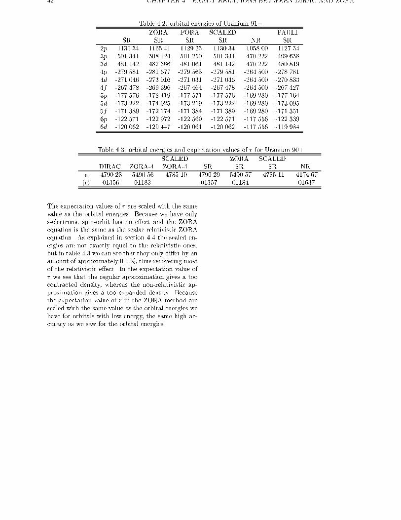
42 CHAPTER 4. EXACT RELATIONS BETWEEN DIRAC AND ZORA
Table 4.2: orbital energies of Uranium 91+
ZORA FORA SCALED PAULI
SR SR SR SR NR SR
2p -1130.34 -1165.41 -1129.25 -1130.34 -1058.00 -1127.54
3p -501.341 -508.124 -501.250 -501.341 -470.222 -499.658
3d -481.142 -487.386 -481.061 -481.142 -470.222 -480.819
4p -279.581 -281.677 -279.565 -279.581 -264.500 -278.781
4d -271.046 -273.016 -271.031 -271.046 -264.500 -270.833
4f -267.478 -269.396 -267.464 -267.478 -264.500 -267.427
5p -177.576 -178.419 -177.571 -177.576 -169.280 -177.164
5d -173.222 -174.025 -173.219 -173.222 -169.280 -173.095
5f -171.389 -172.174 -171.384 -171.389 -169.280 -171.351
6p -122.571 -122.972 -122.569 -122.571 -117.556 -122.339
6d -120.062 -120.447 -120.061 -120.062 -117.556 -119.984
Table 4.3: orbital energies and expectation values of r for Uranium 90+
SCALED ZORA SCALED
DIRAC ZORA-4 ZORA-4 SR SR SR NR
� -4790.28 -5490.56 -4785.10 -4790.29 -5490.57 -4785.11 -4174.67
hri .01356 .01183 .01357 .01184 .01637
The expectation values of r are scaled with the same
value as the orbital energies. Because we have only
s-electrons, spin-orbit has no e�ect and the ZORA
equation is the same as the scalar relativistic ZORA
equation. As explained in section 4.4 the scaled en-
ergies are not exactly equal to the relativistic ones,
but in table 4.3 we can see that they only di�er by an
amount of approximately 0.1 %, thus recovering most
of the relativistic e�ect. In the expectation value of
r we see that the regular approximation gives a too
contracted density, whereas the non-relativistic ap-
proximation gives a too expanded density. Because
the expectation value of r in the ZORA method are
scaled with the same value as the orbital energies we
have for orbitals with low energy, the same high ac-
curacy as we saw for the orbital energies.
Chapter 5
Numerical atomic calculations
5.1 Introduction
Relativistic e�ects are important in the study of
heavy elements. Instead of the Schr�odinger equa-
tion one now has to solve the Dirac equation, which
involves a four-component Hamiltonian. Fully rel-
ativistic calculations are no more complicated than
non-relativistic ones, as far as integral evaluation is
concerned, but they are very time consuming. The
dimension of the secular problem will be very large
since there are four components and many basis func-
tions are required. If one wants to use a variational
technique then one has to make sure that no spurious
solutions appear. This can be done using so-called
kinetically balanced basis sets [53, 54, 55], but then
one needs in principal di�erent basis functions for the
small component than for the large component of the
Dirac spinor, which increases integral evaluation time
and storage requirements.
An attractive alternative is to transform the Dirac
Hamiltonian to a two-component form. Standard
approaches are the elimination-of-small-components
(esc) and the Foldy-Wouthuysen (FW) transforma-
tion. We refer to the recent discussion by Kutzel-
nigg [30] for a detailed exposition of the various ap-
proaches and the di�culties that arise in the form
of divergent terms and singularities at r ! 0. The
di�culties connected with the Foldy-Wouthuysen
transformation have for instance been investigated
by Moss et al. [56, 57, 58, 59] and Farazdel and
Smith [23] have criticized the mass-velocity term,
pointing out that for large momenta (p > ��1) themass-velocity term �(�2=8)p4 is not obtained unless
one uses the expansion of the square-root operator for
the kinetic energy outside its radius of convergence.
The source of the di�culties is that the expansions
that are being used implicitly or explicitly rely on
an expansion in (E � V )=2c2, which is invalid for
particles in a Coulomb potential, where there will al-
ways be a region of space (close to the nucleus) where
(E�V )=2c2 > 1 and the expansion is not valid. This
was already noticed by Gollisch and Fritsche [41] in
their work on a scalar relativistic approximation to
the atomic Dirac equation, essentially equivalent to
the one of Koelling and Harmon [42].
In chapter 2 we considered expansions which are ap-
propriate in the sense that the expansion "parame-
ter" is � 1 over all space. In section 2.1 we �rst
discussed expansions in the case of classical rela-
tivistic mechanics in a Coulomb potential. This re-
vealed the essential error in the standard expansions
as well as providing a simple remedy. In section 2.2.1
we demonstrated that exactly the same expansion
is made in the standard derivations (both esc and
FW) of the Pauli Hamiltonian, leading to a simi-
lar error. It is shown that one can avoid this er-
ror, leading in both the esc and FW methods to a
two-component relativistic Hamiltonian that is, at
least in zeroth order, variationally stable and contains
similar relativisitic corrections as are present in the
Pauli Hamiltonian but in a regularized form. This
zeroth order regular approximated (ZORA) Hamil-
tonian turns out to be identical to the zeroth or-
der Hamiltonian derived earlier by Chang, P�elissier
and Durand using the theory of e�ective Hamiltoni-
ans [5] and by Heully, Lindgren, Lindroth, Lundqvist
and M�artensson-Pendrill [6]. The performance of
the derived hamiltonians is investigated �rst in self-
consistent atomic calculations in section 5.3. They
perform exceedingly well, especially valence orbital
energies are in much better agreement than the ener-
gies obtained with the standard Pauli Hamiltonian.
For deep core levels the error in the energy is of or-
der E2=2c2 and is still sizable in an absolute sense.
The �rst order Hamiltonian corrects this de�ciency
in a �rst order perturbation calculation. The scaled
ZORA approach is even more accurate, because it in-
cludes some higher orders up to in�nity and gives ex-
act energies for the hydrogen-like atoms. This scaled
ZORA approach turns out to give deep core orbital
energies that are accurate in the order of 0.1% for
43
44 CHAPTER 5. NUMERICAL ATOMIC CALCULATIONS
such a heavy system as the neutral Uranium atom.
The advantages of the present formulation are that,
in contrast to the Pauli Hamiltonian, a variation-
ally stable two-component Hamiltonian has been ob-
tained that includes relativistic e�ects to a high de-
gree of accuracy. It is important that the relativis-
tic e�ects can be treated self-consistently, since this
has been shown to be important in very heavy el-
ements such as actinides, cf. refs. [27] and [28].
This advantage is shared with the most successful
two-component relativistic method to date, the no-
pair formalism with external �eld projectors. This
method has been developed for atomic and molecu-
lar calculations by Hess [38] on the basis of theoretical
work by Sucher [14] and Douglas and Kroll [37]. A
density-functional implementation has been provided
by Knappe and R�osch [40]. These schemes rely on
momentum space evaluation of integrals and require
the assumption of completeness of the �nite basis sets
employed in practical calculations. It is an advan-
tage of the present simpler approach that the required
matrix elements can easily be evaluated without fur-
ther aproximations in schemes that rely on 3D nu-
merical integration, see e.g. refs. [60]and [45], mak-
ing this method very straightforwardly applicable to
molecules.
5.2 Selfconsistent calculations
We discuss �rst the construction of the potential V (~r)in the hamiltonian Hzora from the one-electron solu-
tions to eq. 3.2 during the iterations of a selfconsis-
tent calculation. In the present work the simple X�version [61] of the density functional theory is used.
The electron-electron potential Vee is thus split in theclassical Coulomb interaction VC and the exchange-
correlation potential Vxc. Magnetic e�ects and retar-
dation were not taken into account for the electron-
electron potential. The potentials are calculated from
the electron density � in the following way:
V = VN + Vee = VN + VC + Vxc (5.1)
where:
VN (~r) = �Xi
Zij~r � ~rij
(5.2)
VC(~r) =
Z�(~r2)
j~r � ~r2jd3r2 (5.3)
Vxc(~r) = Vxc(�) = �3�[3
8��(~r)]
1
3 (5.4)
with � = 0:7. The Dirac equation with this ap-
proximation for the exchange-correlation potential is
called the Dirac-Slater equation. Our two-component
calculations are to be considered as approximations
to Dirac-Slater calculations. [In such calculations
no attempt is made to include relativistic e�ects
to the exchange-correlation potential (see for exam-
ple [62]).] When carrying the calculations through
to self-consistency, the density and the potential are
derived from the solutions �zora to eq. 3.2.
We note that Chang et al. [5] did not carry through
self-consistent calculations on many-electron atoms.
From one-electron calculations they obtained rela-
tivistic correction potentials that were used in many-
electron systems (noble gases). The potentials they
use thus do not take screening e�ects on the rela-
tivistic correction potential into account, which will
be treated in the present self-consistent approach.
5.2.1 Separation of the radial variable
from angular and spin variables
To solve the equations for an atom it is useful to sep-
arate variables just like in the non-relativistic case.
Here we follow the standard approach, which can be
found in for example refs. [63, 64]. Because the po-
tential of an atom is spherically symmetric, the total
angular momentum ~j = ~l + ~s of a particle is con-
served. ~j commutes with the ZORA Hamiltonian, so
we may construct simultaneous eigenfunctions of H ,
j2 and jz . The eigenfunctions can also be classi�ed
according to parity. It is convenient to introduce the
operator �̂:
�̂ = ~� �~l + 1 = ~� � (~r � ~p) + 1 (5.5)
Eigenfunctions of this operator are written as �m� with
eigenvalue ��:
�̂�m� = ���m� (5.6)
These are functions of angular and spin variables with
a de�nite parity. The relativistic quantum number �is given by:
� =
��(l + 1) = �(j + 1
2) j = l + 1
2
+l = +(j + 12) j = l � 1
2
(5.7)
�m� is explicitely given by:
�m� =Xm0;ms
hlm0smsjjmiYlm0�sms(5.8)
In this equation m = m0 +ms holds and �smsis the
eigenfunction of S2 and Sz. One can now separate
variables. Writing
� = R(r)�m� (5.9)
5.3. ALL-ELECTRON CALCULATIONS ON U 45
it is possible to calculate ~� � ~p�:
�r �~� � ~rr
; �r�m� = ��m�� ; �2r = 1 (5.10)
~� � ~p� = �2r~� � ~p� =~� � ~rr
(~� � ~rr~� � ~p)�
= �r
�1
r~r � ~p+
i
r~� � (~r � ~p)
�� =
= �r
��i
@
@r+i
r~� �~l
�(R(r)�m� ) =
�r
��i@R
@r� i
�+ 1
rR
��m� =
i
�@R
@r+�+ 1
rR
��m�� (5.11)
Now it is possible to separate the spin and angular
variables from the radial variable in the ZORA-Slater
equations, because the ~� � ~p operator appears twice.
The �rst one will give something proportional to �m��,the second one will give back something proportional
to �m� .Due to the separation of radial from angular and
spin variables, the Dirac-Slater and the ZORA-Slater
equation can be solved numerically. This will be done
for the Uranium atom, see next section.
5.2.2 Basis set calculations
To prepare for future applications to molecules, the
ZORA-Slater equation is also solved in a basis set
expansion. To solve the ZORA-Slater equation 3.2 for
atoms in a basis, one needs to calculate the following
matrix elements:
h�ij�ji ; h�ijV j�ji ;1
2h�ij~� � ~pf~� � ~pj�ji (5.12)
where
�i = Ri(r)�mi
�i; f = (1� V=2c2)�1 (5.13)
The �rst two are the same as in the non-relativistic
case. The last one can be written as (with the aid of
equation 5.11 ):
1
2h�ij~� � ~pf~� � ~pj�ji =
1
2�mimj
��i�j �Z 1
0
�@Ri
@r+�+ 1
rRi
��
�@Rj
@r+�+ 1
rRj
�fr2dr (5.14)
Because f = (1�V=2c2)�1 depends on the potential,it is convenient to do a numerical integration. To
solve the ZORA-Slater equations one can now use the
same techniques as in the non-relativistic case. The
basis set consists of normalized Slater-type functions:
[(2n)!]�1
2 (2�)n+1
2 rn�1e��r (5.15)
The di�erent n's and �'s used in the analytical cal-
culation are listed in table 5.1. The exponents were
�tted to the numerical orbitals. The reason one needs
such high exponents for the s1=2-orbitals, is that forr ! 0 the wave-function has a weak singularity, just
like in the fully relativistic case.
5.3 All-electron calculations on
U
Results of all-electron calculations on the U atom
are given in table 5.2. The non-relativistic results
(NR) are from a numerical solution of the one-
electron Hartree-Fock-Slater equations. The results
with the Pauli Hamiltonian (PAULI PERT) are from
a perturbation theory approach from Snijders and
Baerends [65].
The di�erence between the non-relativistic and rel-
ativistic (DIRAC) results is quite large, the non-
relativistic one-electron energy of a valence level like
the 5f deviating by several tenths of an a.u. from the
relativistic one. The non-relativistic levels are even in
the wrong order. The ZORA energies reproduce the
Dirac ones to an accuracy of better than 0.001 a.u.
in the valence region. The PAULI PERT results do
give the right qualitative picture, but the 6s1=2 and
6p1=2 orbital energies still have errors of about 0.1
a.u., compared with the DIRAC values. One reason
for this di�erence between ZORA and PAULI PERT
is that if one uses the zero order ZORA Hamilto-
nian, which includes much of the relativistic e�ects,
one can also fully incorporate indirect e�ects (from
the relativistic orbital contractions and expansions)
through the self-consistent calculations. The PAULI
PERT results include such e�ects as a �rst order per-
turbation to the potential V (r). It has been noted
before [27] that considerable improvement over the
PAULI PERT results can be obtained by performing
so called quasi-relativistic selfconsistent calculations
with the Pauli Hamiltonian, using a diagonalisation
in the space of non-relativistic orbitals to avoid col-
lapse to the nucleus and other problems mentioned
before (cf. last column of table 5.6). Although this
approach has proven quite successful in applications
to heavy element compounds, cf. refs. [27], [28] and
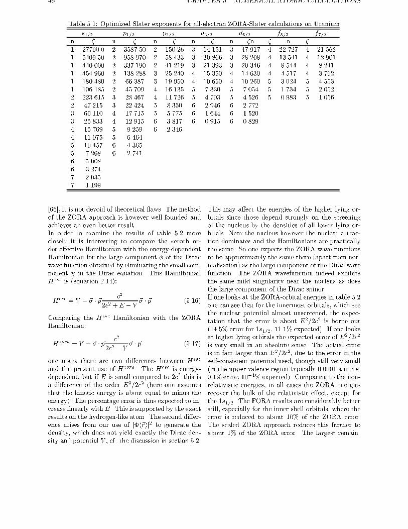
46 CHAPTER 5. NUMERICAL ATOMIC CALCULATIONS
Table 5.1: Optimized Slater exponents for all-electron ZORA-Slater calculations on Uranium
s1=2 p1=2 p3=2 d3=2 d5=2 f5=2 f7=2n � n � n � n � n �n � n �
1 27700.0 2 3587.50 2 150.26 3 64.151 3 47.917 4 22.727 4 21.562
1 5409.50 2 958.970 2 58.433 3 30.866 3 28.208 4 13.541 4 12.901
1 440.000 2 337.190 2 41.219 3 21.393 3 20.346 4 8.544 4 8.241
1 454.960 2 138.288 3 25.240 4 15.350 4 14.630 4 4.517 4 3.792
1 180.480 2 66.387 3 19.950 4 10.650 4 10.260 5 3.024 5 4.553
1 106.185 2 45.709 4 16.135 5 7.330 5 7.054 5 1.734 5 2.052
2 223.615 3 28.467 4 11.726 5 4.703 5 4.526 5 0.983 5 1.056
2 47.215 3 22.424 5 8.350 6 2.946 6 2.772
3 60.110 4 17.715 5 5.775 6 1.644 6 1.520
3 25.833 4 12.915 6 3.817 6 0.915 6 0.829
4 15.769 5 9.259 6 2.346
4 11.075 5 6.464
5 10.457 6 4.365
5 7.268 6 2.741
6 5.008
6 3.274
7 2.035
7 1.199
[66], it is not devoid of theoretical aws. The method
of the ZORA approach is however well founded and
achieves an even better result.
In order to examine the results of table 5.2 more
closely it is interesting to compare the zeroth or-
der e�ective Hamiltonian with the energy-dependent
Hamiltonian for the large component � of the Dirac
wave function obtained by eliminating the small com-
ponent � in the Dirac equation. This Hamiltonian
Hesc is (equation 2.14):
Hesc = V + ~� � ~pc2
2c2 +E � V~� � ~p (5.16)
Comparing the Hesc Hamiltonian with the ZORA
Hamiltonian:
Hzora = V + ~� � ~pc2
2c2 � V~� � ~p (5.17)
one notes there are two di�erences between Hesc
and the present use of Hzora. The Hesc is energy-
dependent, but if E is small compared to 2c2 this isa di�erence of the order E2=2c2 (here one assumes
that the kinetic energy is about equal to minus the
energy). The percentage error is thus expected to in-
crease linearly with E. This is supported by the exactresults on the hydrogen-like atom. The second di�er-
ence arises from our use of j�(~r)j2 to generate the
density, which does not yield exactly the Dirac den-
sity and potential V , cf. the discussion in section 5.2.
This may a�ect the energies of the higher lying or-
bitals since those depend strongly on the screening
of the nucleus by the densities of all lower lying or-
bitals. Near the nucleus however the nuclear attrac-
tion dominates and the Hamiltonians are practically
the same. So one expects the ZORA wave functions
to be approximately the same there (apart from nor-
malisation) as the large component of the Dirac wave
function. The ZORA wavefunction indeed exhibits
the same mild singularity near the nucleus as does
the large component of the Dirac spinor.
If one looks at the ZORA-orbital energies in table 5.2
one can see that for the innermost orbitals, which see
the nuclear potential almost unscreened, the expec-
tation that the error is about E2=2c2 is borne out
(14.5% error for 1s1=2, 11.1% expected). If one looks
at higher lying orbitals the expected error of E2=2c2
is very small in an absolute sense. The actual error
is in fact larger than E2=2c2, due to the error in the
self-consistent potential used, though still very small
(in the upper valence region typically 0.0001 a.u. i.e.
0.1% error, 10�4% expected). Comparing to the non-
relativistic energies, in all cases the ZORA energies
recover the bulk of the relativistic e�ect, except for
the 1s1=2. The FORA results are considerably better
still, especially for the inner shell orbitals, where the
error is reduced to about 10% of the ZORA error.
The scaled ZORA approach reduces this further to
about 1% of the ZORA error. The largest remain-
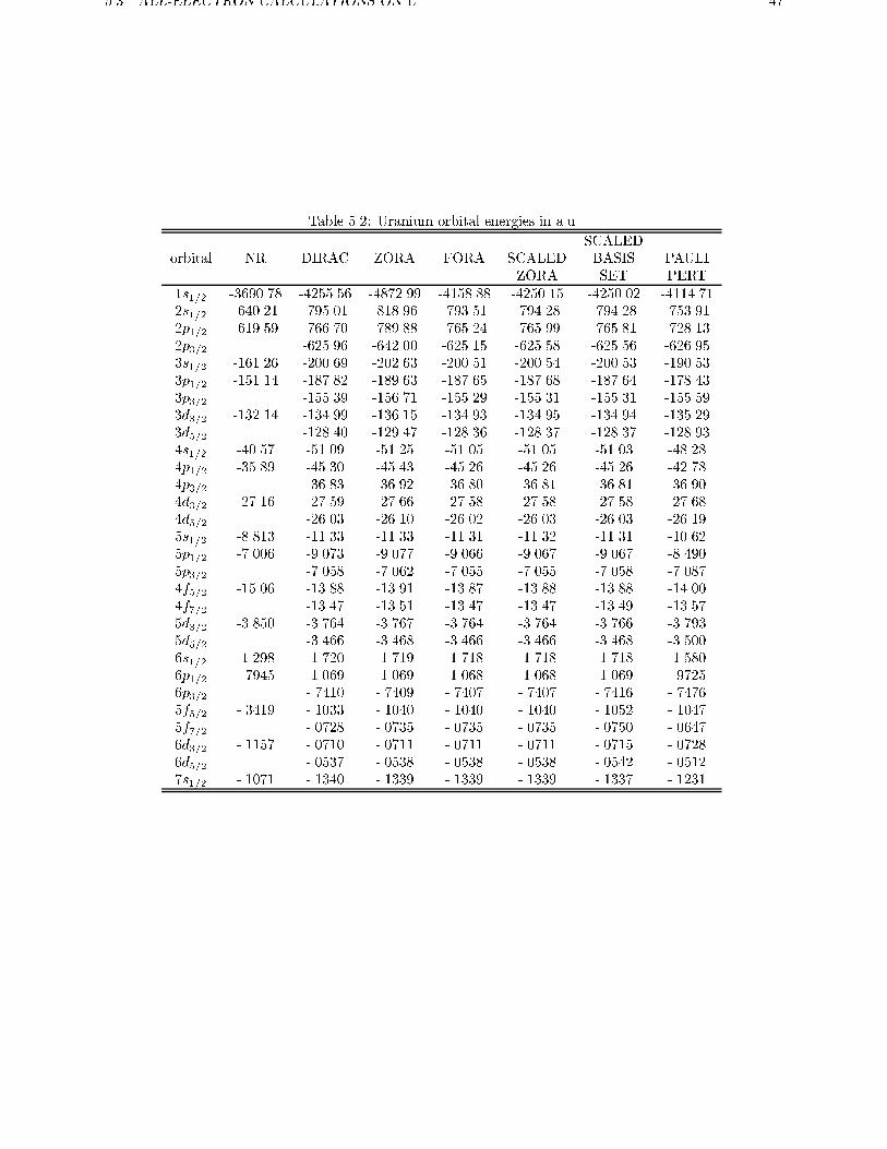
5.3. ALL-ELECTRON CALCULATIONS ON U 47
Table 5.2: Uranium orbital energies in a.u.
SCALED
orbital NR DIRAC ZORA FORA SCALED BASIS PAULI
ZORA SET PERT
1s1=2 -3690.78 -4255.56 -4872.99 -4158.88 -4250.15 -4250.02 -4114.71
2s1=2 -640.21 -795.01 -818.96 -793.51 -794.28 -794.28 -753.91
2p1=2 -619.59 -766.70 -789.88 -765.24 -765.99 -765.81 -728.13
2p3=2 -625.96 -642.00 -625.15 -625.58 -625.56 -626.95
3s1=2 -161.26 -200.69 -202.63 -200.51 -200.54 -200.53 -190.53
3p1=2 -151.14 -187.82 -189.63 -187.65 -187.68 -187.64 -178.43
3p3=2 -155.39 -156.71 -155.29 -155.31 -155.31 -155.59
3d3=2 -132.14 -134.99 -136.15 -134.93 -134.95 -134.94 -135.29
3d5=2 -128.40 -129.47 -128.36 -128.37 -128.37 -128.93
4s1=2 -40.57 -51.09 -51.25 -51.05 -51.05 -51.03 -48.28
4p1=2 -35.89 -45.30 -45.43 -45.26 -45.26 -45.26 -42.78
4p3=2 -36.83 -36.92 -36.80 -36.81 -36.81 -36.90
4d3=2 -27.16 -27.59 -27.66 -27.58 -27.58 -27.58 -27.68
4d5=2 -26.03 -26.10 -26.02 -26.03 -26.03 -26.19
5s1=2 -8.813 -11.33 -11.33 -11.31 -11.32 -11.31 -10.62
5p1=2 -7.006 -9.073 -9.077 -9.066 -9.067 -9.067 -8.490
5p3=2 -7.058 -7.062 -7.055 -7.055 -7.058 -7.087
4f5=2 -15.06 -13.88 -13.91 -13.87 -13.88 -13.88 -14.00
4f7=2 -13.47 -13.51 -13.47 -13.47 -13.49 -13.57
5d3=2 -3.850 -3.764 -3.767 -3.764 -3.764 -3.766 -3.793
5d5=2 -3.466 -3.468 -3.466 -3.466 -3.468 -3.500
6s1=2 -1.298 -1.720 -1.719 -1.718 -1.718 -1.718 -1.580
6p1=2 -.7945 -1.069 -1.069 -1.068 -1.068 -1.069 -.9725
6p3=2 -.7410 -.7409 -.7407 -.7407 -.7416 -.7476
5f5=2 -.3419 -.1033 -.1040 -.1040 -.1040 -.1052 -.1047
5f7=2 -.0728 -.0735 -.0735 -.0735 -.0750 -.0647
6d3=2 -.1157 -.0710 -.0711 -.0711 -.0711 -.0715 -.0728
6d5=2 -.0537 -.0538 -.0538 -.0538 -.0542 -.0512
7s1=2 -.1071 -.1340 -.1339 -.1339 -.1339 -.1337 -.1231
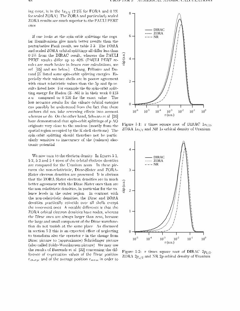
48 CHAPTER 5. NUMERICAL ATOMIC CALCULATIONS
ing error, is in the 1s1=2 (2.2% for FORA and 0.1%
for scaled ZORA). The ZORA and particularly scaled
ZORA results are much superior to the PAULI PERT
ones.
If one looks at the spin-orbit splittings the regu-
lar Hamiltonians give much better results than the
perturbative Pauli result, see table 5.3. The FORA
and scaled ZORA orbital splittings all di�er less than
0.5% from the DIRAC result, whereas the PAULI
PERT results di�er up to 40% (PAULI PERT re-
sults are much better in frozen core calculations, see
ref. [65] and see below). Chang, P�elissier and Du-
rand [5] listed some spin-orbit splitting energies. Es-
pecially their valence shells are in poorer agreement
with exact relativistic values than the 5p and 6p re-
sults listed here. For example the 6p spin-orbit split-
ting energy for Radon (Z=86) is in their work 0.123
a.u. compared to 0.156 for the exact value. The
less accurate results for the valence orbital energies
can possibly be understood from the fact that these
authors did not take screening e�ects into account
whereas we do. On the other hand, Schwarz et al. [26]
have demonstrated that spin-orbit splittings of p AOoriginate very close to the nucleus (mostly from the
spatial region occupied by the K shell electrons). The
spin-orbit splitting should therefore not be partic-
ularly sensitive to inaccuracy of the (valence) elec-
tronic potential.
We now turn to the electron density. In �gures 5.1,
5.2, 5.3 and 5.4 some of the orbital electron densities
are compared for the Uranium atom. In these pic-
tures the non-relativistic, Dirac-Slater and ZORA-
Slater electron densities are presented. It is obvious
that the ZORA-Slater electron densities are in much
better agreement with the Dirac-Slater ones than are
the non-relativistic densities, in particular for the va-
lence levels in the outer region. In contrast with
the non-relativistic densities, the Dirac and ZORA
densities practically coincide over all shells except
the innermost ones. A notable di�erence is that the
ZORA orbital electron densities have nodes, whereas
the Dirac ones are always larger than zero, because
the large and small component of the Dirac wavefunc-
tion do not vanish at the same place. As discussed
in section 5.2 this is an expected e�ect of neglecting
to transform also the operator r in the change from
Dirac picture to (approximate) Schr�odinger picture
(also called Foldy-Wouthuysen picture). We may use
the results of Baerends et al. [32] concerning the dif-
ference of expectation values of the Dirac position
rcharge and of the average position rmass in order to
8
6
4
2
0
ràρ
(a.u
.)
10-6 10-5 10-4 10-3 10-2 10-1 100
r (a.u.)
DIRAC ZORA NR
Figure 5.1: r times square root of DIRAC 1s1=2,ZORA 1s1=2 and NR 1s orbital density of Uranium
4
3
2
1
0
ràρ
(a.u
.)
10-5 10-4 10-3 10-2 10-1 100
r (a.u.)
DIRAC ZORA NR
Figure 5.2: r times square root of DIRAC 2p1=2,ZORA 2p1=2 and NR 2p orbital density of Uranium
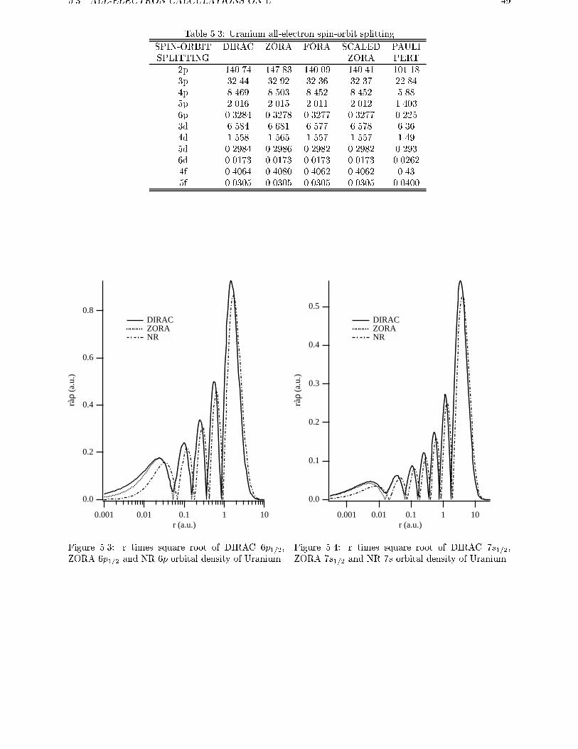
5.3. ALL-ELECTRON CALCULATIONS ON U 49
Table 5.3: Uranium all-electron spin-orbit splitting
SPIN-ORBIT DIRAC ZORA FORA SCALED PAULI
SPLITTING ZORA PERT
2p 140.74 147.83 140.09 140.41 101.18
3p 32.44 32.92 32.36 32.37 22.84
4p 8.469 8.503 8.452 8.452 5.88
5p 2.016 2.015 2.011 2.012 1.403
6p 0.3284 0.3278 0.3277 0.3277 0.225
3d 6.584 6.681 6.577 6.578 6.36
4d 1.558 1.565 1.557 1.557 1.49
5d 0.2984 0.2986 0.2982 0.2982 0.293
6d 0.0173 0.0173 0.0173 0.0173 0.0262
4f 0.4064 0.4080 0.4062 0.4062 0.43
5f 0.0305 0.0305 0.0305 0.0305 0.0400
0.8
0.6
0.4
0.2
0.0
ràρ
(a.u
.)
0.001 0.01 0.1 1 10r (a.u.)
DIRAC ZORA NR
Figure 5.3: r times square root of DIRAC 6p1=2,ZORA 6p1=2 and NR 6p orbital density of Uranium
0.5
0.4
0.3
0.2
0.1
0.0
ràρ
(a.u
.)
0.001 0.01 0.1 1 10r (a.u.)
DIRAC ZORA NR
Figure 5.4: r times square root of DIRAC 7s1=2,ZORA 7s1=2 and NR 7s orbital density of Uranium
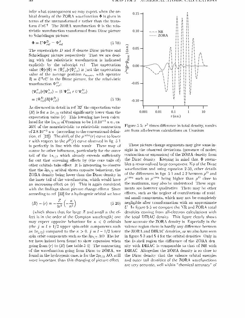
50 CHAPTER 5. NUMERICAL ATOMIC CALCULATIONS
infer what consequences we may expect when the or-
bital density of the ZORA wavefunction � is given in
terms of the untransformed r rather than the trans-
form UrU y. The ZORA wavefunction � is the rela-
tivistic wavefunction transformed from Dirac picture
to Schr�odinger picture:
� = UDrel � S
rel (5.18)
The superscripts D and S denote Dirac picture and
Schr�odinger picture respectively. That we are deal-
ing with the relativistic wavefunction is indicated
explicitly by the subscript rel. The expectation
value h�jrj�i = hSreljrj
Sreli is just the expectation
value of the average position rmass, with operator
R = U yrU in the Dirac picture, for the relativistic
wavefunction Drel:
hSreljrj
Sreli = hUD
reljrjUDreli
= hDreljRj
Dreli (5.19)
As discussed in detail in ref [32] the expectation value
hRi is for a 1s1=2 orbital signi�cantly lower than the
expectation value hri. This lowering has been calcu-
lated for the 1s1=2 of Uranium to be 1:0:10�3 a.u., ca.36% of the nonrelativistic to relativistic contraction
of 2:8:10�3 a.u. (according to the conventional de�ni-tion, cf. [32]). The shift of the �zora(r) curve to lowerr with respect to the �D(r) curve observed in �g. 5.1
is perfectly in line with this result. There may of
course be other in uences, particularly for the outer
tail of the 1s1=2 which already extends su�ciently
far out that screening e�ects by (the core tails of)
other orbitals take e�ect. It is interesting to observe
that the 3p1=2 orbital shows opposite behaviour, theZORA density being lower than the Dirac density in
the inner tail of the wavefunction, which would have
an increasing e�ect on hri. This is again consistent
with the �ndings about picture change e�ects. Since
according to ref. [32] for a hydrogenic orbital we have
hRi � hri = �Z
4c2
���
n2
�(5.20)
(which shows that for large Z and small n the ef-
fect is in the order of the Compton wavelength) one
may expect opposite behaviour for � < 0 orbitals
(the j = l + 1=2 upper spin-orbit components such
as 1s1=2) compared to the � > 0, j = l � 1=2 lower
spin-orbit components such as the 3p1=2 AO. The lat-ter have indeed been found to show expansion when
going from hri to hRi (see table 5.4). The contractingof the wavefunction going from Dirac to ZORA, we
found in the hydrogenic case, is for the 2p1=2 AO, stillmore important than this changing of picture e�ect.
0.15
0.10
0.05
0.00
-0.05
-0.10
r3 *(ρ−
ρ dir
ac )
(a.u
.)
0.001 0.01 0.1 1 10r (a.u.)
NR ZORA
Figure 5.5: r3 times di�erence in total density, resultsare from all-electron calculations on Uranium
These picture change arguments may give some in-
sight in the observed deviations (presence of nodes;
contraction or expansion) of the ZORA density from
the Dirac density. Keeping in mind that � resem-
bles a renormalized large component N� of the Dirac
wavefunction and using equation 2.50, other details
of the di�erences in �gs. 5.1 and 5.2 between �D and
�zora such as �zora being higher than �D close to
the maximum, may also be understood. These argu-
ments are however qualitative. There may be other
e�ects, such as the neglect of contributions of resid-
ual small components, which may not be completely
negligible after transformation with an approximate
U . In �gure 5.5 we compare the NR and ZORA total
densities coming from all-electron calculations with
the total DIRAC density. This �gure clearly shows
how accurate the ZORA density is. Especially in the
valence region there is hardly any di�erence between
the ZORA and DIRAC densities, as we also have seen
in �gure 5.3 and 5.4 for the orbital densities. Only in
the 1s-shell region the di�erence of the ZORA den-
sity with DIRAC is comparable to that of NR with
DIRAC. Altogether the ZORA density is so close to
the Dirac density that the valence orbital energies
and outer tail densities of the ZORA wavefunctions
are very accurate, well within "chemical accuracy" of
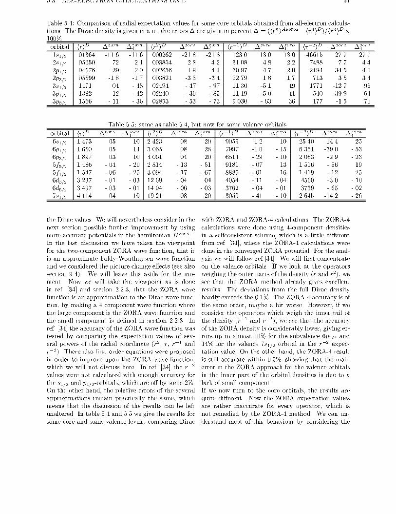
5.3. ALL-ELECTRON CALCULATIONS ON U 51
Table 5.4: Comparison of radial expectation values for some core orbitals obtained from all-electron calcula-
tions. The Dirac density is given in a.u., the errors � are given in percent � = (hrniApprox�hrniD)=hrniD�100%
orbital hriD �zora �zora4 hr2iD �zora �zora
4 hr�1iD �zora �zora4 hr�2iD �zora �zora
4
1s1=2 .01364 -11.6 -11.6 .000262 -21.8 -21.8 123.0 13.0 13.0 46615 27.7 27.7
2s1=2 .05650 -.72 -2.1 .003854 -2.8 -4.2 31.08 -4.8 2.2 7488 -7.7 4.4
2p1=2 .04576 -.29 -2.0 .002656 -1.9 -4.1 30.97 -4.7 2.0 2194 -34.5 4.0
2p3=2 .05599 -1.8 -1.7 .003821 -3.5 -3.4 22.79 1.8 1.7 713 3.5 3.4
3s1=2 .1471 .04 -.48 .02494 -.47 -.97 11.30 -5.1 .49 1771 -12.7 .96
3p1=2 .1382 .12 -.42 .02240 -.30 -.85 11.19 -5.0 .41 540 -39.9 .64
3p3=2 .1566 -.11 -.36 .02853 -.53 -.73 9.030 -.63 .36 177 -1.5 .70
Table 5.5: same as table 5.4, but now for some valence orbitals.
orbital hriD �zora �zora4 hr2iD �zora �zora
4 hr�1iD �zora �zora4 hr�2iD �zora �zora
4
6s1=2 1.473 .05 .10 2.423 .08 .20 .9059 -1.2 -.10 25.40 -14.4 -.25
6p1=2 1.650 .05 .14 3.065 .08 .28 .7997 -1.0 -.15 6.351 -39.0 -.53
6p3=2 1.897 .03 .10 4.061 .04 .20 .6814 -.29 -.10 2.063 -2.9 -.23
5f5=2 1.486 -.04 -.20 2.814 -.13 -.51 .9181 -.07 .13 1.516 -.56 .19
5f7=2 1.547 -.06 -.25 3.094 -.17 -.67 .8885 -.01 .16 1.419 -.12 .25
6d3=2 3.237 -.01 -.03 12.69 -.04 .04 .4054 -.11 -.04 .4560 -3.0 -.10
6d5=2 3.497 -.03 -.01 14.94 -.06 -.03 .3762 -.04 -.01 .3739 -.65 -.02
7s1=2 4.114 .04 .10 19.21 .08 .20 .3059 -.41 -.10 2.645 -14.2 -.26
the Dirac values. We will nevertheless consider in the
next section possible further improvement by using
more accurate potentials in the hamiltonian Hzora.
In the last discussion we have taken the viewpoint
for the two-component ZORA wave function, that it
is an approximate Foldy-Wouthuysen wave function
and we considered the picture change e�ects (see also
section 9.4). We will leave this aside for the mo-
ment. Now we will take the viewpoint as is done
in ref. [34] and section 2.2.3, that the ZORA wave
function is an approximation to the Dirac wave func-
tion, by making a 4-component wave function where
the large component is the ZORA wave function and
the small component is de�ned in section 2.2.3. In
ref. [34] the accuracy of the ZORA wave function was
tested by comparing the expectation values of sev-
eral powers of the radial coordinate (r2, r, r�1 and
r�2). There also �rst order equations were proposedin order to improve upon the ZORA wave function,
which we will not discuss here. In ref. [34] the r�2
values were not calculated with enough accuracy for
the s1=2 and p1=2-orbitals, which are o� by some 2%.
On the other hand, the relative errors of the several
approximations remain practically the same, which
means that the discussion of the results can be left
unaltered. In table 5.4 and 5.5 we give the results for
some core and some valence levels, comparing Dirac
with ZORA and ZORA-4 calculations. The ZORA-4
calculations were done using 4-component densities
in a selfconsistent scheme, which is a little di�erent
from ref. [34], where the ZORA-4 calculations were
done in the converged ZORA potential. For the anal-
ysis we will follow ref.[34]. We will �rst concentrate
on the valence orbitals. If we look at the operators
weighing the outer parts of the density (r and r2), wesee that the ZORA method already gives excellent
results. The deviations from the full Dirac density
hardly exceeds the 0.1%. The ZORA-4 accuracy is of
the same order, maybe a bit worse. However, if we
consider the operators which weigh the inner tail of
the density (r�1 and r�2), we see that the accuracyof the ZORA density is considerably lower, giving er-
rors up to almost 40% for the subvalence 6p1=2 and
14% for the valence 7s1=2 orbital in the r�2 expec-
tation value. On the other hand, the ZORA-4 result
is still accurate within 0.5%, showing that the main
error in the ZORA approach for the valence orbitals
in the inner part of the orbital densities is due to a
lack of small component.
If we now turn to the core orbitals, the results are
quite di�erent. Now the ZORA expectation values
are rather inaccurate for every operator, which is
not remedied by the ZORA-4 method. We can un-
derstand most of this behaviour by considering the
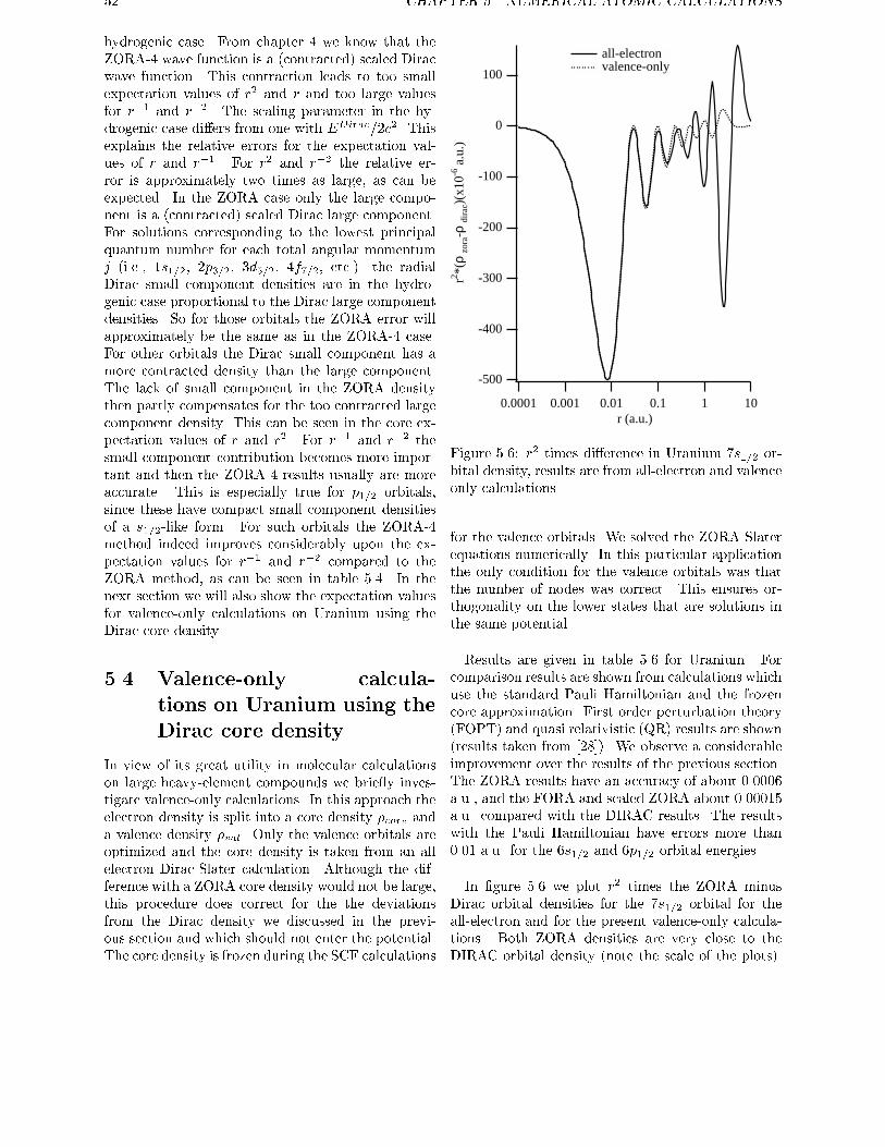
52 CHAPTER 5. NUMERICAL ATOMIC CALCULATIONS
hydrogenic case. From chapter 4 we know that the
ZORA-4 wave function is a (contracted) scaled Dirac
wave function. This contraction leads to too small
expectation values of r2 and r and too large values
for r�1 and r�2. The scaling parameter in the hy-
drogenic case di�ers from one with EDirac=2c2. Thisexplains the relative errors for the expectation val-
ues of r and r�1. For r2 and r�2 the relative er-
ror is approximately two times as large, as can be
expected. In the ZORA case only the large compo-
nent is a (contracted) scaled Dirac large component.
For solutions corresponding to the lowest principal
quantum number for each total angular momentum
j (i.e., 1s1=2, 2p3=2, 3d5=2, 4f7=2, etc.) the radial
Dirac small component densities are in the hydro-
genic case proportional to the Dirac large component
densities. So for those orbitals the ZORA error will
approximately be the same as in the ZORA-4 case.
For other orbitals the Dirac small component has a
more contracted density than the large component.
The lack of small component in the ZORA density
then partly compensates for the too contracted large
component density. This can be seen in the core ex-
pectation values of r and r2. For r�1 and r�2 the
small component contribution becomes more impor-
tant and then the ZORA-4 results usually are more
accurate. This is especially true for p1=2 orbitals,
since these have compact small component densities
of a s1=2-like form. For such orbitals the ZORA-4
method indeed improves considerably upon the ex-
pectation values for r�1 and r�2 compared to the
ZORA method, as can be seen in table 5.4. In the
next section we will also show the expectation values
for valence-only calculations on Uranium using the
Dirac core density.
5.4 Valence-only calcula-
tions on Uranium using the
Dirac core density
In view of its great utility in molecular calculations
on large heavy-element compounds we brie y inves-
tigate valence-only calculations. In this approach the
electron density is split into a core density �core anda valence density �val. Only the valence orbitals are
optimized and the core density is taken from an all
electron Dirac-Slater calculation. Although the dif-
ference with a ZORA core density would not be large,
this procedure does correct for the the deviations
from the Dirac density we discussed in the previ-
ous section and which should not enter the potential.
The core density is frozen during the SCF calculations
-500
-400
-300
-200
-100
0
100
r2 *(ρ
zora
-ρ di
rac)
(x10
-6 a
.u.)
0.0001 0.001 0.01 0.1 1 10r (a.u.)
all-electron valence-only
Figure 5.6: r2 times di�erence in Uranium 7s1=2 or-bital density, results are from all-electron and valence
only calculations
for the valence orbitals. We solved the ZORA-Slater
equations numerically. In this particular application
the only condition for the valence orbitals was that
the number of nodes was correct. This ensures or-
thogonality on the lower states that are solutions in
the same potential.
Results are given in table 5.6 for Uranium. For
comparison results are shown from calculations which
use the standard Pauli Hamiltonian and the frozen
core approximation. First order perturbation theory
(FOPT) and quasi relativistic (QR) results are shown
(results taken from [28]). We observe a considerable
improvement over the results of the previous section.
The ZORA results have an accuracy of about 0.0006
a.u., and the FORA and scaled ZORA about 0.00015
a.u. compared with the DIRAC results. The results
with the Pauli Hamiltonian have errors more than
0.01 a.u. for the 6s1=2 and 6p1=2 orbital energies.
In �gure 5.6 we plot r2 times the ZORA minus
Dirac orbital densities for the 7s1=2 orbital for the
all-electron and for the present valence-only calcula-
tions. Both ZORA densities are very close to the
DIRAC orbital density (note the scale of the plots).
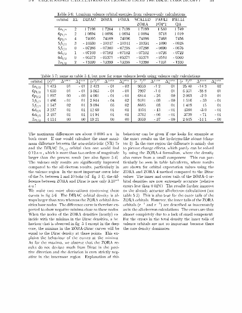
5.4. VALENCE-ONLY CALCULATIONS ON URANIUM USING THE DIRAC CORE DENSITY 53
Table 5.6: Uranium valence orbital energies from valence-only calculations
orbital EL DIRAC ZORA FORA SCALED PAULI PAULI
ZORA FOPT QR
6s1=2 2 -1.7198 -1.7204 -1.7199 -1.7199 -1.580 -1.749
6p1=2 2 -1.0694 -1.0696 -1.0694 -1.0694 -.9718 -1.019
6p3=2 4 -.74095 -.74109 -.74096 -.74096 -.7468 -.7456
5f5=2 3 -.10330 -.10347 -.10344 -.10334 -.1090 -.0928
5f7=2 0 -.07286 -.07300 -.07298 -.07298 -.0690 -.0676
6d3=2 1 -.07103 -.07102 -.07102 -.07102 -.0726 -.0722
6d5=2 0 -.05373 -.05371 -.05371 -.05371 -.0510 -.0560
7s1=2 2 -.13399 -.13399 -.13398 -.13398 -.1231 -.1330
Table 5.7: same as table 5.4, but now for some valence levels using valence only calculations.
orbital hriD �zora �zora4 hr2iD �zora �zora
4 hr�1iD �zora �zora4 hr�2iD �zora �zora
4
6s1=2 1.473 .01 -.01 2.423 -.01 -.02 .9059 -1.2 .01 25.40 -14.3 .02
6p1=2 1.650 .01 -.01 3.065 -.01 -.01 .7997 -1.0 .01 6.351 -38.8 .01
6p3=2 1.897 .00 -.00 4.061 -.01 -.01 .6814 -.26 .00 2.063 -2.9 .01
5f5=2 1.486 -.01 .01 2.814 -.04 .02 .9181 -.09 -.00 1.516 -.59 -.01
5f7=2 1.547 -.02 .01 3.094 -.05 .02 .8885 -.03 -.01 1.419 -.15 -.01
6d3=2 3.237 .01 .01 12.69 .01 .01 .4054 -.13 -.01 .4560 -3.0 -.01
6d5=2 3.497 .01 .01 14.94 .01 .01 .3762 -.06 -.01 .3739 -.71 -.01
7s1=2 4.114 .00 .00 19.21 .00 .00 .3059 -.37 -.00 2.645 -14.1 -.00
The maximum di�erences are about 0.0005 a.u. in
both cases. If one would calculate the same maxi-
mum di�erence between the non-relativistic (NR) 7sand the DIRAC 7s1=2 orbital then one would �nd
0.12 a.u., which is more than two orders of magnitude
larger than the present result (see also �gure 5.4).
The valence-only results are signi�cantly improved
compared to the all-electron results, particularly in
the valence region. In the most important outer lobe
of the 7s, between 1 and 10 bohr (cf. �g. 5.4), the dif-ference between ZORA and Dirac is now only 3:10�5
a.u.!
We make two more observations concerning these
curves in �g 5.6. The DIRAC orbital density is al-
ways larger than zero whereas the ZORA orbital den-
sities have nodes. The di�erence curve is therefore ex-
pected to show negative minima close to these nodes.
When the nodes of the ZORA densities (nearly) co-
incide with the minima in the Dirac densities, a be-
haviour that is observed in �g. 5.4 except in the deep
core, the minima in the ZORA-Dirac curves will be
equal to the Dirac density at those points. This ex-
plains the behaviour of the curves at the minima.
As for the maxima, we observe that the ZORA re-
sults do not deviate much from Dirac in the posi-
tive direction and the deviation is even strictly neg-
ative in the innermost region. Explanation of this
behaviour can be given if one looks for example at
the exact results on the hydrogen-like atoms (chap-
ter 4). In the core region the di�erence is mainly due
to picture change e�ects, which partly can be solved
by using the ZORA-4 formalism, where the density
also comes from a small component. This can par-
ticularly be seen in table tab:ufcvrn, where results
are shown for orbital expectation values using the
ZORA and ZORA-4 method compared to the Dirac
values. The inner and outer tails of the ZORA-4 or-
bital densities are now extremely accurate (relative
errors less than 0.02%). The results further improve
on the already accurate all-electron calculations (see
table 5.5). This is also true for the outer tails of the
ZORA orbitals. However, the inner tails of the ZORA
orbitals (r�1 and r�2) are described as inaccurately
as in the all-electron calculations. The errors are thus
almost completely due to a lack of small component.
For the errors in the total density the inner tails of
valence orbitals are not so important because there
the core density dominates.
54 CHAPTER 5. NUMERICAL ATOMIC CALCULATIONS
Chapter 6
Implementation of ZORA
6.1 Implementation of ZORA
in ADF
The ADF (Amsterdam Density Functional) program
is a program that can perform electronic structure
calculations on molecular systems. It performs self
consistent �eld calculations using density functional
theory, solving the so called one-electron Kohn-Sham
equations. The calculations are done using a Slater
type orbital (STO) basis set. To solve the SR ZORA
and ZORA Kohn-Sham equations one needs to cal-
culate some matrix elements di�erently than in non-
relativistic theory. In the SR ZORA equations the
only di�erence is the calculation of the kinetic energy
matrix. In ADF matrix elements are calculated by
numerical integration. Use is made of the point group
symmetry of the molecule. In the non-relativistic and
scalar relativistic case the basis functions form an or-
thonormalised set of single group symmetry adapted
functions. In the ADF program the derivatives of the
basis functions with respect to the Cartesian coor-
dinates (@=@x; @=@y; @=@z) are calculated in the rel-
ativistic case, which can be done easily for STO's.
The SR ZORA kinetic energy matrix is then calcu-
lated numerically, between basisfunction �i and �jas:
h�ijT zorasr j�ji = h�ij~pc2
2c2 � V~pj�ji =
Xk
h@�i
@xkj
c2
2c2 � Vj@�j
@xki (6.1)
where in the last step partial integration is used. For
the potential in the ZORA kinetic energy matrix two
possibilities are implemented. One can either use
the frozen core potential, which means that one only
has to calculate this matrix once, or one can use the
full potential, which means that in every cycle in the
SCF scheme this matrix has to be calculated. In sec-
tion 6.1.1 we will show the di�erences between these
possibilities in an example.
In the ZORA case, which includes spin-orbit, double
group symmetry adapted functions have to be used.
In this case one needs apart from the SR ZORA ki-
netic energy, also the ZORA spin-orbit matrix. In
terms of double group symmetry adapted functions
�di and �dj (two-component functions), the ZORA
spin-orbit matrix is:
h�di jHzoraso j�dj i = h�di j
c2
(2c2 � V )2~� � (~rV � ~p)j�dj i
= h�di j~� � ~r(c2
2c2 � V)� ~p)j�dj i =
h�di j~� � ~r(V
4c2 � 2V)� ~p)j�dj i =
iXlmn
�lmnh@�di@xm
j�lV
4c2 � 2Vj@�dj@xn
i (6.2)
where again in the last step partial integration is
used. A double group symmetry adapted functions
can be written as a spatial function times spin � plus
a spatial function times spin �:
�di (~r; s) = ��i (~r)� + ��i (~r)� (6.3)
The spin integration can be done easily using the
Pauli spin matrices. The spatial integration one still
has to do is then of the form:
iXmn
�lmnh@�i@xm
jV
4c2 � 2Vj@�j@xn
i (6.4)
Again two possibilities for the potential are imple-
mented. One can either use the frozen core potential,
which means that one only has to calculate this spin-
orbit matrix once, or one can use the full potential,
which means that in every cycle in the SCF scheme
this spin-orbit matrix has to be calculated.
The actual implementation of double group symme-
try in ADF is done along the lines of Snijders [67]. All
55
56 CHAPTER 6. IMPLEMENTATION OF ZORA
symmetry arguments using the Pauli Hamiltonian,
which are used in ref [67] remain valid for the ZORA
Hamiltonians, we will not repeat them here. In the
Pauli approximation one needs to calculate spin-orbit
matrix elements of the form:
iXmn
�lmnh@�i@xm
jV
4c2j@�j@xn
i (6.5)
Compared to this matrix, the ZORA spin-orbit ma-
trix is regularised by the potential in the numerator,
which makes it e�ectively a 1=r potential close to a
nuclues, whereas the Pauli spin-orbit behaves like a
1=r3 potential.For the calculation of the scaled SR ZORA orbital
energies (see equation 3.9) we need matrix elements
of the form:
h�ij~pc2
(2c2 � V )2~pj�ji =
Xk
h@�i@xk
jc2
(2c2 � V )2j@�j@xk
i (6.6)
For the calculation of the scaled ZORA orbital en-
ergies (see equation 3.4) we need matrix elements of
the form:
h�di j~� � ~pc2
(2c2 � V )2~� � ~pj�dj i =
h�di j~pc2
(2c2 � V )2~pj�dj i+
h�di j~� � ~r(c2
(2c2 � V )2)� ~p)j�dj i (6.7)
The �rst term we already have in the SR ZORA case.
The last term can be written as (the gradient of a
constant is zero):
h�di j~� � ~r(c2
(2c2 � V )2)� ~p)j�dj i =
h�di j~� � ~r(V (4c2 � V )
4c2(2c2 � V )2)� ~p)j�dj i =
iXlmn
�lmnh@�di@xm
j�lV (4c2 � V )
4c2(2c2 � V )2j@�dj@xn
i (6.8)
These matrix elements, needed in the scaled (SR)
ZORA case, are not more di�cult to calculate than
the ones we needed for the (SR) ZORA kinetic energy.
The scaled (SR) ZORA orbital energies only have to
be calculated once, after selfconsistency is reached, so
we also have to calculate these matrix elements only
once.
The scaled orbital energies are not used for the cal-
culation of di�erences in energies. For this we use the
(SR) ZORA ESA method described in some detail in
section 3.5, because it is an easy and accurate way.
6.1.1 The frozen core approximation
In ADF usually the frozen core approximation is
used. In this program the frozen core approximation
in the ZORA case (incuding spin-orbit) is not (yet)
implemented. One core orthogonalisation function,
a Slater-type orbital (STO), per core orbital is used
to orhogonalise the basis function on the accurately
calculated core orbitals, coming from atomic calcu-
lations. In general the NR core orbitals are not the
same as scalar relativistic ZORA core orbitals, which
are again di�erent to fully relativistic ZORA (includ-
ing spin-orbit coupling) core orbitals. The most op-
timal core orthogonalisation functions will also di�er
whether one uses NR, SR ZORA or ZORA. In the NR
case the core wiggles of the valence functions can ac-
curately be described by the core orthogonalisations
function, such that one does not need core-like ba-
sis functions to get an accuracy of a few milli atomic
units. On the other hand, in SR ZORA and ZORA
one does need extra core-like basis functions, to get
such high accuracy for the heavier systems. This is
due to the fact that the core wiggles of especially
the s-type valence electrons do not behave like Slater
type orbitals near the nucleus, but more like Dirac
type orbitals which are of the form:
r��1e��r (6.9)
where � does not have to be an integer value. For
STO's � is an integer.
In the SR ZORA case the frozen core approxima-
tion is similar as in the NR case, because one can
use the same single group symmetry. The changes
one has to make are in order of importance the fol-
lowing. The description of the core orbitals should
come from SR ZORA calculations (one can use for
example a SR ZORA version of an atomic basis set
program), for heavier systems one needs to optimise
the STO's in the atomic calculations. The next step
is to optimise the core orthogonalisation functions to
the core wiggles of accurately calculated SR ZORA
valence orbitals for the given atom. A �nal step is to
optimise the valence basis functions. For the heavier
atoms one also should add basisfunctions, which are
able to describe the tail of the valence orbitals more
accurately. In the SR ZORA case it is often enough
to add only one extra 1s-type STO with large expo-
nent � to get an accuracy of a few milli atomic units
in the atomic orbital energies.
In table 6.1 we will show the e�ects if one uses
NR core functions to orthogonalise on in a SR ZORA
calculation. If we use the standard ADF IV basis set
(triple-� valence basis set) with a 5d frozen core, the
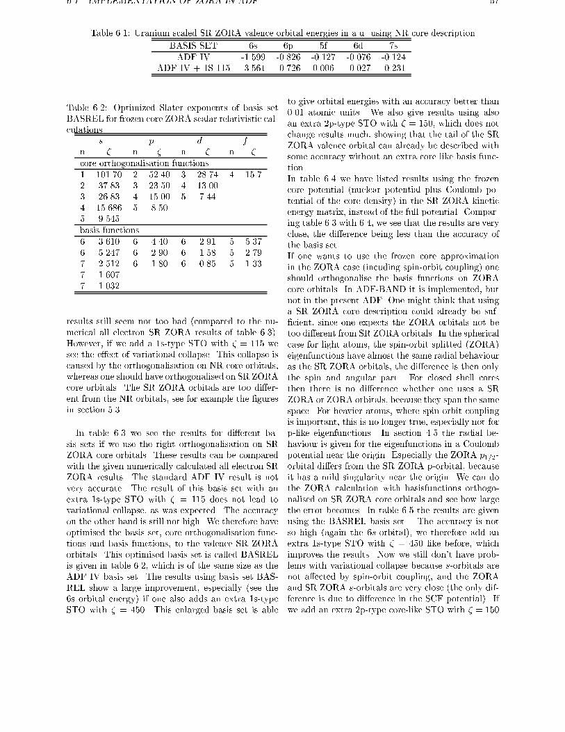
6.1. IMPLEMENTATION OF ZORA IN ADF 57
Table 6.1: Uranium scaled SR ZORA valence orbital energies in a.u. using NR core description
BASIS SET 6s 6p 5f 6d 7s
ADF IV -1.599 -0.826 -0.127 -0.076 -0.124
ADF IV + 1S 115 -3.561 -0.726 0.006 -0.027 -0.231
Table 6.2: Optimized Slater exponents of basis set
BASREL for frozen core ZORA scalar relativistic cal-
culations
s p d fn � n � n � n �
core orthogonalisation functions
1 101.70 2 52.40 3 28.74 4 15.7
2 37.83 3 23.50 4 13.00
3 26.83 4 15.00 5 7.44
4 15.686 5 8.50
5 9.545
basis functions
6 3.610 6 4.40 6 2.91 5 5.37
6 5.247 6 2.90 6 1.58 5 2.79
7 2.512 6 1.80 6 0.85 5 1.33
7 1.607
7 1.032
results still seem not too bad (compared to the nu-
merical all electron SR ZORA results of table 6.3).
However, if we add a 1s-type STO with � = 115 we
see the e�ect of variational collapse. This collapse is
caused by the orthogonalisation on NR core orbitals,
whereas one should have orthogonalised on SR ZORA
core orbitals. The SR ZORA orbitals are too di�er-
ent from the NR orbitals, see for example the �gures
in section 5.3.
In table 6.3 we see the results for di�erent ba-
sis sets if we use the right orthogonalisation on SR
ZORA core orbitals. These results can be compared
with the given numerically calculated all electron SR
ZORA results. The standard ADF IV result is not
very accurate. The result of this basis set with an
extra 1s-type STO with � = 115 does not lead to
variational collapse, as was expected. The accuracy
on the other hand is still not high. We therefore have
optimised the basis set, core orthogonalisation func-
tions and basis functions, to the valence SR ZORA
orbitals. This optimised basis set is called BASREL
is given in table 6.2, which is of the same size as the
ADF IV basis set. The results using basis set BAS-
REL show a large improvement, especially (see the
6s orbital energy) if one also adds an extra 1s-type
STO with � = 450. This enlarged basis set is able
to give orbital energies with an accuracy better than
0.01 atomic units. We also give results using also
an extra 2p-type STO with � = 150, which does not
change results much, showing that the tail of the SR
ZORA valence orbital can already be described with
some accuracy without an extra core like basis func-
tion.
In table 6.4 we have listed results using the frozen
core potential (nuclear potential plus Coulomb po-
tential of the core density) in the SR ZORA kinetic
energy matrix, instead of the full potential. Compar-
ing table 6.3 with 6.4, we see that the results are very
close, the di�erence being less than the accuracy of
the basis set.
If one wants to use the frozen core approximation
in the ZORA case (incuding spin-orbit coupling) one
should orthogonalise the basis functions on ZORA
core orbitals. In ADF-BAND it is implemented, but
not in the present ADF. One might think that using
a SR ZORA core description could already be suf-
�cient, since one expects the ZORA orbitals not be
too di�erent from SR ZORA orbitals. In the spherical
case for light atoms, the spin-orbit splitted (ZORA)
eigenfunctions have almost the same radial behaviour
as the SR ZORA orbitals, the di�erence is then only
the spin and angular part. For closed shell cores
then there is no di�erence whether one uses a SR
ZORA or ZORA orbitals, because they span the same
space. For heavier atoms, where spin-orbit coupling
is important, this is no longer true, especially not for
p-like eigenfunctions. In section 4.5 the radial be-
haviour is given for the eigenfunctions in a Coulomb
potential near the origin. Especially the ZORA p1=2-orbital di�ers from the SR ZORA p-orbital, because
it has a mild singularity near the origin. We can do
the ZORA calculation with basisfunctions orthogo-
nalised on SR ZORA core orbitals and see how large
the error becomes. In table 6.5 the results are given
using the BASREL basis set . The accuracy is not
so high (again the 6s-orbital), we therefore add an
extra 1s-type STO with � = 450 like before, which
improves the results. Now we still don't have prob-
lems with variational collapse because s-orbitals arenot a�ected by spin-orbit coupling, and the ZORA
and SR ZORA s-orbitals are very close (the only dif-ference is due to di�erence in the SCF potential). If
we add an extra 2p-type core-like STO with � = 150
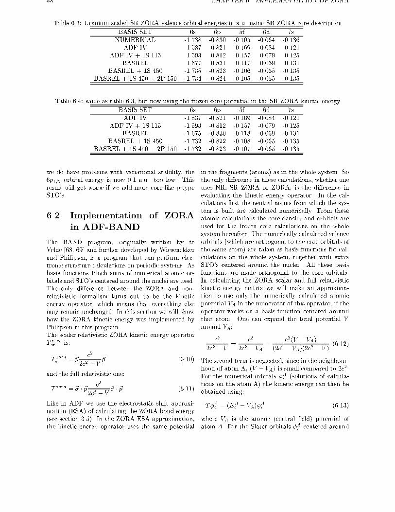
58 CHAPTER 6. IMPLEMENTATION OF ZORA
Table 6.3: Uranium scaled SR ZORA valence orbital energies in a.u. using SR ZORA core description
BASIS SET 6s 6p 5f 6d 7s
NUMERICAL -1.738 -0.830 -0.105 -0.064 -0.136
ADF IV -1.537 -0.821 -0.169 -0.084 -0.121
ADF IV + 1S 115 -1.593 -0.812 -0.157 -0.079 -0.125
BASREL -1.677 -0.831 -0.117 -0.069 -0.131
BASREL + 1S 450 -1.735 -0.823 -0.106 -0.065 -0.135
BASREL + 1S 450 + 2P 150 -1.734 -0.824 -0.105 -0.065 -0.135
Table 6.4: same as table 6.3, but now using the frozen core potential in the SR ZORA kinetic energy
BASIS SET 6s 6p 5f 6d 7s
ADF IV -1.537 -0.821 -0.169 -0.084 -0.121
ADF IV + 1S 115 -1.593 -0.812 -0.157 -0.079 -0.125
BASREL -1.675 -0.830 -0.118 -0.069 -0.131
BASREL + 1S 450 -1.732 -0.822 -0.108 -0.065 -0.135
BASREL + 1S 450 + 2P 150 -1.732 -0.823 -0.107 -0.065 -0.135
we do have problems with variational stability, the
6p1=2 orbital energy is now 0.1 a.u. too low. This
result will get worse if we add more core-like p-type
STO's.
6.2 Implementation of ZORA
in ADF-BAND
The BAND program, originally written by te
Velde [68, 69] and further developed by Wiesenekker
and Philipsen, is a program that can perform elec-
tronic structure calculations on periodic systems. As
basis functions Bloch sums of numerical atomic or-
bitals and STO's centered around the nuclei are used.
The only di�erence between the ZORA and non-
relativistic formalism turns out to be the kinetic
energy operator, which means that everything else
may remain unchanged. In this section we will show
how the ZORA kinetic energy was implemented by
Philipsen in this program.
The scalar relativistic ZORA kinetic energy operator
T zorasr is:
T zorasr = ~pc2
2c2 � V~p (6.10)
and the full relativistic one:
T zora = ~� � ~pc2
2c2 � V~� � ~p (6.11)
Like in ADF we use the electrostatic shift approxi-
mation (ESA) of calculating the ZORA bond energy
(see section 3.5). In the ZORA ESA approximation,
the kinetic energy operator uses the same potential
in the fragments (atoms) as in the whole system. So
the only di�erence in these calculations, whether one
uses NR, SR ZORA or ZORA, is the di�erence in
evaluating the kinetic energy operator. In the cal-
culations �rst the neutral atoms from which the sys-
tem is built are calculated numerically. From these
atomic calculations the core density and orbitals are
used for the frozen core calculations on the whole
system hereafter. The numerically calculated valence
orbitals (which are orthogonal to the core orbitals of
the same atom) are taken as basis functions for cal-
culations on the whole system, together with extra
STO's centered around the nuclei. All these basis
functions are made orthogonal to the core orbitals.
In calculating the ZORA scalar and full relativistic
kinetic energy matrix we will make an approxima-
tion to use only the numerically calculated atomic
potential VA in the numerator of this operator, if the
operator works on a basis function centered around
that atom. One can expand the total potential Varound VA:
c2
2c2 � V=
c2
2c2 � VA+
c2(V � VA)
(2c2 � VA)(2c2 � V )(6.12)
The second term is neglected, since in the neighbour-
hood of atom A, (V � VA) is small compared to 2c2.For the numerical orbitals �Ai (solutions of calcula-
tions on the atom A) the kinetic energy can then be
obtained using:
T�Ai = (EAi � VA)�
Ai (6.13)
where VA is the atomic (central �eld) potential of
atom A. For the Slater orbitals �Ai centered around
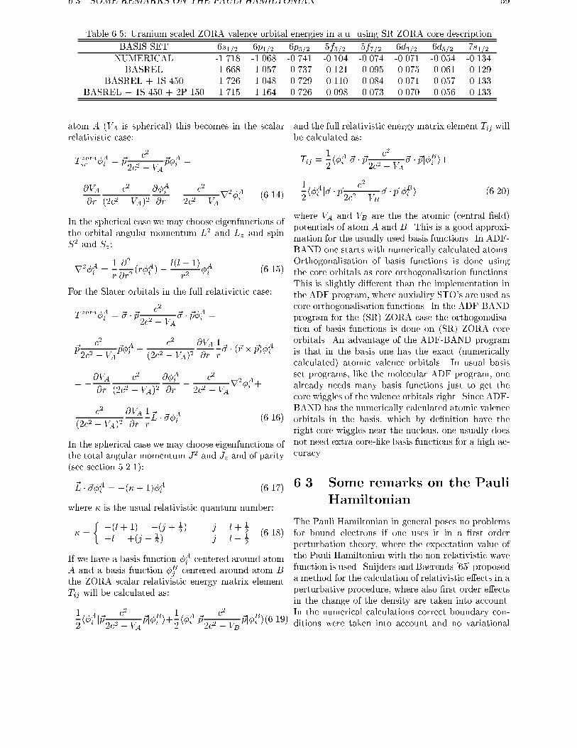
6.3. SOME REMARKS ON THE PAULI HAMILTONIAN 59
Table 6.5: Uranium scaled ZORA valence orbital energies in a.u. using SR ZORA core description
BASIS SET 6s1=2 6p1=2 6p3=2 5f5=2 5f7=2 6d3=2 6d5=2 7s1=2NUMERICAL -1.718 -1.068 -0.741 -0.104 -0.074 -0.071 -0.054 -0.134
BASREL -1.668 -1.057 -0.737 -0.121 -0.095 -0.075 -0.061 -0.129
BASREL + 1S 450 -1.726 -1.048 -0.729 -0.110 -0.084 -0.071 -0.057 -0.133
BASREL + 1S 450 + 2P 150 -1.715 -1.164 -0.726 -0.098 -0.073 -0.070 -0.056 -0.133
atom A (VA is spherical) this becomes in the scalar
relativistic case:
T zorasr �Ai = ~pc2
2c2 � VA~p�Ai =
�@VA@r
c2
(2c2 � VA)2@�Ai@r
�c2
2c2 � VAr2�Ai (6.14)
In the spherical case we may choose eigenfunctions of
the orbital angular momentum L2 and Lz and spin
S2 and Sz:
r2�Ai =1
r
@2
@r2(r�Ai )�
l(l + 1)
r2�Ai (6.15)
For the Slater orbitals in the full relativictic case:
T zora�Ai = ~� � ~pc2
2c2 � VA~� � ~p�Ai =
~pc2
2c2 � VA~p�Ai +
c2
(2c2 � VA)2@VA@r
1
r~� � (~r � ~p)�Ai
= �@VA@r
c2
(2c2 � VA)2@�Ai@r
�c2
2c2 � VAr2�Ai +
c2
(2c2 � VA)2@VA@r
1
r~L � ~��Ai (6.16)
In the spherical case we may choose eigenfunctions of
the total angular momentum J2 and Jz and of parity(see section 5.2.1):
~L � ~��Ai = �(�+ 1)�Ai (6.17)
where � is the usual relativistic quantum number:
� =
��(l + 1) = �(j + 1
2) j = l + 1
2
+l = +(j + 12) j = l � 1
2
(6.18)
If we have a basis function �Ai centered around atom
A and a basis function �Bj centered around atom Bthe ZORA scalar relativistic energy matrix element
Tij will be calculated as:
1
2h�Ai j~p
c2
2c2 � VA~pj�Bi i+
1
2h�Ai j~p
c2
2c2 � VB~pj�Bi i(6.19)
and the full relativistic energy matrix element Tij willbe calculated as:
Tij =1
2h�Ai j~� � ~p
c2
2c2 � VA~� � ~pj�Bi i+
1
2h�Ai j~� � ~p
c2
2c2 � VB~� � ~pj�Bi i (6.20)
where VA and VB are the the atomic (central �eld)
potentials of atom A and B. This is a good approxi-
mation for the usually used basis functions. In ADF-
BAND one starts with numerically calculated atoms.
Orthogonalisation of basis functions is done using
the core orbitals as core orthogonalisation functions.
This is slightly di�erent than the implementation in
the ADF program, where auxialiry STO's are used as
core orthogonalisation functions. In the ADF-BAND
program for the (SR) ZORA case the orthogonalisa-
tion of basis functions is done on (SR) ZORA core
orbitals. An advantage of the ADF-BAND program
is that in the basis one has the exact (numerically
calculated) atomic valence orbitals. In usual basis
set programs, like the molecular ADF program, one
already needs many basis functions just to get the
core wiggles of the valence orbitals right. Since ADF-
BAND has the numerically calculated atomic valence
orbitals in the basis, which by de�nition have the
right core wiggles near the nucleus, one usually does
not need extra core-like basis functions for a high ac-
curacy.
6.3 Some remarks on the Pauli
Hamiltonian
The Pauli Hamiltonian in general poses no problems
for bound electrons if one uses it in a �rst order
perturbation theory, where the expectation value of
the Pauli Hamiltonian with the non-relativistic wave
function is used. Snijders and Baerends [65] proposed
a method for the calculation of relativistic e�ects in a
perturbative procedure, where also �rst order e�ects
in the change of the density are taken into account.
In the numerical calculations correct boundary con-
ditions were taken into account and no variational
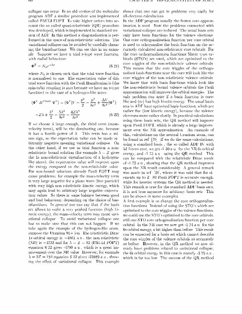
60 CHAPTER 6. IMPLEMENTATION OF ZORA
collapse can occur. In an old version of the molecular
program ADF a similar procedure was implemented
called PAULI FOPT. To take higher orders into ac-
count the so called quasi-relativistic (QR) procedure
was developed, which is implemented in standard ver-
sion of ADF. In this method a diagonalisation is per-
formed in the space of non-relativistic solutions. The
variational collapse can be avoided by carefully choos-
ing the basisfunctions. We can see this in an exam-
ple. Suppose we have a trial s-type wave function,
with radial behaviour:
�T = N�e��r (6.21)
where N� is chosen such that the trial wave function
is normalised to one. The expectation value of this
trial wave function with the Pauli Hamiltonian is (the
spin-orbit coupling is zero because we have an s-type
function) in the case of a hydrogen-like atom:
h�T jHPaulij�T i = h�T jV +p2
2�
p4
8c2+�V
8c2j�T i
= �Z�+�2
2�5�4
8c2+4Z�3
8c2(6.22)
If we choose � large enough, the third term (mass-
velocity term), will be the dominating one, because
it has a fourth power of �. This term has a mi-
nus sign, so the expectation value can be made ar-
bitrarily negative meaning variational collapse. On
the other hand, if we use as trial function a non-
relativistic bound solution (for example � = Z gives
the 1s non-relativistic eigenfunction of a hydrogen-
like atom), the expectation value will improve upon
the energy compared to the non-relativistic value.
For non-bound solutions already Pauli FOPT may
cause problems: for example the mass-velocity term
is very large negative for a plane wave (free particle)
with very high non-relativistic kinetic energy, which
may again lead to arbitrary large negative expecta-
tion values. So there is some balance between good
and bad behaviour, depending on the choice of bas-
isfunctions. In general one can say that if the basis
set allows to make a very peaked function (high ki-
netic energy), the mass-velocity term may cause vari-
ational collapse. To avoid variational collapse one
has to make sure that this can not happen. If we
take again the example of the hydrogen-like atom,
suppose the Uranium 91+ ion. The relativistic Dirac
1s-orbital energy is �4861 a.u., the non-relativistic
(NR) is �4232 and for � = Z = 92 (PAULI FOPT)
equation 6.22 gives -4709 a.u., which is a great im-
provement over the NR value. However, for example
� = 2Z = 184 equation 6.22 gives -22889 a.u., show-
ing the e�ect of variational collapse. This example
shows that one can get in problems very easily for
all-electron calculations.
In the ADF program usually the frozen core approx-
imation is used. Now the problems connected with
variational collapse are reduced. The usual basis sets
only have basis functions for the valence electrons.
One core orthogonalisation function per core orbital
is used to orhogonalise the basis function on the ac-
curately calculated non-relativistic core orbitals. For
the core orthogonalisation functions Slater type or-
bitals (STO's) are used, which are optimised to the
core wiggles of the non-relativistic valence orbitals.
This means that the core wiggles of the orthogo-
nalised basis functions near the core will look like the
core wiggles of the non-relativistic valence orbitals.
We know that with basis functions which look like
the non-relativistic bound valence orbitals the Pauli
approximation will improve the orbital energies. The
only problem can arise if a basis function is core-
like and (or) has high kinetic energy. The usual basis
sets in ADF have optimised basis functions, which are
rather at (low kinetic energy), because the valence
electrons move rather slowly. In practical calculations
using these basis sets, the QR method will improve
upon Pauli FOPT, which is already a large improve-
ment over the NR approximation. An example of
this, calculations on the neutral Uranium atom, can
be found in ref. [70]. If we do the same calculations,
using a standard basis , the so called ADF IV with
5d frozen core, we get -1.30 a.u. for the NR 6s orbital
energy, and -1.75 a.u. using the QR method. This
can be compared with the relativistic Dirac result
of -1.72 a.u., showing that the QR method improves
upon the NR result considerably. A general remark
was made in ref. [28], where it was said that for el-
ements up to Z=80 Pauli FOPT is accurate enough,
while for heavier systems the QR method is needed.
This remark is true for the standard ADF basis sets,
it is not true anymore for arbitrary basis sets. This
can be shown in some examples.
A �rst example is to change the core orthogonalisa-
tion functions. Instead of using the STO's which are
optimised to the core wiggles of the valence functions,
we could use the STO's optimised to the core orbitals,
still one STO core orhogonalisation function per core
orbital. In the NR case we now get -1.24 a.u. for the
6s orbital energy, a bit higher than before. This result
can be expected for a basis set which cannot describe
the core wiggles of the valence orbitals as accurately
as before. However, in the QR method we now al-
ready have problems related to variational collapse,
the 6s orbital energy in this case is namely -3.75 a.u.,
which is far too low. The success of the QR method
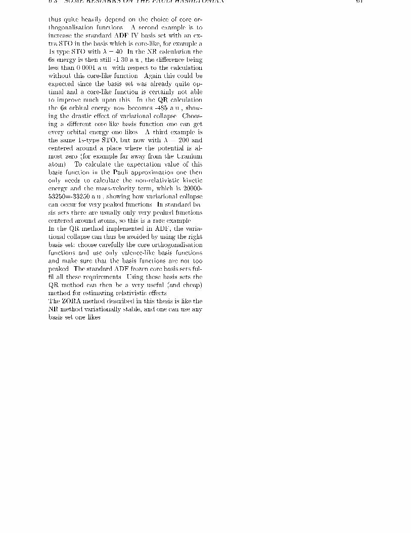
6.3. SOME REMARKS ON THE PAULI HAMILTONIAN 61
thus quite heavily depend on the choice of core or-
thogonalisation functions. A second example is to
increase the standard ADF IV basis set with an ex-
tra STO in the basis which is core-like, for example a
1s-type STO with � = 40. In the NR calculation the
6s energy is then still -1.30 a.u., the di�erence being
less than 0.0001 a.u. with respect to the calculation
without this core-like function. Again this could be
expected since the basis set was already quite op-
timal and a core-like function is certainly not able
to improve much upon this. In the QR calculation
the 6s orbital energy now becomes -485 a.u., show-
ing the drastic e�ect of variational collapse. Choos-
ing a di�erent core-like basis function one can get
every orbital energy one likes. A third example is
the same 1s-type STO, but now with � = 200 and
centered around a place where the potential is al-
most zero (for example far away from the Uranium
atom). To calculate the expectation value of this
basis function in the Pauli approximation one then
only needs to calculate the non-relativistic kinetic
energy and the mass-velocity term, which is 20000-
53250=-33250 a.u., showing how variational collapse
can occur for very peaked functions. In standard ba-
sis sets there are usually only very peaked functions
centered around atoms, so this is a rare example.
In the QR method implemented in ADF, the varia-
tional collapse can thus be avoided by using the right
basis set: choose carefully the core orthogonalisation
functions and use only valence-like basis functions
and make sure that the basis functions are not too
peaked. The standard ADF frozen core basis sets ful-
�l all these requirements. Using these basis sets the
QR method can then be a very useful (and cheap)
method for estimating relativistic e�ects.
The ZORA method described in this thesis is like the
NR method variationally stable, and one can use any
basis set one likes.

62 CHAPTER 6. IMPLEMENTATION OF ZORA
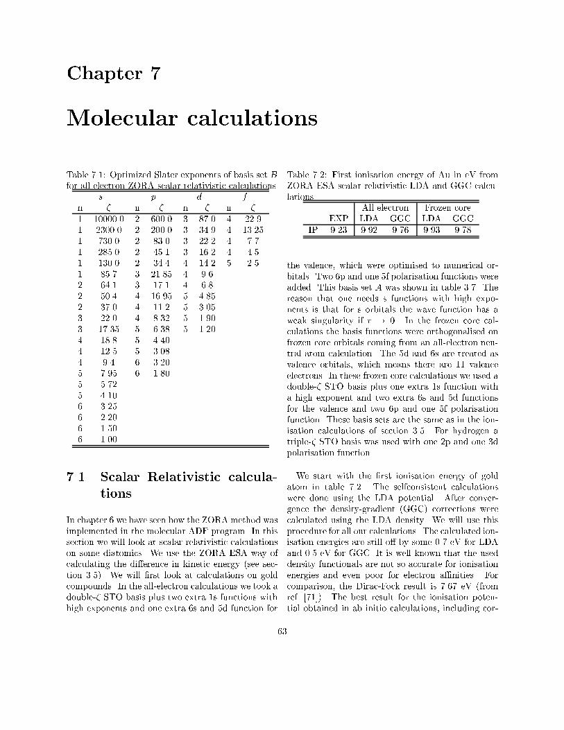
Chapter 7
Molecular calculations
Table 7.1: Optimized Slater exponents of basis set Bfor all electron ZORA scalar relativistic calculations
s p d fn � n � n � n �
1 10000.0 2 600.0 3 87.0 4 22.9
1 2300.0 2 200.0 3 34.9 4 13.25
1 730.0 2 83.0 3 22.2 4 7.7
1 285.0 2 45.1 3 16.2 4 4.5
1 130.0 2 34.4 4 14.2 5 2.5
1 85.7 3 21.85 4 9.6
2 64.1 3 17.1 4 6.8
2 50.4 4 16.95 5 4.85
2 37.0 4 11.2 5 3.05
3 22.0 4 8.32 5 1.90
3 17.35 5 6.38 5 1.20
4 18.8 5 4.40
4 12.5 5 3.08
4 9.4 6 3.20
5 7.95 6 1.80
5 5.72
5 4.10
6 3.25
6 2.20
6 1.50
6 1.00
7.1 Scalar Relativistic calcula-
tions
In chapter 6 we have seen how the ZORA method was
implemented in the molecular ADF program. In this
section we will look at scalar relativistic calculations
on some diatomics. We use the ZORA ESA way of
calculating the di�erence in kinetic energy (see sec-
tion 3.5). We will �rst look at calculations on gold
compounds. In the all-electron calculations we took a
double-� STO basis plus two extra 1s functions with
high exponents and one extra 6s and 5d function for
Table 7.2: First ionisation energy of Au in eV from
ZORA ESA scalar relativistic LDA and GGC calcu-
lations
All electron Frozen core
EXP LDA GGC LDA GGC
IP 9.23 9.92 9.76 9.93 9.78
the valence, which were optimised to numerical or-
bitals. Two 6p and one 5f polarisation functions were
added. This basis set A was shown in table 3.7. The
reason that one needs s functions with high expo-
nents is that for s orbitals the wave function has a
weak singularity if r ! 0. In the frozen core cal-
culations the basis functions were orthogonalised on
frozen core orbitals coming from an all-electron neu-
tral atom calculation. The 5d and 6s are treated as
valence orbitals, which means there are 11 valence
electrons. In these frozen core calculations we used a
double-� STO basis plus one extra 1s function with
a high exponent and two extra 6s and 5d functions
for the valence and two 6p and one 5f polarisation
function. These basis sets are the same as in the ion-
isation calculations of section 3.5. For hydrogen a
triple-� STO basis was used with one 2p and one 3d
polarisation function.
We start with the �rst ionisation energy of gold
atom in table 7.2. The selfconsistent calculations
were done using the LDA potential. After conver-
gence the density-gradient (GGC) corrections were
calculated using the LDA density. We will use this
procedure for all our calculations. The calculated ion-
isation energies are still o� by some 0.7 eV for LDA
and 0.5 eV for GGC. It is well known that the used
density functionals are not so accurate for ionisation
energies and even poor for electron a�nities. For
comparison, the Dirac-Fock result is 7.67 eV (from
ref. [71]). The best result for the ionisation poten-
tial obtained in ab initio calculations, including cor-
63
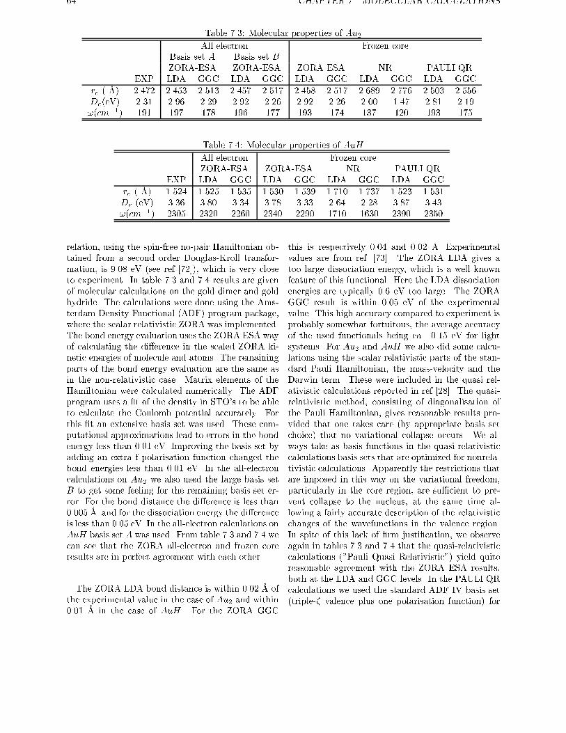
64 CHAPTER 7. MOLECULAR CALCULATIONS
Table 7.3: Molecular properties of Au2
All electron Frozen core
Basis set A Basis set BZORA-ESA ZORA-ESA ZORA ESA NR PAULI QR
EXP LDA GGC LDA GGC LDA GGC LDA GGC LDA GGC
re ( �A) 2.472 2.453 2.513 2.457 2.517 2.458 2.517 2.689 2.776 2.503 2.556
De(eV) 2.31 2.96 2.29 2.92 2.26 2.92 2.26 2.00 1.47 2.81 2.19
!(cm�1) 191 197 178 196 177 193 174 137 120 193 175
Table 7.4: Molecular properties of AuH
All electron Frozen core
ZORA-ESA ZORA-ESA NR PAULI QR
EXP LDA GGC LDA GGC LDA GGC LDA GGC
re ( �A) 1.524 1.525 1.535 1.530 1.539 1.710 1.737 1.523 1.531
De (eV) 3.36 3.80 3.34 3.78 3.33 2.64 2.28 3.87 3.43
!(cm�1) 2305 2320 2260 2340 2290 1710 1630 2390 2350
relation, using the spin-free no-pair Hamiltonian ob-
tained from a second order Douglas-Kroll transfor-
mation, is 9.08 eV (see ref [72]), which is very close
to experiment. In table 7.3 and 7.4 results are given
of molecular calculations on the gold dimer and gold
hydride. The calculations were done using the Ams-
terdam Density Functional (ADF) program package,
where the scalar relativistic ZORA was implemented.
The bond energy evaluation uses the ZORA ESA way
of calculating the di�erence in the scaled ZORA ki-
netic energies of molecule and atoms. The remaining
parts of the bond energy evaluation are the same as
in the non-relativistic case. Matrix elements of the
Hamiltonian were calculated numerically. The ADF
program uses a �t of the density in STO's to be able
to calculate the Coulomb potential accurately. For
this �t an extensive basis set was used. These com-
putational approximations lead to errors in the bond
energy less than 0.01 eV. Improving the basis set by
adding an extra f polarisation function changed the
bond energies less than 0.01 eV. In the all-electron
calculations on Au2 we also used the large basis set
B to get some feeling for the remaining basis set er-
ror. For the bond distance the di�erence is less than
0.005 �A and for the dissociation energy the di�erence
is less than 0.05 eV. In the all-electron calculations on
AuH basis set A was used. From table 7.3 and 7.4 we
can see that the ZORA all-electron and frozen core
results are in perfect agreement with each other.
The ZORA LDA bond distance is within 0.02 �A of
the experimental value in the case of Au2 and within
0.01 �A in the case of AuH . For the ZORA GGC
this is respectively 0.04 and 0.02 �A. Experimental
values are from ref. [73]. The ZORA LDA gives a
too large dissociation energy, which is a well known
feature of this functional. Here the LDA dissociation
energies are typically 0.6 eV too large. The ZORA
GGC result is within 0.05 eV of the experimental
value. This high accuracy compared to experiment is
probably somewhat fortuitous, the average accuracy
of the used functionals being ca. 0.15 eV for light
systems. For Au2 and AuH we also did some calcu-
lations using the scalar relativistic parts of the stan-
dard Pauli Hamiltonian, the mass-velocity and the
Darwin term. These were included in the quasi rel-
ativistic calculations reported in ref [28]. The quasi-
relativistic method, consisting of diagonalisation of
the Pauli Hamiltonian, gives reasonable results pro-
vided that one takes care (by appropriate basis set
choice) that no variational collapse occurs. We al-
ways take as basis functions in the quasi-relativistic
calculations basis sets that are optimized for nonrela-
tivistic calculations. Apparently the restrictions that
are imposed in this way on the variational freedom,
particularly in the core region, are su�cient to pre-
vent collapse to the nucleus, at the same time al-
lowing a fairly accurate description of the relativistic
changes of the wavefunctions in the valence region.
In spite of this lack of �rm justi�cation, we observe
again in tables 7.3 and 7.4 that the quasi-relativistic
calculations ("Pauli Quasi Relativistic") yield quite
reasonable agreement with the ZORA ESA results,
both at the LDA and GGC levels. In the PAULI QR
calculations we used the standard ADF IV basis set
(triple-� valence plus one polarisation function) for
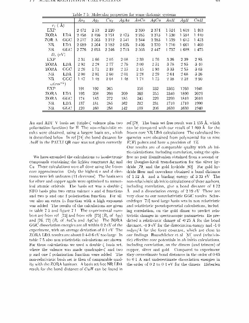
7.1. SCALAR RELATIVISTIC CALCULATIONS 65
Table 7.5: Molecular properties for some diatomic systems.
Au2 Ag2 Cu2 AgAu AuCu AgCu AuH AgH CuH
re ( �A)EXP 2.472 2.53 2.220 2.330 2.374 1.524 1.618 1.463
ZORA LDA 2.458 2.486 2.151 2.473 2.285 2.313 1.530 1.594 1.440
ZOR A GGC 2.517 2.563 2.212 2.541 2.344 2.383 1.539 1.615 1.453
NR LDA 2.689 2.564 2.182 2.625 2.426 2.370 1.710 1.661 1.460
NR GGC 2.776 2.653 2.246 2.713 2.503 2.447 1.737 1.688 1.475
De (eV)
EXP 2.31 1.66 2.05 2.08 2.39 1.76 3.36 2.39 2.85
ZORA LDA 2.92 2.28 2.77 2.76 3.09 2.51 3.78 2.95 3.40
ZORA GGC 2.26 1.71 2.19 2.15 2.45 1.93 3.33 2.55 3.03
NR LDA 2.00 2.01 2.60 2.01 2.28 2.29 2.64 2.68 3.26
NR GGC 1.47 1.48 2.04 1.48 1.74 1.75 2.28 2.32 2.90
!(cm�1)
EXP 191 192 265 250 232 2305 1760 1941
ZORA LDA 193 208 298 209 269 255 2340 1890 2070
ZORA GGC 174 183 272 185 245 229 2290 1810 2010
NR LDA 137 181 285 162 212 231 1710 1710 1990
NR GGC 120 160 258 142 189 206 1630 1630 1940
Au and ADF V basis set (triple-� valence plus two
polarisation function) for H. The non-relativistic re-
sults were obtained, using a largere basis set, which
is decscribed below. In ref [74] the bond distance for
AuH in the PAULI QR case was not given correctly.
We have extended the calculations to isoelectronic
compounds containing the lighter congeners Ag and
Cu. These calculations were all done using the frozen
core approximation. Only the highest s and d elec-
trons were left unfrozen (11 electrons). The basis sets
for silver and copper again were optimised to numer-
ical atomic orbitals. The basis set was a double-�STO basis plus two extra valence s and d functions
and two p and one f polarisation function. For sil-
ver also an extra 1s function with a high exponent
was added. The results of the calculations are given
in table 7.5 and �gure 7.1. The experimental num-
bers are from ref. [73] and from refs. [75] (Re of Ag2)and [76, 77] (Re of AuCu and AgCu). The ZORA
GGC dissociation energies are all within 0.2 eV of the
experiment, with an average deviation of 0.1 eV. The
ZORA LDA results are about 0.4-0.6 eV too large. In
table 7.5 also non-relativistic calculations are shown.
For these calculations we used a double-� basis set,
where the valence was made quadruple-� and two
p and one f polarisation function were added. The
non-relativistic basis set is then of comparable qual-
ity with the ZORA basis set. A basis set free NR LDA
result for the bond distance of CuH can be found in
ref [78]. The basis set free result was 1.455 �A, which
can be compared with our result of 1.460 �A for the
frozen core NR LDA calculations. The calculated fre-
quencies were obtained from polynomial �ts to nine
E(R) points and have a precision of 1%.
Our results are of comparable quality with ab ini-
tio calculations, including correlation, using the spin-
free no-pair Hamiltonian obtained from a second or-
der Douglas-Kroll transformation for the silver hy-
dride [79] and the gold hydride [80]. For gold hy-
dride Hess and coworkers obtained a bond distance
of 1.52 �A and a binding energy of 3.33 eV. The
non-relativistic ab initio calculations of these authors,
including correlation, give a bond distance of 1.72�A and a dissociation energy of 2.19 eV. These are
very close to our nonrelativistic GGC results. Schw-
erdtfeger [71] used large basis sets in non-relativistic
and relativistic pseudopotential calculations, includ-
ing correlation, on the gold dimer to predict rela-
tivistic changes in spectroscopic parameters. He pre-
dicted a relativistic change of -0.25 �A for the bond
distance, -0.9 eV for the dissociation energy and -1.0
mdyn/�A for the force constant, which are close to
our �ndings. Bauschlicher et al. [81] used (relativis-
tic) e�ective core potentials in ab initio calculations,
including correlation, on the dimers (and trimers) of
copper, silver and gold. Compared to experiment
they overestimate bond distances in the order of 0.05
to 0.1 �A and underestimate dissociation energies in
the order of 0.2 to 0.4 eV for the dimers. H�aberlen
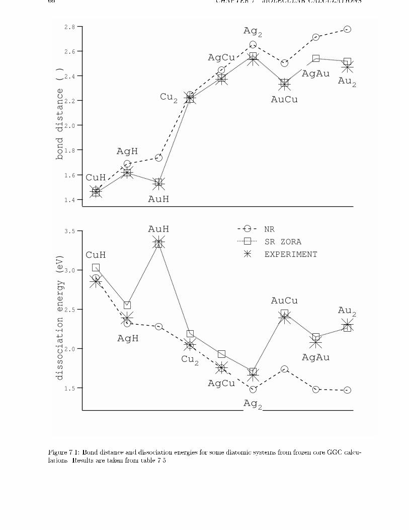
66 CHAPTER 7. MOLECULAR CALCULATIONS
2.8
2.6
2.4
2.2
2.0
1.8
1.6
1.4
bond
dis
tanc
e (
)
AgH
AuH
Cu2
AgCu
Ag2
AuCu
AgAuAu2
CuH
3.5
3.0
2.5
2.0
1.5
diss
ocia
tion
ene
rgy
(eV)
CuH
AgH
AuH
Cu2
AgCu
Ag2
AuCu
AgAu
Au2
NR
SR ZORA
EXPERIMENT
Figure 7.1: Bond distance and dissociation energies for some diatomic systems from frozen core GGC calcu-
lations. Results are taken from table 7.5.
7.2. SPIN-ORBIT EFFECTS 67
and R�osch [82] used the spin-free no-pair Hamiltonian
obtained from a second order Douglas-Kroll trans-
formation in local density functional calculations on
Au2, AuH and AuCl. Their relativistic and non-
relativistic LDA results on the gold dimer are in close
agreement with our LDA results. There is more de-
viation in the results on the gold hydride. We were
not able to �nd an explanation for the discrepancy
in the NR LDA calculations on the bond length of
this compound. All-electron Dirac-Fock-Slater calcu-
lations on Au2 were carried out by Ba�stu�g et al. [83].Our results can not be compared directly, because we
use a di�erent density functional, but the calculated
relativistic e�ects are of comparable size.
7.2 Spin-orbit e�ects
In the last section (see also ref. [74]) the zeroth or-
der regular approximated (ZORA) Dirac equation
was successfully applied in scalar relativistic calcu-
lations on molecules. In this section we will concen-
trate on the spin-orbit e�ects, using non-relativistic
local density functionals (LDA) including gradient
correction (GGC) terms for the calculation of the
exchange-correlation energy. The Becke correction
for exchange [84] and the Perdew correction for cor-
relation [85], that have been successfully applied in
nonrelativistic calculations [86, 87] and in scalar rel-
ativistic ZORA calculations (see last section), have
been used.
If spin-orbit coupling is present in closed shell systems
we will use a one-determinantal j-j (! � !) coupledstate, obtained from one-electron spinorbitals which
are eigenfunctions of j2 and jz . For open shell atoms
j-j coupling is not a good approximation and we use
intermediate coupling to ensure the right scalar rel-
ativistic limit if the spin-orbit operator goes to zero
(see section 7.2.1). In section 7.2.3 results are shown
for some atomic multiplets using this method.
In section 7.3 we analyse the spin-orbit e�ects on
some closed shell molecules, namely I2, Au2, Bi2,HI , AuH , T lH , IF , T lF , T lI , PbO and PbTe, look-ing at bond distance, harmonic frequencies, dissocia-
tion energies and dipole moments. In order to obtain
very accurate results for the dissociation energies it is
needed to include gradient correction (GGC) terms in
the energy and use the intermediate coupled energy
for the atoms. Results are then all within 0.3 eV of
the experiment, with an average deviation of 0.1 eV
for these compounds.
In spin-orbit calculations we want the energies to
converge to the scalar relativistic energies in the limit
that the spin-orbit operator goes to zero. In this limit
the one-determinantal state obtained using j-j (!�!)coupling is identical to the state obtained using L-S
(���) coupling. So for closed shell systems we can
use j-j (!�!) coupling without any corrections. Foropen shell systems this is not true anymore. To let
the spin-orbit calculations converge to the scalar rel-
ativistic energies, if the spin-orbit operator goes to
zero, we have to use intermediate coupling for open
shell systems. How we do this in our density func-
tional calculations is shown in the next section.
7.2.1 Open shell systems
An important question in relativistic density func-
tional theory is how to obtain the ground state en-
ergy of some open shell system with the present day
approximate density functionals. This is also a prob-
lem in non-relativistic density functional theory, but
the problems become more complicated if the spin-
orbit operator is present. In the non-relativistic case
one solution is to �nd the lowest energy, without any
symmetry constraints. For an open shell atom this
means that the lowest energy can be obtained for a
nonspherical density and where the solution is not a
pure spin state. In an ab initio scheme these problems
can be solved unambiguously, also in the relativistic
case.
The relativistic Hamiltonian can be divided in a
scalar relativistic (SR) and a spin-orbit (SO) part:
HREL = HSR +HSO (7.1)
A possibility would be to start with the calculation of
the energies of all j-j (! �!) coupled states. Present
day density functionals have not been developed to
use them in this case. In intermediate coupling, states
which have the same total J and Jz can couple, be-
cause of the electron-electron interaction.
Another possibility is to solve the whole spectrum of
the scalar relativistic Hamiltonian. The energies of
the multiplet states can for example be calculated us-
ing the diagonal sum-method as suggested in ref [88]
or the alternative method of ref. [89] and we have the
energies of the L-S coupled states. We then can cal-
culate the spin-orbit interaction between those states.
From angular momentum conservation we know that
only those states can couple through the spin-orbit
operator which have the same total J and Jz. We can
diagonalize the resultant matrix and we have the en-
ergies of the intermediate coupled states. The prob-
lem here is that in principle many states can cou-
ple and we have to know the energies of the excited
states, which is not straightforward in density func-
tional theory. We therefore have to approximate this
68 CHAPTER 7. MOLECULAR CALCULATIONS
procedure, by using for example only the lowest lying
excited states.
The direct e�ect of the spin-orbit operator on valence
orbitals is large if we have an open shell atom with
partially occupied p,d or f shells. We can see this in
the splitting of states which would be degenerate in
the L-S coupled scheme. For light atoms a �rst or-
der treatment of the spin-orbit coupling is su�cient,
whereas for heavier atoms one needs the intermediate
coupling scheme. The limit where j-j coupling is much
more important than L-S coupling is not reached for
the known elements.
There can also be an e�ect of spin-orbit coupling on
fully occupied shells, although if we start with a scalar
relativistic solution, the �rst order e�ect of the spin-
orbit coupling on the energy is zero. The total ef-
fect of spin-orbit coupling is not zero anymore for
deep core fully occupied shells of heavy atoms. We
can see this e�ect already if we look at the hydrogen-
like heavy atom, for example the Uranium 91+ atom.
The averaged relativistic 2p orbital energy -1045.54
(1/3 times -1257.39 (2p1=2) plus 2/3 times -1089.61
(2p3=2)) is approximate 15 a.u. lower than the scalar
relativistic orbital energy -1130.34. So even for closed
shells spin-orbit interaction can be of importance, due
to the second and higher order e�ects of the spin-orbit
coupling. The radial part of the 2p1=2 orbital is thennot so close to the radial part of the 2p3=2 orbital any-more. If we start with the scalar relativistic states we
need very high excited states if we want to take this
e�ect into account. On the other hand, as we have
tested in valence only calculations, the e�ect of the
change in density of the core orbitals due to spin-orbit
e�ects has very little e�ect on valence orbitals.
In practical calculations it is often convenient to
express the ground state energy with respect to
some average-of-con�guration energy. In the scalar
relativistic case we will choose this average-of-
con�guration calculation where the electrons are dis-
tributed equally over the subspecies of the open shell
irreps. For atoms this will ensure a spherical density
and a spin-� density, which is the same as that of
spin-�. If spin-orbit coupling is present we will dividethe electrons in a spin-orbit averaged way over the
di�erent open shell irreps such that if the spin-orbit
coupling is zero the occupation would be the same as
in the scalar relativistic case. For an atom with a p1
con�guration this will mean that 1/3 of an electron is
placed in the p1=2 orbital and 2/3 in the p3=2 orbital.These reference states are not physical states. The
scalar relativistic multiplet states (L-S coupling) can
be obtained using the method of ref [88] or ref. [89].
From the di�erence in energy of the lowest j-j coupled
state and the reference state, in which we both use a
spherically and spin averaged density, we calculate an
e�ective spin-orbit parameter. Together with the en-
ergies of the L-S coupled states we will calculate the
energies of the intermediate coupled states, using the
results given in section 7.2.2, as if they remain valid
in our calculations. In the present approximations
we do not take excited states from di�erent con�gu-
rations into account.
Below we will give an example that may clarify
the problems if one uses the spin-orbit operator in
present day approximate density functionals, without
thinking about their limitations. Suppose we have a
hydrogen atom with a p1 con�guration. Many of the
present day density functionals will not give the same
energy whether the electron is placed in the pz orbitalor in the (px + ipy)=
p2 orbital. Sometimes a spher-
ically averaged atom is chosen, which will give yet
another energy. This problem already occurs if we
use density functionals, which do not depend on the
spin-polarisation. In general the spin-polarised den-
sity functionals will give di�erent results if the elec-
tron is placed in the pz orbital with spin � or with a
mixed spin state (� + �)=p2, although these states
are degenerate according to the Schr�odinger equa-
tion. A solution is then to take only the state which
is purely spin � or �. These problems occur when
the Schr�odinger equation has degenerate solutions,
which means that any linear combination of these so-
lutions is also a solution to the Schr�odinger equation.
In this way one obtains di�erent spin-densities which
should have the same energy, but many of the present
day density functionals will not give the same energy.
In fact similar problems can arise in almost degener-
ate cases. One of the approximate solutions to these
problems is to use a method suggested in ref [88].
Another possibility is to use the method of Becke et
al. [89], which uses 'local pair' densities instead of lo-
cal spin densities in their calculations.
Relativistic Hamiltonians will, besides scalar rela-
tivistic corection terms to the non-relativistic Hamil-
tonian, also have a spin-orbit operator. If we take
again the example of the hydrogen atom with p1 con-�guration. The p1=2 orbitals will have 1/3 of one
spin and 2/3 of the other spin. If we use this den-
sity in a density functional, which depends on spin-
polarisation, we will get a di�erent answer than the
scalar relativistic result obtained from a pure spin �or pure spin � density. These results di�er even if we
let the spin-orbit operator go to zero, in which case
the di�erence is only due to the fact that in the one
case we have a pure spin state and in the other some
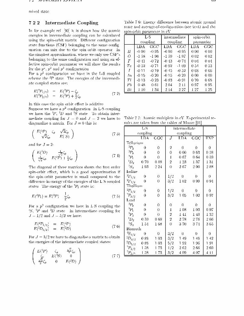
7.2. SPIN-ORBIT EFFECTS 69
mixed state.
7.2.2 Intermediate Coupling
In for example ref. [90] it is shown how the atomic
energies in intermediate coupling can be calculated
using the spin-orbit matrix. Di�erent con�guration
state functions (CSF) belonging to the same con�g-
uration can mix due to the spin-orbit operator. In
the simplest approximation, where we only use CSF's
belonging to the same con�guration and using an ef-
fective spin-orbit parameter we will show the results
for the p1, p2 and p3 con�guration.For a p1 con�guration we have in the L-S coupled
scheme the 2P state. The energies of the intermedi-
ate coupled states are:
E(2P1=2) = E(2P )� �pE(2P3=2) = E(2P ) + 1
2�p
(7.2)
In this case the spin-orbit e�ect is additive.
Suppose we have a p2 con�guration. In L-S coupling
we have the 3P , 1D and 1S state. To obtain inter-
mediate coupling for J = 0 and J = 2 we have to
diagonalize a matrix. For J = 0 this is:�E(3P )� �p
p2�pp
2�p E(1S)
�(7.3)
and for J = 2: E(1D) 1p
2�p
1p2�p E(3P ) + 1
2�p
!(7.4)
The diagonal of these matrices shows the �rst order
spin-orbit e�ect, which is a good approximation if
the spin-orbit parameter is small compared to the
di�erence in energy of the energies of the L-S coupled
states. The energy of the 3P1 state is:
E(3P1) = E(3P )�1
2�p (7.5)
For a p3 con�guration we have in L-S coupling the4S, 2P and 2D state. In intermediate coupling for
J = 1=2 and J = 5=2 we have:
E(2P1=2) = E(2P )E(2D5=2) = E(2D)
(7.6)
For J = 3=2 we have to diagonalise a matrix to obtainthe energies of the intermediate coupled states:0B@ E(2P ) �p
p52�p
�p E(4S) 0p52�p 0 E(2D)
1CA (7.7)
Table 7.6: Energy di�erence between atomic ground
state and average-of-con�guration (see text) and the
spin-orbit parameter in eV.
L-S intermediate spin-orbit
coupling coupling parameter
LDA GGC LDA GGC LDA GGC
H -0.90 -0.95 -0.90 -0.95 0.00 0.00
O -1.58 -1.96 -1.59 -1.97 0.02 0.02
F -0.41 -0.72 -0.43 -0.74 0.04 0.04
Te -0.52 -0.71 -0.92 -1.09 0.54 0.53
I -0.11 -0.19 -0.45 -0.52 0.68 0.66
Au -0.15 -0.20 -0.15 -0.20 0.00 0.00
T l -0.13 -0.23 -0.83 -0.91 0.70 0.68
Pb -0.48 -0.61 -2.04 -2.11 0.97 0.95
Bi -1.10 -1.34 -2.14 -2.27 1.27 1.25
Table 7.7: Atomic multiplets in eV. Experimental re-
sults are taken from the tables of Moore [91]
L-S intermediate
coupling coupling
LDA GGC J LDA GGC EXP
Tellurium3P2 0 0 2 0 0 03P0 0 0 0 0.60 0.63 0.583P1 0 0 1 0.67 0.64 0.591D2 0.70 0.88 2 1.23 1.37 1.311S0 1.93 2.24 0 2.67 2.90 2.88
Iodine2P1=2 0 0 1/2 0 0 02P3=2 0 0 3/2 1.02 0.99 0.94
Thallium2P1=2 0 0 1/2 0 0 02P3=2 0 0 3/2 1.05 1.02 0.97
Lead3P0 0 0 0 0 0 03P1 0 0 1 1.08 1.03 0.973P2 0 0 2 1.41 1.40 1.321D2 0.59 0.69 2 2.78 2.76 2.661S0 1.54 1.68 0 3.70 3.74 3.65
Bismuth4S3=2 0 0 3/2 0 0 02D3=2 0.88 1.03 3/2 1.49 1.48 1.422D5=2 0.88 1.03 5/2 1.92 1.96 1.912P1=2 1.58 1.73 1/2 2.62 2.66 2.692P3=2 1.58 1.73 3/2 4.09 4.07 4.11
70 CHAPTER 7. MOLECULAR CALCULATIONS
7.2.3 Spin-orbit e�ects in atoms
In section 7.2.2 we have shown how we calculate
atomic energies of intermediate coupled states. We
will use this in our density functional calculations.
Our main objective is to get the energy of the ground
state, if spin-orbit coupling is present. We want this
energy to converge to the scalar relativistic ground
state energy if the spin-orbit operator goes to zero.
To obtain the correction term for the energy of the
physical ground state compared to the unphysical
spin-averaged and spherically averaged atom in the
scalar relativistic case, we have done selfconsistent
spin-polarised calculations on the atoms inD1h sym-
metry, using every possible way to distribute the
electrons. The lowest energy was considered to be
the ground state energy. One can also calculate
one-determinantal wave-functions using restricted or-
bitals coming from a spherically averaged and spin-
averaged atom and then calculate the energies using
spin-polarised density functionals. This may give en-
ergies which are higher than the converged results
up to 0.15 eV, especially for the lighter open shell
systems. For the heavier elements we have used the
di�erence is less than 0.05 eV, between converged
and non-converged results. We have used the con-
verged results, which are shown in table 7.6 under
the header 'L-S coupling'. For the calculation of the
energies of the L-S coupled states using the diagonal
sum-method of Ziegler et al. [88] we also used the
converged results. Formally this is not justi�ed, but
as we have said before the di�erence between the en-
ergies using the restricted or the unrestricted orbitals
is small for the heavier atoms, for which we need this
diagonal sum-method. In table 7.7 we show the re-
sulting energies for the heavier elements. The diago-
nal sum-method is only used for Te, Pb and Bi. Thismethod su�ers from the cited problems, that two dif-
ferent determinants belonging to the same state yield
somewhat di�erent energies, with present day func-
tionals. Due to this arbitrariness the calculated split-
tings have an accuracy of about 0.2 eV for these sys-
tems. For H , F , I , Au and T l we only have one statein L-S coupling for the lowest con�guration, and for
O the spin-orbit e�ect is so small we don't have to
consider other L-S coupled states for the calculation
of the energy of the intermediate coupled state. In ta-
ble 7.6 we show the e�ective spin-orbit parameters we
have calculated. For the energies of the intermediate
coupled states, we use the method in section 7.2.2.
Results for the atomic energies of the intermediate
coupled states are shown in 7.7, together with the
experimental values [91]. Both LDA and the den-
sity gradient corrected (GGC) splittings are in close
Table 7.8: Optimized Slater exponents for all electron
ZORA scalar relativistic calculations for iodine
s p d fn � n � n � n �
1 1000.0 2 185.0 3 22.1 4 2.5
1 240.0 2 56.2 3 13.3 4 1.5
1 83.0 2 28.75 3 9.05
1 53.5 2 21.25 4 7.23
2 42.0 3 16.25 4 4.89
2 29.5 3 12.2 4 3.40
2 22.2 3 9.5 4 2.48
3 13.25 4 9.55 5 2.00
3 10.4 4 6.05
4 8.55 4 4.25
4 6.00 5 3.90
4 4.45 5 2.60
5 3.51 5 1.70
5 2.44 5 1.12
5 1.70
6 1.40
agreement with experiment, deviations less than 0.1
eV. For Te, Pb and Bi this accuracy is better than
the intrinsic accuracy of the diagonal sum-method,
so this accuracy has to be considered somewhat for-
tuitous.
The total energy of the atoms, using spin-orbit in-
teraction, is for the heavier systems much lower than
the scalar relativistic total energies. As explained
before this is mainly due to the core electrons. For
di�erences in energy this e�ect will be almost com-
pletely negligible. On the other hand, the valence
open shell spin-orbit e�ects are not negligible. We
therefore formally put the SR ZORA spin and spher-
ically averaged atomic total energy at the same level
as the ZORA spin, spherically and spin-orbit aver-
aged atomic total energy. We then can combine mul-
tiplet splittings and spin-orbit e�ects together using
intermediate coupling. The results are shown in ta-
ble 7.6 under the header 'intermediate coupling'.
7.3 Spin-orbit e�ects in closed
shell molecules
The selfconsistent calculations were done using the
LDA potential. After convergence density-gradient
(GGC) corrections were calculated using the LDA
potential. For gold we use the large basis set B of
section 7.1. The hydrogen basis set is also described
there. For thallium, lead and bismuth we use opti-
mised basis sets to numerical scalar relativistic ZORA
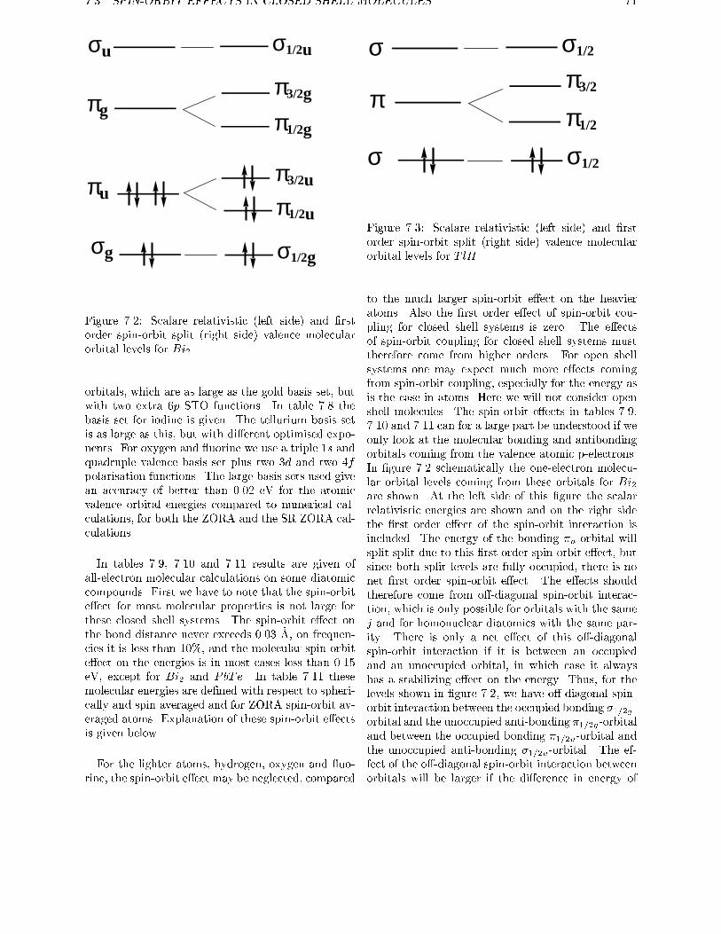
7.3. SPIN-ORBIT EFFECTS IN CLOSED SHELL MOLECULES 71
σu
πg
πu
σg
σ1/2u
π3/2g
π1/2g
π3/2u
π1/2u
σ1/2g
Figure 7.2: Scalare relativistic (left side) and �rst
order spin-orbit split (right side) valence molecular
orbital levels for Bi2
orbitals, which are as large as the gold basis set, but
with two extra 6p STO functions. In table 7.8 the
basis set for iodine is given. The tellurium basis set
is as large as this, but with di�erent optimised expo-
nents. For oxygen and uorine we use a triple 1s andquadruple valence basis set plus two 3d and two 4fpolarisation functions. The large basis sets used give
an accuracy of better than 0.02 eV for the atomic
valence orbital energies compared to numerical cal-
culations, for both the ZORA and the SR ZORA cal-
culations.
In tables 7.9, 7.10 and 7.11 results are given of
all-electron molecular calculations on some diatomic
compounds. First we have to note that the spin-orbit
e�ect for most molecular properties is not large for
these closed shell systems. The spin-orbit e�ect on
the bond distance never exceeds 0.03 �A, on frequen-
cies it is less than 10%, and the molecular spin-orbit
e�ect on the energies is in most cases less than 0.15
eV, except for Bi2 and PbTe. In table 7.11 these
molecular energies are de�ned with respect to spheri-
cally and spin averaged and for ZORA spin-orbit av-
eraged atoms. Explanation of these spin-orbit e�ects
is given below.
For the lighter atoms, hydrogen, oxygen and uo-
rine, the spin-orbit e�ect may be neglected, compared
σ1/2
π1/2
π3/2
σ1/2
σ
π
σ
Figure 7.3: Scalare relativistic (left side) and �rst
order spin-orbit split (right side) valence molecular
orbital levels for T lH
to the much larger spin-orbit e�ect on the heavier
atoms. Also the �rst order e�ect of spin-orbit cou-
pling for closed shell systems is zero. The e�ects
of spin-orbit coupling for closed shell systems must
therefore come from higher orders. For open shell
systems one may expect much more e�ects coming
from spin-orbit coupling, especially for the energy as
is the case in atoms. Here we will not consider open
shell molecules. The spin-orbit e�ects in tables 7.9,
7.10 and 7.11 can for a large part be understood if we
only look at the molecular bonding and antibonding
orbitals coming from the valence atomic p-electrons.
In �gure 7.2 schematically the one-electron molecu-
lar orbital levels coming from these orbitals for Bi2are shown. At the left side of this �gure the scalar
relativistic energies are shown and on the right side
the �rst order e�ect of the spin-orbit interaction is
included. The energy of the bonding �u-orbital willsplit split due to this �rst order spin-orbit e�ect, but
since both split levels are fully occupied, there is no
net �rst order spin-orbit e�ect. The e�ects should
therefore come from o�-diagonal spin-orbit interac-
tion, which is only possible for orbitals with the same
j and for homonuclear diatomics with the same par-
ity. There is only a net e�ect of this o�-diagonal
spin-orbit interaction if it is between an occupied
and an unoccupied orbital, in which case it always
has a stabilizing e�ect on the energy. Thus, for the
levels shown in �gure 7.2, we have o�-diagonal spin-
orbit interaction between the occupied bonding �1=2g-orbital and the unoccupied anti-bonding �1=2g-orbitaland between the occupied bonding �1=2u-orbital andthe unoccupied anti-bonding �1=2u-orbital. The ef-
fect of the o�-diagonal spin-orbit interaction between
orbitals will be larger if the di�erence in energy of
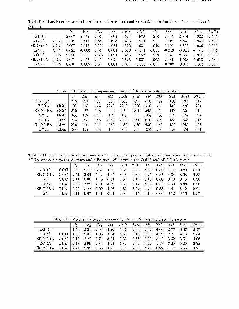
72 CHAPTER 7. MOLECULAR CALCULATIONS
Table 7.9: Bond length re and spin-orbit correction to the bond length �sore in �Angstroms for some diatomic
systems.
I2 Au2 Bi2 HI AuH T lH IF T lF T lI PbO PbTe
EXP[73] 2.667 2.472 2.661 1.609 1.524 1.870 1.910 2.084 2.814 1.922 2.595
ZORA GGC 2.719 2.511 2.685 1.628 1.535 1.900 1.951 2.119 2.858 1.937 2.633
SR ZORA GGC 2.697 2.517 2.655 1.625 1.535 1.931 1.940 2.126 2.872 1.939 2.629
�sore GGC 0.022 -0.006 0.030 0.003 0.000 -0.031 0.011 -0.013 -0.014 -0.002 0.004
ZORA LDA 2.670 2.452 2.637 1.624 1.526 1.868 1.919 2.073 2.783 1.910 2.588
SR ZORA LDA 2.651 2.457 2.613 1.621 1.525 1.901 1.908 2.081 2.798 1.913 2.586
�sore LDA 0.019 -0.005 0.024 0.003 0.001 -0.033 0.011 -0.008 -0.015 -0.003 0.002
Table 7.10: Harmonic frequencies !e in cm�1 for some diatomic systems.
I2 Au2 Bi2 HI AuH T lH IF T lF T lI PbO PbTe
EXP[73] 215 191 173 2309 2305 1391 610 477 (150) 721 212
ZORA GGC 197 178 174 2240 2270 1330 570 455 142 720 204
SR ZORA GGC 210 177 193 2260 2270 1320 595 450 142 730 212
�so!e GGC -6% 1% -10% -1% 0% 1% -4% 1% 0% -1% -4%
ZORA LDA 214 198 186 2260 2330 1390 610 490 155 755 216
SR ZORA LDA 226 196 203 2280 2330 1370 630 485 155 765 223
�so!e LDA -5% 1% -8% -1% 0% 1% -3% 1% 0% -1% -3%
Table 7.11: Molecular dissociation energies in eV with respect to spherically and spin averaged and for
ZORA spin-orbit averaged atoms and di�erence �so between the ZORA and SR ZORA result
I2 Au2 Bi2 HI AuH T lH IF T lF T lI PbO PbTe
ZORA GGC 2.62 2.71 6.52 4.71 4.52 3.96 4.31 6.37 4.14 8.23 5.74
SR ZORA GGC 2.51 2.65 5.42 4.68 4.48 3.84 4.21 6.37 4.04 8.08 5.38
�so GGC 0.11 0.06 1.10 0.03 0.04 0.12 0.10 0.00 0.10 0.15 0.36
ZORA LDA 3.07 3.29 7.11 4.99 4.87 4.12 4.85 6.83 4.53 8.88 6.28
SR ZORA LDA 2.96 3.22 6.00 4.96 4.83 3.97 4.75 6.83 4.41 8.72 5.91
�so LDA 0.11 0.07 1.11 0.03 0.04 0.15 0.10 0.00 0.12 0.16 0.37
Table 7.12: Molecular dissociation energies De in eV for some diatomic systems
I2 Au2 Bi2 HI AuH T lH IF T lF T lI PbO PbTe
EXP[73] 1.56 2.31 2.03 3.20 3.36 2.06 2.92 4.60 2.77 3.87 2.57
ZORA GGC 1.58 2.31 1.98 3.24 3.37 2.10 3.05 4.72 2.71 4.15 2.54
SR ZORA GGC 2.13 2.25 2.74 3.54 3.33 2.66 3.30 5.42 3.62 5.51 4.06
ZORA LDA 2.17 2.99 2.83 3.64 3.82 2.39 3.97 5.57 3.25 5.25 3.32
SR ZORA LDA 2.74 2.92 3.80 3.95 3.78 2.94 4.23 6.29 4.17 6.66 4.91
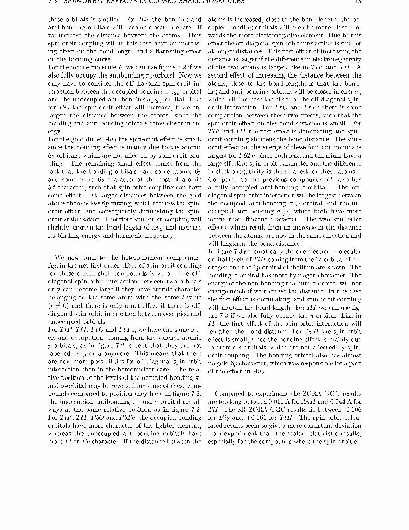
7.3. SPIN-ORBIT EFFECTS IN CLOSED SHELL MOLECULES 73
these orbitals is smaller. For Bi2 the bonding and
anti-bonding orbitals will become closer in energy if
we increase the distance between the atoms. Thus
spin-orbit coupling will in this case have an increas-
ing e�ect on the bond length and a attening e�ect
on the bonding curve.
For the iodine molecule I2 we can use �gure 7.2 if we
also fully occupy the antibonding �g-orbital. Now we
only have to consider the o�-diagonal spin-orbit in-
teraction between the occupied bonding �1=2u-orbitaland the unoccupied anti-bonding �1=2u-orbital. Likefor Bi2 the spin-orbit e�ect will increase, if we en-
largen the distance between the atoms, since the
bonding and anti-bonding orbitals come closer in en-
ergy.
For the gold dimer Au2 the spin-orbit e�ect is small,since the bonding e�ect is mainly due to the atomic
6s-orbitals, which are not a�ected by spin-orbit cou-
pling. The remaining small e�ect comes from the
fact that the bonding orbitals have some atomic 6pand some extra 6s character at the cost of atomic
5d character, such that spin-orbit coupling can have
some e�ect. At larger distances between the gold
atoms there is less 6p-mixing, which reduces the spin-orbit e�ect, and consequently diminishing the spin-
orbit stabilisation. Therefore spin-orbit coupling will
slightly shorten the bond length of Au2 and increase
its binding energy and harmonic frequency.
We now turn to the hetero-nuclear compounds.
Again the net �rst order e�ect of spin-orbit coupling
for these closed shell compounds is zero. The o�-
diagonal spin-orbit interaction between two orbitals
only can become large if they have atomic character
belonging to the same atom with the same l-value(l 6= 0) and there is only a net e�ect if there is o�-
diagonal spin-orbit interaction between occupied and
unoccupied orbitals.
For T lF , T lI , PbO and PbTe, we have the same lev-els and occupation, coming from the valence atomic
p-orbitals, as in �gure 7.2, except that they are not
labelled by g or u anymore. This means that there
are now more possibilities for o�-diagonal spin-orbit
interaction than in the homonuclear case. The rela-
tive position of the levels of the occupied bonding �-and �-orbital may be reversed for some of these com-pounds compared to position they have in �gure 7.2,
the unoccupied antibonding �- and �-orbital are al-ways at the same relative position as in �gure 7.2.
For T lF , T lI , PbO and PbTe, the occupied bonding
orbitals have more character of the lighter element,
whereas the unoccupied anti-bonding orbitals have
more T l or Pb character. If the distance between the
atoms is increased, close to the bond length, the oc-
cupied bonding orbitals will even be more biased to-
wards the more electronegative element. Due to this
e�ect the o�-diagonal spin-orbit interaction is smaller
at longer distances. This �rst e�ect of increasing the
distance is larger if the di�erence in electronegativity
of the two atoms is larger, like in T lF and T lI . A
second e�ect of increasing the distance between the
atoms, close to the bond length, is that the bond-
ing and anti-bonding orbitals will be closer in energy,
which will increase the e�ect of the o�-diagonal spin-
orbit interaction. For PbO and PbTe there is somecompetition between these two e�ects, such that the
spin-orbit e�ect on the bond distance is small. For
T lF and T lI the �rst e�ect is dominating and spin-
orbit coupling shortens the bond distance. The spin-
orbit e�ect on the energy of these four compounds is
largest for PbTe, since both lead and tellurium have a
large e�ective spin-orbit parameter and the di�erence
in electronegativity is the smallest for these atoms.
Compared to the previous compounds IF also has
a fully occupied anti-bonding �-orbital. The o�-
diagonal spin-orbit interaction will be largest between
the occupied anti-bonding �1=2-orbital and the un-
occupied anti-bonding �1=2, which both have more
iodine than uorine character. The two spin-orbit
e�ects, which result from an increase in the distance
between the atoms, are now in the same direction and
will lengthen the bond distance.
In �gure 7.3 schematically the one-electron molecular
orbital levels of T lH coming from the 1s-orbital of hy-drogen and the 6p-orbital of thallium are shown. The
bonding �-orbital has more hydrogen character. Theenergy of the non-bonding thallium �-orbital will notchange much if we increase the distance. In this case
the �rst e�ect is dominating, and spin-orbit coupling
will shorten the bond length. For HI we can use �g-
ure 7.3 if we also fully occupy the �-orbital. Like inIF the �rst e�ect of the spin-orbit interaction will
lengthen the bond distance. For AuH the spin-orbit
e�ect is small, since the bonding e�ect is mainly due
to atomic s-orbitals, which are not a�ected by spin-
orbit coupling. The bonding orbital also has almost
no gold 6p character, which was responsible for a partof the e�ect in Au2.
Compared to experiment the ZORA GGC results
are too long between 0.011 �A for AuH and 0.044 �A for
T lI . The SR ZORA GGC results lie between -0.006
for Bi2 and +0.061 for T lH . The spin-orbit calcu-
lated results seem to give a more consistent deviation
from experiment than the scalar relativistic results,
especially for the compounds where the spin-orbit ef-
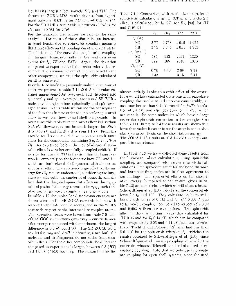
74 CHAPTER 7. MOLECULAR CALCULATIONS
fect has its largest e�ect, namely Bi2 and T lH . The
theoretical ZORA LDA results deviate from experi-
ment between -0.031 �A for T lI and +0.015 for HI .For the SR ZORA result this is between -0.048 �A for
Bi2 and +0.031 for T lH .
For the harmonic frequencies we can do the same
analysis. For most of these diatomics an increase
in bond length due to spin-orbit coupling means a
attening e�ect on the bonding curve and vica versa.
The attening of the curve due to spin-orbit coupling
can be quite large, especially for Bi2, and to a lesser
extent for I2, IF and PbTe. Again, the deviation
compared to experiment of the scalar relativistic re-
sult for Bi2 is somewhat out of line compared to the
other compounds, whereas the spin-orbit calculated
result is consistent.
In order to identify the genuinely molecular spin-orbit
e�ect we present in table 7.11 ZORA molecular en-
ergies minus spin-orbit averaged, and therefore also
spherically and spin averaged, atoms and SR ZORA
molecular energies minus spherically and spin aver-
aged atoms. In this table we can see the consequence
of the fact that in �rst order the molecular spin-orbit
e�ect is zero for these closed shell compounds.. In
most cases this molecular spin-orbit e�ect is less than
0.15 eV. However, it can be much larger: for PbTeit is 0.36 eV and for Bi2 it is even 1.1 eV. From the
atomic results one could have expected much more
e�ect for the compounds containing Te, I , T l, Pb orBi. As explained before the net o�-diagonal spin-
orbit e�ect is zero between fully occupied orbitals. If
we take for example T lI in the situation that one elec-tron is completely on the iodine we have T l+ and I�,which are both closed shell systems with almost no
spin-orbit e�ect. The relatively large e�ect on the en-
ergy for Bi2 can be understood, considering the largee�ective spin-orbit parameter of of bismuth, and the
fact that the diagonal spin-orbit e�ect on the �1=2g-orbital pushes its energy towards the �1=2g such that
o�-diagonal spin-orbit coupling has large e�ects.
In table 7.12 the molecular dissociation energies are
shown where in the SR ZORA case this is done with
respect to the L-S coupled atoms, and in the ZORA
case with respect to the intermediate coupled atoms.
The correction terms were taken from table 7.6. The
ZORA GGC calculations gives very accurate dissoci-
ation energies compared with experiment, the largest
di�erence is 0.3 eV for PbO. The SR ZORA GGC
results for Au2 and AuH is accurate, since both the
molecule and its fragments do not su�er from spin-
orbit e�ects. For the other compounds the di�erence
compared to experiment is larger, between 0.3 (HI)and 1.6 eV (PbO) too deep. The reason for this lies
Table 7.13: Comparison with results from correlated
relativistic calculations using ECP's, where the SO
e�ect is calculated, for I2 [92], for Bi2 [93], for HIand T lH [94]
I2 Bi2 HI T lH
re (�A)SO 2.77 2.768 1.616 1.925
SR 2.75 2.734 1.614 1.953
!e (cm�1)
SO 185 153 2331 1329
SR 199 165 2340 1310
De (eV)
SO 0.76 1.49 2.88 2.32
SR 1.43 3.15 2.41
almost entirely in the spin-orbit e�ect of the atoms.
If we would have calculated the atoms in intermediate
coupling the results would improve considerably, an
accuracy better than 0.2 eV except for PbTe (devia-tion of 0.4 eV) and Bi2 (deviation of 1.1 eV), which
are exactly the same molecules which have a large
molecular spin-orbit correction in the energies (see
table 7.11). In �gure 7.4 these results are shown in a
form that makes it easier to see the atomic and molec-
ular spin-orbit e�ects on the dissociation energy.
The ZORA LDA results are 0.3-1.4 eV too deep com-
pared to experiment.
In table 7.13 we have collected some results from
the literature, where calculations, using spin-orbit
coupling, are compared with scalar relativistic cal-
culations. The spin-orbit e�ect for the bond distance
and harmonic frequencies are in close agreement to
our �ndings. The spin-orbit e�ects on the dissoci-
ation energy (compared to the results given in ta-
ble 7.12) are not so close, which we will discuss below.
Schwerdtfeger et al. [103] calculated the spin-orbit ef-
fects for I2 and HI . They calculate an increase in
bondlength for I2 of 0.015 and for HI 0.003 �A due
to spin-orbit coupling, compared to respectively 0.02
and 0.003 �A from our calculations. The spin-orbit
e�ect in the dissociation energy they calculated for
HI 0.06 and for I2 0.14 eV, which can be compared
with respectively 0.03 and 0.11 eV from our calcula-
tions. Teichteil and P�elissier [92], who �nd less than
0.01 eV for the spin-orbit e�ect on I2, criticize the
results obtained by Schwerdtfeger et al. [103], since
Schwerdtfeger et al. use a j-j coupling scheme for the
molecule, whereas Teichteil and P�elissier used inter-
mediate coupling. Note that we only use intermedi-
ate coupling for open shell systems, since the used
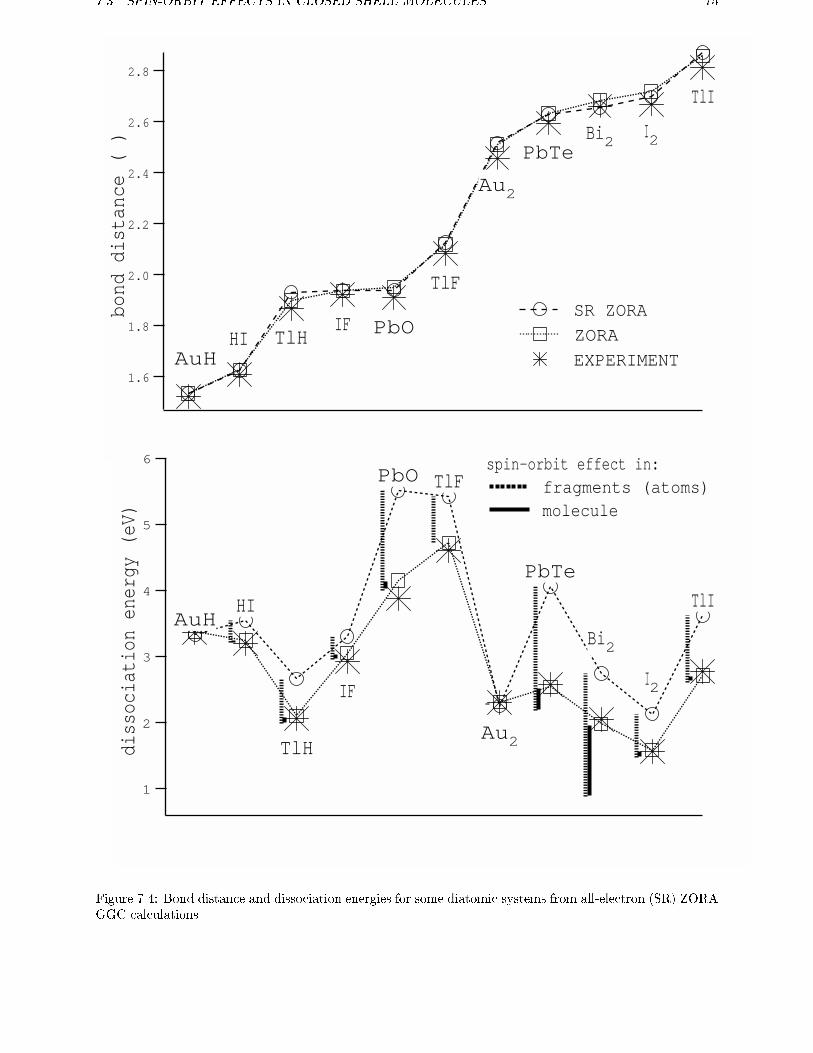
7.3. SPIN-ORBIT EFFECTS IN CLOSED SHELL MOLECULES 75
2.8
2.6
2.4
2.2
2.0
1.8
1.6
bond
dis
tanc
e (
)
AuHHI TlH
IF PbO
TlF
Au2
PbTeBi2 I2
TlI
SR ZORA
ZORA
EXPERIMENT
6
5
4
3
2
1
diss
ocia
tion
ene
rgy
(eV)
AuHHI
TlH
IF
PbO TlF
Au2
PbTe
Bi2
I2
TlI
spin-orbit effect in: fragments (atoms) molecule
Figure 7.4: Bond distance and dissociation energies for some diatomic systems from all-electron (SR) ZORA
GGC calculations.
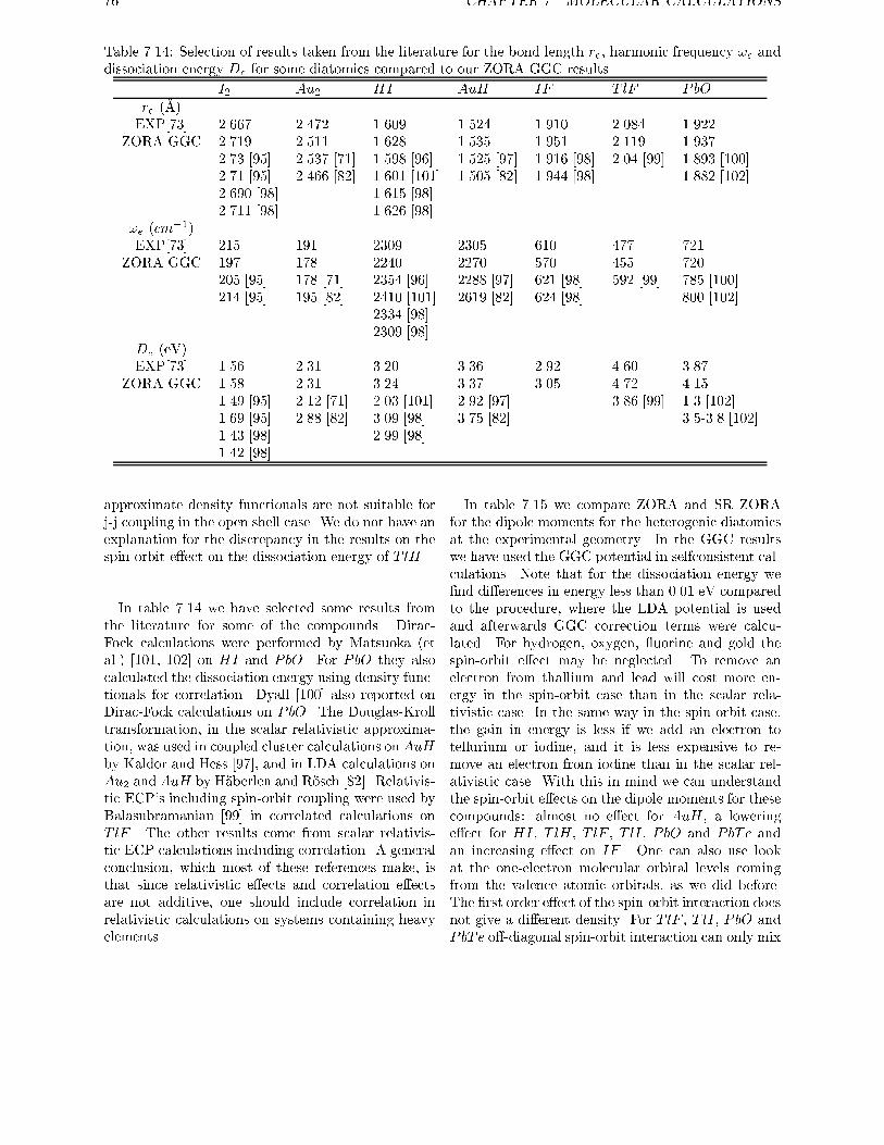
76 CHAPTER 7. MOLECULAR CALCULATIONS
Table 7.14: Selection of results taken from the literature for the bond length re, harmonic frequency !e anddissociation energy De for some diatomics compared to our ZORA GGC results.
I2 Au2 HI AuH IF T lF PbO
re (�A)EXP[73] 2.667 2.472 1.609 1.524 1.910 2.084 1.922
ZORA GGC 2.719 2.511 1.628 1.535 1.951 2.119 1.937
2.73 [95] 2.537 [71] 1.598 [96] 1.525 [97] 1.916 [98] 2.04 [99] 1.893 [100]
2.71 [95] 2.466 [82] 1.601 [101] 1.505 [82] 1.944 [98] 1.882 [102]
2.690 [98] 1.615 [98]
2.711 [98] 1.626 [98]
!e (cm�1)
EXP[73] 215 191 2309 2305 610 477 721
ZORA GGC 197 178 2240 2270 570 455 720
205 [95] 178 [71] 2354 [96] 2288 [97] 621 [98] 592 [99] 785 [100]
214 [95] 195 [82] 2410 [101] 2619 [82] 624 [98] 800 [102]
2334 [98]
2309 [98]
De (eV)
EXP[73] 1.56 2.31 3.20 3.36 2.92 4.60 3.87
ZORA GGC 1.58 2.31 3.24 3.37 3.05 4.72 4.15
1.49 [95] 2.12 [71] 2.03 [101] 2.92 [97] 3.86 [99] 1.3 [102]
1.69 [95] 2.88 [82] 3.09 [98] 3.75 [82] 3.5-3.8 [102]
1.43 [98] 2.99 [98]
1.42 [98]
approximate density functionals are not suitable for
j-j coupling in the open shell case. We do not have an
explanation for the discrepancy in the results on the
spin-orbit e�ect on the dissociation energy of T lH .
In table 7.14 we have selected some results from
the literature for some of the compounds. Dirac-
Fock calculations were performed by Matsuoka (et
al.) [101, 102] on HI and PbO. For PbO they also
calculated the dissociation energy using density func-
tionals for correlation. Dyall [100] also reported on
Dirac-Fock calculations on PbO. The Douglas-Krolltransformation, in the scalar relativistic approxima-
tion, was used in coupled cluster calculations on AuHby Kaldor and Hess [97], and in LDA calculations on
Au2 and AuH by H�aberlen and R�osch [82]. Relativis-
tic ECP's including spin-orbit coupling were used by
Balasubramanian [99] in correlated calculations on
T lF . The other results come from scalar relativis-
tic ECP calculations including correlation. A general
conclusion, which most of these references make, is
that since relativistic e�ects and correlation e�ects
are not additive, one should include correlation in
relativistic calculations on systems containing heavy
elements.
In table 7.15 we compare ZORA and SR ZORA
for the dipole moments for the heterogenic diatomics
at the experimental geometry. In the GGC results
we have used the GGC potential in selfconsistent cal-
culations. Note that for the dissociation energy we
�nd di�erences in energy less than 0.01 eV compared
to the procedure, where the LDA potential is used
and afterwards GGC correction terms were calcu-
lated. For hydrogen, oxygen, uorine and gold the
spin-orbit e�ect may be neglected. To remove an
electron from thallium and lead will cost more en-
ergy in the spin-orbit case than in the scalar rela-
tivistic case. In the same way in the spin-orbit case,
the gain in energy is less if we add an electron to
tellurium or iodine, and it is less expensive to re-
move an electron from iodine than in the scalar rel-
ativistic case. With this in mind we can understand
the spin-orbit e�ects on the dipole moments for these
compounds: almost no e�ect for AuH , a lowering
e�ect for HI , T lH , T lF , T lI , PbO and PbTe and
an increasing e�ect on IF . One can also use look
at the one-electron molecular orbital levels coming
from the valence atomic orbitals, as we did before.
The �rst order e�ect of the spin-orbit interaction does
not give a di�erent density. For T lF , T lI , PbO and
PbTe o�-diagonal spin-orbit interaction can only mix
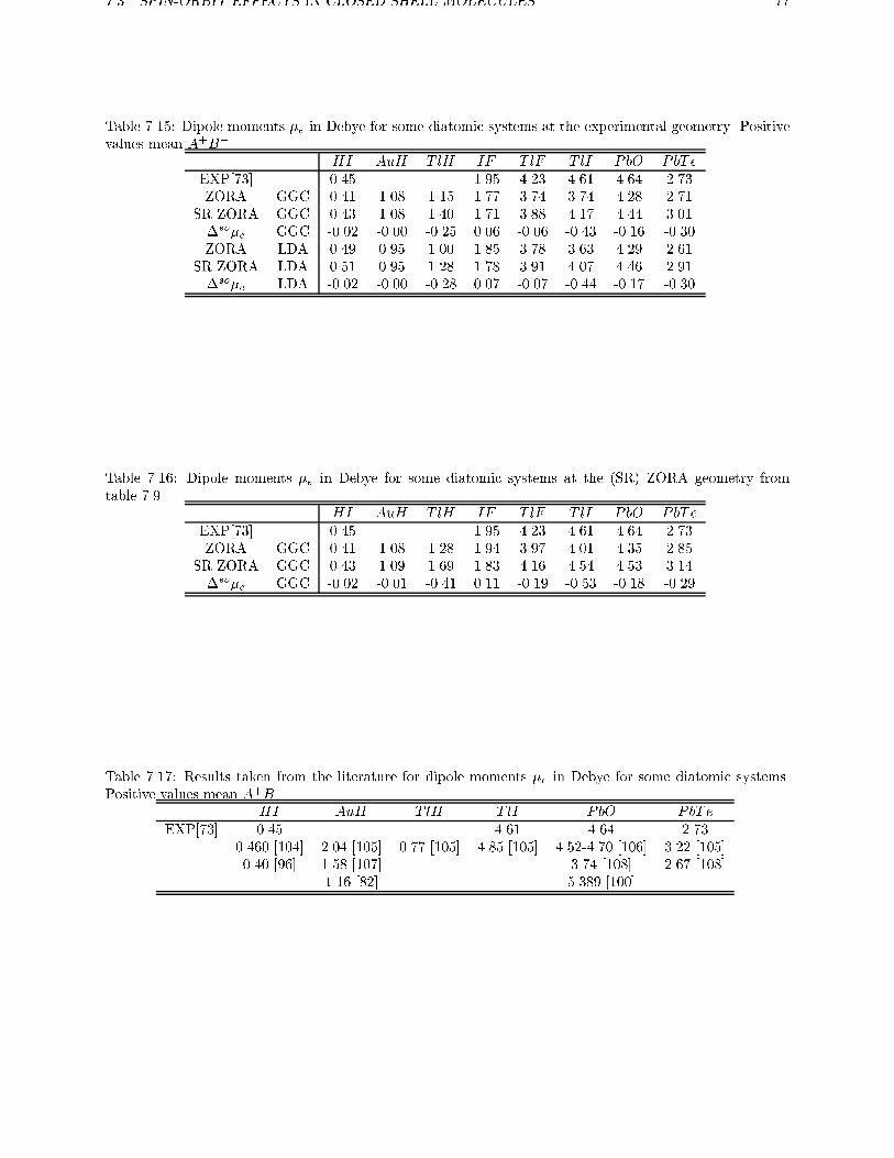
7.3. SPIN-ORBIT EFFECTS IN CLOSED SHELL MOLECULES 77
Table 7.15: Dipole moments �e in Debye for some diatomic systems at the experimental geometry. Positive
values mean A+B�.HI AuH T lH IF T lF T lI PbO PbTe
EXP[73] 0.45 1.95 4.23 4.61 4.64 2.73
ZORA GGC 0.41 1.08 1.15 1.77 3.74 3.74 4.28 2.71
SR ZORA GGC 0.43 1.08 1.40 1.71 3.88 4.17 4.44 3.01
�so�e GGC -0.02 -0.00 -0.25 0.06 -0.06 -0.43 -0.16 -0.30
ZORA LDA 0.49 0.95 1.00 1.85 3.78 3.63 4.29 2.61
SR ZORA LDA 0.51 0.95 1.28 1.78 3.91 4.07 4.46 2.91
�so�e LDA -0.02 -0.00 -0.28 0.07 -0.07 -0.44 -0.17 -0.30
Table 7.16: Dipole moments �e in Debye for some diatomic systems at the (SR) ZORA geometry from
table 7.9.
HI AuH T lH IF T lF T lI PbO PbTe
EXP[73] 0.45 1.95 4.23 4.61 4.64 2.73
ZORA GGC 0.41 1.08 1.28 1.94 3.97 4.01 4.35 2.85
SR ZORA GGC 0.43 1.09 1.69 1.83 4.16 4.54 4.53 3.14
�so�e GGC -0.02 -0.01 -0.41 0.11 -0.19 -0.53 -0.18 -0.29
Table 7.17: Results taken from the literature for dipole moments �e in Debye for some diatomic systems.
Positive values mean A+B�.HI AuH T lH T lI PbO PbTe
EXP[73] 0.45 4.61 4.64 2.73
0.460 [104] 2.04 [105] 0.77 [105] 4.85 [105] 4.52-4.70 [106] 3.22 [105]
0.40 [96] 1.58 [107] 3.74 [108] 2.67 [108]
1.16 [82] 5.389 [100]
78 CHAPTER 7. MOLECULAR CALCULATIONS
in orbitals, which have more character on T l or Pb.For IF the main o�-diagonal spin-orbit interaction
is between an occupied anti-bonding �1=2-orbital andan unoccupied anti-bonding �1=2-orbital. The anti-
bonding �1=2-orbital has more iodine character thanthe anti-bonding �1=2-orbital, thus the spin-orbit ef-fect decreases the charge on iodine. In T lH the un-
occupied thallium �1=2-orbital of �g 7.3 will mix in
with the occupied bonding �1=2-orbital and in HI theoccupied iodine �1=2-orbital will mix with the unoc-
cupied anti-bonding �1=2-orbital, which explains the
observed spin-orbit e�ects.
In ref. [109] the spin-orbit e�ect on the dipole mo-
ment forHI was calculated using correlated relativis-tic ECP's, At the experimental geometry they �nd it
to be -0.019 Debye, which is the same as we have
found. Dolg et al. [106] estimated the spin-orbit cor-
rection for PbO to be between -0.07 and -0.23 Debye,
our theoretical result -0.16 lies in this range.
Compared to experiment the ZORA GGC and SR
ZORA GGC results have an average deviation of
about 10%. In table 7.16 we also have calculated
the dipole moments for the same systems at the the-
oretical (SR) ZORA geometry of table 7.9. The de-
viations from experiment are reduced. Except for IFand PbTe the scalar relativistic results are closer tothe (known) experimental values than the spin-orbit
results, with an average deviation of approximately
5% for SR ZORA GGC and 7% for ZORA GGC.
In table 7.17 we give some results for the calcula-
tion of the dipole moment taken from the litera-
ture. Ref. [105] used Dirac-Fock calculations, ex-
cept forAuH , where correlation e�ects were included.
Dyall [100] also used Dirac-Fock calculations for PbO.The only relativistic LDA results in the table are from
H�aberlen et al.[82] for AuH . Their result for AuHis much closer to our result than the other two. The
remaining results in this table come from calculations
using relativistic ECP's.
7.4 Conclusions
In the last sections we have shown what the spin-orbit
e�ects are in closed shell molecules. For the calcu-
lated compounds the spin-orbit e�ect on the bond
distance never exceeded 0.03 �A, and on frequencies
less than 10%. Also the molecular spin-orbit e�ect on
the energies is often small, except for Bi2 and PbTe.To obtain the spin-orbit e�ects in the dissociation
energy it is also important to look at the e�ect on
the constituent atomic fragments. It is shown that
it is necessary to include spin-orbit e�ects for open
shell atoms, since they can be very large. A method
is proposed for open shell atoms, which uses present
day density functionals in an intermediate coupling
scheme. This method is used for the calculation of
some atomic multiplet splittings and it is shown to
give realistic energy di�erences. Using these inter-
mediate coupled atomic energies for the calculation
of the dissociation energies for the compounds under
study, we obtain high accuracy if we include gradient
correction (GGC) terms in the energy. The ZORA
GGC results are then all within 0.3 eV of the exper-
iment, with an average deviation of 0.1 eV for these
compounds. For most compounds this accuracy in
energy can be obtained, by only reckoning with spin-
orbit e�ects in the atoms, except for Bi2 and PbTe.For these compounds it is shown that, to obtain high
accuracy, it is also necessary to take spin-orbit e�ects
for the molecular energy into account. Except for
these energies, in most cases the molecular spin-orbit
e�ects are in the order of the accuracy of the cal-
culations compared to experiment. The theoretical
calculated dipole moments at the experimental ge-
ometry are still o� by approximately 10% compared
to the known experimental results in both the spin-
orbit and scalar relativistic case.
Chapter 8
Elimination of the small component
In this chapter we will solve the Dirac equation by
solving the two-component energy-dependent equa-
tion for the large component that results from the
elimination of the small component. This requires
for every occupied orbital the diagonalisation of a
Hamiltonian. Advantages are, however, that these
Hamiltonians are all bounded from below, unlike the
Dirac Hamiltonian, and that only a basis set for the
large component is needed. In this chapter we will
use Dirac type Slater orbitals, adapted from solutions
to the hydrogen-like atom. This o�ers the perspec-
tive of performing relativistic calculations to the same
accuracy as non-relativistic ones, with a comparable
number of basis functions.
8.1 Introduction
Traditional relativistic basis set methods (examples
can be found in [51, 110, 111, 112, 113] and more re-
cently in [114, 115, 116, 117]) use the four-component
Dirac Hamiltonian and need a basis set for the
large and the small component. In this chapter we
will solve the Dirac equation, using the well known
method of elimination of the small component (esc).
In our approach the matrix elements of the result-
ing energy dependent Hamiltonian for the large com-
ponent are calculated directly, which means we only
need a large component basis set and kinetic balance
problems never arise. Another possibility is to use an
auxiliary basis set for the small component, as done
by Wood et al. [118], and to evaluate the matrix ele-
ments of the large component Hamiltonian as matrix
products. In that case, however, the same kinetic
balance problems occur as in four-component meth-
ods and much of the advantage of the esc method
is lost. It is however easy to calculate the energy-
dependent matrix elements directly in a numerical
integration scheme [45] when we have a simple local
potential. This is the situation in density functional
calculations, where numerical integrations are widely
employed in nonrelativistic calculations as well. A
disadvantage is that the present procedure is already
iterative on the one-electron level since the orbital en-
ergies are not known beforehand, as was already ob-
served by Aerts [119]. However, this is not a real dis-
advantage in selfconsistent �eld procedures, because
one can optimise the potential and the orbital ener-
gies at the same time. It remains a disadvantage of
course that the energy dependent equation has to be
solved for every occupied orbital separately.
The Hamiltonians used in this approach are all
bounded from below, unlike the Dirac Hamiltonian.
For the hydrogen-like atom it was shown [120] that
in a �nite basis set this procedure gives convergence
from above, with increasing number of basis func-
tions, to the exact Dirac eigenvalue. We will show
that it is economical to use as basis functions Dirac
type Slater functions (DTO's). Working with the
large component only and employing the e�cient
DTO's enables one to performe relativistic calcula-
tions to the same accuracy as non-relativistic ones,
with a comparable number of basis functions.
The scaled zeroth order regular approximation
(scaled ZORA) to the Dirac equation is known to
give very accurate deep core and valence orbital en-
ergies [121, 74]. For other properties than the energy,
the accuracy is high for (sub-) valence orbitals [34]
but less so for deep core orbitals. However, if one
starts with the converged potential of the ZORA
method one obtains after 1 cycle (called FCPD-4
in [34]) already very accurate properties also for the
deep core orbitals. If even higher accuracy is re-
quired, one may use the method presented in this
chapter, which can be thought of as a natural exten-
sion of the ZORA approach to all orders. Further
(dis-)advantages of this method will be explained in
section 8.3. Results using an e�cient basis set are
presented in section 8.4.
79
80 CHAPTER 8. ELIMINATION OF THE SMALL COMPONENT
8.2 Solving the large compo-
nent equation
We can write the total energy of a many-electron
system in a relativistic density functional approach
(without the interaction energy of the nuclei) as:
EDiracTOT = EKIN +
Zd1�VN +EC +EXC [�] (8.1)
where:
EKIN =
NXi=1
Zd1(�yi c~� � ~p�i + �yi c~� � ~p�i � 2c2�yi�i)
EC =1
2
Z Zd1d2
�(1)�(2)
r12
� =
NXi=1
(�yi�i + �yi�i) (8.2)
and EXC is the exchange-correlation energy density
functional, which in this chapter will be approxi-
mated with the simple Slater exchange approxima-
tion (� = 0:7). For the electron-electron repulsion
the non-relativistic operator is used. The Kohn-Sham
formulation of density functional theory leads to the
one-electron Dirac equations:�V c~� � ~p
c~� � ~p �2c2 + V
���i�i
�= �i
��i�i
�(8.3)
where the Kohn-Sham one-electron potential is given
by:
V (~r1) = VN (~r1) +
Z�(2)
r12d~r2 +
�EXC [�]
��(~r1)(8.4)
In a four-component relativistic basis set calcula-
tion one can diagonalise this one-electron full Dirac
Hamiltonian. In that case the small component basis
set has to be chosen with care in order to avoid kinetic
balance failure. The solutions to the one-electron
equations can be obtained self-consistently, where the
orbitals with the lowest positive energies (eigenvalue
+ c2) are occupied. Because of the fact that the DiracHamiltonian is not bounded from below, there will
also be negative energy solutions, which are not of
interest to us but may cause complications.
An alternative procedure is to eliminate the small
component �:
�i =c
2c2 +Ei � V~� � ~p�i (8.5)
to obtain the Hamiltonian Hesc, which is energy de-
pendent and works solely on the large component �:
Hesc�i = (V + ~� � ~pc2
2c2 + �i � V~� � ~p)�i = �i�i(8.6)
We can solve this two-component equation self-
consistently in a basis set calculation using only a
basis set for the large component, which is a great
advantage compared to the four-component calcula-
tions. In order to calculate the matrix elements by
numerical integration we need in each grid point the
density and the Coulomb and exchange-correlation
potentials. In order to obtain the density the small
component is needed, for which equation 8.5 can
be used. In the atomic calculations we performed,
the density is calculated in every point of the radial
grid. In the essentially one-dimensional atomic prob-
lem the potentials can be calculated easily at the
grid points from this numerical density. Although
we will restrict ourselves to applications to atoms, it
should be pointed out that application to molecules
is straightforward, at least if numerical integration is
used. Once the density has been obtained in all grid
points of the molecular integration grid, the Coulomb
potential can be calculated in a routine manner, e.g.
by using a �t of the density [122] or by solving the
Poisson equation numerically [123].
The energy dependent eigenvalue equation is solved
iteratively, but apart from the density (or equiva-
lently the potential) also the eigenvalues have to be
iterated to self-consistency. This means that on every
cycle we have to perform a diagionalisation for ev-
ery di�erent eigenvalue. Suppose that we have after
N �1 cycles a potential V N�1 and eigenvalues �N�1j .
In the next cycle we have to diagonalise for every jcorresponding to an occupied orbital the Hamiltonian
HN�1j :
HN�1j = V N�1 + ~� � ~p
c2
2c2 + �N�1j � V N�1~� � ~p(8.7)
If �N�1j is the j'th energy of a given symmetry, we
have to choose the eigenvalue and density of the j'th
eigenfunction for the next cycle. In the case of the
s1=2-symmetry of the neutral Uranium atom it means
that one has to diagonalise on every cycle seven times
in this symmetry, because there are seven occupied
s1=2 orbitals. This is a disadvantage of this method
compared to four-component calculations, where only
one diagonalisation has to be performed on each cy-
cle. In �gure 8.1 the procedure is presented in a pic-
torial way. For each Hamiltonian only the bold eigen-
values and the corresponding orbitals are of interest.
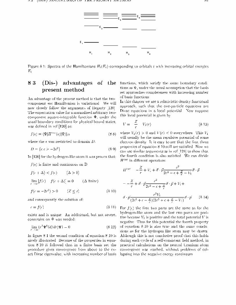
8.3. (DIS-) ADVANTAGES OF THE PRESENT METHOD 81
Figure 8.1: Spectra of the Hamiltonians Hi(Ei) corresponding to orbitals i with increasing orbital energies
Ei
8.3 (Dis-) advantages of the
present method
An advantage of the present method is that the two-
component esc Hamiltonian is variational. We will
now closely follow the arguments of Hegarty [120].
The expectation value for a normalised arbitrary two-
component square-integrable function , under the
usual boundary conditions for physical bound states,
was de�ned in ref [120] as:
f(�) = hjHesc(�)jijD (8.8)
where the � was restricted to domain D:
D = f�j� � �2c2g (8.9)
In [120] for the hydrogen-like atom it was proven that:
f(�) is �nite and continuous on D
f(�+�) < f(�) (� > 0)
lim�!1
[f(�)� f(�+�)] = 0 (� �nite)
f(� = �2c2) > 0 (Z � c) (8.10)
and consequently the solution of:
� = f(�) (8.11)
exists and is unique. An additional, but not severe,
constraint on was needed:
limr!1
(r3y(d=dr)) = 0 (8.12)
In �gure 8.1 the second condition of equation 8.10 is
nicely illustrated. Because of the properties in equa-
tion 8.10 it followed that in a �nite basis set the
procedure gives convergence from above to the ex-
act Dirac eigenvalue, with increasing number of basis
functions, which satisfy the same boundary condi-
tions as , under the usual assumption that the basis
set approaches completeness with increasing number
of basis functions.
In this chapter we use a relativistic density functional
approach, such that the one-particle equations are
Dirac equations in a local potential. Now suppose
this local potential is given by
V = �Z
r+ V1(r) (8.13)
where V1(r) > 0 and V (r) < 0 everywhere. This V1will usually be the mean repulsive potential of some
electron density. It is easy to see that the �rst three
properties of equation 8.10 still are satis�ed. Now we
can use similar arguments as in ref [124] to show that
the fourth condition is also satis�ed. We can divide
Hesc in di�erent operators:
Hesc = �Z
r+ V1 + ~� � ~p
c2
2c2 + �+ Zr� V1
~� � ~p =
= �Z
r+ ~� � ~p
c2
2c2 + �+ Zr
~� � ~p+ V1+
~� � ~pc2V1
(2c2 + �+ Zr)(2c2 + �+ Z
r� V1)
~� � ~p (8.14)
For f(�) the �rst two parts are the same as for the
hydrogen-like atom and the last two parts are posi-
tive because V1 is positive and the total potential V is
negative. Thus for this potential the fourth property
of equation 8.10 is also true and the same conclu-
sions as for the hydrogen-like atom may be drawn.
Although this is not conclusive proof that this holds
during each cycle of a self-consistent �eld method, in
practical calculations on the neutral Uranium atom
convergence was reached, without problems of col-
lapsing into the negative energy continuum.
82 CHAPTER 8. ELIMINATION OF THE SMALL COMPONENT
In the present method we only need to calculate ma-
trix elements for the large component. The matrix
elements can easily be calculated using numerical in-
tegration schemes [45]. In general in four-component
basis set methods one needs at least as many, usu-
ally more, basis functions for the small component
as for the large component, because of the kinetic
balance condition [53]. This will lead to a larger di-
agonalisation problem than in the present method,
but here one has to diagonalise for every di�erent
eigenvalue of the occupied spectrum. If the number
of di�erent occupied orbitals per symmetry is small
the present method can be competitive in computa-
tional time with respect to four-component methods.
Some diagonalisation procedures can make use of the
fact that one only needs one eigenfunction and eigen-
value per diagonalisation. One may also think of ways
to decrease the number of diagonalisations per cycle.
For example one can freeze the core and converge the
valence orbitals and then freeze the valence and con-
verge the core orbitals, etcetera.
It is possible to reduce the number of cycles if one
starts with an accurate initial potential. For ex-
ample one can use the solution of the zeroth order
regular approximation (ZORA) [121] to the Dirac
equation. Matrix elements can be calculated in the
present method in practically the same way as in the
ZORA method. One of the di�erences is that in the
present method one also has to use the small com-
ponent density for the calculation of the potential.
The small component density can be generated in
points of the integration grid using eq. 8.5, with-
out the need of introducing a small component basis
set. Implementation of the present method is there-
fore straightforward, once one has implemented the
ZORA method. It is thus perfectly feasible to �rst
converge a ZORA calculation, and subsequently con-
tinue with the present method if one wishes to obtain
results identical to full Dirac calculations. In the next
section we will show some calculations on the Ura-
nium atom which use the converged ZORA result for
the start-up potential.
The present method can of course also be used to �nd
solutions of the scalar relativistic equation [41, 42]:
HSR�i = (V + pc2
2c2 +ESRi � V
p)�i
= ESRi �i (8.15)
This equation is analogous to the spin-free modi�ed
Dirac equation of ref [125, 33] after eliminating the
lower component in that equation.
8.4 Basis set selection and re-
sults
Even if the basis set problem is strongly reduced by
eliminating the small component, one may still be
forced to use more basis functions than in a compa-
rable nonrelativistic calculation because of the weak
singularity at the nucleus of the relativistic solutions.
An example is provided by the ZORA calculations of
ref. [121]. In the STO basis set 6 basis functions were
used to describe the 1s1=2- and 2p1=2-orbital, yieldingan accuracy of about 0.2 a.u. in the deep core eigen-
values. Such a large number of STO's are needed,
because the weak singularity at the nucleus is di�-
cult to desribe with Slater type functions.
In order to solve this problem we have employed in
the present work Dirac type Slater orbitals (DTO's),
which are of the form:
r��1e��r (8.16)
where � does not have to be an integer value. The
�'s were optimised by a least squares �t to numerical
orbitals. For the lowest DTO in a given symmetry
we also optimised �. For the other �'s it turned out
not to be very critical whether one chooses integer or
non-integer values. We chose them in each symmetry
by a linear scaling procedure, such that the highest
� is equal to the n of the valence level of a given
symmetry (see table 8.1). Dirac type Slater orbitals
were for example used by Drake and Goldman [126] in
four-component Dirac calculations on the hydrogen-
like atom. Dirac type Slater orbitals are the nat-
ural choice for relativistic calculations on atoms, in
the same way as STO's are for nonrelativistic cal-
culations, because the solutions to the hydrogen-like
atom with a point charge nucleus have this form. Us-
ing DTO's one can easily ful�l the correct boundary
conditions at the nucleus. Especially for the s1=2-and p1=2-symmetry one needs much fewer DTO's to
obtain the same accuracy than one needs STO's or
Gaussian type orbitals (GTO's). We tested our im-
plementation of DTO basis sets on the problem of one
electron in a hydrogen-like potential, using DTO's
which could reproduce the exact solution. The ex-
act eigenvalues and eigenfunctions were correctly ob-
tained.
In table 8.1 we give our optimised DTO's in the
case of a neutral Uranium atom with a point charge.
In table 8.2 the calculated eigenvalues are given for
some deep core levels and in table 8.3 for some va-
lence levels using the DTO basis set of table 8.1. In
table 8.4 the corresponding radial expectation values
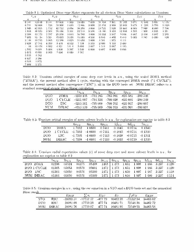
8.4. BASIS SET SELECTION AND RESULTS 83
Table 8.1: Optimised Dirac-type Slater exponents for all-electron Dirac-Slater calculations on Uraniums1=2 p1=2 p3=2 d3=2 d5=2 f5=2 f7=2
� � � � � � � � � � � � � �
0.741 150.00 0.741 62.856 1.369 79.000 2.609 31.164 2.887 37.769 3.627 17.646 3.687 17.797
0.741 92.000 1.728 53.906 1.639 42.806 3.000 25.153 2.939 25.943 3.678 11.233 3.759 11.328
1.845 82.915 1.732 42.712 2.058 38.256 3.000 19.721 2.920 19.483 4.000 7.848 4.000 7.796
1.810 48.535 2.264 25.196 2.551 22.210 3.500 13.480 3.433 12.950 4.333 4.368 4.333 4.221
2.300 43.173 2.797 23.350 3.043 16.700 4.000 10.302 3.947 9.948 4.667 2.430 4.667 2.293
2.665 25.134 3.331 15.693 3.536 15.580 4.500 6.646 4.460 6.410 5.000 1.247 5.000 1.138
3.146 19.745 3.865 12.590 4.029 11.650 5.000 4.581 4.973 4.411
3.628 17.701 4.399 8.470 4.522 7.738 5.333 2.606 5.333 2.460
4.110 13.476 4.932 6.324 5.014 5.686 5.667 1.514 5.667 1.405
4.592 9.099 5.466 4.036 5.507 3.539 6.000 0.887 6.000 0.806
5.073 6.893 6.000 2.696 6.000 2.307
5.555 4.582
6.037 3.188
6.518 1.872
7.000 1.171
Table 8.2: Uranium orbital energies of some deep core levels in a.u., using the scaled ZORA method
("ZORA"), the present method after 1 cycle, starting with the converged ZORA result ("1 CYCLE"),
and the present method after convergence ("ESC"), all in the DTO basis set. NUM DIRAC refers to a
standard numerical atomic Dirac-Slater calculation.
1s1=2 2s1=2 2p1=2 2p3=2 3s1=2DTO ZORA -4250.155 -794.285 -765.991 -625.581 -200.546
DTO 1 CYCLE -4251.097 -794.324 -766.028 -625.605 -200.549
DTO ESC -4255.561 -795.008 -766.702 -625.957 -200.697
NUM DIRAC -4255.559 -795.009 -766.703 -625.961 -200.691
Table 8.3: Uranium orbital energies of some valence levels in a.u., for explanation see caption to table 8.2.
6s1=2 6p1=2 6p3=2 5f5=2 6d3=2 7s1=2DTO ZORA -1.7192 -1.0690 -0.7411 -0.1045 -0.0714 -0.1340
DTO 1 CYCLE -1.7192 -1.0690 -0.7411 -0.1045 -0.0714 -0.1340
DTO ESC -1.7205 -1.0699 -0.7413 -0.1038 -0.0713 -0.1341
NUM DIRAC -1.7198 -1.0694 -0.7410 -0.1033 -0.0710 -0.1340
Table 8.4: Uranium radial expectation values hri of some deep core and some valence levels in a.u., for
explanation see caption to table 8.2.
1s1=2 2s1=2 2p1=2 2p3=2 3s1=2 6s1=2 6p1=2 6p3=2 5f5=2 6d3=2 7s1=2DTO ZORA .01206 .05524 .04475 .05498 .1463 1.473 1.651 1.898 1.486 3.237 4.120
DTO 1 CYCLE .01365 .05653 .04579 .05601 .1472 1.473 1.651 1.898 1.486 3.237 4.120
DTO ESC .01364 .05650 .04576 .05599 .1471 1.473 1.650 1.897 1.487 3.237 4.118
NUM DIRAC .01364 .05650 .04576 .05599 .1471 1.473 1.650 1.897 1.486 3.237 4.114
Table 8.5: Uranium energies in a.u., using the esc equation in a STO and a DTO basis set and the numerical
Dirac resultETOT
P�i EXC EC
R�VN EKIN
STO ESC -28080.51 -17757.57 -477.79 10482.20 -72552.94 34468.02
DTO ESC -28081.69 -17759.23 -477.74 10481.71 -72548.38 34462.72
NUM DIRAC -28081.76 -17759.07 -477.74 10481.95 -72549.55 34463.58
84 CHAPTER 8. ELIMINATION OF THE SMALL COMPONENT
are given as an example of orbital properties. We
may judge the basis set quality by comparing the
DTO ESC results with the standard numerical (basis
free) four-component Dirac (NUM DIRAC) results,
to which they should be identical. The hri expec-tation values have been obtained in the DTO ESC
calculations by including the small component from
eq. 8.5. We note that the DTO ESC results are in all
cases very close to the numerical Dirac results, which
demonstrates the feasibility of the present approach
and at the same time shows that a DTO basis set can
indeed be very useful in this kind of calculation. Ta-
ble 8.5 contains various energy terms from both STO
and DTO calculations, so one can judge the accuracy
of the DTO and STO basis sets for the individual
energy terms by comparing to the numerical Dirac
reference values. In the DTO basis the accuracy is
quite high, although the individual terms (notably
the kinetic and nuclear attraction energies) exhibit
somewhat stronger deviation than the total energy.
The STO basis set is clearly somewhat less accurate,
although it is considerably larger.
A similar conclusion can be drawn for the relative
performance of DTO's and STO's for one-electron
energies. In the current DTO basis set we get an
accuracy of better than 0.01 a.u. in the deep core
eigenvalues, as can be seen in table 8.2. This com-
pares very favorably to the quoted 0.02 a.u. [121] for
the STO basis. This improvement is achieved with
only 2 basis functions for the 1s1=2-orbital and 3 for
the 2p1=2-orbital, which is to be compared to the 6
basis functions for 1s and 2p in the STO basis. Only
replacing in the STO basis set these six 1s STO's andsix 2p STO's for the two resp. three corresponding
DTO's already provided the major part of the im-
provement. [In the present work we also optimised,
for consistency, all other DTO basis functions because
in ref [121] the STO basis set was optimised to the
ZORA orbitals instead of to the large components
of the Dirac equation.] We conclude that a DTO ba-
sis set, in combination with the present ESC method,
o�ers the perspective of performing relativistic calcu-
lations to the same accuracy as non-relativistic ones,
with a comparable number of basis functions.
Given the reliability of the DTO basis set, we may
compare the performance of the scaled ZORA ap-
proach (DTO ZORA [74], cf. CPD-4 in [34]) with
the improvement obtained after performing one cycle
with the present method using the converged ZORA
potential as starting point (DTO 1 CYCLE) and with
the fully converged ESC (or, equivalently, full Dirac)
result. We observe again [121] that for valence lev-
els the ZORA results are very close to Dirac results.
They are so close that even the present accurate ba-
sis has errors of the same order of magnitude as the
di�erence between ZORA and Dirac. For deep core
orbitals the ZORA error is larger (see also [124]), at
least for the hri expection value. If one uses the con-
verged ZORA potential as starting potential for the
present method one obtains in the �rst cycle what is
called FCPD-4 in ref [34]. In tables 8.2-8.4 we also
show these results (DTO 1 CYCLE) in the same DTO
basis set. It is clear that for deep core levels one does
still improve upon the scaled ZORA results. For the
hri expection value of 1s1=2 the 1-cycle result is veryclose to the converged ESC (Dirac) result, see ref [34]
for extensive discussion.
8.5 Conclusion
In this chapter we have solved the Dirac equation us-
ing only a large component basis set. The method of
elimination of the small component has been used, re-
sulting in an energy-dependent equation. In spite of
the disadvantage of this method, that on every cycle
for every occupied orbital a separate Hamiltonian has
to be diagonalised, the method o�ers the clear advan-
tages of being variationally stable [120], of requiring
only modest size basis sets, and of being capable of
reproducing the full Dirac result. If Dirac type or-
bitals (DTO's) are used instead of STO's or GTO's,
the basis set size does not have to be any larger than
in a nonrelativistic calculation. The DTO's are very
e�cient due to the fact that they have the right be-
haviour near the nucleus.
Further it is shown that this method can be very use-
ful if one takes the solution of the scaled ZORA equa-
tion [121, 74, 34] as a starting point. If one wants to
go beyond this already very accurate scaled ZORA
approach, one may use the method of this chapter
to calculate the full Dirac result. In fact, most of
the time (e.g. for chemical purposes) one is proba-
bly already satis�ed with the scaled ZORA approach,
because it gives very accurate energies and (sub-)
valence orbital properties. Only for deep core or-
bital properties (other than the energy) ZORA may
not give enough accuracy, but the error is largely
accounted for already after one cycle with the esc
Hamiltonian (cf. also [34]). It is with the present
method straightforward to converge to the Dirac an-
swer, if desired.
Chapter 9
The exact Foldy-Wouthuysen
transformation
In this chapter it is shown how within the frame-
work of a basisset expansion method the exact (i.e.
to all orders in the inverse velocity of light) Foldy-
Wouthuysen transformation that separates the nega-
tive and positive energy spectrum of the Dirac equa-
tion, can be constructed for an arbitrary potential
once the Dirac equation has been solved. On this ba-
sis an iterative procedure to solve the Dirac equation
is suggested that involves only the large component.
The methods are used to compare the expectation
value of the radial distance operator in the Dirac pic-
ture and in the Schr�odinger picture for the orbitals
of the Uranium atom.
9.1 Introduction
As is well known [18] the non-relativistic limit of
the Dirac equation for an electron in an external po-
tential is not reached simply by letting the velocity
of light go to in�nity. Rather this limiting process
entails a unitary transformation at the same time,
which block diagonalizes the Dirac hamiltonian by
separating the positive and negative energy part of
its spectrum. This unitary transformation, known as
the Foldy-Wouthuysen transformation, is equivalent
to a change of picture and consequently in compar-
ing relativistic and non-relativistic expectation values
(other than the energy) one has to be aware that the
same operator (such as the radial distance operator
r in an atom) does not represent the same physical
quantity in both pictures [127, 32]. Unfortunately
this transformation is only known exactly a priori for
a free particle. When an external potential is present,
the transformation is usually determined by expand-
ing in the inverse velocity of light to some �nite or-
der. In the case the potential is Coulombic in nature,
however, this expansion is known to be highly prob-
lematic, leading to divergencies except in the lowest
order. This does not mean that the transformation
as such does not exist, only that it should not be
expanded in this way. In this chapter we will show
that it is quite possible to obtain this exact unitary
transformation within the frame work of a basis set
method without resorting to any perturbational ex-
pansion once the Dirac equation has been solved for
its positive energy solutions.
In section 9.3 it is shown how on the basis of this
method, one can in fact obtain the large components
of the Dirac orbitals in a �nite basis set approxi-
mation in an iterative way, without �rst solving the
Dirac equation itself. This iterative procedure, which
can also be used in self consistent �eld calculations,
might be an alternative way to solve the Dirac equa-
tion that does not involve the small component. The
methods are used to compare the expectation value
of the radial distance operator in the Dirac picture
and in the Schr�odinger picture for the orbitals of the
Uranium atom.
9.2 The exact
Foldy-Wouthuysen
transformation
The time-independent Dirac equation for an electron
in an external potential V reads (in atomic units):
HDDi �
�V c~� � ~p
c~� � ~p V � 2c2
���Di�Di
�=
EDi
��Di�Di
�= ED
i Di (9.1)
Here D is the four-component Dirac wave function
and �D and �D are its large and small components.
85
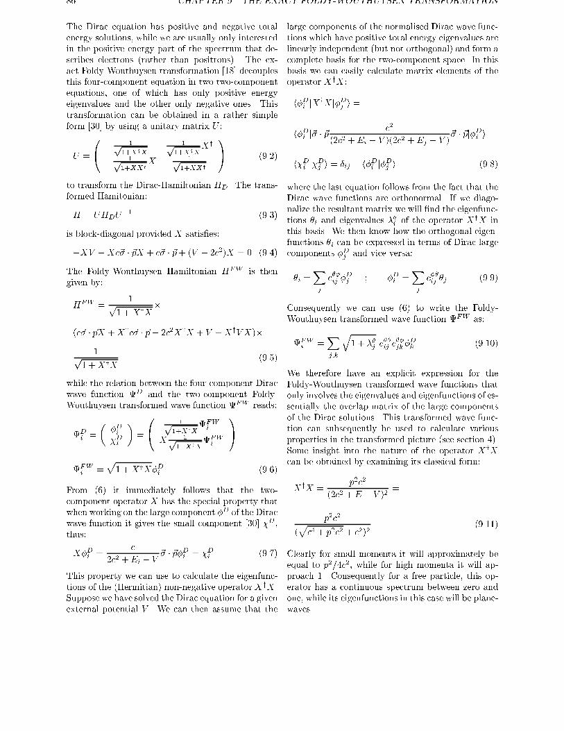
86 CHAPTER 9. THE EXACT FOLDY-WOUTHUYSEN TRANSFORMATION
The Dirac equation has positive and negative total
energy solutions, while we are usually only interested
in the positive energy part of the spectrum that de-
scribes electrons (rather than positrons). The ex-
act Foldy-Wouthuysen transformation [18] decouples
this four-component equation in two two-component
equations, one of which has only positive energy
eigenvalues and the other only negative ones. This
transformation can be obtained in a rather simple
form [30] by using a unitary matrix U :
U =
0@ 1p
1+XyX
1p1+XyX
Xy
� 1p1+XXy
X 1p1+XXy
1A (9.2)
to transform the Dirac-Hamiltonian HD. The trans-
formed Hamitonian:
H = UHDU�1 (9.3)
is block-diagonal provided X satis�es:
�XV �Xc~� � ~pX + c~� � ~p+ (V � 2c2)X = 0 (9.4)
The Foldy-Wouthuysen Hamiltonian HFW is then
given by:
HFW =1
p1 +XyX
�
(c~� � ~pX +Xyc~� � ~p� 2c2XyX + V +XyV X)�
1p1 +XyX
(9.5)
while the relation between the four-component Dirac
wave function D and the two-component Foldy-
Wouthuysen transformed wave function FW reads:
Di =
��Di�Di
�=
0@ 1p
1+XyXFWi
X 1p1+XyX
FWi
1A
FWi =
p1 +XyX�Di (9.6)
From (6) it immediately follows that the two-
component operator X has the special property that
when working on the large component �D of the Dirac
wave function it gives the small component [30] �D,thus:
X�Di =c
2c2 +Ei � V~� � ~p�Di = �Di (9.7)
This property we can use to calculate the eigenfunc-
tions of the (Hermitian) non-negative operator XyX .
Suppose we have solved the Dirac equation for a given
external potential V . We can then assume that the
large components of the normalised Dirac wave func-
tions which have positive total energy eigenvalues are
linearly independent (but not orthogonal) and form a
complete basis for the two-component space. In this
basis we can easily calculate matrix elements of the
operator XyX :
h�Di jXyX j�Dj i =
h�Di j~� � ~pc2
(2c2 +Ei � V )(2c2 +Ej � V )~� � ~pj�Di i =
h�Di j�Dj i = �ij � h�Di j�
Dj i (9.8)
where the last equation follows from the fact that the
Dirac wave functions are orthonormal. If we diago-
nalize the resultant matrix we will �nd the eigenfunc-
tions �i and eigenvalues ��i of the operator XyX in
this basis. We then know how the orthogonal eigen-
functions �i can be expressed in terms of Dirac large
components �Dj and vice versa:
�i =Xj
c��ij �Dj ; �Di =
Xj
c��ij �j (9.9)
Consequently we can use (6) to write the Foldy-
Wouthuysen transformed wave function FW as:
FWi =
Xj;k
q1 + ��j c
��ij c
��jk�
Dk (9.10)
We therefore have an explicit expression for the
Foldy-Wouthuysen transformed wave functions that
only involves the eigenvalues and eigenfunctions of es-
sentially the overlap matrix of the large components
of the Dirac solutions. This transformed wave func-
tion can subsequently be used to calculate various
properties in the transformed picture (see section 4).
Some insight into the nature of the operator XyXcan be obtained by examining its classical form:
XyX =p2c2
(2c2 +E � V )2=
p2c2
(pc4 + p2c2 + c2)2
(9.11)
Clearly for small momenta it will approximately be
equal to p2=4c2, while for high momenta it will ap-
proach 1. Consequently for a free particle, this op-
erator has a continuous spectrum between zero and
one, while its eigenfunctions in this case will be plane-
waves.
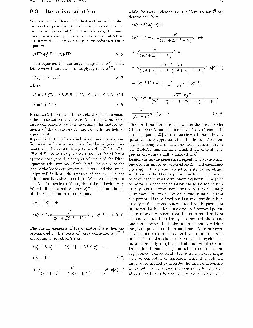
9.3. ITERATIVE SOLUTION 87
9.3 Iterative solution
We can use the ideas of the last section to formulate
an iterative procedure to solve the Dirac equation in
an external potential V that avoids using the small
component entirely. Using equation 9.5 and 9.6 we
can write the Foldy-Wouthuysen transformed Dirac
equation:
HFWFWi = Ei
FWi (9.12)
as an equation for the large component �D of the
Dirac wave function, by multiplying it by ~S1=2:
~H�Di = Ei ~S�Di (9.13)
where:
~H = c~� �~pX+Xyc~� �~p�2c2XyX+V +XyV X(9.14)
~S = 1 +XyX (9.15)
Equation 9.13 is now in the standard form of an eigen-
value equation with a metric ~S. In the basis set of
large components we can determine the matrix ele-
ments of the operators ~H and ~S, with the help of
equation 9.7.
Equation 9.13 can be solved in an iterative manner.
Suppose we have an estimate for the large compo-
nents and the orbital energies, which will be called
�0i and E0i respectively, were i runs over the di�erent
approximate (positive energy) solutions of the Dirac
equation (the number of which will be equal to the
size of the large component basis set) and the super-
script will indicate the number of the cycle in the
subsequent iterative procedure. We then proceed for
the N � 1th cycle to Nth cycle in the following way.
We will �rst normalise every �n�1i such that the or-
bital density is normalised to one:
h�n�1i j�n�1i i+
h�n�1i j~� � ~pc2
(2c2 +En�1i � V )2
~� � ~pj�n�1i i = 1(9.16)
The matrix elements of the operator ~S are then ap-
proximated in the basis of large components �n�1i
according to equation 9.7 as:
h�n�1i j ~Sj�n�1j i = h�n�1i j1 +XyX j�n�1j i =
h�n�1i j1+ (9.17)
~� � ~pc2
(2c2 +En�1i � V )(2c2 +En�1
j � V )~� � ~pj�n�1j i
while the matrix elements of the Hamiltonian ~H are
determined from:
h�n�1i j ~H j�n�1j i =
h�n�1i jV + ~� � ~pc2
(2c2 +En�1i � V )
~� � ~p+
~� � ~pc2
(2c2 +En�1j � V )
~� � ~p�
~� � ~pc2(2c2 � V )
(2c2 +En�1i � V )(2c2 +En�1
j � V )~� � ~pj�n�1j i
= h�n�1i jV + ~� � ~pc2
(2c2 � V )~� � ~pj�n�1j i�
h�n�1i j~� � ~pEn�1i En�1
j
(2c2 +En�1i � V )(2c2 +En�1
j � V )�
c2
(2c2 � V )~� � ~pj�n�1j i (9.18)
The �rst term can be recognized as the zeroth order
CPD or ZORA hamiltonian extensively discussed in
earlier papers [128] which was shown to already give
quite accurate approximations to the full Dirac en-
ergies in many cases. The last term, which corrects
this ZORA hamiltonian, is small if the orbital ener-
gies involved are small compared to c2.Diagonalising the generalized eigenfunction equation,
one obtains improved eigenvalues Eni and eigenfunc-
tions �ni . By iterating to selfconsistency we obtain
solutions to the Dirac equation without ever having
to calculate the small component explicitly. The price
to be paid is that the equation has to be solved iter-
atively. On the other hand this price is not as large
as it may seem if one considers the usual case that
the potential is not �xed but is also determined iter-
atively until selfconsistency is reached. In particular
in the density functional method the improved poten-
tial can be determined from the improved density at
the end of each iterative cycle described above and
one can converge both the potential and the Dirac
large component at the same time. Note however,
that the matrix elements of ~H have to be calculated
in a basis set that changes from cycle to cycle. The
matrix has only roughly half of the size of the full
Dirac Hamiltonian being limited to the positive en-
ergy space. Consequently the current scheme might
well be competative, especially since it avoids the
large bases needed to describe the small components
accurately. A very good starting point for the iter-
ative procedure is formed by the zeroth order CPD
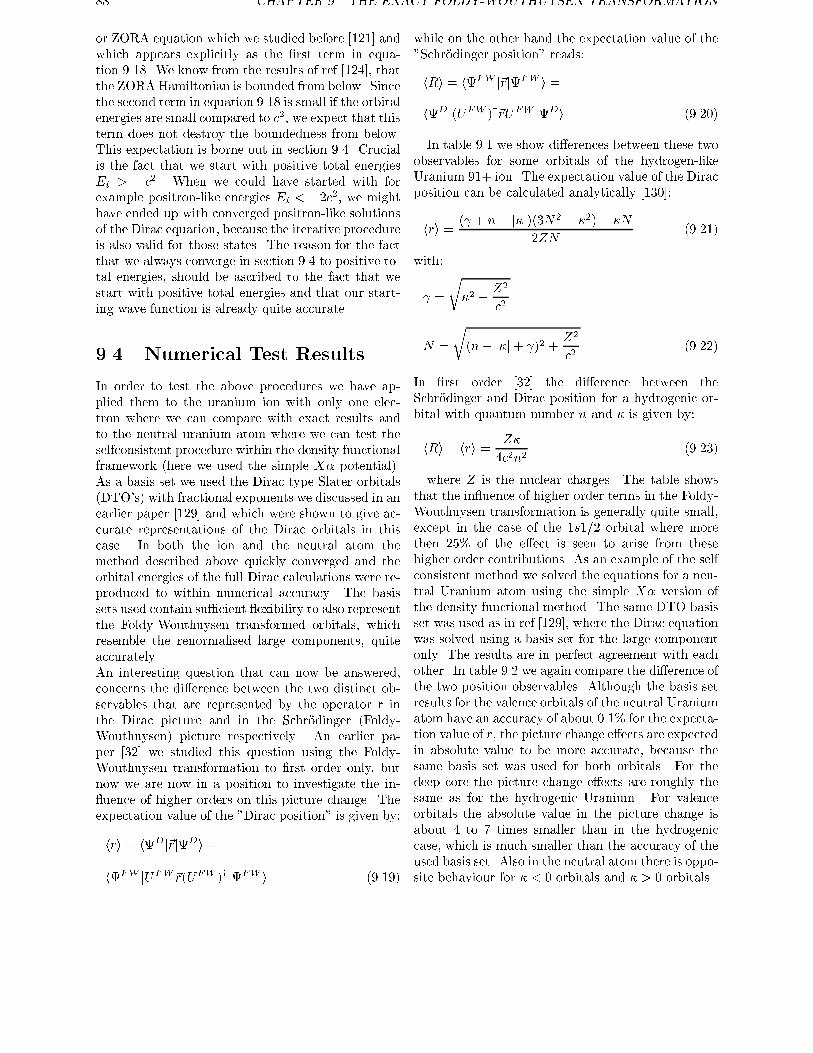
88 CHAPTER 9. THE EXACT FOLDY-WOUTHUYSEN TRANSFORMATION
or ZORA equation which we studied before [121] and
which appears explicitly as the �rst term in equa-
tion 9.18. We know from the results of ref [124], that
the ZORAHamiltonian is bounded from below. Since
the second term in equation 9.18 is small if the orbital
energies are small compared to c2, we expect that thisterm does not destroy the boundedness from below.
This expectation is borne out in section 9.4. Crucial
is the fact that we start with positive total energies
Ei > �c2. When we could have started with for
example positron-like energies Ei < �2c2, we mighthave ended up with converged positron-like solutions
of the Dirac equation, because the iterative procedure
is also valid for those states. The reason for the fact
that we always converge in section 9.4 to positive to-
tal energies, should be ascribed to the fact that we
start with positive total energies and that our start-
ing wave function is already quite accurate.
9.4 Numerical Test Results
In order to test the above procedures we have ap-
plied them to the uranium ion with only one elec-
tron where we can compare with exact results and
to the neutral uranium atom where we can test the
selfconsistent procedure within the density functional
framework (here we used the simple X� potential).
As a basis set we used the Dirac type Slater orbitals
(DTO's) with fractional exponents we discussed in an
earlier paper [129] and which were shown to give ac-
curate representations of the Dirac orbitals in this
case. In both the ion and the neutral atom the
method described above quickly converged and the
orbital energies of the full Dirac calculations were re-
produced to within numerical accuracy. The basis
sets used contain su�cient exibility to also represent
the Foldy-Wouthuysen transformed orbitals, which
resemble the renormalised large components, quite
accurately.
An interesting question that can now be answered,
concerns the di�erence between the two distinct ob-
servables that are represented by the operator r in
the Dirac picture and in the Schr�odinger (Foldy-
Wouthuysen) picture respectively. An earlier pa-
per [32] we studied this question using the Foldy-
Wouthuysen transformation to �rst order only, but
now we are now in a position to investigate the in-
uence of higher orders on this picture change. The
expectation value of the "Dirac position" is given by:
hri = hDj~rjDi =
hFW jUFW~r(UFW )yjFW i (9.19)
while on the other hand the expectation value of the
"Schr�odinger position" reads:
hRi = hFW j~rjFW i =
hDj(UFW )y~rUFW jDi (9.20)
In table 9.1 we show di�erences between these two
observables for some orbitals of the hydrogen-like
Uranium 91+ ion. The expectation value of the Dirac
position can be calculated analytically [130]:
hri =( + n� j�j)(3N2 � �2)� �N
2ZN(9.21)
with:
=
r�2 �
Z2
c2
N =
r(n� j�j+ )2 +
Z2
c2(9.22)
In �rst order [32] the di�erence between the
Schr�odinger and Dirac position for a hydrogenic or-
bital with quantum number n and � is given by:
hRi � hri =Z�
4c2n2(9.23)
where Z is the nuclear charges. The table shows
that the in uence of higher order terms in the Foldy-
Wouthuysen transformation is generally quite small,
except in the case of the 1s1=2 orbital where more
then 25% of the e�ect is seen to arise from these
higher order contributions. As an example of the self
consistent method we solved the equations for a neu-
tral Uranium atom using the simple X� version of
the density functional method. The same DTO basis
set was used as in ref [129], where the Dirac equation
was solved using a basis set for the large component
only. The results are in perfect agreement with each
other. In table 9.2 we again compare the di�erence of
the two position observables. Although the basis set
results for the valence orbitals of the neutral Uranium
atom have an accuracy of about 0.1% for the expecta-
tion value of r, the picture change e�ects are expectedin absolute value to be more accurate, because the
same basis set was used for both orbitals. For the
deep core the picture change e�ects are roughly the
same as for the hydrogenic Uranium. For valence
orbitals the absolute value in the picture change is
about 4 to 7 times smaller than in the hydrogenic
case, which is much smaller than the accuracy of the
used basis set. Also in the neutral atom there is oppo-
site behaviour for � < 0 orbitals and � > 0 orbitals.
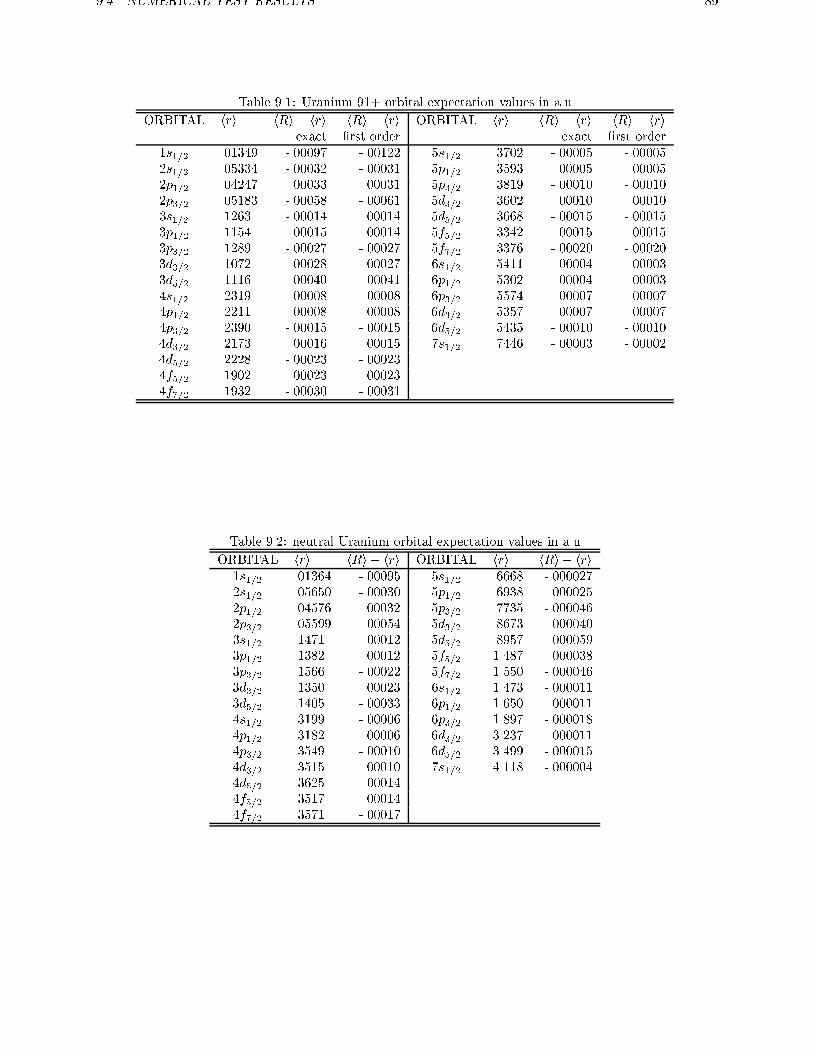
9.4. NUMERICAL TEST RESULTS 89
Table 9.1: Uranium 91+ orbital expectation values in a.u.
ORBITAL hri hRi � hri hRi � hri ORBITAL hri hRi � hri hRi � hriexact �rst order exact �rst order
1s1=2 .01349 -.00097 -.00122 5s1=2 .3702 -.00005 -.00005
2s1=2 .05334 -.00032 -.00031 5p1=2 .3593 .00005 .00005
2p1=2 .04247 .00033 .00031 5p3=2 .3819 -.00010 -.00010
2p3=2 .05183 -.00058 -.00061 5d3=2 .3602 .00010 .00010
3s1=2 .1263 -.00014 .00014 5d5=2 .3668 -.00015 -.00015
3p1=2 .1154 .00015 .00014 5f5=2 .3342 .00015 .00015
3p3=2 .1289 -.00027 -.00027 5f7=2 .3376 -.00020 -.00020
3d3=2 .1072 .00028 .00027 6s1=2 .5411 -.00004 -.00003
3d5=2 .1116 -.00040 -.00041 6p1=2 .5302 .00004 .00003
4s1=2 .2319 -.00008 -.00008 6p3=2 .5574 -.00007 -.00007
4p1=2 .2211 .00008 .00008 6d3=2 .5357 .00007 .00007
4p3=2 .2390 -.00015 -.00015 6d5=2 .5435 -.00010 -.00010
4d3=2 .2173 .00016 .00015 7s1=2 .7446 -.00003 -.00002
4d5=2 .2228 -.00023 -.00023
4f5=2 .1902 .00023 .00023
4f7=2 .1932 -.00030 -.00031
Table 9.2: neutral Uranium orbital expectation values in a.u.
ORBITAL hri hRi � hri ORBITAL hri hRi � hri1s1=2 .01364 -.00095 5s1=2 .6668 -.000027
2s1=2 .05650 -.00030 5p1=2 .6938 .000025
2p1=2 .04576 .00032 5p3=2 .7735 -.000046
2p3=2 .05599 -.00054 5d3=2 .8673 .000040
3s1=2 .1471 -.00012 5d5=2 .8957 -.000059
3p1=2 .1382 .00012 5f5=2 1.487 .000038
3p3=2 .1566 -.00022 5f7=2 1.550 -.000046
3d3=2 .1350 .00023 6s1=2 1.473 -.000011
3d5=2 .1405 -.00033 6p1=2 1.650 .000011
4s1=2 .3199 -.00006 6p3=2 1.897 -.000018
4p1=2 .3182 .00006 6d3=2 3.237 .000011
4p3=2 .3549 -.00010 6d5=2 3.499 -.000015
4d3=2 .3515 .00010 7s1=2 4.118 -.000004
4d5=2 .3625 -.00014
4f5=2 .3517 .00014
4f7=2 .3571 -.00017
90 CHAPTER 9. THE EXACT FOLDY-WOUTHUYSEN TRANSFORMATION
9.5 Conclusions
In this chapter the exact Foldy-Wouthuysen trans-
formation is constructed for an arbitrary potential.
On the basis of this construction an iterative proce-
dure is formulated that constitutes an alternative way
for solving the Dirac equation, obviating the need
for a small component basis. The procedure seems
especially attractive when used in a self-consistent
�eld scheme, since then the iterative procedure can
be run concurrently with the SCF iterations. The
method has been applied to the calculation of the
picture change e�ects in the expectation value of the
position operators with the uranium atom as an ex-
ample. Higher then �rst order e�ects of this picture
change turn out the be only important for the deep
core orbitals, where they can be as large as 25% in
the case of hydrogen-like uranium.
Samenvatting
De meeste materie om ons heen bestaat uit moleculen of kristallen, die op hun beurt weerte ontleden zijn in atomen. Een atoom bestaat uit een positief geladen kern, die eenaantrekkende kracht uitoefent op elektronen die zich rondom die kern bewegen. De atoom-
kernen bewegen zich veel langzamer dan de relatief lichte elektronen. Zware elementen, zoalsbijvoorbeeld goud, kwik en lood, hebben een grote positieve kernlading. Hoe groter dezepositieve lading van de atoomkern is, hoe sterker de aantrekkingskracht is op de elektronen.Deze elektrische kracht is ook sterker, naarmate de elektronen dichter bij de kern komen.
De binnenste elektronen, die het meest gebonden zijn en ook wel core-elektronen worden ge-noemd, bewegen daardoor met grote snelheid die in de buurt kan komen van de lichtsnelheid.Voor een juiste beschrijving van de beweging van deze snelle elektronen moet men daaromde speciale relativiteitstheorie van Einstein gebruiken. De buitenste elektronen, de valentie-elektronen, bewegen gemiddeld een stuk langzamer. Deze elektronen zijn chemisch het meest
interessant, omdat zij in grote mate bepalen of een binding tussen atomen tot stand komt,en hoe sterk die binding is. Langzame elektronen kunnen zeer goed beschreven worden metniet-relativistische bewegingsvergelijkingen. Echter zelfs valentie-elektronen hebben een kansdat ze vlak in de buurt van de atoomkern komen, en zullen dan door de enorme krachten
van de kern erg snel bewegen. De niet-relativistische bewegingsvergelijking is in dit gebieddaarom niet nauwkeurig genoeg meer. Men kan zelfs zeggen, klassiek mechanisch gezien, datvoor elke plek in het atoom geldt, dat een valentie-elektron zich harder voortbeweegt daneen core-elektron. Dat een valentie-elektron gemiddeld langzamer beweegt, komt omdat het
veel minder kans heeft om vlak bij de atoomkern te komen dan een core-elektron. Hoeweldeze kans vrij klein is, is het relativistische e�ect toch niet te verwaarlozen voor valentie-elektronen van de zwaardere atomen.In dit proefschrift zullen we een benaderde bewegingsvergelijking gebruiken die nauwkeurigis voor valentie-elektronen, zelfs als ze dicht in de buurt van een atoomkern bewegen. Deze
regulier benaderde relativistische vergelijking, genaamd ZORA, is de simpelste vergelijkingdie men krijgt als men de relativistische vergelijking expandeert in E=(2mc2 � V ). In dezeexpansie-parameter is E de bindingsenergie van de elektronen, die voor valentie-elektronenvan de orde van enkele eV's is. De rustmassa-energie van het elektron mc2 is ongeveer gelijkaan een half miljoen eV. De potentiaal V , die gerelateerd is aan de elektrische kracht, is inhet algemeen klein ten opzichte van de rustmassa-energie van het elektron, behalve in debuurt van een atoomkern. In deze buurt kan de potentaal V erg groot worden, zeker als menkijkt naar de zwaardere elementen. Aangezien de potentiaal V attractief is, dus negatief, is
de expansieparameter E=(2mc2 � V ) overal veel kleiner dan 1 voor valentie-elektronen. DeZORA-vergelijking is daarom erg nauwkeurig voor valentie-elektronen. Voor core-elektronenis de bindingsenergie E veel groter, wat tot gevolg heeft dat ook de expansieparameter veel
91
92 SAMENVATTING
groter wordt. Voor deze elektronen is de ZORA-vergelijking dan een stuk minder nauwkeurig.De niet-relativistische vergelijking kan men opvatten als de simpelste vergelijking die menkrijgt als men de relativistische vergelijking expandeert in (E�V )=(2mc2). Deze expansiepa-rameter is voor valentie-elektronen niet meer klein in de buurt van een atoomkern, omdatde potentiaal V daar grote waarden kan bereiken. Voor valentie-elektronen is de ZORA-vergelijking dus een betere benadering dan de niet-relativistische vergelijking. Berekeningenlaten zien dat dit ook geldt voor de meeste andere elektronen. De expansies die hier gebruikt
zijn, kunnen zowel in de klassieke mechanica, als in de quantummechanica gebruikt worden.
Het standaardmodel voor de beschrijving van de electromagnetische wisselwerking en be-weging van electronen is tegenwoordig de QuantumElectroDynamica (QED). Nauwkeurige
QED berekeningen zijn nog vrijwel alleen gedaan aan kleine systemen, zoals het waterstof-en heliumatoom, maar geven dan ook zeer goede overeenstemming met zeer nauwkeurigeexperimenten. Voor grotere systemen zijn nauwkeurige QED berekeningen meestal veel teduur (veel computertijd).Een benadering op deze methode is de Dirac-vergelijking. Dit is een relativistische quan-
tummechanische bewegingsvergelijking voor bijvoorbeeld elektronen. Net als in de klassiekemechanica, kan men in de quatummechanica de relativistische vergelijking benaderen metbehulp van expansies. De niet-relativistische quantummechanische vergelijking wordt ookwel de Schr�odinger-vergelijking genoemd. In de quatummechanica is het niet meer juist om
het (tegelijkertijd) over de plaats en de snelheid van een deeltje te hebben. Deeltjes worden indeze theorie beschreven met behulp van een gol�unctie, die de kans aangeeft om een deeltjeergens aan te tre�en. De oplossing van de Dirac-vergelijking is een 4-componentige gol�unc-tie, die bestaat uit twee grote en twee kleine componenten. Een van de standaardmethodes
om moleculaire quantummechanische vergelijkingen op te lossen gebruikt een ontwikkelingvan de gol�unctie in basisfuncties. Voor het oplossen van de Dirac-vergelijking wordenmeestal basisfuncties gebruikt, die de grote en de kleine componenten goed moeten kunnenbeschrijven. In hoofdstuk 8 and 9 worden methodes gebruikt om de Dirac-vergelijking op telossen, die alleen basisfuncties voor de twee grote componenten nodig hebben en waarin de
twee kleine componenten alleen impliciet worden gebruikt.Het hoofdbestanddeel van dit proefschrift gaat over een benadering op de Dirac-vergelijking,de ZORA-vergelijking. In hoodstuk 2 wordt deze deze vergelijking afgeleid met behulp vanverschillende methodes en in hoodstuk 3 wordt een aantal eigenschappen van deze verge-
lijking bekeken. Exacte oplossingen van het het waterstof-achtige atoom worden gegevenin hoofdstuk 4. In dit geval zijn de zogenaamde geschaalde ZORA energie�en exact gelijkaan de Dirac energie�en. In hoofdstuk 5 worden numerieke atomaire berekeningen gedaan.Het verschil tussen de oplossingen van de Dirac en de ZORA-vergelijking is erg klein, zeker
als men kijkt naar valentie-elektronen, die zo belangrijk zijn voor chemische eigenschappen.Het verschil met de niet-relativistische oplossingen is veel groter. Hoofdstuk 6 laat zienhoe de ZORA methode is geimplementeerd in een moleculair rekenprogramma en in eenprogramma dat geschikt is om systemen met periodiciteit (bijvoorbeeld kristallen) uit terekenen. Hoofdstuk 7 bevat resultaten van berekeningen aan twee-atomige moleculen. De
ZORA berekeningen leveren dan een grote mate van overeenstemming op met experimentelegegevens.
Summary
Most matter around us consists of molecules or crystals. These can be further divided intoatoms. An atom consists of a postively charged nucleus, which attracts the surroundingelectrons. The atomic nuclei move much slower than the relatively light electrons. Heavy
elements, like for example gold, mercury and lead, have a large positive nuclear charge. Thelarger this charge is, the stronger the nucleus attracts the electrons. This electric force isalso stronger if the electrons are closer to the nucleus. The inner electrons, or core electrons,move with a speed that might approach closely the velocity of light. For a good decription of
the motion of these fast electrons it is necessary to use Einsteins special theory of relativity.The outer electrons, or valence electrons, have a lower average velocity. These electrons arechemically the most interesting ones, since they are for a large part responsible for the bond-ing and strength of bonding between atoms. Slow electrons can be described satisfactorywith non-relativistic equations of motion. However, even valence electrons will move very
fast once they come close to an atomic nucleus. In that case the non-relativistic equationsof motion are not accurate enough anymore. One can even say, from a classic mechanicalpoint of view, that at every place in an atom a valence electron will move faster than a coreelectron. On the average a valence electron will move slower, because it has much less chance
to come close to an atomic nucleus. Although this chance is relatively small, the relativistice�ect can not be neglected for valence electrons of heavy atoms.In this thesis an approximate equation of motion is used, called the ZORA (zeroth orderrelativistic approximated) equation, which is the simplest equation one gets if one expands
the relativistic equation in E=(2mc2�V ). This expansion can be used in classical mechanicsas well as in quantum mechanics. In this expansion E is the binding energy of the electron,which is in the order of a few eV's for valence electrons and mc2 is the rest mass energy of theelectron, which is approximately half a million eV. The potential V , related to the electricforce, is usually small compared to the rest mass energy of the electron, except in the neigh-
bourhood of the atomic nucleus. In this region the potential can be very large, especiallyfor the heavier elements. Since the potential V is attractive, and therefore negative, theexpansion parameter E=(2mc2�V ) is everywhere much smaller than 1 for valence electrons.For for valence electrons the ZORA equation is thus very accurate. For core electrons the
binding energy E is much larger, and consequently the expansion parameter is also muchlarger. For these electrons the ZORA equation is less accurate.One can consider the non-relativistic equation as the simplest equation one gets if one ex-pands the relativistic equation in (E � V )=(2mc2). For valence electrons this exansion
parameter is not small anymore in the neighbourhood of an atomic nucleus, because the po-tential V is very large there. For valence electrons the ZORA equation is therefore a betterapproximation than the non-relativistic equation. Calculations show that this is also true
93
94 SUMMARY
for most other electrons.In this thesis the ZORA equation is used in atomic and molecular calculations. The potential-dependent expansion, earlier derived by Chang et al. [5] and Heully et al. [6], is rederived
in chapter 2. In the chapters 3 to 7 the ZORA Hamiltonian is further investigated. Inchapter 3 it is shown that this Hamiltonian is bounded from below. There it is also shownthat the ZORA equation is not gauge invariant, but that the scaled ZORA method almostcompletely solves this problem. This method again can be approximated using the so called
electrostatic shift approximation (ESA), which is an easy and accurate way to obtain energydi�erences. In chapter 4 the exact solutions of the ZORA equation are given in the case of ahydrogen-like atom. This is done by scaling of coordinates in the Dirac equation. The samescaling arguments are used to obtain exact relations for one and two electron systems in more
general systems. For the discrete part of the spectrum of the hydrogen-like atom it is shownthere that the scaled ZORA energies are exactly equal to the Dirac energies. Numericalatomic calculations are done in chapter 5, showing the high accuracy of the ZORA methodfor valence orbitals. The implementation of this method in molecular and in band structurecalculations is given in chapter 6. The results of molecular calculations on a number of
diatomics is given in chapter 7, with an explicit treatment of the spinorbit operator. In thischapter a method is proposed for the calculation of the total energy of open shell systemsusing density functionals if spinorbit is present.Chapter 8 and 9 show methods for solving the Dirac equation, using basis sets for the large
components only. In chapter 8 this is done using the standard method of eliminating thesmall component and requires a diagonalisation of a Hamiltonian for every occupied orbital.In chapter 9 the Dirac equation is solved by a new method. In the iterative procedure used, itrequires the evaluation of matrix elements of the Hamiltonian between the large component
solutions of the previous cycle. In this chapter also a method was given for construction ofthe exact Foldy-Wouthuysen transformation, once one has the (large component) solutionto the Dirac equation.
Dankwoord
In de eerste plaats wil ik mijn promotoren Evert-Jan Baerends en Jaap Snijders bedankenvoor de ruimte die ze me geboden hebben om zelf dingen uit te zoeken en voor de kritieken stimulans die ze me gegeven hebben. Robert van Leeuwen, ik wil jou bedanken voorde vele aangename discussies, vaak ook samen met Oleg. Voor dit proefschrift zijn jouwschalingsbewijzen van groot belang geweest, resulterend in een aantal artikelen met jou
samen. Pier Philipsen, ik bedank jou voor je nuchterheid. Jouw speurtocht naar goud heeftnog niet het gewenste e�ect gehad, maar het heeft onder andere wel de spin-baan koppelingopgeleverd. Oleg Gritsenko, I thank you for the pleasant time we had sharing the same roomand for the many lively discussions we had together with Robert.
Voor vele vragen op computer-gebied kon ik terecht bij Pieter V., Gijsbert, Bert, Walteren Olivier. Ik dank ook de (ex-) collega's, waaronder Eric en Margot, C�elia en Matthias,Stan, Simon en Pieter S. en andere leden van de sectie theoretisch chemie, waaronder Ad,Geert-Jan en Andreas voor vele gezellige ko�e-uurtjes.
I thank the foreign visitors, among them Paola, Angela, Tony and Roar, for the extra spherethey have created in our group.
95

96
Bibliography
[1] P.A.M. Dirac. Proc. Roy. Soc. (London), A117:610, 1928.
[2] P.A.M. Dirac. Proc. Roy. Soc. (London), A118:351, 1928.
[3] C.G. Darwin. Proc. Roy. Soc. (London), A118:654, 1928.
[4] W. Gordon. Z. Physik, 48:11, 1928.
[5] Ch. Chang, M. P�elissier, and Ph. Durand. Phys. Scr., 34:394, 1986.
[6] J-L. Heully, I. Lindgren, E. Lindroth, S. Lundqvist, and A-M. M�artensson-Pendrill. J. Phys. B,
19:2799, 1986.
[7] G. Breit. Phys. Rev., 34:553, 1929.
[8] J.A. Gaunt. Proc. Roy. Soc. (London), A122:513, 1929.
[9] P.Hohenberg and W.Kohn. Phys. Rev., 136B:864, 1964.
[10] A.K. Rajagopal and J. Callaway. Phys. Rev. B, 7:1912, 1973.
[11] A.K. Rajagopal. J. Phys. C, 11:L943, 1978.
[12] A.H. MacDonald and S.H. Vosko. J. Phys. C, 12:2977, 1979.
[13] E. Engel, H. M�uller, C. Speicher, and R.M. Dreizler. in Density Functional Theory, (eds.) E.K.U.
Gross and R.M. Dreizler, Plenum Press, New York, page 65, 1995.
[14] J. Sucher. Phys. Rev. A, 22:348, 1980.
[15] J-L. Heully, I. Lindgren, E. Lindroth, and A-M. M�artensson-Pendrill. Phys. Rev. A, 33:4426, 1985.
[16] G. Hardekopf and J. Sucher. Phys. Rev. A, 30:703, 1984.
[17] J.J. Sakurai. Advanced Quantum Mechanics. Addison Wesley, Reading Massachusetts, 1967.
[18] L.L. Foldy and S.A. Wouthuysen. Phys. Rev., 78:29, 1950.
[19] G.E. Brown and D.G. Ravenhall. Proc. Roy. Soc. (London), A208:55, 1951.
[20] J. Sucher. Int. J. Quantum Chem., 25:3, 1984.
[21] E. Lindroth, J-L. Heully, I. Lindgren, and A-M. M�artensson-Pendrill. J. Phys. B, 20:1679, 1987.
[22] W.Kohn and L.J.Sham. Phys. Rev., 140A:1133, 1965.
[23] A. Farazdel and Jr V.H. Smith. Int. J. Quantum Chem., 29:311, 1986.
[24] Berestetski��, Lifshitz, and Pitaevski��. Relativistic Quantum Theory. Clarendon Press, Oxford, 1971.
97
98 BIBLIOGRAPHY
[25] R. McWeeny and B.T. Suthcli�e. Methods of Molecular Quantum Mechanics. Academic Press, London,
1976.
[26] W.H.E. Schwarz, E.M. van Wezenbeek, E.J. Baerends, and J.G. Snijders. J. Phys. B, 22:1515, 1989.
[27] P.M.Boerrigter. Spectroscopy and Bonding of heavy element compounds. PhD thesis, Vrije Universiteit,
Amsterdam, The Netherlands, 1987.
[28] T. Ziegler, V. Tschinke, E.J. Baerends, J.G. Snijders, and W. Ravenek. J. Phys. Chem., 93:3050, 1989.
[29] J. des Cloizeaux. Nucl. Phys., 20:321, 1960.
[30] W. Kutzelnigg. Z. Physik D, 15:27, 1990.
[31] R.E. Moss. Advanced Molecular Quantum Mechanics. Chapman and Hall, London, 1973.
[32] E.J. Baerends, W.H.E. Schwarz, P. Schwerdtfeger, and J.G. Snijders. J. Phys. B, 23:3225, 1990.
[33] A.J. Sadlej and J.G. Snijders. Chem. Phys. Lett., 229:435, 1994.
[34] A.J. Sadlej, J.G. Snijders, E. van Lenthe, and E.J. Baerends. J. Chem. Phys., 102:1758, 1995.
[35] A. Rutkowski. J. Phys. B, 19:149, 1986.
[36] W. Kutzelnigg. Z. Physik D, 11:15, 1989.
[37] M. Douglas and N.M. Kroll. Acta Physica, 82:89, 1974.
[38] B.A. Hess. Phys. Rev. A, 33:3742, 1986.
[39] R. Samzow and B.A. Hess. J. Chem. Phys., 96:1227, 1992.
[40] P. Knappe and N. R�osch. J. Chem. Phys., 92:1153, 1990.
[41] H. Gollisch and L. Fritsche. Phys. Stat. Sol., 86:145, 1978.
[42] D.D. Koelling and B.N. Harmon. J. Phys. C, 10:3107, 1977.
[43] L.D. Landau and E.M. Lifshitz. Quantum Mechanics. Pergamon Press, Oxford, 1977.
[44] P.M. Boerrigter, G. te Velde, and E.J. Baerends. Int. J. Quantum Chem., 33:87, 1988.
[45] G. te Velde and E.J. Baerends. J. Comp. Phys., 99:84, 1992.
[46] E.J.Baerends. Bond energy evaluation. Technical report, Vrije Universiteit, Amsterdam, The Nether-
lands, 1988.
[47] J.M. Levy-Leblond. Comm. Math. Phys., 6:286, 1967.
[48] J.M. Levy-Leblond. Ann. Phys., 57:481, 1970.
[49] E. Schr�odinger. Ann. d. Phys., 79:361, 1926.
[50] V.A. Fock. Z. Physik, 40:632, 1926.
[51] Y-K. Kim. Phys. Rev., 154:1, 1967.
[52] A. Messiah. Quantum Mechanics II. North Holland Publishing Company, Amsterdam, 1965.
[53] R.E. Stanton and S. Havriliak. J. Chem. Phys., 81:1910, 1984.
[54] W. Kutzelnigg. Int. J. Quantum Chem., 25:107, 1984.
[55] P.J.C. Aerts and W.C. Nieuwpoort. Chem. Phys. Lett., 125:83, 1986.
BIBLIOGRAPHY 99
[56] J.D Morrison and R.E. Moss. Molec. Phys., 41:491, 1980.
[57] I.J. Ketley and R.E. Moss. Molec. Phys., 48:1131, 1983.
[58] I.J. Ketley and R.E. Moss. Molec. Phys., 49:1289, 1983.
[59] R.E. Moss. Molec. Phys., 53:269, 1984.
[60] J. G. Snijders, E. J. Baerends, and P. Ros. Molec. Phys., 38:1909, 1979.
[61] J.C.Slater. Phys. Rev., 81:385, 1951.
[62] M.V. Ramana M.P. Das and A.K. Rajagopal. Phys. Rev. A, 22:9, 1980.
[63] M.E. Rose. Relativistic Electron Theory. John Wiley and Sons, Inc., New York, 1961.
[64] J.D. Bjorken and S.D. Drell. Relativistic Quantum Mechanics. McGraw-Hill, Inc., New York, 1964.
[65] J.G. Snijders and E.J. Baerends. Molec. Phys., 36:1789, 1978.
[66] P. M. Boerrigter, E. J. Baerends, and J.G. Snijders. Chem. Phys., 122:357, 1988.
[67] J.G. Snijders. Relativity and pseudopotentials in the HFS method. PhD thesis, Vrije Universiteit,
Amsterdam, The Netherlands, 1979.
[68] G. te Velde and E.J. Baerends. Phys. Rev. B, 44:7888, 1991.
[69] G. te Velde. Numerical integration and other methodological aspects of Bandstructure Calculations.
PhD thesis, Vrije Universiteit, Amsterdam, The Netherlands, 1990.
[70] E.M.Wezenbeek. Relativistic e�ects in Atoms and in Uranium compounds. PhD thesis, Vrije Univer-
siteit, Amsterdam, The Netherlands, 1992.
[71] P. Schwerdtfeger. Chem. Phys. Lett., 183:457, 1991.
[72] A. Pizlo, G. Jansen, B.A. Hess, and W. von Niessen. J. Chem. Phys., 98:3945, 1993.
[73] K.P. Huber and G.Herzberg. Molecular spectra and molecular structure, Vol. 4, Constants of diatomic
molecules. Van Nostrand Reinhold, New York, 1979.
[74] E. van Lenthe, E.J. Baerends, and J.G. Snijders. J. Chem. Phys., 101:9783, 1994.
[75] V. Beutel, H.-G. Kr�amer, G.L. Bhale, M. Kuhn, K. Weyers, and W. Demtr�oder. J. Chem. Phys.,
98:2699, 1993.
[76] G.A. Bishea, N. Marak, and M.D. Morse. J. Chem. Phys., 95:5618, 1991.
[77] G.A. Bishea, J.C. Pinegar, and M.D. Morse. J. Chem. Phys., 95:5630, 1991.
[78] R.M. Dickson and A.D. Becke. J. Chem. Phys., 99:3898, 1993.
[79] B.A. Hess and P. Chandra. Phys. Scr., 36:412, 1987.
[80] G. Jansen and B.A. Hess. Z. Physik D, 13:363, 1989.
[81] Jr. C.W. Bauschlicher, S.R. Langho�, and H. Partridge. J. Chem. Phys., 91:2412, 1989.
[82] O.D. H�aberlen and N. R�osch. Chem. Phys. Lett., 199:491, 1992.
[83] T. Ba�stu�g, D. Heinemann, W.-D. Sepp, D. Kolb, and B. Fricke. Chem. Phys. Lett., 211:119, 1993.
[84] A.D.Becke. Phys. Rev. A, 38:3098, 1988.
[85] J.P.Perdew. Phys. Rev. B, 33:8822, 1986.
100 BIBLIOGRAPHY
[86] A.D.Becke. J. Chem. Phys., 96:2155, 1992.
[87] L.Fan and T.Ziegler. J. Chem. Phys., 94:6057, 1991.
[88] T.Ziegler, A.Rauk, and E.J. Baerends. Theoret. Chim. Acta, 43:261, 1977.
[89] A.D. Becke, A. Savin, and H. Stoll. Theoret. Chim. Acta, 91:147, 1995.
[90] E.U. Condon and G.H. Shortley. The Theory of Atomic Spectra. Cambridge University Press, 1951.
[91] C.E. Moore. Atomic Energy Levels: as derived from the analysis of optical spectra / reissued. National
Bureau of Standard, Washington, 1971.
[92] C. Teichteil and M. P�elissier. Chem. Phys., 180:1, 1994.
[93] K.K. Das, H.-P. Liebermann, and R.J. Buenker. J. Chem. Phys., 102:4518, 1995.
[94] L. Seijo. J. Chem. Phys., 102:8078, 1995.
[95] D. Danovich, J. Hrusak, and S. Shaik. Chem. Phys. Lett., 233:249, 1995.
[96] V. Kello and A.J. Sadlej. J. Chem. Phys., 93:8122, 1990.
[97] U. Kaldor and B.A. Hess. Chem. Phys. Lett., 230:1, 1994.
[98] M.N. Glukhovtsev, A. Pross, M.P. McGrath, and L. Radom. J. Chem. Phys., 103:1878, 1995.
[99] K. Balasubramanian. J. Chem. Phys., 82:3741, 1985.
[100] K.G. Dyall. J. Chem. Phys., 98:2191, 1993.
[101] O. Matsuoka. J. Chem. Phys., 97:2271, 1992.
[102] O. Matsuoka, L. Pisani, and E. Clementi. Chem. Phys. Lett., 202:13, 1992.
[103] P. Schwerdtfeger, L. v. Szentpaly, K. Vogel, H. Silberbach, H. Stoll, and H. Preuss. J. Chem. Phys.,
84:1606, 1986.
[104] D.A. Chapman, K. Balasubramanian, and S.H. Lin. Phys. Rev. A, 38:6098, 1988.
[105] A.F. Ramos, N.C. Pyper, and G.L. Malli. Phys. Rev. A, 38:2729, 1988.
[106] M. Dolg, A. Nicklass, and H. Stoll. J. Chem. Phys., 99:3614, 1993.
[107] A.J. Sadlej. J. Chem. Phys., 95:2614, 1991.
[108] V. Kello and A.J. Sadlej. J. Chem. Phys., 98:1345, 1993.
[109] D.A. Chapman, K. Balasubramanian, and S.H. Lin. J. Chem. Phys., 87:5325, 1987.
[110] T. Kagawa. Phys. Rev. A, 22:2340, 1980.
[111] F. Mark and F. Rosicky. Chem. Phys. Lett., 74:562, 1980.
[112] O. Matsuoka, N. Suzuki, T. Aoyama, and G. Malli. J. Chem. Phys., 73:1320, 1980.
[113] Y.S. Lee and A.D. McLean. J. Chem. Phys., 76:735, 1982.
[114] K.G. Dyall, P.R. Taylor, K. Faegri Jr., and H. Partridge. J. Chem. Phys., 95:2583, 1991.
[115] O. Visser, L. Visscher, P.J.C. Aerts, and W.C. Nieuwpoort. J. Chem. Phys., 96:2910, 1992.
[116] O. Matsuoka. in METECC-94,Vol. A, Chap. 7, (ed.) E. Clementi, STEF, Cagliari, Italy, 1993.
BIBLIOGRAPHY 101
[117] L. Pisani and E. Clementi. in METECC-94,Vol. A, Chap. 8, (ed.) E. Clementi, STEF, Cagliari, Italy,
1993.
[118] J.Wood, I.P. Grant, and S. Wilson. J. Phys. B, 18:3027, 1985.
[119] P.J.C. Aerts. Towards Relativistic Quantum Chemistry. PhD thesis, University of Groningen, Gronin-
gen, The Netherlands, 1986.
[120] D. Hegarty. Theoret. Chim. Acta, 70:351, 1986.
[121] E. van Lenthe, E.J. Baerends, and J.G. Snijders. J. Chem. Phys., 99:4597, 1993.
[122] E.J. Baerends, D.E. Ellis, and P. Ros. Chem. Phys., 2:42, 1973.
[123] A.D. Becke and R.M. Dickson. J. Chem. Phys., 92:3610, 1990.
[124] R. van Leeuwen, E. van Lenthe, E.J. Baerends, and J.G. Snijders. J. Chem. Phys., 101:1272, 1994.
[125] K.G. Dyall. J. Chem. Phys., 100:435, 1994.
[126] G.W.F. Drake and S.P. Goldman. Phys. Rev. A, 23:2093, 1981.
[127] J.G. Snijders and P. Pyykk�o. Chem. Phys. Lett., 75:5, 1980.
[128] E. van Lenthe, R. van Leeuwen, E.J. Baerends, and J.G. Snijders. in New Challenges in Computational
Chemistry, Proceedings of the Symposium in honour of W.C. Nieuwpoort (eds.) R. Broer, P.J.C. Aerts,
and P.S. Bagus, Groningen U. P., Groningen, page 93, 1994.
[129] E. van Lenthe, E.J. Baerends, and J.G. Snijders. Chem. Phys. Lett., 236:235, 1995.
[130] R.H. Garstang and D.F. Mayers. Proc. Cambridge Phil. Soc., 62:777, 1966.