Victor Hugo Robles Sánchez CINVESTAV September 22, 2015
146
Comparing the latest galaxy observations with current dark matter models Victor Hugo Robles Sánchez CINVESTAV September 22, 2015
Transcript of Victor Hugo Robles Sánchez CINVESTAV September 22, 2015
Comparing the latest galaxy observations with
current dark matter models
Victor Hugo Robles Sánchez
CINVESTAV
September 22, 2015

“The freedom of thought is key to be creative”.
Victor H. Robles
III
AGRADECIMIENTOS
• A mis padres Julio Robles Lara y Ofelia Sánches González, asŠ como a mis hermanos
que me han apoyado en mi carrera.
• A mi director de tesis, Dr. Tonatiuh Matos Chassin, por su todo su apoyo que llevo
a la realización de esta tesis.
• A CONACyT por proveer los recursos necesarios para realizar este trabajo.
• A la Escuela Superior de Física y Matemáticas (ESFM) del IPN por brindarme las
bases del conocimiento que me permitierón seguir adelante.
• Al Departamento de Física del Centro de Investigación y de Estudios Avanzados
(CINVESTAV) del IPN por brindarme la formación científica.
• A James S. Bullock y Philip Hopkins por darme la oportunidad de formar parte de
su grupo de trabajo.
• A todos mis compañeros, amigos, profesores, colegas nacionales y en el extranjero,
y a mis familiares que han contribuido a mi actual desarrollo personal y profesional.
VICTOR HUGO ROBLES SÁNCHEZ

IV

Contents
Resumen . . . . . . . . . . . . . . . . . . . . . . . . . . . . . . . . . . . . . . . . V
Abstract . . . . . . . . . . . . . . . . . . . . . . . . . . . . . . . . . . . . . . . . VIII
1 Introduction 1
The Friedmann equations 3
Overview of dark matter models 8
2 Current status of the ΛCDM model 11
Initial fluctuations in the matter-dominated era 11
Large scale structure in CDM 14
Testing CDM with dwarf galaxies 18
2.3.1 Cusp-core problem . . . . . . . . . . . . . . . . . . . . . . . . . . . 18
2.3.2 Missing satellite problem . . . . . . . . . . . . . . . . . . . . . . . . 22
2.3.3 The Local Group: Too-Big-to-Fail . . . . . . . . . . . . . . . . . . . 24
2.3.4 Alignment of satellite galaxies in MW and M31 . . . . . . . . . . . 26
Baryons to the rescue, or not? 27
3 Scalar field dark matter 33
The quantum dark matter paradigm 33
V
VI CONTENTS
Cosmology in SFDM 36
3.2.1 Cosmological evolution of a scalar field with V (Φ) = m2Φ2/2 . . . . 40
3.2.2 Cosmological evolution of a SF with self-interactions. . . . . . . . . 41
Density perturbations 47
Linear growth of scalar field perturbations 53
Halo Mass function and Power Spectrum 55
Spontaneous symmetry break 62
3.6.1 Quantum and thermal corrections in Minkowski space-time . . . . . 65
3.6.2 Thermal corrections in FRW universe . . . . . . . . . . . . . . . . . 69
3.6.3 Analytical solution for SFDM halos . . . . . . . . . . . . . . . . . . 70
4 Consequences of SFDM in galaxies 75
SFDM halos in equilibrium 75
LSB and dwarf galaxies 80
Tidal Stripping in SFDM halos 87
Rings and shells in early type galaxies 95
Galaxy formation scenario in SFDM haloes 98
5 Self interacting dark matter 101
Satellites in SIDM halos 102
Too-Big-to-Fail in SIDM 106
6 Conclusions 115
CONTENTS VII
RESÚMEN
La cosmología actual se encuentra en una etapa de observaciones de alta precisión
capaces de poner a prueba nuestro conocimiento acerca de la formación y evolución de las
galaxias. Gracias a los avances numéricos se pueden simular procesos astrofísicos como
explosiones de supernovas, radiación por vientos estelares, formación estelar entre otros.
Así mismo permiten estudiar la dinámica entre la componente visible de materia y la
presunta materia oscura responsable de mantener estables a las galaxias. Recientemente
las observaciones han revelado algunas discrepancias difíciles de explicar de acuerdo con
lo esperado teoréticamente del modelo estándar de materia oscura fría, esto ha dado en-
trada a reconsiderar nuevas alternativas de materia oscura en busca de una solución a los
problemas del modelo que a su vez sea compatible con los éxitos del modelo estándar, por
ejemplo, la materia oscura con auto interacción o el modelo de materia oscura como un
campo escalar ultra ligero. En esta tesis se abordan las consecuencias sobre los perfiles
de densidad y distribución de materia en galaxias de diferente morfología que resultan de
asumir un campo escalar ultra ligero como materia oscura. Se propone un modelo semi
analitico de formación de halos y se estudia numéricamente los efectos en la evolución
del gas alrededor de galaxias tardías debidos a la naturaleza cuántica del campo escalar
que conforma los halos en los que éstas residen. Se comparan nuestros resultados con
las ultimas observaciones en galaxias y determinamos la validez del modelo de materia
oscura escalar como alternativa, además se estudian algunas soluciones propuestas a las
discrepancias en el contexto de materia oscura auto interactuante. Ante la gran atención
que ha recibido el modelo por reproducir exitosamente las observaciones de estructura a
gran escala, es relevante estudiar y probar la consistencia del modelo en escalas galácticas
así como proveer una descripción de las discrepancias que siguen presentes en el modelo
estándar en donde las soluciones dependen fuertemente de procesos astrofísicos que aun
son fuente de debate, en vista de la gran cantidad de datos de mayor precisión en misiones
futuras enfocadas al estudio de la evolución de galaxias es importante conocer si el mod-
elo de materia oscura escalar ofrece explicaciones a las actuales observaciones y seguir no
solo como un candidato viable de la materia oscura, si no incluso mejorar el conocimiento
actual sobre la formación de nuestro universo.
ABSTRACT
Current cosmology is facing an epoch where high resolution observations and large
data sets can be used to test our actual understanding of galaxy formation and their
evolution. Numerical simulations are now able to track different astrophysical processes
such as feedback from stellar evolution, radiation pressure, star formation among others.
At the same time they serve to study the interplay of visible matter component and the
assumed dark matter required to form galaxies. Recently, some observations have revealed
discrepancies from the expected results found in the standard cold dark matter model, this
has led to reconsider new dark matter alternatives that share the successes of the standard
model and that offer attractive solutions to such discrepancies, for instance, the self-
interacting dark matter and the ultra light scalar field dark matter model. In this thesis we
focus on the consequences of assuming an ultra light scalar field as the dark matter on the
density profiles and matter distribution in galaxies of different morphology. We propose
a semi-analytic model for halo formation and study numerically the effects due to the
quantum nature of the scalar field on the surrounding gas in late type galaxies that reside
in scalar field dark matter halos. We compare our results with recent galaxy observations
and determine the viability of the scalar field model as a dark matter alternative, we
also study some proposed solutions in the context of self-interacting dark matter. Given
the attention that the model has received for the successful description of the large scale
structure, it is relevant to study and test the consistency of the scalar field model in
the galactic scale as well as to provide a description to the problems that persist in the
standard model of cosmology where the solutions are strongly dependent in astrophysical
processes that are still subject to debate. In the advent of high-precision data sets from
several galaxy surveys it is the time to assess the explanations offered by the scalar field
dark matter model if it wants not only to continue as a viable dark matter candidate that
describes our universe.

Chapter 1
Introduction
One of the great mysteries of the universe is how galaxies came to be as we observe
them now. For a long time this question has trigger the curiosity of several scientists,
through time the acquisition of data at different scales became larger and more precise
that now a fair amount of evidence from observations of supernovae, galaxy rotation curves,
gravitational lensing, offset in mass and light distribution, large scale structure, and the
cosmic microwave background (CMB) seem to indicate that there exist other forms of
matter besides the one we can directly observe, one is the dark matter responsible of
galaxy formation, and the second is dark energy believed to drive the current accelerated
expansion of the universe.
The observations support the Cosmological Principle(CP), which states that the universe
is homogeneous and isotropic at sufficiently large scales, from the CMB we observe that
deviations from isotropy are or order 10−5. In order to obtain such degree of homogeneity
we require to assume Inflation, a phase of exponential expansion in the early universe(≈10−35 seconds after the big bang) that smooths out any previous inhomogeneities. If we
add to these hypotheses the assumption of an initial Gaussian field to generate the initial
primordial perturbations that will expand enough to form the seeds that will lead to the
large-scale structure and galaxies, then we end with the standard model of cosmology
known as cold dark matter1(CDM).
The standard model is complemented with a galaxy formation scenario known as the
hierarchical model. In this model galaxies are assembled by mergers, that is, massive
galaxies accrete less massive galaxies and grow in size and mass, this galactic cannibalism
1The standard model also takes into account the cosmological constant Λ, we will simply denote it as
CDM.
1
2 CHAPTER 1. INTRODUCTION
repeats several times in the lifetime of the most massive galaxies, the rate of accretion
and galaxy interactions depend on the environment surrounding a given initial overdensity
region, it is then expected that galaxies in denser regions undergo collisions with galaxies
of different masses more frequently. To get a more realistic description of how galaxies
evolve in time we require getting as much information as possible of the factors that
determine its evolution, for instance, the total mass of gas and stars, stellar supernovae
feedback, its angular momentum etc., in order to account for all these complex processes
we need to have numerical simulations that are able to track the interplay of all these
aspects. It is important to notice that the implementation of algorithms that mimic the
above astrophysical processes are still in development and strongly depend on our current
understanding on the given process. With this in mind, the results of galaxy formation
from numerical simulations should be interpreted with caution.
On the other hand, on large scales the numerical simulations of galaxy formation have
been able to reproduce the observed web-like galaxy distribution when the dark matter is
assumed to be collisionless and with negligible velocity dispersion which gives the name
of “cold” dark matter. Reproducing the large-scale structure is one of the main successes
of CDM (see Figure 1). At scale of ≈ 150 Mpc the Sloan Digital Sky Survey (SDSS) has
found irregularities in the galaxy density on the level of a few percent[Hogg et al. (2005)],
however, the geometry of the universe shows only small deviations from the homogeneous
and isotropic background at the scale of few Mpc, so that large scales2 can be safely
considered as few Mpc. At this scale the baryonic processes do not play a major role
to determine the evolution of the universe, what drives the expansion is the total matter
content, as we will mention below the visible matter doesn’t seem to be the dominant
mass component and for this reason baryons3 are frequently neglected in cosmological
simulations.
Given the importance in cosmology of the CMB and large-scale structure distributions,
they provide a means to test different models. The important statistic for these two cases
is the two-point function, called the power spectrum in Fourier space. If n is the mean
2In cosmology a convenient unit of distance is parsecs with 1 pc = 3.261 light years = 3.085 ×10¹⁶m.3As a convention, baryons, hadrons and charged leptons are all termed baryons, this is a short name
for the known particles of the standard model of elementary particles.
3
density of the galaxies, then we can characterize the inhomogeneities with δ(x) = (n−n)/n
or δ(k). The power spectrum P (k) is defined
〈δ(k)δ(k′)〉 = (2π)3P (k)δ3(k− k′). (1.1)
The angular brackets denote average over the whole distribution, δ3 is the Dirac delta
function which constrains k = k′. Equation (1.1) indicates that the power spectrum is the
spread, or variance, in the distribution, then it will be small if the distribution is smooth,
whereas it is large if there are several extremely under- and overdense regions. It gives
information about the clumpiness on scales k ∝ 1/(length). In Fig. 1.1 we observe that
dark matter is necessary to describe observational data.
§1.1 The Friedmann equations
Our universe can be described by a four-dimensional spacetime (M,g) given by a pseudo-
Riemannian manifold M with metric g. The CP implies that the spacetime admits a
slicing into homogeneous and isotropic, maximally symmetric, 3-spaces. This selection
gives a preferred geodesic time coordinate t, called cosmic or physical time, such that
the 3-spaces of constant time are maximally symmetric spaces, hence spaces of constant
curvature. The metric with these properties is the Robertson-Walker metric
ds2 = −c2 dt2 + a2(t)
[dr2
1−Kr2+ r2(dθ2 + sen2θdϕ2)
]. (1.2)
The function a(t) is called the scale factor and K is the curvature of the 3-space. For a
different sign of K the space is locally isometric to a 3-Sphere(K>0), a three-dimensional
pseudo-sphere (K< 0) or a flat Euclidean space(K=0). We will follow the convention to
normalize the scale factor such that today a0 = 1. Another frequently used time coordinate
is called the conformal time, τ , and it is related to t by a dt=dτ , so that the metric becomes
ds2 = a2(τ)
[− c2 dt2 +
dr2
1−Kr2+ r2(dθ2 + sen2θdϕ2)
]. (1.3)
This metric can be used to describe the observed expanding Universe along with the
Einstein’s equations of general relativity that determine the evolution of the Universe
4 CHAPTER 1. INTRODUCTION
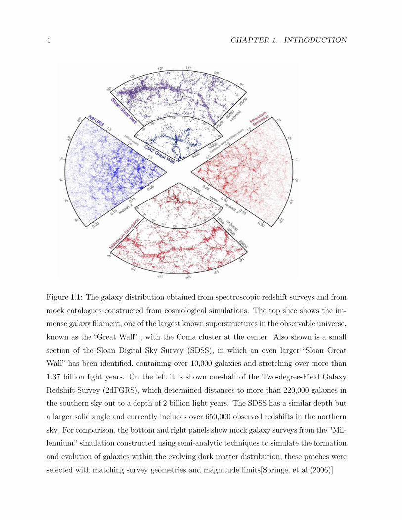
Figure 1.1: The galaxy distribution obtained from spectroscopic redshift surveys and from
mock catalogues constructed from cosmological simulations. The top slice shows the im-
mense galaxy filament, one of the largest known superstructures in the observable universe,
known as the “Great Wall” , with the Coma cluster at the center. Also shown is a small
section of the Sloan Digital Sky Survey (SDSS), in which an even larger “Sloan Great
Wall” has been identified, containing over 10,000 galaxies and stretching over more than
1.37 billion light years. On the left it is shown one-half of the Two-degree-Field Galaxy
Redshift Survey (2dFGRS), which determined distances to more than 220,000 galaxies in
the southern sky out to a depth of 2 billion light years. The SDSS has a similar depth but
a larger solid angle and currently includes over 650,000 observed redshifts in the northern
sky. For comparison, the bottom and right panels show mock galaxy surveys from the "Mil-
lennium" simulation constructed using semi-analytic techniques to simulate the formation
and evolution of galaxies within the evolving dark matter distribution, these patches were
selected with matching survey geometries and magnitude limits[Springel et al.(2006)]
5
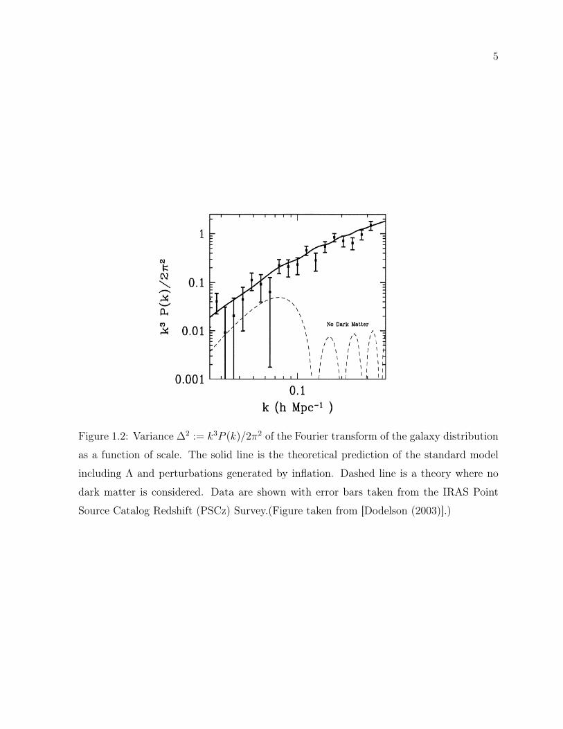
Figure 1.2: Variance ∆2 := k3P (k)/2π2 of the Fourier transform of the galaxy distribution
as a function of scale. The solid line is the theoretical prediction of the standard model
including Λ and perturbations generated by inflation. Dashed line is a theory where no
dark matter is considered. Data are shown with error bars taken from the IRAS Point
Source Catalog Redshift (PSCz) Survey.(Figure taken from [Dodelson (2003)].)
6 CHAPTER 1. INTRODUCTION
according to the matter that it contains, we call a solution of this system a Friedmann-
Robertson-Walker(FRW) universe.
Gµν = Rµν −1
2gµν R =
8πG
c4Tµν − gµνΛ, (1.4)
Rµν is the Ricci curvature tensor, gµν is the metric tensor, Λ is the cosmological constant,
G is Newton’s gravitational constant, c is the speed of light in vacuum, R is the scalar
curvature, and Tµν is the energy-momentum tensor that due to the symmetry of space-
time it can only be diagonal with non-zero components T00 = −ρc2g00 and Tij=pgij. It
is not necessary to assume that the matter content of the Universe is an ideal fluid to
get this from of Tµν , it is simply a consequence of the homogeneity and isotropy of the
universe and it is verified for scalar field matter, a viscous fluid or free-streaming particles
in a FRW universe. The energy density ρc2 and the pressure are defined as the time and
space-like eigenvalues of (Tµν).
The Einstein or Friedmann equations for the FRW universe become
H2 :=
(a
a
)2
=8πG
3c2ρ− kc2
a2+
Λc2
3(1.5)
a
a= −4πG
3
(ρ+
3p
c2
)+
Λc2
3(1.6)
ρ = −3H(ρ+
p
c2
). (1.7)
Where the last equation is also a consequence of the energy conservation T µν;µ = 0, and
it is a consequence of the contracted Bianchi identities. H is the Hubble “constant” or
Hubble parameter4 We parametrize the Hubble parameter by H = 100h km s−1 Mpc−1,
where observations show that h0 ≈ 0.70 ± 0.1 [Komatsu et al. (2011)].
From equation (1.7) we can obtain simple solutions if w = p/ρc2 = constant. One finds
that
ρ = ρ0(a0/a)3(1+w) (1.8)4The Hubble parameter in cosmic time is related to the comoving Hubble parameter H(τ) by
H(t)=H(τ)/a−1. A comoving coordinate system is a system of coordinates fixed with respect to the
overall expansion of the universe, so that a given galaxy’s location in comoving coordinates does not
change as the Universe expands. This allows distances, locations, etc. in an expanding homogeneous and
isotropic cosmology to be related solely in terms of the scale factor.
7
where ρ0 and a0 denote the values of the energy density and the scale factor at the present
time t0. Unless otherwise stated, the subscript 0 refers to quantities evaluated at present
time.
If the energy density is dominated by one component with w = constant and we neglect
the curvature K, then we different scale factors depending on the dominant component.
For non-relativistic matter, usually refer as dust, pm = 0, for radiation(photons or any kin
of massless particles) pr= ρrc2/3. A cosmological constant corresponds to pΛ = −ρΛc
2,
inserting these in eq. (1.8) we obtain
ρm ∝ a−3, a ∝ t2/3 ∝ τ 2 w = 0, (dust), (1.9)
ρr ∝ a−4, a ∝ t1/2 ∝ τ w = 1/3, (radiation), (1.10)
ρΛ = const., a ∝ exp(Ht) ∝ 1/|τ | w = −1, (cosmol. const.), (1.11)
One can define the adiabatic sound speed cs as
c2s =
p
ρ(1.12)
where the derivative is taken respect to cosmic time. From eq. (1.5) we can define a
critical value for the energy density for vanishing curvature and cosmological constant
ρc(t) =3H2c2
8πG, (1.13)
where ρc(t) is called the critical density. The ratio ΩX = ρX/ρc is the “density parameter”
of the component X, it indicates the fraction that the component X contributes to the
expansion of the universe. For the different components we get Ωm(t0) = ρm(t0)/ρc(t0),
Ωr(t0) = ρr(t0)/ρc(t0), ΩΛ(t0) = Λc2/3H20 , and ΩK(t0) = −Kc2/(a2
0H20 ).
We can separate Ωm = Ωdm +Ωb, where Ωdm is the dark matter component and Ωb is the
baryonic density parameter, for the radiation we can separate in photons and neutrinos
Ωr = Ωγ +Ων . Current constrains for all these cosmological parameters come principally
from the CMB combined with large scale structure data given h20Ωm,0 = 0.134, h2
0Ωb,0 ≈0.023, h2
0Ωdm,0 ≈ 0.111, h20ΩΛ,0 ≈ 0.357, h2
0Ωr,0 = 4.15 × 10⁻⁵, h20Ωγ,0 = 2.47 × 10⁻⁵,
h20Ων,0 = 1.68×10⁻⁵, with the fiducial value h0 = 0.7 [Massimo(2008), Spergel et al.(2007),
Page et al. (2007)] we get Ωm,0 = 0.27, Ωb,0 ≈ 0.046, Ωdm,0 ≈ 0.22, ΩΛ,0 ≈ 0.73 Ωγ,0 ≈5.04× 10⁻⁵, Ων,0 ≈ 3.42× 10⁻⁵, Ωr,0 ≈ 8.47× 10⁻⁵.
8 CHAPTER 1. INTRODUCTION
This suggests that ΩK ≈ 0, therefore the geometry of the universe is remarkably flat and
this parameter will be neglected in calculations. Assuming K=0, the age of the universe
is of 13.69 Gyr. We observe that baryons constitute only ∼ 5% of the total energy density
and that there is strong evidence of an unknown component.
§1.2 Overview of dark matter models
The standard model assumes dark matter behaves as dust, there is no particular informa-
tion on its nature. There are several particle candidates for the dark matter thoroughly
reviewed in [Bertone et al. (2005), Feng (2010), Martin et al.(2008)], depending on its the
general properties they can be classified as cold dark matter, self-interacting dark matter,
warm dark matter, ultra light scalar field dark matter, etc.
One of the preferred candidates of cold dark matter are Weakly Interacting Massive
Particles (WIMP) whose mass range is typically from 10 GeV/c2 to 1 TeV/c2, these
kind of dark particles interact in the weak sector with ordinary matter. These par-
ticles became the default CDM candidates and are studied in great detail given that
their cross section yields a value of Ωdm fairly close to the one observed. Another can-
didate widely discussed as a CDM candidate is the axion with mass in the range 10−3 −10−6eV/c2[Sikivie & Yang (2009)], this particle originates from the breaking of the Peccei-
Quin symmetry in the early universe[Peccei & Quinn (1977)] which solves the CP prob-
lem of strong interactions. In the context of warm dark matter are the sterile neutrinos,
their mass scale is ∼ keV/c2 and they are thermal relics with a higher velocity disper-
sion that CDM candidates(hence warm dark matter) and they follow Fermi-Dirac statis-
tics. However recent cosmological constraints to the mass of the sterile neutrino seem
to create tension for this candidate[Villaescusa-Navarro & Dalal (2011), Viel et al.(2013),
Souza et al.(2013), Macció et al.(2012)].
The other contenders that will be treated in more detail in this thesis are the ultra light
scalar fields and self-interacting dark matter, the main motivation to study these models
stems from the accurate descriptions offered to explain some of the problems encounter at
the level of galaxies in the CDM model, in addition to retaining the successful description
at large scales.
9
The above list is not limited to the these classes of dark matter and there exists other
models that can agree with current data, but ultimately there is a trend to apply the
Occam’s razor 5, our best bet is to keep acquiring higher resolution observations at all
scales that let us assess our current theoretical models and eventually we get to unravel
some of the mysteries of the universe.
We have provided the bases of the current standard model of cosmology that will be
the benchmark when comparing results in other alternative dark matter models. As we
mentioned, the standard model struggles to solve some issues at the level of galaxies that
will be discussed in the next chapter in more detail, we also present the current status
of the proposed solutions. In Chapter 3 we explore thoroughly the ultra light scalar field
dark matter pay close attention to the expected properties of the dark matter halos that
result from the model and examine their impact on the visible matter in galaxies. Due to
the increasing interest in the self-interacting dark matter model we dedicate Chapter 4 to
expose the status of this model.
Throughout the thesis several quantities are given in solar units and will always be denoted
by a subscript . We will use units where c = 1, Planck constant h = 1, except in some
cases where they help to make the discussion clearer.
5Occam’s razor is a principle devised by William of Ockham. The principle states that among com-
peting hypotheses, the one with the fewest assumptions should be selected. Other, more complicated
solutions may ultimately prove correct, but in the absence of certainty the fewer assumptions that are
made, the better.

10 CHAPTER 1. INTRODUCTION
Chapter 2
Current status of the ΛCDM model
§2.1 Initial fluctuations in the matter-dominated eraWe can measure the position of an object in the sky from its angular coordinates, but in
order to know how far away it is from us we can use as the third coordinate the redshift z
experienced by photons emitted from the object. A spectral line with intrinsic wavelength
λ is redshifted due to the expansion of the universe, if it is emitted at some time t an
observer on Earth will see it today with wavelength λ0 = λa0/a(t) = (1 + z)λ, this leads
to the definition of the cosmic redshift
z(t) + 1 =a0
a(t). (2.1)
For small redshifts z <<1 Hubble found that objects at a physical distance d = a0r away
from us, it recedes with speed v = H0d, this is called the Hubble’s law. This law can be
related to redshift z approximately by making a Taylor series expansion to lowest order
in z: a(t0) ≈ a(t) + a(t0− t), if in addition the distance to the object is not too large then
the time interval is simply the distance divided by the speed of light t0− t=d/c, therefore
1 + z ≈ 1 +a
a(t0 − t) ≈ 1 +H0
d
c
from where it follows that cz = H0d = v, valid at low redshifts. This is the method usually
applied to measure the Hubble constant. In cosmology it is typical to deal with object far
away from us, this makes the redshift a suitable coordinate to identify the time at which
events take place.
As mentioned in the introduction the deviations from the homogeneous cosmic microwave
background and the large scale structure suggest we need to go beyond the standard model
11
12 CHAPTER 2. CURRENT STATUS OF THE ΛCDM MODEL
of elementary particles(normal matter) to explain the structure of the universe, one of the
implications is the addition of a new dark matter(DM) component.
The temperature we see today of the CMB photons is 2.725 K, as photons are massless
and behave as radiation their temperature decreases with the adiabatical expansion of
the universe as T = a0T0/a(t), at the temperature Tdec ∼ 3000 K the mean free path of
the photons grows larger than the Hubble scale, this means that they effectively decouple
from baryonic matter and the universe becomes transparent to them, by eq. (2.1) this
corresponds to zdec ' 1100, at this time the universe was t ' 105 yr old. From this
point, the small perturbations in the density of baryons can grow to form the galaxies we
observe today. Anisotropies in the CMB tell us how the universe looked like when it was
some hundred thousand years old being excellent probes of the perturbations and a good
reference point for numerical studies.
On the other hand, the non-relativistic dark matter will clump and form overdensity
regions, the standard CDM stops interacting with the rest of the particles at an earlier
epoch than zdec, the DM overdensities can start growing before the decoupling of photons
from baryons so that by the time photons travel freely baryons follow the gravitational
potential wells previously generated by the cold dark matter. In fact, from eqs. (1.9),(1.10)
it follows that after a certain time the matter will start dominating over the energy density
of radiation, from the observed values of the density parameters of matter and radiation
this happens at a redshift
1 + zeq =a0
aeq=h2
0Ωm,0
h20Ωr,0
= 3228.91
(h2
0Ωm,0
0.134
), (2.2)
that is zeq ' 3000 > zdec, after this time of matter-radiation equality the universe is
effectively dominated by non-relativistic matter until the moment dark energy starts being
dominant (z ≈ 0.7), during this epoch DM fluctuations can grow. Eventually, at relatively
recent times, perturbations in the matter ceased to be small and become the nonlinear
structure we see today. Thus, photons decouple from baryons when the universe is already
well into the matter-dominated era, we have seen that the visible matter contributes a
small fraction to Ωm and it is then reasonable to consider that the main component
that determines the evolution of matter fluctuations will be the dark matter, hence a
first approach to study the evolution of density fluctuations consists on analyzing the dark
13
matter growth and its distribution. In order to follow the spatial and time evolution of the
density perturbations up to the time where they collapse to form virialized gravitational
configurations it is necessary to rely on numerical simulations.
In the standard model, dark matter configurations grow and collapse before galaxies as the
latter decouple from photons at a later time, in their evolution DM fluctuations will cluster
and form even larger under- and overdense regions, these large structures strongly attract
more baryons that much later produce stars and form the observed galaxies surrounded
by the large dark matter halos. We can get insight into the galaxy distribution from the
dark matter one as we expect that baryons move according to the underlying dark matter
potentials.
For this reason, a first step that is taken to study the growth of DM perturbations in cold
dark matter simulations consists in neglecting baryons, in order to compare with galaxy
surveys it is required to use semi-analytical models describing the baryonic physics and
use matching techniques to link galaxies with the dark matter background distribution.
Recalling that baryons aren’t the dominant component in Ωm, we see that taking the ap-
proach of first studying only the dark matter evolution, it is possible to get an idea of what
to expect for the galaxy distribution, as seen in Fig 1.1 it is an excellent approximation.
It is important to notice that the DM distribution depends on the dark matter properties
(cold, warm, etc.). Assuming it is cold and collisioness at all scales results in dark matter
halo formation at practically all scales. A direct consequence of these hypotheses is that
DM halos will form accreting other halos several times increasing their masses and their
sizes, as more massive structures are assembled, smaller halos in the neighborhood will
also be accreted turning this merging process quite chaotic. Nevertheless, once the merger
rate slows down, the number of halos that survive and the orbiting subhalos that remain
bounded within a given distance from the final massive host can be compared with obser-
vations applying techniques like abundance matching that relates the galaxy stellar mass
to the halo mass, we should always consider similar environmental conditions as galaxies
that are in more isolated regions present different structural properties.
The above discussion displays the relevance of the CMB in the study of structure formation,
the catch is that it offers a detailed map of the building blocks that will give rise to the
observable universe. A detailed discussion of how the primordial fluctuations arise from
14 CHAPTER 2. CURRENT STATUS OF THE ΛCDM MODEL
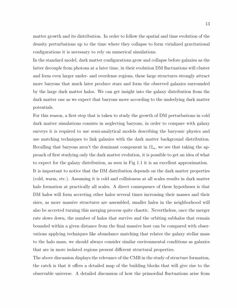
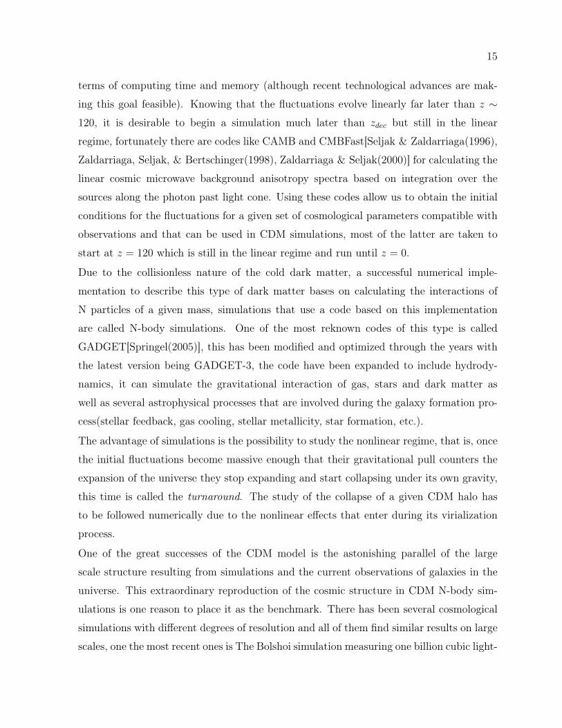
Figure 2.1: Relation between the halo mass and the stellar mass using the abundance
matching technique for the Millenium Simulation(MS) and Millenium II(MS-II), taken
from [Guo et al(2011)]. The halo mass is taken as the maximum mass that the halo ever
attained in the simulation. Green symbols are for central galaxies, while red symbols are
for satellites. The blue curve is the relation derived directly from the SDSS stellar mass
function and from subhalo abundances in the MS and the MS-II under the assumption
that the two quantities are monotonically related without scatter [Guo et al(2010)].
inflation can be found in [Liddle & Lyth (2000)] and i will not pursue it further because
it would get us sidetracked from our main focus, galaxies and dark matter. Below we
describe how simulations make use of the CMB to evolve linear perturbations up to the
nonlinear regime.
§2.2 Large scale structure in CDMThere is evidence from the CMB that the primordial fluctuations are well described
by an initial random gaussian distribution, there are codes[Hahn & Abel(2011)] in the
literature that allow to generate initial conditions with these characteristics. Evolv-
ing the CMB density field since zdec ∼ 1100 becomes extremely time consuming in
15
terms of computing time and memory (although recent technological advances are mak-
ing this goal feasible). Knowing that the fluctuations evolve linearly far later than z ∼120, it is desirable to begin a simulation much later than zdec but still in the linear
regime, fortunately there are codes like CAMB and CMBFast[Seljak & Zaldarriaga(1996),
Zaldarriaga, Seljak, & Bertschinger(1998), Zaldarriaga & Seljak(2000)] for calculating the
linear cosmic microwave background anisotropy spectra based on integration over the
sources along the photon past light cone. Using these codes allow us to obtain the initial
conditions for the fluctuations for a given set of cosmological parameters compatible with
observations and that can be used in CDM simulations, most of the latter are taken to
start at z = 120 which is still in the linear regime and run until z = 0.
Due to the collisionless nature of the cold dark matter, a successful numerical imple-
mentation to describe this type of dark matter bases on calculating the interactions of
N particles of a given mass, simulations that use a code based on this implementation
are called N-body simulations. One of the most reknown codes of this type is called
GADGET[Springel(2005)], this has been modified and optimized through the years with
the latest version being GADGET-3, the code have been expanded to include hydrody-
namics, it can simulate the gravitational interaction of gas, stars and dark matter as
well as several astrophysical processes that are involved during the galaxy formation pro-
cess(stellar feedback, gas cooling, stellar metallicity, star formation, etc.).
The advantage of simulations is the possibility to study the nonlinear regime, that is, once
the initial fluctuations become massive enough that their gravitational pull counters the
expansion of the universe they stop expanding and start collapsing under its own gravity,
this time is called the turnaround. The study of the collapse of a given CDM halo has
to be followed numerically due to the nonlinear effects that enter during its virialization
process.
One of the great successes of the CDM model is the astonishing parallel of the large
scale structure resulting from simulations and the current observations of galaxies in the
universe. This extraordinary reproduction of the cosmic structure in CDM N-body sim-
ulations is one reason to place it as the benchmark. There has been several cosmological
simulations with different degrees of resolution and all of them find similar results on large
scales, one the most recent ones is The Bolshoi simulation measuring one billion cubic light-
16 CHAPTER 2. CURRENT STATUS OF THE ΛCDM MODEL
years compared to the Milky Way that is only about 100,000 light-years long or the Local
Group of just 10 million light-years in diameter. The simulation covered a massive portion
of the universe, and it simulated the interactions of 8.6 billion dark matter particles. Start-
ing from the relatively smooth dark matter distribution of the early universe discerned from
the CMB, the Bolshoi simulation tracked the universe’s evolution to the present epoch as-
suming the CDM model. In similarity to lower resolution simulations, it displays knots of
dark matter, long filaments and clusters of galaxies, all gravitationally dominated by dark
matter. These structures are also found in DM-only simulations, but they do not directly
predict anything about the galaxies themselves, requiring an extra step in order to bridge
the gap with observations. Two dominant approaches have been used to establish the link:
(1) the technique of semi-analytical modeling, whereby baryonic physics are modeled at
the scale of an entire galaxy, and applied in post-processing on top of DM simulations, and
(2) hydrodynamic simulations, whereby the evolution of the gaseous component of the uni-
verse is treated using the methods of computational fluid dynamics. The latter approach
enables the complex interaction of the different baryonic components (gas, stars, black
holes) to be treated at a much smaller scale, ideally yielding a self-consistent and power-
fully predictive calculation. Hydrodynamical cosmological simulations have a high compu-
tational cost and have usually targeted specific problems, only very recently have several
groups started projects following approach (2), one of them is the Illustris simulation. The
technical details of the simulation can be found in the webpage1 and some introductory ar-
ticles are [Vogelsberger et al.(2014), Vogelsberger et al.(2014b), Genel et al.(2014)], given
the massive data sets that it produced the project is still ongoing and much of the analysis
has yet to be done, it is worth pointing out these type of projects may change some of
the previous results that were obtained following approach (1), but in the meantime, it is
worth discussing the known results that were obtained using the link (1).
One useful technique to link the number DM halos and the galaxy population in the
universe assuming they should match is called abundance matching, it essentially links the
observed galaxies in the expected dark matter halo according to semi-analytical models
which imposed a set of rules based on observed properties of gas and stars in galaxies that
are then implemented by hand in simulations[Guo et al(2011)]. A relevant parameter is
1http://www.illustris-project.org/
17
the efficiency with which halos are able to condense gas at their centers and form stars
and is called “galaxy efficiency”. Abundance matching models suggest that this galaxy
efficiency depends strongly on halo mass, for systems like the Milky Way(MW) with halo
mass of M200 := M(r = r200) ∼ 1× 10¹² M (r200 is the radius in which the density is 200
times the critical cosmological density ρc), about 20% of the available baryons are turned
to stars. For halos of an order of magnitude smaller this number drops quickly to ∼ 5%,
and plumbers to even less than 1% for dwarf galaxies inhabiting halos with mass M200 <
1×10¹⁰ M (see Fig. 2.1). Dwarf galaxies is a general term for galaxies that are faint, they
can have stellar masses at least two orders of magnitude below the stellar mass of a Milky
Way-like galaxy. There are several dwarfs with luminosities as low as L ∼ 1×10³L. Two
of the most massive dwarfs nearby are the small and large Magellanic Clouds visible by
the naked eye on dark nights from the Southern Hemisphere.
Unfortunately, observing these faint objects is challenging, the galaxy luminosity function2
is only reliably measured for dwarfs with stellar masses log(M∗) ∼ 8.5 and above, not
fainter. Thus, if we are interested on dimmer dwarfs, like dwarf spheroidals or ultra faint
dwarfs, we have to make an extrapolation of the halo mass-galaxy mass relation observed
towards faint dwarfs, assuming that the stellar mass-halo mass relation is correct, then
for all dwarfs with measured stellar mass we know the halo they live in, in fact from Fig.
2.1, we expect that all dwarfs with stellar masses larger than M∗ ∼ 1 × 10⁶ M live in
halos with virial mass M200 = 1 × 10¹⁰ M and larger. We require more data to confirm
the validity of extrapolating the abundance matching (AM) relation to the faint end of
the luminosity function, the potential candidates that will provide this confirmation are
expected to be dwarf and ultrafaint dwarf galaxies, moreover, if we consider these are
systems that are dominated by dark matter, we would expect baryons to move according
to the underlying potential, therefore it would be reasonable to expect that the kinematics
of the gas and stars are almost completely determined by the DM halo distribution. This
can be checked by comparing the circular velocity profile predicted by such dark halo
with the measured rotation curve of the dwarf, as the baryons are considered to have a
2The luminosity function gives the number of stars or galaxies per luminosity interval. The luminosity
is the total amount of energy emitted by a star, galaxy, or other astronomical object per unit time. It is
related to the brightness, which is the luminosity of an object in a given spectral region.
18 CHAPTER 2. CURRENT STATUS OF THE ΛCDM MODEL
minor contribution to the total mass, hence acting as tracers of the much more dominant
dark matter potential, the observed profiles should be remarkably similar to the DM only
profile. Despite the accuracy of AM for MW like galaxies or larger, it was found that its
extrapolating to lower masses breaks, meaning that there exist more scatter for the low
mass dwarfs.
There has been a great deal of work trying to explain why most of the dwarfs of log(M∗/M)
=106-107 are inconsistent with the expected M200 > 1 × 10¹⁰ M and seem to be better
described with lower mass halos. Unfortunately, lowering the mass also translates into
a lower stellar mass leading to a characteristic density divergent profile that is in ten-
sion with the flatter profiles found in observed dwarfs. The success of AM in galaxies of
log(M∗) ≥ 8.5 is undeniable, what remains fuzzy is the cause of the discrepancy of CDM
predictions and the low mass galaxies. This conundrum is just one of the cornerstones
that motivates exploring other dark matter models.
§2.3 Testing CDM with dwarf galaxies
2.3.1 Cusp-core problem
Analyzing a statistical sample of CDM halos from the high resolution simulations, there
exists some common structural properties in the DM distribution of such collapsed struc-
tures despite the chaotic history associated to the formation of each halo. One such
property is the universal density profile known as Navarro-Frenk-White (NFW) profile
[Navarro et al.(1996)]. The NFW profile emerges from numerical simulations that use only
CDM and are based on the ΛCDM model [Navarro et al.(1996), Navarro et al.(1997)]. Its
density profile is
ρNFW (r) =ρi
(r/Rs)(1 + r/Rs)2(2.3)
ρi is related to the density of the universe at the moment the halo collapsed and R2s is a
characteristic radius. We notice that in collissionless CDM the inner region of DM halos
show a density distribution described by a power law ρ ∼ rα with α ≈ −1, such behaviour
19
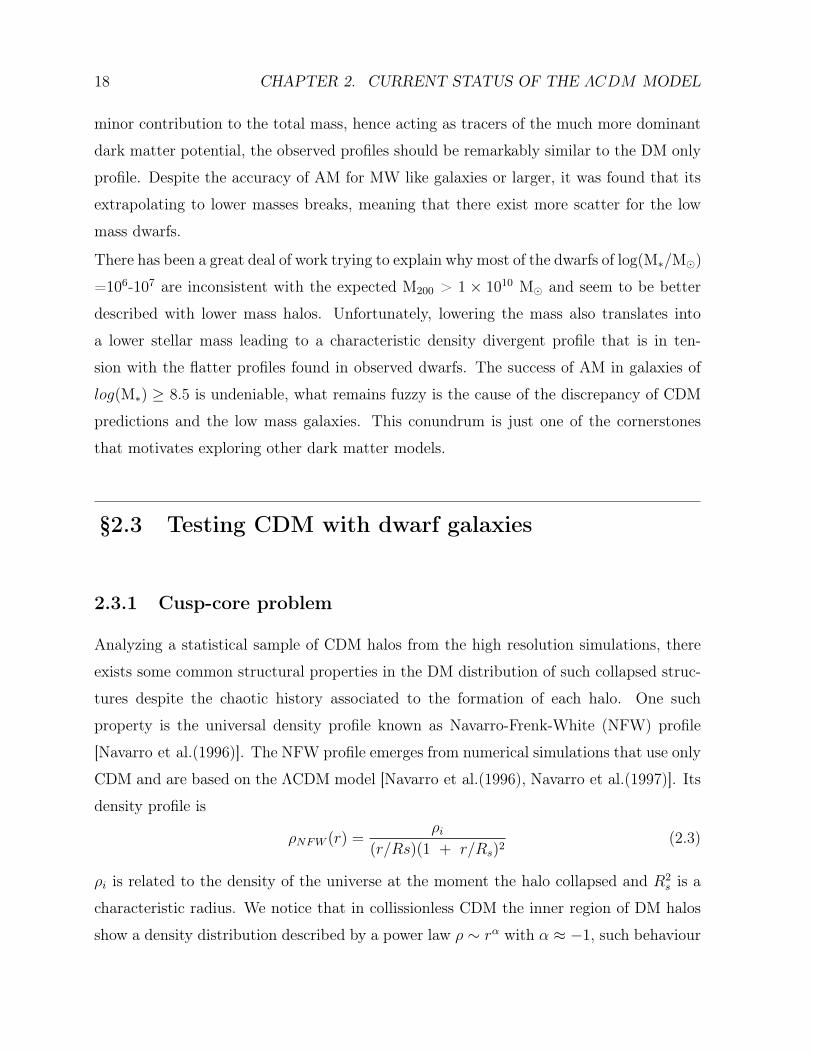
Figure 2.2: The inner slope of the dark matter density profile plotted against the radius of
the innermost point. The inner density slope α is measured by a least squares fit to the in-
ner data point as described in the small figure. The inner-slopes of the mass density profiles
of the 7 THINGS dwarf galaxies are overplotted with earlier papers and they are consistent
with previous measurements of LSB galaxies. The pseudo-isothermal model with its char-
acteristic core seems to provide a better fit to the data than the NFW model. Gray sym-
bols: open circles [de Blok et al.(2001)]; triangles [de Blok & Bosma(2002)]; open stars
[Swaters et al.(2003)].
20 CHAPTER 2. CURRENT STATUS OF THE ΛCDM MODEL
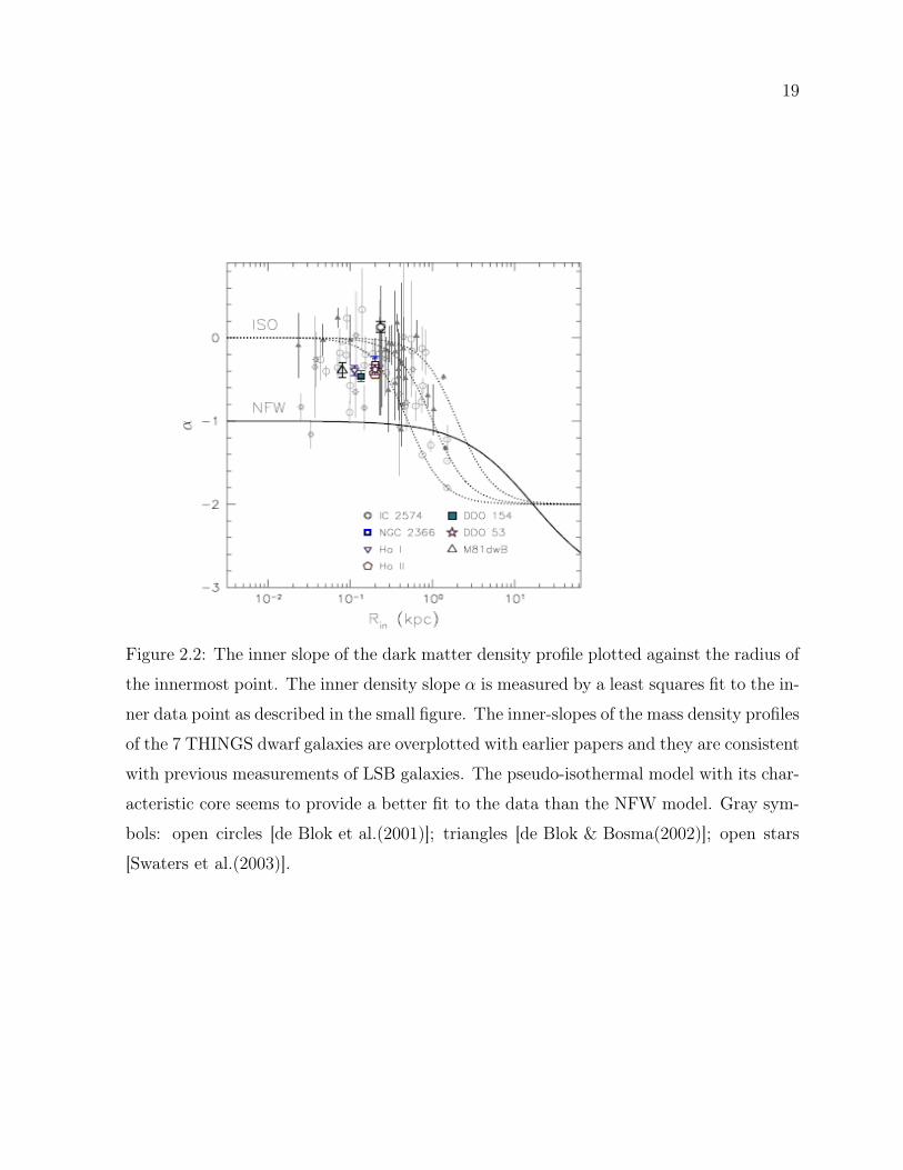
Figure 2.3: Observed galaxies in the Local Group shown in proportion to their measured
distances. The most massive galaxies in th group are our Milky Way and M31(Andromeda
galaxy).Image by Andrew Z. Colvin“5 Local Galactic Group (ELitU)”.
21
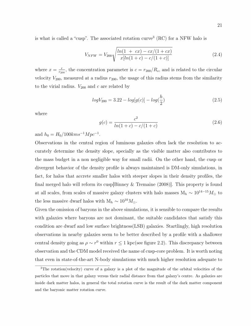
is what is called a “cusp”. The associated rotation curve3 (RC) for a NFW halo is
VNFW = V200
√ln(1 + cx)− cx/(1 + cx)
x[ln(1 + c)− c/(1 + c)](2.4)
where x = rr200
, the concentration parameter is c = r200/Rs, and is related to the circular
velocity V200, measured at a radius r200, the usage of this radius stems from the similarity
to the virial radius. V200 and c are related by
logV200 = 3.22− log[g(c)]− log(h
2) (2.5)
where
g(c) =c2
ln(1 + c)− c/(1 + c)(2.6)
and h0 = H0/100kms−1Mpc−1.
Observations in the central region of luminous galaxies often lack the resolution to ac-
curately determine the density slope, specially as the visible matter also contributes to
the mass budget in a non negligible way for small radii. On the other hand, the cusp or
divergent behavior of the density profile is always maintained is DM-only simulations, in
fact, for halos that accrete smaller halos with steeper slopes in their density profiles, the
final merged halo will reform its cusp[Binney & Tremaine (2008)]. This property is found
at all scales, from scales of massive galaxy clusters with halo masses Mh ∼ 1014−15M to
the less massive dwarf halos with Mh ∼ 1010M.
Given the omission of baryons in the above simulations, it is sensible to compare the results
with galaxies where baryons are not dominant, the suitable candidates that satisfy this
condition are dwarf and low surface brightness(LSB) galaxies. Startlingly, high resolution
observations in nearby galaxies seem to be better described by a profile with a shallower
central density going as ρ ∼ r0 within r ≤ 1 kpc(see figure 2.2). This discrepancy between
observation and the CDMmodel received the name of cusp-core problem. It is worth noting
that even in state-of-the-art N-body simulations with much higher resolution adequate to
3The rotation(velocity) curve of a galaxy is a plot of the magnitude of the orbital velocities of the
particles that move in that galaxy versus their radial distance from that galaxy’s centre. As galaxies are
inside dark matter halos, in general the total rotation curve is the result of the dark matter component
and the baryonic matter rotation curve.
22 CHAPTER 2. CURRENT STATUS OF THE ΛCDM MODEL
resolve the inner kpc the resulting density profile is still cuspy. Adding baryons may reduce
the problem, but as we see below this is not the only issue that seems to required baryons
to agree with observations.
2.3.2 Missing satellite problem
In the hierarchical galaxy formation scenario a large number of halos are consumed by
more massive ones, however, there are still many dark matter substructrures that are not
disrupted and that remain orbtting a massive halo, these surrounding structures are called
subhalos and the central massive one is called the host halo. The number of subhalos can
be predicted by CDM simulations, in particular, it is found that the low mass halos are
always more numerous, given the apparent universal NFW profile these halos don’t suffer
strong tidal stripping so as to be completely destroyed, resulting in host with a large
population of low mass subhalos. This picture also appears at larger scales, in galaxy
clusters the gravitational potential is stronger and can capture more subhalos, given the
above properties of CDM halos there will be also a great abundance of dwarfs halos,
some are associated to a particular host but some others are not, the latter are called
halos(galaxies) in the field, simply representing that they are somewhat isolated and are
not satellites that belong to a specific host.
It is straightforward to compare the number of observed satellites to the predicted subhalos
using AM. As the more precise observations are in our local neighborhood, an obvious
candidate is our own Milky Way or the Andromeda galaxy(M31) and their respective
satellite galaxies. One way to proceed is to choose a MW mass halo from a cosmological
simulation that resembles as close as possible our environmental conditions, it is frequent
to have more than a Milky Way analogue in these simulations, this suggests that we have
to count the subhalos of all these MWs and give a statistical result. Another way is
to simulate with a much higher resolution an isolated MW like system with much more
detailed so that it can have a closer resemblance to our observed Via Lactea, such systems
are choosen from large simulated boxes that allow the formation of at least one halo of
Mh ∼ 1012M. Among the most famous simulations that study MW halos is the Aquarius
project[Navarro et al.(2010), Springel et al.(2008)]. The Aquarius simulations study an
23
isolated halo similar in mass to that of the Milky Way at various resolutions, about 200
million particles at r200 and one at even higher resolution with almost 1.5 billion particles
within this radius. These simulations are being used to understand the fine-scale structure
predicted around the Milky Way by the standard structure formation model.
A problems emerged when the abundance of satellites expected from CDM simulations
was found to be overpredicting the number of dwarf satellite galaxies in the MW and
M31, this mismatch was initially of an order of magnitude larger[Klypin et al.(1999)]
and called the “missing satellite problem” (MSP), nowadays, the discovery of more ul-
tra faint dwarfs (UFD) within the MW halo has reduced the missing satellite problem
(e.g.[Simon & Geha(2007)]),The problem can be rephrased by saying that there are more
subhalos with circular velocities Vcirc < 30 km/s than observed satellites around MW and
M31.
There are solutions to this problem that based on redefining the MSP, for instance, con-
sidering only the mass within 600 pc M0.6[Strigari et al.(2007)], doing this it was found
that models where the brightest satellites correspond to the earliest forming subhalos or
the most massive accreted objects both reproduce the observed mass function.
Another possibility is that despite the existence of DM subhalos, most of them will not
host galaxies, hence, aren’t observed. This solution relies on the efficiency of star forma-
tion, which requires baryons to be included forcing us to use hydrodynamical simulations.
It is likely that dwarfs are the most affected by reoinization, the epoch where the neu-
tral hydrogen get ionized, at early times the smallest galaxies first dominate but given
their small gravitational potentials their own star formation blows out their primordial
gas through their own supernovae and heating of their environment. Therefore, they stop
forming stars for not much longer after reionization and if the star formation was very in-
efficient at that time, only the DM halo will remain today and no galaxy will be observed.
Three year WMAP data found that reionization began at z = 11 and the Universe ionized
by z=7.[Spergel et al.(2007)]. Assuming the unrealistic case of an instantaneous reioniza-
tion, the combination of results from the Planck mission, WMAP polarization, CMB and
BAO measurements yield a redshift of zreio = 11.3 ± 1.1.[Ade et al. (2007)]. Although a
value of 7 is in much better agreement with the quasar data. In view of the uncertainty
of zreio the baryonic solution to the MSP is still uncertain. Moreover, if dwarf galaxies
24 CHAPTER 2. CURRENT STATUS OF THE ΛCDM MODEL
are the primary source of ionizing photons during the epoch of reionization they will be
star forming, but this continual star formation will again overproduce the abundance of
the Via Lactea’s satellites at z=0[Boylan-Kolchin et al. (2014)].
Incorporating baryons in current simulations seems to be mandatory, but the required
fraction of baryons to dark matter has to be carefully controlled, as pointed in Peñarrubia
et al. (2012), solving the cusp-core problem with strong stellar feedback may result in
luminosities at odds with those of MW satellites. Before jumping to result from hydrody-
namic simulations let us see a more recent issue related to the above discrepancies.
2.3.3 The Local Group: Too-Big-to-Fail
Our galaxy resides in a group of galaxies that spans a diameter of 3 Mpc termed the Local
Group (LG). The group’s most massive members are the Milky Way and M31(Andromeda)
galaxies, these two spiral galaxies have a system of satellite galaxies. The LG comprises
around 78 galaxies[Pawlowski et al.(2013)]. The group itself is a part of the larger Virgo
Supercluster (i.e. the Local Supercluster[Tully (1982)]). In fig. 2.3 we see the distribution
of most of the galaxies in the LG.
In the spirit of abundance matching, it is prudent to expect that the most massive satellites
of the MW reside in the most most massive subhalos that are found in simulations, a
similar situation is natural for other hosts with their respective galaxies. As mentioned,
observations of nearby dwarfs suggest high mass-to-light ratios(10-1000M/L) so the
kinematics of stars are good tracers of the DM halo distribution.
By carefully studying the results of CDM simulations that emulate the MW, it was found
that the central densities of MW dSph galaxies are required to be significantly lower
than the densities of the largest subhalos found in collisionless DM simulations to agree
with the observed data(Boylan-Kolchin et al. 2011; Garrison-Kimmel et al. 2014). CDM
simulations of the Aquarius Project suggest that the MW-size halos should inhabit at least
eight subhalos with maximum circular velocities exceeding 30 km/s, while observations
indicate that only three satellite galaxies of the MW posses halos with maximum circular
velocities > 30 km/s. This discrepancy is not particular of the MW, it is expected for
M31 and even in galaxies outside the LG. This issue differs from the MSP in that there
25
are multiple subhalos that have no visible counterpart, from the above results, out of the
8 subhalos with similar masses, only 3 have a visible pair even though the remaining 5
are just as massive to cool hydrogen, form stars and eventually host a galaxy, so why
do we observe only three galaxies when we should see eight? These subhalos would be
massive“failures” because they fail to form galaxies, and this issue is known as the Too-
big-to-fail(TBTF) problem.
In virtue of the hierarchical model, we could expect that the presence of our close com-
panion M31 may change our results since it is as massive as the MW and at a distance
of 775 kpc. If we are more strict we should consider the Large Magellanic Cloud (LMC)
that is ∼ 41kpc from us. In the search of a fair comparison a first approach was to
analyze pair of galaxies resembling the MW and M31. This was done in the ELVIS4
suite[Garrison-Kimmel et al. (2014a)].
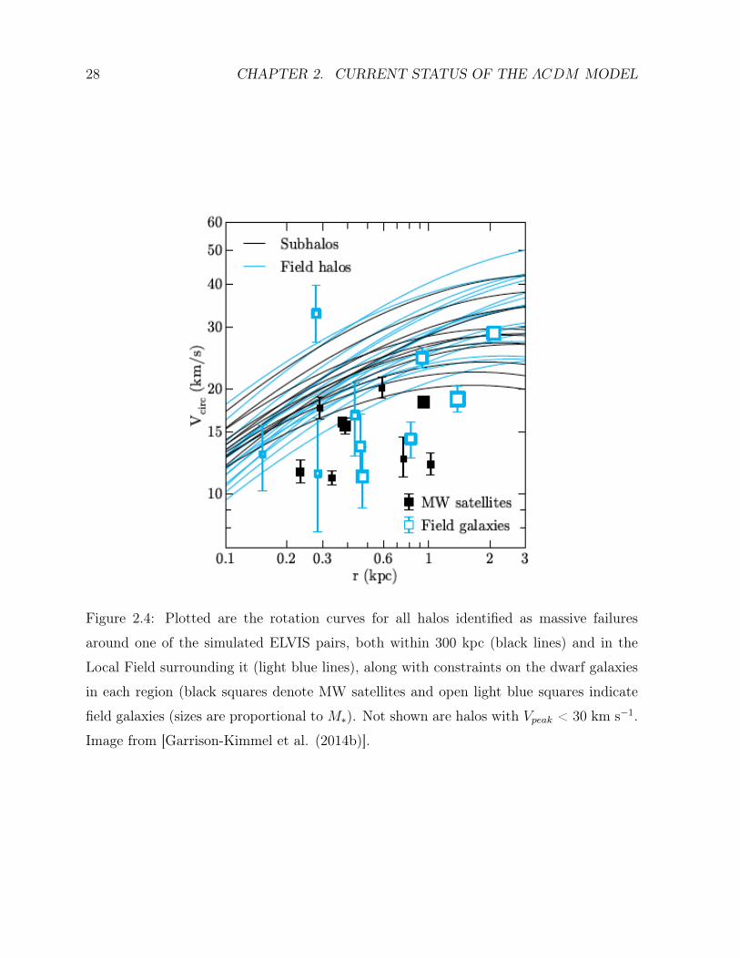
The analyses reveal that the TBTF persists within the virial radius of each host, in fact,
it is also present at the scale of the LG (see fig. 2.4). In their study the authors found
that within 300 kpc of the Milky Way, the number of unaccounted-for massive halos
ranges from 2 - 25 over their full sample. Moreover, this “too big to fail” count grows as
the comparison is extended to the outer regions of the Local Group: within 1.2 Mpc of
either giant(the MW and M31) they find that there are 12-40 unaccounted-for massive
halos. This count excludes volumes within 300 kpc of both the MW and M31, and thus
they conclude that these systems should be largely unaffected by any baryonically-induced
environmental processes. According to abundance matching, all of these missing massive
systems should have been quite bright, with M∗>106M. This outcome was to be expected
as more massive hosts will attract more dark matter that can also end as DM subhalos.
An evident solution would be to consider tidal stripping, although this seems plausible
for galaxies that are in orbits with close pericenter distance to their host it is unclear
that this mechanism is the main reason to reach agreement with current data, principally
because several studies have shown that tidal stripping of CDM halos with cuspy profiles
4ELVIS is a suite of high-resolution, cosmological zoom-in simulations. The suite contains 48 halos, each
with up to 15 million particles within the virial radius and 53 million particles within an uncontaminated
sphere centered on each halo. Half of these halos exist in Local Group-like configurations, chosen to mimic
the Milky Way and Andromeda in mass and phase space configuration.
26 CHAPTER 2. CURRENT STATUS OF THE ΛCDM MODEL
is not effective enough to destroy the subhalos, however, we need to include baryons in
the studies to assess this solution, in the end what we observe are galaxies. Notice that
the TBTF problem remains for galaxies in the field where tidal stripping is subdominant.
2.3.4 Alignment of satellite galaxies in MW and M31
Until very recently, the peculiar distribution of satellites around the MW and M31 caught
the attention of several astronomers. Dark matter simulations predict the accretion of var-
ious subhalos around massive hosts, but statistically its distribution tends to be isotropic.
Unexpectedly, the observed nearby satellites of our galaxy and those in M31 show a certain
degree of spatial arrangement. Both galaxies of the Local Group are surrounded by thin
planes of mostly co-orbiting satellite galaxies, the vast polar structure (VPOS) around the
Milky Way and the Great Plane of Andromeda (GPoA) around M31[Ibata et al.(2013)].
This issue is further review in [Pawlowski et al.(2013)].
Some of the proposed scenarios trying to explain the LG galaxy structures as either orig-
inating from cosmological structures or from tidal debris of a past galaxy encounter. On
large scales, the cosmic web consists of massive clusters that are connected with dark
matter “filaments”, these filaments serve as fountains of particles that feed dark matter to
massive concentrations of halo clusters and superclusters, it is quite similar to networks
of neurons in our brain, in fact, it is outstanding that the large scale structure of the
universe presents such similarity to the micro scale in our brains, whether this appar-
ent coincidence hides a deeper meaning is an interesting question that may deserve to
be subject to further scrutiny, for now i will leave it as a side comment. Getting back
to the satellites, one of the scenarios concentrates on how the satellite distribution is
correlated to the direction of filaments, mainly in intersections of the filamentary struc-
ture. During the formation of a MW-mass host, part of the dark matter flows along
the filament so that as DM clumps and halos form in such filament, their peculiar ve-
locities can share a preferential direction, as a result, when they become bounded to a
massive host they can possess a particular orientation that today give the pattern of
a plane[Pawlowski et al.(2013), Ibata et al.(2013), Pawlowski & McGaugh (2014)]. This
scenario can explain the orientation of the satellites in one host galaxy, under the same
27
framework we would expect that the satellites in M31 and our galaxy, both being relatively
close and part of the LG, share a particular direction in one plane, what is observed is that
each set of satellites has its own plane implying that they don’t originated in the same
filament. Looking at the vast cosmic structure in principle it should be possible to find
two host with the desired satellite distribution, in contrast, it has proven difficult to find
pairs of hosts whose satellites are in planes with the observed inclinations. There exist the
uncertainty that the MW and M31 are cosmologically rare, it may be that the criteria to
look for akin systems in simulations needs to be redefine or simply that there is a different
formation mechanism tied to the halo shape that is not fully understood. Also explored
is that they are tidal debris of a past galaxy encounter, the details and feasibility of this
solution requires a more convoluted study. Although it is worth noting that because of the
proximity of M31 and MW to us, it is possible to obtain accurate measurements of these
systems, however this doesn’t imply that such pairs are statistically significant of the.
There currently exists no full detailed model which satisfactorily explains the existence of
the thin symmetric LG planes.
§2.4 Baryons to the rescue, or not?
The above issues led to much effort in improving the resolution of simulations so that
regions of order kpc could be resolve and the results are not biased by numerical errors
due to a lack of convergence. The problem that attracted most of the attention is the
cusp-core issue. This results undoubtedly change when astrophysics are involved, due to
the large concentration of DM particles in the center of subhalos, we need to identify an
energetic process capable of efficiently expelling the DM and disperse to a more uniform
distribution to form a core. This naturally points to supernova feedback, each supernova
type II comes along a massive explosion injecting ∼ 1051ergs to the surrounding gas, after
several of these events the dark matter which interacts gravitationally will be modified
and in the best scenario a core will be formed. Under this picture most hydrodynamical
simulations have focused on modeling supernovae feedback(FB) to accurately implement
it into numerical simulations.
Reproducing the general properties of dwarfs in a cosmological setting has been quite chal-
28 CHAPTER 2. CURRENT STATUS OF THE ΛCDM MODEL
Figure 2.4: Plotted are the rotation curves for all halos identified as massive failures
around one of the simulated ELVIS pairs, both within 300 kpc (black lines) and in the
Local Field surrounding it (light blue lines), along with constraints on the dwarf galaxies
in each region (black squares denote MW satellites and open light blue squares indicate
field galaxies (sizes are proportional to M∗). Not shown are halos with Vpeak < 30 km s−1.
Image from [Garrison-Kimmel et al. (2014b)].
29
lenging. So far the relation of stellar mass and halo mass inferred from local galaxy counts
implies a suppression of galaxy formation by a factor of∼ 103[Garrison-Kimmel et al. (2014b),
Brook et al.(2014)], if stellar feedback is the main ingredient to achieve the desired effect
we need to get a physically realistic model that so far has proven difficult.
As for a feedback-driven core formation, there is still debate. One of the most success-
ful simulations at producing cores in dwarf galaxies with supernova feedback have sug-
gested a transition mass of M ∼ 107 M below which core formation becomes difficult
[Governato et al.(2012)]. Using a slightly different approach, [Di Cintio et al.(2013)] find
similar results, where the cusp-core transition should be most effective when the ratio of
stellar mass to dark matter halo mass is relatively high, they find cores in massive dwarfs
with M ∼ 108 M and Mvir ∼ 3 ×1010.5 M. It may be that at some mass scale, galaxy
formation becomes stochastic (e.g., [Boylan-Kolchin et al.(2011), Power et al.(2014)]). Re-
cent work by [?], however, suggests that stochasticity may appear at lower mass scales
(Mvir ∼ 109 − 109.5 M). The results of Di Cintio et al. (2013) and Governato et al.
(2012) agree reasonably well, in contrast, results from a different set of high resolution
simulations with a simpler implementation of stellar feedback have not produced cores
in dwarf galaxy halos at any mass ([Vogelsberger et al.(2014)]), even though a number of
other observables are well matched. One caveat of these simulations is that the sub-grid
inter stellar medium (ISM) and star formation (SF) model leads to SF histories smoothed
in time, compared to the bursty star formation found in the above models or in the highly
resolve explicit feedback models ([Hopkins et al.(2014)]).
Until now, feedback has needed ad-hoc approximations due to the lack of resolution of
molecular clouds where star formation takes place, for instance, turning off cooling for
material heated by SNe. It is then unclear that the sub-grid feedback recipes capture
the expectations from stellar evolution models and end forming large cores. To this end,
[Oñorbe et al.(2015)] simulated two typical isolated dwarfs with M ∼ 1010 M using a
more realistic explicit implementation of feedback using the code GIZMO[Hopkins (2014)].
They found that their simulated dwarfs present bursty star formation, in the event that
it continues until late times a core of ∼ 1 kpc can form and at the same time the dwarf
galaxy can sit on the M∗ vs Mvir relation to mathc the LG stellar mass function via
abundance matching. The success depends strongly on the star formation histories, indeed,
30 CHAPTER 2. CURRENT STATUS OF THE ΛCDM MODEL
they conclude that the presence of cores in galaxies with M∗= ∼ 106 − 107 M requires
substantial late time star formation. It is also questionable if subsequent accretions could
reform the cusp.
Although the cusp-core issue remains an open question, we can conclude that in hydrody-
namical CDM simulations transforming a cusp into a core seem to be strongly dependent on
bursty periods of star formation and a steady supernovae feedback to avoid the cusp regen-
eration. Recently [Trujillo-Gomez et al.(2015)] found in their simulations that radiation
pressure from massive stars is the most important source of core formation, not thermal
feedback from supernova, which has been the primary mode used by other groups that have
produced cores. This approach may seem promising, but from the experience with feedback
models, forming a core may result in a mismatch with other galaxy properties, it remains
to be seen whether the radiation pressure model is consistent with other observables such
as the stellar metallicity-stellar mass correlation [Gallazzi et al.(2005), Kirby et al.(2013)].
Regarding the MSP and the TBTF, many attempts to decrease the subhalo population
focus on the interaction of the satellites with the galactic disk. In general, the closer
the subhalos are to the disk, the larger the influence and their destruction. Simulations
studying the dynamics of several dwarf subhalos in different orbits with and without the
presence of a disk component in the host show that halos that are accreted possessing an
initial cuspy profile will always leave a remnant, they are not fully destroyed even if its
outer envelope is heavily dispersed. For subhalos in orbits whose pericenters are smaller
than the disk length, the effects are enhanced such that only a compact structure remains
loosing almost 90% of its initial mass [Peñarrubia et al.(2010), Łokas et al.(2012)]. CDM
simulations don’t predict cores naturally and baryons must be taken into account, but
for comparison, the tidal stripping effects where also studied assuming a CDM halo with
an empirical core profile, it was found that subhalos with initial core profiles that fully
dive inside the disk several times are completely torn down, whereas they can survive if
their pericenter distances are larger than the disk’s size albeit with more mass lost than
their cuspy analogues. These simulations have considered controlled orbits, the results
look promising to get a lower abundance of satellites even though some subhalos may still
be present after the mass lost from the disk they will be devoid of stars, it remains to be
seen that orbits that come from cosmological simulations fall into the same regime of close
31
disk-subhalo interactions as these idealized simulations.
The potential success of tidal stripping in dwarfs led to consider a combined model of
feedback and tidal stripping in the hope that the circular velocities are reduced and alle-
viate the tension suggested in the TBTF issue. This combination of effects was studied
in high resolution cosmological hydrodynamical simulations of Milky Way-massed disk
galaxies[Zolotov et al.(2012), Brooks & Zolotov (2014)], they found that supernovae feed-
back and tidal stripping lower the central masses of bright (-15 < MV < -8) satellite
galaxies, the bursty star formation can reduce dark matter densities forming shallower
inner density profiles in the massive satellite progenitors (Mvir ≥ 109 M , M ≥ 107 M) compared to DM-only simulations. In the progenitors of the lower mass satellites are
unable to maintain bursty star formation histories, due to both heating at reionization
and gas loss from initial star forming events, preserving the steep inner density profile pre-
dicted by DM-only simulations. After infall (when galaxies enter the virial radius of the
host galaxy), tidal stripping further reduces the central densities of the luminous satellites,
particularly those that enter with cored dark matter halos, consistent with the expected
results where each effect is treated separately. It seems that an over simplification of the
MW potential where the disk is not taken into account may be the source of the discrep-
ancies in DM-only simulations, even taking this solution at face value, it would imply that
if cores are indeed present in galaxies in the field, where interactions with the disk are of
minor importance, supernovae feedback will be left as the most efficient agent contributing
to core formation, as mentioned in the cusp-core issue, forming cores in CDM simulations
is often correlated to late bursty star formation but at the same time we require a strong
suppression of star formation in low-mass haloes in order to explain the small number of
visible satellites, unifying the solutions may require some tuning or a better understanding
of the dark-baryons coupling as well as the galaxy formation process itself.
We have seen that including hydrodynamics into CDM simulations has provided different
scenarios that could explain the long standing problems of DM-only simulations. Up until
now there is not unanimity in the cause of these conflicts, it may seem that supernova
feedback seen as the main mechanism to form cores in dwarfs requires detailed modeling
so as not to aggravate the fit to other observations. Curiously, the few cases that have sim-
ulated DM halos with pre assumed flat inner profiles seem to lead to simpler descriptions,
32 CHAPTER 2. CURRENT STATUS OF THE ΛCDM MODEL
specially since no fine tuning of stellar feedback is needed, although cores are not natu-
rally produce in CDM they can arise in alternative dark matter models, this in turn leads
to study in more detail the explanations that these other models offer. Unquestionably,
dwarf galaxies will be a key factor to unravel the properties of dark matter.
The list of issues that I have presented in this chapter forms just part of other puz-
zling observations, such as the how statistically significant is the “Bullet cluster” in sim-
ulations [Hayes et al.(2006), Lee & Lim(2010)], the details of the relation between the
specific angular momentum distribution of DM halos and the one observed in the gas
component[Bullock et al. (2001), van den Bosch et al. (2001)], why there are less observed
galaxies in the local void than in simulations[Peebles & Nusser (2010)], the formation of
rings and shells in early type elliptical galaxies in non interacting environments, etc.
[Hau & Forbes (2006), Taehyun et al. (2012), Koprolin & Zeilinger (2000)].
All these observations are intriguing enough to explore the outcome from modifications to
the CDM model, mainly at small scales given its extraordinary success at large scales, as it
appears that the non appearance of core profiles in CDM halos is tightly related to all the
problems, in the next chapter we will then explore one model in which the core formation
is simply a natural consequence of the dark matter properties, this type of solution is
usually preferable to invoking poorly understood astrophysical processes
Chapter 3
Scalar field dark matter
§3.1 The quantum dark matter paradigm
In CDM there are several dark matter candidates, many of them proposed from extensions
of the standard model of particles, among which the most popular ones at present are in the
form of weakly interacting massive particles (WIMPs), see [Goodman & Witten (1985),
Scherrer & Turner(1986), Drukier et al. (1986)]. The main characteristics that identify
the WIMPs are being collisionless and massive (> GeV).
Furthermore, current dark matter detection experiments, both direct and indirect ones,
have not yet discovered any compelling signals of WIMPs [Bauer et al. (2013)]. As a mat-
ter of fact, while WIMPs are mostly expected to be the lightest supersymmetric particle in
the Minimal Supersymmetric Standard Model(MSSM), [Griest & Kamionkowski (2000)],
recent data from the Large Hadron Collider has found no evidence of a deviation from
the standard model of particles on GeV scales, significantly restricting the allowed region
of MSSM parameters [Aad et al.(2013)]. It is clear that the microscopic nature of dark
matter is sufficiently unsettled as to justify the consideration of alternative candidates for
the CDM paradigm.
One of these assumptions is to assume that the dark matter particles are described by a
spin-0 scalar field(SF) with a possible self-interaction and a very small mass. There are
several scalar fields that have been predicted by a variety of unification theories, e.g., string
theories and other multi dimensional theories [Carroll (1998), Arkani et al. (1999)]. The
bosonic particles we are envisaging are typically ultralight, with masses down to the order
of 10−33eV/c2. This small mass suggests the possibility of formation of a Bose-Einstein
33
34 CHAPTER 3. SCALAR FIELD DARK MATTER
condensate (BEC), i.e., a macroscopic occupancy of the many-body ground state. In
principle, for a fixed number of (locally) thermalized identical bosons, a BEC will form
if nλ3deB » 1, where n is the number density and λdeB is the de Broglie wavelength. This
is also equivalent to the existence of a critical temperature Tc , below which a BEC can
form.
Recently the idea of the scalar field has gained interest, given the uncertainty in the pa-
rameters the model has adopted different names in the literature depending on the regime
that is under discussion, for instance, if the interactions are not present and the mass is
∼ 10−22eV/c2 this limit was called fuzzy dark matter[Hu, Barkana & Gruzinov(2000)] or
more recently wave dark matter[Schive et al.(2014)], another limit is when the SF self-
interactions are described with a quartic term in the scalar field potential and dominate
over the mass(quadratic) term, this was studied in [Goodman (2000), Slepian &Goodman]
and called repulsive dark matter or fluid dark matter by[Peebles(2000)].
Notice that for a scalar field mass of ∼ 10−22eV/c2 that is non-relativistic the critical
temperature of condensation for the field is Tcrit ∼ m−5/3 ∼TeV, which is very high, if
the temperature of the field is below its critical temperature it can form a cosmological
Bose Einstein condensate, if it condenses it is called Bose-Einstein condensed(BEC) dark
matter[Colpi,Shapiro,& Wasserman(1986), Guzmán & Matos(2000), Matos & Ureña(2001),
Bernal et al.(2010), Harko(2011), Chavanis & Harko (2012), Robles & Matos(2013)]. One
type of bosonic particle suggested as a major candidate for dark matter is the QCD axion.
It is the pseudo-Nambu-Goldstone boson in the Peccei-Quinn mechanism, proposed as a
dynamical solution to the strong CP-problem in QCD. For the axion to be CDM, it has
to be very light, m ∼ 10−5 eV/c2 ([Sikivie(2012)]). More recently [Sikivie & Yang (2009)]
mentioned that axions could also form Bose-Einstein condensates, however, the result was
contested in [Davidson & Elmer(2013)], this suggest that the condensation process should
be study in more detail to confirm it can remain as BEC dark matter.
In [Ureña-Lopez(2009)], it was found that complex scalar field with m<10−14eV/c2 that
decoupled being still relativistic will always form a cosmological Bose-Einstein conden-
sate described by the ground state wavefunction, this does not preclude the existence
of bosons with higher energy, particularly in dark matter halos. A fully relativistic
treatment(kBT >> mc2) of Bose-Einstein(BE) condensation was given by [Kapusta (1981),
35
Haber & Weldon (1982)], including the relationship between BE condensation and sym-
metry breaking of a scalar field. Those authors showed that, for an ultra relativistic ideal
charged boson gas, described by a complex scalar field,
Tc =(~3c)1/2
kB
(3q
m
)1/2
(3.1)
where q is the charge per unit proper volume. This does not take self-interactions into
account. In [Haber & Weldon (1982)] it was shown that, in the case of an adiabatically
expanding boson gas, if the scalar field has a generic quartic self-interaction, then the
bosons must either be condensed at all temperatures (i.e. at all times) or else never form
a BEC. In this case, the charge per unit comoving volume, Q (Q = qa3), and entropy per
unit comoving volume, S, are both conserved. In their work they establish the condition
for the formation of a BECQ
S=
5
4πkB
(λ
4
)1/2
(3.2)
where λ is the dimensionless coupling strength of the quartic self-interaction, in natural
units. The SF is assumed to have has essentially zero entropy per unit comoving volume
and for the typical boson masses we are interested,m<10−14eV/c2, the conserved charge
density in the comoving frame, Q, is extremely high, given the observed dark matter energy
density today ρdm,0, for Q ≈ ρdm,0/(mc2). Therefore, inequality (3.2) would be satisfied
and thus almost all of the bosons occupy the lowest available energy state. It is important
to notice, that the condensation process requires Bose-Einstein statistics in the first place,
i.e., local thermalization [Sikivie & Yang (2009), Erken et al.(2012)], it has been argued
that thermal decoupling within the bosonic dark matter can occur when the expansion rate
exceeds its thermalization rate, without disturbing the condensate, however, just like with
QCD axions the thermalization might break with the expansion of the universe, although
a large number of dark matter bosons would stay in the ground state and the classical
field remains a good description, it will no longer be completely BEC dark matter, this is
still something that remains to be seen.
From the above discussion we see that the smallness of the boson mass is its characteristic
property and cosmological condensation is a likely consequence. The preferred mass of the
scalar field dark matter(SFDM) lies close to ∼ 10−22eV/c2 satisfying the above constraint,
36 CHAPTER 3. SCALAR FIELD DARK MATTER
although there are still uncertainties on the mass parameter, in order to avoid confusion
with the already known axion and help with the identification in future works, we find it
useful and appropriate to name the scalar field dark matter candidate, given the above
characteristics we can define it as a particle with mass m<10−14eV/c2, being commonly
described by its wavefunction, we have named this DM candidate psyon.
It is worth emphasizing that despite the variety of names given to the model the main
idea mentioned above remains the same, it is the quantum properties that arise due to
the small mass of the boson that characterize and distinguishes this paradigm, analogous
to the standard cosmological model represented by the CDM paradigm whose preferred
dark matter candidates are the WIMPs(weakly interacting massive particles), we see that
all the above regimes SFDM, Repulsive DM, Axion DM, or any other model assuming an
ultra light bosonic particle comprise a single class of paradigm, which we call Quantum
Dark Matter(QDM) paradigm.
As pointed before, in the QDM paradigm the small mass of the dark matter boson leads
to the possibility of forming cosmological condensates, even for axions which are non-
thermally produced and have masses in 10−3−10−6eV/c2[Sikivie & Yang (2009)], from here
we can obtain a characteristic property that distinguishes these dark matter candidates
from WIMPs or neutrinos, namely, the existence of bosons in the condensed state, or
simply BICS, from our above discussion the axion and psyon are included in the BICS.
Now that we have given a classification of the variants and regimes of QDM it is of particu-
lar interest for us the SFDM alternative with psyons of typical mass m ∼ 10−22eV/c2 such
that its de Broglie wavelength is of order ∼ kpc, relevant for galactic scales and cosmo-
logical scales. Indeed, the quantum behavior of the field has created much interest in the
model due to its success to account for some CDM discrepancies with dark matter proper-
ties only, for example, the small mass keeps the central density from increasing indefinitely
due to the uncertainty principle in contrast to CDM simulations where supernova feedback
is required[Governato et al.(2010), Governato et al.(2012), Pontzen & Governato(2012),
Scannapieco et al.(2012)].
§3.2 Cosmology in SFDM
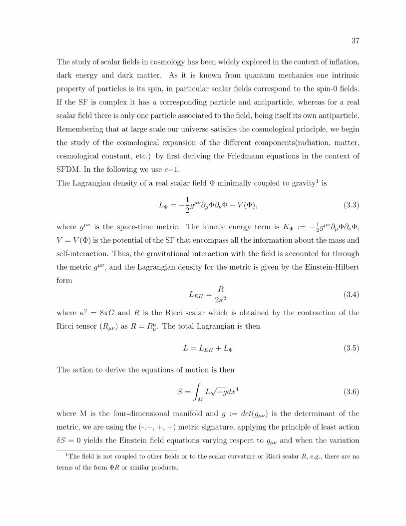
37
The study of scalar fields in cosmology has been widely explored in the context of inflation,
dark energy and dark matter. As it is known from quantum mechanics one intrinsic
property of particles is its spin, in particular scalar fields correspond to the spin-0 fields.
If the SF is complex it has a corresponding particle and antiparticle, whereas for a real
scalar field there is only one particle associated to the field, being itself its own antiparticle.
Remembering that at large scale our universe satisfies the cosmological principle, we begin
the study of the cosmological expansion of the different components(radiation, matter,
cosmological constant, etc.) by first deriving the Friedmann equations in the context of
SFDM. In the following we use c=1.
The Lagrangian density of a real scalar field Φ minimally coupled to gravity1 is
LΦ = −1
2gµν∂µΦ∂νΦ− V (Φ), (3.3)
where gµν is the space-time metric. The kinetic energy term is KΦ := −12gµν∂µΦ∂νΦ,
V = V (Φ) is the potential of the SF that encompass all the information about the mass and
self-interaction. Thus, the gravitational interaction with the field is accounted for through
the metric gµν , and the Lagrangian density for the metric is given by the Einstein-Hilbert
form
LEH =R
2κ2(3.4)
where κ2 = 8πG and R is the Ricci scalar which is obtained by the contraction of the
Ricci tensor (Rµν) as R = Rµµ. The total Lagrangian is then
L = LEH + LΦ (3.5)
The action to derive the equations of motion is then
S =
∫M
L√−gdx4 (3.6)
where M is the four-dimensional manifold and g := det(gµν) is the determinant of the
metric, we are using the (-,+, +, +) metric signature, applying the principle of least action
δS = 0 yields the Einstein field equations varying respect to gµν and when the variation
1The field is not coupled to other fields or to the scalar curvature or Ricci scalar R, e.g., there are no
terms of the form ΦR or similar products.
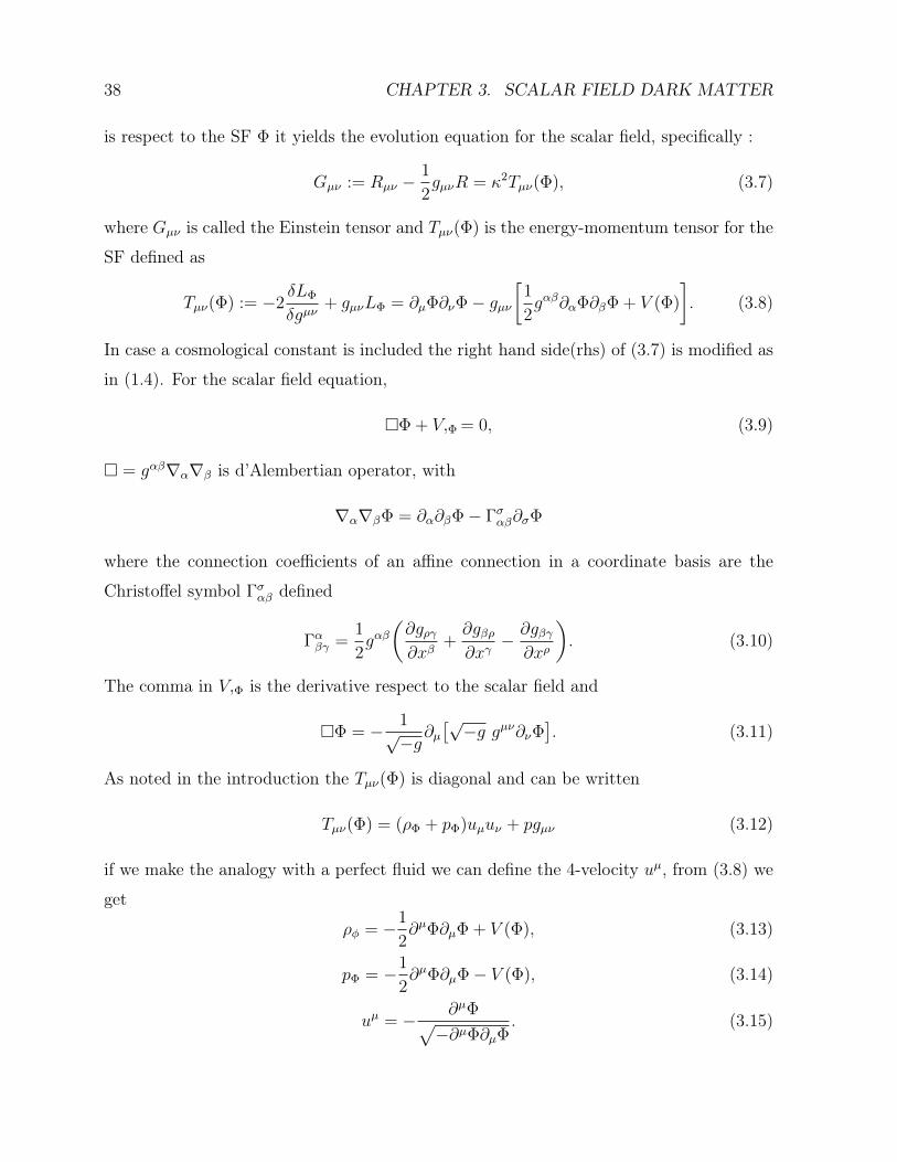
38 CHAPTER 3. SCALAR FIELD DARK MATTER
is respect to the SF Φ it yields the evolution equation for the scalar field, specifically :
Gµν := Rµν −1
2gµνR = κ2Tµν(Φ), (3.7)
where Gµν is called the Einstein tensor and Tµν(Φ) is the energy-momentum tensor for the
SF defined as
Tµν(Φ) := −2δLΦ
δgµν+ gµνLΦ = ∂µΦ∂νΦ− gµν
[1
2gαβ∂αΦ∂βΦ + V (Φ)
]. (3.8)
In case a cosmological constant is included the right hand side(rhs) of (3.7) is modified as
in (1.4). For the scalar field equation,
Φ + V,Φ = 0, (3.9)
= gαβ∇α∇β is d’Alembertian operator, with
∇α∇βΦ = ∂α∂βΦ− Γσαβ∂σΦ
where the connection coefficients of an affine connection in a coordinate basis are the
Christoffel symbol Γσαβ defined
Γαβγ =1
2gαβ(∂gργ∂xβ
+∂gβρ∂xγ
− ∂gβγ∂xρ
). (3.10)
The comma in V,Φ is the derivative respect to the scalar field and
Φ = − 1√−g
∂µ[√−g gµν∂νΦ
]. (3.11)
As noted in the introduction the Tµν(Φ) is diagonal and can be written
Tµν(Φ) = (ρΦ + pΦ)uµuν + pgµν (3.12)
if we make the analogy with a perfect fluid we can define the 4-velocity uµ, from (3.8) we
get
ρφ = −1
2∂µΦ∂µΦ + V (Φ), (3.13)
pΦ = −1
2∂µΦ∂µΦ− V (Φ), (3.14)
uµ = − ∂µΦ√−∂µΦ∂µΦ
. (3.15)
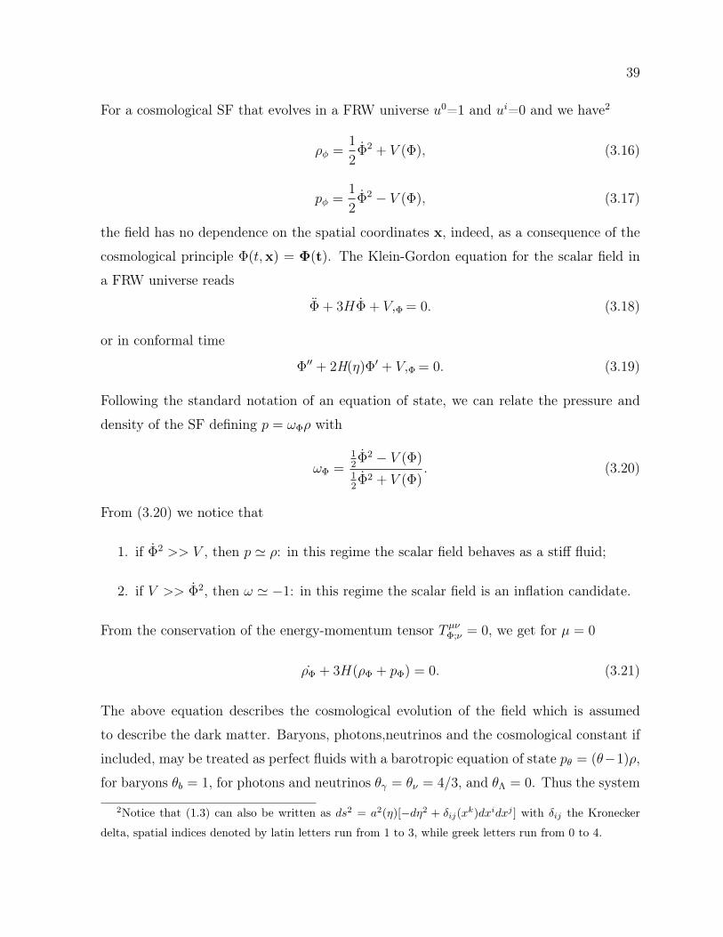
39
For a cosmological SF that evolves in a FRW universe u0=1 and ui=0 and we have2
ρφ =1
2Φ2 + V (Φ), (3.16)
pφ =1
2Φ2 − V (Φ), (3.17)
the field has no dependence on the spatial coordinates x, indeed, as a consequence of the
cosmological principle Φ(t,x) = Φ(t). The Klein-Gordon equation for the scalar field in
a FRW universe reads
Φ + 3HΦ + V,Φ = 0. (3.18)
or in conformal time
Φ′′ + 2H(η)Φ′ + V,Φ = 0. (3.19)
Following the standard notation of an equation of state, we can relate the pressure and
density of the SF defining p = ωΦρ with
ωΦ =12Φ2 − V (Φ)
12Φ2 + V (Φ)
. (3.20)
From (3.20) we notice that
1. if Φ2 >> V , then p ' ρ: in this regime the scalar field behaves as a stiff fluid;
2. if V >> Φ2, then ω ' −1: in this regime the scalar field is an inflation candidate.
From the conservation of the energy-momentum tensor T µνΦ;ν = 0, we get for µ = 0
ρΦ + 3H(ρΦ + pΦ) = 0. (3.21)
The above equation describes the cosmological evolution of the field which is assumed
to describe the dark matter. Baryons, photons,neutrinos and the cosmological constant if
included, may be treated as perfect fluids with a barotropic equation of state pθ = (θ−1)ρ,
for baryons θb = 1, for photons and neutrinos θγ = θν = 4/3, and θΛ = 0. Thus the system
2Notice that (1.3) can also be written as ds2 = a2(η)[−dη2 + δij(xk)dxidxj ] with δij the Kronecker
delta, spatial indices denoted by latin letters run from 1 to 3, while greek letters run from 0 to 4.
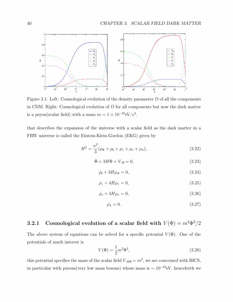
40 CHAPTER 3. SCALAR FIELD DARK MATTER
Figure 3.1: Left: Cosmological evolution of the density parameter Ω of all the components
in CDM. Right: Cosmological evolution of Ω for all components but now the dark matter
is a psyon(scalar field) with a mass m = 1× 10⁻²³eV/c2.
that describes the expansion of the universe with a scalar field as the dark matter in a
FRW universe is called the Eintein-Klein-Gordon (EKG) given by
H2 =κ2
3(ρΦ + ρb + ργ + ρν + ρΛ), (3.22)
Φ + 3HΦ + V,Φ = 0, (3.23)
ρb + 3HρB = 0, (3.24)
ργ + 4Hργ = 0, (3.25)
ρν + 4Hρν = 0, (3.26)
ρΛ = 0. (3.27)
3.2.1 Cosmological evolution of a scalar field with V (Φ) = m2Φ2/2
The above system of equations can be solved for a specific potential V (Φ). One of the
potentials of much interest is
V (Φ) =1
2m2Φ2, (3.28)
this potential specifies the mass of the scalar field V,ΦΦ = m2, we are concerned with BICS,
in particular with psyons(very low mass bosons) whose mass is ∼ 10−22eV, henceforth we
41
will omit the subscript Φ for the SF quantities. Clearly the pressure and density will be
ρ =1
2Φ2 +
1
2m2Φ2, (3.29)
p =1
2Φ2 − 1
2m2Φ2, (3.30)
with
ω =12Φ2 − 1
2m2Φ2,
12Φ2 + 1
2m2Φ2,
. (3.31)
A numerical solution of the EKG system was given in [Magaña et al.(2012)], in Figure (3.1)
we show the background evolution of all the components for the potential V (φ) = m2Φ2/2
using a mass of 1 × 10⁻²³eV from a = 10−6 until today a = 1. For comparison we also
show the evolution in the standard model (CDM) where the fluid is pressureless p=0.
We observe that results using a psyon with potential (3.28) are completely equivalent to
those in CDM, this is a major success of the model. For the SFDM we have the early
phase where photons and neutrinos(radiation) are dominant, later on as the universe keeps
expanding the matter and radiation energy densities are equal at aeq ∼ 1.6 × 10⁻⁴(using
data from WMAP-73), from this point the matter is the dominant component and small
DM fluctuations can start growing as we will see below. The time in which the photon’s
energy is small enough that electron can start combining with protons to form atomic
nuclei, the decoupling time, happens at a ∼ 10−3 (z ∼ 1000) similar to CDM. We see that
as expected, the cosmological constant will dominate the late time dynamics at zΛ ∼ 0.7.
But what causes the SFDM to behave as a CDM cosmologically? The answers lies in the
fact that despite the rapid oscillation of the field arond the minimum of V (Φ), the time
average of the pressure is 〈p〉 ≈ 0, this in turn makes 〈ωΦ〉 ≈ 0, hence the equation of
state for the psyons tends to zero and the field behaves effectively as a pressureless fluid
(dust) implying ρ ∼ a−3[Matos et al.(2009)] and hence mimics the CDM model.
Before jumping to the study of linear fluctuations, we will discuss the case where the
two-body interactions of the SF are included in the potential.
3In this calculation Ωdm,0 = 0.226, Ωb,0 = 0.0455, Ωγ,0 = 4× 10⁻⁵, Ων,0 = 2.7× 10⁻⁵, ΩbΛ,0 = 0.728,
TCMB,0 = 2.702K and h = 0.704.
42 CHAPTER 3. SCALAR FIELD DARK MATTER
3.2.2 Cosmological evolution of a SF with self-interactions.
As this case is of particular importance in our future study of galaxies in the SFDM, we
get back to physical units (c 6= 1 6= ~) to make the discussion more clearly in the hope
that the upcoming results are easily followed.
When self-interactions are included in a real scalar field the Lagrangian density for the
field is
LΦ = −1
2gµν∂µΦ∂νΦ− V (Φ), (3.32)
with
V (Φ) =1
2
m2c2
~2Φ2 +
λ
4~2c2Φ4, (3.33)
where the dimensionless self-interaction parameter is λ. This same scalar field model
has been studied considering it to be complex [Pitaevskii & Stringari(2003), Woo & Chi-
hue(2009)] It is this latter case that will occupy our attention in this subsection, we will
follow the approach of [Li et al.(2014)]. We write then the Lagrangian for the complex
scalar field as
LΨ = − ~2
2mgµν∂µΨ∂νΨ− V (Ψ), (3.34)
and
V (Ψ) =1
2m|Ψ|2 +
λ
4|Ψ|4. (3.35)
We choose to denoted the complex scalar field by Ψ. We recall that any two Lagrangians
that differ by a constant yield the same equations of motion, therefore if Φ is complex in
(3.32) we can relate (3.33) and (3.35) by
LΦ →1
~cLΦ := LΨ (3.36)
Φ→(~3c
m
)1/2
Ψ (3.37)
noting that λ = λ2
~3m2c
. The units are then [LΨ]=J/m3, [Ψ]=m−3/2, [λ]=Jm3, [Φ]= J,
[λ]=1. For example, for the QCD axion with decay constant f ' 1012 GeV we have a
dimensionless coupling λ ≈ 10−53[Sikivie & Yang (2009)]. It is a good approximation to
ignore higher order interactions when the bosonic gas is dilute, i.e. when the particle self-
interaction range is much smaller than the mean inter particle distance, as the cosmological
43
expansion dilutes the field, it is sufficient to consider only two-body s-wave scatterings,
then the coupling coefficient λ is a constant and related to the s-wave scattering length
as as λ = 4π~2as/m, which is the first Born approximation. An interesting property of
the Lagragian for a complex field is the global U(1) symmetry (Ψ → eiθΨ), by Noether’s
theorem this leads to a conserved charge density Q in real space, or equivalently, the
conservation of the comoving charge density Qa3, this conserved charge corresponds to
the particle number and it should not be confused with the electrical charged of a particle,
in our case the scalar field is not electrically charged. Moreover, the charge is defined
as the total number of bosons and the total number of anti-bosons, in particular, the
formation of a BEC the charge is essentially equal to the total number of bosons. The
conservation of particle number is an inherent property of complex scalar fields minimally
coupled to gravity and is not present for a real scalar field, as the latter does not possess
a U(1) symmetry, in fact, we already mentioned that in this case the boson is its own
anti-boson.
The cosmological evolution is determined by the Friedmann equation
H2 =
(da/dt
a
)2
=8πG
3c2(ρΦ + ρb + ργ + ρν + ρΛ), (3.38)
and the energy conservation equation
∂ρ
∂t+
3da/dt
a(ρ+ p) = 0. (3.39)
Where now the density and pressure are
ρ =~2
2mc2|∂tΨ|2 +
1
2mc2|Ψ|2 +
1
2λ|Ψ|4 (3.40)
p =~2
2mc2|∂tΨ|2 −
1
2mc2|Ψ|2 − 1
2λ|Ψ|4 (3.41)
and (3.23) becomes
~2
2mc2∂2t Ψ +
~2
2mc2
3da/dt
a∂tΨ +
1
2mc2Ψ + λ|Ψ|2Ψ = 0. (3.42)
Due to the oscillations of the field over time, it is convenient to define the oscillation angular
frequency as ω = ∂tθ. This system of equations is solved numerically in [Li et al.(2014)].
44 CHAPTER 3. SCALAR FIELD DARK MATTER
There are certain limits in which the behavior of the field changes, we first get an expression
for ω in the limit when the SF oscillates faster than the Hubble expansion (ω/H >> 1).
By rewriting the complex function in terms of its amplitude and phase as Ψ = |Ψ|eiθ andplugging it back into (3.42) we get
~2
2mc2(∂2t |Ψ| − |Ψ|(∂tθ)2) +
~2
2mc2
3da/dt
a∂t|Ψ|+
1
2mc2|Ψ|+ λ|Ψ|3 = 0, (3.43)
~2
2mc2(2∂t|Ψ|∂tθ + |Ψ|(∂2
t θ) +~2
2mc2
3da/dt
a|Ψ|∂tθ = 0. (3.44)
It is the phase θ that carries the oscillation behavior of Ψ, the time dependence of the
amplitude is smooth, hence it is safe to assume ∂t|Ψ|/|Ψ| << ∂tθ. Assuming also that
ω := ∂tθ >> H = (da/dt)/a , then we can neglect the terms ∂t|Ψ| and H in (3.43) and it
results
− ~2
2mc2|Ψ|(∂tθ)2 +
1
2mc2|Ψ|+ λ|Ψ|3 = 0, (3.45)
using ω := ∂tθ the above equation becomes
ω =mc2
~
√1 +
2λ
mc2|Ψ|2, (3.46)
valid only when ω >> H. In the free field case (λ=0) we get ω = mc2/~, from here it is
easy to see that small values of the mass translates into high oscillation frequencies.
Integrating (3.44) we get
∂t(a3|Ψ|2∂tθ) = 0⇐⇒ |Ψ|2∂tθ =
const.
a3. (3.47)
where a3|Ψ|2∂tθ is the conserved charge, in fact it is the conservation of the comoving
charge density Qa3.
Given the fast oscillation of the field we can follow the cosmological evolution of the time-
average values of ρ and p, a similar situation is found for the non-interacting case, although
in that case the equivalence of the exact and time-average evolution of the scalar field has
been worked out[Magaña et al.(2012)].
If we now multiply (3.42) by Ψ∗ and average over a time interval much longer that the field
oscillation period (∝ 1/ω) but shorter than the Hubble time results in[Woo & Chihue(2009),
Dutta & Scherrer (2010)]
~2
2mc2〈|Ψ|2〉 =
1
2mc2〈|Ψ|2〉+ λ〈|Ψ|4〉 = 0. (3.48)
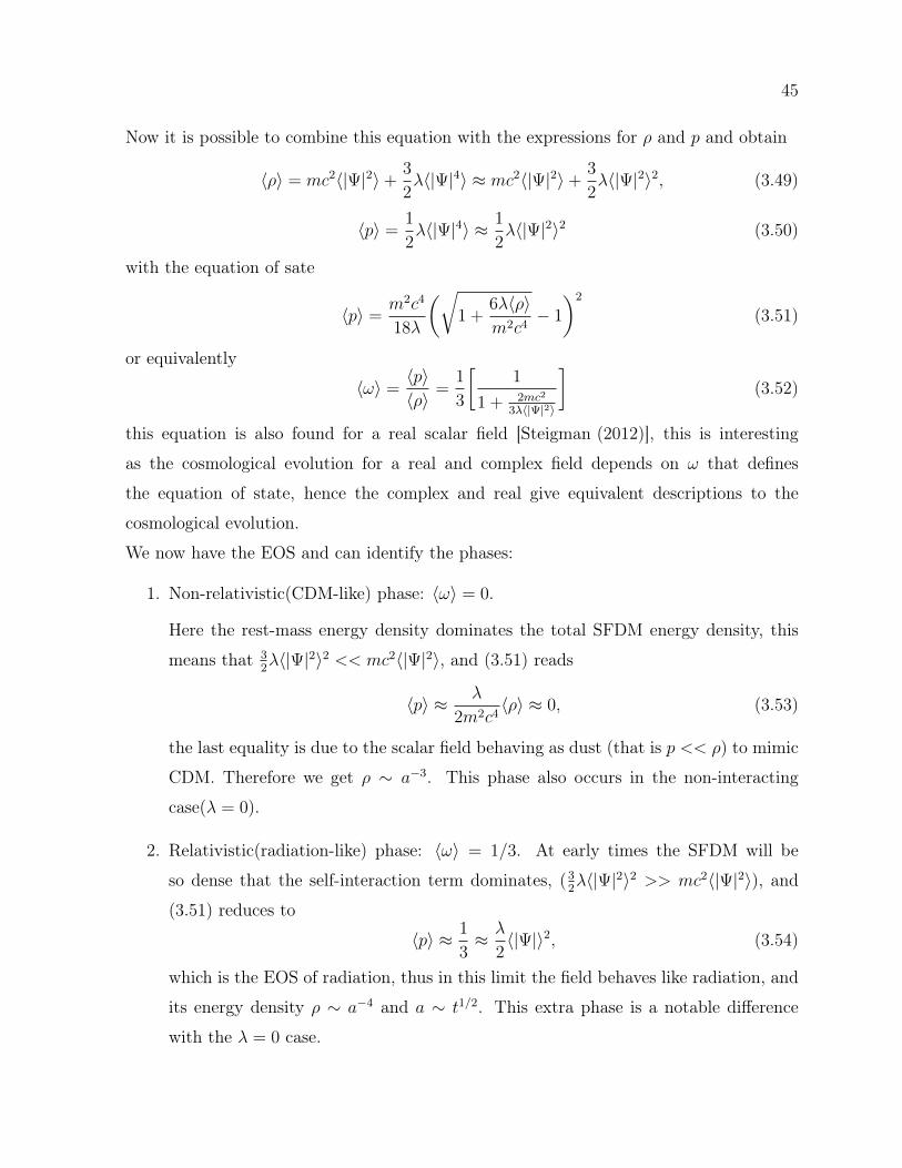
45
Now it is possible to combine this equation with the expressions for ρ and p and obtain
〈ρ〉 = mc2〈|Ψ|2〉+3
2λ〈|Ψ|4〉 ≈ mc2〈|Ψ|2〉+
3
2λ〈|Ψ|2〉2, (3.49)
〈p〉 =1
2λ〈|Ψ|4〉 ≈ 1
2λ〈|Ψ|2〉2 (3.50)
with the equation of sate
〈p〉 =m2c4
18λ
(√1 +
6λ〈ρ〉m2c4
− 1
)2
(3.51)
or equivalently
〈ω〉 =〈p〉〈ρ〉
=1
3
[1
1 + 2mc2
3λ〈|Ψ|2〉
](3.52)
this equation is also found for a real scalar field [Steigman (2012)], this is interesting
as the cosmological evolution for a real and complex field depends on ω that defines
the equation of state, hence the complex and real give equivalent descriptions to the
cosmological evolution.
We now have the EOS and can identify the phases:
1. Non-relativistic(CDM-like) phase: 〈ω〉 = 0.
Here the rest-mass energy density dominates the total SFDM energy density, this
means that 32λ〈|Ψ|2〉2 << mc2〈|Ψ|2〉, and (3.51) reads
〈p〉 ≈ λ
2m2c4〈ρ〉 ≈ 0, (3.53)
the last equality is due to the scalar field behaving as dust (that is p << ρ) to mimic
CDM. Therefore we get ρ ∼ a−3. This phase also occurs in the non-interacting
case(λ = 0).
2. Relativistic(radiation-like) phase: 〈ω〉 = 1/3. At early times the SFDM will be
so dense that the self-interaction term dominates, (32λ〈|Ψ|2〉2 >> mc2〈|Ψ|2〉), and
(3.51) reduces to
〈p〉 ≈ 1
3≈ λ
2〈|Ψ|〉2, (3.54)
which is the EOS of radiation, thus in this limit the field behaves like radiation, and
its energy density ρ ∼ a−4 and a ∼ t1/2. This extra phase is a notable difference
with the λ = 0 case.
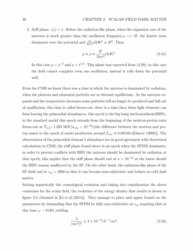
46 CHAPTER 3. SCALAR FIELD DARK MATTER
3. Stiff phase: 〈ω〉 = 1. Before the radiation-like phase, when the expansion rate of the
universe is much greater than the oscillation frequency,ω << H, the kinetic term
dominates over the potential and ~22mc2|∂tΨ|2 ∝ H2. Then
p ≈ ρ ≈ ~2
2mc2|∂tΨ|2. (3.55)
In this case ρ ∼ a−6 and a ∼ t1/3. This phase was expected from (3.20), in this case
the field cannot complete even one oscillation, instead it rolls down the potential
well.
From the CMB we know there was a time in which the universe is dominated by radiation,
when the photons and elemental particles are in thermal equilibrium. As the universe ex-
pands and the temperature decreases some particles will no longer be produced and fall out
of equilibrium, this time is called freeze-out, there is a time then when light elements can
form leaving the primordial abundances, this epoch is the big bang nucleosynthesis(BBN),
in the standard model this epoch extends from the beginning of the neutron-proton ratio
freeze-out at Tn/p=1.293 MeV(an/p ∼ 10−10)(the difference between the neutron and pro-
ton mass) to the epoch of nuclei production around Tnuc ≈ 0.085Mev[Durrer (2008)]. The
observations of the primordial element’s abundance are in good agreement with theoretical
calculations in CDM, the stiff phase found above is an epoch when the SFDM dominates,
in order to prevent conflicts with BBN the universe should be dominated by radiation at
that epoch, this implies that the stiff phase should end at a ∼ 10−10 at the latest should
the BBN remain unaffected by the SF. On the other hand, the radiation-like phase of the
SF shall end at zeq ∼ 3000 so that it can become non-relativistic and behave as cold dark
matter.
Solving numerically the cosmological evolution and taking into consideration the above
constrains for the scalar field, the evolution of the energy density that results is shown in
figure 3.2 obtained in [Li et al.(2014)]. They manage to place and upper bound on the
parameters by demanding that the SFDM be fully non-relativistic at zeq requiring that at
this time ω = 0.001 yielding
λ
(mc2)2≤ 4× 10⁻¹⁷eV −1cm3, (3.56)
47
while imposing that the SFDM changes from the stiff to the radiation-like phase by the
end of BBN (anuc) and that the number of relativistic degrees of freedom Neff during the
BBN be all the time within 1σ of the measured value
Neff = 3.71+0.47−0.45 (3.57)
taken from [Arbey et al.(2002)], results in
9.5× 10⁻¹⁹eV −1cm3 ≤ λ/(mc2)2 ≤ 1.5× 10⁻¹⁶eV −1cm3. (3.58)
It is important to notice that (3.58) is rather arbitrary, in principle the radiation phase
can also be reached before anuc and this bound will no longer hold. Instead, if we want the
scalar field to be the dark matter that forms the large scale structure of the universe the
radiation-CDM transition should take place before decoupling (zdec)which makes (3.56) a
strong bound for a large class of models whose particle candidate is BICS.
The stiff phase is also present in the free field case (V (Φ) = 12m2Φ2), we expect a similar
situation but the transition would be from the stiff to the non-relativistic phase, however,
temperature corrections of the field, insofar neglected, could lead to the appearance of a
relativistic phase, this interesting fact is of relevance mainly in the non-interacting case of
the scalar field and we are currently studying.
It is also relevant to note that when self interactions are considered in the potential, the
cosmological constraints are on λ(mc2)2
, hence we require independent tests to constraint
the mass or the interaction given that they appear in the above combination and are
degenerated.
§3.3 Density perturbationsIn the study of perturbations we require to specify the coordinates. A choice of coordinates
defines a threading of space-time into lines (corresponding to fixed x) and a slicing into
hypersurfaces (corresponding to fixed t). The lines of fixed x are chosen to be timelike,
so they are world lines of possible observes, and the slices are chose to be spacelike. As
a reminder to the reader, unless otherwise specified(like in the previous section), we keep
using natural units.
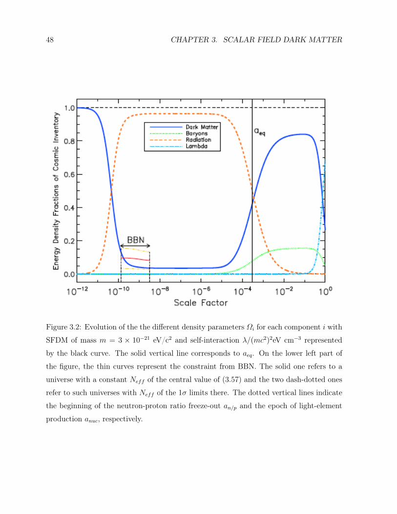
48 CHAPTER 3. SCALAR FIELD DARK MATTER
Figure 3.2: Evolution of the the different density parameters Ωi for each component i with
SFDM of mass m = 3 × 10⁻²¹ eV/c2 and self-interaction λ/(mc2)2eV cm−3 represented
by the black curve. The solid vertical line corresponds to aeq. On the lower left part of
the figure, the thin curves represent the constraint from BBN. The solid one refers to a
universe with a constant Neff of the central value of (3.57) and the two dash-dotted ones
refer to such universes with Neff of the 1σ limits there. The dotted vertical lines indicate
the beginning of the neutron-proton ratio freeze-out an/p and the epoch of light-element
production anuc, respectively.
49
Consider for instance the case of the unperturbed universe (in our case the FRW universe).
In this case there are preferred coordinates. The threading corresponds to the motion of
comoving observers, defines as those who see zero momentum density at their own position.
The comoving observers are free-falling and the expansion defined by them is isotropic,
The slicing is orthogonal to the threading, and on each slice, the universe is homogeneous.
The time coordinate is chosen to correspond to proper time along each worldline. In the
case that slices are flat( zero spatial curvature), the space coordinates can be chosen to
be Cartesian. This array of properties makes this preferred coordinate so valuable that
no others are considered. This is the slicing and threading that we have been using in all
this work for the cosmological description.
When we deal with perturbations, it is impossible to find coordinates satisfying all these
properties, and there is no uniquely preferred choice. The way people have deal with this
issue is by requiring that the coordinates must reduce to the standard ones in the limit
where the perturbations vanish. A choice of coordinates satisfying this constrain is called
a gauge, and there is no unique preferred gauge.
As we see, the only function of a gauge choice in cosmological perturbation theory is to
define a slicing and threading of space-time. The slicing and threading in turn define the
perturbations. For a perturbation g(x, t), the space-time coordinates can be regarded as
those of unperturbed space-time because to include their perturbation would be a second
order effect. Hence, the perturbation live in the unperturbed space-time.
As we will be concerned with scalar perturbations we will choose a suitable gauge to
isolate them from the vector and tensor perturbations. Notice that a slicing is needed to
specify perturbations in quantities such as the energy density, which have nonzero(and
time-varying) values in the unperturbed universe. Take for instance the energy density ,
given a slicing, we write
ρ(x, t) = ρ(t) + δρ(x, t). (3.59)
The first term is the unperturbed part, the one we have been calling the background
density in the FRW universe, and as mentioned, once δρ(x, t) is defined the coordinates x
and t can be identify to the standard ones in the unperturbed space-time. The slicing that
we will use to make use of the unperturbed (or background) space-time is the comoving
50 CHAPTER 3. SCALAR FIELD DARK MATTER
slicing, orthogonal to the worldlines of comoving observers. Also, it can be shown that
the perturbation in a scalar quantity is independent of the threading, the only effect of
a change in threading is to change the values of the space coordinates of each point, the
measured scalar perturbation by one observer will differ only by an amount of order v2,
with v the relative velocity of the other observer [Liddle & Lyth (2000)].
When the scalar field perturbations are small, we can study them with linear perturbation
theory. We consider the real scalar field. We then write
gµν = g0µν + δgµν (3.60)
here g0µν is the unperturbed FRW metric. In conformal time η the most general form of
the linearly perturbed FRW metric is ([Malik(2001)])
ds2 = a2(η)[−(1 + 2ψ)dη2 + 2B,i dηdxi + [(1− 2φ)δij + 2E,ij ]dxidxj]. (3.61)
where the perturbations are given in terms of four scalar functions: ψ the lapse function,
φ gravitational potential, B the shift, and E the anisotropic potential. The perturbed
component are
δg00 = −a2(η)2ψ, (3.62)
δg0i = δgi0 = a2(η)B,i (3.63)
δgij = −2a2(η)(φδij − E,ij ). (3.64)
Additionally, Φ(η,x) = Φ0(η) + δΦ(η,x), in the linear regime δΦ << Φ0 so we can
approximate V (Φ) ≈ V (Φ0). We define the density contrast by
δ :=δρ
ρ0
, (3.65)
the density contrast δ gives information about the amplitude of the perturbations as they
evolve in the expanding homogeneous background, according the CMB observations this
are δ ∼ 10−5. We can use the freedom in the gauge choice to set two of the four scalar
metric perturbations to zero, we choose the Newtonian gauge where B = 0 = E leaving
only the Bardeen potentials, the metric reads
ds2 = a2(η)[−(1 + 2ψ)dη2 + [(1− 2φ)δijdxidxj]. (3.66)
51
In this gauge, the physics appears rather simple since the hypersurfaces of constant time
are orthogonal to the worldlines of observers at rest in the coordinates (since B = 0) and
the induced geometry of the constant-time hypersurfaces is isotropic (since E = 0). In the
absence of anisotropic stress the metric is diagonal and ψ = φ. Note the similarity of the
metric to the usual weak-field limit of general relativity about Minkowski space; then φ
can be identified with the gravitational potential. The Newtonian gauge is our preferred
gauge for studying the formation of large-scale structures.
For the perturbed energy momentum tensor we have
T = T0 + δT, (3.67)
with T0 = T0(t) and δT = δT (xµ) with xµ = (t,x). Explicitly the perturbed density δρ
and the perturbed pressure δp in comoving time t (d/dη = a(d/dt)) are defined in terms
of the perturbed energy momentum tensor as
δT 00 = −δρ = −(Φ0
˙δΦ− Φ20ψ + V,Φ δΦ),
δT 0i = −1
a(Φ0δΦ,i ),
δT ij = δp = (Φ0˙δΦ− Φ2
0ψ − V,Φ δΦ)δij. (3.68)
δρ is the perturbed energy density of the scalar field, δp is the perturbed pressure and δΦ
the scalar field fluctuation.
The perturbed EKG system in the Newtonian gauge δGij = κ2δT ij is
−8πGδρ = 6H(φ+Hφ)− 2
a2∇2φ,
8πGΦ0δΦ,i = 2(φ+Hφ),i ,
8πGδp = 2[φ+ 4Hφ+ (2H + 3H2)φ] (3.69)
with ˙ = ∂/∂t and H = d(ln a)/dt.
The above system of equations describe the evolution of the scalar perturbations(Malik(2001),
Ma & Bertschinger(1995)). Summing the first and third equations in (3.69) and from (3.68)
we get δp− δρ=−2V,Φ and we get an equation for the gravitational potential
δφ+ 7H ˙δφ− 1
a2∇2δφ+ 2(H + 3H2)φ+ 8πGV,Φ Φ = 0. (3.70)
52 CHAPTER 3. SCALAR FIELD DARK MATTER
To study the evolution of the SF perturbations we use the perturbed Klein-Gordon equa-
tion
δΦ + 3H ˙δΦ− 1
a2∇2δΦ + V,ΦΦ δΦ + 2V,Φ φ− 4Φ0φ = 0. (3.71)
Equation (3.71) can be rewritten as:
δΦ +d2V
dΦ2
∣∣∣∣Φ0
δΦ + 2dV
dΦ
∣∣∣∣Φ0
φ− 4Φ0φ = 0, (3.72)
where the D’Alambertian operator is defined as
:=∂2
∂t2+ 3H
∂
∂t− 1
a2∇2. (3.73)
The equations can be studied in the Fourier space, this approach is usually convenient
because in the linear regime each Fourier model evolves independently. The Fourier trans-
form at first order is readily obtain
δΦ(t,x) =
∫d3kδΦ(t,k)exp(i k · x) =
∫d3kδΦkexp(i k · x) (3.74)
k is the wave number defined by k = 2π/λk, where λk denotes the size of the scalar field
perturbation. The perturbed EKG system can be transform to its Fourier equivalent by
changing δΦ→ δΦk, ∇2 → −k2 with k2 = kiki and ∂i → −iki. The system transforms to
8πG(3HΦ0δΦk) +2k2
a2φk = −8πG(Φ0
˙δΦ− Φ20φk + V,Φ δΦ),
2(φk +Hφk) = 8πGΦ0δΦk,
2[φk + 4Hφk + (2H + 3H2)φk] = 8πG(Φ0˙δΦ− Φ2
0φk − V,Φ δΦ) (3.75)
and¨δφk + 7H ˙δφk + (
k2
a2+ 2H + 6H2)φk + 8πGV,Φ Φk = 0. (3.76)
¨δΦk + 3H ˙δΦk + (k2
a2+ V,ΦΦ )δΦk + 2φkV,Φ−4Φ0φk = 0. (3.77)
The system (3.75), (3.76) and (3.77) describe the cosmological evolution in the linear
regime for a scalar field perturbation with wave number k. Essentially, equation (3.77)
represents a harmonic oscillator with a damping 3H ˙δΦK and an extra force −2φkV,Φ. The
damping term in (3.76) goes as 6Hφk, the term 2H < 0 and the gravitational fluctuations
can grow provided (k2
a2+2H+6H2)<0. Equation (3.77) has oscillatory solutions if (V,ΦΦ +
53
k2
a2) < 0. This equation contains growing solutions if this term is negative, that is, if V,ΦΦ<0
and k2
a2is small enough. From here we see an important feature. These perturbations grow
only if V has a maximum, even if it is a local one. Here, the potential is unstable and during
the time when the scalar field remains in the maximum, the scalar field fluctuations grow
until they reach a new stable point where the gravitational structures can keep growing
until they collapse and form the dark matter halos. Therefore, the term (V,ΦΦ + k2
a2)
defines a wave number below which the fluctuations don’t grow and keep oscillating, this
is equivalent to the Jeans length in CDM,
kefJ :=√a2V,ΦΦ. (3.78)
Only fluctuations with k < kefJ can grow. We can define an associated Jeans length
[Ma et al. (1999), Hwang& Noh (2001)]
λefJ =2π
a√V,ΦΦ
= 2π/ma. (3.79)
From this relation we see that the mass of the boson(V,ΦΦ = m2) determines a minimum
scale for the growing modes, thus fixing the mass naturally implies a cut-off in the mass
power spectrum, this particular feature is of extreme importance because it implies a
supresion of dark matter substructure below a certain scale kefJ , which helps to reduce
the satellite overabundance and serve to solve the missing satellite problem present in
CDM[Hu, Barkana & Gruzinov(2000), Matos & Ureña(2001), Marsh & Silk(2014)]. For
instance, if m ∼ 10−23eV we have λefJ ∼ 4 kpc at the epoch or recombination a ∼ 10−3.
§3.4 Linear growth of scalar field perturbationsAlthough it is possible to obtain the complete evolution of the psyon perturbations by solv-
ing the perturbed EKG system[Magaña et al.(2012)], it is nevertheless useful to have an
equation for the linear evolution of the density contrast δ. The equation follows after doing
a lengthy but otherwise straightforward algebra in complete analogy to the calculation for
CDM perturbations[Suárez & Matos (2011), Suárez & Chavanis (2015)].
For the cold dark matter model the equation for the evolution of the density contrast is
given byd2δ
dt2+ 2H
dδ
dt+(c2s
k2
a2− 4πGρ0
)δ = 0, (3.80)
54 CHAPTER 3. SCALAR FIELD DARK MATTER
where cs is defined as the sound velocity. For cold and pressureless dark matter the
equation of state ω = 0 and the sound speed cs = δp/δρ = 0, then at a ≥ aeq the
interesting fluctuation modes (galactic-size) are well within the horizon, we have a ∼ t2/3
and ρ ∼ a−3, thusd2δ
dt2+
4
3t
dδ
dt− 2
3t2δ = 0, (3.81)
The solutions to this equation are of the form
t→ t2/3C1 +C2
t(3.82)
where C1 and C2 are integration constants, from this solution we can see that we have
modes that will disappear as time goes by, and modes that grow proportionally to the
expansion of the Universe δ ∼ a. The matter fluctuations that enter the horizon in the
radiation era(a < aeq) have a logarithmic growth δ ∼ ln(a), had there been no loga-
rithmic growth these fluctuations would have experience no growth from horizon entry
until the epoch of equality, their amplitude relative to large scale modes (small k) would
be suppressed. A more detailed analysis will not be treated here, but can be found in
[Dodelson (2003)].
Now, in the case of a free scalar field V (Ψ) = m2Φ2/2, the relevant scale is the Hub-
ble scale, H. The (time average) equation of state (EOS) transitions from ω = −1
to ω = 0 when the psyon mass overcomes the Hubble friction in the Klein-Gordon
equation, also the structure is suppressed on scales of order the horizon when H ∼m[Marsh & Silk(2014), Hu, Barkana & Gruzinov(2000), Marsh & Ferreira(2010)]. When
the field is oscillating about the potential minimum at times t > tosc, where H(tosc) ∼ m,
the EOS and sound speed in the effective fluid description averaged over periods t > 1/m
are given by ([Hu, Barkana & Gruzinov(2000), Park et al. (2012)])
ω = 0, (3.83)
c2s =
v2q
1 + v2q
. (3.84)
where we define
v2q :=
k2
4m2a2. (3.85)
55
Notice that cs is now scale-dependent, the term v2q comes from the oscillation frequency
of the field. The equation for the density contrast takes the form
d2δ
dt2+ 2H
dδ
dt+(c2s
k2
a2− 4πGρ0
)δ = 0, (3.86)
or in conformal time
d2δ
dη2+ 2H(η)
dδ
dη+(c2sk
2 − 4πGρ0a2)δ = 0, (3.87)
where H(η)= aH(t) is the conformal Hubble rate as usual.
For the large scale perturbations with k2 << a2m2 we have c2s ≈ v2
q << 1 and the sound
speed goes to zero, here we recover the scale-independent linear growth with δ ∼ a on
large scales. For large k, or k2 >> a2m2, the sound speed c2s ≈ 1 and the overdensity
oscillates rather than grows. This is consistent with the discussion in the last section, the
transition between growth and oscillation occurs at the Jeans scale
kJ = a(16πGρ0)1/4m1/2. (3.88)
For k > kJ there is no growth of structure. There is scale-dependent growth as k decreases
from kJ , continuously interpolating to the standard scale-independent linear growth on
the largest scales, k << kJ .
When self-interactions are included as in (3.33) , (3.86) turns
d2δ
dt2+ 2H
dδ
dt+((c2s + ωλρ0)
k2
a2− 4πGρ0
)δ = 0, (3.89)
with ωλ = 9λ/2m2[Suárez & Matos (2011)]. Therefore λ 6= 0 changes the Jeans scale in
the free-field case.
The evolution of the linear growth of psyon perturbations when c2s ≈ v2
q was obtained in
(Suarez & Matos 2011), as shown in figure (3.4) linear growth after aeq ∼ 10−4 proceeds
just like CDM (δ ∼ a), the case self-interacting field however, shows an earlier amplitude
growth. These results can impact the large scale structure, a faster growth implies that
the structures can become non-linear faster and the dark matter potential wells that will
host galaxies are formed before CDM, after decoupling the gas will follow the potential
wells and can condense earlier forming stars and hence galaxies at high redshift, this can
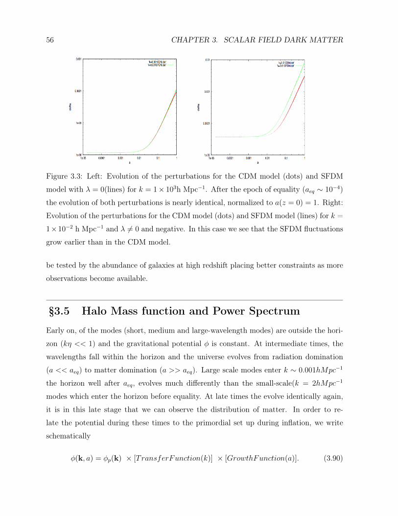
56 CHAPTER 3. SCALAR FIELD DARK MATTER
Figure 3.3: Left: Evolution of the perturbations for the CDM model (dots) and SFDM
model with λ = 0(lines) for k = 1× 10³h Mpc−1. After the epoch of equality (aeq ∼ 10−4)
the evolution of both perturbations is nearly identical, normalized to a(z = 0) = 1. Right:
Evolution of the perturbations for the CDM model (dots) and SFDM model (lines) for k =
1×10⁻² h Mpc−1 and λ 6= 0 and negative. In this case we see that the SFDM fluctuations
grow earlier than in the CDM model.
be tested by the abundance of galaxies at high redshift placing better constraints as more
observations become available.
§3.5 Halo Mass function and Power Spectrum
Early on, of the modes (short, medium and large-wavelength modes) are outside the hori-
zon (kη << 1) and the gravitational potential φ is constant. At intermediate times, the
wavelengths fall within the horizon and the universe evolves from radiation domination
(a << aeq) to matter domination (a >> aeq). Large scale modes enter k ∼ 0.001hMpc−1
the horizon well after aeq, evolves much differently than the small-scale(k = 2hMpc−1
modes which enter the horizon before equality. At late times the evolve identically again,
it is in this late stage that we can observe the distribution of matter. In order to re-
late the potential during these times to the primordial set up during inflation, we write
schematically
φ(k, a) = φp(k) × [TransferFunction(k)] × [GrowthFunction(a)]. (3.90)
57
where φp is the primordial value of the potential, set during inflation. The transfer func-
tion describes the evolution of perturbations through the epochs of horizon crossing and
radiation/mater transition, while the growth factor describes the wavelength-independent
growth at late times. There are two conventions, one is to set the transfer function equal
to on large scales, therefore the transfer function is defined as
T (k) :=φ(k, alate)
φLarge−scale(k, alate)(3.91)
where alate denotes an epoch well after the transfer function regime and the Large-scale
solution is the primordial φ decreased by a small amount, in CDM this factor is equal to
(9/10) neglecting anisotropic stresses [Dodelson (2003)]. The second convention concerns
the growth function. The ratio of the potential to its value right after the transfer function
regime is defined to be
φ(a)
φ(alate):=
D(a)
a(a > alate) (3.92)
where D is called the growth function. When the potential is constant D(a) = a. With
these conventions we have
φ(k, a) =9
10φp(k)T (k)
D(a)
a(a > alate) (3.93)
From the above section we saw that when the potential is constant and all the modes are
within the horizon, the overdensity grows as δ ∼ a, D describes the growth of the matter
perturbations at late times, for this reason D is called the growth function despite the
potential remains constant. This picture is consistent with the intuitive idea that as time
evolves, overdense regions attract more matter, thereby becoming more overdense.
Let us first the case of the standard model. The simplest way to relate the matter over-
density to the potential at late times is to use Poisson’s equation in Fourier space (for the
large-k and no-radiation limit)
φ =4πGρma
2δ
k2(3.94)
where the background density of matter ρm = Ωmρcrit/a3, and 4πGρcrit = (3/2)H2
0 , so
δ(k, a) =k2φ(k, a)a
(3/2)ΩmH20
(a > alate), (3.95)
58 CHAPTER 3. SCALAR FIELD DARK MATTER
substituting the expression for φ(k, a) allow us to relate the overdensity today to the
primordial potential
δ(k, a) =3
5
k2
ΩmH20
φp(k)T (k)D(a) (a > alate), (3.96)
this equation holds regardless of how the initial perturbation φp was generated. In the
context of inflation φp(k) is drawn from a Gaussian distribution with mean zero and
variance
Pφ =50π2
9k3
(k
H0
)n−1
δ2H
(Ωm
D(a = 1)
)2
(3.97)
so the power spectrum of matter at late times is
P (k, a) = 2π2δ2H
kn
Hn+30
T 2(k)
(D(a)
D(a = 1)
)2
(a > alate). (3.98)
The power spectrum has dimensions of (length)3, to convert it into a dimensionless quan-
tity one often associates dk3P (k)/(2π)3 with the excess power in a bin of width k centered
at k, after integrating over all orientations of k this becomes (dk/k)∆2(k), with
∆2(k) :=k3P (k)
2π2(3.99)
Small ∆ then corresponds to small inhomogeneities, while a large value indicates nonlinear
perturbations. With the conventions used, for a Harrison-Zel’dovich-Peebles spectrum(n =
1) today we have ∆2 = δ2H on a horizon-sized scale(k = H0).
On large scales the transfer function is unity and P ∝ k corresponding to the simplest
inflationary model, wherein n = 1. There is a turn over over in the power spectrum at a
scale corresponding to the one which enters the horizon at matter/radiation equality. We
can see why this happens with an example. A small-scale mode with k = 2hMpc−1 enters
the horizon well before matter/radiation equality, during the radiation era the potential
decays, so T (k) is much smaller than unity. The effect on matter perturbations will be to
retard the growth of δ after the mode has entered the horizon until the universe is matter
dominated. Modes that enter the horizon earlier undergo more suppression, thus the
power spectrum is a decreasing function of k on small scales. This turnover is important
as it can restricts the number of small scale modes that remain at z=0. One scale that
is also important is in which nonlinearities cannot be ignored, this is set by ∆(knl ' 1),
corresponding in CDM usually to knl ' 0.2hMpc−1.
59
Now, in a cosmology where the pysons are the dark matter, or in general a fraction of it
fp = Ωp/Ωd, the suppression scale occurs for modes that enter the horizon when the sound
speed was large,we will neglect self-interactions. The suppression is centered around km,
which depends on the mass, and the fraction Ωp.
In [Marsh & Silk(2014)], they compute the transfer function and matter power spectrum
in cosmologies containing CDM plus SFDM using a modified version of the code CAMB.
They define the transfer function of the SFDM
Tsfdm(k) =
(PsfdmPΛCDM
)1/2
. (3.100)
A well defined characteristic scale to assign to any such step-like transfer function is the
’half mode’
T (km) = 0.5(1− T (k →∞)), (3.101)
where T (k → ∞) ≥ 0 is the constant value of the transfer function on small scales. For
comparison we include the warm dark matter(WDM) model transfer function [Bode et
al.(2001)]
TWDM(k) = (1 + (αk)2µ)−5/µ, (3.102)
where µ = 1.12 and α ≈ 0.065h−1Mpc chosen to give the same km than in SFDM. This
selection of km in SFDM is not the Jeans scale where all structure is suppressed, but it is
useful when comparing different dark matter models because it is well-defined. Taking a
typical mass of the psyon m ∼ 10−22eV, it is found km(10−22) = 6.7hMpc−2.
One popular way to characterize power on a particular scale is to compute the expected
root-mean-squared overdensity in a sphere of radius R,
σ2R := 〈δ2
R(x)〉 (3.103)
Here
δR(x) :=
∫d3x′δ(x)WR(x - x′) (3.104)
where WR(x) is the top-hat window function, equal to 1 for x < R and 0 otherwise; the
angular brackets denote the average over all space. The variance of the power spectrum,
can be rewritten as
σ2R :=
∫ ∞0
dk
k∆2(k)W 2
R(k) (3.105)
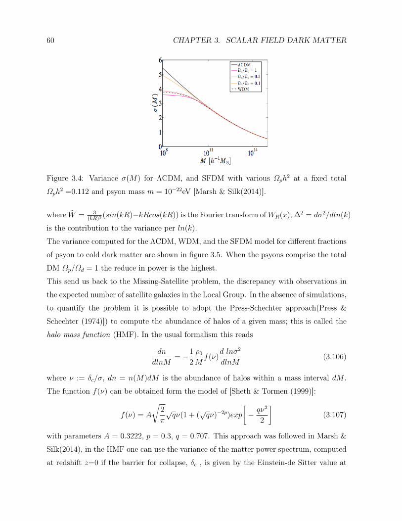
60 CHAPTER 3. SCALAR FIELD DARK MATTER
Figure 3.4: Variance σ(M) for ΛCDM, and SFDM with various Ωph2 at a fixed total
Ωph2 =0.112 and psyon mass m = 10−22eV [Marsh & Silk(2014)].
where W = 3(kR)3
(sin(kR)−kRcos(kR)) is the Fourier transform ofWR(x), ∆2 = dσ2/dln(k)
is the contribution to the variance per ln(k).
The variance computed for the ΛCDM, WDM, and the SFDM model for different fractions
of psyon to cold dark matter are shown in figure 3.5. When the psyons comprise the total
DM Ωp/Ωd = 1 the reduce in power is the highest.
This send us back to the Missing-Satellite problem, the discrepancy with observations in
the expected number of satellite galaxies in the Local Group. In the absence of simulations,
to quantify the problem it is possible to adopt the Press-Schechter approach(Press &
Schechter (1974)]) to compute the abundance of halos of a given mass; this is called the
halo mass function (HMF). In the usual formalism this reads
dn
dlnM= −1
2
ρ0
Mf(ν)
d lnσ2
dlnM(3.106)
where ν := δc/σ, dn = n(M)dM is the abundance of halos within a mass interval dM .
The function f(ν) can be obtained form the model of [Sheth & Tormen (1999)]:
f(ν) = A
√2
π
√qν(1 + (
√qν)−2p)exp
[− qν2
2
](3.107)
with parameters A = 0.3222, p = 0.3, q = 0.707. This approach was followed in Marsh &
Silk(2014), in the HMF one can use the variance of the matter power spectrum, computed
at redshift z=0 if the barrier for collapse, δc , is given by the Einstein-de Sitter value at
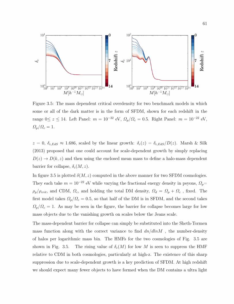
61
Figure 3.5: The mass dependent critical overdensity for two benchmark models in which
some or all of the dark matter is in the form of SFDM, shown for each redshift in the
range 0≤ z ≤ 14. Left Panel: m = 10−22 eV, Ωp/Ωc = 0.5. Right Panel: m = 10−22 eV,
Ωp/Ωc = 1.
z = 0, δc,EdS ≈ 1.686, scaled by the linear growth: δc(z) = δc,EdS/D(z). Marsh & Silk
(2013) proposed that one could account for scale-dependent growth by simply replacing
D(z)→ D(k, z) and then using the enclosed mean mass to define a halo-mass dependent
barrier for collapse, δc(M, z).
In figure 3.5 is plotted δ(M, z) computed in the above manner for two SFDM cosmologies.
They each take m = 10−22 eV while varying the fractional energy density in psyons, Ωp=
ρp/ρcrit, and CDM, Ωc, and holding the total DM density, Ωd = Ωp + Ωc , fixed. The
first model takes Ωp/Ωc = 0.5, so that half of the DM is in SFDM, and the second takes
Ωp/Ωc = 1. As may be seen in the figure, the barrier for collapse becomes large for low
mass objects due to the vanishing growth on scales below the Jeans scale.
The mass-dependent barrier for collapse can simply be substituted into the Sheth-Tormen
mass function along with the correct variance to find dn/dlnM , the number-density
of halos per logarithmic mass bin. The HMFs for the two cosmologies of Fig. 3.5 are
shown in Fig. 3.5. The rising value of δc(M) for low M is seen to suppress the HMF
relative to CDM in both cosmologies, particularly at high-z. The existence of this sharp
suppression due to scale-dependent growth is a key prediction of SFDM. At high redshift
we should expect many fewer objects to have formed when the DM contains a ultra light
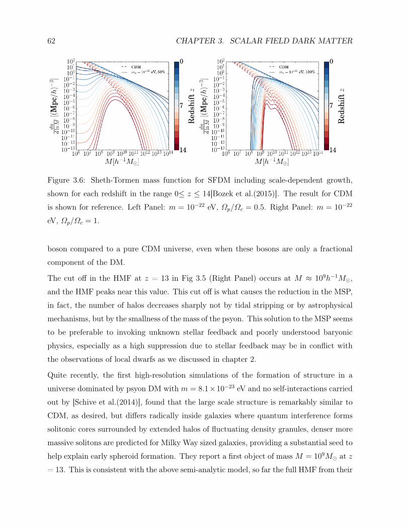
62 CHAPTER 3. SCALAR FIELD DARK MATTER
Figure 3.6: Sheth-Tormen mass function for SFDM including scale-dependent growth,
shown for each redshift in the range 0≤ z ≤ 14[Bozek et al.(2015)]. The result for CDM
is shown for reference. Left Panel: m = 10−22 eV, Ωp/Ωc = 0.5. Right Panel: m = 10−22
eV, Ωp/Ωc = 1.
boson compared to a pure CDM universe, even when these bosons are only a fractional
component of the DM.
The cut off in the HMF at z = 13 in Fig 3.5 (Right Panel) occurs at M ≈ 109h−1M,
and the HMF peaks near this value. This cut off is what causes the reduction in the MSP,
in fact, the number of halos decreases sharply not by tidal stripping or by astrophysical
mechanisms, but by the smallness of the mass of the psyon. This solution to the MSP seems
to be preferable to invoking unknown stellar feedback and poorly understood baryonic
physics, especially as a high suppression due to stellar feedback may be in conflict with
the observations of local dwarfs as we discussed in chapter 2.
Quite recently, the first high-resolution simulations of the formation of structure in a
universe dominated by psyon DM with m = 8.1×10⁻²³ eV and no self-interactions carried
out by [Schive et al.(2014)], found that the large scale structure is remarkably similar to
CDM, as desired, but differs radically inside galaxies where quantum interference forms
solitonic cores surrounded by extended halos of fluctuating density granules, denser more
massive solitons are predicted for Milky Way sized galaxies, providing a substantial seed to
help explain early spheroid formation. They report a first object of massM = 109M at z
= 13. This is consistent with the above semi-analytic model, so far the full HMF from their
63
simulations has not been reported which makes difficult addressing more quantitatively
either the Too-Big-To-Fail or the satellite problem.
Although the self interactions do change the linear structure, it is uncertain how different
the cosmological nonlinear evolution will be from the free field case, mainly due to the
small coupling parameter for a m ∼ 10−22eV and the fact that after adec the equation
of state for the field p ≈ 0 cosmologically just as in the CDM model, this would be an
interesting study for the future.
§3.6 Spontaneous symmetry break
We have exploited the smallness of the psyon mass to show that the large scale structure is
well reproduced in the SFDM model. So far we have considered a scalar field to be at zero
temperature and use the classical description, as we mentioned the BICS candidates have
a large fraction of bosons in the ground state which may lead to BEC condensation, this
implies that a large number of bosons are in single state justifying the classical approach.
But how do we include the effects of a non zero temperature?
Given the similarity with a flat FRW space-time, let us first remember the situation in
flat four-dimensional Minkowski’s space.
The equation of motion for a real scalar field Φ of mass m is the Klein-Gordon equation
(+m2)Φ := Φ−∇Φ +m2Φ = 0. (3.108)
where the dot denotes differentiation with respect to time. The general solution of this
equation is expressible as a superposition of plane waves, corresponding to the propagation
of particles of mass m and momentum k[Bogolyubov & Shirkov (1980)]
Φ(x) = (2π)−3/2
∫d4kδ(k2 −m2)[eikxΦ+(k) + e−ikxΦ−(k)]
= (2π)−3/2
∫d3k√2k0
[eikxa+(k) + e−ikxa−(k)], (3.109)
where a±(k)= 1√2k0
Φ±(k), k0=√
k + m2, kx = k0t−k ·x. According to (??), the field will
oscillate about the point Φ = 0, the reason being that the minimum of the potential energy
density for the field occurs at this value. The functions a±(k) can be put in correspondence
64 CHAPTER 3. SCALAR FIELD DARK MATTER
with the creation and annihilation operators a±k for particles with momentum k. The
commutation relations take the form[Bogolyubov & Shirkov (1980)]
1
2k0
[Φ−k ,Φ+k ] := [a−k , a
+k ] = δ(k− q), (3.110)
where the operator a−k acting on the vacuum gives zero:
a−k |0〉 = 0; 〈0|a+k = 0. (3.111)
The operator a+k creates a particle with momentum k and a−k annihilates it,
a+k |Φ〉 = |Φ,k〉 (3.112)
a−k |Φ,k〉 = |Φ〉. (3.113)
The Green’s function for the scalar field
G(x) = 〈0|T [Φ(x)Φ(0)]|0〉 =1
(2π)4
∫e−ikx
m2 − k2 − iεd4k. (3.114)
Here T denotes the time-ordering operator, and ε shows how to perform the integration
near the singularity at k2=m2. Calculating G(0) one obtains (after transforming to Eu-
clidean space by a Wick rotation k0 → −ik4)
G(0) = 〈0|Φ2|0〉 =1
(2π)4
∫d4k
k2 +m2=
1
(2π)3
∫d3k
2√k2 +m2
(3.115)
or if the average is carried out over a state containing particles other than the conventional
vacuum state, representing 〈Φ2〉 := 〈0|Φ2|0〉 we get
〈Φ2〉 =1
(2π)3
∫d3k√k2 +m2
(1
2+ nk
)(3.116)
where nk=〈a+k a−k 〉 is the number density of particles with momentum k. For a Bose gas
at nonzero temperature
nk =1
exp(√
k2+m2
T
)− 1
. (3.117)
An important case is the Bose Einstein condensate Φ0 of non-interacting particles of the
field Φ, with mass m and vanishing momentum (k) for which
nk = (2π)3Φ20mδ(k), (3.118)
65
or a coherent wave of particles of momentum p:
nk = (2π)3Φ2p
√p +m2δ(k− p). (3.119)
in both cases, nk »1 at some value k, this means that we the fact that the operators a±kdo not commute can be ignored in (3.116) and the field can be treated as classical.
Let us now consider the following Lagrangian
L =1
2(∂µΦ)2 +
µ
2Φ2 − λ
4Φ4. (3.120)
with potential
V (Φ) = −µ2
Φ2 +λ
4Φ4 (3.121)
Instead of oscillations about Φ = 0, the solution corresponding to (3.109) gives modes
that grow exponentially near Φ = 0 when k < µ2:
δΦ(k) ∼ exp(±√µ2 − k2t) · exp(±ik · x). (3.122)
This means that the minimum of the potential will now occur at Φc = ±µ/√λ. Thus
even if the field is zero initially, it soon undergoes a transition (after a time of order
µ−1) to a stable state with the classical field Φc = ±µ/√λ, this phenomenon is known as
spontaneous symmetry breaking(SB).
After spontaneous SB, excitations of the field Φ near Φc can also be described by a solution
like (3.109), we require a change of variables to do it
Φ→ Φ + Φ0 (3.123)
Then (3.120) takes the form
L(Φ + Φ0) =1
2(∂µ(Φ + Φ0))2 +
µ
2(Φ + Φ0)2 − λ
4(Φ + Φ0)4,
=1
2(∂µΦ)2 − 3λΦ0 − µ2
2Φ2 − λΦ0Φ3 − λ
4Φ4 (3.124)
+µ2
2Φ2
0 −λ
4Φ4
0 − Φ(λΦ20 − µ)Φ0.
from here we see that when Φ 6= 0, the effective mass squared of the field φ is not −µ2,
but becomes
m2 = 3λΦ20 − µ2, (3.125)
66 CHAPTER 3. SCALAR FIELD DARK MATTER
and when Φ0 = ±µ/√λ, at the minimum of the potential V (Φ) we have
m2 = 2λΦ20 = 2µ2 > 0; (3.126)
this is the mass of the field. Reverting to the original variables, we can write the solution
for Φ in the form
Φ(x) = Φ0 + (2π)−3/2
∫d3k√2k0
[eikxa+(k) + e−ikxa−(k)]. (3.127)
the integral in (3.127) corresponds to particles (quanta) of the field Φ with mass given
by (3.126), propagating against the background of the constant classical field Φ0. The
presence of Φ0 over all space will not give rise to any preferred reference frame associated
with that field: the Lagrangian (3.124) is covariant, irrespective of the magnitude of Φ0.
3.6.1 Quantum and thermal corrections in Minkowski space-time
Quantum corrections to the classical expression for the potential are given by a set of
all one-particle irreducible vacuum diagrams (diagrams that do not dissociate into two
when a single line is cut) in a theory with the Lagrangian L(Φ + Φ0) without the terms
linear in Φ[Coleman & Weinberg(1973), Jackiw (1973)]. In the case of (3.121) expansion
in the number of loops corresponds to expansion in the small coupling constant λ. In the
one-loop approximation
V (Φ) = −µ2
Φ2 +λ
4Φ4 +
1
2(2π)4
∫d4k ln[k2 +m2(Φ)]. (3.128)
Here k2 = k24 + k2 (resulting after a Wick rotation k0 → −ik4 and integrating over
Euclidean momentum space), and the effective mass of the field m = 3λΦ2 − µ2 (we omit
the subscript 0 from the classical field Φ). The integral in (3.128) diverges at large k.
To supplement the definition counter terms must be added in order to renormalize the
wave function, mass, coupling constant, and vacuum energy [Slavnov & Faddeev (1980),
Taylor(1976), ’t Hooft(1971)]. The counter terms for L(Φ + Φ0) in (3.120) are C1∂µ(Φ +
Φ0)∂µ(Φ + Φ0), C2(Φ + Φ0)2,C3(Φ + Φ0)4 and C4. Integrating (3.128) over k4, the result
(up to an infinite constant that is eliminated by renormalization of the vacuum energy,
i.e. by the addition of C4 to L(Φ + Φ0)) is
V (Φ) = −µ2
Φ2 +λ
4Φ4 +
1
(2π)3
∫d3k√k2 +m2(Φ). (3.129)
67
thus in the one-loop approximation the effective potential V (Φ) is given by the sum of
the classical expression for the potential energy of the field Φ and a Φ-dependent vac-
uum energy shift due to quantum fluctuations of the field. To determine the quantities
Ci, we require to impose normalization conditions on the potential, these can be chosen
[Linde (1976)]
dV
dΦ|Φ=µ/
√λ = 0,
d2V
dΦ2|Φ=µ/
√λ = 2µ2. (3.130)
These conditions ensure that the location of the minimum of V (Φ) for Φ = µ/√λ and the
curvature of V (Φ) at the minimum (which is the same to lowest order in λ as the mass
squared of the scalar field Φ) remain the same as in the classical theory. This conditions
are suitable to study theories that have spontaneous symmetry breaking. Applying this
conditions, the potential takes the form
V (Φ) = −µ2
Φ2 +λ
4Φ4 +
(3λΦ2 − µ2)2
64π2ln
(3λΦ2 − µ2
2µ2
)+
21λµ2
64π2Φ2 − 27λ2
128π2Φ4. (3.131)
For λ << 1, quantum corrections only become important for asympototically large Φ
(when λ ln(Φ/µ) >> 1, where higher order corrections need to be taken into account,
however, for λ > 0, it becomes extremely difficult to sum all higher-order corrections to
the expression for V (Φ) at large Φ. Based on this calculation, given that in the SFDM we
have λ << 1, to first approximation the quantum corrections can then be neglected.
Having discussed the basic features of spontaneous SB, we can now turn to a consideration
of symmetry behavior in systems of particles in thermodynamic equilibrium. For scalar
particles Φ with Lagrangian (3.120), they carry no charge, nor their number is a conserved
quantity, the chemical potential therefore vanishes for such particles and their density in
momentum space is
nk =1
exp(k0/T
)− 1
(3.132)
where k0 =√
k2 + m2 is the energy of a particle with momentum k and mass m. In this
case, at finite temperatures, the symmetry breaking parameter is the classical scalar field
and depends on the temperature. A theory of phase transitions involving the disappear-
ance of the classical field Φ is discussed in [Linde (1979)]. The idea is that the equilibrium
68 CHAPTER 3. SCALAR FIELD DARK MATTER
value of the field at fixed temperature T 6= 0 is governed not by the location of the mini-
mum of the potential energy density V (Φ), but by the location of the minimum of the free
energy density F (Φ, T ):=V (Φ, T ), which equals V (Φ) at T=0. The temperature dependent
contribution to the free energy F from ultra relativistic scalar particles of mass m at tem-
perature T »m was given in [Landau & Lifshitz (1968)], see also[Linde (1990)]. We briefly
summarize the process. To calculate V (Φ, T ), it suffices to recall that at T 6= 0, quantum
statistics is equivalent to Euclidean quantum field theory in a space which is periodic, with
period 1/T along the “imaginary time” axis[Weinberg (1974), Dolan & Jackiw (1974)]. To
go from V (Φ, 0) to V (Φ, T ) one should replace all boson momenta k4 in the Euclidean
integrals by 2πnT for bosons and (2n + 1)πT for fermions, and sum over n instead of
integrating over k4: ∫d4k → 2πT
∞∑n=−∞
. For example, at T 6= 0, equation (3.128) for V (Φ) in the theory (3.120) transforms into
V (Φ, T ) = −µ2
2Φ2 +
λ
4Φ4 +
T
2(2π)3
∞∑n=∞
∫d3kln[(2πnT )2 + k2 +m2(Φ)], (3.133)
where m2(Φ) = 3λΦ2 − µ2. This expression can be normalized using the same counter
terms as for T=0. The potential for T >> m then reads
V (Φ, T ) = −µ2
2Φ2 +
λ
4Φ4 +
λT 2
8Φ2 − π2
90T 4 + · · · , (3.134)
where the other terms do not depend on Φ and are of lower order in (m/T ), in fact
as derived in [Landau & Lifshitz (1968)] the temperature-dependent contribution in this
limit is
∆F = ∆V (Φ, T ) = −π2
90T 4 +
m2
24T 2
(1 +O
(m
T
)). (3.135)
with m2(Φ) = 3λΦ2 − µ2. The equation that determines the minimum dV/dΦ = 0 is
Φ(T )[λΦ2(T )− µ2 +λ
4T 2] = 0, (3.136)
at sufficiently low temperature, this equation has two solutions,
Φ0(T ) = 0 (3.137)
Φ0(T ) =
õ
λ− T 2
4. (3.138)
69
The second of these vanishes above a critical temperature Tc
Tc =2µ√λ. (3.139)
The excitation spectrum (perturbations of the background) can be computed carrying out
the shift Φ → Φ + δΦ. We determine the mass of the scalar field with d2V/dΦ2, when
Φ = 0 the mass is
m2 = −µ2 +λ
4T 2 (3.140)
which is positive when T>Tc. For the second solution (3.138) Φc :=√
µλ− T 2
4, the mass,
corresponding to the normalization conditions (3.130) that we will use for the potential,
takes the value
m2(Φ) = 3λΦ2 − µ2 +λ
4T 2 = 2λΦ2
c(T ). (3.141)
This solution is stable T<Tc, and vanishes for T>Tc at the instant when the solution
Φ = 0 becomes stable. This means that a phase transition with restoration of symmetry
takes place at a temperature T = Tc[Kirzhnits (1972), Kirzhnits & Linde (1972)]. From
(3.133) it follows that as T rises, the equilibrium value of Φ at the minimum of V (Φ, T )
decreases continuously to zero with increasing temperature, above Tc the only minimum
is the one at Φ = 0 and symmetry is restored, the restoration of symmetry corresponds to
a second-order phase transition. Finally it is interesting to note that when λ«1 and T»m
(Φ ≤ Φc) the high-temperature expansion of V (Φ, T ) in powers of m/T is justified.
3.6.2 Thermal corrections in FRW universe
Here we return to our notation where Φ0 denotes the background cosmological scalar field.
We will use the results of the previous subsection in the spirit that the potential energy
density of a scalar field is (up to quantum corrections that we will neglect) takes the form
of its classical description.
Additionally, in the flat FRW universe, the preferred slicing that we are using and the
Newtonian gauge make the surfaces of constant time spatially flat, in fact the FRW metric
in conformal time is (see (1.13)) conformally flat (to Minkowski’s metric). This semi-
classical approach seems to be reasonable when the system we are dealing is composed of
a large number of bosons because we are interested in the collective behavior of all of the
70 CHAPTER 3. SCALAR FIELD DARK MATTER
particles, as an order of magnitude estimate if we assume that psyons comprise all the dark
matter today, then ρdm,0 ≈ 23% ρcrit, where ρcrit ≈ 4.19 × 10⁻¹¹eV4, thus the number of
bosons will be n ≈ (ρdm/m) ≈ 1012eV3, moreover, for a mass of m ∼ 10−23eV this estimate
implies according to (3.1) a critical temperature of condensation of TBEC ≈ 1.7× 10¹⁷eV
∼ 1021K, suggesting that cosmologically mostly all bosons would be in the form of a BEC,
the study of BE condensation in a relativistic boson gas was given in [Ureña-López (2009)].
We now consider the potential energy density with thermal correction given by
V (Φ) = −µ2
2Φ2 +
λ
4Φ4 +
λT 2
8Φ2 − π2
90T 4. (3.142)
notice that in the FRW universe the d’Alambertian operator is given by (3.73). If we plug
this potential in (3.71) we obtain
δΦ +λ
4[(T 2 − T 2
C) + 12Φ20]δΦ− 4Φ0φ+
λ
2[(T 2 − T 2
C) + 4Φ20]Φ0φ = 0. (3.143)
The numerical evolution of this equation has been solved in [Magaña et al.(2012)]. They
have analyzed with some detail the evolution of a perturbation with wavelength 2 Mpc
and density contrast δ = 1 × 10⁻⁷ after the SB, they took as initial condition a=10−6
and evolve it until a=10−3. They also analyzed the case T∼Tc and show that as the
temperature decreases and goes below Tc, Φ0 converges rapidly to a new minimum where
it remains oscillating with small amplitudes, whereas the SF fluctuation grows quickly as
Φ0 approaches the new minimum.
It is always desirable and useful to obtain analytical solutions when possible as they are
frequently easier to handle. In order to get such solution we have to restrict ourselves to
a simple limit which is given in the following section.
3.6.3 Analytical solution for SFDM halos
We are concerned with DM halos after their formation, thus, we constrain ourselves to solve
the weak field limit of equation (3.143) when Φ is near the minimum of the SF potential
and after the SB, where we expect it to be stable as suggested by the numerical result
showing small amplitude oscillations around the minimum. In this limit, the gravitational
potential may be locally homogeneous in the beginning of its collapse, thus, φ ≈ 0. For
clarity, we stop using units in which c=1.
71
Assuming the SF is at the minimum of the potential (V ′(Φ)|Φ0 = 0), i.e., whenΦ20=Φ2
min=
k2B(T2
c−T2Φ)/4 and TΦ <Tc (neglecting the expansion H = 0), eq. (3.143) reads
δΦ−∇2δΦ +λk2
B
2~2(T 2
c − T 2Φ)δΦ = 0. (3.144)
Equation (3.144) describes a SF fluctuation which formed in the regime where the sym-
metry is broken. We mentioned that after the SB, the perturbations can grow until they
reach their new minimum, thus, each perturbation has a temperature at which it forms
and separates from the background field following its own evolution, we denote this tem-
perature of formation by TΦ. We can regard equation (3.144) as a first approximation to
DM halos of early isolated galaxies or those not heavily influenced by their neighbors, for
instance, systems that were born in low density regions.
Taking the ansatz
δΦ = δΦ0sin(kr)
krcos(ωt) (3.145)
we found that it is an exact solution to equation (3.144) provided
ω2 = k2c2 +λk2
B
2~2(T 2
c − T 2Φ). (3.146)
Here δΦ0 is the amplitude of the fluctuation. It is convenient to write the latter equation
using the standard definition of number density n(x , t)=κ(δΦ)2, where κ is a constant
that gives us the necessary units so that we can interpret n(x , t) as the number density
of DM particles, as in our treatment Φ has units of energy. With this in mind, we can
define an effective mass density of the SF fluctuation by ρ = mn and a central density by
ρ0 = mκ(δΦ0)2. The value of ρ0 is a more familiar quantity and can be obtained fitting
rotation curves.
For the static solution of a SFDM halo the analytical approximation has the following
mass density profile [Robles & Matos (2013)]
ρ(r) = ρ0sin2(kr)
(kr)2, (3.147)
provided Φ20 = Φ2
min, here k and ρ0=ρ0 are parameters to be constrained by observations.
Equation (3.147) results in a mass and rotation curve profiles given by
M(r) =4πGρ0
k2
r
2
(1− sin(2kr)
2kr
), (3.148)
V 2(r) =4πGρ0
2k2
(1− sin(2kr)
2kr
). (3.149)
72 CHAPTER 3. SCALAR FIELD DARK MATTER
respectively. Considering the SFDM distribution to be localized in a given spherical region
of space of radius R, we get a cut-off radius set by the condition ρ(R) = 0. This in turn
results in the appearance of excited states (identified by the number of nodes, n, in their
density profile), as solutions of equation (3.144), in fact, they provide the relation
kjR = jπ, j = 1, 2, 3, ... (3.150)
where j := 1+n serves to index the state of the halo, usually being the minimum state to fit
a galaxy RC up to the last measured point. In general, there can be halos in combination
of excited states in which the total density ρtot is the sum of the densities in the different
states, given by
ρtot =∑j
ρj0sin2(jπr/R)
(jπr/R)2, (3.151)
with ρj0 the central density of the state j. The number of states that compose one DM halo
depends of each halo and can vary, on the other hand, it would be reasonable to expect
that the smallest structures are those that are in the ground state, although there might
be some contribution from other states, we will explore this issues in the next chapter.
An additional feature of equation (3.147) is the presence of “wiggles,” these oscillations
characteristic of SF configurations in excited states were also seen in [Sin (1994)]. Also,
if we define the distance where the first peak (maximum) in the RC is reached as r1max,
this determines the first local maximum of the RC velocity, which can be obtained from
equation (3.152)cos(2πjy)
2(πj)2y
[tan(2πjy)
2πjy− 1]
= 0, (3.152)
where we used equation (3.150) and y := (r1max/R).
As galaxies are thought to form inside DM halos, we can get a rough estimate for j, taken
as the minimum excited state necessary to agree with the data up to the outermost regions,
for some galaxies where the rotation curves(RCs) allow to resolve the first maximum in
the profile, we can identify the last measured point in a RC as R and the innermost visible
peak in the RC as r1max, then, we look for the closest value of j associated with this y in
Figure 3.6.3 (the values of Figure 3.6.3 are determined by equation (3.152)). This provides
us roughly with the dominant state in the center of the galaxy and at the same time with
the minimum state required to fit current observations. This estimate is in fact a lower
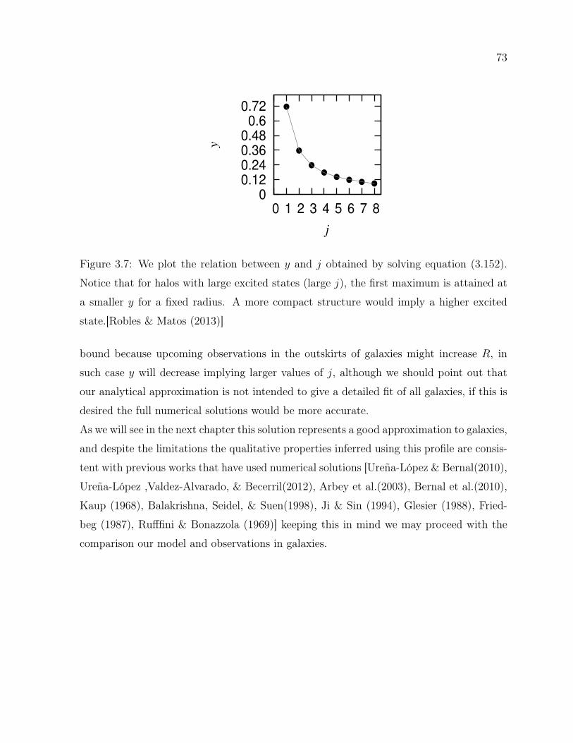
73
0
0.12
0.24
0.36
0.48
0.6
0.72
0 1 2 3 4 5 6 7 8y
j
Figure 3.7: We plot the relation between y and j obtained by solving equation (3.152).
Notice that for halos with large excited states (large j), the first maximum is attained at
a smaller y for a fixed radius. A more compact structure would imply a higher excited
state.[Robles & Matos (2013)]
bound because upcoming observations in the outskirts of galaxies might increase R, in
such case y will decrease implying larger values of j, although we should point out that
our analytical approximation is not intended to give a detailed fit of all galaxies, if this is
desired the full numerical solutions would be more accurate.
As we will see in the next chapter this solution represents a good approximation to galaxies,
and despite the limitations the qualitative properties inferred using this profile are consis-
tent with previous works that have used numerical solutions [Ureña-López & Bernal(2010),
Ureña-López ,Valdez-Alvarado, & Becerril(2012), Arbey et al.(2003), Bernal et al.(2010),
Kaup (1968), Balakrishna, Seidel, & Suen(1998), Ji & Sin (1994), Glesier (1988), Fried-
beg (1987), Rufffini & Bonazzola (1969)] keeping this in mind we may proceed with the
comparison our model and observations in galaxies.

74 CHAPTER 3. SCALAR FIELD DARK MATTER

Chapter 4
Consequences of SFDM in galaxies
In this chapter we will apply the results that have been widely discussed in the literature
regarding equilibrium configurations of self gravitating scalar field dark matter in the
weak field limit, including our approximate solution given in the previous chapter. It is
not my aim to redo all the calculations, but for the sake of completeness i provide a brief
background on the Schrödinger-Poisson analysis including references for the interested
reader.
§4.1 SFDM halos in equilibrium
There has been considerable work to find numerical solutions to the non-interacting
SFDM in the non-relativistic regime to model spherically symmetric halos [Guzmán &
Matos(2000), Guzmán & Ureña-López(2004), Ureña-López & Bernal(2010), Bernal et
al.(2010), Bray(2012), Rufffini & Bonazzola (1969), Kaup (1968), Seidel & Suen(1991),
Lee & Koh(1996), Lee & Lim(2010)] and also for the self-interacting SFDM [Böhmer &
Harko(2007), Robles & Matos(2012), Colpi,Shapiro,& Wasserman(1986), Rindler-Daller
& Shapiro(2012), Balakrishna, Seidel, & Suen(1998), Goodman (2000), Rindler-Daller &
Shapiro(2014)], the equation that describes a dilute gas of bosons in the non relativis-
tic limit with two-body point-like interactions of the form V (~r′ − ~r) = gδ(~r′ − ~r) is the
non-linear equation
i~∂
∂tψ(~r, t) =
(− ~2
2m∇2 +mφ+ g|ψ(~r, t)|2
)ψ(~r, t). (4.1)
Where g|ψ(~r, t)|2 is the interaction term. The scattering cross-section of indistinguishable
bosons becomes constant in the low-energy limit, σs =8πa2s ,with the s-wave scattering
75
76 CHAPTER 4. CONSEQUENCES OF SFDM IN GALAXIES
length being as. The coupling constant of the effective interaction is then simply propor-
tional to asg =
4π~2asm
, (4.2)
which is the (first) Born approximation. As before φ is the gravitational potential that
satisfies the Poisson equation
∇2φ = 4πGρ, (4.3)
and ρ = m|ψ|2. In spherical symmetry (in units ~=1, c=1) the SF solutions index by
the number of nodes Φn, satisfying the Einstein-Klein-Gordon system are related to the
Schrödinger-Poisson (SP) wavefunctions through
√8πGΦn(x, t) = e−imtψn(x, t) (4.4)
with m the mass of the SF. It is worth noting that in the absence of interactions, as
mentioned in [Guzmán & Ureña-López(2004)], in the weak field limit the Einstein-Klein-
Gordon system, for a complex and a real scalar field reduces to solving the Schrödinger-
Poisson equations[Arbey et al.(2003)].
From current bounds reported in [Li et al.(2014)] obtained by imposing that the SF be-
haves cosmologically as pressureless matter(dust) we obtained that the interacting parame-
ter would be extremely small for the typical mass of ∼10−22eV/c2 (see eq. (3.56)), therefore
solutions to the SP system without interactions would behave qualitatively similar to those
when self-interactions are included, this assumption is supported by the similarity in the
solutions for a small self-coupling found in other works[Balakrishna, Seidel, & Suen(1998),
Colpi,Shapiro,& Wasserman(1986), Briscese(2011)], nevertheless, including interactions
can increase the maximum mass of stability[Colpi,Shapiro,& Wasserman(1986)] and mod-
ify the configuration radius, for instance, without the self interactions (SIs) λΦ4, the mass
of a self-bound zero node configuration is
M = 0.633m2pl/m
where mpl is the Planck mass, while including a repulsive SI term [Balakrishna, Seidel, &
Suen(1998)] the mass becomes
M ∼ 0.06√λm3pl
m2,
77
which for m = 1GeV it is larger than the former by ∼√λmpl
m∼ 1019λ.
In principle both terms, the mass and self interaction, are contributing to the profile of
the self gravitating object, solving different limits can give us an idea of the behavior of
the solutions, in fact a complete numerical treatment of these two regimes can be found
in [Chavanis (2011), Chavanis & Delfini (2011), Chavanis & Harko (2012)]. In the case
where the SI are neglected the equation is
i~∂
∂tψ(~r, t) =
(− ~2
2m∇2 +mφ
)ψ(~r, t), (4.5)
in the other regime called the Thomas-Fermi limt the self interacting term dominates over
the kinetic term (also called the quantum term).
Given the similarities in the solutions, such as the density profiles, the existence of
a stable and unstable branch and stationary solutions with a characteristic oscillation
frequency[Ureña-López & Bernal(2010), Chavanis & Harko (2012), Balakrishna, Seidel, &
Suen(1998), Seidel & Suen(1990)] we may explore the non-interacting case and take it as
representative of the SFDM predictions.
The SP system has been solved to look for equilibrium configurations that could be com-
pared with some of the nearby galaxies, assuming they are in equilibrium. One char-
acteristic feature of stationary solutions of the form ψ(x, t) = e−iEntϕ(r) for the SP
system is the appearance of nodes in the spatial function ϕ(r), these nodes are asso-
ciated to different energy states of the SF, the zero node solution corresponds to the
ground state, one node to the first excited state, and so on. These excited states so-
lutions fit rotation curves(RCs) of large galaxies up to the outermost measured data
and can even reproduce the wiggles seen at large radii in high-resolution observations
[Sin (1994), Colpi,Shapiro,& Wasserman(1986), Robles & Matos(2013)]. Halos that are
purely in a single excited state seem to be unstable when the number of particles is
not conserved(finite perturbations) and decay to the ground state with different decay
rates[Guzmán & Ureña-López(2004), Balakrishna, Seidel, & Suen(1998)], though they ap-
pear to be stable when the number of particles is conserved(infinitesimal perturbations).
The ground state solution is stable under finite perturbations and infinitesimal pertur-
bations [Bernal et al.(2010), Seidel & Suen(1990)], but has difficulties to correctly fit the
rotation curves in large galaxies because its associated RC has a fast keplerian behavior
78 CHAPTER 4. CONSEQUENCES OF SFDM IN GALAXIES
shortly after reaching its maximum value unable to remain flat enough at large radii,
recently [Guzman et al.(2014)] have included rotation and find that the RCs can flatten
at large radii for certain values of angular momentum, although it remains unclear if the
same scheme works for galaxies of all sizes.
Another approach to get better fits in the RCs for both, large and small radii, was to
consider that bosons are not in one state but instead coexist in different states within
the halo, given the intention to describe dark matter halos I will refer to such configu-
rations as multistate halos(MSHs), albeit they were first study in the context of boson
stars[Ureña-López & Bernal(2010), Matos & Ureña-López(2007), Robles & Matos(2013),
Robles & Matos(2013b)]. The size of the MSH is determined by the most excited state
that accurately fits the RC for large radii, bosons in excited states are distributed to larger
radii than the ground state, and in contrast to the halo with a single state there are MSHs
that are stable under finite perturbations provided the ground state in the final halo con-
figuration has enough mass to stabilize the coexisting state[Ureña-López & Bernal(2010),
Bernal et al.(2010)]. In other words, when the ground state becomes the dominant state(in
terms of boson number density) in a MSH, it will provide enough support to prevent the
halo to collapse to a single state only, we may think of this as a quantum pressure produced
due to the degeneracy of the state.
In [Bernal et al.(2010)] it was shown that MSHs can be studied in the classical approach
as a collection of classical scalar fields coupled through gravity, one field ψi for each state,
this would modify the SP system such that its source of energy density would be the sum of
densities in each state[Ureña-López & Bernal(2010)], which corresponds to the non linear
case of eq (3.151), each state satisfies its respective Schrödinger equation while remaining
coupled through the Newtonian gravitational potential φ.
For stationary solutions we can assume wavefunctions of the form ψn(x, t) = e−iEntϕ(r),
then the SP system effectively reads
∇2ϕn = 2(φ− En)ϕn
∇2φ =∑n
|ϕn|2 (4.6)
with ∇2 the Laplacian operator, and En the energy eigenstates.
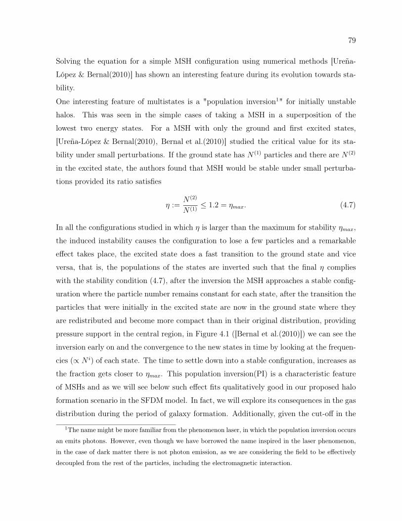
79
Solving the equation for a simple MSH configuration using numerical methods [Ureña-
López & Bernal(2010)] has shown an interesting feature during its evolution towards sta-
bility.
One interesting feature of multistates is a "population inversion1" for initially unstable
halos. This was seen in the simple cases of taking a MSH in a superposition of the
lowest two energy states. For a MSH with only the ground and first excited states,
[Ureña-López & Bernal(2010), Bernal et al.(2010)] studied the critical value for its sta-
bility under small perturbations. If the ground state has N (1) particles and there are N (2)
in the excited state, the authors found that MSH would be stable under small perturba-
tions provided its ratio satisfies
η :=N (2)
N (1)≤ 1.2 = ηmax. (4.7)
In all the configurations studied in which η is larger than the maximum for stability ηmax,
the induced instability causes the configuration to lose a few particles and a remarkable
effect takes place, the excited state does a fast transition to the ground state and vice
versa, that is, the populations of the states are inverted such that the final η complies
with the stability condition (4.7), after the inversion the MSH approaches a stable config-
uration where the particle number remains constant for each state, after the transition the
particles that were initially in the excited state are now in the ground state where they
are redistributed and become more compact than in their original distribution, providing
pressure support in the central region, in Figure 4.1 ([Bernal et al.(2010)]) we can see the
inversion early on and the convergence to the new states in time by looking at the frequen-
cies (∝ N i) of each state. The time to settle down into a stable configuration, increases as
the fraction gets closer to ηmax. This population inversion(PI) is a characteristic feature
of MSHs and as we will see below such effect fits qualitatively good in our proposed halo
formation scenario in the SFDM model. In fact, we will explore its consequences in the gas
distribution during the period of galaxy formation. Additionally, given the cut-off in the
1The name might be more familiar from the phenomenon laser, in which the population inversion occurs
an emits photons. However, even though we have borrowed the name inspired in the laser phenomenon,
in the case of dark matter there is not photon emission, as we are considering the field to be effectively
decoupled from the rest of the particles, including the electromagnetic interaction.
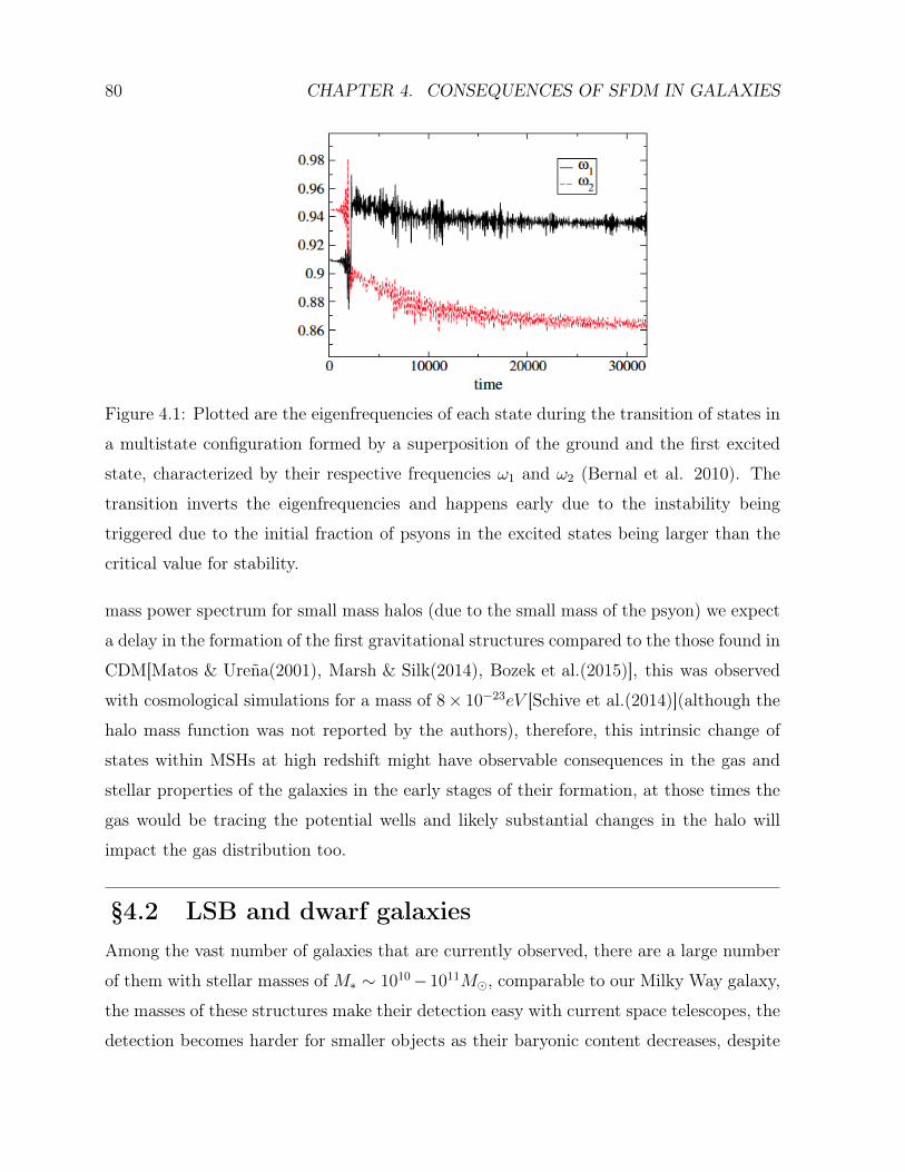
80 CHAPTER 4. CONSEQUENCES OF SFDM IN GALAXIES
Figure 4.1: Plotted are the eigenfrequencies of each state during the transition of states in
a multistate configuration formed by a superposition of the ground and the first excited
state, characterized by their respective frequencies ω1 and ω2 (Bernal et al. 2010). The
transition inverts the eigenfrequencies and happens early due to the instability being
triggered due to the initial fraction of psyons in the excited states being larger than the
critical value for stability.
mass power spectrum for small mass halos (due to the small mass of the psyon) we expect
a delay in the formation of the first gravitational structures compared to the those found in
CDM[Matos & Ureña(2001), Marsh & Silk(2014), Bozek et al.(2015)], this was observed
with cosmological simulations for a mass of 8× 10⁻²³eV [Schive et al.(2014)](although the
halo mass function was not reported by the authors), therefore, this intrinsic change of
states within MSHs at high redshift might have observable consequences in the gas and
stellar properties of the galaxies in the early stages of their formation, at those times the
gas would be tracing the potential wells and likely substantial changes in the halo will
impact the gas distribution too.
§4.2 LSB and dwarf galaxiesAmong the vast number of galaxies that are currently observed, there are a large number
of them with stellar masses of M∗ ∼ 1010−1011M, comparable to our Milky Way galaxy,
the masses of these structures make their detection easy with current space telescopes, the
detection becomes harder for smaller objects as their baryonic content decreases, despite
81
the limitations we know there are galaxies with M∗ ∼ 104 − 107M that remain bounded
even in our own galaxy, these dwarf galaxies required large mass-to-light ratios (∼ 10 −100[Walter & Peñarrubia(2011)]) which is usually interpreted as being in massive dark
matter halos that contribute largely to their mass budget, this interpretation becomes
more probable when the estimated mass-to-light ratios expected from stellar population
models lie below the inferred ratio obtained from the movements of the stars in the galaxy.
Dwarf spheroidal galaxies (dSphs) orbiting the MW are effectively devoid of gas and
although they have a variety of star formation histories most of them have old stellar pop-
ulations[Madau et al.(2014), Weisz et al.(2014a), Weisz et al.(2014b), Weisz et al.(2014c),
Weisz et al.(2015)]. In addition to nearby dwarfs there are extragalactic low surface
brightness galaxies whose dark matter content is also though to be high [Kuzio de Naray
et al.(2010), Kuzio de Naray & Spekkens(2011), Kuzio de Naray & Kaufmann(2011)] but
these are usually more extended with observed radii larger than ∼ 1kpc as is frequently
the case for dwarfs. These systems are particularly interesting candidates to test dark
matter models as their baryonic matter may be neglected as a first approximation, on the
other hand some of them lack enough resolution that frequently hinders the comparison
in the inner parts.
Assuming that the stellar systems of the dSphs are pressure supported and in dynamic
equilibrium2, we follow the procedure of [Walker et al.(2009)] to find the relationship be-
tween the mass distribution of a SFDM halo and the stellar distribution, this is given by
the Jeans equation1
ν
d
dr(ν〈v2
r〉) + 2β〈v2
r〉r
= −GM(r)
r2, (4.8)
where ν(r),〈v2r〉, and β(r) describe the 3-dimensional density, radial velocity dispersion,
and orbital anisotropy, respectively, of the stellar component. The parameter β quantifies
the degree of radial stellar anisotropy and there is no preference for either radially, β > 0,
or tangentially, β < 0, biased systems. For circular orbits β = −∞ ,〈v2r〉 = 0 ; if 〈v2
r〉 =
2The assumption of dynamical equilibrium is not necessarily true for all galaxies, the environment
can affect such condition and even play a significant role in the halo and stellar distributions making
the conclusions from the dynamical equilibrium hypothesis dubious and could possibly be the cause of
discrepancies between the fits and observations. Although it is uncertain if galaxies are in true dynamical
equilibrium, assuming the latter is often a good first approximation in dwarf spheroidals.
82 CHAPTER 4. CONSEQUENCES OF SFDM IN GALAXIES
〈v2θ〉 = 〈v2
φ〉, β = 0 (isotropic orbits); and for radial orbits β = 1, 〈v2φ〉 = 〈v2
θ〉 = 0. Although
β can take all this values, we restrict the anisotropy to be in the range −0.6 ≤ β ≤ 0.3
for the most realistic scenarios [Walker et al.(2009)], and consistent with other estimates
using also the dSphs [Lokas(2009)].
In the simplest case the orbital anisotropy is independent of r ( β = const), the solution of
the Jeans equation relates the projection of the velocity dispersion along the line-of-sight,
σ2los(R), and the mass profileM(r), to the stellar density I(R) [Binney & Tremaine (2008)]
through
σ2los =
2G
I(R)
∫ ∞R
dr′ν(r′)M(r′)(r′)2β−2F (β,R, r′), (4.9)
with
F (β,R, r′) ≡∫ r′
R
dr
(1− βR
2
r2
)r−2β+1
√r2 −R2
, (4.10)
and R the projected radius.
We adopt an analytic profile for the projected stellar density I(R). As in [Walker et
al.(2010), Salucci et al.(2011)], we consider a Plummer profile for the stellar density with
the projected half-light radius, rhalf , as the only shape parameter,
I(R) =L
πr2half
1
[1 + (R/rhalf )2]2, (4.11)
where L is the total luminosity. With the projected stellar density known, one can recover
the 3-dimensional stellar density [Binney & Tremaine (2008)]
ν(r) = − 1
π
∫ ∞r
dI
dR
dR√R2 − r2
. (4.12)
substituting eq. (4.11) in eq. (4.12) for the Plummer profile we have
ν(r) =3L
4πr3half
1
[1 + (r/rhalf )2]5/2. (4.13)
Using eqs. (4.9) and (4.10) we can find the halo parameters that best reproduce the
velocity dispersion data. We have three free parameters per galaxy: the scale radius
∼ 1/kj, the density, and the orbital anisotropy β. For the stellar component we use rhalffrom [Walker et al.(2009)].
One advantage of the analytical approximation we derived in the last chapter is that in
the core region where the density will be dominated by the ground state once the halo
83
has reach stability the analytical approximation resembles the numerical solution with
high accuracy, this is not surprising as the inner distributions is given by the quantum
pressure which is just Heisenberg’s uncertainty principle acting on such scales. In fact,
from the simulations in [Schive et al.(2014)] the inner kiloparsec of the density profiles of
different SFDM halos displays an ubiquitous core, in the supplementary information of
[Schive et al.(2014)] the authors provided an empirical fit to the inner profile (where the
solitonic core is present) for the dwarf galaxy Fornax given by
ρ(r) ≈ 1.9(m/10−23eV )−2(rc/kpc)−4
[1 + 9.1× 10⁻²(r/rc)2]8Mpc
−3. (4.14)
where core radius rc is defined as the radius in which the density has has dropped to
one-half its peak value, for appropriate normalization values our analytical profile is in
good agreement with the latter numerically motivated. We will comment on the reason of
these similarities and the interpretation below when we give our halo formation scenario,
for the moment we will assume (3.147) to model the dwarf galaxies.
We first model the dSphs assuming the ground state is enough, this means setting j=1 and
thus eq.(3.147) has no oscillations, we obtained good fits restricting to realistic values of the
orbital anisotropy, −0.6 ≤ β ≤ 0.3, in previous studies where the Thomas-Fermi(TF) ap-
proximation is taken at zero temperature [Robles & Matos(2012), Böhmer & Harko(2007),
Lora & Magaña(2014), Diez-Tejedor et al.(2014)] only the pure condensate was physically
allowed, for reference we include the solution under the TF approximation [Robles &
Matos(2012), Böhmer & Harko(2007)]
ρ(r) = ρ00
sin(πr/r0max)
(πr/r0max)
, (4.15)
where ρ00 is the central density of the condensate, r0
max =√π2Λ/2(~/mc) is considered as
a configuration radius where ρ(r0max) = 0 and therefore ρ(r) = 0 for r ≥ r0
max , m is the
mass of the scalar field, Λ = λm2Planck/4πm
2, and λ is the dimensionless parameter that
determines the two-body interactions of the field.
Using only the ground state for our analytical profile produces dispersion velocity fits in
dSphs that are almost indistinguishable to those using eq. (4.15) within ∼ 500pc, the
region where the condensed state best fits the data. The latter implies that within this
84 CHAPTER 4. CONSEQUENCES OF SFDM IN GALAXIES
radius the dSphs are also well reproduced using our profile
ρj(r) = ρj0sin2(kjr)
(kjr)2,
with only the condensed state(j = 1). There are several values of β that produce a fit
consistent within the error bars of σlos, with the upcoming surveys MaNGA, Gaia it will be
possible to have much better precision of the velocities of nearby stars, allowing possibly
to improve to distinguish subtle differences such as the existence of more than the ground
state bosons conforming the halos.
If we now include the first excited state in the analysis we see in Figure 4.2 that there is a
difference mostly in the outer regions, associated to a wider distribution of excited-state
psyons in the halo[Martinez-Medina, Robles, & Matos(2015)]. The relevance of adding
excited states is mostly seen in larger galaxies as they play an important role to flatten
the rotation curves and reach agreement with HI observations.
We see that dSphs of similar sizes and properties are described with a single state, in
fact this is shown in Fig. 4.2 for the dSphs within 500pc, notice that the corrections
due to the first excited state are small but not zero, we must take into consideration
that the larger the galaxy is, the more relevant are the contributions of other states.
In Table 1 we give the values of the best fit parameters used for the modeled galaxies.
Indeed, if we model extended galaxies where the rotation curves remain flat for more
than 10 kpc the need of more excited states becomes clear, Figure 4.3 illustrates this
feature, here we fitted three LSB galaxies assuming multistate halos and we obtained
good fits to all radii, in fact the wiggles in the data are also nicely reproduced. In this
figure we have also compared with the typical Einasto profile that is used to model CDM
halos[Navarro et al.(2010), Merrit et al.(2006), Graham et al.(2006)],
V 2E = 4πGρ−2
r3−2
r
[e2/α
α
(α
2
)(3/α)
γ(3
α, x′)
], (4.16)
with γ the incomplete gamma function given by
γ(3
α, x′) =
∫ x′
0
e−τ τ (3/α)−1dτ
with x′ := 2α
( rr−2
)α, r−2 is the radius in which the logarithmic slope of the density is −2,
ρ−2 is the density at the radius r−2, and α is a parameter that describes the degree of
curvature of the profile[Merrit et al.(2006), Graham et al.(2006)].
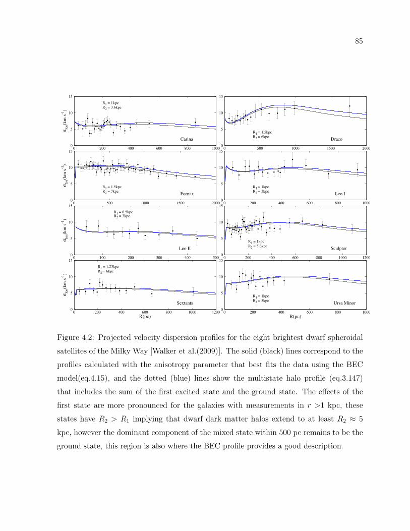
85
0
5
10
15
0 200 400 600 800 1000
σlo
s(k
m s
-1)
R1 = 1kpc
R2 = 3.6kpc
Carina
0
5
10
15
0 500 1000 1500 2000
R1 = 1.5kpc
R2 = 6kpcDraco
0
5
10
15
0 500 1000 1500 2000
σlo
s(k
m s
-1)
R1 = 1.5kpc
R2 = 7kpcFornax
0
5
10
15
0 200 400 600 800 1000
R1 = 1kpc
R2 = 5kpcLeo I
0
5
10
15
0 100 200 300 400 500
σlo
s(k
m s
-1)
R1 = 0.5kpcR2 = 3kpc
Leo II
0
5
10
15
0 200 400 600 800 1000 1200
R1 = 1kpc
R2 = 5.6kpcSculptor
0
5
10
15
0 200 400 600 800 1000 1200
σlo
s(k
m s
-1)
R(pc)
R1 = 1.25kpc
R2 = 6kpc
Sextants
0
5
10
15
0 200 400 600 800 1000
R(pc)
R1 = 1kpc
R2 = 5kpcUrsa Minor
Figure 4.2: Projected velocity dispersion profiles for the eight brightest dwarf spheroidal
satellites of the Milky Way [Walker et al.(2009)]. The solid (black) lines correspond to the
profiles calculated with the anisotropy parameter that best fits the data using the BEC
model(eq.4.15), and the dotted (blue) lines show the multistate halo profile (eq.3.147)
that includes the sum of the first excited state and the ground state. The effects of the
first state are more pronounced for the galaxies with measurements in r >1 kpc, these
states have R2 > R1 implying that dwarf dark matter halos extend to at least R2 ≈ 5
kpc, however the dominant component of the mixed state within 500 pc remains to be the
ground state, this region is also where the BEC profile provides a good description.
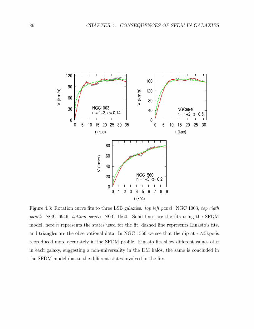
86 CHAPTER 4. CONSEQUENCES OF SFDM IN GALAXIES
0
30
60
90
120
0 5 10 15 20 25 30 35
V (
km
/s)
r (kpc)
NGC1003n = 1+3, α= 0.14
0
40
80
120
160
0 5 10 15 20 25 30
V (
km
/s)
r (kpc)
NGC6946n = 1+2, α= 0.5
0
20
40
60
80
0 1 2 3 4 5 6 7 8 9
V (
km
/s)
r (kpc)
NGC1560n = 1+3, α= 0.2
Figure 4.3: Rotation curve fits to three LSB galaxies. top left panel : NGC 1003, top rigth
panel : NGC 6946, bottom panel : NGC 1560. Solid lines are the fits using the SFDM
model, here n represents the states used for the fit, dashed line represents Einasto’s fits,
and triangles are the observational data. In NGC 1560 we see that the dip at r ≈5kpc is
reproduced more accurately in the SFDM profile. Einasto fits show different values of α
in each galaxy, suggesting a non-universality in the DM halos, the same is concluded in
the SFDM model due to the different states involved in the fits.
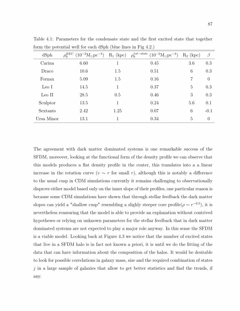
87
Table 4.1: Parameters for the condensate state and the first excited state that together
form the potential well for each dSph (blue lines in Fig 4.2.)
dSph ρBEC0 (10−2Mpc−3) R1 (kpc) ρ1st−state0 (10−2Mpc−3) R2 (kpc) β
Carina 6.60 1 0.45 3.6 0.3
Draco 10.6 1.5 0.51 6 0.3
Fornax 5.09 1.5 0.16 7 0
Leo I 14.5 1 0.37 5 0.3
Leo II 28.5 0.5 0.46 3 0.3
Sculptor 13.5 1 0.24 5.6 0.1
Sextants 2.42 1.25 0.07 6 -0.1
Ursa Minor 13.1 1 0.34 5 0
The agreement with dark matter dominated systems is one remarkable success of the
SFDM, moreover, looking at the functional form of the density profile we can observe that
this models produces a flat density profile in the center, this translates into a a linear
increase in the rotation curve (v ∼ r for small r), although this is notably a difference
to the usual cusp in CDM simulations currently it remains challenging to observationally
disprove either model based only on the inner slope of their profiles, one particular reason is
because some CDM simulations have shown that through stellar feedback the dark matter
slopes can yield a "shallow cusp" resembling a slighly steeper core profile(ρ ∼ r−0.5), it is
nevertheless reassuring that the model is able to provide an explanation without contrived
hypotheses or relying on unknown parameters for the stellar feedback that in dark matter
dominated systems are not expected to play a major role anyway. In this sense the SFDM
is a viable model. Looking back at Figure 4.3 we notice that the number of excited states
that live in a SFDM halo is in fact not known a priori, it is until we do the fitting of the
data that can have information about the composition of the halos. It would be desirable
to look for possible correlations in galaxy mass, size and the required combination of states
j in a large sample of galaxies that allow to get better statistics and find the trends, if
any.
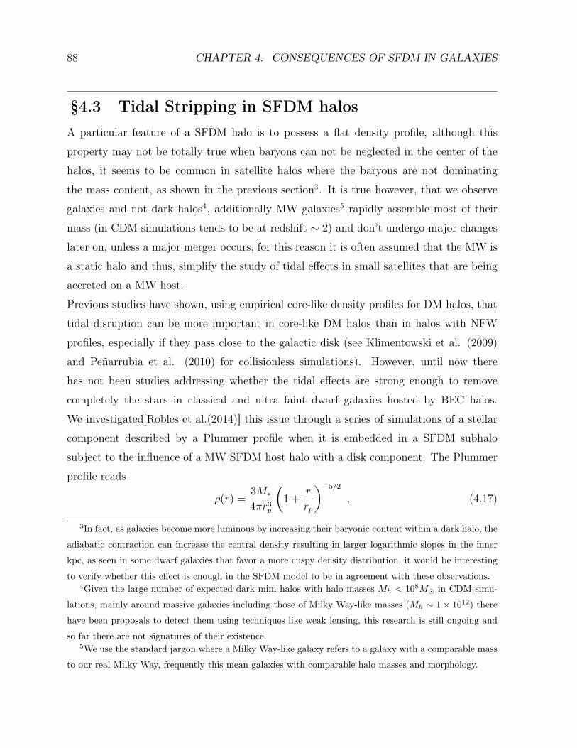
88 CHAPTER 4. CONSEQUENCES OF SFDM IN GALAXIES
§4.3 Tidal Stripping in SFDM halosA particular feature of a SFDM halo is to possess a flat density profile, although this
property may not be totally true when baryons can not be neglected in the center of the
halos, it seems to be common in satellite halos where the baryons are not dominating
the mass content, as shown in the previous section3. It is true however, that we observe
galaxies and not dark halos4, additionally MW galaxies5 rapidly assemble most of their
mass (in CDM simulations tends to be at redshift ∼ 2) and don’t undergo major changes
later on, unless a major merger occurs, for this reason it is often assumed that the MW is
a static halo and thus, simplify the study of tidal effects in small satellites that are being
accreted on a MW host.
Previous studies have shown, using empirical core-like density profiles for DM halos, that
tidal disruption can be more important in core-like DM halos than in halos with NFW
profiles, especially if they pass close to the galactic disk (see Klimentowski et al. (2009)
and Peñarrubia et al. (2010) for collisionless simulations). However, until now there
has not been studies addressing whether the tidal effects are strong enough to remove
completely the stars in classical and ultra faint dwarf galaxies hosted by BEC halos.
We investigated[Robles et al.(2014)] this issue through a series of simulations of a stellar
component described by a Plummer profile when it is embedded in a SFDM subhalo
subject to the influence of a MW SFDM host halo with a disk component. The Plummer
profile reads
ρ(r) =3M∗4πr3
p
(1 +
r
rp
)−5/2
, (4.17)
3In fact, as galaxies become more luminous by increasing their baryonic content within a dark halo, the
adiabatic contraction can increase the central density resulting in larger logarithmic slopes in the inner
kpc, as seen in some dwarf galaxies that favor a more cuspy density distribution, it would be interesting
to verify whether this effect is enough in the SFDM model to be in agreement with these observations.4Given the large number of expected dark mini halos with halo masses Mh < 108M in CDM simu-
lations, mainly around massive galaxies including those of Milky Way-like masses (Mh ∼ 1× 10¹²) there
have been proposals to detect them using techniques like weak lensing, this research is still ongoing and
so far there are not signatures of their existence.5We use the standard jargon where a Milky Way-like galaxy refers to a galaxy with a comparable mass
to our real Milky Way, frequently this mean galaxies with comparable halo masses and morphology.
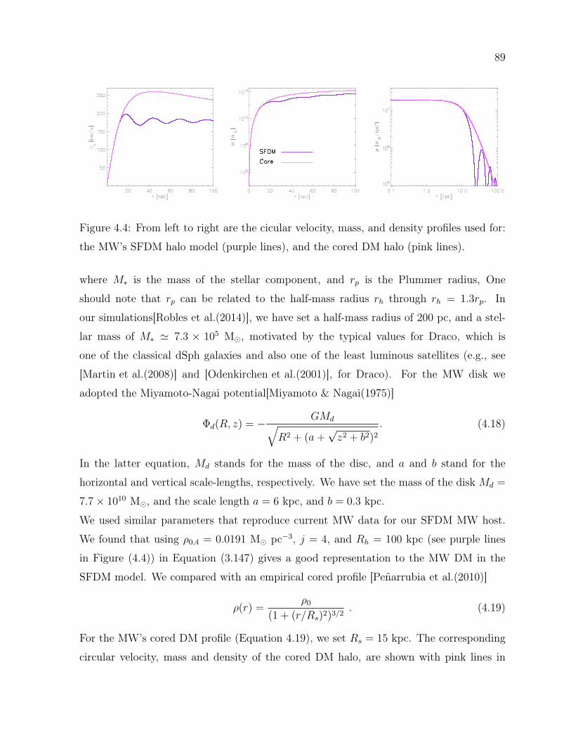
89
Figure 4.4: From left to right are the cicular velocity, mass, and density profiles used for:
the MW’s SFDM halo model (purple lines), and the cored DM halo (pink lines).
where M∗ is the mass of the stellar component, and rp is the Plummer radius, One
should note that rp can be related to the half-mass radius rh through rh = 1.3rp. In
our simulations[Robles et al.(2014)], we have set a half-mass radius of 200 pc, and a stel-
lar mass of M∗ ' 7.3 × 10⁵ M, motivated by the typical values for Draco, which is
one of the classical dSph galaxies and also one of the least luminous satellites (e.g., see
[Martin et al.(2008)] and [Odenkirchen et al.(2001)], for Draco). For the MW disk we
adopted the Miyamoto-Nagai potential[Miyamoto & Nagai(1975)]
Φd(R, z) = − GMd√R2 + (a+
√z2 + b2)2
. (4.18)
In the latter equation, Md stands for the mass of the disc, and a and b stand for the
horizontal and vertical scale-lengths, respectively. We have set the mass of the disk Md =
7.7× 10¹⁰ M, and the scale length a = 6 kpc, and b = 0.3 kpc.
We used similar parameters that reproduce current MW data for our SFDM MW host.
We found that using ρ0,4 = 0.0191 M pc−3, j = 4, and Rh = 100 kpc (see purple lines
in Figure (4.4)) in Equation (3.147) gives a good representation to the MW DM in the
SFDM model. We compared with an empirical cored profile [Peñarrubia et al.(2010)]
ρ(r) =ρ0
(1 + (r/Rs)2)3/2. (4.19)
For the MW’s cored DM profile (Equation 4.19), we set Rs = 15 kpc. The corresponding
circular velocity, mass and density of the cored DM halo, are shown with pink lines in
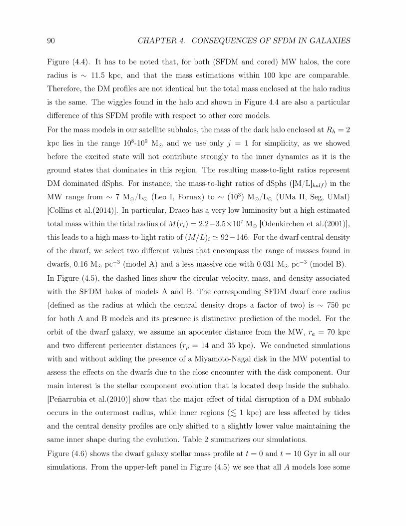
90 CHAPTER 4. CONSEQUENCES OF SFDM IN GALAXIES
Figure (4.4). It has to be noted that, for both (SFDM and cored) MW halos, the core
radius is ∼ 11.5 kpc, and that the mass estimations within 100 kpc are comparable.
Therefore, the DM profiles are not identical but the total mass enclosed at the halo radius
is the same. The wiggles found in the halo and shown in Figure 4.4 are also a particular
difference of this SFDM profile with respect to other core models.
For the mass models in our satellite subhalos, the mass of the dark halo enclosed at Rh = 2
kpc lies in the range 108-109 M and we use only j = 1 for simplicity, as we showed
before the excited state will not contribute strongly to the inner dynamics as it is the
ground states that dominates in this region. The resulting mass-to-light ratios represent
DM dominated dSphs. For instance, the mass-to-light ratios of dSphs ([M/L]half ) in the
MW range from ∼ 7 M/L (Leo I, Fornax) to ∼ (103) M/L (UMa II, Seg, UMaI)
[Collins et al.(2014)]. In particular, Draco has a very low luminosity but a high estimated
total mass within the tidal radius ofM(rt) = 2.2−3.5×10⁷ M [Odenkirchen et al.(2001)],
this leads to a high mass-to-light ratio of (M/L)i ' 92−146. For the dwarf central density
of the dwarf, we select two different values that encompass the range of masses found in
dwarfs, 0.16 M pc−3 (model A) and a less massive one with 0.031 M pc−3 (model B).
In Figure (4.5), the dashed lines show the circular velocity, mass, and density associated
with the SFDM halos of models A and B. The corresponding SFDM dwarf core radius
(defined as the radius at which the central density drops a factor of two) is ∼ 750 pc
for both A and B models and its presence is distinctive prediction of the model. For the
orbit of the dwarf galaxy, we assume an apocenter distance from the MW, ra = 70 kpc
and two different pericenter distances (rp = 14 and 35 kpc). We conducted simulations
with and without adding the presence of a Miyamoto-Nagai disk in the MW potential to
assess the effects on the dwarfs due to the close encounter with the disk component. Our
main interest is the stellar component evolution that is located deep inside the subhalo.
[Peñarrubia et al.(2010)] show that the major effect of tidal disruption of a DM subhalo
occurs in the outermost radius, while inner regions (. 1 kpc) are less affected by tides
and the central density profiles are only shifted to a slightly lower value maintaining the
same inner shape during the evolution. Table 2 summarizes our simulations.
Figure (4.6) shows the dwarf galaxy stellar mass profile at t = 0 and t = 10 Gyr in all our
simulations. From the upper-left panel in Figure (4.5) we see that all A models lose some
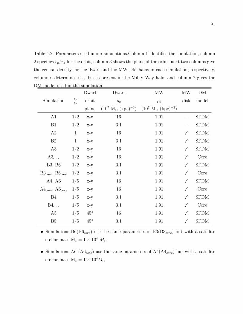
91
Table 4.2: Parameters used in our simulations.Column 1 identifies the simulation, column
2 specifies rp/ra for the orbit, column 3 shows the plane of the orbit, next two columns give
the central density for the dwarf and the MW DM halos in each simulation, respectively,
column 6 determines if a disk is present in the Milky Way halo, and column 7 gives the
DM model used in the simulation.Dwarf Dwarf MW MW DM
Simulation rpra
orbit ρ0 ρ0 disk model
plane (107 M (kpc)−3) (107 M (kpc)−3)
A1 1/2 x-y 16 1.91 – SFDM
B1 1/2 x-y 3.1 1.91 – SFDM
A2 1 x-y 16 1.91 X SFDM
B2 1 x-y 3.1 1.91 X SFDM
A3 1/2 x-y 16 1.91 X SFDM
A3core 1/2 x-y 16 1.91 X Core
B3, B6 1/2 x-y 3.1 1.91 X SFDM
B3core, B6core 1/2 x-y 3.1 1.91 X Core
A4, A6 1/5 x-y 16 1.91 X SFDM
A4core, A6core 1/5 x-y 16 1.91 X Core
B4 1/5 x-y 3.1 1.91 X SFDM
B4core 1/5 x-y 3.1 1.91 X Core
A5 1/5 45 16 1.91 X SFDM
B5 1/5 45 3.1 1.91 X SFDM
• Simulations B6(B6core) use the same parameters of B3(B3core) but with a satellite
stellar mass M∗ = 1× 10⁴ M
• Simulations A6 (A6core) use the same parameters of A4(A4core) but with a satellite
stellar mass M∗ = 1× 10⁴M
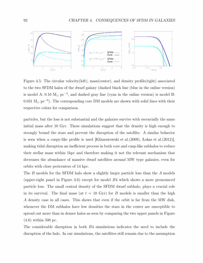
92 CHAPTER 4. CONSEQUENCES OF SFDM IN GALAXIES
Figure 4.5: The circular velocity(left), mass(center), and density profile(right) associated
to the two SFDM halos of the dwarf galaxy (dashed black line (blue in the online version)
is model A: 0.16 M pc−3, and dashed gray line (cyan in the online version) is model B:
0.031 M pc−3). The corresponding core DM models are shown with solid lines with their
respective colors for comparison.
particles, but the loss is not substantial and the galaxies survive with escencially the same
initial mass after 10 Gyr. These simulations suggest that the density is high enough to
strongly bound the stars and prevent the disruption of the satellite. A similar behavior
is seen when a cuspy-like profile is used [Klimentowski et al.(2009), Łokas et al.(2012)],
making tidal disruption an inefficient process in both core and cusp-like subhalos to reduce
their stellar mass within 1kpc and therefore making it not the relevant mechanism that
decreases the abundance of massive dwarf satellites around MW type galaxies, even for
orbits with close pericenters of 14 kpc.
The B models for the SFDM halo show a slightly larger particle loss than the A models
(upper-right panel in Figure 4.6) except for model B4 which shows a more pronounced
particle loss. The small central density of the SFDM dwarf subhalo, plays a crucial role
in its survival. The final mass (at t = 10 Gyr) for B models is smaller than the high
A density case in all cases. This shows that even if the orbit is far from the MW disk,
whenever the DM subhalos have low densities the stars in the center are susceptible to
spread out more than in denser halos as seen by comparing the two upper panels in Figure
(4.6) within 500 pc.
The considerable disruption in both B4 simulations indicates the need to include the
disruption of the halo. In our simulations, the satellites still remain due to the assumption
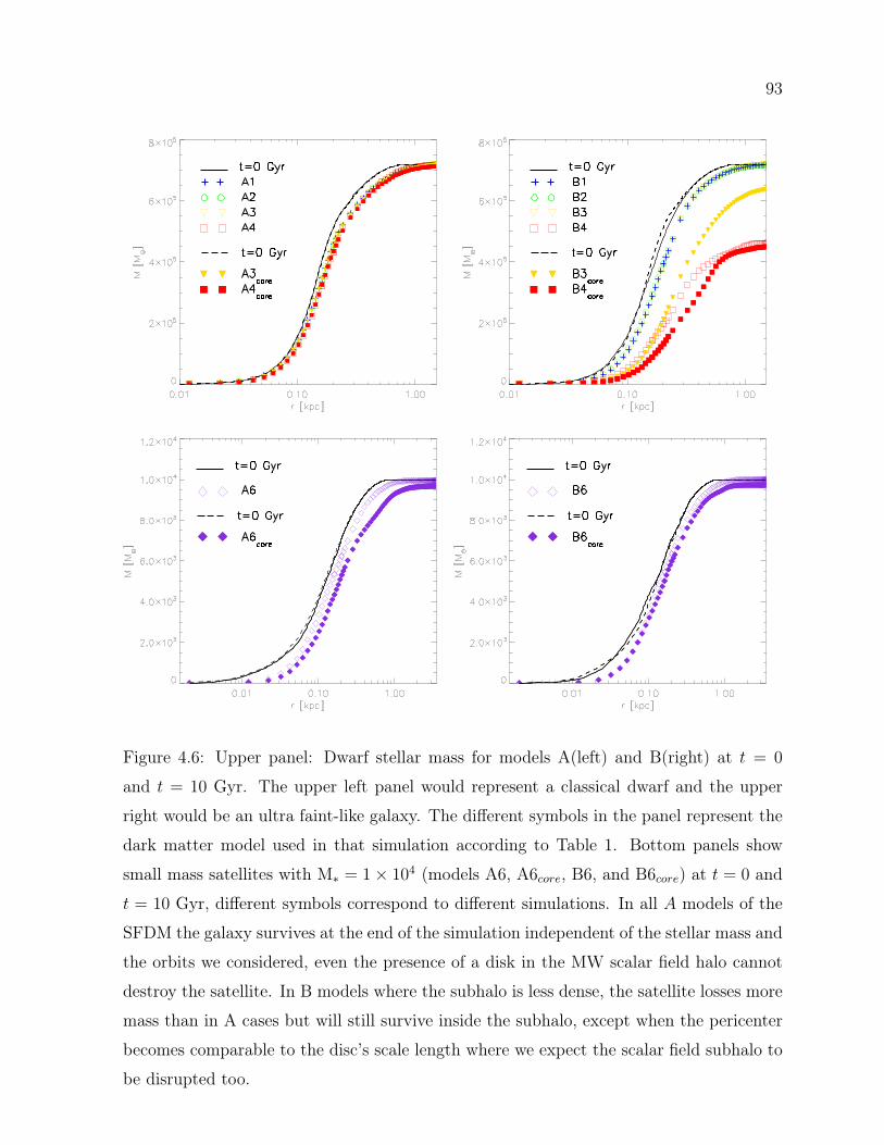
93
Figure 4.6: Upper panel: Dwarf stellar mass for models A(left) and B(right) at t = 0
and t = 10 Gyr. The upper left panel would represent a classical dwarf and the upper
right would be an ultra faint-like galaxy. The different symbols in the panel represent the
dark matter model used in that simulation according to Table 1. Bottom panels show
small mass satellites with M∗ = 1× 10⁴ (models A6, A6core, B6, and B6core) at t = 0 and
t = 10 Gyr, different symbols correspond to different simulations. In all A models of the
SFDM the galaxy survives at the end of the simulation independent of the stellar mass and
the orbits we considered, even the presence of a disk in the MW scalar field halo cannot
destroy the satellite. In B models where the subhalo is less dense, the satellite losses more
mass than in A cases but will still survive inside the subhalo, except when the pericenter
becomes comparable to the disc’s scale length where we expect the scalar field subhalo to
be disrupted too.
94 CHAPTER 4. CONSEQUENCES OF SFDM IN GALAXIES
of fixed subhalo, but we expect the dwarf halos to fully disrupt and that their stars get
dispersed around the MW halo. This one of the restrictions of the simulation, given that
the dark halos are fixed, we can track the evolution of the stars and used them as tracers
of the strength of the tidal interactions. As stars in the center become strongly affected,
shown by the decrease in the stellar densities, it is also a likely that the halo will suffer
some disruption too, this effect is not substantial for most of our simulations but it appears
for B4 due to its proximity to the MW disk and the small subhalo central density.
We also conducted a couple of simulations (A5 and B5) where we set the dwarf galaxy
embedded in the MW SFDM halo potential, with a rp/ra = 1/5 including the baryonic
MW disk component and similar to A4 and B4 models, but now we place the dwarf galaxy
in an orbit inclined 45 from the x−y plane. In this case we observe that the dwarf galaxy
gets destroyed within ∼ 1.5 Gyr. This suggests that orbits with close pericenter distances
and inclination effects are important factors to the survival of low density SFDM dwarf
satellites. In A6 and A6core, the parameters are identical to A4 and A4core respectively, but
the stellar mass of the satellite is smaller M∗ = 1 × 10⁴M.These parameters correspond
to the closest orbit where the tidal effects should be the largest. The other pair, B6 and
B6core, uses M∗ = 1× 10⁴M and the parameters of B3 and B3core respectively. Despite
their low mass the satellites can remain with most of their initial mass after 10 Gyr. Here
we show that if the satellites are in scalar field subhalos with central densities comparable
to classical dSphs, some of their stars are stripped but the galaxies can survive with smaller
masses and hence contribute to the number of dwarf satellites around a MW host. It must
be noted that, in the SFDM model,the substructure is smaller due to the wave properties
causing the cut-off in the power spectrum, as confirmed in [Schive et al.(2014)].
For the lower density dwarfs (comparable to ultra faint dwarfs), we obtained that they
could survive but only if their orbits do not get well inside the disk of their host. On the
other hand, low density halos with close pericenter orbits can be fully stripped of stars if
evolved for a long time even with a fixed subhalo potential, but as we expect them to be
destroyed once the fixed halo hypothesis is relaxed. Therefore, we do not get DM halos
that are tiny and dark, contrary to the CDM predictions where the cusp prevents total
disruption.
Therefore, our results point to an alternative solution to the satellite overabundance prob-
95
lem and the cusp-core issue by means of the quantum DM properties of the scalar field,
and without relying strongly on the messy astrophysical processes. Here, small mass sub-
halos with core profiles (ρ(r) ∼ r0) and with orbits not crossing the host’s disk are able
to survive for a long time, otherwise the close encounters with the disk could completely
destroy them. On the other hand, more massive dwarfs can get closer or farther from the
host’s disk and still survive with core profiles. To determine the final fate of these galaxies
and make a fair comparison with current CDM simulations it is necessary to invoke the
astrophysics but so far we have found that this model seems to offer a good description
to the nearby galaxies, although this is not meant to be a compelling reason to prefer this
model over CDM. In fact, the results might vary if we relax the fixed halo hypothesis for
the satellite, and include gas that is self gravitating6, both conditions could show results
that differ from the ones we found, particularly because the self-gravity of the gas will
make it less difficult to be stripped of stars as the gravitational potential is now deeper,
on the other hand, the subhalo will also feel the tidal interaction, in this case we expect
the the mass loss to be similar to that in [Peñarrubia et al.(2010)], however it is not clear
what effect the oscillations of the MW halo have on the subhalo when both are not fixed,
and how they compare when smooth DM distributions are considered, the limitations of
our approach cannot assess this question but it is undoubtedly something that requires
further exploration.
§4.4 Rings and shells in early type galaxiesAn interesting feature of the intrinsic nature of psyons is to allow for some bosons in excited
states. This property has been pointed out before in the context of multistates in a SFDM
halo, we mentioned the possibility of a population inversion in the states that can turn
an initially unstable multistate halo (MSH) into a stable one according to the ratio of the
particle numbers in each state. This MSHs present ripples in the density profile that are
a consequence of the quantum nature of the psyons, in [Robles, Medina & Matos (2015)]
we have modeled these properties using an analytical model that captures the effect of the
transition and explore how the transition affects the gas embedded in a MSH halo.6When gas is self gravitating the mass of the gas also contributes to the gravitational potential in
addition to the dark matter.
96 CHAPTER 4. CONSEQUENCES OF SFDM IN GALAXIES
We consider a multistate halo with only the first and ground state coexisting, this is
because we know the stability threshold for this multistate configuration. In [Bernal et
al.(2010)] it was seen that the larger the η above the critical value, the faster it settles to
its final stable configuration, to be sure that the MSH is initially in the unstable regime
we pick an intermediate value η=1.6. We explore the evolution of the gas distribution that
follows a disk of gas with a Miyamoto-Nagai profile[Miyamoto & Nagai(1975)] with gas
mass ofMg = 3.9×10⁹M, and for the horizontal and vertical scale-lengths we use a = 6.5
kpc and b = 0.5 kpc respectively, we modified the code ZEUS-MP[Hayes et al.(2006)] to
evolve the gaseous component embedded in the MSH, the gas is not self gravitating and
is treated as a tracer of the potential only.
We use a semi-analytical model that let us control the rate of the transition to a stable
state, this type of isolated and simplified simulations help to identify the main effects of the
transition in the gas and aid the interpretation of the results. However, It remains unclear
when the transition is set for a given halo or its duration, this requires a better sampling of
the problem, first by considering a larger representative sample of halos, and second, how
the properties vary with the transition time. It is in these semi-analytical simulations that
an analytical form of the density profile becomes handy, keeping in mind the limitation
of this profile, we use the form (3.147) to model our MSH, the main idea is to start
from an unstable MSH halo and invert the masses of the states neglecting any particle
loss in the total halo, during the population inversion in the numerical solution both
states lose a few percentage of their initial masses(<10% [Ureña-López & Bernal(2010),
Bernal et al.(2010)]), but this loss would not substantially affect the final halo profile, for
this reason we may neglect the mass loss in our analytical study.
After the inversion the total initial mass of the ground state M i1(Ri
1) becomes the final
mass of the excited state M f2(Rf
2) and vice versa, and the nodes in the wavefunctions will
also have changed, that is
M i1(Ri
1) −→M f2(Rf
2), M i2(Ri
2) −→M f1(Rf
1) (4.20)
j : 1, 2 −→ 2, 1 = j′. (4.21)
where the mass profiles for each state j are now flipped, Rj is taken as a truncation radius
of the corresponding state, that is, for radii grater than Rj the number of particles in the
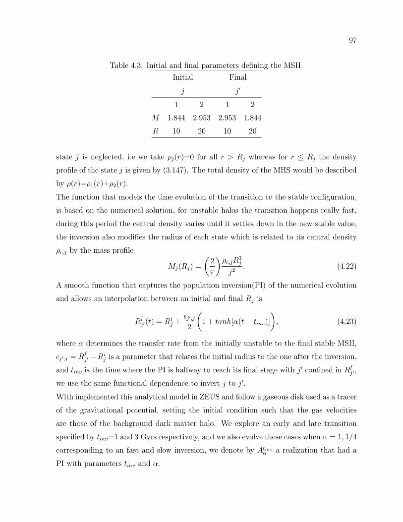
97
Table 4.3: Initial and final parameters defining the MSH.Initial Final
j j′
1 2 1 2
M 1.844 2.953 2.953 1.844
R 10 20 10 20
state j is neglected, i.e we take ρj(r)=0 for all r > Rj whereas for r ≤ Rj the density
profile of the state j is given by (3.147). The total density of the MHS would be described
by ρ(r)=ρ1(r)+ρ2(r).
The function that models the time evolution of the transition to the stable configuration,
is based on the numerical solution, for unstable halos the transition happens really fast,
during this period the central density varies until it settles down in the new stable value,
the inversion also modifies the radius of each state which is related to its central density
ρc,j by the mass profile
Mj(Rj) =
(2
π
)ρc,jR
3j
j2. (4.22)
A smooth function that captures the population inversion(PI) of the numerical evolution
and allows an interpolation between an initial and final Rj is
Rfj′(t) = Ri
j +εj′,j2
(1 + tanh[α(t− tinv)]
), (4.23)
where α determines the transfer rate from the initially unstable to the final stable MSH,
εj′,j = Rfj′ −Ri
j is a parameter that relates the initial radius to the one after the inversion,
and tinv is the time where the PI is halfway to reach its final stage with j′ confined in Rfj′ ,
we use the same functional dependence to invert j to j′.
With implemented this analytical model in ZEUS and follow a gaseous disk used as a tracer
of the gravitational potential, setting the initial condition such that the gas velocities
are those of the background dark matter halo. We explore an early and late transition
specified by tinv=1 and 3 Gyrs respectively, and we also evolve these cases when α = 1, 1/4
corresponding to an fast and slow inversion, we denote by Atinvα a realization that had a
PI with parameters tinv and α.
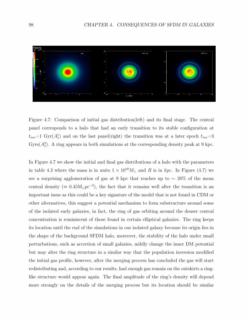
98 CHAPTER 4. CONSEQUENCES OF SFDM IN GALAXIES
Figure 4.7: Comparison of initial gas distribution(left) and its final stage. The central
panel corresponds to a halo that had an early transition to its stable configuration at
tinv=1 Gyr(A11) and on the last panel(right) the transition was at a later epoch tinv=3
Gyrs(A31). A ring appears in both simulations at the corresponding density peak at 9 kpc.
In Figure 4.7 we show the initial and final gas distributions of a halo with the parameters
in table 4.3 where the mass is in units 1 × 10¹⁰M and R is in kpc. In Figure (4.7) we
see a surprising agglomeration of gas at 9 kpc that reaches up to ∼ 20% of the mean
central density (≈ 0.45Mpc−3), the fact that it remains well after the transition is an
important issue as this could be a key signature of the model that is not found in CDM or
other alternatives, this suggest a potential mechanism to form substructure around some
of the isolated early galaxies, in fact, the ring of gas orbiting around the denser central
concentration is reminiscent of those found in certain elliptical galaxies. The ring keeps
its location until the end of the simulations in our isolated galaxy because its origin lies in
the shape of the background SFDM halo, moreover, the stability of the halo under small
perturbations, such as accretion of small galaxies, mildly change the inner DM potential
but may alter the ring structure in a similar way that the population inversion modified
the initial gas profile, however, after the merging process has concluded the gas will start
redistributing and, according to our results, had enough gas remain on the outskirts a ring-
like structure would appear again. The final amplitude of the ring’s density will depend
more strongly on the details of the merging process but its location should be similar
99
to the non perturbed halo provided the DM halo potential was not severely modified as
expected for minor mergers in the past or those relatively more recent, thus, tidal features
are not exclusive of galaxy mergers when the dark matter is an ultra light scalar field.
In these results we have seen that the presence of the symmetric ring is due to the spheri-
cally symmetry hypothesis in the SFDM halo, deviations from this symmetry could result
in incomplete rings and shells although a certain degree of symmetry should remain, which
may be a feature to distinguish the SFDM halo debris from remnants that come from recent
galaxy mergers that depend on the path of the accreted satellites and do not necessar-
ily leave tidal debris of a particular symmetry, our results suggest that outer regions of
dark halos may not be totally smooth. Exploring in more detail the regions where shells
and rings form could also help to put constraints on their origin, their formation, and
serve to test galaxy and halo formation scenarios such as the quantum dark matter(QDM)
paradigm.
§4.5 Galaxy formation scenario in SFDM haloes
Initial fluctuations that grow due to the cosmological expansion of the universe eventu-
ally separate from it and start collapsing due to its own gravity, at this time (known as
turnaround) the halo has a number of psyons that can be in different states, their values
would be determined before the collapse of the configuration, and have some dependence
on the its local environment. Depending on the number density of bosons populating the
excited states we can have different fates and for the halos.
Based on the results exposed in this chapter and the ones reported in the literature, it is
clear that the QDM paradigm deserves some further attention, it is convenient to describe
how the known features would relate, at least qualitatively, with the observed galaxy
populations, for this reason we propose the following galaxy formation scenario in SFDM
halos.
The smallest and less dense systems, such as dwarf galaxies, would reside in SFDM halos
with most bosons in the ground state except possibly for just a few excited particles as seen
in [Martinez-Medina, Robles, & Matos(2015)], this is because the potential wells of these
haloes, being the lowest density systems, would be just massive enough to collapse and
100 CHAPTER 4. CONSEQUENCES OF SFDM IN GALAXIES
allow the existence of the minimum energy state that would form a bound configuration.
Larger configurations that had initially a larger number of bosons in excited states than
in the ground state can undergo a population inversion and reach a stable state, collapse
to a dense ground state or become a black hole depending on how large the fraction of
particles in excited states is after turnaround, given the different possible outcomes for
this case we expect that most galaxies are formed this way, for instance, ellipticals can
form when halos transition to a stable configuration that quickly increases the ground
state and deepens the gravitational potential resulting in a dense and compact structure
where the bulge can form. High surface brightness galaxies usually have RCs that fall
slowly after its maximum speed, they would likely correspond to SFDM halos whose final
stable configuration has a comparable number of bosons in the excited and ground states
as both states would contribute evenly in the central region increasing the gravitational
potential well where more star formation can take place, and for distances larger than
a given radius (likely the first maximum peak in the RC) the ground state would be
a small contribution to the density, thus in the outer regions the baryonic RC would
remain below its maximum. Another possible outcome for extended halos is when the
fraction of excited particles is below its stability threshold, in these cases gravity will
slowly redistribute DM bosons in the stable MSH but mostly keeping the particle number
constant, considering that psyons in the excited states are subdominant and more widely
distributed than the ones in the ground state of a MSH, the DM gravitational potential
in the center would be less dense than in the high surface brightness case so that gas
accretion would also proceed more slowly resulting in rotation curves for the baryonic
matter that slowly increase to large radii or with almost flat profiles, this case is quite
similar to what is found in low surface brightness galaxies[Kuzio de Naray et al.(2010),
Kuzio de Naray & Spekkens(2011), Kuzio de Naray & Kaufmann(2011)].
Overall, this galaxy formation scenario broadly describes different galaxy types showing
that only due to the dark matter properties in the context of SFDM it is possible to agree
with the general features of several galaxies. However, we do not expect this scenario to
represent all galaxies, in fact, to get a better description of individual galaxies we require
taking into account other fundamental parameters that affect their evolution, such as
the environment, angular momentum, galaxy mergers etc., we will leave a more in-depth
101
exploration of the model and comparison to this scenario including the full astrophysical
processes for the years to come, for now the SFDM model looks a promising alternative.

102 CHAPTER 4. CONSEQUENCES OF SFDM IN GALAXIES
Chapter 5
Self interacting dark matter
In the last chapter we have explored the SFDM model, here we will consider another al-
ternative idea proposed in [Spergel & Steinhardt (2000)], it assumes that cold dark mat-
ter has weak interactions with baryons but strong self-interactions, this model received
the name of self-interacting dark matter (SIDM). The required scattering cross-section is
roughly (m/g)−1 cm2 where m in this chapter denotes the particle mass of the dark matter
possessing this type of interaction, a value of 1 cm2/g ≈ 2 barn GeV−1 is approximately
a nuclear-scale cross section. In this case, frequent elastic scattering in the dense central
regions of halos can redistribute energy and angular momentum among particles, creating
an isothermal, round core of approximately constant density [Burkert(2000)].
For the SIDM model to be an attractive alternative to the Cold Dark Matter paradigm,
it should be able to address the issues that CDM faces today, for instance substantially
reduce the central densities of dwarf-size halos.
Early studies suggested that this idea was ruled out by studies of gravitational lensing
[Miralda-Escude(2000)] or by catastrophic gravitational core collapse found in a simulation
of an isolated halo [Kochanek & White(2002)], but recent numerical studies show that
these concerns are not borne out in fully cosmological simulations. SIDM simulations show
that there is a viable window of mass and cross-section where self-interacting dark matter
(SIDM) can produce cored dark matter profiles and remain consistent with observational
constraints [Rocha et al.(2013), Peter et al.(2013)] Elastic scattering in the central regions,
where an average particle experiences a few collisions per Hubble time, flattens the density
cusp and reduces triaxiality, leading to halo shapes being more spherical in the inner
regions. The scattering mechanism would operate across a wide range of halo masses,
from Milky Way-like galaxies to dwarf satellites. Because of their shallower potential,
103
104 CHAPTER 5. SELF INTERACTING DARK MATTER
SIDM subhalos are more easily subject to tidal disruption than CDM subhalos. However,
cosmological simulations suggest only small suppression of the low-mass subhalo count for
allowed cross sections except in the innermost region of the host halo[Rocha et al.(2013),
Vogelsberger et al.(2012)], this has questioned the preference of this alternative to the
standard model.
§5.1 Satellites in SIDM halosIn the past few years there have been several simulations focusing on reproducing the
properties of the dwarf galaxies around MW-like host, motivated in part by the increasing
resolution in observations of local group dwarfs and more detailed observations in their
star formation histories[Weisz et al.(2014a), Weisz et al.(2014b)].
Assuming velocity-independent cross sections in the range 0.1−0.5 cm2/g create cores that
are approximately the right size for Milky Way dwarf galaxies [Markevitch et al.(2004)],
spiral galaxies, and galaxy clusters[Newman et al.(2013a), Newman et al.(2013b)], although
the core sizes in dwarf galaxies are still a matter of debate, the sizes can be modified if
baryons are included in the simulations [Rocha et al.(2013), Kaplinghat et al.(2014)] or
by lacking enough numerical resolution to study the inner kpc[Bastidas Fry et al.(2015),
Vogelsberger et al.(2014)], which is essential in dwarfs. The same range for the cross sec-
tions above are also consistent with observations of merging galaxy clusters [Clowe et
al.(2006), Randall et al.(2008), Dawson et al.(2012)]
Although there is not a particular particle candidate for the model, there have been some
theoretical models that aim to produce SIDM particle candidates [Ackerman et al.(2009),
Buckley & Fox (2010), Feng et al. (2010), Tulin et al. (2013a), Tulin et al. (2013b)], how-
ever in these models the strong self-interactions may only be present in a narrow range of
halo mass, leaving halos on other scales effectively collisionless and indistinguishable from
CDM expectations.
In [Zavala et al.(2013)] they use high resolution cosmological simulations of a Milky-Way
size halo to assess whether a constant cross section per unit mass of σ/m ∼ 0.1 cm2/g is
sufficient to account for the low mass densities in dwarf spheroidal galaxies, they found
that such cross section produces a population of massive subhalos that is inconsistent
with the kinematics of the classical dwarf spheroidals, in particular with the inferred
105
slopes of the mass profiles of Fornax and Sculptor. In their simulation the problem is
solved if σ/m ∼ 0.1 cm2/g at the dwarf spheroidal scales. On the other hand this value
may be in some tension with the constraints obtained from the offset of gas and mass
distribution observed in collisions of galaxy clusters. Using the Chandra and Hubble
Space Telescopes there are 72 observed collisions, including both major and minor mergers.
[Harvey et al.(2015)] combined these measurements statistically, and detect the existence
of dark mass at 7.6σ significance. The position of the dark mass has remained closely
aligned within 5.8± 8.2 kpc of associated stars, they report that the self-interaction cross-
section satisfies σDM/m < 0.47 cm2/g at a 95% confidence level. Their results would
disfavor some proposed extensions to the standard model[Foot (2014), Boddy et al.(2014),
Cline et al.(2014), Tulin et al. (2013a)].
It its known from CDM that including the baryonic component in simulations can affect
the results inferred from dark matter only simulations, in [Kaplinghat et al.(2014)] they
estimated analytically the DM equilibrium configuration that results from a stellar dis-
tribution added to the centre of a SIDM halo, they studied the regime where the stellar
component dominates the gravitational potential and found that the DM core sizes (den-
sities) are smaller (higher) than observed in DM-only SIDM simulations, it is therefore
expected that current SIDM constraints could change as more simulations in this regime
are available.
One of the recent studies that includes baryons and self-interactions is given in Bastidas
Fry et al.(2015), adopting a large constant cross section of 2 cm2/g., they found that
SIDM fails to significantly lower the central dark matter density at halo peak velocities
Vmax < 30 km/s, they associate the cause to low central velocity dispersion and densities
that translate in time scales for SIDM collisions greater than a Hubble time, as well as
the weak supernova feedback found in such low mass galaxies. A direct consequence of
their results is that both CDM and SIDM halos at these low masses have cuspy dark
matter density profiles. In field dwarf galaxies with halo masses larger than ∼ 1010 M,
the baryonic processes create dark matter cores and central DM plus baryon distributions
that are effectively indistinguishable between CDM and SIDM.
Another independent study was given in [Vogelsberger et al.(2014)], they explore the
regime of dwarf galaxies where DM dominates the gravitational potential even in the
106 CHAPTER 5. SELF INTERACTING DARK MATTER
innermost regions. They include baryonic physics using the implementation described in
[Vogelsberger et al.(2013)] employing the moving mesh code AREPO [Springel (2010)].
Their simulated dwarf has a halo mass ∼ 1.1 × 10¹⁰M. They apply different mod-
els to this initial condition, including two cases with a constant cross section σ/m = 1
cm2/g (SIDM1) and σ/m = 10 cm2/g (SIDM10), and two cases with a velocity-dependent
cross section motivated by the particle physics model presented in [Feng et al.(2009),
Loeb & Weiner(2011)], and also studied in [Zavala et al.(2013)], vdSIDMa assumes σ/m
3.5 cm2/g and Vmax = 30 km/s, and vdSIDMb assumes σ/m 35 cm2/g and Vmax = 10
km/s.
For one of the dwarfs (shown in Fig5.1), they used DM particle mass resolution mdm =
7.75×10¹⁰M, a cell mass mb = 1.48×10¹⁰M, the Plummer-equivalent maximum physi-
cal softening length ε = 68pc, and the number of DM particles in the high resolution region
Np=15,353,772. Their values were tested for convergence with a CDM only simulation
with ∼10 times more DM particles which allows to accurately resolve the inner 200pc of
the galaxy, that is, for larger radius the two-body relaxation time is larger than a Hubble
time, having good convergence ensures the lack of unphysical shallower slopes that are not
formed due to the self interactions. One detailed comprehensive study for the convergence
of mass profiles is given in [Power et al.(2003)], there are several considerations and nu-
merical parameters that affect the structure of simulated N-body dark halo, choices of the
gravitational softening, time-step, force accuracy, initial redshift, and particle number. In
their tests, the authors found that for suitably chosen softenings that render particle dis-
creteness effects negligible, convergence in the circular velocity is obtained at radii where
the following conditions are satisfied: (i) the time-step is much shorter than the local or-
bital time-scale; (ii) accelerations do not exceed a characteristic acceleration imprinted by
the gravitational softening; and (iii) enough particles are enclosed so that the collisional
relaxation time-scale is longer than the age of the Universe. Convergence also requires
sufficiently high initial redshift and accurate force computations. Poor spatial, time, or
force resolution leads generally to systems with artificially low central density, but may
also result in the formation of artificially dense central cusps. When dealing with self
interactions and the cusp-core problem, where the relevant scale is of order 1kpc, it is
required to chose the softening to resolve the innermost radii to avoid misinterpreting the
107
results.
[Garrison-Kimmel et al.(2013)] found that for a dwarf halo in CDM simulations with the
Plummer-equivalent softening length to secure convergence at 250pc for a halo of 5×10⁹M
is of ∼ 70pc, using three million particles, however a softening length of ε = 10pc is
required to assure the convergence and study regions larger than 100 pc from the center
of the halo, at this distance the forces are Newtonian and the code Gadget-2 safely tracks
the accelaration of each particle. One of the latest SIDM simulations of a cosmological
and isolated dwarf galaxy (in the field) was given in [Elbert et al.(2014)], they see that
the SIDM has better convergence than CDM for the same number of particles, most likely
the self-interactions are the dominant mechanism rather than being dominated by binary
interactions. In the latter simulation the dark matter self-interactions were calculated
using an SIDM smoothing length equal 0.25ε with a particle mass 1.5 ×10³M and a
Plummer-equivalent force softening ε = 28pc, their halos are of 1 × 10¹⁰M with Vmax =
37km/s and use 4.6×10⁶ particles, this softening allows the author to safely resolve regions
as close as 200 pc.
In [Kauffmann (2014)] they suggested that galaxies with M∗ ∼ 108M suffer ongoing
bursts of star formation with a typical duration (∆tburst) of the order of the character-
istic dynamical time of the galaxy (∆tdyn). Although this might suggest that the gas
outflows from these bursts could change the DM distribution, it is not clear how effi-
cient this would be since the highly efficient regime occurs only once (∆tburst < < ∆tdyn).
In [Vogelsberger et al.(2014)] the star formation rates of their two simulated dwarfs (one
shown in Fig. 5.3) show that the rate of dA is fluctuating around a moderately non-
evolving mean. Most importantly, none of our dwarfs have an exponentially declining star
formation history.
They conclude that baryons have only a minor effect on the evolution and size of the cores
in the SIDM halos, as expected the large σ/m = 10 cm2/g presents the largest difference,
where the shallow DM profile allows supernovae feedback to expand the core a bit more
compared to the DM-only case. They also found that the size of the stellar core is closely
related to the size of the DM core as seen in Figure 5.1.
Additionally, they pointed out that in the constant σ/m case the density within the stellar
core is reduced, in SIDM1 the reduction is by a factor of ∼ 2-3 compared to the CDM case.
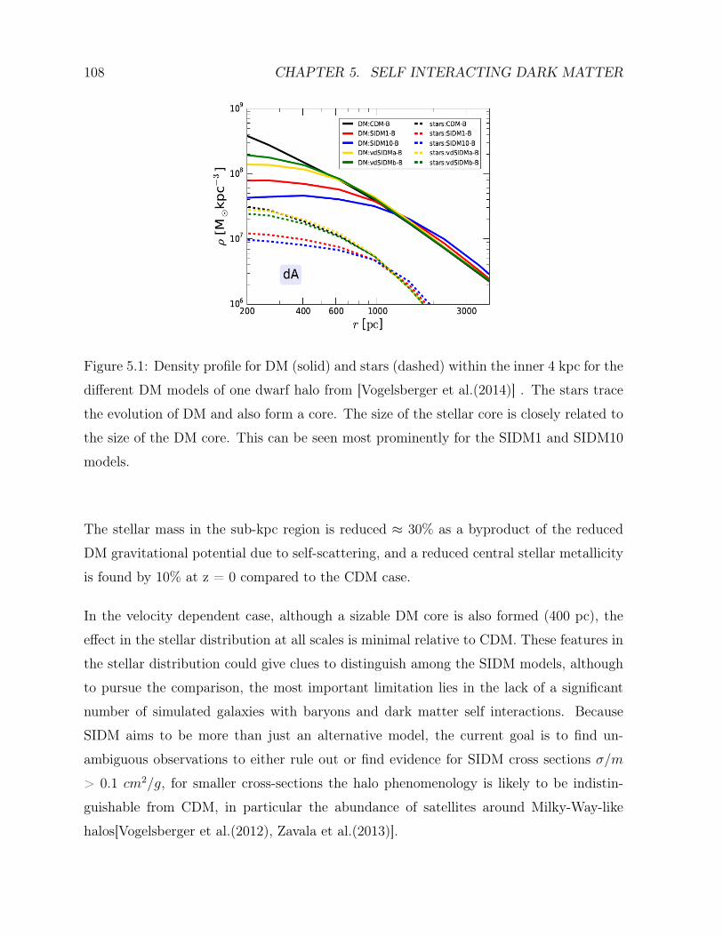
108 CHAPTER 5. SELF INTERACTING DARK MATTER
Figure 5.1: Density profile for DM (solid) and stars (dashed) within the inner 4 kpc for the
different DM models of one dwarf halo from [Vogelsberger et al.(2014)] . The stars trace
the evolution of DM and also form a core. The size of the stellar core is closely related to
the size of the DM core. This can be seen most prominently for the SIDM1 and SIDM10
models.
The stellar mass in the sub-kpc region is reduced ≈ 30% as a byproduct of the reduced
DM gravitational potential due to self-scattering, and a reduced central stellar metallicity
is found by 10% at z = 0 compared to the CDM case.
In the velocity dependent case, although a sizable DM core is also formed (400 pc), the
effect in the stellar distribution at all scales is minimal relative to CDM. These features in
the stellar distribution could give clues to distinguish among the SIDM models, although
to pursue the comparison, the most important limitation lies in the lack of a significant
number of simulated galaxies with baryons and dark matter self interactions. Because
SIDM aims to be more than just an alternative model, the current goal is to find un-
ambiguous observations to either rule out or find evidence for SIDM cross sections σ/m
> 0.1 cm2/g, for smaller cross-sections the halo phenomenology is likely to be indistin-
guishable from CDM, in particular the abundance of satellites around Milky-Way-like
halos[Vogelsberger et al.(2012), Zavala et al.(2013)].
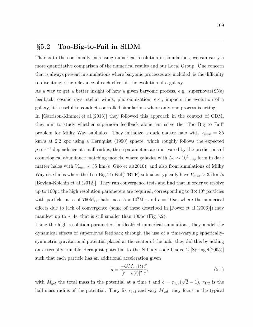
109
§5.2 Too-Big-to-Fail in SIDMThanks to the continually increasing numerical resolution in simulations, we can carry a
more quantitative comparison of the numerical results and our Local Group. One concern
that is always present in simulations where baryonic processes are included, is the difficulty
to disentangle the relevance of each effect in the evolution of a galaxy.
As a way to get a better insight of how a given baryonic process, e.g. supernovae(SNe)
feedback, cosmic rays, stellar winds, photoionization, etc., impacts the evolution of a
galaxy, it is useful to conduct controlled simulations where only one process is acting.
In [Garrison-Kimmel et al.(2013)] they followed this approach in the context of CDM,
they aim to study whether supernova feedback alone can solve the “Too Big to Fail”
problem for Milky Way subhalos. They initialize a dark matter halo with Vmax = 35
km/s at 2.2 kpc using a Hernquist (1990) sphere, which roughly follows the expected
ρ ∝ r−1 dependence at small radius, these parameters are motivated by the predictions of
cosmological abundance matching models, where galaxies with LV ∼ 105 L form in dark
matter halos with Vmax ∼ 35 km/s [Guo et al(2010)] and also from simulations of Milky
Way-size halos where the Too-Big-To-Fail(TBTF) subhalos typically have Vmax > 35 km/s
[Boylan-Kolchin et al.(2012)]. They run convergence tests and find that in order to resolve
up to 100pc the high resolution parameters are required, corresponding to 3×10⁶ particles
with particle mass of 760M, halo mass 5 × 10⁹M and ε = 10pc, where the numerical
effects due to lack of convergence (some of these described in [Power et al.(2003)]) may
manifest up to ∼ 4ε, that is still smaller than 100pc (Fig 5.2).
Using the high resolution parameters in idealized numerical simulations, they model the
dynamical effects of supernovae feedback through the use of a time-varying spherically-
symmetric gravitational potential placed at the center of the halo, they did this by adding
an externally tunable Hernquist potential to the N-body code Gadget2 [Springel(2005)]
such that each particle has an additional acceleration given
~a =−GMgal(t)
[r − b(t)]2~r
r, (5.1)
with Mgal the total mass in the potential at a time t and b = r1/2(√
2 − 1), r1/2 is the
half-mass radius of the potential. They fix r1/2 and vary Mgal, they focus in the typical
110 CHAPTER 5. SELF INTERACTING DARK MATTER
Figure 5.2: Plotted left: is the mass in the central potential as a function of time for the
blowout scheme. The gray line shows how the mass varies for a single blowout with Mmax
= 108M; the red dotted line shows the same for repeated blowouts withMmax = 107 M.
A single cycle takes 500 Myr. These two cases result in the same cumulative total of mass
displaced. Right: density profile for a CDM halo of 5 × 10⁹M for different resolutions,
unresolving the inner regions creates artificial cores[Garrison-Kimmel et al.(2013)].
value among the bright Milky Way dSphs of r1/2 = 500pc. In order to mimic a blowout
they varyMgal in time according to the following cycle: firstMgal varies linearly from zero
to its maximum value in 200 Myr(we can think of this as gas slowly accumulating in the
center), it remains there for 100 Myr and then instantaneously returns to zero for another
200 Myr, the last step is what mimics the feedback from SNe(see figure 5.2).
They find that for a fixed amount of mass expelled from the galaxy (but not necessarily
from the halo and hence it may be recycled) cyclic blowouts preferentially remove DMmass
from the centers of halos, being most dramatic if r1/2=100pc for a fixed expelled mass.
Despite the central density is reduced to a mild cusp ρ ∝ r−α, with α ≥ 0.5, it is still above
those observed in dSphs by [Walter & Peñarrubia(2011), Amorisco & Evans (2012)], they
also found unlikely that SNe blowouts can affect the total mass within the stellar extent at
the level required to resolve the TBTF problem without fine tuning, mainly because the
required energy injected into the dark matter by explosive feedback exceeds, in six of the
nine MW satellite galaxies of concern, the total available energy budget for all of the type
111
II supernova that have occurred in the galaxies assuming a typical initial mass function
[Kroupa (2002)], where one expects approximately one SNII explosion per 100 M formed,
these results consider that the energy is injected directly into the dark matter with 100%
coupling. For instance, assuming a stellar-mass-to-light ratio M∗/LV for Ursa Minor, the
energy equivalent of more than 40,000 supernovae must be delivered with 100% efficiency
directly to the dark matter in order to have the dwarf simulations agree with the mass of
this galaxy.
The latter results suggest that in the CDM model solving simultaneously the cusp-core
and TBFT requires more than just accounting for blowouts from SNe feedback. It is
reasonable to question how the situation changes if self-interactions and blowout feedback
from SNe are now working together.
To answer the question we use the same feedback model of [Garrison-Kimmel et al.(2013)]
and consider two scenarios[Robles et al.(2015)], one in which each massive blowout cycle
expels 108M(A) and one less massive where 107M (B) are driven out from the center
of the halo. In order to maximize the differences between CDM and SIDM when baryons
are included, we study the most efficient feedback model found in Garrison-Kimmel et
al.(2013), thus, we use r1/2 = 100 pc. Following [Garrison-Kimmel et al.(2013)], we gener-
ated the initial condition(IC) with the publicly available code spherIC1 and use the same
parameters for the halo, the dark matter self-interactions were calculated using an SIDM
smoothing length equal to 0.25 ε, as described in [Rocha et al.(2013)].
From the last section σ/m seem to lie in the range 0.1 cm2g−1 < σ/m < 1 cm2g−1,
[Miralda-Escude(2000), Yoshida et al.(2000), Davé et al.(2001), Peter et al.(2013)], taken
σ/m ≈ 1 cm2g−1 is more consistent with dSphs and their observed core sizes as seen in
[Rocha et al.(2013), Zavala et al.(2013)].
In [Peter et al.(2013)] they argue that σ/m =1 cm2g−1 may be in conflict with halo shapes
in clusters, but taken into account the uncertainties in the halo shape analysis, and the
preference of dSphs for such value, we decide to use σ/m =1 cm2g−1 in our analysis. All
our simulations are high-resolution, that is, we use 3×10⁶ particles, force softening of 10 pc
and particle mass of 760 M, these values guarantee that the radii of interest (r< 1kpc)
is well resolved and the core, when formed, is due to self-interactions and not due to lack1The code and documentation can be downloaded from https://bitbucket.org/migroch/spheric.
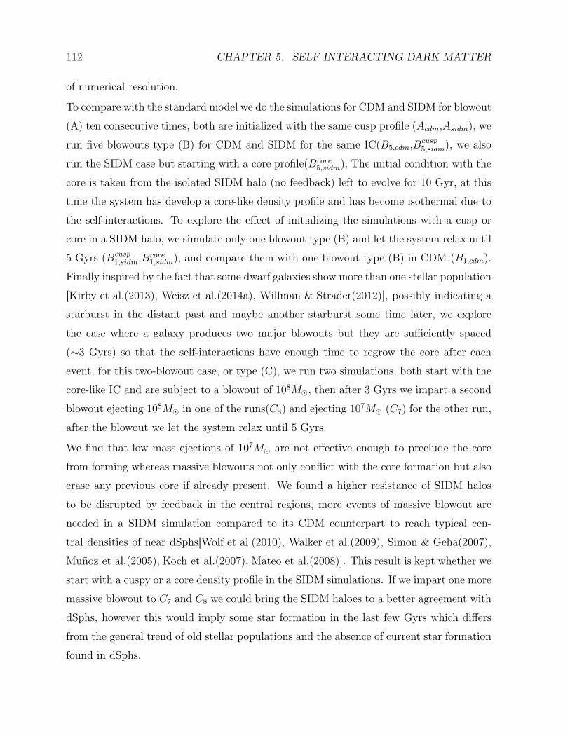
112 CHAPTER 5. SELF INTERACTING DARK MATTER
of numerical resolution.
To compare with the standard model we do the simulations for CDM and SIDM for blowout
(A) ten consecutive times, both are initialized with the same cusp profile (Acdm,Asidm), we
run five blowouts type (B) for CDM and SIDM for the same IC(B5,cdm,Bcusp5,sidm), we also
run the SIDM case but starting with a core profile(Bcore5,sidm), The initial condition with the
core is taken from the isolated SIDM halo (no feedback) left to evolve for 10 Gyr, at this
time the system has develop a core-like density profile and has become isothermal due to
the self-interactions. To explore the effect of initializing the simulations with a cusp or
core in a SIDM halo, we simulate only one blowout type (B) and let the system relax until
5 Gyrs (Bcusp1,sidm,B
core1,sidm), and compare them with one blowout type (B) in CDM (B1,cdm).
Finally inspired by the fact that some dwarf galaxies show more than one stellar population
[Kirby et al.(2013), Weisz et al.(2014a), Willman & Strader(2012)], possibly indicating a
starburst in the distant past and maybe another starburst some time later, we explore
the case where a galaxy produces two major blowouts but they are sufficiently spaced
(∼3 Gyrs) so that the self-interactions have enough time to regrow the core after each
event, for this two-blowout case, or type (C), we run two simulations, both start with the
core-like IC and are subject to a blowout of 108M, then after 3 Gyrs we impart a second
blowout ejecting 108M in one of the runs(C8) and ejecting 107M (C7) for the other run,
after the blowout we let the system relax until 5 Gyrs.
We find that low mass ejections of 107M are not effective enough to preclude the core
from forming whereas massive blowouts not only conflict with the core formation but also
erase any previous core if already present. We found a higher resistance of SIDM halos
to be disrupted by feedback in the central regions, more events of massive blowout are
needed in a SIDM simulation compared to its CDM counterpart to reach typical cen-
tral densities of near dSphs[Wolf et al.(2010), Walker et al.(2009), Simon & Geha(2007),
Muñoz et al.(2005), Koch et al.(2007), Mateo et al.(2008)]. This result is kept whether we
start with a cuspy or a core density profile in the SIDM simulations. If we impart one more
massive blowout to C7 and C8 we could bring the SIDM haloes to a better agreement with
dSphs, however this would imply some star formation in the last few Gyrs which differs
from the general trend of old stellar populations and the absence of current star formation
found in dSphs.
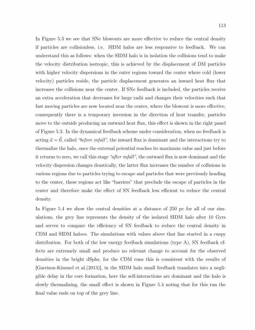
113
In Figure 5.3 we see that SNe blowouts are more effective to reduce the central density
if particles are collisionless, i.e. SIDM halos are less responsive to feedback. We can
understand this as follows: when the SIDM halo is in isolation the collisions tend to make
the velocity distribution isotropic, this is achieved by the displacement of DM particles
with higher velocity dispersions in the outer regions toward the center where cold (lower
velocity) particles reside, the particle displacement generates an inward heat flux that
increases the collisions near the center. If SNe feedback is included, the particles receive
an extra acceleration that decreases for large radii and changes their velocities such that
fast moving particles are now located near the center, where the blowout is more effective,
consequently there is a temporary inversion in the direction of heat transfer, particles
move to the outside producing an outward heat flux, this effect is shown in the right panel
of Figure 5.3. In the dynamical feedback scheme under consideration, when no feedback is
acting ~a = ~0, called “before infall”, the inward flux is dominant and the interactions try to
thermalize the halo, once the external potential reaches its maximum value and just before
it returns to zero, we call this stage “after infall”, the outward flux is now dominant and the
velocity dispersion changes drastically, the latter flux increases the number of collisions in
various regions due to particles trying to escape and particles that were previously heading
to the center, these regions act like “barriers” that preclude the escape of particles in the
center and therefore make the effect of SN feedback less efficient to reduce the central
density.
In Figure 5.4 we show the central densities at a distance of 250 pc for all of our sim-
ulations, the grey line represents the density of the isolated SIDM halo after 10 Gyrs
and serves to compare the efficiency of SN feedback to reduce the central density in
CDM and SIDM haloes. The simulations with values above that line started in a cuspy
distribution. For both of the low energy feedback simulations (type A), SN feedback ef-
fects are extremely small and produce no relevant change to account for the observed
densities in the bright dSphs, for the CDM runs this is consistent with the results of
[Garrison-Kimmel et al.(2013)], in the SIDM halo small feedback translates into a negli-
gible delay in the core formation, here the self-interactions are dominant and the halo is
slowly thermalizing, the small effect is shown in Figure 5.4 noting that for this run the
final value ends on top of the grey line.
114 CHAPTER 5. SELF INTERACTING DARK MATTER
Figure 5.3: Left:Initial and final density profiles after two massive blowouts ejecting a total
cumulative mass 1× 10⁸M for both SIDM(solid line) and CDM (dashed line).The shaded
region shows observational data for bright dSphs with r1/2 comparable to the one used
in our simulations. Right:Velocity dispersion for SIDM in isolation, before and after the
first infall of 108M. The arrows show the direction of the heat flux, before infall hotter
particles transfer heat to cold ones in the center as expected from the SIDM scenario,
however, at infall time there is an inversion of heat flux where the particles at the center,
being now hotter, can move to the outer regions.
115
Figure 5.4: Densities at 250pc from the center for all the simulations. For simulations C7,
C8, and all type B with 5 blowouts we plot the density after their respective blowouts.
For all the other simulations we plot initial and final values only. The density always
decreases after each blowout. The gray line represents the central density of a SIDM halo
in isolation.
In fact, in case that observations confirm that low mass DM dominated systems possess
large cores, SIDM would still be an attractive candidate, especially because low energy
feedback events applied to collisionless particles cannot transform the characteristic cusp
into a more constant density profile [Governato et al.(2012), Hopkins et al.(2014)]. Al-
though we obtained that in the less massive SNe feedback scenario (blowouts of type A)
the TBTF problem persists in both CDM and SIDM models, the result could change
if we consider a full cosmological SIDM simulation, it has been seen that cosmological
SIDM halos have lower central densities at the end of the simulations than our isolated
run [Rocha et al.(2013), Zavala et al.(2013)], but it is possible that the difference is due to
their lower numerical resolution, in fact, lately the increase in resolution could reopen the
possibility of using larger values of σ/m= 0.5 - 50 cm2/g and solve the TBTF issue and cre-
ate cores of comparable sizes to those found in dSphs as suggested in [Elbert et al.(2014)].
Today, it seems clear that there is still work to be done in the SIDM model before it can
be preferred over the standard paradigm.

116 CHAPTER 5. SELF INTERACTING DARK MATTER
Chapter 6
Conclusions
In this thesis i have provided an overview of the current standing of the standard model
of cosmology, also knwon and Cold Dark Matter(CDM). I have focused my study in the
challenges at galactic scales that the model is currently facing and described some of the
ideas in the literature that could bring the standard model to reasonable agreement with
the newest observations. Being in the era of high-resolution observations, it is now possible
to test some of the long standing theoretical predictions of the standard cosmological
paradigm, so far the cosmological probes reveal an excellent agreement with the expected
behavior in large scales. This seems to be continuouly verified performing numerical
simulations that include the relevant physical processes at those scales, at the same time
these simulations also reveal the existence of discrepancies in the small scale regime, i.e. in
galactic scales, some of the discrepancies treated in this thesis are the ubiquitous cusp-core
problem, the missing satellite problem and the Too-Big-To-Fail issue.
In chapter 2 I have described in more detail solutions to these discrepancies in the cold
dark matter model and their obsevational implications in dwarf galaxies. The most likely
explanation seems to require modeling the interplay of astrophysical processes and the dark
component in a self cosistent way, seemingly only when the processes oparate collectively
is that we obtain the correct predictions. Although the latter is numerically plausible,
there remains some skepticism of the results from hydrodynamical simulations, principally
because the implemented routines that aim to describe the astropysical process are in most
cases approximations of our already incomplete understanding of baryonic processes.
Instead of blaming the stellar and gas physics for the apparent discrepancies of CDM
predictions and obsevations in small scales, there exists the possibilty that our assumptions
on the dark matter are still missing something essential. Following the latter approach has
117
118 CHAPTER 6. CONCLUSIONS
led to several proposals of dark matter models, two strong contenders were presented here,
the scalar field dark matter(SFDM) and the self-interacting dark matter(SIDM) models.
In Chapter 3 we described the status and conceptual bases of the SFDM model in the
cosmological regime. We provided a classification of the models that assume an ultra light
boson as dark matter to clearly identify the main properties of the dark matter particle
under study. We propose that a spontaneos symmetry break in the early universe led to
the decoupling of the scalar field, by means of the temperature corrections and the fact
that the universe cools due to the expansion of the universe, at some time the temperature
drops enough such that the symmetry break appears and we interpret that time when the
scalar field decouples from the rest matter. Once the field is set in its new minimum,we
can derive an explicit analytical approximation of the density distribution of a scalar field
dark matter halo made of psyons(the corresponding bosonic dark matter particles) which
is quite useful when dealing with obsevational tests in galactic scales.
We devote chapter 4 to evaluate the SFDM model in galactic scales. We focus our study
in dwarf spheroidal galaxies, being the origin of the discrepancies found in CDM, they are
suitable systems where we can test alternative models and possibly find clues to distinguish
among the different DM proposals. We have found good agreement with the central
shallow density slopes found in local dSphs, a consequence of the core profile predicted by
the SFDM model whose origin lies in Heisenberg’s uncertainty principle acting at ∼ 1kpc
scales due to the small mass of the psyon. Assuming a mass of m ≈ 1×10⁻²²eV/c2 for the
psyon drastically decreases the formation of halos below 108M, additionally, we found
that SFDM subhalos with ∼ kpc cores orbitting around MW-like hosts that also possess a
SFDM halo, are more susceptible to be tidally disrupted when they closely interact with
the host’s disk, but that their stars can remain within the subhalos when the latter are
in orbits whose pericenters are larger than the disk’s length. If we assume one galaxy per
halo the expected satellite abundance around Milky-Way-like galaxies should be smaller
than the predicted value of CDM cosmological simulations, even the most massive ones,
in the upcomming years identifying more satellites around massive hosts will help to set
more stringent constraints on the SFDM model, in case the surveys increase the satellite
abundance substantially we might need to reconsider the preference of the SFDM model
over CDM, in the opposite case, the model offers a simpler explanation than the messy
119
baryonics physics to the missing satellite problem and possibly to the Too-Big-To-Big
issue, although it is worth noticing that the value of the mass is contraint by observations
and not predicted by the model.
Finally, in chapter 5 we discuss the status of the SIDM model regarding the cusp-core
and TBTF issue. The appearance of high resolution hydrodynamical simulations, both
cosmological and of isolated galaxies, have attracted the attention to the SIDM model
of a large part of scientists in the past few years. The simulations imply that previous
theoretical contraints on the cross-section per unit mass of σ/m < 1 cm2/g can be modified
and still give cosnistent results with the central masses of dwarf galaxies when baryons are
included. There are increasingly more works suggesting that neither self-interactions with
constant σ/m <0.5 cm2/g nor supernovae II feedback alone can account for the flattening
of the central density profile in dSphs and simultaneously substantially reduce the missing
satellite or the TBTF problem. In fact, we have shown that SIDM with constant σ/m = 1
cm2/g(a preferential value to create core sizes comparable to the stellar half-mass radius in
nearby dwarfs) and blowout feedback from SNe modeled by a time-varying potential that
mimics the effect of a SNII explosion, produce very similar results to the CDM + baryons
solution, and hence it is difficult to distinguish between these models when baryons are in
the play. Slighly modifying the model to allow for a velocity dependent cross section has
not reveal a substantial change to the predictions of constant σ/m, which can question
the motivation to include the velocity dependence in the future. Despite SIDM being
apparently indistinguishable from CDM for current constraints of the scattering cross
section, it remains a viable model when astrophysical processes are accounted for in the
simulations.
At this point, it seems that there is still much work to be done in SIDM and other models
before they can become the new benchmark in cosmology, although there is a discouraging
tone in the sentence, I have always found new ideas quite exciting. Even if it takes some
time to develop them, they offer the opportunity for a great discovery, quoting the chinese
philosopher Lao-tzu: “A journey of a thousand miles begins with a single step”.
120 CHAPTER 6. CONCLUSIONS
Appendix
Publication List
• "Flat Central Density Profile and Constant DM Surface Density in Galaxies from
Scalar Field Dark Matter" , Victor H. Robles, T. Matos, MNRAS, 422, 282-289
(2012)
• "Exact Solution to Finite Temperature SFDM: Natural Cores without Feedback",
Victor H. Robles, T. Matos, ApJ , 763 , 19 (2013)
• "Strong Lensing with Finite Temperature Scalar Field Dark Matter" Victor H. Rob-
les, T. Matos, 2013, Phys.Rev. D88, 083008 (2013)
• "Dwarf galaxies in multistate Scalar Field Dark matter halos" Martinez-Medina, L.
A. , V. H. Robles, T. Matos, PRD 91, 023519 (2015)
• "Evolution of a dwarf satellite galaxy embedded in a scalar field dark matter halo"
Victor H. Robles, V. Lora, T. Matos, F.J. Sanchez-Salcedo., arXiv:1404.3424, sub-
mitted to MNRAS
• "SFDM: A new formation mechanism of tidal debris" Victor H. Robles, L.A. Martinez-
Medina, T. Matos 2015, arXiv:1503.00799, in revision.
• Victor H. Robles, James S. Bullock, Shea Garrison-Kimmel, O. Elbert, in prepara-
tion. (2015). I have included the main results from this work in Section 5.2.
Articles published in proceedings
• "Finite Temperature Density Profile in SFDM" Victor H. Robles, T. Matos, 2013.
Published in Sources and Detection of Dark Matter and Dark Energy in the Universe,
Ed. David Cline, Springer Proceedings in Physics, Vol. 148, Springer Netherlands,
2013, pp 17-24.
121
• "A Review on the Scalar Field Bose-Einstein Condensate Dark Matter Model" Abril
Suarez, Victor H. Robles, Tonatiuh Matos, In: Accelerated Cosmic Expansion. Ed.
By Claudia Moreno González, José Edgar Madríz Aguilar, and Luis Marina Reyes
Barrera. Astrophysics and Space Science Proceedings, Vol. 38, Springer Interna-
tional Publishing, 2014, pp. 107-142.

122 CHAPTER 6. CONCLUSIONS
Bibliography
[Hogg et al. (2005)] Hogg D. et al., ApJ, 624, 54, (2005)
[Komatsu et al. (2011)] Komatsu E. et al., ApJS, 182, 18 (2011)
[Spergel et al. (2007)] Spergel D.N., et al., ApJS, 170, 377 (2007)
[Page et al. (2007)] Page L., et al., ApJS, 170, 335 (2007)
[Massimo(2008)] Massimo. G., A Primer on the Physics of the Cosmic Microwave Back-
ground, World Scientific, Singapore (2008)
[Bertone et al. (2005)] Bertone et al., Physics Reports, 405, 279, (2005)
[Taoso(2008)] Taoso M., Bertone G:, Masiero A., JCAP 0803:022, (2008)
[Sikivie & Yang (2009)] Sikivie P. & Yang Q., PRL, 103, 111301, (2009)
[Dodelson (2003)] Dodelson S., Modern Cosmology, Academic Press, USA (2003)
[Springel et al.(2006)] Springel V., Frenk C. S. & White S.D.M., Nature 440, 1137 (2006)
[Feng (2010)] Feng J.L., Annual Review of Astronomy and Astrophysics, Vol. 48, 495
(2010)
[Peccei & Quinn (1977)] Peccei R. D. and Quinn H. R., Phys. Rev. Lett. 38, 1440, 1977
[Villaescusa-Navarro & Dalal (2011)] Villaescusa-Navarro F. & Dalal N., JCAP03, 024,
(2011)
123
124 BIBLIOGRAPHY
[Viel et al.(2013)] Viel M., Becker G.D., Bolton J.S., Haehnelt M.G., PRD, 88, 043502,
2013
[Souza et al.(2013)] de Souza R. S., Mesinger A., Ferrara A. et al., MNRAS, 432, 3218
(2013)
[Macció et al.(2012)] Macció A.V., Paduroiu S., Anderhalden D., Schneider A. & Moore
B.,MNRAS,424 (2), 1105 (2012).
[Guo et al(2010)] Guo Q., White S., Li C., Boylan-Kolchin, M., MNRAS,404, Issue 3,
1111 (2010)
[Guo et al(2011)] Guo Q. White S., Boylan-Kolchin M. et al., MNRAS, 413 (1):
101,(2011)
[Hahn & Abel(2011)] Hahn 0., Abel T., MNRAS, 415, 2101 (2011)
[Seljak & Zaldarriaga(1996)] Seljak, U., & Zaldarriaga, M., ApJ, 469, 437 (1996)
[Zaldarriaga, Seljak, & Bertschinger(1998)] Zaldarriaga, M., Seljak, U., Bertschinger, E.,
ApJ, 494, 491 (1998)
[Zaldarriaga & Seljak(2000)] Zaldarriaga, M., & Seljak, U., ApJS, 129, pp 431-434 (2000)
[Springel(2005)] Springel V.,MNRAS, 364, 1105 (2005)
[Vogelsberger et al.(2014)] Vogelsberger M., Genel S., Springel V. et al., Nature,509, 177,
(2014)
[Vogelsberger et al.(2014b)] Vogelsberger M., Genel S., Springel V. et al.,arXiv:1405.2921
(2014b)
[Genel et al.(2014)] Genel S., Vogelsberger M., Springel V.,et al. MNRAS, 445 (2): 175-
200 (2014)
[de Blok et al.(2001)] de Blok W. J. G., McGaugh S. S., Bosma A., & Rubin V. C., ApJ,
552, 23 (2001)
BIBLIOGRAPHY 125
[de Blok & Bosma(2002)] de Blok W. J. G. & Bosma A., A&A, 385, 816 (2002)
[Swaters et al.(2003)] Swaters R. A., Madore B. F., van den Bosch F. C., & Balcells M.,
ApJ, 583, 732 (2003)
[Navarro et al.(1996)] Navarro J. F., Frenk C. S., White S. D. M., ApJ., 462, 563 (1996)
[Navarro et al.(1997)] Navarro J. F., Frenk C. S., White S. D. M., ApJ, 490, 493 (1997)
[Binney & Tremaine (2008)] Binney J. & Tremaine S., Galactic Dynamics, Second Edi-
tion, Princeton University Press, New Jersey,USA (2008)
[Navarro et al.(2010)] Navarro J. F., Ludlow A., Springel V. et al., MNRAS, 402, 21 (2010)
[Springel et al.(2008)] Springel V., Wang J., Vogelsberger M. et al., MNRAS, 391,1685
(2008)
[Klypin et al.(1999)] Klypin A. et al., ApJ. 522,82 (1999).
[Simon & Geha(2007)] Simon J. D., Geha M., ApJ, 670, 313 (2007)
[Strigari et al.(2007)] Strigari L.E. , Bullock J.S., Kaplinghat M., et al. ApJ 669 676 (2007)
[Spergel et al.(2007)] Spergel D. N., Bean R., Doré O. et al., Astrophys.J.Suppl. 170:377
(2007)
[Ade et al. (2007)] Planck Collaboration: Ade P. A.R., Aghanim N., Alves M.I.R. et al.,
A&A, 571 (2014) A1
[Boylan-Kolchin et al. (2014)] Boylan-Kolchin M., Bullock J.S., Garrison-Kimmel S., MN-
RAS, 443, L44 (2014)
[Peñarrubia et al. (2012)] Peñarrubia J., Pontzen A., Walker M.G., Koposov S. E., ApJ
759 L42 (2012)
[Pawlowski et al.(2013)] Pawlowski M.S., Kroupa P., Jerjen H., arXiv:1307.6210 (2013)
[Pawlowski & McGaugh (2014)] Pawlowski M. & McGaugh S., ApJL, 789, L2 (2014)
126 BIBLIOGRAPHY
[Tully (1982)] Tully B., Astrophys. J. 257: 389âĂŞ422 (1982)
[Garrison-Kimmel et al. (2014a)] Garrison-Kimmel S., et al., MNRAS, 438, 2578 (2014a)
[Garrison-Kimmel et al. (2014b)] Garrison-Kimmel S., Boylan-Kolchin M., Bullock J.S.,
Kirby E.N., MNRAS 444, 222 (2014b)
[Ibata et al.(2013)] Ibata R. et al. Nature 493, 62 (2013)
[Brook et al.(2014)] Brook C. et al., ApJL, 784, L14 (2014)
[Governato et al.(2012)] Governato F. et al., MNRAS, 422, 1231 (2012)
[Di Cintio et al.(2013)] Di Cintio, Knebe, A., Libeskind, N. I., et al., MNRAS, 431, 1220
(2013)
[Boylan-Kolchin et al.(2011)] Boylan-Kolchin M., Bullock J. S., Kaplinghat M., MNRAS,
415, L40 (2011)
[Power et al.(2014)] Power C., Wynn G. A., Robotham A.S. G. et al., arXiv:1406.7097
(2014)
[Sawala et al.(2014)] Sawala T., Frenk C.S., Fattahi A. et al. arXiv:1404.3724 (2014)
[Vogelsberger et al.(2014)] Vogelsberger M., Zavala J., Simpson C., Jenkins A., MNRAS,
444, 3684 (2014)
[Hopkins et al.(2014)] Hopkins P. F. et al., MNRAS, 445, 581 (2014)
[Oñorbe et al.(2015)] Oñorbe J., Boylan-Kolchin M., Bullock J.S. et al. arXiv:1502.02036
(2015)
[Hopkins (2014)] Hopkins P.F., arXiv:1409.7395 (2014)
[Trujillo-Gomez et al.(2015)] Trujillo-Gomez S., Klypin A., Colin P. et al., MNRAS, 446,
1140 (2015)
[Gallazzi et al.(2005)] Gallazzi A., Charlot S., Brinchmann J., White S. D. M., Tremonti
C. A., MNRAS, 362, 41 (2005)
BIBLIOGRAPHY 127
[Kirby et al.(2013)] Kirby E. N., Cohen J. G., Guhathakurta P., et al., ApJ, 779, 102
(2013)
[Peñarrubia et al.(2010)] Peñarrubia J. et al. MNRAS 406, 1290 (2010)
[Łokas et al.(2012)] Łokas E. L., Majewski S.R., Kazantzidis S. et al. ApJ 751, 61 (2012)
[Zolotov et al.(2012)] Zolotov A., Brooks A. M., Willman B., et al., ApJ 761 71 (2012)
[Brooks & Zolotov (2014)] Brooks A. M. and Zolotov A., ApJ 786 87 (2014)
[Hayashi & White (2006)] Hayashi E. & White S.D.M, MNRAS, 370, L38 (2006)
[Lee & Komatsu (2010)] Lee J. and Komatsu E., ApJ.718,60-65 (2010)
[Bullock et al. (2001)] Bullock J. S. et al. ApJ, 555, 240 (2001)
[van den Bosch et al. (2001)] van den Bosch F. C., Burkert A., and Swaters R.A.,MNRAS,
326, 1205, 2001.
[Peebles & Nusser (2010)] Peebles P.J.E. & Nusser Adi, Nature, 465, 565 (2010)
[Taehyun et al. (2012)] Taehyun K., Sheth K., Hinz J.L. et al., ApJ, 753, 43 (2012)
[Hau & Forbes (2006)] Hau G.K.T., & Forbes D.A., MNRAS, 371, 633 (2006)
[Koprolin & Zeilinger (2000)] Koprolin, W., Zeilinger, W., A&A, 145, 71 (2000)
[Goodman & Witten (1985)] Goodman M.W. & Witten E., Phys. Rev. D 31, 3059 (1985).
[Scherrer & Turner(1986)] Scherrer R.J. and Turner M.S., Phys. Rev. D 33, 1585 (1986).
[Drukier et al. (1986)] Drukier A. K., Freese K., and Spergel D.N., Phys. Rev. D 33, 3495
(1986).
[Bauer et al. (2013)] Bauer et al., arXiv:1305.1605 (2013)
[Griest & Kamionkowski (2000)] Griest K. & Kamionkowski M., Physics Reports 333, 167
(2000)
128 BIBLIOGRAPHY
[Aad et al.(2013)] Aad G. et al., Journal of High Energy Physics 10, 130 (2013)
[Carroll (1998)] Carroll S. M., Physical Review Letters 81, 3067 (1998),
[Arkani et al. (1999)] Arkani-Hamed N., Dimopoulos S., and Dvali G., Phys. Rev. D 59,
086004 (1999)
[Hu, Barkana & Gruzinov(2000)] Hu W., Barkana R., Gruzinov A., Phys.Rev.Lett. 85,
1158 (2000)
[Schive et al.(2014)] Schive H.-Y., Chiueh T., Broadhurst T., Nature Physics, 10, 496
(2014)
[Goodman (2000)] Goodman J., New Astronomy,vol. 5, Issue 2, 103 (2000)
[Slepian & Goodman (2012)] Slepian Z.,& Goodman J., MNRAS, 427, 839 (2012)
[Peebles(2000)] Peebles P.J.E., ApJ, 534, L127 (2000)
[Colpi,Shapiro,& Wasserman(1986)] Colpi M., Shapiro S. L., & Wasserman I., PRL, 57,
2485 (1986)
[Matos & Ureña(2001)] Matos, T., & Ureña-López, L.A. PRD, 63, 063506 (2001)
[Guzmán & Matos(2000)] Guzmán, F. S., & Matos, T., Class. Quant. Grav., 17, L9 (2000)
[Bernal et al.(2010)] Bernal A., Barranco J., Alic D., & Palenzuela C., PRD, 81, 044031
(2010)
[Robles & Matos(2013)] Robles V.H., & Matos T., ApJ, 763, 19 (2013)
[Harko(2011)] Harko T., PRD, 83, 123515 (2011)
[Chavanis(2012)] Chavanis P.H., A&A 537, A127 (2012)
[Li et al.(2014)] Li B., Rindler-Daller T., & Shapiro P.R., PRD, 89, 083536 (2014)
[Sikivie(2012)] Sikivie P., arXiv:1210.0040 (2012)
[Davidson & Elmer(2013)] Davidson S., & Elmer M., JCAP12, 034 (2013)
BIBLIOGRAPHY 129
[Ureña-Lopez(2009)] Ureña-Lopez L.A., JCAP01, 014 (2009)
[Kapusta (1981)] Kapusta I. Phys. Rev. D 24, 426 (1981).
[Haber & Weldon (1982)] Haber H.E. & Weldon H.A., PRD 25, 502 (1982)
[Erken et al.(2012)] Erken O., Sikivie P., Tam H. and Yang Q.,PRD 85, 063520 (2012)
[Governato et al.(2010)] Governato F., Brook C., Mayer L. et al., Nature, 463, 203 (2010)
[Pontzen & Governato(2012)] Pontzen A., & Governato F., MNRAS, 421, 3464 (2012)
[Scannapieco et al.(2012)] Scannapieco C., Wadepuhl M., Parry O.H. et al., MNRAS, 423,
1726 (2012)
[Magaña et al.(2012)] Magaña J., Matos T., Suárez A., Sánchez-Salcedo F. J. ,
JCAP,10,003, 2012
[Matos et al.(2009)] Matos T., Vazquez-Gonzalez A., Magaña J., MNRAS, 393, 1359,
(2009)
[Pitaevskii & Stringari(2003)] Pitaevskii L.P. & Stringari S., Bose-Einstein Condensation,
International Series of Monographs on Physics (Clarendon Press, 2003).
[Woo & Chihue(2009)] Woo T.P.& Chiueh T., ApJ, 697, 850 (2009)
[Dutta & Scherrer (2010)] Dutta S. & Scherrer R.J., Phys. Rev. D 82, 083501 (2010)
[Steigman (2012)] Steigman G., arXiv:1208.0032 (2012)
[Durrer (2008)] Durrer R., The Cosmic Microwave Background, Cambridge University
Press, Cambridge (2008)
[Liddle & Lyth (2000)] Liddle A. & Lyth D.H., Cosmological Inflation and Large-Scale
Structure, Cambridge University Press, Cambridge (2000).
[Malik(2001)] Malik K.A., Ph.D. Thesis, University, arxiv: astro-ph/0101563 (2001)
[Ma & Bertschinger(1995)] Ma C.P. & Bertschinger E., ApJ, 455,7 (1995)
130 BIBLIOGRAPHY
[Ma et al. (1999)] Ma C.P., Caldwell R., Bode R. & Wang L., ApJ, 521, L1, (1999)
[Hwang& Noh (2001)] Hwang J.C., & Noh H., PRD, 64, 103509, (2001)
[Marsh & Silk(2014)] Marsh D.J.E., & Silk J., MNRAS, 437, 2652 (2014)
[Marsh & Ferreira(2010)] Marsh D. J. E., Ferreira P.G., Physical Review D, 82, 103528
(2010)
[Park et al. (2012)] Park C.G., Hwang J., Noh H., PRD, 86, 083535 (2012)
[Suárez & Matos (2011)] Suárez A., Matos T., MNRAS, 416, 87 (2011)
[Suárez & Chavanis (2015)] Suárez A., Chavanis P.H., arXiv:1503.07437
[Bode et al.(2001)] Bode P., Ostriker J.P., Turok N., ApJ, 556, 93 (2001)
[Press & Schechter (1974)] Press W. H., Schechter P., ApJ, 187, 425 (1974)
[Sheth & Tormen (1999)] Sheth R. K., Tormen G., MNRAS, 308, 119 (1999)
[Bozek et al.(2015)] Bozek B., Marsh D. J. E., Silk J., Wyse R.F.G., MNRAS 450, 209
(2015)
[Bogolyubov & Shirkov (1980)] Bogolyubov N.N.& Shirkov D.V., Introduction to the the-
ory of quantized fields, Wiley, New York (1980)
[Coleman & Weinberg(1973)] Coleman S. & Weinberg E.J. PRD, 6, 1888 (1973)
[Jackiw (1973)] Jackiw R., PRD, 9, 1686 (1973)
[’t Hooft(1971)] ’t Hooft, Nucl. Phys. B35, No. 1, 167 (1971)
[Slavnov & Faddeev (1980)] Slavnov A.A.& Faddeev L.D., Gauge Fields: Introduction to
Quantum Theory, Benjamin-Cummings, London (1980)
[Taylor(1976)] Taylor J.C., Gauge Theories of Weak Interactions, Cambridge University
Press, Cambridge (1976)
[Linde (1976)] Linde A.D., JETP Lett., 23, 73 (1976)
BIBLIOGRAPHY 131
[Linde (1979)] Linde A.D., Rep. Prog. Phys., 42, 389 (1979)
[Landau & Lifshitz (1968)] Landau L.D. & Lifshitz E.M., Statistical Physics, Pergamon,
London (1968)
[Linde (1990)] Linde A.D., Particle Physics and inflationary cosmology, Harwood Aca-
demic Publishers, Switzerland (1990)
[Weinberg (1974)] Weinberg S., PRD, 9, 3320 (1974)
[Dolan & Jackiw (1974)] Dolan & Jackiw, PRD, 9, 3357 (1974)
[Kirzhnits (1972)] Kirzhnits D.A., JETP Lett., 15, 529 (1972)
[Kirzhnits & Linde (1972)] Kirzhnits D.A. & Linde A.D., Phys. Rev. Lett., 42B, 471
(1972)
[Ureña-López (2009)] Ureña-López L.A., JCAP01, 014, (2009)
[Robles & Matos (2013)] Robles V.H. & Matos T., ApJ, 763, 19 (2013)
[Sin (1994)] Sin S.J., PRD,50, 3650 (1994)
[Ureña-Lopez(2002)] Ureña-Lopez L.A., Class. Quant. Grav., 19, 2617 (2012)
[Ureña-López & Bernal(2010)] Ureña-López L.A., & Bernal A., PRD, 82, 123535 (2010)
[Ureña-Lopez,Valdez-Alvarado, & Becerril(2012)] Ureña-Lopez L.A., Valdez-Alvarado S.,
Becerril R., Class.Quant.Grav., 29, 065021 (2012)
[Arbey et al.(2003)] Arbey A., Lesgourgues J., & Salati P., PRD, 68, 023511 (2003)
[Balakrishna, Seidel, & Suen(1998)] Balakrishna J., Seidel E., & Suen W-M., PRD, 58,
104004 (1998)
[Bernal et al.(2010)] Bernal A., Barranco J., Alic D., & Palenzuela C., PRD, 81, 044031
(2010)
[Kaup (1968)] Kaup D. J., Phys. Rev. 172, 1331 (1968)
132 BIBLIOGRAPHY
[Ji & Sin (1994)] Ji S. U. and Sin S. J., Phys. Rev. D, 50, 3655 (1994)
[Rufffini & Bonazzola (1969)] Rufffini R. & Bonazzola S., Phys. Rev., 187 ,1767 -1783
(1969)
[Glesier (1988)] Gleiser M. Phys;. Rev. D, 38, 2376 (1988)
[Friedbeg (1987)] Friedbeg R. et al., Phys. Rev. D, 35, 3640 (1987)
[Arbey et al.(2002)] Arbey A., Lesgourgues J., and Salati P., PRD 65, 083514 (2002)
[Guzmán & Ureña-López(2004)] Guzmán F.S., & Ureña-López L.A., PRD, 69, 124033
(2004)
[Guzmán & Matos(2000)] Guzmán, F. S., & Matos, T., Class. Quant. Grav., 17, L9 (2000)
[Seidel & Suen(1991)] Seidel E., & Suen W.M., PRL, 66 , 1659 (1991)
[Lee & Koh(1996)] Lee J.W, & Koh I.G., PRD, 53, 2236 (1996)
[Lee & Lim(2010)] Lee J.W., & Lim S., JCAP01, 007 (2010)
[Bray(2012)] Bray H.L., 2012, arXiv:1212.5745
[Böhmer & Harko(2007)] Böhmer C.G., & Harko T., JCAP06, 025 (2007)
[Robles & Matos(2012)] Robles V.H., & Matos T., MNRAS, 422, 282 (2012)
[Rindler-Daller & Shapiro(2012)] Rindler-Daller T., Shapiro P.R., MNRAS, 422, 135
(2012)
[Rindler-Daller & Shapiro(2014)] Rindler-Daller T., & Shapiro P.R., Mod. Phys. Lett. A,
29, 1430002 (2014)
[Briscese(2011)] Briscese F., Phys.Lett.B, 696, 315 (2011)
[Chavanis (2011)] Chavanis P.H., Phys. Rev. D 84, 043531 (2011)
[Chavanis & Delfini (2011)] Chavanis P.H., Delfini L., Phys. Rev. D 84, 043532 (2011)
BIBLIOGRAPHY 133
[Chavanis & Harko (2012)] Chavanis P.H., Harko T., PRD 86, 064011 (2012)
[Seidel & Suen(1990)] Seidel E., & Suen W-M., PRD, 42, 384 (1990)
[Guzman et al.(2014)] Guzman F.S., Lora-Clavijo F. D. et al. PRD, 89, 063507 (2014)
[Matos & Ureña-López(2007)] Matos T., Ureña-López L.A., Gen. Relativ. Gravit., 39,
1279 (2007)
[Robles & Matos(2013b)] Robles V.H., & Matos T. Phys. Rev. D 88, 083008 (2013b)
[Walter & Peñarrubia(2011)] Walker, M. G., & Peñarrubia, J., ApJ, 742, 20 (2011)
[Madau et al.(2014)] Madau P., Weisz D.R., Conroy C., 2014, ApJ, 790, L17
[Weisz et al.(2014a)] Weisz D. R. et al., ApJ 789 147 (2014a)
[Weisz et al.(2014b)] Weisz D. R. et al., ApJ 789 148 (2014b)
[Weisz et al.(2014c)] Weisz D. R., Skillman E.D., et al. ApJ, 789, 24 (2014c)
[Weisz et al.(2015)] Weisz D. R. et al., ApJ 804 136 (2015)
[Kuzio de Naray & Spekkens(2011)] Kuzio de Naray R.,& Spekkens K., ApJ, 741, L29
(2011)
[Kuzio de Naray & Kaufmann(2011)] Kuzio de Naray R., & Kaufmann T., MNRAS, 414,
3617 (2011)
[Kuzio de Naray et al.(2010)] Kuzio de Naray R. et al., ApJ, 710, L161 (2010)
[Walker et al.(2009)] Walker M. G., Mateo M., Olszewski E. W., et al., ApJ, 704, 1274
(2009)
[Lokas(2009)] Lokas, E. L., MNRAS, 394, L102 (2009)
[Salucci et al.(2011)] Salucci P., Wilkinson M.I., Walker M.G., et al., MNRAS, 420 2034
(2011)
[Walker et al.(2010)] Walker, M. G., McGaugh, S. S. et al., ApJ, 717, L87 (2010)
134 BIBLIOGRAPHY
[Lora & Magaña(2014)] Lora V. & Magaña J., JCAP, 09, 011 (2014)
[Diez-Tejedor et al.(2014)] Diez-Tejedor A., Gonzalez-Morales A. X., Profumo S., PRD,
90, 043517 (2014)
[Martinez-Medina, Robles, & Matos(2015)] Martinez-Medina L.A., Robles V.H., & Matos
T., PRD, 91, 023519 (2015)
[Navarro et al.(2010)] Navarro, J.F., Ludlow, A., Springel V., et al., MNRAS, 402, 21
(2010)
[Merrit et al.(2006)] Merrit D., Graham A.W., Moore B., Diemand, J., & Terzić, B., ApJ,
132, 2685 (2006)
[Graham et al.(2006)] Graham, A.W., Merrit, D., Moore, B., Diemand, J., & Terzić, B,
AJ, 132, 2701 (2006)
[Robles et al.(2014)] Robles V. H., Lora V., Matos T., Sanchez-Salcedo F. J.,
arXiv:1404.3424 (2014)
[Martin et al.(2008)] Martin N. F., de Jong J. T. A., Rix H. W., ApJ, 684, 1075 (2008)
[Odenkirchen et al.(2001)] Odenkirchen M., Grebel E. K., Harbeck, D., Dehnen, W. et
al., AJ, 122, 2538 (2001)
[Miyamoto & Nagai(1975)] Miyamoto M., & Nagai R., PASJ, 27, 533 (1975)
[Collins et al.(2014)] Collins M. L. M., Chapman S. C., Rich R. M., et. al, ApJ, 783, 7
(2014)
[Klimentowski et al.(2009)] Klimentowski, J., Łokas, E. L., Kazantzidis, S., Mayer, L.,
Mamon, G.A., MNRAS, 397, 2015 (2009)
[Łokas et al.(2012)] Łokas E. L., Kazantzidis S., & Mayer L., ApJ, 751, L15 (2012)
[Robles, Medina & Matos (2015)] Victor H. Robles, L.A. Martinez-Medina, T. Matos,
arXiv:1503.00799 (2015)
BIBLIOGRAPHY 135
[Hayes et al.(2006)] Hayes J.C., Norman M.L., Fiedler R.A., ApJS, 165, 188 (2006)
[Spergel & Steinhardt (2000)] Spergel D. N., Steinhardt P. J., Phys.Rev.Lett., 84,3760
(2000)
[Burkert(2000)] Burkert, A., Astrophys. J. Lett., 534, L143 (2000)
[Miralda-Escude(2000)] Miralda-Escude J., Astrophys. J., 564, 60 (2002)
[Kochanek & White(2002)] Kochanek C. S., & White M., ApJ, 543, 514 (2002)
[Rocha et al.(2013)] Rocha M., Peter A. H. G., Bullock J. S. et al. MNRAS, 430, 81 (2013)
[Peter et al.(2013)] Peter A. H. G., Rocha M., Bullock J. S., & Kaplinghat M.,MNRAS,
430, 105 (2013)
[Vogelsberger et al.(2012)] Vogelsberger M., Zavala J., & Loeb A., MNRAS, 423, 3740
(2012)
[Newman et al.(2013a)] Newman A. B. et al., Astrophys. J., 765, 24 (2013a)
[Newman et al.(2013b)] Newman A. B. et al., Astrophys. J., 765, 25 (2013b)
[Markevitch et al.(2004)] Markevitch M. et al. ApJ 606 819 (2004)
[Kaplinghat et al.(2014)] Kaplinghat M., Keeley R. E., Linden T., Yu H.B. , Phys. Rev.
Lett. 113, 021302 (2014)
[Bastidas Fry et al.(2015)] Bastidas Fry A., Governato F., Pontzen A. et al.,
arXiv:1501.00497 (2015)
[Vogelsberger et al.(2014)] Vogelsberger M., Zavala J., Simpson C., Jenkins A.,
arXiv:1405.5216 (2014)
[Clowe et al.(2006)] Clowe, D. et al., Astrophys.J. Lett., 648, L109 (2006)
[Randall et al.(2008)] Randall, S. W. et al., Astrophys. J., 679, 1173 (2008)
[Dawson et al.(2012)] Dawson W. A., et al., Astrophys. J. Lett., 747, L42 (2012)
136 BIBLIOGRAPHY
[Ackerman et al.(2009)] Ackerman, L., Buckley, M. R., Carroll, S. M., & Kamionkowski,
M.,Phys Rev D, 79, 023519 (2009)
[Buckley & Fox (2010)] Buckley, M. R., & Fox, P. J., PRD, 81, 083522 (2010)
[Feng et al. (2010)] Feng, J. L., Kaplinghat, M., & Yu H.-B., Physical Review Letters,
104, 151301 (2010)
[Tulin et al. (2013a)] Tulin, S., Yu, H.-B., & Zurek, K. M.,Physical Review Letters, 110,
111301 (2013a)
[Tulin et al. (2013b)] Tulin, S., Yu, H.-B., & Zurek, K. M., arXiv:1302.3898 (2013b)
[Zavala et al.(2013)] Zavala, J., Vogelsberger, M., & Walker, M. G. 2013, MNRAS, 431,
L20 (2013)
[Harvey et al.(2015)] Harvey D., et al., Science,volume 347 no. 6229, 1462 (2015)
[Foot (2014)] Foot R., International Journal of Modern Physics A 29, 30013 (2014)
[Boddy et al.(2014)] Boddy K. K. et al, PRD 89, 115017 (2014)
[Cline et al.(2014)] Cline J. M. et al., PRD 90, 015023 (2014)
[Vogelsberger et al.(2013)] Vogelsberger, M., Genel, S., Sijacki, D., et al., MNRAS, 436,
3031 (2013)
[Springel (2010)] Springel, V., MNRAS, 401, 791 (2010)
[Feng et al.(2009)] Feng, J. L., Kaplinghat, M., Tu, H., & Yu, H.-B., JCAP, 7, 4 (2009)
[Loeb & Weiner(2011)] Loeb A., Weiner N., PRL, 106, 171302 (2011)
[Garrison-Kimmel et al.(2013)] Garrison-Kimmel S. et al., MNRAS 433, 3539 (2013)
[Boylan-Kolchin et al.(2012)] Boylan-Kolchin M., Bullock J. S., & Kaplinghat M., MN-
RAS, 422, 1203 (2012)
[Amorisco & Evans (2012)] Amorisco N. C., & Evans N. W., MNRAS, 419, 184 (2012)
BIBLIOGRAPHY 137
[Kroupa (2002)] Kroupa, P., Science, 295, 82 (2002)
[Yoshida et al.(2000)] Yoshida N., Springel V., White S. D. M., Tormen G., ApJ, 544, L87
(2000)
[Davé et al.(2001)] Davé R., Spergel D. N., Steinhardt P. J., Wandelt B. D., ApJ, 547,
574 (2001)
[Willman & Strader(2012)] Willman B. & Strader J., The Astronomical Journal, 144, 76
(2012)
[Muñoz et al.(2005)] Muñoz R. R. et al., ApJ, 631, L137 (2005)
[Wolf et al.(2010)] Wolf J., Martinez G. D., Bullock J. S. et al., MNRAS, 406, 1220 (2010)
[Koch et al.(2007)] Koch A., Kleyna J. T., Wilkinson M. I., et al., AJ, 134, 566 (2007)
[Power et al.(2003)] Power et al. MNRAS 338, 14 (2003)
[Kauffmann (2014)] Kauffmann, G., arXiv:1401.8091(2014)
[Mateo et al.(2008)] Mateo M., Olszewski E. W., Walker M. G., ApJ, 675, 201 (2008)
[Elbert et al.(2014)] Elbert O.D., Bullock J.S. et al., arXiv:1412.1477 (2014)
[Robles et al.(2015)] Robles V.H., Bullock J.S., et al., in preparation. (2015b)