Power System Operation - uwig.org · Power System Operation with Large-Scale Wind Power in...
193
Transcript of Power System Operation - uwig.org · Power System Operation with Large-Scale Wind Power in...
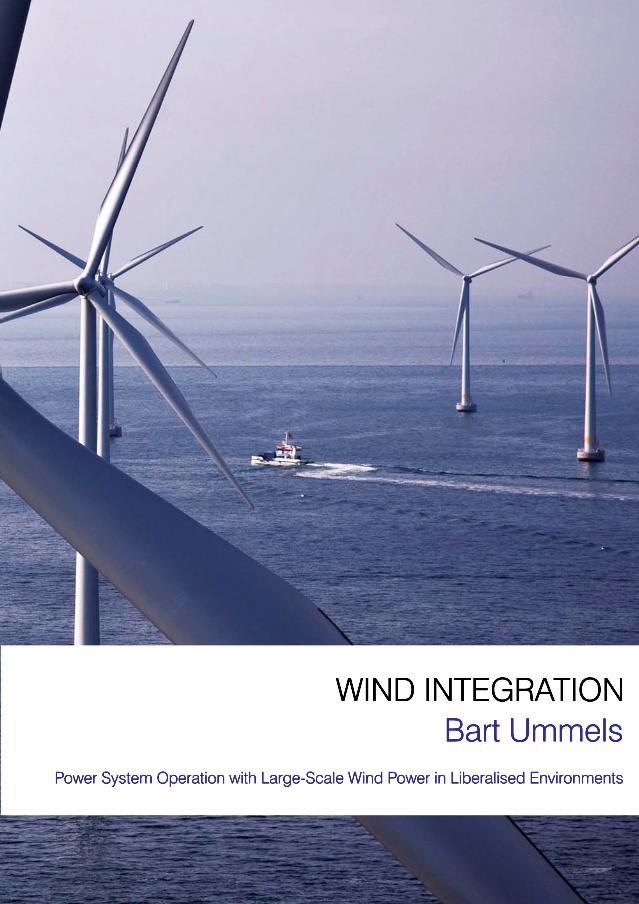
Power System Operationwith Large-Scale Wind Powerin Liberalised Environments
PROEFSCHRIFT
ter verkrijging van de graad van doctoraan de Technische Universiteit Delft,
op gezag van de Rector Magnificus prof.dr.ir. J.T. Fokkema,voorzitter van het College voor Promoties,
in het openbaar te verdedigen op donderdag 26 februari 2009 om 10:00 uur
door
Bart Christiaan UMMELS
ingenieur technische bestuurskunde
geboren te IJsselstein.
Dit proefschrift is goedgekeurd door de promotor:
Prof.ir. W.L. Kling
Samenstelling promotiecomissie:
Rector Magnificus voorzitterProf.ir. W.L. Kling Technische Universiteit Delft, promotorProf.dr.ir. G.A.M. van Kuik Technische Universiteit DelftProf.dr.ir. T.H.J.J. van der Hagen Technische Universiteit DelftProf.dr.ir. P.P.J. van den Bosch Technische Universiteit EindhovenProf.dr.ir. R.J.M. Belmans Katholieke Universiteit Leuven, BelgieProf.dr. M.J. O’Malley University College Dublin, Ierlanding. E. Pelgrum TenneT TSO, Arnhem, adviseur
Reservelid:Prof.dr. J.A. Ferreira Technische Universiteit Delft
The research described in this thesis forms part of the project PhD@Sea, which is fundedunder the BSIK-programme (BSIK03041) of the Dutch Government and supported by theconsortium We@Sea (http://www.we-at-sea.org/).
Copyright c© 2008 by B.C. UmmelsAll rights reserved.
No part of the material protected by this copyright notice may be reproduced or utilised inany form or by any means, electronic or mechanical, including photocopying, recording orby any information storage and retrievals system, without permission from the author.
Cover Design: Redmar van Leeuwen and Bart UmmelsPhotography: Courtesy of c© Siemens Wind Power, DenmarkSummary Editing: Josine Pieters-UmmelsPrint: Labor Grafimedia bv, Utrecht

If a man knows not what harbour he is making for, no wind is favourable.L. A. Seneca

General Summary
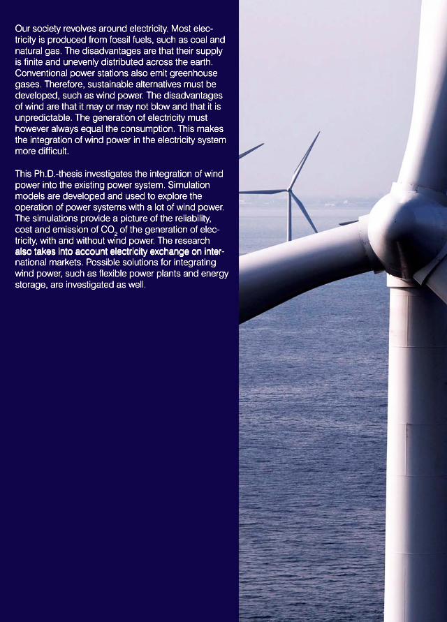
Reason for this researchOur society revolves around electricity. Most electricity comes from electric power stationsthat use coal and natural gas. These are reliable and affordable fuels, but they also havedisadvantages. The supply of fossil fuels is finite and unevenly distributed across the earth.Besides, conventional power stations emit greenhouse gases. There is an urgent need forsustainable alternatives, such as wind power. The disadvantages of wind are that sometimesit is blowing and sometimes it is not and that it is unpredictable. The generation of electricitymust however equal demand at all times. This makes the integration of wind power in theelectricity system more difficult.
Goal and methodThis Ph.D.-thesis is about the question what are the consequences of the integration of a lot ofwind power for the existing power system. What problems do we run into and what solutionsare available? Is it possible to produce one third of the electricity demand with onshore andoffshore wind energy? To come to an answer to these questions, first, it has been calculatedhow much electricity the future wind parks would produce, and when. This information hasbeen added to an existing power system simulation model. This simulation model calculateswhich power stations must be turned on and off at which moment to provide in the electricitydemand throughout the year. Electricity exchange with other countries is also calculated. Thesimulations provide a picture of the reliability, costs and emissions of the generation of elec-tricity, with and without wind power. A second simulation model, developed in this research,computes how the power system reacts to wind energy during certain circumstances, for ex-ample during a storm. By combining the two models, possible problems with the integrationof wind power in the existing power system become clear. The possible solutions, such asflexible electric power plants and energy storage, are also investigated by using these models.
Wind variations and forecast errorsElectricity demand changes continuously: for example, during the day we use much moreelectricity than at night. On top of that, the supply of wind power changes, because some-
vi General Summary
times it is very windy and sometimes there is almost no wind. These two uncertainties areexamined simultaneously in the simulations in order to explore the worst combinations. Theresults indicate that more wind power demands for more flexibility of the existing power sta-tions. Sometimes more reserves are needed, but much more often the power stations mustreduce their output to make room for wind power. It is important to compute the commitmentof the power stations again and again using the latest wind forecast. Then it is possible toreduce forecast errors and to integrate wind power better into the system.
If the wind is or is not blowing...It turns out that the Dutch power stations will be able to set off the variations in demand andwind supply at any moment in the future, provided that actual and improved wind forecastsare taken into account. There are however limits to the integration of wind power. This is,for example, because coal-fired power plants cannot be turned off just like that. Therefore,if there is a lot of wind and little demand, there will be a surplus of wind power. Instead ofthe often posed question ‘What to do when the wind does not blow?’, the question ‘What todo with all the electricity if it is very windy at night?’ is much more relevant. An importantsolution for this lies in the international trade of electricity, because foreign countries canoften use this surplus. Besides, expanding the ‘opening hours’ of the international electricitymarket is favourable for wind power. At present, electricity companies determine how muchelectricity they will buy or sell abroad one day ahead. Then, the international market closes.The wind forecast is still inaccurate one day ahead. Wind power can be integrated better ifthe time difference between trade and the making of the wind forecast would be smaller, forexample one or only a few hours.
Integrating wind power into the power systemThe integration of wind energy in the Dutch system would provide a reduction of the oper-ating cost of the system as a whole of e 1.5 billion a year. This is because the wind is free,while coal and natural gas are not. By using less coal and natural gas, also the emission ofCO2 decreases by 19 million tons a year. This research also shows that with the amountsof wind energy investigated here, no facilities for energy storage have to be developed. Theresults indicate that international electricity trade is a promising and cheaper solution for theintegration of wind power. Also making power stations more flexible turns out to be a bettersolution. For example, the use of heat boilers allows for a more flexible operation of com-bined heat and power stations, which consequently can clear the way for wind during thenight. Also a second electricity cable to Norway seems to be a good alternative for buildingpumped hydro power energy storage in the Netherlands itself.
Recommendations for further researchThis Ph.D.-research focuses on the Netherlands especially. Further research should considerthe situation in other countries in a better way, especially that in Scandinavia. The electricitymarkets should be investigated on a European scale. Further research is also needed on thecapacity of the electricity network in Europe. The future lies in a better cooperation betweendifferent countries and markets; this way, differences in electricity demand and the supplythrough sustainable energy sources can be bridged better and more easily.

Algemene Samenvatting
Aanleiding voor dit onderzoekOnze samenleving draait op elektriciteit. De meeste elektriciteit is afkomstig van elek-triciteitscentrales die kolen en aardgas gebruiken. Dit zijn betrouwbare en betaalbare brand-stoffen, maar ze kennen ook nadelen. De voorraad fossiele brandstoffen is eindig en ongelijkverdeeld over de aarde. Daarnaast stoten conventionele centrales broeikasgassen uit. Er isdringend behoefte aan duurzame alternatieven, zoals windenergie. Het nadeel van wind is dathet soms wel en soms niet waait en dat wind onvoorspelbaar is. Het aanbod van elektriciteitmoet echter op elk moment gelijk zijn aan het verbruik. Dit bemoeilijkt de inpassing vanwindenergie in het elektriciteitssysteem.
Doel en werkwijzeDit proefschrift gaat over de vraag wat de gevolgen zijn van de inpassing van veel wind-energie voor het bestaande elektriciteitssysteem. Tegen welke problemen lopen we aan enwelke oplossingen zijn er beschikbaar? Is het mogelijk om met windenergie op land enop zee eenderde van de elektricteitsvraag te produceren? Om deze vragen te beantwoor-den, is eerst berekend hoeveel elektriciteit de toekomstige windparken zouden produceren,en wanneer. Deze informatie is toegevoegd aan een bestaand simulatiemodel van de elek-triciteitsvoorziening. Dit simulatiemodel berekent welke centrales op welk moment aan- enuitgezet moeten worden om gedurende het hele jaar in de elektriciteitsvraag te voorzien. Ookwordt de uitwisseling met andere landen berekend. De simulaties geven een beeld van de be-trouwbaarheid, de kosten en de emissies van de opwekking van elektriciteit, met en zonderwindenergie. Een tweede simulatiemodel, dat voor dit onderzoek is ontwikkeld, berekentdaarna hoe het elektriciteitssysteem reageert op windenergie tijdens bepaalde omstandighe-den, bijvoorbeeld tijdens een storm. Door de twee modellen te combineren, wordt duidelijkwat de eventuele problemen zijn bij de inpassing van windenergie in het bestaande elek-triciteitssysteem. Ook de mogelijke oplossingen, zoals flexibele centrales of energieopslag,zijn onderzocht met deze modellen.
Variaties en voorspellingsfouten van windDe vraag naar elektriciteit verandert continu: overdag gebruiken we bijvoorbeeld veel meerelektriciteit dan ’s nachts. Het aanbod van windenergie varieert ook, want soms waait het

viii Algemene Samenvatting
hard en soms bijna niet. Deze twee onzekerheden worden in de simulaties tegelijkertijdonderzocht om de meest ongunstige combinaties te bekijken. De resultaten geven aan datwindenergie vraagt om een grotere flexibiliteit van de bestaande elektriciteitscentrales. Somszijn er meer reserves nodig, maar veel vaker zullen de centrales juist hun productie moetenverlagen om ruimte te maken voor wind. Het is belangrijk om de inzet van de elektriciteits-centrales steeds opnieuw te berekenen met de laatste windvoorspelling. Het is dan mogelijkvoorspellingsfouten te verminderen en windenergie beter in te passen.
Als het wel of niet waait...Het blijkt dat de Nederlandse elektriciteitscentrales de variaties in vraag en windaanbod ookin de toekomst op elk moment kunnen opvangen, mits er gebruik wordt gemaakt van actueleen verbeterde windvoorspellingen. Er zijn wel grenzen aan de inpassing van windenergie.Dit komt bijvoorbeeld omdat een kolencentrale niet zomaar kan worden uitgezet. Als er veelwind is en weinig vraag, ontstaat er een overschot aan wind. In plaats van de vaakgehoordevraag ‘Wat doen we als het niet waait?’ is de vraag ‘Waar laten we alle elektriciteit als het’s nachts hard waait?’ veel relevanter. Een belangrijke oplossing hiervoor zit in interna-tionale handel van elektriciteit, omdat het buitenland dit overschot vaak wel kan gebruiken.Daarnaast is een verruiming van de ‘openingstijden’ van de internationale elektriciteitsmarktgunstig voor windenergie. Momenteel bepalen de elektriciteitsbedrijven een dag van tevorenhoeveel elektriciteit ze in het buitenland gaan kopen of verkopen. Dan sluit de internationalemarkt. De windvoorspelling is een dag tevoren nog onnauwkeurig. Windenergie kan beterworden ingepast als het tijdsverschil tussen de handel en het maken van de windvoorspellingkleiner is, bijvoorbeeld een of enkele uren.
Inpassing van windenergie in het elektriciteitssysteemDe inpassing van windenergie in het Nederlandse elektriciteitssysteem kan zorgen voor eenvermindering van de productiekosten van het totale systeem van e 1,5 miljard per jaar. Datkomt omdat de wind gratis is, terwijl kolen en aardgas dat niet zijn. Door minder kolen enaardgas te verstoken, neemt ook de CO2-uitstoot af met 19 miljoen ton per jaar. Dit onder-zoek wijst ook uit dat er met de onderzochte hoeveelheden windenergie geen voorzieningenvoor energieopslag hoeven te komen. De resultaten geven aan dat internationale elektrici-teitshandel een veelbelovende en goedkopere oplossing is voor de inpassing van windenergie.Ook het flexibeler maken van elektriciteitscentrales is een betere oplossing. Het gebruik vanwarmteboilers zorgt bijvoorbeeld voor een flexibelere bedrijfsvoering van warmtekrachtcen-trales, die daardoor ’s nachts ruimte kunnen maken voor wind. Ook een tweede elektriciteits-kabel naar Noorwegen lijkt een goed alternatief voor het bouwen van waterkrachtopslag inNederland zelf.
Aanbevelingen voor verder onderzoekDit promotie-onderzoek richt zich vooral op Nederland. Verder onderzoek zou de situatiein andere landen beter moeten bekijken, vooral die van Scandinavie. De elektriciteitsmark-ten moeten op Europese schaal worden onderzocht. Ook is verder onderzoek nodig naar decapaciteit van het elektriciteitsnet in Europa. De toekomst ligt in een betere samenwerkingtussen verschillende landen en markten; zo zijn verschillen in elektriciteitsvraag en aanbodvanuit duurzame bronnen beter en gemakkelijker te overbruggen.
Contents
General Summary v
Algemene Samenvatting vii
Contents ix
1 Introduction 11.1 Development of Renewable Energy . . . . . . . . . . . . . . . . . . . . . . 1
1.1.1 Energy and Sustainability . . . . . . . . . . . . . . . . . . . . . . . 11.1.2 Promotion of Renewables . . . . . . . . . . . . . . . . . . . . . . . 21.1.3 Wind Power . . . . . . . . . . . . . . . . . . . . . . . . . . . . . . . 31.1.4 Wind Power in the Netherlands . . . . . . . . . . . . . . . . . . . . 4
1.2 Wind Power and Power Systems . . . . . . . . . . . . . . . . . . . . . . . . 51.2.1 Developments in Wind Power . . . . . . . . . . . . . . . . . . . . . 51.2.2 Electrical Power Systems . . . . . . . . . . . . . . . . . . . . . . . . 61.2.3 Integration Aspects of Wind Power . . . . . . . . . . . . . . . . . . 9
1.3 Research Objective and Approach . . . . . . . . . . . . . . . . . . . . . . . 101.3.1 Research Scope . . . . . . . . . . . . . . . . . . . . . . . . . . . . . 101.3.2 Problem Statement . . . . . . . . . . . . . . . . . . . . . . . . . . . 151.3.3 Approach . . . . . . . . . . . . . . . . . . . . . . . . . . . . . . . . 171.3.4 Research Framework: We@Sea . . . . . . . . . . . . . . . . . . . . 18
1.4 Thesis Outline . . . . . . . . . . . . . . . . . . . . . . . . . . . . . . . . . . 18
2 System Load and Wind Power 212.1 Introduction . . . . . . . . . . . . . . . . . . . . . . . . . . . . . . . . . . . 212.2 System Load . . . . . . . . . . . . . . . . . . . . . . . . . . . . . . . . . . 22
2.2.1 Data Time Resolution . . . . . . . . . . . . . . . . . . . . . . . . . 22
x CONTENTS
2.2.2 Development of Load Data . . . . . . . . . . . . . . . . . . . . . . . 222.2.3 Load Duration Curves . . . . . . . . . . . . . . . . . . . . . . . . . 24
2.3 Development of Wind Speed Data . . . . . . . . . . . . . . . . . . . . . . . 242.3.1 Literature Background . . . . . . . . . . . . . . . . . . . . . . . . . 242.3.2 Methodology . . . . . . . . . . . . . . . . . . . . . . . . . . . . . . 262.3.3 Results . . . . . . . . . . . . . . . . . . . . . . . . . . . . . . . . . 30
2.4 Development of Wind-Power Data . . . . . . . . . . . . . . . . . . . . . . . 302.4.1 Literature Background . . . . . . . . . . . . . . . . . . . . . . . . . 302.4.2 Relationship between Wind Speed and Wind Power . . . . . . . . . . 312.4.3 Wind Speed – Wind Power Conversion . . . . . . . . . . . . . . . . 322.4.4 Results . . . . . . . . . . . . . . . . . . . . . . . . . . . . . . . . . 36
2.5 Analysis of System Load and Wind Power Data . . . . . . . . . . . . . . . . 372.5.1 Load-less-Wind-Power Duration Curves . . . . . . . . . . . . . . . . 372.5.2 Aggregated Power Variations . . . . . . . . . . . . . . . . . . . . . . 382.5.3 Wind Power Forecast Errors . . . . . . . . . . . . . . . . . . . . . . 39
2.6 Summary and Conclusions . . . . . . . . . . . . . . . . . . . . . . . . . . . 40
3 Unit Commitment and Economical Despatch Model 413.1 Introduction . . . . . . . . . . . . . . . . . . . . . . . . . . . . . . . . . . . 413.2 Literature Overview and Contribution of this Thesis . . . . . . . . . . . . . . 42
3.2.1 Overview of relevant UC–ED Tools . . . . . . . . . . . . . . . . . . 423.2.2 Contribution of this Thesis . . . . . . . . . . . . . . . . . . . . . . . 44
3.3 Simulation Model . . . . . . . . . . . . . . . . . . . . . . . . . . . . . . . . 453.3.1 Generation Outages . . . . . . . . . . . . . . . . . . . . . . . . . . . 453.3.2 Optimisation Structure . . . . . . . . . . . . . . . . . . . . . . . . . 473.3.3 Simulation Attributes . . . . . . . . . . . . . . . . . . . . . . . . . . 513.3.4 Input and Output Data . . . . . . . . . . . . . . . . . . . . . . . . . 523.3.5 Validation of the Simulation Model . . . . . . . . . . . . . . . . . . 54
3.4 Thermal Generation Unit Models . . . . . . . . . . . . . . . . . . . . . . . . 553.4.1 Operational Flexibility . . . . . . . . . . . . . . . . . . . . . . . . . 553.4.2 Unit Operating Cost . . . . . . . . . . . . . . . . . . . . . . . . . . 563.4.3 Emissions . . . . . . . . . . . . . . . . . . . . . . . . . . . . . . . . 573.4.4 Combined Heat and Power . . . . . . . . . . . . . . . . . . . . . . . 583.4.5 Flexible CHP-Units . . . . . . . . . . . . . . . . . . . . . . . . . . . 58
3.5 Hydro Power and Energy Storage Models . . . . . . . . . . . . . . . . . . . 593.5.1 Energy Storage and Power System Operation . . . . . . . . . . . . . 603.5.2 Value-of-Energy Method . . . . . . . . . . . . . . . . . . . . . . . . 613.5.3 Hydro Power Models . . . . . . . . . . . . . . . . . . . . . . . . . . 613.5.4 Energy Storage Alternatives . . . . . . . . . . . . . . . . . . . . . . 62
3.6 International Exchange . . . . . . . . . . . . . . . . . . . . . . . . . . . . . 653.6.1 Areas and Interconnectors . . . . . . . . . . . . . . . . . . . . . . . 653.6.2 Possibilities for International Exchange . . . . . . . . . . . . . . . . 65
3.7 Summary and Conclusions . . . . . . . . . . . . . . . . . . . . . . . . . . . 66

xi
4 Impacts of Wind Power on Unit Commitment and Economic Despatch 674.1 Introduction . . . . . . . . . . . . . . . . . . . . . . . . . . . . . . . . . . . 674.2 Simulation Parameters . . . . . . . . . . . . . . . . . . . . . . . . . . . . . 68
4.2.1 Technical Limits . . . . . . . . . . . . . . . . . . . . . . . . . . . . 684.2.2 Economic Impacts . . . . . . . . . . . . . . . . . . . . . . . . . . . 694.2.3 Environmental Impacts . . . . . . . . . . . . . . . . . . . . . . . . . 70
4.3 Power System Model Specification . . . . . . . . . . . . . . . . . . . . . . . 704.3.1 The Netherlands . . . . . . . . . . . . . . . . . . . . . . . . . . . . 704.3.2 Neighbouring Areas . . . . . . . . . . . . . . . . . . . . . . . . . . 724.3.3 Power System Overview . . . . . . . . . . . . . . . . . . . . . . . . 74
4.4 System Simulations . . . . . . . . . . . . . . . . . . . . . . . . . . . . . . . 754.4.1 Base Variants . . . . . . . . . . . . . . . . . . . . . . . . . . . . . . 764.4.2 Wind Power Integration Solutions . . . . . . . . . . . . . . . . . . . 784.4.3 Simulations Set-Up . . . . . . . . . . . . . . . . . . . . . . . . . . . 78
4.5 Simulation Results . . . . . . . . . . . . . . . . . . . . . . . . . . . . . . . 804.5.1 Technical Limits . . . . . . . . . . . . . . . . . . . . . . . . . . . . 804.5.2 Economic Impacts . . . . . . . . . . . . . . . . . . . . . . . . . . . 824.5.3 Environmental Impacts . . . . . . . . . . . . . . . . . . . . . . . . . 854.5.4 Integration Solutions for Wind Power . . . . . . . . . . . . . . . . . 864.5.5 Cost-Benefit Analysis of Integration Solutions . . . . . . . . . . . . 89
4.6 Summary and Conclusions . . . . . . . . . . . . . . . . . . . . . . . . . . . 91
5 Power System Dynamic Model 935.1 Introduction . . . . . . . . . . . . . . . . . . . . . . . . . . . . . . . . . . . 935.2 Literature Overview and Contribution of this Thesis . . . . . . . . . . . . . . 94
5.2.1 Literature Overview on Power-Frequency Control and Wind Power . 945.2.2 Contribution of this Thesis . . . . . . . . . . . . . . . . . . . . . . . 95
5.3 Power–Frequency Control Model . . . . . . . . . . . . . . . . . . . . . . . . 965.3.1 Modeling Approach . . . . . . . . . . . . . . . . . . . . . . . . . . 965.3.2 Mechanical Power System Model . . . . . . . . . . . . . . . . . . . 97
5.4 Validation of the Modeling Approach . . . . . . . . . . . . . . . . . . . . . 995.4.1 Simulations . . . . . . . . . . . . . . . . . . . . . . . . . . . . . . . 1015.4.2 Validation Results . . . . . . . . . . . . . . . . . . . . . . . . . . . 102
5.5 Validation of the Model and Full Model Development . . . . . . . . . . . . . 1035.5.1 Validation of the UCTE-Interconnection Model . . . . . . . . . . . . 1045.5.2 Secondary Control . . . . . . . . . . . . . . . . . . . . . . . . . . . 1055.5.3 Energy Program Responsibility . . . . . . . . . . . . . . . . . . . . 1075.5.4 Dynamic Generation Unit Models . . . . . . . . . . . . . . . . . . . 110
5.6 Summary and Conclusions . . . . . . . . . . . . . . . . . . . . . . . . . . . 113
6 Impacts of Wind Power on Short-Term Power System Operation 1156.1 Introduction . . . . . . . . . . . . . . . . . . . . . . . . . . . . . . . . . . . 1156.2 Market Designs for Wind Power . . . . . . . . . . . . . . . . . . . . . . . . 116
6.2.1 Organisation of Markets . . . . . . . . . . . . . . . . . . . . . . . . 1166.2.2 Program Responsibility for Wind Power . . . . . . . . . . . . . . . . 1176.2.3 Prioritisation of Wind Power . . . . . . . . . . . . . . . . . . . . . . 118
xii CONTENTS
6.2.4 Comparison of Market Designs for Wind Power . . . . . . . . . . . . 1186.3 Power System Model . . . . . . . . . . . . . . . . . . . . . . . . . . . . . . 119
6.3.1 Simulation Parameters . . . . . . . . . . . . . . . . . . . . . . . . . 1196.3.2 The Netherlands’ Control Zone . . . . . . . . . . . . . . . . . . . . 1206.3.3 Rest of the UCTE-System . . . . . . . . . . . . . . . . . . . . . . . 121
6.4 System Simulations . . . . . . . . . . . . . . . . . . . . . . . . . . . . . . . 1226.4.1 Simulation Procedure . . . . . . . . . . . . . . . . . . . . . . . . . . 1226.4.2 Wind Power Worst Cases . . . . . . . . . . . . . . . . . . . . . . . . 1236.4.3 Market Designs for Wind Power . . . . . . . . . . . . . . . . . . . . 1246.4.4 Short-Term Balancing Solutions . . . . . . . . . . . . . . . . . . . . 1256.4.5 Overview . . . . . . . . . . . . . . . . . . . . . . . . . . . . . . . . 126
6.5 Simulation Results . . . . . . . . . . . . . . . . . . . . . . . . . . . . . . . 1266.5.1 Wind Power Worst Cases . . . . . . . . . . . . . . . . . . . . . . . . 1286.5.2 Market Design for Wind Power . . . . . . . . . . . . . . . . . . . . 1306.5.3 Short-Term Balancing Solutions . . . . . . . . . . . . . . . . . . . . 132
6.6 Summary and Conclusions . . . . . . . . . . . . . . . . . . . . . . . . . . . 135
7 Conclusions and Recommendations 1377.1 Conclusions . . . . . . . . . . . . . . . . . . . . . . . . . . . . . . . . . . . 137
7.1.1 Power System Integration of Wind Power . . . . . . . . . . . . . . . 1377.1.2 Impacts of Wind Power on Long-Term Power System Operation . . . 1387.1.3 Impacts of Wind Power on Short-Term Power System Operation . . . 1397.1.4 System Integration Solutions . . . . . . . . . . . . . . . . . . . . . . 140
7.2 Recommendations for Further Research . . . . . . . . . . . . . . . . . . . . 1417.2.1 UC–ED Model Extension . . . . . . . . . . . . . . . . . . . . . . . 1417.2.2 Power Transmission and Load Flows . . . . . . . . . . . . . . . . . 1427.2.3 International Trade and Markets . . . . . . . . . . . . . . . . . . . . 1427.2.4 Large-Scale Renewables and Energy Demand . . . . . . . . . . . . . 142
Bibliography 143
A Wind Speed Measurement Locations 155
B Wind Power Locations 159
C German Wind Power Data 163
D Validation Test System Data 165
E Nomenclature 169
Publications 173
Acknowledgement 177
Curriculum Vitae 179
CHAPTER 1Introduction
1.1 Development of Renewable Energy
1.1.1 Energy and Sustainability
Modern society is critically dependent on its energy supply, in particular the supply of elec-tricity. Electricity provides light, heating, cooling, communication and transportation andpowers a wide range of industrial processes. Electrical energy presently comprises about fif-teen percent of energy demand in the world [80], but this percentage is considerably higherfor developed societies and tends to increase. Moreover, electricity consumption is stronglycorrelated with economic growth: economic growth allows further use of electric applianceswhich in turn increases electricity demand [121]. In the past three decades, economic growthhas been an important factor in tripling the electricity consumption worldwide. The con-tinuing development of economies such as China and India will increase the demand forelectrical energy much further, while the United States, Japan and Europe will still need in-creasing amounts of electricity to provide for growth of consumption and to power the evergrowing number of applications.
In 1987 the United Nations’ World Commission on Environment and Development(WCED), chaired by Ms. Gro Harlem Brundtland, published its report ’Our Common Fu-ture’ [187]. This publication and the work of WCED has put environmental issues on globaland national political agendas. The Brundtland report defines the concept of sustainabledevelopment as development that meets the needs of the present without compromising the
2 Introduction
ability of future generations to meet their own needs. Sustainable development cruciallydepends on the availability of energy resources which are both environmentally sound andeconomically viable. The report specifically touched sustainability aspects of energy, such asefficiency, conservation and impacts on public health [176]. Two decades later, there is now awidespread consensus that dramatic changes in electricity generation and energy use in gen-eral are needed in order to decrease CO2 emissions and adverse effects on global warming[159].
At present, electricity is produced largely by large power plants using coal, natural gas,hydro or nuclear fission as primary energy source. These generation technologies are gener-ally affordable and reliable and have been used in power systems for decades. An importantdisadvantage of the use of fossil fuels and uranium however is their finiteness, making powergeneration from these resources inherently unsustainable. A second disadvantage which ap-plies especially to natural gas and uranium is the unequal distribution of fuel supplies betweenregions, creating fuel dependencies between them and possibilities for exercising political in-fluence. A third disadvantage is the emission of greenhouse gases, in particular CO2, whenburning coal, oil and natural gas for power generation. This disadvantage does not apply tonuclear fission, but has the disadvantage of nuclear waste and the development of new in-stallations is difficult in many countries. Large hydro does not have the drawbacks of fossilfuel-powered generation since it uses a sustainable supply of rainfall for power generation.However, its potential has already been exploited for a large part, especially in developedcountries, and the construction of new large installations has considerable challenges of itsown kind [103]. New plants are likely to be located far from load centres, requiring bulkpower transmission over large distances. Also, the creation of hydro reservoirs requiresflooding of vast areas, which has devastating effects on local environments. Clearly, thereare limits to the extent that conventional generation technologies can be part of a future,sustainable power supply.
In the past decades, new power generation technologies have been developed which donot have the disadvantages of the technologies above. Renewable energy technologies suchas biomass, geothermal, wind power, solar photovoltaics, tidal and wave power make use ofthe natural energy sources (biomass, the earth’s heat, wind, sunlight, water flows) for the gen-eration of electricity. The contribution of the renewable energy sources (RES) in power gen-eration has been increasing rapidly in the past years, but is presently still small at about 2%of the total energy demand [80]. RES have disadvantages of their own as well, of which themost important two are cost and controllability. Most renewable power generation technolo-gies are for the moment still more expensive than conventional technologies and thereforerequire (governmental) support in order to make them feasible. The second disadvantage ofrenewable power is that they are mostly less controllable than conventional generation sincethe primary energy source cannot be controlled (geothermal, hydro and biomass are the ex-ceptions). Therefore, the integration of large amounts of renewables into the power systemis technically and economically challenging.
1.1.2 Promotion of Renewables
At the moment, the advantages of renewables are valued such that governments have de-veloped policy instruments aimed at the promotion of renewables. Governmental policy is
1.1 Development of Renewable Energy 3
formulated in order to create a level playing field for renewables by targeting the higher costand lower controllability of these technologies.
Since the advantages of renewables are mostly externalities benefiting society rather thanthe project developer (i.e. less fuel dependency and emissions), governmental support sche-mes may be used in order to return these added values to the investor. Such schemes nar-row the gap between investment and operation cost of RES and the revenues from energysales on power markets. Often, support mechanisms are organised as a long-term fixed price(e/MWh) for feeding renewable energy into the power system. Such a fixed feed-in tariffimplies a guaranteed long-term income for electrical energy generated by RES, providing astable, long-term guarantee of revenues for the sustainable energy producer and thus a shelterfor market risks. Feed-in tariffs have proven to be very effective in promoting wind powerdevelopment, e.g. in Denmark, Germany and Spain [113, 114]. Another way to supportRES is to subsidise the difference between generation cost and the received electricity price(’unprofitable top’) or to provide investment tax reductions. A third option is to internalisethe societal benefits of renewables through the issuing of ’green certificates’ in combinationwith a quotum obligation or emission ceilings. A certificate of origin represents the rightto emit a certain amount of emissions and this right is tradable, providing the investor withadditional revenues. Demand for certificates is stimulated by mandating requirements for theshare of renewables or by defining emission limits. Such a tradable green certificate systemintroduces a separate market mechanism for the environmental value of electricity generationfrom RES and compensates renewable energy producers for the environmental benefits theyprovide [117].
Due to their lower controllability, renewables introduce additional uncertainty in the op-eration of power systems. The lower controllability of most renewables must be solved bythe power system, which is a technical challenge requiring additional control actions fromconventional generation units and of renewables themselves. Since such control actions comeat a certain cost, the system integration of renewables is also an economic challenge. Thesechallenges are generally taken away from the producer since governments often formulateregulation stating that renewables are assigned as prioritised production. This means thatrenewables have first access to the system and that the system integration aspects are to betaken care of by the power system operator rather than the producer. In case renewable poweris not prioritised, the integration cost have to be taken by the project developer.
1.1.3 Wind Power
Wind power has a number of benefits that set it apart from other renewables. First of all, itsprimary energy source, the wind, is globally available in abundance both on land (onshore)and at sea (offshore). Secondly, wind power investment cost is relatively low, for examplecompared to solar photovoltaics. Furthermore, the environmental quality of wind turbinesis high. Wind power generates enough electricity within around six months to compensatefor all energy used during material extraction, turbine construction, installation, operation,demolition and recycling [36, 178], with life-spans designed for twenty years. Even thoughwind turbines have an effect on the landscape, which is not appreciated by everyone, theimpacts of wind turbines on nature and wildlife are small, especially if wind turbines aresited well.
4 Introduction
1990 1995 2000 20050
20
40
60
80
100
Year
Inst
alle
d W
ind
Pow
er C
apac
ity [G
W]
WorldwideEU
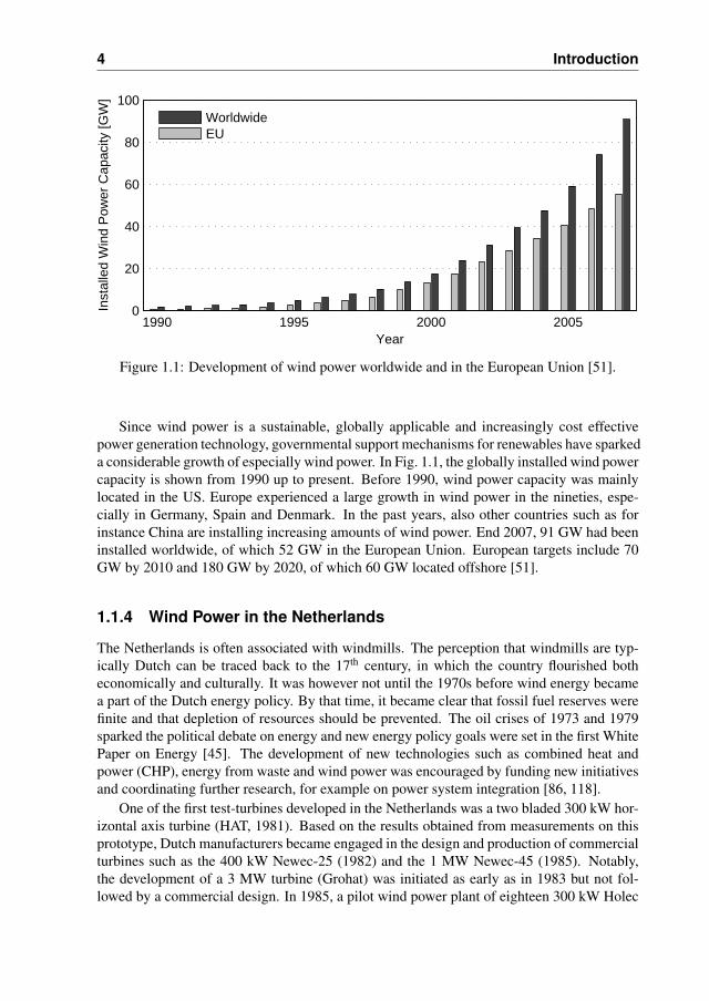
Figure 1.1: Development of wind power worldwide and in the European Union [51].
Since wind power is a sustainable, globally applicable and increasingly cost effectivepower generation technology, governmental support mechanisms for renewables have sparkeda considerable growth of especially wind power. In Fig. 1.1, the globally installed wind powercapacity is shown from 1990 up to present. Before 1990, wind power capacity was mainlylocated in the US. Europe experienced a large growth in wind power in the nineties, espe-cially in Germany, Spain and Denmark. In the past years, also other countries such as forinstance China are installing increasing amounts of wind power. End 2007, 91 GW had beeninstalled worldwide, of which 52 GW in the European Union. European targets include 70GW by 2010 and 180 GW by 2020, of which 60 GW located offshore [51].
1.1.4 Wind Power in the Netherlands
The Netherlands is often associated with windmills. The perception that windmills are typ-ically Dutch can be traced back to the 17th century, in which the country flourished botheconomically and culturally. It was however not until the 1970s before wind energy becamea part of the Dutch energy policy. By that time, it became clear that fossil fuel reserves werefinite and that depletion of resources should be prevented. The oil crises of 1973 and 1979sparked the political debate on energy and new energy policy goals were set in the first WhitePaper on Energy [45]. The development of new technologies such as combined heat andpower (CHP), energy from waste and wind power was encouraged by funding new initiativesand coordinating further research, for example on power system integration [86, 118].
One of the first test-turbines developed in the Netherlands was a two bladed 300 kW hor-izontal axis turbine (HAT, 1981). Based on the results obtained from measurements on thisprototype, Dutch manufacturers became engaged in the design and production of commercialturbines such as the 400 kW Newec-25 (1982) and the 1 MW Newec-45 (1985). Notably,the development of a 3 MW turbine (Grohat) was initiated as early as in 1983 but not fol-lowed by a commercial design. In 1985, a pilot wind power plant of eighteen 300 kW Holec
1.2 Wind Power and Power Systems 5
turbines was developed with an active involvement of the Dutch Generating Board SEP1.SEP was involved in the research on the system integration of wind power in the 1980s andnoted that a significant improvement in cost and performance was needed [64]. Technicalproblems and the associated financial risks were common for all Dutch manufacturers. Fromthe early 1990s, foreign turbine manufacturers began to take over the Dutch market. Dan-ish and German turbines were considered to have a better price-performance ratio due totheir reliability and size. The absence of a strong Dutch market for wind turbines and a lackof collaboration between turbine owners, manufacturers and research institutes resulted in astagnation of innovation [92]. This eventually led to the disappearance of all Dutch windturbine manufacturers, although a small number of new manufactures has emerged recently.
In 1985, the Dutch government formulated the target for onshore wind power capacity of1000 MW installed by the year 2000. This capacity was however not reached before 2004,which may be explained by the absence of an accessible market for small market players, nocoherent governmental commitment to wind power and an inconsistent and changing energypolicy [1]. Permission procedures (local planning) are also regarded as a weak link in thedevelopment of wind power in the Netherlands [21]. Current installed capacity (end 2008)equals around 2100 MW, of which 247 MW located offshore and around 1850 MW onshore[189]. The Netherlands has a large potential for wind power and national targets for end2011 include 4000 MW onshore and 700 MW offshore. Furthermore, a target of 6000 MWoffshore wind power has been formulated for the year 2020 [47]. It is this latter target that ispart of the rationale behind this research work.
1.2 Wind Power and Power Systems
1.2.1 Developments in Wind Power
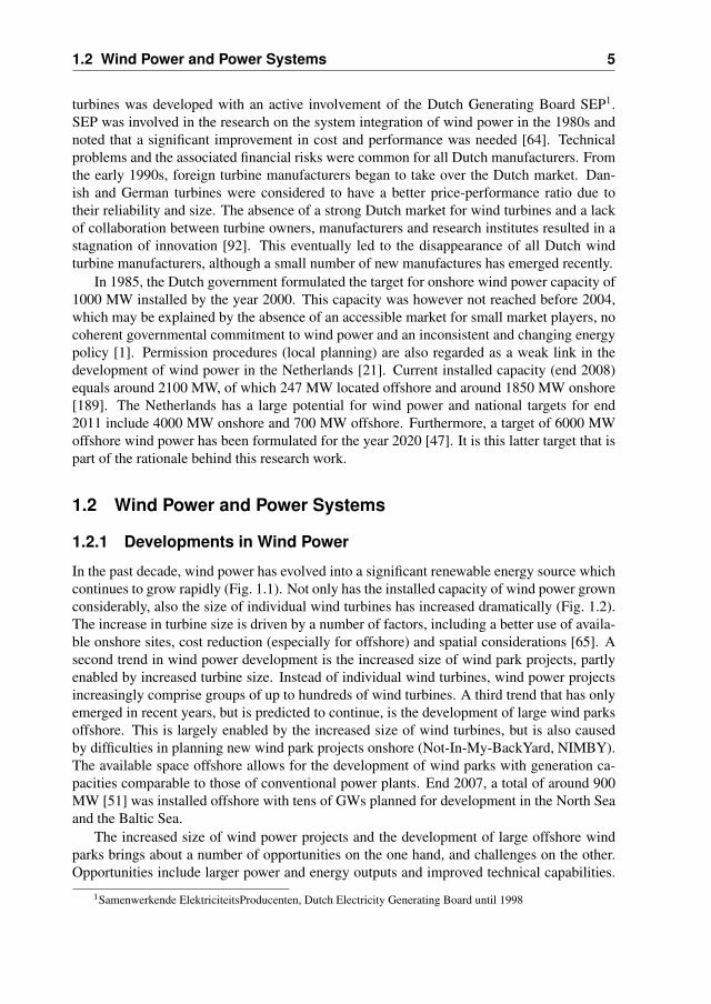
In the past decade, wind power has evolved into a significant renewable energy source whichcontinues to grow rapidly (Fig. 1.1). Not only has the installed capacity of wind power grownconsiderably, also the size of individual wind turbines has increased dramatically (Fig. 1.2).The increase in turbine size is driven by a number of factors, including a better use of availa-ble onshore sites, cost reduction (especially for offshore) and spatial considerations [65]. Asecond trend in wind power development is the increased size of wind park projects, partlyenabled by increased turbine size. Instead of individual wind turbines, wind power projectsincreasingly comprise groups of up to hundreds of wind turbines. A third trend that has onlyemerged in recent years, but is predicted to continue, is the development of large wind parksoffshore. This is largely enabled by the increased size of wind turbines, but is also causedby difficulties in planning new wind park projects onshore (Not-In-My-BackYard, NIMBY).The available space offshore allows for the development of wind parks with generation ca-pacities comparable to those of conventional power plants. End 2007, a total of around 900MW [51] was installed offshore with tens of GWs planned for development in the North Seaand the Baltic Sea.
The increased size of wind power projects and the development of large offshore windparks brings about a number of opportunities on the one hand, and challenges on the other.Opportunities include larger power and energy outputs and improved technical capabilities.
1Samenwerkende ElektriciteitsProducenten, Dutch Electricity Generating Board until 1998
6 Introduction
1985 1990 1995 2000 2005.05 .3 .5 1.3 1.6 2.0 4.5 5.0 6.0
Ø 12 m.
Ø 126 m.
MWYear
Airbus A380
Figure 1.2: Development of size and rating of wind turbines (prototypes).
The larger power and energy outputs however simultaneously present rather fundamentalchallenges due to the uncontrollability of the primary energy source, the wind. A first chal-lenge of using wind as a primary energy source for power generation is its variability: windspeeds fluctuate on timescales varying from seconds to seasons. This means that the outputof wind turbines fluctuates as well, depending on the relationship between wind speed andwind turbine output power. A second challenge is that wind speed depends on a large num-ber of meteorological factors that can only be forecast up to a limited extent. As wind speedvariations can only be predicted with accuracies decreasing with the forecast lead time, it isnot possible to accurately assess wind power output for longer time-ranges. As the amountof wind power installed in power systems increases, the impacts of wind power’s variabil-ity and limited predictability become significant as well from the point of view of a reliableoperation of power systems.
1.2.2 Electrical Power Systems
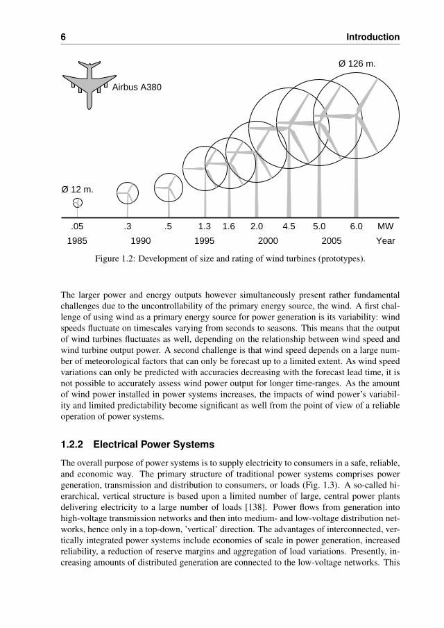
The overall purpose of power systems is to supply electricity to consumers in a safe, reliable,and economic way. The primary structure of traditional power systems comprises powergeneration, transmission and distribution to consumers, or loads (Fig. 1.3). A so-called hi-erarchical, vertical structure is based upon a limited number of large, central power plantsdelivering electricity to a large number of loads [138]. Power flows from generation intohigh-voltage transmission networks and then into medium- and low-voltage distribution net-works, hence only in a top-down, ’vertical’ direction. The advantages of interconnected, ver-tically integrated power systems include economies of scale in power generation, increasedreliability, a reduction of reserve margins and aggregation of load variations. Presently, in-creasing amounts of distributed generation are connected to the low-voltage networks. This
1.2 Wind Power and Power Systems 7
Generation Transmission Distribution Load
Load
Power Flow
Figure 1.3: Overview of a traditional power system structure.
trend increasingly leads to bi-directional power flows in the distribution system [145].In observing the primary structure of power systems, it is important to note that electrical
energy as such cannot be stored in significant amounts. Electrical power is consumed at thesame moment it is generated. For a reliable power supply it is therefore essential to maintaina precise balance between demand (total system load including transmission and distributionlosses) and generation. It is in principle possible to maintain the power balance by adjustingboth generation and demand, but historically, mostly the central generation units have beenused to follow the demand at all times. The operation of power systems is therefore criticallydependent on the capabilities of generators for balancing the load.
Power Generation
For the generation of electrical power, traditionally, primary energy sources such as coal andnatural gas are used. The primary energy source is combusted to generate heat which is usedin a steam-cycle to convert the thermal energy into mechanical energy, which is then usedto power electric generators which produce electricity. Nuclear units are based on the sameprinciple, but use nuclear fission as the energy source. For hydro power, the gravitationalenergy of water in large reservoirs is converted into kinetic energy and then into mechanicalenergy using hydro turbines, which drive electric generators.
Power generation in traditional power systems is based on controllable primary energysources: fossil fuels (or water) are stored until they are used for power generation. The ad-vantages of using large-scale, central generation units based on fossil fuels is that the primaryenergy can be fully controlled: hence a relatively small number of generation units sufficesto control the power balance in the entire power system. The benefits of conventional gener-ation have made it possible that nowadays, system load can vary widely and freely during theday and during the year. As long as sufficient generation capacity is installed to match thesystem load at all times, generators will be able to ensure a reliable operation of the system.
For the operation of power systems with significant amounts of renewables, the impor-tance of conventional generation will remain or may increase even further in order to guar-antee a reliable power supply. The other way around, the integration of large amounts of
8 Introduction
renewables may in future require the system load to be more attuned to power generationavailability.
Transmission
Power transmission is carried out at high voltage over long distances from central generationunits to the load centres. Power transformers are used to transform generated power to a highvoltage and to transform power to lower voltage levels near the loads. Historically, transmis-sion capacity was planned integrally with generation capacity, based on load forecasts. Withthe liberalisation of electricity sectors in the past decade, generation planning is decoupledfrom transmission planning. Generation investments are done by generating companies whiletransmission system operators (TSOs) are responsible for transmission planning and reliablesystem operation in their areas. In order to serve the market, it is the task of the TSO to en-sure that transmission capacity is sufficient for the connection of all new generation capacityand for market trading.
Distribution and Load
Power distribution is done at medium- and low-voltage levels over shorter distances, carryingpower from the power transformers connected to the transmission system to the consumers.Distribution systems were originally designed as ’passive’ networks: no generation was con-nected to these grids. Because of a number of developments, including the liberalisationof the electricity sector and growth of renewables, increasing numbers of relatively smallgenerators are being connected near the loads. This influences the operation of distributionsystems, i.e. the power flows become more diverse and power generation at that levels makesthem more ’active’ [145].
Liberalisation of the Electricity Sector
In the past decade, the electricity sector has gone through some important restructuring pro-cesses. With the liberalisation of the electricity sector, ownership of generation became de-coupled from transmission. Generation units are now operated by commercial parties withthe objective of maximising profit and electrical energy is traded on markets much like othercommodities. Since electrical energy cannot be stored in significant amounts, different mar-kets have emerged for different timescales, ranging from long-term (yearly to monthly, suchas ENDEX) and day-ahead (such as APX Spot) to hour-ahead (such as APX Intraday), allow-ing a close match of supply and demand up until the moment of operation. In real-time, theTSO uses power reserves made available by market parties to maintain the power balance.This can also be organised as a market.
The restructuring of the electricity sector has a number of impacts on the operation ofpower systems. The planning and operation of generation units is more and more governed bymarket prices and each individual market party optimises its portfolio for profit maximisation.Furthermore, energy transactions take place on increasingly international markets rather thenon a national scale. The market-driven operation of generation units and international aspectsof power system operation are particularly relevant for the system integration of wind power.This is because wind power may influence market prices and a pread of wind power over alarger area reduces its overall variability.
1.2 Wind Power and Power Systems 9
1.2.3 Integration Aspects of Wind Power
The variability and limited predictability of wind power have raised concerns about the im-pacts on power system reliability and cost. The impacts of wind power on power systemscan roughly be divided into local impacts and system-wide aspects [155], taking into accountboth the electrical aspects of wind turbines and the characteristics of the wind. Furthermore,the connection of wind power challenges the planning and operation of the grid. Another as-pect is the formulation of grid-code requirements especially for wind power. Last, the designof electricity markets also has consequences for the system integration of wind power. All ofthese aspects are discussed below.
Local Impacts
The integration of small-scale wind power mostly involves the connection of individual windturbines to distribution grids. The local impacts of wind power therefore mainly dependon local grid conditions and the connected wind-turbine type, and the effects become lessnoticeable with the (electrical) distance from the source. The observed phenomena includechanged branch flows, altered voltage levels, increased fault currents and the risk of electricalislanding, which complicate system protection, and possibly power quality problems, suchas harmonics and flicker [158]. Modern wind turbines are equipped with versatile powerelectronics and can be designed to mitigate some of these problems [115]. The rest must becaptured by strict grid requirements and new designs for the distribution networks.
System-Wide Impacts
System-wide impacts are largely a result of the variability and limited predictability of thewind and mainly depend on a number of factors, including wind power penetration level, ge-ographical dispersion of wind power and the size of the system [73]. As more wind power isinstalled in power systems, the possible impacts of wind power increase. A large geographi-cal dispersion of wind power may reduce some of these impacts however, especially if theseare related to wind power variability. The system-wide impacts of wind power on powersystems include impacts on power system dynamics, [2, 146, 155], load-frequency control[37] and power reserves [44, 70]. Furthermore, the operation of other generation units in thesystem may be influenced by wind power thereby the system operation cost and emissions[39, 70, 176]. The system-wide aspects of wind power relevant to this research project arecovered in Section 1.3.
Grid Connection Aspects
Large wind power projects and especially offshore wind parks challenge the planning andoperation of transmission grids. Availability of wind energy is often best in remote, openareas far away from demand. Transmission systems, already used by existing generationcapacity, are often not dimensioned to also accommodate large-scale wind power or are sim-ply not available nearby. Grid connection challenges are not only technical, but also includeeconomical issues (cost for offshore wind power connection), spatial planning aspects (longpermission procedures), the low capacity factor of transmission capacity for wind power [20]and legal issues [94, 188]. As a result of wind power connection, transmission bottlenecks
10 Introduction
may occur, which may be solved by a number of solutions, including grid reinforcement [40]or phase shifting transformers [177], wind energy curtailment, or even local storage [109].
Grid Codes
With increasing wind power penetration levels, an increasing number of countries is adopt-ing grid codes with requirements for wind turbines. The objective for this is to manage theimpacts that wind power may have on the power system due to its specific characteristics.Since the grid code requirements for wind power are implemented on a national scale, a widerange of technical requirements now exists between countries [82]. Important requirementsspecified in most of these codes include operational ranges for voltage and frequency, activeand reactive power control requirements, wind turbine behaviour in case of a voltage dip (theso-called fault ride-through behaviour of wind turbines) and turbine communication with theoperator or transmission system operator (TSO). With some modern wind turbines capableof fulfilling such strict grid-code requirements, wind farms are increasingly capable of sup-plying ancillary services necessary for reliable power system operation just like conventionalgeneration technologies [172].
Market Designs
Apart from the technical integration aspects of wind power associated with the variability andlimited predictability of wind power, the integration of wind power in electricity markets hasalso become a subject of interest. Since wind power forecast errors increase with the forecastlead time, wind power cannot be scheduled as long in advance as conventional generation.Therefore, a number of market aspects are of importance for wind power integration, includ-ing market closure-times, the design and size of the market for balancing reserves and thegeographical size of the system/market wind power is integrated into [72, 73]. A final aspectrelevant for wind power is the organisation of support schemes for wind power, which canbe to prioritise wind power over other generation technologies, to integrate wind power intothe market. In the latter case, market parties must take into account the risks of wind powerin their market strategies [109].
1.3 Research Objective and Approach
From the integration aspects discussed above, it has become clear that wind power introducesa wide range of challenges for power system operation. In order to formulate a clear researchobjective, it is necessary to describe the aspects of power systems and power system operationmost relevant to this research. Using the description, the scope of the research can then bedefined and a definition is made.
1.3.1 Research Scope
Power System
Power systems are large technical systems comprising power generation, transmission, distri-bution and consumption. A more formal definition of a power system is a network of one or
1.3 Research Objective and Approach 11
Primary Energy Imports
Generation TransmissionExports
Consumption
TradePhysical flowInformation flow
Balancing
Figure 1.4: Organisational structure of a liberalised power supply [95].
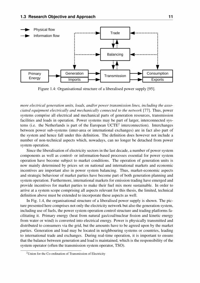
more electrical generation units, loads, and/or power transmission lines, including the asso-ciated equipment electrically and mechanically connected to the network [77]. Thus, powersystems comprise all electrical and mechanical parts of generation resources, transmissionfacilities and loads in operation. Power systems may be part of larger, interconnected sys-tems (i.e. the Netherlands is part of the European UCTE2 interconnection). Interchangesbetween power sub-systems (inter-area or international exchanges) are in fact also part ofthe system and hence fall under this definition. The definition does however not include anumber of non-technical aspects which, nowadays, can no longer be detached from powersystem operation.
Since the liberalisation of electricity sectors in the last decade, a number of power systemcomponents as well as control- or information-based processes essential for power systemoperation have become subject to market conditions. The operation of generation units isnow mainly determined by prices set on national and international markets and economicincentives are important also in power system balancing. Thus, market-economic aspectsand strategic behaviour of market parties have become part of both generation planning andsystem operation. Furthermore, international markets for emission trading have emerged andprovide incentives for market parties to make their fuel mix more sustainable. In order toarrive at a system scope comprising all aspects relevant for this thesis, the limited, technicaldefinition above must be extended to incorporate these aspects as well.
In Fig. 1.4, the organisational structure of a liberalised power supply is shown. The pic-ture presented here comprises not only the electricity network but also the generation system,including use of fuels, the power system operation control structure and trading platforms fa-cilitating it. Primary energy (heat from natural gas/coal/nuclear fission and kinetic energyfrom water or wind) is converted into electrical energy. Power is physically transmitted anddistributed to consumers via the grid, but the amounts have to be agreed upon by the marketparties. Generation and load may be located in neighbouring systems or countries, leadingto international trade and exchanges. During real-time operation, it is important to ensurethat the balance between generation and load is maintained, which is the responsibility of thesystem operator (often the transmission system operator, TSO).
2Union for the Co-ordination of Transmission of Electricity
12 Introduction
Power System Stability
Wind power has impacts on the operation of power systems and thereby on power systemstability. Power system stability has been defined as the ability of an electric power system,for a given initial operating condition, to regain a state of operating equilibrium after beingsubjected to a physical disturbance, with most system variables bounded so that practicallythe entire system remains intact [100]. Thus power systems can be regarded as stable if it isin balanced operation and is able to either maintain this operating state or regain a balancedoperating state different from the original when subjected to a disturbance.
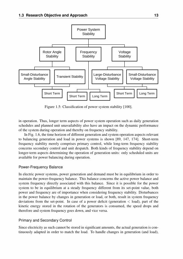
In order to allow a more detailed investigation of power system stability, three kinds ofstability have been distinguished: rotor angle stability, voltage stability and frequency sta-bility, where each can be classified in further detail (Fig. 1.5 [100]). Rotor angle stabilityrefers to the ability of synchronous machines in a power system to remain in synchronismafter being subjected to a disturbance. It primarily concerns the electromechanical oscilla-tions in power systems. Voltage stability refers to the ability of a power system to retainsteady voltages at all buses in the system after being subjected to a disturbance. It dependson the provision of reactive power in the system. Frequency stability comprises the ability ofa power system to retain a steady frequency after significant disturbances.
It is important to state that the power system as such must be studied considering bothelectrical and mechanical aspects, and the three types of stability identified are interrelated.Frequency stability and voltage stability both depend on the ability to maintain or restoreequilibrium between generation and demand in the system. Furthermore, voltage stabilitymay also be associated with rotor angle instability for certain system states. A clear dis-tinction between frequency stability and voltage stability can be made when considering thatsystem frequency is a system-wide parameter directly related to the active power balance[32], while voltage is a more local parameter resulting from the reactive power balance as-sociated with power transmission in particular. Thus, when considering the impact of windpower variability and limited predictability of wind power on balancing generation and loadin power system operation, frequency stability is the most relevant.
Frequency Stability
System frequency is a common factor in alternating current (ac) power systems, being thecentral indicator of the mismatch between the generation and the demand. The electric fre-quency is a measure for the rotation speed of the synchronised generators in the system.Assessment of power system frequency stability generally falls in the category of long-termdynamics of power systems (tens of s to min.), although also short-term frequency stability(s) has been identified [100].
Short-term frequency stability mainly concerns rapid changes such as frequency dropsfollowing a significant generation outage (s), while long-term frequency stability generallyrefers to the composite, dynamic performance of generation and load maintaining systemfrequency and returning it to its rated value (min.). Even though the passive contributionof system load should not be neglected, generators are equipped with control systems thatactively take care of frequency regulation and are therefore considered to be decisive forthe system’s dynamic performance [157]. Since different generators have different controlcapabilities, the dynamic performance of the system highly depends on the generation units
1.3 Research Objective and Approach 13
Power System Stability
Rotor Angle Stability
Frequency Stability
Voltage Stability
Small-Disturbance Angle Stability Transient Stability Large-Disturbance
Voltage StabilitySmall-Disturbance Voltage Stability
Short TermShort Term Long Term
Short Term Long Term
Figure 1.5: Classification of power system stability [100].
in operation. Thus, longer term aspects of power system operation such as daily generationschedules and planned unit unavailability also have an impact on the dynamic performanceof the system during operation and thereby on frequency stability.
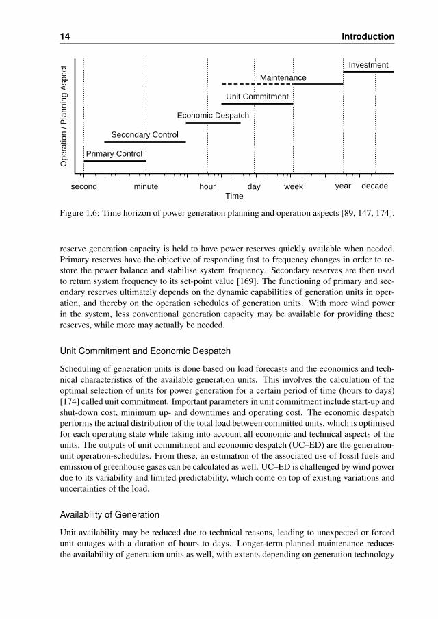
In Fig. 1.6, the time horizon of different generation and system operation aspects relevantto balancing generation and load in power systems is shown [89, 147, 174]. Short-termfrequency stability merely comprises primary control, while long-term frequency stabilityconcerns secondary control and unit despatch. Both kinds of frequency stability depend onlonger-term aspects determining the operation of generation units: only scheduled units areavailable for power balancing during operation.
Power-Frequency Balance
In electric power systems, power generation and demand must be in equilibrium in order tomaintain the power-frequency balance. This balance concerns the active power balance andsystem frequency directly associated with this balance. Since it is possible for the powersystem to be in equilibrium at a steady frequency different from its set-point value, bothpower and frequency are of importance when considering frequency stability. Disturbancesin the power balance by changes in generation or load, or both, result in system frequencydeviations from the set-point. In case of a power deficit (generation < load), part of thekinetic energy stored in the rotation of the generators is consumed, the speed drops andtherefore and system frequency goes down, and vice versa.
Primary and Secondary Control
Since electricity as such cannot be stored in significant amounts, the actual generation is con-tinuously adapted in order to match the load. To handle changes in generation (and load),
14 Introduction
Primary Control
dayhoursecond minute year decade
Secondary Control
Economic Despatch
week
Unit Commitment
MaintenanceInvestment
Ope
ratio
n / P
lann
ing
Aspe
ct
Time
Figure 1.6: Time horizon of power generation planning and operation aspects [89, 147, 174].
reserve generation capacity is held to have power reserves quickly available when needed.Primary reserves have the objective of responding fast to frequency changes in order to re-store the power balance and stabilise system frequency. Secondary reserves are then usedto return system frequency to its set-point value [169]. The functioning of primary and sec-ondary reserves ultimately depends on the dynamic capabilities of generation units in oper-ation, and thereby on the operation schedules of generation units. With more wind powerin the system, less conventional generation capacity may be available for providing thesereserves, while more may actually be needed.
Unit Commitment and Economic Despatch
Scheduling of generation units is done based on load forecasts and the economics and tech-nical characteristics of the available generation units. This involves the calculation of theoptimal selection of units for power generation for a certain period of time (hours to days)[174] called unit commitment. Important parameters in unit commitment include start-up andshut-down cost, minimum up- and downtimes and operating cost. The economic despatchperforms the actual distribution of the total load between committed units, which is optimisedfor each operating state while taking into account all economic and technical aspects of theunits. The outputs of unit commitment and economic despatch (UC–ED) are the generation-unit operation-schedules. From these, an estimation of the associated use of fossil fuels andemission of greenhouse gases can be calculated as well. UC–ED is challenged by wind powerdue to its variability and limited predictability, which come on top of existing variations anduncertainties of the load.
Availability of Generation
Unit availability may be reduced due to technical reasons, leading to unexpected or forcedunit outages with a duration of hours to days. Longer-term planned maintenance reducesthe availability of generation units as well, with extents depending on generation technology

1.3 Research Objective and Approach 15
and operation-strategy considerations, but typically in ranges of weeks to months. On thevery long term, generation investments determine the availability of generation technologiesand thereby their technical capabilities, which ultimately determines the power-frequencybehaviour during power system operation.
1.3.2 Problem Statement
Power System Balancing with Wind Power
In the past decade wind power has become the fastest growing renewable energy technology(absolute numbers) and this development can be expected to continue. Due to the variabilityand limited predictability of the wind speed, the output of wind turbines cannot be controlledto the same extent as conventional generation technologies. Currently, conventional genera-tion plays a pivotal role in maintaining the power balance between generation and demand.Wind power challenges power system balancing in two ways. On the one hand, wind powerintroduces additional variations and uncertainty. On the other hand, provided the wind isavailable for longer periods of time, the presence of wind power reduces the amount of con-ventional generation capacity scheduled and available for balancing purposes.
The impacts of wind power on power system operation comprise different time scalesranging from seconds to weeks. On the shorter time-scale, ranging from seconds (s) to min-utes (min.), wind power has a direct impact on system frequency, the central parameter forthe power balance between generation and load. Primary and secondary reserves are used formaintaining this balance. On the longer time-scale, ranging from hours to weeks, wind powerinfluences the economic despatch and commitment of conventional generation units. Windpower reduces the output level and/or operating hours of the conventional generation unitswhile these units are crucial for the compensation of the wind power’s variability and limitedpredictability. The question is, to what extent large-scale wind power can be integrated intopower systems while maintaining reliable operation.
Research Objective
As shown in Section 1.2.3, wind power has a wide range of impacts on power system op-eration and design. The local impacts of wind power, i.e. changed branch flows and powerquality aspects, have already been studied extensively and generally these impacts can bemanaged [73, 115]. The system-wide aspects of wind power integration become relevant athigh wind power penetration levels and some of these aspects have been studied as well. Theimpacts of modern wind turbines (i.e. variable-speed technologies) on short-term voltagestability [2] and rotor-angle stability [155] have been found to be small, also for larger windpenetrations. The remaining aspects of wind power that challenge power system operationare related to its variable output and limited predictability, and therefore to short-term andlong-term frequency stability. The central research objective for this thesis is then:
To investigate the impacts of large-scale wind power on power system frequency stability andto explore measures to mitigate negative consequences, if any.
In order to achieve this research objective, a number of steps must be taken. Each of thesesteps comprises a sub-objective directly related to the overall research objective:
16 Introduction
• The first sub-objective is to investigate the characteristics of large-scale wind power gener-ation on the short- and long-term. Wind speeds and wind power output must be quantifiedfor future wind park locations in a consistent manner. Furthermore, the overall variabilityand predictability of large-scale wind power must be quantified for both the short- andlong-term.
• The second sub-objective is to develop a methodology for the exploration of the impacts ofwind power on the commitment and economic despatch of conventional generation units.This must be applied to obtain insight into changes in system reliability, operation cost andemissions as a result of large-scale wind power. Also, the methodology should allow forassessing the short-term operation schedules of conventional generation units.
• The third sub-objective is to develop a methodology for the investigation of short-term fre-quency stability with large-scale wind power. Since the impacts of wind power are firmlydependent on the conventional generation units in operation, representative conventionalgeneration-unit schedules developed under the second sub-objective, must be applied asa starting point for this analysis. The methodology should allow for the exploration ofpower-frequency control and the impact of large-scale wind power on it. As soon as thesethree sub-objectives are met, the first part of the research objective is achieved.
• The fourth, and final sub-objective is to explore solutions facilitating the system integrationof wind power. Using the insights obtained above into the relevant system parameters, theneed for integration solutions can be assessed and their costs and benefits quantified. Thus,optimal solutions for system integration of large-scale wind power can then be determinedand the second part of the research objective is attained.
Focus and Demarcation
The focus is on the technical aspects of power systems and power system operation, whiletaking into account market/economic and environmental aspects. The technical focus of thisresearch is explicitly on the active power balance and does not concern the consequences forthe power flows in the network. As a guideline for power system balancing, the operationalrequirements of the UCTE interconnection are applied.
The developed methodologies are illustrated on a predicted future layout of the Dutchpower system. The Netherlands has a very large potential for wind power, in particular off-shore, the target being 6000 MW offshore wind power under consideration for 2020, providesa good starting point for a case-study on large-scale wind power integration. Furthermore,the Netherlands’ power system has a number of characteristics which make this exerciseeven more challenging, such as the absence of energy storage facilities, the composition andtechnical characteristics of the Dutch generation mix (in particular the large shares of com-bined heat and power (CHP) units and of distributed generation), the large difference betweenoff-peak and peak load and the Netherlands’ geographical position in the emerging Western-European electricity market. The conventional generation mix of the Netherlands is keptthe same regardless of wind power; generation investment costs and exploring an optimalgeneration mix for wind power fall outside the scope of this thesis.
1.3 Research Objective and Approach 17
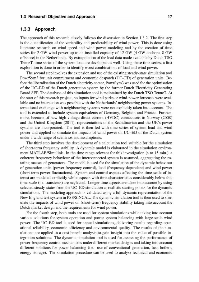
1.3.3 Approach
The approach of this research closely follows the discussion in Section 1.3.2. The first stepis the quantification of the variability and predictability of wind power. This is done usingliterature research on wind speed and wind-power modeling and by the creation of timeseries for 2 GW wind power up to an installed capacity of 12 GW (4 GW onshore, 8 GWoffshore) in the Netherlands. By extrapolation of the load data made available by Dutch TSOTenneT, time series of the system load are developed as well. Using these time series, a firstexploration is done in order to identify worst combinations of load and wind power.
The second step involves the extension and use of the existing steady-state simulation toolPowrSym3 for unit commitment and economic despatch (UC–ED) of generation units. Be-fore the liberalisation of the Dutch electricity sector, PowrSym3 was used for the optimisationof the UC–ED of the Dutch generation system by the former Dutch Electricity GeneratingBoard SEP. The database of this simulation tool is maintained by the Dutch TSO TenneT. Atthe start of this research project, no inputs for wind parks or wind-power forecasts were avai-lable and no interaction was possible with the Netherlands’ neighbouring power systems. In-ternational exchange with neighbouring systems were not explicitly taken into account. Thetool is extended to include system equivalents of Germany, Belgium and France. Further-more, because of new high-voltage direct current (HVDC) connections to Norway (2008)and the United Kingdom (2011), representations of the Scandinavian and the UK’s powersystems are incorporated. The tool is then fed with time series of system load and windpower and applied to simulate the impacts of wind power on UC–ED of the Dutch systemunder a wide range of scenarios and assumptions.
The third step involves the development of a calculation tool suitable for the simulationof short-term frequency stability. A dynamic model is elaborated in the simulation environ-ment MATLAB/Simulink. In the time range relevant for this investigation (s to 15 min.) acoherent frequency behaviour of the interconnected system is assumed, aggregating the ro-tating masses of generators. The model is used for the simulation of the dynamic behaviourof generation units (power frequency control), load (frequency dependent) and wind power(short-term power fluctuations). System and control aspects affecting the time-scale of in-terest are modeled explicitly while aspects with time characteristics considerably below thistime-scale (i.e. transients) are neglected. Longer time aspects are taken into account by usingselected steady-states from the UC–ED simulation as realistic starting points for the dynamicsimulations. The modeling approach is validated using a full dynamic representation of theNew England test system in PSS/SINCAL. The dynamic simulation tool is then used to sim-ulate the impacts of wind power on (short-term) frequency stability taking into account theDutch market design and the requirements for wind power.
For the fourth step, both tools are used for system simulations while taking into accountvarious solutions for system operation and power system balancing with large-scale windpower. The UC–ED tool is used for annual simulations, delivering results regarding oper-ational reliability, economic efficiency and environmental quality. The results of the sim-ulations are applied in a cost-benefit analysis to gain insight into the value of possible in-tegration solutions. The dynamic simulation tool is used for assessing the performance ofpower-frequency control mechanisms under different market designs and taking into accountdifferent solutions for power balancing (i.e. use of conventional generation, heat-boilers,energy storage). The simulation procedure can be used to analyse technical and economic

18 Introduction
opportunities of changes in market design and control mechanisms in order to integrate largequantities of wind power.
1.3.4 Research Framework: We@Sea
The Dutch government is considering a target for the development of 6000 MW of windpower in the Dutch part of the North Sea by 2020. In order to meet this target, knowledgeand technical expertise are required to build and operate these wind farms in a reliable andefficient way. The provision of a subsidy for gaining such expertise and knowledge was thedriving force in the formation of the consortium We@Sea (Wind energy at Sea). The objec-tive of We@Sea is the acquisition of knowledge in order to facilitate a sound implementation(minimisation of risks) of wind power in the North Sea. The experience of the first twooffshore wind parks in Dutch waters will be used. Application of acquired knowledge andexperiences is a continuous process, in which We@Sea wants to play an active role. TheWe@Sea consortium has over thirty industrial and research partners.
The organisation of We@Sea consists of two foundations: the We@Sea foundation andthe We@Sea/Bsik foundation. The first foundation is an organisation aiming for the acqui-sition of offshore wind power knowledge. The We@Sea foundation has obtained a subsidy(Bsik) for the research and development program ’Large-scale wind power generation off-shore’. The We@Sea/Bsik foundation is an intermediary for this subsidy from the Dutch gov-ernmental agency for sustainability and innovation, SenterNovem, to the different research andevelopment projects. These projects comprise seven research lines covering technical, eco-nomical, market, installation and environmental aspects of large-scale offshore wind powerand have a total budget exceeding e 26 million.
The Ph.D. program of We@Sea tackles some of the more academic questions that requirea deeper scope and longer period of knowledge and technology development and of which theoutcome and benefits are less certain at the outset. The Ph.D. programme comprises elevenPh.D. projects, three of which fall under research line 3: Energy transport and distribution.The aim of the research project ’Grid Stability’, which has led to this thesis, is to facilitatelarge-scale integration of wind power in the electrical power system by the development ofsolutions for problems in maintaining the power balance.
1.4 Thesis Outline
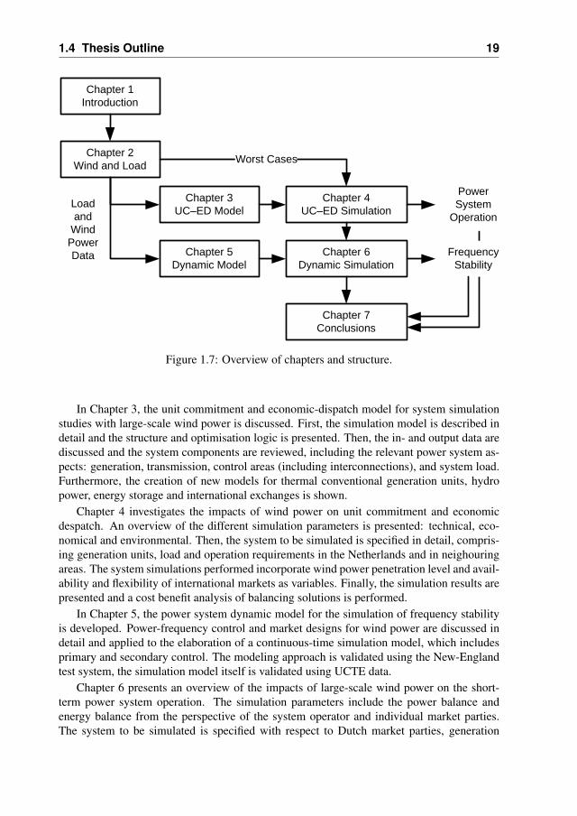
The structure of this thesis reflects the research objective and its sub-objectives formulatedabove. Every chapter starts with a short introduction, presenting the most relevant topics tobe treated and stating the specific contributions of this research, and ends with a summaryand conclusions on the main findings. The thesis’ overall structure is presented in Fig. 1.7.
In Chapter 2, the development of wind power in relation to system load estimates is dis-cussed. Taking the Netherlands as a case-study, wind speed time-series for on- and offshoremeasurement locations are used for the development of wind power time-series at current andpredicted wind park locations for capacities up to 12 GW (4 GW onshore, 8 GW offshore).Time series for system load and wind power are analysed in combination in order to developduration curves, providing a first glance of the possible impacts of large-scale wind power onthe operation of the Dutch power system.
1.4 Thesis Outline 19
Chapter 1 Introduction
Chapter 2Wind and Load
Chapter 3UC–ED Model
Chapter 4UC–ED Simulation
Chapter 5Dynamic Model
Chapter 6Dynamic Simulation
Worst Cases
Load and
Wind Power Data
Power System
Operation
Chapter 7Conclusions
Frequency Stability
Figure 1.7: Overview of chapters and structure.
In Chapter 3, the unit commitment and economic-dispatch model for system simulationstudies with large-scale wind power is discussed. First, the simulation model is described indetail and the structure and optimisation logic is presented. Then, the in- and output data arediscussed and the system components are reviewed, including the relevant power system as-pects: generation, transmission, control areas (including interconnections), and system load.Furthermore, the creation of new models for thermal conventional generation units, hydropower, energy storage and international exchanges is shown.
Chapter 4 investigates the impacts of wind power on unit commitment and economicdespatch. An overview of the different simulation parameters is presented: technical, eco-nomical and environmental. Then, the system to be simulated is specified in detail, compris-ing generation units, load and operation requirements in the Netherlands and in neighouringareas. The system simulations performed incorporate wind power penetration level and avail-ability and flexibility of international markets as variables. Finally, the simulation results arepresented and a cost benefit analysis of balancing solutions is performed.
In Chapter 5, the power system dynamic model for the simulation of frequency stabilityis developed. Power-frequency control and market designs for wind power are discussed indetail and applied to the elaboration of a continuous-time simulation model, which includesprimary and secondary control. The modeling approach is validated using the New-Englandtest system, the simulation model itself is validated using UCTE data.
Chapter 6 presents an overview of the impacts of large-scale wind power on the short-term power system operation. The simulation parameters include the power balance andenergy balance from the perspective of the system operator and individual market parties.The system to be simulated is specified with respect to Dutch market parties, generation

20 Introduction
portfolios and secondary control parameters. The simulation procedure is discussed, whichinvolves the selection of worst cases for wind power and load, simulation of these cases usingthe UC–ED tool, selection of units for secondary control and finally the choice of a certainshort-term balancing strategy. Then, system simulations are set-up for a range of wind powerlevels and market designs and the simulation results are presented.
In Chapter 7, the conclusions of this research are presented and recommendations forfurther research are made.
CHAPTER 2System Load and Wind Power
2.1 Introduction
In this chapter, system load and wind power data are developed, analysed and made availablefor use as inputs for the simulations to be performed later. Before going into the developmentof these data, it is important to realise what their intended applications are: use as input forsimulations of unit commitment and economic despatch and for frequency-stability simula-tions. Since these simulations comprise different time-scales, different time resolutions areused for which different data-sets are required. Existing work on the use of wind power andload data in simulation studies are discussed.
The contribution of this chapter is twofold. First, quantitative data are developed forlarge-scale wind power foreseen to be installed and these data are processed for use in systemsimulation studies. A methodology developed dr. Gibescu and dr. Brand [57] for windpower integration studies is applied for the developmenttion of wind power data taking intoaccount correlations. Second, detailed insight is gained into wind power’s variability andunpredictability on a power system scale. A first assessment of the possible impacts of windpower on power system operation is made by data analysis. The methodologies presented inthis chapter are applied here for the development of load and wind power data for simulationstudies of the Dutch system, but are generally applicable.
This chapter is organised as follows. First, adequate time resolutions are determined forthe development of data series for this research. System load data are investigated for periodicvariations (i.e. hourly, weekly) and extrapolated for the load expected in the year 2014, using
22 System Load and Wind Power
the Dutch system as a case-study. Then, a methodology is presented for the developmentof wind power data from wind speed measurements. A statistical interpolation method isused for the generation of wind speed time-series for onshore wind power and offshore windparks. Using the same methodology, lead-time dependent time-series of wind power forecasterrors are developed. The relation between wind speed and wind power is investigated fordifferent wind turbine technologies. Wind park production time-series and power system-aggregated wind power output time-series are then developed for the long- and short-termusing aggregated wind park power curves. System load and wind power are aggregated inorder to developte load-less-wind power duration curves, providing a first view on the impactof wind power at power system level.
2.2 System Load
2.2.1 Data Time Resolution
The research objectives distinguish between a long- and a short-term horizon, for power sys-tem operation and frequency stability, respectively. The long-term horizon covers unit com-mitment and economic dispatch (UC–ED), a steady-state optimisation process taking intoaccount generation cost and international trading possibilities, done in the hour (h.) to weektime-horizon. The short-term horizon comprises power system balancing, involving primaryand secondary control and subject to operation requirements formulated in the second (s) tominute (min.) time range. For the development of data, the time resolutions associated withthese must be determined. These are set based on power system operation requirements andmarket trading horizons applicable to the Netherlands.
Optimisation of unit commitment and economic dispatch is a long-term activity. Typi-cally, the time resolution for such simulations is one hour, being the time resolution for spotmarkets and for international exchange schedules throughout Europe [110]. System oper-ational requirements as set by UCTE for secondary control are specified for 15 min. timeintervals. Similarly, the imbalance (secondary reserve) market in the Netherlands applies atime resolution of 15 min. Taking into account that the continuous-time simulations of powersystem balancing use the simulation results of the UC–ED schedule as a starting point, thetime resolution for UC–ED in this research is also set to 15 min.
Power system balancing is a time-continuous process involving primary and secondarycontrol. Operation requirements for primary control as specified by UCTE include an actionbeginning within a few seconds (s) and a full activation within 30 s. The frequency and thepower exchanges must start returning to their set-point values as a result of secondary con-trol after 30 s with the correction completed within 15 min. [169]. Data used by UCTE formonitoring primary control and system frequency has a time resolution of 4 s. Measurementsof the system frequency are used by the transmission system operator (TSO) for the deve-lopment of a reference signal for secondary control, updated every 4 s [162]. Based on thisinformation, the time resolution for simulations of power system balancing is set at 4 s.
2.2.2 Development of Load Data
This research takes the Netherlands’ power system in the year 2014 as a base-case. Forthe estimation of the system load for the year 2014, aggregated load data obtained from
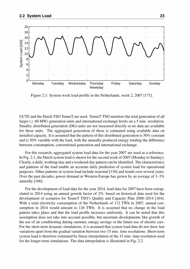
2.2 System Load 23
Monday Tuesday Wednesday Thursday Friday Saturday Sunday02468
101214161820
Weekday
Sys
tem
Loa
d [G
W]
Figure 2.1: System week load-profile in the Netherlands, week 2, 2007 [171].
UCTE and the Dutch TSO TenneT are used. TenneT TSO monitors the total generation of alllarger (≥ 60 MW) generation units and international exchange levels on a 5 min. resolution.Smaller, distributed generation (DG) units are not measured directly so no data are availablefor those units. The aggregated generation of these is estimated using available data oninstalled capacity. It is assumed that the pattern of this distributed generation is 50% constantand is 50% variable with the load, with the annually produced energy totaling the differencebetween consumption, conventional generation and international exchange.
For this research, aggregated system load data for the year 2007 are used as a reference.In Fig. 2.1, the Dutch system load is shown for the second week of 2007 (Monday to Sunday).Clearly, a daily, working-day and a weekend-day pattern can be identified. The characteristicsand patterns of the load enable an accurate daily prediction of system load for operationalpurposes. Other patterns in system load include seasonal [138] and trends over several years.Over the past decades, power demand in Western-Europe has grown by an average of 1–3%annually [166].
For the development of load data for the year 2014, load data for 2007 have been extrap-olated to 2014 using an annual growth factor of 2%, based on historical data used for thedevelopment of scenarios for TenneT TSO’s Quality and Capacity Plan 2008–2014 [164].With a total electricity consumption of the Netherlands of 112 TWh in 2007, annual con-sumption in 2014 would amount to 126 TWh. It is assumed that no change in the loadpattern takes place and that the load profile increases uniformly. It can be noted that thisassumption does not take into account possible, but uncertain developments like growth ofthe use of air conditioning during summer, energy savings or the future use of electric cars.For the short-term dynamic simulations, it is assumed that system load data do not show fastvariations apart from the gradual variation between two 15 min. time resolutions. Short-termsystem load is therefore estimated by linear interpolation of the 15 min. time resolution usedfor the longer-term simulations. The data interpolation is illustrated in Fig. 2.2.
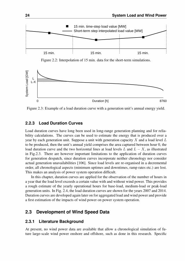
24 System Load and Wind Power
15 min. 15 min. 15 min.
Short-term step interpolated load value [MW]15 min. time-step load value [MW]
Figure 2.2: Interpolation of 15 min. data for the short-term simulations.
Duration [h] 87600
LL-X
Sys
tem
Loa
d [G
W]
Figure 2.3: Example of a load duration curve with a generation unit’s annual energy yield.
2.2.3 Load Duration Curves
Load duration curves have long been used in long-range generation planning and for relia-bility calculations. The curves can be used to estimate the energy that is produced over ayear by each generation unit. Suppose a unit with generation capacity X and a load level Lto be produced, then the unit’s annual yield comprises the area captured between hour 0, theload duration curve and the two horizontal lines at load levels L and L − X , as illustratedin Fig.2.3. There are however important limitations to the application of duration curvesfor generation despatch, since duration curves incorporate neither chronology nor consideractual generation unavailabilities [106]. Since load levels are re-organised in a decrementalorder, all chronological aspects (minimum uptimes and downtimes, ramp rates etc.) are lost.This makes an analysis of power system operation difficult.
In this chapter, duration curves are applied for the observation of the number of hours ina year that the load level exceeds a certain value with and without wind power. This providesa rough estimate of the yearly operational hours for base-load, medium-load or peak-loadgeneration units. In Fig. 2.4, the load duration curves are shown for the years 2007 and 2014.Duration curves are developed again later on for aggregated load and wind power and providea first estimation of the impacts of wind power on power system operation.
2.3 Development of Wind Speed Data
2.3.1 Literature Background
At present, no wind power data are available that allow a chronological simulation of fu-ture large-scale wind power onshore and offshore, such as done in this research. Specific

2.3 Development of Wind Speed Data 25
1000 2000 3000 4000 5000 6000 7000 8000 87600
2
4
6
8
10
12
14
16
18
20
22
Duration [h]
Sys
tem
Loa
d [G
W]
Load 2014 (forecast)Load 2007
Figure 2.4: Load duration curves for the Netherlands in 2007 and 2014 (forecast).
data must therefore be developed, based on available measurements of wind speed. Thetime-series aspects of wind speed data for the development of wind power data are of crit-ical importance. Furthermore, spatial correlations exist between wind speeds at differentlocations. The aggregated variability and unpredictability of wind park outputs are not cor-rectly assessed in case spatial correlations of wind speeds are not taken into account, sincegeographical spreading of wind power leads to smoothing effects of the total output [122].Approaches based on probability distribution functions (i.e. Weibul) such as (embedded)Markov-chain models or the Shinozuka algorithm [91] are thus insufficient for this research.
Existing wind power integration studies generally do not include all wind speed charac-teristics required for chronological simulation studies. In reference [37], cross-correlationsbetween wind park locations are specifically taken into account using power spectrum density(PSD) functions and wind speed coherence (spatial correlation). However, rather than usingwind speed measurements, reference [37] develops synthetic wind speed data-series basedon wind speed distributions by application of the Shinozuka method. Furthermore, the loga-rithmic approach applied for height transformation is insufficient for an accurate estimationof wind speeds at turbine hub-height. Reference [44] uses only synthesised wind speed data,providing insufficient guarantee of a correct representation of wind power. Combinations ofmeasured and synthesised wind speed time series are used for the assessment of hourly windpower variations in [71].
The correlation of wind speeds in park-sized areas are analysed in [123] with the inclusionof wind direction, velocity and fluctuation effects. The study shows that power variationsexceeding 10 min. time intervals are most important, rather than the variations within 10 minwhich balance out between different wind parks. Correlation coefficients of the output ofdistant wind turbines differ considerably between days and the smoothing effects amongwind farms distributed over hundreds of km. are not so significant [122]. Thus, the impacts ofwind power variability on power system operation must be predominantly considered in the10 min and above time ranges and this variability is considerable, even over large distances.
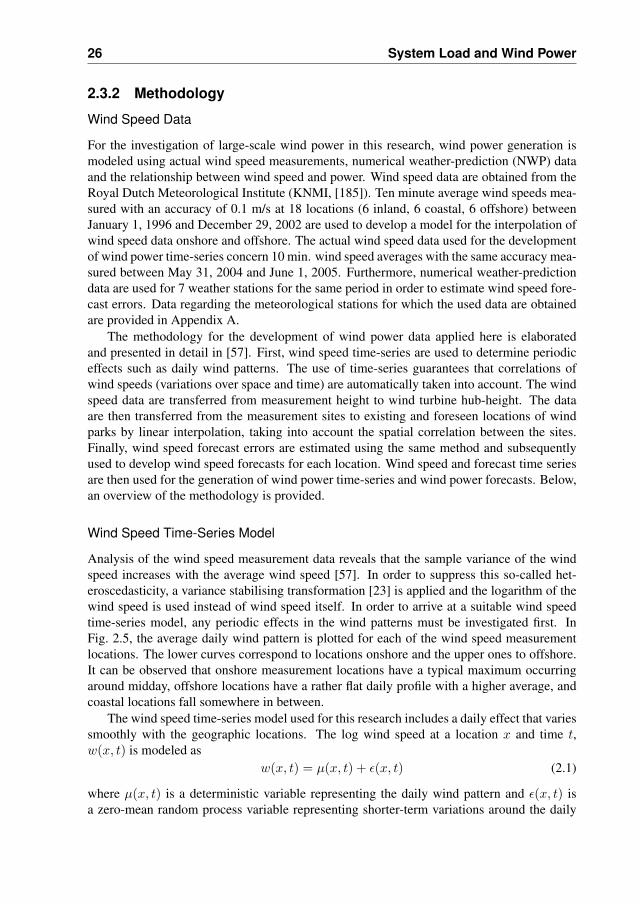
26 System Load and Wind Power
2.3.2 Methodology
Wind Speed Data
For the investigation of large-scale wind power in this research, wind power generation ismodeled using actual wind speed measurements, numerical weather-prediction (NWP) dataand the relationship between wind speed and power. Wind speed data are obtained from theRoyal Dutch Meteorological Institute (KNMI, [185]). Ten minute average wind speeds mea-sured with an accuracy of 0.1 m/s at 18 locations (6 inland, 6 coastal, 6 offshore) betweenJanuary 1, 1996 and December 29, 2002 are used to develop a model for the interpolation ofwind speed data onshore and offshore. The actual wind speed data used for the developmentof wind power time-series concern 10 min. wind speed averages with the same accuracy mea-sured between May 31, 2004 and June 1, 2005. Furthermore, numerical weather-predictiondata are used for 7 weather stations for the same period in order to estimate wind speed fore-cast errors. Data regarding the meteorological stations for which the used data are obtainedare provided in Appendix A.
The methodology for the development of wind power data applied here is elaboratedand presented in detail in [57]. First, wind speed time-series are used to determine periodiceffects such as daily wind patterns. The use of time-series guarantees that correlations ofwind speeds (variations over space and time) are automatically taken into account. The windspeed data are transferred from measurement height to wind turbine hub-height. The dataare then transferred from the measurement sites to existing and foreseen locations of windparks by linear interpolation, taking into account the spatial correlation between the sites.Finally, wind speed forecast errors are estimated using the same method and subsequentlyused to develop wind speed forecasts for each location. Wind speed and forecast time seriesare then used for the generation of wind power time-series and wind power forecasts. Below,an overview of the methodology is provided.
Wind Speed Time-Series Model
Analysis of the wind speed measurement data reveals that the sample variance of the windspeed increases with the average wind speed [57]. In order to suppress this so-called het-eroscedasticity, a variance stabilising transformation [23] is applied and the logarithm of thewind speed is used instead of wind speed itself. In order to arrive at a suitable wind speedtime-series model, any periodic effects in the wind patterns must be investigated first. InFig. 2.5, the average daily wind pattern is plotted for each of the wind speed measurementlocations. The lower curves correspond to locations onshore and the upper ones to offshore.It can be observed that onshore measurement locations have a typical maximum occurringaround midday, offshore locations have a rather flat daily profile with a higher average, andcoastal locations fall somewhere in between.
The wind speed time-series model used for this research includes a daily effect that variessmoothly with the geographic locations. The log wind speed at a location x and time t,w(x, t) is modeled as
w(x, t) = µ(x, t) + ε(x, t) (2.1)
where µ(x, t) is a deterministic variable representing the daily wind pattern and ε(x, t) isa zero-mean random process variable representing shorter-term variations around the daily
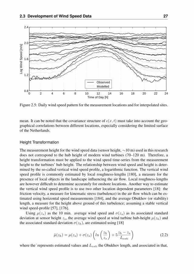
2.3 Development of Wind Speed Data 27
0 2 4 6 8 10 12 14 16 18 20 22 240.8
1.2
1.6
2.0
2.4
Time of Day [h]
Log
Win
d S
peed
[m/s
]
ModelledObserved
Figure 2.5: Daily wind speed pattern for the measurement locations and for interpolated sites.
mean. It can be noted that the covariance structure of ε(x, t) must take into account the geo-graphical correlations between different locations, especially considering the limited surfaceof the Netherlands.
Height Transformation
The measurement height for the wind speed data (sensor height,∼10 m) used in this researchdoes not correspond to the hub height of modern wind turbines (70–120 m). Therefore, aheight transformation must be applied to the wind speed time-series from the measurementheight to the turbines’ hub height. The relationship between wind speed and height is deter-mined by the so-called vertical wind speed profile, a logarithmic function. The vertical windspeed profile is commonly estimated by local roughness-lengths [180], a measure for thepresence of local objects in the landscape influencing the air flow. Local roughness-lengthsare however difficult to determine accurately for onshore locations. Another way to estimatethe vertical wind speed profile is to use two other location dependent parameters [18]: thefriction velocity, a measure for kinematic stress (turbulence) in the air flow which can be es-timated using horizontal speed measurements [184], and the average Obukhov (or stability)length, a measure for the height above ground of this turbulence; assuming a stable verticalwind speed-profile [57], [176].
Using µ(zs) as the 10 min. average wind speed and σ(zs) as its associated standarddeviation at sensor height zs, the average wind speed at wind turbine hub-height µ(zh) andthe associated standard deviation σ(zh), are estimated using [18]
µ(zh) = µ(zs) + σ(zs)(
ln
(zh
zs
)+ 5
zh − zs
Lesti
)(2.2)
where theˆrepresents estimated values and Lesti the Obukhov length, and associated in that,
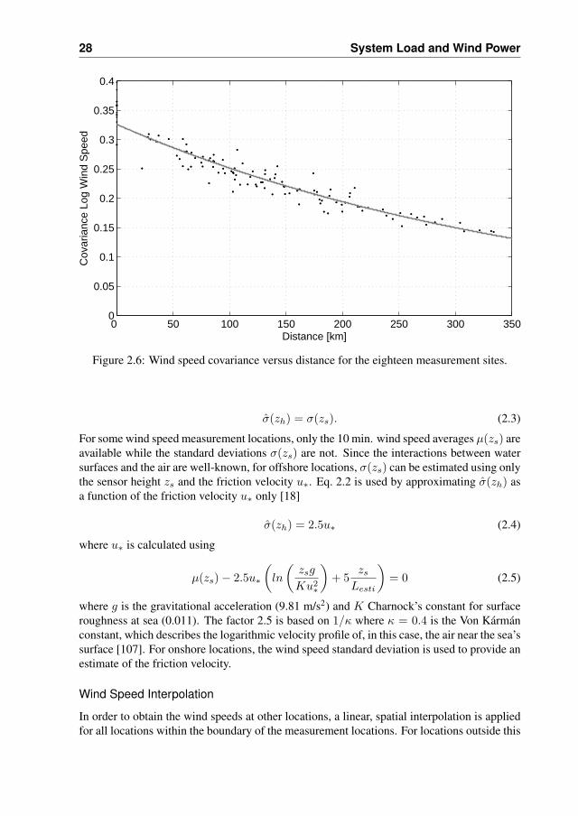
28 System Load and Wind Power
0 50 100 150 200 250 300 3500
0.05
0.1
0.15
0.2
0.25
0.3
0.35
0.4
Distance [km]
Cov
aria
nce
Log
Win
d S
peed
Figure 2.6: Wind speed covariance versus distance for the eighteen measurement sites.
σ(zh) = σ(zs). (2.3)
For some wind speed measurement locations, only the 10 min. wind speed averages µ(zs) areavailable while the standard deviations σ(zs) are not. Since the interactions between watersurfaces and the air are well-known, for offshore locations, σ(zs) can be estimated using onlythe sensor height zs and the friction velocity u∗. Eq. 2.2 is used by approximating σ(zh) asa function of the friction velocity u∗ only [18]
σ(zh) = 2.5u∗ (2.4)
where u∗ is calculated using
µ(zs)− 2.5u∗
(ln
(zsg
Ku2∗
)+ 5
zs
Lesti
)= 0 (2.5)
where g is the gravitational acceleration (9.81 m/s2) and K Charnock’s constant for surfaceroughness at sea (0.011). The factor 2.5 is based on 1/κ where κ = 0.4 is the Von Karmanconstant, which describes the logarithmic velocity profile of, in this case, the air near the sea’ssurface [107]. For onshore locations, the wind speed standard deviation is used to provide anestimate of the friction velocity.
Wind Speed Interpolation
In order to obtain the wind speeds at other locations, a linear, spatial interpolation is appliedfor all locations within the boundary of the measurement locations. For locations outside this

2.3 Development of Wind Speed Data 29
boundary, nearest-neighbour interpolation is applied. For the estimation of the random com-ponent ε(z, t), the covariance cov(ε(z1, t), ε(z2, t)) between two locations z1(x1, y1) andz2(x2, y2) is calculated. In Fig. 2.6, wind speed covariances (here: a measure for the cor-relation of wind speed variations between locations) are plotted versus the distance betweenmeasurement locations. Assuming that covariance approaches zero at large distances, it ismodeled through an exponential decay:
cov(ε(z1, h), ε(z2, h)) = Ce−a||z1−z2|| (2.6)
Parameters C and a are estimated using a least square fit, also shown in Fig. 2.6, with 1/aas the characteristic distance or decay parameter. Translation of this decay-fit from log windspeed to wind speed gives a characteristic distance of 610 km, a value in line with valuesreported in [59, 71].
The locations for thirteen onshore and 25 offshore wind parks are determined, as shownin Appendix B. The wind speeds at these locations are estimated by interpolation of the windspeed data at the eighteen measurement locations (Appendix A). The linear interpolationtakes into account the spatial correlations among multiple sites to arrive at wind speed time-series for existing and foreseen wind power locations [57]. The results are cross-validated byremoving one location from the n-site measurement set at a time and using the remaining n-1measurement sites to estimate it.
Linear interpolation is also been used to construct the lag-1 (auto-)covariances (Fig. 2.6).Correlations between subsequent 10 min. intervals are also taken into account. It is assumedthat the wind speed time series have the Markov property: given the measurements at time t,and the measured and interpolated values at time t − 1, the interpolated values at time t areindependent of values at previous time steps t− k, for k > 1. The obtained 10 min. averagesof wind speed at the foreseen wind park locations are then converted to 15 min. averages.
Wind Speed Forecast Errors
The 15 min. averaged wind speed time-series developed above are applied using the forecastmethodology for wind power AVDE (Aanbodvoorspelling Duurzame Energie, in English:supply forecast of renewable energy). This method developed in [19] is a physical one with astatistics module output comparable to the approach applied in [102] and takes into accountthe local influences of roughness, obstacles, and stability on wind speeds at the specifiedheight. The forecasts are based on underlying runs of the atmospheric High-Resolution Lim-ited Area Model (HIRLAM). HIRLAM numerically approximates the physical state of theatmosphere at 6 h. intervals with initial conditions taken from recent observations. Thewind speeds approximated by HIRLAM are post-processed by AVDE into 15 min. averagedwind speed at hub-height for two onshore and five offshore measurement locations. Theseapproximated wind speeds are then compared to the measured wind speeds to obtain windspeed forecast errors. Using the same method applied for interpolating wind speed data, thewind speed forecast errors are interpolated to the foreseen locations, and finally added tothe interpolated wind speeds to develop forecast wind speed time series at the locations ofinterest. Since the time-dependency of wind speeds is taken into account in the wind speedinterpolation method, time-dependence is automatically included in the forecast time seriesas well.

30 System Load and Wind Power
Monday Tuesday Wednesday Thursday Friday Saturday Sunday0
2
4
6
8
10
12
14
16
Weekday
Win
d S
peed
[m/s
]
Onshore LocationOffshore Location AOffshore Location B
Figure 2.7: Calculated wind speeds for one week for one onshore and two offshore locations.
The minimum lead-time of the NWP-model fed forecasting method used here is 6 h.The first 0–6 h. are filled-in by a persistence-based forecasting method fed by real-timemeasurement data. For this, the 12–36 h. ahead aggregated wind power forecast errors aremodeled as a first-order auto-regressive moving average (ARMA) process:
φ(t) = aφ(t− 1) + bγ(t− 1) + γ(t) (2.7)
where γ(t) ∼ N (0, σ) is a zero-mean, normally-distributed noise term of standard deviationσ. The a, b and σ parameters of the ARMA process are estimated via the MLE (MaximumLikelihood Estimator) method [23]. One 1–36 h. ahead wind power forecast is developed foreach hour of the year.
2.3.3 Results
The methodology presented above is used to generate one year of 15 min. average windspeed time-series for specified onshore and offshore locations. The time-series for all loca-tions are consistent with respect to correlations in time and geography. Furthermore, windspeed forecasts are developd for the same locations for each hour, with a 15 min. resolution,for forecast lead-time of up to 36 h. while also respecting the correlation structure amongthe various locations. Fig. 2.7 illustrates the generated wind speed data for three locations,for one week. The generated time-series are used to develop wind power time-series forindividual wind park locations.
2.4 Development of Wind-Power Data
2.4.1 Literature Background
Different methodologies exist for the development of wind power from wind speed data andinclude the use of wind turbine power curves, aggregated wind park power curves and sta-tistical modeling [141]. Power curves for the conversion of wind speed to wind power are
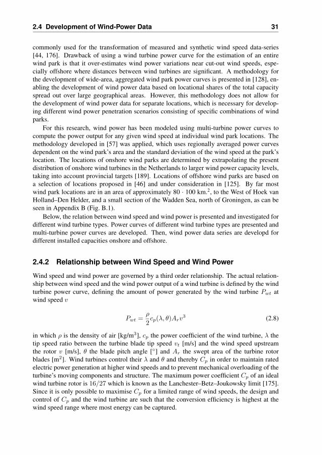
2.4 Development of Wind-Power Data 31
commonly used for the transformation of measured and synthetic wind speed data-series[44, 176]. Drawback of using a wind turbine power curve for the estimation of an entirewind park is that it over-estimates wind power variations near cut-out wind speeds, espe-cially offshore where distances between wind turbines are significant. A methodology forthe development of wide-area, aggregated wind park power curves is presented in [128], en-abling the development of wind power data based on locational shares of the total capacityspread out over large geographical areas. However, this methodology does not allow forthe development of wind power data for separate locations, which is necessary for develop-ing different wind power penetration scenarios consisting of specific combinations of windparks.
For this research, wind power has been modeled using multi-turbine power curves tocompute the power output for any given wind speed at individual wind park locations. Themethodology developed in [57] was applied, which uses regionally averaged power curvesdependent on the wind park’s area and the standard deviation of the wind speed at the park’slocation. The locations of onshore wind parks are determined by extrapolating the presentdistribution of onshore wind turbines in the Netherlands to larger wind power capacity levels,taking into account provincial targets [189]. Locations of offshore wind parks are based ona selection of locations proposed in [46] and under consideration in [125]. By far mostwind park locations are in an area of approximately 80 · 100 km.2, to the West of Hoek vanHolland–Den Helder, and a small section of the Wadden Sea, north of Groningen, as can beseen in Appendix B (Fig. B.1).
Below, the relation between wind speed and wind power is presented and investigated fordifferent wind turbine types. Power curves of different wind turbine types are presented andmulti-turbine power curves are developed. Then, wind power data series are developd fordifferent installed capacities onshore and offshore.
2.4.2 Relationship between Wind Speed and Wind Power
Wind speed and wind power are governed by a third order relationship. The actual relation-ship between wind speed and the wind power output of a wind turbine is defined by the windturbine power curve, defining the amount of power generated by the wind turbine Pwt atwind speed v
Pwt =ρ
2cp(λ, θ)Arv
3 (2.8)
in which ρ is the density of air [kg/m3], cp the power coefficient of the wind turbine, λ thetip speed ratio between the turbine blade tip speed vt [m/s] and the wind speed upstreamthe rotor v [m/s], θ the blade pitch angle [◦] and Ar the swept area of the turbine rotorblades [m2]. Wind turbines control their λ and θ and thereby Cp in order to maintain ratedelectric power generation at higher wind speeds and to prevent mechanical overloading of theturbine’s moving components and structure. The maximum power coefficient Cp of an idealwind turbine rotor is 16/27 which is known as the Lanchester–Betz–Joukowsky limit [175].Since it is only possible to maximise Cp for a limited range of wind speeds, the design andcontrol of Cp and the wind turbine are such that the conversion efficiency is highest at thewind speed range where most energy can be captured.
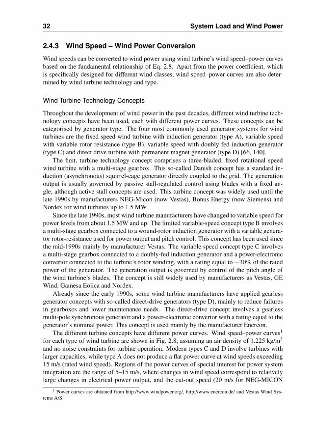
32 System Load and Wind Power
2.4.3 Wind Speed – Wind Power Conversion
Wind speeds can be converted to wind power using wind turbine’s wind speed–power curvesbased on the fundamental relationship of Eq. 2.8. Apart from the power coefficient, whichis specifically designed for different wind classes, wind speed–power curves are also deter-mined by wind turbine technology and type.
Wind Turbine Technology Concepts
Throughout the development of wind power in the past decades, different wind turbine tech-nology concepts have been used, each with different power curves. These concepts can becategorised by generator type. The four most commonly used generator systems for windturbines are the fixed speed wind turbine with induction generator (type A), variable speedwith variable rotor resistance (type B), variable speed with doubly fed induction generator(type C) and direct drive turbine with permanent magnet generator (type D) [66, 140].
The first, turbine technology concept comprises a three-bladed, fixed rotational speedwind turbine with a multi-stage gearbox. This so-called Danish concept has a standard in-duction (asynchronous) squirrel-cage generator directly coupled to the grid. The generationoutput is usually governed by passive stall-regulated control using blades with a fixed an-gle, although active stall concepts are used. This turbine concept was widely used until thelate 1990s by manufacturers NEG-Micon (now Vestas), Bonus Energy (now Siemens) andNordex for wind turbines up to 1.5 MW.
Since the late 1990s, most wind turbine manufacturers have changed to variable speed forpower levels from about 1.5 MW and up. The limited variable-speed concept type B involvesa multi-stage gearbox connected to a wound-rotor induction generator with a variable genera-tor rotor-resistance used for power output and pitch control. This concept has been used sincethe mid-1990s mainly by manufacturer Vestas. The variable speed concept type C involvesa multi-stage gearbox connected to a doubly-fed induction generator and a power-electronicconvertor connected to the turbine’s rotor winding, with a rating equal to ∼30% of the ratedpower of the generator. The generation output is governed by control of the pitch angle ofthe wind turbine’s blades. The concept is still widely used by manufacturers as Vestas, GEWind, Gamesa Eolica and Nordex.
Already since the early 1990s, some wind turbine manufacturers have applied gearlessgenerator concepts with so-called direct-drive generators (type D), mainly to reduce failuresin gearboxes and lower maintenance needs. The direct-drive concept involves a gearlessmulti-pole synchronous generator and a power-electronic convertor with a rating equal to thegenerator’s nominal power. This concept is used mainly by the manufacturer Enercon.
The different turbine concepts have different power curves. Wind speed–power curves1
for each type of wind turbine are shown in Fig. 2.8, assuming an air density of 1.225 kg/m3
and no noise constraints for turbine operation. Modern types C and D involve turbines withlarger capacities, while type A does not produce a flat power curve at wind speeds exceeding15 m/s (rated wind speed). Regions of the power curves of special interest for power systemintegration are the range of 5–15 m/s, where changes in wind speed correspond to relativelylarge changes in electrical power output, and the cut-out speed (20 m/s for NEG-MICON
1 Power curves are obtained from http://www.windpower.org/, http://www.enercon.de/ and Vestas Wind Sys-tems A/S

2.4 Development of Wind-Power Data 33
0 5 10 15 20 25 30 350
0.2
0.4
0.6
0.8
1
Wind Speed [m/s]
Pow
er O
utpu
t [p.
u.]
NM48 (A) V52 (B) V90 (C) E82 (D)
Figure 2.8: Wind turbine power curves for the NEG-MICON NM48 (A), Vestas V52 (B),Vestas V90 (C) and Enercon E82 with storm control (D).
NM48, 25 m/s for Vestas V52 and V90), around which the power output of the wind turbinealternates between full and no power.
Development of Long-Term Wind Power Data
A differentiation is made between long-term simulations (UC–ED, 15 min. time resolution)and short-term simulations (frequency stability, 4 s). For the development of long-term datafor regional onshore wind power output and offshore wind parks, the multi-turbine approachdeveloped in [57] is used. This approach makes use of the distance between wind turbineswithin a wind park to develop a Gaussian filter (normal distribution function), estimating thewind speed deviations at wind turbine locations around the park’s average wind speed. Foreach wind park, a location-dependent power curve is developed based on the local standarddeviation of wind speed and the geographical size of the wind park. The approach ignorespark effects such as wind turbine wakes. Park effects may slightly alter annual yields [97] butare considered here to be negligible compared to the assumptions made regarding wind parklocations, distances of turbines and wind park lay-out and the differences in energy contentbetween various wind years.
The method establishes a regionally averaged speed–power curve for each wind parkby applying a distance scale and Gaussian filter to the single-turbine power curve. The filteroriginates from the local wind climate, taking into account regional variations of wind speedsbased on exponential decay. The width σF of the Gaussian filter is calculated from
σF = σ√
0.5(1− e−Dave/Ddecay
)(2.9)
where σ is the standard deviation of the local wind speed, Dave is the distance scale (av-erage distance between locations) and Ddecay is the characteristic distance of the decay ofcorrelation.

34 System Load and Wind Power
Since the individual turbine locations are not known, the distance scale Dave must beestimated. Considering a wind park with area A with N wind turbines, the length scale Lthat characterises the area, can be defined as
L =√
A/π (2.10)
The average distance scale Dave can be estimated from the minimum and maximum distancedistance between two turbines Dmin and Dmax. Introducing the area per turbine locationAT as
AT =A
N(2.11)
and the corresponding characteristic length scale for each turbine LT as
LT =A
πN, (2.12)
Dmin is estimated as 2*LT , while Dmax is estimated as 2*L. The average distance scaleDave is estimated to be
Dave =dmax + 2dmin
3=
23
√A
π
(1 +
2√N
). (2.13)
In this research, the wind park area A is related to a Dutch province for the onshore parks andto an individual wind farm for the offshore. The area of an individual park is approximatedby the area of a rectangle with sides depending on the number of turbines N and the rotordiameter and capacity of the wind turbines. For the onshore locations, it is assumed that thesecomprise the most common type C or D turbines with power curves as presented in Fig. 2.8.Each onshore turbine has an installed power of 2 MW and a rotor diameter of 80 m and theonshore wind turbines are spaced at 400 m (five times rotor diameter). Offshore wind parksare assumed to consist of 5 MW C-type turbines, since wind turbine of this capacity presentlyavailable are of this type. It is assumed that offshore wind turbines have rotor diameters of120 m and are spaced by 720 m (six times rotor diameter) based on practical experienceswith existing offshore wind parks.
The multi-turbine curves for individual wind parks are obtained by applying the aboveGaussian filter (σF ) to the wind turbine power curves, delivering a multi-turbine curve foreach wind park. Fig. 2.9 shows an example of a multi-turbine curve developed for an offshorewind park using the method explained in [57]. The influence of the Gaussian filter is mostvisible around the cut-out wind speed (25 m/s), where the wind turbine alternates betweenfull power and no power. This illustrates how the wind speed deviations from the wind park’saverage wind speed at individual turbine locations result in a smoothing of the wind park’spower curve. The wind speed data developed above for each wind park location can bemultiplied with the parks’ multi-turbine power curve in order to develop wind power data.
The last step for the development of the wind power time-series for each wind park is theincorporation of the unavailability of wind turbines. This can be done in different ways, witha full Monte Carlo outage approach delivering the most accurate results. The large number ofwind turbines (∼1000 for the smallest penetration level) and the aggregation of wind poweroutput at system level makes that the added value of this approach is limited compared to an
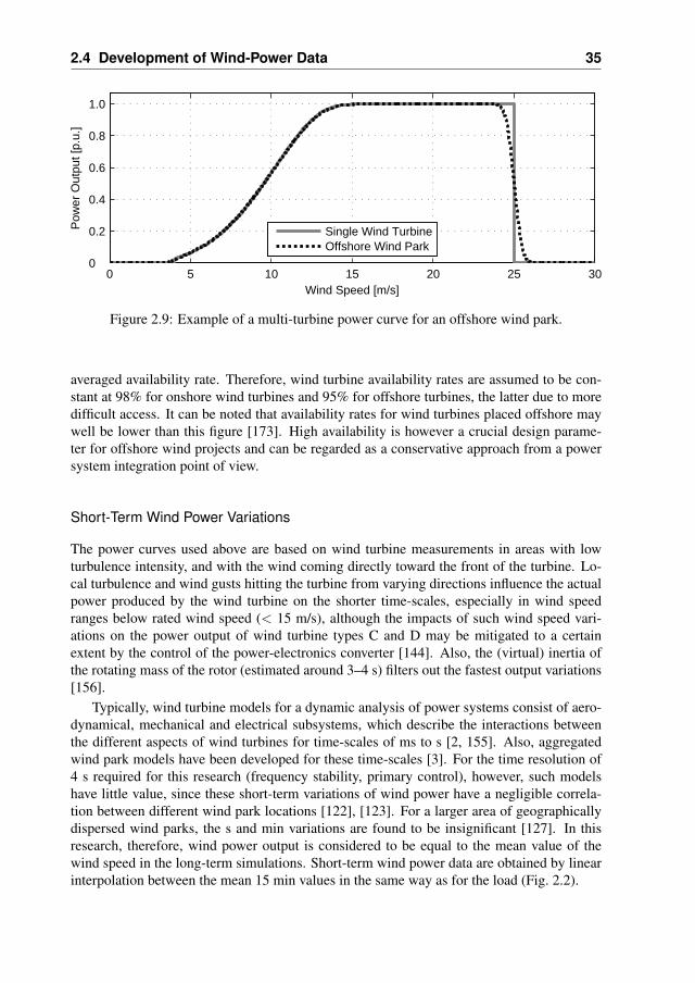
2.4 Development of Wind-Power Data 35
0 5 10 15 20 25 300
0.2
0.4
0.6
0.8
1.0
Wind Speed [m/s]
Pow
er O
utpu
t [p.
u.]
Single Wind TurbineOffshore Wind Park
Figure 2.9: Example of a multi-turbine power curve for an offshore wind park.
averaged availability rate. Therefore, wind turbine availability rates are assumed to be con-stant at 98% for onshore wind turbines and 95% for offshore turbines, the latter due to moredifficult access. It can be noted that availability rates for wind turbines placed offshore maywell be lower than this figure [173]. High availability is however a crucial design parame-ter for offshore wind projects and can be regarded as a conservative approach from a powersystem integration point of view.
Short-Term Wind Power Variations
The power curves used above are based on wind turbine measurements in areas with lowturbulence intensity, and with the wind coming directly toward the front of the turbine. Lo-cal turbulence and wind gusts hitting the turbine from varying directions influence the actualpower produced by the wind turbine on the shorter time-scales, especially in wind speedranges below rated wind speed (< 15 m/s), although the impacts of such wind speed vari-ations on the power output of wind turbine types C and D may be mitigated to a certainextent by the control of the power-electronics converter [144]. Also, the (virtual) inertia ofthe rotating mass of the rotor (estimated around 3–4 s) filters out the fastest output variations[156].
Typically, wind turbine models for a dynamic analysis of power systems consist of aero-dynamical, mechanical and electrical subsystems, which describe the interactions betweenthe different aspects of wind turbines for time-scales of ms to s [2, 155]. Also, aggregatedwind park models have been developed for these time-scales [3]. For the time resolution of4 s required for this research (frequency stability, primary control), however, such modelshave little value, since these short-term variations of wind power have a negligible correla-tion between different wind park locations [122], [123]. For a larger area of geographicallydispersed wind parks, the s and min variations are found to be insignificant [127]. In thisresearch, therefore, wind power output is considered to be equal to the mean value of thewind speed in the long-term simulations. Short-term wind power data are obtained by linearinterpolation between the mean 15 min values in the same way as for the load (Fig. 2.2).
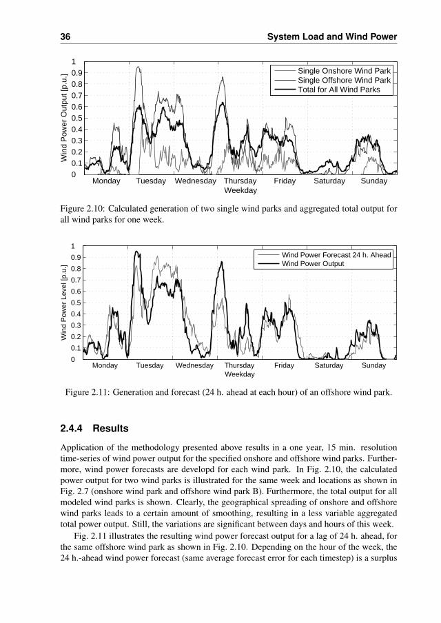
36 System Load and Wind Power
Monday Tuesday Wednesday Thursday Friday Saturday Sunday0 0.10.20.30.40.50.60.70.80.91
Weekday
Win
d P
ower
Out
put [
p.u.
]
Single Onshore Wind ParkSingle Offshore Wind ParkTotal for All Wind Parks
Figure 2.10: Calculated generation of two single wind parks and aggregated total output forall wind parks for one week.
Monday Tuesday Wednesday Thursday Friday Saturday Sunday0 0.10.20.30.40.50.60.70.80.91
Weekday
Win
d P
ower
Lev
el [p
.u.]
Wind Power Forecast 24 h. AheadWind Power Output
Figure 2.11: Generation and forecast (24 h. ahead at each hour) of an offshore wind park.
2.4.4 Results
Application of the methodology presented above results in a one year, 15 min. resolutiontime-series of wind power output for the specified onshore and offshore wind parks. Further-more, wind power forecasts are developd for each wind park. In Fig. 2.10, the calculatedpower output for two wind parks is illustrated for the same week and locations as shown inFig. 2.7 (onshore wind park and offshore wind park B). Furthermore, the total output for allmodeled wind parks is shown. Clearly, the geographical spreading of onshore and offshorewind parks leads to a certain amount of smoothing, resulting in a less variable aggregatedtotal power output. Still, the variations are significant between days and hours of this week.
Fig. 2.11 illustrates the resulting wind power forecast output for a lag of 24 h. ahead, forthe same offshore wind park as shown in Fig. 2.10. Depending on the hour of the week, the24 h.-ahead wind power forecast (same average forecast error for each timestep) is a surplus
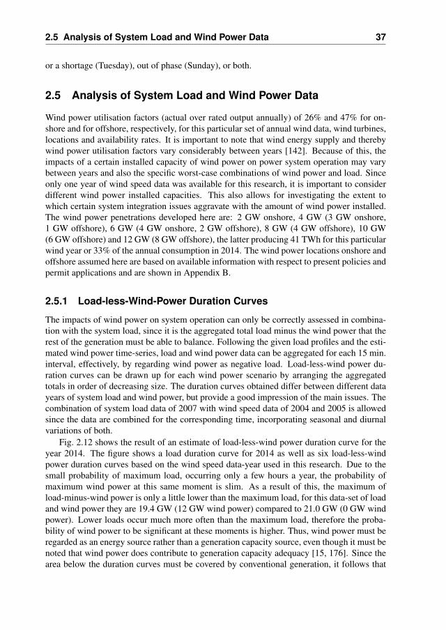
2.5 Analysis of System Load and Wind Power Data 37
or a shortage (Tuesday), out of phase (Sunday), or both.
2.5 Analysis of System Load and Wind Power Data
Wind power utilisation factors (actual over rated output annually) of 26% and 47% for on-shore and for offshore, respectively, for this particular set of annual wind data, wind turbines,locations and availability rates. It is important to note that wind energy supply and therebywind power utilisation factors vary considerably between years [142]. Because of this, theimpacts of a certain installed capacity of wind power on power system operation may varybetween years and also the specific worst-case combinations of wind power and load. Sinceonly one year of wind speed data was available for this research, it is important to considerdifferent wind power installed capacities. This also allows for investigating the extent towhich certain system integration issues aggravate with the amount of wind power installed.The wind power penetrations developed here are: 2 GW onshore, 4 GW (3 GW onshore,1 GW offshore), 6 GW (4 GW onshore, 2 GW offshore), 8 GW (4 GW offshore), 10 GW(6 GW offshore) and 12 GW (8 GW offshore), the latter producing 41 TWh for this particularwind year or 33% of the annual consumption in 2014. The wind power locations onshore andoffshore assumed here are based on available information with respect to present policies andpermit applications and are shown in Appendix B.
2.5.1 Load-less-Wind-Power Duration Curves
The impacts of wind power on system operation can only be correctly assessed in combina-tion with the system load, since it is the aggregated total load minus the wind power that therest of the generation must be able to balance. Following the given load profiles and the esti-mated wind power time-series, load and wind power data can be aggregated for each 15 min.interval, effectively, by regarding wind power as negative load. Load-less-wind power du-ration curves can be drawn up for each wind power scenario by arranging the aggregatedtotals in order of decreasing size. The duration curves obtained differ between different datayears of system load and wind power, but provide a good impression of the main issues. Thecombination of system load data of 2007 with wind speed data of 2004 and 2005 is allowedsince the data are combined for the corresponding time, incorporating seasonal and diurnalvariations of both.
Fig. 2.12 shows the result of an estimate of load-less-wind power duration curve for theyear 2014. The figure shows a load duration curve for 2014 as well as six load-less-windpower duration curves based on the wind speed data-year used in this research. Due to thesmall probability of maximum load, occurring only a few hours a year, the probability ofmaximum wind power at this same moment is slim. As a result of this, the maximum ofload-minus-wind power is only a little lower than the maximum load, for this data-set of loadand wind power they are 19.4 GW (12 GW wind power) compared to 21.0 GW (0 GW windpower). Lower loads occur much more often than the maximum load, therefore the proba-bility of wind power to be significant at these moments is higher. Thus, wind power must beregarded as an energy source rather than a generation capacity source, even though it must benoted that wind power does contribute to generation capacity adequacy [15, 176]. Since thearea below the duration curves must be covered by conventional generation, it follows that
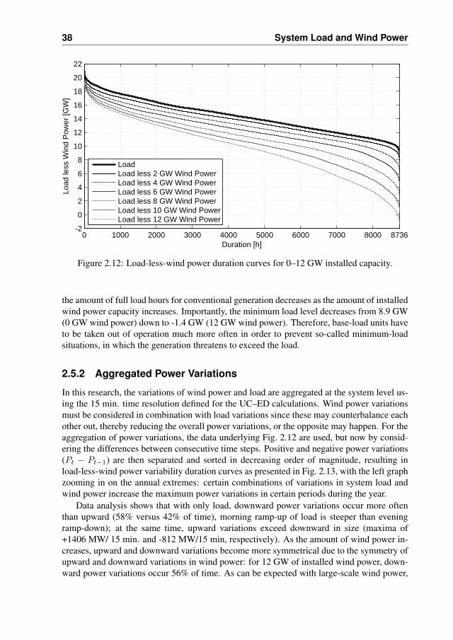
38 System Load and Wind Power
0 1000 2000 3000 4000 5000 6000 7000 8000 8736-2
0
2
4
6
8
10
12
14
16
18
20
22
Duration [h]
Load
less
Win
d P
ower
[GW
]
LoadLoad less 2 GW Wind PowerLoad less 4 GW Wind PowerLoad less 6 GW Wind PowerLoad less 8 GW Wind PowerLoad less 10 GW Wind PowerLoad less 12 GW Wind Power
Figure 2.12: Load-less-wind power duration curves for 0–12 GW installed capacity.
the amount of full load hours for conventional generation decreases as the amount of installedwind power capacity increases. Importantly, the minimum load level decreases from 8.9 GW(0 GW wind power) down to -1.4 GW (12 GW wind power). Therefore, base-load units haveto be taken out of operation much more often in order to prevent so-called minimum-loadsituations, in which the generation threatens to exceed the load.
2.5.2 Aggregated Power Variations
In this research, the variations of wind power and load are aggregated at the system level us-ing the 15 min. time resolution defined for the UC–ED calculations. Wind power variationsmust be considered in combination with load variations since these may counterbalance eachother out, thereby reducing the overall power variations, or the opposite may happen. For theaggregation of power variations, the data underlying Fig. 2.12 are used, but now by consid-ering the differences between consecutive time steps. Positive and negative power variations(Pt − Pt−1) are then separated and sorted in decreasing order of magnitude, resulting inload-less-wind power variability duration curves as presented in Fig. 2.13, with the left graphzooming in on the annual extremes: certain combinations of variations in system load andwind power increase the maximum power variations in certain periods during the year.
Data analysis shows that with only load, downward power variations occur more oftenthan upward (58% versus 42% of time), morning ramp-up of load is steeper than eveningramp-down); at the same time, upward variations exceed downward in size (maxima of+1406 MW/ 15 min. and -812 MW/15 min, respectively). As the amount of wind power in-creases, upward and downward variations become more symmetrical due to the symmetry ofupward and downward variations in wind power: for 12 GW of installed wind power, down-ward power variations occur 56% of time. As can be expected with large-scale wind power,
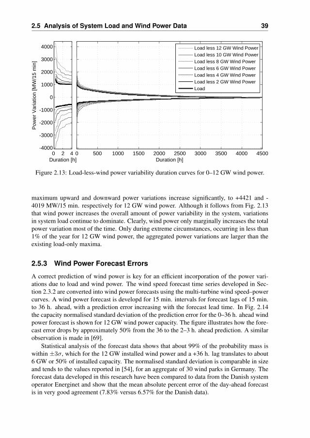
2.5 Analysis of System Load and Wind Power Data 39
0 500 1000 1500 2000 2500 3000 3500 4000 4500
Duration [h]
0 1000 2000 3000 4000 5000 6000 7000 8000 8736-202468
10121416182022
Duration [h]Lo
ad le
ss W
ind
Pow
er [G
W]
Load less 12 GW Wind PowerLoad less 10 GW Wind PowerLoad less 8 GW Wind PowerLoad less 6 GW Wind PowerLoad less 4 GW Wind PowerLoad less 2 GW Wind PowerLoad
0 2 4-4000
-3000
-2000
-1000
0
1000
2000
3000
4000
Pow
er V
aria
tion
[MW
/15
min
]
Duration [h]
Figure 2.13: Load-less-wind power variability duration curves for 0–12 GW wind power.
maximum upward and downward power variations increase significantly, to +4421 and -4019 MW/15 min. respectively for 12 GW wind power. Although it follows from Fig. 2.13that wind power increases the overall amount of power variability in the system, variationsin system load continue to dominate. Clearly, wind power only marginally increases the totalpower variation most of the time. Only during extreme circumstances, occurring in less than1% of the year for 12 GW wind power, the aggregated power variations are larger than theexisting load-only maxima.
2.5.3 Wind Power Forecast Errors
A correct prediction of wind power is key for an efficient incorporation of the power vari-ations due to load and wind power. The wind speed forecast time series developed in Sec-tion 2.3.2 are converted into wind power forecasts using the multi-turbine wind speed–powercurves. A wind power forecast is developd for 15 min. intervals for forecast lags of 15 min.to 36 h. ahead, with a prediction error increasing with the forecast lead time. In Fig. 2.14the capacity normalised standard deviation of the prediction error for the 0–36 h. ahead windpower forecast is shown for 12 GW wind power capacity. The figure illustrates how the fore-cast error drops by approximately 50% from the 36 to the 2–3 h. ahead prediction. A similarobservation is made in [69].
Statistical analysis of the forecast data shows that about 99% of the probability mass iswithin ±3σ, which for the 12 GW installed wind power and a +36 h. lag translates to about6 GW or 50% of installed capacity. The normalised standard deviation is comparable in sizeand tends to the values reported in [54], for an aggregate of 30 wind parks in Germany. Theforecast data developed in this research have been compared to data from the Danish systemoperator Energinet and show that the mean absolute percent error of the day-ahead forecastis in very good agreement (7.83% versus 6.57% for the Danish data).
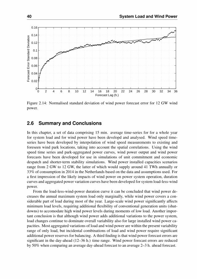
40 System Load and Wind Power
0 2 4 6 8 10 12 14 16 18 20 22 24 26 28 30 32 34 360
0.02
0.04
0.06
0.08
0.1
0.12
0.14
0.16
Forecast Lag (h.)
Fore
cast
Erro
r Sta
ndar
d D
evia
tion
Figure 2.14: Normalised standard deviation of wind power forecast error for 12 GW windpower.
2.6 Summary and Conclusions
In this chapter, a set of data comprising 15 min. average time-series for for a whole yearfor system load and for wind power have been developd and analysed. Wind speed time-series have been developed by interpolation of wind speed measurements to existing andforeseen wind park locations, taking into account the spatial correlations. Using the windspeed time series and park-aggregated power curves, wind power output and wind powerforecasts have been developed for use in simulations of unit commitment and economicdespatch and shorter-term stability simulations. Wind power installed capacities scenariosrange from 2 GW to 12 GW, the latter of which would supply around 41 TWh annually or33% of consumption in 2014 in the Netherlands based on the data and assumptions used. Fora first impression of the likely impacts of wind power on power system operation, durationcurves and aggregated power variation curves have been developed for system load-less-windpower.
From the load-less-wind-power duration curve it can be concluded that wind power de-creases the annual maximum system load only marginally, while wind power covers a con-siderable part of load during most of the year. Large-scale wind power significantly affectsminimum load levels, requiring additional flexibility of conventional generation units (shut-downs) to accomodate high wind power levels during moments of low load. Another impor-tant conclusion is that although wind power adds additional variations to the power system,load changes continue to dominate overall variability also for large installed wind power ca-pacities. Most aggregated variations of load and wind power are within the present variabilityrange of only load, but incidental combinations of load and wind power require significantadditional power reserves for balancing. A third finding is that wind power forecast errors aresignificant in the day-ahead (12–36 h.) time range. Wind power forecast errors are reducedby 50% when comparing an average day-ahead forecast to an average 2–3 h. ahead forecast.

CHAPTER 3Unit Commitment and
Economical Despatch Model
3.1 Introduction
Unit commitment in itself is a straightforward concept: a generation unit is committed whenit is on-line: either generating or immediately capable of generating electric power. The op-timisation of unit commitment is however not an easy task since it must take into account allpossible reasons for bringing units on-line or shutting them down [174]. After unit commit-ment has been decided upon, despatch is then performed, distributing system load betweenthe committed units such that overall operating cost are lowest. Unit commitment and eco-nomical despatch (UC–ED) are two optimisation tasks (ED being a sub-set of UC) requiringdifferent optimisation procedures and comprising different time frames. Unit commitmentdecisions are nowadays assessed typically once or twice a day, while generation despatch iscarried out throughout the day. With the reasonable predictability of system load, intra-daycalculations for unit commitment are in principle necessary only when unexpected, signifi-cant changes occur in generation (e.g. outages) or demand. This changes when significantamounts of wind power must be taken into account, since its variations are more difficult topredict.
The emergence of international markets and the growth of wind power have complicatedthe optimisation of UC–ED in the sense that more variables and uncertainties (i.e. market

42 Unit Commitment and Economical Despatch Model
prices, wind power forecasts) must be taken into account. In liberalised markets, the gen-eration units owners are responsible only for supplying their own customers (i.e. long-termcontracts and short-term trading agreements). Each individual owner therefore optimises theUC–ED of the generation units under its control, taking into account the market price. Forexisting systems, ideal markets in princple lead to the same outcome regarding the schedulingof generation as would have been the case with central optimisation. Thus, there is merely aconceptual difference between markets and the traditional generation scheduling (i.e. marketparticipant price bids instead of operating cost minimisation). Therefore, solutions for thetraditional central optimisation of UC–ED based on cost are still highly relevant [25].
The contribution of this chapter is twofold. First, an existing UC–ED optimisation tool isextended to include models for wind power, interconnectors to neighbouring power systems,additional thermal unit types and energy storage facilities. Second, a methodology is devel-oped for studying the impact of market gate-closure times on the optimal UC–ED schedules.Also, the model’s database is organised into separate classes, enabling the creation of largenumbers of internally consistent simulation scenarios. The additions make the UC–ED toolusable for international system integration studies of large-scale wind power in liberalisedenvironments.
The chapter is organised as follows. First, a literature overview is provided on availabletools and procedures for UC–ED and the contribution of this thesis to the development ofsuch tools and procedures is stated. Then, the simulation tool is investigated in detail and thestructure and optimisation logic are presented, including the needed input data and the desiredoutput. Models for all relevant power system aspects are included: generation, transmission,control areas (including interconnections), and system load. Furthermore, the creation ofmodels for thermal conventional generation units, hydro power, energy storage, internationalexchanges and the model integration of wind power are shown.
3.2 Literature Overview and Contribution of this Thesis
Unit commitment is a large-scale (many units), mixed-integer, and non-linear programmingproblem. The optimisation of unit commitment therefore requires significant computationaleffort, explaining the substantial research efforts in this area over the past decades. Unitcommitment may be optimised using different techniques, including the use of mixed-integerlinear programming, dynamic programming, Lagrangian relaxation, heuristics and other ap-proaches [25, 136]. The optimisation methods have different strengths and weaknesses and awide range of UC–ED tools has been developed for the optimisation of different generationsystems.
3.2.1 Overview of relevant UC–ED Tools
A wide range of tools has been developed for the simulation of UC–ED or electricity mar-ket operation ranging from weekly operations planning to generation unit investment plan-ning. Even though these models have different characteristics, making them more suitablefor different applications, they all have the objective of simulating the scheduling of the gen-eration system while optimising total cost. Taking into account the focus of this research,only chronological tools capable of system simulation including wind power are discussed,
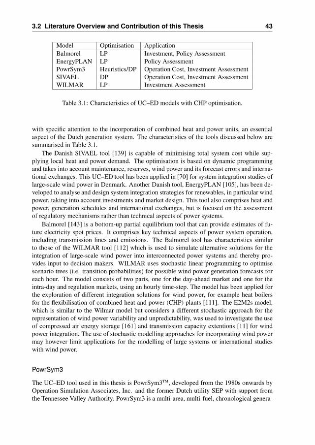
3.2 Literature Overview and Contribution of this Thesis 43
Model Optimisation ApplicationBalmorel LP Investment, Policy AssessmentEnergyPLAN LP Policy AssessmentPowrSym3 Heuristics/DP Operation Cost, Investment AssessmentSIVAEL DP Operation Cost, Investment AssessmentWILMAR LP Investment Assessment
Table 3.1: Characteristics of UC–ED models with CHP optimisation.
with specific attention to the incorporation of combined heat and power units, an essentialaspect of the Dutch generation system. The characteristics of the tools discussed below aresummarised in Table 3.1.
The Danish SIVAEL tool [139] is capable of minimising total system cost while sup-plying local heat and power demand. The optimisation is based on dynamic programmingand takes into account maintenance, reserves, wind power and its forecast errors and interna-tional exchanges. This UC–ED tool has been applied in [70] for system integration studies oflarge-scale wind power in Denmark. Another Danish tool, EnergyPLAN [105], has been de-veloped to analyse and design system integration strategies for renewables, in particular windpower, taking into account investments and market design. This tool also comprises heat andpower, generation schedules and international exchanges, but is focused on the assessmentof regulatory mechanisms rather than technical aspects of power systems.
Balmorel [143] is a bottom-up partial equilibrium tool that can provide estimates of fu-ture electricity spot prices. It comprises key technical aspects of power system operation,including transmission lines and emissions. The Balmorel tool has characteristics similarto those of the WILMAR tool [112] which is used to simulate alternative solutions for theintegration of large-scale wind power into interconnected power systems and thereby pro-vides input to decision makers. WILMAR uses stochastic linear programming to optimisescenario trees (i.e. transition probabilities) for possible wind power generation forecasts foreach hour. The model consists of two parts, one for the day-ahead market and one for theintra-day and regulation markets, using an hourly time-step. The model has been applied forthe exploration of different integration solutions for wind power, for example heat boilersfor the flexibilisation of combined heat and power (CHP) plants [111]. The E2M2s model,which is similar to the Wilmar model but considers a different stochastic approach for therepresentation of wind power variability and unpredictability, was used to investigate the useof compressed air energy storage [161] and transmission capacity extentions [11] for windpower integration. The use of stochastic modelling approaches for incorporating wind powermay however limit applications for the modelling of large systems or international studieswith wind power.
PowrSym3
The UC–ED tool used in this thesis is PowrSym3TM, developed from the 1980s onwards byOperation Simulation Associates, Inc. and the former Dutch utility SEP with support fromthe Tennessee Valley Authority. PowrSym3 is a multi-area, multi-fuel, chronological genera-
44 Unit Commitment and Economical Despatch Model
tion cost simulation model for electrical power systems including combined heat and power,energy storage and energy limited fuel contracts [131]. PowrSym3 is a rolling UC–ED opti-misation tool, i.e. UC–ED are updated every simulation state based on best available load andwind power forecast, while taking into account technical constraints following from previousstates. The tool allows different simulation time-steps and 15 min. time-step was applied inthis research PowrSym3 applies heuristics, or computer intelligence based on operational ex-perience, for an initial optimisation of the UC–ED. The solution obtained from the heuristicsis used as an input for a so-called ’smart’ dynamic programming algorithm for further opti-misation of the unit commitment. The model is capable of using multiple processors runningin parallel for very large system studies, by use of a master server handling the database andco-ordinating the different jobs between different computers. PowrSym3 is used for optimi-sation of operation cost and generation capacity planning by utilities throughout the world,including TVA (USA), Western Power (AUS) and Transelectrica (RO). A previous versionof PowrSym3 was applied in the late 1980s by the former Dutch utility SEP for economicalanalysis and capacity credit calculation of 1000 MW wind power in the Netherlands by theyear 2000 [63].
The reasons for choosing to use PowrSym3 for this research are the following. The first isthat the model’s database contains validated models for the existing conventional generationunits in the Netherlands. PowrSym3 has been used in the centrally organised optimisationof the UC–ED of the Dutch generation units up until 1998, when unbundling of the Dutchpower sector started. Since then, the database has been maintained by Dutch TSO TenneTand the model continues to be used for system studies and adequacy forecasts [165]. In orderto obtain additional modeling data and for validating the generation unit models, interviewshave been held with the six largest Dutch utilities (balance responsible parties, or in theNetherlands, program responsible parties, PRPs). The second reason for using PowrSym3 isthat little effort had to be spent on the development of a simulation tool, the acquisition ofdata and the validation of both. This allows efforts to be concentrated on the operation ofthe power system rather than the model, which is in line with the approach of the researchconsortium We@Sea. Finally, the use of PowrSym3 enabled a very useful exchange of expertknowledge with TenneT TSO, which has extensive experience with these kind of simulations.
3.2.2 Contribution of this Thesis
At the start of this research, the database of PowrSym3 comprised validated models of thelargest seventy power generation units in the Netherlands and models for sixteen heat ar-eas. The database did not include any of the following aspects: wind power, conventionalgeneration unit ramp rates, energy storage, cross-border interconnections or international ex-changes. The contribution of this thesis lies in the extension of PowrSym3 to include thefollowing, additional aspects, both in the model itself and in the database:• Wind power, by making wind power and forecast data suitable for use by the tool• Ramp rates, by consulting market parties and using literature research to esitimate these• Hydro power and energy storage, by developing new models in the tools database• Interconnections and international exchanges, by developing new areas representing neigh-
bouring countries of the NetherlandsApart from these additions, additional thermal power unit models are developed to representplanned generation units. Furthermore, a methodology is developed for the simulation of
3.3 Simulation Model 45
different market gate closure times and wind power forecast errors. By a sequence of simula-tions and some input and output data processing, the method can be used to provide realisticgeneration schedules based on wind power forecasts. These schedules are then used as fixedinput data for intra-day simulations which use updated wind power forecasts, available aftergate-closure of international markets. This addition is now being included by OSA to becomean integral part of the optimisation logic of PowrSym3. Furthermore, the database has beenre-organised in such a way that it is possible to create large number of internally consistentsimulation scenario’s within very short time-spans.
The contributions made to the development of TenneT TSO’s database in PowrSym3make it a highly useful tool for system studies. The tool is now very suitable to investigatepower system operation with large-scale wind power, international markets and integrationsolutions for wind power.
3.3 Simulation Model
The generation cost simulation model PowrSym3 comprises a number of aspects discussedbelow. The optimisation includes probabilities of generation unit outages and captures allrelevant chronological aspects by rolling UC–ED, most importantly the operational flexibilityof conventional generation units. First, the modeling of generation unavailability due tooutages is elaborated upon and a choice between different options is made. Then, the generalmodel and simulation structure of PowrSym3 is presented. Following this, the annual, weeklyand short-term optimisation methodology is described. Furthermore, different simulationattributes that must be defined beforehand are discussed. Finally, an overview is given of theinput and output data.
3.3.1 Generation Outages
Outages comprise all events leading to a (partial) unavailability of generation units in thesystem. A differentiation can be made between unforced or planned outages, such as dueto scheduled maintenance, and forced outages, such as due to unexpected technical failuresof the unit. In order to capture generation unavailability, derating of generating capacity hasbeen suggested in order to minimise the computational effort but this is only suitable if largecapacities of one generation technology are present in the system. An improvement of thederating method comprises the addition of analytical approximations for the calculation ofoutages, in particular the use of cumulants for the representation of the equivalent load distri-bution between generation units [160]. Modern computers have however made it possible tofully incorporate generation outages by probability density functions, to be used in long-termchronological simulations.
Planned Outage Models
Planned outages are usually scheduled with the objective of minimising opportunity lossesor the loss-of-load probability (LOLP), a widely used reliability measure in generation plan-ning. This can be done by scheduling maintenance when prices are assumed to be low (lowload periods) or by distributing maintenance between different units over different periods,resulting in a rather constant generation adequacy during the year. Planned maintenance

46 Unit Commitment and Economical Despatch Model
has important impacts on power system operation, in particular cost and system reliability,but also on reserve levels and total emissions [179]. Different models are available for thesimulation of planned outages, four of which are included in Powrsym3:• Pre-scheduled maintenance• Calculated maintenance schedule• Combined maintenance scheduleThe pre-scheduled maintenance is in fact a manually prepared maintenance schedule or ref-erence planning that serves as an input to the simulation. Disadvantages of this method arethe implicit choices made which are not necessarily related to the system under investiga-tion. Therefore, its impact on the simulation results is unclear. It is also difficult to adapt theschedule to a different generation portfolio. A calculated maintenance schedule is based onan assessment of the LOLP for a given period. The conventional method of calculating theLOLP of a given power system comprises the computation of a cumulative outage probabilitytable, determining the generation deficiency for each load level and summing all deficiencyprobabilities [181]. The advantage of the calculated one is mainly its focus on reliability,leading to an equal reserve margin throughout the year. A pre-scheduled maintenance sched-ule can also be combined with a calculated schedule. For accurate results during shorterperiods, a weekly reliability model is available.
For this research, maintenance is assumed to be scheduled such that LOLP is levelisedthroughout the year, with most maintenance scheduled at periods of relatively low load.PowrSym3 calculates the maintenance schedule taking into account expected system load(hourly values) and the maintenance probabilities of individual units. Generation units maybe assigned to maintenance groups, for which rules may be given regarding minimum ca-pacity available etc. PowrSym3 will deliver an identical schedule for a particular simulationset-up for each run (repeatable results).
Forced Outage Models
Different models for forced outages included in PowrSym3 are:• Fixed outage schedule• Derating method• Gradient derate method• Random Monte Carlo• Selected sample Monte Carlo• Semi-guided Monte CarloA fixed outage schedule has the benefit of being fast to compute since it requires no iterationsfor convergence, but can only be applied for specific short-term operational studies. Thederating method reduces the capacity of generation units by the forced outage rate. Thismethod is also fast and in general applicable, but has the disadvantage that it may resultin considerable errors in the computation of the reliability indices [68]. Therefore also theestimation of the operation of peak-load units or other units with limited operational hours isincorrect. The gradient derate method [131] is a similar method that approaches the deratingmethod after several simulation hours and is suitable only for short-term operational studies.
The random Monte Carlo method calculates the expected unit operation hours by averag-ing a number of outage scenarios created by a random number generator. The outage length
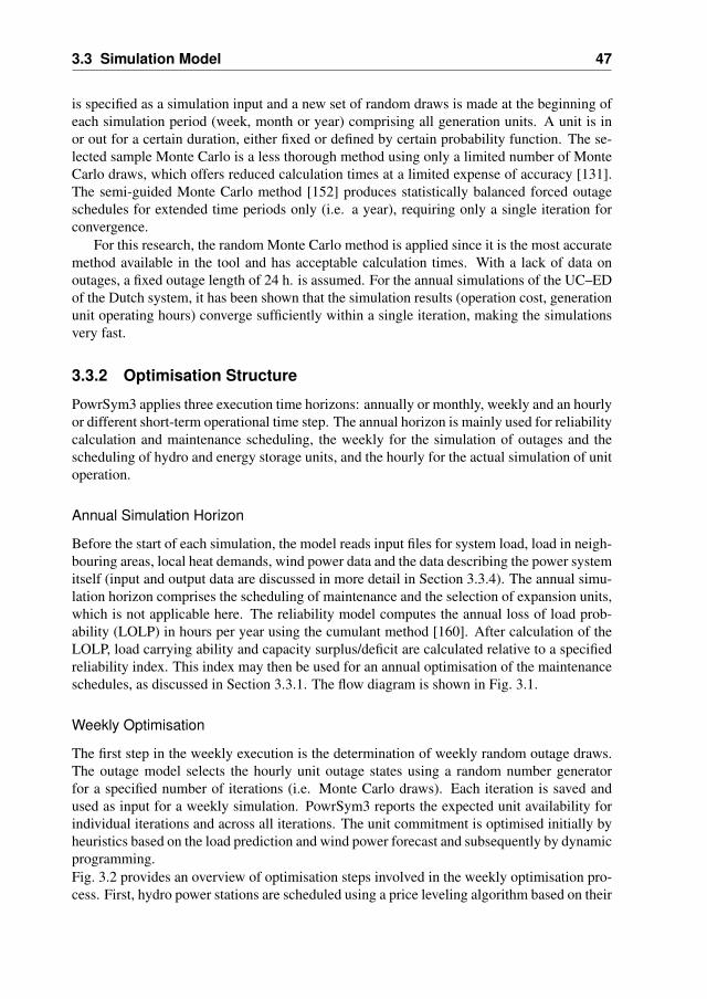
3.3 Simulation Model 47
is specified as a simulation input and a new set of random draws is made at the beginning ofeach simulation period (week, month or year) comprising all generation units. A unit is inor out for a certain duration, either fixed or defined by certain probability function. The se-lected sample Monte Carlo is a less thorough method using only a limited number of MonteCarlo draws, which offers reduced calculation times at a limited expense of accuracy [131].The semi-guided Monte Carlo method [152] produces statistically balanced forced outageschedules for extended time periods only (i.e. a year), requiring only a single iteration forconvergence.
For this research, the random Monte Carlo method is applied since it is the most accuratemethod available in the tool and has acceptable calculation times. With a lack of data onoutages, a fixed outage length of 24 h. is assumed. For the annual simulations of the UC–EDof the Dutch system, it has been shown that the simulation results (operation cost, generationunit operating hours) converge sufficiently within a single iteration, making the simulationsvery fast.
3.3.2 Optimisation Structure
PowrSym3 applies three execution time horizons: annually or monthly, weekly and an hourlyor different short-term operational time step. The annual horizon is mainly used for reliabilitycalculation and maintenance scheduling, the weekly for the simulation of outages and thescheduling of hydro and energy storage units, and the hourly for the actual simulation of unitoperation.
Annual Simulation Horizon
Before the start of each simulation, the model reads input files for system load, load in neigh-bouring areas, local heat demands, wind power data and the data describing the power systemitself (input and output data are discussed in more detail in Section 3.3.4). The annual simu-lation horizon comprises the scheduling of maintenance and the selection of expansion units,which is not applicable here. The reliability model computes the annual loss of load prob-ability (LOLP) in hours per year using the cumulant method [160]. After calculation of theLOLP, load carrying ability and capacity surplus/deficit are calculated relative to a specifiedreliability index. This index may then be used for an annual optimisation of the maintenanceschedules, as discussed in Section 3.3.1. The flow diagram is shown in Fig. 3.1.
Weekly Optimisation
The first step in the weekly execution is the determination of weekly random outage draws.The outage model selects the hourly unit outage states using a random number generatorfor a specified number of iterations (i.e. Monte Carlo draws). Each iteration is saved andused as input for a weekly simulation. PowrSym3 reports the expected unit availability forindividual iterations and across all iterations. The unit commitment is optimised initially byheuristics based on the load prediction and wind power forecast and subsequently by dynamicprogramming.Fig. 3.2 provides an overview of optimisation steps involved in the weekly optimisation pro-cess. First, hydro power stations are scheduled using a price leveling algorithm based on their
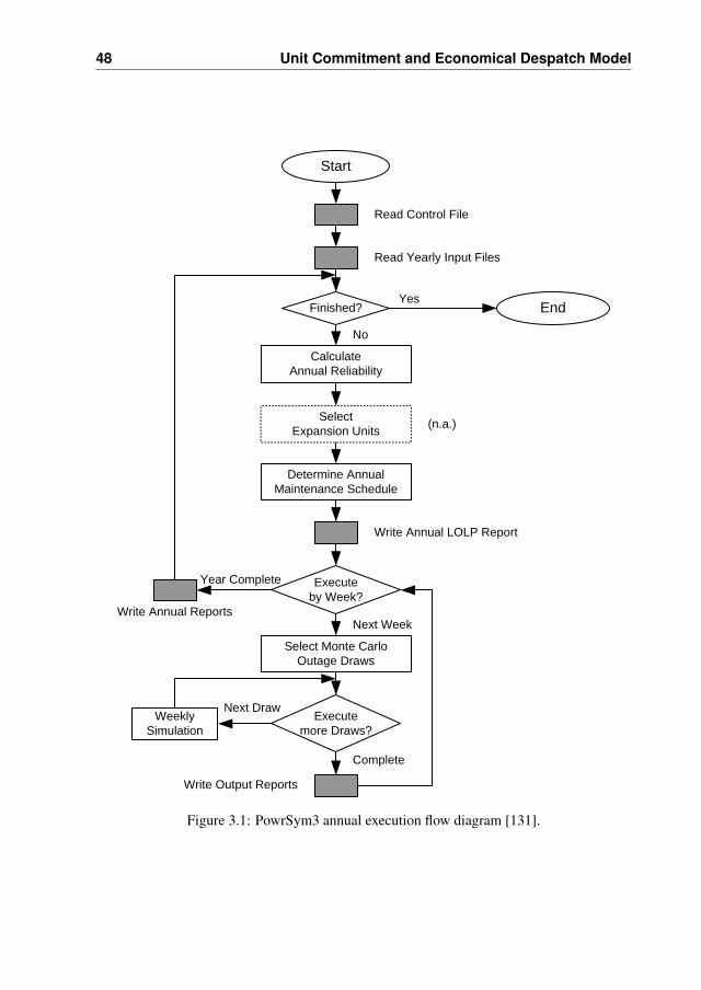
48 Unit Commitment and Economical Despatch Model
Write Annual ReportsNext Week
Next Draw
Read Control File
Start
End
Read Yearly Input Files
Finished?Yes
No
Calculate Annual Reliability
Select Expansion Units
Determine Annual Maintenance Schedule
Write Annual LOLP Report
Executeby Week?
Select Monte Carlo Outage Draws
Executemore Draws?
Write Output Reports
Complete
Weekly Simulation
Year Complete
(n.a.)
Figure 3.1: PowrSym3 annual execution flow diagram [131].

3.3 Simulation Model 49
Start
End
DP CommitOptimisation
Write Output Reports
Schedule Hydro for Week by Hours
Initially Simulate Thermal Units
Schedule Energy Storage
Simulate Thermal Units
Generate CasesDynamic Programming
For EachDP Case?
Simulate Thermal Units
Complete
Simulate Thermal Units
Create Decremental Cost Curves
(n.a.)
Figure 3.2: PowrSym3 weekly simulation flow diagram [131].
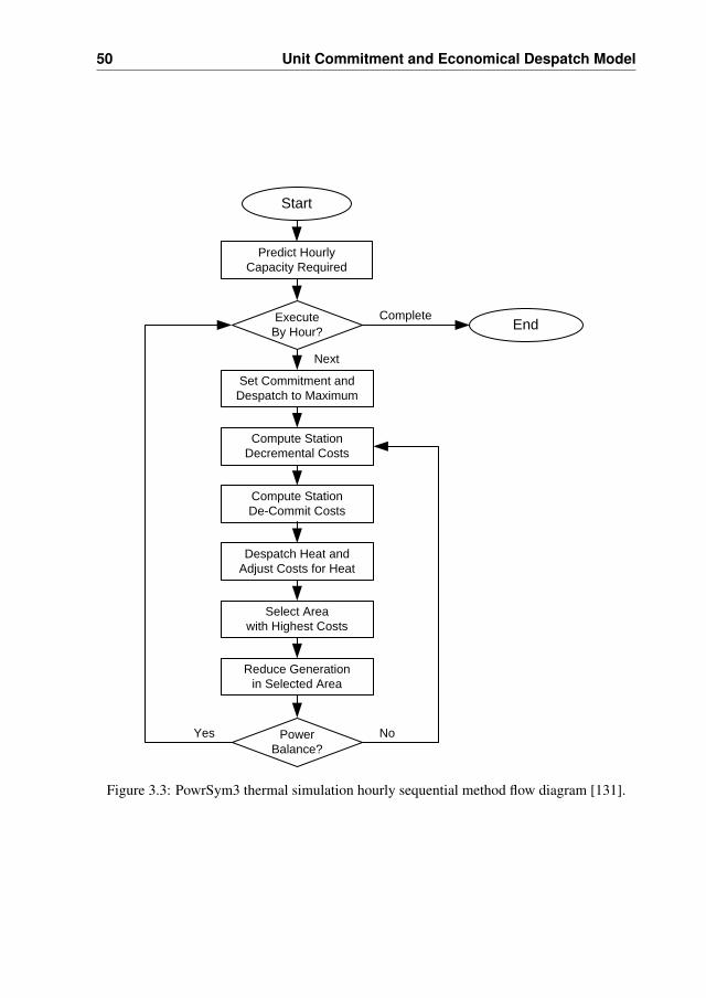
50 Unit Commitment and Economical Despatch Model
Yes
Next
Complete
Start
No
Predict Hourly Capacity Required
ExecuteBy Hour? End
Set Commitment and Despatch to Maximum
Compute Station Decremental Costs
Compute Station De-Commit Costs
Despatch Heat and Adjust Costs for Heat
Select Area with Highest Costs
Reduce Generation in Selected Area
Power Balance?
Figure 3.3: PowrSym3 thermal simulation hourly sequential method flow diagram [131].
3.3 Simulation Model 51
weekly energy constraint, load prediction and wind power forecast. The hydro schedules aresubject to hourly minimum and maximum generation levels and ramp rate limitations. Themodel then uses local heat demands, system load, wind power and wind power forecasts forthe scheduling of the thermal generation units, which are also subject to technical constraints.Based on the operational cost estimates obtained here, energy storage is scheduled such thattotal operating cost over the week are minimised. After this, the simulation results generatedby the heuristics may be optimised further using dynamic programming, which goes throughthe same steps as the heuristics. Finally, the simulation results are saved as formatted outputreports.
Short-Term Optimisation
Unit operation is simulated on an hourly or another short time-step (i.e. 15 min. in thisthesis) while preserving the chronology (Fig. 3.3). Pre-scheduled units, such as industrialor distributed generation, may be included using a fixed operating schedule for such units.The starting condition of the short-term simulation is defined by the output of the weeklysimulation and the generation units’ states at the end of the previous week, taking into accountoutages and minimum up- and downtimes. The heuristic optimisation process is done usingthe Equal Incremental Cost Method [131], which comprises the following steps:1) Set all available generation units at maximum power level, taking into account operating
constraints2) Calculate decremental cost arrays for each short-term time step3) Find the largest unit decremental cost4) De-commit or ramp down most expensive unit(s)The construction of the decremental cost arrays takes into account system load, heat despatchand de-commitment cost while satisfying minimum up- and downtimes and ramp rates. Thecost of generating heat by CHP units are taken into account in the calculations of the marginalcost of these units. In case the system comprises different areas, decremental cost arrays areconstructed for each area taking into account trans-area transmission constraints (i.e. NetTransfer Capacity, NTC, between areas), if applicable. After completion of the decrementprocedure, system cost are calculated and these steps are repeated until load, heat demandand reserve requirements are balanced. The repetitive process provides marginal cost for allareas and all units. It can be noted that the must-run status of many base-load units in theDutch system(coal, industrial CHP) reduce the complexity of unit commitment optimisation.
3.3.3 Simulation Attributes
Technical Constraints
PowrSym3 handles UC–ED as an optimisation problem, where the operating cost functionis minimised within the boundary conditions of serving system load and local heat demands,and maximum integration of wind power. The UC–ED formulation includes typical genera-tion unit parameters such as minimum up- and down-times and ramp rates as well as com-bined heat-and-power operating constraints. Unit commitment and despatch are optimisedon a rolling, 15 min. basis to achieve minimum operating cost at the system level while alltechnical constraints are met, including system or transmission area load, heat demand in all
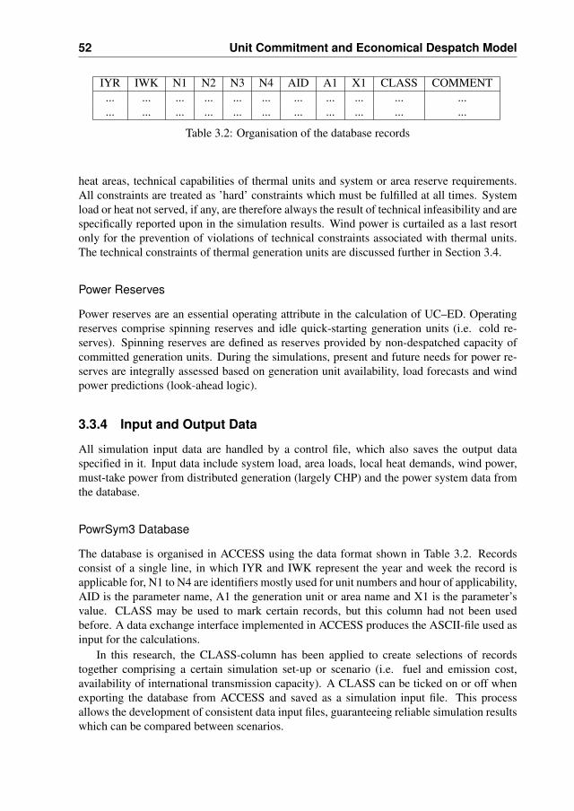
52 Unit Commitment and Economical Despatch Model
IYR IWK N1 N2 N3 N4 AID A1 X1 CLASS COMMENT... ... ... ... ... ... ... ... ... ... ...... ... ... ... ... ... ... ... ... ... ...
Table 3.2: Organisation of the database records
heat areas, technical capabilities of thermal units and system or area reserve requirements.All constraints are treated as ’hard’ constraints which must be fulfilled at all times. Systemload or heat not served, if any, are therefore always the result of technical infeasibility and arespecifically reported upon in the simulation results. Wind power is curtailed as a last resortonly for the prevention of violations of technical constraints associated with thermal units.The technical constraints of thermal generation units are discussed further in Section 3.4.
Power Reserves
Power reserves are an essential operating attribute in the calculation of UC–ED. Operatingreserves comprise spinning reserves and idle quick-starting generation units (i.e. cold re-serves). Spinning reserves are defined as reserves provided by non-despatched capacity ofcommitted generation units. During the simulations, present and future needs for power re-serves are integrally assessed based on generation unit availability, load forecasts and windpower predictions (look-ahead logic).
3.3.4 Input and Output Data
All simulation input data are handled by a control file, which also saves the output dataspecified in it. Input data include system load, area loads, local heat demands, wind power,must-take power from distributed generation (largely CHP) and the power system data fromthe database.
PowrSym3 Database
The database is organised in ACCESS using the data format shown in Table 3.2. Recordsconsist of a single line, in which IYR and IWK represent the year and week the record isapplicable for, N1 to N4 are identifiers mostly used for unit numbers and hour of applicability,AID is the parameter name, A1 the generation unit or area name and X1 is the parameter’svalue. CLASS may be used to mark certain records, but this column had not been usedbefore. A data exchange interface implemented in ACCESS produces the ASCII-file used asinput for the calculations.
In this research, the CLASS-column has been applied to create selections of recordstogether comprising a certain simulation set-up or scenario (i.e. fuel and emission cost,availability of international transmission capacity). A CLASS can be ticked on or off whenexporting the database from ACCESS and saved as a simulation input file. This processallows the development of consistent data input files, guaranteeing reliable simulation resultswhich can be compared between scenarios.
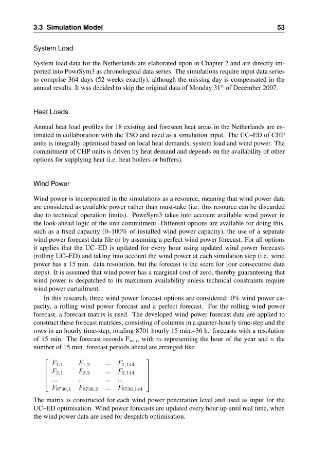
3.3 Simulation Model 53
System Load
System load data for the Netherlands are elaborated upon in Chapter 2 and are directly im-ported into PowrSym3 as chronological data series. The simulations require input data seriesto comprise 364 days (52 weeks exactly), although the missing day is compensated in theannual results. It was decided to skip the original data of Monday 31st of December 2007.
Heat Loads
Annual heat load profiles for 18 existing and foreseen heat areas in the Netherlands are es-timated in collaboration with the TSO and used as a simulation input. The UC–ED of CHPunits is integrally optimised based on local heat demands, system load and wind power. Thecommitment of CHP units is driven by heat demand and depends on the availability of otheroptions for supplying heat (i.e. heat boilers or buffers).
Wind Power
Wind power is incorporated in the simulations as a resource, meaning that wind power dataare considered as available power rather than must-take (i.e. this resource can be discardeddue to technical operation limits). PowrSym3 takes into account available wind power inthe look-ahead logic of the unit commitment. Different options are available for doing this,such as a fixed capacity (0–100% of installed wind power capacity), the use of a separatewind power forecast data file or by assuming a perfect wind power forecast. For all optionsit applies that the UC–ED is updated for every hour using updated wind power forecasts(rolling UC–ED) and taking into account the wind power at each simulation step (i.e. windpower has a 15 min. data resolution, but the forecast is the seem for four consecutive datasteps). It is assumed that wind power has a marginal cost of zero, thereby guaranteeing thatwind power is despatched to its maximum availability unless technical constraints requirewind power curtailment.
In this research, three wind power forecast options are considered: 0% wind power ca-pacity, a rolling wind power forecast and a perfect forecast. For the rolling wind powerforecast, a forecast matrix is used. The developed wind power forecast data are applied toconstruct these forecast matrices, consisting of columns in a quarter-hourly time-step and therows in an hourly time-step, totaling 8701 hourly 15 min.–36 h. forecasts with a resolutionof 15 min. The forecast records Fm,n with m representing the hour of the year and n thenumber of 15 min. forecast periods ahead are arranged like
F1,1 F1,2 ... F1,144
F2,1 F2,2 ... F2,144
... ... ... ...F8736,1 F8736,2 ... F8736,144
The matrix is constructed for each wind power penetration level and used as input for theUC–ED optimisation. Wind power forecasts are updated every hour up until real time, whenthe wind power data are used for despatch optimisation.
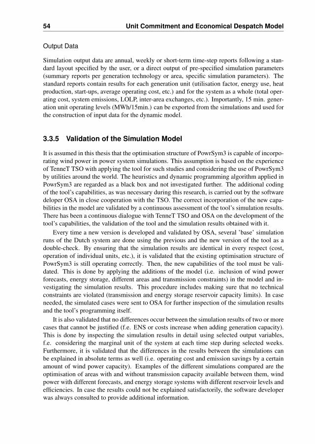
54 Unit Commitment and Economical Despatch Model
Output Data
Simulation output data are annual, weekly or short-term time-step reports following a stan-dard layout specified by the user, or a direct output of pre-specified simulation parameters(summary reports per generation technology or area, specific simulation parameters). Thestandard reports contain results for each generation unit (utilisation factor, energy use, heatproduction, start-ups, average operating cost, etc.) and for the system as a whole (total oper-ating cost, system emissions, LOLP, inter-area exchanges, etc.). Importantly, 15 min. gener-ation unit operating levels (MWh/15min.) can be exported from the simulations and used forthe construction of input data for the dynamic model.
3.3.5 Validation of the Simulation Model
It is assumed in this thesis that the optimisation structure of PowrSym3 is capable of incorpo-rating wind power in power system simulations. This assumption is based on the experienceof TenneT TSO with applying the tool for such studies and considering the use of PowrSym3by utilities around the world. The heuristics and dynamic programming algorithm applied inPowrSym3 are regarded as a black box and not investigated further. The additional codingof the tool’s capabilities, as was necessary during this research, is carried out by the softwaredeloper OSA in close cooperation with the TSO. The correct incorporation of the new capa-bilities in the model are validated by a continuous assessment of the tool’s simulation results.There has been a continuous dialogue with TenneT TSO and OSA on the development of thetool’s capabilities, the validation of the tool and the simulation results obtained with it.
Every time a new version is developed and validated by OSA, several ’base’ simulationruns of the Dutch system are done using the previous and the new version of the tool as adouble-check. By ensuring that the simulation results are identical in every respect (cost,operation of individual units, etc.), it is validated that the existing optimisation structure ofPowrSym3 is still operating correctly. Then, the new capabilities of the tool must be vali-dated. This is done by applying the additions of the model (i.e. inclusion of wind powerforecasts, energy storage, different areas and transmission constraints) in the model and in-vestigating the simulation results. This procedure includes making sure that no technicalconstraints are violated (transmission and energy storage reservoir capacity limits). In caseneeded, the simulated cases were sent to OSA for further inspection of the simulation resultsand the tool’s programming itself.
It is also validated that no differences occur between the simulation results of two or morecases that cannot be justified (f.e. ENS or costs increase when adding generation capacity).This is done by inspecting the simulation results in detail using selected output variables,f.e. considering the marginal unit of the system at each time step during selected weeks.Furthermore, it is validated that the differences in the results between the simulations canbe explained in absolute terms as well (i.e. operating cost and emission savings by a certainamount of wind power capacity). Examples of the different simulations compared are theoptimisation of areas with and without transmission capacity available between them, windpower with different forecasts, and energy storage systems with different reservoir levels andefficiencies. In case the results could not be explained satisfactorily, the software developerwas always consulted to provide additional information.
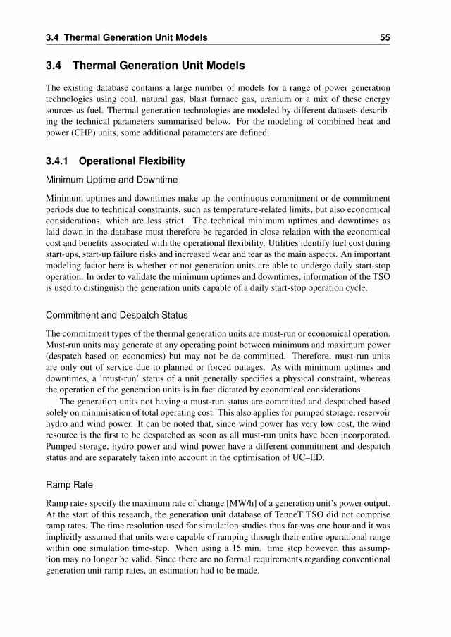
3.4 Thermal Generation Unit Models 55
3.4 Thermal Generation Unit Models
The existing database contains a large number of models for a range of power generationtechnologies using coal, natural gas, blast furnace gas, uranium or a mix of these energysources as fuel. Thermal generation technologies are modeled by different datasets describ-ing the technical parameters summarised below. For the modeling of combined heat andpower (CHP) units, some additional parameters are defined.
3.4.1 Operational Flexibility
Minimum Uptime and Downtime
Minimum uptimes and downtimes make up the continuous commitment or de-commitmentperiods due to technical constraints, such as temperature-related limits, but also economicalconsiderations, which are less strict. The technical minimum uptimes and downtimes aslaid down in the database must therefore be regarded in close relation with the economicalcost and benefits associated with the operational flexibility. Utilities identify fuel cost duringstart-ups, start-up failure risks and increased wear and tear as the main aspects. An importantmodeling factor here is whether or not generation units are able to undergo daily start-stopoperation. In order to validate the minimum uptimes and downtimes, information of the TSOis used to distinguish the generation units capable of a daily start-stop operation cycle.
Commitment and Despatch Status
The commitment types of the thermal generation units are must-run or economical operation.Must-run units may generate at any operating point between minimum and maximum power(despatch based on economics) but may not be de-committed. Therefore, must-run unitsare only out of service due to planned or forced outages. As with minimum uptimes anddowntimes, a ’must-run’ status of a unit generally specifies a physical constraint, whereasthe operation of the generation units is in fact dictated by economical considerations.
The generation units not having a must-run status are committed and despatched basedsolely on minimisation of total operating cost. This also applies for pumped storage, reservoirhydro and wind power. It can be noted that, since wind power has very low cost, the windresource is the first to be despatched as soon as all must-run units have been incorporated.Pumped storage, hydro power and wind power have a different commitment and despatchstatus and are separately taken into account in the optimisation of UC–ED.
Ramp Rate
Ramp rates specify the maximum rate of change [MW/h] of a generation unit’s power output.At the start of this research, the generation unit database of TenneT TSO did not compriseramp rates. The time resolution used for simulation studies thus far was one hour and it wasimplicitly assumed that units were capable of ramping through their entire operational rangewithin one simulation time-step. When using a 15 min. time step however, this assump-tion may no longer be valid. Since there are no formal requirements regarding conventionalgeneration unit ramp rates, an estimation had to be made.
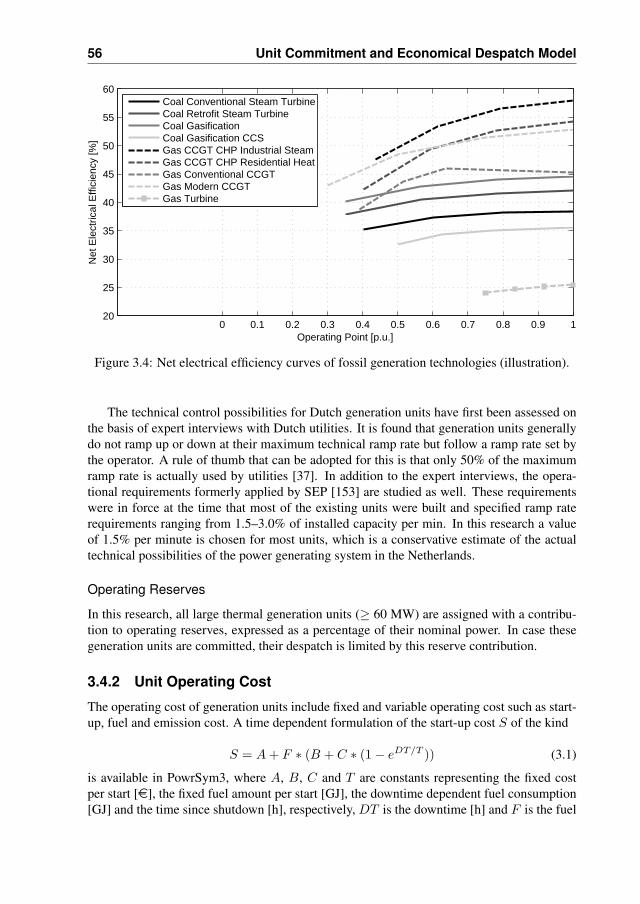
56 Unit Commitment and Economical Despatch Model
0 0.1 0.2 0.3 0.4 0.5 0.6 0.7 0.8 0.9 120
25
30
35
40
45
50
55
60
Operating Point [p.u.]
Net
Ele
ctric
al E
ffici
ency
[%]
Coal Conventional Steam TurbineCoal Retrofit Steam TurbineCoal GasificationCoal Gasification CCSGas CCGT CHP Industrial SteamGas CCGT CHP Residential HeatGas Conventional CCGTGas Modern CCGTGas Turbine
Figure 3.4: Net electrical efficiency curves of fossil generation technologies (illustration).
The technical control possibilities for Dutch generation units have first been assessed onthe basis of expert interviews with Dutch utilities. It is found that generation units generallydo not ramp up or down at their maximum technical ramp rate but follow a ramp rate set bythe operator. A rule of thumb that can be adopted for this is that only 50% of the maximumramp rate is actually used by utilities [37]. In addition to the expert interviews, the opera-tional requirements formerly applied by SEP [153] are studied as well. These requirementswere in force at the time that most of the existing units were built and specified ramp raterequirements ranging from 1.5–3.0% of installed capacity per min. In this research a valueof 1.5% per minute is chosen for most units, which is a conservative estimate of the actualtechnical possibilities of the power generating system in the Netherlands.
Operating Reserves
In this research, all large thermal generation units (≥ 60 MW) are assigned with a contribu-tion to operating reserves, expressed as a percentage of their nominal power. In case thesegeneration units are committed, their despatch is limited by this reserve contribution.
3.4.2 Unit Operating Cost
The operating cost of generation units include fixed and variable operating cost such as start-up, fuel and emission cost. A time dependent formulation of the start-up cost S of the kind
S = A + F ∗ (B + C ∗ (1− eDT/T )) (3.1)
is available in PowrSym3, where A, B, C and T are constants representing the fixed costper start [e], the fixed fuel amount per start [GJ], the downtime dependent fuel consumption[GJ] and the time since shutdown [h], respectively, DT is the downtime [h] and F is the fuel

3.4 Thermal Generation Unit Models 57
Generation Technology Fuel Heat Value CO2 NOx SO2
GJ/ton ton/MWh kg/MWh kg/MWhNuclear U 5·105 0 0 0Conventional Steam Turbine Coal 26.3 0.88 1.39 0.70Retrofit Steam Turbine Coal 26.3 0.80 1.27 0.64Gasification Steam Turbine Coal 26.3 0.76 1.20 0.60Gasification ST CCS Coal 26.3 0.17 1.50 0.76CCGT CHP Industrial Steam NG 31.7 0.35 0.28 0CCGT CHP Residential Heat NG 31.7 0.37 0.30 0Conventional CCGT NG 31.7 0.45 0.36 0Modern CCGT NG 31.7 0.38 0.31 0Gas Turbine NG 31.7 0.64 0.79 0
U = uranium, NG = natural gas
Table 3.3: Energy content and emissions of fossil generation technologies (illustration foroptimal operating point).
cost [e/GJ]. However, no data could be obtained from Dutch utilities for an accurate modelof this kind. Therefore, start cost are defined as a fixed cost per start only, for which datawere available in the database. These could however not be validated.
The fuel consumption of each generation unit is modeled either using heat rates or byspecifically modelling the unit’s efficiency. Net heat rate levels for up to five power levelscan be defined (i.e. P1..5,H1..5) for each unit with Px [MW] and Hx [GJ/MWh] and P1 beingthe minimum power output level. Together, the levels form a monotonically increasing piece-wise linear function (incremental heat rate always increases) describing the units efficiency.In Fig. 3.4, the net electrical efficiencies (i.e. excluding heat production) of different powergeneration technologies are illustrated. This also shows the technical operational range of thepower generation units modeled here.
The use of fossil fuels in power generation units gives emissions, the most important ofwhich are carbon dioxide CO2, sulphur dioxide SO2 and nitrogen oxides NOx. The emissionsreleased into the air are in principle defined by the elements involved in the chemical reactionsbetween air and fuel. This is mostly methane (CH4) for natural gas, and carbon (C), metalcompounds and several other compounds involving hydrogen (H), sulphur (S) and nitrogen(N) for coal. Emission levels of CO2 and SO2 are connected only to the fuel compositionand the operating efficiency of the unit. For NOx, the emission levels are also significantlydependent upon a range of factors in the thermodynamic processes in the plant [39].
3.4.3 Emissions
Emission levels are defined in the model as fixed coefficients on a fuel energy content base[ton/GJ]. The database contained already validated emission coefficients for CO2, SO2 andNOx emissions, the latter taking into account the impact of de-NOx-installations possiblypresent at some plants, now and in the future. SO2 emissions for natural gas-fired plants arezero. Starting emissions are not taken into account, but these are generally considered to besmall. In Table 3.3, typical emission rates of fossil fuels are presented per technology. It can
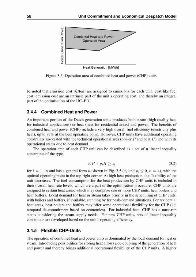
58 Unit Commitment and Economical Despatch Model
Combined Heat and PowerOperation Area
Heat Generation [MWth]
Pow
er G
ener
atio
n [M
We]
Figure 3.5: Operation area of combined heat and power (CHP) units.
be noted that emission cost [e/ton] are assigned to emissions for each unit. Just like fuelcost, emission cost are an intrinsic part of the unit’s operating cost, and thereby an integralpart of the optimisation of the UC–ED.
3.4.4 Combined Heat and Power
An important portion of the Dutch generation units produces both steam (high quality heatfor industrial applications) or heat (heat for residential areas) and power. The benefits ofcombined heat and power (CHP) include a very high overall fuel efficiency (electricity plusheat), up to 87% at the best operating point. However, CHP units have additional operatingconstraints associated with the technical operational area (power P and heat H) and with itsoperational status due to heat demand.
The operation area of each CHP unit can be described as a set of n linear inequalityconstraints of the type
xiP + yiH ≥ zi (3.2)
for i = 1...n and has a general form as shown in Fig. 3.5 (xi and yi ≤ 0, n = 4), with theoptimal operating point in the top-right corner. At high heat production, the flexibility of theunit decreases. The fuel consumption for the heat production by CHP units is included intheir overall heat rate levels, which are a part of the optimisation procedure. CHP units areassigned to certain heat areas, which may comprise one or more CHP units, heat boilers andheat buffers. Local demand for heat or steam takes priority in the scheduling of CHP units,with boilers and buffers, if available, standing by for peak-demand situations. For residentialheat areas, heat boilers and buffers may offer some operational flexibility for the CHP (i.e.temporal de-commitment based on economics). For industrial heat, CHP has a must-runstatus considering the steam supply needs. For new CHP units, sets of linear inequalityconstraints are developed based on the unit’s operating efficiency.
3.4.5 Flexible CHP-Units
The operation of combined heat and power units is dominated by the local demand for heat orsteam. Introducing possibilities for storing heat allows a de-coupling of the generation of heatand power and thereby brings additional operational flexibility of the CHP units. A higher
3.5 Hydro Power and Energy Storage Models 59
flexibility of CHP units reduces the amount of must-run capacity in the system and maytherefore be an alternative to the development of energy storage for wind power integration.For other systems with a significant share of CHP in the generation mix, such as the Danish,possibilities have been investigated for using heat storage or the use of heat boilers in orderto integrate additional amounts of wind energy [104, 111]. In this research, the flexibilisationof CHP-units is considered as a possibility for wind power integration.
A locational scan has been performed with Dutch utilities for the residential heat areasof Amsterdam, the Hague, Leiden, Purmerend, Utrecht, and Rotterdam. It is found that theadditional possibilities for a more flexible operation of the CHP-units connected to theseareas are scarce since heat boilers and heat buffers are already installed and used there. Heatboilers are also present at all industrial CHP locations but presently operated only in case ofan outage of the CHP units. Additional operational flexibility of industrial CHP units wouldbe technically possible but is often considered as unfeasible due to the risks associated withstarting and stopping. This consideration is likely to change with the integration of large-scalewind power, since the impacts of wind power on market prices can be significant, especiallyduring periods of low-load. A must-run status of combined CHP, allowing operation onlybetween minimum and maximum output, becomes less profitable with the development oflarge-scale wind power.
Integration Alternative for Wind Power
For the use of flexible CHP-units as an integration solution for wind power, it is assumedthat a total capacity of 1.5 GW of must-run industrial CHP no longer has a must-run status.Instead, these units have an operational flexibility depending on minimum up- and down-times (technical) and start-up cost and efficiency (economical). An efficiency of 95% isassumed for the additional heat boilers introduced for new CHP units. It can be noted thatthe operation of heat boilers instead of CHP units results in a lower overall energy efficiency.While the revenues for an individual CHP may be low, total cost for generating power andheat separately is still higher. Heat storage is therefore used only as a last resort for theintegration of additional wind power, when a trade-off is made between wind power and heatboiler operation versus wasted wind and CHP operation.
3.5 Hydro Power and Energy Storage Models
It is often suggested that wind and hydro power and/or energy storage form a natural com-bination. Therefore, wind power and (hydro) energy storage are often considered in a backto back configuration [26] or as an hybrid system to provide firm power [87]. Wind powermay be used to fill up storage reservoirs during high wind periods, either by pumping upor saving water, and the stored energy may be used for electricity generation during lowwind periods. As large-scale wind power will become an important part of a power system,however, the cumulative technical capabilities of the rest of this system will determine thetechnical constraints, if any, for the integration of wind power. Consequently, the technicaland economical benefits of energy storage facilities must be assessed on an integral systembasis, i.e. by taking into account the whole power system.
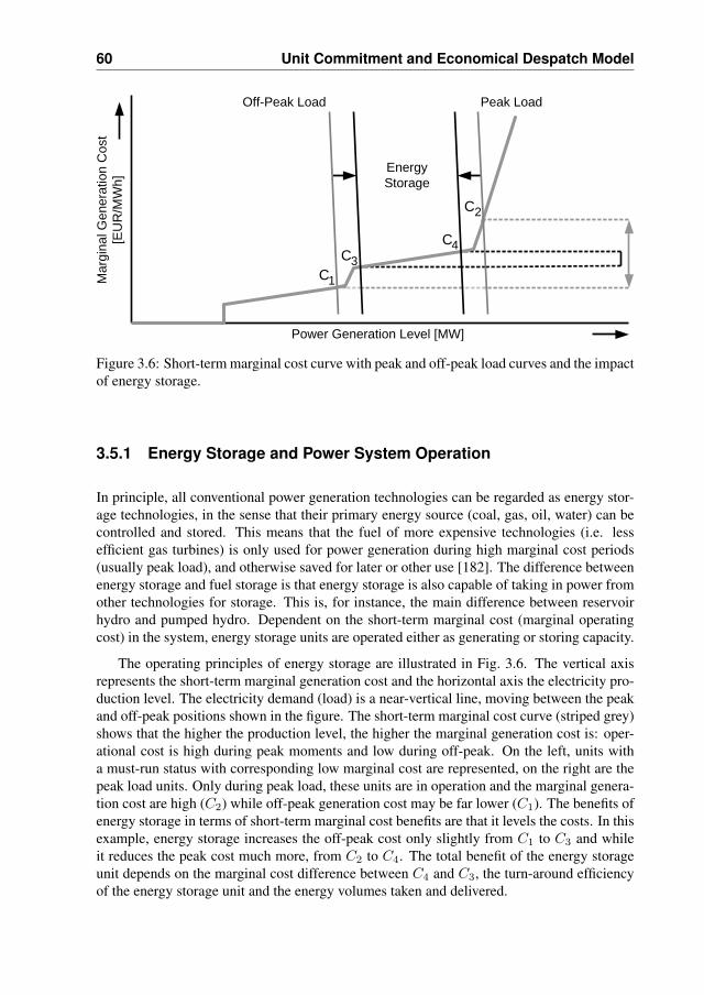
60 Unit Commitment and Economical Despatch Model
Mar
gina
l Gen
erat
ion
Cos
t [E
UR
/MW
h]
Power Generation Level [MW]
Energy Storage
C1
C2
C3
C4
Off-Peak Load Peak Load
Figure 3.6: Short-term marginal cost curve with peak and off-peak load curves and the impactof energy storage.
3.5.1 Energy Storage and Power System Operation
In principle, all conventional power generation technologies can be regarded as energy stor-age technologies, in the sense that their primary energy source (coal, gas, oil, water) can becontrolled and stored. This means that the fuel of more expensive technologies (i.e. lessefficient gas turbines) is only used for power generation during high marginal cost periods(usually peak load), and otherwise saved for later or other use [182]. The difference betweenenergy storage and fuel storage is that energy storage is also capable of taking in power fromother technologies for storage. This is, for instance, the main difference between reservoirhydro and pumped hydro. Dependent on the short-term marginal cost (marginal operatingcost) in the system, energy storage units are operated either as generating or storing capacity.
The operating principles of energy storage are illustrated in Fig. 3.6. The vertical axisrepresents the short-term marginal generation cost and the horizontal axis the electricity pro-duction level. The electricity demand (load) is a near-vertical line, moving between the peakand off-peak positions shown in the figure. The short-term marginal cost curve (striped grey)shows that the higher the production level, the higher the marginal generation cost is: oper-ational cost is high during peak moments and low during off-peak. On the left, units witha must-run status with corresponding low marginal cost are represented, on the right are thepeak load units. Only during peak load, these units are in operation and the marginal genera-tion cost are high (C2) while off-peak generation cost may be far lower (C1). The benefits ofenergy storage in terms of short-term marginal cost benefits are that it levels the costs. In thisexample, energy storage increases the off-peak cost only slightly from C1 to C3 and whileit reduces the peak cost much more, from C2 to C4. The total benefit of the energy storageunit depends on the marginal cost difference between C4 and C3, the turn-around efficiencyof the energy storage unit and the energy volumes taken and delivered.
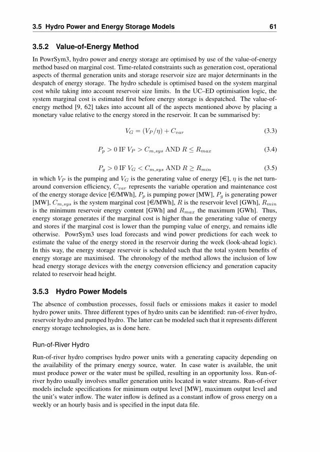
3.5 Hydro Power and Energy Storage Models 61
3.5.2 Value-of-Energy Method
In PowrSym3, hydro power and energy storage are optimised by use of the value-of-energymethod based on marginal cost. Time-related constraints such as generation cost, operationalaspects of thermal generation units and storage reservoir size are major determinants in thedespatch of energy storage. The hydro schedule is optimised based on the system marginalcost while taking into account reservoir size limits. In the UC–ED optimisation logic, thesystem marginal cost is estimated first before energy storage is despatched. The value-of-energy method [9, 62] takes into account all of the aspects mentioned above by placing amonetary value relative to the energy stored in the reservoir. It can be summarised by:
VG = (VP /η) + Cvar (3.3)
Pp > 0 IF VP > Cm,sys AND R ≤ Rmax (3.4)
Pg > 0 IF VG < Cm,sys AND R ≥ Rmin (3.5)
in which VP is the pumping and VG is the generating value of energy [e], η is the net turn-around conversion efficiency, Cvar represents the variable operation and maintenance costof the energy storage device [e/MWh], Pp is pumping power [MW], Pg is generating power[MW], Cm,sys is the system marginal cost [e/MWh], R is the reservoir level [GWh], Rmin
is the minimum reservoir energy content [GWh] and Rmax the maximum [GWh]. Thus,energy storage generates if the marginal cost is higher than the generating value of energyand stores if the marginal cost is lower than the pumping value of energy, and remains idleotherwise. PowrSym3 uses load forecasts and wind power predictions for each week toestimate the value of the energy stored in the reservoir during the week (look-ahead logic).In this way, the energy storage reservoir is scheduled such that the total system benefits ofenergy storage are maximised. The chronology of the method allows the inclusion of lowhead energy storage devices with the energy conversion efficiency and generation capacityrelated to reservoir head height.
3.5.3 Hydro Power Models
The absence of combustion processes, fossil fuels or emissions makes it easier to modelhydro power units. Three different types of hydro units can be identified: run-of-river hydro,reservoir hydro and pumped hydro. The latter can be modeled such that it represents differentenergy storage technologies, as is done here.
Run-of-River Hydro
Run-of-river hydro comprises hydro power units with a generating capacity depending onthe availability of the primary energy source, water. In case water is available, the unitmust produce power or the water must be spilled, resulting in an opportunity loss. Run-of-river hydro usually involves smaller generation units located in water streams. Run-of-rivermodels include specifications for minimum output level [MW], maximum output level andthe unit’s water inflow. The water inflow is defined as a constant inflow of gross energy on aweekly or an hourly basis and is specified in the input data file.
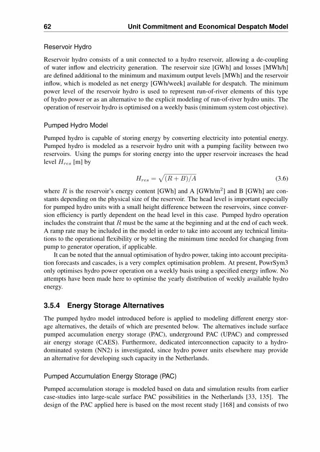
62 Unit Commitment and Economical Despatch Model
Reservoir Hydro
Reservoir hydro consists of a unit connected to a hydro reservoir, allowing a de-couplingof water inflow and electricity generation. The reservoir size [GWh] and losses [MWh/h]are defined additional to the minimum and maximum output levels [MWh] and the reservoirinflow, which is modeled as net energy [GWh/week] available for despatch. The minimumpower level of the reservoir hydro is used to represent run-of-river elements of this typeof hydro power or as an alternative to the explicit modeling of run-of-river hydro units. Theoperation of reservoir hydro is optimised on a weekly basis (minimum system cost objective).
Pumped Hydro Model
Pumped hydro is capable of storing energy by converting electricity into potential energy.Pumped hydro is modeled as a reservoir hydro unit with a pumping facility between tworeservoirs. Using the pumps for storing energy into the upper reservoir increases the headlevel Hres [m] by
Hres =√
(R + B)/A (3.6)
where R is the reservoir’s energy content [GWh] and A [GWh/m2] and B [GWh] are con-stants depending on the physical size of the reservoir. The head level is important especiallyfor pumped hydro units with a small height difference between the reservoirs, since conver-sion efficiency is partly dependent on the head level in this case. Pumped hydro operationincludes the constraint that R must be the same at the beginning and at the end of each week.A ramp rate may be included in the model in order to take into account any technical limita-tions to the operational flexibility or by setting the minimum time needed for changing frompump to generator operation, if applicable.
It can be noted that the annual optimisation of hydro power, taking into account precipita-tion forecasts and cascades, is a very complex optimisation problem. At present, PowrSym3only optimises hydro power operation on a weekly basis using a specified energy inflow. Noattempts have been made here to optimise the yearly distribution of weekly available hydroenergy.
3.5.4 Energy Storage Alternatives
The pumped hydro model introduced before is applied to modeling different energy stor-age alternatives, the details of which are presented below. The alternatives include surfacepumped accumulation energy storage (PAC), underground PAC (UPAC) and compressedair energy storage (CAES). Furthermore, dedicated interconnection capacity to a hydro-dominated system (NN2) is investigated, since hydro power units elsewhere may providean alternative for developing such capacity in the Netherlands.
Pumped Accumulation Energy Storage (PAC)
Pumped accumulation storage is modeled based on data and simulation results from earliercase-studies into large-scale surface PAC possibilities in the Netherlands [33, 135]. Thedesign of the PAC applied here is based on the most recent study [168] and consists of two
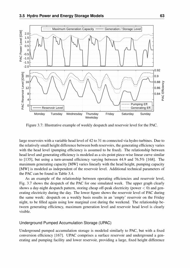
3.5 Hydro Power and Energy Storage Models 63
-2.0-1.5-1.0-0.5
00.51.01.52.0
PA
C P
ower
Lev
el [G
W]
Maximum Generation Capacity Generation / Storage Level
0
4
8
12
16
20
PA
C R
eser
voir
Leve
l [G
Wh]
Monday Tuesday Wednesday Thursday Friday Saturday Sunday
0.84
0.86
0.88
0.9
0.92
Weekday
PA
C E
ffici
ency
Reservoir LevelPumping Eff.Generating Eff.
Figure 3.7: Illustrative example of weekly despatch and reservoir level for the PAC.
large reservoirs with a variable head level of 42 to 31 m connected via hydro turbines. Due tothe relatively small height difference between both reservoirs, the generating efficiency varieswith the head level (pumping efficiency is assumed to be fixed). The relationship betweenhead level and generating efficiency is modeled as a six-point piece-wise linear curve similarto [135], but using a turn-around efficiency varying between 44.9 and 76.5% [168]. Themaximum generating capacity [MW] varies linearly with the head height, pumping capacity[MW] is modeled as independent of the reservoir level. Additional technical parameters ofthe PAC can be found in Table 3.4.
As an example of the relationship between operating efficiencies and reservoir level,Fig. 3.7 shows the despatch of the PAC for one simulated week. The upper graph clearlyshows a day-night despatch pattern, storing cheap off-peak electricity (power < 0) and gen-erating electricity during the day. The lower figure shows the reservoir level of PAC duringthe same week: despatch on a weekly basis results in an ’empty’ reservoir on the Fridaynight, to be filled again using low marginal cost during the weekend. The relationship be-tween generating efficiency, maximum generation level and reservoir head level is clearlyvisible.
Underground Pumped Accumulation Storage (UPAC)
Underground pumped accumulation storage is modeled similarly to PAC, but with a fixedconversion efficiency [167]. UPAC comprises a surface reservoir and underground a gen-erating and pumping facility and lower reservoir, providing a large, fixed height difference
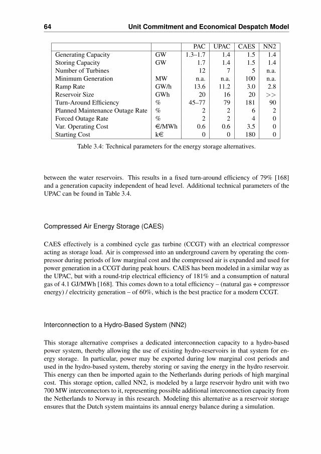
64 Unit Commitment and Economical Despatch Model
PAC UPAC CAES NN2Generating Capacity GW 1.3–1.7 1.4 1.5 1.4Storing Capacity GW 1.7 1.4 1.5 1.4Number of Turbines 12 7 5 n.a.Minimum Generation MW n.a. n.a. 100 n.a.Ramp Rate GW/h 13.6 11.2 3.0 2.8Reservoir Size GWh 20 16 20 >>Turn-Around Efficiency % 45–77 79 181 90Planned Maintenance Outage Rate % 2 2 6 2Forced Outage Rate % 2 2 4 0Var. Operating Cost e/MWh 0.6 0.6 3.5 0Starting Cost ke 0 0 180 0
Table 3.4: Technical parameters for the energy storage alternatives.
between the water reservoirs. This results in a fixed turn-around efficiency of 79% [168]and a generation capacity independent of head level. Additional technical parameters of theUPAC can be found in Table 3.4.
Compressed Air Energy Storage (CAES)
CAES effectively is a combined cycle gas turbine (CCGT) with an electrical compressoracting as storage load. Air is compressed into an underground cavern by operating the com-pressor during periods of low marginal cost and the compressed air is expanded and used forpower generation in a CCGT during peak hours. CAES has been modeled in a similar way asthe UPAC, but with a round-trip electrical efficiency of 181% and a consumption of naturalgas of 4.1 GJ/MWh [168]. This comes down to a total efficiency – (natural gas + compressorenergy) / electricity generation – of 60%, which is the best practice for a modern CCGT.
Interconnection to a Hydro-Based System (NN2)
This storage alternative comprises a dedicated interconnection capacity to a hydro-basedpower system, thereby allowing the use of existing hydro-reservoirs in that system for en-ergy storage. In particular, power may be exported during low marginal cost periods andused in the hydro-based system, thereby storing or saving the energy in the hydro reservoir.This energy can then be imported again to the Netherlands during periods of high marginalcost. This storage option, called NN2, is modeled by a large reservoir hydro unit with two700 MW interconnectors to it, representing possible additional interconnection capacity fromthe Netherlands to Norway in this research. Modeling this alternative as a reservoir storageensures that the Dutch system maintains its annual energy balance during a simulation.
3.6 International Exchange 65
3.6 International Exchange
3.6.1 Areas and Interconnectors
In order to simulate the Netherlands’ power system as part of the UCTE-interconnection,models for neighbouring areas and interconnections have been developed and included. Ar-eas are defined by an area name and number, to which generation unit models, load time-series and reserves are assigned. In this research, the Netherlands (NL) is assumed to be acentral area with interconnections to Belgium (B), France (F), Germany (D), Norway (NOR)and Great Britain (GB). Interconnectors between the areas are modeled as links, with eachlink being defined for one direction specifically. An interconnection therefore consists of twoseparate links, each with a transmission capacity and a loss percentage. Link capacity is fixedfor individual weeks and can be adjusted to take into account scheduled maintenance, linklosses are assumed to be zero for synchronous interconnectors. Interconnection capacitiesused here are based on existing interconnection capacities between countries and additionalcapacity foreseen by the TSO [164].
3.6.2 Possibilities for International Exchange
Inter-area exchanges can be simulated as part of overall system operating cost optimisationunder the implicit assumption that all feasible transactions are made. This means the sys-tem is optimised for international exchanges up until the moment of operation, taking intoaccount the best available wind power forecast. In reality, however, international marketsare commonly closed day-ahead or earlier. For the simulation of day-ahead or other gateclosure times ahead of operation, a methodology has been developed to settle internationalexchange schedules at the different periods before real time. For the settlement of inter-national exchange at gate closure, the best wind power forecast available at gate closure isused. Three gate-closure times are considered: day-ahead, 3 h. ahead and 1 h. ahead. Inter-national exchange is scheduled as part of the UC–ED such that all feasible transactions aremade, under the assumption that the future wind power output is equal to the best wind powerforecast available at gate closure. After gate closure, optimisation of the UC–ED continueswithin each area until real time, while keeping international exchange levels as settled at gateclosure.
The methodology consists of the following steps:
1) Selection of the relevant wind power forecast data from the wind power forecast matrix2) Creation of a new wind power time series consisting of the selected forecast data3) First simulation of the UC–ED and calculation of international exchange, with the new
wind power time series as input4) Adapting the original area load files with the international exchange levels as settled in
the first simulation run5) Second simulation of the UC–ED, with all link capacities between areas set to zero, using
the actual wind power as input
Taking into account the structure of the wind power forecast matrix, the selected data for a12–36 h. ahead forecast comprise 24 forecast records for each time step. These are
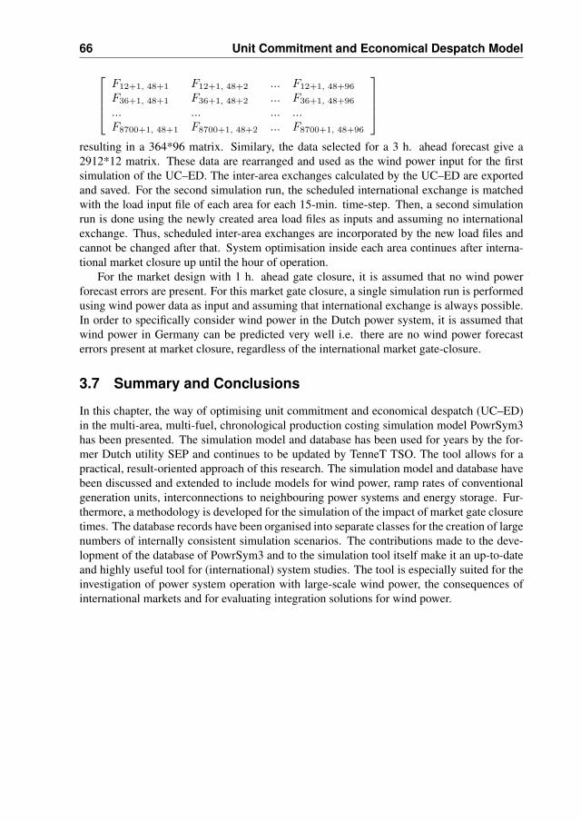
66 Unit Commitment and Economical Despatch Model
F12+1, 48+1 F12+1, 48+2 ... F12+1, 48+96
F36+1, 48+1 F36+1, 48+2 ... F36+1, 48+96
... ... ... ...F8700+1, 48+1 F8700+1, 48+2 ... F8700+1, 48+96
resulting in a 364*96 matrix. Similary, the data selected for a 3 h. ahead forecast give a2912*12 matrix. These data are rearranged and used as the wind power input for the firstsimulation of the UC–ED. The inter-area exchanges calculated by the UC–ED are exportedand saved. For the second simulation run, the scheduled international exchange is matchedwith the load input file of each area for each 15-min. time-step. Then, a second simulationrun is done using the newly created area load files as inputs and assuming no internationalexchange. Thus, scheduled inter-area exchanges are incorporated by the new load files andcannot be changed after that. System optimisation inside each area continues after interna-tional market closure up until the hour of operation.
For the market design with 1 h. ahead gate closure, it is assumed that no wind powerforecast errors are present. For this market gate closure, a single simulation run is performedusing wind power data as input and assuming that international exchange is always possible.In order to specifically consider wind power in the Dutch power system, it is assumed thatwind power in Germany can be predicted very well i.e. there are no wind power forecasterrors present at market closure, regardless of the international market gate-closure.
3.7 Summary and Conclusions
In this chapter, the way of optimising unit commitment and economical despatch (UC–ED)in the multi-area, multi-fuel, chronological production costing simulation model PowrSym3has been presented. The simulation model and database has been used for years by the for-mer Dutch utility SEP and continues to be updated by TenneT TSO. The tool allows for apractical, result-oriented approach of this research. The simulation model and database havebeen discussed and extended to include models for wind power, ramp rates of conventionalgeneration units, interconnections to neighbouring power systems and energy storage. Fur-thermore, a methodology is developed for the simulation of the impact of market gate closuretimes. The database records have been organised into separate classes for the creation of largenumbers of internally consistent simulation scenarios. The contributions made to the deve-lopment of the database of PowrSym3 and to the simulation tool itself make it an up-to-dateand highly useful tool for (international) system studies. The tool is especially suited for theinvestigation of power system operation with large-scale wind power, the consequences ofinternational markets and for evaluating integration solutions for wind power.
CHAPTER 4Impacts of Wind Power on
Unit Commitment andEconomic Despatch
4.1 Introduction
In Chapter 3, an existing unit commitment and economic despatch (UC–ED) tool has beenpresented and extended to include models for wind power, interconnections to neighbouringpower systems, and energy storage. In this chapter, a representative model of the Nether-lands’ and the North-West Europe’s generation systems and the interconnections betweenthe different countries is developed. This model is used for a range of system simulationsfocused on large-scale wind power integration, comprising technical, economic and environ-mental aspects. The impacts of wind power on system operation is assessed and differentsolutions for wind power integration, including energy storage, are addressed. From thesesimulations, 15-min. operational set-points for Dutch generation units can be obtained to beused as input for the dynamic simulations to be performed in Chapter 6.
The chapter is organised as follows. First, the different integration aspects of large-scalewind power is revealed. Simulation parameters are identified to assess the technical, eco-nomic and environmental aspects of integrating of large-scale wind power into the Dutch

68 Impacts of Wind Power on Unit Commitment and Economic Despatch
power system. Then, the system to be simulated is specified in detail, comprising load, gener-ation units, and wind power. Representative models of neighbouring countries are included.Transmission capacities are considered between different countries. Then, an overview ispresented of all system simulations and the simulation set-up. Different simulations are per-formed for several wind power penetration levels, taking into account the possibilities ofinternational markets, examining the consequences of forecast accuracy and considering dif-ferent integration solutions for wind power.
4.2 Simulation Parameters
Since this research is specifically focused on the technical integration of wind power in elec-trical power systems, different technical limits for the system integration of wind power isidentified first. Relevant simulation parameters is identified in order to quantify these limits,if any. After this, the economic and environmental impacts of wind power on power sys-tem operation are discussed and simulation parameters for the assessment of these are alsoidentified.
4.2.1 Technical Limits
In the simulation of the chronological UC–ED for the power system as a whole includingwind power, the following situations may occur that indicate technical limitations for thesystem integration of large-scale wind power:• Minimum load problems• Insufficient upward power reserves• Insufficient downward power reserves
Minimum Load Problems
Based on the analysis carried out in Chapter 2 (Fig. 2.12), the first technical limit for windpower integration is expected to concern minimum load problems. This means that technicaloperating constraints of conventional units (must-run status, minimum power level, mini-mum up-times) prevent a full integration of available wind power during low load periods.When generation threatens to exceed load, simulation results show increased power exports(if interconnection capacity is available), lower output of base-load generation units and ul-timately a spill of the available wind energy. The use of heat boilers is also researched sincethe use of these could allow a temporary shut-down of combined heat and power (CHP) units.
Insufficient Reserves
As was shown in Chapter 2, Fig. 2.13, significantly larger amounts of power reserves arerequired to balance wind power variations on a 15-min. time scale on top of the existing loadvariations. Based on Fig. 2.13, it can be expected that situations with insufficient upwardand downward power reserves may occur but only during a limited number of hours (≤ 100)during the year. Furthermore, sufficient upward reserves may at times not be available tobalance wind power because of technical operating constraints, unscheduled outages, or largewind power forecast errors.
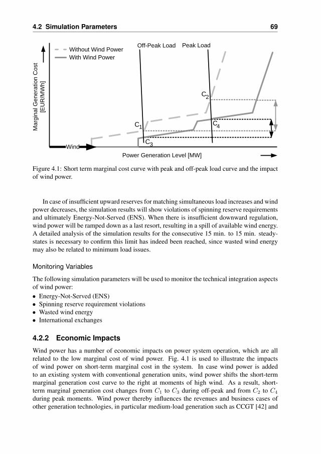
4.2 Simulation Parameters 69
Power Generation Level [MW]Wind
Mar
gina
l Gen
erat
ion
Cos
t [E
UR
/MW
h]
C1
C2
C3
C4
Off-Peak Load Peak LoadWithout Wind PowerWith Wind Power
Figure 4.1: Short term marginal cost curve with peak and off-peak load curve and the impactof wind power.
In case of insufficient upward reserves for matching simultaneous load increases and windpower decreases, the simulation results will show violations of spinning reserve requirementsand ultimately Energy-Not-Served (ENS). When there is insufficient downward regulation,wind power will be ramped down as a last resort, resulting in a spill of available wind energy.A detailed analysis of the simulation results for the consecutive 15 min. to 15 min. steady-states is necessary to confirm this limit has indeed been reached, since wasted wind energymay also be related to minimum load issues.
Monitoring Variables
The following simulation parameters will be used to monitor the technical integration aspectsof wind power:• Energy-Not-Served (ENS)• Spinning reserve requirement violations• Wasted wind energy• International exchanges
4.2.2 Economic Impacts
Wind power has a number of economic impacts on power system operation, which are allrelated to the low marginal cost of wind power. Fig. 4.1 is used to illustrate the impactsof wind power on short-term marginal cost in the system. In case wind power is addedto an existing system with conventional generation units, wind power shifts the short-termmarginal generation cost curve to the right at moments of high wind. As a result, short-term marginal generation cost changes from C1 to C3 during off-peak and from C2 to C4
during peak moments. Wind power thereby influences the revenues and business cases ofother generation technologies, in particular medium-load generation such as CCGT [42] and
70 Impacts of Wind Power on Unit Commitment and Economic Despatch
base-load. This aspect, as well as the optimality (cost, emissions etc.) of the generation mixwith increasing wind power penetration levels, falls outside the scope of this thesis, however.
The extent to which wind power indeed lowers the short-term marginal cost curve of thesystem as a whole, depends on a number of factors. The most important is the technicalflexibility of the system wind power is integrated into. Wind power has been reported toreduce spot market prices in some countries with significant wind power penetrations, such asDenmark [132] and Germany [16]. The extent to which this is structural for the whole marketdepends on the costs of additional power reserves and the decreased operational efficienciesof conventional units, which increase total operating costs. In this research, these aspects aretaken into account by the simulation model and are expressed in the total system operatingcost.
Monitoring Variables
Based on the above, the economic impacts of wind power are quantified by monitoring• Total operating cost• Utilisation factors of conventional generation unitsOperating cost [Me/year] will be monitored for the Netherlands specifically. This also ap-plies for the total electricity produced [TWh/y] per conventional generation technology (nu-clear, coal, CCGT, CHP, gas turbine, etc.).
4.2.3 Environmental Impacts
The environmental aspects of wind power are an important driving force behind the develop-ment of wind power. Electricity generated by wind power replaces fossil-fired conventionalgeneration and thereby saves fuel and CO2 and other emissions. The simulation model in-tegrally takes into account emission cost [e/ton] during the optimisation of the UC–ED byincorporating these as part of the operation cost (CO2 content of fuel, operating efficiency).For monitoring the environmental impacts of wind power, emissions (CO2, but also NOx
and SO2) will be assessed at the system level for the Netherlands and presented for eachconventional generating technology.
4.3 Power System Model Specification
The power system model used here comprises a physical representation of different areas,each representing the generating systems of the Netherlands and its neighbouring areas: Bel-gium, France, Germany, Norway and Great Britain. Interconnections between these areas aremodeled explicitly, transmission constraints within each area are not considered here.
4.3.1 The Netherlands
As was discussed in Chapter 3, at the start of this research, PowrSym3’s database containedmodels for all larger (≥ 60 MW) conventional generation units in the Netherlands. Thisdatabase is updated to represent the Dutch power system for 2014, the year chosen for inves-tigation. Up to 2014, a large amount of new conventional generating capacity is planned orunder development, comprising especially new coal- and gas-fired generation capacity. It is
4.3 Power System Model Specification 71
foreseen that some of the older installations will be shut down by that time but market partieshave not provided information. The Dutch generating portfolio for 2014 is based on the ex-isting portfolio with the addition of new units specified in [164]. This generation portfolio isassumed for all simulations and no attempts have been made to optimise this portfolio withrespect to wind power integration. This is because such an excercise, however useful, is out-side the scope of this thesis, which comprises wind power integration from a technical pointof view. The interconnection capacity of the Netherlands is based on transmission capacity(net transfer capacities, NTC) forecasts of TenneT TSO for 2014 [164] and ETSO [49].
New Conventional Generation
New coal-fired units (total 5.3 GW) are assumed to have a higher maximum operating ef-ficiency of 44.5% and a efficiency curve shape similar to coal-fired units already present inthe database. These new units do not have a must-run status but a minimum up-time anddown-time of 16 h. This allows for temporary shut-downs during periods of low prices, forinstance during weekends.
New natural gas-fired units (total 3.68 GW) are CCGTs with a maximum operating effi-ciency of 58% and an efficiency curve shape similar to existing CCGTs. Of the new CCGTs,two units (1.26 GW total) are modeled as industrial CHPs with a must-run status, deliveringsteam to a separate industrial heat area. The heat load curves of these areas are modeledbased on existing curves in the database. The heat areas are equipped with heat boilers as-sumed only to be used during maintenance of the CHP units, similar to existing CHP unitmodels.
New Distributed Generation – Excluding Wind Power
New distributed generation (DG) capacity in the Netherlands mostly involves installations,i.e. gas engines, in Dutch greenhouses. These CHP units produce electricity, heat and CO2
for the greenhouses, with heat boilers as back-up and heat buffers for several days of storage.Due to the availability of a full heat back-up, the generation units are operated against spotmarket prices and have a very high operational flexibility. A total capacity of 3.0 GW ofgas engines have been modeled, with maximum electrical efficiency of 40%, no minimumup-time or down-time and a 10% unavailability. Ramp rates of these DG units are estimatedto allow a ramp from minimum to maximum output within 15 min.
Other, existing DG, is modeled as non-despatchable capacity (3.4 GW) and aggregatedinto a fixed schedule, simulated as must-take power on the basis of natural gas-fired gen-eration. This capacity represents non-despatchable industrial units, waste incineration, andother small DG units. The output of this DG is assumed to be 50% constant and 50% variablewith system load and has an efficiency of 19%.
Wind Power
For the Netherlands, a one year data series of 15 min. wind power data for seven wind powerpenetration levels have been developed in Chapter 2 for respectively 0 GW, 2 GW (225MW offshore), 4 GW (1 GW offshore), 6 GW (2 GW offshore), 8 GW (4 GW offshore), 10GW (6 GW offshore) and 12 GW (8 GW offshore). It is assumed that wind power does not
72 Impacts of Wind Power on Unit Commitment and Economic Despatch
replace any conventional capacity. In reality, wind power has a capacity credit [41, 176] andwill lead to changes in the total installed generation capacity and the generation mix. Theseaspects fall outside the scope of this thesis.
4.3.2 Neighbouring Areas
Areas and Interconnectors
In this research, the Netherlands (NL) is assumed to be a central area with interconnectionsto Belgium (B), France (F), Germany (D), and Great Britain (GB), and Norway (NOR) toa very limited extent. Each country is represented as a single area comprising generationand load, with interconnections to neighbouring areas based on [49, 164]. Only cross-bordertransmission capacities between countries are taken into account. The power system modelwith all areas and interconnectors is shown in Fig. 4.2, representing the Netherlands as partof the West European interconnected system. The NODE area (grey) is an empty area usedto incorporate the transmission capacity limits foreseen by TenneT TSO for 2014 for theNetherlands with Belgium and Germany. Apart from the separate interconnection capacitieswhich exist between the Netherlands and Belgium (2300 MW) and Germany (5400 MW),a net export/import transmission capacity maximum of 5650 MW is applied between theNetherlands and these countries together (NTC defined by TenneT TSO).
The transmission capacities NL–NOR (NorNed), NL–GB (BritNed) and F–GB (Cross-Channel) are high voltage direct current (DC) sub-marine interconnectors, for which an avail-ability of 98% is assumed, other interconnections have an availability of 100%. Transmissionlosses are assumed to be 5% of the transmitted power for NorNed, and 4% for BritNed andCross-Channel.
Area Load
Load data for the areas outside the Netherlands for the year 2014 are developed using UCTEload data for the relevant countries for the year 2007 [171]. This assures that correlationsamong momentary loads in all countries are automatically taken into account. The load dataare processed similarly to the Dutch load data using annual growth rates up until 2014 basedon [170, 166]. The growth rates for load in 2014 relative to 2007 are 1.08, 1.08, 1.03 and1.10 for Belgium, France, Germany and Great Britain, respectively.
Fossil-Fired Generation
Models for conventional generation units in the neighbouring areas of the Netherlands weredeveloped based on installed capacity estimates made in [124, 170]. Generating technologyefficiencies and other technical factors were estimated based on an extensive generation unitdatabase made available by TenneT TSO and using the existing models for the Dutch units inthe PowrSym3 database. Each generation technology type outside the Netherlands is mod-eled as an aggregation of units with identical characteristics, with a total generating capacityequaling the capacity foreseen to be installed in 2014.
The most important technical parameters for the fossil-fired generation units are sum-marised for each technology in Table 4.1, with MR = must-run and EC = economic opera-tion. Nuclear generation units in Belgium, Germany and Great Britain are modeled as having
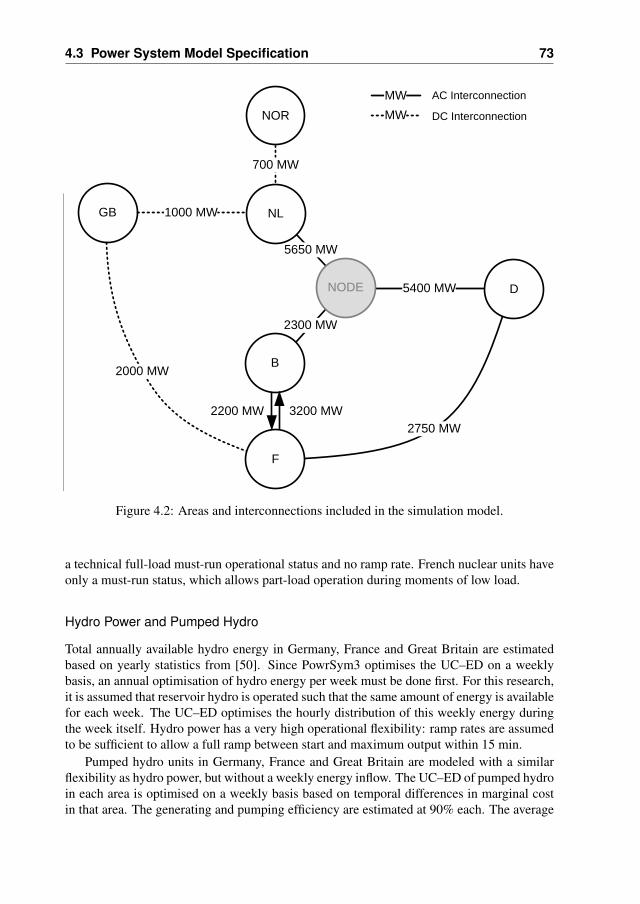
4.3 Power System Model Specification 73
NOR
GB
D
B
700 MW
1000 MW
2000 MW
2750 MW
F
5400 MW
2200 MW 3200 MW
5650 MW
NL
2300 MW
NODE
MWMW AC Interconnection
DC Interconnection
Figure 4.2: Areas and interconnections included in the simulation model.
a technical full-load must-run operational status and no ramp rate. French nuclear units haveonly a must-run status, which allows part-load operation during moments of low load.
Hydro Power and Pumped Hydro
Total annually available hydro energy in Germany, France and Great Britain are estimatedbased on yearly statistics from [50]. Since PowrSym3 optimises the UC–ED on a weeklybasis, an annual optimisation of hydro energy per week must be done first. For this research,it is assumed that reservoir hydro is operated such that the same amount of energy is availablefor each week. The UC–ED optimises the hourly distribution of this weekly energy duringthe week itself. Hydro power has a very high operational flexibility: ramp rates are assumedto be sufficient to allow a full ramp between start and maximum output within 15 min.
Pumped hydro units in Germany, France and Great Britain are modeled with a similarflexibility as hydro power, but without a weekly energy inflow. The UC–ED of pumped hydroin each area is optimised on a weekly basis based on temporal differences in marginal costin that area. The generating and pumping efficiency are estimated at 90% each. The average

74 Impacts of Wind Power on Unit Commitment and Economic Despatch
Parameter Nuclear Coal Lignite CCGT Oil GTCommitment MR MR MR EC EC ECDespatch MR / EC EC EC EC EC ECMin. Downtime [h.] n.a. n.a. n.a. 6 4 4Min. Uptime [h.] n.a. n.a. n.a. 4 4 2Min. Power Level [%/Pn] 100 / 50 50 50 50 60 60Ramp Rate [%/Pn/h.] n.a. / 25 40 40 80 80 160Max. eff. [%] n.a. 39 39 51 37 26Unavailability [%] 20 15 18 14 18 14
MR = Must Run, EC = Economic Optimisation
Table 4.1: Fossil-fired generation models in neighbouring areas.
unavailability of pumped hydro is determined at 2%, due to the absence of thermodynamicprocesses in these units.
Wind Power
Wind power in neighbouring areas is only taken into account for Germany. This is becauseGermany already has a large installed capacity of wind power, which is foreseen to increasesignificantly [51, 170]. Furthermore, wind power outputs in the Netherlands and Germany arestrongly correlated and a large interconnection capacity is available between these countries.In a North-West European market, the presence of large-scale wind power in Germany couldpresent additional barriers for wind power in the Netherlands.
In order to correctly incorporate the correlation between wind power in the Netherlandsand Germany, 15 min. average wind power data for the German areas EON-Netz, RWE andVattenfall were obtained from the respective TSOs for the same period as the Dutch meteo-rological data (June 1, 2004 to May 31st, 2005). Also, day-ahead forecast data were obtainedfor this period. Wind power and wind power prediction data are scaled to represent the 32GW of installed capacity foreseen for 2014 (Appendix C). It is found that the correlation be-tween the 15 min. aggregated average wind power data sets for the Netherlands and Germanyis 0.73. Thus, interconnection capacity to Germany may not be (fully) available for exportsduring moments of low load and high wind power, resulting in wasted wind energy. Windpower in Germany is modeled such that it is integrated with a higher priority than Dutchwind power in order to guarantee that wind power in the Netherlands is not integrated intothe system at the expense of German wind power.
4.3.3 Power System Overview
Installed generating capacities per technology are based on forecasts made for the relevantcountries for 2014 in [124, 164, 170]. The installed capacities are presented per technologyand per country in Table 4.2.
An important assumption is that Norway is represented as a pumped hydro unit withoutinflow, with a generating/pumping capacity equaling the interconnection capacity betweenthe Netherlands and Norway. The hydro power system of Norway has a high operational
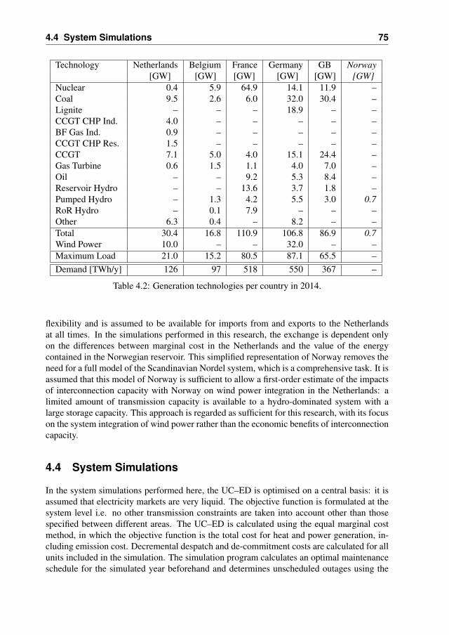
4.4 System Simulations 75
Technology Netherlands Belgium France Germany GB Norway[GW] [GW] [GW] [GW] [GW] [GW]
Nuclear 0.4 5.9 64.9 14.1 11.9 –Coal 9.5 2.6 6.0 32.0 30.4 –Lignite – – – 18.9 – –CCGT CHP Ind. 4.0 – – – – –BF Gas Ind. 0.9 – – – – –CCGT CHP Res. 1.5 – – – – –CCGT 7.1 5.0 4.0 15.1 24.4 –Gas Turbine 0.6 1.5 1.1 4.0 7.0 –Oil – – 9.2 5.3 8.4 –Reservoir Hydro – – 13.6 3.7 1.8 –Pumped Hydro – 1.3 4.2 5.5 3.0 0.7RoR Hydro – 0.1 7.9 – – –Other 6.3 0.4 – 8.2 – –Total 30.4 16.8 110.9 106.8 86.9 0.7Wind Power 10.0 – – 32.0 – –Maximum Load 21.0 15.2 80.5 87.1 65.5 –Demand [TWh/y] 126 97 518 550 367 –
Table 4.2: Generation technologies per country in 2014.
flexibility and is assumed to be available for imports from and exports to the Netherlandsat all times. In the simulations performed in this research, the exchange is dependent onlyon the differences between marginal cost in the Netherlands and the value of the energycontained in the Norwegian reservoir. This simplified representation of Norway removes theneed for a full model of the Scandinavian Nordel system, which is a comprehensive task. It isassumed that this model of Norway is sufficient to allow a first-order estimate of the impactsof interconnection capacity with Norway on wind power integration in the Netherlands: alimited amount of transmission capacity is available to a hydro-dominated system with alarge storage capacity. This approach is regarded as sufficient for this research, with its focuson the system integration of wind power rather than the economic benefits of interconnectioncapacity.
4.4 System Simulations
In the system simulations performed here, the UC–ED is optimised on a central basis: it isassumed that electricity markets are very liquid. The objective function is formulated at thesystem level i.e. no other transmission constraints are taken into account other than thosespecified between different areas. The UC–ED is calculated using the equal marginal costmethod, in which the objective function is the total cost for heat and power generation, in-cluding emission cost. Decremental despatch and de-commitment costs are calculated for allunits included in the simulation. The simulation program calculates an optimal maintenanceschedule for the simulated year beforehand and determines unscheduled outages using the
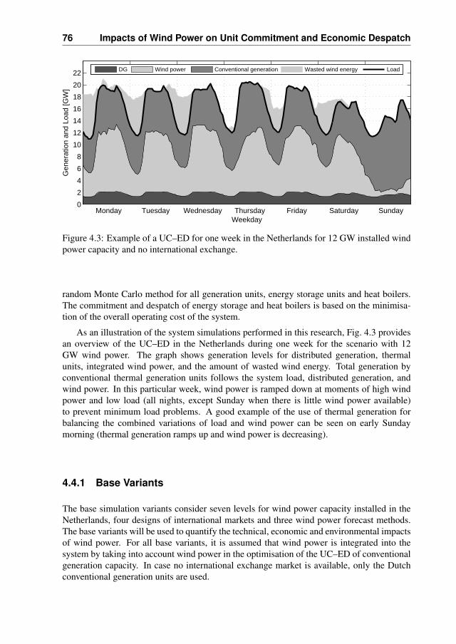
76 Impacts of Wind Power on Unit Commitment and Economic Despatch
Monday Tuesday Wednesday Thursday Friday Saturday Sunday02468
10121416182022
Weekday
Gen
erat
ion
and
Load
[GW
]
DG Wind power Conventional generation Wasted wind energy Load
Figure 4.3: Example of a UC–ED for one week in the Netherlands for 12 GW installed windpower capacity and no international exchange.
random Monte Carlo method for all generation units, energy storage units and heat boilers.The commitment and despatch of energy storage and heat boilers is based on the minimisa-tion of the overall operating cost of the system.
As an illustration of the system simulations performed in this research, Fig. 4.3 providesan overview of the UC–ED in the Netherlands during one week for the scenario with 12GW wind power. The graph shows generation levels for distributed generation, thermalunits, integrated wind power, and the amount of wasted wind energy. Total generation byconventional thermal generation units follows the system load, distributed generation, andwind power. In this particular week, wind power is ramped down at moments of high windpower and low load (all nights, except Sunday when there is little wind power available)to prevent minimum load problems. A good example of the use of thermal generation forbalancing the combined variations of load and wind power can be seen on early Sundaymorning (thermal generation ramps up and wind power is decreasing).
4.4.1 Base Variants
The base simulation variants consider seven levels for wind power capacity installed in theNetherlands, four designs of international markets and three wind power forecast methods.The base variants will be used to quantify the technical, economic and environmental impactsof wind power. For all base variants, it is assumed that wind power is integrated into thesystem by taking into account wind power in the optimisation of the UC–ED of conventionalgeneration capacity. In case no international exchange market is available, only the Dutchconventional generation units are used.
4.4 System Simulations 77
Wind Power Levels
All base simulations will be carried out for six wind power penetration levels, as developedin Chapter 2 (2–12 GW), and for a 0 MW wind power variant to be used as a reference.
International Exchange
International exchange is modeled and simulated for four market designs:• No international exchange• International market gate closure time day ahead• International market gate closure time 3 h. ahead• International market gate closure time 1 h. aheadThe base-case for this research is the Netherlands seen as an isolated power system. Interna-tional exchange with Belgium, France, Germany, Norway and Great Britain is assumed to bezero at all times. This variant serves as a reference to consider the integration of wind powerin the Dutch power system using the technical capacities available in the Netherlands only.
The other market designs all comprise international exchange possibilities between theNetherlands and its neighbours, but using different gate closure times. This means that theimports and exports of the Netherlands are optimised using the wind power forecast availa-ble at market gate closure. After market gate closure, the international exchange schedulesbecome fixed and are executed as scheduled. For the day ahead (12–36 h.) ahead market clo-sure, wind power forecast errors are significant (Fig. 2.14). This will result in a sub-optimalscheduling of imports and exports from a wind power integration point of view. Forecasterrors will have decreased by about 50% if market gate closure is delayed up to 3 h. ahead ofoperation, and no forecast errors are present for the market design with near real-time opera-tion (1 h. ahead), which allows an optimal scheduling of international exchange consideringwind power.
Wind Power Forecasts
The following wind power forecasts are considered as a base-case variants:• 0 MW wind power forecast (fuel saver approach [55])• Best available forecast• Perfect forecastFor the 0 MW wind power forecast, the UC–ED is optimised without incorporating windpower capacity in the planning stage, although actual wind power output is taken into ac-count in the operational stage. This forecast leads to an over-commitment of conventionalgenerating capacity and serves as a worst-case planning situation. The best available forecastcomprises an hourly update of the wind power forecast (’rolling forecast’), based on updatedwind power forecasts, and a subsequent recalculation of the UC–ED taking these into ac-count. For a perfect forecast, the actual wind power levels are exactly known in all stages ofthe UC–ED.
It is important to note that that for all wind power forecasts, the real-time wind poweroutput level is assumed to be exactly known and used as an input for economic despatch inthe following hours. Furthermore, it is assumed that UC–ED is continuously optimised upuntil the hour of operation (1 h. ahead). This re-calculation of the UC–ED is in fact much
78 Impacts of Wind Power on Unit Commitment and Economic Despatch
more frequent that presently applied by Dutch PRPs, who usually do this 2–4 times a day. Itcan also be noted that the central optimisation of the UC–ED such as applied in this research,does not take into account the behaviour of individual market parties or generation clusterson the electricity market (i.e. fuel contracts, individual reserve power considerations). Theavailability of a better wind power forecast may be very beneficial for the market operatingstrategy of traders and lead to significant revenues. Here, only the opportunities of windpower forecasts for the maximisation of the system integration of wind power are considered.
4.4.2 Wind Power Integration Solutions
Technical limits may exist for the system integration of wind power in the Dutch power sys-tem. After the determination and quantification of these limits, different alternatives will beexplored for overcoming these integration limits. For all simulations, conventional genera-tion units are used for balancing wind power. More flexible base-load generation capacitymay provide additional technical space for wind power during low-load, high-wind situa-tions. For this alternative, the commitment status of selected industrial CHP units is changedfrom must-run to economic. The existing heat boilers could in principle take over the gen-eration of steam for the industrial processes at times when the CHP is shut down to allow afurther integration of wind power.
The energy storage alternatives included in this research include surface pumped accu-mulation energy storage (PAC), underground PAC (UPAC), compressed air energy storage(CAES) and creating additional interconnection capacity between the Netherlands and thehydropower-dominated system of Norway (NN2). Models for these alternatives were devel-oped in Chapter 3. It can be noted that no specific attempt has been made here to optimisethe design of the energy storage: the energy storage capacities and reservoir sizes applied in[168] have been adopted here.
4.4.3 Simulations Set-Up
The simulations of the UC–ED are carried out for a future year 2014, with a resolution of15 minutes, for different installed wind power capacities, wind power forecasts, internationalmarket designs and balancing solutions. An optimised unit maintenance schedule is calcu-lated ahead of each simulation and unscheduled outages are introduced using the RandomMonte Carlo method for all generation units, energy storage units and heat boilers, for ev-ery week. UC–ED are centrally optimised (well functioning electricity markets) in order toachieve minimum operating cost at the system level, while all technical constraints are ful-filled. The UC–ED is calculated using an equal marginal cost method, in which the objectivefunction is the total cost for generating both heat and power. A calculation of unit despatch isperformed every 15 minutes using the given load profile and an estimation of the wind powerproduction levels.
Power Reserves
Spinning reserves and fast regulating power are provided by the non-despatched capacityof committed generation units. All coal- and gas-fired generation units in the Netherlandssized 60 MW and above are assigned with a spinning reserve contribution of 1% of its rated
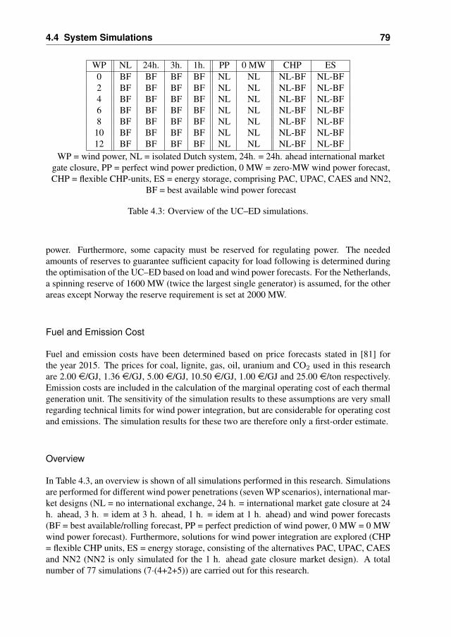
4.4 System Simulations 79
WP NL 24h. 3h. 1h. PP 0 MW CHP ES0 BF BF BF BF NL NL NL-BF NL-BF2 BF BF BF BF NL NL NL-BF NL-BF4 BF BF BF BF NL NL NL-BF NL-BF6 BF BF BF BF NL NL NL-BF NL-BF8 BF BF BF BF NL NL NL-BF NL-BF
10 BF BF BF BF NL NL NL-BF NL-BF12 BF BF BF BF NL NL NL-BF NL-BF
WP = wind power, NL = isolated Dutch system, 24h. = 24h. ahead international marketgate closure, PP = perfect wind power prediction, 0 MW = zero-MW wind power forecast,CHP = flexible CHP-units, ES = energy storage, comprising PAC, UPAC, CAES and NN2,
BF = best available wind power forecast
Table 4.3: Overview of the UC–ED simulations.
power. Furthermore, some capacity must be reserved for regulating power. The neededamounts of reserves to guarantee sufficient capacity for load following is determined duringthe optimisation of the UC–ED based on load and wind power forecasts. For the Netherlands,a spinning reserve of 1600 MW (twice the largest single generator) is assumed, for the otherareas except Norway the reserve requirement is set at 2000 MW.
Fuel and Emission Cost
Fuel and emission costs have been determined based on price forecasts stated in [81] forthe year 2015. The prices for coal, lignite, gas, oil, uranium and CO2 used in this researchare 2.00 e/GJ, 1.36 e/GJ, 5.00 e/GJ, 10.50 e/GJ, 1.00 e/GJ and 25.00 e/ton respectively.Emission costs are included in the calculation of the marginal operating cost of each thermalgeneration unit. The sensitivity of the simulation results to these assumptions are very smallregarding technical limits for wind power integration, but are considerable for operating costand emissions. The simulation results for these two are therefore only a first-order estimate.
Overview
In Table 4.3, an overview is shown of all simulations performed in this research. Simulationsare performed for different wind power penetrations (seven WP scenarios), international mar-ket designs (NL = no international exchange, 24 h. = international market gate closure at 24h. ahead, 3 h. = idem at 3 h. ahead, 1 h. = idem at 1 h. ahead) and wind power forecasts(BF = best available/rolling forecast, PP = perfect prediction of wind power, 0 MW = 0 MWwind power forecast). Furthermore, solutions for wind power integration are explored (CHP= flexible CHP units, ES = energy storage, consisting of the alternatives PAC, UPAC, CAESand NN2 (NN2 is only simulated for the 1 h. ahead gate closure market design). A totalnumber of 77 simulations (7·(4+2+5)) are carried out for this research.
80 Impacts of Wind Power on Unit Commitment and Economic Despatch
4.5 Simulation Results
4.5.1 Technical Limits
Possible technical limits for the integration of wind power are minimum load problems andinsufficient upward power reserves or downward regulation reserves for balancing load andwind power variations. The simulation results for all base simulation variants (0–12 GWwind power) do not report ENS nor spinning reserve violations in the Netherlands. Thisapplies for all three different wind power forecast modes (0-MW forecast, best availableforecast and perfect prediction). From this result, it can be concluded that sufficient upwardpower reserves and downward regulation are present at all moments during the year in orderto balance the aggregated load and wind power and load variations. This was to be expectedsince the total generation portfolio is rather large compared to the maximum load. The inte-gration of wind power in the Dutch power system does however result in an increase of heatproduction by boilers at CHP locations (especially residential), wasting of wind energy (es-pecially during low-load periods), and increased exports to neighbouring countries (idem).This indicates that minimum load problems pose a technical limit for the integration of windpower, which is in line with the observations made in Chapter 2.
The simulation results for wasted wind energy and international exchanges vary consid-erably between the different international market designs, since they are mutually dependent,and to some extent between the different wind power forecast methods investigated here.
Wasted Wind Energy – International Market Design
In Fig. 4.4, wind energy integrated into the Dutch power system is shown for different windpower penetrations and different market designs. Wasted wind energy becomes significantin the range of 6–8 GW installed wind power capacity for the Dutch power system, in themarket design without international exchange. The slight change in steepness of the availablewind energy curve at 2 and 6 GW installed capacity is due to increased capacity factor ofwind power (offshore vs. onshore). The use of international exchange provides significantadditional space for the integration of wind power (middle-grey area is additionally integratedwind energy). The light grey area representing wasted wind in a 1 h. ahead market gateclosure is very small and not visible in this figure.
Fig. 4.5 focuses further on a comparison of the amount of wasted wind energy for differ-ent market designs. Only wind power forecast errors in the Netherlands are considered here.In case no interconnection capacity is available for balancing purposes, an estimated amountof 6.2 TWh/y or 15% of available wind energy in the Netherlands cannot be integrated intothe system. In case international exchanges can be used for exports at high wind power lev-els, additional wind power can be integrated, with only 0.05 TWh or 0.1% of available windenergy being wasted for the 1 h. ahead market gate closure.
Interestingly, a day-ahead or 3 h. ahead international market gate closure time results inlarger amounts of wasted wind power at smaller wind power capacities. This is the resultof the methodology applied for the optimisation of international exchange at market gateclosure, which is based on the assumption that all feasible international transactions are beingmade. In case a significant wind power forecast error is present at the moment that thesetransactions become fixed, scheduled imports may prevent the integration of unpredicted

4.5 Simulation Results 81
0 2 4 6 8 10 120
5
10
15
20
25
30
35
40
Installed Wind Power Capacity [GW]
Win
d E
nerg
y [T
Wh/
y]
Integrated wind energy, no international exchangePossible additional integration using international exchangeWasted wind energyAvailable wind energy
Figure 4.4: Integrated and wasted wind energy in the Netherlands.
0 2 4 6 8 10 120
1
2
3
4
5
6
Installed Wind Power Capacity [GW]
Was
ted
Win
d E
nerg
y [T
Wh/
y]
No international exchangeDay-ahead international market gate closure3 h. ahead international market gate closure1 h. ahead international market gate closure
Figure 4.5: Wasted wind energy for different international market designs, best availablewind power forecast.
1 2 3 4 5 6 7 8 9 10 11 12 13 0
100
200
300
400
500
Week Number
Was
ted
Win
d E
nerg
y [G
Wh/
wk]
Perfect forecastBest available forecast0-MW prediction
Figure 4.6: Weekly wasted wind energy for different forecast methods, 12 GW wind power,no international exchange.
82 Impacts of Wind Power on Unit Commitment and Economic Despatch
surpluses of wind power, leading to larger amounts of wasted wind energy. For large windpower penetrations, however, the benefits of international exchange capacity outweigh thedisadvantage of forecast errors. Clearly, a more conservative scheduling of internationalexchanges (imports) will result in less wasted wind energy. This result illustrates the benefitsof postponed international market gate closure times for integrating wind power.
In case interconnection capacity is available and the market design allows an adjustmentof international exchange up until the moment of operation (1 h. ahead international marketgate closure), the potential for additionally integrated wind energy is high. Still, even the mostflexible international market design cannot prevent a small amount of wasted wind energy,starting from 8–10 GW installed capacity in the Netherlands (bottom of Fig. 4.5, not visiblein Fig. 4.4). The reason for this is that, even though international transmission capacity maybe sufficient, this capacity is not always fully available for exports. This applies to Germanyin particular. Germany has a significant must-run conventional generation capacity and alarge amount of wind power (32 GW in the year 2014) which is highly correlated (0.73)to wind power in the Netherlands. Both factors reduce the possibilities for exports of windpower from the Netherlands, especially during critical periods.
Wasted Wind Energy – Forecast Method
The different types of wind power forecasts only have a minor influence on the amount ofwasted wind energy on an annual basis. Fig. 4.6 shows the amount of wasted wind energyfor all weeks for 12 GW wind power, with no international exchange possible. Interestingly,some differences are present in the amount of wasted wind between the 0-MW and the bestavailable forecast method. The simulation results show that an over-commitment of conven-tional generation capacity may be beneficial for wind power integration during some hoursof the week. Generally, however, the differences in wasted wind between the 0-MW forecast,the best available wind power forecast and the perfect forecast are small (<<5% of wastedwind energy). This can be explained by the frequent re-calculation of the UC–ED which isapplied to all simulations, which allows the inclusion of the real-time wind power output andof regularly updated wind power forecasts. Since actual wind power levels are accuratelyknown and wind power output generally does not change significantly between 15 min. in-tervals, the conventional generation units in operation will typically be adequate for the nexttime-interval as well, explaining the relatively good performance of the 0-MW forecast.
4.5.2 Economic Impacts
Operating Cost
As was illustrated in Fig. 4.1, wind power decreases marginal operating costs in the system.Fig. 4.7 shows the annual savings in operating cost due to wind power, for the Netherlandswithout international exchange and in case international exchange is possible (1 h. aheadmarket gate closure time) for the North-West European system as a whole, with the Dutchpart as a dotted line. As the figure shows, the operating cost savings by wind power increasewith the amount of wind power installed. For the fuel and operating costs assumed here,the overall annual operating cost savings by wind power are estimated to be in the order of1.5 billion e annually for 12 GW wind power capacity. The slight differences in total costsavings between an isolated Dutch system versus a North-West European system are due to
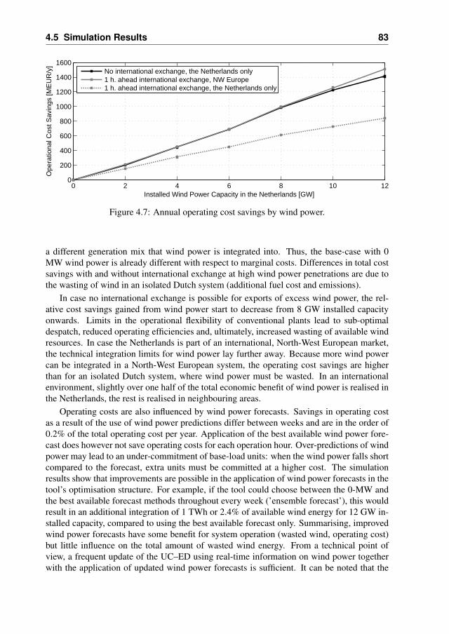
4.5 Simulation Results 83
0 2 4 6 8 10 120
200
400
600
800
1000
1200
1400
1600
Installed Wind Power Capacity in the Netherlands [GW]
Ope
ratio
nal C
ost S
avin
gs [M
EU
R/y
]
No international exchange, the Netherlands only1 h. ahead international exchange, NW Europe1 h. ahead international exchange, the Netherlands only
Figure 4.7: Annual operating cost savings by wind power.
a different generation mix that wind power is integrated into. Thus, the base-case with 0MW wind power is already different with respect to marginal costs. Differences in total costsavings with and without international exchange at high wind power penetrations are due tothe wasting of wind in an isolated Dutch system (additional fuel cost and emissions).
In case no international exchange is possible for exports of excess wind power, the rel-ative cost savings gained from wind power start to decrease from 8 GW installed capacityonwards. Limits in the operational flexibility of conventional plants lead to sub-optimaldespatch, reduced operating efficiencies and, ultimately, increased wasting of available windresources. In case the Netherlands is part of an international, North-West European market,the technical integration limits for wind power lay further away. Because more wind powercan be integrated in a North-West European system, the operating cost savings are higherthan for an isolated Dutch system, where wind power must be wasted. In an internationalenvironment, slightly over one half of the total economic benefit of wind power is realised inthe Netherlands, the rest is realised in neighbouring areas.
Operating costs are also influenced by wind power forecasts. Savings in operating costas a result of the use of wind power predictions differ between weeks and are in the order of0.2% of the total operating cost per year. Application of the best available wind power fore-cast does however not save operating costs for each operation hour. Over-predictions of windpower may lead to an under-commitment of base-load units: when the wind power falls shortcompared to the forecast, extra units must be committed at a higher cost. The simulationresults show that improvements are possible in the application of wind power forecasts in thetool’s optimisation structure. For example, if the tool could choose between the 0-MW andthe best available forecast methods throughout every week (’ensemble forecast’), this wouldresult in an additional integration of 1 TWh or 2.4% of available wind energy for 12 GW in-stalled capacity, compared to using the best available forecast only. Summarising, improvedwind power forecasts have some benefit for system operation (wasted wind, operating cost)but little influence on the total amount of wasted wind energy. From a technical point ofview, a frequent update of the UC–ED using real-time information on wind power togetherwith the application of updated wind power forecasts is sufficient. It can be noted that the

84 Impacts of Wind Power on Unit Commitment and Economic Despatch
The Netherlands Belgium Germany France Great Britain Norway6050403020100
10203040506070
Country, for 0-12 GW Wind Power Capacity in the Netherlands
Impo
rt an
d E
xpor
t [TW
h/y]
Figure 4.8: International exchange in North-West Europe for 0–12 GW wind power installedcapacity in the Netherlands.
benefits of improved wind power forecasts for trading on markets are not considered here.Such benefits may be significant for the individual market parties for the formulation of theirmarket trading strategy [58].
International Exchange
In case international exchange is possible, the integration of wind power in the Netherlandsinfluences in principle the exchanges between all countries. In Fig. 4.8, imports and exportsare shown for each country with each bar representing a wind power penetration scenario.Clearly, the Netherlands increases its annual exports and decreases its imports in case morewind power is installed. This influences mainly imports and exports of Germany and GreatBritain, and Belgium to a limited extent.
Large interconnection capacities are present between Germany and the Netherlands andDutch wind power mainly decrease the full-load hours for base-load coal and lignite in Ger-many, but also some CCGT. Wind power furthermore reduces the exports of base-load coalpower from Belgium and to a lesser extent from France during periods of low load (nights andweekends). Germany reduces its imports from France at times of high wind in the Nether-lands. Exchanges with Norway stay constant in volume since it is modeled as such, althoughthe moments of exports and imports are increasingly determined by wind power as its in-stalled capacity in the Netherlands increases. These results clearly show the importance ofthe larger, Germany system for the integration of wind power in the Dutch system.
Generation Output Mix
In Fig.4.9, the change in annual electricity output between different generation technologiesis shown for the Netherlands (no international exchange) with increasing wind power capac-ity. Nuclear, being a full-load must-run technology, is not affected by wind power integration.Wind power does reduce the full-load hour equivalents of coal-fired units, CCGT CHP andCCGT. Importantly, the profits of these units also decrease during the hours that they are in
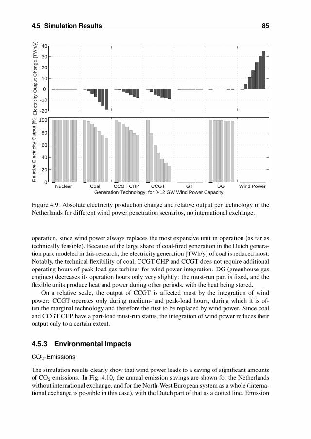
4.5 Simulation Results 85
-20
-10
0
10
20
30
40
Ele
ctric
ity O
utpu
t Cha
nge
[TW
h/y]
Nuclear Coal CCGT CHP CCGT GT DG Wind Power0
20
40
60
80
100
Generation Technology, for 0-12 GW Wind Power Capacity
Rel
ativ
e E
lect
ricity
Out
put [
%]
Figure 4.9: Absolute electricity production change and relative output per technology in theNetherlands for different wind power penetration scenarios, no international exchange.
operation, since wind power always replaces the most expensive unit in operation (as far astechnically feasible). Because of the large share of coal-fired generation in the Dutch genera-tion park modeled in this research, the electricity generation [TWh/y] of coal is reduced most.Notably, the technical flexibility of coal, CCGT CHP and CCGT does not require additionaloperating hours of peak-load gas turbines for wind power integration. DG (greenhouse gasengines) decreases its operation hours only very slightly: the must-run part is fixed, and theflexible units produce heat and power during other periods, with the heat being stored.
On a relative scale, the output of CCGT is affected most by the integration of windpower: CCGT operates only during medium- and peak-load hours, during which it is of-ten the marginal technology and therefore the first to be replaced by wind power. Since coaland CCGT CHP have a part-load must-run status, the integration of wind power reduces theiroutput only to a certain extent.
4.5.3 Environmental Impacts
CO2-Emissions
The simulation results clearly show that wind power leads to a saving of significant amountsof CO2 emissions. In Fig. 4.10, the annual emission savings are shown for the Netherlandswithout international exchange, and for the North-West European system as a whole (interna-tional exchange is possible in this case), with the Dutch part of that as a dotted line. Emission

86 Impacts of Wind Power on Unit Commitment and Economic Despatch
0 2 4 6 8 10 120
2
4
6
8
10
12
14
16
18
20
Installed Wind Power Capacity [GW]
CO
2-E
mis
sion
Sav
ings
[M
ton/
y]
No international exchange, the Netherlands only1 h. ahead international exchange, NW Europe1 h. ahead international exchange, the Netherlands only
Figure 4.10: CO2 emission savings by wind power.
savings are estimated to lie around 19 Mton annually for 12 GW wind power, with highersavings for the isolated Dutch system due to the large share of coal in the generation mix. Incase international exchange is possible, more expensive, less efficient units (mainly CCGT)have already been pushed out of the market at the 0 MW wind power. Wind power will alsoreplace more expensive CCGT-generation during the day rather than coal-fired units in theisolated Dutch system, resulting in lower emission savings for the cases with internationalexchange. It can be noted that emission savings also positively impact operating costs, sinceCO2 emission savings are part of the total operating cost. The change in steepness of thecurves at 2 and 6 GW installed wind power capacity is due to the higher capacity factor ofoffshore wind power. For the isolated Dutch system, there is a change at 8 GW wind powerdue to the increasing amounts of wasted wind energy. The results for emission savings forSO2 and NOx show similar trends as CO2. Total annual emissions show an estimated de-crease of 11 Mton and 20 kton for SO2 and NOx, respectively, for an isolated Dutch system.
4.5.4 Integration Solutions for Wind Power
The integration of wind power in the Dutch power system leads to savings in emissions andoperational cost. The technical limit for wind power integration is mainly the minimum-load,leading to increasing amounts of wasted wind energy, while the variability and limited pre-dictability of up to 12 GW wind power can be solved using existing, conventional generationunits. In this section, solutions for the integration of wind power in the Dutch power systemwill be explored. Models for the different solutions were developed in Chapter 3 and consistof pumped accumulation storage (PAC, 1700 MW), underground PAC (UPAC, 1400 MW),compressed air energy storage (CAES, 1500 MW), flexible CHP-units by installing and usingheat boilers (CHP, 1500 MW) and an extra interconnection between the Netherlands and Nor-way (NN2, 1400 MW). It is assumed that energy storage and the additional interconnectioncapacity to Norway do not replace conventional generation capacity.
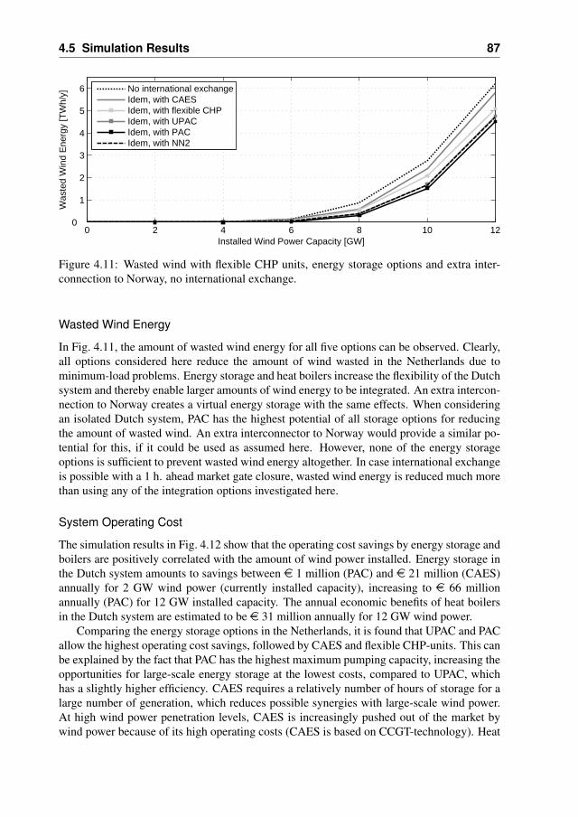
4.5 Simulation Results 87
0 2 4 6 8 10 120
1
2
3
4
5
6
Installed Wind Power Capacity [GW]
Was
ted
Win
d E
nerg
y [T
Wh/
y]
No international exchangeIdem, with CAESIdem, with flexible CHPIdem, with UPACIdem, with PACIdem, with NN2
Figure 4.11: Wasted wind with flexible CHP units, energy storage options and extra inter-connection to Norway, no international exchange.
Wasted Wind Energy
In Fig. 4.11, the amount of wasted wind energy for all five options can be observed. Clearly,all options considered here reduce the amount of wind wasted in the Netherlands due tominimum-load problems. Energy storage and heat boilers increase the flexibility of the Dutchsystem and thereby enable larger amounts of wind energy to be integrated. An extra intercon-nection to Norway creates a virtual energy storage with the same effects. When consideringan isolated Dutch system, PAC has the highest potential of all storage options for reducingthe amount of wasted wind. An extra interconnector to Norway would provide a similar po-tential for this, if it could be used as assumed here. However, none of the energy storageoptions is sufficient to prevent wasted wind energy altogether. In case international exchangeis possible with a 1 h. ahead market gate closure, wasted wind energy is reduced much morethan using any of the integration options investigated here.
System Operating Cost
The simulation results in Fig. 4.12 show that the operating cost savings by energy storage andboilers are positively correlated with the amount of wind power installed. Energy storage inthe Dutch system amounts to savings between e 1 million (PAC) and e 21 million (CAES)annually for 2 GW wind power (currently installed capacity), increasing to e 66 millionannually (PAC) for 12 GW installed capacity. The annual economic benefits of heat boilersin the Dutch system are estimated to be e 31 million annually for 12 GW wind power.
Comparing the energy storage options in the Netherlands, it is found that UPAC and PACallow the highest operating cost savings, followed by CAES and flexible CHP-units. This canbe explained by the fact that PAC has the highest maximum pumping capacity, increasing theopportunities for large-scale energy storage at the lowest costs, compared to UPAC, whichhas a slightly higher efficiency. CAES requires a relatively number of hours of storage for alarge number of generation, which reduces possible synergies with large-scale wind power.At high wind power penetration levels, CAES is increasingly pushed out of the market bywind power because of its high operating costs (CAES is based on CCGT-technology). Heat
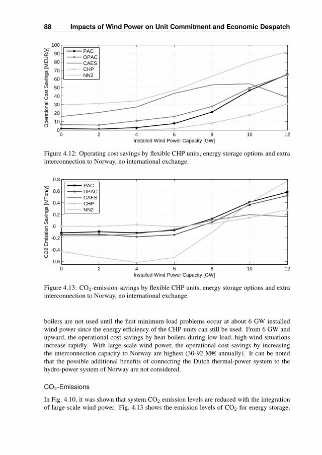
88 Impacts of Wind Power on Unit Commitment and Economic Despatch
0 2 4 6 8 10 120
10
20
30
40
50
60
70
80
90
100
Installed Wind Power Capacity [GW]
Ope
ratio
nal C
ost S
avin
gs [M
EU
R/y
]
PACOPACCAESCHPNN2
Figure 4.12: Operating cost savings by flexible CHP units, energy storage options and extrainterconnection to Norway, no international exchange.
0 2 4 6 8 10 12-0.6
-0.4
-0.2
0
0.2
0.4
0.6
0.8
Installed Wind Power Capacity [GW]
CO
2 E
mis
sion
Sav
ings
[MTo
n/y]
PACUPACCAESCHPNN2
Figure 4.13: CO2-emission savings by flexible CHP units, energy storage options and extrainterconnection to Norway, no international exchange.
boilers are not used until the first minimum-load problems occur at about 6 GW installedwind power since the energy efficiency of the CHP-units can still be used. From 6 GW andupward, the operational cost savings by heat boilers during low-load, high-wind situationsincrease rapidly. With large-scale wind power, the operational cost savings by increasingthe interconnection capacity to Norway are highest (30-92 Me annually). It can be notedthat the possible additional benefits of connecting the Dutch thermal-power system to thehydro-power system of Norway are not considered.
CO2-Emissions
In Fig. 4.10, it was shown that system CO2 emission levels are reduced with the integrationof large-scale wind power. Fig. 4.13 shows the emission levels of CO2 for energy storage,
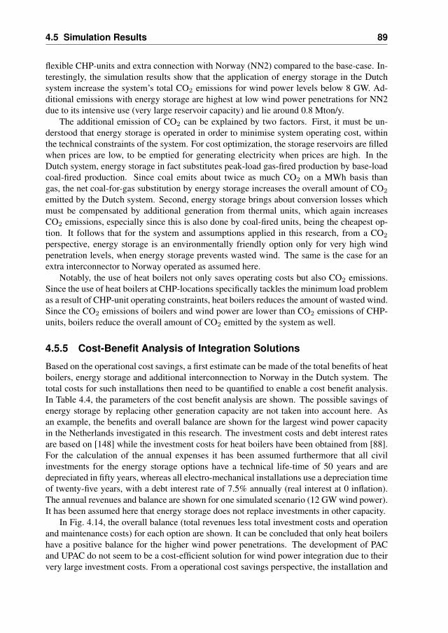
4.5 Simulation Results 89
flexible CHP-units and extra connection with Norway (NN2) compared to the base-case. In-terestingly, the simulation results show that the application of energy storage in the Dutchsystem increase the system’s total CO2 emissions for wind power levels below 8 GW. Ad-ditional emissions with energy storage are highest at low wind power penetrations for NN2due to its intensive use (very large reservoir capacity) and lie around 0.8 Mton/y.
The additional emission of CO2 can be explained by two factors. First, it must be un-derstood that energy storage is operated in order to minimise system operating cost, withinthe technical constraints of the system. For cost optimization, the storage reservoirs are filledwhen prices are low, to be emptied for generating electricity when prices are high. In theDutch system, energy storage in fact substitutes peak-load gas-fired production by base-loadcoal-fired production. Since coal emits about twice as much CO2 on a MWh basis thangas, the net coal-for-gas substitution by energy storage increases the overall amount of CO2
emitted by the Dutch system. Second, energy storage brings about conversion losses whichmust be compensated by additional generation from thermal units, which again increasesCO2 emissions, especially since this is also done by coal-fired units, being the cheapest op-tion. It follows that for the system and assumptions applied in this research, from a CO2
perspective, energy storage is an environmentally friendly option only for very high windpenetration levels, when energy storage prevents wasted wind. The same is the case for anextra interconnector to Norway operated as assumed here.
Notably, the use of heat boilers not only saves operating costs but also CO2 emissions.Since the use of heat boilers at CHP-locations specifically tackles the minimum load problemas a result of CHP-unit operating constraints, heat boilers reduces the amount of wasted wind.Since the CO2 emissions of boilers and wind power are lower than CO2 emissions of CHP-units, boilers reduce the overall amount of CO2 emitted by the system as well.
4.5.5 Cost-Benefit Analysis of Integration Solutions
Based on the operational cost savings, a first estimate can be made of the total benefits of heatboilers, energy storage and additional interconnection to Norway in the Dutch system. Thetotal costs for such installations then need to be quantified to enable a cost benefit analysis.In Table 4.4, the parameters of the cost benefit analysis are shown. The possible savings ofenergy storage by replacing other generation capacity are not taken into account here. Asan example, the benefits and overall balance are shown for the largest wind power capacityin the Netherlands investigated in this research. The investment costs and debt interest ratesare based on [148] while the investment costs for heat boilers have been obtained from [88].For the calculation of the annual expenses it has been assumed furthermore that all civilinvestments for the energy storage options have a technical life-time of 50 years and aredepreciated in fifty years, whereas all electro-mechanical installations use a depreciation timeof twenty-five years, with a debt interest rate of 7.5% annually (real interest at 0 inflation).The annual revenues and balance are shown for one simulated scenario (12 GW wind power).It has been assumed here that energy storage does not replace investments in other capacity.
In Fig. 4.14, the overall balance (total revenues less total investment costs and operationand maintenance costs) for each option are shown. It can be concluded that only heat boilershave a positive balance for the higher wind power penetrations. The development of PACand UPAC do not seem to be a cost-efficient solution for wind power integration due to theirvery large investment costs. From a operational cost savings perspective, the installation and
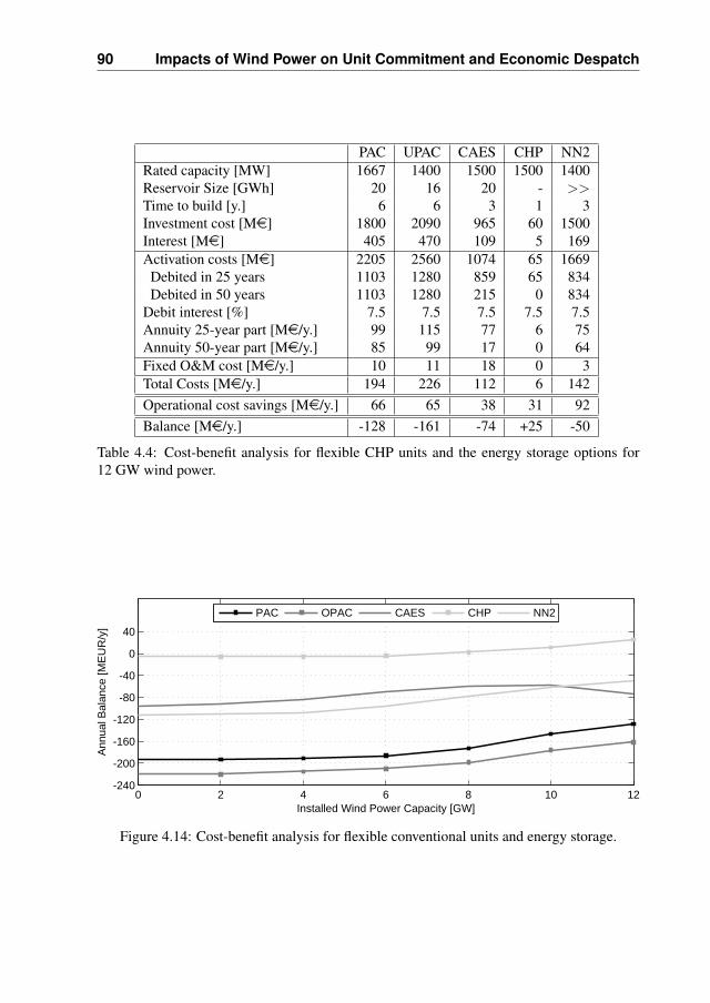
90 Impacts of Wind Power on Unit Commitment and Economic Despatch
PAC UPAC CAES CHP NN2Rated capacity [MW] 1667 1400 1500 1500 1400Reservoir Size [GWh] 20 16 20 - >>Time to build [y.] 6 6 3 1 3Investment cost [Me] 1800 2090 965 60 1500Interest [Me] 405 470 109 5 169Activation costs [Me] 2205 2560 1074 65 1669Debited in 25 years 1103 1280 859 65 834Debited in 50 years 1103 1280 215 0 834
Debit interest [%] 7.5 7.5 7.5 7.5 7.5Annuity 25-year part [Me/y.] 99 115 77 6 75Annuity 50-year part [Me/y.] 85 99 17 0 64Fixed O&M cost [Me/y.] 10 11 18 0 3Total Costs [Me/y.] 194 226 112 6 142Operational cost savings [Me/y.] 66 65 38 31 92Balance [Me/y.] -128 -161 -74 +25 -50
Table 4.4: Cost-benefit analysis for flexible CHP units and the energy storage options for12 GW wind power.
0 2 4 6 8 10 12-240
-200
-160
-120
-80
-40
0
40
Installed Wind Power Capacity [GW]
Ann
ual B
alan
ce [M
EU
R/y
]
PAC OPAC CAES CHP NN2
Figure 4.14: Cost-benefit analysis for flexible conventional units and energy storage.

4.6 Summary and Conclusions 91
use of heat boilers at CHP locations and a further development of interconnection capacitybetween the Netherlands and Norway seem to have the highest potential for the integrationof large-scale wind power into the Dutch system.
Reflection
Above, a straightforward cost-benefit analysis has been carried for investments for makingCHP units more flexible, for developing energy storage options and for an extra interconnec-tion to Norway. The results obtained here suggest that the development of energy storagein the Netherlands, although providing additional opportunities for wind power integration,is not a very attractive solution for this. The benefits of energy storage increase with theamount of wind power installed, but are dependent on the differences between peak and off-peak marginal cost. Because of that, fuel prices, emission prices, international exchangepossibilities, electricity demand (level, profile) and the generation portfolio all influence thebusiness-case for energy storage. Therefore, the economic benefits of energy storage must beassessed using a wide range of scenarios for these aspects, while taking into account that theenergy storage options may reduce the need for investments in conventional generation. Also,the development of of additional interconnection capacity between the Netherlands and Nor-way may have additional benefits because of possible synergies between the two generationsystems. These aspects fall outside of the scope of this research.
Although it specifically addresses one cause for minimum load issues, the use of heatboilers at the selected industrial CHP locations alone is not sufficient for the prevention ofwasting available wind resources altogether. Therefore, this solution should be expanded toother CHP-locations as well. Furthermore, more research is needed into the optimisation ofthe generation mix in order to remove the minimum load problem, in particular making otherbase-load units more flexible. Demand-side management would also be a possibility to solvethis issue. Above all, however, the results illustrate the importance of international exchangesfor wind power integration.
4.6 Summary and Conclusions
The UC–ED model developed in Chapter 3 is applied in this chapter to the Netherlands aspart of the North-West European interconnected system. Representative models have beendeveloped of the Netherlands’ power system, the neighbouring areas and the interconnec-tions between these. Annual simulations have been performed for a range of wind powerpenetrations of 0–12 GW in the Netherlands, market designs (isolated system – flexible useof interconnections) and wind power forecasts. Technical limits to the system integration ofwind power in the Dutch system have been identified and the economic and environmentalimpacts of wind power on system operation quantified. Furthermore, the opportunities of en-ergy storage and heat boilers for the integration of wind power in the Dutch system have beenexplored. Pumped accumulation storage (PAC), underground PAC (UPAC), compressed airenergy storage (CAES), the use of heat boilers at selected combined heat and power (CHP)locations and increased interconnection capacity with Norway (NN2) may provide additionaltechnical space for wind power integration.
The simulation results indicate that for the Dutch thermal generation system, ramp rateproblems due to the aggregated variations of load and wind power are rare. This can be
92 Impacts of Wind Power on Unit Commitment and Economic Despatch
explained by the existing commitment constraints imposed on base-load coal units (must-runstatus) and combined heat and power units due to heat demand, resulting in a high operatingreserve levels. The high reserve levels provide sufficient ramping capacity for balancingwind power variability in addition to existing load variations. For the optimization of systemoperation with large-scale wind power, it can be noted that accurate, actualisations of windpower output and a continuous re-calculation of UC–ED are essential.
Although the additional variations introduced by wind power can be integrated, limits forwind power integration increasingly occur during high wind and low load periods. Dependingon the international market design, significant wind power opportunity may have to be wastedto prevent minimum load problems. Wind power integration benefits from postponed gateclosure times of international markets, as international exchange may be optimised furtherwhen improved wind power predictions become available. The limited predictability of windpower, although important for the scheduling of international exchange, is shown to have onlya limited influence on wasted wind and operating costs in an isolated Dutch power system.
Wind power has a number of consequences for power system operation. The simulationresults show that wind power reduces total system operating costs, mainly by saving fueland emission costs. Wind power reduces the number of full-load hours of base-load coal-fired generation and CCGT with and without CHP-function. This has particular impacts onthe revenues of these conventional generation units (operating hours, marginal cost, etc.).By replacing fossil-fired generation, wind power significantly reduces the total exhaust ofemissions (CO2, SO2, NOx). In case possibilities for international exchange exist, windpower significantly reduces imports and increases exports of the area it is integrated into. Inthe case study performed here, it is shown that the presence of large-scale wind power inGermany limits the use of exports for wind power integration in the Netherlands during someperiods. Still, international exchange is shown to be key for wind power integration.
It can be concluded that energy storage, which has been often suggested as a logicalpartner for wind energy, is not the most attractive solution for the integration of large-scalewind power in the system investigated here. This is because significant amounts of availablewind power continue to be wasted at high wind power penetrations in an isolated powersystem. An interesting result is that energy storage is shown to increase overall emissionsof CO2 for the system as a whole at lower wind power penetrations. This can be explainedby the use of energy storage for substituting clean, peak-load gas generation for base-loadcoal generation and the conversion losses inherent to operating storage. Heat boilers alwaysprovide CO2 emission savings with increasing amounts with wind power installed capacity.
The cost benefit analysis performed here shows that neither PAC nor UPAC are likely tohave a positive balance, even at very high wind power penetrations, which is mainly due to thevery large investment costs associated with these options. CAES may be an option for higherwind power penetrations, although its benefits for wind power integration are limited. NN2has the largest potential for wind power integration and for operational cost savings due toits very large reservoir size and low conversion losses. Considering this alternative for windpower integration only however results in a negative balance. For the Dutch power system,the use of heat boilers at CHP locations and the development of additional interconnectioncapacity with Norway seem to have the highest potential for efficiently creating additionaltechnical space for wind power integration. Possibilities for international exchange should beregarded as a promising alternative for the development of energy storage in the Netherlands.
CHAPTER 5Power System Dynamic Model
5.1 Introduction
Apart from the impacts on unit commitment and economic despatch, wind power also has,as a generation technology of growing significance, increasing impacts on the behaviour ofpower systems. These impacts are mainly due to two reasons: wind turbines often use gen-erator types different from conventional ones and wind turbines have a an uncontrollableprimary energy source: the wind. The effects of wind power on system frequency are relatedto the changing rotating mass of synchronously coupled generators and keeping the powerbalance between generation and load. An important aspect which determines the impact ofwind power on power system operation is the market design for wind power. The respon-sibility for securing additional resources needed for balancing wind power may lie with thetransmission system operator (TSO) or may be assigned to the associated market party. Inthe latter case, wind power is exposed to the market mechanism.
In this chapter, a dynamic simulation model is developed specifically for the assessmentof the performance of secondary control with wind power in liberalised environments. Themodel allows for evaluating market design impacts on power system operation, taking intoaccount essential system parameters such as inertia and primary response, secondary controlmechanisms and operational strategies of individual market parties. The dynamic model isdesigned such that optimised unit commitment and economic despatch (UC–ED) schedulesare imported and used as a starting point for the dynamic simulations. This ensures thatrealistic sets of conventional generation units are used in the dynamic simulations.

94 Power System Dynamic Model
The chapter is organised as follows. First, a literature overview is provided and the con-tribution of this thesis with respect to existing dynamic models for power–frequency controlis stated. Then, the modeling approach and structure are presented and the core of the dy-namic model is described. The modeling approach is built upon the hypothesis the powersystem’s frequency response can be computed without considering voltage aspects (i.e. con-stant power load). This approach is validated through simulations of the New England testsystem with a dedicated power system simulation tool. After this, relevant technical conceptsare introduced and the power system model is developed and validated for the Dutch powersystem as part of the UCTE interconnection.
5.2 Literature Overview and Contribution of this Thesis
5.2.1 Literature Overview on Power-Frequency Controland Wind Power
A lot of research is available on the consequences of different generator types used in windturbines. Because wind turbines often have a-synchronous generators (Section 2.4.3), the me-chanical properties of wind turbines (rotor speed and mechanical power) are rather decoupledfrom the electrical properties (active power output). Therefore, wind turbines have a differentbehaviour than conventional generation in response to system disturbances [155]. Althoughfixed speed wind turbines provide inertial response similar to conventional synchronous gen-erators [101], the presently far more common, variable speed, doubly-fed induction genera-tor (DFIG) concepts are usually not equipped to do so, although this is technically possible[17, 116, 120, 144]. The impacts of wind power on power system inertia is particularly im-portant in smaller, isolated systems with a relatively small rotating inertia as a starting point,such as the Irish [43, 119]. This might be a limiting factor for the penetration level of windpower in such systems [145].
A second and generally more challenging aspect influencing frequency stability, is thevariability of wind power. Wind power introduces additional power fluctuations to the sys-tem which may coincide with existing power variations of load and generation, requiringadditional power reserves. This regards secondary and longer-term reserves especially [37,44, 70]. Because the wind speed variations can be predicted only to a limited extent, addi-tional reserves are needed as well to compensate for this uncertainty [44]. Wind power alsoinfluences the UC–ED of conventional generation units (Chapter 4). Therefore, different orless conventional generation capacity is available for power–frequency control. Thus, windpower has a direct and an indirect effect on frequency stability it the sense that a differentgeneration mix leads to a different dynamic behaviour of the system.
A third aspect which influences power–frequency control is the design of the liberalisedmarket with respect to wind power [69]. The responsibility for integrating wind into systemoperation lies with the transmission system operator (TSO) or with the individual marketparties having wind power as part of their portfolio. In the latter case especially, wind powerchallenges the planning and operation of the market party’s individual generation portfolioand influences the market bidding strategy [52, 154]. These aspects also influence the extentto which conventional generation is available for power–frequency control. It can be notedthat TSOs increasingly require wind power to supply system services, including speed-droop
5.2 Literature Overview and Contribution of this Thesis 95
control, just like conventional generation. The technical capabilities of wind power plants tosupply such services have been shown in [98, 172].
Models in Literature
Different models have been developed for the investigation of the dynamic interaction be-tween wind power and system behaviour. Reference [101] applies a single-bus power systemmodel for the assessment of the impact of wind power on the primary frequency responsein an isolated system. The approach is based based on a mechanical power system model-ing approach first introduced in [134], which is similar to the models that can be found in[5, 27, 34]. Unfortunately, these models do not comprise operational aspects extending overthe range of 20–60 s and are used only for the assessment of primary control. The impactsof large-scale wind power on system frequency are also investigated in [96] but using a testsystem rather than an actual power system and without considering geographical spreadingof wind power. In [32], a methodology for redesigning frequency control is proposed, whichincorporates some market aspects and a central bidding process for secondary reserves. Ref-erence [129] presents a case-study for the assessment of power reserves for wind power usinga steady-state simulation method based on existing load flow simulation models. It can benoted that a steady-state approach is not suitable for the assessment of frequency stability, asattempted in this research.
None of the models discussed above fully comprise the long-term dynamic aspects ofpower system operation with large-scale wind power, nor do they include the market as-pects relevant to secondary control in liberalised markets, in particular the responsibility forbalancing wind power. Research focused on market design or bidding strategies such as[6, 12, 13, 52] does not comprise the technical aspects of system stability. Furthermore, ex-isting models disregard the impacts of UC–ED optimisation with wind power on the plantmix available for balancing in real-time. Considering the wide range of technical and market-related modeling aspects, a dedicated general approach must be developed in order to incor-porate all these.
5.2.2 Contribution of this Thesis
The contribution of this chapter is twofold. First, an accurate dynamic power system modelis developed for the simulation of power–frequency control in the presence of wind power,taking into account a liberalised trading environment. Parameters for the dynamic model,which include system inertia, speed droops and frequency-dependent load damping are vali-dated for the Dutch control zone as a part of the UCTE interconnection. The dynamic modelcontains realistic dynamic representations of generation units and generation control schemespresently applied both by the TSO and by individual market parties. Since classical dynamicmodels for power-frequency control do not comprise market aspects such as market parties’operational strategies and bidding mechanisms for secondary control, the model developedhere can be regarded as novel.
The second contribution of this chapter lies in the fact that the model structure developedhere is designed such that it can be used to simulate selected cases following from optimisedUC–ED schedules. The dynamic model comprises the same generation units as implementedin the UC–ED tool. By importing the cases, only generation units scheduled for operation

96 Power System Dynamic Model
are available for power balancing and reserves. Since wind power is an integral part of theUC–ED optimisation, the dynamic model is provided with realistic sets of generation unitoperating points before starting the simulation of the control performance. This methodologyensures that the dynamic performance of the system reflects the generation mix resulting fromUC–ED. The availability of a full year optimal UC-ED-schedule in which realistic windpower data are incorporated, provides a very large number of possible cases for dynamicsimulation. This makes the method highly flexible and very accurate, since worst cases canbe identified from the UC–ED first and then simulated using the dynamic model.
5.3 Power–Frequency Control Model
5.3.1 Modeling Approach
The modeling approach applied here results from the specific focus of this research on fre-quency stability. Models of frequency control that neglect transmission network or voltageaspects have been developed in [5, 134]. The mechanical modeling approach (single-buspower system representation) allows the inclusion of longer-term aspects such as secondarycontrol and energy-based control, such as done in [150]. Such an approach is based on two as-sumptions, namely that inter-machine and inter-area oscillations are absent and that impactsof network-related aspects on frequency response can be disregarded. The first assumptioncomes down to the application of a uniform system frequency and aggregated moment ofinertia. The second involves a lossless network that serves active power loads only: loads areassumed to be constant power and only frequency-dependent. Below, a short background forthese assumptions is given and the possible impacts on the simulation results are given.
Uniform System Frequency and Aggregated Moment of Inertia
Frequency is directly related to the rotating speed of synchronously connected generators.During normal operation, slight differences in rotating speeds are present due to the ever-changing equilibrium between generation and load and the control actions which are per-formed continuously. Large, interconnected systems may also experience frequency oscilla-tions between different areas. These inter-area frequency oscillations caused by the delaysin the controls and are specifically related to the geographical size and the loading of thetransmission system. In the UCTE interconnection, but also in the North American sys-tems, Wide Area Monitoring Systems (WAMS) are applied to investigate these oscillations.WAMS data are also used for the development of system simulation models and the assess-ment of damping solutions [22, 61]. For such non-uniform frequency studies, a simulationtool must be used that is fully based on differential equations, explaining the use of for in-stance PSSTMNETOMAC [24] for such exercises.
This research considers the Dutch system in particular, as part of the Western-Europeanregion of the UCTE system. This part of the UCTE interconnection is rather meshed with rel-atively short transmission lines, resulting in low reactances between generators and large syn-chronising torques. The Netherlands can be considered as part of a coherent North-WesternEuropean area [22]. For this research, it is therefore assumed that the system is absolutelystiff i.e. that inter-area oscillations between the Dutch zone and rest of the area will not ap-pear. When also inter-area oscillations are assumed to be absent on a system-wide basis, all

5.3 Power–Frequency Control Model 97
generators operate in synchronism with a single system frequency. Since the rotating speedof generators is directly proportional to frequency, all rotating masses in the system can beaggregated to a single moment of inertia.
Frequency Independent of Voltage
Under normal operating conditions, frequency and voltage can largely be regarded as inde-pendent parameters. In short-term stability studies (ms to s time-range), voltage aspects arenormally neglected [99]. The voltage dependency of consumption [134] and the impedancesof transmission lines may however lead to different levels of consumption and losses, whichmay have a significant impact on system frequency. Therefore, the assumption to regardfrequency as independent of the voltage must be validated. This will be done in Section 5.4.
5.3.2 Mechanical Power System Model
Power Balance
Using the assumptions given above, a mechanical modeling approach is used, looking at thepower system as a large, single rotating mass. In case of an imbalance between the torquesacting on this rotating mass, the net torque causing acceleration or deceleration is
Ta = Tm − Te (5.1)
with Tm as mechanical torque and Te as electromagnetic torque [99]. In case Tm 6= Te,the mass will experience an angular deceleration or acceleration dω/dt determined by theequation of motion / Newton’s Second Law for rotational motion
Ta = Jdω
dt(5.2)
with J as the mass’ rotational inertia. Applying
P = ωT (5.3)
gives the relationship between the mechanical power Pm, the electrical power Pe and theacceleration
dω
dt=
Pm − Pe
Jω(5.4)
Moment of Inertia
The power system’s moment of inertia or mechanical starting time is proportional to theamount of rotating mass in the system. The moment of inertia determines the rate-of-changeof the frequency immediately after a disturbance: the larger system inertia is, the less isthe frequency rate-of-change following a power imbalance [99]. Replacing dω/dt with thefrequency rate-of-change df/dt, Pm with the mechanical power input of all generators PG,Pe with the electrical power output of all generators, equal to system load including lossesPL, allows rewriting Eq. 5.4 to give the relationship between generation, load and frequencychange in a power system
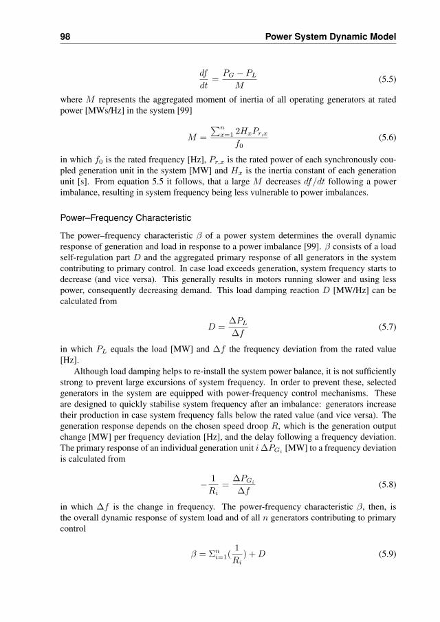
98 Power System Dynamic Model
df
dt=
PG − PL
M(5.5)
where M represents the aggregated moment of inertia of all operating generators at ratedpower [MWs/Hz] in the system [99]
M =∑n
x=1 2HxPr,x
f0(5.6)
in which f0 is the rated frequency [Hz], Pr,x is the rated power of each synchronously cou-pled generation unit in the system [MW] and Hx is the inertia constant of each generationunit [s]. From equation 5.5 it follows, that a large M decreases df/dt following a powerimbalance, resulting in system frequency being less vulnerable to power imbalances.
Power–Frequency Characteristic
The power–frequency characteristic β of a power system determines the overall dynamicresponse of generation and load in response to a power imbalance [99]. β consists of a loadself-regulation part D and the aggregated primary response of all generators in the systemcontributing to primary control. In case load exceeds generation, system frequency starts todecrease (and vice versa). This generally results in motors running slower and using lesspower, consequently decreasing demand. This load damping reaction D [MW/Hz] can becalculated from
D =∆PL
∆f(5.7)
in which PL equals the load [MW] and ∆f the frequency deviation from the rated value[Hz].
Although load damping helps to re-install the system power balance, it is not sufficientlystrong to prevent large excursions of system frequency. In order to prevent these, selectedgenerators in the system are equipped with power-frequency control mechanisms. Theseare designed to quickly stabilise system frequency after an imbalance: generators increasetheir production in case system frequency falls below the rated value (and vice versa). Thegeneration response depends on the chosen speed droop R, which is the generation outputchange [MW] per frequency deviation [Hz], and the delay following a frequency deviation.The primary response of an individual generation unit i ∆PGi
[MW] to a frequency deviationis calculated from
− 1Ri
=∆PGi
∆f(5.8)
in which ∆f is the change in frequency. The power-frequency characteristic β, then, isthe overall dynamic response of system load and of all n generators contributing to primarycontrol
β = Σni=1(
1Ri
) + D (5.9)

5.4 Validation of the Modeling Approach 99
PG, UCTE
PL, UCTE
PG, NL
PL, NL
+- +-
f0
M
/x 1/s
/xD x
-1/Ri x
+
++
f
x x
Figure 5.1: Overview of the dynamic model as used in this research.
The system frequency response ∆f [Hz] to any power imbalance ∆P [MW] is determinedby
∆f =∆P
β(5.10)
The mechanical model as presented here is introduced into the simulation tool MATLAB/SIMULINK. Simulink is a well established and highly flexible tool with a user-friendly in-terface, which allows an orderly and surveyable development of the dynamic model. Further-more, this tool allows the inclusion of longer-term aspects relevant for this research, such assecondary control. It is flexible enough to allow the modeling of different market designs forwind power and capable of using external data as input for the dynamic simulations. Fig. 5.1provides a schematic overview of the model, where PG,NL, PL,NL, PG,UCTE and PL,UCTE
represent the total generation and load of the Netherlands and the rest of the UCTE-system,respectively. The generator droop of individual generators −1/Ri are implemented at thegeneration unit level in the Netherlands and for an aggregated generation unit for the rest ofthe UCTE-system. The model set-up is validated by comparing the simulation results to man-ual calculations for different parameter settings (moment of inertia of the system, generatordroops) and power imbalances, as done in [99].
5.4 Validation of the Modeling Approach
The use of the mechanical approach itself must be validated as a representation of an elec-trical power system. This can only be done by comparing the simulation results of the me-chanical model to those obtained by an established power system simulation tool. Successivesystem simulations are carried out while omitting certain electrical aspects in order to validatethe extent to which electrical aspects can indeed be neglected when investigating long-termfrequency stability.
For the analysis, a validated, multi-bus, multi-generator, multi-load test system is mod-eled using the mechanical approach in Simulink, and then compared to a full electrical and
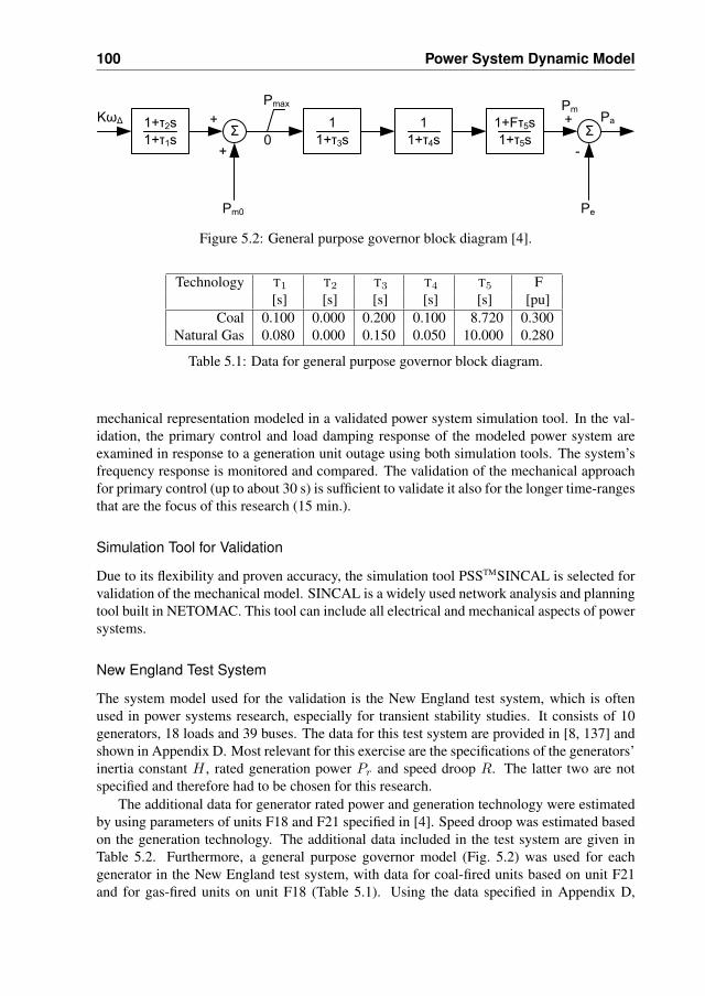
100 Power System Dynamic Model
1+τ2s1+τ1s
11+τ3s
11+τ4s
1+Fτ5s1+τ5s
Σ+
+Kω∆
Pm0
ΣPa
Pe
-
+Pm
Pmax
0
Figure 5.2: General purpose governor block diagram [4].
Technology T1 T2 T3 T4 T5 F[s] [s] [s] [s] [s] [pu]
Coal 0.100 0.000 0.200 0.100 8.720 0.300Natural Gas 0.080 0.000 0.150 0.050 10.000 0.280
Table 5.1: Data for general purpose governor block diagram.
mechanical representation modeled in a validated power system simulation tool. In the val-idation, the primary control and load damping response of the modeled power system areexamined in response to a generation unit outage using both simulation tools. The system’sfrequency response is monitored and compared. The validation of the mechanical approachfor primary control (up to about 30 s) is sufficient to validate it also for the longer time-rangesthat are the focus of this research (15 min.).
Simulation Tool for Validation
Due to its flexibility and proven accuracy, the simulation tool PSSTMSINCAL is selected forvalidation of the mechanical model. SINCAL is a widely used network analysis and planningtool built in NETOMAC. This tool can include all electrical and mechanical aspects of powersystems.
New England Test System
The system model used for the validation is the New England test system, which is oftenused in power systems research, especially for transient stability studies. It consists of 10generators, 18 loads and 39 buses. The data for this test system are provided in [8, 137] andshown in Appendix D. Most relevant for this exercise are the specifications of the generators’inertia constant H , rated generation power Pr and speed droop R. The latter two are notspecified and therefore had to be chosen for this research.
The additional data for generator rated power and generation technology were estimatedby using parameters of units F18 and F21 specified in [4]. Speed droop was estimated basedon the generation technology. The additional data included in the test system are given inTable 5.2. Furthermore, a general purpose governor model (Fig. 5.2) was used for eachgenerator in the New England test system, with data for coal-fired units based on unit F21and for gas-fired units on unit F18 (Table 5.1). Using the data specified in Appendix D,

5.4 Validation of the Modeling Approach 101
Generator Fuel Base Droop[MW] [MW/Hz]
G10 Natural Gas 250 125.0G02 Natural Gas 600 250.0G03 Coal 700 233.3G04 Coal 700 233.3G05 Natural Gas 600 250.0G06 Coal 700 233.3G07 Natural Gas 600 250.0G08 Natural Gas 600 250.0G09 Coal 1000 333.3G01 Coal 1000 –Total 7050 2158.3
Table 5.2: Additional generator data used for the New England system.
Table D.1, Table 5.2 and Eq. 5.6, the aggregated moment of inertia M for the New EnglandTest System was determined at 2609.0 MWs/Hz.
5.4.1 Simulations
First, the response of the New England test system to an outage of generator G10 will beexamined. The outage will result in an immediate change of frequency, which depends onthe system’s moment of inertia and the output level of the outaged generator. Frequency willeventually settle at a value deviating from the rated value (60 Hz), which depends on primarycontrol reaction and load damping. The responses of both models (SINCAL and Simulink)are first validated with respect to each other and then compared when taking into accountdifferent electrical aspects in SINCAL. The following simulations are made:1) Steady-state calculation of the load flow in the New England test system in SINCAL2) Dynamic simulation of the frequency after outage of generator G10 in the New England
test system model in SINCAL, with constant power load and a single bus representation3) Dynamic simulation of the frequency after the same outage in the same system, using the
swing equations in Simulink4) Dynamic simulation of the same outage using SINCAL with full representation of the
New England test system and constant impedance load5) Dynamic simulation of the same outage using SINCAL with full representation of the
New England test system and constant power loadThe load flow is performed for ensuring the correct representation of the New England testsystem in SINCAL. The common assumption is applied that the load is independent of thevoltage (constant PQ) to examine the load flow results validated for this system in [75]. Theload flow is used to provide the initial states for the dynamic simulations performed in SIN-CAL, which must equal those in Simulink. In the second simulation in SINCAL, voltage-related aspects (lines, transformers, generator voltage droop) are removed from the model,effectively creating a constant power load, single-bus representation of the New England testsystem. The simulation results of SINCAL are compared to the third simulation which is
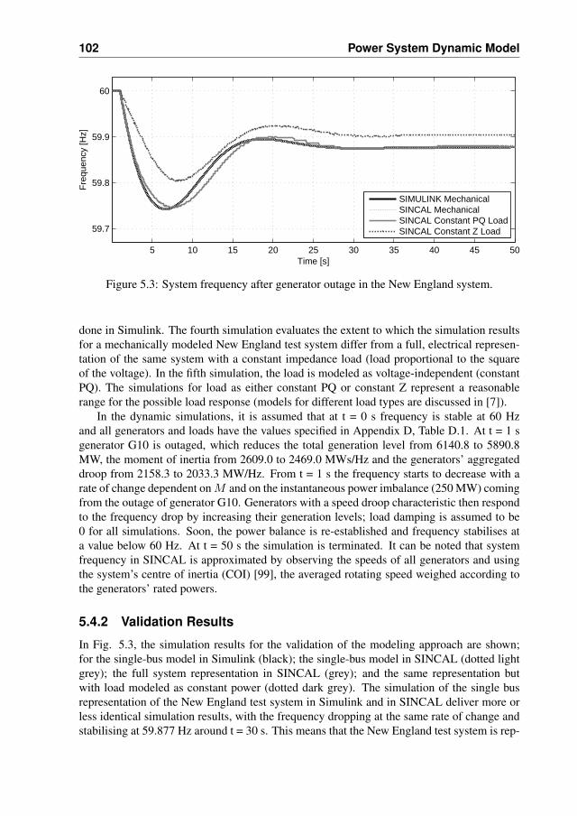
102 Power System Dynamic Model
5 10 15 20 25 30 35 40 45 50
59.7
59.8
59.9
60
Time [s]
Freq
uenc
y [H
z]
SIMULINK MechanicalSINCAL MechanicalSINCAL Constant PQ LoadSINCAL Constant Z Load
Figure 5.3: System frequency after generator outage in the New England system.
done in Simulink. The fourth simulation evaluates the extent to which the simulation resultsfor a mechanically modeled New England test system differ from a full, electrical represen-tation of the same system with a constant impedance load (load proportional to the squareof the voltage). In the fifth simulation, the load is modeled as voltage-independent (constantPQ). The simulations for load as either constant PQ or constant Z represent a reasonablerange for the possible load response (models for different load types are discussed in [7]).
In the dynamic simulations, it is assumed that at t = 0 s frequency is stable at 60 Hzand all generators and loads have the values specified in Appendix D, Table D.1. At t = 1 sgenerator G10 is outaged, which reduces the total generation level from 6140.8 to 5890.8MW, the moment of inertia from 2609.0 to 2469.0 MWs/Hz and the generators’ aggregateddroop from 2158.3 to 2033.3 MW/Hz. From t = 1 s the frequency starts to decrease with arate of change dependent on M and on the instantaneous power imbalance (250 MW) comingfrom the outage of generator G10. Generators with a speed droop characteristic then respondto the frequency drop by increasing their generation levels; load damping is assumed to be0 for all simulations. Soon, the power balance is re-established and frequency stabilises ata value below 60 Hz. At t = 50 s the simulation is terminated. It can be noted that systemfrequency in SINCAL is approximated by observing the speeds of all generators and usingthe system’s centre of inertia (COI) [99], the averaged rotating speed weighed according tothe generators’ rated powers.
5.4.2 Validation Results
In Fig. 5.3, the simulation results for the validation of the modeling approach are shown;for the single-bus model in Simulink (black); the single-bus model in SINCAL (dotted lightgrey); the full system representation in SINCAL (grey); and the same representation butwith load modeled as constant power (dotted dark grey). The simulation of the single busrepresentation of the New England test system in Simulink and in SINCAL deliver more orless identical simulation results, with the frequency dropping at the same rate of change andstabilising at 59.877 Hz around t = 30 s. This means that the New England test system is rep-
5.5 Validation of the Model and Full Model Development 103
resented correctly in both tools and therefore that the dynamic modeling approach developedin Simulink is applied correctly.
Simulation of the New England test system model in SINCAL with a constant impedanceload yields a frequency stabilising at 59.904 Hz, a difference of 0.027 Hz compared to thesingle-bus approach. The reduced change in frequency is caused by the reduction in load, dueto the voltage decrease after the generation outage. Using a constant PQ load, the frequencystabilises also at 59.877 Hz and the frequency shows a very similar response to the Simulinksingle-bus representation. This proves that neglecting the transmission network in Simulinkdoes not change the primary response of the system to a power imbalance. It can be notedthat the inclusion of network-aspects results in a slight delay of the frequency response to theoutage, amounting to 1–2 s for the outage considered here.
Conclusion
From the simulation results it can be concluded that the modeling approach used and appliedin Simulink is valid for the simulation of frequency stability. A single-bus test system rep-resentation in SINCAL leads to identical simulation results for the same generator outage.Voltage related system aspects such as transmission lines, transformers and losses do nothave a significant impact on the frequency response of the model in SINCAL. In case a con-stant impedance load is assumed, a local voltage decrease due to the outage of generator G10results in lower consumption of active power, which partly compensates the power imbalanceand results in a less severe decrease in frequency. Application of constant PQ loads ignoresthis effect and leads to simulation results that are very similar to the single-bus representation.Since inclusion of voltage-dependent load models results in a smaller frequency deviation,the single-bus modeling approach applied in this thesis can be considered as conservativefrom the perspective of frequency variation.
5.5 Validation of the Model and Full Model Development
Below, the power system dynamic model described in the previous paragraphs will be ex-tended to include longer term aspects such as secondary control, energy program responsi-bility and a power imbalance market. The full model comprises the following elements:
• An aggregated moment of inertia, representative for the UCTE interconnected system• A power–frequency characteristic of the UCTE interconnected system• Secondary control as performed by the Dutch system operator• Energy program responsibility• Short-term operational aspects of Dutch generation units
First, a two area model with one single moment of inertia is set up and validated for theDutch power system as part of the UCTE interconnection. Secondary control is includedin the model as well, with the transmission system operator (TSO) as being responsible forthe overall power balance, and the market parties responsible for their individual energyexchanges with the system. Dynamic models are developed for the same conventional gen-eration units as those of the Dutch area in the UC–ED model.
104 Power System Dynamic Model
5.5.1 Validation of the UCTE-Interconnection Model
In Section 5.3.2, a mechanical model has been developed for the simulation of the powersystem’s frequency response to a power imbalance. The approach most importantly involvesthe following parameters: the system’s moment of inertia M (Eq. 5.6) and a power-frequencycharacteristic β (Eq. 5.9), consisting of load damping D (Eq. 5.7) and the primary reactionof the generation units (Eq. 5.8).
System Inertia
The power system’s inertia consists of the aggregated inertia constants H of individual, syn-chronously coupled machines, typically lying in the range of 2–7 s [4, 60, 99, 120]. Becausesystem inertia comprises a very large number of separate masses, system inertia is typicallyassessed by using system frequency observations immediately after a significant disturbance[29, 79, 93].
For the estimation of system inertia of the UCTE-interconnection as a whole, includ-ing the Dutch area, frequency deviation measurements at a sample rate of 4 s were ob-tained from the Dutch TSO for 87 significant instantaneous power imbalances in the UCTE-interconnection from 1/10/2004–11/12/2006. These events involve power imbalances andfrequency deviations between 1–2.6 GW and 20–110 mHz, respectively. df/dt is approxi-mated using the ∆f/∆t immediately after the power imbalance. M is estimated using Eq.5.5 to obtain an estimation of M , as illustrated by the dotted line in Fig. 5.4.
Load Damping and Primary Response
As with system inertia, load parameters may be possible to assess with some accuracy forsmaller, isolated systems [133], but it is generally more difficult for larger, interconnectedsystems such as the UCTE interconnection. This is because it is practically impossible toverify the primary and secondary control settings for each generator, which allows a differ-entiation between the generation response and the load response. A typical value for C inEq. 5.7 is 1 (a 1% change in frequency implies a 1% change in load) [76, 99] and this valueis applied by UCTE as well [169].
Primary reserves for immediate power balancing in the UCTE interconnected system aredivided between different control zones, each of which is responsible for a fixed amount[MW]. In case of a certain power imbalance, all control zones contribute by their individualshare of the total, which presently comprises 3000 MW. In order to guarantee such a con-tribution, a generation speed droop as well as a response time may be laid down in the gridconnection requirements of individual countries or control zones. Typical values are a droopof 10% (10% change in frequency implies a 100% change in generation) and a full primarycontrol response within 30 s [169]. A frequency measurement inaccuracy of up to 10 mHz isallowed in the Netherlands [130]. It can be noted that this also prevents very fast changes ingeneration output around the rated frequency (50 Hz for UCTE).
By investigating the ∆f for the same events as used for the estimation of system in-ertia, Eq. 5.10 delivers an estimation of β, the aggregation of load damping and primaryresponse. A comprehensive investigation conducted in 1997 [183] estimated a range for β of2–5·104 MW/Hz. In the following, the UCTE data will be used to approximate β.

5.5 Validation of the Model and Full Model Development 105
0 5 10 15 20 25 3049.93
49.94
49.95
49.96
49.97
49.98
49.99
50
Time [s]
Freq
uenc
y [H
z]
Figure 5.4: Validation of system inertia and power–frequency characteristic (in black) usingdata of UCTE (representative selection out of total of 87 events, in grey).
Validation Results
Data analysis of all available events shows that M lies within a range of 1.2·105 and 4.8·105
MWs/Hz, with a mean of 2.6·105 MWs/Hz and a standard deviation of 1.1·105 MWs/Hz.Correlations between M and the time of day, the type of day or the season were found tobe insignificant. For this research, M is approximated at 2·105 MWs/Hz since it is a ratherconservative estimate within the range found in the analysis. Using Eq. 5.6 and estimatingPr,UCTE at 5.0·105 MW, HUCTE would be estimated at 10 s. This relatively high valuecompared to the references given above may be explained by the contribution to systeminertia of rotating motors in the system, and a possible voltage response of loads locatedclose to the outaged generation unit, resulting in less severe initial drop of frequency.
The power–frequency characteristic was found to lie between 1.2·104 and 4.7·104 MW/Hz, with a mean of 2.6·104 MW/Hz and a standard deviation of 7.3·103 MW/Hz. Correla-tions between β and the time of day, the weekday and the season were found to be insignifi-cant. It is in fact likely that there exists a function between β and the time of day (plant mix)but this could not be concluded based on the available data. For the simulations, β of UCTEis assumed to be 2.6·104 MW/Hz for all simulations, regardless of the load level (i.e. timeof day). Assuming a primary control dead band of 10 mHz, the resulting primary responseof the system model to an outage of 1144 MW is shown in Fig. 5.4, together with a smallnumber of representative data recordings used for the validation.
5.5.2 Secondary Control
Area Control Error
Secondary control has the objective of returning the system frequency to its rated valueand the area exchanges at their scheduled values [83, 74]. Before the liberalisation of theelectricity sector, mostly a central generation co-ordinating organisation was responsible for
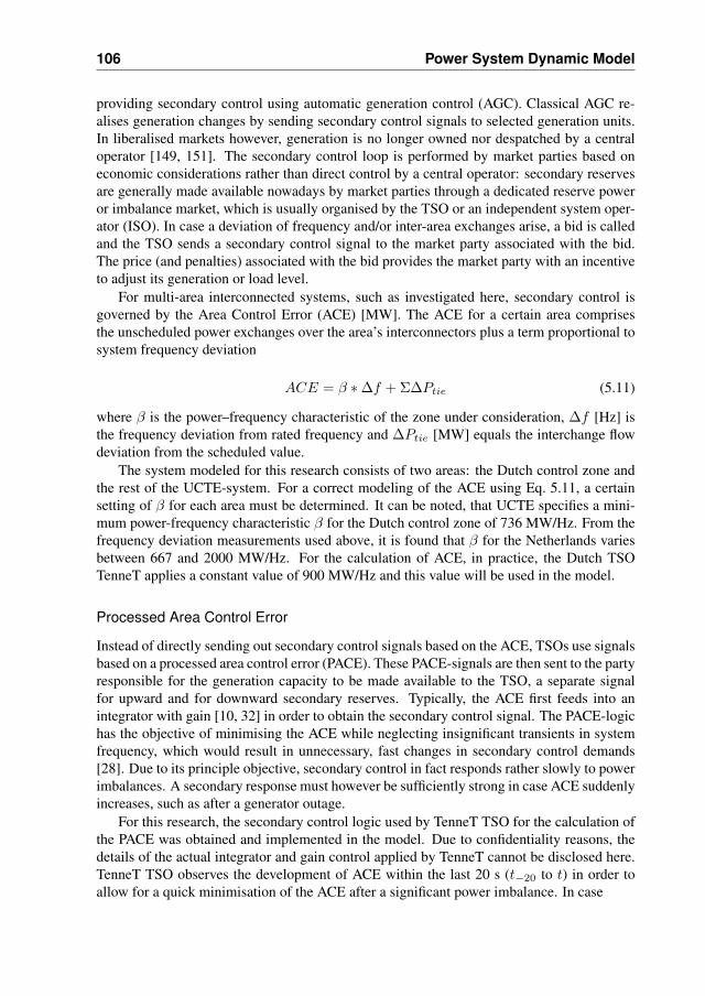
106 Power System Dynamic Model
providing secondary control using automatic generation control (AGC). Classical AGC re-alises generation changes by sending secondary control signals to selected generation units.In liberalised markets however, generation is no longer owned nor despatched by a centraloperator [149, 151]. The secondary control loop is performed by market parties based oneconomic considerations rather than direct control by a central operator: secondary reservesare generally made available nowadays by market parties through a dedicated reserve poweror imbalance market, which is usually organised by the TSO or an independent system oper-ator (ISO). In case a deviation of frequency and/or inter-area exchanges arise, a bid is calledand the TSO sends a secondary control signal to the market party associated with the bid.The price (and penalties) associated with the bid provides the market party with an incentiveto adjust its generation or load level.
For multi-area interconnected systems, such as investigated here, secondary control isgoverned by the Area Control Error (ACE) [MW]. The ACE for a certain area comprisesthe unscheduled power exchanges over the area’s interconnectors plus a term proportional tosystem frequency deviation
ACE = β ∗∆f + Σ∆Ptie (5.11)
where β is the power–frequency characteristic of the zone under consideration, ∆f [Hz] isthe frequency deviation from rated frequency and ∆Ptie [MW] equals the interchange flowdeviation from the scheduled value.
The system modeled for this research consists of two areas: the Dutch control zone andthe rest of the UCTE-system. For a correct modeling of the ACE using Eq. 5.11, a certainsetting of β for each area must be determined. It can be noted, that UCTE specifies a mini-mum power-frequency characteristic β for the Dutch control zone of 736 MW/Hz. From thefrequency deviation measurements used above, it is found that β for the Netherlands variesbetween 667 and 2000 MW/Hz. For the calculation of ACE, in practice, the Dutch TSOTenneT applies a constant value of 900 MW/Hz and this value will be used in the model.
Processed Area Control Error
Instead of directly sending out secondary control signals based on the ACE, TSOs use signalsbased on a processed area control error (PACE). These PACE-signals are then sent to the partyresponsible for the generation capacity to be made available to the TSO, a separate signalfor upward and for downward secondary reserves. Typically, the ACE first feeds into anintegrator with gain [10, 32] in order to obtain the secondary control signal. The PACE-logichas the objective of minimising the ACE while neglecting insignificant transients in systemfrequency, which would result in unnecessary, fast changes in secondary control demands[28]. Due to its principle objective, secondary control in fact responds rather slowly to powerimbalances. A secondary response must however be sufficiently strong in case ACE suddenlyincreases, such as after a generator outage.
For this research, the secondary control logic used by TenneT TSO for the calculation ofthe PACE was obtained and implemented in the model. Due to confidentiality reasons, thedetails of the actual integrator and gain control applied by TenneT cannot be disclosed here.TenneT TSO observes the development of ACE within the last 20 s (t−20 to t) in order toallow for a quick minimisation of the ACE after a significant power imbalance. In case
5.5 Validation of the Model and Full Model Development 107
[ACE ≥ 300MW ] AND [ACEt−20 −ACEt ≥ 150MW ] (5.12)
holds, the PACE-logic is by-passed and the secondary control signal is set such that all avai-lable downward regulating power available is called. This results in a maximum demand forsecondary control in order to quickly bring ACE within bounds again (≤ 300 MW). A similarlogic is applied for negative ACE.
Power Reserve Bidding Ladder
The bids for secondary reserves received from market parties are arranged by the TSO in aprice order, creating a power reserve bidding ladder. A separate ladder is created for upwardand for downward reserves. A bid ladder model is developed, with each bid defined as avector b
b = (id, PTU, size, rr, p) (5.13)
in which id is the market party identifier, PTU is the program time unit for which the bidis applicable, size is the size of the bid [MW], rr is the ramp-rate [% of size/min.] and p isprice of the activated part of the bid [EUR/MWh].
During real-time operation, the TSO applies the PACE to the bidding ladder in order toselect the bids necessary for power balancing. The PACE is re-calculated and applied to thebidding ladder every 4 s, possibly requiring the call of additional bids. The market partyassociated with the next activated bid then receives a signal ∆P [MW] from the TSO, witha desired rate-of-change [MW/min.] constrained by the ramp-rate specified in the bid. Inthe Netherlands, rr must equal at least 7% of size/min., allowing a full activation of the bidwithin 15 min. In case PACE drops and the bid is no longer necessary, the bid is reducedaccordingly. Because of the ramp rates specified in the bids, secondary control may changeslower than system frequency and positive and negative bids can be active simultaneously. Itis the responsibility of the market party associated with the bids called to adjust its generationoperating points and/or load schedules accordingly. This responsibility is part of energyprogram responsibility that every party in the system has.
5.5.3 Energy Program Responsibility
A system of balance or energy program (e-program) responsibility has been developed in or-der to guarantee an orderly organised market and to allow for a continuous balance betweengeneration and load. In this system, balance responsible parties or in the Netherlands, pro-gram responsible parties (PRPs), have been made responsible for keeping their own energybalance: generation is supposed to be delivered to the power system only if there is a load tomatch it. Therefore any customer (generator or load) connected to the system must be associ-ated with a PRP. A PRP must maintain its energy balance [MWh] for each settlement period,which is the program time-unit (PTU, 15 min. in the Netherlands but generally an hour).Below, the system of program responsibility as organised in the Netherlands is discussed.
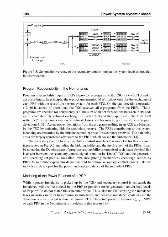
108 Power System Dynamic Model
+
+Bid 1Bid ..Bid n
Bid 1Bid ..Bid m
PIACE
Frequency
InternationalExchange
+ PACEPower System-1
β ∆up∆up∆up
∆down∆down∆down
PRPPRPPRP
PRPPRPPRP
portfolioportfolioportfolio
portfolioportfolioportfolio
Σ ∆up
Σ ∆down
MWMWMW
MWMWMW
TSO Market
Figure 5.5: Schematic overview of the secondary control loop at the system level as modeledin this research.
Program Responsibility in the Netherlands
Program responsibility requires PRPs to provide e-programs to the TSO for each PTU and toact accordingly. In principle, the e-programs mention MWh-values only for the exchange ofeach PRP with the rest of the system system for each PTU. On the day preceding operation(12–36 h. ahead of operation), the TSO receives all e-programs from the PRPs. The e-programs are checked for consistency (i.e. the sum of all net transactions between PRPs addsup to scheduled international exchange for each PTU) and then approved. The TSO itselfis the PRP for the compensation of network losses and for matching all real-time e-programdeviations [162]. Actual power deviations from the program resulting in an ACE are balancedby the TSO by activating bids for secondary reserve. The PRPs contributing to this systembalancing are rewarded by the imbalance market price for secondary reserves. The balancingcosts are largely transfered afterward to the PRPs which caused the imbalance [14].
The secondary control loop at the Dutch control zone level, as modeled for this research,is presented in Fig. 5.5, including the bidding ladder and the involvement of the PRPs. It canbe noted that the Dutch system of program responsibility is organised such that a physical linkis absent between the secondary control signals sent out by TenneT TSO and the generationunit operating set-points. So-called imbalance pricing mechanisms encourage actions byPRPs to minimise e-program deviations and to follow secondary control orders. Below,models are developed for the power and energy balance of the individual PRPs.
Modeling of the Power Balance of a PRP
While a power imbalance is picked up by the TSO and secondary control is activated, theimbalance will also be noticed by the PRP responsible for it: generation and/or load levelsof its portfolio do not match the scheduled value. Thus, also the PRP causing the imbalancetakes measures in order to minimise its imbalance and possible imbalance costs in case thedeviation is not corrected within the current PTU. The actual power imbalance Pimb,t [MW]of each PRP in the Netherlands is modeled in this research by
Pimb,t = ∆PG,t −∆PL,t − P2nd,up,t + P2nd,down,t (5.14)
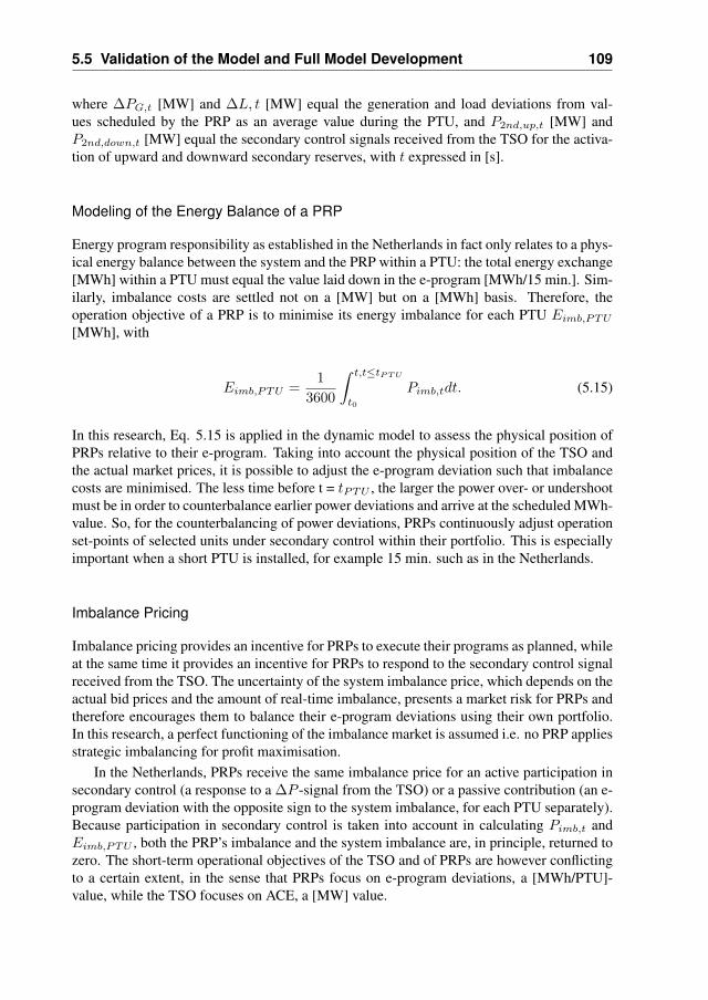
5.5 Validation of the Model and Full Model Development 109
where ∆PG,t [MW] and ∆L, t [MW] equal the generation and load deviations from val-ues scheduled by the PRP as an average value during the PTU, and P2nd,up,t [MW] andP2nd,down,t [MW] equal the secondary control signals received from the TSO for the activa-tion of upward and downward secondary reserves, with t expressed in [s].
Modeling of the Energy Balance of a PRP
Energy program responsibility as established in the Netherlands in fact only relates to a phys-ical energy balance between the system and the PRP within a PTU: the total energy exchange[MWh] within a PTU must equal the value laid down in the e-program [MWh/15 min.]. Sim-ilarly, imbalance costs are settled not on a [MW] but on a [MWh] basis. Therefore, theoperation objective of a PRP is to minimise its energy imbalance for each PTU Eimb,PTU
[MWh], with
Eimb,PTU =1
3600
∫ t,t≤tP T U
t0
Pimb,tdt. (5.15)
In this research, Eq. 5.15 is applied in the dynamic model to assess the physical position ofPRPs relative to their e-program. Taking into account the physical position of the TSO andthe actual market prices, it is possible to adjust the e-program deviation such that imbalancecosts are minimised. The less time before t = tPTU , the larger the power over- or undershootmust be in order to counterbalance earlier power deviations and arrive at the scheduled MWh-value. So, for the counterbalancing of power deviations, PRPs continuously adjust operationset-points of selected units under secondary control within their portfolio. This is especiallyimportant when a short PTU is installed, for example 15 min. such as in the Netherlands.
Imbalance Pricing
Imbalance pricing provides an incentive for PRPs to execute their programs as planned, whileat the same time it provides an incentive for PRPs to respond to the secondary control signalreceived from the TSO. The uncertainty of the system imbalance price, which depends on theactual bid prices and the amount of real-time imbalance, presents a market risk for PRPs andtherefore encourages them to balance their e-program deviations using their own portfolio.In this research, a perfect functioning of the imbalance market is assumed i.e. no PRP appliesstrategic imbalancing for profit maximisation.
In the Netherlands, PRPs receive the same imbalance price for an active participation insecondary control (a response to a ∆P -signal from the TSO) or a passive contribution (an e-program deviation with the opposite sign to the system imbalance, for each PTU separately).Because participation in secondary control is taken into account in calculating Pimb,t andEimb,PTU , both the PRP’s imbalance and the system imbalance are, in principle, returned tozero. The short-term operational objectives of the TSO and of PRPs are however conflictingto a certain extent, in the sense that PRPs focus on e-program deviations, a [MWh/PTU]-value, while the TSO focuses on ACE, a [MW] value.

110 Power System Dynamic Model
Modeling of Imbalance Control by PRPs
For imbalance minimisation at the PRP-level, an imbalance control is developed in this re-search based on interviews with Dutch PRPs. Although no detailed information could beobtained on the formulation of the actual controls, it was found that Dutch PRPs apply acontinuous control signal which is largely based on the actual e-program deviation. PRPsconsider imbalance control as a reactive process, because of the short duration of a PTU inthe Netherlands. This means that only feedback loops are applied.
The controller developed in this research reacts on the momentary program deviationEimb,t and the actual power imbalance Pimb,t. The value for the Eimb,t is reset to zero atthe end of each PTU. The integral of the Pimb,t is used since a controller based solely on theactual energy imbalance would result in an abrupt change of the control signal at each PTU-crossing. An additional benefit is that imbalance control is continued over different PTUsafter a significant power imbalance which cannot be managed within one PTU (i.e. ramp ratelimitations). The secondary control signal used by the PRP, 2ndPRP,t [MW] is
2ndPRP,t = −c1Eimb,t −c2
3600
∫ t
t0
Pimb,tdt + P2nd,up,t − P2nd,down,t (5.16)
assuming that all secondary control requested by the TSO is directly transfered to the PRP’sunits under secondary control and with c1 and c2 set to 10 [h−1] and 3.6 [h−1], respectively.The values of c1 and c2 have been determined such that 2ndPRP accumulates fast enough toallow for Eimb,t to return to zero after a power imbalance, but without an overshoot due tothe ramp rate limitations of the units under secondary control. It can be noted that this con-troller could not be optimised further, since no data were available for doing so. It has beenassumed that the secondary control signal is the same for all PRPs and for all simulations.The secondary control signal is transferred to the operating set-points of selected generationunits, which will then change their output correspondingly.
Overview of the PRP-Model
In this research, each PRP is modeled with a portfolio consisting of conventional generationunits, wind power, distributed generation, and load. In the short-term, the operation of thegeneration unit portfolio as a whole is governed by the minimisation of e-program deviations.A schematic illustration of the modeling of a PRP is shown in Fig. 5.6, with in this case onlya single unit n selected for secondary control.
5.5.4 Dynamic Generation Unit Models
Dynamic models are developed for all large (≥ 60 MW) conventional generation units inthe Netherlands. These large units are typically used for primary and secondary control.Especially primary control involves a relatively fast output change. The maximum ramp-rates used in the secondary control are equal to those applied in the UC–ED. Shorter-termvariations within the 15 min. range are not included for load, distributed generation units andwind power. For these, linear interpolation between the 15 min. set-points obtained fromUC–ED is applied.
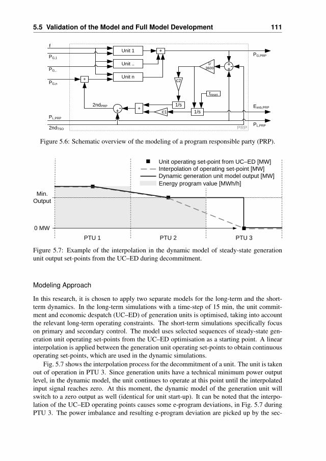
5.5 Validation of the Model and Full Model Development 111
fUnit 1
Unit ..
Unit n
+
1/s
+
PG,1
PG,..
PG,n
PL,PRP
2ndTSO
PG,PRP
PRPPL,PRP
2ndPRP
treset
1/s
c2
+1/3600
+
+-
+- Eimb,PRPc1
Figure 5.6: Schematic overview of the modeling of a program responsible party (PRP).
PTU 1 PTU 2 PTU 3
Interpolation of operating set-point [MW]Unit operating set-point from UC–ED [MW]
Dynamic generation unit model output [MW]
0 MW
Min.Output
Energy program value [MWh/h]
Figure 5.7: Example of the interpolation in the dynamic model of steady-state generationunit output set-points from the UC–ED during decommitment.
Modeling Approach
In this research, it is chosen to apply two separate models for the long-term and the short-term dynamics. In the long-term simulations with a time-step of 15 min, the unit commit-ment and economic despatch (UC–ED) of generation units is optimised, taking into accountthe relevant long-term operating constraints. The short-term simulations specifically focuson primary and secondary control. The model uses selected sequences of steady-state gen-eration unit operating set-points from the UC–ED optimisation as a starting point. A linearinterpolation is applied between the generation unit operating set-points to obtain continuousoperating set-points, which are used in the dynamic simulations.
Fig. 5.7 shows the interpolation process for the decommitment of a unit. The unit is takenout of operation in PTU 3. Since generation units have a technical minimum power outputlevel, in the dynamic model, the unit continues to operate at this point until the interpolatedinput signal reaches zero. At this moment, the dynamic model of the generation unit willswitch to a zero output as well (identical for unit start-up). It can be noted that the interpo-lation of the UC–ED operating points causes some e-program deviations, in Fig. 5.7 duringPTU 3. The power imbalance and resulting e-program deviation are picked up by the sec-
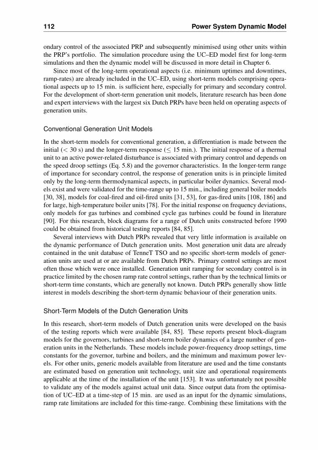
112 Power System Dynamic Model
ondary control of the associated PRP and subsequently minimised using other units withinthe PRP’s portfolio. The simulation procedure using the UC–ED model first for long-termsimulations and then the dynamic model will be discussed in more detail in Chapter 6.
Since most of the long-term operational aspects (i.e. minimum uptimes and downtimes,ramp-rates) are already included in the UC–ED, using short-term models comprising opera-tional aspects up to 15 min. is sufficient here, especially for primary and secondary control.For the development of short-term generation unit models, literature research has been doneand expert interviews with the largest six Dutch PRPs have been held on operating aspects ofgeneration units.
Conventional Generation Unit Models
In the short-term models for conventional generation, a differentiation is made between theinitial (< 30 s) and the longer-term response (≤ 15 min.). The initial response of a thermalunit to an active power-related disturbance is associated with primary control and depends onthe speed droop settings (Eq. 5.8) and the governor characteristics. In the longer-term rangeof importance for secondary control, the response of generation units is in principle limitedonly by the long-term thermodynamical aspects, in particular boiler dynamics. Several mod-els exist and were validated for the time-range up to 15 min., including general boiler models[30, 38], models for coal-fired and oil-fired units [31, 53], for gas-fired units [108, 186] andfor large, high-temperature boiler units [78]. For the initial response on frequency deviations,only models for gas turbines and combined cycle gas turbines could be found in literature[90]. For this research, block diagrams for a range of Dutch units constructed before 1990could be obtained from historical testing reports [84, 85].
Several interviews with Dutch PRPs revealed that very little information is available onthe dynamic performance of Dutch generation units. Most generation unit data are alreadycontained in the unit database of TenneT TSO and no specific short-term models of gener-ation units are used at or are available from Dutch PRPs. Primary control settings are mostoften those which were once installed. Generation unit ramping for secondary control is inpractice limited by the chosen ramp rate control settings, rather than by the technical limits orshort-term time constants, which are generally not known. Dutch PRPs generally show littleinterest in models describing the short-term dynamic behaviour of their generation units.
Short-Term Models of the Dutch Generation Units
In this research, short-term models of Dutch generation units were developed on the basisof the testing reports which were available [84, 85]. These reports present block-diagrammodels for the governors, turbines and short-term boiler dynamics of a large number of gen-eration units in the Netherlands. These models include power-frequency droop settings, timeconstants for the governor, turbine and boilers, and the minimum and maximum power lev-els. For other units, generic models available from literature are used and the time constantsare estimated based on generation unit technology, unit size and operational requirementsapplicable at the time of the installation of the unit [153]. It was unfortunately not possibleto validate any of the models against actual unit data. Since output data from the optimisa-tion of UC–ED at a time-step of 15 min. are used as an input for the dynamic simulations,ramp rate limitations are included for this time-range. Combining these limitations with the
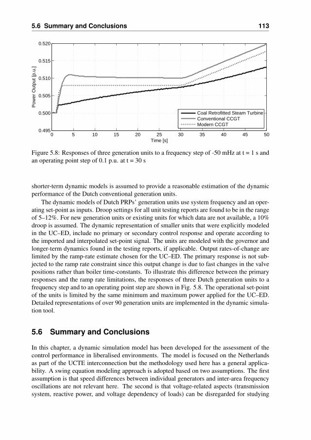
5.6 Summary and Conclusions 113
0 5 10 15 20 25 30 35 40 45 500.495
0.500
0.505
0.510
0.515
0.520
Time [s]
Pow
er O
utpu
t [p.
u.]
Coal Retrofitted Steam TurbineConventional CCGTModern CCGT
Figure 5.8: Responses of three generation units to a frequency step of -50 mHz at t = 1 s andan operating point step of 0.1 p.u. at t = 30 s
shorter-term dynamic models is assumed to provide a reasonable estimation of the dynamicperformance of the Dutch conventional generation units.
The dynamic models of Dutch PRPs’ generation units use system frequency and an oper-ating set-point as inputs. Droop settings for all unit testing reports are found to be in the rangeof 5–12%. For new generation units or existing units for which data are not available, a 10%droop is assumed. The dynamic representation of smaller units that were explicitly modeledin the UC–ED, include no primary or secondary control response and operate according tothe imported and interpolated set-point signal. The units are modeled with the governor andlonger-term dynamics found in the testing reports, if applicable. Output rates-of-change arelimited by the ramp-rate estimate chosen for the UC–ED. The primary response is not sub-jected to the ramp rate constraint since this output change is due to fast changes in the valvepositions rather than boiler time-constants. To illustrate this difference between the primaryresponses and the ramp rate limitations, the responses of three Dutch generation units to afrequency step and to an operating point step are shown in Fig. 5.8. The operational set-pointof the units is limited by the same minimum and maximum power applied for the UC–ED.Detailed representations of over 90 generation units are implemented in the dynamic simula-tion tool.
5.6 Summary and Conclusions
In this chapter, a dynamic simulation model has been developed for the assessment of thecontrol performance in liberalised environments. The model is focused on the Netherlandsas part of the UCTE interconnection but the methodology used here has a general applica-bility. A swing equation modeling approach is adopted based on two assumptions. The firstassumption is that speed differences between individual generators and inter-area frequencyoscillations are not relevant here. The second is that voltage-related aspects (transmissionsystem, reactive power, and voltage dependency of loads) can be disregarded for studying

114 Power System Dynamic Model
power-frequency control. The modeling approach is validated by comparing a mechanicalrepresentation of the New England test system in Simulink with a full representation in thepower system simulation tool SINCAL. A primary response to a generator outage was sim-ulated to validate the modeling approach. The simulation was repeated in SINCAL whilesubsequently considering different electro-technical aspects of the model representation inthis tool. It was concluded that a mechanical swing equation approach is valid for this re-search. From a frequency point of view, it is in fact a conservative approach since inclusionof voltage-dependent aspects of the load in practice leads to reduced frequency deviationsafter a power imbalance.
The dynamic model developed in this chapter incorporates system aspects such as in-ertia and primary control. The model is validated against frequency data of teh UCTE-interconnection of the primary response of the system following significant disturbances. Thevalidation allows an estimation of the system’s moment of inertia and the power-frequencycharacteristic. The model is extended to include secondary control mechanisms at the levelof the TSO and balancing control mechanisms of individual market parties. The model isdesigned such that UC–ED schedules can be used as a starting point for the dynamic sim-ulations. The modeling procedure is based on the import of operating set-points of Dutchgeneration units from the UC–ED and a linear interpolation of these set-points during thedynamic simulations. This methodology ensures that only realistic sets of generation unitsare used for power balancing in the dynamic simulations. Since long-term operational as-pects are already included in the optimisation of the UC–ED, short-term dynamic models ofgeneration units consider only aspects relevant for primary and secondary control. Short-term models for Dutch generation units have been developed based on historical unit testingreports, expert interviews with Dutch utilities and literature research. The dynamic modelhas been validated for the Dutch control zone as part of the UCTE interconnection and set upto include different PRPs’ portfolios, comprising conventional generation units, distributedgeneration, load and wind power.
CHAPTER 6Impacts of Wind Power onShort-Term Power System
Operation
6.1 Introduction
The variability and limited predictability of wind power increasingly challenge the real-timebalancing of generation and load in electrical power systems and require additional secondaryreserves. The way these reserves are provided and operated is no longer straightforward inmarket environments, and it is even more complicated if wind power is integrated into thesemarkets and subject to program responsibility. In order to assess the performance of theoperation, a dynamic model of the power system has been developed. The model comprisesautomatic control mechanisms of the generators and the actions of the Transmission SystemOperator (TSO) and the market parties, taking into account the market design adopted forwind power integration.
In this chapter, the previously presented dynamic simulation model is applied to assessfrequency stability in the presence of large-scale wind power. Furthermore, the dynamic per-formance of the system is analysed for different wind power penetrations and market designs.The possible use of wind power and pumped hydro energy storage as short-term balancing

116 Impacts of Wind Power on Short-Term Power System Operation
solutions are also simulated. The Netherlands is used as a case-study, with estimations forthe generation portfolios of six Dutch PRPs in the year 2014.
This chapter is organised as follows. First, the main two market designs for wind power,i.e. with or without program responsibility for wind power, are presented and discussed. Therelevant simulation parameters for the technical integration of wind power in the system areidentified, with a focus on frequency stability and short-term power system behaviour. Afterthis, the power system model is specified in detail, considering the Dutch market partiesand their generation portfolios, power reserves and secondary control. An estimate is madeof the rest of the UCTE-system. The system simulations to be performed are discussed,including the simulation procedure, identification of worst cases, different market designsfor wind power and short-term balancing strategies. The simulation results are presentedusing the simulation parameters identified earlier. The chapter ends with the conclusionson the simulation results, indicating the impacts of wind power on short-term power systemoperation.
6.2 Market Designs for Wind Power
6.2.1 Organisation of Markets
With the liberalisation of energy markets in Europe, generation unit despatch has become de-coupled from system operation. Market parties are free nowadays to make arrangements fortrading electrical energy, which is done on different electricity markets. The largest energyvolume is traded in the period before day-ahead: energy derivatives are traded for longer timeperiods in the future so that market parties can settle their physical positions (i.e. schedulingof generation unit maintenance, long-term base-load contracts etc.). Until one day ahead ofoperation, trading can be done on the spot market, which may be a national or an internationalmarket. Spot market trading allows for a more accurate scheduling of units since updated de-mand forecasts are available. This optimisation continues during intra-day, by trading onadjustment markets and by offering generation capacity to the TSO as power reserves. Theactual demand to be covered by a market party’s generation units during each program timeunit (PTU) is the sum of the loads of its customers plus the power exchanges settled for thisperiod with other market parties.
After closure of the day-ahead spot market, market parties submit their scheduled ex-changes with other parties to the TSO. Market parties may have the possibility to continuetrading on an intra-day adjustment market and adjust their schedules accordingly. At themoment of (intra-day) market gate closure, the control over the power system is passed to animbalance settlement administrator, usually the TSO [67]. This is necessary because, eventhough generation and load are scheduled to match, this does not guarantee a physical powerbalance in real-time. Therefore, on top of the automated primary actions, the TSO man-ages secondary reserves (regulating power, available within 15 minutes) and tertiary reserves(reserve power, available after 15 minutes) in order to maintain the balance in the systemin real-time. Secondary and tertiary reserves are generally made available by market par-ties according to the submitted bids for operating reserves to the TSO. The balancing costsencountered by the TSO are mostly passed on to market parties who deviated from their pro-grams. The volumes called by the TSO may be settled against the price of the bid or the priceof the highest bid that is called for [48, 56, 162]. In the Netherlands, PRPs receive the same
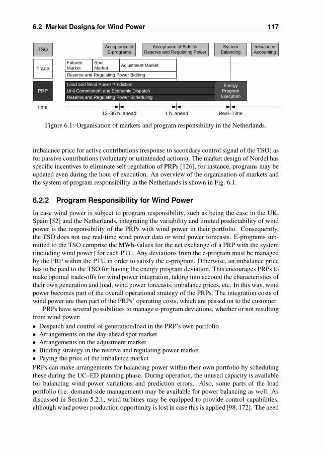
6.2 Market Designs for Wind Power 117
Futures Market
12 - 36 h. 1 h. Real–Time
Acceptance of E-programs
Adjustment Market
Acceptance of Bids for Reserve and Regulating Power
System Balancing
Imbalance Accounting
Reserve and Regulating Power SchedulingUnit Commitment and Economic Dispatch
TSO
PRP
Trade
1 h. ahead12–36 h. ahead
Load and Wind Power Prediction
time
Energy Program Execution
Reserve and Regulating Power Bidding
Spot Market
Figure 6.1: Organisation of markets and program responsibility in the Netherlands.
imbalance price for active contributions (response to secondary control signal of the TSO) asfor passive contributions (voluntary or unintended actions). The market design of Nordel hasspecific incentives to eliminate self-regulation of PRPs [126], for instance, programs may beupdated even during the hour of execution. An overview of the organisation of markets andthe system of program responsibility in the Netherlands is shown in Fig. 6.1.
6.2.2 Program Responsibility for Wind Power
In case wind power is subject to program responsibility, such as being the case in the UK,Spain [52] and the Netherlands, integrating the variability and limited predictability of windpower is the responsibility of the PRPs with wind power in their portfolio. Consequently,the TSO does not use real-time wind power data or wind power forecasts. E-programs sub-mitted to the TSO comprise the MWh-values for the net exchange of a PRP with the system(including wind power) for each PTU. Any deviations from the e-program must be managedby the PRP within the PTU in order to satisfy the e-program. Otherwise, an imbalance pricehas to be paid to the TSO for having the energy program deviation. This encourages PRPs tomake optimal trade-offs for wind power integration, taking into account the characteristics oftheir own generation and load, wind power forecasts, imbalance prices, etc. In this way, windpower becomes part of the overall operational strategy of the PRPs. The integration costs ofwind power are then part of the PRPs’ operating costs, which are passed on to the customer.
PRPs have several possibilities to manage e-program deviations, whether or not resultingfrom wind power:• Despatch and control of generation/load in the PRP’s own portfolio• Arrangements on the day-ahead spot market• Arrangements on the adjustment market• Bidding strategy in the reserve and regulating power market• Paying the price of the imbalance marketPRPs can make arrangements for balancing power within their own portfolio by schedulingthese during the UC–ED planning phase. During operation, the unused capacity is availablefor balancing wind power variations and prediction errors. Also, some parts of the loadportfolio (i.e. demand-side management) may be available for power balancing as well. Asdiscussed in Section 5.2.1, wind turbines may be equipped to provide control capabilities,although wind power production opportunity is lost in case this is applied [98, 172]. The need

118 Impacts of Wind Power on Short-Term Power System Operation
for reserves for wind power decreases with the geographical spread of wind power within thePRPs’ portfolios, although this applies only to a limited extent in the Netherlands. As thetime of operation draws nearer, wind power prediction errors decrease and more accuratewind power predictions can be used to continue trade on the intra-day adjustment market,which is especially valuable for wind power integration [12, 69]. Certainly, PRPs must findan optimum between prices on the spot-market and adjustment market, wind power balancingcosts, lost production opportunity of their own generation units, and costs incurred on theimbalance market.
6.2.3 Prioritisation of Wind Power
In case wind power is assigned as prioritised generation (a.o. Germany and Denmark), windpower is partly or fully exempted from program responsibility. The TSO may be set respon-sible for forecasting wind power, buying the electricity generated by wind power, nominatingit in the market and compensating its variability and limited predictability. Usually, the fore-cast wind power is nominated by the TSO and assigned to the PRPs, which cover part oftheir load with the assigned wind power. In case wind power generates more than nominated,the TSO sells the excess energy to the market, and on the other hand buys any deficits. Bydoing so, the TSO incurs the costs for integrating wind power into the system, effectivelysocialising these costs.
Comprehensive economic studies concerning the imbalance cost of wind power showthat with increasing wind power penetrations, the imbalance costs increase as well. At windpower penetration levels of up to 10% of annual electricity demand [TWh], the integrationcosts associated with wind power are estimated to be 1–4 e/MWh; at higher penetrationlevels up to 30%, this cost estimate is 2–5 e/MWh [6, 35, 70]. Although these cost estimatesare modest compared to average electricity market prices, these costs are certainly significant.The prioritisation of wind power not only keeps wind power integration costs away from windpark owners and operators, it also shields wind power from market risks.
6.2.4 Comparison of Market Designs for Wind Power
The variability and limited predictability of wind power is a specific disadvantage for PRPswith wind power in their portfolio. The capabilities of the other generation units (minimumuptimes and downtimes, ramp-rates, efficiency curves) largely determine the technical andeconomic integration of wind power into the operational strategy of each PRP. In order tominimise their individual risks, PRPs are inclined to balance the wind power within theirportfolio by operating reserves individually. The total amount of reserves held by all PRPstogether is however likely to be larger than if a system-wide coordination of reserves wouldbe used, such as when wind power deviations are handled by the TSO. In order to minimisethis inefficiency, some market designs include incentives to promote the management of im-balances on markets rather than by individual PRPs [126].
In case wind power is integrated on a cross-border level (i.e. the Dutch power systemas part of a larger control zone within the UCTE-interconnection), wind power is integratedinto a larger system. Provided sufficient transmission capacity is available, more conven-tional generation capacity is available for integrating the wind power. Also, the total vari-ability and limited predictability of wind power may decrease with the larger geography of
6.3 Power System Model 119
the system, reducing the total amount of reserves needed for wind power integration. Thesenotions not only hold for wind power specifically, but for system balancing in general (com-pare e.g. the coordination of primary reserves in the UCTE-system). For a relatively smallcountry, such as the Netherlands, the variations and forecast errors of wind power are highlycorrellated (Chapter 2) and international exchange allows the integration of larger amountsof wind power (Chapter 4). An international market design allowing the adjustment of ex-change schedules close to real-time is the most beneficial for wind power integration. Inorder to investigate the impacts of market designs on the system integration of wind power, itis however decided to focus on the Dutch system without scheduled international exchange.This conservative assumption makes that wind power ’stresses’ the system much more thanit would in an international setting, enabling the comparison of market designs for windpower specifically. Both market designs investigated here concern wind power being subjectto program responsibility and as prioritised generation. These market designs concern theshort-term range, in which the real-time deviations from scheduled values of wind power arebalanced either by the associated PRP or by the TSO.
6.3 Power System Model
6.3.1 Simulation Parameters
The dynamic simulation model is focused on the shorter-term technical impacts of windpower on power system operation. Relevant simulation parameters will be identified in orderto quantify these impacts. The simulation parameters to be monitored will be discussedshortly below.
Power Balance
The simulation parameters used for assessment of the power balance are:• Frequency: active power balance in the system• Area control error (ACE): power-frequency balance• Processed ACE (PACE): need for secondary reserves by the TSOThe central parameter for the active power balance is the system frequency. The frequencyshould stay within certain bounds to ensure reliable operation of the system. The dynamicpower system model presented in the previous chapter allows the assessment of power-frequency stability, comprising not only system frequency but also deviations from sched-uled power exchanges between zones. It is the objective of the TSO to maintain a stablefrequency (50 Hz in the UCTE-system) and simultaneously to minimise the ACE. For this,the TSO calls off bids for reserve and regulating power, the amount of which is determinedby the PACE. It is assumed that power variations should be balanced within the control areain which they occur in less than 15 min. as is required by UCTE [169]. This means a fullrecovery of ACE within 15 min. and returns PACE to zero as well.
Energy Balance
The simulation parameters used for assessment of the energy balance are:• Power balancing reserves activated by the PRPs
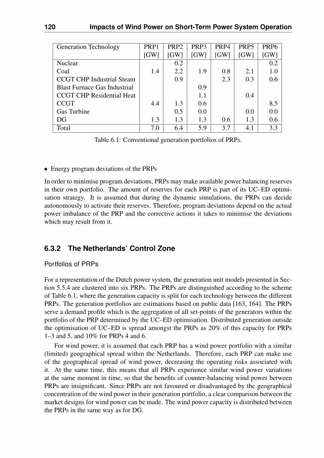
120 Impacts of Wind Power on Short-Term Power System Operation
Generation Technology PRP1 PRP2 PRP3 PRP4 PRP5 PRP6[GW] [GW] [GW] [GW] [GW] [GW]
Nuclear 0.2 0.2Coal 1.4 2.2 1.9 0.8 2.1 1.0CCGT CHP Industrial Steam 0.9 2.3 0.3 0.6Blast Furnace Gas Industrial 0.9CCGT CHP Residential Heat 1.1 0.4CCGT 4.4 1.3 0.6 8.5Gas Turbine 0.5 0.0 0.0 0.0DG 1.3 1.3 1.3 0.6 1.3 0.6Total 7.0 6.4 5.9 3.7 4.1 3.3
Table 6.1: Conventional generation portfolios of PRPs.
• Energy program deviations of the PRPs
In order to minimise program deviations, PRPs may make available power balancing reservesin their own portfolio. The amount of reserves for each PRP is part of its UC–ED optimi-sation strategy. It is assumed that during the dynamic simulations, the PRPs can decideautonomously to activate their reserves. Therefore, program deviations depend on the actualpower imbalance of the PRP and the corrective actions it takes to minimise the deviationswhich may result from it.
6.3.2 The Netherlands’ Control Zone
Portfolios of PRPs
For a representation of the Dutch power system, the generation unit models presented in Sec-tion 5.5.4 are clustered into six PRPs. The PRPs are distinguished according to the schemeof Table 6.1, where the generation capacity is split for each technology between the differentPRPs. The generation portfolios are estimations based on public data [163, 164]. The PRPsserve a demand profile which is the aggregation of all set-points of the generators within theportfolio of the PRP determined by the UC–ED optimisation. Distributed generation outsidethe optimisation of UC–ED is spread amongst the PRPs as 20% of this capacity for PRPs1–3 and 5, and 10% for PRPs 4 and 6.
For wind power, it is assumed that each PRP has a wind power portfolio with a similar(limited) geographical spread within the Netherlands. Therefore, each PRP can make useof the geographical spread of wind power, decreasing the operating risks associated withit. At the same time, this means that all PRPs experience similar wind power variationsat the same moment in time, so that the benefits of counter-balancing wind power betweenPRPs are insignificant. Since PRPs are not favoured or disadvantaged by the geographicalconcentration of the wind power in their generation portfolio, a clear comparison between themarket designs for wind power can be made. The wind power capacity is distributed betweenthe PRPs in the same way as for DG.
6.3 Power System Model 121
Secondary Control and Power Balancing Reserves of PRPs
For the dynamic simulations, it is assumed that Dutch PRPs fully respond to the secondarycontrol signal of the TSO. It can be noted that this is in accordance with the operationalstrategy of Dutch PRPs, especially since most PRPs have contracts with TenneT TSO forbidding in on secondary regulation. During the simulations, the delta-signals for upwardand downward regulating power received from the TSO are combined with the autonomousbalance control signal of the PRP (Section 5.5.3). The aggregated control signal is then addedto the operating set-points of selected generation units within the PRPs portfolio.
The generation units used for secondary control by each PRP are selected based on lowestmarginal operating cost, with the exception of nuclear units. For most of the PRPs modeledhere this comes down to the use of base-load (coal-fired, CHP) generation units within thegeneration portfolio during the day and during the night. This is in accordance with thepresent operation practices of Dutch PRPs. Benefits of this operating strategy is that theseunits have a rather flat efficiency curve, are always available for reserves unless outaged andthat this allows the despatch of natural gas-fired, medium- and peak-load generation units attheir best operating points. It can be noted that in the Netherlands, the ramp-rates of coal-fired generation units are sufficient to provide secondary reserve. For the simulations, it isassumed that no reserves additional to the 1600 MW total minimum included in UC–ED aretaken into account by Dutch PRPs.
Secondary Control by TSO TenneT
TenneT TSO uses system frequency and unscheduled international exchange as inputs (to-gether forming the ACE) and uses the PACE-logic for sending out the secondary controlsignals to Dutch PRPs (delta-signals for upward and downward regulation). The secondarycontrol logic applied by TenneT TSO includes a bidding ladder which is limited to 1000 MWof upward and downward regulating power (available within 15 min.) and reserve power(call time > 15 min.). The bids for secondary and longer-term reserves received from DutchPRPs are arranged in order to marginal cost and this order is assumed to not change betweendifferent PTUs.
6.3.3 Rest of the UCTE-System
The rest of the UCTE-system is modeled as an aggregation of generation and load accord-ing to the approach developed in Section 5.3.2. Scheduled international exchange with theNetherlands, in case possible and optimised as part of UC–ED, is modeled as a difference inload in UCTE. The moment of inertia of the UCTE interconnection is assumed to be con-stant at 2·105 MWs/Hz and its β at 2.6·104 MW/Hz. A dead-band of 10 mHz for primarycontrol is applied. International exchange between the Dutch area and the rest of the UCTE-interconnection is treated only by the Dutch ACE and the secondary control actions takenin the Netherlands. It is assumed that no disturbances occur outside the Dutch area and thatthere is no secondary reaction from UCTE to assist the Netherlands.
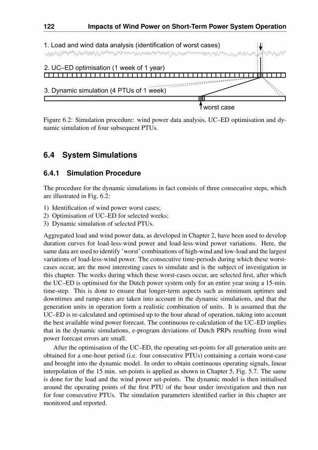
122 Impacts of Wind Power on Short-Term Power System Operation
–
Figure 6.2: Simulation procedure: wind power data analysis, UC–ED optimisation and dy-namic simulation of four subsequent PTUs.
6.4 System Simulations
6.4.1 Simulation Procedure
The procedure for the dynamic simulations in fact consists of three consecutive steps, whichare illustrated in Fig. 6.2:
1) Identification of wind power worst cases;2) Optimisation of UC–ED for selected weeks;3) Dynamic simulation of selected PTUs.
Aggregated load and wind power data, as developed in Chapter 2, have been used to developduration curves for load-less-wind power and load-less-wind power variations. Here, thesame data are used to identify ’worst’ combinations of high-wind and low-load and the largestvariations of load-less-wind power. The consecutive time-periods during which these worst-cases occur, are the most interesting cases to simulate and is the subject of investigation inthis chapter. The weeks during which these worst-cases occur, are selected first, after whichthe UC–ED is optimised for the Dutch power system only for an entire year using a 15-min.time-step. This is done to ensure that longer-term aspects such as minimum uptimes anddowntimes and ramp-rates are taken into account in the dynamic simulations, and that thegeneration units in operation form a realistic combination of units. It is assumed that theUC–ED is re-calculated and optimised up to the hour ahead of operation, taking into accountthe best available wind power forecast. The continuous re-calculation of the UC–ED impliesthat in the dynamic simulations, e-program deviations of Dutch PRPs resulting from windpower forecast errors are small.
After the optimisation of the UC–ED, the operating set-points for all generation units areobtained for a one-hour period (i.e. four consecutive PTUs) containing a certain worst-caseand brought into the dynamic model. In order to obtain continuous operating signals, linearinterpolation of the 15 min. set-points is applied as shown in Chapter 5, Fig. 5.7. The sameis done for the load and the wind power set-points. The dynamic model is then initialisedaround the operating points of the first PTU of the hour under investigation and then runfor four consecutive PTUs. The simulation parameters identified earlier in this chapter aremonitored and reported.
6.4 System Simulations 123
6.4.2 Wind Power Worst Cases
The worst cases are selected situations from one PTU to the next with large power variationsand low-load, high-wind combinations. The former require additional ramping actions fromconventional generation units. Even though the simulation results of the UC–ED did notreport any ramping problems, unit ramping is likely to have an impact on short-term powersystem operation (frequency, ACE). The low-load, high-wind periods may result in less con-ventional capacity being available for primary and secondary control actions. Therefore, alsooutages of a large generation unit are simulated and analysed for the worst cases identified be-low. It is assumed that the Netherlands balances its own wind power i.e. all ramping actionsrequired for balancing the Dutch load and wind power are performed by Dutch conventionalgeneration units.
Aggregated Load and Wind Power Variations
For identifying the worst case for variability, the largest aggregated variation of load andwind power within 15 min. is selected from the data developed in Chapter 2. Since it isassumed that wind power can always be ramped down, only the maximum simultaneous loadincrease and wind power decrease is considered here. For an installed capacity of 12 GWwind power, the worst case variation of the system load and wind power data developed inChapter 2 is +4421 MW/15 min. This worst case consists of a combination of a load increase(+171 MW) and a wind power decrease (-4250 MW, falling from 10105 MW to 5855 MWwithin 15 min.). However, it was found that the variation of wind power during the actualsimulation of UC–ED is only 1275 MW. The reason for this is that a significant amount ofwind energy ccould not be integrated anyhow (wasted wind energy), so that the actual windpower level is only 7130 MW instead of the available 10105 MW. The wind power levelthen drops to 5855 MW, resulting in a total power variation of load less wind power of only+1446 MW/15 min instead of +4421 MW/15 min.
In order to find the worst case actually uccuring during UC–ED, the simulation results ofUC–ED are analysed. The largest upward variation of load-less-wind power occurring duringthe UC–ED is found to be +1890 MW/15 min. for 12 GW wind power. In this case, also wast-ing of wind energy occurs: the variation of foreseen wind power is -3020 MW/15 min (from6862 to 3842 MW/15 min.), while the wind power variation in UC–ED is -1527 MW/15 min.
For the simulation of the worst case, three different wind power penetration levels areconsidered: 0 GW (reference), 6 GW and 12 GW. The largest upward load-less-wind powervariation from the perspective of the UC–ED is simulated for each penetration level. For12 GW wind power, the worst case is as described above. For 6 GW wind power, this caseinvolves a wind power drop from 2210 MW to 1332 MW. With the load variation in that pe-riod (+363 MW), this implies an aggregated variation of load-less-wind power of +1241 MW.It can be noted that during the simulation, UC–ED results in a number of conventional gen-eration units being brought on-line at their minimum power level. As a worst case, it isfurthermore assumed that a 600 MW coal-fired unit is outaged during the dynamic simula-tion. These events will result in sudden changes in the power balance in the system and willtherefore be visible when monitoring frequency and ACE. To illustrate this, the power im-balance and e-program deviations are monitored of the PRPs that bring units on-line or takethese off-line during the simulation.
124 Impacts of Wind Power on Short-Term Power System Operation
Low-Load, High-Wind Situation
During low-load, high-wind periods, conventional generation units have to be taken out ofoperation in order to allow for the integration of wind power. During such periods, lessconventional generation capacity is available for providing primary and secondary reserves.As a result of this, a generation unit outage may result in a larger excursion of frequencyand/or the ACE during such situations. The worst case selected here comprises a generationunit outage during a high wind (11266 MW available), low load (10467 MW) situation. Inorder to prevent minimum load problems, conventional generation units are shut-down foras far as technically possible, and otherwise ramped down to their operational minimum.Must-run nuclear and coal units at minimum load still supply a total of 4316 MW, whilemust-run CHP-units and distributed generation supply a further 5204 MW, resulting in atotal of 9520 MW of generation other than wind power. As a result, a very large amount ofwind power (10319 MW) must be wasted in order to avoid minimum load problems. Only947 MW of wind power can be integrated at this moment, which is very low.
The high level of must-take generation and the absence of possibilities for internationalexchange are not optimal for wind power integration during this low-load situation. Whenthe maximum flexibility of industrial CHP-units would be assumed, this would allow theshut-down of these units and the integration of a further 3 GW of wind power. Would inter-national exchange be possible, then this would likely not result in a different commitment ofconventional generation units in the Netherlands but only in exports of excess wind power.With both assumptions, still the same coal-fired generation capacity would be available forpower balancing in the Netherlands as without these assumptions. Therefore, even thoughnot optimal for wind power integration, this case still represents a reasonable worst case forinvestigating frequency stability with wind power.
For this simulation, it is assumed that the conventional generation unit supplying mostpower at this moment in time is tripped in the dynamic simulation at t = 100 s. An industrialCHP-unit is at this moment operating at a level of 550 MW and is part of the portfolio ofPRP4. It is assumed that shortly after the occurrence of the outage, PRP4 re-dispatches thepower to be supplied by the outaged unit between the conventional generation units withinits portfolio available for secondary control. In this case, this mainly concerns two coal-firedgeneration units of 800 MW each, operating at minimum load (385 MW) at the moment ofthe outage.
6.4.3 Market Designs for Wind Power
The market designs for wind power discussed and compared in Section 6.2 can be analysedas well using the dynamic simulation tool. For this case, deviations in wind power (i.e. dueto forecast errors) are introduced during the simulation and the results between the differentmarket designs are compared. For these simulations, the maximum load-less-wind powervariation case for 6 GW wind power is used. At the beginning of the simulation, no deviationsfrom the scheduled wind power are expected. Between t = 450 s and t = 1350 s (halfwayPTU 1 and PTU 2), a wind power deviation is initiated going from 0% to 6% of the predictedvalue, which is in line with the forecast error present 15 min. ahead of operation (Chapter 2,Fig. 2.14). As a worst case, it is assumed that a positive forecast error is present, leading to awind power decrease between PTUs 1 and 2 on top of the existing large variation.
6.4 System Simulations 125
In case wind power is subject to program responsibility, balancing the forecast errors ofwind power is done by the PRPs. It is assumed that all PRPs experience a similar forecasterror since their wind turbines and parks have the same geographical spread and the PRPsare likely to use similar weather forecast data. For PRPs 1, 2, 3, and 5, a 6% forecast errorleads to a power deviation of -16 MW; for PRPs 4 and 6, this forecast error leads to a powerdeviations -8 MW. After t = 1350 s, it is assumed that the forecast error increases further bythe same amounts for each consecutive 900 s until the end of the simulation.
In case wind power is prioritised, the TSO is responsible for forecasting wind powerand scheduling it into the market. It is assumed that wind power is assigned to the PRPs inthe same distribution as under program responsibility. PRPs do not take into account windpower deviations in the calculation of their power imbalances and e-program deviations.Wind power deviations result in an ACE and subsequent PACE, leading to secondary controlsignals sent out by the TSO.
6.4.4 Short-Term Balancing Solutions
For the dynamic simulations discussed above, existing conventional generation units are usedfor balancing wind power. In principle, wind power plants could also be considered to per-form short-term regulating actions. Furthermore, pumped hydro energy storage could beadded to the system and used to obtain fast regulating power.
Regulation by Wind Power Plants
Wind power plants have the potential to supply very fast upward and downward powerreserves, provided that wind is available and not fully used in case of upward regulation[98, 172]. Wind power may then be used for primary and secondary control, although somewind energy must be wasted in these cases (opportunity loss). In this simulation, the sameconventional generation unit outage of PRP4 as discussed in Section 6.4.2 is simulated forthe 12 GW wind power scenario. It is assumed that all PRPs use their wind power plantsfor secondary control and the performance of wind power plants is compared to conventionalunits.
For PRP4, it is assumed that it has 200 MW of fast regulating reserve available by ap-plying pitch control on wind turbines in operation (delta control). This capacity is assumedto be capable of a ramp from zero to full power within 30 s, including a 2 s activation time.Other reserves provided by wind power are assumed to comprise shut-down or ramped downwind parks. Bringing these on-line requires yawing the turbines into the wind and startingthese up. It is assumed that the additional reserve capacity by wind parks is gradually madeavailable within 5 minutes following the outage. At this moment, PRP4 can make availablean additional 500 MW from otherwise wasted wind energy. As a conservative assumption,the other PRPs with a similar wind power opportunity available, do not apply these reserves.
Regulation by Pumped Hydro Energy Storage
Pumped hydro storage is technically capable of fast ramping by adjusting its generation orpumping power. Compared to wind power plants, the availability of this capacity for power-frequency control does not depend on the wind. For this simulation, it is assumed that a

126 Impacts of Wind Power on Short-Term Power System Operation
WP Variation LL–HW Variation LL-HW Variation[GW] Outage Outage Market Design WPP PAC
0 PRPs6 PRPs PRPs,TSO
12 PRPs PRPs PRPs PRPsWP = Wind Power level, PRPs = wind power balanced by PRPs, TSO = idem by TSO,
LL–HW = Low-Load, High-Wind situation, WPP = regulating Wind Power Plant,PAC = fast-ramping Pumped Accumulation energy storage
Table 6.2: Overview of the dynamic simulations.
pumped hydro accumulation storage unit (PAC) is part of the portfolio of PRP1. The pres-ence of PAC in the Dutch power system results in a different UC–ED, since the PAC canbe used to balance wind power and thereby allows a more gradual operation of the UC–ED of conventional generation units. For a clear comparison of results, it is assumed thatPRP1 bids in the same amount of secondary reserves to the TSO as is done without PAC.Certainly, PRP1 may in reality change its bidding strategy with PAC as part of its portfolio.PRP1 applies PAC both for providing secondary control to the TSO and for balancing its ownportfolio.
6.4.5 Overview
In Table 6.2, an overview is shown of all dynamic simulations performed here. Simulationsare done for different wind power penetrations (WP), worst cases (Variation = large powervariation situation, LL–HW = low-load, high-wind situation), market designs for wind power(PRPs = wind power balancing performed by PRPs / e-program responsibility, TSO = windpower balancing performed by TSO / prioritisation), and balancing solutions for wind power(WPP = regulating wind power plants, PAC = use of PAC for fast-ramping). In total, eightcombinations of a UC–ED and dynamic simulation are carried out for this research. A simu-lation input file consisting of the unit operational set-points obtained from UC–ED is gener-ated, following the procedure described in Section 6.4.1.
6.5 Simulation Results
The simulation results comprise system frequency, ACE, and PACE and the e-program devi-ations of selected PRPs. As an illustration, Fig. 6.3 shows a combination of the simulationresults for the largest power variation on a 15-min. timescale in case of 0 GW wind power.Variations in frequency and ACE are the result of a unit outage at t = 1350 s and of the opera-tional actions undertaken by the PRPs and the TSO. PACE is the summed secondary controlsignal sent to the PRPs for secondary control. During unit commitment, different generationunits have been scheduled for shut-down or start-up. Dommitment or de-commitment deci-sions result in instantaneous power imbalances due to the minimum output levels of theseunits.
In order to illustrate the simulation results, Fig. 6.3 presents a dynamic simulation of fourconsecutive PTUs. In the upper graph is also plotted a one-hour, 4 s time series of UCTE-
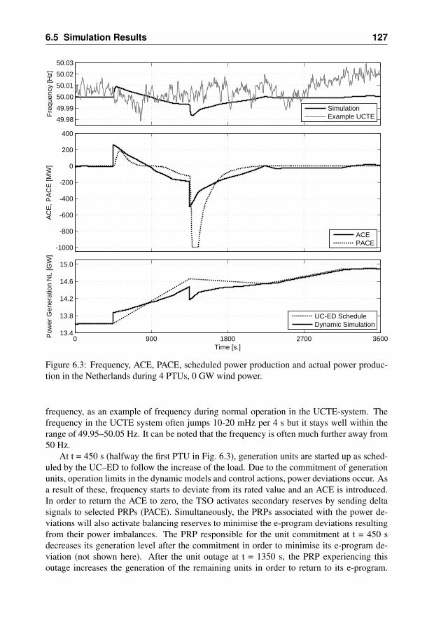
6.5 Simulation Results 127
-1000
-800
-600
-400
-200
0
200
400
AC
E, P
AC
E [M
W]
0 900 1800 2700 360013.4
13.8
14.2
14.6
15.0
Time [s.]
Pow
er G
ener
atio
n N
L [G
W]
ACEPACE
UC-ED ScheduleDynamic Simulation
49.9849.9950.0050.0150.0250.03
Freq
uenc
y [H
z]
SimulationExample UCTE
Figure 6.3: Frequency, ACE, PACE, scheduled power production and actual power produc-tion in the Netherlands during 4 PTUs, 0 GW wind power.
frequency, as an example of frequency during normal operation in the UCTE-system. Thefrequency in the UCTE system often jumps 10-20 mHz per 4 s but it stays well within therange of 49.95–50.05 Hz. It can be noted that the frequency is often much further away from50 Hz.
At t = 450 s (halfway the first PTU in Fig. 6.3), generation units are started up as sched-uled by the UC–ED to follow the increase of the load. Due to the commitment of generationunits, operation limits in the dynamic models and control actions, power deviations occur. Asa result of these, frequency starts to deviate from its rated value and an ACE is introduced.In order to return the ACE to zero, the TSO activates secondary reserves by sending deltasignals to selected PRPs (PACE). Simultaneously, the PRPs associated with the power de-viations will also activate balancing reserves to minimise the e-program deviations resultingfrom their power imbalances. The PRP responsible for the unit commitment at t = 450 sdecreases its generation level after the commitment in order to minimise its e-program de-viation (not shown here). After the unit outage at t = 1350 s, the PRP experiencing thisoutage increases the generation of the remaining units in order to return to its e-program.
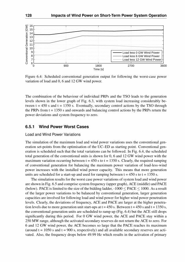
128 Impacts of Wind Power on Short-Term Power System Operation
0 900 1800 2700 36006789
10111213141516
Time [s]
Con
vent
iona
l Gen
erat
ion
[GW
]
Load less 0 GW Wind PowerLoad less 6 GW Wind PowerLoad less 12 GW Wind Power
Figure 6.4: Scheduled conventional generation output for following the worst-case powervariation of load and 0, 6 and 12 GW wind power.
The combination of the behaviour of individual PRPs and the TSO leads to the generationlevels shown in the lower graph of Fig. 6.3, with system load increasing considerably be-tween t = 450 s and t = 1350 s. Eventually, secondary control actions by the TSO throughthe PRPs from t = 1350 s and onwards and balancing control actions by the PRPs return thepower deviations and system frequency to zero.
6.5.1 Wind Power Worst Cases
Load and Wind Power Variations
The simulation of the maximum load and wind power variations uses the conventional gen-eration set-points from the optimisation of the UC–ED as starting point. Conventional gen-eration is scheduled such that the total variations can be followed. In Fig. 6.4, the scheduledtotal generation of the conventional units is shown for 0, 6 and 12 GW wind power with themaximum variation occurring between t = 450 s to t = 1350 s. Clearly, the required rampingof conventional generation for balancing the maximum power variation of load-less-windpower increases with the installed wind power capacity. This means that more generationunits are scheduled for a start-up and used for ramping between t = 450 s to t = 1350 s.
The simulation results for the worst case power variations of system load and wind powerare shown in Fig. 6.5 and comprise system frequency (upper graph), ACE (middle) and PACE(below). PACE is limited to the size of the bidding ladder, -1000≤ PACE≤ 1000. As a resultof the larger power variations to be balanced by conventional generation, larger generationcapacities are involved for following load and wind power for higher wind power penetrationlevels. Clearly, the deviations of frequency, ACE and PACE are larger at the higher penetra-tion levels due to more generation unit start-ups at t = 450 s. Between t = 450 s and t = 1350 s,the conventional generation units are scheduled to ramp up (Fig. 6.4) but the ACE still dropssignificantly during this period. For 0 GW wind power, the ACE and PACE stay within a250 MW range, although the activated secondary reserves do not return the ACE to zero. For6 and 12 GW wind power, the ACE becomes so large that the PACE reaches its maximum(around t = 1050 s and t = 900 s, respectively) and all available secondary reserves are acti-vated. Also, the frequency drops below 49.99 Hz which results in the activation of primary

6.5 Simulation Results 129
0 900 1800 2700 3600-1000
-750
-500
-250
0
250
500
750
10001000
Time [s.]
PA
CE
[MW
]
0 GW Wind Power6 GW Wind Power12 GW Wind Power
-1000
-750
-500
-250
0
250
500
750
10001000
AC
E [M
W]
0 GW Wind Power6 GW Wind Power12 GW Wind Power
49.97
49.98
49.99
50.00
50.01
50.02
Freq
uenc
y [H
z]
0 GW Wind Power6 GW Wind Power12 GW Wind Power
Figure 6.5: ACE and PACE during the worst case of load-less-wind power variation for 0, 6and 12 GW wind power.
reserves. Primary and secondary reserves stabilise the frequency and the ACE but secondaryreserves are insufficient to decrease the ACE. Limits for ramping exist for the 6 and 12 GWwind power scenarios since the conventional generation capacity is already scheduled in theUC–ED for following the power variations of load and wind (Fig. 6.4).
At t = 1350 s a generation unit outage is simulated and the ACE drops further. For 0 GWwind power, the outage results in the PACE increasing to -1000 MW, calling all availablesecondary reserves on the bidding ladder. The PACE-logic is by-passed after the outage(250 MW, minimum operation level of the outaged unit) at t = 1350 s since the ACE is below-300 MW and a power imbalance≥ 150 MW occurs. Also, the frequency drops below 49.99Hz and primary reserves are activated. As a result of the activation of additional secondaryreserves, frequency and ACE are brought back within 15 min. after the outage. For 6 and12 GW wind power, the PACE is already at its maximum before the outage due to the largeACE. Secondary reserves only start to decrease the ACE after t = 1350 s, when the largevariation of load and wind power ends and conventional generation capacity is available for

130 Impacts of Wind Power on Short-Term Power System Operation
ramping. Some overshoots of ACE and PACE occur after t = 1800 s due to the ramp-ratelimited de-activation of the secondary reserves, but frequency deviations and the ACE areeventually returning to zero. Notably, PACE is sooner at its maximum for the 6 and 12 GWwind power penetration levels (lower graph of Fig. 6.5). Because more secondary reserveshave been activated, the ACE returns to zero somewhat faster than for load variations only(middle graph of Fig. 6.5, after t = 1350 s).
From the simulations, it follows that frequency, ACE and PACE are influenced by theadditional commitment decisions of conventional generation, rather than directly by windpower variations. The instantaneous frequency deviations as a result of unit commitmentmay in reality be lower than simulated here, since it is unlikely that start-ups and shut-downsof different units occur exactly at the same moment. The additional start-ups of conventionalunits, together with their ramping capabilities, are sufficient to incorporate the variations ofload and wind power. The frequency variations as a result of wind power integration are inthe order of an additional 10 mHz on top of the 10 mHz as a result of existing load variations(upper graph in Fig. 6.5. In any case, these frequency deviations are within the range of fre-quency deviations occurring during normal operation in the UCTE-interconnection (Fig. 6.3).Furthermore, it is found that the secondary reserves available to the TSO and the secondaryreserves applied by PRPs are sufficient to return the ACE to zero within 15 min. after asignificant power imbalance, as required by UCTE.
Low-Load, High-Wind Situation
In Fig. 6.6, the simulation results for a low-load, high-wind situation with a conventionalgeneration unit outage are shown. The results comprise system frequency, ACE and PACEand the power imbalance and the development of the energy program deviation of PRP4, thePRP associated with the outaged unit (550 MW power imbalance). The outage at t = 100 sresults in a frequency deviation of 20 mHz and a primary response of conventional gener-ation units in the whole system. The frequency and the ACE for the Netherlands resultingfrom the outage subsequently trigger secondary control at the national level (PACE drops to-1000 MW, resulting in the calling of all available secondary reserves), as well as balancingcontrol actions by PRP4. PRP4 is able to significantly reduce its imbalance and the deve-lopment of its e-program deviation is limited within half an hour (actual program deviationis reset to zero at the beginning of each PTU), although some imbalance remains. ACE isreturned within bounds within 15 min. (PACE = 0 at t = 900 s) and returned to zero within1250 s after the event.
From the simulation results it can be concluded that, even during high-wind, low-loadperiods, the performance of secondary control is still adequate. This is because significantamounts of conventional generation units must remain on-line due to the technical require-ments and are therefore available for secondary control during these periods. Similarly, PRP4has sufficient conventional generation on-line within its portfolio to re-distribute the load ini-tially covered by the outaged unit between its remaining units.
6.5.2 Market Design for Wind Power
The simulation results for both market designs for wind power balancing, energy programresponsibility and prioritisation, are shown in Fig. 6.7. The figure comprises system fre-
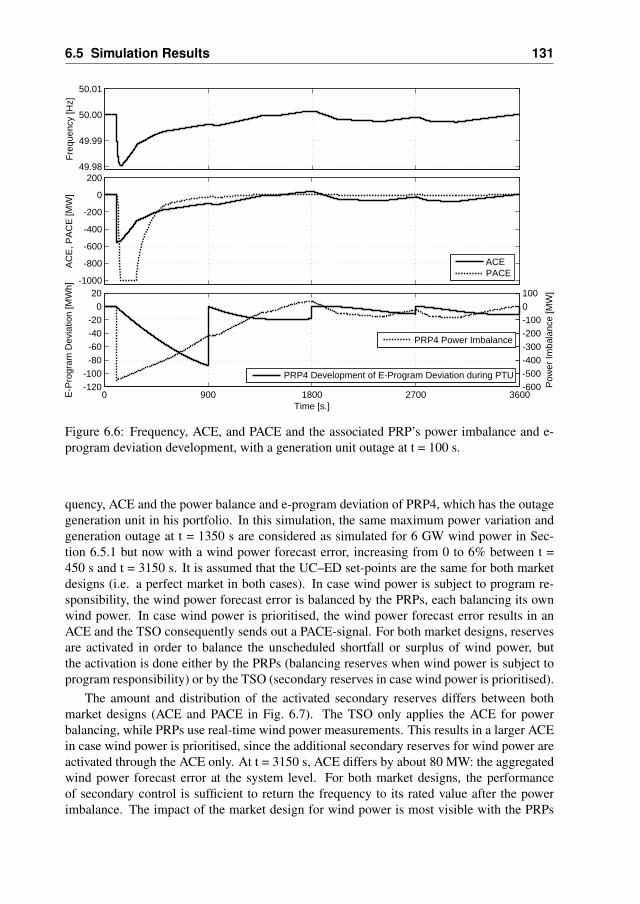
6.5 Simulation Results 131
-1000
-800
-600
-400
-200
0
200
AC
E, P
AC
E [M
W]
ACEPACE
49.98
49.99
50.00
50.01
Freq
uenc
y [H
z]
0 900 1800 2700 3600 -120-100-80-60-40-20
020
Time [s.]
E-P
rogr
am D
evia
tion
[MW
h]
-600-500-400-300-200-1000100
Pow
er Im
bala
nce
[MW
]
PRP4 Power Imbalance
PRP4 Development of E-Program Deviation during PTU
Figure 6.6: Frequency, ACE, and PACE and the associated PRP’s power imbalance and e-program deviation development, with a generation unit outage at t = 100 s.
quency, ACE and the power balance and e-program deviation of PRP4, which has the outagegeneration unit in his portfolio. In this simulation, the same maximum power variation andgeneration outage at t = 1350 s are considered as simulated for 6 GW wind power in Sec-tion 6.5.1 but now with a wind power forecast error, increasing from 0 to 6% between t =450 s and t = 3150 s. It is assumed that the UC–ED set-points are the same for both marketdesigns (i.e. a perfect market in both cases). In case wind power is subject to program re-sponsibility, the wind power forecast error is balanced by the PRPs, each balancing its ownwind power. In case wind power is prioritised, the wind power forecast error results in anACE and the TSO consequently sends out a PACE-signal. For both market designs, reservesare activated in order to balance the unscheduled shortfall or surplus of wind power, butthe activation is done either by the PRPs (balancing reserves when wind power is subject toprogram responsibility) or by the TSO (secondary reserves in case wind power is prioritised).
The amount and distribution of the activated secondary reserves differs between bothmarket designs (ACE and PACE in Fig. 6.7). The TSO only applies the ACE for powerbalancing, while PRPs use real-time wind power measurements. This results in a larger ACEin case wind power is prioritised, since the additional secondary reserves for wind power areactivated through the ACE only. At t = 3150 s, ACE differs by about 80 MW: the aggregatedwind power forecast error at the system level. For both market designs, the performanceof secondary control is sufficient to return the frequency to its rated value after the powerimbalance. The impact of the market design for wind power is most visible with the PRPs
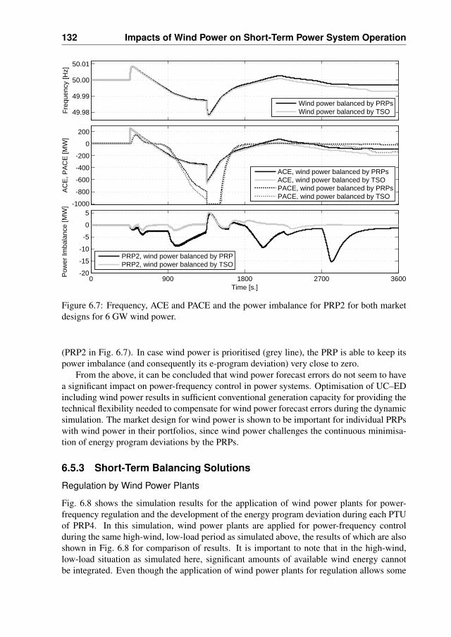
132 Impacts of Wind Power on Short-Term Power System Operation
-1000
-800
-600
-400
-200
0
200
AC
E, P
AC
E [M
W]
49.98
49.99
50.00
50.01Fr
eque
ncy
[Hz]
0 900 1800 2700 3600-20
-15
-10
-5
0
5
Time [s.]
Pow
er Im
bala
nce
[MW
]
ACE, wind power balanced by PRPsACE, wind power balanced by TSOPACE, wind power balanced by PRPsPACE, wind power balanced by TSO
Wind power balanced by PRPsWind power balanced by TSO
PRP2, wind power balanced by PRPPRP2, wind power balanced by TSO
Figure 6.7: Frequency, ACE and PACE and the power imbalance for PRP2 for both marketdesigns for 6 GW wind power.
(PRP2 in Fig. 6.7). In case wind power is prioritised (grey line), the PRP is able to keep itspower imbalance (and consequently its e-program deviation) very close to zero.
From the above, it can be concluded that wind power forecast errors do not seem to havea significant impact on power-frequency control in power systems. Optimisation of UC–EDincluding wind power results in sufficient conventional generation capacity for providing thetechnical flexibility needed to compensate for wind power forecast errors during the dynamicsimulation. The market design for wind power is shown to be important for individual PRPswith wind power in their portfolios, since wind power challenges the continuous minimisa-tion of energy program deviations by the PRPs.
6.5.3 Short-Term Balancing Solutions
Regulation by Wind Power Plants
Fig. 6.8 shows the simulation results for the application of wind power plants for power-frequency regulation and the development of the energy program deviation during each PTUof PRP4. In this simulation, wind power plants are applied for power-frequency controlduring the same high-wind, low-load period as simulated above, the results of which are alsoshown in Fig. 6.8 for comparison of results. It is important to note that in the high-wind,low-load situation as simulated here, significant amounts of available wind energy cannotbe integrated. Even though the application of wind power plants for regulation allows some
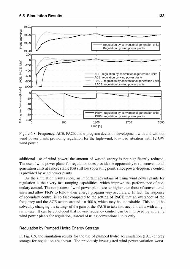
6.5 Simulation Results 133
-1000
-800
-600
-400
-200
0
200
AC
E, P
AC
E [M
W]
49.98
49.99
50.00
50.01
Freq
uenc
y [H
z]
0 900 1800 2700 3600 -100
-80
-60
-40
-20
0
Time [s.]
E-P
rogr
am D
evia
tion
[MW
h]
Regulation by conventional generation unitsRegulation by wind power plants
ACE, regulation by conventional generation unitsACE, regulation by wind power plantsPACE, regulation by conventional generation unitsPACE, regulation by wind power plants
PRP4, regulation by conventional generation unitsPRP4, regulation by wind power plants
Figure 6.8: Frequency, ACE, PACE and e-program deviation development with and withoutwind power plants providing regulation for the high-wind, low-load situation with 12 GWwind power.
additional use of wind power, the amount of wasted energy is not significantly reduced.The use of wind power plants for regulation does provide the opportunity to run conventionalgeneration units at a more stable (but still low) operating point, since power-frequency controlis provided by wind power plants.
As the simulation results show, an important advantage of using wind power plants forregulation is their very fast ramping capabilities, which improve the performance of sec-ondary control. The ramp rates of wind power plants are far higher than those of conventionalunits and allow PRPs to follow their energy program very accurately. In fact, the responseof secondary control is so fast compared to the setting of PACE that an overshoot of thefrequency and the ACE occurs around t = 400 s, which may be undesirable. This could besolved by changing the settings of the gain of the PACE to take into account units with a highramp-rate. It can be concluded that power-frequency control can be improved by applyingwind power plants for regulation, instead of using conventional units only.
Regulation by Pumped Hydro Energy Storage
In Fig. 6.9, the simulation results for the use of pumped hydro accumulation (PAC) energystorage for regulation are shown. The previously investigated wind power variation worst-
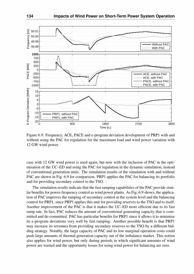
134 Impacts of Wind Power on Short-Term Power System Operation
0 900 1800 2700 3600-20-15-10-505
1015
Time [s.]
E-P
rogr
am D
evia
tion
[MW
h]
-1000-750-500-250
0250500750
10001000
PA
CE
[MW
]
PRP1, without PACPRP1, with PAC
49.98
49.99
50.00
50.01Fr
eque
ncy
[Hz]
Without PACWith PAC
ACE, without PACACE, with PACPACE, without PACPACE, with PAC
Figure 6.9: Frequency, ACE, PACE and e-program deviation development of PRP1 with andwithout using the PAC for regulation for the maximum load and wind power variation with12 GW wind power.
case with 12 GW wind power is used again, but now with the inclusion of PAC in the opti-misation of the UC–ED and using the PAC for regulation in the dynamic simulation, insteadof conventional generation units. The simulation results of the simulation with and withoutPAC are shown in Fig. 6.9 for comparison. PRP1 applies the PAC for balancing its portfolioand for providing secondary control to the TSO.
The simulation results indicate that the fast ramping capabilities of the PAC provide simi-lar benefits for power-frequency control as wind power plants. As Fig. 6.9 shows, the applica-tion of PAC improves the ramping of secondary control at the system level and the balancingcontrol for PRP1, since PRP1 applies this unit for providing reserves to the TSO and to itself.Another improvement of the PAC is that it makes the UC–ED more efficient due to its fastramp rate. In fact, PAC reduces the amount of conventional generating capacity that is com-mitted and de-committed. PAC has particular benefits for PRP1 since it allows it to minimiseits e-program deviations very well by fast ramping. Another possible benefit is that PRP1may increase its revenues from providing secondary reserves to the TSO by a different bid-ding strategy. Notably, the large capacity of PAC and its low marginal operation costs couldpush large amounts of thermal generation capacity out of the imbalance market. This notionalso applies for wind power, but only during periods in which significant amounts of windpower are wasted and the opportunity losses for using wind power for balancing are zero.
6.6 Summary and Conclusions 135
6.6 Summary and Conclusions
In this chapter, the dynamic simulation model developed in Chapter 5 is applied to assessfrequency stability in the presence of large-scale wind power. The dynamic performanceof the system is compared for different wind power penetrations and market designs forwind power.It is assumed that the Netherlands balances wind power independently of theneighbouring areas. Furthermore, the use of wind power plants and pumped hydro energystorage for power-frequency balancing is simulated, using the Netherlands as a case-study.
From the simulation set-up and the results, it is concluded that the power variations dueto wind power require a more dynamic operation of conventional generation units. The addi-tional power variations introduced by wind power can be handled by frequently re-calculatingthe UC–ED using updated wind power forecasts. The dynamic simulations show that theintegration of wind power during power system operation may require additional secondaryreserves, mainly due to the commitment and de-commitment of conventional generation unitsand due to wind power forecast errors. The additional commitment and de-commitment de-cisions necessary for incorporating the variability of wind power are found to have an impactof power system frequency and the ACE, rather than wind power’s variability itself.
The performance of existing secondary control mechanism of the TSO is found to besufficient to return ACE to within bounds within one PTU (15 min.) for all wind powerworst cases investigated here. The same applies for the use of balancing control by the PRPsto minimise energy program deviations. The simulations show that sufficient secondary re-serves can be made available regardless of wind power situation or the market design forbalancing wind power (energy program responsibility or prioritisation). Importantly, alsoduring high-wind, low-load periods, the performance of secondary control is found to be ad-equate. Although technical operating constraints of conventional generation on the one handresult in a lot of wasted wind power during low-load, high-wind periods, these constraintson the other hand ensure that sufficient conventional generation capacity is available for sec-ondary control during such situations. The performance of secondary control and balancingmay be improved by using wind power plants or pumped hydro energy storage facilities.Their fast ramping capabilities provide opportunities for individual PRPs and for the TSOfor power balancing, and may be alternatives for using only conventional generation units.
Finally, some observations can be made based on the worst cases examined here. Thefirst has to do with the wasted wind occurring during high-wind, low load situations. Thewasted wind energy in fact reduces the total variability of wind power that is integrated intothe system. In case additional generation units could be de-committed during high wind,low-load situations, the generation system would at times also have to balance larger windpower variations. Then again, such a generation system would also be better equipped to dothat. The second observation is that conventional generation unit outages during high-wind,low-load situations are unlikely to have a large impact on power system operation. This isbecause conventional units are likely to operate at their minimum power level during theseperiods, reducing the maximum power imbalance resulting from an outage. The technicaloperating constraints of these units thereby ensure that sufficient upward power reserves areavailable during these situations. A third observation is that the balance control objectivesof the TSO (secondary reserves) and the PRPs (balancing reserves) are not fully aligned.Strategic behaviour of PRPs for minimising their program deviation [MWh] may temporarilyincrease the ACE [MW], triggering additional secondary reserves at the system level.

CHAPTER 7Conclusions and
Recommendations
7.1 Conclusions
7.1.1 Power System Integration of Wind Power
The present day need for electricity is largely covered by coal-fired, gas-fired, hydro andnuclear power plants. Although generally reliable, affordable and proven, the disadvantagesof the use of fossil fuels and uranium are that these resources are finite and unequally dis-tributed between states, which may lead to political conflicts. Furthermore, the burning offossil fuels for power generation results in the emission of greenhouse gases, in particularCO2. So along with the increasing electricity demand worldwide, there is a growing need forsustainable power generation technologies, such as wind power.
In the past decade, wind power has become a generation technology of significance ina number of countries, and its growth is foreseen to continue. When integrating significantamounts of wind power in power systems, technical challenges arise due to the uncontrolla-bility of the primary energy source, the wind. While power system operation requires a con-tinuous power balance between generation and load, the variability and limited predictabilityof wind power introduces additional uncertainty into power system operation. The question
138 Conclusions and Recommendations
arises, to what extent the power system can accommodate wind power while maintaining areliable electricity supply.
This research has been focused on the impacts of large-scale wind power on power sys-tem operation, in particular on power balancing. With power system frequency as the centralparameter for the active power balance between generation and load, this thesis has investi-gated in fact the frequency stability with large-scale wind power at different time-scales. Inthe long-term time-scale (time resolution 15 min.), unit commitment and economic despatch(UC–ED) are simulated. The simulation results are used in a second, dynamic model explor-ing long-term frequency stability (time resolution 4 s). The research includes an explorationof measures to mitigate the possible negative consequences of wind power on power systemoperation. The following steps have been taken:1) Investigation of the variability and limited predictability of large-scale wind power, both
on the short-term (s. to min.) and long-term (h. to weeks) time-scales (Chapter 2);2) Further development of an existing UC–ED model to simulate long-term power system
operation with wind power (Chapter 3 and 4);3) Development of a new dynamic power system model to simulate short-term power system
operation with wind power (Chapter 5 and 6);4) Application of both models to explore solutions that facilitate the system integration of
large-scale wind power (Chapter 4 and 6).The focus project has been on the technical aspects of power systems design and power sys-tem operation, but also takes into account economical and market aspects and to some extentenvironmental aspects. The developed methodology is illustrated using a foreseen futuresetup of the Dutch power system in 2014. International exchanges and trading on interna-tional and national markets are included. This research considers wind power penetrations upto 12 GW (4 GW onshore, 8 GW offshore), supplying up to a third of the electricity demandof the Netherlands estimated for 2014.
7.1.2 Impacts of Wind Power on Long-Term Power System Operation
Technical Integration Limits
The wind power and load data for the Dutch system have been used for a preliminary assess-ment of the possible impacts of wind power on power system operation. From this, load-less-wind power curves (power levels) and load-less-wind power variation curves (rampinglevels) have been developed. From these curves it is observed that wind power reduces thedemand for conventional generation, especially for base-load and medium-load generation.The aggregated power variations of system load and wind power lie mostly within the vari-ability range of system load itself and conventional generation is capable of matching thesevariations. Wind power does however increase the occurrence and size of the maximum vari-ations occurring a few hours during the year and care has to be taken that the conventionalgeneration can manage these situations. Minimum load issues during high wind, low loadperiods are likely to present the first technical integration limit for wind power.
The simulation results for unit commitment and economic despatch (UC–ED) confirmthe above observations. It is concluded that the variability of load and wind power can betechnically accommodated by the conventional generation units of the simulated system.Ramp rate problems as a result of the aggregated variations of load and wind power are
7.1 Conclusions 139
found to be absent. It can be noted that the technical constraints imposed on base-load coaland combined heat and power (CHP) units do not allow their de-commitment and therebyguarantee that sufficient power reserves are available at all times. The limited predictabilityof wind power requires a more frequent re-calculation of UC–ED (i.e. rolling UC–ED).The present quality of the updated wind power forecasts are found to be adequate for theoptimisation of UC–ED. A frequent re-calculation of UC–ED also allows for the schedulingof additional power reserves close to the moment of operation, if necessary.
Impacts of Wind Power on UC–ED
The simulation results show that wind power reduces total system operating costs in theUC–ED of conventional units, mainly by saving fuel and emission costs. A first estimationof these benefits shows that the operating cost savings lie in the range of e 1.5 billion an-nually, and CO2-emission savings around 19 Mton for 12 GW wind power installed in theNetherlands. These benefits are dependent on fuel prices, the conventional generation mix,electricity consumption, the yearly wind regime, the international market design, intercon-nection capacity, etc. but are considerable in any case. It is shown that wind power reducesthe number of full-load hours of especially base-load generation units (coal, combined heatand power) and of medium-load CCGT. For high wind power penetrations, the presence oflarge capacities of must-run base-load generation results in large amounts of wasted wind inthe Netherlands, especially during low load periods.
In case international exchange is taken into account in the optimisation of UC–ED, theamounts of wasted wind are very much reduced. It is found that wind power significantlyincreases the exports and/or reduces the imports of the area it is integrated into, in this casethe Netherlands. International exchange provides a very large potential for wind power inte-gration in the Netherlands, especially at high penetration levels. However, limits may existto the use of interconnections for wind power integration in case neighbouring systems alsocomprise significant amounts of wind power. In the case study performed here, it is shownthat the presence of large-scale wind power in Germany may limit exports from the Nether-lands during low-load, high-wind periods. Despite the high geographical correlation of windpower output in Western Europe, international exchange still provides a large potential forthe integration of additional wind power in the Netherlands.
7.1.3 Impacts of Wind Power on Short-Term Power System Operation
Frequency Deviations
From the simulation results, it can be concluded that the variability and limited predictabilityof large-scale wind power do not reduce frequency stability. The variations of large-scalewind power occur in the time-ranges of minutes and upward and thereby do not impact fre-quency stability directly. The most important impact of wind power variability is the moredynamic operation required from conventional generation units. Since these units are com-mitted and decommitted at a certain minimum power levels, such events lead to power imbal-ances and thereby frequency deviations. These frequency deviations are however well withinthe normal frequency range in UCTE and insignificant from a frequency stability point ofview. Taking into account the large system inertia of the UCTE-system, there are no in-dications that the system integration of wind power would be limited by frequency-related
140 Conclusions and Recommendations
aspects. It can furthermore be noted that modern, variable speed wind turbines are techni-cally capable of contributing to power system inertia and to some extent to power-frequencycontrol.
Secondary Control
In this research, it is found that the additional power variations introduced by wind powercan be adequately handled provided that wind power is integrated into the optimisation ofUC–ED of the program responsible parties (PRPs). The performance of existing automaticgeneration control (AGC)-mechanisms of both the TSO and PRPs is found to be sufficientto return the area control error (ACE) to within bounds within one 15 min., as required byUCTE. This conclusion holds for large combined variations of system load and wind power,for high-wind, low-load situations and for conventional generation unit outages. Additionalsecondary reserves will be required during real-time operation to incorporate the additionalpower imbalances, due to the commitment and de-commitment of conventional generationunits and because of wind power forecast errors. Since existing base-load generation unitsremain in operation due to technical operating constraints, sufficient conventional generationcapacity is available for the provision of upward reserves at all times. It is found that the useof wind power plants or pumped accumulation energy storage for regulation may improvethe performance of secondary control due to their very high ramp rates, reducing the need forconventional units for providing this.
7.1.4 System Integration Solutions
International Exchange and Postponed Gate-Closure of Markets
In case international exchange is possible using the available interconnection capacity, mini-mum load problems and wasted wind power in the Netherlands are very much reduced sinceexcess wind power may be exported to neighbouring areas. The simulation results show thatwind power also benefits from postponed gate-closure times of international markets, sinceinternational exchange can be based on improved wind power forecasts. For the Netherlands,flexible international exchange and markets largely eliminate the need for other integrationsolutions for wind power.
Energy Storage and More Flexible Base-Load Generation
Energy storage is often suggested as a logical complement for power systems with large-scale wind power. From this research, however, it can be concluded that energy storagefacilities are not the most efficient solution for the integration of large-scale wind powerin the Netherlands. With regard to an isolated Dutch power system, significant amountsof available wind energy continue to be wasted even if large-scale energy storage solutionsare implemented. A cost–benefit analysis furthermore shows that pumped hydro solutionsin the Netherlands are unlikely to have a positive outcome, even at very high wind powerpenetrations. This is mainly due to the very large investment costs associated with theseoptions. It must be noted however that business cases for energy storage depend on thedifferences in marginal costs between peak and off-peak, which are dependent on a widerange of factors.
7.2 Recommendations for Further Research 141
An important simulation result is that energy storage increases the emission of CO2 ofthe system as a whole, especially at low wind power penetrations. This is because energystorage allows storing power from cheap coal-fired plants for substitution of expensive, butrelatively clean peak-load natural gas-fired units. Furthermore, energy storage brings aboutsignificant conversion losses, which must be produced as well. In fact, energy storage partlyannuls CO2 emission savings by wind power, unless very large amounts of wind power areinstalled.
It can be concluded that a more flexible operation of base-load generation technologies,in the Netherlands in particular the use of heat boilers at industrial CHP-locations, provides acost-efficient solution for wind power integration. During periods of high-wind and low-load,the CHP-units may be decommitted, allowing the integration of additional wind power. Thisalso prevents the operation of the CHP-units at a loss during low-load, high-wind periods.The development of additional interconnection capacity, for instance with Norway createsthe largest additional technical space for wind power integration. A business case for thisoption largely depends on the synergies between the Netherlands’ and Norwegian generationsystems and cannot be made only for wind power integration.
7.2 Recommendations for Further Research
7.2.1 UC–ED Model Extension
The Netherlands is strongly interconnected to its neighbours in the UCTE-interconnection,to Norway and in the future also to Great Britain. Strong interconnections are very im-portant for the further development of international electricity markets. As a result of theinternational trade in electricity between countries, generation planning and operation arebecoming international rather than national affairs. Consequently, the system integration ofwind power should no longer be investigated only for ’isolated’ power systems. Even thoughnational studies will continue to provide highly useful insights into power system operationwith wind power, a national scope is likely to underestimate the technical possibilities forwind power integration in the power system.
In this research, important steps have been taken toward an international power systemmodel for wind power integration studies. The UC–ED model should be extended furtherto include other European countries and especially the Scandinavian Nordel system. TheNordel system has a large impact on the marginal prices of the North-West European elec-tricity markets and connection to the Scandinavian hydro reservoirs can be foreseen to playan important role for wind power integration in the future. In order to perform internationalstudies it will be needed to include the transmission bottlenecks within countries or areas ina more profound way. All areas must be optimised simultaneously while subject to trans-mission constraints between or within areas. This way, inter-area exchanges are an integralresult of the system optimisation with wind power, which is essential for a correct estimationof technical limits for wind power integration. Furthermore, a more unit-specific (rather thantechnology-specific) modeling approach should be applied to the generation systems outsidethe Netherlands.

142 Conclusions and Recommendations
7.2.2 Power Transmission and Load Flows
In further research, the extended UC–ED model should be used as an input for detailed loadflow studies in order to determine the transmission limits for wind power integration. Insteadof assuming a selected set of worst cases on beforehand, it is recommended to determine theworst-cases based on a large set of generation, wind power and load combinations follow-ing from UC–ED schedules. This UC–ED-based load flow analysis mirrors the operationof international electricity markets with an implicit auction of transmission capacity and thepower flows resulting from the international transactions. Investigation of the worst cases de-rived from this analysis makes sure that the correct worst cases are captured and investigated:these cases are difficult to determine on beforehand for power systems with large-scale windpower.
7.2.3 International Trade and Markets
In this research, it has been shown that large amounts of wind power can be technicallyintegrated into the power system. It has also been shown that international exchange is animportant enabling factor for this. The extent to which interconnection capacity is indeedavailable for exchanges during moments of low-load and high-wind power, depends on theextent to which an international market is available to facilitate this. This market is governedby technical aspects (i.e. the technical characteristics of conventional generation units) butalso on the organisation of the market itself (gate-closure times, auctioning of transmissioncapacities, market design for wind power, etc.). Additional research is necessary into thedevelopment of suitable international market designs to allow an efficient system integrationof wind power.
7.2.4 Large-Scale Renewables and Energy Demand
At present, renewables such as wind power, geothermal and solar altogether supply less than1% of energy demand worldwide [80]. With a substantially larger penetration, the variabilityand periodic unavailability of renewables presents a formidable challenge for existing energysystems in general, and for power systems in particular. The methodologies developed herefor the power system integration of wind power are in principle applicable for a wide rangeof renewables, since most renewables have a limited controllability of their respective energysources. Future research in the integration of renewables in existing energy systems shouldrevolve around three questions: 1) How large are the differences in time and in size betweenthe energy demand and the energy supply? 2) How do increased amounts of renewablesinfluence these differences? 3) How can the differences between demand and supply benarrowed in the best possible way? The electricity system must be regarded as an integralpart of a much larger energy supply system. The development of integrated solutions willrequire substantial research efforts.

Bibliography
[1] S. Agterbosch. Empowering Wind Power. PhD thesis, Universiteit Utrecht, TheNetherlands, 2006.
[2] V. Akhmatov. Analysis of Dynamic Behaviour of Electric Power Systems with LargeAmount of Wind Power. PhD thesis, Ørsted, Denmarks Tekniske Universitet, Den-mark, 2003.
[3] V. Akhmatov and A. H. Knudsen. An Aggregate Model of a Grid-Connected, LargeScale, Offshore Wind Farm for Power Stability Investigations – Importance of Wind-mill Mechanical System. Electrical Power & Energy Systems, 24:709–717, 2002.
[4] P. M. Anderson and A. A. Fouad. Power System Control and Stability. Iowa StateUniversity Press, 1977.
[5] P. M. Anderson and M. Mirheydar. A Low-Order System Frequency Response Model.IEEE Transactions on Power Systems, 5(3):720–729, Aug. 1990.
[6] J. L. Angarita-Marquez, C. A. Hernandez-Aramburo, and J. Usaola-Garcia. Analy-sis of a Wind Farm’s Revenue in the British and Spanish Markets. Energy Policy,35(10):5051–5059, Oct. 2007.
[7] J. Arrillaga and N. R. Watson. Computer Modelling of Electrical Power Systems. JohnWiley & Sons, Inc., 2001.
[8] T. Athay, R. Podmore, and S. Virmani. A Practical Method for Direct Analysis of Tran-sient Stability. IEEE Transactions on Power Apparatus and Systems, PAS–99(5):573–584, Mar./Apr. 1979.
[9] R. A. Babb. Pumped Hydro Dispatch by the Value of Energy Method in a ProductionCost Model. 5 pp.
[10] B. H. Bakken and O. S. Grande. Automatic Generation Control in a DeregulatedPower System. IEEE Transactions on Power Systems, 13(4):1401–1406, Nov. 1998.
[11] R. Barth, H. Brand, D. J. Swider, C. Weber, and P. Meibom. Regional ElectricityPrice Differences due to Intermittent Wind Power in Germany: Impact of Extended

144 BIBLIOGRAPHY
Transmission and Storage Capacities. Int. J. Global Energy Issues, 25(3/4):276–297,2006.
[12] R. J. Barthelmie, F. Murray, and S. C. Pryor. The Economic Benefit of Short-TermForecasting for Wind Energy in the UK Electricity Market. Energy Policy, 36:1687–1696, Mar. 2008.
[13] G. N. Bathurst, J. Weatherill, and G. Strbac. Trading Wind Generation in Short-TermEnergy Markets. IEEE Transactions on Power Systems, 17(3):782–789, Aug. 2002.
[14] R. Beune and F. A. Nobel. System Balancing in the Netherlands. In Proc. Methods toSecure Peak Load Capacity on Deregulated Electricity Markets, Stockholm, Sweden,June 7–8 2001. 12 pp.
[15] R. Billinton and G. Bai. Generating Capacity Adequacy Associated with Wind Energy.IEEE Transactions on Energy Conversion, 19(3):641–646, Sept. 2004.
[16] S. Bode. On the impact of renewable energy support schemes on power prices. Tech-nical report, Hamburg Institute of International Economics, 2006. 24 pp.
[17] P. Bousseau, R. Belhomme, E. Monnot, N. Laverdure, D. Boeda, D. Roye, andS. Bacha. Contribution of Wind Farms to Ancillary Services. In Proc. CIGRE Session,Paris, France, Aug. 24–29 2006. 11 pp.
[18] A. J. Brand. Observed and Predicted Wind Speed Time Series in the Netherlands andthe North Sea. Technical report, Energy Research Centre of the Netherlands (ECN),ECN–C–06–007, 2006.
[19] A. J. Brand and J. K. Kok. Aanbodvoorspeller Duurzame Energie Deel 2: Korte-termijn prognose van windvermogen (in Dutch). Technical report, Energy ResearchCentre of the Netherlands (ECN), ECN–C–03–049, 2003.
[20] P. Bresesti, W. L. Kling, R. L. Hendriks, and R. Vailati. HVDC Connection of OffshoreWind Farms to the Transmission System. IEEE Transactions on Energy Conversion,22(1):37–43, March 2007.
[21] S. Breukers and M. Wolsink. Wind Power Implementation in Changing InstitutionalLandscapes: An International Comparison. Energy Policy, 35:2737–2750, January2007.
[22] H. Breulmann, E. Grebe, M. Losung, W. Winter, R. Witzmann, P. Dupuis, M. P.Houry, T. Margotin, J. Zerenyi, J. Dudzik, J. Machowski, L. Martın, J. M. Rodrıguez,and E. Urretavizcaya. Analysis and Damping of Inter-Area Oscillations in theUCTE/CENTREL Power System. In Proc. CIGRE Session, Paris, France, Aug. 27–Sept. 1 2000. 10 pp.
[23] P. J. Brockwell and R. A. Davis. Time Series: Theory and Models. 2nd ed., Springer,1991.
[24] B. M. Buchholz, D. Povh, and D. Retzmann. Stability Analysis for large Power SystemInterconnections in Europe. In Proc. IEEE PowerTech Conference, St. Petersburg,Russia, June 27–30 2005. 7 pp.
[25] M. Carrion and J. M. Arroyo. A Computationally Efficient Mixed-Integer Linear For-mulation for the Thermal Unit Commitment Problem. IEEE Transactions on PowerSystems, 21(3):1371–1378, Aug. 2006.
[26] E. D. Castronuovo and J. A. Pecas Lopes. Optimal operation and hydro storage sizingof a wind-hydro power plant. Electrical Power and Energy Systems, 26:771–778, July2004.
[27] M. L. Chan, R. D. Dunlop, and F. C. Schweppe. Dynamic equivalents for average sys-
145
tem frequency behavior following major disturbances. In Proc. IEEE Winter Meeting,1972.
[28] L. Chang-Chien, C. Ong, and R. A. Kramer. Field Tests and Refinements of an ACEModel. IEEE Transactions on Power Systems, 18(2):898–903, May 2003.
[29] D. P. Chassin, Z. Huang, M. K. Donnelly, C. Hassler, E. Ramirez, and C. Ray. Esti-mation of WECC System Inertia Using Observed Frequency Transients. IEEE Trans-actions on Power Systems, 20(2):1190–1192, May 2005.
[30] P. K. Chawdhry and B. W. Hogg. Identification of Boiler Models. Proceedings of theIEE, 136(5):261–271, Sep. 1989.
[31] E. Cheres. Small and Medium Size Boiler Models suitable for Long Term DynamicResponse. IEEE Transactions on Energy Conversion, 5(4):686–692, Dec. 1990.
[32] G. A. Chown and B. Wigdorowitz. A Methodology for the Redesign of FrequencyControl for AC Networks. IEEE Transactions on Power Systems, 19(3):1546–1554,Aug. 2004.
[33] Commission for Electricity and Storage (COE). Opslag van Elektriciteit in Nederland:Haalbaar en aanvaardbaar? (in Dutch). Technical report, Dutch Ministry of EconomicAffairs, Den Haag, 1988. 33 pp.
[34] Y. Dai, T. Zhao, Y. Tian, and L. Gao. Research on the Primary Frequency ControlCharacteristics of Generators in Power Systems. In Proc. 2nd IEEE Conference onIndustrial Electronics and Applications, 23–25 May 2007.
[35] L. Dale, D. Milborrow, R. Slark, and G. Strbac. Total Cost Estimates for Large-ScaleWind Scenarios in UK. Energy Policy, 32(17):1949–1956, Nov. 2004.
[36] Danish Wind Energy Association. The Energy Balance of Modern Wind Turbines.Wind Power Notes, (16):1–16, Dec. 1997.
[37] G. Dany. Kraftwerksreserve in elektrischen Verbundsystemen mit hohem Windener-gieanteil (in German). PhD thesis, RWTH Aachen, Germany, 2000.
[38] F. P. de Mello. Boiler Models for System Dynamic Performance Studies. IEEE Trans-actions on Power Systems, 6(1):66–74, 1991.
[39] E. Denny and M. J. O’Malley. Quantifying the Total Net Benefits of Grid IntegratedWind. IEEE Transactions on Power Systems, 22(2):605–615, May 2007.
[40] DEWI, E.ON Netz, EWI, RWE Transportnetz Strom, VE Transmission. Energiewirt-schaftliche Planung fur die Netzintegration von Windenergie in Deutschland an Landund Offshore bis zum Jahr 2020 (in German). Technical report, 2005.
[41] A. Dimitrovski and K. Tomsovic. Impact of Wind Generation Uncertainty on Gen-erating Capacity Adequacy. In Proc. 9th International Conference on ProbabilisticMethods Applied to Power Systems, Stockholm, Sweden, June 11-15 2006. 6 pp.
[42] R. Doherty, E. Denny, and M. J. O’Malley. System Operation with a Significant WindPower Penetration. In Proc. IEEE Power Energy Society General Meeting, volume 1,Denver, CO, USA, June 6–10 2004. pp. 1002–1007.
[43] R. Doherty, G. Lalor, and M. J. O’Malley. Frequency Control in Competitive Electric-ity Market Dispatch. IEEE Transactions on Power Systems, 20(3):1558–1596, Aug.2005.
[44] R. Doherty and M. J. O’Malley. A New Approach to Quantify Reserve Demand inSystems with Significant Installed Wind Capacity. IEEE Transactions on Power Sys-tems, 20(2):587–595, May. 2005.
[45] Dutch Ministry of Economic Affairs. Eerste Energie Nota (in Dutch). Technical report,
146 BIBLIOGRAPHY
1974. The Hague.[46] Dutch Ministry of Economic Affairs. Connect 6.000 MW, Eindrapportage (in Dutch).
Technical report, 2004. 44 pp.[47] Dutch Ministry of Economic Affairs. Energierapport 2008 (in Dutch). Technical
report, 2008. Available online at: http://www.ez.nl/ Last accessed: Oct. 2008.[48] ELIA. Note Concerning the Mechanism for Managing the Balance of
the ELIA Control Area. Technical report, 2007. Available online at:http://www.elia.be/repository/pages/ Last accessed: Oct. 2008.
[49] ETSO. Net Transfer Capacities Matrix, 2008. Available online at: http://www.etso-net.org/ Last accessed: Oct. 2008.
[50] European Commission – Eurostat Homepage. Available online at:http://epp.eurostat.ec.europa.eu/ Last accessed: Oct. 2008.
[51] European Wind Energy Association. Available online at: http://www.ewea.org/ Lastaccessed: Oct. 2008.
[52] A. Fabbri, T. Gomez San Roman, J. Rivier Abbad, and V. H. Mendez Quezada. As-sessment of the Cost Associated With Wind Generation Prediction Errors in a Liber-alized Electricity Market. IEEE Transactions on Power Systems, 20(3):1440–1446,Aug. 2005.
[53] M. E. Flynn and M. J. O’Malley. A Drum Boiler Model for Long Term Power Sys-tem Dynamic Simulation. IEEE Transactions on Power Systems, 14(1):209–217, Feb.1999.
[54] U. Focken, M. Lange, K. Monnich, H. P. Waldl, H. G. Beyer, and A. Luig. Short-Term prediction of the aggregated power output of wind farms - a statistical analysisof the reduction of the prediction error by spatial smoothing effects. Journal of WindEngineering & Industrial Aerodynamics, 90:231–246, 2002.
[55] B. Fox, D. Flynn, L. Bryans, N. Jenkins, D. Milborrow, M. O’Malley, R. Watson,and O. Anaya-Lara. Wind Power Integration: Connection and System OperationalAspects. IET Power and Energy, 2007.
[56] G. Shuttleworth and I. McKenzie. A Comparative Study of the Electricity Marketsin UK, Spain and Nord Pool. Technical report, NERA Economic Consulting, 2002.46 pp.
[57] M. Gibescu, A. J. Brand, and W. L. Kling. Estimation of Variability and Predictabilityof Large-Scale Wind Energy in the Netherlands. Wind Energy, (published online):20,Sept. 29 2008.
[58] M. Gibescu, E. W. van Zwet, W. L. Kling, and R. D. Christie. Optimal BiddingStrategy for Mixed-Portfolio Producers in a Dual Imbalance Pricing System. In Proc.Power Systems Computational Conference, Glasgow, UK, July 14–18 2008. 7 pp.
[59] G. Giebel. On the Benefits of Distributed Generation of Wind Energy in Europe. PhDthesis, Carl von Ossietsky Universitat Oldenburg, Germany, 2001.
[60] J. J. Grainger and W. D. Stevenson. Power System Analysis. McGraw-Hill Inc., 1994.[61] E. Grebe, C. Jahnke, and W. Sattinger. Wide Area Monitoring im UCTE-Netz -
Uberwachung der Netzdynamik im europaischen Verbundnetz. 2007. 6 pp.[62] N. Halberg. Assessment of Novel Energy Storage Systems using the Value of Energy
Concept. In Proc. N.V. SEP–EPRI International Conference on Applications of PowerProduction Simulation, Washington, DC, USA, June 11–13 1990. 16 pp.
[63] N. Halberg. Power Production Simulation for Wind Assisted Systems. In Proc. N.V.
147
SEP–EPRI International Conference on Applications of Power Production Simulation,Washington, DC, USA, June 11–13 1990. 15 pp.
[64] N. Halberg and B. A. Kleinbloesem. Wind Energy Research Activities of the DutchElectricity Generating Board. In Proc. World Energy Conference, Montreal, Canada,Sept. 17–22 1989. 5 pp.
[65] K. Hanjalic, R. van de Krol, and A. Lekic (editors). Sustainable Energy Technologies:Options and Prospects. Springer Verlag, 2008.
[66] A. D. Hansen and L. H. Hansen. Wind Turbine Concept Market Penetration over 10Years (19952004). Wind Energy, 10:81–97, Nov. 2006.
[67] S. Hesmondhalgh. Is NETA the Blueprint for Wholesale Electricity Trading Arrange-ments of the Future? IEEE Transactions on Power Systems, 18(2):548–554, May2003.
[68] J. Hoffer. Modelling the Partial Planned Outages in Production Costing Simulation.Electrical Power & Energy Systems, 17(6):377–380, 1995.
[69] H. Holttinen. Optimal Electricity Market for Wind Energy. Energy Policy, 33:2052–2063, May 2004.
[70] H. Holttinen. The impact of large scale wind power production on the Nordic electric-ity system. PhD thesis, Helsinki University of Technology, Finland, 2004.
[71] H. Holttinen. Hourly Wind Power Variations in the Nordic Countries. Wind Energy,8:173–195, Nov. 2005.
[72] H. Holttinen. Handling of Wind Power Forecast Errors in the Nordic Power Market.In Proc. Probabilistic Methods Applied to Power Systems, Stockholm, Sweden, 11–15June 2006. 6 pp.
[73] H. Holttinen, B. Lemstrom, P. Meibom, H. Bindner, A. Orths, F. Van Hulle, C. Ensslin,A. Tiedemann, L. Hofmann, W. Winter, A. Tuohy, M. O’Malley, P. Smith, J. Pierik,J. O. Tande, A. Estanqueiro, J. Ricardo, E. Gomez, L. Soder, G. Strbac, A. Shakoor,J.C. Smith, B. Parsons, M. Milligan, and Y. H. Wan. Design and Operation of PowerSystems with Large Amounts of Wind Power, State-of-the-Art Report. Technical re-port, Working Paper 82, VTT Finland, 2007. 119 pp.
[74] Ibraheem, P. Kumar, and D. P. Kothari. Recent Philosophies of Automatic Gener-ation Control Strategies in Power Systems. IEEE Transactions on Power Systems,20(1):346–357, Feb. 2005.
[75] IEEE Benchmarks, Power System Test Cases, Home Page. Available online at:http://psdyn.ece.wisc.edu/ Last accessed: Oct. 2008.
[76] IEEE Task Force on Load Representation for Dynamic Performance. Load Repre-sentation for Dynamic Performance Analysis. IEEE Transactions on Power Systems,8(2):472–482, May 1993.
[77] IEEE Task Force on Terms & Definitions, System Dynamic Performance Subcom-mittee, Power System Engineering Committee. Proposed Terms & Definitionas forPower System Stability. IEEE Transactions on Power Apparatus and Systems, PAS-101(7):1894–1898, July 1982.
[78] T. Inoue, H. Taniguchi, and Y. Ikeguchi. A Model of Fossil Fueled Plant with Once-Through Boiler for Power System Frequency Simulation Studies. IEEE Transactionson Power Systems, 15(4):1322–1328, Nov. 2000.
[79] T. Inoue, H. Taniguchi, Y. Ikeguchi, and K. Yoshida. Estimation of Power System In-ertia Constant and Capacity of Spinning-reserve Support Generators Using Measured
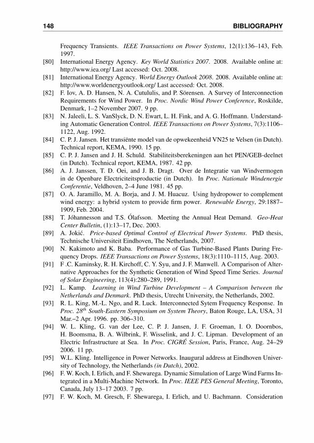
148 BIBLIOGRAPHY
Frequency Transients. IEEE Transactions on Power Systems, 12(1):136–143, Feb.1997.
[80] International Energy Agency. Key World Statistics 2007. 2008. Available online at:http://www.iea.org/ Last accessed: Oct. 2008.
[81] International Energy Agency. World Energy Outlook 2008. 2008. Available online at:http://www.worldenergyoutlook.org/ Last accessed: Oct. 2008.
[82] F. Iov, A. D. Hansen, N. A. Cutululis, and P. Sorensen. A Survey of InterconnectionRequirements for Wind Power. In Proc. Nordic Wind Power Conference, Roskilde,Denmark, 1–2 November 2007. 9 pp.
[83] N. Jaleeli, L. S. VanSlyck, D. N. Ewart, L. H. Fink, and A. G. Hoffmann. Understand-ing Automatic Generation Control. IEEE Transactions on Power Systems, 7(3):1106–1122, Aug. 1992.
[84] C. P. J. Jansen. Het transiente model van de opwekeenheid VN25 te Velsen (in Dutch).Technical report, KEMA, 1990. 15 pp.
[85] C. P. J. Jansen and J. H. Schuld. Stabiliteitsberekeningen aan het PEN/GEB-deelnet(in Dutch). Technical report, KEMA, 1987. 42 pp.
[86] A. J. Janssen, T. D. Oei, and J. B. Dragt. Over de Integratie van Windvermogenin de Openbare Electriciteitsproductie (in Dutch). In Proc. Nationale WindenergieConferentie, Veldhoven, 2–4 June 1981. 45 pp.
[87] O. A. Jaramillo, M. A. Borja, and J. M. Huacuz. Using hydropower to complementwind energy: a hybrid system to provide firm power. Renewable Energy, 29:1887–1909, Feb. 2004.
[88] T. Johannesson and T.S. Olafsson. Meeting the Annual Heat Demand. Geo-HeatCenter Bulletin, (1):13–17, Dec. 2003.
[89] A. Jokic. Price-based Optimal Control of Electrical Power Systems. PhD thesis,Technische Universiteit Eindhoven, The Netherlands, 2007.
[90] N. Kakimoto and K. Baba. Performance of Gas Turbine-Based Plants During Fre-quency Drops. IEEE Transactions on Power Systems, 18(3):1110–1115, Aug. 2003.
[91] F .C. Kaminsky, R. H. Kirchoff, C. Y. Syu, and J. F. Manwell. A Comparison of Alter-native Approaches for the Synthetic Generation of Wind Speed Time Series. Journalof Solar Engineering, 113(4):280–289, 1991.
[92] L. Kamp. Learning in Wind Turbine Development – A Comparison between theNetherlands and Denmark. PhD thesis, Utrecht University, the Netherlands, 2002.
[93] R. L. King, M.-L. Ngo, and R. Luck. Interconnected Sytem Frequency Response. InProc. 28th South-Eastern Symposium on System Theory, Baton Rouge, LA, USA, 31Mar.–2 Apr. 1996. pp. 306–310.
[94] W. L. Kling, G. van der Lee, C. P. J. Jansen, J. F. Groeman, I. O. Doornbos,H. Boomsma, B. A. Wilbrink, F. Wisselink, and J. C. Lipman. Development of anElectric Infrastructure at Sea. In Proc. CIGRE Session, Paris, France, Aug. 24–292006. 11 pp.
[95] W.L. Kling. Intelligence in Power Networks. Inaugural address at Eindhoven Univer-sity of Technology, the Netherlands (in Dutch), 2002.
[96] F. W. Koch, I. Erlich, and F. Shewarega. Dynamic Simulation of Large Wind Farms In-tegrated in a Multi-Machine Network. In Proc. IEEE PES General Meeting, Toronto,Canada, July 13–17 2003. 7 pp.
[97] F. W. Koch, M. Gresch, F. Shewarega, I. Erlich, and U. Bachmann. Consideration
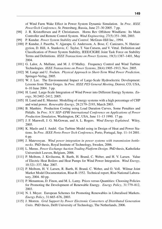
149
of Wind Farm Wake Effect in Power System Dynamic Simulation. In Proc. IEEEPowerTech Conference, St. Petersburg, Russia, June 27–30 2005. 7 pp.
[98] J. R. Kristoffersen and P. Christiansen. Horns Rev Offshore Windfarm: Its MainController and Remote Control System. Wind Engineering, 27(5):351–360, 2003.
[99] P. Kundur. Power System Stability and Control. McGraw-Hill Inc., 1994.[100] P. Kundur, J. Paserba, V. Ajjarapu, G. Andersson, A. Bose, C. Canizares, N. Hatziar-
gyriou, D. Hill, A. Stankovic, C. Taylor, T. Van Cutsem, and V. Vittal. Definition andClassification of Power System Stability, IEEE/CIGRE Joint Task Force on StabilityTerms and Definitions. IEEE Transactions on Power Systems, 19(3):1387–1401, May2004.
[101] G. Lalor, A. Mullane, and M. J. O’Malley. Frequency Control and Wind TurbineTechnologies. IEEE Transactions on Power Systems, 20(4):1905–1913, Nov. 2005.
[102] M. Lange and U. Focken. Physical Approach to Short-Term Wind Power Prediction.Springer-Verlag, 2005.
[103] W. J. Lee. The Environmental Impact of Large-Scale Hydroelectric Development:Lessons from Three Gorges. In Proc. IEEE PES General Meeting, Denver, CO, USA,6–10 June 2004. 3 pp.
[104] H. Lund. Large-Scale Integration of Wind Power into Different Energy Systems. En-ergy, 30:2402–2412, 2005.
[105] H. Lund and E. Munster. Modelling of energy systems with a high percentage of CHPand wind power. Renewable Energy, 28:2179–2193, March 2003.
[106] B. Manhire. Production Costing using Load Duration Curves, Some Penalties andPitfalls. In Proc. N.V. SEP–EPRI International Conference on Applications of PowerProduction Simulation, Washington, DC, USA, June 11–13 1990. 17 pp.
[107] J. F. Manwell, J. G. McGowan, and A. L. Rogers. Wind Energy Explained. Wiley,2005.
[108] K. Maslo and J. Andel. Gas Turbine Model using in Design of Heat and Power Sta-tions. In Proc. IEEE Porto Power Tech Conference, Porto, Portugal, Sep. 11–14 2001.6 pp.
[109] J. Matevosyan. Wind power integration in power systems with transmission bottle-necks. PhD thesis, Royal Institute of Technology, Sweden, 2006.
[110] L. Meeus. Power Exchange Auction Trading Platform Design. PhD thesis, KatholiekeUniversiteit Leuven, Belgium, 2006.
[111] P. Meibom, J. Kiviluoma, R. Barth, H. Brand, C. Weber, and H. V. Larsen. Valueof Electric Heat Boilers and Heat Pumps for Wind Power Integration. Wind Energy,10:321–337, Mar. 2007.
[112] P. Meibom, H. V. Larsen, R. Barth, H. Brand, C. Weber, and O. Voll. Wilmar JointMarket Model Documentation, Risø-R-1552. Technical report, Risø National Labora-tory, 2004. 60 pp.
[113] P. Menanteau, D. Finon, and M. L. Lamy. Prices versus Quantities: Choosing Policiesfor Promoting the Development of Renewable Energy. Energy Policy, 31:779–812,2003.
[114] N. I. Meyer. European Schemes for Promoting Renewables in Liberalised Markets.Energy Policy, 31:665–676, 2003.
[115] J. Morren. Grid Support by Power Electronic Converters of Distributed GenerationUnits. PhD thesis, Delft University of Technology, The Netherlands, 2006.
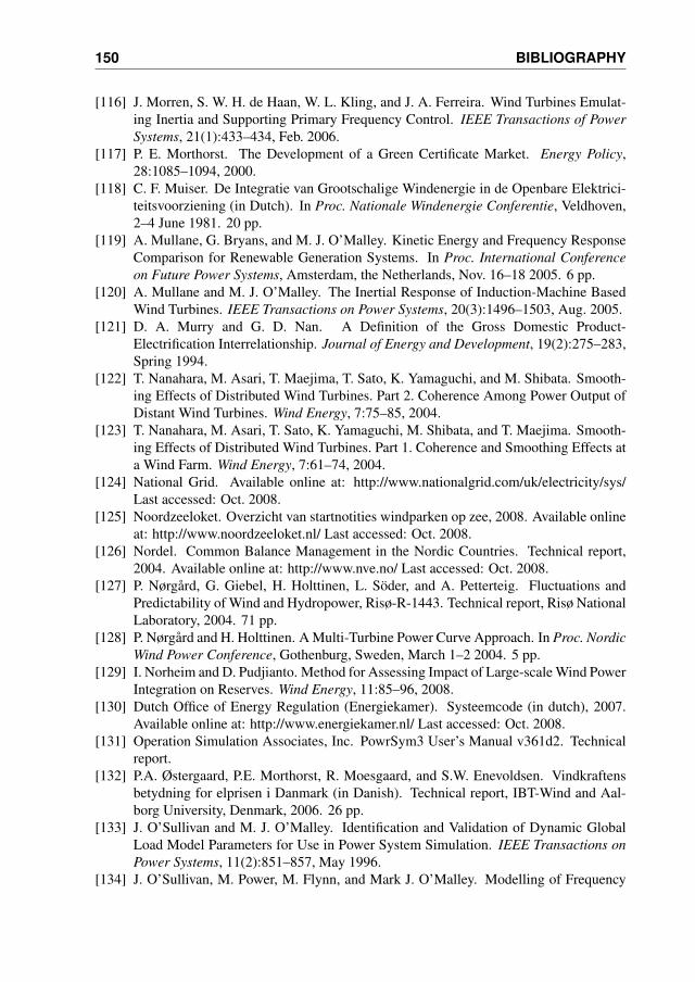
150 BIBLIOGRAPHY
[116] J. Morren, S. W. H. de Haan, W. L. Kling, and J. A. Ferreira. Wind Turbines Emulat-ing Inertia and Supporting Primary Frequency Control. IEEE Transactions of PowerSystems, 21(1):433–434, Feb. 2006.
[117] P. E. Morthorst. The Development of a Green Certificate Market. Energy Policy,28:1085–1094, 2000.
[118] C. F. Muiser. De Integratie van Grootschalige Windenergie in de Openbare Elektrici-teitsvoorziening (in Dutch). In Proc. Nationale Windenergie Conferentie, Veldhoven,2–4 June 1981. 20 pp.
[119] A. Mullane, G. Bryans, and M. J. O’Malley. Kinetic Energy and Frequency ResponseComparison for Renewable Generation Systems. In Proc. International Conferenceon Future Power Systems, Amsterdam, the Netherlands, Nov. 16–18 2005. 6 pp.
[120] A. Mullane and M. J. O’Malley. The Inertial Response of Induction-Machine BasedWind Turbines. IEEE Transactions on Power Systems, 20(3):1496–1503, Aug. 2005.
[121] D. A. Murry and G. D. Nan. A Definition of the Gross Domestic Product-Electrification Interrelationship. Journal of Energy and Development, 19(2):275–283,Spring 1994.
[122] T. Nanahara, M. Asari, T. Maejima, T. Sato, K. Yamaguchi, and M. Shibata. Smooth-ing Effects of Distributed Wind Turbines. Part 2. Coherence Among Power Output ofDistant Wind Turbines. Wind Energy, 7:75–85, 2004.
[123] T. Nanahara, M. Asari, T. Sato, K. Yamaguchi, M. Shibata, and T. Maejima. Smooth-ing Effects of Distributed Wind Turbines. Part 1. Coherence and Smoothing Effects ata Wind Farm. Wind Energy, 7:61–74, 2004.
[124] National Grid. Available online at: http://www.nationalgrid.com/uk/electricity/sys/Last accessed: Oct. 2008.
[125] Noordzeeloket. Overzicht van startnotities windparken op zee, 2008. Available onlineat: http://www.noordzeeloket.nl/ Last accessed: Oct. 2008.
[126] Nordel. Common Balance Management in the Nordic Countries. Technical report,2004. Available online at: http://www.nve.no/ Last accessed: Oct. 2008.
[127] P. Nørgard, G. Giebel, H. Holttinen, L. Soder, and A. Petterteig. Fluctuations andPredictability of Wind and Hydropower, Risø-R-1443. Technical report, Risø NationalLaboratory, 2004. 71 pp.
[128] P. Nørgard and H. Holttinen. A Multi-Turbine Power Curve Approach. In Proc. NordicWind Power Conference, Gothenburg, Sweden, March 1–2 2004. 5 pp.
[129] I. Norheim and D. Pudjianto. Method for Assessing Impact of Large-scale Wind PowerIntegration on Reserves. Wind Energy, 11:85–96, 2008.
[130] Dutch Office of Energy Regulation (Energiekamer). Systeemcode (in dutch), 2007.Available online at: http://www.energiekamer.nl/ Last accessed: Oct. 2008.
[131] Operation Simulation Associates, Inc. PowrSym3 User’s Manual v361d2. Technicalreport.
[132] P.A. Østergaard, P.E. Morthorst, R. Moesgaard, and S.W. Enevoldsen. Vindkraftensbetydning for elprisen i Danmark (in Danish). Technical report, IBT-Wind and Aal-borg University, Denmark, 2006. 26 pp.
[133] J. O’Sullivan and M. J. O’Malley. Identification and Validation of Dynamic GlobalLoad Model Parameters for Use in Power System Simulation. IEEE Transactions onPower Systems, 11(2):851–857, May 1996.
[134] J. O’Sullivan, M. Power, M. Flynn, and Mark J. O’Malley. Modelling of Frequency
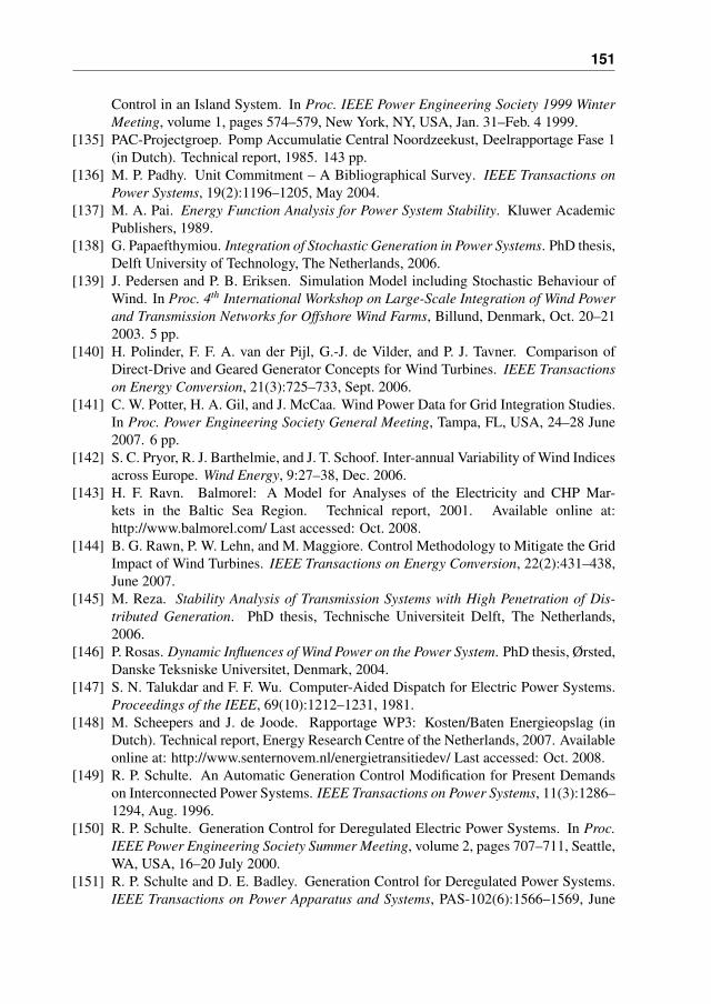
151
Control in an Island System. In Proc. IEEE Power Engineering Society 1999 WinterMeeting, volume 1, pages 574–579, New York, NY, USA, Jan. 31–Feb. 4 1999.
[135] PAC-Projectgroep. Pomp Accumulatie Central Noordzeekust, Deelrapportage Fase 1(in Dutch). Technical report, 1985. 143 pp.
[136] M. P. Padhy. Unit Commitment – A Bibliographical Survey. IEEE Transactions onPower Systems, 19(2):1196–1205, May 2004.
[137] M. A. Pai. Energy Function Analysis for Power System Stability. Kluwer AcademicPublishers, 1989.
[138] G. Papaefthymiou. Integration of Stochastic Generation in Power Systems. PhD thesis,Delft University of Technology, The Netherlands, 2006.
[139] J. Pedersen and P. B. Eriksen. Simulation Model including Stochastic Behaviour ofWind. In Proc. 4th International Workshop on Large-Scale Integration of Wind Powerand Transmission Networks for Offshore Wind Farms, Billund, Denmark, Oct. 20–212003. 5 pp.
[140] H. Polinder, F. F. A. van der Pijl, G.-J. de Vilder, and P. J. Tavner. Comparison ofDirect-Drive and Geared Generator Concepts for Wind Turbines. IEEE Transactionson Energy Conversion, 21(3):725–733, Sept. 2006.
[141] C. W. Potter, H. A. Gil, and J. McCaa. Wind Power Data for Grid Integration Studies.In Proc. Power Engineering Society General Meeting, Tampa, FL, USA, 24–28 June2007. 6 pp.
[142] S. C. Pryor, R. J. Barthelmie, and J. T. Schoof. Inter-annual Variability of Wind Indicesacross Europe. Wind Energy, 9:27–38, Dec. 2006.
[143] H. F. Ravn. Balmorel: A Model for Analyses of the Electricity and CHP Mar-kets in the Baltic Sea Region. Technical report, 2001. Available online at:http://www.balmorel.com/ Last accessed: Oct. 2008.
[144] B. G. Rawn, P. W. Lehn, and M. Maggiore. Control Methodology to Mitigate the GridImpact of Wind Turbines. IEEE Transactions on Energy Conversion, 22(2):431–438,June 2007.
[145] M. Reza. Stability Analysis of Transmission Systems with High Penetration of Dis-tributed Generation. PhD thesis, Technische Universiteit Delft, The Netherlands,2006.
[146] P. Rosas. Dynamic Influences of Wind Power on the Power System. PhD thesis, Ørsted,Danske Teksniske Universitet, Denmark, 2004.
[147] S. N. Talukdar and F. F. Wu. Computer-Aided Dispatch for Electric Power Systems.Proceedings of the IEEE, 69(10):1212–1231, 1981.
[148] M. Scheepers and J. de Joode. Rapportage WP3: Kosten/Baten Energieopslag (inDutch). Technical report, Energy Research Centre of the Netherlands, 2007. Availableonline at: http://www.senternovem.nl/energietransitiedev/ Last accessed: Oct. 2008.
[149] R. P. Schulte. An Automatic Generation Control Modification for Present Demandson Interconnected Power Systems. IEEE Transactions on Power Systems, 11(3):1286–1294, Aug. 1996.
[150] R. P. Schulte. Generation Control for Deregulated Electric Power Systems. In Proc.IEEE Power Engineering Society Summer Meeting, volume 2, pages 707–711, Seattle,WA, USA, 16–20 July 2000.
[151] R. P. Schulte and D. E. Badley. Generation Control for Deregulated Power Systems.IEEE Transactions on Power Apparatus and Systems, PAS-102(6):1566–1569, June
152 BIBLIOGRAPHY
1983.[152] A. Scully, A. Harpur, K. D. Le, J. T. Day, M. J. Malone, and T. E. Mousseau. Us-
ing a Semi-Guided Monte Carlo Method for Faster Simulation of Forced Outages ofGenerating Units. IEEE Transactions on Power Systems, 7(3):1313–1321, Aug. 1992.
[153] SEP, Dutch Electricity Generating Board. Uitvoeringsregeling ex artikel OVS ternadere uitwerking van artikel 6, lid 1 OVS (Bedrijfsvaardigheidsproeven), 13e uitgave(in Dutch). Technical report, 1994.
[154] S. N. Singh and I. Erlich. Strategies for Wind Power Trading in Competitive ElectricityMarkets. IEEE Transactions on Energy Conversio, 23(1):249–256, Mar. 2008.
[155] J. G. Slootweg. Wind Power, Modelling and Impact on Power System Dynamics. PhDthesis, Delft University of Technology, The Netherlands, 2003.
[156] J. G. Slootweg, S. W. H. de Haan, H. Polinder, and W. L. Kling. General Model forRepresenting Variable Speed Wind Turbines in Power System Dynamics Simulations.IEEE Transactions on Power Systems, 18(1):144–151, Feb. 2003.
[157] J. G. Slootweg and W. L. Kling. Impacts of Wind Power on Power System Dynamics,pages 629–651. Wind Power in Power Systems, T. Ackermann (editor), John Wiley &Sons, Ltd., 2005.
[158] J. Soens. Impact of Wind Energy in a Future Power Grid. PhD thesis, KatholiekeUniversiteit Leuven, Belgium, 2005.
[159] S. Solomon, D. Qin, M. Manning, Z. Chen, M. Marquis, K.B. Averyt, M.Tignor, andH.L. Miller (editors). Climate Change 2007: The Physical Science Basis. Contributionof Working Group I to the Fourth Assessment Report of the Intergovernmental Panelon Climate Change. Cambridge University Press, Cambridge, United Kingdom andNew York, NY, USA, 2007.
[160] J. P. Stremel, R. T. Jenkins, R. A. Babb, and W. D. Bayless. Production Costing Usingthe Cumulant Method of Representing the Equivalent Load Curve. IEEE Transactionson Power Apparatus and Systems, PAS–99(5):1947–1956, Sept./Oct. 1980.
[161] D. J. Swider. Compressed Air Energy Storage in an Electricity System with SignificantWind Power Generation. IEEE Transactions on Energy Conversion, 22(1):95–102,Mar. 2007.
[162] TenneT TSO BV. Managing Concept BS-NES 02-064. Technical report, 2002. Avai-lable online at: http://www.tennet.org/english/ Last accessed: Oct. 2008.
[163] TenneT TSO BV. Opgesteld Productievermogen 5 MW en Hoger (in Dutch), July2004.
[164] TenneT TSO BV. Quality and Capacity Plan 2008-2014. Technical report, 2008.Available online at: http://www.tennet.org/english/ Last accessed: Oct. 2008.
[165] TenneT TSO BV. Report on Monitoring of Reliability of Supply 2007-2023. Technicalreport, 2008. Available online at: http://www.tennet.org/english/ Last accessed: Oct.2008.
[166] TenneT TSO BV. Vision 2030. Technical report, 2008. Available online at:http://www.tennet.org/english/ Last accessed: Oct. 2008.
[167] TH Delft, HASKONING and Koninklijke Volker Stevin. Ondergrondse Pomp Accu-mulatie Centrale in Nederland - Vooronderzoek (in Dutch). Technical report, 1980.
[168] Transition Platform Sustainable Electricity Supply. Onderzoek naar de ToegevoegdeWaarde van Grootschalige Elektriciteitsopslag in Nederland (in Dutch). Technicalreport, 2008.
153
[169] UCTE. Operation Handbook, Policy 1: Load-Frequency Control andPerformance, v.2.2. Technical report, 2004. Available online at:http://www.ucte.org/resources/publications/ophandbook/ Last accessed: Oct. 2008.
[170] UCTE. System Adequacy Forecast 2008–2020. Technical report, 2008. Availableonline at: http://www.ucte.org/resources/publications/systemadequacy/ Last accessed:Oct. 2008.
[171] Union for the Co-ordination of Transmission of Electricity. Consumption data. Avai-lable online at: http://www.ucte.org/resources/dataportal/ Last accessed: Oct. 2008.
[172] H. Urdal and J. Horne. 2GW of Wind and Rising Fast - Grid Code Ccompliance ofLarge Wind Farms in the Great Britain Transmission System. In Proc. Nordic WindPower Conference, Roskilde, Denmark, 1–2 November 2007. 9 pp.
[173] G. J. W. van Bussel and M. B. Zaaijer. Reliability, Availability and MaintenanceAspects of Large-Scale Offshore Wind Farms, a Concepts Study. In Proc. MARECMarine Renewable Energies Conference, volume 113, 2001.
[174] P. P. J. van den Bosch. Short-Term Optimisation of Thermal Power Systems. PhDthesis, Technische Hogeschool Delft, The Netherlands, 1983.
[175] G. A. M. van Kuik. The Lanchester–Betz–Joukowsky Limit. Wind Energy, 10:289–291, February 2007.
[176] A. J. M. van Wijk. Wind Energy and Electricity Production. PhD thesis, UniversiteitUtrecht, The Netherlands, 1990.
[177] J. Verboomen, D. van Hertem, P. H. Schavemaker, F. J. C. M. Spaan, J-. M. Delince,R. Belmans, and W. L. Kling. Phase Shifter Coordination for Optimal Transmis-sion Capacity using Particle Swarm Optimization. Electric Power Systems Research,78(9):1648–1653, Sep. 2008.
[178] Vestas Wind Systems A/S. Life Cycle Assessment of Offshore and Onshore SitedWind Power Plants based on Vestas V90-3.0 MW Turbines. Technical report, 2006.Available online at: http://www.vestas.com/ Last accessed: Oct. 2008.
[179] K. Voorspools. The Modelling of Large Electricity-Generation Systems with Applica-tions in Emission-Reduction Scenarios and Electricity Trade. PhD thesis, KatholiekeUniversiteit Leuven, Belgium, 2004.
[180] J. F. Walker and N. Jenkins. Wind Energy Technology. Wiley, 1997.[181] L. Wang. The Effects of Uncertainties in Forced Outage Rates and Load Forecasts on
the Loss-Of-Load Probability (LOLP). IEEE Transactions on Power Apparatus andSystems, PAS-96(6):1920–1927, Nov.–Dec. 1977.
[182] S. J. Wang, M. Shahidehpour, and N. D. Xiang. Power Systems Marginal CostCurve and its Applications. IEEE Transactions on Power Apparatus and Systems,10(3):1321–1327, Aug. 1995.
[183] H. W. Weber, H. P. Asal, and E. Grebe. Characteristic Numbers of Primary Controlin the UCPTE Power System and Future Requirements. In Proc. ETG 97 SummerMeeting, pages 395–404, Berlin, 21–22 July 1997.
[184] R. O. Weber. Remarks on the Definition and Estimations of Friction Velocity.Boundary-Layer Meteorology, 93:197–209, April 1999.
[185] Wind Speed Records Available online at, KNMI Hydra Project. Available online at:http://www.knmi.nl/samenw/hydra/index.html Last accessed: Oct. 2008.
[186] Working Group on Prime Mover and Energy Supply Models for System DynamicPerformance Studies. Dynamic Models for Combined Cycle Plants in Power System

Studies. IEEE Transactions on Power Systems, 9(3):1698–1708, 1994.[187] World Commission on Environment and Development. Our Common Future. Oxford
University Press, 1987.[188] A. Woyte, P. Gardner, and H. Snodin. European Concerted Action on Offshore Wind
Energy Deployment: Inventory and Analysis of Power Transmission Barriers in EightMember States. Wind Energy, 10:357–378, April 2007.
[189] Wind Service Holland (WSH). Available online at: http://home.planet.nl/ windsh/Last accessed: Oct. 2008.
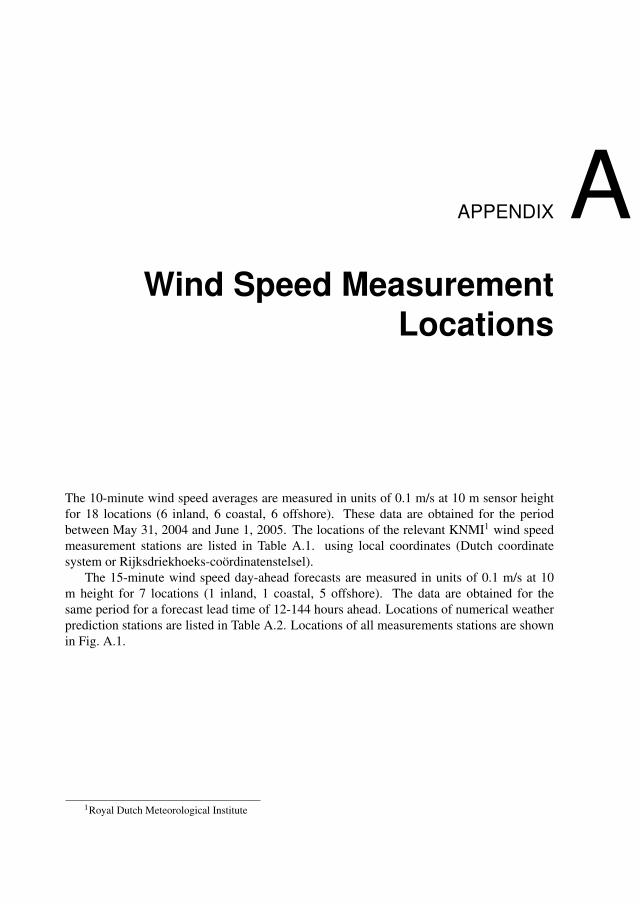
APPENDIX AWind Speed Measurement
Locations
The 10-minute wind speed averages are measured in units of 0.1 m/s at 10 m sensor heightfor 18 locations (6 inland, 6 coastal, 6 offshore). These data are obtained for the periodbetween May 31, 2004 and June 1, 2005. The locations of the relevant KNMI1 wind speedmeasurement stations are listed in Table A.1. using local coordinates (Dutch coordinatesystem or Rijksdriekhoeks-coordinatenstelsel).
The 15-minute wind speed day-ahead forecasts are measured in units of 0.1 m/s at 10m height for 7 locations (1 inland, 1 coastal, 5 offshore). The data are obtained for thesame period for a forecast lead time of 12-144 hours ahead. Locations of numerical weatherprediction stations are listed in Table A.2. Locations of all measurements stations are shownin Fig. A.1.
1Royal Dutch Meteorological Institute

156 Wind Speed Measurement Locations
Location inland/coastal/offshore X Y[m] [m]
De Bilt inland 140827 456835Europlatform offshore 10044 447580F3 offshore 111995 763069Gilze Rijen inland 123731 397594Hoek van Holland coastal 65550 445050Huibertgat offshore 222037 621279K13 offshore 10240 583356Lauwersoog coastal 209000 603125Leeuwarden inland 178970 581970L.E. Goeree offshore 36662 437913Lelystad inland 164125 497125M. Noordwijk offshore 80512 476658Marknesse inland 188850 523975Stavoren coastal 154725 545250Texelhors coastal 110125 556875Vlissingen coastal 30475 385125Woensdrecht inland 2820 384700IJmuiden coastal 98450 497450
Table A.1: KNMI 10-minute wind speed measurement locations (local coordinates) [185].
location inland/coastal/offshore X Y[m] [m]
Cabauw inland 123350 442580Europlatform offshore 10044 447580EWTW1 coastal 131500 540250F3 offshore 111995 763069FINO offshore 150100 635100K13 offshore 10240 583356NSW offshore 89651 514267
Table A.2: Numerical weather prediction locations (local coordinates).

Wind Speed Measurement Locations 157
50 km
Cadzand
L.E. Goerree Holland
M. Noordwijk
Huibertgat
Leeuwarden
Vlieland
Lelystad
Marknesse
IJmuiden
De Bilt
F3 FINO
Gilze Rijen
K13
Lauwersoog
Stavoren
Texelhors
Vlissingen Woensdrecht
Cabauw
EWTW1
Hoek van
Europlatform
OnshoreCoastalOffshore
NSW
Figure A.1: Inland, coastal and offshore wind speed measurement and numerical weatherprediction locations.

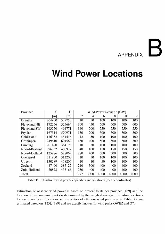
APPENDIX BWind Power Locations
Province X Y Wind Power Scenario [GW][m] [m] 2 4 6 8 10 12
Drenthe 204900 529750 10 50 100 100 100 100Flevoland NE 172256 525694 300 450 600 600 600 600Flevoland SW 163550 494771 340 500 550 550 550 550Fryslan 167514 570971 150 200 300 300 300 300Gelderland 176352 451416 12 50 100 100 100 100Groningen 249610 601562 150 400 500 500 500 500Limburg 201420 364190 10 50 100 100 100 100Noord-Brabant 96752 406977 40 100 150 150 150 150Noord-Holland 125986 528069 280 400 500 500 500 500Overijssel 211800 512200 10 50 100 100 100 100Utrecht 130289 458206 10 10 50 100 100 100Zeeland 47490 387127 210 300 400 400 400 400Zuid-Holland 70878 433166 250 400 400 400 400 400Total 1772 3000 4000 4000 4000 4000
Table B.1: Onshore wind power capacities and locations (local coordinates).
Estimation of onshore wind power is based on present totals per province [189] and thelocation of onshore wind parks is determined by the weighed average of existing locationsfor each province. Locations and capacities of offshore wind park sites in Table B.2 areestimated based on [125], [189] and are exactly known for wind parks OWEZ and Q7.
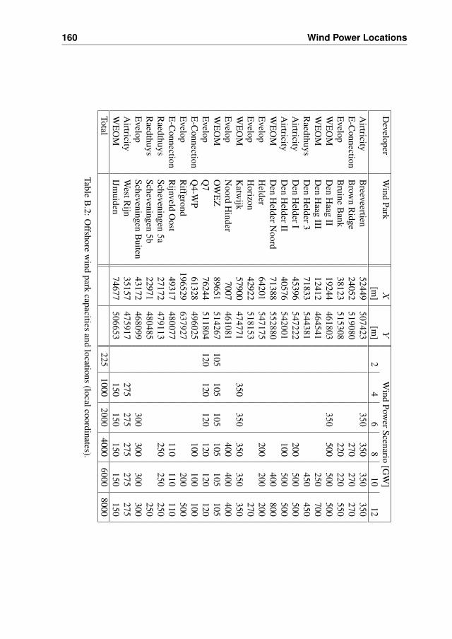
160 Wind Power Locations
Developer
Wind
ParkX
YW
indPow
erScenario[G
W]
[m]
[m]
24
68
1012
Airtricity
Breeveertien
52449507423
350350
350350
E-C
onnectionB
rown
Ridge
24052519080
270270
270E
velopB
ruineB
ank38123
515308220
220550
WE
OM
Den
Haag
II19244
461803350
500500
500W
EO
MD
enH
aagIII
12412464541
250700
Raedthuys
Den
Helder3
71833544381
450450
Airtricity
Den
HelderI
45396547222
200500
500A
irtricityD
enH
elderII40576
542001100
500500
WE
OM
Den
HelderN
oord71388
552880400
800E
velopH
elder64201
547175200
200200
Evelop
Horizon
42922518153
270W
EO
MK
atwijk
57900474771
350350
350350
350E
velopN
oordH
inder7007
461081400
400400
WE
OM
OW
EZ
89651514267
105105
105105
105105
Evelop
Q7
76244511804
120120
120120
120120
E-C
onnectionQ
4-WP
61328496025
100100
100E
velopR
iffgrond196529
637927200
500E
-Connection
Rijnveld
Oost
49317480077
110110
110R
aedthuysScheveningen
5a27172
479113250
250250
Raedthuys
Scheveningen5b
22971480485
250E
velopScheveningen
Buiten
43172468099
300300
300300
Airtricity
WestR
ijn35157
475917275
275275
275275
WE
OM
IJmuiden
74677506653
150150
150150
150Total
2251000
20004000
60008000
TableB
.2:Offshore
wind
parkcapacities
andlocations
(localcoordinates).
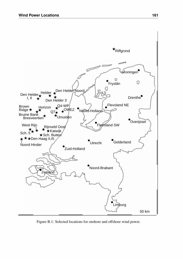
Wind Power Locations 161
Breeveertien
Den Haag II,III
Den HelderDen Helder Noord
Katwijk
Noord Hinder
OWEZQ7
Q4-WP
Riffgrond
Sch. Buiten
West Rijn
IJmuiden
Fryslân
Groningen
Drenthe
Flevoland NE
Flevoland SWOverijssel
GelderlandUtrecht
Noord-Holland
Zuid-Holland
Noord-BrabantZeeland
Limburg
Brown
Bruine Bank
Den Helder 3
Helder
Horizon
Rijnveld Oost
Sch. 5
Ridge
I, II
50 km
Figure B.1: Selected locations for onshore and offshore wind power.

APPENDIX CGerman Wind Power Data
German wind power and forecast data obtained for this research comprise the following:• E.ON: 15 min. averaged wind power data from June 1st, 2004 to May 31st, 2005 for
installed capacity of 6427–7088 MW (May 18th, 2004 and June 13th, 2005), 15 min. aver-aged, hourly updated day-ahead forecasts from September 1st, 2004 to May 31st, 2005
• RWE: 15 min. averaged wind power data from June 1st, 2004 to May 31st, 2005 forunknown installed capacity (maximum output 2702 MW)
• Vattenfall Europe: 15 min. averaged wind power data from June 1st, 2004 to May 31st,2005 for installed capacity of 5678–6400 MW (June 30st and May 31st, 15 min. averaged,hourly updated day-ahead forecasts from June 1st, 2004 to May 31st, 2005
The wind power and forecast data comprise the same period as the Netherlands’ wind speeddata series used in Chapter 2 in order to take automatically capture existing correllationsbetween wind power output in both countries. Correlations between forecast and realisedwind power were found to be 0.95 on average for the E.On Netz data and 0.90 for the Vat-tenfall Europe data, where it can be noted that the graphical area of the E.On Netz area issignificantly larger. For the 2014 wind power forecast it is assumed that the total forecastcorrellation is 0.95. Based on statistics obtained from [51], German installed wind powercapacity mid 2004 and mid 2005 comprised an estimated total of 15.600 and 17.500 MW,respectively. The wind power data above represent approximately 95% of installed capacity(with the E.ON area representing 40%, Vattenfall Europe 36% and RWE 19%), the windforecast data represent about 40–76%.
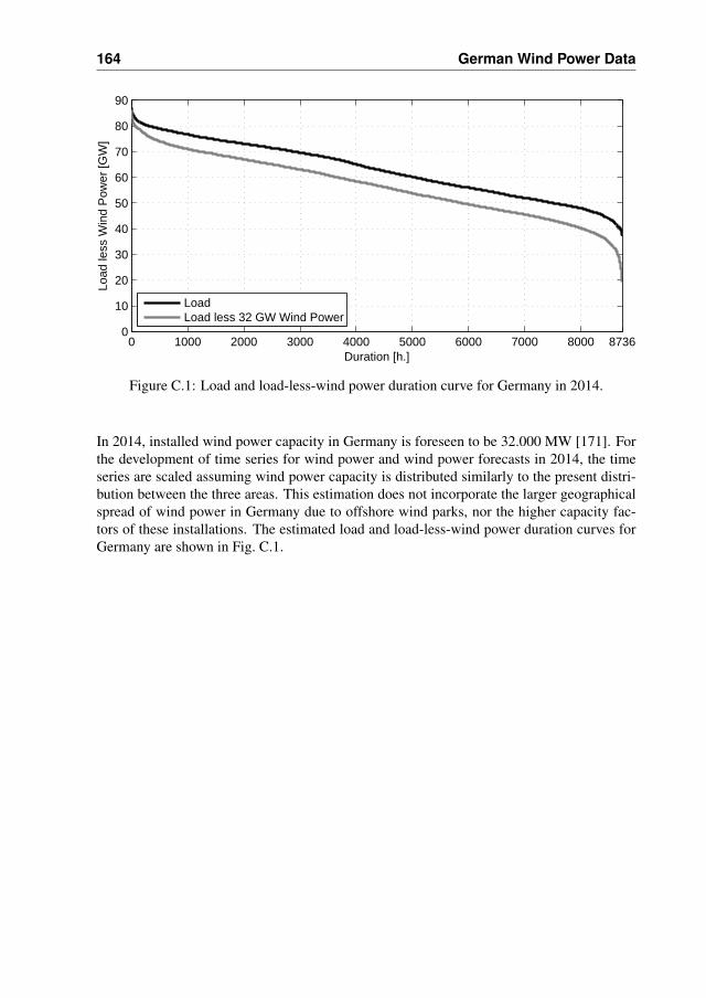
164 German Wind Power Data
0 1000 2000 3000 4000 5000 6000 7000 8000 87360
10
20
30
40
50
60
70
80
90
Duration [h.]
Load
less
Win
d P
ower
[GW
]
LoadLoad less 32 GW Wind Power
Figure C.1: Load and load-less-wind power duration curve for Germany in 2014.
In 2014, installed wind power capacity in Germany is foreseen to be 32.000 MW [171]. Forthe development of time series for wind power and wind power forecasts in 2014, the timeseries are scaled assuming wind power capacity is distributed similarly to the present distri-bution between the three areas. This estimation does not incorporate the larger geographicalspread of wind power in Germany due to offshore wind parks, nor the higher capacity fac-tors of these installations. The estimated load and load-less-wind power duration curves forGermany are shown in Fig. C.1.

APPENDIX DValidation Test System Data
The data in this appendix are adopted from [8], [137] except for the last column of Table D.1which is added for model validation purposes in this thesis only. Additional data used for thisresearch are specified in Table 5.2, page 101. Bus 31 is assigned as the slack bus, generatorG02 as the slack generator.
Table D.1: Bus data of the New England 39 bus test system.
Bus Volts Load Load Gen. Gen.- [pu] [MW] [MVAr] [MW] Name1 - 0 0 02 - 0 0 03 - 322.0 2.4 04 - 500.0 184.0 05 - 0 0 06 - 0 0 07 - 233.8 84.0 08 - 522.0 176.0 09 - 0 0 0
10 - 0 0 011 - 0 0 012 - 7.5 88.0 0
Continued on next page
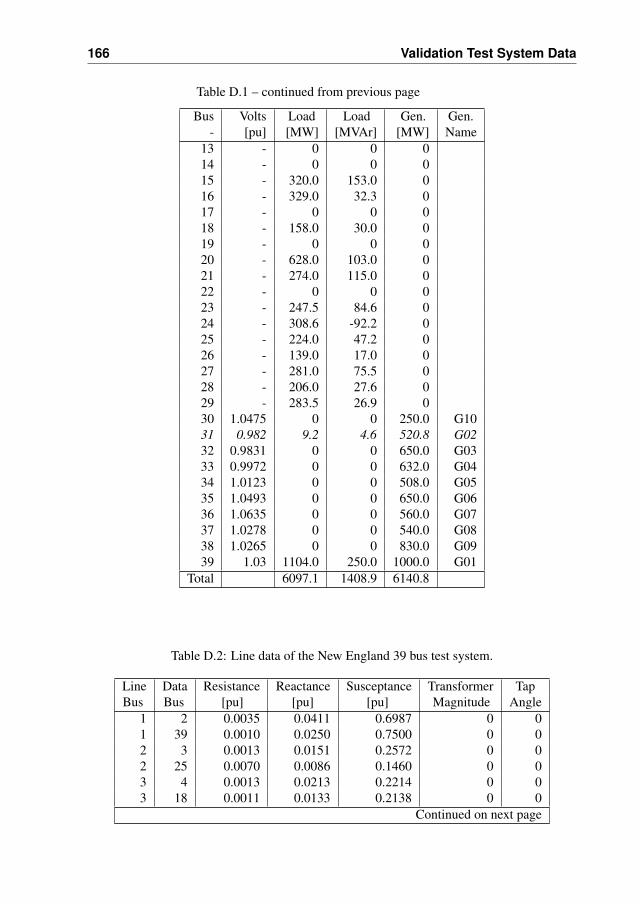
166 Validation Test System Data
Table D.1 – continued from previous page
Bus Volts Load Load Gen. Gen.- [pu] [MW] [MVAr] [MW] Name
13 - 0 0 014 - 0 0 015 - 320.0 153.0 016 - 329.0 32.3 017 - 0 0 018 - 158.0 30.0 019 - 0 0 020 - 628.0 103.0 021 - 274.0 115.0 022 - 0 0 023 - 247.5 84.6 024 - 308.6 -92.2 025 - 224.0 47.2 026 - 139.0 17.0 027 - 281.0 75.5 028 - 206.0 27.6 029 - 283.5 26.9 030 1.0475 0 0 250.0 G1031 0.982 9.2 4.6 520.8 G0232 0.9831 0 0 650.0 G0333 0.9972 0 0 632.0 G0434 1.0123 0 0 508.0 G0535 1.0493 0 0 650.0 G0636 1.0635 0 0 560.0 G0737 1.0278 0 0 540.0 G0838 1.0265 0 0 830.0 G0939 1.03 1104.0 250.0 1000.0 G01
Total 6097.1 1408.9 6140.8
Table D.2: Line data of the New England 39 bus test system.
Line Data Resistance Reactance Susceptance Transformer TapBus Bus [pu] [pu] [pu] Magnitude Angle
1 2 0.0035 0.0411 0.6987 0 01 39 0.0010 0.0250 0.7500 0 02 3 0.0013 0.0151 0.2572 0 02 25 0.0070 0.0086 0.1460 0 03 4 0.0013 0.0213 0.2214 0 03 18 0.0011 0.0133 0.2138 0 0
Continued on next page

Validation Test System Data 167
Table D.2 – continued from previous page
Line Data Resistance Reactance Susceptance Transformer TapBus Bus [pu] [pu] [pu] Magnitude Angle
4 5 0.0008 0.0128 0.1342 0 04 14 0.0008 0.0129 0.1382 0 05 6 0.0002 0.0026 0.0434 0 05 8 0.0008 0.0112 0.1476 0 06 7 0.0006 0.0092 0.1130 0 06 11 0.0007 0.0082 0.1389 0 07 8 0.0004 0.0046 0.0780 0 08 9 0.0023 0.0363 0.3804 0 09 39 0.0010 0.0250 1.2000 0 0
10 11 0.0004 0.0043 0.0729 0 010 13 0.0004 0.0043 0.0729 0 013 14 0.0009 0.0101 0.1723 0 014 15 0.0018 0.0217 0.3660 0 015 16 0.0009 0.0094 0.1710 0 016 17 0.0007 0.0089 0.1342 0 016 19 0.0016 0.0195 0.3040 0 016 21 0.0008 0.0135 0.2548 0 016 24 0.0003 0.0059 0.0680 0 017 18 0.0007 0.0082 0.1319 0 017 27 0.0013 0.0173 0.3216 0 021 22 0.0008 0.0140 0.2565 0 022 23 0.0006 0.0096 0.1846 0 023 24 0.0022 0.0350 0.3610 0 025 26 0.0032 0.0323 0.5130 0 026 27 0.0014 0.0147 0.2396 0 026 28 0.0043 0.0474 0.7802 0 026 29 0.0057 0.0625 1.0290 0 028 29 0.0014 0.0151 0.2490 0 02 30 0.0000 0.0181 0.0000 1.025 06 31 0.0000 0.0250 0.0000 1.070 0
10 32 0.0000 0.0200 0.0000 1.070 012 11 0.0016 0.0435 0.0000 1.006 012 13 0.0016 0.0435 0.0000 1.006 019 20 0.0007 0.0138 0.0000 1.060 019 33 0.0007 0.0142 0.0000 1.070 020 34 0.0009 0.0180 0.0000 1.009 022 35 0.0000 0.0143 0.0000 1.025 023 36 0.0005 0.0272 0.0000 1.000 025 37 0.0006 0.0232 0.0000 1.025 029 38 0.0008 0.0156 0.0000 1.025 0

168 Validation Test System Data
1
1
1
1
1
1
1
1
1
1 1
1
1
1
1
1
1 1
1
1
1
1
1
1
1
1
1
1
38
40
27
2628
29
2417
16
15
14
2122
35
19
4212
23
33
2013
10
34
11
6
7
8
9
41
3
39
1
2 18
30 25
37
5
4
31
32
Figure D.1: Single line diagram of the New England 39 bus test system
APPENDIX ENomenclature
List of Abbreviations
ACE Area Control ErrorAGC Automatic Generation ControlARP Access Responsible PartyB BelgiumBF Blast Furnace gasBRP Balance Responsible PartyCAES Compressed Air Energy StorageCCGT Combined Cycle Gas TurbineCCS Carbondioxide Capture and SequestrationCHP Combined Heat and PowerCO2 CarbondioxideCOI Centre of InertiaD GermanyEC Economic OptimisationENS Energy-Not-ServedF FranceGB Great BritainGT Gas TurbineHIRLAM HIgh-Resolution Limited Area ModelHVDC High Voltage Direct Current

170 Nomenclature
ISO Independent System OperatorLOLP Loss-Of-Load ProbabilityMLE Maximum Likelihood EstimatorMR Must RunNG Natural GasNL The NetherlandsNN2 NorNed 2, submarine transmission cable between the Netherlands and NorwayNOR NorwayNOx Nitrogen oxidesNTC Net Transfer CapacityNWP Numerical Weather PredictionO&M Operation and MaintenancePAC Pumped ACcumulation energy storagePACE Processed ACEPP Perfect wind power PredictionPRP Program Responsible PartyPSD Power Spectrum DensityPTU Program Time UnitRES Renewable Energy SourcesRoR Run-of-RiverSO2 SulfurdioxideST Steam TurbineTSO Transmission System OperatorUCTE Union for the Coordination of Transmission of Electricity,
association of transmission system operators in continental EuropeUC–ED Unit Commitment and Economic DispatchUPAC Underground Pumped ACcumulation energy storageU UraniumWAMS Wide Area Measurement System
List of Symbols
2ndPRP,t secondary control signala inverse of characteristic distance [km−1]A area [m2]Ar swept turbine rotor area [m2]AT area per turbine location [m2]ACEt ACE at moment t [MW]cp power coefficient of the wind turbineC1..8 cost level [e]Cvar variable operation and maintenance cost [e/MWh]Cm,sys system marginal cost [e]cov covariance, correlation of wind speed variations between locationsD distance or load damping reaction [MW/Hz]
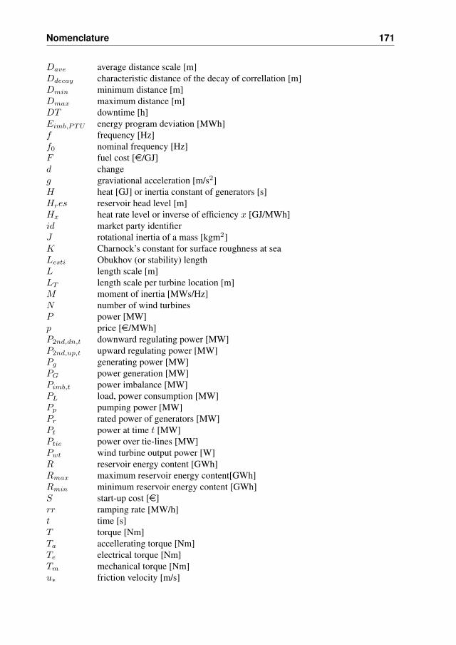
Nomenclature 171
Dave average distance scale [m]Ddecay characteristic distance of the decay of correllation [m]Dmin minimum distance [m]Dmax maximum distance [m]DT downtime [h]Eimb,PTU energy program deviation [MWh]f frequency [Hz]f0 nominal frequency [Hz]F fuel cost [e/GJ]d changeg graviational acceleration [m/s2]H heat [GJ] or inertia constant of generators [s]Hres reservoir head level [m]Hx heat rate level or inverse of efficiency x [GJ/MWh]id market party identifierJ rotational inertia of a mass [kgm2]K Charnock’s constant for surface roughness at seaLesti Obukhov (or stability) lengthL length scale [m]LT length scale per turbine location [m]M moment of inertia [MWs/Hz]N number of wind turbinesP power [MW]p price [e/MWh]P2nd,dn,t downward regulating power [MW]P2nd,up,t upward regulating power [MW]Pg generating power [MW]PG power generation [MW]Pimb,t power imbalance [MW]PL load, power consumption [MW]Pp pumping power [MW]Pr rated power of generators [MW]Pt power at time t [MW]Ptie power over tie-lines [MW]Pwt wind turbine output power [W]R reservoir energy content [GWh]Rmax maximum reservoir energy content[GWh]Rmin minimum reservoir energy content [GWh]S start-up cost [e]rr ramping rate [MW/h]t time [s]T torque [Nm]Ta accellerating torque [Nm]Te electrical torque [Nm]Tm mechanical torque [Nm]u∗ friction velocity [m/s]

172 Nomenclature
v wind speed [m/s]vt blade tip speed [m/s]VG generating value of energy [e/MWh]VP pumping value of energy [e/MWh]w(x, t) log wind speed at location x and time tz1(x1, y1) location with parameters x1 and y1
zh location hub height [m]zs location sensor height [m]N (0, σ) zero-mean, normally-distributed term of standard deviation σβ power-frequency characteristicγ(t) zero-mean, normally-distributed noise term∆ deviationε(x, t) zero-mean random process variable for intra-day wind speed variationsη net turn-around conversion efficiencyθ blade pitch angle [◦]κ Von Karman constantλ tip speed ratio between the turbine blade tip speedµ(x, t) mean wind speed pattern at location x and time t [m/s]µ(zh) mean wind speed at wind turbine hub-height [m/s]π ratio of a circle’s circumference to its diameterρ density of airσF width of Gaussian filter Fσ(zh) standard deviation at hub heightσ(zs) standard deviation at sensor heightΣ sumφ(t) first-order auto-regressive moving average (ARMA) processω rotational speed
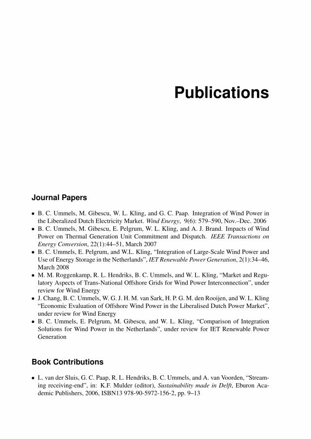
Publications
Journal Papers
• B. C. Ummels, M. Gibescu, W. L. Kling, and G. C. Paap. Integration of Wind Power inthe Liberalized Dutch Electricity Market. Wind Energy, 9(6): 579–590, Nov.–Dec. 2006
• B. C. Ummels, M. Gibescu, E. Pelgrum, W. L. Kling, and A. J. Brand. Impacts of WindPower on Thermal Generation Unit Commitment and Dispatch. IEEE Transactions onEnergy Conversion, 22(1):44–51, March 2007
• B. C. Ummels, E. Pelgrum, and W.L. Kling, “Integration of Large-Scale Wind Power andUse of Energy Storage in the Netherlands”, IET Renewable Power Generation, 2(1):34–46,March 2008
• M. M. Roggenkamp, R. L. Hendriks, B. C. Ummels, and W. L. Kling, “Market and Regu-latory Aspects of Trans-National Offshore Grids for Wind Power Interconnection”, underreview for Wind Energy
• J. Chang, B. C. Ummels, W. G. J. H. M. van Sark, H. P. G. M. den Rooijen, and W. L. Kling“Economic Evaluation of Offshore Wind Power in the Liberalised Dutch Power Market”,under review for Wind Energy
• B. C. Ummels, E. Pelgrum, M. Gibescu, and W. L. Kling, “Comparison of IntegrationSolutions for Wind Power in the Netherlands”, under review for IET Renewable PowerGeneration
Book Contributions
• L. van der Sluis, G. C. Paap, R. L. Hendriks, B. C. Ummels, and A. van Voorden, “Stream-ing receiving-end”, in: K.F. Mulder (editor), Sustainability made in Delft, Eburon Aca-demic Publishers, 2006, ISBN13 978-90-5972-156-2, pp. 9–13
174 Publications
• G. A. M. van Kuik, B. C. Ummels, and R. L. Hendriks, “Perspectives of Wind Energy”, in:K. Hanjalic, R. van de Krol, A. Lekic (editors), Sustainable Energy Technologies: Optionsand Prospects, Springer Verlag, 2008, ISBN 978-1-4020-6723-5, pp. 75–97
Conference Contributions
• B. C. Ummels, M. Gibescu, W. L. Kling, and G. C. Paap. Power System Balancing withOffshore Wind Power in the Netherlands. In Proc. 5th International Workshop on Large-Scale Integration of Wind Power and Power Systems, Glasgow, April 7–8, 2005, 8 pp.
• B. C. Ummels, M. Gibescu, W. L. Kling, and G. C. Paap, Conventional Generation for Bal-ancing 6 GW Offshore Wind Power., In Proc. Copenhagen Offshore Wind, Copenhagen,October 25–27, 2005, 10 pp.
• B. C. Ummels, E. H. M. Mast, W. L. Kling, and G. A. M. van Kuik. Scenarios to AssessSystem Integration of Offshore Wind Power in the Netherlands. In Proc. European WindEnergy Conference, Athens, February 27–March 2, 2006, 10 pp.
• B. C. Ummels, M. Gibescu, W. L. Kling, and G. C. Paap. Simulation Method for PowerSystem Balancing with Large-Scale Wind Power subject to Program Responsibility. InProc. 3rd IEEE Young Researchers Symposium in Electrical Power Engineering, Ghent,April 27–28, 2006, 8 pp.
• M. Gibescu, B. C. Ummels, and W. L. Kling. Statistical Wind Speed Interpolation forSimulating Aggregated Wind Power Production under Unit Commitment and Dispatch. InProc. 9th International Conference on Probabilistic Methods Applied to Power Systems,Stockholm, June 11–15, 2006, 8 pp.
• B. C. Ummels, M. Gibescu, W. L. Kling, and E. Pelgrum. System Integration of Large-Scale Wind Power in the Netherlands. In Proc. IEEE PES General Meeting, Montreal,June 18–22, 2006, 8 pp.
• G. A. M. van Kuik, B. C. Ummels, and R. L. Hendriks. Perspectives of Wind Energy.In Proc. Advances in New and Sustainable Energy Conversion and Storage TechnologiesConference, Dubrovnik, September 23–25, 2006, 19 pp.
• K. Verhaegen, B. C. Ummels, R. J. M. Belmans, and W. L. Kling. Comparison of Sup-port Schemes and Market Designs for Wind Power. In Proc. 6th International Workshopon Large-Scale Integration of Wind Power and Transmission Networks for Offshore WindFarms, Delft, October 26–28, 2006, 8 pp.
• B. C. Ummels, R. L. Hendriks, M. Gibescu, W. L. Kling, and G. A. M. van Kuik. Overviewof System Integration of Wind Power in the Netherlands. In Proc. 6th International Work-shop on Large-Scale Integration of Wind Power and Transmission Networks for OffshoreWind Farms, Delft, October 26–28, 2006, 7 pp.
• R. L. Hendriks, B. C. Ummels, and T. Ackermann (Editors). Proc. 6th International Work-shop on Large-Scale Integration of Wind Power and Transmission Networks for OffshoreWind Farms, Delft, October 26–28, 2006, 493 pp.
• B. C. Ummels. System Integration of Wind Power – Summary of the Delft Workshop.EWEA Policy Conference on Large Scale Integration of Wind Power, Brussels, November7–8, 2006, 12 slides
• B. C. Ummels, M. Gibescu, W. L. Kling, and G. C. Paap. Optimization of Generation PlantMix in case of Large-Scale Wind Power. In Proc. European Wind Energy Conference
Publications 175
2007, Milan, 7–10 May, 2007, 9 pp.• W. L. Kling, B. C. Ummels, and R. L. Hendriks. Transmission and System Integration
of Wind Power in the Netherlands. In Proc. IEEE PES General Meeting, Tampa, 24–28June, 2007, 6 pp.
• G. Koustas, G. Papaefthymiou, B. C. Ummels, and L. van der Sluis. Stochastic Assessmentof Wind Power Curtailment Opportunities. In Proc. Nordic Wind Power Conference 2007,Roskilde, 1–2 November 2007, 6 pp.
• P. P. T. Groenewoud, R. L. Hendriks, B. C. Ummels, and W. L. Kling. Real-Time Digi-tal Simulation of a VSC-Connected Offshore Wind Farm. In Proc. Nordic Wind PowerConference 2007, Roskilde, 1–2 November 2007, 7 pp.
• B. C. Ummels, M. Gibescu, W. L. Kling, and G. C. Paap. Performance of AutomaticGeneration Control Mechanisms with Large-Scale Wind Power. In Proc. Nordic WindPower Conference 2007, Roskilde, 1–2 November 2007, 7 pp.
• M. M. Roggenkamp, R. L. Hendriks, B. C. Ummels, and W. L. Kling. Market and Reg-ulatory Aspects of Trans-National Offshore Grids for Wind Power Interconnection. InProc.European Offshore Wind 2007, Berlin, 3–6 December 2007, 10 pp.
• B. C. Ummels, E. Pelgrum, W. L. Kling, and H. Droog. Energy Storage Options for SystemIntegration of Offshore Wind Power in the Netherlands. In Proc. European Wind EnergyConference, Brussels, 31 March–3 April 2008, 10 pp.
• W. L. Kling and B. C. Ummels. The Need for Large-Scale Energy Storage in the DutchElectricity System. International Congress on Innovation for Sustainable Production2008, Bruges, April 22–25 2008, 12 slides
• H. Holttinen, P. Meibom , A. Orths , M. J. O’Malley, B. C. Ummels, J. O. Tande, A. Es-tanqueiro, E. Gomez, J. C. Smith and E. Ela. Impacts of Large Amounts of Wind Poweron Design and Operation of Power Systems, Results of IEA Collaboration. In Proc. 7th
International Workshop on Large-Scale Integration of Wind Power into Power Systems aswell as on Transmission Networks for Offshore Wind Farms, Madrid, May 26–27, 2008,and in Proc. Wind Power 2008, Houston, Texas, 1–4 June, 2008, 8 pp.
• B.C. Ummels, M. Gibescu, G.C. Paap, W.L. Kling. Development of a Simulation Modelfor Secondary Control Performance Assessment with Significant Wind Power in a MarketEnvironment. In Proc. Power Systems Computational Conference 2008, Glasgow, July14–18, 2008, 8 pp.
• W. L. Kling, M. Gibescu, B. C. Ummels, and R. L. Hendriks. Implementation of WindPower in the Dutch Power System. In Proc. IEEE PES General Meeting, Pittsburgh,24–28 July, 2008, 5 pp.
• B. C. Ummels, W. L. Kling, M. Gibescu, E. Pelgrum, and G. C. Paap. Power SystemOperation with Large Scale Offshore Wind Power in the Netherlands – Simulation of WorstCases. In Proc. CIGRE Session 2008, Paris, 24–29 August, 2008, 8 pp.
• M. Gibescu, B. C. Ummels, W. L. Kling, E. Pelgrum and R. A. Van Offeren. Case Studyfor the Integration of 12 GW Wind Power in the Dutch Power System by 2020. In Proc.IEEE PES/CIGRE Integration of Wide-Scale Renewable Resources into the Power DeliverySystem Symposium, Calgary, 29–31 July, 2009 (accepted for publication)
• K. Ntotas, M. Gibescu, W. L. Kling, B. C. Ummels, E. Pelgrum. Flexible InternationalExchanges: a Possible Solution for Large-Scale Wind Power Integration within the FuturePower System. In Proc. IEEE PowerTech, Bucharest, June 28–July 2, 2009 (abstractsubmitted)
176 Publications
Other Publications
• E. Pelgrum and B. C. Ummels. Integrating Wind Power into the Dutch System. TechnicalReport for TenneT TSO b.v., Arnhem, November 2005, 33 pp.
• R. L. Hendriks and B. C. Ummels. Netinpassing van grootschalige offshore windenergie(in Dutch), Energie+, Vakblad over besparing, efficiency en duurzaamheid, yr 25, nr. 6,Dec. 2005, pp. 22–23
• European Wind Energy Association, F. Van Hulle et al (a.o. B. C. Ummels). Large ScaleIntegration of Wind Energy in the European Power Supply: Analysis, Issues and Recom-mendations. European Wind Energy Association, Brussels, December 2005, 170 pp.
• B. C. Ummels, R. L. Hendriks, and W. L. Kling. Inpassing van Grootschalig OffshoreWindvermogen (in Dutch). Technical Report for Strategy Group Transition Offshore WindEnergy (TOW), Delft, February 2007, 39 pp.
• E. Pelgrum and B. C. Ummels. Grootschalig Windvermogen en Energieopslag in de Ned-erlandse Elektriciteitsvoorziening (in Dutch). Technical Report for TenneT TSO b.v., Arn-hem, May 2007, 23 pp.
• B. C. Ummels, C. Sinos, J. Verboomen, W. L. Kling, E. Pelgrum, and F. Spaan. Deve-lopment and Results of a Robust Capacity Bottleneck Identification Method for the DutchTransmission System. Technical Report for TenneT TSO b.v., Delft, May 2007, 17 pp.
• W. W. de Boer, A. J. Brand, M. Gibescu, and B. C. Ummels. System Balancing with 6 GWOffshore Wind Energy in the Netherlands - Instruments for Balance Control – SummaryWork Package 3. Technical Report for We@Sea, Delft, June 2007, 20 pp.
• B. C. Ummels. Quick-Scan Windenergie en Energieopslag, Eindrapport WP1 (in Dutch).Technical Report for Dutch Ministry of Economic Affairs and Transition Platform for Sus-tainable Electricity Supply, Delft, December 2007, 21 pp.
• B. C. Ummels. Simulatiestudie Windenergie, Basislastvermogen en Internationale Uitwis-seling (in Dutch). Technical Report for SenterNovem, Transition Platform for SustainableElectricity Supply and CE Delft, Delft, October 2008, 16 pp.
Presentations and Interviews
• Dutch Wind Workshops, October 11, 2006, Energy Research Centre of the Netherlands,• Energie+, “Grootschalige opslag in Energie-eiland”, Energie+ nr. 5, Sept. 2007, pp. 36–37• IEA Wind Task 25, September 19, 2007, Oslo, Norway• Dutch Wind Workshops, October 27, 2008, Delft University Wind Energy Research Insti-
tute (DUWIND)

Acknowledgement
Using wind at sea to create fire on land! All four classical elements come together whenlarge-scale wind power is integrated in power systems. It really has been a great subject todedicate four years of research to. I am very grateful to prof. Wil Kling for giving me theopportunity to do this Ph.D. project. Wil, you have given me the freedom to shape large partsof this research myself and at the same time kept me focused on my subject. You encouragedme to get involved in many studies outside university which has been very good for mypersonal development. Your ability to always open up new research perspectives has beeninspiring. Thank you for four very good years.
I would also like to thank my daily supervisors at TU Delft, dr. Madeleine Gibescu anddr. Bob Paap. Madeleine, thank you for your constant and insightful feedback on my Ph.Dwork. I am indebted to you and dr. Arno Brand of ECN for developing the wind power datathat have enabled me and many others within the framework of We@Sea to do our research.Bob, special thanks for your useful suggestions for the development of the dynamic model.I furthermore acknowledge the highly useful and detailed feedback of all members of theexamination committee on the thesis manuscript.
Ralph Hendriks, my partner in wind power research and honoured paranymf, I thank youvery much for our magnificent cooperation in the past three years. Your help in validating mydynamic model using SinCal has been indispensable and it was great to organise together theinternational wind power integration workshop in Delft. Dr. Jody Verboomen, my roommate,I would like to thank you for four years of excellent company and for being my LATEX lay-outhelpline. A cordial thank also goes out to my M.Sc. students. It was a pleasure for me tosupervise you and to help you graduate: Charis on load flows, Junying on electricity markets,Reinier on the West-European power system and Kostas on the Nordel power system model.Good luck in your working lives!
Then I would like to thank everyone at Electrical Power Engineering Department and thePower Systems Group in especial. Prof. Lou van der Sluis is acknowledged for providingme the facilities to perform research at the Power Systems Laboratory. My fellow Ph.D.

178 Acknowledgement
students and colleagues, thank you for the good times and we’ll be in touch: Jens Bomer, AnaCiupuliga, Deborah Dongor, Freek Baalbergen, dr. George Papaefthymiou, dr. MuhamadReza, Nima Farkondeh, dr. Ezra van Lanen, Zongyu Liu, Arjen van der Meer, dr. MarjanPopov, Laura Ramirez Elizondo, dr. Pieter Schavemaker, Barbara Slagter, Else Veldman,Johan Vijftigschild, dr. Arjan van Voorden, Ioanna Xyngi, Baukje Ypma and Helly de Zutter.
This research has been performed within the framework of We@Sea. I would liketo thank the director of the We@Sea foundation, Chris Westra, the scientific director, JosBeurskens, and the chairman of the board, prof. Gijs van Kuik, for enabling this initiativeand for their specific and ongoing attention for my work. I admire your courage and per-sistence in making wind power to happen in the Netherlands (it will!) and look forward tocontinuing our cooperation.
Then, there are a number of people and institutions that I would like to thank here forproviding me expert information that has enabled me to direct my research well and to moveforward quickly. First and foremost, Engbert Pelgrum of TenneT TSO is thanked for sharinghis experience and knowledge with me. Eppie, together we have learnt a great lot on powersystem operation with wind power. I look back with joy on our excellent cooperation atTenneT. Further, I would like to thank the experts from the Dutch utilities for useful discus-sions and views: Jan Maas and Johan Bolkenbaas (Delta); Sikke Klein and Jur Oosterheert(Electrabel); Michel Tellman (Eneco); Henk Compter, Jan Kromhout and Edwin van denBerg (E.ON Benelux), Geert Ardon, Remco Frenken, Jurgen Klaassen, Nico Klappe, HanSlootweg and Wim Willeboer (Essent); and Robert de Kler and Radoslav Gnutek (NUON).Ton Kokkelink of TenneT TSO is acknowledged for sharing his knowledge on primary andsecondary control and for provision of UCTE frequency data for the validation of the dy-namic model. Frank Nobel and Piet Toussaint of TenneT TSO are thanked for highly usefuland amusing discussions regarding electricity market design, and future power system de-velopments. Also, I am very grateful having been a member of IEA Wind Task 25 and ofWorking Group 3 of the European Wind Energy Technical Platform (TP Wind), both chairedby dr. Hannele Holttinen. These memberships have provided me with many good insightsand platforms to discuss my research results. My gratitude also goes out to my former col-legues at Energinet.dk in Denmark for useful discussions.
Furthermore, I thank the people who have provided me with the many data that wereneeded in order to do this research: Bart Hoefakkers and Huub den Rooijen (Shell/Noordzee-Wind), Jacob Tanggaard Madsen (previously with Energinet.dk), Uwe Zimmermann andFriedhelm Witte (EON Energie), dr. Bernhard Ernst (RWE), Stephan Schlunke (VattenfallEurope), Hydra Project (KNMI), UCTE, ETSO and National Grid. Thomas Jackson andRoger Babb (OSA) are acknowledged for their work on the PowrSym3 software.
And finally, some last thank yous for those who have been around and will continue to doso. John Eli Nielsen, thank you for introducing me into the world of wind power some fiveyears ago. All at DUWIND, it was great meeting you at TU Delft and I am looking forwardto staying in touch. All at Cafe Parkzicht, thanks for the cappuccini and breakfasts on Sundaymornings. My collegues at Siemens Wind Power, finally, it is brilliant to work on offshorewind power with you. Thank you!
And last, best... A kiss for my beautiful wife and daughters. Josine, Evy and Saartje, Ilove you! Thank you for everything.
Utrecht, 12 January 2009

Curriculum Vitae
Bart Christiaan Ummels was born on July 27 1979, in IJsselstein, the Netherlands. Heattended secondary school at the Adelbert College in Wassenaar, the Netherlands, where hegraduated in 1997 (Gymnasium β, cum laude). He studied Integrated Engineering at theUniversity of Reading, England for one year before studying Aerospace Engineering at DelftUniversity of Technology, the Netherlands, until 1999. Between 1999 and 2004, he studiedSystems Engineering, Policy and Management at Delft University of Technology. During hisstudies, he joined Eltra (now Energinet.dk), Transmission System Operator of Denmark, andKEMA T&D Consulting, the Netherlands for internships on the system integration of windpower and on power system operation. He obtained the M.Sc. degree with an annotationin sustainable technological development in November 2004, with a thesis on power systemoperation and sustainability. From 2004 to 2008, he has worked towards a Ph.D. degree inElectrical Engineering on power system operation with large-scale wind power. During hisPh.D, he has been involved in wind power integration studies for Dutch TSO TenneT. He hasdone a number of research projects on energy storage, wind power integration and long-termgeneration planning for the Dutch Ministry of Economic Affairs and the Transition PlatformSustainable Electricity Supply. In November 2008, he joined Siemens Wind Power in theHague and Brande, Denmark as a technical project manager for the development of offshorewind parks. Furthermore, he lectures on sustainable energy and on wind power for the Stich-ting Post Hoger Onderwijs Energiekunde (PHOE) and writes and translates informative textson wind power integration. Bart Ummels is married and has two daughters.