
Steam Boilers: Process Models for Improved Operation and ...
144
Steam Boilers: Process Models for Improved Operation and Design Proefschrift ter verkrijging van de graad van doctor aan de Technische Universiteit Delft op gezag van de Rector Magnificus prof.dr.ir. J.T. Fokkema voorzitter van het College voor Promoties, in het openbaar te verdedigen op dinsdag 11 september 2007 om 10.00 uur door Falk AHNERT Diplom-Ingenieur der Verfahrenstechnik, Technische Universität Bergakademie Freiberg, Germany geboren te Dresden, Duitsland
Transcript of Steam Boilers: Process Models for Improved Operation and ...
Steam Boilers: Process Models for Improved Operation and Design
Proefschrift
ter verkrijging van de graad van doctor aan de Technische Universiteit Delft
op gezag van de Rector Magnificus prof.dr.ir. J.T. Fokkema voorzitter van het College voor Promoties,
in het openbaar te verdedigen op dinsdag 11 september 2007 om 10.00 uur
door
Falk AHNERT
Diplom-Ingenieur der Verfahrenstechnik, Technische Universität Bergakademie Freiberg, Germany
geboren te Dresden, Duitsland
Dit proefschrift is goedgekeurd door de promotor: Prof. Dr.-Ing. H. Spliethoff Samenstelling promotiecommissie: Rector Magnificus, voorzitter Prof. Dr.-Ing. H. Spliethoff, Technische Universiteit Delft, promotor Prof.ir. O. Bosgra, Technische Universiteit Delft / TU Eindhoven Prof. Dr. E. Kakaras, National Technical University of Athens, Greece Prof.dr.ir. G.Brem, Universiteit Twente / TNO Prof.dr.ir. A.A. van Steenhoven, TU Eindhoven Dr. P. Colonna, Technische Universiteit Delft Dr.ir. J.F. Kikstra, Cargill, Bergen op Zoom Prof.ir. J.P. van Buijtenen, Technische Universiteit Delft, reservelid ISBN 978-3-00-021919-1 Copyright © 2007 by Falk Ahnert Cover designed by Claudia Filipek This research has been funded in part by the European Commission under the 5th Framework Programme, Contract ERK5-CT-1999-00009. Keywords: Biomass, Combustion, Slagging, Fouling, Moving Boundary, Dynamic Modelling All rights reserved. No parts of this publication may be reproduced, stored in a retrieval system, or transmitted in any form or by any means without the prior written permission of the copyright owner. Any use or application of data, methods and/or results etc., presented in this book will be at user’s own risk. The author accept no liability for damages suffered from use or application. An electronic version of this dissertation is available at http://www.library.tudelft.nl .

„The time is out of joint.“ Hamlet (Act 1, Scene 5)

Steam Boilers: Process Models for Improved Operation and Design
II
Summary Biomass combustion can be an economic way to contribute to the reduction of CO2 emissions, which are a main suspect of the so-called greenhouse effect. In order to promote a widespread utilization of biomass combustion, operational problems like fuel treatment, slagging, fouling and corrosion have to be solved. There are few research initiatives focused on the improvement of design and operation, for example combustion modeling, material research or equipment optimization. In this work, two aspects are considered: performance improvement due to the optimization of cleaning cycles to reduce slagging and the use of predictive dynamic models as an aid for control and equipment design. These objectives can be accomplished by using process models that share a number of characteristics. The first part includes the development and application of an online process-monitoring tool to recognize deposit phenomena during biomass combustion. Slagging and fouling refers to deposits of solids on heat exchanger surfaces. Since slagging and fouling is a local process highly dependent on time and temperature, the analysis of the heat transfer diagrams is used to study the deposit tendency in an early stage of the process. In this work, heat transfer transients of the evaporator, the economizer and the superheaters are analyzed on the basis of a physical model. Measured data from a biomass-fired power plant, e.g. from an acoustic pyrometry and the process control system, were used as input for the monitoring. A thermodynamic steady state model was developed and validated with data from several boiler types, i.e. pulverized fuel, fluidized bed and grate. The monitoring campaign was combined with fuel and ash measurements. The fuel from the power plants showed clear slagging tendencies. Measured material properties were analyzed and used to improve the model’s accuracy. Deposits on the heat exchangers could be accurately detected and the overall soot blowing strategy could be optimized, something not possible without a process-monitoring model. The model has been verified and validation of the results proved the correct diagnosis of the deposit status inside the furnace. A predictive dynamic model was developed, based on the steady state results and is presented in the second part of this thesis. The steam boiler is one of the most complex components of a thermal power plant as far as the process control is concerned. A common boiler configuration is the once-through arrangement and this is the type of boiler considered in this work. A problem in two-phase systems modeling is the correct calculation of the phase boundary, because the position of the phase transition changes rapidly, depending on load conditions and temperature distribution along the walls. The prediction of the correct spatial distribution of the phases is crucial with respect to the accuracy of the model. A lumped parameters model with a moving boundary approach is developed instead of a finely discretized CFD model. The model takes into account the influence of radiation and convection on the fluegas side. The flow inside the pipes is divided into three regions (sub-cooled, two-phase, superheated) and the model predicts the positions of the phase transition. The system is discretized and a so-called staggered grid is applied for higher numerical stability. The model is implemented in the Aspen Custom Modeler (ACM) computer program. Input data, parameters and geometry are taken from the existing large-scale pulverized fuel boiler in Uppsala, Sweden. Results include the calculation of the system response during load variation, a validation by comparison with field data and by comparison with a model implemented in commercial software for power plant simulations. The results of the predictive dynamic model are
Steam Boilers: Process Models for Improved Operation and Design
III
useful for control design and efficiency improvement and can be, in future, implemented in operator training software. This work was part of the project “Slagging and Fouling Prediction by Dynamic Modeling” supported by the European Union.
Falk Ahnert
Steam Boilers: Process Models for Improved Operation and Design
IV
Samenvatting Biomassa verbranding is een economische manier om bij te dragen aan de reductie van CO2 uitstoot, een hoofdverdachte van het broeikas effect. Om een wijdverspreid gebruik van biomassa verbranding te bevorderen moeten operationele problemen zoals slagging, fouling en corrosie opgelost worden. Het doel van het project "Slagging en Fouling, voorspelling door dynamisch modelvorming" is de ontwikkeling van een online- methode om deze fenomenen tijdens bedrijf van elektriciteitscentrale te herkennen. Slagging en fouling is het aankoeken van materiaal op pijpen van warmtewisselaars in een energiecentrale, waarbij slagging duidt op het aankleven van natte as, terwijl fouling wordt gebruikt om het aankoeken van droog poeder aan te duiden. In dit onderzoek is deposit gedrag tijdens biomassa verbranding bestudeerd en slagging en fouling gebaseerd op experimentele gegevens beschreven. Omdat slagging en fouling een plaatselijk en zeer tijd en temperatuur afhankelijk proces is, wordt de analyse van de warmteoverdracht gebruikt om het deposit (aankoek) gedrag in een vroeg stadium van het proces te bestuderen. In dit werk zijn warmteoverdracht transiënten op basis van een fysisch model geanalyseerd, bijvoorbeeld van de verdamper, de economizer en de overhitter. Meetgegevens van een elektriciteitscentrale gestookt met biomassa, zowel temperatuur metingen op basis van akoestische pyrometry alsook de meetgegevens uit het proces regelsysteem zijn gebruikt als ingangssignaal voor de monitoring. Een thermodynamisch steady-state model is met gegevens van enkele boilers (PF, BFB, Rooster) ontwikkeld en gevalideerd. De online meetcampagne werd met brandstof en as metingen gecombineerd. De brandstof van de elektriciteitscentrales toonde duidelijke slagging neigingen. Gemeten materiaal eigenschapen werden geanalyseerd en gebruikt om de model nauwkeurigheid te verbeteren. Slagging op de oppervlakken van warmtewisselaars, voornamelijk in de straling zone, kon geidentificeerd worden en de totale strategie van het roetblazen kon hiermee geoptimaliseerd worden. Het functioneren van het monitoring model werd voornamelijk beperkt door onvoldoende of falende meetpunten. Gebaseerd op dit steady-state resultaat is een dynamisch model ontwikkeld. Dynamisch modelvorming en simulatie van elektriciteitscentrales zijn breed geaccepteerd als methode voor ontwerp van installaties inclusief regelsystemen, operator training, rendement verbetering en online diagnostiek. De boiler is een van de lastigste componenten van de thermische elektriciteitscentrale wat betreft procesregeling. Een gebruikelijke boiler configuratie is de zogenaamde “once-through” opzet, hierin wordt onderin de boiler water geintroduceerd, en boven komt er oververhitte stoom uit. Een specifieke probleem in deze tweefase systemen is de correcte berekening van de fase grens, want de locatie van de fase overgang verandert snel afhankelijk van belastingsituatie en temperatuur distributie langs de verdamper pijpen. In plaats van een fijne discretiseerd CFD model, is een vereenvoudigd model met een “moving boundary”(bewegende grens) benadering ontwikkeld om de fysische fenomenen te beschreven. Het model houdt rekening met de invloed van straling en convectie aan de rookgas zijde. De stroom in de verdamper pijpen is verdeeld in 3 gebieden (onderkoeld water, twee fasen, oververhitte stoom) en het model voorspelt de locaties van de twee fase overgangen. Het systeem is grof discretiseerd en gecodeerd in het computerprogramma Aspen Custom Modeler (ACM). Resultaten omvatten de berekening van de systeem respons tijdens belastingvariatie en een vergelijking met metingen. Het model is vergeleken met commerciële software voor elektriciteitscentrale simulaties (Modular Modeling System). Input gegevens, parameters en geometrie zijn van een bestaande energiecentrale gelegen in Uppsala, Zweden. Slagging en Fouling evenals
Steam Boilers: Process Models for Improved Operation and Design
V
boiler operatie zijn zeer dynamische processen, echter met heel verschillende tijdsschalen. Om deze reden kan wanneer de dynamische operatie doorgerekend wordt de deposit laag aangenomen worden als vaste waarde. Het model is gevalideerd en overeenkomst tussen meting en voorspelling bewees de correcte diagnose van de deposit status in de ketel. Deze proefschrift wordt bewerkt in de ramen van het project “Slagging and Fouling Prediction by Dynamic Boiler Modelling” met financiele steun van de Europese Unie.
Falk Ahnert
Steam Boilers: Process Models for Improved Operation and Design
VI
Table of Contents
SUMMARY............................................................................................................II SAMENVATTING............................................................................................... IV TABLE OF CONTENTS...................................................................................... VI
1. INTRODUCTION & MOTIVATION.....................................................................1 2. DEPOSIT FORMATION DURING SOLID FUEL COMBUSTION.....................5 2.1. Status of combustion technology............................................................................ 5 2.2. Solid fuels ............................................................................................................... 6 2.2.1. Coal ......................................................................................................................... 7 2.2.2. Biomass................................................................................................................... 7 2.2.3. Co-firing.................................................................................................................. 8 2.3. Furnace design ........................................................................................................ 8 2.4. Ashes....................................................................................................................... 9 2.4.1. Ash formation, transport and deposition................................................................. 9 2.4.2. Deposit removal .................................................................................................... 12 2.5. Deposit characterization........................................................................................ 14 2.5.1. Offline analysis ..................................................................................................... 14 2.5.2. Online tests............................................................................................................ 16 3. PROCESS MONITORING MODELS AS A TOOL FOR ONLINE DEPOSIT
DETECTION .........................................................................................................19 3.1. Classification of process models........................................................................... 19 3.2. Application............................................................................................................ 20 3.3. Model equations.................................................................................................... 22 3.3.1. Laws of conservation ............................................................................................ 22 3.3.2. Heat transfer phenomena in steam boilers ............................................................ 25 3.4. CFD models as an aid to predict slagging and fouling ......................................... 34 4. PROCESS MONITORING: RESULTS................................................................35 4.1. Online measurements of deposits in a lab scale furnace....................................... 35 4.1.1. Fuel and deposit analysis ...................................................................................... 35 4.1.2. Measurements of deposits..................................................................................... 38 4.2. The pulverized-fuel plant at Uppsala.................................................................... 42 4.2.1. Plant layout ........................................................................................................... 42 4.2.2. Results of the steady state monitoring model ....................................................... 44 4.2.3. Results of the CFD model: calculation of the furnace exit gas temperature ........ 56 4.3. The Nyköping fluidized bed plant ........................................................................ 59 4.3.1. Plant layout ........................................................................................................... 59 4.3.2. Results of the steady state monitoring model ....................................................... 60 4.4. Process monitoring: a useful tool for cleaning cycle optimization....................... 65 5. PREDICTIVE DYNAMIC MODELING FOR CONTROL AND EQUIPMENT
DESIGN IMPROVEMENT...................................................................................67 5.1. Introduction to dynamic modeling and simulation of a once-through boiler ....... 67 5.2. Laws of conservation ............................................................................................ 75 5.2.1. Flow node.............................................................................................................. 75
Steam Boilers: Process Models for Improved Operation and Design
VII
5.2.2. Liquid thermal node.............................................................................................. 76 5.2.3. Saturated liquid thermal node ............................................................................... 76 5.2.4. Water two-phase thermal nodes............................................................................ 78 5.2.5. Water saturated vapor thermal node ..................................................................... 79 5.2.6. Vapor thermal node............................................................................................... 82 5.2.7. Thermal nodes of the fluegas side ........................................................................ 83 5.2.8. Wall element ......................................................................................................... 83 5.3. Software aspects.................................................................................................... 84 5.4. Implementation of the moving boundary model................................................... 86 5.5. Validation, results and discussion......................................................................... 90 5.5.1. Parameter estimation............................................................................................. 91 5.5.2. Steady state validation .......................................................................................... 94 5.5.3. “Open loop” validation by comparison with the MMS reference model ............. 99 5.5.4. Dynamic validation by comparison with field data ............................................ 102 5.5.5. Dynamic vs. steady state results ......................................................................... 105 5.6. Application of the modelling paradigm to natural circulation boilers................ 106 6. CONCLUSIONS & RECOMMENDATIONS....................................................111 7. REFERENCES ....................................................................................................113 8. NOMENCLATURE ............................................................................................120
APPENDIX A: LIST OF INPUT VARIABLES OF THE PROCESS-MONITORING MODEL (POWER PLANT UPPSALA) ......................123
APPENDIX B: LIST OF INPUT VARIABLES OF THE PROCESS-MONITORING MODEL (POWER PLANT NYKÖPING) ...................126
DANKWOORD...................................................................................................129 CURRICULUM VITAE......................................................................................131
Steam Boilers: Process Models for Improved Operation and Design
1
1. INTRODUCTION & MOTIVATION This thesis deals with the very common and important problems of energy conversion. Electrical energy production has undergone significant changes during the last few years. After the liberalization of the energy market in the US in 1978, Great Britain (1989) and the European Union (2001) have followed in liberalizing their electrical energy markets. Members of the European Union have been committed to being fully open to competition from January 2005. Generation and distribution of electrical energy are not seen as natural monopolies anymore. The cost structure of electrical energy becomes more transparent when the cost of generation is unbundled from the cost of transmission. The liberalization of the energy market led to an increase in competition and a far-reaching change in power plant utilization. Customers have a choice of electrical energy supplier and independent power producers gain access to the market. The energy producers now have to be able to respond very quickly to the fast-changing market conditions. Although the competition is mainly focused on price, the quality of the energy is of importance as well. Advanced electronic equipment is very sensitive to voltage and frequency changes. Additionally, the use of unsteady sustainable resources, e.g. wind, water and solar energy demands a higher flexibility of the power plants in order to compensate for fluctuations. The control system has to be flexible enough to reject disturbances and guarantee a constant operation up to the process and design limits. The automation and optimization of the control system is occurring in parallel with the reduction of the work force. Older analog and digital controllers were replaced by distributed control systems (DCS). Former constraints of mechanical and analog solutions have disappeared with the introduction of multilevel model-based control. The development moves towards fuzzy logic, expert system, model predictive control and artificial neural networks (Michel 2003). Environmental factors are driving the current research beside the above-mentioned economic and technological aspects. Burning fossil fuels releases undesirable emissions into the atmosphere. Fluegas cleaning, through active and passive methods, is common practice to remove particles and hazardous gases, e.g. NOx and SOx in order to meet strict environmental regulations. Recently, the discussion about fine particle pollution has intensified. Fossil fuel power plants were identified as a major source of cancer promoting emissions. Carbon dioxide is suspected to contribute to the so-called green house effect. Recent attempts of legislation aim to freeze the level of emissions below the output in 1990 (Kyoto protocol). This corresponds to the target of the European Union to double the share of renewable energy conversion compared to conversion from fossil fuels from 6 to 12 percent as described in the “White Paper for a Community Strategy and Action Plan” (EU 1997). Higher energy independence from oil is expected through renewable energy sources in parallel with reduced CO2 emissions. Post-combustion CO2 capture and storage is another advanced form of technology that can be adopted to reduce CO2 emissions. The first demonstration plants are expected to become operational within the next 10 years. CO2 neutral fuels are a perfect supplement to zero emission technology. Biomass has a high potential as an energy source comparable with large-scale hydropower and wind energy. Nevertheless, biomass technology constitutes currently the largest gap between “business as usual” and the policy of “best practice” (Ragwitz 2004). Biomass, as a resource, still has not fulfilled expectations and is largely under-exploited, while wind energy is exceeding its forecasts. It can be stated that biomass development depends strongly on political support, as recent history in countries like Sweden or Denmark
Steam Boilers: Process Models for Improved Operation and Design
2
demonstrates. The replacement of fossil fuels with renewable energy sources with a zero CO2 balance can even be enhanced by the increase in energy conversion efficiency. However, operational problems can take away any benefit derived from the use of clean technologies and are one reason for the delay in establishing large-scale biomass utilization. Operational problems are related to the correct processing of variable biomass fuel qualities and frequent load changes. Additionally, slagging, fouling, corrosion, erosion, incomplete combustion, poor ignition and incomplete mill behavior are typical problems of biomass combustion. Deposits on heat exchanger surfaces affect conversion efficiency and this phenomenon is even more relevant with chlorine-rich, humid and ashy alternative fuels. Combustion deposits are a well-known problem of fossil fuels ever since they have been used for heat and electrical energy production. Solid fossil and biomass fuel contains a certain amount of mineral impurities, which are transformed into ashes during combustion. The ashes are aerodynamically transported through the boiler as fly ash. Deposits on heat exchangers can build-up either continuously or sporadically, creating homogeneous and heterogeneous layers. Former powdery deposits sinter and build-up insoluble layers. The growing deposits can break off and badly damage pipes or other equipment in the hopper. In order to ensure safe and cost-effective operation of a plant, slagging and fouling is a common reason for an unscheduled boiler shutdown. The decreased heat transfer is directly related to efficiency losses and causes degradation of the overall performance. Previous and ongoing research activities include analytical and experimental work for deposit prediction, CFD modeling with deposit formation calculation and thermodynamic modeling of the boiler to optimize the heat transfer. As a design tool, CFD can identify parts of the boiler exposed to slagging, which can be modified and optimized during a revamp or even before construction. Due to the fact that solely computational tools still are not fully satisfactory, monitoring tools and online measurements are applied to large-scale boilers. These tools are originally applied to limit the deposits during fuel and operational changes by initiating countermeasures like soot blowing. Soot blowing is a classical optimization problem: the effect of better heat transfer is counterbalanced by the costs of the consumed utilities. Increased soot blowing and cleaning cycles have a negative impact on the operating costs. The main optimization problem is the determination of the optimum time frequency of cleaning cycles. At the moment no measurement device exists for direct online qualitative and quantitative measurements either of deposits or to spot local differences. Monitoring tools for soot blowing optimization are offered commercially and mainly large-scale furnaces are equipped with this software. The experience of power plant operators shows however that these software tools are barely optimized in practice. Moreover, they are rarely used for smaller, CHP or biomass-fired plants. Inexpensive and effective monitoring tools are therefore required and an example is presented in this thesis. Therefore the first goal of this work is the development and application of low-cost monitoring tools based on state-of-the-art steady state models and the definition of their possibilities and limitations when applied to biomass-fired steam power plants. Monitoring of slagging and fouling consists in the application of an online model which solves conservation and heat transfer equations to calculate and evaluate slag and fouling parameters. This online slagging detection system is used to start countermeasures in time and optimize the frequency of cleaning cycles. Hence, the online process-monitoring model provides the operators with an easily accessible tool to reduce deposit problems
Steam Boilers: Process Models for Improved Operation and Design
3
during plant operation. It is important that degradation is promptly detected and identified, so as to maintain a high level of performance. The second goal of this work is to improve dynamic models of boilers of steam power plants. These models can be used for overall process design and can allow to taken into account the dynamic performance of the plant in the early stages of the design process. Neither static nor black box models are suitable for model-based control. Static models do not capture dynamic responses and black box models are only valid for predetermined operation conditions. Black box models are often employed for design control, but they are not suitable for model predictive control, a recent control strategy in process design. The lack of good, accurate and reliable nonlinear dynamic process models constitutes a bottleneck with respect to the use of model-based controllers (Åström 2000). Therefore, the dynamic model could be used to develop model-based controllers which could guarantee a better performance in terms of efficiency, emissions and lifetime. Dynamic models can also be incorporated in so called plant simulators. These simulators are generally used for training of plant operators or for investigations of load change behavior. A dynamic model is developed and applied to a pulverized fuel plant with a once-through boiler configuration. The results are validated with steady state simulations and measurement data. The model is correctly able to take into account the dynamic response of a boiler, which promises better accuracy. The dynamic response of the boiler to changes in the load is correctly recovered for several different cases. The transient operating conditions of the boiler should be well known for safe operation and reliable control. The contents of this thesis can be summarizes as follows:
• Laboratory analysis of fuel and ashes of the biomass-fired power plants with different furnace technology, e.g. fluidized bed and pulverized fuel combustion, provides first information of the slag propensity. The measured values are compared with literature data and classified. The high slagging propensity of the biomass requires online detection and the investigation of slagging tendencies in large-scale furnaces.
• A process-monitoring model paradigm was developed. It calculates the overall mass and energy balances as well as the heat transfer rates of the single heat exchangers of the furnace. Sub-routines take the different types of heat exchange into account. A calculated and load independent deposit parameter characterizes the status of deposits.
• The developed process-monitoring model paradigm is customized to selected biomass-fired power plants and tested as an online slagging monitoring tool. The operator has direct access to the visualization of the output generated by the monitoring program. The frequency of the cleaning cycles can be optimized with the help of the deposit parameter.
• A dynamic model is developed which includes a moving boundary approach for the two-phase zone of water evaporation. Physical phenomena of the two-phase evaporation zone are studied. The model was tested for selected operational cases. The model correctly takes into account the dynamic interaction during the operation. It can be used as a predictive tool and as a tool to optimize the control design.

Steam Boilers: Process Models for Improved Operation and Design
4
This work was done in the framework of the project titled “Slagging and Fouling Prediction by Dynamic Boiler Modeling” (SLAGMOD). A European research group was established to investigate the deposits phenomena and dynamic boiler performance. Five universities (ÅBO academy, NTUA Athens, IST Lisbon, TU Delft and IVD Stuttgart) and an electrical energy company (Vattenfall AB, Sweden) participated in the research project. This project was supported by the European Union (SLAGMOD 2003, contract ERK5-CT-1999-00009).
Steam Boilers: Process Models for Improved Operation and Design
5
2. DEPOSIT FORMATION DURING SOLID FUEL COMBUSTION Overview Deposit formation on heat transfer surfaces is one of the main problems associated with combustion of fossil fuels and biomass. Reducing deposit formation or changing deposit properties can optimize plant operation and extend the lifetime of power plants. Literature reviews show a clear demand for research into methods of online detection, modeling and measurements of deposits in large-scale boilers.
2.1. Status of combustion technology Energy conversion technology, e.g. combustion, pyrolysis and gasification, is a wide field covering all kinds of chemical processes in order to produce heat and electrical energy. Combustion is still the most widespread technology and it is estimated that combustion covers 97 percent of the human demand for heat and electrical energy. Combustion, as a relatively easy to handle process, is applied from small open fireplaces up to large-scale furnaces. All combustion technology suffers from limited efficiency and deposit problems. Pyrolysis and gasification, like incineration, are options for the recovery of heat from carbonaceous material. Both technologies first convert the energy into valuable intermediate products before transforming it into electrical energy. This technology is superior for waste handling since it minimizes harmful emissions. The higher costs and safety requirements limit their use at present, even at a slightly higher efficiency than combustion. Fuel cells are another advanced concept for higher efficiency and lower emissions, but durability, service life and costs are the future challenges. Fossil fuels are the main source for power and heat production worldwide. In the past, the motivation to use biomass has often been regarded as a way of disposing of organic waste or using low-cost fuels. The growing interest in global warming, due to carbon dioxide emissions, has drawn fresh attention to the use of biomass as a substitute for coal, gas and oil. The thermal utilization of biomass or waste represents one of the few technically feasible options to contribute to the reduction of CO2 emissions. Biomass combustion and biomass/coal co-firing technologies are expected to expand considerably during the next few years. Biomass combustion can be introduced into existing thermal power plants and, with regard to investment costs, is cheaper than other renewable energy sources. Large-scale (>10 MWel) biomass power plants are mainly in operation in countries such as the United States, Denmark, Sweden and Finland. In Germany, most of the biomass use is decentralized in units smaller than 20 MWel. Table 2-1 compares the overall energy and material balances for traditional and alternative types of electrical energy production. The first column compares the annual utilization time. Green energy like water, wind and solar energy depends upon the weather conditions and has a limited utilization time, e.g. the duration of exploitable sunshine hours does not generally exceed 1,000 hours per year. Fossil or nuclear power plants are in a continuous service - with the exclusion of an annual revision. The second column compares the installed material divided by the installed power. Material and energy consuming constructions indicate a poor overall energy balance. For process and safety reasons, nuclear power initially demands a higher investment of material and energy per MWhel produced. Manufacturing of solar technology based on silicium is a very energy-intensive process. It will take as long as four years before a solar power plant produces the energy which it has consumed during its fabrication. Local factors such as
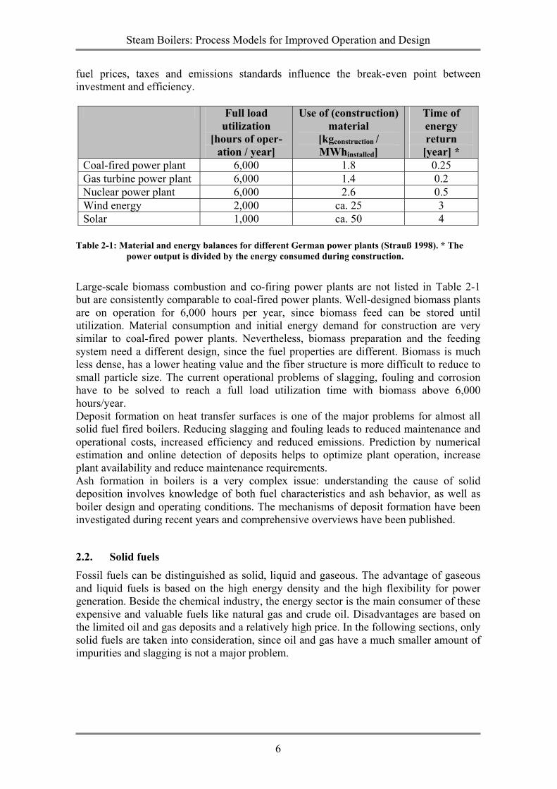
Steam Boilers: Process Models for Improved Operation and Design
6
fuel prices, taxes and emissions standards influence the break-even point between investment and efficiency.
Full load utilization
[hours of oper-ation / year]
Use of (construction) material
[kgconstruction / MWhinstalled]
Time of energy return
[year] * Coal-fired power plant 6,000 1.8 0.25 Gas turbine power plant 6,000 1.4 0.2 Nuclear power plant 6,000 2.6 0.5 Wind energy 2,000 ca. 25 3 Solar 1,000 ca. 50 4
Table 2-1: Material and energy balances for different German power plants (Strauß 1998). * The power output is divided by the energy consumed during construction.
Large-scale biomass combustion and co-firing power plants are not listed in Table 2-1 but are consistently comparable to coal-fired power plants. Well-designed biomass plants are on operation for 6,000 hours per year, since biomass feed can be stored until utilization. Material consumption and initial energy demand for construction are very similar to coal-fired power plants. Nevertheless, biomass preparation and the feeding system need a different design, since the fuel properties are different. Biomass is much less dense, has a lower heating value and the fiber structure is more difficult to reduce to small particle size. The current operational problems of slagging, fouling and corrosion have to be solved to reach a full load utilization time with biomass above 6,000 hours/year. Deposit formation on heat transfer surfaces is one of the major problems for almost all solid fuel fired boilers. Reducing slagging and fouling leads to reduced maintenance and operational costs, increased efficiency and reduced emissions. Prediction by numerical estimation and online detection of deposits helps to optimize plant operation, increase plant availability and reduce maintenance requirements. Ash formation in boilers is a very complex issue: understanding the cause of solid deposition involves knowledge of both fuel characteristics and ash behavior, as well as boiler design and operating conditions. The mechanisms of deposit formation have been investigated during recent years and comprehensive overviews have been published.
2.2. Solid fuels
Fossil fuels can be distinguished as solid, liquid and gaseous. The advantage of gaseous and liquid fuels is based on the high energy density and the high flexibility for power generation. Beside the chemical industry, the energy sector is the main consumer of these expensive and valuable fuels like natural gas and crude oil. Disadvantages are based on the limited oil and gas deposits and a relatively high price. In the following sections, only solid fuels are taken into consideration, since oil and gas have a much smaller amount of impurities and slagging is not a major problem.
Steam Boilers: Process Models for Improved Operation and Design
7
2.2.1. Coal Coal is the most abundant of the fossil fuels and is responsible for about 27 percent of the world’s primary commercial energy use. Coal consists of the altered remains of prehistoric vegetation that originally accumulated as plant material in swamps and peat bogs. Through tectonic movements, the organic material was covered airtight and moved to a geologically deeper position. Elevated temperature and pressure caused biochemical and geochemical processes, which converted the carbonaceous material by dehydrogenation and methanogenesis to peat, brown coal (lignite), hard coals and finally anthracite. Methane and light hydrocarbon gases are vola tized step by step. Coal is, therefore, classified by the degree of metamorphism, which has an influence on its chemical and physical properties. Low rank coals like lignite are typically softer, friable materials with an earthy appearance; high moisture levels and low carbon contents cause a low heating value. Higher rank coals are typically harder and stronger and often have a black vitreous lustre combined with a low moisture and high carbon content. Hard coal is traded worldwide, where a broad spectrum of heating values and impurities is available. The higher water and ash contents and low heating value of lignite limit their use. Economic utilization is only feasible close to the mining area. The use of lignite is under discussion, due to its high CO2 and particle emission. The ratification of the Kyoto Protocol and the implementation of the EU directives for greenhouse gas emissions present a mounting pressure to the coal utilization community to mitigate their CO2 emissions. The magnitude of the problem will require parallel actions to be implemented by the industry; these include options such as the increase in efficiency, co-firing with renewable fuels, and CO2 capture and sequestration. These technologies will be a necessity for coal-based power generation in the medium- and long-term future and can be categorized in three major approaches, namely:
• precombustion capture or fuel decarbonisation; • combustion with nitrogen-free comburent such as oxy-fuel and chemical-looping
combustion; • post-combustion capture with CO2 separation from fluegas.
2.2.2. Biomass Biomass energy was the most primitive energy source employed by our ancestors. Its purpose and use have changed rapidly and, nowadays, biomass fuel includes sawdust, wood chips, bark, straw, cereals, grass, other agricultural waste, as well as aquatic plants, algae, animal waste, waste paper and similar residuals. Biomass offers plenty of advantages for combustion, due to its highly volatile matter and high reactivity. However, it should be mentioned that the carbon content and heating value is low compared to coal. Biomass production is distributed over a large area and collection, preparation and usage demand additional effort. Biomass is a fuel with a less consistent fuel quality, e.g. heating value, moisture content, composition or density vary according to origin and local weather influences. A classification of biomass fuels is necessary to predict the combustion behavior, preferably based on simple test methods. Since the investigation of coal has a long tradition in combustion science, a clear classification system is available. Biomass, with more diversity regarding composition and structure, needs another detailed approach concerning, e.g. different impurities, as well as their inhomogeneous distribution, origin and structure. Test methods include pyrolysis behavior, tar yield and volatile composition, combined with measurements of the yield and composition of the char and its reactivity towards O2. Experimental tools have been developed to characterize the
Steam Boilers: Process Models for Improved Operation and Design
8
fuels in order to predict the deposit behavior (Unterberger 2001). Databases of biomass fuels composition are available. Alkali and alkaline earth metals, in combination with other fuel elements, e.g. silicon and sulfur, and supported by the presence of chlorine, are the origin of undesirable reaction and deposit problems in boilers (Jenkins 1998).
2.2.3. Co-firing Co-firing, the common practice of adding another fuel to a base fuel, is an extension of a traditional fuel blending practice. Many coal-fired power plants were originally designed to combust coal with a narrow range of quality variation from a local producer. Nowadays, reasons for a potential change of fuel include the low availability of the local fuel, cost structure and emission limits (SO2, NOx). The reuse of existing combustion plants for new and alternative fuels is another economic advantage, instead of the construction of brand-new biomass power plants. Comparably low investment costs are required in order to utilize renewable energy as a supplementary fuel, by adjusting the combustion conditions and especially the fuel handling (Demirbas 2004, Ireland 2004). Some European countries support this development with special tax reductions, or fees on air pollution. Fuel blending does not mean that the properties of the mixture are consistent with the properties of the single components. Some phenomena like deposit tendency, emission level or corrosion are intensified or minimized by a certain mixing ratio. Rushdi (2004) reported a non-additive behavior of coal blends as a result of interaction between ash particles within the deposit layer, which cannot be predicted from the source of coal yet. On the other hand, reactions between the species and synergetic effects between the fuels can cause tremendous operational problems. Literature reviews present deposit issues specifically related to the co-firing of coal with biomass fuels (Sami 2001).
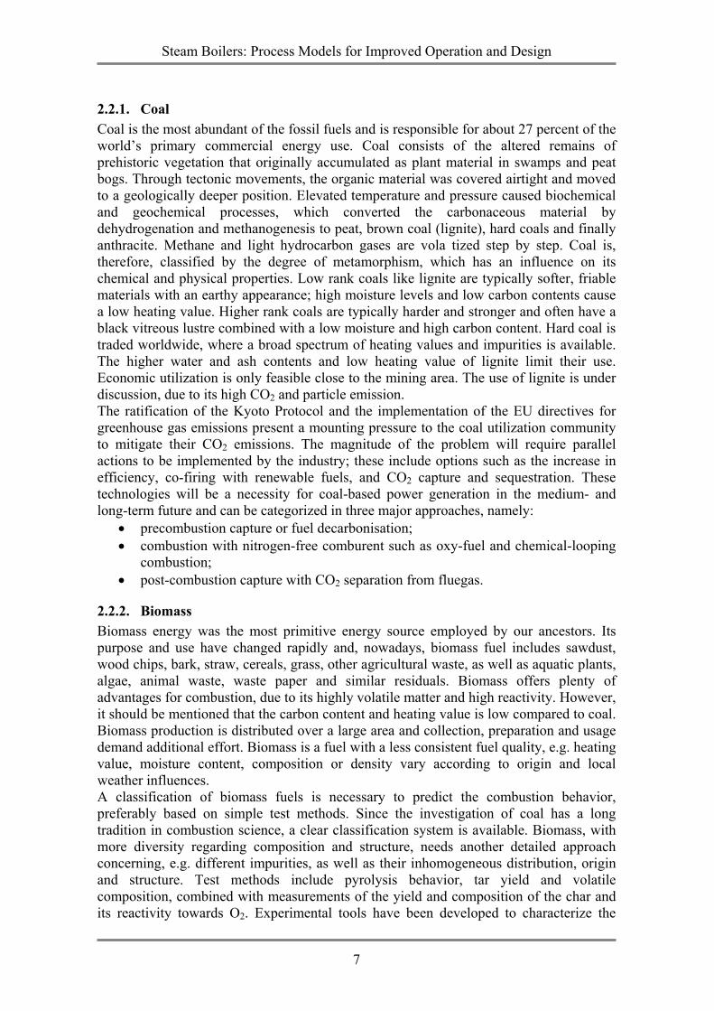
2.3. Furnace design An inadequate design of the combustion chamber in relation to the fuel being burned is one reason for the deposit problem. The factors that have to be considered when designing a boiler are mainly: fuel preparation, heat transfer, boiler size in relation to the heat demand, combustion conditions and soot blowing strategy. Deposit problems appear when these factors have not been considered related to the fuel being burnt (Cortes 1991). Additionally, the current research and development in material sciences leads to extreme steam parameters (up to 720 °C and 350 bar). Austenitic steel based on Ni-Cr-Fe alloys is proven as suitable material and allows higher furnace temperatures.
Figure 2-1: Classification of boiler types (Strauß 1998).
Steam Boilers: Process Models for Improved Operation and Design
9
Different efficient and environmentally friendly combustion technologies are currently in use. Pulverized fuel boilers, fluidized bed boilers and grate-fired boilers are distinguished by the grade of fuel suspension. All three technologies can suffer from deposit problems. Pulverized fuel (PF) combustion is the most common boiler technology for large-scale coal combustion. The fuel is grinded to very small particles and combusted in an entrained flow. The considerable amount of pretreatment of the fuel is a disadvantage of this technology. PF boilers have a high efficiency, due to their relatively high combustion density (0.5-1 MWm-3) and high heat transfer rates (0.1-1 MWm-2). Grate-fired boilers are more widespread for smaller units or when special fuel preparation is difficult. Waste incinerators usually use a grate for combustion if an environmentally safe treatment of the waste is a priority. The shredded fuel is burned on top of the grate. Within the group of grate-fired boilers, one can distinguish boilers with a stationary, a traveling or a vibrating grate. The low boiler efficiency caused by the high level of excess air for complete combustion is the main disadvantage of grate-fired boilers. Fluidized bed combustion (FB) is the most advanced technology, but special attention has to be paid to the operational stability. FB boilers are flexible to all kinds of fuel qualities and a broad range of particle sizes. It is preferred when burning low-grade fuels and when extreme pollution control is required. Fluidized bed can be distinguished by air velocity in a bubbling and circulating bed. The main disadvantage is the fact that both require a high fan capacity. Van den Broek (1996) compared efficiency, investment costs and emission of these boiler types fired solely by biomass. Plants with vibrating grates and circulating fluidized beds turn out to have the highest efficiency at the moment. Nevertheless, none of the existing technologies was found to be superior. In the following chapters, all three technologies are discussed. Extensive literature reviews cover the physical and chemical fundamentals, as well as the operational problems induced by deposits (Couch 1994, Bryers 1996, Raask 1985). Design and redesign of boilers consider minimized NOx emissions in parallel to the deposit problem. Low NOx technology includes primary and secondary methods. An example of a primary method to separate NOx is absorption by activated carbon. Decreasing average combustion temperature by air staging and extending the burnout zone is a proven secondary method to avoid NOx formation. On the other hand, this method increases the deposit problems since volatiles condense in the furnace and flames with sticky particles reach the heat exchanger section. Therefore, NOx reduction and deposit minimization have to be optimized together. A computational fluid dynamic (CFD) model analyzes both during planning and design. The study of particle trajectories provides information about sensitive places for deposition inside the furnace. A CFD-based deposition model for the software Fluent is now available, which was developed in the framework of the Danish Biomass Project (Kaer 2003).
2.4. Ashes
2.4.1. Ash formation, transport and deposition All fossil fuels contain impurities to a certain extent. Sulfur is partly emitted as gaseous sulfur oxides to the fluegas, or is bound to the fly or bottom ash. The presence of sulfur is a potentially severe problem as corrosion and harmful emissions to the atmosphere may
Steam Boilers: Process Models for Improved Operation and Design
10
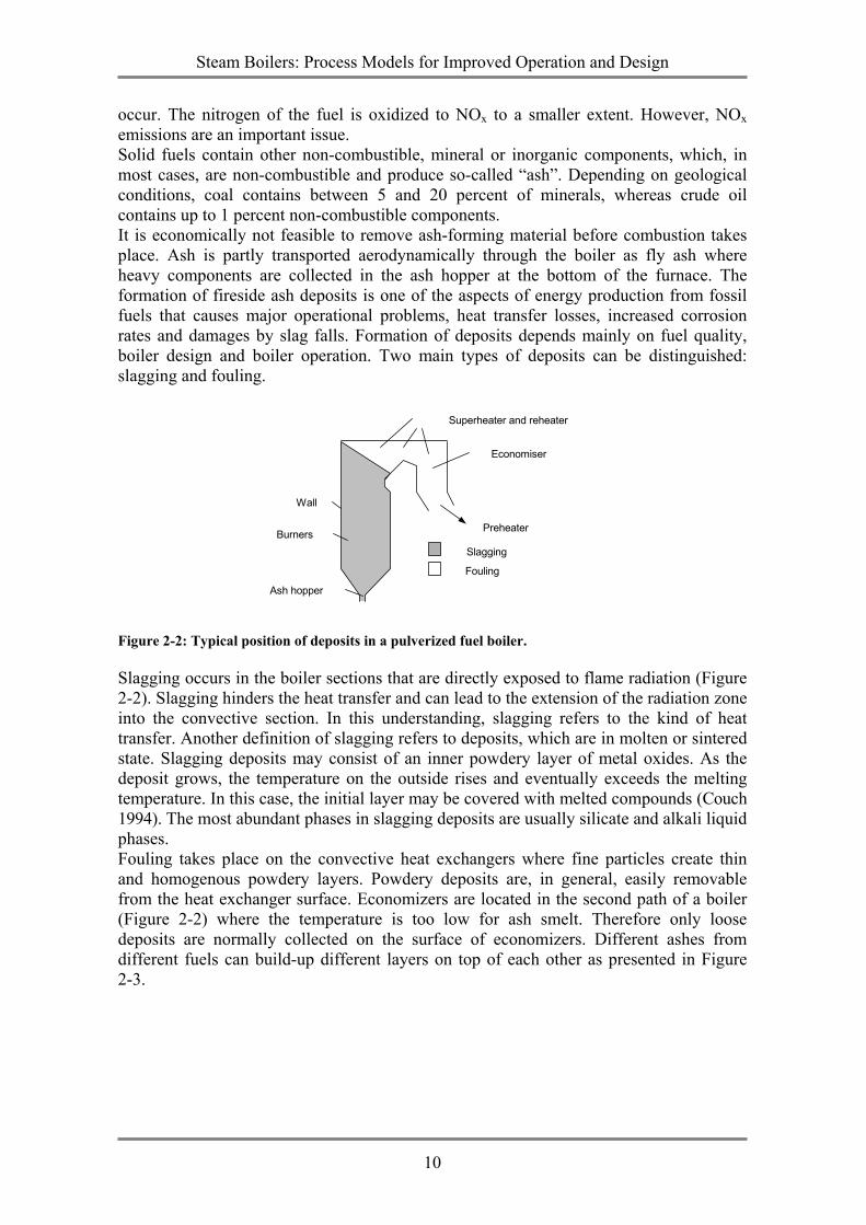
occur. The nitrogen of the fuel is oxidized to NOx to a smaller extent. However, NOx emissions are an important issue. Solid fuels contain other non-combustible, mineral or inorganic components, which, in most cases, are non-combustible and produce so-called “ash”. Depending on geological conditions, coal contains between 5 and 20 percent of minerals, whereas crude oil contains up to 1 percent non-combustible components. It is economically not feasible to remove ash-forming material before combustion takes place. Ash is partly transported aerodynamically through the boiler as fly ash where heavy components are collected in the ash hopper at the bottom of the furnace. The formation of fireside ash deposits is one of the aspects of energy production from fossil fuels that causes major operational problems, heat transfer losses, increased corrosion rates and damages by slag falls. Formation of deposits depends mainly on fuel quality, boiler design and boiler operation. Two main types of deposits can be distinguished: slagging and fouling.
Superheater and reheater
Ash hopper
Burners
Wall
Economiser
Preheater
Slagging
Fouling
Figure 2-2: Typical position of deposits in a pulverized fuel boiler.
Slagging occurs in the boiler sections that are directly exposed to flame radiation (Figure 2-2). Slagging hinders the heat transfer and can lead to the extension of the radiation zone into the convective section. In this understanding, slagging refers to the kind of heat transfer. Another definition of slagging refers to deposits, which are in molten or sintered state. Slagging deposits may consist of an inner powdery layer of metal oxides. As the deposit grows, the temperature on the outside rises and eventually exceeds the melting temperature. In this case, the initial layer may be covered with melted compounds (Couch 1994). The most abundant phases in slagging deposits are usually silicate and alkali liquid phases. Fouling takes place on the convective heat exchangers where fine particles create thin and homogenous powdery layers. Powdery deposits are, in general, easily removable from the heat exchanger surface. Economizers are located in the second path of a boiler (Figure 2-2) where the temperature is too low for ash smelt. Therefore only loose deposits are normally collected on the surface of economizers. Different ashes from different fuels can build-up different layers on top of each other as presented in Figure 2-3.
Steam Boilers: Process Models for Improved Operation and Design
11
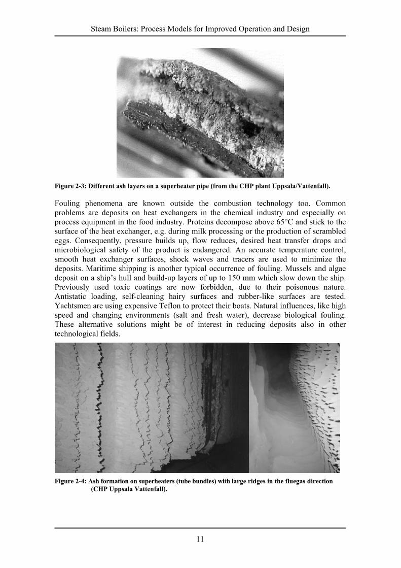
Figure 2-3: Different ash layers on a superheater pipe (from the CHP plant Uppsala/Vattenfall).
Fouling phenomena are known outside the combustion technology too. Common problems are deposits on heat exchangers in the chemical industry and especially on process equipment in the food industry. Proteins decompose above 65°C and stick to the surface of the heat exchanger, e.g. during milk processing or the production of scrambled eggs. Consequently, pressure builds up, flow reduces, desired heat transfer drops and microbiological safety of the product is endangered. An accurate temperature control, smooth heat exchanger surfaces, shock waves and tracers are used to minimize the deposits. Maritime shipping is another typical occurrence of fouling. Mussels and algae deposit on a ship’s hull and build-up layers of up to 150 mm which slow down the ship. Previously used toxic coatings are now forbidden, due to their poisonous nature. Antistatic loading, self-cleaning hairy surfaces and rubber-like surfaces are tested. Yachtsmen are using expensive Teflon to protect their boats. Natural influences, like high speed and changing environments (salt and fresh water), decrease biological fouling. These alternative solutions might be of interest in reducing deposits also in other technological fields.
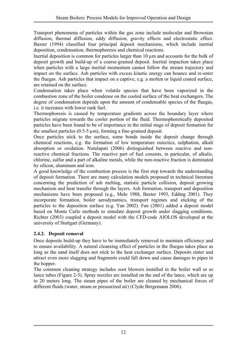
Figure 2-4: Ash formation on superheaters (tube bundles) with large ridges in the fluegas direction
(CHP Uppsala Vattenfall).
Steam Boilers: Process Models for Improved Operation and Design
12
Transport phenomena of particles within the gas zone include molecular and Brownian diffusion, thermal diffusion, eddy diffusion, gravity effects and electrostatic effect. Baxter (1994) classified four principal deposit mechanisms, which include inertial deposition, condensation, thermophoresis and chemical reactions. Inertial deposition is common for particles larger than 10 µm and accounts for the bulk of deposit growth and build-up of a coarse-grained deposit. Inertial impaction takes place when particles with a large inertial momentum cannot follow the stream trajectory and impact on the surface. Ash particles with excess kinetic energy can bounce and re-enter the fluegas. Ash particles that impact on a captive, e.g. a molten or liquid coated surface, are retained on the surface. Condensation takes place when volatile species that have been vaporized in the combustion zone of the boiler condense on the cooled surface of the heat exchangers. The degree of condensation depends upon the amount of condensable species of the fluegas, i.e. it increases with lower rank fuel. Thermophoresis is caused by temperature gradients across the boundary layer where particles migrate towards the cooler portion of the fluid. Thermophoretically deposited particles have been found to be of importance in the initial stage of deposit formation for the smallest particles (0.5-5 µm), forming a fine-grained deposit. Once particles stick to the surface, some bonds inside the deposit change through chemical reactions, e.g. the formation of low temperature eutectics, sulphation, alkali absorption or oxidation. Nutalapati (2006) distinguished between reactive and non-reactive chemical fractions. The reactive part of fuel consists, in particular, of alkalis, chlorine, sulfur and a part of alkaline metals, while the non-reactive fraction is dominated by silicon, aluminum and iron. A good knowledge of the combustion process is the first step towards the understanding of deposit formation. There are many calculation models proposed in technical literature concerning the prediction of ash melting, statistic particle collision, deposit growing mechanism and heat transfer through the layers. Ash formation, transport and deposition mechanisms have been proposed (e.g., Melo 1988, Baxter 1993, Edding 2001). They incorporate formation, boiler aerodynamics, transport regimes and sticking of the particles to the deposition surface (e.g. Yan 2002). Fan (2001) added a deposit model based on Monte Carlo methods to simulate deposit growth under slagging conditions. Richter (2003) coupled a deposit model with the CFD-code AIOLOS developed at the university of Stuttgart (Germany).
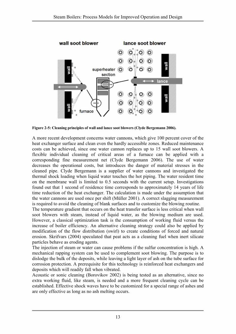
2.4.2. Deposit removal Once deposits build-up they have to be immediately removed to maintain efficiency and to ensure availability. A natural cleansing effect of particles in the fluegas takes place as long as the sand itself does not stick to the heat exchanger surface. Deposits sinter and attract even more slagging and fragments could fall down and cause damages to pipes in the hopper. The common cleaning strategy includes soot blowers installed in the boiler wall or as lance tubes (Figure 2-5). Spray nozzles are installed on the end of the lance, which are up to 20 meters long. The steam pipes of the boiler are cleaned by mechanical forces of different fluids (water, steam or pressurized air) (Clyde Bergemann 2006).
Steam Boilers: Process Models for Improved Operation and Design
13
Figure 2-5: Cleaning principles of wall and lance soot blowers (Clyde Bergemann 2006).
A more recent development concerns water cannons, which give 100 percent cover of the heat exchanger surface and clean even the hardly accessible zones. Reduced maintenance costs can be achieved, since one water cannon replaces up to 15 wall soot blowers. A flexible individual cleaning of critical areas of a furnace can be applied with a corresponding fine measurement net (Clyde Bergemann 2006). The use of water decreases the operational costs, but introduces the danger of material stresses in the cleaned pipe. Clyde Bergemann is a supplier of water cannons and investigated the thermal shock loading when liquid water touches the hot piping. The water resident time on the membrane wall is limited to 0.5 seconds with the current setup. Investigations found out that 1 second of residence time corresponds to approximately 14 years of life time reduction of the heat exchanger. The calculation is made under the assumption that the water cannons are used once per shift (Müller 2001). A correct slagging measurement is required to avoid the cleaning of blank surfaces and to customize the blowing routine. The temperature gradient that occurs on the heat transfer surface is less critical when wall soot blowers with steam, instead of liquid water, as the blowing medium are used. However, a classical optimization task is the consumption of working fluid versus the increase of boiler efficiency. An alternative cleaning strategy could also be applied by modification of the flow distribution (swirl) to create conditions of forced and natural erosion. Skrifvars (2004) speculated that peat acts as a cleaning fuel when inert silicate particles behave as eroding agents. The injection of steam or water can cause problems if the sulfur concentration is high. A mechanical rapping system can be used to complement soot blowing. The purpose is to dislodge the bulk of the deposits, while leaving a light layer of ash on the tube surface for corrosion protection. A prerequisite for this technology is reinforced heat exchangers and deposits which will readily fall when vibrated. Acoustic or sonic cleaning (Borovikov 2002) is being tested as an alternative, since no extra working fluid, like steam, is needed and a more frequent cleaning cycle can be established. Effective shock waves have to be customized for a special range of ashes and are only effective as long as no ash melting occurs.
Steam Boilers: Process Models for Improved Operation and Design
14
2.5. Deposit characterization Ash deposits can be investigated qualitatively and quantitatively and analyzed offline and online.
2.5.1. Offline analysis Laboratory analyses of fuel and ash are typical examples of offline tests. Historically, the classification of ashes started with the industrial use of hard coal. Deposit prediction, based on ash analyses, is the most traditional method. Standard tables for indices were developed, based on elementary analysis combined with softening and flow temperatures. The ash analysis suffers from 5 main disadvantages:
• Fuel analysis is normally carried out only for batches and may not be fully representative for the entire process. To collect a sufficient amount of deposits the probe has to be installed inside the furnace for several hours. In addition, it has to be assumed that the fuel has a homogeneous composition during the test. Dis-continuities of the process are reflected as an inhomogeneous deposit. As a consequence, the tests are rarely repeatable and reproducible.
• The tests analyze the ashes after combustion. A prediction would be possible if the fuel was classified for its deposit probability before combustion. However, a mineral analysis of ashes is cheaper than an elemental analysis of fuels.
• Due to the high combustion temperature, ashes can only be analyzed after cooling down the probe. Cooling can cause changes to the structure, chemical processes or re-crystallization of the deposits.
• The circumstances of the test are unequal to the conditions in the critical parts of the furnace. The test does not take into account properly the furnace geometry, the burner setup and the air ratio which have a major influence on the ash quality.
• The development of dimensionless indices for deposit prediction is restricted by the great number of possible influences and the existence of eutectica. E.g. a great number of complex phase diagrams for mixtures of FeO-SiO2-Al2O3 and CaO-SiO2-Al2O3 have been developed.
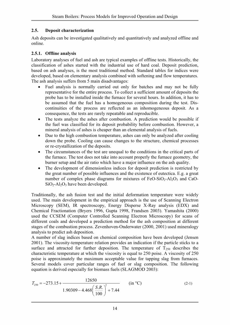
Traditionally, the ash fusion test and the initial deformation temperature were widely used. The main development in the empirical approach is the use of Scanning Electron Microscopy (SEM), IR spectroscopy, Energy Disperse X-Ray analysis (EDX) and Chemical Fractionation (Bryers 1996, Gupta 1998, Frandsen 2003). Yamashita (2000) used the CCSEM (Computer Controlled Scanning Electron Microscopy) for scans of different coals and developed a prediction method for the ash composition at different stages of the combustion process. Zevenhoven-Onderwater (2000, 2001) used mineralogy analysis to predict ash deposition. A number of slag indices based on chemical composition have been developed (Jensen 2001). The viscosity-temperature relation provides an indication if the particle sticks to a surface and attracted for further deposition. The temperature of T250 describes the characteristic temperature at which the viscosity is equal to 250 poise. A viscosity of 250 poise is approximately the maximum acceptable value for tapping slag from furnaces. Several models cover particular ranges of fuel or slag composition. The following equation is derived especially for biomass fuels (SLAGMOD 2003):
250 212650273.15
. .1.90309 4.468 7.44100
TS R
= − + − +
(in °C) (2-1)
Steam Boilers: Process Models for Improved Operation and Design
15
where the silica ratio (SR) is defined as:
( ) MgOCaOOFeequivalentSiOSiOSR
+++×=
322
2100 (2-2)
and
( ) OFeFeOOFeOFeequivalent 43.111.13232 ++= . (2-3)
the values of the oxides are in weight percent.
Slagging Tendencies/Values Index Low High
T250 of ash, °C > 1370 <1200 Silica Ratio S.R. >90 <75 Table 2-2: Ash viscosity (Juniper 1996).
A widely used predictor for the deposition behavior, based on laboratory ash analysis, is the base-to-acid ratio RB/A, where ‘base’ and ‘acid’ are simply the sums of the weight of the percentages of the considered basic and acidic oxides:
( )( )2322
2232/ %
%TiOOAlSiO
OKONaMgOCaOOFeR AB ++++++
= . (2-4)
Slagging Tendencies/Values Index Formula/definition Low Medium High Severe
Base-acid ratio (RB/A)
( )( )2322
2232
%%
TiOOAlSiOOKONaMgOCaOOFe
++++++
< 0.5 (<0.09) 0.5-1.0 ← 1.0-1.75 →
(>0.3)
Slagging Factor (RS)
dryAB SR / < 0.6 0.6-2.0 2.0-2.6 > 2.6
Iron-calcium ratio (I/C)
CaOOFe
%% 32
< 0.3
>3.0
Silica-alumina ratio (S/A) 32
2
%%
OAlSiO
Low ↔ High
Lignitic Factor (LF)
( )32%
%OFeMgOCaO +
Dolomite percentage (DP)
2 3 2 2
100 CaO MgOFe O CaO MgO Na O K O
+×
+ + + +
Table 2-3: Slagging Propensity (Juniper 1996).
Viscosity is a measure of the resistance of a fluid to deform under shear stress. Ash viscosity tends to be parabolic with respect to RB/A, reaching a minimum at intermediate values (melting point eutectica). For coal, a minimum is frequently located in the vicinity of RB/A equal to a value from 0.75 to 1, but for biomass, the minimum tends to appear at lower values. The value of RB/A was empirically formulated, but, nowadays, is under
Steam Boilers: Process Models for Improved Operation and Design
16
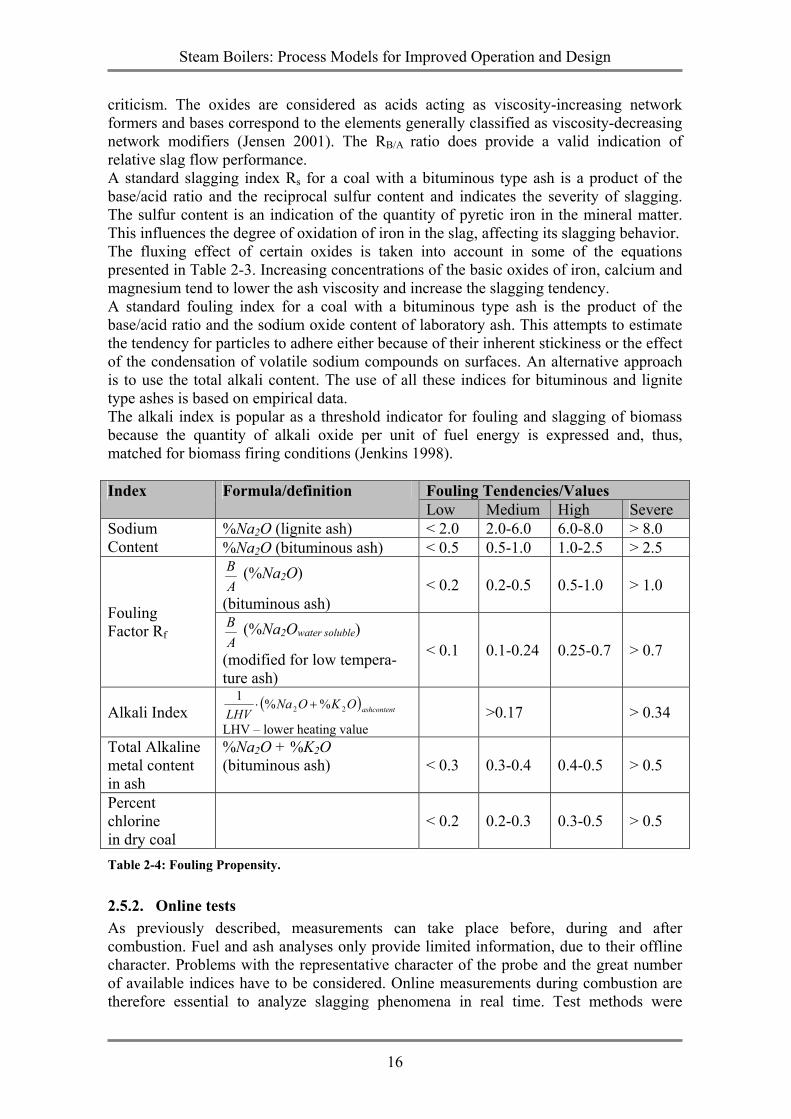
criticism. The oxides are considered as acids acting as viscosity-increasing network formers and bases correspond to the elements generally classified as viscosity-decreasing network modifiers (Jensen 2001). The RB/A ratio does provide a valid indication of relative slag flow performance. A standard slagging index Rs for a coal with a bituminous type ash is a product of the base/acid ratio and the reciprocal sulfur content and indicates the severity of slagging. The sulfur content is an indication of the quantity of pyretic iron in the mineral matter. This influences the degree of oxidation of iron in the slag, affecting its slagging behavior. The fluxing effect of certain oxides is taken into account in some of the equations presented in Table 2-3. Increasing concentrations of the basic oxides of iron, calcium and magnesium tend to lower the ash viscosity and increase the slagging tendency. A standard fouling index for a coal with a bituminous type ash is the product of the base/acid ratio and the sodium oxide content of laboratory ash. This attempts to estimate the tendency for particles to adhere either because of their inherent stickiness or the effect of the condensation of volatile sodium compounds on surfaces. An alternative approach is to use the total alkali content. The use of all these indices for bituminous and lignite type ashes is based on empirical data. The alkali index is popular as a threshold indicator for fouling and slagging of biomass because the quantity of alkali oxide per unit of fuel energy is expressed and, thus, matched for biomass firing conditions (Jenkins 1998).
Fouling Tendencies/Values Index Formula/definition Low Medium High Severe
%Na2O (lignite ash) < 2.0 2.0-6.0 6.0-8.0 > 8.0 Sodium Content %Na2O (bituminous ash) < 0.5 0.5-1.0 1.0-2.5 > 2.5
AB (%Na2O)
(bituminous ash) < 0.2 0.2-0.5 0.5-1.0 > 1.0
Fouling Factor Rf A
B (%Na2Owater soluble)
(modified for low tempera-ture ash)
< 0.1 0.1-0.24 0.25-0.7 > 0.7
Alkali Index ( )ashcontentOKONaLHV 22 %%1
+⋅
LHV – lower heating value >0.17 > 0.34
Total Alkaline metal content in ash
%Na2O + %K2O (bituminous ash) < 0.3 0.3-0.4 0.4-0.5 > 0.5
Percent chlorine in dry coal
< 0.2 0.2-0.3 0.3-0.5 > 0.5
Table 2-4: Fouling Propensity.
2.5.2. Online tests As previously described, measurements can take place before, during and after combustion. Fuel and ash analyses only provide limited information, due to their offline character. Problems with the representative character of the probe and the great number of available indices have to be considered. Online measurements during combustion are therefore essential to analyze slagging phenomena in real time. Test methods were
Steam Boilers: Process Models for Improved Operation and Design
17
developed for lab and pilot scale furnaces (Kiel 1999, Robinson 1999, 2001, Heinzel 1998) up to full-scale boilers (Cortes 1991, Miles 1996, Garret 1985). Tests and instrumentation needed to assess deposit impacts of solid fuels have been described (EPRI's Guidelines for Fireside Testing in Coal-Fired Power Plants, 1988), including furnace exit gas temperatures, other temperature measurements through the system, deposit probes, radiant heat flux measurements, direct observations by camera or video, furnace wall measurements, coal feed and ash deposit sampling (Couch 1994). Different probes to monitor gas-side fouling build-ups had already been identified in previous surveys, including local heat flux meters, mass accumulation probes designed to quantitatively determine the mass of the deposit, optical devices limited to laboratory investigations and deposition probes to collect deposits on a qualitative basis. One of the main effects of deposit formation on boiler operations is the reduction of heat transfer between the fireside and the water-steam side. That results in a remarkable increase of the fluegas temperature and loss in efficiency. The furnace exit gas temperature (FEGT) is therefore one of the major parameters for analyzing deposits. It is a particularly difficult task to measure fluegas temperatures up to 1600 °C. Thermo-couples are normally installed close to the wall and exposed to radiation and slagging. More expensive, but less erroneous, solutions include infrared pyrometry or acoustic pyrometry. Acoustic pyrometry is one of the techniques that can provide information about temperature (FEGT) and fluegas velocity in the furnace (Sielschott 1995, 1997, Blug 2002). It is a tomographic method and the aim is to identify the temperature distribution in a horizontal layer of the combustion chamber. This method is non-intrusive to the measured medium and radiation does not affect the measurement. Acoustic pyrometry is based on measuring the propagation time of sound. From this, the mean temperature on each path can be computed, which is given by the following equation (Blug 2002):
2 1m
LTBτ
=
(2-5)
where mT is the average (mean) temperature, L the length of the temperature path (distance between transmitter and receiver), τ is the flying time of a sound signal and B is the acoustic coefficient. The acoustic coefficient can be calculated from the following equation (Blug 2002):
RBMκ
= (2-6)
where κ is an adiabatic exponent, R the universal gas constant and M the molecular weight of the gas. The measurement error does not only depend on the length of the path, but, also, on the composition of the fluegas and its density. Hence, the error of the measurements can be in the range from 2 to 15 percent, with the biggest deviations close to the walls, due to geometrical and physical problems (Blug 2002). Thermal absorption diagnostics can be done via direct measurement of heat flux by instrumentation installed in the heat transfer tubes and through mass and energy calculations. Further developments are needed in both methods. The uncertainty of heat flux measurements is largely due to the calibration problems and because the measurements only cover a small area of the furnace. Data interpretation and statistical analysis therefore need to be improved (Valero 1996).
Steam Boilers: Process Models for Improved Operation and Design
18
The heat transfer is influenced by the thermal properties of the deposits, especially the total emissivity and thermal conductivity, which accounts for radiation-convection-conduction through the deposit. These thermal properties depend on the processes and on their physical and chemical character. A number of researchers have measured the thermal conductivity of ashes obtained from full-scale power plants. This parameter depends on physical structure, temperature, porosity, sintering time and, to a smaller extent, chemical composition. Thermal conductivity has been identified as increasing with rising temperature. It is higher for sintered than for unsintered ash samples; it changes irreversibly with temperature and sintering time; it increases with decreasing porosity and is only slightly influenced by chemical composition. Models have been developed to predict thermal conductivity (Rezaei 2000) and to assess the dependence of average thermal conductivity on macroscopic and microscopic structural properties (Baxter 1993, Robinson 2001). A technique has been developed to make in-situ, time resolved measurements of the effective thermal conductivity of ash deposits formed under simulated fouling conditions (Robinson 1999, 2001). FTIR has been used online to identify the changing composition of ash deposits as they form and results have been related to strength and tenacity of the deposits (Baxter 1993). Optical methods have been reported and research is currently being done in this direction. The thickness and growing rate of the slag layer can be monitored online with an appro-priate image acquisition and treatment system. Different technologies are proposed: high temperature cameras, thermographs and edge detection (Derichs 1999) and advanced laser diagnostics (Baxter 2000). Other methods have taken into account the hydrodynamic functioning of heat exchangers, measuring increasing pressure drops due to fouling. Online tests can be executed in full-scale, pilot-scale or laboratory-scale experiments. Measurement conditions are more standardized, defined and stable in smaller units, but only show a restricted view of the deposit phenomena. This chapter summarized some ash and fuel tests. Even if not all offline and online methods were presented, a demand for research in in-situ and online tests is evident. At the moment, numerous institutes worldwide still do research in the field of slagging and fouling detection. One goal of this thesis is, therefore, to participate in the development of an online model in order to measure slagging inside the furnace. A process-monitoring tool is able to recognize the status of the deposit and provide useful information to start countermeasures and to optimize the cleaning strategy. Additionally, information derived from the development of the process-monitoring model will be used to continue with a dynamic approach. Both applications share some common characteristics and submodules.
Steam Boilers: Process Models for Improved Operation and Design
19
3. PROCESS MONITORING MODELS AS A TOOL FOR ONLINE
DEPOSIT DETECTION
Overview The previous literature review showed a demand for online identification of slagging and fouling, and gave an overview of ongoing research activities. The EU project “Slagging and fouling prediction by dynamic boiler modeling” (SLAGMOD) was founded to intensify the research, especially in biomass combustion. A thermodynamic and deposit-monitoring program is developed in the framework of the SLAGMOD project. The monitoring model is able to measure a so-called deposit parameter online, simultanously enabling the operator to optimize the soot blowing effort.
3.1. Classification of process models
Eykhoff (1974) defined modeling as a representation of the essential aspects of a system, which presents knowledge of that state in a usable form. Modeling is an abstraction of the reality, with different degrees of complexity, purposes and strategies. A theoretical approach, based on mathematical equations, can be distinguished from an experimental approach in which the process data is identified. This classification is, in a technical jargon, called white box and black box models. A white or clear box model gives the physical insight into the process based on the laws of conservation. A black box model represents the input/output relationship of the process in an empirical way. In technical processes, detailed empirical information is limited. Thus black box models have to be used for identification of the processes, as they do not require a priori knowl-edge of the process. White box models are well established as a design tool when meas-ured process information is absent and the design is based on physical laws. Gray box models represent a wide range of combinations of white and black box models, and are in fact characteristic for the models used in this thesis. Steady state or static models only take into account the process under the assumption of static conditions. Even in cases of an online application, they do not take into account any dynamics, i.e., accumulation of energy and mass. Steady state models with a limited complexity can be employed as online monitoring tools due to their minimal computational time demand. These simplified models are a compromise between real time capability and necessary complexity. Dynamic simulation involves the solution of differential equations, with time as an inde-pendent variable. In thermal processes these differential equations are based on the physical conservation laws. Dynamic models can be used to study start up, shut down behavior, load changes and system responses during pipe breaks, feed water pump loss, burner level failure or a turbine trip. They have proven to be an indispensable tool in the study of material stresses, interaction of different units, and for emergency case prediction in nuclear power plants. Regarding the time dependency of the application, models can be divided into offline and online. Models which are online are under the direct control of another device, i.e., in this case the data logging system. Online models are coupled in real time with the process data and give an immediate evaluation. Offline models are independent from the process time scale, and are used for design or post processing of data. Models are further characterized with regard to linearity (linear and non-linear models), homogeneity (distributed and lumped parameter models), and the type of time discretization (continuous time and discrete event models).
Steam Boilers: Process Models for Improved Operation and Design
20
3.2. Application It is necessary to develop comprehensive boiler monitoring systems and better instru-mentation to improve the understanding of operating conditions and to provide informa-tion that will help the operator minimize ash deposition problems (Couch 1994). Diagnostic systems of power plants have been a topic of investigation for several years. Practical use and implementation into the control and operating system was limited for a long time due to an uncertainty of correlated values (Sturm 2003). The implementation of diagnostic tools requires a certain amount of experimental data since the output of a neural network or any other data refining system is based on a long record of observed past responses (Díez 2001). Bartels (2006) reported from a sample time of 8 months after the system had collected sufficient reference data and the control and optimization system could move to an automatic mode. A neural network does not replace installed measurements, but is dependent as well on adequate heat transfer measurements (Teruel 2005). Monitoring programs are available which re-calculate process data in order to draw conclusions about the deposit status or the current heating value of the fuel, which is normally not measured online. Kessel (2003) presented a calorific value sensor for waste incineration, which take knowledge of the conversion process into account in order to determine online the heating value and water content of the fuel. These programs do not take into account any microscopic deposit phenomena, but are based on overall heat and mass balances. This makes them a strong tool to operate and optimize the plant, but can neither avoid nor explain the initial deposit build-up. Fouling-monitor and alarm software usually aims at:
• Alerting operators to a potential impending fouling problem. • Identifying adverse boiler firing practice that increases the risk of fouling. • Displaying graphs of key parameters to aid in fouling event diagnostics. • Keeping a record of alarms for subsequent analysis.
Different kinds of commercial software are used at present e.g., the FEMA® software (Thompson 2000), DIGEST (Siemens), KEDI (Babcock), SR4 (KETEK) or FACOS (Clyde Bergemann). KEDI works with fixed limits for heat transfer resistance at which soot blowing is activated. This makes it an easy tool to handle, but it neglects the interaction between heat exchangers. Selective soot blowing of one heat exchanger affects the heat balance of other heat exchangers. Soot blowing controlled by the SR4 system is not based on fixed thermodynamics but on economical limits; the cost of soot blowing and the use of steam are compared with the benefit of the total efficiency. Material limitations, i.e., thermal stresses and dynamic fatigue as well as burner stability are additional criteria in SR4 (Mensonidis 1999). FACOS is an integrated intelligent solution for optimized operation. This modular system consists of a cleaning management element, a strategy calculator, a report block, a database with reference modes and tube lifetime estimation. The input information to the program is extended with advanced heat flux measurements, such as a Smart Flux TM Sensor (Clyde Bergemann 2006). Advanced measurements are integrated with the logic system. Research demand for methods for online detection of deposits in large-scale boilers derives from previous and ongoing activities, as well as experience from the operation of biomass-fired boilers. Online information about the deposits being formed in the boiler is of importance to operators for the application of operational changes, cleaning procedures and use of different fuel qualities ensuring low risk of slagging, fouling or corrosion phenomena. Further development takes place in the direction of a finer resolution in
Steam Boilers: Process Models for Improved Operation and Design
21
parallel with improvements of computational technology. Computational Fluid Dynamic calculations gain importance not only as design tools, but also as a tool for analysis and monitoring. The program AshProSM is an example of a CFD code coupled with ash for-mation, transport and deposition sub-routines (Ma 2006). The main objective of the modeling activities in this work is to visualize deposit tenden-cies by applying an online monitoring model. Governing equations (mass and energy balances) are applied in order to model heat transfer between the fluegases and the water/steam cycle and deposit formation on heat exchanger surfaces. The model is intended to characterize the heat transfer of the evaporator, economizer, superheater (SH) and reheater (RH) sections of the boiler. Analyzing results and measured data of the plant helps to reveal the deposit tendency at an early stage of the process. The calculations are based on accessible plant data, e.g., pressure, temperature and flow measurements. Data mining is a non-trivial process of identifying valid, potentially useful and understandable patterns in data sources. Since not all data is available or are difficult to measure, some additional calculations have to be made. This is applicable for fluegas temperatures, which are calculated for the high temperature zone of the boiler. In this way the model could also serve as a soft sensor of the heating or calorific value. This is particularly important for waste combustion, where fuel quality changes rapidly and online measurements are usually unavailable (Kessel 2001). The fuel flow is not measured directly either, and is instead estimated over the heat bal-ance. Zhang (2003) reported a pulverized fuel measurement which could serve to gain a better understanding of the process in advance, especially the influence of the individual burners. For fast changing fuel qualities, e.g., waste or biomass, a neural network can pre-dict the combustion behavior (Dong 2002). All monitoring tools demand permanent maintenance once they are installed, i.e., cali-bration and clean up of measurements, check of plausibility and adaptation to changing design and environment.
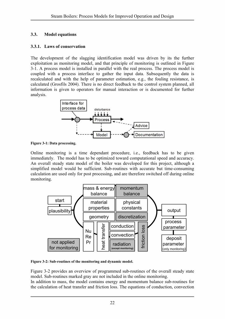
Steam Boilers: Process Models for Improved Operation and Design
22
3.3. Model equations
3.3.1. Laws of conservation The development of the slagging identification model was driven by its the further exploitation as monitoring model, and that principle of monitoring is outlined in Figure 3-1. A process model is installed in parallel with the real process. The process model is coupled with a process interface to gather the input data. Subsequently the data is recalculated and with the help of parameter estimation, e.g., the fouling resistance, is calculated (Grosfils 2004). There is no direct feedback to the control system planned, all information is given to operators for manual interaction or is documented for further analysis.
Figure 3-1: Data processing.
Online monitoring is a time dependant procedure, i.e., feedback has to be given immediately. The model has to be optimized toward computational speed and accuracy. An overall steady state model of the boiler was developed for this project, although a simplified model would be sufficient. Sub-routines with accurate but time-consuming calculation are used only for post processing, and are therefore switched off during online monitoring.
Figure 3-2: Sub-routines of the monitoring and dynamic model.
Figure 3-2 provides an overview of programmed sub-routines of the overall steady state model. Sub-routines marked gray are not included in the online monitoring. In addition to mass, the model contains energy and momentum balance sub-routines for the calculation of heat transfer and friction loss. The equations of conduction, convection
plausibility output
NuRePr
heat
tran
sfer
radiation (except monitoring)
conduction
convection
frict
ion
loss
momentumbalance
mass & energybalance
not applied for monitoring
process parameter
depositparameter (only monitoring)
physicalconstants
materialproperties
discretization
start
geometryplausibility output
NuRePr
heat
tran
sfer
radiation (except monitoring)
conduction
convection
frict
ion
loss
momentumbalance
mass & energybalance
not applied for monitoring
process parameter
depositparameter (only monitoring)
physicalconstants
materialproperties
discretization
start
geometry
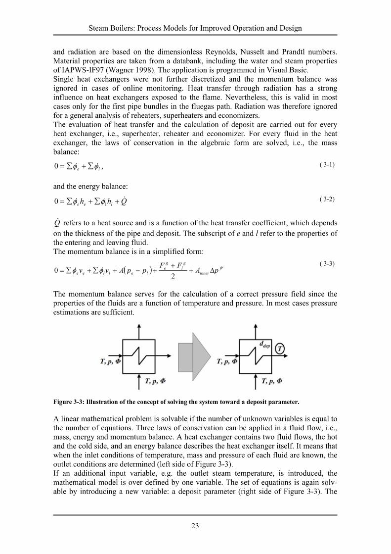
Steam Boilers: Process Models for Improved Operation and Design
23
and radiation are based on the dimensionless Reynolds, Nusselt and Prandtl numbers. Material properties are taken from a databank, including the water and steam properties of IAPWS-IF97 (Wagner 1998). The application is programmed in Visual Basic. Single heat exchangers were not further discretized and the momentum balance was ignored in cases of online monitoring. Heat transfer through radiation has a strong influence on heat exchangers exposed to the flame. Nevertheless, this is valid in most cases only for the first pipe bundles in the fluegas path. Radiation was therefore ignored for a general analysis of reheaters, superheaters and economizers. The evaluation of heat transfer and the calculation of deposit are carried out for every heat exchanger, i.e., superheater, reheater and economizer. For every fluid in the heat exchanger, the laws of conservation in the algebraic form are solved, i.e., the mass balance:
le φφ ∑+∑=0 , ( 3-1)
and the energy balance:
Qhh lee&+∑+∑= 10 φφ ( 3-2)
Q& refers to a heat source and is a function of the heat transfer coefficient, which depends on the thickness of the pipe and deposit. The subscript of e and l refer to the properties of the entering and leaving fluid. The momentum balance is in a simplified form:
( ) frinner
gl
ge
lellee pAFF
ppAvv ∆++
+−+∑+∑=2
0 φφ ( 3-3)
The momentum balance serves for the calculation of a correct pressure field since the properties of the fluids are a function of temperature and pressure. In most cases pressure estimations are sufficient.
Figure 3-3: Illustration of the concept of solving the system toward a deposit parameter.
A linear mathematical problem is solvable if the number of unknown variables is equal to the number of equations. Three laws of conservation can be applied in a fluid flow, i.e., mass, energy and momentum balance. A heat exchanger contains two fluid flows, the hot and the cold side, and an energy balance describes the heat exchanger itself. It means that when the inlet conditions of temperature, mass and pressure of each fluid are known, the outlet conditions are determined (left side of Figure 3-3). If an additional input variable, e.g. the outlet steam temperature, is introduced, the mathematical model is over defined by one variable. The set of equations is again solv-able by introducing a new variable: a deposit parameter (right side of Figure 3-3). The
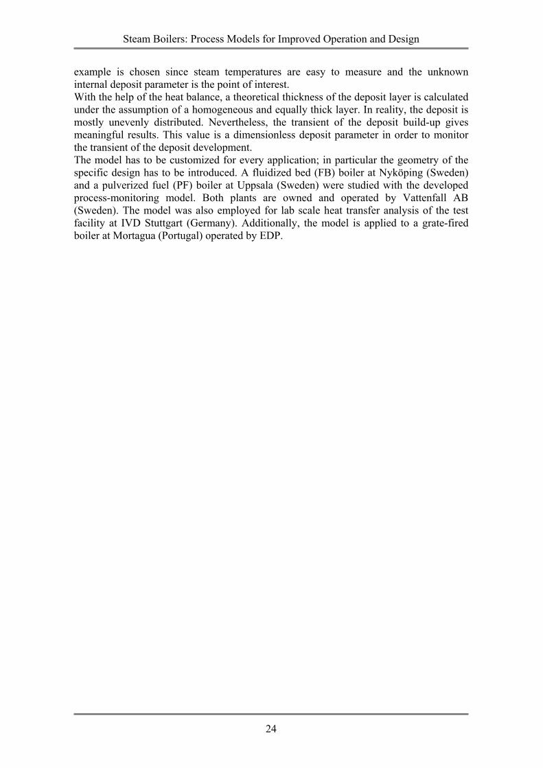
Steam Boilers: Process Models for Improved Operation and Design
24
example is chosen since steam temperatures are easy to measure and the unknown internal deposit parameter is the point of interest. With the help of the heat balance, a theoretical thickness of the deposit layer is calculated under the assumption of a homogeneous and equally thick layer. In reality, the deposit is mostly unevenly distributed. Nevertheless, the transient of the deposit build-up gives meaningful results. This value is a dimensionless deposit parameter in order to monitor the transient of the deposit development. The model has to be customized for every application; in particular the geometry of the specific design has to be introduced. A fluidized bed (FB) boiler at Nyköping (Sweden) and a pulverized fuel (PF) boiler at Uppsala (Sweden) were studied with the developed process-monitoring model. Both plants are owned and operated by Vattenfall AB (Sweden). The model was also employed for lab scale heat transfer analysis of the test facility at IVD Stuttgart (Germany). Additionally, the model is applied to a grate-fired boiler at Mortagua (Portugal) operated by EDP.
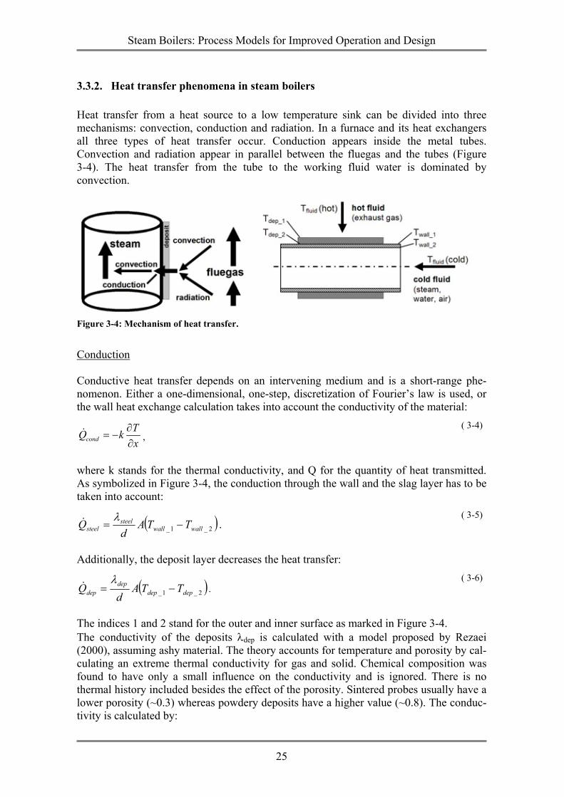
Steam Boilers: Process Models for Improved Operation and Design
25
3.3.2. Heat transfer phenomena in steam boilers Heat transfer from a heat source to a low temperature sink can be divided into three mechanisms: convection, conduction and radiation. In a furnace and its heat exchangers all three types of heat transfer occur. Conduction appears inside the metal tubes. Convection and radiation appear in parallel between the fluegas and the tubes (Figure 3-4). The heat transfer from the tube to the working fluid water is dominated by convection.
Figure 3-4: Mechanism of heat transfer.
Conduction Conductive heat transfer depends on an intervening medium and is a short-range phe-nomenon. Either a one-dimensional, one-step, discretization of Fourier’s law is used, or the wall heat exchange calculation takes into account the conductivity of the material:
condTQ kx
∂= −
∂& ,
( 3-4)
where k stands for the thermal conductivity, and Q for the quantity of heat transmitted. As symbolized in Figure 3-4, the conduction through the wall and the slag layer has to be taken into account:
( )2_1_ wallwallsteel
steel TTAd
Q −=λ& .
( 3-5)
Additionally, the deposit layer decreases the heat transfer:
( )2_1_ depdepdep
dep TTAd
Q −=λ& .
( 3-6)
The indices 1 and 2 stand for the outer and inner surface as marked in Figure 3-4. The conductivity of the deposits λdep is calculated with a model proposed by Rezaei (2000), assuming ashy material. The theory accounts for temperature and porosity by cal-culating an extreme thermal conductivity for gas and solid. Chemical composition was found to have only a small influence on the conductivity and is ignored. There is no thermal history included besides the effect of the porosity. Sintered probes usually have a lower porosity (~0.3) whereas powdery deposits have a higher value (~0.8). The conduc-tivity is calculated by:
Steam Boilers: Process Models for Improved Operation and Design
26
0.750.0038g Tλ = for the gaseous phase and ( 3-7)
1.10.0015s Tλ = for the solid phase. ( 3-8) By assuming a parallel deposition layer, the overall heat transfer definition is:
1
1
depg s
λλ λε ε
=+
−
, ( 3-9)
Where porosityε is a measure of the void spaces of the material. Convection The calculation of the convective heat transfer is based on the Prandtl-Nusselt relation as described in the VDI-Wärmeatlas (1993). The heat transfer coefficient α can be expressed as a function of the Nusselt number:
LNu αλ
= . ( 3-10)
with L for the geometric equivalent diameter and λ as conductivity. An empirical formula for the Nusselt number of a turbulent flow inside a pipe is calculated with the Gnielinski correlation (VDI- Wärmeatlas 1993),
( )( )
2 / 3
2 / 3
/ 8 Re 1000 Pr1
1 12.7 / 8 Pr 1id
Nul
ξ
ξ
− = + + −
( 3-11)
which is assumed to be valid down to a Reynolds number equal to 2300. The Reynolds number is the most important non-dimensional number for a fluid flow problem. By defi-nition, the Reynolds number is:
Re wLρη
= ( 3-12)
Where ρ and η are fluid density and dynamic viscosity respectively, w is the fluid veloc-ity and L is the characteristic length. The Prandtl number (Pr) is expressed as:
Pr pcηλ
= ( 3-13)
with cp as specific heat. And the so-called Fanning friction factor or drag coefficient cor-relation ξ:
( ) 2101.82 log Re 1.64ξ −= − . ( 3-14)
Figure 3-4 is introduced for a better understanding of the heat transfer on a typical heat transfer pipe such as in an economizer, superheater or reheater, including deposit formed on the surface. For convective heat transfer the heat flux can be calculated as:
Steam Boilers: Process Models for Improved Operation and Design
27
( )fluidwallconv TTAQ −= α& . ( 3-15)
The wall and fluid temperature corresponds to the average temperature of the volume element. The calculation of the heat transfer coefficient of the fluegas flow is similar. The Nusselt number for a pipe in cross flow is defined as:
( )2 20.3a lam turbNu f Nu Nu= + + . ( 3-16)
The correction factor fa takes the order of pipes into account. The Nusselt number in case of laminar and turbulent flow reads:
30.664 Re PrlamNu = , ( 3-17)
0.8
20.1 3
0.037 Re Pr
1 2.443Re Pr 1turbNu
−
=
+ −
. ( 3-18)
Evaporation and two-phase flows are common in many processes. The physical phenom-ena during evaporation are complicated since the dynamics and material properties of the fluid are non-linear, and quantities like the dry-out point or the steam quality are difficult to measure. Calculation of the heat transfer coefficient of a two-phase mixture differs in the following way: The major difference consists of the inhomogeneous mixture in the cross section of the tube. Typical flow patterns of a two-phase flow for vertical and horizontal tubes are distinguished in literature (Lienhard 2002). The helically wound tubes of the investigated once-through boiler have an average angle to the horizontal line of approximately 20 degrees. The model for the vertical tube is applied since a turbulent flow regime and a perfect mixed volume are assumed for every spatial node. The second simulated case of an evaporator with drum separator is built with vertical tubes. Heat transfer coefficients based on the Chen correlation (Whalley 1990) are calculated liquid and gaseous apart for both phases and cover wide regions of the two-phase flow. These correlations have been successfully applied in drum boiler evaporators. The return flow to the drum has two-phase properties with a steam quality up to 50 percent. The steam quality is defined as a mass relation, 50 weight percent steam quality is equal to approximately 95 volumetric percent steam fraction, depending on the pressure. The Chen correlation is limited to 90 percent steam quality, which is stated in Whalley (1987). A once-through evaporator model has to cover steam qualities up to 100 percent, corresponding to a full vapor flow.
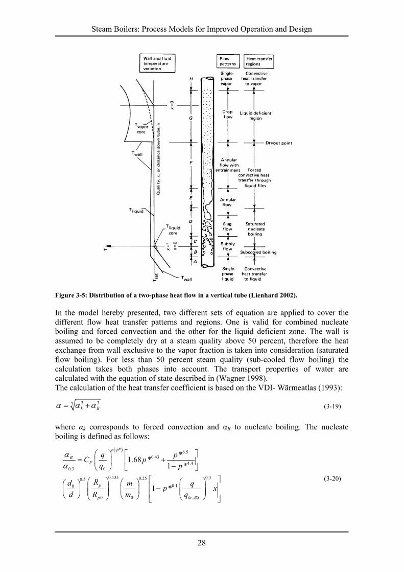
Steam Boilers: Process Models for Improved Operation and Design
28
Figure 3-5: Distribution of a two-phase heat flow in a vertical tube (Lienhard 2002).
In the model hereby presented, two different sets of equation are applied to cover the different flow heat transfer patterns and regions. One is valid for combined nucleate boiling and forced convection and the other for the liquid deficient zone. The wall is assumed to be completely dry at a steam quality above 50 percent, therefore the heat exchange from wall exclusive to the vapor fraction is taken into consideration (saturated flow boiling). For less than 50 percent steam quality (sub-cooled flow boiling) the calculation takes both phases into account. The transport properties of water are calculated with the equation of state described in (Wagner 1998). The calculation of the heat transfer coefficient is based on the VDI- Wärmeatlas (1993):
3 33k Bα α α= + (3-19)
where αk corresponds to forced convection and αB to nucleate boiling. The nucleate boiling is defined as follows:
( )* 6.50.43
4.40.3 0
0.133 0.30.250.50.10
0 0 ,
*1.68 *1 *
1 *
n p
BF
p
p kr BS
q pC pq p
Rd m qp xd R m q
αα
= + −
−
(3-20)
Steam Boilers: Process Models for Improved Operation and Design
29
α 0.3 is a tabularized value of the heat transfer coefficient α for defined fluid at 30 percent of the critical pressure. The index 0 refers to normalized values with diameter d0 equal to 10-2 meter, and roughness parameter Rp0 is equal to 10-6 meter. Value Cf is an empirical factor for water equal to 0.7. The heat transfer coefficient αk by forced convection is based on the liquid ρ’ and vapor density ρ’’ of water, and the steam quality x:
( )
( )
0.52.20.370.4
20.670.7
'1 1.2''
'1 8 1''
k
LOGO
LO
x x
x
ρρα
α α ρα ρ
−−
−
− + + = + −
(3-21)
The index of LO refers to the total liquid flow, GO to the total mass flow of vapor. Radiation All bodies constantly emit energy by radiation. The nature of thermal radiation is either described by electromagnetic waves or by mass-less energy packages called photons, whereby both concepts can be interchanged. The intensity of a radiative energy flux depends upon the temperature of the body and the nature of its surface. Radiation becomes significant at high temperatures due to the tem-perature influence at the fourth power in the Stefan-Boltzman-law, describing the emis-sive power for a black body:
4E Tσ= . (3-22)
Incident radiation in a boiler is a result of combustion. High temperature gases and solids absorb and emit energy. The most important radiative gases are the combustion products CO2 and H2O, while other heteropolar molecules like CO, NOx, SOx and CH4 are ignored due to the low concentration. Radiation from solids, e.g. carbon particles and ash, is called luminous radiation and significantly increases both the emission and absorption. Combustion gases like CO2 and H2O absorb and emit only at certain wavelength, solids emit at any wavelength. Radiation waves crossing a medium may be partly absorbed, transmitted or reflected. Radiative heat transfer can be characterized as a long-range phenomenon; different from convection and conduction, which are characterized as short-range phenomena. Convection models are limited to a boundary layer; where radiation modeling is based on volume elements since an intermediate medium has to be considered. The discretization of the gas enclosure is an optimization between accuracy, modeling effort and calculation time. Radiative heat transfer in a furnace combustion chamber is a combination of two phenomena: gas radiation and surface radiation of the furnace walls. The mathematical formulation of radiative transfer through an absorbing, emitting and scattering medium is presented by equation (3-23). This so-called radiative transfer equation is an integro-dif-ferential equation that describes the radiative intensity field within an enclosure as a function of its location, direction and spectral variable (wavelength λ). It is derived from an energy balance on the monochromatic radiation passing in a specified direction through a small volume element in the medium (see Figure 3-6), and is given as:
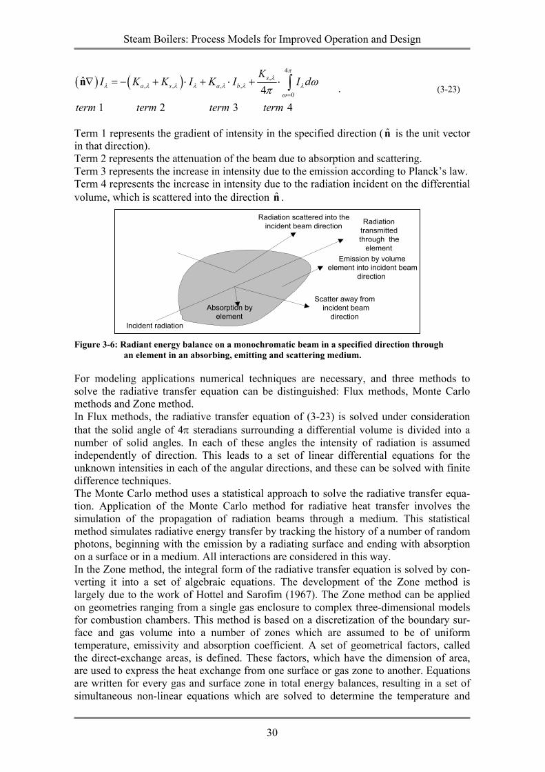
Steam Boilers: Process Models for Improved Operation and Design
30
( ) ( )4
,, , , ,
0
ˆ4
1 2 3 4
sa s a b
KI K K I K I I d
term term term term
πλ
λ λ λ λ λ λ λω
ωπ =
∇ = − + ⋅ + ⋅ + ⋅ ∫n . (3-23)
Term 1 represents the gradient of intensity in the specified direction ( n̂ is the unit vector in that direction). Term 2 represents the attenuation of the beam due to absorption and scattering. Term 3 represents the increase in intensity due to the emission according to Planck’s law. Term 4 represents the increase in intensity due to the radiation incident on the differential volume, which is scattered into the direction n̂ .
Figure 3-6: Radiant energy balance on a monochromatic beam in a specified direction through an element in an absorbing, emitting and scattering medium.
For modeling applications numerical techniques are necessary, and three methods to solve the radiative transfer equation can be distinguished: Flux methods, Monte Carlo methods and Zone method. In Flux methods, the radiative transfer equation of (3-23) is solved under consideration that the solid angle of 4π steradians surrounding a differential volume is divided into a number of solid angles. In each of these angles the intensity of radiation is assumed independently of direction. This leads to a set of linear differential equations for the unknown intensities in each of the angular directions, and these can be solved with finite difference techniques. The Monte Carlo method uses a statistical approach to solve the radiative transfer equa-tion. Application of the Monte Carlo method for radiative heat transfer involves the simulation of the propagation of radiation beams through a medium. This statistical method simulates radiative energy transfer by tracking the history of a number of random photons, beginning with the emission by a radiating surface and ending with absorption on a surface or in a medium. All interactions are considered in this way. In the Zone method, the integral form of the radiative transfer equation is solved by con-verting it into a set of algebraic equations. The development of the Zone method is largely due to the work of Hottel and Sarofim (1967). The Zone method can be applied on geometries ranging from a single gas enclosure to complex three-dimensional models for combustion chambers. This method is based on a discretization of the boundary sur-face and gas volume into a number of zones which are assumed to be of uniform temperature, emissivity and absorption coefficient. A set of geometrical factors, called the direct-exchange areas, is defined. These factors, which have the dimension of area, are used to express the heat exchange from one surface or gas zone to another. Equations are written for every gas and surface zone in total energy balances, resulting in a set of simultaneous non-linear equations which are solved to determine the temperature and
Radiation scattered into theincident beam direction
Incident radiation
Radiationtransmittedthrough the
elementEmission by volume
element into incident beamdirection
Scatter away from incident beam
directionAbsorption by
element
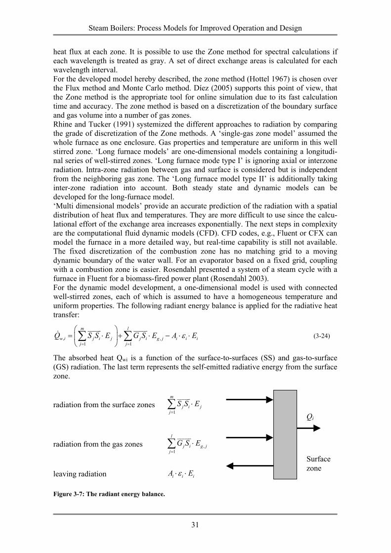
Steam Boilers: Process Models for Improved Operation and Design
31
heat flux at each zone. It is possible to use the Zone method for spectral calculations if each wavelength is treated as gray. A set of direct exchange areas is calculated for each wavelength interval. For the developed model hereby described, the zone method (Hottel 1967) is chosen over the Flux method and Monte Carlo method. Díez (2005) supports this point of view, that the Zone method is the appropriate tool for online simulation due to its fast calculation time and accuracy. The zone method is based on a discretization of the boundary surface and gas volume into a number of gas zones. Rhine and Tucker (1991) systemized the different approaches to radiation by comparing the grade of discretization of the Zone methods. A ‘single-gas zone model’ assumed the whole furnace as one enclosure. Gas properties and temperature are uniform in this well stirred zone. ‘Long furnace models’ are one-dimensional models containing a longitudi-nal series of well-stirred zones. ‘Long furnace mode type I’ is ignoring axial or interzone radiation. Intra-zone radiation between gas and surface is considered but is independent from the neighboring gas zone. The ‘Long furnace model type II’ is additionally taking inter-zone radiation into account. Both steady state and dynamic models can be developed for the long-furnace model. ‘Multi dimensional models’ provide an accurate prediction of the radiation with a spatial distribution of heat flux and temperatures. They are more difficult to use since the calcu-lational effort of the exchange area increases exponentially. The next steps in complexity are the computational fluid dynamic models (CFD). CFD codes, e.g., Fluent or CFX can model the furnace in a more detailed way, but real-time capability is still not available. The fixed discretization of the combustion zone has no matching grid to a moving dynamic boundary of the water wall. For an evaporator based on a fixed grid, coupling with a combustion zone is easier. Rosendahl presented a system of a steam cycle with a furnace in Fluent for a biomass-fired power plant (Rosendahl 2003). For the dynamic model development, a one-dimensional model is used with connected well-stirred zones, each of which is assumed to have a homogeneous temperature and uniform properties. The following radiant energy balance is applied for the radiative heat transfer:
, ,1 1
m l
w i j i j j i g j i i ij j
Q S S E G S E A Eε= =
= ⋅ + ⋅ − ⋅ ⋅
∑ ∑
uuuuv uuuuv& (3-24)
The absorbed heat Qwi is a function of the surface-to-surfaces (SS) and gas-to-surface (GS) radiation. The last term represents the self-emitted radiative energy from the surface zone.
radiation from the surface zones 1
m
j i jj
S S E=
⋅∑uuuuv
radiation from the gas zones ,1
l
j i g jj
G S E=
⋅∑uuuuv
leaving radiation i i iA Eε⋅ ⋅
Figure 3-7: The radiant energy balance.
Qi
Surface zone
Steam Boilers: Process Models for Improved Operation and Design
32
A ‘Long furnace model type I’ is chosen due to the optical properties of fluegas and the special geometry (Rhine 1991). In the ‘Long furnace model I’ the radiant energy balance is defined without inter-zone radiation and the surface-to-surface radiation term is zero. A ‘Long furnace model type II’ with inter-zone radiation was not further developed due to the calculation time and high programming effort. The radiant energy E is calculated with the Stefan-Boltzmann-Law and the corresponding wall or gas temperature. The remaining direct flux areas are defined as follows
( ) ( ), ,1
g
n
N
i j g n g i i j K KnG S a T G S
==
= ⋅∑uuuur
(3-25)
i jG Suuuur
refers to the direct flux area taking into account geometry and the radiation
source temperature. i jG S refers to the total exchange area taking into account geome-try and surface emissivity. Since the traditional zone method is based on cubic enclo-sures, the method of Becker (1967) is chosen to calculate rectangular enclosure with variable side length due to the moving boundaries of the corresponding thermal nodes. The total exchange area is based on the theory of (Becker 1967):
( )2cos /Kr
A VGS Ke r dVdAθ π−= ∫ ∫ (3-26)
The emissivity and absorptivity of the gases are calculated with the Weighted Sum of Gray Gases Model (WSGGM) (Smith 1982). A correct solution must account for each individual spectral line. A simplified gray gas ignores wavelength dependency and is characterized by a single uniform absorption coefficient. The WSGGM method calculates the total emissivity and absorptivity of a real gas by assuming that it as a mixture of gray gases. The emissivity of a real gas is derived as weighted sum of emissivities of a number of gray gases:
( ) ( )( ), 2 2
,0
1g
g n H O CO
Nk p p L
g g n gn
a T eε − +
=
= ⋅ − ∑ . (3-27)
The summation ranges over a total of Ng gray gases, each with its own weighting coeffi-cient ag,n. The weighting coefficients are temperature dependent according to Planck’s law:
( ), , 1, 2, ,g n g i n n g ia T b b T= + ⋅ . (3-28) The so-called standard gas mixture is described as a mixture of two gray gases and one clear gas in the WSGGM. The absorption coefficient for n equal to 0 (corresponds to kg,0) is assigned the value 0 for the spectrums of the clear gas, where kg,1=2.5 and kg,2=109 is valid for the used biomass mixture (Schreurs 2003). The calculation is based on the gas composition. The presence of soot particles in flames significantly increases both the emission and absorption of radiation. Their presence can often double or triple the heat radiated by the gaseous products alone. The emissivity of the soot particles is similarly defined, but soot radiation is continuously distributed over the wavelength spectrum and no clear gas or
Steam Boilers: Process Models for Improved Operation and Design
33
zero values exist (Felske 1982). The gas containing the soot is modeled as a mixture of three gray gases.
( ) ( ),, 1 s n sk c L
s s n gn
a T eε − = ⋅ − ∑ . (3-29)
To determine the emissivity value of a gas-soot mixture using the WSGGM method, the procedure outlined in Felske (1982) is applied where the weighting coefficients are cal-culated out of the separate coefficients of soot and gas. Radiation from particles other than mentioned above is not calculated, due to the low ash content of the burned biomass and missing measurement data of the unburned carbon.
Steam Boilers: Process Models for Improved Operation and Design
34
3.4. CFD models as an aid to predict slagging and fouling Computational Fluid Dynamics (CFD) models are strong tools for the accurate calcula-tion of the combustion chamber. The computational requirements are still an enormous obstacle for online calculation. Nevertheless, CFD models are used as validation and post processing tools for online models (Díez 2005). For the slagging monitoring model as described in this thesis, a CFD model was used to calculate the furnace exit temperature and the temperature distribution inside the combustion zone in order to validate the slag-ging monitoring model. Computational fluid dynamics has become more popular in the study of microscopic deposit phenomena, as well as the macroscopic deposit behavior in a boiler. Three dimensional codes developed at universities (Xu 2002, Schnell 2001) or as commercial programs (Fluent, CFX) are extended with deposit routines. The routines include e.g. the chemical fractionation analysis or multi-component multi-phase equilibrium calculation (Lundmark 2003). To determine whether a particle rebounds or sticks to a surface, it is not only the particle trajectory that is important. It is assumed that a particle rebounces from the wall with the exception of particles where at least 15 percent of them are in a molten state. These particles stick to the surface due to the adhesive forces. The melting point depends on the chemical composition. Nielsen et al (2002) included two mainly size-dependant mechanisms of deposition, the inertial impact and the impact driven by boundary mechanism. Inertial impact occurs when the aerodynamic response time of particles is greater than the local time scales of the flow. This corresponds to particles greater than approximately 10 microns, where, for smaller diameters, boundary layer mechanisms are responsible. Small particles do not possess enough inertia to traverse the boundary layer. Instead, other forces act on these particles in the vicinity of walls. The most important of these are thermophoresis and turbulent fluctuations in the boundary layer. The authors reported a problem concerning sufficient resolution in the near wall grid, since the geometrical scale of these phenomena is too small. Kaer (2003) modeled the deposit mechanism at less than full scale by traditional Lagrangian particle tracking, but adapted an approach based on a deposition velocity correlation.
Steam Boilers: Process Models for Improved Operation and Design
35
4. PROCESS MONITORING: RESULTS
Overview Monitoring models are appropriate for the visualization of deposit tendencies under dif-ferent load conditions. The developed process-monitoring model calculates an overall deposit parameter and is able to fulfil its purpose, such as visualisation of the deposit thickness tendencies for individual heat exchangers. This information can be used to provide guidance for an optimal soot blowing strategy. In this chapter, the developed thermodynamic model is applied to large-scale power plants. This application, programmed in Visual Basic, is customized to different boiler types. The project covered three main applications: a pulverized fuel plant, a fluidized bed boiler and a grate fired plant. Experiments took place to study the influence of ash deposits on heat transfer by using a heat flux probe. Tests were performed on a controlled pilot-scale furnace to find out a quantitative relation between heat transfer and the amount of deposition. Monitoring programs were applied to the furnace, similar to the tools used in the large-scale industrial furnaces. Additionally, fuel and ash analyses were performed to indicate the slagging tendency of the investigated fuel. Monitoring tools are widely used in coal-fired power plants but very rarely in biomass-fired plants. Biomass combustion is characterized by smaller units with fewer measurement devices, high fluctuation in fuel quality and the combination with CHP requires more frequent load changes. The monitoring tests were therefore performed in Sweden. The Swedish power industry is a pioneer in using sustainable fuels for power production. Wood residuals are a diverse natural source of bio-fuels. Operating systems with accompanied slagging problems offer the possibility for development and testing of new monitoring systems and disclose limitations of the approach. Where large-scale coal-fired plants reach an output of electricity up to 1200 MWel per unit, and 800 MWel are considered as standard size, the selected biomass-fired plants have a capacity of 100 MWel for the pulverized fuel plant and 30 MWel for the fluidized bed combustion.
4.1. Online measurements of deposits in a lab scale furnace
4.1.1. Fuel and deposit analysis Fuel of the CHP power plant in Uppsala/Sweden was investigated. The lab scale experiments were performed in order to measure characteristic properties. The fuel was delivered in a crushed and dried state. Table 4-1 compares the investigated wood-based fuel with the properties of some typical solid fuels. The fuel of the CHP Uppsala power plant consists of 70 per cent wood residuals and 30 per cent peat. A highly volatile matter characterizes the fuel, which is typical for bio-fuels. The values of fixed carbon (25.5 per cent) exceed the expected value of wood and peat (10-20 per cent). It is unlikely that wood is a source of an increased fixed carbon content but peat, with a higher carbonization degree, can contribute to this result.
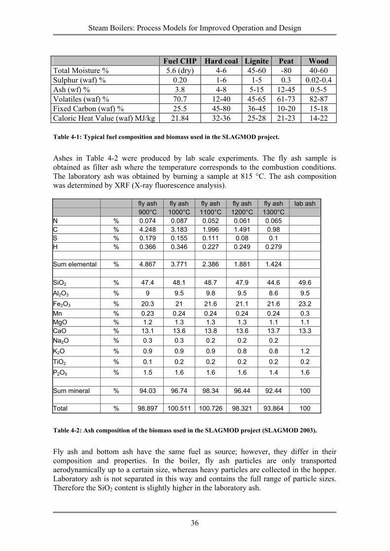
Steam Boilers: Process Models for Improved Operation and Design
36
Fuel CHP Hard coal Lignite Peat Wood Total Moisture % 5.6 (dry) 4-6 45-60 -80 40-60 Sulphur (waf) % 0.20 1-6 1-5 0.3 0.02-0.4 Ash (wf) % 3.8 4-8 5-15 12-45 0.5-5 Volatiles (waf) % 70.7 12-40 45-65 61-73 82-87 Fixed Carbon (waf) % 25.5 45-80 36-45 10-20 15-18 Caloric Heat Value (waf) MJ/kg 21.84 32-36 25-28 21-23 14-22
Table 4-1: Typical fuel composition and biomass used in the SLAGMOD project.
Ashes in Table 4-2 were produced by lab scale experiments. The fly ash sample is obtained as filter ash where the temperature corresponds to the combustion conditions. The laboratory ash was obtained by burning a sample at 815 °C. The ash composition was determined by XRF (X-ray fluorescence analysis). fly ash fly ash fly ash fly ash fly ash lab ash 900°C 1000°C 1100°C 1200°C 1300°C N % 0.074 0.087 0.052 0.061 0.065 C % 4.248 3.183 1.996 1.491 0.98 S % 0.179 0.155 0.111 0.08 0.1 H % 0.366 0.346 0.227 0.249 0.279 Sum elemental % 4.867 3.771 2.386 1.881 1.424 SiO2 % 47.4 48.1 48.7 47.9 44.6 49.6 Al2O3 % 9 9.5 9.8 9.5 8.6 9.5 Fe2O3 % 20.3 21 21.6 21.1 21.6 23.2 Mn % 0.23 0.24 0.24 0.24 0.24 0.3 MgO % 1.2 1.3 1.3 1.3 1.1 1.1 CaO % 13.1 13.6 13.8 13.6 13.7 13.3 Na2O % 0.3 0.3 0.2 0.2 0.2 K2O % 0.9 0.9 0.9 0.8 0.8 1.2 TiO2 % 0.1 0.2 0.2 0.2 0.2 0.2 P2O5 % 1.5 1.6 1.6 1.6 1.4 1.6 Sum mineral % 94.03 96.74 98.34 96.44 92.44 100 Total % 98.897 100.511 100.726 98.321 93.864 100 Table 4-2: Ash composition of the biomass used in the SLAGMOD project (SLAGMOD 2003).
Fly ash and bottom ash have the same fuel as source; however, they differ in their composition and properties. In the boiler, fly ash particles are only transported aerodynamically up to a certain size, whereas heavy particles are collected in the hopper. Laboratory ash is not separated in this way and contains the full range of particle sizes. Therefore the SiO2 content is slightly higher in the laboratory ash.
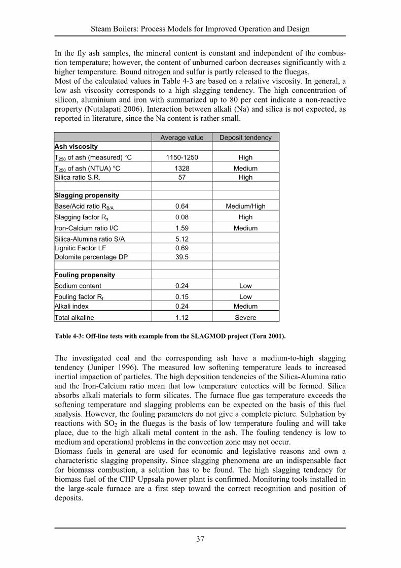
Steam Boilers: Process Models for Improved Operation and Design
37
In the fly ash samples, the mineral content is constant and independent of the combus-tion temperature; however, the content of unburned carbon decreases significantly with a higher temperature. Bound nitrogen and sulfur is partly released to the fluegas. Most of the calculated values in Table 4-3 are based on a relative viscosity. In general, a low ash viscosity corresponds to a high slagging tendency. The high concentration of silicon, aluminium and iron with summarized up to 80 per cent indicate a non-reactive property (Nutalapati 2006). Interaction between alkali (Na) and silica is not expected, as reported in literature, since the Na content is rather small.
Average value Deposit tendency Ash viscosity T250 of ash (measured) °C 1150-1250 High T250 of ash (NTUA) °C 1328 Medium Silica ratio S.R. 57 High Slagging propensity Base/Acid ratio RB/A 0.64 Medium/High Slagging factor Rs 0.08 High Iron-Calcium ratio I/C 1.59 Medium Silica-Alumina ratio S/A 5.12 Lignitic Factor LF 0.69 Dolomite percentage DP 39.5 Fouling propensity Sodium content 0.24 Low Fouling factor Rf 0.15 Low Alkali index 0.24 Medium
Total alkaline 1.12 Severe
Table 4-3: Off-line tests with example from the SLAGMOD project (Torn 2001).
The investigated coal and the corresponding ash have a medium-to-high slagging tendency (Juniper 1996). The measured low softening temperature leads to increased inertial impaction of particles. The high deposition tendencies of the Silica-Alumina ratio and the Iron-Calcium ratio mean that low temperature eutectics will be formed. Silica absorbs alkali materials to form silicates. The furnace flue gas temperature exceeds the softening temperature and slagging problems can be expected on the basis of this fuel analysis. However, the fouling parameters do not give a complete picture. Sulphation by reactions with SO2 in the fluegas is the basis of low temperature fouling and will take place, due to the high alkali metal content in the ash. The fouling tendency is low to medium and operational problems in the convection zone may not occur. Biomass fuels in general are used for economic and legislative reasons and own a characteristic slagging propensity. Since slagging phenomena are an indispensable fact for biomass combustion, a solution has to be found. The high slagging tendency for biomass fuel of the CHP Uppsala power plant is confirmed. Monitoring tools installed in the large-scale furnace are a first step toward the correct recognition and position of deposits.
Steam Boilers: Process Models for Improved Operation and Design
38
4.1.2. Measurements of deposits The aim of the experiments was to determine the influence of deposit formation on heat transfer from the flue gas to a cooling medium in situ. In order to calculate the effective thermal conductivity, the following parameters were measured: the surface temperature of the probe, the surface temperature of the deposits and the properties of the cooling medium. Information about the deposit height was calculated from the heat transfer rate through the deposit. The advantage of the probe is based on a well-defined and limited area of measurement inside the furnace. The main problem is the selection of the adequate cooling medium that allows identical behavior as in the furnace. Steam, as in the real pipe, is difficult to handle for measurement purposes. Other synthetic cooling mediums are limited by the maximum temperature which can occur close to the pipe surface. Finally, air is chosen, even though it does not match the correct flow conditions, e.g. Reynolds, Prandtl and Nusselt number, as in the steam tubes. The deposits are unequally distributed with variances along the pipe, as well as in the cross section. Up to now, a homogeneous slag layer has been assumed in the model. A relation between uniform deposit thickness and wedge-shaped deposit height needs to be found experimentally, in order to complete the model. Generally, the effective thermal conductivity coefficient is treated as a lumped parameter. The majority of the reported thermal conductivity measurements are based on post-mortem analysis techniques that destroy, or, significantly alter, the physical structure of the deposit. The elucidated in situ measurement by Robinson et al. (2001), allowed direct examination of the thermal conductivity of actual deposits. The results showed a decrease in heat transfer due to the deposits and, thus, the possibility of performing such measurements. The reported experiments were carried out at a relatively low probe temperature (300-400 °C), so no sintering of the deposits occurred.
Figure 4-1: Probe and inner rod with four thermocouple housings.
An in situ probe was designed and built at the IVD, Stuttgart (Figure 4-1). This probe is an air-cooled metal tube with an inserted metal rod. The rod houses four thermocouples, with which metal temperature (inner wall) and air temperature can be measured. Deposits form on the probe located inside the furnace where combustion of pulverized fuel takes place. After each test, the tube is removed and photographed and a new tube is inserted.
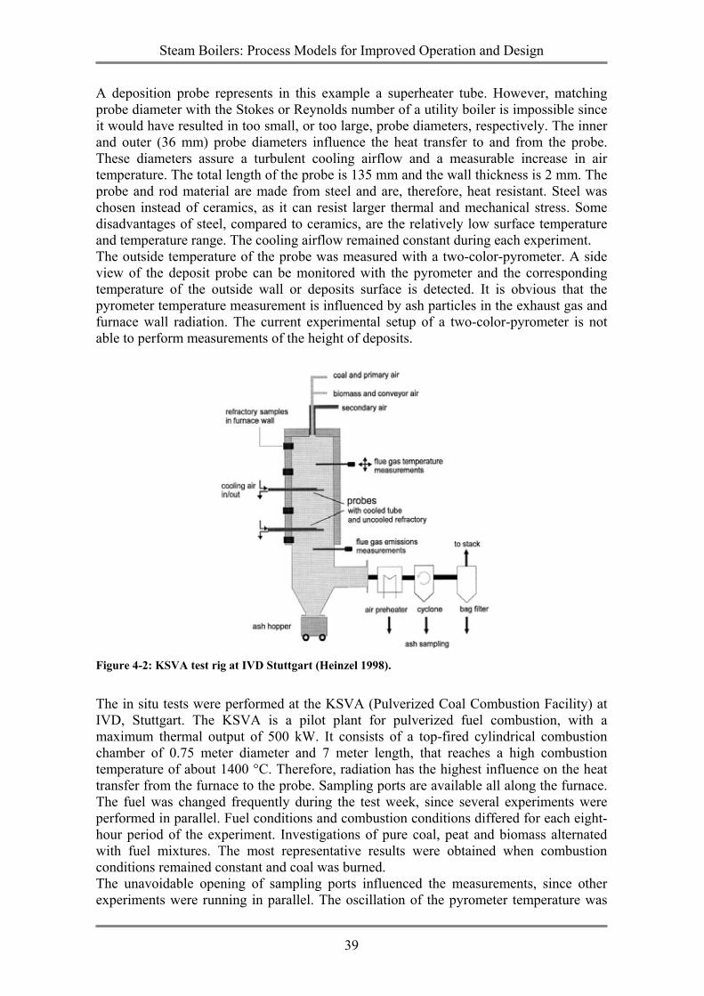
Steam Boilers: Process Models for Improved Operation and Design
39
A deposition probe represents in this example a superheater tube. However, matching probe diameter with the Stokes or Reynolds number of a utility boiler is impossible since it would have resulted in too small, or too large, probe diameters, respectively. The inner and outer (36 mm) probe diameters influence the heat transfer to and from the probe. These diameters assure a turbulent cooling airflow and a measurable increase in air temperature. The total length of the probe is 135 mm and the wall thickness is 2 mm. The probe and rod material are made from steel and are, therefore, heat resistant. Steel was chosen instead of ceramics, as it can resist larger thermal and mechanical stress. Some disadvantages of steel, compared to ceramics, are the relatively low surface temperature and temperature range. The cooling airflow remained constant during each experiment. The outside temperature of the probe was measured with a two-color-pyrometer. A side view of the deposit probe can be monitored with the pyrometer and the corresponding temperature of the outside wall or deposits surface is detected. It is obvious that the pyrometer temperature measurement is influenced by ash particles in the exhaust gas and furnace wall radiation. The current experimental setup of a two-color-pyrometer is not able to perform measurements of the height of deposits.
Figure 4-2: KSVA test rig at IVD Stuttgart (Heinzel 1998).
The in situ tests were performed at the KSVA (Pulverized Coal Combustion Facility) at IVD, Stuttgart. The KSVA is a pilot plant for pulverized fuel combustion, with a maximum thermal output of 500 kW. It consists of a top-fired cylindrical combustion chamber of 0.75 meter diameter and 7 meter length, that reaches a high combustion temperature of about 1400 °C. Therefore, radiation has the highest influence on the heat transfer from the furnace to the probe. Sampling ports are available all along the furnace. The fuel was changed frequently during the test week, since several experiments were performed in parallel. Fuel conditions and combustion conditions differed for each eight-hour period of the experiment. Investigations of pure coal, peat and biomass alternated with fuel mixtures. The most representative results were obtained when combustion conditions remained constant and coal was burned. The unavoidable opening of sampling ports influenced the measurements, since other experiments were running in parallel. The oscillation of the pyrometer temperature was
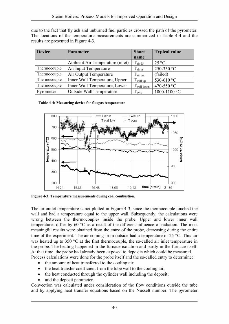
Steam Boilers: Process Models for Improved Operation and Design
40
due to the fact that fly ash and unburned fuel particles crossed the path of the pyrometer. The locations of the temperature measurements are summarized in Table 4-4 and the results are presented in Figure 4-3.
Device Parameter Short name
Typical value
Ambient Air Temperature (inlet) Tair 25 25 °C Thermocouple Air Input Temperature Tair in 250-350 °C Thermocouple Air Output Temperature Tair out (failed) Thermocouple Inner Wall Temperature, Upper Twall up 530-610 °C Thermocouple Inner Wall Temperature, Lower Twall down 470-550 °C Pyrometer Outside Wall Temperature Tpyro 1000-1100 °C
Table 4-4: Measuring device for fluegas temperature
Figure 4-3: Temperature measurements during coal combustion.
The air outlet temperature is not plotted in Figure 4-3, since the thermocouple touched the wall and had a temperature equal to the upper wall. Subsequently, the calculations were wrong between the thermocouples inside the probe. Upper and lower inner wall temperatures differ by 60 °C as a result of the different influence of radiation. The most meaningful results were obtained from the entry of the probe, decreasing during the entire time of the experiment. The air coming from outside had a temperature of 25 °C. This air was heated up to 350 °C at the first thermocouple, the so-called air inlet temperature in the probe. The heating happened in the furnace isolation and partly in the furnace itself. At that time, the probe had already been exposed to deposits which could be measured. Process calculations were done for the probe itself and the so-called entry to determine:
• the amount of heat transferred to the cooling air; • the heat transfer coefficient from the tube wall to the cooling air; • the heat conducted through the cylinder wall including the deposit; • and the deposit parameter.
Convection was calculated under consideration of the flow conditions outside the tube and by applying heat transfer equations based on the Nusselt number. The pyrometer
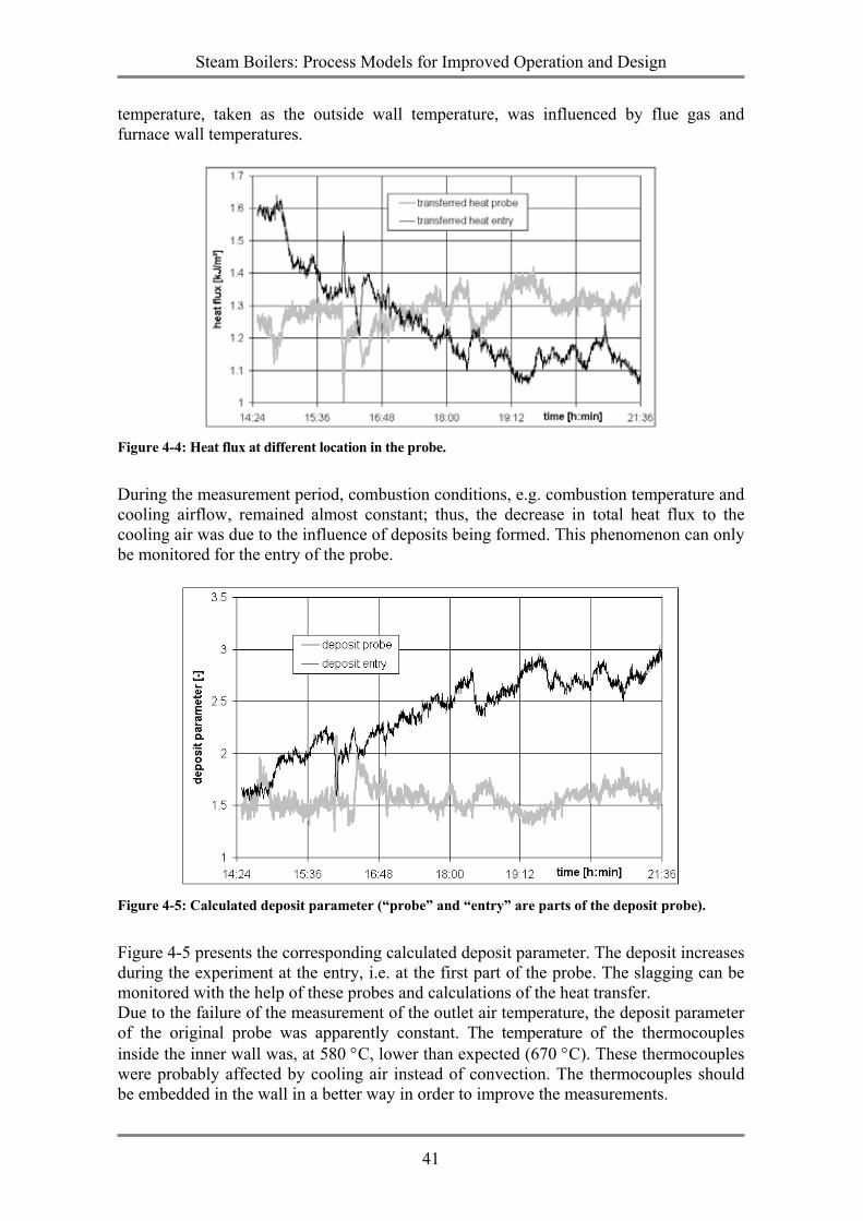
Steam Boilers: Process Models for Improved Operation and Design
41
temperature, taken as the outside wall temperature, was influenced by flue gas and furnace wall temperatures.
Figure 4-4: Heat flux at different location in the probe.
During the measurement period, combustion conditions, e.g. combustion temperature and cooling airflow, remained almost constant; thus, the decrease in total heat flux to the cooling air was due to the influence of deposits being formed. This phenomenon can only be monitored for the entry of the probe.
Figure 4-5: Calculated deposit parameter (“probe” and “entry” are parts of the deposit probe).
Figure 4-5 presents the corresponding calculated deposit parameter. The deposit increases during the experiment at the entry, i.e. at the first part of the probe. The slagging can be monitored with the help of these probes and calculations of the heat transfer. Due to the failure of the measurement of the outlet air temperature, the deposit parameter of the original probe was apparently constant. The temperature of the thermocouples inside the inner wall was, at 580 °C, lower than expected (670 °C). These thermocouples were probably affected by cooling air instead of convection. The thermocouples should be embedded in the wall in a better way in order to improve the measurements.
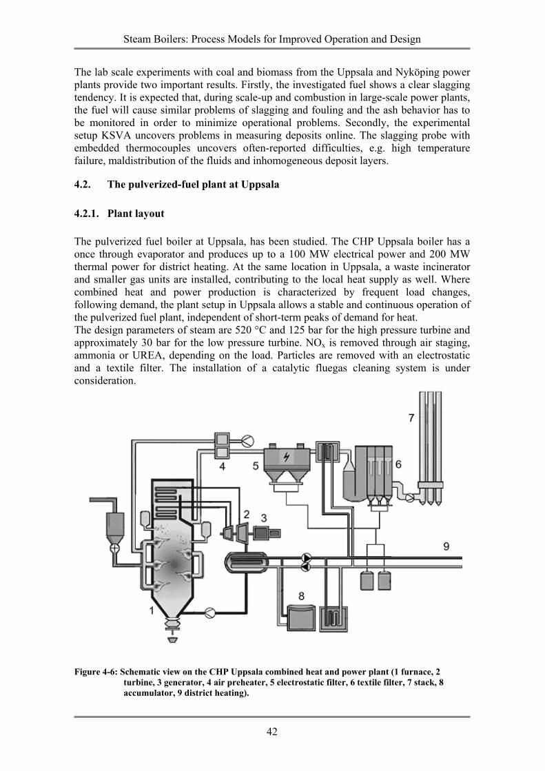
Steam Boilers: Process Models for Improved Operation and Design
42
The lab scale experiments with coal and biomass from the Uppsala and Nyköping power plants provide two important results. Firstly, the investigated fuel shows a clear slagging tendency. It is expected that, during scale-up and combustion in large-scale power plants, the fuel will cause similar problems of slagging and fouling and the ash behavior has to be monitored in order to minimize operational problems. Secondly, the experimental setup KSVA uncovers problems in measuring deposits online. The slagging probe with embedded thermocouples uncovers often-reported difficulties, e.g. high temperature failure, maldistribution of the fluids and inhomogeneous deposit layers.
4.2. The pulverized-fuel plant at Uppsala
4.2.1. Plant layout The pulverized fuel boiler at Uppsala, has been studied. The CHP Uppsala boiler has a once through evaporator and produces up to a 100 MW electrical power and 200 MW thermal power for district heating. At the same location in Uppsala, a waste incinerator and smaller gas units are installed, contributing to the local heat supply as well. Where combined heat and power production is characterized by frequent load changes, following demand, the plant setup in Uppsala allows a stable and continuous operation of the pulverized fuel plant, independent of short-term peaks of demand for heat. The design parameters of steam are 520 °C and 125 bar for the high pressure turbine and approximately 30 bar for the low pressure turbine. NOx is removed through air staging, ammonia or UREA, depending on the load. Particles are removed with an electrostatic and a textile filter. The installation of a catalytic fluegas cleaning system is under consideration.
Figure 4-6: Schematic view on the CHP Uppsala combined heat and power plant (1 furnace, 2 turbine, 3 generator, 4 air preheater, 5 electrostatic filter, 6 textile filter, 7 stack, 8 accumulator, 9 district heating).
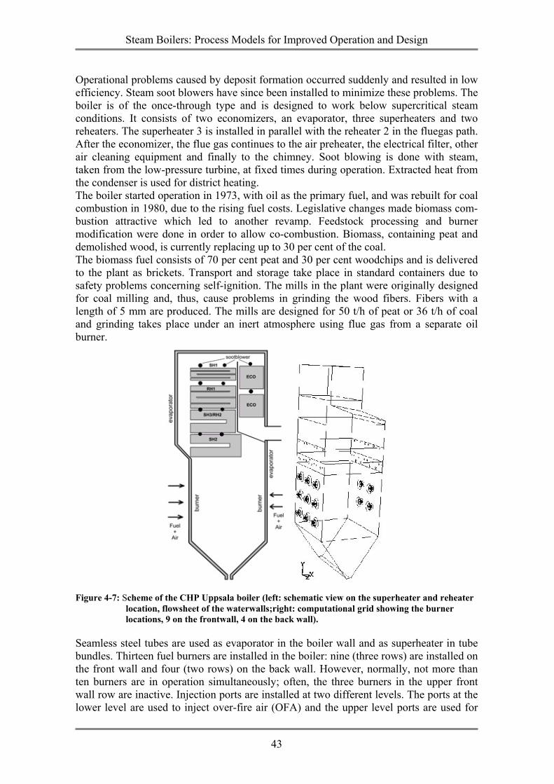
Steam Boilers: Process Models for Improved Operation and Design
43
Operational problems caused by deposit formation occurred suddenly and resulted in low efficiency. Steam soot blowers have since been installed to minimize these problems. The boiler is of the once-through type and is designed to work below supercritical steam conditions. It consists of two economizers, an evaporator, three superheaters and two reheaters. The superheater 3 is installed in parallel with the reheater 2 in the fluegas path. After the economizer, the flue gas continues to the air preheater, the electrical filter, other air cleaning equipment and finally to the chimney. Soot blowing is done with steam, taken from the low-pressure turbine, at fixed times during operation. Extracted heat from the condenser is used for district heating. The boiler started operation in 1973, with oil as the primary fuel, and was rebuilt for coal combustion in 1980, due to the rising fuel costs. Legislative changes made biomass com-bustion attractive which led to another revamp. Feedstock processing and burner modification were done in order to allow co-combustion. Biomass, containing peat and demolished wood, is currently replacing up to 30 per cent of the coal. The biomass fuel consists of 70 per cent peat and 30 per cent woodchips and is delivered to the plant as brickets. Transport and storage take place in standard containers due to safety problems concerning self-ignition. The mills in the plant were originally designed for coal milling and, thus, cause problems in grinding the wood fibers. Fibers with a length of 5 mm are produced. The mills are designed for 50 t/h of peat or 36 t/h of coal and grinding takes place under an inert atmosphere using flue gas from a separate oil burner.
Figure 4-7: Scheme of the CHP Uppsala boiler (left: schematic view on the superheater and reheater
location, flowsheet of the waterwalls;right: computational grid showing the burner locations, 9 on the frontwall, 4 on the back wall).
Seamless steel tubes are used as evaporator in the boiler wall and as superheater in tube bundles. Thirteen fuel burners are installed in the boiler: nine (three rows) are installed on the front wall and four (two rows) on the back wall. However, normally, not more than ten burners are in operation simultaneously; often, the three burners in the upper front wall row are inactive. Injection ports are installed at two different levels. The ports at the lower level are used to inject over-fire air (OFA) and the upper level ports are used for
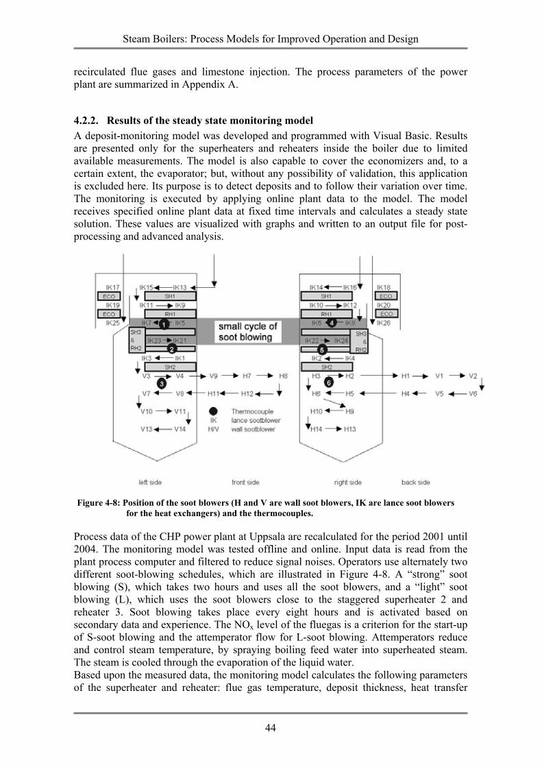
Steam Boilers: Process Models for Improved Operation and Design
44
recirculated flue gases and limestone injection. The process parameters of the power plant are summarized in Appendix A.
4.2.2. Results of the steady state monitoring model A deposit-monitoring model was developed and programmed with Visual Basic. Results are presented only for the superheaters and reheaters inside the boiler due to limited available measurements. The model is also capable to cover the economizers and, to a certain extent, the evaporator; but, without any possibility of validation, this application is excluded here. Its purpose is to detect deposits and to follow their variation over time. The monitoring is executed by applying online plant data to the model. The model receives specified online plant data at fixed time intervals and calculates a steady state solution. These values are visualized with graphs and written to an output file for post-processing and advanced analysis.
Figure 4-8: Position of the soot blowers (H and V are wall soot blowers, IK are lance soot blowers
for the heat exchangers) and the thermocouples.
Process data of the CHP power plant at Uppsala are recalculated for the period 2001 until 2004. The monitoring model was tested offline and online. Input data is read from the plant process computer and filtered to reduce signal noises. Operators use alternately two different soot-blowing schedules, which are illustrated in Figure 4-8. A “strong” soot blowing (S), which takes two hours and uses all the soot blowers, and a “light” soot blowing (L), which uses the soot blowers close to the staggered superheater 2 and reheater 3. Soot blowing takes place every eight hours and is activated based on secondary data and experience. The NOx level of the fluegas is a criterion for the start-up of S-soot blowing and the attemperator flow for L-soot blowing. Attemperators reduce and control steam temperature, by spraying boiling feed water into superheated steam. The steam is cooled through the evaporation of the liquid water. Based upon the measured data, the monitoring model calculates the following parameters of the superheater and reheater: flue gas temperature, deposit thickness, heat transfer
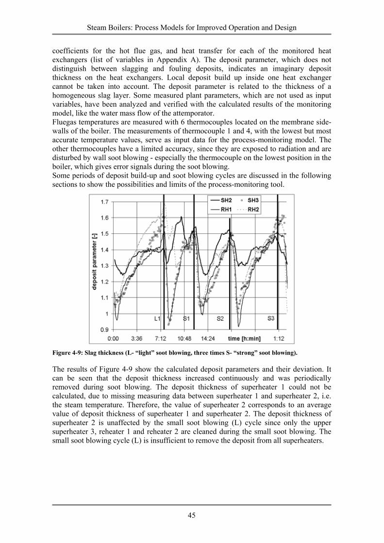
Steam Boilers: Process Models for Improved Operation and Design
45
coefficients for the hot flue gas, and heat transfer for each of the monitored heat exchangers (list of variables in Appendix A). The deposit parameter, which does not distinguish between slagging and fouling deposits, indicates an imaginary deposit thickness on the heat exchangers. Local deposit build up inside one heat exchanger cannot be taken into account. The deposit parameter is related to the thickness of a homogeneous slag layer. Some measured plant parameters, which are not used as input variables, have been analyzed and verified with the calculated results of the monitoring model, like the water mass flow of the attemporator. Fluegas temperatures are measured with 6 thermocouples located on the membrane side-walls of the boiler. The measurements of thermocouple 1 and 4, with the lowest but most accurate temperature values, serve as input data for the process-monitoring model. The other thermocouples have a limited accuracy, since they are exposed to radiation and are disturbed by wall soot blowing - especially the thermocouple on the lowest position in the boiler, which gives error signals during the soot blowing. Some periods of deposit build-up and soot blowing cycles are discussed in the following sections to show the possibilities and limits of the process-monitoring tool.
Figure 4-9: Slag thickness (L- “light” soot blowing, three times S- “strong” soot blowing).
The results of Figure 4-9 show the calculated deposit parameters and their deviation. It can be seen that the deposit thickness increased continuously and was periodically removed during soot blowing. The deposit thickness of superheater 1 could not be calculated, due to missing measuring data between superheater 1 and superheater 2, i.e. the steam temperature. Therefore, the value of superheater 2 corresponds to an average value of deposit thickness of superheater 1 and superheater 2. The deposit thickness of superheater 2 is unaffected by the small soot blowing (L) cycle since only the upper superheater 3, reheater 1 and reheater 2 are cleaned during the small soot blowing. The small soot blowing cycle (L) is insufficient to remove the deposit from all superheaters.
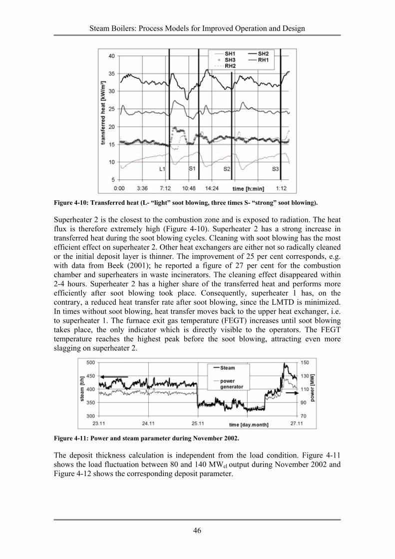
Steam Boilers: Process Models for Improved Operation and Design
46
Figure 4-10: Transferred heat (L- “light” soot blowing, three times S- “strong” soot blowing).
Superheater 2 is the closest to the combustion zone and is exposed to radiation. The heat flux is therefore extremely high (Figure 4-10). Superheater 2 has a strong increase in transferred heat during the soot blowing cycles. Cleaning with soot blowing has the most efficient effect on superheater 2. Other heat exchangers are either not so radically cleaned or the initial deposit layer is thinner. The improvement of 25 per cent corresponds, e.g. with data from Beek (2001); he reported a figure of 27 per cent for the combustion chamber and superheaters in waste incinerators. The cleaning effect disappeared within 2-4 hours. Superheater 2 has a higher share of the transferred heat and performs more efficiently after soot blowing took place. Consequently, superheater 1 has, on the contrary, a reduced heat transfer rate after soot blowing, since the LMTD is minimized. In times without soot blowing, heat transfer moves back to the upper heat exchanger, i.e. to superheater 1. The furnace exit gas temperature (FEGT) increases until soot blowing takes place, the only indicator which is directly visible to the operators. The FEGT temperature reaches the highest peak before the soot blowing, attracting even more slagging on superheater 2.
Figure 4-11: Power and steam parameter during November 2002.
The deposit thickness calculation is independent from the load condition. Figure 4-11 shows the load fluctuation between 80 and 140 MWel output during November 2002 and Figure 4-12 shows the corresponding deposit parameter.
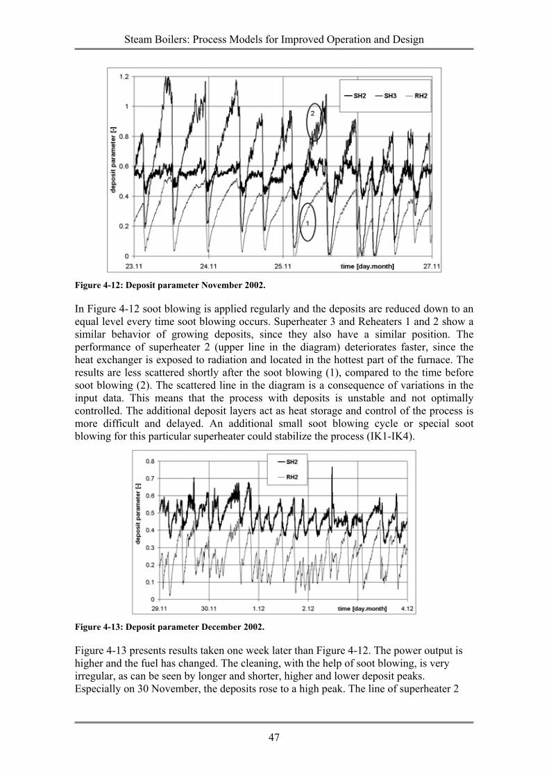
Steam Boilers: Process Models for Improved Operation and Design
47
Figure 4-12: Deposit parameter November 2002.
In Figure 4-12 soot blowing is applied regularly and the deposits are reduced down to an equal level every time soot blowing occurs. Superheater 3 and Reheaters 1 and 2 show a similar behavior of growing deposits, since they also have a similar position. The performance of superheater 2 (upper line in the diagram) deteriorates faster, since the heat exchanger is exposed to radiation and located in the hottest part of the furnace. The results are less scattered shortly after the soot blowing (1), compared to the time before soot blowing (2). The scattered line in the diagram is a consequence of variations in the input data. This means that the process with deposits is unstable and not optimally controlled. The additional deposit layers act as heat storage and control of the process is more difficult and delayed. An additional small soot blowing cycle or special soot blowing for this particular superheater could stabilize the process (IK1-IK4).
Figure 4-13: Deposit parameter December 2002.
Figure 4-13 presents results taken one week later than Figure 4-12. The power output is higher and the fuel has changed. The cleaning, with the help of soot blowing, is very irregular, as can be seen by longer and shorter, higher and lower deposit peaks. Especially on 30 November, the deposits rose to a high peak. The line of superheater 2
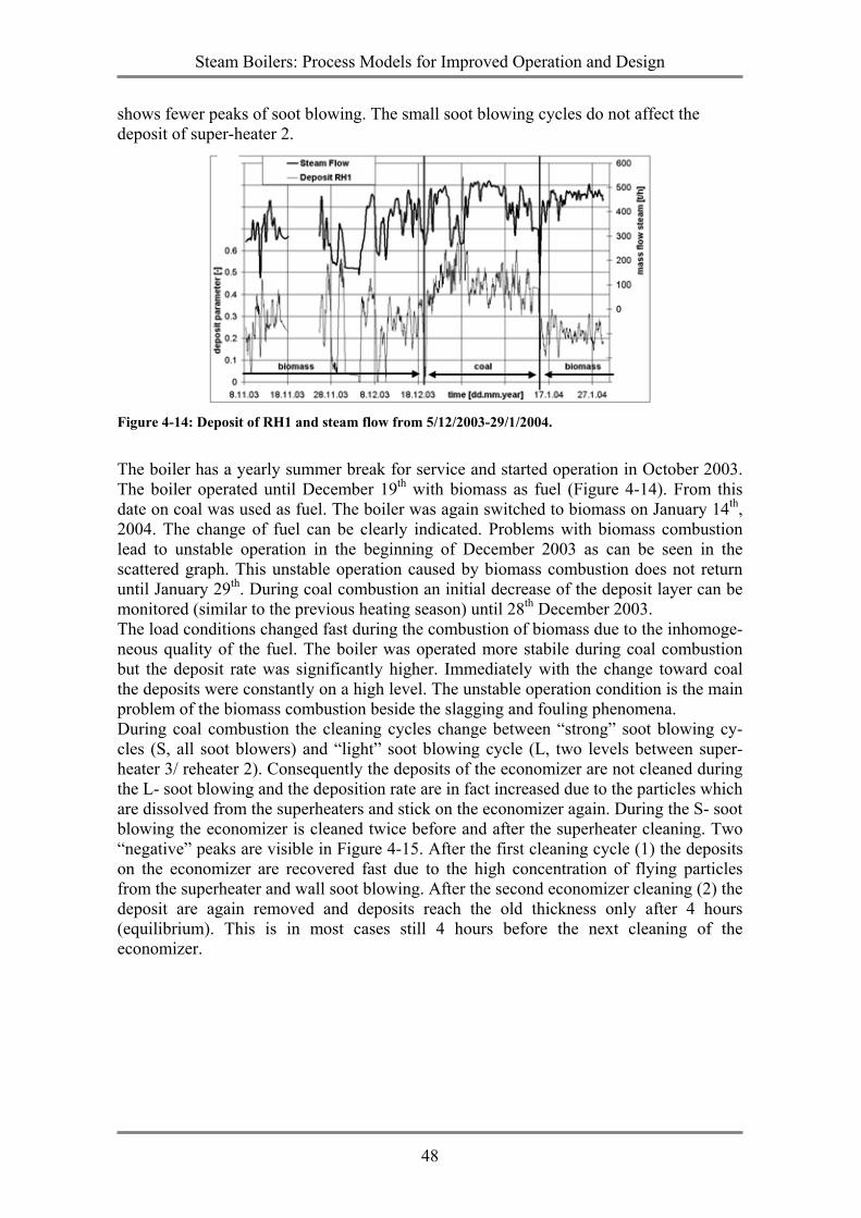
Steam Boilers: Process Models for Improved Operation and Design
48
shows fewer peaks of soot blowing. The small soot blowing cycles do not affect the deposit of super-heater 2.
Figure 4-14: Deposit of RH1 and steam flow from 5/12/2003-29/1/2004.
The boiler has a yearly summer break for service and started operation in October 2003. The boiler operated until December 19th with biomass as fuel (Figure 4-14). From this date on coal was used as fuel. The boiler was again switched to biomass on January 14th, 2004. The change of fuel can be clearly indicated. Problems with biomass combustion lead to unstable operation in the beginning of December 2003 as can be seen in the scattered graph. This unstable operation caused by biomass combustion does not return until January 29th. During coal combustion an initial decrease of the deposit layer can be monitored (similar to the previous heating season) until 28th December 2003. The load conditions changed fast during the combustion of biomass due to the inhomoge-neous quality of the fuel. The boiler was operated more stabile during coal combustion but the deposit rate was significantly higher. Immediately with the change toward coal the deposits were constantly on a high level. The unstable operation condition is the main problem of the biomass combustion beside the slagging and fouling phenomena. During coal combustion the cleaning cycles change between “strong” soot blowing cy-cles (S, all soot blowers) and “light” soot blowing cycle (L, two levels between super-heater 3/ reheater 2). Consequently the deposits of the economizer are not cleaned during the L- soot blowing and the deposition rate are in fact increased due to the particles which are dissolved from the superheaters and stick on the economizer again. During the S- soot blowing the economizer is cleaned twice before and after the superheater cleaning. Two “negative” peaks are visible in Figure 4-15. After the first cleaning cycle (1) the deposits on the economizer are recovered fast due to the high concentration of flying particles from the superheater and wall soot blowing. After the second economizer cleaning (2) the deposit are again removed and deposits reach the old thickness only after 4 hours (equilibrium). This is in most cases still 4 hours before the next cleaning of the economizer.
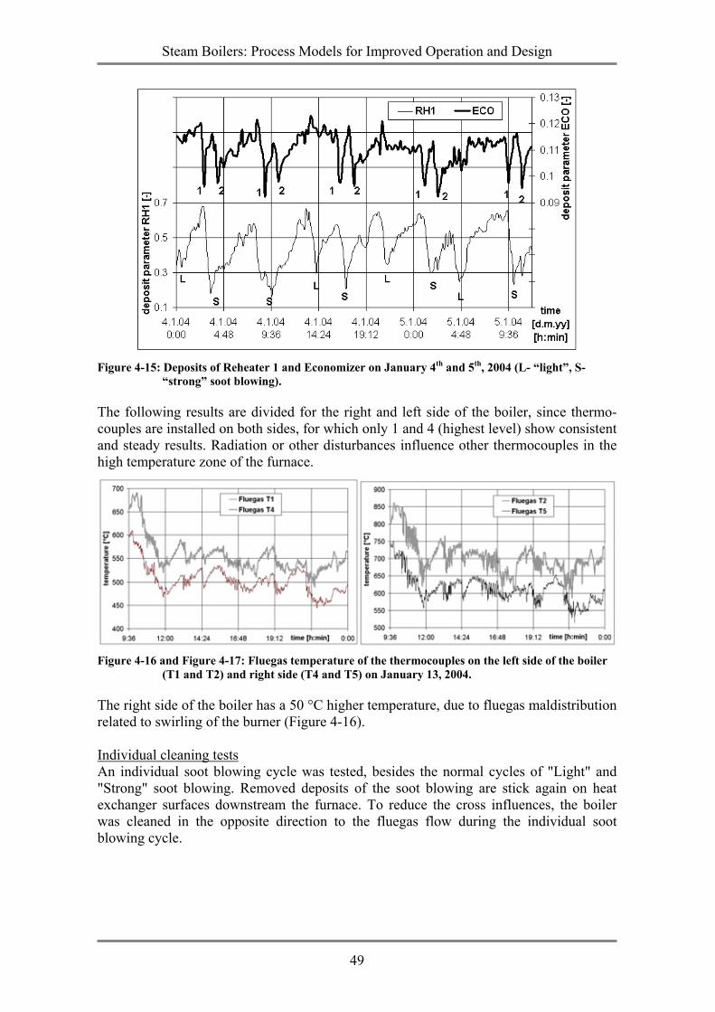
Steam Boilers: Process Models for Improved Operation and Design
49
Figure 4-15: Deposits of Reheater 1 and Economizer on January 4th and 5th, 2004 (L- “light”, S-
“strong” soot blowing).
The following results are divided for the right and left side of the boiler, since thermo-couples are installed on both sides, for which only 1 and 4 (highest level) show consistent and steady results. Radiation or other disturbances influence other thermocouples in the high temperature zone of the furnace.
Figure 4-16 and Figure 4-17: Fluegas temperature of the thermocouples on the left side of the boiler (T1 and T2) and right side (T4 and T5) on January 13, 2004.
The right side of the boiler has a 50 °C higher temperature, due to fluegas maldistribution related to swirling of the burner (Figure 4-16). Individual cleaning tests An individual soot blowing cycle was tested, besides the normal cycles of "Light" and "Strong" soot blowing. Removed deposits of the soot blowing are stick again on heat exchanger surfaces downstream the furnace. To reduce the cross influences, the boiler was cleaned in the opposite direction to the fluegas flow during the individual soot blowing cycle.
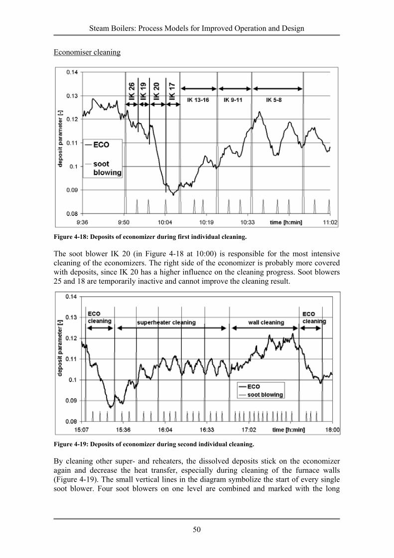
Steam Boilers: Process Models for Improved Operation and Design
50
Economiser cleaning
Figure 4-18: Deposits of economizer during first individual cleaning.
The soot blower IK 20 (in Figure 4-18 at 10:00) is responsible for the most intensive cleaning of the economizers. The right side of the economizer is probably more covered with deposits, since IK 20 has a higher influence on the cleaning progress. Soot blowers 25 and 18 are temporarily inactive and cannot improve the cleaning result.
Figure 4-19: Deposits of economizer during second individual cleaning.
By cleaning other super- and reheaters, the dissolved deposits stick on the economizer again and decrease the heat transfer, especially during cleaning of the furnace walls (Figure 4-19). The small vertical lines in the diagram symbolize the start of every single soot blower. Four soot blowers on one level are combined and marked with the long
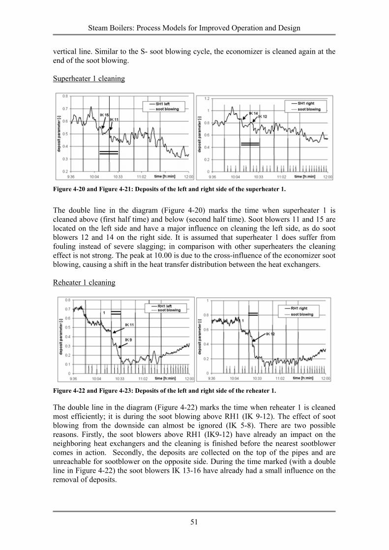
Steam Boilers: Process Models for Improved Operation and Design
51
vertical line. Similar to the S- soot blowing cycle, the economizer is cleaned again at the end of the soot blowing. Superheater 1 cleaning
Figure 4-20 and Figure 4-21: Deposits of the left and right side of the superheater 1.
The double line in the diagram (Figure 4-20) marks the time when superheater 1 is cleaned above (first half time) and below (second half time). Soot blowers 11 and 15 are located on the left side and have a major influence on cleaning the left side, as do soot blowers 12 and 14 on the right side. It is assumed that superheater 1 does suffer from fouling instead of severe slagging; in comparison with other superheaters the cleaning effect is not strong. The peak at 10.00 is due to the cross-influence of the economizer soot blowing, causing a shift in the heat transfer distribution between the heat exchangers. Reheater 1 cleaning
Figure 4-22 and Figure 4-23: Deposits of the left and right side of the reheater 1.
The double line in the diagram (Figure 4-22) marks the time when reheater 1 is cleaned most efficiently; it is during the soot blowing above RH1 (IK 9-12). The effect of soot blowing from the downside can almost be ignored (IK 5-8). There are two possible reasons. Firstly, the soot blowers above RH1 (IK9-12) have already an impact on the neighboring heat exchangers and the cleaning is finished before the nearest sootblower comes in action. Secondly, the deposits are collected on the top of the pipes and are unreachable for sootblower on the opposite side. During the time marked (with a double line in Figure 4-22) the soot blowers IK 13-16 have already had a small influence on the removal of deposits.
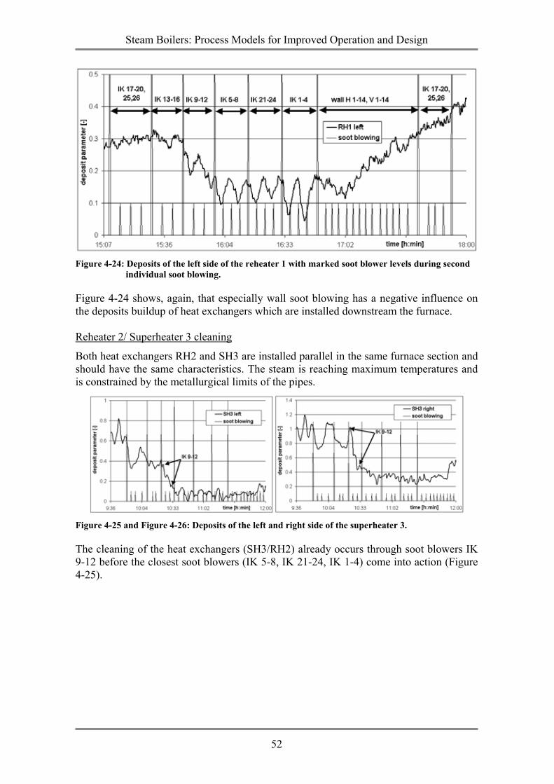
Steam Boilers: Process Models for Improved Operation and Design
52
Figure 4-24: Deposits of the left side of the reheater 1 with marked soot blower levels during second individual soot blowing.
Figure 4-24 shows, again, that especially wall soot blowing has a negative influence on the deposits buildup of heat exchangers which are installed downstream the furnace. Reheater 2/ Superheater 3 cleaning
Both heat exchangers RH2 and SH3 are installed parallel in the same furnace section and should have the same characteristics. The steam is reaching maximum temperatures and is constrained by the metallurgical limits of the pipes.
Figure 4-25 and Figure 4-26: Deposits of the left and right side of the superheater 3.
The cleaning of the heat exchangers (SH3/RH2) already occurs through soot blowers IK 9-12 before the closest soot blowers (IK 5-8, IK 21-24, IK 1-4) come into action (Figure 4-25).
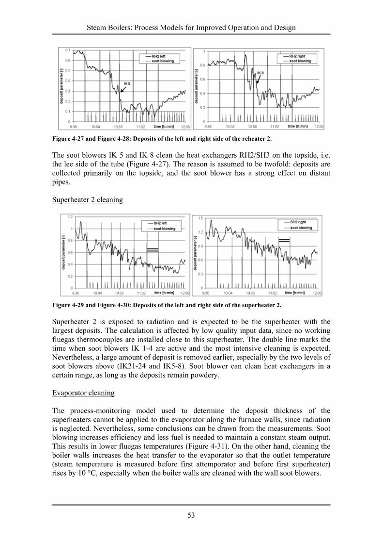
Steam Boilers: Process Models for Improved Operation and Design
53
Figure 4-27 and Figure 4-28: Deposits of the left and right side of the reheater 2.
The soot blowers IK 5 and IK 8 clean the heat exchangers RH2/SH3 on the topside, i.e. the lee side of the tube (Figure 4-27). The reason is assumed to be twofold: deposits are collected primarily on the topside, and the soot blower has a strong effect on distant pipes. Superheater 2 cleaning
Figure 4-29 and Figure 4-30: Deposits of the left and right side of the superheater 2.
Superheater 2 is exposed to radiation and is expected to be the superheater with the largest deposits. The calculation is affected by low quality input data, since no working fluegas thermocouples are installed close to this superheater. The double line marks the time when soot blowers IK 1-4 are active and the most intensive cleaning is expected. Nevertheless, a large amount of deposit is removed earlier, especially by the two levels of soot blowers above (IK21-24 and IK5-8). Soot blower can clean heat exchangers in a certain range, as long as the deposits remain powdery. Evaporator cleaning The process-monitoring model used to determine the deposit thickness of the superheaters cannot be applied to the evaporator along the furnace walls, since radiation is neglected. Nevertheless, some conclusions can be drawn from the measurements. Soot blowing increases efficiency and less fuel is needed to maintain a constant steam output. This results in lower fluegas temperatures (Figure 4-31). On the other hand, cleaning the boiler walls increases the heat transfer to the evaporator so that the outlet temperature (steam temperature is measured before first attemporator and before first superheater) rises by 10 °C, especially when the boiler walls are cleaned with the wall soot blowers.
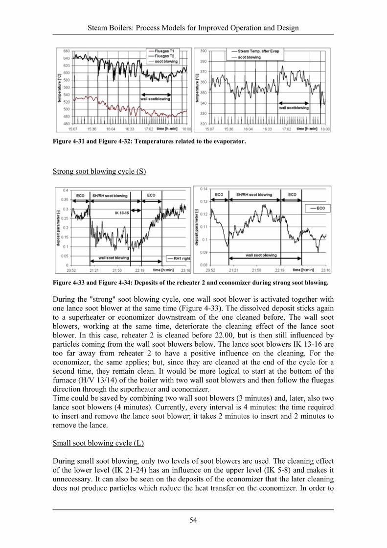
Steam Boilers: Process Models for Improved Operation and Design
54
Figure 4-31 and Figure 4-32: Temperatures related to the evaporator.
Strong soot blowing cycle (S)
Figure 4-33 and Figure 4-34: Deposits of the reheater 2 and economizer during strong soot blowing.
During the "strong" soot blowing cycle, one wall soot blower is activated together with one lance soot blower at the same time (Figure 4-33). The dissolved deposit sticks again to a superheater or economizer downstream of the one cleaned before. The wall soot blowers, working at the same time, deteriorate the cleaning effect of the lance soot blower. In this case, reheater 2 is cleaned before 22.00, but is then still influenced by particles coming from the wall soot blowers below. The lance soot blowers IK 13-16 are too far away from reheater 2 to have a positive influence on the cleaning. For the economizer, the same applies; but, since they are cleaned at the end of the cycle for a second time, they remain clean. It would be more logical to start at the bottom of the furnace (H/V 13/14) of the boiler with two wall soot blowers and then follow the fluegas direction through the superheater and economizer. Time could be saved by combining two wall soot blowers (3 minutes) and, later, also two lance soot blowers (4 minutes). Currently, every interval is 4 minutes: the time required to insert and remove the lance soot blower; it takes 2 minutes to insert and 2 minutes to remove the lance. Small soot blowing cycle (L) During small soot blowing, only two levels of soot blowers are used. The cleaning effect of the lower level (IK 21-24) has an influence on the upper level (IK 5-8) and makes it unnecessary. It can also be seen on the deposits of the economizer that the later cleaning does not produce particles which reduce the heat transfer on the economizer. In order to
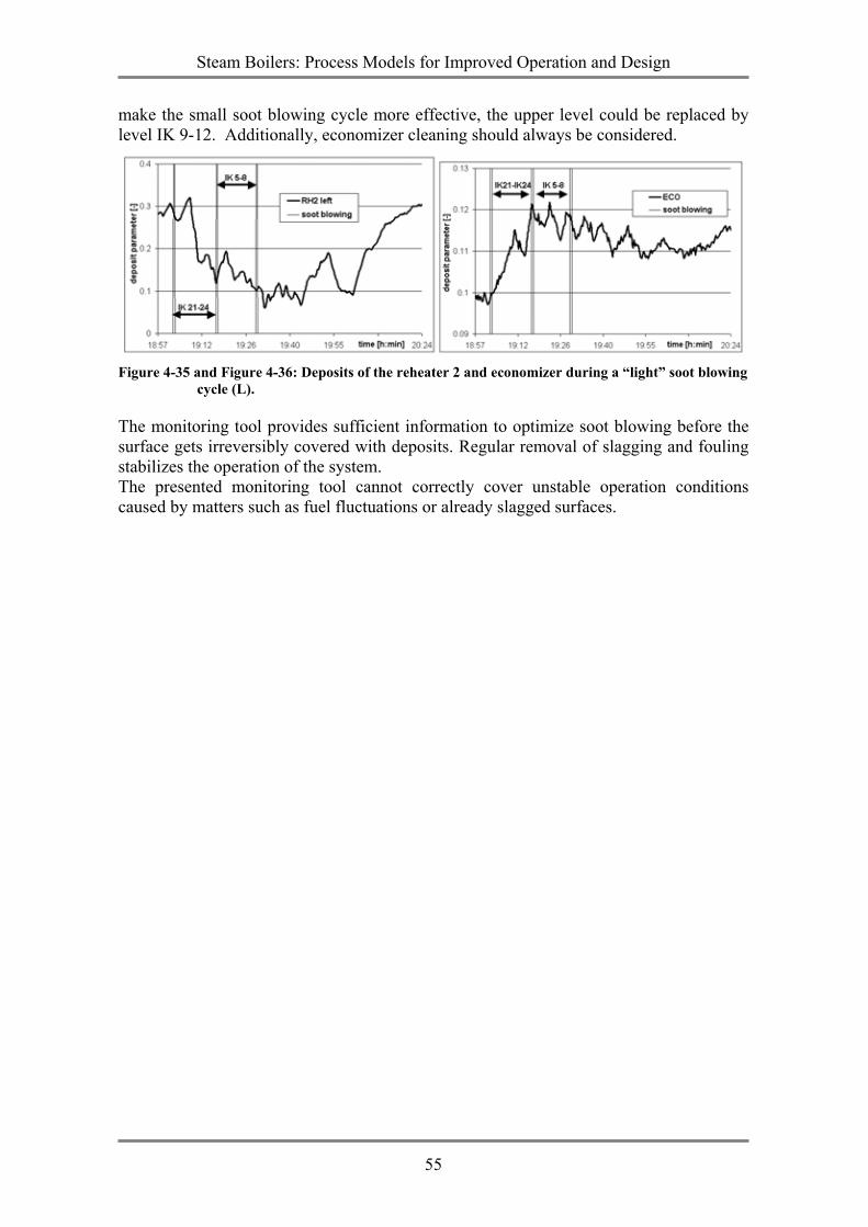
Steam Boilers: Process Models for Improved Operation and Design
55
make the small soot blowing cycle more effective, the upper level could be replaced by level IK 9-12. Additionally, economizer cleaning should always be considered.
Figure 4-35 and Figure 4-36: Deposits of the reheater 2 and economizer during a “light” soot blowing cycle (L).
The monitoring tool provides sufficient information to optimize soot blowing before the surface gets irreversibly covered with deposits. Regular removal of slagging and fouling stabilizes the operation of the system. The presented monitoring tool cannot correctly cover unstable operation conditions caused by matters such as fuel fluctuations or already slagged surfaces.
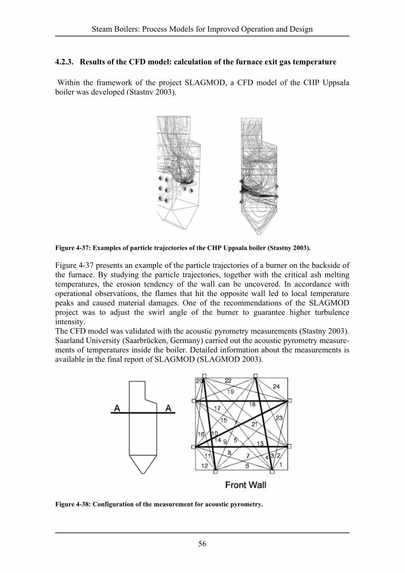
Steam Boilers: Process Models for Improved Operation and Design
56
4.2.3. Results of the CFD model: calculation of the furnace exit gas temperature Within the framework of the project SLAGMOD, a CFD model of the CHP Uppsala boiler was developed (Stastny 2003).
Figure 4-37: Examples of particle trajectories of the CHP Uppsala boiler (Stastny 2003).
Figure 4-37 presents an example of the particle trajectories of a burner on the backside of the furnace. By studying the particle trajectories, together with the critical ash melting temperatures, the erosion tendency of the wall can be uncovered. In accordance with operational observations, the flames that hit the opposite wall led to local temperature peaks and caused material damages. One of the recommendations of the SLAGMOD project was to adjust the swirl angle of the burner to guarantee higher turbulence intensity. The CFD model was validated with the acoustic pyrometry measurements (Stastny 2003). Saarland University (Saarbrücken, Germany) carried out the acoustic pyrometry measure-ments of temperatures inside the boiler. Detailed information about the measurements is available in the final report of SLAGMOD (SLAGMOD 2003).
Figure 4-38: Configuration of the measurement for acoustic pyrometry.
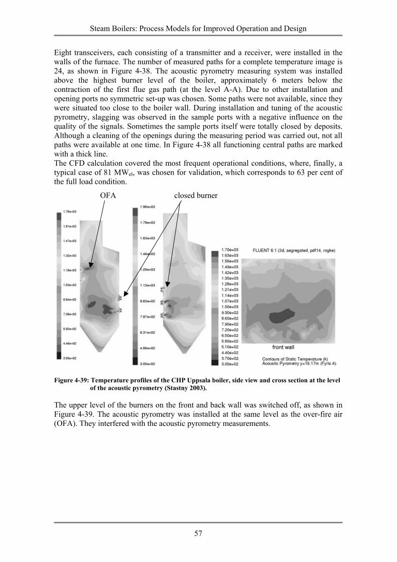
Steam Boilers: Process Models for Improved Operation and Design
57
Eight transceivers, each consisting of a transmitter and a receiver, were installed in the walls of the furnace. The number of measured paths for a complete temperature image is 24, as shown in Figure 4-38. The acoustic pyrometry measuring system was installed above the highest burner level of the boiler, approximately 6 meters below the contraction of the first flue gas path (at the level A-A). Due to other installation and opening ports no symmetric set-up was chosen. Some paths were not available, since they were situated too close to the boiler wall. During installation and tuning of the acoustic pyrometry, slagging was observed in the sample ports with a negative influence on the quality of the signals. Sometimes the sample ports itself were totally closed by deposits. Although a cleaning of the openings during the measuring period was carried out, not all paths were available at one time. In Figure 4-38 all functioning central paths are marked with a thick line. The CFD calculation covered the most frequent operational conditions, where, finally, a typical case of 81 MWel, was chosen for validation, which corresponds to 63 per cent of the full load condition.
OFA closed burner
Figure 4-39: Temperature profiles of the CHP Uppsala boiler, side view and cross section at the level of the acoustic pyrometry (Stastny 2003).
The upper level of the burners on the front and back wall was switched off, as shown in Figure 4-39. The acoustic pyrometry was installed at the same level as the over-fire air (OFA). They interfered with the acoustic pyrometry measurements.
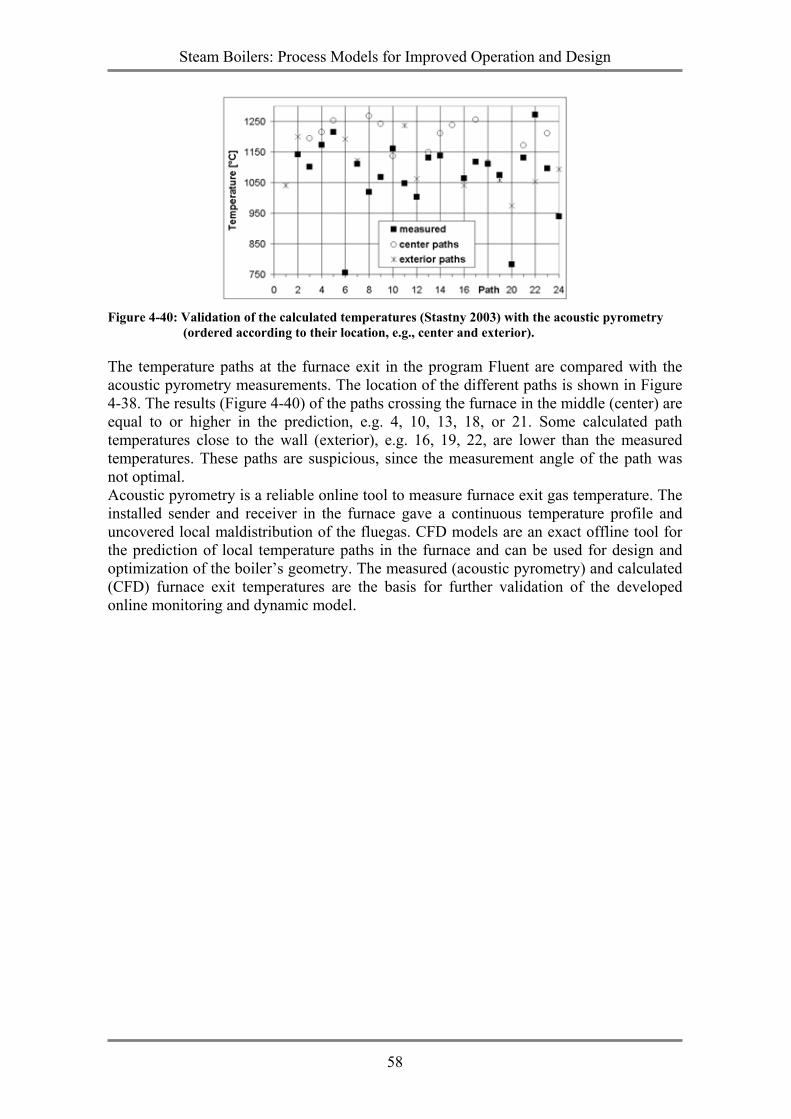
Steam Boilers: Process Models for Improved Operation and Design
58
Figure 4-40: Validation of the calculated temperatures (Stastny 2003) with the acoustic pyrometry
(ordered according to their location, e.g., center and exterior).
The temperature paths at the furnace exit in the program Fluent are compared with the acoustic pyrometry measurements. The location of the different paths is shown in Figure 4-38. The results (Figure 4-40) of the paths crossing the furnace in the middle (center) are equal to or higher in the prediction, e.g. 4, 10, 13, 18, or 21. Some calculated path temperatures close to the wall (exterior), e.g. 16, 19, 22, are lower than the measured temperatures. These paths are suspicious, since the measurement angle of the path was not optimal. Acoustic pyrometry is a reliable online tool to measure furnace exit gas temperature. The installed sender and receiver in the furnace gave a continuous temperature profile and uncovered local maldistribution of the fluegas. CFD models are an exact offline tool for the prediction of local temperature paths in the furnace and can be used for design and optimization of the boiler’s geometry. The measured (acoustic pyrometry) and calculated (CFD) furnace exit temperatures are the basis for further validation of the developed online monitoring and dynamic model.
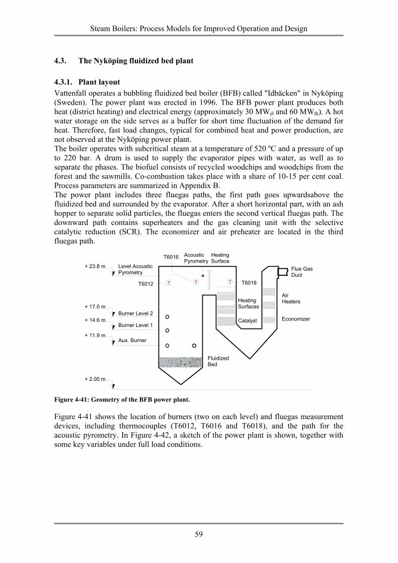
Steam Boilers: Process Models for Improved Operation and Design
59
4.3. The Nyköping fluidized bed plant
4.3.1. Plant layout Vattenfall operates a bubbling fluidized bed boiler (BFB) called "Idbäcken" in Nyköping (Sweden). The power plant was erected in 1996. The BFB power plant produces both heat (district heating) and electrical energy (approximately 30 MWel and 60 MWth). A hot water storage on the side serves as a buffer for short time fluctuation of the demand for heat. Therefore, fast load changes, typical for combined heat and power production, are not observed at the Nyköping power plant. The boiler operates with subcritical steam at a temperature of 520 ºC and a pressure of up to 220 bar. A drum is used to supply the evaporator pipes with water, as well as to separate the phases. The biofuel consists of recycled woodchips and woodchips from the forest and the sawmills. Co-combustion takes place with a share of 10-15 per cent coal. Process parameters are summarized in Appendix B. The power plant includes three fluegas paths, the first path goes upwardsabove the fluidized bed and surrounded by the evaporator. After a short horizontal part, with an ash hopper to separate solid particles, the fluegas enters the second vertical fluegas path. The downward path contains superheaters and the gas cleaning unit with the selective catalytic reduction (SCR). The economizer and air preheater are located in the third fluegas path.
Aux. Burner + 11.9 m
Burner Level 1 + 14.6 m
Burner Level 2+ 17.0 m
Level AcousticPyrometry
+ 23.8 m Flue GasDuct
AirHeaters
EconomizerCatalyst
HeatingSurfaces
HeatingSurface
AcousticPyrometry
FluidizedBed
+ 2.00 m
T T TT6012
T6016
T6018
Figure 4-41: Geometry of the BFB power plant.
Figure 4-41 shows the location of burners (two on each level) and fluegas measurement devices, including thermocouples (T6012, T6016 and T6018), and the path for the acoustic pyrometry. In Figure 4-42, a sketch of the power plant is shown, together with some key variables under full load conditions.
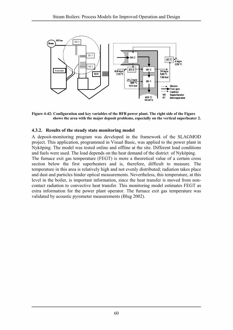
Steam Boilers: Process Models for Improved Operation and Design
60
Figure 4-42: Configuration and key variables of the BFB power plant. The right side of the Figure
shows the area with the major deposit problems, especially on the vertical superheater 2.
4.3.2. Results of the steady state monitoring model A deposit-monitoring program was developed in the framework of the SLAGMOD project. This application, programmed in Visual Basic, was applied to the power plant in Nyköping. The model was tested online and offline at the site. Different load conditions and fuels were used. The load depends on the heat demand of the district of Nyköping. The furnace exit gas temperature (FEGT) is more a theoretical value of a certain cross section below the first superheaters and is, therefore, difficult to measure. The temperature in this area is relatively high and not evenly distributed; radiation takes place and dust and particles hinder optical measurements. Nevertheless, this temperature, at this level in the boiler, is important information, since the heat transfer is moved from non-contact radiation to convective heat transfer. This monitoring model estimates FEGT as extra information for the power plant operator. The furnace exit gas temperature was validated by acoustic pyrometer measurements (Blug 2002).
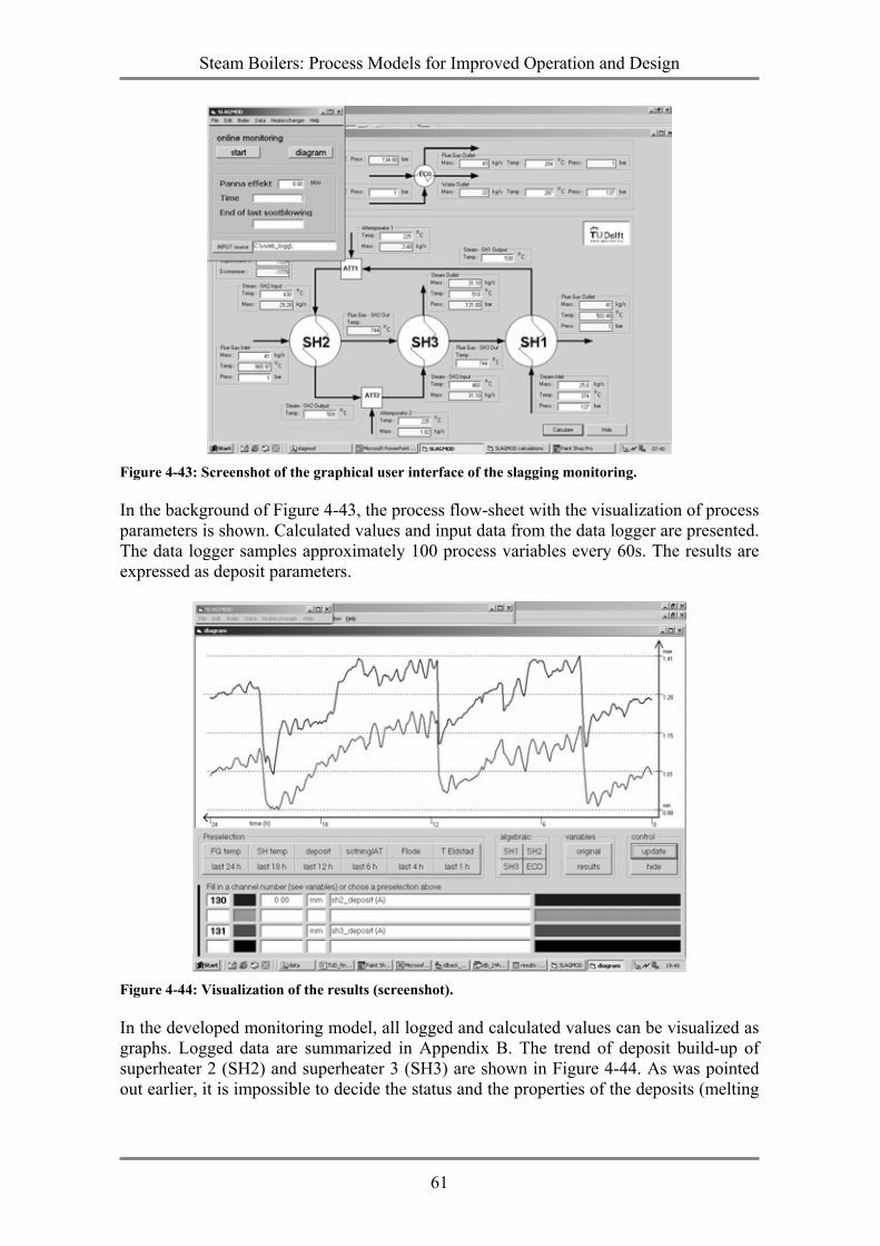
Steam Boilers: Process Models for Improved Operation and Design
61
Figure 4-43: Screenshot of the graphical user interface of the slagging monitoring.
In the background of Figure 4-43, the process flow-sheet with the visualization of process parameters is shown. Calculated values and input data from the data logger are presented. The data logger samples approximately 100 process variables every 60s. The results are expressed as deposit parameters.
Figure 4-44: Visualization of the results (screenshot).
In the developed monitoring model, all logged and calculated values can be visualized as graphs. Logged data are summarized in Appendix B. The trend of deposit build-up of superheater 2 (SH2) and superheater 3 (SH3) are shown in Figure 4-44. As was pointed out earlier, it is impossible to decide the status and the properties of the deposits (melting
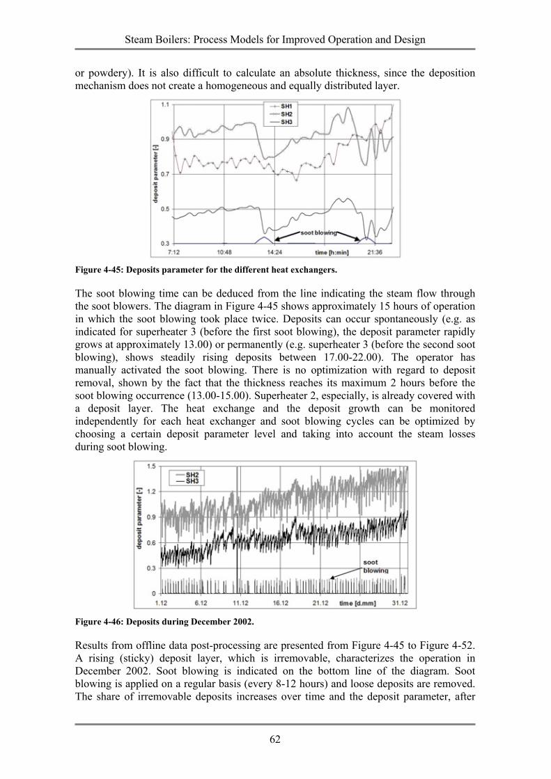
Steam Boilers: Process Models for Improved Operation and Design
62
or powdery). It is also difficult to calculate an absolute thickness, since the deposition mechanism does not create a homogeneous and equally distributed layer.
Figure 4-45: Deposits parameter for the different heat exchangers.
The soot blowing time can be deduced from the line indicating the steam flow through the soot blowers. The diagram in Figure 4-45 shows approximately 15 hours of operation in which the soot blowing took place twice. Deposits can occur spontaneously (e.g. as indicated for superheater 3 (before the first soot blowing), the deposit parameter rapidly grows at approximately 13.00) or permanently (e.g. superheater 3 (before the second soot blowing), shows steadily rising deposits between 17.00-22.00). The operator has manually activated the soot blowing. There is no optimization with regard to deposit removal, shown by the fact that the thickness reaches its maximum 2 hours before the soot blowing occurrence (13.00-15.00). Superheater 2, especially, is already covered with a deposit layer. The heat exchange and the deposit growth can be monitored independently for each heat exchanger and soot blowing cycles can be optimized by choosing a certain deposit parameter level and taking into account the steam losses during soot blowing.
Figure 4-46: Deposits during December 2002.
Results from offline data post-processing are presented from Figure 4-45 to Figure 4-52. A rising (sticky) deposit layer, which is irremovable, characterizes the operation in December 2002. Soot blowing is indicated on the bottom line of the diagram. Soot blowing is applied on a regular basis (every 8-12 hours) and loose deposits are removed. The share of irremovable deposits increases over time and the deposit parameter, after
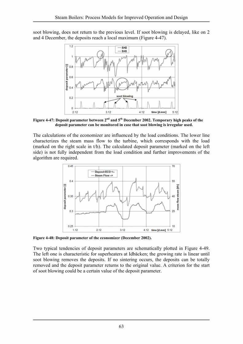
Steam Boilers: Process Models for Improved Operation and Design
63
soot blowing, does not return to the previous level. If soot blowing is delayed, like on 2 and 4 December, the deposits reach a local maximum (Figure 4-47).
Figure 4-47: Deposit parameter between 2nd and 5th December 2002. Temporary high peaks of the
deposit parameter can be monitored in case that soot blowing is irregular used.
The calculations of the economizer are influenced by the load conditions. The lower line characterizes the steam mass flow to the turbine, which corresponds with the load (marked on the right scale in t/h). The calculated deposit parameter (marked on the left side) is not fully independent from the load condition and further improvements of the algorithm are required.
Figure 4-48: Deposit parameter of the economizer (December 2002).
Two typical tendencies of deposit parameters are schematically plotted in Figure 4-49. The left one is characteristic for superheaters at Idbäcken; the growing rate is linear until soot blowing removes the deposits. If no sintering occurs, the deposits can be totally removed and the deposit parameter returns to the original value. A criterion for the start of soot blowing could be a certain value of the deposit parameter.
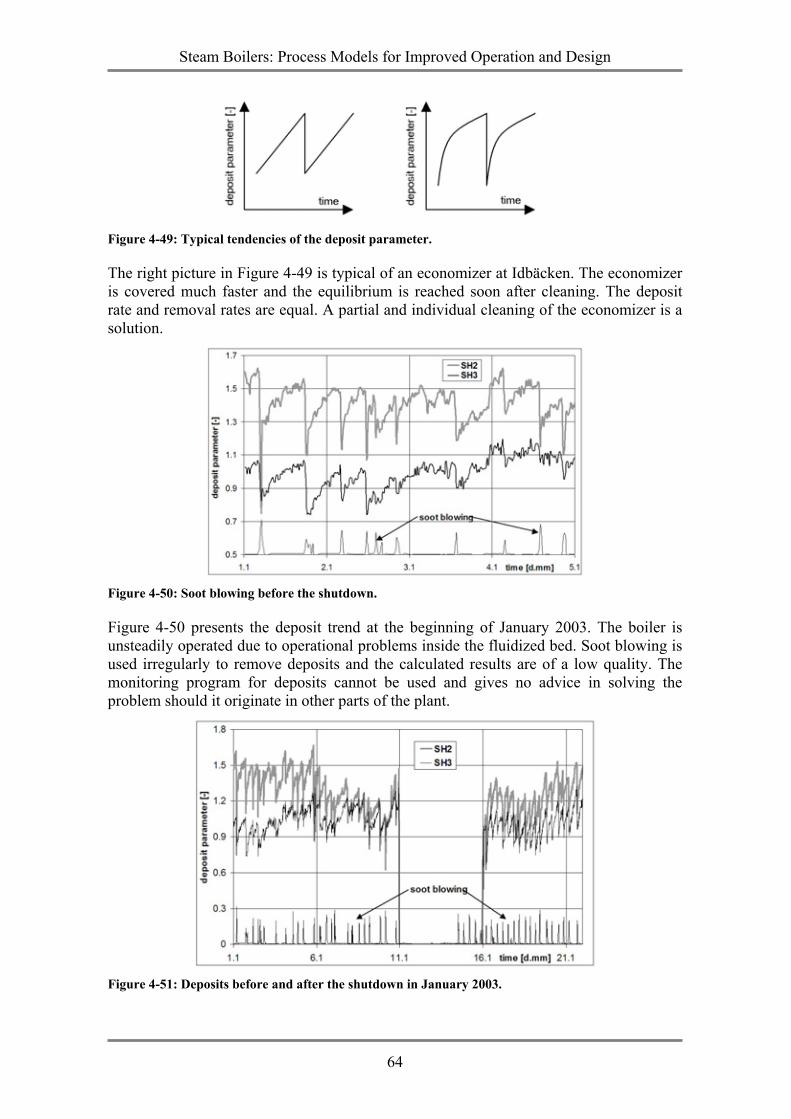
Steam Boilers: Process Models for Improved Operation and Design
64
Figure 4-49: Typical tendencies of the deposit parameter.
The right picture in Figure 4-49 is typical of an economizer at Idbäcken. The economizer is covered much faster and the equilibrium is reached soon after cleaning. The deposit rate and removal rates are equal. A partial and individual cleaning of the economizer is a solution.
Figure 4-50: Soot blowing before the shutdown.
Figure 4-50 presents the deposit trend at the beginning of January 2003. The boiler is unsteadily operated due to operational problems inside the fluidized bed. Soot blowing is used irregularly to remove deposits and the calculated results are of a low quality. The monitoring program for deposits cannot be used and gives no advice in solving the problem should it originate in other parts of the plant.
Figure 4-51: Deposits before and after the shutdown in January 2003.
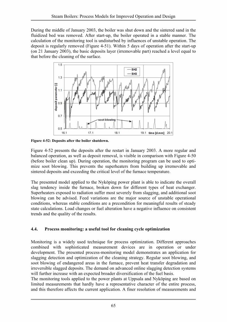
Steam Boilers: Process Models for Improved Operation and Design
65
During the middle of January 2003, the boiler was shut down and the sintered sand in the fluidized bed was removed. After start-up, the boiler operated in a stable manner. The calculation of the monitoring tool is undisturbed by influences of unstable operation. The deposit is regularly removed (Figure 4-51). Within 5 days of operation after the start-up (on 21 January 2003), the basic deposits layer (irremovable part) reached a level equal to that before the cleaning of the surface.
Figure 4-52: Deposits after the boiler shutdown.
Figure 4-52 presents the deposits after the restart in January 2003. A more regular and balanced operation, as well as deposit removal, is visible in comparison with Figure 4-50 (before boiler clean up). During operation, the monitoring program can be used to opti-mize soot blowing. This prevents the superheaters from building up irremovable and sintered deposits and exceeding the critical level of the furnace temperature. The presented model applied to the Nyköping power plant is able to indicate the overall slag tendency inside the furnace, broken down for different types of heat exchanger. Superheaters exposed to radiation suffer most severely from slagging, and additional soot blowing can be advised. Feed variations are the major source of unstable operational conditions, whereas stable conditions are a precondition for meaningful results of steady state calculations. Load changes or fuel alteration have a negative influence on consistent trends and the quality of the results.
4.4. Process monitoring: a useful tool for cleaning cycle optimization Monitoring is a widely used technique for process optimization. Different approaches combined with sophisticated measurement devices are in operation or under development. The presented process-monitoring model demonstrates an application for slagging detection and optimization of the cleaning strategy. Regular soot blowing, and soot blowing of endangered areas in the furnace, prevent heat transfer degradation and irreversible slagged deposits. The demand on advanced online slagging detection systems will further increase with an expected broader diversification of the fuel basis. The monitoring tools applied to the power plants at Uppsala and Nyköping are based on limited measurements that hardly have a representative character of the entire process, and this therefore affects the current application. A finer resolution of measurements and
Steam Boilers: Process Models for Improved Operation and Design
66
modeling is important for an individual cleaning strategy. The bottleneck of adequate measurements is the real challenge, and this cannot solely be covered by sophisticated data refining techniques. During unstable operational conditions, the monitoring tool is still unable to provide similarly valuable information since the source of disturbances is mostly outside the modeling boundary. Another outlook is connected to developments in computer science, and increasing computing performance. It is obvious that technological progress will allow the use of microscopic CFD models as online tools in the future. During operation of the power plant also, other different dynamic interaction take place, and these are per definition not covered by a steady state solution. Typical changes are; pressure alternations with time transients in fractions of a second, load changes with transients in minutes, or deposit growth with normal build–up rates in several hours. Where pressure alternations and the momentum balance are widely neglected, the dynamics of slagging and fouling are such slow processes that steady state solutions are sufficient. The remaining points of interest are load changes and heat transfer shifts during, e.g., soot blowing. A combined heat and power plant is normally characterized by fast load changes, following the heat demand of the consumer. These continuous fluctuations of load were not typical of the investigated power plants due to the operation of the plant. Other units on the integrated system compensated the changes of heat demand at Nyköping and Uppsala, and load changes were only occasionally monitored. These monitored load changes and unstable conditions caused by external influences are not covered by the current steady state solution. The dynamic model presented in the next chapter shares many characteristics with the process-monitoring models. Both application use similar sub-models for heat transfer and laws of conservation. Nevertheless, the motivation of the dynamic model is based on application as a predictive model for control purposes, and not as a monitoring tool.
Steam Boilers: Process Models for Improved Operation and Design
67
5. PREDICTIVE DYNAMIC MODELING FOR CONTROL AND EQUIPMENT DESIGN IMPROVEMENT
Overview Dynamic modeling and simulation of steam power plants is often adopted as a tool for control design and tuning, personnel training, efficiency improvement and system diag-nostics. The boiler is one of the most complex components of the thermal power plant. A usual boiler configuration is the so-called once-through arrangement. A common prob-lem in two-phase systems modeling is the correct calculation of the phase boundary position. This is technically interesting and important in such boilers: the position of the phase transition changes rapidly depending on load conditions and temperature distri-bution along the walls. Abruptly reduced heat transfer in the dry out region can cause metal stresses and changes the slagging tendency. A lumped parameter, one-dimensional evaporator model implementing a moving bound-ary approach is presented and first validation results are discussed. The model takes into account the influence of radiation and convection on the gas side. The flow inside the pipes is divided into 3 regions (sub-cooled, two-phase, superheated) and the model calculates the positions of the two-phase transition and the average steam quality along the pipes. The system is discretized using a staggered grid for higher numerical stability and is implemented in the computer program Aspen Custom Modeler (ACM). Results include the calculation of the system response to input signals simulating a load variation, and a validation by comparison with a model implemented in commercial software for power plant simulations (MMS). Input data, parameters and geometry are taken from an existing plant operating in Uppsala, Sweden.
5.1. Introduction to dynamic modeling and simulation of a once-through boiler Steady state models are commonly used but static design does not capture dynamics. Dynamic modeling in the energy-engineering sector started with studies on thermal stresses in pressurized systems. The thick steel walls of the drum and collector are sensi-tive to fast load changes, causing fatigue fracture and steam losses (Doležal 1990). Backup systems of boilers connected in parallel were common due to the low availability of the plant. Nowadays, dynamic modeling and simulation is becoming increasingly important. It is used not only as a design tool for control purposes, but also as a diagnostic tool and is important during discontinuous operations, e.g., start-up, shutdown and load changes. To stabilize the AC frequency in the grid, load changes from 6 to 10 percent per minute are normally required. In case of major disturbances, even a 20 percent load increase within 5 seconds is common practice. Modeling of power plants may be approached from different points of view, depending on the purpose for which the model is intended. To simulate the dynamic behavior of a steam power plant, all relevant components have to be modeled and the lumped parame-ters approach is usually adopted. In cases where the model is used as a component of an online diagnostic system, it must comply with the real-time requirement, and the introduction of appropriate simplifications may be necessary. Computer models of power plants and specific programs are available for a variety of purposes (Flynn 2003, Ordys 1994, Modelica 2000, Elmegaard 1999). There are many proposals in scientific and technical literature concerning the modeling of components and the modeling of the entire power plant. They differ greatly in complexity: for example some detailed component models are available only for steady state simulations
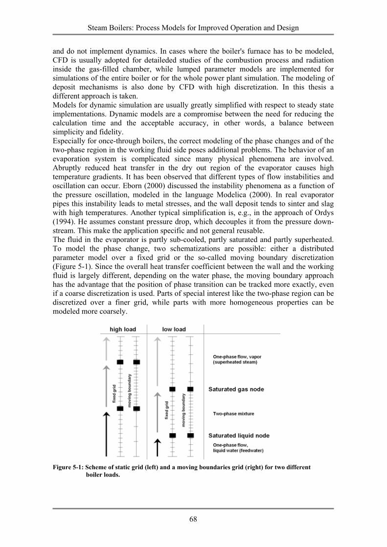
Steam Boilers: Process Models for Improved Operation and Design
68
and do not implement dynamics. In cases where the boiler's furnace has to be modeled, CFD is usually adopted for detaileded studies of the combustion process and radiation inside the gas-filled chamber, while lumped parameter models are implemented for simulations of the entire boiler or for the whole power plant simulation. The modeling of deposit mechanisms is also done by CFD with high discretization. In this thesis a different approach is taken. Models for dynamic simulation are usually greatly simplified with respect to steady state implementations. Dynamic models are a compromise between the need for reducing the calculation time and the acceptable accuracy, in other words, a balance between simplicity and fidelity. Especially for once-through boilers, the correct modeling of the phase changes and of the two-phase region in the working fluid side poses additional problems. The behavior of an evaporation system is complicated since many physical phenomena are involved. Abruptly reduced heat transfer in the dry out region of the evaporator causes high temperature gradients. It has been observed that different types of flow instabilities and oscillation can occur. Eborn (2000) discussed the instability phenomena as a function of the pressure oscillation, modeled in the language Modelica (2000). In real evaporator pipes this instability leads to metal stresses, and the wall deposit tends to sinter and slag with high temperatures. Another typical simplification is, e.g., in the approach of Ordys (1994). He assumes constant pressure drop, which decouples it from the pressure down-stream. This make the application specific and not general reusable. The fluid in the evaporator is partly sub-cooled, partly saturated and partly superheated. To model the phase change, two schematizations are possible: either a distributed parameter model over a fixed grid or the so-called moving boundary discretization (Figure 5-1). Since the overall heat transfer coefficient between the wall and the working fluid is largely different, depending on the water phase, the moving boundary approach has the advantage that the position of phase transition can be tracked more exactly, even if a coarse discretization is used. Parts of special interest like the two-phase region can be discretized over a finer grid, while parts with more homogeneous properties can be modeled more coarsely.
Figure 5-1: Scheme of static grid (left) and a moving boundaries grid (right) for two different
boiler loads.
Steam Boilers: Process Models for Improved Operation and Design
69
A large class of free and moving boundary problems are often called Stefan problems, with reference to the work of the Austrian scientist Josef Stefan, who is more famous for his work on radiation. He also studied the problem of ice formation in the polar sea and first introduced the moving boundaries approach to investigate phase change. The story of how Stefan obtained experimental data for his moving boundary calculation is quite a curious one and worth mentioning. In spite of Columbus’ discoveries, the existence of a Northwest Passage connecting the Atlantic with the Pacific was still an open issue. Several commercial and scientific expeditions tried to find a way through in the 19th century. The British expedition of Sir John Franklin in 1850 ended tragically. All its members died of lead poisoning, since lead was used for the cans to store food. Several rescue expeditions were sent to find the missing crew. In the long and icy arctic winter all of them were trapped in the polar-ice and they had plenty of time to study and record the growth of the ice layer under their ships. These datasets were the basis upon which to model the moving interface between the water and the ice (Vuik 1993). The moving boundary approach is also used for the modeling of refrigeration cycles, evaporators and condensers (Willatzen 1998, Jensen 2002) and for heat pump cycles (Grald 1992, Bendapudi 2002). Moreover, moving boundary models are employed to simulate water channels in boiling water nuclear reactors for safety studies of density-wave oscillations (Abdalla 1994, Garea 1999). The general advantage of this approach is that it avoids the use of a static grid, which must contain a multitude of nodes in order to correctly track the phase boundary position. Additionally, the moving boundary approach simplifies the dynamics of the system, since, by changing only the position of the node, every node keeps its material properties unmodified. Smaller changes of the state variables result in larger time steps during the simulation in the case of a variable time step algorithm. Details concerning the adopted modeling paradigm can be found in Kikstra (2001 and 2002), where the modularity principle is applied, the unknown variables of a module (component) are computed as a function of variables within the module. Building models of blocks with input-output functions is a common practice in engineering. This permits a whole system to be constructed from independently developed and compatible compo-nent models (e.g., superheater, evaporator, pump, etc.). In this model, every component module is further discretized in small control volumes (modules). The macroscopic continuous conservation laws are solved, instead of solving the microscopic alternatives. The spatial discretization is obtained by dividing the boiler into sections orthogonal to the flow direction of fluegas and water/steam, for which bal-ance equations are solved in the hypothesis of homogeneous fluid properties inside the control volume, the so-called well-stirred tank approximation. The control volumes are taken with their axis coincident with the axis of the flow direction. Every control volume represents a one-dimensional system. All fluid flows, i.e., in this case the fluegas and water/steam streams, are divided into an equal number of equidistant and alternating cylindrical volumes, the so-called thermal nodes and flow nodes (Figure 5-2). Every thermal node consists of half of the neighbor-ing flow nodes, i.e., the thermal node “i” consist of half of the flow node “j+1” and “j”. The flow node “j” consists of two half thermal nodes “i-1” and “i”. The difference in diameter depicted in Figure 5-2 is simply for graphical clarity. For each thermal node the energy and mass balances are solved, while the momentum balance is calculated in the flow nodes.
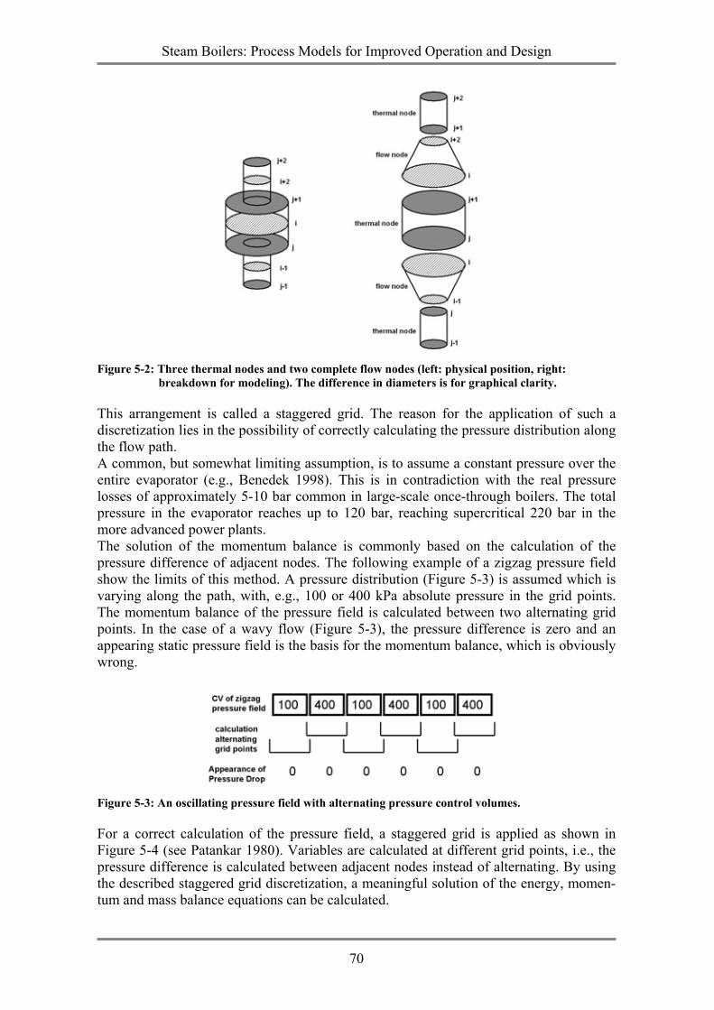
Steam Boilers: Process Models for Improved Operation and Design
70
Figure 5-2: Three thermal nodes and two complete flow nodes (left: physical position, right:
breakdown for modeling). The difference in diameters is for graphical clarity.
This arrangement is called a staggered grid. The reason for the application of such a discretization lies in the possibility of correctly calculating the pressure distribution along the flow path. A common, but somewhat limiting assumption, is to assume a constant pressure over the entire evaporator (e.g., Benedek 1998). This is in contradiction with the real pressure losses of approximately 5-10 bar common in large-scale once-through boilers. The total pressure in the evaporator reaches up to 120 bar, reaching supercritical 220 bar in the more advanced power plants. The solution of the momentum balance is commonly based on the calculation of the pressure difference of adjacent nodes. The following example of a zigzag pressure field show the limits of this method. A pressure distribution (Figure 5-3) is assumed which is varying along the path, with, e.g., 100 or 400 kPa absolute pressure in the grid points. The momentum balance of the pressure field is calculated between two alternating grid points. In the case of a wavy flow (Figure 5-3), the pressure difference is zero and an appearing static pressure field is the basis for the momentum balance, which is obviously wrong.
Figure 5-3: An oscillating pressure field with alternating pressure control volumes.
For a correct calculation of the pressure field, a staggered grid is applied as shown in Figure 5-4 (see Patankar 1980). Variables are calculated at different grid points, i.e., the pressure difference is calculated between adjacent nodes instead of alternating. By using the described staggered grid discretization, a meaningful solution of the energy, momen-tum and mass balance equations can be calculated.
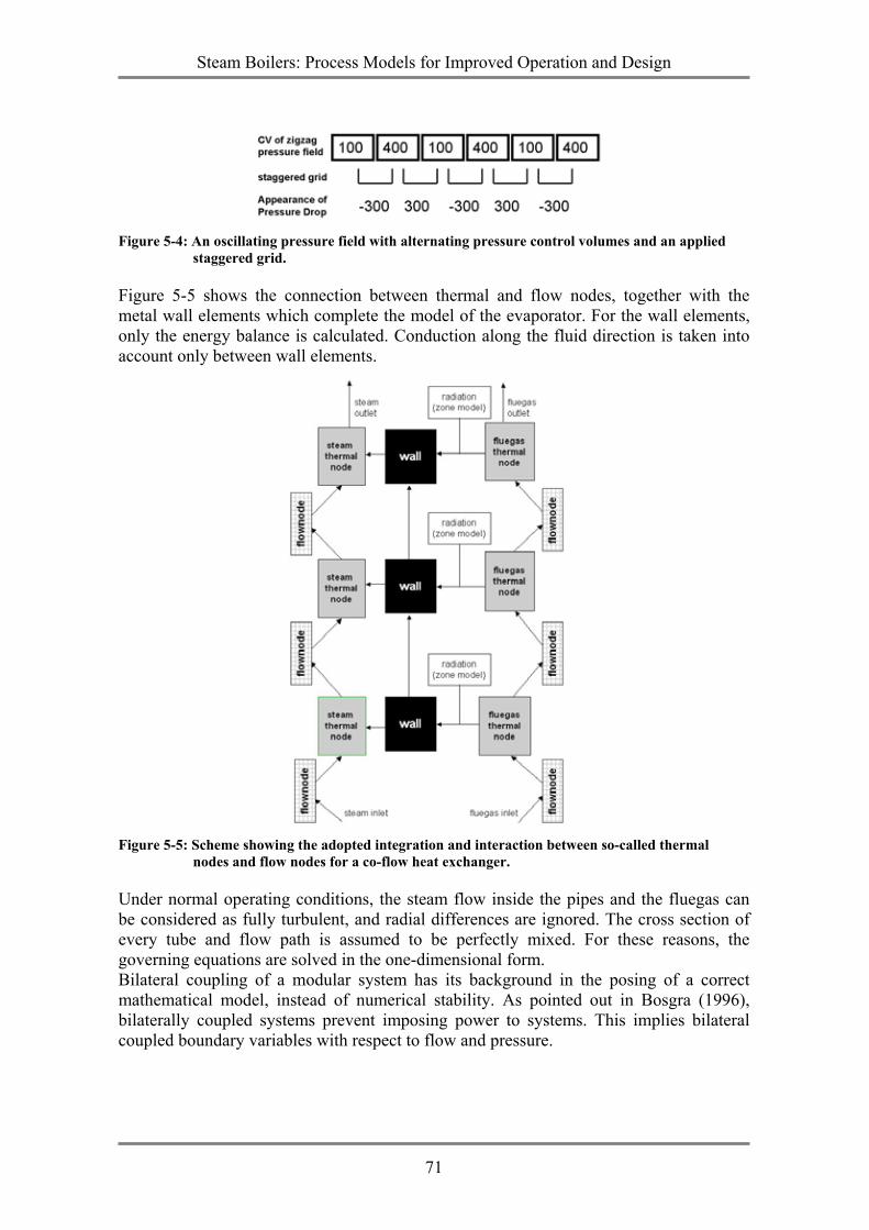
Steam Boilers: Process Models for Improved Operation and Design
71
Figure 5-4: An oscillating pressure field with alternating pressure control volumes and an applied
staggered grid.
Figure 5-5 shows the connection between thermal and flow nodes, together with the metal wall elements which complete the model of the evaporator. For the wall elements, only the energy balance is calculated. Conduction along the fluid direction is taken into account only between wall elements.
Figure 5-5: Scheme showing the adopted integration and interaction between so-called thermal
nodes and flow nodes for a co-flow heat exchanger.
Under normal operating conditions, the steam flow inside the pipes and the fluegas can be considered as fully turbulent, and radial differences are ignored. The cross section of every tube and flow path is assumed to be perfectly mixed. For these reasons, the governing equations are solved in the one-dimensional form. Bilateral coupling of a modular system has its background in the posing of a correct mathematical model, instead of numerical stability. As pointed out in Bosgra (1996), bilaterally coupled systems prevent imposing power to systems. This implies bilateral coupled boundary variables with respect to flow and pressure.
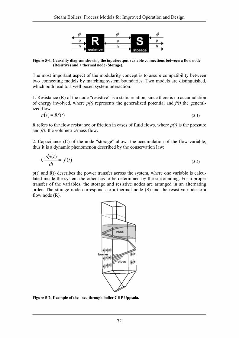
Steam Boilers: Process Models for Improved Operation and Design
72
Figure 5-6: Causality diagram showing the input/output variable connections between a flow node
(Resistive) and a thermal node (Storage).
The most important aspect of the modularity concept is to assure compatibility between two connecting models by matching system boundaries. Two models are distinguished, which both lead to a well posed system interaction: 1. Resistance (R) of the node “resistive” is a static relation, since there is no accumulation of energy involved, where p(t) represents the generalized potential and f(t) the general-ized flow.
( ) ( )p t Rf t= (5-1)
R refers to the flow resistance or friction in cases of fluid flows, where p(t) is the pressure and f(t) the volumetric/mass flow. 2. Capacitance (C) of the node “storage” allows the accumulation of the flow variable, thus it is a dynamic phenomenon described by the conservation law:
( ) ( )dp tC f tdt
= (5-2)
p(t) and f(t) describes the power transfer across the system, where one variable is calcu-lated inside the system the other has to be determined by the surrounding. For a proper transfer of the variables, the storage and resistive nodes are arranged in an alternating order. The storage node corresponds to a thermal node (S) and the resistive node to a flow node (R).
Figure 5-7: Example of the once-through boiler CHP Uppsala.
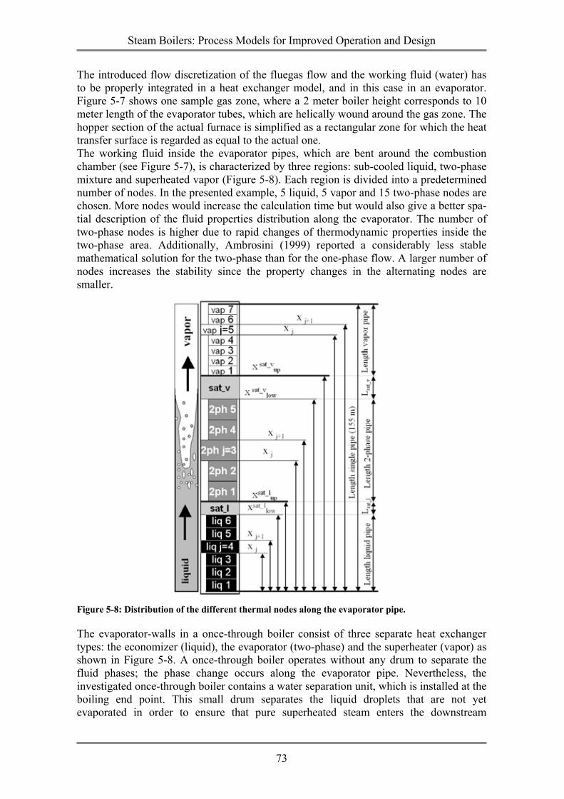
Steam Boilers: Process Models for Improved Operation and Design
73
The introduced flow discretization of the fluegas flow and the working fluid (water) has to be properly integrated in a heat exchanger model, and in this case in an evaporator. Figure 5-7 shows one sample gas zone, where a 2 meter boiler height corresponds to 10 meter length of the evaporator tubes, which are helically wound around the gas zone. The hopper section of the actual furnace is simplified as a rectangular zone for which the heat transfer surface is regarded as equal to the actual one. The working fluid inside the evaporator pipes, which are bent around the combustion chamber (see Figure 5-7), is characterized by three regions: sub-cooled liquid, two-phase mixture and superheated vapor (Figure 5-8). Each region is divided into a predetermined number of nodes. In the presented example, 5 liquid, 5 vapor and 15 two-phase nodes are chosen. More nodes would increase the calculation time but would also give a better spa-tial description of the fluid properties distribution along the evaporator. The number of two-phase nodes is higher due to rapid changes of thermodynamic properties inside the two-phase area. Additionally, Ambrosini (1999) reported a considerably less stable mathematical solution for the two-phase than for the one-phase flow. A larger number of nodes increases the stability since the property changes in the alternating nodes are smaller.
Figure 5-8: Distribution of the different thermal nodes along the evaporator pipe.
The evaporator-walls in a once-through boiler consist of three separate heat exchanger types: the economizer (liquid), the evaporator (two-phase) and the superheater (vapor) as shown in Figure 5-8. A once-through boiler operates without any drum to separate the fluid phases; the phase change occurs along the evaporator pipe. Nevertheless, the investigated once-through boiler contains a water separation unit, which is installed at the boiling end point. This small drum separates the liquid droplets that are not yet evaporated in order to ensure that pure superheated steam enters the downstream
Steam Boilers: Process Models for Improved Operation and Design
74
superheaters. Under regular operating conditions, the mass flow at the outlet of the boiler is fully superheated. Only during the start-up procedure is a measurable liquid water flow separated and recycled. In order to calculate the position of the phase change, two boundary nodes, one liquid-two-phase and one two-phase-vapor, are introduced: for these nodes, saturated properties are imposed (sat_l and sat_v in Figure 5-8).
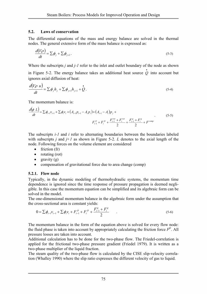
Steam Boilers: Process Models for Improved Operation and Design
75
5.2. Laws of conservation The differential equations of the mass and energy balance are solved in the thermal nodes. The general extensive form of the mass balance is expressed as:
( )1+∑+∑= jjdt
Vd φφρ . (5-3)
Where the subscripts j and j-1 refer to the inlet and outlet boundary of the node as shown
in Figure 5-2. The energy balance takes an additional heat source •
Q into account but ignores axial diffusion of heat:
( ) •
++ +∑+∑= Qhhdt
uVdjjjj 11φφ
ρ. (5-4)
The momentum balance is:
( ) ( ) ( )
compg
ig
irot
irot
ifri
fri
jiiiiiiiiii
FFFFFFF
pAApApAvvdt
Ld
++
++
++
+−+−+∑+∑=
−−−
−−−−−
2211
1
11111 φφφ. (5-5)
The subscripts i-1 and i refer to alternating boundaries between the boundaries labeled with subscripts j and j+1 as shown in Figure 5-2. L denotes to the axial length of the node. Following forces on the volume element are considered
• friction (fr) • rotating (rot) • gravity (g) • compensation of gravitational force due to area change (comp)
5.2.1. Flow node Typically, in the dynamic modeling of thermohydraulic systems, the momentum time dependence is ignored since the time response of pressure propagation is deemed negli-gible. In this case the momentum equation can be simplified and its algebraic form can be solved in the model. The one-dimensional momentum balance in the algebraic form under the assumption that the cross-sectional area is constant yields:
2
0 1111
gi
gifr
ifr
iiiiiFFFFvv +
+++∑+∑= −−−− φφ . (5-6)
The momentum balance in the form of the equation above is solved for every flow node: the fluid phase is taken into account by appropriately calculating the friction force Ffr. All pressure losses are taken into account. Additional calculation has to be done for the two-phase flow. The Friedel-correlation is applied for the frictional two-phase pressure gradient (Friedel 1979). It is written as a two-phase multiplier of the liquid fraction. The steam quality of the two-phase flow is calculated by the CISE slip-velocity correla-tion (Whalley 1990) where the slip ratio expresses the different velocity of gas to liquid.
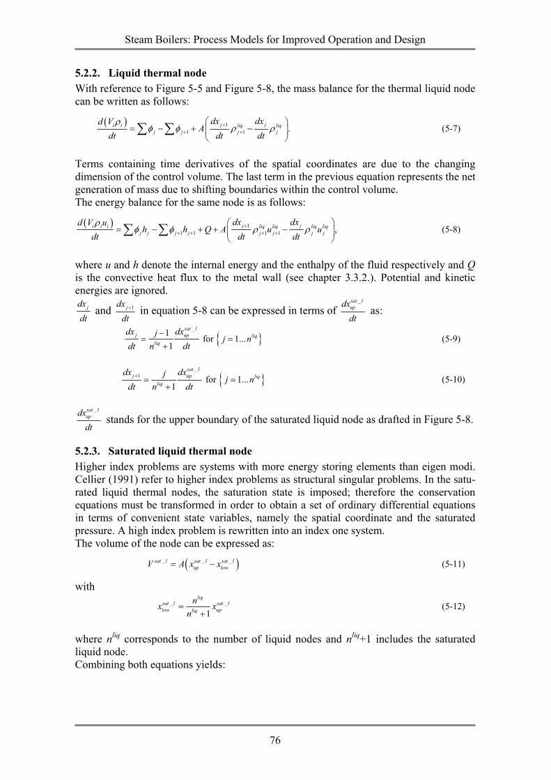
Steam Boilers: Process Models for Improved Operation and Design
76
5.2.2. Liquid thermal node With reference to Figure 5-5 and Figure 5-8, the mass balance for the thermal liquid node can be written as follows:
( ) 11 1 .j ji i liq liq
j j j j
dx dxd VA
dt dt dtρ
φ φ ρ ρ++ +
= − + −
∑ ∑ (5-7)
Terms containing time derivatives of the spatial coordinates are due to the changing dimension of the control volume. The last term in the previous equation represents the net generation of mass due to shifting boundaries within the control volume. The energy balance for the same node is as follows:
( ) 11 1 1 1 ,j ji i i liq liq liq liq
j j j j j j j j
dx dxd V uh h Q A u u
dt dt dtρ
φ φ ρ ρ++ + + +
= − + + −
∑ ∑ (5-8)
where u and h denote the internal energy and the enthalpy of the fluid respectively and Q is the convective heat flux to the metal wall (see chapter 3.3.2.). Potential and kinetic energies are ignored.
jdxdt
and 1jdxdt
+ in equation 5-8 can be expressed in terms of _sat l
updxdt
as:
}{_1 for 1...
1
sat lj up liq
liq
dx dxj j ndt dtn
−= =
+ (5-9)
}{_
1 for 1...1
sat lj up liq
liq
dx dxj j ndt dtn
+ = =+
(5-10)
_sat l
updxdt
stands for the upper boundary of the saturated liquid node as drafted in Figure 5-8.
5.2.3. Saturated liquid thermal node Higher index problems are systems with more energy storing elements than eigen modi. Cellier (1991) refer to higher index problems as structural singular problems. In the satu-rated liquid thermal nodes, the saturation state is imposed; therefore the conservation equations must be transformed in order to obtain a set of ordinary differential equations in terms of convenient state variables, namely the spatial coordinate and the saturated pressure. A high index problem is rewritten into an index one system. The volume of the node can be expressed as:
( )_ _ _sat l sat l sat lup lowV A x x= − (5-11)
with
_ _
1
liqsat l sat llow upliq
nx xn
=+
(5-12)
where nliq corresponds to the number of liquid nodes and nliq+1 includes the saturated liquid node. Combining both equations yields:
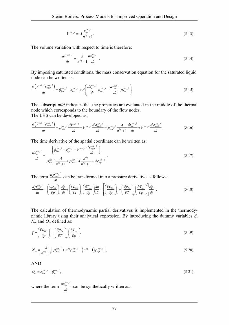
Steam Boilers: Process Models for Improved Operation and Design
77
_
_ .1
sat lupsat l
liq
xV A
n=
+ (5-13)
The volume variation with respect to time is therefore:
__
1
sat lsat lup
liq
dxdV Adt dtn
=+
. (5-14)
By imposing saturated conditions, the mass conservation equation for the saturated liquid node can be written as:
( )_ _ _ __ _ _ _ .
sat l sat l sat l sat lmid upsat l sat l sat l sat llow
low up up low
d V dx dxA
dt dt dt
ρφ φ ρ ρ
= − + −
(5-15)
The subscript mid indicates that the properties are evaluated in the middle of the thermal node which corresponds to the boundary of the flow nodes. The LHS can be developed as:
( )_ _ __ ___ _ _ _
1
sat l sat l sat lsat l sat lsat lmid upsat l sat l sat l sat lmid mid
mid mid liq
d V dxd ddV AV Vdt dt dt dt dtn
ρ ρ ρρ ρ= + = +
+. (5-16)
The time derivative of the spatial coordinate can be written as:
__ _ _
_
_ _ _
1 1
sat lsat l sat l sat l midlow upsat l
upliq
sat l sat l sat lmid low upliq liq
dVdx dt
dt A nA An n
ρφ φ
ρ ρ ρ
− −
=+ −
+ +
. (5-17)
The term _sat l
midddt
ρ can be transformed into a pressure derivative as follows:
_sat lliq liq liq liqmid sat sat
T p T p
d T Tdp dp dpdt p dt t p dt p T p dt
ρ ρ ρ ρρ ∂ ∂ ∂ ∂ ∂ ∂ = + = + ∂ ∂ ∂ ∂ ∂ ∂
. (5-18)
The calculation of thermodynamic partial derivatives is implemented in the thermody-namic library using their analytical expression. By introducing the dummy variables ξ, Nm and Om defined as:
,liq liq sat
T P
Tp T p
ρ ρξ
∂ ∂ ∂ = + ∂ ∂ ∂
(5-19)
( )_ _ _1 ,1
sat l liq sat l liq sat lm mid low upliq
AN n nn
ρ ρ ρ = + − + + (5-20)
AND
_ _ ,sat l sat lm low upO φ φ= − (5-21)
where the term _sat l
updxdt
can be synthetically written as:
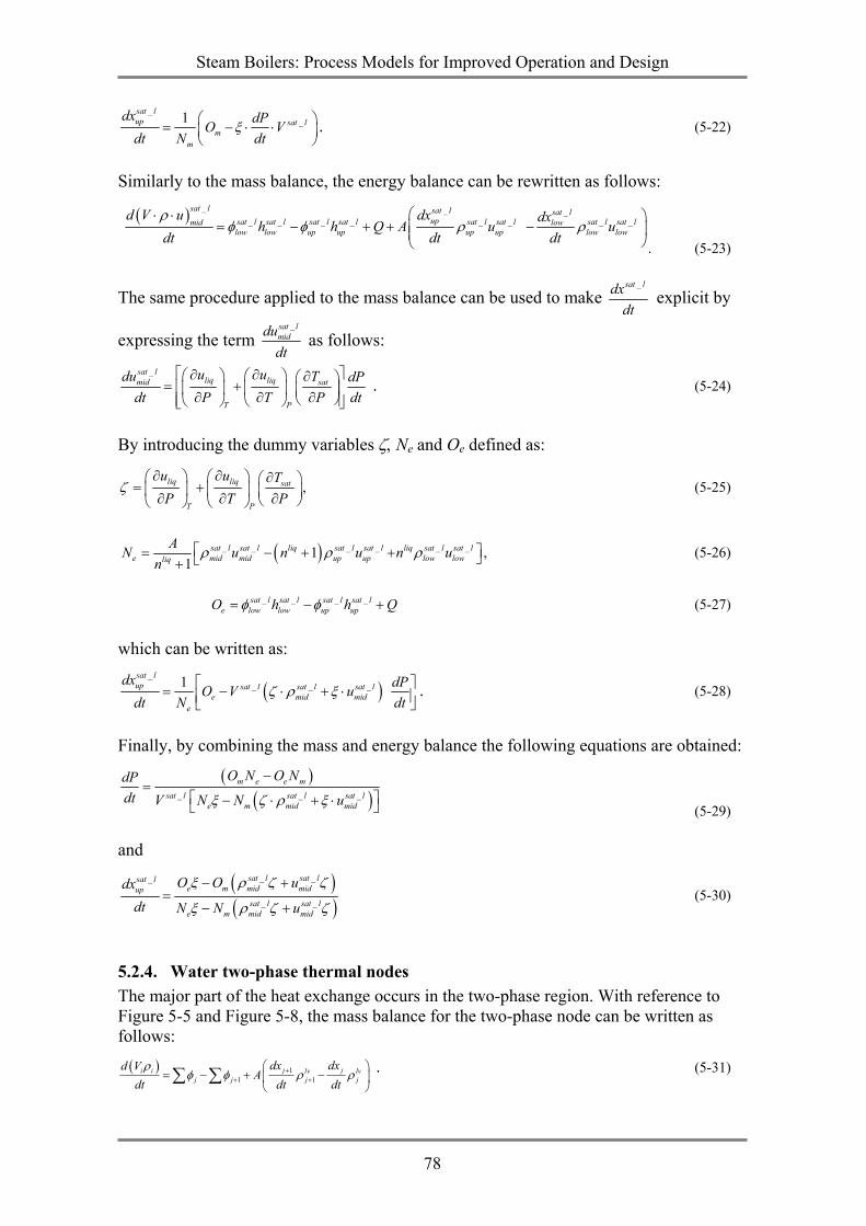
Steam Boilers: Process Models for Improved Operation and Design
78
__1sat l
up sat lm
m
dx dPO Vdt N dt
ξ = − ⋅ ⋅
. (5-22)
Similarly to the mass balance, the energy balance can be rewritten as follows:
( ) _ _ __ _ _ _ _ _ _ _
sat l sat l sat lupsat l sat l sat l sat l sat l sat l sat l sat lmid low
low low up up up up low low
d V u dx dxh h Q A u u
dt dt dtρ
φ φ ρ ρ⋅ ⋅
= − + + − . (5-23)
The same procedure applied to the mass balance can be used to make _sat ldx
dt explicit by
expressing the term _sat l
middudt
as follows:
_sat lliq liqmid sat
T P
u udu T dPdt P T P dt
∂ ∂ ∂ = + ∂ ∂ ∂ . (5-24)
By introducing the dummy variables ζ, Ne and Oe defined as:
,liq liq sat
T P
u u TP T P
ζ∂ ∂ ∂ = + ∂ ∂ ∂
(5-25)
( )_ _ _ _ _ _1 ,1
sat l sat l liq sat l sat l liq sat l sat le mid mid up up low lowliq
AN u n u n un
ρ ρ ρ = − + + + (5-26)
_ _ _ _sat l sat l sat l sat l
e low low up upO h h Qφ φ= − + (5-27) which can be written as:
( )_
_ _ _1 sat lup sat l sat l sat l
e mid mide
dx dPO V udt N dt
ζ ρ ξ = − ⋅ + ⋅ . (5-28)
Finally, by combining the mass and energy balance the following equations are obtained:
( )( )_ _ _
m e e m
sat l sat l sat le m mid mid
O N O NdPdt V N N uξ ζ ρ ξ
−=
− ⋅ + ⋅ (5-29) and
( )( )
_ __
_ _
sat l sat lsat le m mid midup
sat l sat le m mid mid
O O udxdt N N u
ξ ρ ζ ζ
ξ ρ ζ ζ
− +=
− + (5-30)
5.2.4. Water two-phase thermal nodes The major part of the heat exchange occurs in the two-phase region. With reference to Figure 5-5 and Figure 5-8, the mass balance for the two-phase node can be written as follows:
( ) 11 1
j ji i lv lvj j j j
dx dxd VA
dt dt dtρ
φ φ ρ ρ++ +
= − + −
∑ ∑ . (5-31)
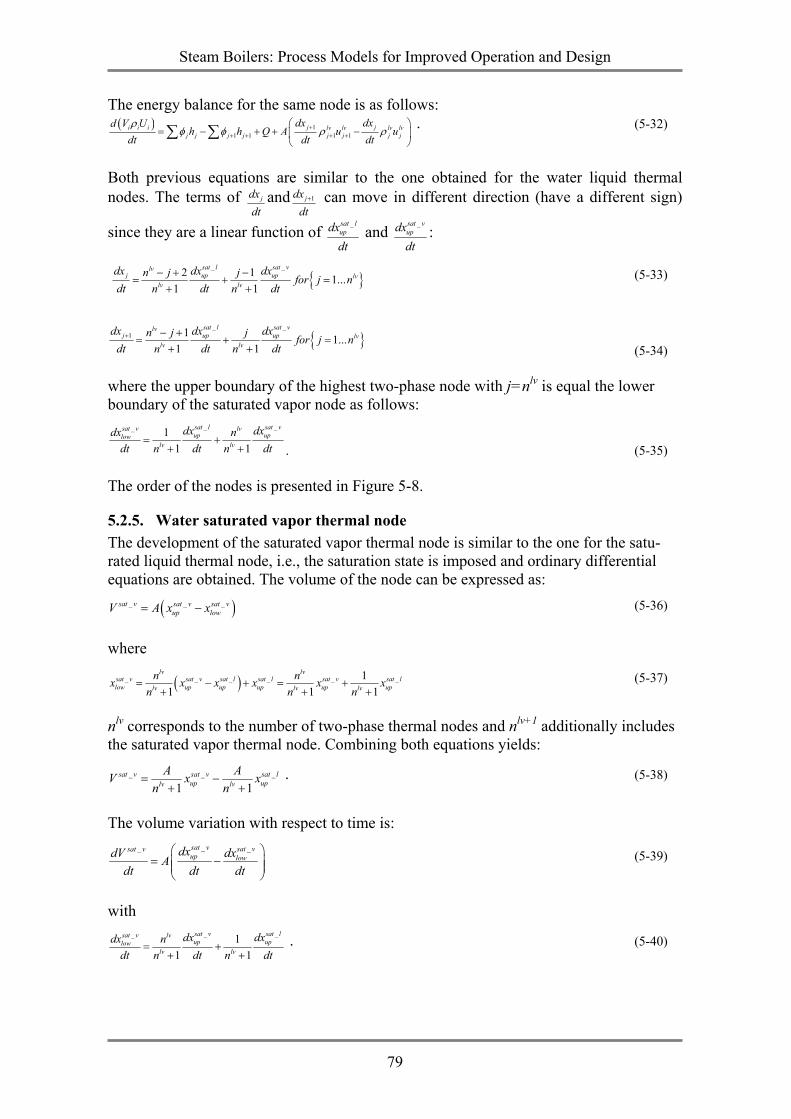
Steam Boilers: Process Models for Improved Operation and Design
79
The energy balance for the same node is as follows: ( ) 1
1 1 1 1j ji i i lv lv lv lv
j j j j j j j j
dx dxd V Uh h Q A u u
dt dt dtρ
φ φ ρ ρ++ + + +
= − + + −
∑ ∑ . (5-32)
Both previous equations are similar to the one obtained for the water liquid thermal nodes. The terms of jdx
dtand 1jdx
dt+ can move in different direction (have a different sign)
since they are a linear function of _sat l
updxdt
and _sat v
updxdt
:
}{_ _2 1 1...
1 1
sat l sat vlvj up up lv
lv lv
dx dx dxn j j for j ndt n dt n dt
− + −= + =
+ + (5-33)
}{_ _
1 1 1...1 1
sat l sat vlvj up up lv
lv lv
dx dx dxn j j for j ndt n dt n dt
+ − += + =
+ + (5-34) where the upper boundary of the highest two-phase node with j=nlv is equal the lower boundary of the saturated vapor node as follows:
_ __ 11 1
sat l sat vsat v lvup uplow
lv lv
dx dxdx ndt n dt n dt
= ++ + . (5-35)
The order of the nodes is presented in Figure 5-8.
5.2.5. Water saturated vapor thermal node The development of the saturated vapor thermal node is similar to the one for the satu-rated liquid thermal node, i.e., the saturation state is imposed and ordinary differential equations are obtained. The volume of the node can be expressed as:
( )_ _ _sat v sat v sat vup lowV A x x= − (5-36)
where
( )_ _ _ _ _ _11 1 1
lv lvsat v sat v sat l sat l sat v sat llow up up up up uplv lv lv
n nx x x x x xn n n
= − + = ++ + +
(5-37)
nlv corresponds to the number of two-phase thermal nodes and nlv+1 additionally includes the saturated vapor thermal node. Combining both equations yields:
_ _ _
1 1sat v sat v sat l
up uplv lv
A AV x xn n
= −+ +
. (5-38)
The volume variation with respect to time is:
_ __ sat v sat vsat vup lowdx dxdV A
dt dt dt
= −
(5-39)
with
_ __ 11 1
sat v sat lsat v lvup uplow
lv lv
dx dxdx ndt n dt n dt
= ++ +
. (5-40)
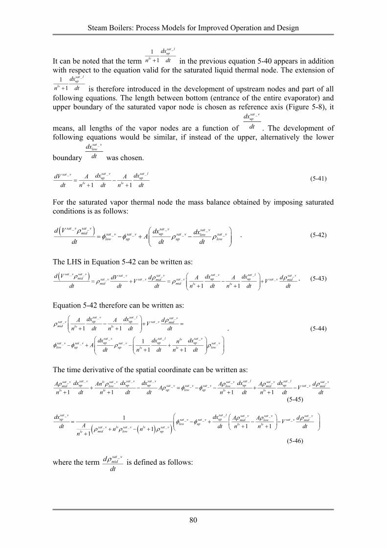
Steam Boilers: Process Models for Improved Operation and Design
80
It can be noted that the term
_11
sat lup
lv
dxn dt+ in the previous equation 5-40 appears in addition
with respect to the equation valid for the saturated liquid thermal node. The extension of _1
1
sat lup
lv
dxn dt+ is therefore introduced in the development of upstream nodes and part of all following equations. The length between bottom (entrance of the entire evaporator) and upper boundary of the saturated vapor node is chosen as reference axis (Figure 5-8), it
means, all lengths of the vapor nodes are a function of
_sat vupdxdt . The development of
following equations would be similar, if instead of the upper, alternatively the lower
boundary
_sat vlowdxdt was chosen.
_ __
1 1
sat v sat lsat vup up
lv lv
dx dxdV A Adt n dt n dt
= −+ +
(5-41)
For the saturated vapor thermal node the mass balance obtained by imposing saturated conditions is as follows:
( )_ _ _ __ _ _ _
sat v sat v sat v sat vmid upsat v sat v sat v sat vlow
low up up low
d V dx dxAdt dt dt
ρφ φ ρ ρ
= − + −
. (5-42)
The LHS in Equation 5-42 can be written as:
( )_ _ _ __ ___ _ _ _
1 1
sat v sat v sat v sat lsat v sat vsat vmid up upsat v sat v sat v sat vmid mid
mid mid lv lv
d V dx dxd ddV A AV Vdt dt dt n dt n dt dt
ρ ρ ρρ ρ
= + = − + + +
. (5-43)
Equation 5-42 therefore can be written as:
_ _ __ _
_ _ __ _ _ _
1 1
11 1
sat v sat l sat vup upsat v sat v mid
mid lv lv
sat v sat l sat vlvup up upsat v sat v sat v sat v
low up up lowlv lv
dx dx dA A Vn dt n dt dt
dx dx dxnAdt n dt n dt
ρρ
φ φ ρ ρ
− + = + +
− + − + + +
. (5-44)
The time derivative of the spatial coordinate can be written as:
_ _ _ _ __ _ _ _ __ _ _ _
1 1 1 1
sat v sat v sat v sat l sat lsat v lv sat v sat v sat v sat vup up up up upsat v sat v sat v sat vmid low low mid mid
up low uplv lv lv lv
dx dx dx dx dxA An A A dA Vn dt n dt dt n dt n dt dtρ ρ ρ ρ ρρ φ φ+ − = − − + −
+ + + +
(5-45)
( )( )_ _ _ _ _
_ _ _
_ _ _
1 1 11
1
sat v sat l sat v sat v sat vup upsat v sat v sat vmid low mid
low up lv lvsat v lv sat v lv sat vmid low uplv
dx dx A A dVAdt dt n n dtn nn
ρ ρ ρφ φρ ρ ρ
= − + − − + + + − +
+
(5-46)
where the term _sat v
midddt
ρ is defined as follows:
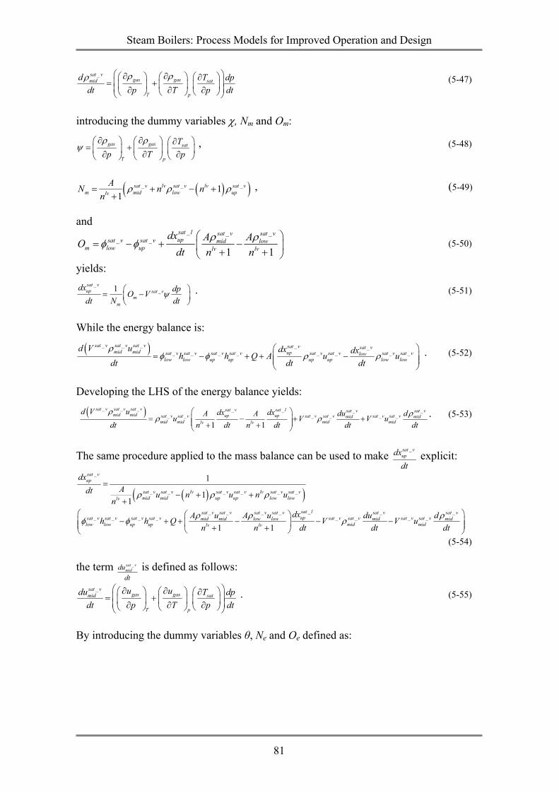
Steam Boilers: Process Models for Improved Operation and Design
81
_sat vgas gasmid sat
T p
d T dpdt p T p dt
ρ ρρ ∂ ∂ ∂ = + ∂ ∂ ∂
(5-47)
introducing the dummy variables χ, Nm and Om:
gas gas sat
T p
Tp T p
ρ ρψ
∂ ∂ ∂= + ∂ ∂ ∂
, (5-48)
( )( )_ _ _11
sat v lv sat v lv sat vm mid low uplv
AN n nn
ρ ρ ρ= + − ++
, (5-49)
and
_ _ __ _
1 1
sat l sat v sat vupsat v sat v mid low
m low up lv lv
dx A AOdt n n
ρ ρφ φ
= − + − + + (5-50)
yields:
__1
sat vup sat v
mm
dx dpO Vdt N dt
ψ = −
. (5-51)
While the energy balance is:
( )_ _ _ _ __ _ _ _ _ _ _ _
sat v sat v sat v sat v sat vmid mid upsat v sat v sat v sat v sat v sat v sat v sat vlow
low low up up up up low low
d V u dx dxh h Q A u udt dt dt
ρφ φ ρ ρ
= − + + −
. (5-52)
Developing the LHS of the energy balance yields:
( )_ _ _ _ _ _ __ _ _ _ _ _
1 1
sat v sat v sat v sat v sat l sat v sat vmid mid up upsat v sat v sat v sat v sat v sat vmid mid
mid mid mid midlv lv
d V u dx dx du dA Au V V udt n dt n dt dt dt
ρ ρρ ρ
= − + + + +
. (5-53)
The same procedure applied to the mass balance can be used to make
_sat vupdxdt
explicit:
( )( )_
_ _ _ _ _ _
__ _ _ __ _ _ _ _ _
1
11
1 1
sat vup
sat v sat v lv sat v sat v lv sat v sat vmid mid up up low lowlv
sat lsat v sat v sat v sat vupsat v sat v sat v sat v sat v satmid mid low low
low low up up midlv lv
dxAdt u n u n u
ndxA u A uh h Q V
n n dt
ρ ρ ρ
ρ ρφ φ ρ
=− + +
+
− + + − − + +
_ __ _
sat v sat vv sat v sat vmid mid
middu dV u
dt dtρ
−
(5-54) the term _sat v
middudt
is defined as follows:
_sat vgas gasmid sat
T p
u udu T dpdt p T p dt
∂ ∂ ∂ = + ∂ ∂ ∂
. (5-55)
By introducing the dummy variables θ, Ne and Oe defined as:
Steam Boilers: Process Models for Improved Operation and Design
82
gas gas sat
T p
u u Tp T p
θ∂ ∂ ∂
= + ∂ ∂ ∂ , (5-56)
( )( )_ _ _ _ _ _11
sat v sat v lv sat v sat v lv sat v sat ve mid mid up up low lowlv
AN u n u n un
ρ ρ ρ= − + ++
, (5-57)
__ _ _ _
_ _ _ _
1 1
sat lsat v sat v sat v sat vupsat v sat v sat v sat v mid mid low low
e low low up up lv lv
dxA u A uO h h Qn n dt
ρ ρφ φ
= − + + − + + ,
(5-58) yields:
( )_
_ _ _1sat vup sat v sat v sat v
e mid mide
dx dpO V udt N dt
ρ θ ψ = − +
. (5-59)
Finally, by combining the mass and energy balance, the following equations are obtained:
( )_ _ _ _1 1sat v sat v sat v sat ve mid mid m
e m
dp dpO V u O VN dt N dt
ρ θ ψ ψ − + = −
, (5-60)
( )
( )( )_ _ _
m e e m
sat l sat l sat le m mid mid
O N O Ndpdt V N N uψ ρ θ ψ
−=
− + (5-61)
using the energy and mass balances for the development of the derivative of _sat v
updxdt
yields:
( )( )( )( )
_ __
_ _
sat v sat vsat ve part m mid part mid partup
sat v sat ve part m mid part mid part
O O u udxdt N N u u
ρ ρ ρ
ρ ρ ρ
− +=
− + . (5-62)
5.2.6. Vapor thermal node The total length of the vapor pipe is the remaining length of the evaporator:
_ _pipe liq sat l lv sat v vapL L L L L L= + + + + . (5-63) With reference to Figure 5-5 and Figure 5-8, the mass balance for the vapor thermal node can be written as follows:
( ) 11 1
j ji i vap vapj j j j
dx dxd VA
dt dt dtρ
φ φ ρ ρ++ +
= − + −
∑ ∑ . (5-64)
The energy balance for the same node is defined as follows:
( ) 11 1 1 1
j ji i i vap vap vap vapj j j j j j j j
dx dxd V Uh h Q A u u
dt dt dtρ
φ φ ρ ρ++ + + +
= − + + −
∑ ∑ . (5-65)
jdx
dtand 1jdx
dt+ are linear functions of
_sat vupdxdt
:
Steam Boilers: Process Models for Improved Operation and Design
83
}{_1 1...
sat vvapj up vap
vap
dx dxn j for j ndt n dt
− += = (5-66)
and
}{_
1 1...sat vvap
j up vapvap
dx dxn j for j ndt n dt
+ −= = . (5-67)
5.2.7. Thermal nodes of the fluegas side The thermal nodes of the fluegas side are similar to the presented thermal nodes of the working fluid water with following changes and simplifications:
- fluegas properties in place of water properties are used - total height of the boiler is 31 meter compared with 155 meter length of a pipe
due to the helically wound pipes. Since the number of nodes on each side is equal it consequently means every fluegas node has a 5 time shorter length compared with the corresponding water/steam thermal node
- heat transfer to the wall element is not only based on convection but dominated by radiation
With reference to Figure 5-2 the mass balance for the thermal fluegas node can be written as follows:
( ) 11 1 .j ji i
j j j j
dx dxd VA
dt dt dtρ
φ φ ρ ρ++ +
= − + −
∑ ∑ (5-68)
Terms containing time derivatives of the spatial coordinates are due to the changing dimension of the control volume. The last term is the net generation of mass within the control volume. The energy balance for the fluegas thermal node is as follows:
( ) 11 1 1 1 ,j ji i i
j j j j j j j j
dx dxd V uh h Q A u u
dt dt dtρ
φ φ ρ ρ++ + + +
= − + + −
∑ ∑ (5-69)
where u and h denotes the internal energy and the enthalpy of the fluid respectively and Q indicate the sum of radiative and convective heat transfer.
5.2.8. Wall element The wall element includes all solid parts of the boiler wall, i.e., the metal pipe and the deposits on the fluegas side. Waterside fouling is ignored. Each wall element coupled to one fluegas and one water/steam thermal node and therefore moves in the same direction as the corresponding thermal nodes. The heat flux is calculated in the thermal node and includes
- conduction through the wall element from fluegas surface to steam surface - conduction to the neighboring wall elements - convection to the water/steam thermal node - convection and radiation to the thermal fluegas node.
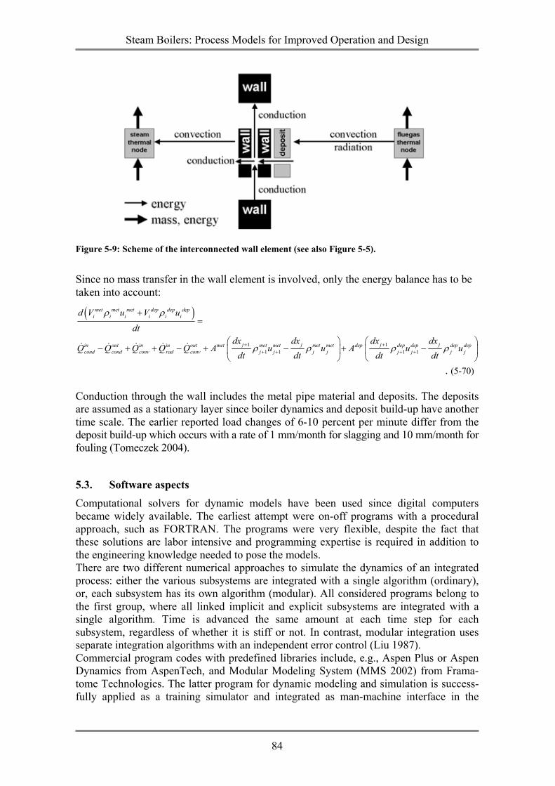
Steam Boilers: Process Models for Improved Operation and Design
84
Figure 5-9: Scheme of the interconnected wall element (see also Figure 5-5).
Since no mass transfer in the wall element is involved, only the energy balance has to be taken into account:
( )
1 11 1 1 1
met met met dep dep depi i i i i i
j j j jin out in in out met met met met met dep dep dep dep depcond cond conv rad conv j j j j j j j j
d V u V u
dtdx dx dx dx
Q Q Q Q Q A u u A u udt dt dt dt
ρ ρ
ρ ρ ρ ρ+ ++ + + +
+=
− + + − + − + −
& & & & &
. (5-70) Conduction through the wall includes the metal pipe material and deposits. The deposits are assumed as a stationary layer since boiler dynamics and deposit build-up have another time scale. The earlier reported load changes of 6-10 percent per minute differ from the deposit build-up which occurs with a rate of 1 mm/month for slagging and 10 mm/month for fouling (Tomeczek 2004).
5.3. Software aspects Computational solvers for dynamic models have been used since digital computers became widely available. The earliest attempt were on-off programs with a procedural approach, such as FORTRAN. The programs were very flexible, despite the fact that these solutions are labor intensive and programming expertise is required in addition to the engineering knowledge needed to pose the models. There are two different numerical approaches to simulate the dynamics of an integrated process: either the various subsystems are integrated with a single algorithm (ordinary), or, each subsystem has its own algorithm (modular). All considered programs belong to the first group, where all linked implicit and explicit subsystems are integrated with a single algorithm. Time is advanced the same amount at each time step for each subsystem, regardless of whether it is stiff or not. In contrast, modular integration uses separate integration algorithms with an independent error control (Liu 1987). Commercial program codes with predefined libraries include, e.g., Aspen Plus or Aspen Dynamics from AspenTech, and Modular Modeling System (MMS 2002) from Frama-tome Technologies. The latter program for dynamic modeling and simulation is success-fully applied as a training simulator and integrated as man-machine interface in the
Steam Boilers: Process Models for Improved Operation and Design
85
distributed control system (DCS) at different fossil and nuclear power plants, and is thoroughly validated by several industrial applications (Schoen 1993). The modules in the MMS library are based on the conservation of mass and energy as a lumped parameter model, since components that are recognizable as equivalent are used in power plants such as heaters, condenser or turbines. MMS Model Builder is a graphical interface for the use of the MMS library. Source code for the physical model and the control logic are merged into one source code. This code makes use of the Advanced Continuous Simulation Language (ACSL) from Mitchell and Gauthier Associates. The ACSL translator produces a FORTRAN file. ACSL provides a runtime executive with command line interface for control and for testing the model (Jones 1995). Easy5 from Boing Inc. can be used as an alternative for the ACSL translator. However, a major criticism of ACSL and similar programs is that these packages are suitable only for systems that can be modeled with relatively small numbers of explicit ordinary differential equations (Barton 1992). Equation oriented approaches with symbolic language overcome these shortcomings and can simultaneously solve up to tens of thousands of equations. The equations presented in the previous chapter are implemented in such software as Aspen Custom Modeler (ACM) from AspenTech. ACM is an object-oriented solver for continuous-system modeling, with similarities to general-purpose solvers like gProms, SpeedUp, Simulink (Matlab) and Modellica. Time differential equations for use in dynamic models and partial differ-ential equations for modeling distributed systems are directly programmed and saved in a library. Flow-sheets of self-developed models can be built within Aspen Custom Modeler using the graphical flow-sheet editor. The equation oriented flow-sheet solver is capable of steady state and dynamic simulations of engineering systems. Steady state or dynamic estimation is possible for fitting model parameters to experimental or plant data. Optimization of design and operation of continuous or batch processes is another feature of ACM. Algebraic equations can be coded in the implicit form. Interfaces for Windows application, Visual Basic and process control and information management are included for applications such as monitoring, documentation, training or inferential measurement (Aspen Technology 2006). Both programs, ACM and MMS, offer a choice of different integration algorithms, including Gear’s stiff. This numerical method is generally recommended for large stiff systems (i.e., covering a wide range of time constants) and is chosen for the presented simulations. The next generation of process modeling tools tends in the direction of interfacing of CFD with dynamic process modeling tools. A major advantage of CFD in this context is its ability to describe arbitrarily complex geometry, allowing the detailed characterization of the involved fluid dynamics. On the other hand, CFD lacks the wide scope of general purpose solvers for process modeling (Bezzo 2000).
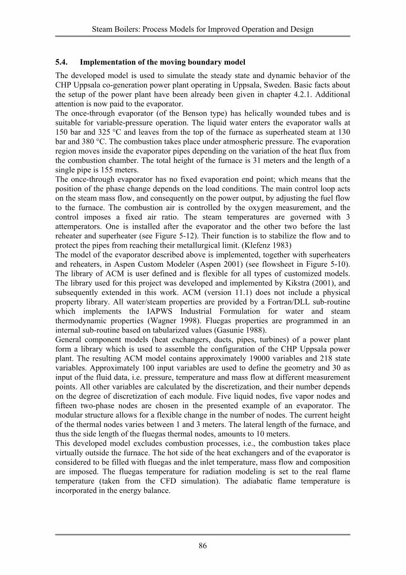
Steam Boilers: Process Models for Improved Operation and Design
86
5.4. Implementation of the moving boundary model The developed model is used to simulate the steady state and dynamic behavior of the CHP Uppsala co-generation power plant operating in Uppsala, Sweden. Basic facts about the setup of the power plant have been already been given in chapter 4.2.1. Additional attention is now paid to the evaporator. The once-through evaporator (of the Benson type) has helically wounded tubes and is suitable for variable-pressure operation. The liquid water enters the evaporator walls at 150 bar and 325 °C and leaves from the top of the furnace as superheated steam at 130 bar and 380 °C. The combustion takes place under atmospheric pressure. The evaporation region moves inside the evaporator pipes depending on the variation of the heat flux from the combustion chamber. The total height of the furnace is 31 meters and the length of a single pipe is 155 meters. The once-through evaporator has no fixed evaporation end point; which means that the position of the phase change depends on the load conditions. The main control loop acts on the steam mass flow, and consequently on the power output, by adjusting the fuel flow to the furnace. The combustion air is controlled by the oxygen measurement, and the control imposes a fixed air ratio. The steam temperatures are governed with 3 attemperators. One is installed after the evaporator and the other two before the last reheater and superheater (see Figure 5-12). Their function is to stabilize the flow and to protect the pipes from reaching their metallurgical limit. (Klefenz 1983) The model of the evaporator described above is implemented, together with superheaters and reheaters, in Aspen Custom Modeler (Aspen 2001) (see flowsheet in Figure 5-10). The library of ACM is user defined and is flexible for all types of customized models. The library used for this project was developed and implemented by Kikstra (2001), and subsequently extended in this work. ACM (version 11.1) does not include a physical property library. All water/steam properties are provided by a Fortran/DLL sub-routine which implements the IAPWS Industrial Formulation for water and steam thermodynamic properties (Wagner 1998). Fluegas properties are programmed in an internal sub-routine based on tabularized values (Gasunie 1988). General component models (heat exchangers, ducts, pipes, turbines) of a power plant form a library which is used to assemble the configuration of the CHP Uppsala power plant. The resulting ACM model contains approximately 19000 variables and 218 state variables. Approximately 100 input variables are used to define the geometry and 30 as input of the fluid data, i.e. pressure, temperature and mass flow at different measurement points. All other variables are calculated by the discretization, and their number depends on the degree of discretization of each module. Five liquid nodes, five vapor nodes and fifteen two-phase nodes are chosen in the presented example of an evaporator. The modular structure allows for a flexible change in the number of nodes. The current height of the thermal nodes varies between 1 and 3 meters. The lateral length of the furnace, and thus the side length of the fluegas thermal nodes, amounts to 10 meters. This developed model excludes combustion processes, i.e., the combustion takes place virtually outside the furnace. The hot side of the heat exchangers and of the evaporator is considered to be filled with fluegas and the inlet temperature, mass flow and composition are imposed. The fluegas temperature for radiation modeling is set to the real flame temperature (taken from the CFD simulation). The adiabatic flame temperature is incorporated in the energy balance.
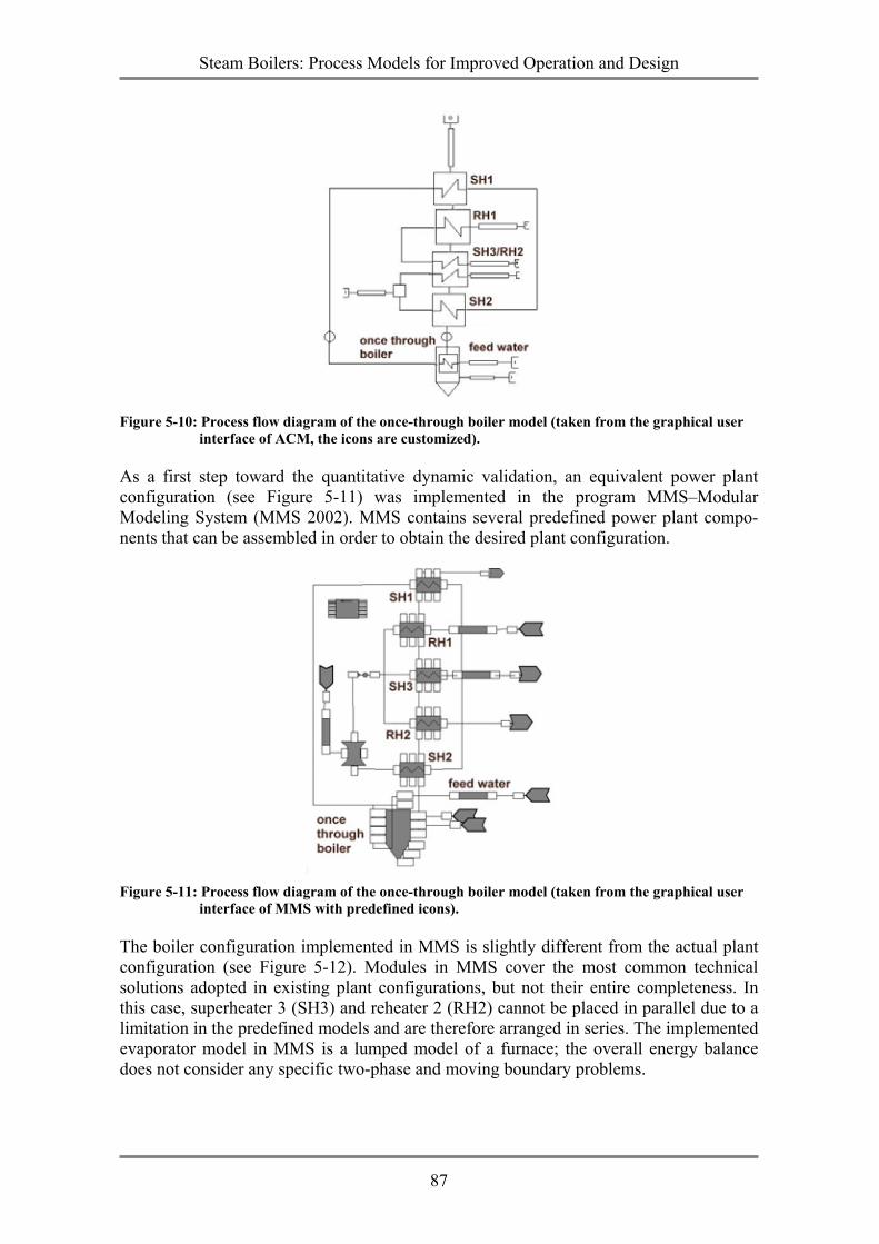
Steam Boilers: Process Models for Improved Operation and Design
87
Figure 5-10: Process flow diagram of the once-through boiler model (taken from the graphical user
interface of ACM, the icons are customized).
As a first step toward the quantitative dynamic validation, an equivalent power plant configuration (see Figure 5-11) was implemented in the program MMS–Modular Modeling System (MMS 2002). MMS contains several predefined power plant compo-nents that can be assembled in order to obtain the desired plant configuration.
Figure 5-11: Process flow diagram of the once-through boiler model (taken from the graphical user
interface of MMS with predefined icons).
The boiler configuration implemented in MMS is slightly different from the actual plant configuration (see Figure 5-12). Modules in MMS cover the most common technical solutions adopted in existing plant configurations, but not their entire completeness. In this case, superheater 3 (SH3) and reheater 2 (RH2) cannot be placed in parallel due to a limitation in the predefined models and are therefore arranged in series. The implemented evaporator model in MMS is a lumped model of a furnace; the overall energy balance does not consider any specific two-phase and moving boundary problems.
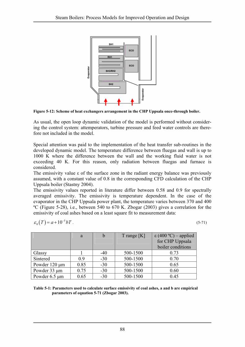
Steam Boilers: Process Models for Improved Operation and Design
88
Figure 5-12: Scheme of heat exchangers arrangement in the CHP Uppsala once-through boiler.
As usual, the open loop dynamic validation of the model is performed without consider-ing the control system: attemperators, turbine pressure and feed water controls are there-fore not included in the model. Special attention was paid to the implementation of the heat transfer sub-routines in the developed dynamic model. The temperature difference between fluegas and wall is up to 1000 K where the difference between the wall and the working fluid water is not exceeding 40 K. For this reason, only radiation between fluegas and furnace is considered. The emissivity value ε of the surface zone in the radiant energy balance was previously assumed, with a constant value of 0.8 in the corresponding CFD calculation of the CHP Uppsala boiler (Stastny 2004). The emissivity values reported in literature differ between 0.58 and 0.9 for spectrally averaged emissivity. The emissivity is temperature dependent. In the case of the evaporator in the CHP Uppsala power plant, the temperature varies between 370 and 400 ºC (Figure 5-28), i.e., between 540 to 670 K. Zbogar (2003) gives a correlation for the emissivity of coal ashes based on a least square fit to measurement data:
( ) 50 10T a bTε −= + . (5-71)
a b
T range [K]
ε (400 ºC) – applied
for CHP Uppsala boiler conditions
Glassy 1 -40 500-1500 0.73 Sintered 0.9 -30 500-1500 0.70 Powder 120 µm 0.85 -30 500-1500 0.65 Powder 33 µm 0.75 -30 500-1500 0.60 Powder 6.5 µm 0.65 -30 500-1500 0.45
Table 5-1: Parameters used to calculate surface emissivity of coal ashes, a and b are empirical parameters of equation 5-71 (Zbogar 2003).

Steam Boilers: Process Models for Improved Operation and Design
89
The deposit can be assumed as sintered, since biomass ashes of the Uppsala boiler have a low fusion temperature, and the value of 0.70 was chosen as a constant (Table 5-1). A wavelength dependent measurement would be more accurate (Linka 2003). The calculated parameters of the WSGGM are calculated with the partial pressures of pw equal to 0.0937 bar and pc equal to 0.1438 bar for the H2O and CO2 components respectively at a temperature of 1000 ºC. The emissivity parameters of the WSGGM model are first calculated independently for the gas and the soot, and then summed.
Steam Boilers: Process Models for Improved Operation and Design
90
5.5. Validation, results and discussion Testing and verification of the model is performed by comparison of the results with other sources, e.g., literature, similar dynamic models or field data. Five different cases are studied and listed in Table 5-2. The five cases differ in the solver (dynamic vs. steady state) and the number of input variables in order to guarantee comparable initial conditions.
Case № (chapter)
Solver Number of manipulated input variables
Purpose
1 (5.5.1.) Steady state 15 (Figure 5-13) Deposit Parameter Estimation 2 (5.5.2.) Steady state 15 (Figure 5-13) Physical phenomena 3 (5.5.3.) Dynamic 2 (Figure 5-29) Open loop validation:
Comparison with MMS 4 (5.5.4.) Dynamic 4 (Figure 5-35) Dynamic validation:
Comparison with field data 5 (5.5.5.) Steady state
& Dynamic 4 (Figure 5-35) Comparison dynamic vs. steady state
Table 5-2: Simulation cases used to validate the once-through boiler model.
There are two solver options available in the program Aspen Custom Modeler: static (steady state) and dynamic. Parameters, i.e., the deposit, that have constant values during the considered load changes are calculated first. Second, during the quasi-static validation the steady state parameters at different load points are compared with the design or measurement data (case 2). The dynamic validation of case 3 is applied with modified control settings. In the case of an open loop validation, the control system is disabled to study the pure dynamic behavior of the static equipment. Case 4 validates the dynamic results of disturbances, load changes etc. The results of the simulation are compared to measured field data collected by the Distributed Control System (DCS) of the plant. For the comparison with field data, a simple control scheme is applied. Case 5 investigate the advantages of a dynamic over a steady state model by comparing both models with measured data of a load change.
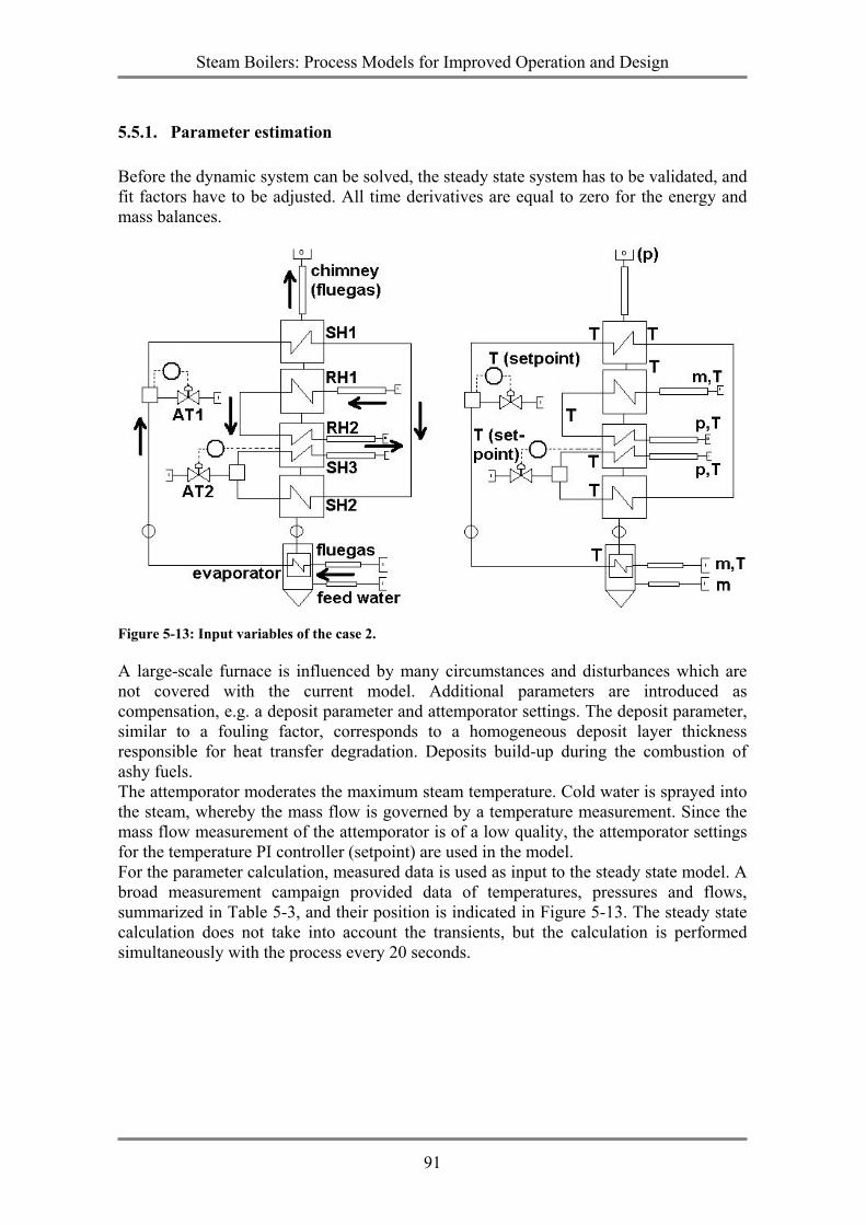
Steam Boilers: Process Models for Improved Operation and Design
91
5.5.1. Parameter estimation Before the dynamic system can be solved, the steady state system has to be validated, and fit factors have to be adjusted. All time derivatives are equal to zero for the energy and mass balances.
Figure 5-13: Input variables of the case 2.
A large-scale furnace is influenced by many circumstances and disturbances which are not covered with the current model. Additional parameters are introduced as compensation, e.g. a deposit parameter and attemporator settings. The deposit parameter, similar to a fouling factor, corresponds to a homogeneous deposit layer thickness responsible for heat transfer degradation. Deposits build-up during the combustion of ashy fuels. The attemporator moderates the maximum steam temperature. Cold water is sprayed into the steam, whereby the mass flow is governed by a temperature measurement. Since the mass flow measurement of the attemporator is of a low quality, the attemporator settings for the temperature PI controller (setpoint) are used in the model. For the parameter calculation, measured data is used as input to the steady state model. A broad measurement campaign provided data of temperatures, pressures and flows, summarized in Table 5-3, and their position is indicated in Figure 5-13. The steady state calculation does not take into account the transients, but the calculation is performed simultaneously with the process every 20 seconds.
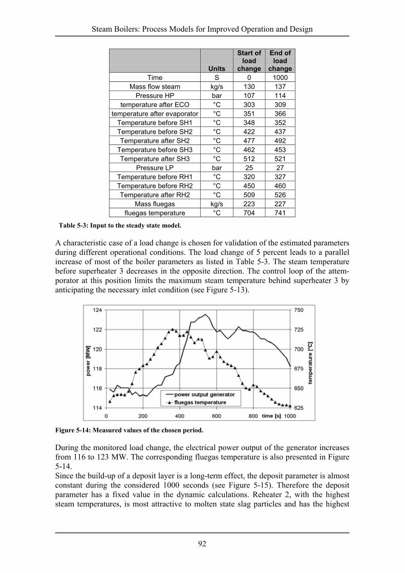
Steam Boilers: Process Models for Improved Operation and Design
92
Units
Start of load
change
End of load
change Time S 0 1000
Mass flow steam kg/s 130 137 Pressure HP bar 107 114
temperature after ECO °C 303 309 temperature after evaporator °C 351 366
Temperature before SH1 °C 348 352 Temperature before SH2 °C 422 437 Temperature after SH2 °C 477 492
Temperature before SH3 °C 462 453 Temperature after SH3 °C 512 521
Pressure LP bar 25 27 Temperature before RH1 °C 320 327 Temperature before RH2 °C 450 460 Temperature after RH2 °C 509 526
Mass fluegas kg/s 223 227 fluegas temperature °C 704 741
Table 5-3: Input to the steady state model.
A characteristic case of a load change is chosen for validation of the estimated parameters during different operational conditions. The load change of 5 percent leads to a parallel increase of most of the boiler parameters as listed in Table 5-3. The steam temperature before superheater 3 decreases in the opposite direction. The control loop of the attem-porator at this position limits the maximum steam temperature behind superheater 3 by anticipating the necessary inlet condition (see Figure 5-13).
Figure 5-14: Measured values of the chosen period.
During the monitored load change, the electrical power output of the generator increases from 116 to 123 MW. The corresponding fluegas temperature is also presented in Figure 5-14. Since the build-up of a deposit layer is a long-term effect, the deposit parameter is almost constant during the considered 1000 seconds (see Figure 5-15). Therefore the deposit parameter has a fixed value in the dynamic calculations. Reheater 2, with the highest steam temperatures, is most attractive to molten state slag particles and has the highest
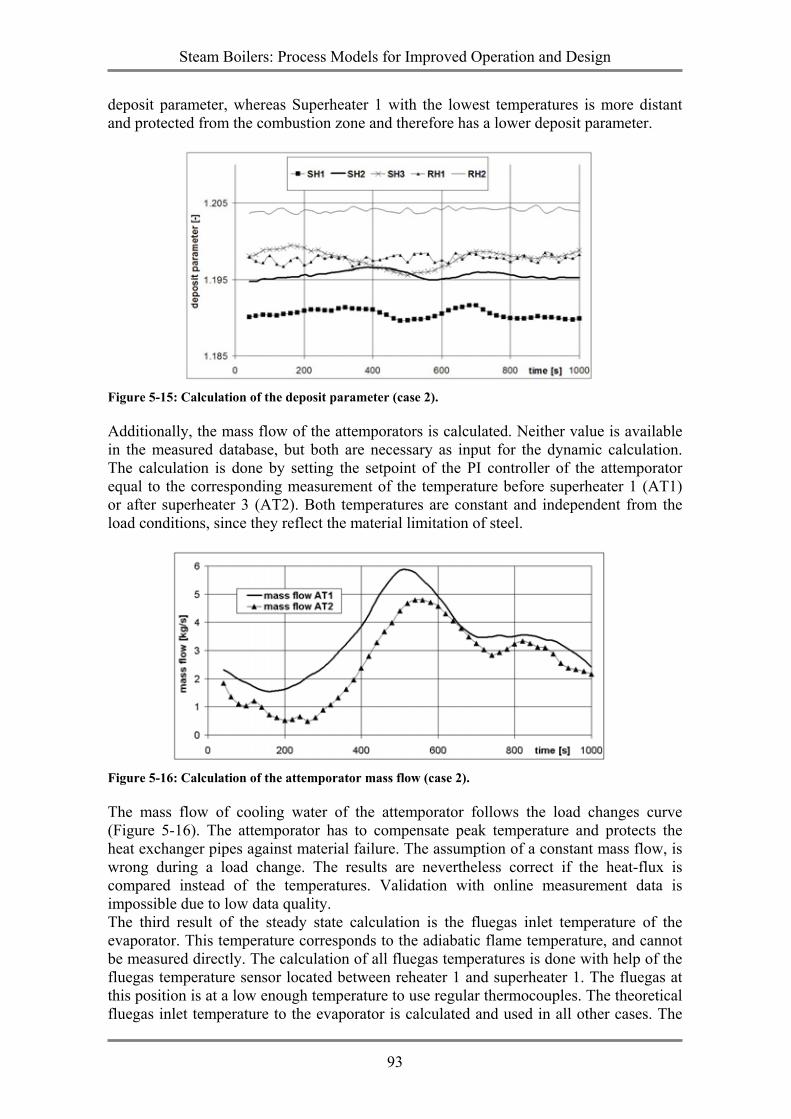
Steam Boilers: Process Models for Improved Operation and Design
93
deposit parameter, whereas Superheater 1 with the lowest temperatures is more distant and protected from the combustion zone and therefore has a lower deposit parameter.
Figure 5-15: Calculation of the deposit parameter (case 2).
Additionally, the mass flow of the attemporators is calculated. Neither value is available in the measured database, but both are necessary as input for the dynamic calculation. The calculation is done by setting the setpoint of the PI controller of the attemporator equal to the corresponding measurement of the temperature before superheater 1 (AT1) or after superheater 3 (AT2). Both temperatures are constant and independent from the load conditions, since they reflect the material limitation of steel.
Figure 5-16: Calculation of the attemporator mass flow (case 2).
The mass flow of cooling water of the attemporator follows the load changes curve (Figure 5-16). The attemporator has to compensate peak temperature and protects the heat exchanger pipes against material failure. The assumption of a constant mass flow, is wrong during a load change. The results are nevertheless correct if the heat-flux is compared instead of the temperatures. Validation with online measurement data is impossible due to low data quality. The third result of the steady state calculation is the fluegas inlet temperature of the evaporator. This temperature corresponds to the adiabatic flame temperature, and cannot be measured directly. The calculation of all fluegas temperatures is done with help of the fluegas temperature sensor located between reheater 1 and superheater 1. The fluegas at this position is at a low enough temperature to use regular thermocouples. The theoretical fluegas inlet temperature to the evaporator is calculated and used in all other cases. The
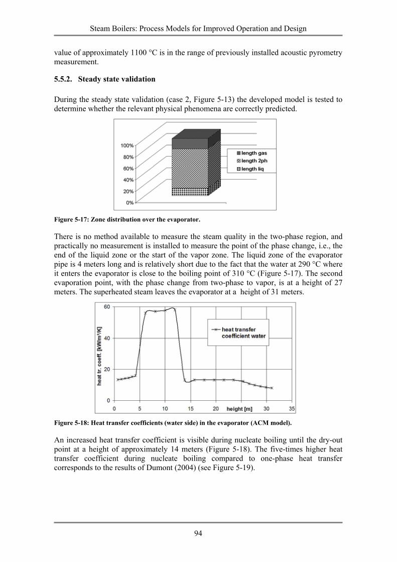
Steam Boilers: Process Models for Improved Operation and Design
94
value of approximately 1100 °C is in the range of previously installed acoustic pyrometry measurement.
5.5.2. Steady state validation During the steady state validation (case 2, Figure 5-13) the developed model is tested to determine whether the relevant physical phenomena are correctly predicted.
Figure 5-17: Zone distribution over the evaporator.
There is no method available to measure the steam quality in the two-phase region, and practically no measurement is installed to measure the point of the phase change, i.e., the end of the liquid zone or the start of the vapor zone. The liquid zone of the evaporator pipe is 4 meters long and is relatively short due to the fact that the water at 290 °C where it enters the evaporator is close to the boiling point of 310 °C (Figure 5-17). The second evaporation point, with the phase change from two-phase to vapor, is at a height of 27 meters. The superheated steam leaves the evaporator at a height of 31 meters.
Figure 5-18: Heat transfer coefficients (water side) in the evaporator (ACM model).
An increased heat transfer coefficient is visible during nucleate boiling until the dry-out point at a height of approximately 14 meters (Figure 5-18). The five-times higher heat transfer coefficient during nucleate boiling compared to one-phase heat transfer corresponds to the results of Dumont (2004) (see Figure 5-19).
Steam Boilers: Process Models for Improved Operation and Design
95
Figure 5-19: Heat transfer coefficients (water) in a heat recovery steam generator (Dumont 2004).
The evaporator model of Dumont (2004) refers to a counter-flow tube bundle in a heat recovery steam generator, taking into account the economizer, evaporator and superheater.
Figure 5-20: Theoretical wall and fluid temperature (of a vertical tube, rotated for comparison),
whole system in Figure 3-5.
Figure 5-20 presents a section of Figure 3-5. The drawing shows an idealized case of an evaporator with a constant pressure and a constant heat flux in the entire tube. The saturation temperature is constant until the dry-out point.
Figure 5-21 and Figure 5-22: Total pressure in the boiler.
Steam Boilers: Process Models for Improved Operation and Design
96
The pressure profile in the calculated evaporator (Figure 5-21) decreases gradually over the whole length of the pipe due to frictional losses, deviating to the idealized case in Figure 5-20. The maximum pressure losses are located in the the two-phase flow area, visible in the (negative) force on the fluid (Figure 5-21 right).
Figure 5-23: Temperature distribution of the co-flow heat exchanger.
The temperature of the two-phase flow is expected to be constant. Nevertheless, the temperature (Figure 5-23) partly decreases due to the friction pressure losses. Every thermal node operates exactly at the boiling temperature. The lower temperature corre-sponds to a lower pressure in the node.
Figure 5-24: Enthalpy profile.
The enthalpy of the two-phase mixture increases according to rising steam quality, despite a drop in temperature (Figure 5-24). The evaporator is modeled as a co-flow heat exchanger. A co-flow heat exchanger has the highest heat flux at the inlet, where the LMTD normally has a maximum value. In contrary, the CHP Uppsala evaporator model has a distributed flow inlet. The lowest 5 meters of the boiler, which correspond with the hopper of the furnace, receives only 25 percent of the total circulating fluegas (data taken from CFD). The burner inlet and combustion zone are modeled at a height of 8 meters. The heat flow is therefore maximized at the burner level (Figure 5-25).
Steam Boilers: Process Models for Improved Operation and Design
97
Figure 5-25: Heat flux.
Reported heat fluxes for low grade coal are up to 600 kW/m2 (Valero 1996). Calculated heat fluxes (Figure 5-25) are substantially lower due to the low heating value of the investigated peat. Advanced NOx reduction with air staging lowers the peak temperatures as well as the heat.
Figure 5-26: Radiant heat flux and percentage of radiation of the total heat flux.
Radiation is the dominant heat transfer mechanism at high temperatures. Convective heat transfer replaces the radiation in the upper zone, which is important for the deposit probability in the superheaters. The lower hopper section is not fully exposed to radiation since the burners are installed above at a height of 8 meters. Figure 5-26 describes the impact of radiation on the furnace walls. Convective heat trans-fer is under normal operation conditions the dominant phenomena for superheaters and for evaporators located in the upper part of the furnace. The first row of superheater tubes is considered to perform the function of a shield which screens the rest of the tube bundle from radiation, similar the approach of Stehlik (1996).
Steam Boilers: Process Models for Improved Operation and Design
98
Figure 5-27: Wall (steel) temperature in the evaporator.
The steel or wall temperature of the boiler is approximately 20 °C higher than the water-steam temperature inside the tubes. Nevertheless, the trend function is very similar since the heat transfer to the water is 10 times higher compared to the fluegas side (Figure 5-27). The dry-out point at a height of 13 meters is not as sharp as in theory (Figure 5-20), as a result of a coarse discretization.
Figure 5-28: Comparison of deposit and steel temperature.
The deposit is assumed as a homogenous layer. The temperature curve of the deposit is parallel to the steel temperature in the lower part of the boiler, with a difference up to 60 °C (Figure 5-28). Special attention has to be paid to the dry-out point of the steam, which corresponds to a local maximum of the deposit temperature. This point is attractive for slag melting and additional slagging. On the upper part of the boiler (above the height of 20 meter) the temperature of the deposit decreases due to reduced influence of radiation. The state of the ash may change from melted to powdery depending on the maximum temperature. The temperature of the deposit rises again above 27 meter due to higher steam temperatures inside the steam pipes. This tendency continues in the superheaters above the evaporator.
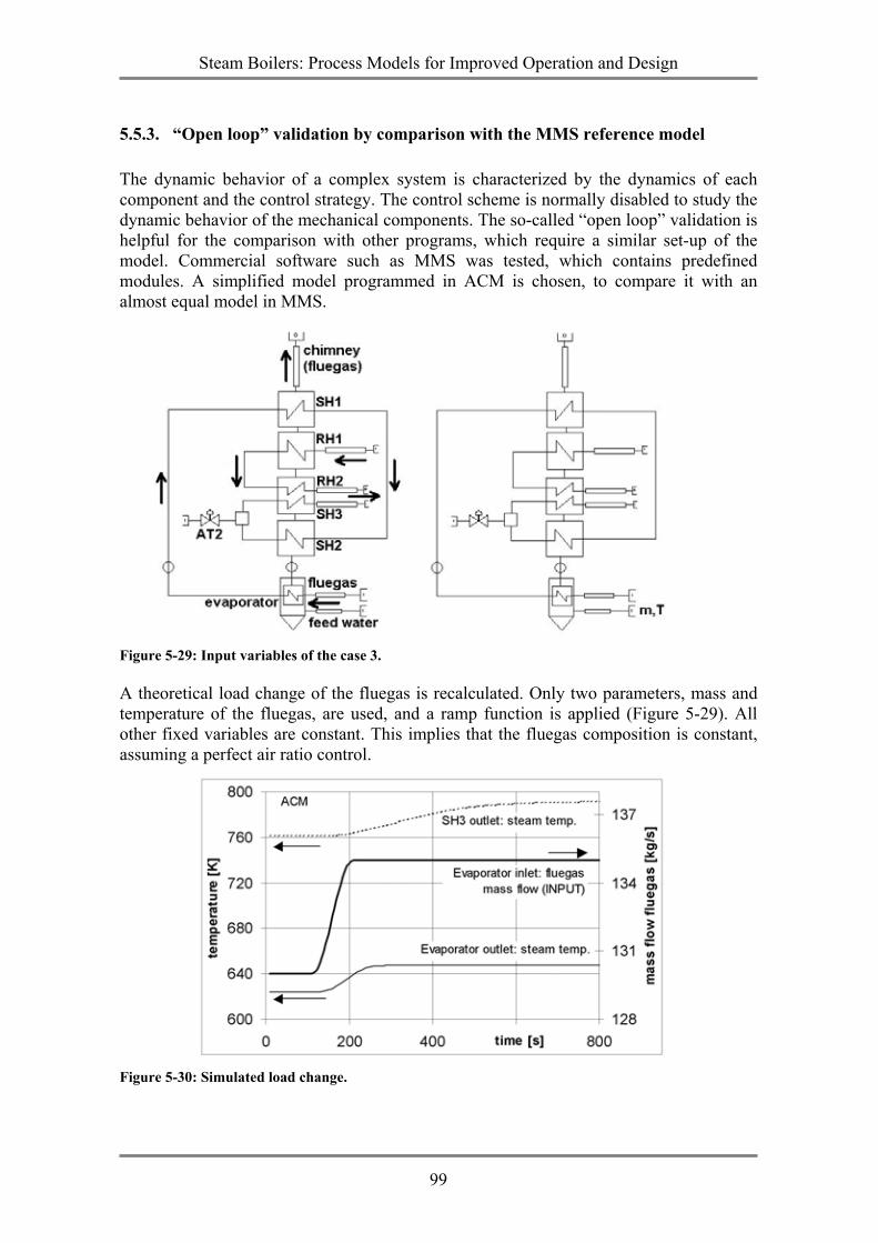
Steam Boilers: Process Models for Improved Operation and Design
99
5.5.3. “Open loop” validation by comparison with the MMS reference model The dynamic behavior of a complex system is characterized by the dynamics of each component and the control strategy. The control scheme is normally disabled to study the dynamic behavior of the mechanical components. The so-called “open loop” validation is helpful for the comparison with other programs, which require a similar set-up of the model. Commercial software such as MMS was tested, which contains predefined modules. A simplified model programmed in ACM is chosen, to compare it with an almost equal model in MMS.
Figure 5-29: Input variables of the case 3.
A theoretical load change of the fluegas is recalculated. Only two parameters, mass and temperature of the fluegas, are used, and a ramp function is applied (Figure 5-29). All other fixed variables are constant. This implies that the fluegas composition is constant, assuming a perfect air ratio control.
Figure 5-30: Simulated load change.
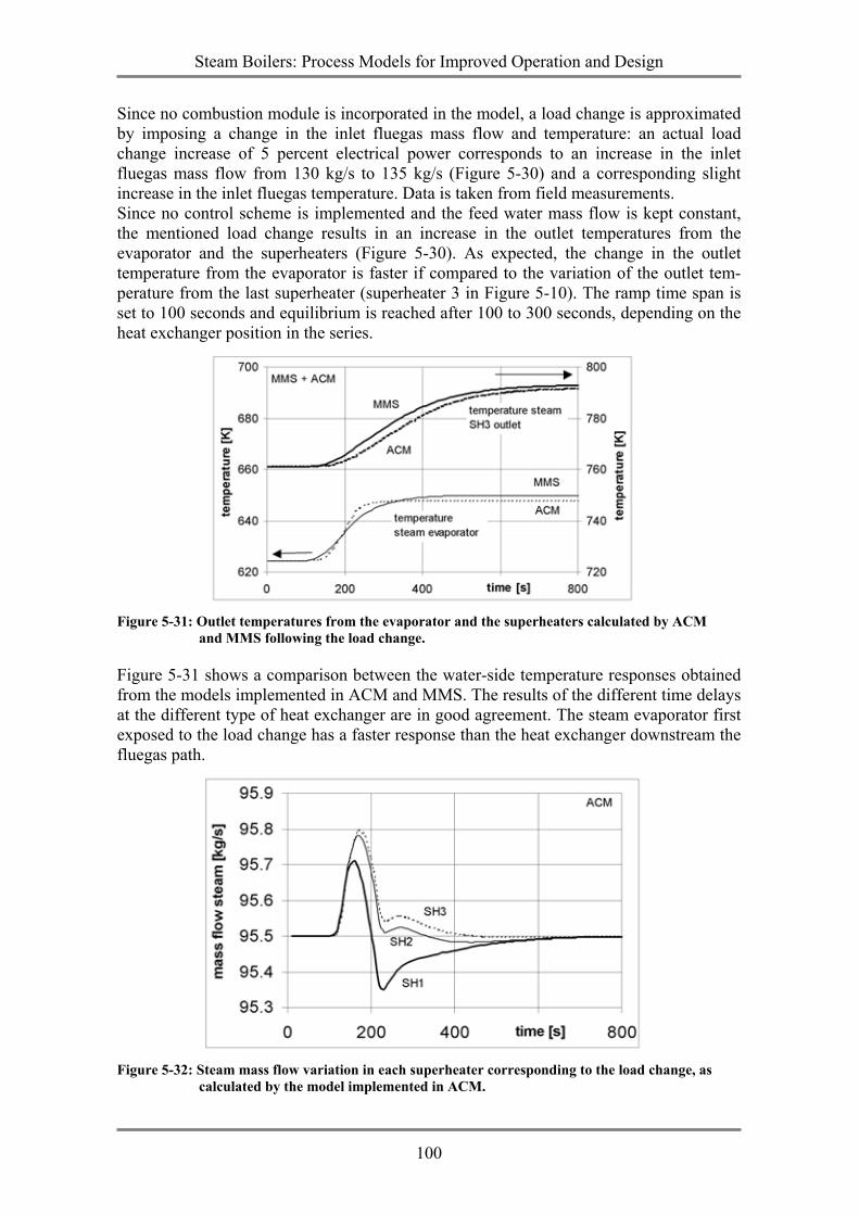
Steam Boilers: Process Models for Improved Operation and Design
100
Since no combustion module is incorporated in the model, a load change is approximated by imposing a change in the inlet fluegas mass flow and temperature: an actual load change increase of 5 percent electrical power corresponds to an increase in the inlet fluegas mass flow from 130 kg/s to 135 kg/s (Figure 5-30) and a corresponding slight increase in the inlet fluegas temperature. Data is taken from field measurements. Since no control scheme is implemented and the feed water mass flow is kept constant, the mentioned load change results in an increase in the outlet temperatures from the evaporator and the superheaters (Figure 5-30). As expected, the change in the outlet temperature from the evaporator is faster if compared to the variation of the outlet tem-perature from the last superheater (superheater 3 in Figure 5-10). The ramp time span is set to 100 seconds and equilibrium is reached after 100 to 300 seconds, depending on the heat exchanger position in the series.
Figure 5-31: Outlet temperatures from the evaporator and the superheaters calculated by ACM
and MMS following the load change.
Figure 5-31 shows a comparison between the water-side temperature responses obtained from the models implemented in ACM and MMS. The results of the different time delays at the different type of heat exchanger are in good agreement. The steam evaporator first exposed to the load change has a faster response than the heat exchanger downstream the fluegas path.
Figure 5-32: Steam mass flow variation in each superheater corresponding to the load change, as
calculated by the model implemented in ACM.
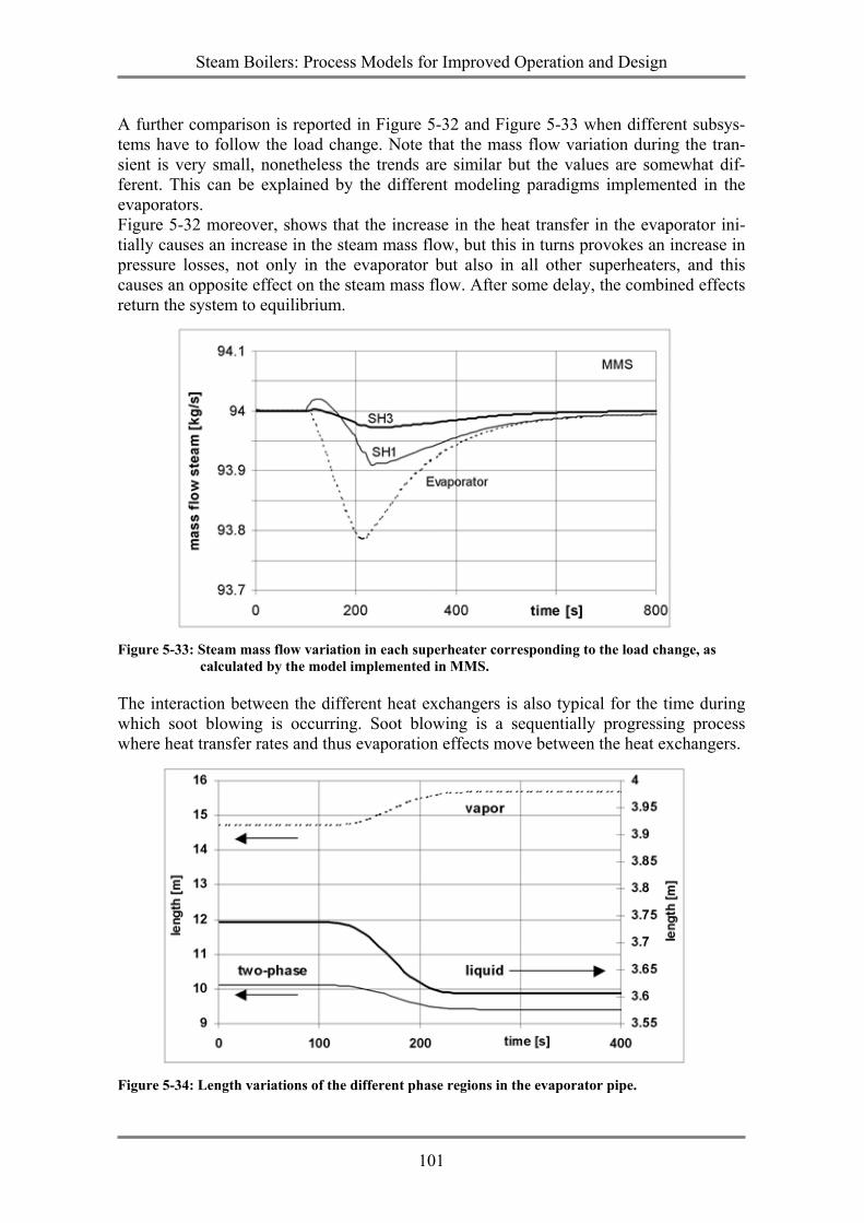
Steam Boilers: Process Models for Improved Operation and Design
101
A further comparison is reported in Figure 5-32 and Figure 5-33 when different subsys-tems have to follow the load change. Note that the mass flow variation during the tran-sient is very small, nonetheless the trends are similar but the values are somewhat dif-ferent. This can be explained by the different modeling paradigms implemented in the evaporators. Figure 5-32 moreover, shows that the increase in the heat transfer in the evaporator ini-tially causes an increase in the steam mass flow, but this in turns provokes an increase in pressure losses, not only in the evaporator but also in all other superheaters, and this causes an opposite effect on the steam mass flow. After some delay, the combined effects return the system to equilibrium.
Figure 5-33: Steam mass flow variation in each superheater corresponding to the load change, as
calculated by the model implemented in MMS.
The interaction between the different heat exchangers is also typical for the time during which soot blowing is occurring. Soot blowing is a sequentially progressing process where heat transfer rates and thus evaporation effects move between the heat exchangers.
Figure 5-34: Length variations of the different phase regions in the evaporator pipe.
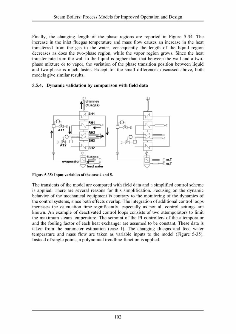
Steam Boilers: Process Models for Improved Operation and Design
102
Finally, the changing length of the phase regions are reported in Figure 5-34. The increase in the inlet fluegas temperature and mass flow causes an increase in the heat transferred from the gas to the water, consequently the length of the liquid region decreases as does the two-phase region, while the vapor region grows. Since the heat transfer rate from the wall to the liquid is higher than that between the wall and a two-phase mixture or to vapor, the variation of the phase transition position between liquid and two-phase is much faster. Except for the small differences discussed above, both models give similar results.
5.5.4. Dynamic validation by comparison with field data
Figure 5-35: Input variables of the case 4 and 5.
The transients of the model are compared with field data and a simplified control scheme is applied. There are several reasons for this simplification. Focusing on the dynamic behavior of the mechanical equipment is contrary to the monitoring of the dynamics of the control systems, since both effects overlap. The integration of additional control loops increases the calculation time significantly, especially as not all control settings are known. An example of deactivated control loops consists of two attemporators to limit the maximum steam temperature. The setpoint of the PI controllers of the attemporator and the fouling factor of each heat exchanger are assumed to be constant. These data is taken from the parameter estimation (case 1). The changing fluegas and feed water temperature and mass flow are taken as variable inputs to the model (Figure 5-35). Instead of single points, a polynomial trendline-function is applied.
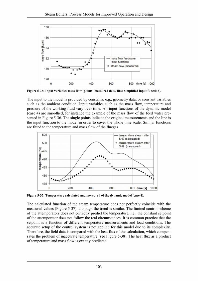
Steam Boilers: Process Models for Improved Operation and Design
103
Figure 5-36: Input variables mass flow (points: measured data, line: simplified input function).
The input to the model is provided by constants, e.g., geometry data, or constant variables such as the ambient condition. Input variables such as the mass flow, temperature and pressure of the working fluid vary over time. All input functions of the dynamic model (case 4) are smoothed, for instance the example of the mass flow of the feed water pre-sented in Figure 5-36. The single points indicate the original measurements and the line is the input function to the model in order to cover the whole time scale. Similar functions are fitted to the temperature and mass flow of the fluegas.
Figure 5-37: Temperature calculated and measured of the dynamic model (case 4).
The calculated function of the steam temperature does not perfectly coincide with the measured values (Figure 5-37), although the trend is similar. The limited control scheme of the attemporators does not correctly predict the temperature, i.e., the constant setpoint of the attemporator does not follow the real circumstances. It is common practice that the setpoint is a function of different temperature measurements and load conditions. The accurate setup of the control system is not applied for this model due to its complexity. Therefore, the field data is compared with the heat flux of the calculation, which compen-sates the problem of inaccurate temperature (see Figure 5-38). The heat flux as a product of temperature and mass flow is exactly predicted.
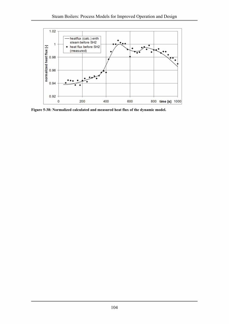
Steam Boilers: Process Models for Improved Operation and Design
104
Figure 5-38: Normalized calculated and measured heat flux of the dynamic model.
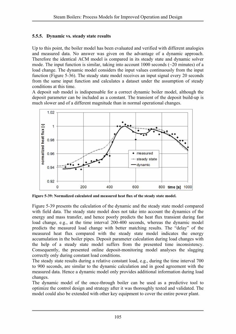
Steam Boilers: Process Models for Improved Operation and Design
105
5.5.5. Dynamic vs. steady state results Up to this point, the boiler model has been evaluated and verified with different analogies and measured data. No answer was given on the advantage of a dynamic approach. Therefore the identical ACM model is compared in its steady state and dynamic solver mode. The input function is similar, taking into account 1000 seconds (~20 minutes) of a load change. The dynamic model considers the input values continuously from the input function (Figure 5-36). The steady state model receives an input signal every 20 seconds from the same input function and calculates a dataset under the assumption of steady conditions at this time. A deposit sub model is indispensable for a correct dynamic boiler model, although the deposit parameter can be included as a constant. The transient of the deposit build-up is much slower and of a different magnitude than in normal operational changes.
Figure 5-39: Normalized calculated and measured heat flux of the steady state model.
Figure 5-39 presents the calculation of the dynamic and the steady state model compared with field data. The steady state model does not take into account the dynamics of the energy and mass transfer, and hence poorly predicts the heat flux transient during fast load change, e.g., at the time interval 200-400 seconds, whereas the dynamic model predicts the measured load change with better matching results. The “delay” of the measured heat flux compared with the steady state model indicates the energy accumulation in the boiler pipes. Deposit parameter calculation during load changes with the help of a steady state model suffers from the presented time inconsistency. Consequently, the presented online deposit-monitoring model analyses the slagging correctly only during constant load conditions. The steady state results during a relative constant load, e.g., during the time interval 700 to 900 seconds, are similar to the dynamic calculation and in good agreement with the measured data. Hence a dynamic model only provides additional information during load changes. The dynamic model of the once-through boiler can be used as a predictive tool to optimize the control design and strategy after it was thoroughly tested and validated. The model could also be extended with other key equipment to cover the entire power plant.
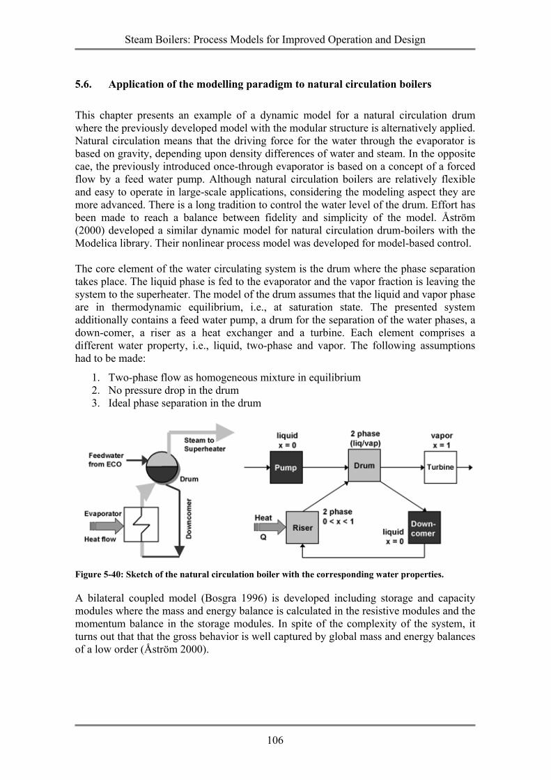
Steam Boilers: Process Models for Improved Operation and Design
106
5.6. Application of the modelling paradigm to natural circulation boilers This chapter presents an example of a dynamic model for a natural circulation drum where the previously developed model with the modular structure is alternatively applied. Natural circulation means that the driving force for the water through the evaporator is based on gravity, depending upon density differences of water and steam. In the opposite cae, the previously introduced once-through evaporator is based on a concept of a forced flow by a feed water pump. Although natural circulation boilers are relatively flexible and easy to operate in large-scale applications, considering the modeling aspect they are more advanced. There is a long tradition to control the water level of the drum. Effort has been made to reach a balance between fidelity and simplicity of the model. Åström (2000) developed a similar dynamic model for natural circulation drum-boilers with the Modelica library. Their nonlinear process model was developed for model-based control. The core element of the water circulating system is the drum where the phase separation takes place. The liquid phase is fed to the evaporator and the vapor fraction is leaving the system to the superheater. The model of the drum assumes that the liquid and vapor phase are in thermodynamic equilibrium, i.e., at saturation state. The presented system additionally contains a feed water pump, a drum for the separation of the water phases, a down-comer, a riser as a heat exchanger and a turbine. Each element comprises a different water property, i.e., liquid, two-phase and vapor. The following assumptions had to be made:
1. Two-phase flow as homogeneous mixture in equilibrium 2. No pressure drop in the drum 3. Ideal phase separation in the drum
Figure 5-40: Sketch of the natural circulation boiler with the corresponding water properties.
A bilateral coupled model (Bosgra 1996) is developed including storage and capacity modules where the mass and energy balance is calculated in the resistive modules and the momentum balance in the storage modules. In spite of the complexity of the system, it turns out that that the gross behavior is well captured by global mass and energy balances of a low order (Åström 2000).
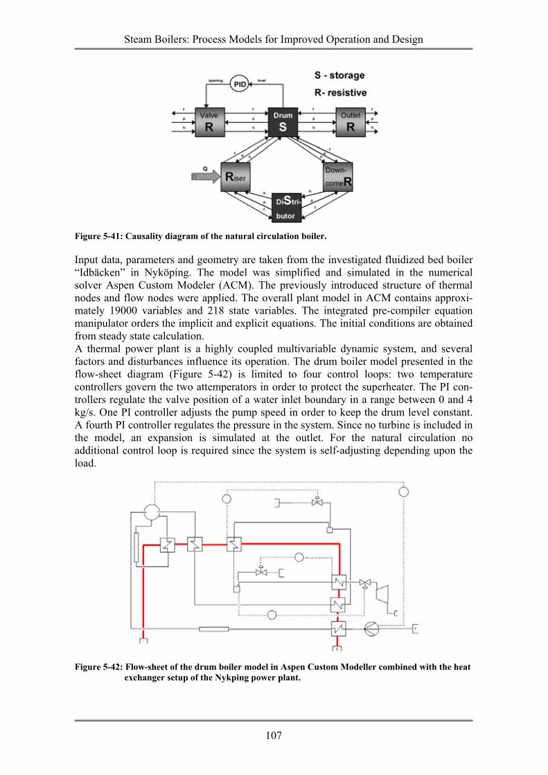
Steam Boilers: Process Models for Improved Operation and Design
107
Figure 5-41: Causality diagram of the natural circulation boiler.
Input data, parameters and geometry are taken from the investigated fluidized bed boiler “Idbäcken” in Nyköping. The model was simplified and simulated in the numerical solver Aspen Custom Modeler (ACM). The previously introduced structure of thermal nodes and flow nodes were applied. The overall plant model in ACM contains approxi-mately 19000 variables and 218 state variables. The integrated pre-compiler equation manipulator orders the implicit and explicit equations. The initial conditions are obtained from steady state calculation. A thermal power plant is a highly coupled multivariable dynamic system, and several factors and disturbances influence its operation. The drum boiler model presented in the flow-sheet diagram (Figure 5-42) is limited to four control loops: two temperature controllers govern the two attemperators in order to protect the superheater. The PI con-trollers regulate the valve position of a water inlet boundary in a range between 0 and 4 kg/s. One PI controller adjusts the pump speed in order to keep the drum level constant. A fourth PI controller regulates the pressure in the system. Since no turbine is included in the model, an expansion is simulated at the outlet. For the natural circulation no additional control loop is required since the system is self-adjusting depending upon the load.
Figure 5-42: Flow-sheet of the drum boiler model in Aspen Custom Modeller combined with the heat
exchanger setup of the Nykping power plant.
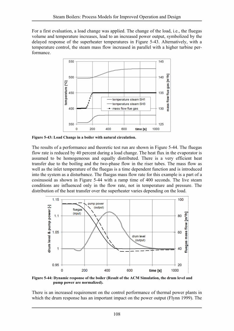
Steam Boilers: Process Models for Improved Operation and Design
108
For a first evaluation, a load change was applied. The change of the load, i.e., the fluegas volume and temperature increases, lead to an increased power output, symbolized by the delayed response of the superheater temperatures in Figure 5-43. Alternatively, with a temperature control, the steam mass flow increased in parallel with a higher turbine per-formance.
Figure 5-43: Load Change in a boiler with natural circulation.
The results of a performance and theoretic test run are shown in Figure 5-44. The fluegas flow rate is reduced by 40 percent during a load change. The heat flux in the evaporator is assumed to be homogeneous and equally distributed. There is a very efficient heat transfer due to the boiling and the two-phase flow in the riser tubes. The mass flow as well as the inlet temperature of the fluegas is a time dependent function and is introduced into the system as a disturbance. The fluegas mass flow rate for this example is a part of a cosinusoid as shown in Figure 5-44 with a ramp time of 400 seconds. The live steam conditions are influenced only in the flow rate, not in temperature and pressure. The distribution of the heat transfer over the superheater varies depending on the load.
Figure 5-44: Dynamic response of the boiler (Result of the ACM Simulation, the drum level and
pump power are normalized).
There is an increased requirement on the control performance of thermal power plants in which the drum response has an important impact on the power output (Flynn 1999). The
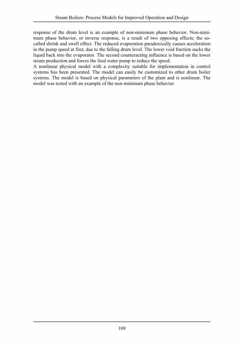
Steam Boilers: Process Models for Improved Operation and Design
109
response of the drum level is an example of non-minimum phase behavior. Non-mini-mum phase behavior, or inverse response, is a result of two opposing effects; the so-called shrink and swell effect. The reduced evaporation paradoxically causes acceleration in the pump speed at first, due to the falling drum level. The lower void fraction sucks the liquid back into the evaporator. The second counteracting influence is based on the lower steam production and forces the feed water pump to reduce the speed. A nonlinear physical model with a complexity suitable for implementation in control systems has been presented. The model can easily be customized to other drum boiler systems. The model is based on physical parameters of the plant and is nonlinear. The model was tested with an example of the non-minimum phase behavior.

Steam Boilers: Process Models for Improved Operation and Design
110
Steam Boilers: Process Models for Improved Operation and Design
111
6. CONCLUSIONS & RECOMMENDATIONS This thesis addresses two key issues related to the operational performance of steam power plants. One is the slagging and fouling reduction by optimization of soot blowing cycles, the other is the dynamic behavior of a once-through boiler during load changes. Both issues requires advanced models and models aimed at the solution of these problems are presented. The first part of the work is aimed at a better knowledge and understanding of deposit phenomena during coal and biomass combustion and to develop adequate measurement tools to monitor deposits in order to start countermeasures in time. First lab-scale measurements provided a clear correlation between fuel quality and ash behavior that lead to full-scale investigations of slagging and fouling. A numerical process model was developed to monitor online the heat transfer of heat exchangers in biomass-fired power plants. It was successfully applied to different types of boilers and a lab scale furnace. The modular structure makes it a tool for detecting and analyzing slagging and fouling deposits for each separate heat exchanger. The model provides information about the deposit build-up rate, as well as the ash removal during soot blowing. An optimized soot blowing strategy was proposed. The evaporator and superheater exposed to radiation suffer extremely from slagging and additional soot blowing is favorable. The fast build-up of slagging and especially the unsteady fuel quality are the main causes for the unstable operation of the boilers. The model strongly relies on the measurement devices and the quality of their measurements. Especially during unstable operations, the information contained in the calculated results is of limited value. Small changes or wrong signals deteriorate the accuracy of the predicted values. Often the measurements were not representative of the process and, often, were a source of faulty results. Thermocouples installed for high temperature fluegas measurements are, in most cases, responsible for incorrect measurements. Acoustic pyrometry was tested successfully as an alternative to measure the fluegas exit temperature. Online deposits probes are under development and could be an alternative for fault-prone thermocouples. CFD calculations completed the investigations for this thesis. The CFD simulation identified areas in the boiler with a high slagging propensity. The online process model was installed in the power plant as a permanent monitoring tool and the frequency of the cleaning cycles was optimized. It is a simple tool for operators and it can be effective if qualified personnel are able to provide the necessary software maintenance from time to time. Changes in the boiler design, equipment and configuration, like modification in the measurement devices, have to be reflected in the model in order to guarantee meaningful results. In addition, there is no automatic soot blowing activation coupled to the monitoring tool yet. In addition, a predictive dynamic model was developed, partly based on the results of the steady state model. The model focused on steam boilers, one of the most complex components with a highly dynamic behavior. The nonlinear model is based on the physical parameters of the plant and follows the lumped parameters approach. It implements a one-dimensional staggered grid discretization for higher numerical stability and includes radiative and convective heat transfer. The developed dynamic model of a once-through boiler evaporator contains a moving boundary instead of a fixed grid. The moving boundary approach allows for the accurate calculation of the phase transition positions inside the water-steam pipes, even with a limited number of computational nodes. The modular structure of the dynamic model can easily be customized to other
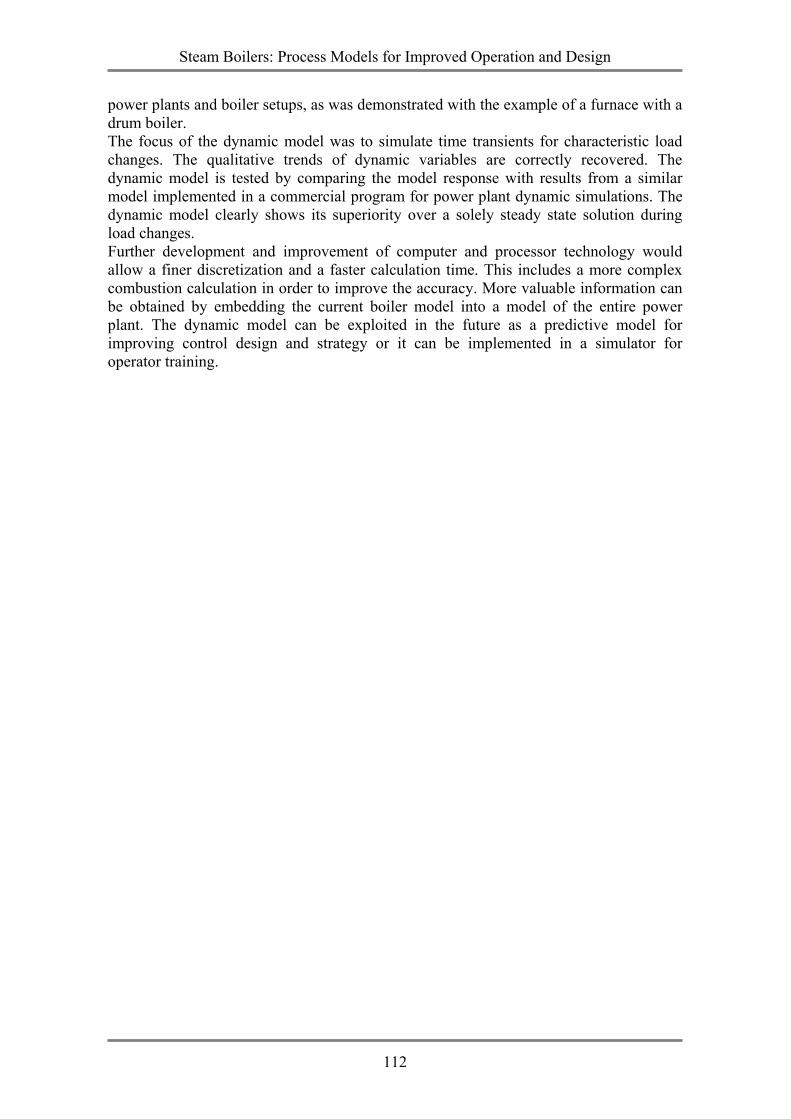
Steam Boilers: Process Models for Improved Operation and Design
112
power plants and boiler setups, as was demonstrated with the example of a furnace with a drum boiler. The focus of the dynamic model was to simulate time transients for characteristic load changes. The qualitative trends of dynamic variables are correctly recovered. The dynamic model is tested by comparing the model response with results from a similar model implemented in a commercial program for power plant dynamic simulations. The dynamic model clearly shows its superiority over a solely steady state solution during load changes. Further development and improvement of computer and processor technology would allow a finer discretization and a faster calculation time. This includes a more complex combustion calculation in order to improve the accuracy. More valuable information can be obtained by embedding the current boiler model into a model of the entire power plant. The dynamic model can be exploited in the future as a predictive model for improving control design and strategy or it can be implemented in a simulator for operator training.
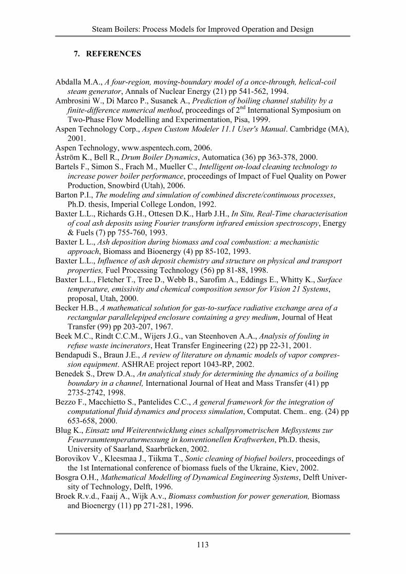
Steam Boilers: Process Models for Improved Operation and Design
113
7. REFERENCES Abdalla M.A., A four-region, moving-boundary model of a once-through, helical-coil
steam generator, Annals of Nuclear Energy (21) pp 541-562, 1994. Ambrosini W., Di Marco P., Susanek A., Prediction of boiling channel stability by a
finite-difference numerical method, proceedings of 2nd International Symposium on Two-Phase Flow Modelling and Experimentation, Pisa, 1999.
Aspen Technology Corp., Aspen Custom Modeler 11.1 User's Manual. Cambridge (MA), 2001.
Aspen Technology, www.aspentech.com, 2006. Åström K., Bell R., Drum Boiler Dynamics, Automatica (36) pp 363-378, 2000. Bartels F., Simon S., Frach M., Mueller C., Intelligent on-load cleaning technology to
increase power boiler performance, proceedings of Impact of Fuel Quality on Power Production, Snowbird (Utah), 2006.
Barton P.I., The modeling and simulation of combined discrete/continuous processes, Ph.D. thesis, Imperial College London, 1992.
Baxter L.L., Richards G.H., Ottesen D.K., Harb J.H., In Situ, Real-Time characterisation of coal ash deposits using Fourier transform infrared emission spectroscopy, Energy & Fuels (7) pp 755-760, 1993.
Baxter L L., Ash deposition during biomass and coal combustion: a mechanistic approach, Biomass and Bioenergy (4) pp 85-102, 1993.
Baxter L.L., Influence of ash deposit chemistry and structure on physical and transport properties, Fuel Processing Technology (56) pp 81-88, 1998.
Baxter L.L., Fletcher T., Tree D., Webb B., Sarofim A., Eddings E., Whitty K., Surface temperature, emissivity and chemical composition sensor for Vision 21 Systems, proposal, Utah, 2000.
Becker H.B., A mathematical solution for gas-to-surface radiative exchange area of a rectangular parallelepiped enclosure containing a grey medium, Journal of Heat Transfer (99) pp 203-207, 1967.
Beek M.C., Rindt C.C.M., Wijers J.G., van Steenhoven A.A., Analysis of fouling in refuse waste incinerators, Heat Transfer Engineering (22) pp 22-31, 2001.
Bendapudi S., Braun J.E., A review of literature on dynamic models of vapor compres-sion equipment. ASHRAE project report 1043-RP, 2002.
Benedek S., Drew D.A., An analytical study for determining the dynamics of a boiling boundary in a channel, International Journal of Heat and Mass Transfer (41) pp 2735-2742, 1998.
Bezzo F., Macchietto S., Pantelides C.C., A general framework for the integration of computational fluid dynamics and process simulation, Computat. Chem.. eng. (24) pp 653-658, 2000.
Blug K., Einsatz und Weiterentwicklung eines schallpyrometrischen Meßsystems zur Feuerraumtemperaturmessung in konventionellen Kraftwerken, Ph.D. thesis, University of Saarland, Saarbrücken, 2002.
Borovikov V., Kleesmaa J., Tiikma T., Sonic cleaning of biofuel boilers, proceedings of the 1st International conference of biomass fuels of the Ukraine, Kiev, 2002.
Bosgra O.H., Mathematical Modelling of Dynamical Engineering Systems, Delft Univer-sity of Technology, Delft, 1996.
Broek R.v.d., Faaij A., Wijk A.v., Biomass combustion for power generation, Biomass and Bioenergy (11) pp 271-281, 1996.
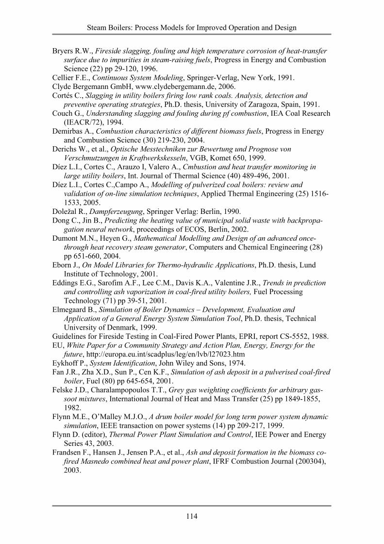
Steam Boilers: Process Models for Improved Operation and Design
114
Bryers R.W., Fireside slagging, fouling and high temperature corrosion of heat-transfer surface due to impurities in steam-raising fuels, Progress in Energy and Combustion Science (22) pp 29-120, 1996.
Cellier F.E., Continuous System Modeling, Springer-Verlag, New York, 1991. Clyde Bergemann GmbH, www.clydebergemann.de, 2006. Cortés C., Slagging in utility boilers firing low rank coals. Analysis, detection and
preventive operating strategies, Ph.D. thesis, University of Zaragoza, Spain, 1991. Couch G., Understanding slagging and fouling during pf combustion, IEA Coal Research
(IEACR/72), 1994. Demirbas A., Combustion characteristics of different biomass fuels, Progress in Energy
and Combustion Science (30) 219-230, 2004. Derichs W., et al., Optische Messtechniken zur Bewertung und Prognose von
Verschmutzungen in Kraftwerkskesseln, VGB, Komet 650, 1999. Díez L.I., Cortes C., Arauzo I, Valero A., Cmbustion and heat transfer monitoring in
large utility boilers, Int. Journal of Thermal Science (40) 489-496, 2001. Díez L.I., Cortes C.,Campo A., Modelling of pulverized coal boilers: review and
validation of on-line simulation techniques, Applied Thermal Engineering (25) 1516-1533, 2005.
Doležal R., Dampferzeugung, Springer Verlag: Berlin, 1990. Dong C., Jin B., Predicting the heating value of municipal solid waste with backpropa-
gation neural network, proceedings of ECOS, Berlin, 2002. Dumont M.N., Heyen G., Mathematical Modelling and Design of an advanced once-
through heat recovery steam generator, Computers and Chemical Engineering (28) pp 651-660, 2004.
Eborn J., On Model Libraries for Thermo-hydraulic Applications, Ph.D. thesis, Lund Institute of Technology, 2001.
Eddings E.G., Sarofim A.F., Lee C.M., Davis K.A., Valentine J.R., Trends in prediction and controlling ash vaporization in coal-fired utility boilers, Fuel Processing Technology (71) pp 39-51, 2001.
Elmegaard B., Simulation of Boiler Dynamics – Development, Evaluation and Application of a General Energy System Simulation Tool, Ph.D. thesis, Technical University of Denmark, 1999.
Guidelines for Fireside Testing in Coal-Fired Power Plants, EPRI, report CS-5552, 1988. EU, White Paper for a Community Strategy and Action Plan, Energy, Energy for the
future, http://europa.eu.int/scadplus/leg/en/lvb/l27023.htm Eykhoff P., System Identification, John Wiley and Sons, 1974. Fan J.R., Zha X.D., Sun P., Cen K.F., Simulation of ash deposit in a pulverised coal-fired
boiler, Fuel (80) pp 645-654, 2001. Felske J.D., Charalampopoulos T.T., Grey gas weighting coefficients for arbitrary gas-
soot mixtures, International Journal of Heat and Mass Transfer (25) pp 1849-1855, 1982.
Flynn M.E., O’Malley M.J.O., A drum boiler model for long term power system dynamic simulation, IEEE transaction on power systems (14) pp 209-217, 1999.
Flynn D. (editor), Thermal Power Plant Simulation and Control, IEE Power and Energy Series 43, 2003.
Frandsen F., Hansen J., Jensen P.A., et al., Ash and deposit formation in the biomass co-fired Masnedo combined heat and power plant, IFRF Combustion Journal (200304), 2003.
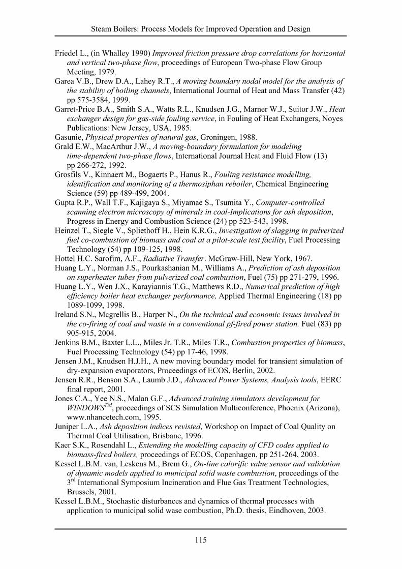
Steam Boilers: Process Models for Improved Operation and Design
115
Friedel L., (in Whalley 1990) Improved friction pressure drop correlations for horizontal and vertical two-phase flow, proceedings of European Two-phase Flow Group Meeting, 1979.
Garea V.B., Drew D.A., Lahey R.T., A moving boundary nodal model for the analysis of the stability of boiling channels, International Journal of Heat and Mass Transfer (42) pp 575-3584, 1999.
Garret-Price B.A., Smith S.A., Watts R.L., Knudsen J.G., Marner W.J., Suitor J.W., Heat exchanger design for gas-side fouling service, in Fouling of Heat Exchangers, Noyes Publications: New Jersey, USA, 1985.
Gasunie, Physical properties of natural gas, Groningen, 1988. Grald E.W., MacArthur J.W., A moving-boundary formulation for modeling
time-dependent two-phase flows, International Journal Heat and Fluid Flow (13) pp 266-272, 1992.
Grosfils V., Kinnaert M., Bogaerts P., Hanus R., Fouling resistance modelling, identification and monitoring of a thermosiphan reboiler, Chemical Engineering Science (59) pp 489-499, 2004.
Gupta R.P., Wall T.F., Kajigaya S., Miyamae S., Tsumita Y., Computer-controlled scanning electron microscopy of minerals in coal-Implications for ash deposition, Progress in Energy and Combustion Science (24) pp 523-543, 1998.
Heinzel T., Siegle V., Spliethoff H., Hein K.R.G., Investigation of slagging in pulverized fuel co-combustion of biomass and coal at a pilot-scale test facility, Fuel Processing Technology (54) pp 109-125, 1998.
Hottel H.C. Sarofim, A.F., Radiative Transfer. McGraw-Hill, New York, 1967. Huang L.Y., Norman J.S., Pourkashanian M., Williams A., Prediction of ash deposition
on superheater tubes from pulverized coal combustion, Fuel (75) pp 271-279, 1996. Huang L.Y., Wen J.X., Karayiannis T.G., Matthews R.D., Numerical prediction of high
efficiency boiler heat exchanger performance, Applied Thermal Engineering (18) pp 1089-1099, 1998.
Ireland S.N., Mcgrellis B., Harper N., On the technical and economic issues involved in the co-firing of coal and waste in a conventional pf-fired power station. Fuel (83) pp 905-915, 2004.
Jenkins B.M., Baxter L.L., Miles Jr. T.R., Miles T.R., Combustion properties of biomass, Fuel Processing Technology (54) pp 17-46, 1998.
Jensen J.M., Knudsen H.J.H., A new moving boundary model for transient simulation of dry-expansion evaporators, Proceedings of ECOS, Berlin, 2002.
Jensen R.R., Benson S.A., Laumb J.D., Advanced Power Systems, Analysis tools, EERC final report, 2001.
Jones C.A., Yee N.S., Malan G.F., Advanced training simulators development for WINDOWSTM, proceedings of SCS Simulation Multiconference, Phoenix (Arizona), www.nhancetech.com, 1995.
Juniper L.A., Ash deposition indices revisted, Workshop on Impact of Coal Quality on Thermal Coal Utilisation, Brisbane, 1996.
Kaer S.K., Rosendahl L., Extending the modelling capacity of CFD codes applied to biomass-fired boilers, proceedings of ECOS, Copenhagen, pp 251-264, 2003.
Kessel L.B.M. van, Leskens M., Brem G., On-line calorific value sensor and validation of dynamic models applied to municipal solid waste combustion, proceedings of the 3rd International Symposium Incineration and Flue Gas Treatment Technologies, Brussels, 2001.
Kessel L.B.M., Stochastic disturbances and dynamics of thermal processes with application to municipal solid wase combustion, Ph.D. thesis, Eindhoven, 2003.
Steam Boilers: Process Models for Improved Operation and Design
116
Kiel J.H.A., Coal ash behaviour in reducing environments (CABRE), ECN-NOVEM, 1999.
Kikstra J.F., Modelling, Design, and Control of a Cogenerating nuclear Gas Turbine Plant,. Ph.D. thesis, Delft University of Technology, 2001.
Kikstra J.F., Verkooijen A.H.M., Dynamic Modeling of a Cogeneration Nuclear Gas Turbine Plant - Part I: Modeling and Validation, Transactions of the ASME, Journal of Engineering for Gas Turbines and Power (124) pp 725-733, 2002.
Kikstra J.F., Verkooijen A.H.M., Dynamic Modeling of a Cogeneration Nuclear Gas Turbine Plant - Part II: Dynamic Behaviour and Control, Transactions of the ASME, Journal of Engineering for Gas Turbines and Power (124) pp 734-743, 2002.
Klefenz G., Die Regelung von Dampfkraftwerken, B.I. Wissenschaftsverlag: Mannheim 1983.
Lienhard IV J.H., Lienhard V J.H., A Heat Transfer Text Book, Philigiston Press, Cambridge Massachusetts, 2002.
Linka S., Wirtz S., Scherer V., Investigations on thermal radiation characteristics of coal ashes and slags, proceedings of CleanAir, Lisbon, 2003.
Liu Y.C., Brosilow C.B., Simulation of large scale dynamic systems- I. Modular integration methods, Comput. Chem. Engng (11) pp 241-253, 1987.
Lu S., Dynamic modeling and simulation of power plant systems, proceedings of Instn. Mech Engrs., 213, pp 7-23, 1999.
Lundmark D., Mueller C., Skrifvars B.-J., Hupa M., CFD-Modelling of combustion and deposition in a biofuel co-fired bubbling fluidised bed combustor, proceedings of CleanAir, Lisbon, 2003.
Ma Z., Iman F., Lu P., Sears R. Kong J., Rokanuzzaman A.S., McCollor D.P., Benson S.A., A comprehensive slagging and fouling prediction tool for coal-fired boilers and its validation, proceedings of Impact of Fuel Quality on Power Production, Snowbird (Utah), 2006.
Melo L.F. et al. (editor), Fouling Science and Technology, Kluwer: Dordrecht, 1988. Mensonidis G.I., Ermittlung einer optimalen Reinigungsstrategie für Prozeßoptimierung
von Dampferzeugern, M.Sc. Thesis, Delft, 1999 Michel J.B., Gentsch R., Grenet E., Heitger F., Onillon E., Verjus C., Low cost sensors
and methods for combustion control, proceedings of CleanAir, 2003. Miles T.R., et al., Boiler deposits from firing biomass fuels, Biomass and Bioenergy (10)
pp 125-138, 1996. MMS - Modular Modeling System Version 6.0, nHance Technologies, Lynchburg, VA.,
2002. Modelica Design Group, The Modelica Language Specification, Version 1.4, 2000. Müller J., Cannons hit the mark, Modern Power Systems, pp 63-66, 5/2001. Nielsen C., Jorgensen K., Iversen S., Mosbech H., Hassing H., Glarborg P., Rosendahl
L., Improved Modelling of Grate Combustion Concept, proceedings BIOMASS’02 Amsterdam, 2002.
Nutalapati D., Gupta R., Moghtaderi B., Wall T.F., Assessing slagging and fouling during biomass combustion: a thermodynamic approach allowing for alkali/ash reaction, proceedings of Impact of Fuel Quality on Power Production, Snowbird (Utah), 2006.
Obernberger I., Decentralized biomass combustion: state of the art and future develop-ment, Biomass and Bioenergy (14) pp 33-56, 1998.
Ordys A.W., Modelling and simulation of power generation plants, London, Springer, 1994.
Steam Boilers: Process Models for Improved Operation and Design
117
Patankar S.V., Numerical heat transfer and fluid flow. Hemisphere, Washington D.C., 1980.
Raask E., Mineral Impurities in Coal Combustion. Hemisphere, Washington, 1985. Ragwitz M., Schleich J., Huber C., et al., Forres 2020, Analysis of renewable energy’s
evolution up to 2020, abstract of first results, 2004. Rezaei H.R., Gupta R.P., Wall T.F., Miyamae S., Makino K., Modelling the initial
structure of ash deposits and structure changes due to sintering, proceedings of Impact of mineral impurities in solid fuel combustion, Kluwer Academic: New York, 1999.
Rezaei H.R., Gupta R.P., Bryant G.W., Hart J.G. Liu G.S. et al., Thermal conductivity of coal ash and slags and models used, Fuel (79) pp 1697-1710, 2000.
Rhine J.M., Tucker R.J., Modelling of Gas-Fired Furnaces and Boilers, British Gas, 1991.
Richter S., Numerische Simulation der Flugaschedeposition in kohlestaubgefeuerten Dampferzeugern, VDI-Verlag: Düsseldorf, 2003.
Robinson A.L., Buckley S.G., Yang N., Baxter L.L., In situ measurements of the thermal conductivity of ash deposits formed in a pilot-scale combustor, Impact of mineral im purities in solid fuel combustion, New York, 1999.
Robinson A.L., Buckley S.G., Yang N., Baxter L.L., Experimental measurements of the thermal conductivity of ahs deposits: Part 1. Measurement technique, Energy & Fuels (15) pp 66-74, 2001.
Robinson A.L., et al., Experimental measurements of the thermal conductivity of ahs deposits: Part 2. Effects of sintering and deposit microstructure, Energy & Fuels (15) pp 75-84, 2001.
Rosendahl L., Grue J., Salimi P., Rasmussen A.R., Integrated furnace-steam cycle simulations of biomass-fired power plants, proceedings of ECOS, pp 289-296, 2003.
Rushdi A., Sharma A., Gupta R., An experimental study of the effect of coal blending on ash depositon, Fuel (83) pp 495-506, 2004.
Sami M., Annamalai K., Wooldridge M., Co-firing of coal and biomass fuel blends, Progress in Energy and Combustion Science (27) pp 171-214, 2001.
Schnell U., Richter S., Hein K.R.G., Numerical simulation of slagging and fouling in a pulverized coal-fired utility boiler, proceedings of UEF Conference on Heat Exchanger Fouling, 2001.
Schoen P., Dynamic Modeling and Control of Integrated Cool Gasification Combined Cycle Units, Ph.D. thesis, Delft University of Technology, 1993.
Schreurs G., Modelling of the Radiative Heat Transfer of a Biomass-Fired Pulverised Fuel Boiler, M.Sc. thesis, Delft University of Technology, 2003.
Sielschott H., Derichs W., Use of collocation methods under inclusion of a priori infor-mation in acoustic pyrometry, Proceedings of UMIST, 1995.
Sielschott H., Measurement of horizontal flow in a large scale furnace using acoustic vector tomography, Flow Measurment and Instrumentation (8) pp 191-197, 1997.
Skrifvars B.J., Lauren T., Hupa M., Korbee R., Ljung P., Ash behaviour in a pulverized wood fired boiler – a case study, Fuel (excepted) 2004.
SLAGMOD, Final report of the SLAGMOD project, 2003. Smith T.F., Shen Z.F., Friedman J.N., Evaluation of coefficients for the weighted sum of
grey gases model, Journal of Heat Transfer (104) pp 602-608, 1982. Stastny M., Numerical Simulation of the Combustion Process in a Biomass-fired Pul-
verised Fuel Boiler, Ph.D. thesis, University of Technology Praha, 2003. Stehlik P, Konoutek J., Jebacek V, Simple mathematical model of furnace and its possi-
ble application, Computer Chem. Eng. (20), pp 1369-1372, 1996.
Steam Boilers: Process Models for Improved Operation and Design
118
Strauß K., Kraftwerkstechnik, Springer: Berlin, 1998. Sturm F.A., Efficient Operations- Intelligent Diagnosis and Maintenance, proceedings of
VGB Power Tech, Essen, 2003. Su S., Pohl J.H., Holcombe D., Fouling propensities of blended coals in pulverized coal-
fired power station boilers, Fuel (82) 1653-1667, 2003. Teruel E, Cortes C., Díez L.I., Arauzo I., Monitoring and prediction of fouling in coal –
fired utility boilers using neural networks, Chemical Engineering Science (60) pp 5035-5048, 2005.
Thompson E., Hickinbotham A., Fouling monitor and alarm software- recent develop-ments, Proceedings of Mega Symposium, Chicago Il, 2003.
Torn C.J., Ash deposition: Characteristics and Influence on Heat Transfer, M.Sc. thesis, TU Delft, 2001.
Tomeczek J., Palugniok H., Ochman J., Modelling of deposit formation on heating tubes in pulverized coal boilers, Fuel (83) pp 213-221. 2004.
Unterberger S., Lopez C., Hein K.R.G., EU-Project “Prediction of Ash and Deposit Formation for Biomass pf Co-Combustion”, proceedings of Power Production in the 21st Century: Impacts of Fuel Quality and Operations, Engineering Foundation Con-ference, Utah, 2001.
Valero A., Cortés C., Ash fouling in coal-fired utility boilers. Monitoring and optimiza-tion of on-load cleaning, Progress in Energy and Combustion Science (22) pp 189-200, 1996.
Verloop C.M., Modellering van de stralingswarmteoverdracht in de vuurhaard van een gasgestookte industrieketel, M.Sc. thesis, Delft University of Technology, 1990.
Vuik C., Some historical notes about the Stefan problem, Nieuw Archief voor Wiskunde, (4e serie 11) pp 157-167, 1993.
VDI-Wärmeatlas, Berechnungsblätter für Wärmeübergang. VDI-Verlag GmbH: Düsseldorf, 1993.
Wagner W., Kruse A. Properties of Water and Steam, IAPWS-IF97: The Industrial Stan-dard IAPWS-IF97 for the Thermodynamic Properties and Supplementary Equations for Other Properties. Springer-Verlag: Berlin, 1998.
Whalley P.B., Boiling Condensation and Gas-Liquid Flow, Oxford University Press, Oxford, UK, 1990.
Wieringa, J.A., Spectral Radiative Heat Transfer in Gas-Fired Furnaces, Ph.D. thesis, Delft University of Technology, 1992.
Willatzen M., Pettit N.B.O.L., Ploeg-Sorensen L., A general dynamic simulation model for evaporators and condensers in refrigeration, International Journal of Refrigera-tion (21) pp 398-414, 1998.
Xu M., He X., Azevedo J.L.T., Carvalho M.G., An advanced model to assess fouling and slagging in coal-fired boiler, International Journal of Energy Research (26) pp 1221-1236, 2002.
Yan L., Gupta R.P., Wall T.F., A mathematical model of ash formation during pulverized coal combustion, Fuel (81) pp 337-344, 2002.
Yamashita T., Tominga H., Orimoto M., Asahiro N., Modeling of Ash formation behavior during pulverised coal combustion, IFRF Combustion Journal (2000008), 2000.
Zbogar A., Frandsen F., Surface emissivity of coal ashes, IFRF Combustion Journal (200305), 2003.
Zevenhoven-Onderwater M., Blomquist J.-P., Skrifvars B.-J., Backman R., Hupa M., The prediction of behavior of ashes from five different solid fuels in fluidized bed com-bustion, Fuel (79) pp 1353-1361, 2000.

Steam Boilers: Process Models for Improved Operation and Design
119
Zevenhoven-Onderwater M., Ash-Forming Matter in Biomass Fuels, Ph.D. thesis, Åbo Akademi: Åbo/Turku, 2001.
Zhang J., Coulthard J., Kech R., Cheng R., Asquith P., Measuring and Controlling Pulverised Fuel on Coal-Fired Plant, Proceedings of CleanAir, Lisbon, 2003.
Steam Boilers: Process Models for Improved Operation and Design
120
8. NOMENCLATURE
Variables: α heat transfer coefficient in J m-2 K-1 s-1 ε porosity [-] ε emissivity [-] η dynamic viscosity in kg m-1 s-1 κ adiabatic coefficient λ conductivity in J m-1 K-1 s-1
ξ fanning friction factor [-] ρ density in kg m-3 σ Boltzmann constant 1.38066 10-23 J K-1
τ time (flying time of a sound signal) in s φ mass flow rate in kg s-1 A cross sectional area in m2
B acoustic coefficient [-] C Capacitance cp specific heat in J kg-1 K-1 d diameter/ thickness in m
E emissive power F force in N h specific enthalpy in J kg-1 k thermal conductivity in W m-1 K-1 L length/ geometric equivalent diameter in m M moleculare weight in kg mol-1 n number of nodes Nu Nusselt number [-] P Potential p pressure in bar Pr Prandtl number [-] Q heat flow in J s-1 R Resistance R universal gas constant in J mol-1 K-1 Re Reynolds number [-] T temperature in K (exception T250 in °C) t time in s u specific internal energy in J kg-1 V volume in m³ w velocity in m s-1 x length in m
Steam Boilers: Process Models for Improved Operation and Design
121
Subscripts: b nucleate boiling B/A Base-acid ratio cond conduction conv convection e energy e entrance el electrical f fouling i lower boundary of the flow node i-1 upper boundary of the flow node j lower boundary of the thermal node j+1 upper boundary of the thermal node k forced convection l exit lam laminar low lower boundary of the saturated thermal node m mass up upper boundary of the saturated thermal node mid average property of the saturated thermal node rad radiation s slagging turb turbulent Superscripts: c compensation dep deposit fr friction g gravity liq liquid lv two-phase met metal/steel rot rotational sat_l saturated liquid condition sat_v saturated vapor condition vap vapor
Steam Boilers: Process Models for Improved Operation and Design
122
Abbreviation: AC Alternating current ACM Aspen Custom Modeler ACSL Advanced Continuous Simulation Language BFB Bubbling Fluidized Bed CCSEM Computer Controlled Scanning Electron Microscope CFD Computational Fluid Dynamics CHP Combined heat and power (plant) DCS Distributed Control System DP Dolomite percentage EDP Energias de Portugal EDX Energy Disperse X-Ray F Function FB Fluidized Bed (Combustion) FEGT Furnace Exit Gas Temperature G Gas HP high pressure (steam) I/C Iron-calcium ratio IST Instituto Superior Tecnico Lisbon (Portugal) IVD Institut für Verfahrenstechnik und Dampfkesselwesen Stuttgart (Germany) KSVA Kohlenstaubverbrennungsanlage - Pulverized Coal Combustion Facility LF Lignitic Factor LHS left hand side LHV Lower heating value LMTD Logarithmic mean temperature difference LP low pressure (steam) MB Moving Boundary MMS Modular Modeling System NTUA National Technical University of Athens (Greece) OFA Over Fired Air PF Pulverized Fuel (Combustion) RAH Regenerative Air Heater RH reheater RHS right hand side RS Slagging Factor S Surface S/A Silica-alumina ratio SEM Scanning Electron Microscope SCR Selective Catalytic Reduction SH superheater VDI Verein Deutscher Ingenieure waf water and ash free wf water free WSGGM Weighted Sum of Gray Gases Model
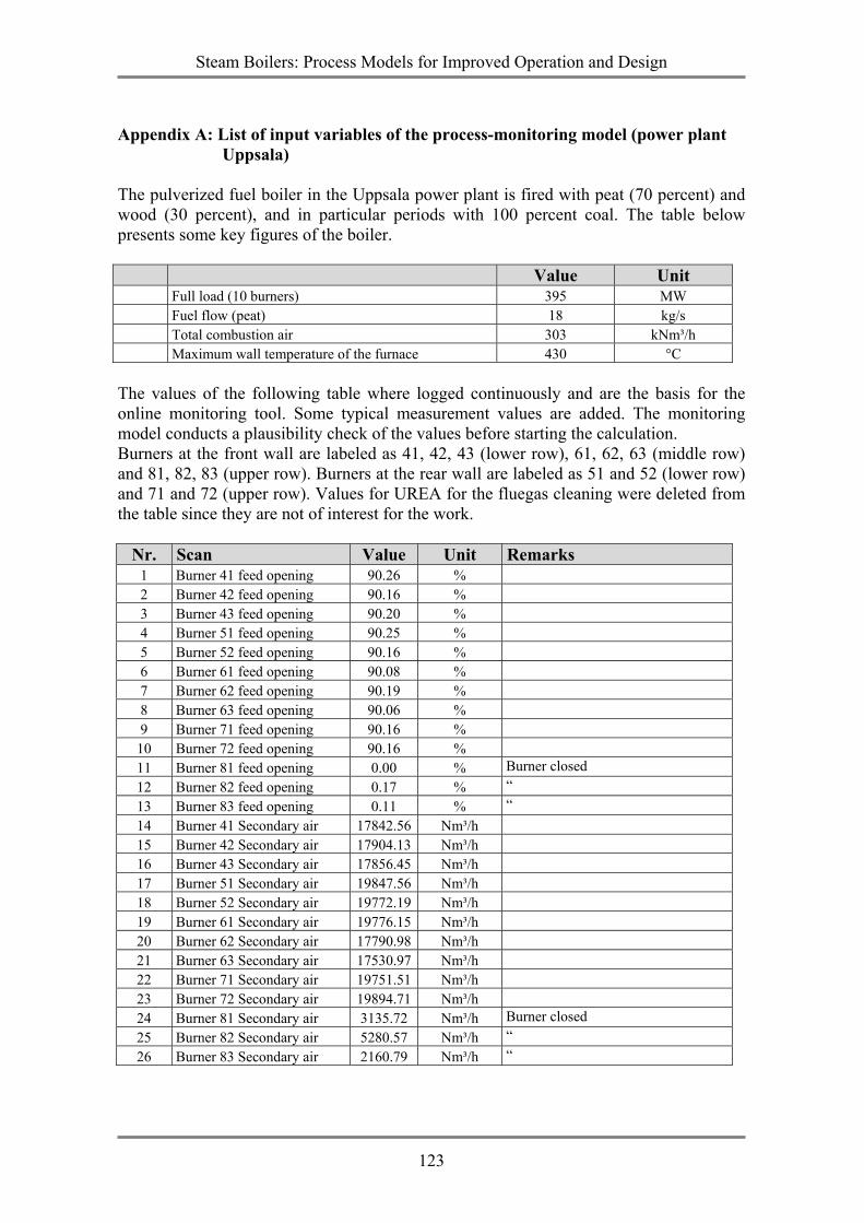
Steam Boilers: Process Models for Improved Operation and Design
123
Appendix A: List of input variables of the process-monitoring model (power plant
Uppsala) The pulverized fuel boiler in the Uppsala power plant is fired with peat (70 percent) and wood (30 percent), and in particular periods with 100 percent coal. The table below presents some key figures of the boiler.
Value Unit Full load (10 burners) 395 MW Fuel flow (peat) 18 kg/s Total combustion air 303 kNm³/h Maximum wall temperature of the furnace 430 °C
The values of the following table where logged continuously and are the basis for the online monitoring tool. Some typical measurement values are added. The monitoring model conducts a plausibility check of the values before starting the calculation. Burners at the front wall are labeled as 41, 42, 43 (lower row), 61, 62, 63 (middle row) and 81, 82, 83 (upper row). Burners at the rear wall are labeled as 51 and 52 (lower row) and 71 and 72 (upper row). Values for UREA for the fluegas cleaning were deleted from the table since they are not of interest for the work.
Nr. Scan Value Unit Remarks 1 Burner 41 feed opening 90.26 % 2 Burner 42 feed opening 90.16 % 3 Burner 43 feed opening 90.20 % 4 Burner 51 feed opening 90.25 % 5 Burner 52 feed opening 90.16 % 6 Burner 61 feed opening 90.08 % 7 Burner 62 feed opening 90.19 % 8 Burner 63 feed opening 90.06 % 9 Burner 71 feed opening 90.16 %
10 Burner 72 feed opening 90.16 % 11 Burner 81 feed opening 0.00 % Burner closed 12 Burner 82 feed opening 0.17 % “ 13 Burner 83 feed opening 0.11 % “ 14 Burner 41 Secondary air 17842.56 Nm³/h 15 Burner 42 Secondary air 17904.13 Nm³/h 16 Burner 43 Secondary air 17856.45 Nm³/h 17 Burner 51 Secondary air 19847.56 Nm³/h 18 Burner 52 Secondary air 19772.19 Nm³/h 19 Burner 61 Secondary air 19776.15 Nm³/h 20 Burner 62 Secondary air 17790.98 Nm³/h 21 Burner 63 Secondary air 17530.97 Nm³/h 22 Burner 71 Secondary air 19751.51 Nm³/h 23 Burner 72 Secondary air 19894.71 Nm³/h 24 Burner 81 Secondary air 3135.72 Nm³/h Burner closed 25 Burner 82 Secondary air 5280.57 Nm³/h “ 26 Burner 83 Secondary air 2160.79 Nm³/h “
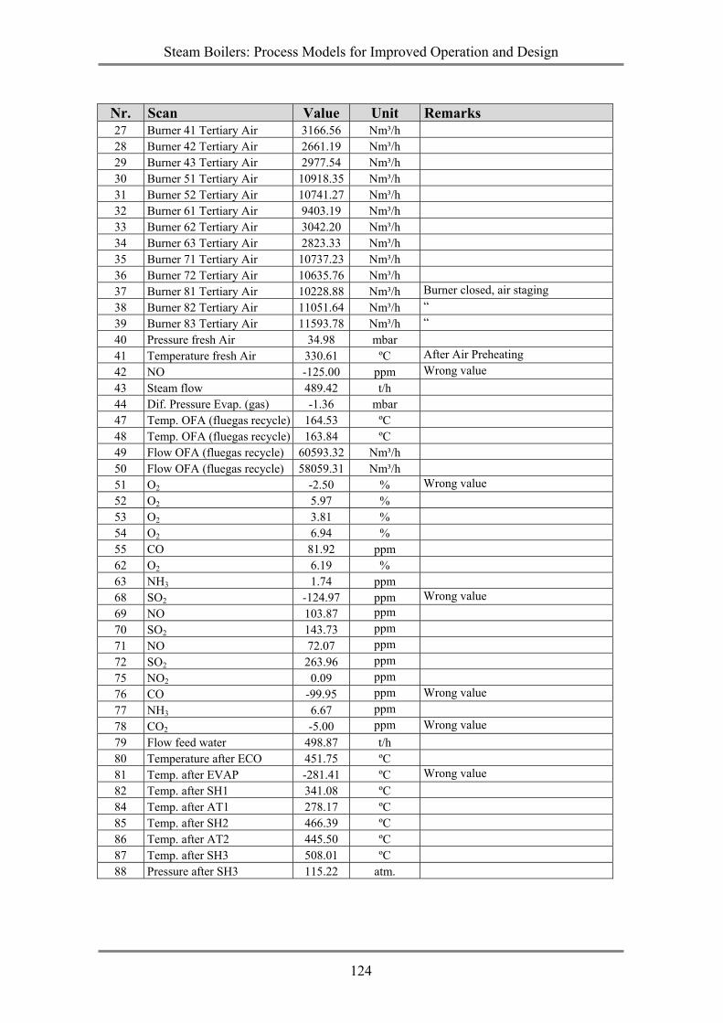
Steam Boilers: Process Models for Improved Operation and Design
124
Nr. Scan Value Unit Remarks 27 Burner 41 Tertiary Air 3166.56 Nm³/h 28 Burner 42 Tertiary Air 2661.19 Nm³/h 29 Burner 43 Tertiary Air 2977.54 Nm³/h 30 Burner 51 Tertiary Air 10918.35 Nm³/h 31 Burner 52 Tertiary Air 10741.27 Nm³/h 32 Burner 61 Tertiary Air 9403.19 Nm³/h 33 Burner 62 Tertiary Air 3042.20 Nm³/h 34 Burner 63 Tertiary Air 2823.33 Nm³/h 35 Burner 71 Tertiary Air 10737.23 Nm³/h 36 Burner 72 Tertiary Air 10635.76 Nm³/h 37 Burner 81 Tertiary Air 10228.88 Nm³/h Burner closed, air staging 38 Burner 82 Tertiary Air 11051.64 Nm³/h “ 39 Burner 83 Tertiary Air 11593.78 Nm³/h “ 40 Pressure fresh Air 34.98 mbar 41 Temperature fresh Air 330.61 ºC After Air Preheating 42 NO -125.00 ppm Wrong value 43 Steam flow 489.42 t/h 44 Dif. Pressure Evap. (gas) -1.36 mbar 47 Temp. OFA (fluegas recycle) 164.53 ºC 48 Temp. OFA (fluegas recycle) 163.84 ºC 49 Flow OFA (fluegas recycle) 60593.32 Nm³/h 50 Flow OFA (fluegas recycle) 58059.31 Nm³/h 51 O2 -2.50 % Wrong value 52 O2 5.97 % 53 O2 3.81 % 54 O2 6.94 % 55 CO 81.92 ppm 62 O2 6.19 % 63 NH3 1.74 ppm 68 SO2 -124.97 ppm Wrong value 69 NO 103.87 ppm 70 SO2 143.73 ppm 71 NO 72.07 ppm 72 SO2 263.96 ppm 75 NO2 0.09 ppm 76 CO -99.95 ppm Wrong value 77 NH3 6.67 ppm 78 CO2 -5.00 ppm Wrong value 79 Flow feed water 498.87 t/h 80 Temperature after ECO 451.75 ºC 81 Temp. after EVAP -281.41 ºC Wrong value 82 Temp. after SH1 341.08 ºC 84 Temp. after AT1 278.17 ºC 85 Temp. after SH2 466.39 ºC 86 Temp. after AT2 445.50 ºC 87 Temp. after SH3 508.01 ºC 88 Pressure after SH3 115.22 atm.
Steam Boilers: Process Models for Improved Operation and Design
125
Nr. Scan Value Unit Remarks 89 Temp. after RH1 320.14 ºC 90 Pressure after RH1 25.74 atm. 91 Temp. after AT_RH 426.37 ºC 92 Temp. after RH2 511.03 ºC 93 Pressure after RH2 0.00 atm. 94 Delta pressure air preheater 18.61 mbar 98 Electrical Output Generator 122.60 MW 103 Oil flow 220.67 L/h Burner support
Following additional values were measured manually and not continuously:
Nr. Scan Value Unit 1 Opening of attemperator 1 valve 80 % 2 Opening of attemperator 2 valve 30 % 3 Opening of attemperator valve reheater side1 0 % 4 Pressure inlet to temperatur 120 bar 5 Pressure inlet boiler walls 95 bar 6 Ambient Air Temperature 42 ºC 7 Secondary and Tertiary Air Temperature 290 ºC 8 Fluegas temperature after economizer before RAH 300 ºC 9 Fluegas temperature after RAH (Regenerative air heater) 160 ºC 9 Temperature Chimney 92 ºC 9 Temperature Chimney 153 ºC
11 Temperature inlet economizer 200 ºC 14 Temperature exit screen wall 15 385 ºC 15 Temperature after rehaeater 1 390 ºC 16 Temperature steam before rehaeater 1 390 ºC 17 Mass flow inlet economizer 250 t/h 18 Mass flow inlet boiler walls 290 t/h 19 Mass flow to superheater attemperators 17 t/h 20 Mass flow attemperator before Reheater 0 t/h 21 Economizer temperature 290 ºC
Steam Boilers: Process Models for Improved Operation and Design
126
Appendix B: List of input variables of the process-monitoring model (power plant Nyköping)
The fluidized bed boiler of the Nyköping Power Plant is fired with a mixture of biomass and coal (85/15), where the biomass itself is a mixture of wood waste and forest residue with moisture content of approximately 20-30 percent. Some key figures of the power plant are summarized in the following table. Value Unit Full load (thermal) 97 MW Mass flow steam (average) 40 kg/s Pressure steam (max) 140 bar Medium temperature steam (max) 540 °C Primary Air Flow 37 kNm³/h Secondary Air Flow 62 kNm³/h Tertiary Air Flow 24 kNm³/h Total Combustion Air 143 kNm³/h Exhaust Recirculation Air 20 kNm³/h Data points of the online logging system, which are the basis of the monitoring model, are summarized below, completed with some typical values.
Nr. Scan Value Unit Remarks 1 Primary Air flow rate 21.19 kNm³/h (fluidized bed) 2 plus add. Recirculated fluegas 44.97 kNm³/h 3 Air temperature before fan 38.48 °C 4 Air temperature after fan 115.46 °C 5 Air temp. after airheater 1 143.79 °C 6 Air temp. after airheater 2 195.24 °C 7 Air temperature fluidized bed 815.00 °C 8 Air temperature fluidized bed 798.01 °C 9 Air temperature fluidized bed 809.29 °C
10 Air temperature fluidized bed 781.78 °C 11 Air temperature fluidized bed 810.52 °C 12 Air temperature fluidized bed 820.19 °C 13 Air temperature fluidized bed 811.43 °C 14 Air temperature fluidized bed 794.73 °C 15 Secondary air flow rate 50.87 kNm³/h 16 Air temperature before fan 39.66 °C 17 Air temperature after fan 94.17 °C 18 Air temp. after air heater 182.99 °C 19 Ratio coal / biomass 0.9 0…1 1 = 100% coal 20 Electrical power 47.75 MW 21 Fluegas temp. fluidized bed 616.33 °C 22 Fluegas temp. fluidized bed 899.13 °C 23 Fluegas temperature roof 901.89 °C 24 Fluegas temperature roof 841.9 °C
Steam Boilers: Process Models for Improved Operation and Design
127
Nr. Scan Value Unit Remarks 25 Fluegas temp. middle section 609.36 °C 26 Fluegas temp. middle section 567.82 °C 27 Fluegas temp. second path 615.77 °C 28 Fluegas temp. second path 613.37 °C 29 Fluegas temp. before ECO 368.2 °C 30 Fluegas temp. after ECO 219.45 °C 31 Fluegas temp. after air heater 94.03 °C 32 Fluegas flow 117.1 kNm³/h 33 Fluegas flow 89.62 kNm³/h 34 NOx 6.57 ppm 35 NOx after SCR 4.9 ppm 36 CO 70.67 mg/Nm³ 37 CO2 14.46 % 38 NH3 2.46 mg/Nm³ 39 H2O 12.67 % 40 SO2 13.82 mg/Nm³ 41 NO 34.59 mg/Nm³ 42 N2O 0 mg/Nm³ 43 O2 2.52 % 44 Feed water stream 18.8 kg/s 45 Feed water temperature 193.96 °C 46 Feed water pressure 13.88 MPa 47 Mass flow live steam 18.46 kg/s 48 Temperature live steam 528.16 °C 49 Pressure flow live steam 12.87 MPa 50 Mass flow to AT 1 bef. SH1 0.48 kg/s 51 Temp. AT 1 before SH1 463.06 °C 52 Temp. AT 1 before SH1 470.98 °C 53 Mass flow to AT 2 bef. SH1 0.47 kg/s 54 Temp. AT 2 before SH1 497.3 °C 55 Temp. AT 2 before SH1 498.3 °C 56 Temperature steam roof 330.12 °C 57 Temperature steam roof 340.4 °C 58 Temperature steam roof 335.94 °C 59 Temperature steam roof 347.17 °C 60 Temp. of steam rear wall 357.88 °C 61 Temp. of steam rear wall 0 °C 62 Temp. of steam rear wall 353.04 °C 63 Temp. of steam rear wall 350.41 °C 64 Temp. of steam side wall 361.38 °C 65 Temp. of steam side wall 359.59 °C 66 Temp. of steam side wall 363.88 °C 67 Temp. of steam side wall 363.16 °C 68 Temperature collector SH1 358.54 °C 69 Temp. before attemperator 1 470.3 °C 70 Temp. before attemperator 1 494.03 °C 71 Temperature SH2 487.22 °C 72 Temperature SH2 538.16 °C
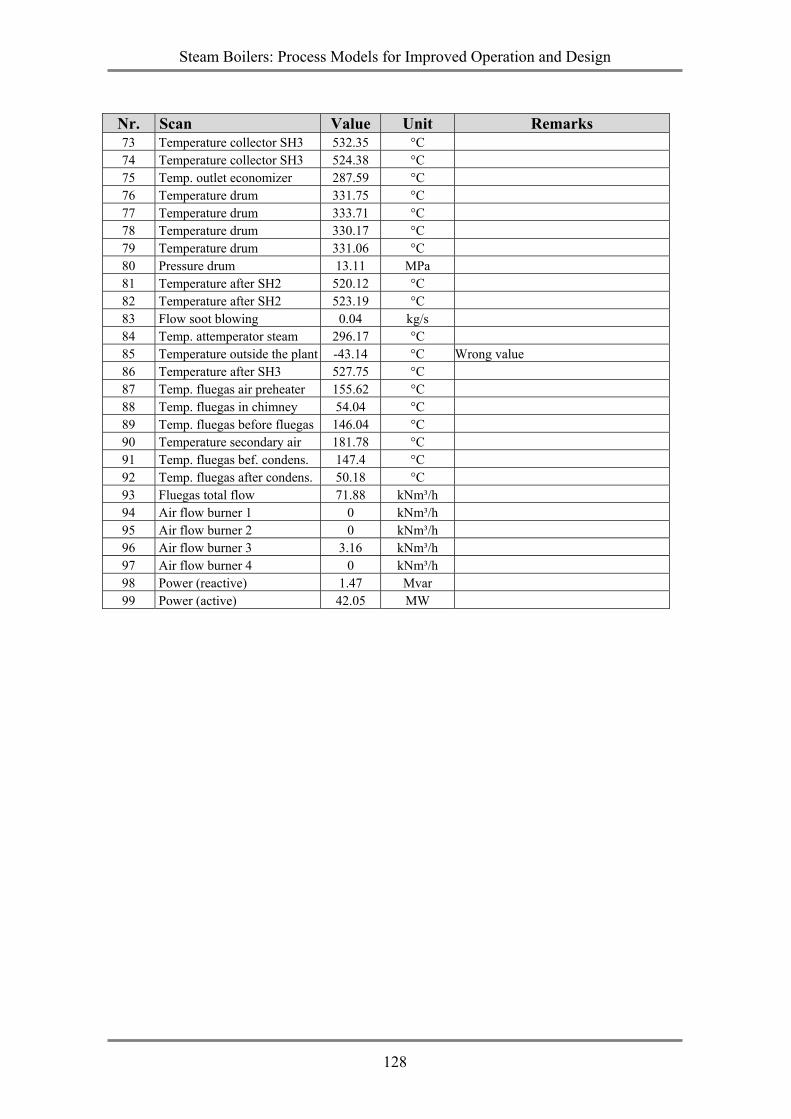
Steam Boilers: Process Models for Improved Operation and Design
128
Nr. Scan Value Unit Remarks 73 Temperature collector SH3 532.35 °C 74 Temperature collector SH3 524.38 °C 75 Temp. outlet economizer 287.59 °C 76 Temperature drum 331.75 °C 77 Temperature drum 333.71 °C 78 Temperature drum 330.17 °C 79 Temperature drum 331.06 °C 80 Pressure drum 13.11 MPa 81 Temperature after SH2 520.12 °C 82 Temperature after SH2 523.19 °C 83 Flow soot blowing 0.04 kg/s 84 Temp. attemperator steam 296.17 °C 85 Temperature outside the plant -43.14 °C Wrong value 86 Temperature after SH3 527.75 °C 87 Temp. fluegas air preheater 155.62 °C 88 Temp. fluegas in chimney 54.04 °C 89 Temp. fluegas before fluegas 146.04 °C 90 Temperature secondary air 181.78 °C 91 Temp. fluegas bef. condens. 147.4 °C 92 Temp. fluegas after condens. 50.18 °C 93 Fluegas total flow 71.88 kNm³/h 94 Air flow burner 1 0 kNm³/h 95 Air flow burner 2 0 kNm³/h 96 Air flow burner 3 3.16 kNm³/h 97 Air flow burner 4 0 kNm³/h 98 Power (reactive) 1.47 Mvar 99 Power (active) 42.05 MW
Steam Boilers: Process Models for Improved Operation and Design
129
DANKWOORD Ik wil nog heel veel mensen en instellingen bedanken, die mij met de realisatie van mijn proefschrift hielpen. De initiatiefnemer van dit werk was mijn promotor Professor Hartmut Spliethoff. Hoewel wij in Delft samenwerkten, woonden wij allebij slechts een beperkte tijd in Nederland. Ik had mijn eerste interview in Stuttgart en de afsluitende gesprekken over mijn proefschrift in München. Dank u voor uw hulp bij het voltooien van dit proefschrift. Voor hun dagelijkse steun wil ik mijn supervisors Arie Korving en Piero Colonna bedanken. Ik prijs mij gelukkig met de samenwerking en vriendschap met andere AIO's (assistent in opleiding), Jan Foeke Kikstra, Ana Abel Tortosa Masia, Johanna Vaittinen, Hans van Putten, Martin Stastny en Radek Gnutek. Ook alle AIO's die ik nu niet persoonlijk vermeld wil ik mij blijven herinneren voor het delen van gedachten en vrije tijd, zij waren een bron van inspiratie en uitwisseling. De collega's van de sectie energievoorziening wil ik bedanken voor hun behulpzame besprekingen en hun belangstelling in mijn werk en natuurlijk voor de onvergetelijke koffiepauzes van toen. De financiële steun van de Europese Unie werd in dankbaarheid ontvangen. Ik genoot van de internationale geest van alle projectpartners, dat zijn IST Lissabon, NTUA Athene en ABO Academie Turku. De Universiteit van Stuttgart (IVD) was de project-leider terwijl Jean Claude Loux er de coördinator was. Vattenfall AB en in het bijzonder Lennart Gardman, Per Kallner en Ole Sass wil ik bedanken voor de gelegenheid om in hun elektriciteitscentrales in Uppsala en Nyköping te werken. Tijdens mijn tijd als AIO heb ik vier studenten, Cees-Jan van de Toorn, Edwin Nieuwland, Ana Sotelo Giron en Guido Schreurs, begeleid met hun afstudeeropdracht. Hun werk is essentieel voor het voltooien van mijn proefschrift en hun vragen moedigden mij altijd aan om meer vooruit te denken. Mijn positie aan de Universiteit van Delft werd als AIO, assistent in opleiding geëtiketteerd. In mijn opvatting is leren nooit eenrichtingsverkeer. Les te geven en zelf leren was voor mij een eenheid waarmee ik mijn eigen onderwijsvaardigheden kon ont-wikkelen. Eerste jaarsstudenten waren het slagveld van zelfvertrouwen en zelf-weer-spiegeling. Dank ook aan al mijn roeiploegmaten bij DDS Delft voor het op peil houden van mijn concentratie door het verbinden van intellectuele arbeid op de universiteit met oefeningen in de boot. Overbodig te zeggen, ik mis Delft. Terug in Duitsland, en neergestreken in het mooie Bad Soden am Taunus zijn er veel mensen die mij aanmoedigden, hielpen of gewoon de ruimte lieten om verder te werken. Ouders, vrienden, collega's en vooral Ivonne, bij deze, hartelijk bedankt.

Steam Boilers: Process Models for Improved Operation and Design
130
Steam Boilers: Process Models for Improved Operation and Design
131
Curriculum Vitae The author Falk Ahnert was born on August 10, 1974 in Dresden, Germany. In 1993 he completed his high school studies at the “Gymnasium Dresden-Blasewitz”. He studied Chemical Engineering at the University of Mining and Technology Freiberg, Germany and the Gubkin University of Oil and Gas at Moscow, Russia. In 1999 he received a master degree (Diplom-Ingenieur) of Chemical Engineering of both universities. For the final graduation project “Investigation of the Mechanism of Aromatics Adsorption on Activated Carbon” he worked at the University of Cincinnati (1999). In 2000 Falk Ahnert started as Ph.D. student at the section energievoorziening (later Energy Technology), Faculty of Mechanical Engineering, Delft University of Technology under the supervision of Prof. Hartmut Spliethoff. Currently Falk Ahnert works as Senior Process Engineer at Uhde Gmbh in the department of Edeleanu Refining Technologies.

Stellingen behorende bij het proefschrift
Stoom Ketels: Proces Modellen voor verbeterde Operatie en Ontwerp
1. Deze stellingen zijn niet vertaalbaar. Door een vertaling wordt de context van de gedachte verlaten. Desondanks zijn alle stellingen niet in hun universaliteit beperkt.
2. Integratie is niet alleen een taak voor kwetsbare vluchtelingen maar ook voor westerse Europese allochtonen.
3. Integratie is gebaseerd op taalkennis en niet op culturele homogeniteit. Voor een buitenlander is het toelaatbaar cultureel onbeschaamd dom te zijn.
4. Een integratie-inspanning van wetenschappers die slechts voor korte tijd in een gastland verblijven, is geen schending van de geest van de internationale onderzoeksgemeenschap.
5. Wanneer Nederlandse kerken samengaan, ontstaat er normaal gesproken een kerk extra, ondanks het feit dat de belijdenisgeschriften niet tot de bijbelse canon behoren.
6. Het aantal slagging parameters is onbeperkt groot. (dit proefschrift)
7. Het laten convergeren van een berekening die simultaan meerdere niet-lineaire vergelijkingen oplost, is een vorm van wetenschappelijk verantwoorde tovenarij.
8. Gezien de beperkte bruikbaarheid van computersoftware dient de verpakking ervan te zijn voorzien van een houdbaarheidsdatum.
9. Bij het oplossen van problemen aan een grootschalige installatie is een simpele analyse belangrijker dan een geavanceerde meting. (dit proefschrift)
10. Slagging en Fouling zijn, evenals het gedrag van de boiler, zeer dynamische processen, echter met heel verschillende tijdsschalen. Bij het doorrekenen van het dynamisch gedrag van de ketel kan de dikte van de deposietlaag zelfs als een vaste waarde worden aangenomen. (dit proefschrift)
11. Voor fundamenteel onderzoek op de universiteit zijn kleurrijke CFD-plaatjes weinig nuttig (dit proefschrift). Zij zijn wel een goede marketing methode in het bedrijfsleven.
Deze stellingen worden opponeerbaar en verdedigbaar geacht en zijn als zodanig goedgekeurd door de promoter Prof. Dr.-Ing. H. Spliethoff.

Propositions
belonging to the PhD thesis of Falk Ahnert Steam Boilers: Process Models for Improved Operation and Design
1. It is impossible to translate these propositions. A translation leaves the context of
the thought. In spite of this fact, all propositions are not limited in their universality.
2. Integration is not only a task for vulnerable refugees, but also for western European immigrants.
3. Integration is largely based on language knowledge and should not necessarily lead to cultural homogeneity. As a foreigner, you can behave culturally stupid unpunished.
4. Integration-effort of scientists which only stay for a short time in a guest country is no betrayal and violation of the spirit of the international research community.
5. When Dutch churches unite, usually more new churches are created. This is despite the fact that the credo is not written in the canon of the bible.
6. The number of slagging parameters is in an unrestricted way endless large. (this thesis)
7. Converging calculations of simultaneous non-linear equations solvers sometimes seem to have a magic nature.
8. Also computer software has an expiry date, which unfortunately is not given on the package.
9. A simple analysis is more important than an advanced measurement for problem solving in a large-scale installation. (this thesis)
10. Slagging and fouling, as well as boiler operation, are highly dynamic processes with very different time transients. For this reason, deposit behavior can be assumed to be steady state, in case boiler dynamics is simulated. (this thesis)
11. The usage of colorful CFD-prints for fundamental research is limited (this thesis). However, they are a good marketing tool in the commercial world.
These propositions are considered opposable and defendable and as such have been approved by the supervisor Prof. Dr.-Ing. H. Spliethoff.