ISBN 3-033-00313-3

© Pedram Sendi, 2005

Cover picture: Aresu A. Naderi, Le sourire des ballons, 2004. Oil on canvas

Printed by: Druckerei Hanemann, Wei! am Rhein-Otlingen, Germany

Decision rules and uncertainty in the economic

evaluation of health care technologies

Beslisregels en onzekerheid bij de economische

evaluatie van interventies in de gezondheidszorg

Proefschrift

ter verkrijging van de graad van doctor

aan de Erasmus Universiteit Rotterdam

op gezag van de Rector Magnificus

Prof.dr. S.W.J. Lamberts en volgens

besluit van het College voor Promoties

De openbare verdediging zal plaatsvinden

op donderdag 6 januari 2005 om 16.00 uur

door

Peter Pedram Sendi

geboren te Basel, Switserland

The printing of this thesis was financially supported by the Swiss Acade1py of Medical

Sciences, Roche Pharma AG, Switzerland and Aventis Pharma AG, Switzerland

Promotiecommissie

Promotor Prof.dr. F.F.H. Rutten

Overige !eden

Prof.dr. M.G.M. Hunink

Prof.dr. B.A. van Hout

Prof.dr. H. Bleichrodt

Copromoter Dr. M.j. AI

Publications'

Chapters 2 to 9 are based on the follov.ing articles:

Chapter 2 Sendi P, Gafni A, Birch S. Opportunity costs and uncertainty in the economic evaluation of health care interventions. Health Economics 2002;11:23-31.

Chapter 3 Sendi P, AI MJ, Gafni A, Birch S. Optimizing a portfolio of health care programs in the presence of uncertainty and constrained resources. Social Science & Medicine 2003;57:2207-2215.

Chapter 4 Sendi P, AI MJ. Revisiting the decision rule of cost-effectiveness analysis under certainty and uncertainty. Social Science & Medicine 2003;57:969-974.

Chapter 5 Sendi PP, Briggs AH. Affordability and cost-effectiveness: decision making on the cost-effectiveness plane. Health Economics 2001;10:675-680.

Chapter 6 Sendi P, AI MJ, Rutten FFH. Portfolio theory and cost-effectiveness analysis: a further discussion. Value in Health 2004;7:595-601.

Chapter 7 Sendi P, AI MJ, Zimmermann H. A risk-adjusted approach to comparing the return on investment in health care programs. International Journal of Health Care Finance and Economics 2004;4:199-210.

Chapter 8 Sendi PP, Bucher HC, Harr T, Craig BA, Schwietert M, Pfluger D, Gafni A, Battegay M. Cost-effectiveness of highly active antiretroviral therapy in HIV-infected patients. AIDS 1999;13:1115-1122.

Chapter 9 Sendi PP, Craig BA, Meier G, Pfluger D, Gafni A, Opravil M, Battegay M, Bucher HC. Cost-effectiveness of azithromycin for preventing Mycobacterium avium complex infection in HIV-positive patients in the era of highly active antiretroviral therapy. Journal of Antimicrobial Chemotherapy 1999;44:811-817.

1 Rerpinted with kind permission of Elsevier Science Ltd (chapter 3 and 4), fohn Wiley & Sons Ltd (chapter 2 and 5), Blaci..'Well Publishing (chapter 6), Kluwer Academic Publishers (chapter 7), Lippincott Williams & Wilkins Ltd (chapter 8), and Oxford University Press Ltd (chapter 9).

•contens

Chapters 1 10

Chapter 2 22

Chapter 3 36

Chapter4 54

Chapter 5 64

Chapter 6 72

Chapter 7 86

ChapterS 98

Chapter9 112

Chapters 10 122

References 136

Samenvatting 144

Curriculum vitae 152

Acknowledgments 154

Introduction

Opportunity costs and uncertainty in the economic valuation of health care interventions

Optimizing a portfolio of health care programs in the presence of uncertainty and constrained resources

Revisiting the decision rule of cost-effectiveness analysis under certainty and uncertainty

Affordability and cost-effectiveness: decision making on the cost-effectiveness plane

Portfolio theory and cost-effectiveness analysis: a further discussion

A risk-adjusted approach to comparing the return on investment in health care programs

Cost-effectiveness of highly active antiretroviral therapy in HIV-infected patients

Cost-effectiveness of azithromycin for preventing Mycobacterium avium complex infection in HIV-positive patients in the era of highly active antiretroviral therapy

Discussion

• Ehapter il Introduction

10 Chapter 1

Health is often regarded as the most precious good of all. This is frequently

illustrated by the widespread opinion that no expense should be spared to

maintain one's health. However, in most societies the awareness that health

care expenditure should be controlled in one way or another is highly preva­

lent. In most Western countries health care expenditure expanded substanti­

ally over the past decades, not only in absolute terms but also as a proportion

of the Gross Domestic Product (GDP). In 2000, The Netherlands, Switzerland

and the USA spent 8.1 o/o, 10.7 o/o and 13.0% of their GDP on health care. In the

same countries in 1980 the expenditure for health care was 7.5o/o, 7.6% and

8.7%, respectively ('Vv11!VV.oecd.org). In the face of mounting pressure to contain

health care resource consumption, policy-makers are increasingly forced to consider an economics perspective when judging whether a new medical tech­

nology should be financed.

The most widely used framework to compare the costs and effects of health

care interventions is cost-effectiveness analysis, where two or more interventi­

ons are compared in terms of both cost and effect in an incremental analysis.

The results of the cost-effectiveness analysis are then presented as cost-effec­

tiveness ratios, i.e. the cost per unit of effectiveness or quality-adjusted life­

year (QALY) gained. A program with a low cost-effectiveness ratio yields more

returns on investment than a program with a high cost-effectiveness ratio.

In the basic cost-effectiveness model, the decision as to whether a program

should be funded or not rests on whether a particular cost-effectiveness ratio

is acceptable, i.e. smaller than the threshold cost-effectiveness ratio used as a

cut-off point for resource allocation (Weinstein, 1995). Programs with a cost­

effectiveness ratio smaller than the threshold cost-effectiveness ratio are fun­

ded, while programs with a cost-effectiveness ratio larger than this threshold

are not implemented. This decision rule is based on the solution to a simple

optimization problem (Weinstein and Zeckhauser, 1973; Weinstein, 1995). A

decision-maker with an explicit budget constraint faces a menu of programs,

all of which use resources and contribute to the QALYs gained, and the ob­

jective is to maximize QALYs for any given level of resources. The optimal

allocation of resources ranks programs according to their cost-effectiveness

ratio and implements them starting with the most cost-effective program,

until the budget is exhausted Oohannesson and Weinstein, 1993; Weinstein,

1995; Karlsson andjohannesson, 1996). The cost-effectiveness ratio of the last

implemented program represents the threshold cost-effectiveness ratio used

as a cut-off point for resource allocation. This classical decision rule of cost­

effectiveness analysis was described by Weinstein and Zeckhauser (1973) more

than three decades ago.

This decision rule has initially been proposed for the situation where any

combination of programs is possible, which requires the average cost-effective­

ness ratio of the programs under investigation to be calculated and compared

Chapter 1 11

(Weinstein, 1995). However, for the case of mutually exclusive programs, i.e.

competing alternative treatment modalities for the same disease condition,

the decision rule following from the optimization problem requires that incre­

mental cost-effectiveness ratios be calculated (Weinstein, 1995; Karlsson and

Johannesson, 1996). This leads us to the concept of dominance and extended

dominance. A treatment option is dominated if it is less effective and more

costly compared to an alternative; such a treatment will never be adopted. A

program may also be excluded by extended dominance when the incremental

cost-effectiveness ratio is higher than that of a more effective treatment. This

means that greater effectiveness can be achieved for the same cost by using

other treatment options (Weinstein, 1995; Karlsson and Johannesson, 1996).

Karlsson andJohannesson (1996) distinguish between using a decision rule

based on budget as opposed to a threshold cost-effectiveness ratio. These two

approaches are inherently connected in the sense that a decision rule based

on budget yields a threshold cost-effectiveness ratio, whereas one based on

a threshold cost-effectiveness ratio implies a budget. However, it is perhaps

more natural to assume that policy-makers hold budgets from which to fund

health care programs, rather than assuming that the budget is determined ex

post after all programs with a cost-effectiveness ratio below the threshold value

are implemented. The widespread acceptance of the decision rule described

above is documented by the fact that incremental cost-effectiveness analysis,

with the results expressed as incremental cost-effectiveness ratios, has become

the most popular analytic vehicle to compare the costs and effects of health

care programs.

The classical decision rule was initially described from a deterministic pers­

pective, i.e. it was assumed that the costs and effects of a program are certain.

In recent years, however, with the increased availability of patient-level data

from randomized controlled trials, there has been extensive research on how

to handle uncertainty in cost-effectiveness analysis (Briggs and Gray, 1999).

Since future costs and effects of health care programs are inherently uncer­

tain, the decision rule of cost-effectiveness analysis needs to be recast in that

light. Moreover, some researchers have seriously criticized the assumptions on

which the classical decision rule is based (Birch and Gafni, 1992; Gafni and

Birch, 1993; Birch and Gafni, 1993). These include the notion of constant

returns to scale and complete divisibility. Constant returns to scale means

that the cost-effectiveness ratio is independent of the size of the program, and

complete divisibility means that the program can be bought in infinitely small

increments. These assumptions may not always hold true in the real world.

This thesis critically appraises the assumptions of the classical decision rule

of cost-effectiveness analysis, and suggests alternative approaches to choo­

sing among health care programs when costs and effects are uncertain and

resources constrained. How cost·effectiveness information should be used in

12 Chapter 1

the presence of uncertainty is an important area of debate. One main focus of

this thesis is the exploration of approaches that relax the assumptions of the

classical decision rule of cost-effectiveness analysis. Also, the applicability of

portfolio theory is considered as a means to select among health care programs

when outcomes are subject to a distribution. This is followed by two practical

stochastic cost-effectiveness analyses where the decision rule is discussed in

light of the results of the analysis.

Areas of debate The assumptions of the decision rule

Birch and Gafni have criticized the use of cost-effectiveness ratios as a decision

rule with the argument that the assumptions on which this decision rule is

based, i.e. constant returns to scale and complete divisibility, are unlikely to

be met in real-world situations (Birch and Gafni, 1992; Gafni and Birch, 1993;

Birch and Gafni, 1993). In other words, the linear programming approach

to budget allocation may not be appropriate in practice. Birch and Gafni

(1992,1993) suggest an integer programming approach to budget allocation,

which handles health care programs as indivisible units, thereby relaxing the

assumptions of constant returns to scale and complete divisibility. Equity is

an important argument for treating health care programs as completely indi­

visible.

Indeed, Ubel et al. (1996) asked prospective jurors, medical ethicists and

experts in medical decision-making to choose between two hypothetical scree­

ning tests for colon cancer in a low-risk population. Test 1 costs $200,000 and

prevents 1000 deaths from colon cancer; test 2 costs $400,000 and prevents

2200 deaths from colon cancer. However, the available budget is $200,000

and test 2 can therefore only be offered to half of the population, while test 1

can be offered to everyone in the population. But test 2 brings more benefit:

1100 deaths averted versus 1000 with test 1. The study showed that people

place greater importance on equity than efficiency: 56% of the prospective

jurors, 53% of the medical ethicists and 41 o/o of the experts in medical decisi­

on-making recommended offering the less effective screening test to the whole

population (Ubel et al., 1996). This clearly indicates that the assumption of

complete divisibility might be problematic in reality, and that the assumption

of complete indivisibility may rather reflect the decision-making behavior of

people when confronted with equity considerations.

The assumption of constant returns to scale may also fail to be met in some

circumstances. For example, radiation therapy of cancer patients requires high

capital costs because expensive equipment has to be bought before this treat­

ment option can be made available to patients. Investing in modem techno­

logy might be cost-effective if many patients require this therapy. However, if

only a few patients need this treatment option then the program might not be

Chapter 1 13

cost-effective due to the high capital costs and low number of QALYs gained.

This is an example of increasing returns to scale, i.e. the cost-effectiveness ratio

decreases with increasing size of the program. On the other hand, treatments

that are solely based on prescription drugs may satisfy the assumption of con­

stant returns to scale, assuming that the cost of the drug will be independent

of the size of the program. However, even this assumption might be criticized

since a large-scale production of a drug usually results in low costs for a margi­

nal batch of the respective pharmaceutical (Davidoff, 2001).

The classical decision rule is equivalent to a linear programming approach

to budget allocation. Birch and Gafni (1992, 1993), on the other hand, advo­

cate a pure integer programming framework that treats programs as completely

indivisible. In response to this debate, Stinnett and Paltiel (1996) have bridged

these two points of view by suggesting a mixed integer programming frame­

work. This permits the incorporation of both integer and continuous variables

into the programming problem and allows the modeling of more complex

scenarios, such as partial indivisibilities and non-constant returns to scale.

For example, a certain implementation level of an immunization program is

usually required in order to achieve herd immunity (the protection of non­

immunized people by immunized people), so the decision-maker may not

want to introduce an immunization program below the indicated threshold

level, i.e. the program is partially indivisible. Similarly, the mixed integer

programming framework allows the modeling of increasing and decreasing

returns to scale. As already mentioned, a typical example of a program with

an increasing return to scale is one with a large initial fixed cost followed by a

constant variable cost (such a radiation therapy).

However, it should be clear that mixed integer programming requires

information that is not readily available in most health care systems. The

linear programming approach requires less input information but relies on

assumptions that may not always hold in real-world situations. The integer

programming approach requires the same information on costs and effects

as the linear programming approach, but assumes complete indivisibility, an

assumption that may be too restrictive in some circumstances (such as in the

case of the immunization program discussed above). All approaches, however,

require that the budget constraint and the costs and effects of the complete

menu of programs are known. Even this information might not be available

in many health care systems. This has led some researchers to suggest a more

pragmatic approach to using cost-effectiveness information.

An ad hoc approach to deciding whether a health care technology should

be implemented or not has been suggested by Laupads et a!. (1992). The au­

thors distinguish between grade A-E technologies. Grade A technology is more

effective and less costly than the alternative technology and should therefore

be adopted. Grade B-D technologies are more costly (expressed in Canadian

14 Chapter 1

dollars) and more effective than the existing one; a grade B technology has

an incremental cost-effectiveness ratio of less than $20,000 per QALY gained,

a grade C technology has an incremental cost-effectiveness ratio between

$20,000 and $100,000 per QALY gained, and a grade D technology has an

incremental cost-effectiveness ratio of more than $100,000 per QALY gained.

Grade E technology is less effective and more costly than the alternative and

should never be adopted. While the decision is clear for grade A and E techno­

logies, the question is whether grade B-D technologies should be implemen­

ted. Laupacis et al. (1992) state that there is strong evidence for adoption of a

grade B technology, moderate evidence for adoption of a grade C technology,

and weak evidence for adoption of a grade D technology.

However, as Gafni and Birch (1993) argue, using a fixed value for the thres­

hold cost-effectiveness ratio will lead to an uncontrolled growth of health care

expenditures as more health care programs with a favorable cost-effectiveness

ratio become available and are funded. This is because the critical ratio de­

pends on the menu of available programs and the budget constraint. If a new

technology with a favorable cost-effectiveness ratio becomes available, then

resources must be deployed from the least cost-effective programs in order to

fund the new program. If the new program requires as many or more resources

tban the least cost-effective program, then the latter will cease to be funded. ln

order to enter the portfolio of funded programs, any new program must now

have a cost-effectiveness ratio lower than the new threshold cost-effectiveness

ratio, the cost-effectiveness ratio of the last implemented program. If this link

betvveen the critical ratio, the budget constraint and the menu of available pro­

grams is ignored, an ever-increasing demand is made on resource consumpti­

on. This is inconsistent with the widely stated objective of cost-effectiveness

analysis: to maximize benefits for any given level of resources.

An alternative decision rule, which is consistent with the objective of im­

proving the efficiency of resource allocation, has been suggested by those who

have criticized the approaches mentioned above (Gafni and Birch, 1993). In

order to fund a new program, an already existing program must be identified

that, if cancelled, releases sufficient resources to fund the new program. In

addition, the health benefits gained by introducing the new program should

exceed those lost by relinquishing the old program. This method is a second­

best solution in the sense that more than one program in the current portfolio

might satisfy these conditions. However, it represents an unambiguous impro­

vement in the allocation of resources since it results in more heath benefits wi­

thout calling for additional resources. This approach forces the decision-maker

to choose how to allocate resources and to think in terms of opportunity costs,

i.e. the highest-valued alternative use of scarce resources.

Chapter 1 15

The decision rule and uncertainty

The debate about the appropriate decision rule has so far taken place in a

deterministic world where the costs and effects of health care programs are

certain. In recent years, with the increasing availability of patient-level data on

costs and effects from randomized controlled trials, there has been a growing

body of research on statistical methods for handling uncertainty in cost-effec­

tiveness analysis (O'Brien et al., 1994; Briggs and Gray, 1999). It soon became

evident that confidence interval estimation for cost-effectiveness ratios may

pose technical difficulties, due to the discontinuous distribution of the cost-ef­

fectiveness ratio, as well as problems of interpretation (Briggs and Gray, 1999).

As the effect difference approaches zero, the cost-effectiveness ratio approa­

ches infinity; when the effect difference is equal to zero, the ratio is not defi­

ned. If the joint distribution of cost and effecr extends over all four quadrants

of the cost-effectiveness plane, i.e. when the effect and cost difference is not

statistically significant, the confidence interval is too wide as no ratio can be

excluded. Moreover, the interpretation of negative cost-effectiveness ratios is

ambiguous (Briggs and Gray, 1999). The magnitude of negative cost-effective­

ness ratios does not provide information in the same way that positive cost­

effectiveness ratios do. For example, in the southeast quadrant (D.E positive,

t>C negative) of the cost-effectiveness plane, points that are further from the

origin on a line defining a single cost-effectiveness ratio dominate those points

that are closer to the origin (Glick et al., 2001). Moreover, in the same sou­

theast quadrant, a higher cost difference for a given level of effect difference

is preferable (i.e. a lower value of the ratio is preferable). On the other hand, a

higher effect difference for a given level of cost difference is preferable (i.e. a

higher value of the ratio is preferable).

In response to these limitations two approaches have been suggested in the

literature: the cost-effectiveness acceptability curve (van Hout et al., 1994) and

the net health benefit approach (Stinnett and Mullahy, 1998). The cost-effec­

tiveness acceptability curve has probably become the most popular approach

to summarize uncertainty in cost-effectiveness analyses. The cost-effectiveness

acceptability curve informs the decision-maker about the probability that the

intervention is cost-effective for a wide range of threshold ratios. Graphical­

ly, the cost-effectiveness acceptability curve is constructed by estimating the

proportion of the joint distribution of costs and effects below the line defining

the threshold ratio while that line rotates from the horizontal through to the

vertical on the cost-effectiveness plane. For each specified limit of the thres­

hold ratio, the cost-effectiveness acceptability curve provides the one-sided p­

value for the cost-effectiveness of the intervention. Some commentators have

argued that the interpretation of the cost-effectiveness acceptability curve

(the probability an intervention is cost-effective given a critical ratio) is Bay­

esian in nature (Luce and Claxton, 1999; O'Hagan et al., 2000). However, the

16 Chapter 1

frequentist approach will yield the same results as a Bayesian approach when

non-informative priors are used (Briggs, 1999).

The other important development has been the introduction of the net-be­

nefit statistic (Stinnett and Mullahy, 1998), based on the standard decision rule

that a program should be implemented if its cost-effectiveness ratio is below a

certain threshold value A.. The net-benefit can be expressed on the monetary

scale as net monetary benefits [NMB = (A. x t-E) - t-C] or on the health outcome

scale as net health benefits [NHB = t-E- (t-C!A.)]. Programs with a NMB or NHB

greater than zero should be implemented. The advantage of using the net-be­

nefit statistic is that it provides a continuous measure of outcome that avoids

the difficulties associated with ratio statistics. However, it should be noted that

by using the net-benefit statistic, information on the return on investment of a

specific health care program is lost. For example, assuming a A. of $100,000 per

QALY, consider program A with t-CA = $90,000 and t-EA= 1 QALY. The NMB of

program A is $10,000. Now consider program B with t-C, = $10,000 and t-E, =

0.2 QALY. The NMB of program B is also $10,000. That is, both programs offer

the same net monetary benefit, but the cost-effectiveness ratios of the two pro­

grams are different: $90,000/QALY gained for program A versus $50,000/QALY

gained for program B.

Both the net-benefit approach and the cost-effectiveness acceptability

curve explidtly make use of a critical ratio as a cut-off point for resource allo­

cation. lt should be noted that the critical rario here no longer results from a

solution to an optimization problem. The budget constraint is not explicit and

resources may well come from departments other than the health care sector,

such as education or national defense. It is usually more difficult to abandon

technologies that are already implemented in order to free resources for new

programs, than to prevent the implementation of technologies that have not

yet passed the hurdle of inclusion in the basic insurance package. This means

that more resources have to be made available by cutting the budget of other

sectors of economy, by taxation or by increasing insurance premiums. This

may also be one of the reasons why health insurance premiums in Switzerland

(which are mandatory by law and subsidized by the government for low-in­

come groups) have increased substantially (insurance premiums increased by

92% between 1991 and 1999 in the state Basel-Stadt) (Schopper et al., 2002).

In the absence of an explicit budget constraint for health care, the oppor­

tunity cost of health care resources is usually in areas other than health. The

cost-effectiveness question then boils down to how much society is willing to

pay for a QALY gained, as advocated by Weinstein (1995) and Johannesson

and Meltzer (1998). Hirth et al. (2000) reviewed the value-of-life literature in

order to generate a baseline estimate and a range for the value of a QALY. The

authors distinguished between four different methods to assess the value of

life: human capital methods, revealed preference studies based on job risk,

Chapter 1 17

revealed preference studies based on non-occupational safety risks, and con­

tingent valuation studies about WTP for reductions in risk. The estimates were

expressed in 1997 US dollars. The lowest median value per QALY was observed

in studies that were based on the human capital approach ($24,777). Revealed

preference job-risk studies yielded the highest median value ($428,286), while

revealed preference safety studies yielded a median value of $93,402 and

contingent valuation studies a median value of $161,305. The wide range of

estimates observed for the value of a QALY plainly indicates that a clear-cut

estimate for the critical ratio cannot be determined. It is noteworthy that, with

the exception of the human capital approach, all methods yielded estimates

that are higher than the rules of thumb suggested by Laupacis et a!. (1992).

However, the approaches described above are appropriate for societal deci­

sion-making. As ]ohannesson and Meltzer (1998) argue, the fixed budget as a

decision rule is problematic since a fictitious total cost level for society that in­

cludes all relevant costs needs to be determined. This would not correspond to

any real-world budget. Nonetheless, most decision-makers have to operate at a

sub-societal level and have to meet budget constraints. It is therefore not clear

how they should actually use information on cost-effectiveness and uncertain­

ty when not all programs that are deemed cost-effective can be implenfented

because of limited resources. Moreover, the assumptions of constant returns to

scale and complete divisibility have not yet been addressed by current approa­

ches to handle uncertainty in cost-effectiveness analyses.

Another issue that has attracted attention is the use of portfolio theory

to select between health care programs when costs and effects are uncertain

(O'Brien and Sculpher, 2000). The basic idea is that by spreading the budget

over many programs the risk-return characteristics of investments in health

care programs can be improved. In other words, investing the budget in a

mix of programs rather than individual programs yields greater expected re­

turn for the same degree of risk (assuming that the programs are not perfectly

correlated). The optimal portfolio is then determined by the decision-maker's

preferences over expected return and risk. However, health care finance differs

from financial economics in a number of ways, which is also addressed in the

present thesis.

Outline of this thesis Chapter 2 discusses the limitations of the decision rule based on a critical ratio

and builds upon the alternative decision rule described by Birch and Gafni

(1992,1993). The principal idea is that all resources are already consumed by

current programs. In order to introduce a new program, an already existing

program must be deleted to release resources for the new program. The health

benefits gained by introducing the new program should exceed those lost by

deleting the old program. This dedsion rule is discussed in the presence of un-

18 Chapter 1

certainty associated with costs and effects. The decision-making plane is then

introduced as a means to communicate with policy makers and graphically

present the results of the analysis, i.e. the probability that the decision rule will

lead to a more efficient allocation of resources.

In chapter 3 the decision rule described in chapter 2 is extended for the

situation where the decision-maker has to fund a portfolio of health care

programs. Although the alternative decision rule may lead to a more efficient

allocation of resources, it does not necessarily meet the decision-maker's total

budget constraint. In the presence of uncertainty and a portfolio of health care

programs, a decision-maker may only want to introduce a new program if the

probability of exceeding the total budget lies below some threshold level. In

other words, a switch of programs that is deemed worthwhile when only the

programs under investigation are considered is an essential but not necessarily

a sufficient condition for introducing that program. A program only qualifies

for implementation if the change of programs leads to a more efficient alloca­

tion of resources and the decision-maker's total budget constraints are met.

Chapter 4 revisits the decision rule of cost-effectiveness analysis under cer­

tainty and uncertainty. It is argued that the assumption of complete divisibility

and hence a linear programming approach to budget allocation is problematic

since patients are not divisible. Therefore, an integer programming approach

to budget allocation is suggested that handles individuals as indivisible units.

It is shown that by using an integer programming approach, treatments that

would have been excluded by extended dominance using the classical decision

rule of cost-effectiveness analysis are indeed provided to some patients. The

integer-programming framework can be extended to the situation where costs

and effects are uncertain. Expected aggregate effects is defined as the objective

function, which is penalized if the budget is exceeded in order to account for

the opportunity costs of the additional resource use.

In chapter 5 the cost-effectiveness affordability curve is introduced. The

cost-effectiveness affordability curve is an extension of the cost-effectiveness

acceptability curve that presents the joint probability that an intervention is

cost-effective and affordable. The need for this additional information stems

from the fact that the critical ratio used for decision-making is not usually

linked to an explicit budget constraint, rather it reflects a convenient round

number often used by researchers to argue whether an intervention is cost­

effective. However, since decision-makers at the sub-societal level are usually

limited by real-world budgets, the additional information on the affordability

of a program (i.e. the probability that the program lies within the budget cons­

traint) may be relevant for deciding whether there are sufficient resources to

implement the program.

Chapter 6 discusses one of the particularities of health care finance that

must be considered when portfolio theory is used to select between health

Chapter 1 19

care programs when economic and health outcomes are subject to a distribu­

tion. In health care finance the investment decision to spread the budget over

many programs can be realized from the beginning. In health care, on the

other hand, future resource use of the programs in the portfolio is uncertain.

Therefore, the budget that was initially allocated to the individual programs

does not necessarily correspond to the final distribution of the budget over the

programs. For example, if a program turns out to use fewer resources than bud­

geted, the remaining resources may be allocated to programs that still require

more resources. It is shown that once the budget corresponds to the expected

costs of the programs in the portfolio, there will be no further benefit from

diversification due to the suggested reallocation policy.

In chapter 7 the idea of a risk-adjusted measure to compare the return on

investment in health care programs is developed. Return on investment is de­

fined as the net monetary benefit over the costs of the program. The concept

of capital allocation across a risky and a risk-free asset is used to construct

a measure that allows us to compare the performance of mutually exclusive

interventions in the presence of uncertainty associated with return on invest­

ment. The slope of the capital allocation line, defined by the return of the

risk-free asset and the risk-return characteristics of the risky asset, the so-called

reward-to-variability ratio, is also known in financial economics as the Sharpe

Ratio. This slope informs us about the extra return we can expect per extra

unit of risk: the steeper the capital allocation line, the better the performance

of the program, meaning we would prefer a program with a higher reward-to­

variability ratio.

Chapter 8 presents an example of a cost-effectiveness analysis where the

decision as to whether the program should be funded or not is clear, since it

is a dominant strategy from the societal perspective. The a~alysis investigates

the cost-effectiveness of highly active antiretroviral therapy in HIV-infected

patients in Switzerland. The study was based on a Markov model, which was

evaluated probabilistically and by scenario analysis. However, since the incre­

mental costs are positive when health care utilization alone is included in the

analysis, consideration must be given to where these resources come from.

In chapter 9 the example of a cost-effectiveness analysis from the health

care perspective is presented. This study represents an economic evaluation

of Mycobacterium avium complex prophylaxis in patients taking antiretroviral

triple combination therapy. The joint distribution of costs and effects are pre­

sented on the cost-effectiveness plane for different scenarios of durability of

highly active antiretroviral therapy. Since the incremental costs and effects are

positive, ranges for the cost-effectiveness ratios are calculated. As this inter­

vention calls for more health care resources, the applicability of the alternative

decision rule is discussed.

20 Chapter 1

21

• Cha ter2 Opportunity costs and uncertainty in the economic evaluation of health care interventions

Summary Considerable methodological research has been conducted on handling un­

certainty in cost-effectiveness analysis. The current literature suggests the

concepts of net health benefits and cost-effectiveness acceptability curves to

circumvent the technical shortcomings of cost-effectiveness ratio statistics.

However, these approaches do not provide a solution for the inherent problem

that the threshold cost-effectiveness ratio itself is unknown. The authors sug­

gest analyzing uncertainty in cost-effectiveness analysis by directly addressing

the concept of opportunity costs using the decision rule described by Birch

and Gafni (1992) and introduce a new graphical framework (the "decision

making plane") for communicating with policy makers.

22 Chapter 2

Introduction In today's economic climate it has become important to assess the costs and

benefits of new and existing health care technologies. Cost-effectiveness ana­

lysis is the most widely applied analytic framework for comparing alternative

health care interventions from an economics perspective. Results of cost-effec­

tiveness analyses are usually expressed in terms of incremental cost-effective­

ness ratios (ICER) which represent the ratio of the difference in mean cost to

the difference in mean effectiveness between two health care strategies. Uncer­

tainty in cost-effectiveness models has traditionally been analyzed using uni­

variate and multivariate sensitivity analysis (Briggs and Gray, 1999). Although

sensitivity analysis is useful for evaluating the robustness of the assumptions

in cost-effectiveness analysis, it does not inform us about the joint uncertainty

of all variables in the analysis (Sendi eta!., 1999).

A paper by O'Brien et a!. (1994) has stimulated a growing area of research

associated with the methodological problem of how to handle uncertainty in

"stochastic" cost-effectiveness analysis where patient level data are available

(O'Brien et a!., 1994). Various methods for estimating confidence intervals

around cost-effectiveness ratios have been presented in the literature (Briggs

and Gray, 1999; Polsky et a!., 1997). Stinnett and Mullahy (1998) recently

outlined the major limitations of using ratio statistics in cost-effectiveness ana­

lysis. The technical difficulties associated with ratio statistics become evident

when the joint distribution of incremental cost and incremental effectiveness

extends over more than one quadrant of the cost-effectiveness plane (Briggs

and Gray, 1999; Stinnett and Mullahy, 1998). Since the ICER is a discontinuous

function of the mean difference in effectiveness, it is an ill-defined parameter

and has no meaning without further information about the joint distribution

of incremental cost and effectiveness on the cost-effectiveness plane (Briggs

and Gray, 1999; Stinnett and Mullahy, 1998; Briggs and Penn, 1998). The stati­

stical intractability of the ICER has led to alternative approaches for reporting

uncertainty in cost-effectiveness analysis. One approach involves the concept

of Net Health Benefits (NHB) (Stinnett and Mullahy, 1998) where

NHB = (E,-E,)- (C,-C,)/A.

and E, and C, represent the effects and costs of program i (i=1,2) and A. rep­

resents the threshold cost-effectiveness ratio above which an intervention

would be regarded as cost-ineffective (Stinnett and Mullahy, 1998).

Use of NHB avoids the difficulties associated with ratio statistics since it

provides a continuous measure of outcome. However, a major limitation of

the NHB approach is that A. is not known (Stinnett and Mullahy, 1998; Briggs,

1999). In response to this limitation, Briggs (1999) uses cost-effectiveness ac­

ceptability curves, as suggested by van Hout eta!. (1994), which reflect the

Chapter 2 23

proportion of the joint distribution of incremental cost and incremental effec­

tiveness with an ICER below the threshold value for all possible A. The cost­

effectiveness acceptability curve informs the policy maker, for a given A, the

probability that a strategy is cost-effective. However, the use of cost-effective­

ness acceptability curves does not provide a solution to the problem that A is

subjective. It rather forces the policy maker to make his own value judgement

about A based on the range of A for which an intervention is "cost-effective"

with a specific level of probability.

In this paper we propose an alternative approach to analyzing uncertain­

ty in cost-effectiveness analysis. The problem addressed is as follows: Given

an existing budget allocated to various programs, a new program A is being

considered for implementation, with an existing program B being targeted

for cancellation because there are no new resources. How does one decide if

implementing A and canceling B is worthwhile? In the next section we discuss

the limitations of the decision rule based on a threshold cost-effectiveness

ratio. We then present an alternative decision rule for a deterministic case. In

"The dedsion making plane'' we introduce the "decision making plane" as a

graphical framework for analyzing the decision problem. In "Accounting for

uncertainty" we extend our decision rule to account for uncertainty by taking

a Bayesian perspective, and in "Discussion" we discuss the implications of our

approach.

Limitations of the "critical ratio" approach The threshold value A reflects the shadow price per unit effectiveness (e.g. dol­

lars per life-years saved) in the absence of a market (Weinstein and Zeckhauser,

1973; Johannessen and Weinstein, 1993; Karlsson and]ohanesson, 1996). Ac­

cording to this decision rule, any intervention with a price per unit effective­

ness above A would not be implemented. This implies, on the other hand, that

any program with an !CER below A would be implemented. The limitations

of allocating health care resources in this way have been described in detail

elsewhere (Birch and Gafni, 1992, 1993; Gafni, 1996). Here we summarize our

main concerns:

I) According to Weinstein and Zeckhauser (1973) the "critical ratio"

A represents the shadow price of the constrained budget or opportunity

cost of health care resources. However, under some analytical perspectives

(e.g. a societal perspective) it may be difficult to determine precisely the

budget constraint. In this case the value of A cannot be determined.

II) The approach assumes that the size of the health care budget does not

affect the marginal opportunity cost of health care resources (Birch and

Gafni, 1992). It assumes that the value of benefits forgone would be the

same for every dollar taken from other sources and hence that the margi-

24 Chapter 2

nal opportunity cost of resources is constant for all levels of resource con­

sumption and for all settings (Birch and Gafni, 1992). Similar assumptions

underlie the individual utility maximizing approach recently presented by

Meltzer (2001).

III) When A represents the shadow price of the budget (or the opportunity

cost) it should be equal to the cost-effectiveness ratio of the last program

selected before the budget is exhausted (Weinstein and Zeckhauser, 1973).

But like the new program under consideration, the costs and effects of the

last program are uncertain (i.e. subject to a distribution). As a result (a) the

"critical ratio" A is therefore stochastic and subject to a distribution. This

latter uncertainty is typically not accounted for when cost-effectiveness

acceptability curves are constructed. The cost-effectiveness acceptability

curve informs us about the probability a program is cost-effective for a

range of deterministic A (Briggs and Gray, 1999) and not for a distribution

associated with A; and (b) as new programs are funded, the program that

was the last to be funded also changes, and therefore the distribution of A

also changes.

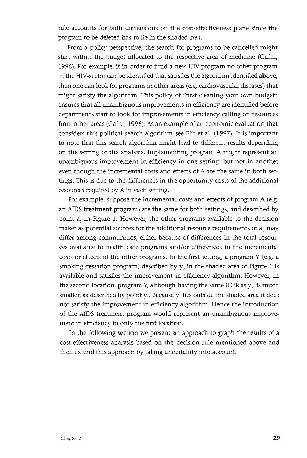
/ I x, I I I I

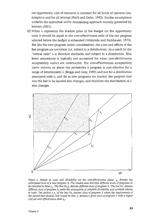
Figure 1. Return to scale and divisibility on the cost-effectiveness plane. a1

denotes the anticipated level of a new program A. The shaded area describes different levels of programs to be cancelled to fund a

1• The line Oxzx1 denotes different sizes of program X. The line Ox1 denotes

different sizes of program X under the assumption of complete divisibility and constant returns to scale. The section x3x~ of the line Ox1 denotes sizes of program X where the requirements of the second-best decision role would be met. y

1 denotes a given level of program Y with a higher

cost per unit effectiveness than a1

•

25 Chapter 2

IV) The use of ic as a decision rule is based on the implicit assumption of con­

stant returns to scale and complete divisibility of ·health care programs

(Birch and Gafni, 1992). The difference in cost and effectiveness between

two health care programs can be displayed on the cost-effectiveness plane

(Figure 1). The ICER is traditionally presented as the slope of a line through

the origin. Complete divisibility assumes that we can buy the program in

infinitely small increments. Constant returns to scale implies that the ICER

is independent of the size of the program. Constant returns to scale of pro­

gram X would be reflected by the line Ox, in Figure 1. However, program X

described by point x, (Figure 1) might not exhibit constant returns to scale

in the real world. For example, different sizes of the same program X might

be described by the line Ox,x, (Figurel). In this case, the slope of a line

through the origin would not be the same for every point on Ox,x, which

reflects the behavior of program X in terms of returns to scale. In this case

the ICER depends on the particular size of the program being considered.

In addition, a program could be indivisible (in part or completely) and

require high capital costs so that the curve may not start at the origin of

the cost-effectiveness plane. High capital costs are often needed for health

care programs that necessitate expensive technologies such as CT or MRI

(Karlsson and Johannessen, 1998). A program might also be indivisible

because of equity consideration (Ubel eta!., 1996). Policy makers may not

want to implement a program without the ability of providing it to all

patients even though the effectiveness and/or costs, and hence the ICER,

are systematically different among identifiable groups in the population.

Integer programming can be used to accommodate indivisibilities and

non-constant returns to scale (Birch and Gafni, 1992,1993). Stinnett and

Pal tiel (1996) refined the integer programming framework to process more

complex information regarding returns to scale and divisibility. However,

both approaches involve data requirements that cannot yet be satisfied in

most health care systems.

An alternative decision rule For the case of a deterministic world, a less data-hungry but feasible alternati­

ve approach with the objective of identifying unambiguous improvements in

resource allocation has been presented (Birch and Gafni, 1992). The approach

is a second-best solution in that it can be used to identify improvements in,

but not optimization of, resource allocations. A program (or a set of programs)

B is identified that, if cancelled, would free up enough resources to fund the

additional costs of the new program A. If the increased outcomes associated

with the new program A are greater than the outcomes forgone from canceling

B, then the adoption of the new program represents a more effident allocation

of resources (Birch and Gafni, 1992). Note that the program cancelled may

26 Chapter 2

not be the highest valued alternative and hence the rule does not necessarily

comply with the definition of opportunity cost. For simplicity, here we limit

our algorithm to identifying one program instead of a set of programs that

must be cancelled to free up the additional resources required by A. Also, we

assume that resources freed up from cancellation of program B represent the

additional costs of A and that no infrastructural costs of B are used by A. So for

program A to be implemented we need to find a program B such that

t.C(B) " t.C(A) (1)

and

t.E(B) < t.E(A) (2)

where t.C(A) is the incremental cost of (or the additional resources required

by) A compared to the cost of how the same patients would be treated if A

was not available, and t.C(B) is the incremental savings (or resources released)

by canceling B (i.e. the cost of B compared to the cost of how these patients

would be treated if B was not available). Similarly, t.E(A) is the incremental ef­

fectiveness of A, and t.E(B) the incremental effectiveness forgone by canceling

B compared to the effectiveness associated with how these patients would be

treated if A and B were not available. The conditions in Equation (1) and (2)

can be extended to include situations where introducing A and canceling B

neither increases nor decreases effects but results in resources being released

for other uses. Therefore, in addition to Equation (1) and (2) we can regard the

following conditions as favorable:

t.C(B) > t.C(A) (3)

and

t.E(B) = t.E(A) (4)

Note that by these four equations the situation where t.C(B) = t.C(A) and t.E(B)

= t.E(A) has been excluded. In such a situation we would be indifferent bet­

ween implementing program A or retaining program B. Also, note that these

four equations are different from the current use of a decision rule that the in­

cremental net benefit must be positive. The decision rule, as currently defined

and used, is based on the assumptions that all programs exhibit constant re­

turns to scale, are completely divisible, and that the marginal opportunity cost

is constant for all levels of resource consumption. Moreover, this decision rule

forces the decision maker to choose a specific value of A. which is very difficult

to determine in real life. These assumptions are not required for the decision

rule presented in this paper.

Chapter 2 27

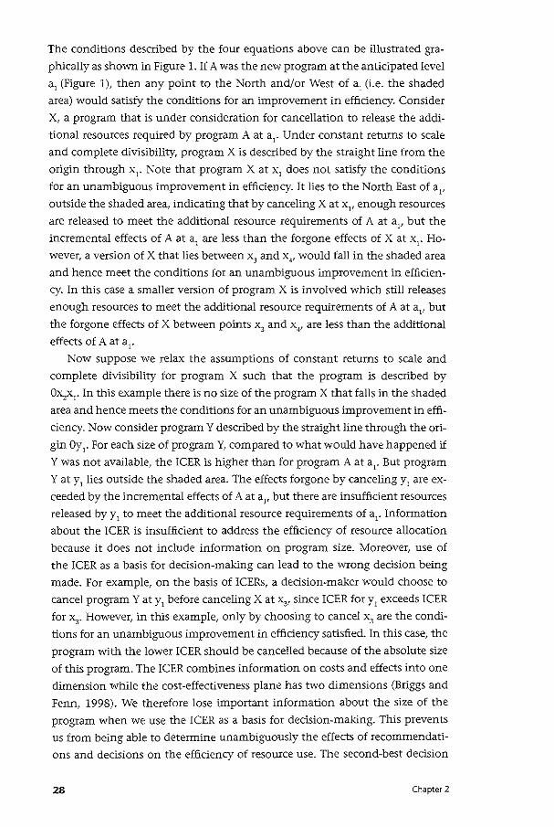
The conditions described by the four equations above can be illustrated gra­

phically as shown in Figure 1. If A was the new program at the anticipated level

a1 (Figure 1), then any point to the North and/or West of a1 (i.e. the shaded

area) would satisfy the conditions for an improvement in efficiency. Consider

X, a program that is under consideration for cancellation to release the addi­

tional resources required by program A at a1

• Under constant returns to scale

and complete divisibility, program X is described by the straight line from the

origin through x1

• Note that program X at x1 does not satisfy the conditions

for an unambiguous improvement in efficiency. It lies to the North East of a11

outside the shaded area, indicating that by canceling X at x1

, enough resources

are released to meet the additional resource requirements of A at al' but the

incremental effects of A at a1 are less than the forgone effects of X at x1

• Ho­

wever, a version of X that lies between x3

and x,., would fall in the shaded area

and hence meet the conditions for an unambiguous improvement in efficien­

cy. In this case a smaller version of program X is involved which still releases

enough resources to meet the additional resource requirements of A at a1, but

the forgone effects of X between points x3 and x . ., are less than the additional

effects of A at a1•

Now suppose we relax the assumptions of constant returns to scale and

complete divisibility for program X such that the program is described by

Ox,x1• In this example there is no size of the program X that falls in the shaded

area and hence meets the conditions for an unambiguous improvement in effi­

ciency. Now consider program Y described by the straight line through the ori­

gin Oy1

• For each size of program Y, compared to what would have happened if

Y was not available, the !CER is higher than for program A at ar But program

Y at y1 lies outside the shaded area. The effects forgone by canceling y1 are ex­

ceeded by the incremental effects of A at al' but there are insufficient resources

released by y 1 to meet the additional resource requirements of a1• Information

about the !CER is insufficient to address the efficiency of resource allocation

because it does not include information on program size. Moreover, use of

the ICER as a basis for decision-making can lead to the wrong decision being

made. For example, on the basis of !CERs, a decision-maker would choose to

cancel program Y at y1 before canceling X at x, since !CER for y1 exceeds !CER

for x3

• However, in this example, only by choosing to cancel x3 are the condi­

tions for an unambiguous improvement in efficiency satisfied. In this case, the

program with the lower ICER should be cancelled because of the absolute size

of this program. The lCER combines information on costs and effects into one

dimension while the cost-effectiveness plane has two dimensions (Briggs and

Fenn, 1998). We therefore lose important information about the size of the

program when we use the ICER as a basis for dedsion-making. This prevents

us from being able to determine unambiguously the effects of recommendati­

ons and decisions on the efficiency of resource use. The second-best decision

28 Chapter 2

rule accounts for both dimensions on the cost-effectiveness plane since the

program to be deleted has to lie in the shaded area.

From a policy perspective, the search for programs to be cancelled might start within the budget allocated to the respective area of medicine (Gafni,

1996). For example, if in order to fund a new HIV-program no other program

in the H!V-sector can be identified that satisfies the algorithm identified above,

then one can look for programs in other areas (e.g. cardiovascular diseases) that

might satisfy the algorithm. This policy of "first cleaning your own budget"

ensures that all unambiguous improvements in efficiency are identified before

departments start to look for improvements in effidency calling on resources

from other areas (Gafni, 1996). As an example of an economic evaluation that

considers this political search algorithm see Elit et a!. (1997). It is important

to note that this search algorithm might lead to different results depending

on the setting of the analysis. Implementing program A might represent an

unambiguous improvement in efficiency in one setting, but not in another

even though the incremental costs and effects of A are the same in both set­

tings. This is due to the differences in the opportunity costs of the additional

resources required by A in each setting.

For example, suppose the incremental costs and effects of program A (e.g.

an AIDS treatment program) are the same for both settings, and described by

point a1

in Figure 1. However, the other programs available to the dedsion

maker as potential sources for the additional resource requirements of a1 may

differ among communities, either because of differences in the total resour­

ces available to health care programs and/or differences in the incremental

costs or effects of the other programs. In the first setting, a program Y (e.g. a

smoking cessation program) described by y2 in the shaded area of Figure 1 is

available and satisfies the improvement in efficiency algorithm. However, in

the second location, program Y, although having the same ICER as y2, is much

smaller, as described by point y1• Because y1 lies outside the shaded area it does

not satisfy the improvement in efficiency algorithm. Hence the introduction

of the AIDS treatment program would represent an unambiguous improve­

ment in efficiency in only the first location.

In the following section we present an approach to graph the results of a

cost-effectiveness analysis based on the decision rule mentioned above and

then extend this approach by taking uncertainty into account.

Chapter 2 29

The "decision making plane" The cost-effectiveness plane presents information on the joint distribution

of incremental cost and incremental effectiveness (Briggs and Gray, 1999). It

does not, however, inform us about the opportunity cost of programs under

consideration. To overcome this limitation we suggest a different graphical

presentation that we call the "decision making plane". This framework incor­

porates information on both the incremental costs and incremental effects of

the new program (i.e., A) and the program to be cancelled (i.e., B). To clarify

this issue, we can rewrite Equation (1) and (2) for an unambiguous improve­

ment in efficiency as

L'.C(A) - I'>C(B) $ 0 (la)

and

I'>E(A) - I'>E(B) > 0 (Za)

and Equation (3) and ( 4) as:

I'>C(A) - I'>C(B) < 0 (3a)

and

<'>E(A) - I'>E(B) = 0 (4a)

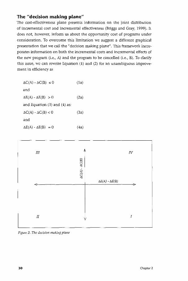
III IV

M(A} -M(B)

II I

Figure 2. The decision making plane

30 Chapter 2

•

• •

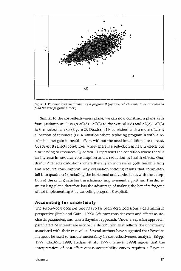
A

Figure 3. Posterior joint distribution of a program B (squares) which needs to be cancelled to fund the new program A (dots)

Similar to the cost-effectiveness plane, we can now construct a plane with four quadrants and assign i;C(A) - i;C(B) to the vertical axis and i;E(A) - i;E(B)

to the horizontal axis (Figure 2). Quadrant I is consistent with a more efficient

allocation of resources (i.e. a situation where replacing program B with A re­

sults in a net gain in health effects without the need for additional resources).

Quadrant II reflects conditions where there is a reduction in health effects but

a net saving of resources. Quadrant III represents the condition where there is

an increase in resource consumption and a reduction in health effects. Qua­

drant IV reflects conditions where there is an increase in both health effects

and resource consumption. Any evaluation yielding results that completely

fall into quadrant I (including the horizontal and vertical axes with the excep­

tion of the origin) satisfies the efficiency improvement algorithm. The decisi­

on making plane therefore has the advantage of making the benefits forgone

of not implementing A by canceling program B explicit.

Accounting for uncertainty The second-best decision rule has so far been described from a deterministic

perspective (Birch and Gafni, 1992). We now consider costs and effects as sto­

chastic parameters and take a Bayesian approach. Under a Bayesian approach,

parameters of interest are ascribed a distribution that reflects the uncertainty

associated with their true value. Several authors have suggested that Bayesian

methods be used to handle uncertainty in cost-effectiveness analysis (Briggs,

1999; Claxton, 1999; Heitjan et al., 1999). Grieve (1998) argues that the

interpretation of cost-effectiveness acceptability curves requires a Bayesian

Chapter 2 31

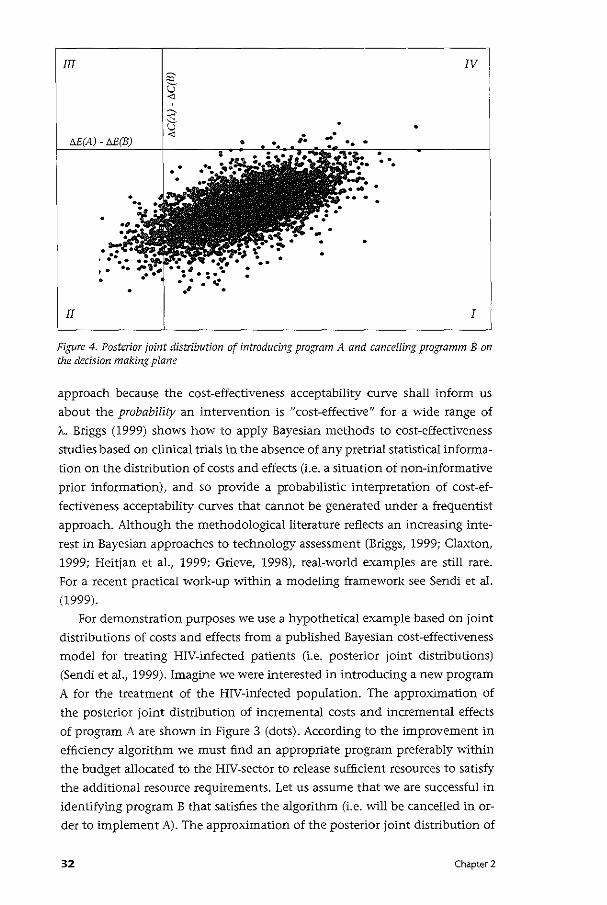
III IV

• •

. ·.

II I

Figure 4. Posterior joint distribution of introducing program A and cancelling programm B on the decision making plane

approach because the cost-effectiveness acceptability curve shall inform us

about the probability an intervention is "cost-effective" for a wide range of

A.. Briggs (1999) shows how to apply Bayesian methods to cost-effectiveness

studies based on clinical trials in the absence of any pretrial statistical informa­

tion on the distribution of costs and effects (i.e. a situation of non-informative

prior information), and so provide a probabilistic interpretation of cost-ef­

fectiveness acceptability curves that cannot be generated under a frequentist

approach. Although the methodological literature reflects an increasing inte­

rest in Bayesian approaches to technology assessment (Briggs, 1999; Claxton,

1999; Heitjan et a!., 1999; Grieve, 1998), real-world examples are still rare.

For a recent practical work-up within a modeling framework see Sendi et al.

(1999).

For demonstration purposes we use a hypothetical example based on joint

distributions of costs and effects from a published Bayesian cost-effectiveness

model for treating HIV-infected patients (i.e. posterior joint distributions)

(Sendi et a!., 1999). Imagine we were interested in introducing a new program

A for the treatment of the HIV-infected population. The approximation of

the posterior joint distribution of incremental costs and incremental effects

of program A are shown in Figure 3 (dots). According to the improvement in

efficiency algorithm we must find an appropriate program preferably within

the budget allocated to the HIV-sector to release sufficient resources to satisfy

the additional resource requirements. Let us assume that we are successful in

identifying program B that satisfies the algorithm (i.e. will be cancelled in or­

der to implement A). The approximation of the posterior joint distribution of

32 Chapter 2

incremental costs and effects of canceling B is also shown in Figure 3 (squares).

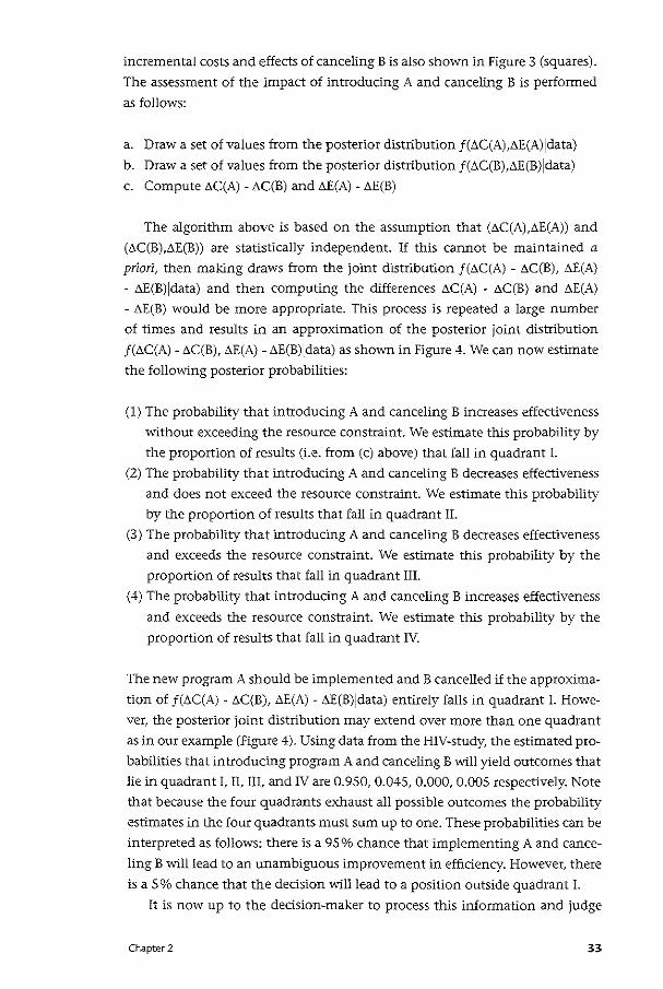
The assessment of the impact of introducing A and canceling B is performed

as follows:

a. Draw a set of values from the posterior distribution f(t-C(A),t-E(Alldata)

b. Draw a set of values from the posterior distribution f(t-C(B),t-E(Blldata)

c. Compute t-C(A) - t-C(B) and t-E(A) - t-E(B)

The algorithm above is based on the assumption that (t-C(A),t-E(A)) and

(I'>C(B),I'>E(B)) are statistically independent. If this cannot be maintained a

priori, then making draws from the joint distribution f(t-C(A) - t-C(B), t-E(A)

- t-E(B)Idata) and then computing the differences t-C(A) - t-C(B) and t-E(A)

- t-E(B) would be more appropriate. This process is repeated a large number

of times and results in an approximation of the posterior joint distribution

f(t-C(A)- t-C(B), t-E(A)- t-E(B)Idata) as shown in Figure 4. We can now estimate

the following posterior probabilities:

(1) The probability that introducing A and canceling B increases effectiveness

without exceeding the resource constraint. We estimate this probability by

the proportion of results (i.e. from (c) above) that fall in quadrant I.

(2) The probability that introducing A and canceling B decreases effectiveness

and does not exceed the resource constraint. We estimate this probability

by the proportion of results that fall in quadrant II.

(3) The probability that introducing A and canceling B decreases effectiveness

and exceeds the resource constraint. We estimate this probability by the

proportion of results that fall in quadrant Ill.

(4) The probability that introducing A and canceling B increases effectiveness

and exceeds the resource constraint. We estimate this probability by the

proportion of results that fall in quadrant IV.

The new program A should be implemented and B cancelled if the approxima­

tion of f(t-C(A) - t-C(B), t-E(A) - t-E(Blldata) entirely falls in quadrant I. Howe­

ver, the posterior joint distribution may extend over more than one quadrant

as in our example (Figure 4). Using data from the HIV-study, the estimated pro­

babilities that introducing program A and canceling B will yield outcomes that

lie in quadrant I, II, Ill, and IV are 0.950, 0.045, 0.000, 0.005 respectively. Note

that because the four quadrants exhaust all possible outcomes the probability

estimates in the four quadrants must sum up to one. These probabilities can be

interpreted as follows: there is a 95o/o chance that implementing A and cance­

ling B will lead to an unambiguous improvement in efficiency. However, there

is a 5 o/o chance that the decision will lead to a position outside quadrant I.

It is now up to the decision-maker to process this information and judge

Chapter 2 33

whether he will accept the risk of other possible outcomes. The decision-maker

may well exhibit different preferences for inefficiencies occurring in quadrant

Il, III or IV. Note that the decision making plane informs us of both the size

and nature of different risks. For example, there is a 4.5 o/o cent chance that the

total health effects are reduced but resources remain unused at the end of the

year (quadrant II). In contrast, there is a 0.5% cent chance that insufficient re­

sources are released to support the new program. In this case the program will

run out of resources during the year and hence be unable to produce the full

anticipated effects unless additional resources can be found from elsewhere.

However, consideration would need to be given to the opportunity costs of

these additional resources.

Discussion This paper addresses the difficulties associated with using a particular value of

A as a decision rule. Alternative approaches such as integer programming or

mixed integer programming techniques have been suggested in the literature

(Birch and Gafni, 1992; Stinnett and Paltiel, 1996). The practical application

of optimization techniques in health services research have recently been de­

monstrated by Granata and Hillman (1998). The authors used data on costs

and effects from published economic evaluations and simulated the reallocati­

on of resources under different budgets to maximize population effectiveness.

However, the authors used linear programming techniques and accepted the

assumptions underlying the current practice of cost-effectiveness analysis. Mo­

reover, uncertainty was not incorporated in their study.

We outline the advantage of using the decision rule as described by Birch

and Gafni (1992) and introduce a new graphical framework for explaining the

idea behind a more efficient allocation of resources in this way. We do not

assume that there are unused resources available or that there is a stream of

additional resources available at a constant opportunity cost. Instead we take

the position that the budget is used up by existing programs. A new program,

therefore, cannot be implemented unless resources are freed up by eliminating

existing programs. The action of canceling existing programs in order to fund

new programs would only be justifiable from an economics perspective where

it leads to a more efficient allocation of resources. This forces us to think about

the opportunity costs of the new program. We would not want to introduce

the new program if we were unable to find at least one existing program that

would do less good than the new program using the same or less resources.

The decision-making plane helps us visualize the effects forgone of not

implementing a new program in this way. Any point in quadrant I including

the lines (with the exception of the origin) is consistent with a more efficient

allocation of resources.

Under conditions of uncertainty, however, the joint distribution may

34 Chapter 2

extend over more than one quadrant. In this case the advantage of a Bayesian

approach to incorporating uncertainty becomes apparent. We are interested in

the probability that our decision of deleting an existing program to fund a new

program will fail to provide an unambiguous improvement in efficiency reflec­

ted in quadrants li-N. A Bayesian framework therefore coincides with this way

of thinking (Briggs, 1999; Claxton, 1999; Heitjan et al., 1999; Spiegelhalter et

al., 1999).

A clinical trial yields data for a particular intervention of interest (i.e.,

program A). For possible candidate programs for cancellation (i.e., B) there

may or may not be data available from other clinical trials. In addition, trial

data may differ between settings of the clinical trial. Modeling might therefore

be unavoidable since different "local distributions" are usually not produced

within clinical trials (Buxton et al., 1997). We also feel that it is impottant that

investigators share their data from clinical trials in order to enable comparison

of programs.

For the sake of simplicity, we have limited our algorithm to identifying

a single program to be eliminated. However, this could be extended, for ex­

ample, to include a set of programs to be cancelled to fund the new program.

Under uncertainty a simulation approach would result in an approximation

of a posterior joint distribution for f(t>C(A) - (t>C(B,) + ... + t>C(B,)), t>E(A)

- (t>E(B1)+ ... +t>E(B,))Idata) where the programs to be cancelled are i=1+ ... +n.

While this adds little to the computational burden of the exercise, it might

increase the burden associated with identifying those programs. Moreover,

our approach might be difficult in cases where information on outcomes is

not readily available for those programs that are potential candidates for can­

cellation.

If the posterior joint distribution extends over more than one quadrant,

then we must ask whether we are willing to accept the risk of "bad" outcomes.

Since it seems reasonable to assume that we will not always find posterior joint

distributions that are limited to quadrant I, we must find ways to handle such

situations. One possibility would be to limit this risk to an arbitrary level, say

0.05, similar to the arbitrary decision of accepting a 5% Type I error in hypo­

thesis testing. Decision-makers, however, may be risk-averse or risk-seeking

and may have varying preferences for outcomes in the different quadrants on

the decision making plane. Whether and how such preferences can be assessed

should be subject to further research.

Chapter 2 35

( ;((:\ *"' G ;) ~ ' ' ' i " ~ , " 1 , 1i & '

' ' ' ., El:ia ite~:~: 3! Optimizing a portfolio of health care programs in the presence of uncer­tainty and constrained resources

Summary Much research has been devoted to handling uncertainty in cost-effectiveness

analysis. The current literature suggests summarizing uncertainty in cost-ef­

fectiveness analysis using acceptability curves or net health benefits. These ap­

proaches, however, focus only on uncertainty associated with costs and effects

of the programs under consideration. In the real world, most decision-makers

have to fund a portfolio of health care programs. Therefore, a more compre­

hensive approach would include in the analysis the uncertainty of costs and

effects of all programs supported by the fixed budget. This paper extends the

decision rule described by Birch and Gafni (Journal of Health Economics,

1992) within the context of a portfolio of programs when costs and effects are

uncertain and resources constrained.

36 Chapter 3

Introduction Cost-effectiveness acceptability curves (van Hout eta!., 1994) and net health

benefits (Stinnett and Mullahy, 1998) or net monetary benefits (Tambour et

al., 1998) have been introduced as ways of incorporating uncertainty associa­

ted with costs and effects in cost-effectiveness analysis. In both approaches a

threshold cost-effectiveness ratio is applied. A program with a cost-effectiveness

ratio above the threshold ratio is not accepted while a program with a cost-ef­

fectiveness ratio below the threshold ratio is accepted. It has been argued that

the use of a fixed ratio as a decision rule can lead to an uncontrolled growth

of expenditures as more programs with an acceptable cost-effectiveness ratio

become available and are funded (Gafni and Birch, 1993). Furthermore, even

if the threshold cost-effectiveness ratio is allowed to vary according to the bud­

get, its use is based on the assumptions of constant returns to scale (constant

cost-effectiveness ratio for different sizes of the program), complete divisibility

of programs (program can be bought in [infinitely] small increments), and

constant marginal opportunity costs (Birch and Gafni, 1992, 1993; Weinstein,

1995).

An alternative decision rule (which relaxes the assumptions mentioned

above) with the goal of increasing health outcomes without calling for ad­

ditional resources has been suggested by Birch and Gafni (1992). In order to

implement a new program, an already existing program must be identified and

cancelled that releases enough resources to fund the new program. Further­

more, the health gains forgone by deleting a program should be smaller than

those gained by introducing the new program. This decision rule results in an

unambiguous improvement of the allocation of resources (Birch and Gafni,

1992). The decision rule is a second-best solution in the sense that more than

one program might satisfy the conditions described above. On the other hand,

the advantage of this decision rule is that it is not as data-hungry as mathe­

matical programming techniques used for the optimization of resource alloca­

tion (Birch and Gafni, 1992; Stinnett and Paltiel, 1996). It is therefore suitable

for situations where data on costs and effects are scarce, which is currently the

case in most health care systems.

The decision rule has first been described for the case of a deterministic

world (Birch and Gafni, 1992). In a separate paper we have illustrated the

application of the decision rule when costs and effects of health care pro­

grams are uncertain (Sendi et al., 2002). However, the approach assumes that

information on costs and effects of the specific programs under consideration

are sufficient to guide policy makers. In the real world, most decision-makers

have to fund a portfolio of health care programs. The decision-maker should

therefore include, in her evaluation, the uncertainty associated with costs and

effects of all health care programs supported by the fixed budget. In this paper

we extend the decision rule described by Birch and Gafni (1992) within the

Chapter 3 37

context of a portfolio of programs when costs and effects are uncertain and

resources constrained. In the next section we review the decision rule under

certainty and uncertainty. In "Stochastic dominance and affordability" we

analyze the decision rule from the perspective of stochastic dominance and

affordability. In "A portfolio of multiple programs" we embed the decision rule

within a portfolio of multiple programs. In the last section we conclude with

a discussion of our approach.

The decision rule under certainty and uncertainty The decision rule starts with the premise that scarce resources are already used

up by programs which are implemented (Birch and Gafni, 1992,1993; Gafni

and Birch, 1993). Therefore, in order to introduce a new program, resources

must be deployed from existing programs. That is, some additional resources

need to be found in order to support the resource requirements of new pro­

gram A over the resources used by current program a. These resources can

be found by replacing existing program B with program b that requires less

resources. More formally, the decision rule can be expressed as follows. Let B

be an existing program to be deleted and A the new program to be implemen­

ted. By deleting program B, the patients who used to receive treatment B now

receive treatment b. Similarly, by introducing program A, the patients who

used to receive treatment a now receive treatment A. Program A and program

a are mutually exclusive. Similarly, program B and program b are mutually

exclusive. We denote with lowercase letters programs, which are both less

expensive and less effective than the alternative program. We write CA > ca, CB > Cb, EA > E;j and EB > Eb where cl is the total cost and Ei the total effect of

program i=A,a,B,b. We denote the incremental costs and effects of program A

compared to program a as llC(A) = CA-C, and ilE(A) = EA-E,. Similarly, we de­

note the incremental costs and effects of program B compared to program b as

ilC(B) = c,-Cb and ilE(B) = E,-Eb. The decision rule is satisfied if the following

conditions are met:

llC(A) - ilC(B) " 0 (1)

and

ilE(A) -ilE(B) > 0 (2)

38 Chapter 3

For example, let's assume that Ll.C(B) is $10'000'000 and Ll.C(A) is $9'000'000.

Further, let us assume that Ll.E(B) is 4'000 life-years and Ll.E(A) is 5'000 life-years.

Canceling program B and shifting the released resources to program A results

in a gain of 1'000 life-years, and a leftover of $1'000'000 for other uses. The

decision rule is also satisfied if the following conditions are met:

Ll.C(A) - Ll.C(B) < 0 (3)

and

Ll.E(A) -Ll.E(B) = 0 (4)

For example, let's assume that Ll.C(B) is $10'000'000 and Ll.C(A) is $9'000'000.

Further, let's assume that Ll.E(B) is 5'000 life-years and Ll.E(A) is 5'000 life-years.

Canceling program B and shifting the released resources to program A results

in a leftover of $1'000'000 for other uses, without compromising overall

health outcomes. Note that we have excluded the situation where

Ll.C(B) = Ll.C(A) (5)

and

Ll.E(B) = Ll.E(A) (6)

In such a situation we would be indifferent between retaining program B and

implementing program A.

The decision rule can be extended to account for uncertainty associated

with costs and effects of health care programs. Under uncertainty, we can write

conditions (1) and (2) in terms of the joint probability

P(Ll.C(A) - Ll.C(B) s 0, Ll.E(A) -Ll.E(B) > 0) (7)

Similarly, conditions (3) and ( 4) can be written as

P(Ll.C(A) - Ll.C(B) < 0, Ll.E(A) -Ll.E(B) = 0) (8)

Chapter 3 39

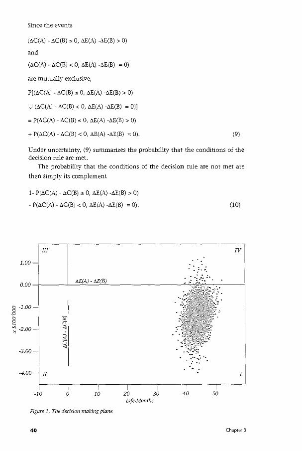
Since the events

(t>C(A) - t>C(B) "'0, LlE(A) -LlE(B) > 0)

and

(LlC(A) - LlC(B) < 0, LlE(A) -LlE(B) ; 0)

are mutually exclusive,

P[(t>C(A) - t>C(B)"' 0, LlE(A) -LlE(B) > 0)

U (t>C(A) - t>C(B) < 0, t>E(A) -t>E(B) ; 0)]

; P(LlC(A)- LlC(B) "'0, t>E(A) -LlE(B) > 0)

+ P(LlC(A) - LlC(B) < 0, t>E(A) -t>E(B) ; 0). (9)

Under uncertainty, (9) summarizes the probability that the conditions of the decision rule are met.

The probability that the conditions of the decision rule are not met are

then simply its complement

1- P(t>C(A)- LlC(B)"' 0, t>E(A) -LlE(B) > 0)

- P(LlC(A) - t>C(B) < 0, t>E(A) -t>E(B) ; 0).

III

1.00

0.00

(10)

IV

. -. . : _.:. :..

5 -1.00

" c c ~

~ -2.00

-3.00-

-4.00 II

-10 0 10

Figure 1. The decision making plane

40

30 Life-Months

40

- --- . I

50

Chapter 3

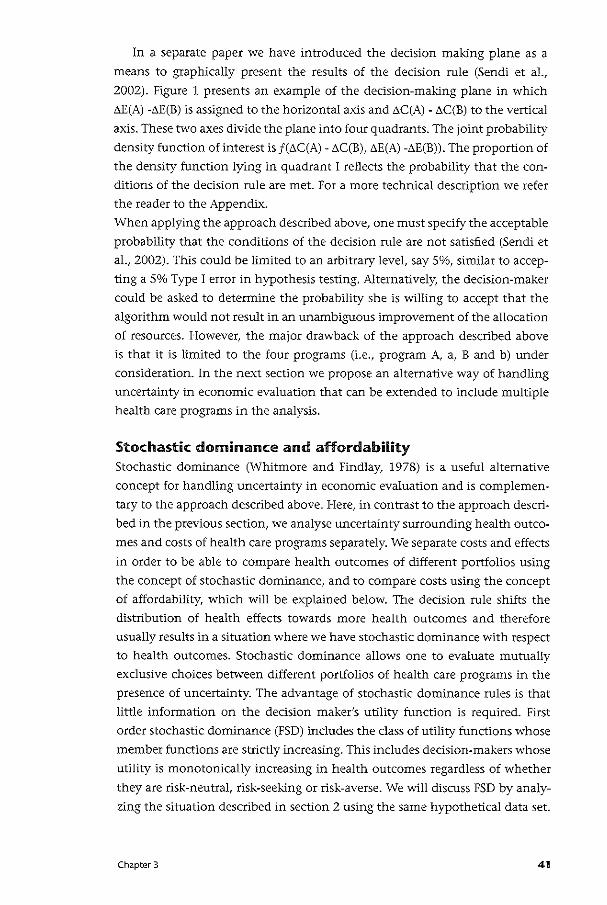
In a separate paper we have introduced the decision making plane as a

means to graphically present the results of the decision rule (Sendi et a!.,

2002). Figure 1 presents an example of the decision-making plane in which

t>E(A) -t>E(B) is assigned to the horizontal axis and t>C(A) - t>C(B) to the vertical

axis. These two axes divide the plane into four quadrants. The joint probability

density function of interest is f(t>C(A)- t>C(B), t>E(A) -t>E(B)). The proportion of

the density function lying in quadrant I reflects the probability that the con­

ditions of the decision rule are met. For a more technical description we refer

the reader to the Appendix.

When applying the approach described above, one must specify the acceptable

probability that the conditions of the decision rule are not satisfied (Sendi et

a!., 2002). This could be limited to an arbitrary level, say 5%, similar to accep­

ting a So/o Type I error in hypothesis testing. Alternatively, the decision-maker

could be asked to determine the probability she is willing to accept that the

algorithm would not result in an unambiguous improvement of the allocation

of resources. However, the major drawback of the approach described above

is that it is limited to the four programs (i.e., program A, a, B and b) under

consideration. In the next section we propose an alternative way of handling

uncertainty in economic evaluation that can be extended to include multiple

health care programs in the analysis.

Stochastic dominance and affordabiiity Stochastic dominance (Whitmore and Findlay, 1978) is a useful alternative

concept for handling uncertainty in economic evaluation and is complemen­tary to the approach described above. Here, in contrast to the approach descri­

bed in the previous section, we analyse uncertainty surrounding health outco­

mes and costs of health care programs separately. We separate costs and effects

in order to be able to compare health outcomes of different portfolios using

the concept of stochastic dominance, and to compare costs using the concept

of affordability, which will be explained below. The decision rule shifts the

distribution of health effects towards more health outcomes and therefore

usually results in a situation where we have stochastic dominance with respect

to health outcomes. Stochastic dominance allows one to evaluate mutually

exclusive choices between different portfolios of health care programs in the

presence of uncertainty. The advantage of stochastic dominance rules is that

little information on the decision maker's utility function is required. First

order stochastic dominance (FSD) includes the class of utility functions whose

member functions are strictly increasing. This includes decision-makers whose

utility is monotonically increasing in health outcomes regardless of whether

they are risk-neutral, risk-seeking or risk-averse. We will discuss FSD by analy­

zing the situation described in section 2 using the same hypothetical data set.

Chapter 3 41

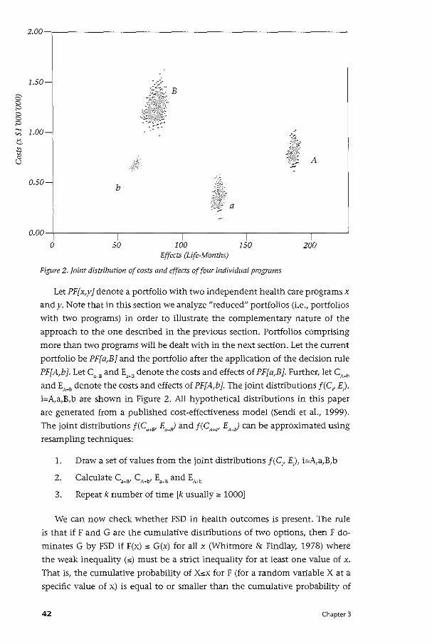
2 a ::0 a a ::0 ~

"' .::s

"' ~ B

2.00-,-------------------------------------------------~

1.50-B

1.oo~

A

0.50-b

a

0.00

0 50 100 150 200 Effects (Life-Months)

Figure 2. Joint distribution of costs and effects of four individual programs

Let PF[x,y] denote a portfolio with two independent health care programs x

andy. Note that in this section we analyze "reduced" portfolios (i.e., portfolios

with two programs) in order to illustrate the complementary nature of the

approach to the one described in the previous section. Portfolios comprising

more than two programs will be dealt with in the next section. Let the current

portfolio be PF[a,B] and the portfolio after the application of the dedsion rule

PF[A,b]. Let C"" and E""' denote the costs and effects of PF[a,B]. Further, let c,_, and EA·b denote the costs and effects of PF[A,b]. The joint distributions f(C, E),

i=A,a,B,b are shown in Figure 2. All hypothetical distributions in this paper

are generated from a published cost-effectiveness model (Sendi et aL, 1999).

The joint distributions f(C""" E,r) and f(CA.v EMJ can be approximated using

resampling techniques:

1. Draw a set of values from the joint distributions f(C,, E), i=A,a,B,b

3. Repeat k number of time [k usually" 1000]

We can now check whether FSD in health outcomes is present. The rule

is that if F and G are the cumulative distributions of two options, then F do­

minates G by FSD if F(x) s G(x) for all x (Whitmore & Findlay, 1978) where

the weak inequality (s) must be a strict inequality for at least one value of x.

That is, the cumulative probability of Xsx for F (for a random variable X at a

specific value of x) is equal to or smaller than the cumulative probability of

42 Chapter 3

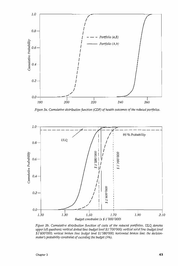
1.0

0.8-

0.2-

/ I I I I I I I I I I I I I I I I

I

Portfolio (a,B)

Portfolio (A,b)

/ 0.0-f-----~"'--T--------,1------;1-===-------1,--~

180 200 220 240 260

Figure 3a. Cumulative distribution function (CDF) of health outcomes of the reduced portfolios.

Budget constraint (x $ 1 '000'000)

Figure 3b. Cumulative distribution function of costs of the reduced portfolios. ULQ denotes upper left quadrant; vertical dotted line: budget level $1 '700'000; vertical solid line: budget level $1'600'000; vertical broken line: budget level $1'580'000; horizontal broken line: the dedsion­maker's probability constraint of exceeding the budget (5%).

Chapter 3 43

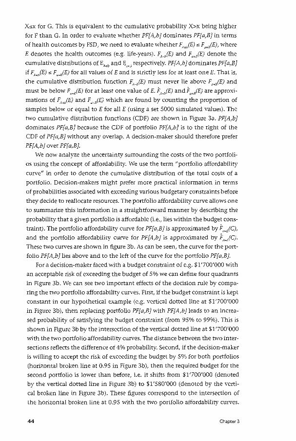
Xsx for G. This is equivalent to the cumulative probability X>x being higher

for F than G. In order to evaluate whether PF[A,h1 dominates PF[a,B1 in terms

of health outcomesbyFSD, we need to evaluate whether F"',(E) sF,.,(E), where

E denotes the health outcomes (e.g. life-years). (,jE) and F,jE) denote the

cumulative distributions of EA~b and E,_, respectively. PF[A,b 1 dominates PF[ a,B 1

if F,jE) s F,~iE) for all values of E and is strictly less for at least one E. That is,

the cumulative distribution function ~1+0(E) must never lie above Fa ... s(E) and

must be below F,jE) for at least one value of E. F,jE) and F,.,(E) are approxi­

mations of FA+/E) and F,I+/E) which are found by counting the proportion of

samples below or equal toE for all E (using a set 5000 simulated values). The

two cumulative distribution functions (CDF) are shown in Figure 3a. PF[A,h1

dominates PF[a,B1 because the CDF of portfolio PF[A,h1 is to the right of the

CDF of PF[a,B1 without any overlap. A decision-maker should therefore prefer

PF[A,h1 over PF[a,B1.

We now analyze the uncertainty surrounding the costs of the two portfoli­

os using the concept of affordability. We use the term "portfolio affordability

curve" in order to denote the cumulative distribution of the total costs of a

portfolio. Decision-makers might prefer more practical information in terms

of probabilities associated with exceeding various budgetary constraints before

they decide to reallocate resources. The portfolio affordability curve allows one

to summarize this information in a straightforward manner by describing the

probability that a given portfolio is affordable (i.e., lies within the budget cons­

traint). The portfolio affordability curve for PF[a,B1 is approximated by F"jC),

and the portfolio affordability curve for PF[A,b 1 is approximated by j:,jC).

These two curves are shown in figure 3b. As can be seen, the curve for the port­

folio PF[A,h1lies above and to the left of the curve for the portfolio PF[a,B1.

For a decision-maker faced with a budget constraint of e.g. $1'700'000 with

an acceptable risk of exceeding the budget of 5% we can define four quadrants

in Figure 3b. We can see two important effects of the decision rule by compa­

ring the two portfolio affordability curves. First, if the budget constraint is kept

constant in our hypothetical example (e.g. vertical dotted line at $1'700'000

in Figure 3b), then replacing portfolio PF[a,B1with PF[A,h1leads to an increa­

sed probability of satisfying the budget constraint (from 95% to 99%). This is

shown in Figure 3b by the intersection of the vertical dotted line at $1'700'000

with the two portfolio affordability curves. The distance between the two inter­

sections reflects the difference of 4% probability. Second, if the decision-maker

is willing to accept the risk of exceeding the budget by 5% for both portfolios

(horizontal broken line at 0.95 in Figure 3b), then the required budget for the

second portfolio is lower than before, i.e. it shifts from $1'700'000 (denoted

by the vertical dotted line in Figure 3b) to $1'580'000 (denoted by the verti­

cal broken line in Figure 3b). These figures correspond to the intersection of

the horizontal broken line at 0.95 with the two portfolio affordability curves.

44 Chapter 3

This means that the decision-maker could invest the difference of $120'000 in

other health care programs since the budget requirements of the new portfolio

are lower than the budget requirements of the old portfolio.

Information about the decision maker's risk-tolerance of exceeding a given

budget (reflected by a horizontal line in Figure 3b at the respective risk level)

in combination with the actual size of the budget (reflected by a vertical line

in Figure 3b at the respective budget level) allows one to guide policy makers.

With these two pieces of information four quadrants can be defined. If the

portfolio affordability curve crosses the upper left quadrant (including the

origin), then the requirements of the decision-maker are satisfied. The upper

left quadrant reflects the situation where the risk of exceeding a given budget

is lower than the decision-maker's acceptable risk. In cases where the portfolio

affordability curve of a particular portfolio does not cross the upper left qua­

drant, the decision rule might help us to achieve this goal. This can be seen

in Figure 3b. The portfolio affordability curve of the portfolio PF[a,B] does

not cross the upper left quadrant if we take $1'600'000 as the budget (vertical

solid line in Figure 3b) and 5% as the acceptable risk of exceeding the budget

(horizontal broken line at 0.95). The decision rule, i.e. sMtching from portfo­

lio PF[a,B] to portfolio PF[A,b], results in a shift of the portfolio affordability

curve to the left so that the portfolio affordability curve now crosses the upper

left quadrant. This indicates that the requirements of the decision maker are

satisfied by the new portfolio PF[A,b ].

It is important to note that the approach described in the second section

(i.e., the decision making plane approach) and the approach described in this

section (i.e, the portfolio affordability approach) are complementary and do

answer different questions as described below. We used the same hypothetical

data set for the calculations in section two and section three. The decision

making plane allowed us to estimate the probability P(CA+b > CH8), which was

2%. Note that c,., > C,., is equivalent to Ll.C(A) > Ll.C(B), i.e. [(C,-C) > (C,-C,)]

= [(CA+C,) > (C"+CJ]. The portfolio affordability curve allows one to estimate

the probabilities P(C""' $ BC I BC) and P(C'"' $ BC I BC), where BC denotes the

budget constraint. That is, although P(C""' $ BC I BC) ~ P(C,, $ BC I BC) for

all BC as shown in Figure 3b, it happens with 2% probability that CM, > C,.,

when applying the decision rule (Figure 1). In other words, the approach using

the decision making plane answers the question of what is the probability that

the decision rule does not lead to a more efficient allocation of resources. The

approach using the portfolio affordability curve, on the other hand, informs

us, for a given budget constraint, what the probability is that this budget is

exceeded.

Chapter 3 45

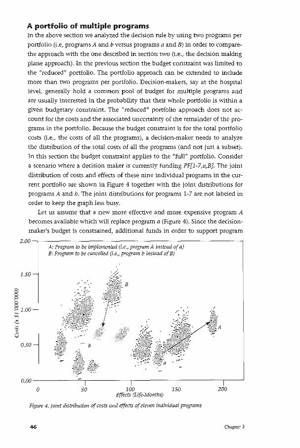
A portfolio of multiple programs In the above section we analyzed the decision rule by using two programs per

portfolio (i.e, programs A and b versus programs a and B) in order to compare­

the approach with the one described in section two (i.e., the decision making

plane approach). In the previous section the budget constraint was limited to

the "reduced" portfolio. The portfolio approach can be extended to include

more than two programs per portfolio. Decision-makers, say at the hospital

level, generally hold a common pool of budget for multiple programs and

are usually interested in the probability that their whole portfolio is within a

given budgetaty constraint. The "reduced" portfolio approach does not ac­

count for the costs and the associated uncertainty of the remainder of the pro­

grams in the portfolio. Because the budget constraint is for the total portfolio

costs (i.e., the costs of all the programs), a decision-maker needs to analyze

the distribution of the total costs of all the programs (and not just a subset).

In this section the budget constraint applies to the "full" portfolio. Consider

a scenario where a decision maker is currently funding PF[l-7,a,B]. The joint

distribution of costs and effects of these nine individual programs in the cur­

rent portfolio are shown in Figure 4 together with the joint distributions for

programs A and b. The joint distributions for programs 1-7 are not labeled in

order to keep the graph less busy.

Let us assume that a new more effective and more expensive program A

becomes available which will replace program a (Figure 4). Since the decision­

maker's budget is constrained, additional funds in order to support program

2.00--------------------------------------------------~ A: Program to be implemented (i.e., program A instead of a) B: Program to be cancelled (i.e., program b instead of B)

B

0.00 -f---------...-:..,_----------,--------....,------,--~

0 50 100 150 200 Effects (Life-Months)

Figure 4. Joint distribution of costs and effects of eleven individual programs

46 Chapter 3

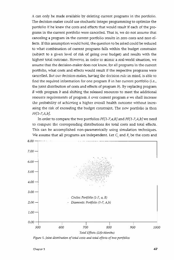
A can only be made available by deleting current programs in the portfolio.

The dedsion-maker could use stochastic integer programming to optimize the

portfolio if he knew the costs and effects that would result if each of the pro­

grams in the current portfolio were cancelled. That is, we do not assume that

canceling a program in the current portfolio results in zero costs and zero ef­

fects. If this assumption would hold, the question to be asked could be reduced

to what combination of current programs falls 'Within the budget constraint

(subject to a given level of risk of going over budget) and results with the

highest total outcome. However, in order to mimic a real-world situation, we

assume that the decision-maker does not know, for all programs in the current

portfolio, what costs and effects would result if the respective programs were

cancelled. But our decision-maker, having the decision rule in mind, is able to

find the required information for one program B in her current portfolio (i.e.,

the joint distribution of costs and effects of program b). By replacing program

B with program b and shifting the released resources to meet the additional

resource requirements of program A over current program a we shall increase

the probability of achieving a higher overall health outcome without incre­

asing the risk of exceeding the budget constraint. The new portfolio is then

PF[l-7,A,b].

In order to compare the two portfolios PF[l-7,a,B] and PF[l-7,A,b] we need

to compute the corresponding distributions for total costs and total effects.

This can be accomplished non-parametrically using simulation techniques.

We assume that all programs are independent. Let C1 and E1

be the costs and

8.00~--------------------------------------------------,

7.00

6.00=·

5.00

4.00

3.00

2.00

Circles: Portfolio (1-7, a, B)

Diamonts: Portfolio (1-7, A,b)

0.00 ---t-----,1 -----,------.,-----...,-------1

500 600 700 800 900 1000

Total Effects (Life-Months)

Figure S.Joint distribution of total costs and total effects of two portfolios

Chapter 3 47

effects of program i=l,Z, ... ,n describing a portfolio with n individual pro­

grams:

l. Draw a sample from the joint distribution f(C1 ,E) for i=l,Z, ... ,n.

• • 2. Calculate cport(olio= 2j~lcl and Eport{OI!o= 'ii=IEI

3. Repeat k number of times [k usually~ 1000] to approximate the joint distri-

bution f(CportfOIIm Eport(olio).

This procedure allows us to include the additional uncertainty associa­

ted with costs and effects in programs l-7. For the first portfolio PF[l-7,a,B],

which is the portfolio before applying the decision rule, we include in the

sampling procedure the joint distributions of costs and effects of programs

l-7 and programs Band a. This approximates the joint distribution of total

costs and effects of the portfolio PF[l-7,a,B} as depicted in Figure 5. For the

second portfolio PF[l-7,A,b}, which is the portfolio after the application of

the decision rule, we include in the sampling procedure programs 1-7 and

programs A and b. The joint distribution of total costs and effects of the

second portfolio PF[l-7,A,b} is also shown in Figure 5. As we can see, by

applying the decision rule, the joint distribution of the portfolio shifrs to the

southeast on a plane where total costs are plotted against total effects. This

means that the probability of achieving more health outcomes is increased

while the risk of exceeding the budget constraint is decreased. That is, the goal

of increasing total effectiveness without the need of increasing the budget is

met.

The impact of the decision rule on total effectiveness is also shown in

Figure 6a. The new portfolio is stochastically dominant over the old port­

folio. Furthermore, the portfolio affordability curve (Figure 6b) for PF[l-7,A,b}

lies to the left of the one for PF[l-7,a,B ], indicating that the required budget

decreased at the same 5% risk-level of exceeding the budget (denoted by the

intersection of the horizontal broken line in figure 6b with the tvvo portfolio

affordability curves). Or alternatively, that the probability of exceeding a given

budget constraint decreased (indicated by the intersection of the vertical bro­

ken line in Figure 6b with the two portfolio affordability curves). Note that the

inclusion of the uncertainty of those programs in the portfolio which are not

subject to the decision rule leads to similar figures as described in the above

section. This is because we expect the decision rule to have the same effect in

terms of changes of overall costs and effects in a "full" portfolio of programs

although the relative magnitude of the effect will be smaller. However, de­

cision-makers (e.g. hospital managers) may know the total costs rather than

the total health outcomes associated with their portfolio. In such a situation

we could assess the impact of the decision rule using the "full" portfolio ap-

48 Chapter 3

~

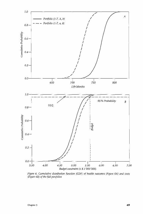
1.0

0.8-

0.2-

Portfolio (1-7, A, b)

Portfolio (1-7, a, B)

/ I

I I I

I I I I I I I I

I I

I /

/ / A

/ O.O-L----------,------=~---_,----~~--,1-----------,----__J

650 700

Life-Months

750 800

1.0-,---------------------------~~r-----------------,

0.8

:. --------_7----- /~--95%Probability __ _ • / / , B

ULQ 1 I

I I

"% 0.6- I I ~ I

I I

I I

I 0.2-

I I

o.o+l -----,-"""'~---,1 /_/_/_,1 ___ ,1 _;___-.,1 ___ ,1 -----11 3.50 4.00 4.50 5.00 5.50 6.00 6.50 7.00

Budget constraint (x S 1 ~aao~OOO)

Figure 6. Cumulative distribution function (CDF) of health outcomes (Figure 6A) and costs (Figure 6B) of the full portfolios

Chapter 3 49

proach for costs (since the constraint is on total costs) and the "reduced" port­

folio approach for health outcomes, assuming that programs are independent.

However, any interdependence betvveen programs would require modification

of the equations for the assessment of both outcomes and costs.

Note that the "full" portfolio approach is needed in order to assess whether

a reallocation of resources meets the decision-maker's probability threshold

for exceeding the total budget. This information is not provided by the "re­

duced" portfolio approach, which ignores the impact of the decision rule on

total expenses. A switch of programs, which might be deemed worthwhile

from the "reduced" portfolio perspective, does not necessarily need to meet

the decision-maker's constraints when total costs are considered. That is, only

the portfolio affordability curve for the "full" portfolio informs us whether

the requirements of the decision-maker in terms of containing total costs are

satisfied.

Finally, in addition to analyzing the distributions of overall health

outcomes and total costs, we could impose the additional constraint that

P(E,.b < E,.,) = 0. This would correspond to the probability of any outcome fal­

ling in quadrant II and quadrant III of the decision making plane being zero

(which was the case in our hypothetical example, see Figure 1). This additional

constraint prevents that replacing program a and program B by program A and

program b, respectively, would result in a reduction of health outcomes.

Discussion In the real world, decision makers usually have to operate a portfolio of health

care programs, are limited by budgetary constraints and face uncertainty

associated with costs and effects of all health care programs. Moreover, the

availability of information on all programs in a health care system is imperfect

so that lack of data is a common problem. We have suggested a framework for

handling such a situation by embedding the decision rule described by Birch

and Gafni (1992) within a portfolio of multiple programs in the context of

maximizing health outcomes from available health care resources.

The decision-maker's budget and probability constraints are central in our

paper. In order to determine whether the requirements of the decision-maker

are met, we need information about the available budget and the decision­

maker's risk-tolerance. There are different options to determine this risk-level.

First, one could use an arbitrary threshold such as a 5%-risk level of exceeding

the budget. Second, one could elicit the risk-level by asking the decision-ma­

ker. Different decision-makers might accept different risk-levels of exceeding

the budget. Finally, the risk level could be derived from the current portfolio.

The current portfolio has a risk of going over budget associated with it. By

choosing that portfolio the decision-maker has implicitly consented to accept

that level of risk. In addition to the probability of going over budget, the de-

50 Chapter 3

cision-maker might also be interested in the magnitude of deviation from the

budget at the respective risk-level. Although not discussed in this paper, this

information might influence the decision-maker's risk-tolerance in the sense

that a low risk of a high deviation might be less acceptable that a high risk of

a low deviation.

The upper left quadrant (on a plane where we plot the portfolio affordability

curve) defined by the budget and the acceptable risk of exceeding the budget can

be used to build up/modify portfolios of health care programs. The decision-maker

can successively add programs to the portfolio as long as the portfolio affordability

curve crosses the upper left quadrant. Once the portfolio affordability curve of the

portfolio does not cross the upper left quadrant, the investment is not within the

prescribed boundaries anymore. Health outcomes can then only be increased by

reallocating resources. The use of the algorithm delineates the fact that the decisi­

on-maker has reached a point where she cannot add programs to her portfolio any­

more without downsizing/deleting other programs. If different sizes of programs

were to be considered in the analysis, then the respective distributions of costs and

effects would be needed (which might not be readily available in practice). Howe­

ver, by changing the composition of the portfolio according to the decision rule

she can make more efficient use of the available resources.

In conclusion, where information is available on the distribution of costs and

effects of those programs under consideration, the approach presented in this pa­

per offers a feasible method of making more efficient use of available resources. In

particular, the decision rule can be used to inform policy makers faced with uncer­

tainty associated with costs and effects and constrained resources. The information

needed to optimize the portfolio until it meets the requirements of the decision

maker is the size of the budget and the acceptable risk of going over budget. Alt­

hough the information requirements may not be currently satisfied, the research

required to generate such information may be a small price to pay to achieve a

more efficient use of health care resources.

Chapter 3 51

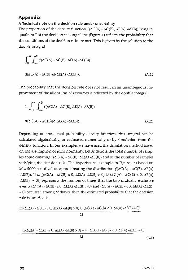
Appendix A Technical note on the decision rule under uncertainty

The proportion of the density function f(l>C(A) - l>C(B), l>E(A) -l>E(B)) lying in

quadrant I of the decision making plane (Figure 1) reflects the probability that

the conditions of the decision rule are met. This is given by the solution to the

double integral

i~ J0 f(l>C(A) - l>C(B), l>E(A) -l>E(B))

0 -oo

d(l>C(A)- l>C(B))d(l>E(A) -l>E(B)). (A.l)

The probability that the decision rule does not result in an unambiguous im­

provement of the allocation of resources is reflected by the double integral

1- .C f 0 f(l>C(A)- l>C(B), l>E(A) -l>E(B))

0 -~

d(l>C(A) - l>C(B))d(l>E(A) -l>E(B)). (A.2)

Depending on the actual probability density function, this integral can be

calculated algebraically, or estimated numerically or by simulation from the

density function. In our examples we have used the simulation method based

on the assumption of joint normality. Let M denote the total number of samp­

les approximating f(l>C(A)- l>C(B), l>E(A) -l>E(B)) and m the number of samples

satisfying the dedsion rule. The hypothetical example in Figure 1 is based on

M = 5000 set of values approximating the distribution f(l>C(A) - l>C(B), l>E(A)

-l>E(B)). If m[(l>C(A) - l>C(B) ~ 0, l>E(A) -l>E(B) > 0) U (l>C(A) - l>C(B) < 0, l>E(A)

-l>E(B) = 0)] represents the number of times that the two mutually exclusive

events (l>C(A)- t;C(B) ~ 0, l>E(A) -l>E(B) > 0) and (l>C(A)- l>C(B) < 0, l>E(A) -l>E(B)

= 0) occurred among M draws, then the estimated probability that the decision

rule is satisfied is

m[(I>C(A) -i>C(B) s 0, I>E(A) -I>E(B) > 0) U (I>C(A)- l>C(B) < 0, l>E(A) -I>E(B) = 0)]

M

m(l>C(A) - i>C(B) ~ 0, I>E(A) -I>E(B) > 0) + m (i>C(A) -I>C(B) < 0, I>E(A) -l>E(B) = 0)

M (A.3)

52 Chapter 3

and the estimated probability that the decision rule is not satisfied is

m[(t.C(A)- t.C(B) < 0, t.E(A) -LIE(B) > 0) + m (LIC(A)- LIC(B) < 0, LIE(A) -LIE(B) = 0) 1- ___:_:___:____:____:__:_____:____:_ _ ___:____:_ _ ___:____:_ _ ___:____:____:____:____:__ M (A.4)

In the example in Figure 1, the estimated probability that the decision rule is

satisfied is 0.98, and the estimated probability that it is not satisfied is 0.02 =

(1-0.98). Note that the samples are limited to quadrant I and IV which simpli­

fies the estimation of the probability that the decision rule is satisfied to

m (LIC(A) - LIC(B) < 0)

M

Chapter 3

(A.S)

53

• Cha ter4 Revisiting the decision rule of cost-effectiveness analysis under certainty and uncertainty

Summary The classical decision rule of cost-effectiveness analysis uses a threshold cost­

effectiveness ratio as a cut-off point for resources allocation. One assumption

of this decision rule is complete divisibility of health care programs. In this

article we argue that health care programs cannot be completely divisible since

individuals are not divisible. Consequently, instead of a linear programming

approach, an integer programming approach to budget allocation is suggested.

The integer programming framework can be extended to include uncertainty

in the analysis. An objective function (expected aggregate effects) is maximi­

zed subject to the constraint that the probability of exceeding the budget is

limited to an arbitrary level (e.g., 0.05). In case the budget is exceeded, the

objective function is penalized in order to account for the opportunity costs of

the additional resource requirements.

54 Chapter 4

Introduction Cost-effectiveness analysis is increasingly being used to inform policy and

decision makers in the health care field. It is usually assumed that the goal of

cost-effectiveness analysis is to maximize health outcomes for a given budget.

Under the assumption of complete divisibility of programs, the decision rule

algorithm follows from a linear programming problem (Weinstein and Zeck­

hauser, 1973; Stinnett and Paltiel, 1996). According to this decision rule, an

optimal allocation of resources is achieved by ordering programs according

to their cost-effectiveness ratio and successively implementing them, starting

with the most cost-effective program, until the budget is exhausted Gohannes­

son and Weinstein, 1993; Weinstein, 1995; Karlsson and]ohannesson, 1996).

The cost-effectiveness ratio of the last implemented pro grain, then, represents

the critical ratio used as a cut-off point for resources allocation. This decision

rule of cost-effectiveness analysis has been hashed and rehashed by different

authors (Weinstein, 1995; Karlsson and]ohannesson, 1996; Johannessen and

Weinstein, 1993; Birch and Gafni, 1992,1993; Gafni and Birch, 1993).

Arguably, the assumption of perfect divisibility is not realistic in practice.

It can be unethical to introduce a new treatment for only a fraction of the eli­

gible patients, while the remaining patients receive an 'old' treatment which

is less effective. However, ethics aside, complete divisibility is an assumption

that will never be met in practice since individuals are not divisible. The de­

cision rule may therefore lead to suboptimal budget allocation decisions as

we 'Will show in this paper. Consequently, an integer programming approach

where individuals represent indivisible units is more appropriate to formulate

the budget allocation problem. We extend the integer programming approach

to include uncertainty in the analysis. Hereby the objective function is maxi­

mized subject to the constraint that the probability of exceeding the budget is

limited to an arbitrary level. We then introduce the idea of penalizing the ob­

jective function in situations where the budget is exceeded in order to account

for the opportunity costs of the additional resource requirements.

Note that in this paper we shall not question the assumption of constant

returns to scale, which is also needed for the decision rule to be valid. Whether

the assumption of constant returns to scale is met in a specific situation is an

empirical question. For example, the assumption of constant returns to scale

will not be met when programs have high capital costs (e.g. radiation therapy

in oncology), but it may be met when patients undergo treatments that are

solely based on prescription drugs (e.g. antibiotic treatment of infectious di­

seases). Thus, if the whole health care budget is not subject to the allocation

process, but for example only the budget for pharmaceuticals, then the as­

sumption of constant returns to scale maybe appropriate. This situation might

for instance occur in The Netherlands, where the health care budget is divided

into separate compartments with one specifically for pharmaceuticals.

Chapter 4 55

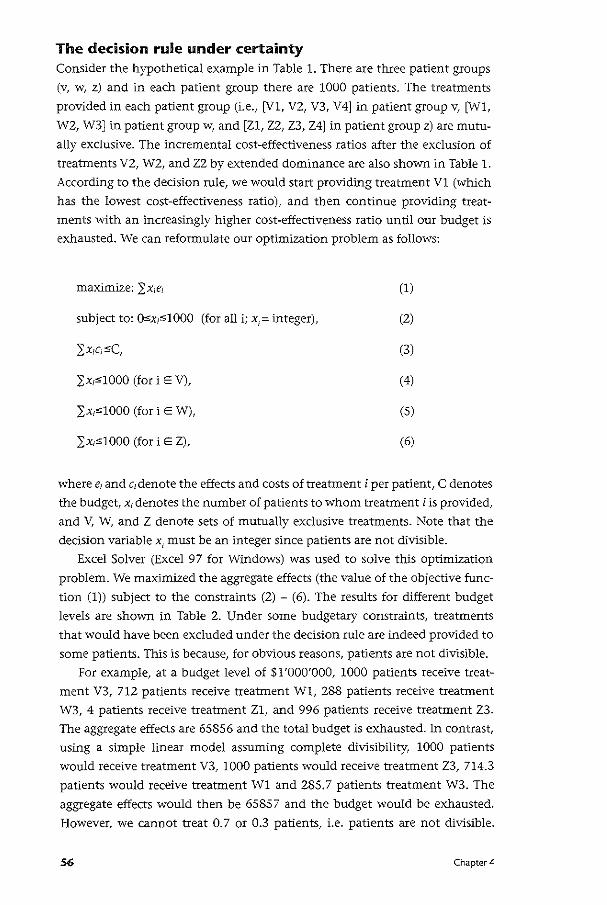
The decision rule under certainty Consider the hypothetical example in Table 1. There are three patient groups

(v, w, z) and in each patient group there are 1000 patients. The treatments

provided in each patient group (i.e., [V1, V2, V3, V4] in patient group v, [W1,

W2, W3] in patient group w, and [Z1, Z2, Z3, Z4] in patient group z) are mutu­

ally exclusive. The incremental cost-effectiveness ratios after the exclusion of

treatments V2, W2, and ZZ by extended dominance are also shown in Table 1.

According to the decision rule, we would start providing treatment V1 (which

has the lowest cost-effectiveness ratio), and then continue providing treat­

ments with an increasingly higher cost-effectiveness ratio until our budget is

exhausted. We can reformulate our optimization problem as follows:

(1)

subject to: O,;x,,.1000 (for all i; x1; integer), (2)

(3)

}:x,,1000 (fori E V), (4)

}:x,,1000 (fori E W), (5)

}:x,;;1000 (fori E Z), (6)

where e1 and c1denote the effects and costs of treatment i per patient, C denotes

the budget, x, denotes the number of patients to whom treatment i is provided,

and V, W, and Z denote sets of mutually exclusive treatments. Note that the

decision variable x1 must be an integer since patients are not divisible.

Excel Solver (Excel 97 for Windows) was used to solve this optimization

problem. We maximized the aggregate effects (the value of the objective func­

tion (1)) subject to the constraints (2) - (6). The results for different budget

levels are shown in Table 2. Under some budgetary constraints, treatments

that would have been excluded under the decision rule are indeed provided to

some patients. This is because, for obvious reasons, patients are not divisible.

For example, at a budget level of $1'000'000, 1000 patients receive treat­

ment V3, 712 patients receive treatment Wl, 288 patients receive treatment

W3, 4 patients receive treatment Zl, and 996 patients receive treatment Z3.

The aggregate effects are 65856 and the total budget is exhausted. In contrast,

using a simple linear model assuming complete divisibility, 1000 patients

would receive treatment V3, 1000 patients would receive treatment Z3, 714.3

patients would receive treatment W1 and 285.7 patients treatment W3. The

aggregate effects would then be 6585 7 and the budget would be exhausted.

However, we cannot treat 0. 7 or 0.3 patients, i.e. patients are not divisible.

56 Chapter 4

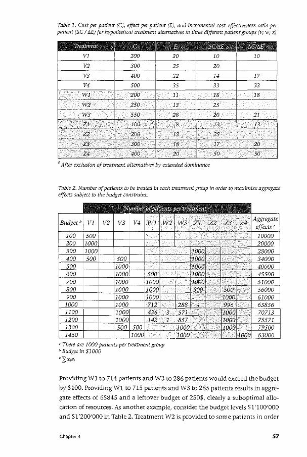
Table 1. Cost per patient (C), effect per patient (E), and incremental cost-effectiveness ratio per patient (t:..C I !:JE) for hypothetical treatment alternatives in three different patient groups (v; w; z)

Treatment

VJ

V2

a After exclusion of treatment alternatives by extended dominance

Table 2. Number of patients to be treated in each treatment group in order to maximize a&,rrregate effects subject to the budget constraint.

"There are 1000 patients per treatment group b Budget in $1000

cl:x1e;

Providing W1 to 714 patients and W3 to 286 patients would exceed the budget

by $100. Providing W1 to 715 patients and W3 to 285 patients results in aggre­

gate effects of 65845 and a leftover budget of 250$, clearly a suboptimal allo­

cation of resources. As another example, consider the budget levels $1 '100'000

and $1 '200'000 in Table 2. Treatment W2 is provided to some patients in order

Chapter 4 57

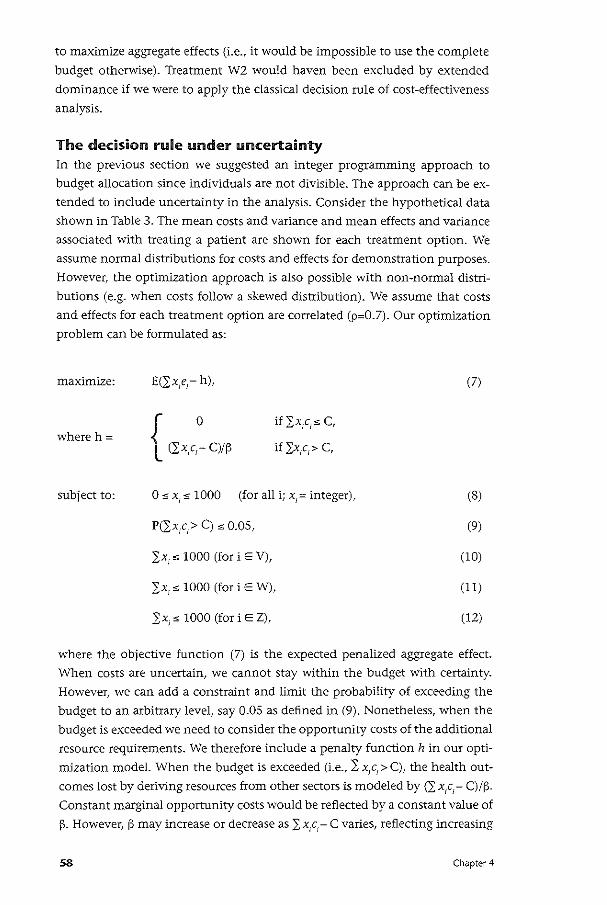
to maximize aggregate effects (i.e., it would be impossible to use the complete

budget otherwise). Treatment WZ would haven been excluded by extended

dominance if we were to apply the classical decision rule of cost-effectiveness

analysis.

The decision rule under uncertainty In the previous section we suggested an integer programming approach to

budget allocation since individuals are not divisible. The approach can be ex­

tended to include uncertainty in the analysis. Consider the hypothetical data

shown in Table 3. The mean costs and variance and mean effects and variance

associated with treating a patient are shovvn for each treatment option. We

assume normal distributions for costs and effects for demonstration purposes.

However, the optimization approach is also possible with non~normal distri­

butions (e.g. when costs follow a skewed distribution). We assume that costs

and effects for each treatment option are correlated (p=0.7). Our optimization

problem can be formulated as:

maximize: (7)

where h =

subject to: 0 s x1 s 1000 (for all i; x

1= integer), (8)

(9)

2;x1 s 1000 (fori E V), (10)

2;x1 s 1000 (fori E W), (11)

2;x1 s 1000 (fori E Z), (12)

where the objective function (7) is the expected penalized aggregate effect.

When costs are uncertain, we cannot stay within the budget with certainty.

However, we can add a constraint and limit the probability of exceeding the

budget to an arbitrary level, say 0.05 as defined in (9). Nonetheless, when the

budget is exceeded we need to consider the opportunity costs of the additional

resource requirements. We therefore include a penalty function h in our opti­

mization model. When the budget is exceeded (i.e., Lx,c,>C), the health out­

comes lost by deriving resources from other sectors is modeled by (2: x,c,- C)/B.

Constant marginal opportunity costs would be reflected by a constant value of

p. However, !3 may increase or decrease as 2: x,.c;- C varies, reflecting increasing

58 Chapter 4

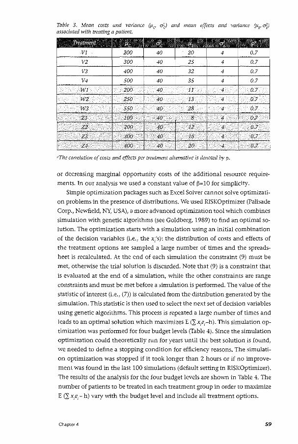
Table 3. Mean costs and variance (Pc o~) and mean effects and variance (JIF dfJ associated with treating a patient.

Treatment lfc q, P, "% p' VI 200 40 20 4 0.7

V2 300 40 25 4 0.7

V3 400 40 32 4 0.7

V4 500 40 35 4 0.7

WI 200 40 11 4 0.7

W2 250 40 I3 4 0.7

W3 550 40 28 4 0.7

Zl IOO 40 8 4 0.7

Z2 • 200 40 . I2 4 0.7

Z3 • 300 40 18 4 0.7

Z4 400 40 20 4 0.7

"The correlation of costs and effects per treatment alternative is denoted by p.

or decreasing marginal opportunity costs of the additional resource require­

ments. In our analysis we used a constant value of (3=10 for simplicity.

Simple optimization packages such as Excel Solver cannot solve optimizati­

on problems in the presence of distributions. We used RiSK Optimizer (Palisade

Corp., Newfield, NY, USA), a more advanced optimization tool which combines

simulation with genetic algorithms (see Goldberg, 1989) to find an optimal so­

lution. The optimization starts with a simulation using an initial combination

of the decision variables (i.e., the x/s): the distribution of costs and effects of

the treatment options are sampled a large number of times and the spreads­

heet is recalculated. At the end of each simulation the constraint (9) must be

met, otherwise the trial solution is discarded. Note that (9) is a constraint that

is evaluated at the end of a simulation, while the other constraints are range

constraints and must be met before a simulation is performed. The value of the

statistic of interest (i.e., (7)) is calculated from the distribution generated by the

simulation. This statistic is then used to select the next set of decision variables

using genetic algorithms. This process is repeated a large number of times and

leads to an optimal solution which maximizes E (lx1e1-h). This simulation op­

timization was performed for four budget levels (Table 4). Since the simulation

optimization could theoretically run for years until the best solution is found,

we needed to define a stopping condition for efficiency reasons. The simulati­

on optimization was stopped if it took longer than 2 hours or if no improve­

ment was found in the last 100 simulations (default setting in RiSK Optimizer).

The results of the analysis for the four budget levels are shown in Table 4. The

number of patients to be treated in each treatment group in order to maximize

E (I x,e;- h) vary with the budget level and include all treatment options.

Chapter4 59

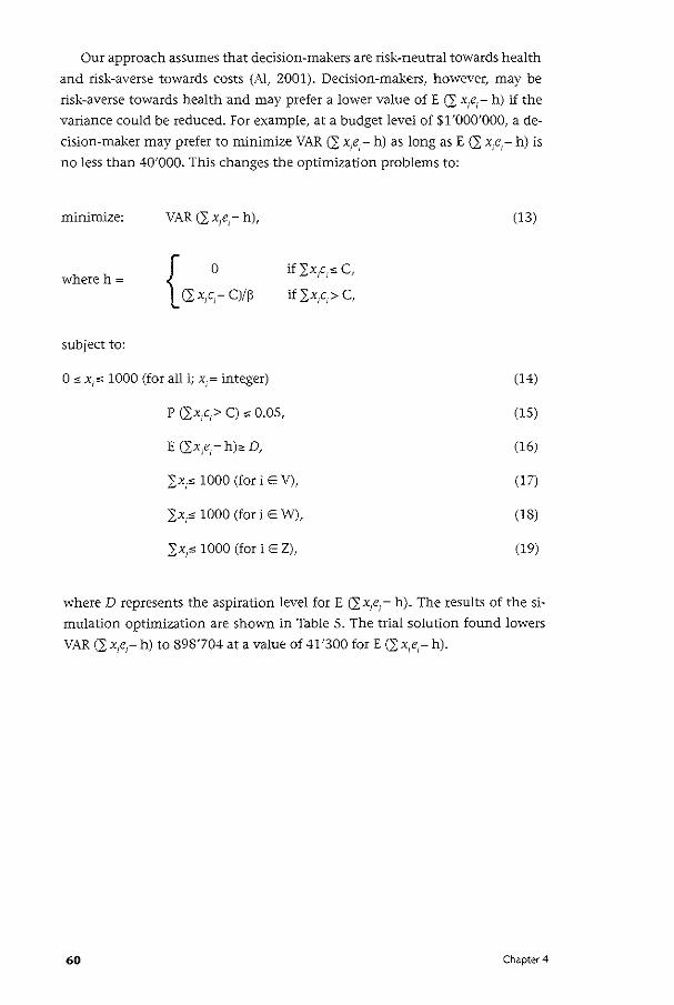
Our approach assumes that decision-makers are risk-neutral towards health

and risk-averse towards costs (Al, 2001). Decision-makers, however, may be

risk-averse towards health and may prefer a lower value of E (2; x1e1- h) if the

variance could be reduced. For example, at a budget level of $1'000'000, a de­

cision-maker may prefer to minimize VAR (2; x,e,- h) as long as E C2: x,e,- h) is

no less than 40'000. This changes the optimization problems to:

minimize:

where h =

subject to:

if .L:x/;s C,

if 2:X/,> C,

0 ~ x1 ~ 1000 (for all i; x, = integer)

2:X,~ 1000 (fori E V),

2:X1~ 1000 (fori E W),

(13)

(14)

(15)

(16)

(17)

(18)

(19)

where D represents the aspiration level forE (2;x1e,- h). The results of the si­

mulation optimization are shown in Table 5. The trial solution found lowers

VAR (2; x1e

1- h) to 898'704 at a value of 41'300 forE C2: x,e,- h).

60 Chapter 4

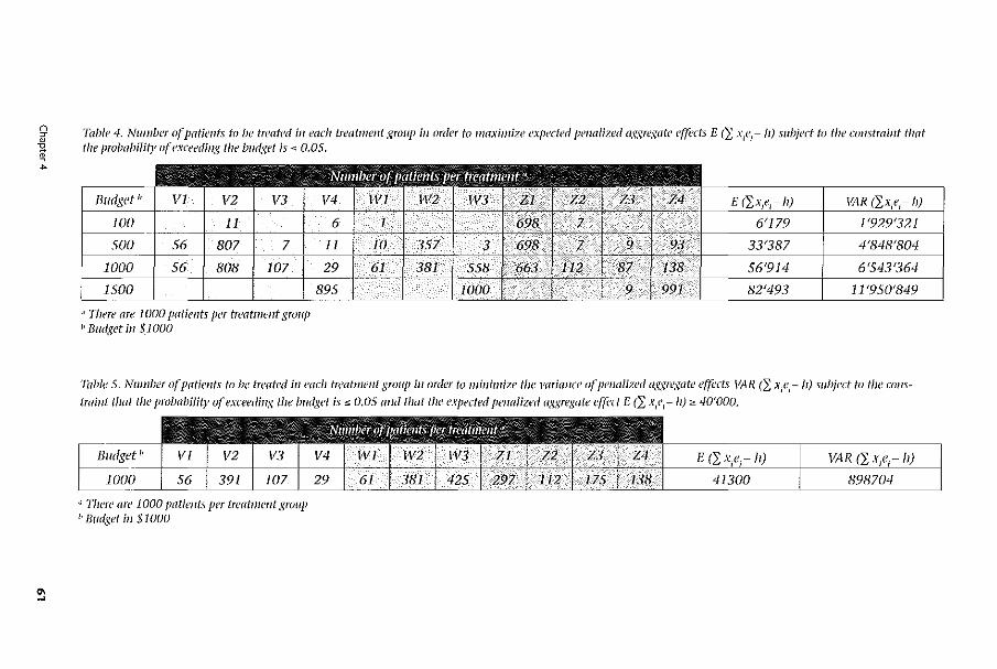
~ Table 4. Number o(Jmtients to be treated in each treatment group i11 order to maximize cxpectt'd pmalized oggregotc cf(ccts E (}: x1e1-II) subject to the cu11stmint tllat ~ the probobility of exceeding the lmdget is ,_ 0.05 . ..

"' -

Budget"

" There are I 000 potimts per treatmmt group 1' BW/,'\et ill $1000

ll,i\R - !J)

Table 5. Number of patimts to be treated in each treatmmt group in order to minimize the 1'11riance of penalized aggregate effects \'l-\.R <L X;f;- h) subject to tile cons­traillt tllat the probability a( exceeding the budget is :s; 0.05 and that the expected penalized oggregate cf{i:ct E (}: X/1-11);:;,. 40'000.

'' '111erc' are 1000 patients per trcatmmt group ~> Budget in $1000

II)

Discussion In this paper we have argued that health care programs can technically never

be treated as completely divisible because patients are not divisible. Conse­

quently, the usual decision rule of cost-effectiveness analysis may lead to

suboptimal budget allocation decisions at the margin. However, as Weinstein

(1995) argues, the linear programming approach may be seen as a reasonable

approximation to the integer programming approach under deterministic as­

sumptions. Whether this is true when costs and effects are stochastic is an area

for future research.

Birch and Gafni (1992, 1993) discussed the issue of divisibility at the level

of programs, i.e. they described the optimization problem assuming that a

program is either completely implemented or not at all. Stinnett and Paltiel

(1996) suggested a mixed integer programming approach to handle partial

indivisibilities in the sense that a threshold implementation level must be met

before a program is (partially or completely) implemented. This approach can,

for example, be used to model partial indivisibilities because of ethical reasons

or capital costs. However, the issue that programs are partially indivisible be­

cause individuals are indivisible has not been addressed yet. This is modeled

by constraining the decision variables (i.e., number of patients) in the optimi­

zation model to be integers. When using an integer programming approach,

treatments that would have been excluded by extended dominance or that

would not have been provided under the assumption of complete divisibility

(i.e., using a linear programming approach) may now be provided to some

patients.

The integer programming approach can be extended to handle uncer­

tainty of costs and effects at the patient level. Current methods for handling

uncertainty in cost-effectiveness analysis (such as net health benefits or cost­

effectiveness acceptability curves) (Stinnett and Mullahy, 1998; van Hout et

a!., 1994) are descriptive and hence do not per se provide any guidance as to

how the budget should be allocated (AI, 2001). The decision-maker's prefe­

rences over uncertain costs and effects are explicitly or implicitly needed in

decision-making (AI, 2001). A pragmatic approach is to maximize expected

health outcomes subject to the constraint that the probability of exceeding the

budget is limited to an arbitrary level (e.g., 0.05). However, decision-makers

such as insurance companies may also be risk-averse towards health outcomes

(Al, 2001). The decision-maker might then want to minimize uncertainty sur­

rounding health outcomes subject to the constraint that an aspiration level for

health outcomes is met. This is similar to the portfolio approach by O'Brien

and Sculpher (2000) where a tradeoff is made between maximizing expected

returns and minimizing uncertainty. However, O'Brien and Sculpher (2000)

based their framework on the effectiveness-cost ratio, which might become

problematic if the effectiveness-cost ratio takes on negative values. Moreover,

62 Chapter 4

the variance of the effectiveness-cost ratio may often not be defined. Our op­

timization approach, in contrast, handles costs and effects separately and also

includes the correlation between the two in the analysis.

An interesting recent attempt to address the decision-maker's problem is the stochastic league table approach (Hutubessy et al., 2001). Stochastic

league tables provide information about the probability of inclusion in the

optimal mix of programs at different budget levels. However, in their original

paper Hutubessy et al. (2001) modeled uncertainty of costs and effects at the

program level and not individual level. Furthermore, the information .con­

tained in stochastic league tables is probabilistic. Simulation optimization, in ·

contrast, provides decision-makers with a clear-cut decision of how to allocate

a given budget by determining the number of patients to be treated in each

treatment group.

Chapter 4 63

•ella terS Affordabi/ity and cost-effectiveness: decision-making on the

cost-effectiveness plane

Summary Much recent research interest has focused on handling uncertainty in cost­

effectiveness analysis and in particular the calculation of confidence intervals

for incremental cost-effectiveness ratios (ICERs). Problems of interpretation

when ICERs are negative have led to nvo important and related developments:

the use of the net-benefit statistic and the presentation of uncertainty in cost­

effectiveness analysis using acceptability curves. However, neither of these

developments directly addresses the problem that decision-makers are cons­

trained by a fixed-budget and may not be able to fund new, more expensive in­

terventions, even if they have been shown to represent good value for money.

In response to this limitation, the authors introduce the "affordability curve"

which reflects the probability that a program is affordable for a wide range of

threshold budgets. The authors argue that the joint probability an interventi­

on is affordable and cost-effective is more useful for decision-making since it

captures both dimensions of the decision problem faced by those responsible

for health service budgets.

64 Chapter 5

Introduction The inclusion of economic outcomes in clinical trials is now common (Drum~

mond, 1994) and the analysis of such trials has encouraged much research into

statistical methods for so-called stochastic cost-effectiveness analysis (Mullahy

and Manning, 1995; Coyle, 1996; Siegel eta!., 1996). The problem of estima­

ting confidence limits for cost-effectiveness ratios has received much attention

and the most important of the recent developments in this area are the use of

the net-benefit statistic to avoid the problems associated with ratio statistics

(Stinnett and Mullahy, 1998) and the use of cost-effectiveness acceptability

curves to summarize uncertainty on the cost-effectiveness plane (van Hout et

a!., 1994). Both these approaches employ a critical threshold value of the ICER

that represents the maximum society is willing to pay for health gain in order

to distinguish between what is and what is not cost-effective.

The use of such a critical threshold for the purposes of decision-making in

cost-effectiveness analysis is widespread; however, there is no consensus on

what exactly the value of this critical ratio might be. Speculative suggestions

have been made as to what thresholds might be appropriate (Goldman eta!.,

1992; Laupacis et a!., 1992), but these have received much criticism and it is

suggested that commonly used thresholds may owe more to belng convenient

round numbers than to being a valid statement concerning the value of health

(Weinstein, 1995; Garber and Phlebs, 1997)

More generally, the use of such thresholds for decision·making in cost-ef­

fectiveness analysis has been criticized on the basis that they will lead to an

uncontrolled growth in health care expenditure (Gafni and Birch, 1993). The

problem is that in using such thresholds, no explicit consideration is given to

the fact that health systems are resource constrained and that decision-makers

hold budgets, which must be balanced.

In the next section we introduce an example of the posterior joint distribu­

tion of incremental costs and effects from a published Bayesian cost-effective­

ness model that evaluated a prophylactic agent against opportunistic infections

in HIV-positive individuals (Sendi eta!., 1999). Using this example we illustra­

te the problem of using a threshold decision rule in cost-effectiveness analysis

and argue that recent developments for handling uncertainty in cost-effective­

ness analysis are of limited value to decision-makers because of their failure to

explicitly address the resource constraints of the decision-making process. We

then introduce the "affordability curve" and "cost-effectiveness affordability

curve" in order to provide this additional information to decision-makers in a

way that may help them to interpret the results of stochastic cost-effectiveness

analyses. A final section offers some concluding comments.

Chapter 5 65

~

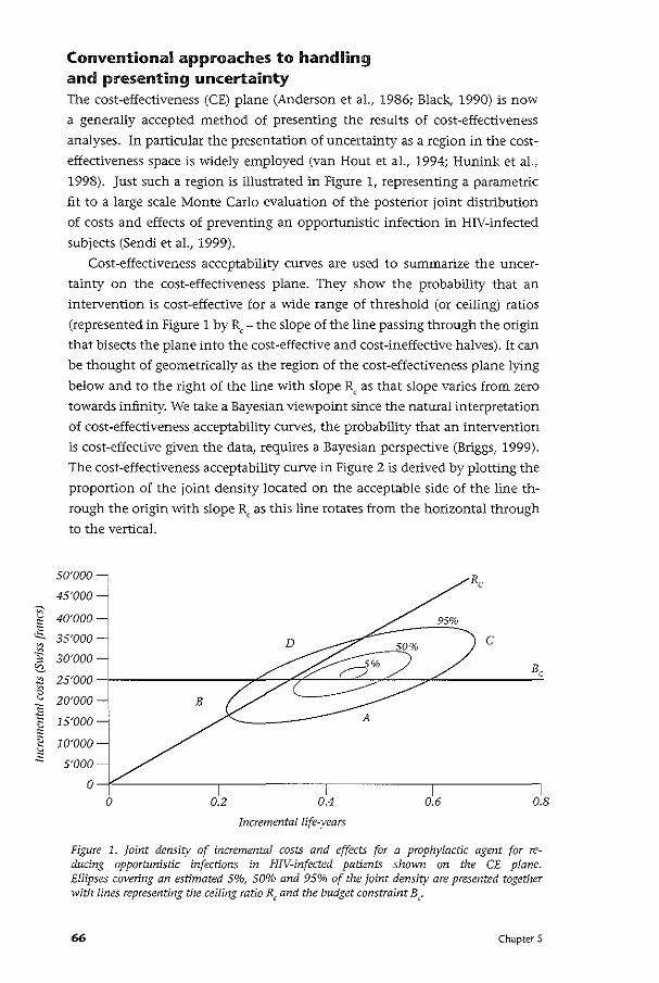
~ ·E.. ~

·~ ~

"' ~ 0 v

:g ~

" ~ ~ ~

""

Conventional approaches to handling and presenting uncertainty The cost-effectiveness (CE) plane (Anderson et al., 1986; Black, 1990) is now

a generally accepted method of presenting the results of cost-effectiveness

analyses. In particular the presentation of uncertainty as a region in the cost­

effectiveness space is widely employed (van Hout et al., 1994; Hunink et al.,

1998). Just such a region is illustrated in Figure 1, representing a parametric

fit to a large scale Monte Carlo evaluation of the posterior joint distribution

of costs and effects of preventing an opportunistic infection in HIV-infected

subjects (Sendi et al., 1999).

Cost-effectiveness acceptability curves are used to summarize the uncer­

tainty on the cost-effectiveness plane. They show the probability that an

intervention is cost-effective for a wide range of threshold (or ceiling) ratios

(represented in Figure 1 by R,- the slope of the line passing through the origin

that bisects the plane into the cost-effective and cost-ineffective halves). It can

be thought of geometrically as the region of the cost-effectiveness plane lying

below and to the right of the line with slope Rc as that slope varies from zero

towards infinity. We take a Bayesian viewpoint since the natural interpretation

of cost-effectiveness acceptability curves, the probability that an intervention

is cost-effective given the data, requires a Bayesian perspective (Briggs, 1999).

The cost-effectiveness acceptability curve in Figure 2 is derived by plotting the

proportion of the joint density located on the acceptable side of the line th­

rough the origin vvith slope Rc as this line rotates from the horizontal through

to the vertical.

5o·ooo-,

45'000

40'000

35'000

30'000

25'000

20'000 B

15'000 -j

10'000

5'000

0

0 0.2 i

0.4

Incremental life-years

c

0.6 0.8

Figure 1. Joint density of incremental costs and effects for a prophylactic agent for re­ducing opportunistic infections in HIV-infected patients shown on the CE plane. Ellipses covering an estimated 5%, SO% and 95% of the joint density are presented together with lines representing the ceiling ratio R, and the budget constraint B,.

66 Chapter 5

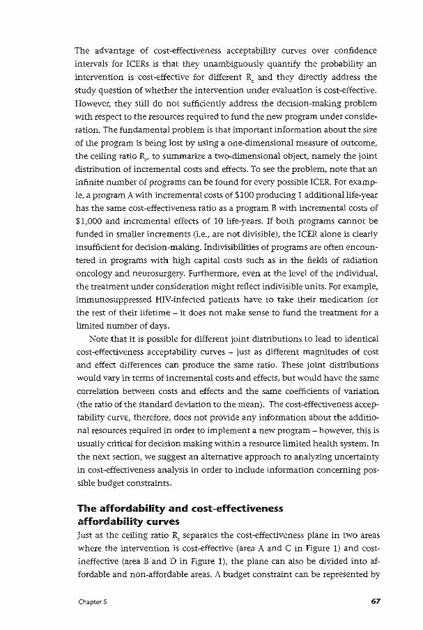
The advantage of cost-effectiveness acceptability curves over confidence

intervals for ICERs is that they unambiguously quantify the probability an

intervention is cost-effective for different R, and they directly address the

study question of whether the intervention under evaluation is cost-effective.

However, they still do not sufficiently address the decision-making problem

with respect to the resources required to fund the new program under conside­

ration. The fundamental problem is that important information about the size

of the program is being lost by using a one-dimensional measure of outcome,

the ceiling ratio Rc, to summarize a two-dimensional object, namely the joint

distribution of incremental costs and effects. To see the problem, note that an

infinite number of programs can be found for every possible ICER. For examp­

le, a program A with incremental costs of $100 producing 1 additional life-year

has the same cost-effectiveness ratio as a program B with incremental costs of

$1,000 and incremental effects of 10 life-years. If both programs cannot be

funded in smaller increments (i.e., are not divisible), the ICER alone is clearly

insufficient for decision-making. Indivisibilities of programs are often encoun­

tered in programs with high capital costs such as in the fields of radiation

oncology and neurosurgery. Furthermore, even at the level of the individual,

the treatment under consideration might reflect indivisible units. For example,

immunosuppressed HIV-infected patients have to take their medication for

the rest of their lifetime - it does not make sense to fund the treatment for a

limited number of days.

Note that it is possible for different joint distributions to lead to identical

cost-effectiveness acceptability curves - just as different magnitudes of cost

and effect differences can produce the same ratio. These joint distributions

would vary in terms of incremental costs and effects, but would have the same

correlation between costs and effects and the same coefficients of variation

(the ratio of the standard deviation to the mean). The cost-effectiveness accep­

tability curve, therefore, does not provide any information about the additio­

nal resources required in order to implement a new program- however, this is

usually critical for decision making within a resource limited health system. In

the next section, we suggest an alternative approach to analyzing uncertainty

in cost-effectiveness analysis in order to include information concerning pos­

sible budget constraints.

The affordability and cost-effectiveness affordability curves Just as the ceiling ratio Rc separates the cost~effectiveness plane in two areas

where the intervention is cost-effective (area A and C in Figure 1) and cost­

ineffective (area B and D in Figure 1), the plane can also be divided into af­

fordable and non-affordable areas. A budget constraint can be represented by

Chapter 5 67

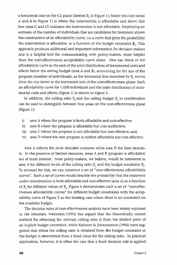
a horizontal line on the CE plane (labeled B, in Figure 1); below this line (areas

A and B in Figure 1) is where the intervention is affordable and above this

line (area C and D) indicates the intervention is not affordable. Employing an

estimate of the number of individuals that are candidates for treatment allows

the construction of an affordability curve, i.e. a curve that plots the probability

the intervention is affordable, as a function of the budget constraint B,. This

approach produces additional and important information for decision-makers

and is a helpful tool for communicating with policy-makers, more helpful

than the cost-effectiveness acceptability curve alone. One can think of the

affordability CUI\le as the area of the joint distribution of incremental costs and

effects below the ceiling budget (area A and B), accounting for the size of the

program (number of individuals), as the horizontal line described by Be moves

from the top down to the horizontal axis of the cost-effectiveness plane. Such

an affordability curve for 1,000 individuals and the joint distribution of incre­

mental costs and effects (Figure 1) is shown in Figure 3.

In addition, the ceiling ratio Rc and the ceiling budget Be in combination

can be used to distinguish between four areas on the cost-effectiveness plane

(Figure 1):

i) area A where the program is both affordable and cost-effective;

ii) area B where the program is affordable but cost-ineffective;

iii) area C where the program is not affordable but cost-effective; and,

iv) area D where the new program is neither affordable nor cost-effective.

Area A reflects the most desirable outcome while area D the least desirab­

le. In the presence of limited resources, areas A and B (program is affordable)

are of most interest. Most policy-makers, we believe, would be interested in

area A for different levels of the ceiling ratio R, and the budget constraint B,.

To account for this, we can construct a set of "cost-effectiveness affordability

curves". Such a set of curves would describe the probability that the treatment

under consideration is both affordable and cost-effective (area A) as a function

of RJor different values of B,. Figure 4 demonstrates such a set of "cost-effec­

tiveness affordability curves" for different budget constraints with the accep­

tability curve of Figure 2 as the limiting case where there is no constraint on

the available budget.

The decision rules of cost-effectiveness analysis have been widely explored

in the literature. Weinstein (1995) has argued that the theoretically correct

method for obtaining the relevant ceiling ratio is from the shadow price of

an explicit budget constraint, while Karlsson & Johannessen (1996) have sug­

gested that either the ceiling ratio is obtained from the budget constraint or

the budget is determined from a fixed value for the ceiling ratio. ln practical

application, however, it is often the case that a fixed decision rule is applied

68 Chapter 5

~

"' ~ ~ ~

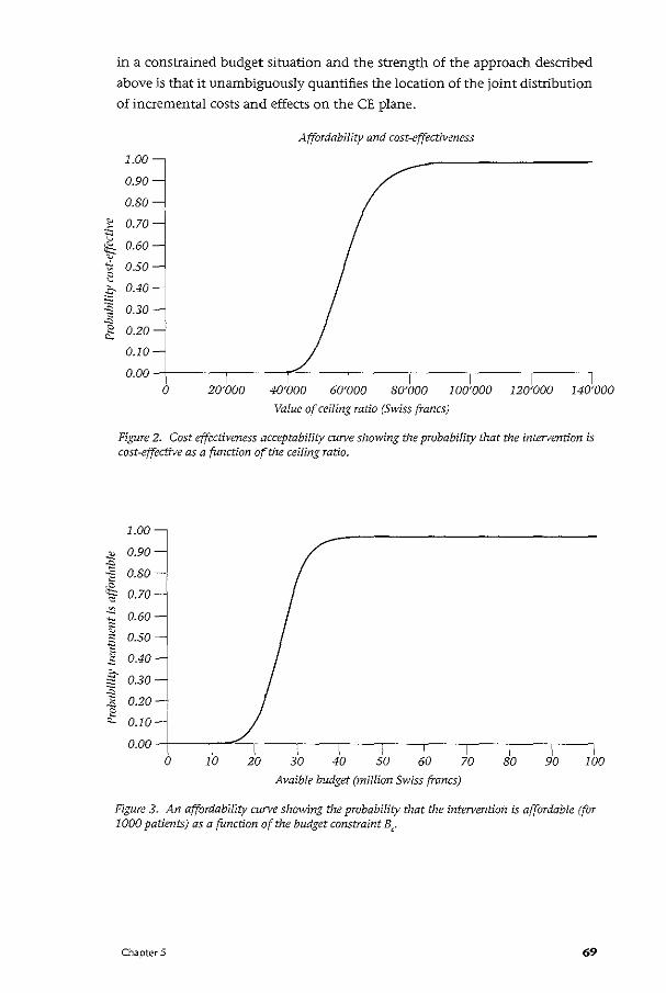
""-~ " g :E ~

"" 2 ""

~ -" ~

in a constrained budget situation and the strength of the approach described

above is that it unambiguously quantifies the location of the joint distribution

of incremental costs and effects on the CE plane.

Affordability and cost-effectiveness

1.003 0.90

0.80

0.70

0.60

0.50

0.40

0.30

0.20 _j

0.10

0.00

0 20'000 40'000 60'000 80'000 100'000 120'000 140'000

Value of ceiling ratio (Swiss francs)

Figure 2. Cost effectiveness acceptability curve showing the probability that the intervention is cost-effective as a function of the ceiling ratio.

1.00j 0.90

0.80 ' ~ 0.70 ~

-~ 0.60

"' ;:;

" 0.50 "' ~ 1; 0.40

. .s- 0.30 ~ ~ 0.20 "" ~ 0.10

0.00 0 10 20 30 40

I 50 60

Avaible budget (million Swiss francs)

70 so 90 100

Figure 3. An affordability cu:rve showing the probability that the intervention is affordable (for 1000 patients) as a function of the budget constraint B,.

Chapter 5 69

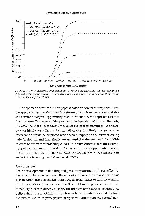
Affordability and costs·effectiveness

-No budget constraint ·····-Budget= CHF 30'000'000

1.00l

~ .:; , ·---Budget= CHF 25'000'000 i 05

J- -'W<"-~ ~-~ooo .// ······

:~ ~ 2

0.40

0.10

o 2o·ooo 4o·ooo 6o·ooo so·ooo 1oo·ooo 12o'ooo 14o·ooo Value of ceiling ratio (Swiss francs)

Figure 4. A cost·effectiveness affordability curve showing the probability that an intervention is simultaneously cost-effective and affordable (for 1000 patients) as a function of the ceiling ratio and the budget constraint.

The approach described in this paper is based on several assumptions. First,

the approach assumes that there is a stream of additional resources available

at a constant marginal opportunity cost. Furthermore, the approach assumes

that the cost-effectiveness of the program is independent of its size. Similarly,

it is assumed that affordability is not related to cost-effectiveness- if a thera­

PY were highly cost-effective, but not affordable, it is likely that some other

intervention would be displaced which would impact on the relevant ceiling

ratio for dedsion-making. Finally, we assumed that the program is indivisible

in order to estimate affordability curves. In circumstances where the assump­

tions of constant returns to scale and constant marginal opportunity costs do

not hold, an alternative method for handling uncertainty in cost-effectiveness

analysis has been suggested (Sendi et al., 2002).

Conclusion Recent developments in handling and presenting uncertainty in cost-effective­

ness analysis have not addressed the issue of a resource constrained health care

system where decision makers hold budgets from which to fund new health

care interventions. In order to address this problem, we propose the use of af­

fordability curves to directly quantify the problem of resource constraints. We

believe that this sort of information is especially important for analyses from

the system and third party payer's perspective (rather than the societal pers-

70 Chapter 5

pective) where the budget for the treatment under consideration is often given

and therefore easier to determine. We believe that in times of scarcity of health

care resources, information about both cost-effectiveness and affordability is

likely to produce more useful information for policy makers.

Chapter 5 71

•cha ter6 Portfolio theory and cost-effectiveness analysis: a further discussion

Summary Background: Portfolio theory has been suggested as a means to improve the

risk-return characteristics of investments in health care programs through di­

versification when costs and effects are uncertain. This approach is based on

the assumption that the investment proportions are not subject to uncertainty

and that the budget can be invested in toto in health care programs.

Methods: In the present paper we develop an algorithm that accounts for the

fact that investment proportions in health care programs may be uncertain

(due to the uncertainty associated with costs) and limited (due to the size of

the programs). The initial budget allocation across programs may therefore be

revised at the end of the investment period to cover the extra costs of some

programs with the leftover budget of other programs in the portfolio.

Results: Once the total budget is equivalent to or exceeds the expected costs

of the programs in the portfolio, the initial budget allocation policy does not

impact the risk-return characteristics of the combined portfolio, i.e. there is no

benefit from diversification anymore.

Conclusion: The applicability of portfolio methods to improve the risk-return

characteristics of investments in health care is limited to situations where the

available budget is much smaller than the expected costs of the programs to

be funded.

72 Chapter 6

Introduction The classical decision rule of cost-effectiveness analysis where programs are

ranked according to the expected cost-effectiveness ratio and successively implemented, starting with the program with the most favorable cost-effec­

tiveness ratio (i.e., highest expected return), until the budget is exhausted,

represents a situation where the decision maker is assumed to be risk-neutral

(Al, 2001; O'Brien and Sculpher, 2000). This is consistent with Arrow and

Lind's argument that risk should be irrelevant in public investment decisions

because of the ability of spreading risk over many consumers (Arrow and Lind,

1970). However, risk-spreading may be limited in countries where health in­

surance is provided in the private market since the financial burden to some

individuals may be substantial (Zivin and Bridges, 2002). Moreover, even in

countries where the financial burden is spread across all individuals such as

in Switzerland where basic health insurance is compulsory by law, the health

outcomes experienced by the individuals are not transferable (Zivin, 2001;

Ben Zion and Gafni, 1983). For example, patients with diabetic retinopathy

cannot "share" with others their loss of visual acuity. Others have argued that

decision-makers may operate at a subsocietal level and have to meet budge­

tary constraints and outcome performance targets at the same time (O'Brien

and Sculpher, 2000). Therefore, the probability of exceeding the budget and/

or a shortfall in health outcomes is of great importance to many decision-ma­

kers. Hence, the uncertainty associated with return on investment should be

accounted for when selecting health care programs.

Much research interest has focused on methods for handling uncertainty

in cost-effectiveness analysis (van Hout et al., 1994; Briggs and Gray, 1999;

Briggs et al., 2002; Briggs, 2001; Sendi and Briggs, 2001). O'Brien and Sculpher

(2000) have recently started the discussion as to how portfolio theory can be

used to rank health care programs with different risk-return parameters. The

decision-maker's preferences over expected return and risk, and the principle

of diversification to reduce uncertainty, may be borrowed from portfolio the­

ory and applied in health care finance (O'Brien and Sculpher, 2000). However,

these concepts have so far been presented as a method to deal with uncertain­

ty in costs and effects without explicit consideration of the size of the budget

and the resource requirements of the programs in the portfolio.

In health care finance, the investment proportions in the different pro­

grams may be limited by the size of the programs. This is very different from

the situation in financial economics where the investment decision with re­

gard to the mix of risk-y assets is performed initially and the budget is usually

spent in toto. Moreover, in health care finance, the investment proportions

are usually uncertain due to the uncertainty associated with the costs of the

programs, as opposed to certain in financial economics. Health care programs

may happen to need more or less resources tlian initially budgeted. In such

Chapter 6 73

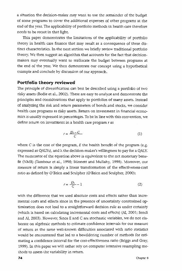
a situation the decision-maker may want to use the remainder of the budget

of some programs to cover the additional expenses of other programs at the

end of the year. The applicability of portfolio methods in health care therefore

needs to be recast in that light.

This paper demonstrates the limitations of the applicability of portfolio

theory in health care finance that may result as a consequence of these dis­

tinct characteristics. In the next section we briefly review traditional portfolio

theory. We then suggest an algorithm that accounts for the fact that decision­

makers may eventually want to reallocate the budget between programs at

the end of the year. We then demonstrate our concept using a hypothetical

example and conclude by discussion of our approach.

Portfolio theory reviewed The principle of diversification can best be described using a portfolio of two

risk-y assets (Bodie eta!., 2002). These are easy to analyze and demonstrate the

principles and considerations that apply to portfolios of many assets. Instead

of analyzing the risk and return parameters of bonds and stocks, we consider

health care programs as rish.y assets. Return on investment in financial econo­

mics is usually expressed in percentages. To be in line with this convention, we

define return on investment in a health care program r as

T= EA-C c (1)

where Cis the cost of the program, E the health benefit of the program (e.g.

expressed as QALYs), and A. the decision-maker's willingness to pay for a QALY.

The numerator of the equation above is equivalent to the net monetary bene­

fit (NMB) (Tambour et a!., 1998; Stinnett and Mullahy, 1998). Moreover, our

measure of return is simply a linear transformation of the effectiveness-cost

ratio as defined by O'Brien and Sculpher (O'Brien and Sculpher, 2000):

EA T= c;-1 (2)

with the difference that we used absolute costs and effects rather than incre­

mental costs and effects since in the presence of uncertainty constrained op­

timization does not lead to a straightforward decision rule as under certainty

(which is based on calculating incremental costs and effects) (AI, 2001; Sendi

and AI, 2003). However, Since E and Care stochastic variables, we do not ela­

borate on algebraic methods to estimate confidence intervals for our measure

of return as the same well-known difficulties associated with ratio statistics

would be encountered that led to a bewildering number of methods for esti­

mating a confidence interval for the cost-effectiveness ratio (Briggs and Gray,

1999). In this paper we will rather rely on computer intensive resampling me­

thods to assess the variability in return.

74 Chapter 6

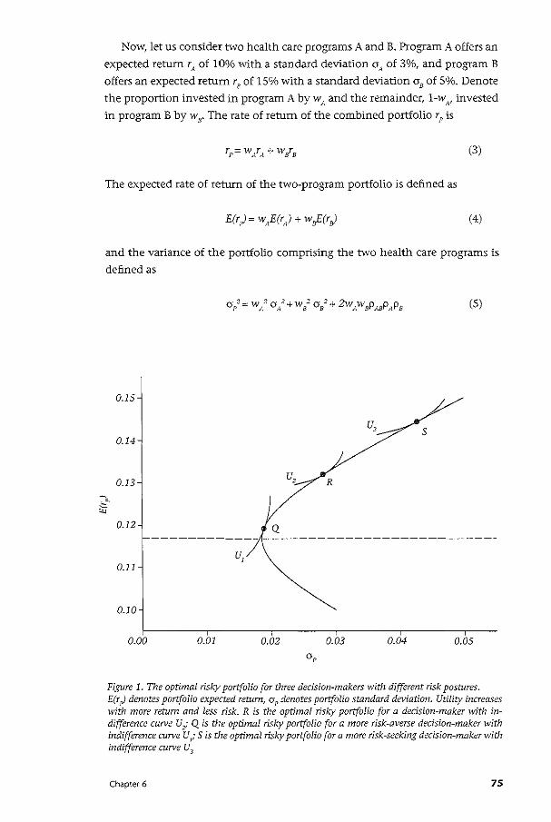
Now, let us consider two health care programs A and B. Program A offers an

expected return rA of 10% with a standard deviation aA of 3%, and program B

offers an expected return re of 15% with a standard deviation ae of 5%. Denote

the proportion invested in program A by wA and the remainder, 1-w,v invested

in program B by we. The rate of return of the combined portfolio rP is

(3)

The expected rate of return of the two-program portfolio is defined as

(4)

and the variance of the portfolio comprising the two health care programs is

defined as

(5)

0.15

0.14

0.13 u, R

0.12

u, 0.11

0.10

0.00 0.01 0.02 0.03 0.04 0.05

Figure 1. The optimal risky portfolio for three decision-makers with different risk postures. E(r p) denotes portfolio expected return, oP denotes portfolio standard deviation. Utility increases with more return and less risk. R is the optimal risf...y portfolio for a decision-maker with in­difference curve Ui Q is the optimal risf...y portfolio for a more risk-averse decision-maker 1-Vith indifference curve UJI- Sis the optimal risf...y portfolio for a more risk-seeking decision-maker with indifference curve U3

Chapter 6 75

We can see from Equation (5) that the standard deviation of the combined

portfolio, given the standard deviation of the individual programs, increases

when the correlation coefficient PAs is higher. The smaller PAw the more effec­

tive the reduction in total risk will be.

A portfolio opportunity set shows all risk-return combinations that can be

constructed by varying the investment proportions. Figure 1 shows such an

investment opportunity set assuming that the correlation betvveen the return

of program A and B as specified above is -0.5. The section of the curve that

lies above the minimum variance portfolio (indicated by the intersection of

the horizontal broken line with the portfolio opportunity set) is called the

efficient frontier. An investor typically chooses a portfolio that lies on the ef­

ficient frontier since for every combination of w s and wr~ that lies below the

minimum variance portfolio there exists a combination ofws and wA above the

minimum variance portfolio that offers more returns for the same degree of

risk. The investor has then to decide on the proportions to invest in program

A and B. This is accomplished by superimposing the investor's indifference

map (i.e., a set of indifference curves) on the efficient frontier. An indifference

curve connects all points on the risk-return plane that offer the same level of

utility to a decision-maker. Since we assume that decision-makers prefer more

expected return and less risk, indifference curves that lie in the North-West of

the indifference map indicate a higher level of utility. The indifference curve

that is tangent to the efficient frontier therefore reflects the combination of

w 8 and w A with the highest utility. Such a curve is shown for three different

investors in Figure 1. The slope of the indifference curve measures the rate at

which a decision maker is willing to engage in a riskier investment (indicated

on the horizontal axis) in return for an increase in expected return (indicated

on the vertical axis), while holding utility constant. The steeper the slope of

the indifference curve is, the more expected return is needed to compensate

for an increase in an additional unit of risk. The slope of the indifference curve

depends on the decision-maker's risk-tolerance. An investor with indifference

curve U2

would choose portfolio R. A more risk-averse investor with a steeper

indifference curve U 1 would choose portfolio Q. And a risk-seeking investor

with indifference curve U3 would choose portfolioS. The indifference map of a

decision-maker is difficult to construct in practice. However, different methods

are available to elicit the decision-maker's risk-posture, which are described in

detail elsewhere (e.g. Bodie eta!., 2002).

76 Chapter 6

Stochastic costs and budget allocation We have so far simply adopted the portfolio methods in health care finance.

However, there are some important differences to note between budget allo­

cation in health care finance and budget allocation in financial economics.

In financial economics, the proportion of the budget used by the different

risky assets is not uncertain. Let us say we want to invest 50% of our budget

in Microsoft stocks and SO% in Intel stocks. In financial economics, we can

completely spend our budget as contemplated. We can do so because our bud­

get is usually much smaller than the value of all available shares of a stock on

the market (Bodie et al., 2002). This is different from the situation in health

care finance where resource use is uncertain and the investment proportions

limited by the size of the programs. Note that the uncertainty of return on in­

vestment in financial economics stems from the variability of the market value

of risky assets. In health care finance, on the other hand, the uncertainty of

return on investment results from the variability associated with both resource

use and health outcomes. Because resource use is uncertain, the proportion of

the budget used by health care programs is also uncertain. Hence, we do not

know beforehand whether our budget will be completely consumed or whe­

ther a part of the budget will be left at the end of the year. This has important

implications for the applicability of portfolio theory in health care finance

and the prindple of diversification is not applicable without modification. We

therefore need an algorithm to handle this distinct characteristic in health

care finance.

When resource use is uncertain, the proportion of the budget initially al­

located to a program does not necessarily correspond to the proportion of the

budget that is actually consumed by that program. This usually occurs when

a program turns out to use fewer resources than budgeted. If there are other

programs in the portfolio that tum out to need a larger proportion of the bud­

get at the end of the year, it makes sense to shift the remaining budget of the

first program to these latter programs to cover the extra costs. If there is srill

some leftover after this reallocation, then that unused part of the budget may

be seen as an investment in a risk-free asset, e.g. money market instruments.

We can formulate this budget allocation policy more formally for a situation in

which we have a portfolio of two health care programs. As already mentioned

in the previous section, a portfolio of two health care programs is straightfor­

ward to analyze and the same concepts and prindples also apply to portfolios

comprising multiple programs.

Chapter 6 77

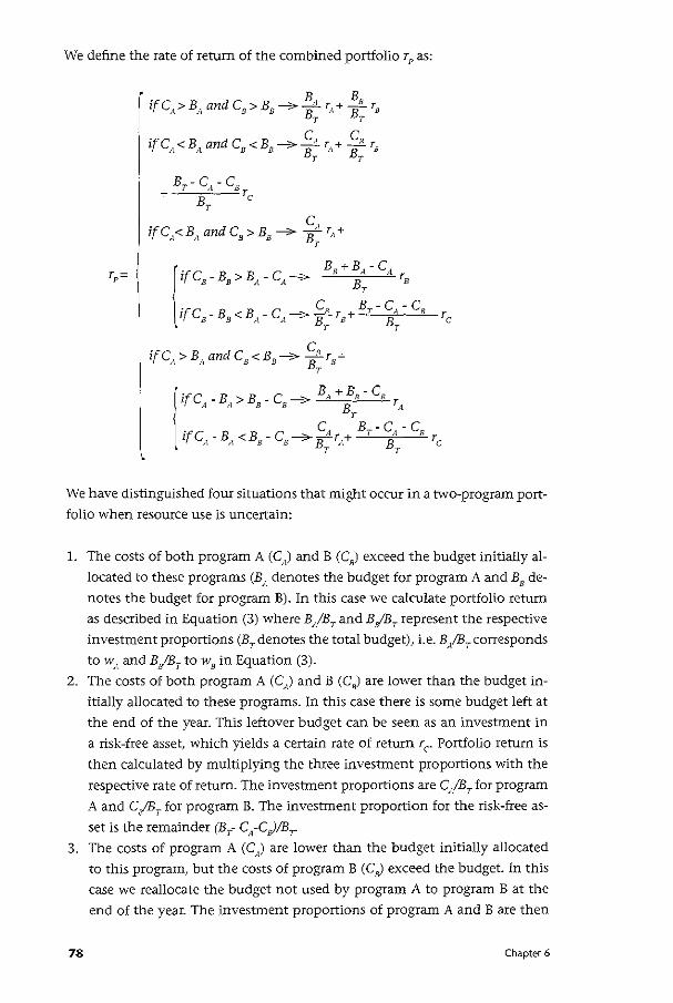
We define the rate of return of the combined portfolio rP as:

r = p

ifCA>BAandCs>Bs----7 ~A rA+ ;s 's T T

ifCA<BAandCs<Bs-----7 ~A r,1+ ~R rs T T

ifCA>BAandCs<Bs-> ~B Ts+ T

We have distinguished four situations that might occur in a two-program port­

folio when resource use is uncertain:

1. The costs of both program A (C) and B (C,) exceed the budget initially al­

located to these programs (B" denotes the budget for program A and B8 de­

notes the budget for program B). In this case we calculate portfolio return

as described in Equation (3) where B/BT and B/f!T represent the respective

investment proportions (BT denotes the total budget), i.e. B,/BT corresponds

tow" and BjBT to w8 in Equation (3).

2. The costs of both program A (C) and B (C8

) are lower than the budget in­

itially allocated to these programs. In this case there is some budget left at

the end of the year. This leftover budget can be seen as an investment in

a risk-free asset, which yields a certain rate of return rc Portfolio return is

then calculated by multiplying the three investment proportions with the

respective rate of return. The investment proportions are CA!BT for program

A and CjBT for program B. The investment proportion for the risk-free as­

set is the remainder (BT- CA-CJ!Br

3. The costs of program A (C) are lower than the budget initially allocated

to this program, but the costs of program B (C8) exceed the budget. In this

case we reallocate the budget not used by program A to program B at the

end of the year. The investment proportions of program A and B are then

78 Chapter 6

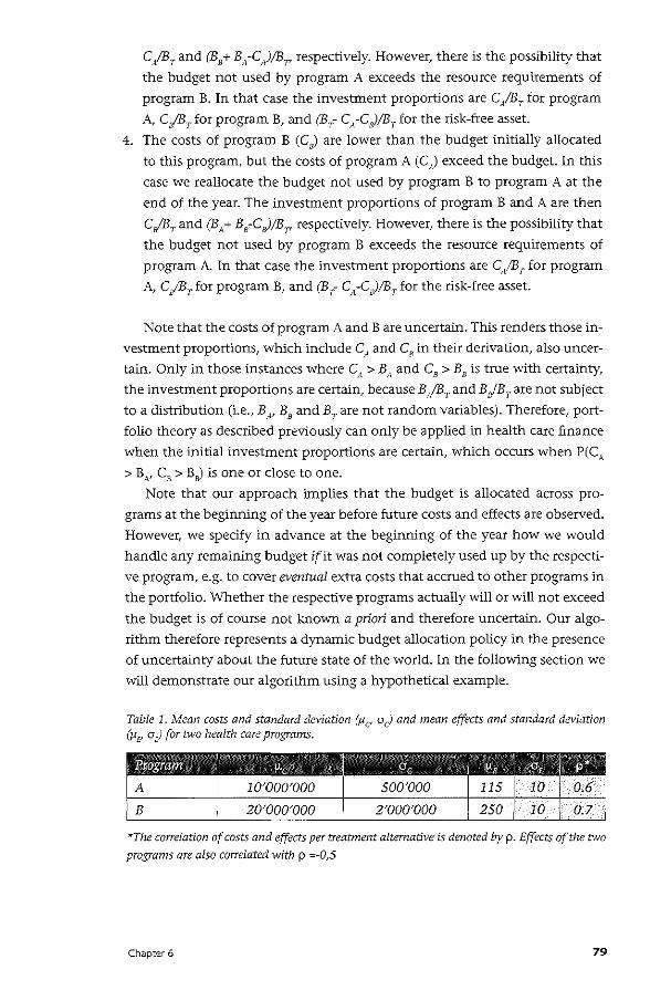
CfBT and (B8+ B"-C)/BT' respectively. However, there is the possibility that

the budget not used by program A exceeds the resource requirements of

program B. In that case the investment proportions are C~/B7 for program

A, c;sT for program B, and (BT- CA-CB)/BT for the risk-free asset.

4. The costs of program B (C8

) are lower than the budget initially allocated

to this program, but the costs of program A (C) exceed the budget. In this

case we reallocate the budget not used by program B to program A at the end of the year. The investment proportions of program B and A are then

C/BT and (BA+ B8-C,)/BT, respectively. However, there is the possibility that

the budget not used by program B exceeds the resource requirements of

program A In that case the investment proportions are C./Br for program A, C,IBT for program B, and (BT- CA-CJ!BT for the risk-free asset.

Note that the costs of program A and Bare uncertain. This renders those in­

vestment proportions, which include CA and C8

in their derivation, also uncer­

tain. Only in those instances where C/1 > BA and C8 > B8 is true with certainty,

the investment proportions are certain, because B,fBr and BefB7 are not subject to a distribution (i.e., BN B

8 and Br are not random variables). Therefore, port­

folio theory as described previously can only be applied in health care finance

when the initial investment proportions are certain, which occurs when P(CA

> B N C8 > B8) is one or close to one.

Note that our approach implies that the budget is allocated across pro­

grams at the beginning of the year before future costs and effects are observed.

However, we specify in advance at the beginning of the year how we would

handle any remaining budget if it was not completely used up by the respecti­

ve program, e.g. to cover eventual extra costs that accrued to other programs in

the portfolio. Whether the respective programs actually will or will not exceed

the budget is of course not known a priori and therefore uncertain. Our algo­

rithm therefore represents a dynamic budget allocation policy in the presence

of uncertainty about the future state of the world. In the following section we

will demonstrate our algorithm using a hypothetical example.

Table 1. Mean costs and standard deviation (Jicr a c) and mean effects and standard deviation (Jl£' a E) for two health care programs.

*The correlation of costs and effects per treatment alternative is denoted by p. Effects of the two

programs are also correlated with p =-0,5

Chapter 6 79

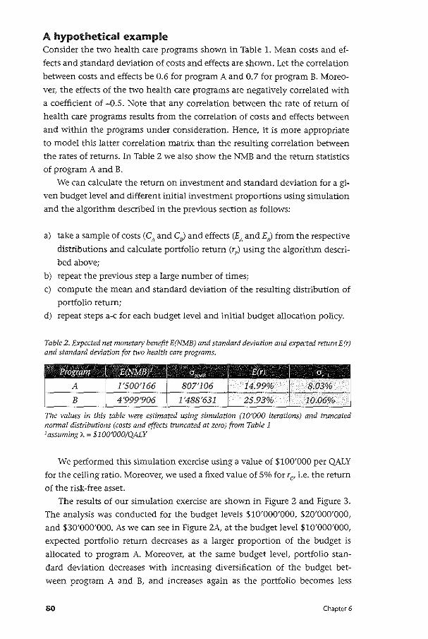
A hypothetical example Consider the two health care programs shown in Table 1. Mean costs and ef­

fects and standard deviation of costs and effects are shown. Let the correlation

between costs and effects be 0.6 for program A and 0.7 for program B. Moreo­

ver, the effects of the two health care programs are negatively correlated with

a coefficient of -0.5. Note that any correlation between the rate of return of

health care programs results from the correlation of costs and effects between

and within the programs under consideration. Hence, it is more appropriate

to model this latter correlation matrix than the resulting correlation between

the rates of returns. In Table 2 we also show the NMB and the return statistics

of program A and B.

We can calculate the return on investment and standard deviation for a gi­

ven budget level and different initial investment proportions using simulation

and the algorithm described in the previous section as follows:

a) take a sample of costs (C" and C,) and effects (EA and£8

) from the respective

distributions and calculate portfolio return (rp) using the algorithm descri­

bed above;

b) repeat the previous step a large number of times;

c) compute the mean and standard deviation of the resulting distribution of

portfolio return;

d) repeat steps a-c for each budget level and initial budget allocation policy.

Table 2. Expected net monetary benefit E(NMB) and standard deviation and expected return E(r) and standard deviation for two health care programs.

The values in this table were estimated using simulation (lOJOOO iterations) and truncated nonnal distributions (costs and effects truncated at zero) from Table 1 1assuming).. = $100'000/QALY

We performed this simulation exercise using a value of $100'000 per QALY

for the ceiling ratio. Moreover, we used a fixed value of 5% for r C' i.e. the return

of the risk-free asset.

The results of our simulation exercise are shown in Figure 2 and Figure 3.

The analysis was conducted for the budget levels $10'000'000, $20'000'000,

and $30'000'000. As we can see in Figure 2A, at the budget level $10'000'000,

expected portfolio return decreases as a larger proportion of the budget is

allocated to program A. Moreover, at the same budget level, portfolio stan­

dard deviation decreases with increasing diversification of the budget bet­

ween program A and B, and increases again as the portfolio becomes less

80 Chapter 6

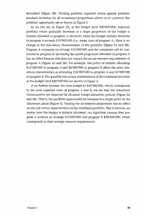
diversified (Figure 2B). Plotting portfolio expected return against portfolio

standard deviation for all investment proportions allows us to construct the

portfolio opportunity set as shown in Figure 3.

As we can see in Figure 2A, at the budget level $20'000'000, expected

portfolio return gradually decreases as a larger proportion of the budget is

initially allocated to program A. However, when the budget initially allocated

to program A exceeds $10'000'000 (i.e., mean costs of program A), there is no

change in the risk-return characteristics of the portfolio (Figure 2A and 2B).

Program A consumes on average $10'000'000 and the remainder will be real­

located to program B. Increasing the initial proportion allocated to program A

has no effect because this does not impact the actual resource requirements of

program A (Figure 2A and 2B). For example, the policy of initially allocating

$12'000'000 to program A and $8'000'000 to program B offers the same risk­

return characteristics as allocating $18'000'000 to program A and $2'000'000

to program B. The possible risk-return combinations of the combined portfolio

at the budget level $20'000'000 are shown in Figure 3.

If we further increase the total budget to $30'000'000, which corresponds

to the total expected costs of program A and B, we see that the risk-return

characteristics are identical for all initial budget allocation policies (Figure 2A

and ZB). That is, the portfolio opportunity set collapses to a single point on the

risk-return plane (Figure 3). Varying the investment proportions has no effect

on the risk~retum characteristics of the combined portfolio. This is because, no

matter how the budget is initially allocated, our algorithm ensures that pro­

gram A receives on average $10'000'000 and program B $20'000'000, which

corresponds to their average resource requirements.

Chapter 6 81

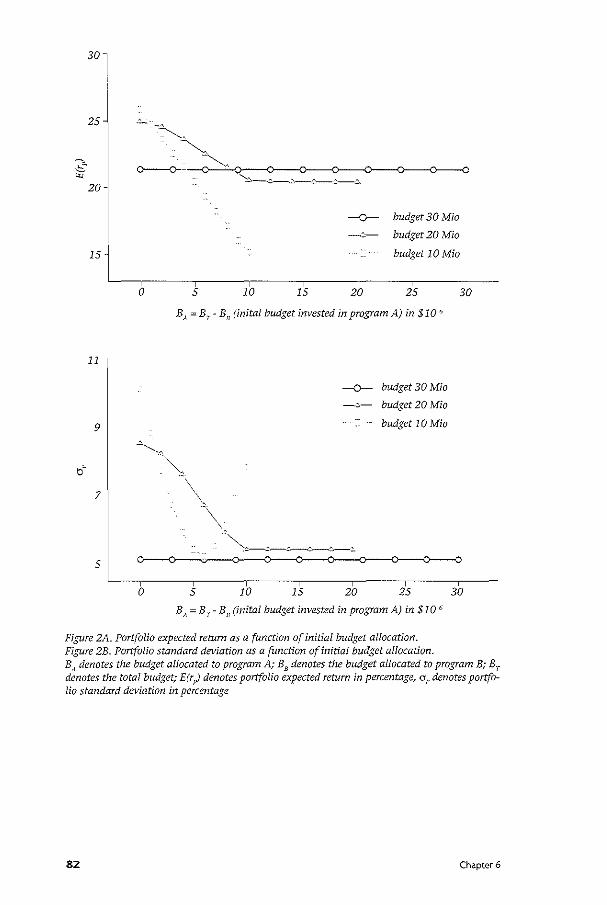
30

25

-o- budget 30 Mia

-:::-- budget 20 Mia

15 budget 10 Mia

0 5 10 15 20 25 30

BA = Br- B8

(inital budget invested in program A) in $10 ~

11

--o- budget 30 Mia

~:,- budget 20 Mia

9 budget 10 Mia

~

b~ -~,

7 -\" -\

.. ~~---~------"-~ 5

0 5 10 15 20 25 30

B,~ = Br- B 8

(inital budget invested in program A) in $10 6

Figure 2A. Portfolio expected return as a function of initial budget allocation. Figure 2B. Portfolio standard deviation as a function of initial budget allocation. B" denotes the budget allocated to program A; BB denotes the budget allocated to program B; Br denotes the total budget; E(r pJ denotes portfolio expected return in percentage, ar denotes portfo­lio standard deviation in percentage

82 Chapter 6

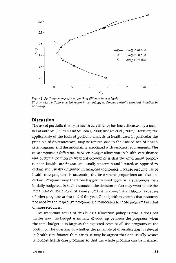
25

23

21 0,/

( 17

15

0 6 7 8

-o- budget 30 Mia

budget 20 Mia

o budget 10 Mia

9 10

Figure 3. Portfolio opportunity set for three different budget levels. E(r ;J denotes portfolio expected return in percentage; aP denotes portfolio standard deviation in percentage

Discussion The use of portfolio theory in health care finance has been discussed by a num­

ber of authors (O'Brien and Sculpher, 2000; Bridges et al., 2002). However, the

applicability of the tools of portfolio analysis in health care, in particular the

prindple of diversification, may be limited due to the limited size of health

care programs and the uncertainty associated with resource requirements. The

most important difference between budget allocation in health care finance

and budget allocation in financial economics is that the investment propor­

tions in health care finance are usually uncertain and limited, as opposed to

certain and usually unlimited in financial economics. Because resource use of

health care programs is uncertain, the investment proportions are also un­

certain. Programs may therefore happen to need more or less resources than initially budgeted. In such a situation the decision-maker may want to use the

remainder of the budget of some programs to cover the additional expenses of other programs at the end of the year. Our algorithm ensures that resources

not used by the respective programs are reallocated to those programs in need of more resources.

An important result of this budget allocation policy is that it does not

matter how the budget is initially divided up between the programs when

the total budget is as large as the expected costs of all the programs in the

portfolio. The question of whether the principle of diversification is relevant

in health care finance then arises. It may be argued that one usually wishes

to budget health care programs so that the whole program can be financed.

Chapter 6 83

However, when the budget corresponds to the expected costs of the portfolio,

there is a 50% chance that we will need more resources, which might already

be seen as an unacceptable figure in practice. But note that there is already no

benefit from diversification anymore at this budget level. The implication for

decision-makers is that the initial budget allocation and hence the principle of

diversification does not matter in these situations.

The applicability of portfolio theory in health care may prove difficult

because of other limitations as well. Information on the correlation of costs

and effects between an intervention and up-stream or down-stream inter­

ventions are usually not available from randomized controlled trials as these

mostly only focus on the intervention of interest. In addition, portfolio the­

ory assumes that programs can be implemented partially (assumes complete

divisibility) and that the return on investment is independent of the size of

the program (constant returns to scale). Partial implementation would imply

that, for example, half of the HN-infected population would be treated with

new medications whereas the other half would get the less effective cheaper

therapy. Such a policy is certainly problematic because of ethical reasons (Ubel

eta!., 1996). Constant return to scales would imply that, for example, buying

radiation equipment to treat cancer patients would be equally cost-effective

when only 10 cancer patients are treated per year compared to 1000 patients.

However, in case of large capital costs, health care programs usually exhibit

an increasing return to scale (Birch and Gafni, 1992). The limitations of the

assumptions of complete divisibility and constant returns to scale are further

described in detail elsewhere (Sendi and A!, 2003; Sendi eta!., 2002; Birch and

Gafni, 1992, 1993; Gafni and Birch, 1993).

In conclusion, the applicability of portfolio methods to improve the risk­

return characteristics of investments in health care is limited to situations

where the available budget is much smaller than the expected costs of the

programs to be funded. The advantage of diversification disappears once the

total budget corresponds to or exceeds the expected costs of the programs in

the portfolio. The development of methods that address the limitations of tra­

ditional portfolio analysis in health care should be a research priority.

84 Chapter 6

85

•cha ter7 A risk-adjusted approach to comparing the return on investment in health care programs

Summary The league table approach to rank ordering health care programs according to

the incremental cost-effectiveness ratio is a common method to guide policy

makers in setting priorities for resource allocation. In the presence of uncer­

tainty, however, ranking programs is complicated by the degree of variability

associated with each program. Confidence intervals for cost-effectiveness ra­

tios may be overlapping. Moreover, confidence intervals may include negative

ratios and the interpretation of negative cost-effectiveness ratios is ambiguous.

We suggest to rank mutually exclusive health care programs according to their

rate of return which is defined as the net monetary benefit over the costs of

the program. However, how does a program with a higher expected return but

higher uncertainty compare to a program with a lower expected return but

lower risk? In the present paper we propose a risk-adjusted measure to compa­

re the return on investment in health care programs. Financing a health care

program is treated as an investment in a risky asset. The risky asset is combined

with a risk-free asset in order to construct a combined portfolio. The weights

attributed to the risk-free and risky assets are chosen in such a manner that all

programs under consideration exhibit the same degree of uncertainty. We can

then compare the performance of the individual programs by constructing a

risk-adjusted league table of expected returns.

86 Chapter 7

Introduction In a league table health care programs are ranked according to their incremen­

tal cost-effectiveness ratio in order to guide prioritization in resource allocati­

on (Chapman eta!., 2000, Drummond et al.,1993, Mason et al.,l993). In the

presence of uncertainty, however, rank ordering programs according to their

cost-effectiveness ratio is complicated by the degree of uncertainty associated

with each program. Confidence intervals of cost-effectiveness ratios for diffe­

rent programs may be overlapping. Moreover, confidence intervals may inclu­

de negative ratios and the interpretation of negative cost-effectiveness ratios is

ambiguous (Briggs and Fenn, 1998). The question of how health care programs

should be ranked when co.sts and effects are uncertain naturally emerges.

O'Brien and Sculpher (2000) recently outlined the concept of portfolio

theory as a method for choosing between health care programs with different

risk-return trade-offs. Decision-makers are assumed to be risk-averse and prefer

higher returns for a given level of risk. In addition, the decision-maker's utility

function is assumed to be strictly concave, i.e. that the indifference curves for

(risk, return) pairs exhibit a diminishing marginal rate of substitution between

reduced risk and increased expected return. Following this approach, one

posits health care programs on the risk-return space and superimposes the

decision-maker's indifference map. Health care programs that lie on a higher­

valued indifference curve (or iso-utility curve) are ranked higher than those

located on a lower-valued indifference curve. This procedure allows one to

rank health care programs, in the presence of uncertainty, according to the

decision-maker's utility function. However, although the authors' approach is

based on sound economic principles, some practical problems arise. First, the

decision-maker's indifference map is difficult to measure in practice. Second,

the authors used the inverse of the cost-effectiveness ratio as their measure

of return. The advantage of using the inverse of the cost-effectiveness ratio

is that it provides a more intuitive meaning to analysts who are used to con­

duct economic evaluations of health care technologies. However, when the

concept of capital allocation across a risky asset (e.g. a health care program)

and a risk-free asset (e.g. time deposits) shall be used, then it is perhaps more

convenient to have a common benchmark which can be used to compare the

return on investments across economic disciplines (e.g. in financial economics

and health care finance). Finally, the concept of diversification assumes that

partial implementation is possible. From an ethical viewpoint, it might be seen

as highly problematic to offer to some patients the newer and better treatment

while others may receive the "old" therapy. Policy makers may therefore want

to implement only one alternative of a set of mutually exclusive programs.

In the present paper we introduce an alternative approach to ranking

mutually exclusive health care programs when costs and effects are uncertain

using standard portfolio theory as developed by Markowitz more than fifty

Chapter 7 87

years ago. In the next section we suggest an alternative measure of return. In

"Capital allocation across a risky and a risk-free asset" we highlight the capital

allocation decision between risky and risk-free assets as a basis for modifying

the risk-return parameters of a portfolio. In "A risk-adjusted measure of per­

formance" we use this prindple to measure portfolio performance and rank

mutually exclusive health care programs. Finally, we conclude by a discussion

of our approach.

Measuring return on investment In portfolio performance evaluation we typically measure return on invest­

ment r as the terminal value of an asset v,.. after a specific time interval sub­

tracted by the amount invested at the beginning of the interval, v;, and then

dividing this difference by the amount invested V1:

v:.- VI r=-­

v, (1)

Intermediate cash flows are typically added to the terminal value. For example,

if we invest $100 in an asset and end up with $110 at the end of the year, then

the return on this investment is ($110-$100)/$100 = 0.1 or 10%. Return on

investment in financial economics is typically expressed in percentages.

Now, let us consider the financing of a health care program as an invest­

ment decision. We denote the amount invested in a program A as C A (the cost

of program A) and the benefits of program A in monetary terms as E}-. where

EA is the health outcome of program A (expressed as quality-adjusted life-years:

QALYs) and f. the decision-maker's willingness to pay for a QALY. We define

return on investment in program A (rA) as:

(2)

Our measure of return is expressed in percentages and therefore builds a bridge

for the comparison of investments in the health care sector with financial in­

vestments. Note that the numerator of the expression (2) is equivalent to the

net monetary benefit (NMB) of program A:

(3)

The net monetary benefit of a program is similar to the net health benefit ap­

proach introduced by Stinnett and Mullahy (1998) with the difference that the

net benefit is expressed in monetary terms rather than health outcomes. Note,

however, that A represents here the decision-maker's willingness to pay for a

QALY and not an incremental QALY. Since we regard the financing of a health

care program as an investment decision, it is perhaps more natural to express

88 Chapter 7

the net benefit of a program on the monetary scale.

In the presence of uncertainty, ranking health care programs according to

the rate of return is complicated by the degree of uncertainty associated with

each program. How does a program with a higher expected return but higher

uncertainty compare to a program with a lower expected return but lower risk?

We will use principles of portfolio theory, in particular the concept of capital

allocation, in order to describe the risk-return trade-off of a portfolio compri­

sing a health care program (i.e. a risky asset) and a risk-free asset.

Capital allocation across a risky and a risk-free asset Portfolio managers usually search for the best possible trade-off between risk

and expected return. An investor typically selects a combination of risk"Y assets

(such as stocks and bonds) and a risk-free asset (such as money market instru­

ments, e.g. time deposits or Treasury bills). The capital allocation decision is

the choice of the proportion of the money to invest in risky assets and risk-free

assets. The financing of a health care program can be seen as an investment in

a risky asset, since costs and effects are uncertain. Denote the risk-free asset as

F and the health care program as A. For a given budget, we invest the propor­

tion yin program A and the proportionl-y in the risk-free asset F. Denote the

return on program A by r"' the expected return on program A by E(r), and its

standard deviation by crA. We denote the risk-free rate of return as r r The rate

of return of the combined portfolio C, denoted r c• is defined as:

(4)

The expected value E(rc) of the complete portfolio's rate of return is

E(r J = yE(r,) + (1 - y)r, = r, + y[E(r)- r J (5)

and the standard deviation of the complete portfolio, denoted oc is

(6)

That is, the standard deviation of the complete portfolio is proportional to

both the standard deviation of the risky asset and the proportion invested in

it. Note that the interpretation of ( 4) is that the rate of return of the complete

portfolio is based on the risk-free rate rF and an expected risk-premium which

depends on E(r)- rF and the decision-maker's exposure to the risky asset (i.e.,

program A), denoted by y.

Let us now look at a numerical example. Consider program A with costs

and effects as described in Table 1. We assume that costs and effects are correla­

ted with p = 0. 7. The expected return on A is E(r) = 9.94% and the standard

Chapter 7 89

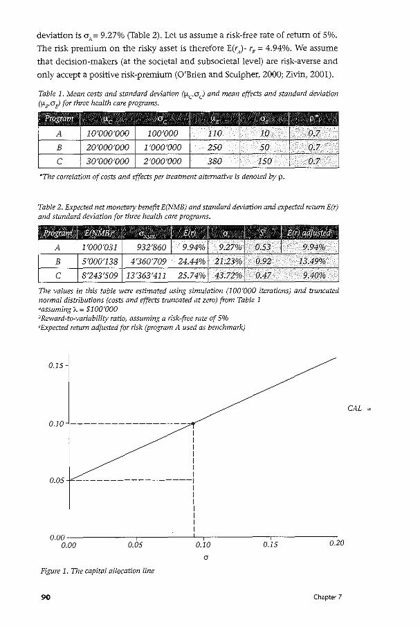
deviation is crA = 9.27% (Table 2). Let us assume a risk-free rate of return of So/o.

The risk premium on the risky asset is therefore E(r)- r, = 4.94%. We assume

that decision-makers (at the societal and subsocietallevel) are risk-averse and

only accept a positive risk-premium (O'Brien and Sculpher, 2000; Zivin, 2001).

Table 1. Mean costs and standard deviation (!-teO c) and mean effects and standard deviation (1-LE'<J£) for three health care programs.

l?iogr;am I !-'c I Clc I !-'e I "'• I p•

! A 1 10'ooo·ooo 100'000 110 10 0.7

B 1 2o·ooo·ooo 1'000'000 250 . so 0.7

c 1 3o·ooo·ooo 2'000'000 380 150 0.7

"The correlation of costs and effects per treatment alternative is denoted by p.

Table 2. Expected net monetary benefit E(NMB) and standard deviation and expected return E(r) and standard deviation for three health care programs.

Biogr;am I E@SIMB)' I O:N\fB E(r) I a, S' E(p) adjusted'

A 1'000'031 932'860 9.94% 9.27% 0.53 9.94%

B 5'000'138 4'360'709 24.44% 21.23% 0.92 13.49%

c 8'243'509 13'363'411 25.74% 43.72% 0.47 9.40%

The values in this table were estimated using simulation (100'000 iterations) and trnncated nonnal distributions (costs and effects truncated at zero) from Table 1 aassuming A = $1 00'000 bReward-to-variability ratio, assuming a risk-free rate of 5% 'Expected return adjusted for risk (program A used as benchmark)

0.15

0.10 -----------------I I I I I I I

0.05 -----------------1 I I I I I I I

o.ooL------,------1.--,------,------o.oo 0.05 0.10 0.15 0.20

Figure 1. The capital allocation line

90 Chapter 7

CAL

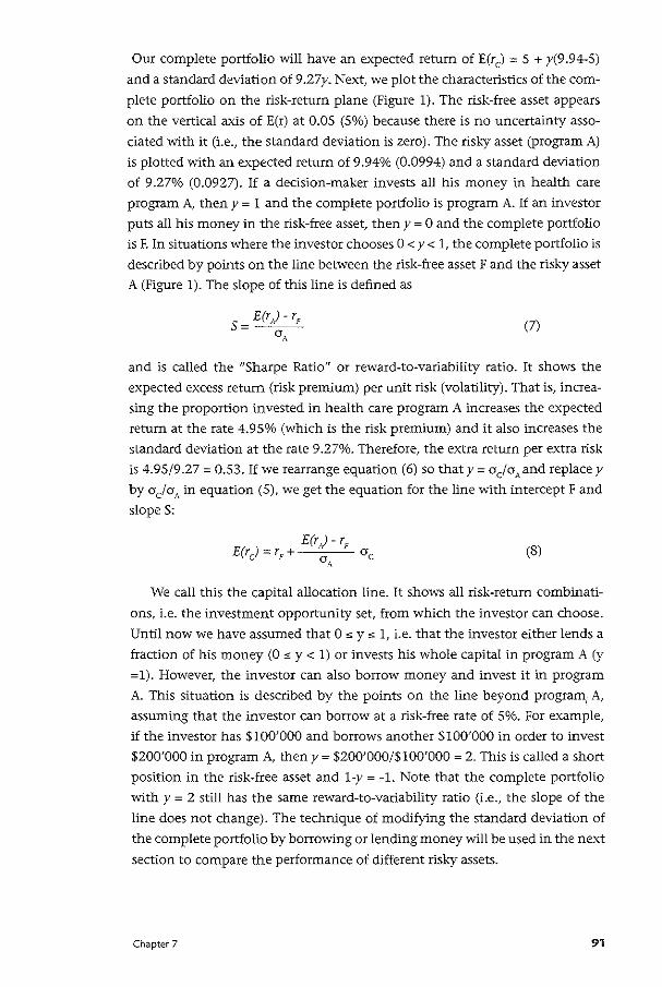
Our complete portfolio will have an expected return of E(rc) = 5 + y(9.94-5)

and a standard deviation of 9 .27y. Next, we plot the characteristics of the com­

plete portfolio on the risk-return plane (Figure 1). The risk-free asset appears

on the vertical axis of E(r) at 0.05 (5o/a) because there is no uncertainty asso­

ciated with it (i.e., the standard deviation is zero). The risky asset (program A)

is plotted with an expected return of 9.94% (0.0994) and a standard deviation

of 9.27% (0.0927). If a decision-maker invests all his money in health care

program A, then y = 1 and the complete portfolio is program A. If an investor

puts all his money in the risk-free asset, then y = 0 and the complete portfolio

is F. In situations where the investor chooses 0 < y < 1, the complete portfolio is

described by points on the line between the risk-free asset F and the risky asset

A (Figure 1). The slope of this line is defined as

5 = E(r)- r,

a A (7)

and is called the "Sharpe Ratio" or reward-to-variability ratio. It shows the

expected excess return (risk premium) per unit risk (volatility). That is, increa­

sing the proportion invested in health care program A increases the expected

return at the rate 4.95% (which is the risk premium) and it also increases the

standard deviation at the rate 9.27%. Therefore, the extra return per extra risk

is 4.95/9.27 = 0.53. If we rearrange equation (6) so that y =a cia., and replace y

by aclaA in equation (5), we get the equation for the line with intercept F and

slopeS:

E(r)- r, E(rJ =r,+ ac a A

(8)

We call this the capital allocation line. It shows all risk-return combinati­

ons, i.e. the investment opportunity set, from which the investor can choose.

Until now we have assumed that 0:::::;; y:::::;; 1, i.e. that the investor either lends a

fraction of his money (0 ~ y < 1) or invests his whole capital in program A (y

=1). However, the investor can also borrow money and invest it in program

A. This situation is described by the points on the line beyond program1 A,

assuming that the investor can borrow at a risk-free rate of 5%. For example,

if the investor has $100'000 and borrows another $100'000 in order to invest

$200'000 in program A, then y = $200'000/$100'000 = 2. This is called a short

position in the risk-free asset and 1-y = -1. Note that the complete portfolio

withy= 2 still has the same reward-to-variability ratio (i.e., the slope of the

line does not change). The technique of modifying the standard deviation of

the complete portfolio by borrowing or lending money will be used in the next

section to compare the performance of different risk-y assets.

Chapter 7 91

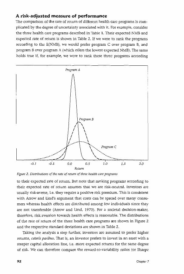
A risk-adjusted measure of performance The comparison of the rate of return of different health care programs is com­

plicated by the degree of uncertainty associated with it. For example, consider

the three health care programs described in Table 1. Their expected NMB and

expected rate of return is shown in Table 2. If we were to rank the programs

according to the E(NMB), we would prefer program C over program B, and

program B over program A (which offers the lowest expected NMB). The same

holds true if, for example, we were to rank these three programs according

-0.1 -0.5

Program A

Program B .... I \

\ / \ I \

I \ I ...... \ .. ·· .....

I·" \~',, Program C

0.0 0.5

Return

\ · .. \ ·· ... ' ·· ..

........ ~------

1.0

Figure 2. Distributions of the rate of return of three health care programs

1.5 2.0

to their expected rate of return. But note that ranking programs according to

their expected rate of return assumes that we are risk-neutral. Investors are

usually risk-averse, i.e. they require a positive risk premium. This is consistent

with Arrow and Lind's argument that costs can be spread over many consu­

mers whereas health effects are distributed among few individuals since they

are not transferable (Arrow and Lind, 1970). For a societal decision-maker,

therefore, risk aversion towards health effects is reasonable. The distributions

of the rate of return of the three health care programs are shown in Figure 2

and the respective standard deviations are shown in Table 2.

Taking the analysis a step further, investors are assumed to prefer higher

returns, ceteris paribus. That is, an investor prefers to invest in an asset with a

steeper capital allocation line, i.e. more expected returns for the same degree

of risk. We can therefore compare the reward-to-variability ratios (or Sharpe

92 Chapter 7

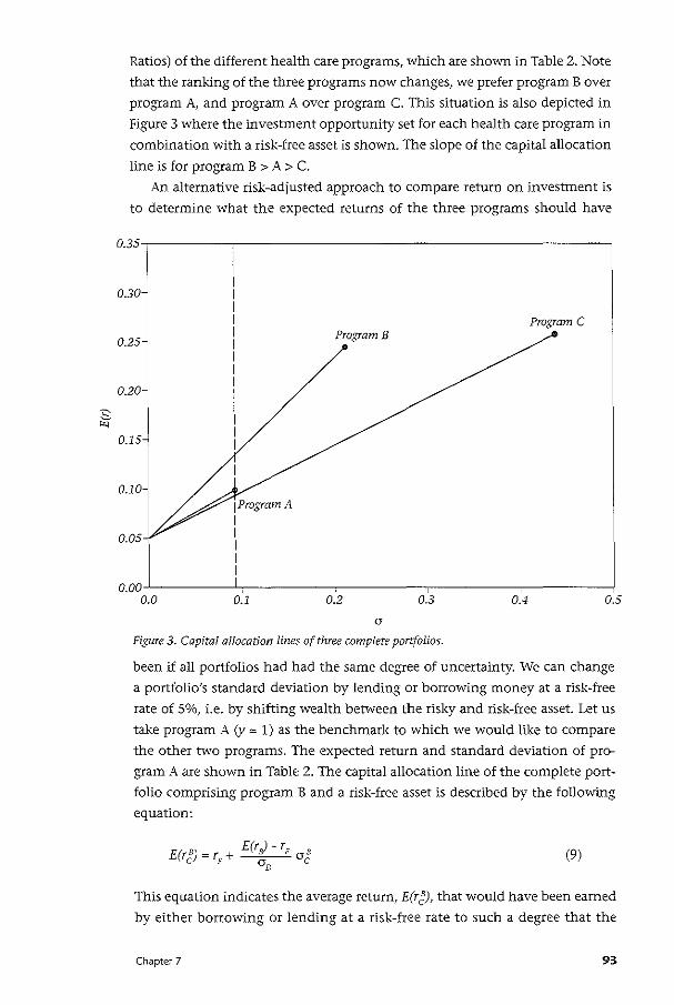
:s "-'

Ratios) of the different health care programs, which are shown in Table 2. Note

that the ranking of the three programs now changes, we prefer program B over

program A, and program A over program C. This situation is also depicted in

Figure 3 where the investment opportunity set for each health care program in

combination with a risk-free asset is shown. The slope of the capital allocation

line is for program B > A > C.

An alternative risk-adjusted approach to compare return on investment is

to determine what the expected returns of the three programs should have

0.35

0.30

0.25

0.20

0.15

0.10-

0.05

0.00 0.0

1ProgramA I I I I I

0.1

Program B

0.2 0.3

a

Figure 3. Capital allocation lines of three complete portfolios.

Program C

0.4 0.5

been if all portfolios had had the same degree of uncertainty. We can change

a portfolio's standard deviation by lending or borrowing money at a risk-free

rate of So/o, i.e. by shifting wealth between the risky and risk-free asset. Let us

take program A (y = 1) as the benchmark to which we would like to compare

the other two programs. The expected return and standard deviation of pro­

gram A are shown in Table 2. The capital allocation line of the complete port­

folio comprising program B and a risk-free asset is described by the following

equation:

(9)

This equation indicates the average return, E(r~), that would have been earned

by either borrowing or lending at a risk-free rate to such a degree that the

Chapter 7 93

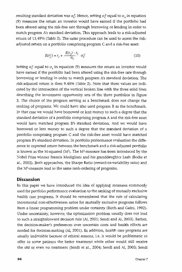
resulting standard deviation was ar Hence, setting ag equal to (JAin equation

(9) measures the return an investor would have earned if the portfolio had

been altered using the risk-free rate through borrowing or lending in order to

match program A's standard deviation. This approach leads to a risk-adjusted

return of 13.49% (Table 2). The same procedure can be used to assess the risk­

adjusted return on a portfolio comprising program C and a risk-free asset:

E(r '- r E(rc) = r + <Y F a c

c F Oc C (10)

Setting of equal to a A in equation (9) measures the return an investor would

have earned if the portfolio had been altered using the risk-free rate through

borrowing or lending in order to match program A's standard deviation. The

risk-adjusted return is then 9.40o/o (Table 2). Note that these values are indi­

cated by the intersection of the vertical broken line with the three solid lines

describing the investment opportunity sets of the three portfolios in Figure

3. The choice of the program serving as a benchmark does not change the

ranking of programs. We could have also used program B as the benchmark.

In that case we would have borrowed or lent money to such a degree that the

standard deviation of a portfolio comprising program A and the risk-free asset

would have matched program B's standard deviation. And we would have

borrowed or lent money to such a degree that the standard deviation of a

portfolio comprising program C and the risk-free asset would have matched

program B's standard deviation. In portfolio performance evaluation the diffe­

rence in expected return between the benchmark and a risk-adjusted portfolio

is known as theM-squared (M2). The M'-measure has been introduced by the

Nobel Prize winner Francis Modigliani and his granddaughter Leah (Bodie et

al., 2002). Both approaches, the Sharpe Ratio (reward-to-variability ratio) and

the M'-measure lead to the same rank-ordering of programs.

Discussion In this paper we have introduced the idea of applying measures commonly

used for portfolio performance evaluation to the ranking of mutually exclusive

health care programs. It should be remembered that the rule of calculating

incremental cost-effectiveness ratios for mutually exclusive programs follows

from a linear programming problem under certainty (Birch and Gafni, 1992).

Under uncertainty, however, the optimization problem usually does not lead

to such a straightforward decision rule (Al, 2001; Sendi and Al, 2003). Rather,

the decision-maker's preferences over uncertain costs and health effects are

needed for decision-making (Al, 2001). In addition, health care programs are

usually indivisible because of ethical reasons, i.e. it would be problematic to

offer to some patients the better treatment while other would still receive

the old or even no treatment (Sendi et al., 2004; Sendi and Al, 2003; Sendi

94 Chapter 7

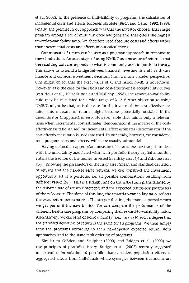
et al., 2002). In the presence of indivisibility of programs, the calculation of

incremental costs and effects becomes obsolete (Birch and Gafni, 1992,1993).

Finally, the premise in our approach was that the investor chooses that single

program among a set of mutually exclusive programs that offers the highest

reward-to-variability ratio. We therefore used absolute costs and effects rather

than incremental costs and effects in our calculations. Our measure of return can be seen as a pragmatic approach in response to

these limitations. An advantage of using NMB/C as a measure of return is that

the resulting unit corresponds to what is commonly used in portfolio theory.

This allows us to build a bridge between financial investments and health care

finance and consider investment decisions from a much broader perspective.

One might object that the exact value of 'A, and hence NMB, is not known.

However, as is the case for the NMB and cost-effectiveness acceptability curves

(van Hout et al., 1994; Stinnett and Mullahy, 1998), the reward-to-variability

ratio may be calculated for a wide range of A. A further objection to using

NMB/C might be that, as is the case for the inverse of the cost-effectiveness

ratio, this measure of return might become potentially unstable if the

denominator C approaches zero. However, note that this is only a relevant

issue when incremental cost estimates (denominator if the inverse of the cost­

effectiveness ratio is used) or incremental effect estimates (denominator if the

cost-effectiveness ratio is used) are used. In our study, however, we considered

total program costs and effects, which are usually substantial.

Having defined an appropriate measure of return, the next step is to deal

with the uncertainty associated with it. ln portfolio theory capital allocation

entails the fraction of the money invested in a risky asset (y) and risk-free asset

(1-y). Knowing the parameters of the risky asset (mean and standard deviation

of return) and the risk-free asset (return), we can construct the investment

opportunity set of a portfolio, i.e. all possible combinations resulting from

different values for y. This is a straight line on the risk-return plane defined by

the risk-free rate of return (intercept) and the expected return-risk parameters

of the risky asset. The slope of this line, the reward-to-variability ratio, reflects

the extra return per extra risk. The steeper the line, the more expected return

we get per unit increase in risk. We can compare the performance of the

different health care programs by comparing their reward-to-variability ratios.

Alternatively, we can lend or borrow money (i.e., vary y) to such a degree that

the standard deviation of return is the same for all programs. We then simply

rank the programs according to their risk-adjusted expected return. Both

approaches lead to the same rank ordering of programs.

Similar to O'Brien and Sculpher (2000) and Bridges et al. (2002) we

use principles of portfolio theory. Bridges et al. (2002) recently suggested

an extended formulation of portfolio that considers population effects as

aggregated effects from individuals where synergies between treatments are

Chapter 7 95

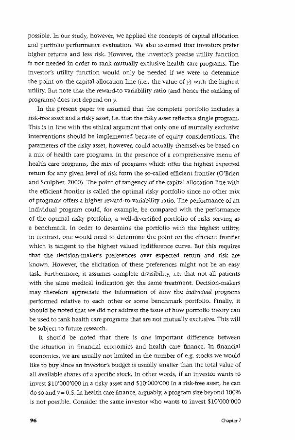
possible. ln our study, however, we applied the concepts of capital allocation

and portfolio performance evaluation. We also assumed that investors prefer

higher returns and less risk. However, the investor's precise utility function

is not needed in order to rank mutually exclusive health care programs. The

investor's utility function would only be needed if we were to determine

the point on the capital allocation line (i.e., the value of y) with the highest

utility. But note that the reward-to variability ratio (and hence the ranking of

programs) does not depend on y.

In the present paper we assumed that the complete portfolio includes a

risk-free asset and a risky asset, i.e. that the risky asset reflects a single program.

This is in line with the ethical argument that only one of mutually exclusive

interventions should be implemented because of equity considerations. The

parameters of the risky asset, however, could actually themselves be based on

a mix of health care programs. In the presence of a comprehensive menu of

health care programs, the mix of programs which offer the highest expected

return for any given level of risk form the so-called efficient frontier (O'Brien

and Sculpher, 2000). The point of tangency of the capital allocation line with

the efficient frontier is called the optimal risky portfolio since no other mix

of programs offers a higher reward-to-variability ratio. The performance of an

individual program could, for example, be compared with the performance

of the optimal risky portfolio, a well-diversified portfolio of risks serving as

a benchmark. In order to determine the portfolio with the highest utility,

in contrast, one would need to determine the point on the efficient frontier

which is tangent to the highest valued indifference curve. But this requires

that the decision-maker's preferences over expected return and risk are

known. However, the elicitation of these preferences might not be an easy

task. Furthermore, it assumes complete divisibility, i.e. that not all patients

with the same medical indication get the same treatment. Dedsion-makers

may therefore appreciate the information of how the individual programs

performed relative to each other or some benchmark portfolio. Finally, it

should be noted that we did not address the issue of how portfolio theory can

be used to rank health care programs that are not mutually exclusive. This will

be subject to future research.

It should be noted that there is one important difference between

the situation in financial economics and health care finance. In financial

economics, we are usually not limited in the number of e.g. stocks we would

like to buy since an investor's budget is usually smaller than the total value of

all available shares of a specific stock. In other words, if an investor wants to

invest $10'000'000 in a risb:y asset and $10'000'000 in a risk-free asset, he can

do so andy= 0.5. In health care finance, arguably, a program size beyond lOOo/o

is not possible. Consider the same investor who wants to invest $10'000'000

96 Chapter 7

in health care program A and $10'000'000 in a risk-free asset. Since the cost

of program A is normally distributed (with mean $10'000'000 and standard

deviation $100'000), there is a 50% chance that the cost of program A will

be lower than $10'000'000. That is, we may not end up investing the total

amount of $10'000'000 in program A. In other words, the fraction invested

in program A (the risky asset) is itself subject to a distribution, which depends

on the cost of program A. If the cost of program A, CA, happens to be more

than $10'000'000, then y = 0.5. If CA happens to be less than $10'000'000,

theny= C)$20'000'000. On the other hand, if we had $1'000'000 and wanted

to completely finance program A, we could borrow at a risk-free rate and y =

C_j$1'000'000. Since CA is uncertain, y is also subject to a distribution. In that

case we will most likely end up with a short position in the risk-free asset.

However, the fact that y is subject to a distribution in health care finance does

not affect the relevance of the analysis for ranking health care programs. Note

that although the value of y may be uncertain, the reward-to-variability ratio

is not, since the slope S of the capital allocation line as defined in (7) does not

include y.

An interesting approach for including risk in league tables has recently

been suggested by Hutubessy et al. (2001). The probability of inclusion in

the optimal mix of programs for different budget levels is then displayed in a

so-called expansion path. However, the authors' approach is different in the

sense that they provide the probability of an intervention being chosen in

the optimal mix of programs in the presence of uncertainty. Our approach,

in contrast, borrows methods from financial economics and takes a standard

approach for risk-adjusting the returns from an investment.

In conclusion, we believe that methods developed in financial economics

offer a valuable source of knowledge for dealing with uncertainty in health

care finance. Measuring return on investment is a natural approach to rank

ordering health care programs. In the presence of uncertainty, risk-adjusted

expected returns may be helpful to guide policy and decision makers in setting

priorities for resource allocation.

Chapter 7 97

• ella ter 8 Cost-effectiveness of highly active antiretroviral therapy in HIV-infected

patients

Summary Background: Highly active antiretroviral therapy (HAART) has become the most

important strategy for treating HIV-infection in developed countries. However,

access to HAART might vary under different funding policies. The Swiss health

care system provides unrestricted access to HAART for all patients who need

these newer combination therapies. This study investigated the impact of this

funding policy on the society and health care system.

Methods: A cost-effectiveness analysis with natural history data and producti­

vity estimates was based on the Swiss HIV Cohort Study. A random sample of

patient charts was used to estimate health care costs. In addition to a base-case

scenario, a pessimistic and an optimistic scenario of natural disease history

was developed. Costs were expressed in 1997 Swiss Francs (100 CHF corres­

pond to about 43 £)and effects as projected years of life gained.

Results: In the analysis limited to health care costs, on the basis of projected

survival in each scenario, the cost effectiveness ratio was CHF 33,000 (base­

case), CHF 14,000 (optimistic), and CHF 45,000 (pessimistic) per year of life

gained. When changes in productivity were included, cost savings occurred

in the base-case and optimistic scenarios. The cost effectiveness ratio was CHF

11,000 per year of life gained in the pessimistic scenario.

Conclusions: HAART increases expected survival and health care costs. Howe­

ver, when productivity gains are included, society vvill probably save costs or

pay a low price for substantial health benefits. The study provides strong argu­

ments, from a societal perspective, to continue the current policy of providing

unrestricted access to HAART in Switzerland. The presented results also suggest

that this policy could be of interest for other developed countries. Decision

makers in developed countries where access to HAART is limited should re­

evaluate their policy for the benefit of the society at large.

98 Chapter 8

Introduction Highly active antiretroviral therapy (HAART) reduces morbidity and mortality

in individuals infected with HIV (Palella et al., 1998; Egger et al., 1997). In

developed countries, antiretroviral three-drug regimens including a proteinase

inhibitor have become the recommended standard for treating HIV-positive

patients (CDC, 1998). Although substantial health care resources are used to

fund the widespread use of these newer combination therapies (Perdue et al.,

1998), the acquisition costs for HAART may be offset by a decline of expen­

sive in-patient care, increased quality of life, and increased job productivity

as a consequence of a decline in morbidity and mortality Oohannesson and Meltzer, 1998). The Swiss health care system, because of equity considerations,

provides unrestricted access to all necessary medications and medical proce­

dures in HIV-positive patients. This funding policy allows the consequences of

providing HAART to all patients in need of this potent antiretroviral regimen

to be estimated within a setting without eligibility restrictions for basic health

care. This study illustrates the consequences of a health care policy that might

be of interest for other developed countries.

The cost effectiveness analysis was conducted from both the Swiss sode­

tal and health care perspectives. The societal perspective is the most relevant

since it captures the important effects of HAART on costs outside the health

care system (Drummond et al., 1997). If HAART is found to be desirable from

a societal perspective, the health care perspective informs about the eventu­

al resources required to fund this program (Birch and Gafni, 1992). In times

of scarcity of health care resources, this information is valuable, since policy

makers could then identify and cancel less-efficient programs to guarantee the

widespread use of HAART without exceeding a given budget.

Methods This cost effectiveness analysis was performed on the basis of data extracted

from the Swiss HIV Cohort Study (SHCS) (Ledergerber et al., 1994). The SHCS

is one of the world largest cohort studies on HIV disease with over 9000 en­

rolled patients since 1988. Patients have regular follow-up visits every six

months. The mean age of patients enrolled in the SHCS is 33 years. This was

the starting age of an HIV-infected individual used in our analysis.

In Switzerland, HAART was introduced in1996 (Egger et al., 1997). In the

presented analysis a cohort of HIV-infected patients receiving HAART was used

that reflected the SHCS during the period 1996-1997. This cohort was stratified

by CD4-cell count and histoty of an AIDS-defining disease, as defined by the

European classification of AIDS (Ancelle-Park et al., 1995). The strategy of pro­

viding HAART was compared with the strategy of providing no antiretroviral

therapy (NART). Therapy regimens other than HAART are no longer recom­

mended (CDC, 1998) and the NART as a comparison strategy demonstrates the

Chapter 8 99

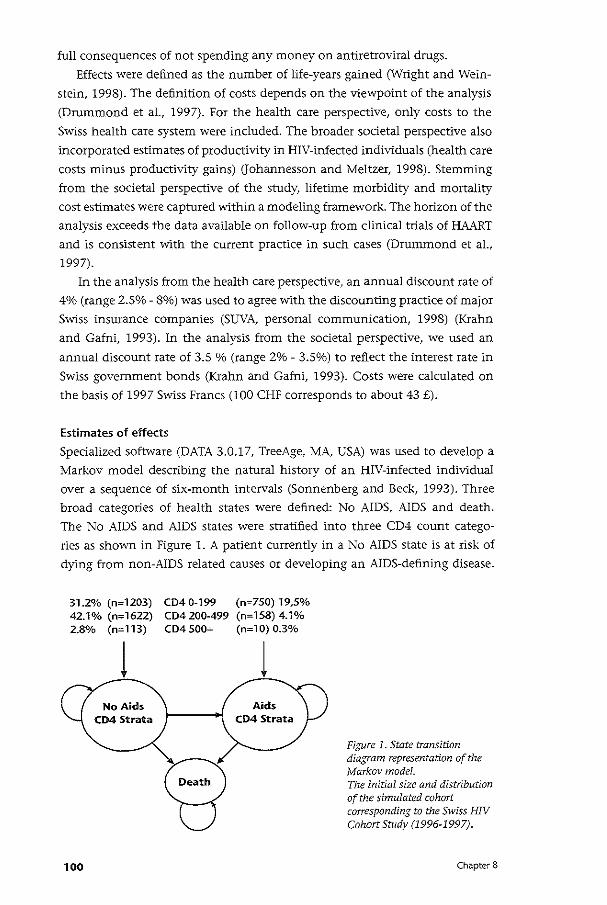
full consequences of not spending any money on antiretroviral drugs.

Effects were defined as the number of life-years gained (Wright and Wein­

stein, 1998). The definition of costs depends on the viewpoint of the analysis

(Drummond et al., 1997). For the health care perspective, only costs to the

Swiss health care system were included. The broader societal perspective also

incorporated estimates of productivity in HIV-infected individuals (health care

costs minus productivity gains) (Johannessen and Meltzer, 1998). Stemming

from the societal perspective of the study, lifetime morbidity and mortality

cost estimates were captured within a modeling framework. The horizon of the

analysis exceeds the data available on follow-up from clinical trials of HAART

and is consistent with the current practice in such cases (Drummond et al.,

1997).

In the analysis from the health care perspective, an annual discount rate of

4% (range 2.5%- 8%) was used to agree with the discounting practice of major

Swiss insurance companies (SUVA, personal communication, 1998) (Krahn

and Gafni, 1993). In the analysis from the societal perspective, we used an

annual discount rate of 3.5 % (range 2%- 3.5%) to reflect the interest rate in

Swiss government bonds (Krahn and Gafni, 1993). Costs were calculated on

the basis of 1997 Swiss Francs (100 CHF corresponds to about 43 £).

Estimates of effects

Specialized software (DATA 3.0.17, TreeAge, MA, USA) was used to develop a

Markov model describing the natural history of an HIV-infected individual

over a sequence of six-month intervals (Sonnenberg and Beck, 1993). Three

broad categories of health states were defined: No AIDS, AIDS and death.

The No AIDS and AIDS states were stratified into three CD4 count catego­

ries as shown in Figure 1. A patient currently in a No AIDS state is at risk of

dying from non-AIDS related causes or developing an AIDS-defining disease.

31.2% (n= 1203) 42.1% (n=1622) 2.8% (n= 113)

100

CD4 0-199 (n=750) 19,5% CD4200-499 (n=158) 4.1% CD4 500+ (n= 1 0) 0.3%

Figure 1. State transition diagram representation of the Markov modeL The initial size and distribution of the simulated cohort corresponding to the Swiss HIV Cohort Study (1996-1997).

Chapter 8

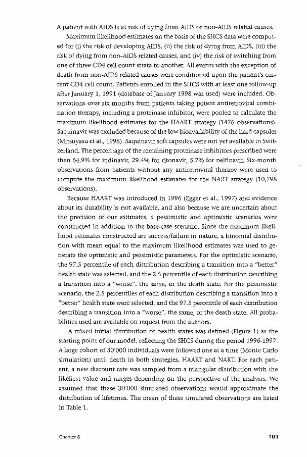
A patient with AJDS is at risk of dying from AIDS or non-AIDS related causes.

Maximum likelihood estimates on the basis of the SHCS data were comput­

ed for (i) the risk of developing AIDS, (ii) the risk of dying from AIDS, (iii) the

risk of dying from non-AIDS related causes, and (iv) the risk of switching from

one of three CD4 cell count strata to another. All events with the exception of

death from non-AIDS related causes were conditioned upon the patient's cur­

rent CD4 cell count. Patients enrolled in the SHCS with at least one follow-up

after January 1, 1991 (database of January 1998 was used) were included. Ob­

servations over six months from patients taking potent antiretroviral combi­

nation therapy, including a proteinase inhibitor, were pooled to calculate the

maximum likelihood estimates for the HAART strategy (1476 observations).

Saquinavir was excluded because of the low bioavailability of the hard capsules

(Mitsuyasu eta!., 1998). Saquinavir soft capsules were not yet available in Swit­

zerland. The percentage of the remaining proteinase inhibitors prescribed were

then 64.9% for indinavir, 29.4% for ritonavir, 5.7% for nelfinavir. Six-month

observations from patients without any antiretroviral therapy were used to

compute the maximum likelihood estimates for the NART strategy (10,798

observations).

Because HAART was introduced in 1996 (Egger eta!., 1997) and evidence

about its durability is not available, and also because we are uncertain about

the precision of our estimates, a pessimistic and optimistic scenarios were

constructed in addition to the base-case scenario. Since the maximum likeli­

hood estimates constructed are success/failure in nature, a binomial distribu­

tion with mean equal to the maximum likelihood estimates was used to ge­

nerate the optimistic and pessimistic parameters. For the optimistic scenario,

the 97.5 percentile of each distribution describing a transition into a "better"

health state was selected, and the 2.5 percentile of each distribution describing

a transition into a "worse", the same, or the death state. For the pessimistic

scenario, the 2.5 percentiles of each distribution describing a transition into a

"better" health state were selected, and the 97.5 percentile of each distribution

describing a transition into a "worse", the same, or the death state. All proba­

bilities used are available on request from the authors.

A mixed initial distribution of health states was defined (Figure 1) as the

starting point of our model, reflecting the SHCS during the period 1996-1997.

A large cohort of 30'000 individuals were followed one at a time (Monte Carlo

simulation) until death in both strategies, HAART and NART. For each pati­

ent, a new discount rate was sampled from a triangular distribution with the

likeliest value and ranges depending on the perspective of the analysis. We

assumed that these 30'000 simulated observations would approximate the

distribution of lifetimes. The mean of these simulated observations are listed

in Table 1.

Chapter 8 101

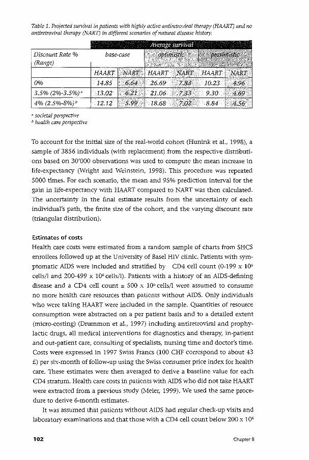
Table 1. Projected survival in patients with highly active antiretroviral therapy (HAART) and no antiretroviral therapy (NARY) in different scenarios of natural disease history.

a societal perspective v health care perspective

To account for the initial size of the real-world cohort (Hunink et al., 1998), a

sample of 3856 individuals (with replacement) from the respective distributi­

ons based on 30'000 observations was used to compute the mean increase in

life-expectancy (Wright and Weinstein, 1998). This procedure was repeated

5000 times. For each scenario, the mean and 95o/o prediction interval for the

gain in life-expectancy with HAART compared to NART was then calculated.

The uncertainty in the final estimate results from the uncertainty of each

individual's path, the finite size of the cohort, and the varying discount rate

(triangular distribution).

Estimates of costs

Health care costs were estimated from a random sample of charts from SHCS

enrollees followed up at the University of Basel HIV clinic. Patients with sym­

ptomatic AIDS were included and stratified by CD4 cell count (0-199 x 106

cells/! and 200-499 x 106 cells/!). Patients with a history of an AIDS-defining

disease and a CD4 cell count 2: 500 x 106 cells/l were assumed to consume

no more health care resources than patients without AIDS. Only individuals

who were taking HAART were included in the sample. Quantities of resource

consumption were abstracted on a per patient basis and to a detailed extent

(micro-costing) (Drummon et al., 1997) including antiretroviral and prophy­

lactic drugs, all medical interventions for diagnostics and therapy, in-patient

and out-patient care, consulting of specialists, nursing time and doctor's time.

Costs were expressed in 1997 Swiss Francs (100 CHF correspond to about 43

£) per six-month of follow-up using the Swiss consumer price index for health

care. These estimates were then averaged to derive a baseline value for each

CD4 stratum. Health care costs in patients with AIDS who did not take HAART

were extracted from a previous study (Meier, 1999). We used the same proce­

dure to derive 6-month estimates.

It was assumed that patients without AIDS had regular check-up visits and

laboratory examinations and that those with a CD4 cell count below 200 x 106

102 Chapter 8

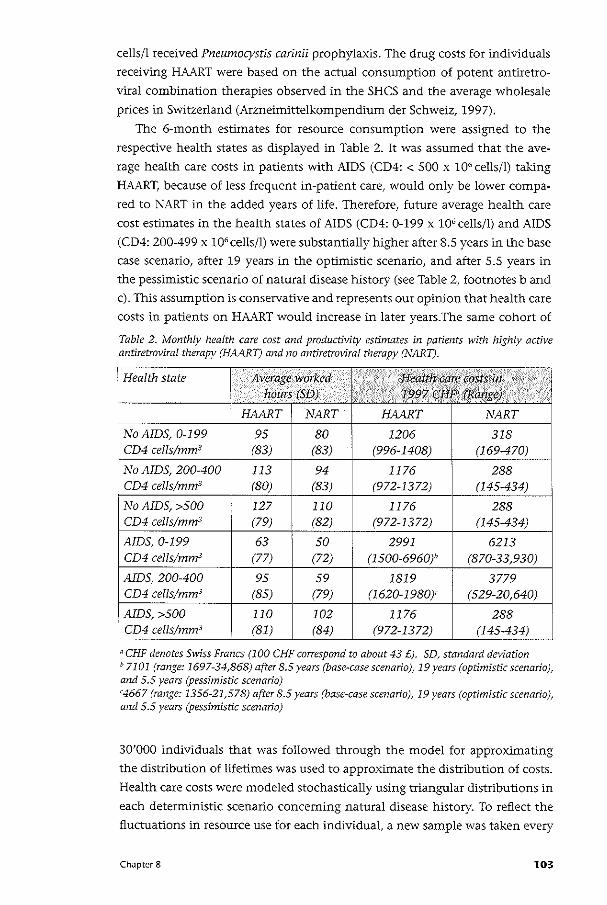
cells/l received Pneumocystis carinii prophylaxis. The drug costs for individuals

receiving HAART were based on the actual consumption of potent antiretro­

viral combination therapies observed in the SHCS and the average wholesale

prices in Switzerland (Arzneimittelkompendium der Schweiz, 1997).

The 6-month estimates for resource consumption were assigned to the

respective health states as displayed in Table 2. It was assumed that the ave­

rage health care costs in patients with AIDS (CD4: < 500 x 106 cells/!) taking

HAART, because of less frequent in-patient care, would only be lower compa­

red to NART in the added years of life. Therefore, future average health care

cost estimates in the health states of AIDS (CD4: 0-199 x 106 cells/l) and AIDS

(CD4: 200-499 x 106 cells/l) were substantially higher after 8.5 years in the base

case scenario, after 19 years in the optimistic scenario, and after 5.5 years in

the pessimistic scenario of natural disease history (see Table 2, footnotes b and

c). This assumption is conservative and represents our opinion that health care

costs in patients on HAART would increase in later years.The same cohort of

Table 2. Monthly health care cost and productivity estimates in patients with highly active antiretroviral therapy (HAART) and no antiretroviral therapy (NARY).

Health state Average worked I /<·· H¢altf1 c~re cost;5in ·•··. . '

hours (SD) 1997 t:;Hf'Jf(Range).

HAART NART HAART NART

No AIDS, 0-199 95 80 1206 318 CD4 cells/mm3 (83) (83) (996-1408) (169-470)

No AIDS, 200-400 113 94 1176 288 CD4 cells/mm3 (80) (83) (972-1372) (145-434) !

No AIDS, >500 127 110 1176 288 CD4 cells/mm3 ' (79) (82) (972-1372) (145-434)

AIDS, 0-199 63 !

50 2991 6213 CD4 cells/mm3 (77) (72) (1500-6960)" (870-33,930)

AlDS, 200-400 95 59 1819 3779 CD4 cells/mm3 (85) (79) (1620-1980)' (529-20,640)

I AlDS, >500 110 102 1176 288 CD4 cells/mm3 (81) (84) (972-1372) (145-434)

"CHF denotes Swiss Francs (100 CHF correspond to about 43 £). SD, standard deviation & 7101 (range: 1697-34,868) after 8.5 years (base-case scenario), 19 years (optimistic scenario), and 5.5 years (pessimistic scenario) '4667 (range: 1356-21,578) after 8.5 years (base-case scenario), 19 years (optimistic scenario), and 5.5 years (pessimistic scenario)

30'000 individuals that was followed through the model for approximating

the distribution of lifetimes was used to approximate the distribution of costs.

Health care costs were modeled stochastically using triangular distributions in

each deterministic scenario concerning natural disease history. To reflect the

fluctuations in resource use for each individual, a new sample was taken every

Chapter 8 103

six months until the patient entered the death state. Since our cost estimates

were derived from patients followed at the University of Basel HIV clinic, all

samples for costs were multiplied by 0.86 (range: 0.83-0.88) to adjust for the

average resource use in Switzerland (Meier, 1999). On this basis, the lifetime

estimates for consumption of health care resources were computed as shown

in Table 3.

Productivity changes were included in the analysis from the societal per­

spective. In an analysis from the societal perspective, all costs are considered

(Drummond eta!., 1997). Costs other than productivity changes are conside­

red to be negligible in this analysis. The SHCS database contains detailed in­

formation on the ability to work and the number of worked hours per month.

The ability to work (a value between Oo/o and 100%) does not reflect the actual

productivity of an individual. Consequently, the average number of hours

worked in a specific health state was extracted to derive the true estimates for

productivity. We computed separate estimates for patients with HAART and

NART (Table 2). These turned out to approximate a normal distribution.

Again, the same cohort of 30'000 patients used for health care costs was

followed through the model, one at a time, to approximate the distribution

of productivity over a lifetime. To reflect fluctuations in productivity, every 6

months a new sample for the number of worked hours was taken. This value

was then multiplied by 25 (range: 20- 31) which is the average hourly income

in Swiss Francs (Ledergerber et a!., 1998; Bundesamt fur Statistik, 1997). The

means of these distributions are shown in Table 3..

Table 3. Projected health care cost and productivity estimates in patients with highly active antiretroviral therapy (HAART) and no antiretroviral therapy (NART) in different scenarios of natural disease history.

base-case

" societal perspective b health care perspective 'CHF denotes Swiss Francs (CHF 100 correspond to about £43).

104 Chapter 8

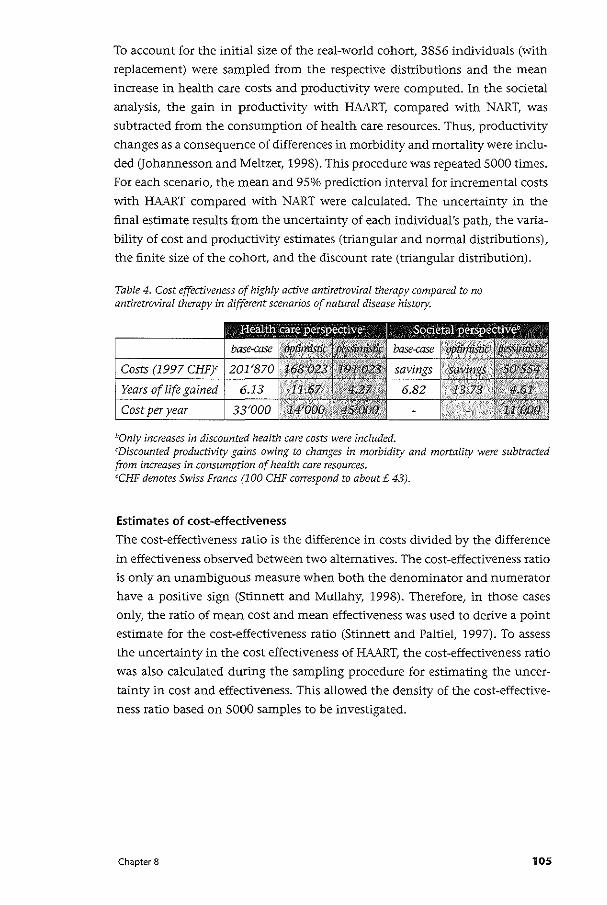
To account for the initial size of the real-world cohort, 3856 individuals (with

replacement) were sampled from the respective distributions and the mean

increase in health care costs and productivity were computed. In the societal

analysis, the gain in productivity with HAART, compared with NART, was

subtracted from the consumption of health care resources. Thus, productivity

changes as a consequence of differences in morbidity and mortality were inclu­

ded (Johannesson and Meltzer, 1998). This procedure was repeated 5000 times.

For each scenario, the mean and 95% prediction interval for incremental costs

with HAART compared with NART were calculated. The uncertainty in the

final estimate results from the uncertainty of each individual's path, the varia­

bility of cost and productivity estimates (triangular and normal distributions),

the finite size of the cohort, and the discount rate (triangular distribution).

Table 4. Cost effectiveness of highly active antiretroviral therapy compared to no antiretroviral therapy in different scenarios of natural disease history.

00nly increases in discounted health care costs were included. 'Discounted productivity gains owing to changes in morbidity and mortality were subtracted from increases in consumption of health care resources. 'CHF denotes Swiss Francs (100 CHF correspond to about£ 43).

Estimates of cost-effectiveness

The cost-effectiveness ratio is the difference in costs divided by the difference

in effectiveness observed between two alternatives. The cost-effectiveness ratio

is only an unambiguous measure when both the denominator and numerator

have a positive sign (Stinnett and Mullahy, 1998). Therefore, in those cases

only, the ratio of mean cost and mean effectiveness was used to derive a point

estimate for the cost-effectiveness ratio (Stinnett and Paltiel, 1997). To assess

the uncertainty in the cost effectiveness of HMRT, the cost-effectiveness ratio

was also calculated during the sampling procedure for estimating the uncer­

tainty in cost and effectiveness. This allowed the density of the cost-effective­

ness ratio based on 5000 samples to be investigated.

Chapter 8 105

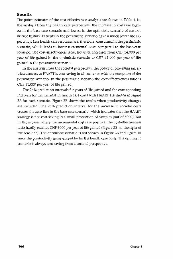
Results The point estimates of the cost-effectiveness analysis are shown in Table 4. In

the analysis from the health care perspective, the increase in costs are high­

est in the base-case scenario and lowest in the optimistic scenario of natural

disease history. Patients in the pessimistic scenario have a much lower life ex­

pectancy. Less health care resources are, therefore, consumed in the pessimistic

scenario, which leads to lower incremental costs compared to the base-case

scenario. The cost-effectiveness ratio, however, increases from CHF 14,000 per

year of life gained in the optimistic scenario to CHF 45,000 per year of life

gained in the pessimistic scenario.

In the analysis from the societal perspective, the policy of providing unres­

tricted access to HAART is cost saving in all scenarios with the exception of the

pessimistic scenario. In the pessimistic scenario the cost-effectiveness ratio is

CHF 11,000 per year of life gained.

The 95% prediction intervals for years of life gained and the corresponding

intervals for the increase in health care costs with HAART are shovm in Figure

2A for each scenario. Figure 2B shows the results when productivity changes

are included. The 95% prediction interval for the increase in societal costs

crosses the zero-line in the base-case scenario, which indicates that the HAART

strategy is not cost saving in a small proportion of samples (out of 5000). But

in those cases where the incremental costs are positive, the cost-effectiveness

ratio hardly reaches CHF 5000 per year of life gained (Figure 3B, to the right of

the zero-line). The optimistic scenario is not shown in Figure ZB and Figure 3B

since the productivity gains exceed by far the health care costs. The optimistic

scenario is always cost saving from a societal perspective.

106 Chapter 8

-~

-~

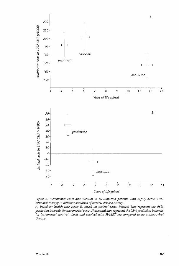
220~ A

210

T 200

190-J

180 t base-case T '

optimist

770

760

pessimistic

750

3 4 5 6 7 8 9 70 77 12 73

Years of life gained

::J + ~~. pessimistic 30

1

B

20"

70

o+--------------+-------------------------7 0

-20-i

-30 base-case

-40

3 4 5 6 7 8 9 70 7 7 12 13

Years of life gained

Figure 2. Incremental costs and survival in HIV-infected patients with highly active anti­retroviral therapy in different scenarios of natural disease history. A based on health care costs; B, based on societal costs. Vertical bars represent the 95% prediction intervals for incremental costs. Horizontal bars represent the 95% prediction intervals for incremental survival. Costs and survival with HAART are compared to no antiretroviraf therapy.

Chapter 8 107

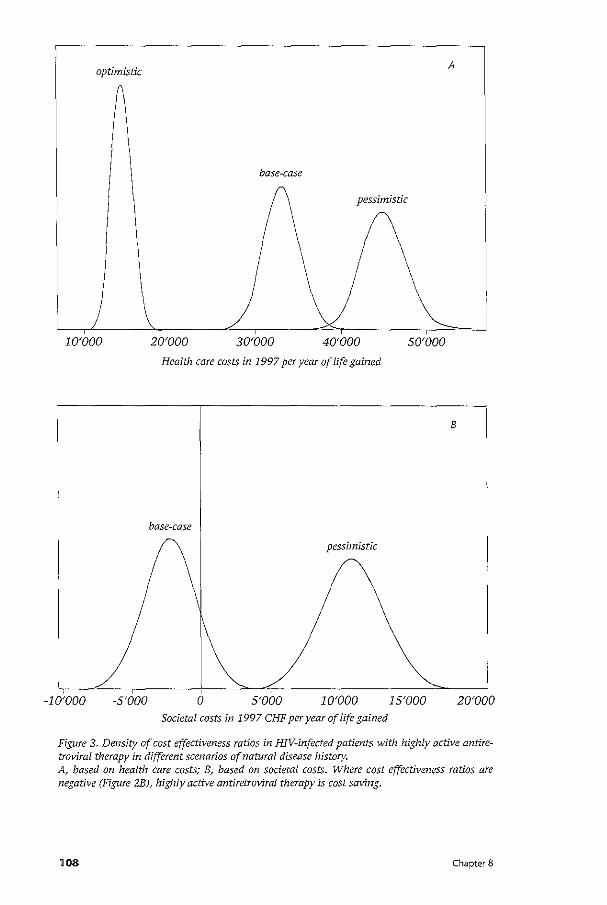
optimistic A

base-case

pessimistic

10'000 20'000 30'000 40'000 50'000

Health care costs in 1997 per year of life gained

8

base-case

pessimistic

-10'000 -5'000 0 5'000 10'000 15'000 20'000 Societal costs in 1997 CHF per year of life gained

Figure 3. Density of cost effectiveness ratios in HIV-infected patients with highly active antire­troviral therapy in different scenarios of natural disease history. A, based on health care costs; B, based on societal costs. Where cost effectiveness ratios are negative (Figure 2B), highly active antiretroviral therapy is cost saving.

108 Chapter 8

Discussion Newer antiretroviral combination therapies including proteinase inhibitors

represent a major improvement in treating HIV-infected individuals. Overall

health care costs with HAART, which includes acquisition costs for antiretrovi­

ral drugs, exceed the average health care costs with NART substantially. This is

because individuals have a higher life expectancy with HAART, consequently

more health care resources are needed to treat this chronic disease condition.

However, since the expensive costs for in-patient treatment are postponed to later years in patients receiving HAART, discounting has a major impact on

overall health care costs. For example, undiscounted health care costs in the

optimistic scenario (CHF 617,000) are higher than in the base-case scenario

(CHF 505,000). But when respecting time preference, the same health care

costs are CHF 387,000 and CHF 389,000, respectively. In most cases over all

scenarios, however, the cost effectiveness was below CHF 50,000 per year of

life gained in our sampling exercise.

One of the most important causes of death in young people in Switzerland

is AIDS (Bundesamt fur Statistik, 1997), which affects the society as a whole.

The societal viewpoint is the broadest viewpoint and, therefore, the most rele­

vant. The policy of providing HAART to HIV-infected individuals saves costs to

the society. Only in the pessimistic scenario is this not the case. Even though

there are no Swiss standards to assess the acceptability of a cost-effectiveness

ratio, we believe that CHF 11,000 per year of life saved is not a high price re­

lative to what is currently provided. Our analysis from the viewpoint of the

health care system illustrates that HAART increases both average survival and

health care costs. If the health care system wants to contain costs, it would

need to find programs to be canceled where the loss in health terms will be

smaller than the health gains from the HAART program (Birch and Gafni,

1993). Our analysis from the health care perspective can provide some input

into this process.

The cost-effectiveness of HAART has also been investigated in two previous

studies in the United States (Moore and Bartlett, 1996) and Canada (Anis et

al., 1998). The results of these studies are comparable to the present study.

However, the authors did not assess the societal implications of treating HIV­

infected individuals with HAART. We think that our study provides better evi­

dence of the clinical and economic consequences of prescribing these newer

antiretroviral combination therapies to HIV-infected patient because natural

history and cost data are extracted from the same patient population, enrolled

in the SHCS. Furthermore, observational data reflecting the real-world situ­

ation (external validity) are used (Drummond, 1998). The cost-effectiveness

exercise, therefore, does encompass non-adherence to complex drug regimens,

as observed in general practice. Finally, the SHCS is one of the world largest

cohort studies on HIV disease, which increases the reliability of the results.

Chapter 8 109

This cost effectiveness analysis has limitations that should be considered. A

model is always a simplification of the real world. This study does not expli­

citly model all AIDS-defining diseases separately. However, more complicated

models do not necessarily provide more reliable results (Naimark eta!., 1997).

Importantly, extrapolation into the future was involved (Buxton et a!., 1997)

but the future is unknown for many aspects in this highly dynamic field. Con­

sequently, extreme scenarios of natural history of HIV disease were devised.

Changes in therapy such as moving from a three-drug or four-drug regimen

to five or more drugs were rarely observed in the SHCS. Such a shift would

lower the cost-effectiveness of HAART. Not only would the acquisition costs

be higher, but also patient would be less likely to adhere to such complex drug

regimens. However, we believe that the emerging knowledge about drug-resis­

tance patterns and the advent of new antiretroviral drugs will lead to a more

efficient use of drug combinations. Finally, patients were assumed to remain on

HAART until death in our model. Patients may not be on therapy until death in

reality. But this would reduce acquisition costs of antiretroviral drugs, and the

assumption may, therefore, be regarded as a conservative assumption.

For decision makers in Switzerland, equity considerations have principally

been more important than maximizing health benefits from a fixed resource

pool. This conception is also shared by many policy and decision makers in

other countries (Ubel et a!., 1996). The promising results here, including the

pessimistic societal scenario, justify the policy of providing unrestricted access

to HAART for all HIV-infected individuals in Switzerland. Society will likely

benefit even in the case where the policy would be based solely on economic

grounds. The presented results also suggest that this policy could be of interest

for other developed countries. Decision makers in developed countries where

access to HAART is limited should re-evaluate their policy for the benefit of the

society at large.

110 Chapter 8

Chapter 8 111

• Ella ter9 Cost-effectiveness of azithromycin for preventing Mycobacterium avium

complex infection in HIV-infected patients in the era of highly active anti­

retrovira/ therapy

Summary We conducted a cost-effectiveness analysis to determine the clinical and econo­

mic consequences of Mycobacterium avium complex (MAC) prophylaxis in HIV­

infected patients in the era of highly active antiretroviral therapy (HAART) in

a health care system with access unrestricted by financial barriers. The analysis

was performed from a health care perspective and compared azithromycin

(1200 mg/week) with no prophylaxis over a period of 10 years based on data

from the Swiss HIV Cohort Study (SHCS) and randomized controlled trials.

The main outcome measures were: expected survival; average health care costs;

and cost-effectiveness in 1997 Swiss Francs (£1 corresponds to about CHF 2.3)

per life-year saved. In patients with an initial CD4 count <50 cells/mm3 and no

AIDS, azithromycin increased expected survival by 4 months. In patients with

AIDS, HAART durability had a major impact on expected survival and costs.

Incremental survival increased from 2 to 4 months if we assumed a 10 year, in­

stead of a 3 year, HAART effect. The cost-effectiveness of azithromycin relative

to no prophylaxis in patients without AIDS was between CHF 47,000 (3-year

HAART effect) and CHF 60,000 (10-year HAART effect) per life-year saved. The

cost-effectiveness ratio increased to CHF 118,000 per life-year saved in patients

with symptomatic AIDS. In conclusion, in the era of HAART, MAC prophylaxis

with azithromycin increases expected survival and health care costs substanti­

ally. Starting MAC prophylaxis in patients without AIDS is more effective and

cost-effective than in patients with AIDS.

112 Chapter 9

Introduction Disseminated Mycobacterium avium complex (MAC) infection in severely

immunosuppressed HN-infected patients is associated with increased mor­

bidity and mortality (Horsburgh, 1991). Randomized controlled trials have

documented the benefit of MAC prophylaxis with macrolides in HIV-infected

patients with advanced immunosuppression (Pierce et al., 1996; Havlir et al.,

1996; Oldfield et al., 1998). Economic studies, based on models with clinical

data gathered before (Freedberg et al., 1997; Freedberg et al., 1998) and after

(Bayoumi and Redelmeier, 1998) highly active antiretroviral therapy (HAART)

became widely available, have investigated the policy implications of MAC

prophylaxis in the USA. However, the cost-effectiveness of MAC prophyla­

xis within a European setting has not yet been evaluated. The Swiss health

care system, as an example of a Western European-type health care system,

provides unrestricted access to all approved therapies for patients with HIV

infection. The majority (66.2%) of the Swiss health care resources are funded

by consumers either directly (out-of- pocket payment) or indirectly (insuran­

ce companies) (Bundesamt fur Statistik, 1998). Official federal organizations

fund most of the remainder (Bundesamt fur Statistik, 1998). We conducted

a cost-effectiveness analysis from the health care perspective to address the

clinical and economic implications of MAC prophylaxis with azithromycin in

the era of HAART. Our analysis is based on the Swiss HIV Cohort Study (SHCS)

(Ledergerber et al., 1994). This study offers additional insights about the con­

sequences of MAC prophylaxis in HIV-infected individuals receiving care in a

system with access unrestricted by finandal barriers. In addition, we applied

Bayesian analytical techniques to reflect overall parameter uncertainty (Craig

et al., 1999).

Methods The model

We developed a Markov (or state-transition) model (Sonnenberg and Beck,

1993) that desctibes the disease history of HIV-infected subjects as a sequence

of monthly health states. We defined four broad categories of health: No AIDS

(asymptomatic HIV-positive), AIDS (non-MAC), MAC and death. We used the

European classification for AIDS (Ancelle-Park et al., 1995). The No AIDS and

AIDS states were further stratified into three CD4-cell count categories: 0-49

cells/mm3, 50-74 cells/mm3 and «75 cells/mm3• A patient currently in a No

AIDS state is at risk of dying from non-AIDS-related causes, developing MAC

or developing an AIDS-defining disease other than MAC. A patient with AIDS

is at risk of dying from AIDS or developing MAC. A patient with MAC is at

risk of dying from MAC. Prophylactic drug efficacy is expressed as a reduction

in MAC incidence. A low adherence in tum is modeled as a low drug efficacy.

Severe drug toxicity results in discontinuation of MAC prophylaxis. The model

Chapter 9 113

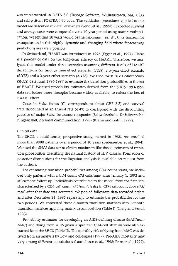
was implemented in DATA 3.0 (TreeAge Software, Williamstown, MA, USA)

and self-written FORTRAN 90 code. The validation procedures applied to our

model are described in detail elsewhere (Sendi et al., 1999b). Expected survival

and average costs were computed over a 10-year period using matrix multipli­

cation. We felt that 10 years would be the maximum realistic time-horizon for

extrapolation in this highly dynamic and changing field where far-reaching

predictions are rarely possible.

In Switzerland, HAART was introduced in 1996 (Egger et al., 1997). There

is a paucity of data on the long-term efficacy of HAART. Therefore, we ana­

lyzed this model under three scenarios assuming different levels of HAART

durability: a continuous time effect scenario (CTES), a 5-year effect scenario

(5-YES) and a 3-year effect scenario (3-YES). We used Swiss HIV Cohort Study

(SHCS) data from 1996-1997 to estimate the transition probabilities in the era

of HAART. We used probability estimates derived from the SHCS 1993-1995

data set, before those therapies became widely available, to reflect the loss of

HAART effect.

Costs in Swiss francs (£1 corresponds to about CHF 2.3) and survival

were discounted at an annual rate of 4% to correspond with the discounting

practice of major Swiss Insurance companies (Schweizerische Unfallversiche­

rungsanstalt, personal communication, 1998) (Krahn and Gafni, 1997).

Clinical data

The SHCS, a multi-center, prospective study, started in 1988, has enrolled

more than 9000 patients over a period of 10 years (Ledergerber et al., 1994).

We used the SHCS data set to obtain maximum likelihood estimates of transi­

tion probabilities describing the natural history of HIV disease. Formation of

posterior distributions for the Bayesian analysis is available on request from

the authors.

For estimating transition probabilities among CD4 count strata, we inclu­

ded only patients with a CD4 count <75 cells/mm3 after January 1, 1993 and

at least one follow-up. Individuals contributed to the model from the first date

characterized by a CD4-cell count <75/mm3• A rise in CD4-cell count above 75/

mm3 after that date was accepted. We pooled follow-up data recorded before

and after December 31, 1995 separately, to estimate the probabilities for the

two periods. We converted these 6-month transition matrices into 1-month

transition matrices applying matrix decomposition (Table I) (Craig and Sendi,

1998).

Probability estimates for developing an AIDS-defining disease (MAC/non­

MAC) and dying from AIDS given a specified CD4-cell stratum were also ex­

tracted from the SHCS (Table II). The monthly risk of dying from MAC was de­

rived from an analysis by Low and colleagues (1997). Pre-AIDS mortality may

vary among different populations (Laurichesse et al., 1998; Prins et al., 1997).

114 Chapter 9

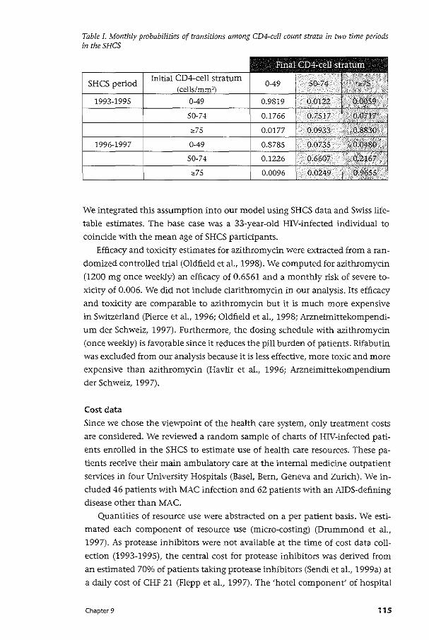
Table I. Monthly probabilities of transitions among CD4~cell count strata in two time periods in theSHCS

SHCS period Initial

We integrated this assumption into our model using SHCS data and Swiss life­

table estimates. The base case was a 33-year-old HIV-infected individual to

coindde with the mean age of SHCS partidpants.

Efficacy and toxicity estimates for azithromycin were extracted from a ran­

domized controlled trial (Oldfield eta!., 1998). We computed for azithromydn

(1200 mg once weekly) an efficacy of 0.6561 and a monthly risk of severe to­

xidty of 0.006. We did not include clarithromycin in our analysis. Its efficacy

and toxicity are comparable to azithromycin but it is much more expensive

in Switzerland (Pierce eta!., 1996; Oldfield eta!., 1998; Arzneimittekompendi­

um der Schweiz, 1997). Furthermore, the dosing schedule with azithromycin

(once weekly) is favorable since it reduces the pill burden of patients. Rifabutin

was excluded from our analysis because it is less effective, more toxic and more

expensive than azithromycin (Havlir et al., 1996; Arzneimittekompendium

der Schweiz, 1997).

Cost data

Since we chose the viewpoint of the health care system, only treatment costs

are considered. We reviewed a random sample of charts of HIV-infected pati­

ents enrolled in the SHCS to estimate use of health care resources. These pa­

tients receive their main ambulatory care at the internal medicine outpatient

services in four University Hospitals (Basel, Bern, Geneva and Zurich). We in­

cluded 46 patients with MAC infection and 62 patients with an AIDS-defining

disease other than MAC.

Quantities of resource use were abstracted on a per patient basis. We esti­

mated each component of resource use (micro-costing) (Drummond et al.,

1997). As protease inhibitors were not available at the time of cost data coll­

ection (1993-1995), the central cost for protease inhibitors was derived from

an estimated 70o/o of patients taking protease inhibitors (Sendi et a!., 1999a) at

a daily cost of CHF 21 (Flepp eta!., 1997). The 'hotel component' of hospital

Chapter 9 115

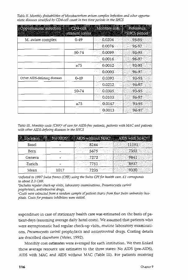
Table II. Monthly probabilities of Mycobacterium avium complex infection and other opportu~ nistic diseases stratified by CD4-cell count in two time periods in the SHCS

®ppormnistic infection I GD4-cell I Monthly risk

I Reference

stratum (cells) SHGSperiod

M. avium complex 0-49 0.0204 93-95

0.0076 96-97

50-74 0.0099 93-95

0.0016 96-97

;,75 0.0052 93-95

0.0003 96-97

Other AIDS~defining diseases 0-49 0.0393 93-95

0.0212 96-97

50-74 0.0305 93-95

0.0103 96-97

;,75 0.0167 93-95

0.0013 96-97

Table III. Monthly costs (CHF)" of care for AIDS-free patients, patients with MAC and patients with other AIDS-defining diseases in the SHCS

"inflated to 1997 Swiss francs (CHF) using the Swiss CPI for health care. £1 corresponds to about 2.3 CHF. "Includes regular check~up visits, laboratory examinations, Pneumocystis carinii prophylaxis, antiretroviral drugs. ccosts were extracted from a random sample of patient charts from four Swiss university has~ pitals. Costs for protease inhibitors were added.

expenditure in case of stationary health care was estimated on the basis of pa­

tient-days (assuming average daily hotel costs). We assumed that patients who

were asymptomatic had regular check-up visits, routine laboratory examinati­

ons, Pncumocystis carinii prophylaxis and antiretroviral drugs. Costing details

are described elsewhere (Meier. 1992).

Monthly cost estimates were averaged for each institution. We then linked

these average resource use estimates to the three states: No AIDS (pre-AIDS),

AIDS with MAC and AIDS without MAC (Table Ill). For patients receiving

116 Chapter 9

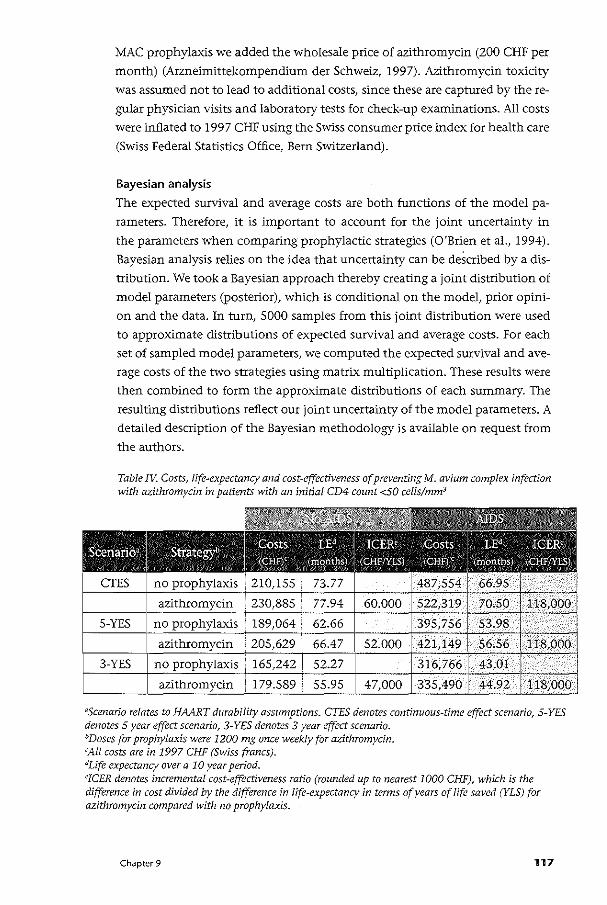
MAC prophylaxis we added the wholesale price of azithromycin (ZOO CHF per

month) (Arzneimittekompendium der Schweiz, 1997). Azithromycin toxicity

was assumed not to lead to additional costs, since these are captured by there­

gular physidan visits and laboratory tests for check-up examinations. All costs

were inflated to 1997 CHF using the Swiss consumer price index for health care

(Swiss Federal Statistics Office, Bern Switzerland).

Bayesian analysis

The expected survival and average costs are both functions of the model pa­

rameters. Therefore, it is important to account for the joint uncertainty in

the parameters when comparing prophylactic strategies (O'Brien et al., 1994).

Bayesian analysis relies on the idea that uncertainty can be described by a dis­

tribution. We took a Bayesian approach thereby creating a joint distribution of

model parameters (posterior), which is conditional on the model, prior opini­

on and the data. In turn, 5000 samples from this joint distribution were used

to approximate distributions of expected survival and average costs. For each

set of sampled model parameters, we computed the expected survival and ave­

rage costs of the two strategies using matrix multiplication. These results were

then combined to form the approximate distributions of each summary. The

resulting distributions reflect our joint uncertainty of the model parameters. A

detailed description of the Bayesian methodology is available on request from

the authors.

Table TV. Costs, life-expectancy and cost-effectiveness of preventing M. avium complex infection with azithromycin in patients with an initial CD4 count <50 cells/mm:;

~scenario relates to HAART durability assumptions. CTES denotes continuous-time effect scenario, 5-YES denotes 5 year effect scenario, 3-YES denotes 3 year effect scenario. 0Doses for prophylaxis were 1200 mg once weekly for azithromycin. 'All costs are in 1997 CHF (Swiss francs). JLife expectancy over a 10 year period. eJCER denotes incremental cost-effectiveness ratio (rounded up to nearest 1000 CHF), which is the difference in cost divided by the difference in life-expectancy in tenns of years of life saved (YLS) for azithromycin compared with no prophylaxis.

Chapter 9 117

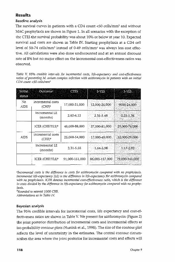
Results Baseline analysis

The survival curves in patients with a CD4 count <50 cells/mm3 and without

MAC prophylaxis are shown in Figure 1. In all scenarios with the exception of

the CTES the survival probability was about 10% or below at year 10. Expected

survival and costs are shown in Table IV. Starting prophylaxis at a CD4 cell

level of 50-74 cells/mm3 instead of 0-49 cells/mm3 was always less cost effec­

tive. All calculations were also done undiscounted and at an annual discount

rate of 8% but no major effect on the incremental cost-effectiveness ratios was

observed.

Table V. 95% credible intervals for incremental costs, life-expectancy and cost-effectiveness ratios of preventing M. avium complex infection with azithromycin in patients with an initial CD4 count <50 cells/mm3

Initial

I

Outcomea

I

CTES

I

5-YES

I

3-YES

status

No incremental costs AIDS (CHF)b 17,000-31,000 12,000-26,000 9000-24,000

incremental LE

(months) 2.63-6.13 2.35-5.48 2.25-5.36

!CER (CHF/YLS)b 48,000-88,000 37,000-81,000 29,000-76,000

incremental costs AIDS (CHF)b 25,000-54,000 17,000-49,000 12,000-29,000

.

incremental LE

(months) 2.31-5.58 1.64-3.90 1.17-2.92

ICER (CHF/YLS)b 91,000-151,000 86,000-157,000 79,000-165,000

'

"Incremental costs is the difference in costs for azithromycin compared with no prophylaxis. Incremental life-expectancy (LE) is the difference in life-expectancy for azithromycin compared with no prophylaxis. ICER denotes incremental cost-effectiveness ratio, which is the difference in costs divided by the difference in life-expectancy for azithromycin compared with no prophy­laxis. bRounded to nearest 1000 CHF. Abbreviations as in Table tV.

Bayesian analysis The 95% credible intervals for incremental costs, life expectancy and cost-ef­

fectiveness ratios are shown in Table V. We present for azithromycin (Figure 2)

the joint posterior distribution of incremental costs and incremental effects as

iso-probability contour plots (Hunink et al., 1998). The size of the contour plot

reflects the level of uncertainty in the estimates. The central contour drcum­

scribes the area where the joint posterior for incremental costs and effects will

118 Chapter 9

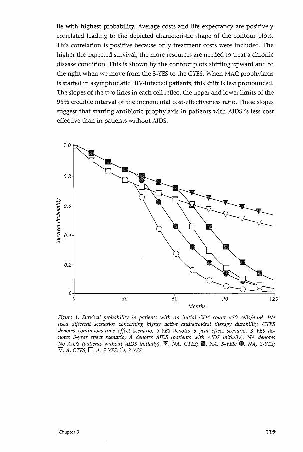
lie with highest probability. Average costs and life expectancy are positively

correlated leading to the depicted characteristic shape of the contour plots.

This correlation is positive because only treatment costs were included. The

higher the expected survival, the more resources are needed to treat a chronic

disease condition. This is shown by the contour plots shifting upward and to

the right when we move from the 3-YES to the CTES. When MAC prophylaxis

is started in asymptomatic HN-infected patients, this shift is less pronounced.

The slopes of the two lines in each cell reflect the upper and lower limits of the

9So/o credible interval of the incremental cost-effectiveness ratio. These slopes

suggest that starting antibiotic prophylaxis in patients with AIDS is less cost

effective than in patients without AIDS.

7.0 '

0.8

.2:-

~ 0.6

"' e 0,

~ "§ 0.4'

"'

0.2

ol 0

Months

Figure 1. Survival probability in patients with an initial CD4 count <50 cells/mm3• We used different scenarios concerning highly active antiretroviral therapy durability. CTES denotes continuous-time effect scenario, 5-YES denotes 5 year effect scenario. 3 YES de­notes 3-year effect scenario, A denotes AIDS (patients with AIDS initially), NA denotes No AIDS (patients without AIDS initially). 'f, NA. CTES; II. NA. 5-YES; G. NA, 3-YES; V. A, CTES; D. A, 5-YES; 0, 3-YES.

Chapter 9 119

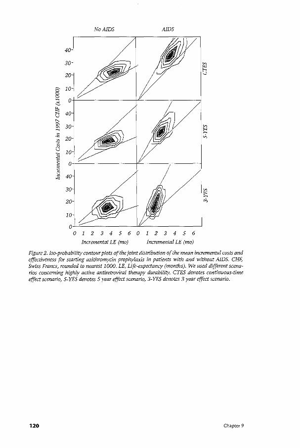
No AIDS AIDS

40-

30-

20-

2 10 a a ~ o-6

~ u 40-

" & 30-~

~ -~ 20-.:0 ~ 0 u JO-i ""' ;; ~ 0

~ 40 "'

30-

20-

10-

1234560123456

Incremental LE (mo) Incremental LE (mo)

Figure 2. !so-probability contour plots of the joint distribution of the mean incremental costs and effectiveness for starting azithromycin prophylaxis in patients with and without AIDS. CHF; Swiss Francs~ rounded to nearest 1000. LE, Life-expectancy (months). We used different scena­rios concerning highly active antiretroviral therapy durability. CTES denotes continuous-time effect scenario, 5-YES denotes 5 year effect scenario, 3-YES denotes 3 year effect scenario.

120 Chapter 9

Discussion In the era of HAART, MAC infection is still one of the most frequent oppor­

tunistic infections among HIV- positive individuals in Switzerland and parts

of Europe (Egger, 1998). Nonetheless, the incidence of AIDS-defining diseases,

including MAC, has declined since the introduction of HAART (Egger et a!.,

1997; Gebhardt et a!., 1998), which disfavors antibiotic prophylaxis (Wright

and Weinstein, 1998). However, the expected survival of patients with advan­

ced CD4 cell depletion has increased remarkably. This, in contrast, makes MAC

prophylaxis more beneficial (Wright and Weinstein, 1998). Although HAART

lowers the monthly risk of acquiring MAC at a given CD4 cell level and may

also partially restore immune function, our model shows that these effects are

by far outweighed by a higher cumulative risk of MAC infection associated

with a higher life expectancy. This is documented by an increasing gain in

survival vvith azithromycin in the more optimistic scenarios of HAART dura­

bility. Azithromydn was only discontinued when severe toxic reactions were

experienced, but not when HAART increased the CD4 cell count above the cut­

off point (sSO CD4 cells/mm3) for MAC prophylaxis (USPHS/IDSA Prevention

of Opportunistic Infections Working Group, 1997). We found an average gain

in survival comparable to the estimates reported by Bayoumi and Redelmeier

(1998) for a North American setting.

MAC prophylaxis leads to a substantial amount of resource consumption

within the Swiss health care sector. Antibiotic prophylaxis in patients with

AIDS increases direct medical costs more than in AIDS-free patients and results

in a lower gain in survival. This translates into a cost-effectiveness ratio that

is higher. It would not be uncommon for the cost-effectiveness ratio for azi­

thromycin in patients with AIDS to exceed CHF 150,000 per life-year saved. If

MAC prophylaxis is started in AIDS-free patients, there is a negligible chance

that this would cost CHF 100,000 per life-year saved. If the health care system

wants to contain costs, it needs to cancel programs where the loss in health

terms is lower than the health gains from the azithromycin program (Birch

and Gafni, 1992). Alternatively, policy decision-makers should find ways to

increase the health care budget.

Chapter 9 121

• Cha ter 10 Discussion

122 Chapter 10

In this thesis, three different approaches to the decision rule of cost-effective­

ness analysis have been discussed when costs and effects are uncertain: i) the

alternative decision rule, ii) the classical decision rule, and iii) portfolio theory

for choosing among health care programs.

The alternative decision rule In chapter 2 the alternative decision rule has been illustrated when costs and

effects are subject to uncertainty. The motivation for using the alternative

decision rule is that a decision-maker's available resources may all be used by

current programs. If a new program becomes available which contributes to

gains in QALYs but calls for additional resources, then one must ask where

these resources will come from. In such a situation, other programs need to be

cancelled in order to free up resources to fund the new program. If the health

benefits gained by introducing the new program are greater than those lost

by relinquishing the old program, then an unambiguous improvement in the

allocation of resources is achieved. This is a second-best approach, since more

than one program in the current portfolio might satisfy these requirements

(Gafni, 1996). However, in practice, the information on the costs and effects

of all programs in the current portfolio might not be available. The practical

advantage of the alternative decision rule then becomes apparent: information

on the costs and effects of only one program that satisfies the requirements of

the decision rule is sufficient for increasing the efficiency of resource allocati­

on.

The decision-making plane has been introduced as a means to graphically

present the results of the alternative approach, plotting t.C(A) - t.C(B) on the

vertical axis against t.E(A) - t.E(B) on the horizontal axis. If we write out the

terms, the vertical axis denotes (CA- C) - (C,- C,), i.e. the incremental costs

of introducing program A compared to the costs which would accrue if pro­

gram A was not available, minus the resources that would be released if pro­

gram B was cancelled. Note that by introducing program A we replace program

a with program A, and by canceling program B we replace it with program b.

The same prindple holds true for the horizontal axis: writing out the terms

t.E(A) - t.E(B) is equivalent to (EA- E)- (E,- Eb). The alternative decision rule

requires that t.C(A) - t.C(B) " 0 and t.E(A) - t.E(B) ;,0. If both t.C(A) - t.C(B) =

0 and t.E(A) - t.E(B) = 0, then we would be indifferent with respect to intro­

ducing program A since this neither results in any health gains nor releases

resources that could be used otherwise to improve health.

An interesting alternative approach to view the decision-making plane is

that it actually corresponds to the cost-effectiveness plane, but with the dif­

ference that two strategies are compared, each representing a combination of

two programs. Note that (CA- C)- (C,- Cb) = (CA + Cb)- (C, +C)= cA.b- c,.", i.e. the costs of the combination of program A plus b are compared to the costs

Chapter 1 0 123

of the combination of program B plus a. The same holds true for the effects.

The term "decision-making plane" has been chosen in order to emphasize that

this comparison actually involves four programs instead of two. In this compa­

rison, the alternative decision rule requires that the combination of program

A plus b should be dominant over the combination of program B plus a. In

the presence of uncertainty associated with the costs and effects of health care

programs, the joint distribution of costs and effects may not be limited to the

southeastern quadrant of the decision-making plane. However, only outcomes

that fall in the southeastern quadrant of the decision-making plane are con­

sistent with an improvement in the efficiency of resource allocation. In such a

situation it has been suggested that the decision-maker's acceptable risk of ac­

cepting outcomes in other quadrants may be limited to an arbitrary level, such

as the arbitrary decision of accepting a 5% Type I error in hypothesis testing.

However, a more elegant approach to summarize uncertainty on the deci­

sion-making plane is to apply the cost-effectiveness acceptability curve (van

Hout eta!., 1994).1fthe joint distribution of costs and effects falls completely

in the southeastern quadrant of the decision-making plane, which is what

we aim for when applying the alternative decision rule, then this switch of

programs would be cost-effective for all levels of the threshold ratio. That is,

the cost-effectiveness acceptability curve would correspond to a horizontal

line at the probability level of one. In case the joint distribution also extends

over other quadrants of the decision-making plane, then the cost-effectiveness

acceptability curve would inform the decision-maker about the range of the

threshold ratio for which the switch of program would be cost-effective with

a high probability.

Combining the cost-effectiveness acceptability cur:;e with the alternati­

ve decision rule in the presence of uncertainty can be seen as a "marriage"

between the two approaches. The use of the cost-effectiveness acceptability

curve to summarize uncertainty on the decision making plane seems, perhaps,

to be inconsistent with the original idea that led to the development of the

alternative decision rule. The alternative decision rule has been suggested as

an alternative to using a fixed-threshold cost-effectiveness ratio, since this

would lead to uncontrolled growth of health care expenditures as more pro­

grams with an acceptable cost-effectiveness ratio are implemented (Gafni and

Birch, 1993). However, it should be noted that the alternative decision rule,

on the other hand, does not allow growth of the health care budget. The use

of the cost-effectiveness acceptability curve in combination with the decision­

making plane may, therefore, be seen as a method that allows for controlled

growth of the budget.

In chapter 3 the alternative decision rule was analyzed from a different

perspective. Stochastic dominance rules were used to provide a way to make

decisions based on little or limited knowledge of a decision-maker's risk prefe-

124 Chapter l 0

renee. The alternative decision rule shifts the cumulative distribution of health

outcomes to the right and the cumulative distribution of costs to the left. First­

order stochastic dominance requires that the decision-maker prefers more to

less, no matter his risk-preference. First-order stochastic dominance requires

that choice A+b is always preferred to choice B+a if the cumulative density

function associated with B+a is not less than that with A+b for any outcome

level and is greater than that with A+b for at least one outcome level. Howe­

ver, when the decision-maker prefers less to more, as in the case of costs, then

first-order stochastic dominance requires that choice A+b is always preferred to

choice B+a if the cumulative density function associated with B+a is not more

than that with A+b for any outcome level and is smaller than that with A+b

for at least one outcome level. In order to make this distinction of preferring

less to more we have used the term "affordability". As emphasized in chapter

3, the use of stochastic dominance rules is complementary to the approach of

presenting the results on the decision-making plane. However, the more the

joint distribution of costs and effects shifts to the southeast on the decision­

making plane, the more the cumulative distributions of the costs and effects

of programs A+b and B+a will move apart.

An advantage of using the cumulative distribution of costs and effects as a

basis for decision-making is that the uncertainty associated with all programs

in the current portfolio can be included in the analysis. If the decision-ma­

ker has a total budget from which to fund all health care programs. then

the cumulative distribution of total portfolio costs can be used to assess the

probability that the budget is exceeded and whether this risk is acceptable to

the decision-maker. Note that the budget does not need to be constant for

this approach; it could be that a decision-maker needs to deal with a lower

budget than in the preceding years. For example, policy-makers may decide

to curtail the available budget to providers such as hospitals as a measure to

reduce overall health care costs. In such a situation, program A can only be

introduced if a program B can be found that would not only release sufficient

resources to fund program A, but would also shift the cumulative distribution

of total costs to the left to such a degree that the risk of exceeding the budget

becomes acceptable.

In chapter 8 a cost-effectiveness analysis of highly active antiretroviral

therapy (HAART) in HIV-infected patients has been presented. The analysis

was conducted from the societal as well as the health care perspective. In the

analysis from the societal perspective, when productivity costs were included

HAART resulted in cost-savings as well as gains in life-years. However, when

the analysis was limited to health care costs, HAART was more effective but

also more costly, with the cost-effectiveness ratio ranging from 14,000 CHF

to 45,000 CHF. The societal perspective is broad in the sense that everyone

affected by the intervention is considered and all health outcomes and costs

Chapter 10 125

that result from the intervention are counted. However, as shown in the study

described in chapter 8, a strategy that is dominant from the societal perspecti­

ve need not be dominant when a health care perspective is taken. The HAART

program calls for additional health care resources and consideration must

therefore be given as to where these resources will come from. If the health care

budget is already spent on current programs and there is no other possibility

to increase the health care budget, then the alternative decision rule may be

used, i.e. a program B may be identified and cancelled that releases sufficient

resources to fund HAART. However, deleting a program that is well established

is a difficult task and often not feasible. Decision-makers may therefore prefer

to increase the health care budget, e.g. by taxation or by increasing insurance

premiums (Weinstein, 1995). In that case, the opportunity costs of the addi­

tional resources would be in areas other than health. However, increasing the

health care budget would only be justifiable from an economics perspective if

the health benefits gained from the HAART program are greater than those lost

by cutting the budget of other sectors of the economy. It could also be said that

by deciding to increase the health care budget society has implicitly applied

the alternative decision rule across sectors of economy.

In chapter 9, the cost-effectiveness of azithromyin for preventing Myco­

bacterium avium complex infection in HIV-positive patients taking HAART

was assessed. The analysis showed that azithromycin is more cost-effective in

patients without clinical AIDS (47,000 CHF- 60,000 CHF per life-year gained)

than in patients with AIDS (118,000 CHF per life-year gained). Starting azi­

thromycin in HIV-infected patients without AIDS therefore represents a more

efficient allocation of resources than waiting until the patient has experienced

an AIDS-defining disease. However, in both patient subgroups the incremental

costs were positive. This means that more health care resources are needed in

order to prevent 1\lfycobacterium avium complex infections in HIV-infected pa­

tients. Here again, as discussed above, the required resources may come from

cutting the budget of other health care departments or from increasing the

health care budget by taxation, higher insurance premiums, or reducing the

budget of other sectors of economy such as education or national defense. In

either case, a choice has to be made with respect to resource allocation, which

forces the decision-maker to think in terms of opportunity costs of scarce re­

sources.

The classical decision rule In chapter 4 the assumption of complete divisibility of the classical decision

rule of cost-effectiveness has been addressed. We argued that an integer pro­

gramming approach where patients represent individual units might be more

appropriate than a linear programming approach to formulate the budget al­

location problem. Then we showed that treatments ruled-out by a linear pro-

126 Chapter 1 0

gramming approach could be provided to some patients in order to maximize

total health benefit, subject to a budget constraint. It should be noted that

there is a difference between the integer programming approach suggested by

Birch and Gafni (1992) and the one discussed in chapter 4. In chapter 4 the

number of patients to be treated were programmed as integers (i.e. 0- 1000),

which allows the size of the program to vary. Birch and Gafni, on the other

hand, suggested that the whole program should be handled with an integer

variable (i.e, 1 or 0) in order to model complete indivisibility (Birch and Gafni,

1992). Chapter 4 simply addresses the fact that patients are not divisible, but

accepts the assumption of constant return to scale and divisibility at the pro­

gram level. However, sub-optimal budget allocation decisions at the margin

can be corrected for if individuals are modeled as integers.

Another idea introduced in chapter 4 is the application of simulation opti­

mization to maximize the objective function of the constrained optimization

problem. We defined expected aggregate effects as the objective function,

which is penalized in case the budget is exceeded. This method allows the

inclusion of the opportunity costs of the additional resource requirements in

the analysis. Described in the first part of chapter 4, the method assumes that

decision-makers are risk-neutral towards health effects and risk-averse towards

costs. This may certainly be reasonable for decision-makers at the sub-societal

level, who have budget constraints to meet. However, since the benefits of

the programs only accrue to some individuals, a decision-maker might also be

risk-averse towards health effects. In that case, the variance of aggregate effects

may need to be minimized, subject to the constraint that some aspiration level

for expected aggregate effects is met. Al (2001) suggested that for societal de­

cision-making, risk-neutrality towards costs and risk-aversion towards health

outcomes may be more in line with the arguments of Arrow and Lind (1970),

and therefore formulated the optimization problem as minimizing expected

costs under the constraint that the probability of total effects exceeding some

aspiration level was at least 95%.

Zivin (2001) also recently discussed the appropriate risk-posture for socie­

tal decision-maldng and illustrated the limitations associated with the Pareto

compensation criterion in health care and argued that sodal planners should

be risk-averse towards health outcomes. Assuming a normal distribution for

outcomes, the ex ante mean is usually not the same as the ex post mean. The

ex ante uncertainty may be separated into the two components of statistical

uncertainty (sampling variability) inherent in a trial and uncertainty about

the appropriate values assigned to various components of the analysis, which

is generally evaluated by traditional sensitivity analysis. Once a program is

implemented by moving from a clinical trial to the general health care setting,

some of the uncertainty will be reduced and the ex post mean will usually dif­

fer from the ex ante mean. Only when the ex ante sample is sufficiently large,

Chapter 10 127

a very expensive undertaking, will the ex post distribution be approximated.

Therefore, it is not true that ex post half of the outcomes will be above the ex ante mean and half below it, i.e. the winners are not necessarily able to com­

pensate the losers. Moreover, Zivin (2001) argues that even if the uncertainty

embodied in cost-effectiveness analyses is a reflection of true stochasticity,

justifying a risk-neutral societal decision-maker based on the Pareto compen­

sation criterion may be problematic because people are usually risk-averse

with respect to lifetime. Risk-aversion implies that the utility gained from one

additional year is less than the utility lost from one less year. This means that

those who experience above average results will not be able to compensate for

those who experience below average results.

The main difference between the variants of the classical approach discus­

sed in chapter 4 and the classical approach presented in AI (2001) is that in

chapter 4 the objective function is penalized in case the budget is exceeded.

However, AI (2001) also suggested a much wider perspective of the budget al­

location problem by extending the idea of a fixed budget to a flexible budget,

which may compete with resources from other sectors of economy (such as

education or national defense). This is accomplished by extending the maxi­

mization of health outcomes subject to a budget constraint in order to optimi­

ze the value derived from health outcomes and non-health care budgets com­

peting with health care expenditures (AI, 2001). This method is then extended

when costs and health outcomes are uncertain by defining a utility function

for both money and health outcomes. However, defining an explicit utility

function may prove difficult for practical decision-making and pragmatic al­

ternative approaches such as those discussed above may be less demanding in

terms of information required.

Hutubessy eta!. (2001) suggested an alternative approach to decision-ma­

king when the distribution of costs and effects of all the available programs

are known. In their hypothetical example the authors defined mutually ex­

clusive alternatives for different disease conditions. They then constructed a

"stochastic league table" by i) taking random draws from the distribution of

total costs and effects for each treatment option in the menu, ii) constructing

a standard league table for each iteration of the simulation (for a given budget

level), and iii) estimating the number of times that an intervention is included

in the optimal mix of programs (Hutubessy et a!., 2001). The probability an

intervention is included in the optimal mix of programs for all levels of resour­

ce availability allows the construction of what the authors call an expansion

path. This method and the method presented in chapter 4 both assume that

the budget as well as the distribution of the costs and effects of the programs

is known. In chapter 4, however, a constrained optimization problem with an

explicit objective function has been formulated. The information contained in

128 Chapter 1 0

stochastic league tables, on the other hand, is probabilistic in nature and can

rather be seen as a method to summarize uncertainty.

The method described in chapter 4 requires that the costs and effects of

the whole portfolio of programs and the budget is known. For sodetal decisi­

on-making, a real-world budget cannot be defined Oohannesson and Meltzer,

1998), and the costs and effects of the total portfolio of health care programs

are not usually known. On the contrary, decision-makers at the sub-societal

level (e.g. health care providers and insurance companies) may know their

budget, but the information on total costs and effects of all health care pro­

grams is not available in most health care systems. The use of a threshold ratio

as a cut-off level may be seen as a pragmatic response to these limitations without any reference to an explicit optimization problem. In the presence

of uncertainty, the cost-effectiveness acceptability curve plots for all possible

values of the critical ratio the probability of an intervention being cost-effec­

tive. However, in the absence of an optimization problem, cost-effectiveness

alone may be insufficient to decide whether a program should be funded, and

consideration must be given to the impact of the program on the available

health care budget.

In chapter 5 the cost-effectiveness affordability curve has been introduced

as an extension of the cost-effectiveness acceptability curve. The cost-effective­

ness affordability curve plots the probability that for a given budget level and

for all possible values of the critical ratio the program is both cost-effective

and does not exceed the available budget. Decision-makers who hold budgets

from which to fund health care programs may prefer this type of information

to cost-effectiveness alone. In particular, budgetary impact may be relevant for

reimbursement dedsions of new pharmaceuticals, dedsion-makers may not

only be interested in assessing whether a new drug represents value for money

but also what demands will be made on the total health care budget (Nuijten

and Rutten, 2002).

Recently, several other extensions of the cost-effectiveness acceptability cri­

terion have been suggested in the literature. For example, O'Brien et a!. (2002)

have questioned whether the threshold ratio is symmetrical for both gains

and losses: whether the threshold ratio can be represented as a straight line

through the northeastern and southwestern quadrant of the cost-effective­

ness plane. In their paper, O'Brien et a!. (2002) illustrate in a literature review

that the consumers' willingness-to-accept monetary compensation to forgo a

program is usually greater than the willingness-to-pay for the same program.

A difference in slope of the acceptability criterion in the southwestern and

northeastern quadrant of the cost-effectiveness plane would, of course, require

a modification of the standard approach of constructing the cost-effectiveness

acceptability curve (O'Brien eta!., 2002).

Chapter 10 129

Another alternative representation of uncertainty in cost~effectiveness

analysis suggested is the concept of the cost~effectiveness frontier. Fenwick et

a!. (2001) argue that decisions should be based on expected net benefit and

that interventions with a higher probability of a positive incremental net be­

nefit are not necessarily those with a higher expected gain in net benefit. This

happens if outcome distributions are skewed. The cost-effectiveness frontier,

which is based on the expected net benefit dedsion rule, accounts for this ske~

wing of data. The cost-effectiveness frontier is constructed by identifying the

range of the threshold ratio for which each intervention represents the a priori

decision (Fenwick eta!., 2001). This approach can be extended to include more

than two interventions. However, one limitation of the cost-effectiveness fron­

tier is that it does not address the issue of affordability, i.e. the impact of the

intervention on the health care budget.

In a recent paper, Briggs eta!. (2002) suggest an extension of the cost-effec­

tiveness acceptability curve that can be used to handle more than two mutual­

ly exclusive treatments. In their example, the authors use a Bayesian modeling

framework to generate the joint distribution of the costs and effects for each of

the six treatment options included in the analysis by sampling a large number

of times from the distributions assigned to the model parameters. For each re­

plication, the strategy of choice was that with the highest average net benefit.

The proportion of times a treatment option had the greatest net benefit for

each level of the threshold ratio was used to form a set of acceptability curves.

The strategies with the highest probability of being cost-effective could then

be identified for a wide range of the threshold ratio (Briggs et a!., 2002). A

further advantage of using net benefits in this framework was that stochastic

dominance rules could be used to rule out strategies, because net benefits,

as opposed to cost-effectiveness ratios, are separable. However, although the

authors did not explicitly discuss the issue of budgetary impact, the authors'

method could be extended to include the demands that are made on health

care resources.

A further important recent development is the combination of regression

modeling strategies with the net benefit framework, which explicitly makes

use of a threshold ratio as a decision rule (Hoch eta!., 2002). The linear nature

of the net benefit statistic allows the use of standard regression analysis tech­

niques to analyze patient level data from randomized controlled trials. The ad­

vantage of this method lies in the ability to include co-variates and interaction

terms in the regression equation, and allows for the adjustment of imperfect

randomization and the evaluation of the cost-effectiveness of interventions in

different patient sub-groups (Hoch eta!., 2002).

130 Chapter l 0

Portfolio theory A further issue that has recently gained attention is the application of methods

developed in financial economics to address the decision of how health care

programs should be selected when costs and effects are uncertain. Most notab­

ly, a paper by O'Brien and Sculpher (2000) has started the discussion as to how

portfolio theory can be used to build uncertainty into cost-effectiveness ran­

kings of health care programs. The authors highlight two important principles

of portfolio theory: i) the concept of return and risk and the decision maker's

preferences over these two moments, and ii) the principle of diversification in

order to reduce uncertainty for a given level of expected return (O'Brien and

Sculpher, 2000). These two concepts are fundamental in portfolio theory as

applied in finandal economics. The first step in financial economics usually

requires the construction of the portfolio opportunity set, i.e. for each level of

expected return the standard deviation of a portfolio of risk-y assets that may

be correlated with each other is minimized. That part of the portfolio oppor­

tunity set that is above the minimum variance portfolio is called the efficient

frontier. The point of tangency between the decision-maker's indifference cur­

ve with the effident frontier determines the optimal risk-y portfolio and hence

the investment proportions in the respective risky assets.

The construction of the portfolio opportunity set corresponds to a

constrained optimization problem, which is usually solved with specialized

software packages such as NUOPT for S-Pius (see www.insightful.com) or

RISKOptimizer (see www.palisade.com) since the number of risk-y assets that

form a portfolio may be very large. These software packages also allow the

inclusion of additional constraints in the analysis.

In chapter 6 we emphasized that the uncertainty associated with return

on investment in a portfolio of risky assets in financial economics stems from

the fluctuations in market value of the respective assets. The uncertainty

associated with return on investment in health care finance, on the other

hand, stems from the fact that costs and health outcomes of health care

programs are inherently uncertain. This difference has important implications

for the applicability of portfolio theory in health care finance. In chapter 6

we demonstrated that the ex ante investment proportions in the different

health care programs do not necessarily reflect the ex post investment

proportions. That is, standard portfolio theory can only be used in the special

situation where all programs tum out to use the complete budget with a very

high probability. However, since resource use is uncertain, the investment

proportions may change over time as suggested by the algorithm developed in

chapter 6. We have shown that the effident frontier collapses to a single point

on the risk-return plane once the total budget corresponds to the expected

costs of the programs.

Chapter 10 131

A further ethical problem that may follow from spreading the budget over

many programs is partial implementation. Partial implementation occurs

when optimal treatment is only provided to some patients and is withheld

from other patients with the same disease and medical indications. This,

of course, is against any egalitarian principle and may form an important characteristic of health care systems where basic health care is provided for the

whole population. These concerns, however, are not new and are similar to the

standard cost-effectiveness model under certainty where complete divisibility

of programs is assumed, as discussed in more detail in the introduction to this

thesis

In chapter 7 we introduced the idea of a risk-adjusted approach to

comparing the return on investment in health care programs. The concept

of capital allocation across a risky asset (i.e. a health care program) and a

risk-free asset was used to construct a combined portfolio with a standard

deviation that may vary according to the proportion of the budget invested

in the risky and risk-free asset. The risk-free asset allows us technically to

adjust the investment outcomes for risk since the standard deviation of the

combined portfolio decreases when the proportion invested in the risk-free

asset increases, or vice versa. This method can be used to choose between

health care programs that are mutually exclusive at the program level; that is,

we do not assume that the budget is spread over many programs for the same

medical indication but instead is invested in one single program. This policy is

in line with the ethical argument that all patients should be treated equally if

they have the same disease condition. The construction of an efficient frontier,

which has been discussed in chapter 6, is therefore not relevant under these

circumstances. An efficient frontier would only be a mandatory step in the

analysis if we were to accept the policy that patients with the same disease

condition might be treated differently in order to be able to implement the

optimal risky portfolio.

ln order to rank mutually exclusive programs, in chapter 7 we suggest using

the reward-to-variability ratio, i.e. the extra return we receive per extra risk.

The program with the highest reward-to-variability ratio should be preferred

by any decision-maker who is risk-averse. That is, the steeper the capital

allocation line, the greater the extra expected return per extra risk offered

by that program. An advantage of this approach is that the decision-maker's

precise utility function is not needed in order to choose among risky programs

that are mutually exclusive. This may be seen as a practical advantage of this

approach. The decision-maker's utility function would only be needed if we

were to determine the investment proportions in the risk-free and risky asset.

However, varying the investment proportions does not impact the reward­

to-variability ratio of the combined portfolio, and the analysis can therefore

be limited to determining the program with the highest reward-to-variability

ratio.

132 Chapter 10

The method described in chapter 7 can easily handle more than two

comparators and it would be interesting to compare this approach with that

suggested by Briggs et a!. (2002) where multiple mutually exclusive programs

are evaluated according to their probability of being net beneficial. Briggs eta!.

(2002) estimate these probabilities for each mutually exclusive treatment and

for all possible values for the threshold ratio. In chapter 7 we use a value of

$100,000 in order to estimate return, defined as the net monetary benefit over

the cost of the program. The analysis could be repeated for all possible values

for the threshold ratio and the reward-to-variability ratios of the respective

programs plotted. One advantage of evaluating multiple mutually exclusive

programs using the reward-to-variability ratio may be that the reward-to-varia­

bility ratio is a measure that combines both expected return and risk. However,

both approaches rely on the same assumption, the threshold ratio is incorpo­

rated in the outcome measure. It should also be noted that in chapter 7 no

attempt was made to compare mutually exclusive programs incrementally.

The concept of incremental cost-effectiveness analysis follows from a constrai­

ned optimization problem that is addressed with a linear programming ap­

proach. Linear programming assumes complete divisibility of programs, and

the method described in chapter 7 focuses on the question of which single

program from several mutually exclusive programs offers the highest expected

return per extra unit of risk.

A recent paper by Bridges et a!. (2002) has also focused on how portfolio

theory may be applied in cost-effectiveness analysis. One novelty in the mo­

dified portfolio theory suggested by Bridges et al. (2002) is that it allows for a

synergy between interventions. A synergistic treatment effect means that the

joint health benefit of two interventions in a patient is greater than the sum

of the health benefits separately. For example, highly active antiretroviral the­

rapy in HIV-infected patients entails a combination of drugs where the joint

effect of this drug cocktail in terms of patient survival is greater that the sum

of the effects of the individual drugs alone. This is because a therapy with only

one antiretroviral compound may lead to insufficient viral suppression and

hence to the occurrence of viral resistance. In their paper, the authors used

a deterministic cost component and a stochastic effect component to form

standardized effectiveness ratios, which is the ratio of stochastic effects to

deterministic costs (Bridges eta!., 2002). The authors hereby shift the whole

uncertainty to the effect side of the equation and therefore measure random

increases in health per monetary unit spent. However, one limitation of this

concept is that it assumes that, as is the case in financial economics, the bud­

get can be spent in toto as contemplated. As we have shown in chapter 6, the

resource requirements of health care programs are uncertain and the budget

may not be consumed as initially distributed over individuals and programs.

The investment in a treatment option can clearly not exceed the cost of that

Chapter l 0 133

treatment. Moreover, in chapter 6 we have shown that the benefit of diver­

sification disappears as the health care budget in relation to the cost of the

programs increases and approaches the expected cost of the programs.

An interesting recent approach that also uses methods developed in finan­

cial economics to decide whether a new technology should be introduced in

the presence of uncertainty is the real option approach (Palmer and Smith,

2000). The real option approach is based on the following key characteristics:

i) there is uncertainty about the future state of the world, ii) the investment

decision is at least partially irreversible, i.e. implies sunk costs, and iii) there is

the possibility to defer an investment decision. If the benefit of a technology

is uncertain and its implementation would be (partially) irreversible, then fle­

xibility in the timing of the decision entails an option with economic value.

The real option approach implies that the ICER of a technology be adjusted

for the degree of uncertainty and irreversibility before being compared with

the threshold ratio. The higher the degree of irreversibility and uncertainty

implicit in the decision, the higher the value of the adjusted ICER will be.

However, it should be emphasized that the possibility of delaying a decision (a

basic assumption of the real option approach) with respect to the introduction

of a new technology until more information has become available is often

not possible in the real world because of ethical reasons. For example, there is

some evidence that genotypic and phenotypic antiretroviral resistance testing

to identify compounds to which the HIV is resistant may help to optimize

treatment strategies and lead to a better virological suppression. However, the­

re is no evidence that this would improve the patient's immunological status

and (AIDS-free) survival since this would require randomized controlled trials

with a time-horizon of 5-10 years. Yet this technology has been introduced

in clinical practice and is included in current guidelines for the treatment of

HIV infection. That is, the option of delaying the introduction of a potentially

beneficial new technology with highly uncertain evidence about its long-term

(cost-)effectiveness is often not feasible in health care. Finally, irreversibility

is likely to play a role in health care investment decisions that require high

capital costs (e.g. equipment in radio-oncology) but might be less important in

pharrnacoeconomics where an old drug A ought to be replaced with new drug

B for the same disease condition.

Areas for future research The decision-making plane presented in this thesis has been suggested as a

means to graphically present the results of the alternative decision rule in the

presence of uncertainty. When the joint distribution of costs and effects is not

limited to the southeastern quadrant, then there is a corresponding probabili­

ty that the alternative dedsion rule does not lead to a more efficient allocation

of resources. How decision-makers may value the outcomes in the different

134 Chapter 10

quadrants and to what extend such deviations are acceptable is an interesting

area for future research.

A further topic that needs exploration is empirical evidence as to what ex­

tent the assumptions of constant returns to scale and complete divisibility are

acceptable in practice. Such empirical research is needed in order to confirm or

question these critical assumptions in different areas of health care.

Methods developed in financial economics offer a rich source of approa­

ches to deal with decision-making under uncertainty in health care finance.

In this thesis we have borrowed the principle of capital allocation across a

risk-y and a risk-free asset for ranking mutually exclusive programs according

to their reward-to-variability ratio. However, financial methods are available

that allow the ranking of programs that are not mutually exclusive and their

application to economic evaluation in health care should be subject to future

research.

Epilogue In this thesis different decision rules in the presence of uncertain costs and

effects were discussed. The decision rule adopted depends on the school of

thought adhered to: there are those who adopt the use of a critical ratio and

those who question the assumptions on which it is based. Uncertainty affects

both schools of thought, and methods to deal with uncertainty are relevant

for both perspectives, as demonstrated in this thesis. Ultimately, empirical evi­

dence about the assumptions of the different decision rules is needed in order

to make judgements about how research efforts should be directed towards

methods for handling uncertainty in cost-effectiveness analysis. This line of

thinking may offer a potentially fruitful agenda for future research.

Chapter 10 135

• References

136 References

AI MJ. Evaluating health care technologies: certain methods for uncertain situations. Thesis,

Erasmus University, Rotterdam, 2001.

Ancelle-Park RA, Alix J, Downs AM, Brunet JB. Impact of 1993 revision of adult/

adolescent AIDS surveillance case-definition for Europe. National Coordinators for AIDS Sur­

veillance in 38 European countries. Lancet 1995;345:789-90.

Anderson JP, Bush JW, Chen M, Dolenc D. Policy space areas and properties of benefit­

cost/utility analysis. [AMA 1986;255:794-795.

Anis AH, Hogg RS, Wang XH et al. Modelling the potential economic impact of viral load­

driven triple drug combination antiretroviral therapy. Pharmacoeconomics 1998;13:697-705.

Arrow KJ, Lind RC. Risk and uncertainty: uncertainty and the evaluation of public investment

decisions. Am Econ Review 1970;60:364-78.

Arzneimittelkompendium der Schweiz. Documed AG, 1997.

Bayoumi AM, Redelmeier DA. Preventing Mycobacterium avium complex in patients who

are using protease inhibitors: a cost-effectiveness analysis. AIDS 1998;20:1503-12.

Ben Zion U, Gafni A. Evaluation of public investment in health care. Is the risk irrelevant?

! Health Econ 1983;2:161-5.

Birch S, Gafni A. Cost effectiveness/utility analyses. Do current decision rules lead us to where

we want to be? J Health Econ 1992;11:279-96.

Birch S, Gafni A. Changing the problem to fit the solution: fohannesson and Weinstein's (mis)

application of economics to real world problems.! Health Econ 1993;12:469-76.

Black WC. The CE plane: A graphic representation of cost-effectiveness. Med Decis Making

1990;10:212-4.

Bodie Z, Kane A, Marcus AJ. Investments. Irwin: McGraw-Hill, 2002

BridgesJFB, Stewart M, King MT, van Gool K Adapting portfolio theory for the evaluation

of multiple investments in health with a multiplicative extension for treatment synergies. Eur!

Health Econom 2002;3:47-53.

Briggs A, Fenn P. Confidence intervals or surfaces? Uncertainty on the cost-effectiveness plane.

Health Economics 1998;7:723-740.

Briggs AH. A Bayesian approach to stochastic cost-effectiveness analysis. Health Econ 1999;8:

257-61.

Briggs AH, Gray AM. Handling uncertainty when performing economic evaluation of health­

care interventions. Health Techno! Assess 1999;3:1-134.

Briggs AH. A Bayesian approach to stochastic cost-effectiveness analysis. An illustration

and application to blood pressure control in type 2 diabetes. Int! Techno! Assess Health Care

2001;17:69-82.

Briggs AH, Goeree R, Blackhouse G, O'Brien BJ. Probabilistic analysis of cost-effectiveness

models: choosing between treatment strategies for gastroesophageal reflux disease. Med Decis

Making 2002;22:290-308.

Bundesamt fiir Statistik. Statistisches Jahrbuch der Schweiz 1997. Bern, Schweiz, 1997.

Bundesamt fiir Statistik. Anstieg der Gesundheitskosten. Pressemitteilung Nr. 32/98, Bern,

Switzerland.

References 137

Buxton MJ, Drummond MF, van Hout BA, Prince RL, Sheldon TA, Szucs T, Vray M.

Modelling in economic evaluation: an unavoidable fact of life. Health Econ 1997;6:217-227.

Centers for Diseases Control and Prevention (CDC). Report of the NIH panel to define

principles of therapy ofHIV infection and guidelines for the use of antiretroviral agents in HIV­

infected adults and adolescents. MMWR 1998/47:RR-5.

Chapman RH, Stone PW, Sandberg EA, Bell C, Neumann PJ. A comprehensive league ta­

ble of cost-utility ratios and a sub-table of"panel-worthy" studies. Med Decis Making 2000/20:

451-67.

Claxton K. Bayesian approaches to the value ofinfonnation: implications for the regulation of

nevv phannaceuticals. Health Econ 1999,·8:269-274.

Coyle D. Statistical analysis in phannacoeconomic studies. PhannacoEconomics 1996;9:

506-16.

Craig BA, Sendi PP. Estimation of the transition matrix of a discrete-time Markov chain.

Health Econ 2002;11 :33-42.

Craig BA, Fryback DG, Klein R, Klein BE. A Bayesian approach to modelling the natural

history of a chronic condition from observations with intetYention. Stat Med 1999/18(11):

1355-71.

Davidoff F. The heartbreak of drug pricing. Ann Intern Med 2001;134:1068-1071.

Drummond MF. Economic analysis alongside controlled trials. Department of Health; 1994.

Drummond MF. Experimental versus observational data in the economic evaluation of phar­

maceuticals. Med Decis Making 1998;18:S12-S18.

Drummond MF, 0/Brien B/ Stoddart GL, Torrance GW. Methods for the economic

evaluation of health care programms. 2nd ed. Oxford University Press, New York 1997

Drummond M, Torrance G, Mason J. Cost-effectiveness league tables: more hann than

good? Soc Sci Med 1993;37:33-40.

Egger M. Opportunistic infections in the era of.HAART. 1211' World AIDS Conference, Geneva,

Switzerland, 1998

Egger M, Hirschel B, Francioli Petal. Impact of new antiretroviral combination therapies

in HIV infected patients in Switzerland: prospective multicentre study. Swiss HIV Cohort Study.

BMJ 1997;315:1194-99.

Elit LM, Gafni A, Levine MN. Economic and policy implications of adopting paclitaxel as

fi-rst-line therapy for advanced ovarian cancer: an Ontario perspective. f Clin Oneal 1997;15:

632-639.

Fenwick E, Claxton K, Sculpher M. Representing uncertainty: the role of cost-effectiveness

acceptability curves. Health Econ 2001;10:779-87.

Flepp M, jost ], Malinvemi R, Vemazza P, Battegay M, Bernasconi E. Neue Empfeh­

lungen zur Behandlung der HIV-Infektion bei Erwachsenen. Bundesamt fii-r Gesundheit (BAG},

Bulletin 20, 1997.

Freedberg KA, Cohen CJ, Barber TW. Prophylaxis for disseminated Mycobacterium avium

complex (MAC} infection in patients with AIDS: a cost-effectiveness analysis. f Acquir Immune

Defic Syndr Hum Retroviro/1997;15:275-82.

138 References

Freedberg KA, Scharfstein ]A, Seage GR, III, Losina E, Weinstein MC, Craven DE,

Paltiel AD. The cost-effectiveness of preventing AIDS-related opportunistic infections. lAMA

1998;279:130-136.

Gafni A. Economic evaluation of health care interventions: an economist's perspective. ACP 1

Club 1996;124:A12-A14.

Gafni A, Birch S. Guidelines for the adoption of ne\11 technologies: a prescription for uncont­

rolledgrowth in expenditures and how to avoid the problem. CMAJ1993;148:913-17.

Garber AM, Phelps CE. Economic foundations of cost-effectiveness analysis. 1 Health Bean

1997;16:1-31.

Gebhardt M, Rickenbach M, Egger M. Impact of antiretroviral combination therapies on

AIDS surveillance reports in Switzerland. Swiss HIV Cohort Study. AIDS 1998;12:1195-201.

Glick HA, Briggs AH, Polsk-y D. Quantifying stochastic uncertainty and presenting results of

cost-effectiveness analyses. Expert Rev Pharmacoeconomics Outcomes Res 2001;1:25-36.

Goldberg ED. Genetic algorithms in search, optimization and machine learning. Addison

Wesley: Boston, USA, 1989

Goldman L, Gordon DJ, Rifkind BM, Hulley SB, Detsky AS, Goodman DW, Kinosian

B, Weinstein MC. Cost and health implications of cholesterol lowering. Circulation 1992;85:

1960-8.

Granata AV, Hillman AL. Competing practice guidelines: using cost-effectiveness analysis to

make optimal decisions. Ann Intern Med 1998;128:56-63.

Grieve AP. Issues for statisticians in pharmaco-economic evaluations. Stat Med 1998;17:

1715-1723.

Havlir DV, Dube M:r. Sattler FR, Forthal DN, Kemper CA, Dunne MVV, Parenti DM,

Lavelle J~ White AC, Jr., Witt MD, Bozzette SA, McCutchan JA . Prophylaxis against

disseminated Mycobacterium avium complex with weekly azithromycin, daily rifabutin, or

both. California Collaborative Treatment Group. N EnglJ Med 1996;335:392-98.

Heitjan DF, Moskowitz AJ, Whang W. Bayesian estimation of cost-effectiveness ratios from

clinical trials. Health Bean 1999;8:191-201.

Hirth RA, Chemew ME, Miller E, Fendrick AM, Weissert WG . Willingness to pay for a

quality-adjusted life year: in search of a standard. Med Decis Making 2000;20:332-42.

Hoch JS, Briggs AH, Willan AR. Something old, something ne\11, something borrowed, some­

thing blue: a frame\1/ork for the marriage of health econometrics and cost-effectiveness analysis.

Health Econ 2002; 11:415-30.

Horsburgh CR, Jr. Mycobacterium avium complex infection in the acquired immunodeficiency

syndrome. N Eng/ J Med 1991;324:1332-38.

Hunink MG, Bult JR, de V], Weinstein MC. Uncertainty in decision models analyzing

cost-effectiveness: the joint distribution of incremental costs and effectiveness evaluated with a

nonparametric bootstrap method. Med Decis Making 1998;18:337-46.

Hutubessy RC, Baltussen RM, Evans DB, Barendregt JJ, Murray CJ. Stochastic league

tables: communicating cost-effectiveness results to decision-makers. Health Bean 2001;10:

473-77.

References 139

Johannesson M, Meltzer D. Some reflections on cost~effectiveness analysis. Health Econ

1998;7:1-7.

johannesson M, Weinstein MC. On the decision rules of cost-effectiveness analysis. f Health

Econ 1993;12:459-67.

Karlsson G, Johannesson M. The decision rules of cost-effectiveness analysis. Phannacoeco­

nomics 1996;9:113-20.

Karlsson G, ]ohannesson M. Cost-effectiveness analysis and capital costs. Social Science and

Medicine 1998;46:1183-1191.

Krahn M, Gafni A. Discounting in the economic evaluation of health care interventions. Med

Care 1993;31:403-18.

Laupacis A, Feeny D, Detskyr AS, Tugv.rell PX. How attractive does a mw technology have

to be to warrant adoption and utilization? Tentative guidelines for using clinical and economic

evaluations. CMA! 1992;146:473-81.

Laurichesse HA, Mortimer], Evans BG, Farrington CP. Pre-AIDS mortality in HIV-infec­

ted individuals in England, Wales and Northern Ireland, 1982-1996. AIDS 1998;12:651-58.

Ledergerber B, von Overbeck], Egger M, Luthy R. The Swiss HIV Cohort Study: rationa­

le, organization and selected baseline characteristics. Soz Praventivmed 1994;39:387-94.

Ledergerber B, Egger M, Rickenbach M, Weber R. Poverty and prognosis ofHIV infection

in Switzerland. Swiss HIV Cohort Study. AIDS 1998;12:1933-34.

Low N, Pfluger D, Egger M. Disseminated Mycobacterium avium complex disease in the

Swiss HIV Cohort Study: increasing incidence, unchanged prognosis. AIDS 1997;11:1165-71.

Luce BR, Claxton K. Redefining the analytical approach to pharmacoeconomics. Health Econ

1999;8: 187-89.

Mason], Drummond M, Torrance G. Some guidelines on the use of cost effectiveness league

tables. BM! 1993;306:570-572.

Meier G. Kosteneffektivitiit der Mycobacetrium avium complex Prophylax.e bei HIV-Infektion in

der Schweiz. University of Basel, Switzerland, 1999

Meltzer D. Addressing uncertainty in medical cost~effectiveness analysis implications of expec­

ted utility maximization for methods to perform sensitivity analysis and the use of cost-effec­

tiveness analysis to set priorities for medical research. f Health Bean 2001;20:109-129.

Mitsuyasu RT, Skolnik PR, Cohen SR et al. Activity of the soft gelatin formulation of sa­

quinavir in combination therapy in antiretroviral-naive patients. NF15355 Study Team. AIDS

1998; 12:F 103-F 109.

Moore RD, Bartlett ]G. Combination antiretroviral therapy in HIV infection. An economic

perspective. Pharmacoeconomics 1996;10:109-13.

Mullahy ], Manning WG. Statistical issues in cost-effectiveness analyses. In: Sloan FA,

editors. Valuing health care. Cambridge: Cambridge University Press; 1995.

Naimark D, Krahn MD, Naglie G, Redelmeier DA, Detsky AS. Primer on medical decisi­

on analysis: Part 5--Working with Markov processes. Med Decis Making 1997;17:152~59.

Nuijten MJ, Rutten F. Combining a budgetary-impact analysis and a cost-effectiveness analy­

sis using decision-analytic modelling techniques. Pharmacoeconomics 2002;20:855-67.

140 References

O'Brien BJ, Drummond MF, Labelle RJ, Willan A. In search of power and significance:

issues in the design and analysis of stochastic cost-effectiveness studies in health care. Med Care

1994;32:150-163.

O'Brien BJ, Gertsen K, Willan AR, Faulkner LA. Is there a kink in consumers' threshold

value for cost-effectiveness in health care? Health Econ 2002;11:175-80.

O'Brien BJ, Sculpher MJ. Building uncertainty into cost-effectiveness rankings: portfolio risk­

return tradeoffs and implications for decision roles. Med Care 2000;38:460-468.

O'Hagan A, Stevens JW, Montmartin J. Inference for the cost-effectiveness acceptability

curve and cost-effectiveness ratio. Pharmacoeconomics 2000;17:339-49.

Oldfield EC, III, Fessel WJ, Dunne MW, Dickinson G, Wallace MR, Byrne W, Chung

R, Wagner KF, Paparella SF, Craig DB, Melcher G, Zajdowicz M, Williams RF, Kelly

JW, Zelaskl' M, Heifets LB, Berman JD. Once weekly azithromycin therapy for prevention

of Mycobacterium avium complex infection in patients with AIDS: a randomized, double-blind,

placebo-controlled multicenter trial. Clin Infect Dis 1998;26:611-19.

Palella FJ, Jr., Delaney KM, Moorman AC et al. Declining morbidity and mortality among

patients with advanced human immunodeficiency virus infection. HIV Outpatient Study Inves­

tigators. N Eng/ J Med 1998;338:853-60.

PalmerS, Smith PC. Incorporating option values into the economic evaluation of health care

technologies. J Health Econ 2000;19;755-766.

Perdue BE, Weidle PJ, Everson-Mays RE, Bozek PS. Evaluating the cost of medications

for ambulatory HIV-infected persons in association with landmark changes in antiretroviral

therapy. J Acquir Immune Defic Syndr Hum Retrovirol1998;17:354-60.

Pierce M, Crampton S, Henry D, Heifets L, LaMarca A, Montecalvo M, Wormser

GP, Jablonowski H, Jemsek J, Cynamon M, Yangco BG, Notario G, Craft JC. A ran­

domized trial of clarithromycin as prophylaxis against disseminated Mycobacterium avium

complex infection in patients with advanced acquired immunodeficiency syndrome. N Eng! !

Med 1996;335:384-91.

Polsky D, Glick HA, Willke R, Schulman K. Confidence intervals for cost-effectiveness

ratios: a comparison of four methods. Health Econ 1997;6:243-252.

Prins M, Hernandez A, I, Brettle RP, Robertson JR, Broers B, Carre N, Goldberg DJ,

Zangerle R, Coutinho RA, van den HA. Pre-AIDS mortality from natural causes associated

with HIV disease progression: evidence from the European Seroconverter Study among injecting

drug users. AIDS 1997;11:1747-56.

$chopper D, Baumann-HOlzle R, Lange F, Beeler I, Roth F, Tanner M. Mittelverteilung

im schweizerischen Gesundheitswesen am Beispiel der Kantone ZUrich und Basel-Stadt. Schwei­

zerische Aerztezeitung 2002;83:2364-68.

Sendi PP. Craig BA, Meier G, Pfluger D, Gafni A, Opravil M, Battegay M, Bucher HC.

Cost-effectiveness of azithromycin for preventing Mycobacterium avium complex infection in

HIV-positive patients in the era of highly active antiretroviral therapy. ! Antimicrob.Chemother

1999;44:811-817.

References 141

Sendi PP, Bucher HC, Craig BA, Pfluger D, Battegay M. Estimating AIDS-free survival in

a severely immunosuppressed asymptomatic HIV-infected population in the era of antiretroviral

triple combination therapy. Swiss HIV Cohort Study. 1 Acquir Immune Defic Syndr Hum Retro­

virol1999a;20:376-81.

Sendi PP, Craig BA, Pfluger D, Gafni A, Bucher HC. Systematic validation of disease mo­

dels for pharmacoeconomic evaluations.! Eva! Clin Pract 1999b;5:283-295.

Sendi PP, Briggs AH. Affordability and cost-effectiveness: dedsion-making on the cost-effec­

tiveness plane. Health Econ 2001;10:675-80.

Sendi P, Gafni A, Birch S. Opportunity costs and uncertainty in the economic evaluation of

health care intetventions. Health Econ 2002;11:23-31.

Sendi P, AI MJ. Revisiting the decision role of cost-effectiveness analysis under certainty and

uncertainty. Soc Sd Med 2003;57:969-74.

Sendi P, AI MJ, Gafni A, Birch S. Portfolio theory and the alternative decision rnle of cost­

effectiveness analysis: theoretical and practical considerations. Soc Sci Med 2004;58:1853-55.

Siegel C, Laska E, Meisner M. Statistical methods for cost-effectiveness analyses. Control

Clin Trials 1996;17:387-406.

Sonnenberg FA, BeckJR Markov models in medical decision making: a practical guide. Med

Decis Making 1993,·13:322-38.

Spiegelhalter DJ, Myles JP, jones DR, Abrams KR. Methods in health service research. An

introduction to bayesian methods in health technology assessment. BM!1999;319:508-512.

Stinnett A.A., Mullahy J. Net health benefits: a new framework for the analysis of uncertainty

in cost-effectiveness analysis. Med Decis Making 1998;1S;S68-S80.

Stinnett A.A., Paltiel AD. Estimating CE ratios under second-order uncertainty: the mean ratio

versus the ratio of means. Med Decis Making 1997;17:483-89.

Stinnett A.A., Pal tiel AD. Mathematical programming for the efficient allocation of health care

resources.! Health Econ 1996;15: 641-653.

Tambour M, Zethraeus N, Johannesson M. A note on confidence intetvals in cost-effective­

ness analysis. Int 1 Technol Assess Health Care 1998;14:467-71.

Ubel PA, DeKay ML, Baron], Asch DA. Cost-effectiveness analysis in a setting of budget

constraints--is it equitable? N Engl! Med 1996;334:1174-77.

USPHS/IDSA Prevention of Opportunistic Infections Working Group. 1997 USPHS!

IDSA guidelines for the prevention of opportunistic infections in persons infected with human

immunodeficiency virns. Morbidity and Mortality Weekly Report 46, RR-12, 1-46.

van Rout BA, AI MJ, Gordon GS, Rutten FF. Costs, effects and C/E-ratios alongside a cli­

nical trial. Health Econ 1994;3:309-19.

Weinstein MC. From cost-effectiveness ratios to resource allocation: where to draw the line? In

Sloan FA, ed. Valuing Health Care. Cambridge, Cambridge University Press, 1995

Weinstein MC, Zeckhauser RJ. Critical ratios and efficient allocation. f Public Econ 1973;2:

147-57.

Whitmore GA, Findlay MC. Stochastic dominance. Lexington Books, D.C. Heath and Com­

pany, Lexington, USA, 1978

142 References

Wright JC, Weinstein MC. Gains in life expectancy from medical interventions--standardi­

zing data on outcomes. N Eng! J Med 1998;339:380-386.

ZivinjG. Cost-effectiveness analysis with risk aversion. Health Econ 2001;10:499-508.

Zivin JG, Bridges JF. Addressing risk preferences in cost-effectiveness analyses. Appl Health

Econ Health Policy 2002;1:135-9.

References 143

• Samenvattin Bes/isregels en onzekerheid bij de economische evaluatie van interventies in de gezondheidszorg

144 Samenvatting

lnleiding

De discussie over het toepassen van de juiste beslisregel heeft tot dusverre

plaatsgevonden in een deterministische context waarin de kosten en effecten

van gezondheidszorgprogramma's vast staan. De laatste jaren zijn dankzij ge­

randomiseerd gecontroleerd onderzoek meer gegevens over kosten en effecten

op patientniveau beschikbaar gekomen. Op basis daarvan is in toenemende

mate onderzoek gedaan naar statistische methoden voor het omgaan met on­

zekerheid in kosteneffectiviteitsanalyses (O'Brien et al., 1994; Briggs en Gray,

1999). Het werd al snel duidelijk dat bij schatting van de betrouwbaarheidsin­

tervallen voor kosteneffectiviteitsratio's technische problemen kllnnen optre­

den als gevolg van de discontinue verdeling van de kosteneffectiviteitsratio,

alsook interpretatieproblemen (Briggs en Gray, 1999). Om tegemoet te komen

aan deze beperkingen zijn in de literatuur twee benaderingen voorgesteld: de

kosteneffectiviteits-"acceptability" curve (van Hout et al., 1994) en de benade­

ring gebaseerd op netto gezondheidsvoordeel (Stinnett en Mullahy, 1998). In

beide benaderingen wordt expliciet gebruik gemaakt van een kritische ratio als

afkappunt voor de allocatie van middelen. Opgemerkt dient te worden dat de

kritische ratio hierbij niet meer voortkomt uit de oplossing van een optimali­

satieprobleem. De budgetbeperking is niet expliciet en middelen kunnen ook

afkomstig zijn van andere ministeries dan volksgezondheid, zoals onderwijs

of defensie.

In afwezigheid van een expliciete budgetbeperking voor gezondheids­

zorg zijn de altematieve kosten voor hulpbronnen in de gezondheidszorg

gewoonlijk te vinden op andere terreinen dan de gezondheid. De kwestie van

kosteneffectiviteit komt dan neer op de vraag hoe vee! de maatschappij bereid

is te betalen per gewonnen QALY, zoals voorgesteld door Weinstein (1995) en

]ohannesson en Meltzer (1998). Volgens ]ohannesson en Meltzer (1998) is het

gebruik van een vast budget als beslisregel problematisch bij maatschappelijke

beslissingen, aangezien dan een fictief totaal kostenniveau voor de maatschap­

pij moet worden bepaald, waarin aile relevante kosten zijn verwerkt. Dit zou

dan niet overeenkomen met het werkelijke budget. Desalniettemin werken de

meeste besluitvormers op een lager niveau dan dat van de maatschappij als

geheel, en hebben ze te maken met budgetbeperkingen. Daardoor is het niet

duidelijk hoe ze informatie over kosteneffectiviteit en onzekerheid in feite

moeten gebruiken als vanwege de beperkte middelen niet aile programma's

die als kosteneffectief worden beschouwd, kunnen wordengeilnplementeerd.

Bovendien worden in de huidige benaderingen voor het omgaan met

onzekerheid in kosteneffectiviteitsanalyses de aannamen van constante

schaalopbrengsten en volledige deelbaarheid niet aan de orde gesteld.

Een ander onderwerp dat de aandacht heeft getrokken is het toepassen van

de portfoliotheorie om te kunnen kiezen tussen programma's in de gezond­

heidszorg als de kosten en effecten onzeker zijn (O'Brien en Sculpher, 2000).

Samenvatting 145

Het onderliggende idee is dat door het spreiden van het budget over een groot

aantal programma's de risico/rendementskarakteristiek van de investeringen

in gezondheidszorgprogramma's kan worden verbeterd. Met andere woorden:

als het budget wordt gelnvesteerd in een mix van programma's in plaats van in

afzonderlijke programma's, zal het verwachte rendement bij hetzelfde risico­

niveau hager zijn (aangenomen dat de programma's niet volledig gecorreleerd

zijn). De optimale portfolio wordt dan bepaald door de voorkeuren van de

besluitvormer ten aanzien van het verwachte rendement en het risico. Daarbij

moet echter worden bedacht dat de financiering van de gezondheidszorg in

een aantal opzichten verschilt van de normale financiele economie, een aspect

waaraan in dit proefschrift ook aandacht wordt besteed.

In dit proefschrift worden drie verschillende benaderingen besproken

van de beslisregel voor de kosteneffectiviteitsanalyse bij onzekere kosten en

effecten: i) de alternatieve beslisregel, ii) de klassieke beslisregel en iii) de port­

foliotheorie voor het kiezen tussen verschillend programma's in de gezond­

heidszorg.

De alternatieve beslisregel

In hoofdstuk 2 worden de beperkingen besproken van de op een kritische ra­

tio gebaseerde beslisregel, en wordt voortgebouwd op de door Birch en Gafni

(1992,1993) beschreven altematieve beslisregel. De hoofdgedachte hierbij is

dat aile middelen reeds worden gebruikt door de bestaande programma's. Een

nieuw programma kan dus aileen worden gelntroduceerd door een bestaand

programma te schrappen, om zodoende middelen vrij te maken voor het

nieuwe. De gezondheidsvoordelen die verdwijnen door het wegvallen van

het oude programma dienen kleiner te zijn dan de voordelen die worden ver­

kregen door het invoeren van het nieuwe programma. Deze beslisregel wordt

besproken in een context van onzekerheid ten aanzien van kosten en effecten.

Als er een nieuw programma beschikbaar komt dat bijdraagt aan een toename

in het aantal QALYs maar aanvullende middelen vereist, moet de vraag wor­

den gesteld waar deze middelen vandaan moeten komen. In een dergelijke

situatie dienen andere programma's geschrapt te worden om middelen voor

het nieuwe programma vrij te maken. Als de gezondheidsvoordelen die ver­

dwijnen door het schrappen van het oude programma geringer zijn dan die

welke bereikt worden door het invoeren van het nieuwe, wordt hiermee een

ondubbelzinnige verbetering in de allocatie van de middelen verlaegen. Dit is

nag niet de ideale aanpak, aangezien er in de bestaande portfolio meer dan een

programma aanwezig kan zijn dat aan deze vereisten voldoet (Gafni, 1996). In

de praktijk echter kan het voorkomen dat de informatie over kosten en effec­

ten niet voor aile programma's in de huidige portfolio beschikbaar is. Op dat

moment blijken de praktische voordelen van de altematieve beslisregel: zelfs

als er maar voor een programma informatie over kosten en effecten beschik-

146 Samenvatting

baar is en dit programma voldoet aan de vereisten van de beslisregel, is dit

voldoende voor het verhogen van de efficientie van de allocatie van middelen.

Vervolgens wordt het "decision-making plane" gelntroduceerd als middel om

met beleidsmakers te communiceren en om op grafische wijze de resultaten te

tonen van de analyse in een context van onzekerheid, d.w.z. de kans dat de

beslisregel zalleiden tot een efficientere allocatie van middelen.

In hoofdstuk 3 wordt de alternatieve beslisregel geanalyseerd vanuit een an­

der perspectief. In deze studie werden stochastische dominantieregels gebruikt

als middel om beslissingen te nemen terwijl weinig of geen kennis aanwezig

is over de risicopreferentie van een besluitvormer. In dit hoofdstuk wordt

benadrukt dat het gebruik van stochastische dominantieregels een aanvulling

betekent op de benadering waarbij de resultaten op het decision-making pla­

ne worden gepresenteerd. Een voordeel van het gebruik van de cumulatieve

verdelingen van kosten en effecten als basis voor het nemen van beslissingen

is dat voor aile in de huidige portfolio opgenomen programma's de ermee sa­

menhangende onzekerheid in de analyse kan worden opgenomen. Indien de

besluitvormer beschikt over een totaal budget waarmee alle programma's in de

gezondheidszorg moeten worden gefinancierd, kan de cumulatieve verdeling

van de totale portfoliokosten gebruikt worden om te bepalen wat de kans is

dat het budget zal worden overschreden en of dit risico voor de besluitvormer

aanvaardbaar is. Merk op dat het voor deze benadering niet nodig is dat het

budget constant blijft. Het kan zijn dat een besluitvormer te maken krijgt met

een lager budget dan in de voorafgaande jaren. Zo kunnen beleidsmakers be­

sluiten te korten op het bestaande budget voor aanbied.ers zoals ziekenhuizen,

teneinde te bezuinigen op de totale kosten van de gezondheidszorg. In een

dergelijke situatie kan een nieuw programma alleen worden ingevoerd als een

bestaand programma kan worden gevonden waarvan het schrappen voldoen­

de middelen zou vrijmaken om het nieuwe programma te financieren, maar

dat oak de cumulatieve verdeling van de totale kosten zodanig naar links doet

verschuiven dat het risico van budgetoverschrijding aanvaardbaar wordt.

In hoofdstuk 8 wordt een kosteneffectiviteitsanalyse gepresenteerd van de

zogenaamde highly active antiretroviral therapy (HAART) voor met HIV be­

smette patienten. De analyse is uitgevoerd vanuit zowel maatschappelijk per­

spectief als het perspectief van de gezondheidszorg. De analyse vanuit maat­

schappelijk perspectief, waarbij productiviteitskosten werden meegenomen,

liet zien dat de HAART resulteerde in kostenbesparingen en een verhoging van

het aantal gewonnen levensjaren. Maar toen de analyse werd beperkt tot de

kosten van de gezondheidszorg, bleek de HAART weliswaar effectiever, maar

oak duurder, waarbij de kosteneffectiviteitsratio uiteenliep van CHF 14.000

tot CHF 45.000 (€ 9000- 28.000, omrekeningskoers dd. 19 november 2003).

Aangezien invoering van het HAART-programma additionele middelen vereist

voor de gezondheidszorg, moet aandacht worden besteed aan de vraag waar

Samenvatting 147

deze vandaan moeten komen. Als het gehele budget voor gezondheidszorg al

wordt gebruikt voor de bestaande programma's, en het niet mogelijk is het

budget te verhogen, dan kan de alternatieve beslisregel worden toegepast.

Dit wil zeggen dat er een bestaand programma kan worden gezocht, waarvan

het schrappen voldoende middelen vrijmaakt om de HAART te bekostigen.

In de studie die wordt beschreven in hoofdstuk 9 werd de kosteneffectiviteit

bepaald van het gebruik van azitromycine ter voorkoming van infecties met

Mycobacterium avium complex bij HIV-positieve patienten die de HAART ge­

bruiken. Uit de analyse bleek dat de kosteneffectiviteit van azitromycine hoger

is bij patienten zonder klinische aids (CHF 47.000- 60.000) per gewonnen

levensjaar) dan bij patienten met aids (CHF 118.000) per gewonnen levens­

jaar). Dit betekent dat het starten van een behandeling met azitromycine bij

HIV-gelnfecteerden zonder aids een meer efficiente allocatie van middelen

inhoudt dan wachten tot de patient een aids-definierende aandoening kri­

jgt. Maar bij beide patientengroepen waren de alternatieve kosten positief,

hetgeen betekent dater meer hulpbronnen nodig zijn om infecties met Mycobac­

teriwn avis complex bij HIV-gelnfecteerden te voorkomen. Ook hier kunnen de

benodigde middelen worden gevonden door te korten op het budget van

andere sectoren in de gezondheidszorg, en kan de alternatieve beslisregel

worden toegepast.

De klassieke beslisregel

In hoofdstuk 4 wordt de bij de klassieke beslisregel voor kosteneffectiviteit

gemaakte aanname van volledige deelbaarheid aan de orde gesteld. Gesteld

wordt dat bij het formuleren van het budgetallocatieprobleem een benadering

middels integer programming, waarin de patienten de afzonderlijke eenheden

vormen, geschikter kan zijn dan het gebruik van lineaire programmering.

Voorts wordt aangetoond dat behandelingen die bij lineaire programmering

zouden worden afgewezen, bij sommige patienten toch zouden worden toe­

gepast om de totale gezondheidsvoordelen te maximaliseren bij een bepaalde

budgetbeperking. Een ander idee dat in hoofdstuk 4 wordt ge1ntroduceerd is de

toepassing van simulatie-optimalisatie voor het maximaliseren van de doel­

functie van het optimalisatieprobleem onder randvoorwaarden. Hierbij wordt

de doelfunctie gedefinieerd als de verwachte totale effecten min een korting

als het budget wordt overschreden. Deze methode maakt het mogelijk de op­

portuniteitskosten van de vereiste aanvullende middelen in de analyse mee te

nemen. De in het eerste dee! van hoofdstuk 4 beschreven methode gaat ervan

uit dat besluitvormers zich risiconeutraal gedragen ten opzichte van gezond­

heidseffecten en risicomijdend ten opzichte van kosten. Deze aanname lijkt

redelijk voor besluitvormers op een lager niveau dan de maatschappij als ge­

heel, die te maken hebben met budgetbeperkingen. Maar aangezien de

voordelen alleen aan sommige individuen ten goede komen, zou een

148 Samenvatting

besluitv"ormer zich ook risicomijdend kunnen opstellen ten opzichte van de

gezondheidseffecten. In dat geval kan hij/zij ervoor kiezen de variantie van de

tQtale effecten te minimaliseren, gegeven dat wordt voldaan aan een bepaald

aspiratieniveau voor de verwachte totale effecten.

In hoofdstuk 5 wordt de kosteneffectiviteits-"affordability" curve gein­

troduceerd. Dit is een uitbreiding van de kosteneffectiviteits-"acceptability"

curve, en geeft de waarschijnlijkheid aan dat een interventie kosteneffectief

en betaalbaar is. De behoefte aan deze aanvullende informatie vloeit voort uit

het feit dat de voor besluitvorming gebruikte kritische ratio gewoonlijk niet

gekoppeld is aan een expliciete budgetbeperking. In plaats daarvan gaat het

gewoonlijk om een gemakkelijk rond getal, dat vaak door onderzoekers wordt

gebruikt om te bepalen of een interventie kosteneffectief is. Maar aangezien

besluitvormers op lager niveau dan de maatschappij als geheel in werke­

lijkheid vaak te maken hebben met een beperkt budget, kan de aanvullende

informatie over de betaalbaarheid van een programma (d.w.z. de kans dat de

kosten van het programma binnen het beschikbare budget blijven) relevant

zijn voor de beslissing of er voldoende middelen zijn om het programma te

implementeren.

Portfoliotheorie

Hoofdstuk 6 handelt over een van de spedale kenmerken van de financiering

van de gezondheidszorg die in acht moeten worden genomen als men de port­

foliotheorie wil gebruiken om te kiezen uit een aantal gezondheidszorgpro­

gramma's waarvan de kosten en effecten onzeker zijn. In de financiE:le

conomie kan de beslissing om het budget te spreiden over een groot aantal

programma's gewoonlijk vanaf het begin worden gerealiseerd, en vloeit de

onzekerheid aangaande het rendement voort uit de volatiliteit van de risico­

dragende activa. Daarentegen vloeit bij de financiering van de gezondheids­

zorg de onzekerheid aangaande het rendement van investeringen in

zorgprogramma's voort uit het feit dat de kosten en gezondheidsvoor­

delen inherent onzeker zijn. Dit verschil heeft belangrijke gevolgen voor de

toepasbaarheid van de portfoliotheorie op de financiering van de gezondheids­

zorg. In hoofdstuk 6 wordt aangetoond dat de ex ante investeringsverhoudingen

over de verschillende programma's in de gezondheidszorg niet noodzakelijker­

wijze worden weerspiegeld door de ex post investeringsverhouding. Dat houdt

in dat de standaard portfoliotheorie alleen kan worden toegepast in de speciale

situatie waarin alle programma's met een zeer grote mate van waarschijnlijk­

heid het volledige budget blijken te gebruiken. Aangezien de benutting van de

middelen echter onzeker is, kunnen de investeringsverhoudingen in de loop

van de tijd veranderen als gevolg van herverdeling van budgetten. Wij hebben

aangetoond dat de efficient frontier (effidente grens) ineenkrimpt tot een punt

op het risk-return plane als het totale budget overeenkomt met de verwachte

Samenvatting 149

kosten van de programma's. Een ethisch probleem dat kan voortvloeien uit

het spreiden van het budget over een groat aantal programma's is dat van

de partie!e implementatie. Dit houdt in dat de optimale behandeling aileen

wordt verstrekt aan bepaalde patienten, terwijl andere patienten, met dezelfde

aandoening en dezelfde med.ische indicatie, deze behandeling wordt onthouden.

Deze problemen zijn echter niet nieuw; ze treden ook op bij het gebruikelijke

kosteneffectiviteitsmodel zonder onzekerheid als wordt uitgegaan van

volledige deelbaarheid.

In hoofdstuk 7 wordt het idee gelntroduceerd van een voor risico gecor­

rigeerde aanpak voor het vergelijken van de rendementen van investeringen

in programma's in de gezondheidszorg. Het concept van kapitaalverdeling

over een risicovol actief (d.w.z. een programma) en een risicoloos actief wordt

gebruikt voor het construeren van een gecombineerde portfolio met een standaardafwijking die kan varieren met het dee! van het budget dat wordt

gelnvesteerd in de risicovolle en risicoloze activa. De helling van de kapitaal­

allocatieli jn, die wordt gedefinieerd door het rendementvan het risicovrije actief

en de risico/rendementskarakteristiek van het risicovolle actief, de zogenaam­

de reward-to-variability ratio, staat in de financiele economie bekend als de

Sharpe-Ratio. Deze belling zegt iets over het extra rendement dat we kunnen

verwachten per additionele eenheid van risico. Hoe steiler de kapitaalallocatie­

lijn, hoe beter het programma presteert; met andere woorden, een programma

met een hogere reward-to-variability ratio verdient de voorkeur. Deze methode

kan worden toegepast bij het kiezen tussen programma's in de gezondheidszorg

die elkaar op programmaniveau wederzijds uitsluiten. Dit betekent dat we niet

aannemen dat het budget wordt gespreid over een groat aantal programma's

voor dezelfde medische indicatie, maar wordt toegewezen aan een programma.

Dit beleid is in overeenstemming met de ethische overweging dat aile

patienten met dezelfde aandoening gelijk behandeld moeten worden.

Epiloog

Dit proefschrift handelt over verschillende beslisregels in een situatie die

wordt gekenmerkt door onzekerheden wat betreft kosten en effecten. Welke

beslisregel wordt toegepast, hangt af van de denkrichting die men aanhangt:

sommigen prefereren het gebruik van een kritische ratio, terwijl anderen de

aannamen waarop deze is gebaseerd, ter discussie stellen. Aangezien onzeker­

heid van invloed is op beide denkrichtingen, zijn methoden voor het omgaan

met onzekerheid relevant voor beide perspectieven, zoals in dit proefschrift

wordt aangetoond. Uiteindelijk zullen empirische gegevens over de aannamen

bij de verschillende beslisregels nodig zijn om te kunnen beoordelen welk on­

derzoek gedaan moet worden naar methoden voor het omgaan met onzeker­

heid bij de kosteneffectiviteitsanalyse. Deze gedachtegang kan een potentieel

vruchtbare agenda opleveren voor toekomstig onderzoek.

150 Samenvatting

151

• Curriculum vitae

152 Curriculum vitae

Pedram Sendi was born in Basel in 1969. He studied medicine at the

Universities of Basel and Lausanne, Switzerland, and graduated in 1996,

receiving his Doctorate in Medicine from the University of Lausanne in the same year. He worked as a research fellow in the outpatient department of internal

medicine at Basel University Hospital from 1997, and held a fellowship from

the Swiss National Science Foundation between 1999 and 2002. In 1999, he

visited McMaster University, and completed the nihes MSc and DSc

program in Health Services Research while working at the institute for Medical

Technology Assessment (iMTA), Erasmus University Rotterdam, from 2000

to 2002. He returned to Basel in 2002 where he is focusing his research on

methodological and applied issues in economic evaluation.

Curriculum vitae 153

• 1\:cknowled ments

154 Acknowledgments

It is a pleasure to thank the many people who made this thesis possible.

First of all, my sincere and warm thanks go to my fantastic promotor and

copromoter Frans Rutten and Maiwenn AI. During my stay in Rotterdam, I was

very fortunate that Frans offered me the opportunity to pursue my interests at

the institute for Medical Technology Assessment. I was aware of the significant

research output of the iMTA before I came to Rotterdam, but it was an even

greater pleasure to work closely with the people whose work I have admired

when I was still in Basel. This dissertation would not have been possible wit­

hout the expert guidance of Maiwenn. Not only was she readily available, so

I could drop by her office any time for stimulating discussions, but she also

managed to keep the thesis going when I had to return to Basel again.

I would also like to express my gratitude to Amiram Gafni and Stephen

Birch, with whom I worked during my stay in Canada. They taught me to

think from an economics perspective and motivated me to deepen my know­

ledge in methodological research. I am very thankful to Amiram, who spent

a lot of time with me during my stay at CHEPA, which helped me to look at

things from a different angle.

I thank all co-authors. Especially, I want to thank Heinz Zimmermann and

Andy Briggs, whose support and expertise have affected me greatly. I am gra­

teful to the committee members for their time and work - Myriam Hunink,

Ben van Hout, Han Bleichrodt, Eddy van Doorslaer, Hans Severens, Maarten

Postma and Thierry Post. I thank my mentors Manuel Battegay and Heiner Bucher from the Basel

University Hospital for all their support. They offered me a position as a re­

search fellow 8 years ago when I was working on my first economic evaluation,

an experience that has influenced my professional life ever since.

I have always received the highest mental and financial support from my

dear family. My parents, my mother Schahla and my father Roschan, I thank

you from my heart. To my brother Parham go my sincere thanks for sharing so

many relaxing and cheerful moments with me.

Finally, I owe my loving thanks to my fiance, A.resu. Without your continuous

love and support, the making of this thesis would have been much more dif­

ficult.

Acknowledgments 155