
Modelleren en simuleren van supply chains door middel...
220
Faculteit Ingenieurswetenschappen Vakgroep Technische Bedrijfsvoering Voorzitter: Prof. dr. ir. H. Van Landeghem Academiejaar 2006–2007 Modelleren en simuleren van supply chains door middel van Petri Netten Thomas Decan Promotor: Prof. dr. ir. H. Van Landeghem Begeleider: dr. C. Bobeanu Scriptie voorgedragen tot het behalen van de graad van Burgerlijk Ingenieur Werktuigkunde Elektrotechniek optie: Bedrijfskunde
Transcript of Modelleren en simuleren van supply chains door middel...
Faculteit Ingenieurswetenschappen
Vakgroep Technische Bedrijfsvoering
Voorzitter: Prof. dr. ir. H. Van Landeghem
Academiejaar 2006–2007
Modelleren en simuleren van supply chains
door middel van Petri Netten
Thomas Decan
Promotor: Prof. dr. ir. H. Van Landeghem
Begeleider: dr. C. Bobeanu
Scriptie voorgedragen tot het behalen van de graad van
Burgerlijk Ingenieur Werktuigkunde Elektrotechniek
optie: Bedrijfskunde
Voorwoord
Na wat denk- en zoekwerk had ik voor mezelf uitgemaakt in mijn scriptie een theoretisch onderwerp
te willen behandelen. In de suggesties van Prof. dr. ir. H. Van Landeghem kon ik het onderwerp
”Modelleren en simuleren van supply chains door middel van Petri Netten” vinden. Onmiddellijk
trok deze titel mijn aandacht. ”Modelleren” was voor mij onontgonnen terrein en het leek mij dan
ook interessant dit nieuwe gebied beter te leren kennen en uit te diepen.
Prof. dr. ir. H. Van Landeghem aanvaardde dat ik het onderwerp zou behandelen. Mijn oprechte
dank gaat dan ook naar hem uit voor de kans die ik aldus kreeg.
Dr. C. Bobeanu heeft mij heel wat vakliteratuur aangereikt. Zij heeft helpen zoeken naar bepaalde
oplossingen en zij verbeterde in detail mijn eindwerk. Tevens was zij steeds bereid materile hulp
te bieden bij het opstarten van simulaties. Kortom, zij was mijn dagelijkse toeverlaat, waarvoor
ik haar zeer hartelijk dank.
De Heer Kurt De Cock, computerbeheerder, heeft gedurende het hele traject, de veelvuldige
softwareproblemen opgelost. Veel van zijn kostbare tijd heeft hij geschonken om mij vooruit te
helpen. Ik ben hem daar uiterst dankbaar voor.
Een bijzonder woord van dank gaat naar mijn vriendin Isabel Decramer, die veel begrip aan de
dag legde gedurende deze thesistijd.
Niet in het minst dank ik mijn ouders, die mij hielpen bij heel wat praktische zaken tijdens de
volledige onderzoeks- en schrijfperiode.
Alle hiervoor genoemde personen betekenden, elk op hun manier, een ongelofelijke steun voor mij.
Thomas Decan, juni 2007
De auteur en promotor geven de toelating deze scriptie voor consultatie beschikbaar te stellen.
Elk ander gebruik valt onder de beperkingen van het auteursrecht, in het bijzonder met betrekking
tot de verplichting uitdrukkelijk de bron te vermelden bij het aanhalen van resultaten uit deze
scriptie.
The author and promoter give the permission to use this thesis for consultation. Every other use
is subject to the copyright laws, more specifically the source must be extensively specified when
using from this thesis.
Gent, Juni 2007
De promotor De begeleider De auteur
Prof. dr. ir. H. Van Landeghem dr. Carmen Bobeanu Thomas Decan
Modelleren en simuleren van supply
chains door middel van Petri Netten
door
Thomas Decan
Scriptie ingediend tot het behalen van de academische graad van
Burgerlijk Ingenieur Werktuigkunde - Elektrotechniek:
optie bedrijfskunde
Academiejaar 2006–2007
Promotor: Prof. dr. ir. H. Van Landeghem
Scriptiebegeleider: dr. C. Bobeanu
Faculteit Ingenieurswetenschappen
Universiteit Gent
Vakgroep Industrial Management
Voorzitter: Prof. dr. ir. H. Van Landeghem
Samenvatting
In deze thesis is een analyse gemaakt van het modelleren en simuleren van supply chains doormiddel van Petri Netten (PN). Het voorgestelde PN-model werd gebouwd en gesimuleerd in de toolGreatSPN. Het model is opgebouwd uit twee basis componenten: de leverancier en een mechanismevoor het verweken van de orders en het aansturen van de leveranciers. Deze modules laten toe omsnel diverse supply chains te modeleren. Voor- en nadelen van het simuleren van supply chains inPN wordenopgesomd, alsook de voor- en nadelen van de tool GreatSPN. Resultaten van simulatiesworden gepresenteerd en vergeleken met resultaten verkregen uit een simulatie in een spreadsheet(Vila, 2004).
Trefwoorden
Supply Chain, Modelleren, Petri Netten, Discrete Event Systems, Simuleren
Modelling and Simulating Supply
Chains by Petri Nets
by
Thomas Decan
Mastersthesis submitted to gain the academic degree of
Master of Electromechanical Engineering
Main Subject: Industrial Engineering
Academic year 2006–2007
Promoter: Prof. dr. ir. H. Van Landeghem
Supervisor: dr. C. Bobeanu
Faculty of Engineering
Ghent University
Department Industrial Management
Head of the Department: Prof. dr. ir. H. Van Landeghem
Abstract
In this mastersthesis an analysis is made of the modelling and simulating Supply Chains in themodeling language Petri Nets. The proposed model was built and simulated with the tool Great-SPN. The model is composed from two modules: a supplier and a mechanism to process theorders and the deliveries between suppliers. The connection of several of these modules resulted ina complete supply chain with multiple competitors at every level. Results of several expermentson this model are provided. Also some problems when simulating supply chains by Petri Nets inthe tool GreatSPN are denoted.
Keywords
Supply Chain, Modelling, Simulating, Petri Nets, Discrete Event Systems
Modelling and Simulating Supply Chains with PetriNets
Thomas Decan
Supervisor(s): Hendrik Van Landeghem, Carmen Bobeanu
Abstract—This thesis proposes a simulation model of Supply Chains (SC)in the modeling language Petri Nets. Two modules were developped: a sup-plier and an order and delivery mechanism. The connection of several ofthese modules resulted in a complete supply chain with multiple competi-tors at every level. Results of several experments on this model are pro-vided. Also some problems when simulating supply chains by Petri Nets inthe tool GreatSPN are denoted.
Keywords—Supply Chain, Modeling, Petri Nets, Discrete Event Systems
I. INTRODUCTION
SIMULATING can be used as a support tool for optimizingsupply chains at tactical level. Supply Chains are often mod-
eled with textual languages. In the proceeding research a com-puter model of a supply chain is proposed. This model was madein the modeling language Petri Nets (PN) and several scenario’swere under investigation. Petri Nets are a mathematical and agraphical environment and are fundamentally different than tex-tual modeling languages. This approach with PN could result inother insights then those gained by textual languages.
II. SUPPLY CHAINS
A supply chain is a coordinated system of companies whichpurpose it is to bring products or services to their final cus-tomers. The performance of a supply chain is defined by sev-eral parameters: There is cost, lead-time, reliability, robustness,capacity, spoilage,. . . Optimizing all those performance indica-tors and making good trade-offs is the difficulty of supply chainmanagement.
In practice every supply chain for every product is different.Willing to present a model and its experimental results, a certainsupply chain is selected. The selected supply chain is describedby [6] and already simulated in a spreadsheet by [7]. The advan-tage of simulating a well-known suplly chain is that comparisonaftherwards is possible. The modelled supply chain conforms tothe next requirements:• The first 3 levels of suppliers have several competitors at sev-eral locations• The 4th level of suppliers has one competitor who deliversdirectly to the customer• Orders are transmitted between levels only once per week• The suppliers of the first three levels can all break down andhave their own MTBF an MTTR• Spoilage: When a product is produced or has arrived at oneof the first three levels, there is a possibility that the product iswasted• Only complete orders are sent to their customers• Orders can be processed directly or they can be backlogged
III. PETRI NETS
Petri nets (PNs) are a mathematical language which is definedby CA Petri in 1962. The dynamic behavior of systems canbe modeled in PNs. Petri Nets were designed as a languagewhere it is possible for some events to occur concurrently. Fromthe definition of Petri Nets, Petri Nets can be visualized as anordered bipartite graph without isolated nodes; this results in agraphical representation [4].
IV. SIMULATION MODEL
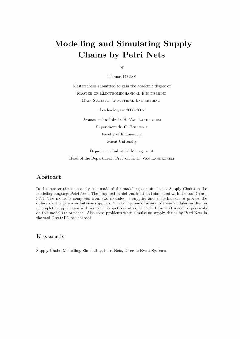
An advantage of modeling in PN is the possibility to builtmodels by coupling modules [2]. Two modules were developed.One representing a supplier located between suppliers, see Fig-ure 1 (small modifications make it possible to transform this sup-plier for use at the end or at the beginning of a supply chain). Anexplication of the places of Figure 1 is shown in Tables I.
P10P
P11
P12
P8
PP9P
P3 P1
P7
P5
P2
P14
P13
P4
s
P6
P15P16 P17
t23t22
t21
t19
t10
t9
t8
t24
t25t26
t27 t28t29
t20
t18
t17
t16
t15
t13t12
t11
t3
t2
t1
t5
2π
t7
2π
t6
2π
t4
4π
t14
7π
_2 _2_3
_2 _2_3
_2 _2 _3
Fig. 1. Supplier Module
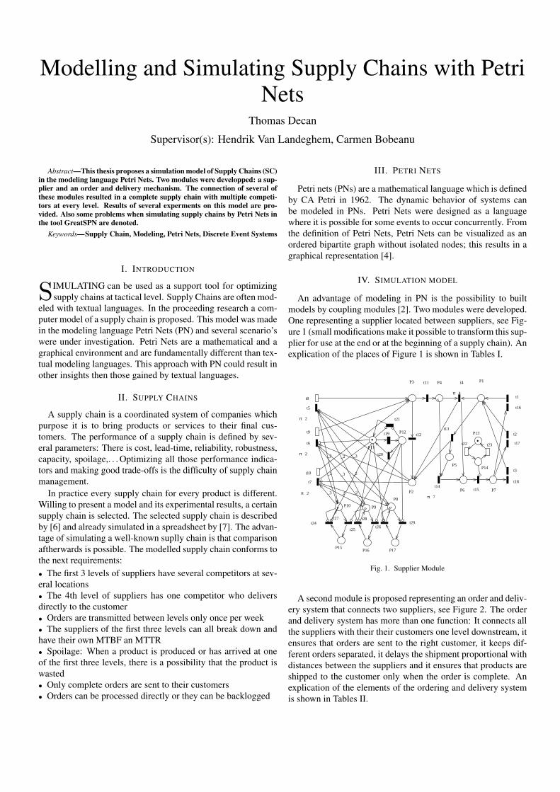
A second module is proposed representing an order and deliv-ery system that connects two suppliers, see Figure 2. The orderand delivery system has more than one function: It connects allthe suppliers with their their customers one level downstream, itensures that orders are sent to the right customer, it keeps dif-ferent orders separated, it delays the shipment proportional withdistances between the suppliers and it ensures that products areshipped to the customer only when the order is complete. Anexplication of the elements of the ordering and delivery systemis shown in Tables II.
Notation InterpretationP1 Incoming ordersP2 Outgoing ordersP3 Available productsP4 Stock of goodsP5 BackordersP6 Stock of assigned goodsP7 Outgoing goodsP8, P9 &P10
The implementation of the 40% source limit.
P11 State: Do not send ordersP12 State: Send OrdersP13 State: Shipping department is upP14 State: Shipping department is downP15, P16& P17
Token storage per 100
TABLE ITHE PLACES OF A SUPPLIER OF LEVEL 2 OR 3 FROM FIGURE 1
P9
P7
P5
P4 P3 P2 P1
P8
P6
t11
t10
t8
t7
t6
t3t5
2π
t4
3π
t2
3π
t9
4π
t1
4π
Fig. 2. Ordering and Delivery Mechanism Module
Not. InterpretationP1 Last order in rowP2 Place to keep the third and the second order sepa-
ratedP3 Second order in row waiting until the first order is
complete and releasedP4 Place to keep the first and the second order separatedP5 First order in rowP6 One token is stored here when an order arrives at an
empty queue to prevent the order from splitting at t3P7 Assigned products for the first order, waiting until
the order is complete (= until P6 is empty)P8 Goods on their way to the customerP9 Orders
TABLE IITHE PLACES OF A SIMPLE QUEUE FROM FIGURE 2
V. THE ACTUAL SIMULATIONS AND RESULTS
Four optimal scenario’s are calculated with the linear pro-gramming method (see [7] and [6]):
basic serial model: At every level only the cheapest supplierbasic model: Because the basic serial model proposes only onepath, the whole supply chain is extremely vulnerable for com-plete disruptions. In the basic model suppliers can order maxi-mum 40% to the same supplier.high reliability model: With a higher number of suppliers thereliability drops. Here a higher reliability is guaranteed by usinghigh reliable suppliers. Also with a 40% source limit.60% source limit model: To obtain a higher reliability with lesscostly suppliers, the total number of suppliers will be dropped.Control Layer Model: An extra layer is added to the basicmodel. It is not possible anymore for a customer to send ordersto a supplier with many backlogs.
VI. CONCLUSION
During the building of the model there were no obstaclesfound that PN couldn’t overcome. For this reason it is the au-thor’s belief that Petri Nets in general are a very powerful mod-eling language and GSPN specifically are very well suited forthe simulation of supply chains. Compared to other languagesgives the graphical representation of the model an extremelygood overview and a quick insight of the dynamics of the model.In addition of these PN-benefits, it was possible to build thisvery complex and large model in a short time. This because theauthor started from the methodology provided in [2] and [5].This methodology allows the user to built models on a incre-mental and systematical way by coupling basic components bywell defined rules. Several experiments were performed on themodel. From their results we can conclude that on this model,the most important disturbance factor on the performance mea-sures is the random transport time. If the objective is to mini-mize costs, spoilage has to be reduced. Plant breakdowns haveonly a minor influence. When there are more reliable suppliersused, cost increase but the service factors don’t. When we cutthe total number of suppliers, costs drop without the loss of per-formance. Best results were gained with a minimum of low-costsuppliers.
REFERENCES
[1] C. A. Petri, Nets, time and space, Theor. Comput. Sci., vol. 153, number1-2, p. 3-48, Elsevier Science Publishers Ltd., Essex, UK, 1996
[2] Carmen-Veronica Bobeanu and Eugene J.H. Kerckhoffs and Hendrik VanLandeghem, modeling of Discrete Event Systems:A Holistic and Incremen-tal Approach Using Petri Nets, Ghent University, Delft University of Tech-nology, ACM Transactions on modeling and Computer Simulation, p. 389-423, vol. 14, number 4, ACM Press, New York, NY, USA, okt. 2004
[3] Prof.dr.ir. Hendrik Van Landeghem, Advanced Methods in Production &Logistics, Universiteit Gent, 2006
[4] Carmen-Veronica Bobeanu, Modelling and Simulating Manufacturing andService Systems using Petri Nets, Universiteit Gent, 2005
[5] Rik Van Landeghem and Carmen-Veronica Bobeanu, Formal Modelling ofSupply Chain: An Incremental Approach Using Petri Nets
[6] Markus Bundschuh and Diego Klabjan and Deborah L. Thurston, Mod-elling Robust and Reliable Supply Chains, University of Illinois at Urbana-Champaign, journal????, 2003, June
[7] Ester Massons Vila, Supply Chain modeling: Optimization Versus Simula-tion, Ghent University, jul. 2004
[8] GreatSPN User’s Manual v. 2.0.2, Universita di Torino, Dipartimento diInformatica, Performance Evaluation group, July 2004
[9] Gianfranco Balbo and Jorg Desel and Kurt Jensen and Wolfgang Reisigand Grzegorz Rozenberg and Manuel Silva, Introductory Tutorial PetriNets, 21st International Conference on Application and Theory of PetriNets, Aarhus, Denmark, June, 2000
Contents
Overzicht iii
Overzicht iv
Extended abstract v
List of Abbreviations x
1 Introduction 1
2 Supply Chains 2
2.1 General . . . . . . . . . . . . . . . . . . . . . . . . . . . . . . . . . . . . . . . . . . 2
2.2 The Supply Chain in case . . . . . . . . . . . . . . . . . . . . . . . . . . . . . . . . 2
2.3 Parameters . . . . . . . . . . . . . . . . . . . . . . . . . . . . . . . . . . . . . . . . 3
3 Petri Nets 5
3.1 Petri Net Formalism . . . . . . . . . . . . . . . . . . . . . . . . . . . . . . . . . . . 5
3.2 Elementary Net Systems . . . . . . . . . . . . . . . . . . . . . . . . . . . . . . . . . 5
3.2.1 The static structure of EN-Systems . . . . . . . . . . . . . . . . . . . . . . . 5
3.2.2 The dynamic behaviour of EN-Systems . . . . . . . . . . . . . . . . . . . . 6
3.3 Place/ Transition Nets . . . . . . . . . . . . . . . . . . . . . . . . . . . . . . . . . . 7
3.3.1 The static structure of Place/ Transition-Nets . . . . . . . . . . . . . . . . . 7
3.3.2 The dynamic behaviour of P/T-Nets . . . . . . . . . . . . . . . . . . . . . . 7
3.4 Timed Petri Nets . . . . . . . . . . . . . . . . . . . . . . . . . . . . . . . . . . . . . 8
3.4.1 Approaches . . . . . . . . . . . . . . . . . . . . . . . . . . . . . . . . . . . . 8
3.4.2 Timed PN terminology . . . . . . . . . . . . . . . . . . . . . . . . . . . . . 8
3.5 Stochastic Petri Nets . . . . . . . . . . . . . . . . . . . . . . . . . . . . . . . . . . . 8
3.6 Generalized Stochastic Petri Nets . . . . . . . . . . . . . . . . . . . . . . . . . . . . 9
3.7 Motivation for modeling with GSPN . . . . . . . . . . . . . . . . . . . . . . . . . . 9
vii
CONTENTS viii
3.8 GreatSPN . . . . . . . . . . . . . . . . . . . . . . . . . . . . . . . . . . . . . . . . . 9
4 The Model 11
4.1 The Overall Model . . . . . . . . . . . . . . . . . . . . . . . . . . . . . . . . . . . . 11
4.2 Supplier level 1 . . . . . . . . . . . . . . . . . . . . . . . . . . . . . . . . . . . . . . 13
4.3 Supplier level 2 and 3 . . . . . . . . . . . . . . . . . . . . . . . . . . . . . . . . . . 13
4.4 Supplier level 4 . . . . . . . . . . . . . . . . . . . . . . . . . . . . . . . . . . . . . . 15
4.5 Ordering and Delivery Mechanism . . . . . . . . . . . . . . . . . . . . . . . . . . . 16
4.5.1 Simple Queue . . . . . . . . . . . . . . . . . . . . . . . . . . . . . . . . . . . 18
4.5.2 Advanced Queue . . . . . . . . . . . . . . . . . . . . . . . . . . . . . . . . . 21
4.6 Adaptation of the Description . . . . . . . . . . . . . . . . . . . . . . . . . . . . . . 21
5 Optimization at strategic level 24
5.1 Basic serial model . . . . . . . . . . . . . . . . . . . . . . . . . . . . . . . . . . . . 24
5.2 Basic model . . . . . . . . . . . . . . . . . . . . . . . . . . . . . . . . . . . . . . . . 25
5.3 High Reliability model . . . . . . . . . . . . . . . . . . . . . . . . . . . . . . . . . . 25
5.4 60% source limit model . . . . . . . . . . . . . . . . . . . . . . . . . . . . . . . . . 26
6 Simulation 28
6.1 Performance indicators . . . . . . . . . . . . . . . . . . . . . . . . . . . . . . . . . . 28
6.2 Target Stock . . . . . . . . . . . . . . . . . . . . . . . . . . . . . . . . . . . . . . . 29
6.3 Experiments . . . . . . . . . . . . . . . . . . . . . . . . . . . . . . . . . . . . . . . . 30
6.3.1 Analysis of the models . . . . . . . . . . . . . . . . . . . . . . . . . . . . . . 30
6.3.2 Analysis between models . . . . . . . . . . . . . . . . . . . . . . . . . . . . 30
7 Control Layer Model 33
7.1 Implementation in the model . . . . . . . . . . . . . . . . . . . . . . . . . . . . . . 33
7.2 Results . . . . . . . . . . . . . . . . . . . . . . . . . . . . . . . . . . . . . . . . . . . 33
8 Conclusion 36
Appendix A 37
Appendix B 41
Bibliography 43
List of Figures 45
List of Tables 46
List of Abbreviations
CT Cycle Time
cu currency unit
DES Discrete Event Systems
DTPNs Deterministic Timed Petri Nets
ENS Elementary Net Systems
GreatSPN GRaphical Editor and Analyzer for Timed and
Stochastic Petri Nets
GSPN Generalized Stochastic Petri Net
GUI Graphical Users Interface
MTBF Mean Time Between Failures
MTTR Mean Time To Repair
PN Petri Net
P/T Nets Place/ Transition Nets
SC Supply Chain
SPNs Stochastic Petri Nets
SS Safety Stock
STPN Stochastic Timed Petri Net
SWN Stochastic Well Formed Net
TPPN Timed Places Petri Net
TS Target Stock
TTPN Timed Transitions Petri Net
ix
Chapter 1
Introduction
It is the intention of this mastersthesis to obtain a better insight in supply chains and to optimize
them by simulation. Simulating a supply chain by running a computer model is a support tool
to optimize supply chains at tactical level. In the preceding research a computer model has been
made of a supply chain. This model was made in the modeling language Petri Nets . Petri Nets
are a mathematical and a graphical environment and are fundamentally different than textual
languages. Supply Chains are often modeled with textual languages. This approach could result
in new insights then those gained by textual languages.
The two most important parameters/measures through the whole project are:
The price The total cost of production, transport, spoilage and stock.
The performance at customer level Service level is measured at the end consumer.
Supply Chains are a very interesting subject because they are hard to predict and they have a
difficult dynamic behaviour. They are also very interesting because everyone has to deal with
them daily. Only think at all those times a certain product is not in stock at the hypermarket or
at the local grocery.
1
Chapter 2
Supply Chains
2.1 General
A supply chain is a coordinated system of companies which purpose it is to bring products or
services to their final customers. These companies can deliver as well services as goods. It is the
intention of supply chain management to intervene in the supply chain in such way that the perfor-
mance is raised. The performance of a supply chain is not defined by one single parameter: There
is cost, lead-time, reliability, robustness, capacity, spoilage,. . . Optimizing all those performance
indicators and making good trade-offs is the difficulty of supply chain management.
2.2 The Supply Chain in case
In practice every supply chain for every product is different. As we can model only one supply
chain (but run several scenarios on that model), choices have to be made. To make comparison
possible, the supply chain modeled in this mastersthesis is one used in previous research. See
Bundschuh et al. (2003) and Vila (2004). The supply chain in case has to conform to the next
requirements:
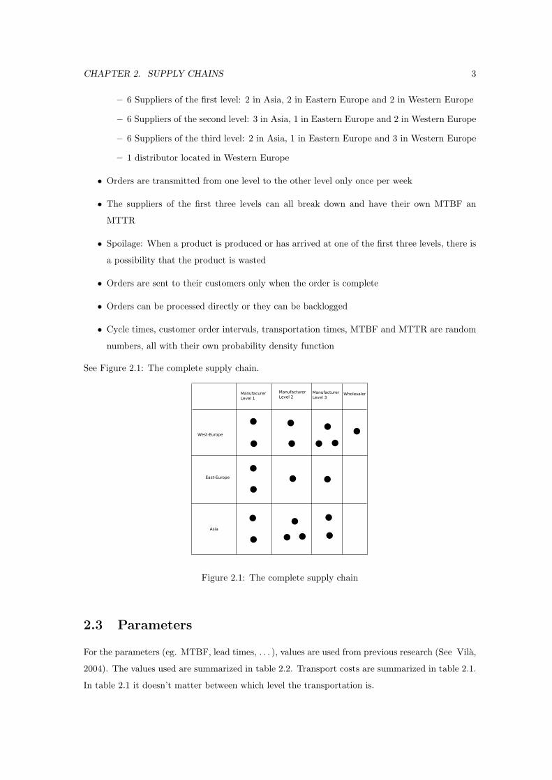
• The supply chain has 4 levels of suppliers:
– First level: Production of raw materials
– Second level: Production of semi-finished products
– Third level: Production of finished products
– Fourth level: Distributor of the products
• Every level of suppliers has several competitors at several locations:
2
CHAPTER 2. SUPPLY CHAINS 3
– 6 Suppliers of the first level: 2 in Asia, 2 in Eastern Europe and 2 in Western Europe
– 6 Suppliers of the second level: 3 in Asia, 1 in Eastern Europe and 2 in Western Europe
– 6 Suppliers of the third level: 2 in Asia, 1 in Eastern Europe and 3 in Western Europe
– 1 distributor located in Western Europe
• Orders are transmitted from one level to the other level only once per week
• The suppliers of the first three levels can all break down and have their own MTBF an
MTTR
• Spoilage: When a product is produced or has arrived at one of the first three levels, there is
a possibility that the product is wasted
• Orders are sent to their customers only when the order is complete
• Orders can be processed directly or they can be backlogged
• Cycle times, customer order intervals, transportation times, MTBF and MTTR are random
numbers, all with their own probability density function
See Figure 2.1: The complete supply chain.
Figure 2.1: The complete supply chain
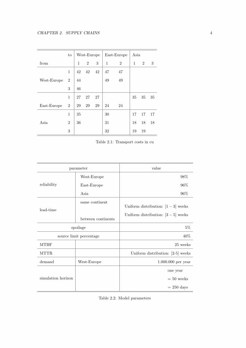
2.3 Parameters
For the parameters (eg. MTBF, lead times, . . . ), values are used from previous research (See Vila,
2004). The values used are summarized in table 2.2. Transport costs are summarized in table 2.1.
In table 2.1 it doesn’t matter between which level the transportation is.
CHAPTER 2. SUPPLY CHAINS 4
to West-Europe East-Europe Asia
from 1 2 3 1 2 1 2 3
1 42 42 42 47 47
West-Europe 2 44 49 49
3 46
1 27 27 27 35 35 35
East-Europe 2 29 29 29 24 24
1 35 30 17 17 17
Asia 2 36 31 18 18 18
3 32 19 19
Table 2.1: Transport costs in cu
parameter value
reliability
West-Europe
East-Europe
Asia
98%
96%
96%
lead-time
same continent
between continents
Uniform distribution: [1− 3] weeks
Uniform distribution: [3− 5] weeks
spoilage 5%
source limit percentage 40%
MTBF 25 weeks
MTTR Uniform distribution: [2-5] weeks
demand West-Europe 1.000.000 per year
simulation horizon
one year
= 50 weeks
= 250 days
Table 2.2: Model parameters
Chapter 3
Petri Nets
3.1 Petri Net Formalism
Petri nets (PNs) are a mathematical language which is defined by CA Petri in 1962. The dynamic
behaviour of systems can be modeled in PNs. Petri Nets were designed as a language where it
is possible for some events to occur concurrently. PN are typically strong at describing systems
with synchronisation and resource sharing. Petri Nets have a graphical representation wich is very
helpful for the comprehention of the dynamic stucture.
There are several levels of petri nets. In the next sections some of the relevant classes of PNs for
this mastersthesis are discussed.
3.2 Elementary Net Systems
3.2.1 The static structure of EN-Systems
Definition 3.1 (Elementary Net System) (Petri, 1996) A triple N = (S, T, F ), with:
• S the set of state-elements
• T the set of transition-elements
• a relation F for “flow”
is called a net iff S, T and F fulfill the following conditions (net axioms):
N1: S ∪ T 6= �
N2: S ∩ T = �
N3: domF ∪ ranF = S ∪ T
5
CHAPTER 3. PETRI NETS 6
N4: F ∩ F−1 = �
A net is used to represent the underlying static structure (potential dynamics). From the definition
of Petri Nets, Petri Nets can be visualized as an ordered bipartite graph without isolated nodes;
this results in a nice graphical representation:
• S-elements: circles © (Storage places)
• T-elements: bars or boxes � (Servers)
• Flow relation: arcs −→ (connection elements)
Additional concepts
For a given net N = (S, T, F ), XN := S ∪ T (the set of all net elements), and for x ∈ XN :
•x = {y ∈ XN : (y, x) ∈ F}, Input of a net element
x• = {y ∈ XN : (x, y) ∈ F}, Output of a net element
•x• :=• x ∪ x•, Environment of a net element
3.2.2 The dynamic behaviour of EN-Systems
PNs incorporate a notion of state which is denoted by a function M , called marking. For a given
net N = (S, T, F ):
M := {m : m ⊆ S}, (The class of conceivable markings);
E := {e : e ⊆ T, e 6= �}, (The class of all conceivable events)
The dynamic behaviour of the net is the evolution of the state of the net.
The firing rule (Petri, 1996)
The firing process is the evolving from one state to the other state. The firing rule indicates when
it is possible for a transition to fire, and what the changes are on the marking:
1. An event transforms a marking M into a different marking M ′.
2. An event is a set E of transitions; events are the only source of change.
3. Transitions in the same event E have disjoint neighbourhoods •t• (transitions may individ-
ually occur without interfering with each other).
4. The preconditions •t of each transition t ∈ E belong to M but not to M ′ and the postcon-
ditions t• of each t ∈ E belong to M ′ but not to M .
CHAPTER 3. PETRI NETS 7
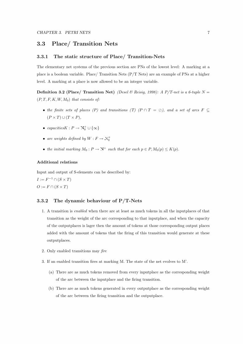
3.3 Place/ Transition Nets
3.3.1 The static structure of Place/ Transition-Nets
The elementary net systems of the previous section are PNs of the lowest level: A marking at a
place is a boolean variable. Place/ Transition Nets (P/T Nets) are an example of PNs at a higher
level. A marking at a place is now allowed to be an integer variable.
Definition 3.2 (Place/ Transition Net) (Desel & Reisig, 1998): A P/T-net is a 6-tuple N =
(P, T, F, K,W, M0) that consists of:
• the finite sets of places (P) and transitions (T) (P ∩ T = �), and a set of arcs F ⊆
(P × T ) ∪ (T × P ),
• capacitiesK : P → N+0 ∪ {∞}
• arc weights defined by W : F → N+0
• the initial marking M0 : P → N+ such that for each p ∈ P,M0(p) ≤ K(p).
Additional relations
Input and output of S-elements can be described by:
I := F−1 ∩ (S × T )
O := F ∩ (S × T )
3.3.2 The dynamic behaviour of P/T-Nets
1. A transition is enabled when there are at least as much tokens in all the inputplaces of that
transition as the weight of the arc corresponding to that inputplace, and when the capacity
of the outputplaces is lager then the amount of tokens at those corresponding output places
added with the amount of tokens that the firing of this transition would generate at these
outputplaces.
2. Only enabled transitions may fire
3. If an enabled transition fires at marking M. The state of the net evolves to M’.
(a) There are as much tokens removed from every inputplace as the corresponding weight
of the arc between the inputplace and the firing transition.
(b) There are as much tokens generated in every outputplace as the corresponding weight
of the arc between the firing transition and the outputplace.
CHAPTER 3. PETRI NETS 8
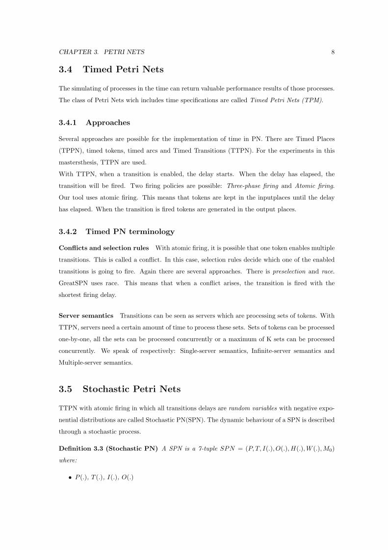
3.4 Timed Petri Nets
The simulating of processes in the time can return valuable performance results of those processes.
The class of Petri Nets wich includes time specifications are called Timed Petri Nets (TPM).
3.4.1 Approaches
Several approaches are possible for the implementation of time in PN. There are Timed Places
(TPPN), timed tokens, timed arcs and Timed Transitions (TTPN). For the experiments in this
mastersthesis, TTPN are used.
With TTPN, when a transition is enabled, the delay starts. When the delay has elapsed, the
transition will be fired. Two firing policies are possible: Three-phase firing and Atomic firing.
Our tool uses atomic firing. This means that tokens are kept in the inputplaces until the delay
has elapsed. When the transition is fired tokens are generated in the output places.
3.4.2 Timed PN terminology
Conflicts and selection rules With atomic firing, it is possible that one token enables multiple
transitions. This is called a conflict. In this case, selection rules decide which one of the enabled
transitions is going to fire. Again there are several approaches. There is preselection and race.
GreatSPN uses race. This means that when a conflict arises, the transition is fired with the
shortest firing delay.
Server semantics Transitions can be seen as servers which are processing sets of tokens. With
TTPN, servers need a certain amount of time to process these sets. Sets of tokens can be processed
one-by-one, all the sets can be processed concurrently or a maximum of K sets can be processed
concurrently. We speak of respectively: Single-server semantics, Infinite-server semantics and
Multiple-server semantics.
3.5 Stochastic Petri Nets
TTPN with atomic firing in which all transitions delays are random variables with negative expo-
nential distributions are called Stochastic PN(SPN). The dynamic behaviour of a SPN is described
through a stochastic process.
Definition 3.3 (Stochastic PN) A SPN is a 7-tuple SPN = (P, T, I(.), O(.),H(.),W (.),M0)
where:
• P (.), T (.), I(.), O(.)
CHAPTER 3. PETRI NETS 9
• H(.) Inhibitor arc: Arcs from a place to a transition. The arc has a parameter attached, his
weight. When there are as many tokens in the place as the weight of the arc, the transition
is disabled. Tokens are never consumed by inhibitor arcs. The graphical representation is a
line ending in a circle.
• W (.) is the function defined on the set of transitions that associates a rate with each transi-
tion; this rate is the inverse of the average firing time of the transition.
• M0 The initial marking
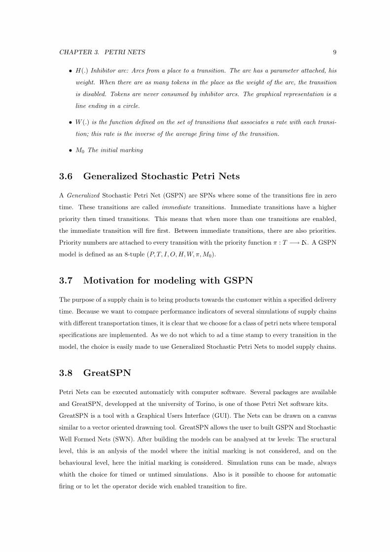
3.6 Generalized Stochastic Petri Nets
A Generalized Stochastic Petri Net (GSPN) are SPNs where some of the transitions fire in zero
time. These transitions are called immediate transitions. Immediate transitions have a higher
priority then timed transitions. This means that when more than one transitions are enabled,
the immediate transition will fire first. Between immediate transitions, there are also priorities.
Priority numbers are attached to every transition with the priority function π : T −→ N. A GSPN
model is defined as an 8-tuple (P, T, I, O, H,W, π, M0).
3.7 Motivation for modeling with GSPN
The purpose of a supply chain is to bring products towards the customer within a specified delivery
time. Because we want to compare performance indicators of several simulations of supply chains
with different transportation times, it is clear that we choose for a class of petri nets where temporal
specifications are implemented. As we do not which to ad a time stamp to every transition in the
model, the choice is easily made to use Generalized Stochastic Petri Nets to model supply chains.
3.8 GreatSPN
Petri Nets can be executed automaticly with computer software. Several packages are available
and GreatSPN, developped at the university of Torino, is one of those Petri Net software kits.
GreatSPN is a tool with a Graphical Users Interface (GUI). The Nets can be drawn on a canvas
similar to a vector oriented drawning tool. GreatSPN allows the user to built GSPN and Stochastic
Well Formed Nets (SWN). After building the models can be analysed at tw levels: The sructural
level, this is an anlysis of the model where the initial marking is not considered, and on the
behavioural level, here the initial marking is considered. Simulation runs can be made, always
whith the choice for timed or untimed simulations. Also is it possible to choose for automatic
firing or to let the operator decide wich enabled transition to fire.

CHAPTER 3. PETRI NETS 10
In this mastersthesis GreatSPN is used to examine supply chains by a GSPN model.
Chapter 4
The Model
In this chapter we describe the model. First we take a short look at the overall model and
afterwards every component of the model will be explained
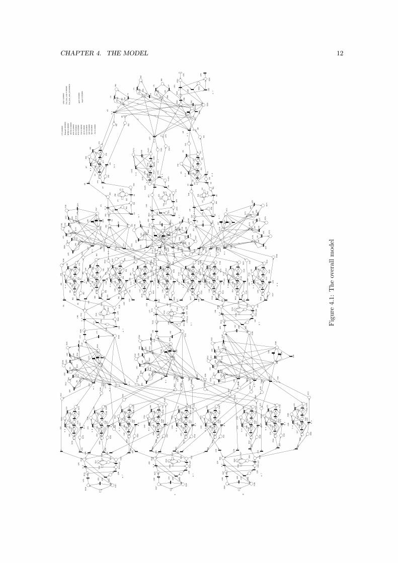
4.1 The Overall Model
In Figure 4.1 there is a plot of the overall model built in GreatSPN, used for all the experiments.
The the model consists of six suppliers of each of the first three levels and one supplier of the
fourth level. The supplier of the fourth level is the one who delivers at the customer. It is also on
this level that the performance of the supply chain is measured.
11
CHAPTER 4. THE MODEL 12P7
8
P76
P77
P79
P80
P82
P81
P335
P334
P333
P332
P331
P330
P329
P328
P327
P326
P325
P324
P323
P322
P321
P320
P319
P318
P317
P316
P315
P314
P313
P312
P311
P310
P309
P308
P307
P306
P305
P304
P303
P302
P301
P300
P299
P298
P297
P296
P295
P294
P293
P292
P291
P290
P289
P288
P287
P286
P285
P284
P283
P282
P281
P280
P279
P278
P277
P276
P275
P274
P273
P61
P166
P167
P181
P180
P179
P178
P183
P182
P254
P253
P252
P251
P250
P249
P248
P247
P245
P244
P243
P242
P241
P240
P239
P238
P236
P235
P234
P233
P232
P231
P230
P229
P160
P159
P158
P157
P162
P161
P163 50
P164
P165
P227
P226
P225 50
P224
P223
P222
P221
P220P2
19
P218
P217
P216 50
P215
P214
P213
P212
P211P2
10
P209
P208
P207 50
P206
P205
P204
P203
P202P2
01
P66
P67
P68P6
5
P63
P64
P62 50
P60
P156
P155
P154 50
P153
P152
P151
P150
P149 P1
48
P147
P146
P145 50
P144
P143
P142
P141
P140
P139
P79
P78
P80
P77
P76
P69
P70
P138
P137
P136
P135
P134
P133
P132
P131
P130
P129
P128
P127
P126
P125
P124
P123
P122
P121
P120
P119
P118
P117
P116
P115
P114
P113
P112
P111
P110
P109
P108
P107
P106
P105
P104
P103
P102
P101
P100
P99
P98
P97
P96
P95
P94
P93
P92
P91
P90
P89
P88
P87
P86
P85
P84
P83
P147
4
P295 P1
677
P147
5
P147
6
P147
8
P147
3
P73
P72
P25
P26
P979
P75
P74
P71
P147
7
P147
9
P433
50
P137
P102
4 P290
P291
P292
P293
P294
P439
150
P42
P43
P44
P45
P46
P47
P48
P49
P50
50P5
1
P52
P53
P54
P55
P56
P57
P58
P59
P81
P82
P83 P8
4
P85
P86
P87
P88
P168
P169
P170
P171
P172
P173
P174
P175
P176
P177
P184
P185
P186 P1
87
P188
P189
P190
P191
P192
P193 P1
94P1
95
P196
P197
P198
P199
P200
P201
P202
P203
P204
P205
P206
P207
P255
P256
P257
P258
P259
P260P2
61
P262
P263 P2
64
P265
P266
P267
P268
P269
P270
P271
P272
MT
BF=
0.00
8000
MT
TR
=0.
2000
00
EA
=0.
0500
00
AE
=0.
0500
00
WA
=0.
0500
00
AW
=0.
0500
00
EW
=0.
1000
00
WE
=0.
0500
00
Dem
and=
4.00
0000
CT
=2.
0000
00or
der=
5.00
0000
WW
=0.
1000
00
EE
=0.
1000
00
AA
=0.
1000
00
spoi
l=0.
0500
00
nspo
il=0.
9500
00
firs
t_tim
e_or
der=
0.00
0010
firs
t_tim
e_or
der_
II=
0.00
0020
T30
4T28
9
T27
4
T29
0
T21
1
T21
2
T21
3
T24
5
t218
T30
5
T30
3
T30
2
T30
1
T28
8
T28
7
T28
6
T27
5
T27
3
T27
2
T27
1
T18
4
T18
3
T25
8
T25
7
T25
6
T24
3
T24
2
T24
1
T22
8
T22
7
T22
6
T24
4
t222
t220
T20
6
T20
5
T20
9
T20
8
T20
7
T21
0
T24
3
t72
t71
T17
5T
174
T16
6T
165
t66
t376
t49
t33
t34
t29
T28
t378
T94
8
t89
t90
t373
t372
t366
t365
t359
t358
t352
t351
t345
t344
t338
t337
t331
t330
t324
t323
t317
t316
t219
t235
t230
t231
t232
t234
t233
t315
t314
t313
t312
t311
t310
t309
t300
t299
t298
t297
t296
t295
t294
t285
t284
t283
t282
t281
t280
t279
t163
t164
t154
t155
t145
t146
t188
t190 t189t191
t270
t269
t268
t267
t266
t265
t264
t263
t262
t261
t255
t254
t253
t252
t250
t249
t248
t247
t246
t240
t239
t238
t237
t236
t235
t234
t233
t232
t231
t241
t240
t239
t238
t237
t236
t229
t228
t227
t226
t225
t224
t223
t221
t55
t53
t51
t69
t182t1
81
t180
t179
t173
t172
t171
t170
t68
t63
t57
t56
t162
t161
t153
t152
t144
t143
t137
t136
t135
t134
t128
t127
t126
t125
t119
t118
t117
t116
t110
t109
t108
t107
t101
t100
t99
t98
t92 t9
1
t78
t77
t76
t75
t74
t73
t32
t37
t46
t43
t42
t41
t39
t36
t116
4
t116
3
t60
t59
t344
t962
t979
t961
t949
1
t362
t968
t364
t379
t88
2π
t376
2π
t369
2π
t362
2π
t355
2π
t348
2π
t341
2π
t334
2π
t327
2πt3
20
2π
t61
2π
t160
2π
t151
2π
t142
2π
t133
2π
t124
2π
t115
2π
t106
2π
t97
2π
t44
2π
t116
7
2π
t84
3π
t85
3π
t375
3π
t374
3π
t368
3π
t367
3π
t361
3π
t360
3π
t354
3π
t353
3π
t347
3π
t346
3π
t340
3π
t339
3π
t333
3π
t332
3π
t326
3π
t325
3π
t319
3π
t318
3π
t64
3π
t62
3π
t157
3π
t156
3π
t148
3π
t147
3π
t139
3π
t138
3π
t130
3π
t129
3π
t121
3π
t120
3π
t112
3π
t111
3π
t103
3π
t102
3π
t94
3π
t93
3π
t47
3π
t45
3π
t116
5
3π
t116
6
3π
t86
4π
t87
4π
t378
4π
t377
4π
t371
4π
t370
4π
t364
4π
t363
4π
t357
4π
t356
4π
t350
4π
t349
4π
t343
4π
t342
4π
t336
4π
t335
4π
t329
4π
t328
4π
t322
4πt321
4π
t186
4π
t260
4π
t245
4π
t230
4π
t52
4π
t177
4π
t168
4π
t67
4π
t58
4π
t159
4πt1
58
4π
t150
4πt1
49
4π
t141
4πt1
40
4π
t132
4πt1
31
4π
t123
4πt1
22
4π
t114
4πt1
13
4π
t105
4πt1
04
4π
t96
4πt9
5
4π
t38
4π
t50
4π
t35
4π
t116
2
4π
t116
1
4π
t343
4π
t363
4π
t215
5π
t216
5π
t217
5π
t308
5π
t307
5π
t306
5π
t293
5π
t292
5π
t291
5π
t278
5π
t277
5π
t276
5π
t200
5π
t199
5π
t198
5π
t197
5π
t196
5π
t214
5π
t65
5π
t48
5π
t377
5π
t187
7π
t259
7π
t244
7π
t229
7π
t54
7π
t178
7π
t169
7π
t40
7π
t345
7π
t365
7π
_2
_2
_3 _2
_2 _3
_2_2
_3
_2_2
_3 _2
_2_3 _2
_2
_3 _2_2
_3 _2
_2_3 _2
_2
_3
_2
_2_3
_2_2
_3_2_2
_3
_2
_2_3
_2_2
_3_2_2
_3
_2
_2_3_2
_2
_3
_2
_2
_3
_2_2
_3 _2_2
_3
_2
_2_3
_100
_50 _
100
_50 _
100
_100
_100
_50 _1
00
_50 _1
00_1
00
_50 _1
00_1
00_5
0 _100
_100
_50_1
00_1
00
_50
_100
_100
_50 _1
00_1
00
_50
_100
_100
_50_1
00_1
00
_100
_50
_100
_50
_100
_100
_50_1
00_1
00
_100
_50
_100
_50_1
00_1
00
_50_1
00_1
00
_100
_50
_100
_50
_100
_100
_100
_50_1
00
_100
_50
_100
Fig
ure
4.1:
The
over
allm
odel
CHAPTER 4. THE MODEL 13
4.2 Supplier level 1
Suppliers of level one are those at the beginning of the supply chain. So, these suppliers don’t
have any suppliers, only customers. In the model description there are six suppliers of level one
(Bundschuh et al., 2003). That is two in West-Europe, two in Eastern-Europe en two in Asia. As
we will only need at maximum 3 suppliers of level 1 per simulation (Vila, 2004), there are in the
overall model 3 of them. When different suppliers are needed, only their parameters are changed.
In this way the model is kept small.
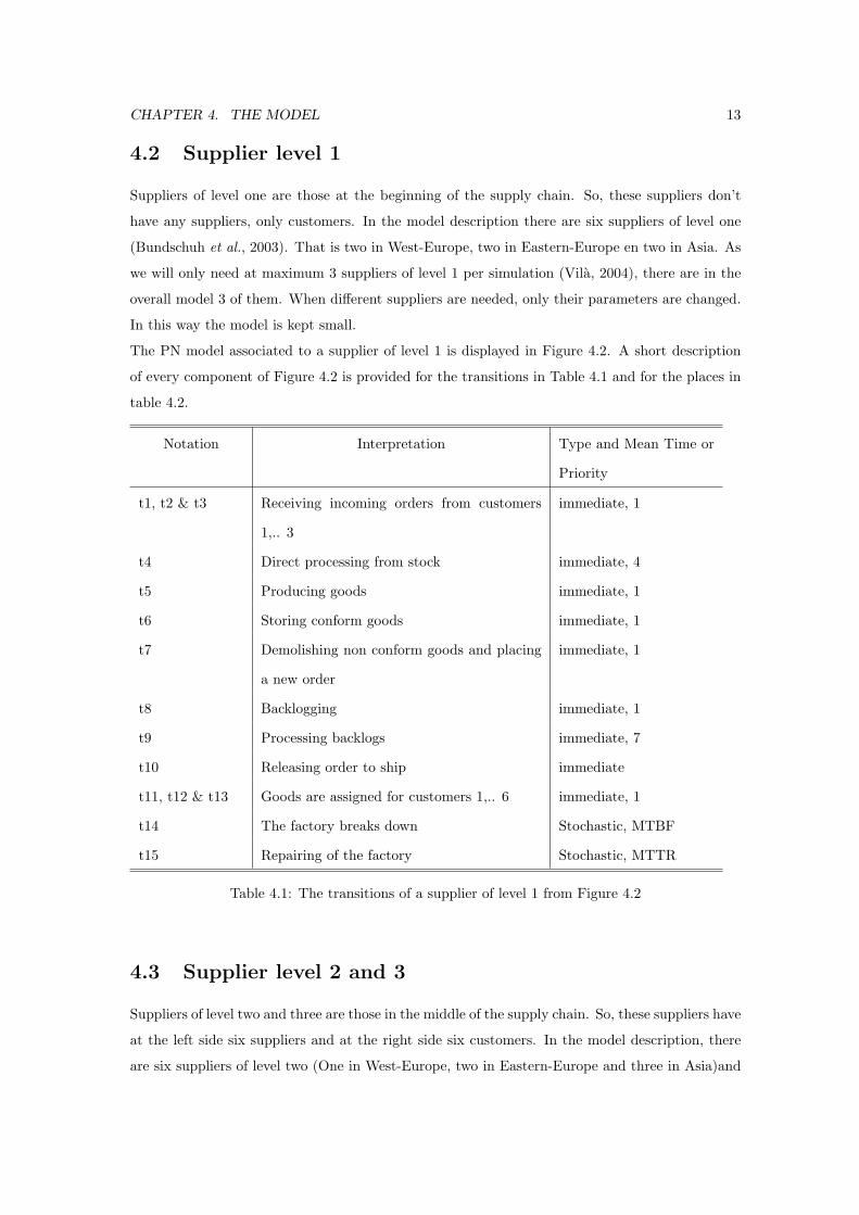
The PN model associated to a supplier of level 1 is displayed in Figure 4.2. A short description
of every component of Figure 4.2 is provided for the transitions in Table 4.1 and for the places in
table 4.2.
Notation Interpretation Type and Mean Time or
Priority
t1, t2 & t3 Receiving incoming orders from customers
1,.. 3
immediate, 1
t4 Direct processing from stock immediate, 4
t5 Producing goods immediate, 1
t6 Storing conform goods immediate, 1
t7 Demolishing non conform goods and placing
a new order
immediate, 1
t8 Backlogging immediate, 1
t9 Processing backlogs immediate, 7
t10 Releasing order to ship immediate
t11, t12 & t13 Goods are assigned for customers 1,.. 6 immediate, 1
t14 The factory breaks down Stochastic, MTBF
t15 Repairing of the factory Stochastic, MTTR
Table 4.1: The transitions of a supplier of level 1 from Figure 4.2
4.3 Supplier level 2 and 3
Suppliers of level two and three are those in the middle of the supply chain. So, these suppliers have
at the left side six suppliers and at the right side six customers. In the model description, there
are six suppliers of level two (One in West-Europe, two in Eastern-Europe and three in Asia)and
CHAPTER 4. THE MODEL 14
Notation Interpretation
P1 Incoming orders
P2 Orders waiting for production (backlogs, direct processed and spoiled products)
P3 Available products (conform and non conform specifications)
P4 Goods in stock
P5 Backorders
P6 Orders waiting to be released for shipping
P8 Factory is up
P7 Outgoing Goods
P9 Factory is down, orders can not be produced
Initially there are s goods stored, s is also the target stock
Table 4.2: The places of a supplier of level 1 from Figure 4.2
P3 P1
P2 P7
P5
P8
P9
P4
s
P6
t15t14t5
t12
t11
t13t10
t8
t7
t6
t3
t2
t1
t9
4π
t4
4π
Figure 4.2: A supplier of level 1
six of level three(three in West-Europe, one in Eastern-Europe and two in Asia).As we will only
need at maximum 3 suppliers of level 2 and at maximum suppliers of level 3 per simulation (Vila,
2004), there are in the overall model 3 of them. When different suppliers are needed, only their
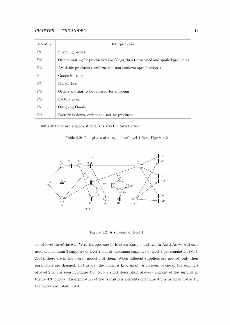
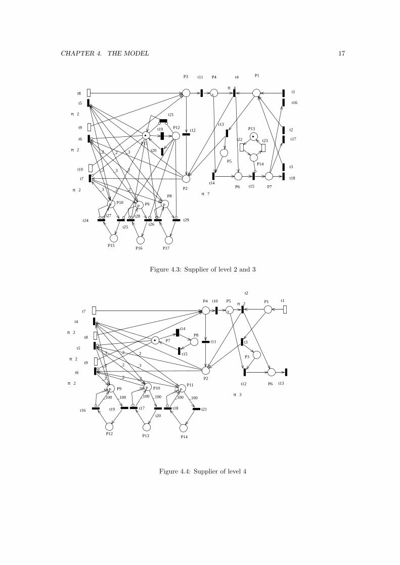
parameters are changed. In this way the model is kept small. A close-up of one of the suppliers
of level 2 or 3 is seen in Figure 4.3. Now a short description of every element of the supplier in
Figure 4.3 follows. An explication of the transitions elements of Figure 4.3 is listed in Table 4.3
the places are listed in 4.4.
CHAPTER 4. THE MODEL 15
Notation Interpretation Type and Mean Time
or Priority
t1, t2 & t3 Incoming orders from customers 1,.. 3 immediate, 1
t4 Processing orders immediate, 1
t5, t6 & t7 Sending orders to suppliers 1,.. 3 immediate, 1
t8, t9 & t10 Goods entering from suppliers 1,.. 3 Stochastic, (Table 2.2)
t11 Storing conform goods immediate, 1
t12 Demolishing non conform goods and placing a new
order
immediate, 1
t13 Backlogging immediate, 1
t14 Processing backlogs immediate, 1
t15 granting orders to be sent immediate, 1
t16, t17 & t18 Sending goods to customers 1,.. 3 immediate, 1
t19 Setting state to: send orders deterministic, 5 days
t20 Setting state to: don’t send orders immediate, 1
t21 Initializing state to: don’t send orders determ., 10−9 days
t22 The factory breaks down Stochastic, MTBF
t23 Repairing of the factory Stochastic, MTTR
t24, t25 & t26 Ungrouping 1 token in 100 Immediate (take 1,
give 100)
t27, t28 & t29 Grouping 100 tokens in 1 Immediate (take 100,
give 1)
Table 4.3: The transitions of a supplier of level 2 or 3 from Figure 4.3
4.4 Supplier level 4
The supplier of level four is the supplier at the end of the supply chain. This is the supplier who
delivers directly to the customers. It is at this supplier where the performance is measured. There
is only one supplier at this level, located in Western Europe. A close-up of this suppliers is shown
in Figure 4.4. Now a short description of every element of the supplier in Figure 4.4 follows. An
explication of the transitions of Figure 4.4 is listed in Table 4.5 the places are listed in 4.6.1In GreatSPN, it is not possible to store more then 255 tokens per place
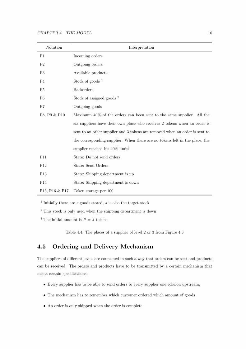
CHAPTER 4. THE MODEL 16
Notation Interpretation
P1 Incoming orders
P2 Outgoing orders
P3 Available products
P4 Stock of goods 1
P5 Backorders
P6 Stock of assigned goods 2
P7 Outgoing goods
P8, P9 & P10 Maximum 40% of the orders can been sent to the same supplier. All the
six suppliers have their own place who receives 2 tokens when an order is
sent to an other supplier and 3 tokens are removed when an order is sent to
the corresponding supplier. When there are no tokens left in the place, the
supplier reached his 40% limit3.
P11 State: Do not send orders
P12 State: Send Orders
P13 State: Shipping department is up
P14 State: Shipping department is down
P15, P16 & P17 Token storage per 100
1 Initially there are s goods stored, s is also the target stock
2 This stock is only used when the shipping department is down
3 The initial amount is P = 3 tokens
Table 4.4: The places of a supplier of level 2 or 3 from Figure 4.3
4.5 Ordering and Delivery Mechanism
The suppliers of different levels are connected in such a way that orders can be sent and products
can be received. The orders and products have to be transmitted by a certain mechanism that
meets certain specifications:
• Every supplier has to be able to send orders to every supplier one echelon upstream.
• The mechanism has to remember which customer ordered which amount of goods
• An order is only shipped when the order is complete
CHAPTER 4. THE MODEL 17
P10P
P11
P12
P8
PP9P
P3 P1
P7
P5
P2
P14
P13
P4
s
P6
P15P16 P17
t23t22
t21
t19
t10
t9
t8
t24
t25t26
t27 t28t29
t20
t18
t17
t16
t15
t13t12
t11
t3
t2
t1
t5
2π
t7
2π
t6
2π
t4
4π
t14
7π
_2 _2_3
_2 _2_3
_2 _2 _3
Figure 4.3: Supplier of level 2 and 3
P11P
P7P8
P10PP9P
P2
P1P4
P6
P3
P5
s
P12 P13 P14
t14
t9
t8
t7
t1
t21
t20
t19 t18t17t16
t15
t13
t11
t10
t3
t2
2π
t6
2π
t5
2π
t4
2π
t12
3π
_2
_2
_2
_100_100
_3
_2
_2
_100_100 _100 _100
_3
_2
_2
_50 _50_50
Figure 4.4: Supplier of level 4
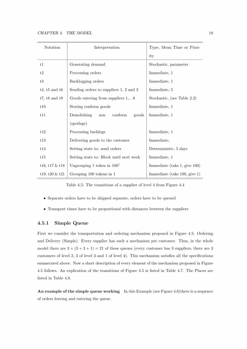
CHAPTER 4. THE MODEL 18
Notation Interpretation Type, Mean Time or Prior-
ity
t1 Generating demand Stochastic, parameter
t2 Processing orders Immediate, 1
t3 Backlogging orders Immediate, 1
t4, t5 and t6 Sending orders to suppliers 1, 2 and 3 Immediate, 5
t7, t8 and t9 Goods entering from suppliers 1,.. 6 Stochastic, (see Table 2.2)
t10 Storing conform goods Immediate, 1
t11 Demolishing non conform goods
(spoilage)
Immediate, 1
t12 Processing backlogs Immediate, 1
t13 Delivering goods to the customer Immediate,
t14 Setting state to: send orders Deterministic, 5 days
t15 Setting state to: Block until next week Immediate, 1
t16, t17 & t18 Ungrouping 1 token in 1001 Immediate (take 1, give 100)
t19, t20 & t21 Grouping 100 tokens in 1 Immediate (take 100, give 1)
Table 4.5: The transitions of a supplier of level 4 from Figure 4.4
• Separate orders have to be shipped separate, orders have to be queued
• Transport times have to be proportional with distances between the suppliers
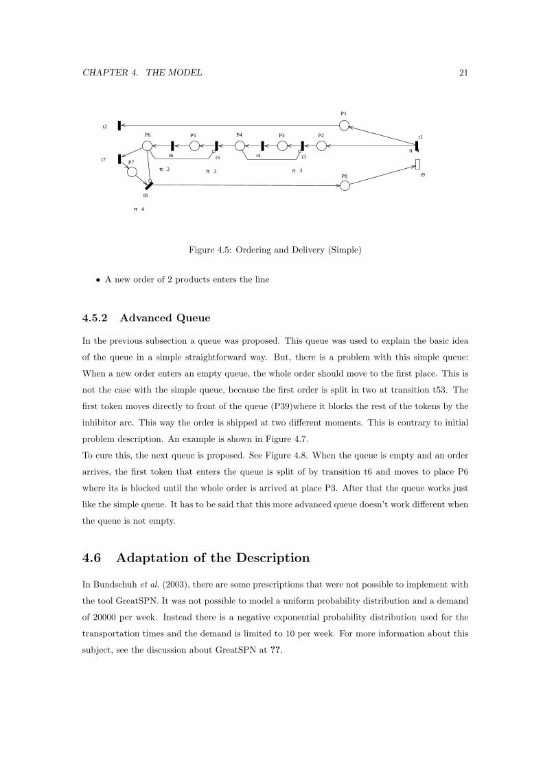
4.5.1 Simple Queue
First we consider the transportation and ordering mechanism proposed in Figure 4.5: Ordering
and Delivery (Simple). Every supplier has such a mechanism per customer. Thus, in the whole
model there are 3× (3 + 3 + 1) = 21 of these queues (every customer has 3 suppliers, there are 3
customers of level 2, 3 of level 3 and 1 of level 4). This mechanism satisfies all the specifications
enumerated above. Now a short description of every element of the mechanism proposed in Figure
4.5 follows. An explication of the transitions of Figure 4.5 is listed in Table 4.7. The Places are
listed in Table 4.8.
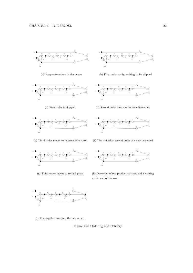
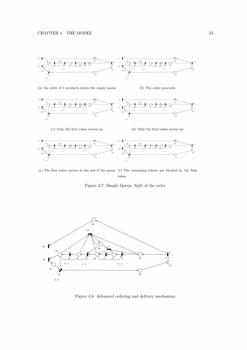
An example of the simple queue working In this Example (see Figure 4.6)there is a sequence
of orders leaving and entering the queue.
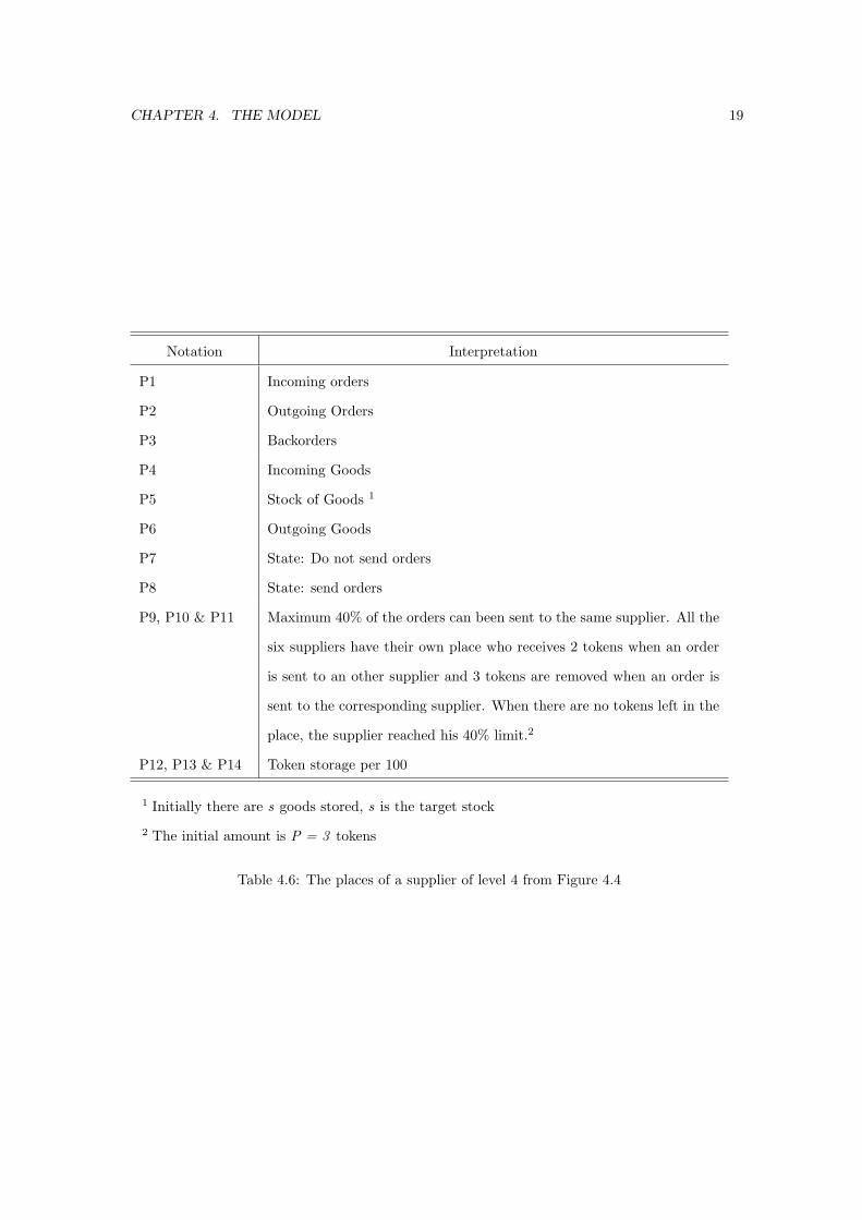
CHAPTER 4. THE MODEL 19
Notation Interpretation
P1 Incoming orders
P2 Outgoing Orders
P3 Backorders
P4 Incoming Goods
P5 Stock of Goods 1
P6 Outgoing Goods
P7 State: Do not send orders
P8 State: send orders
P9, P10 & P11 Maximum 40% of the orders can been sent to the same supplier. All the
six suppliers have their own place who receives 2 tokens when an order
is sent to an other supplier and 3 tokens are removed when an order is
sent to the corresponding supplier. When there are no tokens left in the
place, the supplier reached his 40% limit.2
P12, P13 & P14 Token storage per 100
1 Initially there are s goods stored, s is the target stock
2 The initial amount is P = 3 tokens
Table 4.6: The places of a supplier of level 4 from Figure 4.4
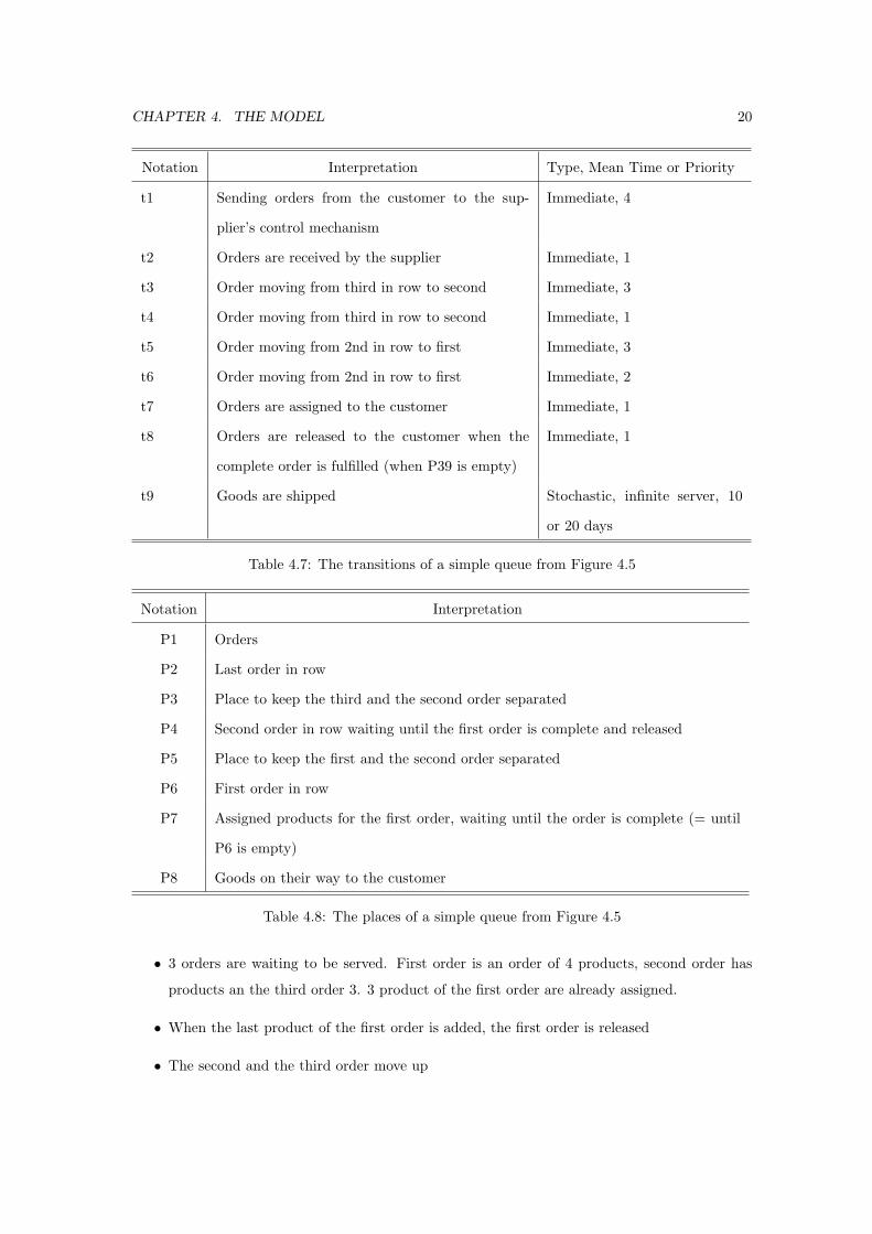
CHAPTER 4. THE MODEL 20
Notation Interpretation Type, Mean Time or Priority
t1 Sending orders from the customer to the sup-
plier’s control mechanism
Immediate, 4
t2 Orders are received by the supplier Immediate, 1
t3 Order moving from third in row to second Immediate, 3
t4 Order moving from third in row to second Immediate, 1
t5 Order moving from 2nd in row to first Immediate, 3
t6 Order moving from 2nd in row to first Immediate, 2
t7 Orders are assigned to the customer Immediate, 1
t8 Orders are released to the customer when the
complete order is fulfilled (when P39 is empty)
Immediate, 1
t9 Goods are shipped Stochastic, infinite server, 10
or 20 days
Table 4.7: The transitions of a simple queue from Figure 4.5
Notation Interpretation
P1 Orders
P2 Last order in row
P3 Place to keep the third and the second order separated
P4 Second order in row waiting until the first order is complete and released
P5 Place to keep the first and the second order separated
P6 First order in row
P7 Assigned products for the first order, waiting until the order is complete (= until
P6 is empty)
P8 Goods on their way to the customer
Table 4.8: The places of a simple queue from Figure 4.5
• 3 orders are waiting to be served. First order is an order of 4 products, second order has
products an the third order 3. 3 product of the first order are already assigned.
• When the last product of the first order is added, the first order is released
• The second and the third order move up
CHAPTER 4. THE MODEL 21
P8
P2P3P4P5P6
P7
P1
t9
t7t4
t2
t6
2π
t5
3π
t3
3π
t8
4π
t1
4π
Figure 4.5: Ordering and Delivery (Simple)
• A new order of 2 products enters the line
4.5.2 Advanced Queue
In the previous subsection a queue was proposed. This queue was used to explain the basic idea
of the queue in a simple straightforward way. But, there is a problem with this simple queue:
When a new order enters an empty queue, the whole order should move to the first place. This is
not the case with the simple queue, because the first order is split in two at transition t53. The
first token moves directly to front of the queue (P39)where it blocks the rest of the tokens by the
inhibitor arc. This way the order is shipped at two different moments. This is contrary to initial
problem description. An example is shown in Figure 4.7.
To cure this, the next queue is proposed. See Figure 4.8. When the queue is empty and an order
arrives, the first token that enters the queue is split of by transition t6 and moves to place P6
where its is blocked until the whole order is arrived at place P3. After that the queue works just
like the simple queue. It has to be said that this more advanced queue doesn’t work different when
the queue is not empty.
4.6 Adaptation of the Description
In Bundschuh et al. (2003), there are some prescriptions that were not possible to implement with
the tool GreatSPN. It was not possible to model a uniform probability distribution and a demand
of 20000 per week. Instead there is a negative exponential probability distribution used for the
transportation times and the demand is limited to 10 per week. For more information about this
subject, see the discussion about GreatSPN at ??.
CHAPTER 4. THE MODEL 22
P8
P2P3P4P5P6
P7
P1
t9
t7t4
t2
t6
2π
t5
3π
t3
3π
t8
4π
t1
4π
(a) 3 separate orders in the queue
P8
P2P3P4P5P6
P7
P1
t9
t7t4
t2
t6
2π
t5
3π
t3
3π
t8
4π
t1
4π
(b) First order ready, waiting to be shipped
P8
P2P3P4P5P6
P7
P1
t9
t7t4
t2
t6
2π
t5
3π
t3
3π
t8
4π
t1
4π
(c) First order is shipped
P8
P2P3P4P5P6
P7
P1
t9
t7t4
t2
t6
2π
t5
3π
t3
3π
t8
4π
t1
4π
(d) Second order moves to intermediate state
P8
P2P3P4P5P6
P7
P1
t9
t7t4
t2
t6
2π
t5
3π
t3
3π
t8
4π
t1
4π
(e) Third order moves to intermediate state
P8
P2P3P4P5P6
P7
P1
t9
t7t4
t2
t6
2π
t5
3π
t3
3π
t8
4π
t1
4π
(f) The -initially- second order can now be served
P8
P2P3P4P5P6
P7
P1
t9
t7t4
t2
t6
2π
t5
3π
t3
3π
t8
4π
t1
4π
(g) Third order moves to second place
P8
P2P3P4P5P6
P7
P1
t9
t7t4
t2
t6
2π
t5
3π
t3
3π
t8
4π
t1
4π
(h) One order of two products arrived and is waiting
at the end of the row.
P8
P2P3P4P5P6
P7
P1
t9
t7t4
t2
t6
2π
t5
3π
t3
3π
t8
4π
t1
4π
(i) The supplier accepted the new order.
Figure 4.6: Ordering and Delivery
CHAPTER 4. THE MODEL 23
P28
P30
P39 P40
P41 P42 P43
P51
t39
t54t29
t27
t40
2π
t53
3π
t55
3π
t64
4π
t38
4π
(a) An order of 4 products enters the empty queue
P28
P30
P39 P40
P41 P42 P43
P51
t39
t54t29
t27
t40
2π
t53
3π
t55
3π
t64
4π
t38
4π
(b) The order proceeds
P28
P30
P39 P40
P41 P42 P43
P51
t39
t54t29
t27
t40
2π
t53
3π
t55
3π
t64
4π
t38
4π
(c) Only the first token moves up
P28
P30
P39 P40
P41 P42 P43
P51
t39
t54t29
t27
t40
2π
t53
3π
t55
3π
t64
4π
t38
4π
(d) Only the first token moves up
P28
P30
P39 P40
P41 P42 P43
P51
t39
t54t29
t27
t40
2π
t53
3π
t55
3π
t64
4π
t38
4π
(e) The first token arrives at the end of the queue
P28
P30
P39 P40
P41 P42 P43
P51
t39
t54t29
t27
t40
2π
t53
3π
t55
3π
t64
4π
t38
4π
(f) The remaining tokens are blocked by the first
token
Figure 4.7: Simple Queue: Split of the order
P9
P7
P5
P4 P3 P2 P1
P8
P6
t11
t10
t8
t7
t6
t3t5
2π
t4
3π
t2
3π
t9
4π
t1
4π
Figure 4.8: Advanced ordering and delivery mechanism
Chapter 5
Optimization at strategic level
In the previous chapter a PN model of a supply chain was proposed. Before we have a look
at the experiments, some strategic level decisions have to be made. The model can simulate
several scenario’s. This means that at a higher decision-level, there can be decided that some less
desired suppliers are not considered. This can result in a Supply chain with a very high reliability
or a scenario where only the cheapest suppliers are used. The results obtained in this chapter
are calculated with the linear programming method. The total cost was always minimized with
constraints on the reliability and the robustness. These calculations are outside the scope of this
mastersthesis, for details see Vila (2004).
Four scenario’s are under investigation.
basic serial model The cost is minimized
basic model Because the basic serial model proposes only one path, the whole supply chain
is extremely vulnerable for complete disruptions. In the basic model suppliers can order
maximum 40% to the same supplier.
high reliability model As the number of suppliers decreases, the reliability drops. Here a cer-
tain higher reliability is guaranteed by using high reliable suppliers. The 40% source limit
is still set.
60% source limit model To obtain a higher reliability with less costly suppliers, the total num-
ber of suppliers will be dropped.
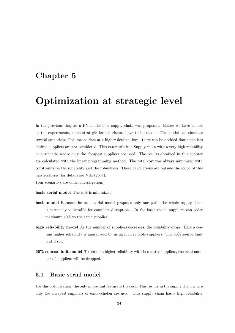
5.1 Basic serial model
For this optimization, the only important feature is the cost. This results in the supply chain where
only the cheapest suppliers of each echelon are used. This supply chain has a high reliability
24
CHAPTER 5. OPTIMIZATION AT STRATEGIC LEVEL 25
((96%)3 = 88%), 88% of the time are all the elements of the supply chain operational. The
disadvantage of this cheap and high reliable supply chain is the robustness. When one of the
elements is down, the entire supply chain is down. No bypasses are possible. The total minimum
cost of this supply chain is 69, 3 ∗ 106 currency units. See Figure 5.1.
Figure 5.1: Basic serial
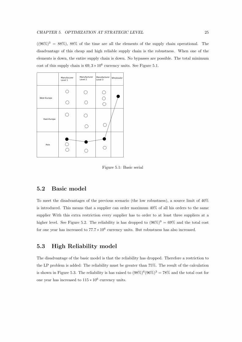
5.2 Basic model
To meet the disadvantages of the previous scenario (the low robustness), a source limit of 40%
is introduced. This means that a supplier can order maximum 40% of all his orders to the same
supplier With this extra restriction every supplier has to order to at least three suppliers at a
higher level. See Figure 5.2. The reliability is has dropped to (96%)9 = 69% and the total cost
for one year has increased to 77.7 ∗ 106 currency units. But robustness has also increased.
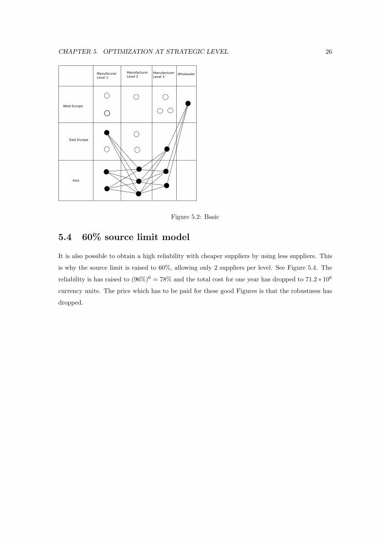
5.3 High Reliability model
The disadvantage of the basic model is that the reliability has dropped. Therefore a restriction to
the LP problem is added: The reliability must be greater than 75%. The result of the calculation
is shown in Figure 5.3. The reliability is has raised to (98%)6(96%)3 = 78% and the total cost for
one year has increased to 115 ∗ 106 currency units.
CHAPTER 5. OPTIMIZATION AT STRATEGIC LEVEL 26
Figure 5.2: Basic
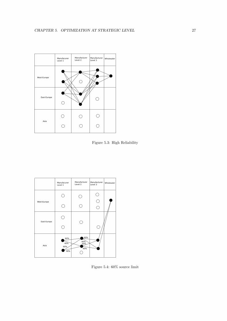
5.4 60% source limit model
It is also possible to obtain a high reliability with cheaper suppliers by using less suppliers. This
is why the source limit is raised to 60%, allowing only 2 suppliers per level. See Figure 5.4. The
reliability is has raised to (96%)6 = 78% and the total cost for one year has dropped to 71.2 ∗ 106
currency units. The price which has to be paid for these good Figures is that the robustness has
dropped.
CHAPTER 5. OPTIMIZATION AT STRATEGIC LEVEL 27
Figure 5.3: High Reliability
Figure 5.4: 60% source limit
Chapter 6
Simulation
When the optimization at strategic level is completed, the tactical planning begins. In this case this
is: When the suppliers are chosen, there has to be decided how service levels have to be attained.
The parameters we can manipulate are the target stocks for every supplier. The simulation of
several models will support us to find appropriate parameters with their resulting service levels.
6.1 Performance indicators
As supply chains have more then one level of interest, we now define the several supply chain
performance indicators used in the discussion below.
Stockout periods It indicates the number of periods that the deliveries where not met at the
last echelon (the echelon of the customer).
Service level P1 It is the percentage of the periods that there was no stockout:(1− StockoutPeriods
TotalPeriods
)× 100%
Service level P2 or fill rate It is the percentage of the fulfilled demand to the total demand:(1− DemandCovered
DemandTotal
)× 100%
Transport cost See Table 2.1
Average Inventory The sum of the average inventory of every supplier.
Total Cost The sum of the transportation costs, the fixed cost per transportation route, the
inventory costs and the backlog costs. With an inventory cost of 1 cu per period and a
backlog cost of 2 cu’s per period.
28
CHAPTER 6. SIMULATION 29
Average breakdown The total time of all the breakdowns compared to the simulation duration.
Spoilage The amount of product spoiled per day.
6.2 Target Stock
Target stock is the stock every supplier tries to attain. The average stock at a supplier will always
be lower than the target stock. This because of the transport times, the time orders have to wait
until submitted to a supplier, stockouts of a supplier, etc.
The level of the target stock which has to be set depends on the demand during leadtime (LT) and
the service levels we want to attain. The demand during LT is a distribution δ (µδ, σδ) which is the
result of two distributions: The demand (µD, σD) and the lead time (µLT , σLT ). Because we want
to examine the impact of the target stock on the service level, we simulate every scenarios with
different z-factors z = 0, 1, 2, 3, 4, this is the number of times we use σδ as safety stock (SS). The
target stock is calculated using next formula for the suppliers of level 2, 3 and 4 (See Landeghem
(2005)):
TS = µδ + Z × σδ =µD × µLT
n× spoilech+ Z ×
√µLT × σ2
D + µ2D × σ2
LT
with:
TS The Target Stock
µδ Average demand during LT
Z The number of times σδ we use as safety stock (SS)
σδ The standard deviation on the demand during LT
µLT Average Lead Time or transport time
µD Average Demand
n The total number of suppliers in the echelon
spoil The amount wasted per echelon1
ech The number of times spoilage has to be count in 2
Z The z-factor
σD The standard deviation on the Demand1standard spoil = 0.952For echelon 1,2,3 & 4 ech is respectively 4, 3, 2 & 1
CHAPTER 6. SIMULATION 30
σLT The standard deviation on the Lead Time or transport time3.
Suppliers of the 1st echelon have unlimited stocks (see Bundschuh et al. (2003)). For the simulation
target stocks of 50 at the 1st echelon could be replenished fast enough, so it seemed like they were
infinite.
Every scenario was simulated with and without uncertainty factors. If we calculate for the same
scenario the Target Stock for different levels of uncertainty, Target Stocks will be different. To
make comparison easier, Target Stocks are for every level of uncertainty the same for same scenarios
and same values of Z.
Target stocks for uncertainty factor Z from 0 to 4 are shown in the appendix on p. 42 Table 1.
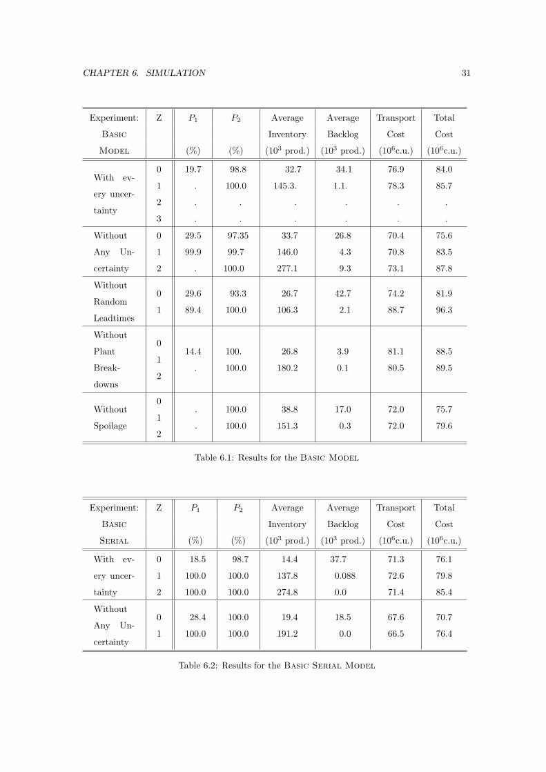
6.3 Experiments
Several scenarios were simulated with the PN-model. In Table 6.1, 6.2, 6.3 and 6.4 are the results
presented.
6.3.1 Analysis of the models
to be continued . . .
6.3.2 Analysis between models
to be continued . . .
3Because the lead time is simulated as a exponential distribution, σLT = µLT . When a supplier has n multiple
supplier, σ lowers with a factor 1√n
.
CHAPTER 6. SIMULATION 31
Experiment: Z P1 P2 Average Average Transport Total
Basic Inventory Backlog Cost Cost
Model (%) (%) (103 prod.) (103 prod.) (106c.u.) (106c.u.)
With ev-
ery uncer-
tainty
0
1
2
3
19.7
.
.
.
98.8
100.0
.
.
32.7
145.3.
.
.
34.1
1.1.
.
.
76.9
78.3
.
.
84.0
85.7
.
.
Without
Any Un-
certainty
0
1
2
29.5
99.9
.
97.35
99.7
100.0
33.7
146.0
277.1
26.8
4.3
9.3
70.4
70.8
73.1
75.6
83.5
87.8
Without
Random
Leadtimes
0
1
29.6
89.4
93.3
100.0
26.7
106.3
42.7
2.1
74.2
88.7
81.9
96.3
Without
Plant
Break-
downs
0
1
2
14.4
.
100.
100.0
26.8
180.2
3.9
0.1
81.1
80.5
88.5
89.5
Without
Spoilage
0
1
2
.
.
100.0
100.0
38.8
151.3
17.0
0.3
72.0
72.0
75.7
79.6
Table 6.1: Results for the Basic Model
Experiment: Z P1 P2 Average Average Transport Total
Basic Inventory Backlog Cost Cost
Serial (%) (%) (103 prod.) (103 prod.) (106c.u.) (106c.u.)
With ev-
ery uncer-
tainty
0
1
2
18.5
100.0
100.0
98.7
100.0
100.0
14.4
137.8
274.8
37.7
0.088
0.0
71.3
72.6
71.4
76.1
79.8
85.4
Without
Any Un-
certainty
0
1
28.4
100.0
100.0
100.0
19.4
191.2
18.5
0.0
67.6
66.5
70.7
76.4
Table 6.2: Results for the Basic Serial Model
CHAPTER 6. SIMULATION 32
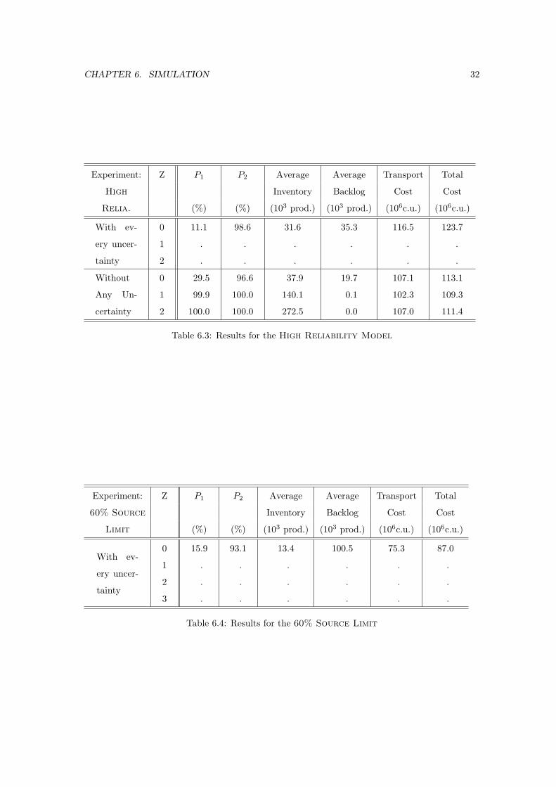
Experiment: Z P1 P2 Average Average Transport Total
High Inventory Backlog Cost Cost
Relia. (%) (%) (103 prod.) (103 prod.) (106c.u.) (106c.u.)
With ev-
ery uncer-
tainty
0
1
2
11.1
.
.
98.6
.
.
31.6
.
.
35.3
.
.
116.5
.
.
123.7
.
.
Without
Any Un-
certainty
0
1
2
29.5
99.9
100.0
96.6
100.0
100.0
37.9
140.1
272.5
19.7
0.1
0.0
107.1
102.3
107.0
113.1
109.3
111.4
Table 6.3: Results for the High Reliability Model
Experiment: Z P1 P2 Average Average Transport Total
60% Source Inventory Backlog Cost Cost
Limit (%) (%) (103 prod.) (103 prod.) (106c.u.) (106c.u.)
With ev-
ery uncer-
tainty
0
1
2
3
15.9
.
.
.
93.1
.
.
.
13.4
.
.
.
100.5
.
.
.
75.3
.
.
.
87.0
.
.
.
Table 6.4: Results for the 60% Source Limit
Chapter 7
Control Layer Model
In the previous chapter several scenario’s are proposed and simulated. All those scenario’s use the
same model based on the supply chain described by Bundschuh et al. (2003). In that description,
the state of a customer’s suppliers is not considered when that customer decides where he sends
his orders to. In this case it is possible that a customer sends orders to a supplier with many
backlogs. If the customer would have the appropriate information of his suppliers to send his
orders only to those suppliers who can deliver directly from stock, supply chain performance can
possibly be raised. In this chapter we implement a control layer in the model so that customers
have more information about the status of their suppliers at the ordering moment.
7.1 Implementation in the model
The only modification that has to be added in the model are inhibitor arcs between the backlog
places (e.g. place P5 in Table 4.1 and Figure 4.2) and the send-order transitions (e.g. transitions
t230, t232, ..t240 in Table 4.3 and Figure 4.3). Weights can be added to each inhibitor arc to
permit a certain level of backlogs at each supplier. There were simulation runs with weights of 0,
2 and 5. In Figure 7.1 a close-up is shown of the Control Layer Model. Note the inhibitor arcs
from P63, P75 & P48 to respectively t65, t377, & t48.
7.2 Results
Results of the simulation are shown in Table 7.1. Best results are with inhibitor arc weight of
. . . If comparison is made with the results of Chapter 6 . . .
33
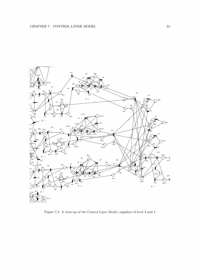
CHAPTER 7. CONTROL LAYER MODEL 34
P347
P346P355
P354
P353
P352
P351
P350
P349
P348
P334
P333 P342
P341
P340
P339
P336
P335
P264
P263
P340
P339
P338
P337
P336
P335
P270
P269
P332
P331
P330 P329
P328
P327
P315
P321
P316P317P318
P319P320
P324 P323
P322 P321 P320
P319
P318
P317 P316
P315 P314 P313
P312
P311
P310 P309
P308P307 P306
P305
P304
P258
P296
P303
P302
P301P300
P299
P298
P295
P294 P293
P292 P291 P290
P289
P288
P287 P286
P285 P284 P283
P282
P281
P280 P279
P278 P277 P276
P275
P219
P221
P222P223
P224
P22550
P226
P227
P220
P260
P259
P258
P257
50
P256
P255P254
P253
P252
P251
P250
P249
P248
50
P247
P246P245
P244
P243
P78
P76P77P79
P80P82
P81
P314
P313 P312
P311P310 P309
P308
P307
P306 P305
P304 P303 P302
P301
P61
P166
P167
P181
P180
P179 P178
P183
P182
P160
P159
P158
P157P162
P161
P163
11
P164
P165
P66
P67
P68
P65
P63
P64
P6215
P60
P156
P155
P154
11
P153
P152
P151
P150
P149
P148
P147
P146
P145
11
P144
P143
P142
P141
P140
P139
P79
P78
P80
P77
P76
P69
P70
P138
P137
P136
P135
P134
P133P132
P131
P130
P129
P128
P127
P126 P125
P124
P123
P122
P121
P120
P119 P118
P117
P116
P115
P114
P113
P112 P111
P110
P109
P108
P107
P106
P105 P104
P103
P102
P101
P100
P99
P98 P97
P96
P95
P94
P93
P92
P91P90
P89
P88
P87
P86
P85
P84
P83
P1474
P295
P1677
P1475
P1476
P1478
P1473
P73
P72
P25
P26
P979
P75
P74
P71
P1477
P1479
P4338
P137 P1024
P290
P291P292
P293
P294
P439
43
P42
P43
P44
P45
P46
P47
P48
P49
P508P51
P52
P53 P54
P55 P56P57
P58
P59
P81
P82
P83
P84
P85
P86
P87
P88P168P169
P170
P171
P172
P173
P174
P175
P176P177
P184
P185
P186
P187
P188
P189
P190
P191
P192
P193P194
P195
P196
P197
P198
P199 P200
P201
P202
P203
P204
P205
P206
P207
MTBF=0.040000MTTR=0.285714
EA=0.050000
AE=0.050000
WA=0.050000
AW=0.050000
EW=0.050000
WE=0.050000
Demand=2.000000CT=2.000000
order=5.000000
WW=0.100000
EE=0.100000
AA=0.100000
spoil=0.050000nspoil=0.950000
first_time_order=0.000010first_time_order_II=0.000020
T211
T210
T205
T388
T287
T345
T272
T378
T302
T209
T208
T207
T206
T212
T213
t49
t376
t66
T387
T386
T383
T377
T376
T373
T347
T346
T340
T256T257
T258
T291T290
T289
T276 T275T274
T245
t218
T184T183
T244
t222
t220
T243
t72t71
T175 T174
T166 T165
t33 t34
t29T28
t378T948
t393 t392t401
t400
t399
t398t397t396
t395 t394
t381 t382 t390t389t388t387
t384 t383
t389
t379
t359
t358
t368
t367
t361
t360
t354
t353
t349
t337
t336
t330
t329
t323
t322
t261
t262
t263
t264
t265
t266
t267
t268
t269
t270
t303
t302
t301
t300
t299
t298
t297
t296
t295
t294
t288t287
t286
t285
t284
t283
t282
t281
t280
t279
t89
t90
t352
t351
t345
t344
t219
t235 t230
t231t232
t234
t233
t163
t164t154
t155
t145
t146
t188
t190
t189
t191
t241t240
t239t238
t237
t236
t229
t228
t227t226
t225t224
t223
t221
t55
t53t51
t69
t182
t181
t180
t179
t173
t172
t171
t170
t68
t63
t57
t56
t162
t161
t153
t152
t144
t143
t137
t136
t135
t134
t128
t127
t126
t125
t119
t118
t117
t116
t110
t109
t108
t107
t101
t100
t99
t98
t92
t91
t78
t77
t76
t75
t74
t73
t32
t37
t46
t43
t42
t41
t39
t36
t1164
t1163
t60
t59
t344t962
t979
t961
t9491
t362
t968
t364
t379
t362
2π
t366
2π
t359
2π
t352
2π
t333
2π
t326
2π
t319
2π
t88
2π
t355
2π
t348
2π
t61
2π
t160
2π
t151
2π
t142
2π
t133
2π
t124
2π
t115
2π
t106
2π
t97
2π
t44
2π
t1167
2π
t360
3π
t361
3π
t365
3πt364
3π
t358
3πt357
3π
t351
3πt350
3π
t335
3π
t334
3π
t328
3π
t327
3π
t321
3π
t320
3π
t84
3π
t85
3π
t354
3πt353
3π
t347
3πt346
3π
t64
3π
t62
3π
t157
3πt156
3π
t148
3πt147
3π
t139
3πt138
3π
t130
3πt129
3π
t121
3πt120
3π
t112
3πt111
3π
t103
3πt102
3π
t94
3πt93
3π
t47
3π
t45
3π
t1165
3π
t1166
3π
t364
4π
t363
4π
t370
4π
t369
4π
t363
4π
t362
4π
t356
4π
t355
4π
t339
4π
t338
4π
t332
4π
t331
4π
t325
4π
t324
4π
t260
4π
t292
4π
t277
4π
t86
4π
t87
4π
t357
4π
t356
4π
t350
4π
t349
4π
t186
4π
t52
4π
t177
4π
t168
4πt67
4π
t58
4π
t159
4π
t158
4π
t150
4π
t149
4π
t141
4π
t140
4πt132
4π
t131
4π
t123
4π
t122
4πt114
4π
t113
4π
t105
4π
t104
4πt96
4π
t95
4π
t38
4π
t50
4π
t35
4π
t1162
4π
t1161
4π
t343
4π
t363
4πt292
5π
t390
5π
t385
5π
t307
5π
t380
5π
t375
5π
t277
5π
t348
5π
t343
5π
t215
5π
t216
5π
t217
5π
t200
5π
t199
5π
t198
5π
t197
5π
t196
5π
t214
5π
t65
5π
t48
5π
t377
5π
t259
7π
t293
7π
t278
7π
t187
7π
t54
7π
t178
7π
t169
7π
t40
7π
t345
7π
t365
7π
_5
_2
_2
_3
_5
_2
_2
_3
_5
_2
_2
_3
_5
_2_2
_3
_5 _2
_2
_3
_5
_2
_2_3
_5
_2_2 _3
_5
_2_2_3
_5 _2_2_3
_5
_2_2
_3
_5
_2_2_3
_5
_2
_2 _3
_5
_2 _2_3
_5
_2_2 _3
_5
_2_2 _3
_5
_2_2
_3_5
_2_2
_3
_5
_2
_2_3
_5
_2_2
_3
_5
_2
_2 _3
_5
_2
_2
_3
_100
_50_100
_50_100
_100
_100
_50_100
_50_100 _100
_50_100
_100_50
_100_100
_50_100 _100
_50_100 _100
_50_100
_100
_50 _100
_100
_100_50_100
_100
_50_100
_100_50 _100
_50_100
_100 _50_100
_100_100_50
_100
_100_50
_100
_100 _50_100
_100_50_100
_50_100
_100_100_50
_100
Figure 7.1: A close-up of the Control Layer Model, suppliers of level 3 and 4
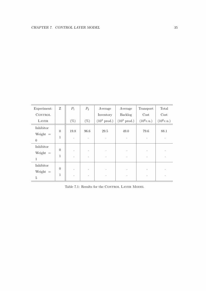
CHAPTER 7. CONTROL LAYER MODEL 35
Experiment: Z P1 P2 Average Average Transport Total
Control Inventory Backlog Cost Cost
Layer (%) (%) (103 prod.) (103 prod.) (106c.u.) (106c.u.)
Inhibitor
Weight =
0
0
1
19.8
.
96.6
.
29.5
.
49.0
.
79.6
.
88.1
.
Inhibitor
Weight =
1
0
1
.
.
.
.
.
.
.
.
.
.
.
.
Inhibitor
Weight =
5
0
1
.
.
.
.
.
.
.
.
.
.
.
.
Table 7.1: Results for the Control Layer Model
Chapter 8
Conclusion
It was the goal of this thesis to model and simulate supply chains by Petri Nets (PN). First we
have to say that these goals are reached. A model of a supply chain was constructed and several
simulation runs were performed successfully.
During the building of the model there were no obstacles found that PN couldn’t overcome. For
this reason it is the author’s belief that Petri Nets in general are a very powerful modeling language
and GSPN specifically are very well suited for the simulation of supply chains. Compared to other
languages gives the graphical representation of the model an extremely good overview and a quick
insight of the dynamics of the model. The graphical representation has a great added value to
the reader in terms of the understanding of the model. In addition of these PN-benefits, it was
possible to build this very complex and large model in a short time. This because the author
started from the methodology provided in Bobeanu et al. (2004) and Landeghem & Bobeanu
(2002). This methodology allows the user to built models on a incremental and systematical way
by coupling basic components by well defined rules. While building the supply chain model in the
tool GreatSPN, only one hard restriction could not been overcome: It is not possible for a place to
contain more than 255 tokens. Therefore 2000 products had to be modeled by one token. Several
experiments were performed on the model. From their results we can conclude that on this model,
the most important disturbance factor on the performance measures is the random transport time.
If the objective is to minimize costs, spoilage has to be reduced. Plant breakdowns have only a
minor influence. When there are more reliable suppliers used, cost increase but the service factors
don’t. When we cut the total number of suppliers, costs drop without the loss of performance.
Best results were gained with a minimum of low-cost suppliers.
36

Appendix A
37
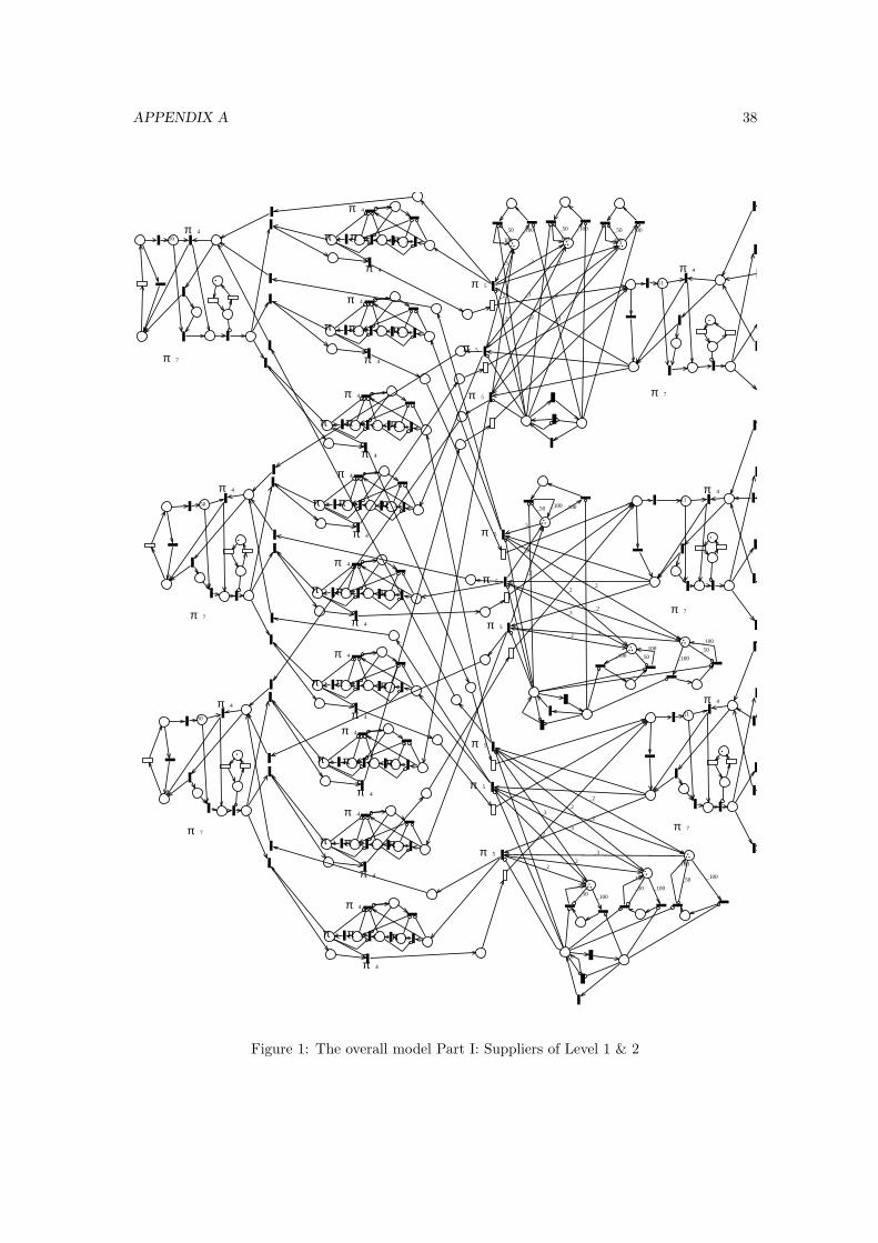
APPENDIX A 38
50
50
50
11
11
11
2π
2π
2π
2π
2π
2π
2π
2π
2π
3π 3π
3π 3π
3π 3π
3π 3π
3π 3π
3π 3π
3π 3π
3π 3π
3π 3π
4π
4π
4π
4π
4π
4π
4π
4π
4π
4π
4π
4π
4π
4π
4π
4π
4π
4π
4π
4π
4π
4π
4π
4π
5π
5π
5π
5π
5π
5π
5π
5π
5π
7π
7π
7π
7π
7π
7π
_2_2_3
_2 _2 _3
_2 _2_3
_2
_2
_3
_2_2
_3
_2
_2_3
_2_2
_3
_2
_2
_3
_2
_2_3
_100_50 _100
_50
_100
_100 _50
_100
_100_100_50
_100
_100_50
_100
_100 _50
_100
_100
_50
_100
_50
_100
_100
_100_50
_100
Figure 1: The overall model Part I: Suppliers of Level 1 & 2
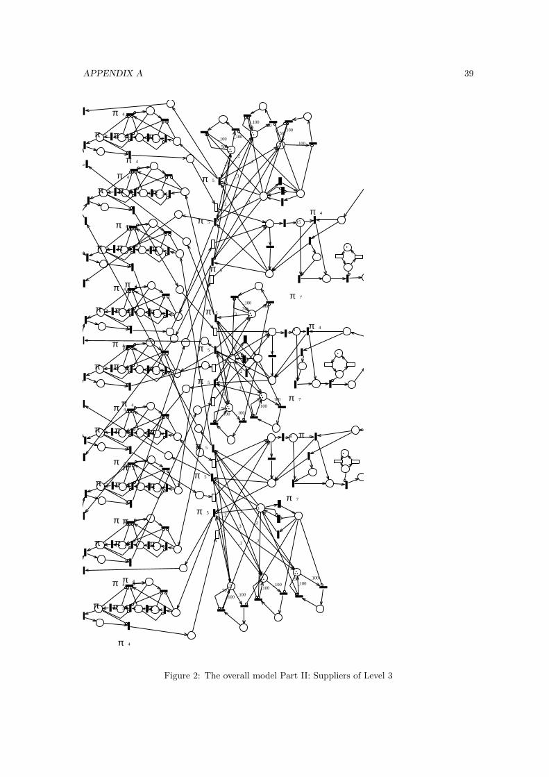
APPENDIX A 39
15
8
8
2π
2π
2π
2π
2π
2π
2π
2π
2π
3π 3π
3π 3π
3π 3π
3π 3π
3π 3π
3π 3π
3π 3π
3π 3π
3π 3π
4π
4π
4π
4π
4π 4π
4π 4π
4π 4π
4π 4π
4π 4π
4π 4π
4π 4π
4π
4π
4π
5π
5π
5π
5π
5π
5π
5π
5π
5π
7π
7π
7π
_2_2
_3
_2
_2_3
_2
_2
_3
_2_2
_3
_2
_2_3
_2 _2
_3
_2_2_3
_2 _2_3
_2
_2_3
_50
_100 _100
_50
_100_100
_50_100
_100
_50_100
_100
_50_100 _100
_50
_100
_100
_50_100
_100
_100_50_100
_100
_50
_100
Figure 2: The overall model Part II: Suppliers of Level 3
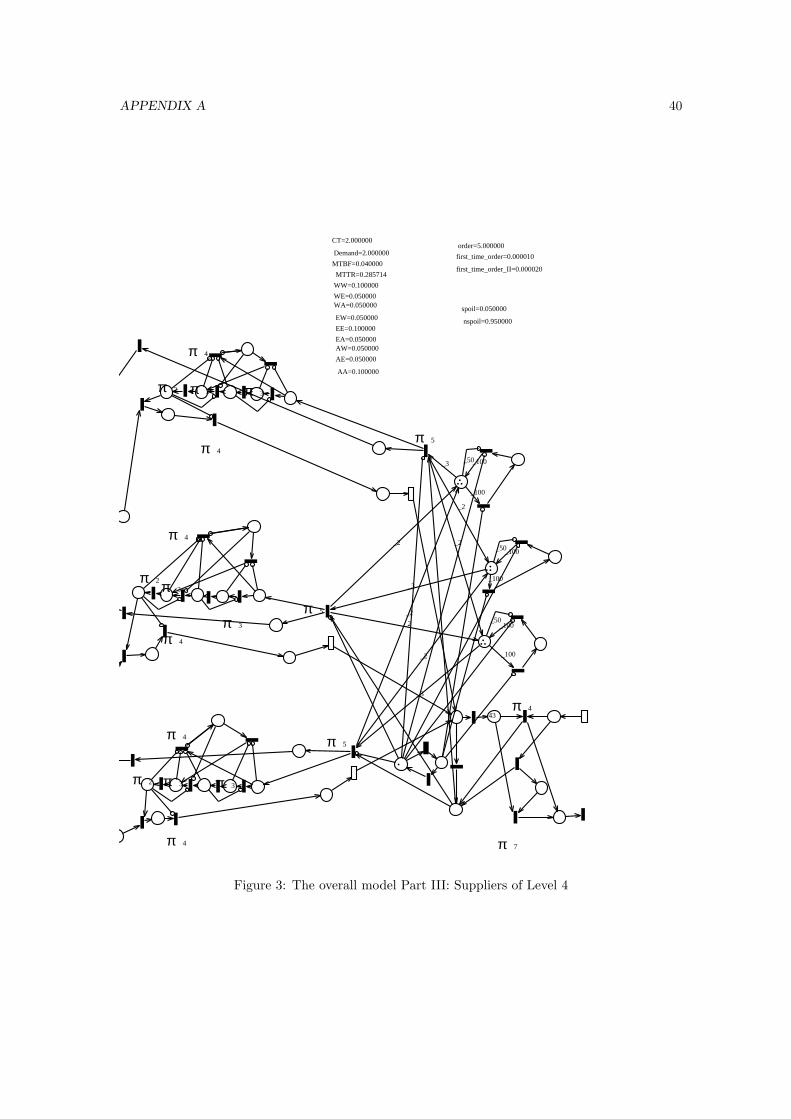
APPENDIX A 40
43
MTBF=0.040000
MTTR=0.285714
EA=0.050000
AE=0.050000
WA=0.050000
AW=0.050000
EW=0.050000
WE=0.050000
Demand=2.000000
CT=2.000000order=5.000000
WW=0.100000
EE=0.100000
AA=0.100000
spoil=0.050000
nspoil=0.950000
first_time_order=0.000010
first_time_order_II=0.000020
2π
2π
2π
3π 3π
3π 3π
3π
3π
4π
4π
4π
4π
4π
4π
4π
5π
5π
5π
7π
_2
_2
_3
_2
_2
_3
_2
_2
_3
_100
_50_100
_50_100
_100
_100
_50_100
Figure 3: The overall model Part III: Suppliers of Level 4

Appendix B
41
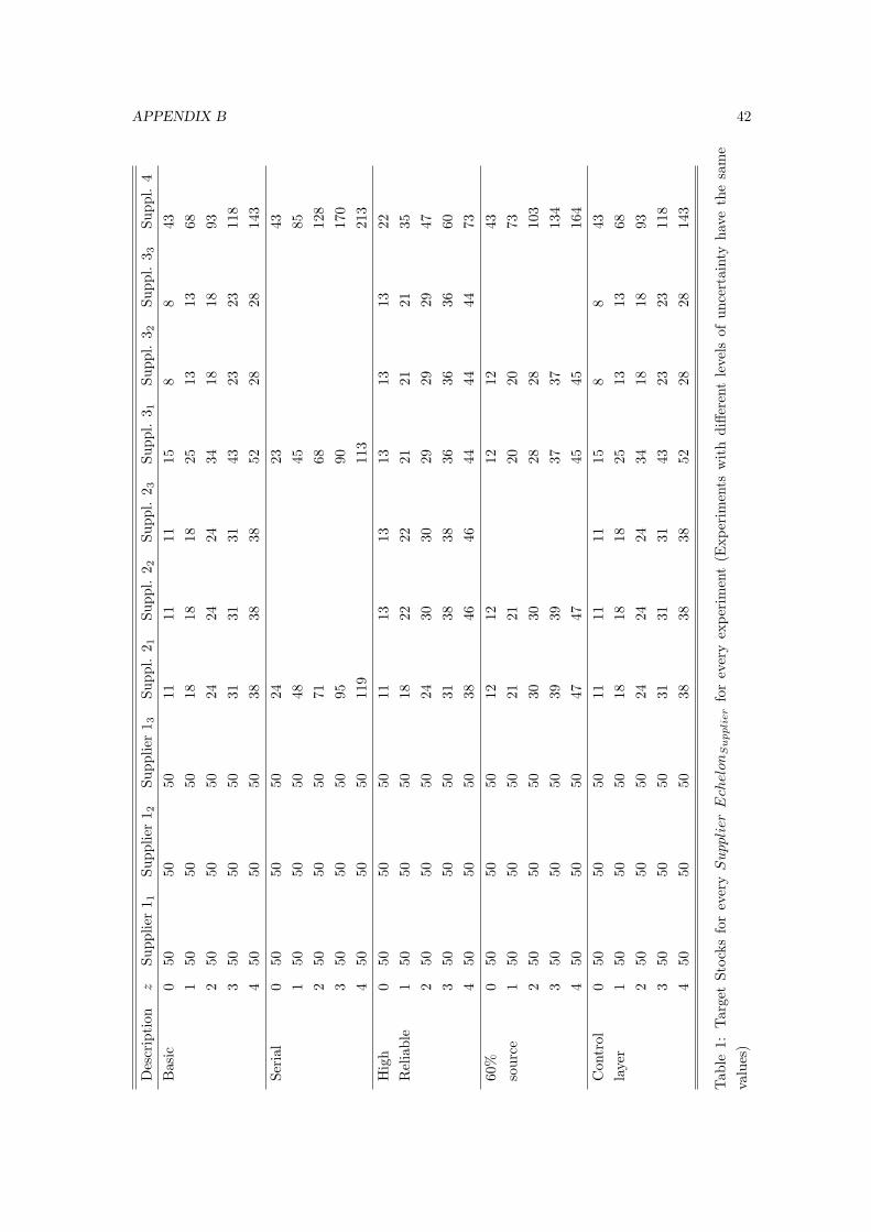
APPENDIX B 42
Des
crip
tion
zSu
pplie
r1 1
Supp
lier
1 2Su
pplie
r1 3
Supp
l.2 1
Supp
l.2 2
Supp
l.2 3
Supp
l.3 1
Supp
l.3 2
Supp
l.3 3
Supp
l.4
Bas
ic0
5050
5011
1111
158
843
150
5050
1818
1825
1313
682
5050
5024
2424
3418
1893
350
5050
3131
3143
2323
118
450
5050
3838
3852
2828
143
Seri
al0
5050
5024
2343
150
5050
4845
852
5050
5071
6812
83
5050
5095
9017
04
5050
5011
911
321
3H
igh
050
5050
1113
1313
1313
22R
elia
ble
150
5050
1822
2221
2121
352
5050
5024
3030
2929
2947
350
5050
3138
3836
3636
604
5050
5038
4646
4444
4473
60%
050
5050
1212
1212
43so
urce
150
5050
2121
2020
732
5050
5030
3028
2810
33
5050
5039
3937
3713
44
5050
5047
4745
4516
4C
ontr
ol0
5050
5011
1111
158
843
laye
r1
5050
5018
1818
2513
1368
250
5050
2424
2434
1818
933
5050
5031
3131
4323
2311
84
5050
5038
3838
5228
2814
3
Tab
le1:
Tar
get
Stoc
ksfo
rev
ery
Supplier
Ech
elon
Su
ppli
er
for
ever
yex
peri
men
t(E
xper
imen
tsw
ith
diffe
rent
leve
lsof
unce
rtai
nty
have
the
sam
eva
lues
)
Appendix C
In this appendix a selection is made of interesting results of the several experiments. Token
distibutions are shown for several Stocks, Backlogs and transport delay places.
43
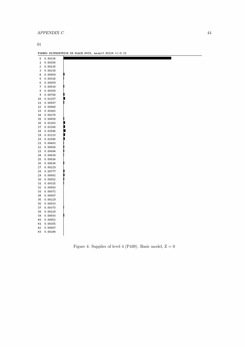
APPENDIX C 44
01
Figure 4: Supplier of level 4 (P439). Basic model, Z = 0
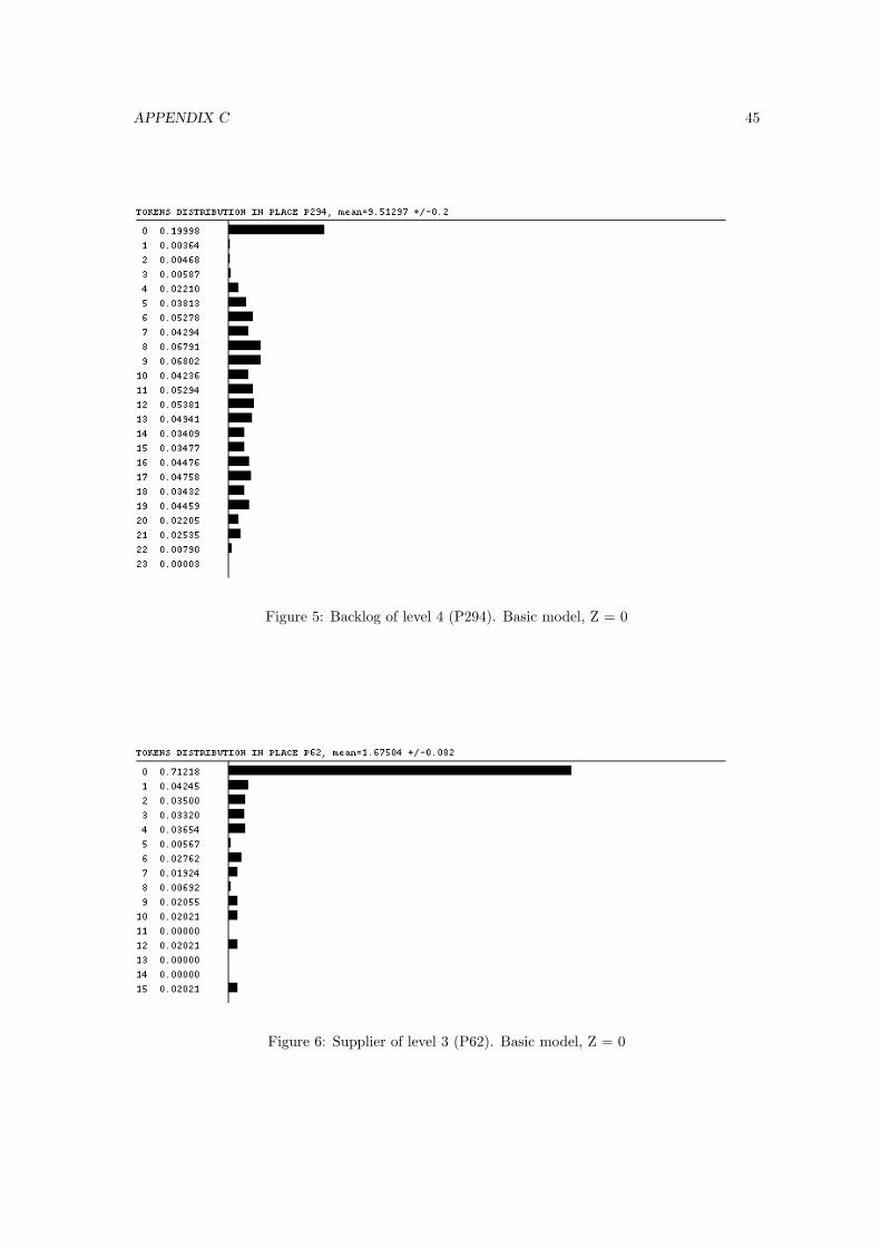
APPENDIX C 45
Figure 5: Backlog of level 4 (P294). Basic model, Z = 0
Figure 6: Supplier of level 3 (P62). Basic model, Z = 0
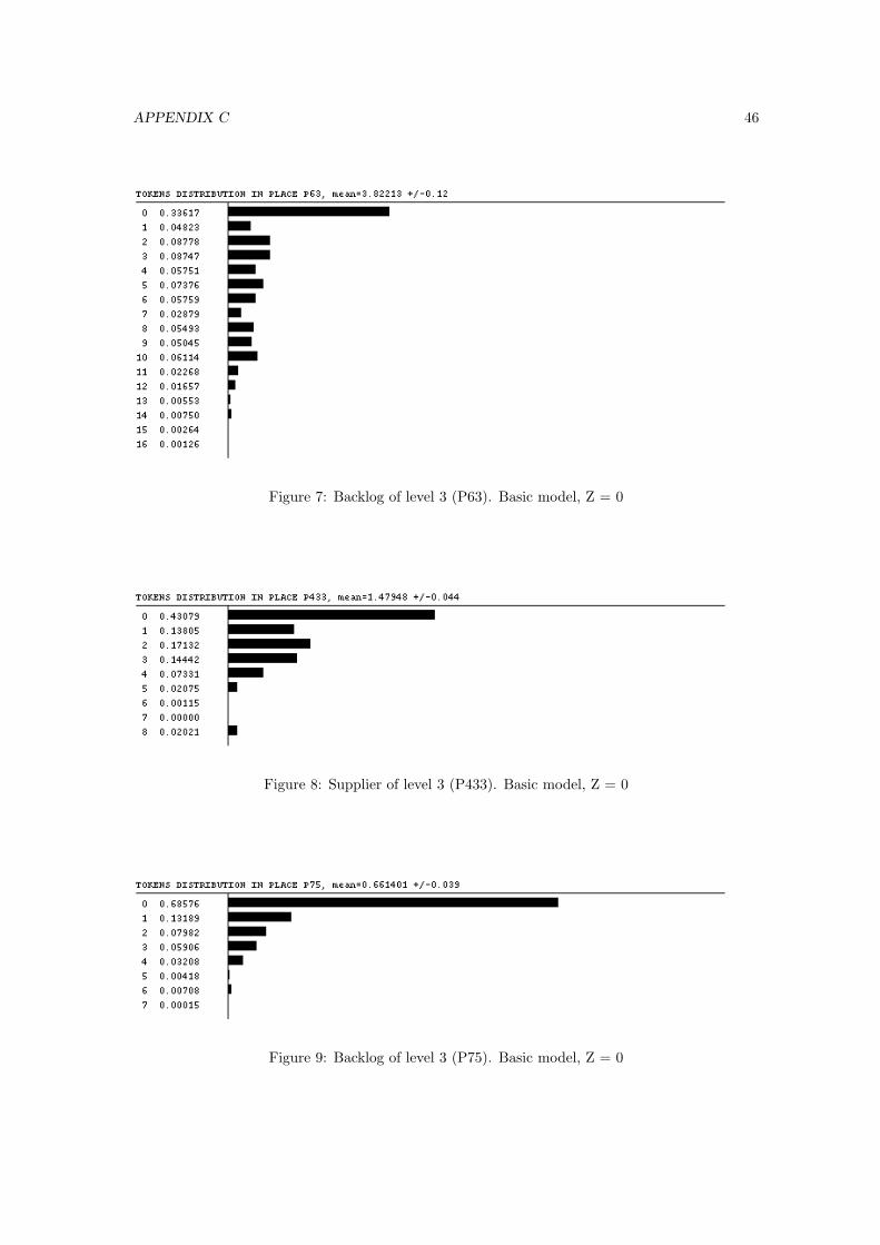
APPENDIX C 46
Figure 7: Backlog of level 3 (P63). Basic model, Z = 0
Figure 8: Supplier of level 3 (P433). Basic model, Z = 0
Figure 9: Backlog of level 3 (P75). Basic model, Z = 0
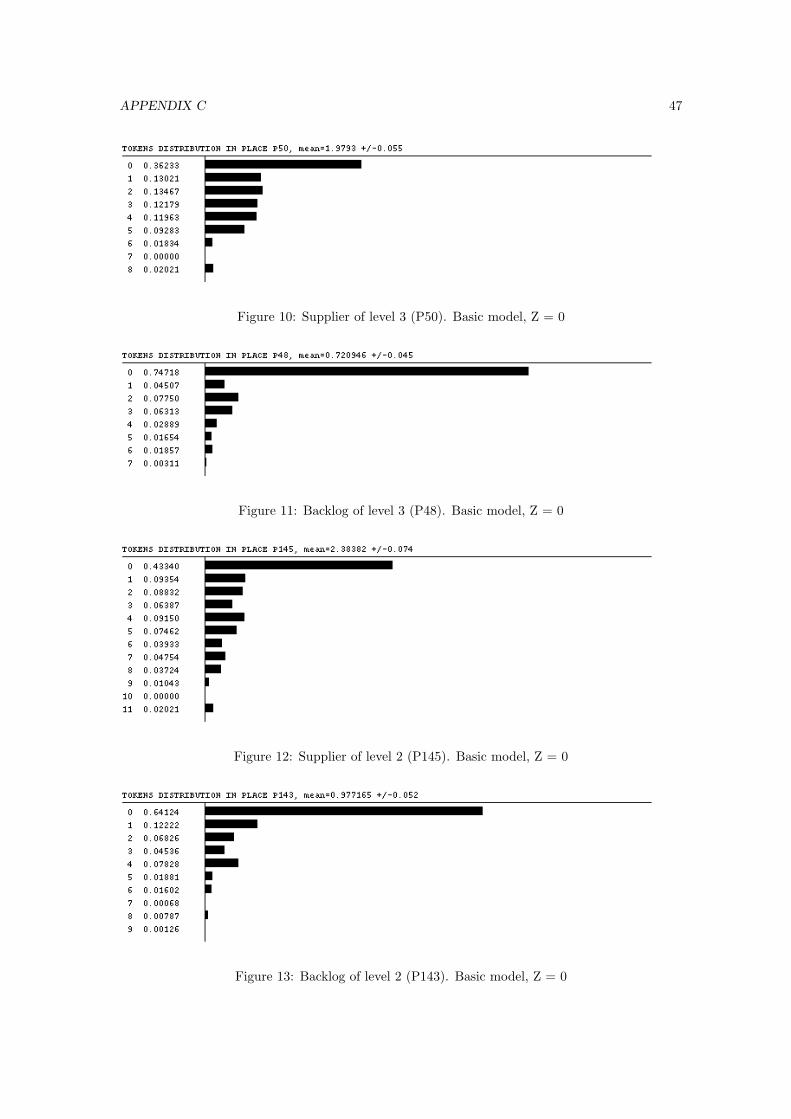
APPENDIX C 47
Figure 10: Supplier of level 3 (P50). Basic model, Z = 0
Figure 11: Backlog of level 3 (P48). Basic model, Z = 0
Figure 12: Supplier of level 2 (P145). Basic model, Z = 0
Figure 13: Backlog of level 2 (P143). Basic model, Z = 0
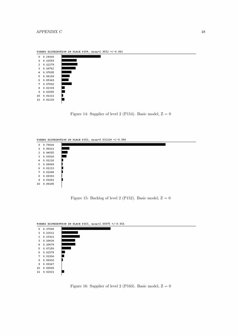
APPENDIX C 48
Figure 14: Supplier of level 2 (P154). Basic model, Z = 0
Figure 15: Backlog of level 2 (P152). Basic model, Z = 0
Figure 16: Supplier of level 2 (P163). Basic model, Z = 0
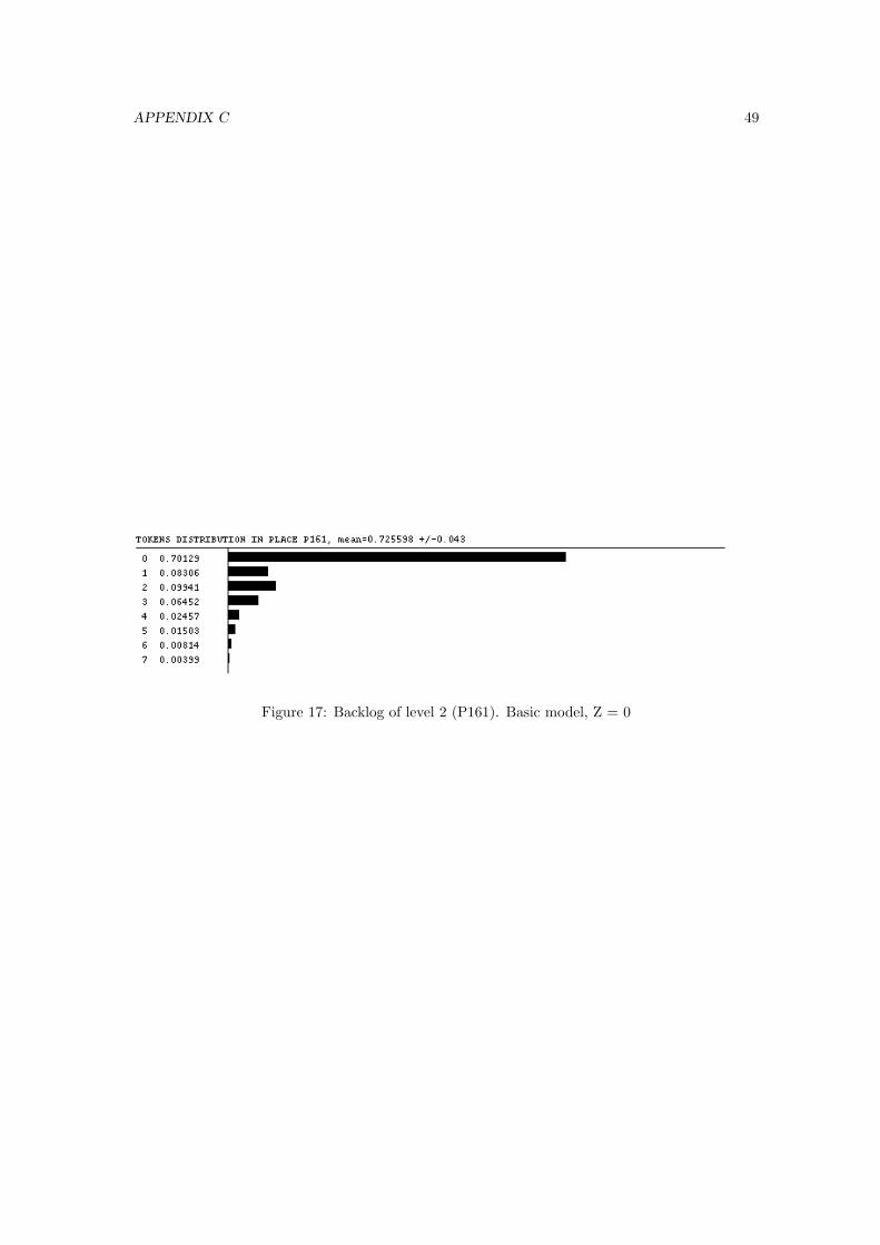
APPENDIX C 49
Figure 17: Backlog of level 2 (P161). Basic model, Z = 0

APPENDIX C 50
02
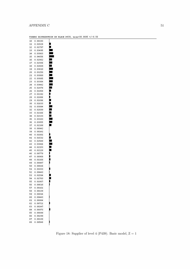
APPENDIX C 51
Figure 18: Supplier of level 4 (P439). Basic model, Z = 1
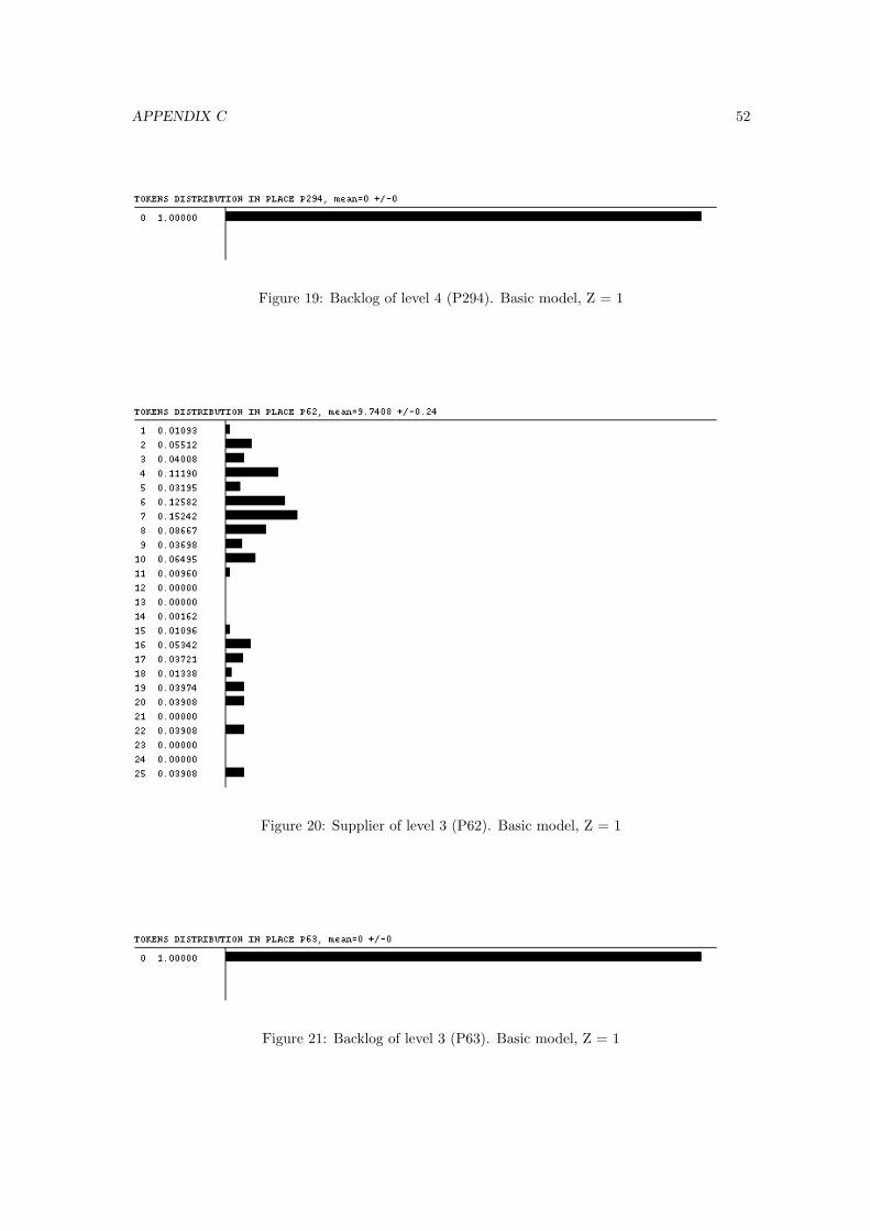
APPENDIX C 52
Figure 19: Backlog of level 4 (P294). Basic model, Z = 1
Figure 20: Supplier of level 3 (P62). Basic model, Z = 1
Figure 21: Backlog of level 3 (P63). Basic model, Z = 1
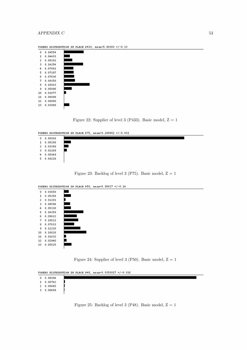
APPENDIX C 53
Figure 22: Supplier of level 3 (P433). Basic model, Z = 1
Figure 23: Backlog of level 3 (P75). Basic model, Z = 1
Figure 24: Supplier of level 3 (P50). Basic model, Z = 1
Figure 25: Backlog of level 3 (P48). Basic model, Z = 1
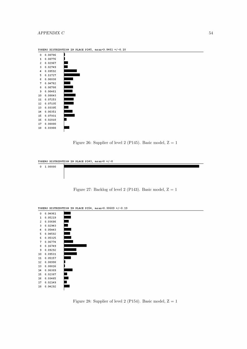
APPENDIX C 54
Figure 26: Supplier of level 2 (P145). Basic model, Z = 1
Figure 27: Backlog of level 2 (P143). Basic model, Z = 1
Figure 28: Supplier of level 2 (P154). Basic model, Z = 1
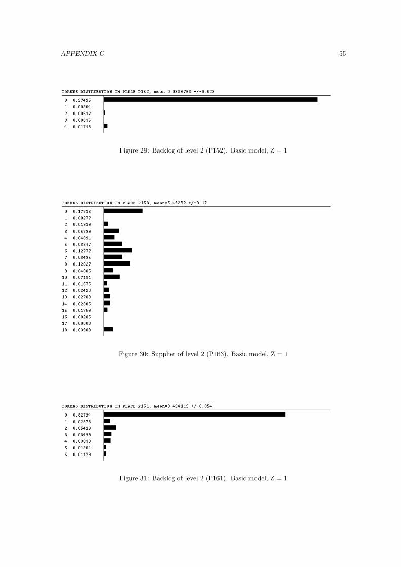
APPENDIX C 55
Figure 29: Backlog of level 2 (P152). Basic model, Z = 1
Figure 30: Supplier of level 2 (P163). Basic model, Z = 1
Figure 31: Backlog of level 2 (P161). Basic model, Z = 1
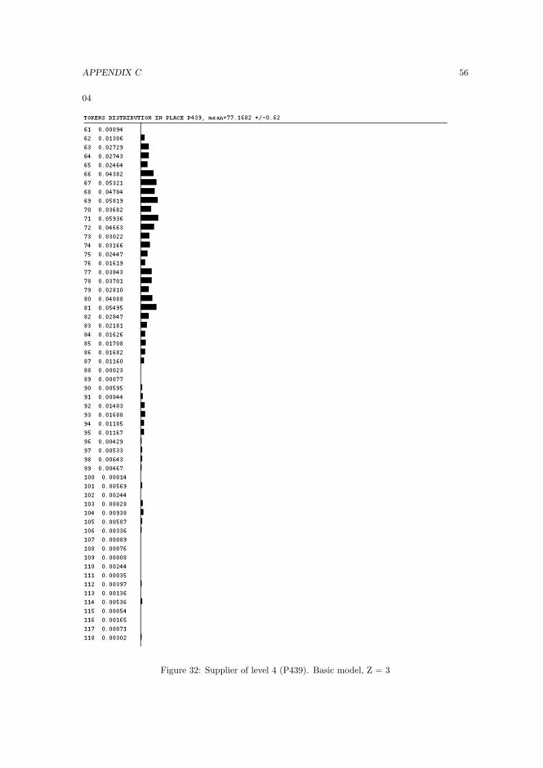
APPENDIX C 56
04
Figure 32: Supplier of level 4 (P439). Basic model, Z = 3
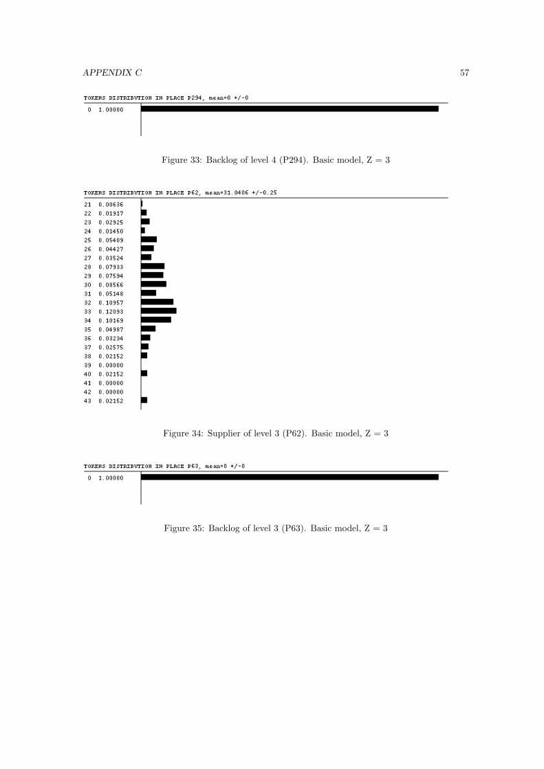
APPENDIX C 57
Figure 33: Backlog of level 4 (P294). Basic model, Z = 3
Figure 34: Supplier of level 3 (P62). Basic model, Z = 3
Figure 35: Backlog of level 3 (P63). Basic model, Z = 3
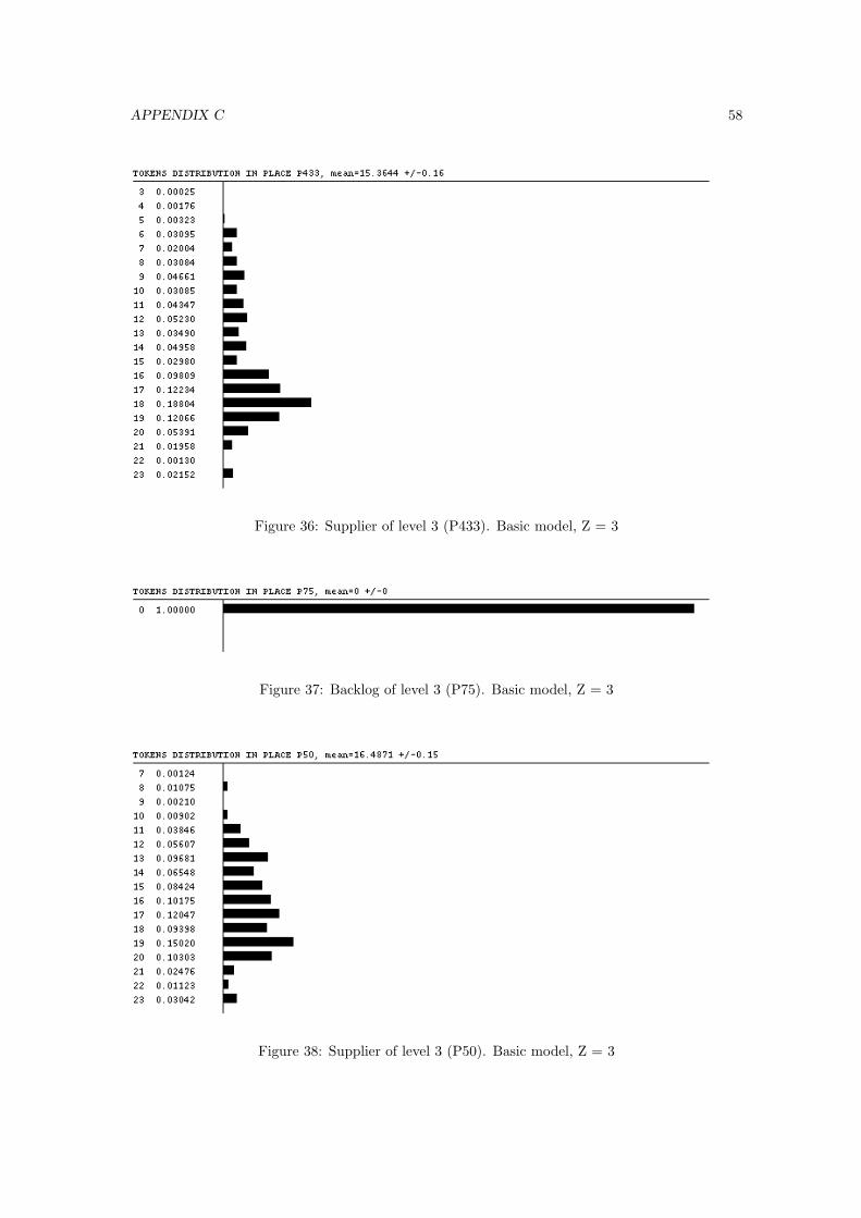
APPENDIX C 58
Figure 36: Supplier of level 3 (P433). Basic model, Z = 3
Figure 37: Backlog of level 3 (P75). Basic model, Z = 3
Figure 38: Supplier of level 3 (P50). Basic model, Z = 3

APPENDIX C 59
Figure 39: Backlog of level 3 (P48). Basic model, Z = 3
Figure 40: Supplier of level 2 (P145). Basic model, Z = 3
Figure 41: Backlog of level 2 (P143). Basic model, Z = 3
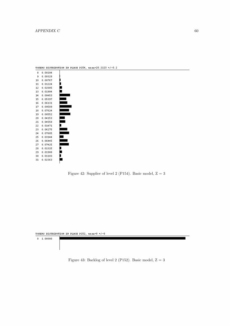
APPENDIX C 60
Figure 42: Supplier of level 2 (P154). Basic model, Z = 3
Figure 43: Backlog of level 2 (P152). Basic model, Z = 3
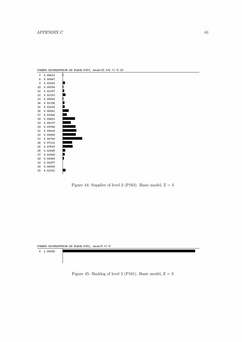
APPENDIX C 61
Figure 44: Supplier of level 2 (P163). Basic model, Z = 3
Figure 45: Backlog of level 2 (P161). Basic model, Z = 3
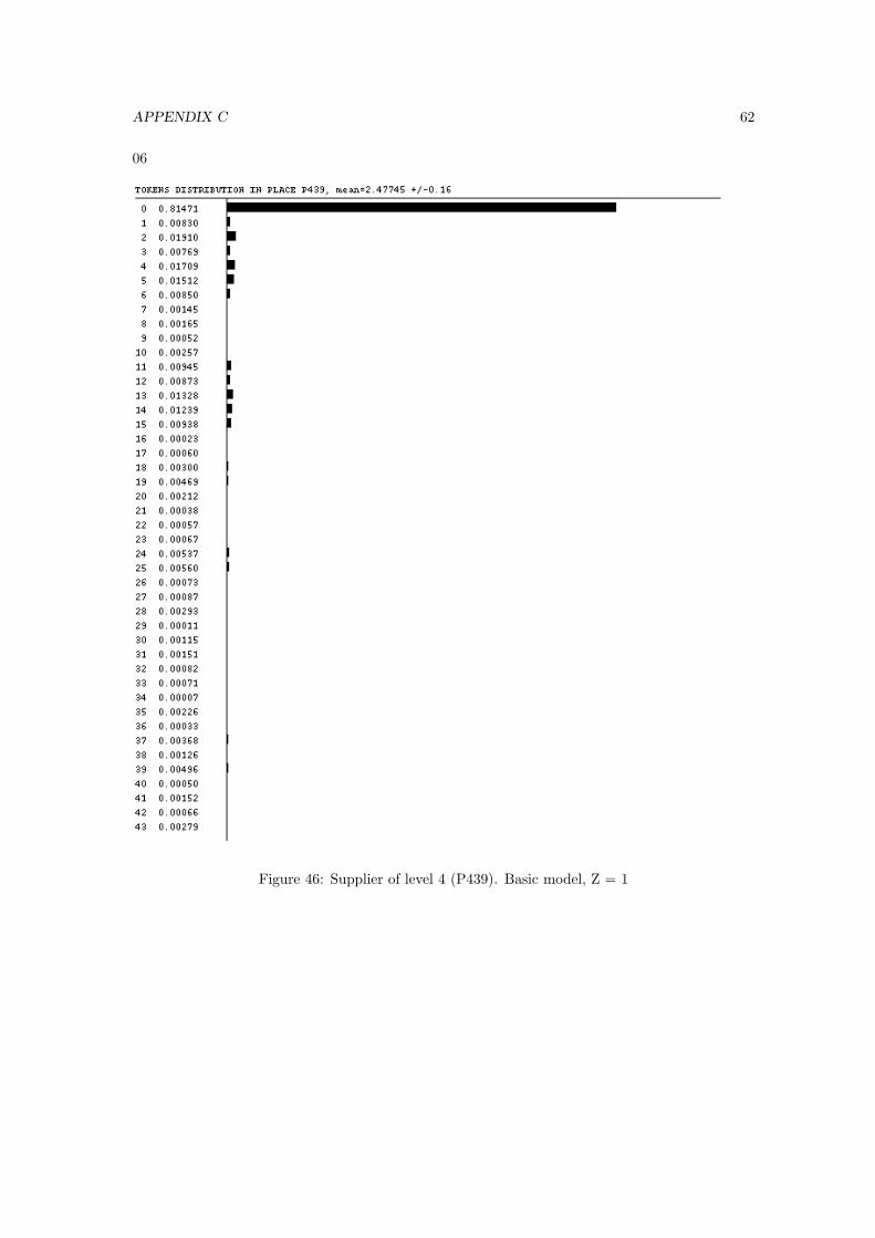
APPENDIX C 62
06
Figure 46: Supplier of level 4 (P439). Basic model, Z = 1
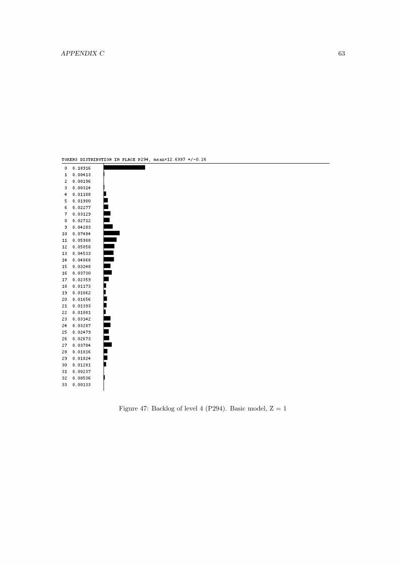
APPENDIX C 63
Figure 47: Backlog of level 4 (P294). Basic model, Z = 1
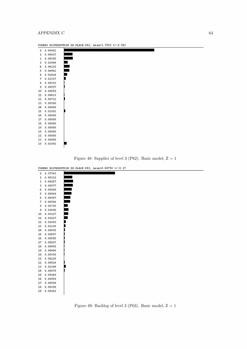
APPENDIX C 64
Figure 48: Supplier of level 3 (P62). Basic model, Z = 1
Figure 49: Backlog of level 3 (P63). Basic model, Z = 1
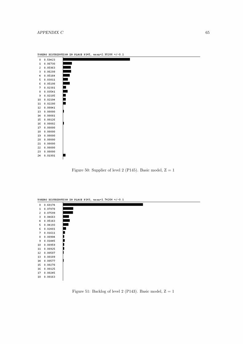
APPENDIX C 65
Figure 50: Supplier of level 2 (P145). Basic model, Z = 1
Figure 51: Backlog of level 2 (P143). Basic model, Z = 1
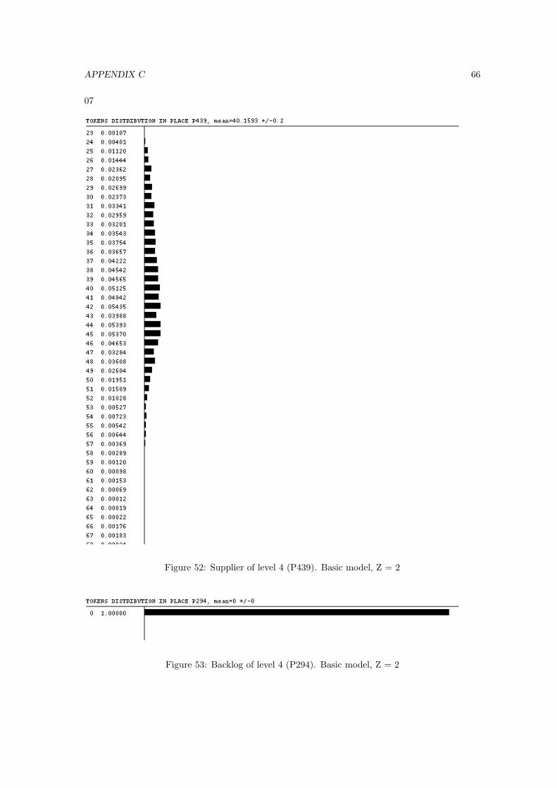
APPENDIX C 66
07
Figure 52: Supplier of level 4 (P439). Basic model, Z = 2
Figure 53: Backlog of level 4 (P294). Basic model, Z = 2
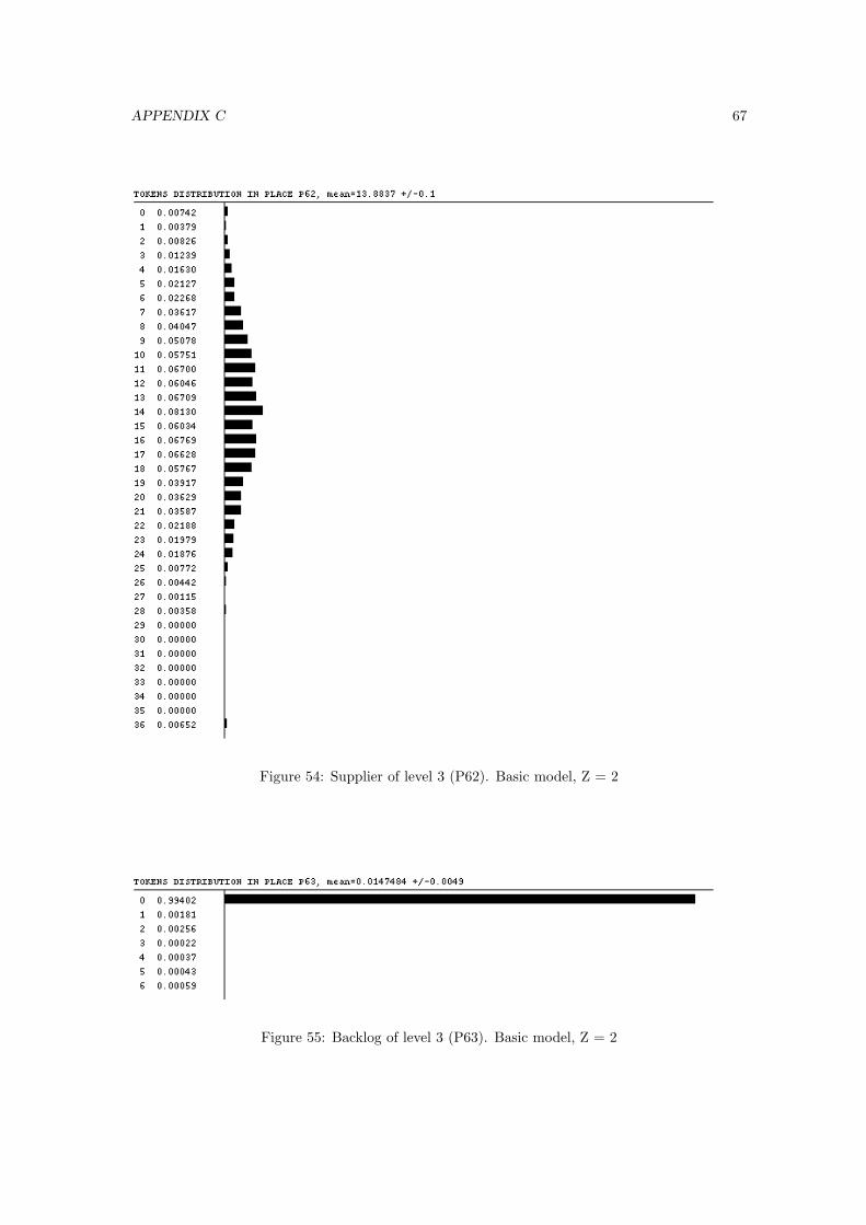
APPENDIX C 67
Figure 54: Supplier of level 3 (P62). Basic model, Z = 2
Figure 55: Backlog of level 3 (P63). Basic model, Z = 2
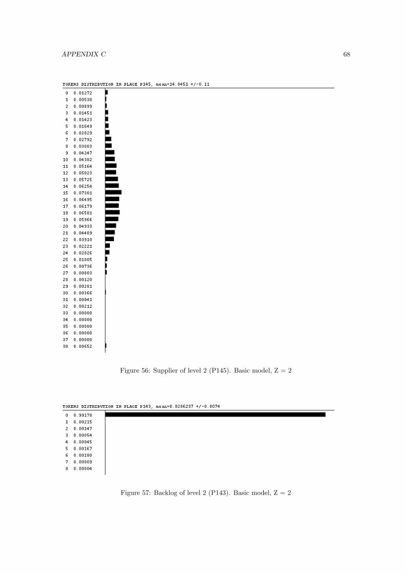
APPENDIX C 68
Figure 56: Supplier of level 2 (P145). Basic model, Z = 2
Figure 57: Backlog of level 2 (P143). Basic model, Z = 2

APPENDIX C 69
08
Figure 58: Supplier of level 4 (P439). Basic model, Z = 3
Figure 59: Backlog of level 4 (P294). Basic model, Z = 3
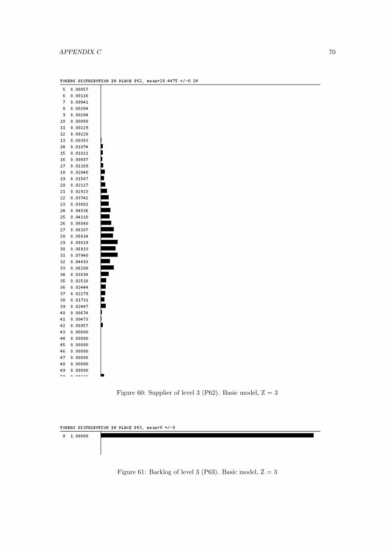
APPENDIX C 70
Figure 60: Supplier of level 3 (P62). Basic model, Z = 3
Figure 61: Backlog of level 3 (P63). Basic model, Z = 3
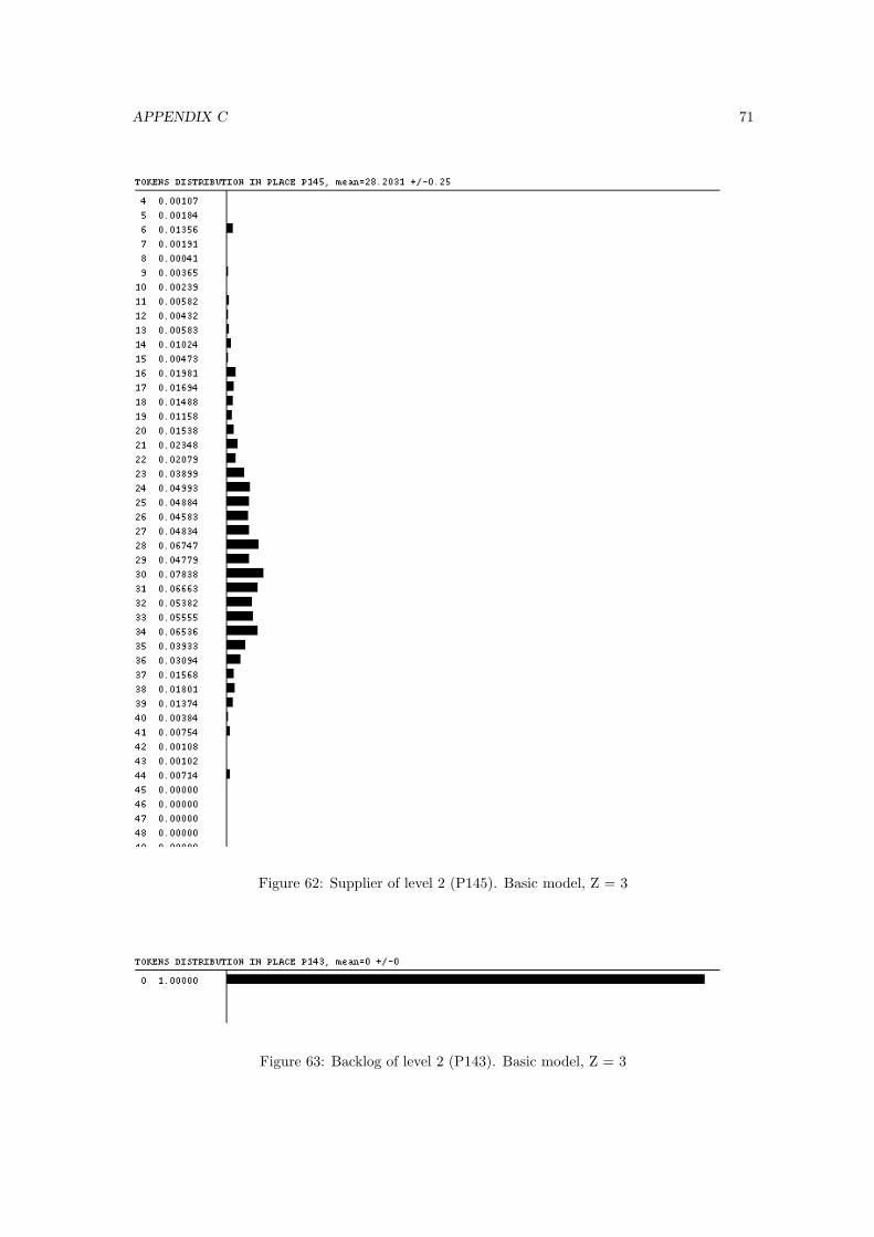
APPENDIX C 71
Figure 62: Supplier of level 2 (P145). Basic model, Z = 3
Figure 63: Backlog of level 2 (P143). Basic model, Z = 3
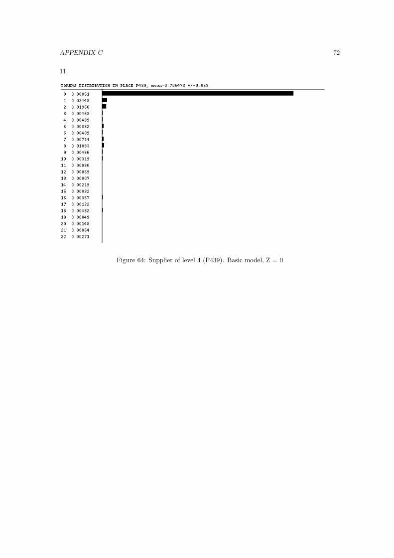
APPENDIX C 72
11
Figure 64: Supplier of level 4 (P439). Basic model, Z = 0
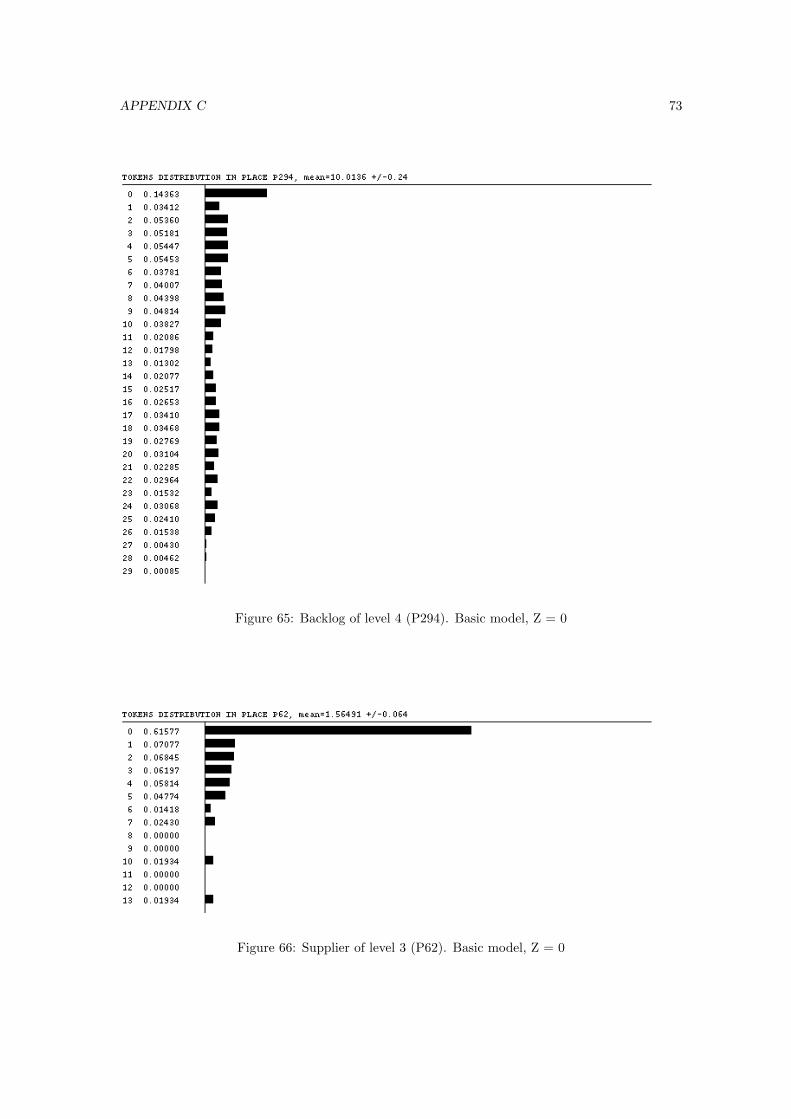
APPENDIX C 73
Figure 65: Backlog of level 4 (P294). Basic model, Z = 0
Figure 66: Supplier of level 3 (P62). Basic model, Z = 0
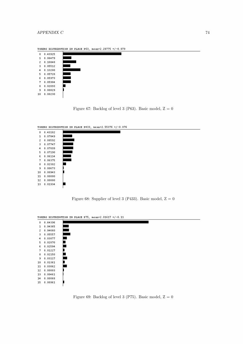
APPENDIX C 74
Figure 67: Backlog of level 3 (P63). Basic model, Z = 0
Figure 68: Supplier of level 3 (P433). Basic model, Z = 0
Figure 69: Backlog of level 3 (P75). Basic model, Z = 0
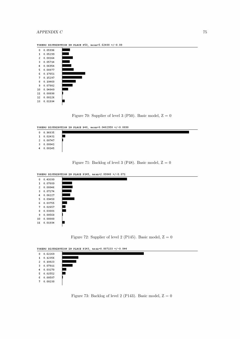
APPENDIX C 75
Figure 70: Supplier of level 3 (P50). Basic model, Z = 0
Figure 71: Backlog of level 3 (P48). Basic model, Z = 0
Figure 72: Supplier of level 2 (P145). Basic model, Z = 0
Figure 73: Backlog of level 2 (P143). Basic model, Z = 0
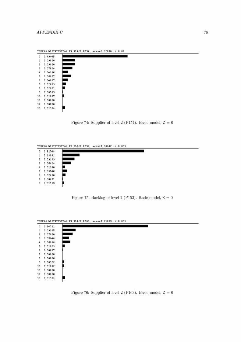
APPENDIX C 76
Figure 74: Supplier of level 2 (P154). Basic model, Z = 0
Figure 75: Backlog of level 2 (P152). Basic model, Z = 0
Figure 76: Supplier of level 2 (P163). Basic model, Z = 0
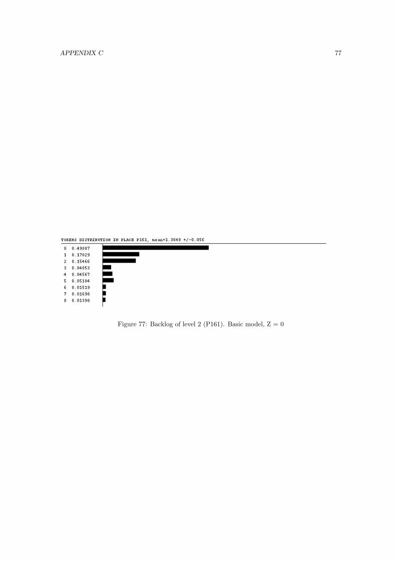
APPENDIX C 77
Figure 77: Backlog of level 2 (P161). Basic model, Z = 0
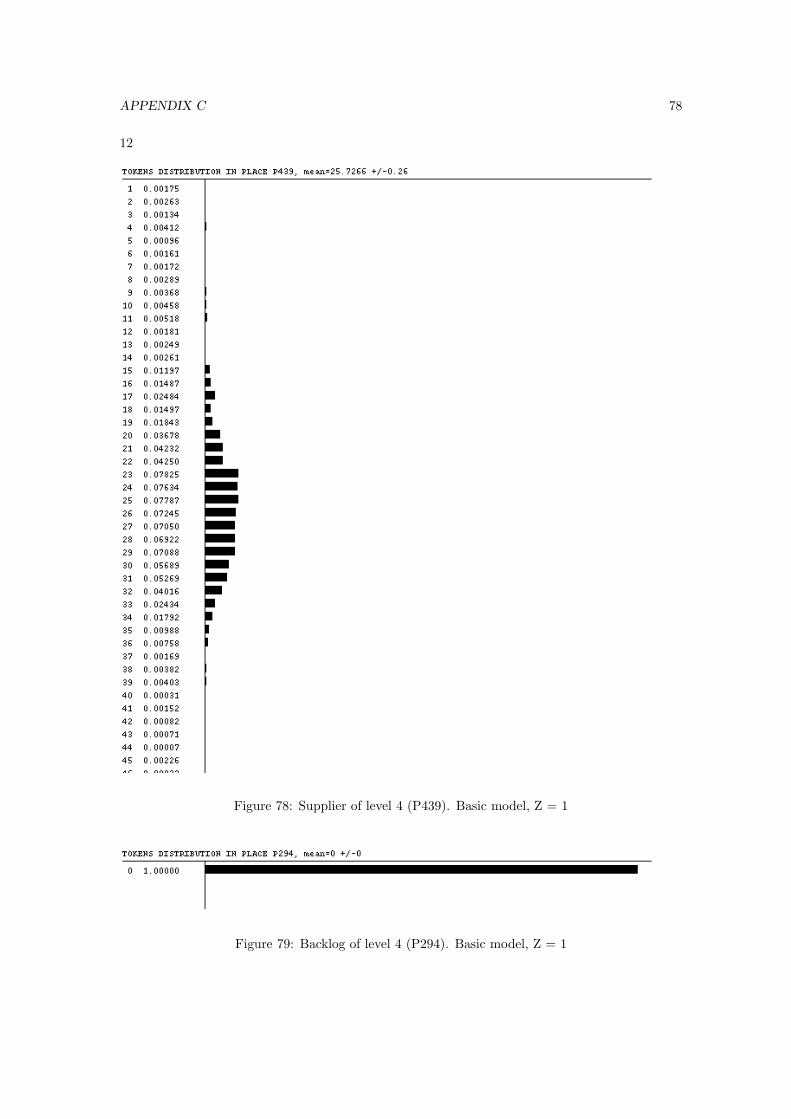
APPENDIX C 78
12
Figure 78: Supplier of level 4 (P439). Basic model, Z = 1
Figure 79: Backlog of level 4 (P294). Basic model, Z = 1
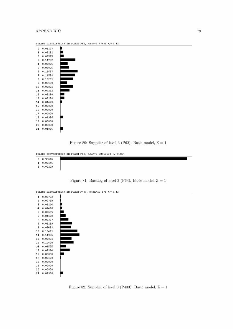
APPENDIX C 79
Figure 80: Supplier of level 3 (P62). Basic model, Z = 1
Figure 81: Backlog of level 3 (P63). Basic model, Z = 1
Figure 82: Supplier of level 3 (P433). Basic model, Z = 1
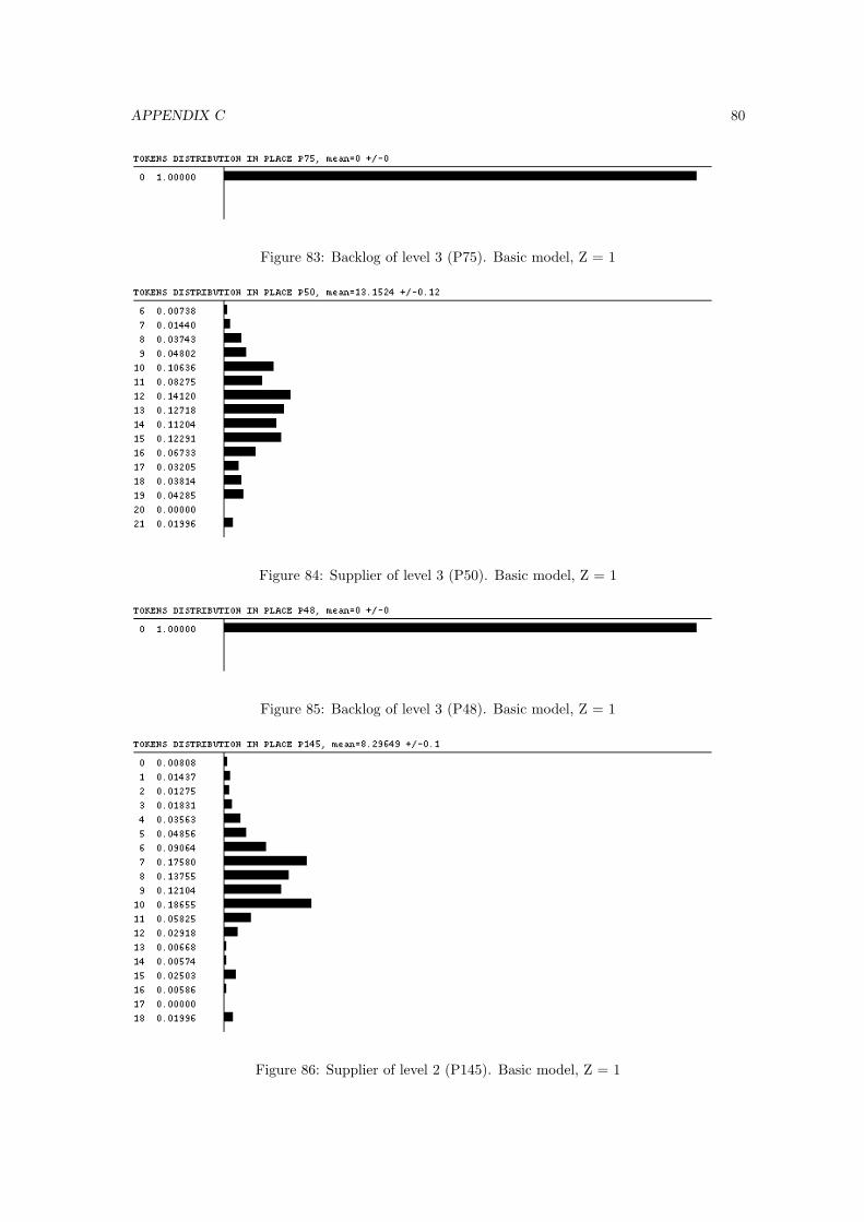
APPENDIX C 80
Figure 83: Backlog of level 3 (P75). Basic model, Z = 1
Figure 84: Supplier of level 3 (P50). Basic model, Z = 1
Figure 85: Backlog of level 3 (P48). Basic model, Z = 1
Figure 86: Supplier of level 2 (P145). Basic model, Z = 1
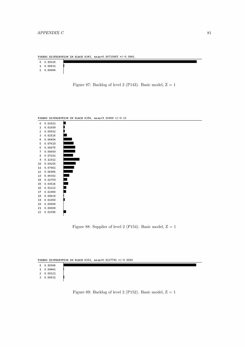
APPENDIX C 81
Figure 87: Backlog of level 2 (P143). Basic model, Z = 1
Figure 88: Supplier of level 2 (P154). Basic model, Z = 1
Figure 89: Backlog of level 2 (P152). Basic model, Z = 1
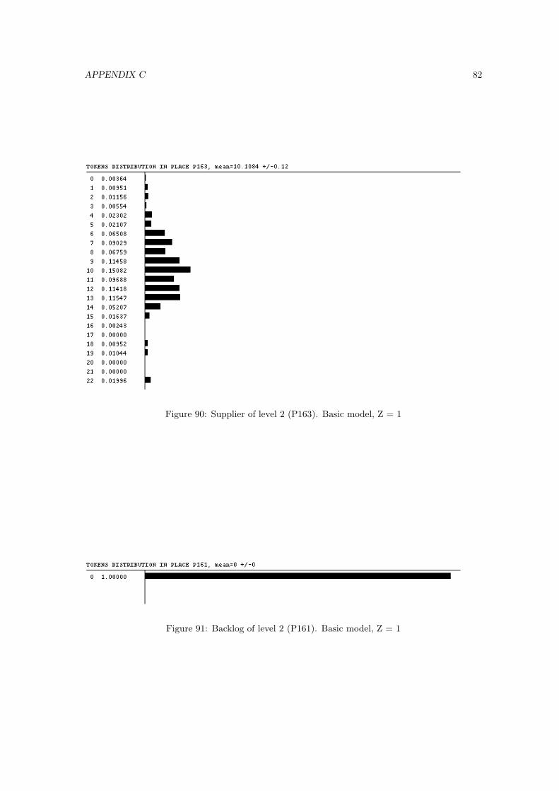
APPENDIX C 82
Figure 90: Supplier of level 2 (P163). Basic model, Z = 1
Figure 91: Backlog of level 2 (P161). Basic model, Z = 1
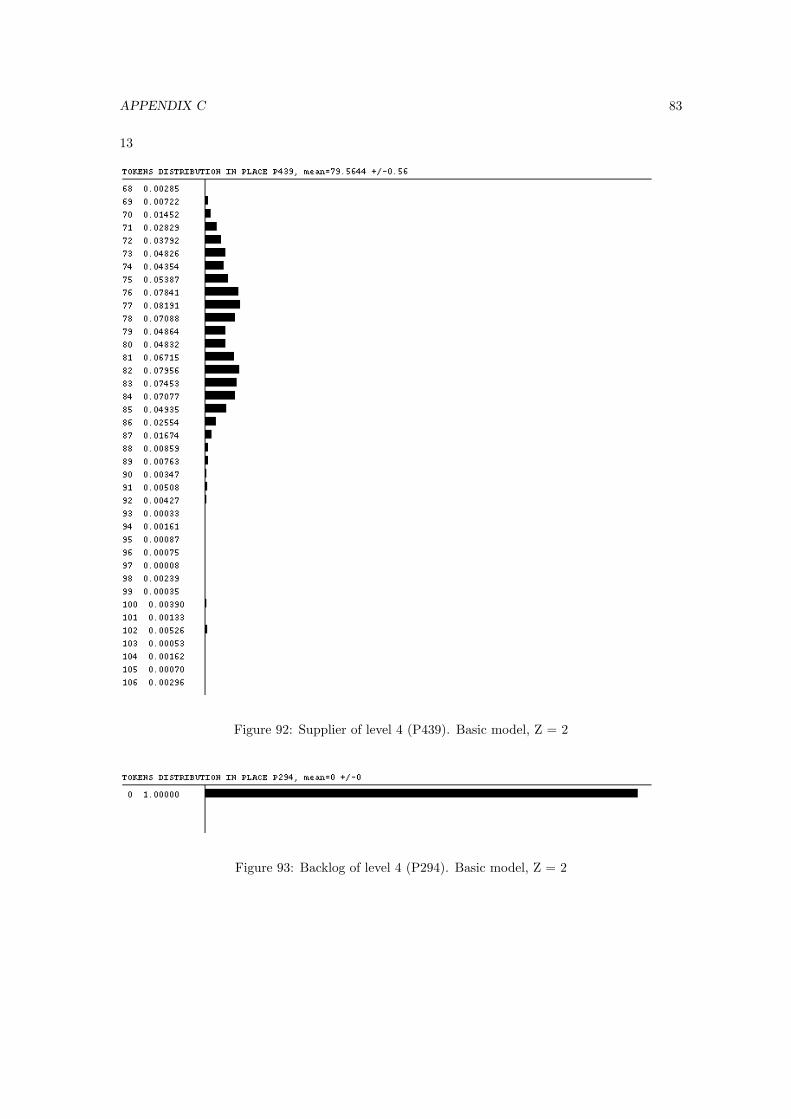
APPENDIX C 83
13
Figure 92: Supplier of level 4 (P439). Basic model, Z = 2
Figure 93: Backlog of level 4 (P294). Basic model, Z = 2
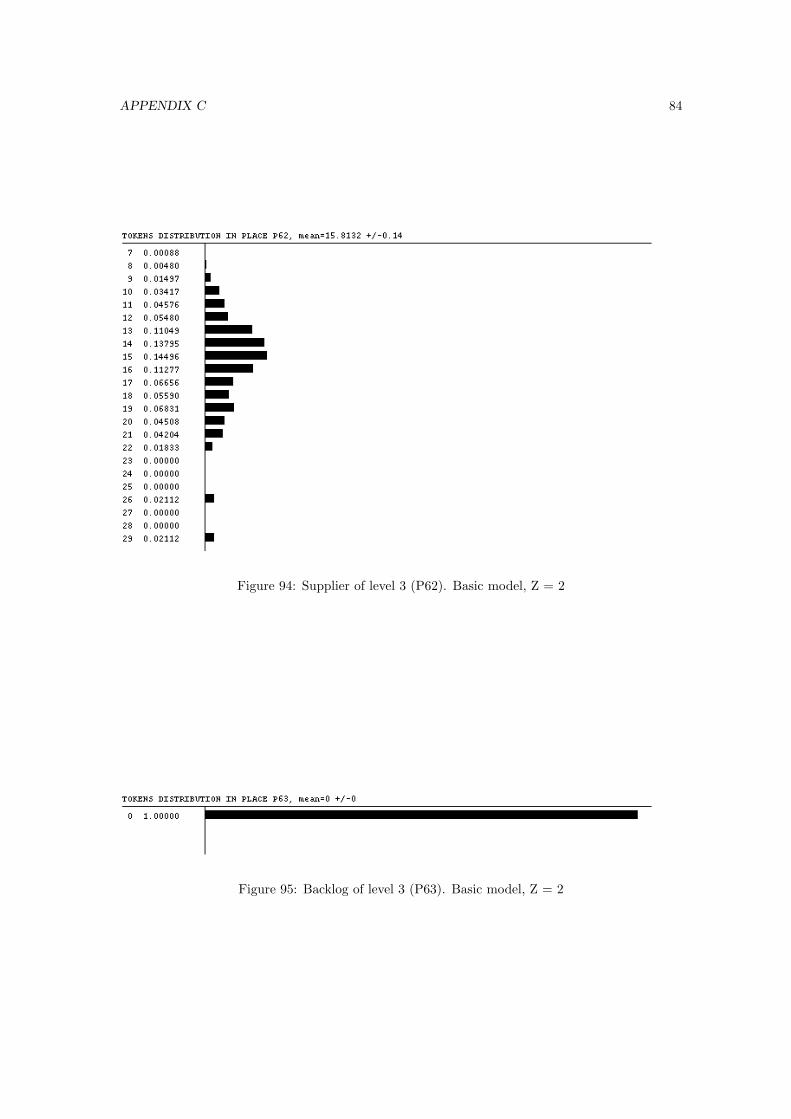
APPENDIX C 84
Figure 94: Supplier of level 3 (P62). Basic model, Z = 2
Figure 95: Backlog of level 3 (P63). Basic model, Z = 2
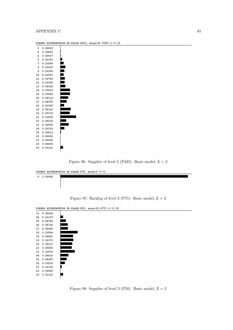
APPENDIX C 85
Figure 96: Supplier of level 3 (P433). Basic model, Z = 2
Figure 97: Backlog of level 3 (P75). Basic model, Z = 2
Figure 98: Supplier of level 3 (P50). Basic model, Z = 2
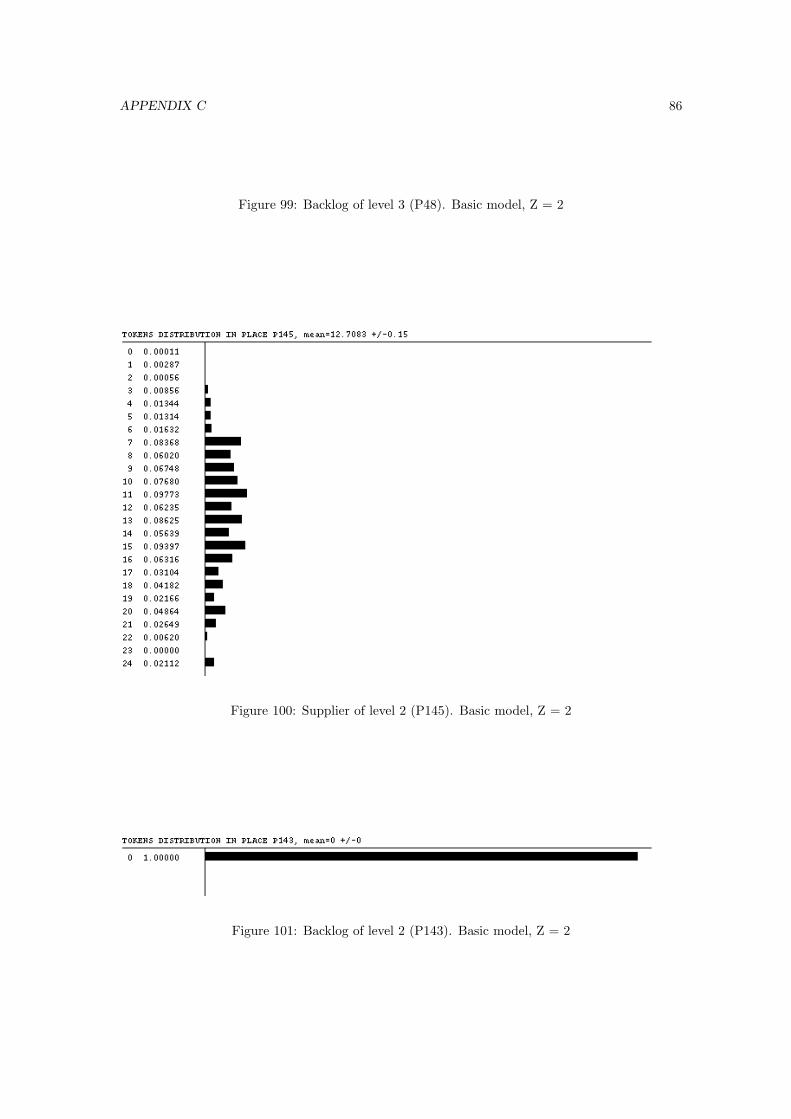
APPENDIX C 86
Figure 99: Backlog of level 3 (P48). Basic model, Z = 2
Figure 100: Supplier of level 2 (P145). Basic model, Z = 2
Figure 101: Backlog of level 2 (P143). Basic model, Z = 2
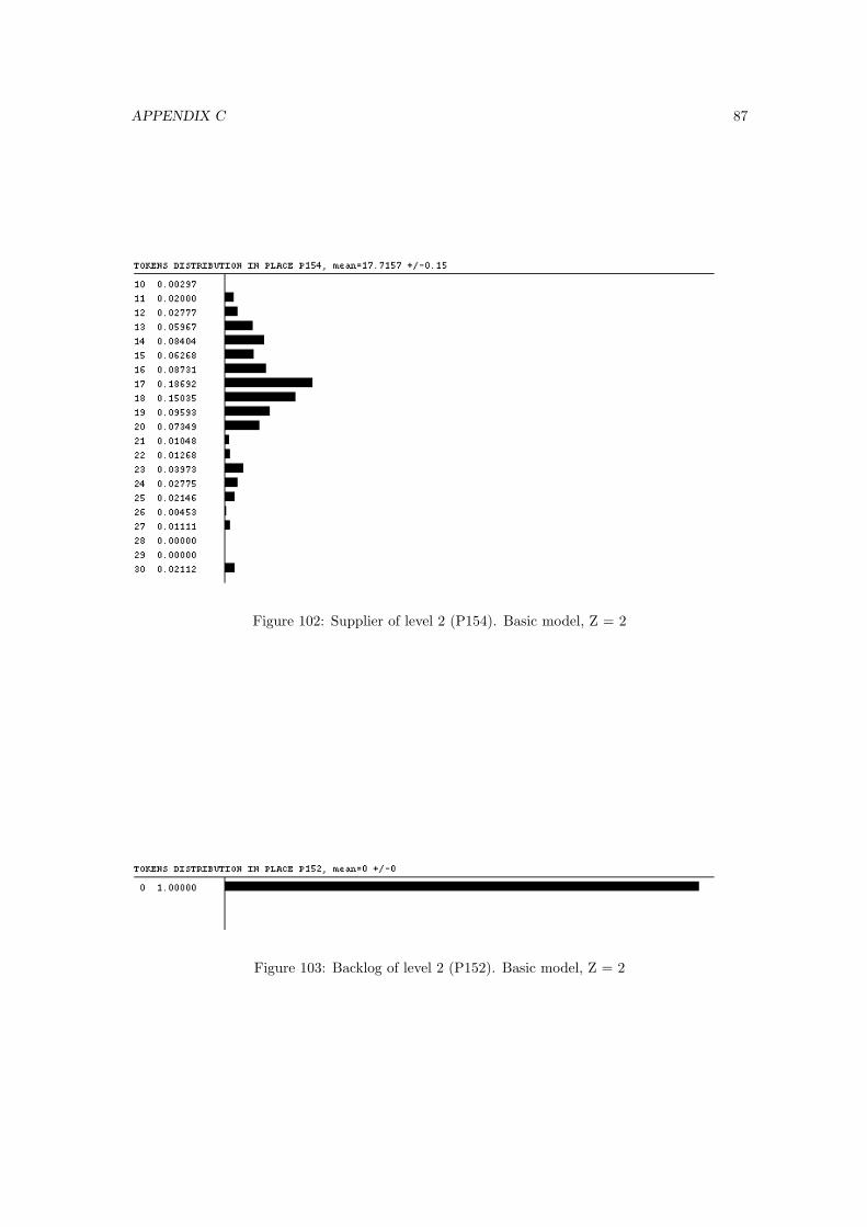
APPENDIX C 87
Figure 102: Supplier of level 2 (P154). Basic model, Z = 2
Figure 103: Backlog of level 2 (P152). Basic model, Z = 2
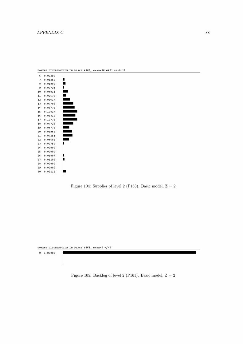
APPENDIX C 88
Figure 104: Supplier of level 2 (P163). Basic model, Z = 2
Figure 105: Backlog of level 2 (P161). Basic model, Z = 2
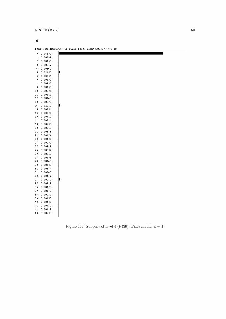
APPENDIX C 89
16
Figure 106: Supplier of level 4 (P439). Basic model, Z = 1
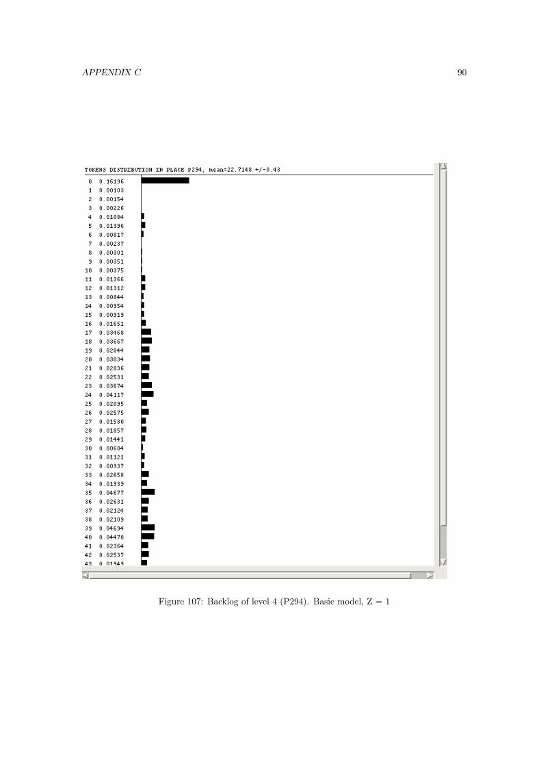
APPENDIX C 90
Figure 107: Backlog of level 4 (P294). Basic model, Z = 1
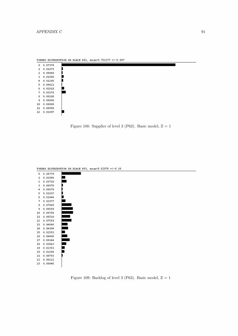
APPENDIX C 91
Figure 108: Supplier of level 3 (P62). Basic model, Z = 1
Figure 109: Backlog of level 3 (P63). Basic model, Z = 1
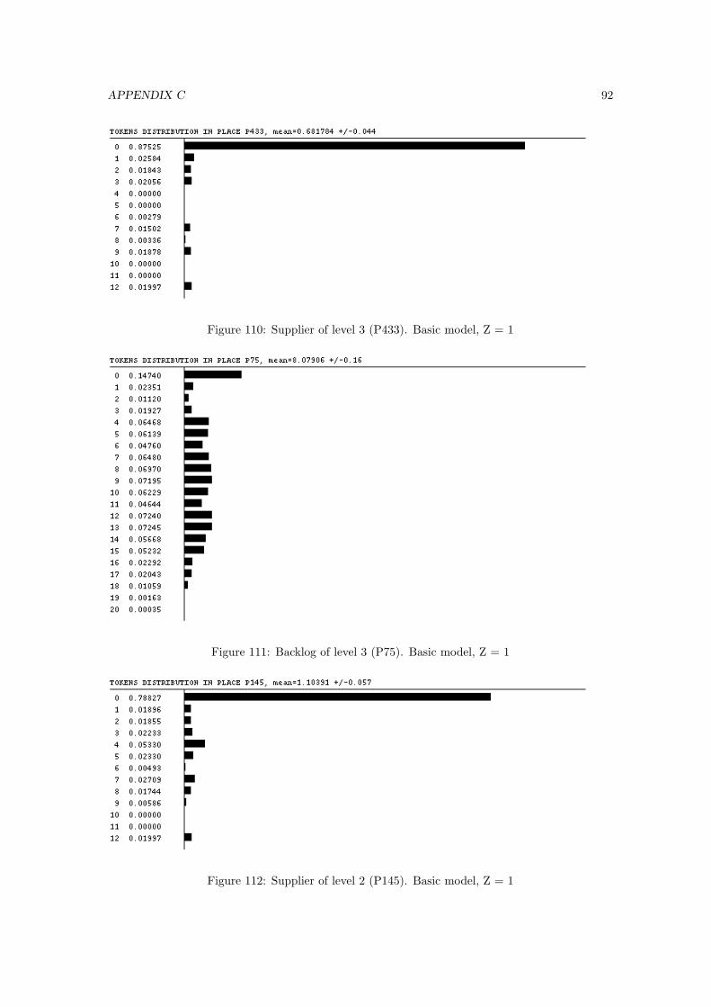
APPENDIX C 92
Figure 110: Supplier of level 3 (P433). Basic model, Z = 1
Figure 111: Backlog of level 3 (P75). Basic model, Z = 1
Figure 112: Supplier of level 2 (P145). Basic model, Z = 1
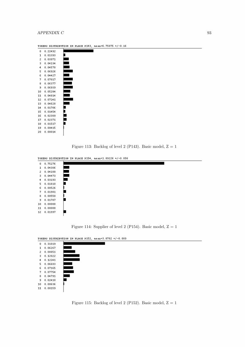
APPENDIX C 93
Figure 113: Backlog of level 2 (P143). Basic model, Z = 1
Figure 114: Supplier of level 2 (P154). Basic model, Z = 1
Figure 115: Backlog of level 2 (P152). Basic model, Z = 1
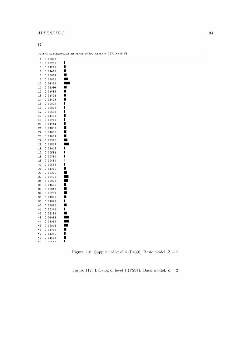
APPENDIX C 94
17
Figure 116: Supplier of level 4 (P439). Basic model, Z = 2
Figure 117: Backlog of level 4 (P294). Basic model, Z = 2
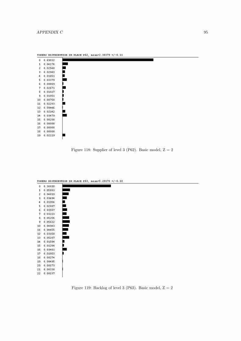
APPENDIX C 95
Figure 118: Supplier of level 3 (P62). Basic model, Z = 2
Figure 119: Backlog of level 3 (P63). Basic model, Z = 2
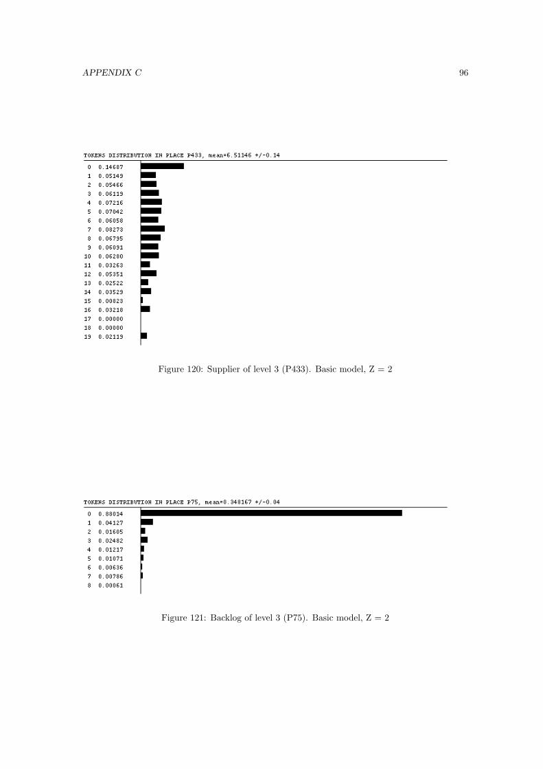
APPENDIX C 96
Figure 120: Supplier of level 3 (P433). Basic model, Z = 2
Figure 121: Backlog of level 3 (P75). Basic model, Z = 2
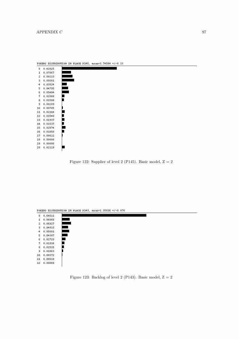
APPENDIX C 97
Figure 122: Supplier of level 2 (P145). Basic model, Z = 2
Figure 123: Backlog of level 2 (P143). Basic model, Z = 2
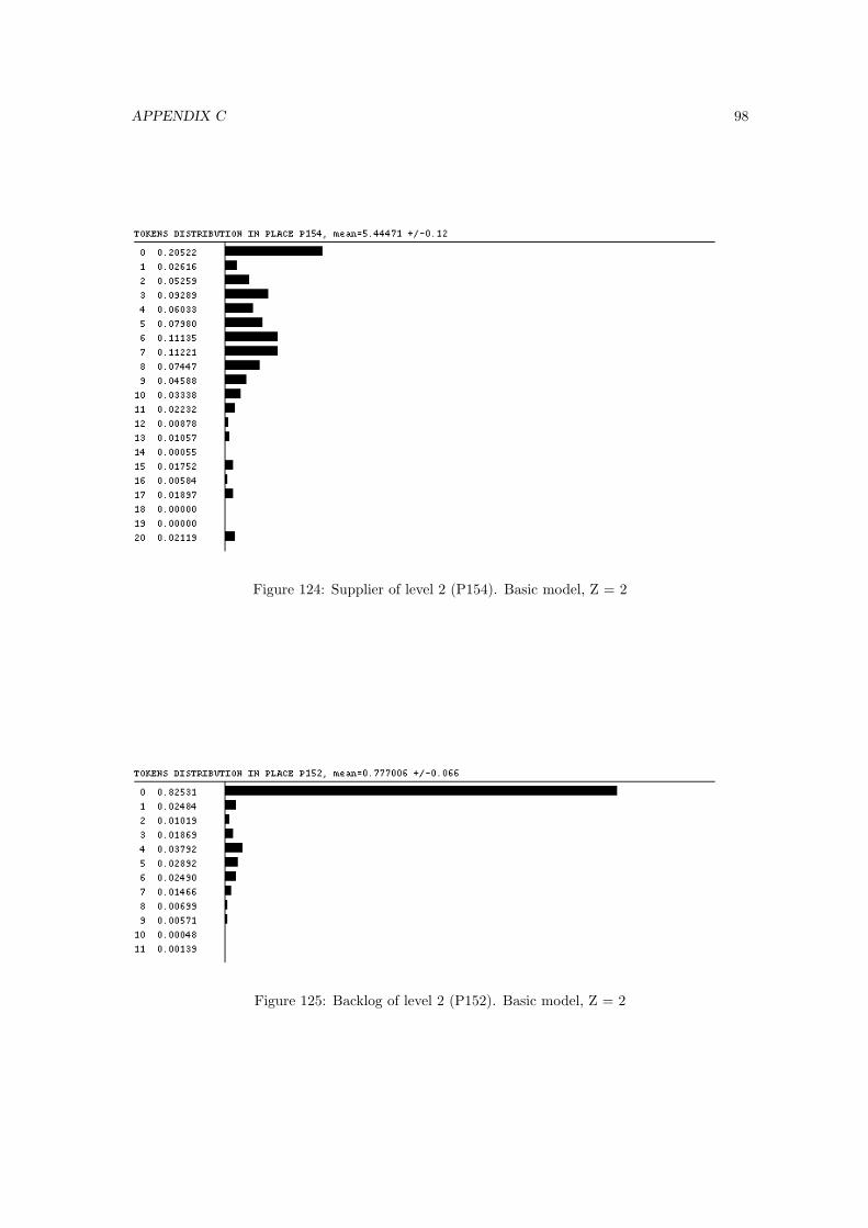
APPENDIX C 98
Figure 124: Supplier of level 2 (P154). Basic model, Z = 2
Figure 125: Backlog of level 2 (P152). Basic model, Z = 2

APPENDIX C 99
18
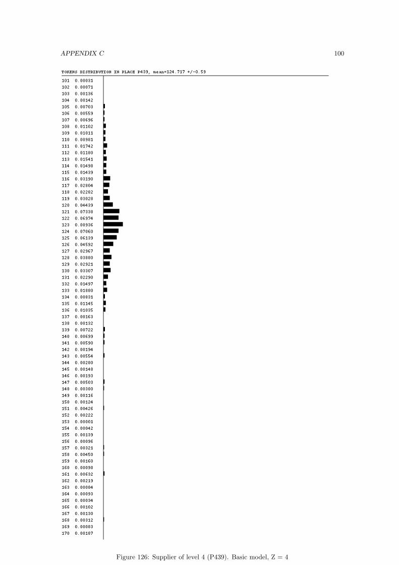
APPENDIX C 100
Figure 126: Supplier of level 4 (P439). Basic model, Z = 4
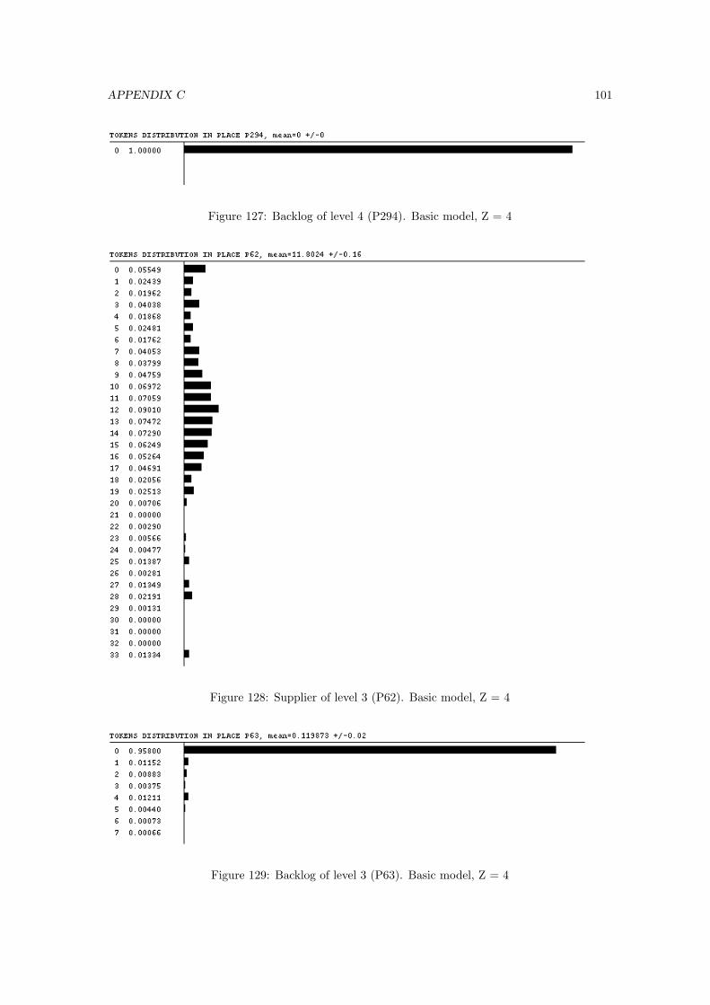
APPENDIX C 101
Figure 127: Backlog of level 4 (P294). Basic model, Z = 4
Figure 128: Supplier of level 3 (P62). Basic model, Z = 4
Figure 129: Backlog of level 3 (P63). Basic model, Z = 4
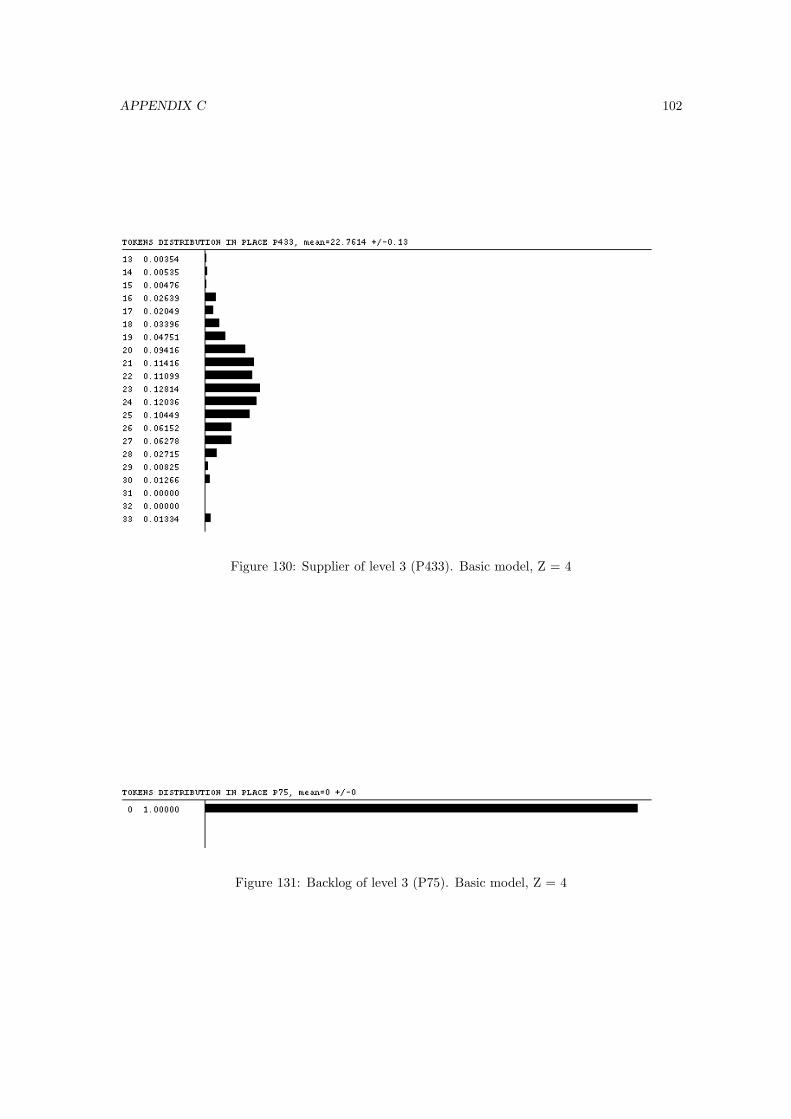
APPENDIX C 102
Figure 130: Supplier of level 3 (P433). Basic model, Z = 4
Figure 131: Backlog of level 3 (P75). Basic model, Z = 4
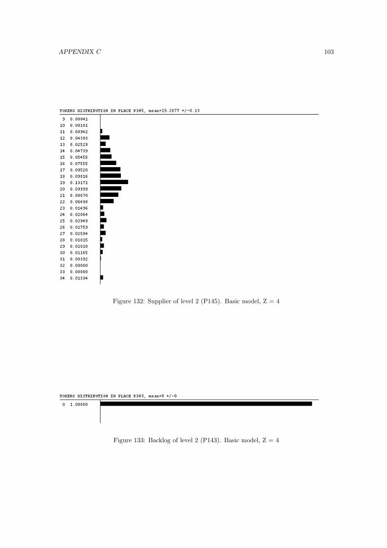
APPENDIX C 103
Figure 132: Supplier of level 2 (P145). Basic model, Z = 4
Figure 133: Backlog of level 2 (P143). Basic model, Z = 4
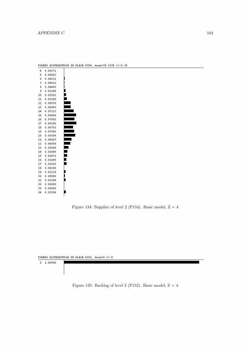
APPENDIX C 104
Figure 134: Supplier of level 2 (P154). Basic model, Z = 4
Figure 135: Backlog of level 2 (P152). Basic model, Z = 4
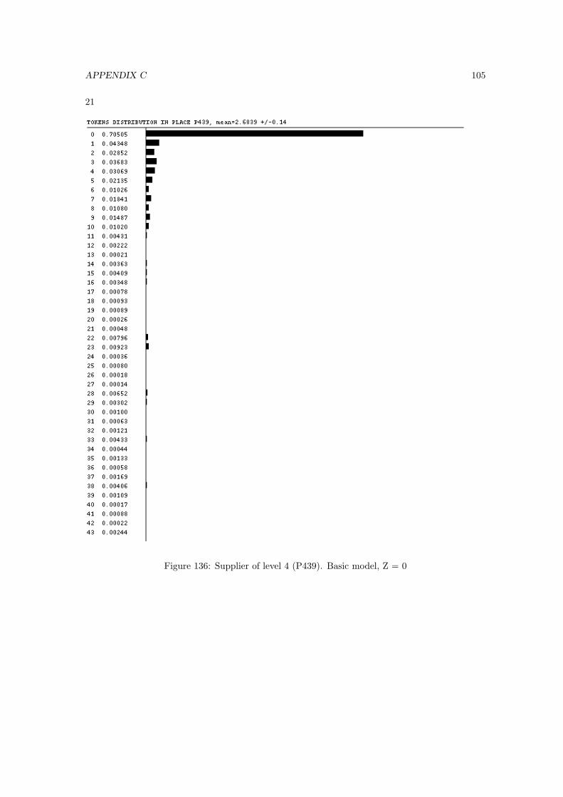
APPENDIX C 105
21
Figure 136: Supplier of level 4 (P439). Basic model, Z = 0
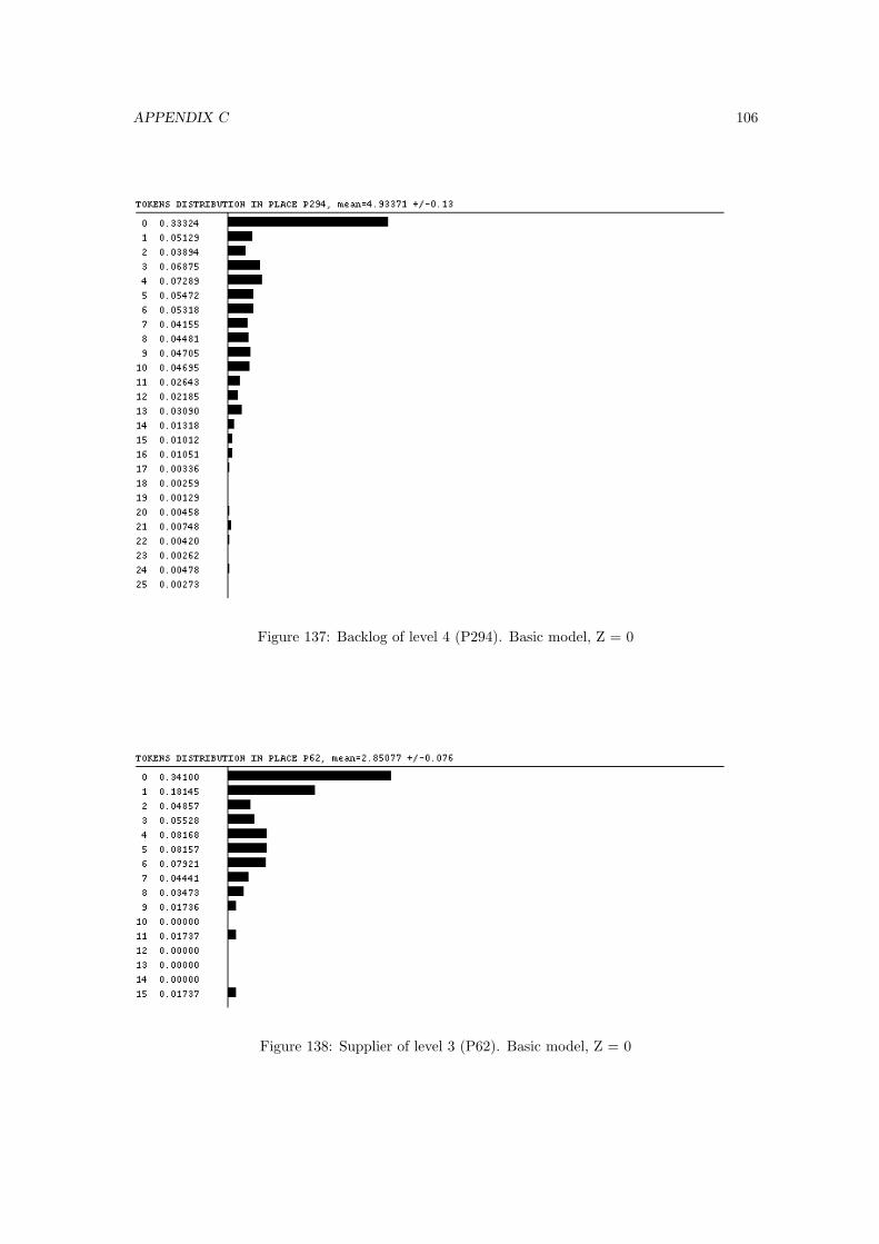
APPENDIX C 106
Figure 137: Backlog of level 4 (P294). Basic model, Z = 0
Figure 138: Supplier of level 3 (P62). Basic model, Z = 0
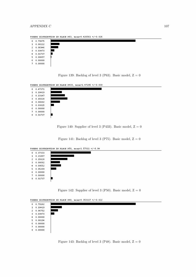
APPENDIX C 107
Figure 139: Backlog of level 3 (P63). Basic model, Z = 0
Figure 140: Supplier of level 3 (P433). Basic model, Z = 0
Figure 141: Backlog of level 3 (P75). Basic model, Z = 0
Figure 142: Supplier of level 3 (P50). Basic model, Z = 0
Figure 143: Backlog of level 3 (P48). Basic model, Z = 0
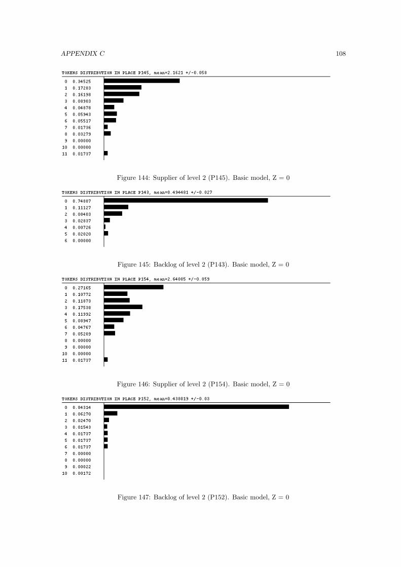
APPENDIX C 108
Figure 144: Supplier of level 2 (P145). Basic model, Z = 0
Figure 145: Backlog of level 2 (P143). Basic model, Z = 0
Figure 146: Supplier of level 2 (P154). Basic model, Z = 0
Figure 147: Backlog of level 2 (P152). Basic model, Z = 0
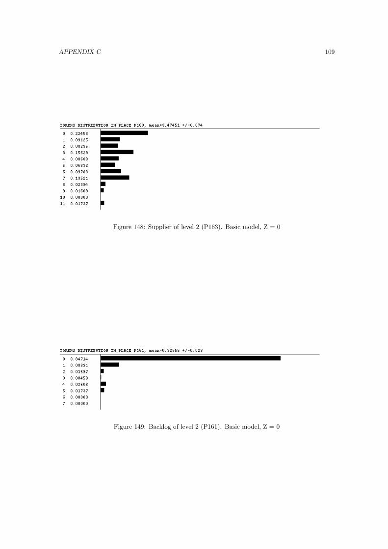
APPENDIX C 109
Figure 148: Supplier of level 2 (P163). Basic model, Z = 0
Figure 149: Backlog of level 2 (P161). Basic model, Z = 0
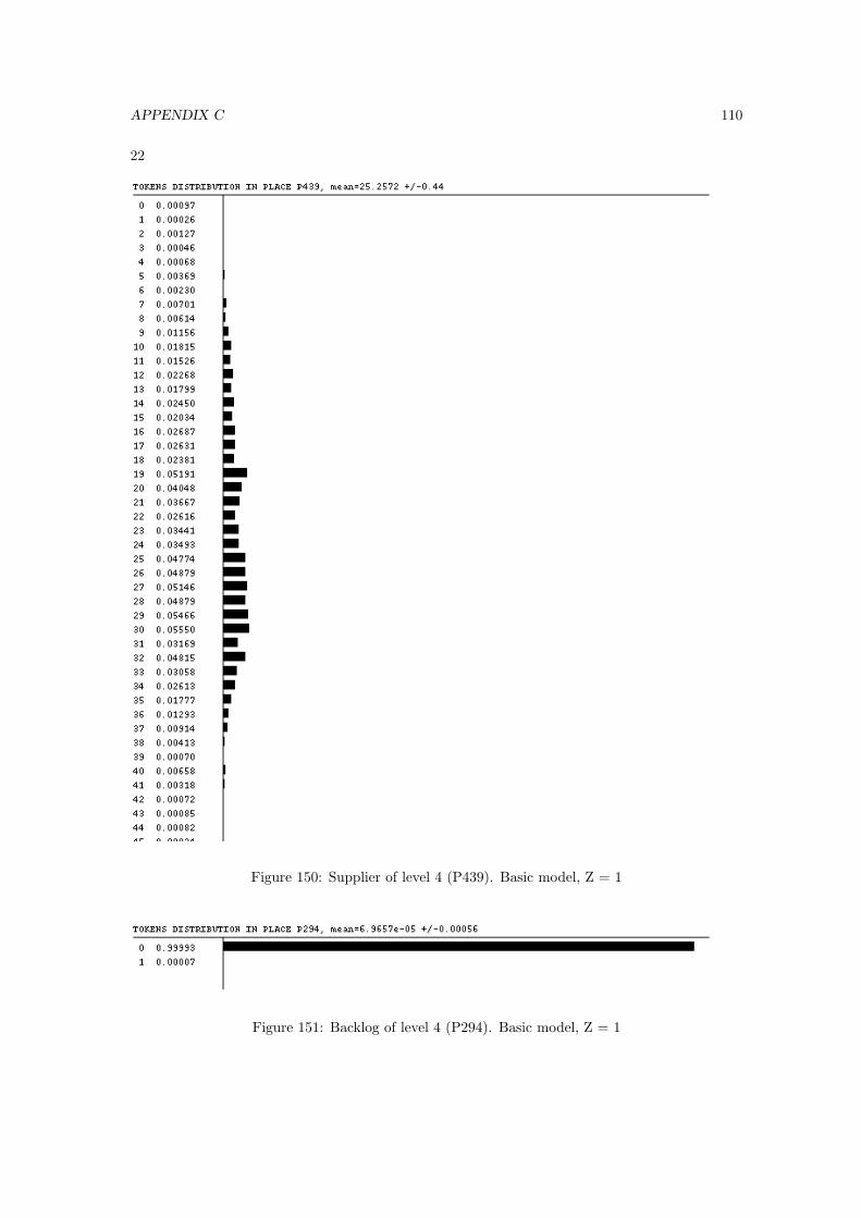
APPENDIX C 110
22
Figure 150: Supplier of level 4 (P439). Basic model, Z = 1
Figure 151: Backlog of level 4 (P294). Basic model, Z = 1
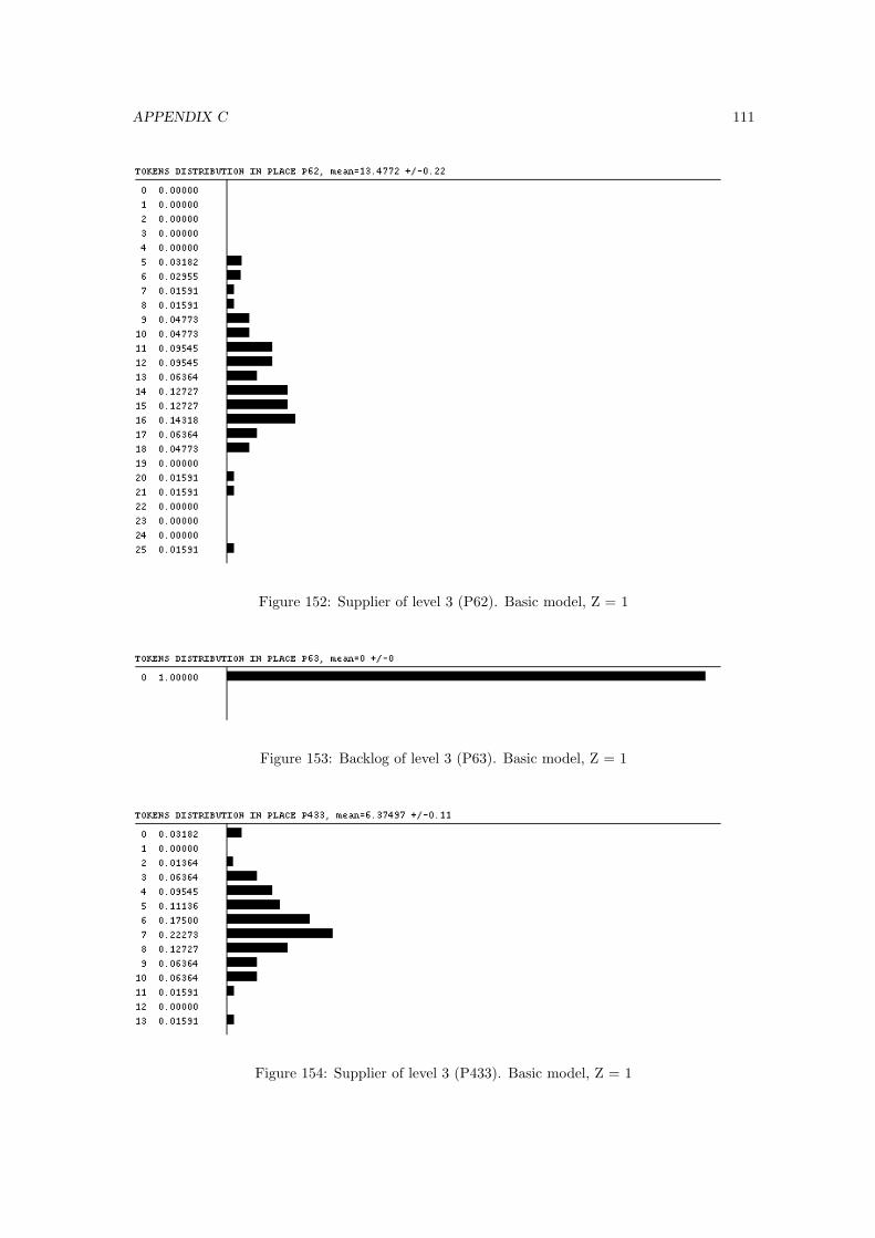
APPENDIX C 111
Figure 152: Supplier of level 3 (P62). Basic model, Z = 1
Figure 153: Backlog of level 3 (P63). Basic model, Z = 1
Figure 154: Supplier of level 3 (P433). Basic model, Z = 1
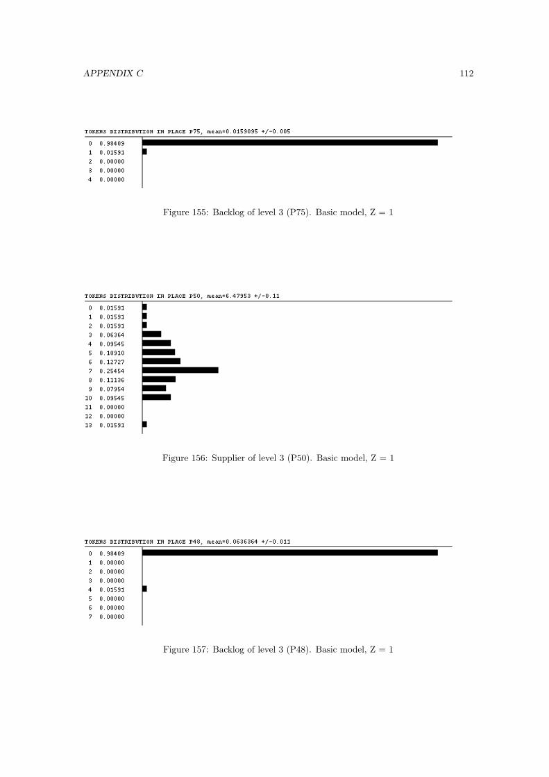
APPENDIX C 112
Figure 155: Backlog of level 3 (P75). Basic model, Z = 1
Figure 156: Supplier of level 3 (P50). Basic model, Z = 1
Figure 157: Backlog of level 3 (P48). Basic model, Z = 1
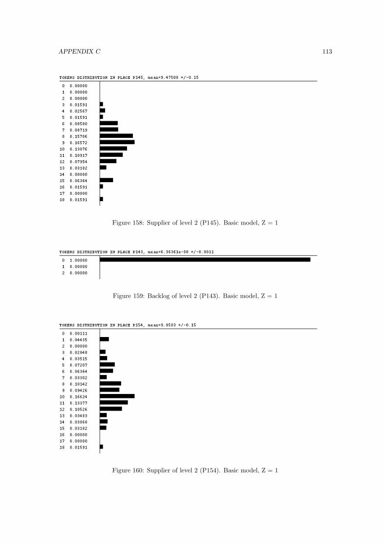
APPENDIX C 113
Figure 158: Supplier of level 2 (P145). Basic model, Z = 1
Figure 159: Backlog of level 2 (P143). Basic model, Z = 1
Figure 160: Supplier of level 2 (P154). Basic model, Z = 1

APPENDIX C 114
Figure 161: Backlog of level 2 (P152). Basic model, Z = 1
Figure 162: Supplier of level 2 (P163). Basic model, Z = 1
Figure 163: Backlog of level 2 (P161). Basic model, Z = 1

APPENDIX C 115
23
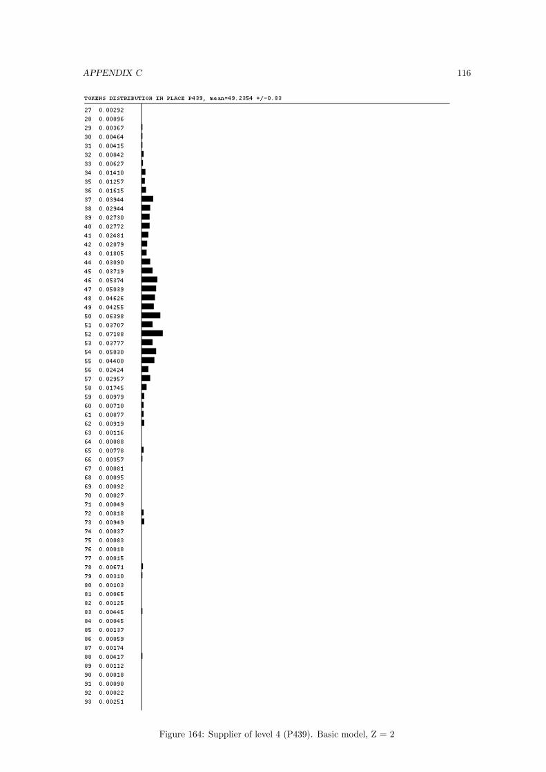
APPENDIX C 116
Figure 164: Supplier of level 4 (P439). Basic model, Z = 2
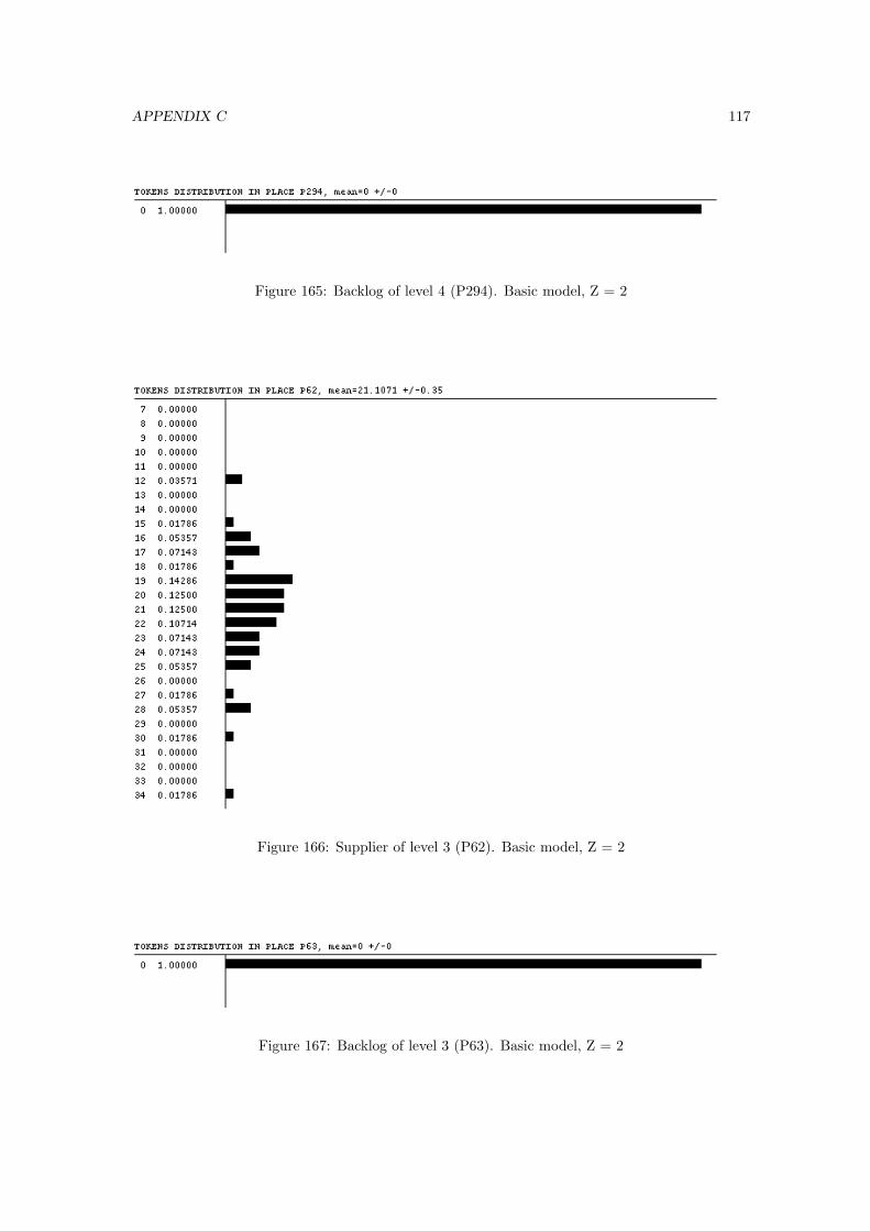
APPENDIX C 117
Figure 165: Backlog of level 4 (P294). Basic model, Z = 2
Figure 166: Supplier of level 3 (P62). Basic model, Z = 2
Figure 167: Backlog of level 3 (P63). Basic model, Z = 2
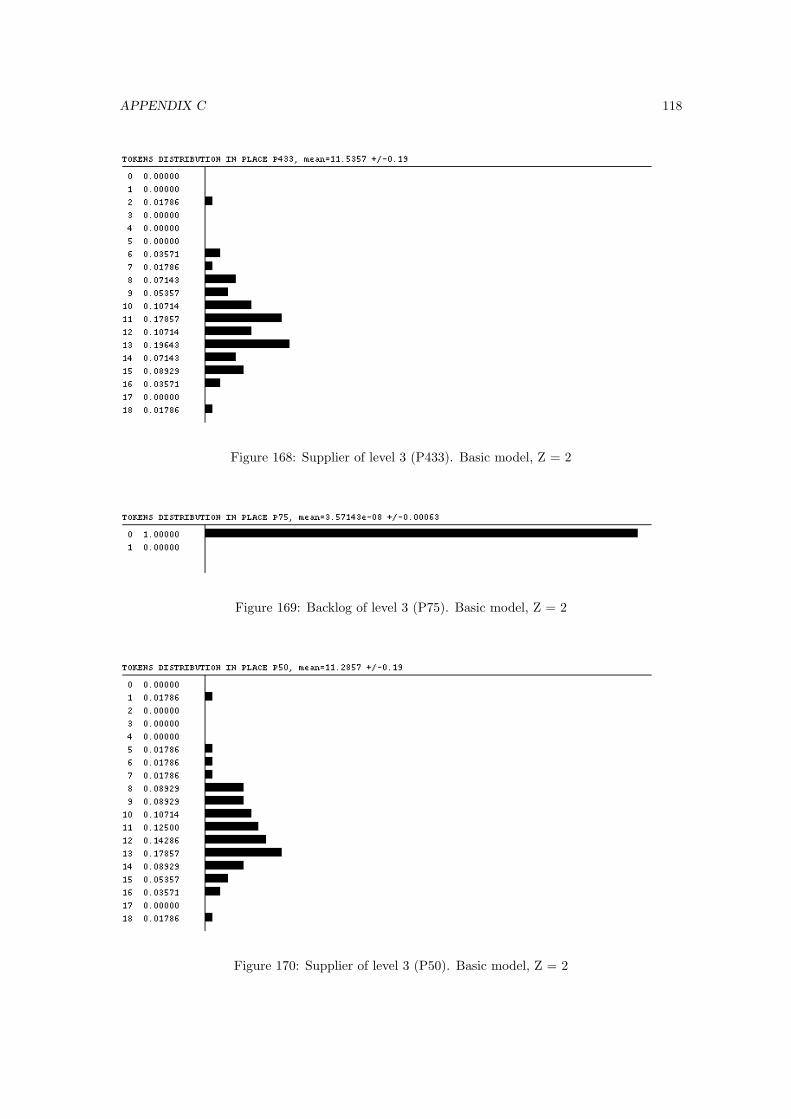
APPENDIX C 118
Figure 168: Supplier of level 3 (P433). Basic model, Z = 2
Figure 169: Backlog of level 3 (P75). Basic model, Z = 2
Figure 170: Supplier of level 3 (P50). Basic model, Z = 2
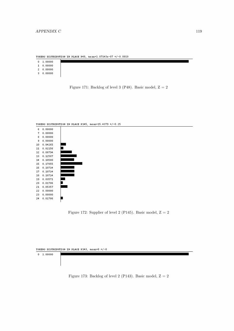
APPENDIX C 119
Figure 171: Backlog of level 3 (P48). Basic model, Z = 2
Figure 172: Supplier of level 2 (P145). Basic model, Z = 2
Figure 173: Backlog of level 2 (P143). Basic model, Z = 2
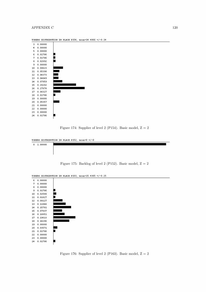
APPENDIX C 120
Figure 174: Supplier of level 2 (P154). Basic model, Z = 2
Figure 175: Backlog of level 2 (P152). Basic model, Z = 2
Figure 176: Supplier of level 2 (P163). Basic model, Z = 2
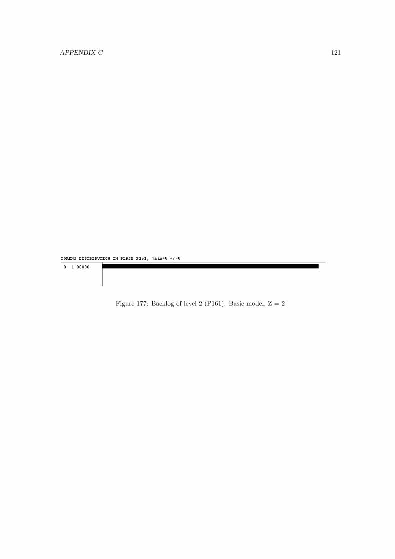
APPENDIX C 121
Figure 177: Backlog of level 2 (P161). Basic model, Z = 2

APPENDIX C 122
26
Figure 178: Supplier of level 4 (P439). Basic model, Z = 1
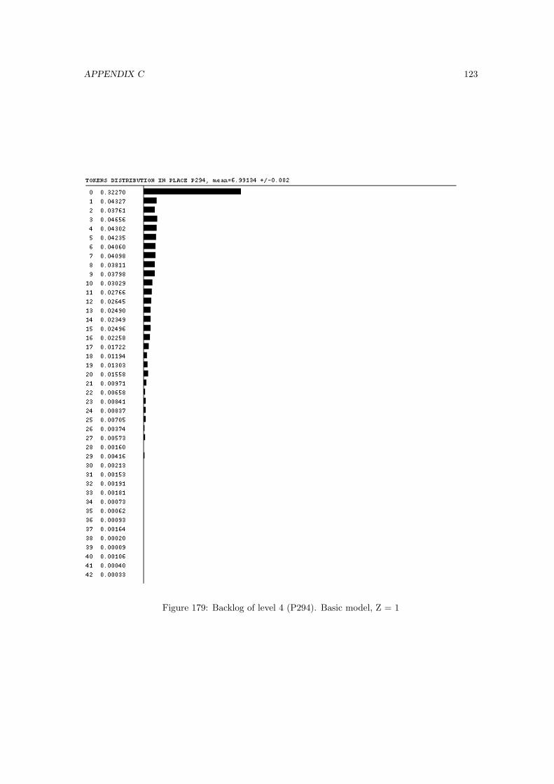
APPENDIX C 123
Figure 179: Backlog of level 4 (P294). Basic model, Z = 1
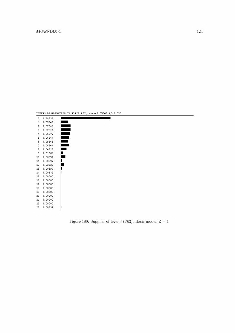
APPENDIX C 124
Figure 180: Supplier of level 3 (P62). Basic model, Z = 1
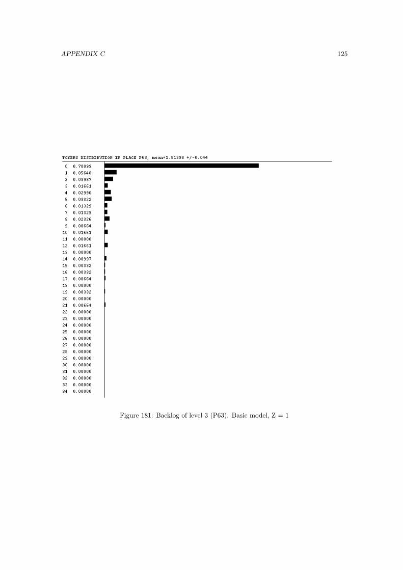
APPENDIX C 125
Figure 181: Backlog of level 3 (P63). Basic model, Z = 1
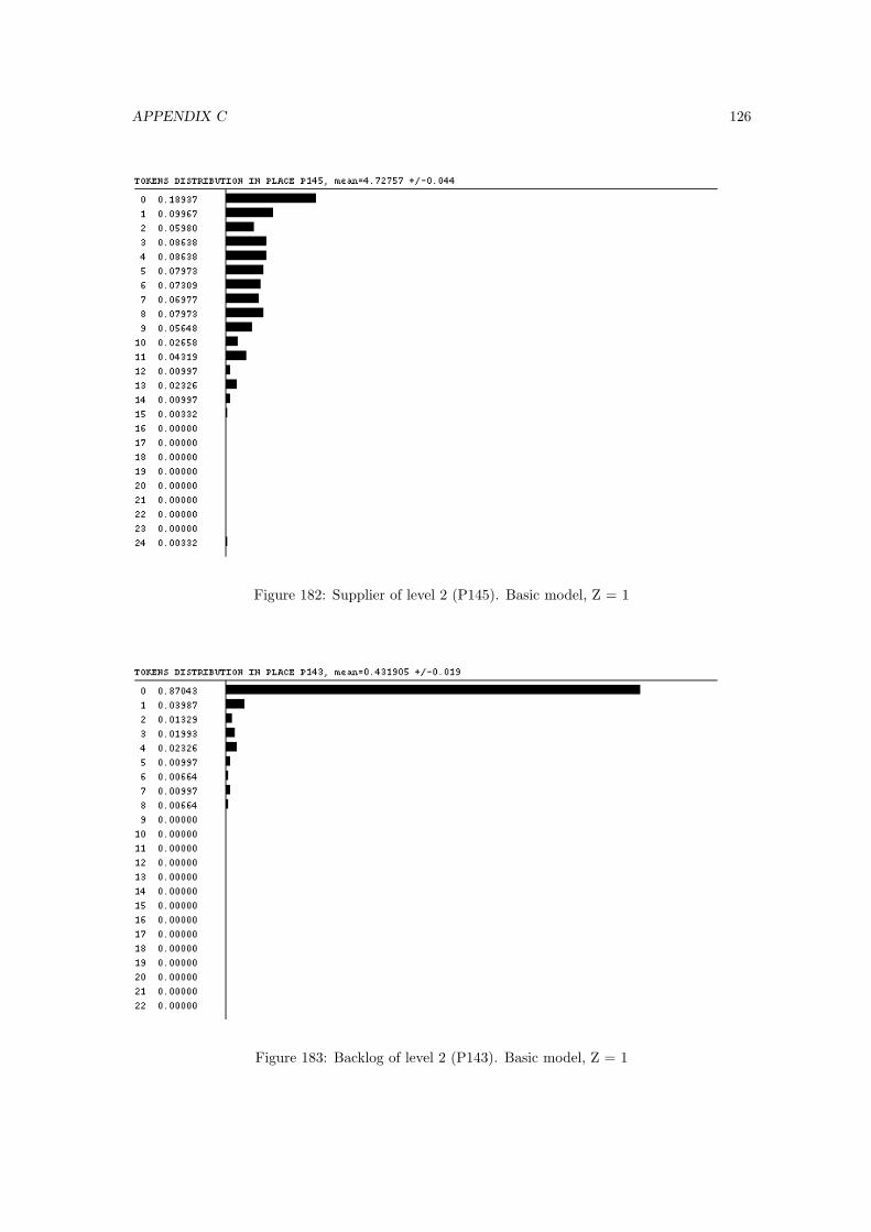
APPENDIX C 126
Figure 182: Supplier of level 2 (P145). Basic model, Z = 1
Figure 183: Backlog of level 2 (P143). Basic model, Z = 1

APPENDIX C 127
27
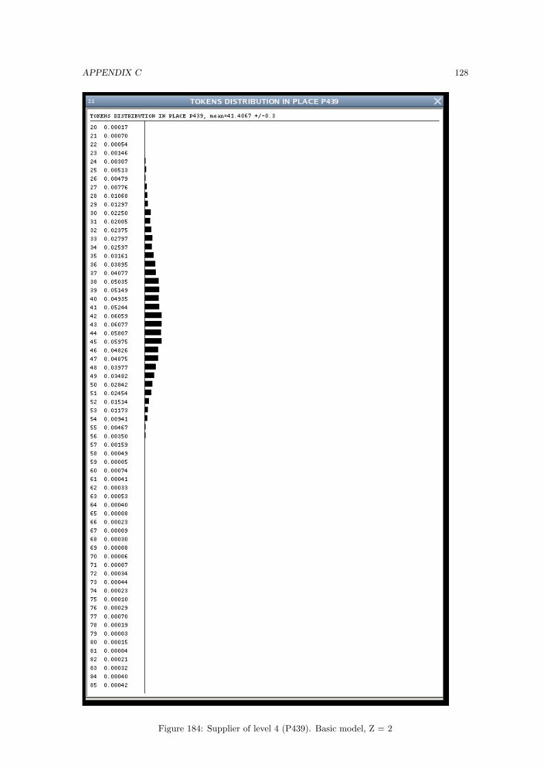
APPENDIX C 128
Figure 184: Supplier of level 4 (P439). Basic model, Z = 2
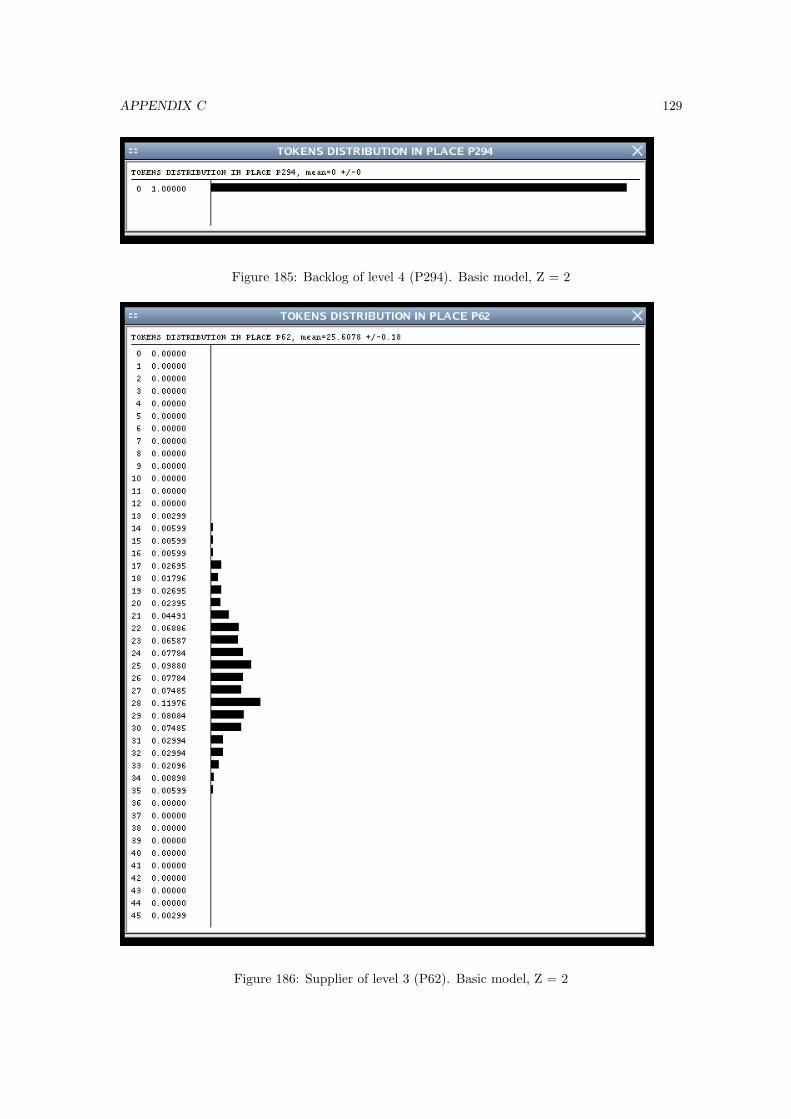
APPENDIX C 129
Figure 185: Backlog of level 4 (P294). Basic model, Z = 2
Figure 186: Supplier of level 3 (P62). Basic model, Z = 2
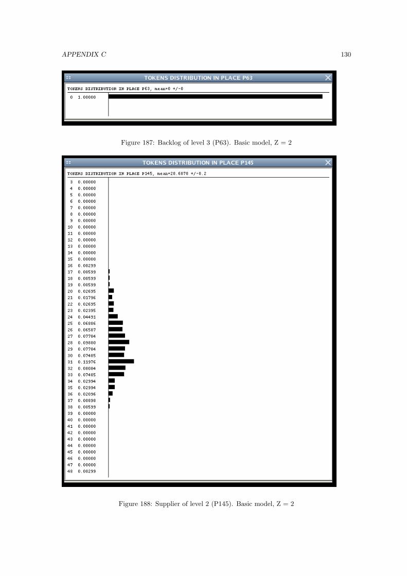
APPENDIX C 130
Figure 187: Backlog of level 3 (P63). Basic model, Z = 2
Figure 188: Supplier of level 2 (P145). Basic model, Z = 2

APPENDIX C 131
Figure 189: Backlog of level 2 (P143). Basic model, Z = 2
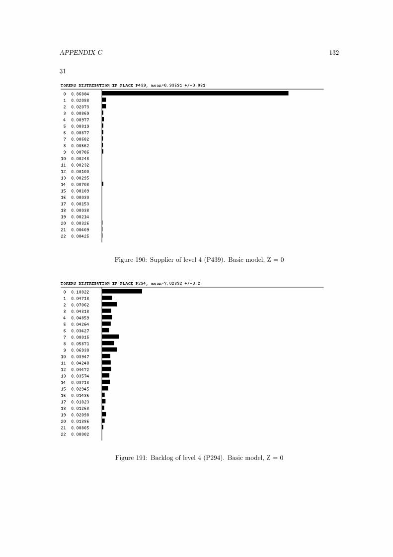
APPENDIX C 132
31
Figure 190: Supplier of level 4 (P439). Basic model, Z = 0
Figure 191: Backlog of level 4 (P294). Basic model, Z = 0
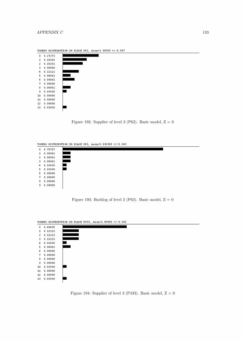
APPENDIX C 133
Figure 192: Supplier of level 3 (P62). Basic model, Z = 0
Figure 193: Backlog of level 3 (P63). Basic model, Z = 0
Figure 194: Supplier of level 3 (P433). Basic model, Z = 0
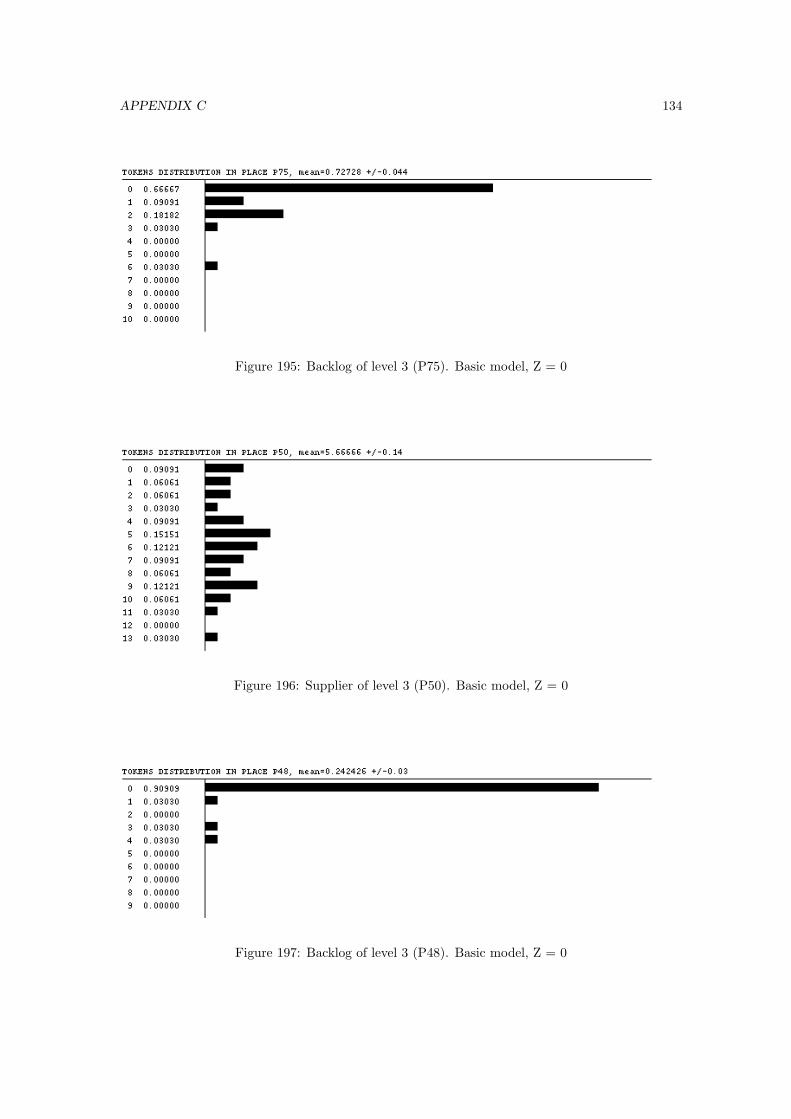
APPENDIX C 134
Figure 195: Backlog of level 3 (P75). Basic model, Z = 0
Figure 196: Supplier of level 3 (P50). Basic model, Z = 0
Figure 197: Backlog of level 3 (P48). Basic model, Z = 0
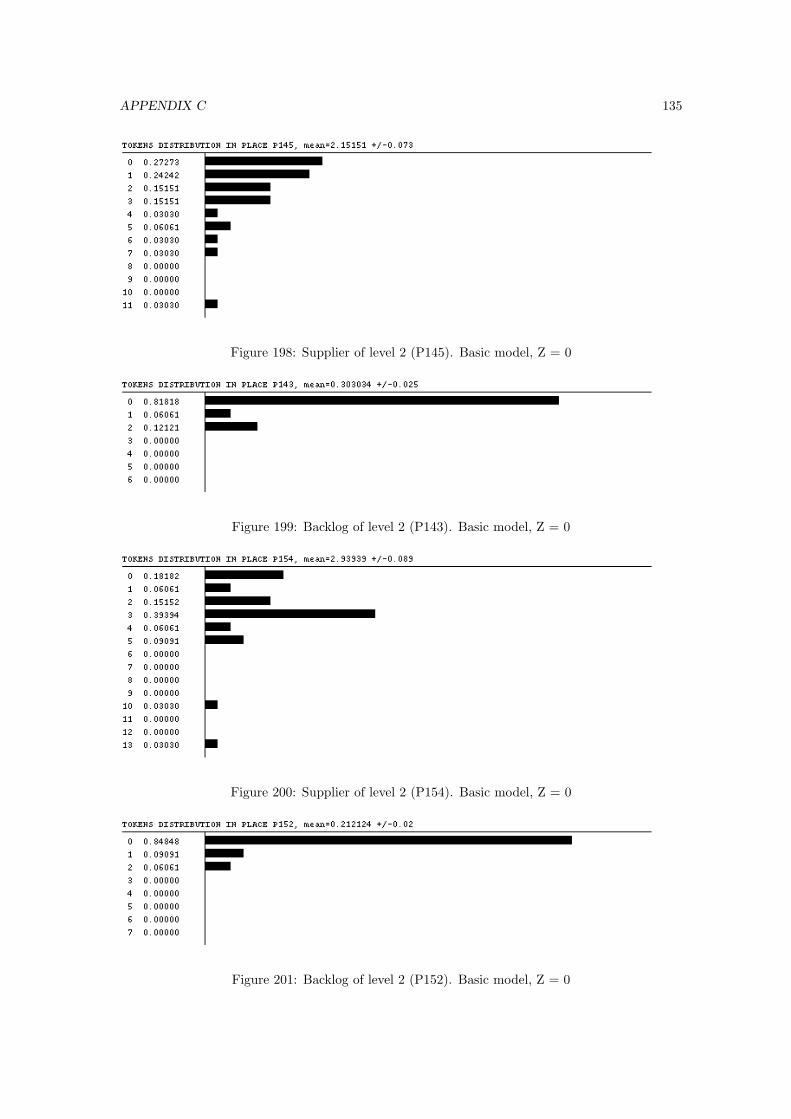
APPENDIX C 135
Figure 198: Supplier of level 2 (P145). Basic model, Z = 0
Figure 199: Backlog of level 2 (P143). Basic model, Z = 0
Figure 200: Supplier of level 2 (P154). Basic model, Z = 0
Figure 201: Backlog of level 2 (P152). Basic model, Z = 0

APPENDIX C 136
Figure 202: Supplier of level 2 (P163). Basic model, Z = 0
Figure 203: Backlog of level 2 (P161). Basic model, Z = 0
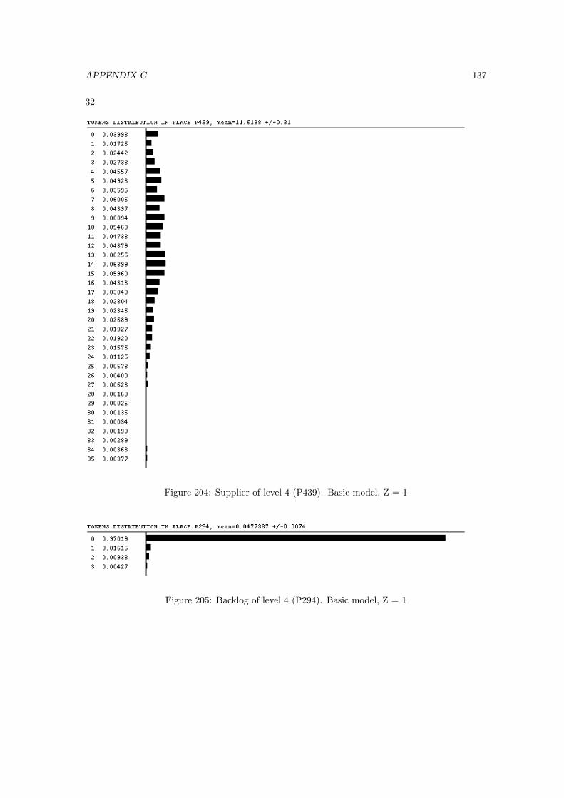
APPENDIX C 137
32
Figure 204: Supplier of level 4 (P439). Basic model, Z = 1
Figure 205: Backlog of level 4 (P294). Basic model, Z = 1
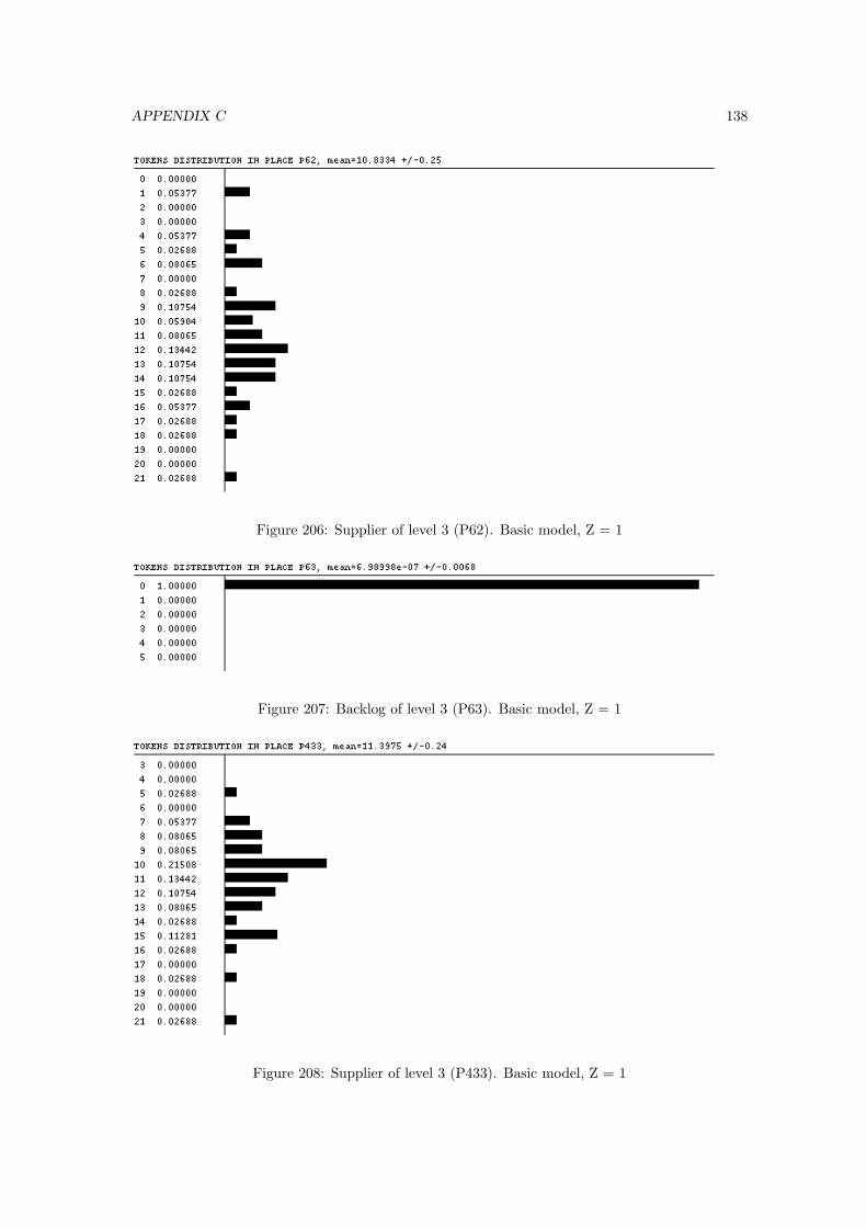
APPENDIX C 138
Figure 206: Supplier of level 3 (P62). Basic model, Z = 1
Figure 207: Backlog of level 3 (P63). Basic model, Z = 1
Figure 208: Supplier of level 3 (P433). Basic model, Z = 1

APPENDIX C 139
Figure 209: Backlog of level 3 (P75). Basic model, Z = 1
Figure 210: Supplier of level 3 (P50). Basic model, Z = 1
Figure 211: Backlog of level 3 (P48). Basic model, Z = 1
Figure 212: Supplier of level 2 (P145). Basic model, Z = 1
Figure 213: Backlog of level 2 (P143). Basic model, Z = 1
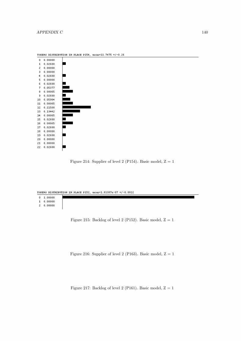
APPENDIX C 140
Figure 214: Supplier of level 2 (P154). Basic model, Z = 1
Figure 215: Backlog of level 2 (P152). Basic model, Z = 1
Figure 216: Supplier of level 2 (P163). Basic model, Z = 1
Figure 217: Backlog of level 2 (P161). Basic model, Z = 1
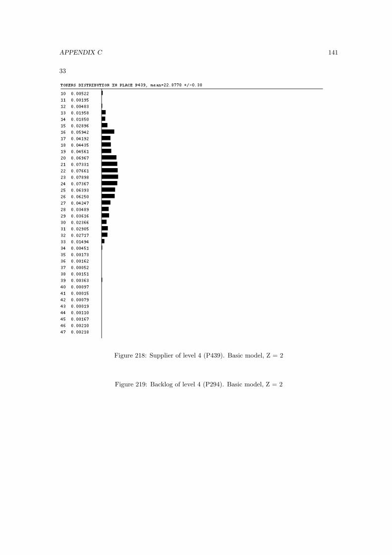
APPENDIX C 141
33
Figure 218: Supplier of level 4 (P439). Basic model, Z = 2
Figure 219: Backlog of level 4 (P294). Basic model, Z = 2
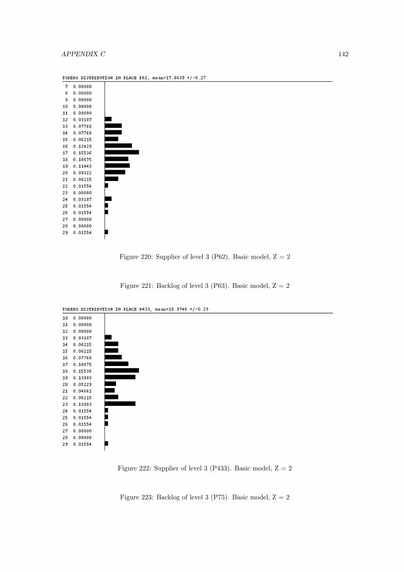
APPENDIX C 142
Figure 220: Supplier of level 3 (P62). Basic model, Z = 2
Figure 221: Backlog of level 3 (P63). Basic model, Z = 2
Figure 222: Supplier of level 3 (P433). Basic model, Z = 2
Figure 223: Backlog of level 3 (P75). Basic model, Z = 2
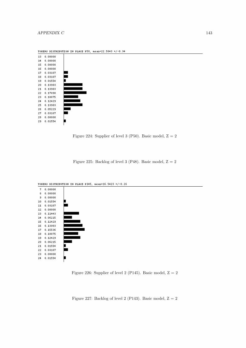
APPENDIX C 143
Figure 224: Supplier of level 3 (P50). Basic model, Z = 2
Figure 225: Backlog of level 3 (P48). Basic model, Z = 2
Figure 226: Supplier of level 2 (P145). Basic model, Z = 2
Figure 227: Backlog of level 2 (P143). Basic model, Z = 2
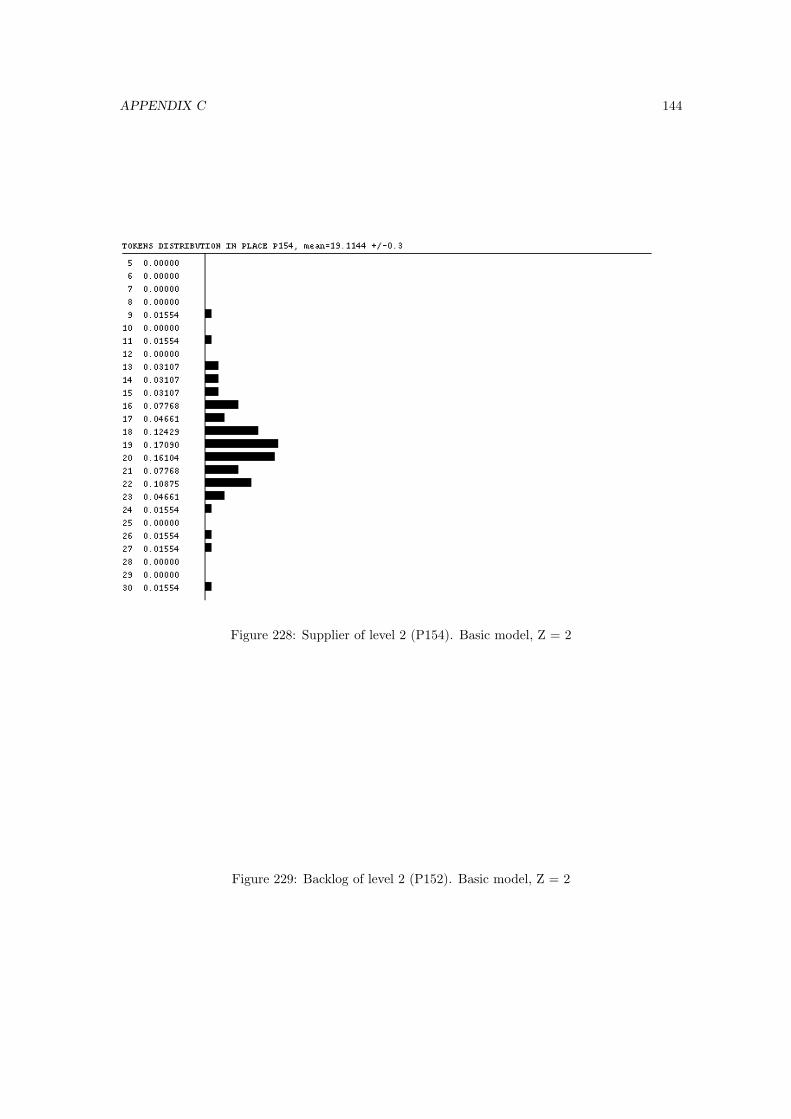
APPENDIX C 144
Figure 228: Supplier of level 2 (P154). Basic model, Z = 2
Figure 229: Backlog of level 2 (P152). Basic model, Z = 2
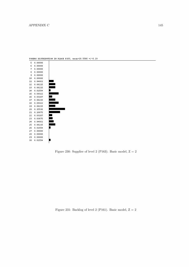
APPENDIX C 145
Figure 230: Supplier of level 2 (P163). Basic model, Z = 2
Figure 231: Backlog of level 2 (P161). Basic model, Z = 2
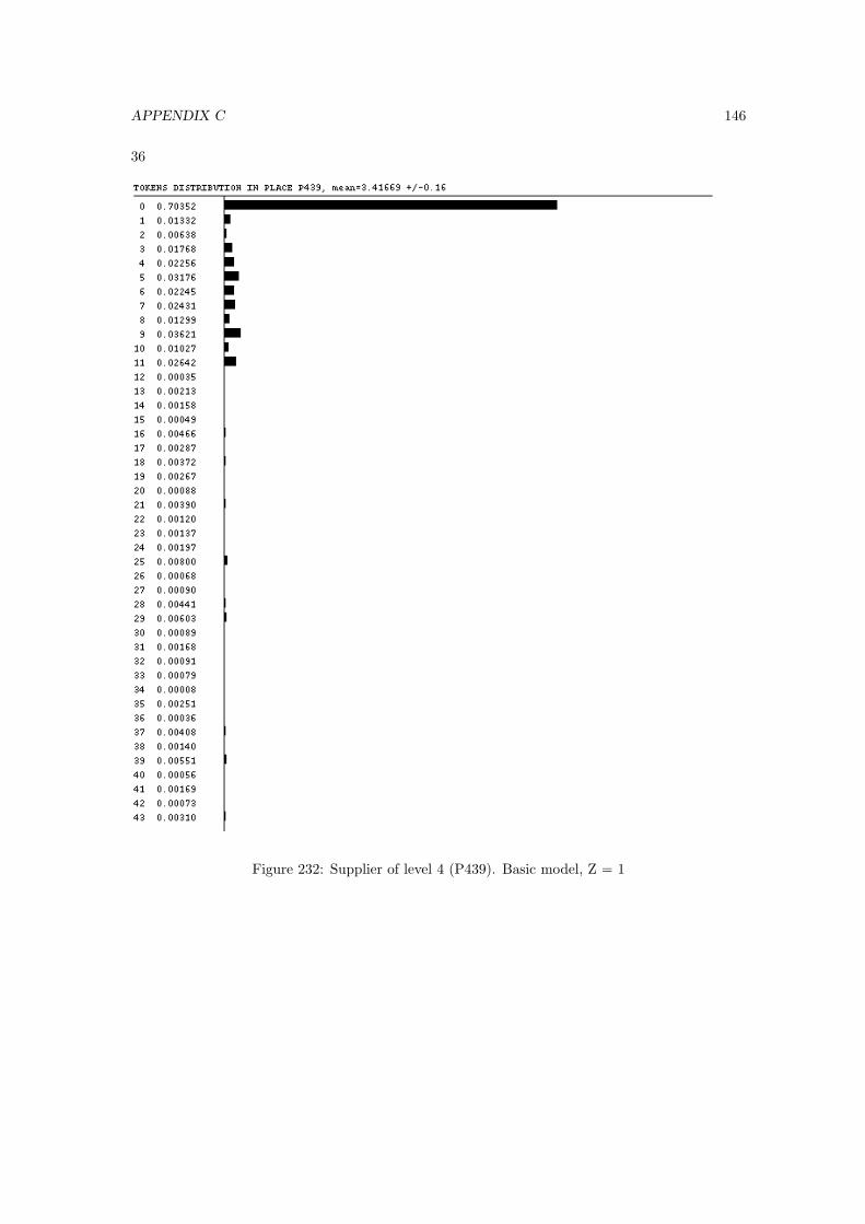
APPENDIX C 146
36
Figure 232: Supplier of level 4 (P439). Basic model, Z = 1
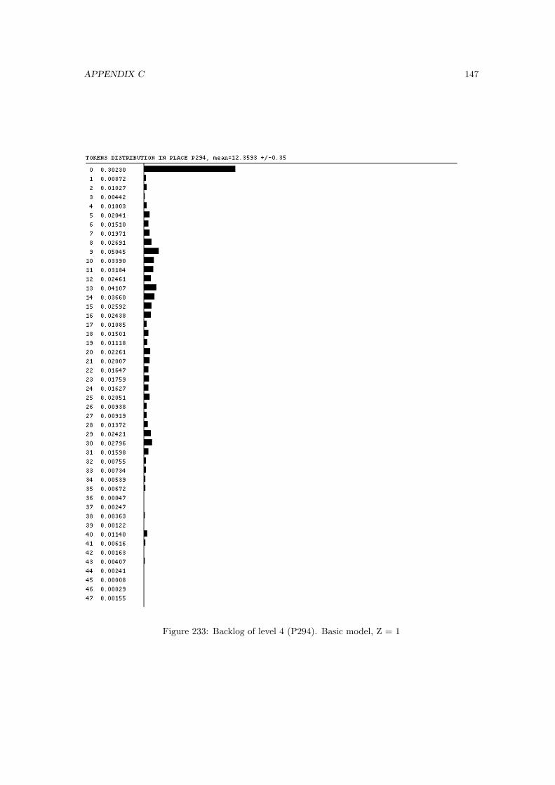
APPENDIX C 147
Figure 233: Backlog of level 4 (P294). Basic model, Z = 1
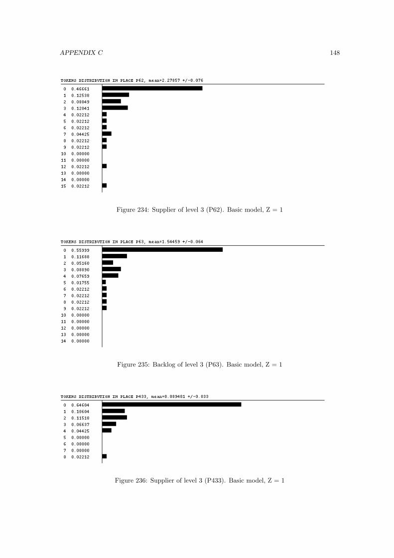
APPENDIX C 148
Figure 234: Supplier of level 3 (P62). Basic model, Z = 1
Figure 235: Backlog of level 3 (P63). Basic model, Z = 1
Figure 236: Supplier of level 3 (P433). Basic model, Z = 1
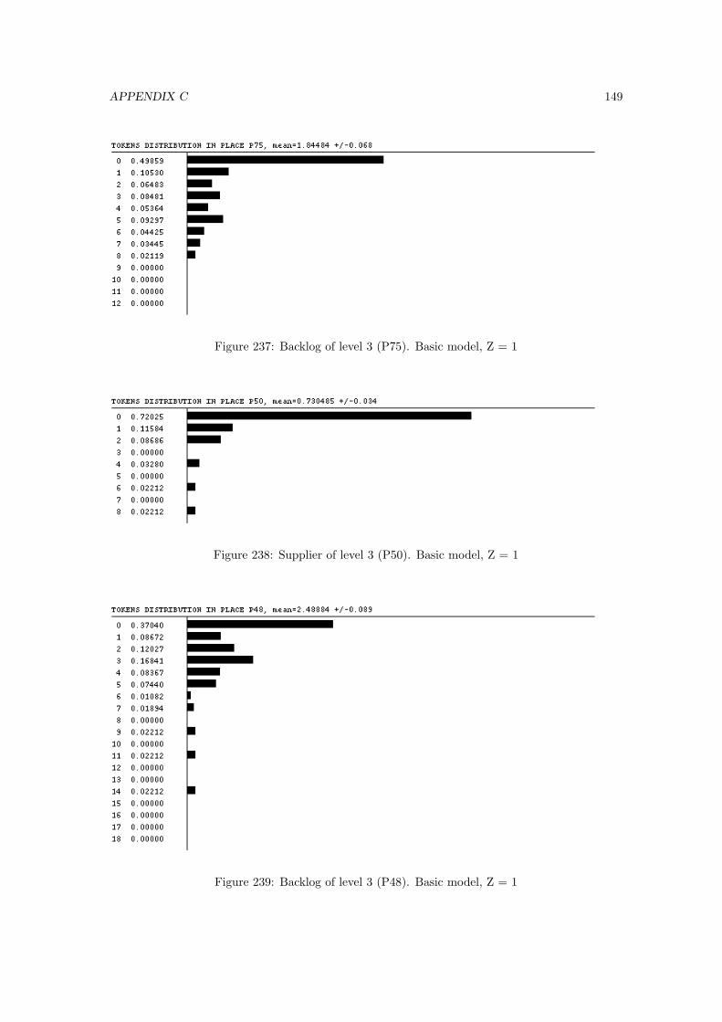
APPENDIX C 149
Figure 237: Backlog of level 3 (P75). Basic model, Z = 1
Figure 238: Supplier of level 3 (P50). Basic model, Z = 1
Figure 239: Backlog of level 3 (P48). Basic model, Z = 1
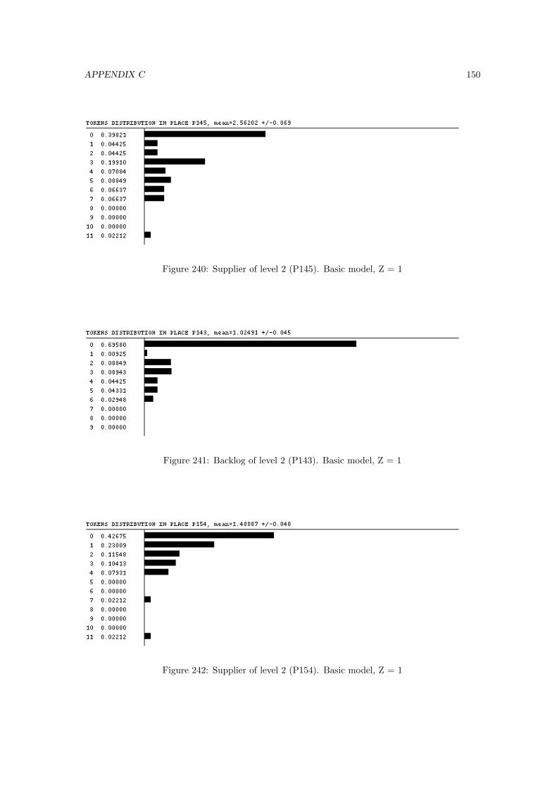
APPENDIX C 150
Figure 240: Supplier of level 2 (P145). Basic model, Z = 1
Figure 241: Backlog of level 2 (P143). Basic model, Z = 1
Figure 242: Supplier of level 2 (P154). Basic model, Z = 1
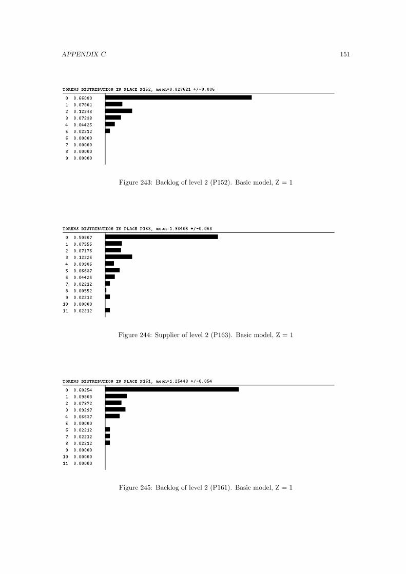
APPENDIX C 151
Figure 243: Backlog of level 2 (P152). Basic model, Z = 1
Figure 244: Supplier of level 2 (P163). Basic model, Z = 1
Figure 245: Backlog of level 2 (P161). Basic model, Z = 1

APPENDIX C 152
37
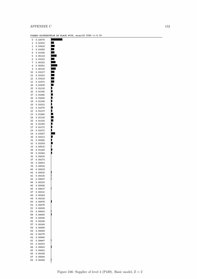
APPENDIX C 153
Figure 246: Supplier of level 4 (P439). Basic model, Z = 2
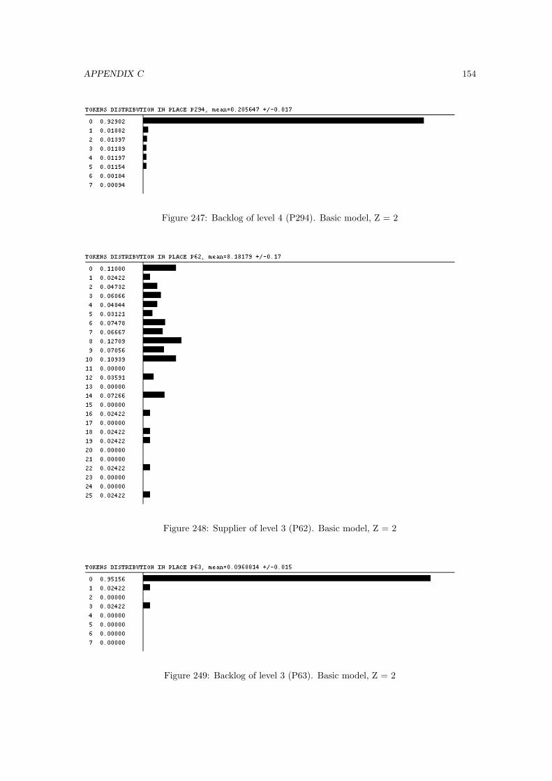
APPENDIX C 154
Figure 247: Backlog of level 4 (P294). Basic model, Z = 2
Figure 248: Supplier of level 3 (P62). Basic model, Z = 2
Figure 249: Backlog of level 3 (P63). Basic model, Z = 2
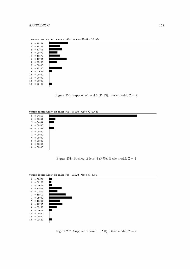
APPENDIX C 155
Figure 250: Supplier of level 3 (P433). Basic model, Z = 2
Figure 251: Backlog of level 3 (P75). Basic model, Z = 2
Figure 252: Supplier of level 3 (P50). Basic model, Z = 2
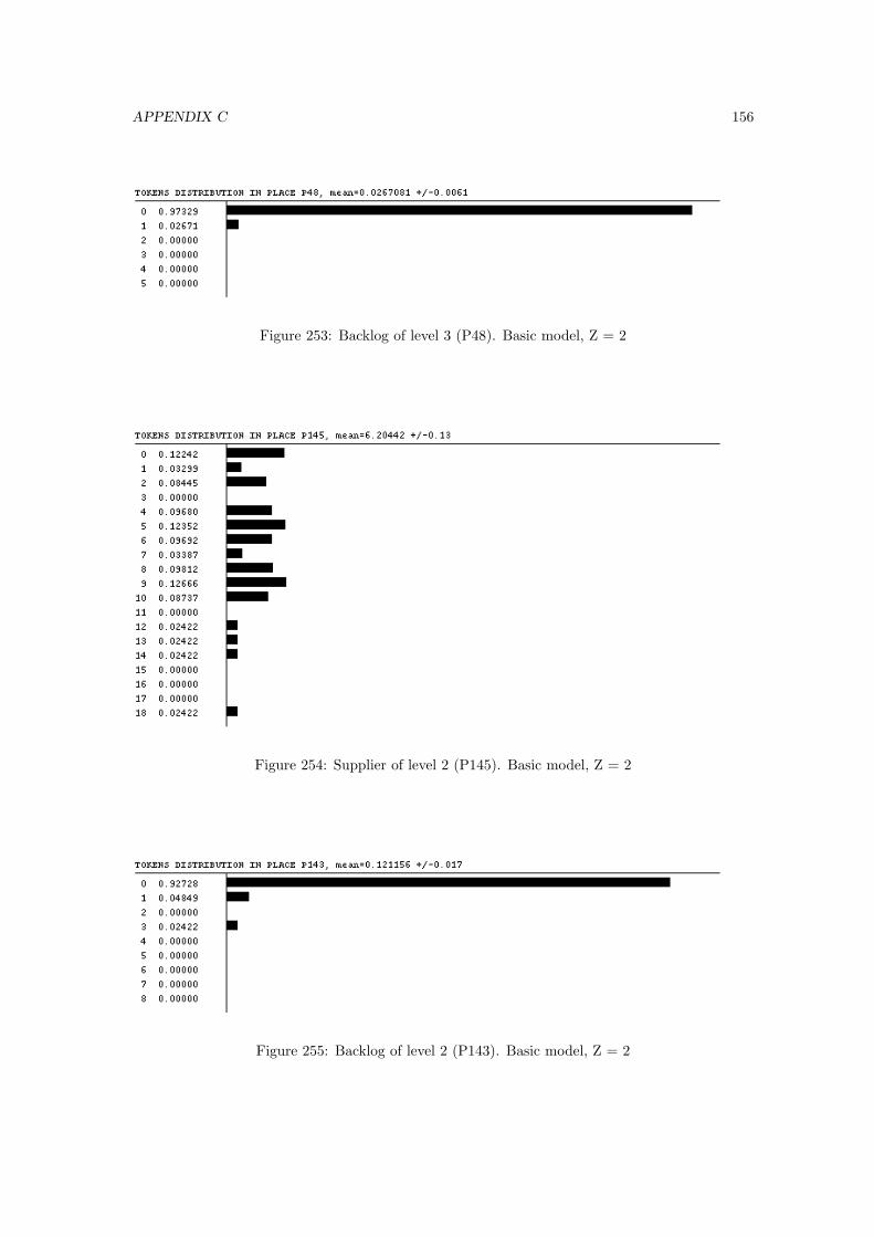
APPENDIX C 156
Figure 253: Backlog of level 3 (P48). Basic model, Z = 2
Figure 254: Supplier of level 2 (P145). Basic model, Z = 2
Figure 255: Backlog of level 2 (P143). Basic model, Z = 2
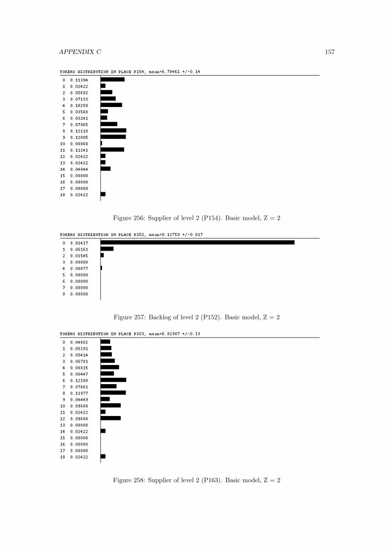
APPENDIX C 157
Figure 256: Supplier of level 2 (P154). Basic model, Z = 2
Figure 257: Backlog of level 2 (P152). Basic model, Z = 2
Figure 258: Supplier of level 2 (P163). Basic model, Z = 2
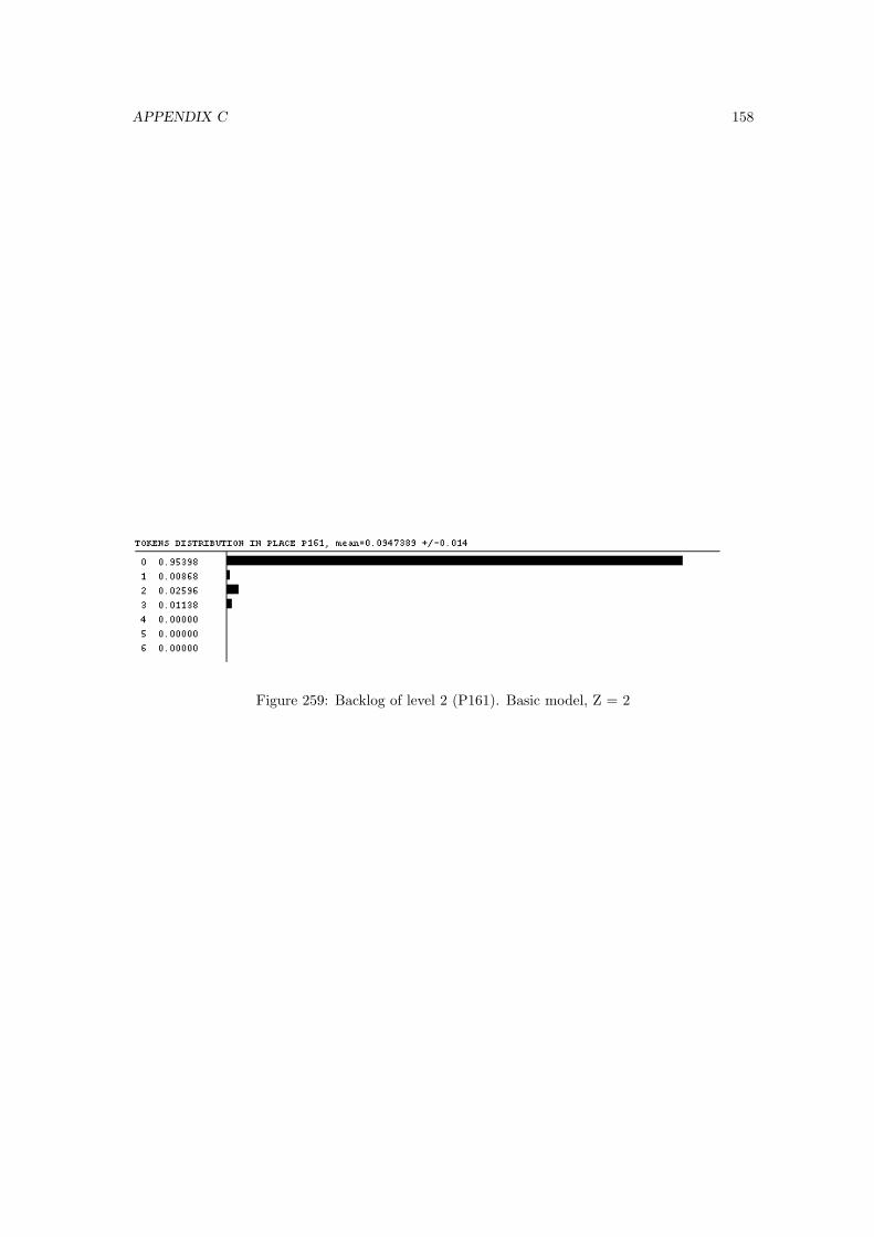
APPENDIX C 158
Figure 259: Backlog of level 2 (P161). Basic model, Z = 2
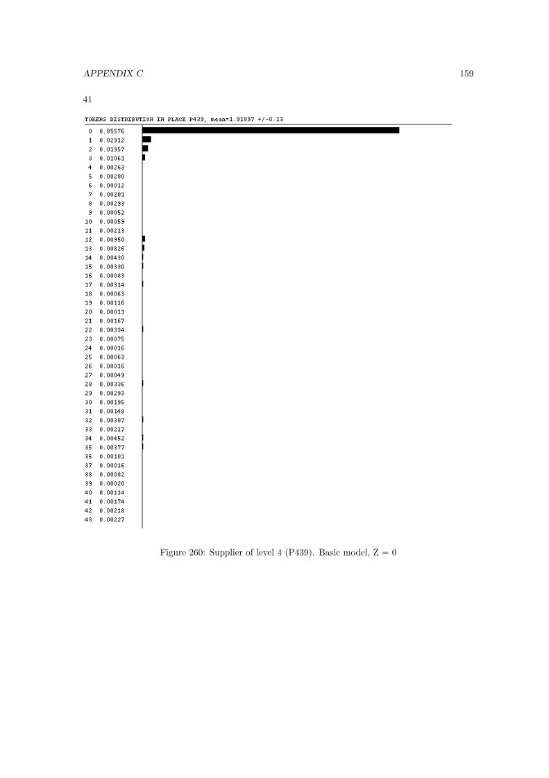
APPENDIX C 159
41
Figure 260: Supplier of level 4 (P439). Basic model, Z = 0
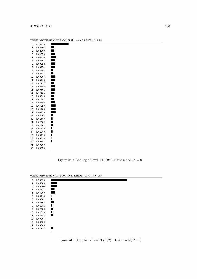
APPENDIX C 160
Figure 261: Backlog of level 4 (P294). Basic model, Z = 0
Figure 262: Supplier of level 3 (P62). Basic model, Z = 0
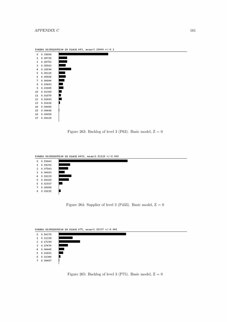
APPENDIX C 161
Figure 263: Backlog of level 3 (P63). Basic model, Z = 0
Figure 264: Supplier of level 3 (P433). Basic model, Z = 0
Figure 265: Backlog of level 3 (P75). Basic model, Z = 0
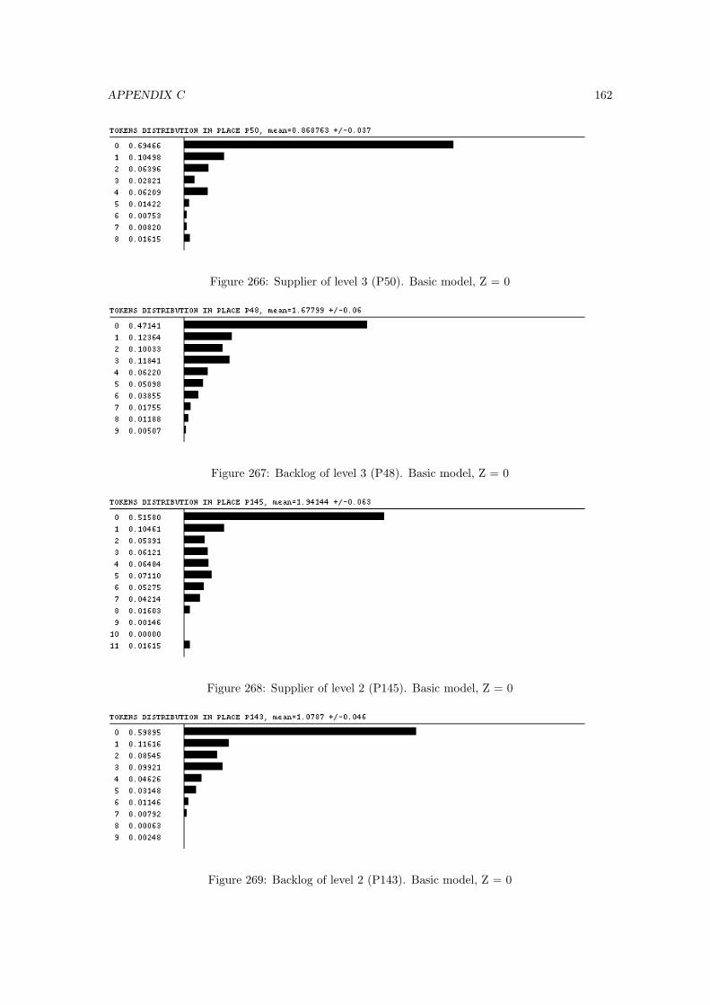
APPENDIX C 162
Figure 266: Supplier of level 3 (P50). Basic model, Z = 0
Figure 267: Backlog of level 3 (P48). Basic model, Z = 0
Figure 268: Supplier of level 2 (P145). Basic model, Z = 0
Figure 269: Backlog of level 2 (P143). Basic model, Z = 0
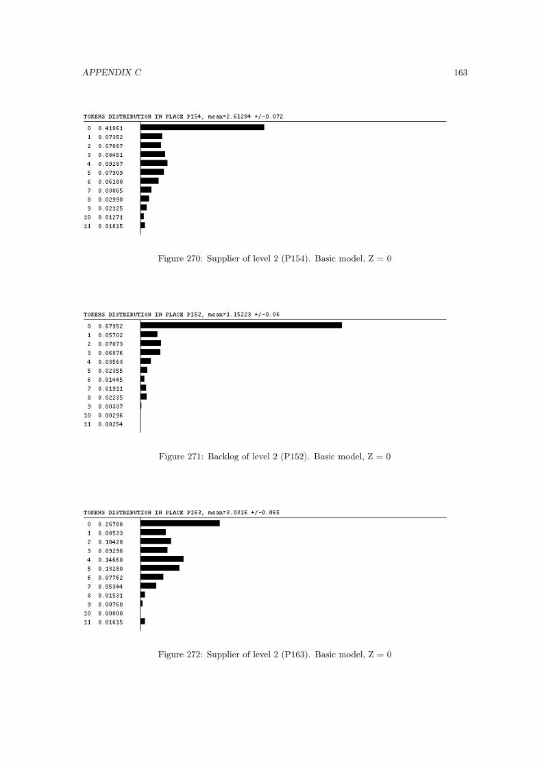
APPENDIX C 163
Figure 270: Supplier of level 2 (P154). Basic model, Z = 0
Figure 271: Backlog of level 2 (P152). Basic model, Z = 0
Figure 272: Supplier of level 2 (P163). Basic model, Z = 0
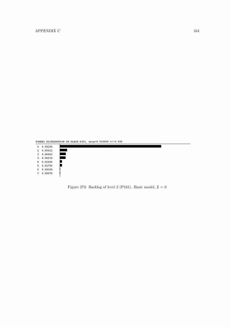
APPENDIX C 164
Figure 273: Backlog of level 2 (P161). Basic model, Z = 0

APPENDIX C 165
42
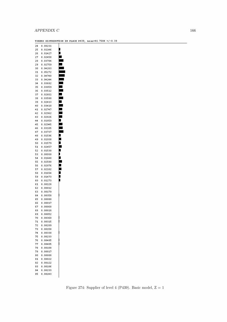
APPENDIX C 166
Figure 274: Supplier of level 4 (P439). Basic model, Z = 1

APPENDIX C 167
Figure 275: Backlog of level 4 (P294). Basic model, Z = 1
Figure 276: Supplier of level 3 (P62). Basic model, Z = 1
Figure 277: Backlog of level 3 (P63). Basic model, Z = 1
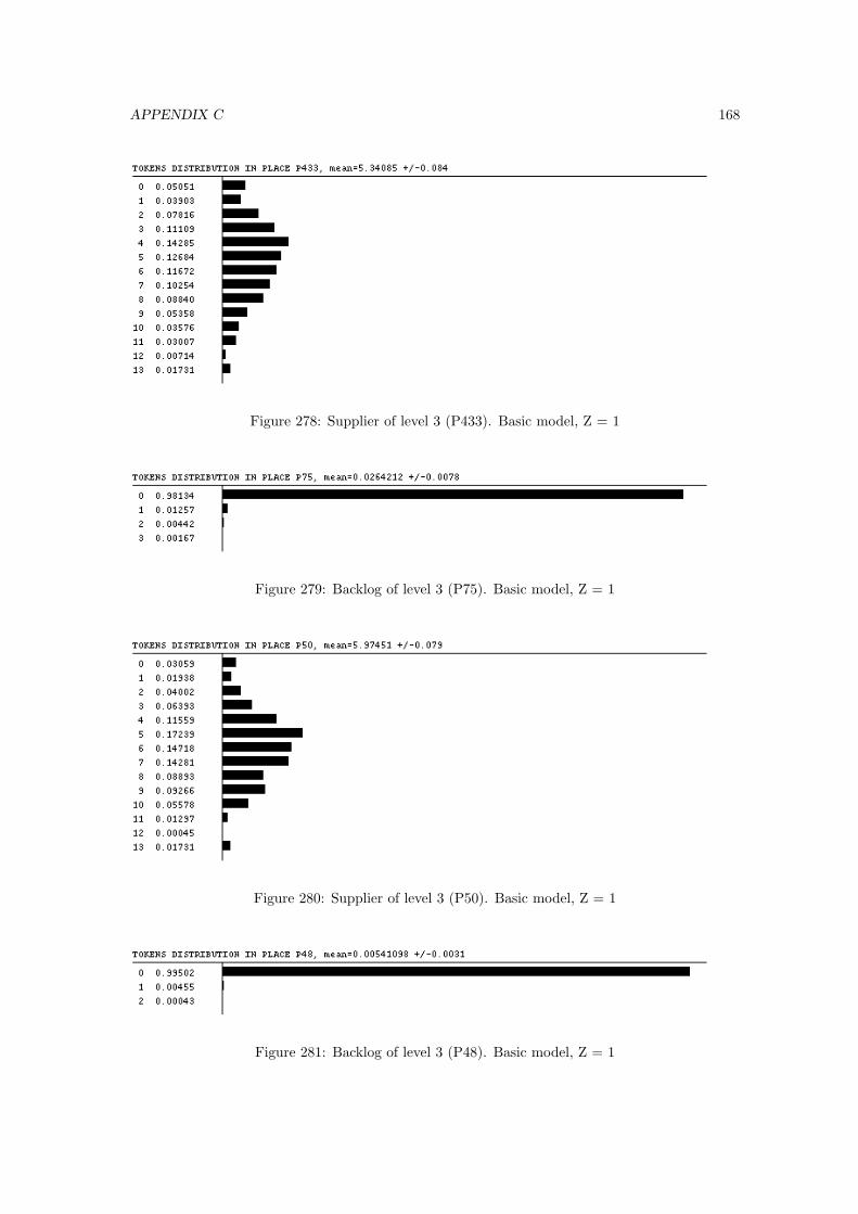
APPENDIX C 168
Figure 278: Supplier of level 3 (P433). Basic model, Z = 1
Figure 279: Backlog of level 3 (P75). Basic model, Z = 1
Figure 280: Supplier of level 3 (P50). Basic model, Z = 1
Figure 281: Backlog of level 3 (P48). Basic model, Z = 1
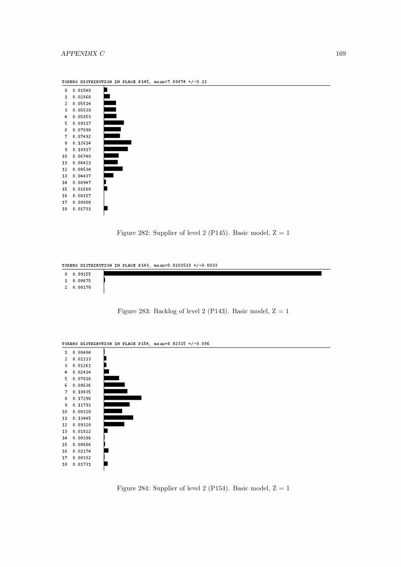
APPENDIX C 169
Figure 282: Supplier of level 2 (P145). Basic model, Z = 1
Figure 283: Backlog of level 2 (P143). Basic model, Z = 1
Figure 284: Supplier of level 2 (P154). Basic model, Z = 1
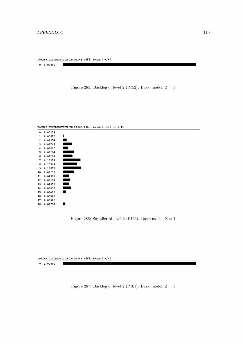
APPENDIX C 170
Figure 285: Backlog of level 2 (P152). Basic model, Z = 1
Figure 286: Supplier of level 2 (P163). Basic model, Z = 1
Figure 287: Backlog of level 2 (P161). Basic model, Z = 1
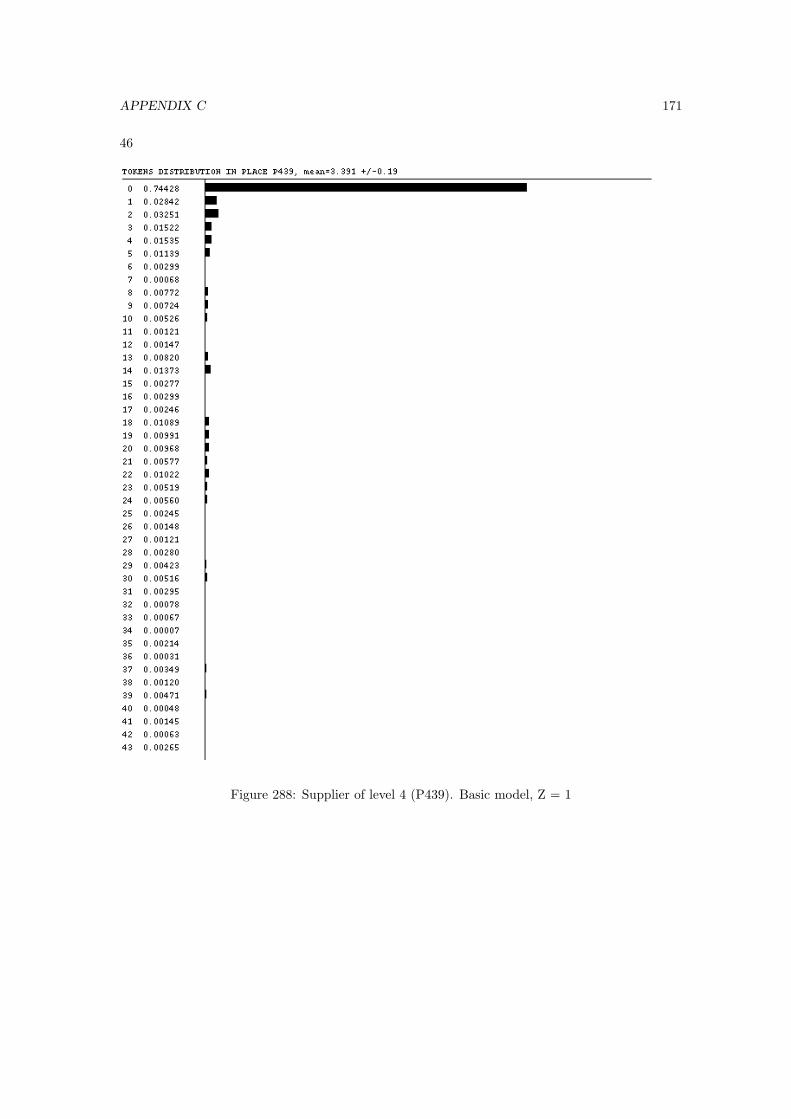
APPENDIX C 171
46
Figure 288: Supplier of level 4 (P439). Basic model, Z = 1
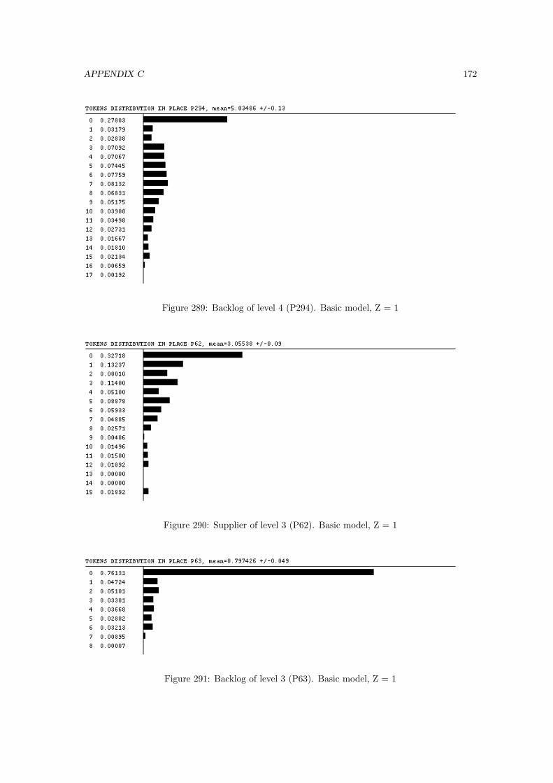
APPENDIX C 172
Figure 289: Backlog of level 4 (P294). Basic model, Z = 1
Figure 290: Supplier of level 3 (P62). Basic model, Z = 1
Figure 291: Backlog of level 3 (P63). Basic model, Z = 1

APPENDIX C 173
Figure 292: Supplier of level 3 (P433). Basic model, Z = 1
Figure 293: Backlog of level 3 (P75). Basic model, Z = 1
Figure 294: Supplier of level 3 (P50). Basic model, Z = 1
Figure 295: Backlog of level 3 (P48). Basic model, Z = 1
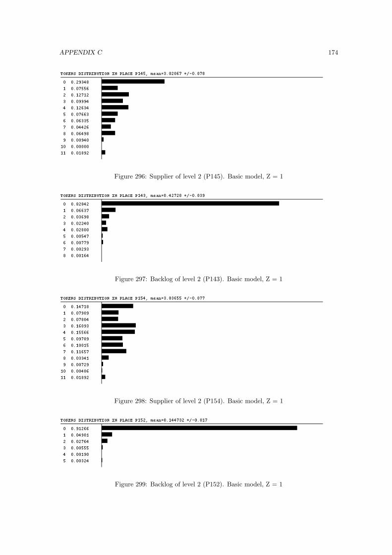
APPENDIX C 174
Figure 296: Supplier of level 2 (P145). Basic model, Z = 1
Figure 297: Backlog of level 2 (P143). Basic model, Z = 1
Figure 298: Supplier of level 2 (P154). Basic model, Z = 1
Figure 299: Backlog of level 2 (P152). Basic model, Z = 1

APPENDIX C 175
Figure 300: Supplier of level 2 (P163). Basic model, Z = 1
Figure 301: Backlog of level 2 (P161). Basic model, Z = 1

APPENDIX C 176
47
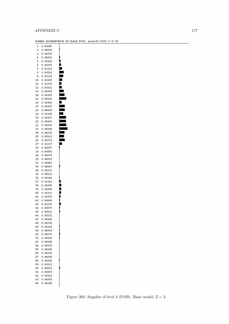
APPENDIX C 177
Figure 302: Supplier of level 4 (P439). Basic model, Z = 2
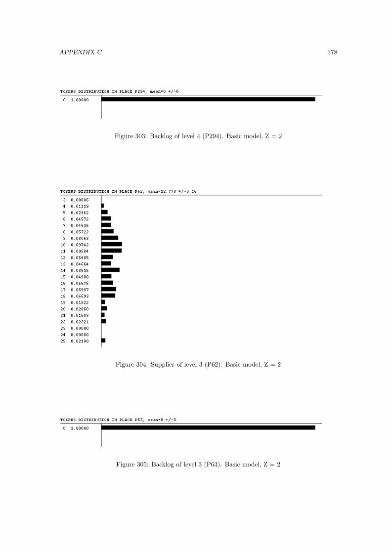
APPENDIX C 178
Figure 303: Backlog of level 4 (P294). Basic model, Z = 2
Figure 304: Supplier of level 3 (P62). Basic model, Z = 2
Figure 305: Backlog of level 3 (P63). Basic model, Z = 2
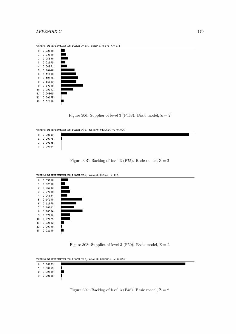
APPENDIX C 179
Figure 306: Supplier of level 3 (P433). Basic model, Z = 2
Figure 307: Backlog of level 3 (P75). Basic model, Z = 2
Figure 308: Supplier of level 3 (P50). Basic model, Z = 2
Figure 309: Backlog of level 3 (P48). Basic model, Z = 2
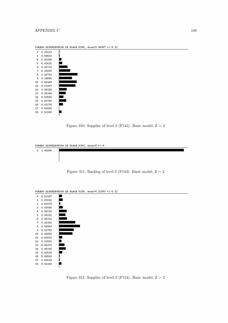
APPENDIX C 180
Figure 310: Supplier of level 2 (P145). Basic model, Z = 2
Figure 311: Backlog of level 2 (P143). Basic model, Z = 2
Figure 312: Supplier of level 2 (P154). Basic model, Z = 2
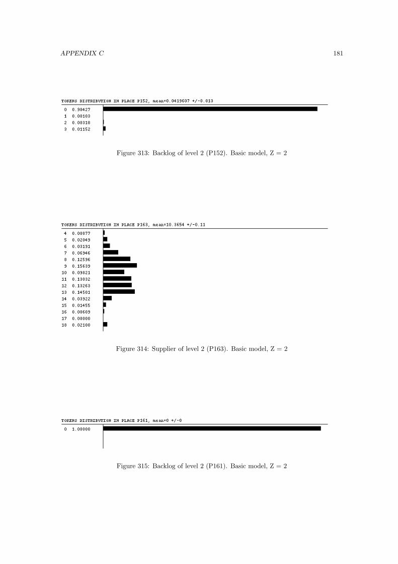
APPENDIX C 181
Figure 313: Backlog of level 2 (P152). Basic model, Z = 2
Figure 314: Supplier of level 2 (P163). Basic model, Z = 2
Figure 315: Backlog of level 2 (P161). Basic model, Z = 2
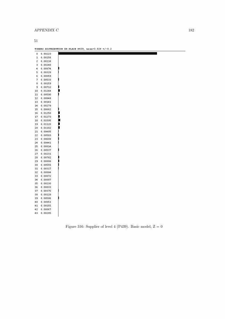
APPENDIX C 182
51
Figure 316: Supplier of level 4 (P439). Basic model, Z = 0
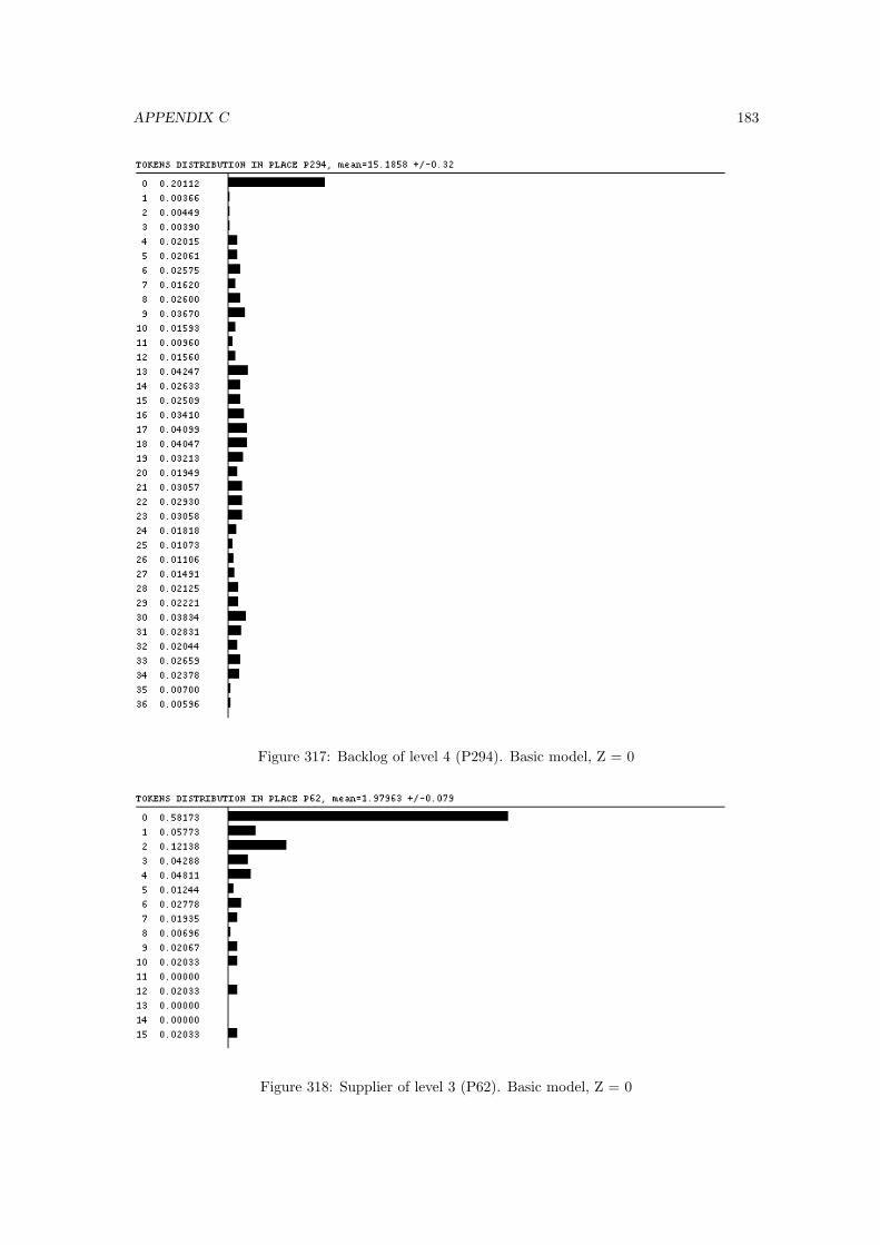
APPENDIX C 183
Figure 317: Backlog of level 4 (P294). Basic model, Z = 0
Figure 318: Supplier of level 3 (P62). Basic model, Z = 0
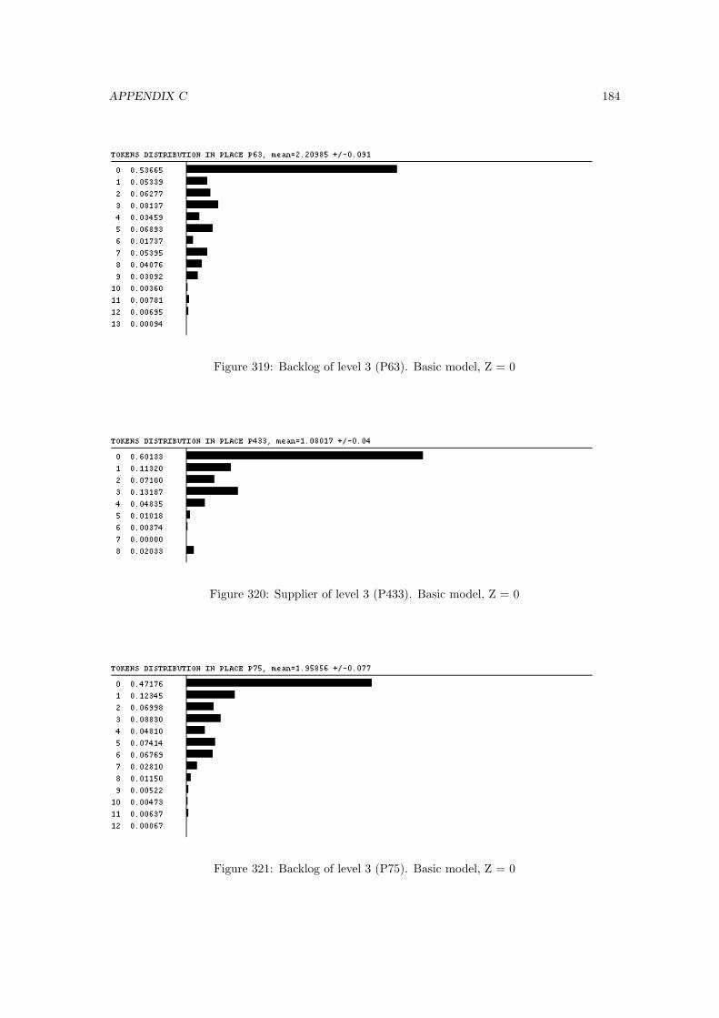
APPENDIX C 184
Figure 319: Backlog of level 3 (P63). Basic model, Z = 0
Figure 320: Supplier of level 3 (P433). Basic model, Z = 0
Figure 321: Backlog of level 3 (P75). Basic model, Z = 0
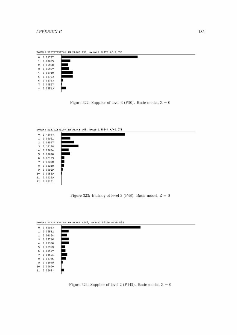
APPENDIX C 185
Figure 322: Supplier of level 3 (P50). Basic model, Z = 0
Figure 323: Backlog of level 3 (P48). Basic model, Z = 0
Figure 324: Supplier of level 2 (P145). Basic model, Z = 0
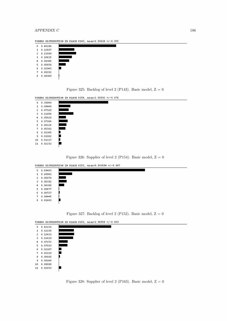
APPENDIX C 186
Figure 325: Backlog of level 2 (P143). Basic model, Z = 0
Figure 326: Supplier of level 2 (P154). Basic model, Z = 0
Figure 327: Backlog of level 2 (P152). Basic model, Z = 0
Figure 328: Supplier of level 2 (P163). Basic model, Z = 0

APPENDIX C 187
Figure 329: Backlog of level 2 (P161). Basic model, Z = 0
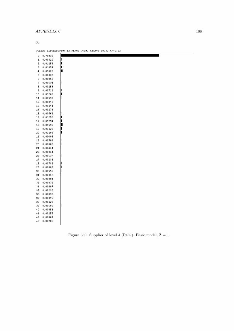
APPENDIX C 188
56
Figure 330: Supplier of level 4 (P439). Basic model, Z = 1
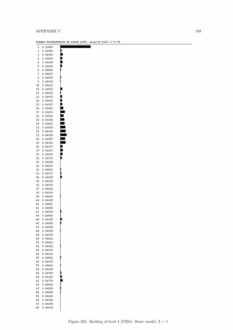
APPENDIX C 189
Figure 331: Backlog of level 4 (P294). Basic model, Z = 1

APPENDIX C 190
Figure 332: Supplier of level 3 (P62). Basic model, Z = 1
Figure 333: Backlog of level 3 (P63). Basic model, Z = 1
Figure 334: Supplier of level 3 (P433). Basic model, Z = 1
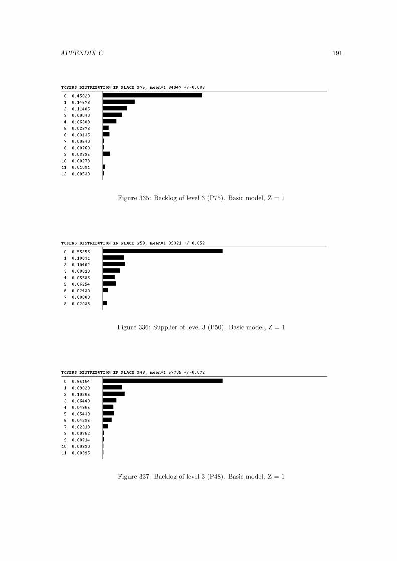
APPENDIX C 191
Figure 335: Backlog of level 3 (P75). Basic model, Z = 1
Figure 336: Supplier of level 3 (P50). Basic model, Z = 1
Figure 337: Backlog of level 3 (P48). Basic model, Z = 1
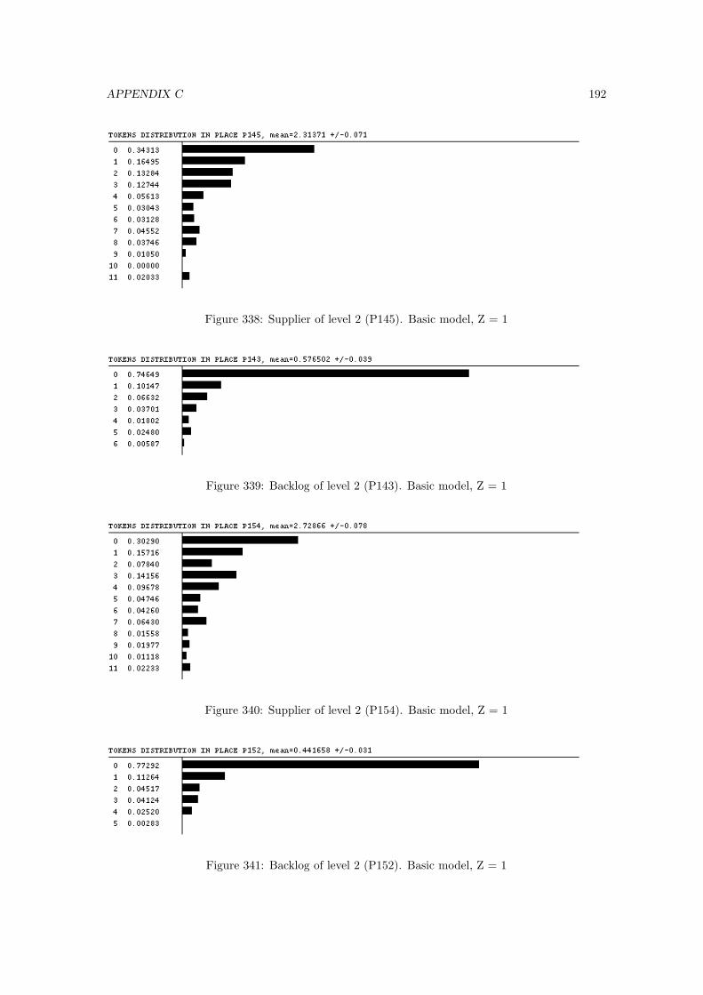
APPENDIX C 192
Figure 338: Supplier of level 2 (P145). Basic model, Z = 1
Figure 339: Backlog of level 2 (P143). Basic model, Z = 1
Figure 340: Supplier of level 2 (P154). Basic model, Z = 1
Figure 341: Backlog of level 2 (P152). Basic model, Z = 1
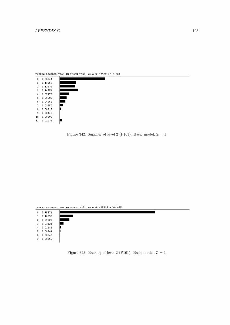
APPENDIX C 193
Figure 342: Supplier of level 2 (P163). Basic model, Z = 1
Figure 343: Backlog of level 2 (P161). Basic model, Z = 1

APPENDIX C 194
57
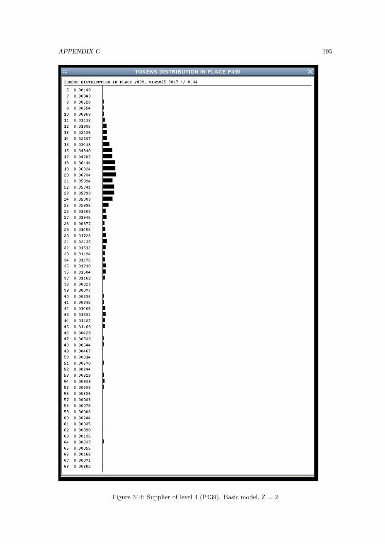
APPENDIX C 195
Figure 344: Supplier of level 4 (P439). Basic model, Z = 2
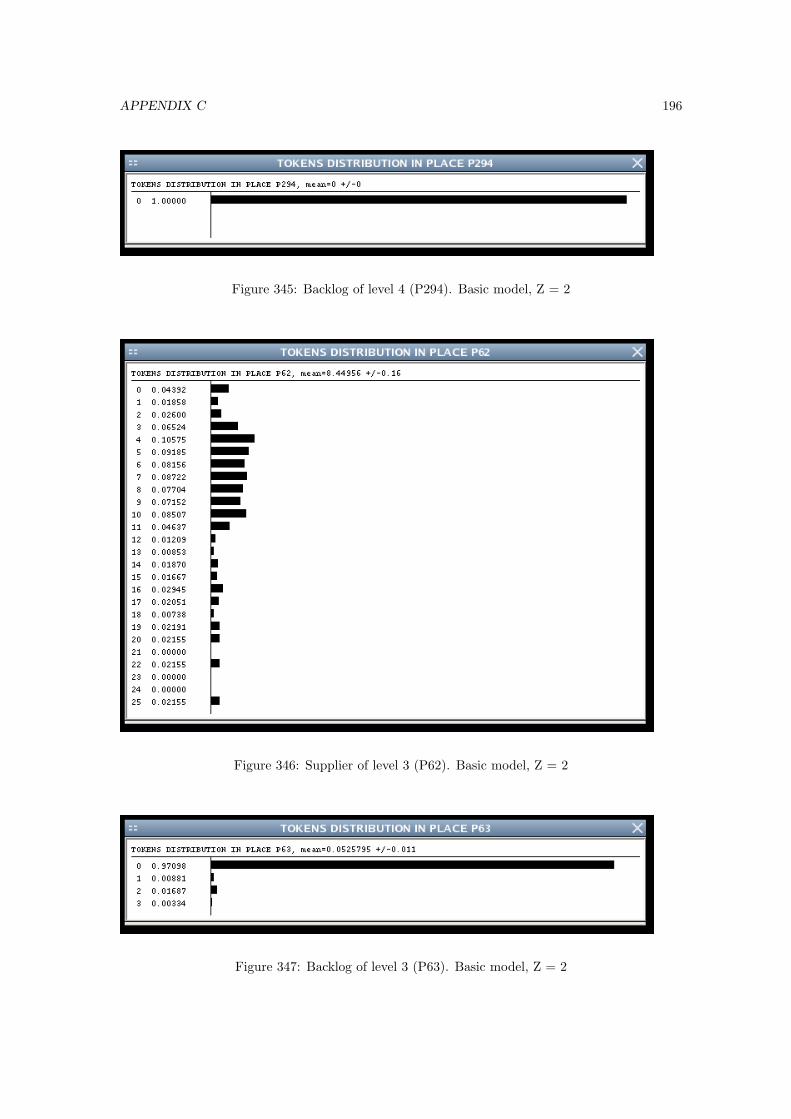
APPENDIX C 196
Figure 345: Backlog of level 4 (P294). Basic model, Z = 2
Figure 346: Supplier of level 3 (P62). Basic model, Z = 2
Figure 347: Backlog of level 3 (P63). Basic model, Z = 2
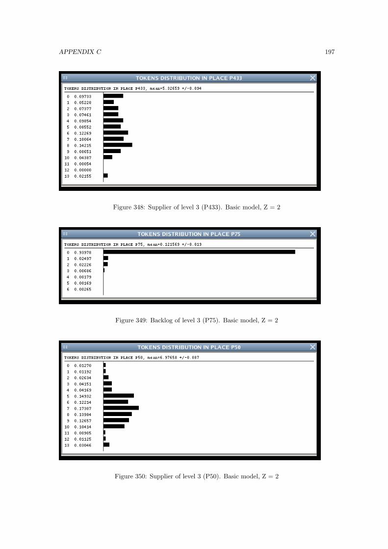
APPENDIX C 197
Figure 348: Supplier of level 3 (P433). Basic model, Z = 2
Figure 349: Backlog of level 3 (P75). Basic model, Z = 2
Figure 350: Supplier of level 3 (P50). Basic model, Z = 2
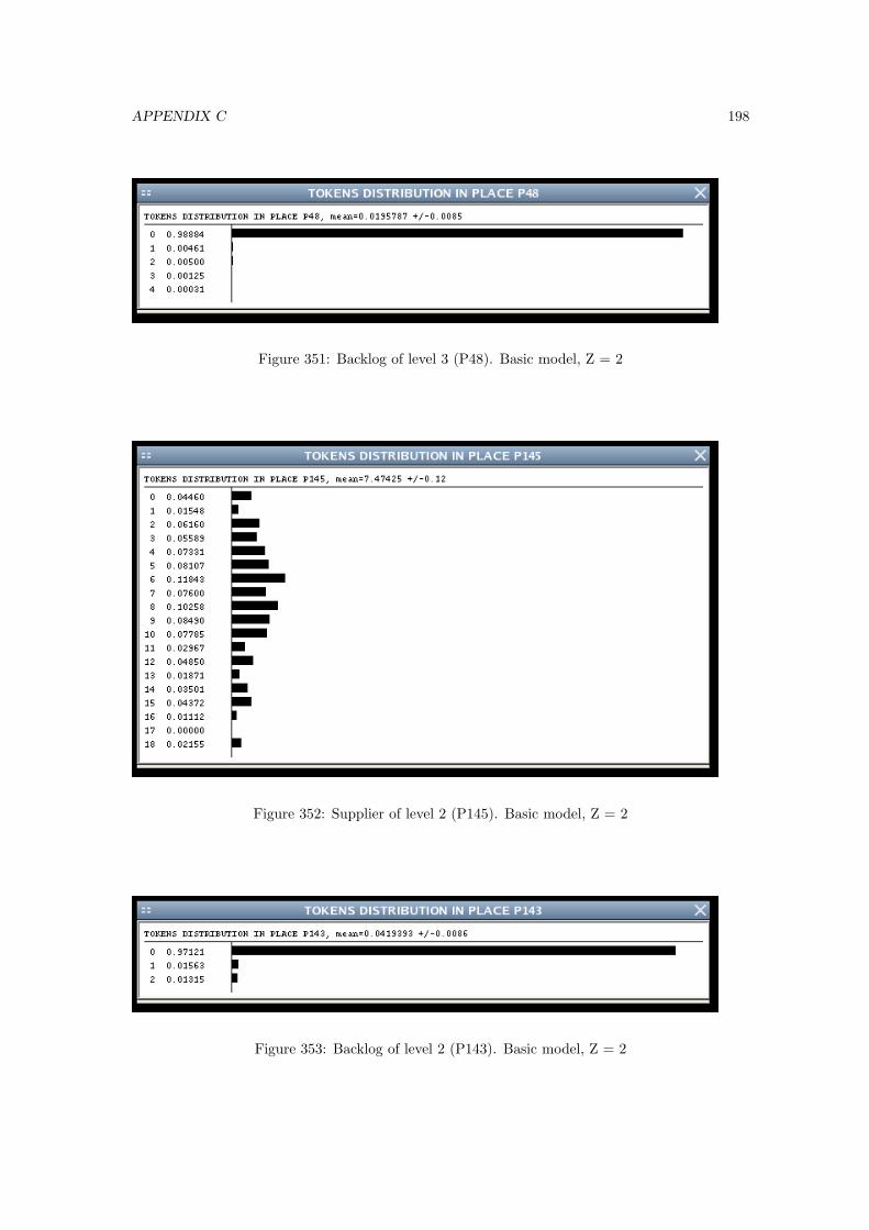
APPENDIX C 198
Figure 351: Backlog of level 3 (P48). Basic model, Z = 2
Figure 352: Supplier of level 2 (P145). Basic model, Z = 2
Figure 353: Backlog of level 2 (P143). Basic model, Z = 2
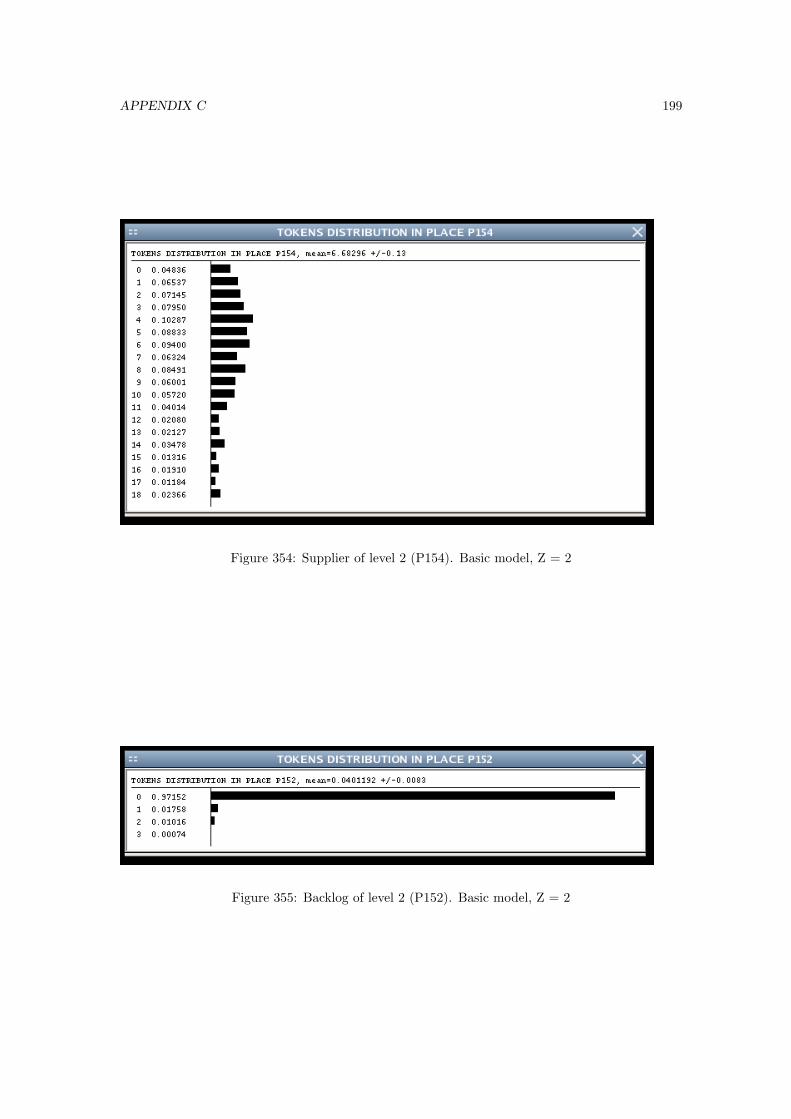
APPENDIX C 199
Figure 354: Supplier of level 2 (P154). Basic model, Z = 2
Figure 355: Backlog of level 2 (P152). Basic model, Z = 2
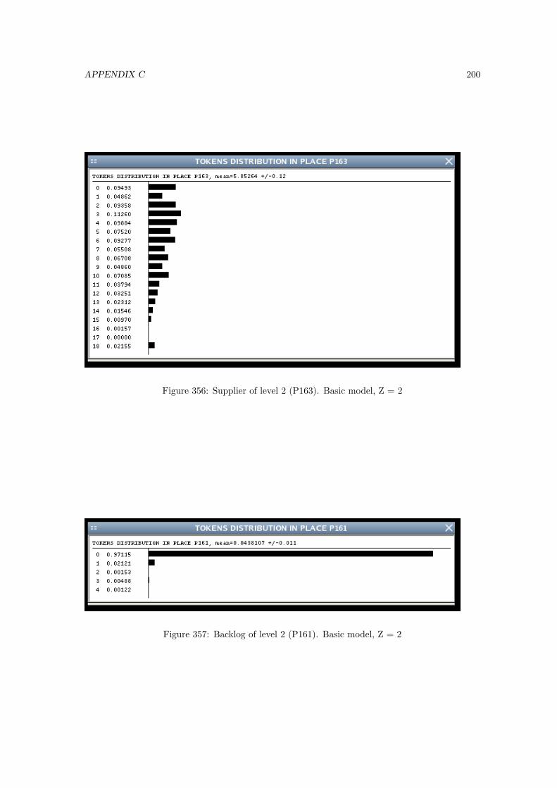
APPENDIX C 200
Figure 356: Supplier of level 2 (P163). Basic model, Z = 2
Figure 357: Backlog of level 2 (P161). Basic model, Z = 2
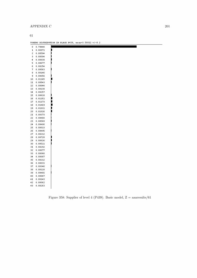
APPENDIX C 201
61
Figure 358: Supplier of level 4 (P439). Basic model, Z = aaaresults/61
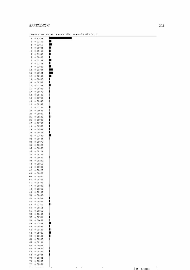
APPENDIX C 202
Figure 359: Backlog of level 4 (P294). Basic model, Z = aaaresults/61
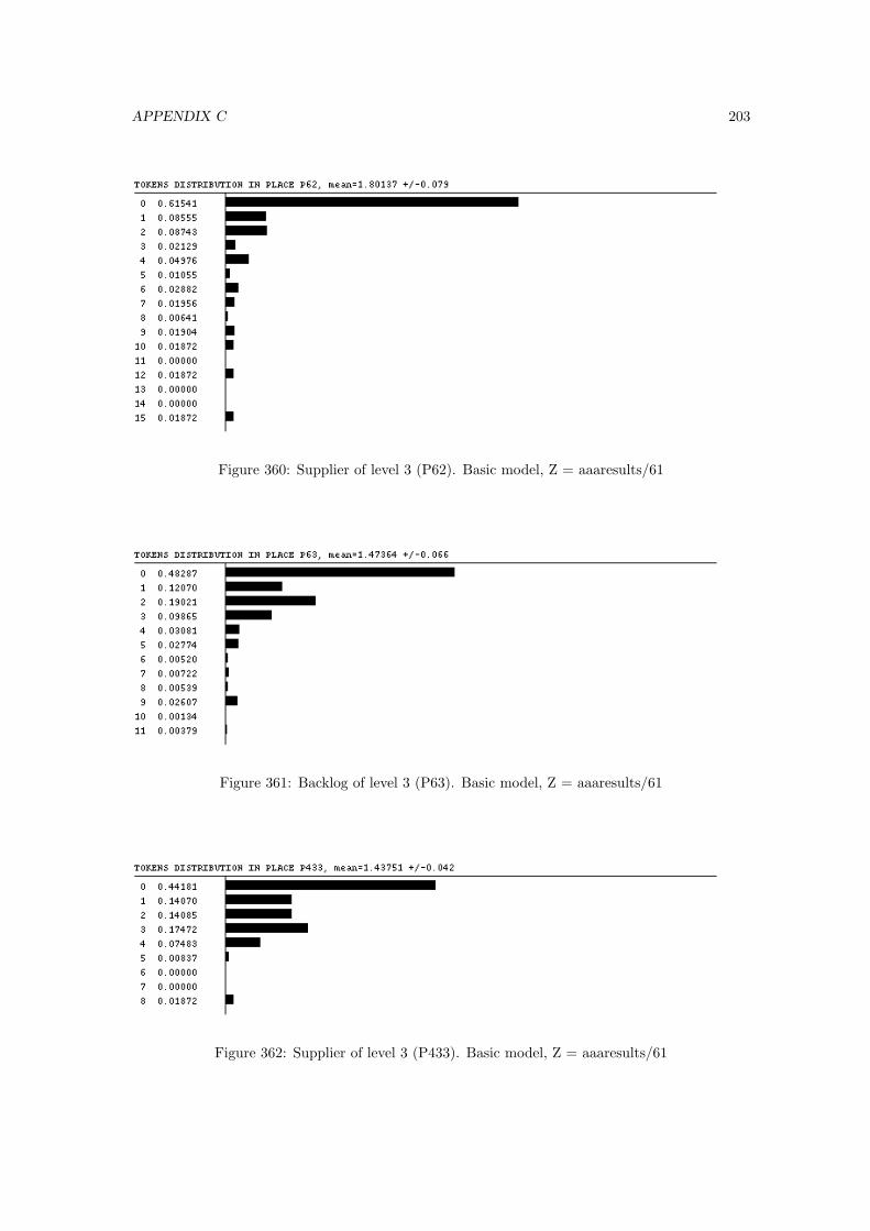
APPENDIX C 203
Figure 360: Supplier of level 3 (P62). Basic model, Z = aaaresults/61
Figure 361: Backlog of level 3 (P63). Basic model, Z = aaaresults/61
Figure 362: Supplier of level 3 (P433). Basic model, Z = aaaresults/61
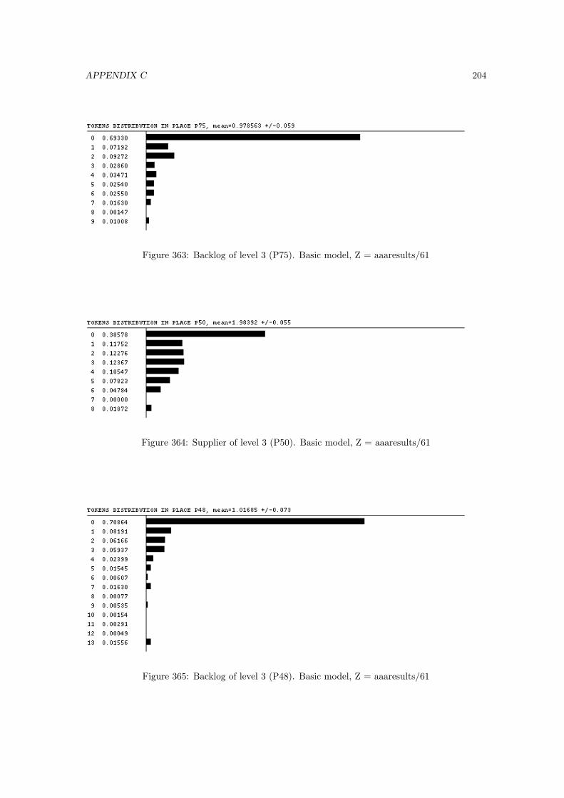
APPENDIX C 204
Figure 363: Backlog of level 3 (P75). Basic model, Z = aaaresults/61
Figure 364: Supplier of level 3 (P50). Basic model, Z = aaaresults/61
Figure 365: Backlog of level 3 (P48). Basic model, Z = aaaresults/61
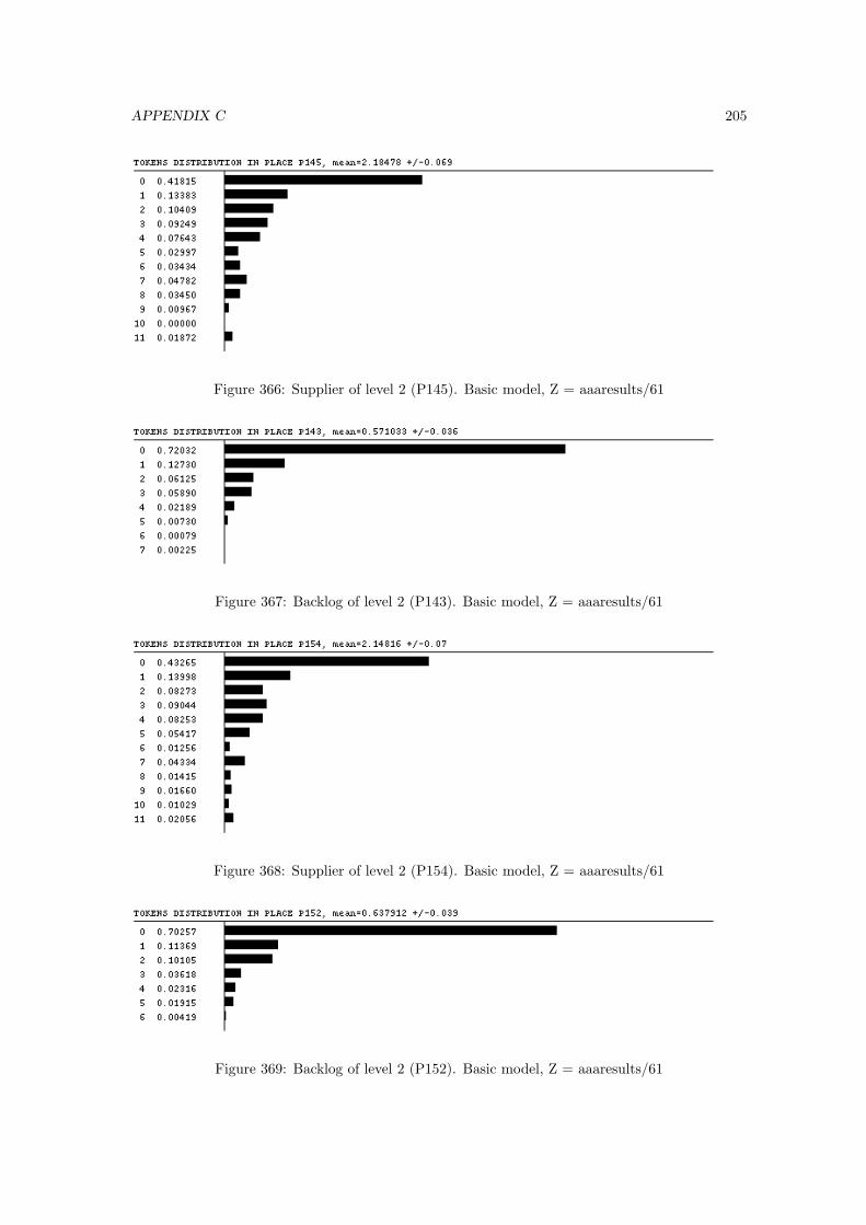
APPENDIX C 205
Figure 366: Supplier of level 2 (P145). Basic model, Z = aaaresults/61
Figure 367: Backlog of level 2 (P143). Basic model, Z = aaaresults/61
Figure 368: Supplier of level 2 (P154). Basic model, Z = aaaresults/61
Figure 369: Backlog of level 2 (P152). Basic model, Z = aaaresults/61
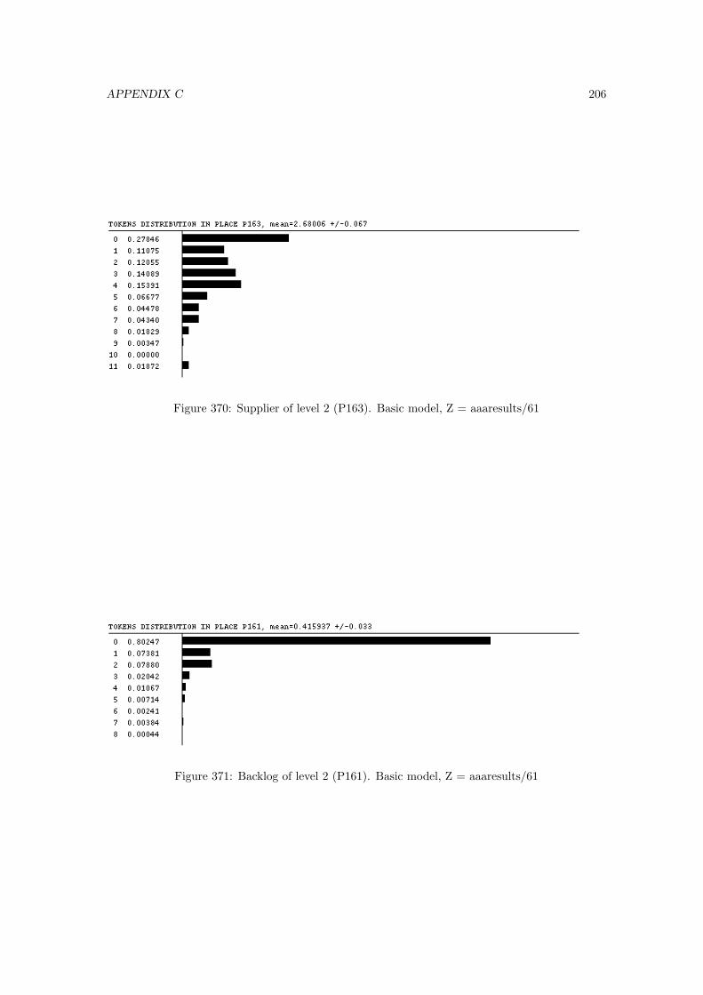
APPENDIX C 206
Figure 370: Supplier of level 2 (P163). Basic model, Z = aaaresults/61
Figure 371: Backlog of level 2 (P161). Basic model, Z = aaaresults/61
Bibliography
G. Balbo, J. Desel, K. Jensen, W. Reisig, G. Rozenberg & M. Silva (2000). Introductory tutorial
petri nets. 21st International Conference on Application and Theory of Petri Nets, Aarhus,
Denmark.
C.-V. Bobeanu (2005). Modelling and Simulating Manufacturing and Service Systems using Petri
Nets. Universiteit Gent.
C.-V. Bobeanu, E. J. Kerckhoffs & H. V. Landeghem (2004). Formal Modelling of Discrete Event
Systems:A Holistic and Incremental Approach Using Petri Nets. ACM Transactions on mod-
elling and Computer Simulation, 14(4):389–423.
M. Bundschuh, D. Klabjan & D. L. Thurston (2003). Modelling Robust and Reliable Supply
Chains. journal????
P. Z. Chen, S. C. Bruell & G. Balbo (1990). Alternative Methods for Incorporating Non-
Exponential Distributions into Stochastic Timed Petri Nets. In PNPM89. Proceedings of the
Third International Workshop On Petri Nets and Performance Models, 1989, Kyoto, Japan,
pp. 187–197. IEEE Computer Society Press, Los Alamitos, CA, USA. NewsletterInfo: 36.
J. Desel & W. Reisig (1998). Place/Transition Petri Nets. In Petri Nets, pp. 122–173.
H. V. Landeghem (2005). Inleiding tot Bedrijfs- en Productiebeheer. Universiteit Gent.
H. V. Landeghem (2006). Advanced Methods in Production & Logistics. Universiteit Gent.
H. V. Landeghem & C.-V. Bobeanu (2002). Formal Modelling of Supply Chain: An Incremental
Approach Using Petri Nets. In Verbraeck, A. and Krug, W. (Eds.), Simulation in Industry,
Proceedings of the 14th European Simulation Symposium, ESS’2002, pp. 323–327. SCS European
Publishing House.
C. A. Petri (1996). Nets, time and space. Theor. Comput. Sci., 153(1-2):3–48. ISSN 0304-3975.
Universita di Torino (2004). GreatSPN User’s Manual, 2.0.2 edition.
207
BIBLIOGRAPHY 208
E. M. Vila (2004). Supply Chain modelling: Optimization Versus Simulation. Master’s thesis,
Ghent University.

List of Figures
2.1 The complete supply chain . . . . . . . . . . . . . . . . . . . . . . . . . . . . . . . 3
4.1 The overall model . . . . . . . . . . . . . . . . . . . . . . . . . . . . . . . . . . . . 12
4.2 A supplier of level 1 . . . . . . . . . . . . . . . . . . . . . . . . . . . . . . . . . . . 14
4.3 Supplier of level 2 and 3 . . . . . . . . . . . . . . . . . . . . . . . . . . . . . . . . . 17
4.4 Supplier of level 4 . . . . . . . . . . . . . . . . . . . . . . . . . . . . . . . . . . . . . 17
4.5 Ordering and Delivery (Simple) . . . . . . . . . . . . . . . . . . . . . . . . . . . . . 21
4.6 Ordering and Delivery . . . . . . . . . . . . . . . . . . . . . . . . . . . . . . . . . . 22
4.7 Simple Queue: Split of the order . . . . . . . . . . . . . . . . . . . . . . . . . . . . 23
4.8 Advanced ordering and delivery mechanism . . . . . . . . . . . . . . . . . . . . . . 23
5.1 Basic serial . . . . . . . . . . . . . . . . . . . . . . . . . . . . . . . . . . . . . . . . 25
5.2 Basic . . . . . . . . . . . . . . . . . . . . . . . . . . . . . . . . . . . . . . . . . . . . 26
5.3 High Reliability . . . . . . . . . . . . . . . . . . . . . . . . . . . . . . . . . . . . . . 27
5.4 60% source limit . . . . . . . . . . . . . . . . . . . . . . . . . . . . . . . . . . . . . 27
7.1 A close-up of the Control Layer Model, suppliers of level 3 and 4 . . . . . . . . . . 34
1 The overall model Part I: Suppliers of Level 1 & 2 . . . . . . . . . . . . . . . . . . 38
2 The overall model Part II: Suppliers of Level 3 . . . . . . . . . . . . . . . . . . . . 39
3 The overall model Part III: Suppliers of Level 4 . . . . . . . . . . . . . . . . . . . . 40
209
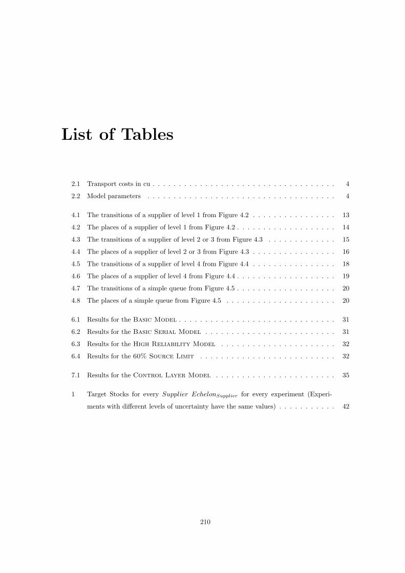
List of Tables
2.1 Transport costs in cu . . . . . . . . . . . . . . . . . . . . . . . . . . . . . . . . . . . 4
2.2 Model parameters . . . . . . . . . . . . . . . . . . . . . . . . . . . . . . . . . . . . 4
4.1 The transitions of a supplier of level 1 from Figure 4.2 . . . . . . . . . . . . . . . . 13
4.2 The places of a supplier of level 1 from Figure 4.2 . . . . . . . . . . . . . . . . . . . 14
4.3 The transitions of a supplier of level 2 or 3 from Figure 4.3 . . . . . . . . . . . . . 15
4.4 The places of a supplier of level 2 or 3 from Figure 4.3 . . . . . . . . . . . . . . . . 16
4.5 The transitions of a supplier of level 4 from Figure 4.4 . . . . . . . . . . . . . . . . 18
4.6 The places of a supplier of level 4 from Figure 4.4 . . . . . . . . . . . . . . . . . . . 19
4.7 The transitions of a simple queue from Figure 4.5 . . . . . . . . . . . . . . . . . . . 20
4.8 The places of a simple queue from Figure 4.5 . . . . . . . . . . . . . . . . . . . . . 20
6.1 Results for the Basic Model . . . . . . . . . . . . . . . . . . . . . . . . . . . . . . 31
6.2 Results for the Basic Serial Model . . . . . . . . . . . . . . . . . . . . . . . . . 31
6.3 Results for the High Reliability Model . . . . . . . . . . . . . . . . . . . . . . 32
6.4 Results for the 60% Source Limit . . . . . . . . . . . . . . . . . . . . . . . . . . 32
7.1 Results for the Control Layer Model . . . . . . . . . . . . . . . . . . . . . . . 35
1 Target Stocks for every Supplier EchelonSupplier for every experiment (Experi-
ments with different levels of uncertainty have the same values) . . . . . . . . . . . 42
210


![arXiv:2006.05914v1 [cs.CR] 10 Jun 2020 · Abstract Contact tracing apps running on mobile devices promise to reduce the manual effort re-quired for identifying infection chains and](https://static.fdocuments.nl/doc/165x107/5f4bd03f0580064c1d1e91cc/arxiv200605914v1-cscr-10-jun-2020-abstract-contact-tracing-apps-running-on.jpg)