M. Duspara, K. Sabo, A. Stoić Praćenje trošenja alata pomoću akustične emisije

ISSN 1330-3651(Print), ISSN 1848-6339 (Online) UDC/UDK [621.9.014:534.63]:517.443

ACOUSTIC EMISSION AS TOOL WEAR MONITORING Miroslav Duspara, Kristian Sabo, Antun Stoić

Original scientific paper This paper describes a fast Fourier transformation and its application to monitoring tool wear. It describes the transformation of the collected signal during cutting from the time domain to the frequency. The introduction describes the discrete Fourier transform, DFT deficiency observed in a large number of samples. Therefore, its use in this case is fast Fourier transform. As an example, an indirect method for monitoring tool wear is shown, based on the measurement values of process variables (acoustic emission) and the relationship between tool wear and these values. Tool wear monitoring is a difficult task because many machining processes are non-linear time-variant systems, which makes them difficult to model and the signals obtained from sensors are dependent on a number of other factors, such as machining conditions. Keywords: acoustic emission, FFT, tool wear, tool wear monitoring Praćenje trošenja alata pomoću akustične emisije

Izvorni znanstveni članak U radu je opisana brza Fouriova transformacija te njena primjena na praćenje trošenja alata. Opisana je transformacija prikupljenog signala tijekom rezanja iz vremenske domene u frekvencijsku. U uvodu je opisana diskretna Fouriova transformacija, nedostatak DFT se primjećuje kod većeg broja uzoraka. Stoga svoju primjenu u ovim slučajevima nalazi brza Fouriova transformacija. Kao primjer opisana je indirektna metoda za praćenje stanja alata koja se temelji na mjerenju vrijednosti procesnih varijabli (akustična emisija), na koje utječe vrijednost istrošenja alata.Praćenje trošenja alata je težak zadatak, jer mnogi obradni procesi su nelinearni vremenski promjenljivi sustavi, te se kao takvi ne mogu modelirati i ti signali dobiveni iz senzora ovise o nizu drugih čimbenika, kao što su uvjeti strojne obrade. Ključne riječi: akustična emisija, FFT, praćenje trošenja, trošenje alata 1 Introduction

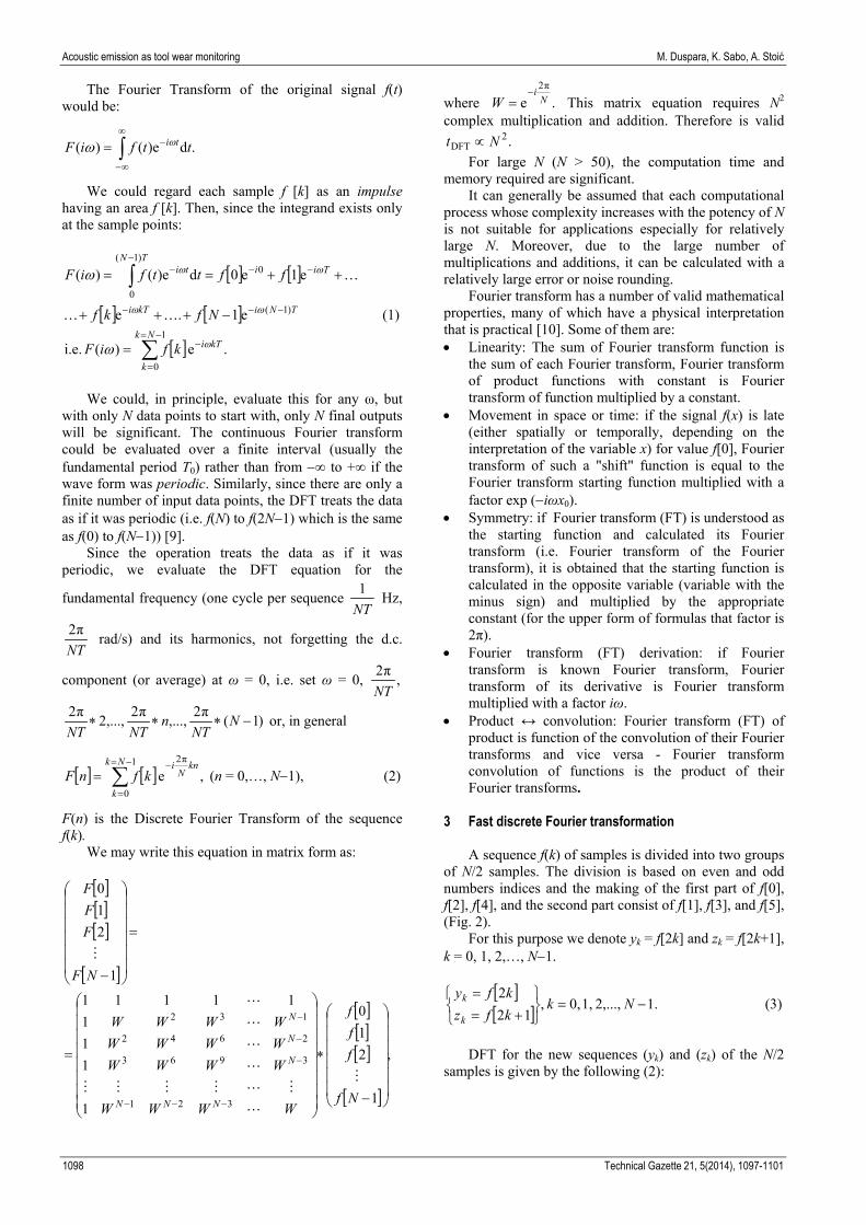
Tool wear is an important feature for monitoring in machining processes, because the quality of the surface roughness, dimensional accuracy and cut, the amount of energy needed to remove the metal directly depend on the degree of tool wear. Included here are two mechanisms of tool wear, flank wear and cratering. Every system for monitoring tools must be able to recognize one or both of the wear mechanisms [1]. The first section of the paper shows discrete Fourier transformation and its disadvantages (time of calculating) for using in the sound signal processing. This paper describes mathematical model of fast Fourier transformation. It shows how, with help, fast Fourier transformation transformed signal from time domain to frequency domain. The most suitable way for monitoring tool wear is through frequency of acoustic emission. As an example, the sound signals were analysed which were obtained from the milling process for tool wear monitoring. Based on the knowledge accumulated from conventional cutting tool condition monitoring research, indirect sensing technologies, such as power, cutting force, vibration, and acoustic emission signals are candidates for detecting tool conditions [2, 3, 4]. However, installing a contact sensor on the system of machine tools or production lines is usually a significant challenge for engineers. An experienced worker on the machine can determine the condition of the tool according to the sound generated by the cutting process. Thus, sound signals have attracted attention in the development of tool wear monitoring [5, 6]. The noncontact microphone feature provides a solution to the challenge of installing contact sensors on the structure of the machine. Unlike other signals, such as vibration, acoustic emission, cutting force and spindle current, sound signals collected during metal cutting have not been extensively

investigated for failure monitoring tool (Fig. 1).The sound signals obtained from the microphone were first collected and transformed to a frequency domain using FFT [7]. Novelty in this work is potentiality automatisation and optimization of any conventional or nonconventional cutting process with using sound signals.

Figure 1 Schematic of tool condition monitoring

2 DFT (Discrete Fourier Transformation)

When computing spectra on a computer, it is not possible to carry out the integrals involved in the continuous time of Fourier transform. Instead, a related transform called the discrete Fourier transform is used [8].

The Discrete Fourier Transform (DFT) is the equivalent to the continuous Fourier Transform for signals known only at N instants separated by sample times T (i.e. a finite sequence of data). If f(t) is the continuous signal which is the source of the data, then N samples are denoted f[0], f[1], f[2],..., f[k],..., f[N−1].

Tehnički vjesnik 21, 5(2014), 1097-1101 1097

Acoustic emission as tool wear monitoring M. Duspara, K. Sabo, A. Stoić

The Fourier Transform of the original signal f(t) would be:

.d)e()( ttfiF ti∫∞

∞−

−= ωω

We could regard each sample f [k] as an impulse having an area f [k]. Then, since the integrand exists only at the sample points:

[ ] [ ]

[ ] [ ]

[ ] .e )( i.e.

e1.e

e1e0d)e()(

1

0

)1(

0)1(

0

kTiNk

k

TNikTi

TiiTN

ti

kfiF

Nfkf

ffttfiF

ω

ωω

ωω

ω

ω

−−=

=

−−−

−−−

−

∑

∫

=

−+++

++==

(1)

We could, in principle, evaluate this for any ω, but

with only N data points to start with, only N final outputs will be significant. The continuous Fourier transform could be evaluated over a finite interval (usually the fundamental period T0) rather than from −∞ to +∞ if the wave form was periodic. Similarly, since there are only a finite number of input data points, the DFT treats the data as if it was periodic (i.e. f(N) to f(2N−1) which is the same as f(0) to f(N−1)) [9].

Since the operation treats the data as if it was periodic, we evaluate the DFT equation for the

fundamental frequency (one cycle per sequence NT1 Hz,

NTπ2 rad/s) and its harmonics, not forgetting the d.c.

component (or average) at ω = 0, i.e. set ω = 0, ,π2NT

)1(π2 ,...,π2 2,...,π2−∗∗∗ N

NTn

NTNT or, in general

[ ] [ ] ,e π21

0

knN

iNk

kkfnF

−−=

=∑= (n = 0,…, N−1), (2)

F(n) is the Discrete Fourier Transform of the sequence f(k).

We may write this equation in matrix form as:

[ ][ ][ ]

[ ]

[ ][ ][ ]

[ ]

,

1

210

1

111

11111

1

210

321

3963

2642

132

−

∗

=

=

−

−−−

−

−

−

Nf

fff

WWWW

WWWWWWWWWWWW

NF

FFF

NNN

N

N

N

4

3

434444

3

3

3

3

4

where .eπ2

Ni

W−

= This matrix equation requires N2 complex multiplication and addition. Therefore is valid

.2DFT Nt ∝

For large N (N > 50), the computation time and memory required are significant.

It can generally be assumed that each computational process whose complexity increases with the potency of N is not suitable for applications especially for relatively large N. Moreover, due to the large number of multiplications and additions, it can be calculated with a relatively large error or noise rounding.

Fourier transform has a number of valid mathematical properties, many of which have a physical interpretation that is practical [10]. Some of them are: • Linearity: The sum of Fourier transform function is

the sum of each Fourier transform, Fourier transform of product functions with constant is Fourier transform of function multiplied by a constant.

• Movement in space or time: if the signal f(x) is late (either spatially or temporally, depending on the interpretation of the variable x) for value f[0], Fourier transform of such a "shift" function is equal to the Fourier transform starting function multiplied with a factor exp (−iωx0).

• Symmetry: if Fourier transform (FT) is understood as the starting function and calculated its Fourier transform (i.e. Fourier transform of the Fourier transform), it is obtained that the starting function is calculated in the opposite variable (variable with the minus sign) and multiplied by the appropriate constant (for the upper form of formulas that factor is 2π).

• Fourier transform (FT) derivation: if Fourier transform is known Fourier transform, Fourier transform of its derivative is Fourier transform multiplied with a factor iω.

• Product ↔ convolution: Fourier transform (FT) of product is function of the convolution of their Fourier transforms and vice versa - Fourier transform convolution of functions is the product of their Fourier transforms.

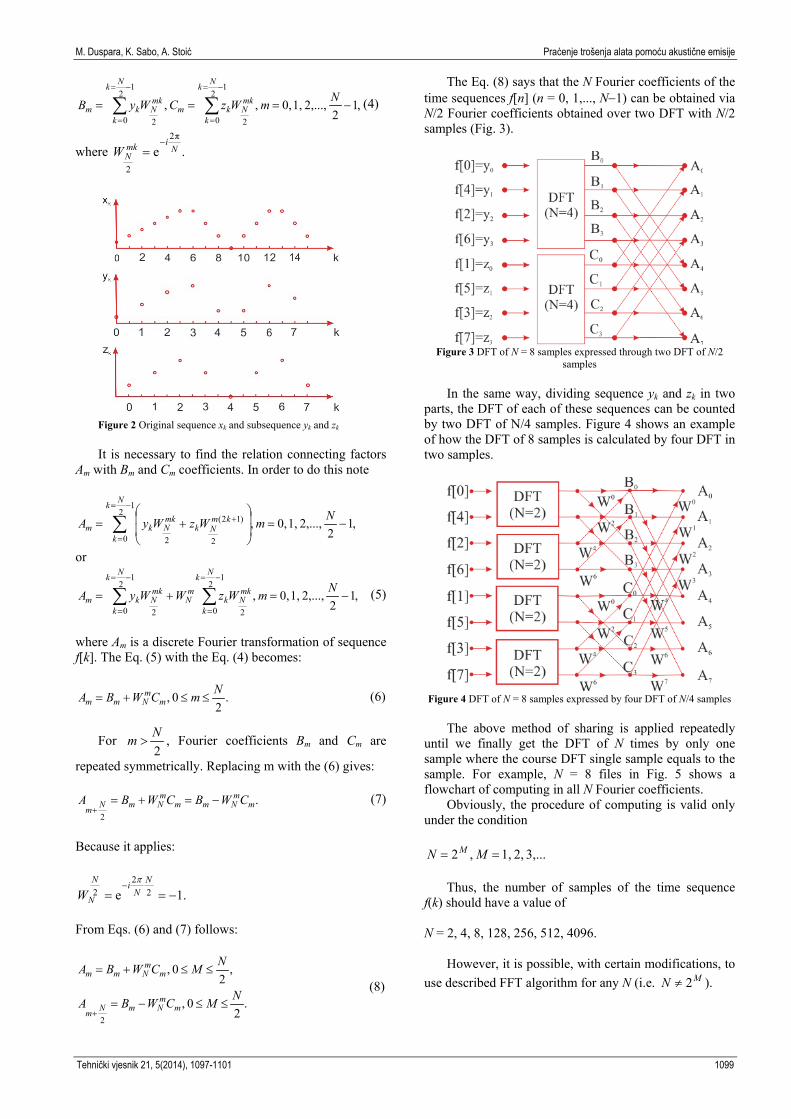
3 Fast discrete Fourier transformation A sequence f(k) of samples is divided into two groups

of N/2 samples. The division is based on even and odd numbers indices and the making of the first part of f[0], f[2], f[4], and the second part consist of f[1], f[3], and f[5], (Fig. 2).

For this purpose we denote yk = f[2k] and zk = f[2k+1], k = 0, 1, 2,…, N−1.

[ ][ ] .1 2,..., 1, 0, ,

122

−=

+==

Nkkfzkfy

k

k (3)

DFT for the new sequences (yk) and (zk) of the N/2

samples is given by the following (2):

1098 Technical Gazette 21, 5(2014), 1097-1101

M. Duspara, K. Sabo, A. Stoić Praćenje trošenja alata pomoću akustične emisije

,12

2,..., 1, 0, , ,1

2

0 2

12

0 2

−=== ∑∑−=

=

−=

=

NmWzCWyB

Nk

k

mkNkm

Nk

k

mkNkm (4)

where .eπ2

2

Nimk

NW−

=

Figure 2 Original sequence xk and subsequence yk and zk It is necessary to find the relation connecting factors

Am with Bm and Cm coefficients. In order to do this note

,12

2,..., 1, 0, ,1

2

0

)12(

22

−=

+= ∑

−=

=

+ NmWzWyA

Nk

k

kmNk

mkNkm

or

,12

2,..., 1, 0, ,1

2

0 2

12

0 2

−=+= ∑∑−=

=

−=

=

NmWzWWyA

Nk

k

mkNk

mN

Nk

k

mkNkm (5)

where Am is a discrete Fourier transformation of sequence f[k]. The Eq. (5) with the Eq. (4) becomes:

.2

0 , NmCWBA mm

Nmm ≤≤+= (6)

For 2

Nm > , Fourier coefficients Bm and Cm are

repeated symmetrically. Replacing m with the (6) gives:

.2

mm

Nmmm

NmNmCWBCWBA −=+=

+ (7)

Because it applies:

.1e 22

2 −==−

NN

iN

NWπ

From Eqs. (6) and (7) follows:

.2

0 ,

,2

0 ,

2

NMCWBA

NMCWBA

mm

NmNm

mm

Nmm

≤≤−=

≤≤+=

+

(8)

The Eq. (8) says that the N Fourier coefficients of the time sequences f[n] (n = 0, 1,..., N−1) can be obtained via N/2 Fourier coefficients obtained over two DFT with N/2 samples (Fig. 3).

Figure 3 DFT of N = 8 samples expressed through two DFT of N/2

samples In the same way, dividing sequence yk and zk in two

parts, the DFT of each of these sequences can be counted by two DFT of N/4 samples. Figure 4 shows an example of how the DFT of 8 samples is calculated by four DFT in two samples.

Figure 4 DFT of N = 8 samples expressed by four DFT of N/4 samples

The above method of sharing is applied repeatedly

until we finally get the DFT of N times by only one sample where the course DFT single sample equals to the sample. For example, N = 8 files in Fig. 5 shows a flowchart of computing in all N Fourier coefficients.

Obviously, the procedure of computing is valid only under the condition

3,... 2, 1, ,2 == MN M Thus, the number of samples of the time sequence

f(k) should have a value of N = 2, 4, 8, 128, 256, 512, 4096.

However, it is possible, with certain modifications, to

use described FFT algorithm for any N (i.e. MN 2≠ ).

Tehnički vjesnik 21, 5(2014), 1097-1101 1099

Acoustic emission as tool wear monitoring M. Duspara, K. Sabo, A. Stoić

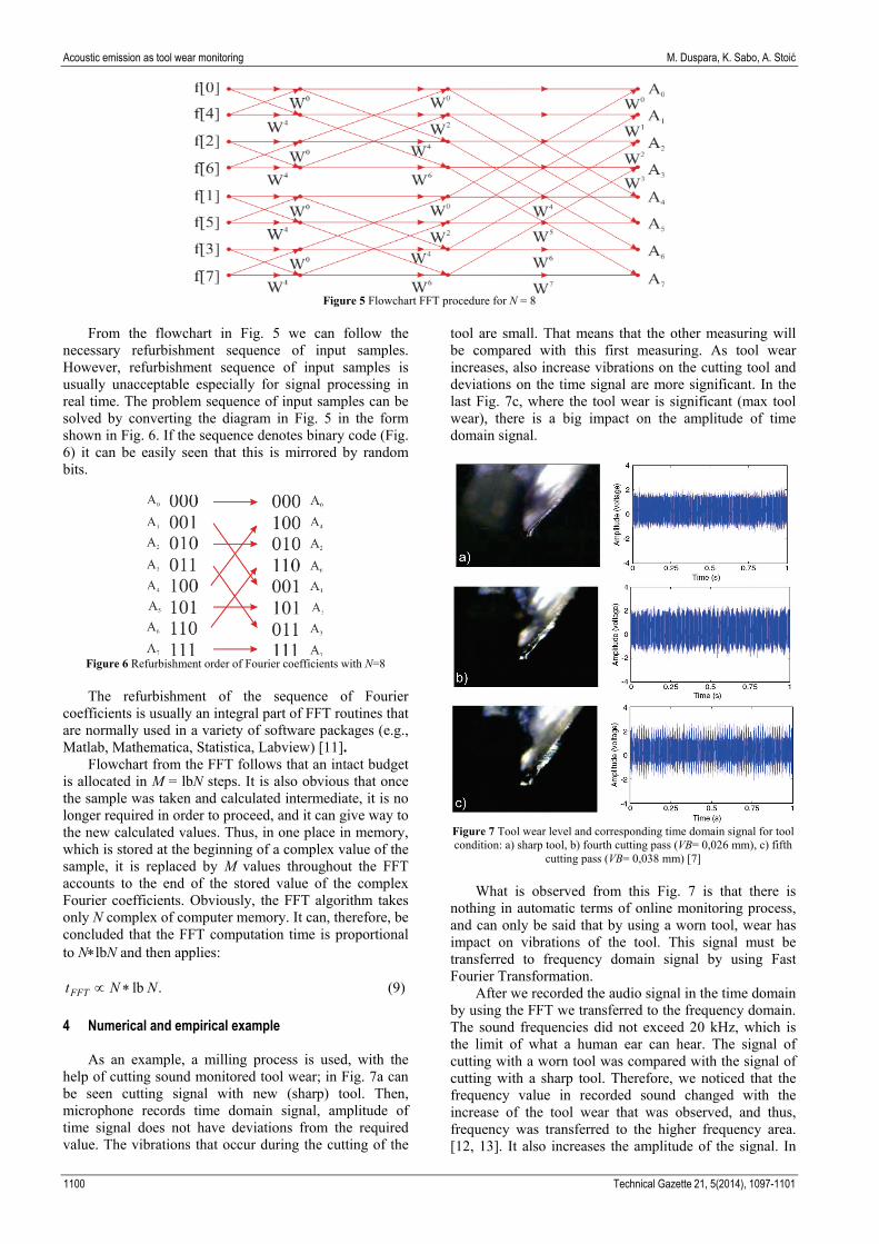
Figure 5 Flowchart FFT procedure for N = 8

From the flowchart in Fig. 5 we can follow the necessary refurbishment sequence of input samples. However, refurbishment sequence of input samples is usually unacceptable especially for signal processing in real time. The problem sequence of input samples can be solved by converting the diagram in Fig. 5 in the form shown in Fig. 6. If the sequence denotes binary code (Fig. 6) it can be easily seen that this is mirrored by random bits.

Figure 6 Refurbishment order of Fourier coefficients with N=8

The refurbishment of the sequence of Fourier

coefficients is usually an integral part of FFT routines that are normally used in a variety of software packages (e.g., Matlab, Mathematica, Statistica, Labview) [11].

Flowchart from the FFT follows that an intact budget is allocated in M = lbN steps. It is also obvious that once the sample was taken and calculated intermediate, it is no longer required in order to proceed, and it can give way to the new calculated values. Thus, in one place in memory, which is stored at the beginning of a complex value of the sample, it is replaced by M values throughout the FFT accounts to the end of the stored value of the complex Fourier coefficients. Obviously, the FFT algorithm takes only N complex of computer memory. It can, therefore, be concluded that the FFT computation time is proportional to N∗lbN and then applies:

. lb NNtFFT ∗∝ (9) 4 Numerical and empirical example

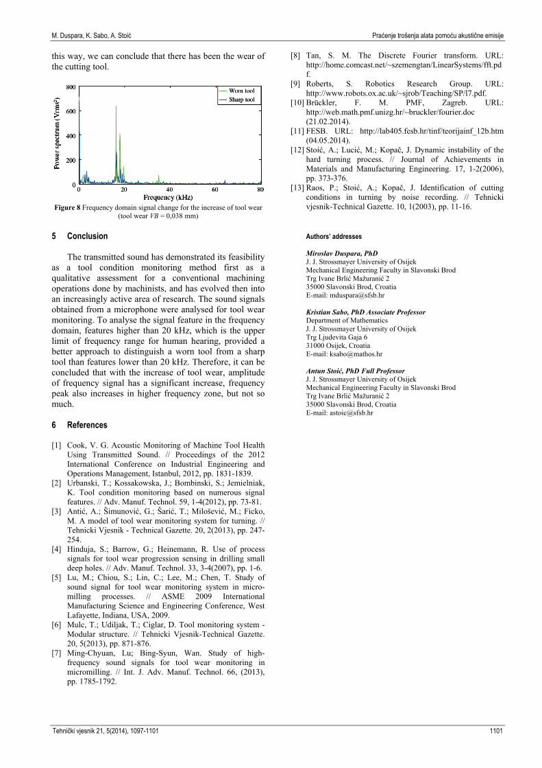
As an example, a milling process is used, with the help of cutting sound monitored tool wear; in Fig. 7a can be seen cutting signal with new (sharp) tool. Then, microphone records time domain signal, amplitude of time signal does not have deviations from the required value. The vibrations that occur during the cutting of the

tool are small. That means that the other measuring will be compared with this first measuring. As tool wear increases, also increase vibrations on the cutting tool and deviations on the time signal are more significant. In the last Fig. 7c, where the tool wear is significant (max tool wear), there is a big impact on the amplitude of time domain signal.

Figure 7 Tool wear level and corresponding time domain signal for tool condition: a) sharp tool, b) fourth cutting pass (VB= 0,026 mm), c) fifth

cutting pass (VB= 0,038 mm) [7]

What is observed from this Fig. 7 is that there is nothing in automatic terms of online monitoring process, and can only be said that by using a worn tool, wear has impact on vibrations of the tool. This signal must be transferred to frequency domain signal by using Fast Fourier Transformation.

After we recorded the audio signal in the time domain by using the FFT we transferred to the frequency domain. The sound frequencies did not exceed 20 kHz, which is the limit of what a human ear can hear. The signal of cutting with a worn tool was compared with the signal of cutting with a sharp tool. Therefore, we noticed that the frequency value in recorded sound changed with the increase of the tool wear that was observed, and thus, frequency was transferred to the higher frequency area. [12, 13]. It also increases the amplitude of the signal. In

1100 Technical Gazette 21, 5(2014), 1097-1101

M. Duspara, K. Sabo, A. Stoić Praćenje trošenja alata pomoću akustične emisije

this way, we can conclude that there has been the wear of the cutting tool.

Figure 8 Frequency domain signal change for the increase of tool wear (tool wear VB = 0,038 mm)

5 Conclusion

The transmitted sound has demonstrated its feasibility as a tool condition monitoring method first as a qualitative assessment for a conventional machining operations done by machinists, and has evolved then into an increasingly active area of research. The sound signals obtained from a microphone were analysed for tool wear monitoring. To analyse the signal feature in the frequency domain, features higher than 20 kHz, which is the upper limit of frequency range for human hearing, provided a better approach to distinguish a worn tool from a sharp tool than features lower than 20 kHz. Therefore, it can be concluded that with the increase of tool wear, amplitude of frequency signal has a significant increase, frequency peak also increases in higher frequency zone, but not so much.

6 References

[1] Cook, V. G. Acoustic Monitoring of Machine Tool Health Using Transmitted Sound. // Proceedings of the 2012 International Conference on Industrial Engineering and Operations Management, Istanbul, 2012, pp. 1831-1839.

[2] Urbanski, T.; Kossakowska, J.; Bombinski, S.; Jemielniak, K. Tool condition monitoring based on numerous signal features. // Adv. Manuf. Technol. 59, 1-4(2012), pp. 73-81.

[3] Antić, A.; Šimunović, G.; Šarić, T.; Milošević, M.; Ficko, M. A model of tool wear monitoring system for turning. // Tehnicki Vjesnik - Technical Gazette. 20, 2(2013), pp. 247-254.

[4] Hinduja, S.; Barrow, G.; Heinemann, R. Use of process signals for tool wear progression sensing in drilling small deep holes. // Adv. Manuf. Technol. 33, 3-4(2007), pp. 1-6.

[5] Lu, M.; Chiou, S.; Lin, C.; Lee, M.; Chen, T. Study of sound signal for tool wear monitoring system in micro-milling processes. // ASME 2009 International Manufacturing Science and Engineering Conference, West Lafayette, Indiana, USA, 2009.

[6] Mulc, T.; Udiljak, T.; Ciglar, D. Tool monitoring system - Modular structure. // Tehnicki Vjesnik-Technical Gazette. 20, 5(2013), pp. 871-876.

[7] Ming-Chyuan, Lu; Bing-Syun, Wan. Study of high-frequency sound signals for tool wear monitoring in micromilling. // Int. J. Adv. Manuf. Technol. 66, (2013), pp. 1785-1792.

[8] Tan, S. M. The Discrete Fourier transform. URL: http://home.comcast.net/~szemengtan/LinearSystems/fft.pdf.

[9] Roberts, S. Robotics Research Group. URL: http://www.robots.ox.ac.uk/~sjrob/Teaching/SP/l7.pdf.

[10] Brückler, F. M. PMF, Zagreb. URL: http://web.math.pmf.unizg.hr/~bruckler/fourier.doc (21.02.2014).

[11] FESB. URL: http://lab405.fesb.hr/tinf/teorijainf_12b.htm (04.05.2014).

[12] Stoić, A.; Lucić, M.; Kopač, J. Dynamic instability of the hard turning process. // Journal of Achievements in Materials and Manufacturing Engineering. 17, 1-2(2006), pp. 373-376.

[13] Raos, P.; Stoić, A.; Kopač, J. Identification of cutting conditions in turning by noise recording. // Tehnicki vjesnik-Technical Gazette. 10, 1(2003), pp. 11-16.

Authors’ addresses

Miroslav Duspara, PhDJ. J. Strossmayer University of Osijek Mechanical Engineering Faculty in Slavonski Brod Trg Ivane Brlić Mažuranić 2 35000 Slavonski Brod, Croatia E-mail: mduspara@sfsb.hr

Kristian Sabo, PhD Associate Professor Department of Mathematics J. J. Strossmayer University of Osijek Trg Ljudevita Gaja 6 31000 Osijek, Croatia E-mail: ksabo@mathos.hr

Antun Stoić, PhD Full Professor J. J. Strossmayer University of Osijek Mechanical Engineering Faculty in Slavonski Brod Trg Ivane Brlić Mažuranić 2 35000 Slavonski Brod, Croatia E-mail: astoic@sfsb.hr

Tehnički vjesnik 21, 5(2014), 1097-1101 1101

1102