eZdsp PV-MPPT Steepest Decent Control 2007-11 Consult
11
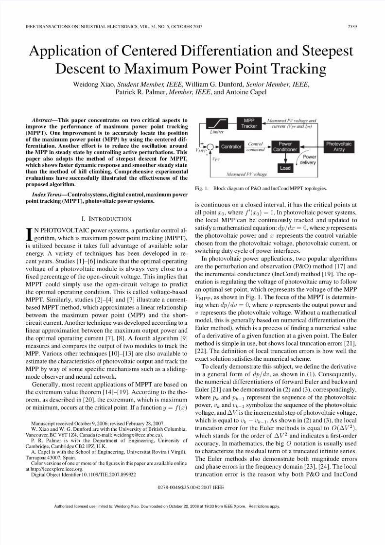
IEEE TRANSACTIONS ON INDUSTRIAL ELECTRONICS, VOL. 54, NO. 5, OCTOBER 2007 2539 Application of Centered Differentiation and Steepest Descent to Maximum Power Point Tracking Weidong Xiao, Student Member , IEEE , William G. Dunford, Senior Member, IEEE , Patrick R. Palmer, Member, IEEE , and Antoine Capel Abstract—Thi s paper concentrates on two critica l aspects to impro ve the performa nce of maximum power point tra cki ng (MPPT ). One improve ment is to accu ratel y locat e the position of the maximum power point (MPP) by using the centered dif- fer entiation. Another effort is to red uce the oscillation around the MPP in steady state by controlling active perturbations. This paper also adopts the me thod of ste epe st des cen t for MPP T, which shows faster dynamic response and smoother steady state than the method of hill climb ing. Compre hensi ve expe rime ntal eval uatio ns have success fully illus trate d the effe ctiv eness of the proposed algorithm. Index T erms—Con trol syste ms, digit al contr ol, maximum powe r point tracking (MPPT), photovoltaic power systems. I. I NTRODUCTION I N PHOTOVOLTAIC power systems, a particular control al- gorithm, which is maximum power point tracking (MPPT), is utilized because it takes full advantage of available solar ene rgy . A va rie ty of tec hni que s has bee n deve lop ed in re- cent years. Studies [1]–[6] indicate that the optimal operating voltage of a photovoltaic module is always very close to a fixed percentage of the open-circuit voltage. This implies that MPPT cou ld simply use the ope n-c irc uit vo lta ge to pre dic t the optimal operating condition. This is called voltage-based MPPT. Similarly, studies [2]–[4] and [7] illustrate a current- based MPPT method, which approximates a linear relationship bet wee n the max imum po wer poi nt (MPP) and the short- circuit current. Another technique was developed according to a linear approximation between the maximum output power and the optimal operating current [7], [8]. A fourth algorithm [9] measures and compares the output of two modules to track the MPP. Various other techniques [10]–[13] are also available to estimate the characteristics of photovoltaic output and track the MPP by way of some specific mechanisms such as a sliding- mode observer and neural network. Generally, most recent applications of MPPT are based on the extremum value theorem [14]–[19]. According to the the- orem, as described in [20], the extremum, which is maximum or minimum, occurs at the critical point. If a function y = f (x) Manuscript received October 9, 2006; revised February 28, 2007. W. Xiao and W. G. Dunford are with the University of British Columbia, V ancouver , BC V6T 1Z4, Canada (e-mail: weidongx@ece.ubc.ca). P. R. Pal mer is wit h the Dep art men t of Eng ineering, Uni versit y of Cambridge, Cambridge CB2 1PZ, U.K. A. Capel is with the School of Engineering, Universitat Rovira i Virgili, Tarrago na 43007, Spain. Color versions of one or more of the figures in this paper are available online at http://ieeexplore.ieee.org. Digital Object Identifier 10.1109/TIE.2007.8999 22 Fig. 1. Block diag ram of P&O and IncCond MPPT topo logies. is continuous on a closed interval, it has the critical points at all point x 0 , where f (x 0 ) = 0. In photovoltaic power systems, the local MPP can be con tin uou sly tracked and updat ed to satisfy a mathe matic al equat ion: dp/dx = 0, wher e p represents the photovoltaic power and x represents the control variable chosen from the photovoltaic voltage, photovoltaic current, or switching duty cycle of power interfaces. In photovoltaic power applications, two popular algorithms are the perturbation and observation (P&O) method [17] and the incremental conductance (IncCond) method [19]. The op- eration is regulating the voltage of photovoltaic array to follow an optimal set point, which represents the voltage of the MPP V MPP , as shown in Fig. 1. The focus of the MPPT is determin- ing when dp/dv = 0, where p represents the output power and v represents the photovoltaic voltage. Without a mathematical model, this is generally based on numerical differentiation (the Euler method), which is a process of finding a numerical value of a derivative of a given function at a given point. The Euler method is simple in use, but shows local truncation errors [21], [22]. The definition of local truncation errors is how well the exact solution satisfies the numerical scheme. To clearly demonstrate this subject, we define the derivative in a general form of dp/dv, as shown in (1). Consequently, the numerical differentiations of forward Euler and backward Euler [21] can be demonstrated in (2) and (3), correspondingly, where p k and p k−1 represent the sequence of the photovoltaic power, v k and v k−1 symbolize the sequence of the photovoltaic volt age, and ∆V is the inc rement al step of photovo ltaic voltage, which is equal to v k − v k−1 . As shown in (2) and (3), the local truncation error for the Euler methods is equal to O(∆V 2 ), which stands for the order of ∆V 2 and indicates a first-order accuracy. In mathematics, the big O notation is usually used to characterize the residual term of a truncated infinite series. The Euler metho ds also demonst rate both magni tude errors and phase errors in the frequency domain [23], [24]. The local truncation error is the reason why both P&O and IncCond 0278-0046 /$25.00 © 2007 IEEE Authorized licensed use limited to: Weidong Xiao. Downloaded on October 22, 2008 at 19:33 from IEEE Xplore. Restrictions apply.
-
Upload
hophamhuyanh9289 -
Category
Documents
-
view
227 -
download
1
Transcript of eZdsp PV-MPPT Steepest Decent Control 2007-11 Consult
8/6/2019 eZdsp PV-MPPT Steepest Decent Control 2007-11 Consult
http://slidepdf.com/reader/full/ezdsp-pv-mppt-steepest-decent-control-2007-11-consult 1/11
IEEE TRANSACTIONS ON INDUSTRIAL ELECTRONICS, VOL. 54, NO. 5, OCTOBER 2007 2539
Application of Centered Differentiation and SteepestDescent to Maximum Power Point Tracking
Weidong Xiao, Student Member, IEEE , William G. Dunford, Senior Member, IEEE ,Patrick R. Palmer, Member, IEEE , and Antoine Capel
Abstract—This paper concentrates on two critical aspects toimprove the performance of maximum power point tracking(MPPT). One improvement is to accurately locate the positionof the maximum power point (MPP) by using the centered dif-ferentiation. Another effort is to reduce the oscillation aroundthe MPP in steady state by controlling active perturbations. Thispaper also adopts the method of steepest descent for MPPT,which shows faster dynamic response and smoother steady statethan the method of hill climbing. Comprehensive experimentalevaluations have successfully illustrated the effectiveness of theproposed algorithm.
IndexTerms—Control systems, digital control, maximum powerpoint tracking (MPPT), photovoltaic power systems.
I. INTRODUCTION
IN PHOTOVOLTAIC power systems, a particular control al-
gorithm, which is maximum power point tracking (MPPT),
is utilized because it takes full advantage of available solar
energy. A variety of techniques has been developed in re-
cent years. Studies [1]–[6] indicate that the optimal operating
voltage of a photovoltaic module is always very close to a
fixed percentage of the open-circuit voltage. This implies that
MPPT could simply use the open-circuit voltage to predictthe optimal operating condition. This is called voltage-based
MPPT. Similarly, studies [2]–[4] and [7] illustrate a current-
based MPPT method, which approximates a linear relationship
between the maximum power point (MPP) and the short-
circuit current. Another technique was developed according to a
linear approximation between the maximum output power and
the optimal operating current [7], [8]. A fourth algorithm [9]
measures and compares the output of two modules to track the
MPP. Various other techniques [10]–[13] are also available to
estimate the characteristics of photovoltaic output and track the
MPP by way of some specific mechanisms such as a sliding-
mode observer and neural network.
Generally, most recent applications of MPPT are based onthe extremum value theorem [14]–[19]. According to the the-
orem, as described in [20], the extremum, which is maximum
or minimum, occurs at the critical point. If a function y = f (x)
Manuscript received October 9, 2006; revised February 28, 2007.W. Xiao and W. G. Dunford are with the University of British Columbia,
Vancouver, BC V6T 1Z4, Canada (e-mail: [email protected]).P. R. Palmer is with the Department of Engineering, University of
Cambridge, Cambridge CB2 1PZ, U.K.A. Capel is with the School of Engineering, Universitat Rovira i Virgili,
Tarragona 43007, Spain.Color versions of one or more of the figures in this paper are available online
at http://ieeexplore.ieee.org.Digital Object Identifier 10.1109/TIE.2007.899922
Fig. 1. Block diagram of P&O and IncCond MPPT topologies.
is continuous on a closed interval, it has the critical points at
all point x0, where f (x0) = 0. In photovoltaic power systems,
the local MPP can be continuously tracked and updated to
satisfy a mathematical equation:dp/dx = 0, where p represents
the photovoltaic power and x represents the control variable
chosen from the photovoltaic voltage, photovoltaic current, or
switching duty cycle of power interfaces.
In photovoltaic power applications, two popular algorithms
are the perturbation and observation (P&O) method [17] and
the incremental conductance (IncCond) method [19]. The op-
eration is regulating the voltage of photovoltaic array to follow
an optimal set point, which represents the voltage of the MPPV MPP, as shown in Fig. 1. The focus of the MPPT is determin-
ing when dp/dv = 0, where p represents the output power and
v represents the photovoltaic voltage. Without a mathematical
model, this is generally based on numerical differentiation (the
Euler method), which is a process of finding a numerical value
of a derivative of a given function at a given point. The Euler
method is simple in use, but shows local truncation errors [21],
[22]. The definition of local truncation errors is how well the
exact solution satisfies the numerical scheme.
To clearly demonstrate this subject, we define the derivative
in a general form of dp/dv, as shown in (1). Consequently,
the numerical differentiations of forward Euler and backwardEuler [21] can be demonstrated in (2) and (3), correspondingly,
where pk and pk−1 represent the sequence of the photovoltaic
power, vk and vk−1 symbolize the sequence of the photovoltaic
voltage, and ∆V is the incremental step of photovoltaic voltage,
which is equal to vk − vk−1. As shown in (2) and (3), the local
truncation error for the Euler methods is equal to O(∆V 2),
which stands for the order of ∆V 2 and indicates a first-order
accuracy. In mathematics, the big O notation is usually used
to characterize the residual term of a truncated infinite series.
The Euler methods also demonstrate both magnitude errors
and phase errors in the frequency domain [23], [24]. The local
truncation error is the reason why both P&O and IncCond
0278-0046/$25.00 © 2007 IEEE
Authorized licensed use limited to: Weidong Xiao. Downloaded on October 22, 2008 at 19:33 from IEEE Xplore. Restrictions apply.

8/6/2019 eZdsp PV-MPPT Steepest Decent Control 2007-11 Consult
http://slidepdf.com/reader/full/ezdsp-pv-mppt-steepest-decent-control-2007-11-consult 2/11
8/6/2019 eZdsp PV-MPPT Steepest Decent Control 2007-11 Consult
http://slidepdf.com/reader/full/ezdsp-pv-mppt-steepest-decent-control-2007-11-consult 3/11
XAIO et al.: APPLICATION OF CENTERED DIFFERENTIATION AND STEEPEST DESCENT TO MPPT 2541
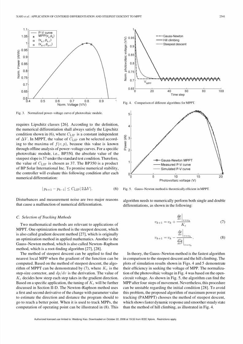
Fig. 3. Normalized power–voltage curve of photovoltaic module.
requires Lipschitz classes [26]. According to the definition,
the numerical differentiation shall always satisfy the Lipschitz
condition shown in (6), where C LIP is a constant independent
of ∆V . In MPPT, the value of C LIP can be selected accord-
ing to the maxima of f (v, p), because this value is known
through offline analysis of power–voltage curves. For a specific
photovoltaic module, i.e., BP350, the absolute value of the
steepest slope is 37 under the standard test condition. Therefore,
the value of C LIP is chosen as 37. The BP350 is a product
of BP Solar International Inc. To promise numerical stability,
the controller will evaluate this following condition after each
numerical differentiation:
| pk+1 − pk−1| ≤ C LIP| 2∆V |. (6)
Disturbances and measurement noise are two major reasons
that cause a malfunction of numerical differentiation.
C. Selection of Tracking Methods
Two mathematical methods are relevant to applications of
MPPT. One optimization method is the steepest descent, which
is also called gradient descent method [27], which is originally
an optimization method in applied mathematics. Another is theGauss–Newton method, which is also called Newton–Raphson
method, which is a root-finding algorithm [27], [28].
The method of steepest descent can be applied to find the
nearest local MPP when the gradient of the function can be
computed. Based on the method of steepest descent, the algo-
rithm of MPPT can be demonstrated by (7), where K ε is the
step-size corrector, and dp/dv is the derivation. The value of
K ε decides how steep each step takes in the gradient direction.
Based on a specific application, the tuning of K ε will be further
discussed in Section II-D. The Newton–Raphson method uses
a first and second derivative of the change with parameter value
to estimate the direction and distance the program should to
go to reach a better point. When it is used to track MPPs, thecomputation of operating point can be illustrated in (8). This
Fig. 4. Comparison of different algorithms for MPPT.
Fig. 5. Gauss–Newton method is theoretically efficient in MPPT.
algorithm needs to numerically perform both single and double
differentiations, as shown in the following:
vk+1 = vk +
dp
dv
v=vk
K ε(7)
vk+1 = vk −
dp
dv
v=vk
d2
pdv2v=vk
. (8)
In theory, the Gauss–Newton method is the fastest algorithm
in comparison to the steepest descent and the hill climbing. The
plots of simulation results shown in Figs. 4 and 5 demonstrate
their efficiency in seeking the voltage of MPP. The normaliza-
tion of the photovoltaic voltage in Fig. 4 was based on the open-
circuit voltage. As shown in Fig. 5, the algorithm can find the
MPP after four steps of movement. Nevertheless, this procedure
can be unstable regarding the initial condition [28]. To avoid
this problem, the proposed algorithm of maximum power point
tracking (PAMPPT) chooses the method of steepest descent,
which shows faster dynamic response and smoother steady statethan the method of hill climbing, as illustrated in Fig. 4.
Authorized licensed use limited to: Weidong Xiao. Downloaded on October 22, 2008 at 19:33 from IEEE Xplore. Restrictions apply.
8/6/2019 eZdsp PV-MPPT Steepest Decent Control 2007-11 Consult
http://slidepdf.com/reader/full/ezdsp-pv-mppt-steepest-decent-control-2007-11-consult 4/11
2542 IEEE TRANSACTIONS ON INDUSTRIAL ELECTRONICS, VOL. 54, NO. 5, OCTOBER 2007
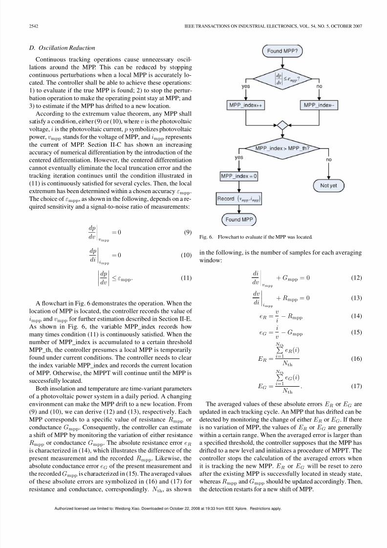
D. Oscillation Reduction
Continuous tracking operations cause unnecessary oscil-
lations around the MPP. This can be reduced by stopping
continuous perturbations when a local MPP is accurately lo-
cated. The controller shall be able to achieve these operations:
1) to evaluate if the true MPP is found; 2) to stop the pertur-
bation operation to make the operating point stay at MPP; and3) to estimate if the MPP has drifted to a new location.
According to the extremum value theorem, any MPP shall
satisfy a condition, either (9) or (10), where v is the photovoltaic
voltage, i is the photovoltaic current, p symbolizes photovoltaic
power, vmpp stands for the voltage of MPP, and impp represents
the current of MPP. Section II-C has shown an increasing
accuracy of numerical differentiation by the introduction of the
centered differentiation. However, the centered differentiation
cannot eventually eliminate the local truncation error and the
tracking iteration continues until the condition illustrated in
(11) is continuously satisfied for several cycles. Then, the local
extremum has been determined within a chosen accuracy εmpp.The choice of εmpp, as shown in the following, depends on a re-
quired sensitivity and a signal-to-noise ratio of measurements:
dp
dv
vmpp
= 0 (9)
dp
di
impp
= 0 (10)
dp
dv
≤ εmpp. (11)
A flowchart in Fig. 6 demonstrates the operation. When the
location of MPP is located, the controller records the value of
impp and vmpp for further estimation described in Section II-E.
As shown in Fig. 6, the variable MPP_index records how
many times condition (11) is continuously satisfied. When the
number of MPP_index is accumulated to a certain threshold
MPP_th, the controller presumes a local MPP is temporarily
found under current conditions. The controller needs to clear
the index variable MPP_index and records the current location
of MPP. Otherwise, the MPPT will continue until the MPP is
successfully located.Both insolation and temperature are time-variant parameters
of a photovoltaic power system in a daily period. A changing
environment can make the MPP drift to a new location. From
(9) and (10), we can derive (12) and (13), respectively. Each
MPP corresponds to a specific value of resistance Rmpp or
conductance Gmpp. Consequently, the controller can estimate
a shift of MPP by monitoring the variation of either resistance
Rmpp or conductance Gmpp. The absolute resistance error eRis characterized in (14), which illustrates the difference of the
present measurement and the recorded Rmpp. Likewise, the
absolute conductance error eG of the present measurement and
the recordedGmpp is characterized in (15). The averaged values
of these absolute errors are symbolized in (16) and (17) forresistance and conductance, correspondingly. N th, as shown
Fig. 6. Flowchart to evaluate if the MPP was located.
in the following, is the number of samples for each averaging
window:
di
dv
vmpp
+ Gmpp = 0 (12)
dv
di
impp
+ Rmpp = 0 (13)
eR =v
i−Rmpp (14)
eG =i
v−Gmpp (15)
E R =
N thi=1
eR(i)
N th(16)
E G =
N th
i=1
eG(i)
N th. (17)
The averaged values of these absolute errors E R or E G are
updated in each tracking cycle. An MPP that has drifted can be
detected by monitoring the change of either E R or E G. If there
is no variation of MPP, the values of E R or E G are generally
within a certain range. When the averaged error is larger than
a specified threshold, the controller supposes that the MPP has
drifted to a new level and initializes a procedure of MPPT. The
controller stops the calculation of the averaged errors when
it is tracking the new MPP. E R or E G will be reset to zero
after the existing MPP is successfully located in steady state,
whereas Rmpp and Gmpp should be updated accordingly. Then,the detection restarts for a new shift of MPP.
Authorized licensed use limited to: Weidong Xiao. Downloaded on October 22, 2008 at 19:33 from IEEE Xplore. Restrictions apply.
8/6/2019 eZdsp PV-MPPT Steepest Decent Control 2007-11 Consult
http://slidepdf.com/reader/full/ezdsp-pv-mppt-steepest-decent-control-2007-11-consult 5/11
XAIO et al.: APPLICATION OF CENTERED DIFFERENTIATION AND STEEPEST DESCENT TO MPPT 2543
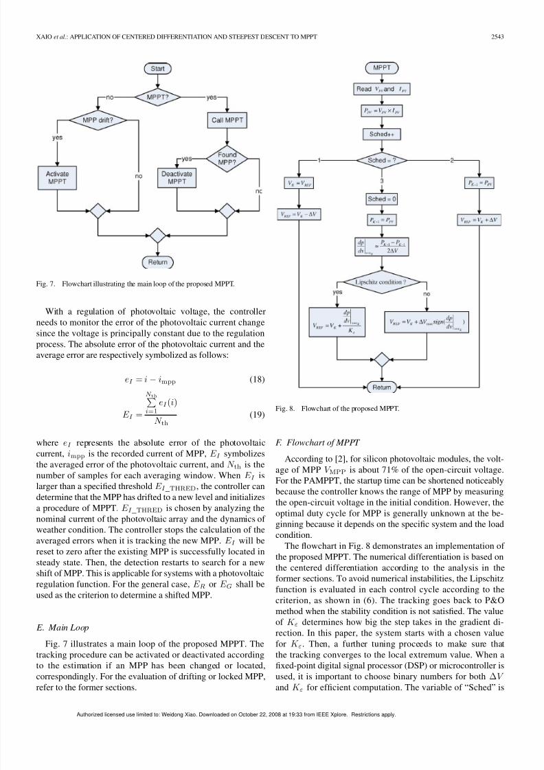
Fig. 7. Flowchart illustrating the main loop of the proposed MPPT.
With a regulation of photovoltaic voltage, the controller
needs to monitor the error of the photovoltaic current change
since the voltage is principally constant due to the regulation
process. The absolute error of the photovoltaic current and the
average error are respectively symbolized as follows:
eI = i− impp (18)
E I =
N th
i=1 eI (i)
N th(19)
where eI represents the absolute error of the photovoltaic
current, impp is the recorded current of MPP, E I symbolizes
the averaged error of the photovoltaic current, and N th is the
number of samples for each averaging window. When E I is
larger than a specified threshold E I _THRED, the controller can
determine that the MPP has drifted to a new level and initializes
a procedure of MPPT. E I _THRED is chosen by analyzing the
nominal current of the photovoltaic array and the dynamics of
weather condition. The controller stops the calculation of the
averaged errors when it is tracking the new MPP. E I will bereset to zero after the existing MPP is successfully located in
steady state. Then, the detection restarts to search for a new
shift of MPP. This is applicable for systems with a photovoltaic
regulation function. For the general case, E R or E G shall be
used as the criterion to determine a shifted MPP.
E. Main Loop
Fig. 7 illustrates a main loop of the proposed MPPT. The
tracking procedure can be activated or deactivated according
to the estimation if an MPP has been changed or located,
correspondingly. For the evaluation of drifting or locked MPP,refer to the former sections.
Fig. 8. Flowchart of the proposed MPPT.
F. Flowchart of MPPT
According to [2], for silicon photovoltaic modules, the volt-
age of MPP V MPP is about 71% of the open-circuit voltage.
For the PAMPPT, the startup time can be shortened noticeably
because the controller knows the range of MPP by measuring
the open-circuit voltage in the initial condition. However, the
optimal duty cycle for MPP is generally unknown at the be-
ginning because it depends on the specific system and the load
condition.The flowchart in Fig. 8 demonstrates an implementation of
the proposed MPPT. The numerical differentiation is based on
the centered differentiation according to the analysis in the
former sections. To avoid numerical instabilities, the Lipschitz
function is evaluated in each control cycle according to the
criterion, as shown in (6). The tracking goes back to P&O
method when the stability condition is not satisfied. The value
of K ε determines how big the step takes in the gradient di-
rection. In this paper, the system starts with a chosen value
for K ε. Then, a further tuning proceeds to make sure that
the tracking converges to the local extremum value. When a
fixed-point digital signal processor (DSP) or microcontroller is
used, it is important to choose binary numbers for both ∆V and K ε for efficient computation. The variable of “Sched” is
Authorized licensed use limited to: Weidong Xiao. Downloaded on October 22, 2008 at 19:33 from IEEE Xplore. Restrictions apply.
8/6/2019 eZdsp PV-MPPT Steepest Decent Control 2007-11 Consult
http://slidepdf.com/reader/full/ezdsp-pv-mppt-steepest-decent-control-2007-11-consult 6/11
2544 IEEE TRANSACTIONS ON INDUSTRIAL ELECTRONICS, VOL. 54, NO. 5, OCTOBER 2007
TABLE IIMPORTANT PARAMETERS USED IN FIG S. 6 AN D 8
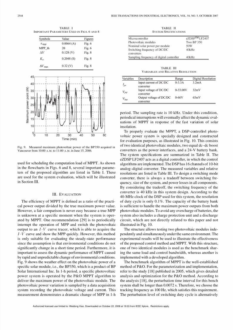
Fig. 9. Measured maximum photovoltaic power of the BP350 acquired inVancouver from 10:00 A.M. to 11:00 A.M. in June 15, 2006.
used for scheduling the computation load of MPPT. As shown
in the flowcharts in Figs. 6 and 8, several important parame-
ters of the proposed algorithm are listed in Table I. Theseare used for the system evaluation, which will be illustrated
in Section III.
III. EVALUATION
The efficiency of MPPT is defined as a ratio of the practi-
cal power output divided by the true maximum power value.
However, a fair comparison is never easy because a true MPP
is unknown at a specific moment when the system is oper-
ated by MPPT. One recommendation [29] is to periodically
interrupt the operation of MPP and switch the photovoltaic
output to an I –V curve tracer, which is able to acquire theI –V curve and show the MPP quickly. However, this method
is only suitable for evaluating the steady-state performance
since the assumption is that environmental conditions do not
significantly change in a short time period. Furthermore, it is
important to assess the dynamic performance of MPPT caused
by rapid and unpredictable change of environmental conditions.
Fig. 9 shows the weather effect on the photovoltaic power of a
specific solar module, i.e., the BP350, which is a product of BP
Solar International Inc. In 1-h period, a specific photovoltaic
power system is operated by the P&O MPPT algorithm to
deliver the maximum power of the photovoltaic module. The
photovoltaic power variation is sampled by a data acquisition
system recording the photovoltaic voltage and current. Thismeasurement demonstrates a dramatic change of MPP in 1-h
TABLE IISYSTEM SPECIFICATIONS
TABLE IIIVARIABLES AND RELATIVE RESOLUTION
period. The sampling rate is 10 kHz. Under this condition,
periodical interruptions will eventually affect the dynamic eval-
uations of MPPT in response of the fast variation of solar
insolation.
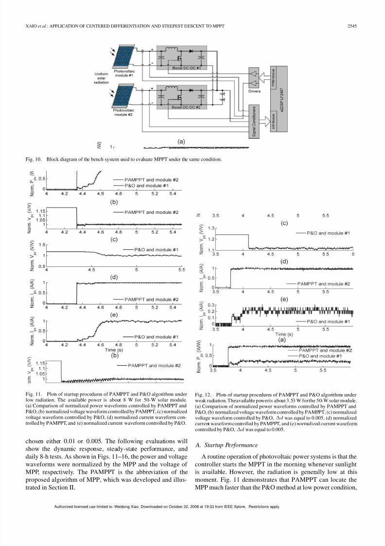
To properly evaluate the MPPT, a DSP-controlled photo-
voltaic power system is specially designed and constructed
for evaluation purposes, as illustrated in Fig. 10. This consists
of two identical photovoltaic modules, two equal dc–dc boost
converters as the power interfaces, and a 24-V battery bank.
The system specifications are summarized in Table II. The
eZDSP LF2407 acts as a digital controller, in which the control
algorithms are implemented. The DSP has 16 channels of 10-bit
analog–digital converter. The measured variables and relative
resolutions are listed in Table III. To design a switching modeconverter, there is always a tradeoff between switching fre-
quency, size of the system, and power losses in all components.
By considering the tradeoff, the switching frequency of the
converter is 40 kHz in this system design. According to the
40-MHz clock of the DSP used for this system, the resolution
of duty cycle is only 0.1%. The capacity of the battery bank
is sufficient to handle the maximum power outputs from both
photovoltaic modules. To avoid any overcharge of batteries, the
system also includes a charge protection unit and a discharge
circuit, which are not directly related to this paper and not
illustrated in Fig. 10.
The structure allows testing two photovoltaic modules inde-pendently and simultaneously under the same environment. The
experimental results will be used to illustrate the effectiveness
of the proposed control method and MPPT. With this structure,
one of two identical modules is used as the benchmark shar-
ing the same load and control bandwidth, whereas another is
implemented with a developed algorithm.
The benchmark algorithm of MPPT is the well-established
method of P&O. For the parameterization and implementation,
refer to the study [18] published in 2005, which gives detailed
analysis and optimization for the P&O method. According to
the analysis [18], the perturbation time interval for this bench
system shall be longer than 0.0072 s. Therefore, we choose the
tracking frequency as 100 Hz, which satisfies this requirement.The perturbation level of switching duty cycle is alternatively
Authorized licensed use limited to: Weidong Xiao. Downloaded on October 22, 2008 at 19:33 from IEEE Xplore. Restrictions apply.
8/6/2019 eZdsp PV-MPPT Steepest Decent Control 2007-11 Consult
http://slidepdf.com/reader/full/ezdsp-pv-mppt-steepest-decent-control-2007-11-consult 7/11
XAIO et al.: APPLICATION OF CENTERED DIFFERENTIATION AND STEEPEST DESCENT TO MPPT 2545
Fig. 10. Block diagram of the bench system used to evaluate MPPT under the same condition.
Fig. 11. Plots of startup procedures of PAMPPT and P&O algorithms underlow radiation. The available power is about 8 W for 50-W solar module.(a) Comparison of normalized power waveforms controlled by PAMPPT andP&O, (b) normalized voltage waveform controlled by PAMPPT, (c) normalizedvoltage waveform controlled by P&O, (d) normalized current waveform con-trolled by PAMPPT, and (e) normalized current waveform controlled by P&O.
chosen either 0.01 or 0.005. The following evaluations will
show the dynamic response, steady-state performance, and
daily 8-h tests. As shown in Figs. 11–16, the power and voltage
waveforms were normalized by the MPP and the voltage of
MPP, respectively. The PAMPPT is the abbreviation of the
proposed algorithm of MPP, which was developed and illus-trated in Section II.
Fig. 12. Plots of startup procedures of PAMPPT and P&O algorithms underweak radiation. Theavailable poweris about 3.53 W forthe 50-W solar module.(a) Comparison of normalized power waveforms controlled by PAMPPT andP&O, (b) normalized voltage waveform controlled by PAMPPT, (c) normalizedvoltage waveform controlled by P&O, ∆d was equal to 0.005, (d) normalizedcurrent waveform controlled by PAMPPT, and (e) normalized current waveformcontrolled by P&O,∆d was equal to 0.005.
A. Startup Performance
A routine operation of photovoltaic power systems is that the
controller starts the MPPT in the morning whenever sunlight
is available. However, the radiation is generally low at this
moment. Fig. 11 demonstrates that PAMPPT can locate theMPP much faster than the P&O method at low power condition,
Authorized licensed use limited to: Weidong Xiao. Downloaded on October 22, 2008 at 19:33 from IEEE Xplore. Restrictions apply.
8/6/2019 eZdsp PV-MPPT Steepest Decent Control 2007-11 Consult
http://slidepdf.com/reader/full/ezdsp-pv-mppt-steepest-decent-control-2007-11-consult 8/11
2546 IEEE TRANSACTIONS ON INDUSTRIAL ELECTRONICS, VOL. 54, NO. 5, OCTOBER 2007
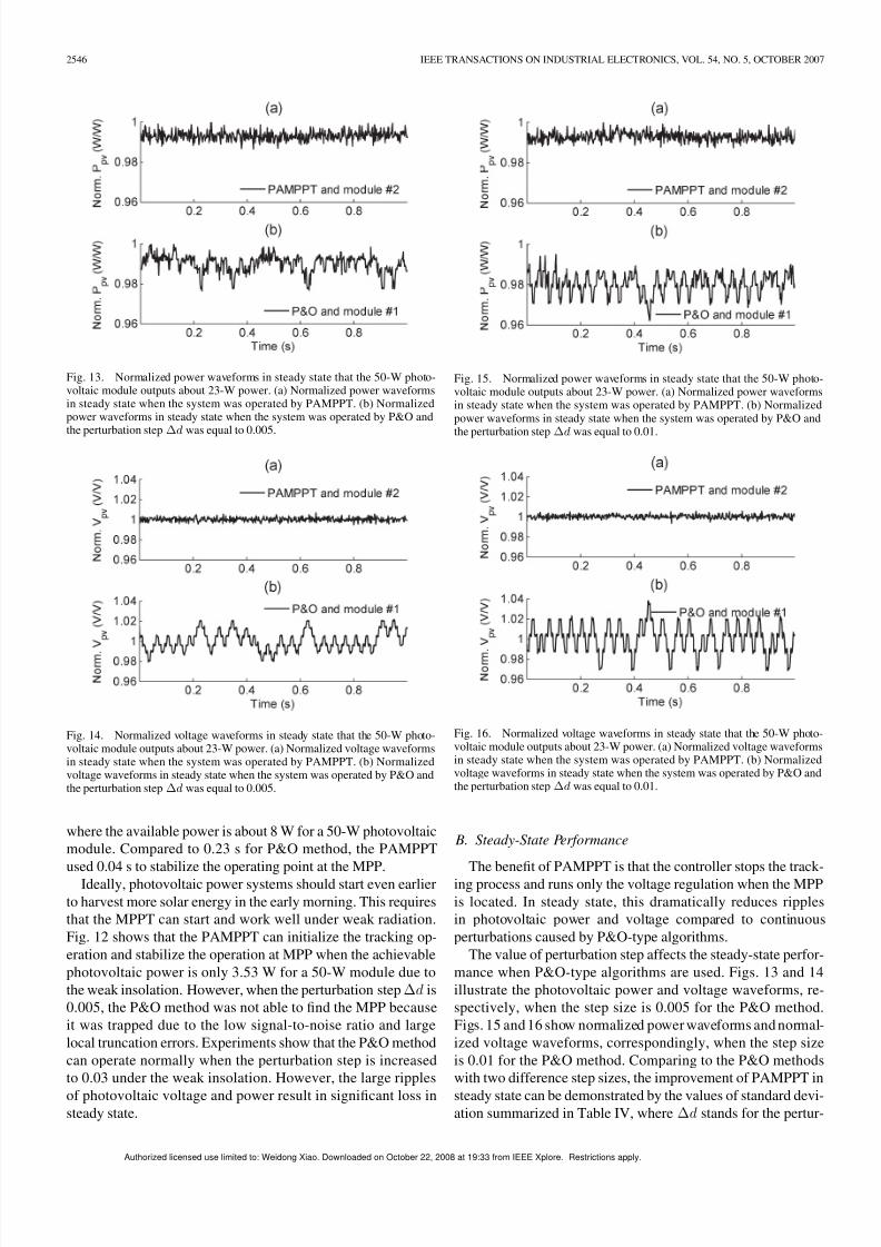
Fig. 13. Normalized power waveforms in steady state that the 50-W photo-voltaic module outputs about 23-W power. (a) Normalized power waveformsin steady state when the system was operated by PAMPPT. (b) Normalizedpower waveforms in steady state when the system was operated by P&O andthe perturbation step∆d was equal to 0.005.
Fig. 14. Normalized voltage waveforms in steady state that the 50-W photo-voltaic module outputs about 23-W power. (a) Normalized voltage waveformsin steady state when the system was operated by PAMPPT. (b) Normalizedvoltage waveforms in steady state when the system was operated by P&O andthe perturbation step∆d was equal to 0.005.
where the available power is about 8 W for a 50-W photovoltaic
module. Compared to 0.23 s for P&O method, the PAMPPT
used 0.04 s to stabilize the operating point at the MPP.Ideally, photovoltaic power systems should start even earlier
to harvest more solar energy in the early morning. This requires
that the MPPT can start and work well under weak radiation.
Fig. 12 shows that the PAMPPT can initialize the tracking op-
eration and stabilize the operation at MPP when the achievable
photovoltaic power is only 3.53 W for a 50-W module due to
the weak insolation. However, when the perturbation step ∆d is
0.005, the P&O method was not able to find the MPP because
it was trapped due to the low signal-to-noise ratio and large
local truncation errors. Experiments show that the P&O method
can operate normally when the perturbation step is increased
to 0.03 under the weak insolation. However, the large ripples
of photovoltaic voltage and power result in significant loss insteady state.
Fig. 15. Normalized power waveforms in steady state that the 50-W photo-voltaic module outputs about 23-W power. (a) Normalized power waveformsin steady state when the system was operated by PAMPPT. (b) Normalizedpower waveforms in steady state when the system was operated by P&O and
the perturbation step∆d
was equal to 0.01.
Fig. 16. Normalized voltage waveforms in steady state that the 50-W photo-voltaic module outputs about 23-W power. (a) Normalized voltage waveformsin steady state when the system was operated by PAMPPT. (b) Normalizedvoltage waveforms in steady state when the system was operated by P&O andthe perturbation step∆d was equal to 0.01.
B. Steady-State Performance
The benefit of PAMPPT is that the controller stops the track-ing process and runs only the voltage regulation when the MPP
is located. In steady state, this dramatically reduces ripples
in photovoltaic power and voltage compared to continuous
perturbations caused by P&O-type algorithms.
The value of perturbation step affects the steady-state perfor-
mance when P&O-type algorithms are used. Figs. 13 and 14
illustrate the photovoltaic power and voltage waveforms, re-
spectively, when the step size is 0.005 for the P&O method.
Figs. 15 and 16 show normalized power waveforms and normal-
ized voltage waveforms, correspondingly, when the step size
is 0.01 for the P&O method. Comparing to the P&O methods
with two difference step sizes, the improvement of PAMPPT in
steady state can be demonstrated by the values of standard devi-ation summarized in Table IV, where ∆d stands for the pertur-
Authorized licensed use limited to: Weidong Xiao. Downloaded on October 22, 2008 at 19:33 from IEEE Xplore. Restrictions apply.
8/6/2019 eZdsp PV-MPPT Steepest Decent Control 2007-11 Consult
http://slidepdf.com/reader/full/ezdsp-pv-mppt-steepest-decent-control-2007-11-consult 9/11
XAIO et al.: APPLICATION OF CENTERED DIFFERENTIATION AND STEEPEST DESCENT TO MPPT 2547
TABLE IVPERFORMANCE COMPARISON IN STEADY STATE
bation step of duty cycle. Table IV also demonstrates the mean
values of power outputs. The standard deviation of photovoltaic
voltage controlled by PAMPPT is much smaller than that com-
manded by P&O algorithm. As a result, the proposed control
system delivers more solar power under the same condition.
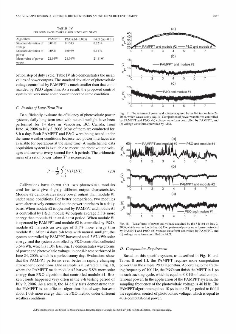
C. Results of Long-Term Test
To sufficiently evaluate the efficiency of photovoltaic power
systems, daily long-term tests with natural sunlight have been
performed for 14 days in Vancouver, BC, Canada, from
June 14, 2006 to July 3, 2006. Most of them are conducted for
8 h a day. Both PAMPPT and P&O were being tested under
the same weather conditions because two power interfaces are
available for operations at the same time. A multichannel data
acquisition system is available to record the photovoltaic volt-
ages and currents every second for 8-h periods. The arithmetic
mean of a set of power values P is expressed as
P =1
N
N
k=1
V (k)I (k). (20)
Calibrations have shown that two photovoltaic modules
used for tests give slightly different output characteristics.
Module #2 demonstrates more power output than module #1
under same conditions. For better comparison, two modules
were alternatively connected to the power interfaces in a daily
basis. When module #2 is operated by PAMPPT and module #1
is controlled by P&O, module #2 outputs average 5.3% more
energy than module #1 in an 8-h test period. When module #1
is operated by PAMPPT and module #2 is controlled by P&O,
module #2 harvests an average of 3.3% more energy than
module #1. After 14 days 8-h tests with natural sunlight, thesystem controlled by PAMPPT harvested total 3.67-kWh solar
energy, and the system controlled by P&O controlled collected
3.64 kWh, which is 1.0% less. Fig. 17 demonstrates waveforms
of power and photovoltaic voltage, in one 8-h test performed in
June 24, 2006, which is a perfect sunny day. Evaluations show
that the PAMPPT performs even better in rapidly changing
atmospheric conditions. One example is illustrated in Fig. 18,
where the PAMPPT made module #2 harvest 5.8% more solar
energy than P&O algorithm that controlled module #1. Bro-
ken clouds happened very often in the 8-h testing period of
July 9, 2006. As a result, the 14 daily tests demonstrate that
the PAMPPT is an efficient algorithm that always harvests
about 1.0% more energy than the P&O method under differentweather conditions.
Fig. 17. Waveforms of power and voltage acquired by the 8-h test on June 24,
2006, which was a sunny day. (a) Comparison of power waveforms controlledby PAMPPT and P&O, (b) voltage waveform controlled by PAMPPT, and(c) voltage waveform controlled by P&O.
Fig. 18. Waveforms of power and voltage acquired by the 8-h test on July 9,2006, which was a cloudy day. (a) Comparison of power waveforms controlledby PAMPPT and P&O, (b) voltage waveform controlled by PAMPPT, and
(c) voltage waveform controlled by P&O.
D. Computation Requirement
Based on this specific system, as described in Fig. 10 and
Tables II and III, the PAMPPT requires more computation
power than the simple P&O algorithm. According to the track-
ing frequency of 100 Hz, the P&O can finish the MPPT in 1 µs
in each tracking cycle, which is equal to 0.01% of total compu-
tational power. In the application of the PAMPPT system, the
sampling frequency of the photovoltaic voltage is 40 kHz. The
PAMPPT algorithm requires 10 µs in one 25-µs period to fulfill
the regulation control of photovoltaic voltage, which is equal to40% computational power.
Authorized licensed use limited to: Weidong Xiao. Downloaded on October 22, 2008 at 19:33 from IEEE Xplore. Restrictions apply.
8/6/2019 eZdsp PV-MPPT Steepest Decent Control 2007-11 Consult
http://slidepdf.com/reader/full/ezdsp-pv-mppt-steepest-decent-control-2007-11-consult 10/11
2548 IEEE TRANSACTIONS ON INDUSTRIAL ELECTRONICS, VOL. 54, NO. 5, OCTOBER 2007
IV. CONCLUSION
This paper proposed an algorithm of MPPT, which can
accurately locate the position of MPP and reduce the oscillation
around the MPP in steady state. Instead of the Euler method
of numerical differentiation, this paper proposes the centered
differentiation, which improves the approximation to a second-
order accuracy. The algorithm also occasionally stops trackingoperations to avoid unnecessary oscillations around the MPP.
Long-term evaluations show that it is an efficient algorithm that
always harvests about 1% more energy than the P&O method
under different weather conditions. However, a much simpler
controller could be used for the P&O algorithm because its
computational requirement is much less than the PAMPPT. This
paper also illustrates the effectiveness of the test bench system
and the evaluation method with natural sunlight.
REFERENCES
[1] J. H. R. Enslin, M. S. Wolf, D. B. Snyman, and W. Swiegers, “Integratedphotovoltaic maximum power point tracking converter,” IEEE Trans. Ind.
Electron., vol. 44, no. 6, pp. 769–773, Dec. 1997.[2] M. A. S. Masoum, H. Dehbonei, and E. F. Fuchs, “Theoretical and exper-
imental analyses of photovoltaic systems with voltage and current-basedmaximum power-point tracking,” IEEE Trans. Energy Convers., vol. 17,no. 4, pp. 514–522, Dec. 2002.
[3] J. Appelbaum, “Discussion of theoretical and experimental analy-ses of photovoltaic systems with voltage and current-based maximumpower point tracking,” IEEE Trans. Energy Convers., vol. 19, no. 3,pp. 651–652, Sep. 2004.
[4] J. Martynaitis, “Discussion of theoretical and experimental analyses of photovoltaic systems with voltage and current-based maximum powerpoint tracking,” IEEE Trans. Energy Convers., vol. 19, no. 3, p. 652,Sep. 2004.
[5] H. E. S. A. Ibrahim, F. F. Houssiny, H. M. Z. El-Din, and M. A.
El-Shibini, “Microcomputer controlled buck regulator for maximumpower point tracker for DC pumping system operates from photovoltaicsystem,” in Proc. IEEE Int. Fuzzy Syst. Conf., Seoul, Korea, Aug. 1999,pp. 406–411.
[6] W. Swiegers and J. H. R. Enslin, “An integrated maximum power pointtracker for photovoltaic panels,” in Proc. IEEE Int. Symp. Ind. Electron.,Pretoria, South Africa, Jul. 1998, pp. 40–44.
[7] T. Noguchi, S. Togashi, and R. Nakamoto, “Short-current pulse-basedmaximum-power-point tracking method for multiple photovoltaic-and-converter module system,” IEEE Trans. Ind. Electron., vol. 49, no. 1,pp. 217–223, Feb. 2002.
[8] M. Nobuyoshi and I. Takayoshi, “A control method to charge series-connected ultraelectric double-layer capacitors suitable for photovoltaicgeneration systems combining MPPT control method,” IEEE Trans. Ind.
Electron., vol. 54, no. 1, pp. 374–383, Feb. 2007.[9] J. H. Park, J. Y. Ahn, B. H. Cho, and G. J. Yu, “Dual-module-based
maximum power point tracking control of photovoltaic systems,” IEEE
Trans. Ind. Electron., vol. 53, no. 4, pp. 1036–1047, Jun. 2006.[10] M. Veerachary, T. Senjyu, and K. Uezato, “Neural-network-based
maximum-power-point tracking of coupled-inductor interleaved-boost-converter-supplied PV system using fuzzy controller,” IEEE Trans. Ind.
Electron., vol. 50, no. 4, pp. 749–758, Aug. 2003.[11] N. Kasa, T. Iida, and L. Chen, “Flyback inverter controlled by sensor-
less current MPPT for photovoltaic power system,” IEEE Trans. Ind.
Electron., vol. 52, no. 4, pp. 1145–1152, Aug. 2005.[12] M. Veerachary, T. Senjyu, and K. Uezato, “Voltage-based maximum
power point tracking control of PV system,” IEEE Trans. Aerosp.
Electron. Syst., vol. 38, no. 1, pp. 262–270, Jan. 2002.[13] I. S. Kim, M. B. Kim, and M. J. Youn, “New maximum power point
tracker using sliding-mode observer for estimation of solar array currentin the grid-connected photovoltaic system,” IEEE Trans. Ind. Electron.,vol. 53, no. 4, pp. 1027–1035, Jun. 2006.
[14] H. Koizumi, T. Mizuno, T. Kaito, Y. Noda, N. Goshima, M. Kawasaki,
K. Nagasaka, and K. Kurokawa, “A novel microcontroller for grid-connected photovoltaic systems,” IEEE Trans. Ind. Electron., vol. 53,no. 6, pp. 1889–1897, Dec. 2006.
[15] W. Xiao, M. G. J. Lind, W. G. Dunford, and A. Capel, “Real-time identifi-cation of optimal operating points in photovoltaic power systems,” IEEE
Trans. Ind. Electron., vol. 53, no. 4, pp. 1017–1026, Jun. 2006.[16] K. Yeong-Chau, L. Tsorng-Juu, and C. Jiann-Fuh, “Novel maximum-
power-point-tracking controller for photovoltaic energy conversion sys-tem,” IEEE Trans. Ind. Electron., vol. 48, no. 3, pp. 594–601, Jun. 2001.
[17] H. Chihchiang,L. Jongrong,and S. Chihming, “Implementationof a DSP-controlled photovoltaic system with peak power tracking,” IEEE Trans.
Ind. Electron., vol. 45, no. 1, pp. 99–107, Feb. 1998.[18] N. Femia, G. Petrone, G. Spagnuolo, and M. Vitelli, “Optimization of per-turb and observe maximum power point tracking method,” IEEE Trans.
Power Electron., vol. 20, no. 4, pp. 963–973, Jul. 2005.[19] K. H. Hussein, I. Muta, T. Hoshino, and M. Osakada, “Maximum pho-
tovoltaic power tracking: An algorithm for rapidly changing atmosphericconditions,” Proc. Inst. Electr. Eng.—Gener. Transm. Distrib., vol. 142,no. 1, pp. 59–64, Jan. 1995.
[20] J. Galambos, J. Lechner, and E. Simiu, Extreme Value Theory and
Applications. Boston, MA: Kluwer, 1994.[21] C. W. Gear, Numerical Initial Value Problems in Ordinary Differential
Equations. Englewood Cliffs, NJ: Prentice-Hall, 1971.[22] U. M. Ascher and L. R. Petzold, Computer Methods for Ordinary Dif-
ferential Equations and Differential-Algebraic Equations. Philadelphia,PA: SIAM, 1998.
[23] H. W. Dommel, Error in Frequency Domain for Trapezoidal Rule of
Integration. Vancouver, BC, Canada: Univ. British Columbia, 2006.
EECE459 Class notes.[24] H. W. Dommel, EMTP Theory Book , 2nd ed. Vancouver, BC, Canada:
Microtran Power Syst. Anal. Corporation, 1996.[25] W. Xiao, “A modified adaptive hill climbing maximum power point track-
ing (MPPT) control method for photovoltaic power systems,” M.A.Sc.thesis, Dept. Electr. Comput. Eng., Univ. British Columbia, Vancouver,BC, Canada, 2004.
[26] H. Jeffreys and B. S. Jeffreys, Methods of Mathematical Physics, vol. 1.Cambridge, U.K.: Cambridge Univ. Press, 1988, p. 53. No. 3.
[27] G. Arfken, Mathematical Methods for Physicists. Orlando, FL: Acad-emic, 1985, pp. 428–436.
[28] E. W. Weisstein. (2006, Mar.) “Newton’s method,” MathWorld-A
Wolfram Web Resource. [Online]. Available: http://mathworld.wolfram.com/NewtonsMethod.html
[29] M. Jantsch, M. Real, H. Häberlin, C. Whitaker, K. Kurokawa, G. Blässer,P. Kremer, and C. W. G. Verhoeve, “Measurement of PV maximum power
point tracking performance,” Energy Res. Centre Netherlands, Petten,The Netherlands, 1997. RX97040.
Weidong Xiao (S’03) received the M.A.Sc.degree in electrical engineering from the Universityof British Columbia, Vancouver, BC, Canada, in2003, where he is currently working toward thePh.D. degree.
His research interests include power electronicsand applications of renewable energy sources.
William G. Dunford (S’78–M’81–SM’92) receivedthe B.S. degree in engineering from the ImperialCollege London, London, U.K., and the Ph.D. de-gree from the University of Toronto, Toronto, ON,Canada.
He is with the Clean Energy Research Centre,University of British Columbia, Vancouver, BC,Canada. He wasalso part of a team modeling satellitebatteries at Alcatel, Toulouse, France. He has workedon photovoltaic applications for a number of years.His other interests include distributed systems in
general with particular emphasis on efficiency, power quality, and automotive
applications.Dr. Dunford wasthe General Chair of theIEEE Power Electronics SpecialistsConference in 1986 and 2001.
Authorized licensed use limited to: Weidong Xiao. Downloaded on October 22, 2008 at 19:33 from IEEE Xplore. Restrictions apply.

8/6/2019 eZdsp PV-MPPT Steepest Decent Control 2007-11 Consult
http://slidepdf.com/reader/full/ezdsp-pv-mppt-steepest-decent-control-2007-11-consult 11/11
XAIO et al.: APPLICATION OF CENTERED DIFFERENTIATION AND STEEPEST DESCENT TO MPPT 2549
Patrick R. Palmer (M’87) received the B.S. andPh.D. degrees in electrical engineering from theImperial College of Science and Technology, Uni-versity of London, London, U.K., in 1982 and 1985,respectively.
He joined the faculty of the Department of Engi-neering, University of Cambridge, Cambridge, U.K.,in 1985. He is an Engineering Fellow (elected 1987)
at St. Catharine’s College, University of Cambridge.He joined the Department of Electrical and Com-puter Engineering, University of British Columbia,
Vancouver, BC, Canada, in 2004, returning to Cambridge as a Reader inelectrical engineering in 2005. He has extensive publications in his areas of interest. He is the holder of two patents. His research is mainly concernedwith the characterization and application of high-power semiconductor devices,computer analysis, simulation, and design of power devices and circuits, and hehas further interests in fuel cell hybrid vehicles.
Dr. Palmer is a Chartered Engineer in the U.K.
Antoine Capel received the Ph.D. degree from theUniversity of Toulouse, Toulouse, France.
After teaching at Toulouse and at the Univer-sity of Pernambouc, Récife, Brazil, he joined theEuropean Space Agency as a Power SystemEngineer. In 1983, he joined Alcatel Espace,Toulouse, where he first managed the Power SupplyLaboratory and was Head of the Power System Sim-
ulation Division. He is currently with the School of Engineering, Universitat Rovira i Virgili, Tarragona,Spain. He is the holder of five U.S. patents.