Alain Geens - vubirelec.be
283
Vrije Universiteit Brussel Faculteit Toegepaste Wetenschappen Departement ELEC Pleinlaan 2, B-1050 Brussels, Belgium MEASUREMENT AND MODELLING OF THE NOISE BEHAVIOUR OF HIGH-FREQUENCY NONLINEAR ACTIVE SYSTEMS Alain Geens Mei 2002 Promotor: Prof. Dr. Ir. Yves Rolain Proefschrift ingediend tot het behalen van de academische graad van doctor in de toegepaste wetenschappen
Transcript of Alain Geens - vubirelec.be
Vrije Universiteit BrusselFaculteit Toegepaste Wetenschappen
Departement ELECPleinlaan 2, B-1050 Brussels, Belgium
MEASUREMENT AND MODELLING OF THE NOISE BEHAVIOUR OF HIGH-FREQUENCY NONLINEAR ACTIVE
SYSTEMS
Alain Geens
Mei 2002
Promotor: Prof. Dr. Ir. Yves Rolain Proefschrift ingediend tot het behalen vande academische graad van doctor in detoegepaste wetenschappen
Vrije Universiteit BrusselFaculteit Toegepaste Wetenschappen
Departement ELECPleinlaan 2, B-1050 Brussels, Belgium
MEASUREMENT AND MODELLING OF THE NOISE BEHAVIOUR OF HIGH-FREQUENCY NONLINEAR ACTIVE
SYSTEMS
Alain Geens
Voorzitter:Prof. G. Maggetto (Vrije Universiteit Brussel)
Vice-voorzitter:Prof. J. Vereecken (Vrije Universiteit Brussel)
Promotor:Prof. Y. Rolain (Vrije Universiteit Brussel)
Secretaris:Prof. R. Pintelon (Vrije Universiteit Brussel)
Jury:Prof. R. Pollard ( University of Leeds, United Kingdom)Prof. D. Van Hoenacker (Université Catholique de Louvain)Prof. J.C. Pedro (Universidade de Aveiro, Portugal)Prof. A. Barel (Vrije Universiteit Brussel)

Voor Wendy, papa en mama

Table of Contents i
Preface v
List of Symbols ix
CHAPTER 1Noise, Linear Systems and Nonlinear Systems 11.1 Introduction 21.2 Sources of noise 5
1.2.1 Thermal noise or Johnson noise 51.2.2 Shot Noise 91.2.3 Other noise sources 10
1.3 Linear time invariant systems 111.3.1 Definition of a linear time invariant system 111.3.2 Spectral properties of a LTI system 111.3.3 Description of LTI systems at high frequencies 12
1.4 Noise and linear time invariant systems 151.4.1 The presence of noise in a LTI system 151.4.2 Noise figure 171.4.3 Input noise temperature dependence 181.4.4 Noise Figure measurements concepts: the Y-factor technique 181.4.5 Noise temperature 21
1.5 Nonlinear systems 241.5.1 Definition of a nonlinear time invariant system 241.5.2 Spectral properties of a NICE system 261.5.3 Importance of the absolute phase spectra for NICE systems 27
1.6 Noise and nonlinear systems 311.6.1 The presence of noise in a NICE system 311.6.2 Applying signal and noise together to a NICE system 33
1.7 Conclusion 421.8 Appendices 43
Appendix 1.A : Cross-correlation of deterministic signals and ergodic noise43
Appendix 1.B : Transfer function of a LTI system 45Appendix 1.C : Z and Y matrix of a n-port 47Appendix 1.D : Output PSD of the noisy LTI system 47Appendix 1.E : Determining the noise figure with the Y-factor method 48Appendix 1.F : Signal-to-noise ratio deterioration for other input noise levels
49Appendix 1.G : The noise figure of a cascade of noisy LTI systems:
Friis’formula 50Appendix 1.H : Combinatory analysis to determine the discrete output
spectrum of a -th order Volterra operator 52α
i
CHAPTER 2Noise figure measurements on NICE systems 552.1 Introduction 562.2 A very simple model for the NICE system 572.3 Determining the output spectrum of the modelled system 602.4 Determination of the noise figure 652.5 Discussion on the yielded noise figures 732.6 Experimental results 802.7 Conclusion 842.8 Appendices 85
Appendix 2.A : Autocorrelation of band-limited, white noise 85Appendix 2.B : Fifteen ways of partitioning six random variables in products
of averages of pairs 86Appendix 2.C : The combined contributions of the auto-correlation
87Appendix 2.D : The convolution of the noise spectrum with itself 89
CHAPTER 3Extension of the “Noise Figure” towards NICE systems 933.1 Introduction 94
3.1.1 Goal 943.1.2 The model for the noisy NICE system up to the 1 dB compression point 97
3.2 Variation of the NICE noise figure, as a function of the input amplitude 993.2.1 Determining the output power spectral density 993.2.2 Signal-to-noise ratio variation: the NICE noise figure 1023.2.3 Special case: a noiseless NICE system 1103.2.4 Experimental results 1123.2.5 Conclusion 114
3.3 Variation of the NICE noise figure, as a function of the input amplitude and the input noise power 1163.3.1 Introduction 1163.3.2 Determining the analytical expression 116
3.3.3 First case: 118
3.3.4 Second case: 121
3.3.5 Third case: 122
3.3.6 Variation of the NICE noise figure in hard compression 1253.3.7 Conclusion 1373.3.8 Experimental results 138
3.4 Variation of the noise power gain, as a function of a general periodic or ergodic input signal 143
Rηη τ( )
PSDnA
1( ) f( ) Nin⁄ G ′nu»
PSDnA
1( ) f( ) Nin⁄ G ′nu≈
PSDnA
1( ) f( ) Nin⁄ G ′nu«
ii

3.4.1 Introduction 1433.4.2 Determining the output power spectral density 1443.4.3 Experimental results 149
3.5 Conclusion 1533.6 Appendices 155
Appendix 3.A : Calculation of the 1 dB compression point for the third degree polynomial model 155
Appendix 3.B : Calculation of the output power spectral density for an input consisting of a single tone and thermal noise 156
Appendix 3.C : Variation of over a small bandwidth 164
Appendix 3.D : Taylor series expansion of an atan function 164Appendix 3.E : Probability of creating a zero crossing 165Appendix 3.F : Boundaries of the linear region 167Appendix 3.G : Autocorrelation of the noisy NICE system’s output for a
general input waveform 167Appendix 3.H : Auto-correlation of a non zero-mean signal 169
CHAPTER 4Noise-like signals and NICE systems 1714.1 Introduction 1724.2 Considerations about the output spectrum 1744.3 Discussion on fundamental issues of NPR measurements 179
4.3.1 Existing measurement techniques 1794.3.2 General framework 1814.3.3 Properties of the Frequency Response Function 1844.3.4 Reconciling the NPR and the CCPR method 1874.3.5 Proposed measurement method 1894.3.6 Experimental results 1914.3.7 Conclusion 197
4.4 Extension towards multi-port systems: mixers 1984.4.1 Introduction 1984.4.2 A simple mixer model 1984.4.3 Defining an FRF or transmission parameter for the mixer 2014.4.4 Getting extra information about the nonlinear mechanism of the mixer 2064.4.5 Experimental results 211
4.5 The mixer as a real three-port device: phase noise example 2184.5.1 Introduction 2184.5.2 Considerations about the LO multisine 2194.5.3 Properties of the FRF 2214.5.4 Experimental results 228
4.6 Conclusion 2324.7 Appendices 234
PSDny
1( ) f( )
iii
Appendix 4.A : Absence of an underlying linear system for amplifiers exhibiting cross-over distortion 234
Appendix 4.B : Systematic and stochastic contributions of the FRF 236Appendix 4.C : IF spectrum of the ideal mixer 237Appendix 4.D : Comparing two models for a nonlinear multiplier 239Appendix 4.E : Output spectral components of a two input NICE system
where a single tone signal is applied at both input ports 241Appendix 4.F : Systematic and stochastic contributions of the mixer’s FRF
239Appendix 4.G : The three noise sources are uncorrelated 245
Conclusions and Ideas for Further Research 247
References 253
Publications 259
iv
PREFACE
During the last years, nonlinear system theory has gained importance due the ever increasing
demand for high performance circuits that operate using ever decreasing DC power. The
consequence of these demands is that real-world devices often operate at (or close to) the limits
of their linear region. Hence, the knowledge of the behavior of those devices operating in their
nonlinear region is very important, and has been (and is still being) studied. To validate these
theories, new types of measurement instruments were developed, especially designed to
measure the nonlinear behavior of the studied Devices Under Test (DUT). However, minimal
attention was paid to the noise generated or processed by these nonlinear devices. Since the
noise power is usually much smaller than the signal power, noise would at first sight never
drive a system into its nonlinear operation mode. Similarly, since the noise power is that small,
one could intuitively think that this noise will be linearly processed by the DUT, even when the
system operates in its nonlinear mode due to a large input signal power. Furthermore, noise is
often considered as the “trash” of the system: when a circuit does not behave as expected,
disturbances and noise are often blamed to cause the failure.
However, sometimes a trash can “overflow”: If the input signal-to-noise ratio of the nonlinear
system is quite small, it is important to know the degradation of this signal-to-noise ratio
through the system. For Linear Time Invariant (LTI) systems, this degradation is quantified by
using the noise figure [6]. The open question is of course if this noise figure is also able to
v

quantify the signal-to-noise ratio degradation of a nonlinear system. A bad luck scenario could
be that the signal-to-noise ratio degradation for a nonlinear system is several orders of
magnitude larger than for the underlying LTI system. In telecommunication equipment, some
effects of the noise behavior of nonlinear systems are well known, and described using figures
such as the Noise Power Ratio [20], Co-Channel Power Ratio [23], Adjacent Channel Power
Ratio [34], etc.
The goal of this work is to get an insight in the way a nonlinear system will deal with noise.
This insight will be built up throughout the chapters:
In chapter 1, an overview will be given of the possible sources of noise, and the way the noise
behavior of LTI systems is characterized. Since the class of nonlinear systems contains a too
large variety of systems (i.e. all systems that do not always obey the superposition property),
main focus will be set on the class of NICE systems, which converge in mean square sense to a
Volterra model [7] of eventually infinite order.
Chapter 2 will investigate the possibility to use classical noise figure measurement methods in
order to determine the noise behavior of NICE systems. This chapter will also give an answer
to the question: “What errors will I make when I measure the noise figure of a nonlinear
system using classical techniques designed for LTI systems?”
One intuitively sees that simple figures of merit used for LTI systems, such as the noise figure,
are not rich enough to fully describe the noise behavior of a nonlinear system. In chapter 3, the
concept of noise figure is extended towards a nonlinear figure of merit, i.e. the NICE noise
figure, that describes the signal-to-noise ratio deterioration of NICE systems, as function of the
input signal power and the input noise power spectral density.
In chapter 4, the constraint of deterministic input signals (as assumed in all previous chapters)
will be removed, and the noise behavior of a NICE system, excited with the superposition of
noise and noise-like signals will be investigated. These noise-like signals are typically
encountered in telecommunication links, where the stochastic content of information itself is
vi

responsible for the noise-like properties of these input signals. The obtained results for two-
port systems such as amplifiers will be extended towards multi-port systems such as mixers.
Contributions of this work:
This work fills a gap that existed in the nonlinear world: the interaction of noise and nonlinear
RF systems.
Signal-to-noise ratio evolution, for a Continuous Wave (CW) input signal:
• A simple model for a noisy NICE system is proposed (chapter 1).
• The effect of classical noise figure measurements on NICE systems is
described (chapter 2).
• An extension of the concept “noise figure” towards NICE systems is
proposed (chapter 3).
• The evolution of this “NICE noise figure” is described as function of the
input signal and noise power (chapter 3).
• A measurement method for the NICE noise figure is proposed (chapter 3).
In-band distortions for noise-like (modulated) input signals:
• A model for the NICE system is given, based on systematic and stochastic
nonlinear contributions (chapter 4).
• A unified view on the NPR and the CCPR method is proposed (chapter 4).
• A measurement method is developed to measure systematic and
stochastic contributions (chapter 4).
• The theory and measurement techniques for systematic and stochastic
nonlinear contributions are extended towards mixers (chapter 4).
vii

Words of thank
I wish to thank everybody who has contributed to the realisation of this Ph. D. thesis.
First of all, Yves Rolain, Rik Pintelon and Johan Schoukens, for their helpful suggestions and
advice.
All my colleagues, for exchanging interesting ideas.
Our “technical staff”: Wilfried, Jean-Pierre and Wim, for realizing the Printed Circuit Boards,
and for their help concerning several mechanical and technical problems.
And last but not least, my dear wife Wendy, who has always supported and encouraged me,
with an infinite patience.
And, of course, everybody that I may have forgotten to mention.
Alain Geens
viii
LIST OF SYMBOLS
OPERATORS AND NOTATIONAL CONVENTIONS
number of repetitive combinations of
elements, taken -by- .
Discrete Fourier Transform of the samples
vector ,
time mean of the waveform
mathematical expectation
continuous Fourier transform:
continuous inverse Fourier transform
system operator
Cnp n p 1–+( )!
p! n 1–( )!⋅----------------------------= n
p p
DFT x mTs( )( ) 1M----- x mTs( )e
j2πkM
---------m–
m 0=
M 1–
∑=
x mTs( ) m 0 1 … M 1–, , ,=
E x t( ) 1T---
T ∞→lim x t( ) td
T 2⁄–
T 2⁄∫= x t( )
E
ℑ
ℑ x t( ) x t( )e j– ωt td∞–
∞∫=
ℑ 1–
ℑ 1– X f( ) X f( )ej2πft fd∞–
∞∫=
H [ ] y t( ) H u t( )[ ]=
ix
-th order Volterra operator
Volterra operator (of a two input system) of the
-th order in the first input ( ), and of the
-th order in the second input ( )
Briggs logarithm of the quantity
ordo, an expression is when
with .
probability density function of the waveform
auto-correlation of
cross-correlation of and
real part of the quantity
root mean square value of the waveform
magnitude of the complex value
number of repetitive variations of elements,
taken -by- .
subscript B bias or systematic nonlinear contribution
Hα [ ] α
Hαβ u1 t( ) u2 t( ),[ ]
α u1 t( )
β u2 t( )
x( )log x( )log10= x
O x( ) O x( )O x( )
x------------
x 0→lim c= 0 c ∞< <
pdf x( )
x t( )
Rxx τ( ) E x t( )x t τ+( ) =
1T---
T ∞→lim x t( )x t τ+( ) td
T 2⁄–
T 2⁄∫=
x t( )
Rxy τ( ) E x t( )y t τ+( ) =
1T---
T ∞→lim x t( )y t τ+( ) td
T 2⁄–
T 2⁄∫=
x t( ) y t( )
Re X( ) X
xrms E x2 t( ) = x t( )
X X X*⋅= X
Vnp np= n
p p
x
subscript S stochastic nonlinear contribution
superscript complex conjugate
time variance of the waveform
variance of the quantity
convolution,
for continuous signals:
for discrete signals:
number of
*
σx t( )2 E x t( ) E x t( ) –
2
= x t( )
σX2 E X E X – 2 = X
*
x t( )*y t( ) x τ( )y t τ–( ) τd∞–
∞∫=
X k( )*Y k( ) X κ( )Y k κ–( )κ∑=
#
xi
SYMBOLS
incident wave at port
reflected wave at port
bandwidth of the system
set of the complex numbers
e natural base:
frequency
intermediate frequency
local oscillator frequency
RF frequency
sample frequency
Discrete frequency response function
set of all the functions dependent on the time,
whose range is
noise power gain
noise power gain of the underlying noiseless
system.
ai i
bi i
B
C
e 1 1x---+
x
x ∞→lim=
f
fIF
fLO
fRF
fs
FRF k( )
FR
Gnu
G ′nu
xii
signal power gain
h Planck’s constant Js
impulse response of a LTI system
-th order symmetrized Volterra kernel
frequency response function of a LTI system
-dimensional Laplace transform of
j imaginary unit
k Boltzmann’s constant J/K
single sided standard noise power spectral
density dBm/Hz.
single sided input noise power spectral density
noise generated by the system itself
discrete Fourier transform of the samples
,
, single sided power spectral density of a cold
and hot noise source respectively
Gu0
h 6.546 34–×10=
h t( )
hα τ1 … τα, ,( ) α
H ω( )
Hα f1 … fα, ,( ) α
hα τ1 … τα, ,( )
j2 1–=
k 1.38 23–×10=
N0
N0 kT0 174–= =
Nin
nA t( )
NA k( )
nA mTs( ) m 0 1 … M 1–, , ,=
Nc Nh
xiii
disturbing time domain noise of the input
and output signals, respectively. Note that
is part of
discrete Fourier transform of the samples
and , ,
respectively
Noise Figure
NICE Noise Figure
disturbing time domain noise on the
instantaneous phase function
discrete Fourier transform of the samples
,
set of the natural numbers
single sided power spectral density of the
waveform
double sided (mathematical) power spectral
density of the waveform
total power of the waveform
set of the real numbers
continuous time variable
nu t( ) ny t( ), u t( )
y t( )
nA t( ) ny t( )
NU k( ) NY k( ),
nu mTs( ) ny mTs( ) m 0 1 … M 1–, , ,=
NF ω( )
NNF ω( )
nθ t( )
θ t( )
Nθ k( )
nθ mTs( ) m 0 1 … M 1–, , ,=
N
PSDx1( ) ω( )
2PSDx2( ) ω( ) ω 0≠⇔
PSDx2( ) ω( ) ω⇔ 0=
=
x t( )
PSDx2( ) ω( )
x t( )
Px x t( )
R
t
xiv
absolute temperature
absolute standard temperature
effective noise temperature
operational noise temperature
sampling period
input and output time signals respectively
input and output signals, respectively,
free from the disturbing time domain noise.
,
Fourier transform of and respectively
discrete Fourier transform of the samples
and ,
part of the output signal due to the -th order
Volterra operator: .
set of the integer numbers
characteristic impedance
set of the integer numbers, except zero
T
T0 T0 290K=
Te
Top
Ts
u t( ) y t( ),
u0 t( ) y0 t( ), u t( ) y t( )
u t( ) u0 t( ) nu t( )+= y t( ) y0 t( ) ny t( )+=
U ω( ) Y ω( ), u t( ) y t( )
U k( ) Y k( ),
u mTs( ) y mTs( ) m 0 1 … M 1–, , ,=
y α( ) t( ) α
y α( ) t( ) Hα u t( )[ ]=
Z
Z0
Z0
Z0 Z \ 0 =
xv
δ t( ) 0 for t 0≠=
Dirac impulsediscrete Dirac impulse ,
frequency grid spacing
output signal of the noiseless system
. Note that still
contains a portion of .
instantaneous phase (time dependent)
phase function of ,
angular frequency
δ t( )δ t( ) td
∞–
∞∫ 1=
δ k( ) δ k( ) 1= for k 0=
δ k( ) 0= for k 0≠
∆f
η t( )
η t( ) y t( ) nA t( )–= η t( )
ny t( )
θ t( )
φX ω( ) X ω( )
X ω( ) X ω( ) ejφX ω( )⋅=
ω ω 2πf=
xvi

ABBREVIATIONS
ADSL Asymmetric Digital Subscriber Line
AWG Arbitrary Waveform Generator
CCPR Co-Channel Power Ratio
CW Continuous Wave
DC Direct Current
DUT Device Under Test
e.g. for example
ENR Excess Noise Ratio
FRF Frequency Response Function
gcd greatest common divisor
GSM Global System for Mobile
i.e. id est (in other words)
IF Intermediate Frequency
LO Local Oscillator
LTI Linear Time Invariant
xvii
NF Noise Figure
NNF NICE Noise Figure
NPR Noise Power Ratio
NVNA Nonlinear Vectorial Network Analyzer
pdf probability density function
PSD Power Spectral Density
RF Radio Frequency
rms root mean square
RLDS Related Linear Dynamic System
SNR Signal-to-Noise Ratio
xviii
CHAPTER 1
NOISE, LINEAR SYSTEMS ANDNONLINEAR SYSTEMS
Abstract: If a circuit does not behave as expected, disturbances
and noise are often blamed as the cause of the failure. The sources
of these phenomena are often not quite well understood, which
makes the noisy results even more “mystical”. The interaction
between noise and linear systems has been described both
qualitatively and quantitatively in earlier work [6]. But the
interaction between noise, signals, and nonlinear systems remains
mainly an open problem.
This chapter serves as a foundation to construct a possible answer
to that question. Hitter to, several questions about noise and
nonlinearities require an answer. In this chapter, the fundamental
questions that lead to a possible description of the noise-signal
system interaction for nonlinear systems are stated. First, the
linear noise theory is rehearsed. The main focus here will be on the
similarities and differences between this linear and a nonlinear
framework. Next, an extension is proposed towards soft
nonlinearities with simple excitation signals, such as sine waves.
1
Noise, Linear Systems and Nonlinear Systems
1.1 IntroductionEven if in a theoretical framework, the concept of noise is well defined as a stochastic process,
in practical applications, the concept “noise” is a very vague concept, because people always
tend to tag all disturbing signals as “noise”. Noise is the common denominator of every
spontaneous fluctuation in electronic circuits. This is merely due to the fact that in the days that
electronic circuitry was mainly used in audio applications, noise showed itself in cracks, pops
and hisses in speakers. Because all physical processes deal in one way or another with
spontaneous fluctuations, noise is omnipresent, and it is impossible to completely eliminate
noise phenomena.
In this work, the kind of disturbances that will be studied, is the ergodic noise.
Definition 1.1
Ergodic noise is a random variable, whose -th order moments are identical, when taken over
time or realization, or
(1-1)
where represents the mathematical expectation over the realizations of , and
represents the time mean of .
Examples of disturbances that are not ergodic noise are e.g. induction in an electrical circuit of
a 50 Hz spectral component coming from the power grid, fluorescent lights or computer
equipment. The presence of dust between the sliding contacts of a sliding resistor also can
cause bad contact and sparkling between the contacts.
An advantage of working with ergodic noise, is that the cross-correlation between the -th
power of a deterministic periodic signal , and the -th power of the ergodic noise ,
can be split into the product of both time averages:
α
n t( ) is ergodic noise ⇔
α N∈∀ :E nα t( ) E nα t( ) =
E nα t( ) nα t( )
E nα t( ) 1T---
T ∞→lim nα t( ) td
T 2⁄–
T 2⁄∫= nα t( )
α
u0α t( ) β nu
β t( )
2
Introduction
(1-2)
(see Appendix 1.A). This property will be very useful when determining the power spectral
density of the output of a nonlinear system.
Since noise is always present, the design rules will be oriented towards the minimization of the
signal degradation that is caused by this noise. Noise elimination will therefore be replaced by
signal-to-noise ratio maximisation in the design rules. The reason therefore is quite obvious: if
the signal is amplified with a factor 100, this is very good, and everybody will acclaim the
amplification properties of the system. But if that same nonlinear system amplifies the noise
with a factor , the signal will be drown in the noise. Hence, while it is important to know
the signal behavior of a system, the importance of the knowledge of its noise behavior should
not be underestimated. Understanding noise behavior, can help people to adequately minimize
its influence or propagation through electrical systems.
To reach this goal, it is no longer sufficient to know what factors cause the noise. One also has
to know the type of system and the class of excitation signals that are used. For a very long
time, systems were assumed to be linear, and hence the properties of these systems together
with their noise behavior was studied in detail. The main reason for this assumption is the
simplicity of the mathematics associated to the response calculation of such systems. One
single convolution equation is sufficient to describe linear systems under all operating
conditions. This easy equation has led to a wide variety of design frameworks that allow
straightforward translation of a series of system specifications to be obtained into a circuit that
reaches the design goals. Thereto, safety margins were included in the designs to ensure that
the basic linearity assumption was met. During the last decade, applications became more and
more demanding. The portable telecommunication market pushed designers towards ever
increasing levels of power efficiency and complex modulations requiring high linearity. As a
consequence, the safety margins shrunk and nonlinear distortions played an ever increasing
role in the system performance.
E u0α t( )nu
β t τ+( )
E u0α t( )
E nuβ t τ+( )
⋅=
104
3
Noise, Linear Systems and Nonlinear Systems
Several approaches and theories were developed to describe the signal properties of such
mildly nonlinear systems [1]. However, to our knowledge only very few attempts were made
to study the noise properties of such nonlinear systems. As explained earlier, the signal-to-
noise ratio of a device output is the main parameter governing the noise performance.
In this chapter, the answer to the noise description of a linear time independent system will be
given. What is noise? What is a linear system? How to quantify and qualify the influence of
noise in a linear time invariant (LTI) circuit? Starting from this framework, an extension will
be selected. A class of nonlinear systems will be defined to replace the LTI systems, and the
behavior of this system class will then be studied.
4
Sources of noise
1.2 Sources of noiseIn this section, some sources of noise will be highlighted, together with their properties.
Noise is generated by some stochastic process and, therefore, is a stochastic quantity itself.
These stochastic processes generating the noise can be caused by several mechanisms, leading
to various sources of noise. Thermal noise (also known as Johnson noise) and shot noise are
the two most important ones in electronic circuits.
1.2.1 Thermal noise or Johnson noiseThermal noise is caused by the thermal agitation of electrons in conductors. This agitation is a
pure stochastic process. The statistically fluctuating charge displacements create a varying
potential difference between the terminals of the conductor. Because the electron agitation is
proportional to the temperature, a noise source is present in every conductor whose
temperature is different from zero Kelvin (0 K).
The probability density function (pdf) of the voltage across the terminals of an
impedance having a resistive part, due to the thermal noise source, has a Gaussian distribution:
(1-3)
where , the variance of the noise voltage.
Furthermore, thermal noise has zero mean, hence . This implies that for noise,
the root mean square (rms) value and the standard deviation yield the same value.
Nyquist has theoretically deduced that the rms value (and hence the standard deviation) of the
noise voltage of a resistor with resistance R and at an absolute temperature is given by [2]:
(1-4)
nu t( )
pdf nu t( )( ) 12πσnu t( )
-------------------------e
nu t( ) E nu t( ) –( )2
–
2σnu t( )2
-------------------------------------------------------
=
σnu t( )2 E nu t( ) E nu t( ) –( )
2
=
E nu t( ) 0=
σnu t( )
T
σnu t( ) nurms E nu
2 t( ) 4kTRB= = =
5
Noise, Linear Systems and Nonlinear Systems
where J/K (Boltzmann’s constant) and [Hz] is the bandwidth of the
system that carries the noise.
From equation (1-4) it follows that when the bandwidth tends to infinity, the rms value of
the noise source also becomes infinitely large. Clearly, this means that the proposed model (1-
4) is not valid for extremely large bandwidths. This is explained by the fact that in reality the
rms value of the noise source is given by Planck’s black body radiation law [3]:
(1-5)
where Js (Planck’s constant) and is the center frequency at which the
noise rms value is measured. Planck’s black body radiation law is an extension of Nyquist’s
formula (1-4), that is valid for all bandwidths and frequencies, and does not yield an infinite
rms value when the system bandwidth tends to infinity.
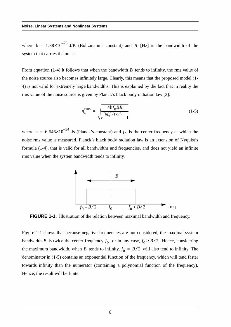
Figure 1-1 shows that because negative frequencies are not considered, the maximal system
bandwidth is twice the center frequency , or in any case, . Hence, considering
the maximum bandwidth, when tends to infinity, will also tend to infinity. The
denominator in (1-5) contains an exponential function of the frequency, which will tend faster
towards infinity than the numerator (containing a polynomial function of the frequency).
Hence, the result will be finite.
FIGURE 1-1. Illustration of the relation between maximal bandwidth and frequency.
k 1.38 23–×10= B
B
nurms 4hf0BR
ehf0( ) kT( )⁄
1–-----------------------------------=
h 6.546 34–×10= f0
freq
B
f0f0 B 2⁄– f0 B 2⁄+
B f0 f0 B 2⁄≥
B f0 B 2⁄=
6
Sources of noise
Nyquist’s formula (1-4) is an approximation of the general black body radiation law (1-5), for
low frequencies and high temperatures. Assuming that , the exponential function in
(1-5) can be approximated by its Taylor series up to the first degree:
(1-6)
Substituting (1-6) into (1-5) yields Nyquist’s formula (1-4).
The power spectral density (PSD) corresponding to a noise source with rms value can
easily be calculated using the formulae (1-4) and (1-5). The noisy resistor can be modelled
through its Thévenin equivalent circuit, consisting of the noise source and a noiseless resistor.
The noisy resistor will transfer a maximal power, if it is connected to a resistor with the same
value R (see Figure 1-2). Note that all results can be extended to impedances instead of
resistances, but one has to keep in mind that only the resistive part of the impedance will
generate the noise. Ideal inductors and capacitors do not generate thermal noise [2].
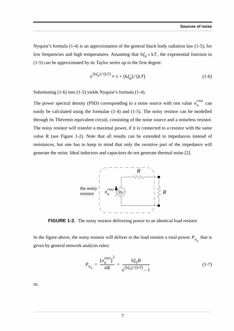
In the figure above, the noisy resistor will deliver to the load resistor a total power that is
given by general network analysis rules:
(1-7)
or,
FIGURE 1-2. The noisy resistor delivering power to an identical load resistor
hf0 kT«
e hf0( ) kT( )⁄ 1 hf0( ) kT( )⁄+≈
nurms
R
Rnurmsthe noisy
resistor
Pnu
Pnu
nurms( )
2
4R------------------
hf0B
e hf0( ) kT( )⁄ 1–-----------------------------------= =
7
Noise, Linear Systems and Nonlinear Systems
(1-8)
when assuming that .
To get the power spectral density, one has to calculate , yielding:
(1-9)
or, again for :
(1-10)
This means that where the approximation is valid, the power spectral density of thermal noise
is constant throughout the whole frequency spectrum, and depends linearly on the absolute
temperature.
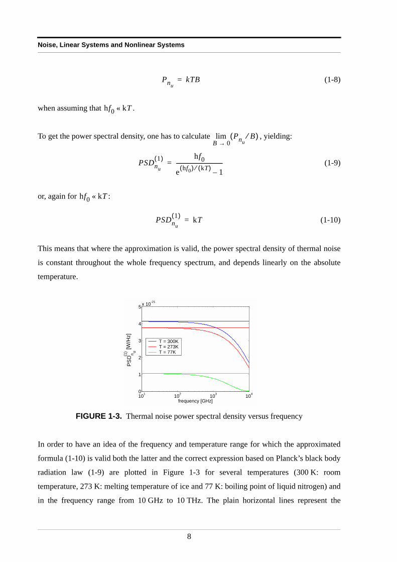
In order to have an idea of the frequency and temperature range for which the approximated
formula (1-10) is valid both the latter and the correct expression based on Planck’s black body
radiation law (1-9) are plotted in Figure 1-3 for several temperatures (300 K: room
temperature, 273 K: melting temperature of ice and 77 K: boiling point of liquid nitrogen) and
in the frequency range from 10 GHz to 10 THz. The plain horizontal lines represent the
FIGURE 1-3. Thermal noise power spectral density versus frequency
PnukTB=
hf0 kT«
PnuB⁄( )
B 0→lim
PSDnu
1( ) hf0e hf0( ) kT( )⁄ 1–-----------------------------------=
hf0 kT«
PSDnu
1( ) kT=
101
102
103
104
0
1
2
3
4
5x 10
-21
frequency [GHz]
T = 300KT = 273KT = 77K
PSD
n u
(1)
[W/H
z]
8
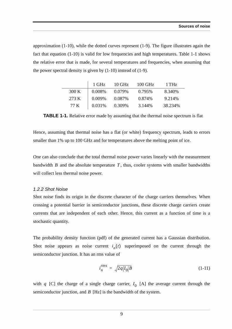
Sources of noise
approximation (1-10), while the dotted curves represent (1-9). The figure illustrates again the
fact that equation (1-10) is valid for low frequencies and high temperatures. Table 1-1 shows
the relative error that is made, for several temperatures and frequencies, when assuming that
the power spectral density is given by (1-10) instead of (1-9).
Hence, assuming that thermal noise has a flat (or white) frequency spectrum, leads to errors
smaller than 1% up to 100 GHz and for temperatures above the melting point of ice.
One can also conclude that the total thermal noise power varies linearly with the measurement
bandwidth and the absolute temperature , thus, cooler systems with smaller bandwidths
will collect less thermal noise power.
1.2.2 Shot NoiseShot noise finds its origin in the discrete character of the charge carriers themselves. When
crossing a potential barrier in semiconductor junctions, these discrete charge carriers create
currents that are independent of each other. Hence, this current as a function of time is a
stochastic quantity.
The probability density function (pdf) of the generated current has a Gaussian distribution.
Shot noise appears as noise current superimposed on the current through the
semiconductor junction. It has an rms value of
(1-11)
with [C] the charge of a single charge carrier, [A] the average current through the
semiconductor junction, and [Hz] is the bandwidth of the system.
1 GHz 10 GHz 100 GHz 1 THz300 K 0.008% 0.079% 0.795% 8.340%273 K 0.009% 0.087% 0.874% 9.214%77 K 0.031% 0.309% 3.144% 38.234%
TABLE 1-1. Relative error made by assuming that the thermal noise spectrum is flat
B T
in t( )
inrms 2q I0 B=
q I0
B
9

Noise, Linear Systems and Nonlinear Systems
1.2.3 Other noise sourcesIt is clear that there are also several other stochastic processes that can cause the generation of
noise. A number of them will be briefly mentioned in what follows.
A. Flicker NoiseIn many components, the noise seems to contain an extra contribution whose power spectral
density is inverse proportional to the frequency. Hence, Flicker noise is also often called
noise. At high frequencies, this noise contribution is insignificant compared to the thermal
noise. The frequency at which thermal noise and flicker noise have the same power spectral
density varies from several Hz to several MHz, depending on the type of electrical component.
B. Plasma noiseThis type of noise is caused by the random motion of charges in ionized gasses, such as the
ionosphere or sparkling electrical contacts.
1 f⁄
10

Linear time invariant systems
1.3 Linear time invariant systemsIn the following section, the definition and properties of a linear time invariant (LTI) system
will be given.
1.3.1 Definition of a linear time invariant system
Definition 1.2
A linear time invariant system is a system whose properties do not change with time, and that
obeys the superposition principle. In other words, a linear combination of input signals must
result in the same linear combination of output signals, and this has to be independent of the
moment at which the experiment is performed.
Or,
(1-12)
where represents the set of the real numbers, and represents the set of all the functions
dependent of the time , whose range is .
1.3.2 Spectral properties of a LTI systemSince the Fourier Transform is a linear operator, the response spectrum of a LTI system
to an input spectrum can be written as (see Appendix 1.B):
(1-13)
where represents the transfer function of the LTI system. The response spectrum
is only the multiplication of the input spectrum with the transfer function . It only
contains energy at those frequency intervals where the input spectrum contains energy.
H is the operator of a linear system ⇔
ci R ui t( ) F :H ui t( )[ ] yi t( )= H ciui t( )
i 1=
N
∑⇒ ciH ui t( )[ ]
i 1=
N
∑ ciyi t( )
i 1=
N
∑= =∈∀,∈∀
R Ft R
Y ω( )
U ω( )
Y ω( ) U ω( ) H ω( )⋅=
H ω( ) Y ω( )
U ω( ) H ω( )
U ω( )
11
Noise, Linear Systems and Nonlinear Systems
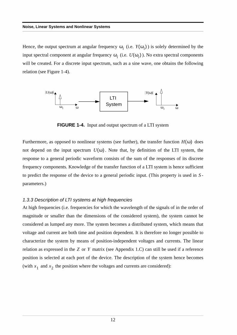
Hence, the output spectrum at angular frequency (i.e. ) is solely determined by the
input spectral component at angular frequency (i.e. ). No extra spectral components
will be created. For a discrete input spectrum, such as a sine wave, one obtains the following
relation (see Figure 1-4).
Furthermore, as opposed to nonlinear systems (see further), the transfer function does
not depend on the input spectrum . Note that, by definition of the LTI system, the
response to a general periodic waveform consists of the sum of the responses of its discrete
frequency components. Knowledge of the transfer function of a LTI system is hence sufficient
to predict the response of the device to a general periodic input. (This property is used in -
parameters.)
1.3.3 Description of LTI systems at high frequenciesAt high frequencies (i.e. frequencies for which the wavelength of the signals of in the order of
magnitude or smaller than the dimensions of the considered system), the system cannot be
considered as lumped any more. The system becomes a distributed system, which means that
voltage and current are both time and position dependent. It is therefore no longer possible to
characterize the system by means of position-independent voltages and currents. The linear
relation as expressed in the or matrix (see Appendix 1.C) can still be used if a reference
position is selected at each port of the device. The description of the system hence becomes
(with and the position where the voltages and currents are considered):
FIGURE 1-4. Input and output spectrum of a LTI system
ωi Y ωi( )
ωi U ωi( )
LTISystem
Y ω( )
ω
U ω( )
ωω1 ω1
H ω( )
U ω( )
S
Z Y
x1 x2
12
Linear time invariant systems
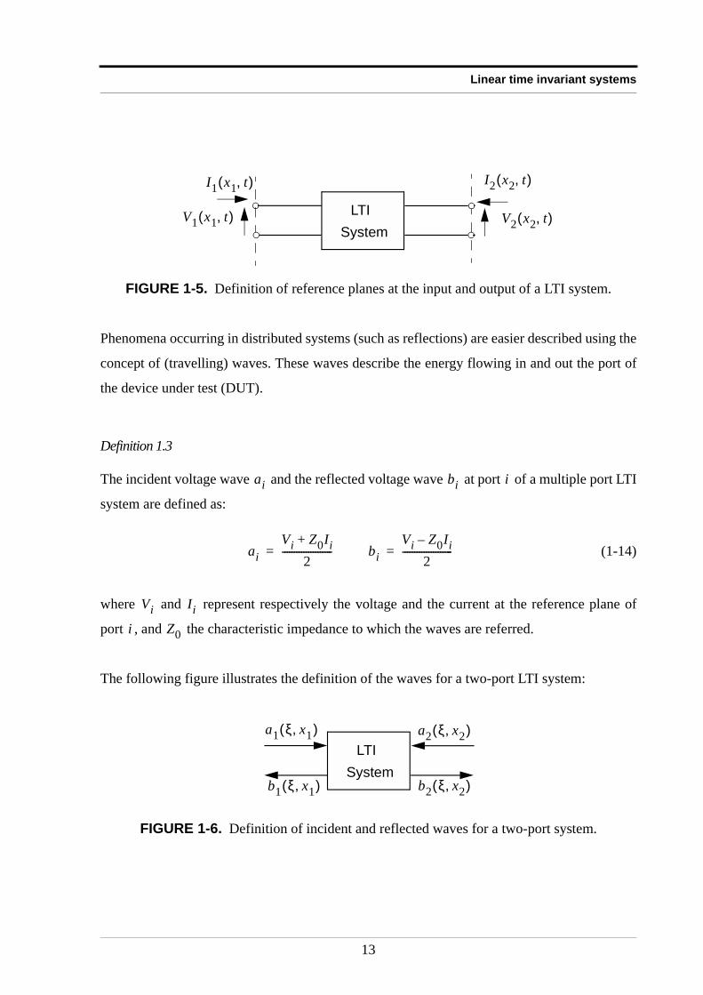
Phenomena occurring in distributed systems (such as reflections) are easier described using the
concept of (travelling) waves. These waves describe the energy flowing in and out the port of
the device under test (DUT).
Definition 1.3
The incident voltage wave and the reflected voltage wave at port of a multiple port LTI
system are defined as:
(1-14)
where and represent respectively the voltage and the current at the reference plane of
port , and the characteristic impedance to which the waves are referred.
The following figure illustrates the definition of the waves for a two-port LTI system:
FIGURE 1-5. Definition of reference planes at the input and output of a LTI system.
FIGURE 1-6. Definition of incident and reflected waves for a two-port system.
LTISystem
V1 x1 t,( ) V2 x2 t,( )
I1 x1 t,( ) I2 x2 t,( )
ai bi i
aiVi Z0Ii+
2---------------------= bi
Vi Z0Ii–2
---------------------=
Vi Ii
i Z0
LTISystem
a1 ξ x1,( ) a2 ξ x2,( )
b1 ξ x1,( ) b2 ξ x2,( )
13
Noise, Linear Systems and Nonlinear Systems
The waves are a function of the independent variable , which represents either time or
frequency, and of the position.
Since the waves and are obtained as a linear combination of the voltages and
currents at the reference ports (see (1-14)), the relation between the incident and
reflected waves is also a linear combination of the form:
(1-15)
The matrix still fully describes the DUT, since it is only a linear transformation of the -
matrix. The matrix is the well-known -parameter representation, which is defined as
follows:
Definition 1.4
The -matrix of a LTI system with ports is a complex n-by-n matrix whose elements are
defined as follows [36]:
(1-16)
Thus the -matrix fully describes a LTI system at high frequencies.
ξ
ai bi Vi xi ξ,( )
Ii xi ξ,( )
b1…bn
Sa1…an
⋅=
S Z
S S
S n
Si j,biaj----
m j:am≠∀ 0=
=
S
14
Noise and linear time invariant systems
1.4 Noise and linear time invariant systemsFirst, a model for a noisy LTI system is introduced. Based on this model, the classical method
used to quantify the noise behavior of a noisy LTI system is built up. Care is taken to clearly
state and explain all the required assumptions. This can then be used as a sound basis for
extension towards nonlinear systems.
1.4.1 The presence of noise in a LTI systemSince any practical electronic system contains electrical components, such as resistors or
semiconductor devices, the output signal of the system will contain noise generated in these
components. As seen in section 1.2, the resistors will mainly create Johnson noise, while the
semiconductor devices will mainly be responsible for the shot noise. Other sources can also
contribute to the noise present at the output of the system. Note that, according to the definition
of a LTI system (Definition 1.2), a LTI system must be noiseless. Since a LTI system has no
contribution to the noise of its own, it can only process the input noise as an additional signal
source. From (1-12), it follows that if the input signal equals zero, the output signal
must also be zero. In practice, it is clear that even when no input signal is present, the noise
sources in the system still exist, and noise will be present at the output of the system. Hence,
the LTI model has to be enhanced for noise.
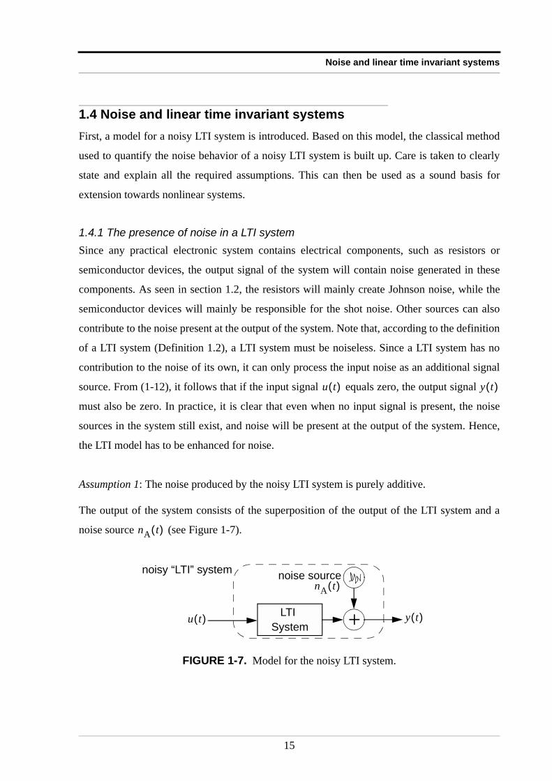
Assumption 1: The noise produced by the noisy LTI system is purely additive.
The output of the system consists of the superposition of the output of the LTI system and a
noise source (see Figure 1-7).
FIGURE 1-7. Model for the noisy LTI system.
u t( ) y t( )
nA t( )
LTISystem +
noise sourcenoisy “LTI” system
y t( )u t( )
nA t( )
15
Noise, Linear Systems and Nonlinear Systems
Assumption 2: There is a perfect impedance match at the input and the output of the system, i.e.
The input and output impedances of the system are equal to .
By assumption 1, the output of the system can be written as:
(1-17)
where represents the noise superimposed on the output of the LTI system.
Some additional hypotheses are made about the noise source :
1. Stationarity of the noise: The properties of the noise source remain constant in time.
Furthermore, disturbances (such as e.g. a noise spark due to lightning) are not taken into
account as stated previously.
2. The noise source is statistically independent of the input signal . Of course,
can depend on the bias current of the system (e.g. in the case of a transistor). It is
clear that a larger DC bias current can yield more thermal noise (due to the warming up
of the resistors) and shot noise (whose rms current is directly proportional to the square
root of the DC current through the device). However, the bias current of the system will
be considered as a constant property of the system, and not as an extra input signal.
Since the noise source is not correlated with the input signal, the cross-correlation between
signal and noise is zero, i.e. . This implies that (1-17) can be rewritten
in terms of power spectral densities as (see Appendix 1.D):
(1-18)
where , and represent respectively the (double sided)
power spectral densities of the output signal , the input signal and the noise added by
the noisy linear system .
Z0
y t( ) h t( )*u t( ) nA t( )+=
nA t( )
nA t( )
nA t( ) u t( )
nA t( )
E u t( )nA t τ+( ) 0=
PSDy2( ) ω( ) H ω( ) 2PSDu
2( ) ω( ) PSDnA
2( ) ω( )+=
PSDy2( ) ω( ) PSDu
2( ) ω( ) PSDnA
2( ) ω( )
y t( ) u t( )
nA t( )
16
Noise and linear time invariant systems
1.4.2 Noise figureIn order to quantify the power spectrum of the noise source present in the noisy linear system,
one has to define a figure of merit. As stated in the introduction of this chapter, a figure of
merit that is given in terms of the deterioration of the signal-to-noise ratio (SNR) will be the
best choice.
Definition 1.5
The Noise Figure (NF) of a noisy linear system quantifies the system-induced degradation of
the signal-to-noise ratio between the input and the output of the device. It is the ratio of the
signal-to-noise ratio at the input of the system to the signal-to-noise ratio at the output of the
system, when the noise component of the input signal consists of thermal noise generated at
290 K, and the system is ideally matched at the input and output [6].
(1-19)
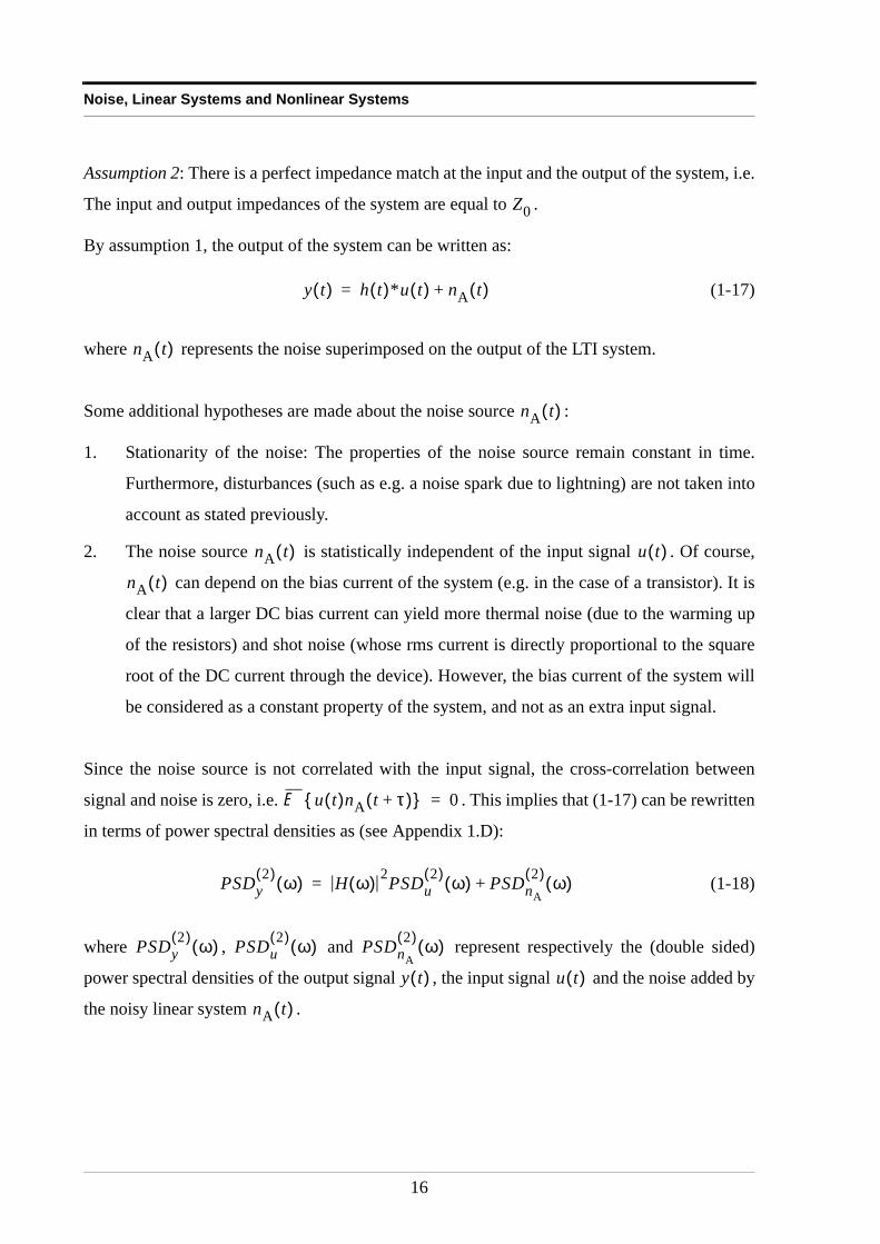
The noise figure of a noisy LTI system (as shown in Figure 1-8) will be determined next.
No prerequisites are made about the properties of the noiseless input signal itself, since
for LTI systems, it will be shown that the noise figure is independent of the properties of .
The thermal noise power spectral density (which is constant over the frequency, see section
1.2.1) at 290 K can easily be calculated using (1-10):
FIGURE 1-8. Signal and noise applied to a noisy LTI system
NFSNRinSNRout------------------
T0 290K=
=
u0 t( )
nu t( )u t( )
Z0
Z0
LTISystem +
nA t( )
noisy LTI system
u0 t( )
u0 t( )
17
Noise, Linear Systems and Nonlinear Systems
1 (1-20)
The noise power spectral density at the output of the system at angular frequency can be
written as: . Hence, the noise figure can be calculated using its
definition (1-19):
(1-21)
Note that the noise figure cannot be smaller than one. In the limit case where it is equal to one,
the system does not produce any added noise, i.e. . Hence, the signal-to-noise
ratio can only deteriorate, and in the best case (when the system is noiseless) it remains
constant. Note also that the noise figure is independent of the input signal , it depends only
on the transfer function of the noisy LTI system.
1.4.3 Input noise temperature dependenceIf the input noise source is at absolute temperature , instead of , but the temperature of all
the other noise sources in the system remains unchanged, the signal-to-noise ratio degradation
can easily be calculated (see Appendix 1.F) as:
(1-22)
1.4.4 Noise Figure measurements concepts: the Y-factor techniqueThe most straightforward approach to measure the noise figure would be to measure the signal
and noise power spectral densities at the input and output of the system and to compare them
with each other. This is an impossible approach, because it would require measurement
1. dBm means dB as referred to a standard power of 1 mW. A value of W corresponds to.
PSDnu
1( )
T0 290K=kT0 4 21–×10 W Hz⁄ 174dBm Hz⁄–= = =
ξ10 ξW 1mW⁄( )log⋅
ω
H ω( ) 2 kT0⋅ PSDnA
1( ) ω( )+
NF ω( )
2 U ω( ) 2 Z0⁄kT0
--------------------------------
2 H ω( ) 2 U ω( ) 2 Z0⁄
H ω( ) 2kT0 PSDnA
1( ) ω( )+--------------------------------------------------------------- --------------------------------------------------------------------- 1
PSDnA
1( ) ω( )
H ω( ) 2 kT0⋅---------------------------------+= =
PSDnA
1( ) ω( ) 0=
u t( )
T T0
SNRinSNRout------------------
T
1 NF 1–( )T0T------+=
18
Noise and linear time invariant systems
equipment with an extremely large dynamic range to measure both the signal and the noise.
Moreover, the measurement itself would add so much noise that the measured noise power
would be drown in the noise of the measurement system.
Since it is impossible to measure directly the signal-to-noise ratio in order to determine the
noise figure, an indirect measurement method is used. Suppose that only noise is fed at the
input of the system (hence ). This noise is Johnson noise generated by
a resistor whose absolute temperature is variable. The power spectral density of the signal at
the input of the system will then be a flat spectrum, whose magnitude is temperature dependent
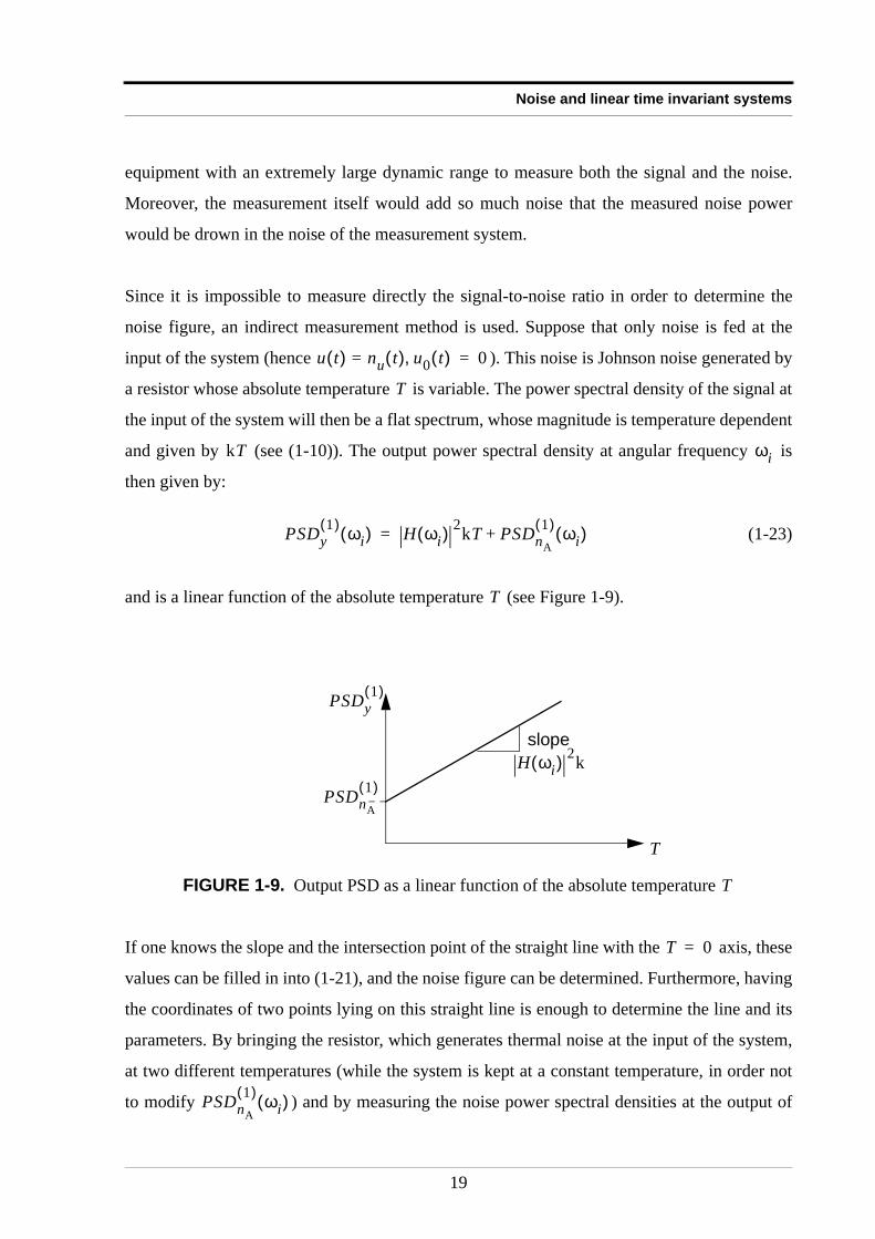
and given by (see (1-10)). The output power spectral density at angular frequency is
then given by:
(1-23)
and is a linear function of the absolute temperature (see Figure 1-9).
If one knows the slope and the intersection point of the straight line with the axis, these
values can be filled in into (1-21), and the noise figure can be determined. Furthermore, having
the coordinates of two points lying on this straight line is enough to determine the line and its
parameters. By bringing the resistor, which generates thermal noise at the input of the system,
at two different temperatures (while the system is kept at a constant temperature, in order not
to modify ) and by measuring the noise power spectral densities at the output of
FIGURE 1-9. Output PSD as a linear function of the absolute temperature
u t( ) nu t( )= u0 t( ), 0=
T
kT ωi
PSDy1( ) ωi( ) H ωi( ) 2kT PSDnA
1( ) ωi( )+=
T
T
PSDy1( )
PSDnA
1( )H ωi( ) 2k
slope
T
T 0=
PSDnA
1( ) ωi( )
19
Noise, Linear Systems and Nonlinear Systems
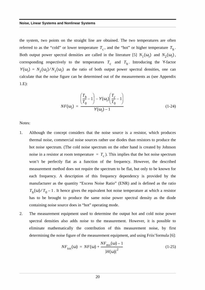
the system, two points on the straight line are obtained. The two temperatures are often
referred to as the “cold” or lower temperature , and the “hot” or higher temperature .
Both output power spectral densities are called in the literature [5] and ,
corresponding respectively to the temperatures and . Introducing the Y-factor
as the ratio of both output power spectral densities, one can
calculate that the noise figure can be determined out of the measurements as (see Appendix
1.E):
(1-24)
Notes:
1. Although the concept considers that the noise source is a resistor, which produces
thermal noise, commercial noise sources rather use diodes than resistors to produce the
hot noise spectrum. (The cold noise spectrum on the other hand is created by Johnson
noise in a resistor at room temperature ). This implies that the hot noise spectrum
won’t be perfectly flat as a function of the frequency. However, the described
measurement method does not require the spectrum to be flat, but only to be known for
each frequency. A description of this frequency dependency is provided by the
manufacturer as the quantity “Excess Noise Ratio” (ENR) and is defined as the ratio
. It hence gives the equivalent hot noise temperature at which a resistor
has to be brought to produce the same noise power spectral density as the diode
containing noise source does in “hot” operating mode.
2. The measurement equipment used to determine the output hot and cold noise power
spectral densities also adds noise to the measurement. However, it is possible to
eliminate mathematically the contribution of this measurement noise, by first
determining the noise figure of the measurement equipment, and using Friis’formula [6]:
(1-25)
Tc Th
N1 ωi( ) N2 ωi( )
Tc Th
Y ωi( ) N2 ωi( ) N1 ωi( )⁄=
NF ωi( )
ThT0------ 1–
Y ωi( )TcT0------ 1–
–
Y ωi( ) 1–--------------------------------------------------------------=
Tc=
Th ω( ) T0⁄ 1–
NFtot ω( ) NF ω( )NFms ω( ) 1–
H ω( ) 2--------------------------------+=
20
Noise and linear time invariant systems
, and represent respectively the noise figures of the DUT
plus the measurement system, the DUT alone and the measurement system alone.
represents the transfer function of the DUT (see Appendix 1.G).
1.4.5 Noise temperatureAn alternative quantity that describes the noise power spectral density, generated by a device,
is the noise temperature.
Definition 1.6
A device has a noise temperature , when it generates noise with a power spectral density
.
Hence, the noise figure can indeed be defined as the ratio of the signal-to-noise ratio at the
input of a device to the signal-to-noise ratio at the output of that device, when the device is
excited with a generator that has a frequency independent noise temperature of 290 K. If the
noise temperature of the source impedance differs too much from 290 K (e.g. for satellite
communications where at unclouded sky), the noise figure is not such a practical
quantity to describe the signal-to-noise evolution through the system. In such cases, it is more
convenient to use the concepts “operational noise temperature” and “effective noise
temperature” .
A. Operational noise temperatureThe operational noise temperature is defined as the absolute temperature that has to be
assigned to the source impedance, in order to get a noise power spectral density at the output of
the noiseless LTI system equal to the noise power spectral density at the output of the noisy
NFtot ω( ) NF ω( ) NFms ω( )
H ω( )
Tn ω( )
PSDn1( ) ω( ) kTn ω( )=
Tn 10K≈
Top
Te
Top ω( )
21
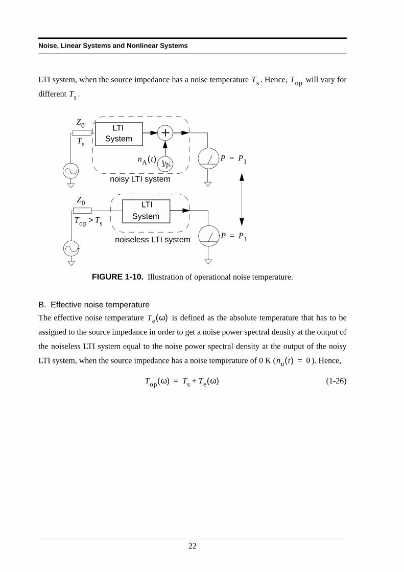
Noise, Linear Systems and Nonlinear Systems
LTI system, when the source impedance has a noise temperature . Hence, will vary for
different .
B. Effective noise temperatureThe effective noise temperature is defined as the absolute temperature that has to be
assigned to the source impedance in order to get a noise power spectral density at the output of
the noiseless LTI system equal to the noise power spectral density at the output of the noisy
LTI system, when the source impedance has a noise temperature of 0 K ( ). Hence,
(1-26)
FIGURE 1-10. Illustration of operational noise temperature.
Ts Top
Ts
Z0 LTISystem +
nA t( )
noisy LTI system
Ts
P P1=
Z0 LTISystem
noiseless LTI system
Top Ts>
P P1=
Te ω( )
nu t( ) 0=
Top ω( ) Ts Te ω( )+=
22
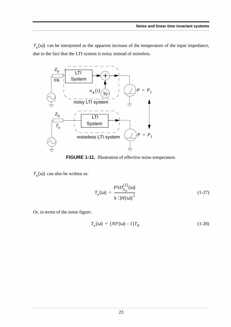
Noise and linear time invariant systems
can be interpreted as the apparent increase of the temperature of the input impedance,
due to the fact that the LTI system is noisy instead of noiseless.
can also be written as:
(1-27)
Or, in terms of the noise figure:
(1-28)
FIGURE 1-11. Illustration of effective noise temperature.
Te ω( )
Z0 LTISystem +
nA t( )
noisy LTI system
0K
P P1=
Z0 LTISystem
noiseless LTI system
Te
P P1=
Te ω( )
Te ω( )PSDnA
1( ) ω( )
k H ω( ) 2⋅---------------------------=
Te ω( ) NF ω( ) 1–( )T0=
23
Noise, Linear Systems and Nonlinear Systems
1.5 Nonlinear systemsJust as for LTI systems, one has to know the definition and the properties of the subclass of
systems that will be used when dealing with nonlinear systems. The subclass of systems that is
considered in this text is introduced here, and is selected such as to allow a gentle departure
from the linear behavior. This allows consideration of systems that are close to be linear. It is
then a good engineering practice to extend the methods explained for linear system noise
characterization to cope with this extended class of systems that enclose the LTI systems. The
importance of knowing the phase relation between spectral components at different
frequencies is also pinpointed.
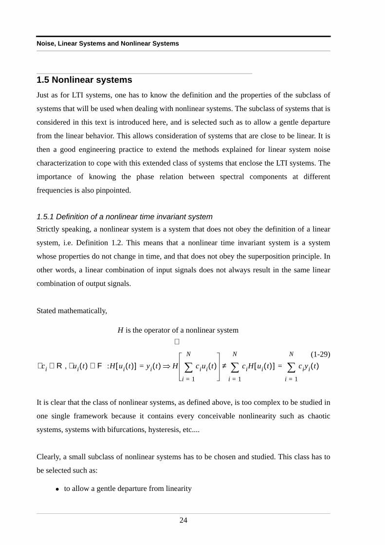
1.5.1 Definition of a nonlinear time invariant systemStrictly speaking, a nonlinear system is a system that does not obey the definition of a linear
system, i.e. Definition 1.2. This means that a nonlinear time invariant system is a system
whose properties do not change in time, and that does not obey the superposition principle. In
other words, a linear combination of input signals does not always result in the same linear
combination of output signals.
Stated mathematically,
(1-29)
It is clear that the class of nonlinear systems, as defined above, is too complex to be studied in
one single framework because it contains every conceivable nonlinearity such as chaotic
systems, systems with bifurcations, hysteresis, etc....
Clearly, a small subclass of nonlinear systems has to be chosen and studied. This class has to
be selected such as:
• to allow a gentle departure from linearity
H is the operator of a nonlinear system ⇔
c∃ i R ui t( ) F :H ui t( )[ ] yi t( )= H ciui t( )
i 1=
N
∑⇒ ciH ui t( )[ ]
i 1=
N
∑≠ ciyi t( )
i 1=
N
∑=∈∃,∈
24
Nonlinear systems
• to include linear systems as a special case
• to describe the behavior of many practical nonlinear circuits
• to have a suitable, simple mathematical model to allow design and
analysis
The choice falls on the subclass that can be tagged as “NICE” systems, which is an extension
of the Volterra systems.
Definition 1.7
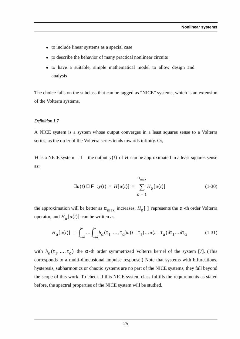
A NICE system is a system whose output converges in a least squares sense to a Volterra
series, as the order of the Volterra series tends towards infinity. Or,
is a NICE system the output of can be approximated in a least squares sense
as:
(1-30)
the approximation will be better as increases. represents the -th order Volterra
operator, and can be written as:
(1-31)
with the -th order symmetrized Volterra kernel of the system [7]. (This
corresponds to a multi-dimensional impulse response.) Note that systems with bifurcations,
hysteresis, subharmonics or chaotic systems are no part of the NICE systems, they fall beyond
the scope of this work. To check if this NICE system class fulfills the requirements as stated
before, the spectral properties of the NICE system will be studied.
H ⇔ y t( ) H
u∀ t( ) F :y t( )∈ H u t( )[ ] Hα u t( )[ ]
α 1=
αmax
∑= =
αmax Hα [ ] α
Hα u t( )[ ]
Hα u t( )[ ] …∞–
∞∫ hα τ1 … τα, ,( )u t τ1–( )…u t τα–( ) τ1d … ταd
∞–
∞∫=
hα τ1 … τα, ,( ) α
25
Noise, Linear Systems and Nonlinear Systems
Note that the definition does not state that the output of the NICE system equals a Volterra
series. It only tells that the NICE system output can be approximated in a least squares sense as
a Volterra series. Hence, Volterra systems are a subset of the NICE systems. A similar
reasoning is the fact that a function can be approximated in least squares sense as a
polynomial. The Taylor series expansion is a special polynomial approximation of a function,
that uniformly converges to the given function within its convergence circle.
Note also that, NICE systems can also be defined as systems that convert a periodic input
signal to a periodic output signal, with the same period.
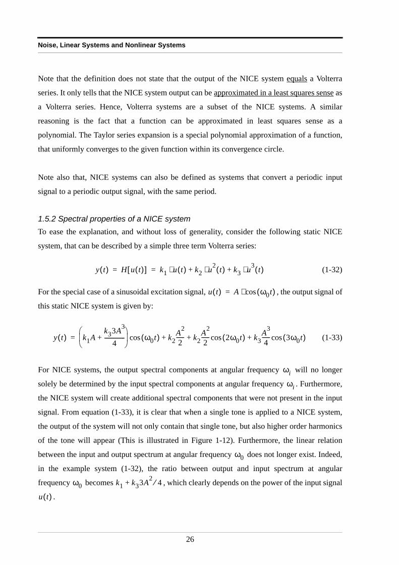
1.5.2 Spectral properties of a NICE systemTo ease the explanation, and without loss of generality, consider the following static NICE
system, that can be described by a simple three term Volterra series:
(1-32)
For the special case of a sinusoidal excitation signal, , the output signal of
this static NICE system is given by:
(1-33)
For NICE systems, the output spectral components at angular frequency will no longer
solely be determined by the input spectral components at angular frequency . Furthermore,
the NICE system will create additional spectral components that were not present in the input
signal. From equation (1-33), it is clear that when a single tone is applied to a NICE system,
the output of the system will not only contain that single tone, but also higher order harmonics
of the tone will appear (This is illustrated in Figure 1-12). Furthermore, the linear relation
between the input and output spectrum at angular frequency does not longer exist. Indeed,
in the example system (1-32), the ratio between output and input spectrum at angular
frequency becomes , which clearly depends on the power of the input signal
.
y t( ) H u t( )[ ] k1 u t( )⋅ k2 u2 t( )⋅ k3 u3 t( )⋅+ += =
u t( ) A ω0t( )cos⋅=
y t( ) k1Ak33A3
4---------------+
ω0t( )cos k2A2
2------ k2
A2
2------ 2ω0t( )cos k3
A3
4------ 3ω0t( )cos+ + +=
ωi
ωi
ω0
ω0 k1 k33A2 4⁄+
u t( )
26
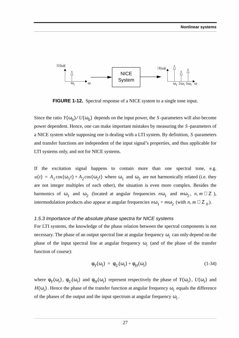
Nonlinear systems
Since the ratio depends on the input power, the -parameters will also become
power dependent. Hence, one can make important mistakes by measuring the -parameters of
a NICE system while supposing one is dealing with a LTI system. By definition, -parameters
and transfer functions are independent of the input signal’s properties, and thus applicable for
LTI systems only, and not for NICE systems.
If the excitation signal happens to contain more than one spectral tone, e.g.
where and are not harmonically related (i.e. they
are not integer multiples of each other), the situation is even more complex. Besides the
harmonics of and (located at angular frequencies and , ),
intermodulation products also appear at angular frequencies (with ).
1.5.3 Importance of the absolute phase spectra for NICE systemsFor LTI systems, the knowledge of the phase relation between the spectral components is not
necessary. The phase of an output spectral line at angular frequency can only depend on the
phase of the input spectral line at angular frequency (and of the phase of the transfer
function of course):
(1-34)
where , and represent respectively the phase of , and
. Hence the phase of the transfer function at angular frequency equals the difference
of the phases of the output and the input spectrum at angular frequency .
FIGURE 1-12. Spectral response of a NICE system to a single tone input.
NICESystem
Y ω( )
ω
U ω( )
ωω1 ω1 2ω1 3ω1
Y ω0( ) U ω0( )⁄ S
S
S
u t( ) A1 ω1t( )cos A2 ω2t( )cos+= ω1 ω2
ω1 ω2 nω1 mω2 n m Z∈,
nω1 mω2+ n m Z0∈,
ωi
ωi
φY ωi( ) φU ωi( ) φH ωi( )+=
φY ωi( ) φU ωi( ) φH ωi( ) Y ωi( ) U ωi( )
H ωi( ) ωi
ωi
27
Noise, Linear Systems and Nonlinear Systems
For NICE systems however, if the input signal is a sine wave the output
signal can be e.g.
(1-35)
where , and are factors that can be function of . , and are the phases of
the output spectrum at angular frequencies , and compared to the phase of the
input spectrum at angular frequency . In this case, it is important to know the phases ,
and , otherwise the output time waveform cannot be determined. Since a
nonlinearity essentially operates on the instantaneous value of the time signal, not much can be
said about a DUT’s nonlinear behavior if this time waveform is unknown.
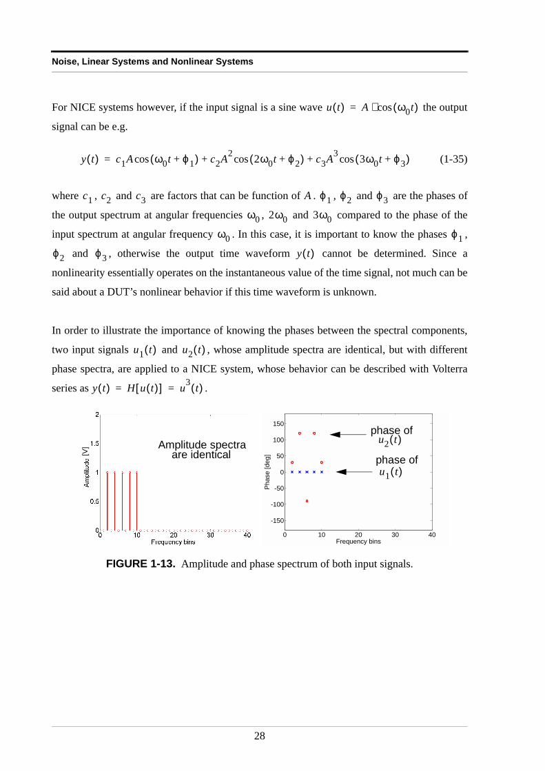
In order to illustrate the importance of knowing the phases between the spectral components,
two input signals and , whose amplitude spectra are identical, but with different
phase spectra, are applied to a NICE system, whose behavior can be described with Volterra
series as .
FIGURE 1-13. Amplitude and phase spectrum of both input signals.
u t( ) A ω0t( )cos⋅=
y t( ) c1A ω0t ϕ1+( )cos c2A2 2ω0t ϕ2+( )cos c3A3 3ω0t ϕ3+( )cos+ +=
c1 c2 c3 A ϕ1 ϕ2 ϕ3
ω0 2ω0 3ω0
ω0 ϕ1
ϕ2 ϕ3 y t( )
u1 t( ) u2 t( )
y t( ) H u t( )[ ] u3 t( )= =
0 10 20 30 40
-150
-100
-50
0
50
100
150
Frequency bins
Phase [deg]
u1 t( )
u2 t( )phase of
phase ofAmplitude spectra
are identical[V]
28
Nonlinear systems
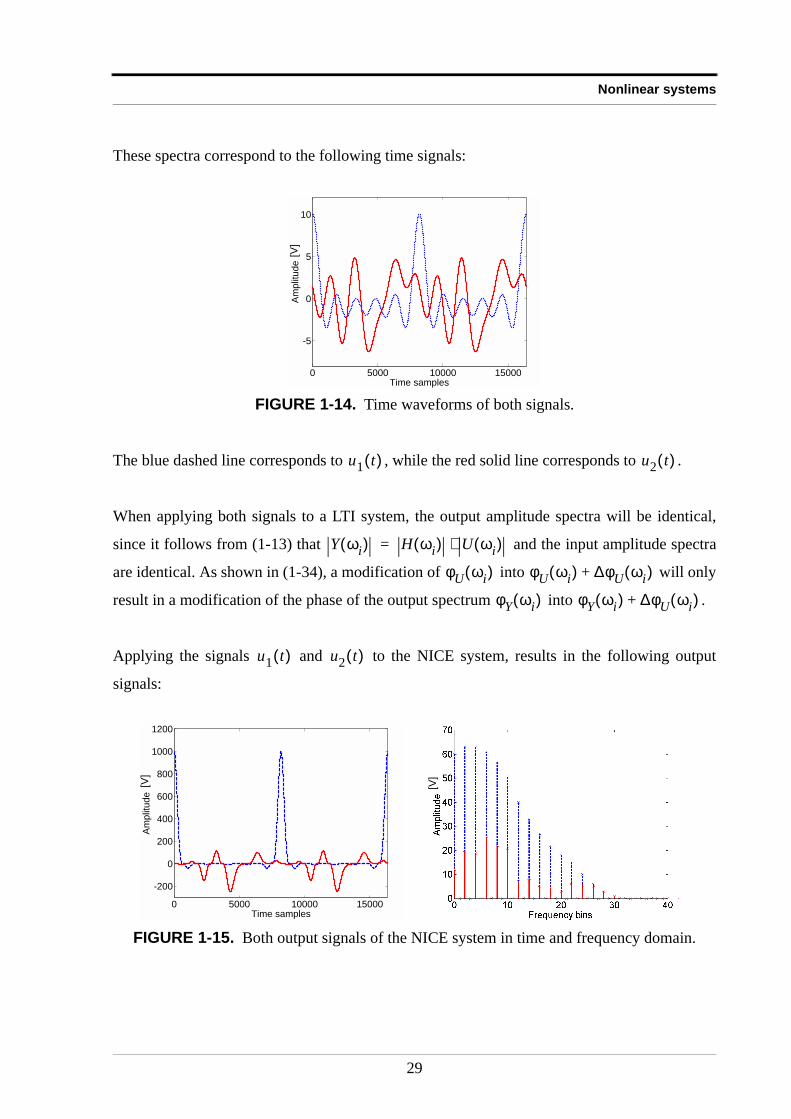
These spectra correspond to the following time signals:
The blue dashed line corresponds to , while the red solid line corresponds to .
When applying both signals to a LTI system, the output amplitude spectra will be identical,
since it follows from (1-13) that and the input amplitude spectra
are identical. As shown in (1-34), a modification of into will only
result in a modification of the phase of the output spectrum into .
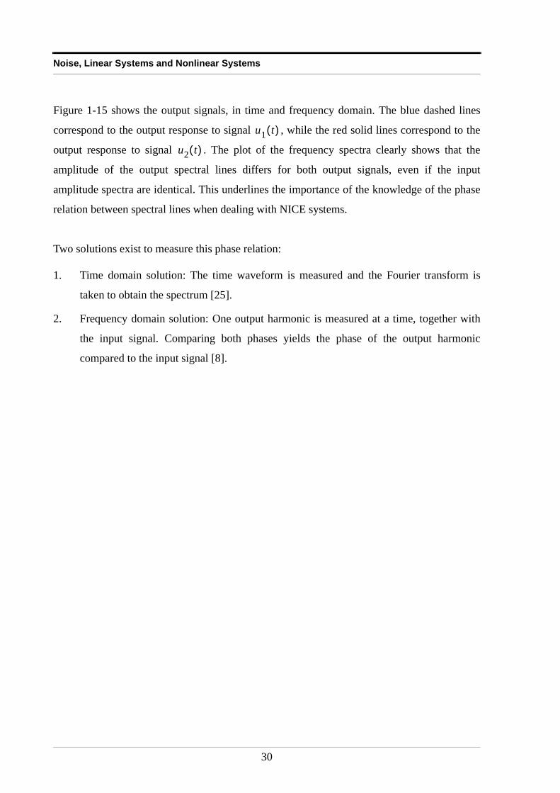
Applying the signals and to the NICE system, results in the following output
signals:
FIGURE 1-14. Time waveforms of both signals.
FIGURE 1-15. Both output signals of the NICE system in time and frequency domain.
0 5000 10000 15000
-5
0
5
10
Time samples
Am
plit
ude
[V]
u1 t( ) u2 t( )
Y ωi( ) H ωi( ) U ωi( )⋅=
φU ωi( ) φU ωi( ) ∆φU ωi( )+
φY ωi( ) φY ωi( ) ∆φU ωi( )+
u1 t( ) u2 t( )
0 5000 10000 15000
-200
0
200
400
600
800
1000
1200
Time samples
Am
plit
ude
[V]
[V]
29
Noise, Linear Systems and Nonlinear Systems
Figure 1-15 shows the output signals, in time and frequency domain. The blue dashed lines
correspond to the output response to signal , while the red solid lines correspond to the
output response to signal . The plot of the frequency spectra clearly shows that the
amplitude of the output spectral lines differs for both output signals, even if the input
amplitude spectra are identical. This underlines the importance of the knowledge of the phase
relation between spectral lines when dealing with NICE systems.
Two solutions exist to measure this phase relation:
1. Time domain solution: The time waveform is measured and the Fourier transform is
taken to obtain the spectrum [25].
2. Frequency domain solution: One output harmonic is measured at a time, together with
the input signal. Comparing both phases yields the phase of the output harmonic
compared to the input signal [8].
u1 t( )
u2 t( )
30
Noise and nonlinear systems
1.6 Noise and nonlinear systemsKnowing the noise power spectral density at the output of a NICE system is as important as
knowing the signal power spectral density. The reason therefore is quite obvious: in many
applications the signal-to-noise ratio is a very critical parameter that has to be maximized.
Using an identical approach as earlier described for the noisy LTI system, a noisy NICE system
is introduced. Next, it is shown that the output spectrum of a noisy NICE system, excited by
the sum of signal and noise can be divided into four disjunct sets of terms, according to the
behavior of these terms. Based on this classification, different setups are introduced.
1.6.1 The presence of noise in a NICE systemLike LTI systems, real-world NICE systems also consist of electrical components, including
resistors or semiconductor devices. Again, noise is generated in the electrical components of
the NICE system, and appears at the output of the system. Like a LTI system, a NICE system
(Definition 1.7), must be noiseless by definition. (1-30) and (1-31) show that for a zero input
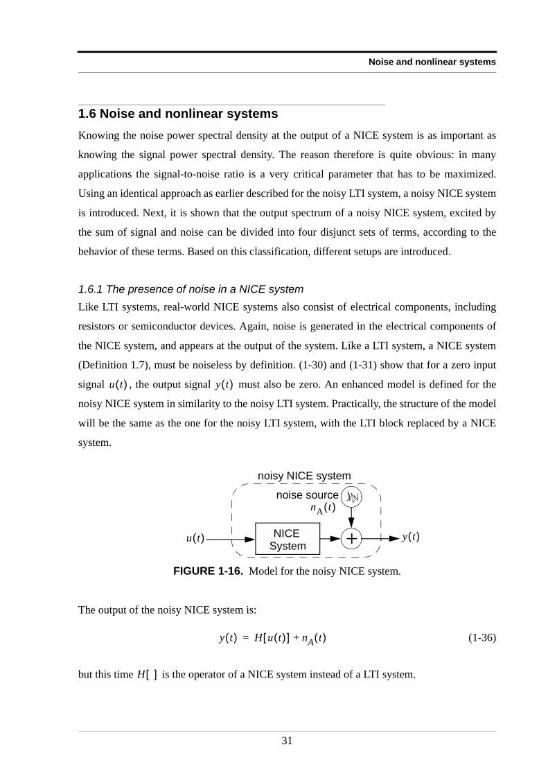
signal , the output signal must also be zero. An enhanced model is defined for the
noisy NICE system in similarity to the noisy LTI system. Practically, the structure of the model
will be the same as the one for the noisy LTI system, with the LTI block replaced by a NICE
system.
The output of the noisy NICE system is:
(1-36)
but this time is the operator of a NICE system instead of a LTI system.
FIGURE 1-16. Model for the noisy NICE system.
u t( ) y t( )
NICESystem +
noise source
noisy NICE system
y t( )u t( )
nA t( )
y t( ) H u t( )[ ] nA t( )+=
H [ ]
31
Noise, Linear Systems and Nonlinear Systems
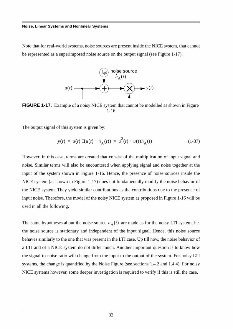
Note that for real-world systems, noise sources are present inside the NICE system, that cannot
be represented as a superimposed noise source on the output signal (see Figure 1-17).
The output signal of this system is given by:
(1-37)
However, in this case, terms are created that consist of the multiplication of input signal and
noise. Similar terms will also be encountered when applying signal and noise together at the
input of the system shown in Figure 1-16. Hence, the presence of noise sources inside the
NICE system (as shown in Figure 1-17) does not fundamentally modify the noise behavior of
the NICE system. They yield similar contributions as the contributions due to the presence of
input noise. Therefore, the model of the noisy NICE system as proposed in Figure 1-16 will be
used in all the following.
The same hypotheses about the noise source are made as for the noisy LTI system, i.e.
the noise source is stationary and independent of the input signal. Hence, this noise source
behaves similarly to the one that was present in the LTI case. Up till now, the noise behavior of
a LTI and of a NICE system do not differ much. Another important question is to know how
the signal-to-noise ratio will change from the input to the output of the system. For noisy LTI
systems, the change is quantified by the Noise Figure (see sections 1.4.2 and 1.4.4). For noisy
NICE systems however, some deeper investigation is required to verify if this is still the case.
FIGURE 1-17. Example of a noisy NICE system that cannot be modelled as shown in Figure 1-16
+
noise sourcenA t( )
u t( ) y t( )X
y t( ) u t( ) u t( ) nA t( )+( )⋅ u2 t( ) u t( )nA t( )+= =
nA t( )
32
Noise and nonlinear systems
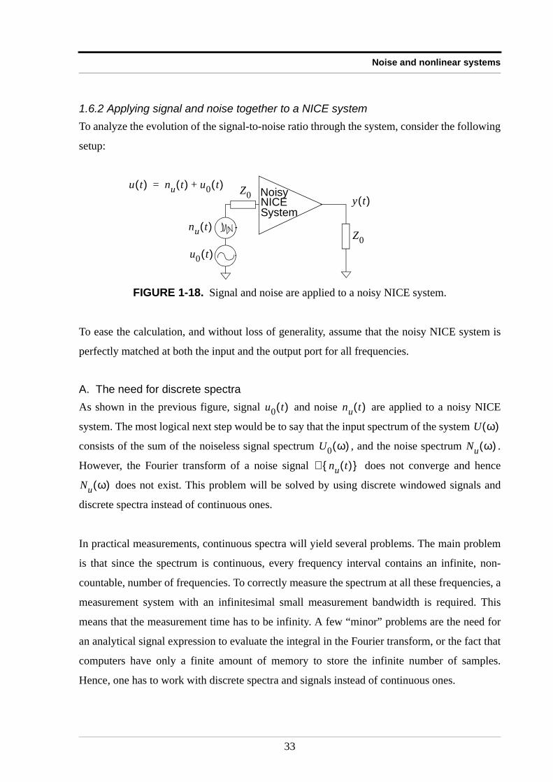
1.6.2 Applying signal and noise together to a NICE systemTo analyze the evolution of the signal-to-noise ratio through the system, consider the following
setup:
To ease the calculation, and without loss of generality, assume that the noisy NICE system is
perfectly matched at both the input and the output port for all frequencies.
A. The need for discrete spectraAs shown in the previous figure, signal and noise are applied to a noisy NICE
system. The most logical next step would be to say that the input spectrum of the system
consists of the sum of the noiseless signal spectrum , and the noise spectrum .
However, the Fourier transform of a noise signal does not converge and hence
does not exist. This problem will be solved by using discrete windowed signals and
discrete spectra instead of continuous ones.
In practical measurements, continuous spectra will yield several problems. The main problem
is that since the spectrum is continuous, every frequency interval contains an infinite, non-
countable, number of frequencies. To correctly measure the spectrum at all these frequencies, a
measurement system with an infinitesimal small measurement bandwidth is required. This
means that the measurement time has to be infinity. A few “minor” problems are the need for
an analytical signal expression to evaluate the integral in the Fourier transform, or the fact that
computers have only a finite amount of memory to store the infinite number of samples.
Hence, one has to work with discrete spectra and signals instead of continuous ones.
FIGURE 1-18. Signal and noise are applied to a noisy NICE system.
System
u0 t( )
NoisyNICE
nu t( )
u t( ) nu t( ) u0 t( )+= Z0
Z0
y t( )
u0 t( ) nu t( )
U ω( )
U0 ω( ) Nu ω( )
ℑ nu t( )
Nu ω( )
33
Noise, Linear Systems and Nonlinear Systems
However, some important considerations have to be taken into account:
First, the time signal has to be sampled, i.e. only the instantaneous values of with
are retained. represents the sampling period and is the inverse of the sampling
frequency . To avoid alias, the sample frequency has to obey Shannon’s theorem, i.e.
, where represents the highest frequency component present in . Since
contains noise whose bandwidth was supposed to be infinity by approximation (see
section 1.2.1), the problem arises that at first sight . However, since bandwidth of
the NICE system is finite, using a lowpass filter with a bandwidth equal to that of the NICE
system, and setting will do the job. At this point, the time waveform is discrete, but
the spectrum of is still a continuous one, it is the lowpass filtered spectrum of ,
that repeats itself each integer multiple of the sample frequency .
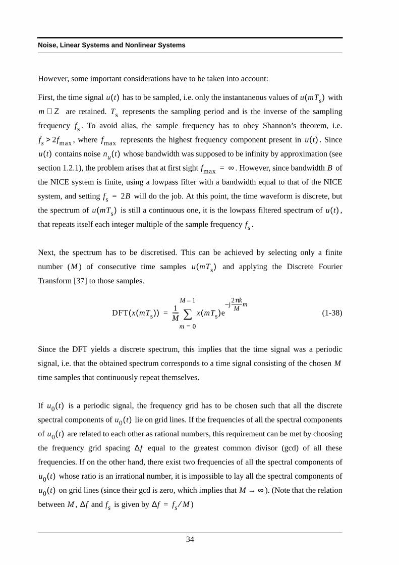
Next, the spectrum has to be discretised. This can be achieved by selecting only a finite
number ( ) of consecutive time samples and applying the Discrete Fourier
Transform [37] to those samples.
(1-38)
Since the DFT yields a discrete spectrum, this implies that the time signal was a periodic
signal, i.e. that the obtained spectrum corresponds to a time signal consisting of the chosen
time samples that continuously repeat themselves.
If is a periodic signal, the frequency grid has to be chosen such that all the discrete
spectral components of lie on grid lines. If the frequencies of all the spectral components
of are related to each other as rational numbers, this requirement can be met by choosing
the frequency grid spacing equal to the greatest common divisor (gcd) of all these
frequencies. If on the other hand, there exist two frequencies of all the spectral components of
whose ratio is an irrational number, it is impossible to lay all the spectral components of
on grid lines (since their gcd is zero, which implies that ). (Note that the relation
between , and is given by )
u t( ) u mTs( )
m Z∈ Ts
fsfs 2fmax> fmax u t( )
u t( ) nu t( )
fmax ∞= B
fs 2B=
u mTs( ) u t( )
fs
M u mTs( )
DFT x mTs( )( ) 1M----- x mTs( )e
j2πkM
---------m–
m 0=
M 1–
∑=
M
u0 t( )
u0 t( )
u0 t( )
∆f
u0 t( )
u0 t( ) M ∞→
M ∆f fs ∆f fs M⁄=
34
Noise and nonlinear systems
Since the input noise is an aperiodic signal, one theoretically needs an infinite number of
time samples to adequately describe spectrum using the DFT, yielding a frequency grid
spacing of 0 Hz. Practically, one has to choose a frequency grid such that the noise spectrum
does not vary too much from one grid line to another. Since by assumption was thermal
noise that has a flat power spectral density, the grid spacing obtained by guaranteeing that the
spectral components of lie on grid lines, will often be sufficient to describe the
variations in the noise spectrum. Note however, that the resulting noise spectrum obtained with
the DFT is a spectrum of a periodical signal, and thus one is dealing with periodic noise.
If on the other hand, is aperiodic, or contains irrationally related frequency components,
a frequency grid has to be chosen that is dense enough to adequately describe the variations of
the signal spectrum.
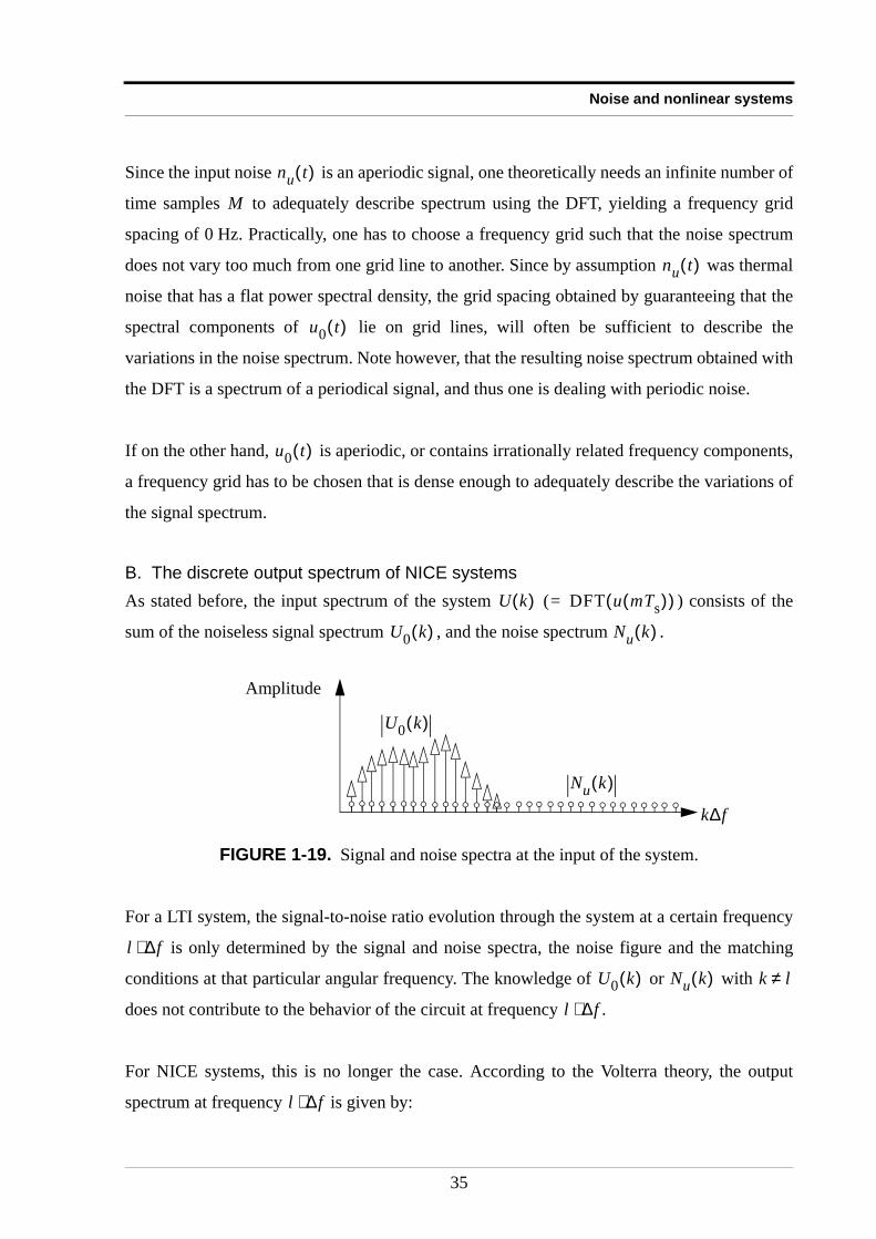
B. The discrete output spectrum of NICE systemsAs stated before, the input spectrum of the system ( ) consists of the
sum of the noiseless signal spectrum , and the noise spectrum .
For a LTI system, the signal-to-noise ratio evolution through the system at a certain frequency
is only determined by the signal and noise spectra, the noise figure and the matching
conditions at that particular angular frequency. The knowledge of or with
does not contribute to the behavior of the circuit at frequency .
For NICE systems, this is no longer the case. According to the Volterra theory, the output
spectrum at frequency is given by:
FIGURE 1-19. Signal and noise spectra at the input of the system.
nu t( )
M
nu t( )
u0 t( )
u0 t( )
U k( ) DFT u mTs( )( )=
U0 k( ) Nu k( )
Nu k( )
U0 k( )
Amplitude
k∆f
l ∆f⋅
U0 k( ) Nu k( ) k l≠
l ∆f⋅
l ∆f⋅
35
Noise, Linear Systems and Nonlinear Systems
(1-39)
and can be written as:
(1-40)
where are chosen so that . Hence, the portion of the
output spectrum at grid line (lying at frequency ), due to the Volterra kernel of the -th
degree, is the sum of all possible combinations of input spectral components, lying at grid
lines , such that their sum equals . Thus, the signal-to-noise ratio at the output
of the NICE system at frequency is no longer only a function of the input signal and noise
at that particular frequency , but it will also depend on the properties of and
where . (1-39) and (1-40) will be illustrated through the following example.
Example 1.8
Consider the following static NICE system that can be described through its Volterra series:
(1-41)
According to the Volterra theory, the output spectrum at angular frequency is given by
(1-39):
(1-42)
where
Y l( ) Y α( ) l( )
α 1=
∞
∑= where Y α( ) l( ), DFT Hα u mTs( )[ ]( )k l=
=
Y α( ) l( )
Y α( ) l( ) … Hα k1 … kα 1– L, , ,( )U k1( )…U kα 1–( )U L( )
kα 1–M2-----–=
M2----- 1–
∑k1
M2-----–=
M2----- 1–
∑=
k1 … kα 1– L, , , k1 … kα 1– L+ + + l=
l l ∆f⋅ α
α
k1 … kα 1– L, , , l
lf0lf0 U0 k( ) Nu k( )
k l≠
y t( ) H u t( )[ ] H1 u t( )[ ] H3 u t( )[ ]+ u t( ) u3 t( )+= = =
l ∆f⋅
Y l( ) Y 1( ) l( ) Y 3( ) l( )+=
36
Noise and nonlinear systems
(1-43)
can also be written as:
(1-44)
According to (1-40), and knowing that , can be expressed as:
(1-45)
where the three grid lines are chosen so that . This means that there
are two grid lines that can be independently chosen ( and ) and the third grid line ( ) has
to be such that . Since time samples are chosen, the DFT will also yield
frequency lines. Hence, the sums in (1-45) have to be taken over these grid lines, instead as
over an infinite number. Consider also , with equal to the
frequency grid spacing . In that case, the DFT spectrum is given by:
(1-46)
Equation (1-45) with becomes:
(1-47)
Y 1( ) l( ) DFT H1 u mTs( )[ ]( )k l=
DFT u mTs( )( )k l=
= =
Y 3( ) l( ) DFT H3 u mTs( )[ ]( )k l=
DFT u3 mTs( )( )k l=
= =
Y 1( ) l( )
Y 1( ) l( ) H1 l( )U l( ) U l( )= =
H3 k1 k2 k3, ,( ) 1= Y 3( ) l( )
Y 3( ) l( ) U k1( )U k2( )U L( )
k2M2-----–=
M2----- 1–
∑k1
M2-----–=
M2----- 1–
∑=
k1 k2 L, , k1 k2 L+ + l=
k1 k2 L
k1 k2 L+ + l= M M
M
u t( ) A 2πf0t ϕ+( )cos⋅= f0∆f
U 1( ) A2---ejϕ=
U 1–( ) A2---e jϕ–=
U k( ) 0= k 1±≠⇔
l 1=
Y 3( ) 1( ) U 1( )U 1( )U 1–( ) U 1( )U 1–( )U 1( ) U 1–( )U 1( )U 1( )+ +=
3U 1( )U 1( )U 1–( )= 3A3
8---------ejϕ=
37
Noise, Linear Systems and Nonlinear Systems
For , (1-45) yields that , i.e. there are no combinations of only non-zero
spectral lines that yield .
For , (1-45) becomes:
(1-48)
Two more non-zero output spectral lines will be obtained through similar reasoning:
(1-49)
Combinatory analysis can predict the coefficients and the number of distinct combinations in
the output spectrum (see Appendix 1.H).
C. Hypotheses about the signal and the noise spectrum1. The signal spectrum is a deterministic spectrum and information-carrying
(random) signals such as used in telecommunication systems, are not taken into account.
If different realisations of the input signal are considered, will always be the
same, since it is deterministic. Mathematically expressed, this implies that
(1-50)
at those lines where signal power is present.
2. The input noise spectrum however, has also become a non-random spectrum due
to the usage of the DFT, which represents the noise spectrum as the spectrum of periodic
noise instead of random noise. If different realisations of the noisy input signal are
considered, other noise samples will be used to calculate the DFT, and hence the noise
spectrum will vary randomly over the different realisations. The noise spectrum is
a stochastic spectrum. At each spectral line the noise is circular complex normally
distributed and independent over the frequencies [9]. This is especially true for fine
frequency grids (large ). Hence,
l 2= Y 3( ) 2( ) 0=
Y 3( ) 2( )
l 3=
Y 3( ) 3( ) U 1( )U 1( )U 1( ) A3
8------ej3ϕ= =
Y 3( ) 1–( ) 3A3
8---------e j– ϕ= Y 3( ) 3–( ) A3
8------e j– 3ϕ=
U0 k( )
U0 k( )
E U0 k( ) U k( ) 0≠=
Nu k( )
Nu k( )
M
38
Noise and nonlinear systems
(1-51)
D. Grouping the output spectrum terms as function of their propertiesThe output spectrum of the NICE system calculated with (1-39) and (1-40) contains a lot of
terms, of which some contribute to the signal output spectrum and others to the output
noise spectrum . Again, some terms exist only due to the interaction of the signal and the
noise. In order to better understand how a NICE system treats the noisy input signal, these
terms will be grouped into several sets, depending on their properties.
Before starting immediately with the formulae and criteria for noisy NICE systems, a simple
example using a noisy LTI system will be given first in order to enhance the readability of the
text.
Starting from
, (1-52)
collect all the terms that depend solely on the noise free input signal . These terms are
grouped in . Hence, for the LTI case,
(1-53)
The remainder contains terms that are solely a function of the input noise or the noise
added by the noisy LTI system itself . These terms will be labelled as :
(1-54)
E Nu k( ) 0=
E Nu2 k( )
0=
E Nu k( )Nu* l( )
0= for k l≠
E Nu k( ) 2
σNu
2 k( )=
Y0 k( )
Ny k( )
Y k( ) H1 k( )U0 k( ) H1 k( )Nu k( ) NA k( )+ +=
U0 k( )
A U0( )
A U0( ) H1 k( )U0 k( )=
Nu k( )
NA k( ) B N( )
B N( ) H1 k( )Nu k( ) NA k( )+=
39
Noise, Linear Systems and Nonlinear Systems
Note that (1-54) contains two noise sources: the input noise and the noise added by the
system itself , therefore these terms are tagged as instead of as .
There are no terms in the output spectrum that are due to an interaction between the noiseless
input signal and the input noise .
is the noiseless (deterministic) output spectrum , while is the spectrum of
the noise on the output signal .
For noisy NICE systems, we will start from (1-39) and (1-40) with .
First, all the terms that depend solely on the noise free input signal are grouped in
. Some terms of are: , coming from the linear Volterra operator,
and , coming from the higher order Volterra operators.
is a part of the noiseless output spectrum . It is the noiseless output spectrum that
would be obtained if only was applied at the input of the NICE system.
Second, the terms that are solely a function of the input noise or the noise added by the
noisy NICE system itself , are grouped into . Some terms of are: ,
. is a part of the output noise spectrum . It is the
output noise spectrum that would be obtained if only was applied at the input of the
NICE system.
The remaining terms in the output spectrum are terms that depend jointly on and
. They are grouped depending on their realization average.
The terms that depend jointly on and , and whose realization average is non-
zero, are grouped into . Note that out of (1-50) follows that
(1-55)
Nu k( )
NA k( ) B N( ) B Nu( )
U0 k( ) Nu k( )
A U0( ) Y0 k( ) B N( )
Ny k( )
U k( ) U0 k( ) Nu k( )+=
U0 k( )
A U0( ) A U0( ) H1 k( )U0 k( )
Hα k1 … kα, ,( )U0 k1( )…U0 kα( )
A U0( ) Y0 k( )
U0 k( )
Nu k( )
NA k( ) B N( ) B N( ) NA k( )
Hα k1 … kα, ,( )Nu k1( )…Nu kα( ) B N( ) Ny k( )
Nu k( )
U0 k( )
Nu k( )
U0 k( ) Nu k( )
A ′ U0 N,( )
E Hα k1 … kα, ,( )U0 k1( )…U0 kα1( )Nu kα1 1+( )…Nu kα( )
Hα k1 … kα, ,( )U0 k1( )…U0 kα1( )E Nu kα1 1+( )…Nu kα( ) =
40
Noise and nonlinear systems
and this latter realization average can only be different from zero if it consists of pairs of
complex conjugate noise spectral lines (see (1-51)). Hence, a term of is e. g.
. Since these terms have a non-zero realization
average, they contribute to the deterministic output spectrum of the system . They hence
create a bias on the deterministic part of the system’s output spectrum. This bias depends on
, and hence on the input noise power spectral density.
The remaining terms that depend jointly on and , and that have a zero realization
average, are grouped into . Out of (1-51) and (1-55) follows that the realization
average is different from zero if it does not consist of pairs of complex conjugate noise spectral
lines. A term of is e. g. . Since these terms
have a zero realization average, they only contribute to the variability of the output spectrum of
the system . They hence contribute to the noise at the output of the NICE system.
Hence, the output spectrum of the noisy NICE system can be written as:
(1-56)
Where
(1-57)
A′ U0 N,( )
H3 k1 k2 k2–, ,( )U0 k1( )Nu k2( )Nu k2–( )
Y0 k( )
σNu
2
U0 k( ) Nu k( )
B ′ U0 N,( )
B ′ U0 N,( ) H3 k1 k2 k3, ,( )U0 k1( )Nu k2( )Nu k3( )
Ny k( )
Y k( ) Y0 k( ) Ny k( )+=
Y0 k( ) A U0( ) A′ U0 N,( )+=
Ny k( ) B N( ) B′ U0 N,( )+=
41
Noise, Linear Systems and Nonlinear Systems
1.7 ConclusionIn this chapter, an introduction is given about noise and its influence on a linear as well as on a
nonlinear system. First of all, several sources of noise are described and the properties of the
two most important ones (thermal noise and shot noise) are highlighted. Assuming that thermal
noise has a flat power spectral density, leads to errors smaller than 1% for frequencies up to
100 GHz and temperatures above 273 K.
Next, the definition and spectral properties of a noisy LTI system were given. The noise figure
that describes the deterioration of the signal-to-noise ratio through the LTI system proved to be
a very good figure to describe the noise behavior of a LTI system. A common measurement
technique (the Y-factor method) to determine the noise figure was also explained.
Finally, NICE systems, which are a subclass of nonlinear systems are introduced. NICE
systems, whose behavior can be described through Volterra series were chosen to be the target
class to extend the noise behavior analysis of LTI systems to.
Studying the output spectrum of a NICE system, when applying a deterministic signal
superimposed on stochastic (ergodic) noise at its input, allows to prove that the output can be
split into four disjunct sets. This also illustrates the interactions between the deterministic input
signal and the input noise.
42

Appendices
1.8 Appendices
Appendix 1.A: Cross-correlation of deterministic signals and ergodic noiseConsider to be a periodic, deterministic signal, and ergodic noise. Let
. will still be a periodic, deterministic signal. The time cross-correlation
between and is in that case (per definition) given by:
(1-58)
Using the definition of the Riemann Integral [32], this yields:
(1-59)
Since tends to infinity, one can assume that is an integer multiple of the period of .
If this is not the case, the contribution to the Riemann sum of that part, that is only a fraction of
the period of can be neglected anyway, since . Let be the period of ,
in that case, . Normally, the Riemann sum is made sequential over the intervals
. However, one can also first add all the contributions of every interval, located at the same
position, relative to one period of , and then add all these contributions over all the
relative positions of the intervals in one period. This is illustrated in Figure 1-20, for a simple
sine wave. Instead of sequential adding the contributions of the intervals, first all the surfaces
of the same color and pattern are added, and eventually, the sum is made over all colors and
patterns.
u0 t( ) nu t( )
α β, N0∈ u0α t( )
u0α t( ) nu
β t( )
E u0α t( )nu
β t τ+( ) 1
T--- u0
α t( )nuβ t τ+( ) td
T 2⁄–
T 2⁄∫T ∞→
lim=
1T--- u0
α ti( )nuβ ti τ+( )∆ti
i∑∆tj 0→
limT ∞→lim=
T T u0α t( )
u0α ti( ) T ∞→ T
u0α u0
α t( )
T kT Tu0
α⋅=
∆tiu0
α t( )
43
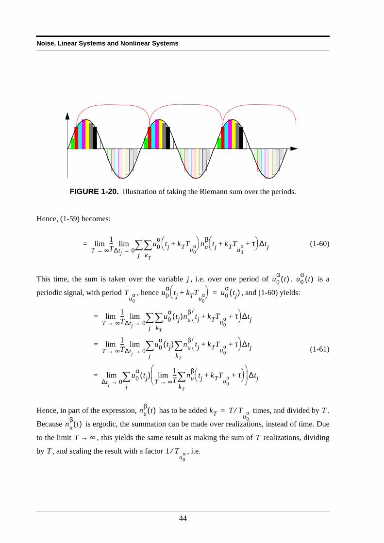
Noise, Linear Systems and Nonlinear Systems
Hence, (1-59) becomes:
(1-60)
This time, the sum is taken over the variable , i.e. over one period of . is a
periodic signal, with period , hence , and (1-60) yields:
(1-61)
Hence, in part of the expression, has to be added times, and divided by .
Because is ergodic, the summation can be made over realizations, instead of time. Due
to the limit , this yields the same result as making the sum of realizations, dividing
by , and scaling the result with a factor , i.e.
FIGURE 1-20. Illustration of taking the Riemann sum over the periods.
1T--- u0
α
kT
∑ tj kTTu0
α+ nu
β tj kTTu0
α τ+ + ∆tj
j∑∆tj 0→
limT ∞→lim=
j u0α t( ) u0
α t( )
Tu0
α u0α tj kTT
u0α+
u0α tj( )=
1T--- u0
α
kT
∑ tj( )nuβ tj kTT
u0α τ+ +
∆tj
j∑∆tj 0→
limT ∞→lim=
1T--- u0
α tj( ) nuβ tj kTT
u0α τ+ +
∆tj
kT
∑j∑∆tj 0→
limT ∞→lim=
u0α tj( ) 1
T--- nu
β tj kTTu0
α τ+ +
kT
∑T ∞→lim
∆tjj∑∆tj 0→
lim=
nuβ t( ) kT T T
u0α⁄= T
nuβ t( )
T ∞→ T
T 1 Tu0
α⁄
44
Appendices
(1-62)
And due to the ergodicity of , the time and realization average are the same, thus (1-
61) becomes:
(1-63)
The latter integral in (1-63), divided by represents the mean value of , over one
period, and hence the time mean of .
Conclusion:
Appendix 1.B: Transfer function of a LTI systemConsider to be the impulse response of a LTI system, i.e. is the output signal of the
system, when the input signal is a Dirac impulse : .
Using the pincet property of the Dirac distribution, one can write a general input signal as
follows:
(1-64)
The output signal is:
1T--- nu
β tj kTTu0
α τ+ +
kT
∑T ∞→lim E nu
β t τ+( ) 1
Tu0
α--------=
nuβ t τ+( )
u0α tj( ) E nu
β t τ+( ) 1
Tu0
α--------
∆tjj∑∆tj 0→
lim=
E nuβ t τ+( )
1
Tu0
α-------- u0
α tj( )∆tjj∑∆tj 0→
lim=
E nuβ t τ+( )
1
Tu0
α-------- u0
α t( ) t d0
Tu0
α
∫=
Tu0
α u0α t( )
u0α t( )
E u0α t( )nu
β t τ+( )
E nuβ t τ+( )
E u0α t( )
⋅=
h t( ) h t( )
δ t( ) h t( ) H δ t( )[ ]=
u t( )
u t( ) u τ( )δ t τ–( ) τd∞–
∞∫=
y t( )
45
Noise, Linear Systems and Nonlinear Systems
(1-65)
Since the integration is a linear operation, and is a linear time-invariant operator,
(1-66)
This last integral is the definition of a convolution integral, hence:
(1-67)
To calculate the output spectrum, one has to take the Fourier transform of the above
expression:
(1-68)
Switching the integration order, one gets:
(1-69)
Using the shift property of the Fourier transform, and defining the Fourier transform of the
impulse response as the transfer function of the LTI system yields:
(1-70)
Hence, the convolution in time domain corresponds to a multiplication in frequency domain.
Note that if one wants to treat the sine wave as the superposition of two complex
signals and , the definition of an LTI system (Definition 1.2) has to be modified.
In that case, the constants have to be complex numbers, and the range of the functions of
has to be instead of . But then it has to be specified that the LTI system’s impulse
response is a real function and not a complex one.
y t( ) H u t( )[ ] H u τ( )δ t τ–( ) τd∞–
∞∫= =
H [ ]
y t( ) u τ( )H δ t τ–( )[ ] τd∞–
∞∫ u τ( )h t τ–( ) τd
∞–
∞∫= =
y t( ) u t( )*h t( )=
Y ω( ) ℑ y t( ) y t( )e jωt– td∞–
∞∫ u τ( )h t τ–( ) τd
∞–
∞∫ e jωt– td
∞–
∞∫= = =
Y ω( ) u τ( ) h t τ–( )e jωt– td∞–
∞∫ τd
∞–
∞∫ u τ( )ℑ h t τ–( ) τd
∞–
∞∫= =
Y ω( ) u τ( )H ω( )e jωτ– τd∞–
∞∫ H ω( ) u τ( )e jωτ– τd
∞–
∞∫ H ω( ) U ω( )⋅= = =
t( )cos
ejt 2⁄ e jt– 2⁄
ci FC R
h t( )
46
Appendices
Appendix 1.C: Z and Y matrix of a n-portLet and be respectively the voltages and currents at the n ports of the
system.
Definition 1.9
The -matrix and the -matrix of the system are the complex n-by-n matrices that satisfy
(1-71)
where and are the Laplace or Fourier transforms of and
respectively.
Out of the definition follows that the and matrices are each other inverse, or
(1-72)
Appendix 1.D: Output PSD of the noisy LTI systemThe theorem of Wiener-Kinchin [4] states that the power spectral density of a signal can
be calculated as the Fourier transform of the auto-correlation, hence:
(1-73)
The reference impedance is often selected to be in microwave environments. The
reason for this rescaling is that the auto-correlation is expressed in volts square, and hence the
unit of its Fourier transform is . In order to obtain a power spectral density (in
), the latter result must be divided by the characteristic impedance.
U1 … Un, , I1 … In, ,
Z Y
U1…Un
Z11 … Z1n… … …Zn1 … Znn
I1…In
⋅=I1…In
Y11 … Y1n… … …Yn1 … Ynn
U1…Un
⋅=
I1 … In, , U1 … Un, , i1 t( ) … in t( ), ,
u1 t( ) … un t( ), ,
Z Y
Y11 … Y1n… … …Yn1 … Ynn
Z11 … Z1n… … …Zn1 … Znn
1–
=
y t( )
PSDy2( ) 1
Z0------ ℑ Ryy τ( ) =
Z0 50Ω=
V2 Hz⁄
W Hz⁄
47
Noise, Linear Systems and Nonlinear Systems
The auto-correlation is defined as:
(1-74)
Defining as the output of the noiseless LTI system, one can write that:
(1-75)
Because the input signal and the noise are uncorrelated (as assumed in section
1.4.1), and will also be uncorrelated. Rewriting (1-75) in terms of
power spectral density yields [4]:
(1-76)
Since the PSD of a signal can also be written as , considering
that the Fourier transform exists, (1-76) can also be expressed as (assuming
the Fourier transform of exists):
(1-77)
Appendix 1.E: Determining the noise figure with the Y-factor methodWith the coordinates of the two points ( , ) and ( , ), one can write down the equation
of the straight line in the , plane going through these two points:
(1-78)
The slope of this function is given by: , while the intersection with the axis is
given by: . Filling in these values in (1-21) yields:
Ryy τ( ) E y t( )y t τ+( ) =
η t( ) h t( )*u t( )=
Ryy τ( ) E η t( ) nA t( )+( ) η t τ+( ) nA t τ+( )+( ) =
E η t( )η t τ+( ) E nA t( )nA t τ+( ) + Rηη τ( ) RnAnAτ( )+= =
u t( ) nA t( )
η t( ) h t( )*u t( )= nA t( )
PSDy2( ) ω( ) PSDη
2( ) ω( ) PSDnA
2( ) ω( )+ H ω( ) 2PSDu2( ) ω( ) PSDnA
2( ) ω( )+= =
x t( ) PSDx2( ) ω( ) X ω( ) 2 Z0⁄=
X ω( ) ℑ x t( ) =
u t( )
PSDy2( ) ω( ) H ω( ) 2 U ω( ) 2
Z0------------------- PSDnA
2( ) ω( )+=
Tc N1 Th N2
T PSDy1( )
PSDy1( ) N1–
N2 N1–Th Tc–------------------- T Tc–( )⋅=
N2 N1–Th Tc–------------------- T 0=
N1N2 N1–Th Tc–-------------------Tc+
48
Appendices
(1-79)
with . Further simplification and regrouping terms gives:
(1-80)
Appendix 1.F: Signal-to-noise ratio deterioration for other input noise levelsUsing (1-21) follows that the power spectral density of the noise added by the LTI system can
be written as:
(1-81)
Since, by hypothesis, the temperature of the system is kept constant, will not
change for other input noise temperatures. The signal-to-noise ratio deterioration for other
input noise power levels is then given by:
(1-82)
Substituting (1-81) into (1-82) yields:
(1-83)
NF 1N1
N2 N1–Th Tc–-------------------Tc+
N2 N1–Th Tc–-------------------T0
--------------------------------------+ 11 1 Y–
Th Tc–-----------------Tc+
Y 1–Th Tc–-----------------T0
---------------------------------+= =
Y N2 N1⁄=
NF 1Th YTc–( )T0 Y 1–( )---------------------------+
ThT0------ 1–
YTcT0------ 1–
–
Y 1–---------------------------------------------------= =
PSDnA
1( ) ω( ) NF ω( ) 1–( ) H ω( ) 2kT0=
PSDnA
1( ) ω( )
SNRinSNRout------------------
T
H ω( ) 2kT PSDnA
1( ) ω( )+
H ω( ) 2kT------------------------------------------------------------=
SNRinSNRout------------------
T
H ω( ) 2kT NF ω( ) 1–( ) H ω( ) 2kT0+
H ω( ) 2kT--------------------------------------------------------------------------------------------- 1 NF ω( ) 1–( )
T0T------+= =
49
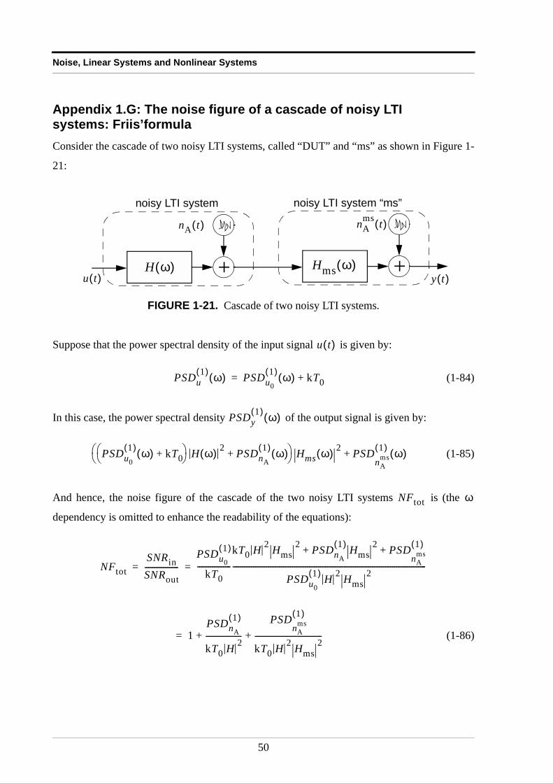
Noise, Linear Systems and Nonlinear Systems
Appendix 1.G: The noise figure of a cascade of noisy LTI systems: Friis’formulaConsider the cascade of two noisy LTI systems, called “DUT” and “ms” as shown in Figure 1-
21:
Suppose that the power spectral density of the input signal is given by:
(1-84)
In this case, the power spectral density of the output signal is given by:
(1-85)
And hence, the noise figure of the cascade of the two noisy LTI systems is (the
dependency is omitted to enhance the readability of the equations):
(1-86)
FIGURE 1-21. Cascade of two noisy LTI systems.
+
noisy LTI system
y t( )u t( )
nA t( )
+
nAms t( )
H ω( ) Hms ω( )
noisy LTI system “ms”
u t( )
PSDu1( ) ω( ) PSDu0
1( ) ω( ) kT0+=
PSDy1( ) ω( )
PSDu0
1( ) ω( ) kT0+ H ω( ) 2 PSDnA
1( ) ω( )+ Hms ω( ) 2 PSD
nAms1( ) ω( )+
NFtot ω
NFtotSNRinSNRout------------------
PSDu0
1( )
kT0------------------
kT0 H 2 Hms2 PSDnA
1( ) Hms2 PSD
nAms1( )+ +
PSDu0
1( ) H 2 Hms2
--------------------------------------------------------------------------------------------------------= =
1PSDnA
1( )
kT0 H 2-------------------
PSDnA
ms1( )
kT0 H 2 Hms2
------------------------------------+ +=
50
Appendices
The first two terms of (1-86) equal the noise figure of the first noisy LTI system , while the
last term in (1-86) can be rewritten as:
(1-87)
Hence, out of (1-86) and (1-87) follows that:
(1-88)
The last step is to determine . This can be done without performing more measurements
than those needed to determine and . To determine , using the Y-factor
method, the power spectral densities and are applied to the measurement system (noisy
LTI system “ms”) only, and the corresponding and are measured. These measured
values can be written as:
(1-89)
Similarly, to determine , using the Y-factor method, the power spectral densities and
are applied to the cascade of the DUT and the measurement system, and the corresponding
and are measured. These measured values can be written as:
(1-90)
can the be determined out of these four measured power spectral densities, as:
(1-91)
NF
PSDnA
ms1( )
kT0 Hms2
--------------------------
H 2-------------------------------
NFms 1–
H 2-----------------------=
NFtot NFNFms 1–
H 2-----------------------+=
H 2
NFtot NFms NFms
Nc Nh
N1ms N2
ms
N1ms Nc Hms
2 PSDnA
ms1( )+= N2
ms Nh Hms2 PSD
nAms1( )+=
NFtot Nc
Nh
N1tot N2
tot
N1 2,tot Nc h, H 2 PSDnA
1( )+ Hms
2 PSDnA
ms1( )+=
H 2
H 2 N2tot N1
tot–
N2ms N1
ms–--------------------------=
51
Noise, Linear Systems and Nonlinear Systems
Appendix 1.H: Combinatory analysis to determine the discrete output spectrum of a -th order Volterra operatorThe discrete output spectrum of a -th order Volterra operator consists of all the combinations
that can be made by multiplying input spectral lines , rescaled by
(the -th order Laplace transform of the Volterra kernel). Hence,
(1-92)
considering that results at different grid lines cannot be added, since they represent coefficients
of different spectral lines.
Consider that the input spectrum contains non-zero spectral lines. The number of
terms in (1-92) is then given by the number of repetitive variations of elements, taken -
by- , i.e.
(1-93)
In the case of Example 1.8, where only and were present in the input spectrum,
the number of terms created by the third order Volterra operator is , i.e.:
Not all these terms are different, e.g. . All the
permutations of the factors in a term yield the same term. Hence, the number of different terms
in (1-92) is given by the number of repetitive combinations of elements, taken -by- ,
i.e.:
(1-94)
α
α
α U k1( ) … U kα( ), ,
Hα k1 … kα, ,( ) α
… Hα k1 … kα, ,( )U k1( )…U kα( )
kαM2-----–=
M2----- 1–
∑
k1M2-----–=
M2----- 1–
∑
U k( ) M ′
M ′ α
α
#terms VM ′α M ′α= =
U 1( ) U 1–( )
V23 8=
U 1( )U 1( )U 1( ) U 1( )U 1( )U 1–( ) U 1( )U 1–( )U 1( ) U 1( )U 1–( )U 1–( )U 1–( )U 1( )U 1( ) U 1–( )U 1( )U 1–( ) U 1–( )U 1–( )U 1( ) U 1–( )U 1–( )U 1–( )
U 1( )U 1( )U 1–( ) U 1( )U 1–( )U 1( )=
M ′ α α
# different terms CM ′α M ′ α 1–+( )!
α! M ′ 1–( )!⋅--------------------------------= =
52
Appendices
In the case of Example 1.8, the number of different terms is . These terms
are:
The last question is to find out for each different term, how many identical siblings it had. This
will be its coefficient in the resulting output spectrum. Hence, the number of distinct
permutations of the factors of each term is required. Each term consists of factors
, but not all the are different. All the factors of the term can be
grouped in sets of identical factors. Suppose that there exist such sets of identical factors,
and that the number of identical factors in each set is given by (with
). In that case, the number of distinct permutations that can be obtained
with the factors is given by:
(1-95)
In the case of Example 1.8, the number of distinct permutations that can be obtained with
terms and is given by , and the number of
distinct permutations that can be done with terms and is
given by .
C23 4! 3!⁄ 4= =
U 1( )U 1( )U 1( ) U 1( )U 1( )U 1–( )U 1( )U 1–( )U 1–( ) U 1–( )U 1–( )U 1–( )
α
U k1( ) … U kα( ), , k1 … kα, ,
m ′
α1 … αm ′, ,
α1 … αm ′+ + α=
α
α!α1! … αm ′!⋅ ⋅----------------------------------
U 1( )U 1( )U 1( ) U 1–( )U 1–( )U 1–( ) 3! 3!⁄ 1=
U 1( )U 1( )U 1–( ) U 1( )U 1–( )U 1–( )
3! 2! 1!⋅( )⁄ 3=
53

Noise, Linear Systems and Nonlinear Systems
54
CHAPTER 2
NOISE FIGURE MEASUREMENTSON NICE SYSTEMS
Abstract: The noise figure, which is defined as the deterioration of
the signal-to-noise ratio from the input to the output of a LTI
system can easily be measured using the Y-factor technique when
dealing with LTI systems. For NICE systems, however, the method
for determining the noise figure remains a big question mark. This
chapter investigates if the Y-factor method is also valid for
determining the “noise figure” of NICE systems.
55
Noise figure measurements on NICE systems
2.1 IntroductionSince the noise figure is a very useful and widely used figure to describe the noise behavior of
a LTI system [10], [11], the question arises if it can be used for NICE systems. Except for the
fact that the noise contribution at angular frequency is not only a function of the input noise
spectrum at the same angular frequency , but also depends on the noise at other angular
frequencies, there is almost no difference between the noise behavior of a LTI and a NICE
system. Hence, one can assume that the noise figure is also applicable for NICE systems. At
first glance, the Y-factor method appears to be still valid for NICE systems. If it really is the
case, that would be great! If the Y-factor method can really be applied to NICE systems, it is
important to know if all the assumptions and calculations used to derive the method still hold.
One can then determine the eventual errors made if the Y-factor method is used on a NICE
system, as if it were a LTI system.
The Y-factor technique is a method that implicitly assumes that there is no interaction between
the signal and the noise that are applied to the system and neither between the noise added by
the system itself and the input signal. Or in terms of the sets defined in section 1.6.2,
and are zero, or at least negligible compared to and .
Hence the question about the validity of the Y-factor method can be rephrased as follows: Is it
possible to give an accurate description of the noise produced by a NICE system under the
hypothesis or constraint that the interaction between signal and noise can be neglected?
This chapter will give an answer to those questions, using the -factor technique on a very
simple NICE system, and studying the results.
ωi
ωi
A ′ U0 N,( ) B ′ U0 N,( ) A U0( ) B N( )
Y
56

A very simple model for the NICE system
2.2 A very simple model for the NICE systemIn order to determine the influence of a NICE system on the Y-factor method, a model for the
NICE system is required. The correct approach would be to use the property that the output of
a NICE system can be approximated as a Volterra series (see also (1-30) and (1-31)):
(2-1)
The problem is that this model contains an large sum of Volterra operators, and is therefore
quite difficult to deal with. Therefore, we will select a special (simple) NICE system to
determine if the nonlinearity of a NICE system influences the Y-factor method. In order to be
of practical use, the NICE system has to be selected such as to come close to a practical
system. To ensure that the system is of practical meaning, both the signal and noise need to be
large enough to allow for compression1 of the signal. For the noise properties, band limited
noise signals will be selected. To ease the calculations, it will be assumed that no noise shaping
will be additionally introduced: the noise will be left unchanged in-band and perfectly filtered
out, out of the selected frequency band.
A very simple model for a NICE system is shown in Figure 2-1
1. Compression means that the output spectrum of the NICE system is smaller than predicted by the linear model,describing the NICE system in its linear region. Hence, gain compression means that the gain of the NICEsystem becomes smaller than the linear gain.
FIGURE 2-1. A noisy Wiener-Hammerstein system as model for the NICE system.
y t( ) … hα τ1 … τα, ,( )u t τ1–( )…u t τα–( ) τ1…d ταd∞–
∞∫∞–
∞∫
α 1=
αmax
∑=
+fB fB
u t( ) y t( )
nA t( )
k1 u t( )⋅
k3 u3 t( )⋅
u t( ) +η t( )
57
Noise figure measurements on NICE systems
This model is a Wiener-Hammerstein system [12] with noise superimposed on its output. A
Wiener-Hammerstein system consists of a static nonlinearity with at its input and output a LTI
system. The input and output LTI systems are both ideal lowpass filters, that perfectly block
every frequency above Hz, and have a unity transfer function below Hz. We assume that
the noise power spectral density at the input of the noisy NICE system is a flat spectrum that is
frequency independent (and given by (1-10)). For a practical system, the
noise spectrum will only propagate through the system up to the bandwidth of the system.
Above this frequency, the noise power spectral density will decrease. In the proposed model,
this decrease is replaced by an immediate perfect attenuation. Furthermore, a flat noise power
spectral density, that is frequency independent implies an infinite total noise power .
Indeed, . This remark has already been made in section 1.2.1,
and the solution was to use the correct expression (1-9) for the power spectral density instead
of the frequency independent approximation. Hence, with this model, it is allowed to assume
that contains a noise term, whose power spectral density is given by , instead of using
the complex formula. The output filter is required because every system has a limited output
bandwidth. Above this frequency, the system stops to produce spectral output after a certain
frequency. The properties of the noise source are the same as discussed in section 1.6.1.
An additional constraint is placed on the noise source by assuming that its power spectral
density is zero above Hz.
If is the input signal of the system (assuming that the complete spectrum of fits in
the frequency interval ), will be the output signal of the
system (again, assuming that the complete spectrum of fits in the frequency interval
). Note furthermore that only the first and third order Volterra operator are used in the
model, while the second order operator is omitted. When the system is excited with a pure sine
wave, this results in compression of the fundamental (at frequency ) and existence of energy
at three times the frequency of the fundamental, and no distortion at two times the fundamental
frequency. In practical systems, it is often observed that the contribution at frequency is
much smaller than the contribution at . The reason is that the presence of an even order
Volterra operator compresses the maxima and the minima of a sine wave in a different way.
This asymmetric treatment of the maxima and minima is typically due to a bad biasing of the
B B
PSDnu
1( ) ω( ) kT=
Pnu
PnukT fd0
∞∫ kT fd0
∞∫ ∞= = =
u t( ) kT
nA t( )
B
u t( ) u t( )
0 B,[ ] y t( ) k1u t( ) k3u3 t( )+=
u3 t( )
0 B,[ ]
f0
2f03f0
58
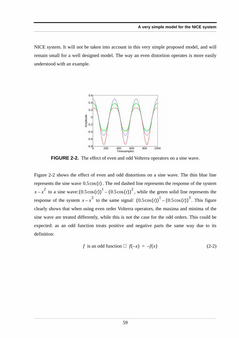
A very simple model for the NICE system
NICE system. It will not be taken into account in this very simple proposed model, and will
remain small for a well designed model. The way an even distortion operates is more easily
understood with an example.
Figure 2-2 shows the effect of even and odd distortions on a sine wave. The thin blue line
represents the sine wave . The red dashed line represents the response of the system
to a sine wave: , while the green solid line represents the
response of the system to the same signal: . This figure
clearly shows that when using even order Volterra operators, the maxima and minima of the
sine wave are treated differently, while this is not the case for the odd orders. This could be
expected: as an odd function treats positive and negative parts the same way due to its
definition:
(2-2)
FIGURE 2-2. The effect of even and odd Volterra operators on a sine wave.
0 200 400 600 800 1000-0.8
-0.6
-0.4
-0.2
0
0.2
0.4
0.6
Timesamples
Am
plit
ude
0.5 t( )cos
x x2– 0.5 t( )cos( )1 0.5 t( )cos( )2–
x x3– 0.5 t( )cos( )1 0.5 t( )cos( )3–
f is an odd function f x–( )⇔ f x( )–=
59
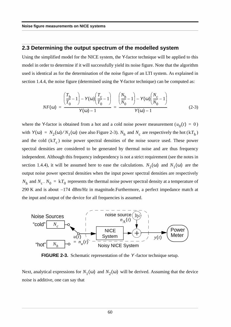
Noise figure measurements on NICE systems
2.3 Determining the output spectrum of the modelled systemUsing the simplified model for the NICE system, the Y-factor technique will be applied to this
model in order to determine if it will successfully yield its noise figure. Note that the algorithm
used is identical as for the determination of the noise figure of an LTI system. As explained in
section 1.4.4, the noise figure (determined using the Y-factor technique) can be computed as:
(2-3)
where the Y-factor is obtained from a hot and a cold noise power measurement ( )
with (see also Figure 2-3). and are respectively the hot ( )
and the cold ( ) noise power spectral densities of the noise source used. These power
spectral densities are considered to be generated by thermal noise and are thus frequency
independent. Although this frequency independency is not a strict requirement (see the notes in
section 1.4.4), it will be assumed here to ease the calculations. and are the
output noise power spectral densities when the input power spectral densities are respectively
and . represents the thermal noise power spectral density at a temperature of
290 K and is about dBm/Hz in magnitude.Furthermore, a perfect impedance match at
the input and output of the device for all frequencies is assumed.
Next, analytical expressions for and will be derived. Assuming that the device
noise is additive, one can say that
FIGURE 2-3. Schematic representation of the -factor technique setup.
NF ω( )
ThT0------ 1–
Y ω( )TcT0------ 1–
–
Y ω( ) 1–-------------------------------------------------------------
NhN0------ 1–
Y ω( )NcN0------ 1–
–
Y ω( ) 1–--------------------------------------------------------------= =
u0 t( ) 0=
Y ω( ) N2 ω( ) N1 ω( )⁄= Nh Nc kTh
kTc
N2 ω( ) N1 ω( )
Nh Nc N0 kT0=
174–
“cold”
“hot”
PowerMeter
Nc
Nh
Noise Sources
NICESystem +
noise sourcenA t( )
Noisy NICE System
u t( ) y t( )nu t( )=
Y
N1 ω( ) N2 ω( )
60
Determining the output spectrum of the modelled system
(2-4)
with the power spectral density of the noise source that is independent of
the input power and uncorrelated with the input noise (see section 1.6.1). The function
has to be determined next.
The power spectral density of the output of the modelled NICE system is obtained by taking
the Fourier transform of the auto-correlation of the system output .
(2-5)
The Fourier transform is divided by , because the power is calculated in a
reference impedance as commonly used in microwave environments. The auto-correlation
of the device output signal consists of the contributions of the noise added by the
system itself and the auto-correlation of the system if were equal to zero (because
and the input noise are uncorrelated). Hence:
(2-6)
Where represents the auto-correlation of the output signal of the noiseless NICE
system (see Figure 2-3). In the case of the example system described in section 2.2, if the
input signal consists only of noise , can be written as:
(2-7)
(2-7) consists of four terms:
(2-8)
N1 2, ω( ) Φ Nc h,( ) PSDnA
1( ) ω( )+=
PSDnA
1( ) ω( ) nA t( )
Φ Nc h,( )
y t( )
PSDy2( ) f( ) 1
Z0------ ℑ Ryy τ( ) =
Z0 50Ω= 50Ω
Ryy τ( )
nA t( )
nA t( )
Ryy τ( ) Rηη τ( ) RnAnAτ( )+=
Rηη τ( )
η t( )
u t( ) nu t( ) Rηη τ( )
Rηη τ( ) E k1nu t( ) k3nu3 t( )+( ) k1nu t τ+( ) k3nu
3 t τ+( )+( )
=
Rηη τ( ) E k12nu t( )nu t τ+( )
E k32nu
3 t( )nu3 t τ+( )
+=
E k1k3nu t( )nu3 t τ+( )
E k1k3nu3 t( )nu t τ+( )
+ +
61
Noise figure measurements on NICE systems
Hence, the following terms have to be evaluated: the linear, the cubic and the combined
contribution. The linear contribution can be rewritten as:
(2-9)
with the auto-correlation function of the input noise . Because the system has a
bandwidth , and is white, thermal noise, one can consider to be band-limited,
flat, zero-mean Gaussian noise with auto-correlation (see Appendix 2.A.)
(2-10)
The cubic contribution can be rewritten as:
(2-11)
The problem now is to determine the expected value of the product of six (ergodic) random
variables. The literature [7], [38] tells that the expected value of the product of an even number
( ) of zero-mean jointly Gaussian random variables can be written as:
(2-12)
The symbol stands for the summation over all distinct ways of partitioning the
random variables into products of averages of pairs, where within a pair the permutation of the
variables does not yield another contribution. The number of distinct ways to obtain this is
given by:
(2-13)
E k12nu t( )nu t τ+( )
k12 Rnunu
τ( )⋅=
Rnunuτ( ) nu t( )
B nu t( ) nu t( )
Rnunu
c h, τ( ) Z0Nc h, B 2πBτ( )sin2πBτ
--------------------------=
E k32nu
3 t( )nu3 t τ+( )
k32E nu t( )nu t( )nu t( )nu t τ+( )nu t τ+( )nu t τ+( ) =
1 2 3 4 5 6
2M n τ1( ) … n τ2M( ), ,
E n τ1( ) … n τ2M( )⋅ ⋅ ΣΠ E n τ i( ) n τ j( )⋅ =
ΣΠ 2M
2M( )!
M!2M---------------
62
Determining the output spectrum of the modelled system
For six variables, , and (2-13) yields that the number of ways to partition the variables
equals fifteen. Appendix 2.B shows these fifteen ways and rewrites the terms as products of
auto-correlations. One will find that:
(2-14)
The auto-correlation is known and given by (2-10), hence the cubic contribution can
eventually be written as:
(2-15)
Similar calculations (see Appendix 2.C) show that the combined contributions can be written
as:
(2-16)
Hence, the auto-correlation of the output signal of the system is:
(2-17)
In a last step, (2-5) will be applied, in order to determine the output power spectral density of
the system. Using (2-39) and (2-35) of Appendix 2.A,
(2-18)
M 3=
E k32nu
3 t( )nu3 t τ+( )
k32 9Rnunu
2 0( )Rnunuτ( ) 6Rnunu
3 τ( )+ =
Rnunuτ( )
E k32nu
3 t( )nu3 t τ+( )
k32Z0
3Nc h,3 B3 9 2πBτ( )sin
2πBτ-------------------------- 6 2πBτ( )sin
2πBτ--------------------------
3+
=
E k1k3nu t( )nu3 t τ+( )
3k1k3Z02Nc h,
2 B2 2πBτ( )sin2πBτ
--------------------------=
E k1k3nu3 t( )nu t τ+( )
3k1k3Z02Nc h,
2 B2 2πBτ( )sin2πBτ
--------------------------=
Ryy τ( )
Ryy τ( ) k12Z0Nc h, B 2πBτ( )sin
2πBτ-------------------------- 6k1k3Z0
2Nc h,2 B2 2πBτ( )sin
2πBτ-------------------------- + +=
k32Z0
3Nc h,3 B3 9 2πBτ( )sin
2πBτ-------------------------- 6 2πBτ( )sin
2πBτ--------------------------
3+
RnAnAτ( )+
PSDy2( ) f( ) ℑ Nc h, B 2πBτ( )sin
2πBτ--------------------------
=
63
Noise figure measurements on NICE systems
The output power spectral density of the system thus becomes:
(2-19)
Where * denotes the convolution. (Note that the Fourier transform of a product equals the
convolution of the Fourier transforms.) After a few calculations (see Appendix 2.D), one
obtains that the single sided power spectral density (from DC to ) of the output of the
nonlinear system is:
(2-20)
Note that during the calculation of the convolution, spectral components with a frequency
larger than were taken into account. This represents no problem since the model of the
internal nonlinear circuit is not band-limited and hence allows frequency components beyond
frequency . Real-world devices often behave similarly. Inside the system, high frequency
components exist that are filtered out at the output, due to the lowpass filter behavior of
connectors, transmission lines or the package of the device.
PSDy2( ) f( ) k1
2PSDnu
2( ) f( ) 6k1k3Z0Nc h, BPSDnu
2( ) f( ) + +=
9k32Z0
2Nc h,2 B2PSDnu
2( ) f( ) 6k32Z0
2PSDnu
2( ) f( )*PSDnu
2( ) f( )*PSDnu
2( ) f( ) PSDnA
2( ) f( )+ +
B
PSDy1( ) f( ) k1
2Nc h, 6k1k3Z0Nc h,2 B
k32Nc h,
3 Z02
2----------------------- 27B2 3f2–( ) PSDnA
1( ) f( )+ ++=
B
B
64
Determination of the noise figure
2.4 Determination of the noise figureAt this point, the power spectral density at the output of the NICE system excited by input
noise only is known (2-20), and it is possible to determine the results of a classical noise figure
measurement on the proposed example. The terms in (2-20) can be grouped in terms
corresponding to the linear and the nonlinear behavior:
(2-21)
Where represents the contribution of the linear part of the system to the output power
spectral density, i.e.
(2-22)
contains the contributions to the output power spectral density due to the nonlinear
part of the NICE system.
(2-23)
Hence the measured noise figure at frequency will be:
(2-24)
It is possible to split this expression for the noise figure in the sum of a linear noise figure
(i.e. the noise figure for the linear system, i.e. ) and a correction term:
(2-25)
PSDy1( ) f( ) N1 2,
L f( ) N1 2,Nice f( )+=
N1 2,L f( )
N1 2,L f( ) k1
2Nc h, PSDnA
1( ) f( )+=
N1 2,Nice f( )
N1 2,Nice f( ) 6k1k3Z0Nc h,
2 Bk3
2Nc h,3 Z0
2
2----------------------- 27B2 3f2–( )+=
f
NF f( )
NhN0------ 1– N2
L f( ) N2Nice f( )+
N1L f( ) N1
Nice f( )+------------------------------------------
NcN0------ 1–
–
N2L f( ) N2
Nice f( )+
N1L f( ) N1
Nice f( )+------------------------------------------ 1–
-------------------------------------------------------------------------------------------=
NFlin k3 0=
NF f( ) NFlin f( )b f( ) NFlin f( ) d f( )⋅–
c f( ) d f( )+---------------------------------------------------+=
65
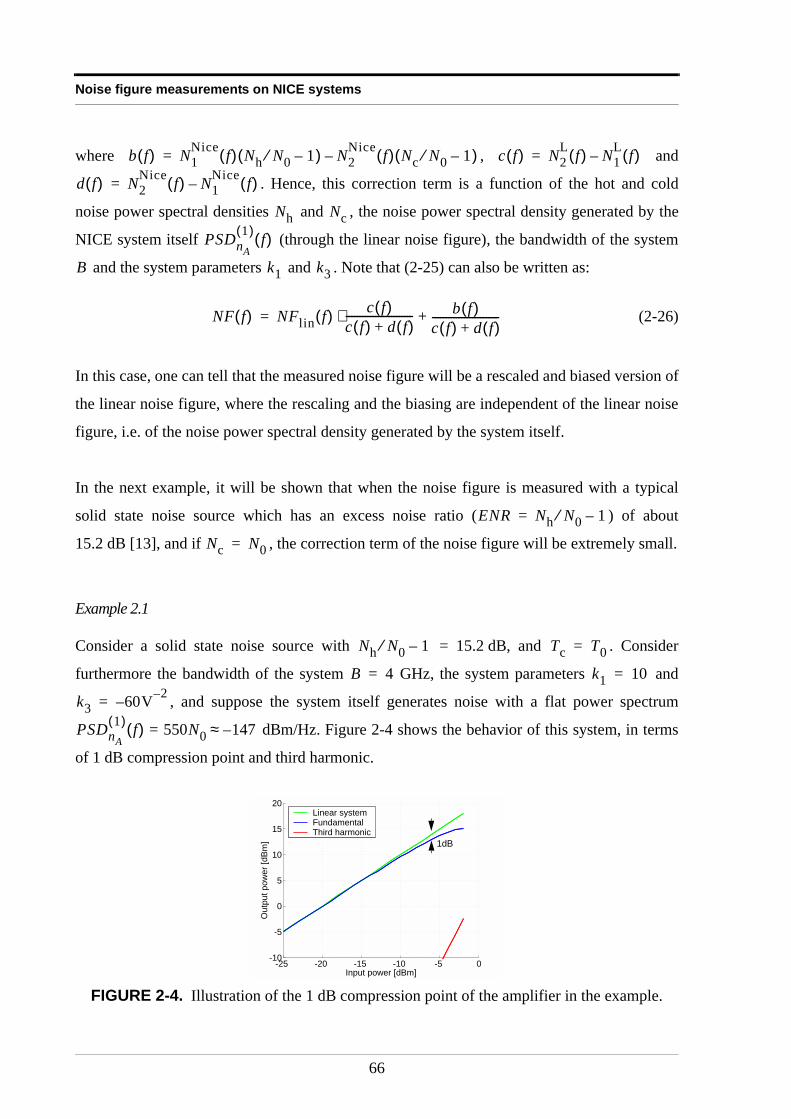
Noise figure measurements on NICE systems
where , and
. Hence, this correction term is a function of the hot and cold
noise power spectral densities and , the noise power spectral density generated by the
NICE system itself (through the linear noise figure), the bandwidth of the system
and the system parameters and . Note that (2-25) can also be written as:
(2-26)
In this case, one can tell that the measured noise figure will be a rescaled and biased version of
the linear noise figure, where the rescaling and the biasing are independent of the linear noise
figure, i.e. of the noise power spectral density generated by the system itself.
In the next example, it will be shown that when the noise figure is measured with a typical
solid state noise source which has an excess noise ratio ( ) of about
15.2 dB [13], and if , the correction term of the noise figure will be extremely small.
Example 2.1
Consider a solid state noise source with = 15.2 dB, and . Consider
furthermore the bandwidth of the system GHz, the system parameters and
, and suppose the system itself generates noise with a flat power spectrum
dBm/Hz. Figure 2-4 shows the behavior of this system, in terms
of 1 dB compression point and third harmonic.
FIGURE 2-4. Illustration of the 1 dB compression point of the amplifier in the example.
b f( ) N1Nice f( ) Nh N0⁄ 1–( ) N2
Nice f( ) Nc N0⁄ 1–( )–= c f( ) N2L f( ) N1
L f( )–=
d f( ) N2Nice f( ) N1
Nice f( )–=
Nh Nc
PSDnA
1( ) f( )
B k1 k3
NF f( ) NFlin f( ) c f( )c f( ) d f( )+-------------------------⋅ b f( )
c f( ) d f( )+-------------------------+=
ENR Nh N0⁄ 1–=
Nc N0=
Nh N0⁄ 1– Tc T0=
B 4= k1 10=
k3 60V 2––=
PSDnA
1( ) f( ) 550N0= 147–≈
-25 -20 -15 -10 -5 0-10
-5
0
5
10
15
20
Input power [dBm]
Ou
tpu
t p
ow
er
[dB
m]
Linear system Fundamental Third harmonic
1dB
66
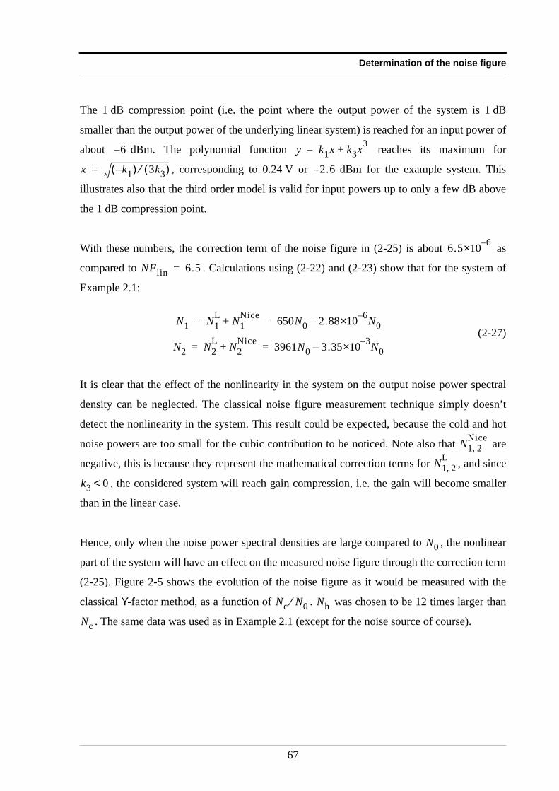
Determination of the noise figure
The 1 dB compression point (i.e. the point where the output power of the system is 1 dB
smaller than the output power of the underlying linear system) is reached for an input power of
about dBm. The polynomial function reaches its maximum for
, corresponding to 0.24 V or dBm for the example system. This
illustrates also that the third order model is valid for input powers up to only a few dB above
the 1 dB compression point.
With these numbers, the correction term of the noise figure in (2-25) is about as
compared to . Calculations using (2-22) and (2-23) show that for the system of
Example 2.1:
(2-27)
It is clear that the effect of the nonlinearity in the system on the output noise power spectral
density can be neglected. The classical noise figure measurement technique simply doesn’t
detect the nonlinearity in the system. This result could be expected, because the cold and hot
noise powers are too small for the cubic contribution to be noticed. Note also that are
negative, this is because they represent the mathematical correction terms for , and since
, the considered system will reach gain compression, i.e. the gain will become smaller
than in the linear case.
Hence, only when the noise power spectral densities are large compared to , the nonlinear
part of the system will have an effect on the measured noise figure through the correction term
(2-25). Figure 2-5 shows the evolution of the noise figure as it would be measured with the
classical Y-factor method, as a function of . was chosen to be 12 times larger than
. The same data was used as in Example 2.1 (except for the noise source of course).
6– y k1x k3x3+=
x k1–( ) 3k3( )⁄= 2.6–
6.5 6–×10
NFlin 6.5=
N1 N1L N1
Nice+ 650N0 2.88 6–×10 N0–= =
N2 N2L N2
Nice+ 3961N0 3.35 3–×10 N0–= =
N1 2,Nice
N1 2,L
k3 0<
N0
Nc N0⁄ Nh
Nc
67
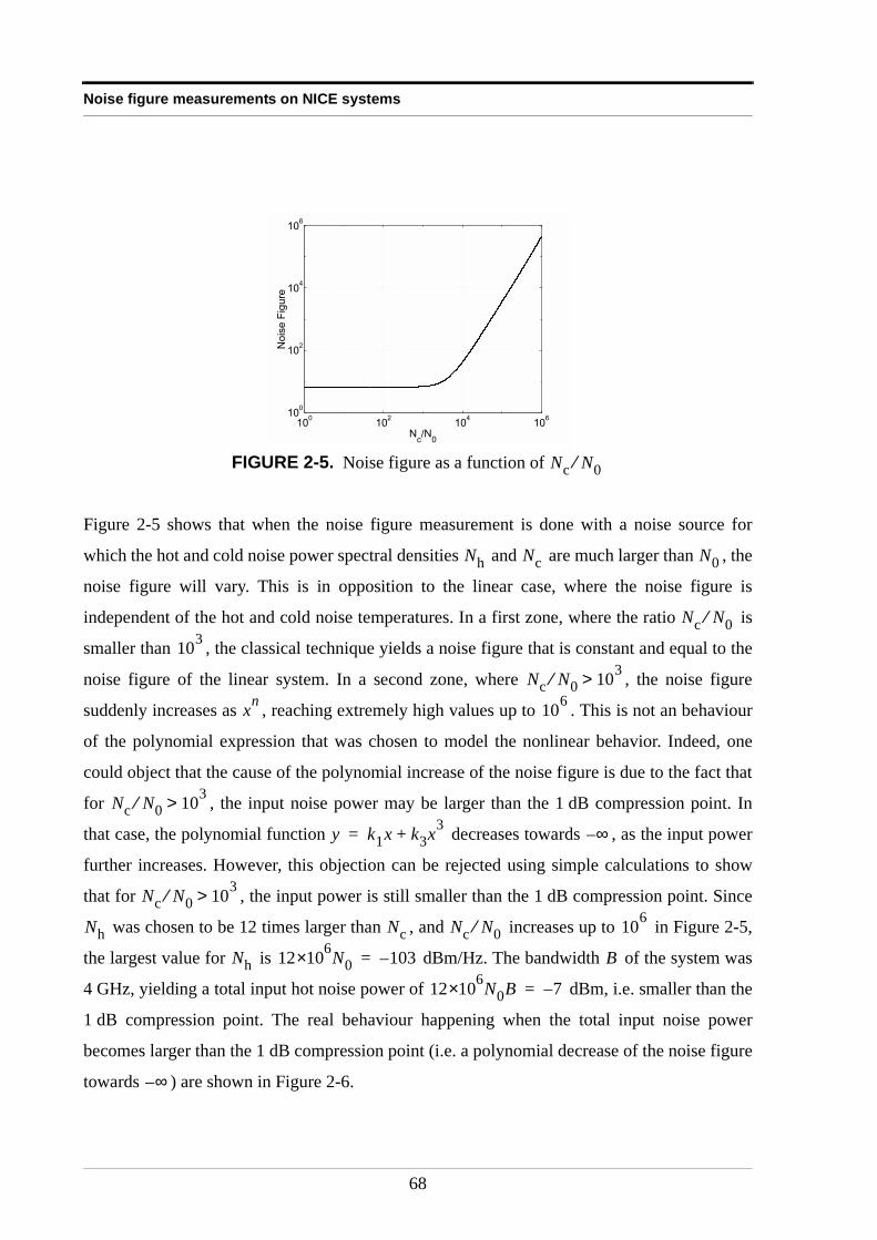
Noise figure measurements on NICE systems
Figure 2-5 shows that when the noise figure measurement is done with a noise source for
which the hot and cold noise power spectral densities and are much larger than , the
noise figure will vary. This is in opposition to the linear case, where the noise figure is
independent of the hot and cold noise temperatures. In a first zone, where the ratio is
smaller than , the classical technique yields a noise figure that is constant and equal to the
noise figure of the linear system. In a second zone, where , the noise figure
suddenly increases as , reaching extremely high values up to . This is not an behaviour
of the polynomial expression that was chosen to model the nonlinear behavior. Indeed, one
could object that the cause of the polynomial increase of the noise figure is due to the fact that
for , the input noise power may be larger than the 1 dB compression point. In
that case, the polynomial function decreases towards , as the input power
further increases. However, this objection can be rejected using simple calculations to show
that for , the input power is still smaller than the 1 dB compression point. Since
was chosen to be 12 times larger than , and increases up to in Figure 2-5,
the largest value for is dBm/Hz. The bandwidth of the system was
4 GHz, yielding a total input hot noise power of dBm, i.e. smaller than the
1 dB compression point. The real behaviour happening when the total input noise power
becomes larger than the 1 dB compression point (i.e. a polynomial decrease of the noise figure
towards ) are shown in Figure 2-6.
FIGURE 2-5. Noise figure as a function of
100 102 104 106100
102
104
106
Nc/N
0
Noi
se F
igur
e
Nc N0⁄
Nh Nc N0
Nc N0⁄
103
Nc N0⁄ 103>
xn 106
Nc N0⁄ 103>
y k1x k3x3+= ∞–
Nc N0⁄ 103>
Nh Nc Nc N0⁄ 106
Nh 12 6×10 N0 103–= B
12 6×10 N0B 7–=
∞–
68
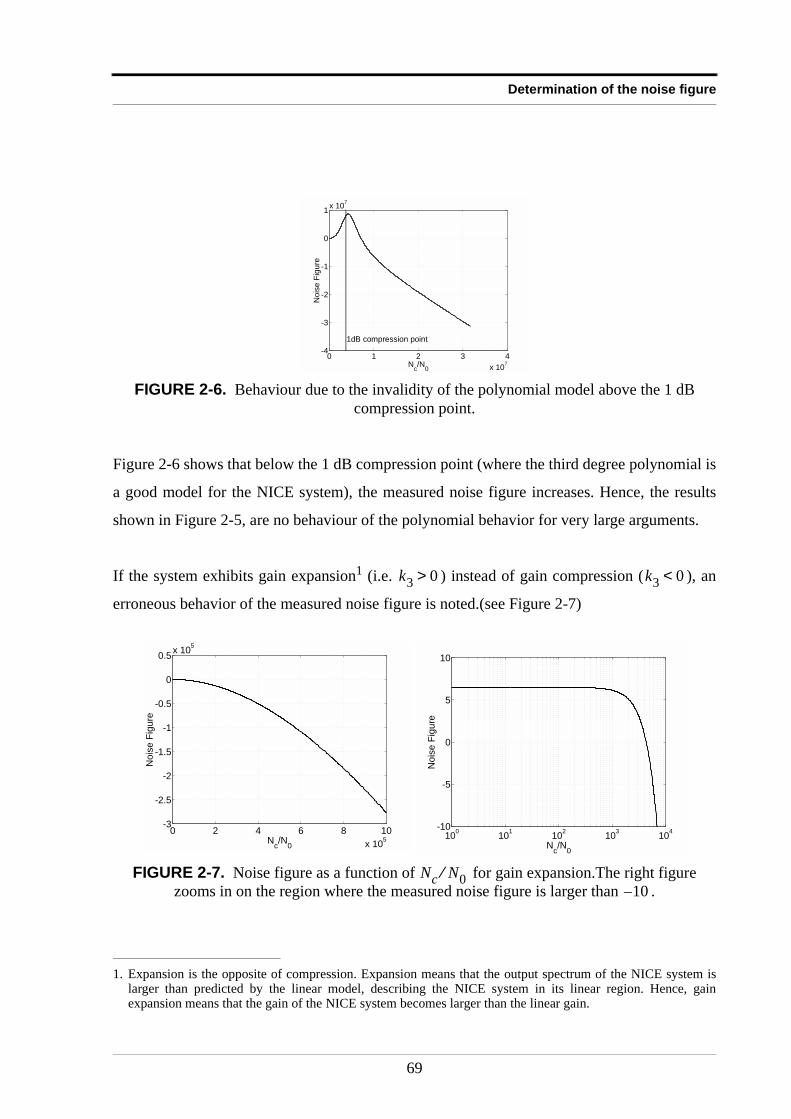
Determination of the noise figure
Figure 2-6 shows that below the 1 dB compression point (where the third degree polynomial is
a good model for the NICE system), the measured noise figure increases. Hence, the results
shown in Figure 2-5, are no behaviour of the polynomial behavior for very large arguments.
If the system exhibits gain expansion1 (i.e. ) instead of gain compression ( ), an
erroneous behavior of the measured noise figure is noted.(see Figure 2-7)
FIGURE 2-6. Behaviour due to the invalidity of the polynomial model above the 1 dB compression point.
1. Expansion is the opposite of compression. Expansion means that the output spectrum of the NICE system islarger than predicted by the linear model, describing the NICE system in its linear region. Hence, gainexpansion means that the gain of the NICE system becomes larger than the linear gain.
FIGURE 2-7. Noise figure as a function of for gain expansion.The right figure zooms in on the region where the measured noise figure is larger than .
0 1 2 3 4
x 107
-4
-3
-2
-1
0
1x 10
7
Nc/N
0
Nois
e F
igure
1dB compression point
k3 0> k3 0<
0 2 4 6 8 10
x 105
-3
-2.5
-2
-1.5
-1
-0.5
0
0.5x 10
5
Nc/N
0
Nois
e F
igure
100
101
102
103
104
-10
-5
0
5
10
Nc/N
0
Nois
e F
igure
Nc N0⁄10–
69
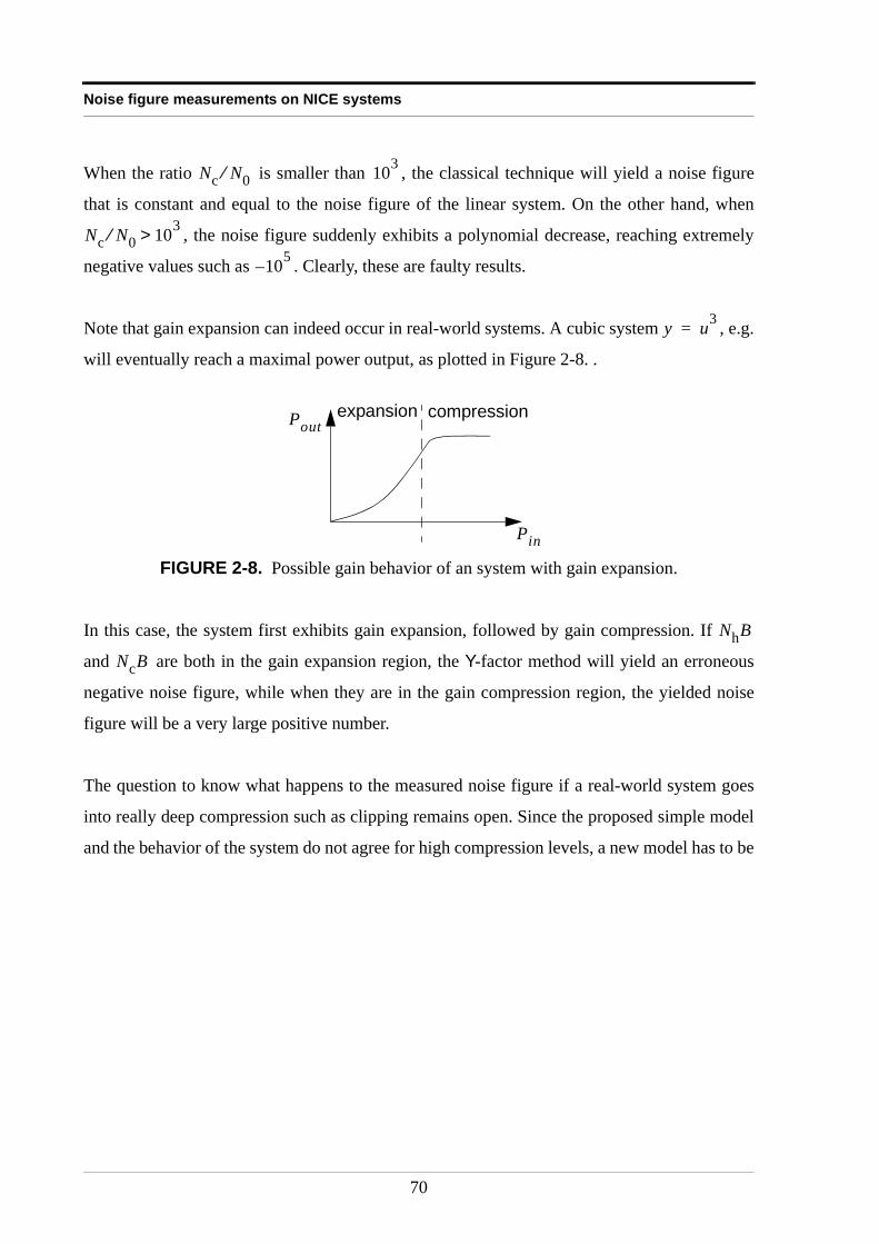
Noise figure measurements on NICE systems
When the ratio is smaller than , the classical technique will yield a noise figure
that is constant and equal to the noise figure of the linear system. On the other hand, when
, the noise figure suddenly exhibits a polynomial decrease, reaching extremely
negative values such as . Clearly, these are faulty results.
Note that gain expansion can indeed occur in real-world systems. A cubic system , e.g.
will eventually reach a maximal power output, as plotted in Figure 2-8. .
In this case, the system first exhibits gain expansion, followed by gain compression. If
and are both in the gain expansion region, the Y-factor method will yield an erroneous
negative noise figure, while when they are in the gain compression region, the yielded noise
figure will be a very large positive number.
The question to know what happens to the measured noise figure if a real-world system goes
into really deep compression such as clipping remains open. Since the proposed simple model
and the behavior of the system do not agree for high compression levels, a new model has to be
FIGURE 2-8. Possible gain behavior of an system with gain expansion.
Nc N0⁄ 103
Nc N0⁄ 103>
10– 5
y u3=
Pin
Poutcompressionexpansion
NhB
NcB
70
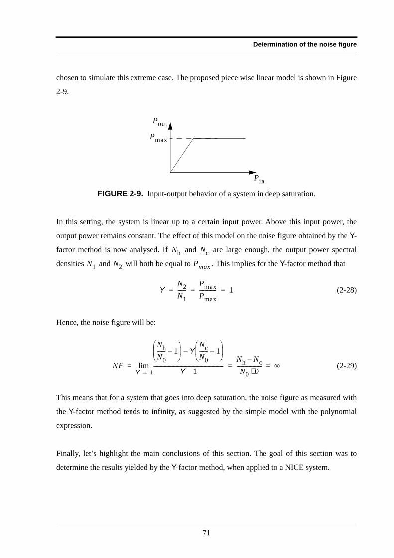
Determination of the noise figure
chosen to simulate this extreme case. The proposed piece wise linear model is shown in Figure
2-9.
In this setting, the system is linear up to a certain input power. Above this input power, the
output power remains constant. The effect of this model on the noise figure obtained by the Y-
factor method is now analysed. If and are large enough, the output power spectral
densities and will both be equal to . This implies for the Y-factor method that
(2-28)
Hence, the noise figure will be:
(2-29)
This means that for a system that goes into deep saturation, the noise figure as measured with
the Y-factor method tends to infinity, as suggested by the simple model with the polynomial
expression.
Finally, let’s highlight the main conclusions of this section. The goal of this section was to
determine the results yielded by the Y-factor method, when applied to a NICE system.
FIGURE 2-9. Input-output behavior of a system in deep saturation.
Pin
Pout
Pmax
Nh Nc
N1 N2 Pmax
YN2N1------
PmaxPmax------------- 1= = =
NF
NhN0------ 1–
YNcN0------ 1–
–
Y 1–-----------------------------------------------------
Y 1→lim
Nh Nc–N0 0⋅
------------------- ∞= = =
71
Noise figure measurements on NICE systems
• Using a model with a third degree polynomial, the NICE system can be
modelled for input noise powers up to the 1 dB compression point. During
a classical noise figure measurement, the NICE system is excited with a
noise source for which the cold ( ) and hot ( ) power spectral
densities are of the order of magnitude of the standard thermal noise
power spectral density ( ). The nonlinear part of the system will be
ignored by this measurement technique, and the noise figure of the
underlying linear system will be obtained. This is because the cold and
hot noise powers are too small to excite the nonlinear part of the system.
When and are made several orders of magnitude larger than ,
in order to excite the nonlinearity, the yielded noise figure increases up to
.
• When using noise powers below the 1 dB compression point, and when
the system exhibits gain expansion, the yielded noise figure decreases
towards , having no more physical meaning. Hence, the Y-factor
method will fail, when applied to systems exhibiting gain expansion.
• To get an idea about the measured noise figure for input noise powers
above the 1 dB compression point, a piecewise linear model is proposed.
This model predicts that the measured noise figure will become infinity in
deep compression.
Nc Nh
N0
Nc Nh N0
106
∞–
72
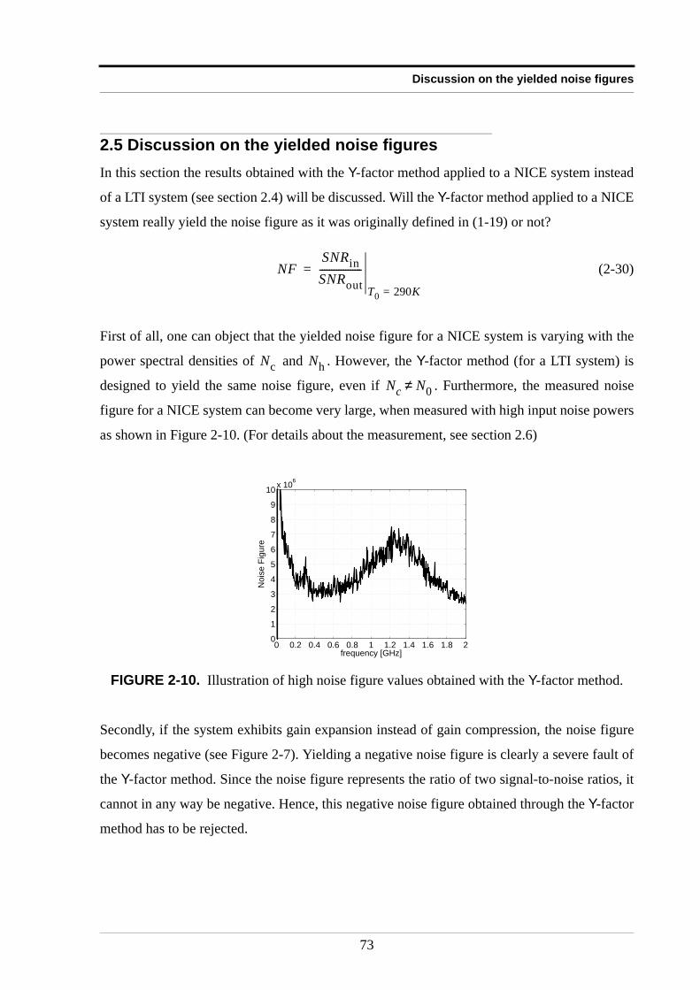
Discussion on the yielded noise figures
2.5 Discussion on the yielded noise figuresIn this section the results obtained with the Y-factor method applied to a NICE system instead
of a LTI system (see section 2.4) will be discussed. Will the Y-factor method applied to a NICE
system really yield the noise figure as it was originally defined in (1-19) or not?
(2-30)
First of all, one can object that the yielded noise figure for a NICE system is varying with the
power spectral densities of and . However, the Y-factor method (for a LTI system) is
designed to yield the same noise figure, even if . Furthermore, the measured noise
figure for a NICE system can become very large, when measured with high input noise powers
as shown in Figure 2-10. (For details about the measurement, see section 2.6)
Secondly, if the system exhibits gain expansion instead of gain compression, the noise figure
becomes negative (see Figure 2-7). Yielding a negative noise figure is clearly a severe fault of
the Y-factor method. Since the noise figure represents the ratio of two signal-to-noise ratios, it
cannot in any way be negative. Hence, this negative noise figure obtained through the Y-factor
method has to be rejected.
FIGURE 2-10. Illustration of high noise figure values obtained with the Y-factor method.
NFSNRinSNRout------------------
T0 290K=
=
Nc Nh
Nc N0≠
0 0.2 0.4 0.6 0.8 1 1.2 1.4 1.6 1.8 20
1
2
3
4
5
6
7
8
9
10x 10
6
Noi
se F
igur
e
frequency [GHz]
73
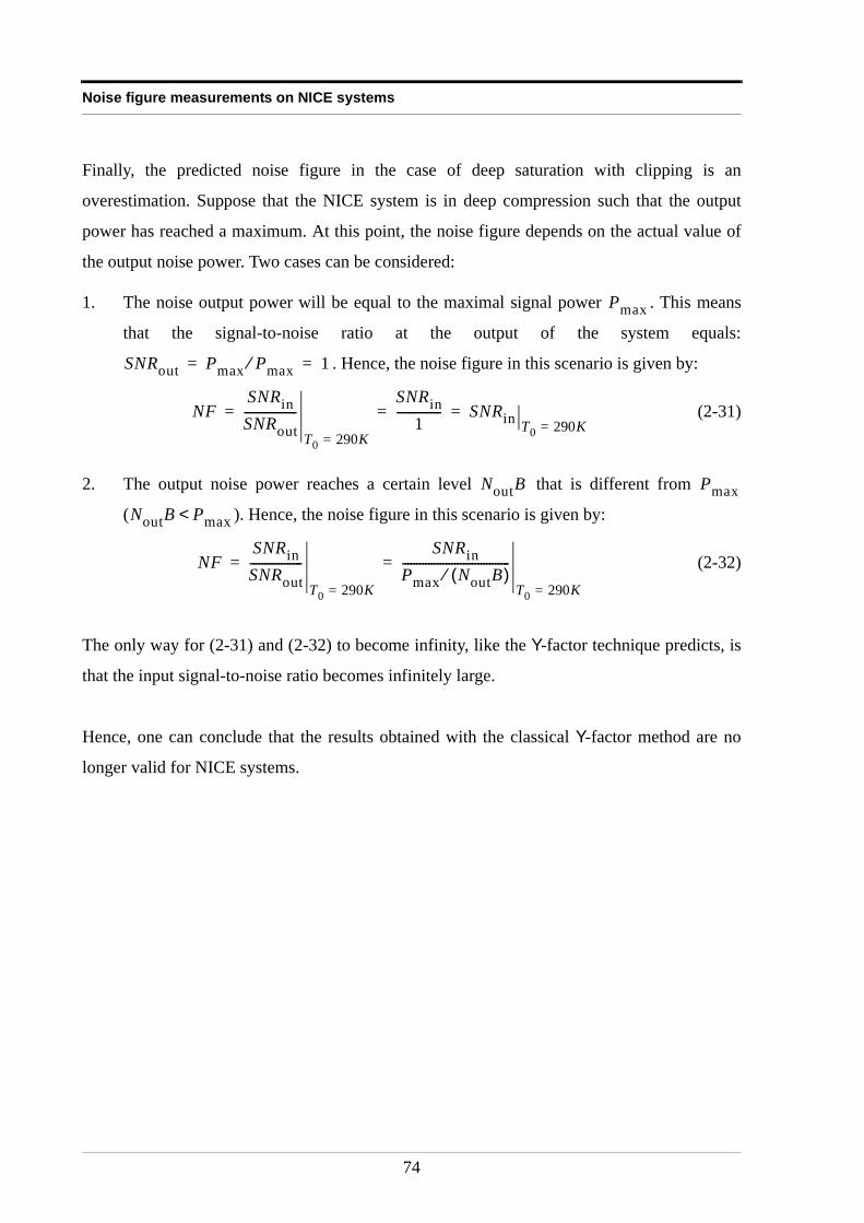
Noise figure measurements on NICE systems
Finally, the predicted noise figure in the case of deep saturation with clipping is an
overestimation. Suppose that the NICE system is in deep compression such that the output
power has reached a maximum. At this point, the noise figure depends on the actual value of
the output noise power. Two cases can be considered:
1. The noise output power will be equal to the maximal signal power . This means
that the signal-to-noise ratio at the output of the system equals:
. Hence, the noise figure in this scenario is given by:
(2-31)
2. The output noise power reaches a certain level that is different from
( ). Hence, the noise figure in this scenario is given by:
(2-32)
The only way for (2-31) and (2-32) to become infinity, like the Y-factor technique predicts, is
that the input signal-to-noise ratio becomes infinitely large.
Hence, one can conclude that the results obtained with the classical Y-factor method are no
longer valid for NICE systems.
Pmax
SNRout Pmax Pmax⁄ 1= =
NFSNRinSNRout------------------
T0 290K=
SNRin1
--------------- SNRin T0 290K== = =
NoutB Pmax
NoutB Pmax<
NFSNRinSNRout------------------
T0 290K=
SNRinPmax NoutB( )⁄-------------------------------------
T0 290K=
= =
74
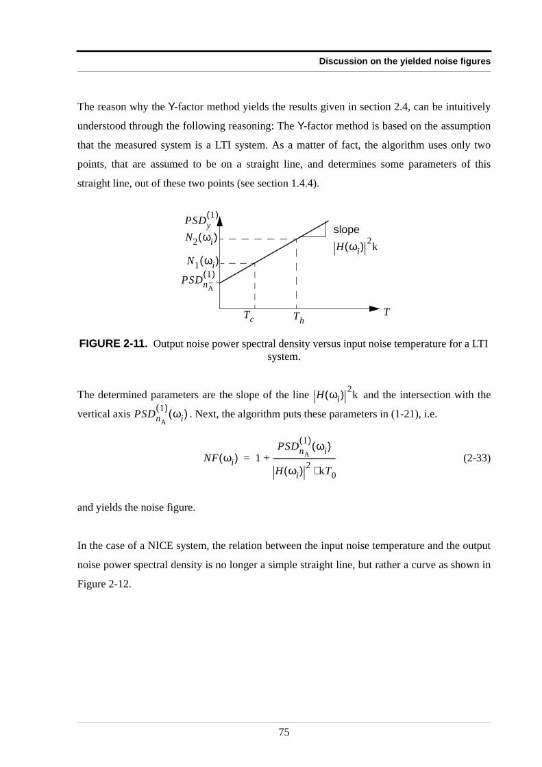
Discussion on the yielded noise figures
The reason why the Y-factor method yields the results given in section 2.4, can be intuitively
understood through the following reasoning: The Y-factor method is based on the assumption
that the measured system is a LTI system. As a matter of fact, the algorithm uses only two
points, that are assumed to be on a straight line, and determines some parameters of this
straight line, out of these two points (see section 1.4.4).
The determined parameters are the slope of the line and the intersection with the
vertical axis . Next, the algorithm puts these parameters in (1-21), i.e.
(2-33)
and yields the noise figure.
In the case of a NICE system, the relation between the input noise temperature and the output
noise power spectral density is no longer a simple straight line, but rather a curve as shown in
Figure 2-12.
FIGURE 2-11. Output noise power spectral density versus input noise temperature for a LTI system.
T
PSDy1( )
PSDnA
1( )
H ωi( ) 2kslope
Tc Th
N1 ωi( )
N2 ωi( )
H ωi( ) 2k
PSDnA
1( ) ωi( )
NF ωi( ) 1PSDnA
1( ) ωi( )
H ωi( ) 2 kT0⋅----------------------------------+=
75
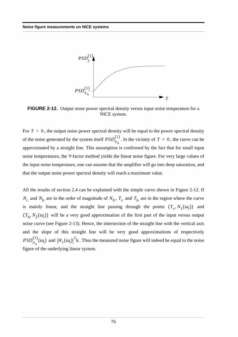
Noise figure measurements on NICE systems
For , the output noise power spectral density will be equal to the power spectral density
of the noise generated by the system itself . In the vicinity of , the curve can be
approximated by a straight line. This assumption is confirmed by the fact that for small input
noise temperatures, the Y-factor method yields the linear noise figure. For very large values of
the input noise temperature, one can assume that the amplifier will go into deep saturation, and
that the output noise power spectral density will reach a maximum value.
All the results of section 2.4 can be explained with the simple curve shown in Figure 2-12. If
and are in the order of magnitude of , and are in the region where the curve
is mainly linear, and the straight line passing through the points and
will be a very good approximation of the first part of the input versus output
noise curve (see Figure 2-13). Hence, the intersection of the straight line with the vertical axis
and the slope of this straight line will be very good approximations of respectively
and . Thus the measured noise figure will indeed be equal to the noise
figure of the underlying linear system.
FIGURE 2-12. Output noise power spectral density versus input noise temperature for a NICE system.
T
PSDy1( )
PSDnA
1( )
T 0=
PSDnA
1( ) T 0=
Nc Nh N0 Tc Th
Tc N1 ωi( ),( )
Th N2 ωi( ),( )
PSDnA
1( ) ωi( ) H1 ωi( ) 2k
76
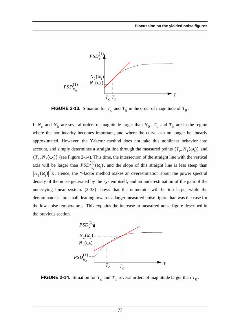
Discussion on the yielded noise figures
If and are several orders of magnitude larger than , and are in the region
where the nonlinearity becomes important, and where the curve can no longer be linearly
approximated. However, the Y-factor method does not take this nonlinear behavior into
account, and simply determines a straight line through the measured points and
(see Figure 2-14). This time, the intersection of the straight line with the vertical
axis will be larger than , and the slope of this straight line is less steep than
. Hence, the Y-factor method makes an overestimation about the power spectral
density of the noise generated by the system itself, and an underestimation of the gain of the
underlying linear system. (2-33) shows that the numerator will be too large, while the
denominator is too small, leading towards a larger measured noise figure than was the case for
the low noise temperatures. This explains the increase in measured noise figure described in
the previous section.
FIGURE 2-13. Situation for and in the order of magnitude of .
FIGURE 2-14. Situation for and several orders of magnitude larger than .
T
PSDy1( )
PSDnA
1( )
Tc Th
N1 ωi( )N2 ωi( )
Tc Th T0
Nc Nh N0 Tc Th
Tc N1 ωi( ),( )
Th N2 ωi( ),( )
PSDnA
1( ) ωi( )
H1 ωi( ) 2k
T
PSDy1( )
PSDnA
1( )
Tc Th
N1 ωi( )N2 ωi( )
Tc Th T0
77
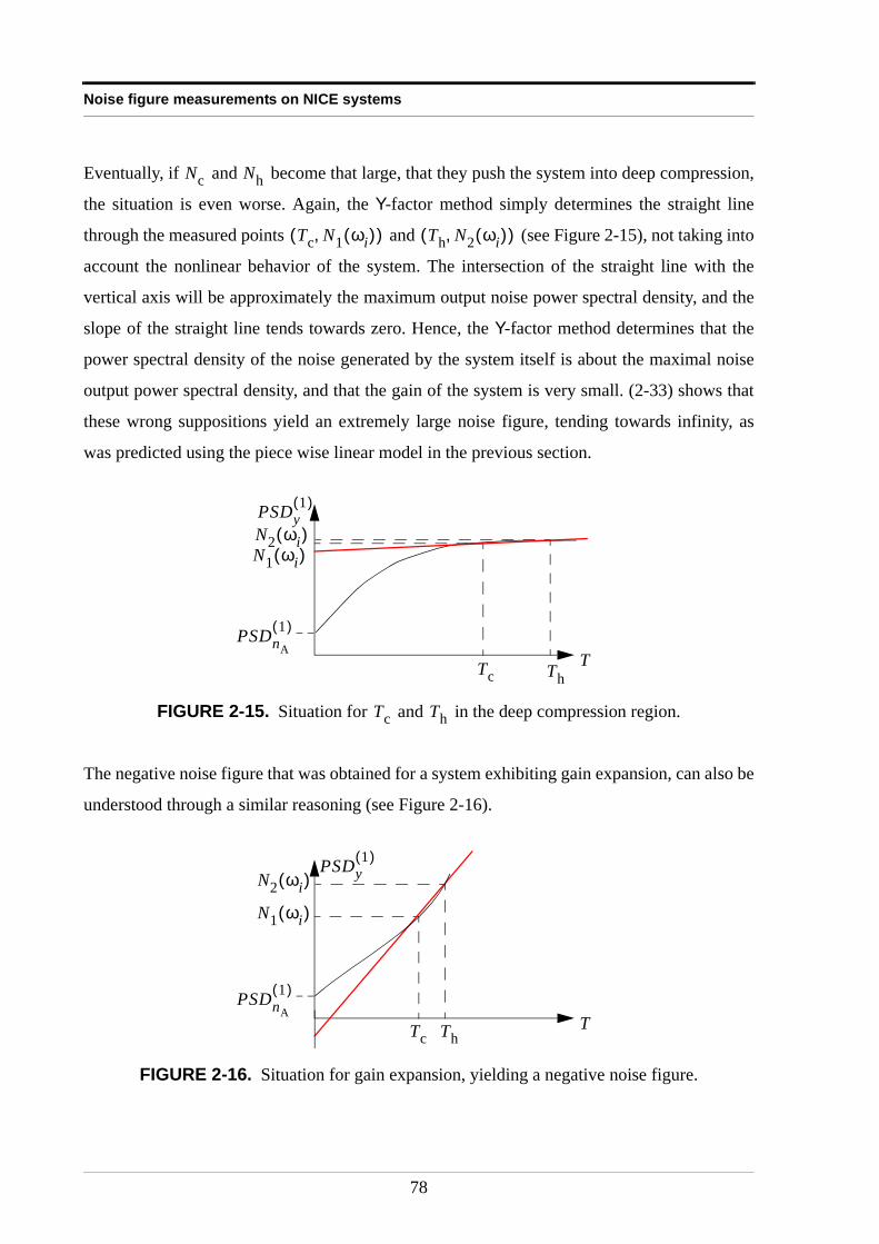
Noise figure measurements on NICE systems
Eventually, if and become that large, that they push the system into deep compression,
the situation is even worse. Again, the Y-factor method simply determines the straight line
through the measured points and (see Figure 2-15), not taking into
account the nonlinear behavior of the system. The intersection of the straight line with the
vertical axis will be approximately the maximum output noise power spectral density, and the
slope of the straight line tends towards zero. Hence, the Y-factor method determines that the
power spectral density of the noise generated by the system itself is about the maximal noise
output power spectral density, and that the gain of the system is very small. (2-33) shows that
these wrong suppositions yield an extremely large noise figure, tending towards infinity, as
was predicted using the piece wise linear model in the previous section.
The negative noise figure that was obtained for a system exhibiting gain expansion, can also be
understood through a similar reasoning (see Figure 2-16).
FIGURE 2-15. Situation for and in the deep compression region.
FIGURE 2-16. Situation for gain expansion, yielding a negative noise figure.
Nc Nh
Tc N1 ωi( ),( ) Th N2 ωi( ),( )
T
PSDy1( )
PSDnA
1( )
Tc Th
N1 ωi( )N2 ωi( )
Tc Th
T
PSDy1( )
PSDnA
1( )
Tc Th
N1 ωi( )
N2 ωi( )
78
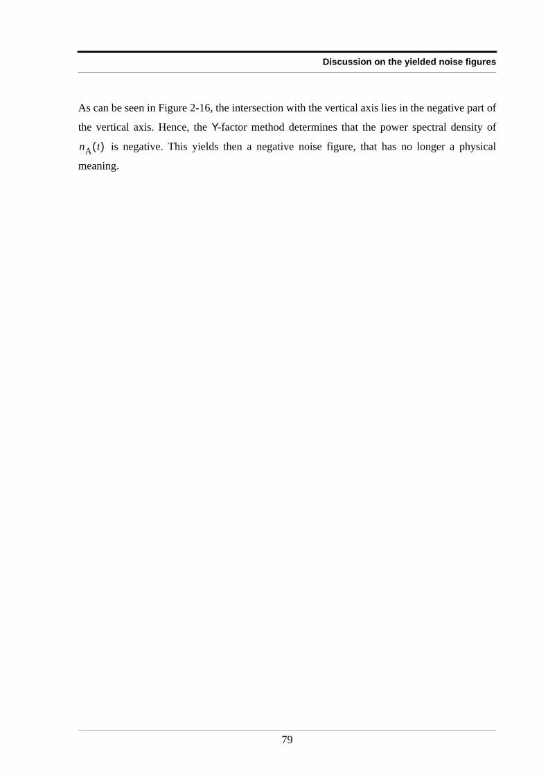
Discussion on the yielded noise figures
As can be seen in Figure 2-16, the intersection with the vertical axis lies in the negative part of
the vertical axis. Hence, the Y-factor method determines that the power spectral density of
is negative. This yields then a negative noise figure, that has no longer a physical
meaning.
nA t( )
79
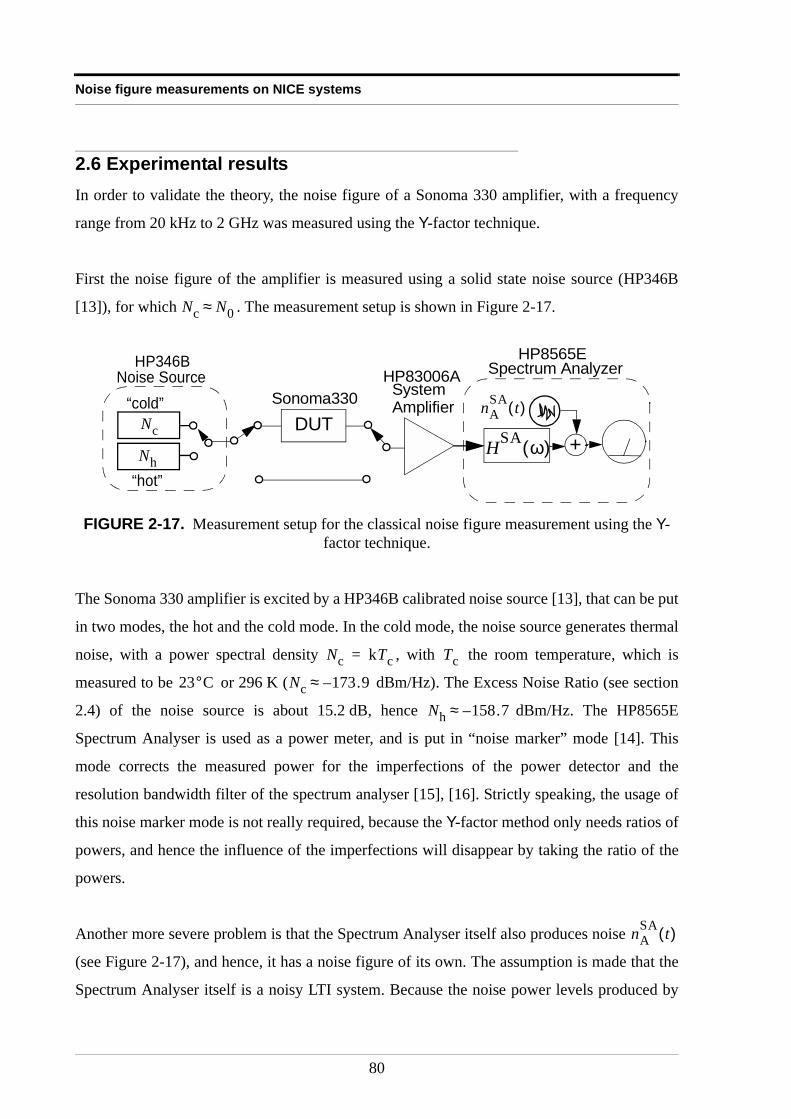
Noise figure measurements on NICE systems
2.6 Experimental resultsIn order to validate the theory, the noise figure of a Sonoma 330 amplifier, with a frequency
range from 20 kHz to 2 GHz was measured using the Y-factor technique.
First the noise figure of the amplifier is measured using a solid state noise source (HP346B
[13]), for which . The measurement setup is shown in Figure 2-17.
The Sonoma 330 amplifier is excited by a HP346B calibrated noise source [13], that can be put
in two modes, the hot and the cold mode. In the cold mode, the noise source generates thermal
noise, with a power spectral density , with the room temperature, which is
measured to be or 296 K ( dBm/Hz). The Excess Noise Ratio (see section
2.4) of the noise source is about 15.2 dB, hence dBm/Hz. The HP8565E
Spectrum Analyser is used as a power meter, and is put in “noise marker” mode [14]. This
mode corrects the measured power for the imperfections of the power detector and the
resolution bandwidth filter of the spectrum analyser [15], [16]. Strictly speaking, the usage of
this noise marker mode is not really required, because the Y-factor method only needs ratios of
powers, and hence the influence of the imperfections will disappear by taking the ratio of the
powers.
Another more severe problem is that the Spectrum Analyser itself also produces noise
(see Figure 2-17), and hence, it has a noise figure of its own. The assumption is made that the
Spectrum Analyser itself is a noisy LTI system. Because the noise power levels produced by
FIGURE 2-17. Measurement setup for the classical noise figure measurement using the Y-factor technique.
Nc N0≈
“cold”
“hot”
Nc
Nh
Noise Source
DUT+
Sonoma330
HP8565ESpectrum AnalyzerHP346B
HSA ω( )
nASA t( )
HP83006ASystemAmplifier
Nc kTc= Tc
23°C Nc 173.9–≈
Nh 158.7–≈
nASA t( )
80
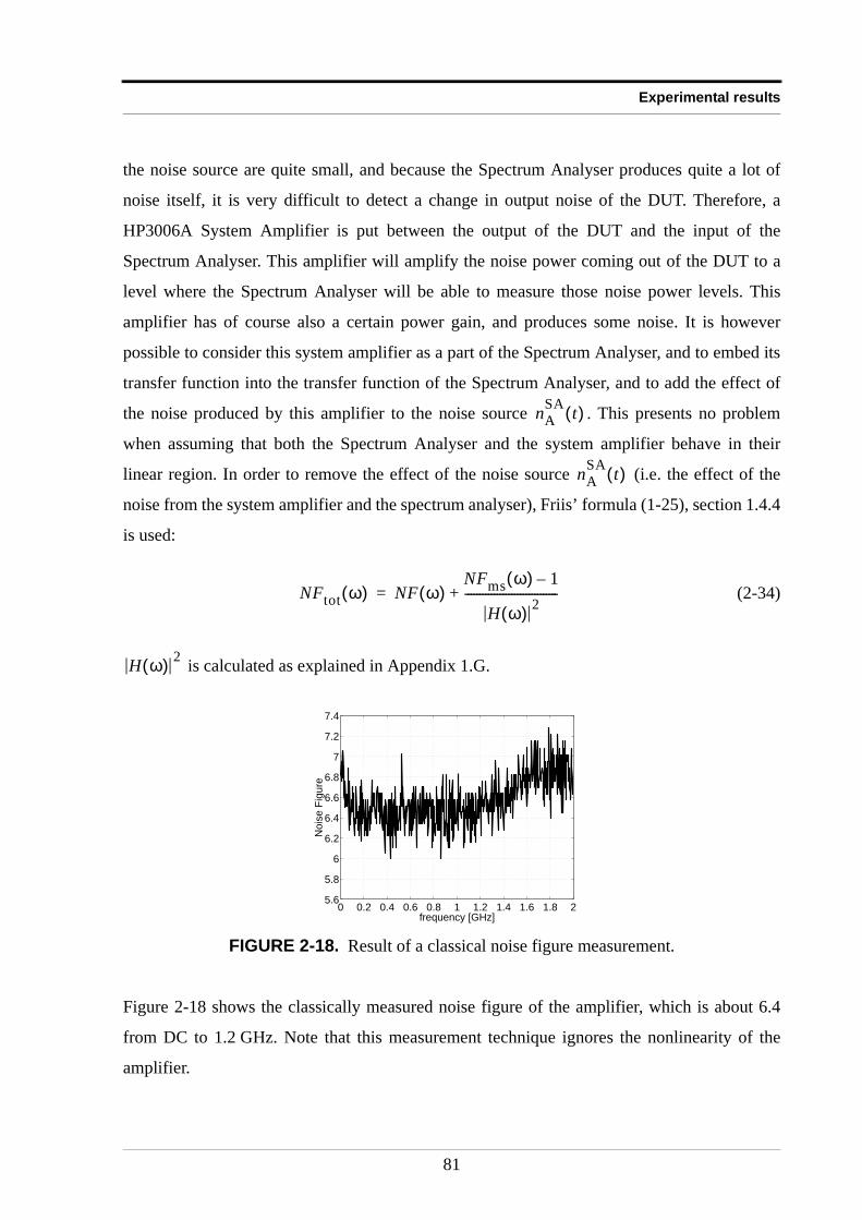
Experimental results
the noise source are quite small, and because the Spectrum Analyser produces quite a lot of
noise itself, it is very difficult to detect a change in output noise of the DUT. Therefore, a
HP3006A System Amplifier is put between the output of the DUT and the input of the
Spectrum Analyser. This amplifier will amplify the noise power coming out of the DUT to a
level where the Spectrum Analyser will be able to measure those noise power levels. This
amplifier has of course also a certain power gain, and produces some noise. It is however
possible to consider this system amplifier as a part of the Spectrum Analyser, and to embed its
transfer function into the transfer function of the Spectrum Analyser, and to add the effect of
the noise produced by this amplifier to the noise source . This presents no problem
when assuming that both the Spectrum Analyser and the system amplifier behave in their
linear region. In order to remove the effect of the noise source (i.e. the effect of the
noise from the system amplifier and the spectrum analyser), Friis’ formula (1-25), section 1.4.4
is used:
(2-34)
is calculated as explained in Appendix 1.G.
Figure 2-18 shows the classically measured noise figure of the amplifier, which is about 6.4
from DC to 1.2 GHz. Note that this measurement technique ignores the nonlinearity of the
amplifier.
FIGURE 2-18. Result of a classical noise figure measurement.
nASA t( )
nASA t( )
NFtot ω( ) NF ω( )NFms ω( ) 1–
H ω( ) 2--------------------------------+=
H ω( ) 2
0 0.2 0.4 0.6 0.8 1 1.2 1.4 1.6 1.8 25.6
5.8
6
6.2
6.4
6.6
6.8
7
7.2
7.4
frequency [GHz]
Noi
se F
igur
e
81
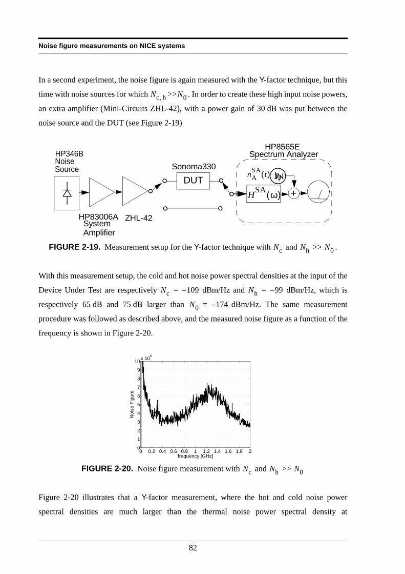
Noise figure measurements on NICE systems
In a second experiment, the noise figure is again measured with the Y-factor technique, but this
time with noise sources for which >> . In order to create these high input noise powers,
an extra amplifier (Mini-Circuits ZHL-42), with a power gain of 30 dB was put between the
noise source and the DUT (see Figure 2-19)
With this measurement setup, the cold and hot noise power spectral densities at the input of the
Device Under Test are respectively dBm/Hz and dBm/Hz, which is
respectively 65 dB and 75 dB larger than dBm/Hz. The same measurement
procedure was followed as described above, and the measured noise figure as a function of the
frequency is shown in Figure 2-20.
Figure 2-20 illustrates that a Y-factor measurement, where the hot and cold noise power
spectral densities are much larger than the thermal noise power spectral density at
FIGURE 2-19. Measurement setup for the Y-factor technique with and >> .
FIGURE 2-20. Noise figure measurement with and >>
Nc h, N0
HP83006A
Noise
DUT+
Sonoma330
HP8565ESpectrum AnalyzerHP346B
HSA ω( )
nASA t( )Source
SystemAmplifier
ZHL-42
Nc Nh N0
Nc 109–= Nh 99–=
N0 174–=
0 0.2 0.4 0.6 0.8 1 1.2 1.4 1.6 1.8 20
1
2
3
4
5
6
7
8
9
10x 10
6
Noi
se F
igur
e
frequency [GHz]
Nc Nh N0
82

Experimental results
K, yields a much too large noise figure (in this case in the order of magnitude of
) as was predicted in Figure 2-5.
T0 290=
106
83
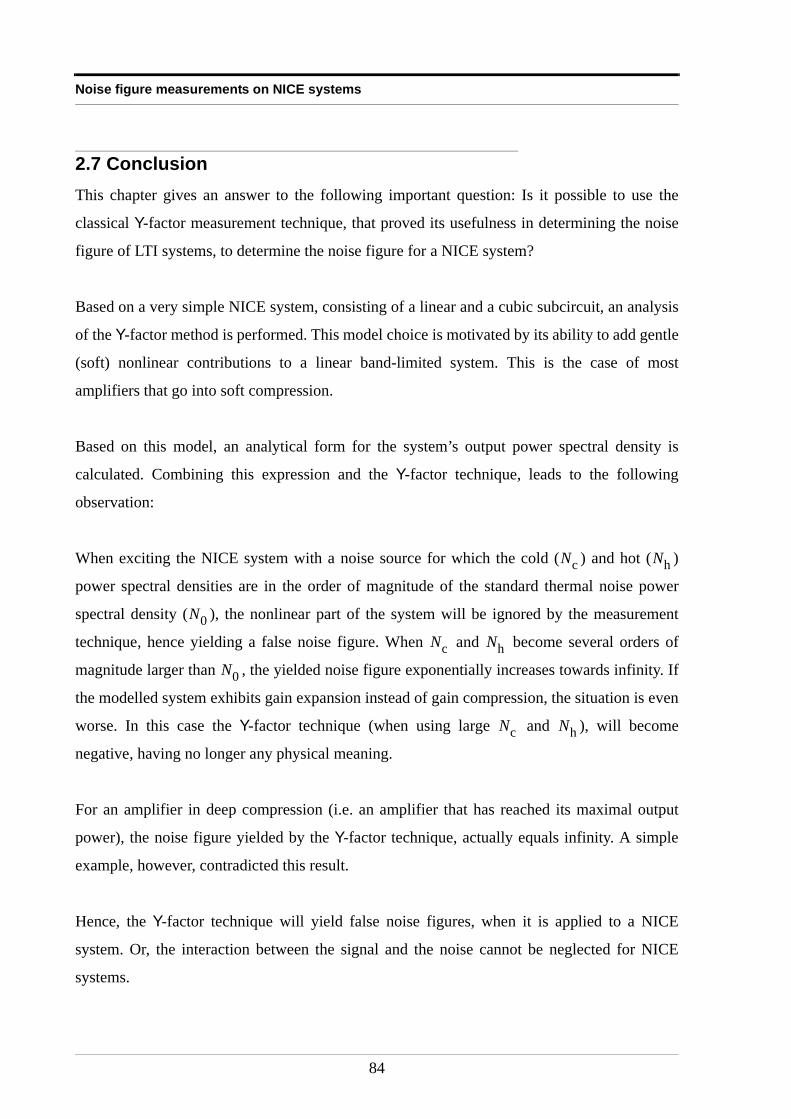
Noise figure measurements on NICE systems
2.7 ConclusionThis chapter gives an answer to the following important question: Is it possible to use the
classical Y-factor measurement technique, that proved its usefulness in determining the noise
figure of LTI systems, to determine the noise figure for a NICE system?
Based on a very simple NICE system, consisting of a linear and a cubic subcircuit, an analysis
of the Y-factor method is performed. This model choice is motivated by its ability to add gentle
(soft) nonlinear contributions to a linear band-limited system. This is the case of most
amplifiers that go into soft compression.
Based on this model, an analytical form for the system’s output power spectral density is
calculated. Combining this expression and the Y-factor technique, leads to the following
observation:
When exciting the NICE system with a noise source for which the cold ( ) and hot ( )
power spectral densities are in the order of magnitude of the standard thermal noise power
spectral density ( ), the nonlinear part of the system will be ignored by the measurement
technique, hence yielding a false noise figure. When and become several orders of
magnitude larger than , the yielded noise figure exponentially increases towards infinity. If
the modelled system exhibits gain expansion instead of gain compression, the situation is even
worse. In this case the Y-factor technique (when using large and ), will become
negative, having no longer any physical meaning.
For an amplifier in deep compression (i.e. an amplifier that has reached its maximal output
power), the noise figure yielded by the Y-factor technique, actually equals infinity. A simple
example, however, contradicted this result.
Hence, the Y-factor technique will yield false noise figures, when it is applied to a NICE
system. Or, the interaction between the signal and the noise cannot be neglected for NICE
systems.
Nc Nh
N0
Nc Nh
N0
Nc Nh
84
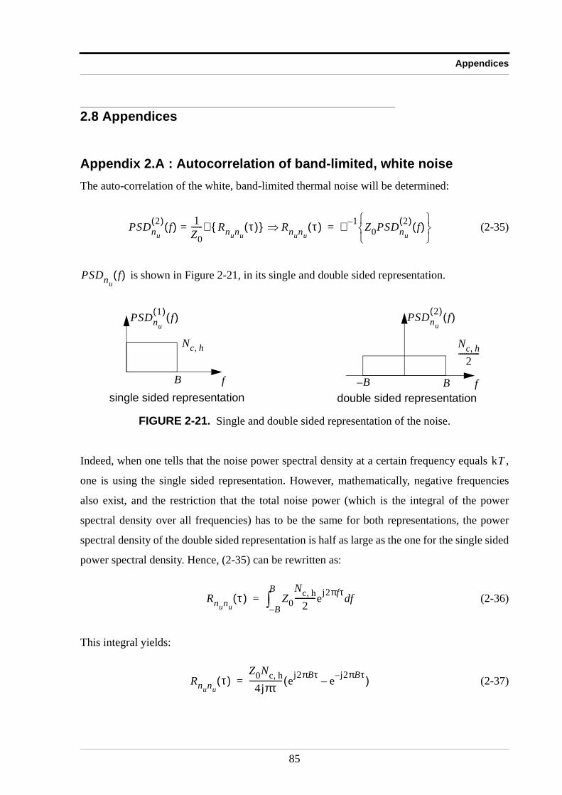
Appendices
2.8 Appendices
Appendix 2.A : Autocorrelation of band-limited, white noiseThe auto-correlation of the white, band-limited thermal noise will be determined:
(2-35)
is shown in Figure 2-21, in its single and double sided representation.
Indeed, when one tells that the noise power spectral density at a certain frequency equals ,
one is using the single sided representation. However, mathematically, negative frequencies
also exist, and the restriction that the total noise power (which is the integral of the power
spectral density over all frequencies) has to be the same for both representations, the power
spectral density of the double sided representation is half as large as the one for the single sided
power spectral density. Hence, (2-35) can be rewritten as:
(2-36)
This integral yields:
(2-37)
FIGURE 2-21. Single and double sided representation of the noise.
PSDnu
2( ) f( ) 1Z0------ ℑ Rnunu
τ( ) = Rnunuτ( )⇒ ℑ 1– Z0PSDnu
2( ) f( )
=
PSDnuf( )
f
Nc h,2
-----------
f
Nc h,
B BB–single sided representation double sided representation
PSDnu
1( ) f( ) PSDnu
2( ) f( )
kT
Rnunuτ( ) Z0
Nc h,2
-----------ej2πfτ fdB–
B∫=
Rnunuτ( )
Z0Nc h,4jπτ
----------------- ej2πBτ e j– 2πBτ–( )=
85
Noise figure measurements on NICE systems
using the fact that
(2-38)
(2-37) becomes:
(2-39)
Appendix 2.B : Fifteen ways of partitioning six random variables in products of averages of pairsThe cubic contribution is written as (see (2-11))
(2-40)
The six random variables are tagged “1” to “6”. The fifteen ways of partitioning the six tags
are:
(2-41)
ejα e jα––2j
------------------------ α( )sin=
Rnunuτ( ) Z0Nc h, B 2πBτ( )sin
2πBτ--------------------------=
E k32nu
3 t( )nu3 t τ+( )
k32E nu t( )nu t( )nu t( )nu t τ+( )nu t τ+( )nu t τ+( ) =
1 2 3 4 5 6
121212131313141414151515161616
343536242526232526232426232425
564645564645563635463634453534
86
Appendices
Since terms , and , pairs of tags pointing to equal terms will yield
factors:
, (2-42)
and pairs of tags pointing to different terms will yield factors:
(2-43)
Hence, (2-41) eventually yields:
(2-44)
Appendix 2.C : The combined contributions of the auto-correlation
The first combined contribution can be rewritten as:
(2-45)
The time average of the product of four random variables equals the sum over all distinct ways
of partitioning the four random variables into products of averages of pairs. The number of
distinct ways to do this is given by (2-13) with , yielding three ways:
(2-46)
Since terms , pairs of tags pointing to equal terms will yield factors:
, (2-47)
1 2 3= = 4 5 6= =
E nu t( )nu t( ) E nu t τ+( )nu t τ+( ) Rnunu0( )= =
E nu t( )nu t τ+( ) Rnunuτ( )=
E nu3 t( )nu
3 t τ+( )
6Rnunu
3 τ( ) 9Rnunu
2 0( )Rnunuτ( )+=
Rηη τ( )
E k1k3nu t( )nu3 t τ+( )
k1k3E nu t( )nu t τ+( )nu t τ+( )nu t τ+( ) =1 2 3 4
M 2=
12 3413 2414 23
2 3 4= =
E nu t( )nu t( ) E nu t τ+( )nu t τ+( ) Rnunu0( )= =
87
Noise figure measurements on NICE systems
and pairs of tags pointing to different terms will yield factors:
(2-48)
Hence, (2-46) eventually yields:
(2-49)
The second term can be calculated, using the anti-symmetry property of
the cross-correlation function:
(2-50)
Hence,
(2-51)
But since the auto-correlation is an even function: , both terms of the
combined contribution are equal, and hence:
(2-52)
E nu t( )nu t τ+( ) Rnunuτ( )=
E nu t( )nu3 t τ+( )
3Rnunu0( )Rnunu
τ( )=
E nu3 t( )nu t τ+( )
Rαβ τ( ) Rβα τ–( )=
E nu3 t( )nu t τ+( )
E nu t( )nu3 t τ–( )
3Rnunu0( )Rnunu
τ–( )= =
Rαα τ( ) Rαα τ–( )=
E k1k3nu3 t( )nu t τ+( )
E k1k3nu t( )nu3 t τ+( )
+ 6Rnunu0( )Rnunu
τ( )=
88
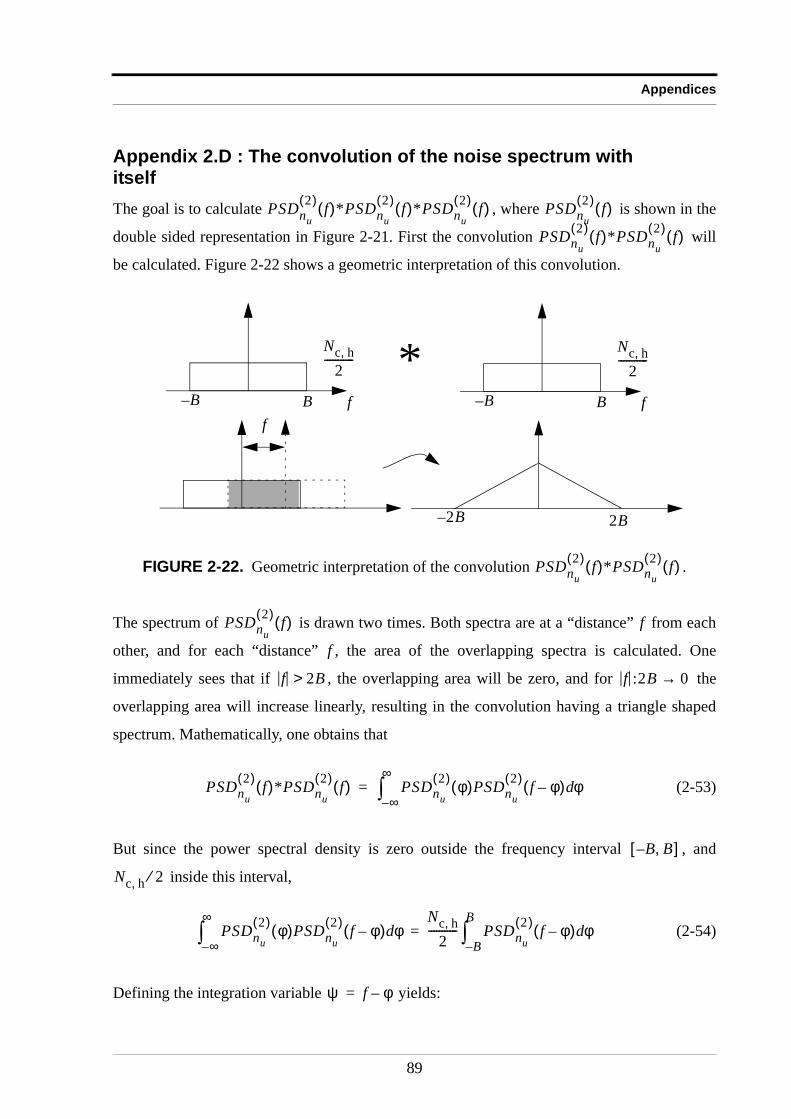
Appendices
Appendix 2.D : The convolution of the noise spectrum with itselfThe goal is to calculate , where is shown in the
double sided representation in Figure 2-21. First the convolution will
be calculated. Figure 2-22 shows a geometric interpretation of this convolution.
The spectrum of is drawn two times. Both spectra are at a “distance” from each
other, and for each “distance” , the area of the overlapping spectra is calculated. One
immediately sees that if , the overlapping area will be zero, and for the
overlapping area will increase linearly, resulting in the convolution having a triangle shaped
spectrum. Mathematically, one obtains that
(2-53)
But since the power spectral density is zero outside the frequency interval , and
inside this interval,
(2-54)
Defining the integration variable yields:
FIGURE 2-22. Geometric interpretation of the convolution .
PSDnu
2( ) f( )*PSDnu
2( ) f( )*PSDnu
2( ) f( ) PSDnu
2( ) f( )
PSDnu
2( ) f( )*PSDnu
2( ) f( )
f
Nc h,2
-----------
BB– f
Nc h,2
-----------
BB–
*f
2B– 2B
PSDnu
2( ) f( )*PSDnu
2( ) f( )
PSDnu
2( ) f( ) f
f
f 2B> f :2B 0→
PSDnu
2( ) f( )*PSDnu
2( ) f( ) PSDnu
2( ) φ( )PSDnu
2( ) f φ–( ) φd∞–
∞∫=
B B,–[ ]
Nc h, 2⁄
PSDnu
2( ) φ( )PSDnu
2( ) f φ–( ) φd∞–
∞∫
Nc h,2
----------- PSDnu
2( ) f φ–( ) φdB–
B∫=
ψ f φ–=
89
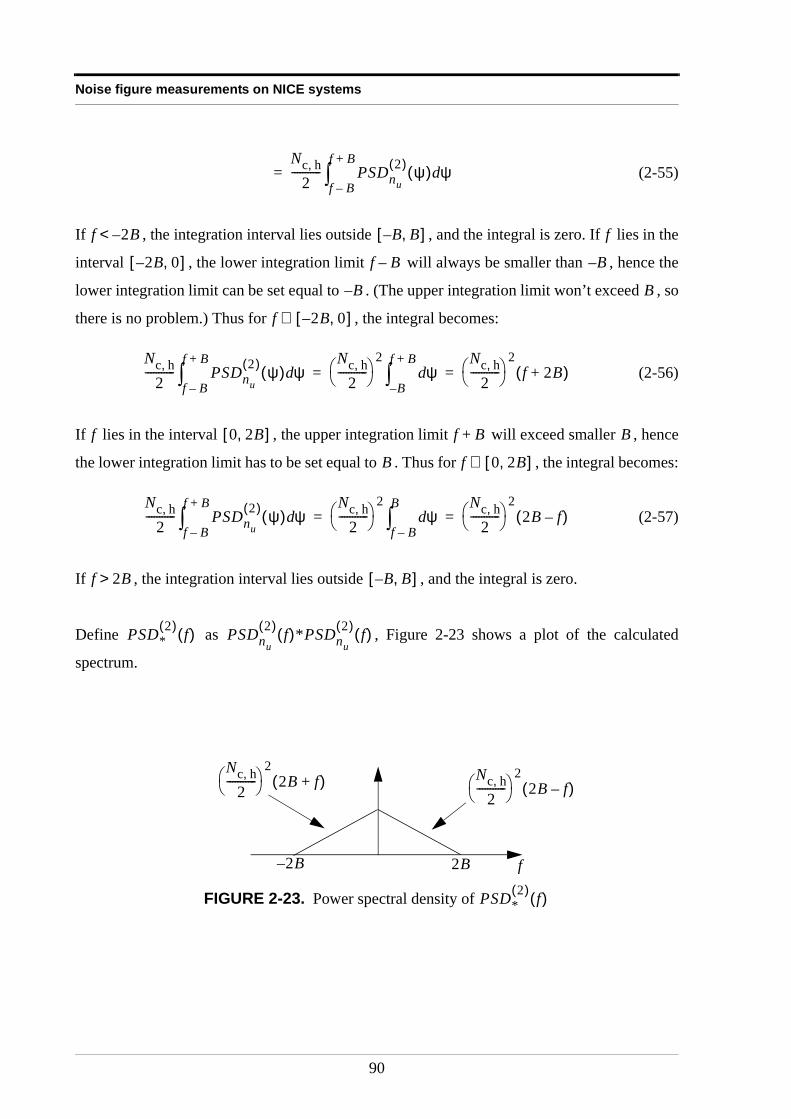
Noise figure measurements on NICE systems
(2-55)
If , the integration interval lies outside , and the integral is zero. If lies in the
interval , the lower integration limit will always be smaller than , hence the
lower integration limit can be set equal to . (The upper integration limit won’t exceed , so
there is no problem.) Thus for , the integral becomes:
(2-56)
If lies in the interval , the upper integration limit will exceed smaller , hence
the lower integration limit has to be set equal to . Thus for , the integral becomes:
(2-57)
If , the integration interval lies outside , and the integral is zero.
Define as , Figure 2-23 shows a plot of the calculated
spectrum.
FIGURE 2-23. Power spectral density of
Nc h,
2----------- PSDnu
2( ) ψ( ) ψdf B–
f B+∫=
f 2B–< B B,–[ ] f
2B 0,–[ ] f B– B–
B– B
f 2B 0,–[ ]∈
Nc h,2
----------- PSDnu
2( ) ψ( ) ψdf B–
f B+∫
Nc h,2
-----------
2ψd
B–
f B+∫
Nc h,2
-----------
2f 2B+( )= =
f 0 2B,[ ] f B+ B
B f 0 2B,[ ]∈
Nc h,2
----------- PSDnu
2( ) ψ( ) ψdf B–
f B+∫
Nc h,2
-----------
2ψd
f B–
B∫
Nc h,2
-----------
22B f–( )= =
f 2B> B B,–[ ]
PSD*2( ) f( ) PSDnu
2( ) f( )*PSDnu
2( ) f( )
f
Nc h,2
-----------
22B f–( )
2B2B–
Nc h,2
-----------
22B f+( )
PSD*2( ) f( )
90
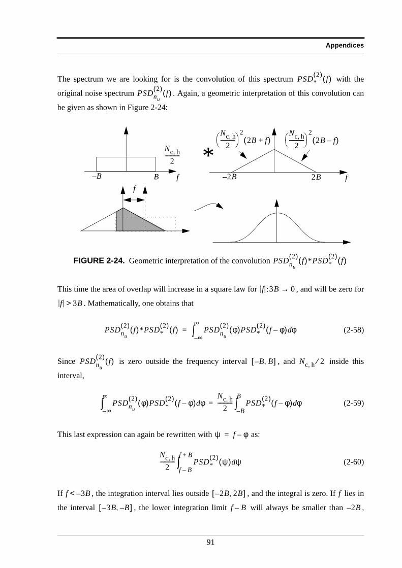
Appendices
The spectrum we are looking for is the convolution of this spectrum with the
original noise spectrum . Again, a geometric interpretation of this convolution can
be given as shown in Figure 2-24:
This time the area of overlap will increase in a square law for , and will be zero for
. Mathematically, one obtains that
(2-58)
Since is zero outside the frequency interval , and inside this
interval,
(2-59)
This last expression can again be rewritten with as:
(2-60)
If , the integration interval lies outside , and the integral is zero. If lies in
the interval , the lower integration limit will always be smaller than ,
FIGURE 2-24. Geometric interpretation of the convolution
PSD*2( ) f( )
PSDnu
2( ) f( )
f
Nc h,2
-----------
BB–
*f
f
Nc h,2
-----------
22B f–( )
2B2B–
Nc h,2
-----------
22B f+( )
PSDnu
2( ) f( )*PSD*2( ) f( )
f :3B 0→
f 3B>
PSDnu
2( ) f( )*PSD*2( ) f( ) PSDnu
2( ) φ( )PSD*2( ) f φ–( ) φd
∞–
∞∫=
PSDnu
2( ) f( ) B B,–[ ] Nc h, 2⁄
PSDnu
2( ) φ( )PSD*2( ) f φ–( ) φd
∞–
∞∫
Nc h,2
----------- PSD*2( ) f φ–( ) φd
B–
B∫=
ψ f φ–=
Nc h,2
----------- PSD*2( ) ψ( ) ψd
f B–
f B+∫
f 3B–< 2B 2B,–[ ] f
3B B–,–[ ] f B– 2B–
91
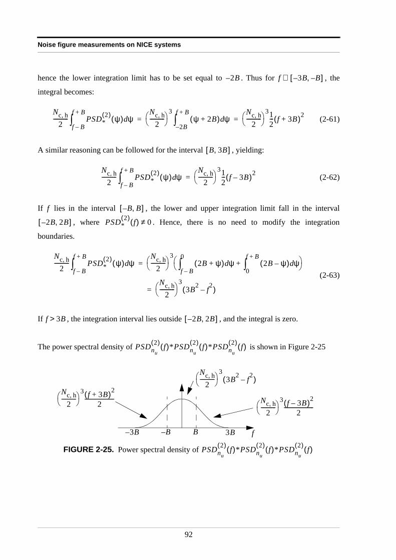
Noise figure measurements on NICE systems
hence the lower integration limit has to be set equal to . Thus for , the
integral becomes:
(2-61)
A similar reasoning can be followed for the interval , yielding:
(2-62)
If lies in the interval , the lower and upper integration limit fall in the interval
, where . Hence, there is no need to modify the integration
boundaries.
(2-63)
If , the integration interval lies outside , and the integral is zero.
The power spectral density of is shown in Figure 2-25
FIGURE 2-25. Power spectral density of
2B– f 3B B–,–[ ]∈
Nc h,2
----------- PSD*2( ) ψ( ) ψd
f B–
f B+∫
Nc h,2
-----------
3ψ 2B+( ) ψd
2B–
f B+∫
Nc h,2
-----------
312--- f 3B+( )2= =
B 3B,[ ]
Nc h,2
----------- PSD*2( ) ψ( ) ψd
f B–
f B+∫
Nc h,2
-----------
312--- f 3B–( )2=
f B B,–[ ]
2B 2B,–[ ] PSD*2( ) f( ) 0≠
Nc h,2
----------- PSD*2( ) ψ( ) ψd
f B–
f B+∫
Nc h,2
-----------
32B ψ+( ) ψd
f B–
0∫ 2B ψ–( ) ψd
0
f B+∫+
=
Nc h,
2-----------
33B2 f2–( )=
f 3B> 2B 2B,–[ ]
PSDnu
2( ) f( )*PSDnu
2( ) f( )*PSDnu
2( ) f( )
f
Nc h,2
-----------
33B2 f2–( )
3B3B–
Nc h,2
-----------
3 f 3B–( )2
2----------------------
BB–
Nc h,2
-----------
3 f 3B+( )2
2----------------------
PSDnu
2( ) f( )*PSDnu
2( ) f( )*PSDnu
2( ) f( )
92
CHAPTER 3
EXTENSION OF THE “NOISEFIGURE” TOWARDS NICE
SYSTEMS
Abstract: Since the behavior of a NICE system is dependent on the
power of its input signal, it is clear that the “noise figure” (defined
as the signal-to-noise ratio deterioration) will also strongly depend
on the power of the input signal, including the input noise. In this
chapter, the dependency of the power of the excitation signal (i.e.
the superposition of the input signal and the noise) on the “noise
figure” of the noisy NICE system is analysed in detail.
93
Extension of the “Noise Figure” towards NICE systems
3.1 Introduction
3.1.1 GoalSince the Y-factor technique is not able to yield correct noise figures for NICE systems, other
methods have to be developed to replace it. The design goal for such an alternative method is
that it must give an accurate description of the deterioration of the signal-to-noise ratio through
the NICE system. On top of that, a more fundamental question arises: Is the noise figure still a
convenient figure to describe the signal-to-noise ratio deterioration through a NICE system?
For Linear Time Invariant systems, the knowledge of the noise figure allows prediction of the
signal-to-noise ratio deterioration for any type of input signal, (since the noise figure is
independent of the input signal ), and for noise sources at any temperature
K. However, since the power of the input signal has an effect on the ratio
for NICE systems (see section 1.5.2), one can already suspect that deterioration
of the signal-to-noise ratio for these systems will be a function of the power contained in the
excitation signal (and thus of both the power of the input noise and the
power of the input signal). Note also that just as in the previous chapters, the noise added by
the NICE system itself, that combines with the input terms will be omitted.
Hence, the noise figure, as defined for linear systems , has to be extended to a NICE
noise figure , that describes the signal-to-noise ratio deterioration for NICE systems. As
opposed to the linear noise figure, that was defined for an input noise temperature of 290 K,
and that was independent of the input signal , the NICE noise figure is defined as the
ratio of the signal-to-noise ratio at the input of the noisy NICE system, to the signal-to-noise
ratio at the output of the noisy NICE system.
(3-1)
This NICE noise figure will be a function of (among others) the following variables: the total
input signal power , the total input noise power , and of course the frequency . With
this definition, the linear noise figure is a special case of the NICE noise figure, applied on a
u0 t( )
T T0 290=≠
Y ωi( ) U ωi( )⁄
u t( ) u0 t( ) nu t( )+=
NFlin
NNF
u0 t( )
NNFSNRinSNRout------------------=
Pu0Pnu
f
94
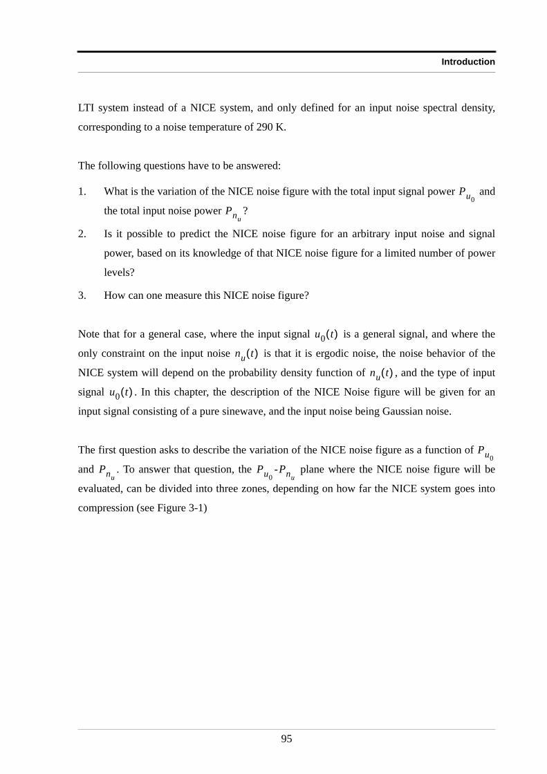
Introduction
LTI system instead of a NICE system, and only defined for an input noise spectral density,
corresponding to a noise temperature of 290 K.
The following questions have to be answered:
1. What is the variation of the NICE noise figure with the total input signal power and
the total input noise power ?
2. Is it possible to predict the NICE noise figure for an arbitrary input noise and signal
power, based on its knowledge of that NICE noise figure for a limited number of power
levels?
3. How can one measure this NICE noise figure?
Note that for a general case, where the input signal is a general signal, and where the
only constraint on the input noise is that it is ergodic noise, the noise behavior of the
NICE system will depend on the probability density function of , and the type of input
signal . In this chapter, the description of the NICE Noise figure will be given for an
input signal consisting of a pure sinewave, and the input noise being Gaussian noise.
The first question asks to describe the variation of the NICE noise figure as a function of
and . To answer that question, the - plane where the NICE noise figure will be
evaluated, can be divided into three zones, depending on how far the NICE system goes into
compression (see Figure 3-1)
Pu0
Pnu
u0 t( )
nu t( )
nu t( )
u0 t( )
Pu0
PnuPu0
Pnu
95
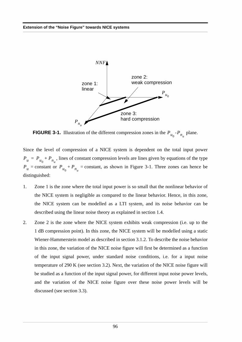
Extension of the “Noise Figure” towards NICE systems
Since the level of compression of a NICE system is dependent on the total input power
, lines of constant compression levels are lines given by equations of the type
= constant or = constant, as shown in Figure 3-1. Three zones can hence be
distinguished:
1. Zone 1 is the zone where the total input power is so small that the nonlinear behavior of
the NICE system is negligible as compared to the linear behavior. Hence, in this zone,
the NICE system can be modelled as a LTI system, and its noise behavior can be
described using the linear noise theory as explained in section 1.4.
2. Zone 2 is the zone where the NICE system exhibits weak compression (i.e. up to the
1 dB compression point). In this zone, the NICE system will be modelled using a static
Wiener-Hammerstein model as described in section 3.1.2. To describe the noise behavior
in this zone, the variation of the NICE noise figure will first be determined as a function
of the input signal power, under standard noise conditions, i.e. for a input noise
temperature of 290 K (see section 3.2). Next, the variation of the NICE noise figure will
be studied as a function of the input signal power, for different input noise power levels,
and the variation of the NICE noise figure over these noise power levels will be
discussed (see section 3.3).
FIGURE 3-1. Illustration of the different compression zones in the - plane.
Pu0
Pnu
NNF
zone 1:zone 2:
zone 3:hard compression
linearweak compression
Pu0Pnu
Pu Pu0Pnu
+=
Pu Pu0Pnu
+
96
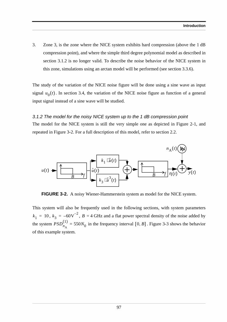
Introduction
3. Zone 3, is the zone where the NICE system exhibits hard compression (above the 1 dB
compression point), and where the simple third degree polynomial model as described in
section 3.1.2 is no longer valid. To describe the noise behavior of the NICE system in
this zone, simulations using an arctan model will be performed (see section 3.3.6).
The study of the variation of the NICE noise figure will be done using a sine wave as input
signal . In section 3.4, the variation of the NICE noise figure as function of a general
input signal instead of a sine wave will be studied.
3.1.2 The model for the noisy NICE system up to the 1 dB compression pointThe model for the NICE system is still the very simple one as depicted in Figure 2-1, and
repeated in Figure 3-2. For a full description of this model, refer to section 2.2.
This system will also be frequently used in the following sections, with system parameters
, , = 4 GHz and a flat power spectral density of the noise added by
the system = in the frequency interval . Figure 3-3 shows the behavior
of this example system.
FIGURE 3-2. A noisy Wiener-Hammerstein system as model for the NICE system.
u0 t( )
+fB fB
u t( ) y t( )
nA t( )
k1 u t( )⋅
k3 u3 t( )⋅
u t( ) +η t( )
k1 10= k3 60V 2––= B
PSDnA
1( ) 550N0 0 B,[ ]
97
Extension of the “Noise Figure” towards NICE systems
The 1 dB compression point (i.e. the point where the output power of the system is 1 dB
smaller than the output power of the underlying linear system) is reached for an input power of
about dBm (see Appendix 3.A). The polynomial function reaches its
maximum for , corresponding to 0.24 V or dBm for the example.
This illustrates also that the third order model is valid for input powers up to the 1 dB
compression point.
To determine the NICE noise figure, one will consider that the excitation signal of this system
consists of a deterministic part and an additive noise source . This excitation
signal can be written as:
(3-2)
where can be considered as band-limited, flat, zero-mean Gaussian noise with power
spectral density . ( represents the input noise temperature.)
FIGURE 3-3. Illustration of the 1 dB compression point of the system in the example.
-25 -20 -15 -10 -5 0-10
-5
0
5
10
15
20
Input power [dBm]
Ou
tpu
t p
ow
er
[dB
m]
Linear system Fundamental Third harmonic
1dB
6– y k1x k3x3+=
x k1–( ) 3k3( )⁄= 2.6–
u t( ) u0 t( ) nu t( )
u t( ) u0 t( ) nu t( )+ A 2πf0t( )cos⋅ nu t( )+= =
nu t( )
Nin kTin= Tin
98
Variation of the NICE noise figure, as a function of the input amplitude
3.2 Variation of the NICE noise figure, as a function of the input amplitudeFirst, the NICE noise figure as a function of the power of the input signal will be
studied, when a pure sinewave, superimposed on white thermal noise (generated by a resistor
at standard temperature K) is applied to a noisy NICE system.
3.2.1 Determining the output power spectral density
The output signal of the noisy NICE system is:
(3-3)
or,
(3-4)
It is possible to predict for each term of (3-4), if it will contribute to the output noise or
to the output signal , without prior knowledge of the spectra or , by using
section 1.6.2. According to this section, all the terms in (3-4) will generate spectral
contributions, that can be split into four disjunct sets, based on their dependency on and
. By checking in which set the spectral contributions generated by each term of (3-4)
fall, one is able to predict the effect of each term of (3-4).
• The term will only generate spectral contributions that contain
one single component of . Hence, it produces elements of the set
that are not affected by the properties of . This is quite
obvious, because comes from the linear part of the system.
u0 t( )
T0 290=
y t( )
y t( ) k1 A 2πf0t( )cos nu t( )+( ) k3 A 2πf0t( )cos nu t( )+( )3 nA t( )+ +=
y t( ) k1nu t( ) k1A 2πf0t( )cos k3nu3 t( ) 3k3Anu
2 t( ) 2πf0t( )cos + + + +=
3k3A2nu t( ) 2πf0t( )cos( )2 k3A3 2πf0t( )cos( )3 nA t( )+ +
ny t( )
y0 t( ) Nu k( ) U0 k( )
Nu k( )
U0 k( )
k1nu t( )
Nu k( )
B N( ) u0 t( )
k1nu t( )
99
Extension of the “Noise Figure” towards NICE systems
• The term will only generate spectral contributions that
contain one single component of . Hence, it produces elements of
the set that are not affected by the properties of . Again, this
is quite obvious, because comes from the linear part of
the system.
• The term generates output spectral components created by the
combination of three spectral components of and thus also creates
terms of set .
• The term on the other hand generates output
spectral components created by combining two noise spectral components
and one signal spectral component. It produces not only elements of set
(such as ) that are noise contributions,
affected by the properties of , but it will also produce elements of
set (e.g. ), that are corrections on the
output signal spectrum, due to the noise.
• Term generates output spectral components
created by combining two signal spectral lines, and one noise spectral
line. It produces only elements of set (such as
) that are noise contributions, affected by the
properties of .
• Term at last, generates output spectral components
created by combining three spectral components of and thus also
creates terms of set .
Next, the output power spectral density of the noisy NICE system will be analytically
determined. Equation (3-4) can also be rewritten as:
(3-5)
k1A 2πf0t( )cos
U0 k( )
A U0( ) nu t( )
k1A 2πf0t( )cos
k3nu3 t( )
Nu k( )
B N( )
3k3Anu2 t( ) 2πf0t( )cos
B′ U0 N,( ) 3k3Nu l( )Nu m( )U0 k( )
U0 k( )
A′ U0 N,( ) 3k3N l( )N l–( )U k( )
3k3A2nu t( ) 2πf0t( )cos( )2
B′ U0 N,( )
3k3Nu l( )U0 k–( )U0 k( )
U0 k( )
k3A3 2πf0t( )cos( )3
U0 k( )
A U0( )
y t( ) k134---k3A2+
A 2πf0t( )cos 14---k3A3 2π3f0t( )cos + +=
k132---k3A2+
nu t( ) 32---k3A2nu t( ) 2π2f0t( )cos 3k3Anu
2 t( ) 2πf0t( )cos k3nu3 t( ) nA t( )+ + + +
100
Variation of the NICE noise figure, as a function of the input amplitude
Following section 2.3, the output power spectral density will be calculated by taking the
Fourier transform of the auto-correlation of the system output (see (2-5)). Since the noise
added by the system itself is uncorrelated with the input signal and input noise, (2-6) (i.e.
) remains valid. If the terms in (3-5) are called respectively
to and , (i.e. the auto-correlation of the output of the noiseless NICE system)
can be written as (using the anti-symmetry property of the cross-correlation:
):
(3-6)
Where
(3-7)
In Appendix 3.B, all the terms in (3-6) are calculated, and the corresponding power spectral
densities are determined. The output power at frequency is given by:
(3-8)
With the deterministic part of the output signal (note that , as
shown in (3-8)). When there is no input noise ( ), the latter two terms in (3-8) are
absent. This means that they are not taken into account when performing a classical modeling
y t( )
Ryy τ( ) Rηη τ( ) RnAnAτ( )+= ς1
ς6 nA t( ) Rηη τ( )
Rαβ τ( ) Rβα τ–( )=
Rηη τ( ) Rςiςiτ( )
i 1=
6
∑ Rςiςjτ( ) Rςiςj
τ–( )+( )
j i 1+=
6
∑i 1=
5
∑+=
ς1 k134---k3A2+
A 2πf0t( )cos=
ς214---k3A3 2π3f0t( )cos=
ς3 k132---k3A2+
nu t( )=
ς432---k3A2nu t( ) 2π2f0t( )cos=
ς5 3k3Anu2 t( ) 2πf0t( ) cos=
ς6 k3nu3 t( )=
f0
PSDy0
1( ) f0( )
δ f f0–( )---------------------------- k1
34---k3A2+
2 A2
2Z0---------
3k3A( )2
2--------------------Z0N0
2B2 3k3 k134---k3A2+
A2N0B+ +=
y0 t( ) y t( ) y0 t( ) H u0 t( )[ ]≠
N0 0=
101
Extension of the “Noise Figure” towards NICE systems
of the device (that assumes ). However, those terms yield a (systematic) contribution
in the output signal power at frequency , and are therefore added to the signal output power.
A third harmonic of the input signal will appear at frequency , and with a
power given by:
(3-9)
The output noise power spectral density will be a frequency dependent quantity (see Appendix
3.B), given by:
(3-10)
where if , and if . on the other hand will be given by the following
criterion (see (3-85) and (3-86)):
(3-11)
Note that represents the stochastic part of the output signal .
3.2.2 Signal-to-noise ratio variation: the NICE noise figureAt this point, the signal and noise power spectral densities are known at the input and at the
output of the considered system. It is thus possible to apply the definition of the NICE noise
figure (3-1) i.e.
N0 0=
f0
A 2πf0t( )cos⋅ 3f0
PSDy0
1( ) 3f0( )
δ f 3f0–( )------------------------------- 1
4---k3A2
2 A2
2Z0---------=
PSDny
1( ) f( ) k132---k3A2+
2N0
k32N0
3Z02
2------------------ 27B2 3f2–( ) 6 k1
32---k3A2+
k3Z0N02B+ +=
32---k3A2
2
2-----------------------N0β 3k3A( )2Z0
N02
------
22 2B φ–( ) PSDnA
1( ) f( )+ + +
φ f0= f f0< φ f= f f0> β
f0B2---<
β 1= f B 2f0–≤⇔
β 1 2⁄= f B 2f0–>⇔⇒
f0B2--->
β 0= f 2f0 B–<⇔
β 1 2⁄= f 2f0 B–≥⇔⇒
ny t( ) y t( )
102
Variation of the NICE noise figure, as a function of the input amplitude
(3-12)
to the obtained results. However, because the signal power spectral density is a Dirac impulse,
(i.e. all the power is concentrated at one single frequency) while the noise spectrum is a
spectral density (i.e. the power is not concentrated at one frequency, but is smeared out in a
frequency band), the signal and noise power will be compared in a frequency interval of 1 Hz
around frequency . Note that choosing this bandwidth equal to 1 Hz can be done without
loss of generality. One could object that a bandwidth of a few kHz around frequency is
more realistic. But in that case, the input noise power is , while the output noise power in
the frequency interval can be approximated as (see
Appendix 3.C), if the noise power spectral densities are flat inside this frequency interval.
Hence, the value of will be eliminated in the division of the signal-to-noise ratios, or in
other words, stating = 1 Hz can be done without loss of generality.
The signal-to-noise ratio at frequency is given by:
(3-13)
and the signal-to-noise ratio at frequency is given by the ratio of (3-8) divided by
(3-10). In (3-10), , while the criterion (3-11) for , becomes (with ):
(3-14)
By defining the signal power gain
, (3-15)
the noise power gain
NNFSNRinSNRout------------------=
f0B0 f0
B0N0
f0 B0 2⁄– f0 B0 2⁄+,[ ] B0PSDnyf0( )
B0
B0
SNRin f0
SNRin f0( ) A2
2Z0 N0⋅--------------------=
SNRout f0φ f0= β f f0=
f0 B 3⁄≤ β⇒ 1=
f0 B 3⁄> β⇒ 1 2⁄=
Gu0
PSDy0
1( ) f0( )
PSDu0
1( ) f0( )----------------------------=
103
Extension of the “Noise Figure” towards NICE systems
, (3-16)
and the noise power gain of the underlying noiseless system
, (3-17)
the NICE noise figure can be rewritten as:
(3-18)
With
(3-19)
and
(3-20)
Note that some terms in (3-19) and (3-20) can be neglected compared to others, because is
a very small quantity (recall that W/Hz). The terms in (3-19) and (3-20) can be
expressed in orders of magnitude of the dimensionless1 total noise power
. For (3-19) this yields:
Gnu
PSDny
1( ) f0( )
PSDnu
1( ) f0( )----------------------------=
G ′nu
PSDny
1( ) f0( ) PSDnA
1( ) f0( )–
PSDnu
1( ) f0( )--------------------------------------------------------------=
NNFA2 2Z0 N0⋅( )⁄
Gu0
A2
2Z0---------⋅
GnuN0⋅( )⁄
----------------------------------------------------------Gnu
Gu0
---------G ′nu
PSDnA
1( ) f0( ) N0⁄+
Gu0
--------------------------------------------------------= = =
Gu0k1
34---k3A2+
23k3Z0N0B( )2 6k3 k1
34---k3A2+
N0BZ0+ +=
k134---k3A2 3k3Z0N0B+ +
2
=
G ′nuk1
32---k3A2+
2 k3
2N02Z0
2
2------------------ 27B2 3f0
2–( ) 6 k132---k3A2+
k3Z0N0B+ +=
32---k3A2
2
2-----------------------β 3k3A( )2Z0
N02
------ 2B f0–( )+ +
N0
N0 4 21–×10=
ΠnuPnu
1W( )⁄ B N0⋅( ) 1W( )⁄= =
104
Variation of the NICE noise figure, as a function of the input amplitude
(3-21)
Since is very small (e.g. W for = 4 GHz), the second and third term
of (3-21) can be neglected with respect to the first one. Calculating the terms of (3-21) for the
example system given in section 3.1.2, and with = 0.16 V (this corresponds to a total power
of the sinewave of dBm/Hz, i.e. the 1 dB compression point) yields:
. This illustrates the fact that the second and third term in (3-
19) can be neglected with respect to the first one. Hence, can be approximated as:
(3-22)
Looking at the orders of magnitude of the terms of (3-20) yields:
(3-23)
Again, since is very small, the second, third and fifth term can be neglected with respect
to the others. Hence, the noise power gain can be approximated as:
(3-24)
1. because it is impossible to compare Watts with .Watts2
Gu0k1
34---k3A2+
23k3Z0N0B( )2 6k3 k1
34---k3A2+
N0BZ0+ +=
O Πnu
0 O Πnu
2 O Πnu
1
PnuPnu
1.6 11–×10= B
A
6–
Gu078 2.5 6–×10– 2 14–×10+=
Gu0
Gu0k1
34---k3A2+
2
=
G ′nuk1
32---k3A2+
2 k32N0
2Z02
2------------------ 27B2 3f0
2–( ) 6 k132---k3A2+
k3Z0N0B+ +=
32---k3A2
2
2-----------------------β 3k3A( )2Z0
N02
------ 2B f0–( )+ +
O Πnu
2 O Πnu
0 O Πnu
1
O Πnu
0 O Πnu
1
Πnu
Gnuk1
32---k3A2+
232---k3A2
2
2-----------------------β
PSDnA
1( ) f0( )
N0----------------------------+ +=
105
Extension of the “Noise Figure” towards NICE systems
Hence, the NICE noise figure is then given by:
(3-25)
It is possible to write the NICE noise figure as an expression containing the linear noise figure
(i.e. the noise figure for the simple system with ). Knowing that the linear noise
figure is given by:
(3-26)
(3-18) can be written in terms of the linear noise figure and a correction term as:
(3-27)
or, in terms of a scaling and biasing of the linear noise figure as:
(3-28)
The correction term in (3-27) is function of the linear noise figure , the bandwidth of the
system , the system parameters and , and as expected, the amplitude of the input
NNF f0( )k1
32---k3A2+
2 1
2--- 3
2---k3A2
2β+
N0 PSDnA
1( ) f0( )+
k134---k3A2+
2N0
------------------------------------------------------------------------------------------------------------------------=
NFlin k3 0=
NFlin
NFlin
k12N0 PSDnA
1( ) f0( )+
k12N0
----------------------------------------------=
NNF NFlin
G ′nuk1
2– NFlin Gu0k1
2– ⋅–
Gu0
-------------------------------------------------------------------------+ =
NFlin
18 9β+8
------------------- k3A2( )2
3k1k3A2+ NFlin
916------ k3A2( )
2 32---k1k3A2+
–
k134---k3A2+
2--------------------------------------------------------------------------------------------------------------------------------------------------------+=
NNF NFlink1
2
Gu0
---------⋅G ′nu
k12–
Gu0
---------------------- +=
NNF NFlink1
2
k134---k3A2+
2
-----------------------------------⋅
18 9β+8
------------------- k3A2( )2
3k1k3A2+
k134---k3A2+
2
------------------------------------------------------------------------+=
NFlin
B k1 k3 A
106
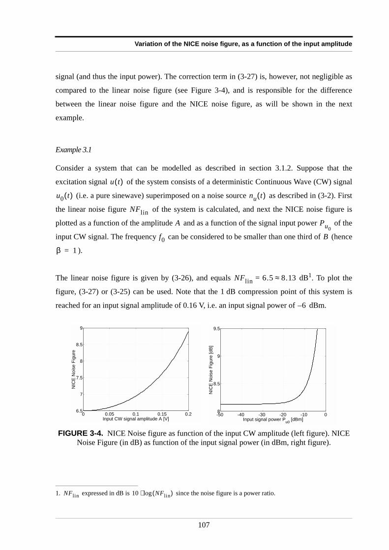
Variation of the NICE noise figure, as a function of the input amplitude
signal (and thus the input power). The correction term in (3-27) is, however, not negligible as
compared to the linear noise figure (see Figure 3-4), and is responsible for the difference
between the linear noise figure and the NICE noise figure, as will be shown in the next
example.
Example 3.1
Consider a system that can be modelled as described in section 3.1.2. Suppose that the
excitation signal of the system consists of a deterministic Continuous Wave (CW) signal
(i.e. a pure sinewave) superimposed on a noise source as described in (3-2). First
the linear noise figure of the system is calculated, and next the NICE noise figure is
plotted as a function of the amplitude and as a function of the signal input power of the
input CW signal. The frequency can be considered to be smaller than one third of (hence
).
The linear noise figure is given by (3-26), and equals dB1. To plot the
figure, (3-27) or (3-25) can be used. Note that the 1 dB compression point of this system is
reached for an input signal amplitude of 0.16 V, i.e. an input signal power of dBm.
1. expressed in dB is since the noise figure is a power ratio.
FIGURE 3-4. NICE Noise figure as function of the input CW amplitude (left figure). NICE Noise Figure (in dB) as function of the input signal power (in dBm, right figure).
u t( )
u0 t( ) nu t( )
NFlin
A Pu0
f0 B
β 1=
NFlin 6.5= 8.13≈
NFlin 10 NFlin( )log⋅
6–
-50 -40 -30 -20 -10 08
8.5
9
9.5
Input signal power Pu0
[dBm]
NIC
E N
ois
e F
igure
[dB
]
0 0.05 0.1 0.15 0.26.5
7
7.5
8
8.5
9
Input CW signal amplitude A [V]
NIC
E N
ois
e F
igure
107
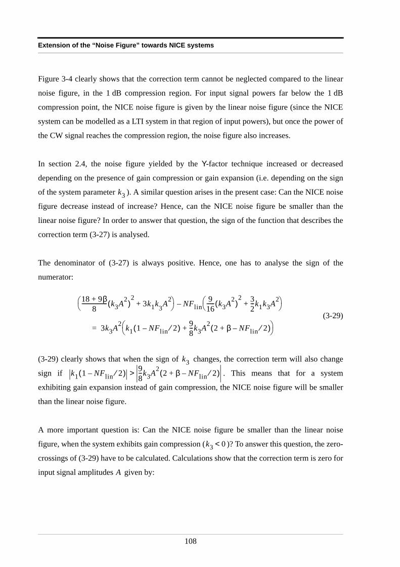
Extension of the “Noise Figure” towards NICE systems
Figure 3-4 clearly shows that the correction term cannot be neglected compared to the linear
noise figure, in the 1 dB compression region. For input signal powers far below the 1 dB
compression point, the NICE noise figure is given by the linear noise figure (since the NICE
system can be modelled as a LTI system in that region of input powers), but once the power of
the CW signal reaches the compression region, the noise figure also increases.
In section 2.4, the noise figure yielded by the Y-factor technique increased or decreased
depending on the presence of gain compression or gain expansion (i.e. depending on the sign
of the system parameter ). A similar question arises in the present case: Can the NICE noise
figure decrease instead of increase? Hence, can the NICE noise figure be smaller than the
linear noise figure? In order to answer that question, the sign of the function that describes the
correction term (3-27) is analysed.
The denominator of (3-27) is always positive. Hence, one has to analyse the sign of the
numerator:
(3-29)
(3-29) clearly shows that when the sign of changes, the correction term will also change
sign if . This means that for a system
exhibiting gain expansion instead of gain compression, the NICE noise figure will be smaller
than the linear noise figure.
A more important question is: Can the NICE noise figure be smaller than the linear noise
figure, when the system exhibits gain compression ( )? To answer this question, the zero-
crossings of (3-29) have to be calculated. Calculations show that the correction term is zero for
input signal amplitudes given by:
k3
18 9β+8
------------------- k3A2( )2
3k1k3A2+ NFlin
916------ k3A2( )
2 32---k1k3A2+
–
3k3A2 k1 1 NFlin 2⁄–( ) 98---k3A2 2 β NFlin 2⁄–+( )+
=
k3
k1 1 NFlin 2⁄–( ) 98---k3A2 2 β NFlin 2⁄–+( )>
k3 0<
A
108
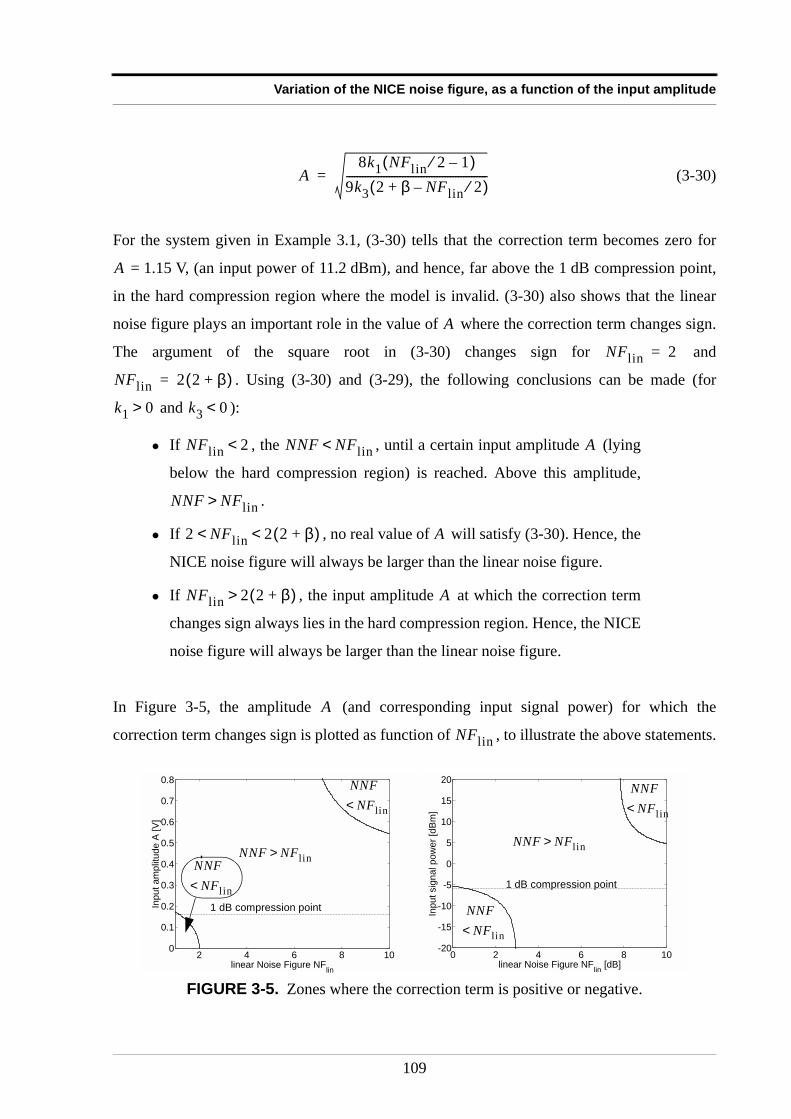
Variation of the NICE noise figure, as a function of the input amplitude
(3-30)
For the system given in Example 3.1, (3-30) tells that the correction term becomes zero for
= 1.15 V, (an input power of 11.2 dBm), and hence, far above the 1 dB compression point,
in the hard compression region where the model is invalid. (3-30) also shows that the linear
noise figure plays an important role in the value of where the correction term changes sign.
The argument of the square root in (3-30) changes sign for and
. Using (3-30) and (3-29), the following conclusions can be made (for
and ):
• If , the , until a certain input amplitude (lying
below the hard compression region) is reached. Above this amplitude,
.
• If , no real value of will satisfy (3-30). Hence, the
NICE noise figure will always be larger than the linear noise figure.
• If , the input amplitude at which the correction term
changes sign always lies in the hard compression region. Hence, the NICE
noise figure will always be larger than the linear noise figure.
In Figure 3-5, the amplitude (and corresponding input signal power) for which the
correction term changes sign is plotted as function of , to illustrate the above statements.
FIGURE 3-5. Zones where the correction term is positive or negative.
A8k1 NFlin 2⁄ 1–( )
9k3 2 β NFlin 2⁄–+( )-----------------------------------------------------=
A
A
NFlin 2=
NFlin 2 2 β+( )=
k1 0> k3 0<
NFlin 2< NNF NFlin< A
NNF NFlin>
2 NFlin 2 2 β+( )< < A
NFlin 2 2 β+( )> A
A
NFlin
2 4 6 8 100
0.1
0.2
0.3
0.4
0.5
0.6
0.7
0.8
linear Noise Figure NFlin
Inp
ut
am
plit
ud
e A
[V
]
0 2 4 6 8 10-20
-15
-10
-5
0
5
10
15
20
linear Noise Figure NFlin
[dB]
Input sig
nal pow
er
[dB
m]
1 dB compression point
1 dB compression point
NNF NFlin>NNF NFlin>
NNF NFlin<
NNF NFl in<
NNF NFlin<
NNF NFl in<
109
Extension of the “Noise Figure” towards NICE systems
As an illustration, Figure 3-6 shows the noise figure as function of the input amplitude and
input signal power for the example system with dB.
Figure 3-6 shows that for the given system parameters and linear noise figure, the NICE noise
figure first becomes smaller than the linear noise figure (up to V). When becomes
larger than 0.15 V, the NICE noise figure becomes larger than the linear noise figure, as
predicted in Figure 3-5. Hence, an amplifier has not necessarily to exhibit gain expansion for
the NICE noise figure to become smaller than the linear noise figure.
3.2.3 Special case: a noiseless NICE systemSince the region of input signal amplitudes where is larger for smaller linear
noise figures, the special case with the smallest possible linear noise figure ( , see
section 1.4.2) is considered. occurs when the considered NICE system is noiseless,
i.e. it does not produce any noise by itself, or . The previous
section showed that for , the NICE noise figure is smaller than the linear noise
figure: . Hence, a noiseless NICE system has a very special property, that is
impossible to obtain for an LTI system: The NICE noise figure of a noiseless NICE system can
be smaller than one. This means that the signal-to-noise ratio at the output of the system is
larger than the signal-to-noise ratio at the input of the system. Or in other words, a noiseless
NICE system improves the signal-to-noise ratio instead of deteriorating it.
For , the expression for the NICE noise figure (3-25) becomes:
FIGURE 3-6. Noise figure vs. input CW amplitude and power.
A
Pu0NFlin 1.8= 2.55≈
0 0.05 0.1 0.15 0.21.78
1.8
1.82
1.84
1.86
1.88
1.9
Input CW signal amplitude A [V]
NIC
E N
ois
e F
igu
re
-50 -40 -30 -20 -10 02.5
2.55
2.6
2.65
2.7
2.75
2.8
Input signal power Pu0
[dBm]
NIC
E N
ois
e F
igu
re [
dB
]
A 0.15≈ A
NNF NFlin<
NFlin 1=
NFlin 1=
nA t( ) 0= PSDnA
1( ) f( ) 0=
NFlin 1=
NNF 1<
PSDnA
1( ) f( ) 0=
110
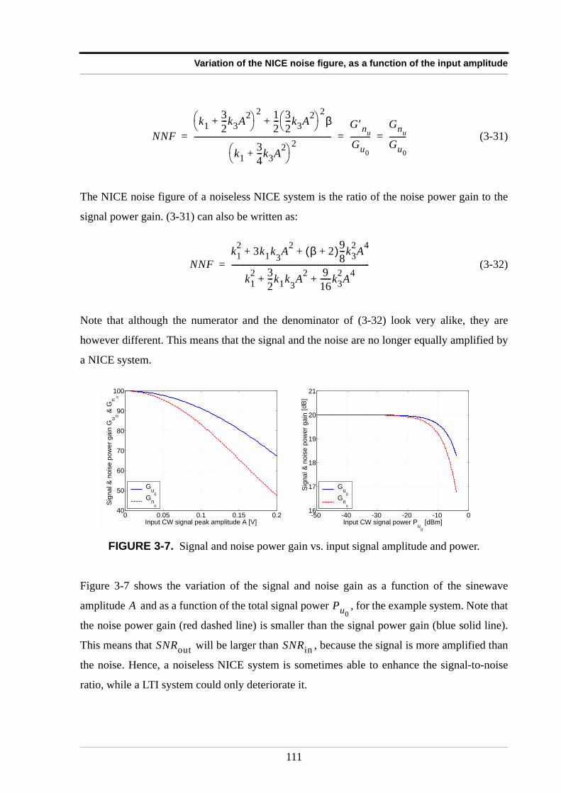
Variation of the NICE noise figure, as a function of the input amplitude
(3-31)
The NICE noise figure of a noiseless NICE system is the ratio of the noise power gain to the
signal power gain. (3-31) can also be written as:
(3-32)
Note that although the numerator and the denominator of (3-32) look very alike, they are
however different. This means that the signal and the noise are no longer equally amplified by
a NICE system.
Figure 3-7 shows the variation of the signal and noise gain as a function of the sinewave
amplitude and as a function of the total signal power , for the example system. Note that
the noise power gain (red dashed line) is smaller than the signal power gain (blue solid line).
This means that will be larger than , because the signal is more amplified than
the noise. Hence, a noiseless NICE system is sometimes able to enhance the signal-to-noise
ratio, while a LTI system could only deteriorate it.
FIGURE 3-7. Signal and noise power gain vs. input signal amplitude and power.
NNFk1
32---k3A2+
2 12--- 3
2---k3A2
2β+
k134---k3A2+
2-------------------------------------------------------------------------
G ′nu
Gu0
-----------Gnu
Gu0
---------= = =
NNFk1
2 3k1k3A2 β 2+( )98---k3
2A4+ +
k12 3
2---k1k3A2 9
16------k3
2A4+ +-------------------------------------------------------------------------=
0 0.05 0.1 0.15 0.240
50
60
70
80
90
100
Input CW signal peak amplitude A [V]
Sig
na
l &
no
ise
po
we
r g
ain
Gu
0
& G
nu
Gu
0G
nu
-50 -40 -30 -20 -10 016
17
18
19
20
21
Input CW signal power Pu
0
[dBm]
Sig
na
l &
no
ise
po
we
r g
ain
Gu
0G
nu
[dB]
A Pu0
SNRout SNRin
111
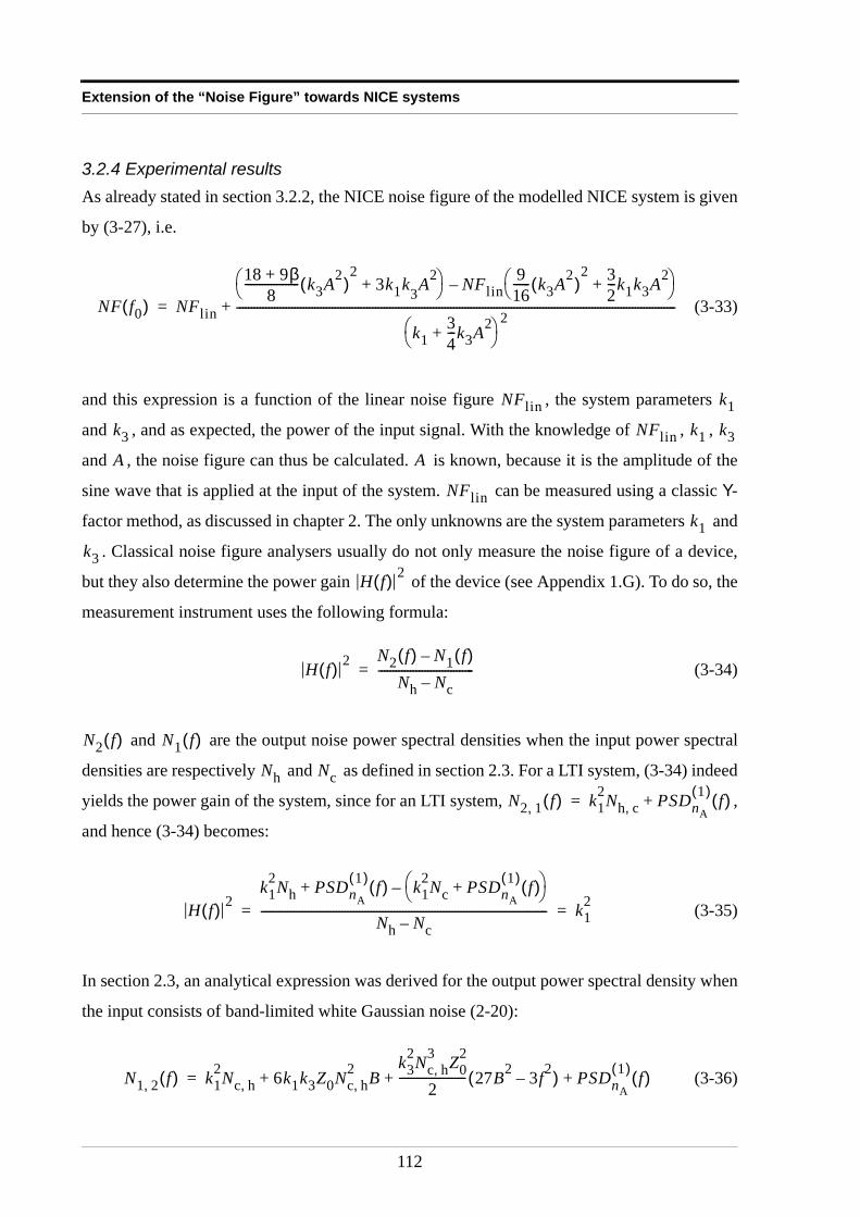
Extension of the “Noise Figure” towards NICE systems
3.2.4 Experimental resultsAs already stated in section 3.2.2, the NICE noise figure of the modelled NICE system is given
by (3-27), i.e.
(3-33)
and this expression is a function of the linear noise figure , the system parameters
and , and as expected, the power of the input signal. With the knowledge of , ,
and , the noise figure can thus be calculated. is known, because it is the amplitude of the
sine wave that is applied at the input of the system. can be measured using a classic Y-
factor method, as discussed in chapter 2. The only unknowns are the system parameters and
. Classical noise figure analysers usually do not only measure the noise figure of a device,
but they also determine the power gain of the device (see Appendix 1.G). To do so, the
measurement instrument uses the following formula:
(3-34)
and are the output noise power spectral densities when the input power spectral
densities are respectively and as defined in section 2.3. For a LTI system, (3-34) indeed
yields the power gain of the system, since for an LTI system, ,
and hence (3-34) becomes:
(3-35)
In section 2.3, an analytical expression was derived for the output power spectral density when
the input consists of band-limited white Gaussian noise (2-20):
(3-36)
NF f0( ) NFlin
18 9β+8
------------------- k3A2( )2
3k1k3A2+ NFlin
916------ k3A2( )
2 32---k1k3A2+
–
k134---k3A2+
2
--------------------------------------------------------------------------------------------------------------------------------------------------------+=
NFlin k1
k3 NFlin k1 k3
A A
NFlin
k1
k3
H f( ) 2
H f( ) 2 N2 f( ) N1 f( )–Nh Nc–
---------------------------------=
N2 f( ) N1 f( )
Nh Nc
N2 1, f( ) k12Nh c, PSDnA
1( ) f( )+=
H f( ) 2k1
2Nh PSDnA
1( ) f( ) k12Nc PSDnA
1( ) f( )+ –+
Nh Nc–--------------------------------------------------------------------------------------------------- k1
2= =
N1 2, f( ) k12Nc h, 6k1k3Z0Nc h,
2 Bk3
2Nc h,3 Z0
2
2----------------------- 27B2 3f2–( ) PSDnA
1( ) f( )+ ++=
112
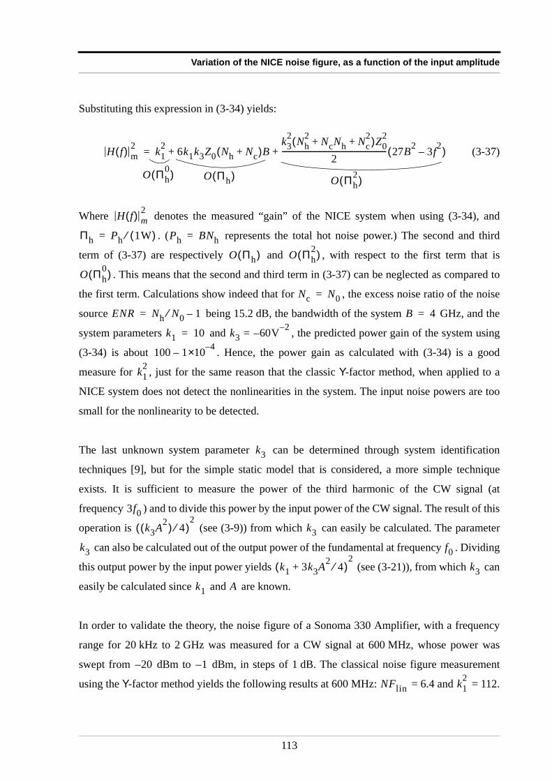
Variation of the NICE noise figure, as a function of the input amplitude
Substituting this expression in (3-34) yields:
(3-37)
Where denotes the measured “gain” of the NICE system when using (3-34), and
. ( represents the total hot noise power.) The second and third
term of (3-37) are respectively and , with respect to the first term that is
. This means that the second and third term in (3-37) can be neglected as compared to
the first term. Calculations show indeed that for , the excess noise ratio of the noise
source being 15.2 dB, the bandwidth of the system GHz, and the
system parameters and , the predicted power gain of the system using
(3-34) is about . Hence, the power gain as calculated with (3-34) is a good
measure for , just for the same reason that the classic Y-factor method, when applied to a
NICE system does not detect the nonlinearities in the system. The input noise powers are too
small for the nonlinearity to be detected.
The last unknown system parameter can be determined through system identification
techniques [9], but for the simple static model that is considered, a more simple technique
exists. It is sufficient to measure the power of the third harmonic of the CW signal (at
frequency ) and to divide this power by the input power of the CW signal. The result of this
operation is (see (3-9)) from which can easily be calculated. The parameter
can also be calculated out of the output power of the fundamental at frequency . Dividing
this output power by the input power yields (see (3-21)), from which can
easily be calculated since and are known.
In order to validate the theory, the noise figure of a Sonoma 330 Amplifier, with a frequency
range for 20 kHz to 2 GHz was measured for a CW signal at 600 MHz, whose power was
swept from dBm to dBm, in steps of 1 dB. The classical noise figure measurement
using the Y-factor method yields the following results at 600 MHz: = 6.4 and = 112.
H f( ) m2 k1
2 6k1k3Z0 Nh Nc+( )Bk3
2 Nh2 NcNh Nc
2+ +( )Z02
2-------------------------------------------------------- 27B2 3f2–( )++=
O Πh( ) O Πh2( )O Πh
0( )
H f( ) m2
Πh Ph 1W( )⁄= Ph BNh=
O Πh( ) O Πh2( )
O Πh0( )
Nc N0=
ENR Nh N0⁄ 1–= B 4=
k1 10= k3 60–= V 2–
100 1 4–×10–
k12
k3
3f0k3A2( ) 4⁄( )
2k3
k3 f0k1 3k3A2 4⁄+( )
2k3
k1 A
20– 1–
NFlin k12
113
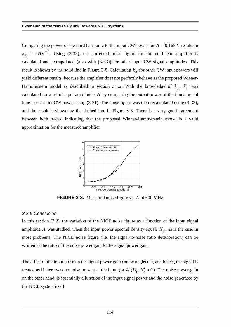
Extension of the “Noise Figure” towards NICE systems
Comparing the power of the third harmonic to the input CW power for = 0.165 V results in
. Using (3-33), the corrected noise figure for the nonlinear amplifier is
calculated and extrapolated (also with (3-33)) for other input CW signal amplitudes. This
result is shown by the solid line in Figure 3-8. Calculating for other CW input powers will
yield different results, because the amplifier does not perfectly behave as the proposed Wiener-
Hammerstein model as described in section 3.1.2. With the knowledge of , was
calculated for a set of input amplitudes by comparing the output power of the fundamental
tone to the input CW power using (3-21). The noise figure was then recalculated using (3-33),
and the result is shown by the dashed line in Figure 3-8. There is a very good agreement
between both traces, indicating that the proposed Wiener-Hammerstein model is a valid
approximation for the measured amplifier.
3.2.5 ConclusionIn this section (3.2), the variation of the NICE noise figure as a function of the input signal
amplitude was studied, when the input power spectral density equals , as is the case in
most problems. The NICE noise figure (i.e. the signal-to-noise ratio deterioration) can be
written as the ratio of the noise power gain to the signal power gain.
The effect of the input noise on the signal power gain can be neglected, and hence, the signal is
treated as if there was no noise present at the input (or ). The noise power gain
on the other hand, is essentially a function of the input signal power and the noise generated by
the NICE system itself.
FIGURE 3-8. Measured noise figure vs. at 600 MHz
A
k3 65V 2––=
k3
k3 k1
A
0 0.05 0.1 0.15 0.2 0.25 0.36
7
8
9
10
11
12
Input CW signal amplitude [V]
Noi
se F
igur
e
α and G vary with A α and G are constantsk1k1
k3k3
NIC
E
A
A N0
A′ U0 N,( ) 0≈
114
Variation of the NICE noise figure, as a function of the input amplitude
The NICE noise figure can be written as the sum of the linear noise figure, and a correction
term. If the linear noise figure is larger than 2, this correction term is always positive, yielding
a worse signal-to-noise ratio deterioration for the NICE system than for its underlying linear
system. However, if the linear noise figure is smaller than 2, the correction term will be
negative, indicating that the NICE system’s signal-to-noise ratio deterioration is less than that
of the underlying linear system. In the special case of a noiseless NICE system, there will be a
signal-to-noise ratio improvement instead of a deterioration, which is impossible for LTI
systems.
Hence, the minimum noise figure for nonlinear amplifiers can be smaller than for linear
amplifiers, and can theoretically even be smaller than one. Driving the amplifier into low
saturation can possibly enhance the signal-to-noise ratio.
115
Extension of the “Noise Figure” towards NICE systems
3.3 Variation of the NICE noise figure, as a function of the input amplitude and the input noise power
3.3.1 IntroductionIn this section, the variation of the NICE noise figure as a function of the input amplitude and
the input noise power will be studied. This study will be done in two steps.
First, the variation of the NNF will be studied in the linear and the weak compression zone,
using the noisy NICE system model, proposed in section 3.1.2. This NNF variation will be
studied as a function of the input signal power, for different input noise powers, and an
variation over the noise powers will be sought (sections 3.3.2 to 3.3.5).
Next, the variation of the NNF will be studied in the hard compression zone, using simulations
performed on a (nonlinear) arc-tangent (atan) model (section 3.3.6).
3.3.2 Determining the analytical expressionFor LTI systems, the noise figure is defined at an input thermal noise power spectral
density, generated by a resistor at an absolute temperature of K. By applying a
transformation (1-22) on that noise figure, the signal-to-noise ratio deterioration can be
obtained for other levels of input noise power spectral densities. This transformation is based
on (1-21), that considers that the gain of the signal power and the noise power spectral density
are equal. Since section 3.2 showed that this hypothesis does not hold for NICE systems, the
transformation (1-22) will not be applicable to NICE systems. However, a similar reasoning as
in Appendix 1.F can be followed to determine the dependency of the NICE noise figure on the
input noise power levels.
The power spectral density of the noise added by the noisy NICE system itself can be written
in a similar form as (1-81):
(3-38)
NFlin
T0 290=
PSDnA
1( ) f( ) NFlin f( ) 1–( )k12N0=
116
Variation of the NICE noise figure, as a function of the input amplitude and the input noise
which depends on the linear noise figure , the power gain of the underlying linear
system and the standard thermal noise power spectral density . Note that by assumption,
the properties of the noise added by the system itself is independent of the input signal of the
system (see section 1.6.1). Hence (3-38) is not only valid for an LTI system, but also for the
considered noisy NICE system. The NICE noise figure for a certain input noise power spectral
density can be expressed as (see also (3-18)):
(3-39)
and are respectively the signal power gain, and noise power gain of the underlying
noiseless system, that are functions of the input signal amplitude (and thus ), and the
input noise power spectral density (and thus ). The expression for the signal power gain
is:
(3-40)
and for the noise power gain of the underlying noiseless system :
(3-41)
Or, in a worst case scenario, i.e. (thus ), the noise power gain will be maximized
as function of the frequency,
NFlin
k12 N0
Nin
NNF Nin A,( )G ′nu
PSDnA
1( ) f( ) Nin⁄+
Gu0
-------------------------------------------------------G ′nu
Gu0
-----------NFlin 1–( )k1
2 N0Nin--------
Gu0
------------------------------------------+= =
Gu0G ′nu
A Pu0
Pnu
Gu0
Gu0k1
34---k3A2+
2
3k3( )2Z02Nin
2 B2 6k3 k134---k3A2+
NinBZ0+ +=
k134---k3A2 3k3NinBZ0+ +
2
k132---k3Z0 Pu0
2Pnu+( )+
2
= =
G ′nu
G ′nuk1
32---k3A2+
2 k3
2Nin2 Z0
2
2-------------------- 27B2 3f0
2–( ) 6 k132---k3A2+
k3Z0NinB + + +=
32---k3A2
2
2-----------------------β 3k3A( )2Z0
Nin2
-------- 2B f0–( )+
f0 0→ β 1=
117
Extension of the “Noise Figure” towards NICE systems
(3-42)
Hence, (3-39) is the general formula that describes the variation of the NICE noise figure as a
function of and , up to the 1 dB compression point.
In (3-39), three cases can be considered, mainly depending on the input noise power level:
1.
2.
3.
3.3.3 First case:
The noisy NICE system produces much more noise (that does not mix with the input) than the
amplified input noise. This situation can be due to two factors. First, the noisy NICE system
produces a tremendous amount of noise. This situation is highly improbable and usually occurs
when the system is malfunctioning. (Typical values for are a few hundred times ).
A second possibility is that the input noise power spectral density is very low, as is the case for
satellite communications, where the input noise temperature is about 10 K (i.e.
dBm/Hz). In this case, the approximated formula (3-22) for the signal power gain
can be used, and can be neglected with respect to . The NICE noise
figure (3-39) for very low input noise power spectral densities hence becomes:
(3-43)
Since the signal and noise power gain and both have the same order of magnitude
(see Figure 3-7), the denominator of (3-43) will also be much smaller than the numerator,
G ′nuk1
32---k3A2 3k3Z0NinB+ +
2 9k3
2
2-------- A2
2------ Z0NinB+
2 k32
2-----9A2Z0NinB+ +=
k1 3k3Z0 Pu0Pnu
+( )+( )2 9k32Z0
2
2--------------- Pu0
Pnu+( )2 9k3
2Z02Pnu
Pu0+ + =
Pu0Pnu
PSDnA
1( ) f( ) Nin⁄ G ′nu»
PSDnA
1( ) f( ) Nin⁄ G ′nu≈
PSDnA
1( ) f( ) Nin⁄ G ′nu«
PSDnA
1( ) f( ) Nin⁄ G ′nu»
PSDnA
1( ) N0
Nin 189–≈
Gu0G ′nu
PSDnA
1( ) f( ) Nin⁄
NNFNFlin 1–( )k1
2 N0Nin--------
Gu0
------------------------------------------NFlin 1–( )k1
2 T0Tin-------
k134---k3A2+
2------------------------------------------= =
Gu0G ′nu
118
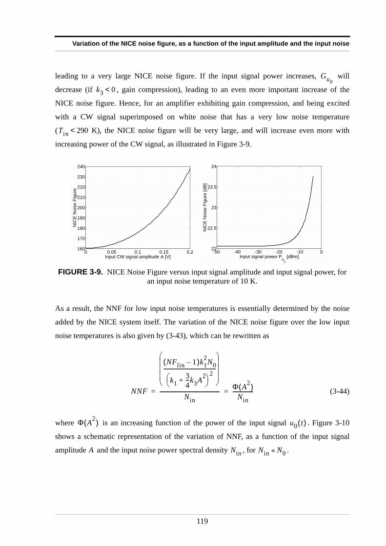
Variation of the NICE noise figure, as a function of the input amplitude and the input noise
leading to a very large NICE noise figure. If the input signal power increases, will
decrease (if , gain compression), leading to an even more important increase of the
NICE noise figure. Hence, for an amplifier exhibiting gain compression, and being excited
with a CW signal superimposed on white noise that has a very low noise temperature
( K), the NICE noise figure will be very large, and will increase even more with
increasing power of the CW signal, as illustrated in Figure 3-9.
As a result, the NNF for low input noise temperatures is essentially determined by the noise
added by the NICE system itself. The variation of the NICE noise figure over the low input
noise temperatures is also given by (3-43), which can be rewritten as
(3-44)
where is an increasing function of the power of the input signal . Figure 3-10
shows a schematic representation of the variation of NNF, as a function of the input signal
amplitude and the input noise power spectral density , for .
FIGURE 3-9. NICE Noise Figure versus input signal amplitude and input signal power, for an input noise temperature of 10 K.
Gu0
k3 0<
Tin 290<
0 0.05 0.1 0.15 0.2160
170
180
190
200
210
220
230
240
Input CW signal amplitude A [V]
NIC
E N
ois
e F
igu
re
-50 -40 -30 -20 -10 022
22.5
23
23.5
24
Input signal power Pu
0
[dBm]
NIC
E N
ois
e F
igu
re [
dB
]
NNF
NFlin 1–( )k12N0
k134---k3A2+
2
----------------------------------------
Nin---------------------------------------------- Φ A2( )
Nin----------------= =
Φ A2( ) u0 t( )
A Nin Nin N0«
119
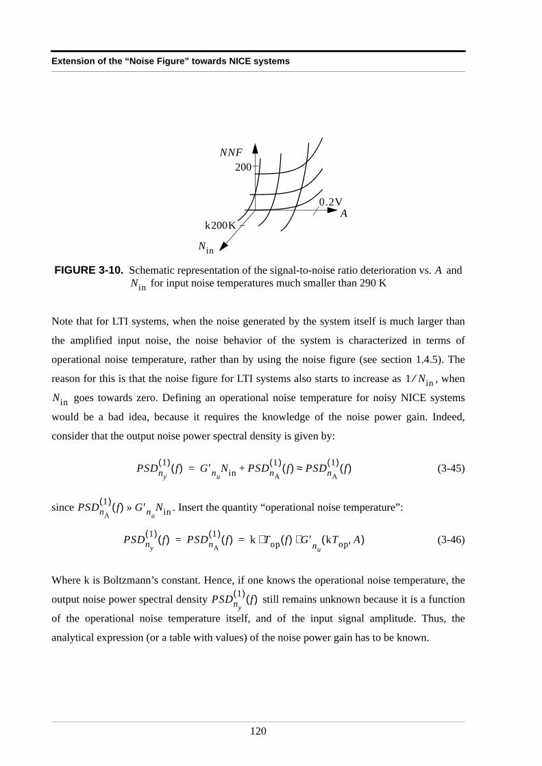
Extension of the “Noise Figure” towards NICE systems
Note that for LTI systems, when the noise generated by the system itself is much larger than
the amplified input noise, the noise behavior of the system is characterized in terms of
operational noise temperature, rather than by using the noise figure (see section 1.4.5). The
reason for this is that the noise figure for LTI systems also starts to increase as , when
goes towards zero. Defining an operational noise temperature for noisy NICE systems
would be a bad idea, because it requires the knowledge of the noise power gain. Indeed,
consider that the output noise power spectral density is given by:
(3-45)
since . Insert the quantity “operational noise temperature”:
(3-46)
Where k is Boltzmann’s constant. Hence, if one knows the operational noise temperature, the
output noise power spectral density still remains unknown because it is a function
of the operational noise temperature itself, and of the input signal amplitude. Thus, the
analytical expression (or a table with values) of the noise power gain has to be known.
FIGURE 3-10. Schematic representation of the signal-to-noise ratio deterioration vs. and for input noise temperatures much smaller than 290 K
A
NNF
Nin
k200K
0.2V
200
ANin
1 Nin⁄
Nin
PSDny
1( ) f( ) G ′nuNin PSDnA
1( ) f( )+ PSDnA
1( ) f( )≈=
PSDnA
1( ) f( ) G ′nuNin»
PSDny
1( ) f( ) PSDnA
1( ) f( ) k Top f( ) G⋅ ′nukTop A,( )⋅= =
PSDny
1( ) f( )
120
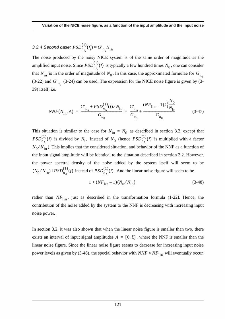
Variation of the NICE noise figure, as a function of the input amplitude and the input noise
3.3.4 Second case:
The noise produced by the noisy NICE system is of the same order of magnitude as the
amplified input noise. Since is typically a few hundred times , one can consider
that is in the order of magnitude of . In this case, the approximated formulae for
(3-22) and (3-24) can be used. The expression for the NICE noise figure is given by (3-
39) itself, i.e.
(3-47)
This situation is similar to the case for as described in section 3.2, except that
is divided by instead of (hence is multiplied with a factor
). This implies that the considered situation, and behavior of the NNF as a function of
the input signal amplitude will be identical to the situation described in section 3.2. However,
the power spectral density of the noise added by the system itself will seem to be
instead of . And the linear noise figure will seem to be
(3-48)
rather than , just as described in the transformation formula (1-22). Hence, the
contribution of the noise added by the system to the NNF is decreasing with increasing input
noise power.
In section 3.2, it was also shown that when the linear noise figure is smaller than two, there
exists an interval of input signal amplitudes , where the NNF is smaller than the
linear noise figure. Since the linear noise figure seems to decrease for increasing input noise
power levels as given by (3-48), the special behavior with will eventually occur.
PSDnA
1( ) fi( ) G ′nuNin≈
PSDnA
1( ) f( ) N0
Nin N0 Gu0
G ′nu
NNF Nin A,( )G ′nu
PSDnA
1( ) f( ) Nin⁄+
Gu0
-------------------------------------------------------G ′nu
Gu0
-----------NFlin 1–( )k1
2 N0Nin--------
Gu0
------------------------------------------+= =
Nin N0=
PSDnA
1( ) f( ) Nin N0 PSDnA
1( ) f( )
N0 Nin⁄
N0 Nin⁄( ) PSDnA
1( ) f( )⋅ PSDnA
1( ) f( )
1 NFlin 1–( ) N0 Nin⁄( )+
NFlin
A 0 ξ,[ ]=
NNF NFlin<
121
Extension of the “Noise Figure” towards NICE systems
Example 3.2
If = 6.5, according to (3-48), the apparent linear noise figure will decrease below 2 if
, or, in terms of , if .
Figure 3-11 shows a schematic representation of the variation of the NICE noise figure, as a
function of the input signal amplitude and the input noise power spectral density , for
.
Hence, the more increases, the less the noise added by the system itself becomes
important in the NNF, and the more the noise behavior of the system resembles that of a
noiseless NICE system.
3.3.5 Third case:
The noise produced by the noisy NICE system is much smaller than the amplified input noise.
This means that is several orders of magnitude larger than . The expression for the
NICE noise figure is then given by:
(3-49)
This expression is independent of the noise produced by the noisy NICE system itself. Note
that due to the polynomial model of third degree that was chosen to represent the NICE
FIGURE 3-11. Schematic representation of the signal-to-noise ratio deterioration vs. and for input noise temperatures around 290 K
NFlin
Nin NFlin 1–( )N0≥ 5.5N0= PSDnA
1( ) f( ) Nin PSDnA
1( ) f( ) k12⁄≥
A Nin
Nin N0≈
A
NNF
Nin
N0
0.2V2
ANin
Nin
PSDnA
1( ) fi( ) G ′nuNin«
Nin N0
NNFG ′nu
Gu0
-----------=
122
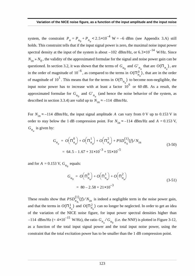
Variation of the NICE noise figure, as a function of the input amplitude and the input noise
system, the constraint W = dBm (see Appendix 3.A) still
holds. This constraint tells that if the input signal power is zero, the maximal noise input power
spectral density at the input of the system is about dBm/Hz, or 6. W/Hz. Since
, the validity of the approximated formulae for the signal and noise power gain can be
questioned. In section 3.2, it was shown that the terms of and that are , are
in the order of magnitude of , as compared to the terms in , that are in the order
of magnitude of . This means that for the terms in to become non-negligible, the
input noise power has to increase with at least a factor or 60 dB. As a result, the
approximated formulae for and (and hence the noise behavior of the system, as
described in section 3.3.4) are valid up to dBm/Hz.
For dBm/Hz, the input signal amplitude can vary from 0 V up to 0.153 V in
order to stay below the 1 dB compression point. For dBm/Hz and = 0.153 V,
is given by:
(3-50)
and for = 0.153 V, equals:
(3-51)
These results show that is indeed a negligible term in the noise power gain,
and that the terms in and can no longer be neglected. In order to get an idea
of the variation of the NICE noise figure, for input power spectral densities higher than
dBm/Hz (= W/Hz), the ratio (i.e. the NNF) is plotted in Figure 3-12,
as a function of the total input signal power and the total input noise power, using the
constraint that the total excitation power has to be smaller than the 1 dB compression point.
Pu Pu0Pnu
+= 2.5 4–×10< 6–
102– 3 14–×10
Nin N0»
Gu0G ′nu
O Πnu( )
10 6– O Πnu0( )
101 O Πnu( )
106
Gu0G ′nu
Nin 114–≈
Nin 114–≈ A
Nin 114–≈ A
Gnu
GnuO Πnu
0 O Πnu
1 O Πnu
2 PSDnA
1( ) f( ) Nin⁄+ + +=
64.5 1.67– 31 3–×10 55 5–×10+ + =
A Gu0
Gu0O Πnu
0 O Πnu
1 O Πnu
2 + +=
80 2.58– 21 3–×10 +=
PSDnA
1( ) f( ) Nin⁄
O Πnu1( ) O Πnu
2( )
114– 4 15–×10 GnuGu0
⁄
123
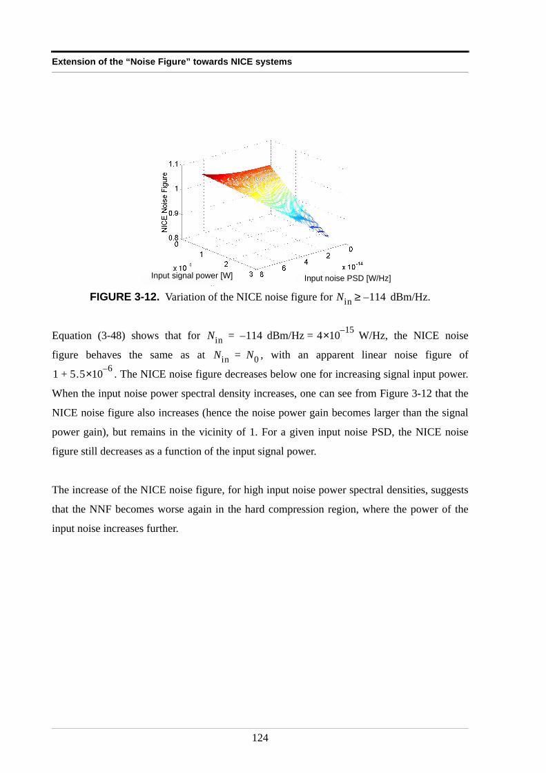
Extension of the “Noise Figure” towards NICE systems
Equation (3-48) shows that for dBm/Hz = W/Hz, the NICE noise
figure behaves the same as at , with an apparent linear noise figure of
. The NICE noise figure decreases below one for increasing signal input power.
When the input noise power spectral density increases, one can see from Figure 3-12 that the
NICE noise figure also increases (hence the noise power gain becomes larger than the signal
power gain), but remains in the vicinity of 1. For a given input noise PSD, the NICE noise
figure still decreases as a function of the input signal power.
The increase of the NICE noise figure, for high input noise power spectral densities, suggests
that the NNF becomes worse again in the hard compression region, where the power of the
input noise increases further.
FIGURE 3-12. Variation of the NICE noise figure for dBm/Hz.
Input signal power [W] Input noise PSD [W/Hz]
Nin 114–≥
Nin 114–= 4 15–×10
Nin N0=
1 5.5 6–×10+
124
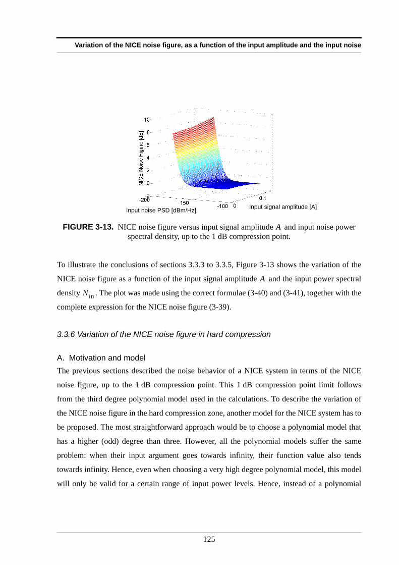
Variation of the NICE noise figure, as a function of the input amplitude and the input noise
To illustrate the conclusions of sections 3.3.3 to 3.3.5, Figure 3-13 shows the variation of the
NICE noise figure as a function of the input signal amplitude and the input power spectral
density . The plot was made using the correct formulae (3-40) and (3-41), together with the
complete expression for the NICE noise figure (3-39).
3.3.6 Variation of the NICE noise figure in hard compression
A. Motivation and modelThe previous sections described the noise behavior of a NICE system in terms of the NICE
noise figure, up to the 1 dB compression point. This 1 dB compression point limit follows
from the third degree polynomial model used in the calculations. To describe the variation of
the NICE noise figure in the hard compression zone, another model for the NICE system has to
be proposed. The most straightforward approach would be to choose a polynomial model that
has a higher (odd) degree than three. However, all the polynomial models suffer the same
problem: when their input argument goes towards infinity, their function value also tends
towards infinity. Hence, even when choosing a very high degree polynomial model, this model
will only be valid for a certain range of input power levels. Hence, instead of a polynomial
FIGURE 3-13. NICE noise figure versus input signal amplitude and input noise power spectral density, up to the 1 dB compression point.
Input noise PSD [dBm/Hz] Input signal amplitude [A]
A
A
Nin
125
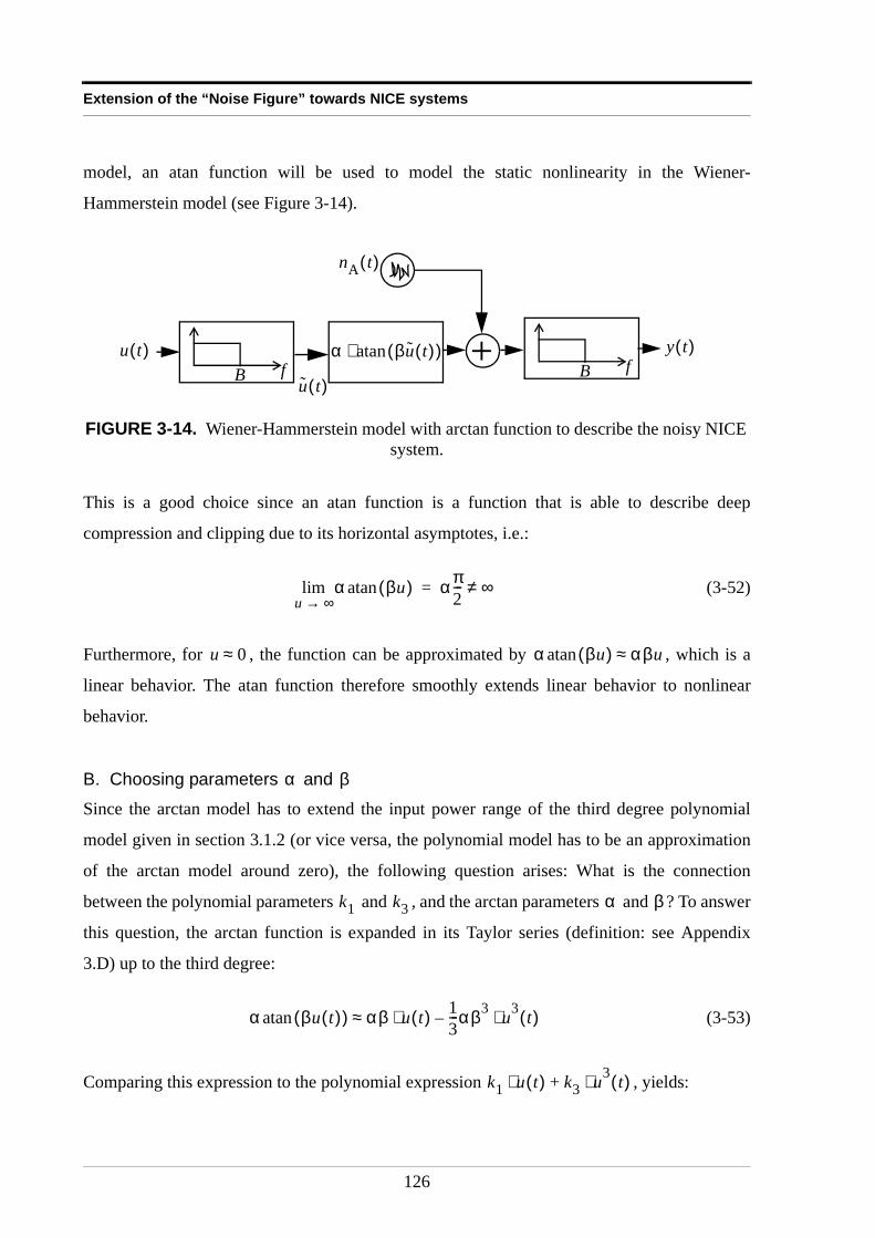
Extension of the “Noise Figure” towards NICE systems
model, an atan function will be used to model the static nonlinearity in the Wiener-
Hammerstein model (see Figure 3-14).
This is a good choice since an atan function is a function that is able to describe deep
compression and clipping due to its horizontal asymptotes, i.e.:
(3-52)
Furthermore, for , the function can be approximated by , which is a
linear behavior. The atan function therefore smoothly extends linear behavior to nonlinear
behavior.
B. Choosing parameters and Since the arctan model has to extend the input power range of the third degree polynomial
model given in section 3.1.2 (or vice versa, the polynomial model has to be an approximation
of the arctan model around zero), the following question arises: What is the connection
between the polynomial parameters and , and the arctan parameters and ? To answer
this question, the arctan function is expanded in its Taylor series (definition: see Appendix
3.D) up to the third degree:
(3-53)
Comparing this expression to the polynomial expression , yields:
FIGURE 3-14. Wiener-Hammerstein model with arctan function to describe the noisy NICE system.
+fB fBu t( ) y t( )
nA t( )
u t( )
α β u t( )( )atan⋅
α βu( )atanu ∞→lim α π
2--- ∞≠=
u 0≈ α βu( )atan αβu≈
α β
k1 k3 α β
α βu t( )( )atan αβ u t( ) 13---αβ3 u3 t( )⋅–⋅≈
k1 u t( )⋅ k3 u3 t( )⋅+
126
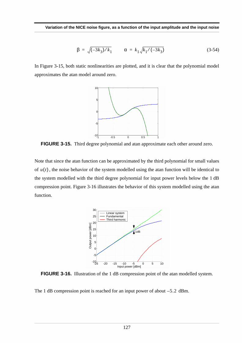
Variation of the NICE noise figure, as a function of the input amplitude and the input noise
(3-54)
In Figure 3-15, both static nonlinearities are plotted, and it is clear that the polynomial model
approximates the atan model around zero.
Note that since the atan function can be approximated by the third polynomial for small values
of , the noise behavior of the system modelled using the atan function will be identical to
the system modelled with the third degree polynomial for input power levels below the 1 dB
compression point. Figure 3-16 illustrates the behavior of this system modelled using the atan
function.
The 1 dB compression point is reached for an input power of about dBm.
FIGURE 3-15. Third degree polynomial and atan approximate each other around zero.
FIGURE 3-16. Illustration of the 1 dB compression point of the atan modelled system.
β 3k3–( ) k1⁄= α k1 k1 3k3–( )⁄=
-1 -0.5 0 0.5 1-10
-5
0
5
10
u t( )
-25 -20 -15 -10 -5 0 5 10-10
-5
0
5
10
15
20
25
30
Input power [dBm]
Outp
ut pow
er
[dB
m]
Linear system Fundamental Third harmonic
1dB
5.2–
127
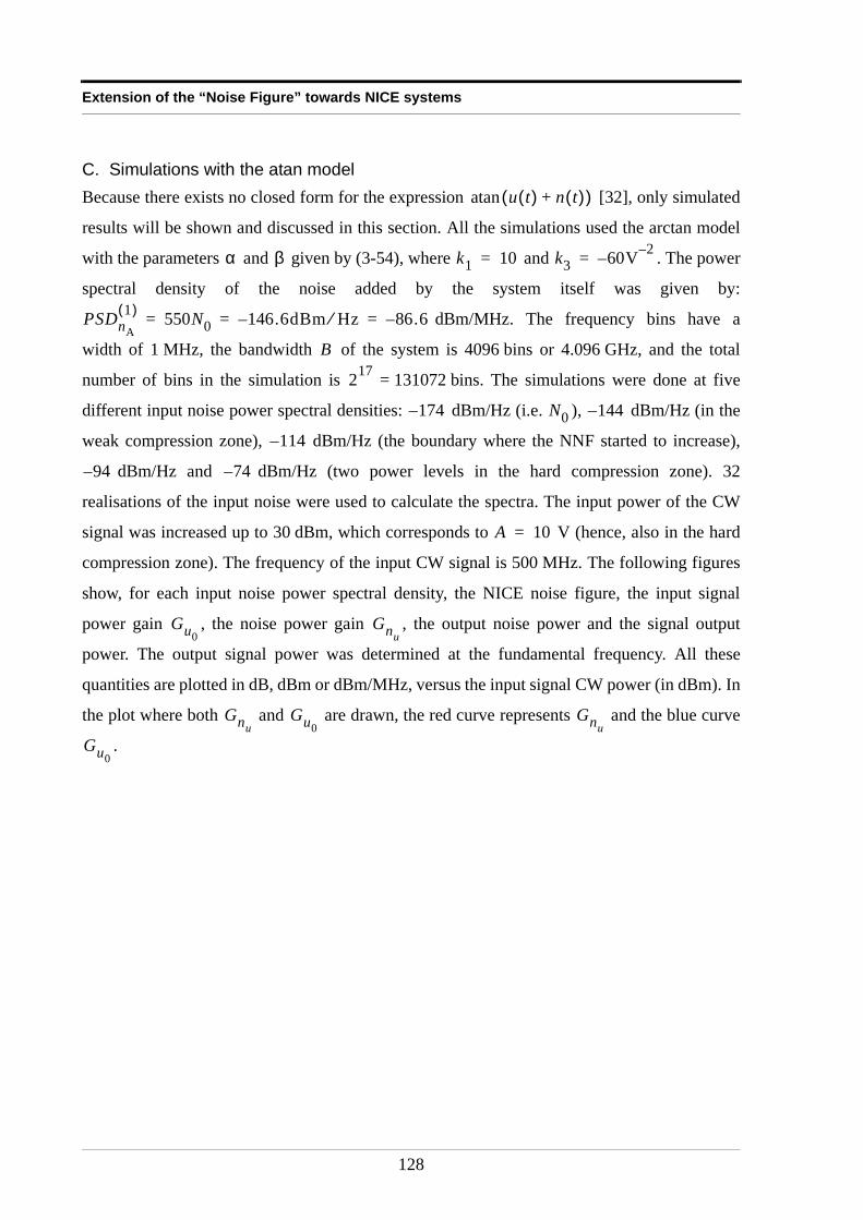
Extension of the “Noise Figure” towards NICE systems
C. Simulations with the atan modelBecause there exists no closed form for the expression [32], only simulated
results will be shown and discussed in this section. All the simulations used the arctan model
with the parameters and given by (3-54), where and . The power
spectral density of the noise added by the system itself was given by:
dBm/MHz. The frequency bins have a
width of 1 MHz, the bandwidth of the system is 4096 bins or 4.096 GHz, and the total
number of bins in the simulation is = 131072 bins. The simulations were done at five
different input noise power spectral densities: dBm/Hz (i.e. ), dBm/Hz (in the
weak compression zone), dBm/Hz (the boundary where the NNF started to increase),
dBm/Hz and dBm/Hz (two power levels in the hard compression zone). 32
realisations of the input noise were used to calculate the spectra. The input power of the CW
signal was increased up to 30 dBm, which corresponds to V (hence, also in the hard
compression zone). The frequency of the input CW signal is 500 MHz. The following figures
show, for each input noise power spectral density, the NICE noise figure, the input signal
power gain , the noise power gain , the output noise power and the signal output
power. The output signal power was determined at the fundamental frequency. All these
quantities are plotted in dB, dBm or dBm/MHz, versus the input signal CW power (in dBm). In
the plot where both and are drawn, the red curve represents and the blue curve
.
u t( ) n t( )+( )atan
α β k1 10= k3 60V 2––=
PSDnA
1( ) 550N0 146.6dBm Hz⁄– 86.6–= = =
B
217
174– N0 144–
114–
94– 74–
A 10=
Gu0Gnu
GnuGu0
Gnu
Gu0
128
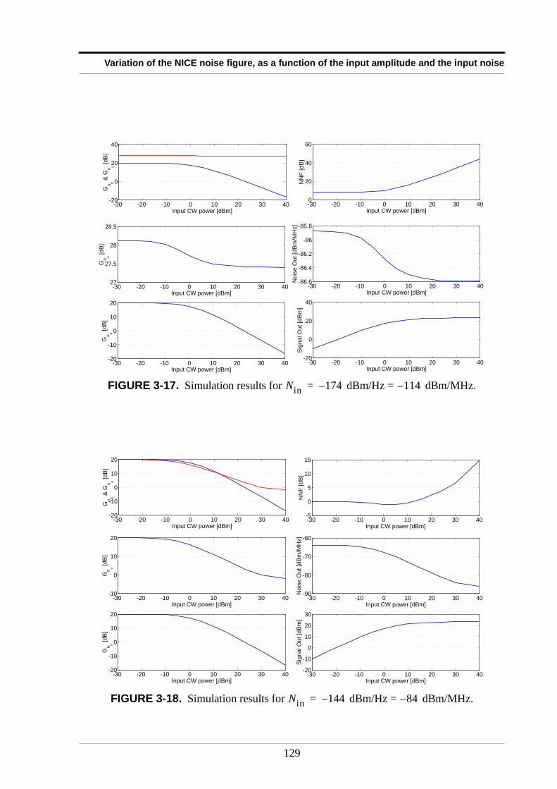
Variation of the NICE noise figure, as a function of the input amplitude and the input noise
FIGURE 3-17. Simulation results for dBm/Hz = dBm/MHz.
FIGURE 3-18. Simulation results for dBm/Hz = dBm/MHz.
-30 -20 -10 0 10 20 30 40-86.6
-86.4
-86.2
-86
-85.8
Input CW power [dBm]N
ois
e O
ut
[dB
m/M
Hz]
-30 -20 -10 0 10 20 30 40-20
0
20
40
Input CW power [dBm]
Sig
na
l O
ut
[dB
m]
-30 -20 -10 0 10 20 30 40-20
-10
0
10
20
Input CW power [dBm]
Gu
0
[d
B]
-30 -20 -10 0 10 20 30 4027
27.5
28
28.5
Input CW power [dBm]
Gn
u
[d
B]
-30 -20 -10 0 10 20 30 40-20
0
20
40
Input CW power [dBm]
Gu
0
& G
nu
[d
B]
-30 -20 -10 0 10 20 30 400
20
40
60
Input CW power [dBm]
NN
F [
dB
]
Nin 174–= 114–
-30 -20 -10 0 10 20 30 40-90
-80
-70
-60
Input CW power [dBm]
No
ise
Ou
t [d
Bm
/MH
z]
-30 -20 -10 0 10 20 30 40-20
-10
0
10
20
30
Input CW power [dBm]
Sig
na
l O
ut
[dB
m]
-30 -20 -10 0 10 20 30 40-5
0
5
10
15
Input CW power [dBm]
NN
F [
dB
]
-30 -20 -10 0 10 20 30 40-20
-10
0
10
20
Input CW power [dBm]
Gu
0
[d
B]
-30 -20 -10 0 10 20 30 40-10
0
10
20
Input CW power [dBm]
Gn
u
[d
B]
-30 -20 -10 0 10 20 30 40-20
-10
0
10
20
Input CW power [dBm]
Gu
0
& G
nu
[d
B]
Nin 144–= 84–
129
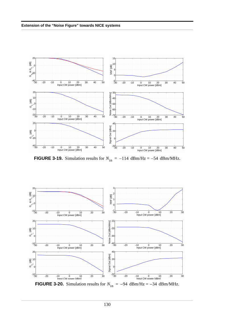
Extension of the “Noise Figure” towards NICE systems
FIGURE 3-19. Simulation results for dBm/Hz = dBm/MHz.
FIGURE 3-20. Simulation results for dBm/Hz = dBm/MHz.
-30 -20 -10 0 10 20 30 40 50-70
-60
-50
-40
-30
Input CW power [dBm]
No
ise
Ou
t [d
Bm
/MH
z]
-30 -20 -10 0 10 20 30 40 50-20
0
20
40
Input CW power [dBm]
Sig
na
l O
ut
[dB
m]
-30 -20 -10 0 10 20 30 40 50-40
-20
0
20
Input CW power [dBm]
Gu
0
[d
B]
-30 -20 -10 0 10 20 30 40 50-20
-10
0
10
20
Input CW power [dBm]
Gn
u
[d
B]
-30 -20 -10 0 10 20 30 40 50-40
-20
0
20
Input CW power [dBm]
Gu
0
& G
nu
[d
B]
-30 -20 -10 0 10 20 30 40 50-5
0
5
10
15
Input CW power [dBm]
NN
F [
dB
]
Nin 114–= 54–
-30 -20 -10 0 10 20 30-40
-30
-20
-10
Input CW power [dBm]
No
ise
Ou
t [d
Bm
/MH
z]
-30 -20 -10 0 10 20 30-20
0
20
40
Input CW power [dBm]
Sig
na
l O
ut
[dB
m]
-30 -20 -10 0 10 20 30-10
0
10
20
Input CW power [dBm]
Gu
0
[d
B]
-30 -20 -10 0 10 20 30-10
0
10
20
Input CW power [dBm]
Gn
u
[d
B]
-30 -20 -10 0 10 20 30-10
0
10
20
Input CW power [dBm]
Gu
0
& G
nu
[d
B]
-30 -20 -10 0 10 20 30-1
0
1
2
3
Input CW power [dBm]
NN
F [
dB
]
Nin 94–= 34–
130
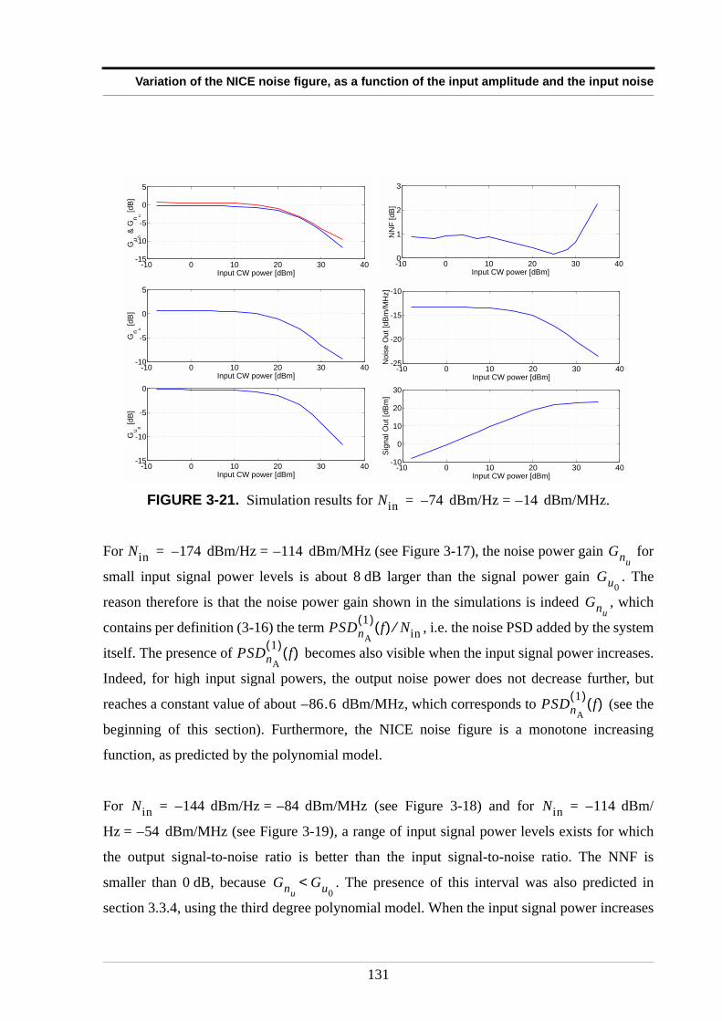
Variation of the NICE noise figure, as a function of the input amplitude and the input noise
For dBm/Hz = dBm/MHz (see Figure 3-17), the noise power gain for
small input signal power levels is about 8 dB larger than the signal power gain . The
reason therefore is that the noise power gain shown in the simulations is indeed , which
contains per definition (3-16) the term , i.e. the noise PSD added by the system
itself. The presence of becomes also visible when the input signal power increases.
Indeed, for high input signal powers, the output noise power does not decrease further, but
reaches a constant value of about dBm/MHz, which corresponds to (see the
beginning of this section). Furthermore, the NICE noise figure is a monotone increasing
function, as predicted by the polynomial model.
For dBm/Hz = dBm/MHz (see Figure 3-18) and for dBm/
Hz = dBm/MHz (see Figure 3-19), a range of input signal power levels exists for which
the output signal-to-noise ratio is better than the input signal-to-noise ratio. The NNF is
smaller than 0 dB, because . The presence of this interval was also predicted in
section 3.3.4, using the third degree polynomial model. When the input signal power increases
FIGURE 3-21. Simulation results for dBm/Hz = dBm/MHz.
-10 0 10 20 30 40-25
-20
-15
-10
Input CW power [dBm]N
ois
e O
ut
[dB
m/M
Hz]
-10 0 10 20 30 40-10
0
10
20
30
Input CW power [dBm]
Sig
na
l O
ut
[dB
m]
-10 0 10 20 30 40-15
-10
-5
0
Input CW power [dBm]
Gu
0
[d
B]
-10 0 10 20 30 40-10
-5
0
5
Input CW power [dBm]
Gn
u
[d
B]
-10 0 10 20 30 40-15
-10
-5
0
5
Input CW power [dBm]
Gu
0
& G
nu
[d
B]
-10 0 10 20 30 400
1
2
3
Input CW power [dBm]
NN
F [
dB
]
Nin 74–= 14–
Nin 174–= 114– Gnu
Gu0
Gnu
PSDnA
1( ) f( ) Nin⁄
PSDnA
1( ) f( )
86.6– PSDnA
1( ) f( )
Nin 144–= 84– Nin 114–=
54–
GnuGu0
<
131
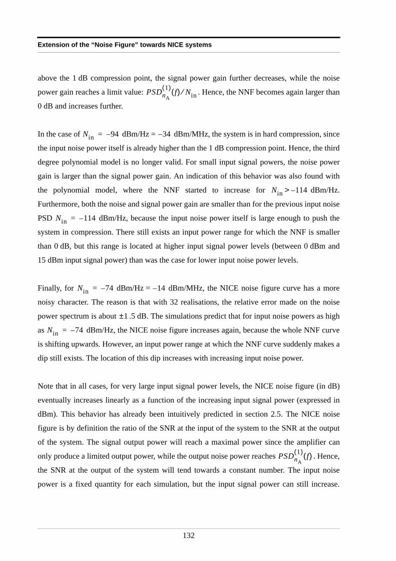
Extension of the “Noise Figure” towards NICE systems
above the 1 dB compression point, the signal power gain further decreases, while the noise
power gain reaches a limit value: . Hence, the NNF becomes again larger than
0 dB and increases further.
In the case of dBm/Hz = dBm/MHz, the system is in hard compression, since
the input noise power itself is already higher than the 1 dB compression point. Hence, the third
degree polynomial model is no longer valid. For small input signal powers, the noise power
gain is larger than the signal power gain. An indication of this behavior was also found with
the polynomial model, where the NNF started to increase for dBm/Hz.
Furthermore, both the noise and signal power gain are smaller than for the previous input noise
PSD dBm/Hz, because the input noise power itself is large enough to push the
system in compression. There still exists an input power range for which the NNF is smaller
than 0 dB, but this range is located at higher input signal power levels (between 0 dBm and
15 dBm input signal power) than was the case for lower input noise power levels.
Finally, for dBm/Hz = dBm/MHz, the NICE noise figure curve has a more
noisy character. The reason is that with 32 realisations, the relative error made on the noise
power spectrum is about .5 dB. The simulations predict that for input noise powers as high
as dBm/Hz, the NICE noise figure increases again, because the whole NNF curve
is shifting upwards. However, an input power range at which the NNF curve suddenly makes a
dip still exists. The location of this dip increases with increasing input noise power.
Note that in all cases, for very large input signal power levels, the NICE noise figure (in dB)
eventually increases linearly as a function of the increasing input signal power (expressed in
dBm). This behavior has already been intuitively predicted in section 2.5. The NICE noise
figure is by definition the ratio of the SNR at the input of the system to the SNR at the output
of the system. The signal output power will reach a maximal power since the amplifier can
only produce a limited output power, while the output noise power reaches . Hence,
the SNR at the output of the system will tend towards a constant number. The input noise
power is a fixed quantity for each simulation, but the input signal power can still increase.
PSDnA
1( ) f( ) Nin⁄
Nin 94–= 34–
Nin 114–>
Nin 114–=
Nin 74–= 14–
1±
Nin 74–=
PSDnA
1( ) f( )
132
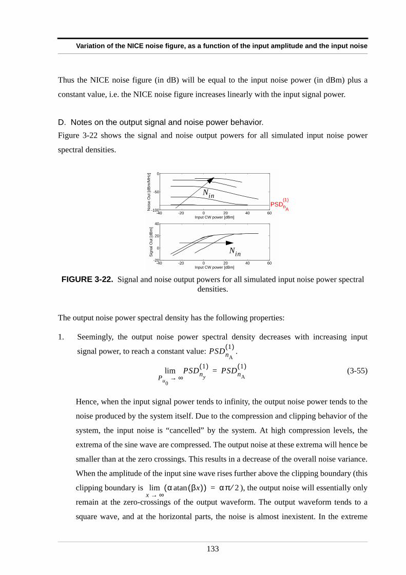
Variation of the NICE noise figure, as a function of the input amplitude and the input noise
Thus the NICE noise figure (in dB) will be equal to the input noise power (in dBm) plus a
constant value, i.e. the NICE noise figure increases linearly with the input signal power.
D. Notes on the output signal and noise power behavior.Figure 3-22 shows the signal and noise output powers for all simulated input noise power
spectral densities.
The output noise power spectral density has the following properties:
1. Seemingly, the output noise power spectral density decreases with increasing input
signal power, to reach a constant value: .
(3-55)
Hence, when the input signal power tends to infinity, the output noise power tends to the
noise produced by the system itself. Due to the compression and clipping behavior of the
system, the input noise is “cancelled” by the system. At high compression levels, the
extrema of the sine wave are compressed. The output noise at these extrema will hence be
smaller than at the zero crossings. This results in a decrease of the overall noise variance.
When the amplitude of the input sine wave rises further above the clipping boundary (this
clipping boundary is ), the output noise will essentially only
remain at the zero-crossings of the output waveform. The output waveform tends to a
square wave, and at the horizontal parts, the noise is almost inexistent. In the extreme
FIGURE 3-22. Signal and noise output powers for all simulated input noise power spectral densities.
-40 -20 0 20 40 60-100
-50
0
Input CW power [dBm]
No
ise
Ou
t [d
Bm
/MH
z]
-40 -20 0 20 40 60-20
0
20
40
Input CW power [dBm]
Sig
na
l O
ut
[dB
m]
Nin
Nin
PSDnA
(1)
PSDnA
1( )
PSDny
1( )
Pu0∞→
lim PSDnA
1( )=
α βx( )atan( )x ∞→lim απ 2⁄=
133
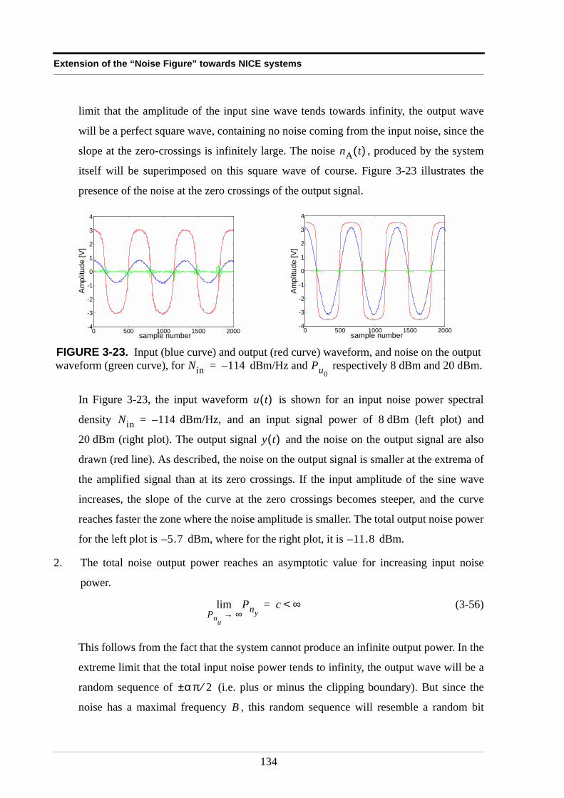
Extension of the “Noise Figure” towards NICE systems
limit that the amplitude of the input sine wave tends towards infinity, the output wave
will be a perfect square wave, containing no noise coming from the input noise, since the
slope at the zero-crossings is infinitely large. The noise , produced by the system
itself will be superimposed on this square wave of course. Figure 3-23 illustrates the
presence of the noise at the zero crossings of the output signal.
In Figure 3-23, the input waveform is shown for an input noise power spectral
density dBm/Hz, and an input signal power of 8 dBm (left plot) and
20 dBm (right plot). The output signal and the noise on the output signal are also
drawn (red line). As described, the noise on the output signal is smaller at the extrema of
the amplified signal than at its zero crossings. If the input amplitude of the sine wave
increases, the slope of the curve at the zero crossings becomes steeper, and the curve
reaches faster the zone where the noise amplitude is smaller. The total output noise power
for the left plot is dBm, where for the right plot, it is dBm.
2. The total noise output power reaches an asymptotic value for increasing input noise
power.
(3-56)
This follows from the fact that the system cannot produce an infinite output power. In the
extreme limit that the total input noise power tends to infinity, the output wave will be a
random sequence of (i.e. plus or minus the clipping boundary). But since the
noise has a maximal frequency , this random sequence will resemble a random bit
FIGURE 3-23. Input (blue curve) and output (red curve) waveform, and noise on the output waveform (green curve), for dBm/Hz and respectively 8 dBm and 20 dBm.
nA t( )
0 500 1000 1500 2000-4
-3
-2
-1
0
1
2
3
4
0 500 1000 1500 2000-4
-3
-2
-1
0
1
2
3
4
Ampl
itude
[V]
Am
plitu
de [V
]
sample number sample number
Nin 114–= Pu0
u t( )
Nin 114–=
y t( )
5.7– 11.8–
PnyPnu∞→
lim c ∞<=
απ 2⁄±
B
134
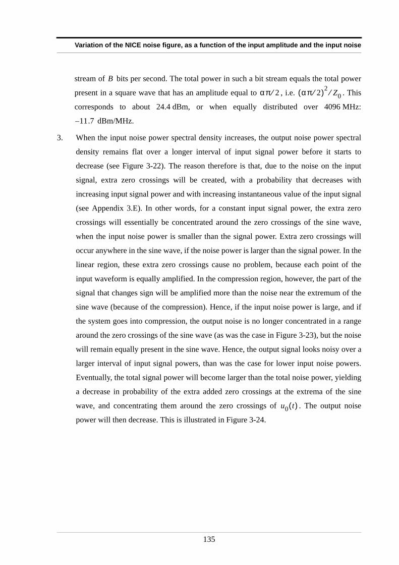
Variation of the NICE noise figure, as a function of the input amplitude and the input noise
stream of bits per second. The total power in such a bit stream equals the total power
present in a square wave that has an amplitude equal to , i.e. . This
corresponds to about 24.4 dBm, or when equally distributed over 4096 MHz:
dBm/MHz.
3. When the input noise power spectral density increases, the output noise power spectral
density remains flat over a longer interval of input signal power before it starts to
decrease (see Figure 3-22). The reason therefore is that, due to the noise on the input
signal, extra zero crossings will be created, with a probability that decreases with
increasing input signal power and with increasing instantaneous value of the input signal
(see Appendix 3.E). In other words, for a constant input signal power, the extra zero
crossings will essentially be concentrated around the zero crossings of the sine wave,
when the input noise power is smaller than the signal power. Extra zero crossings will
occur anywhere in the sine wave, if the noise power is larger than the signal power. In the
linear region, these extra zero crossings cause no problem, because each point of the
input waveform is equally amplified. In the compression region, however, the part of the
signal that changes sign will be amplified more than the noise near the extremum of the
sine wave (because of the compression). Hence, if the input noise power is large, and if
the system goes into compression, the output noise is no longer concentrated in a range
around the zero crossings of the sine wave (as was the case in Figure 3-23), but the noise
will remain equally present in the sine wave. Hence, the output signal looks noisy over a
larger interval of input signal powers, than was the case for lower input noise powers.
Eventually, the total signal power will become larger than the total noise power, yielding
a decrease in probability of the extra added zero crossings at the extrema of the sine
wave, and concentrating them around the zero crossings of . The output noise
power will then decrease. This is illustrated in Figure 3-24.
B
απ 2⁄ απ 2⁄( )2 Z0⁄
11.7–
u0 t( )
135
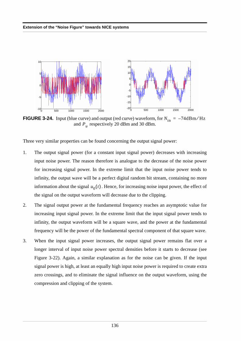
Extension of the “Noise Figure” towards NICE systems
Three very similar properties can be found concerning the output signal power:
1. The output signal power (for a constant input signal power) decreases with increasing
input noise power. The reason therefore is analogue to the decrease of the noise power
for increasing signal power. In the extreme limit that the input noise power tends to
infinity, the output wave will be a perfect digital random bit stream, containing no more
information about the signal . Hence, for increasing noise input power, the effect of
the signal on the output waveform will decrease due to the clipping.
2. The signal output power at the fundamental frequency reaches an asymptotic value for
increasing input signal power. In the extreme limit that the input signal power tends to
infinity, the output waveform will be a square wave, and the power at the fundamental
frequency will be the power of the fundamental spectral component of that square wave.
3. When the input signal power increases, the output signal power remains flat over a
longer interval of input noise power spectral densities before it starts to decrease (see
Figure 3-22). Again, a similar explanation as for the noise can be given. If the input
signal power is high, at least an equally high input noise power is required to create extra
zero crossings, and to eliminate the signal influence on the output waveform, using the
compression and clipping of the system.
FIGURE 3-24. Input (blue curve) and output (red curve) waveform, for and respectively 20 dBm and 30 dBm.
0 500 1000 1500 2000-10
-5
0
5
10
0 500 1000 1500 2000-20
-15
-10
-5
0
5
10
15
20
Nin 74dBm Hz⁄–=Pu
u0 t( )
136
Variation of the NICE noise figure, as a function of the input amplitude and the input noise
Note that the elimination of the effect of an input signal on the output waveform can never
occur in the linear region, since it is a property of the nonlinear mechanism itself.
3.3.7 ConclusionIn order to describe the variation of the NICE noise figure of a noisy NICE system that is
excited by the superposition of a pure sine wave and band-limited Gaussian noise, the -
plane where the NICE noise figure will be evaluated, can be divided into three zones,
depending on how deep the NICE system goes into compression (see Figure 3-1).
In the linear zone, the total input power is that small that the NICE system can be modelled as
a LTI system and its noise behavior can be described using the linear noise theory as explained
in section 1.4. The boundary of this zone is reached when the terms in the signal power gain
(3-40) and noise power gain (3-42), that are due to the nonlinear behavior of the system, can no
longer be neglected as compared to the linear terms (i.e. about dBm total input power, see
Appendix 3.F).
In the weak compression region, the NICE noise figure is given by the ratio of the noise power
gain to the signal power gain: . Hence, the
NICE noise figure consists of two contributions: the effect of the noiseless NICE system
( ) and the effect of the noise produced by the NICE system itself:
. The latter effect decreases as , for increasing noise input PSD.
Up to about 10 dB under the 1 dB compression point, the signal power gain and the noise
power gain of the underlying noiseless system are constant as function of the input noise
PSD . This implies that the variation of the NNF for increasing input noise PSD is the
same as the behavior of that system for input noise PSD equal to , but having an apparent
linear noise figure (i.e. a ) that decreases with increasing . Since it was shown in
section 3.2, that a linear noise figure which is smaller than two, implies the existence of a range
of input signal amplitudes where , an identical behavior will be encountered
when the input noise PSD increases. Hence the apparent linear noise figure decreases below
two. For input noise power spectral densities at about 10 dB under the 1 dB compression point,
the system will actually improve the signal-to-noise ratio. Around the 1 dB compression point,
Pu0
Pnu
33–
NNF GnuGu0
⁄ G ′nuPSDnA
1( ) Nin⁄+ Gu0
⁄= =
G ′nuGu0
⁄
PSDnA
1( ) Nin⁄ Gu0
⁄ 1 Nin⁄
Gu0
G ′nu
Nin
N0
PSDnA
1( ) Nin
NNF NFlin<
137
Extension of the “Noise Figure” towards NICE systems
the noise power gain will become larger than the signal power gain, yielding again an increase
of the NNF.
Hence, with the knowledge of the signal power gain , the noise power gain of the
underlying noiseless system , the linear noise figure and the power gain of the
underlying linear system (needed to obtain ), it is possible to predict the NICE
noise figure for a certain range of input power spectral densities. This range of input power
spectral densities is the range where the noise and signal power gain do not vary much, i.e.
where the total input noise power stays about 10 dB below the 1 dB compression point.
In the zone where the NICE system exhibits hard compression (above the 1 dB compression
point), simulations show that a local minimum in the NNF curve as a function of the input
signal amplitude still exists. However, this local minimum is shifting towards higher input
amplitude values, as the input noise PSD increases. Furthermore, the whole NNF curve shifts
upwards with increasing . For a given , the NNF (in dB) will eventually linearly
increase as function of the (high) input signal power (in dBm).
3.3.8 Experimental resultsAs for the linear case (see chapter 1), the most straightforward approach to measure the NICE
noise figure as a function of the input signal amplitude and the input noise power spectral
density , would be to measure simply the signal-to-noise ratio at the input and at the output
of the system, for a range of values for and . The frequency dependent behavior imposes
this measurement to be repeated for a set of frequencies, covering the bandwidth of the
considered system. However, it is very difficult to measure signal-to-noise ratios when the
input noise power spectral density is very small ( ). Therefore, another method has to
be used. For total input excitation power levels below the 1 dB compression point, it is
possible to use the formula that describes the variation of the NICE noise figure with the input
noise power spectral density (3-39). Hence, with the knowledge of the signal power gain ,
the noise power gain of the underlying noiseless system , the linear noise figure
and the power gain of the underlying linear system (needed to obtain ), it is
possible to predict the NICE noise figure in the linear and the weak compression region.
Gu0
G ′nuNFlin
k12 PSDnA
1( )
Pnu
Nin Nin
A
Nin
A Nin
Nin N0≈
Gu0
G ′nuNFlin
k12 PSDnA
1( )
138
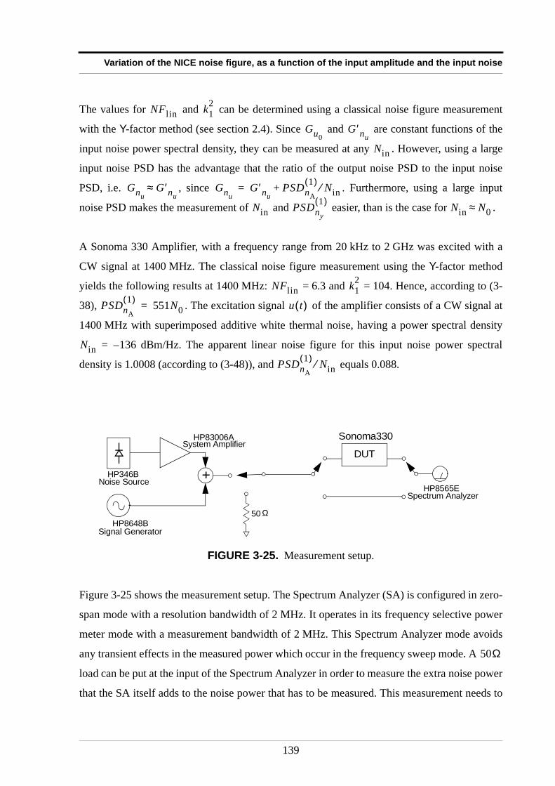
Variation of the NICE noise figure, as a function of the input amplitude and the input noise
The values for and can be determined using a classical noise figure measurement
with the Y-factor method (see section 2.4). Since and are constant functions of the
input noise power spectral density, they can be measured at any . However, using a large
input noise PSD has the advantage that the ratio of the output noise PSD to the input noise
PSD, i.e. , since . Furthermore, using a large input
noise PSD makes the measurement of and easier, than is the case for .
A Sonoma 330 Amplifier, with a frequency range from 20 kHz to 2 GHz was excited with a
CW signal at 1400 MHz. The classical noise figure measurement using the Y-factor method
yields the following results at 1400 MHz: = 6.3 and = 104. Hence, according to (3-
38), . The excitation signal of the amplifier consists of a CW signal at
1400 MHz with superimposed additive white thermal noise, having a power spectral density
dBm/Hz. The apparent linear noise figure for this input noise power spectral
density is 1.0008 (according to (3-48)), and equals 0.088.
Figure 3-25 shows the measurement setup. The Spectrum Analyzer (SA) is configured in zero-
span mode with a resolution bandwidth of 2 MHz. It operates in its frequency selective power
meter mode with a measurement bandwidth of 2 MHz. This Spectrum Analyzer mode avoids
any transient effects in the measured power which occur in the frequency sweep mode. A
load can be put at the input of the Spectrum Analyzer in order to measure the extra noise power
that the SA itself adds to the noise power that has to be measured. This measurement needs to
FIGURE 3-25. Measurement setup.
NFlin k12
Gu0G ′nu
Nin
GnuG ′nu
≈ GnuG ′nu
PSDnA
1( ) Nin⁄+=
Nin PSDny
1( ) Nin N0≈
NFlin k12
PSDnA
1( ) 551N0= u t( )
Nin 136–=
PSDnA
1( ) Nin⁄
DUT
+
50 Ω
Sonoma330
HP8565ESpectrum Analyzer
HP8648BSignal Generator
HP346BNoise Source
HP83006ASystem Amplifier
50Ω
139
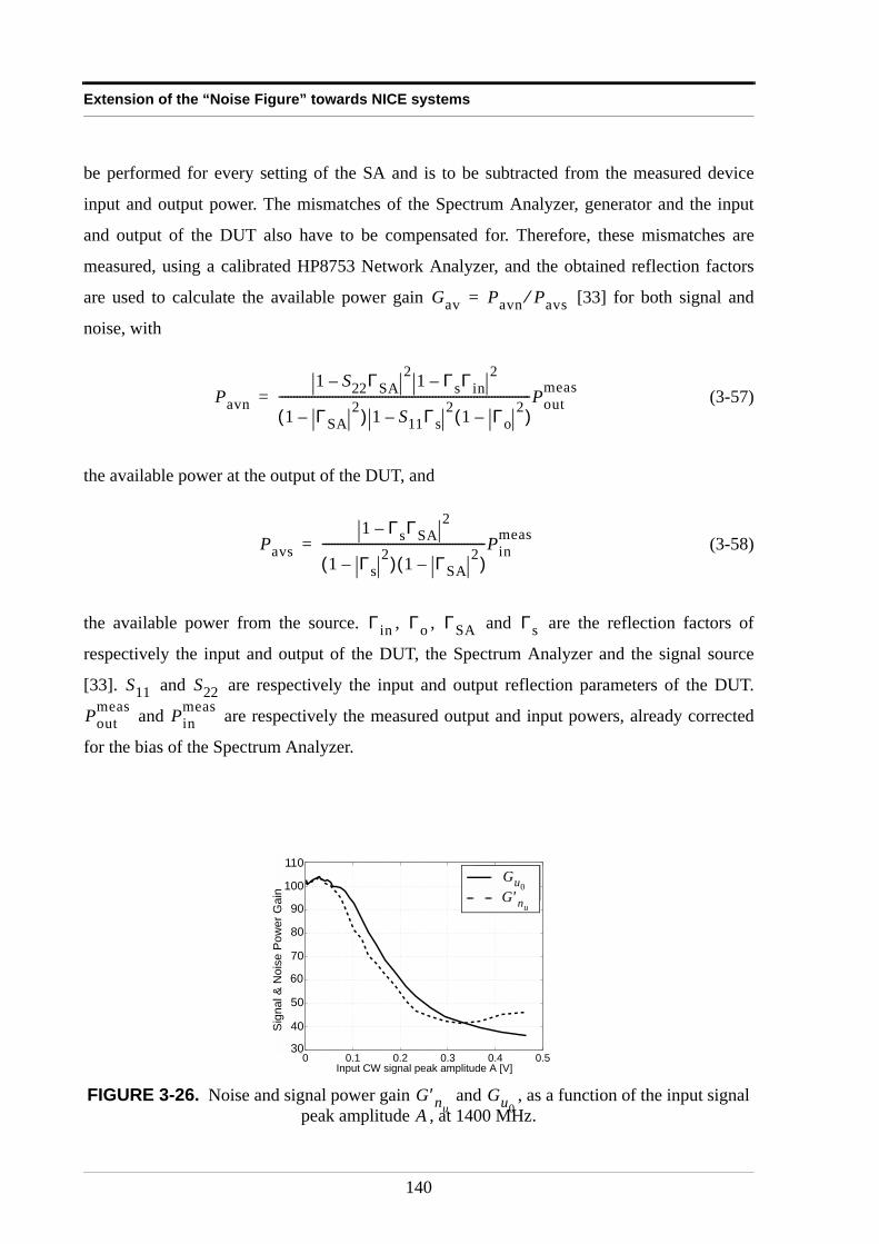
Extension of the “Noise Figure” towards NICE systems
be performed for every setting of the SA and is to be subtracted from the measured device
input and output power. The mismatches of the Spectrum Analyzer, generator and the input
and output of the DUT also have to be compensated for. Therefore, these mismatches are
measured, using a calibrated HP8753 Network Analyzer, and the obtained reflection factors
are used to calculate the available power gain [33] for both signal and
noise, with
(3-57)
the available power at the output of the DUT, and
(3-58)
the available power from the source. , , and are the reflection factors of
respectively the input and output of the DUT, the Spectrum Analyzer and the signal source
[33]. and are respectively the input and output reflection parameters of the DUT.
and are respectively the measured output and input powers, already corrected
for the bias of the Spectrum Analyzer.
FIGURE 3-26. Noise and signal power gain and , as a function of the input signal peak amplitude , at 1400 MHz.
Gav Pavn Pavs⁄=
Pavn1 S22ΓSA– 2 1 ΓsΓ in– 2
1 ΓSA2–( ) 1 S11Γ s– 2 1 Γo
2–( )-------------------------------------------------------------------------------------Pout
meas=
Pavs1 ΓsΓSA– 2
1 Γs2–( ) 1 ΓSA
2–( )-------------------------------------------------------Pin
meas=
Γ in Γo ΓSA Γs
S11 S22
Poutmeas Pin
meas
0 0.1 0.2 0.3 0.4 0.50
10
20
30
40
50
60
70
80
Input CW signal peak amplitude A [V]
Ava
ilabl
e G
ain
[Lin
ear]
Gsignal
Gnoise
100
110
90
80
70
60
50
40
30
Sig
nal &
Noi
se P
ower
Gai
n
Gu0G ′nu
G ′nuGu0A
140
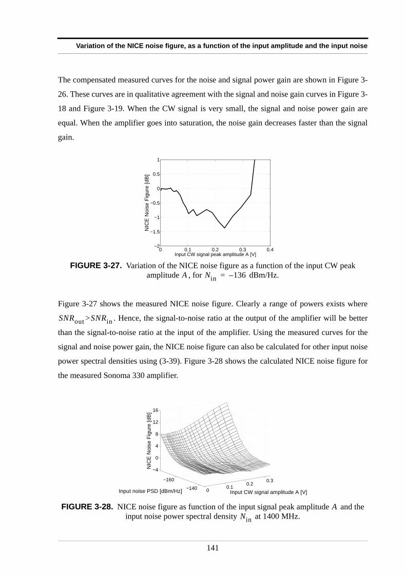
Variation of the NICE noise figure, as a function of the input amplitude and the input noise
The compensated measured curves for the noise and signal power gain are shown in Figure 3-
26. These curves are in qualitative agreement with the signal and noise gain curves in Figure 3-
18 and Figure 3-19. When the CW signal is very small, the signal and noise power gain are
equal. When the amplifier goes into saturation, the noise gain decreases faster than the signal
gain.
Figure 3-27 shows the measured NICE noise figure. Clearly a range of powers exists where
> . Hence, the signal-to-noise ratio at the output of the amplifier will be better
than the signal-to-noise ratio at the input of the amplifier. Using the measured curves for the
signal and noise power gain, the NICE noise figure can also be calculated for other input noise
power spectral densities using (3-39). Figure 3-28 shows the calculated NICE noise figure for
the measured Sonoma 330 amplifier.
FIGURE 3-27. Variation of the NICE noise figure as a function of the input CW peak amplitude , for dBm/Hz.
FIGURE 3-28. NICE noise figure as function of the input signal peak amplitude and the input noise power spectral density at 1400 MHz.
0 0.1 0.2 0.3 0.4−2
−1.5
−1
−0.5
0
0.5
1
Input CW signal peak amplitude A [V]
SN
Ri/S
NR
o [dB
]N
ICE
Noi
se F
igur
e [d
B]
A Nin 136–=
SNRout SNRin
00.1
0.20.3−160
−140
−4
0
4
8
12
16
Input CW signal A [V]Nin
[dBm/Hz]
SN
Ri/S
NR
o [dB
]N
ICE
Noi
se F
igur
e [d
B]
Input CW signal amplitude A [V]Input noise PSD [dBm/Hz]
ANin
141
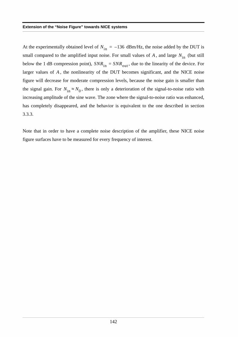
Extension of the “Noise Figure” towards NICE systems
At the experimentally obtained level of dBm/Hz, the noise added by the DUT is
small compared to the amplified input noise. For small values of , and large (but still
below the 1 dB compression point), = , due to the linearity of the device. For
larger values of , the nonlinearity of the DUT becomes significant, and the NICE noise
figure will decrease for moderate compression levels, because the noise gain is smaller than
the signal gain. For , there is only a deterioration of the signal-to-noise ratio with
increasing amplitude of the sine wave. The zone where the signal-to-noise ratio was enhanced,
has completely disappeared, and the behavior is equivalent to the one described in section
3.3.3.
Note that in order to have a complete noise description of the amplifier, these NICE noise
figure surfaces have to be measured for every frequency of interest.
Nin 136–=
A Nin
SNRin SNRout
A
Nin N0≈
142
Variation of the noise power gain, as a function of a general periodic or ergodic input signal
3.4 Variation of the noise power gain, as a function of a general periodic or ergodic input signal
3.4.1 IntroductionIn the previous sections, the variation of the NICE noise figure was studied, when the
excitation signal of a noisy NICE system consists of the superposition of band-limited,
Gaussian noise and a CW signal . The effects of the signal
and noise on the signal and noise power gain were studied. However, practical
amplifiers are mostly used to amplify modulated signals, or even signals whose spectrum is
continuous.
This section investigates the effects on the noise power gain of a noisy NICE system, when its
excitation signal consists of white, Gaussian noise , superimposed on a general
waveform that is zero-mean, and that can be
1. a periodic signal
2. an ergodic signal
3. the product or the sum of a periodic and an ergodic signal.
These restrictions are imposed on the waveform , to be able to use (1-2) in the
calculations. Equation (1-2) states that if is a periodic signal, and is ergodic noise,
(3-59)
If on the other hand, is an ergodic signal, that is uncorrelated with , the proof of (3-
59) is trivial.
It is intuitively clear that both signal and noise power gain will depend on the properties of
. The model used for the noisy NICE system will be again the modified Wiener-
Hammerstein model, where the static nonlinearity is described using a third degree polynomial
model, as discussed in section 3.1.2.
u t( )
nu t( ) u0 t( ) A 2πf0t( )cos= u0 t( )
nu t( )
u t( ) nu t( )
u0 t( )
u0 t( )
u0 t( ) nu t( )
α β, N∈∀ :E u0α t( )nu
β t τ+( )
E u0α t( )
E nuβ t τ+( )
⋅=
u0 t( ) nu t( )
u0 t( )
143
Extension of the “Noise Figure” towards NICE systems
3.4.2 Determining the output power spectral densityThe output signal of the noisy NICE system is:
(3-60)
or,
(3-61)
As in sections 2.3 and 3.2.1, the output power spectral density will be calculated by taking the
Fourier transform of the auto-correlation of the system output (see (2-5)). The noise
added by the system itself is assumed to be uncorrelated with the input signal and input noise.
After a few calculations (see Appendix 3.G), the autocorrelation can be written as:
(3-62)
Since and , (3-62) can be rewritten as:
(3-63)
y t( )
y t( ) k1 u0 t( ) nu t( )+( ) k3 u0 t( ) nu t( )+( )3 nA t( )+ +=
y t( ) k1nu t( ) k1u0 t( ) k3nu3 t( ) k3u0
3 t( ) 3k3u02 t( )nu t( ) 3k3nu
2 t( )u0 t( ) nA t( )+ + + + + +=
y t( )
Ryy τ( )
Ryy τ( ) Ru0u0τ( ) k1 3k3Rnunu
0( )+( )2⋅=
Rnunuτ( ) k1 3k3Rnunu
0( )+( ) k1 3k3 Rnunu0( ) 2Ru0u0
0( )+( )+( )⋅+
9k32R
u02u0
2 τ( )Rnunuτ( ) 6k3
2Rnunu
3τ( ) 18k3
2Ru0u0τ( )Rnunu
2 τ( )+ + +
k3 k1 3k3Rnunu0( )+( ) R
u0u03 τ( ) R
u0u03 τ–( )+
k32R
u03u0
3 τ( )+ +
RnAnAτ( )+
Rnunu0( ) Z0Pnu
= Ru0u00( ) Z0Pu0
=
Ryy τ( ) Ru0u0τ( ) k1 3k3Z0Pnu
+( )2 ⋅=
Rnunuτ( ) k1 3k3Z0Pnu
+( ) k1 3k3Z0 Pnu2Pu0
+( )+( )⋅+
Rnunuτ( ) 9k3
2Ru0
2u02 τ( ) 6k3
2Rnunu
2τ( ) 18k3
2Ru0u0τ( )Rnunu
τ( )+ + ⋅+
k3 k1 3k3Z0Pnu+( ) R
u0u03 τ( ) R
u0u03 τ–( )+
k32R
u03u0
3 τ( ) + +
RnAnAτ( ) +
144
Variation of the noise power gain, as a function of a general periodic or ergodic input signal
The first term in (3-63) shows that the auto-correlation of the input signal , and hence the
input signal’s power spectral density, is amplified with a constant term that depends on the
total noise power. The second term shows a scaling of the autocorrelation of the input noise
, and hence of the input noise power spectral density. This scaling of the input noise is
dependent on both the total noise power and the total signal power. The third line in (3-63)
contains the autocorrelation of the noise , multiplied by a factor that is dependent on
the properties of the signal and the noise. Hence, in the spectral domain, this means that the
third line of (3-63) will yield extra noise contributions, since it contains respectively,
• : the noise power spectral density convolved with
the spectrum of . This yields extra noise contributions, in the order
of magnitude of . Since , its time average
, and due to the properties of the auto-correlation function
which states that , with
, (see Appendix 3.H)
(3-64)
where . Hence, the first term in the third line
of (3-63) will add an extra correction on the scaling of , i.e.
, on top of the extra noise that will be generated.
• : the noise power spectral density, convolved three times
with itself, yielding extra noise, in the order of magnitude of .
• : the noise power spectral density, convolved with
itself and the spectrum of , yielding extra noise, in the order of
magnitude of .
The fourth line in (3-63) contains only signal contributions. These signal contributions are
quite annoying, because they are cross-correlations of the square and the third power of the
input signal , and thus dependent on the properties of this input signal. Hence, not much
u0 t( )
nu t( )
Rnunuτ( )
9k32R
u02u0
2 τ( )Rnunuτ( )
u02 t( )
PnuPu0
2 u02 t( ) 0≥
E u02 t( )
0>
Rαα τ( ) E α t( ) ( )2
Rββ τ( )+=
β t( ) α t( ) E α t( ) –=
Ru0
2u02 τ( ) E u0
2 t( )
2
Ru u
τ( )+ Z0Pu0( )2 R
u uτ( )+= =) ) ) )
u t( ) u02 t( ) E u0
2 t( )
–=)
Rnunuτ( )
9k32Z0
2Pu0
2
6k32Rnunu
3τ( )
Pnu
3
18k32Ru0u0
τ( )Rnunu
2 τ( )
u0 t( )
Pu0Pnu
2
u0 t( )
145
Extension of the “Noise Figure” towards NICE systems
can be said about their general behavior without further knowledge of those properties. In
general, they could possibly yield:
• in-band distortion terms [20], [34], (see chapter 4)
• spectra around (with the fundamental frequency, or center
frequency of )
• extra signal power gain corrections, dependent on the total signal power
(see chapter 4)
Note that these terms only contain signal contributions and that they create signal distortions,
but do not amplify or interact with the input noise . The last term in (3-63) is due to the
noise added by the system itself. To illustrate all the terms in (3-63), the above theory will be
applied on a given input signal.
Example 3.3
Consider . This is the special case for that was studied in the
previous sections. Calculations show that in this case,
(3-65)
(3-66)
(Hence, for this input signal is )
(3-67)
Substituting (3-65) to (3-67) into (3-63), yields for the signal:
3f0 f0u0 t( )
Pu0
nu t( )
u0 t( ) A 2πf0t( )cos⋅= u0 t( )
E u02 t( )u0
2 t τ+( ) A4
4------ A4
8------ 4πf0τ( )cos+ Z0Pu0
( )2 A4
8------ 4πf0τ( )cos+= =
E u0 t( )u03 t τ+( )
3A4
8--------- 2πf0τ( )cos 3A2
4---------Ru0u0
τ( )= =
Ru0u0
3 τ( ) Ru0u0
3 τ–( )=
E u03 t( )u0
3 t τ+( ) A6
32------ 6πf0τ( )cos 9 2πf0τ( )cos+( )=
146
Variation of the noise power gain, as a function of a general periodic or ergodic input signal
(3-68)
which is in agreement with (3-40). Similar calculations can be done for the noise contributions,
yielding:
(3-69)
Further mathematical computations (essentially the same as those done in Appendix 3.B), will
show that (3-69) and (3-41) are in agreement.
Since (3-63) was obtained using the third degree polynomial model, the obtained results are
only valid under the 1 dB compression point. Hence, this means that the total excitation power
must be smaller than dBm, i.e. the 1 dB compression point. In section 3.3.5, it
was also shown that when the input noise power spectral density is smaller than
dBm/Hz, the terms in the noise power gain that are and , can be
neglected as compared to the terms that are . Hence, for dBm/Hz, the
auto-correlation of the output signal (3-63) can be simplified to:
(3-70)
As a result, the output power spectral density is given by:
Ru0u0τ( ) k1 3k3Z0Pnu
+( )2⋅ Ru0u0τ( ) 2k3 k1 3k3Z0Pnu
+( )3A2
4---------⋅ Ru0u0
τ( ) 9k32A4
16------⋅+ +
Ru0u0τ( ) k1 3k3Z0Pnu
34---k3A2+ +
2⋅=
Rnynyτ( ) Rnunu
τ( ) k1 3k3Z0Pnu+( ) k1 3k3Z0 Pnu
A2
Z0------+
+
9k32A4
4------+
⋅=
9k3
2Rnunuτ( )
8------------------------------A4 4πf0τ( )cos 6k3
2Rnunu
3τ( ) 9k3
2Rnunu
2τ( )A2 2πf0τ( )cos+ + +
Pu0Pnu
+ 6–
Nin
114– O Πnu
1 O Πnu
2
O Πnu
0 Nin 114–<
Ryy τ( ) Ru0u0τ( ) k1
2⋅ k1k3 Ru0u0
3 τ( ) Ru0u0
3 τ–( )+ k3
2Ru0
3u03 τ( )+ +=
Rnunuτ( ) k1
2 6k1k3Z0Pu0+
Rnunuτ( ) 9k3
2Ru0
2u02 τ( )⋅+⋅+
RnAnAτ( )+
147
Extension of the “Noise Figure” towards NICE systems
(3-71)
Not much can be told about the signal portion in the output spectrum, because it is too
dependent on the properties of the input signal . For the noise output, however, when
terms in can be neglected as compared to terms in , the expression is very
simple. In this case, it seems that the noise power gain of the underlying noiseless NICE
system, is only a function of the total input signal power. Thus, if , then
(3-72)
At the 1 dB compression point, the relative error made by approximating the noise power gain
of the underlying noiseless system by using (3-72), is about 3.02 %, while 3 dB below the 1 dB
compression point, this relative error is about 0.55 %. Note that the relative errors are
calculated for being a sine wave. Hence, up to the 1 dB compression point, (3-72) will
be a good approximation of the noise power gain of the underlying noiseless system.
According to (3-72), the noise power gain is an expression that is in first approximation only
dependent of the total power of the input signal . The expression for the noise power gain
consists of the power gain of the underlying linear system , corrected with an extra term,
which varies linearly with the total power of the input signal . Hence, the noise power
gain of the underlying noiseless system is a linear function of the total power of the input
signal. Due to the generality of the formulae, the noise power gain will be the same for any
type of input signal . Hence, by measuring the noise power gain as a function of the total
power in a chosen waveform , the noise behavior can be predicted for every other input
signal, having the same total power as .
PSDy2( ) f( ) PSDu0
2( ) f( ) k12⋅
k1k3Z0
----------- ℑ Ru0u0
3 τ( ) Ru0u0
3 τ–( )+ k3
2
Z0------ℑ R
u03u0
3 τ( )
+ +=
Nin2
-------- k12 6k1k3Z0Pu0
+ ⋅
9k32
Z0-------- ℑ Rnunu
τ( )Ru0
2u02 τ( )
P+ SDnA
2( ) f( )+ +
u0 t( )
O Πu0
2 O Πu0
1
G ′nu
O Πu0
2 O Πu0
1 «
G ′nuk1
2 6k1k3Z0Pu0+=
u0 t( )
u0 t( )
k12
u0 t( )
Pu0
u0 t( )
u0 t( )
u0 t( )
148
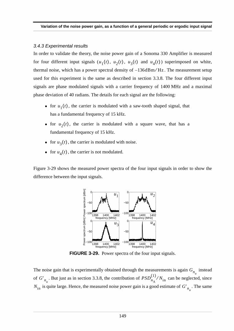
Variation of the noise power gain, as a function of a general periodic or ergodic input signal
3.4.3 Experimental resultsIn order to validate the theory, the noise power gain of a Sonoma 330 Amplifier is measured
for four different input signals ( , , and ) superimposed on white,
thermal noise, which has a power spectral density of . The measurement setup
used for this experiment is the same as described in section 3.3.8. The four different input
signals are phase modulated signals with a carrier frequency of 1400 MHz and a maximal
phase deviation of 40 radians. The details for each signal are the following:
• for , the carrier is modulated with a saw-tooth shaped signal, that
has a fundamental frequency of 15 kHz.
• for , the carrier is modulated with a square wave, that has a
fundamental frequency of 15 kHz.
• for , the carrier is modulated with noise.
• for , the carrier is not modulated.
Figure 3-29 shows the measured power spectra of the four input signals in order to show the
difference between the input signals.
The noise gain that is experimentally obtained through the measurements is again instead
of . But just as in section 3.3.8, the contribution of can be neglected, since
is quite large. Hence, the measured noise power gain is a good estimate of . The same
FIGURE 3-29. Power spectra of the four input signals.
u1 t( ) u2 t( ) u3 t( ) u4 t( )
136dBm Hz⁄–
u1 t( )
u2 t( )
u3 t( )
u4 t( )
1398 1400 1402−100
−50
0
frequency [MHz]1398 1400 1402
−100
−50
0
frequency [MHz]
1398 1400 1402−100
−50
0
frequency [MHz]1398 1400 1402
−100
−50
0
frequency [MHz]
u1
u3 u4
u2
Pow
er s
pect
rum
[dBm
]Po
wer
spe
ctru
m [d
Bm]
Gnu
G ′nuPSDnA
1( ) Nin⁄
Nin G ′nu
149
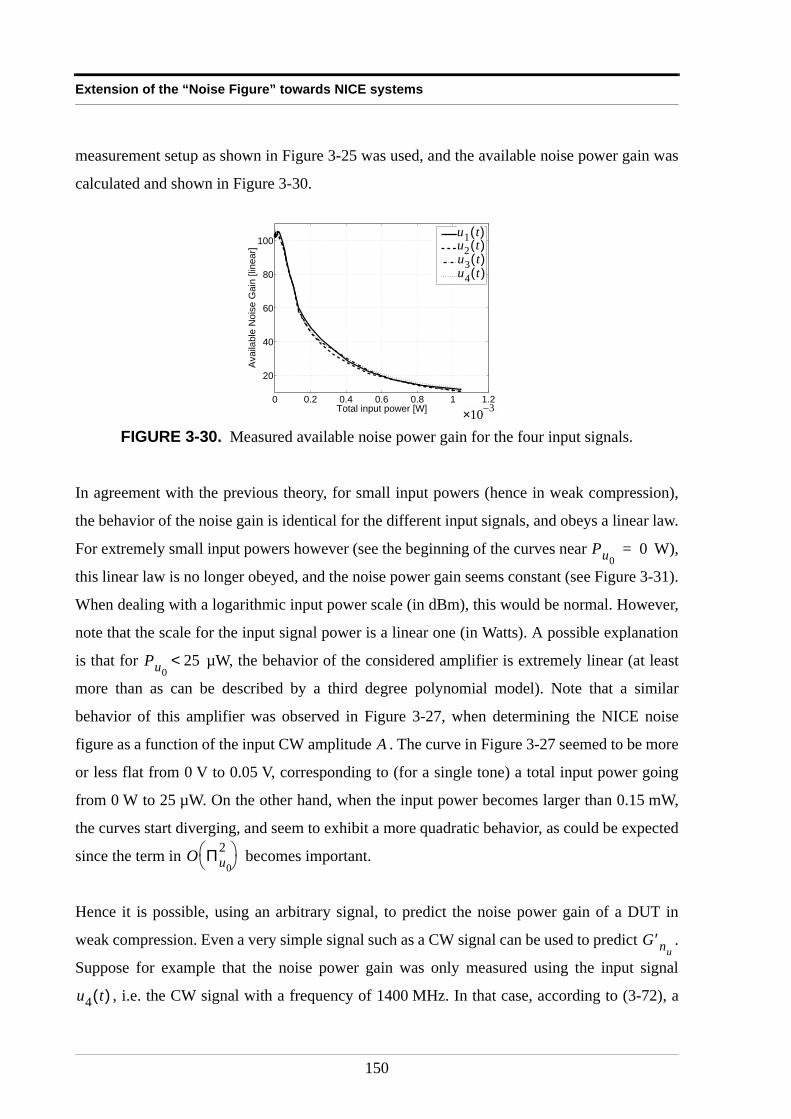
Extension of the “Noise Figure” towards NICE systems
measurement setup as shown in Figure 3-25 was used, and the available noise power gain was
calculated and shown in Figure 3-30.
In agreement with the previous theory, for small input powers (hence in weak compression),
the behavior of the noise gain is identical for the different input signals, and obeys a linear law.
For extremely small input powers however (see the beginning of the curves near W),
this linear law is no longer obeyed, and the noise power gain seems constant (see Figure 3-31).
When dealing with a logarithmic input power scale (in dBm), this would be normal. However,
note that the scale for the input signal power is a linear one (in Watts). A possible explanation
is that for µW, the behavior of the considered amplifier is extremely linear (at least
more than as can be described by a third degree polynomial model). Note that a similar
behavior of this amplifier was observed in Figure 3-27, when determining the NICE noise
figure as a function of the input CW amplitude . The curve in Figure 3-27 seemed to be more
or less flat from 0 V to 0.05 V, corresponding to (for a single tone) a total input power going
from 0 W to 25 µW. On the other hand, when the input power becomes larger than 0.15 mW,
the curves start diverging, and seem to exhibit a more quadratic behavior, as could be expected
since the term in becomes important.
Hence it is possible, using an arbitrary signal, to predict the noise power gain of a DUT in
weak compression. Even a very simple signal such as a CW signal can be used to predict .
Suppose for example that the noise power gain was only measured using the input signal
, i.e. the CW signal with a frequency of 1400 MHz. In that case, according to (3-72), a
FIGURE 3-30. Measured available noise power gain for the four input signals.
0 0.2 0.4 0.6 0.8 1 1.2−3
20
40
60
80
100
Total input power [W]
Ava
ilabl
e N
oise
Gai
n [li
near
]
s1(t)
s2(t)
s3(t)
s4(t)
3–×10
u3 t( )u4 t( )
u2 t( )u1 t( )
Pu00=
Pu025<
A
O Πu0
2
G ′nu
u4 t( )
150
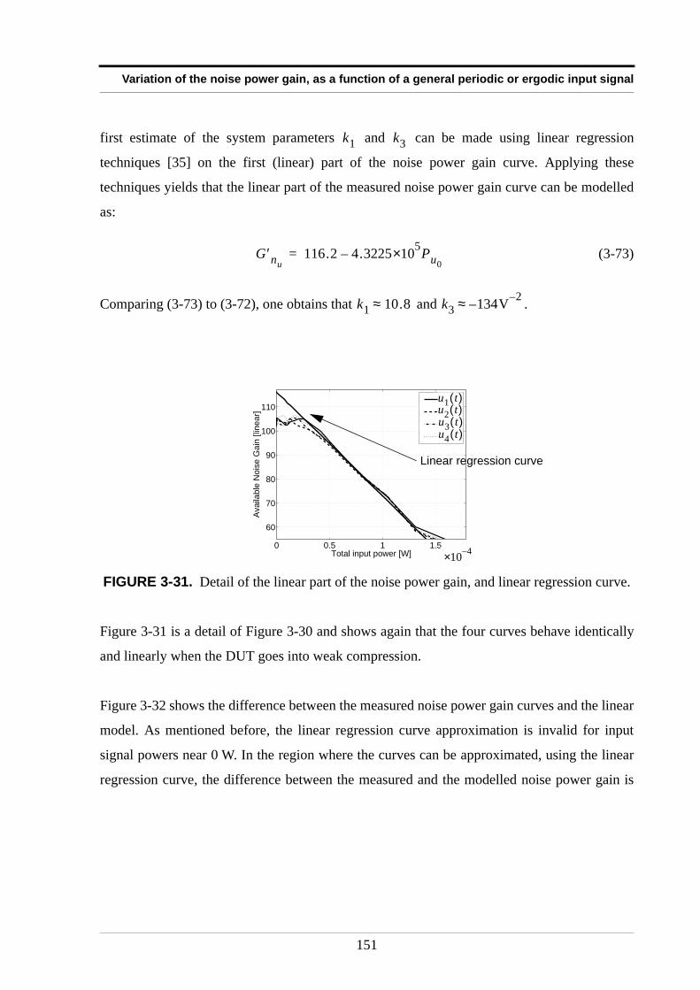
Variation of the noise power gain, as a function of a general periodic or ergodic input signal
first estimate of the system parameters and can be made using linear regression
techniques [35] on the first (linear) part of the noise power gain curve. Applying these
techniques yields that the linear part of the measured noise power gain curve can be modelled
as:
(3-73)
Comparing (3-73) to (3-72), one obtains that and .
Figure 3-31 is a detail of Figure 3-30 and shows again that the four curves behave identically
and linearly when the DUT goes into weak compression.
Figure 3-32 shows the difference between the measured noise power gain curves and the linear
model. As mentioned before, the linear regression curve approximation is invalid for input
signal powers near 0 W. In the region where the curves can be approximated, using the linear
regression curve, the difference between the measured and the modelled noise power gain is
FIGURE 3-31. Detail of the linear part of the noise power gain, and linear regression curve.
k1 k3
G ′nu116.2 4.3225 5×10 Pu0
–=
k1 10.8≈ k3 134– V 2–≈
0 0.5 1 1.5−4
60
70
80
90
100
110
Total input power [W]
Ava
ilabl
e N
oise
Gai
n [li
near
]
s1(t)
s2(t)
s3(t)
s4(t)
u3 t( )u4 t( )
u2 t( )u1 t( )
4–×10
Linear regression curve
151
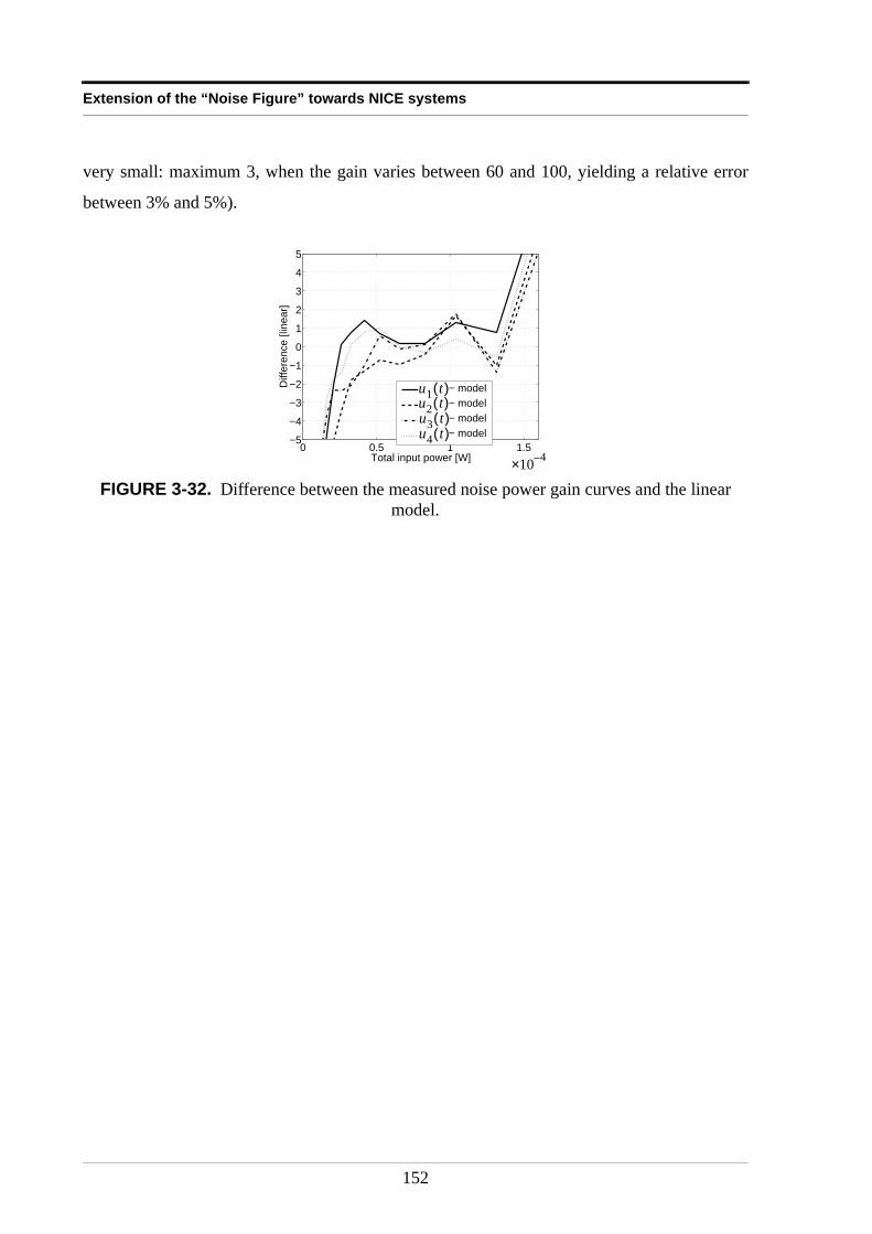
Extension of the “Noise Figure” towards NICE systems
very small: maximum 3, when the gain varies between 60 and 100, yielding a relative error
between 3% and 5%).
FIGURE 3-32. Difference between the measured noise power gain curves and the linear model.
0 0.5 1 1.5−4
−5
−4
−3
−2
−1
0
1
2
3
4
5
Total input power [W]
Diff
eren
ce [l
inea
r]
s1(t) − model
s2(t) − model
s3(t) − model
s4(t) − model
4–×10
u3 t( )u4 t( )
u2 t( )u1 t( )
152
Conclusion
3.5 ConclusionThe linear noise figure is unable to describe adequately the noise behavior of a NICE system,
since it is by assumption a quantity that is the same for each input signal power. As shown in
previous chapters, the output of a NICE system is dependent on the properties of its input
signal, and essentially on the power of this input signal. Hence, the signal-to-noise ratio
deterioration of a NICE system is dependent on the input signal power. Therefore, the
definition of the noise figure is extended towards the NICE noise figure, that is in fact an input
signal power and input noise power dependent noise figure.
In this chapter, the variation of the NICE noise figure is studied as a function of the input noise
power spectral density and the power of the input signal. Using a Wiener-Hammerstein model
with a third degree static nonlinearity, first the effect of the power of a CW input signal on the
NICE noise figure was studied for a standard input noise power spectral density, i.e.
dBm/Hz. Under these circumstances, the NICE noise figure, as a function of the
input signal power, becomes larger or smaller than the noise figure of the underlying linear
system, depending upon the value of this linear noise figure. If , the NICE noise
figure will be larger than the linear noise figure, for increasing input signal power. For
, a decrease in NICE noise figure occurs. In the special case of a noiseless NICE
system, where , the nonlinearity is thus actually able to improve the signal-to-noise
ratio.
Next, the NICE noise figure was determined as a function of both the input signal power and
the input noise power spectral density. Up to 10 dB under the 1 dB compression point, an
increase in input noise power spectral density can be translated into a similar behavior as for
the standard input noise power spectral density, but with a decreasing linear noise figure.
Hence, for large input noise power spectral densities, the apparent linear noise figure tends
towards 1, implicating that the NICE noise figure will be better for the NICE system going into
weak compression than for the underlying linear system. As a result, noisy NICE systems are
able to improve the signal-to-noise ratio under certain conditions. Because the third degree
polynomial model was unable to describe the system’s behavior for input signal and noise
powers, above the 1 dB compression point, simulations were done with a Wiener-
Nin 174–=
NFlin 2>
NFlin 2<
NFlin 1=
153
Extension of the “Noise Figure” towards NICE systems
Hammerstein model where the static nonlinearity is described using an arctan function.
Simulations showed that when the input signal power becomes very large, the NICE noise
figure tends towards infinity. For an increase in noise power spectral density, the NNF curve as
a function of the input signal power shifts upwards.
Finally, the output spectrum of the noisy NICE system with the third degree static nonlinearity
was studied when the input signal is an arbitrary periodic or ergodic waveform. Not much
could be told about the signal behavior, because this behavior was too much dependent on the
signal’s properties. The noise power gain is, however, mainly a linear function of the total
power of the input signal waveform, and is independent of its other properties. Hence, the
noise power gain will, in a first order approximation, be the same for all input waveforms that
have the same total power. This property can be used to predict the noise power gain for any
input signal by measuring the response for only one signal.
154
Appendices
3.6 Appendices
Appendix 3.A : Calculation of the 1 dB compression point for the third degree polynomial modelLet be the input signal of the third degree polynomial model described
by . The output signal is then given by:
(3-74)
The 1 dB compression point is defined as that input power where the linear output power at the
fundamental frequency is exactly 1 dB higher than the actual output of the NICE system.
Hence, it is the solution of the equation:
(3-75)
i.e.,
(3-76)
or, in terms of power:
(3-77)
For parameters , , the 1 dB compression point is about 0.24 mW, or
dBm.
u t( ) A 2πf0t( )cos⋅=
y t( ) k1u t( )= k3u3 t( )+
y t( ) k1A 3k3A3
4------+
2πf0t( )cosk3A3
4------------ 6πf0t( )cos+=
10k1A( )2
2-----------------
log 10k1A 3k3
A3
4------+
2
2---------------------------------------
log– 1=
A2
2------
2k1 101–
20------
1–
3k3-----------------------------------=
P1dB
2k1 101–
20------
1–
3k3Z0-----------------------------------=
k1 10= k3 60V 2––=
6–
155
Extension of the “Noise Figure” towards NICE systems
Appendix 3.B : Calculation of the output power spectral density for an input consisting of a single tone and thermal noiseGiven:
(3-78)
one has to calculate
(3-79)
and .
Since the Fourier transform is a linear operator, one can take the Fourier transform of each
term of (3-79), in order to obtain . Hence, the auto-correlation and corresponding
spectral contributions are:
First and second term:
(3-80)
ς1 k134---k3A2+
A 2πf0t( )cos=
ς214---k3A3 2π3f0t( )cos=
ς3 k132---k3A2+
nu t( )=
ς432---k3A2nu t( ) 2π2f0t( )cos=
ς5 3k3Anu2 t( ) 2πf0t( ) cos=
ς6 k3nu3 t( )=
Rηη τ( ) Rςiςiτ( )
i 1=
6
∑ Rςiςjτ( ) Rςiςj
τ–( )+( )
j i 1+=
6
∑i 1=
5
∑+=
PSDηη2( ) f( ) 1
Z0------ ℑ Rηη τ( ) =
PSDηη2( ) f( )
Rς1ς1τ( ) 1
2--- k1
34---k3A2+
2A2 2πf0τ( )cos=
Rς2ς2τ( ) 1
2--- 1
4---k3A3
22π3f0τ( ) cos=
156
Appendices
(3-81)
Third term:
(3-82)
Fourth term:
(3-83)
(3-84)
Since the Fourier transform of a product equals the convolution of the Fourier transforms.
Figure 3-33 shows the convolution of the noise spectrum with a cosine wave with frequency
. In the upper right corner of Figure 3-33, the two shifted noise spectra are shown. In
the frequency interval , the two shifted noise spectra overlap, indicating that
they have to be added. Eventually, all spectral components above frequency will be cut off
due to the output filter, yielding a spectrum as shown in the lower right corner of Figure 3-33.
PSDς1ς1
2( ) f( )k1
34---k3A2+
2A2
2Z0------------------------------------------1
2--- δ f f0–( ) δ f f0+( )+( )=
PSDς2ς2
2( ) f( )
14---k3A3
2
2Z0-----------------------1
2--- δ f 3f0–( ) δ f 3f0+( )+( ) =
Rς3ς3τ( ) k1
32---k3A2+
2Rnunu
τ( )=
PSDς3ς3
2( ) f( ) k132---k3A2+
2N0
2------ =
Rς4ς4τ( ) 3
2---k3A2
2Rnunu
τ( )12--- 2π2f0τ( )cos=
PSDς4ς4
2( ) f( )
32---k3A2
2
2-----------------------
N02
------*12--- δ f 2f0–( ) δ f 2f0+( )+( )=
2f0 B<
2f0 B– B 2f0–,[ ]
B
157
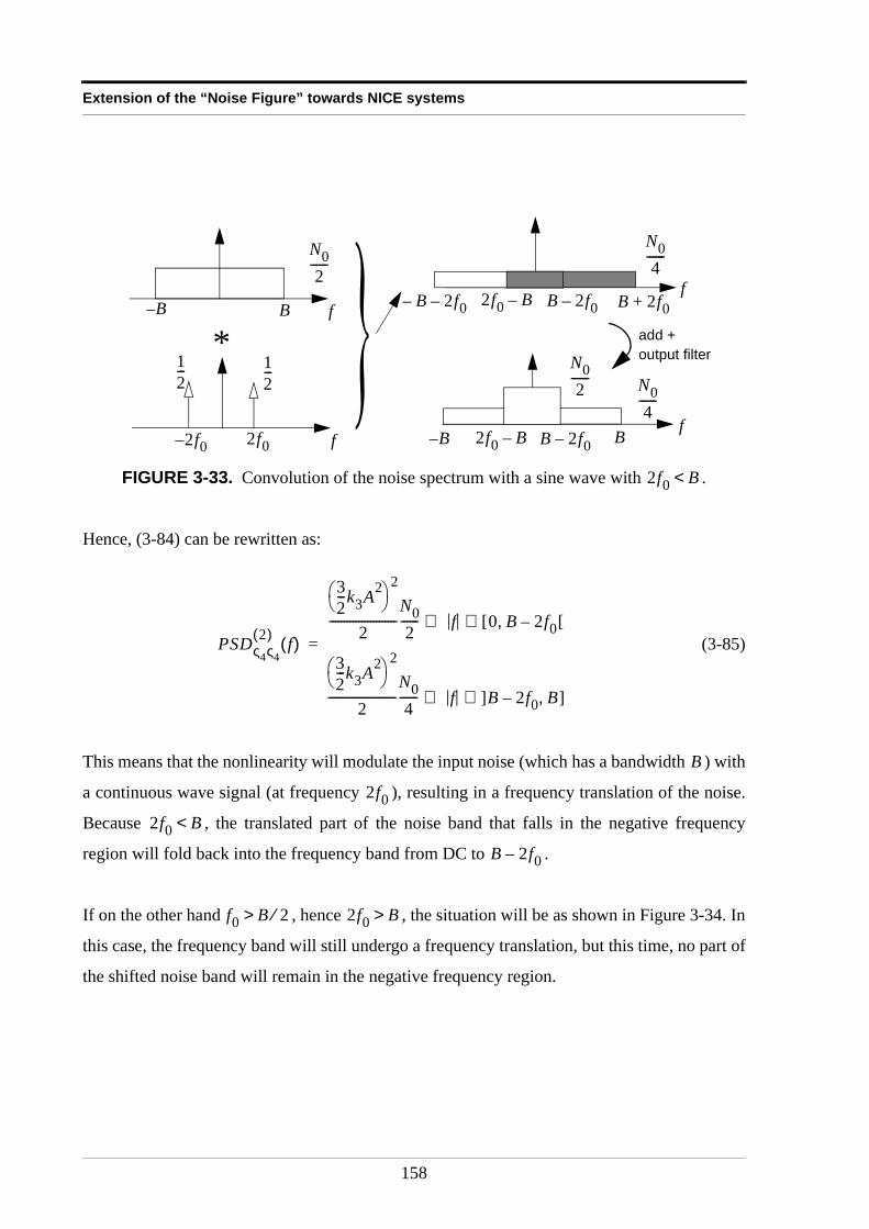
Extension of the “Noise Figure” towards NICE systems
Hence, (3-84) can be rewritten as:
(3-85)
This means that the nonlinearity will modulate the input noise (which has a bandwidth ) with
a continuous wave signal (at frequency ), resulting in a frequency translation of the noise.
Because , the translated part of the noise band that falls in the negative frequency
region will fold back into the frequency band from DC to .
If on the other hand , hence , the situation will be as shown in Figure 3-34. In
this case, the frequency band will still undergo a frequency translation, but this time, no part of
the shifted noise band will remain in the negative frequency region.
FIGURE 3-33. Convolution of the noise spectrum with a sine wave with .
f
N02
------
BB–
f
12---
2f0
*12---
2f0–
f
N04
------
B 2f0–
f
N04
------
N02
------
B 2f0+2f0 B–B– 2f0–
BB– 2f0 B– B 2f0–
add +output filter
2f0 B<
PSDς4ς4
2( ) f( )
32---k3A2
2
2-----------------------
N02
------ f [0 B 2f0–, [∈⇔
32---k3A2
2
2-----------------------
N04
------ f ]B 2f0– B, ]∈⇔
=
B
2f02f0 B<
B 2f0–
f0 B 2⁄> 2f0 B>
158
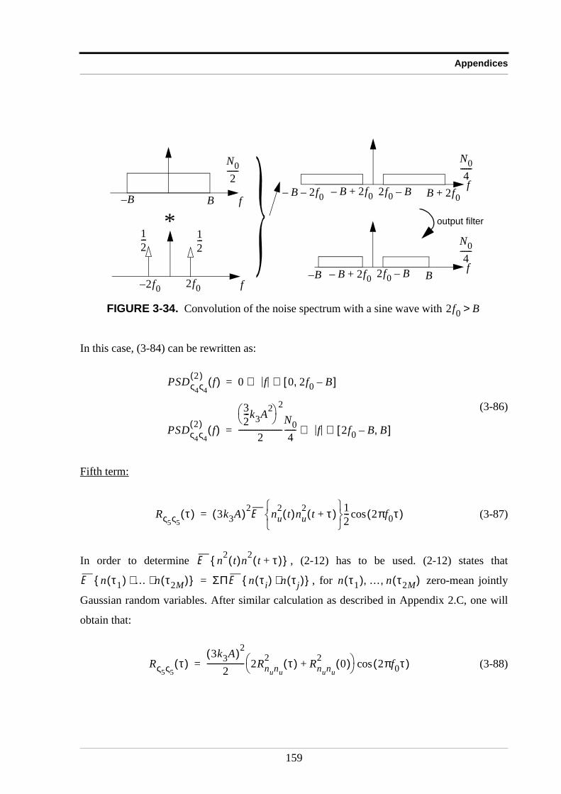
Appendices
In this case, (3-84) can be rewritten as:
(3-86)
Fifth term:
(3-87)
In order to determine , (2-12) has to be used. (2-12) states that
, for zero-mean jointly
Gaussian random variables. After similar calculation as described in Appendix 2.C, one will
obtain that:
(3-88)
FIGURE 3-34. Convolution of the noise spectrum with a sine wave with
f
N02
------
BB–
f
12---
2f0
*12---
2f0–
f
N04
------
B– 2f0+ B 2f0+2f0 B–B– 2f0–
f
N04
------
B– 2f0+ B2f0 B–B–
output filter
2f0 B>
PSDς4ς4
2( ) f( ) 0 f 0 2f0 B–,[ ] ∈⇔=
PSDς4ς4
2( ) f( )
32---k3A2
2
2-----------------------
N04
------ f 2f0 B– B,[ ]∈⇔=
Rς5ς5τ( ) 3k3A( )2E nu
2 t( )nu2 t τ+( )
1
2--- 2πf0τ( )cos=
E n2 t( )n2 t τ+( )
E n τ1( ) … n τ2M( )⋅ ⋅ ΣΠ E n τ i( ) n τ j( )⋅ = n τ1( ) … n τ2M( ), ,
Rς5ς5τ( )
3k3A( )2
2-------------------- 2Rnunu
2 τ( ) Rnunu
2 0( )+ 2πf0τ( )cos=
159
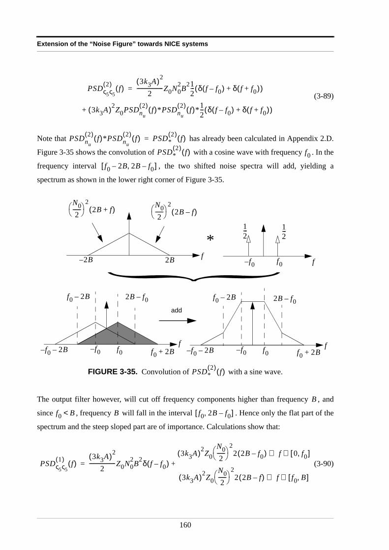
Extension of the “Noise Figure” towards NICE systems
(3-89)
Note that has already been calculated in Appendix 2.D.
Figure 3-35 shows the convolution of with a cosine wave with frequency . In the
frequency interval , the two shifted noise spectra will add, yielding a
spectrum as shown in the lower right corner of Figure 3-35.
The output filter however, will cut off frequency components higher than frequency , and
since , frequency will fall in the interval . Hence only the flat part of the
spectrum and the steep sloped part are of importance. Calculations show that:
(3-90)
FIGURE 3-35. Convolution of with a sine wave.
PSDς5ς5
2( ) f( )3k3A( )2
2--------------------Z0N0
2B212--- δ f f0–( ) δ f f0+( )+( )=
3k3A( )2Z0PSDnu
2( ) f( )*PSDnu
2( ) f( )*12--- δ f f0–( ) δ f f0+( )+( )+
PSDnu
2( ) f( )*PSDnu
2( ) f( ) PSD*2( ) f( )=
PSD*2( ) f( ) f0
f0 2B– 2B f0–,[ ]
N02
------
22B f–( )
2B2B–
N02
------
22B f+( )
ff
12---
f0
12---
f0–
*
ff0f0–
2B f0–f0 2B–
f0 2B+f0 2B–– ff0f0–
2B f0–f0 2B–
f0 2B+f0 2B––
add
PSD*2( ) f( )
B
f0 B< B f0 2B f0–,[ ]
PSDς5ς5
1( ) f( )3k3A( )2
2--------------------Z0N0
2B2δ f f0–( )3k3A( )2Z0
N02
------
22 2B f0–( ) f 0 f0,[ ]∈⇔
3k3A( )2Z0N02
------
22 2B f–( ) f f0 B,[ ]∈⇔
+=
160
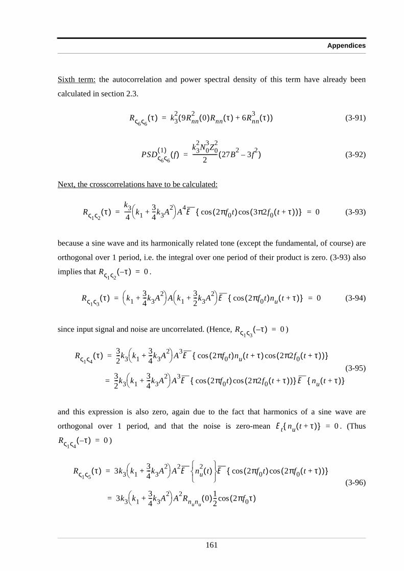
Appendices
Sixth term: the autocorrelation and power spectral density of this term have already been
calculated in section 2.3.
(3-91)
(3-92)
Next, the crosscorrelations have to be calculated:
(3-93)
because a sine wave and its harmonically related tone (except the fundamental, of course) are
orthogonal over 1 period, i.e. the integral over one period of their product is zero. (3-93) also
implies that .
(3-94)
since input signal and noise are uncorrelated. (Hence, )
(3-95)
and this expression is also zero, again due to the fact that harmonics of a sine wave are
orthogonal over 1 period, and that the noise is zero-mean . (Thus
)
(3-96)
Rς6ς6τ( ) k3
2 9Rnn2 0( )Rnn τ( ) 6Rnn
3 τ( )+( )=
PSDς6ς6
1( ) f( )k3
2N03Z0
2
2------------------ 27B2 3f2–( )=
Rς1ς2τ( )
k34----- k1
34---k3A2+
A4E 2πf0t( ) 3π2f0 t τ+( )( )coscos 0= =
Rς1ς2τ–( ) 0=
Rς1ς3τ( ) k1
34---k3A2+
A k1
32---k3A2+
E 2πf0t( )nu t τ+( )cos 0= =
Rς1ς3τ–( ) 0=
Rς1ς4τ( ) 3
2---k3 k1
34---k3A2+
A3E 2πf0t( )nu t τ+( ) 2π2f0 t τ+( )( )coscos =
32---k3 k1
34---k3A2+
A3E 2πf0t( ) 2π2f0 t τ+( )( )coscos E nu t τ+( ) =
Et nu t τ+( ) 0=
Rς1ς4τ–( ) 0=
Rς1ς5τ( ) 3k3 k1
34---k3A2+
A2E nu2 t( )
E 2πf0t( )cos 2πf0 t τ+( )( )cos =
3k3 k134---k3A2+
A2Rnunu0( )1
2--- 2πf0τ( ) cos=
161
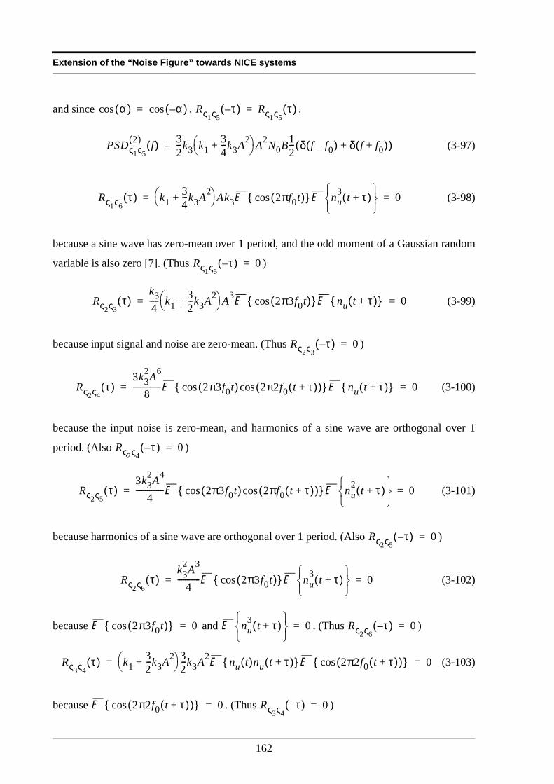
Extension of the “Noise Figure” towards NICE systems
and since , .
(3-97)
(3-98)
because a sine wave has zero-mean over 1 period, and the odd moment of a Gaussian random
variable is also zero [7]. (Thus )
(3-99)
because input signal and noise are zero-mean. (Thus )
(3-100)
because the input noise is zero-mean, and harmonics of a sine wave are orthogonal over 1
period. (Also )
(3-101)
because harmonics of a sine wave are orthogonal over 1 period. (Also )
(3-102)
because and . (Thus )
(3-103)
because . (Thus )
α( )cos α–( )cos= Rς1ς5τ–( ) Rς1ς5
τ( )=
PSDς1ς5
2( ) f( ) 32---k3 k1
34---k3A2+
A2N0B1
2--- δ f f0–( ) δ f f0+( )+( )=
Rς1ς6τ( ) k1
34---k3A2+
Ak3E 2πf0t( )cos E nu3 t τ+( )
0= =
Rς1ς6τ–( ) 0=
Rς2ς3τ( )
k34----- k1
32---k3A2+
A3E 2π3f0t( )cos E nu t τ+( ) 0= =
Rς2ς3τ–( ) 0=
Rς2ς4τ( )
3k32A6
8---------------E 2π3f0t( )cos 2π2f0 t τ+( )( )cos E nu t τ+( ) 0= =
Rς2ς4τ–( ) 0=
Rς2ς5τ( )
3k32A4
4---------------E 2π3f0t( )cos 2πf0 t τ+( )( )cos E nu
2 t τ+( )
0= =
Rς2ς5τ–( ) 0=
Rς2ς6τ( )
k32A3
4------------E 2π3f0t( )cos E nu
3 t τ+( )
0= =
E 2π3f0t( )cos 0= E nu3 t τ+( )
0= Rς2ς6τ–( ) 0=
Rς3ς4τ( ) k1
32---k3A2+
32---k3A2E nu t( )nu t τ+( ) E 2π2f0 t τ+( )( )cos 0= =
E 2π2f0 t τ+( )( )cos 0= Rς3ς4τ–( ) 0=
162
Appendices
(3-104)
because and [7]. (Thus
)
(3-105)
But was determined in Appendix 2.C, hence:
(3-106)
Thus
(3-107)
(3-108)
because a sine wave is not correlated with its harmonic, and [7].
(Thus )
(3-109)
because .
(3-110)
because and [7].
Rς3ς5τ( ) k1
32---k3A2+
3k3AE nu t( )nu
2 t τ+( )
E 2πf0 t τ+( )( )cos 0= =
E 2πf0 t τ+( )( )cos 0= E nu t( )nu2 t τ+( )
0=
Rς3ς5τ–( ) 0=
Rς3ς6τ( ) k1
32---k3A2+
k3E nu t( )nu
3 t τ+( )
=
E nu t( )nu3 t τ+( )
Rς3ς6τ( ) k1
32---k3A2+
k33Rnn 0( )Rnn τ( )=
Rς3ς6τ–( ) Rς3ς6
τ( )=
PSDς3ς6
2( ) f( ) 32--- k1
32---k3A2+
k3Z0N02B=
Rς4ς5τ( ) 9
2---k3
2A3E nu t( )nu2 t τ+( )
E 2π2f0t( )cos 2πf0 t τ+( )( )cos 0= =
E nu t( )nu2 t τ+( )
0=
Rς4ς5τ–( ) 0=
Rς4ς6τ( ) 3
2---k3
2A2E nu t( )nu3 t τ+( )
E 2π2f0t( )cos 0= =
E 2π2f0t( )cos 0=
Rς5ς6τ( ) 3k3
2AE nu2 t( )nu
3 t τ+( )
E 2π2f0t( )cos 0= =
E 2π2f0t( )cos 0= E nu2 t( )nu
3 t τ+( )
0=
163
Extension of the “Noise Figure” towards NICE systems
Appendix 3.C : Variation of over a small bandwidth
In order for
(3-111)
to be true, the variation of over the frequency interval
must be small. From (3-10), it follows that can be
written as:
(3-112)
where is , is and
is . (With ) Hence, essentially the variation of the
power spectral density of the noise produced by the NICE system will determine if the
approximation (3-111) is valid. For high frequency NICE systems, one can indeed assume that
does not vary significantly over an interval of a few kHz.
Appendix 3.D : Taylor series expansion of an atan function
Definition 3.4
Let , and has a ( )-th derivative ( ) that is
continuous over and differentiable over ] [ then, such that
(3-113)
Expression (3-113) is called the Taylor series expansion of in interval .
PSDny
1( ) f( )
PSDny
1( ) f( ) fdf0 B0 2⁄–
f0 B0 2⁄+
∫ B0 PSDny
1( ) f0( )⋅≈
PSDny
1( ) f( ) f0 B0 2⁄– f0 B0 2⁄+,[ ]
PSDny
1( ) f0 B0 2⁄+( ) PSDny
1( ) f0 B0 2⁄–( )–
PSDnA
1( ) f0 B0 2⁄+( ) PSDnA
1( ) f0 B0 2⁄–( )– 3k32N0
3Z02f0B0
94---k3
2A2N02Z0B0––
PSDnA
1( ) f0 B0 2⁄+( ) PSDnA
1( ) f0 B0 2⁄–( )– O ν0( ) 94---k3
2A2N02Z0B0– O ν0
2( )
3k32N0
3Z02f0B0– O ν0
3( ) ν0 N0 1W( )⁄=
PSDnA
1( )
PSDnA
1( ) f( )
a b, R∈ a b≠ f: ab[ ] R→ n 1+ n N0∈
ab[ ] ab c ]ab[∈∃
f b( ) f a( ) f ′ a( )1!
----------- b a–( ) f″ a( )2!
------------ b a–( )2 …+ + +=
f n 1–( ) a( )n 1–( )!
------------------------ b a–( )n 1– f n( ) c( )n!
---------------- b a–( )n+ +
f x( ) ab[ ]
164
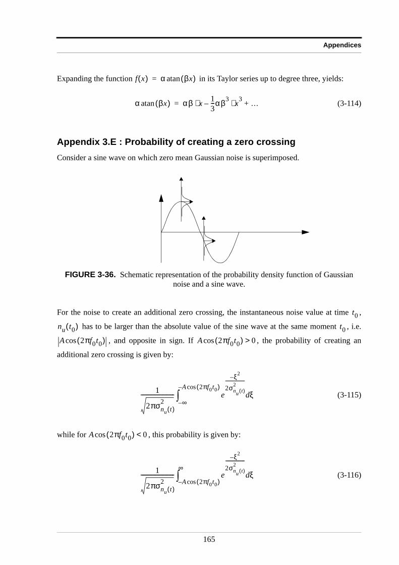
Appendices
Expanding the function in its Taylor series up to degree three, yields:
(3-114)
Appendix 3.E : Probability of creating a zero crossingConsider a sine wave on which zero mean Gaussian noise is superimposed.
For the noise to create an additional zero crossing, the instantaneous noise value at time ,
has to be larger than the absolute value of the sine wave at the same moment , i.e.
, and opposite in sign. If , the probability of creating an
additional zero crossing is given by:
(3-115)
while for , this probability is given by:
(3-116)
FIGURE 3-36. Schematic representation of the probability density function of Gaussian noise and a sine wave.
f x( ) α βx( )atan=
α βx( )atan αβ x 13---αβ3 x3⋅–⋅ …+=
t0nu t0( ) t0A 2πf0t0( )cos A 2πf0t0( )cos 0>
1
2πσnu t( )2
------------------------- e
ξ2–
2σnu t( )2
-----------------
ξd∞–
A 2πf0t0( )cos–
∫
A 2πf0t0( )cos 0<
1
2πσnu t( )2
------------------------- e
ξ2–
2σnu t( )2
-----------------
ξdA– 2πf0t0( )cos
∞∫
165
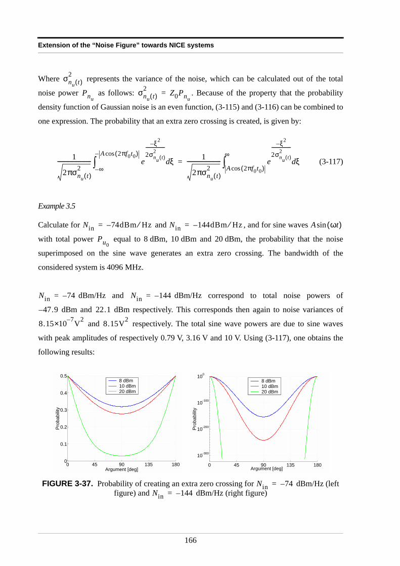
Extension of the “Noise Figure” towards NICE systems
Where represents the variance of the noise, which can be calculated out of the total
noise power as follows: . Because of the property that the probability
density function of Gaussian noise is an even function, (3-115) and (3-116) can be combined to
one expression. The probability that an extra zero crossing is created, is given by:
(3-117)
Example 3.5
Calculate for and , and for sine waves
with total power equal to 8 dBm, 10 dBm and 20 dBm, the probability that the noise
superimposed on the sine wave generates an extra zero crossing. The bandwidth of the
considered system is 4096 MHz.
dBm/Hz and dBm/Hz correspond to total noise powers of
dBm and dBm respectively. This corresponds then again to noise variances of
and respectively. The total sine wave powers are due to sine waves
with peak amplitudes of respectively 0.79 V, 3.16 V and 10 V. Using (3-117), one obtains the
following results:
FIGURE 3-37. Probability of creating an extra zero crossing for dBm/Hz (left figure) and dBm/Hz (right figure)
σnu t( )2
Pnuσnu t( )
2 Z0Pnu=
1
2πσnu t( )2
------------------------- e
ξ2–
2σnu t( )2
-----------------
ξd∞–
A 2πf0t0( )cos–
∫1
2πσnu t( )2
------------------------- e
ξ2–
2σnu t( )2
-----------------
ξdA 2πf0t0( )cos
∞∫=
Nin 74dBm Hz⁄–= Nin 144dBm Hz⁄–= A ωt( )sin
Pu0
Nin 74–= Nin 144–=
47.9– 22.1
8.15 7–×10 V2 8.15V2
0 45 90 135 1800
0.1
0.2
0.3
0.4
0.5
Argument [deg]
Pro
ba
bili
ty
8 dBm 10 dBm20 dBm
0 45 90 135 180
10-300
10-200
10-100
100
Pro
ba
bili
ty
8 dBm 10 dBm20 dBm
Argument [deg]
Nin 74–=Nin 144–=
166
Appendices
At the zero crossings of the sine wave, the probability of creating an extra zero crossing is
50 %, i.e. total uncertainty. For dBm/Hz, and dBm, the probability at
the top of the sine wave is smaller than the numerical precision of the simulator, i.e. .
Appendix 3.F : Boundaries of the linear regionUsing (3-40) and (3-42), and omitting terms in and with (since the
total signal and noise power are small because considering the linear region), one obtains:
(3-118)
(3-119)
The boundary of the linear region will be there where the second term in (3-118) and (3-119)
will not be negligible any more as compared to . Suppose that this is the case when the ratio
of the second term to the first becomes larger than , hence:
(3-120)
(3-121)
yielding for the example system: dBm and dBm. Hence, If
the total input power of the NICE system becomes larger than about dBm, the system
cannot be modelled as a LTI system any more.
Appendix 3.G : Autocorrelation of the noisy NICE system’s output for a general input waveformBecause the noise added by the system itself is not correlated with the input signal or the
input noise , (2-6) is valid (i.e. ). Because the noiseless
output has six terms (see (3-61)), the autocorrelation has thirty-
Nin 144–= Pu020=
10 324–
O Πu0
n O Πnu
n n 2≥
Gu0k1
2 3k1k3Z0 Pu02Pnu
+( )+=
G ′nuk1
2 6k1k3Z0 Pu0Pnu
+( )+=
k12
10 3–
3k3Z0 Pu02Pnu
+( )
k1----------------------------------------------- 10 3–≥ Pu0
2Pnu+
k110 3–
3k3Z0-----------------≥⇒
6k3Z0 Pu0Pnu
+( )
k1------------------------------------------- 10 3–≥ Pu0
Pnu+
k110 3–
6k3Z0-----------------≥⇒
Pu02Pnu
+ 30–≥ Pu0Pnu
+ 33–≥
33–
u0 t( )
nu t( ) Ryy τ( ) Rηη τ( ) RnAnAτ( )+=
η t( ) y t( ) nA t( )–= Rηη τ( )
167
Extension of the “Noise Figure” towards NICE systems
six terms (that are not all different). Because the input signal and the input noise
are uncorrelated and zero-mean, because of the anti-symmetry property of the autocorrelation
function ( ), and because for Gaussian noise, it was shown that
only the following fourteen terms persist:
(3-122)
Using (2-49), (2-14) and Appendix 2.C, (3-122) can be rewritten as:
u0 t( ) nu t( )
Rαβ τ( ) Rβα τ–( )=
Rαβ τ( ) Rβα τ( )=
k12E nu t( )nu t τ+( ) 2k1k3E nu t( )nu
3 t τ+( )
+
6k1k3Et nu t( )nu t τ+( ) E u02 t τ+( )
k12E u0 t( )u0 t τ+( ) + +
6k1k3E u0 t( )u0 t τ+( ) E nu2 t( )
k1k3 E u0 t( )u03 t τ+( )
E u03 t( )u0 t τ+( )
+
+ +
k32E nu
3 t( )nu3 t τ+( )
6k32E nu
3 t( )nu t τ+( )
E u02 t τ+( )
+ +
9k32E nu
2 t( )nu2 t τ+( )
E u0 t( )u0 t τ+( ) +
3+ k32E nu
2 t( )
E u0 t( )u03 t τ+( )
3+ k32E nu
2 t( )
E u03 t( )u0 t τ+( )
9k32E u0
2 t( )u2 t τ+( )
E nu t( )nu t τ+( ) k32E u0
3 t( )u03 t τ+( )
+ +
168

Appendices
(3-123)
Appendix 3.H : Auto-correlation of a non zero-mean signal
Theorem 3.6
If is a periodic or ergodic signal, and , then
(3-124)
proof
If is an ergodic signal, the proof is trivial.
If is a periodic signal,
(3-125)
Using the definition of , it follows that , or:
k12Rnunu
τ( ) 6k1k3Rnunu0( )Rnunu
τ( )+
6k1k3Rnunuτ( )Ru0u0
0( ) k12Ru0u0
τ( )+ +
6k1k3Ru0u0τ( )Rnunu
0( ) k1k3 Ru0u0
3 τ( ) Ru0u0
3 τ–( )+ + +
k32 9Rnunu
τ( )Rnunu
2 0( ) 6Rnunu
3 τ( )+ 6k3
23Rnunu0( )Rnunu
τ( )Ru0u00( )+ +
9k32 Rnunu
2 0( ) 2Rnunu
2 τ( )+ Ru0u0
τ( ) 3k32Rnunu
0( ) Ru0u0
3 τ( ) Ru0u0
3 τ–( )+ + +
9k32R
u02u0
2 τ( )Rnunuτ( ) k3
2Ru0
3u03 τ( )+ +
α t( ) β t( ) α t( ) E α t( ) –=
Rαα τ( ) E α t( ) ( )2
Rββ τ( )+=
α t( )
α t( )
Rαα τ( ) 1T--- α t( )α t τ+( )
T 2⁄–
T 2⁄∫ dt
T ∞→lim=
β t( ) α t( ) β t( ) E α t( ) +=
169
Extension of the “Noise Figure” towards NICE systems
(3-126)
Due to the linearity property of the integral, (3-126) can be rewritten as:
(3-127)
Again, using the definition of , it follows that ,
hence,
(3-128)
And since , the theorem is proven. G
Rαα τ( ) 1T--- β t( ) E α t( ) +( ) β t τ+( ) E α t τ+( ) +( )
T 2⁄–
T 2⁄∫ dt
T ∞→lim=
1T--- (β t( )β t τ+( ) E α t( ) β t τ+( ) β t( )E α t τ+( ) + +
T 2⁄–
T 2⁄∫T ∞→
lim=
E α t( ) E α t τ+( ) + )dt
Rαα τ( ) E β t( )β t τ+( ) E α t( ) E β t τ+( ) +=
E α t τ+( ) E β t( ) E α t( ) E α t τ+( ) + +
β t( ) E β t( ) E α t( ) E α t( ) – 0= =
Rαα τ( ) E β t( )β t τ+( ) E α t( ) ( )2
+=
E β t( )β t τ+( ) Rββ τ( )=
170

CHAPTER 4
NOISE-LIKE SIGNALS AND NICESYSTEMS
Abstract: In telecommunication systems, most processed signals
are narrow band noise-like signals, due to the stochastic nature of
information itself. Intuitively, it can be assumed that the nonlinear
mechanism creates extra noise using these noise-like input signals.
In the literature, the existence of such terms is quantified by the
Noise Power Ratio. This figure quantifies in-band nonlinear
distortions as function of the power of the noise-like input signal.
In this chapter, the response of NICE systems to these noise-like
input signals will be studied and determined experimentally. The
measurement techniques and theory for two-port devices (such as
amplifiers) will then be extended towards multi-port devices (such
as mixers).
171
Noise-like signals and NICE systems
4.1 IntroductionIn the previous chapters, the input signals were all deterministic signals. This hypothesis
is made in section 1.6.2, and allows to discriminate between the deterministic signal output and
the stochastic noise output. However, Shannon’s information theory [17] states that a
deterministic signal (or at least always the same instance of a modulated signal) does not
contain any information, and hence, there is no point in transmitting or amplifying an
informationless signal in a telecommunication channel. Most signals in telecommunication,
such as GSM, NICAM-728 [18], ADSL [42] are noise-like signals, due to scrambling of the
bits or due to the stochastic content of the information itself [17]. Hence, these signals have
properties that are similar to the properties of noise. Note that, in this case, a different instance
is obtained as a function of the information content, and not as a function of time. It is
intuitively clear that the presence of these noise-like signals at the input of a NICE system will
be responsible for an increased noise presence at the output of the noisy NICE system.
Hence, two noise contributions can be found at the output of the NICE system. The first is due
to the noise that is superimposed on the input signal, and that is processed by the system. This
is the kind of noise that was studied in previous chapters. The second contribution is noise that
is created by the nonlinear mechanism itself, out of the randomness of the input signal. The
spectrum of this noise is uncorrelated with the spectrum of the input signal , i.e.
. The power of both noise contributions has to be compared, in order to
compare their relative importance, and to focus on the most important one. Intuitively, one can
already assume that for narrowband devices (as usually used in telecommunications) the total
input noise power will be quite small, and so will be the effect of this noise on the output
signal. This will be mathematically verified later in this chapter.
Another confirmation of the assumption that NICE systems create output noise out of the
noise-like input signal, is the existence of the “Noise Power Ratio” [44], [45]. This is a well-
known quantity in telecommunications, that gives a measure for the power of the in-band
distortions versus the input signal power applied to the NICE system. These figures show that
if the power of the noise-like input signal tends towards zero, the in-band distortions also tend
u0 t( )
NNL k( ) U k( )
E U k( )NNL k( ) 0=
Pnu
172
Introduction
towards zero. This demonstrates that these in-band distortions are created by the input signal,
due to the nonlinear mechanism itself.
In order to adequately describe the noise-like signals that are fed to the NICE systems, these
input signals need to be modelled first. An analysis of the processing of these modelled signals
by the NICE system will give a better insight in the output noise creation mechanisms.
Another important component used in telecommunications is the mixer. This is a “two-input-
port, one-output-port” device where the output signal ideally consists of the multiplication of
the two input signals. This device is mainly used to shift spectral components from one
frequency to another, and is thus essentially a nonlinear device. In this chapter, the possibility
to extend the obtained results for two-port NICE systems towards multi-port systems such as
mixers will also be investigated. Hence, answers to the following questions are required:
• How does a frequency translating device affect signals that are shifted
towards another location in the frequency spectrum?
• How much in-band distortion is created during this frequency translation?
• What is the effect on the shifted signals if a sinewave affected by phase
noise, instead of a pure sinewave, is used to shift the signals in the
frequency spectrum?
Note that in this chapter, is a noise-like signal, that is the signal of interest, and is
the disturbing time domain noise. can be fully controlled and is stochastic over different
instances, due to the stochastic nature of information contained in the signal. Hence, a different
transmitted symbol will yield a different instance of the signal. , on the other hand, is true
noise that cannot be controlled.
u0 t( ) nu t( )
u0 t( )
nu t( )
173
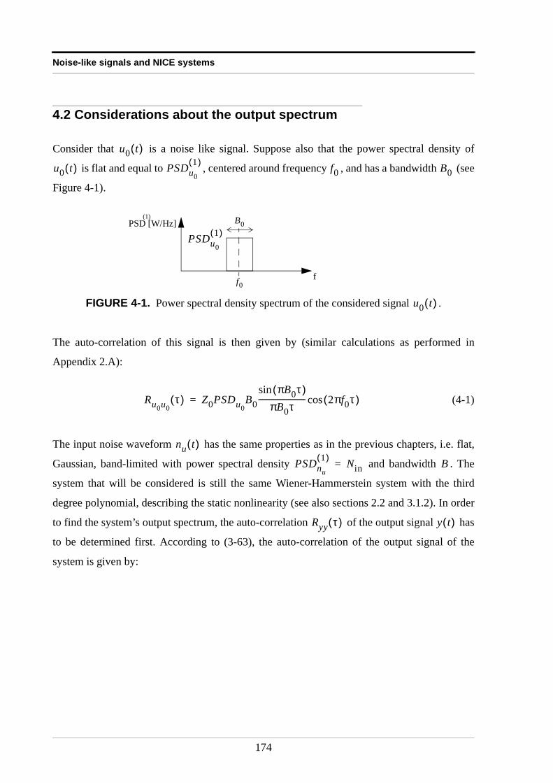
Noise-like signals and NICE systems
4.2 Considerations about the output spectrum
Consider that is a noise like signal. Suppose also that the power spectral density of
is flat and equal to , centered around frequency , and has a bandwidth (see
Figure 4-1).
The auto-correlation of this signal is then given by (similar calculations as performed in
Appendix 2.A):
(4-1)
The input noise waveform has the same properties as in the previous chapters, i.e. flat,
Gaussian, band-limited with power spectral density and bandwidth . The
system that will be considered is still the same Wiener-Hammerstein system with the third
degree polynomial, describing the static nonlinearity (see also sections 2.2 and 3.1.2). In order
to find the system’s output spectrum, the auto-correlation of the output signal has
to be determined first. According to (3-63), the auto-correlation of the output signal of the
system is given by:
FIGURE 4-1. Power spectral density spectrum of the considered signal .
u0 t( )
u0 t( ) PSDu0
1( ) f0 B0
f0
PSD [W/Hz] B0
f
PSDu0
1( )
(1)
u0 t( )
Ru0u0τ( ) Z0PSDu0
B0πB0τ( )sin
πB0τ------------------------- 2πf0τ( )cos=
nu t( )
PSDnu
1( ) Nin= B
Ryy τ( ) y t( )
174
Considerations about the output spectrum
(4-2)
In chapter 3, it was shown that if dBm/Hz (for GHz), (4-2) simplifies to
(see also (3-70)):
(4-3)
If has a Gaussian probability density function, similar calculations as those in Appendix
2.B and Appendix 2.C, yield the following results for the auto-correlations:
(4-4)
(4-5)
(4-6)
Substituting (4-4) to (4-6) into (4-3), and knowing that , yields:
Ryy τ( ) Ru0u0τ( ) k1 3k3Z0Pnu
+( )2 ⋅=
k3 k1 3k3Z0Pnu+( ) R
u0u03 τ( ) R
u0u03 τ–( )+
k32R
u03u0
3 τ( ) + +
Rnunuτ( ) k1 3k3Z0Pnu
+( ) k1 3k3Z0 Pnu2Pu0
+( )+( )⋅+
Rnunuτ( ) 9k3
2Ru0
2u02 τ( ) 6k3
2Rnunu
2τ( ) 18k3
2Ru0u0τ( )Rnunu
τ( )+ + ⋅+
RnAnAτ( ) +
Nin 114–< B 4=
Ryy τ( ) Ru0u0τ( ) k1
2⋅ k1k3 Ru0u0
3 τ( ) Ru0u0
3 τ–( )+ k3
2Ru0
3u03 τ( )+ +=
Rnunuτ( ) k1
2 6k1k3Z0Pu0+
Rnunuτ( ) 9k3
2Ru0
2u02 τ( )⋅+⋅+
RnAnAτ( ) +
u0 t( )
Ru0u0
3 τ( ) 3Ru0u0τ( )Ru0u0
0( ) Ru0u0
3 τ–( )= =
Ru0
2u02 τ( ) Ru0u0
2 0( ) 2Ru0u0
2 τ( ) +=
Ru0
3u03 τ( ) 9Ru0u0
τ( )Ru0u0
2 0( ) 6Ru0u0
3 τ( )+=
Ru0u00( ) Z0Pu0
=
175
Noise-like signals and NICE systems
(4-7)
Note that the hypothesis is not that unrealistic in the case considered. Until now, all
systems considered had quite large system bandwidths . Most commonly GHz was
used in examples and simulations. However, when designing an amplifier for e.g. mobile
telephony signals, whose frequency band goes from 890 MHz to 960 MHz in Europe,
designing an amplifier with a bandwidth of several GHz would be of no use. Hence, a
narrowband amplifier, optimized in the frequency band of interest, will be the best solution.
The total input noise power is given by , and hence, this total noise power will be
much smaller for narrow band amplifiers than for broadband ones, considering the same input
noise power spectral density .
The second and third line of (4-7) are output noise contributions. The first line of (4-7) shows
the amplification of the input signal’s spectrum and the addition of an extra term ,
which corresponds to the triple convolution of the input signal spectrum. When , this
last term cannot be neglected as compared to the largest noise term, which is .
Indeed, the ratio of both terms (at ) is about , or, with
, , W and W, this yields about . Note
furthermore that W corresponds to dBm/Hz over a bandwidth of
4 GHz, or dBm/Hz over a bandwidth of 25 MHz. Hence, W is
quite a lot of noise power for small bandwidths. This means that when considering standard
input noise power spectral density and narrowband amplifiers, the total input noise power will
be even smaller, and thus the term will be even more important as compared to
.
One question remains: What does the term represent? Since it results from
given by (4-6), it is the spectrum of that part of , that is not correlated with
Ryy τ( ) Ru0u0τ( ) k1
2 6k1k3Z0Pu09k3
2Z02Pu0
2+ + ⋅ 6k3
2Ru0u0
3 τ( ) +=
R+ nunuτ( ) k1
2 6k1k3Z0Pu09k3
2Z02Pu0
2+ + 18k3
2Rnunuτ( )Ru0u0
2 τ( )+⋅
RnAnAτ( ) +
PnuPu0
«
B B 4=
PnuB Nin⋅
Nin
6k32Ru0u0
3 τ( )
PnuPu0
«
Rnunuτ( ) k1
2⋅
τ 0= 6k32Z0
3Pu03( ) k1
2Z0Pnu( )⁄
k1 10= k3 60– V 2–= Pnu10 10–= Pu0
10 5–= 6 1÷
Pnu10 10–= Nin 166–=
Nin 144–= Pnu10 10–=
6k32Ru0u0
3 τ( )
Rnunuτ( ) k1
2⋅
6k32Ru0u0
3 τ( )
Ru0
3u03 τ( ) u0
3 t( )
176
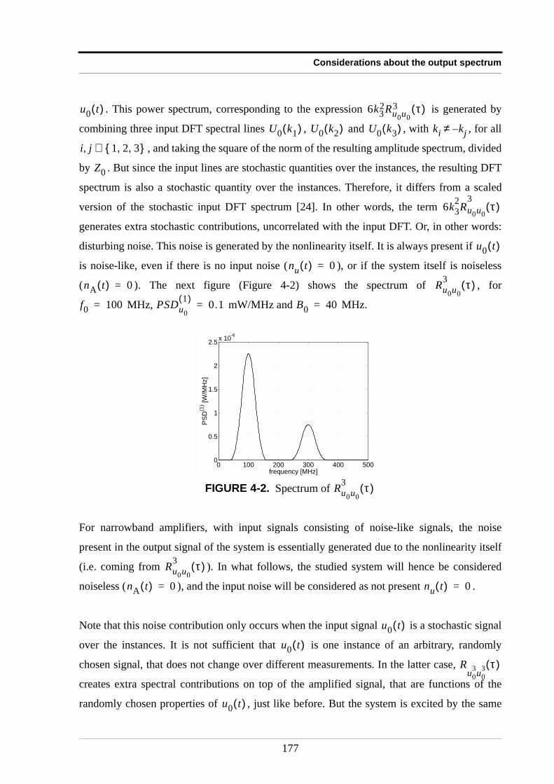
Considerations about the output spectrum
. This power spectrum, corresponding to the expression is generated by
combining three input DFT spectral lines , and , with , for all
, and taking the square of the norm of the resulting amplitude spectrum, divided
by . But since the input lines are stochastic quantities over the instances, the resulting DFT
spectrum is also a stochastic quantity over the instances. Therefore, it differs from a scaled
version of the stochastic input DFT spectrum [24]. In other words, the term
generates extra stochastic contributions, uncorrelated with the input DFT. Or, in other words:
disturbing noise. This noise is generated by the nonlinearity itself. It is always present if
is noise-like, even if there is no input noise ( ), or if the system itself is noiseless
( ). The next figure (Figure 4-2) shows the spectrum of , for
MHz, mW/MHz and MHz.
For narrowband amplifiers, with input signals consisting of noise-like signals, the noise
present in the output signal of the system is essentially generated due to the nonlinearity itself
(i.e. coming from ). In what follows, the studied system will hence be considered
noiseless ( ), and the input noise will be considered as not present .
Note that this noise contribution only occurs when the input signal is a stochastic signal
over the instances. It is not sufficient that is one instance of an arbitrary, randomly
chosen signal, that does not change over different measurements. In the latter case,
creates extra spectral contributions on top of the amplified signal, that are functions of the
randomly chosen properties of , just like before. But the system is excited by the same
FIGURE 4-2. Spectrum of
u0 t( ) 6k32Ru0u0
3 τ( )
U0 k1( ) U0 k2( ) U0 k3( ) ki k– j≠
i j, 1 2 3, , ∈
Z0
6k32Ru0u0
3τ( )
u0 t( )
nu t( ) 0=
nA t( ) 0= Ru0u0
3 τ( )
f0 100= PSDu0
1( ) 0.1= B0 40=
0 100 200 300 400 5000
0.5
1
1.5
2
2.5x 10
-6
frequency [MHz]
PS
D(1
) [W
/MH
z]
Ru0u0
3 τ( )
Ru0u0
3 τ( )
nA t( ) 0= nu t( ) 0=
u0 t( )
u0 t( )
Ru0
3u03 τ( )
u0 t( )
177
Noise-like signals and NICE systems
signal at every measurement. As a consequence, the contributions of will be the
same in each case. Hence, gives a deterministic contribution instead of a stochastic
one.
Furthermore, it is clear that since depends on the properties of the input signal, the
properties of the noise generated by this term, will also depend on the properties of the input
signal [19].
Note that every NICE system containing an odd nonlinear contribution, suffers from these
extra noise contributions that are located in the frequency band of interest, called in-band
distortions. This can easily be shown. Consider e.g. that a ( )-th order contribution is
present ( ). In that case, spectral lines from the DFT spectrum are
combined in the output. If one chooses spectral lines in the
vicinity of frequency , and spectral lines in the vicinity of , such that
(i.e. not all the indices are opposite in
sign to the indices ), the resulting amplitude spectral contribution will lie in the
neighbourhood of frequency (i.e. in the band of interest), but it will be a stochastic
contribution, uncorrelated with where .
Ru0u0
3 τ( )
Ru0u0
3 τ( )
Ru0
3u03 τ( )
u0 t( )
2n 1+
n N∈ 2n 1+ U0 k( )
n 1+ U0 k1( ) … U0 kn 1+( ), ,
f0 n U l1( ) … U ln( ), , f0–
p 1 … n, , q 1 … n, , :lp= k– q∈∃,∈∀( )¬ l1 … ln, ,
k1 … kn 1+, ,
f0U ν( ) ν k1 … kn 1+ l1 … ln+ + + + +=
178
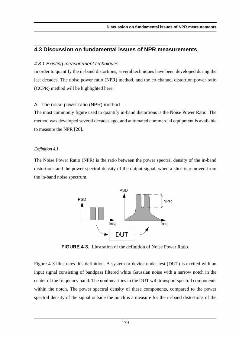
Discussion on fundamental issues of NPR measurements
4.3 Discussion on fundamental issues of NPR measurements
4.3.1 Existing measurement techniquesIn order to quantify the in-band distortions, several techniques have been developed during the
last decades. The noise power ratio (NPR) method, and the co-channel distortion power ratio
(CCPR) method will be highlighted here.
A. The noise power ratio (NPR) methodThe most commonly figure used to quantify in-band distortions is the Noise Power Ratio. The
method was developed several decades ago, and automated commercial equipment is available
to measure the NPR [20].
Definition 4.1
The Noise Power Ratio (NPR) is the ratio between the power spectral density of the in-band
distortions and the power spectral density of the output signal, when a slice is removed from
the in-band noise spectrum.
Figure 4-3 illustrates this definition. A system or device under test (DUT) is excited with an
input signal consisting of bandpass filtered white Gaussian noise with a narrow notch in the
center of the frequency band. The nonlinearities in the DUT will transport spectral components
within the notch. The power spectral density of these components, compared to the power
spectral density of the signal outside the notch is a measure for the in-band distortions of the
FIGURE 4-3. Illustration of the definition of Noise Power Ratio.
NPR
DUT
freqfreq
PSD
PSD
179
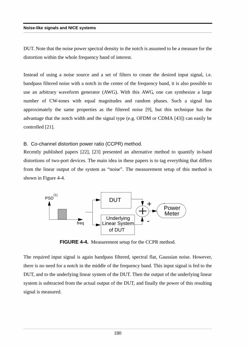
Noise-like signals and NICE systems
DUT. Note that the noise power spectral density in the notch is assumed to be a measure for the
distortion within the whole frequency band of interest.
Instead of using a noise source and a set of filters to create the desired input signal, i.e.
bandpass filtered noise with a notch in the center of the frequency band, it is also possible to
use an arbitrary waveform generator (AWG). With this AWG, one can synthesize a large
number of CW-tones with equal magnitudes and random phases. Such a signal has
approximately the same properties as the filtered noise [9], but this technique has the
advantage that the notch width and the signal type (e.g. OFDM or CDMA [43]) can easily be
controlled [21].
B. Co-channel distortion power ratio (CCPR) method.Recently published papers [22], [23] presented an alternative method to quantify in-band
distortions of two-port devices. The main idea in these papers is to tag everything that differs
from the linear output of the system as “noise”. The measurement setup of this method is
shown in Figure 4-4.
The required input signal is again bandpass filtered, spectral flat, Gaussian noise. However,
there is no need for a notch in the middle of the frequency band. This input signal is fed to the
DUT, and to the underlying linear system of the DUT. Then the output of the underlying linear
system is subtracted from the actual output of the DUT, and finally the power of this resulting
signal is measured.
FIGURE 4-4. Measurement setup for the CCPR method.
+freq
PSD(1)
DUTPowerMeter
UnderlyingLinear System
of DUT
+
-
180
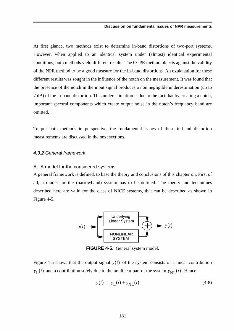
Discussion on fundamental issues of NPR measurements
At first glance, two methods exist to determine in-band distortions of two-port systems.
However, when applied to an identical system under (almost) identical experimental
conditions, both methods yield different results. The CCPR method objects against the validity
of the NPR method to be a good measure for the in-band distortions. An explanation for these
different results was sought in the influence of the notch on the measurement. It was found that
the presence of the notch in the input signal produces a non negligible underestimation (up to
7 dB) of the in-band distortion. This underestimation is due to the fact that by creating a notch,
important spectral components which create output noise in the notch’s frequency band are
omitted.
To put both methods in perspective, the fundamental issues of these in-band distortion
measurements are discussed in the next sections.
4.3.2 General framework
A. A model for the considered systemsA general framework is defined, to base the theory and conclusions of this chapter on. First of
all, a model for the (narrowband) system has to be defined. The theory and techniques
described here are valid for the class of NICE systems, that can be described as shown in
Figure 4-5.
Figure 4-5 shows that the output signal of the system consists of a linear contribution
and a contribution solely due to the nonlinear part of the system . Hence:
(4-8)
FIGURE 4-5. General system model.
+Linear System
NONLINEARSYSTEM
y t( )u t( )
Underlying
y t( )
yL t( ) yNL t( )
y t( ) yL t( ) yNL t( )+=
181
Noise-like signals and NICE systems
Most of the systems that were designed to be linear, but have non-idealities, can be described
by this model. For most well-designed amplifiers, the underlying linear system does indeed
exist. The linear output contribution dominates the nonlinear contribution for sufficiently small
input powers, i.e.
(4-9)
With , the root-mean-square value of signal . Even if (4-9) is not
valid, as is the case for crossover distortion, the theory will still be applicable [9], but in that
case the underlying linear system will not exist (see Appendix 4.A).
Note that many NICE systems can indeed be modelled by Figure 4-5, since the terms of the
Volterra series that describes their input/output relation can be split into two groups: the
operator of first order which characterizes the underlying linear system, and all the other
Volterra operators which characterize the purely nonlinear part of the system.
B. A model for the input signalsThe considered input signals are multi-carrier signals with noise-like properties. When
periodic signals are considered, this class becomes the class of random multisines [9]. These
random multisines will be used as excitation signals for the DUT.
Definition 4.2
A random multisine is a signal consisting of the superposition of sine waves, whose
frequencies are commensurate (i.e. the ratio of two frequencies is a rational number), and
whose phases are instances of an independent distributed random variable over the interval
[ [, such that .
The multisines used in this chapter will be given by:
(4-10)
yNL( )rms
yL( )rms-----------------------
urms 0→lim 0=
xrms E x2 t( ) = x t( )
u t( )
N
ϕ
0 2π, E ejϕ 0=
u0 t( ) 1N
-------- Uκ 2π fmin κ 1–( )fmax fmin–
N 1–---------------------------+
t ϕκ+ cos
κ 1=
N
∑=
182
Discussion on fundamental issues of NPR measurements
and are respectively the maximum and the minimum frequency of the excitation
signal, is the number of frequency components, is the amplitude of the -th frequency
component of the multisine, and the phases are a instance of an independent distributed
random process on the interval [ [, such that . This uniform distribution
can be a continuous or a discrete one. The scaling is performed in order to keep the
total power of the multisine finite, for .
Note that according to (4-10), the -th frequency component of the multisine does not
necessarily lie at frequency grid line . The -th frequency component of the multisine lies at
frequency . If is the frequency grid spacing (see also
section 1.6.2), chosen such that the spectral components of the multisine lie exactly on
frequency grid lines, the grid line number where the -th frequency component lies on is
given by
(4-11)
Assuming that . The frequency difference between two adjacent components of the
multisine is not necessary equal to , but can be an integer multiple of . When working in
narrow bands at high frequencies, the indices of the grid lines on which the components of the
multisine lie can become quite large. (see Example 4.3)
Example 4.3
Consider a multisine consisting of 51 components in the frequency band between
= 900 MHz and = 901 MHz. The frequency grid spacing is kHz. In this
case, the input spectral components lying at the positive side of the frequency axis will be
denoted as .
The advantage of using random multisines instead of a noise source, is their flexibility. The
amplitude and phase of each spectral component can be arbitrary chosen and/or modified. The
only problem that arises is that one instance of a random multisine is a deterministic periodic
fmax fmin
N Uκ κ
ϕκ
0 2π, E ejϕκ 0=
1 N⁄
N ∞→
κ
κ κ
fmin κ 1–( ) fmax fmin–( ) N 1–( )⁄+ ∆f
k κ
kfmin κ 1–( )
fmax fmin–N 1–
---------------------------+
∆f-------------------------------------------------------------=
k N∈
∆f ∆f
fmin fmax ∆f 10=
U0 90000( ) U0 90002( ) … U0 90100( ), , ,
183
Noise-like signals and NICE systems
signal instead of a stochastic one, and hence, with this signal it is difficult to give an accurate
estimate of the in-band distortions of a system, as stated in section 4.2.
However, if several instances of the multisine are considered, then the spectrum of the
multisine is a random quantity when looking over the different instances of the multisine.
Hence, instead of having a signal that varies randomly in time, the signal varies randomly over
the instances. The average of different measurements of a spectral component of one single
multisine instance is no longer zero, since it is a deterministic quantity. The ensemble
(instance) average of a spectral component taken over different multisine instances drawn from
a same amplitude distribution is zero, since the phase of the spectral components is random
distributed over the instances, with , just as was the case for the discrete noise
spectrum discussed in section 1.6.2.
4.3.3 Properties of the Frequency Response FunctionThe considered input signals are noise-like signals, and the study of the simple
polynomial model in section 4.2, revealed that apparently the output signal consists of a
part that is correlated with the input signal, and a part that is not correlated with the input
signal. This means that the frequency response function, will contain terms with similar
properties. But before taking a closer look to the frequency response function, the concepts
“underlying linear system” and “related linear dynamic system” will be highlighted.
The underlying linear system is introduced in Figure 4-5. It is the system that describes the
output signal, when the input signal tends towards zero. In the polynomial model
, the underlying linear system is described by: , i.e. a system that
scales the input signal with a factor . In the model , the underlying linear
system is described by the first term in the Taylor series expansion: , i.e. a system
that scales the input signal with a factor . The underlying linear system is not dependent on
the input signal . Note that the underlying linear system does not always exist, as is the
case for amplifiers exhibiting cross-over distortion (see Appendix 4.A).
E ejϕ 0=
u t( )
y t( )
y k1u k3u3+= y k1u=
k1 y α βu( )atan=
y αβu=
αβ
u t( )
184
Discussion on fundamental issues of NPR measurements
The related linear dynamic system, is the best linear approximation of the system, in mean
squares sense, for a given input signal. In the model , if is a sinewave
with amplitude , the output spectrum at the fundamental frequency will also be a sinewave,
with amplitude (as shown in the previous chapters). Hence, the system has
amplified the original sinewave with a factor . The linear system that best
approximates, in mean squares sense, the input-output relation for the given example, is a
system that has a voltage gain of . Hence, the related linear dynamic system is
dependent on the input signal . In this example, this is illustrated that for input signals
with different amplitudes, the gain of the related linear dynamic system will be different.
Definition 4.4
The Frequency Response Function (FRF) is the ratio of the complex output DFT spectrum
to the complex input DFT spectrum , for the frequency ranges where , or
(4-12)
For NICE systems, this Frequency Response Function will be dependent on the properties of
the input spectrum . For LTI systems, the FRF is independent of , and is simply the
transfer function of the LTI system. For microwave systems, the FRF is usually the ratio
, or an -parameter that depends on the properties of the incident wave for NICE
systems.
When a system is excited with a random multisine, the non parametric frequency response
function (or , see section 1.3.3) can be split into systematic contributions, also called
bias contributions, and stochastic contributions [24] (see also Appendix 4.B).
(4-13)
or, in terms of -parameters:
(4-14)
y k1u k3u3+= u t( )
A
k1 3k3A2 4⁄+( )A
k1 3k3A2 4⁄+
k1 3k3A2 4⁄+
u t( )
Y f( ) U f( ) U f( ) 0≠
FRF f( ) Y f( )U f( )-----------
U f( ) 0≠=
U f( ) U f( )
H f( )
b2 a1⁄ S21 a1
b2 a1⁄
FRF k( ) FRFlin k( ) FRFB k( ) FRFS k( ) NFRF k( )+ + +=
S
b2 k( )a1 k( )------------- S21 k( ) S21 B, k( ) S21 S, k( ) NS21
k( )+ + +=
185
Noise-like signals and NICE systems
Where:
• (or ) is the FRF (or -parameter) of the underlying
linear system (if it exists), i.e. the transfer function .
• (or ) represents the bias or systematic nonlinear
contributions to the FRF, coming from the odd nonlinearities. This value
is independent of the random phases of the multisine.
• (or ) is the stochastic nonlinear contribution to the
FRF, coming from the even and the odd nonlinearities. This value is a
function of the random phases of the multisine and is zero mean, circular
complex normally distributed.
• (or ) is a stochastic component on the FRF. It consists
of input noise , noise added by the NICE system itself , or
the noise added by the measurement system. These contributions are
assumed to be extremely small, as discussed in section 4.2.
Based on (4-13), the output spectrum of a NICE system can be written as:
(4-15)
If the input spectrum of the NICE system can be written as , the
following can be told in terms of the functions , , and
defined in section 1.6.2.D.:
• contains those terms of and which
contain the factor combined only with other terms that have no
phase contribution. The other factors in can hence be grouped into
complex conjugated pairs.
• contains those terms of and which
contain the factor and that are not part of .
FRFlin k( ) S21 k( ) S21
H1 k( )
FRFB k( ) S21 B, k( )
FRFS k( ) S21 S, k( )
NFRF k( ) NS21k( )
Nu k( ) NA k( )
Y k( )
Y k( ) FRFlin k( )U0 k( ) FRFB k( )U0 k( ) FRFS k( )U0 k( ) NS k( )+ + +=
U k( ) U0 k( ) Nu k( )+=
A U0( ) A ′ U0 N,( ) B N( ) B′ U0 N,( )
FRFB k( )U0 k( ) A U0( ) A ′ U0 N,( )
U0 k( )
U0 l( )
FRFS k( )U0 k( ) A U0( ) A ′ U0 N,( )
U0 k( ) FRFB k( )U0 k( )
186
Discussion on fundamental issues of NPR measurements
• contains the effects of the disturbing stochastic noise, and can be
written as . This term will always be
stochastic, even if is a deterministic spectrum over the instances.
4.3.4 Reconciling the NPR and the CCPR methodDepending on the fact that the goal is to characterize the best linear approximation or the
underlying linear system, two different interpretations of the Frequency Response Function
can be distinguished:
A. Goal: determine the best linear approximation is independent of the random phases of the multisine. As a result, will be
the same for every instance of the multisine. In this case, the systematic nonlinear contribution
to the FRF cannot be separated from the frequency response function of the underlying linear
system ( ). The sum of both, called , is defined as the FRF of the related
linear dynamic system (RLDS) of the device under test:
(4-16)
This is the best linear approximation of the nonlinear system in mean squares sense for the
considered class of excitation signals [24]. The output spectrum of the system is then given by:
(4-17)
where represents the stochastic nonlinear contribution to the output
spectrum. Note that since has a stochastic character with respect to the different
instances of the multisine, also behaves as a noise source on the output of the system.
Because the input power is independent of the phase instance of the multisine, is a
constant quantity over the different instances. (4-17) can also be written as
(4-18)
NS k( )
NS k( ) B N( ) B′ U0 N,( )+=
U0 k( )
FRFB k( ) FRFB k( )
FRFlin k( ) FRFR k( )
FRFR k( ) FRFlin k( ) FRFB k( )+=
Y k( ) FRFlin k( ) FRFB k( )+( )U0 k( ) YS k( ) NS k( )+ +=
FRFR k( )U0 k( ) YS k( ) NS k( ) + +=
YS k( ) FRFS k( )U0 k( )=
FRFS k( )
YS k( )
FRFR k( )
Y k( ) Y0 k( ) Ny k( )+=
187
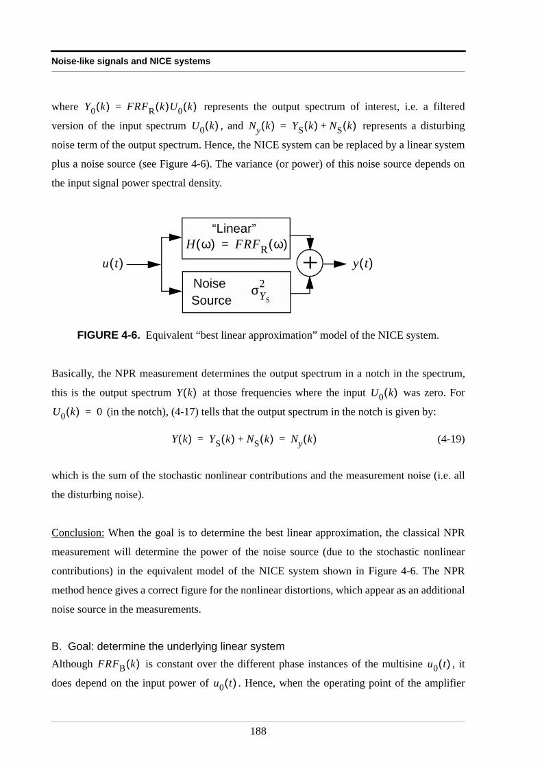
Noise-like signals and NICE systems
where represents the output spectrum of interest, i.e. a filtered
version of the input spectrum , and represents a disturbing
noise term of the output spectrum. Hence, the NICE system can be replaced by a linear system
plus a noise source (see Figure 4-6). The variance (or power) of this noise source depends on
the input signal power spectral density.
Basically, the NPR measurement determines the output spectrum in a notch in the spectrum,
this is the output spectrum at those frequencies where the input was zero. For
(in the notch), (4-17) tells that the output spectrum in the notch is given by:
(4-19)
which is the sum of the stochastic nonlinear contributions and the measurement noise (i.e. all
the disturbing noise).
Conclusion: When the goal is to determine the best linear approximation, the classical NPR
measurement will determine the power of the noise source (due to the stochastic nonlinear
contributions) in the equivalent model of the NICE system shown in Figure 4-6. The NPR
method hence gives a correct figure for the nonlinear distortions, which appear as an additional
noise source in the measurements.
B. Goal: determine the underlying linear systemAlthough is constant over the different phase instances of the multisine , it
does depend on the input power of . Hence, when the operating point of the amplifier
FIGURE 4-6. Equivalent “best linear approximation” model of the NICE system.
Y0 k( ) FRFR k( )U0 k( )=
U0 k( ) Ny k( ) YS k( ) NS k( )+=
+NOISESOURCE
“Linear”H ω( ) FRFR ω( )=
u t( ) y t( )NoiseSource
σYS
2
Y k( ) U0 k( )
U0 k( ) 0=
Y k( ) YS k( ) NS k( )+ Ny k( )= =
FRFB k( ) u0 t( )
u0 t( )
188
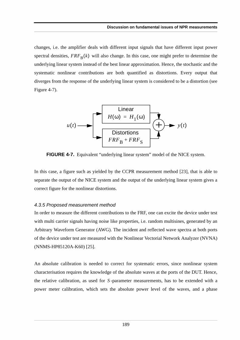
Discussion on fundamental issues of NPR measurements
changes, i.e. the amplifier deals with different input signals that have different input power
spectral densities, will also change. In this case, one might prefer to determine the
underlying linear system instead of the best linear approximation. Hence, the stochastic and the
systematic nonlinear contributions are both quantified as distortions. Every output that
diverges from the response of the underlying linear system is considered to be a distortion (see
Figure 4-7).
In this case, a figure such as yielded by the CCPR measurement method [23], that is able to
separate the output of the NICE system and the output of the underlying linear system gives a
correct figure for the nonlinear distortions.
4.3.5 Proposed measurement methodIn order to measure the different contributions to the FRF, one can excite the device under test
with multi carrier signals having noise like properties, i.e. random multisines, generated by an
Arbitrary Waveform Generator (AWG). The incident and reflected wave spectra at both ports
of the device under test are measured with the Nonlinear Vectorial Network Analyzer (NVNA)
(NNMS-HP85120A-K60) [25].
An absolute calibration is needed to correct for systematic errors, since nonlinear system
characterisation requires the knowledge of the absolute waves at the ports of the DUT. Hence,
the relative calibration, as used for -parameter measurements, has to be extended with a
power meter calibration, which sets the absolute power level of the waves, and a phase
FIGURE 4-7. Equivalent “underlying linear system” model of the NICE system.
FRFB k( )
NOISESOURCE
LinearH ω( ) H1 ω( )=
u t( ) y t( )Distortions
FRFB FRFS+
+
S
189
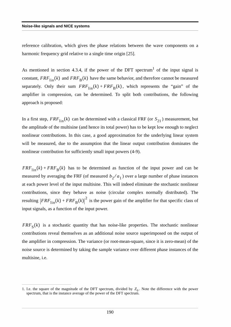
Noise-like signals and NICE systems
reference calibration, which gives the phase relations between the wave components on a
harmonic frequency grid relative to a single time origin [25].
As mentioned in section 4.3.4, if the power of the DFT spectrum1 of the input signal is
constant, and have the same behavior, and therefore cannot be measured
separately. Only their sum , which represents the “gain” of the
amplifier in compression, can be determined. To split both contributions, the following
approach is proposed:
In a first step, can be determined with a classical FRF (or ) measurement, but
the amplitude of the multisine (and hence its total power) has to be kept low enough to neglect
nonlinear contributions. In this case, a good approximation for the underlying linear system
will be measured, due to the assumption that the linear output contribution dominates the
nonlinear contribution for sufficiently small input powers (4-9).
has to be determined as function of the input power and can be
measured by averaging the FRF (of measured ) over a large number of phase instances
at each power level of the input multisine. This will indeed eliminate the stochastic nonlinear
contributions, since they behave as noise (circular complex normally distributed). The
resulting is the power gain of the amplifier for that specific class of
input signals, as a function of the input power.
is a stochastic quantity that has noise-like properties. The stochastic nonlinear
contributions reveal themselves as an additional noise source superimposed on the output of
the amplifier in compression. The variance (or root-mean-square, since it is zero-mean) of the
noise source is determined by taking the sample variance over different phase instances of the
multisine, i.e.
1. I.e. the square of the magnitude of the DFT spectrum, divided by . Note the difference with the powerspectrum, that is the instance average of the power of the DFT spectrum.
Z0
FRFlin k( ) FRFB k( )
FRFlin k( ) FRFB k( )+
FRFlin k( ) S21
FRFlin k( ) FRFB k( )+
b2 a1⁄
FRFlin k( ) FRFB k( )+ 2
FRFS k( )
190
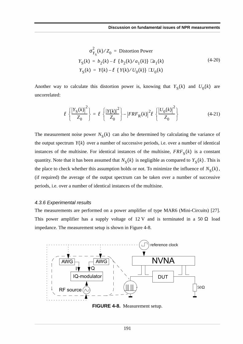
Discussion on fundamental issues of NPR measurements
(4-20)
Another way to calculate this distortion power is, knowing that and are
uncorrelated:
(4-21)
The measurement noise power can also be determined by calculating the variance of
the output spectrum over a number of successive periods, i.e. over a number of identical
instances of the multisine. For identical instances of the multisine, is a constant
quantity. Note that it has been assumed that is negligible as compared to . This is
the place to check whether this assumption holds or not. To minimize the influence of ,
(if required) the average of the output spectrum can be taken over a number of successive
periods, i.e. over a number of identical instances of the multisine.
4.3.6 Experimental resultsThe measurements are performed on a power amplifier of type MAR6 (Mini-Circuits) [27].
This power amplifier has a supply voltage of 12 V and is terminated in a 50 load
impedance. The measurement setup is shown in Figure 4-8.
FIGURE 4-8. Measurement setup.
σYS
2 k( ) Z0⁄ Distortion Power=
YS k( ) b2 k( ) E b2 k( ) a1 k( )⁄ a1 k( )⋅–=
YS k( ) Y k( ) E Y k( ) U0 k( )⁄ U0 k( )⋅–=
YS k( ) U0 k( )
E YS k( ) 2
Z0-------------------
E Y k( ) 2
Z0----------------
FRFR k( ) 2E U0 k( ) 2
Z0--------------------
–=
NS k( )
Y k( )
FRFS k( )
NS k( ) YS k( )
NS k( )
Ω
DUT
50Ω
NVNA
IQ-modulator
AWG AWG
RF source
I Q
reference clock
191
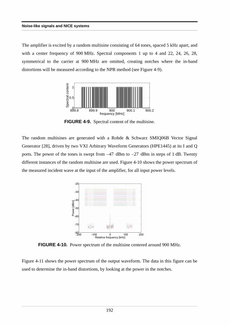
Noise-like signals and NICE systems
The amplifier is excited by a random multisine consisting of 64 tones, spaced 5 kHz apart, and
with a center frequency of 900 MHz. Spectral components 1 up to 4 and 22, 24, 26, 28,
symmetrical to the carrier at 900 MHz are omitted, creating notches where the in-band
distortions will be measured according to the NPR method (see Figure 4-9).
The random multisines are generated with a Rohde & Schwarz SMIQ06B Vector Signal
Generator [28], driven by two VXI Arbitrary Waveform Generators (HPE1445) at its I and Q
ports. The power of the tones is swept from dBm to dBm in steps of 1 dB. Twenty
different instances of the random multisine are used. Figure 4-10 shows the power spectrum of
the measured incident wave at the input of the amplifier, for all input power levels.
Figure 4-11 shows the power spectrum of the output waveform. The data in this figure can be
used to determine the in-band distortions, by looking at the power in the notches.
FIGURE 4-9. Spectral content of the multisine.
FIGURE 4-10. Power spectrum of the multisine centered around 900 MHz.
899.8 899.9 900 900.1 900.20
0.5
1
frequency [MHz]
Spe
ctra
l con
tent
47– 27–
-200 -100 0 100 200-80
-70
-60
-50
-40
-30
-20
Relative frequency [kHz]
Pow
er [d
Bm
]
192
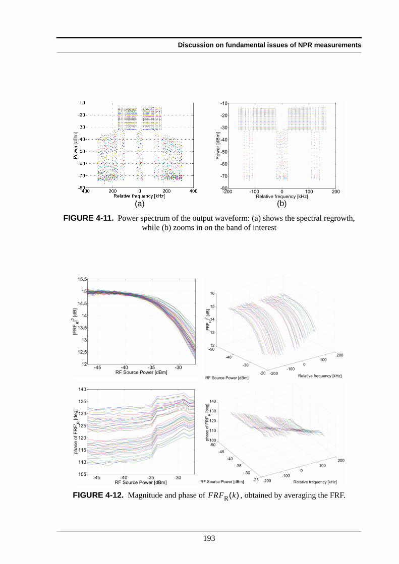
Discussion on fundamental issues of NPR measurements
FIGURE 4-11. Power spectrum of the output waveform: (a) shows the spectral regrowth, while (b) zooms in on the band of interest
FIGURE 4-12. Magnitude and phase of , obtained by averaging the FRF.
-200 -100 0 100 200-80
-70
-60
-50
-40
-30
-20
-10
Relative frequency [kHz]
Pow
er [d
Bm
]
(a) (b)
-45 -40 -35 -3012
12.5
13
13.5
14
14.5
15
15.5
RF Source Power [dBm]
|FR
FR
|2 [dB
]
-50
-40
-30
-20 -200-100
0100
200
12
13
14
15
16
Relative frequency [kHz]RF Source Power [dBm]
|FR
FR
|2 [dB
]
-45 -40 -35 -30105
110
115
120
125
130
135
140
RF Source Power [dBm]
phas
e of
FR
F' R
[deg
]
-50
-45
-40
-35
-30
-25 -200-100
0100
200
100
110
120
130
140
Relative frequency [kHz]RF Source Power [dBm]
phas
e of
FR
F' R
[deg
]
FRFR k( )
193
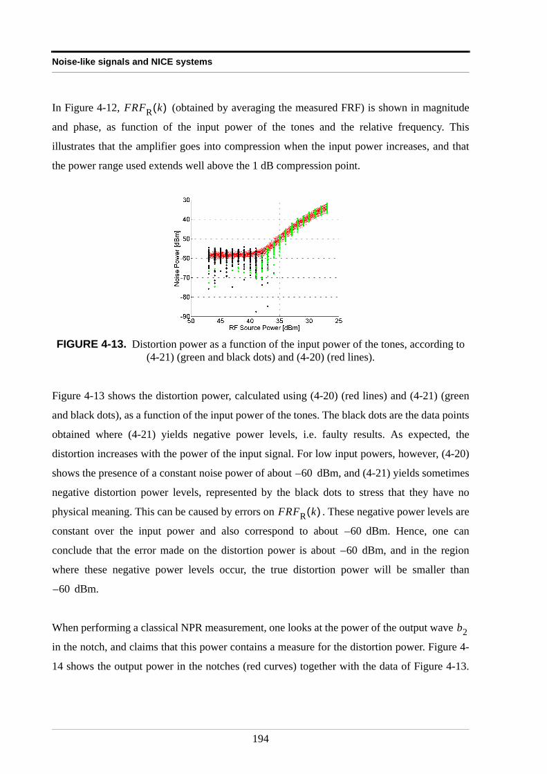
Noise-like signals and NICE systems
In Figure 4-12, (obtained by averaging the measured FRF) is shown in magnitude
and phase, as function of the input power of the tones and the relative frequency. This
illustrates that the amplifier goes into compression when the input power increases, and that
the power range used extends well above the 1 dB compression point.
Figure 4-13 shows the distortion power, calculated using (4-20) (red lines) and (4-21) (green
and black dots), as a function of the input power of the tones. The black dots are the data points
obtained where (4-21) yields negative power levels, i.e. faulty results. As expected, the
distortion increases with the power of the input signal. For low input powers, however, (4-20)
shows the presence of a constant noise power of about dBm, and (4-21) yields sometimes
negative distortion power levels, represented by the black dots to stress that they have no
physical meaning. This can be caused by errors on . These negative power levels are
constant over the input power and also correspond to about dBm. Hence, one can
conclude that the error made on the distortion power is about dBm, and in the region
where these negative power levels occur, the true distortion power will be smaller than
dBm.
When performing a classical NPR measurement, one looks at the power of the output wave
in the notch, and claims that this power contains a measure for the distortion power. Figure 4-
14 shows the output power in the notches (red curves) together with the data of Figure 4-13.
FIGURE 4-13. Distortion power as a function of the input power of the tones, according to (4-21) (green and black dots) and (4-20) (red lines).
FRFR k( )
60–
FRFR k( )
60–
60–
60–
b2
194
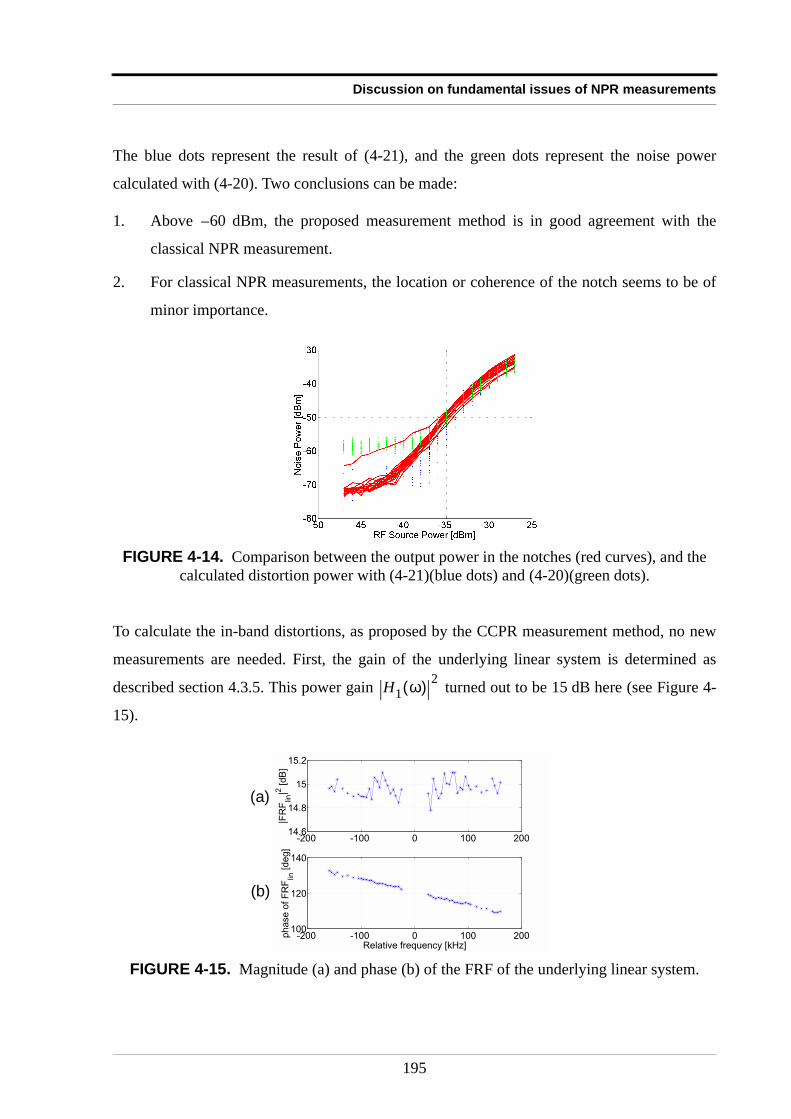
Discussion on fundamental issues of NPR measurements
The blue dots represent the result of (4-21), and the green dots represent the noise power
calculated with (4-20). Two conclusions can be made:
1. Above dBm, the proposed measurement method is in good agreement with the
classical NPR measurement.
2. For classical NPR measurements, the location or coherence of the notch seems to be of
minor importance.
To calculate the in-band distortions, as proposed by the CCPR measurement method, no new
measurements are needed. First, the gain of the underlying linear system is determined as
described section 4.3.5. This power gain turned out to be 15 dB here (see Figure 4-
15).
FIGURE 4-14. Comparison between the output power in the notches (red curves), and the calculated distortion power with (4-21)(blue dots) and (4-20)(green dots).
FIGURE 4-15. Magnitude (a) and phase (b) of the FRF of the underlying linear system.
60–
H1 ω( ) 2
-200 -100 0 100 20014.6
14.8
15
15.2
|FR
Flin
|2 [dB
]
-200 -100 0 100 200100
120
140
Relative frequency [kHz]
phas
e of
FR
Flin
[deg
]
(a)
(b)
195
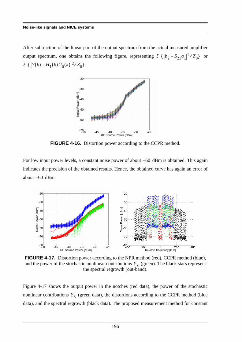
Noise-like signals and NICE systems
After subtraction of the linear part of the output spectrum from the actual measured amplifier
output spectrum, one obtains the following figure, representing or
.
For low input power levels, a constant noise power of about dBm is obtained. This again
indicates the precision of the obtained results. Hence, the obtained curve has again an error of
about dBm.
Figure 4-17 shows the output power in the notches (red data), the power of the stochastic
nonlinear contributions (green data), the distortions according to the CCPR method (blue
data), and the spectral regrowth (black data). The proposed measurement method for constant
FIGURE 4-16. Distortion power according to the CCPR method.
FIGURE 4-17. Distortion power according to the NPR method (red), CCPR method (blue), and the power of the stochastic nonlinear contributions (green). The black stars represent
the spectral regrowth (out-band).
E b2 S21a1– 2 Z0⁄
E Y k( ) H1 k( )U0 k( )– 2 Z0⁄
-50 -45 -40 -35 -30 -25-70
-60
-50
-40
-30
-20N
oise
Pow
er [d
Bm
]
RF Source Power [dBm]
60–
60–
-50 -45 -40 -35 -30 -25-80
-70
-60
-50
-40
-30
-20
Noi
se P
ower
[dB
m]
RF Source Power [dBm] Relative frequency [kHz]
YS
YS
196
Discussion on fundamental issues of NPR measurements
input power, agrees very good with the NPR method, but does not need the presence of notches
in the spectrum. For high input powers, the CCPR method predicts a distortion power that is
much (about 8 dB) larger than the classical NPR method or the constant input power
hypothesis predicts. This is due to the systematic nonlinear contribution which is
tagged as a distortion by the CCPR method.
4.3.7 ConclusionThe NPR method will yield a good measure for the in-band distortions, according to the “best
linear approximation” model for the NICE system. On the other hand, the CCPR measurement
method yields a good measure for the in-band distortions, according to the “underlying linear
system” model for the NICE system.
A third possibility is to measure the systematic and stochastic contributions of the FRF, as
proposed in section 4.3.5. Using the latter method, it is possible to quantify the in-band
distortions, according to both the NPR and the CCPR method.
FRFB k( )
197
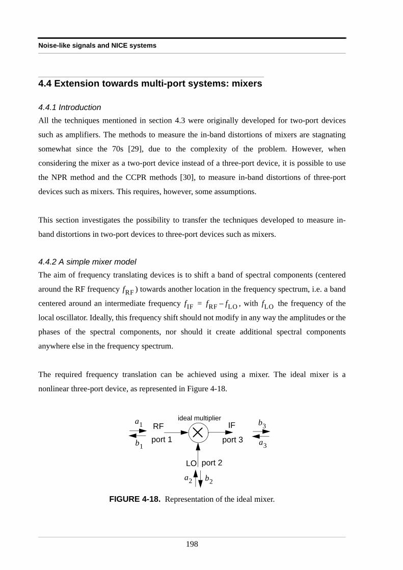
Noise-like signals and NICE systems
4.4 Extension towards multi-port systems: mixers
4.4.1 IntroductionAll the techniques mentioned in section 4.3 were originally developed for two-port devices
such as amplifiers. The methods to measure the in-band distortions of mixers are stagnating
somewhat since the 70s [29], due to the complexity of the problem. However, when
considering the mixer as a two-port device instead of a three-port device, it is possible to use
the NPR method and the CCPR methods [30], to measure in-band distortions of three-port
devices such as mixers. This requires, however, some assumptions.
This section investigates the possibility to transfer the techniques developed to measure in-
band distortions in two-port devices to three-port devices such as mixers.
4.4.2 A simple mixer modelThe aim of frequency translating devices is to shift a band of spectral components (centered
around the RF frequency ) towards another location in the frequency spectrum, i.e. a band
centered around an intermediate frequency , with the frequency of the
local oscillator. Ideally, this frequency shift should not modify in any way the amplitudes or the
phases of the spectral components, nor should it create additional spectral components
anywhere else in the frequency spectrum.
The required frequency translation can be achieved using a mixer. The ideal mixer is a
nonlinear three-port device, as represented in Figure 4-18.
FIGURE 4-18. Representation of the ideal mixer.
fRF
fIF fRF fLO–= fLO
port 1
port 2
port 3RF
LO
IFideal multiplier
a3
b3a1
b1
b2a2
198
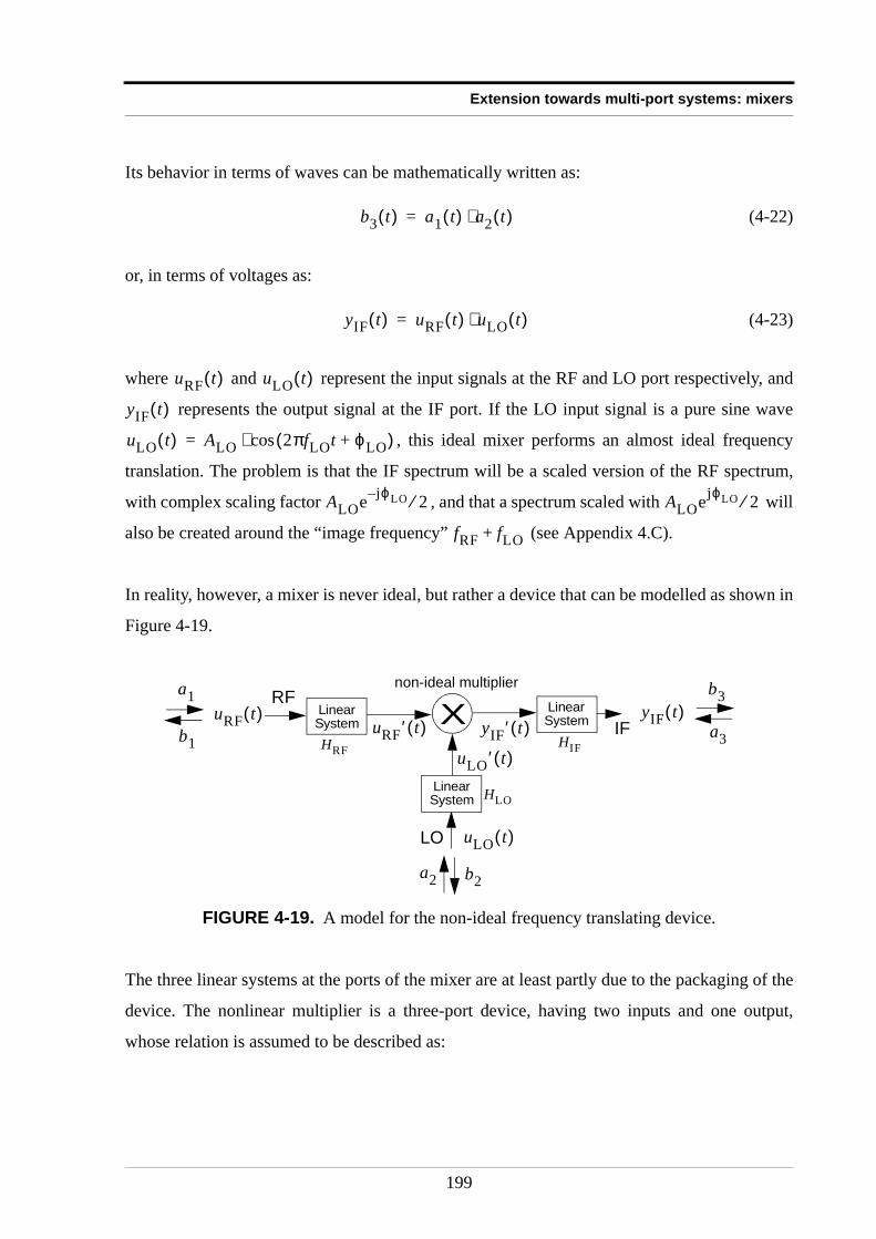
Extension towards multi-port systems: mixers
Its behavior in terms of waves can be mathematically written as:
(4-22)
or, in terms of voltages as:
(4-23)
where and represent the input signals at the RF and LO port respectively, and
represents the output signal at the IF port. If the LO input signal is a pure sine wave
, this ideal mixer performs an almost ideal frequency
translation. The problem is that the IF spectrum will be a scaled version of the RF spectrum,
with complex scaling factor , and that a spectrum scaled with will
also be created around the “image frequency” (see Appendix 4.C).
In reality, however, a mixer is never ideal, but rather a device that can be modelled as shown in
Figure 4-19.
The three linear systems at the ports of the mixer are at least partly due to the packaging of the
device. The nonlinear multiplier is a three-port device, having two inputs and one output,
whose relation is assumed to be described as:
FIGURE 4-19. A model for the non-ideal frequency translating device.
b3 t( ) a1 t( ) a2 t( )⋅=
yIF t( ) uRF t( ) uLO t( )⋅=
uRF t( ) uLO t( )
yIF t( )
uLO t( ) ALO 2πfLOt ϕLO+( )cos⋅=
ALOe j– ϕLO 2⁄ ALOejϕLO 2⁄
fRF fLO+
Xnon-ideal multiplier
RF
LO
IFLinearSystem
LinearSystem
LinearSystem
HRF
HLO
HIF
uRF t( )
uLO t( )
yIF t( )uRF ′ t( ) yIF ′ t( )
uLO ′ t( )a3
b3a1
b1
b2a2
199
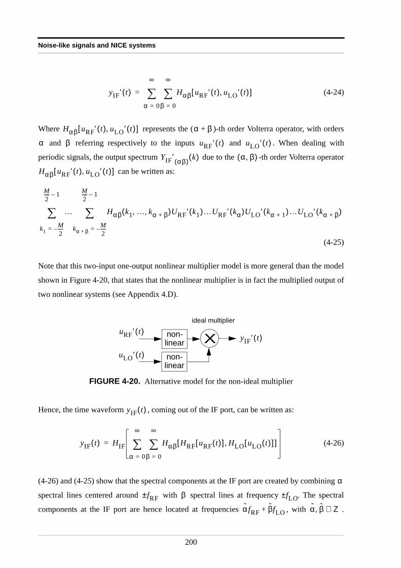
Noise-like signals and NICE systems
(4-24)
Where represents the ( )-th order Volterra operator, with orders
and referring respectively to the inputs and . When dealing with
periodic signals, the output spectrum due to the -th order Volterra operator
can be written as:
(4-25)
Note that this two-input one-output nonlinear multiplier model is more general than the model
shown in Figure 4-20, that states that the nonlinear multiplier is in fact the multiplied output of
two nonlinear systems (see Appendix 4.D).
Hence, the time waveform , coming out of the IF port, can be written as:
(4-26)
(4-26) and (4-25) show that the spectral components at the IF port are created by combining
spectral lines centered around with spectral lines at frequency . The spectral
components at the IF port are hence located at frequencies , with .
FIGURE 4-20. Alternative model for the non-ideal multiplier
yIF ′ t( ) Hαβ uRF ′ t( ) uLO ′ t( ),[ ]
β 0=
∞
∑α 0=
∞
∑=
Hαβ uRF′ t( ) uLO ′ t( ),[ ] α β+
α β uRF ′ t( ) uLO ′ t( )
YIF ′ αβ( ) k( ) α β,( )
Hαβ uRF′ t( ) uLO ′ t( ),[ ]
… Hαβ k1 … kα β+, ,( )URF ′ k1( )…URF ′ kα( )ULO ′ kα 1+( )…ULO ′ kα β+( )
kα β+M2-----–=
M2----- 1–
∑
k1M2-----–=
M2----- 1–
∑
X yIF ′ t( )
ideal multiplieruRF ′ t( )
uLO ′ t( )
non-linear
non-linear
yIF t( )
yIF t( ) HIF Hαβ HRF uRF t( )[ ] HLO uLO t( )[ ],[ ]
β 0=
∞
∑α 0=
∞
∑=
α
fRF± β fLO±
α fRF βfLO+ α β, Z∈
200
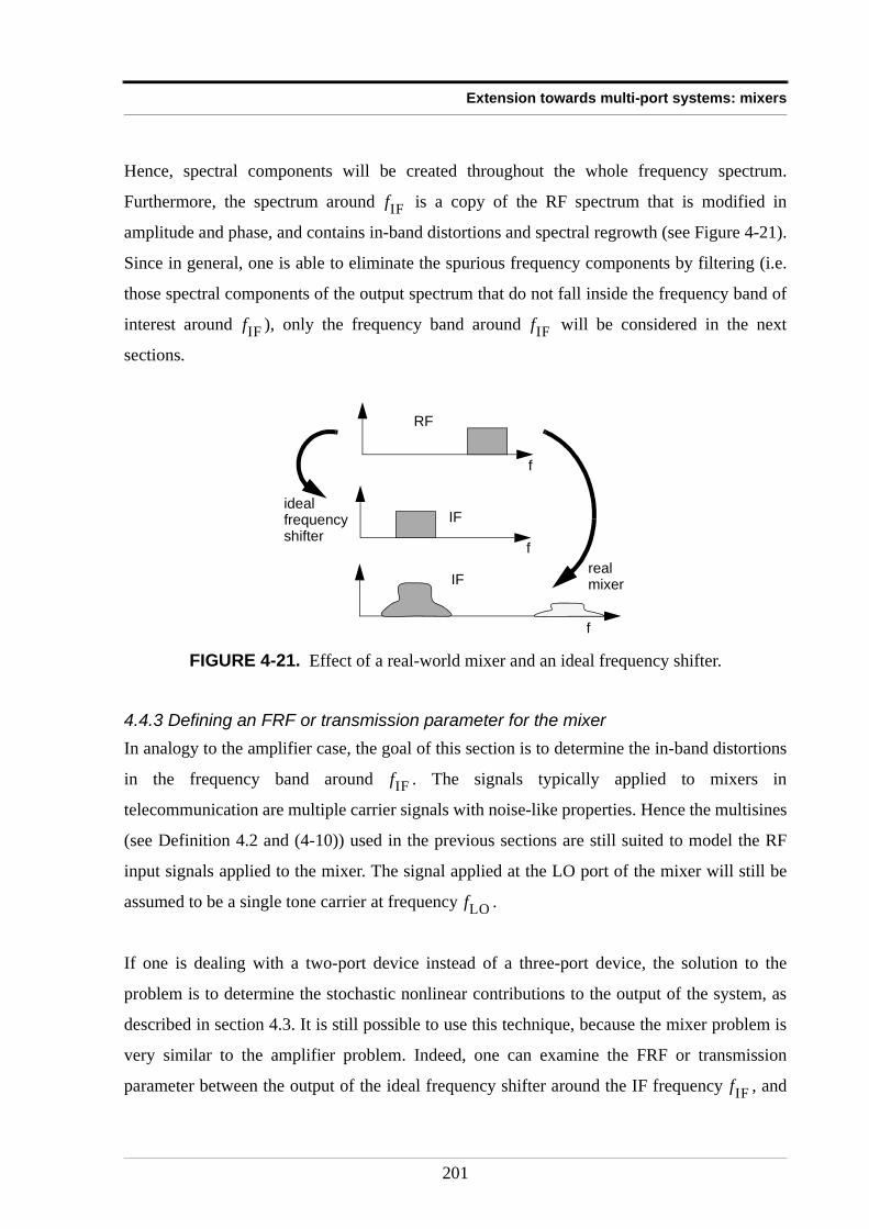
Extension towards multi-port systems: mixers
Hence, spectral components will be created throughout the whole frequency spectrum.
Furthermore, the spectrum around is a copy of the RF spectrum that is modified in
amplitude and phase, and contains in-band distortions and spectral regrowth (see Figure 4-21).
Since in general, one is able to eliminate the spurious frequency components by filtering (i.e.
those spectral components of the output spectrum that do not fall inside the frequency band of
interest around ), only the frequency band around will be considered in the next
sections.
4.4.3 Defining an FRF or transmission parameter for the mixerIn analogy to the amplifier case, the goal of this section is to determine the in-band distortions
in the frequency band around . The signals typically applied to mixers in
telecommunication are multiple carrier signals with noise-like properties. Hence the multisines
(see Definition 4.2 and (4-10)) used in the previous sections are still suited to model the RF
input signals applied to the mixer. The signal applied at the LO port of the mixer will still be
assumed to be a single tone carrier at frequency .
If one is dealing with a two-port device instead of a three-port device, the solution to the
problem is to determine the stochastic nonlinear contributions to the output of the system, as
described in section 4.3. It is still possible to use this technique, because the mixer problem is
very similar to the amplifier problem. Indeed, one can examine the FRF or transmission
parameter between the output of the ideal frequency shifter around the IF frequency , and
FIGURE 4-21. Effect of a real-world mixer and an ideal frequency shifter.
fIF
fIF fIF
f
f
f
RF
IF
IF
idealfrequency
realmixer
shifter
fIF
fLO
fIF
201
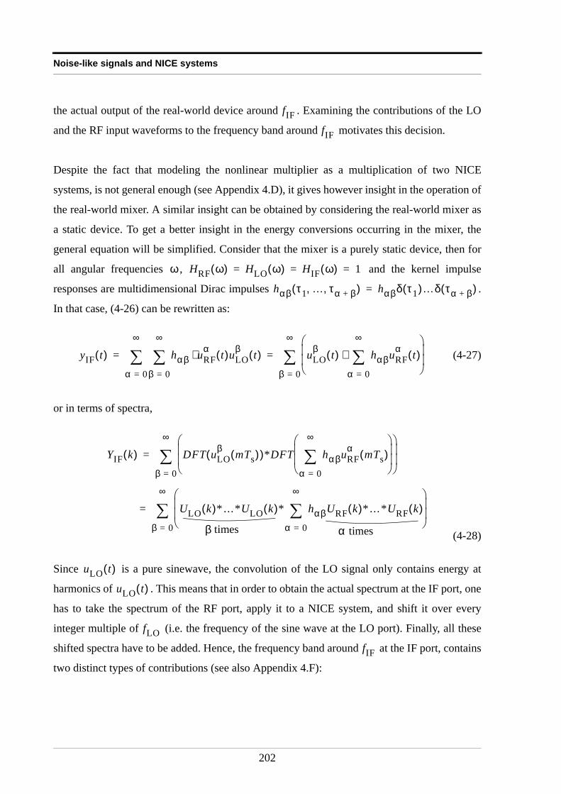
Noise-like signals and NICE systems
the actual output of the real-world device around . Examining the contributions of the LO
and the RF input waveforms to the frequency band around motivates this decision.
Despite the fact that modeling the nonlinear multiplier as a multiplication of two NICE
systems, is not general enough (see Appendix 4.D), it gives however insight in the operation of
the real-world mixer. A similar insight can be obtained by considering the real-world mixer as
a static device. To get a better insight in the energy conversions occurring in the mixer, the
general equation will be simplified. Consider that the mixer is a purely static device, then for
all angular frequencies , and the kernel impulse
responses are multidimensional Dirac impulses .
In that case, (4-26) can be rewritten as:
(4-27)
or in terms of spectra,
(4-28)
Since is a pure sinewave, the convolution of the LO signal only contains energy at
harmonics of . This means that in order to obtain the actual spectrum at the IF port, one
has to take the spectrum of the RF port, apply it to a NICE system, and shift it over every
integer multiple of (i.e. the frequency of the sine wave at the LO port). Finally, all these
shifted spectra have to be added. Hence, the frequency band around at the IF port, contains
two distinct types of contributions (see also Appendix 4.F):
fIF
fIF
ω HRF ω( ) HLO ω( ) HIF ω( ) 1= = =
hαβ τ1 … τα β+, ,( ) hαβδ τ1( )…δ τα β+( )=
yIF t( ) hαβ uRFα t( )uLO
β t( )⋅
β 0=
∞
∑α 0=
∞
∑ uLOβ t( ) hαβuRF
α t( )
α 0=
∞
∑⋅
β 0=
∞
∑= =
YIF k( ) DFT uLOβ mTs( )( )*DFT hαβuRF
α mTs( )
α 0=
∞
∑
β 0=
∞
∑=
ULO k( )*…*ULO k( )* hαβURF k( )*…*URF k( )
α 0=
∞
∑
β 0=
∞
∑=
α timesβ times
uLO t( )
uLO t( )
fLO
fIF
202
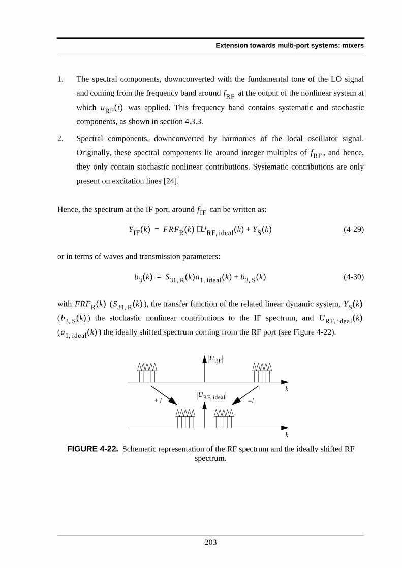
Extension towards multi-port systems: mixers
1. The spectral components, downconverted with the fundamental tone of the LO signal
and coming from the frequency band around at the output of the nonlinear system at
which was applied. This frequency band contains systematic and stochastic
components, as shown in section 4.3.3.
2. Spectral components, downconverted by harmonics of the local oscillator signal.
Originally, these spectral components lie around integer multiples of , and hence,
they only contain stochastic nonlinear contributions. Systematic contributions are only
present on excitation lines [24].
Hence, the spectrum at the IF port, around can be written as:
(4-29)
or in terms of waves and transmission parameters:
(4-30)
with ( ), the transfer function of the related linear dynamic system,
( ) the stochastic nonlinear contributions to the IF spectrum, and
( ) the ideally shifted spectrum coming from the RF port (see Figure 4-22).
FIGURE 4-22. Schematic representation of the RF spectrum and the ideally shifted RF spectrum.
fRF
uRF t( )
fRF
fIF
YIF k( ) FRFR k( ) URF ideal, k( )⋅ YS k( )+=
b3 k( ) S31 R, k( )a1 ideal, k( ) b3 S, k( )+=
FRFR k( ) S31 R, k( ) YS k( )
b3 S, k( ) URF ideal, k( )
a1 ideal, k( )
k
k
URF
URF ideal, l– l+
203
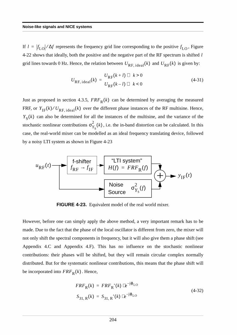
Noise-like signals and NICE systems
If represents the frequency grid line corresponding to the positive , Figure
4-22 shows that ideally, both the positive and the negative part of the RF spectrum is shifted
grid lines towards 0 Hz. Hence, the relation between and is given by:
(4-31)
Just as proposed in section 4.3.5, can be determined by averaging the measured
FRF, or over the different phase instances of the RF multisine. Hence,
can also be determined for all the instances of the multisine, and the variance of the
stochastic nonlinear contributions , i.e. the in-band distortion can be calculated. In this
case, the real-world mixer can be modelled as an ideal frequency translating device, followed
by a noisy LTI system as shown in Figure 4-23
However, before one can simply apply the above method, a very important remark has to be
made. Due to the fact that the phase of the local oscillator is different from zero, the mixer will
not only shift the spectral components in frequency, but it will also give them a phase shift (see
Appendix 4.C and Appendix 4.F). This has no influence on the stochastic nonlinear
contributions: their phases will be shifted, but they will remain circular complex normally
distributed. But for the systematic nonlinear contributions, this means that the phase shift will
be incorporated into . Hence,
(4-32)
FIGURE 4-23. Equivalent model of the real world mixer.
l fLO ∆f⁄= fLO
l
URF ideal, k( ) URF k( )
URF ideal, k( )URF k l+( ) k 0>⇔
URF k l–( ) k 0<⇔=
FRFR k( )
YIF k( ) URF ideal, k( )⁄
YS k( )
σYS
2 k( )
+NOISESOURCE
“LTI system”H f( ) FRFR f( )=uRF t( )
yIF t( )
NoiseSource
σYS
2 f( )
fRF fIF→f-shifter
FRFR k( )
FRFR k( ) FRFR ′ k( ) e jϕLO–⋅=
S31 R, k( ) S31 R, ′ k( ) e jϕLO–⋅=
204
Extension towards multi-port systems: mixers
where ( ) represents that part of that is independent of the
phase of the local oscillator signal.
In order to determine , one has to average the measured FRF (or -parameter)
over different instances of the RF multisine. At this point, four situations can occur:
1. One is able to measure the absolute phase of the local oscillator signal , and of the
RF and IF signals, for every instance of the multisine. In this case, can be de-
embedded out of , and can be determined as:
(4-33)
2. There is a constant phase difference between the phase of the local
oscillator signal, and the RF multisine, by e.g. synchronizing the internal clocks of the
LO source and the RF source. Furthermore, the measured waves are not calibrated in
phase, hence, , and are known except for a constant value. In other words,
(4-34)
where , and represent respectively the measured phases of the LO, RF and
IF signal, and , and are respectively the measurement errors made on the
phases of the RF, LO and IF signal. In this case, by using (4-33), can be
determined except for a constant phase shift. The systematic contributions of the FRF
will always have the following phase (see Appendix 4.F):
(4-35)
Hence, when applying (4-33) on measurements, the result will have the following phase:
(4-36)
FRFR ′ k( ) S31 R, ′ k( ) FRFR k( )
FRFR k( ) S31
ϕLO
e jϕLO–
FRFR k( ) FRFR ′ k( )
FRFR ′ k( ) E FRF k( )ejϕLO
=
∆φ ϕRF ϕLO–=
ϕRF ϕLO ϕIF
ϕRFm ϕRF ϕRF
e+=
ϕLOm ϕLO ϕLO
e+=
ϕIFm ϕIF ϕ IF
e +=
ϕRFm ϕLO
m ϕIFm
ϕRFe ϕLO
e ϕIFe
FRFR ′ k( )
φHαβk1 … kα l1 … lβ, , , , ,( ) ϕRF ϕLO–+( ) ϕRF–
φHαβk1 … kα l1 … lβ, , , , ,( ) ϕRF ϕLO– ϕIF
e ϕRF ϕRFe+( ) ϕLO ϕLO
e+( )+–+ +
φHαβk1 … kα l1 … lβ, , , , ,( ) ϕIF
e ϕRFe ϕLO
e+–+=
205
Noise-like signals and NICE systems
which is the phase of , except for a constant . If the phase
measurement errors do not vary significantly over the frequency band of interest,
is a constant, and the phase relations between the different points of
the transfer function are known.
3. One can guarantee that the phase of the local oscillator will be the same for each
measurement, but this constant phase remains unknown. In this case, will
be a constant, and averaging the FRF will yield the transfer function of the related linear
dynamic system . (4-32) shows that the LO phase independent transfer
function is then known, except for a constant factor ( ) that is frequency
independent. But the phase relations between the different points of the transfer function
are known.
4. If one cannot guarantee that the phase of the local oscillator will be the same for every
instance of the random multisine, and that this phase cannot be determined nor
synchronized with the RF multisine, then or will also be a
stochastic quantity, since it contains the factor . In general will be a instance
of an uniformly distributed random process on [ [. Hence, averaging the FRF (or
) will lead to an erroneous result (i.e. zero). In this case, another measurement
procedure has to be followed in order to determine the transfer function of the related
linear dynamic system. This technique is explained in the following section.
4.4.4 Getting extra information about the nonlinear mechanism of the mixerWhen the phase of the local oscillator is unknown, cannot be determined by
averaging the FRF. In this case, one has to create notches in the RF spectrum. The power of the
spectral components that will fill the notches at the IF port will be a measure for the in-band
distortions, as predicted by the NPR method, and explained in section 4.3.4. This technique is
based on the philosophy of the NPR method, but instead of using one notch in the center of the
frequency band (as the NPR method requires), it is possible to distribute the notches over the
whole band of interest. The question to be answered at this point is: Does an optimal way to
distribute the notches over the frequency band exist in order to get some extra information
about the mixer?
FRFR ′ k( ) ϕIFe ϕRF
e ϕLOe+–
ϕ IFe ϕRF
e ϕLOe+–
ϕLO e jϕLO–
FRFR k( )
e jϕLO–
FRFR k( ) S31 R, k( )
e jϕLO– ϕLO
0 2π,
S31
FRFR ′ k( )
206
Extension towards multi-port systems: mixers
For two-port devices, this problem has already been studied and solved in the literature [31].
This paper states that on one hand, special multisines can be designed to quantify the even and
odd nonlinear contributions of the device, and on the other hand, guidelines exist to give an
optimal estimate of the in-band distortions.
A. The even and odd nonlinearities.The key idea behind the discrimination of even and odd nonlinearities relies on a proper choice
of the excitation frequencies. If the excitation signal is composed only of tones with
frequencies that are an odd multiple of the grid frequency spacing , it is clear that any
product of an even number of frequency lines will be translated to frequency grid lines that are
an even multiple of the frequency grid spacing. This kind of spectral product appears in the
spectral products associated with even order Volterra kernels. On the other hand, if the product
of an odd number of spectral lines is made, the resulting frequency will appear at an odd
multiple of the frequency grid spacing. This is the case for the spectral products associated
with odd order Volterra kernels. Hence, the output spectrum of the even order Volterra
operators will lie at even frequency grid lines, while the output spectrum of the odd order
Volterra operators will lie at the odd frequency grid lines.
For three-port devices such as mixers, applying this simple rule to the RF signal is not correct
because the parity (i.e. the fact that a spectral component lies on an even or on an odd
frequency grid line) of the spectral combinations will no longer only depend on the parity of
the RF signal. The parity of the local oscillator also has to be taken into account. Furthermore,
the Volterra operators as presented for three-port devices (4-25) are no longer simply
even or odd. They can be even or odd both with respect to the RF spectral components and the
LO spectral components.
Depending on the parity of the RF and the LO spectral components, four different spectral
location of , given by
(4-37)
∆f
Hαβ [ ]
Hαβ uRF t( ) uLO t( ),[ ]
URF ki( )
i 1=
α
∏ ULO lj( )
j 1=
β
∏
207
Noise-like signals and NICE systems
can be encountered:
1. The RF multisine lies on even grid lines and the LO spectral components lie on odd grid
lines. Since a sum of even numbers is always even, the value of will determine if the
result lies on even or on odd frequency grid lines. Hence, it is possible to discriminate
between the even and odd order nonlinearities of the LO path in the nonlinear
mechanism:
(4-38)
2. The RF multisine lies on odd grid lines and the LO spectral components lie on even grid
lines. Since a sum of even numbers is always even, only the value of will determine if
the result lies on even or on odd frequency grid lines. Hence, it is possible to discriminate
between the even and odd order nonlinearities of the RF path in the nonlinear
mechanism:
(4-39)
3. Both the RF multisine and the LO spectral components lie on odd grid lines. This time,
will determine if the result lies on even or on odd frequency grid lines. Hence, it is
possible to discriminate between the even and odd order nonlinearities of the ( )-th
order Volterra operator:
(4-40)
4. Both the RF multisine and the LO spectral components lie on even grid lines. In this
case, all the spectral components of the IF spectrum will also fall on even grid lines, and
nothing will be detected at the odd frequency grid lines.
Hence, depending if the goal is to quantify the even and odd nonlinearities of the LO
contributions, or the RF contributions, or the combined ( ) contributions, one of the first
three above mentioned cases can be used.
β
β 2Z∈ Hαβ uRF t( ) uLO t( ),[ ] lies on even grid lines⇒
β 2Z 1+∈ Hαβ uRF t( ) uLO t( ),[ ] lies on odd grid lines⇒
α
α 2Z∈ Hαβ uRF t( ) uLO t( ),[ ] lies on even grid lines⇒
α 2Z 1+∈ Hαβ uRF t( ) uLO t( ),[ ] lies on odd grid lines⇒
α β+
α β+
α β+ 2Z∈ Hαβ uRF t( ) uLO t( ),[ ] lies on even grid lines⇒
α β+ 2Z 1+∈ Hαβ uRF t( ) uLO t( ),[ ] lies on odd grid lines⇒
α β+
208
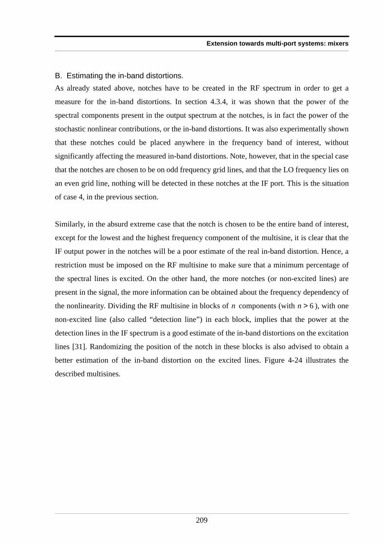
Extension towards multi-port systems: mixers
B. Estimating the in-band distortions.As already stated above, notches have to be created in the RF spectrum in order to get a
measure for the in-band distortions. In section 4.3.4, it was shown that the power of the
spectral components present in the output spectrum at the notches, is in fact the power of the
stochastic nonlinear contributions, or the in-band distortions. It was also experimentally shown
that these notches could be placed anywhere in the frequency band of interest, without
significantly affecting the measured in-band distortions. Note, however, that in the special case
that the notches are chosen to be on odd frequency grid lines, and that the LO frequency lies on
an even grid line, nothing will be detected in these notches at the IF port. This is the situation
of case 4, in the previous section.
Similarly, in the absurd extreme case that the notch is chosen to be the entire band of interest,
except for the lowest and the highest frequency component of the multisine, it is clear that the
IF output power in the notches will be a poor estimate of the real in-band distortion. Hence, a
restriction must be imposed on the RF multisine to make sure that a minimum percentage of
the spectral lines is excited. On the other hand, the more notches (or non-excited lines) are
present in the signal, the more information can be obtained about the frequency dependency of
the nonlinearity. Dividing the RF multisine in blocks of components (with ), with one
non-excited line (also called “detection line”) in each block, implies that the power at the
detection lines in the IF spectrum is a good estimate of the in-band distortions on the excitation
lines [31]. Randomizing the position of the notch in these blocks is also advised to obtain a
better estimation of the in-band distortion on the excited lines. Figure 4-24 illustrates the
described multisines.
n n 6>
209
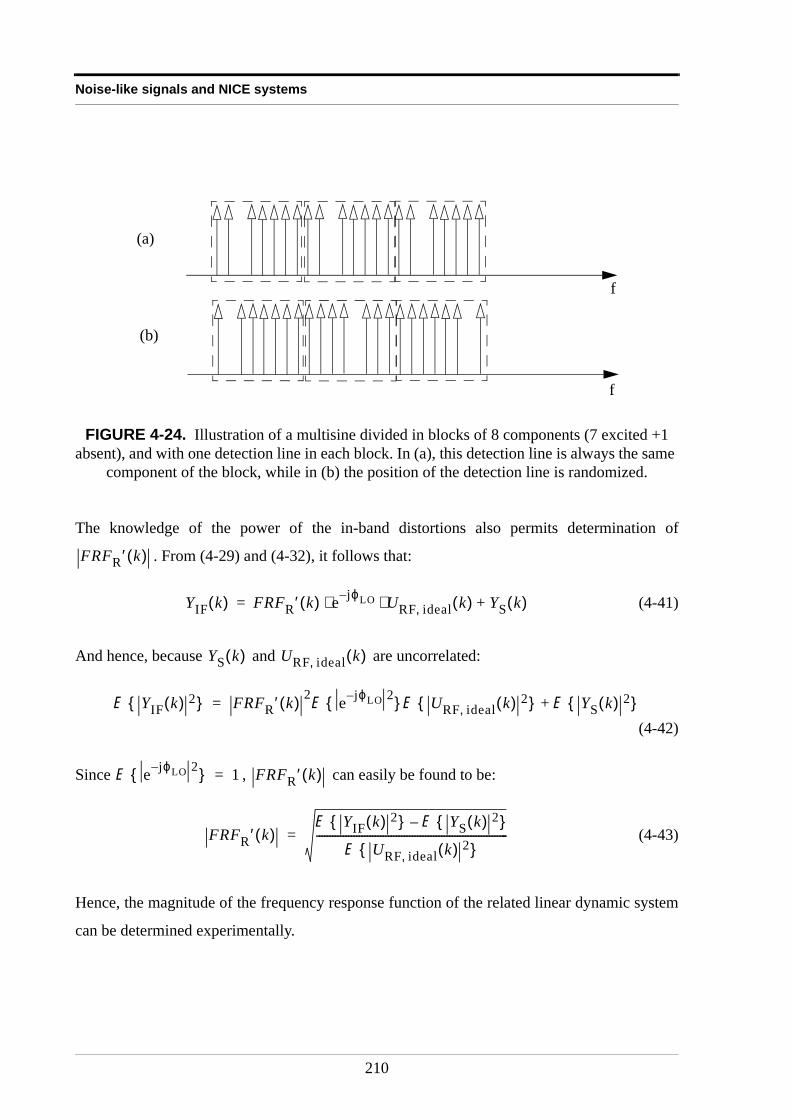
Noise-like signals and NICE systems
The knowledge of the power of the in-band distortions also permits determination of
. From (4-29) and (4-32), it follows that:
(4-41)
And hence, because and are uncorrelated:
(4-42)
Since , can easily be found to be:
(4-43)
Hence, the magnitude of the frequency response function of the related linear dynamic system
can be determined experimentally.
FIGURE 4-24. Illustration of a multisine divided in blocks of 8 components (7 excited +1 absent), and with one detection line in each block. In (a), this detection line is always the same
component of the block, while in (b) the position of the detection line is randomized.
(a)
(b)
f
f
FRFR ′ k( )
YIF k( ) FRFR ′ k( ) e jϕLO– URF ideal, k( )⋅ ⋅ YS k( )+=
YS k( ) URF ideal, k( )
E YIF k( ) 2 FRFR ′ k( ) 2E e jϕLO– 2 E URF ideal, k( ) 2 E YS k( ) 2 +=
E e jϕLO– 2 1= FRFR ′ k( )
FRFR ′ k( )E YIF k( ) 2 E YS k( ) 2 –
E URF ideal, k( ) 2 ------------------------------------------------------------------------=
210
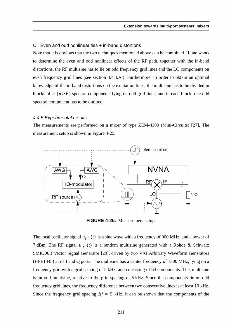
Extension towards multi-port systems: mixers
C. Even and odd nonlinearities + in-band distortionsNote that it is obvious that the two techniques mentioned above can be combined. If one wants
to determine the even and odd nonlinear effects of the RF path, together with the in-band
distortions, the RF multisine has to lie on odd frequency grid lines and the LO components on
even frequency grid lines (see section 4.4.4.A.). Furthermore, in order to obtain an optimal
knowledge of the in-band distortions on the excitation lines, the multisine has to be divided in
blocks of ( ) spectral components lying on odd grid lines, and in each block, one odd
spectral component has to be omitted.
4.4.5 Experimental resultsThe measurements are performed on a mixer of type ZEM-4300 (Mini-Circuits) [27]. The
measurement setup is shown in Figure 4-25.
The local oscillator signal is a sine wave with a frequency of 900 MHz, and a power of
7 dBm. The RF signal is a random multisine generated with a Rohde & Schwarz
SMIQ06B Vector Signal Generator [28], driven by two VXI Arbitrary Waveform Generators
(HPE1445) at its I and Q ports. The multisine has a center frequency of 1300 MHz, lying on a
frequency grid with a grid spacing of 5 kHz, and consisting of 64 components. This multisine
is an odd multisine, relative to the grid spacing of 5 kHz. Since the components lie on odd
frequency grid lines, the frequency difference between two consecutive lines is at least 10 kHz.
Since the frequency grid spacing kHz, it can be shown that the components of the
FIGURE 4-25. Measurement setup.
n n 6>
50Ω
NVNA
IQ-modulator
AWG AWG
RF source
I Q
XRF
LO
IF
reference clock
uLO t( )
uRF t( )
∆f 5=
211
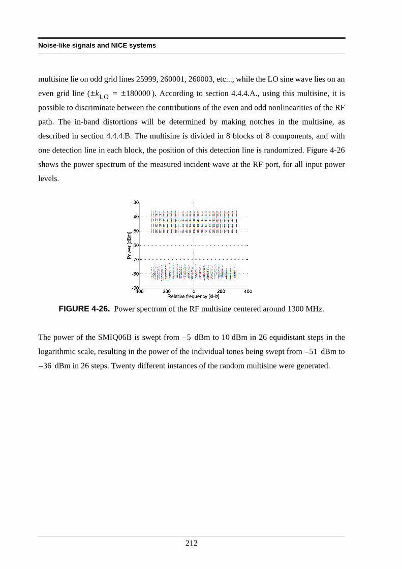
Noise-like signals and NICE systems
multisine lie on odd grid lines 25999, 260001, 260003, etc..., while the LO sine wave lies on an
even grid line ( ). According to section 4.4.4.A., using this multisine, it is
possible to discriminate between the contributions of the even and odd nonlinearities of the RF
path. The in-band distortions will be determined by making notches in the multisine, as
described in section 4.4.4.B. The multisine is divided in 8 blocks of 8 components, and with
one detection line in each block, the position of this detection line is randomized. Figure 4-26
shows the power spectrum of the measured incident wave at the RF port, for all input power
levels.
The power of the SMIQ06B is swept from dBm to 10 dBm in 26 equidistant steps in the
logarithmic scale, resulting in the power of the individual tones being swept from dBm to
dBm in 26 steps. Twenty different instances of the random multisine were generated.
FIGURE 4-26. Power spectrum of the RF multisine centered around 1300 MHz.
kLO± 180000±=
5–
51–
36–
212
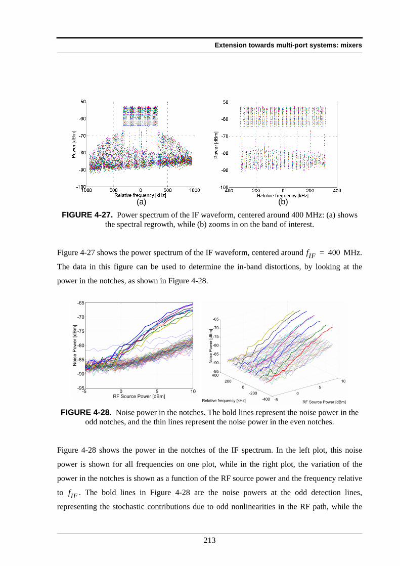
Extension towards multi-port systems: mixers
Figure 4-27 shows the power spectrum of the IF waveform, centered around MHz.
The data in this figure can be used to determine the in-band distortions, by looking at the
power in the notches, as shown in Figure 4-28.
Figure 4-28 shows the power in the notches of the IF spectrum. In the left plot, this noise
power is shown for all frequencies on one plot, while in the right plot, the variation of the
power in the notches is shown as a function of the RF source power and the frequency relative
to . The bold lines in Figure 4-28 are the noise powers at the odd detection lines,
representing the stochastic contributions due to odd nonlinearities in the RF path, while the
FIGURE 4-27. Power spectrum of the IF waveform, centered around 400 MHz: (a) shows the spectral regrowth, while (b) zooms in on the band of interest.
FIGURE 4-28. Noise power in the notches. The bold lines represent the noise power in the odd notches, and the thin lines represent the noise power in the even notches.
(a) (b)
fIF 400=
-5 0 5 10-95
-90
-85
-80
-75
-70
-65
Noi
se P
ower
[dB
m]
RF Source Power [dBm]-5
0
5
10
-400
-200
0
200
400-95
-90
-85
-80
-75
-70
-65
RF Source Power [dBm]Relative frequency [kHz]
Noi
se P
ower
[dB
m]
fIF
213
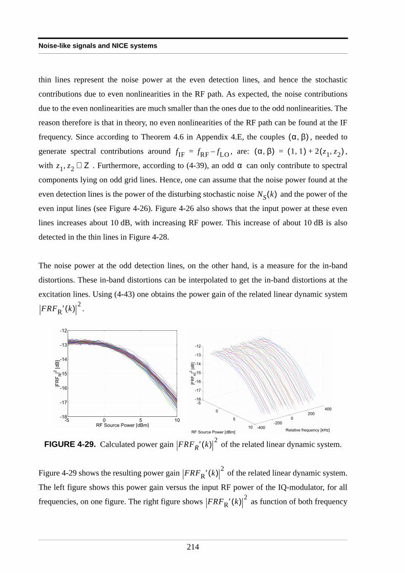
Noise-like signals and NICE systems
thin lines represent the noise power at the even detection lines, and hence the stochastic
contributions due to even nonlinearities in the RF path. As expected, the noise contributions
due to the even nonlinearities are much smaller than the ones due to the odd nonlinearities. The
reason therefore is that in theory, no even nonlinearities of the RF path can be found at the IF
frequency. Since according to Theorem 4.6 in Appendix 4.E, the couples , needed to
generate spectral contributions around , are: ,
with . Furthermore, according to (4-39), an odd can only contribute to spectral
components lying on odd grid lines. Hence, one can assume that the noise power found at the
even detection lines is the power of the disturbing stochastic noise and the power of the
even input lines (see Figure 4-26). Figure 4-26 also shows that the input power at these even
lines increases about 10 dB, with increasing RF power. This increase of about 10 dB is also
detected in the thin lines in Figure 4-28.
The noise power at the odd detection lines, on the other hand, is a measure for the in-band
distortions. These in-band distortions can be interpolated to get the in-band distortions at the
excitation lines. Using (4-43) one obtains the power gain of the related linear dynamic system
.
Figure 4-29 shows the resulting power gain of the related linear dynamic system.
The left figure shows this power gain versus the input RF power of the IQ-modulator, for all
frequencies, on one figure. The right figure shows as function of both frequency
FIGURE 4-29. Calculated power gain of the related linear dynamic system.
α β,( )
fIF fRF fLO–= α β,( ) 1 1,( ) 2 z1 z2,( )+=
z1 z2, Z∈ α
NS k( )
FRFR ′ k( ) 2
-5 0 5 10-18
-17
-16
-15
-14
-13
-12
RF Source Power [dBm]
|FR
FR
|2 [dB
]
-5
0
5
10 -400-200
0200
400
-18
-17
-16
-15
-14
-13
-12
Relative frequency [kHz]RF Source Power [dBm]
|FR
FR
|2 [dB
]
FRFR ′ k( ) 2
FRFR ′ k( ) 2
FRFR ′ k( ) 2
214
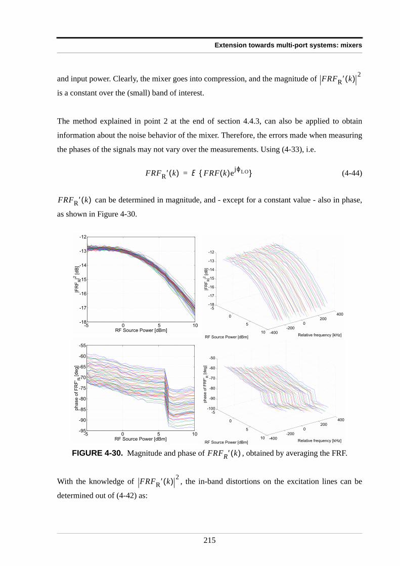
Extension towards multi-port systems: mixers
and input power. Clearly, the mixer goes into compression, and the magnitude of
is a constant over the (small) band of interest.
The method explained in point 2 at the end of section 4.4.3, can also be applied to obtain
information about the noise behavior of the mixer. Therefore, the errors made when measuring
the phases of the signals may not vary over the measurements. Using (4-33), i.e.
(4-44)
can be determined in magnitude, and - except for a constant value - also in phase,
as shown in Figure 4-30.
With the knowledge of , the in-band distortions on the excitation lines can be
determined out of (4-42) as:
FIGURE 4-30. Magnitude and phase of , obtained by averaging the FRF.
FRFR ′ k( ) 2
FRFR ′ k( ) E FRF k( )ejϕLO =
FRFR ′ k( )
-5 0 5 10-18
-17
-16
-15
-14
-13
-12
RF Source Power [dBm]
|FR
FR
|2 [dB
]
-5
0
5
10 -400-200
0200
400
-18
-17
-16
-15
-14
-13
-12
Relative frequency [kHz]RF Source Power [dBm]
|FR
FR
|2 [dB
]
-5 0 5 10-95
-90
-85
-80
-75
-70
-65
-60
-55
RF Source Power [dBm]
phas
e of
FR
F' R
[deg
]
-5
0
5
10 -400-200
0200
400
-100
-90
-80
-70
-60
-50
Relative frequency [kHz]RF Source Power [dBm]
phas
e of
FR
F' R
[deg
]
FRFR ′ k( )
FRFR ′ k( ) 2
215
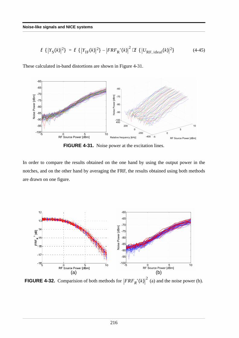
Noise-like signals and NICE systems
(4-45)
These calculated in-band distortions are shown in Figure 4-31.
In order to compare the results obtained on the one hand by using the output power in the
notches, and on the other hand by averaging the FRF, the results obtained using both methods
are drawn on one figure.
FIGURE 4-31. Noise power at the excitation lines.
FIGURE 4-32. Comparision of both methods for (a) and the noise power (b).
E YS k( ) 2 E YIF k( ) 2 FRFR ′ k( ) 2 E URF ideal, k( ) 2 ⋅–=
-5 0 5 10-100
-95
-90
-85
-80
-75
-70
-65
-60
Noi
se P
ower
[dB
m]
RF Source Power [dBm] -5
0
5
10
-400
-200
0
200
400-100
-90
-80
-70
-60
RF Source Power [dBm]Relative frequency [kHz]
Noi
se P
ower
[dB
m]
-5 0 5 10-100
-95
-90
-85
-80
-75
-70
-65
-60
Noi
se P
ower
[dB
m]
RF Source Power [dBm]
(a) (b)
FRFR′ k( ) 2
216

Extension towards multi-port systems: mixers
The red lines in Figure 4-32, are the results obtained by using the output power in the notches,
while the blue dots and lines represent the results obtained using the averaging of the FRF.
Clearly, both methods are in good agreement. Hence, when using the designed multisine, the
output power in the notches is a good estimate for the in-band distortions on the excitation
lines.
217
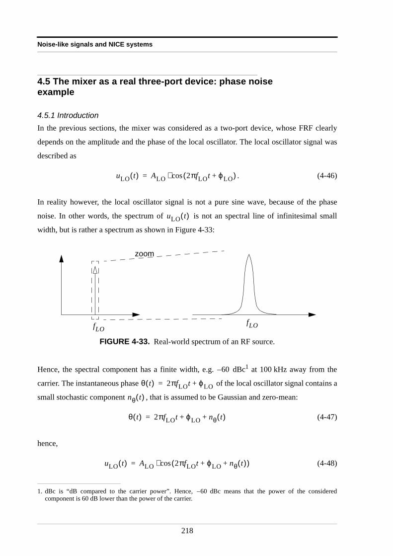
Noise-like signals and NICE systems
4.5 The mixer as a real three-port device: phase noise example
4.5.1 IntroductionIn the previous sections, the mixer was considered as a two-port device, whose FRF clearly
depends on the amplitude and the phase of the local oscillator. The local oscillator signal was
described as
. (4-46)
In reality however, the local oscillator signal is not a pure sine wave, because of the phase
noise. In other words, the spectrum of is not an spectral line of infinitesimal small
width, but is rather a spectrum as shown in Figure 4-33:
Hence, the spectral component has a finite width, e.g. dBc1 at 100 kHz away from the
carrier. The instantaneous phase of the local oscillator signal contains a
small stochastic component , that is assumed to be Gaussian and zero-mean:
(4-47)
hence,
(4-48)
FIGURE 4-33. Real-world spectrum of an RF source.
1. dBc is “dB compared to the carrier power”. Hence, dBc means that the power of the consideredcomponent is 60 dB lower than the power of the carrier.
uLO t( ) ALO 2πfLOt ϕLO+( )cos⋅=
uLO t( )
zoom
fLOfLO
60–
60–
θ t( ) 2πfLOt ϕLO+=
nθ t( )
θ t( ) 2πfLOt ϕLO nθ t( )+ +=
uLO t( ) ALO 2πfLOt ϕLO nθ t( )+ +( )cos⋅=
218
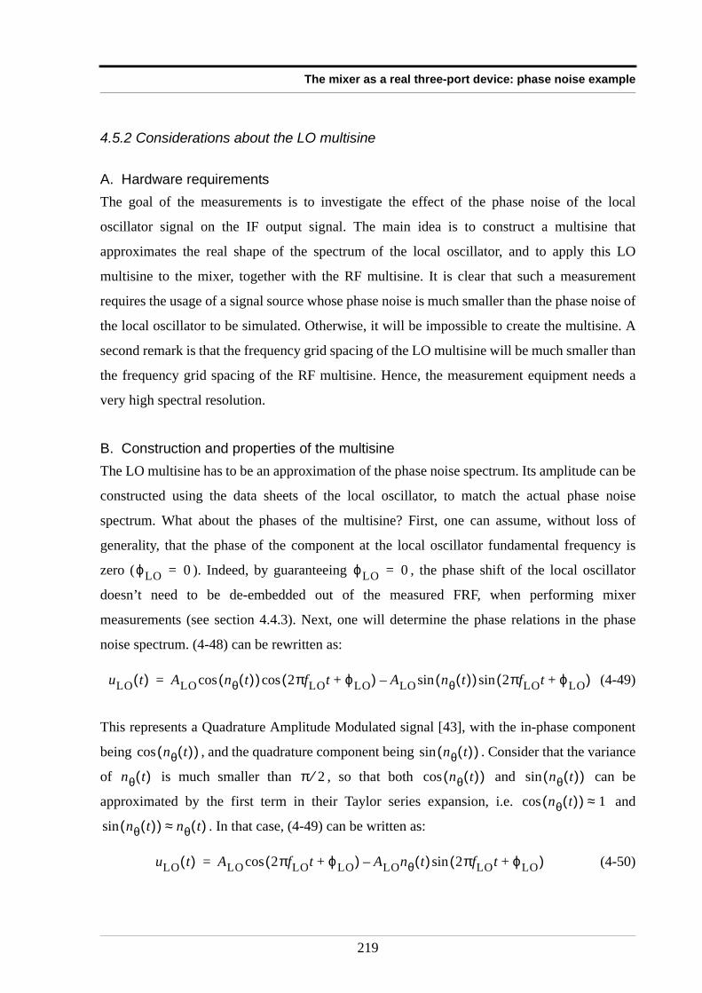
The mixer as a real three-port device: phase noise example
4.5.2 Considerations about the LO multisine
A. Hardware requirementsThe goal of the measurements is to investigate the effect of the phase noise of the local
oscillator signal on the IF output signal. The main idea is to construct a multisine that
approximates the real shape of the spectrum of the local oscillator, and to apply this LO
multisine to the mixer, together with the RF multisine. It is clear that such a measurement
requires the usage of a signal source whose phase noise is much smaller than the phase noise of
the local oscillator to be simulated. Otherwise, it will be impossible to create the multisine. A
second remark is that the frequency grid spacing of the LO multisine will be much smaller than
the frequency grid spacing of the RF multisine. Hence, the measurement equipment needs a
very high spectral resolution.
B. Construction and properties of the multisineThe LO multisine has to be an approximation of the phase noise spectrum. Its amplitude can be
constructed using the data sheets of the local oscillator, to match the actual phase noise
spectrum. What about the phases of the multisine? First, one can assume, without loss of
generality, that the phase of the component at the local oscillator fundamental frequency is
zero ( ). Indeed, by guaranteeing , the phase shift of the local oscillator
doesn’t need to be de-embedded out of the measured FRF, when performing mixer
measurements (see section 4.4.3). Next, one will determine the phase relations in the phase
noise spectrum. (4-48) can be rewritten as:
(4-49)
This represents a Quadrature Amplitude Modulated signal [43], with the in-phase component
being , and the quadrature component being . Consider that the variance
of is much smaller than , so that both and can be
approximated by the first term in their Taylor series expansion, i.e. and
. In that case, (4-49) can be written as:
(4-50)
ϕLO 0= ϕLO 0=
uLO t( ) ALO nθ t( )( ) 2πfLOt ϕLO+( ) ALO nθ t( )( )sin 2πfLOt ϕLO+( )sin–coscos=
nθ t( )( )cos nθ t( )( )sin
nθ t( ) π 2⁄ nθ t( )( )cos nθ t( )( )sin
nθ t( )( )cos 1≈
nθ t( )( )sin nθ t( )≈
uLO t( ) ALO 2πfLOt ϕLO+( ) ALOnθ t( ) 2πfLOt ϕLO+( )sin–cos=
219
Noise-like signals and NICE systems
Taking the DFT of (4-50), over an integer number of periods, yields
(4-51)
where is the frequency grid line corresponding to , represents the discrete Dirac
impulse (or Kronecker delta) ; . represents the
DFT spectrum of , and this DFT spectrum is a narrowband spectrum (typically a few
MHz [39]).
The phase noise spectrum consists of two parts: the spectrum of the pure sinewave
, superimposed on the spectrum of , centered around , and
given a phase shift of .
For , (4-51) becomes:
(4-52)
When , one can state that the phase of simply equals , (or zero in
the considered case).
For , (4-51) becomes:
(4-53)
Hence, the phases of the spectral components symmetrical to are not simply opposite in
sign. They are opposite in sign and each component has a phase shift of , see
Figure 4-34.
ULO k( )ALO
2----------ejϕLO δ k kLO–( ) δ k kLO+( )+( )=
Nθ k( )*ALO
2---------- δ k kLO–( )e
j π2--- ϕLO+
δ k kLO+( )ej π
2--- ϕLO+ –
+
+
kLO fLO δ k( )
δ k( ) 1= for k 0= δ k( ) 0= for k 0≠ Nθ k( )
nθ mTs( )
ALO 2πfLOt ϕLO+( )cos nθ t( ) fLO
90°+
k kLO=
ULO kLO( )ALO
2----------ejϕLO
ALO2
----------ej π
2--- ϕLO+
Nθ 0( )+=
Nθ 0( ) 1« ULO kLO( ) ϕLO
k kLO≠
ULO k( )ALO
2----------e
j π2--- ϕLO+
Nθ k kLO–( )ALO
2----------e
j– π2--- ϕLO+
Nθ k kLO+( )+=
fLO
π 2⁄ ϕLO+
220
The mixer as a real three-port device: phase noise example
Otherwise told, for , components symmetrical to the center frequency have
supplementary angles, i.e. the sum of the angles is always .
Since is Gaussian noise, the spectral components of are circular complex
normally distributed, and hence their phases are uniformly distributed over [ [. Hence the
phases of the spectral components of the phase noise spectrum will also be uniformly
distributed over [ [. Note that the phases of the lower part of the spectrum are
supplementary angles of a uniform distribution over [ [, yielding also a uniform
distribution over [ [.
Conclusion: the constructed LO multisine will be a random multisine, except for the
component at , which is a deterministic one.
4.5.3 Properties of the FRFThe goal of this section is to determine the in-band distortions in the frequency band around
. Hence, the FRF for a mixer as defined in section 4.4.3, will be studied, when a random
multisine is applied at both the RF and the LO port. The output spectrum at the IF port is given
by:
(4-54)
FIGURE 4-34. Schematic representation of the construction of the LO multisine, for .
ϕ π2---+ϕ– π
2---+ 0Phases
Amplitudes
ϕLO 0=
ϕLO 0=
π
nθ t( ) Nθ k( )
0 2π,
0 2π,
0 2π,
0 2π,
fLO
fIF
YIF k( ) YIF αβ( ) k( )β∑
α∑=
221
Noise-like signals and NICE systems
with . The smallest values for and to obtain spectral components around
is . All the other values for and that will yield spectral contributions
around are then given by with (see Theorem 4.6 in
Appendix 4.E). is a (positive) frequency grid line on which a component of the RF multisine
lies, and is the (positive) frequency grid line corresponding to .
The frequency response function of the mixer is given by (for ):
(4-55)
(4-55) consists of terms of the following form:
(4-56)
with the constraint . When not considering very high degrees
of nonlinearity, the constraint has to be split into two constraints and
(see Theorem 4.6 in Appendix 4.E).
Six distinct terms will contribute to the FRF:
(4-57)
1. is the FRF of the “underlying linear system”, i.e. the result of the Volterra
operator , or the term
(4-58)
Its phase is .
2. represents the bias or systematic nonlinear contributions to the FRF, both
with respect to the RF and the LO port. This value is independent of the random phases
of both the RF and the LO multisines. It consists of the terms:
α β, 2N 1+∈ α β
fIF α β 1= = α β
fIF α β,( ) 1 1,( ) 2 γ ε,( )+= γ ε, N∈
k
l fLO
k 0>
FRF k( ) Y k( )URF ideal, k( )--------------------------------
YIF αβ( ) k( )β∑
α∑
URF ideal, k( )----------------------------------------= =
Hαβ k1 … kα l1 … lβ, , , , ,( )URF k1( )…URF kα( )ULO l1( )…ULO lβ( )
URF ideal, k( )----------------------------------------------------------------------------------------------------
k1 … kα l1 … lβ+ + + + + k=
k1 … kα+ + k= l+
l1 … lβ+ + l–=
FRF k( ) FRFlin k( ) FRFBB k( ) FRFBS k( ) FRFSB k( ) FRFSS k( ) NFRF k( )+ + + + +=
FRFlin k( )
H11 uRF t( ) uLO t( ),[ ]
H11 k l+ l–,( )URF k l+( )ULO l–( )
URF ideal, k( )------------------------------------------------ H11 k l+ l–,( )ULO l–( )=
φH11k l+ l–,( ) ϕLO–
FRFBB k( )
222
The mixer as a real three-port device: phase noise example
where one of the indices ( ), and the other s are grouped in
pairs of opposite indices (this is possible since is odd). One of the indices
( ) and the other ‘s are grouped in pairs of opposite indices (this is
possible since is odd). The phase of these terms is .
3. represents the nonlinear contributions to the FRF, that are systematic with
respect to the RF port, and stochastic with respect to the LO port. This value is
independent of the random phases of the RF multisine, but depends on the random
phases of the LO multisines. It consists of the terms:
where one of the indices ( ), and the other s are grouped in
pairs of opposite indices (this is possible since is odd). It is not true that one of the
indices ( ) and the other s are grouped in pairs of opposite
indices. The phase of these terms is
4. represents the nonlinear contributions to the FRF, that are stochastic with
respect to the RF port, and systematic with respect to the LO port. This value is
independent of the random phases of the LO multisine, but depends on the random
phases of the RF multisines. It consists of the terms:
where it is not so that one of the indices ( ), and the other s
are grouped in pairs of opposite indices. But, it is true that one of the indices
( ) and the other s are grouped in pairs of opposite indices. The phase of
these terms is
Hαβ k1 … kα l1 … lβ, , , , ,( )URF k1( )…URF kα( )ULO l1( )…ULO lβ( )
URF ideal, k( )----------------------------------------------------------------------------------------------------
ki k l+= i 1 … α, , ∈ ki
α lj l–=
j 1 … β, , ∈ ljβ φHαβ
k1 … kα l1 … lβ, , , , ,( ) ϕLO–
FRFBS k( )
Hαβ k1 … kα l1 … lβ, , , , ,( )URF k1( )…URF kα( )ULO l1( )…ULO lβ( )
URF ideal, k( )----------------------------------------------------------------------------------------------------
ki k l+= i 1 … α, , ∈ ki
α
lj l–= j 1 … β, , ∈ lj
φHαβk1 … kα l1 … lβ, , , , ,( ) φULO
lj( )
j 1=
β
∑+
FRFSB k( )
Hαβ k1 … kα l1 … lβ, , , , ,( )URF k1( )…URF kα( )ULO l1( )…ULO lβ( )
URF ideal, k( )----------------------------------------------------------------------------------------------------
ki k l+= i 1 … α, , ∈ ki
lj l–=
j 1 … β, , ∈ lj
223
Noise-like signals and NICE systems
5. represents the nonlinear contributions to the FRF, that are stochastic with
respect to both the RF port and the LO port. This value depends on both the random
phases of the RF and the LO multisines. It consists of the terms:
where it is not so that one of the indices ( ), and the other ‘s
are grouped in pairs of opposite indices. And it is not so that one of the indices
( ) and the other ‘s are grouped in pairs of opposite indices. The phase of
these terms is
6. is a stochastic component on the FRF, due to the effect of the input noise, the
noise added by the mixer itself , or due to the noise added by the measurement
system. These contributions are assumed to be extremely small, as discussed in section
4.2
If the phases of the RF and the LO random multisines vary randomly, three circular complex
normally distributed noise sources created by the stochastic character of the input signals will
deteriorate the IF output signal. These noise sources are , and coming
respectively from , and . They hence characterize
respectively the stochastic contributions coming from the LO port, the stochastic contributions
coming from the RF port, and the stochastic contributions coming from both ports. These noise
sources are uncorrelated, and hence their powers can be added (see Appendix 4.G).
As proposed in section 4.3.5, the FRF of the related linear dynamic system
can be determined by averaging the measured FRF over
φHαβk1 … kα l1 … lβ, , , , ,( ) φURF
ki( )
i 1=
α
∑ ϕLO– φURFk( )–+
FRFSS k( )
Hαβ k1 … kα l1 … lβ, , , , ,( )URF k1( )…URF kα( )ULO l1( )…ULO lβ( )
URF ideal, k( )---------------------------------------------------------------------------------------------------
ki k l+= i 1 … α, , ∈ ki
lj l–=
j 1 … β, , ∈ lj
φHαβk1 … kα l1 … lβ, , , , ,( ) φURF
ki( )
i 1=
α
∑ φULOlj( )
j 1=
β
∑ φURFk( )–+ +
NFRF k( )
NA k( )
YBS k( ) YSB k( ) YSS k( )
FRFBS k( ) FRFSB k( ) FRFSS k( )
FRFR k( ) FRFlin k( )= FRFBB k( )+
224
The mixer as a real three-port device: phase noise example
the different phase instances of the RF and the LO multisines. Hence,
can also be determined for all instances of the multisine, and thus
, the variance of all the stochastic nonlinear contributions, i.e. the in-band
distortion can be calculated. Hence, the mixer (including the effect of the phase noise of the
local oscillator) can be modelled as an ideal frequency translating device, followed by a noisy
LTI system as shown in Figure 4-23. This time, the noise source also contains the effect of the
phase noise of the LO.
It is also possible to determine the variances , and (or powers) of
each of the three noise sources separately. Two methods can be used to determine these noise
powers. The first method requires the possibility to measure all the powers and phases at all the
ports, while the second method only requires a power measurement at the IF port.
A. By measuring the FRF• is obtained by applying a random multisine at the RF and the
LO port. From these measurements, one also obtains ,
using
(4-59)
and hence .
• If the same instance of the RF multisine is fed at the RF port, while the
LO multisine varies from instance to instance, the phases of the RF
multisine will be deterministic over the measurements, and hence the
average of the FRF will be:
(4-60)
From these measurements, one also obtains , using
(4-61)
and hence .
YSB k( ) YBS k( ) YSS k( )+ +
σYBS YSB YSS+ +2 k( )
σYBS
2 k( ) σYSB
2 k( ) σYSS
2 k( )
FRFR k( )
YBS YSB YSS+ +
YBS YSB YSS+ + YIF FRFR URF⋅–=
σYBS YSB YSS+ +2
E FRF k( ) FRFlin k( ) FRFBB k( ) FRFSB k( )+ +=
YBS YSS+
YBS YSS+ YIF E FRF URF⋅–=
σYBS YSS+2
225
Noise-like signals and NICE systems
• Next, if the same instance of the LO multisine is fed at the LO port, while
the RF multisine varies from instance to instance, the phases of the LO
multisine will be deterministic over the measurements, and hence the
average of the FRF will be:
(4-62)
From these measurements, one also obtains , using
(4-63)
and hence .
From the three measured variances , and , the variances
of each individual noise source can easily be calculated:
(4-64)
B. By creating notches in the multisinesSuppose that spectral component in the RF multisine. This means that
there will be no systematic contributions coming from the RF multisine in the spectral
component at the IF spectrum (see also section 4.3). Therefore,
and, : the
output spectrum in the notch will contain the powers of only two of the three noise sources, i.e.
the effect of the stochastic properties of the RF input and the effect of the combined RF and LO
stochastic input. Hence, will be measured. However, the effect of the stochastic
properties of the LO input signal, i.e. the disturbing effect of the phase noise on the systematic
nonlinear contributions, will not be measured in the notch.
Alternatively, when omitting a spectral component in the LO multisine, these notches will be
filled in the IF spectrum with only stochastic contributions of the LO multisine, i.e.
E FRF k( ) FRFlin k( ) FRFBB k( ) FRFBS k( )+ +=
YSB YSS+
YSB YSS+ YIF E FRF URF⋅–=
σYSB YSS+2
σYBS YSB YSS+ +2 σYBS YSS+
2 σYSB YSS+2
σYBS
2 σYBS YSB YSS+ +2 σYSB YSS+
2–=
σYSB
2 σYBS YSB YSS+ +2 σYBS YSS+
2–=
σYSS
2 σYBS YSS+2 σYSB YSS+
2 σYBS YSB YSS+ +2–+=
URF ideal, k0( ) 0=
YIF k0( )
FRFlin k0( ) FRFBB k0( ) FRFBS k0( ) 0= = = YIF k0( ) YSB k0( ) YSS k0( )+=
σYSB YSS+2
226
The mixer as a real three-port device: phase noise example
. Again, only the variance of two of the three noise
sources can be measured.
Finally, when a spectral component is omitted in both the RF and the LO multisine, there will
be a spectral line in the IF spectrum, that contains only stochastic contributions from the RF
and IF multisine, and no systematic contributions, i.e. . This means that the
variance in this notch corresponds to the variance of only one of the three noise sources.
With the knowledge of , and , the variance of each of the three
noise sources separately can be determined, was obtained immediately in the last
measurement, and the other two can be determined as follows:
(4-65)
Note that measuring the output power in the notches in order to get an estimate of the in-band
distortions is only valid if the phase noise of the local oscillator can be assumed to be
negligible.
YIF k( ) YBS k( ) YSS k( )+= σYBS YSS+2
YIF k( ) YSS k( )=
σYSS
2
σYSB YSS+2 σYBS YSS+
2 σYSS
2
σYSS
2
σYBS
2 σYBS YSS+2 σYSS
2–=
σYSB
2 σYSB YSS+2 σYSS
2–=
227
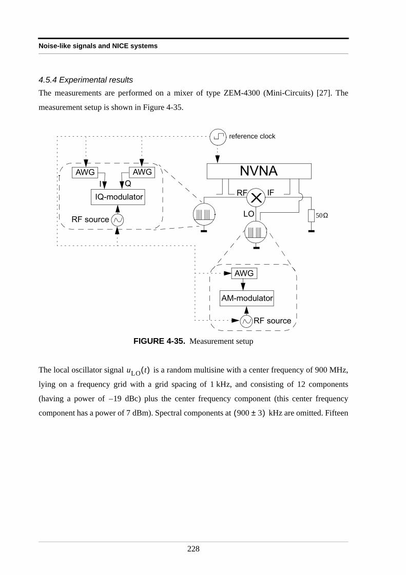
Noise-like signals and NICE systems
4.5.4 Experimental resultsThe measurements are performed on a mixer of type ZEM-4300 (Mini-Circuits) [27]. The
measurement setup is shown in Figure 4-35.
The local oscillator signal is a random multisine with a center frequency of 900 MHz,
lying on a frequency grid with a grid spacing of 1 kHz, and consisting of 12 components
(having a power of dBc) plus the center frequency component (this center frequency
component has a power of 7 dBm). Spectral components at kHz are omitted. Fifteen
FIGURE 4-35. Measurement setup
50Ω
NVNA
IQ-modulator
AWG AWG
RF source
I Q
XRF
LO
IF
reference clock
AM-modulator
AWG
RF source
uLO t( )
19–
900 3±( )
228
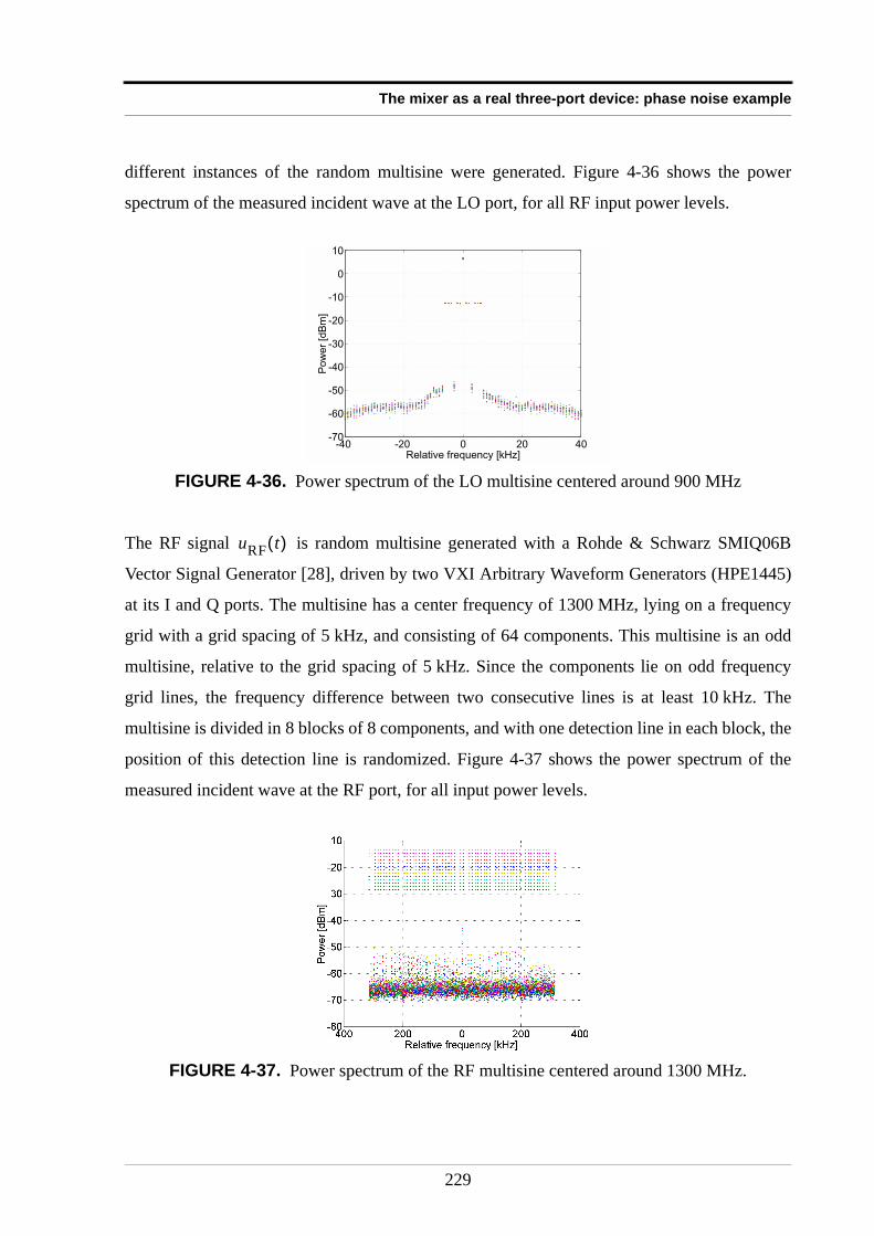
The mixer as a real three-port device: phase noise example
different instances of the random multisine were generated. Figure 4-36 shows the power
spectrum of the measured incident wave at the LO port, for all RF input power levels.
The RF signal is random multisine generated with a Rohde & Schwarz SMIQ06B
Vector Signal Generator [28], driven by two VXI Arbitrary Waveform Generators (HPE1445)
at its I and Q ports. The multisine has a center frequency of 1300 MHz, lying on a frequency
grid with a grid spacing of 5 kHz, and consisting of 64 components. This multisine is an odd
multisine, relative to the grid spacing of 5 kHz. Since the components lie on odd frequency
grid lines, the frequency difference between two consecutive lines is at least 10 kHz. The
multisine is divided in 8 blocks of 8 components, and with one detection line in each block, the
position of this detection line is randomized. Figure 4-37 shows the power spectrum of the
measured incident wave at the RF port, for all input power levels.
FIGURE 4-36. Power spectrum of the LO multisine centered around 900 MHz
FIGURE 4-37. Power spectrum of the RF multisine centered around 1300 MHz.
-40 -20 0 20 40-70
-60
-50
-40
-30
-20
-10
0
10
Relative frequency [kHz]
Pow
er [d
Bm
]
uRF t( )
229
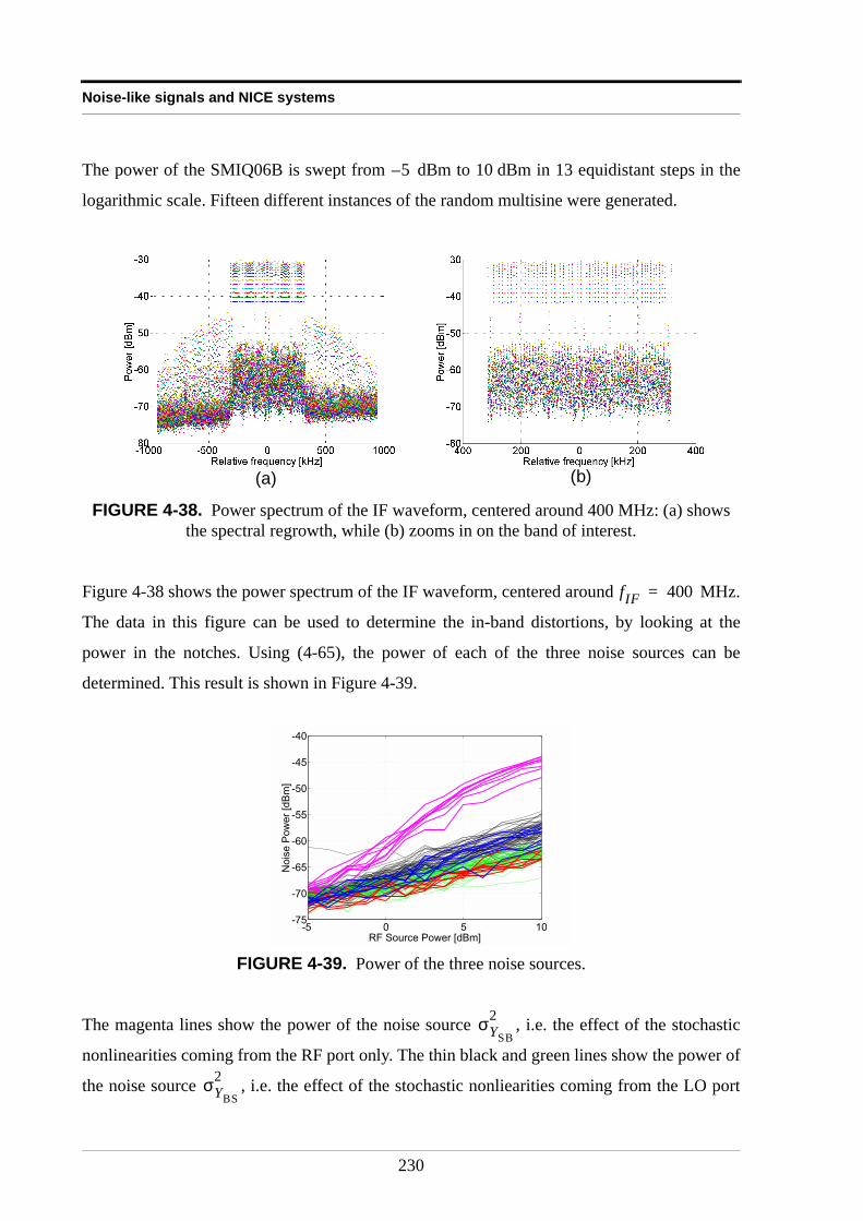
Noise-like signals and NICE systems
The power of the SMIQ06B is swept from dBm to 10 dBm in 13 equidistant steps in the
logarithmic scale. Fifteen different instances of the random multisine were generated.
Figure 4-38 shows the power spectrum of the IF waveform, centered around MHz.
The data in this figure can be used to determine the in-band distortions, by looking at the
power in the notches. Using (4-65), the power of each of the three noise sources can be
determined. This result is shown in Figure 4-39.
The magenta lines show the power of the noise source , i.e. the effect of the stochastic
nonlinearities coming from the RF port only. The thin black and green lines show the power of
the noise source , i.e. the effect of the stochastic nonliearities coming from the LO port
FIGURE 4-38. Power spectrum of the IF waveform, centered around 400 MHz: (a) shows the spectral regrowth, while (b) zooms in on the band of interest.
FIGURE 4-39. Power of the three noise sources.
5–
(b)(a)
fIF 400=
-5 0 5 10-75
-70
-65
-60
-55
-50
-45
-40
Noi
se P
ower
[dB
m]
RF Source Power [dBm]
σYSB
2
σYBS
2
230
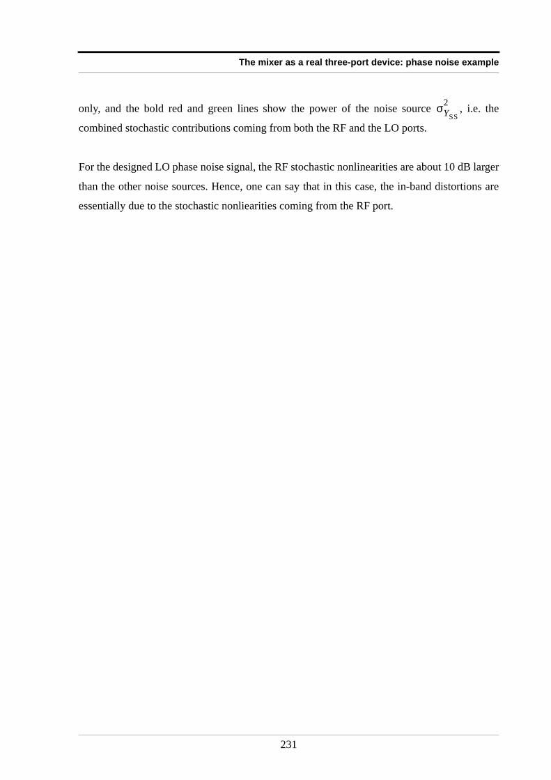
The mixer as a real three-port device: phase noise example
only, and the bold red and green lines show the power of the noise source , i.e. the
combined stochastic contributions coming from both the RF and the LO ports.
For the designed LO phase noise signal, the RF stochastic nonlinearities are about 10 dB larger
than the other noise sources. Hence, one can say that in this case, the in-band distortions are
essentially due to the stochastic nonliearities coming from the RF port.
σYSS
2
231
Noise-like signals and NICE systems
4.6 Conclusion When noise-like signals (such as the ones that are used in telecommunication environments)
are fed to NICE systems, the output noise (i.e. that part of the output spectrum that is not
correlated with the noise-like input signal) consists of two contributions. The first contribution
is due to the noise that is superimposed on the input signal , and that is processed by the
system, or the noise generated by the noisy NICE system itself . This is the noise that
was studied in previous chapters. The second contribution is noise that is created by the
nonlinear mechanism itself, based on the randomness of the input signal. The DFT spectrum of
this noise is uncorrelated with the DFT spectrum of the input signal :
. For narrowband NICE systems, the total power of the noise
superimposed on the input signal is rather small, and hence, the contribution of this noise to the
output noise can be neglected compared to the noise that the NICE system creates out of the
noise-like input signal.
A general framework using random multisines to model the noise-like input signals was
chosen. Multisines have the advantage that the magnitude and phase of each of their spectral
components can be modified at will, and the randomness of the phases assures a noise-like
behavior. Under this framework, it was shown that the output spectrum of the NICE system
contains two types of contributions. Systematic contributions yield a filtered version of the
input random multisine, while stochastic contributions can be modelled as a frequency
dependent noise source, that will be responsible for the in-band distortions. With this
description of the NICE system, using systematic and stochastic contributions, it can be shown
that the NPR and the CCPR method, two apparently contradictory methods in the literature,
used to quantify in-band distortions, both quantify the in-band distortions, but under different
assumptions. Hence, a NICE system excited by noise-like signals, can be modelled as a LTI
system and a noise source, i.e. as a noisy LTI system!
To extend the theory of the systematic and stochastic contributions towards multi-port devices,
the behavior of a mixer, excited with random multisines at its RF port was studied. The local
oscillator was in a first step assumed to be part of the mixer. Hence, the mixer which is a three-
port device could be treated as a two-port device. A frequency response function can then be
nu t( )
nA t( )
NNL k( ) U k( )
E U k( )NNL k( ) 0=
232
Conclusion
defined between the output of the ideal frequency translator, and the actual output of the mixer.
Hence, a mixer that has to shift noise-like signals whose power is constant in the frequency
band, can be modelled as an ideal frequency shifter, followed by a LTI system and a noise
source, i.e. as the cascade of an ideal frequency translator and a noisy LTI system!
In a second step, the local oscillator signal is no longer considered as a pure sinewave, but as a
real sinewave affected by phase noise. In order to know the effect of this phase noise on the
output spectrum of the mixer, the phase noise spectrum is modelled as a random multisine. A
random multisine is now applied at both input ports of the mixer. This time, the contributions
at the output spectrum cannot be simply tagged as stochastic or systematic: they will be
systematic or stochastic with respect to each input port. This leads to four contributions, with
each of the contributions being systematic or stochastic with respect to the RF port and the LO
port. The contribution that is systematic to both ports represents a filtered version of the
convolution of the RF and the LO multisine, and the three other contributions are responsible
for in-band distortions. They represent three independent noise sources: the effect of the
random character of the RF signal alone, the effect of the random character of the LO port
alone (i.e. the phase noise), and the combined random characters. Hence, a mixer that has to
shift noise-like signals whose power is constant in the frequency band, and whose local
oscillator is affected by phase noise, can be modelled as an ideal frequency shifter, followed by
a LTI system and three independent noise sources, i.e. as the cascade of an ideal frequency
translator and a noisy LTI system!
For all these models, two measurement methods are proposed. The first method requires the
measurement of both power and phase at each port of the device, and yields a frequency
response function in magnitude and phase, plus a noise source to quantify the in-band
distortions. The second method only requires the measurement of the power at each of the
ports, and the usage of notches in the random multisine. The latter measurement method only
yields the magnitude of the frequency response function, and the noise source.
233
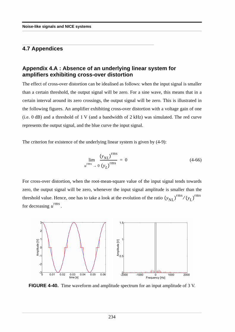
Noise-like signals and NICE systems
4.7 Appendices
Appendix 4.A : Absence of an underlying linear system for amplifiers exhibiting cross-over distortionThe effect of cross-over distortion can be idealised as follows: when the input signal is smaller
than a certain threshold, the output signal will be zero. For a sine wave, this means that in a
certain interval around its zero crossings, the output signal will be zero. This is illustrated in
the following figures. An amplifier exhibiting cross-over distortion with a voltage gain of one
(i.e. 0 dB) and a threshold of 1 V (and a bandwidth of 2 kHz) was simulated. The red curve
represents the output signal, and the blue curve the input signal.
The criterion for existence of the underlying linear system is given by (4-9):
(4-66)
For cross-over distortion, when the root-mean-square value of the input signal tends towards
zero, the output signal will be zero, whenever the input signal amplitude is smaller than the
threshold value. Hence, one has to take a look at the evolution of the ratio
for decreasing .
FIGURE 4-40. Time waveform and amplitude spectrum for an input amplitude of 3 V.
yNL( )rms
yL( )rms----------------------
urms 0→lim 0=
yNL( )rms yL( )rms⁄
urms
0 0.01 0.02 0.03 0.04 0.05 0.06-3
-2
-1
0
1
2
3
time [s]
Am
plitu
de [V
]
-2000 -1000 0 1000 20000
0.5
1
1.5
Frequency [Hz]
Am
plitu
de [V
]
234
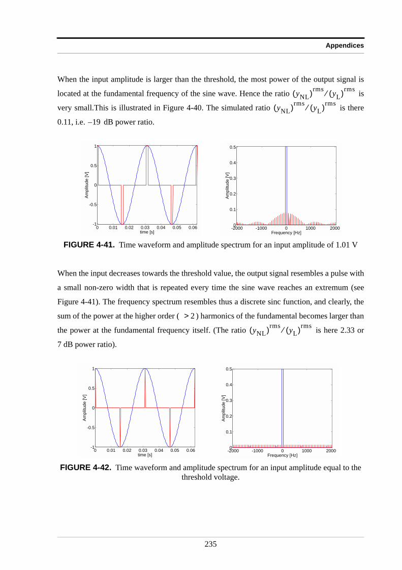
Appendices
When the input amplitude is larger than the threshold, the most power of the output signal is
located at the fundamental frequency of the sine wave. Hence the ratio is
very small.This is illustrated in Figure 4-40. The simulated ratio is there
0.11, i.e. dB power ratio.
When the input decreases towards the threshold value, the output signal resembles a pulse with
a small non-zero width that is repeated every time the sine wave reaches an extremum (see
Figure 4-41). The frequency spectrum resembles thus a discrete sinc function, and clearly, the
sum of the power at the higher order ( ) harmonics of the fundamental becomes larger than
the power at the fundamental frequency itself. (The ratio is here 2.33 or
7 dB power ratio).
FIGURE 4-41. Time waveform and amplitude spectrum for an input amplitude of 1.01 V
FIGURE 4-42. Time waveform and amplitude spectrum for an input amplitude equal to the threshold voltage.
yNL( )rms yL( )rms⁄
yNL( )rms yL( )rms⁄
19–
0 0.01 0.02 0.03 0.04 0.05 0.06-1
-0.5
0
0.5
1
time [s]
Am
plit
ud
e [
V]
-2000 -1000 0 1000 20000
0.1
0.2
0.3
0.4
0.5
Frequency [Hz]A
mp
litu
de
[V
]
2>
yNL( )rms yL( )rms⁄
0 0.01 0.02 0.03 0.04 0.05 0.06-1
-0.5
0
0.5
1
time [s]
Am
plit
ud
e [
V]
-2000 -1000 0 1000 20000
0.1
0.2
0.3
0.4
0.5
Frequency [Hz]
Am
plit
ud
e [
V]
235
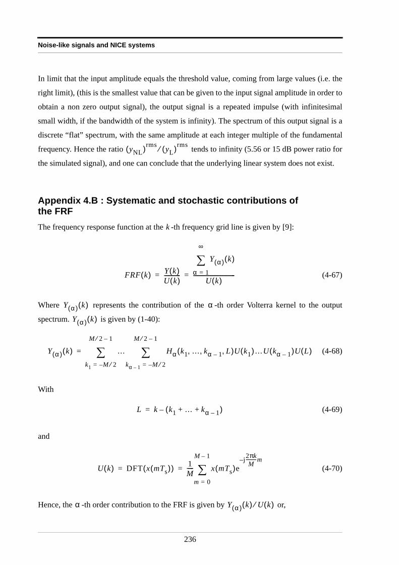
Noise-like signals and NICE systems
In limit that the input amplitude equals the threshold value, coming from large values (i.e. the
right limit), (this is the smallest value that can be given to the input signal amplitude in order to
obtain a non zero output signal), the output signal is a repeated impulse (with infinitesimal
small width, if the bandwidth of the system is infinity). The spectrum of this output signal is a
discrete “flat” spectrum, with the same amplitude at each integer multiple of the fundamental
frequency. Hence the ratio tends to infinity (5.56 or 15 dB power ratio for
the simulated signal), and one can conclude that the underlying linear system does not exist.
Appendix 4.B : Systematic and stochastic contributions of the FRFThe frequency response function at the -th frequency grid line is given by [9]:
(4-67)
Where represents the contribution of the -th order Volterra kernel to the output
spectrum. is given by (1-40):
(4-68)
With
(4-69)
and
(4-70)
Hence, the -th order contribution to the FRF is given by or,
yNL( )rms yL( )rms⁄
k
FRF k( ) Y k( )U k( )------------
Y α( ) k( )
α 1=
∞
∑
U k( )-------------------------------= =
Y α( ) k( ) α
Y α( ) k( )
Y α( ) k( ) … Hα k1 … kα 1– L, , ,( )U k1( )…U kα 1–( )U L( )
kα 1– M 2⁄–=
M 2⁄ 1–
∑k1 M 2⁄–=
M 2⁄ 1–
∑=
L k k1 … kα 1–+ +( )–=
U k( ) DFT x mTs( )( ) 1M----- x mTs( )e
j2πkM
---------m–
m 0=
M 1–
∑= =
α Y α( ) k( ) U k( )⁄
236
Appendices
(4-71)
The term will be a stochastic one if its phase is a
function of the random phases of the input spectral lines. On the other hand, if the phase of this
term is not a function of the random phases of the input spectral lines, the term will represent a
deterministic contribution, and hence be a part of the systematic contributions to the FRF.
Since the denominator has a random phase, a first requirement for (4-71) to be a
deterministic term is that one of the numerator’s factors is equal to the denominator. Take e.g.
, hence (4-69) becomes: . A second constraint has to be put on the
remaining factors: since has random phase, the only way to cancel this random
phase is that one of the remaining indices equals . In other words, the
remaining factors have to be grouped in pairs , such that their phases cancel.
Hence, if is even (i.e. is odd), there will be terms that are systematic contributions of
the FRF.
If the above constraints are not fulfilled, the term will be a stochastic contribution of the FRF.
On the other hand, if is odd (i.e. is even), only stochastic contributions to the FRF will
be created.
Appendix 4.C : IF spectrum of the ideal mixerConsider the RF input signal of the mixer to be a random multisine
(4-72)
FRF α( ) k( ) … Hα k1 … kα 1– L, , ,( )U k1( )…U kα 1–( )U L( )
U k( )---------------------------------------------------------
kα 1– M 2⁄–=
M 2⁄ 1–
∑k1 M 2⁄–=
M 2⁄ 1–
∑=
Hα k1 … kα 1– L, , ,( )U k1( )…U kα 1–( )U L( )
U k( )---------------------------------------------------------
U k( )
L k= k1 … kα 1–+ + 0=
α 1– U k1( )
k2 … kα 1–, , k1– α 1–
U ki( )U ki–( )
α 1– α
α 1– α
uRF t( ) Uκ 2πfκ t ϕκ+( )cosκ 1=
N
∑=
fκ fmin κ 1–( )fmax fmin–
N 1–---------------------------+=
237
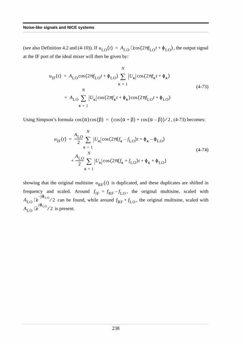
Noise-like signals and NICE systems
(see also Definition 4.2 and (4-10)). If , the output signal
at the IF port of the ideal mixer will then be given by:
(4-73)
Using Simpson’s formula , (4-73) becomes:
(4-74)
showing that the original multisine is duplicated, and these duplicates are shifted in
frequency and scaled. Around , the original multisine, scaled with
can be found, while around , the original multisine, scaled with
is present.
uLO t( ) ALO 2πfLOt ϕLO+( )cos⋅=
uIF t( ) ALO 2πfLOt ϕLO+( )cos Uκ 2πfκ t ϕκ+( )cosκ 1=
N
∑=
ALO Uκ 2πfκ t ϕκ+( ) 2πfLOt ϕLO+( )coscosκ 1=
N
∑=
α( )cos β( )cos α β+( )cos α β–( )cos+( ) 2⁄=
uIF t( )ALO
2---------- Uκ 2π fκ fLO–( )t ϕκ ϕLO–+( )cos
κ 1=
N
∑=
ALO
2---------- Uκ 2π fκ fLO+( )t ϕκ ϕLO+ +( )cos
κ 1=
N
∑+
uRF t( )
fIF fRF fLO–=
ALO ejϕLO–
⋅ 2⁄ fRF fLO+
ALO ejϕLO⋅ 2⁄
238
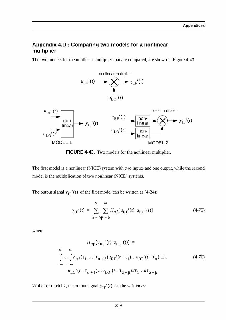
Appendices
Appendix 4.D : Comparing two models for a nonlinear multiplierThe two models for the nonlinear multiplier that are compared, are shown in Figure 4-43.
The first model is a nonlinear (NICE) system with two inputs and one output, while the second
model is the multiplication of two nonlinear (NICE) systems.
The output signal of the first model can be written as (4-24):
(4-75)
where
(4-76)
While for model 2, the output signal can be written as:
FIGURE 4-43. Two models for the nonlinear multiplier.
Xnonlinear multiplier
uRF ′ t( )
yIF ′ t( )
uLO ′ t( )
uRF ′ t( )
uLO′ t( )
yIF ′ t( )non-linear
MODEL 1
X yIF ′ t( )
ideal multiplieruRF ′ t( )
uLO ′ t( )
non-linear
non-linear
MODEL 2
yIF ′ t( )
yIF ′ t( ) Hαβ uRF′ t( ) uLO ′ t( ),[ ]
β 0=
∞
∑α 0=
∞
∑=
Hαβ uRF ′ t( ) uLO ′ t( ),[ ] =
… hαβ τ1 … τα β+, ,( )uRF ′ t τ1–( )…uRF ′ t τα–( ) …⋅
∞–
∞
∫∞–
∞
∫
uLO ′ t τα 1+–( )…uLO ′ t τα β+–( )dτ1…dτα β+
yIF ′ t( )
239
Noise-like signals and NICE systems
(4-77)
where
(4-78)
The two models will be equivalent, if (compare (4-78) to (4-76)):
(4-79)
In other words, the two-input single output NICE system can be represented by a
multiplication of two NICE systems, only if all its Volterra kernels can be written as the
product of a kernel of the RF NICE system and a kernel of the LO NICE system. Since this is
not always possible, model 1 is a more general model than model 2.
The fact that the separability is not always valid can be shown through a simple counter-
example: Suppose that a two-input ( ), one-output ( ) NICE system multiplies
both input signals, and then applies this product to a lowpass filter, with impulse response .
In this case, the output signal can be written as:
(4-80)
Or, in order to obtain the kernel , (4-80) equals:
yIF ′ t( ) HαRF uRF′ t( )[ ]
α 0=
∞
∑
HβLO uLO′ t( )[ ]
β 0=
∞
∑
=
HαRF uRF ′ t( )[ ] Hβ
LO uLO ′ t( )[ ]
β 0=
∞
∑α 0=
∞
∑=
HαRF uRF ′ t( )[ ] Hβ
LO uLO ′ t( )[ ] =
… hαRF τ1 … τα, ,( )hβ
LO τ1 ′ … τ β′, ,( )uRF ′ t τ1–( )…uRF ′ t τα–( ) …⋅
∞–
∞
∫∞–
∞
∫
uLO ′ t τ1 ′–( )…uLO ′ t τβ′–( )dτ1…dταdτ1′…dτβ′
hαβ τ1 … τα β+, ,( ) hαRF τ1 … τα, ,( ) hβ
LO τ1 ′ … τ β′, ,( )⋅=
u1 t( ) u2 t( ), y t( )
e t–
y t( )
y t( ) e t– * u1 t( )u2 t( )( ) e τ1– u1 t τ1–( )u2 t τ1–( ) τ1d∞–
∞∫= =
h11 τ1 τ2,( )
240
Appendices
(4-81)
Yielding the kernel , or in its symmetrized form:
(4-82)
Hence, it is clear that (4-82) cannot be written as product of two first order kernels
Appendix 4.E : Output spectral components of a two input NICE system where a single tone signal is applied at both input portsConsider a two input NICE system, where a spectral component at frequency is applied at
port 1, and a spectral components at frequency is applied at port 2. Suppose that , and
that the frequency difference between the components is small as compared to their
frequencies, i.e. . This is typically the situation that occurs for mixers, where
port 1 is the RF port, and port 2 is the LO port. The frequencies of the signals applied at these
ports are situated in the orders of magnitude of the GHz, while 11.1 MHz is a very commonly
used IF frequency. In that case, one can rename frequency as frequency , and frequency
as frequency , with . The output spectrum of the system will then consist
of clusters of frequency components, that are centered around frequency
( ), or, in the vicinity of , since . Note that for very high degrees of the
nonlinearity, all these clusters will cross each other, since mathematically speaking, the
( )-th degree nonlinearity of and the ( )-th degree nonlinearity of
will fall at the same frequency grid line. This will first occur at the smallest common
multiple of and . However, since both frequencies are high, and lie close to each
other, this smallest common multiple will be an extremely high frequency. (e.g. the smallest
common multiple of 1.5 GHz and 1.45 GHz is 43.5 GHz, needing a nonlinearity of at least
29th degree to produce a frequency component that high.) Hence, one can conclude that the
output spectrum are distinct clusters of spectral components.
e τ1– δ τ1 τ2–( )u1 t τ1–( )u2 t τ2–( ) τ1d τ2d∞–
∞∫∞–
∞∫
h11 τ1 τ2,( ) e τ1– δ τ1 τ2–( )=
h11 τ1 τ2,( )e τ1– δ τ1 τ2–( ) e τ2– δ τ2 τ1–( )+
2-----------------------------------------------------------------------------=
h1A τ1( ) h1
B τ2( )⋅
f1f2 f2 f1<
f1 f2– f1 f2,«
f2 f0f1 f0 ∆+ ∆ f1 f2–=
z f0 ∆ 2⁄+( )⋅
z Z∈ zf0 ∆ 2⁄ f0«
f0 1Hz⁄ f0 ∆+ f0 ∆+( ) 1Hz⁄
f0f0 f0 ∆+
241
Noise-like signals and NICE systems
For each output spectral component, it is possible to determine what degrees of each input port,
or which order Volterra operator contributes to that component.
Theorem 4.5
1. The smallest values of and that are needed to obtain a frequency component at
frequency with is , , .
2. The smallest values of and that are needed to obtain a frequency component at
frequency (with ) is , , .
3. The smallest values of and that are needed to obtain a frequency component at
frequency (with ) is , , .
proof.
1. . Hence,
2. . Hence,
3. . Hence,
Theorem 4.6
If the Volterra operator contributes to a certain frequency component in the output
spectrum of a two input NICE system, then all the Volterra operators with
, will also contribute to that frequency component.
Hαβ [ ]
α β
mf0 µ∆+ µ 0 1 … m, , , ∈ α β+ m= α µ= β m µ–=
α β
mf0 m ν+( )∆+ m ν, N∈ α β+ m 2ν+= α m ν+= β ν=
α β
mf0 ν∆– m ν, N∈ α β+ m 2ν+= α ν= β m ν+=
mf0 µ∆+ mf2 µ f1 f2–( )+ µf1 m µ–( )f2+= =
α µ =β m µ–=α β+ m=
mf0 m ν+( )∆+ mf2 m ν+( ) f1 f2–( )+ m ν+( )f1 νf2–= =
α m ν+=β ν =
α β+ m 2ν+=
mf0 ν∆– mf2 ν f1 f2–( )– ν– f1 m ν+( )f2+= =
α ν =β m ν+=
α β+ m 2ν+=
Hαβ [ ]
Hγε [ ]
γ ε,( ) α β,( ) 2 z1 z2,( )+= z1 z2, N∈
242
Appendices
proof
The frequency component is created by combining spectral components from port
1, lying at frequency grid lines and spectral components from port 2, lying at
frequency grid lines , such that
(4-83)
It is clear that (4-83) also can be written as:
(4-84)
where and are arbitrarily chosen natural numbers. Or, by combining spectral
components from port 1, and spectral components from port 2, it is still possible to
obtain frequency grid line . G
Note that for narrow band signals, centered around and , one can assume that the
conclusions of this appendix are still valid, if the bandwidth of those signals is much smaller
than . The motivation for this claim is similar to the first part of this appendix: In
the previous part of this appendix, the smallest frequency spacing between two consecutive
spectral components of the output spectrum was . Hence, for narrow band signals, one can
consider that the smallest frequency spacing between two consecutive center frequencies in the
output spectrum is also . Thus, assuming that the largest input bandwidth of both narrow
band signals is , at least a ( )-th degree nonlinearity is needed before the spectra
around two consecutive center frequencies overlap. But since was assumed, this degree
will be very high.
Appendix 4.F : Systematic and stochastic contributions of the mixer’s FRFConsider the RF input signal of the mixer to be a random multisine
Y αβ( ) k( ) α
k1 … kα, , β
l1 … lβ, ,
k kii 1=
α
∑= ljj 1=
β
∑+
k kii 1=
α
∑= lj ki ′ ki ′–( )+( ) lj ′ lj ′–( )+( )
j ′ 1=
z2
∑+i ′ 1=
z1
∑+j 1=
β
∑+
z1 z2 α 2z1+
β 2z2+
k
f1 f2
∆ f1 f2–=
∆
∆
B0 B0 ∆⁄
B0 ∆«
243
Noise-like signals and NICE systems
(4-85)
(see also Definition 4.2 and (4-10)), and consider the LO input signal to be a pure sine wave:
. The output spectrum at the IF port at frequency
will then be given by:
(4-86)
with (see Appendix 4.E for motivation of this choice for and ). Assume
that is the (positive) frequency grid line of the local oscillator sine wave ( , with
the frequency grid spacing).
In this case, the frequency response function of the mixer is given by:
(4-87)
Just as shown in Appendix 4.B, (4-87) will consist of terms of the following form:
(4-88)
with the constraint . When not considering very high degrees
of the nonlinearity, the constraint can be split into two constraints and
(see the first part of Appendix 4.E). Knowing that
(this follows out of the definition of ), and assuming that
is a constant, all these terms (4-88) can be split into two disjunct sets:
1. The term (4-88) will be a stochastic one if its phase is a function of the random phases of
the RF input spectral lines, and hence be a part of the stochastic contributions of the FRF.
uRF t( ) Uκ 2πfκ t ϕκ+( )cosκ 1=
N
∑=
fκ fmin κ 1–( )fmax fmin–
N 1–---------------------------+=
uLO t( ) ALO 2πfLOt ϕLO+( )cos⋅=
fIF fRF fLO–=
YIF k( ) YIF αβ( ) k( )β∑
α∑=
α β, 2N 1+∈ α β
l fLO l∆f=
∆f
FRF k( ) Y k( )URF ideal, k( )--------------------------------
YIF αβ( ) k( )β∑
α∑
URF ideal, k( )----------------------------------------= =
Hαβ k1 … kα l1 … lβ, , , , ,( )URF k1( )…URF kα( )ULO l1( )…ULO lβ( )
URF ideal, k( )----------------------------------------------------------------------------------------------------
k1 … kα l1 … lβ+ + + + + k=
k1 … kα+ + k l+=
l1 … lβ+ + l–=
ULO l–( ) ALOe jϕLO– 2⁄= uLO t( )
ϕLO
244
Appendices
2. The term (4-88) will be a deterministic one if its phase is not a function of the random
phases of the RF input spectral lines, and hence be a part of the systematic contributions
to the FRF.
Note that no extra constraint is required for the factor . The reason
therefore is that since is a pure sinewave, the indices can only be , and due
to the constraint and the constraint that is an odd natural number, the
expression must be:
(4-89)
and hence the phase of will always be .
Appendix 4.G : The three noise sources are uncorrelated
In this appendix, the independence of the noise sources , and will be
shown. In other words, the power of the sum of the noise sources has to be equal to the sum of
the power of each noise source. The power of the combined noise sources is given by (the
dependence of the frequency grid line is omitted to enhance readability):
(4-90)
Next, it will be shown that each of the terms of the second line of (4-90) is zero:
1. The phase of depends both on the random phase of the RF multisine (through
)and on the random phase of the LO multisine (through ). Hence, its
expectation over the instances will be zero.
2. For , it might be possible that the random phases of the RF multisine cancel
each other, e.g.:
ULO l1( )…ULO lβ( )
uLO t( ) l1 … lβ, , l±
l1 … lβ+ + l–= β
ULO l1( )…ULO lβ( )
ULO l1( )…ULO lβ( ) ULO l–( )( )β 1+
2------------
ULO l( )( )β 1–
2------------
⋅=
ULO l1( )…ULO lβ( ) ϕLO–
YBS k( ) YSB k( ) YSS k( )
k
E YBS YSB YSS+ + 2 E YBS2 E YSB
2 E YSS2 + +=
2Re E YSBYBS* ( ) 2Re E YSBYSS
* ( ) 2Re E YBSYSS* ( )+ + +
YSBYBS*
YSB YBS*
YSBYSS*
245
Noise-like signals and NICE systems
(4-91)
But even in that case, remains a function of the random phases of the LO
multisine, and thus its mean value will be zero.
3. For , a similar reasoning as for can be done. This time, the phases of
the LO multisine might cancel for a special case, but will remain a function of
the random phases of the RF multisine, yielding a zero average value.
Conclusion:
YSB H31 k1 … k3 l–, , ,( )URF k1( )URF k2( )URF k3( )ULO l–( )=
YSS* H33
* k1 … k3 l1 … l3, , , , ,( )URF* k1( )URF
* k2( )URF* k3( )ULO
* l1( )ULO* l2( )ULO
* l3( )=
YSBYSS*
YBSYSS* YSBYSS
*
YBSYSS*
E YBS YSB YSS+ + 2 E YBS2 E YSB
2 E YSS2 + +=
246
CONCLUSIONS AND IDEAS FORFURTHER RESEARCH
This work tried to describe the way noise is treated by a particular class of nonlinear systems,
i.e. the NICE systems. This class of NICE systems is general enough to describe most of the
systems and circuits used in practical telecommunications equipment. In opposition to the
linear systems, a separated study of the signal and the noise behavior cannot be done when
dealing with NICE systems. The interaction between the signal and the noise due to the
nonlinearity of the NICE system itself makes this separated approach impossible. Since the
noise power is usually much smaller than the signal power, the effect of the noise on the signal
output will be quite small, and hence the signal behavior can be studied as if there was no noise
present, as is done in the literature [41]. However, the noise behavior strongly depends on the
signal properties, and therefore can only be studied together with the signal.
The linear system theory describes the noise behavior of a linear system, using the noise figure.
This quantity describes the signal-to-noise ratio deterioration of a signal, when it is applied to a
linear system, and can be measured using the well-known Y-factor technique. This technique
applies two noise sources at the input of a system, and determines the noise figure out of the
ratio of the respective output powers. However, simply applying measurement techniques
designed for LTI systems to NICE systems can have serious consequences! In its commercial
form, the Y-factor technique is blind for the nonlinearities in a NICE system, because the
power of the noise excitation signals used is far too small. Hence, the measurement technique
247
only sees the underlying linear system of the NICE system and returns the linear noise figure.
Boosting the power levels of the excitation signals in order to detect the nonlinearities is also a
bad idea as it can yield completely meaningless results such as negative power ratios.
Two cases have to be considered when describing the noise behavior of noisy NICE systems,
depending on the input signal.
The first case consideres an input signal consisting of a pure sinewave. Since the noise figure is
independent of the input signal, this quantity is not suited to describe adequately the noise
behavior of NICE systems. Therefore, the definition of the noise figure is extended towards the
NICE noise figure, that is defined as an input signal and noise power dependent signal-to-noise
ratio degradation. For a given input noise power spectral density, the NICE noise figure is an
increasing (when ) or decreasing (when ) function of the input signal
power. Hence, under some special circumstances ( ), it is even possible that the
signal-to-noise ratio at the output of the NICE system is larger than the signal-to-noise ratio at
the input of the NICE system. This is a phenomenon that is impossible when dealing with
linear systems. For input noise power spectral densities up to 10 dB back-off, the NICE noise
figure variation as function of the input signal power is identical to the behavior at ,
but with a modified linear noise figure that decreases with increasing input noise PSD.
Calculations and experimental results also showed that below the 1 dB compression point, the
noise power gain (i.e. the ratio of noise power spectral density at the output to the noise power
spectral density at the input of the system) is a quantity that in first approximation only
depends on the total power of the input signal.
In the second case, random, noise-like signals are applied to the noisy NICE system, as is often
the case in telecommunication equipment. The randomness of these input signals lies in the
stochastic nature of information itself. The nonlinear mechanism in the NICE systems is able
to create output noise from the random property of these noise-like signals. This type of noise
is much larger than the noise that is stochastic with respect to time, and will hence be the main
term for distortions at the output of the system. The nonlinear mechanism produces two types
of output contributions: systematic contributions and stochastic contributions. The systematic
NFlin 2> NFlin 2<
NFlin 1≈
Nin N0=
248
ones are responsible for a filtering effect of the input signals, while the stochastic contributions
present themselves as the noise source that is responsible for in-band distortions. This theory
can be extended towards multi-port devices such as mixers. If the input power of the signals is
constant, a mixer can be modeled as the cascade of an ideal frequency translator and a noisy
LTI system. The noise source inside this LTI system is generated by the randomness of the
signals at the RF and the LO port of the mixer (i.e. due to the stochastic content of the
information, and due to the phase noise of the local oscillator).
Further research
A. Extension of the systematic and stochastic contributions towards MIMO systems.In the last chapter, the extension of the technique involving the systematic and the stochastic
nonlinear contributions was already extended towards a “two-input one-output” NICE system,
i.e. a mixer. This theory can easily be extended to Multiple Input Multiple Output (MIMO)
systems. Since a MIMO system is a parallel circuit of a number of Multiple Input Single
Output (MISO) systems, the theory only needs to be extended towards MISO systems.
Consider e.g. a MISO system with input ports, and at each input port, a random multisine is
applied. In this case, the Frequency Response Function will consist of significant terms,
each having a label that tells whether it contains stochastic or systematic contributions for each
input port. The obtained results can then be used to characterize e.g. an IQ modulator such as
the SMIQ06B [28], used in measurements in chapter 4. This IQ modulator is a “three-input
one-output” NICE system.
B. A full multi-port description.All the techniques in this work assumed that there was a perfect match at all the ports of the
considered device, and only the effect of the noise on the forward gain parameter ( for a
two-port system) was studied. In reality however, mismatch can occur e.g. at the output of the
system, resulting in the noise power being reflected into the output port of the system, and
hence re-appearing (modified) in the reflected input wave. Multiple reflections can hence lead
to a complex noise behavior of the studied system. The use of the noise models for nonlinear
systems have to be generalized to full multi-port operation. Using these true multi-port models,
M
2M
S21
249
accurate predictions of high-level parameters such as the bit-error-rate (BER) and their
dependency on nonlinearities and impedance matching conditions can be obtained.
Hence, in order to obtain a full multi-port model that is valid for a wide range of compression
levels, signal-to-noise ratios and matching impedances, two essential noise sources need to be
extended towards true multi-port behavior:
1. The noise, stochastic with respect to time, i.e. the noise generated by random physical
processes. A closed theoretical framework for the interaction between the nonlinearity
and this type of noise is required. To obtain this, the influence of the wide-band matching
conditions on the noise behavior needs to be investigated.
Based on the obtained theoretical framework, a modelling approach can be built up. For
fairly low noise powers (such as the noise at standard temperature), it is expected that the
noise part of the model can be measured based on linear techniques. Experimental
verification requires the integration of the standard noise-gain analysis and the vectorial
network analyser for nonlinear systems (NVNA) [25] to extract a full signal and noise
model in the first place. Using the considered system in different, but model compatible,
settings then allows to evaluate the prediction power of the model, based on an additional
set of measurements.
2. The noise, created by the nonlinear mechanism itself, out of the stochastic properties of
the input signals. For these noise contributions, depending on the random character of
the input signal, over the different realisations, the modelling is based on the measured
response of the system to a random multisine excitation. The in-band distortions can be
measured by e.g. creating notches in the considered multisine, as described in chapter 4.
The results obtained can then be extended towards multi-port systems such as mixers.
C. The non-harmonic phase calibration problem.In this work, the NVNA was often used in a special mode, where spectral rich, non-
harmonically related multisine signals are used. One of the open problems in this mode of
operation is the absolute phase calibration of the measured signals. For harmonically related
250
signals, the phase calibration was performed using a Step Recovery Diode, that produces a
fundamental tone and all its harmonics [40]. The phase relations of the harmonics of this
fundamental tone are well-known quantities. When measuring the phases of the multisines, the
center frequency was calibrated in phase, and since the multisines were narrowband signals, it
was reasonable to assume that the same correction can be applied to all the components of the
multisine. It is however clear that for a broadband multisine, this hypothesis will no longer be
true.
To improve the accuracy of the phase calibration, a model based approach has to be used.
Using a parametric model for the calibration signal as a function of the fundamental sinewave,
used to generate the reference impulses, will allow removal of the assumptions and provide
calibration at arbitrary interpolated frequencies, where the spectrum of the phase standard is
not specified in the current non parametric approach.
251

252

APPENDIX A
References
253
[1] G. Vendelin, A. Pavio and U. Rohde, “Microwave Circuit Design using Linear and
Nonlinear Techniques”, John Wiley & Sons, New York, 1990.
[2] W. Davenport Jr. and W. Root, “An Introduction to the Theory of Random Signals and
Noise”, IEEE press, New York, 1987.
[3] H. Young, “University Physics”, 8th edition, Addison Wesley, New York, 1992
[4] A. Papoulis, “Probability, Random Variables and Stochastic Processes”, McGraw-Hill,
London, 1965“
[5] B.M. Oliver, “Noise Figure and Its Measurement”, Hewlett-Packard Journal, Vol. 9, No.
5, Jan 1958, pp. 3-5
[6] H. Friis, “Noise Figures of Radio Receivers”, Proceedings of the IRE, Jul 1944, pp. 419-
422.
[7] Martin Schetzen, “The Volterra and Wiener theories of nonlinear systems”, John Wiley
& Sons, New York, 1980
[8] B. Thibaud, C. Arnaud, M. Campovecchio et al. “Measurements of time domain voltage/
current waveforms at R.F. and microwave frequencies, based on the use of a Vector
Network Analyser, for the characterization of nonlinear devices. Application to high
efficiency power amplifiers and frequency mulipliers”, IEEE Transactions on
Instrumentation and Measurement, Vol. 47, pp.1259-1264.
[9] R. Pintelon and J. Schoukens, “System Identification: A Frequency Domain Approach”,
IEEE Press, New Jersey, 2001
[10] A. Di Paola, M. Sanninno, “Noise figure test-set for simultaneous measurements of gain
and noise figure of microwave devices”, 8th Mediterranean Electrotechnical Conference
MELECON ‘96, 1996, Volume 3, pp. 1368-1370.
[11] Wait Randa, “Amplifier noise measurements at NIST”, IEEE Transactions on
Instrumentation and Measurement, Vol. 46, pp. 482-485.
[12] K. Narendra and P. Gallman, “An iterative method for the identification of nonlinear
systems using a Hammerstein model”, IEEE Transactions on Automatic Control, 1966,
Vol. 11, pp. 546-550.
254
[13] “HP 346A/B/C Noise Source Operating and Service Manual”, Hewlett Packard, USA,
1992
[14] “HP8565E-series and EC series Spectrum Analyzers User’s Guide”, Hewlett Packard,
USA, 1998
[15] “Spectrum Analysis ... Noise Figure Measurements”, Hewlett Packard Application Note
150-9, April 1976
[16] “Spectrum Analyzer Measurements and Noise”, Hewlett Packard Application Note
1303, 1998
[17] Claude E. Shannon, “A Mathematical Theory of Communication”, The Bell System
Technical Journal, Vol. 27, pp.379-423, 623-656, July, October 1948
[18] A. Bower, “NICAM 728 - Digital Two-Channel Sound for Terrestrial Television”, BBC
Research Department Report, 1990
[19] R. Thoma, H. Groppe, U. Trautwein and J. Sachs, “Statistics of Input Signals for
Frequency Domain Identification of Weakly Nonlinear Systems in Communications”,
Instrumentation and Measurement Technology Conference, Brussels, Belgium, 1996
[20] “Noise Power Ratio (NPR) Measurements Using the HP E2507B/E2508A Multi-format
Communications Signal Simulator”, HP Product Note E2508-1, 1997
[21] T. Reveyrand, D. Barataud, J. Lajoinie et al., “A novel experimental noise power ratio
characterization method for multicarrier microwave power amplifiers”, 55th ARFTG
Conference, Boston, USA, June 2000
[22] J.C. Pedro and N.B. Carvalho, “On the Use of Multitone Techniques for Assessing RF
Components’ Intermodulation Distortion”, IEEE Transactions on Microwave Theory
and Techniques, Vol. 47, pp. 2393-2402, Dec. 1999
[23] J.C. Pedro and N.B. Carvalho, “A novel set-up for co-channel distortion ratio
evaluation”, IEEE MTT-S Symposium, Boston, USA, June 2000
[24] J. Schoukens, T. Dobrowiecki and R. Pintelon, “Parametric and Nonparametric
Identification of Linear Systems in the Presence of Nonlinear Distortions - A Frequency
Domain Approach”, IEEE Transactions on Automatic Control, Vol. 43, pp. 176-191,
Feb. 1998
255
[25] T. Van Den Broeck and J. Verspecht, “Calibrated Vectorial Nonlinear Network
Analyzer”, IEEE-MTT-S Symposium, San Diego, USA, 1994, pp. 1069-1072.
[26] P. Guillaume, J. Schoukens, R. Pintelon and I. Kollar, “Crest-Factor Minimization Using
Nonlinear Chebychev Approximation Methods”, IEEE Transactions on Instrumentation
and Measurement, Vol. 40, pp. 982-989, December 1991.
[27] “RF/IF Designer’s Guide”, Mini-Circuits, USA, 2000
[28] “SMIQ02B/03B/04B/06B Vector Signal Generator Operating Manual”, Rohde &
Schwarz, Germany, 1999
[29] R. Swerdlow, “Analysis of Intermodulation Noise in Frequency Convertors by Volterra
Series”, IEEE Transactions on Microwave Theory and Techniques, Vol. 26, April 1978
pp. 305-313
[30] J. C. Pedro and N. B. Carvalho, “Analysis and Measurement of Multi-tone
Intermodulation Distortion of Microwave Frequency Converters”, IEEE MTT-S
Symposium, Phoenix, USA, May 2001
[31] K. Vanhoenacker, T. Dobrowiecki and J. Schoukens, “Design of Multisine Excitations to
Characterize the Nonlinear Distortions During FRF-measurements”, Instrumentation
and Measurement Technology Conference, Baltimore, USA, May 2000
[32] L. Råde and B. Westergen, “BETA Mathematics Handbook”, Chartwell-Bratt Ltd, 1990,
England
[33] D. M. Pozar, “Microwave Engineering”, 2nd. edition, John Wiley & Sons, New York,
1998
[34] N.B. Carvalho and J.C. Pedro, “Compact Formulas to relate ACPR and NPR to Two-
tone IMR and IP3”, Microwave Journal, December 1999
[35] M. Kendall and A. Stuart, “The Advanced Theory of Statistics, Volume 2: Inference and
Relationship”, 4th edition, Charles Griffin & Company Limited, London, 1979
[36] K. Kurokawa, “Power Waves and the Scattering Matrix”, IEEE Transactions on
Microwave Theory and Techniques, March 1965, pp. 194-202
[37] E. Oram Birgham, “The Fast Fourier Transform”, Prentice-Hall, New Jersey, 1974.
256
[38] B. Picinbono, “Random Signals and Systems”, Prentice Hall Inc., New Jersey, 1993.
[39] “The ARRL handbook for Radio Amateurs”, The American Radio Relay League,
Newington, USA, 1996
[40] J. Tatum, “Comb Generators and Amplifiers form Active Multipliers”, Microwaves &
RF Magazine, August 1996
[41] W. Van Moer, “Development of New Measuring and Modelling Techniques for RFICs
and their Nonlinear Behaviour”, Ph. D. Disseration, Vrije Universiteit Brussel, June
2001.
[42] W. Chan, “DSL Simulation Techniques and Standards Development for Digital
Subscriber Line Systems”, Macmillan Technical Publishing, Indianapolis, 1998.
[43] J. Proakis, “Digital Communications”, 3rd edition, McGraw-Hill, New York, 1995.
[44] G.L. Heiter, “Characterization of Nonlinearities in Microwave Devices and Systems”,
Transactions on Microwave Theory and Techniques, December 1973, pp. 797-805.
[45] J.C. Gillespie, “Noise Loading of FM Systems. The Noise-Power-Ratio (NPR) and
Customer Requirements”, 1973 G-MTT International Microwave Symposium Digest of
Technical Papers, p. 113
257

258

APPENDIX B
Publications
259
A. Periodical Papers[1] A. Geens and Y. Rolain, “Noise Figure Measurements on Nonlinear Devices”, IEEE
Transactions on Instumentation and Measurement, Vol. 50, No 4, August 2001, pp. 971-
975.
[2] W. Van Moer, Y. Rolain and A. Geens, “Measurement Based Modelling of Spectral
Regrowth”, IEEE Transactions on Instumentation and Measurement, Vol. 50, No 6,
December 2001.
[3] A. Geens, Y. Rolain, K. Vanhoenacker and J. Schoukens, “Discussion on Fundamental
Issues of NPR Measurements”, IEEE Transactions on Instumentation and Measurement,
under review.
B. Conference Papers[4] A. Geens and Y. Rolain, “Noise Figure Measurements on Nonlinear Devices”,
Proceedings of the 17th Instrumentation and Measurement Technology Conference,
Baltimore, USA, May 2000, pp. 796-801.
[5] A. Geens and Y. Rolain, “Noise Behavior of an Amplifier in Compression”, 55th ARFTG
Conference Digest, Boston, USA, June 2000, pp. 127-134.
[6] W. Van Moer, Y. Rolain and A. Geens, “Measurement Based Nonlinear Modelling of
Spectral Regrowth”, IEEE-MTT-S Digest, Boston, USA, June 2000, pp. 1467-1470.
[7] A. Geens and Y. Rolain, “On the Global Noise Behavior of a Third Order Nonlinearity”,
30th European Microwave Conference Proceedings, Paris, France, October 2000, pp.
159-162.
[8] A. Geens, Y. Rolain, K. Vanhoenacker and J. Schoukens, “Discussion on Fundamental
Issues of NPR Measurements”, Proceedings of the 18th Instrumentation and
Measurement Technology Conference, Budapest, Hungary, May 2001, pp. 160-165.
[9] A. Geens, Y. Rolain and W. Van Moer, “NPR & Co-Channel Distortion Ratio: A Happy
Marriage?”, IEEE-MTT-S Digest, Phoenix, USA, May 2001, pp. 1675-1678.
[10] Y. Rolain, W. Van Moer and A. Geens, “PAVO: A Simple Wideband Nonlinear
Component Model”, 57th ARFTG Conference Digest, Phoenix, USA, May 2001, pp.
100-103.
260

[11] A. Geens, Y. Rolain, W. Van Moer, “Discussion on in-band Distortions of Mixers”, 58th
ARFTG Conference Digest, San Diego, USA, November 2001.
[12] A. Geens, Y. Rolain, K. Vanhoenacker and J. Schoukens, “Measuring in-band
Distortions of Mixers”, Proceedings of the 19th Instrumentation and Measurement
Technology Conference, Anchorage, USA, May 2002.
261

262