.

A Theoreti al and ExperimentalStudy of Geometri Networks

Mohammad Farshi

A Theoreti al and Experimental Studyof Geometri NetworksPROEFSCHRIFT

ter verkrijging van de graad van do toraan de Te hnis he Universiteit Eindhoven, op gezag van deRe tor Magni� us, prof.dr.ir. C.J. van Duijn, voor een ommissie aangewezen door het College voorPromoties in het openbaar te verdedigenop dinsdag 8 april 2008 om 16.00 uurdoorMohammad Farshigeboren te Yazd, Iran

Dit proefs hrift is goedgekeurd door de promotor:prof.dr. M.T. de BergCopromotor:dr. J. Gudmundsson

CIP-DATA LIBRARY TECHNISCHE UNIVERSITEIT EINDHOVENFarshi, MohammadA theoreti al and experimental study of geometri networks/ door Mohammad Farshi. -Eindhoven : Te hnis he Universiteit Eindhoven, 2008.Proefs hrift. - ISBN 978-90-386-1135-8NUR 993Subje t headings: omputational geometry / data stru tures / algorithmsCR Subje t Classi� ation (1998): I.3.5, E.1, F.2.2

.

Promotor: prof.dr. M.T. de Berg (Te hnis he Universiteit Eindhoven)Copromotor: dr. J. Gudmundsson (National ICT Australia)Kern ommissie:prof.dr. M.H. Overmars (Utre ht University)prof.dr. M. Smid (Carleton University)prof.dr. J.J. van Wijk (Te hnis he Universiteit Eindhoven)

Ministry of Science, Research and Technology

Islamic Republic of IranThe work in this thesis is supported by the Ministry of S ien e, Resear h andTe hnology of I. R. Iran under s holarship no. 800.341.The work in this thesis has been arried out under the auspi es of the resear hs hool IPA (Institute for Programming resear h and Algorithmi s).IPA dissertation series 2008-12 © Mohammad Farshi 2008. All rights are reserved. Reprodu tion in whole orin part is prohibited without the written onsent of the opyright owner.Printing: Eindhoven University PressIllustration over: a 2-spanner on 532 US ities [NS07℄.

ContentsPrefa e v1 Introdu tion 11.1 Geometri networks . . . . . . . . . . . . . . . . . . . . . . . . . . 11.2 t-Spanners . . . . . . . . . . . . . . . . . . . . . . . . . . . . . . . . 31.3 Why spanners? . . . . . . . . . . . . . . . . . . . . . . . . . . . . . 61.3.1 Approximate minimum spanning tree . . . . . . . . . . . . 71.3.2 Metri spa e sear hing . . . . . . . . . . . . . . . . . . . . . 71.3.3 Broad asting in ommuni ation networks . . . . . . . . . . 81.3.4 Proteins visualization . . . . . . . . . . . . . . . . . . . . . 91.4 Thesis overview . . . . . . . . . . . . . . . . . . . . . . . . . . . . . 102 Region-Fault Tolerant Spanners 132.1 Introdu tion . . . . . . . . . . . . . . . . . . . . . . . . . . . . . . . 132.2 Constru ting C-fault tolerant spanners using the WSPD . . . . . . 162.3 Well-separated pair de omposition . . . . . . . . . . . . . . . . . . 172.3.1 Constru ting a C-fault tolerant spanner . . . . . . . . . . . 182.3.2 Linear-size spanners for spe ial ases . . . . . . . . . . . . . 202.3.3 C-fault tolerant Steiner spanners . . . . . . . . . . . . . . . 222.4 Spe ial ases . . . . . . . . . . . . . . . . . . . . . . . . . . . . . . 242.4.1 C-fault tolerant fat triangulations . . . . . . . . . . . . . . . 242.4.2 Limited boundary dire tions . . . . . . . . . . . . . . . . . 252.5 C-fault tolerant spanners for arbitrary point sets . . . . . . . . . . 262.5.1 SSPDs and fault-tolerant spanners . . . . . . . . . . . . . . 272.5.2 Computing an SSPD . . . . . . . . . . . . . . . . . . . . . . 322.6 Testing for C-fault toleran e . . . . . . . . . . . . . . . . . . . . . . 392.7 Fault-tolerant geodesi spanners . . . . . . . . . . . . . . . . . . . 402.8 Con luding remarks . . . . . . . . . . . . . . . . . . . . . . . . . . 44i

3 Dilation-Optimal Edge Augmentation 473.1 Introdu tion . . . . . . . . . . . . . . . . . . . . . . . . . . . . . . . 473.2 Three simple algorithms . . . . . . . . . . . . . . . . . . . . . . . . 483.2.1 Exa t algorithms . . . . . . . . . . . . . . . . . . . . . . . . 483.2.2 A (1 + ")-approximation for Eu lidean graphs . . . . . . . . 503.3 Adding a bottlene k edge . . . . . . . . . . . . . . . . . . . . . . . 513.4 A (2 + ")-approximation for Eu lidean graphs . . . . . . . . . . . . 553.4.1 Linear number of andidate edges . . . . . . . . . . . . . . 553.4.2 Speeding up algorithm 3.4.1 . . . . . . . . . . . . . . . . . 613.5 A spe ial ase: G has onstant dilation . . . . . . . . . . . . . . . . 623.6 Con luding remarks . . . . . . . . . . . . . . . . . . . . . . . . . . 654 Dilation-Optimal Edge Deletion 674.1 Introdu tion . . . . . . . . . . . . . . . . . . . . . . . . . . . . . . . 674.2 Dilation-minimal edge deletion in a y le . . . . . . . . . . . . . . . 694.2.1 Estimating the dilation of a polygonal path . . . . . . . . . 704.2.2 The de ision problem . . . . . . . . . . . . . . . . . . . . . 724.2.3 The optimization algorithm . . . . . . . . . . . . . . . . . . 764.3 Dilation-maximal edge deletion in a y le . . . . . . . . . . . . . . 774.4 (1 + ")-Approximation algorithm . . . . . . . . . . . . . . . . . . . 814.5 Con luding remarks . . . . . . . . . . . . . . . . . . . . . . . . . . 845 Computing Spanner Diameter 855.1 Introdu tion . . . . . . . . . . . . . . . . . . . . . . . . . . . . . . . 855.2 Dynami programming approa h . . . . . . . . . . . . . . . . . . . 865.3 Improving the omplexity bounds . . . . . . . . . . . . . . . . . . . 905.4 A �nal approa h . . . . . . . . . . . . . . . . . . . . . . . . . . . . 915.5 Experimental results . . . . . . . . . . . . . . . . . . . . . . . . . . 935.6 Con luding remarks . . . . . . . . . . . . . . . . . . . . . . . . . . 946 Experimental Study of Geometri Spanners 976.1 Introdu tion . . . . . . . . . . . . . . . . . . . . . . . . . . . . . . . 976.1.1 Spanner properties . . . . . . . . . . . . . . . . . . . . . . . 986.2 Spanner onstru tion algorithms . . . . . . . . . . . . . . . . . . . 986.2.1 The original greedy algorithm and an improvement . . . . . 996.2.2 The approximate greedy algorithm . . . . . . . . . . . . . . 1016.2.3 The �-graph algorithm . . . . . . . . . . . . . . . . . . . . 1036.2.4 The ordered �-graph algorithm . . . . . . . . . . . . . . . . 1046.2.5 The random ordered �-graph algorithm . . . . . . . . . . . 1066.2.6 The sink-spanner algorithm . . . . . . . . . . . . . . . . . . 1066.2.7 The skip-list spanner algorithm . . . . . . . . . . . . . . . . 1086.2.8 The WSPD algorithm . . . . . . . . . . . . . . . . . . . . . 1096.3 Experimental results . . . . . . . . . . . . . . . . . . . . . . . . . . 1116.3.1 Implementation details . . . . . . . . . . . . . . . . . . . . . 112ii

6.3.2 Size . . . . . . . . . . . . . . . . . . . . . . . . . . . . . . . 1136.3.3 Degree . . . . . . . . . . . . . . . . . . . . . . . . . . . . . . 1156.3.4 Weight . . . . . . . . . . . . . . . . . . . . . . . . . . . . . . 1196.3.5 Spanner diameter . . . . . . . . . . . . . . . . . . . . . . . . 1216.3.6 Maximum and average dilation . . . . . . . . . . . . . . . . 1236.3.7 Crossings . . . . . . . . . . . . . . . . . . . . . . . . . . . . 1256.3.8 The hybrid algorithms . . . . . . . . . . . . . . . . . . . . . 1256.3.9 Number of shortest path queries . . . . . . . . . . . . . . . 1286.3.10 Running time . . . . . . . . . . . . . . . . . . . . . . . . . . 1306.4 Con luding remarks . . . . . . . . . . . . . . . . . . . . . . . . . . 1357 Con lusions 137Referen es 141

iii

iv

Prefa eThis thesis is the result of almost four years of work where I have been a om-panied and supported by many people. I now have the pleasant opportunity toexpress my gratitude to all of them.First of all, I would like to express my deep and sin ere gratitude to my su-pervisors, Mark de Berg and Joa him Gudmundsson for giving me the possibilityto work under their supervision. Thanks to Mark who took the risk of a eptingme, as a person with no knowledge in omputational geometry, in his group andto Joa him who was my daily supervisor and who helped me to understand the on ept of spanners, dis uss problems and read my manus ripts, not only whenhe was in TU/e but also after he left Eindhoven. This work would not have beenpossible without their support and en ouragement, and I am grateful for theirvaluable friendship.I would also like to thank my distinguished o-authors during my PhD studyMohammad Ali Abam, Hee-Kap Ahn, Mark de Berg, Joa him Gudmundsson,Panos Giannopoulos, Christian Knauer, Mi hiel Smid, and Yajun Wang, the re-sults in this thesis is the produ t of our joint work. I would like to express mythanks to the people who made the joint works possible: Alexander Wolf andXavier Goao for inviting me to the Korean Workshop on Computational Geom-etry and the organizers of the workshop on geometri networks and metri spa eembedding at S hloss Dagstuhl. I also thank Joa him Gudmundsson for invitingme to NICTA and his hospitality during my visit.The members of my thesis ommittee are gratefully a knowledged for readingthe thesis, providing useful omments and being present at my defense session. Itwas my privilege to have Mark de Berg, Joa him Gudmundsson, Mark Overmars,Mi hiel Smid and Ja k van Wijk in the thesis ommittee and Rolf Klein in thedefense opposition.

My PhD study was supported by a s holarship from the Ministry of S ien e,Resear h and Te hnology of I. R. Iran. I would like to take this opportunity tothank them for their support. I also would like to thank Khosro Piri, Farhad Rah-mati and Mohammad Hossein Abdollahi, a ademi representatives and dire torsof Iranian students in Europe for their help.I was very lu ky to work with absolutely fantasti people in the Algorithmsgroup. I thank them all for making my years at Eindhoven delightful. Spe ialthanks go to Sonja Joosten for her help at the start of my study and Astrid Volkersfor her help at the �nal stages of my work. I also thank my great oÆ emates YuvalNir, Mark S hroders and Peter Ha henberger.A heart-felt thanks goes to Mohammad Ali Abam for his valuable friendship,enjoyable dis ussions, whi h always ome with ni e ideas, and tea breaks. I learneda lot from him and I'm looking forward to ontinue to work with him.I must thank friends/families whose ompany made my and my family's lifemu h more enjoyable and the weekend/holiday meetings were our most wonderfultimes in the Netherlands. I would like to mention the following families: Cheema,Eslami, Ghasemzadeh, Mousavi, Moosavi Nezhad, Nazarpoor, Nikoufard, Reza-eian, Talebi, Vahedi. I would also like to express my gratitude to Mohammad AliAbam, Mohammad Eslami, Hamed Fatemi, Amir Hossein Ghamarian, Moham-mad Ghasemzadeh, Kamyar Malakpoor, Mohammad Reza Mousavi, MohammadMoosavi Nezhad, Mahmoud Nikoufard, Reza Rezaeian, Mohammad Samimi, SaeidTalebi, Mostafa Vahedi for their kind friendship.I annot end without thanking my family, on whose onstant en ouragementand love I have relied throughout my life. I am grateful to my parents for their un- onditional support, un in hing ourage and onvi tion during my study. I wouldlike to thank my wife Hamideh and my son Alireza for their unwavering support,patien e and understanding during this time. It is to them that I dedi ate thiswork, with love and gratitude.

vi

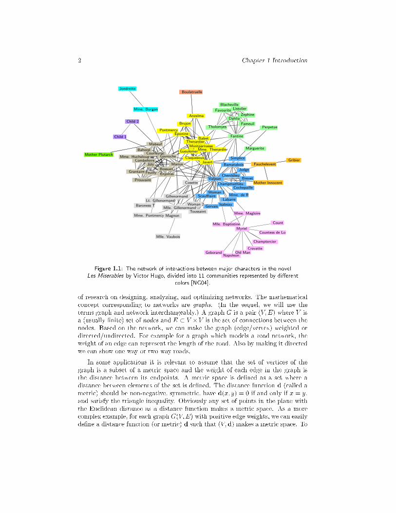
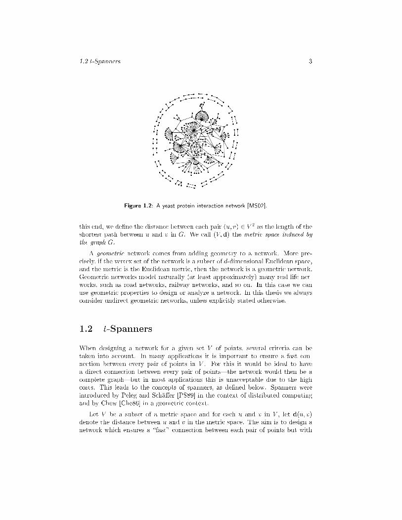
Chapter 1Introdu tion1.1 Geometri networksA network is, informally speaking, a olle tion of \obje ts" with ertain \ on-ne tions" between the obje ts. An obvious example of a network is a omputernetwork. Here the obje ts are omputers and there is a onne tion between two omputers if there is a physi al able onne ting them. Other obvious examplesare road or railway networks. In the latter type of network the obje ts are thestations, and the onne tions are the tra ks onne ting the various stations.There are also many other types of networks, however, where the onne tionsdo not ne essarily have a physi al realization. For example, in so ial s ien es onestudies so ial networks, where the obje ts ould be people and two people are onne ted if they have a ertain so ial relationship| see Figure 1.1. Anotherexample is formed by biologi al networks su h as neural networks, gene regulatorynetworks or protein-protein intera tion networks| see Figure 1.2.Sometimes networks an be rather small|the network in Figure 1.1 for exam-ple is quite small|but sometimes they an also be huge, like the Internet (whi hhas more than 500 million hosts) and the webgraph|a graph whose nodes or-respond to stati pages on the web and whose ar s orrespond to links betweenthese pages|whi h has billions of pages that are onne ted by billions of links.For example, in 2003 Google sear h engine indexed 1.6 billions of URLs and thisin reased to 4.2 billions in 2004.From these examples it is lear that networks form a fundamental model in avariety of appli ation areas. It is not surprising therefore, that there has been a lot

2 Chapter 1 Introdu tion

Myriel

Mlle. Baptistine

Mme. Magloire

Countess de Lo

Geborand

Champtercier

Cravatte

Count

Old ManNapoleon

Valjean

Labarre

Marguerite

Mme. de R

IsabeauGervais

Fantine

Thenardier

Cosette

JavertFaucheleventBamatabois

Simplice

ScaufflaireWoman 1

Judge

Champmathieu

BrevetChenildieu

Cochepaille

Mother Innocent

Mlle. Gillenormand

Marius

Enjolras

Bossuet

Gueulemer

Babet

Claquesous

Montparnasse

Toussaint

Tholomyes

Listolier

Fameuil

Blacheville

Favourite

DahliaZephine

PerpetuePontmercy

Eponine

Boulatruelle

Brujon

Lt. GillenormandGillenormand

Gribier

Mme. Pontmercy

Mabeuf

Jondrette

Mme. Burgon

Combeferre

Prouvaire

Feuilly

Bahorel

Joly

Grantaire

Child 1

Child 2

Mme. Hucheloup

Baroness T

Mlle. Vaubois

Mother Plutarch

Anzelma

Mme. Thenardier

Woman 2

CourfeyracGavroche

Magnon

Figure 1.1: The network of intera tions between major hara ters in the novelLes Miserables by Vi tor Hugo, divided into 11 ommunities represented by di�erent olors [NG04℄.of resear h on designing, analyzing, and optimizing networks. The mathemati al on ept orresponding to networks are graphs. (In the sequel, we will use theterms graph and network inter hangeably.) A graph G is a pair (V;E) where V isa (usually �nite) set of nodes and E ⊂ V ×V is the set of onne tions between thenodes. Based on the network, we an make the graph (edge/vertex) weighted ordire ted/undire ted. For example for a graph whi h models a road network, theweight of an edge an represent the length of the road. Also by making it dire tedwe an show one-way or two-way roads.In some appli ations it is relevant to assume that the set of verti es of thegraph is a subset of a metri spa e and the weight of ea h edge in the graph isthe distan e between its endpoints. A metri spa e is de�ned as a set where adistan e between elements of the set is de�ned. The distan e fun tion d ( alled ametri ) should be non-negative, symmetri , have d(x; y) = 0 if and only if x = y,and satisfy the triangle inequality. Obviously any set of points in the plane withthe Eu lidean distan e as a distan e fun tion makes a metri spa e. As a more omplex example, for ea h graph G(V;E) with positive edge weights, we an easilyde�ne a distan e fun tion (or metri ) d su h that (V;d) makes a metri spa e. To

1.2 t-Spanners 3

Figure 1.2: A yeast protein intera tion network [MS02℄.this end, we de�ne the distan e between ea h pair (u; v) ∈ V 2 as the length of theshortest path between u and v in G. We all (V;d) the metri spa e indu ed bythe graph G.A geometri network omes from adding geometry to a network. More pre- isely, if the vertex set of the network is a subset of d-dimensional Eu lidean spa e,and the metri is the Eu lidean metri , then the network is a geometri network.Geometri networks model naturally (at least approximately) many real-life net-works, su h as road networks, railway networks, and so on. In this ase we anuse geometri properties to design or analyze a network. In this thesis we always onsider undire t geometri networks, unless expli itly stated otherwise.1.2 t-SpannersWhen designing a network for a given set V of points, several riteria an betaken into a ount. In many appli ations it is important to ensure a fast on-ne tion between every pair of points in V . For this it would be ideal to havea dire t onne tion between every pair of points|the network would then be a omplete graph|but in most appli ations this is una eptable due to the high osts. This leads to the on epts of spanners, as de�ned below. Spanners wereintrodu ed by Peleg and S h�a�er [PS89℄ in the ontext of distributed omputingand by Chew [Che86℄ in a geometri ontext.Let V be a subset of a metri spa e and for ea h u and v in V , let d(u; v)denote the distan e between u and v in the metri spa e. The aim is to design anetwork whi h ensures a \fast" onne tion between ea h pair of points but with

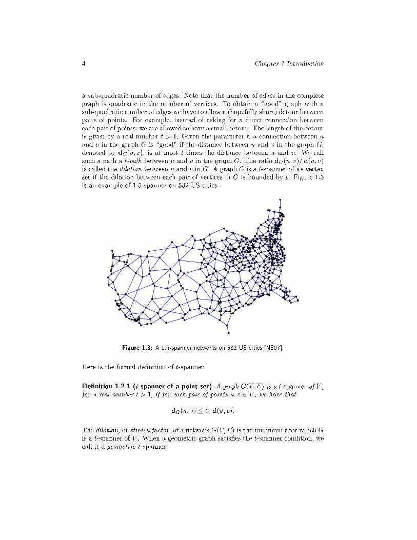
4 Chapter 1 Introdu tiona sub-quadrati number of edges. Note that the number of edges in the ompletegraph is quadrati in the number of verti es. To obtain a \good" graph with asub-quadrati number of edges we have to allow a (hopefully short) detour betweenpairs of points. For example, instead of asking for a dire t onne tion betweenea h pair of points, we are allowed to have a small detour. The length of the detouris given by a real number t > 1. Given the parameter t, a onne tion between uand v in the graph G is \good" if the distan e between u and v in the graph G,denoted by dG(u; v), is at most t times the distan e between u and v. We allsu h a path a t-path between u and v in the graph G. The ratio dG(u; v)=d(u; v)is alled the dilation between u and v in G. A graph G is a t-spanner of its vertexset if the dilation between ea h pair of verti es in G is bounded by t. Figure 1.3is an example of 1:5-spanner on 532 US ities.

Figure 1.3: A 1:5-spanner networks on 532 US ities [NS07℄.Here is the formal de�nition of t-spanner.De�nition 1.2.1 (t-spanner of a point set) A graph G(V;E) is a t-spanner of V ,for a real number t > 1, if for ea h pair of points u; v ∈ V , we have thatdG(u; v) ≤ t · d(u; v):The dilation, or stret h fa tor, of a network G(V;E) is the minimum t for whi h Gis a t-spanner of V . When a geometri graph satis�es the t-spanner ondition, we all it a geometri t-spanner.

1.2 t-Spanners 5Intuitively, the t-spanner property is stronger than the graph onne tivity prop-erty, i.e. we should not only have a path between ea h pair of points in the graphbut also the length of the path should be lose to the distan e between the pair ofpoints. The parameter t de ides how lose the t-spanner approximates the om-plete graph. In other words, the loser t is to one, the loser the t-spanner is tothe omplete graph.We an easily extend De�nition 1.2.1 to a t-spanner of a given graph. Re allthat for any two verti es u and v in a graph G with positive edge weights, dG(u; v)denotes the distan e between u and v in the graph V , that is, the length of theshortest path between u and v in G.De�nition 1.2.2 (t-spanner of a graph) Let G(V;E) be a graph with positive edgeweights. A graph G′(V;E′) on the same vertex set but with edge set E′ ⊆ E is at-spanner of G if for ea h pair of verti es u; v ∈ V we have thatdG′(u; v) ≤ t · dG(u; v):By omparing De�nition 1.2.1 and De�nition 1.2.2 one an see two di�eren es.First, a t-spanner of a given graph G is a subgraph of G. Therefore omputing at-spanner of a graph G is sometimes alled a pruning of G. The se ond di�eren eis that, to he k the t-spanner ondition, the distan e between ea h pair in thet-spanner is ompared to the distan e between them in the input graph. Note thatin De�nition 1.2.2 it is not ne essary that the verti es of the input graph belongto a metri spa e. Instead we use the metri spa e indu ed by the input graph tomeasure the distan e between them.A t-spanner on a point set V|whi h is subset of a metri spa e| an be seenas a t-spanner of the omplete graph on V , denoted by G (V ), where the weightof ea h edge in the omplete graph is the distan e between its endpoints.The main question in designing t-spanners is whether spanners exist that have\good" properties. The desirable properties are the following:Size: The number of edges in the graph. This is the most important measure-ment and generating spanners with a small, ideally near-linear, size is desirable.The fa t that geometri spanners with a near-linear number of edges and smalldilation exist has made the onstru tion of spanners one of the fundamental toolsin the development of approximation algorithms for geometri al problems.Degree: The maximum number of edges in ident to a vertex. This propertyhas been shown to be useful in the development of approximation algorithms[GLNS02a, Yao82℄ and for the onstru tion of ad ho networks [ALW+03, Li03℄where small degree is essential in trying to develop fast lo alized algorithms.Weight: The weight of a network G(V;E) is the sum of the edge weights.(Re all that for geometri graphs the weight of an edge is simply the Eu lideandistan e between its two endpoints.) The best that an be a hieved is a onstant

6 Chapter 1 Introdu tiontimes the weight of the minimum spanning tree, denoted wt(MST (V )). Lowweight spanners have found appli ations in areas su h as metri spa e sear h-ing [NP03, NPC02℄|see Se tion 1.3.2|and broad asting in ommuni ation net-works [FPZW04℄|see Se tion 1.3.3. Also, it has been used in the onstru tion ofseveral approximation algorithms, see [CL00, RS98℄.Spanner diameter: De�ned as the smallest integer D su h that for any pair ofverti es u and v in V , there is a t-path in the graph between u and v ontainingat most D edges. For wireless ad ho networks it is often desirable to have smallspanner diameter sin e it determines the maximum number of times a messagehas to be transmitted in a network. If a graph has spanner diameter D then it issaid to be a D-hop network.It has been shown that for any set V of n points in Rd and for any �xed t > 1there exists a t-spanner with O(n) edges, onstant degree, and whose total weightis O(wt(MST (V ))) [DN97, NS07℄. Arya et al. [AMS99℄ designed a randomizedalgorithm whi h generates a t-spanner of expe ted linear size and expe ted loga-rithmi spanner diameter.Note that some of the above properties are ompeting, e.g., a graph with onstant degree annot have onstant spanner diameter, and a graph with smallspanner diameter annot have a linear number of edges [ADM+95℄.In most ases we are interested in t-spanners, where t is lose to 1. Morepre isely, we are interested in s hemes where we an spe ify any t > 1 and thenobtain a spanner of dilation t. To emphasize the fa t that t is lose to 1, we willsometimes speak about (1 + ")-spanners instead of t-spanners.1.3 Why spanners?Spanners for omplete graphs as well as for arbitrary weighted graphs �nd appli a-tions in roboti s, network topology design, distributed systems, design of parallelma hines, and many other areas. Re ently spanners found interesting pra ti al ap-pli ations in areas su h as metri spa e sear hing [NP03, NPC02℄ and broad astingin ommuni ation networks [ALW+03, FPZW04, Li03℄.Several well-known theoreti al results also use the onstru tion of t-spannersas a building blo k. For example, Rao and Smith [RS98℄ made a breakthroughby showing an optimal O(n logn)-time approximation s heme for the well-knownEu lidean traveling salesperson problem, using t-spanners (or banyans). Simi-larly, Czumaj and Lingas [CL00℄ showed approximation s hemes for minimum- ostmulti- onne tivity problems in geometri graphs. The problem of onstru tinggeometri spanners has re eived onsiderable attention from a theoreti al perspe -tive, see [ADD+93, ADM+95, AMS99, BGM04, DHN93, DN97, DNS95, GLN02,Kei88, KG92, LL92, LNS02, Sal91, Vai91℄, the surveys [Epp00, GK07, Smi00℄ and

1.3 Why spanners? 7the book by Narasimhan and Smid [NS07℄. Note that signi� ant resear h has alsobeen done in the onstru tion of spanners for general graphs, see for example, thebook by Peleg [Pel00℄ or the re ent work by Elkin and Peleg [EP04℄ and Tho-rup and Zwi k [TZ01℄. In this se tion we mention some of the appli ations oft-spanners.1.3.1 Approximate minimum spanning treeThe problem of �nding a minimum weight spanning tree (MST) of a given graphhas re ently attra ted a lot of attention. There are linear time algorithms for om-puting MST in a randomized expe ted ase model [KKT95℄ or with the assumptionthat edge weight are integers [FW94℄. For deterministi omparison-based algo-rithms, slightly superlinear bounds are known [GGST86℄.In the geometri ase, for any dimension d, one an �nd a minimum spanningtree of a set of n points in O(n2) time by onstru ting the omplete graph and omputing all the edge weights (=pairwise distan es) in O(n2) time, and thenrunning any MST algorithm (su h as Prim's algorithm). Most of the faster al-gorithms for the geometri ase use a simple idea: �nd a sparse subgraph of the omplete graph whi h ontains an MST, and then ompute an MST of this sparsesubgraph. In the plane, the Delaunay graph is the appropriate graph to use sin eit only has O(n) edges and an be onstru ted in O(n logn) time [SH75℄. It isnot helpful in higher dimensions be ause the Delaunay graph an have a quadrati number of edges [Eri01℄.Salowe [Sal91℄ showed that if G′ is a (geometri ) t-spanner of a graph Gand wt(MST (G)) denotes the weight of the minimum spanning tree of G, thenwt(MST (G′)) ≤ t · wt(MST (G)). Using this result, we an use any (sparse)t-spanner of a graph to ompute an approximate minimum spanning tree of thegraph. For more details about approximating the minimum spanning tree see thesurvey by Eppstein [Epp00℄.1.3.2 Metri spa e sear hingThe problem of \approximate" proximity sear hing in metri spa es is to �nd theelements of a set whi h are \ lose" to a given query under some similarity riterion.Similarity sear hing has be ome a fundamental omputational task in a variety ofappli ation areas, in luding multimedia information retrieval, pattern re ognition, omputer vision and biomedi al databases. In su h environments, an exa t mat hhas little meaning, and proximity/distan e on epts (similarity/dissimilarity) aretypi ally mu h more fruitful for sear hing. In all of these appli ations we have ametri whi h shows the similarity between obje ts. The smaller the distan e isbetween two obje t, the more similar they are | see [ZADB06℄ for more details.

8 Chapter 1 Introdu tionA typi al query q is:• �nd all elements in the database whi h are within distan e r from q.• �nd the k losest elements to q in the database.If the database ontains n elements, we an answer a query by performing O(n)distan e omputations. But evaluating distan es is expensive and the goal is toredu e the number of distan e evaluations. In general, there are several methods toredu e the number of distan e evaluations, see the survey [CNBYM01℄. A widelyused te hnique for this is AESA [Rui86℄. The main drawba k of this te hnique isthat it omputes all pairwise distan es and stores them in a matrix whi h requiresa lot of spa e.Navarro et al. [NPC02℄ used a t-spanner as a data stru ture for metri spa esear hing to redu e the spa e needed for the AESA. The key idea is to regardthe t-spanner as an approximation of the omplete graph of distan es among theobje ts, and to use it as a ompa t devi e to simulate the large matrix of distan esrequired by su essful sear h algorithms su h as AESA. The t-spanner propertyimplies that we an use the shortest path in the t-spanner to estimate any distan ewith bounded error fa tor t.They propose several t-spanner onstru tion, update, and sear h algorithmsand experimentally evaluated them. The experiments show that their te hniqueis ompetitive against urrent approa hes, and that it has a great potential forfurther improvements.1.3.3 Broad asting in ommuni ation networksWireless networks onsist of a set of wireless devi es ( alled nodes) whi h arespread over a geographi al area. These nodes are able to perform pro essing aswell as ommuni ating with ea h other. The nodes an ommuni ate via multi-hop wireless hannels: a node an rea h all nodes inside its transmission regionwhile nodes far away from ea h other ommuni ate through intermediate nodes.Wireless ommuni ation networks have appli ations in various situations su h asemergen y relief, environmental monitoring, and so on.There are two ommon types of wireless networks: sink-based networks andad ho networks. In a sink-based network, like ellular wireless networks, there isone or multiple sink nodes whi h are in harge of olle ting data from all nodesand managing the whole network. On the other hand, in ad ho networks thereare no su h sink nodes and all nodes are equal in terms of ommuni ation andnetwork management.Energy onsumption and network performan e are the most riti al issues inwireless ad ho networks, be ause wireless devi es are usually powered by batteriesonly and have limited omputing apability and memory.

1.3 Why spanners? 9A wireless ad ho network is modeled by a set V of n wireless nodes distributedin a two-dimensional plane. Ea h node has the same maximum transmission rangeR whi h, by a proper s aling, we an assume that all nodes have the maximumtransmission range to be equal to 1. These wireless nodes de�ne a unit disk graph,denoted by UDG(V ), in whi h there is an edge between two nodes if the Eu lideandistan e between them is at most 1. The most ommon power-attenuation modelin the literature laims that the power needed to support a link (u; v) is ‖uv‖�,where ‖uv‖ is the Eu lidean distan e between u and v and � is a real onstantbetween 2 and 5 depending on the wireless transmission environment. So thepower onsumption of a network is a fun tion of the weight of the network. Theminimum possible weight for a onne ted network is the weight of a minimumspanning tree, however, this might have low performan e.Several graph theoreti al models are used to design ad ho networks with lowenergy onsumption and good performan e|see [Wat05℄. Using a low weightt-spanner of the unit disk graph is one of the ways|see [ALW+03℄. This givesus more exibility to onstru t a network whi h has low energy onsumption aswell as good performan e, like bounded degree. Note that in ad ho networks, anetwork with small node degree, has a better han e to has small interferen e.1.3.4 Proteins visualizationOne of the most important open problems in bioinformati s is the problem ofprotein folding. A protein is a long hain of mole ules alled amino a ids. Innature there exist 20 di�erent amino a ids and several experiments show that the3D-stru ture of a protein is ompletely determined by the sequen e of amino a ids.The protein-folding problem is the problem of determining the 3D-stru tureof a protein given its amino a id sequen e. Various omputational methods havebeen applied to ta kle the protein-folding problem, with varying su ess. Amongthese are neural networks, approximation algorithms, metaheuristi s, bran h-and-bound, distributed systems and omputational geometry.Nowadays, using high omputing power and large s ale storage, resear hersare able to omputationally simulate the protein-folding pro ess in atomisti de-tails. Su h simulations often produ e a large number of folding traje tories, ea h onsisting of a series of 3D onformations of the protein under study. As a re-sult, e�e tively managing and analyzing su h traje tories is be oming in reasinglyimportant.Re ently, Russel and Guibas [RG05℄ suggested using geometri spanners formapping a simulation to a more dis rete ombinatorial representation. They ap-ply geometri spanners to dis over the proximity between di�erent segments ofa protein a ross a range of s ales, and tra k the hanges of su h proximity overtime. This makes the task of understanding and exploring the spa e of protein

10 Chapter 1 Introdu tionmotions easier. Using their stru ture it is possible to visualize proteins in mo-tion whi h none of the ommonly used software pa kages su h as RasMol [Ras℄,ProteinExplorer [Mar02℄, or SPV [GP97℄ have been able to a hieve.1.4 Thesis overviewIn this thesis we onsider several problems related to the design and analysis ofgeometri networks.In Chapter 2, we introdu e the on ept of region-fault tolerant spanners forplanar point sets, and prove the existen e of region-fault tolerant spanners of smallsize. For a geometri graph G on a point set V and a region F , we de�ne G⊖F tobe what remains of G after the verti es and edges of G interse ting F have beenremoved. A C-fault tolerant t-spanner is a geometri graph G on V su h that forany onvex region F , the graph G⊖F is a t-spanner for G (V )⊖F , where G (V )is the omplete geometri graph on V . Fault-tolerant spanners provide high levelsof availability and reliability in network onne tions. These networks keep theirgood properties, even after some part of the network is destroyed e.g. by a naturaldisaster.We prove that any set V of n points admits a C-fault tolerant (1 + ")-spannerof size O(n log n), for any onstant " > 0; if adding Steiner points is allowed thenthe size of the spanner redu es to O(n), and for several spe ial ases we show howto obtain region-fault tolerant spanners of size O(n) without using Steiner points.We also onsider fault-tolerant geodesi t-spanners : this is a variant where, for anydisk D, the distan e in G⊖D between any two points u; v ∈ V \ D is at most ttimes the geodesi distan e between u and v in R

2 \ D. We prove that for anypoint set V we an add O(n) Steiner points to obtain a fault-tolerant geodesi (1 + ")-spanner of size O(n). These results are based on [AdBFG07℄.In appli ations|think of road networks, for instan e|a spanner network issometimes expanded by adding one or more extra onne tions. The main questionis then how to do the expansion su h that the resulting network is as good as pos-sible. In Chapter 3 we study a problem of this type. In parti ular, we onsider theproblem of adding an edge to a given network su h that the dilation of the resultingnetwork is minimized. We present one exa t algorithm and several approximationalgorithms. The best approximation algorithm omputes a (2 + ")-approximationof the optimal solution in O(nm+n2 logn) time using O(n2) spa e, where n is thenumber of verti es and m is the number of edges in the input network. For thespe ial ase, when the dilation of the input network is onstant, we an improvethe approximation fa tor to 1 + " and the running time to O(n2). These resultsare based on [FGG05a℄.

1.4 Thesis overview 11Chapter 4 studies the problem of dilation optimal edge deletion. More pre iselywe are given a geometri network in the plane and we want to �nd an edge inthe network su h that its removal minimizes, or maximizes, the dilation in thenetwork. An obvious appli ation is when we want to remove some onne tions inan existing network, e.g. due to budget onsideration, and we want to know whi hedges should be removed to minimize the e�e t on the quality of the network.We solve the problem in the restri ted ase when the network is a simple y le.A randomized algorithm is presented whi h, given a y le on a set of n points, omputes in O(n log3 n) expe ted time, the edge of the y le whose removal resultsin a polygonal path of smallest possible dilation. It is also shown that the edgewhose removal gives a polygonal path of largest possible dilation an be omputedin O(n log n) time. If the input y le is a onvex polygon, the latter problem anbe solved in O(n) time. Finally, it is shown that given a y le C, for ea h edge eof C, a (1− ")-approximation to the dilation of the path C \ {e} an be omputedin O(n logn) total time. These results are based on [AFK+07℄.In Chapter 5 we present algorithms for omputing the spanner diameter ofa t-spanner. This is the �rst algorithm for omputing spanner diameter of a t-spanner, to the best of our knowledge. The time omplexity of the most eÆ ientalgorithm is O(D·mn), where n is the number of verti es,m is the number of edgesand D is the spanner diameter of the input graph, and it requires O(n) spa e. Wealso ompare the running time of the presented algorithms experimentally. Theseresults are based on [FG06℄.The empiri al study of algorithms is a rapidly growing resear h area. Imple-menting algorithms and testing their performan e shows their eÆ ien y in pra ti eand bring the algorithms to the pra ti al stage. In Chapter 6 we experimentallystudy the performan e and quality of the most ommon t-spanner algorithms forpoints in the Eu lidean plane. The experiments are dis ussed and ompared tothe theoreti al results and in several ases we suggest modi� ations that are im-plemented and evaluated. The quality measurements that we onsider are thenumber of edges, the weight, the maximum degree, the spanner diameter and thenumber of rossings. We ompare the running times of the algorithms and suggestsome improvements. This is the �rst time an extensive omparison has been madebetween the onstru tion algorithms of t-spanners. These results are based on[FG05℄ and [FG07℄.Finally in Chapter 7 we on lude the thesis and state some open problems.

12 Chapter 1 Introdu tion

Chapter 2Region-Fault TolerantSpanners2.1 Introdu tionAs we mentioned before, geometri networks have appli ations in VLSI design,tele ommuni ations, roboti s and distributed systems. The major issues withdesigning su h a network are performan e and reliability. The spanner on ept aptures the performan e when short onne tions between the points are impor-tant. The main question is then whether spanners exist that have a small dilationand a small, ideally near-linear, number of edges. Other desirable properties of aspanner are for example that the total weight of the edges is small, or that themaximum degree is low. As dis ussed in the introdu tion, su h spanners do indeedexist: it has been shown that for any set P of n points in the plane and for any�xed " > 0 there exists a (1 + ")-spanner with O(n=") edges, O(1=") degree, andwhose total weight is O(wt(MST (P ))="4), where wt(MST (P )) is the weight of aminimum spanning tree of P [DN97, NS07℄.Reliability is on erned with the fa t that in many appli ations the nodesand/or links in a network may fail. In a omputer network, for instan e, nodesmay fail be ause omputers an rash, and in a road network links may fail be auseroads an be ome ina essible due to a idents or maintenan e. A network isreliable when it retains its good properties even after some nodes or links fail.With respe t to spanners this means there should still be a short path betweenany two nodes in what remains of the spanner after the fault.

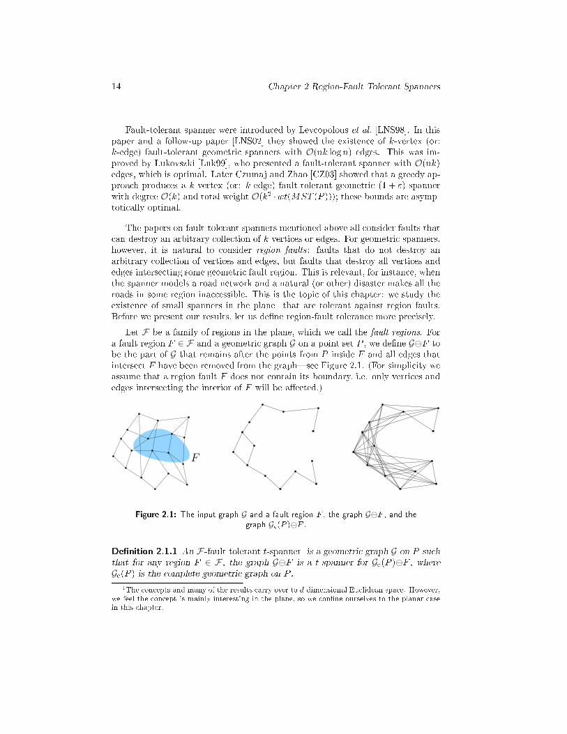
14 Chapter 2 Region-Fault Tolerant SpannersFault-tolerant spanner were introdu ed by Lev opolous et al. [LNS98℄. In thispaper and a follow-up paper [LNS02℄ they showed the existen e of k-vertex (or:k-edge) fault-tolerant geometri spanners with O(nk logn) edges. This was im-proved by Lukovszki [Luk99℄, who presented a fault-tolerant spanner with O(nk)edges, whi h is optimal. Later Czumaj and Zhao [CZ03℄ showed that a greedy ap-proa h produ es a k-vertex (or: k-edge) fault-tolerant geometri (1 + ")-spannerwith degree O(k) and total weight O(k2 ·wt(MST (P ))); these bounds are asymp-toti ally optimal.The papers on fault-tolerant spanners mentioned above all onsider faults that an destroy an arbitrary olle tion of k verti es or edges. For geometri spanners,however, it is natural to onsider region faults : faults that do not destroy anarbitrary olle tion of verti es and edges, but faults that destroy all verti es andedges interse ting some geometri fault region. This is relevant, for instan e, whenthe spanner models a road network and a natural (or other) disaster makes all theroads in some region ina essible. This is the topi of this hapter: we study theexisten e of small spanners in the plane1 that are tolerant against region faults.Before we present our results, let us de�ne region-fault toleran e more pre isely.Let F be a family of regions in the plane, whi h we all the fault regions. Fora fault region F ∈ F and a geometri graph G on a point set P , we de�ne G⊖F tobe the part of G that remains after the points from P inside F and all edges thatinterse t F have been removed from the graph|see Figure 2.1. (For simpli ity weassume that a region fault F does not ontain its boundary, i.e. only verti es andedges interse ting the interior of F will be a�e ted.)F

Figure 2.1: The input graph G and a fault region F , the graph G⊖F , and thegraph G (P )⊖F .De�nition 2.1.1 An F-fault tolerant t-spanner is a geometri graph G on P su hthat for any region F ∈ F , the graph G⊖F is a t-spanner for G (P )⊖F , whereG (P ) is the omplete geometri graph on P .1The on epts and many of the results arry over to d-dimensional Eu lidean spa e. However,we feel the on ept is mainly interesting in the plane, so we on�ne ourselves to the planar asein this hapter.

2.1 Introdu tion 15We are mainly interested in the ase where F is the family C of onvex sets.2We shall also onsider the ase where we are allowed to add Steiner points to thegraph. In other words, instead of onstru ting a geometri network for P , we areallowed to onstru t a network for P ∪Q for some set Q of Steiner points. Thenwe say that a graph G on P ∪ Q is a C-fault tolerant Steiner t-spanner for P if,for any F ∈ C and any two points u; v ∈ P \ F , the distan e between u and v inG⊖F is at most t times their distan e in G (P )⊖F .We also study another variant of region-fault toleran e. In this variant werequire that the distan e between any two points u; v in G⊖F is at most t timesthe geodesi distan e between u and v in R

2 \ F . Note that the geodesi distan ein R2 \F|that is, the length of a shortest path in R

2 \F|is never more than thedistan e between u and v in G (P )⊖F . We all a spanner with this property anF-fault tolerant geodesi t-spanner. It is not diÆ ult to show that �nite size F-faulttolerant geodesi spanners do not exist unless we are allowed to use Steiner points.Even in the ase of Steiner points, �nite size F-fault tolerant geodesi spannersdo not exist when F is the family C of all onvex sets. Hen e, we restri t ourattention to D-fault tolerant geodesi spanners, where D is the family of disks inthe plane.We obtain the following results.

• In Se tion 2.2 we present a general method to onvert a well-separated pairde omposition (WSPD) [CK93℄ for P into a C-fault tolerant spanner for P .We use this method to obtain linear-size C-fault tolerant (1 + ")-spannersfor points in onvex position and for points distributed uniformly at ran-dom inside the unit square, and to obtain linear-size C-fault tolerant Steiner(1 + ")-spanners for arbitrary point sets.• In Se tion 2.4 we onsider two spe ial ases, fat triangulations and polygonalregion faults with limited number of edge dire tions, for whi h linear-sizeC-fault tolerant spanners an be obtained.

• In Se tion 2.5 we study small C-fault tolerant (non-Steiner) spanners forarbitrary point sets. By ombining a more relaxed version of the WSPDwith ideas from �-graphs [Kei88℄, we show that any point set P admits aC-fault tolerant (1 + ")-spanner of size O(n logn).

• In Se tion 2.6 we address a slightly di�erent problem. Instead of designinga C-fault tolerant spanner, it is also interesting to he k whether an existingnetwork is C-fault tolerant or not. In Se tion 2.6 we give an algorithm whi h,given a graph G, he ks whether it is fault tolerant under onvex region faults.2It is easy to see that there are no small region-fault tolerant t-spanners with respe t to non- onvex faults: if HH denotes the family of regions that are the union of two half-planes, thenG (P ) is the only HH-fault tolerant t-spanner for P , for any �nite t.

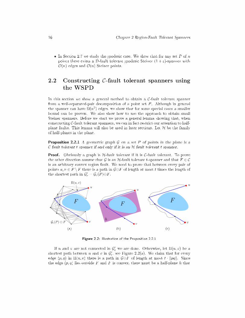
16 Chapter 2 Region-Fault Tolerant Spanners• In Se tion 2.7 we study the geodesi ase. We show that for any set P of npoints there exists a D-fault tolerant geodesi Steiner (1 + ")-spanner withO(n) edges and O(n) Steiner points.2.2 Constru ting C-fault tolerant spanners usingthe WSPDIn this se tion we show a general method to obtain a C-fault tolerant spannerfrom a well-separated-pair de omposition of a point set P . Although in generalthe spanner an have (n2) edges, we show that for some spe ial ases a smallerbound an be proven. We also show how to use the approa h to obtain smallSteiner spanners. Before we start we prove a general lemma showing that, when onstru ting C-fault tolerant spanners, we an in fa t restri t our attention to half-plane faults. This lemma will also be used in later se tions. Let H be the familyof half-planes in the plane.Proposition 2.2.1 A geometri graph G on a set P of points in the plane is a

C-fault tolerant t-spanner if and only if it is an H-fault tolerant t-spanner.Proof. Obviously a graph is H-fault tolerant if it is C-fault tolerant. To provethe other dire tion assume that G is an H-fault tolerant t-spanner and that F ∈ Cis an arbitrary onvex region fault. We need to prove that between every pair ofpoints u; v ∈ P \ F there is a path in G⊖F of length at most t times the length ofthe shortest path in G′ = G (P )⊖F .u

v

F

Gc(P ) ⊖ F

Π(u, v)

(a)u

v

F

h (b)u

v

F

( )Figure 2.2: Illustration of the Proposition 2.2.1If u and v are not onne ted in G′ we are done. Otherwise, let �(u; v) be ashortest path between u and v in G′ , see Figure 2.2(a). We laim that for everyedge (p; q) in �(u; v) there is a path in G⊖F of length at most t · ‖pq‖. Sin ethe edge (p; q) lies outside F and F is onvex, there must be a half-plane h that

2.3 Well-separated pair de omposition 17A

B

CA

CB

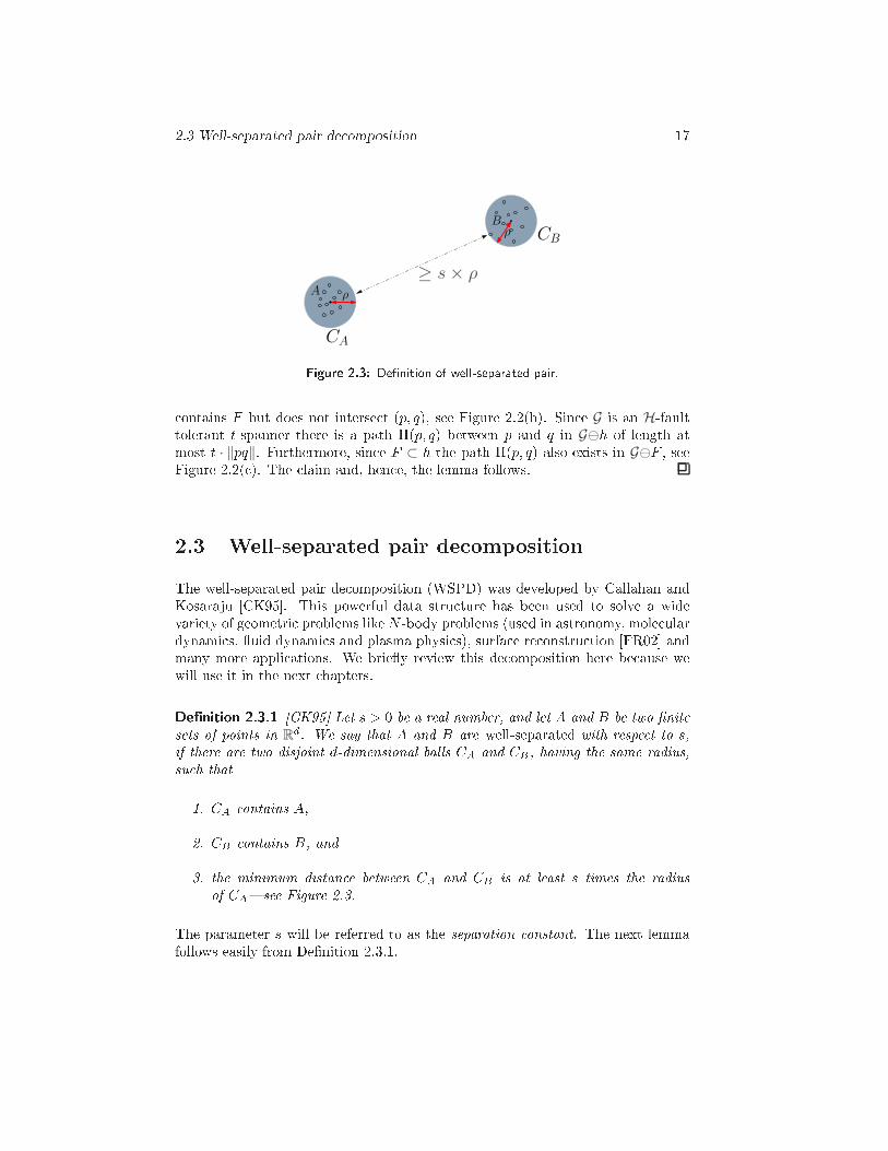
≥ s × ρρ

ρ

Figure 2.3: De�nition of well-separated pair. ontains F but does not interse t (p; q), see Figure 2.2(b). Sin e G is an H-faulttolerant t-spanner there is a path �(p; q) between p and q in G⊖h of length atmost t · ‖pq‖. Furthermore, sin e F ⊂ h the path �(p; q) also exists in G⊖F , seeFigure 2.2( ). The laim and, hen e, the lemma follows.2.3 Well-separated pair de ompositionThe well-separated pair de omposition (WSPD) was developed by Callahan andKosaraju [CK95℄. This powerful data stru ture has been used to solve a widevariety of geometri problems like N -body problems (used in astronomy, mole ulardynami s, uid dynami s and plasma physi s), surfa e re onstru tion [FR02℄ andmany more appli ations. We brie y review this de omposition here be ause wewill use it in the next hapters.De�nition 2.3.1 [CK95℄ Let s > 0 be a real number, and let A and B be two �nitesets of points in Rd. We say that A and B are well-separated with respe t to s,if there are two disjoint d-dimensional balls CA and CB , having the same radius,su h that1. CA ontains A,2. CB ontains B, and3. the minimum distan e between CA and CB is at least s times the radiusof CA|see Figure 2.3.The parameter s will be referred to as the separation onstant. The next lemmafollows easily from De�nition 2.3.1.

18 Chapter 2 Region-Fault Tolerant SpannersLemma 2.3.2 [CK95℄ Let A and B be two �nite sets of points that are well-separated with respe t to s, let x and p be points of A, and let y and q be pointsof B. Then(i) ‖xy‖ ≤ (1 + 4=s) · ‖pq‖, and(ii) ‖px‖ ≤ (2=s) · ‖pq‖.Intuitively, by Lemma 2.3.2, if A and B are well-separated, then the distan ebetween a point in A and a point in B is roughly the same as the distan e betweenthe two sets A and B. Also the distan e between a pair of points whi h both liein one of the sets is mu h smaller than the distan e between the two sets.De�nition 2.3.3 [CK95℄ Let P be a set of n points in Rd, and let s > 0 be a realnumber. A well-separated pair de omposition (WSPD) for P with respe t to s isa sequen e of pairs of non-empty subsets of P , (A1; B1); : : : ; (Am; Bm), su h that1. Ai and Bi are well-separated with respe t to s, for 1 ≤ i ≤ m.2. for any two distin t points p and q of P , there is exa tly one pair (Ai; Bi)in the sequen e, su h that (i) p ∈ Ai and q ∈ Bi, or (ii) q ∈ Ai and p ∈ Bi,The integer m is alled the size of the WSPD.In other words, a well-separated pair de omposition of a point set P onsists of aset of well-separated pairs that over all the pairs of distin t points, i.e., any twodistin t points belong to the di�erent sets of some pair.Callahan and Kosaraju showed that for any point set in Eu lidean spa e andfor any onstant s > 0, there always exist a WSPD of size m = O(sdn) and it an be omputed in O(sdn + n logn) time. In the geometri problems, when weneed all point pairs in a set, we an easily use a WSPD of the point set as anapproximation with linear size.2.3.1 Constru ting a C-fault tolerant spannerCallahan and Kosaraju [CK93℄ showed that the WSPD an be used to obtain asmall (1 + ")-spanner. Similar ideas were used earlier by Salowe [Sal91, Sal92℄ andVaidya [Vai88, Vai89, Vai91℄. To obtain the (1 + ")-spanner one simply omputesa WSPD W with respe t to s := 4 + 8=", and then for ea h well-separated pair(A;B) ∈ W one adds an arbitrary edge onne ting a point from A to a point in B.Unfortunately this onstru tion is not C-fault tolerant, be ause a fault F andestroy the spanner edge that onne ts a pair (A;B), while some other edgesbetween A and B (whi h are not in the spanner) may survive the fault. Hen e,

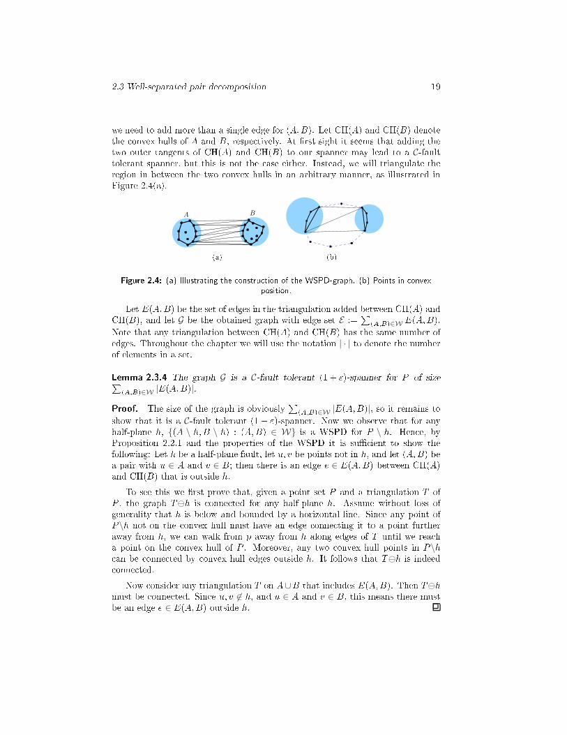
2.3 Well-separated pair de omposition 19we need to add more than a single edge for (A;B). Let CH(A) and CH(B) denotethe onvex hulls of A and B, respe tively. At �rst sight it seems that adding thetwo outer tangents of CH(A) and CH(B) to our spanner may lead to a C-faulttolerant spanner, but this is not the ase either. Instead, we will triangulate theregion in between the two onvex hulls in an arbitrary manner, as illustrated inFigure 2.4(a).A B(a) (b)Figure 2.4: (a) Illustrating the onstru tion of the WSPD-graph. (b) Points in onvexposition.Let E(A;B) be the set of edges in the triangulation added between CH(A) andCH(B), and let G be the obtained graph with edge set E := P(A;B)∈W E(A;B).Note that any triangulation between CH(A) and CH(B) has the same number ofedges. Throughout the hapter we will use the notation | · | to denote the numberof elements in a set.Lemma 2.3.4 The graph G is a C-fault tolerant (1 + ")-spanner for P of sizeP(A;B)∈W |E(A;B)|.Proof. The size of the graph is obviously P(A;B)∈W |E(A;B)|, so it remains toshow that it is a C-fault tolerant (1 + ")-spanner. Now we observe that for anyhalf-plane h, {(A \ h;B \ h) : (A;B) ∈ W} is a WSPD for P \ h. Hen e, byProposition 2.2.1 and the properties of the WSPD it is suÆ ient to show thefollowing: Let h be a half-plane fault, let u; v be points not in h, and let (A;B) bea pair with u ∈ A and v ∈ B; then there is an edge e ∈ E(A;B) between CH(A)and CH(B) that is outside h.To see this we �rst prove that, given a point set P and a triangulation T ofP , the graph T⊖h is onne ted for any half-plane h. Assume without loss ofgenerality that h is below and bounded by a horizontal line. Sin e any point ofP\h not on the onvex hull must have an edge onne ting it to a point furtheraway from h, we an walk from p away from h along edges of T until we rea ha point on the onvex hull of P . Moreover, any two onvex hull points in P\h an be onne ted by onvex hull edges outside h. It follows that T⊖h is indeed onne ted.Now onsider any triangulation T on A∪B that in ludes E(A;B). Then T⊖hmust be onne ted. Sin e u; v 6∈ h, and u ∈ A and v ∈ B, this means there mustbe an edge e ∈ E(A;B) outside h.

20 Chapter 2 Region-Fault Tolerant Spanners2.3.2 Linear-size spanners for spe ial asesThe method des ribed above an be used to get small C-fault tolerant spanners forseveral spe ial ases. For example, if P is in onvex position then |E(A;B)| ≤ 3for any pair (A;B) in the de omposition, see Figure 2.4(b), so we get:Theorem 2.3.5 For any set P of n points in onvex position in the plane and any" > 0, there exists a C-fault tolerant (1 + ")-spanner of size O(n="2).Next we show that we an also get a C-fault tolerant spanner whose expe tedsize is linear if the point set P is generated by pi king n points uniformly at randomin the unit square.Lemma 2.3.6 Let P be a set of n uniformly distributed points in the unit squareand A be a sub-square of the unit square. Then the expe ted number of points onthe onvex hull of P ∩ A is O(log(n · area(A))).Proof. If n points are uniformly distributed in the unit square then it is knownthat the expe ted number of points on the onvex hull of the points isO(logn) [HP98,RS63℄.Now let X be the number of points on the onvex hull of P ∩ A and letY := |P ∩ A|. Clearly EXP[Y ℄ = n · area(A). By the law of total expe tation[Ros98, Proposition 4.1℄ if X and Y are two random variables thenEXP[X ℄ = EXP [EXP[X |Y ℄℄ ;thereforeEXP[X ℄ = EXP [EXP[X |Y ℄℄= EXP[O(log(Y ))℄≤ O (log (EXP[Y ℄)) (Jensen's inequality [Ros98, p. 418℄)= O(log(n · area(A))):Now we ombine the ideas from the previous se tion with Lemma 2.3.6 to onstru ta (1 + ")-spanner of the uniformly distributed point set P .Theorem 2.3.7 Let P be a set of n points uniformly distributed in the unitsquare U . For any " > 0 there is a C-fault tolerant (1 + ")-spanner of expe tedsize O(n="2) for P .Proof. Constru t a quadtree partitioning of U into smaller and smaller squares,until ea h square has size (side length) roughly 1=√n. So the area of any leaf is

2.3 Well-separated pair de omposition 21roughly 1=n whi h means the expe ted number of points in a leaf region is O(1).The quadtree has O(n) leaves. Level ` of the quadtree orresponds to a regularsubdivision of U into squares of size 1=2`. One an show that there exists a WSPDW := {(Ai; Bi)}i of size O(n="2) for P su h that for ea h i, the pair (Ai; Bi) either orresponds to two squares at the same level, orAi and Bi are both singleton pointsthat lie in nearby ells (or the same ell) of the �nal subdivision. Moreover, if wedenote by n` the number of pairs of the WSPD at level ` of the quadtree, thenn` = O(22`="2). The existen e of a WSPD with these properties follows ratherdire tly from the results of Fis her and Har-Peled [FHP05℄. For ompleteness webrie y sket h an argument for our setting.For a node � of the quadtree, let P (�) denote the subset of points from P insidethe square orresponding to �. Consider a level ` of the quadtree. For ea h pairof nodes �; �′ at level ` su h that the point sets P (�) and P (�′) are well-separatedwhile the point sets of the parents of � and �′ are not well-separated, we put thepair (P (�); P (�′)) into the WSPD. In addition, for ea h pair of leaf nodes �; �′su h that P (�) and P (�′) are not well-separated, we put a pair ({p}; {q}) into theWSPD for every pair p ∈ P (�) and q ∈ P (�′). It is easy to verify that this indeedde�nes a WSPD. The bound on the number of pairs added for ea h level followsfrom a standard pa king argument.Now onsider a square � at level `. By Lemma 2.3.6, be ause the area of � is1=22`, the expe ted size of the onvex hull of the points in � is O(log(n=22`)).If (A;B) is an arbitrary pair in W whi h appears at level ` of the quadtreethen EXP [|E(A;B)|℄ ≤ EXP [|CH(A)| + |CH(B)|℄= EXP [|CH(A)|℄ +EXP [|CH(B)|℄= O(log(n=22`)):ThereforeEXP24 X(Ai;Bi)∈W

|E(Ai; Bi)|35 = X(Ai;Bi)∈W

EXP [|E(Ai; Bi)|℄= 12 lognX̀=1 O�n` log(n=22`)�= 12 lognX̀=1 O�(22`="2) log(n=22`)� :

22 Chapter 2 Region-Fault Tolerant SpannersTo bound this summation, we set m := 12 logn and we get:12 lognX̀=1 22` log(n=22`) = mX̀=1 22`(2m− 2`)= 2 mX̀=1 22`(m− `)= 2m−1Xk=0 22(m−k) · k (by setting k = m− `)= 22m+1m−1Xk=0 k22k≤ 22m+1 ∞Xk=0 k22k= O(n):Hen e the expe ted size of the generated (1 + ")-spanner is O(n="2).2.3.3 C-fault tolerant Steiner spannersAbove we showed that the WSPD an be used to onstru t C-fault tolerant span-ners of small size when the points are in onvex position or uniformly distributed.For arbitrary point sets, however, the size of the spanner may be (n2). In thisse tion we will show that if we are allowed to add Steiner points, we an alwaysuse the above method to get a linear-size spanner:Theorem 2.3.8 For any set P of n points in the plane and any " > 0, one an onstru t a C-fault tolerant Steiner (1 + ")-spanner of size O(n="2) by adding atmost 4(n− 1) Steiner points.The idea is to add a set Q of Steiner points to P su h that |E(A;B)| = O(1) forany pair (A;B) in the WSPD of P ∪ Q. Then the theorem immediately followsfrom Lemma 2.3.4.Our method is based on the WSPD onstru tion by Fisher andHar-Peled [FHP05℄. Their onstru tion uses a ompressed quadtree, whi h isde�ned as follows.Let T (P ) be the quadtree on P . We denote the square orresponding to a node� ∈ T (P ) by �(�), and the subset of points from P inside �(�) by P (�). Whensome of the points are very lose together, a quadtree an have superlinear size. A

2.3 Well-separated pair de omposition 23 ompressed quadtree T ∗(P ) for P therefore removes internal nodes � from T (P ) forwhi h all points from P lie in the same quadrant of �(�). A ompressed quadtreehas at most n−1 internal nodes. Fisher and Har-Peled [FHP05℄ show that one anobtain a WSPD of size O(s2n) for P that onsists of pairs (P (�1); P (�2)) where�1 and �2 are nodes in T ∗(P ).The set Q of Steiner points that we use is de�ned as follows. Let T ∗(P ) bea ompressed quadtree for P . Without loss of generality, we may assume thatno point from P lies on any of the splitting lines. For ea h internal node � ofT ∗(P ), we add the four orner points of �(�) to Q. To avoid degenerate ases, weslightly move ea h point into the interior of �(�). Note that two (or more) squares�(�1) and �(�2) may share, for instan e, their top right orner. In this ase weadd the (slightly shifted) orner point only on e. The resulting set Q has size atmost 4(n− 1). The next lemma �nishes the proof of Theorem 2.3.8.

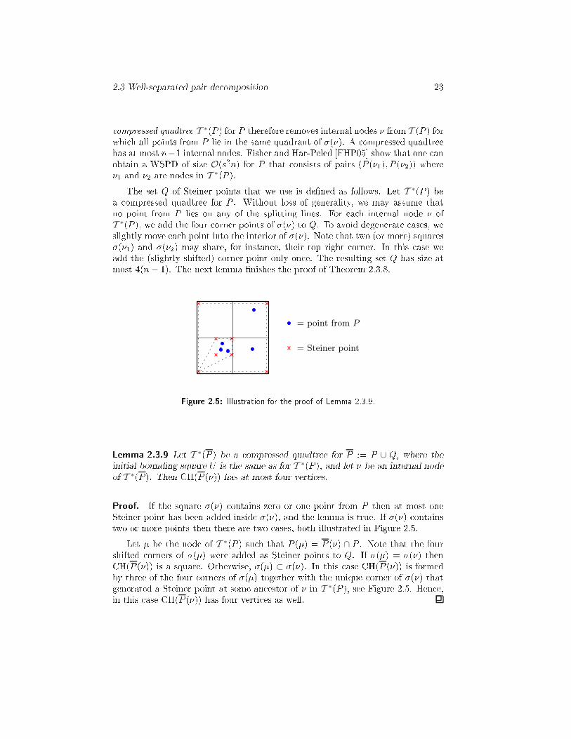
= point from P

= Steiner pointFigure 2.5: Illustration for the proof of Lemma 2.3.9.Lemma 2.3.9 Let T ∗(P ) be a ompressed quadtree for P := P ∪ Q, where theinitial bounding square U is the same as for T ∗(P ), and let � be an internal nodeof T ∗(P ). Then CH(P (�)) has at most four verti es.Proof. If the square �(�) ontains zero or one point from P then at most oneSteiner point has been added inside �(�), and the lemma is true. If �(�) ontainstwo or more points then there are two ases, both illustrated in Figure 2.5.Let � be the node of T ∗(P ) su h that P (�) = P (�) ∩ P . Note that the fourshifted orners of �(�) were added as Steiner points to Q. If �(�) = �(�) thenCH(P (�)) is a square. Otherwise, �(�) ⊂ �(�). In this ase CH(P (�)) is formedby three of the four orners of �(�) together with the unique orner of �(�) thatgenerated a Steiner point at some an estor of � in T ∗(P ), see Figure 2.5. Hen e,in this ase CH(P (�)) has four verti es as well.

24 Chapter 2 Region-Fault Tolerant Spanners2.4 Spe ial asesIn this se tion we present algorithms for onstru ting fault tolerant spanners intwo spe ial ases. In Se tion 2.4.1, we give an algorithm that onstru t a C-faulttolerant spanner for any point set whi h admits a fat triangulation. Then, inSe tion 2.4.2, we onstru t spanners whi h are fault tolerant under more limitedregion faults.2.4.1 C-fault tolerant fat triangulationsWe all a triangulation of a point set �-fat if all its triangles are �-fat or, in otherwords, if all angles in the triangulation are at least �. Karavelas and Guibas [KG01℄showed that any �-fat triangulation T of a point set P is a 2�-spanner for P . Tomake the spanner C-fault tolerant, we add some extra edges: we add an edgebetween every pair of points u; v ∈ P su h that there is a path between u and vin T onsisting of two edges.Theorem 2.4.1 Let P be a set of n points in the plane and let T be a �-fattriangulation of P . Then we an augment T with a set of O(n=�) extra edgessu h that the resulting geometri graph is a C-fault tolerant 2�-spanner.Proof. We onne t ea h node v to all other nodes within two steps from v. Inother words we add an edge between ea h pair of points onne ted by a path of twoedges. Let T ′ be the result. Obviously we add at mostPvD ·deg(v) edges, whereD is the maximum degree in the triangulation T and deg(v) is the degree of thenode v of T . Sin e for ea h triangulation Pv deg(v) ≤ 6n we add O(D · n) edgesto the triangulation T . Note that D = O(1=�) sin e T is a �-fat triangulation.Now the laim is that T ′ is a C-fault tolerant 2�-spanner. Using Proposi-tion 2.2.1, it suÆ es to show that T ′ is an H-fault tolerant 2�-spanner. Let h bean arbitrary half-plane and p; q ∈ P \ h be two arbitrary points. Karavelas andGuibas [KG01, Theorem 2.1℄ proved that there exist a 2�-path �(p; q) betweenp and q in T zig-zagging above and below the line onne ting p to q|see Fig-ure 2.6(a). Note that all the edges in this path interse t the segment between pand q.If all the nodes on �(p; q) lies outside h we are done. Otherwise assumep′ ∈ �(p; q) lies inside h and let q1 and q2 be the other endpoints of the two edgeson �(p; q) in ident to p′|see Figure 2.6(b). Sin e the segment pq lies outside hand any edge on �(p; q) interse t pq, the points q1 and q2 lie outside h. Be ause weadded edges between pairs within two steps|the dashed edges in Figure 2.6(b)|we an repla e the two fat edges (p′; q1) and (p′; q2) with (q1; q2). This way we anobtain a path that stays outside h and with length at most the length of �(p; q).

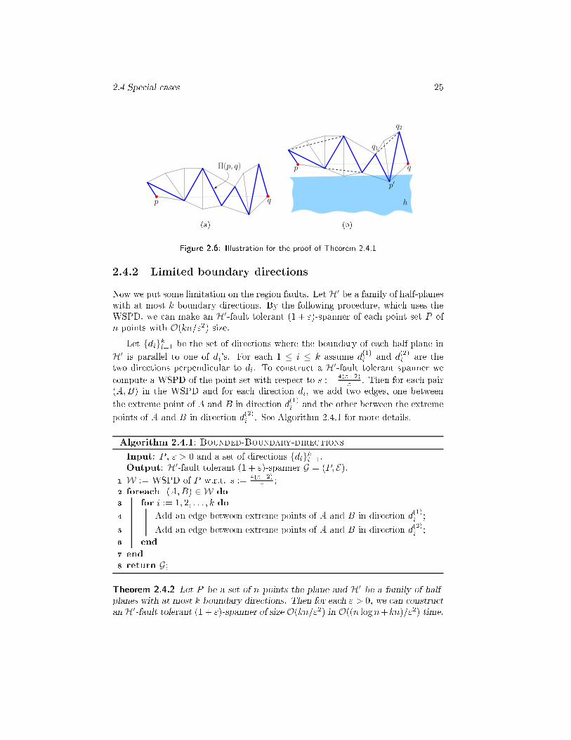
2.4 Spe ial ases 25p q

Π(p, q)

(a)p q

h

p′

q1

q2

(b)Figure 2.6: Illustration for the proof of Theorem 2.4.12.4.2 Limited boundary dire tionsNow we put some limitation on the region faults. Let H′ be a family of half-planeswith at most k boundary dire tions. By the following pro edure, whi h uses theWSPD, we an make an H′-fault tolerant (1 + ")-spanner of ea h point set P ofn points with O(kn="2) size.Let {di}ki=1 be the set of dire tions where the boundary of ea h half-plane inH′ is parallel to one of di's. For ea h 1 ≤ i ≤ k assume d(1)i and d(2)i are thetwo dire tions perpendi ular to di. To onstru t a H′-fault tolerant spanner we ompute a WSPD of the point set with respe t to s := 4("+2)" . Then for ea h pair(A;B) in the WSPD and for ea h dire tion di, we add two edges, one betweenthe extreme point of A and B in dire tion d(1)i and the other between the extremepoints of A and B in dire tion d(2)i . See Algorithm 2.4.1 for more details.Algorithm 2.4.1: Bounded-Boundary-dire tionsInput: P , " > 0 and a set of dire tions {di}ki=1.Output: H′-fault tolerant (1 + ")-spanner G = (P; E).

W := WSPD of P w.r.t. s := 4("+2)" ;1 forea h (A;B) ∈ W do2 for i := 1; 2; : : : ; k do3 Add an edge between extreme points of A and B in dire tion d(1)i ;4 Add an edge between extreme points of A and B in dire tion d(2)i ;5 end6 end7 return G;8Theorem 2.4.2 Let P be a set of n points the plane and H′ be a family of half-planes with at most k boundary dire tions. Then for ea h " > 0, we an onstru tan H′-fault tolerant (1 + ")-spanner of size O(kn="2) in O((n logn+kn)="2) time.

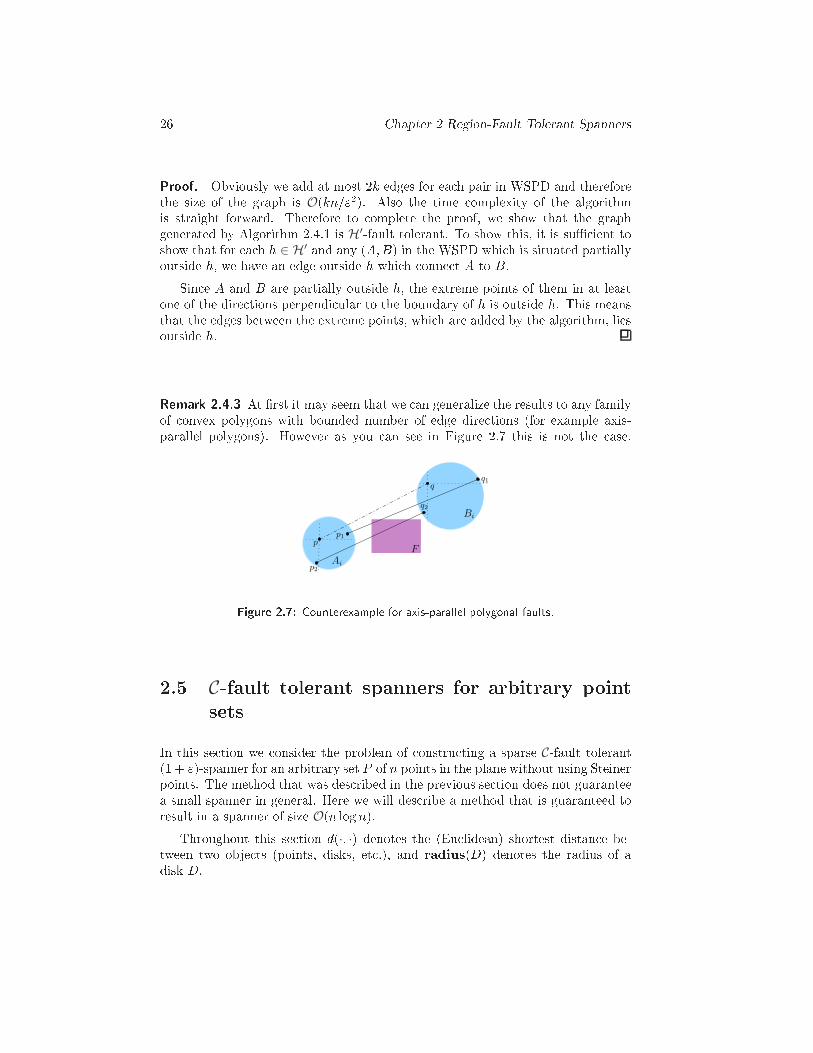
26 Chapter 2 Region-Fault Tolerant SpannersProof. Obviously we add at most 2k edges for ea h pair in WSPD and thereforethe size of the graph is O(kn="2). Also the time omplexity of the algorithmis straight forward. Therefore to omplete the proof, we show that the graphgenerated by Algorithm 2.4.1 is H′-fault tolerant. To show this, it is suÆ ient toshow that for ea h h ∈ H′ and any (A;B) in the WSPD whi h is situated partiallyoutside h, we have an edge outside h whi h onne t A to B.Sin e A and B are partially outside h, the extreme points of them in at leastone of the dire tions perpendi ular to the boundary of h is outside h. This meansthat the edges between the extreme points, whi h are added by the algorithm, liesoutside h.Remark 2.4.3 At �rst it may seem that we an generalize the results to any familyof onvex polygons with bounded number of edge dire tions (for example axis-parallel polygons). However as you an see in Figure 2.7 this is not the ase.p

p1

p2

q

q1

q2

F

Ai

Bi

Figure 2.7: Counterexample for axis-parallel polygonal faults.2.5 C-fault tolerant spanners for arbitrary pointsetsIn this se tion we onsider the problem of onstru ting a sparse C-fault tolerant(1 + ")-spanner for an arbitrary set P of n points in the plane without using Steinerpoints. The method that was des ribed in the previous se tion does not guaranteea small spanner in general. Here we will des ribe a method that is guaranteed toresult in a spanner of size O(n logn).Throughout this se tion d(·; ·) denotes the (Eu lidean) shortest distan e be-tween two obje ts (points, disks, et .), and radius(D) denotes the radius of adisk D.

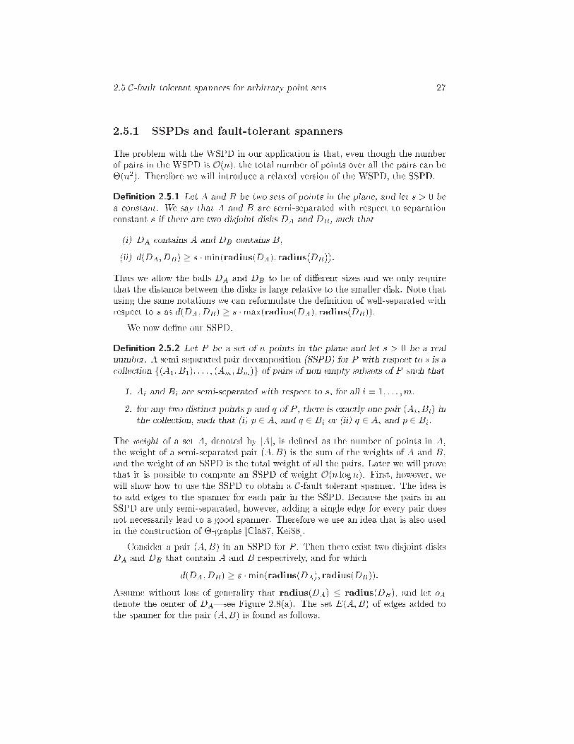
2.5 C-fault tolerant spanners for arbitrary point sets 272.5.1 SSPDs and fault-tolerant spannersThe problem with the WSPD in our appli ation is that, even though the numberof pairs in the WSPD is O(n), the total number of points over all the pairs an be�(n2). Therefore we will introdu e a relaxed version of the WSPD, the SSPD.De�nition 2.5.1 Let A and B be two sets of points in the plane, and let s > 0 bea onstant. We say that A and B are semi-separated with respe t to separation onstant s if there are two disjoint disks DA and DB , su h that(i) DA ontains A and DB ontains B,(ii) d(DA; DB) ≥ s ·min(radius(DA); radius(DB)).Thus we allow the balls DA and DB to be of di�erent sizes and we only requirethat the distan e between the disks is large relative to the smaller disk. Note thatusing the same notations we an reformulate the de�nition of well-separated withrespe t to s as d(DA; DB) ≥ s ·max(radius(DA); radius(DB)).We now de�ne our SSPD.De�nition 2.5.2 Let P be a set of n points in the plane and let s > 0 be a realnumber. A semi-separated pair de omposition (SSPD) for P with respe t to s is a olle tion {(A1; B1); : : : ; (Am; Bm)} of pairs of non-empty subsets of P su h that1. Ai and Bi are semi-separated with respe t to s, for all i = 1; : : : ;m.2. for any two distin t points p and q of P , there is exa tly one pair (Ai; Bi) inthe olle tion, su h that (i) p ∈ Ai and q ∈ Bi or (ii) q ∈ Ai and p ∈ Bi.The weight of a set A, denoted by |A|, is de�ned as the number of points in A,the weight of a semi-separated pair (A;B) is the sum of the weights of A and B,and the weight of an SSPD is the total weight of all the pairs. Later we will provethat it is possible to ompute an SSPD of weight O(n logn). First, however, wewill show how to use the SSPD to obtain a C-fault tolerant spanner. The idea isto add edges to the spanner for ea h pair in the SSPD. Be ause the pairs in anSSPD are only semi-separated, however, adding a single edge for every pair doesnot ne essarily lead to a good spanner. Therefore we use an idea that is also usedin the onstru tion of �-graphs [Cla87, Kei88℄.Consider a pair (A;B) in an SSPD for P . Then there exist two disjoint disksDA and DB that ontain A and B respe tively, and for whi hd(DA; DB) ≥ s ·min(radius(DA); radius(DB)):Assume without loss of generality that radius(DA) ≤ radius(DB), and let oAdenote the enter of DA|see Figure 2.8(a). The set E(A;B) of edges added tothe spanner for the pair (A;B) is found as follows.

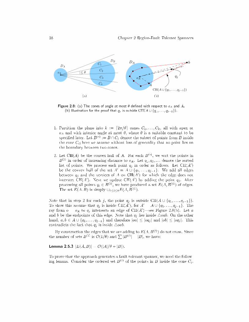
28 Chapter 2 Region-Fault Tolerant SpannersC1

C2

C3

≤ θ

DA

DB

oA

C4(a) oA

a

b

qj

DA

CH(A ∪ {q1, . . . , qj−1})(b)Figure 2.8: (a) The ones of angle at most � de�ned with respe t to oA and A.(b) Illustration for the proof that qj is outside CH(A ∪ {q1; : : : ; qj−1}).1. Partition the plane into k := ⌈2�=�⌉ ones C1; : : : ; Ck, all with apex atoA and with interior angle at most �, where � is a suitable onstant to bespe i�ed later. Let B(i) := B ∩Ci denote the subset of points from B insidethe one Ci; here we assume without loss of generality that no point lies onthe boundary between two ones.2. Let CH(A) be the onvex hull of A. For ea h B(i), we sort the points inB(i) in order of in reasing distan e to oA. Let q1; q2; : : : denote the sortedlist of points. We pro ess ea h point qj in order as follows. Let CH(A′)be the onvex hull of the set A′ = A ∪ {q1; : : : ; qj−1}. We add all edgesbetween qj and the verti es of A on CH(A′) for whi h the edge does notinterse t CH(A′). Next we update CH(A′) by adding the point qj . Afterpro essing all points qi ∈ B(i), we have produ ed a set E(A;B(i)) of edges.The set E(A;B) is simply ∪1≤i≤kE(A;B(i)).Note that in step 2 for ea h j, the point qj is outside CH(A ∪ {q1; : : : ; qj−1}).To show this assume that qj is inside CH(A′), for A′ = A ∪ {q1; : : : ; qj−1}. Theray from o = oA to qj interse ts an edge of CH(A′)|see Figure 2.8(b). Let aand b be the endpoints of this edge. Note that qj lies inside △oab. On the otherhand, a; b ∈ A ∪ {q1; : : : ; qj−1} and therefore |oa| ≤ |oqj | and |ob| ≤ |oqj |. This ontradi ts the fa t that qj is inside △oab.By onstru tion the edges that we are adding to E(A;B(i)) do not ross. Sin ethe number of sets B(i) is O(1=�) and P |B(i)| = |B|, we have:Lemma 2.5.3 |E(A;B)| = O(|A|=� + |B|).To prove that the approa h generates a fault-tolerant spanner, we need the follow-ing lemma. Consider the ordered set B(i) of the points in B inside the one Ci.

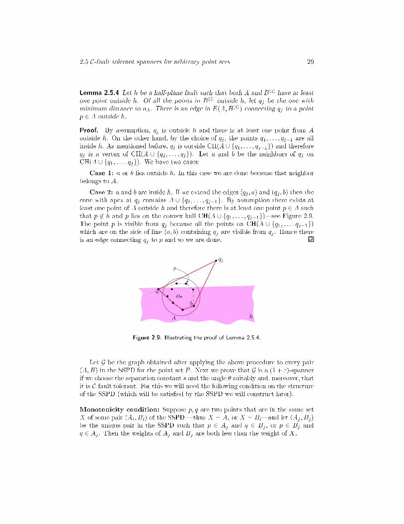
2.5 C-fault tolerant spanners for arbitrary point sets 29Lemma 2.5.4 Let h be a half-plane fault su h that both A and B(i) have at leastone point outside h. Of all the points in B(i) outside h, let qj be the one withminimum distan e to oA. There is an edge in E(A;B(i)) onne ting qj to a pointp ∈ A outside h.Proof. By assumption, qj is outside h and there is at least one point from Aoutside h. On the other hand, by the hoi e of qj , the points q1; : : : ; qj−1 are allinside h. As mentioned before, qj is outside CH(A ∪ {q1; : : : ; qj−1}) and thereforeqj is a vertex of CH(A ∪ {q1; : : : ; qj}). Let a and b be the neighbors of qj onCH(A ∪ {q1; : : : ; qj}). We have two ases:Case 1: a or b lies outside h. In this ase we are done be ause that neighborbelongs to A.Case 2: a and b are inside h. If we extend the edges (qj ; a) and (qj ; b) then the one with apex at qj ontains A ∪ {q1; : : : ; qj−1}. By assumption there exists atleast one point of A outside h and therefore there is at least one point p ∈ A su hthat p 6∈ h and p lies on the onvex hull CH(A ∪ {q1; : : : ; qj−1})|see Figure 2.9.The point p is visible from qj be ause all the points on CH(A ∪ {q1; : : : ; qj−1})whi h are on the side of line (a; b) ontaining qj are visible from qj . Hen e thereis an edge onne ting qj to p and so we are done.o

A

qj

h

a

b

p

Figure 2.9: Illustrating the proof of Lemma 2.5.4.Let G be the graph obtained after applying the above pro edure to every pair(A;B) in the SSPD for the point set P . Next we prove that G is a (1 + ")-spannerif we hoose the separation onstant s and the angle � suitably and, moreover, thatit is C-fault tolerant. For this we will need the following ondition on the stru tureof the SSPD (whi h will be satis�ed by the SSPD we will onstru t later).Monotoni ity ondition: Suppose p; q are two points that are in the same setX of some pair (Ai; Bi) of the SSPD |thus X = Ai or X = Bi|and let (Aj ; Bj)be the unique pair in the SSPD su h that p ∈ Aj and q ∈ Bj , or p ∈ Bj andq ∈ Aj . Then the weights of Aj and Bj are both less than the weight of X .

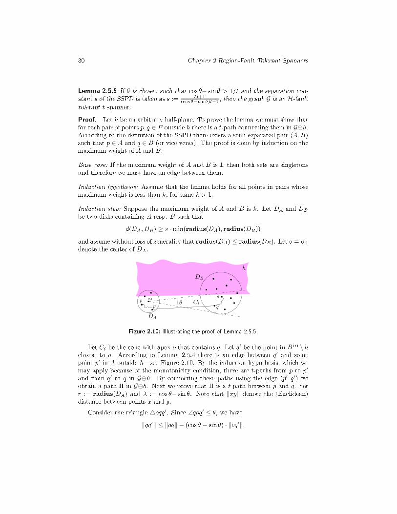
30 Chapter 2 Region-Fault Tolerant SpannersLemma 2.5.5 If � is hosen su h that os �− sin � > 1=t and the separation on-stant s of the SSPD is taken as s := 3t+1( os �− sin �)t−1 , then the graph G is an H-faulttolerant t-spanner.Proof. Let h be an arbitrary half-plane. To prove the lemma we must show thatfor ea h pair of points p; q ∈ P outside h there is a t-path onne ting them in G⊖h.A ording to the de�nition of the SSPD there exists a semi-separated pair (A;B)su h that p ∈ A and q ∈ B (or vi e versa). The proof is done by indu tion on themaximum weight of A and B.Base ase: If the maximum weight of A and B is 1, then both sets are singletonsand therefore we must have an edge between them.Indu tion hypothesis: Assume that the lemma holds for all points in pairs whosemaximum weight is less than k, for some k > 1.Indu tion step: Suppose the maximum weight of A and B is k. Let DA and DBbe two disks ontaining A resp. B su h thatd(DA; DB) ≥ s ·min(radius(DA); radius(DB))and assume without loss of generality that radius(DA) ≤ radius(DB). Let o = oAdenote the enter of DA.θ

p′p

qoA

q′

DA

DB

Ci

h

Figure 2.10: Illustrating the proof of Lemma 2.5.5.Let Ci be the one with apex o that ontains q. Let q′ be the point in B(i) \ h losest to o. A ording to Lemma 2.5.4 there is an edge between q′ and somepoint p′ in A outside h|see Figure 2.10. By the indu tion hypothesis, whi h wemay apply be ause of the monotoni ity ondition, there are t-paths from p to p′and from q′ to q in G⊖h. By onne ting these paths using the edge (p′; q′) weobtain a path � in G⊖h. Next we prove that � is a t-path between p and q. Setr := radius(DA) and � := os �− sin �. Note that ‖xy‖ denote the (Eu lidean)distan e between points x and y.Consider the triangle △oqq′. Sin e ∠qoq′ ≤ �, we have‖qq′‖ ≤ ‖oq‖ − ( os � − sin �) · ‖oq′‖:

2.5 C-fault tolerant spanners for arbitrary point sets 31The total length of �, denoted length(�), an now be bounded as follows.length(�) ≤ t · ‖pp′‖+ ‖p′q′‖+ t · ‖qq′‖≤ 2rt+ (r + ‖oq′‖) + t · (‖oq‖ − ( os � − sin �) · ‖oq′‖)= 2rt+ (r + ‖oq′‖) + t(‖oq‖ − r) + tr − t� · ‖oq′‖≤ 3rt+ (r + ‖oq′‖) + t · ‖pq‖ − t� · ‖oq′‖= t · ‖pq‖+ r(3t+ 1) + (1− t�) · ‖oq′‖:Sin e d(DA; DB) ≥ s · r, we have ‖oq′‖ ≥ s · r. Hen e, sin e � > 1=t we getlength(�) ≤ t · ‖pq‖+ r(3t+ 1) + sr(1− t�)= t · ‖pq‖:This ompletes the proof of the lemma.Now by hoosing � = O(") suitably, we an guarantee that os �− sin � > 1=(1+").This implies s = O(1=") and leads to the following theorem.Theorem 2.5.6 For any set P of n points in the plane and any " > 0, there existsa C-fault tolerant (1 + ")-spanner of P with O((n="3) logn) edges. The spanner an be onstru ted in O((n="2) log2 n) time.Proof. By ombining Proposition 2.2.1 and Lemmas 2.5.5, the graph onstru tedby the algorithm is C-fault tolerant. By Lemma 2.5.3 and with the onstru tionalgorithm presented below for onstru ting an SSPD of weight O(s2n logn), thesize of the onstru ted graph isX(A;B)∈ SSPD |E(A;B)| = X(A;B)∈ SSPD (|A|=� + |B|)

≤ 1� X(A;B)∈ SSPD (|A|+ |B|)= O(s2� n logn)= O( 1"3 n logn):This proves the �rst part of the theorem. To prove the running time, let (A;B)be an arbitrary pair in the SSPD and assume radius(DA) ≤ radius(DB), whereDA and DB are two disks ontaining A and B respe tively that satisfy the semi-separated ondition.The �rst step of the algorithm an be done in O(|B| log |B|) time. In these ond step, we an ompute the onvex hull of A in O(|A| log |A|) time. For ea h

32 Chapter 2 Region-Fault Tolerant Spannersset B(i), sorting an be done in O(|B(i)| log |B(i)|). For every j, to add the non- rossing edges between qj and the points on CH(A′), it is suÆ ient to onne t qjto all the points on CH(A′) whi h are between the two tangent lines of CH(A′)passing through qj . Therefore the time we need for adding non- rossing edges isproportional to the number of edges times O(logn). Finally we an update CH(A′)in O(logm) time, where m is the number of points on the onvex hull of A′, usingan online onvex hull algorithm|see [PS85, Chapter 3.3.6℄.So in total the time for pro essing the pair (A;B) is bounded byO(|A| log |A|+ |B| log |B|+ |B| log(|A|+ |B|) + |E(A;B)| logn):Hen e the total running time is

O

0� X(A;B)∈W

�|A| log |A|+ |B| log |B|+ |B| log(|A|+ |B|) + |E(A;B)| logn�1A

≤ O

0� X(A;B)∈W

�(|A| + |B|) logn+ |E(A;B)| logn�1A= O(s2n log2 n+ n log2 n)= O(s2n log2 n):As we will see in the next se tion, we an ompute the SSPD in O(s2n logn) time,see Lemma 2.5.14, whi h proves the time omplexity of the algorithm.2.5.2 Computing an SSPDTo ompute an SSPD for a given point set P , we use a BAR-tree, as introdu edby Dun an et al. [DGK01℄. A BAR-tree for a point set P is a BSP-tree with thefollowing properties:1. ea h leaf region ontains at most one point from P ,2. the tree has size O(n),3. if we go down two levels in the tree then the size of the subtree redu es bya fa tor of �, for some onstant 1=2 < � < 1, so its depth is O(logn),4. the region R(�) asso iated with an (internal or leaf) node � has aspe tratio at most � for some onstant � > 1, that is, there are on entri disksDI ⊂ R(�) and DO ⊃ R(�) with radius(DO) = � · radius(DI).

2.5 C-fault tolerant spanners for arbitrary point sets 33Moreover, BAR-trees only use splitting lines that are horizonal, verti al, or di-agonal, therefore the omplexity of every node (as a polygon) in a BAR-tree is onstant.Let T be a BAR-tree on the point set P . For a node �, we use pa(�) todenote the parent of �, and we use P (�) to denote the subset of points from Pthat are stored in the leaves of the subtree T� rooted at �. The weight of a node� is the number of points in P (�), and is denoted |P (�)|. We say that a node� in T has weight lass `, for some integer `, if and only if |P (�)| ≤ n=2` and|P (pa(�))| > n=2`. The weight lass of the root is de�ned to be zero. We denotethe olle tion of nodes of weight lass ` by N(`). Obviously we have ⌊logn⌋ weight lasses. Note that some of the nodes in the tree may not be in any weight lass;this an happen when the weight of a node � is almost the same as the weightof its parent. For example, this happens when |P (pa(�))| = n=2` for some ` and|P (�)| = n=2`−1. It an also happen that a node belongs to more than one weight lass, namely when the weight of a node is mu h smaller than the weight of itsparent. The following lemma is straightforward.Lemma 2.5.7 Every leaf node is in weight lass `max, where `max = ⌊logn⌋. Fur-thermore, on any root-to-leaf-path there is exa tly one node with weight lass `,for any 0 ≤ ` ≤ `max.For a node � ∈ N(`), we de�ne its `-parent to be the node �′ ∈ N(` − 1) that ison the path from the root of T to � (in luding � itself). We denote the `-parentof � by pa(`; �). Observe that � an be its own `-parent, namely when � ∈ N(`)and � ∈ N(`−1). By Lemma 2.5.7, if � ∈ N(`) then one of its an estors (possiblyitself) must be in weight lass `−1, so it must have an `-parent. If � is the `-parentof � then we all � a `- hild of �.For a node � in the BAR-tree, the region orresponding to � is denoted byR(�) and for a region R, we let diam(R) denote the diameter of the region R. Asmentioned before, all nodes in the BAR-tree have bounded aspe t ratio, that is,all aspe t ratios are bounded by some �xed onstant �.Lemma 2.5.8 Ifd(R(�);R(�)) ≥ (s+ 1)�2 ·min{diam(R(�));diam(R(�))}then there are two disks D� ⊃ R(�) and D� ⊃ R(�) su h thatd(D� ; D�) ≥ s ·min{radius(D�); radius(D�)}:Proof. Without loss of generality assume diam(R(�)) ≤ diam(R(�)). Let h bea half-plane whi h ontains R(�) su h that the distan e between h and R(�) isd(R(�);R(�)). Note that the half-plane h an be viewed as a disk with in�nite

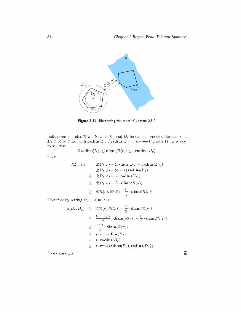
34 Chapter 2 Region-Fault Tolerant Spannersh

DI

Dν

R(µ)

R(ν)

d(D ν

, h)

Figure 2.11: Illustrating the proof of Lemma 2.5.8.radius that ontains R(�). Now let D� and DI be two on entri disks su h thatDI ⊂ R(�) ⊂ D� with radius(D�)= radius(DI) = �|see Figure 2.11. It is easyto see that 2 radius(DI) ≤ diam(R(�)) ≤ 2 radius(D�):Then d(D� ; h) = d(DI ; h)− (radius(D�)− radius(DI))= d(DI ; h)− (�− 1) radius(DI )≥ d(DI ; h)− � · radius(DI)≥ d(DI ; h)− �2 · diam(R(�))≥ d(R(�);R(�)) − �2 · diam(R(�)):Therefore by setting D� = h we haved(D� ; D�) ≥ d(R(�);R(�)) − �2 · diam(R(�))≥ (s+ 1)�2 · diam(R(�)) − �2 · diam(R(�))≥ s · �2 · diam(R(�))≥ s · � · radius(DI )= s · radius(D�)≥ s ·min{radius(D�); radius(D�)}:So we are done.

2.5 C-fault tolerant spanners for arbitrary point sets 35Now we onstru t an SSPD S of the point set P using the following algorithm.1. Constru t a BAR tree T on P . Let � be the maximum aspe t ratio of theregion R(�) for any node � ∈ T . Compute the weight lasses of all nodesin T .2. For ea h weight lass ` with 0 ≤ ` ≤ `max do the following: add to S allpairs (P (�); P (�)) su h that(i) �; � ∈ N(`),(ii) d(R(�);R(�)) ≥ (s+1)�2 ·min{diam(R(�));diam(R(�))} and(iii) d(R(pa(`; �));R(pa(`; �))) < (s+1)�2 ·min{diam(R(pa(`; �)));diam(R(pa(`; �)))}.Lemma 2.5.9 S is an SSPD for P with respe t to s.Proof. By Lemma 2.5.8, all the pairs reported by the algorithm are semi-separated.The only thing that remains to be veri�ed is that for every pair of points p; q thereis a unique pair (P (�); P (�)) ∈ S su h that p ∈ P (�) and q ∈ P (�), or vi e-versa.For any 0 ≤ ` ≤ `max, de�ne �(p; `) and �(q; `) to be the nodes of N(`) onthe sear h path to p and q, respe tively. Observe that these nodes exist and areuniquely de�ned by Lemma 2.5.7. We have �(p; 0) = �(q; 0) = root(T ), so the setsP (�(p; 0)) and P (�(q; 0)) are the same and therefore not semi-separated. On theother hand, �(p; `max) and �(q; `max) are leaves, and so the sets P (�(p; `max)) andP (�(q; `max)) are singletons and therefore ful�ll ondition (ii) of the algorithm.Hen e, there must be a value ` and two nodes �(p; `) and �(q; `) su h that theyful�ll onditions (ii) and (iii) of the algorithm. The region of any node � is on-tained in the region of its parent, whi h is easily seen to imply that ` is unique.To bound the weight of the SSPD, we �rst prove two auxiliary lemmas.Lemma 2.5.10 A node � in T an be an `-parent of at most a onstant numberof nodes in T .Proof. Consider a node � ∈ N(`−1) and let �′ be a node su h that � = pa(`; �′).Then �′ is a node in T� (the subtree of T rooted at �) in weight lass `. Note thatno other node than �′ in T�′ an have � as its `-parent. Re all that the weightof a node redu es by a fa tor of � when we go down two levels in a BAR-tree.Sin e �′ ∈ N(`), its (normal) parent has weight at least n=2`. On the other hand� ∈ N(`−1), so the weight of � is at most n=2`−1. Hen e, the path between � and�′ onsists of at most 2k links, where �k = 1=2. It follows that the total numberof nodes in T that have � as a `-parent is bounded by 22k, whi h is a onstantsin e k is a onstant.

36 Chapter 2 Region-Fault Tolerant SpannersLemma 2.5.11 Let S(`) be the set of all pairs (�; �) su h that �; � ∈ N(`) andd(R(�);R(�)) < (s+1)�2 · min{diam(R(�));diam(R(�))}, where 0 ≤ ` ≤ `max.Then |S(`)| = O(�4(s+ 1)2 · 2`) andX(�;�)∈S(`)(|P (�)| + |P (�)|) = O��4(s+ 1)2 · n� :Proof. We reorder the nodes in the pairs (�; �) su h thatdiam(R(�)) ≤ diam(R(�)):We laim that any node � appears in a onstant number of pairs as the �rst elementof the pair. To show this let (�; �) be an arbitrary ordered pair. Let DP (�) bethe smallest en losing disk of P (�) and let o be its enter. Consider the annulusA between the disks D1 and D2 with enter o and radii r1 := ((s + 1)� + 1) ·radius(DP (�)) and r2 := r1 + radius(DP (�)). Note thatdiam(R(�))=2 ≤ radius(DP (�)) ≤ diam(R(�)):Sin e d(R(�);R(�)) < (s+ 1)�2 · diam(R(�))the region R(�) interse t D1|see Figure 2.12. Now we have two ases:Case 1: The region R(�) lies partially outside D2. By the Pa king Lemma,[DGK01, Lemma 3.2℄ this an happen for O

��2 (r1=(r2 − r1))� = O(�3(s + 1))regions.Case 2: In this ase the region R(�) lies inside D2. Be ause the aspe t ra-tio of the region R(�) is at most �, there are two disks DI and DO su h thatDI ⊂ R(�) ⊂ DO and area(DO) ≤ �2 · area(DI), where area(A) denotes thearea of the region A. Thereforearea(R(�)) ≥ area(DI)≥ 1�2 · area(DO)= 1�2 · � (radius(DO))2≥ 14�2 · � (diam(R(�)))2≥ 14�2 · � (diam(R(�)))2≥ �r224�2 · ((s+ 1)�+ 2)2 :On the other hand, the area of D2 is �r22 , whi h means we an have at most

O(�4(s+ 1)2) su h regions. Hen e in total we an have O(�4(s+ 1)2) pairs that

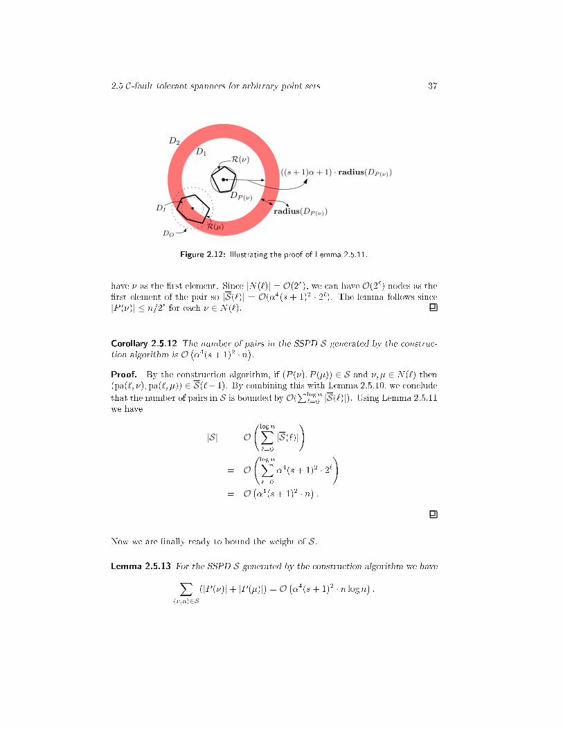
2.5 C-fault tolerant spanners for arbitrary point sets 37DP (ν)

D1R(ν)

D2

R(µ)

((s + 1)α + 1) · radius(DP (ν))

radius(DP (ν))

DO

DI Figure 2.12: Illustrating the proof of Lemma 2.5.11.have � as the �rst element. Sin e |N(`)| = O(2`), we an have O(2`) nodes as the�rst element of the pair so |S(`)| = O(�4(s + 1)2 · 2`). The lemma follows sin e|P (�)| ≤ n=2` for ea h � ∈ N(`).Corollary 2.5.12 The number of pairs in the SSPD S generated by the onstru -tion algorithm is O ��4(s+ 1)2 · n�.Proof. By the onstru tion algorithm, if (P (�); P (�)) ∈ S and �; � ∈ N(`) then(pa(`; �); pa(`; �)) ∈ S(`− 1). By ombining this with Lemma 2.5.10, we on ludethat the number of pairs in S is bounded by O(Plogn`=0 |S(`)|). Using Lemma 2.5.11we have

|S| = O lognX̀=0 |S(`)|!= O lognX̀=0 �4(s+ 1)2 · 2`!= O��4(s+ 1)2 · n� :Now we are �nally ready to bound the weight of S.Lemma 2.5.13 For the SSPD S generated by the onstru tion algorithm we haveX(�;�)∈S

(|P (�)|+ |P (�)|) = O��4(s+ 1)2 · n logn� :

38 Chapter 2 Region-Fault Tolerant SpannersProof. Sin e the number of weight lasses in T is O(logn) it suÆ es to provethat for every �xed ` it holds that:X(�;�)∈S�;�∈N(`)(|P (�)|+ |P (�)|) = O(�4(s+ 1)2n): (2.1)Obviously |P (�)| ≤ |P (pa(`; �))| for ea h node �, so we an bound (2.1) byX(�;�)∈S�;�∈N(`)(|P (pa(`; �))|+ |P (pa(`; �))|): (2.2)From the algorithm we know thatd(R(pa(`; �));R(pa(`; �))) < (s+ 1)�2 ·min{diam(R(pa(`; �)));diam(R(pa(`; �)))}:Furthermore, by Lemma 2.5.10 ea h node an be an `-parent of a onstantnumber of nodes. Hen e, (2.2) an be bounded byX(�;�)∈S(`−1)O(|P (�)| + |P (�)|); (2.3)where S(`− 1) is the set of all pair (�; �) su h that �; � ∈ N(`− 1) andd(R(�);R(�)) < (s+ 1)�2 ·min{diam(R(�));diam(R(�))}:A ording to Lemma 2.5.11 summation (2.3) is O��4(s+ 1)2 · n�, whi h om-pletes the proof of the lemma.Lemma 2.5.14 The SSPD of a set P of n points with respe t to a onstant s anbe omputed in O(s2n+ n logn) time.Proof. The BAR tree T and the weight lasses of nodes of T require O(n logn)time to ompute [DGK01℄. Then we make a tree T ′ from T su h that the levelof ea h node in T ′ represent its weight lass. We do this by making the following hanges in T .1. Remove all the nodes � with no weight lass from the tree and onne t the hildren of � (if they exist) to the parent of �.2. If a node appears in k weight lasses (k > 1) then repeat the node k times.

2.6 Testing for C-fault toleran e 39By Lemma 2.5.10, ea h node in the tree T ′ has onstant degree and also the depthof the tree is O(log n).Now using an algorithm similar to the algorithm for onstru ting a WSPD, we an onstru t a SSPD. That is, for ea h internal node � of the tree T ′, run analgorithm �ndpairs(�1; �2), where �1 and �2 are the hildren of �. This algorithmtests whether the pair satis�es ondition (ii) of the onstru tion des ribed justbefore Lemma 2.5.9. If they do, it reports the node pair. Otherwise it re urses onthe hildren of �1 and �2 i.e. for ea h hild �1 of �1 and ea h hild �2 of �2 it alls�ndpairs(�1; �2).Now the laim is that the running time of the algorithm is O(m) where m isthe size of the SSPD omputed by the algorithm. We prove this using a similarargument used for the WSPD [Cal95℄. Let the algorithm all �ndpairs(�1; �2),where �1 and �2 are the hildren of a node � in T ′. We de�ne the omputation treeof (�1; �2) to be a tree with root at (�1; �2) whi h satis�es the following ondition.A node (�1; �2) is a leaf if it satis�es the ondition (ii) of the onstru tion des ribedjust before Lemma 2.5.9. Otherwise for ea h hild �′1 of �1 and ea h hild �′2 of�2, (�′1; �′2) is a hild of (�1; �2). By Lemma 2.5.10, the degree of ea h node in the omputation tree is bounded by a onstant. So the time omplexity of ea h all of�ndpairs in the algorithm is linear in the number of nodes in the orresponding omputation tree whi h is linear in the number of leaves in the omputation tree.Therefore the total time omplexity is linear in the total number of leaves in the omputation trees whi h is the number of pairs that are output.This proves the lemma sin e there are O(s2n) pairs in the SSPD a ording toCorollary 2.5.12.The following theorem summarizes the results on the SSPD onstru tion.Theorem 2.5.15 Given a set P of n points in the plane and s > 0 we an omputean SSPD with respe t to s of weight O(s2n logn) in time O(s2n+ n logn).2.6 Testing for C-fault toleran eIn the previous se tions we onstru ted fault tolerant spanners. However, aninteresting problem is to de ide if a given (1 + ")-spanner G is C-fault tolerant ornot. In this se tion we give an algorithm whi h in O(n5) time using O(n2) spa e an �nd the answer, where n is the number of verti es of the input graph. Re allthat the faults do not ontain their boundaries.Lemma 2.6.1 Let G(P; E) be a (1 + ")-spanner on a set P of points in the plane.Let H(P ) be the family of all half-planes in the plane su h that the boundary ofea h half-plane in H(P ) passes through at least two points in P . Then the graph

40 Chapter 2 Region-Fault Tolerant SpannersG is a C-fault tolerant (1 + ")-spanner if and only if it is an H(P )-fault tolerant(1 + ")-spanner.Proof. Obviously a graph is H(P )-fault tolerant if it is C-fault tolerant. Toprove the other dire tion assume G is H(P )-fault tolerant. By Proposition 2.2.1 itis suÆ ient to show that the graph G is an H-fault tolerant (1 + ")-spanner. Leth be an arbitrary half-plane. If the boundary of h passes through at least twoverti es of G then h ∈ H(P ) and we are done.Otherwise, if no vertex of G lies on the boundary of h then we expand h,without hanging its boundary dire tion, until it meets a vertex u of G. It is easyto see that the expansion an a�e t an edge only after h meets one of the endpointsof the edge and therefore in the expanding pro ess no new edge is a�e ted. If theboundary meets no vertex of G during the expansion then all the verti es andedges of G are in h and so we are done.Let hu be the new half-plane and assume `u is the boundary of hu. Now werotate the line `u around u until it meets another vertex of G. Note that by thisrotation no new edge is a�e ted. If we h′u be the new half-plane then h′u ∈ H(P )and by the assumption the graph G is fault tolerant under h′u. On the other handh and h′u a�e t the same parts of G and therefore G is fault tolerant under h too.Theorem 2.6.2 For any (1 + ")-spanner G on a set P of n points in the plane we an de ide whether G is a C-fault tolerant (1 + ")-spanner or not in O(n5) timeusing O(n2) spa e.Proof. Let H(P ) be the family of half-planes su h that the boundary of a half-plane h ∈ H(P ) passes through at least two verti es of G. By Lemma 2.6.1, thegraph G is a C-fault tolerant (1 + ")-spanner if and only if it is an H(P )-faulttolerant (1 + ")-spanner.Obviously the set H(P ) ontains O(n2) half-planes. To test a half-plane h, we ompute all-pairs shortest paths in G⊖h whi h an be done in O(mn + n2 logn)time using O(m) spa e, wherem is the number of edges in G. We also an omputeall-pairs shortest paths in G (P )⊖h in O(n3) time using O(n2) spa e. Then usinga na��ve algorithm we an he k if G⊖h is a (1 + ")-spanner of G (P )⊖h in O(n2)time. So in total the he king pro edure takes O(n5) time and O(n2) spa e.2.7 Fault-tolerant geodesi spannersIn this se tion we onsider the problem of onstru ting fault-tolerant geodesi (1 + ")-spanners for a set P of n points in the plane. Here we require that betweenany two points u; v ∈ P outside the region fault F , there is a path in G⊖F whose

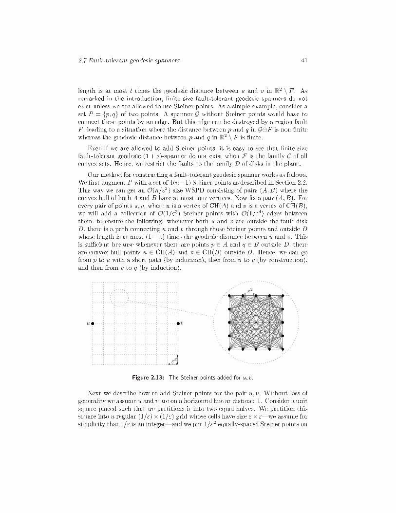
2.7 Fault-tolerant geodesi spanners 41length is at most t times the geodesi distan e between u and v in R2 \ F . Asremarked in the introdu tion, �nite size fault-tolerant geodesi spanners do notexist unless we are allowed to use Steiner points. As a simple example, onsider aset P = {p; q} of two points. A spanner G without Steiner points would have to onne t these points by an edge. But this edge an be destroyed by a region faultF , leading to a situation where the distan e between p and q in G⊖F is non-�nitewhereas the geodesi distan e between p and q in R

2 \ F is �nite.Even if we are allowed to add Steiner points, it is easy to see that �nite sizefault-tolerant geodesi (1 + ")-spanner do not exist when F is the family C of all onvex sets. Hen e, we restri t the faults to the family D of disks in the plane.Our method for onstru ting a fault-tolerant geodesi spanner works as follows.We �rst augment P with a set of 4(n−1) Steiner points as des ribed in Se tion 2.2.This way we an get an O(n="2) size WSPD onsisting of pairs (A;B) where the onvex hull of both A and B have at most four verti es. Now �x a pair (A;B). Forevery pair of points u; v, where u is a vertex of CH(A) and v is a vertex of CH(B),we will add a olle tion of O(1="3) Steiner points with O(1="4) edges betweenthem, to ensure the following: whenever both u and v are outside the fault diskD, there is a path onne ting u and v through those Steiner points and outside Dwhose length is at most (1 + ") times the geodesi distan e between u and v. Thisis suÆ ient be ause whenever there are points p ∈ A and q ∈ B outside D, thereare onvex hull points u ∈ CH(A) and v ∈ CH(B) outside D. Hen e, we an gofrom p to u with a short path (by indu tion), then from u to v (by onstru tion),and then from v to q (by indu tion).v

εε

u

ε2

Figure 2.13: The Steiner points added for u; v.Next we des ribe how to add Steiner points for the pair u; v. Without loss ofgenerality we assume u and v are on a horizontal line at distan e 1. Consider a unitsquare pla ed su h that uv partitions it into two equal halves. We partition thissquare into a regular (1=")× (1=") grid whose ells have size "× "|we assume forsimpli ity that 1=" is an integer|and we put 1="2 equally-spa ed Steiner points on

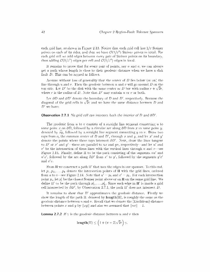
42 Chapter 2 Region-Fault Tolerant Spannersea h grid line, as shown in Figure 2.13. Noti e that ea h grid ell has 1=" Steinerpoints on ea h of its sides, and that we have O(1="3) Steiner points in total. Forea h grid ell we add edges between every pair of Steiner points on its boundary,thus adding O(1="2) edges per ell and O(1="4) edges in total.It remains to prove that for every pair of points, say u and v, we an alwaysget a path whose length is lose to their geodesi distan e when we have a diskfault D. This an be argued as follows.Assume without loss of generality that the enter of D lies below (or on) theline through u and v. Then the geodesi between u and v will go around D on thetop side. Let D′ be the disk with the same enter as D but with radius r +√2",where r is the radius of D. Note that D′ may ontain u or v or both.Let �D and �D′ denote the boundary of D and D′, respe tively. Be ause thediagonal of the grid ells is √2" and we have the same distan e between D andD′ we have:Observation 2.7.1 No grid ell an interse t both the interior of D and �D′.The geodesi from u to v onsists of a straight line segment onne ting u tosome point x on �D, followed by a ir ular ar along �D from x to some point y,denoted by _xy, followed by a straight line segment onne ting y to v. Draw tworays from o, the ommon enter of D and D′, through x and y, and let x′ and y′denote the points where these rays interse t �D′. Next, draw the lines tangentto D′ at x′ and y′|these are parallel to ux and yv, respe tively|and let u′ andv′ be the interse tion of these lines with the verti al lines through u and v|seeFigure 2.14. Finally, de�ne � to be the path onsisting of the segments uu′ andu′x′, followed by the ar along �D′ from x′ to y′, followed by the segments y′v′and v′v.From � we onstru t a path �′ that uses the edges in our spanner. To this end,let p1; p2; : : : ; pk denote the interse tion points of � with the grid lines, orderedfrom u to v|see Figure 2.14. Note that u′ = p1 and v′ = pk. For ea h interse tionpoint pi, let p′i be the losest Steiner point above or on � on the same grid line. Wede�ne �′ to be the path through p′1; : : : ; p′k. Sin e ea h edge in �′ is inside a grid ell interse ted by �D′, by Observation 2.7.1, the path �′ does not interse t D.It remains to show that �′ approximates the geodesi distan e. Firstly weshow the length of the path �, denoted by length(�), is roughly the same as thegeodesi distan e between u and v. Re all that we denote the (Eu lidean) distan ebetween points x and y by ‖xy‖ and also we assumed that ‖uv‖ = 1.Lemma 2.7.2 If is the geodesi distan e between u and v thenlength(�) ≤ �1 + (� + 2)√2"� :

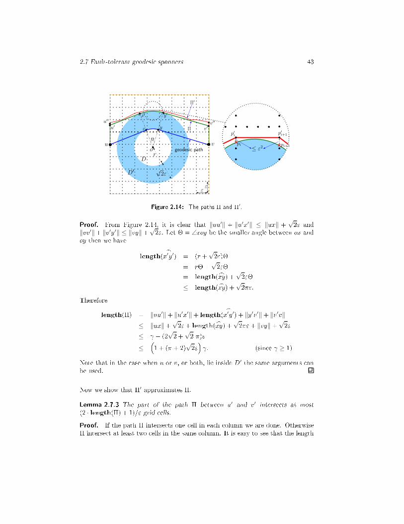
2.7 Fault-tolerant geodesi spanners 43v

εε

u

x y

r

√2ε

D

D′

o

Π′

Θ

u′′

v′′

geodesic path

Π v′u

′

y′x′

pi+1

p′

ip′

i+1

≤ ε2pi

Figure 2.14: The paths � and �′.Proof. From Figure 2.14, it is lear that ‖uu′‖ + ‖u′x′‖ ≤ ‖ux‖ + √2" and‖vv′‖+ ‖v′y′‖ ≤ ‖vy‖+√2". Let � = ∠xoy be the smaller angle between ox andoy then we have length( _x′y′) = (r +√2")�= r�+√2"�= length(_xy) +√2"�

≤ length(_xy) +√2�":Thereforelength(�) = ‖uu′‖+ ‖u′x′‖+ length( _x′y′) + ‖y′v′‖+ ‖v′v‖≤ ‖ux‖+√2"+ length(_xy) +√2�"+ ‖vy‖+√2"≤ + (2√2 +√2 �)"≤

�1 + (� + 2)√2"� : (sin e ≥ 1)Note that in the ase when u or v, or both, lie inside D′ the same arguments anbe used.Now we show that �′ approximates �.Lemma 2.7.3 The part of the path � between u′ and v′ interse ts at most(2 · length(�) + 1)=" grid ells.Proof. If the path � interse ts one ell in ea h olumn we are done. Otherwise� interse t at least two ells in the same olumn. It is easy to see that the length

44 Chapter 2 Region-Fault Tolerant Spannersof the part of the path � whi h lies inside any two onse utive ells in the olumnis at least ". Therefore in total it an interse t at most (2·length(�)+1)=" ells.Lemma 2.7.4 length(�′) ≤ (1 + 6") length(�).Proof. Let `i be the length of the part of � inside the ith ell and (p′i; p′i+1) be theedge on �′ in the same ell|see Figure 2.14. Then obviously ‖p′ip′i+1‖ ≤ `i +2"2.Solength(�′) = ‖up′1‖+ k−1Xi=1 ‖p′ip′i+1‖+ ‖p′kv‖≤ ‖uu′‖+ "2 + k−1Xi=1(`i + 2"2) + ‖v′v‖+ "2= ‖uu′‖+ k−1Xi=1 `i + ‖v′v‖!+ k−1Xi=1 2"2 + 2"2≤ length(�) + 2k"2≤ length(�) + 2(2 · length(�) + 1)" (Lemma 2.7.3)≤ (1 + 6") length(�): (sin e 1 ≤ length(�) ≤ 2)We obtain the following theorem.Theorem 2.7.5 For any set P of n points and any " > 0, there exists a D-fault tol-erant geodesi Steiner (1 + ")-spanner of P with O(n="6) edges that uses O(n="5)Steiner points.Proof. In the pro edure of onstru ting a D-fault tolerant spanner, we added

O(n) Steiner points to have a WSPD of size O(n="2) su h that the onvex hull ofea h set in the WSPD ontains at most four points. Then for ea h pair (A;B) inthe WSPD and for ea h pair of points on CH(A) and CH(B), we added O(1="3)Steiner points and O(1="4) edges between them. Therefore in total we addedO(n="5) Steiner points and the graph ontains O(n="6) edges.2.8 Con luding remarksWe introdu ed the on ept of region-fault tolerant spanners for planar point sets,and proved the existen e of region-fault tolerant spanners of small size. We showed

2.8 Con luding remarks 45that for any set of n points in the plane, we an onstru t a C-fault tolerant spannerof size O(n logn) in O(n log2 n) time.Our spanner onstru tion for arbitrary point sets uses the SSPD, a relaxationof the WSPD. A similar variant with weaker properties, the SSD, was introdu edby Varadarajan [Var98℄ who used it to ompute the min- ost perfe t mat hingfor points in the plane. His algorithm runs in √n phases where ea h phase takestime proportional to the weight of the SSD plus the time it takes to omputethe SSD. Sin e our SSPD satis�es the onditions of Varadarajan's SSD, and we an ompute it faster, we an improve the running time of the min- ost perfe tmat hing algorithm from O(n3=2 log5 n) to O(n3=2 log2 n).The main open problem is to determine whether the spanner size for arbitrarypoint sets an be improved to O(n).Another interesting question is how we an improve the C-fault tolerant he k-ing algorithm. Finally, in our approa h, we used straight line segments as edgesin our spanners. For geodesi spanners, it is interesting to see what happens if weare allowed to add urved edges.

46 Chapter 2 Region-Fault Tolerant Spanners

Chapter 3Dilation-Optimal EdgeAugmentation3.1 Introdu tionAfter designing a network, in addition to performing network maintenan e, it issometimes desirable to improve its quality. In this hapter we onsider the problemwhen one is given a (geometri ) network and the problem at hand is to extendthe network with an additional edge while minimizing the dilation of the resultinggraph. More formally the problem is as follows. Given an edge weighted graphG(V;E) with n verti es and m edges, onstru t a graph G′ by adding an edgeto G su h that the dilation of G′ is minimized. The problem was �rst stated byNarasimhan [Nar02℄ and, surprisingly, it has not been studied earlier, to the bestof our knowledge.The results presented in this hapter are summarized in Table 3.1. Note thatsome of the presented bounds hold for any graph with positive edge weights(weighted graphs) while some only hold for Eu lidean graphs. Re all from theintrodu tion that we assume that the vertex set of any graph is a subset of a met-ri spa e and for ea h pair of verti es u and v in the graph, d(u; v) denotes thedistan e between u and v in the metri spa e. Throughout this hapter G denotesa Eu lidean graph while G denotes a graph with positive edge weights.Throughout this hapter we will use Gopt to denote the optimal solution, whiletopt and t denote the dilation of Gopt and the input graph G respe tively. Also forea h pair of points u; v ∈ V , ÆG(u; v) denotes the shortest path between u and v

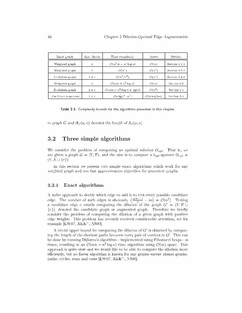
48 Chapter 3 Dilation-Optimal Edge AugmentationInput graph Apx. fa tor Time omplexity Spa e Se tionWeighted graph 1 O(n3m+ n4 logn) O(m) Se tion 3.2.1Weighted graph 1 O(n4) O(n2) Se tion 3.2.1Eu lidean graph 1 + " O(n3="d) O(n2) Se tion 3.2.2Weighted graph 3 O(nm+ n2 logn) O(m) Se tion 3.3Eu lidean graph 2 + " O(nm+ n2(logn+ 1"3d )) O(n2) Se tion 3.4Eu lidean t-spanner 1 + " O(( t7"4 )d · n2) O(n log(tn)) Se tion 3.5Table 3.1: Complexity bounds for the algorithms presented in this hapter.in graph G and dG(u; v) denotes the length of ÆG(u; v).3.2 Three simple algorithmsWe onsider the problem of omputing an optimal solution Gopt. That is, weare given a graph G = (V;E), and the aim is to ompute a topt-spanner Gopt =(V;E ∪ {e}).In this se tion we present two simple exa t algorithms whi h work for anyweighted graph and one fast approximation algorithm for geometri graphs.3.2.1 Exa t algorithmsA na��ve approa h to de ide whi h edge to add is to test every possible andidateedge. The number of su h edges is obviously �n(n−1)2 − m� = O(n2). Testinga andidate edge e entails omputing the dilation of the graph G′ = (V;E ∪{e}), denoted the andidate graph or augmented graph. Therefore we brie y onsider the problem of omputing the dilation of a given graph with positiveedge weights. This problem has re ently re eived onsiderable attention, see forexample [EW07, AKK+, NS00℄.A trivial upper bound for omputing the dilation of G′ is obtained by omput-ing the length of the shortest paths between every pair of verti es in G′. This anbe done by running Dijkstra's algorithm|implemented using Fibona i heaps|ntimes, resulting in an O(mn + n2 logn) time algorithm using O(m) spa e. Thisapproa h is quite slow and we would like to be able to ompute the dilation moreeÆ iently, but no faster algorithm is known for any graphs ex ept planar graphs,paths, y les, stars and trees [EW07, AKK+, NS00℄.

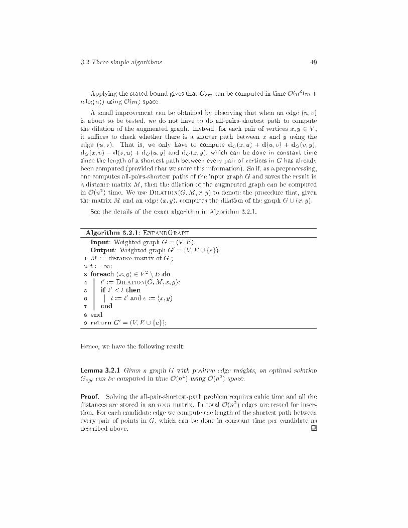
3.2 Three simple algorithms 49Applying the stated bound gives that Gopt an be omputed in time O(n3(m+n logn)) using O(m) spa e.A small improvement an be obtained by observing that when an edge (u; v)is about to be tested, we do not have to do all-pairs-shortest path to omputethe dilation of the augmented graph. Instead, for ea h pair of verti es x; y ∈ V ,it suÆ es to he k whether there is a shorter path between x and y using theedge (u; v). That is, we only have to ompute dG(x; u) + d(u; v) + dG(v; y),dG(x; v) + d(v; u) + dG(u; y) and dG(x; y), whi h an be done in onstant timesin e the length of a shortest path between every pair of verti es in G has alreadybeen omputed (provided that we store this information). So if, as a prepro essing,one omputes all-pairs-shortest paths of the input graph G and saves the result ina distan e matrix M , then the dilation of the augmented graph an be omputedin O(n2) time. We use Dilation(G;M; x; y) to denote the pro edure that, giventhe matrix M and an edge (x; y), omputes the dilation of the graph G ∪ (x; y).See the details of the exa t algorithm in Algorithm 3.2.1.Algorithm 3.2.1: ExpandGraphInput: Weighted graph G = (V;E).Output: Weighted graph G′ = (V;E ∪ {e}).M := distan e matrix of G ;1 t :=∞;2 forea h (x; y) ∈ V 2 \ E do3 t′ := Dilation(G;M; x; y);4 if t′ < t then5 t := t′ and e := (x; y)6 end7 end8 return G′ = (V;E ∪ {e});9Hen e, we have the following result:Lemma 3.2.1 Given a graph G with positive edge weights, an optimal solutionGopt an be omputed in time O(n4) using O(n2) spa e.Proof. Solving the all-pair-shortest-path problem requires ubi time and all thedistan es are stored in an n×n matrix. In total O(n2) edges are tested for inser-tion. For ea h andidate edge we ompute the length of the shortest path betweenevery pair of points in G, whi h an be done in onstant time per andidate asdes ribed above.

50 Chapter 3 Dilation-Optimal Edge Augmentation3.2.2 A (1 + ")-approximation for Eu lidean graphsIn the previous se tion we showed that an optimal solution an be obtained bytesting a quadrati number of andidate edges. Testing ea h andidate edge entailsO(n2) distan e queries, where a distan e query asks for the length of a shortestpath in the graph between two query points. One way to speed up the omputationis to ompute an approximate dilation. The problem of omputing an approximatedilation of a geometri graph was onsidered by Narasimhan and Smid in [NS00℄.They showed the following fa t, whi h states that the WSPD of the vertex setof any Eu lidean graph G an be used to approximate the dilation of G|see alsoSe tion 13.2 of [NS07℄.Fa t 3.2.2 Let V be a set of n points in R

d and let {(Ai; Bi)}mi=1 be a WSPD forV with respe t to separation onstant s := 4(2+ ")=". For ea h j with 1 ≤ j ≤ m,let aj be an arbitrary point in Aj , and let bj be an arbitrary point in Bj . For any onne ted Eu lidean graph G with vertex set V , the following holds: For ea h jwith 1 ≤ j ≤ m, let DG(aj ; bj) be the dilation between aj and bj in G, and lett := max1≤j≤mDG(aj ; bj):Then DG=(1 + ") ≤ t ≤ DG , or equivalently t ≤ DG ≤ (1 + ")t, where DG denotesthe dilation of G.Thus, in order to approximate the dilation of a Eu lidean graph, it is suÆ ientto ompute the dilation between O(n="d) pairs of verti es. Moreover, the hoi e ofthese verti es depends only on the vertex set of the graph, it does not depend onthe edges of the graph. As a result the time to ompute the dilation de reases fromO(n2) to O(n="d), thus the total running time de reases from O(n4) to O(n3="d).Theorem 3.2.3 Given a Eu lidean graph G = (V;E) and a real onstant " > 0, one an in O(n3="d) time, using O(n2) spa e, ompute a t?-spanner G′ = (V;E ∪ {e})su h that topt ≤ t? ≤ (1 + ") · topt.Proof. The time bound follows from the above dis ussion. Obviously the dilationof G′, denoted by t?, reported by the algorithm is at least topt. It remains to provethat t? is bounded by (1 + ") · topt.Assume that t is the approximate dilation of G′ and for ea h andidate graphGi, let ti be its approximate dilation as omputed by the algorithm and let DGibe its exa t dilation. Based on the algorithm t = mini ti and from Fa t 3.2.2 itfollows that for ea h andidate graph Gi, ti ≤ DGi ≤ (1 + ") · ti. Assume thattopt = DGj . Thereforet? ≤ (1 + ") · t ≤ (1 + ") · tj ≤ (1 + ") · DGj = (1 + ") · topt;whi h omplete the proof.

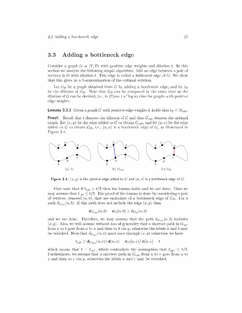
3.3 Adding a bottlene k edge 513.3 Adding a bottlene k edgeConsider a graph G = (V;E) with positive edge weights and dilation t. In thisse tion we analyze the following simple algorithm: Add an edge between a pair ofverti es in G with dilation t. This edge is alled a bottlene k edge of G. We showthat this gives us a 3-approximation of the optimal solution.Let GB be a graph obtained from G by adding a bottlene k edge, and let tBbe the dilation of GB. Note that GB an be omputed in the same time as thedilation of G an be de ided, i.e., in O(mn+n2 logn) time for graphs with positiveedge weights.Lemma 3.3.1 Given a graph G with positive edge weights it holds that tB < 3topt:Proof. Re all that t denotes the dilation of G and that Gopt denotes the optimalgraph. Let (x; y) be the edge added to G to obtain Gopt, and let (u; v) be the edgeadded to G to obtain GB, i.e., (u; v) is a bottlene k edge of G, as illustrated inFigure 3.1.a

b

x

y

u

v(a) Ga

b

x

y

u

v(b) Gopta

b

x

y

u

v( ) GBFigure 3.1: (x; y) is the optimal edge added to G and (u; v) is a bottlene k edge of G.First note that if topt > t=3 then the lemma holds and we are done. Thus wemay assume that topt ≤ t=3. The proof of the lemma is done by onsidering a pairof verti es, denoted (a; b), that are endpoints of a bottlene k edge of GB. Fix apath ÆGopt(a; b). If this path does not in lude the edge (x; y) thendGopt(a; b) = dG(a; b) ≥ dGB(a; b)and we are done. Therefore, we may assume that the path ÆGopt(a; b) in ludes(x; y). Also, we will assume without loss of generality that a shortest path in Goptfrom a to b goes from a to x and then to b via y, otherwise the labels a and b maybe swit hed. Note that ÆGopt(u; v) must pass through (x; y) otherwise we havetopt ≥ dGopt(u; v)=d(u; v) = dG(u; v)=d(u; v) = twhi h means that t = topt, whi h ontradi ts the assumption that topt ≤ t=3.Furthermore, we assume that a shortest path in Gopt from u to v goes from u tox and then to v via y, otherwise the labels u and v may be swit hed.

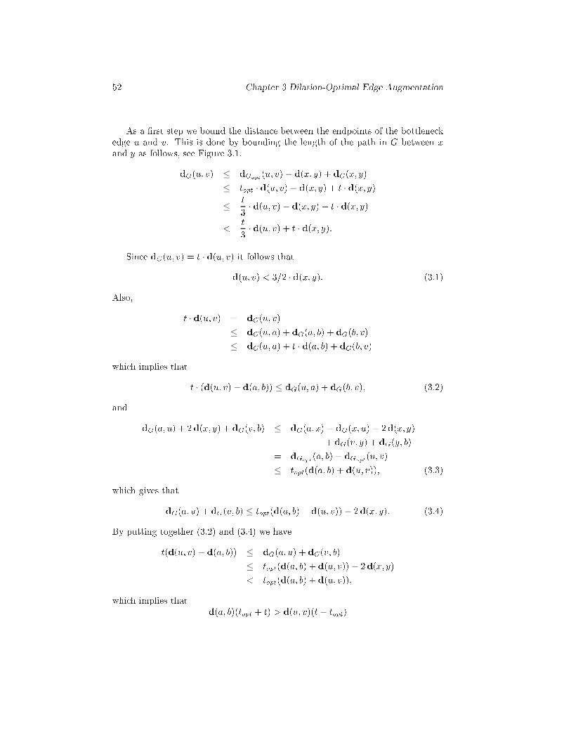
52 Chapter 3 Dilation-Optimal Edge AugmentationAs a �rst step we bound the distan e between the endpoints of the bottlene kedge u and v. This is done by bounding the length of the path in G between xand y as follows, see Figure 3.1.dG(u; v) ≤ dGopt(u; v)− d(x; y) + dG(x; y)≤ topt · d(u; v)− d(x; y) + t · d(x; y)≤ t3 · d(u; v)− d(x; y) + t · d(x; y)< t3 · d(u; v) + t · d(x; y):Sin e dG(u; v) = t · d(u; v) it follows thatd(u; v) < 3=2 · d(x; y): (3.1)Also, t · d(u; v) = dG(u; v)≤ dG(u; a) + dG(a; b) + dG(b; v)≤ dG(u; a) + t · d(a; b) + dG(b; v)whi h implies that t · (d(u; v)− d(a; b)) ≤ dG(u; a) + dG(b; v); (3.2)and dG(a; u) + 2d(x; y) + dG(v; b) ≤ dG(a; x) + dG(x; u) + 2d(x; y)+dG(v; y) + dG(y; b)= dGopt(a; b) + dGopt(u; v)

≤ topt(d(a; b) + d(u; v)); (3.3)whi h gives thatdG(a; u) + dG(v; b) ≤ topt(d(a; b) + d(u; v))− 2d(x; y): (3.4)By putting together (3.2) and (3.4) we havet(d(u; v)− d(a; b)) ≤ dG(a; u) + dG(v; b)≤ topt(d(a; b) + d(u; v))− 2d(x; y)< topt(d(a; b) + d(u; v));whi h implies that d(a; b)(topt + t) > d(u; v)(t− topt)

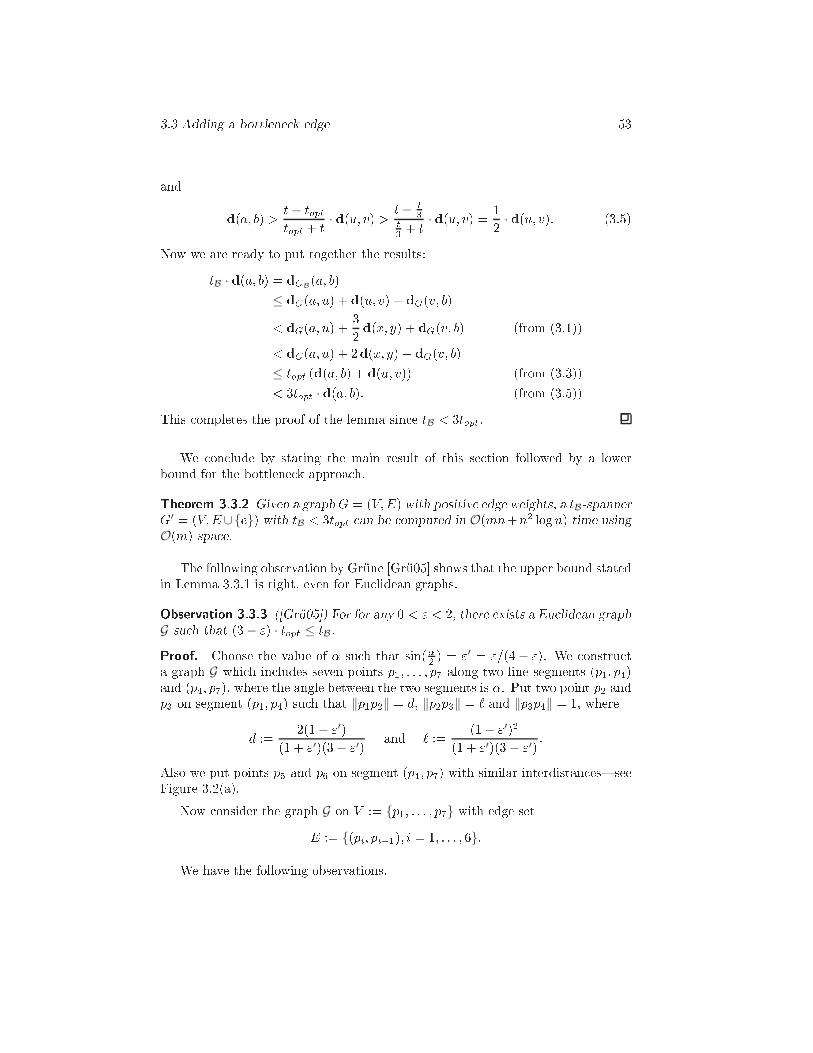
3.3 Adding a bottlene k edge 53and d(a; b) > t− topttopt + t · d(u; v) > t− t3t3 + t · d(u; v) = 12 · d(u; v): (3.5)Now we are ready to put together the results:tB · d(a; b) = dGB(a; b)

≤ dG(a; u) + d(u; v) + dG(v; b)< dG(a; u) + 32 d(x; y) + dG(v; b) (from (3.1))< dG(a; u) + 2d(x; y) + dG(v; b)≤ topt (d(a; b) + d(u; v)) (from (3.3))< 3topt · d(a; b): (from (3.5))This ompletes the proof of the lemma sin e tB < 3topt.We on lude by stating the main result of this se tion followed by a lowerbound for the bottlene k approa h.Theorem 3.3.2 Given a graphG = (V;E) with positive edge weights, a tB-spannerG′ = (V;E∪{e}) with tB < 3topt an be omputed in O(mn+n2 logn) time using

O(m) spa e.The following observation by Gr�une [Gr�u05℄ shows that the upper bound statedin Lemma 3.3.1 is tight, even for Eu lidean graphs.Observation 3.3.3 ([Gr�u05℄) For for any 0 < " < 2, there exists a Eu lidean graphG su h that (3− ") · topt ≤ tB.Proof. Choose the value of � su h that sin(�2 ) = "′ = "=(4− "). We onstru ta graph G whi h in ludes seven points p1; : : : ; p7 along two line segments (p1; p4)and (p4; p7), where the angle between the two segments is �. Put two point p2 andp3 on segment (p1; p4) su h that ‖p1p2‖ = d, ‖p2p3‖ = ` and ‖p3p4‖ = 1, whered := 2(1− "′)(1 + "′)(3− "′) and ` := (1− "′)2(1 + "′)(3− "′) :Also we put points p5 and p6 on segment (p4; p7) with similar interdistan es|seeFigure 3.2(a).Now onsider the graph G on V := {p1; : : : ; p7} with edge setE := {(pi; pi+1); i = 1; : : : ; 6}:We have the following observations.

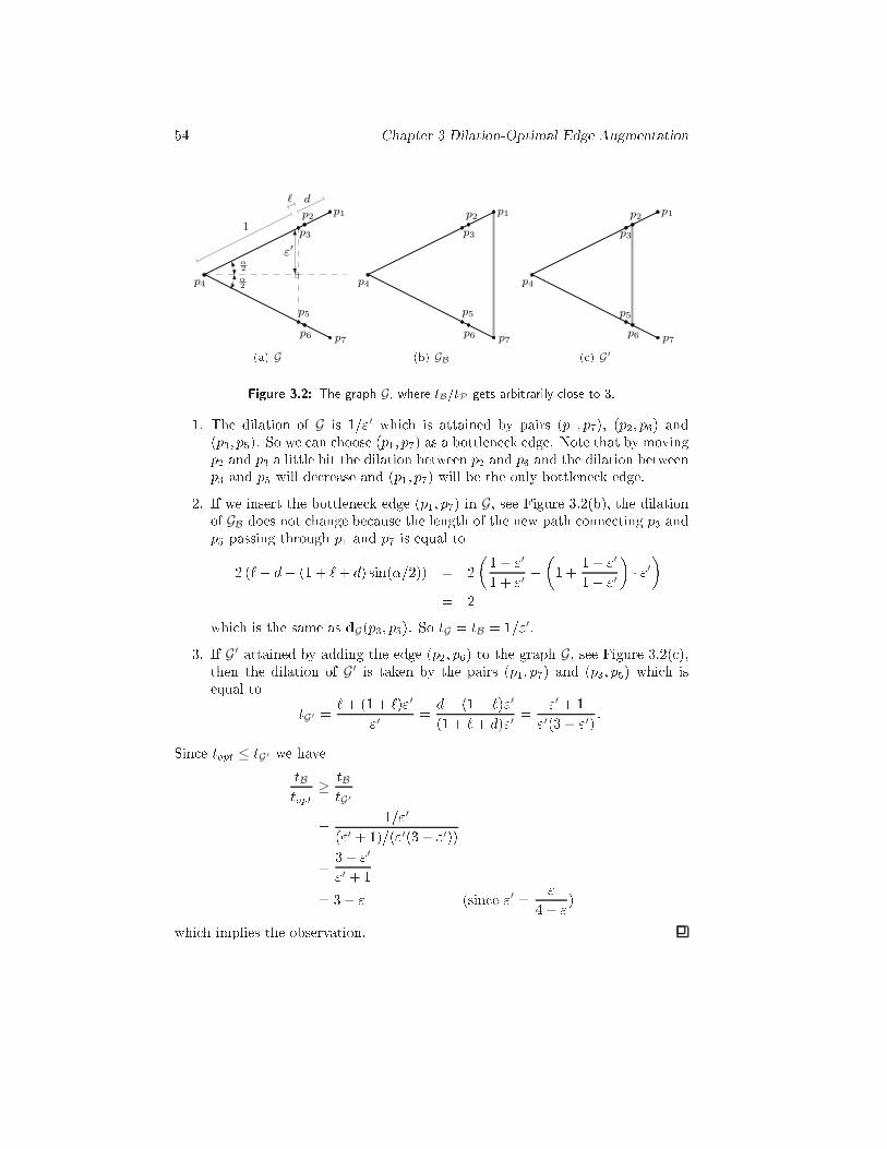
54 Chapter 3 Dilation-Optimal Edge Augmentationα

2

p4α

2

p7p6

p5

p1p2

p3

dℓ

1

ε′

(a) G

p4

p7p6

p5

p1p2

p3

(b) GB

p4

p7p6

p5

p1p2

p3

( ) G′Figure 3.2: The graph G, where tB=tP gets arbitrarily lose to 3.1. The dilation of G is 1="′ whi h is attained by pairs (p1; p7), (p2; p6) and(p3; p5). So we an hoose (p1; p7) as a bottlene k edge. Note that by movingp2 and p3 a little bit the dilation between p2 and p6 and the dilation betweenp3 and p5 will de rease and (p1; p7) will be the only bottlene k edge.2. If we insert the bottlene k edge (p1; p7) in G, see Figure 3.2(b), the dilationof GB does not hange be ause the length of the new path onne ting p3 andp5 passing through p1 and p7 is equal to2 (`+ d+ (1 + `+ d) sin(�=2)) = 2�1− "′1 + "′ +�1 + 1− "′1 + "′� · "′�= 2whi h is the same as dG(p3; p5). So tG = tB = 1="′.3. If G′ attained by adding the edge (p2; p6) to the graph G, see Figure 3.2( ),then the dilation of G′ is taken by the pairs (p1; p7) and (p3; p5) whi h isequal to tG′ = `+ (1 + `)"′"′ = d+ (1 + `)"′(1 + `+ d)"′ = "′ + 1"′(3− "′) :Sin e topt ≤ tG′ we havetBtopt ≥ tBtG′= 1="′("′ + 1)=("′(3− "′))= 3− "′"′ + 1= 3− " (sin e "′ = "4− ")whi h implies the observation.

3.4 A (2 + ")-approximation for Eu lidean graphs 553.4 A (2 + ")-approximation for Eu lidean graphsIn the remainder of the hapter we will develop approximation algorithms for Eu- lidean graphs. In this se tion we present a fast approximation algorithm whi hguarantees an approximation fa tor of (2+"). The algorithm is similar to the algo-rithms presented in Se tion 3.2 in the sense that it tests andidate edges. Testing a andidate edge entails omputing the dilation of the input graph augmented withthe andidate edge. The main di�eren e is that we will show, in Se tion 3.4.1, thatonly a linear number of andidate edges need to be tested to obtain a solution thatgives a (2 + ")-approximation, instead of a quadrati number of edges.Moreover, in Se tion 3.4.2 we show that the same approximation bound anbe a hieved by performing only a linear number of shortest path queries for ea h andidate edge. The andidate edges are sele ted by using the well-separated pairde omposition|see Se tion 2.3.3.4.1 Linear number of andidate edgesIn this se tion we show how to obtain a (2 + ")-approximation in ubi time. Asmentioned above, the algorithm is similar to the algorithm presented in Se tion 3.2in the sense that it tests andidate edges. Here we will show that only a linearnumber of andidate edges is needed to be tested to obtain a solution that gives a(2 + ")-approximation.The approa h is straight-forward, see Algorithm 3.4.1. First the algorithm omputes the length of the shortest path in G between every pair of points in V .The distan es are saved in a matrix M . Next, the well-separated pair de ompo-sition of V is omputed. Note that, in line 5, the andidate edges will be hosenusing the well-separated pair de omposition. In line 6, the fun tion Dilationreturns the dilation of the graph Gi(V;E ∪ {(ai; bi)}), i.e., in lines 5{8, a andi-date edge is tested by omputing the dilation of G with the andidate edge (ai; bi)added to G. Re all that Dilation uses the distan e matri M to answer su h aquery in quadrati time. Next, we bound the running time of the approximationalgorithm and then prove the approximation bound.Lemma 3.4.1 Algorithm 3.4.1 requires O(n3="2d) time and O(n2) spa e.Proof. The omplexity of all lines of the algorithm is straight-forward to al- ulate. Re all that line 1 requires O(mn + n2 logn) time and quadrati spa e,and line 2 requires O(n="2d + n logn) time a ording to Se tion 2.3. Be ausek = O(n="2d), the time needed for lines 4{10 is O(n="2d) times the omplexity ofDilation whi h is O(n2). Thus summing up we get O( n"2d · n2), as stated in thelemma.

56 Chapter 3 Dilation-Optimal Edge AugmentationAlgorithm 3.4.1: Approximate ExpandGraphInput: Eu lidean graph G = (V;E) and a real onstant " > 0.Output: Eu lidean graph G′ = (V;E ∪ {e}).M := distan e matrix of G ;1{(Ai; Bi)}ki=1 := WSPD of the point set V with respe t to s = 256="2;2 t :=∞;3 for i := 1; 2; : : : ; k do4 Sele t arbitrary points ai ∈ Ai and bi ∈ Bi;5 ti := Dilation(Gi;M; ai; bi);6 if ti < t then7 t := ti and e := (ai; bi)8 end9 end10 return G′ = (V;E ∪ {e});11 It remains to analyze the quality of the solution obtained from algorithm 3.4.1.We need to ompare the graph resulting from adding an optimal edge to G andthe graph G′ resulting from Approximate ExpandGraph. Let e = (a; b) bean optimal edge and let (Ai; Bi) be the well-separated pair su h that a ∈ Ai andb ∈ Bi. At �rst sight, it seems that the edge (ai; bi) tested by the algorithm shouldbe a good andidate. However, the separation onstant of our well-separated pairde omposition only depends on " whi h implies that the shortest path between aand ai, and between b and bi ould be very long ompared to the distan e betweena and b. In Lemma 3.4.2, we show the existen e of a \short" edge e′ that is agood approximation of the optimal edge and then, in Lemma 3.4.3, we show thatApproximate ExpandGraph omputes a good approximation of e′.Let �G(p; q) denote the set of point pairs (u; v) in V su h that(p; q) ∈ ÆG∪{(p;q)}(u; v):That is, �G(p; q) is the set of point pairs for whi h a shortest path between themin G ∪ {(p; q)} passes through (p; q). When it is lear whi h graph we are talkingabout, we use �(p; q) instead of �G(p; q).Lemma 3.4.2 For any given onstant 0 < � ≤ 1, there exists a pair p; q ∈ V ofthe graph G su h that for every pair (u; v) ∈ �(p; q) it holds that ‖uv‖ ≥ �2 ‖pq‖,and the dilation of G ∪ {(p; q)} is bounded by (2 + �) · topt.Proof. The proof is done in two steps. First a point pair pj ; qj ∈ V is sele ted thatful�lls the �rst requirement of the lemma. Then, we prove the se ond requirement,i.e., the dilation of G ∪ {(pj ; qj)} is bounded by (2 + �) · topt.Consider an optimal solution G1 = G ∪ {(p1; q1)}, with dilation t1 = topt. If

‖uv‖ ≥ �2 · ‖p1q1‖ for every point pair (u; v) ∈ �(p1; q1) then j = 1, i.e., we have

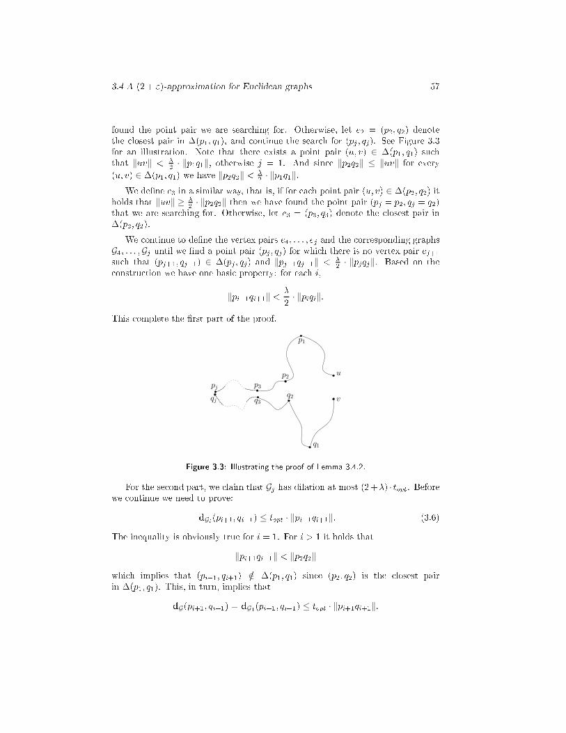
3.4 A (2 + ")-approximation for Eu lidean graphs 57found the point pair we are sear hing for. Otherwise, let e2 = (p2; q2) denotethe losest pair in �(p1; q1), and ontinue the sear h for (pj ; qj). See Figure 3.3for an illustration. Note that there exists a point pair (u; v) ∈ �(p1; q1) su hthat ‖uv‖ < �2 · ‖p1q1‖, otherwise j = 1. And sin e ‖p2q2‖ ≤ ‖uv‖ for every(u; v) ∈ �(p1; q1) we have ‖p2q2‖ < �2 · ‖p1q1‖.We de�ne e3 in a similar way, that is, if for ea h point pair (u; v) ∈ �(p2; q2) itholds that ‖uv‖ ≥ �2 · ‖p2q2‖ then we have found the point pair (pj = p2; qj = q2)that we are sear hing for. Otherwise, let e3 = (p3; q3) denote the losest pair in�(p2; q2).We ontinue to de�ne the vertex pairs e4; : : : ; ej and the orresponding graphsG4; : : : ;Gj until we �nd a point pair (pj ; qj) for whi h there is no vertex pair ej+1su h that (pj+1; qj+1) ∈ �(pj ; qj) and ‖pj+1qj+1‖ < �2 · ‖pjqj‖. Based on the onstru tion we have one basi property: for ea h i,

‖pi+1qi+1‖ < �2 · ‖piqi‖:This omplete the �rst part of the proof.p1

q1

u

v

p2

p3pj

q2q3

qj

Figure 3.3: Illustrating the proof of Lemma 3.4.2.For the se ond part, we laim that Gj has dilation at most (2+�) · topt. Beforewe ontinue we need to prove:dGi(pi+1; qi+1) ≤ topt · ‖pi+1qi+1‖: (3.6)The inequality is obviously true for i = 1. For i > 1 it holds that‖pi+1qi+1‖ < ‖p2q2‖whi h implies that (pi+1; qi+1) =∈ �(p1; q1) sin e (p2; q2) is the losest pairin �(p1; q1). This, in turn, implies thatdG(pi+1; qi+1) = dG1(pi+1; qi+1) ≤ topt · ‖pi+1qi+1‖:

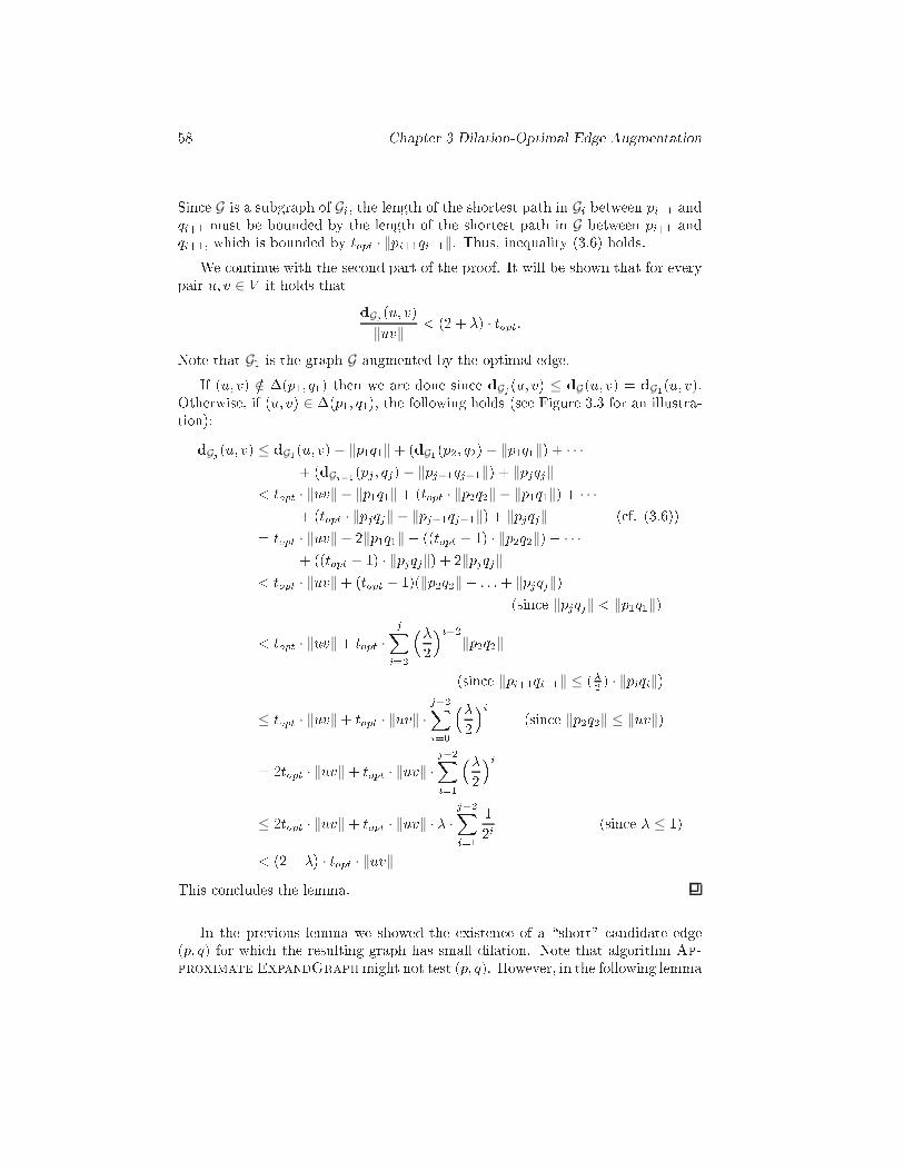
58 Chapter 3 Dilation-Optimal Edge AugmentationSin e G is a subgraph of Gi, the length of the shortest path in Gi between pi+1 andqi+1 must be bounded by the length of the shortest path in G between pi+1 andqi+1, whi h is bounded by topt · ‖pi+1qi+1‖. Thus, inequality (3.6) holds.We ontinue with the se ond part of the proof. It will be shown that for everypair u; v ∈ V it holds that dGj (u; v)‖uv‖ < (2 + �) · topt:Note that G1 is the graph G augmented by the optimal edge.If (u; v) =∈ �(p1; q1) then we are done sin e dGj (u; v) ≤ dG(u; v) = dG1(u; v).Otherwise, if (u; v) ∈ �(p1; q1), the following holds (see Figure 3.3 for an illustra-tion):dGj (u; v) ≤ dG1(u; v)− ‖p1q1‖+ (dG1(p2; q2)− ‖p1q1‖) + · · ·+ (dGj−1(pj ; qj)− ‖pj−1qj−1‖) + ‖pjqj‖< topt · ‖uv‖ − ‖p1q1‖+ (topt · ‖p2q2‖ − ‖p1q1‖) + · · ·+ (topt · ‖pjqj‖ − ‖pj−1qj−1‖) + ‖pjqj‖ ( f. (3.6))= topt · ‖uv‖ − 2‖p1q1‖+ ((topt − 1) · ‖p2q2‖) + · · ·+ ((topt − 1) · ‖pjqj‖) + 2‖pjqj‖< topt · ‖uv‖+ (topt − 1)(‖p2q2‖+ : : :+ ‖pjqj‖)(sin e ‖pjqj‖ < ‖p1q1‖)< topt · ‖uv‖+ topt · jXi=2 ��2�i−2‖p2q2‖(sin e ‖pi+1qi+1‖ ≤ (�2 ) · ‖piqi‖)

≤ topt · ‖uv‖+ topt · ‖uv‖ · j−2Xi=0 ��2�i (sin e ‖p2q2‖ ≤ ‖uv‖)= 2topt · ‖uv‖+ topt · ‖uv‖ · j−2Xi=1 ��2�i≤ 2topt · ‖uv‖+ topt · ‖uv‖ · � ·

j−2Xi=1 12i (sin e � ≤ 1)< (2 + �) · topt · ‖uv‖This on ludes the lemma.In the previous lemma we showed the existen e of a \short" andidate edge(p; q) for whi h the resulting graph has small dilation. Note that algorithm Ap-proximate ExpandGraphmight not test (p; q). However, in the following lemma

3.4 A (2 + ")-approximation for Eu lidean graphs 59it will be shown that algorithm Approximate ExpandGraph will test an edge(a; b) that is almost as good as (p; q).Lemma 3.4.3 For any given onstant 0 < " ≤ 1 it holds that the graph G′ returnedby algorithm Approximate ExpandGraph has dilation at most (2 + ") · topt:Proof. A ording to Lemma 3.4.2, for ea h 0 < � ≤ 1 there exists an edge (p; q)su h that for every pair (u; v) ∈ �(p; q) it holds that ‖uv‖ ≥ �2 ‖pq‖, and thedilation tH of H = G ∪ {(p; q)} is bounded by (2 + �) · topt. Let (Ai; Bi) be thewell-separated pair omputed in line 2 of the algorithm su h that p ∈ Ai andq ∈ Bi. A ording to De�nition 2.3.3 su h a well-separated pair must exist. Next, onsider the andidate edge (ai; bi) tested by the algorithm, su h that ai; p ∈ Aiand bi; q ∈ Bi. For simpli ity of writing we will use a and b to denote ai and birespe tively.Our laim is that the dilation of G′ := G ∪{(a; b)} is bounded by (1+ "=4) · tH .Before we ontinue to prove the laim, we show thatdG(a; p) = dH(a; p) and dG(b; q) = dH(b; q): (3.7)Lemma 3.4.2 states that if (x′; y′) ∈ �(p; q) then‖x′y′‖ ≥ ("=8)‖pq‖:But by Lemma 2.3.2 the distan es ‖ap‖ and ‖bq‖ are less than2s‖pq‖ = "2128‖pq‖;whi h is less than ("=8)‖pq‖ sin e " ≤ 1. As a onsequen e (a; p) =∈ �(p; q)and (b; q) =∈ �(p; q), thus (p; q) =∈ ÆH(a; p) and (p; q) =∈ ÆH(b; q). Hen e, theequation (3.7) holds, whi h we will need below.To prove the laim, we show that the dilation between any pair of points in G′is bounded by (1 + "=4) · tH . Let x and y be arbitrary points of V . We have two ases:Case 1: (x; y) =∈ �(p; q).In this ase we are done, sin edG′(x; y) ≤ dG(x; y) = dH(x; y):Case 2: (x; y) ∈ �(p; q).Consider the length of the path in G′ between x and y as illustrated in Fig-

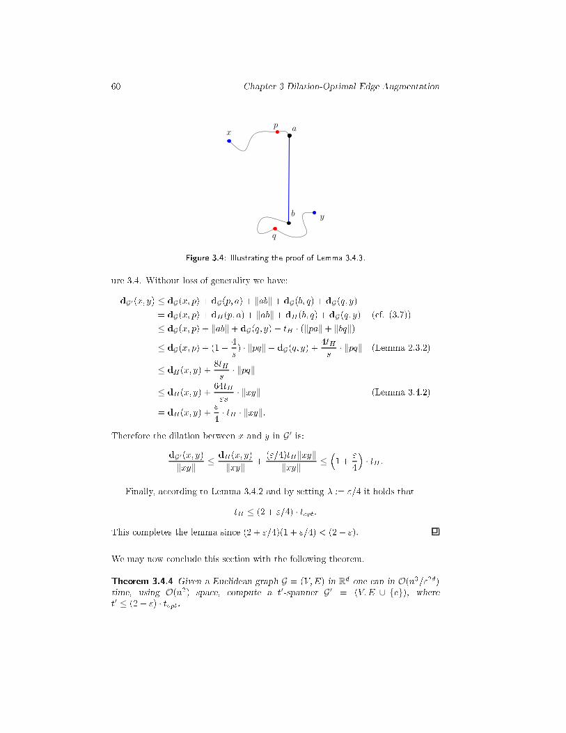
60 Chapter 3 Dilation-Optimal Edge Augmentationp

q

a

b

x

yFigure 3.4: Illustrating the proof of Lemma 3.4.3.ure 3.4. Without loss of generality we have:dG′(x; y) ≤ dG(x; p) + dG(p; a) + ‖ab‖+ dG(b; q) + dG(q; y)= dG(x; p) + dH(p; a) + ‖ab‖+ dH(b; q) + dG(q; y) ( f. (3.7))≤ dG(x; p) + ‖ab‖+ dG(q; y) + tH · (‖pa‖+ ‖bq‖)≤ dG(x; p) + (1 + 4s ) · ‖pq‖+ dG(q; y) + 4tHs · ‖pq‖ (Lemma 2.3.2)≤ dH(x; y) + 8tHs · ‖pq‖≤ dH(x; y) + 64tH"s · ‖xy‖ (Lemma 3.4.2)= dH(x; y) + "4 · tH · ‖xy‖:Therefore the dilation between x and y in G′ is:dG′(x; y)

‖xy‖ ≤ dH(x; y)‖xy‖ + ("=4)tH‖xy‖

‖xy‖ ≤�1 + "4� · tH :Finally, a ording to Lemma 3.4.2 and by setting � := "=4 it holds thattH ≤ (2 + "=4) · topt:This ompletes the lemma sin e (2 + "=4)(1 + "=4) < (2 + ").We may now on lude this se tion with the following theorem.Theorem 3.4.4 Given a Eu lidean graph G = (V;E) in R

d one an in O(n3="2d)time, using O(n2) spa e, ompute a t′-spanner G′ = (V;E ∪ {e}), wheret′ ≤ (2 + ") · topt.

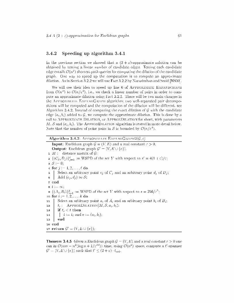
3.4 A (2 + ")-approximation for Eu lidean graphs 613.4.2 Speeding up algorithm 3.4.1In the previous se tion we showed that a (2 + ")-approximate solution an beobtained by testing a linear number of andidate edges. Testing ea h andidateedge entailsO(n2) shortest path queries for omputing the dilation of the andidategraph. One way to speed up the omputation is to ompute an approximatedilation. As in Se tion 3.2.2 we will use Fa t 3.2.2 by Narasimhan and Smid [NS00℄.We will use their idea to speed up line 6 of Approximate Expandgraphfrom O(n2) to O(n="d), i.e., we he k a linear number of pairs in order to om-pute an approximate dilation using Fa t 3.2.2. There will be two main hanges inthe Approximate ExpandGraph algorithm; two well-separated pair de ompo-sitions will be omputed and the omputation of the dilation will be di�erent, seeAlgorithm 3.4.2. Instead of omputing the exa t dilation of G with the andidateedge (ai; bi) added to G, we ompute the approximate dilation. This is done by a all to Approximate Dilation, or ApproxDilation for short, with parametersM , S and (ai; bi). The ApproxDilation algorithm is stated in more detail below.Note that the number of point pairs in S is bounded by O(n="d).Algorithm 3.4.2: Approximate ExpandGraph2(G; ")Input: Eu lidean graph G = (V;E) and a real onstant " > 0.Output: Eu lidean graph G′ = (V;E ∪ {e}).M := distan e matrix of G;1{(Cj ; Dj)}j̀=1 := WSPD of the set V with respe t to s′ = 4(1 + ")=";2S := ∅;3 for j := 1; 2; : : : ; ` do4 Sele t an arbitrary point j of Cj and an arbitrary point dj of Dj ;5 Add ( j ; dj) to S;6 end7 t :=∞;8{(Ai; Bi)}ki=1 := WSPD of the set V with respe t to s = 256="2;9 for i := 1; 2; : : : ; k do10 Sele t an arbitrary point ai of Ai and an arbitrary point bi of Bi;11 ti := ApproxDilation(M;S; ai; bi);12 if ti < t then13 t := ti and e := (ai; bi);14 end15 end16 return G′ = (V;E ∪ {e});17Theorem 3.4.5 Given a Eu lidean graph G = (V;E) and a real onstant " > 0 one an in O(nm+ n2(logn+ 1="3d)) time, using O(n2) spa e, ompute a t′-spanner

G′ = (V;E ∪ {e}) su h that t′ ≤ (2 + ") · topt.

62 Chapter 3 Dilation-Optimal Edge AugmentationAlgorithm 3.4.3: ApproxDilationInput: Distan e matrix M , a set S of point pairs and point pair (a; b).Output: Approximate dilation.forea h (x; y) ∈ S do1 dx;y := min {M [x; y℄;M [x; a℄ + ‖ab‖+M [b; y℄;M [x; b℄ + ‖ba‖+M [a; y℄};2 tx;y := dx;y=‖xy‖;3 end4 return maxx;y tx;y;5Proof. The omplexity of all lines of the algorithm 3.4.2, ex ept line 12, is asin Lemma 3.4.1. Lines 1{9 require O(mn + n2 logn + n="2d) time. It remainsto onsider line 12 of the algorithm. Note that the number of times line 12 isexe uted is O(n="2d). Pro edure ApproxDilation performs O(n="d) shortest-path queries, instead of O(n2), thus the total time needed by line 12 is O( n"2d · n"d ).Summing up the running times gives the stated time omplexity.In Lemma 3.4.3 it was proven that the solution returned by algorithm Ap-proximate ExpandGraph had a dilation that was at most a fa tor (2 + ")worse than the dilation of an optimal solution. Sin e the modi�ed algorithm doesnot ompute the exa t dilation of a andidate graph, but instead omputes a(1 + ")2-approximate dilation it is not hard to verify that the same arguments asin Lemma 3.4.3 an be applied to prove that the algorithm Approximate Ex-pandGraph2 returns a graph with dilation at most (1+ ")2 · (2+ ") · topt. Setting" = min{"=10; 1}, on ludes the proof of the theorem.3.5 A spe ial ase: G has onstant dilationIn the spe ial ase when the dilation of the graph G is known to be onstant thereare well-known tools that we an use to de rease both the time omplexity and thespa e omplexity of the algorithms and improve the approximation fa tor. Themain idea is to use the following fa t by Gudmundsson et al. [GLNS02b℄ whi henable us to ompute an approximate dilation of a andidate graph in linear time.Fa t 3.5.1 ([GLNS02b℄) Let V be a set of n points in Rd, let t > 1 and 0 < " ≤ 1be real numbers, and let G = (V;E) be a t-spanner for V . In

O�m+ nt5d"2d (logn+ (t=")d)�time, we an prepro ess G into a data stru ture of size O((t3d="2d)n log(tn)) su hthat for any two distin t points p and q in V , a (1 + ")-approximation to the

3.5 A spe ial ase: G has onstant dilation 63shortest-path distan e between p and q in G an be omputed in time O�(t5="2)d�.The query stru ture in Fa t 3.5.1 is denotedM ′ and is onstru ted by algorithmQueryStru ture. We have to use a modi�ed version of ApproxDilation, de-noted ApproxDilation2, that takes the query stru ture M ′ as input instead ofthe matrixM . The (exa t) shortest path distan e queries using M in ApproxDi-lation are repla ed in ApproxDilation2 by performing approximate shortestpath distan e queries using M ′.Next we state the main algorithm. Re all that the parameter t is a onstantand an upper bound on the dilation of the input graph G. Also note that thisalgorithm only needs one well-separated pair de omposition.Algorithm 3.5.1: Approximate ExpandGraph3(G; t; ")Input: Eu lidean t-spanner G = (V;E) and two real onstants t > 1 and" > 0.Output: Eu lidean graph G′ = (V;E ∪ {e}).M ′ := QueryStru ture(G; t; ") using Fa t 3.5.1;1{(Ai; Bi)}ki=1 := WSPD of V with respe t to s = 8(t+ 1)=";2S := ∅;3 for j := 1; 2; : : : ; k do4 Sele t an arbitrary point aj of Aj and an arbitrary point bj of Bj ;5 Add (aj ; bj) to S;6 end7 t :=∞;8 for i := 1; 2; : : : ; k do9 ti := ApproxDilation2(M ′;S; ai; bi);10 if ti < t then11 t := ti and e := (ai; bi);12 end13 end14 return G′ = (V;E ∪ {e});15Lemma 3.5.2 Approximate ExpandGraph3 runs in O((t7="4)d · n2) time anduses O((t3="2)d n log(tn)) spa e.Proof. The time omplexity of lines 1{3 is dominated by line 1, thus O(m +n(t5="2)d(logn+(t=")d)) time. Lines 10{13 is exe uted O((t=")dn) times, and ea hiteration requires O((t=")dn · (t5d="2d)) time a ording to Fa ts 3.2.2 and 3.5.1.Summing up the time bounds gives the time bound stated in the lemma.The spa e bound follows sin e the approximate distan e ora le stated inFa t 3.5.1 only uses O((t3="2)d n log(tn)) spa e, instead of the quadrati spa eneeded earlier.

64 Chapter 3 Dilation-Optimal Edge AugmentationNow, we show that this algorithm omputes a (1 + ")-approximation of theoptimal solution. Note that in Approximate ExpandGraph3 the separation onstant depends both on " and t whi h is the main di�eren e ompared to theprevious algorithms. This allows us to improve the approximation fa tor.Lemma 3.5.3 Let G = (V;E) be a Eu lidean graph with onstant dilation t and apositive real onstant ", and let {(Ai; Bi)}ki=1 be a well-separated pair de omposi-tion of V with respe t to s = 8(t+1)=". For every pair (Ai; Bi) and any elementsa1; a2 ∈ Ai and b1; b2 ∈ Bi, let G1 = (V;E∪{(a1; b1)}) and G2 = (V;E∪{(a2; b2)}),and let t1 and t2 denote the dilation of G1 and G2, respe tively. It holds thatt1 ≤ (1 + ")t2.Proof. It suÆ es to prove that for every pair of points (u; v) ∈ �(a2; b2) thereexists a path in G1 of length at most (1 + ") · dG2(u; v). Re all that �(p; q) is theset of point pairs for whi h a shortest path between them in G ∪ {(p; q)} passesthrough (p; q). Without loss of generality we may assume that the shortest pathbetween u and v in G2, goes from u to a2 and to v via b2. We have:dG1(u; v) ≤ dG(u; a2) + dG(a2; a1) + ‖a1b1‖+ dG(b1; b2) + dG(b2; v)≤ dG(u; a2) + t‖a2a1‖+ ‖a1b1‖+ t‖b1b2‖+ dG(b2; v)≤ dG(u; a2) + 4ts ‖a2b2‖+ (1 + 4=s) · ‖a2b2‖+ dG(b2; v)< dG(u; a2) + ‖a2b2‖+ dG(b2; v) + 8ts ‖a2b2‖= dG2(u; v) + t"t+ 1‖a2b2‖< (1 + ") · dG2(u; v):In the se ond inequality we used Lemma 2.3.2, in the �fth inequality we used thefa t that s = 8(t+1)=" and in the �nal step we used that dG2(u; v) ≥ ‖a2b2‖ sin e(u; v) ∈ �(a2; b2). The lemma follows.Lemma 3.5.4 Algorithm Approximate ExpandGraph3 returns a graph withdilation at most (1 + ")3 · topt.Proof. Assume that topt is the dilation of an optimal solution G ∪ {(p; q)}, andlet G′ with dilation tC be the output of the algorithm 3.5.1.We will use the same notations as in the algorithm. For ea h i let t∗i be the(exa t) dilation of Gi = G ∪ {(ai; bi)}. A ording to Fa t 3.2.2, for ea h i,t∗i ≤ ti ≤ (1 + ")2 · t∗i :Let (Aj ; Bj) be the pair in the well-separated pair de omposition su h thatp ∈ Aj and q ∈ Bj , or p ∈ Bj and q ∈ Aj . From Lemma 3.5.3 it follows that

3.6 Con luding remarks 65t∗j ≤ (1 + ") · topt. As a result it follows thattC ≤ tj ≤ (1 + ")2 · t∗j ≤ (1 + ")3 · topt:Therefore topt ≤ tC ≤ (1 + ")3 · topt whi h ompletes the lemma.The following theorem follows by setting " = min{'=15; 1} and ombiningLemmas 3.5.2 and 3.5.4.Theorem 3.5.5 Let V be a set of n points in Rd, let t > 1 and ' > 0 bereal numbers, and let G = (V;E) be a geometri t-spanner of V . One an in

O((t7='4)d · n2) time, using O((t3=')d n log(tn)) spa e, ompute a t′-spannerG′ = (V;E ∪ {e}) su h that t′ ≤ (1 + ') · topt.3.6 Con luding remarksWe onsidered the problem of adding an edge to a Eu lidean graph su h that thedilation of the resulting graph is minimized, and gave several algorithms. Ourmain result is a (2 + ")-approximation algorithm with running time

O�nm+ n2(logn+ 1="3d)�using O(n2) spa e.Several problems remain open.1. Is there an exa t algorithm with running time o(n4) using linear spa e?2. Can we a hieve a (1 + ")-approximation within the same time bound as inTheorem 3.4.5?3. A natural extension is to allow more than one edge to be added. Can wegeneralize our results to this ase?A knowledgementsWe would like to thank Ren�e van Oostrum for fruitful dis ussions during the earlystages of this work, Mohammad Ali Abam for dis ussions about Se tion 3.2.2,Sergio Cabello for simplifying the algorithm in Se tion 3.5 and Ansgar Gr�une forObservation 3.3.3.Finally, we thank the anonymous referees for many insightful omments andsuggestions on how to improve the journal version of this hapter.

66 Chapter 3 Dilation-Optimal Edge Augmentation

Chapter 4Dilation-Optimal EdgeDeletion4.1 Introdu tionGiven a (geometri ) network, a natural question to ask is what happens to thequality of the network when some onne tions are removed. In ase some links ina traÆ network have to be shut down (e.g., due to budget onsiderations), wemay want to know whi h edges of the network should be removed so as to notde rease the quality of the new network too mu h. Alternatively, we may want toknow the most riti al edge in the network, i.e., the edge whose removal ausesthe largest possible de rease in the quality of the new network.In this hapter, we onsider a simple variant of this problem: The initial net-work is a polygonal y le C in the plane, and we have to remove one single edgefrom C. We measure the quality of the resulting polygonal path � by its dilation(or stret h fa tor) D�.Re all that the dilation between two distin t verti es x and y of the path � isde�ned as

D�(x; y) := d�(x; y)‖xy‖ ;where d�(x; y) denotes the Eu lidean length of the subpath of � onne ting x andy, and ‖xy‖ denotes the Eu lidean distan e between x and y. For onvenien e wede�ne D�(x; x) := 1. The dilation between two sets X and Y of verti es of � is

68 Chapter 4 Dilation-Optimal Edge Deletionde�ned asD�(X;Y ) := max{D�(x; y) | x is a vertex of X , y is a vertex of Y };the dilation of a set X of verti es of � is de�ned as

D�(X) := D�(X;X);and the dilation of the path � is de�ned asD� := D�(�) = max{D�(x; y) | x and y are verti es of �}:Re ently the problem of onstru ting minimum-dilation networks on a givenpoint set has attra ted a lot of attention. Klein and Kutz [KK07℄ showed that onstru ting a geometri network on a point set in the plane using a given numberof edges su h that the network has minimum dilation is NP-hard. The problemis NP-hard even for more spe i� ases like minimum dilation spanning tree orminimum dilation path, see [CHL07℄ and [GKM07℄. Minimum dilation stars is the ase whi h we an onstru t in polynomial time, see [EW07℄.All the above problems want to onstru t a network from s rat h but in manyappli ations we already have a network and the problem at hand is to extend/prunethe network su h that the dilation of the resulting network is minimized. InChapter 3 we saw that in the ase of adding an edge, the optimal edge, i.e. thenew edge whi h minimize the dilation of the network, an be omputed in O(n4)time, where n is the number of nodes in the network. There are also severalapproximation algorithms whi h run faster. However, the problem of omputingthe edge in the network whose removal minimizes/maximizes the dilation of theresulting network was not studied before, to the best of our knowledge.The problem we onsider is the following: We are given a polygonal y le

C = (p0; : : : ; pn−1; p0) whose n verti es p0; : : : ; pn−1 are points in the plane. Wewant to determine the edge e of C for whi h the dilation of the polygonal pathC \ {e} is minimized or maximized. In other words, if we denote by �i (for0 ≤ i < n) the polygonal path obtained by removing the edge (pi; pi+1) from C(where indi es are to be read modulo n), then our goal is to ompute

DminC := min0≤i<nD�iand

DmaxC := max0≤i<nD�i :It is known that omputing the dilation of a path, or even approximatingit, need (n logn) time, see [NS07, Theorem 13.1.3℄. Therefore using a na��vealgorithm whi h he ks all the edges of the y le takes (n2 logn) time to omputethe optimal edge in the y le.

4.2 Dilation-minimal edge deletion in a y le 69A summary of our results and the organization of the rest of this hapter arein the following.In Se tion 4.2, we onsider the dilation-minimal edge deletion problem andpresent a randomized algorithm for the problem. We start in Se tion 4.2.1 by de-s ribing an approa h of [AKK+℄ to estimate the dilation of a polygonal path. Theseideas will play a entral role in the algorithm we give in Se tion 4.2.2 for solving ade ision problem asso iated with the problem of omputing DminC

; the algorithmsolving this de ision problem runs in O(n log2 n) expe ted time. In Se tion 4.2.3,we give a simple randomized approa h whi h redu es the problem of omputingDmin

Cto an expe ted number of O(logn) de ision problems of Se tion 4.2.2. Thus,this redu tion in urs a logarithmi slowdown of the de ision pro edure.In Se tion 4.3, we onsider the dilation-maximal edge deletion problem andpresent a O(n logn) time algorithm for the problem. We �rst show that for two�xed verti es x and y of C, it is easy to determine the largest possible dilationbetween them if one edge is removed from C. We then show that, in order to ompute Dmax

C, it suÆ es to onsider pairs (x; y) of verti es whose distan e is atmost twi e the losest-pair distan e in the vertex set of C. Sin e there are only

O(n) su h pairs (x; y), this leads to an eÆ ient algorithm for omputing DmaxC

.Finally, we present an algorithm that omputes in O(n logn) total time an ap-proximation to the dilation of ea h path Pi, as well as an approximation of DminCin Se tion 4.4. The algorithm uses Fa t 3.2.2 whi h states that the well-separatedpair de omposition an be used to redu e the problem of approximating the dila-tion of a Eu lidean graph to the problem of omputing the shortest-path distan esbetween O(n) pairs of verti es. This result, together with the observation that forany two verti es x and y of C, the sequen e D�0(x; y); : : : ;D�n−1(x; y) ontainsonly two distin t values, leads to an O(n logn){time algorithm that approximatesthe dilation of ea h path �i as well as the minimum dilation Dmin

C.

4.2 Dilation-minimal edge deletion in a y leIn this se tion, we give an algorithm whi h given a polygonal y le C, omputes theedge whose removal generates a path whi h has minimum dilation among all thepaths generated by removing an edge from C. The algorithm starts with removinga random edge from C and omputes the dilation � of the generated path. Thenit uses a de ision algorithm whi h for ea h edge e in the y le C, de ides whetherthe dilation of the path C\{e} is less than �. Then it pi ks one of the edges whoseremoval generates a path with dilation less than � and assigns the dilation of thepath to �. It repeats the pro edure until no edge in the y le generates a pathwith dilation less than �.

70 Chapter 4 Dilation-Optimal Edge Deletion4.2.1 Estimating the dilation of a polygonal pathOur algorithm for omputing the edge of a polygonal y le whose removal mini-mizes the dilation of the resulting path uses as a subroutine parts of the algorithmof [AKK+℄ that de ides if the dilation of a polygonal path is less than some giventhreshold � > 1. We des ribe those parts of this algorithm whi h are relevant forus. Let � = (p0; : : : ; pn−1) be a polygonal path whose n verti es are points in theplane and let � ≥ 1 be a real number. Without loss of generality we assume p0 isthe origin. The idea is to use a lifting transformation that rephrases the de isionproblem, i.e., the problem of de iding if D� < �, into a point- one in iden e-problem in R3.We denote the �rst and last verti es of a polygonal path � by f(�) and l(�),respe tively. Thus, f(�) = p0. For ea h vertex p of �, we de�ne the weight of pto be !�(p) := d�(p; f(�))=�:We map ea h vertex p = (xp; yp) of � to the pointh�(p) := (xp; yp; !�(p)) ∈ R

3:Let C denote the three-dimensional oneC := {(x; y; z) ∈ R3 | z =px2 + y2}:We map ea h vertex p of � to the oneC�(p) := C ⊕ h�(p) = { + h�(p) | ∈ C}:Note that we an reformulate the de�nition of C�(p) asC�(p) := �(x; y; z) | z − !�(p) =q(x− xp)2 + (y − yp)2� ; (4.1)and therefore C�(p) is the graph of the bivariate fun tion fp(q) = ‖pq‖ + !�(p)for q ∈ R

2. If p and q are verti es of �, then we say that p is before q on �, ifd�(p; f(�)) < d�(q; f(�));this will be denoted as p <� q. We then get the following lemma.Lemma 4.2.1 For any two verti es p and q of � with p <� q, we haveD�(p; q) < � if and only if h�(q) lies below C�(p).

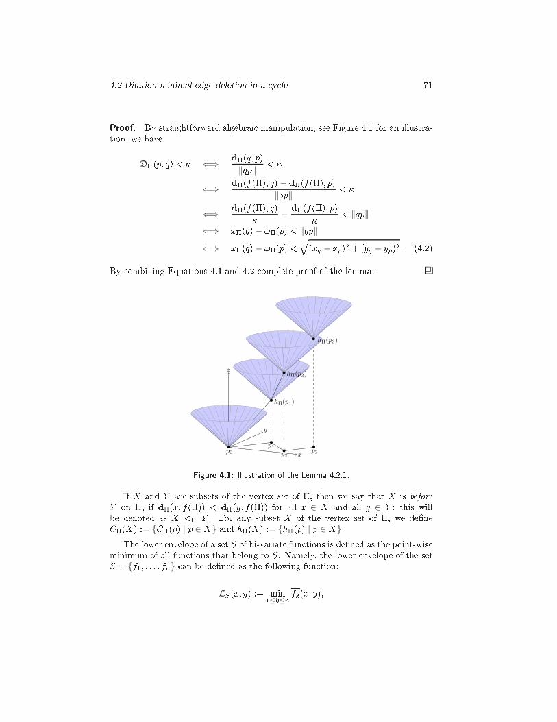
4.2 Dilation-minimal edge deletion in a y le 71Proof. By straightforward algebrai manipulation, see Figure 4.1 for an illustra-tion, we haveD�(p; q) < � ⇐⇒ d�(q; p)

‖qp‖ < �⇐⇒ d�(f(�); q)− d�(f(�); p)

‖qp‖ < �⇐⇒ d�(f(�); q)� − d�(f(�); p)� < ‖qp‖⇐⇒ !�(q)− !�(p) < ‖qp‖⇐⇒ !�(q)− !�(p) <q(xq − xp)2 + (yq − yp)2: (4.2)By ombining Equations 4.1 and 4.2 omplete proof of the lemma.

p0

p1

p2

p3x

y

z

hΠ(p1)

hΠ(p2)

hΠ(p3)

Figure 4.1: Illustration of the Lemma 4.2.1.If X and Y are subsets of the vertex set of �, then we say that X is beforeY on �, if d�(x; f(�)) < d�(y; f(�)) for all x ∈ X and all y ∈ Y ; this willbe denoted as X <� Y . For any subset X of the vertex set of �, we de�neC�(X) := {C�(p) | p ∈ X} and h�(X) := {h�(p) | p ∈ X}:The lower envelope of a set S of bi-variate fun tions is de�ned as the point-wiseminimum of all fun tions that belong to S. Namely, the lower envelope of the setS = {f1; : : : ; fn} an be de�ned as the following fun tion:LS(x; y) := min1≤k≤n fk(x; y);

72 Chapter 4 Dilation-Optimal Edge Deletionwhere fk(x; y) := (fk(x; y) if (x; y) belongs to the domain of fk+∞ otherwise.Lemma 4.2.1 immediately gives the following result.Lemma 4.2.2 For any two subsets X and Y of the vertex set of � with X <� Y ,we haveD�(X;Y ) < � if and only if h�(Y ) lies below LC�(X).The minimization diagram of C�(X), i.e., the proje tion of the lower envelope

LC�(X) onto the xy-plane, is the additively weighted Voronoi diagram1 V�(X) ofX with respe t to the weight fun tion !�. If the point y of Y is lo ated in theVoronoi region of the point x of X , then h�(y) is below LC�(X) if and only ifh�(y) is below C�(x).This yields an eÆ ient algorithm to verify if D�(X;Y ) < � for two subsetsX and Y of the vertex set of � having the property that X <� Y : The Voronoidiagram V�(X) an be omputed in O(|X | log |X |) time, .f. [For87℄. Withinthe same time bound, this diagram an be prepro essed into a linear size datastru ture that supports O(log |X |)-time point-lo ation queries, .f. [Kir83℄. Thisstru ture an now be queried with ea h point y of Y to determine whi h point xof X ontains y in its Voronoi ell. On e this is known, the he k if h�(y) is belowC�(x) an be performed in O(1) time. The total running time of this algorithmis O((|X |+ |Y |) log |X |).4.2.2 The de ision problemLet C be a polygonal y le on a set of n verti es in the plane and let � > 1 be areal number. In this se tion, we present an algorithm that de ides for ea h edge eof C, whether or not the dilation of the polygonal path C \ {e} is less than �. We�rst des ribe the overall approa h. Then, we give two implementations that yieldrunning times of O(n log3 n) and O(n log2 n), respe tively.For a y le C = (p0; p1; : : : ; pn−1; p0), we all pi+1 the su essor of pi in C (whereindi es are to be read modulo n) and denote it by su (pi). If R = (r1; : : : rm)and Q = (q1; : : : ; qn) are two polygonal paths having the property that q1 = f(Q)is the su essor of l(R) = rm in C, then we denote the on atenation of R and Qby R ⊕Q. Thus, R⊕Q is the polygonal path (r1; : : : ; rm; q1; : : : ; qn).In order to fa ilitate a re ursive approa h, we will onsider the following moregeneral problem: Assume that (the vertex set of) C is partitioned into two polyg-onal paths T (the top) and B (the bottom) su h that DT < �. We want to de ide1It's de�ned just like the usual Voronoi diagram, but ea h site has a weight, and the distan eto a site is the usual Eu lidean distan e plus the site weight.

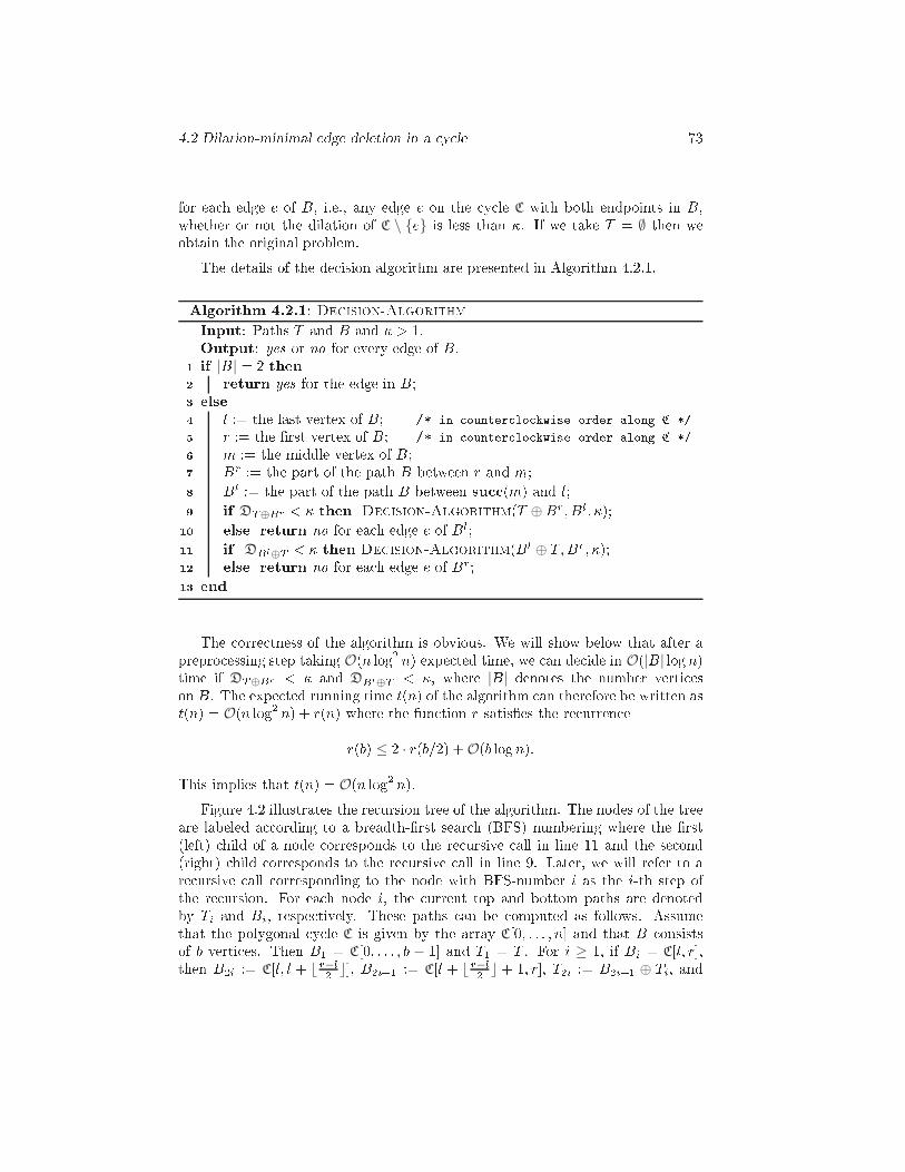
4.2 Dilation-minimal edge deletion in a y le 73for ea h edge e of B, i.e., any edge e on the y le C with both endpoints in B,whether or not the dilation of C \ {e} is less than �. If we take T = ∅ then weobtain the original problem.The details of the de ision algorithm are presented in Algorithm 4.2.1.Algorithm 4.2.1: De ision-AlgorithmInput: Paths T and B and � > 1.Output: yes or no for every edge of B.if |B| = 2 then1 return yes for the edge in B;2 else3 l := the last vertex of B; /* in ounter lo kwise order along C */4 r := the �rst vertex of B; /* in ounter lo kwise order along C */5 m := the middle vertex of B;6 Br := the part of the path B between r and m;7 Bl := the part of the path B between su (m) and l;8 if DT⊕Br < � then De ision-Algorithm(T ⊕Br; Bl; �);9 else return no for ea h edge e of Bl;10 if DBl⊕T < � then De ision-Algorithm(Bl ⊕ T;Br; �);11 else return no for ea h edge e of Br;12 end13 The orre tness of the algorithm is obvious. We will show below that after aprepro essing step taking O(n log2 n) expe ted time, we an de ide in O(|B| logn)time if DT⊕Br < � and DBl⊕T < �, where |B| denotes the number verti eson B. The expe ted running time t(n) of the algorithm an therefore be written ast(n) = O(n log2 n) + r(n) where the fun tion r satis�es the re urren er(b) ≤ 2 · r(b=2) +O(b logn):This implies that t(n) = O(n log2 n).Figure 4.2 illustrates the re ursion tree of the algorithm. The nodes of the treeare labeled a ording to a breadth-�rst sear h (BFS) numbering where the �rst(left) hild of a node orresponds to the re ursive all in line 11 and the se ond(right) hild orresponds to the re ursive all in line 9. Later, we will refer to are ursive all orresponding to the node with BFS-number i as the i-th step ofthe re ursion. For ea h node i, the urrent top and bottom paths are denotedby Ti and Bi, respe tively. These paths an be omputed as follows. Assumethat the polygonal y le C is given by the array C[0; : : : ; n℄ and that B onsistsof b verti es. Then B1 = C[0; : : : ; b − 1℄ and T1 = T . For i ≥ 1, if Bi = C[l; r℄,then B2i := C[l; l + ⌊ r−l2 ⌋℄, B2i+1 := C[l + ⌊ r−l2 ⌋ + 1; r℄, T2i := B2i+1 ⊕ Ti, and

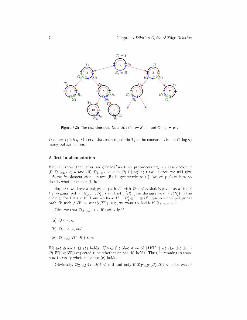
74 Chapter 4 Dilation-Optimal Edge Deletion1

2

4 5

10 11

3

6

... ...

7

T1

T1 = T

T1

T2 T2

T5 T5

T3 T3

G4

B4

G2 B2

B1 = B

B3 G3

p0

B7

G7

G6

B6

G5

B5

B10

G10 B11

G11Figure 4.2: The re ursion tree. Note that G2i := B2i+1 and G2i+1 := B2i.T2i+1 := Ti⊕B2i. Observe that ea h top hain Tj is the on atenation of O(logn)many bottom hains.A �rst implementationWe will show that after an O(n log2 n){time prepro essing, we an de ide if(i) DT⊕Br < � and (ii) DBl⊕T < � in O(|B| log2 n) time. Later, we will givea faster implementation. Sin e (ii) is symmetri to (i), we only show how tode ide whether or not (i) holds.Suppose we have a polygonal path T ′ with DT ′ < � that is given as a list ofk polygonal paths (B′1; : : : ; B′k) su h that f(B′i+1) is the su essor of l(B′i) in the y le C, for 1 ≤ i < k. Thus, we have T ′ = B′1 ⊕ : : :⊕B′k. Given a new polygonalpath B′ with f(B′) = su (l(T ′)) in C, we want to de ide if DT ′⊕B′ < �.Observe that DT ′⊕B′ < � if and only if(a) DT ′ < �,(b) DB′ < �, and( ) DT ′⊕B′(T ′; B′) < �.We are given that (a) holds. Using the algorithm of [AKK+℄ we an de ide inO(|B′| log |B′|) expe ted time whether or not (b) holds. Thus, it remains to showhow to verify whether or not ( ) holds.Obviously, DT ′⊕B′(T ′; B′) < � if and only if DT ′⊕B′(B′i; B′) < � for ea h i

4.2 Dilation-minimal edge deletion in a y le 75with 1 ≤ i ≤ k. Sin e B′i <T ′⊕B′ B′, we know from Lemma 4.2.2 thatDT ′⊕B′(B′i; B′) < � if and only if hT ′⊕B′(B′) lies below LCT ′⊕B′ (B′i):Assume that for ea h path B′i, we have the total a umulated s aled length`i := iXj=1 dB′j (l(B′j); f(B′j))=�and the additively weighted Voronoi diagram VB′i(B′i) that has been augmentedwith a data stru ture to support point-lo ation queries in tlo time per query.Re all that VB′i(B′i) is the proje tion of the lower envelope LCB′i (B′i) onto thexy-plane. It is de�ned with respe t to the weights!B′i(p) = dB′i(p; f(B′i))=�:Sin e !T ′⊕B′(p) = !B′i(p) + `i−1for all p ∈ B′i, we have!T ′⊕B′(p)− !T ′⊕B′(q) = !B′i(p)− !B′i(q)for all p; q ∈ B′i. It follows that the diagram VB′i(B′i) is also the proje tion of thelower envelope LCT ′⊕B′(B′i).The asso iated point-lo ation stru ture of B′i an therefore be used to deter-mine for ea h point b′ in B′, the point t in B′i that ontains b′ in its Voronoi ell inVT ′⊕B′(B′i). On e this is known for ea h point b′ in B′, we an he k if hT ′⊕B′(b′)is below CT ′⊕B′(t). To this end, we ompute the weights !T ′⊕B′(t) = !B′i(t)+`i−1and !T ′⊕B′(b′) = !B′(b′) + `k.The overall running time of this approa h (ex luding the prepro essing time)is O(k|B′|tlo ).In our appli ation, the relevant paths B′i are the bottom paths Bi that appear inthe re ursive alls (see Figure 4.2 and the dis ussion after that). As a onsequen e,k = O(log n), |T ′ ⊕ B′| ≤ n, and we an pre ompute the required information in

O(n log2 n) time by omputing all the diagrams VBi(Bi) along with the point-lo ation data stru tures. Sin e tlo = O(logn), it follows that the overall runningtime of this approa h (after O(n log2 n) prepro essing time) is O(|B′| log2 n). Withthis implementation, Algorithm 4.2.1 runs in O(n log3 n) expe ted time.A faster implementationIn the i-th step of the re ursion, we split Bi (almost evenly) into B2i and B2i+1,and ompute the diagrams VB2i (B2i) and VB2i+1(B2i+1). We then lo ate ea h

76 Chapter 4 Dilation-Optimal Edge Deletionpoint b of B2i in VB2i+1(B2i+1) to determine whi h point t of B2i+1 ontains b inits Voronoi ell in VB2i+1(B2i+1). We store t in a table Tb asso iated with b underthe key 2i+1 that identi�es the set B2i+1. In the same way, we lo ate ea h pointb of B2i+1 in VB2i(B2i) and store the orresponding point t of B2i in a table Tbasso iated with b under the key 2i.Sin e we perform exa tly one point-lo ation query for ea h point b of B1 onea h level of the re ursion tree, the table Tb has O(logn) entries. We an thereforeuse the onstru tion of [FKS84℄ to store Tb in a perfe t-hash table of size O(logn)that supports O(1) a ess time. Note that in the omplexity model of [FKS84℄,it is assumed that the entries ome from a �nite universe and the algorithm isable to randomly a ess ea h memory lo ation in onstant time. Re all thatthe onstru tion of [FKS84℄ is randomized and builds the hash table in O(logn)expe ted time.The total time we spend on ea h level of the re ursion tree is O(n logn), sothe total expe ted prepro essing time is O(n log2 n) and the total time we spendfor answering point-lo ation queries is O(n log2 n).In order to determine for a point b′ of B′, where B′ ⊆ B1, whi h point t of B′i ontains b′ in its Voronoi ell, we �nd the index j for whi h B′i = Bj . Then weretrieve the entry with the key j from Tb′ . This is exa tly the point t of Bj that ontains b in its Voronoi ell in VBj (Bj).It follows that tlo = O(1), so that the overall running time of this approa h(after O(n log2 n) prepro essing time) is O(|B′| logn). With this implementation,Algorithm 4.2.1 runs in O(n log2 n) expe ted time.4.2.3 The optimization algorithmWe now present our algorithm that omputes, for a given polygonal y le C ona set of n points in the plane, the value of DminC

in O(n log3 n) expe ted time.Clarkson and Shor [CS88℄ used a similar randomized approa h to ompute thediameter of a point set. The main idea is to he k all the edges in the y le in arandom order. We start with a random edge e1 ∈ C and ompute the dilation ofthe path C\{e1}, using the algorithm of [AKK+℄, and assign this value to �. Thenwe run Algorithm 4.2.1 to see for ea h edge e of the y le C whether the dilationof the path C \ {e} is less than �. We store with ea h edge e of C a Boolean ag,denoted by flag(e), whi h is true if and only if the dilation of the path C \ {e}is less than �. For any edge e with flag(e) = true, we ompute and assign thedilation of C \ {e} to � and update ags same as before. For more details seealgorithm 4.2.2.The orre tness of the algorithm follows from the fa t that it returns� = min1≤i≤nD�i = DminC ;

4.3 Dilation-maximal edge deletion in a y le 77Algorithm 4.2.2: Optimization AlgorithmInput: A y le C on a set of n points.Output: DminC

.{ei}i := random permutation of the edges of C;1 � := the dilation of the path C \ {e1};2 Run Algorithm 4.2.1 and for ea h edge e of C, update flag(e);3 for i = 2; 3; : : : ; n do4 if flag(ei) = true then5 � := the dilation of the path C \ {ei};6 Run Algorithm 4.2.1 and for ea h edge e of C, update flag(e);7 end8 end9 return �;10where �i is the polygonal path obtained by removing ei from C.Clearly, line 1 takes O(n) time. The algorithm of [AKK+℄ and, therefore,line 2, takes O(n logn) expe ted time. Ea h time we run Algorithm 4.2.1, wespend O(n log2 n) expe ted time. Observe that we run this algorithm on e inline 3 and, moreover, in lines 4{9 ea h time the dilation of �i is less than the urrent value of �. In the latter ase, we also spend O(n logn) expe ted time to ompute the dilation of �i. Sin e the edges of C are in random order, the values

D�1 ; : : : ;D�n are in random order as well. At the start of the i-th iteration oflines 4{9, the value of � is equal to min1≤j<i D�j . Thus, D�i < � if and only ifD�i is the minimum of the set {D�j | 1 ≤ j ≤ i}. It follows that D�i < � withprobability 1=i. Using the linearity of expe tation, it follows that the expe tednumber of times that lines 6 and 7 are performed is equal toPni=2 1=i = O(logn).Thus, the overall expe ted running time of our algorithm is O(n log3 n).Theorem 4.2.3 Given a polygonal y le C on n verti es in the plane, we an ompute Dmin

Cin O(n log3 n) expe ted time.4.3 Dilation-maximal edge deletion in a y leLet C = (p0; : : : ; pn−1; p0) be a polygonal y le whose verti es p0; : : : ; pn−1 arepoints in the plane. Re all from Se tion 4.1 that �i (for 0 ≤ i < n) denotes thepolygonal path obtained by removing the edge (pi; pi+1) from C, d�i(x; y) denotesthe length of the subpath of �i between x and y, D�i(x; y) = d�i(x; y)=‖xy‖denotes the dilation between x and y in �i, and D�i denotes the dilation of �i.In this se tion, we will give an algorithm that omputes

DmaxC = max0≤i<nD�i :

78 Chapter 4 Dilation-Optimal Edge DeletionLet L be the total length of the edges of C. We de�ne �(p0) := 0 and�(pi) := �(pi−1) + ‖pi−1pi‖ for 1 ≤ i < n:Thus, �(pi) is the length of the path (p0; : : : ; pi) and the shortest-path distan edC(pi; pj) between pi and pj in the y le C is given bydC(pi; pj) = min(|�(pi)−�(pj)|; L− |�(pi)−�(pj)|):Consider two distin t verti es x and y of C. We obtain the largest dilationbetween x and y in any path �i, by deleting an arbitrary edge on the shorter ofthe two paths in C between x and y. Thus, the following lemma holds.Lemma 4.3.1 Let x and y be two distin t verti es of C. Thenmax0≤i<nD�i(x; y) = max(|�(x) −�(y)|; L− |�(x) −�(y)|)‖xy‖ ≥ L2‖xy‖ :The next lemma states that the losest pair in the vertex set of C an be usedto obtain a 2-approximation to Dmax

C.Lemma 4.3.2 Let (p; q) be a losest pair in the vertex set of C. Then

DmaxC ≤ 2 · max0≤i<nD�i(p; q):Proof. Let j be an index su h that Dmax

C= D�j and let x and y be two verti esof C su h that D�j = D�j (x; y). Then

DmaxC = d�j (x; y)

‖xy‖ ≤ L‖pq‖ :By Lemma 4.3.1, we have L

‖pq‖ ≤ 2 · max0≤i<nD�i(p; q):Thus, by omputing the losest pair (p; q) in the vertex set of C and then us-ing Lemma 4.3.1 to ompute max0≤i<n D�i(p; q), we obtain a 2-approximationto DmaxC

. We now show that a simple extension leads to an algorithm that om-putes the exa t value of DmaxC

.Let S be the set of all pairs (x; y) in the vertex set of C for whi h x 6= y and‖xy‖ ≤ 2‖pq‖. The following lemma states that it suÆ es to onsider the elementsof S to ompute Dmax

C.

4.3 Dilation-maximal edge deletion in a y le 79Lemma 4.3.3 We haveDmaxC = max(x;y)∈S max0≤i<nD�i(x; y):Proof. It is lear that

DmaxC = maxx; y verti es of C

max0≤i<nD�i(x; y) ≥ max(x;y)∈S max0≤i<nD�i(x; y):Let j be an index su h that DmaxC

= D�j and let x and y be two verti es of C su hthat D�j = D�j (x; y). If we an show that (x; y) ∈ S (i.e., ‖xy‖ ≤ 2‖pq‖), thenthe proof is omplete. By Lemma 4.3.1, we haveL2‖pq‖ ≤ max0≤i<nD�i(p; q):It follows that L2‖pq‖ ≤ max0≤i<nD�i(p; q)≤ maxx; y verti es of C

max0≤i<nD�i(x; y)= DmaxC= D�j (x; y)= d�j (x; y)‖xy‖

≤ L‖xy‖ :This implies that ‖xy‖ ≤ 2‖pq‖.The dis ussion above leads to Algorithm 4.3.1 for omputing the value of Dmax

C.By Lemma 4.3.1, ea h value omputed in line 7 of Algorithm 4.3.1 is equalto max0≤i<n D�i(x; y). By Lemma 4.3.3, the largest of the values omputed inline 9 is equal to Dmax

C. This proves the orre tness of the algorithm. To analyzethe running time of the algorithm, it is lear that lines 1{3 takes O(n) time. The losest-pair omputation in line 4 takes O(n logn) time; see [Smi00℄. In [LS95℄, itis shown that the size of the set S is O(n). It is also shown there that if the pointsin the vertex set of C are stored in two lists X and Y , where the points in X aresorted by x- oordinates and the points in Y are sorted by y- oordinates, and ifthere are ross-pointers between these two lists, then the set S an be omputedin O(n) time. Therefore, line 5 takes O(n logn) time. In lines 6{8, the algorithmspends O(1) time for ea h element of S. Sin e the size of S is O(n), the total timefor lines 6{8 is O(n). Thus, the total time of the algorithm is O(n logn).

80 Chapter 4 Dilation-Optimal Edge DeletionAlgorithm 4.3.1: Criti al EdgeInput: A y le C = p0; p1; : : : ; pn−1; p0.Output: DmaxC

.�(p0) := 0;1 for i := 1; 2; : : : ; n− 1 do �(pi) := �(pi−1) + ‖pi−1pi‖;2 L := �(pn−1) + ‖pn−1p0‖;3 (p; q) := the losest pair in the vertex set of C;4 S := the set of all pairs (x; y) in the vertex set of C for whi h x 6= y and5‖xy‖ ≤ 2‖pq‖;forea h (x; y) ∈ S do6 tx;y := max(|�(x) −�(y)|; L− |�(x) −�(y)|)=‖xy‖;7 end8 return maxx;y tx;y;9 If the y le C is a onvex polygon, then we an improve the running time: In[LP78℄, it is shown that the losest pair an be omputed in O(n) time. Sin e C isa onvex polygon, we an obtain the lists X and Y in O(n) time. It follows thatthe entire algorithm runs in O(n) time.The following observations lead to an alternative O(n){time algorithm for the ase when C is a onvex polygon. The Delaunay triangulation DT of the vertex setof C an be omputed in O(n) time, see [AGSS89℄. This implies that the losestpair an be omputed in the same time bound. We show that DT an be usedto ompute the set S in O(n) time. A proof of the following lemma an be foundin [DDS92℄.Lemma 4.3.4 Consider the Delaunay triangulation DT of the vertex set of C, andlet x and y be two distin t verti es that are not onne ted by an edge in DT . Thenthere exists a path (x = x0; x1; x2; : : : ; xk = y) in DT , su h that1. for ea h i with 0 ≤ i < k, ‖xixi+1‖ < ‖xy‖ and2. for ea h i with 0 ≤ i ≤ k, ‖xxi‖ < ‖xy‖.Let (p; q) be the losest pair in the vertex set of C and let d := 2‖pq‖. Let DT ′be the subgraph of DT onsisting of all edges having length at most d. Lemma 4.3.4implies that we obtain the set S (i.e., all pairs of points whose distan e is at most d)by performing a BFS from ea h vertex x of DT until we rea h a vertex y su hthat ‖xy‖ > d. The total time for this is proportional to the size of S, whi h weknow to be O(n).Theorem 4.3.5 Given a polygonal y le C on n verti es in the plane, we an ompute Dmax

Cin O(n log n) time. If C is a onvex polygon, Dmax

C an be omputedin O(n) time.

4.4 (1 + ")-Approximation algorithm 814.4 (1 + ")-Approximation algorithmConsider again the polygonal y le C = (p0; : : : ; pn−1; p0) whose verti es are pointsin the plane. Let " > 0 be a onstant. In this se tion, we show that an approxi-mation to the dilation of ea h path �i (0 ≤ i < n), as well as an approximation toDmin

C, an be omputed in O(n logn) total time. We use Fa t 3.2.2 to approximatethe dilation of the paths. By Fa t 3.2.2, in order to approximate the dilation ofa Eu lidean graph, it is suÆ ient to ompute the dilation between O(n) pairs ofverti es. Moreover, the hoi e of these verti es depends only on the vertex set ofthe graph, it does not depend on the edges of the graph.In a prepro essing step, we ompute a WSPD {(Aj ; Bj)}mj=1, where m = O(n),for the vertex set {p0; : : : ; pn−1} of the y le C, with respe t to s := 4(2+")=". We an do this in O(n logn) time. For ea h j with 1 ≤ j ≤ m, we pi k an arbitrarypoint aj in Aj , and an arbitrary point bj in Bj . Our algorithm will ompute, forea h i with 0 ≤ i < n, the valueti := max1≤j≤mD�i(aj ; bj):Re all that, by Fa t 3.2.2, D�i=(1 + ") ≤ ti ≤ D�i , whi h means that ti is a(1 + ")-approximation of D�i .Lemma 4.4.1 Let t∗ := min(t0; t1; : : : ; tn−1). Then

DminC(1 + ") ≤ t∗ ≤ D

minC :Proof. Let i be an index su h that t∗ = ti and let j be an index su h that

DminC

= D�j . Then t∗ = ti ≤ tj ≤ D�j = DminCand

DminC = D�j ≤ D�i ≤ (1 + ")ti = (1 + ")t∗:We remark that, by a similar argument, the value t∗∗ := max(t0; t1; : : : ; tn−1) an be shown to satisfy

DmaxC(1 + ") ≤ t∗∗ ≤ D

maxC :In other words, the algorithm that will be presented below an also be used to ompute an approximation to Dmax

Cin O(n logn) time. We have seen in Se -tion 4.3, however, that the exa t value of Dmax

C an be omputed within the sametime bound.

82 Chapter 4 Dilation-Optimal Edge DeletionAs mentioned above, our algorithm omputes ti for i = 0; 1; : : : ; n − 1. Thena��ve algorithm takes O(n2) time to ompute the approximation be ause we testO(n) andidate edges and for ea h one we spend O(n) time to approximate thedilation of the path. But we an improve the running time using the followingalgorithm.The main idea is to maintain, for the urrent value of i, the m dilationsD�i(aj ; bj) (1 ≤ j ≤ m) in a balan ed binary sear h tree T . Observe that, for any�xed index j, the value of D�i(aj ; bj) hanges at most twi e when i is in reasedfrom 0 to n− 1. More pre isely, when we move from testing the edge (pi−1; pi) totesting the edge (pi; pi+1), the value of D�i(aj ; bj) is di�erent from D�i−1(aj ; bj)only if aj = pi or bj = pi. In other words, when we test (pi; pi+1), the dilationof all pairs remains the same ex ept the pairs for whi h one of the points in thepair is the same as pi. As a result, the total number of updates in T will be atmost 2m. So to maintain the sear h tree T , in total, we need O(m logm) time.For the details of the algorithm see Algorithm 4.4.1.Now we show the orre tness and ompute the time omplexity of the algo-rithm. Let � denote the path (p0; p1; : : : ; pn−1). Re all the relation <� of Se -tion 4.2.1. We may assume without loss of generality that aj <� bj for ea h jwith 1 ≤ j ≤ m.In the prepro essing steps, we ompute, in O(n) time, the values�(pi) = d�(p0; pi) (0 ≤ i < n)and the total length L of the y le C. Observe that, for 0 ≤ i < n, the distan ed�i(aj ; bj) between aj and bj in the path �i satis�esd�i(aj ; bj) = � �(bj)−�(aj) if i = n− 1 or pi <� aj or bj <� pi+1,L− (�(bj)−�(aj)) otherwise. (4.3)Using (4.3) we an ompute the dilation between ea h pair of points in on-stant time. Then, in O(n logn) time, we an ompute the WSPD and sele t therepresentatives for ea h pair in the WSPD. In the �nal part of the prepro essingstep, we ompute, for ea h i with 0 < i < n, the setSi := {j | 1 ≤ j ≤ m; aj = pi or bj = pi}:Obviously, all these sets an be omputed in O(m) = O(n) time. Note that Si ontains all indi es j su h that the pairs (aj ; bj) should be updated in step i.The orre tness of the algorithm follows from Lemma 4.4.1 and the dis us-sion above. We have seen already that the prepro essing step, i.e. lines 1{10,takes O(n log n) time. Lines 11{16 take O(m logm) = O(n logn) time. The totaltime for lines 17{25 is proportional to Pn−1i=1 (|Si|+ 1) logm ≤ (2m + n) logm =O(n log n):

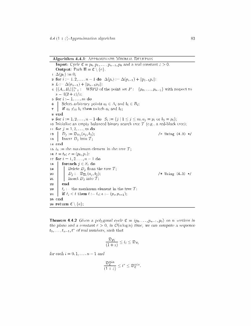
4.4 (1 + ")-Approximation algorithm 83Algorithm 4.4.1: Approximate Minimal DeletionInput: Cy le C = p0; p1; : : : ; pn−1; p0 and a real onstant " > 0.Output: Path � = C \ {e}.�(p0) := 0;1 for i := 1; 2; : : : ; n− 1 do �(pi) := �(pi−1) + ‖pi−1pi‖;2 L := �(pn−1) + ‖pn−1p0‖;3{(Ai; Bi)}mi=1 := WSPD of the point set P := {p0; : : : ; pn−1} with respe t to4 s = 4(2 + ")=";for i := 1; : : : ;m do5 Sele t arbitrary points ai ∈ Ai and bi ∈ Bi;6 if ai 6<� bi then swit h ai and bi;7 end8 for i := 1; 2; : : : ; n− 1 do Si := {j | 1 ≤ j ≤ m; aj = pi or bj = pi};9 Initialize an empty balan ed binary sear h tree T (e.g., a red-bla k tree);10 for j = 1; 2; : : : ;m do11 Dj := D�0(aj ; bj); /* Using (4.3) */12 Insert Dj into T ;13 end14 t0 := the maximum element in the tree T ;15 t = t0; e = (p0; p1);16 for i = 1; 2; : : : ; n− 1 do17 forea h j ∈ Si do18 Delete Dj from the tree T ;19 Dj := D�i(aj ; bj); /* Using (4.3) */20 Insert Dj into T ;21 end22 ti := the maximum element in the tree T ;23 if ti < t then t := ti; e := (pi; pi+1);24 end25 return C \ {e};26Theorem 4.4.2 Given a polygonal y le C = (p0; : : : ; pn−1; p0) on n verti es inthe plane and a onstant " > 0, in O(n logn) time, we an ompute a sequen et0; : : : ; tn−1; t∗ of real numbers, su h that

DPi(1 + ") ≤ ti ≤ DPifor ea h i = 0; 1; : : : ; n− 1 andDmin

C(1 + ") ≤ t∗ ≤ DminC :

84 Chapter 4 Dilation-Optimal Edge Deletion4.5 Con luding remarksRe ently, there has been a fair amount of work on the problem of omputing theoptimal dilation of a given (geometri ) graph [CHL07, EW07, GKM07, KK07℄.In this hapter we onsidered a variation of the problem where we are given apolygonal y le and are supposed to hoose one edge to remove su h that theresulting polygonal path gives the smallest (or the largest) possible dilation.A straightforward and hallenging open problem is to generalize the results tomore general Eu lidean graphs. In that ase it is also interesting to see how we an generalize the results when we want to remove more than one edge.A knowledgmentsWe would like to thank Hee-Kap Ahn, Christian Knauer, Mi hiel Smid and YajunWang, the o-authors on this hapter and Jan Vahrenhold for fruitful dis ussionson the subje t.

Chapter 5Computing SpannerDiameter5.1 Introdu tionThe diameter of an unweighted undire ted graph is the length of the longest short-est path. When studying the diameter of a graph, the length of the path is usuallythe number of edges/links along the path. More pre isely, for a graph G(V;E), thediameter of G, denoted by diam(G), is equal to maxx;y∈V dG(x; y) where dG(x; y)is the shortest path length between x and y in G. To ompute the diameter of agraph G, it is suÆ ient to ompute all-pairs-shortest paths whi h an be done inO(mn + n2 log n) time using O(m + n) spa e where n is the number of verti esand m is the number of edges of the input graph.Now suppose we have a geometri t-spanner. Then normally we would measurethe length of a path as the sum of its edges lengths. We would then de�ne thediameter of the spanner as the maximum distan e between any two points. This,however, is not very useful: in a geometri t-spanner, the diameter is at most ttimes the geometri diameter and sin e t is small (say (1 + ") for some " lose to0) this is not very informative. Sometimes, however, the number of links on a pathalso plays a role. Consider for instan e the network of some airline. We would liketo have a short onne tion between every pair of airports, but we would also liketo have as few stopovers as possible. Also in appli ations involving wireless ad ho networks it is often desirable to have small spanner diameter sin e it determinesthe maximum number of times a message has to be transmitted in a network.This leads us to the following de�nition of diameter where we onsider the number

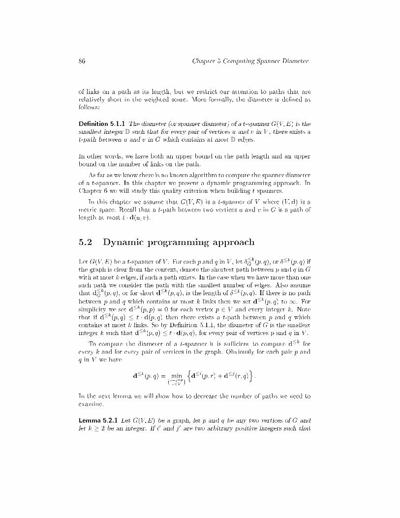
86 Chapter 5 Computing Spanner Diameterof links on a path as its length, but we restri t our attention to paths that arerelatively short in the weighted sense. More formally, the diameter is de�ned asfollows:De�nition 5.1.1 The diameter (or spanner diameter) of a t-spanner G(V;E) is thesmallest integer D su h that for every pair of verti es u and v in V , there exists at-path between u and v in G whi h ontains at most D edges.In other words, we have both an upper bound on the path length and an upperbound on the number of links on the path.As far as we know there is no known algorithm to ompute the spanner diameterof a t-spanner. In this hapter we present a dynami programming approa h. InChapter 6 we will study this quality riterion when building t-spanners.In this hapter we assume that G(V;E) is a t-spanner of V where (V;d) is ametri spa e. Re all that a t-path between two verti es u and v in G is a path oflength at most t · d(u; v).5.2 Dynami programming approa hLet G(V;E) be a t-spanner of V . For ea h p and q in V , let Æ≤kG (p; q), or Æ≤k(p; q) ifthe graph is lear from the ontext, denote the shortest path between p and q in Gwith at most k edges, if su h a path exists. In the ase when we have more than onesu h path we onsider the path with the smallest number of edges. Also assumethat d≤kG (p; q), or for short d≤k(p; q), is the length of Æ≤k(p; q). If there is no pathbetween p and q whi h ontains at most k links then we set d≤k(p; q) to ∞. Forsimpli ity we set d≤k(p; p) = 0 for ea h vertex p ∈ V and every integer k. Notethat if d≤k(p; q) ≤ t · d(p; q) then there exists a t-path between p and q whi h ontains at most k links. So by De�nition 5.1.1, the diameter of G is the smallestinteger k su h that d≤k(p; q) ≤ t · d(p; q), for every pair of verti es p and q in V .To ompute the diameter of a t-spanner it is suÆ ient to ompute d≤k forevery k and for every pair of verti es in the graph. Obviously for ea h pair p andq in V we have d≤k(p; q) = min(i+j=kr∈V )nd≤i(p; r) + d≤j(r; q)o :In the next lemma we will show how to de rease the number of paths we need toexamine.Lemma 5.2.1 Let G(V;E) be a graph, let p and q be any two verti es of G andlet k ≥ 2 be an integer. If i′ and j′ are two arbitrary positive integers su h that

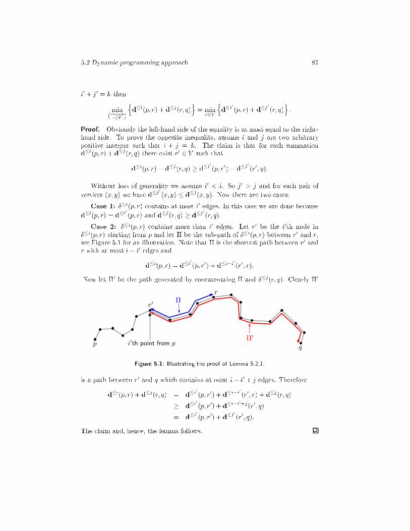
5.2 Dynami programming approa h 87i′ + j′ = k thenmin(i+j=kr∈V )nd≤i(p; r) + d≤j(r; q)o = minr∈V nd≤i′(p; r) + d≤j′ (r; q)o :Proof. Obviously the left-hand side of the equality is at most equal to the right-hand side. To prove the opposite inequality, assume i and j are two arbitrarypositive integers su h that i + j = k. The laim is that for ea h summationd≤i(p; r) + d≤j(r; q) there exist r′ ∈ V su h thatd≤i(p; r) + d≤j(r; q) ≥ d≤i′(p; r′) + d≤j′(r′; q):Without loss of generality we assume i′ < i. So j′ > j and for ea h pair ofverti es (x; y) we have d≤j′ (x; y) ≤ d≤j(x; y). Now there are two ases:Case 1: Æ≤i(p; r) ontains at most i′ edges. In this ase we are done be aused≤i(p; r) = d≤i′(p; r) and d≤j(r; q) ≥ d≤j′(r; q).Case 2: Æ≤i(p; r) ontains more than i′ edges. Let r′ be the i′th node inÆ≤i(p; r) starting from p and let � be the sub-path of Æ≤i(p; r) between r′ and r,see Figure 5.1 for an illustration. Note that � is the shortest path between r′ andr with at most i− i′ edges andd≤i(p; r) = d≤i′(p; r′) + d≤i−i′(r′; r):Now let �′ be the path generated by on atenating � and Æ≤j(r; q). Clearly �′

pq

r

r′

i′th point from p

Π

Π′Figure 5.1: Illustrating the proof of Lemma 5.2.1.is a path between r′ and q whi h ontains at most i− i′ + j edges. Therefored≤i(p; r) + d≤j(r; q) = d≤i′(p; r′) + d≤i−i′(r′; r) + d≤j(r; q)

≥ d≤i′(p; r′) + d≤i−i′+j(r′; q)= d≤i′(p; r′) + d≤j′(r′; q):The laim and, hen e, the lemma follows.

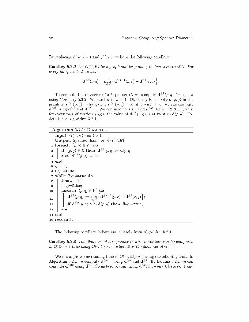
88 Chapter 5 Computing Spanner DiameterBy repla ing i′ by k − 1 and j′ by 1 we have the following orollary.Corollary 5.2.2 Let G(V;E) be a graph and let p and q be two verti es of G. Forevery integer k ≥ 2 we haved≤k(p; q) = minr∈V nd≤k−1(p; r) + d≤1(r; q)o :To ompute the diameter of a t-spanner G, we ompute d≤k(p; q) for ea h kusing Corollary 5.2.2. We start with k = 1. Obviously for all edges (p; q) in thegraph G, d≤1(p; q) = d(p; q) and d≤1(p; q) = ∞ otherwise. Then we an omputed≤k using d≤1 and d≤k−1. We ontinue onstru ting d≤k, for k = 2; 3; : : :, untilfor every pair of verti es (p; q), the value of d≤k(p; q) is at most t · d(p; q). Fordetails see Algorithm 5.2.1.Algorithm 5.2.1: DiameterInput: G(V;E) and t > 1.Output: Spanner diameter of G(V;E).forea h (p; q) ∈ V 2 do1 if (p; q) ∈ E then d≤1(p; q) := d(p; q);2 else d≤1(p; q) := ∞;3 end4 k := 1;5 ag:=true;6 while ag =true do7 k := k + 1;8 ag:=false;9 forea h (p; q) ∈ V 2 do10 d≤k(p; q) := minr∈V nd≤k−1(p; r) + d≤1(r; q)o;11 if d≤k(p; q) > t · d(p; q) then ag:=true;12 end13 end14 return k;15 The following orollary follows immediately from Algorithm 5.2.1.Corollary 5.2.3 The diameter of a t-spanner G with n verti es an be omputedin O(D · n3) time using O(n2) spa e, where D is the diameter of G.We an improve the running time to O(log(D) ·n3) using the following tri k. InAlgorithm 5.2.1 we ompute d≤k+1 using d≤k and d≤1. By Lemma 5.2.1 we an ompute d≤2k using d≤k. So instead of omputing d≤k, for every k between 1 and

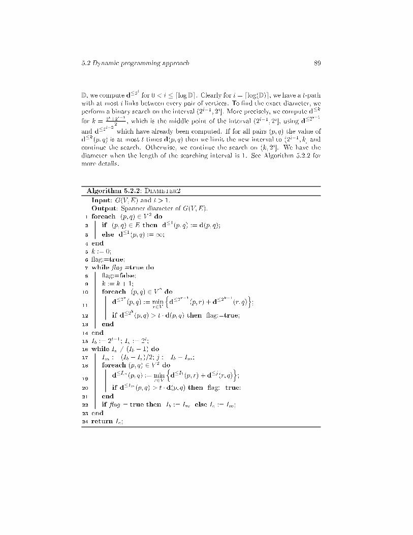
5.2 Dynami programming approa h 89D, we ompute d≤2i for 0 < i ≤ ⌈logD⌉. Clearly for i = ⌈log(D)⌉, we have a t-pathwith at most i links between every pair of verti es. To �nd the exa t diameter, weperform a binary sear h on the interval (2i−1; 2i℄. More pre isely, we ompute d≤kfor k = 2i+2i−12 , whi h is the middle point of the interval (2i−1; 2i℄, using d≤2i−1and d≤2i−2 whi h have already been omputed. If for all pairs (p; q) the value ofd≤k(p; q) is at most t times d(p; q) then we limit the new interval to (2i−1; k℄ and ontinue the sear h. Otherwise, we ontinue the sear h on (k; 2i℄. We have thediameter when the length of the sear hing interval is 1. See Algorithm 5.2.2 formore details.Algorithm 5.2.2: Diameter2Input: G(V;E) and t > 1.Output: Spanner diameter of G(V;E).forea h (p; q) ∈ V 2 do1 if (p; q) ∈ E then d≤1(p; q) := d(p; q);2 else d≤1(p; q) := ∞;3 end4 k := 0;5 ag:=true;6 while ag =true do7 ag:=false;8 k := k + 1;9 forea h (p; q) ∈ V 2 do10 d≤2k (p; q) := minr∈V nd≤2k−1(p; r) + d≤2k−1(r; q)o;11 if d≤2k(p; q) > t · d(p; q) then ag:=true;12 end13 end14 Ib := 2i−1; Ie := 2i;15 while Ie 6= (Ib + 1) do16 Im := (Ib + Ie)=2; j := Ib − Im;17 forea h (p; q) ∈ V 2 do18 d≤Im(p; q) := minr∈V nd≤Ib(p; r) + d≤j(r; q)o;19 if d≤Im(p; q) > t · d(p; q) then ag:=true;20 end21 if ag = true then Ib := Im else Ie := Im;22 end23 return Ie;24

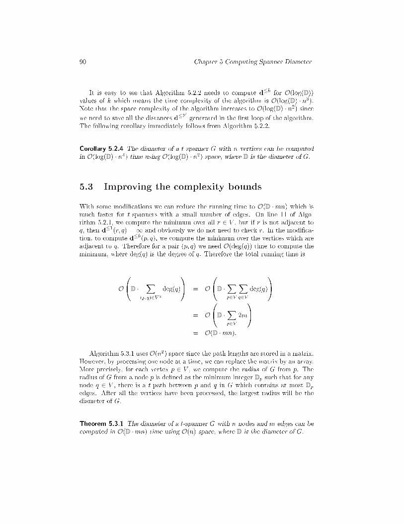
90 Chapter 5 Computing Spanner DiameterIt is easy to see that Algorithm 5.2.2 needs to ompute d≤k for O(log(D))values of k whi h means the time omplexity of the algorithm is O(log(D) · n3).Note that the spa e omplexity of the algorithm in reases to O(log(D) · n2) sin ewe need to save all the distan es d≤2i generated in the �rst loop of the algorithm.The following orollary immediately follows from Algorithm 5.2.2.Corollary 5.2.4 The diameter of a t-spanner G with n verti es an be omputedin O(log(D) · n3) time using O(log(D) · n2) spa e, where D is the diameter of G.5.3 Improving the omplexity boundsWith some modi� ations we an redu e the running time to O(D ·mn) whi h ismu h faster for t-spanners with a small number of edges. On line 11 of Algo-rithm 5.2.1, we ompute the minimum over all r ∈ V , but if r is not adja ent toq, then d≤1(r; q) = ∞ and obviously we do not need to he k r. In the modi� a-tion, to ompute d≤k(p; q), we ompute the minimum over the verti es whi h areadja ent to q. Therefore for a pair (p; q) we need O(deg(q)) time to ompute theminimum, where deg(q) is the degree of q. Therefore the total running time isO

0�D ·X(p;q)∈V 2 deg(q)1A = O

0�D ·Xp∈V Xq∈V deg(q)1A= O

0�D ·Xp∈V 2m1A= O(D ·mn):Algorithm 5.3.1 uses O(n2) spa e sin e the path lengths are stored in a matrix.However, by pro essing one node at a time, we an repla e the matrix by an array.More pre isely, for ea h vertex p ∈ V , we ompute the radius of G from p. Theradius of G from a node p is de�ned as the minimum integer Dp su h that for anynode q ∈ V , there is a t-path between p and q in G whi h ontains at most Dpedges. After all the verti es have been pro essed, the largest radius will be thediameter of G.Theorem 5.3.1 The diameter of a t-spanner G with n nodes and m edges an be omputed in O(D ·mn) time using O(n) spa e, where D is the diameter of G.

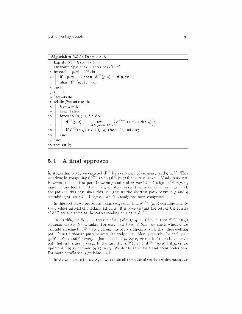
5.4 A �nal approa h 91Algorithm 5.3.1: Diameter3Input: G(V;E) and t > 1.Output: Spanner diameter of G(V;E).forea h (p; q) ∈ V 2 do1 if (p; q) ∈ E then d≤1(p; q) := d(p; q);2 else d≤1(p; q) := ∞;3 end4 k := 1;5 ag:=true;6 while ag =true do7 k := k + 1;8 ag:=false;9 forea h (p; q) ∈ V 2 do10 d≤k(p; q) := minr is adja ent to qnd≤k−1(p; r) + d(r; q)o;11 if d≤k(p; q) > t · d(p; q) then ag:=true;12 end13 end14 return k;155.4 A �nal approa hIn Algorithm 5.3.1, we updated d≤k for every pair of verti es p and q in V . Thiswas done by omputing d≤k−1(p; r)+d≤1(r; q) for every vertex r ∈ V adja ent to q.However, the shortest path between p and r of at most k − 1 edges, Æ≤k−1(p; r),may ontain less than k − 1 edges. We observe that we do not need to he kthe path in this ase sin e this will give us the shortest path between p and q ontaining at most k − 1 edges { whi h already has been omputed.In this se tion we pro ess all pairs (p; q) su h that Æ≤k−1(p; q) ontains exa tlyk − 1 edges instead of he king all pairs. It is obvious that the rest of the entriesof d≤k are the same as the orresponding entries in d≤k−1.To do this, let Sk−1 be the set of all pairs (p; q) ∈ V 2 su h that Æ≤k−1(p; q) ontains exa tly k − 1 links. For ea h pair (p; q) ∈ Sk−1 we he k whether we an add an edge to Æ≤k−1(p; q), from one of its endpoints, su h that the resultingpath forms a shorter path between its endpoints. More pre isely, for ea h pair(p; q) ∈ Sk−1 and for every adja ent node of p, say r, we he k if there is a shorterpath between r and q via p. In the ase that d≤k(q; r) > d≤k−1(p; q)+d(p; r), weupdate d≤k(q; r) and add (q; r) to Sk. We do the same for all adja ent nodes of q.For more details see Algorithm 5.4.1.In the worst ase the set Sk may ontain all the pairs of verti es whi h means we

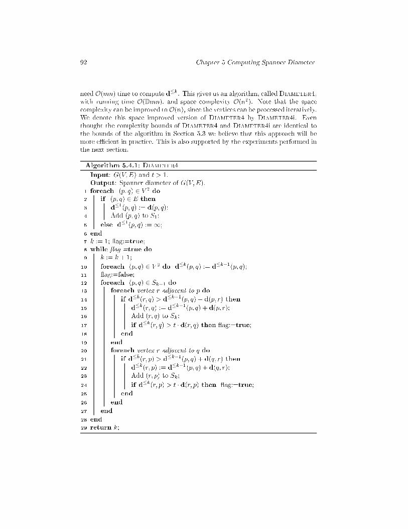
92 Chapter 5 Computing Spanner Diameterneed O(mn) time to ompute d≤k. This gives us an algorithm, alledDiameter4,with running time O(Dmn), and spa e omplexity O(n2). Note that the spa e omplexity an be improved toO(n), sin e the verti es an be pro essed iteratively.We denote this spa e improved version of Diameter4 by Diameter4i. Eventhought the omplexity bounds of Diameter4 and Diameter4i are identi al tothe bounds of the algorithm in Se tion 5.3 we believe that this approa h will bemore eÆ ient in pra ti e. This is also supported by the experiments performed inthe next se tion.Algorithm 5.4.1: Diameter4Input: G(V;E) and t > 1.Output: Spanner diameter of G(V;E).forea h (p; q) ∈ V 2 do1 if (p; q) ∈ E then2 d≤1(p; q) := d(p; q);3 Add (p; q) to S1;4 else d≤1(p; q) := ∞;5 end6 k := 1; ag:=true;7 while ag =true do8 k := k + 1;9 forea h (p; q) ∈ V 2 do d≤k(p; q) := d≤k−1(p; q);10 ag:=false;11 forea h (p; q) ∈ Sk−1 do12 forea h vertex r adja ent to p do13 if d≤k(r; q) > d≤k−1(p; q) + d(p; r) then14 d≤k(r; q) := d≤k−1(p; q) + d(p; r);15 Add (r; q) to Sk;16 if d≤k(r; q) > t · d(r; q) then ag:=true;17 end18 end19 forea h vertex r adja ent to q do20 if d≤k(r; p) > d≤k−1(p; q) + d(q; r) then21 d≤k(r; p) := d≤k−1(p; q) + d(q; r);22 Add (r; p) to Sk;23 if d≤k(r; p) > t · d(r; p) then ag:=true;24 end25 end26 end27 end28 return k;29

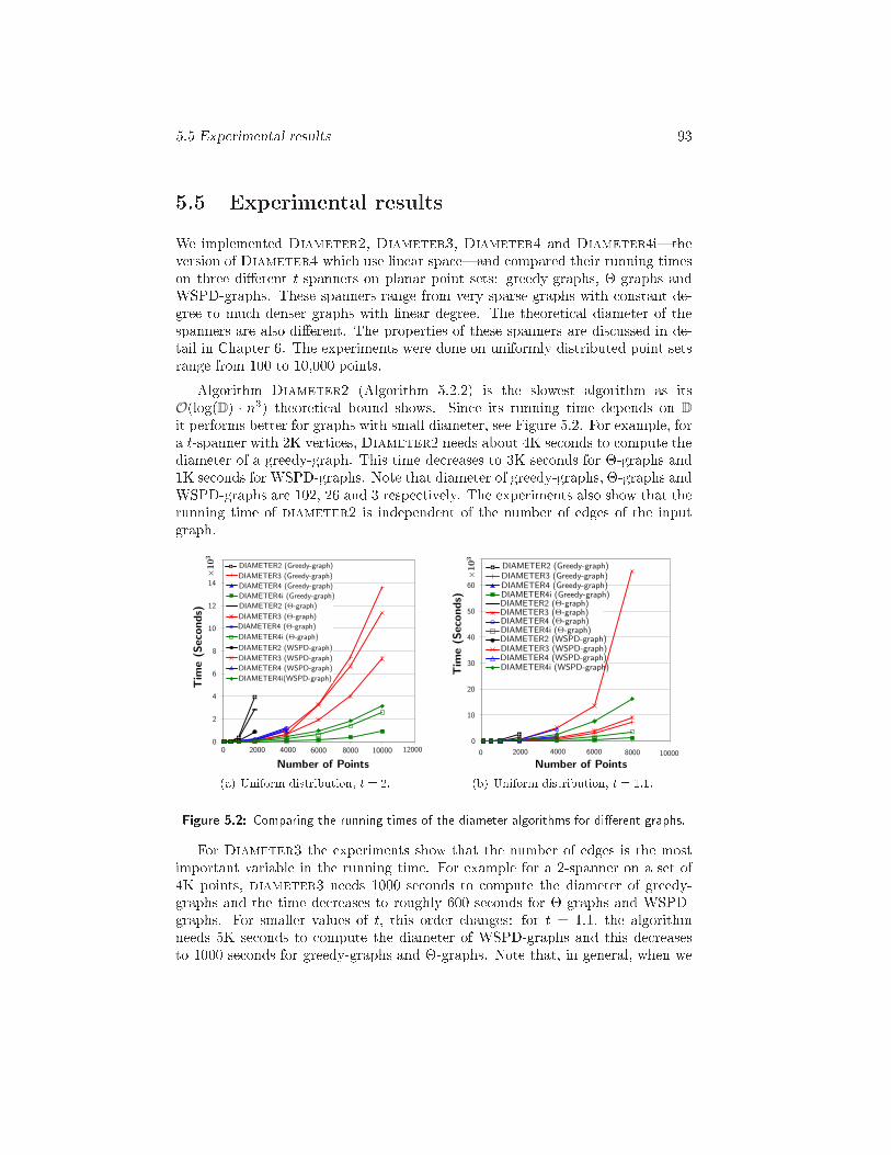
5.5 Experimental results 935.5 Experimental resultsWe implemented Diameter2, Diameter3, Diameter4 and Diameter4i|theversion of Diameter4 whi h use linear spa e|and ompared their running timeson three di�erent t-spanners on planar point sets: greedy-graphs, �-graphs andWSPD-graphs. These spanners range from very sparse graphs with onstant de-gree to mu h denser graphs with linear degree. The theoreti al diameter of thespanners are also di�erent. The properties of these spanners are dis ussed in de-tail in Chapter 6. The experiments were done on uniformly distributed point setsrange from 100 to 10,000 points.Algorithm Diameter2 (Algorithm 5.2.2) is the slowest algorithm as itsO(log(D) · n3) theoreti al bound shows. Sin e its running time depends on Dit performs better for graphs with small diameter, see Figure 5.2. For example, fora t-spanner with 2K verti es, Diameter2 needs about 4K se onds to ompute thediameter of a greedy-graph. This time de reases to 3K se onds for �-graphs and1K se onds for WSPD-graphs. Note that diameter of greedy-graphs, �-graphs andWSPD-graphs are 102, 26 and 3 respe tively. The experiments also show that therunning time of diameter2 is independent of the number of edges of the inputgraph.

0

2

4

6

8

10

12

14

×10

3

Number of Points

Tim

e(S

eco

nds)

DIAMETER2 (Greedy-graph)

DIAMETER3 (Greedy-graph)

DIAMETER4 (Greedy-graph)

DIAMETER4i (Greedy-graph)

DIAMETER2 (Θ-graph)

DIAMETER3 (Θ-graph)

DIAMETER4 (Θ-graph)

DIAMETER4i (Θ-graph)

DIAMETER2 (WSPD-graph)

DIAMETER3 (WSPD-graph)

DIAMETER4 (WSPD-graph)

DIAMETER4i(WSPD-graph)

800060000 120002000 4000 10000(a) Uniform distribution, t = 2. 0

10

20

30

40

50

60

×10

3

Number of Points

Tim

e(S

eco

nds)

DIAMETER2 (Greedy-graph)DIAMETER3 (Greedy-graph)DIAMETER4 (Greedy-graph)DIAMETER4i (Greedy-graph)DIAMETER2 (Θ-graph)DIAMETER3 (Θ-graph)DIAMETER4 (Θ-graph)DIAMETER4i (Θ-graph)DIAMETER2 (WSPD-graph)DIAMETER3 (WSPD-graph)DIAMETER4 (WSPD-graph)DIAMETER4i (WSPD-graph)

40000 80002000 6000 10000(b) Uniform distribution, t = 1:1.Figure 5.2: Comparing the running times of the diameter algorithms for di�erent graphs.For Diameter3 the experiments show that the number of edges is the mostimportant variable in the running time. For example for a 2-spanner on a set of4K points, diameter3 needs 1000 se onds to ompute the diameter of greedy-graphs and the time de reases to roughly 600 se onds for �-graphs and WSPD-graphs. For smaller values of t, this order hanges: for t = 1:1, the algorithmneeds 5K se onds to ompute the diameter of WSPD-graphs and this de reasesto 1000 se onds for greedy-graphs and �-graphs. Note that, in general, when we

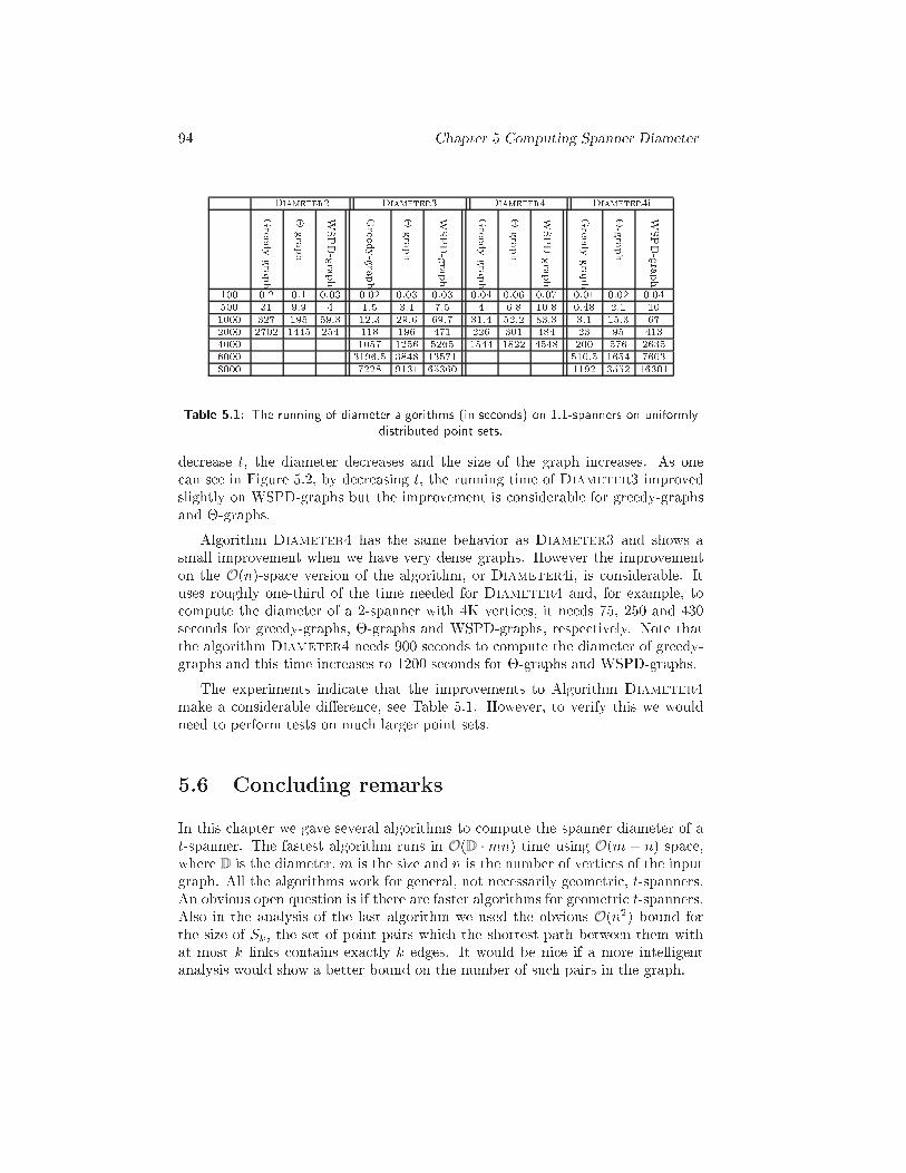
94 Chapter 5 Computing Spanner DiameterDiameter2 Diameter3 Diameter4 Diameter4iGreedy-graph �-graph WSPD-graph Greedy-graph �-graph WSPD-graph Greedy-graph �-graph WSPD-graph Greedy-graph �-graph WSPD-graph100 0.2 0.1 0.03 0.02 0.03 0.03 0.04 0.06 0.07 0.01 0.02 0.04500 31 9.9 4 1.5 3.1 7.5 4 6.8 10.8 0.48 2.1 101000 327 195 59.3 12.3 29.6 69.7 31.4 52.2 83.3 3.1 15.3 672000 2702 1445 254 118 196 471 226 301 484 23 95 4134000 1057 1256 5265 1544 1822 4548 200 576 26356000 3196.5 3848 13571 510.5 1654 76038000 7228 9131 65360 1192 3552 16301Table 5.1: The running of diameter algorithms (in se onds) on 1.1-spanners on uniformlydistributed point sets.de rease t, the diameter de reases and the size of the graph in reases. As one an see in Figure 5.2, by de reasing t, the running time of Diameter3 improvedslightly on WSPD-graphs but the improvement is onsiderable for greedy-graphsand �-graphs.Algorithm Diameter4 has the same behavior as Diameter3 and shows asmall improvement when we have very dense graphs. However the improvementon the O(n)-spa e version of the algorithm, or Diameter4i, is onsiderable. Ituses roughly one-third of the time needed for Diameter4 and, for example, to ompute the diameter of a 2-spanner with 4K verti es, it needs 75, 250 and 430se onds for greedy-graphs, �-graphs and WSPD-graphs, respe tively. Note thatthe algorithm Diameter4 needs 900 se onds to ompute the diameter of greedy-graphs and this time in reases to 1200 se onds for �-graphs and WSPD-graphs.The experiments indi ate that the improvements to Algorithm Diameter4make a onsiderable di�eren e, see Table 5.1. However, to verify this we wouldneed to perform tests on mu h larger point sets.5.6 Con luding remarksIn this hapter we gave several algorithms to ompute the spanner diameter of at-spanner. The fastest algorithm runs in O(D ·mn) time using O(m + n) spa e,where D is the diameter, m is the size and n is the number of verti es of the inputgraph. All the algorithms work for general, not ne essarily geometri , t-spanners.An obvious open question is if there are faster algorithms for geometri t-spanners.Also in the analysis of the last algorithm we used the obvious O(n2) bound forthe size of Sk, the set of point pairs whi h the shortest path between them withat most k links ontains exa tly k edges. It would be ni e if a more intelligentanalysis would show a better bound on the number of su h pairs in the graph.

5.6 Con luding remarks 95A knowledgementsWe would like to thank Shripad Thite for his omments on a talk on this subje twhi h aused the improvement in Algorithm 5.2.2.

96 Chapter 5 Computing Spanner Diameter

Chapter 6Experimental Study ofGeometri Spanners6.1 Introdu tionThe problem of onstru ting spanners has re eived onsiderable attention froma theoreti al perspe tive, see [ADD+93, ADM+95, AMS99, BGM04, CDNS95,DHN93, DN97, DNS95, GLN02, Kei88, KG92, LL92, LNS02, Sal91, Vai91℄, thesurveys [Epp00, GK07, Smi00℄, and the re ent book by Narasimhan andSmid [NS07℄, but almost no attention from a pra ti al or experimental perspe -tive [NP03, SZ04℄.In this hapter we onsider the most well-known algorithms for the onstru -tion of t-spanners in the plane: variants of greedy spanners, variants of �-graphs,spanners onstru ted from the well-separated pair de omposition (WSPD), skip-list spanners, sink spanners and some hybrid algorithms. The quality measure-ments used in the literature is the number of edges, the weight, the maximumdegree, the spanner diameter and the number of rossings. We study ea h of thealgorithms independently, but also in ombination with ea h other. To the best ofour knowledge, this is the �rst time an extensive experimental study has been per-formed on the onstru tion of t-spanners. Navarro and Paredes [NP03℄ presentedfour heuristi s for point sets in high-dimensional metri spa e (d = 20) and showedby empiri al methods that the running time was O(n2:24) and the number of edgesin the produ ed graphs was O(n1:13). In [SZ04℄ Sigurd and Za hariasen onsid-ered the problem of onstru ting a minimum weight t-spanner of a given graph,but they only onsidered sparse graphs of small size, i.e., graphs with at most 64

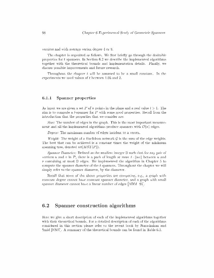
98 Chapter 6 Experimental Study of Geometri Spannersverti es and with average vertex degree 4 or 8.The hapter is organized as follows. We �rst brie y go through the desirableproperties for t-spanners. In Se tion 6.2 we des ribe the implemented algorithmstogether with the theoreti al bounds and implementation details. Finally, wedis uss possible improvements and future resear h.Throughout the hapter t will be assumed to be a small onstant. In theexperiments we used values of t between 1.05 and 2.6.1.1 Spanner propertiesAs input we are given a set P of n points in the plane and a real value t > 1. Theaim is to ompute a t-spanner for P with some good properties. Re all from theintrodu tion that the properties that we onsider are:Size: The number of edges in the graph. This is the most important measure-ment and all the implemented algorithms produ e spanners with O(n) edges.Degree: The maximum number of edges in ident to a vertex.Weight: The weight of a Eu lidean network G is the sum of the edge weights.The best that an be a hieved is a onstant times the weight of the minimumspanning tree, denoted wt(MST (P )).Spanner Diameter: De�ned as the smallest integer D su h that for any pair ofverti es u and v in P , there is a path of length at most t · ‖uv‖ between u andv ontaining at most D edges. We implemented the algorithm in Chapter 5 to ompute the spanner diameter of the t-spanners. Throughout the hapter we willsimply refer to the spanner diameter, by the diameter.Re all that some of the above properties are ompeting, e.g., a graph with onstant degree annot have onstant spanner diameter, and a graph with smallspanner diameter annot have a linear number of edges [ADM+95℄.6.2 Spanner onstru tion algorithmsHere we give a short des ription of ea h of the implemented algorithms togetherwith their theoreti al bounds. For a detailed des ription of ea h of the algorithms onsidered in this se tion please refer to the re ent book by Narasimhan andSmid [NS07℄. A summary of the theoreti al bounds an be found in Table 6.1.

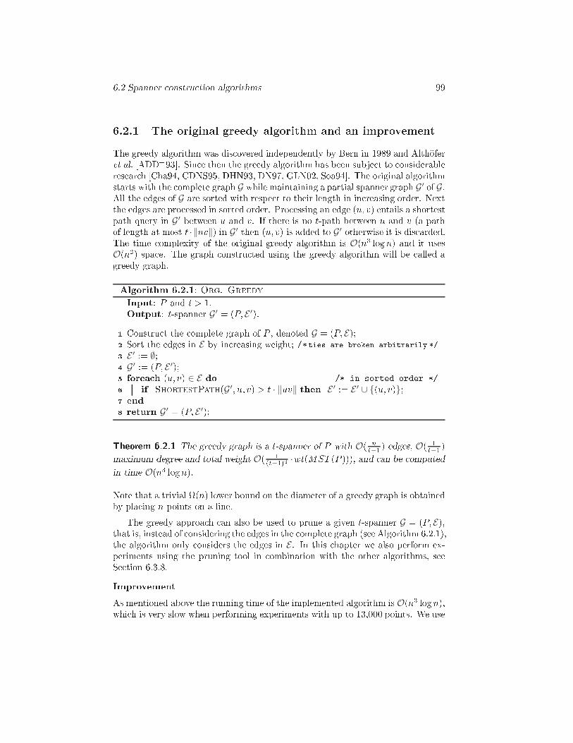
6.2 Spanner onstru tion algorithms 996.2.1 The original greedy algorithm and an improvementThe greedy algorithm was dis overed independently by Bern in 1989 and Alth�oferet al. [ADD+93℄. Sin e then the greedy algorithm has been subje t to onsiderableresear h [Cha94, CDNS95, DHN93, DN97, GLN02, Soa94℄. The original algorithmstarts with the omplete graph G while maintaining a partial spanner graph G′ of G.All the edges of G are sorted with respe t to their length in in reasing order. Nextthe edges are pro essed in sorted order. Pro essing an edge (u; v) entails a shortestpath query in G′ between u and v. If there is no t-path between u and v (a pathof length at most t · ‖uv‖) in G′ then (u; v) is added to G′ otherwise it is dis arded.The time omplexity of the original greedy algorithm is O(n3 logn) and it usesO(n2) spa e. The graph onstru ted using the greedy algorithm will be alled agreedy graph.Algorithm 6.2.1: Org. GreedyInput: P and t > 1.Output: t-spanner G′ = (P; E ′).Constru t the omplete graph of P , denoted G = (P; E);1 Sort the edges in E by in reasing weight; /*ties are broken arbitrarily */2

E ′ := ∅;3G′ := (P; E ′);4 forea h (u; v) ∈ E do /* in sorted order */5 if ShortestPath(G′; u; v) > t · ‖uv‖ then E ′ := E ′ ∪ {(u; v)};6 end7 return G′ = (P; E ′);8Theorem 6.2.1 The greedy graph is a t-spanner of P with O( nt−1 ) edges, O( 1t−1 )maximum degree and total weight O( 1(t−1)4 ·wt(MST (P ))), and an be omputedin time O(n3 logn).Note that a trivial (n) lower bound on the diameter of a greedy graph is obtainedby pla ing n points on a line.The greedy approa h an also be used to prune a given t-spanner G = (P; E),that is, instead of onsidering the edges in the omplete graph (see Algorithm 6.2.1),the algorithm only onsiders the edges in E . In this hapter we also perform ex-periments using the pruning tool in ombination with the other algorithms, seeSe tion 6.3.8.ImprovementAs mentioned above the running time of the implemented algorithm is O(n3 logn),whi h is very slow when performing experiments with up to 13,000 points. We use

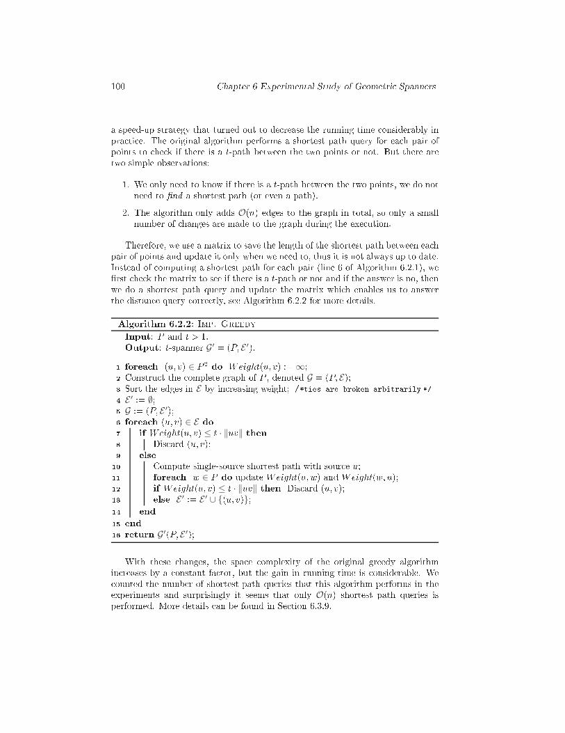
100 Chapter 6 Experimental Study of Geometri Spannersa speed-up strategy that turned out to de rease the running time onsiderably inpra ti e. The original algorithm performs a shortest path query for ea h pair ofpoints to he k if there is a t-path between the two points or not. But there aretwo simple observations:1. We only need to know if there is a t-path between the two points, we do notneed to �nd a shortest path (or even a path).2. The algorithm only adds O(n) edges to the graph in total, so only a smallnumber of hanges are made to the graph during the exe ution.Therefore, we use a matrix to save the length of the shortest path between ea hpair of points and update it only when we need to, thus it is not always up to date.Instead of omputing a shortest path for ea h pair (line 6 of Algorithm 6.2.1), we�rst he k the matrix to see if there is a t-path or not and if the answer is no, thenwe do a shortest path query and update the matrix whi h enables us to answerthe distan e query orre tly, see Algorithm 6.2.2 for more details.Algorithm 6.2.2: Imp. GreedyInput: P and t > 1.Output: t-spanner G′ = (P; E ′).forea h (u; v) ∈ P 2 do Weight(u; v) :=∞;1 Constru t the omplete graph of P , denoted G = (P; E);2 Sort the edges in E by in reasing weight; /*ties are broken arbitrarily */3E ′ := ∅;4G := (P; E ′);5 forea h (u; v) ∈ E do6 if Weight(u; v) ≤ t · ‖uv‖ then7 Dis ard (u; v);8 else9 Compute single-sour e shortest path with sour e u;10 forea h w ∈ P do update Weight(u;w) and Weight(w; u);11 if Weight(u; v) ≤ t · ‖uv‖ then Dis ard (u; v);12 else E ′ := E ′ ∪ {(u; v)};13 end14 end15 return G′(P; E ′);16 With these hanges, the spa e omplexity of the original greedy algorithmin reases by a onstant fa tor, but the gain in running time is onsiderable. We ounted the number of shortest path queries that this algorithm performs in theexperiments and surprisingly it seems that only O(n) shortest path queries isperformed. More details an be found in Se tion 6.3.9.

6.2 Spanner onstru tion algorithms 101Conje ture 6.2.2 Algorithm 6.2.2 performs O(n) shortest path queries.ImplementationThe implementations of the two algorithms are straight-forward. The shortestpath queries are done by using the Dijkstra fun tion in LEDA.6.2.2 The approximate greedy algorithmEven though the improved algorithm is faster than the original greedy algorithmthe running time is still (n2 logn), thus any approa h that an speed-up thealgorithm would be of great interest. The running time is mainly due to the fa tthat �(n2) shortest path queries needed to be answered in a graph with O(n)edges, ea h of whi h ould take O(n logn) time. Das and Narasimhan [DN97℄showed how to use lustering to speed up shortest path queries. The approximategreedy algorithm starts with a pt=t′-spanner G′ with O(n) edges and onstantdegree generated by an O(n logn)-time algorithm. Note that this network maynot have small weight. Then it omputes a√tt′-spanner of G′ using an approximatevariant of the greedy algorithm. To obtain G = (P; E) from G′ the approximategreedy algorithm starts with E = ∅ and adds all the short edges (i.e. those oflength at most D=n, where D is the distan e between the farthest pair of points)to E . For the remaining edges, the algorithm sorts them by in reasing weight andpro esses them in logn phases. Pro essing an edge e = (u; v) entails a shortestpath query whi h is answered by performing an approximate shortest path queryon a \ luster graph" H , whi h is simultaneously maintained. The luster graphH has the following properties:1. distan es in H \ losely" approximate distan es in the urrent graph G.2. every vertex in H has bounded degree, and3. \spe ialized" shortest path queries in H an be answered in onstant time.Algorithm 6.2.3 gives a sket h of the approximate greedy algorithm. For more de-tails see [DN97℄ or [NS07℄. The time omplexity of this algorithm is O(n log2 n).Note that the graph generated by this algorithm is an approximate version of thegraph generated by the original greedy algorithm sin e the algorithm prunes agraph with a linear number of edges and answers shortest path queries approxi-mately.Gudmundsson et al. [GLN02℄ later improved the running time to O(n logn)(using the algebrai de ision tree model extended with indire t addressing) butthe modi�ed version is quite involved and therefore we de ided to only implementthe above version. The following theorem states the theoreti al bounds.

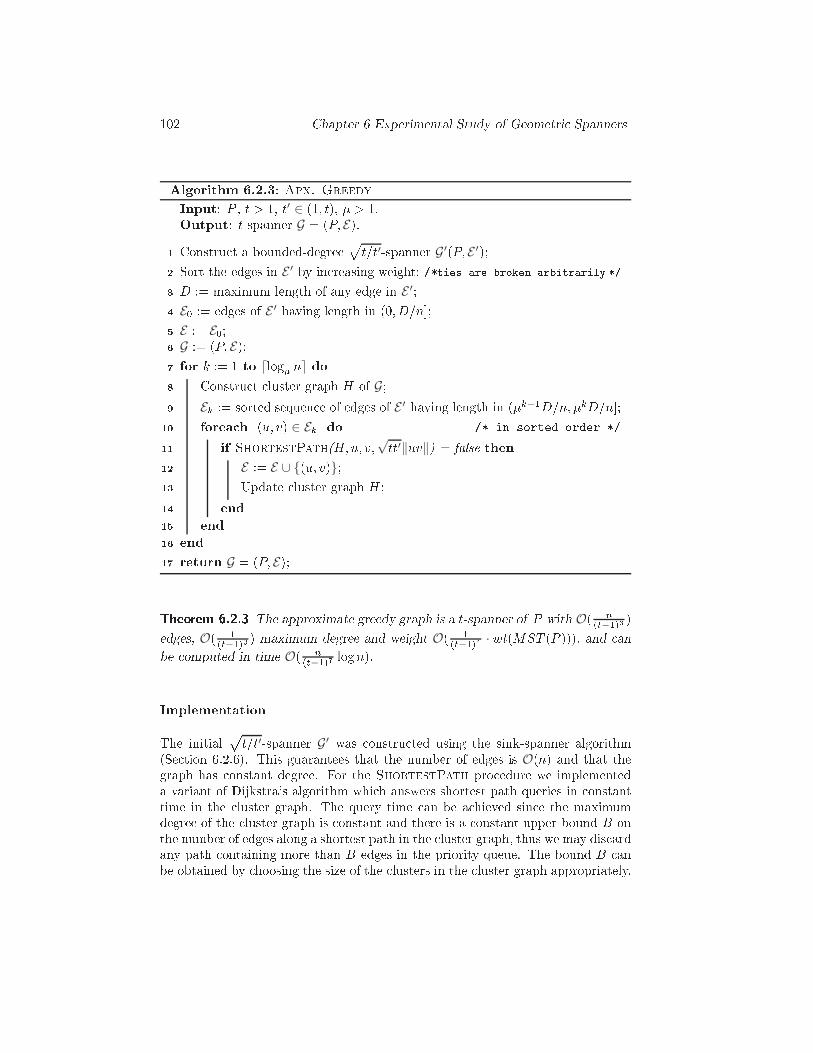
102 Chapter 6 Experimental Study of Geometri SpannersAlgorithm 6.2.3: Apx. GreedyInput: P , t > 1, t′ ∈ (1; t), � > 1.Output: t-spanner G = (P; E).Constru t a bounded-degree pt=t′-spanner G′(P; E ′);1 Sort the edges in E ′ by in reasing weight; /*ties are broken arbitrarily */2 D := maximum length of any edge in E ′;3E0 := edges of E ′ having length in (0; D=n℄;4E := E0;5G := (P; E);6 for k := 1 to ⌈log� n⌉ do7 Constru t luster graph H of G;8

Ek := sorted sequen e of edges of E ′ having length in (�k−1D=n; �kD=n℄;9 forea h (u; v) ∈ Ek do /* in sorted order */10 if ShortestPath(H;u; v;√tt′‖uv‖) = false then11E := E ∪ {(u; v)};12 Update luster graph H ;13 end14 end15 end16 return G = (P; E);17Theorem 6.2.3 The approximate greedy graph is a t-spanner of P with O( n(t−1)3 )edges, O( 1(t−1)3 ) maximum degree and weight O( 1(t−1)4 · wt(MST (P ))), and anbe omputed in time O( n(t−1)7 logn).ImplementationThe initial pt=t′-spanner G′ was onstru ted using the sink-spanner algorithm(Se tion 6.2.6). This guarantees that the number of edges is O(n) and that thegraph has onstant degree. For the ShortestPath pro edure we implementeda variant of Dijkstra's algorithm whi h answers shortest path queries in onstanttime in the luster graph. The query time an be a hieved sin e the maximumdegree of the luster graph is onstant and there is a onstant upper bound B onthe number of edges along a shortest path in the luster graph, thus we may dis ardany path ontaining more than B edges in the priority queue. The bound B anbe obtained by hoosing the size of the lusters in the luster graph appropriately.

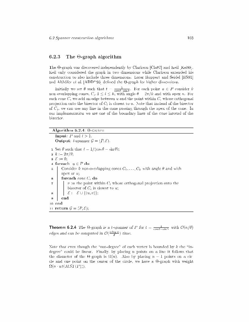
6.2 Spanner onstru tion algorithms 1036.2.3 The �-graph algorithmThe �-graph was dis overed independently by Clarkson [Cla87℄ and Keil [Kei88℄.Keil only onsidered the graph in two dimensions while Clarkson extended his onstru tion to also in lude three dimensions. Later Ruppert and Seidel [RS91℄and Alth�ofer et al. [ADD+93℄ de�ned the �-graph for higher dimensions.Initially we set � su h that t = 1 os �−sin � . For ea h point u ∈ P onsider knon-overlapping ones, Ci; 1 ≤ i ≤ k, with angle � = 2�=k and with apex u. Forea h one Ci we add an edge between u and the point within Ci whose orthogonalproje tion onto the bise tor of Ci is losest to u. Note that instead of the bise torof Ci, we an use any line in the one passing through the apex of the one. Inour implementation we use one of the boundary lines of the one instead of thebise tor.Algorithm 6.2.4: �-graphInput: P and t > 1.Output: t-spanner G = (P; E).Set � su h that t = 1=( os � − sin �);1 k := 2�=�;2E := ∅;3 forea h u ∈ P do4 Consider k non-overlapping ones C1; : : : ; Ck with angle � and with5 apex at u;forea h one Ci do6 v := the point within Ci whose orthogonal proje tion onto the7 bise tor of Ci is losest to u;

E := E ∪ {(u; v)};8 end9 end10 return G = (P; E);11Theorem 6.2.4 The �-graph is a t-spanner of P for t = 1 os �−sin � with O(n=�)edges and an be omputed in O(n logn� ) time.Note that even though the \out-degree" of ea h vertex is bounded by k the \in-degree" ould be linear. Finally, by pla ing n points on a line it follows thatthe diameter of the �-graph is (n). Also by pla ing n − 1 points on a ir- le and one point on the enter of the ir le, we have a �-graph with weight(n · wt(MST (P ))).

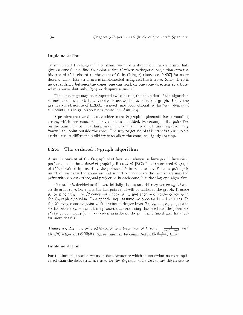
104 Chapter 6 Experimental Study of Geometri SpannersImplementationTo implement the �-graph algorithm, we need a dynami data stru ture that,given a one C, an �nd the point within C whose orthogonal proje tion onto thebise tor of C is losest to the apex of C in O(logn) time, see [NS07℄ for moredetails. This data stru ture is implemented using red-bla k trees. Sin e there isno dependen y between the ones, one an work on one one dire tion at a time,whi h means that only O(n) work spa e is needed.The same edge may be omputed twi e during the exe ution of the algorithmso one needs to he k that an edge is not added twi e to the graph. Using thegraph data stru ture of LEDA, we need time proportional to the \out"-degree ofthe points in the graph to he k existen e of an edge.A problem that we do not onsider in the �-graph implementation is roundingerrors, whi h may ause some edges not to be added. For example, if a point lieson the boundary of an, otherwise empty, one then a small rounding error may\move" the point outside the one. One way to get rid of this error is to use exa tarithmeti . A di�erent possibility is to allow the ones to slightly overlap.6.2.4 The ordered �-graph algorithmA simple variant of the �-graph that has been shown to have good theoreti alperforman e is the ordered �-graph by Bose et al. [BGM04℄. An ordered �-graphof P is obtained by inserting the points of P in some order. When a point p isinserted, we draw the ones around p and onne t p to the previously insertedpoint with losest orthogonal proje tion in ea h one, like the �-graph algorithm.The order is de ided as follows. Initially hoose an arbitrary vertex vn∈P andset its order to n, i.e. this is the last point that will be added to the graph. Pro essvn by pla ing k = 2�=� ones with apex at vn and then adding the edges as inthe �-graph algorithm. In a generi step, assume we pro essed i− 1 verti es. Inthe ith step, hoose a point with maximum degree from P \{vn; : : : ; vn−(i−1)} andset its order to n − i and then pro ess vn−i assuming that we have the point setP \{vn; : : : ; vn−(i−1)}. This de ides an order on the point set. See Algorithm 6.2.5for more details.Theorem 6.2.5 The ordered �-graph is a t-spanner of P for t = 1 os �−sin � withO(n=�) edges and O( log n� ) degree, and an be omputed in O(n log n� ) time.ImplementationFor the implementation we use a data stru ture whi h is somewhat more ompli- ated than the data stru ture used for the �-graph, sin e we require the stru ture

6.2 Spanner onstru tion algorithms 105Algorithm 6.2.5: Ordered-�-graphInput: P and t > 1.Output: t-spanner G = (P; E).Set � su h that t = 1=( os � − sin �);1 k := 2�=�;2E := ∅;3 P ′ := ∅;4 for i := 1; 2; : : : ; |P | do5 Pi k an unmarked vertex u ∈ P \ P ′ with maximum degree in6

G′ := (P; E);P ′ := P ′ ∪ {u};7 forea h one Ci with apex at u do (See Algorithm 6.2.4)8 v := the point in P \ P ′ within Ci whose orthogonal proje tion onto9 the bise tor of Ci is losest to u;E := E ∪ {(u; v)};10 end11 end12 return G = (P; E);13to allow for deletions. We use k range trees, as suggested by Bose et al. [BGM04℄,one for ea h one with apex at the origin. In ea h range tree we store all pointsrepresented in the oordinate system of the two boundaries of the one. To �ndthe suitable point in a one with apex at u, it is suÆ ient to perform a range querywith oordinates of u as keys and hoose the suitable point between the pointsreported by the query. We add one extra pointer to ea h node of the range treewhi h shows the point with minimum y (or x) oordinate in the subtree. Usingthis pointer, we an �nd the suitable point without going through all reportedpoints of the range query. Ea h range query requires O(log2 n) time, so the totaltime omplexity of the implemented algorithm is O(n log2 n) whi h is slightly morethan the theoreti al time bound but mu h simpler to implement.In ea h step of the ordered �-graph algorithm the node with maximum degreehas to be sele ted. To �nd this point, we used a priority queue of all the points.Initially all the nodes have priority n. When an edge (u; v) is added to the partialspanner graph, the priority of u and v is de reased by 1. The point with minimumpriority in the queue is the point with maximum degree in the graph.There is a major di�eren e between the �-graph algorithm and the ordered�-graph algorithm when it omes to the spa e omplexity. As mentioned in theprevious se tion, one an onstru t the �-graph by working on one one dire tionat a time. This is not possible for the ordered �-graph, instead we have to keepall the ones (range trees) in memory. This is due to the fa t that the order is not

106 Chapter 6 Experimental Study of Geometri Spannersknown in advan e. During the pro essing of one node, we need to he k all the ones and add edges if ne essary, thus �(kn) spa e is needed. For small values oft this might ause a major problem. To be more pre ise, the �-graph algorithmused roughly 2% of the memory when onstru ting a 1:05-spanner on a set with10K points, while the ordered �-graph algorithm used almost 85% of the memory.6.2.5 The random ordered �-graph algorithmThe ordered �-graph algorithm inserts points into the graph in a spe i� order.However, if the points are pro essed in random order then the spanner diameterwill be bounded by O(logn) with high probability [BGM04℄. Unfortunately, thedegree bound does not hold in this ase. There are two reasons why we imple-mented the random ordered �-graph.1. Random ordered �-graphs, skip-list spanners (Se tion 6.2.7) and a variantof WSPD-spanner are the only three spanners guaranteed to have boundedspanner diameter. Thus an experimental omparison between the threegraphs is interesting.2. Sin e the verti es are pro essed in random order we may �x a random orderat the beginning whi h implies that the algorithm only requires O(n) spa e, ompared to O(kn) spa e needed in order to onstru t ordered �-graphs.Implementation.The implementation is the same as for the ordered �-graph. We only make arandom permutation on the input point set and then pro ess the points in theorder they appear in the permutation.6.2.6 The sink-spanner algorithmThe sink-spanner onstru tion was de�ned by Arya et al. [ADM+95℄ whi h on-stru t t-spanners with onstant degree. The main idea is as follows. We startwith a dire ted √t-spanner with bounded out-degree, denoted −→G . We will use the�-graph whi h easily an be seen to have out-degree k, but linear in-degree. Forea h vertex q in −→G , repla e every \star" (the subgraph onsisting of all edges in−→G pointing to q) in −→G by a √t-q-sink spanner, see Algorithm 6.2.6 for the details.A √t-q-sink spanner is a dire ted graph where ea h point has a dire ted √t-pathto q. It an be obtained by pro essing ea h node q in −→G as follows. Consider allpoints whi h have an edge pointing to q. Let Aq be the set of all su h nodes. Werepla e all the edges pointing to q by a √t-path using the partial sink spannerpro edure, see Algorithm 6.2.7.

6.2 Spanner onstru tion algorithms 107In the partial sink spanner pro edure we look at k ones with apex at q andwe partition the points in Aq based on the ones. Let Si be the points in the ith one. For ea h one i, add an edge between q and the losest point in Si, say qi,and then re urse on the partial sink spanner pro edure on qi and Si \ {qi}. In the ase that one one ontains more than half of the points, split the points in the one to two almost equal parts and do the same thing as above. This guaranteesthat the subproblems half in size, thus we get:Theorem 6.2.6 The sink-spanner is a t-spanner for P with O(kn) edges andO( 1(t−1)2 ) maximum degree, and an be onstru ted in time O(kn logn).Algorithm 6.2.6: Sink-SpannerInput: P and t > 1.Output: t-spanner G = (P; E).Compute a dire ted √t-spanner −→G (P;−→E ) with bounded out-degree;1

E ′ := ∅; −→G′ := (P;−→E ′);2 forea h q ∈ P do3 Aq := all nodes p ∈ P su h that (p; q) ∈ −→E ;4 Call Partial-Sink-spanner(−→G′; q; Aq ;√t);5 end6 return G′ = (P; E ′);7Algorithm 6.2.7: Partial-Sink-SpannerInput: −→G (P;−→E ), a node q, a set of nodes Aq and t > 1.Output: partial q-sink-spanner −→G (P;−→E ).Set � su h that t = 1=( os � − sin �);1 k := 2�=�;2 Consider k non-overlapping ones C1; : : : ; Ck with angle � and apex at q;3 for i := 1; 2; : : : ; k do4 Si := Aq ∩ Ci;5 qi := losest point in Si to q;6−→E := −→E ∪ {(qi; q)};7 if |Si| ≤ |P |=2 then8 Partial-Sink-Spanner(−→G ; qi; Si \ {qi}; t)9 else10 Split Si \ {qi} to two sets S1 and S2 with almost equal size;11 Partial-Sink-Spanner(−→G ; qi; S1; t);12 Partial-Sink-Spanner(−→G ; qi; S2; t);13 end14 end15 return −→G = (P;−→E );16

108 Chapter 6 Experimental Study of Geometri SpannersImplementationTo onstru t the �rst dire ted √t-spanner, we used the �-graph algorithm, withthe modi� ation that we add dire ted edges instead of undire ted edges.6.2.7 The skip-list spanner algorithmTo obtain a spanner with bounded spanner diameter, one an use skip-list spannersas suggested by Arya et al. [AMS99℄. The idea is to generalize skip-lists and applythem to the onstru tion of t-spanners.To onstru t a t-spanner of P , we onstru t a sequen e of subsets of P ,P = P0 ⊇ P1 ⊇ · · · ⊇ Pk = ∅:To onstru t Pi+1, we ip a fair oin for ea h element of Pi and then add the pointto Pi+1 if the ip produ es heads. The onstru tion ends when the set is empty.Now we onstru t a t-spanner using the �-graph algorithm for ea h Pi and theunion of all these graphs is the skip-list spanner of P , see Algorithm 6.2.8.Algorithm 6.2.8: Skip-List-SpannerInput: P and t > 1.Output: t-spanner G = (P; E).P0 := P ;1 i := 0;2 while Pi 6= ∅ do3 Pi+1 := {x ∈ Pi| oin ip for x produ es heads};4 i := i+ 1;5 end6 i := 0;7 while Pi 6= ∅ do8Gi(Pi; Ei) := a t-spanner on Pi using the �-graph algorithm;9 end10

E := Si Ei;11 return G = (P; E);12Theorem 6.2.7 The skip-list spanner is a t-spanner for P with O(kn) edges,O(log n) spanner diameter and an be onstru ted in time O(kn logn). All thebounds are expe ted with high probability.

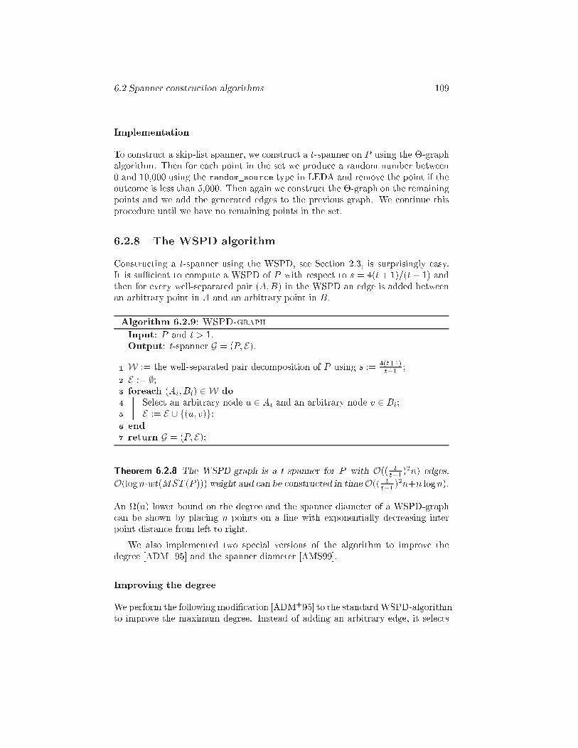
6.2 Spanner onstru tion algorithms 109ImplementationTo onstru t a skip-list spanner, we onstru t a t-spanner on P using the �-graphalgorithm. Then for ea h point in the set we produ e a random number between0 and 10,000 using the random sour e type in LEDA and remove the point if theout ome is less than 5,000. Then again we onstru t the �-graph on the remainingpoints and we add the generated edges to the previous graph. We ontinue thispro edure until we have no remaining points in the set.6.2.8 The WSPD algorithmConstru ting a t-spanner using the WSPD, see Se tion 2.3, is surprisingly easy.It is suÆ ient to ompute a WSPD of P with respe t to s = 4(t+ 1)=(t− 1) andthen for every well-separated pair (A;B) in the WSPD an edge is added betweenan arbitrary point in A and an arbitrary point in B.Algorithm 6.2.9: WSPD-graphInput: P and t > 1.Output: t-spanner G = (P; E).W := the well-separated pair de omposition of P using s := 4(t+1)t−1 ;1E := ∅;2 forea h (Ai; Bi) ∈ W do3 Sele t an arbitrary node u ∈ Ai and an arbitrary node v ∈ Bi;4

E := E ∪ {(u; v)};5 end6 return G = (P; E);7Theorem 6.2.8 The WSPD-graph is a t-spanner for P with O(( tt−1 )2n) edges,O(log n·wt(MST (P ))) weight and an be onstru ted in time O(( tt−1 )2n+n logn).An (n) lower bound on the degree and the spanner diameter of a WSPD-graph an be shown by pla ing n points on a line with exponentially de reasing interpoint distan e from left to right.We also implemented two spe ial versions of the algorithm to improve thedegree [ADM+95℄ and the spanner diameter [AMS99℄.Improving the degreeWe perform the following modi� ation [ADM+95℄ to the standardWSPD-algorithmto improve the maximum degree. Instead of adding an arbitrary edge, it sele ts

110 Chapter 6 Experimental Study of Geometri Spannersthe point whi h has the smallest maximum degree from ea h set and adds an edgebetween them. This does not improve the theoreti al upper bound but we werehoping to see some improvements in the experimental bounds. Note also thatthe (n) lower bound does not hold for the modi�ed WSPD-algorithm. In theexperiments one an see a small improvement for graphs with t > 1:5, for smallervalues the di�eren e is negligible. For t = 1:5 the improvement is roughly a fa tor1.5 and in reases to about 3 for t = 4.Another way to improve the maximum degree is to sele t the point in ea h well-separated pair using a weighted randomization. That is, we assign a weight to ea hpoint whi h is the total number of points minus the number of well-separated pairsthat ontain the point. In other words, points that appear in a smaller number ofwell-separated pairs have greater weight and vi e versa. Now we simply sele t apoint randomly from ea h set based on the weight of the points and then we addan edge between them. Unfortunately, we ould not see any improvements in theexperiments using this approa h ompared to the standard approa h.Improving the spanner diameterArya et al. [AMS99℄ found a way to bound the spanner diameter of a WSPD-graph. The WSPD is onstru ted from the so- alled fair-split tree, and Aryaet al. [AMS99℄ hose a representative point by a sear h in the fair-split tree. Fora node u in the split tree, follow the path down the tree by always hoosingthe larger subtree. The point stored at the leaf in whi h the path ends is therepresentative point for u. This approa h guarantees that the spanner diameterof the onstru ted t-spanner is bounded by 2 · logn.ImplementationWe used a split tree for the onstru tion of the WSPD. The points stored at a nodeis partitioned into two sets by partitioning the non-empty bounding box along itslongest side into two boxes of equal size. The tree onstru tion only requires a fewper ent of the total running time in all our tests.To de ide in onstant time if two sets are well-separated we save the smallesten losing ir le of the points in ea h node. As we mentioned in the note after Def-inition 2.5.1, two sets are well-separated with respe t to s if the distan e betweenthe smallest en losing ir les is at least s times the maximum radius of the twosmallest en losing ir les.

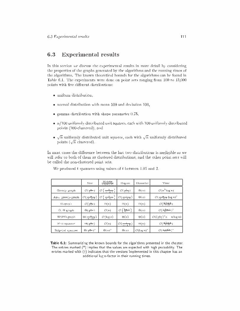
6.3 Experimental results 1116.3 Experimental resultsIn this se tion we dis uss the experimental results in more detail by onsideringthe properties of the graphs generated by the algorithms and the running times ofthe algorithms. The known theoreti al bounds for the algorithms an be found inTable 6.1. The experiments were done on point sets ranging from 100 to 13,000points with �ve di�erent distributions:• uniform distribution,• normal distribution with mean 500 and deviation 100,• gamma distribution with shape parameter 0.75,• n=100 uniformly distributed unit squares, ea h with 100 uniformly distributedpoints (100- lustered), and• √n uniformly distributed unit squares, ea h with √n uniformly distributedpoints (√n- lustered).In most ases the di�eren e between the last two distributions is negligible so wewill refer to both of them as lustered distributions, and the other point sets willbe alled the non- lustered point sets.We produ ed t-spanners using values of t between 1.05 and 2.- Size Weightwt(MST ) Degree Diameter TimeGreedy-graph O( nt−1 ) O

� 1(t−1)4 � O( 1t−1 ) �(n) O(n3 logn)Apx. greedy-graph O� n(t−1)3 � O

� 1(t−1)4 � O� 1(t−1)3 � �(n) O( n(t−1)7 logn)†�-graph O( nt−1 ) �(n) �(n) �(n) O(n lognt−1 )O. �-graph �( nt−1 ) O(n) O� lognt−1 � �(n) O(n lognt−1 )†WSPD-graph �( n(t−1)2 ) O(logn) �(n) �(n) O(( tt−1 )2n+ n log n)Sink-spanner �( nt−1 ) O(n) O� 1(t−1)2 � �(n) O(n lognt−1 )Skip-list spanner �( nt−1 )∗ �(n)∗ �(n) O(logn)∗ O(n lognt−1 )∗Table 6.1: Summarizing the known bounds for the algorithms presented in the hapter.The entries marked (*) implies that the values are expe ted with high probability. Theentries marked with (†) indi ates that the versions implemented in this hapter has anadditional log n-fa tor in their running times.

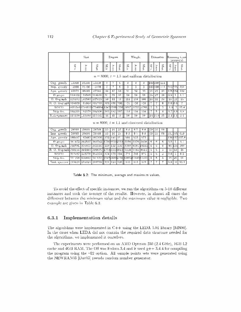
112 Chapter 6 Experimental Study of Geometri SpannersSize Degree Weight Diameter Running time(se onds)Min. Aver. Max. Min. Aver. Max. Min. Aver. Max. Min. Aver. Max. Min. Aver. Max.n = 8000, t = 1:5 and uniform distributionOrg. greedy 15060 15100 15128 7 7 8 3 3 3 103 108 111Imp. greedy 15060 15100 15128 7 7 8 3 3 3 103 108 111 213 225 231Apx. greedy 45879 46469 47543 44 47 54 31 32 33 21 22 23 175 182 192�-graph 118402 118509 118646 51 55 59 58 58 58 26 27 28 0.9 1 1.1O. �-graph 125162 132594 147023 39 44 46 211 259 396 20 22 26 10 12 18R. O. �-graph 164860 165064 165289 169 190 200 135 136 138 7 7 8 6.8 6.9 7WSPD 169534917166521734094 124212881326 5657 5733 5788 3 3 3 11.9 12 12.4Skip-list 192203 192379 192506 183 192 197 154 156 156 7 5 8 4.7 4.9 4.9Sink-spanner 115150 115333 115481 44 45 46 58 59 59 24 24.6 25 2.4 2.4 2.4n = 8000, t = 1:1 and lustered distributionOrg. greedy 29603 29680 29769 15 16 17 8.3 8.7 8.9 49 55 68Imp. greedy 29603 29680 29769 15 16 17 8.3 8.7 8.9 49 55 68 531 585 619Apx. greedy 160497 162482 163208 132 141 151 509 533 573 136 137 137.8�-graph 361672 362557 363762 175019332110 5156 5376 5608 6 6 6 3.5 5 4.1O. �-graph 346791 358055 362146 119 122 126 8203 9384 10233 6 6 6 90 136 283R. O. �-graph 389186 394404 399675 177325123012 7129 7585 8012 5 5 5 40 43 46WSPD 352487 353778 355374 174 179 194 721 766 825 5 5 5 2.8 5 6.3Skip-list 531298 536602 541053 234724092496 106921104311311 5 5 5 19 20 21Sink-spanner 215624 216324 216739 121 123 126 340 345 349 7 7 7 9.8 10 10.4Table 6.2: The minimum, average and maximum values.To avoid the e�e t of spe i� instan es, we ran the algorithms on 5-10 di�erentinstan es and took the average of the results. However, in almost all ases thedi�eren e between the minimum value and the maximum value is negligible. Twoexample are given in Table 6.2.6.3.1 Implementation detailsThe algorithms were implemented in C++ using the LEDA 5.01 library [MN00℄.In the ases when LEDA did not ontain the required data stru ture needed forthe algorithms, we implemented it ourselves.The experiments were performed on an AMD Opteron 250 (2.4 GHz), 1GB L2 a he and 4GB RAM. The OS was Fedora 3.4 and it used g++ 3.4.4 for ompilingthe program using the -O2 option. All sample points sets were generated usingthe NEWRAN03 [Dav05℄ pseudo random number generator.

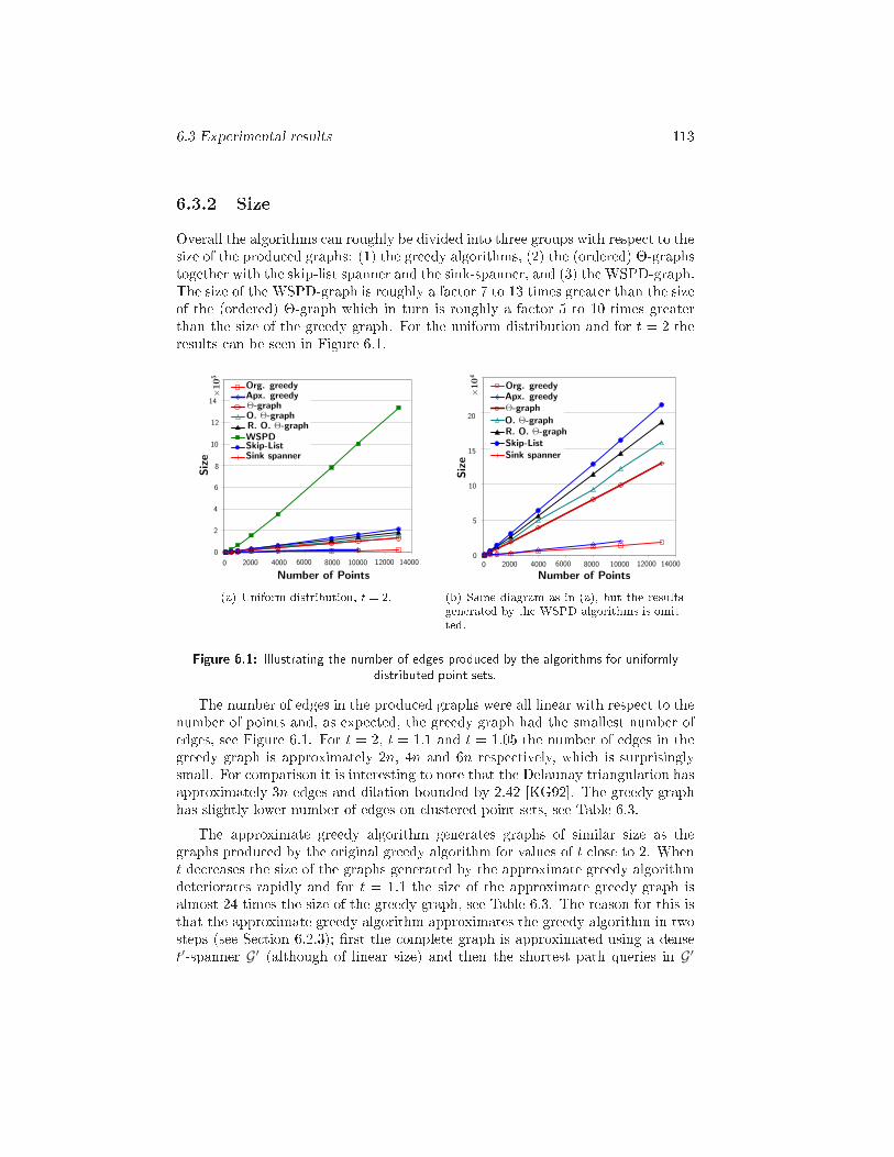
6.3 Experimental results 1136.3.2 SizeOverall the algorithms an roughly be divided into three groups with respe t to thesize of the produ ed graphs: (1) the greedy algorithms, (2) the (ordered) �-graphstogether with the skip-list spanner and the sink-spanner, and (3) the WSPD-graph.The size of the WSPD-graph is roughly a fa tor 7 to 13 times greater than the sizeof the (ordered) �-graph whi h in turn is roughly a fa tor 5 to 10 times greaterthan the size of the greedy graph. For the uniform distribution and for t = 2 theresults an be seen in Figure 6.1.0

2

4

6

8

10

12

14

0

×10

5

Number of Points

Size

Org. greedyApx. greedyΘ-graphO. Θ-graphR. O. Θ-graph

WSPDSkip-ListSink spanner

140002000 4000 6000 8000 10000 12000(a) Uniform distribution, t = 2. 0

5

10

15

20

×10

4

Number of Points

Size

Org. greedyApx. greedy

Θ-graph

O. Θ-graph

R. O. Θ-graph

Skip-List

Sink spanner

0 140002000 4000 6000 8000 10000 12000(b) Same diagram as in (a), but the resultsgenerated by the WSPD-algorithms is omit-ted.Figure 6.1: Illustrating the number of edges produ ed by the algorithms for uniformlydistributed point sets.The number of edges in the produ ed graphs were all linear with respe t to thenumber of points and, as expe ted, the greedy graph had the smallest number ofedges, see Figure 6.1. For t = 2, t = 1:1 and t = 1:05 the number of edges in thegreedy graph is approximately 2n, 4n and 6n respe tively, whi h is surprisinglysmall. For omparison it is interesting to note that the Delaunay triangulation hasapproximately 3n edges and dilation bounded by 2.42 [KG92℄. The greedy graphhas slightly lower number of edges on lustered point sets, see Table 6.3.The approximate greedy algorithm generates graphs of similar size as thegraphs produ ed by the original greedy algorithm for values of t lose to 2. Whent de reases the size of the graphs generated by the approximate greedy algorithmdeteriorates rapidly and for t = 1:1 the size of the approximate greedy graph isalmost 24 times the size of the greedy graph, see Table 6.3. The reason for this isthat the approximate greedy algorithm approximates the greedy algorithm in twosteps (see Se tion 6.2.3); �rst the omplete graph is approximated using a denset′-spanner G′ (although of linear size) and then the shortest path queries in G′

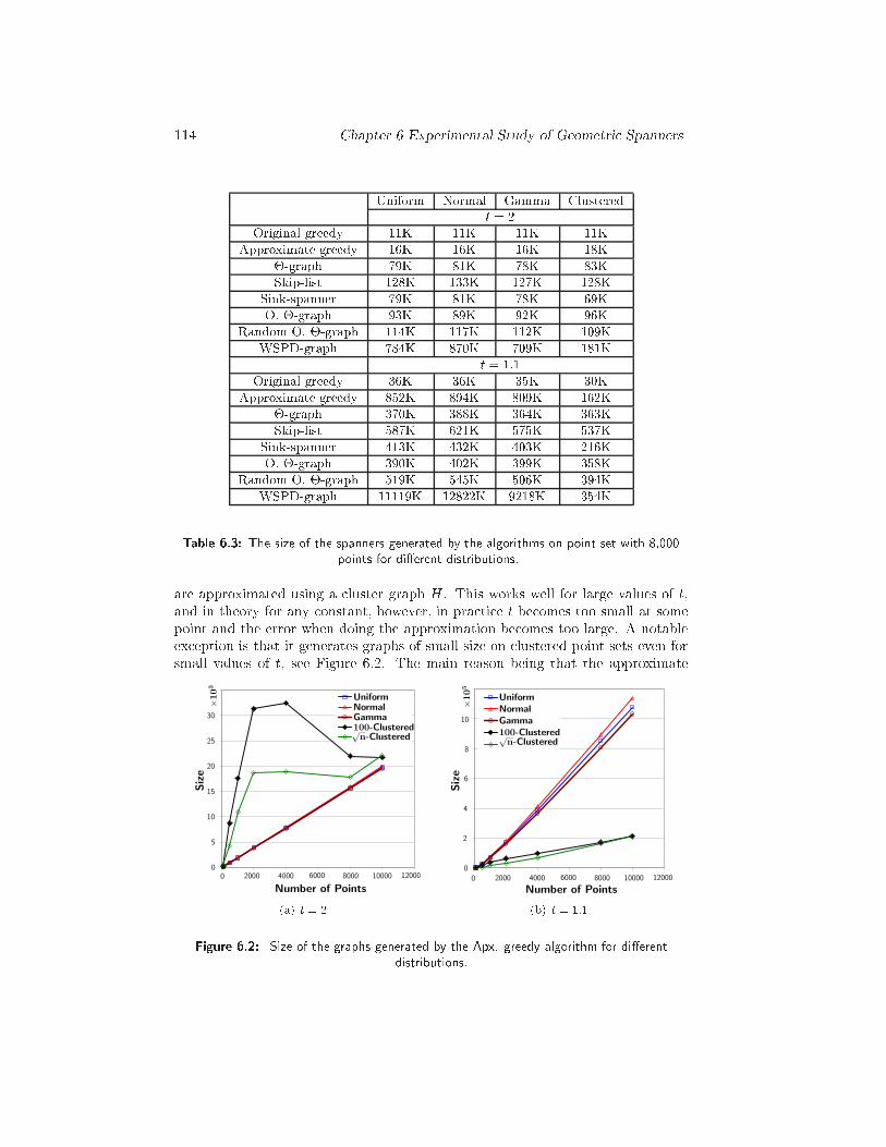
114 Chapter 6 Experimental Study of Geometri SpannersUniform Normal Gamma Clusteredt = 2Original greedy 11K 11K 11K 11KApproximate greedy 16K 16K 16K 18K�-graph 79K 81K 78K 83KSkip-list 128K 133K 127K 128KSink-spanner 79K 81K 78K 69KO. �-graph 93K 89K 92K 96KRandom O. �-graph 114K 117K 112K 109KWSPD-graph 784K 870K 709K 181Kt = 1:1Original greedy 36K 36K 35K 30KApproximate greedy 852K 894K 809K 162K�-graph 370K 388K 364K 363KSkip-list 587K 621K 575K 537KSink-spanner 413K 432K 403K 216KO. �-graph 390K 402K 399K 358KRandom O. �-graph 519K 545K 506K 394KWSPD-graph 11119K 12822K 9218K 354KTable 6.3: The size of the spanners generated by the algorithms on point set with 8,000points for di�erent distributions.are approximated using a luster graph H . This works well for large values of t,and in theory for any onstant, however, in pra ti e t be omes too small at somepoint and the error when doing the approximation be omes too large. A notableex eption is that it generates graphs of small size on lustered point sets even forsmall values of t, see Figure 6.2. The main reason being that the approximate0

5

10

15

20

25

30

×10

3

Number of Points

Siz

e

Uniform

Normal

Gamma

100-Clustered√n-Clustered

0 2000 4000 6000 8000 10000 12000(a) t = 2 0

2

4

6

8

10

×10

5

Number of Points

Size

Uniform

Normal

Gamma

100-Clustered√n-Clustered

0 2000 4000 6000 8000 10000 12000(b) t = 1:1Figure 6.2: Size of the graphs generated by the Apx. greedy algorithm for di�erentdistributions.

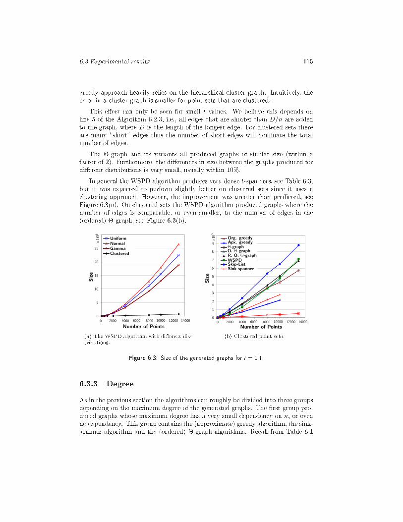
6.3 Experimental results 115greedy approa h heavily relies on the hierar hi al luster graph. Intuitively, theerror in a luster graph is smaller for point sets that are lustered.This e�e t an only be seen for small t values. We believe this depends online 5 of the Algorithm 6.2.3, i.e., all edges that are shorter than D=n are addedto the graph, where D is the length of the longest edge. For lustered sets thereare many \short" edges thus the number of short edges will dominate the totalnumber of edges.The �-graph and its variants all produ ed graphs of similar size (within afa tor of 2). Furthermore, the di�eren es in size between the graphs produ ed fordi�erent distributions is very small, usually within 10%.In general the WSPD algorithm produ es very dense t-spanners, see Table 6.3,but it was expe ted to perform slightly better on lustered sets sin e it uses a lustering approa h. However, the improvement was greater than predi ted, seeFigure 6.3(a). On lustered sets the WSPD algorithm produ ed graphs where thenumber of edges is omparable, or even smaller, to the number of edges in the(ordered) �-graph, see Figure 6.3(b).0

5

10

15

20

25

×10

6

Number of Points

Size

Uniform

Normal

Gamma

Clustered

0 140002000 4000 6000 8000 10000 12000(a) The WSPD algorithm with di�erent dis-tributions. 0

1

2

3

4

5

6

7

8

9

×10

5

Number of Points

Size

Org. greedyApx. greedyΘ-graphO. Θ-graphR. O. Θ-graphWSPDSkip-ListSink spanner

0 140002000 4000 6000 8000 10000 12000(b) Clustered point sets.Figure 6.3: Size of the generated graphs for t = 1:1.6.3.3 DegreeAs in the previous se tion the algorithms an roughly be divided into three groupsdepending on the maximum degree of the generated graphs. The �rst group pro-du ed graphs whose maximum degree has a very small dependen y on n, or evenno dependen y. This group ontains the (approximate) greedy algorithm, the sink-spanner algorithm and the (ordered) �-graph algorithms. Re all from Table 6.1

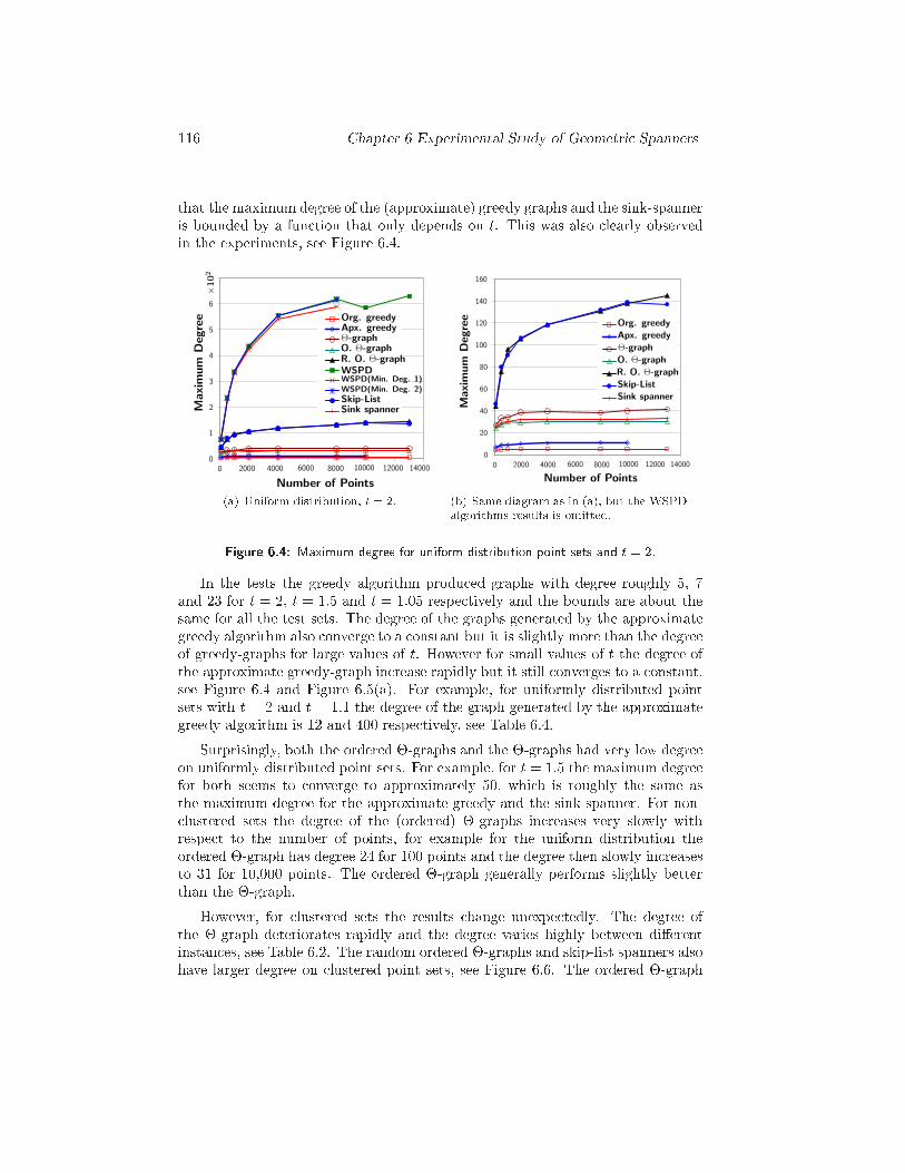
116 Chapter 6 Experimental Study of Geometri Spannersthat the maximum degree of the (approximate) greedy graphs and the sink-spanneris bounded by a fun tion that only depends on t. This was also learly observedin the experiments, see Figure 6.4.0

1

2

3

4

5

6

×10

2

Number of Points

Maxi

mum

Degre

e Org. greedyApx. greedyΘ-graphO. Θ-graphR. O. Θ-graphWSPDWSPD(Min. Deg. 1)WSPD(Min. Deg. 2)

Skip-ListSink spanner

0 140002000 4000 6000 8000 10000 12000(a) Uniform distribution, t = 2. 0

20

40

60

80

100

120

140

160

Number of Points

Maxim

um

Degre

e

Org. greedy

Apx. greedy

Θ-graph

O. Θ-graph

R. O. Θ-graph

Skip-List

Sink spanner

0 140002000 4000 6000 8000 10000 12000(b) Same diagram as in (a), but the WSPD-algorithms results is omitted.Figure 6.4: Maximum degree for uniform distribution point sets and t = 2.In the tests the greedy algorithm produ ed graphs with degree roughly 5, 7and 23 for t = 2, t = 1:5 and t = 1:05 respe tively and the bounds are about thesame for all the test sets. The degree of the graphs generated by the approximategreedy algorithm also onverge to a onstant but it is slightly more than the degreeof greedy-graphs for large values of t. However for small values of t the degree ofthe approximate greedy-graph in rease rapidly but it still onverges to a onstant,see Figure 6.4 and Figure 6.5(a). For example, for uniformly distributed pointsets with t = 2 and t = 1:1 the degree of the graph generated by the approximategreedy algorithm is 12 and 400 respe tively, see Table 6.4.Surprisingly, both the ordered �-graphs and the �-graphs had very low degreeon uniformly distributed point sets. For example, for t = 1:5 the maximum degreefor both seems to onverge to approximately 50, whi h is roughly the same asthe maximum degree for the approximate greedy and the sink-spanner. For non- lustered sets the degree of the (ordered) �-graphs in reases very slowly withrespe t to the number of points, for example for the uniform distribution theordered �-graph has degree 24 for 100 points and the degree then slowly in reasesto 31 for 10,000 points. The ordered �-graph generally performs slightly betterthan the �-graph.However, for lustered sets the results hange unexpe tedly. The degree ofthe �-graph deteriorates rapidly and the degree varies highly between di�erentinstan es, see Table 6.2. The random ordered �-graphs and skip-list spanners alsohave larger degree on lustered point sets, see Figure 6.6. The ordered �-graph

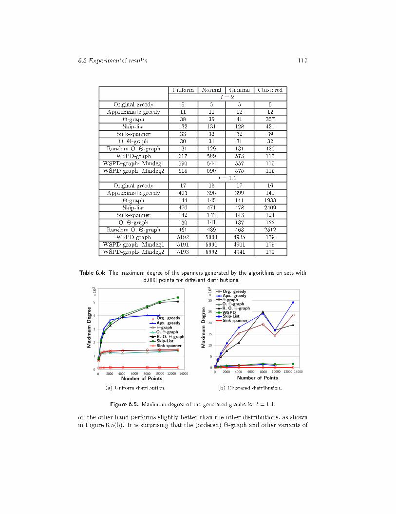
6.3 Experimental results 117Uniform Normal Gamma Clusteredt = 2Original greedy 5 5 5 5Approximate greedy 11 11 12 12�-graph 38 39 41 357Skip-list 132 131 128 421Sink-spanner 33 32 32 39O. �-graph 30 31 31 32Random O. �-graph 131 129 131 430WSPD-graph 617 589 573 115WSPD-graph- Mindeg1 590 544 557 115WSPD-graph- Mindeg2 615 590 575 115t = 1:1Original greedy 17 16 17 16Approximate greedy 403 396 399 141�-graph 144 145 141 1933Skip-list 470 471 478 2409Sink-spanner 142 143 143 124O. �-graph 130 141 137 122Random O. �-graph 461 439 463 2512WSPD-graph 5192 5993 4938 179WSPD-graph- Mindeg1 5191 5991 4901 179WSPD-graph- Mindeg2 5193 5992 4941 179Table 6.4: The maximum degree of the spanners generated by the algorithms on sets with8,000 points for di�erent distributions.0

1

2

3

4

5

×10

2

Number of Points

Maxim

um

Degre

e

Org. greedy

Apx. greedyΘ-graphO. Θ-graphR. O. Θ-graphSkip-ListSink spanner

0 140002000 4000 6000 8000 10000 12000(a) Uniform distribution. 0

5

10

15

20

25

30

×10

2

Number of Points

Maxim

um

Degre

e

Org. greedyApx. greedyΘ-graphO. Θ-graphR. O. Θ-graphWSPDSkip-ListSink spanner

0 140002000 4000 6000 8000 10000 12000(b) Clustered distribution.Figure 6.5: Maximum degree of the generated graphs for t = 1:1.on the other hand performs slightly better than the other distributions, as shownin Figure 6.5(b). It is surprising that the (ordered) �-graph and other variants of

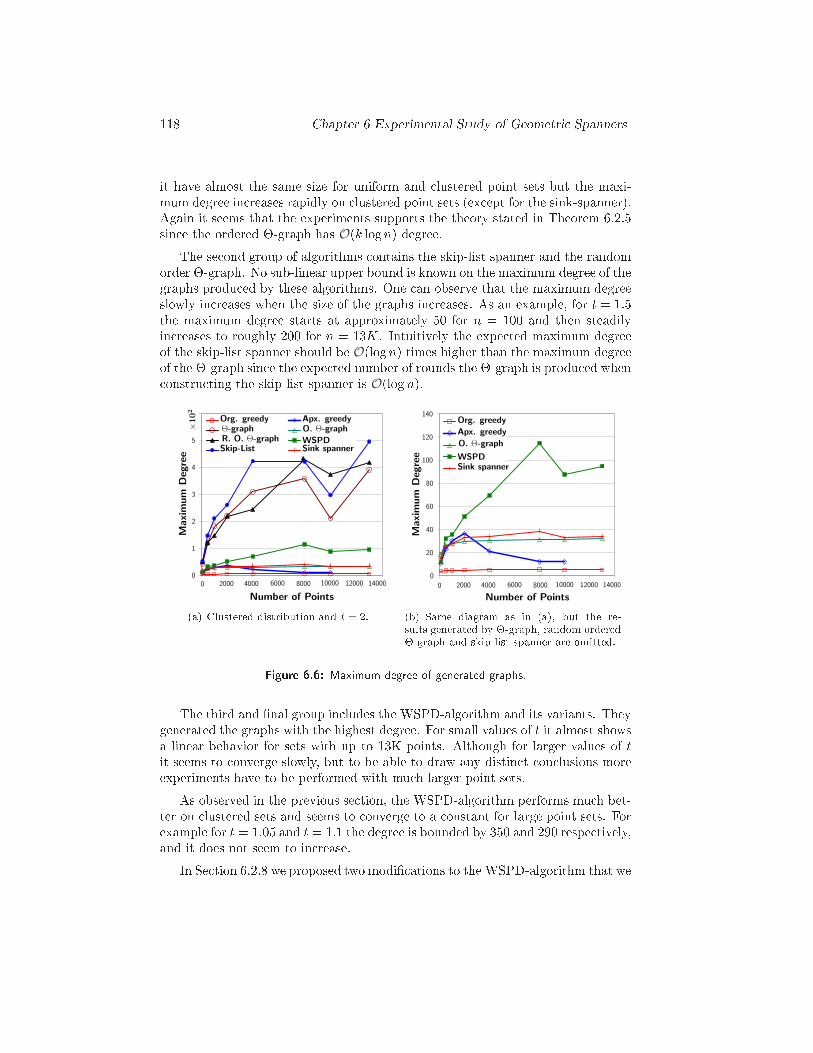
118 Chapter 6 Experimental Study of Geometri Spannersit have almost the same size for uniform and lustered point sets but the maxi-mum degree in reases rapidly on lustered point sets (ex ept for the sink-spanner).Again it seems that the experiments supports the theory stated in Theorem 6.2.5sin e the ordered �-graph has O(k logn) degree.The se ond group of algorithms ontains the skip-list spanner and the randomorder �-graph. No sub-linear upper bound is known on the maximum degree of thegraphs produ ed by these algorithms. One an observe that the maximum degreeslowly in reases when the size of the graphs in reases. As an example, for t = 1:5the maximum degree starts at approximately 50 for n = 100 and then steadilyin reases to roughly 200 for n = 13K. Intuitively the expe ted maximum degreeof the skip-list spanner should be O(logn) times higher than the maximum degreeof the �-graph sin e the expe ted number of rounds the �-graph is produ ed when onstru ting the skip-list spanner is O(logn).0

1

2

3

4

5

×10

2

Number of Points

Maxim

um

Degre

e

Org. greedy Apx. greedyΘ-graph O. Θ-graphR. O. Θ-graph WSPDSkip-List Sink spanner

0 140002000 4000 6000 8000 10000 12000(a) Clustered distribution and t = 2. 0

20

40

60

80

100

120

140

Number of Points

Maxim

um

Degre

eOrg. greedy

Apx. greedy

O. Θ-graph

WSPDSink spanner

0 140002000 4000 6000 8000 10000 12000(b) Same diagram as in (a), but the re-sults generated by �-graph, random ordered�-graph and skip-list spanner are omitted.Figure 6.6: Maximum degree of generated graphs.The third and �nal group in ludes the WSPD-algorithm and its variants. Theygenerated the graphs with the highest degree. For small values of t it almost showsa linear behavior for sets with up to 13K points. Although for larger values of tit seems to onverge slowly, but to be able to draw any distin t on lusions moreexperiments have to be performed with mu h larger point sets.As observed in the previous se tion, the WSPD-algorithm performs mu h bet-ter on lustered sets and seems to onverge to a onstant for large point sets. Forexample for t = 1:05 and t = 1:1 the degree is bounded by 350 and 290 respe tively,and it does not seem to in rease.In Se tion 6.2.8 we proposed two modi� ations to the WSPD-algorithm that we

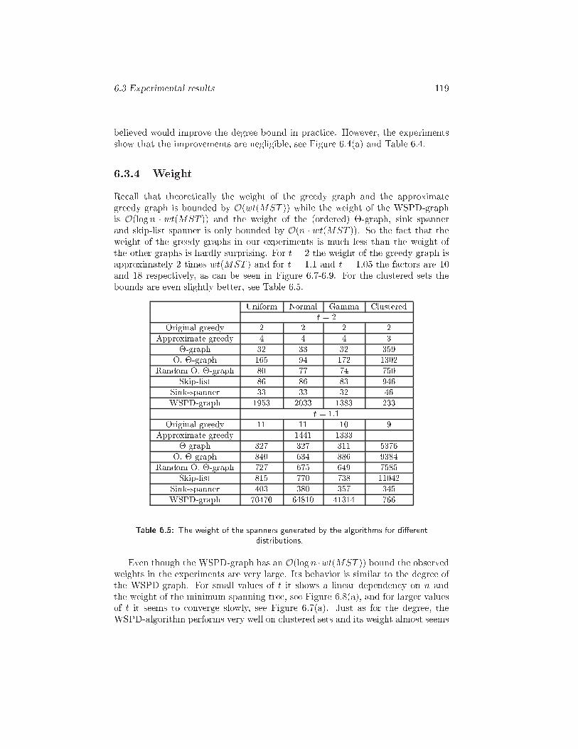
6.3 Experimental results 119believed would improve the degree bound in pra ti e. However, the experimentsshow that the improvements are negligible, see Figure 6.4(a) and Table 6.4.6.3.4 WeightRe all that theoreti ally the weight of the greedy graph and the approximategreedy graph is bounded by O(wt(MST )) while the weight of the WSPD-graphis O(logn · wt(MST )) and the weight of the (ordered) �-graph, sink spannerand skip-list spanner is only bounded by O(n · wt(MST )). So the fa t that theweight of the greedy graphs in our experiments is mu h less than the weight ofthe other graphs is hardly surprising. For t = 2 the weight of the greedy graph isapproximately 2 times wt(MST ) and for t = 1:1 and t = 1:05 the fa tors are 10and 18 respe tively, as an be seen in Figure 6.7-6.9. For the lustered sets thebounds are even slightly better, see Table 6.5.Uniform Normal Gamma Clusteredt = 2Original greedy 2 2 2 2Approximate greedy 4 4 4 3�-graph 32 33 32 359O. �-graph 165 94 172 1302Random O. �-graph 80 77 74 750Skip-list 86 86 83 946Sink-spanner 33 33 32 46WSPD-graph 1953 2033 1383 233t = 1:1Original greedy 11 11 10 9Approximate greedy 1441 1333�-graph 327 327 311 5376O. �-graph 840 634 886 9384Random O. �-graph 727 675 649 7585Skip-list 815 770 738 11042Sink-spanner 403 380 357 345WSPD-graph 70470 64810 41314 766Table 6.5: The weight of the spanners generated by the algorithms for di�erentdistributions.Even though the WSPD-graph has an O(logn ·wt(MST )) bound the observedweights in the experiments are very large. Its behavior is similar to the degree ofthe WSPD-graph. For small values of t it shows a linear dependen y on n andthe weight of the minimum spanning tree, see Figure 6.8(a), and for larger valuesof t it seems to onverge slowly, see Figure 6.7(a). Just as for the degree, theWSPD-algorithm performs very well on lustered sets and its weight almost seems

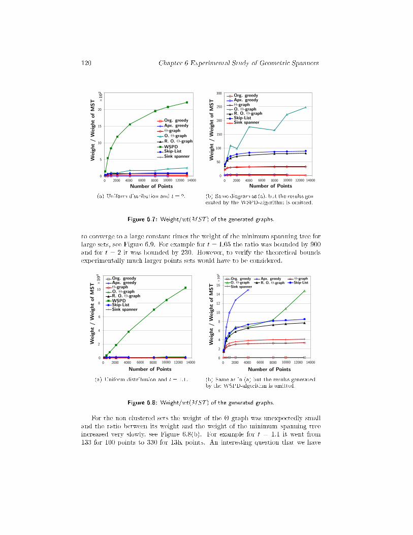
120 Chapter 6 Experimental Study of Geometri Spanners

0

5

10

15

20

×10

2

Number of Points

Weig

ht

/W

eig

ht

ofM

ST

Org. greedyApx. greedyΘ-graphO. Θ-graphR. O. Θ-graph

WSPDSkip-ListSink spanner

0 140002000 4000 6000 8000 10000 12000(a) Uniform distribution and t = 2. 0

50

100

150

200

250

Number of Points

Weig

ht

/W

eig

ht

ofM

ST

Org. greedyApx. greedyΘ-graphO. Θ-graphR. O. Θ-graphSkip-ListSink spanner

0 140002000 4000 6000 8000 10000 12000

300

(b) Same diagram as (a), but the results gen-erated by the WSPD-algorithm is omitted.Figure 6.7: Weight/wt(MST ) of the generated graphs.to onverge to a large onstant times the weight of the minimum spanning tree forlarge sets, see Figure 6.9. For example for t = 1:05 the ratio was bounded by 900and for t = 2 it was bounded by 230. However, to verify the theoreti al boundsexperimentally mu h larger points sets would have to be onsidered.0

2

4

6

8

10

×10

4

Number of Points

Weig

ht

/W

eig

ht

ofM

ST

Org. greedyApx. greedyΘ-graphO. Θ-graphR. O. Θ-graphWSPDSkip-ListSink spanner

0 140002000 4000 6000 8000 10000 12000(a) Uniform distribution and t = 1:1. 0

2

4

6

8

10

12

14

16

×10

2

Number of Points

Weig

ht

/W

eig

ht

ofM

ST

Org. greedy Apx. greedy Θ-graphO. Θ-graph R. O. Θ-graph Skip-ListSink spanner

0 140002000 4000 6000 8000 10000 12000(b) Same as in (a) but the results generatedby the WSPD-algorithm is omitted.Figure 6.8: Weight/wt(MST ) of the generated graphs.For the non- lustered sets the weight of the �-graph was unexpe tedly smalland the ratio between its weight and the weight of the minimum spanning treein reased very slowly, see Figure 6.8(b). For example for t = 1:1 it went from133 for 100 points to 330 for 13K points. An interesting question that we have

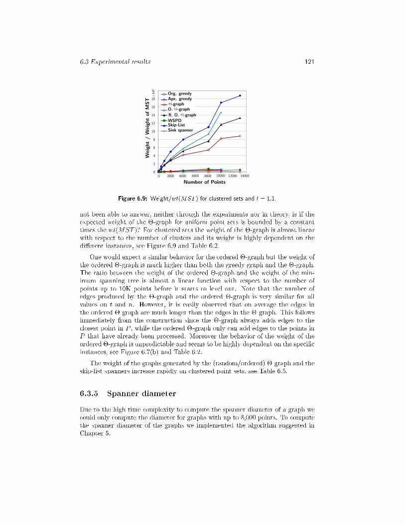
6.3 Experimental results 121

0

2

4

6

8

10

12

14

16

18

×10

3

Number of Points

Weig

ht

/W

eig

ht

ofM

ST

Org. greedyApx. greedyΘ-graphO. Θ-graph

R. O. Θ-graph

WSPDSkip-ListSink spanner

0 140002000 4000 6000 8000 10000 12000Figure 6.9: Weight/wt(MST ) for lustered sets and t = 1:1.not been able to answer, neither through the experiments nor in theory, is if theexpe ted weight of the �-graph for uniform point sets is bounded by a onstanttimes the wt(MST )? For lustered sets the weight of the �-graph is almost linearwith respe t to the number of lusters and its weight is highly dependent on thedi�erent instan es, see Figure 6.9 and Table 6.2.One would expe t a similar behavior for the ordered �-graph but the weight ofthe ordered �-graph is mu h higher than both the greedy graph and the �-graph.The ratio between the weight of the ordered �-graph and the weight of the min-imum spanning tree is almost a linear fun tion with respe t to the number ofpoints up to 10K points before it starts to level out. Note that the number ofedges produ ed by the �-graph and the ordered �-graph is very similar for allvalues on t and n. However, it is easily observed that on average the edges inthe ordered �-graph are mu h longer than the edges in the �-graph. This followsimmediately from the onstru tion sin e the �-graph always adds edges to the losest point in P , while the ordered �-graph only an add edges to the points inP that have already been pro essed. Moreover the behavior of the weight of theordered �-graph is unpredi table and seems to be highly dependent on the spe i� instan es, see Figure 6.7(b) and Table 6.2.The weight of the graphs generated by the (random/ordered) �-graph and theskip-list spanners in rease rapidly on lustered point sets, see Table 6.5.6.3.5 Spanner diameterDue to the high time omplexity to ompute the spanner diameter of a graph we ould only ompute the diameter for graphs with up to 8,000 points. To omputethe spanner diameter of the graphs we implemented the algorithm suggested inChapter 5.

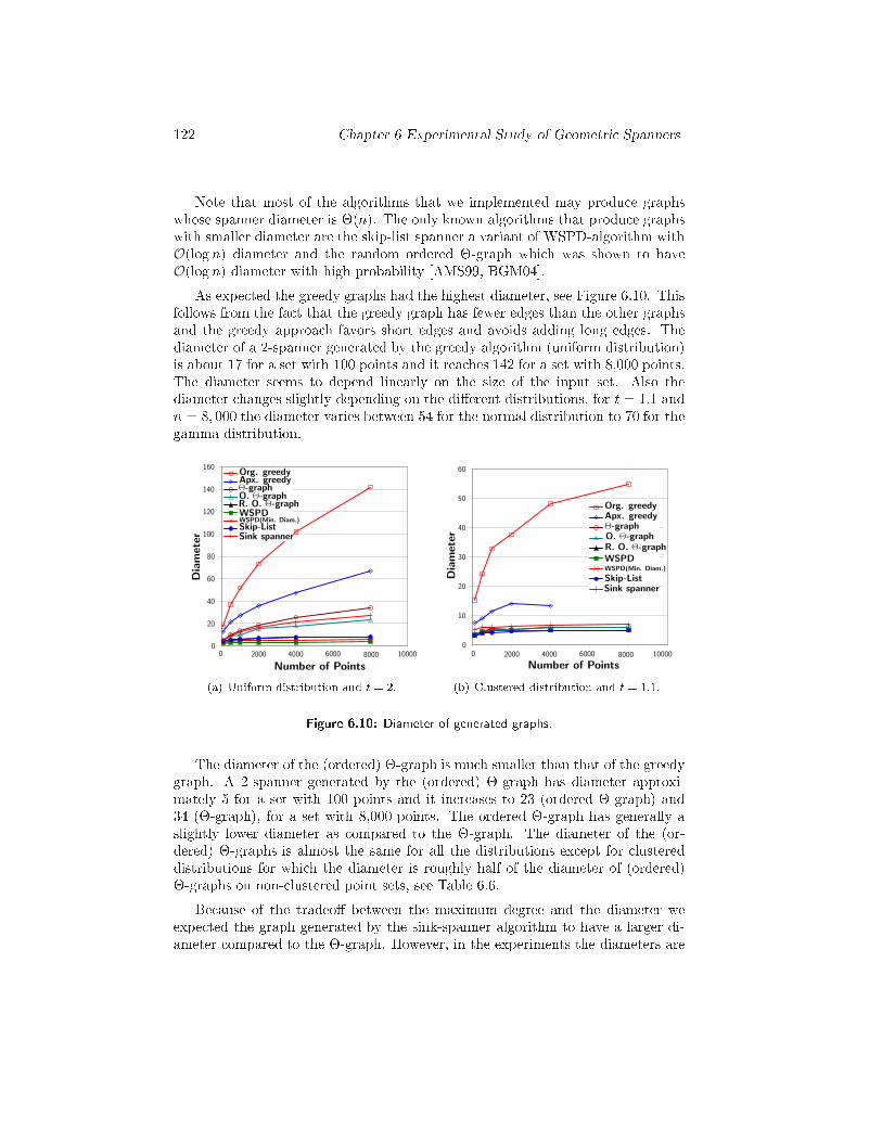
122 Chapter 6 Experimental Study of Geometri SpannersNote that most of the algorithms that we implemented may produ e graphswhose spanner diameter is �(n). The only known algorithms that produ e graphswith smaller diameter are the skip-list spanner a variant of WSPD-algorithm withO(log n) diameter and the random ordered �-graph whi h was shown to haveO(log n) diameter with high probability [AMS99, BGM04℄.As expe ted the greedy graphs had the highest diameter, see Figure 6.10. Thisfollows from the fa t that the greedy graph has fewer edges than the other graphsand the greedy approa h favors short edges and avoids adding long edges. Thediameter of a 2-spanner generated by the greedy algorithm (uniform distribution)is about 17 for a set with 100 points and it rea hes 142 for a set with 8,000 points.The diameter seems to depend linearly on the size of the input set. Also thediameter hanges slightly depending on the di�erent distributions, for t = 1:1 andn = 8; 000 the diameter varies between 54 for the normal distribution to 70 for thegamma distribution.

0

20

40

60

80

100

120

140

160

Number of Points

Dia

mete

r

Org. greedyApx. greedyΘ-graphO. Θ-graphR. O. Θ-graphWSPDWSPD(Min. Diam.)Skip-ListSink spanner

0 2000 4000 6000 8000 10000(a) Uniform distribution and t = 2. 0

10

20

30

40

50

60

Number of Points

Dia

mete

r

Org. greedyApx. greedyΘ-graphO. Θ-graphR. O. Θ-graphWSPDWSPD(Min. Diam.)

Skip-ListSink spanner

0 2000 4000 6000 8000 10000(b) Clustered distribution and t = 1:1.Figure 6.10: Diameter of generated graphs.The diameter of the (ordered) �-graph is mu h smaller than that of the greedygraph. A 2-spanner generated by the (ordered) �-graph has diameter approxi-mately 5 for a set with 100 points and it in reases to 23 (ordered �-graph) and34 (�-graph), for a set with 8,000 points. The ordered �-graph has generally aslightly lower diameter as ompared to the �-graph. The diameter of the (or-dered) �-graphs is almost the same for all the distributions ex ept for lustereddistributions for whi h the diameter is roughly half of the diameter of (ordered)�-graphs on non- lustered point sets, see Table 6.6.Be ause of the tradeo� between the maximum degree and the diameter weexpe ted the graph generated by the sink-spanner algorithm to have a larger di-ameter ompared to the �-graph. However, in the experiments the diameters are

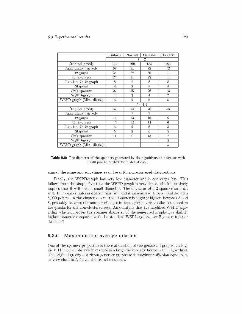
6.3 Experimental results 123Uniform Normal Gamma Clusteredt = 2Original greedy 142 109 155 164Approximate greedy 67 51 72 72�-graph 34 28 36 11O. �-graph 23 21 23 11Random O. �-graph 8 8 8 8Skip-list 8 8 8 8Sink-spanner 27 25 26 13WSPD-graph 4 3 4 7WSPD-graph (Min. diam.) 6 5 6 8t = 1:1Original greedy 57 54 70 55Approximate greedy 7 7�-graph 14 13 16 6O. �-graph 13 12 14 6Random O. �-graph 6 6 6 5Skip-list 5 5 6 5Sink-spanner 11 11 13 7WSPD-graph 5WSPD-graph (Min. diam.) 5Table 6.6: The diameter of the spanners generated by the algorithms on point set with8,000 points for di�erent distributions.almost the same and sometimes even lower for non- lustered distributions.Finally, the WSPD-graph has very low diameter and it onverges fast. Thisfollows from the simple fa t that the WSPD-graph is very dense, whi h intuitivelyimplies that it will have a small diameter. The diameter of a 2-spanner on a setwith 100 points (uniform distribution) is 3 and it in reases to 4 for a point set with8,000 points. In the lustered sets, the diameter is slightly higher, between 3 and8, probably be ause the number of edges in these graphs are smaller ompared tothe graphs for the non- lustered sets. An oddity is that the modi�ed WSPD algo-rithm whi h improves the spanner diameter of the generated graphs has slightlyhigher diameter ompared with the standard WSPD-graphs, see Figure 6.10(a) orTable 6.6.6.3.6 Maximum and average dilationOne of the spanner properties is the real dilation of the generated graphs. In Fig-ure 6.11 one an observe that there is a large dis repan y between the algorithms.The original greedy algorithm generate graphs with maximum dilation equal to t,or very lose to t, for all the tested instan es.

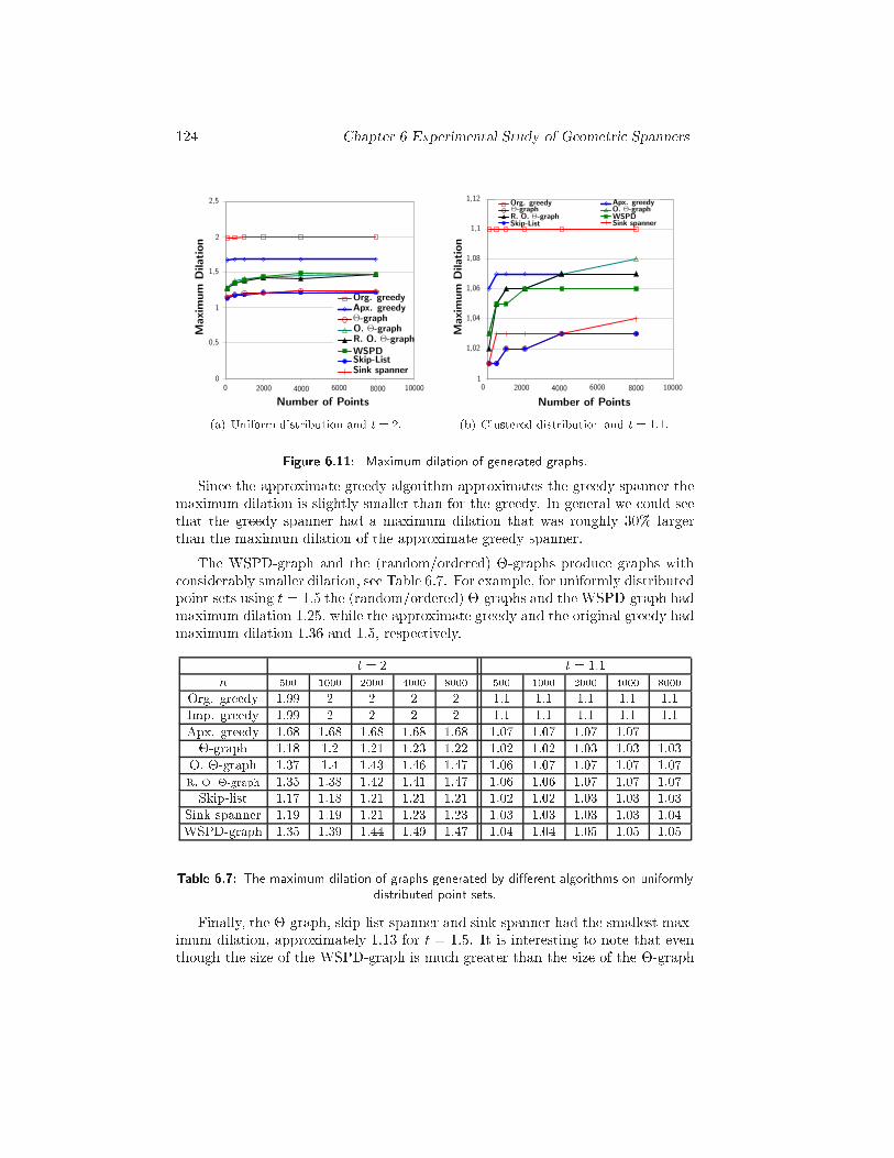
124 Chapter 6 Experimental Study of Geometri Spanners

0

0,5

1

1,5

2

2,5

Number of Points

Org. greedyApx. greedyΘ-graphO. Θ-graphR. O. Θ-graph

WSPDSkip-ListSink spanner

0 2000 4000 6000 8000 10000

Maxim

um

Dilation

(a) Uniform distribution and t = 2. 1

1,02

1,04

1,06

1,08

1,1

1,12

Number of Points

Maxim

um

Dilation

Org. greedy Apx. greedyΘ-graph O. Θ-graphR. O. Θ-graph WSPDSkip-List Sink spanner

0 2000 4000 6000 8000 10000(b) Clustered distribution and t = 1:1.Figure 6.11: Maximum dilation of generated graphs.Sin e the approximate greedy algorithm approximates the greedy spanner themaximum dilation is slightly smaller than for the greedy. In general we ould seethat the greedy spanner had a maximum dilation that was roughly 30% largerthan the maximum dilation of the approximate greedy spanner.The WSPD-graph and the (random/ordered) �-graphs produ e graphs with onsiderably smaller dilation, see Table 6.7. For example, for uniformly distributedpoint sets using t = 1:5 the (random/ordered) �-graphs and the WSPD-graph hadmaximum dilation 1.25, while the approximate greedy and the original greedy hadmaximum dilation 1.36 and 1.5, respe tively.t = 2 t = 1:1n 500 1000 2000 4000 8000 500 1000 2000 4000 8000Org. greedy 1:99 2 2 2 2 1:1 1:1 1:1 1:1 1:1Imp. greedy 1:99 2 2 2 2 1:1 1:1 1:1 1:1 1:1Apx. greedy 1:68 1:68 1:68 1:68 1:68 1:07 1:07 1:07 1:07�-graph 1:18 1:2 1:21 1:23 1:22 1:02 1:02 1:03 1:03 1:03O. �-graph 1:37 1:4 1:43 1:46 1:47 1:06 1:07 1:07 1:07 1:07R. O. �-graph 1:35 1:38 1:42 1:41 1:47 1:06 1:06 1:07 1:07 1:07Skip-list 1:17 1:18 1:21 1:21 1:21 1:02 1:02 1:03 1:03 1:03Sink-spanner 1:19 1:19 1:21 1:23 1:23 1:03 1:03 1:03 1:03 1:04WSPD-graph 1:35 1:39 1:44 1:49 1:47 1:04 1:04 1:05 1:05 1:05Table 6.7: The maximum dilation of graphs generated by di�erent algorithms on uniformlydistributed point sets.Finally, the �-graph, skip-list spanner and sink-spanner had the smallest max-imum dilation, approximately 1.13 for t = 1:5. It is interesting to note that eventhough the size of the WSPD-graph is mu h greater than the size of the �-graph

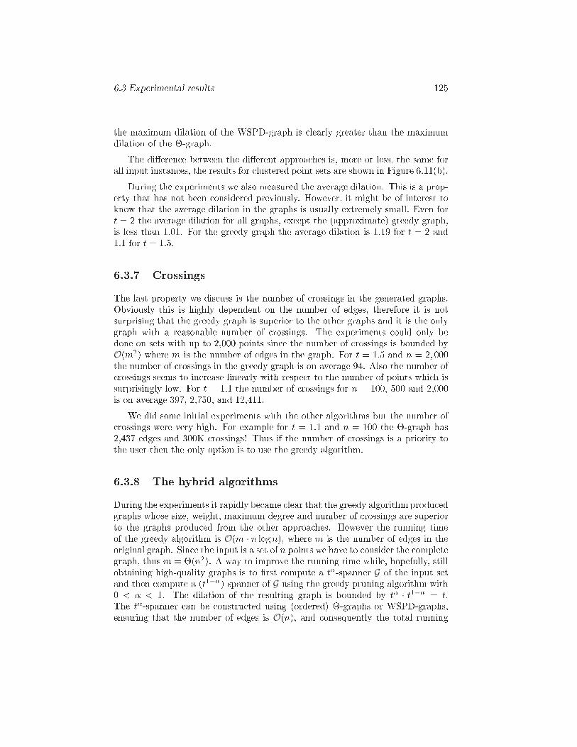
6.3 Experimental results 125the maximum dilation of the WSPD-graph is learly greater than the maximumdilation of the �-graph.The di�eren e between the di�erent approa hes is, more or less, the same forall input instan es, the results for lustered point sets are shown in Figure 6.11(b).During the experiments we also measured the average dilation. This is a prop-erty that has not been onsidered previously. However, it might be of interest toknow that the average dilation in the graphs is usually extremely small. Even fort = 2 the average dilation for all graphs, ex ept the (approximate) greedy graph,is less than 1.01. For the greedy graph the average dilation is 1.19 for t = 2 and1.1 for t = 1:5.6.3.7 CrossingsThe last property we dis uss is the number of rossings in the generated graphs.Obviously this is highly dependent on the number of edges, therefore it is notsurprising that the greedy graph is superior to the other graphs and it is the onlygraph with a reasonable number of rossings. The experiments ould only bedone on sets with up to 2,000 points sin e the number of rossings is bounded byO(m2) where m is the number of edges in the graph. For t = 1:5 and n = 2; 000the number of rossings in the greedy graph is on average 94. Also the number of rossings seems to in rease linearly with respe t to the number of points whi h issurprisingly low. For t = 1:1 the number of rossings for n = 100, 500 and 2,000is on average 397, 2,750, and 12,411.We did some initial experiments with the other algorithms but the number of rossings were very high. For example for t = 1:1 and n = 100 the �-graph has2,437 edges and 300K rossings! Thus if the number of rossings is a priority tothe user then the only option is to use the greedy algorithm.6.3.8 The hybrid algorithmsDuring the experiments it rapidly be ame lear that the greedy algorithm produ edgraphs whose size, weight, maximum degree and number of rossings are superiorto the graphs produ ed from the other approa hes. However the running timeof the greedy algorithm is O(m · n logn), where m is the number of edges in theoriginal graph. Sin e the input is a set of n points we have to onsider the ompletegraph, thus m = �(n2). A way to improve the running time while, hopefully, stillobtaining high-quality graphs is to �rst ompute a t�-spanner G of the input setand then ompute a (t1−�)-spanner of G using the greedy pruning algorithm with0 < � < 1. The dilation of the resulting graph is bounded by t� · t1−� = t.The t�-spanner an be onstru ted using (ordered) �-graphs or WSPD-graphs,ensuring that the number of edges is O(n), and onsequently the total running

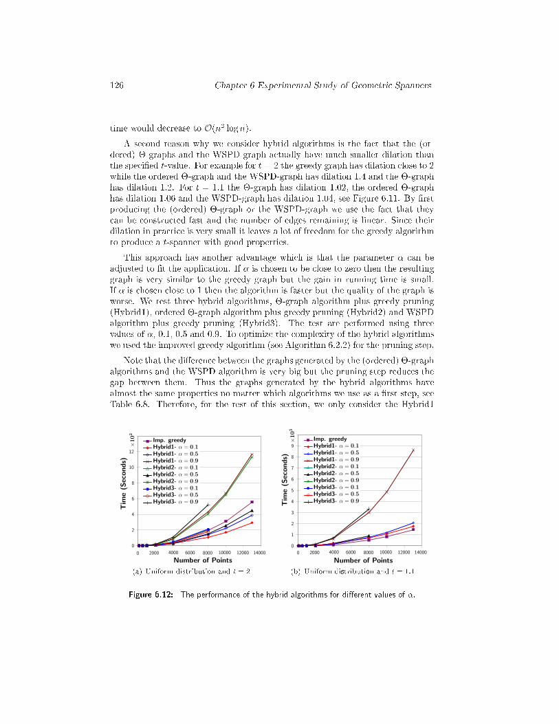
126 Chapter 6 Experimental Study of Geometri Spannerstime would de rease to O(n2 logn).A se ond reason why we onsider hybrid algorithms is the fa t that the (or-dered) �-graphs and the WSPD-graph a tually have mu h smaller dilation thanthe spe i�ed t-value. For example for t = 2 the greedy graph has dilation lose to 2while the ordered �-graph and the WSPD-graph has dilation 1.4 and the �-graphhas dilation 1.2. For t = 1:1 the �-graph has dilation 1.02, the ordered �-graphhas dilation 1.06 and the WSPD-graph has dilation 1.04, see Figure 6.11. By �rstprodu ing the (ordered) �-graph or the WSPD-graph we use the fa t that they an be onstru ted fast and the number of edges remaining is linear. Sin e theirdilation in pra ti e is very small it leaves a lot of freedom for the greedy algorithmto produ e a t-spanner with good properties.This approa h has another advantage whi h is that the parameter � an beadjusted to �t the appli ation. If � is hosen to be lose to zero then the resultinggraph is very similar to the greedy graph but the gain in running time is small.If � is hosen lose to 1 then the algorithm is faster but the quality of the graph isworse. We test three hybrid algorithms, �-graph algorithm plus greedy pruning(Hybrid1), ordered �-graph algorithm plus greedy pruning (Hybrid2) and WSPDalgorithm plus greedy pruning (Hybrid3). The test are performed using threevalues of �, 0.1, 0.5 and 0.9. To optimize the omplexity of the hybrid algorithmswe used the improved greedy algorithm (see Algorithm 6.2.2) for the pruning step.Note that the di�eren e between the graphs generated by the (ordered) �-graphalgorithms and the WSPD algorithm is very big but the pruning step redu es thegap between them. Thus the graphs generated by the hybrid algorithms havealmost the same properties no matter whi h algorithms we use as a �rst step, seeTable 6.8. Therefore, for the rest of this se tion, we only onsider the Hybrid1

0

2

4

6

8

10

12

×10

2

Number of Points

Tim

e(S

eco

nds)

Imp. greedyHybrid1- α = 0.1

Hybrid1- α = 0.5

Hybrid1- α = 0.9

Hybrid2- α = 0.1

Hybrid2- α = 0.5

Hybrid2- α = 0.9

Hybrid3- α = 0.1

Hybrid3- α = 0.5

Hybrid3- α = 0.9

0 140002000 4000 6000 8000 10000 12000(a) Uniform distribution and t = 2 0

1

2

3

4

5

6

7

8

9

×10

3

Number of Points

Tim

e(S

eco

nds)

Imp. greedyHybrid1- α = 0.1

Hybrid1- α = 0.5

Hybrid1- α = 0.9

Hybrid2- α = 0.1

Hybrid2- α = 0.5

Hybrid2- α = 0.9

Hybrid3- α = 0.1

Hybrid3- α = 0.5

Hybrid3- α = 0.9

0 140002000 4000 6000 8000 10000 12000(b) Uniform distribution and t = 1:1Figure 6.12: The performan e of the hybrid algorithms for di�erent values of �.

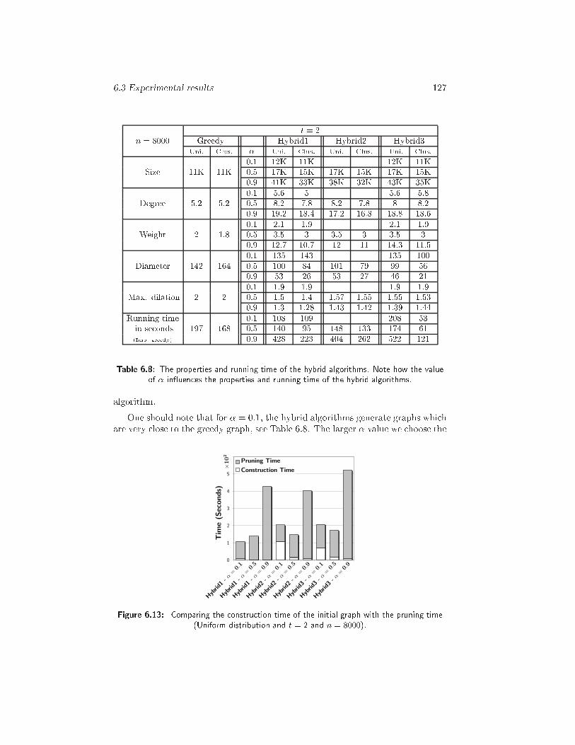
6.3 Experimental results 127t = 2n = 8000 Greedy Hybrid1 Hybrid2 Hybrid3Uni. Clus. � Uni. Clus. Uni. Clus. Uni. Clus.0:1 12K 11K 12K 11KSize 11K 11K 0:5 17K 15K 17K 15K 17K 15K0:9 41K 33K 38K 32K 43K 35K0:1 5.6 5 5.6 5.8Degree 5.2 5.2 0:5 8.2 7.8 8.2 7.8 8 8.20:9 19.2 18.4 17.2 16.8 18.8 18.60:1 2.1 1.9 2.1 1.9Weight 2 1.8 0:5 3.5 3 3.5 3 3.5 30:9 12.7 10.7 12 11 14.3 11.50:1 135 143 135 100Diameter 142 164 0:5 100 84 101 79 99 560:9 53 26 53 27 46 210:1 1.9 1.9 1.9 1.9Max. dilation 2 2 0:5 1.5 1.4 1.57 1.55 1.55 1.530:9 1.3 1.28 1.43 1.42 1.39 1.44Running time 0:1 108 109 208 53in se onds 197 168 0:5 140 95 148 133 174 61(Imp. greedy) 0:9 428 223 404 262 522 121Table 6.8: The properties and running time of the hybrid algorithms. Note how the valueof � in uen es the properties and running time of the hybrid algorithms.algorithm.One should note that for � = 0:1, the hybrid algorithms generate graphs whi hare very lose to the greedy graph, see Table 6.8. The larger � value we hoose the0

1

2

3

4

5

Hybrid

1-α

=

0.1

×10

2

Tim

e(S

eco

nds)

Pruning Time

Construction Time

Hybrid

1-α

=

0.5

Hybrid

1-α

=

0.9

Hybrid

2-α

=

0.1

Hybrid

2-α

=

0.5

Hybrid

2-α

=

0.9

Hybrid

3-α

=

0.1

Hybrid

3-α

=

0.5

Hybrid

3-α

=

0.9Figure 6.13: Comparing the onstru tion time of the initial graph with the pruning time(Uniform distribution and t = 2 and n = 8000).

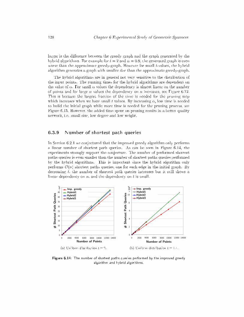
128 Chapter 6 Experimental Study of Geometri Spannerslarger is the di�eren e between the greedy graph and the graph generated by thehybrid algorithms. For example for t = 2 and � = 0:9, the generated graph is evenworse than the approximate greedy-graph. However for small t-values, the hybridalgorithm generates a graph with smaller size than the approximate greedy-graph.The hybrid algorithms are in general not very sensitive to the distribution ofthe input points. The running times for the hybrid algorithms are dependent onthe value of �. For small � values the dependen y is almost linear on the numberof points and for large � values the dependen y on n in reases, see Figure 6.12.This is be ause the largest fra tion of the time is needed for the pruning stepwhi h in reases when we have small t values. By in reasing �, less time is neededto build the initial graph while more time is needed for the pruning pro ess, seeFigure 6.13. However, the added time spent on pruning results in a better qualitynetwork, i.e. small size, low degree and low weight.6.3.9 Number of shortest path queriesIn Se tion 6.2.1 we onje tured that the improved greedy algorithm only performsa linear number of shortest path queries. As an be seen in Figure 6.14, theexperiments strongly support the onje ture. The number of performed shortestpaths queries is even smaller than the number of shortest paths queries performedby the hybrid algorithms. This is important sin e the hybrid algorithm onlyperforms O(n) shortest paths queries, one for ea h edge in the initial graph. Byde reasing t, the number of shortest path queries in reases but it still shows alinear dependen y on n, and the dependen y on t is small.0

5

10

15

20

25

30

35

40

45

×10

3

Number of Points

#Short

est

Path

Queries

Imp. greedy

Hybrid2Hybrid3

0 2000 4000 6000 8000 10000 12000

Hybrid1

14000(a) Uniform distribution t = 2. 0

2

4

6

8

10

×10

4

Number of Points

#Short

est

Path

Queries

Imp. greedy

Hybrid1Hybrid2Hybrid3

0 2000 4000 6000 8000 10000 12000 14000(b) Uniform distribution t = 1:1.Figure 6.14: The number of shortest paths queries performed by the improved greedyalgorithm and hybrid algorithms.

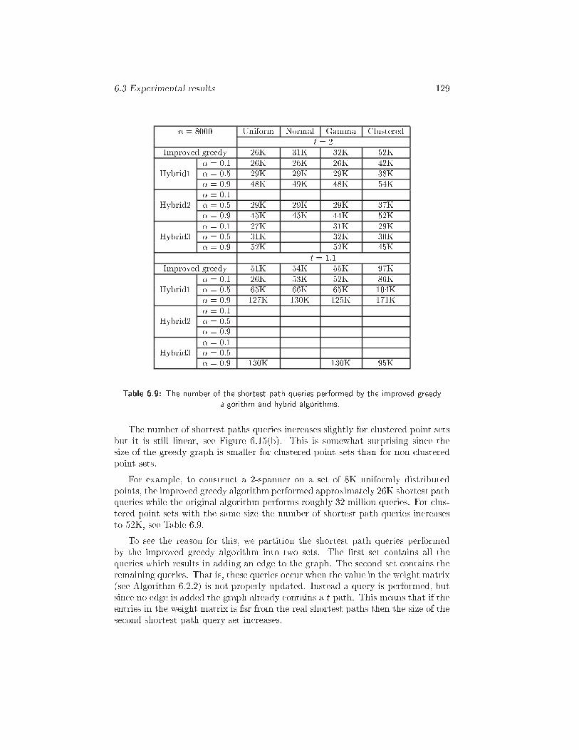
6.3 Experimental results 129n = 8000 Uniform Normal Gamma Clusteredt = 2Improved greedy 26K 31K 32K 52K� = 0:1 26K 26K 26K 42KHybrid1 � = 0:5 29K 29K 29K 38K� = 0:9 48K 49K 48K 54K� = 0:1Hybrid2 � = 0:5 29K 29K 29K 37K� = 0:9 45K 45K 44K 52K� = 0:1 27K 31K 29KHybrid3 � = 0:5 31K 32K 30K� = 0:9 52K 52K 45Kt = 1:1Improved greedy 51K 54K 55K 97K� = 0:1 26K 53K 52K 86KHybrid1 � = 0:5 65K 66K 65K 104K� = 0:9 127K 130K 125K 171K� = 0:1Hybrid2 � = 0:5� = 0:9� = 0:1Hybrid3 � = 0:5� = 0:9 130K 130K 95KTable 6.9: The number of the shortest path queries performed by the improved greedyalgorithm and hybrid algorithms.The number of shortest paths queries in reases slightly for lustered point setsbut it is still linear, see Figure 6.15(b). This is somewhat surprising sin e thesize of the greedy graph is smaller for lustered point sets than for non- lusteredpoint sets.For example, to onstru t a 2-spanner on a set of 8K uniformly distributedpoints, the improved greedy algorithm performed approximately 26K shortest pathqueries while the original algorithm performs roughly 32 million queries. For lus-tered point sets with the same size the number of shortest path queries in reasesto 52K, see Table 6.9.To see the reason for this, we partition the shortest path queries performedby the improved greedy algorithm into two sets. The �rst set ontains all thequeries whi h results in adding an edge to the graph. The se ond set ontains theremaining queries. That is, these queries o ur when the value in the weight matrix(see Algorithm 6.2.2) is not properly updated. Instead a query is performed, butsin e no edge is added the graph already ontains a t-path. This means that if theentries in the weight matrix is far from the real shortest paths then the size of these ond shortest path query set in reases.

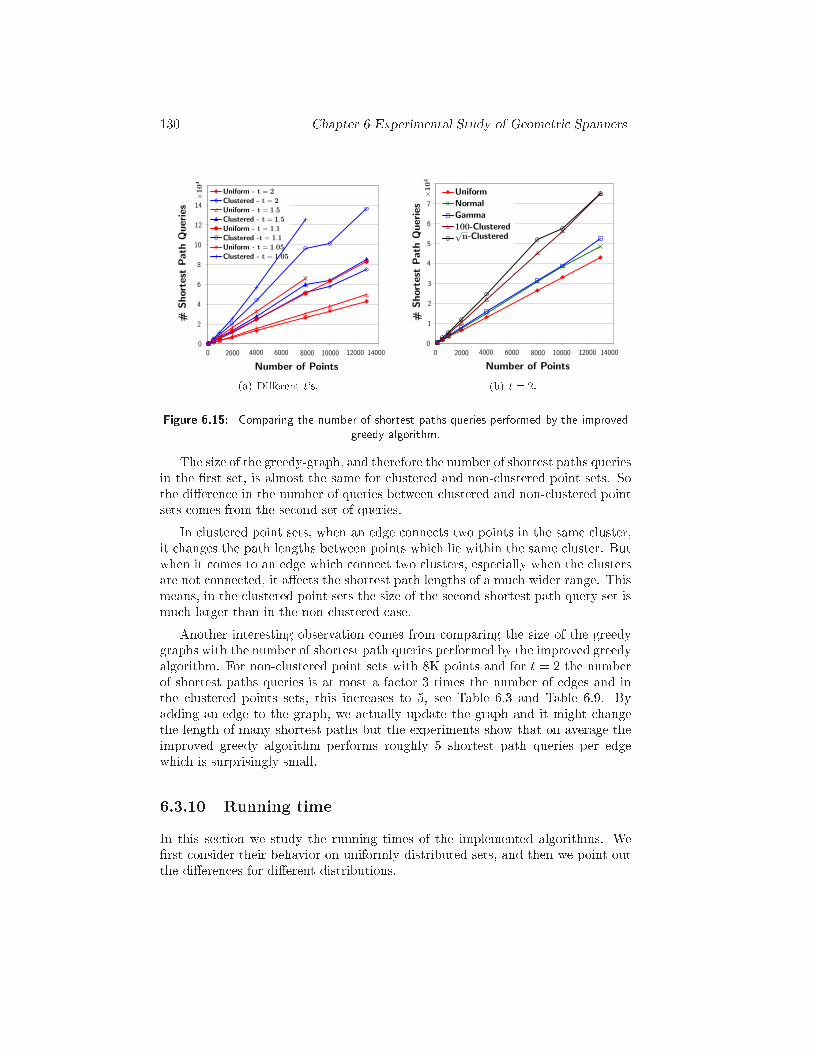
130 Chapter 6 Experimental Study of Geometri Spanners

0

2

4

6

8

10

12

14×

10

4

Number of Points

#Short

est

Path

Queries

Uniform - t = 2

Clustered - t = 2

Uniform - t = 1.5

Clustered - t = 1.5

Uniform - t = 1.1

Clustered -t = 1.1

Uniform - t = 1.05

Clustered - t = 1.05

0 2000 4000 6000 8000 10000 12000 14000(a) Di�erent t's. 0

1

2

3

4

5

6

7

×10

4

Number of Points

#Short

est

Path

Queries

Uniform

Normal

Gamma

100-Clustered√n-Clustered

0 2000 4000 6000 8000 10000 12000 14000(b) t = 2.Figure 6.15: Comparing the number of shortest paths queries performed by the improvedgreedy algorithm.The size of the greedy-graph, and therefore the number of shortest paths queriesin the �rst set, is almost the same for lustered and non- lustered point sets. Sothe di�eren e in the number of queries between lustered and non- lustered pointsets omes from the se ond set of queries.In lustered point sets, when an edge onne ts two points in the same luster,it hanges the path lengths between points whi h lie within the same luster. Butwhen it omes to an edge whi h onne t two lusters, espe ially when the lustersare not onne ted, it a�e ts the shortest path lengths of a mu h wider range. Thismeans, in the lustered point sets the size of the se ond shortest path query set ismu h larger than in the non- lustered ase.Another interesting observation omes from omparing the size of the greedygraphs with the number of shortest path queries performed by the improved greedyalgorithm. For non- lustered point sets with 8K points and for t = 2 the numberof shortest paths queries is at most a fa tor 3 times the number of edges and inthe lustered points sets, this in reases to 5, see Table 6.3 and Table 6.9. Byadding an edge to the graph, we a tually update the graph and it might hangethe length of many shortest paths but the experiments show that on average theimproved greedy algorithm performs roughly 5 shortest path queries per edgewhi h is surprisingly small.6.3.10 Running timeIn this se tion we study the running times of the implemented algorithms. We�rst onsider their behavior on uniformly distributed sets, and then we point outthe di�eren es for di�erent distributions.

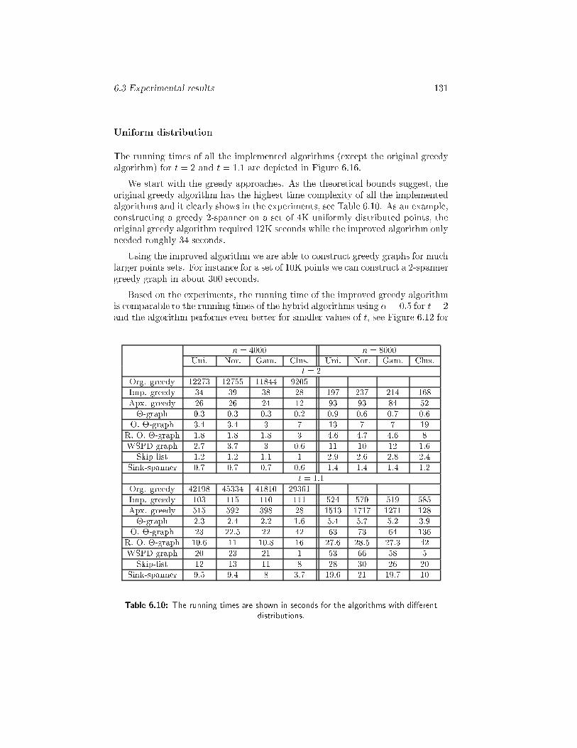
6.3 Experimental results 131Uniform distributionThe running times of all the implemented algorithms (ex ept the original greedyalgorithm) for t = 2 and t = 1:1 are depi ted in Figure 6.16.We start with the greedy approa hes. As the theoreti al bounds suggest, theoriginal greedy algorithm has the highest time omplexity of all the implementedalgorithms and it learly shows in the experiments, see Table 6.10. As an example, onstru ting a greedy 2-spanner on a set of 4K uniformly distributed points, theoriginal greedy algorithm required 12K se onds while the improved algorithm onlyneeded roughly 34 se onds.Using the improved algorithm we are able to onstru t greedy graphs for mu hlarger points sets. For instan e for a set of 10K points we an onstru t a 2-spannergreedy graph in about 300 se onds.Based on the experiments, the running time of the improved greedy algorithmis omparable to the running times of the hybrid algorithms using � = 0:5 for t = 2and the algorithm performs even better for smaller values of t, see Figure 6.12 forn = 4000 n = 8000Uni. Nor. Gam. Clus. Uni. Nor. Gam. Clus.t = 2Org. greedy 12273 12755 11844 9205Imp. greedy 34 39 38 28 197 237 214 168Apx. greedy 26 26 24 12 93 93 84 52�-graph 0.3 0.3 0.3 0.2 0.9 0.6 0.7 0.6O. �-graph 3.4 3.4 3 7 13 7 7 19R. O. �-graph 1.8 1.8 1.8 3 4.6 4.7 4.6 8WSPD-graph 2.7 3.7 3 0.6 11 10 12 1.6Skip-list 1.2 1.2 1.1 1 2.9 2.6 2.8 2.4Sink-spanner 0.7 0.7 0.7 0.6 1.4 1.4 1.4 1.2t = 1:1Org. greedy 42198 45334 41810 29361Imp. greedy 103 115 110 111 524 570 519 585Apx. greedy 515 592 398 28 1513 1717 1271 128�-graph 2.3 2.4 2.2 1.6 5.4 5.7 5.2 3.9O. �-graph 23 22.5 22 42 63 73 64 136R. O. �-graph 10.6 11 10.8 16 27.6 28.5 27.3 42WSPD-graph 20 23 21 1 53 66 58 5Skip-list 12 13 11 8 28 30 26 20Sink-spanner 9.5 9.4 8 3.7 19.6 21 19.7 10Table 6.10: The running times are shown in se onds for the algorithms with di�erentdistributions.

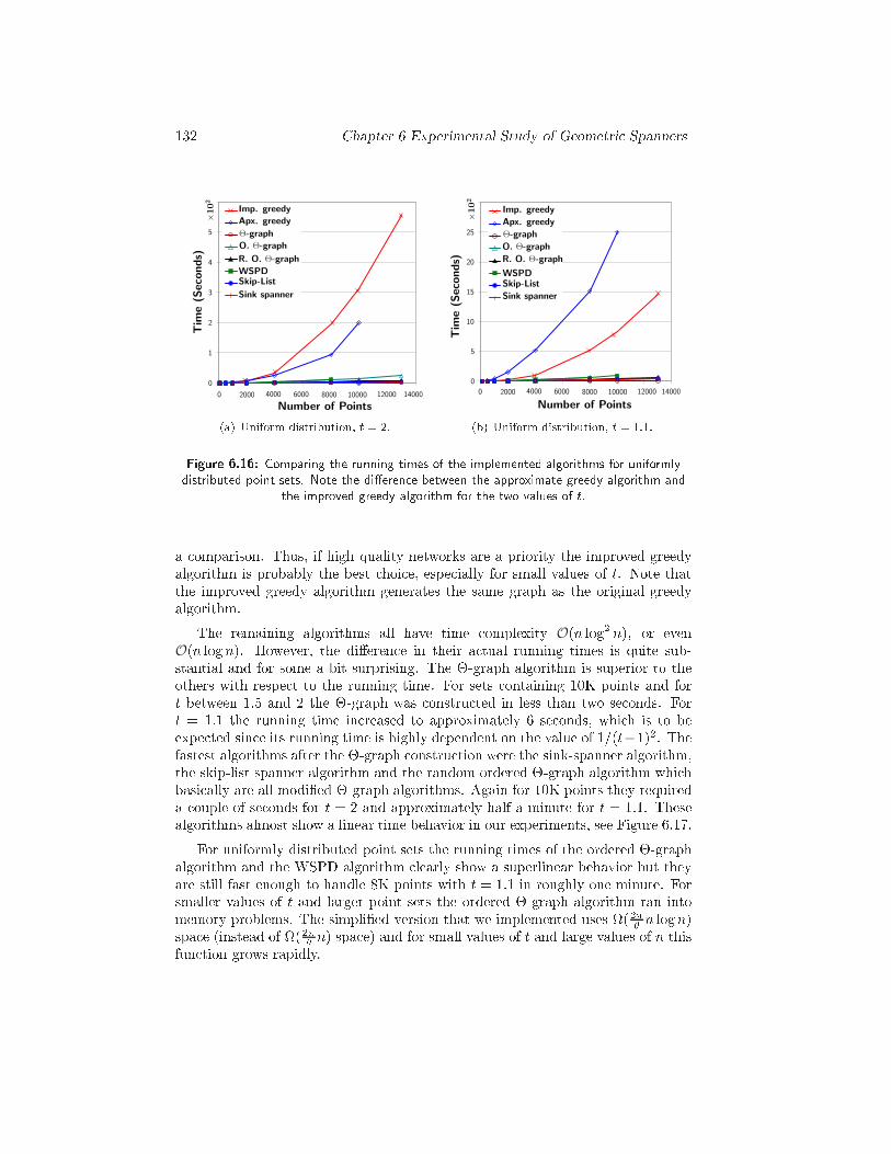
132 Chapter 6 Experimental Study of Geometri Spanners

0

1

2

3

4

5

×10

2

Number of Points

Tim

e(S

eco

nds)

Imp. greedy

Apx. greedy

Θ-graph

O. Θ-graph

R. O. Θ-graph

WSPDSkip-List

Sink spanner

0 2000 4000 6000 8000 10000 12000 14000(a) Uniform distribution, t = 2. 0

5

10

15

20

25

×10

2

Number of Points

Tim

e(S

eco

nds)

Imp. greedy

Apx. greedy

Θ-graph

O. Θ-graph

R. O. Θ-graph

WSPDSkip-List

Sink spanner

0 2000 4000 6000 8000 10000 12000 14000(b) Uniform distribution, t = 1:1.Figure 6.16: Comparing the running times of the implemented algorithms for uniformlydistributed point sets. Note the di�eren e between the approximate greedy algorithm andthe improved greedy algorithm for the two values of t.a omparison. Thus, if high quality networks are a priority the improved greedyalgorithm is probably the best hoi e, espe ially for small values of t. Note thatthe improved greedy algorithm generates the same graph as the original greedyalgorithm.The remaining algorithms all have time omplexity O(n log2 n), or evenO(n log n). However, the di�eren e in their a tual running times is quite sub-stantial and for some a bit surprising. The �-graph algorithm is superior to theothers with respe t to the running time. For sets ontaining 10K points and fort between 1.5 and 2 the �-graph was onstru ted in less than two se onds. Fort = 1:1 the running time in reased to approximately 6 se onds, whi h is to beexpe ted sin e its running time is highly dependent on the value of 1=(t−1)2. Thefastest algorithms after the �-graph onstru tion were the sink-spanner algorithm,the skip-list spanner algorithm and the random ordered �-graph algorithm whi hbasi ally are all modi�ed �-graph algorithms. Again for 10K points they requireda ouple of se onds for t = 2 and approximately half a minute for t = 1:1. Thesealgorithms almost show a linear time behavior in our experiments, see Figure 6.17.For uniformly distributed point sets the running times of the ordered �-graphalgorithm and the WSPD algorithm learly show a superlinear behavior but theyare still fast enough to handle 8K points with t = 1:1 in roughly one minute. Forsmaller values of t and larger point sets the ordered �-graph algorithm ran intomemory problems. The simpli�ed version that we implemented uses ( 2�� n logn)spa e (instead of ( 2�� n) spa e) and for small values of t and large values of n thisfun tion grows rapidly.

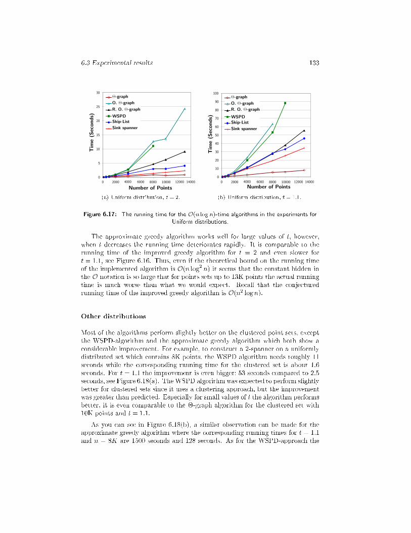
6.3 Experimental results 133

0

5

10

15

20

25

30

Number of Points

Tim

e(S

eco

nds)

Θ-graph

O. Θ-graph

R. O. Θ-graph

WSPDSkip-List

Sink spanner

0 2000 4000 6000 8000 10000 12000 14000(a) Uniform distribution, t = 2. 0

10

20

30

40

50

60

70

80

90

100

Number of Points

Tim

e(S

eco

nds)

Θ-graph

O. Θ-graph

R. O. Θ-graph

WSPDSkip-List

Sink spanner

0 2000 4000 6000 8000 10000 12000 14000(b) Uniform distribution, t = 1:1.Figure 6.17: The running time for the O(n log n)-time algorithms in the experiments forUniform distributions.The approximate greedy algorithm works well for large values of t, however,when t de reases the running time deteriorates rapidly. It is omparable to therunning time of the improved greedy algorithm for t = 2 and even slower fort = 1:1, see Figure 6.16. Thus, even if the theoreti al bound on the running timeof the implemented algorithm is O(n log2 n) it seems that the onstant hidden inthe O-notation is so large that for points sets up to 13K points the a tual runningtime is mu h worse than what we would expe t. Re all that the onje turedrunning time of the improved greedy algorithm is O(n2 logn).Other distributionsMost of the algorithms perform slightly better on the lustered point sets, ex eptthe WSPD-algorithm and the approximate greedy algorithm whi h both show a onsiderable improvement. For example, to onstru t a 2-spanner on a uniformlydistributed set whi h ontains 8K points, the WSPD algorithm needs roughly 11se onds while the orresponding running time for the lustered set is about 1.6se onds. For t = 1:1 the improvement is even bigger; 53 se onds ompared to 2.5se onds, see Figure 6.18(a). TheWSPD algorithmwas expe ted to perform slightlybetter for lustered sets sin e it uses a lustering approa h, but the improvementwas greater than predi ted. Espe ially for small values of t the algorithm performsbetter, it is even omparable to the �-graph algorithm for the lustered set with10K points and t = 1:1.As you an see in Figure 6.18(b), a similar observation an be made for theapproximate greedy algorithm where the orresponding running times for t = 1:1and n = 8K are 1500 se onds and 128 se onds. As for the WSPD-approa h the

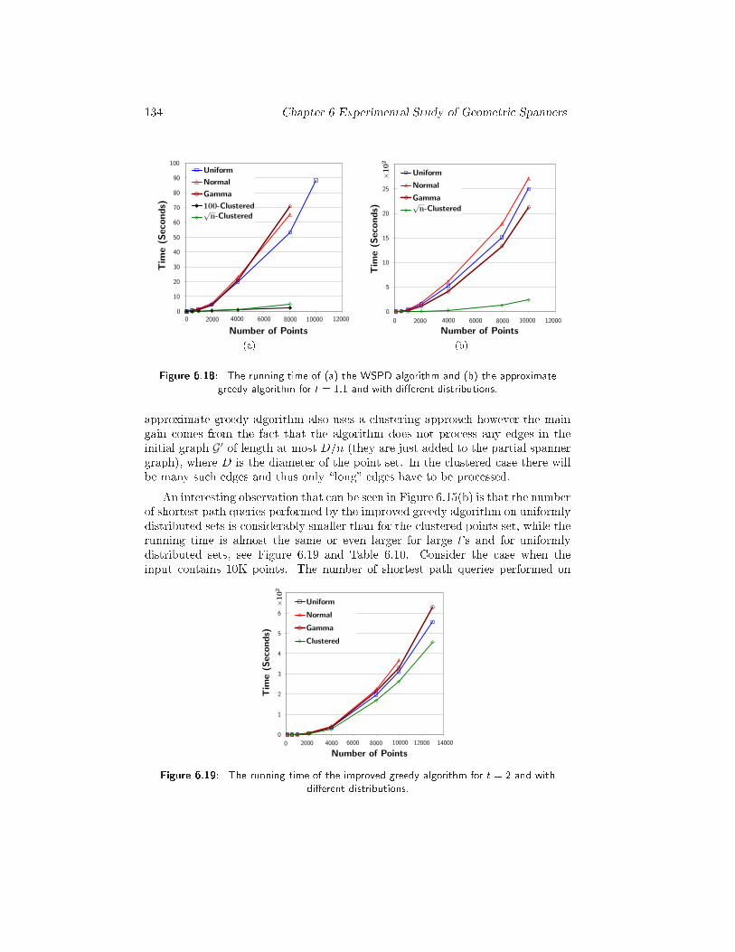
134 Chapter 6 Experimental Study of Geometri Spanners

0

10

20

30

40

50

60

70

80

90

100

Number of Points

Tim

e(S

eco

nds)

Uniform

Normal

Gamma

100-Clustered√

n-Clustered

0 2000 4000 6000 8000 10000 12000(a) 0

5

10

15

20

25

×10

2

Number of Points

Tim

e(S

eco

nds)

Uniform

Normal

Gamma√

n-Clustered

0 2000 4000 6000 8000 10000 12000(b)Figure 6.18: The running time of (a) the WSPD algorithm and (b) the approximategreedy algorithm for t = 1:1 and with di�erent distributions.approximate greedy algorithm also uses a lustering approa h however the maingain omes from the fa t that the algorithm does not pro ess any edges in theinitial graph G′ of length at most D=n (they are just added to the partial spannergraph), where D is the diameter of the point set. In the lustered ase there willbe many su h edges and thus only \long" edges have to be pro essed.An interesting observation that an be seen in Figure 6.15(b) is that the numberof shortest path queries performed by the improved greedy algorithm on uniformlydistributed sets is onsiderably smaller than for the lustered points set, while therunning time is almost the same or even larger for large t's and for uniformlydistributed sets, see Figure 6.19 and Table 6.10. Consider the ase when theinput ontains 10K points. The number of shortest path queries performed on0

1

2

3

4

5

6

×10

2

Number of Points

Tim

e(S

eco

nds)

Uniform

Normal

Gamma

Clustered

0 140002000 4000 6000 8000 10000 12000Figure 6.19: The running time of the improved greedy algorithm for t = 2 and withdi�erent distributions.

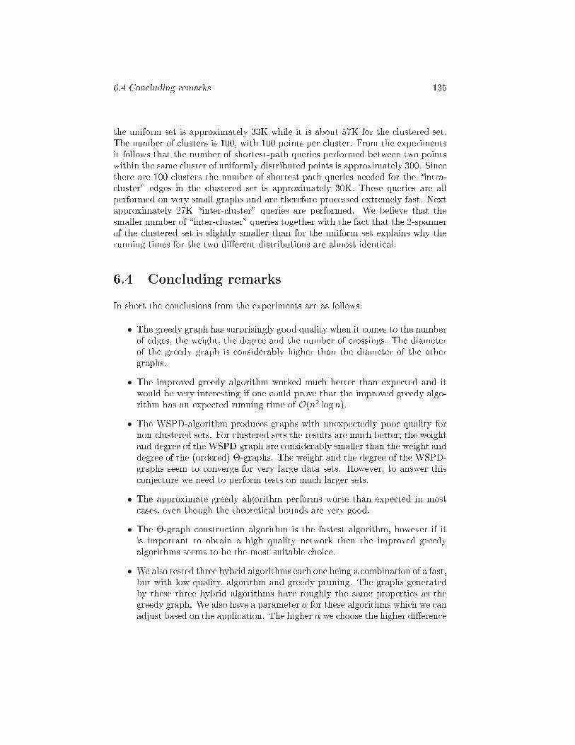
6.4 Con luding remarks 135the uniform set is approximately 33K while it is about 57K for the lustered set.The number of lusters is 100, with 100 points per luster. From the experimentsit follows that the number of shortest-path queries performed between two pointswithin the same luster of uniformly distributed points is approximately 300. Sin ethere are 100 lusters the number of shortest path queries needed for the \intra- luster" edges in the lustered set is approximately 30K. These queries are allperformed on very small graphs and are therefore pro essed extremely fast. Nextapproximately 27K \inter- luster" queries are performed. We believe that thesmaller number of \inter- luster" queries together with the fa t that the 2-spannerof the lustered set is slightly smaller than for the uniform set explains why therunning times for the two di�erent distributions are almost identi al.6.4 Con luding remarksIn short the on lusions from the experiments are as follows:• The greedy graph has surprisingly good quality when it omes to the numberof edges, the weight, the degree and the number of rossings. The diameterof the greedy graph is onsiderably higher than the diameter of the othergraphs.• The improved greedy algorithm worked mu h better than expe ted and itwould be very interesting if one ould prove that the improved greedy algo-rithm has an expe ted running time of O(n2 logn).• The WSPD-algorithm produ es graphs with unexpe tedly poor quality fornon- lustered sets. For lustered sets the results are mu h better; the weightand degree of the WSPD-graph are onsiderably smaller than the weight anddegree of the (ordered) �-graphs. The weight and the degree of the WSPD-graphs seem to onverge for very large data sets. However, to answer this onje ture we need to perform tests on mu h larger sets.• The approximate greedy algorithm performs worse than expe ted in most ases, even though the theoreti al bounds are very good.• The �-graph onstru tion algorithm is the fastest algorithm, however if itis important to obtain a high quality network then the improved greedyalgorithms seems to be the most suitable hoi e.• We also tested three hybrid algorithms ea h one being a ombination of a fast,but with low quality, algorithm and greedy pruning. The graphs generatedby these three hybrid algorithms have roughly the same properties as thegreedy graph. We also have a parameter � for these algorithms whi h we anadjust based on the appli ation. The higher � we hoose the higher di�eren e

136 Chapter 6 Experimental Study of Geometri Spannersbetween the greedy graph and the graph generated by hybrid algorithms butlower time to onstru t the spanner.The main question that remains to be answered experimentally is the depen-den y on the number of dimensions, i.e. how the algorithms and the quality ofthe produ ed graphs depends on the number of dimensions. Also it is interestingto improve the running time of the improved greedy algorithm. We an obtain animprovement by using algorithms whi h perform shortest path queries faster. Soone parameter whi h ould be used to measure the eÆ ien y of all the algorithmsis the number of shortest path queries performed by an algorithm.The experiments show that the weight of the �-graph is very small for non- lustered sets. Proving, or disproving, that the expe ted weight of the �-graph issmall for uniform distributions is an interesting and hallenging open question.A knowledgementsWe would like to thank the anonymous reviewers for omments on an earlier versionof this hapter.

Chapter 7Con lusionsIn this thesis we on entrated on geometri spanner networks. The area attra ted alot of attention in past few years [Epp00, GK07, NS07, Smi00℄ and �nds appli ationin several bran hes like roboti s, network topology design, metri spa e sear hingand bioinformati s. Below we brie y dis uss the most important results from thethesis and the most interesting open problems that remain.One of the major issues in designing a network is reliability. Reliability is on erned with the fa t that in many appli ations the nodes and/or links in anetwork may fail. A network is reliable, or fault-tolerant, when it retains its goodproperties even after some nodes or links fail. With respe t to spanners this meansthere should still be a short path between any two nodes in what remains of thespanner after the fault. The problem of designing k-vertex (or: k-edge) fault-tolerant geometri spanners, faults that an destroy an arbitrary olle tion of kverti es or edges, was studied before [CZ03, LNS98, LNS02, Luk99℄. For geometri spanners, however, it is natural to onsider faults that destroy all verti es and edgesinterse ting some geometri fault region. This is relevant, for instan e, when thespanner models a road network and a natural (or other) disaster makes all theroads in some region ina essible.In Chapter 2 we introdu ed region-fault tolerant spanners and we proved thatany planar point set admits a sparse t-spanner, of near-linear size, whi h is faulttolerant under any onvex region fault; for several spe ial ases or by adding Steinerpoints we ould improve the size to linear. The main problem whi h remains openis whether one an improve the spanner size for arbitrary point sets to linear. Wealso onsidered fault-tolerant geodesi t-spanners: this is a variant where, for anydisk D, the distan e between any two points outside D in the remaining graph is

138 Chapter 7 Con lusionsat most t times the geodesi distan e between them in R2 \ D. We proved thatfor any point set we an add Steiner points to obtain a fault-tolerant geodesi t-spanner of linear size. It would be interesting to generalize the problem to the ase when we have urves as the edges in a network instead of lines. It would alsobe interesting to have a fast algorithm whi h he ks whether a given network isfault tolerant under any onvex region fault or not. Using a simple tri k we obtainan algorithm whi h in O(n5) time using O(n2) spa e an �nd the answer for anetwork with n verti es.Given a geometri network, natural questions to ask are how we an improvethe quality of the network by adding one or more edges. Similarly, one an askhow we an remove an edge from the network su h that the quality of the networkdoes not de rease too mu h. In the ase of extending the network, we studied theproblem of �nding the additional edge while maximizing the improvement, whi hin our ase means minimizing the dilation of the resulting graph. Chapters 3addressed the problem of optimal edge augmentation of a given geometri network.The main results are an exa t algorithm and several approximation algorithms.The main approximation algorithm �nds a (2 + ")-approximation of the optimaledge. A hallenging open problem is to improve the approximation fa tor of theapproximation algorithms to 1 + " with the same time omplexity. Also, is itpossible to �nd an exa t algorithm whi h solves the problem in o(n4) time usinglinear spa e?In Chapter 4 we onsidered the problem of �nding/de iding an optimal edgedeletion in a simple ase. We showed that given a polygonal y le in the plane,in near-linear expe ted time we an ompute the edge of the y le whose removalresults in a polygonal path of smallest possible dilation. It is also shown thatthe edge whose removal gives a polygonal path of largest possible dilation anbe omputed in near-linear time; when the y le is onvex then we an �nd theedge in linear time. Generalizing the results to more general Eu lidean graphs isa hallenging open problem.The spanner diameter of a t-spanner is the smallest integer D su h that forany pair of verti es, there is a t-path in the graph between them ontaining atmost D edges. As far as we know there is no known algorithm to ompute thespanner diameter of a t-spanner. In Chapter 5 we presented several algorithms,using a dynami programming approa h, for omputing the spanner diameter ofa given t-spanner. The fastest algorithm omputes the spanner diameter of at-spanner with n verti es and m edges in O(D ·mn) time using O(m + n) spa e,where D is the spanner diameter of the input network. The algorithms are purely ombinatorial and do not take advantage of the fa t that the graphs are embeddedin Eu lidean spa e. An interesting problem is to improve the omplexity boundsin the geometri ase.

139The empiri al study of algorithms is a rapidly growing resear h area. Imple-menting and doing experiments on algorithms shows their eÆ ien y in pra ti eand brings the algorithms to the pra ti al stage. In Chapter 6, we ompared themost well-known geometri t-spanner algorithms (in 2-dimension) experimentally.The experiments ompared the quality of the generated graphs, like size, weight,maximum degree and diameter as well as the running time. We showed that thegreedy algorithm generates graphs with surprisingly good quality when it omesto the number of edges, the weight, the degree and the number of rossings. How-ever, the greedy algorithm is very slow; we gave several speedup strategies for thegreedy algorithm. The �-graph algorithm is the fastest algorithm for onstru tingt-spanners. The major open problem is to investigate the e�e t of the number ofdimensions on the quality of the graphs and the running time of the algorithms.

140 Chapter 7 Con lusions

Referen es[AdBFG07℄ Mohammad Ali Abam, Mark de Berg, Mohammad Farshi, andJoa him Gudmundsson. Region-fault tolerant geometri spanners.In SODA '07: Pro eedings of the Annual ACM-SIAM Symposiumon Dis rete Algorithms, pages 1{10, 2007.[ADD+93℄ Ingo Alth�ofer, Gautam Das, David P. Dobkin, Deborah Joseph, andJos�e Soares. On sparse spanners of weighted graphs. Dis rete andComputational Geometry, 9(1):81{100, 1993.[ADM+95℄ Sunil Arya, Gautam Das, David M. Mount, Je�rey S. Salowe, andMi hiel Smid. Eu lidean spanners: short, thin, and lanky. InSTOC '95: Pro eedings of the 27th Annual ACM Symposium onTheory of Computing, pages 489{498, 1995.[AFK+07℄ Hee-Kap Ahn, Mohammad Farshi, Christian Knauer, Mi heil Smid,and Yajun Wang. Dilation-optimal edge deletion in polygonal y les.In ISAAC '07: Pro eedings of the 18th International Symposium onAlgorithms and Computation, volume 4835 of Le ture Notes in Com-puter S ien e, pages 88{99. Springer-Verlag, 2007.[AGSS89℄ Alok Aggarwal, Leonidas J. Guibas, James Saxe, and Peter W. Shor.A linear-time algorithm for omputing the Voronoi diagram of a onvex polygon. Dis rete and Computational Geometry, 4:591{604,1989.[AKK+℄ Pankaj K. Agarwal, Rolf Klein, Christian Knauer, Stefan Langer-man, Pat Morin, Mi ha Sharir, and Mi hael Soss. Computing thedetour and spanning ratio of paths, trees and y les in 2D and 3D.Dis rete and Computational Geometry. to appear.141

142 Referen es[ALW+03℄ Khaled M. Alzoubi, Xiang-Yang Li, Yu Wang, Peng-Jun Wan, andOphir Frieder. Geometri spanners for wireless ad ho networks.IEEE Transa tions on Parallel and Distributed Systems, 14(5):1{14,2003.[AMS99℄ Sunil Arya, David M. Mount, and Mi hiel Smid. Dynami algorithmsfor geometri spanners of small diameter: Randomized solutions.Computational Geometry: Theory and Appli ations, 13(2):91{107,1999.[BGM04℄ Prosenjit Bose, Joa him Gudmundsson, and Pat Morin. Orderedtheta graphs. Computational Geometry: Theory and Appli ations,28:11{18, 2004.[Cal95℄ Paul B. Callahan. Dealing with higher dimensions: the well-separatedpair de omposition and its appli ations. Ph.D. thesis, Department ofComputer S ien e, Johns Hopkins University, Baltimore, Maryland,1995.[CDNS95℄ Barun Chandra, Gautam Das, Giri Narasimhan, and Jos�e Soares.New sparseness results on graph spanners. International Journal ofComputational Geometry and Appli ations, 5:124{144, 1995.[Cha94℄ Barun Chandra. Constru ting sparse spanners for most graphs inhigher dimensions. Information Pro essing Letters, 51(6):289{294,1994.[Che86℄ L. Paul Chew. There is a planar graph almost as good as the ompletegraph. In SCG '86: Pro eedings of the 2nd Annual ACM Symposiumon Computational Geometry, pages 169{177, 1986.[CHL07℄ Otfried Cheong, Herman Haverkort, and Mira Lee. Computing aminimum-dilation spanning tree is NP-hard. In CATS '07: Pro eed-ings of the 19th Computing: The Australasian Theory Symposium,pages 15{24. CRPIT, 2007.[CK93℄ Paul B. Callahan and S. Rao Kosaraju. Faster algorithms for somegeometri graph problems in higher dimensions. In SODA '93: Pro- eedings of the 4th Annual ACM-SIAM Symposium on Dis rete Al-gorithms, pages 291{300, Philadelphia, PA, USA, 1993.[CK95℄ Paul B. Callahan and S. Rao Kosaraju. A de omposition of multi-dimensional point sets with appli ations to k-nearest-neighbors andn-body potential �elds. Journal of the ACM, 42:67{90, 1995.[CL00℄ Artur Czumaj and Andrzej Lingas. Fast approximation s hemes forEu lidean multi- onne tivity problems. In ICALP '00: Pro eedings

Referen es 143of the 27th International Colloquium on Automata, Languages andProgramming, volume 1853 of Le ture Notes in Computer S ien e,pages 856{868. Springer-Verlag, 2000.[Cla87℄ Kenneth L. Clarkson. Approximation algorithms for shortest pathmotion planning. In STOC '87: Pro eedings of the 19th Annual ACMSymposium on Theory of Computing, pages 56{65, 1987.[CNBYM01℄ Edgar Ch�avez, Gonzalo Navarro, Ri ardo Baeza-Yates, and Jos�e LuisMarroqu��n. Sear hing in metri spa es. ACM Computing Surveys,33(3):273{321, 2001.[CS88℄ Kenneth L. Clarkson and Peter W. Shor. Algorithms for diametralpairs and onvex hulls that are optimal, randomized, and in remen-tal. In SCG '88: Pro eedings of the 4th Annual ACM Symposium onComputational Geometry, pages 12{17, New York, NY, USA, 1988.ACM Press.[CZ03℄ Artur Czumaj and Hairong Zhao. Fault-tolerant geometri spanners.In SCG '03: Pro eedings of the 19th Annual ACM Symposium onComputational Geometry, pages 1{10, New York, NY, USA, 2003.ACM Press.[Dav05℄ Robert B. Davis. http://www.robertnz.net/nr03do .htm, 2005.[DDS92℄ Matthew T. Di kerson, R. L. S ot Drysdale, and J�org-R�udiger Sa k.Simple algorithms for enumerating interpoint distan es and �nding knearest neighbors. International Journal of Computational Geometryand Appli ations, 2:221{239, 1992.[DGK01℄ Christian A. Dun an, Mi hael T. Goodri h, and Stephen Kobourov.Balan ed aspe t ratio trees: Combining the advan es of k-d treesand o trees. Journal of Algorithms, 38:303{333, 2001.[DHN93℄ Gautam Das, Paul J. He�ernan, and Giri Narasimhan. Optimallysparse spanners in 3-dimensional Eu lidean spa e. In SCG '93: Pro- eedings of the 9th Annual ACM Symposium on Computational Ge-ometry, pages 53{62, 1993.[DN97℄ Gautam Das and Giri Narasimhan. A fast algorithm for onstru tingsparse Eu lidean spanners. International Journal of ComputationalGeometry and Appli ations, 7:297{315, 1997.[DNS95℄ Gautam Das, Giri Narasimhan, and Jos�e Salowe. A new way toweigh malnourished Eu lidean graphs. In SODA '95: Pro eedingsof the 6th Annual ACM-SIAM Symposium on Dis rete Algorithms,pages 215{222, 1995.

144 Referen es[EP04℄ Mi hael Elkin and David Peleg. (1 + �; �)-spanner onstru tions forgeneral graphs. SIAM Journal on Computing, 33:608{631, 2004.[Epp00℄ David Eppstein. Spanning trees and spanners. In J.-R. Sa k andJ. Urrutia, editors, Handbook of Computational Geometry, pages425{461. Elsevier S ien e Publishers, Amsterdam, 2000.[Eri01℄ Je� Eri kson. Ni e point sets an have nasty Delaunay triangula-tions. In SCG'01: Pro eedings of the 7th Annual ACM Symposiumon Computational Geometry, pages 96{105, New York, NY, USA,2001. ACM Press.[EW07℄ David Eppstein and Kevin A. Wortman. Minimum dilation stars.Computational Geometry: Theory and Appli ations, 37(1):27{37,2007.[FG05℄ Mohammad Farshi and Joa him Gudmundsson. Experimental studyof geometri t-spanners. In ESA '05: Pro eedings of the 13th AnnualEuropean Symposium on Algorithms, volume 3669 of Le ture Notesin Computer S ien e, pages 556{567. Springer-Verlag, 2005.[FG06℄ Mohammad Farshi and Joa him Gudmundsson. On algorithms for omputing the diameter of a t-spanner. In AIMC 37: Pro eedingsof the 37th Annual Iranian Mathemati s Conferen e, pages 638{641,2006.[FG07℄ Mohammad Farshi and Joa him Gudmundsson. Experimental studyof geometri t-spanners: A running time omparison. In WEA '07:Pro eedings of the 6th Workshop on Experimental Algorithms, vol-ume 4525 of Le ture Notes in Computer S ien e, pages 270{284.Springer-Verlag, 2007.[FGG05a℄ Mohammad Farshi, Panos Giannopoulos, and Joa him Gudmunds-son. Finding the best short ut in a geometri network. In SCG '05:Pro eedings of the 21st Annual ACM Symposium on ComputationalGeometry, pages 327{335, New York, NY, USA, 2005. ACM Press.[FGG05b℄ Mohammad Farshi, Panos Giannopoulos, and Joa him Gudmunds-son. Finding the best short ut in a geometri network. In EWCG '05:Pro eedings of the 21st European Workshop on Computational Ge-ometry, pages 29{32, 2005.[FHP05℄ John Fis her and Sariel Har-Peled. Dynami well-separated pairde omposition made easy. In CCCG '05: Pro eedings of the 17thCanadian Conferen e on Computational Geometry, pages 235{238,2005.

Referen es 145[FKS84℄ Mi hael L. Fredman, Jan�os Koml�os, and Endre Szemer�edi. Storing asparse table with O(1) worst ase a ess time. Journal of the ACM,31:538{544, 1984.[For87℄ Steven J. Fortune. A sweepline algorithm for Voronoi diagrams.Algorithmi a, 2:153{174, 1987.[FPZW04℄ Arthur M. Farley, Andrzej Proskurowski, Daniel Zappala, andKurt J. Windis h. Spanners and message distribution in networks.Dis rete Applied Mathemati s, 137(2):159{171, 2004.[FR02℄ Stefan Funke and Edgar A. Ramos. Smooth-surfa e re onstru tionin near-linear time. In SODA '02: Pro eedings of the 13th An-nual ACM-SIAM Symposium on Dis rete Algorithms, pages 781{790,2002.[FW94℄ Mi hael L. Fredman and Dan E. Willard. Trans-di hotomous algo-rithms for minimum spanning trees and shortest paths. Journal ofComputer and System S ien es, 48(3):533{551, 1994.[GGST86℄ Hall N. Gabow, Zvi Galil, Thomas H. Spen er, and Robert E. Tar-jan. EÆ ient algorithms for �nding minimum spanning trees in undi-re ted and dire ted graphs. Combinatori a, 6(2):109{122, 1986.[GK07℄ Joa him Gudmundsson and Christian Knauer. Dilation and detourin geometri networks. In Teo�lo Gonzalez, editor, Handbook on ap-proximation algorithms and metaheuristi s. Chapman & Hall/CRC,Amsterdam, 2007.[GKM07℄ Panos Giannopoulos, Christian Knauer, and D�aniel Marx.Minimum-dilation tour (and path) is NP-hard. In EWCG '07: Pro- eedings of the 23rd European Workshop on Computational Geome-try, pages 18{21, 2007.[GLN02℄ Joa him Gudmundsson, Christos Lev opoulos, and Giri Narasimhan.Improved greedy algorithms for onstru ting sparse geometri span-ners. SIAM Journal on Computing, 31(5):1479{1500, 2002.[GLNS02a℄ Joa him Gudmundsson, Christos Lev opoulos, Giri Narasimhan, andMi hiel Smid. Approximate distan e ora les for geometri graph. InSODA '02: Pro eedings of the 13th Annual ACM-SIAM Symposiumon Dis rete Algorithms, pages 828{837, 2002.[GLNS02b℄ Joa him Gudmundsson, Christos Lev opoulos, Giri Narasimhan, andMi hiel Smid. Approximate distan e ora les revisited. In ISAAC '02:Pro eedings of the 13th International Symposium on Algorithms andComputation, volume 2518 of Le ture Notes in Computer S ien e,pages 357{368. Springer-Verlag, 2002.

146 Referen es[GP97℄ Ni olas Guex and Manuel C. Peits h. SWISS-MODELand the Swiss-PdbViewer: an environment for ompara-tive protein modeling. Ele trophoresis, 18(15):2714{23, 1997.http://www.expasy.org/spdbv/.[Gr�u05℄ Ansgar Gr�une. Tightness of upper bound on tB=tP . Manus ript,Mar h 2005.[HP98℄ Sariel Har-Peled. On the expe ted omplexity of random onvexhulls. Te hni al Report 330/98, S hool Math. S i., Tel-Aviv Univ.,Tel-Aviv, Israel, 1998.[Kei88℄ J. Mark Keil. Approximating the omplete Eu lidean graph. InSWAT '88: Pro eedings of the 1st S andinavian Workshop on Al-gorithm Theory, volume 318 of Le ture Notes in Computer S ien e,pages 208{213. Springer-Verlag, 1988.[KG92℄ J. Mark Keil and Carl A. Gutwin. Classes of graphs whi h approx-imate the omplete Eu lidean graph. Dis rete and ComputationalGeometry, 7:13{28, 1992.[KG01℄ Menelaos I. Karavelas and Leonidas J. Guibas. Stati and kineti geometri spanners with appli ations. In SODA '01: Pro eedingsof the 12th Annual ACM-SIAM Symposium on Dis rete Algorithms,pages 168{176, Philadelphia, PA, USA, 2001. So iety for Industrialand Applied Mathemati s.[Kir83℄ David G. Kirkpatri k. Optimal sear h in planar subdivisions. SIAMJournal on Computing, 12:28{35, 1983.[KK07℄ Rolf Klein and Martin Kutz. Computing geometri minimum-dilation graphs is NP-hard. In Mi hael Kaufmann and DorotheaWagner, editors, Graph Drawing, Karlsruhe, Germany, September18-20, 2006, pages 196{207. Springer, 2007.[KKT95℄ David R. Karger, Philip N. Klein, and Robert E. Tarjan. A random-ized linear-time algorithm to �nd minimum spanning trees. Journalof ACM, 42(2):321{328, 1995.[Li03℄ X.-Y. Li. Appli ations of omputational geometry in wireless ad ho networks. In X.-Z. Cheng, X. Huang, and D.-Z. Du, editors, Ad Ho Wireless Networking. Kluwer, 2003.[LL92℄ Christos Lev opoulos and Andrzej Lingas. There are planar graphsalmost as good as the omplete graphs and almost as heap as min-imum spanning trees. Algorithmi a, 8:251{256, 1992.

Referen es 147[LNS98℄ Christos Lev opoulos, Giri Narasimhan, and Mi hiel Smid. EÆ ientalgorithms for onstru ting fault-tolerant geometri spanners. InSTOC '98: Pro eedings of the 30th Annual ACM Symposium onTheory of Computing, pages 186{195, New York, NY, USA, 1998.ACM Press.[LNS02℄ Christos Lev opoulos, Giri Narasimhan, and Mi hiel Smid. Improvedalgorithms for onstru ting fault-tolerant spanners. Algorithmi a,32:144{156, 2002.[LP78℄ D. T. Lee and Fran o P. Preparata. The all nearest-neighbor prob-lem for onvex polygons. Information Pro essing Letters, 7:189{192,1978.[LS95℄ Hans-Peter Lenhof and Mi hiel Smid. Sequential and parallel al-gorithms for the k losest pairs problem. International Journal ofComputational Geometry and Appli ations, 5:273{288, 1995.[Luk99℄ Tam�as Lukovszki. New results of fault tolerant geometri spanners.In WADS '99: Pro eedings of the 6th Workshop on Algorithms andData Stru tures, volume 1663 of Le ture Notes in Computer S ien e,pages 193{204. Springer-Verlag, 1999.[Mar02℄ Eri Martz. Protein explorer: easy yet powerful ma romole ularvisualization. Trends in bio hemi al s ien es, pages 107{109, 2002.http://proteinexplorer.org.[MN00℄ Kurt Mehlhorn and Stefan N�aher. LEDA: A Platform for Com-binatorial and Geometri Computing. Cambridge University Press,Cambridge, UK, 2000.[MS02℄ Sergei Maslov and Kim Sneppen. Spe i� ity and stability in topologyof protein networks. S ien e, pages 910{913, 2002.[Nar02℄ Giri Narasimhan. Geometri spanner networks: Open problems. InInvited talk at the 1st Utre ht-Carleton Workshop on ComputationalGeometry, 2002.[NG04℄ M. E. J. Newman and M. Girvan. Finding and evaluating ommunitystru ture in networks. Physi al Review E, page 026113, 2004.[NP03℄ Gonzalo Navarro and Rodrigo Paredes. Pra ti al onstru tion ofmetri t-spanners. In ALENEX '03: Pro eedings of the 5th Work-shop on Algorithm Engineering and Experiments, pages 69{81. SIAMPress, 2003.

148 Referen es[NPC02℄ Gonzalo Navarro, Rodrigo Paredes, and Edgar Ch�avez. t-spannersas a data stru ture for metri spa e sear hing. In Pro eedings of the9th International Symposium on String Pro essing and InformationRetrieval, volume 2476 of Le ture Notes in Computer S ien e, pages298{309. Springer-Verlag, 2002.[NS00℄ Giri Narasimhan and Mi hiel Smid. Approximating the stret h fa torof Eu lidean graphs. SIAM Journal on Computing, 30(3):978{989,2000.[NS07℄ Giri Narasimhan and Mi hiel Smid. Geometri spanner networks.Cambridge University Press, 2007.[Pel00℄ David Peleg. Distributed Computing: A Lo ality-Sensitive Approa h.SIAM, Philadelphia, PA, 2000.[PS85℄ Fran o P. Preparata and Mi hael Ian Shamos. Computational Ge-ometry: An Introdu tion. Springer-Verlag, New York, USA, 1985.[PS89℄ D. Peleg and A. S h�a�er. Graph spanners. Journal of Graph Theory,13:99{116, 1989.[Ras℄ Rasmol. http://www.umass.edu/mi robio/rasmol/.[RG05℄ Daniel Russel and Leonidas J. Guibas. Exploring protein foldingtraje tories using geometri spanners. Pa i� Symposium on Bio- omputing, pages 40{51, 2005.[Ros98℄ Sheldon Ross. A First Course in Probability. Prenti e-Hall, 5thedition, 1998.[RS63℄ A. R�enyi and R. Sulanke. �Uber die konvexe h�ulle von n zuf�alliggerw�ahten punkten. I. Z. Wahrs h. Verw. Gebiete, 2:75{84, 1963.[RS91℄ Jim Ruppert and Raimund Seidel. Approximating the d-dimensional omplete Eu lidean graph. In CCCG '91: Pro eedings of the 3rdCanadian Conferen e on Computational Geometry, pages 207{210,1991.[RS98℄ Satish B. Rao and Warren D. Smith. Approximating geometri algraphs via \spanners" and \banyans". In STOC '98: Pro eedings ofthe 30th Annual ACM Symposium on Theory of Computing, pages540{550. ACM, 1998.[Rui86℄ E. V. Ruiz. An algorithm for �nding nearest neighbours in (ap-proximately) onstant average time. Pattern Re ognition Letters,4(3):145{157, 1986.

Referen es 149[Sal91℄ Je�rey S. Salowe. Constru ting multidimensional spanner graphs.International Journal of Computational Geometry and Appli ations,1:99{107, 1991.[Sal92℄ Je�rey S. Salowe. Enumerating interdistan es in spa e. InternationalJournal of Computational Geometry and Appli ations, 2(1):49{59,1992.[SH75℄ M.I. Shamos and D. Hoey. Closest point problems. In FOCS '75:Pro- eedings of the 16th Annual IEEE Symposium on Foundations ofComputer S ien e, pages 151{162, 1975.[Smi00℄ Mi hiel Smid. Closest point problems in omputational geometry.In J.-R. Sa k and J. Urrutia, editors, Handbook of ComputationalGeometry, pages 877{935. Elsevier S ien e Publishers, Amsterdam,2000.[Soa94℄ Jos�e Soares. Approximating Eu lidean distan es by small degreegraphs. Dis rete and Computational Geometry, 11:213{233, 1994.[SZ04℄ Mikkel Sigurd and Martin Za hariasen. Constru tion of minimum-weight spanners. In ESA '04: Pro eedings of the 12th Annual Eu-ropean Symposium on Algorithms, volume 3221 of Le ture Notes inComputer S ien e, pages 797{808. Springer-Verlag, 2004.[TZ01℄ Mikkel Thorup and Uri Zwi k. Approximate distan e ora les. InSTOC '01: Pro eedings of the Annual ACM Symposium on Theoryof Computing, pages 183{192, 2001.[Vai88℄ Pravin M. Vaidya. Minimum spanning trees in k-dimensional spa e.SIAM Journal on Computing, 17(3):572{582, 1988.[Vai89℄ Pravin M. Vaidya. An O(n logn) algorithm for the all-nearest-neighbors problem. Dis rete and Computational Geometry, 4:101{115, 1989.[Vai91℄ Pravin M. Vaidya. A sparse graph almost as good as the ompletegraph on points in K dimensions. Dis rete and Computational Ge-ometry, 6(4):369{381, 1991.[Var98℄ Kasturi R. Varadarajan. A divide-and- onquer algorithm for min- ost perfe t mat hing in the plane. In FOCS '98: Pro eedings of the39th Annual IEEE Symposium on Foundations of Computer S ien e,pages 320{331, 1998.[Wat05℄ Roger Wattenhofer. Algorithms for ad ho and sensor networks.Computer Communi ations, 28:1498{1504, 2005.

150 Referen es[Yao82℄ Andrew C. Yao. On onstru ting minimum spanning trees in k-dimensional spa es and related problems. SIAM Journal on Com-puting, 11:721{736, 1982.[ZADB06℄ Pavel Zezula, Giuseppe Amato, Vlastislav Dohnal, and Mi halBatko. Similarity Sear h - The Metri Spa e Approa h. Series: Ad-van es in Database Systems , Vol. 32. Springer, 2006.

SummaryA Theoreti al and Experimental Study ofGeometri NetworksA geometri network on a set V of points in d-dimensional Eu lidean spa e is aweighted undire ted graph G(V;E) with vertex set V su h that the weight of anedge is the Eu lidean distan e between its endpoints. We say that the geometri network G(V;E) is a t-spanner of V , for a t > 1, if for ea h pair of points u and v inV there exist a path in G between u and v of length at most t times the Eu lideandistan e between u and v. The dilation, or stret h fa tor, of a geometri graph Gis the minimum t for whi h G is a t-spanner. We an easily extend the de�nitionof a t-spanner of a point set to a t-spanner of a weighted graph. A graph G′(V;E′)on the same vertex set but with edge set E′ ⊆ E is a t-spanner of G(V;E) if forea h pair of verti es u; v ∈ V there exist a path in G′ between u and v of lengthat most t times the length of the shortest path between u and v in G.This thesis ontains theoreti al and experimental results on geometri net-works. In the theoreti al part, we introdu e the on ept of region-fault tolerantspanners for planar point sets, and prove the existen e of region-fault tolerantspanners of small size. For a geometri graph G on a point set V and a regionF , we de�ne G⊖F to be what remains of G after the verti es and edges of Ginterse ting F have been removed. A C-fault tolerant t-spanner is a geometri graph G on V su h that for any onvex region F , the graph G⊖F is a t-spannerfor G (V )⊖F , where G (V ) is the omplete geometri graph on V . We prove thatevery set V of n points admits a C-fault tolerant (1 + ")-spanner of size O(n logn),for any onstant " > 0. If adding Steiner points is allowed then the size of thespanner an be redu ed to O(n), and for several spe ial ases we show how toobtain region-fault tolerant spanners of O(n) size without using Steiner points.We also onsider fault-tolerant geodesi t-spanners ; this is a variant where, for anydisk D, the distan e in G⊖D between any two points u; v ∈ V \ D is at most ttimes the geodesi distan e between u and v in R

2 \ D. We prove that for anypoint set V we an add O(n) Steiner points to obtain a fault-tolerant geodesi (1 + ")-spanner of size O(n). 151

152 SummaryWe also in lude some results on optimal edge augmentation and optimal edgedeletion on geometri networks. The goal is to add/remove an edge to/from agraph su h that the dilation of the resulting graph is minimized. In edge augmen-tation ase, we present one exa t algorithm and several approximation algorithms.The best approximation algorithm omputes a (2 + ")-approximation of the opti-mal solution in O(nm+ n2 logn) time using O(n2) spa e, where n is the numberof verti es and m is the number of edges in the input network.For the spe ial ase, when the dilation of the input network is onstant, we animprove the approximation fa tor to 1 + " and the running time to O(n2). Forthe problem of dilation optimal edge deletion, we solve the problem in a restri ted ase, when the network is a simple y le. A randomized algorithm is presentedwhi h, given a y le on a set of n points, omputes in O(n log3 n) expe ted time,the edge of the y le whose removal results in a polygonal path of smallest possibledilation. It is also shown that the edge whose removal gives a polygonal path oflargest possible dilation an be omputed in O(n logn) time. If the input y leis a onvex polygon, the latter problem an be solved in O(n) time. Finally, it isshown that given a y le C, for ea h edge e of C, a (1 − ")-approximation to thedilation of the path C \ {e} an be omputed in O(n logn) total time.Computing the spanner diameter of a t-spanner is another problem whi h isaddressed in this thesis. We present an algorithm whi h omputes spanner diam-eter of a t-spanner with n verti es and m edges in O(D ·mn) time using O(m+n)spa e, where D is the spanner diameter of the input network.Finally, we experimentally study the performan e and quality of the most om-mon t-spanner algorithms for points in the Eu lidean plane. The experiments aredis ussed and ompared to the theoreti al results and in several ases we suggestmodi� ations that are implemented and evaluated. The quality measurementsthat we onsider are the number of edges, the weight, the maximum degree, thespanner diameter and the number of rossings. We ompare the running time ofthe algorithms and suggest some improvements. This is the �rst time an extensive omparison has been made between the onstru tion algorithms of t-spanners.

Curri ulum VitaeMohammad Farshi was born on the 14th of June 1974 in Yazd, Iran. He graduatedfrom Kheikhosravi high-s hool in Mathemati s and Physi s in 1992. He re eivedhis Ba helor, in Applied Mathemati s (Computer S ien e), from Yazd Universityin 1996 and his Master, in Pure Mathemati s (Fun tional Analysis), from Shi-raz University in Mar h 1999. He was then employed by Yazd University as aninstru tor at the Department of Mathemati s. In 2002, he was granted a Ph.D.s holarship from Ministry of S ien e, Resear h and Te hnology of I. R. Iran and inJanuary 2004 he started his Ph.D. studies within the Computer S ien e Depart-ment at the Eindhoven University of Te hnology (TU/e), the Netherlands. Theresults of his resear h have been a epted among the resear h ommunity leadingto several publi ations and to this thesis.As from O tober 2007, Mohammad moved to Ottawa, Canada, to join theComputational Geometry Lab at Carleton University as a postdo .

153

154 Curri ulum Vitae

List of Notationsd(p; q) Distan e between p and q in the metri spa e. . . . . . . . . . . . . . . . . . . . . 2‖pq‖ Eu lidean distan e between p and q . . . . . . . . . . . . . . . . . . . . . . . . . . . . . . . 9UDG(V ) The unit disk graph of V . . . . . . . . . . . . . . . . . . . . . . . . . . . . . . . . . . . . . . . . . 9G (V ) Complete geometri graph on V . . . . . . . . . . . . . . . . . . . . . . . . . . . . . . . . . 14C The family of all onvex sets in the plane . . . . . . . . . . . . . . . . . . . . . . . . 15G⊖F What remains from G after removing the part of G whi h lies insidefault area F . . . . . . . . . . . . . . . . . . . . . . . . . . . . . . . . . . . . . . . . . . . . . . . . . . . . . 14D The family of all disks in the plane . . . . . . . . . . . . . . . . . . . . . . . . . . . 15,41CH(A) The onvex hull of the point set A . . . . . . . . . . . . . . . . . . . . . . . . . . . . . . . 19H The family of all half-planes in the plane . . . . . . . . . . . . . . . . . . . . . . . . .16|A| The number of elements in the set A . . . . . . . . . . . . . . . . . . . . . . . . . . . . .19d(·; ·) (Eu lidean)distan e between obje ts . . . . . . . . . . . . . . . . . . . . . . . . . . . . . 26radius(D) The radius of a disk D . . . . . . . . . . . . . . . . . . . . . . . . . . . . . . . . . . . . . . . . . . 26length(�) The length of the path � . . . . . . . . . . . . . . . . . . . . . . . . . . . . . . . . . . . . . . . . 31R(�) The region asso iated with an (internal or leaf) node � in a tree . 32pa(�) The parent of � in the tree . . . . . . . . . . . . . . . . . . . . . . . . . . . . . . . . . . . . . . 33P (�) The subset of points from P that are stored in the leaves of the subtree

T� rooted at � . . . . . . . . . . . . . . . . . . . . . . . . . . . . . . . . . . . . . . . . . . . . . . . . . . . 33155

156 List of notationsT� The subtree of T rooted at � . . . . . . . . . . . . . . . . . . . . . . . . . . . . . . . . . . . . 33N(`) The olle tion of nodes of weight lass ` . . . . . . . . . . . . . . . . . . . . . . . . . 33pa(`; �) The `-parent of � . . . . . . . . . . . . . . . . . . . . . . . . . . . . . . . . . . . . . . . . . . . . . . . . 33diam(R) The diameter of the region R . . . . . . . . . . . . . . . . . . . . . . . . . . . . . . . . . . . . 33area(A) The area of the region A . . . . . . . . . . . . . . . . . . . . . . . . . . . . . . . . . . . . . . . . .36�R The boundary of the region R . . . . . . . . . . . . . . . . . . . . . . . . . . . . . . . . . . . 42Gopt A graph obtained from G by adding a dilation-optimal edge . . . . . 47topt The dilation of Gopt . . . . . . . . . . . . . . . . . . . . . . . . . . . . . . . . . . . . . . . . . . . . . 47ÆG(u; v) The shortest path between u and v in graph G . . . . . . . . . . . . . . . . . . .47dG(u; v) The length of ÆG(u; v) . . . . . . . . . . . . . . . . . . . . . . . . . . . . . . . . . . . . . . . . . . . 48GB A graph obtained from G by adding a bottlene k edge . . . . . . . . . . . 51tB The dilation of GB . . . . . . . . . . . . . . . . . . . . . . . . . . . . . . . . . . . . . . . . . . . . . . 51�G(p; q) The set of vertex pairs in neG for whi h a shortest path between themin G ∪ {(p; q)} passes through (p; q) . . . . . . . . . . . . . . . . . . . . . . . . . . . . . . 56C A polygonal y le in the plane . . . . . . . . . . . . . . . . . . . . . . . . . . . . . . . . . . . 67Æ≤k(p; q) The shortest path between p and q in the graph with at most k edges. . . . . . . . . . . . . . . . . . . . . . . . . . . . . . . . . . . . . . . . . . . . . . . . . . . . . . . . . . . . . . . . .86d≤k(p; q) The length of Æ≤k(p; q) . . . . . . . . . . . . . . . . . . . . . . . . . . . . . . . . . . . . . . . . . . 86

IndexApproximate minimum spanning tree,7bottlene k edge, 51Broad asting in ommuni ation net-works, 8 ompressed quadtree, 23diameter, see spanner diameterdilationbetween two nodes, 4of a network, 4fat triangulation, 24fault toleran e testing, 39Fault-tolerant geodesi spanners, 40greedy algorithm, 99approximate, 101improved, 100original , 99hybrid algorithms, 125`-parent of a node, 33metri spa e, 2indu ed by a graph, 3Metri spa e sear hing, 7network, 1

ad ho , 8geometri , 3Proteins visualization, 9pruning, 5radius of a graph, 90region-fault tolerantfat triangulation, 24spanner, 14, 26Steiner spanners, 15, 22semi-separated pair de omposition, seeSSPDsink-spanner algorithm, 106skip-list spanner algorithm, 108spannergeometri , 4of a graph, 5of a point set, 4region-fault tolerant, see region-fault tolerantspanner diameter, 6, 86, 98SSPD, 27 omputing an, 32stret h fa tor, see dilationt-path, 4t-spanner, see spanner�-graph algorithm, 103ordered, 104random ordered, 106157

158 Indexunit disk graph, 9weightof an SSPD, 27well-separated pair de omposition, seeWSPDWSPD, 18WSPD algorithm, 109

Titles in the IPA Dissertation Series sin e 2002M.C. van Wezel. Neural Networksfor Intelligent Data Analysis: theoret-i al and experimental aspe ts. Fa ultyof Mathemati s and Natural S ien es,UL. 2002-01V. Bos and J.J.T. Kleijn. FormalSpe i� ation and Analysis of IndustrialSystems. Fa ulty of Mathemati s andComputer S ien e and Fa ulty of Me- hani al Engineering, TU/e. 2002-02T. Kuipers. Te hniques for Un-derstanding Lega y Software Systems.Fa ulty of Natural S ien es, Mathe-mati s and Computer S ien e, UvA.2002-03S.P. Luttik. Choi e Quanti� ation inPro ess Algebra. Fa ulty of NaturalS ien es, Mathemati s, and ComputerS ien e, UvA. 2002-04R.J. Willemen. S hool TimetableConstru tion: Algorithms and Com-plexity. Fa ulty of Mathemati s andComputer S ien e, TU/e. 2002-05M.I.A. Stoelinga. Alea Ja ta Est:Veri� ation of Probabilisti , Real-timeand Parametri Systems. Fa ulty ofS ien e, Mathemati s and ComputerS ien e, KUN. 2002-06N. van Vugt. Models of Mole ularComputing. Fa ulty of Mathemati sand Natural S ien es, UL. 2002-07A. Fehnker. Citius, Vilius, Melius:Guiding and Cost-Optimality in ModelChe king of Timed and Hybrid Sys-tems. Fa ulty of S ien e, Mathemati sand Computer S ien e, KUN. 2002-08

R. van Stee. On-line S heduling andBin Pa king. Fa ulty of Mathemati sand Natural S ien es, UL. 2002-09D. Tauritz. Adaptive InformationFiltering: Con epts and Algorithms.Fa ulty of Mathemati s and NaturalS ien es, UL. 2002-10M.B. van der Zwaag. Models andLogi s for Pro ess Algebra. Fa ultyof Natural S ien es, Mathemati s, andComputer S ien e, UvA. 2002-11J.I. den Hartog. Probabilisti Exten-sions of Semanti al Models. Fa ulty ofS ien es, Division of Mathemati s andComputer S ien e, VUA. 2002-12L. Moonen. Exploring Software Sys-tems. Fa ulty of Natural S ien es,Mathemati s, and Computer S ien e,UvA. 2002-13J.I. van Hemert. Applying Evo-lutionary Computation to ConstraintSatisfa tion and Data Mining. Fa ultyof Mathemati s and Natural S ien es,UL. 2002-14S. Andova. Probabilisti Pro ess Al-gebra. Fa ulty of Mathemati s andComputer S ien e, TU/e. 2002-15Y.S. Usenko. Linearization in�CRL. Fa ulty of Mathemati s andComputer S ien e, TU/e. 2002-16J.J.D. Aerts. Random RedundantStorage for Video on Demand. Fa -ulty of Mathemati s and ComputerS ien e, TU/e. 2003-01

M. de Jonge. To Reuse or ToBe Reused: Te hniques for omponent omposition and onstru tion. Fa ultyof Natural S ien es, Mathemati s, andComputer S ien e, UvA. 2003-02J.M.W. Visser. Generi Traversalover Typed Sour e Code Representa-tions. Fa ulty of Natural S ien es,Mathemati s, and Computer S ien e,UvA. 2003-03S.M. Bohte. Spiking Neural Net-works. Fa ulty of Mathemati s andNatural S ien es, UL. 2003-04T.A.C. Willemse. Semanti s andVeri� ation in Pro ess Algebras withData and Timing. Fa ulty of Mathe-mati s and Computer S ien e, TU/e.2003-05S.V. Nedea. Analysis and Simula-tions of Catalyti Rea tions. Fa ulty ofMathemati s and Computer S ien e,TU/e. 2003-06M.E.M. Lijding. Real-time S hedul-ing of Tertiary Storage. Fa ulty ofEle tri al Engineering, Mathemati s &Computer S ien e, UT. 2003-07H.P. Benz. Casual Multimedia Pro- ess Annotation { CoMPAs. Fa ulty ofEle tri al Engineering, Mathemati s &Computer S ien e, UT. 2003-08D. Distefano. On Model he king theDynami s of Obje t-based Software: aFoundational Approa h. Fa ulty ofEle tri al Engineering, Mathemati s &Computer S ien e, UT. 2003-09M.H. ter Beek. Team Automata {A Formal Approa h to the Modeling

of Collaboration Between System Com-ponents. Fa ulty of Mathemati s andNatural S ien es, UL. 2003-10D.J.P. Leijen. The � Abroad { AFun tional Approa h to Software Com-ponents. Fa ulty of Mathemati s andComputer S ien e, UU. 2003-11W.P.A.J. Mi hiels. Performan eRatios for the Di�eren ing Method.Fa ulty of Mathemati s and ComputerS ien e, TU/e. 2004-01G.I. Jojgov. In omplete Proofs andTerms and Their Use in Intera tiveTheorem Proving. Fa ulty of Mathe-mati s and Computer S ien e, TU/e.2004-02P. Fris o. Theory of Mole ular Com-puting { Spli ing and Membrane sys-tems. Fa ulty of Mathemati s andNatural S ien es, UL. 2004-03S. Maneth. Models of Tree Transla-tion. Fa ulty of Mathemati s and Nat-ural S ien es, UL. 2004-04Y. Qian. Data Syn hronizationand Browsing for Home Environments.Fa ulty of Mathemati s and ComputerS ien e and Fa ulty of Industrial De-sign, TU/e. 2004-05F. Bartels. On Generalised Coin-du tion and Probabilisti Spe i� ationFormats. Fa ulty of S ien es, Divi-sion of Mathemati s and ComputerS ien e, VUA. 2004-06L. Cruz-Filipe. Constru tive RealAnalysis: a Type-Theoreti al Formal-ization and Appli ations. Fa ulty ofS ien e, Mathemati s and ComputerS ien e, KUN. 2004-07

E.H. Gerding. Autonomous Agentsin Bargaining Games: An Evolu-tionary Investigation of Fundamentals,Strategies, and Business Appli ations.Fa ulty of Te hnology Management,TU/e. 2004-08N. Goga. Control and Sele tion Te h-niques for the Automated Testing ofRea tive Systems. Fa ulty of Mathe-mati s and Computer S ien e, TU/e.2004-09M. Niqui. Formalising Exa t Arith-meti : Representations, Algorithmsand Proofs. Fa ulty of S ien e, Math-emati s and Computer S ien e, RU.2004-10A. L�oh. Exploring Generi Haskell.Fa ulty of Mathemati s and ComputerS ien e, UU. 2004-11I.C.M. Flinsenberg. Route Plan-ning Algorithms for Car Navigation.Fa ulty of Mathemati s and ComputerS ien e, TU/e. 2004-12R.J. Bril. Real-time S heduling forMedia Pro essing Using ConditionallyGuaranteed Budgets. Fa ulty of Math-emati s and Computer S ien e, TU/e.2004-13J. Pang. Formal Veri� ation of Dis-tributed Systems. Fa ulty of S ien es,Division of Mathemati s and Com-puter S ien e, VUA. 2004-14F. Alkemade. Evolutionary Agent-Based E onomi s. Fa ulty of Te hnol-ogy Management, TU/e. 2004-15E.O. Dijk. Indoor Ultrasoni Posi-tion Estimation Using a Single Base

Station. Fa ulty of Mathemati s andComputer S ien e, TU/e. 2004-16S.M. Orzan. On Distributed Veri� a-tion and Veri�ed Distribution. Fa ultyof S ien es, Division of Mathemati sand Computer S ien e, VUA. 2004-17M.M. S hrage. Proxima - APresentation-oriented Editor forStru tured Do uments. Fa ulty ofMathemati s and Computer S ien e,UU. 2004-18E. Eskenazi and A. Fyukov.Quantitative Predi tion of Quality At-tributes for Component-Based Soft-ware Ar hite tures. Fa ulty of Math-emati s and Computer S ien e, TU/e.2004-19P.J.L. Cuijpers. Hybrid Pro ess Al-gebra. Fa ulty of Mathemati s andComputer S ien e, TU/e. 2004-20N.J.M. van den Nieuwelaar.Supervisory Ma hine Control byPredi tive-Rea tive S heduling. Fa -ulty of Me hani al Engineering, TU/e.2004-21E. �Abrah�am. An Assertional ProofSystem for Multithreaded Java -Theoryand Tool Support- . Fa ulty of Mathe-mati s and Natural S ien es, UL. 2005-01R. Ruimerman. Modeling and Re-modeling in Bone Tissue. Fa ulty ofBiomedi al Engineering, TU/e. 2005-02C.N. Chong. Experiments in RightsControl - Expression and Enfor e-ment. Fa ulty of Ele tri al Engineer-

ing, Mathemati s & Computer S ien e,UT. 2005-03H. Gao. Design and Veri� ation ofLo k-free Parallel Algorithms. Fa ultyof Mathemati s and Computing S i-en es, RUG. 2005-04H.M.A. van Beek. Spe i� ation andAnalysis of Internet Appli ations. Fa -ulty of Mathemati s and ComputerS ien e, TU/e. 2005-05M.T. Ionita. S enario-Based SystemAr hite ting - A Systemati Approa hto Developing Future-Proof System Ar- hite tures. Fa ulty of Mathemati sand Computing S ien es, TU/e. 2005-06G. Lenzini. Integration of Analy-sis Te hniques in Se urity and Fault-Toleran e. Fa ulty of Ele tri al En-gineering, Mathemati s & ComputerS ien e, UT. 2005-07I. Kurtev. Adaptability of ModelTransformations. Fa ulty of Ele tri- al Engineering, Mathemati s & Com-puter S ien e, UT. 2005-08T. Wolle. Computational Aspe ts ofTreewidth - Lower Bounds and Net-work Reliability. Fa ulty of S ien e,UU. 2005-09O. Tveretina. De ision Pro eduresfor Equality Logi with UninterpretedFun tions. Fa ulty of Mathemati sand Computer S ien e, TU/e. 2005-10A.M.L. Liekens. Evolution of Fi-nite Populations in Dynami Environ-ments. Fa ulty of Biomedi al Engi-neering, TU/e. 2005-11

J. Eggermont. Data Mining us-ing Geneti Programming: Classi� a-tion and Symboli Regression. Fa ultyof Mathemati s and Natural S ien es,UL. 2005-12B.J. Heeren. Top Quality Type Er-ror Messages. Fa ulty of S ien e, UU.2005-13G.F. Frehse. Compositional Veri�- ation of Hybrid Systems using Sim-ulation Relations. Fa ulty of S ien e,Mathemati s and Computer S ien e,RU. 2005-14M.R. Mousavi. Stru turing Stru -tural Operational Semanti s. Fa ultyof Mathemati s and Computer S i-en e, TU/e. 2005-15A. Sokolova. Coalgebrai Analysisof Probabilisti Systems. Fa ulty ofMathemati s and Computer S ien e,TU/e. 2005-16T. Gelsema. E�e tive Models for theStru ture of pi-Cal ulus Pro esses withRepli ation. Fa ulty of Mathemati sand Natural S ien es, UL. 2005-17P. Zoeteweij. Composing ConstraintSolvers. Fa ulty of Natural S ien es,Mathemati s, and Computer S ien e,UvA. 2005-18J.J. Vinju. Analysis and Transfor-mation of Sour e Code by Parsing andRewriting. Fa ulty of Natural S i-en es, Mathemati s, and ComputerS ien e, UvA. 2005-19M.Valero Espada. Modal Abstra -tion and Repli ation of Pro esses withData. Fa ulty of S ien es, Division of

Mathemati s and Computer S ien e,VUA. 2005-20A. Dijkstra. Stepping throughHaskell. Fa ulty of S ien e, UU. 2005-21Y.W. Law. Key management andlink-layer se urity of wireless sensornetworks: energy-eÆ ient atta k anddefense. Fa ulty of Ele tri al En-gineering, Mathemati s & ComputerS ien e, UT. 2005-22E. Dolstra. The Purely Fun tionalSoftware Deployment Model. Fa ultyof S ien e, UU. 2006-01R.J. Corin. Analysis Models for Se- urity Proto ols. Fa ulty of Ele tri- al Engineering, Mathemati s & Com-puter S ien e, UT. 2006-02P.R.A. Verbaan. The Computa-tional Complexity of Evolving Systems.Fa ulty of S ien e, UU. 2006-03K.L. Man and R.R.H. S hi�elers.Formal Spe i� ation and Analysis ofHybrid Systems. Fa ulty of Mathe-mati s and Computer S ien e and Fa -ulty of Me hani al Engineering, TU/e.2006-04M. Kyas. Verifying OCL Spe i�- ations of UML Models: Tool Sup-port and Compositionality. Fa ultyof Mathemati s and Natural S ien es,UL. 2006-05M. Hendriks. Model Che king TimedAutomata - Te hniques and Appli a-tions. Fa ulty of S ien e, Mathemati sand Computer S ien e, RU. 2006-06

J. Ketema. B�ohm-Like Trees forRewriting. Fa ulty of S ien es, VUA.2006-07C.-B. Breunesse. On JML: topi s intool-assisted veri� ation of JML pro-grams. Fa ulty of S ien e, Mathemat-i s and Computer S ien e, RU. 2006-08B. Markvoort. Towards HybridMole ular Simulations. Fa ulty ofBiomedi al Engineering, TU/e. 2006-09S.G.R. Nijssen. Mining Stru turedData. Fa ulty of Mathemati s andNatural S ien es, UL. 2006-10G. Russello. Separation and Adap-tation of Con erns in a Shared DataSpa e. Fa ulty of Mathemati s andComputer S ien e, TU/e. 2006-11L. Cheung. Re on iling Nonde-terministi and Probabilisti Choi es.Fa ulty of S ien e, Mathemati s andComputer S ien e, RU. 2006-12B. Badban. Veri� ation te hniquesfor Extensions of Equality Logi . Fa -ulty of S ien es, Division of Mathemat-i s and Computer S ien e, VUA. 2006-13A.J. Mooij. Constru tive formalmethods and proto ol standardization.Fa ulty of Mathemati s and ComputerS ien e, TU/e. 2006-14T. Krilavi ius. Hybrid Te hniquesfor Hybrid Systems. Fa ulty of Ele tri- al Engineering, Mathemati s & Com-puter S ien e, UT. 2006-15M.E. Warnier. Language Based Se- urity for Java and JML. Fa ulty of

S ien e, Mathemati s and ComputerS ien e, RU. 2006-16V. Sundramoorthy. At Home InServi e Dis overy. Fa ulty of Ele tri- al Engineering, Mathemati s & Com-puter S ien e, UT. 2006-17B. Gebremi hael. Expressivity ofTimed Automata Models. Fa ulty ofS ien e, Mathemati s and ComputerS ien e, RU. 2006-18L.C.M. van Gool. FormalisingInterfa e Spe i� ations. Fa ulty ofMathemati s and Computer S ien e,TU/e. 2006-19C.J.F. Cremers. S yther - Seman-ti s and Veri� ation of Se urity Pro-to ols. Fa ulty of Mathemati s andComputer S ien e, TU/e. 2006-20J.V. Guillen S holten. MobileChannels for Exogenous Coordina-tion of Distributed Systems: Seman-ti s, Implementation and Composition.Fa ulty of Mathemati s and NaturalS ien es, UL. 2006-21H.A. de Jong. Flexible Heteroge-neous Software Systems. Fa ulty ofNatural S ien es, Mathemati s, andComputer S ien e, UvA. 2007-01N.K. Kavaldjiev. A run-time re on-�gurable Network-on-Chip for stream-ing DSP appli ations. Fa ulty ofEle tri al Engineering, Mathemati s &Computer S ien e, UT. 2007-02M. van Veelen. Considerations onModeling for Early Dete tion of Abnor-malities in Lo ally Autonomous Dis-tributed Systems. Fa ulty of Mathe-

mati s and Computing S ien es, RUG.2007-03T.D. Vu. Semanti s and Appli ationsof Pro ess and Program Algebra. Fa -ulty of Natural S ien es, Mathemati s,and Computer S ien e, UvA. 2007-04L. Brand�an Briones. Theories forModel-based Testing: Real-time andCoverage. Fa ulty of Ele tri al En-gineering, Mathemati s & ComputerS ien e, UT. 2007-05I. Loeb. Natural Dedu tion: Shar-ing by Presentation. Fa ulty of S i-en e, Mathemati s and Computer S i-en e, RU. 2007-06M.W.A. Streppel. Multifun tionalGeometri Data Stru tures. Fa ulty ofMathemati s and Computer S ien e,TU/e. 2007-07N. Tr� ka. Silent Steps in Transi-tion Systems and Markov Chains. Fa -ulty of Mathemati s and ComputerS ien e, TU/e. 2007-08R. Brinkman. Sear hing in en- rypted data. Fa ulty of Ele tri al En-gineering, Mathemati s & ComputerS ien e, UT. 2007-09A. van Weelden. Putting types togood use. Fa ulty of S ien e, Math-emati s and Computer S ien e, RU.2007-10J.A.R. Noppen. Imperfe t Infor-mation in Software Development Pro- esses. Fa ulty of Ele tri al Engineer-ing, Mathemati s & Computer S ien e,UT. 2007-11

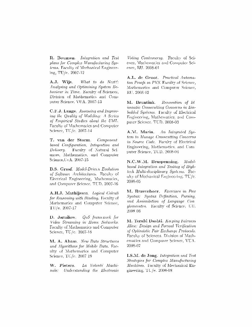
R. Boumen. Integration and Testplans for Complex Manufa turing Sys-tems. Fa ulty of Me hani al Engineer-ing, TU/e. 2007-12A.J. Wijs. What to do Next?:Analysing and Optimising System Be-haviour in Time. Fa ulty of S ien es,Division of Mathemati s and Com-puter S ien e, VUA. 2007-13C.F.J. Lange. Assessing and Improv-ing the Quality of Modeling: A Seriesof Empiri al Studies about the UML.Fa ulty of Mathemati s and ComputerS ien e, TU/e. 2007-14T. van der Storm. Component-based Con�guration, Integration andDelivery. Fa ulty of Natural S i-en es, Mathemati s, and ComputerS ien e,UvA. 2007-15B.S. Graaf. Model-Driven Evolutionof Software Ar hite tures. Fa ulty ofEle tri al Engineering, Mathemati s,and Computer S ien e, TUD. 2007-16A.H.J. Mathijssen. Logi al Cal ulifor Reasoning with Binding. Fa ulty ofMathemati s and Computer S ien e,TU/e. 2007-17D. Jarnikov. QoS framework forVideo Streaming in Home Networks.Fa ulty of Mathemati s and ComputerS ien e, TU/e. 2007-18M. A. Abam. New Data Stru turesand Algorithms for Mobile Data. Fa -ulty of Mathemati s and ComputerS ien e, TU/e. 2007-19W. Pieters. La Volont�e Ma hi-nale: Understanding the Ele troni

Voting Controversy. Fa ulty of S i-en e, Mathemati s and Computer S i-en e, RU. 2008-01A.L. de Groot. Pra ti al Automa-ton Proofs in PVS. Fa ulty of S ien e,Mathemati s and Computer S ien e,RU. 2008-02M. Bruntink. Renovation of Id-iomati Cross utting Con erns in Em-bedded Systems. Fa ulty of Ele tri alEngineering, Mathemati s, and Com-puter S ien e, TUD. 2008-03A.M. Marin. An Integrated Sys-tem to Manage Cross utting Con ernsin Sour e Code. Fa ulty of Ele tri alEngineering, Mathemati s, and Com-puter S ien e, TUD. 2008-04N.C.W.M. Braspenning. Model-based Integration and Testing of High-te h Multi-dis iplinary Systems. Fa -ulty of Me hani al Engineering, TU/e.2008-05M. Bravenboer. Exer ises in FreeSyntax: Syntax De�nition, Parsing,and Assimilation of Language Con-glomerates. Fa ulty of S ien e, UU.2008-06M. Torabi Dashti. Keeping FairnessAlive: Design and Formal Veri� ationof Optimisti Fair Ex hange Proto ols.Fa ulty of S ien es, Division of Math-emati s and Computer S ien e, VUA.2008-07I.S.M. de Jong. Integration and TestStrategies for Complex Manufa turingMa hines. Fa ulty of Me hani al En-gineering, TU/e. 2008-08

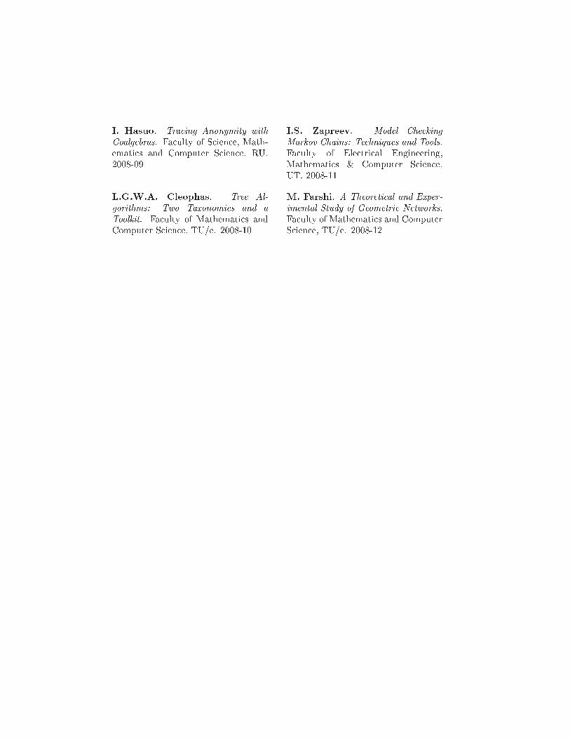
I. Hasuo. Tra ing Anonymity withCoalgebras. Fa ulty of S ien e, Math-emati s and Computer S ien e, RU.2008-09L.G.W.A. Cleophas. Tree Al-gorithms: Two Taxonomies and aToolkit. Fa ulty of Mathemati s andComputer S ien e, TU/e. 2008-10I.S. Zapreev. Model Che kingMarkov Chains: Te hniques and Tools.Fa ulty of Ele tri al Engineering,Mathemati s & Computer S ien e,UT. 2008-11M. Farshi. A Theoreti al and Exper-imental Study of Geometri Networks.Fa ulty of Mathemati s and ComputerS ien e, TU/e. 2008-12

نقطه O(n) کردن اضافه با یا خاص حا¯ت برخی در پایاست. محدب، شکل به ناحیهای خرابی هر تحت کهداد. کاهش O(n) به را یالها تعداد میتوان اشتاینر(۶)

نهایی هدف میشود. ارائه هندسی شبکههای در یال بهینه(۷) کاهش افزایش/ زمینه در نتایجی همچنیندر تأخیر که نحوی به شود حذف شبکه از یال یک یا اضافه شبکه به یال یک که است آن زمینه این دربرای تقریبی الگوریتم چند و دقیق الگوریتم یک یال، بهینه افزایشِ حالت در شود. کمینه حاصل شبکهدر بهینه یال برای ۲)-تقریب + ") یک تقریبی، الگوریتم سریعترین است. شده ارائه بهینه یال محاسبهو رئوس تعداد n آن در که میکند، محاسبه حافظه فضای O(n۲) از استفاده با O(mn+ n۲ logn) زمانبه را تقریب ضریب میتوان باشد ثابت ورودی شبکه در تأخیر که حالتی در است. شبکه یالهای تعداد m

داد. کاهش O(n۲) به را اجرا زمان و ۱+ "

شده بررسی باشد صفحه در دور(۸) یک ورودی گراف که حالتی در مسأله یال بهینه کاهش حالتِ درآن حذف که را یالی صفحه، در رأس n با دور یک برای که است شده ارائه تصادفی الگوریتم یک است.

میکند. محاسبه O(n log۳ n) زمان در را میکند ایجاد حاصل مسیر تاخیر در افزایش کمتریننتیجه است. شده پرداخته آن به پایاننامه این در که است دیگری مسأله t-پوشش یک قطر(۹) محاسبهبا O(D ·mn) زمان در را یال m و رأس n با t-پوشش یک قطر که است الگوریتمی قسمت این در اصلی

است. نظر مورد شبکه قطرِ D آن در که میکند محاسبه حافظه فضای O(m+ n) از استفادهشبکههای و شدهاست انجام t-پوششها ساختن برای مطرح الگوریتمهای روی آزمایشاتی نهایت، درانجام بررسی طبق شدهاست. مقایسه هم با الگوریتمها این اجرای زمان و الگوریتمها این توسط شده تولید

است. t-پوشش سازنده الگوریتمهای روی وسعت این با تجربی بررسی اولین این شده،

Steiner point(۶)optimal edge augmentation/deletion(۷)

cycle(۸)diameter(۹)

هندسی شبکههای روی تجربی و نظری مطالعه یک

فرشی محّمد

چکیدهیک از است عبارت (Rd) حقیقی d-بعدی فضای در نقاط از V مجموعه یک روی هندسی(۱) شبکه یکu بین اقلیدسی فاصله با گراف در (u; v) یال هر وزن که V رئوس مجموعه روی جهتدار غیر وزندارِ گرافِیک ازای به مینامند، V مجموعه برای t-پوشش(۲) یک را G(V;E) هندسی شبکه است. برابر ،|uv| یا ،v ومسیر کوتاهترین طول dG(u; v) که ،dG(u; v) ≤ t · |uv| ،V در v و u رأس دو هر ازای به اگر ،t > ۱ضریب یا تأخیر(۳) را است t-پوشش یک G شبکه آن ازای به که t کوچکترین است. G گراف در v و u بینt-پوشش به میتوان راحتی به را نقاط مجموعه یک برای t-پوشش تعریفِ مینامند. G شبکه کشش(۴)،E′ ⊆ E ،G(V;E) گراف برای t-پوشش یک را G′(V;E′) گراف داد. تعمیم وزندار گرافِ یک برای

.dG′(u; v) ≤ t · dG(u; v) ،V در v و u رئوس از زوج هر ازای به اگر مینامندنظری، قسمت در است. هندسی پوششهای روی تجربی و نظری نتایج سری یک شامل پایاننامه اینثابت و میشود تعریف صفحه روی نقاط مجموعه برای (۵) ناحیهای خرابیهای تحت پایا پوششهای مفهومکم یالهای تعداد با محدب ناحیهای خرابیهای تحت پایا پوششهای نقاط، از مجموعه هر برای میشودG⊖ F کنید فرض صفحه، از F ناحیه یک و صفحه از V نقاط مجموعه روی G گراف برای است. موجودG گراف میآید. بدست میگیرند قرار F ناحیه در که G یالهای و رئوس تمام حذف از که باشد گرافیG ⊖ F ِ گراف ،F محدب ناحیه هر ازای به اگر مینامند محدب خرابیهای تحت پایا t-پوشش یک راقسمت این در اصلی نتیجه است. V روی کامل گراف Gc(V ) که باشد Gc(V ) ⊖ F برای t-پوشش یکمیکند ایجاد یال O(n logn) با پوششی صفحه، از نقطه n از متشکل مجموعه هر برای که است الگوریتمی

geometric network(۱)t-spanner(۲)dilation(۳)

stretch factor(۴)region fault tolerant spanners(۵)