
Search for stop quarks using the matrix element … · Moreover, to get a natural solution for the...
93
Faculteit Wetenschappen Departement Natuurkunde Search for stop quarks using the matrix element method at the LHC Proefschrift ingediend met het oog op het behalen van de graad van Master in de Wetenschappen Lieselotte Moreels Promotor: Prof. Dr. Jorgen D’Hondt Co-promotor: Dr. Petra Van Mulders Academiejaar 2012–2013
Transcript of Search for stop quarks using the matrix element … · Moreover, to get a natural solution for the...
Faculteit WetenschappenDepartement Natuurkunde
Search for stop quarks using the matrix elementmethod at the LHC
Proefschrift ingediend met het oog op het behalen van de graad van Master in de Wetenschappen
Lieselotte Moreels
Promotor: Prof. Dr. Jorgen D’HondtCo-promotor: Dr. Petra Van Mulders
Academiejaar 2012–2013

Contents
1 Introduction 1
2 Beyond the Standard Model 32.1 The Standard Model . . . . . . . . . . . . . . . . . . . . . . . . . . 32.2 The Hierarchy Problem . . . . . . . . . . . . . . . . . . . . . . . . 52.3 Supersymmetry . . . . . . . . . . . . . . . . . . . . . . . . . . . . . 7
2.3.1 The Minimal Supersymmetric Standard Model . . . . . . . 82.3.2 The constrained MSSM . . . . . . . . . . . . . . . . . . . . 92.3.3 Simplified models . . . . . . . . . . . . . . . . . . . . . . . . 9
2.3.3.1 Direct stop quark pair production . . . . . . . . . 102.3.3.2 State of the art . . . . . . . . . . . . . . . . . . . . 11
3 Observation of New Particles 133.1 The Large Hadron Collider . . . . . . . . . . . . . . . . . . . . . . 143.2 The Compact Muon Solenoid Experiment . . . . . . . . . . . . . . 16
3.2.1 Coordinate system . . . . . . . . . . . . . . . . . . . . . . . 163.2.2 The inner tracker . . . . . . . . . . . . . . . . . . . . . . . . 173.2.3 The calorimeter system . . . . . . . . . . . . . . . . . . . . 183.2.4 The muon system . . . . . . . . . . . . . . . . . . . . . . . 19
3.3 Trigger and Data Aquisition . . . . . . . . . . . . . . . . . . . . . . 20
4 Reconstruction of Particles 214.1 Identification of Particles . . . . . . . . . . . . . . . . . . . . . . . 214.2 Object Reconstruction in the Subdetectors . . . . . . . . . . . . . . 22
4.2.1 Track reconstruction in the inner tracker . . . . . . . . . . . 224.2.2 Reconstruction of energy deposits in the calorimeters . . . . 244.2.3 Track reconstruction in the muon system . . . . . . . . . . 24
4.3 The Particle Flow Algorithm . . . . . . . . . . . . . . . . . . . . . 254.3.1 Muon reconstruction . . . . . . . . . . . . . . . . . . . . . . 254.3.2 Electron reconstruction . . . . . . . . . . . . . . . . . . . . 264.3.3 Jet reconstruction . . . . . . . . . . . . . . . . . . . . . . . 27
4.3.3.1 Identification of b jets . . . . . . . . . . . . . . . . 284.3.3.2 Removal of isolated leptons . . . . . . . . . . . . . 29
i
ii CONTENTS
5 Event Selection 315.1 Event Topology . . . . . . . . . . . . . . . . . . . . . . . . . . . . . 315.2 Event Generation and Simulation . . . . . . . . . . . . . . . . . . . 325.3 Selection Requirements . . . . . . . . . . . . . . . . . . . . . . . . . 34
6 Event Reconstruction 396.1 Jet-Parton Matching . . . . . . . . . . . . . . . . . . . . . . . . . . 396.2 Jet-Parton Association . . . . . . . . . . . . . . . . . . . . . . . . . 40
7 The Matrix Element Method 437.1 The Matrix Element Method in a Nutshell . . . . . . . . . . . . . . 437.2 Implementation in MadWeight . . . . . . . . . . . . . . . . . . . . 45
8 Sensitivity of the Matrix Element Method for Stop Quark Searches 498.1 Calculation of the Probability Density for Different Hypotheses . . 498.2 Sensitivity of Different Observables . . . . . . . . . . . . . . . . . . 50
8.2.1 Likelihood ratio . . . . . . . . . . . . . . . . . . . . . . . . . 508.2.2 Regular kinematic observable . . . . . . . . . . . . . . . . . 528.2.3 Transformation of the likelihood ratio . . . . . . . . . . . . 53
8.3 Upper Limit on the Signal Cross Section . . . . . . . . . . . . . . . 55
9 Conclusions & Perspectives 59
10 Summary 61
Samenvatting 63
Acknowledgements 65
References 67
List of Abbreviations 75
Appendix A Jet Reconstruction Algorithms 77A.1 Iterative Cone Algorithms . . . . . . . . . . . . . . . . . . . . . . . 77A.2 Sequential Recombination Algorithms . . . . . . . . . . . . . . . . 78
Appendix B b-tag Scale Factors 81
Appendix C MadWeight Cards 83C.1 Process Cards . . . . . . . . . . . . . . . . . . . . . . . . . . . . . . 83C.2 Transfer Function . . . . . . . . . . . . . . . . . . . . . . . . . . . . 85C.3 MadWeight Card . . . . . . . . . . . . . . . . . . . . . . . . . . . . 86
1
Introduction
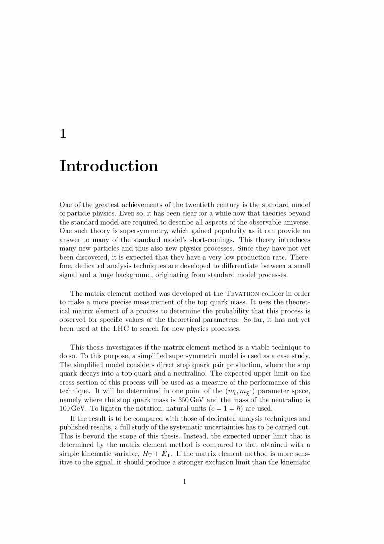
One of the greatest achievements of the twentieth century is the standard modelof particle physics. Even so, it has been clear for a while now that theories beyondthe standard model are required to describe all aspects of the observable universe.One such theory is supersymmetry, which gained popularity as it can provide ananswer to many of the standard model’s short-comings. This theory introducesmany new particles and thus also new physics processes. Since they have not yetbeen discovered, it is expected that they have a very low production rate. There-fore, dedicated analysis techniques are developed to differentiate between a smallsignal and a huge background, originating from standard model processes.
The matrix element method was developed at the Tevatron collider in orderto make a more precise measurement of the top quark mass. It uses the theoret-ical matrix element of a process to determine the probability that this process isobserved for specific values of the theoretical parameters. So far, it has not yetbeen used at the LHC to search for new physics processes.
This thesis investigates if the matrix element method is a viable technique todo so. To this purpose, a simplified supersymmetric model is used as a case study.The simplified model considers direct stop quark pair production, where the stopquark decays into a top quark and a neutralino. The expected upper limit on thecross section of this process will be used as a measure of the performance of thistechnique. It will be determined in one point of the (mt,mχ0) parameter space,namely where the stop quark mass is 350 GeV and the mass of the neutralino is100 GeV. To lighten the notation, natural units (c = 1 = ~) are used.
If the result is to be compared with those of dedicated analysis techniques andpublished results, a full study of the systematic uncertainties has to be carried out.This is beyond the scope of this thesis. Instead, the expected upper limit that isdetermined by the matrix element method is compared to that obtained with asimple kinematic variable, HT + /ET. If the matrix element method is more sens-itive to the signal, it should produce a stronger exclusion limit than the kinematic
1
2 1. INTRODUCTION
variable.
Chapter 2 will briefly describe the theoretical foundations of this thesis. Ashort overview of the standard model particles and forces is given and, via thehierarchy problem, the basics of supersymmetry, especially the MSSM, are intro-duced.
Chapter 3 elaborates on how particles are observed. Apart from the colliderset-up, it also discusses the CMS experiment, that observes the remnants of thecollisions produced by the LHC.
Chapter 4 describes how the electronic detector signals that are produced bythese remnants can be reconstructed into particles. To this purpose, the particleflow algorithm is used.
The signal topology is explained in Chapter 5. This analysis will only considerevents with a semi-muonic decay. Also the main backgrounds are defined, as wellas the selection requirements to select the events and to increase the signal-to-background ratio. The observed data are complemented by simulated signal andbackground samples to correctly estimate their respective effects.
The event topology is reconstructed in Chapter 6. The parton information ofthe tt background sample is used to reconstruct the hadronically decaying W bo-son and its corresponding top quark. This allows for their masses to be estimated.A χ2 method employing these masses is used to assign jets to partons.
Chapter 7 describes the basic components of the matrix element method andthe program that is used to process it, while Chapter 8 contains the results ofthe probability calculations. A variable that discriminates between signal andbackground is constructed and its sensitivity compared to that of HT + /ET.
2
Beyond the Standard Model
The observable world, its elementary particles and their interactions, can be de-scribed by the Standard Model of particle physics (SM). The final piece of thepuzzle seems to be in place with the discovery of the Brout–Englert–Higgs boson—in the remaining text referred to as the Higgs boson. Yet, despite the model’s ex-cellent agreement with precision measurements, there are still some questions thatthe SM cannot answer. For example, the observed ‘dark matter’ does not behavelike the ‘ordinary matter’ described by the SM, not to mention the enigmatic ‘darkenergy’. In addition, the enormous tuning necessary to solve the hierarchy problemcan hardly be called natural. Physicists have to look at so-called BSM-theories(Beyond the Standard Model) to find a solution for these problems, though mosttheories can only solve some of the SM’s weak spots.
A very promising BSM-theory is Supersymmetry (SUSY) [1]. Here, a newsymmetry between fermions and bosons is introduced. This results in supersym-metric partners for all SM particles. Many supersymmetric models have beentheoretically worked out in great detail, but none of them have yet been experi-mentally observed. If a Higgs boson with the observed mass of about 126 GeV is tobe included in the model, the parameter space of SUSY is substantially reduced.Moreover, to get a natural solution for the hierarchy problem, mass restrictionscan be imposed on the supersymmetric particles. For the top squark—or stopquark—, the supersymmetric partner of the top quark, this results in relativelylow masses, of the order TeV or lower, which brings it within the range of theLarge Hadron Collider.
2.1 The Standard Model
The SM describes the world of elementary particles and the forces acting on them.The matter particles are divided into two groups, quarks and leptons. The groupof quarks consists of up-type quarks—the up, charm and top quark—and down-type quarks—the down, strange and bottom quark. The lepton group consists ofneutrinos and electrons, muons and taus. These are arranged into three generations
3
4 2. BEYOND THE STANDARD MODEL
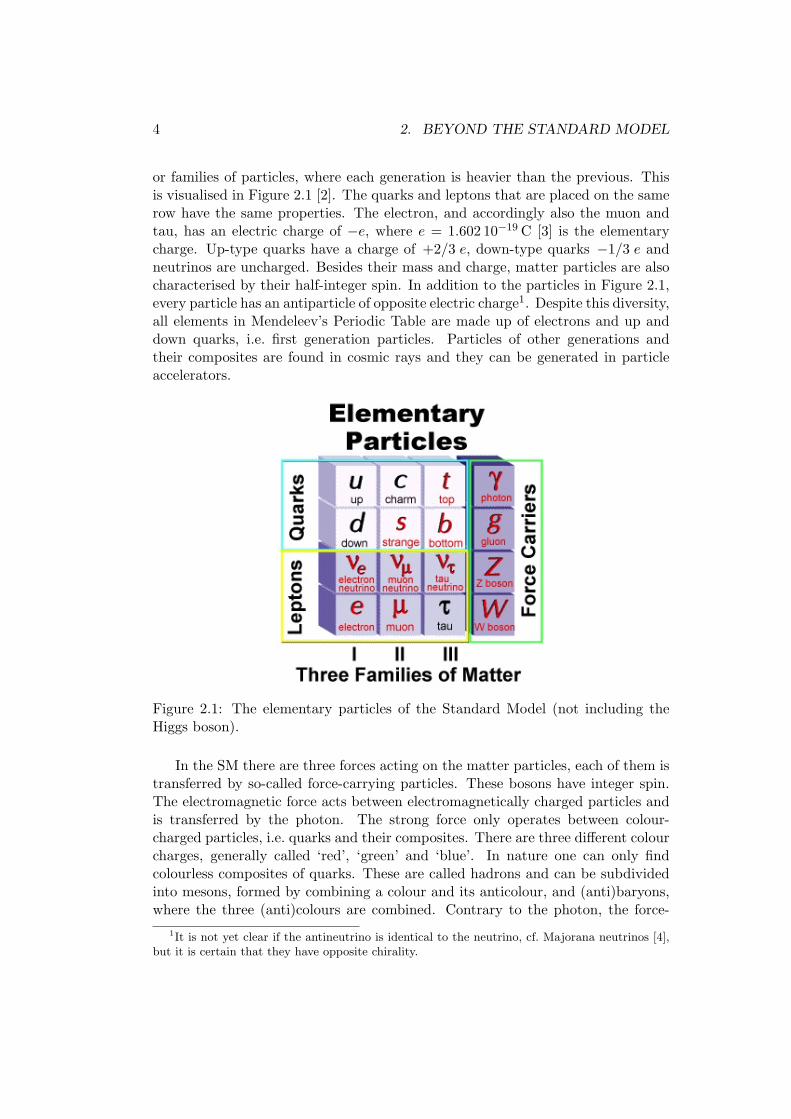
or families of particles, where each generation is heavier than the previous. Thisis visualised in Figure 2.1 [2]. The quarks and leptons that are placed on the samerow have the same properties. The electron, and accordingly also the muon andtau, has an electric charge of −e, where e = 1.602 10−19 C [3] is the elementarycharge. Up-type quarks have a charge of +2/3 e, down-type quarks −1/3 e andneutrinos are uncharged. Besides their mass and charge, matter particles are alsocharacterised by their half-integer spin. In addition to the particles in Figure 2.1,every particle has an antiparticle of opposite electric charge1. Despite this diversity,all elements in Mendeleev’s Periodic Table are made up of electrons and up anddown quarks, i.e. first generation particles. Particles of other generations andtheir composites are found in cosmic rays and they can be generated in particleaccelerators.
Figure 2.1: The elementary particles of the Standard Model (not including theHiggs boson).
In the SM there are three forces acting on the matter particles, each of them istransferred by so-called force-carrying particles. These bosons have integer spin.The electromagnetic force acts between electromagnetically charged particles andis transferred by the photon. The strong force only operates between colour-charged particles, i.e. quarks and their composites. There are three different colourcharges, generally called ‘red’, ‘green’ and ‘blue’. In nature one can only findcolourless composites of quarks. These are called hadrons and can be subdividedinto mesons, formed by combining a colour and its anticolour, and (anti)baryons,where the three (anti)colours are combined. Contrary to the photon, the force-
1It is not yet clear if the antineutrino is identical to the neutrino, cf. Majorana neutrinos [4],but it is certain that they have opposite chirality.
2.2. THE HIERARCHY PROBLEM 5
carrying particle of the strong force, the gluon, is charged itself—actually it isdoubly charged, with one colour and one anticolour—, so both quarks and gluonsare influenced by the strong force. (Composite) particles decay through the weakforce, which is mediated by the charged W+ and W− bosons and the neutralZ boson.
A fourth force, gravity, is not included in the SM as a consistent quantumtheory of gravity is yet to be developed. On the whole, gravity is supposed to betoo weak to have a substantial influence in elementary particle physics. It is 40orders of magnitude weaker than electromagnetism and about 1029 times weakerthan the weak force [5].
One particle is missing in Figure 2.1. The elusive Higgs boson has only beendiscovered in 2012 and is responsible for giving mass to the other particles anditself [6–8]. It is also possible to introduce more complex Higgs mechanisms, whichare generally needed in BSM-theories. These will result in more than one Higgsparticle. The observed Higgs boson with a mass of about 126 GeV does not excludea particular mechanism.
2.2 The Hierarchy Problem
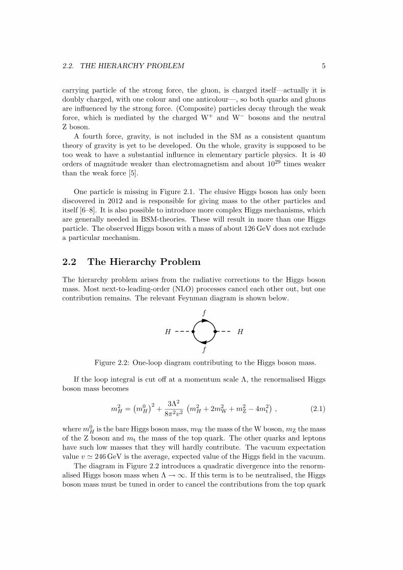
The hierarchy problem arises from the radiative corrections to the Higgs bosonmass. Most next-to-leading-order (NLO) processes cancel each other out, but onecontribution remains. The relevant Feynman diagram is shown below.
f
f
H H
Figure 2.2: One-loop diagram contributing to the Higgs boson mass.
If the loop integral is cut off at a momentum scale Λ, the renormalised Higgsboson mass becomes
m2H =
(m0H
)2 +3Λ2
8π2v2
(m2H + 2m2
W +m2Z − 4m2
t
), (2.1)
wherem0H is the bare Higgs boson mass, mW the mass of the W boson, mZ the mass
of the Z boson and mt the mass of the top quark. The other quarks and leptonshave such low masses that they will hardly contribute. The vacuum expectationvalue v ' 246 GeV is the average, expected value of the Higgs field in the vacuum.
The diagram in Figure 2.2 introduces a quadratic divergence into the renorm-alised Higgs boson mass when Λ→∞. If this term is to be neutralised, the Higgsboson mass must be tuned in order to cancel the contributions from the top quark
6 2. BEYOND THE STANDARD MODEL
and the W and Z bosons.
m2H = 4m2
t − 2m2W −m2
Z ≈ (320 GeV)2 . (2.2)
If the SM is to be consistent, uniting the electroweak and the strong force,it must be valid up to the Grand Unification scale (GUT), i.e. Λ ∼ 1016. AsΛ2 ∼ (1016)2 = 1032 , the Higgs boson mass must be tuned to 32 decimal places.This unnatural tuning hints at the presence of new physics phenomena. The ar-gument above can also be extended to radiative corrections of higher orders.
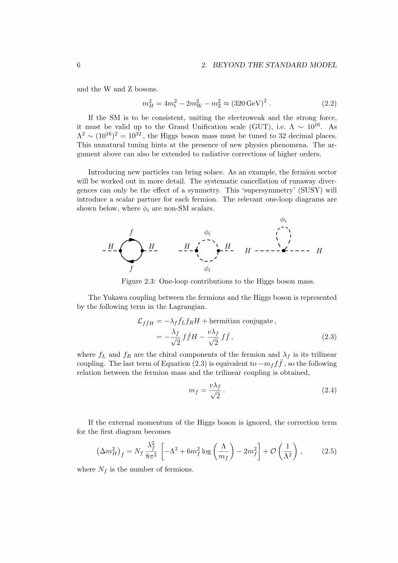
Introducing new particles can bring solace. As an example, the fermion sectorwill be worked out in more detail. The systematic cancellation of runaway diver-gences can only be the effect of a symmetry. This ‘supersymmetry’ (SUSY) willintroduce a scalar partner for each fermion. The relevant one-loop diagrams areshown below, where φi are non-SM scalars.
H
f
H
f
H
φi
H
φi
φi
H H
Figure 2.3: One-loop contributions to the Higgs boson mass.
The Yukawa coupling between the fermions and the Higgs boson is representedby the following term in the Lagrangian.
LffH = −λf fLfRH + hermitian conjugate ,
= −λf√
2ffH −
vλf√2ff , (2.3)
where fL and fR are the chiral components of the fermion and λf is its trilinearcoupling. The last term of Equation (2.3) is equivalent to −mfff , so the followingrelation between the fermion mass and the trilinear coupling is obtained,
mf =vλf√
2. (2.4)
If the external momentum of the Higgs boson is ignored, the correction termfor the first diagram becomes(
∆m2H
)f
= Nf
λ2f
8π2
[−Λ2 + 6m2
f log(
Λmf
)− 2m2
f
]+O
(1
Λ2
), (2.5)
where Nf is the number of fermions.
2.3. SUPERSYMMETRY 7
Assume there are Ns scalar particles with a mass ms, trilinear couplings vλsand quadrilinear couplings λs to the Higgs boson. Then,(
∆m2H
)s
= Nsλs
16π2
[−Λ2 + 2m2
s log(
Λms
)]+Ns
v2λ2s
16π2
[−1 + 2 log
(Λms
)]+O
(1
Λ2
). (2.6)
If λs = λ2f and Ns = 2Nf , then
(∆m2
H
)s
= Nf
λ2f
8π2
[−Λ2 + 2m2
s log(
Λms
)]+Nf
v2λ4f
8π2
[−1 + 2 log
(Λms
)]+O
(1
Λ2
). (2.7)
The total correction term is the sum of Equations (2.5) and (2.7). UsingEquation (2.4) to rewrite Equation (2.7), this becomes
∆m2H = Nf
λ2f
4π2
[(m2
f −m2s) log
(Λms
)+ 3m2
f log(ms
mf
)+m2
f
]. (2.8)
The above correction term no longer contains quadratic divergences. There isstill a logarithmic divergence, but even when Λ ∼ 1019 this term is quite small.
If SUSY is an exact symmetry, ms = mf , the logarithmic term disappearscompletely and the Higgs boson mass is no longer dependent on the energy scale.If SUSY is broken, the masses are no longer equal and the hierarchy problem re-turns when the difference between the masses is too large. In general, the theoryremains stable when the scalars are of order 1 TeV.
Therefore, the hierarchy problem in the fermion sector is solved when, for eachfermion, two scalar particles with couplings related to the SM couplings and amass of order 1 TeV or lower are added. If these relatively light particles exist,they would come within the reach of currently existing experiments. The sameargumentation can be followed for W and Z loops, thus introducing their super-partners.
2.3 Supersymmetry
In the past decades, the SM has been tested on many levels. Though experimentalobservations show great agreement with the theory, it remains insufficient to de-scribe the entire universe. An extension to include other physical phenomena isrequired. Supersymmetry is an elegant way to provide more answers. The newsymmetry introduces an operator that transforms a bosonic state into a fermionicstate and vice versa, i.e.
Q |boson〉 = |fermion〉 , Q |fermion〉 = |boson〉 . (2.9)
8 2. BEYOND THE STANDARD MODEL
These superpartners are combined into a supermultiplet, or superfield, and havethe same quantum numbers, except for their spin [1]. It are the superfields thatwill interact with each other, thus adding many new terms to the Lagrangian. Assupersymmetry deals with transformations in superspace, space-time needs to beextended with new coordinates,
(xµ) −→ (xµ, θ) , (2.10)
where θ are Grassmann variables. These are subject to the Grassmann algebraand the interested reader can find their application to supersymmetry in [9].
As every SM particle gets a new partner, many new particles are added inSUSY and thus also many new parameters. If SUSY is an exact symmetry, thesuperpartners have the same mass as the SM particles. However, no evidencehas been found of these new particles at the expected mass ranges. To allow fordifferent masses, SUSY must be broken. Up till now there is no satisfactory wayto accomplish this. So, instead of a fundamental mechanism, the SUSY breakingterms are added to the Lagrangian by hand.
2.3.1 The Minimal Supersymmetric Standard Model
In the minimal extension of the SM, the Minimal Supersymmetric Standard Model(MSSM), all SM leptons and quarks get scalar, spin-0 superpartners, called sleptonsand squarks. The SM gauge bosons get spin-1/2 superpartners, the gauginos. Su-perparticles are indicated with a tilde, e.g. eL is the left-handed selectron, wherethe left-handedness refers to the chirality of its SM partner, since the selectron isa spin-0 particle. If lepton and baryon number are to be conserved, R-parity isimposed. This is a discrete and multiplicative symmetry and is defined as follows,
R = (−1)2S+3B+L , (2.11)
where S is the particle spin, B is the baryon number and L the lepton number.Every SM particle has a positive R-parity R = +1 and every supersymmetricparticle has R = −1. As a consequence, supersymmetric particles can only becreated in pairs and the lightest supersymmetric particle (LSP) is stable.
Once the desired components of the theory are determined, terms that yieldthis content are added to the Lagrangian. This is obtained from the superpotentialthat is constructed from the superfields [9]. The SUSY breaking terms consist ofmass terms for the sfermions, gauginos and Higgs bosons and the trilinear couplingsbetween the sfermions and the Higgs bosons. This way, 105 new parameters areadded.
With a total of 124 parameters, phenomenological problems emerge. Someparts of the parameter space even yield unphysical results. To avoid this, thenumber of parameters will be reduced by imposing some assumptions. First of all,it will be assumed that the SUSY-breaking terms will not generate CP-violation,which implies that they are all real rather than complex [10]. Secondly, there are
2.3. SUPERSYMMETRY 9
no flavour changing neutral currents at tree level, resulting in diagonal matricesfor the sfermion masses and trilinear couplings. Thirdly, the masses and trilinearcouplings of the first and second generation are presumed equal at low energy.This way only 22 SUSY parameters remain, whereof 10 sfermion masses, 6 trilinearcouplings, 3 gaugino masses and 3 parameters related to the Higgs sector. Themodel thus generated is called the phenomenological MSSM (pMSSM).
2.3.2 The constrained MSSM
The parameter space of the pMSSM can be further constrained if one assumesa hidden sector in which the SUSY breaking occurs that can only interact withthe visible sector through gravity. It is further assumed that these interactionsare flavour blind. If there are universal conditions at the GUT scale (Λ ∼ 1016),the constrained MSSM (cMSSM) or minimal Supergravity model (mSUGRA) onlycontains 4 free parameters and 1 unknown sign,
m0 , m1/2 , A0 , tanβ , signµ , (2.12)
where m0 is the universal scalar mass, m1/2 the universal gaugino mass and A0
the universal trilinear coupling. The parameters tanβ and signµ originate fromthe Higgs sector. The vacuum expectation value of the Higgs boson introduces theparameter tanβ, whereas µ is a mixing parameter in the superpotential [9].
The original parameters can be obtained by evolving these 5 parameters fromthe GUT scale to the electroweak scale.
2.3.3 Simplified models
Models like the cMSSM bring the number of SUSY parameters to a manageablelevel, but they still predict certain mass patterns and signatures. This means thatresults obtained in the cMSSM mass plane (m0,m1/2 ) cannot be generalised toother MSSM models or extensions of these, as a variation of A0, tanβ and signµdoes not reproduce the entire SUSY parameter space. Another approach, that doesallow such a generalisation and can be used to place limits on different theoreticalmodels, are simplified models. Here, a certain topological signature is generatedby the introduction of a limited number of particles and their decay chains. Foreach simplified model, the masses of the particles involved are variable within acertain mass range. Examples of some common production processes can be foundin Equation (2.13),
qq, gg→ gg , qq, gg→ q¯q ,
qq, gg→ χ0χ0 , qq, gg→ χ0χ± ,(2.13)
where g is a gluino, q a squark, χ0 a neutralino and χ± a chargino. These canimmediately decay into the LSP and SM particles or an intermediate particle can
10 2. BEYOND THE STANDARD MODEL
be formed. For example, a chargino can directly decay into a lepton, neutrino andneutralino, χ± → lνχ0, or this final state can be produced by
χ± →W± χ0 , W± → l± ν , (2.14)
χ± → l± ν , l± → l± χ0 , (2.15)
χ± → l± ν , ν → ν χ0 . (2.16)
In each of these cases, the kinematic properties of the lepton will be different, soa certain decay chain can be preferred over the other based on the aim of theanalysis [11].
2.3.3.1 Direct stop quark pair production
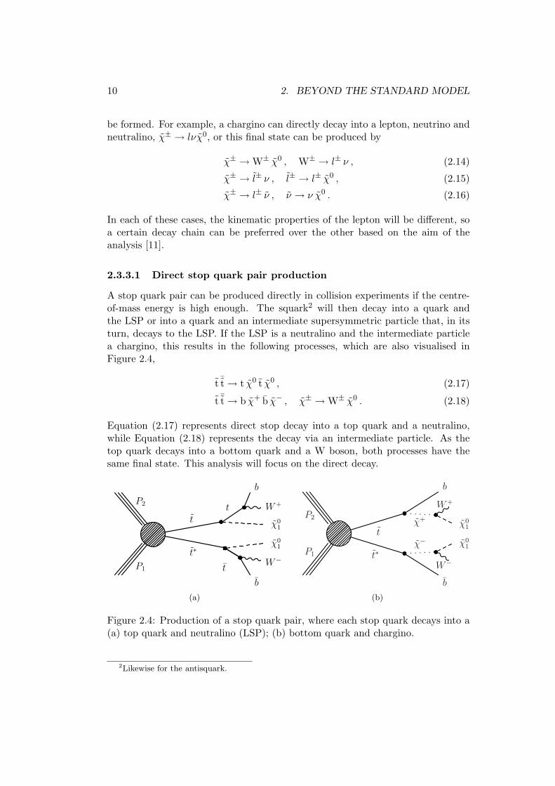
A stop quark pair can be produced directly in collision experiments if the centre-of-mass energy is high enough. The squark2 will then decay into a quark andthe LSP or into a quark and an intermediate supersymmetric particle that, in itsturn, decays to the LSP. If the LSP is a neutralino and the intermediate particlea chargino, this results in the following processes, which are also visualised inFigure 2.4,
t ¯t→ t χ0 t χ0 , (2.17)
t ¯t→ b χ+ b χ− , χ± →W± χ0 . (2.18)
Equation (2.17) represents direct stop decay into a top quark and a neutralino,while Equation (2.18) represents the decay via an intermediate particle. As thetop quark decays into a bottom quark and a W boson, both processes have thesame final state. This analysis will focus on the direct decay.
P1
P2
t⇤
t
t
t
b
W�
�01
�01
W+
b
3
(a)
P1
P2
t!
t!"
W"
!+
W+
b
!01
!01
b
(b)
Figure 2.4: Production of a stop quark pair, where each stop quark decays into a(a) top quark and neutralino (LSP); (b) bottom quark and chargino.
2Likewise for the antisquark.
2.3. SUPERSYMMETRY 11
2.3.3.2 State of the art
Relatively light stop quarks (mt < 1 TeV) are a key object in solving the hierarchyproblem, as the top quark is the heaviest SM particle and will thus contribute themost at one-loop level (see Equation (2.8)). Further, they are especially interestingbecause they should be observable at currently existing particle colliders.
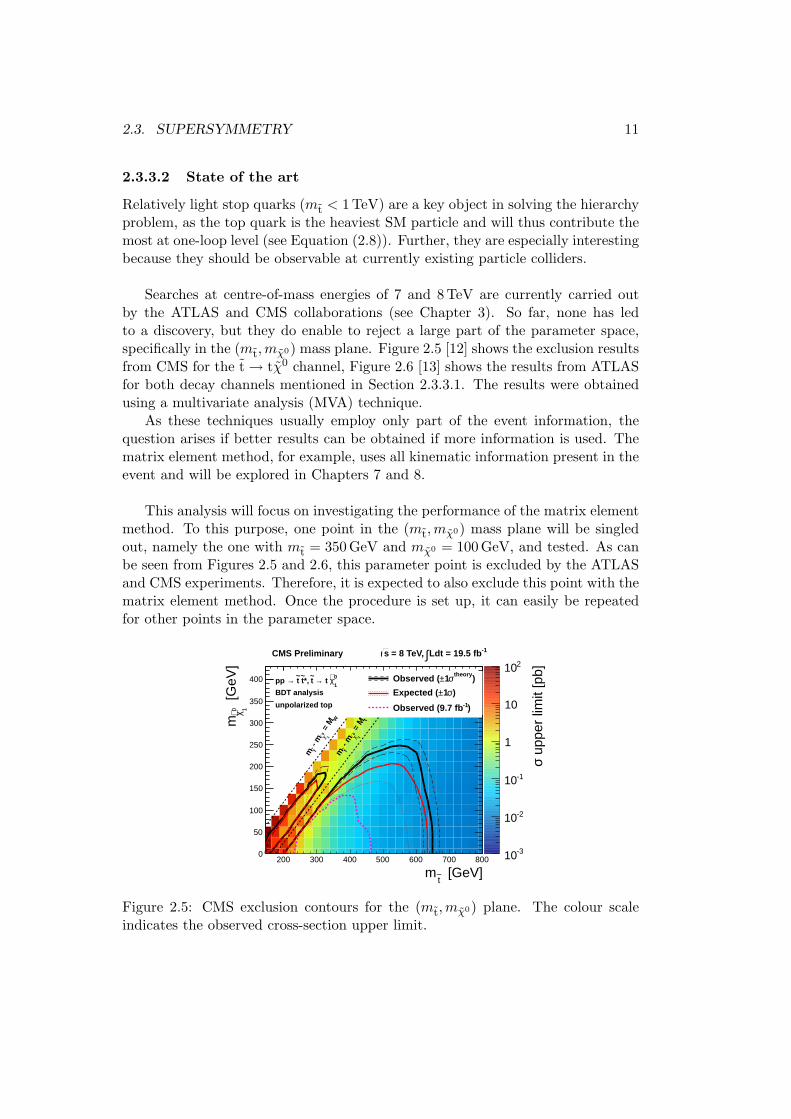
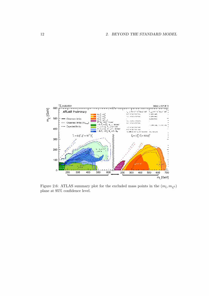
Searches at centre-of-mass energies of 7 and 8 TeV are currently carried outby the ATLAS and CMS collaborations (see Chapter 3). So far, none has ledto a discovery, but they do enable to reject a large part of the parameter space,specifically in the (mt,mχ0) mass plane. Figure 2.5 [12] shows the exclusion resultsfrom CMS for the t→ tχ0 channel, Figure 2.6 [13] shows the results from ATLASfor both decay channels mentioned in Section 2.3.3.1. The results were obtainedusing a multivariate analysis (MVA) technique.
As these techniques usually employ only part of the event information, thequestion arises if better results can be obtained if more information is used. Thematrix element method, for example, uses all kinematic information present in theevent and will be explored in Chapters 7 and 8.
This analysis will focus on investigating the performance of the matrix elementmethod. To this purpose, one point in the (mt,mχ0) mass plane will be singledout, namely the one with mt = 350 GeV and mχ0 = 100 GeV, and tested. As canbe seen from Figures 2.5 and 2.6, this parameter point is excluded by the ATLASand CMS experiments. Therefore, it is expected to also exclude this point with thematrix element method. Once the procedure is set up, it can easily be repeatedfor other points in the parameter space.
[GeV]t~
m200 300 400 500 600 700 800
[G
eV]
10 χ∼m
0
50
100
150
200
250
300
350
400
upp
er li
mit
[pb]
σ
-310
-210
-110
1
10
210
unpolarized top
BDT analysis
0
1χ∼ t → t~*, t
~ t
~ →pp )theoryσ1±Observed (
)σ1±Expected (
)-1Observed (9.7 fb
-1Ldt = 19.5 fb∫ = 8 TeV, sCMS Preliminary
t
= M
1
0χ∼
- m
t~m
W
= M
1
0χ∼
- m
t~m
Figure 2.5: CMS exclusion contours for the (mt,mχ0) plane. The colour scaleindicates the observed cross-section upper limit.
12 2. BEYOND THE STANDARD MODEL
Figure 2.6: ATLAS summary plot for the excluded mass points in the (mt,mχ0)plane at 95% confidence level.
3
Observation of New Particles
Paradoxically, large instruments are necessary to investigate the minute particlesappearing in the SM and BSM-theories. This is because the resolution of commonmicroscopes is not good enough to discern them. In order to detect objects, thewavelength of the microscope needs to be smaller than the wavelength of the object.Elementary particles have a maximum size of about 10−18 m and an even smallerwavelength. Even the most precise microscopes do not meet those requirements.Therefore, colliders are needed to detect elementary particles. The particles areaccelerated to a certain centre-of-mass energy before they collide into each other atthe centre of a particle detector. The larger the centre-of-mass energy, the smallerscales the collider can probe. Colliders have the great advantage that the centre-of-mass energy is equal to the sum of the beam energies. This is not the case fora fixed target accelerator, where part of the energy is used to get the particles inthe centre-of-mass frame.
When the accelerated particles collide, they produce new particles, the rem-nants of which are measured by the detector. Electrons and hadrons, in particularprotons and ions, are the most commonly used accelerated particles. Each havetheir advantages and disadvantages. On the one hand, it is easier to acceleratehadrons to higher energies as they are not so prone to synchrotron radiation. Whenparticles bend, they radiate away part of their energy. This is inversely propor-tional to their mass. As the electron is about 2000 times lighter than the smallesthadrons, the accelerator must provide more energy to electrons than to hadronson curved tracks to make up for this energy loss. On the other hand, hadrons arecomposite particles. When they collide, it are their constituents that are involvedin the actual collision. This means that, contrary to electron–positron collisions,the centre-of-mass energy is not known in hadron–(anti)hadron collisions. Forthese reasons, hadron colliders are most commonly used to make discoveries, whileelectron-positron colliders make precision measurements once the discovery hasbeen made.
13
14 3. OBSERVATION OF NEW PARTICLES
3.1 The Large Hadron Collider
The Large Hadron Collider (LHC), located at CERN at the Franco–Swiss bor-der, is currently the most powerful particle accelerator in the world. It consistsof eight sectors that are more or less straight, connected by eight arcs. The totalcircumference of the accelerator is approximately 27 km. Particles travel throughthe machine in two beam pipes, one in each direction. These are in an ultrahighvacuum state to avoid collisions between the particles and air molecules. Dipolemagnets are used to keep the particles in their orbit and quadrupole magnets focusthem into collimated bunches of about 1011 particles. As these are accelerated tovery high energies, the magnets need to be superconductive. They are cooled withliquid helium to 1.9 K. This way, the dipole magnets can produce a magnetic fieldof about 8.4 T [14].
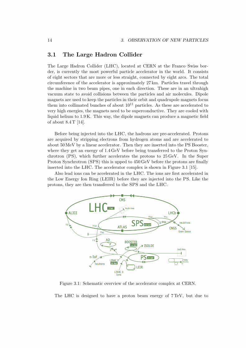
Before being injected into the LHC, the hadrons are pre-accelerated. Protonsare acquired by stripping electrons from hydrogen atoms and are accelerated toabout 50 MeV by a linear accelerator. Then they are inserted into the PS Booster,where they get an energy of 1.4 GeV before being transferred to the Proton Syn-chrotron (PS), which further accelerates the protons to 25 GeV. In the SuperProton Synchrotron (SPS) this is upped to 450 GeV before the protons are finallyinserted into the LHC. The accelerator complex is shown in Figure 3.1 [15].
Also lead ions can be accelerated in the LHC. The ions are first accelerated inthe Low Energy Ion Ring (LEIR) before they are injected into the PS. Like theprotons, they are then transferred to the SPS and the LHC.
Figure 3.1: Schematic overview of the accelerator complex at CERN.
The LHC is designed to have a proton beam energy of 7 TeV, but due to
3.1. THE LARGE HADRON COLLIDER 15
technical problems only beam energies of 3.5 TeV (2011) and 4 TeV (2012) havecurrently been explored. This has proved to be sufficient for the discovery of theHiggs boson, which has a mass of about 126 GeV, but an upgrade to higher beamenergies is favourable for the study of new physics, as the production cross sectionsof new physics processes increase more compared to those of the known processes.This upgrade will be carried out during the Long Shutdown (LS1) in 2013-2014.
The number of collisions in a certain time interval is defined by the luminosity,
L = fnN2
A, (3.1)
where f is the revolution frequency, n the number of bunches, A the cross-sectionalarea of the bunch and N the number of particles per bunch. With about 2800proton bunches and 1011 particles per bunch, the design luminosity of the LHC is1034 cm−2 s−1 [16]. The integrated luminosity is obtained by integrating over timeand is expressed in inverse barns, where 1 b = 10−24 cm2.
Due to the collision of proton bunches instead of single protons, more than oneinteraction can occur during one bunch crossing. Particles belonging to differentcollisions are detected at the same time. This is called pile-up. If the particlescannot be traced back to their original collision, they can contaminate the energymeasurement of others.
Along the accelerator line there are four major experiments to detect andinvestigate the remnants of the particle collisions when the two beams cross. Theseare called ALICE [17], ATLAS [18], CMS [19] and LHCb [20]. ATLAS and CMSare general-purpose detectors examining proton collisions. They are looking fornew physics, but also investigate the SM more closely. The fact that there aretwo independent experiments is advantageous in the sense that one can alwayscross-check the results of the other. ALICE on the other hand looks at lead-ioncollisions or the collisions between a lead ion and a proton to investigate quark–gluon plasma. This is expected to have been the state of the universe right afterthe Big Bang. LHCb looks for an answer to the matter-antimatter asymmetry inthe universe. To this purpose it investigates CP-violation in b-quark physics.
Apart from these four, there are also some smaller experiments installed atthe LHC. LHCf [21] is located near the ATLAS interaction point and Totem [22]resides near CMS. They focus on forward particles, which move close to the beamline.
This project will use proton collisions collected by the CMS experiment in 2012.In the next section, a description of the experiment and its components can befound. During its run time, the CMS experiment has collected about 5.32 fb−1 ofdata at a centre-of-mass energy of 7 TeV (2011) and 20.65 fb−1 at a centre-of-massenergy of 8 TeV (2012) [23].
16 3. OBSERVATION OF NEW PARTICLES
3.2 The Compact Muon Solenoid Experiment
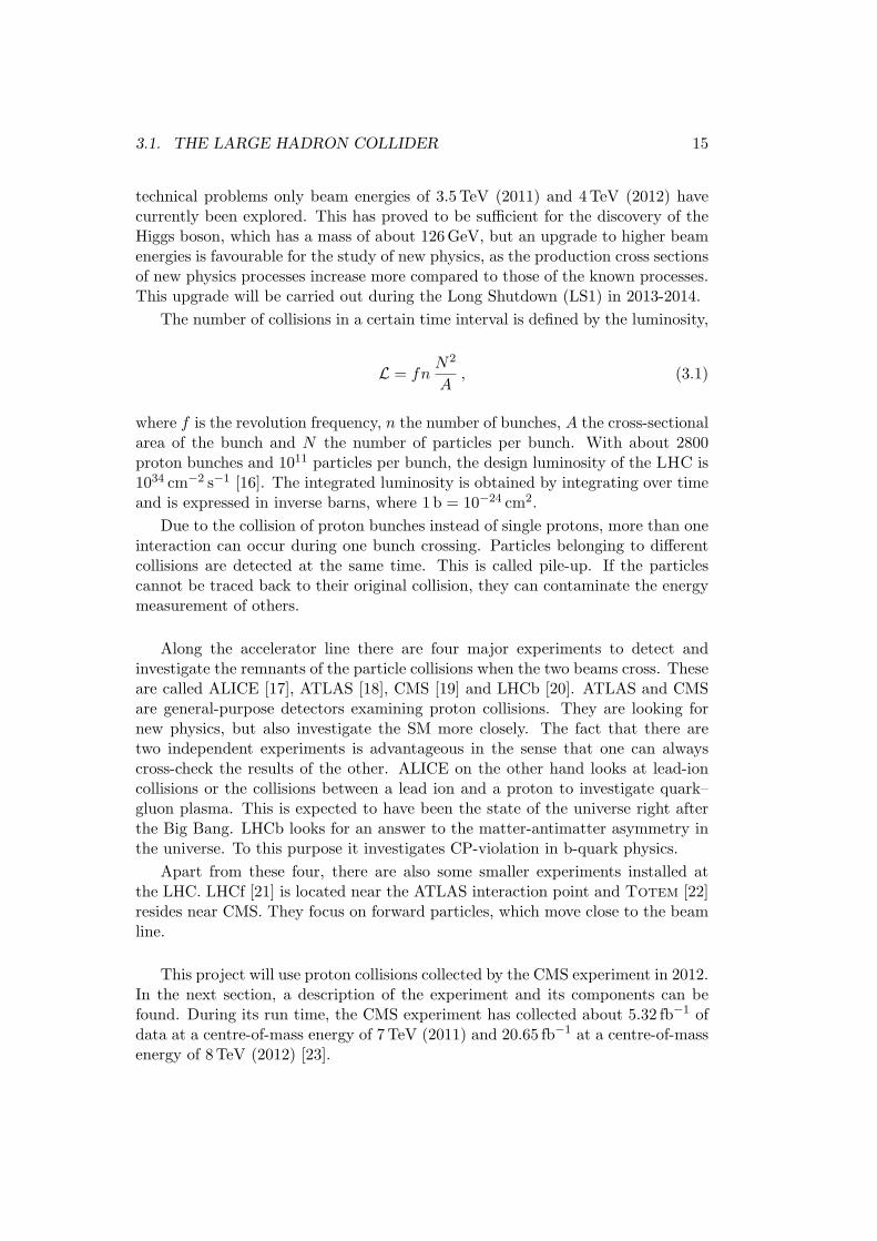
Each particle has intrinsic properties that make it easier or more difficult to de-tect with certain instruments. Therefore, the Compact Muon Solenoid (CMS)experiment is a multilayered structure, where each layer is dedicated to optimallyrecognise certain particle properties. The main component of the CMS detectoris a powerful solenoid magnet that enables to distinguish the charges of particles.The magnet consists of a coil of superconducting cables, producing a magneticfield of 3.8 T [24]. It weighs about 12,000 tonnes and has a diameter of approxim-ately 7 m, thus enveloping a silicon tracker, that is positioned at the heart of thedetector, and an electromagnetic and a hadron calorimeter.
Outside the solenoid there are iron return yokes to close the magnetic field lines.These are interspersed with muon detectors. Muons1 can traverse many metersof iron without interacting. In fact, they are the only particles that will reachthis part of the detector—that is, not counting the neutrinos, which will not bedetected. So as to be most effective to observe the muons, different kinds of muondetectors are used in different locations. As can be seen in Figure 3.2 [25], CMS isdivided into a barrel region, which contains the solenoid, and two endcap regions.The endcaps are formed such that the CMS detector is almost hermetically sealed.This way, one can infer the presence of neutrinos, that will not be measured byany of the CMS components.
3.2.1 Coordinate system
The CMS detector is cylindrical in shape, so it would seem cylindrical coordin-ates present the easiest way to describe the positions of particles in the detector.The endcaps, however, do not have the same structure as the barrel region soas to optimally close the detector. In reality, this makes the usage of sphericalcoordinates more appropriate when the detector as a whole is considered. Fig-ure 3.2 includes the cartesian coordinate system—which can easily be convertedto spherical coordinates r, θ and φ—that is generally used. The z-axis lies alongthe beam pipe and the x-axis points towards the centre of the LHC ring. Thexy-plane, or the plane defined by θ = π/2, is also called the transverse plane. Asprotons are accelerated in the beam pipe, the total energy in the transverse planeis equal to zero before the collision. Since the conservation of energy dictates thatthe total transverse energy also needs to be zero after the collision, the transverseplane presents the ideal location to search for missing energy brought about byneutrinos or other elusive particles from BSM-models.
Instead of the spherical angle θ , collider physicists often use the pseudorapidity.
1In this section and the remainder of this thesis, the term ‘muon’ will be used to indicate boththe muon itself and its antiparticle, unless it is explicitly specified. Likewise, the term ‘electron’will indicate both the electron and the positron.
3.2. THE COMPACT MUON SOLENOID EXPERIMENT 17
Figure 3.2: Schematic overview of the CMS experiment.
This is a Lorentz invariant quantity and is defined as
η = − ln(
tanθ
2
). (3.2)
This means that the transverse plane is located at η = 0 and the beam pipe atη =∞.
3.2.2 The inner tracker
The interaction point in the centre of the CMS experiment is surrounded by atracker, which consists of several layers of silicon detectors that will measure theposition of charged particles. These charged particles will ionise some of the siliconatoms on their way, thus creating electron-hole pairs that will produce a smallelectrical signal. As the energy of the particles is supposed to be determined bythe calorimeters beyond the tracker boundary, it is important that the particles aredisturbed as little as possible. Apart from choosing a light material like silicon, thisis realised by taking just a few measuring points that have a very high precision,in this case about 10µm [26]. The magnetic field produced by the solenoid willbend charged particles into a curved track with radius
r =pT
qB, (3.3)
18 3. OBSERVATION OF NEW PARTICLES
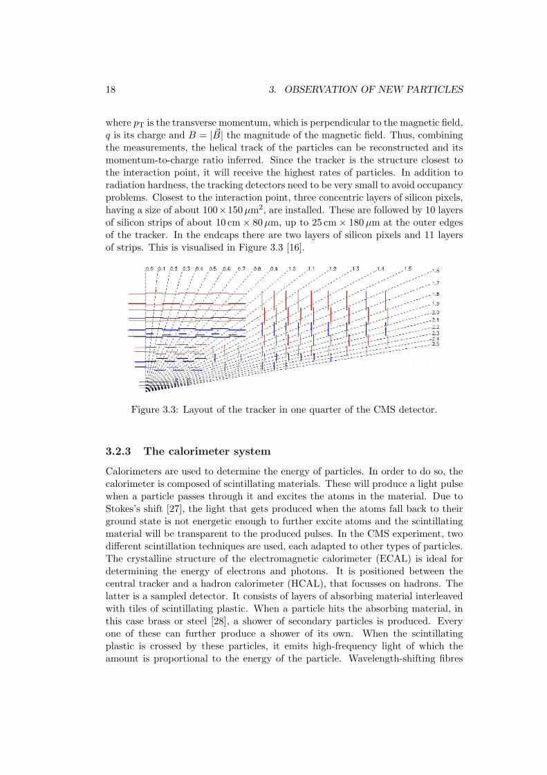
where pT is the transverse momentum, which is perpendicular to the magnetic field,q is its charge and B = | ~B| the magnitude of the magnetic field. Thus, combiningthe measurements, the helical track of the particles can be reconstructed and itsmomentum-to-charge ratio inferred. Since the tracker is the structure closest tothe interaction point, it will receive the highest rates of particles. In addition toradiation hardness, the tracking detectors need to be very small to avoid occupancyproblems. Closest to the interaction point, three concentric layers of silicon pixels,having a size of about 100×150µm2, are installed. These are followed by 10 layersof silicon strips of about 10 cm× 80µm, up to 25 cm× 180µm at the outer edgesof the tracker. In the endcaps there are two layers of silicon pixels and 11 layersof strips. This is visualised in Figure 3.3 [16].
Figure 3.3: Layout of the tracker in one quarter of the CMS detector.
3.2.3 The calorimeter system
Calorimeters are used to determine the energy of particles. In order to do so, thecalorimeter is composed of scintillating materials. These will produce a light pulsewhen a particle passes through it and excites the atoms in the material. Due toStokes’s shift [27], the light that gets produced when the atoms fall back to theirground state is not energetic enough to further excite atoms and the scintillatingmaterial will be transparent to the produced pulses. In the CMS experiment, twodifferent scintillation techniques are used, each adapted to other types of particles.The crystalline structure of the electromagnetic calorimeter (ECAL) is ideal fordetermining the energy of electrons and photons. It is positioned between thecentral tracker and a hadron calorimeter (HCAL), that focusses on hadrons. Thelatter is a sampled detector. It consists of layers of absorbing material interleavedwith tiles of scintillating plastic. When a particle hits the absorbing material, inthis case brass or steel [28], a shower of secondary particles is produced. Everyone of these can further produce a shower of its own. When the scintillatingplastic is crossed by these particles, it emits high-frequency light of which theamount is proportional to the energy of the particle. Wavelength-shifting fibres
3.2. THE COMPACT MUON SOLENOID EXPERIMENT 19
convert this to greenish light, that is collected by optical fibres and sent to areadout box. The amount of light collected over the different layers of scintillatingmaterial is added to cover the track of the particle through the calorimeter andis a measure of its energy. The optical signals will be amplified in a proportionalregime and converted to an electronic signal using hybrid photodiodes (HPD).These are designed especially for CMS and are constructed such that they caneasily operate in places with strong magnetic fields [28,29].
The electromagnetic calorimeter consists of scintillating lead-tungstate (PbWO4)crystals. These are very dense, which means that the ECAL is a remarkably com-pact structure. When an electron or photon enters the crystals, they will producea shower of secondary electrons and photons. As in the HCAL, scintillation lightproportional to the particles’ energy will be produced. In the crystals, however,the amount of light that will be produced will also depend on the temperature. Aprecise cooling system is thus necessary to closely regulate the temperature of thecrystals within 0.1◦C [30]. In general, the light yield of the crystals will be low, sosensitive photodetectors are used to amplify the signal and convert it to electricalpulses. The photodetectors are glued to the back of the crystals and thus need towithstand strong magnetic fields and endure high radiation fluxes. In the barrelregion, silicon avalanche photodiodes (APD) will be used. As the radiation flux inthe endcap regions is too high for silicon photodiodes, vacuum phototriodes (VPT)will be employed there [30,31].
The granularity of the ECAL is about 25 times larger than that of the HCAL.Therefore, the amount of energy deposited is more precisely determined for elec-trons and photons than for hadrons.
3.2.4 The muon system
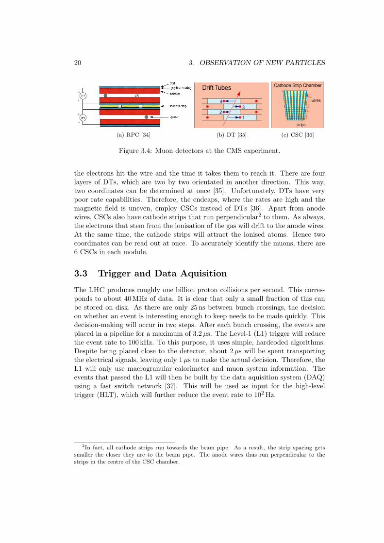
Muons will be observed using gaseous detectors like drift tubes (DT), cathodestrip chambers (CSC) and resistive plate chambers (RPC). In the barrel regionDTs and RPCs are installed. These are visualised in Figure 3.4. RPCs consist oftwo parallel plates of high resistivity separated by a gas gap. The uniformity ofthe gap is ensured by introducing spacers. A voltage difference between the platescreates an electric field in the gap that is suitable for electron multiplication. Whena charged particle like a muon enters the gap, it ionises the gas and the electronssnowball into an avalanche. This is read out by an external readout system, asthe, for CMS, bakelite plates are transparent to the electron signal. CMS usesdouble-gap RPCs with a common readout system, as can be seen in Figure 3.4(a).The copper readout strips are positioned such that a quick momentum estimatecan be made. RPCs have a good spatial resolution and an excellent time resolutionof about 1 ns. As a result, they also have good rate capabilities [32,33].
DTs are especially good at determining the position of passing muons. Theyare about 4 cm wide and have an anode wire in the middle. Whenever a muonruns through it, the gas inside the DT gets ionised. The electrons will then driftto the anode and the position of the ionising particle can be inferred from where
20 3. OBSERVATION OF NEW PARTICLES
(a) RPC [34] (b) DT [35] (c) CSC [36]
Figure 3.4: Muon detectors at the CMS experiment.
the electrons hit the wire and the time it takes them to reach it. There are fourlayers of DTs, which are two by two orientated in another direction. This way,two coordinates can be determined at once [35]. Unfortunately, DTs have verypoor rate capabilities. Therefore, the endcaps, where the rates are high and themagnetic field is uneven, employ CSCs instead of DTs [36]. Apart from anodewires, CSCs also have cathode strips that run perpendicular2 to them. As always,the electrons that stem from the ionisation of the gas will drift to the anode wires.At the same time, the cathode strips will attract the ionised atoms. Hence twocoordinates can be read out at once. To accurately identify the muons, there are6 CSCs in each module.
3.3 Trigger and Data Aquisition
The LHC produces roughly one billion proton collisions per second. This corres-ponds to about 40 MHz of data. It is clear that only a small fraction of this canbe stored on disk. As there are only 25 ns between bunch crossings, the decisionon whether an event is interesting enough to keep needs to be made quickly. Thisdecision-making will occur in two steps. After each bunch crossing, the events areplaced in a pipeline for a maximum of 3.2µs. The Level-1 (L1) trigger will reducethe event rate to 100 kHz. To this purpose, it uses simple, hardcoded algorithms.Despite being placed close to the detector, about 2µs will be spent transportingthe electrical signals, leaving only 1µs to make the actual decision. Therefore, theL1 will only use macrogranular calorimeter and muon system information. Theevents that passed the L1 will then be built by the data aquisition system (DAQ)using a fast switch network [37]. This will be used as input for the high-leveltrigger (HLT), which will further reduce the event rate to 102 Hz.
2In fact, all cathode strips run towards the beam pipe. As a result, the strip spacing getssmaller the closer they are to the beam pipe. The anode wires thus run perpendicular to thestrips in the centre of the CSC chamber.
4
Reconstruction of Particles
When particles move through the CMS detector, they leave electronic signals inits subdetectors that are not easily interpretable. A combination of these signalsinto particle tracks or energy deposits is a lot more intelligible. The particle flowalgorithm [38] will combine the information from all subdetectors to accuratelyreconstruct and identify each stable particle. These will then be used to build jets,reconstruct tau leptons and determine the missing transverse energy /ET.
Section 4.1 will describe how particles are identified, merging the informationfrom the subdetectors. Section 4.2 shows how electronic signals are combined toreconstruct tracks and calorimeter clusters, while Section 4.3 joins this informationto make fully reconstructed ‘particle flow muons’ and ‘particle flow jets’.
4.1 Identification of Particles
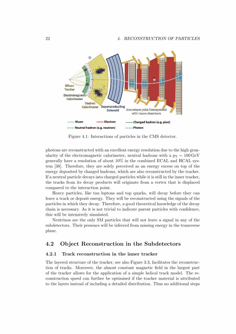
When two protons collide in the centre of the CMS detector, particle debris will flyin all directions and leave behind signals when it crosses the detector. Combiningthe information from the subdetectors, an identification of the particles in questioncan be made. Figure 4.1 [39] shows a transverse slice of the detector where thesignals of some particles are indicated.
Muons will leave a signal in the inner tracker, the calorimeters and in the muonchambers. Due to the position of the solenoid, the direction of the curvature willbe reversed in the muon chambers compared to the tracker. The amount of energydeposited in the calorimeters is typically small.
Electrons, on the other hand, will deposit all their energy in the calorimeters,as will other charged particles. They leave a track in the inner tracker and theposition of the energy deposit depends on the nature of the particle. Electrons willdeposit most of their energy in the electromagnetic calorimeter, while for hadronsthe deposit will be the largest in the hadron calorimeter.
Neutral particles will behave likewise in the calorimeters, but they will notleave a track in the inner tracker, as they cannot create electron-hole pairs. While
21
22 4. RECONSTRUCTION OF PARTICLES
Figure 4.1: Interactions of particles in the CMS detector.
photons are reconstructed with an excellent energy resolution due to the high gran-ularity of the electromagnetic calorimeter, neutral hadrons with a pT ∼ 100 GeVgenerally have a resolution of about 10% in the combined ECAL and HCAL sys-tem [38]. Therefore, they are solely perceived as an energy excess on top of theenergy deposited by charged hadrons, which are also reconstructed by the tracker.If a neutral particle decays into charged particles while it is still in the inner tracker,the tracks from its decay products will originate from a vertex that is displacedcompared to the interaction point.
Heavy particles, like tau leptons and top quarks, will decay before they canleave a track or deposit energy. They will be reconstructed using the signals of theparticles in which they decay. Therefore, a good theoretical knowledge of the decaychain is necessary. As it is not trivial to indicate parent particles with confidence,this will be intensively simulated.
Neutrinos are the only SM particles that will not leave a signal in any of thesubdetectors. Their presence will be inferred from missing energy in the transverseplane.
4.2 Object Reconstruction in the Subdetectors
4.2.1 Track reconstruction in the inner tracker
The layered structure of the tracker, see also Figure 3.3, facilitates the reconstruc-tion of tracks. Moreover, the almost constant magnetic field in the largest partof the tracker allows for the application of a simple helical track model. The re-construction speed can further be optimised if the tracker material is attributedto the layers instead of including a detailed distribution. Thus no additional steps
4.2. OBJECT RECONSTRUCTION IN THE SUBDETECTORS 23
will be necessary to include multiple scattering and energy losses due to ionisationand Bremsstrahlung [40].
The reconstruction of a track starts from a seed that is generally composed ofhits in the first two pixel layers [41]. Starting from a rough estimate of the trackparameters, the seed is iteratively expanded to the next layer, which increases theprecision of the parameters. One of the most time-consuming parts of the trackfit is to find the detectors that most probably contain the next hit, also callednavigation. This is largely solved by organising the detectors in a (quasi-)periodicway. In the transition region between the barrel and the endcaps, however, nav-igation will still play an important role as more than one layer can be the nextdue to the difficult geometry. Often several hits on the next layer are compatiblewith the seed. The trajectory through each of these hits will be calculated andgiven a weight based on their respective uncertainties. Sometimes a particle willnot interact with all layers on its way through the tracker. To keep these ‘invalidhits’ into account, a trajectory where there was no hit in the next layer will becalculated in addition to those with a compatible hit [40]. All these trajectorieswill be expanded to the next layer. However, if the uncertainty on the track para-meters is large, the seed will be compatible with many nearby hits. To avoid anexponential increase of track candidates, a cutoff on the χ2 value of the trajectorywill be applied.
Once the track candidates are fitted, one trajectory is chosen as the recon-structed track. Therefore, the fraction of shared hits between two trajectories isdetermined,
fshared =Nhits
shared
min (Nhits1 , Nhits
2 ), (4.1)
where Nhitsi is the number of hits of the ith trajectory. If fshared > 0.5 , the
trajectory with the least number of hits is discarded. If the trajectories have thesame number of hits, the one with the highest χ2 value will be discarded [40]. Thisambiguity resolving technique will be applied on all track candidates resulting fromone seed, but also on the complete set of tracks that is produced by all the seeds,in case different seeds give the same track.
As the complete information about the track is only available at the last hitin the trajectory, the track will be refitted with a least squares method. Morespecifically, a combination of a standard Kalman filter and a smoothing algorithmwill be implemented [42]. First, the Kalman filter will be initialised at the mostcentral hit with estimates for the track parameters obtained during seeding. Thecorresponding covariance matrix, though, will be scaled with a large factor toavoid bias. In the iterative fit, the position estimate will be re-evaluated for eachhit using the current values of the track parameters. These will then be updated,together with the covariance matrix. A second, ‘smoothing’ filter will work outside-in. It will start with the final value of the first filter, the covariance matrix againscaled with a large factor, and run back towards the centre of the tracker. At eachhit, the updated parameters of the second filter, containing the information from
24 4. RECONSTRUCTION OF PARTICLES
the outermost hit up to—and including—the current hit, will be combined withthe parameters obtained with the first filter, containing the information from theinnermost hit up to—and not including—the current hit. This will give optimalestimates of the parameter values associated with each hit. The effectiveness of thistechnique will especially be visible at the first and last hit of the trajectory [40].
An iterated fit with relaxed constraints on the origin vertex also allows for thereconstruction of secondary particles. Only three hits, a pT larger than 150 GeVand a vertex located maximally 50 cm from the beam axis are necessary to recon-struct charged particles with a fake rate of the order of 1% [38].
4.2.2 Reconstruction of energy deposits in the calorimeters
The clustering of energy deposits will occur independently in the barrel and inthe endcaps. Calorimeter cells containing an energy that is larger than a certainenergy value, which depends on the location of the cell in the calorimeter system,will act as seeds. Topological clusters are formed by aggregating neighbouringcells that have an energy that is at least two standard deviations higher than theelectronic noise [38].
Apart from detecting and measuring the energy and direction of neutral particles,which do not leave a track, calorimeter clusters can also separate these neutralhadrons from charged ones, reconstruct and identify electrons and help with theenergy measurement of charged hadrons with low-quality, or high-pT tracks.
4.2.3 Track reconstruction in the muon system
Track fitting in the muon system is also based on a Kalman filter. A generic inter-face that is also shared with the inner tracker makes sure that it is not importantwhich subdetector recorded the measurements. The tracker and the muon sys-tem can thus use the same tracking tools and track parametrisation [43]. First, aseed is defined by searching for patterns in the DT and CSC stations, using roughgeometrical criteria. Assuming the muon is produced at the interaction point, anestimate of the transverse momentum pT can be made. Then the seed is propag-ated inside-out to refine the seed and get a first estimate of the track parameters.Afterwards, the trajectory is built outside-in. As before, the iterative algorithm todo so will search the next compatible layer and propagate the track parameters.The best measurement is found using a χ2 technique and the track parameters areupdated with the information from the measurement if the χ2 value complies withthe cutoff criterion.
A trajectory will only be accepted as a muon track when there are at least twohits in the fit, whereof at least one is produced in the DT or CSC stations. Thisway, fake tracks due to combinatorics are rejected [43].
In the final step, the trajectory is extrapolated to the beam line. A constrainton the maximum distance from the interaction point will improve the momentumresolution.
4.3. THE PARTICLE FLOW ALGORITHM 25
4.3 The Particle Flow Algorithm
Particles that are the easiest to identify will be the first to be reconstructed. Asall tracks in the muon system specifically indicate the presence of one particle,the particle flow (PF) algorithm will start with the reconstruction of muons (seeSection 4.3.1). Then, electrons, characterised by their short track that clearlyindicates the Bremsstrahlung energy loss, are reconstructed. The tracker beingmuch more precise than the calorimeters, charged hadrons will be next in line.Excluding the muon and electron tracks, the remaining tracks have to complywith strict criteria in order to minimise the number of fake tracks. If the relativeuncertainty on the pT has to be smaller than the average relative energy resolu-tion for charged hadrons, about 0.2% of tracks get rejected. About 10% of theseoriginate from real particles, but they can still be measured with more precision inthe calorimeters [38]. A rough estimate of the expected energy can be made if itis assumed that the mass of the hadron is about equal to the charged pion mass.If an excess energy is found in the calorimeters, photons and neutral hadrons areidentified, depending on the location of the offset. In general, photons are moreprevalent than neutral hadrons [38].
Tau leptons decay hadronically in two out of three cases, most often into oneor three charged hadrons. The PF algorithm will first measure the energy anddirection of its decay products (see above) and then make a reconstruction of thetau lepton in a cone with ∆R = 0.15 around the leading particle.
When the event has been reconstructed, the PF algorithm allows an easy de-termination of the missing transverse energy. The transverse momentum of thereconstructed particles is summed vectorially and reversed. The modulus of thisvector constitutes the missing transverse energy.
The results of the commissioning of the algorithm, using events with a centre-of-mass energy of 0.9 to 2.36 GeV, can be found at [44].
4.3.1 Muon reconstruction
A global muon track is retrieved when the muon track in the inner tracker, ortracker track, is connected with the so-called stand-alone muon track originatingfrom the muon system. As the multiplicity of tracker tracks is large, a subsetof tracks will selected that roughly correspond to the stand-alone muon track inmomentum and position. This subset will be iterated over, ever increasing thestrictness of the spatial and momentum matching conditions in order to select thebest tracker track. Then a global refit of the silicon and muon hits will be done tomake a new global track. If there are several possibilities, the global muon trackwith the least χ2 value is chosen. This ensures that there is only one global muontrack for each stand-alone muon track [43].
There are some cases in which the combination of the tracker track and theentire stand-alone muon track is not advantageous. High energy muons—several
26 4. RECONSTRUCTION OF PARTICLES
hundreds of GeVs or more—can suffer large energy losses in the production ofelectromagnetic showers in the iron return yokes. Not only does this alter thecurvature of the muon’s track, the shower can also contaminate the following muondetectors, producing false hits. To minimise these effects, the global muon trackwill be fitted multiple times with different sets of hits. For example, the First MuonStation algorithm will fit the tracker hits and the hits of the first muon station,while the Picky Muon Reconstructor will apply tighter cuts to the compatibilityof new hits to the trajectory in muon stations with a high multiplicity of hits. Agoodness-of-fit test will then evaluate the different trajectories.
On the other hand, muons having a pT lower than 10 GeV often do not leaveenough hits in the muon system to enable a full stand-alone muon track recon-struction. To identify them, all tracker tracks are considered and signals in thecalorimeters and muon system are checked for their compatibility. The connectionbetween the tracker tracks and the muon system hits is deliberately kept very loosein the search for these ‘tracker muons’, so they should not be used without furtherrequirements [43].
In general, the tracks of low energy muons, that is, with pT < 200 GeV, in themuon system are dominated by multiple scattering.
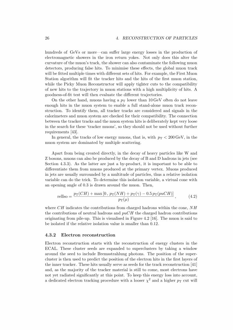
Apart from being created directly, in the decay of heavy particles like W andZ bosons, muons can also be produced by the decay of B and D hadrons in jets (seeSection 4.3.3). As the latter are just a by-product, it is important to be able todifferentiate them from muons produced at the primary vertex. Muons producedin jets are usually surrounded by a multitude of particles, thus a relative isolationvariable can do the trick. To determine this isolation variable, a virtual cone withan opening angle of 0.3 is drawn around the muon. Then,
relIso =pT(CH) + max [0 , pT(NH) + pT(γ)− 0.5 pT(puCH)]
pT(µ), (4.2)
where CH indicates the contributions from charged hadrons within the cone, NHthe contributions of neutral hadrons and puCH the charged hadron contributionsoriginating from pile-up. This is visualised in Figure 4.2 [16]. The muon is said tobe isolated if the relative isolation value is smaller than 0.12.
4.3.2 Electron reconstruction
Electron reconstruction starts with the reconstruction of energy clusters in theECAL. These cluster seeds are expanded to superclusters by taking a windowaround the seed to include Bremsstrahlung photons. The position of the super-cluster is then used to predict the position of the electron hits in the first layers ofthe inner tracker. These hits usually serve as seeds for the track reconstruction [41]and, as the majority of the tracker material is still to come, most electrons havenot yet radiated significantly at this point. To keep this energy loss into account,a dedicated electron tracking procedure with a looser χ2 and a higher pT cut will
4.3. THE PARTICLE FLOW ALGORITHM 27
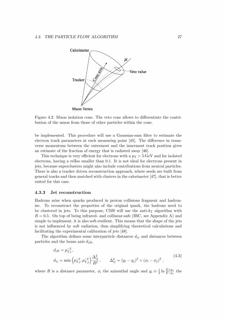
Figure 4.2: Muon isolation cone. The veto cone allows to differentiate the contri-bution of the muon from those of other particles within the cone.
be implemented. This procedure will use a Gaussian-sum filter to estimate theelectron track parameters at each measuring point [45]. The difference in trans-verse momentum between the outermost and the innermost track position givesan estimate of the fraction of energy that is radiated away [46].
This technique is very efficient for electrons with a pT > 5 GeV and for isolatedelectrons, having a relIso smaller than 0.1. It is not ideal for electrons present injets, because superclusters might also include contributions from neutral particles.There is also a tracker driven reconstruction approach, where seeds are built fromgeneral tracks and then matched with clusters in the calorimeter [47], that is bettersuited for this case.
4.3.3 Jet reconstruction
Hadrons arise when quarks produced in proton collisions fragment and hadron-ise. To reconstruct the properties of the original quark, the hadrons need tobe clustered in jets. To this purpose, CMS will use the anti-kT algorithm withR = 0.5 . On top of being infrared- and collinear-safe (IRC, see Appendix A) andsimple to implement, it is also soft-resilient. This means that the shape of the jetsis not influenced by soft radiation, thus simplifying theoretical calculations andfacilitating the experimental calibration of jets [48].
The algorithm defines some interparticle distances dij and distances betweenparticles and the beam axis diB,
diB = p−2T,i ,
dij = min(p−2
T,i, p−2T,j
)∆2ij
R2, ∆2
ij = (yi − yj)2 + (φi − φj)2 ,(4.3)
where R is a distance parameter, φi the azimuthal angle and yi ≡ 12 ln E+pz
E−pz the
28 4. RECONSTRUCTION OF PARTICLES
rapidity of particle i. These distances are determined for all particles. If a dij isthe smallest distance, particles i and j will be combined to a ‘pseudojet’. When aDiB is the smallest jet, particle/pseudojet i is called a jet and will be removed fromthe list of particles. Other jet clustering algorithms are explained in Appendix A.
When there is only one hard particle and several soft particles, the soft particleswill first cluster around the hard particle before clustering amongst themselves.This is a direct consequence of the inverse pT in the distance definition.
Soft particles do not change the shape of jets, hard ones, on the other hand,do. When there is another hard particle within 2R of the first, but farther than R,two hard jets will be created. If pT,1 � pT,2, the first jet will be conical and thesecond one will be partly conical, missing the overlap, which is attributed to thefirst jet. If the transverse momenta are about equal, the overlap will be dividedover the two jets. When two hard particles are within R from each other, only onejet will be formed.
4.3.3.1 Identification of b jets
Jets originating from a b quark have some properties that allow them to be dif-ferentiated from other jets. b quarks often hadronise into B hadrons, which havea considerable lifetime [3]. Contrary to lighter hadrons, they still decay in thetracker and hence produce a secondary vertex (SV). A SV is only designated assuch when it shares less than 65% of its associated tracks with the primary vertex(PV) and its flight direction is within a cone of R = 0.5 around the jet direction.If the radial distance to the PV is longer than 2.5 cm or if its mass is larger than6.5 GeV, the SV candidate is rejected to avoid selecting vertices resulting frominteractions with the detector material or decays of long-lived mesons [49].
Simple algorithms use only one observable, like the flight distance, to tag b jets.Others combine several observables to increase the discriminating power. CMSuses the Combined Secondary Vertex algorithm, or CSV. Contrary to simple sec-ondary vertex algorithms, it also allows for a b jet identification when no SV canbe fitted, thus increasing the efficiency. Since D hadrons have a non-negligiblelifetime, though to a lesser extent than B hadrons, the differentiation between band c jets is more challenging than their distinction from light jets (u, d, s andjets originating from gluons).
b-tag algorithms return a discriminator value for each jet. Depending on thephysics analysis, a minimum threshold is applied to identify a jet as originatingfrom a b quark and to limit the amount of misidentifications [49]. Different workingpoints are defined according to the purity that is required. A loose cut permits amistagging rate of about 10% at pT values of 80 GeV, while this is about 1% fora medium cut and about 0.1% for a tight one. The working point of an analysisis indicated by appending an identifying letter to the algorithm name. For thisanalysis the CSVM tagger will be used.

4.3. THE PARTICLE FLOW ALGORITHM 29
4.3.3.2 Removal of isolated leptons
As mentioned before, several hadrons also have leptonic decay modes, making thepresence of leptons in jets not unusual. It is important, though, to exclude isolatedleptons that accidentally end up in the jet. Therefore, relative isolation cuts willbe applied to the leptons. All muons with a relIso < 0.2 and all electrons withrelIso < 0.15 will be excluded from the jets. These cuts are stricter than those inSections 4.3.1 and 4.3.2 to avoid that isolated leptons would be reconstructed asjets.

30 4. RECONSTRUCTION OF PARTICLES
5
Event Selection
5.1 Event Topology
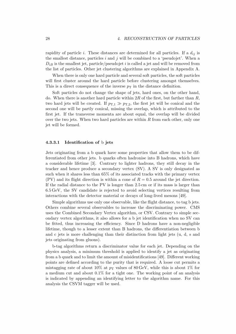
This analysis will consider stop quark pair production, where a stop quark decaysinto a top quark and a neutralino, which is the LSP in this simplified model. Astop quark mass of 350 GeV and a neutralino mass of 100 GeV are assumed. Thisprocess is depicted in Figure 5.1(a). In many ways the process looks like an ‘or-dinary’ pp → tt process, which is visualised in Figure 5.1(b), but there are someimportant differences. First of all, the stop quark decays into a top quark and a
(a) (b)
Figure 5.1: Topology of the semi-muonic decay of a (a) stop quark pair; (b) topquark pair. Antiparticles are indicated with a tilde.
neutralino, which will not be detected by the CMS detector. This will manifestitself in a higher missing transverse energy compared to the missing transverse en-ergy in tt processes. Secondly, the stop quark is heavier than the top quark, whichimplies that its decay products will have a larger transverse momentum than thoseof a top quark.
31
32 5. EVENT SELECTION
The top quark decays almost 100% into a bottom quark and a W boson. Thelatter will decay into a quark pair or into a charged lepton and its correspondingneutrino. The probability for a given particle to decay into a set of other particlesis called the branching ratio (BR). For the W boson these are approximately [3]
BR(W→ q q) ≈ 2/3 , BR(W→ l νl) ≈ 1/3 . (5.1)
The decays of (s)top quark pairs can thus be categorised into fully hadronic decays,where both W bosons decay hadronically, fully leptonic decays, where both W bo-sons decay leptonically, and semi-leptonic decays, where one W boson decays intoa quark pair and the other into a lepton and a neutrino. This analysis will focuson semi-leptonic decays where the lepton is a muon. Being easily recognisable inthe CMS detector, the muon offers a fine trigger. At the same time, the hadronicdecay still allows a full mass reconstruction of the W boson and the top quark.The BR for a semi-muonically decaying top quark pair is
BR(t t→b q q bµ ν) = BR(t→ b W+) · BR(t→ b W−)·[BR(W+ → q q) · BR(W− → l ν) · P (l = µ)+ BR(W+ → l ν) · P (l = µ) · BR(W− → q q)
]≈ 4/27 , (5.2)
where BR(t→ b W) ≈ 1 and the probability that a lepton is a muon is 1/3.As the stop quark has not yet been observed, it is not clear what its branch-
ing ratio to a top quark and a neutralino is. In this analysis, it is assumed to be one.
The amount of produced stop quark pairs depends on the cross section of theprocess and the integrated luminosity. At a centre-of-mass energy of 8 TeV, thecross section times BR is equal to 180.85 fb. As a comparison, the cross section fora semi-muonically decaying tt process is 33.363 pb. The CMS experiment collectedabout 19.1 fb−1 of well-reconstructed proton collisions at 8 TeV. This results inabout 638073 tt events compared to only 3459 t¯t events. If only this tt process isconsidered as background, this corresponds to a signal-to-background ratio S/Bof only 0.5%! So, apart from selecting events with the correct final state, additionalevent selection requirements are needed to increase the signal-to-background ratio.
5.2 Event Generation and Simulation
As can be seen in Figure 5.1, the signature of the signal events, i.e. four jets, amuon and missing transverse energy, can also be produced by other processes.These constitute the background of the analysis. The main background processesare tt, single top, W+jets, Z+jets and QCD multi-jet events.
A Monte Carlo (MC) simulation is made of the background and signal samplesin order to model the events that will meet the selection criteria specified in the
5.2. EVENT GENERATION AND SIMULATION 33
next section. The signal sample and most of the background samples were simu-lated with MadGraph/MadEvent [50]. The single-top samples were simulated withPOWHEG [51–53]. PYTHIA [54] was used to simulate initial and final state radiationand the showering of quarks, using a perturbative model for the fragmentationand the Lund model [55] for the hadronisation.
Besides simulating the signal and background processes, also a simulation of thedetector was made. As the detector is granular, it is possible that some particlesavoid detection by escaping through the cracks. Also interactions with the detectormaterial can obscure the original event. The used materials and the geometry ofthe detector were simulated with GEANT4 [56, 57].
Top quark pairs
The largest background contribution will come from the semi-leptonic decay chan-nel where the lepton is a muon (see Fig. 5.1(b)), but other decay channels willalso have an influence. For example, tt processes without direct muon production,where a tau decays into a muon, doubly-leptonic decays where the second muonis not observed and fully hadronic decays where a non-isolated muon is identifiedas isolated.
Considering a top quark mass of 173 GeV, the NLO cross section for tt processesis 225.2 pb [58]. A sample was simulated corresponding to an integrated luminosityof about 30 fb−1.
Single top (ST)
Top quarks are also produced singly, either in association with another quark orwith a W boson. Especially the tW channel will contribute to the background asonly one additional jet is needed to get the desired final state.
For a top quark mass of 173 GeV, the approximate NNLO cross section ofthe tW channel is about 22.2 pb and about 87.1 pb for the t channel [58]. Thes channel is not considered in this analysis, because, due to the small productioncross section, no events will pass the selection requirements.
The integrated luminosity is about 62 fb−1 for the simulated t channel sampleand about 44 fb−1 for the tW channel.
W+jets
The final state is achieved when a W boson, decaying into a muon and a neutrino,is produced in association with jets.
The NNLO cross section for the production of leptonically decaying W bosonsis approximately 37 509 pb. This is calculated with the FEWZ (Fully Exclusive Wand Z Production) simulation code [59]. In fact, W+jets processes are generatedas a function of the jet multiplicity. This analysis will only use the W+3 jets andthe W+4 jets samples as no events from lower jet multiplicity samples pass theselection criteria in the next section.
34 5. EVENT SELECTION
The integrated luminosity of the W+jets sample is approximately 50 fb−1.
Z+jets
A Z boson is produced in association with jets and decays into a muon pair, ofwhich the second muon is not observed or does not pass the selection criteria.
The NNLO cross section for leptonically decaying Z bosons is approximately3 503.71 pb [60]. The cross section was calculated with the same package as thatof the W+jets sample and the same remarks apply.
The integrated luminosity of the Z+jets sample is approximately 225 fb−1.
QCD multi-jet events
As leptons can be produced within jets, the desired final state can be obtained. Ingeneral, these leptons are not isolated and have a low pT, but, as the cross sectionof these processes is large, contributions from multi-jet events cannot be ruled outcompletely.
As is discussed in the following section, the selection criteria rule out most ofthe multi-jet events. Therefore, this background will not be simulated.
5.3 Selection Requirements
Only events that pass the trigger requiring an isolated muon with a pT larger than24 GeV and a pseudo-rapidity |η| < 2.1 are used. The efficiency of the trigger is notthe same for the data and the simulation. Therefore, a scale factor is implementedfor the simulated samples. As the trigger efficiency depends on the pT and η ofthe muon, also the scale factors depend on these variables. The scale factors aredefined as the ratio of the trigger efficiency in data and the trigger efficiency insimulated Z→ µµ events. [61]
Then, a good primary vertex is sought. As the LHC collides bunches of pro-tons, each containing billions of particles, it is possible that more than one protonpair collides during the same bunch crossing. This results in several primary vertexcandidates. The correct one is determined with the aid of the impact parameter.In the z direction the impact parameter must be smaller than 24 cm and it mustbe smaller than 2 cm in the transverse plane. If there is more than one PV thatfills these requirements, the one maximising the sum of the p2
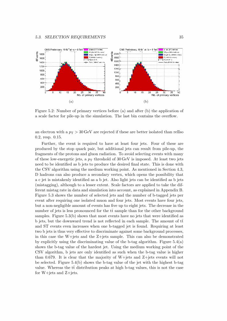
T of its tracks ischosen. The amount of pile-up energy of the so-called underlying event is relatedto the number of primary vertices. The average number of primary vertices perevent is visualised in Figure 5.2(a). The number of PVs in the simulation doesnot correspond with the number of PVs in the data. Therefore, a scale factor isapplied to the simulation. The resulting distribution is shown in Figure 5.2(b).
To get the final state defined in Section 5.1, exactly one isolated muon isrequired. This must have a pT larger than 25 GeV and a pseudo-rapidity η < 2.1.On top of that, events containing a second muon with a pT larger than 10 GeV or
5.3. SELECTION REQUIREMENTS 35
(a) (b)
Figure 5.2: Number of primary vertices before (a) and after (b) the application ofa scale factor for pile-up in the simulation. The last bin contains the overflow.
an electron with a pT > 30 GeV are rejected if these are better isolated than relIso0.2, resp. 0.15.
Further, the event is required to have at least four jets. Four of these areproduced by the stop quark pair, but additional jets can result from pile-up, thefragments of the protons and gluon radiation. To avoid selecting events with manyof these low-energetic jets, a pT threshold of 30 GeV is imposed. At least two jetsneed to be identified as b jets to produce the desired final state. This is done withthe CSV algorithm using the medium working point. As mentioned in Section 4.3,D hadrons can also produce a secondary vertex, which opens the possibility thata c jet is mistakenly identified as a b jet. Also light jets can be identified as b jets(mistagging), although to a lesser extent. Scale factors are applied to take the dif-ferent mistag rate in data and simulation into account, as explained in Appendix B.Figure 5.3 shows the number of selected jets and the number of b-tagged jets perevent after requiring one isolated muon and four jets. Most events have four jets,but a non-negligible amount of events has five up to eight jets. The decrease in thenumber of jets is less pronounced for the tt sample than for the other backgroundsamples. Figure 5.3(b) shows that most events have no jets that were identified asb jets, but the downward trend is not reflected in each sample. The amount of ttand ST events even increases when one b-tagged jet is found. Requiring at leasttwo b jets is thus very effective to discriminate against some background processes,in this case the W+jets and the Z+jets sample. This can also be demonstratedby explicitly using the discriminating value of the b-tag algorithm. Figure 5.4(a)shows the b-tag value of the hardest jet. Using the medium working point of theCSV algorithm, b jets are only identified as such when the b-tag value is higherthan 0.679. It is clear that the majority of W+jets and Z+jets events will notbe selected. Figure 5.4(b) shows the b-tag value of the jet with the highest b-tagvalue. Whereas the tt distribution peaks at high b-tag values, this is not the casefor W+jets and Z+jets.
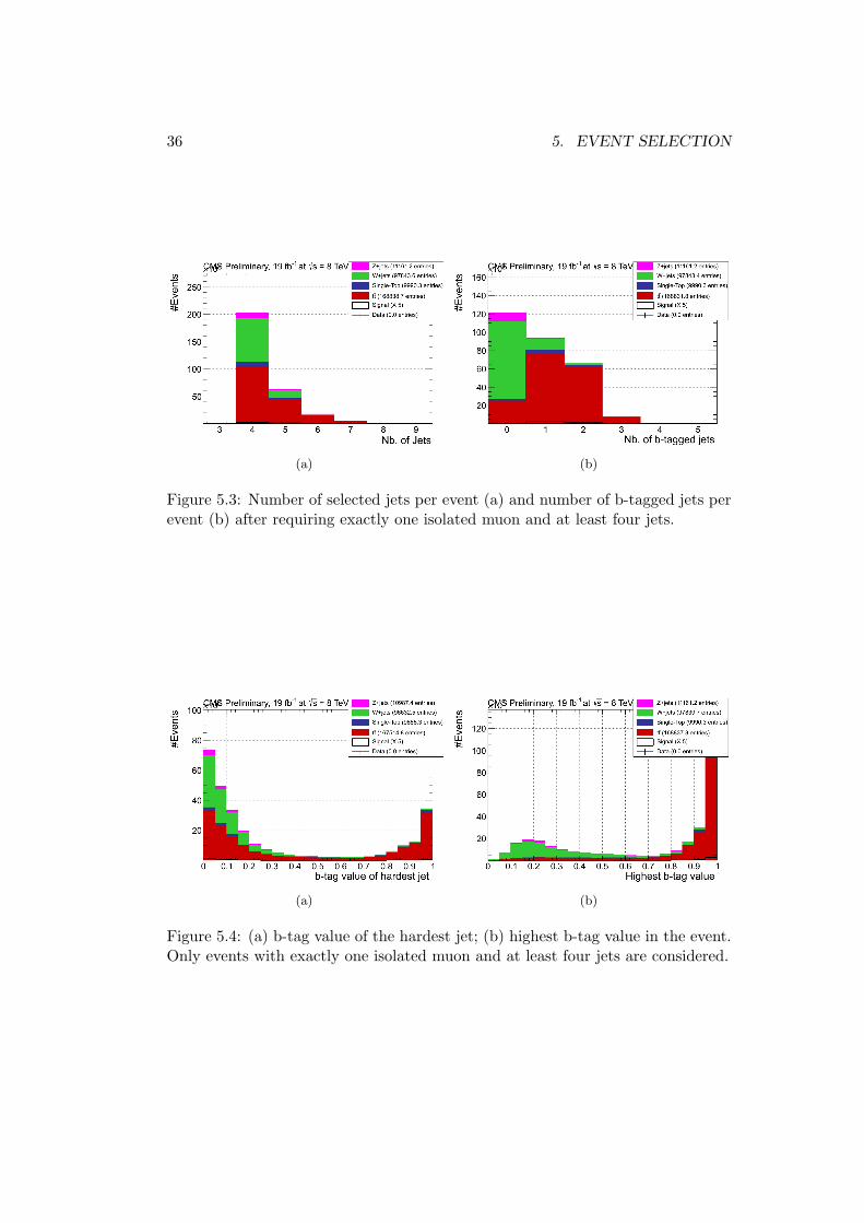
36 5. EVENT SELECTION
(a) (b)
Figure 5.3: Number of selected jets per event (a) and number of b-tagged jets perevent (b) after requiring exactly one isolated muon and at least four jets.
(a) (b)
Figure 5.4: (a) b-tag value of the hardest jet; (b) highest b-tag value in the event.Only events with exactly one isolated muon and at least four jets are considered.
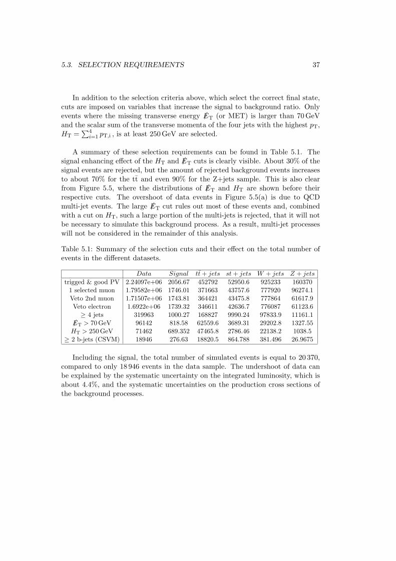
5.3. SELECTION REQUIREMENTS 37
In addition to the selection criteria above, which select the correct final state,cuts are imposed on variables that increase the signal to background ratio. Onlyevents where the missing transverse energy /ET (or MET) is larger than 70 GeVand the scalar sum of the transverse momenta of the four jets with the highest pT,HT =
∑4i=1 pT,i , is at least 250 GeV are selected.
A summary of these selection requirements can be found in Table 5.1. Thesignal enhancing effect of the HT and /ET cuts is clearly visible. About 30% of thesignal events are rejected, but the amount of rejected background events increasesto about 70% for the tt and even 90% for the Z+jets sample. This is also clearfrom Figure 5.5, where the distributions of /ET and HT are shown before theirrespective cuts. The overshoot of data events in Figure 5.5(a) is due to QCDmulti-jet events. The large /ET cut rules out most of these events and, combinedwith a cut on HT, such a large portion of the multi-jets is rejected, that it will notbe necessary to simulate this background process. As a result, multi-jet processeswill not be considered in the remainder of this analysis.
Table 5.1: Summary of the selection cuts and their effect on the total number ofevents in the different datasets.
Data Signal tt+ jets st+ jets W + jets Z + jets
trigged & good PV 2.24097e+06 2056.67 452792 52950.6 925233 1603701 selected muon 1.79582e+06 1746.01 371663 43757.6 777920 96274.1Veto 2nd muon 1.71507e+06 1743.81 364421 43475.8 777864 61617.9Veto electron 1.6922e+06 1739.32 346611 42636.7 776087 61123.6≥ 4 jets 319963 1000.27 168827 9990.24 97833.9 11161.1
/ET > 70 GeV 96142 818.58 62559.6 3689.31 29202.8 1327.55HT > 250 GeV 71462 689.352 47465.8 2786.46 22138.2 1038.5≥ 2 b-jets (CSVM) 18946 276.63 18820.5 864.788 381.496 26.9675
Including the signal, the total number of simulated events is equal to 20 370,compared to only 18 946 events in the data sample. The undershoot of data canbe explained by the systematic uncertainty on the integrated luminosity, which isabout 4.4%, and the systematic uncertainties on the production cross sections ofthe background processes.
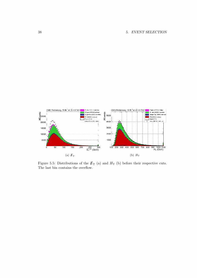
38 5. EVENT SELECTION
(a) /ET (b) HT
Figure 5.5: Distributions of the /ET (a) and HT (b) before their respective cuts.The last bin contains the overflow.
6
Event Reconstruction
A particle detector only registers the final state of the event. In case of the eventtopology in Section 5.1 there are four jets, one muon and missing transverse energy.These objects can be recombined to W bosons, top and stop quarks. This is nottrivial since it is not clear which jet originated from which parton. Therefore, simu-lated samples are used to determine the expected distribution of the reconstructedmass of the W boson and the top quark by matching the jets to the partons andrecombining them into the correct objects. For each possible combination in thereconstructed event, a kinematic variable reflecting the agreement with the expec-ted W boson and top quark masses is calculated. This way, the simulated samplesand the data sample are treated on the same level, without explicitly using theparton information.
6.1 Jet-Parton Matching
The jet-parton matching is carried out using the simulated tt sample. This samplealso contains generated events, where each particle is associated with an identifyingnumber or pdgID [3]. This enables to reconstruct the decay chain, as not only thepdgID of the particle itself, but also that of its ‘mother’ and ‘grandmother’ particlecan be retrieved. Only those simulated events where the full expected decay chainof the top quark is recovered from the kinematics of the observed objects are used.The expected distribution of the W boson and top quark masses is obtained fromthese events.
The jets will be matched with the quarks using an algorithm that orders thequarks according to descending pT values and minimises the sum of the distancesbetween the four quarks and the jets. These distances are defined as,
∆R =√
(ηjet − ηquark)2 + (φjet − φquark)2 , (6.1)
and cannot exceed 0.3 for each jet–quark pair.Using the pdgIDs of the quarks, the masses of the reconstructed hadronically
decaying W boson and the corresponding top quark are calculated. The mass
39
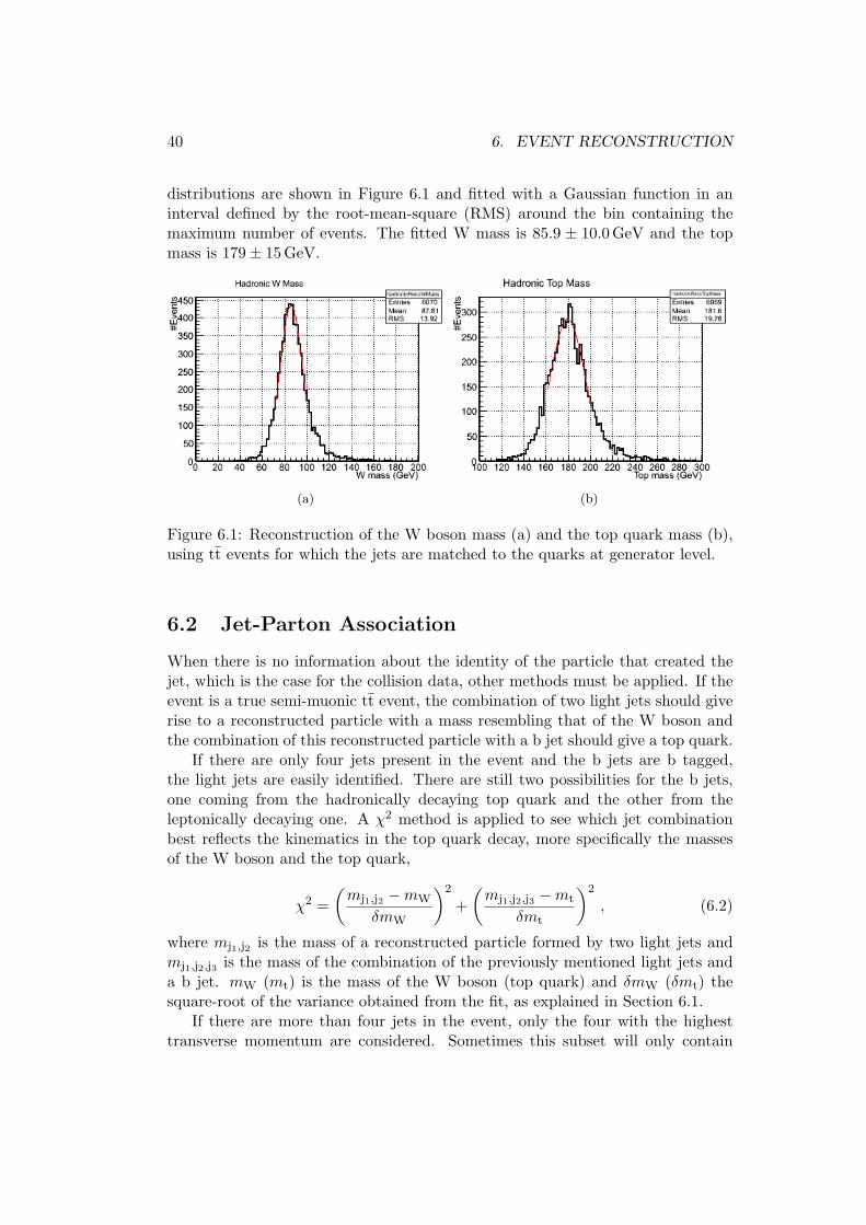
40 6. EVENT RECONSTRUCTION
distributions are shown in Figure 6.1 and fitted with a Gaussian function in aninterval defined by the root-mean-square (RMS) around the bin containing themaximum number of events. The fitted W mass is 85.9 ± 10.0 GeV and the topmass is 179± 15 GeV.
(a) (b)
Figure 6.1: Reconstruction of the W boson mass (a) and the top quark mass (b),using tt events for which the jets are matched to the quarks at generator level.
6.2 Jet-Parton Association
When there is no information about the identity of the particle that created thejet, which is the case for the collision data, other methods must be applied. If theevent is a true semi-muonic tt event, the combination of two light jets should giverise to a reconstructed particle with a mass resembling that of the W boson andthe combination of this reconstructed particle with a b jet should give a top quark.
If there are only four jets present in the event and the b jets are b tagged,the light jets are easily identified. There are still two possibilities for the b jets,one coming from the hadronically decaying top quark and the other from theleptonically decaying one. A χ2 method is applied to see which jet combinationbest reflects the kinematics in the top quark decay, more specifically the massesof the W boson and the top quark,
χ2 =(mj1,j2 −mW
δmW
)2
+(mj1,j2,j3 −mt
δmt
)2
, (6.2)
where mj1,j2 is the mass of a reconstructed particle formed by two light jets andmj1,j2,j3 is the mass of the combination of the previously mentioned light jets anda b jet. mW (mt) is the mass of the W boson (top quark) and δmW (δmt) thesquare-root of the variance obtained from the fit, as explained in Section 6.1.
If there are more than four jets in the event, only the four with the highesttransverse momentum are considered. Sometimes this subset will only contain
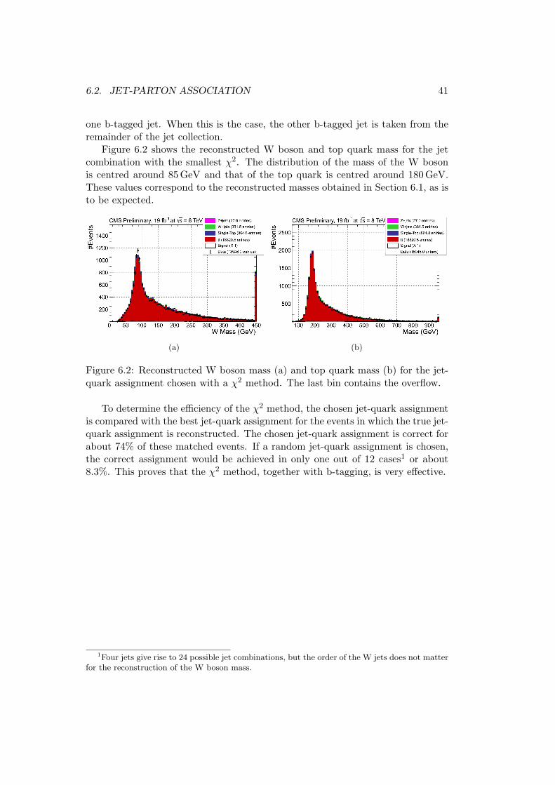
6.2. JET-PARTON ASSOCIATION 41
one b-tagged jet. When this is the case, the other b-tagged jet is taken from theremainder of the jet collection.
Figure 6.2 shows the reconstructed W boson and top quark mass for the jetcombination with the smallest χ2. The distribution of the mass of the W bosonis centred around 85 GeV and that of the top quark is centred around 180 GeV.These values correspond to the reconstructed masses obtained in Section 6.1, as isto be expected.
(a) (b)
Figure 6.2: Reconstructed W boson mass (a) and top quark mass (b) for the jet-quark assignment chosen with a χ2 method. The last bin contains the overflow.
To determine the efficiency of the χ2 method, the chosen jet-quark assignmentis compared with the best jet-quark assignment for the events in which the true jet-quark assignment is reconstructed. The chosen jet-quark assignment is correct forabout 74% of these matched events. If a random jet-quark assignment is chosen,the correct assignment would be achieved in only one out of 12 cases1 or about8.3%. This proves that the χ2 method, together with b-tagging, is very effective.
1Four jets give rise to 24 possible jet combinations, but the order of the W jets does not matterfor the reconstruction of the W boson mass.

42 6. EVENT RECONSTRUCTION
7
The Matrix Element Method
The Matrix element method (MEM) is a fairly recent technique that was firstintroduced at the Tevatron collider to make a more precise measurement of thetop quark mass [62,63]. It will be shown to be also useful for analyses where a smallsignal has to be extracted from a large background. Traditionally, these analysesmake use of multivariate analysis techniques like neural networks, where severalvariables that are sensitive to the signal are combined in order to make a variablethat is even more sensitive. As the matrix element method uses all informationcontained in the event, it is expected that this method is more sensitive than MVAtechniques, which use only a subset of information.
This chapter will describe the matrix element method and explain how it is usedin this analysis. Chapter 8 will compare this technique’s sensitivity to stop quarkproduction with that of a standard kinematic observable, in this case HT + /ET.
7.1 The Matrix Element Method in a Nutshell
The MEM uses the theoretical matrix element to calculate the probability that acertain process is produced and observed assuming a specific theoretical model [64].The observed event is characterised by a set of measured four-momenta pobs andthe probability density is defined as,
P(pobs
∣∣∣~θ) =1
σ(~θ)
∫dptrue
∣∣∣M(~θ∣∣∣ptrue)∣∣∣2 R(ptrue∣∣∣pobs) , (7.1)
where ~θ = θ1, ..., θn are the parameters of the physics model, M(~θ|ptrue) is thetheoretical matrix element of the specific process, σ(~θ) is the total cross section ofthe process and R(ptrue|pobs) is the transfer function.
The matrix element will be calculated at leading order using the parton four-momenta. The four-momenta of the objects are parametrised as E, θ and φ. Asthe partons hadronise and the detector has a limited resolution, this does notcorrespond to the momenta that are actually observed. Also interactions with
43
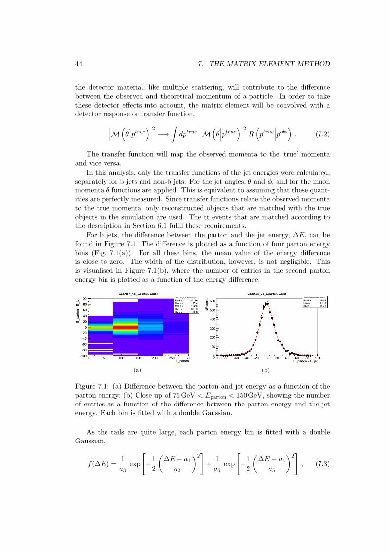
44 7. THE MATRIX ELEMENT METHOD
the detector material, like multiple scattering, will contribute to the differencebetween the observed and theoretical momentum of a particle. In order to takethese detector effects into account, the matrix element will be convolved with adetector response or transfer function.∣∣∣M(
~θ∣∣∣ptrue)∣∣∣2 −→ ∫
dptrue∣∣∣M(
~θ∣∣∣ptrue)∣∣∣2 R(ptrue∣∣∣pobs) . (7.2)
The transfer function will map the observed momenta to the ‘true’ momentaand vice versa.
In this analysis, only the transfer functions of the jet energies were calculated,separately for b jets and non-b jets. For the jet angles, θ and φ, and for the muonmomenta δ functions are applied. This is equivalent to assuming that these quant-ities are perfectly measured. Since transfer functions relate the observed momentato the true momenta, only reconstructed objects that are matched with the trueobjects in the simulation are used. The tt events that are matched according tothe description in Section 6.1 fulfil these requirements.
For b jets, the difference between the parton and the jet energy, ∆E, can befound in Figure 7.1. The difference is plotted as a function of four parton energybins (Fig. 7.1(a)). For all these bins, the mean value of the energy differenceis close to zero. The width of the distribution, however, is not negligible. Thisis visualised in Figure 7.1(b), where the number of entries in the second partonenergy bin is plotted as a function of the energy difference.
(a) (b)
Figure 7.1: (a) Difference between the parton and jet energy as a function of theparton energy; (b) Close-up of 75 GeV < Eparton < 150 GeV, showing the numberof entries as a function of the difference between the parton energy and the jetenergy. Each bin is fitted with a double Gaussian.
As the tails are quite large, each parton energy bin is fitted with a doubleGaussian,
f(∆E) =1a3
exp
[−1
2
(∆E − a1
a2
)2]
+1a6
exp
[−1
2
(∆E − a4
a5
)2], (7.3)
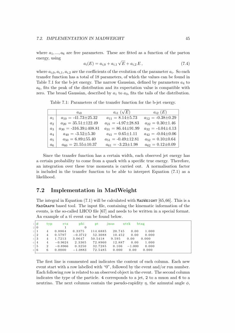
7.2. IMPLEMENTATION IN MADWEIGHT 45
where a1, ..., a6 are free parameters. These are fitted as a function of the partonenergy, using
ai(E) = ai,0 + ai,1√E + ai,2E , (7.4)
where ai,0, ai,1, ai,2 are the coefficients of the evolution of the parameter ai. So eachtransfer function has a total of 18 parameters, of which the values can be found inTable 7.1 for the b-jet energy. The narrow Gaussian, defined by parameters a4 toa6, fits the peak of the distribution and its expectation value is compatible withzero. The broad Gaussian, described by a1 to a3, fits the tails of the distribution.
Table 7.1: Parameters of the transfer function for the b-jet energy.
ai0 ai1 (√E) ai2 (E)
a1 a10 = -41.73±25.32 a11 = 8.14±5.73 a12 = -0.38±0.29a2 a20 = 35.51±122.49 a21 = -4.97±28.83 a22 = 0.30±1.46a3 a30 = -316.39±408.81 a31 = 86.44±91.99 a32 = -4.04±4.13a4 a40 = -3.52±5.30 a41 = 0.65±1.11 a42 = -0.04±0.06a5 a50 = 6.89±55.40 a51 = -0.49±12.81 a52 = 0.10±0.64a6 a60 = 21.55±10.37 a61 = -3.23±1.98 a62 = 0.12±0.09
Since the transfer function has a certain width, each observed jet energy hasa certain probability to come from a quark with a specific true energy. Therefore,an integration over these true momenta is carried out. A normalisation factoris included in the transfer function to be able to interpret Equation (7.1) as alikelihood.
7.2 Implementation in MadWeight
The integral in Equation (7.1) will be calculated with MadWeight [65,66]. This is aMadGraph based tool. The input file, containing the kinematic information of theevents, is the so-called LHCO file [67] and needs to be written in a special format.An example of a tt event can be found below.
1 # typ eta phi pt jmas ntrk btag2 0 1 03 1 4 0 .8864 0 .3375 114.6885 20 .745 0 .00 1 .0004 2 4 0 .5797 −0.3712 52.3088 10 .452 0 .00 0 .0005 3 4 1 .7213 3 .0647 50.5418 9 .595 0 .00 0 .0006 4 4 −0.9624 2 .3365 72.8960 12 .887 0 .00 1 .0007 5 2 −0.8966 0 .3250 32.7285 0 .106 −1.000 0 .0008 6 6 0 .0000 −1.0883 72.5485 0 .000 0 .00 0 .000
The first line is commented and indicates the content of each column. Each newevent start with a row labelled with “0”, followed by the event and/or run number.Each following row is related to an observed object in the event. The second columnindicates the type of the particle. 4 corresponds to a jet, 2 to a muon and 6 to aneutrino. The next columns contain the pseudo-rapidity η, the azimutal angle φ,
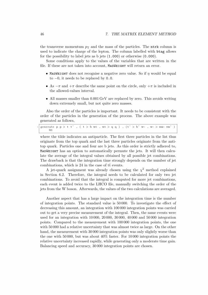
46 7. THE MATRIX ELEMENT METHOD
the transverse momentum pT and the mass of the particles. The ntrk column isused to indicate the charge of the lepton. The column labelled with btag allowsfor the possibility to label jets as b jets (1.000) or otherwise (0.000).
Some conditions apply to the values of the variables that are written in thefile. If these are not taken into account, MadWeight will return an error.
• MadWeight does not recognise a negative zero value. So if η would be equalto −0, it needs to be replaced by 0.0.
• As −π and +π describe the same point on the circle, only +π is included inthe allowed-values interval.
• All masses smaller than 0.001 GeV are replaced by zero. This avoids writingdown extremely small, but not quite zero masses.
Also the order of the particles is important. It needs to be consistent with theorder of the particles in the generation of the process. The above example wasgenerated as follows,
1 generate p p > t t ˜ , ( t > b w+ , w+ > q q ) , ( t ˜ > b˜ w− , w− > mu− vm˜ )@1
where the tilde indicates an antiparticle. The first three particles in the list thusoriginate from the top quark and the last three particles originate from the anti-top quark. Particles one and four are b jets. As this order is strictly adhered to,MadWeight has an option to automatically permute the jets. It will then calcu-late the average of the integral values obtained by all possible jet combinations.The drawback is that the integration time strongly depends on the number of jetcombinations, which is 24 in the case of tt events.
A jet-quark assignment was already chosen using the χ2 method explainedin Section 6.2. Therefore, the integral needs to be calculated for only two jetcombinations. To avoid that the integral is computed for more jet combinations,each event is added twice to the LHCO file, manually switching the order of thejets from the W boson. Afterwards, the values of the two calculations are averaged.
Another aspect that has a large impact on the integration time is the numberof integration points. The standard value is 50 000. To investigate the effect ofdecreasing this amount, an integration with 100 000 integration points was carriedout to get a very precise measurement of the integral. Then, the same events wereused for an integration with 10 000, 20 000, 30 000, 40 000 and 50 000 integrationpoints. Compared to the measurement with 100 000 integration points, the onewith 50 000 had a relative uncertainty that was almost twice as large. On the otherhand, the measurement with 30 000 integration points was only slightly worse thanthe one with 50 000, but was about 40% faster. For 10 000 integration points therelative uncertainty increased rapidly, while generating only a moderate time gain.Balancing speed and accuracy, 30 000 integration points are chosen.

7.2. IMPLEMENTATION IN MADWEIGHT 47
Also the transfer functions have an impact on the integration time. This iswhy only the transfer functions for the jet energies (both b and non-b) were im-plemented.
With these settings, the average integration time for a tt event, with twojet combinations, is about 15 min. In the meantime, developments in MadWeight
continued and, recently, the integration time is reduced by a factor ten or more.

48 7. THE MATRIX ELEMENT METHOD
8
Sensitivity of the MatrixElement Method for StopQuark Searches
8.1 Calculation of the Probability Density for Differ-ent Hypotheses
The matrix element method returns the probability that a certain observed eventis consistent with a specific physics hypothesis. The underlying hypothesis orphysics process can be a stop quark pair process (signal), but also a backgroundprocess. Therefore, the probability is calculated for both the signal and the back-ground hypothesis. The latter is represented by tt production, which is by far thedominant background. This means that there are four integral calculations perevent, as there are two possible jet combinations and two hypotheses.
The integrals are calculated with MadWeight, as is explained in Section 7.2,and the values obtained from the different jet combinations are averaged. Also aweighted average, where higher integral values got a higher weight, was investig-ated, but this turned out to have little effect.
The normalisation factor is defined by the cross section of the process. Asan event selection reduces the number of events, the cross section needs to bemultiplied by the selection efficiency, which is about 2.37% for the tt sample andabout 10.69% for the signal. Combined with the cross-section times branching ratiomentioned in Section 5.1, the normalisation factors become 51.7 for the signal and1.26 for the tt sample.
With these components, the probability in Equation (7.1) can be computed.Some approximations were made in the calculations of the normalisation factor andthe transfer functions, and it was not verified if P(pobs|~θ) can truly be interpretedas a probability. A probabilistic interpretation of P(pobs|~θ) is not necessary for
49
50 8. SENSITIVITY OF THE MEM FOR STOP QUARK SEARCHES
this analysis, since the probabilities are merely used to construct a variable todiscriminate between two physics hypotheses.
Figure 8.1 shows the probabilities for events coming from the simulated sig-nal, tt and W/Z+jets samples, where the last two are combined under ‘other’.P(pobs |t¯t) is indicated by P(S) and P(pobs|tt) by P(B). As the probabilities arevery small, the negative logarithm of the probabilities is displayed. This meansthat the highest values of the probabilities can be found in the bottom left corner.
Figure 8.1(a) shows the probabilities for the signal sample. These seem to beordered on a bisector with a tail in the x direction. For low x values, i.e. highprobabilities when a signal hypothesis is assumed, the spread in the y direction ismuch larger than that in the x direction. This means that the events resemble thesignal hypothesis more than the background hypothesis.
The probabilities for the tt sample can be found in Figure 8.1(b). Figure 8.1(c)shows the probabilities for tt events where the jets were matched to the partons atgenerator level. A comparison of both plots shows that the tail of the distributionand most of the width of the bisector arise from incorrect jet-quark assignments.
Figure 8.1(d) shows the probabilities for W+jets and Z+jets events. These areexpected to resemble the signal and the background hypothesis equally well. Thisis indicated by a rather narrow bisector.
8.2 Sensitivity of Different Observables
8.2.1 Likelihood ratio
The probabilities in Section 8.1 are used to make a discriminating variable. Thisanalysis will use the likelihood ratio (LR), which is defined as
LR =P(S)
P(S) + P(B). (8.1)
The distribution of this variable is plotted in Figure 8.2, using both a linearscale (a) and a logarithmic scale (b). Most events are found in the first and last bin.The first bin is expected to contain events that bear resemblance to backgroundevents and the last bin to contain events that look like signal events.
To determine the sensitivity of the likelihood ratio, the signal-to-backgroundratio S/
√B is determined. All events with a LR value below a certain cut value
are removed and S/√B is calculated from the remaining events. The result is
shown in Figure 8.3. The binning is ten times finer than in Figure 8.2 to get agood view of the tiniest changes.
As is expected, it is better to either apply no cut on the likelihood ratio or toapply a cut close to one. The steep increase at the last bin, however, suggests that,even with this fine binning, most of the sensitivity is contained in the last bin. Thesignificance also gives an indication of the sensitivity that would be achieved if thelikelihood ratio was used in a simple cut-and-count technique.
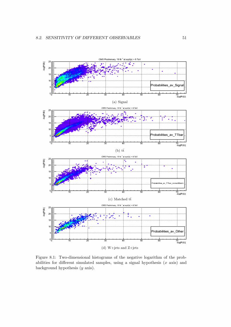
8.2. SENSITIVITY OF DIFFERENT OBSERVABLES 51
(a) Signal
(b) tt
(c) Matched tt
(d) W+jets and Z+jets
Figure 8.1: Two-dimensional histograms of the negative logarithm of the prob-abilities for different simulated samples, using a signal hypothesis (x axis) andbackground hypothesis (y axis).
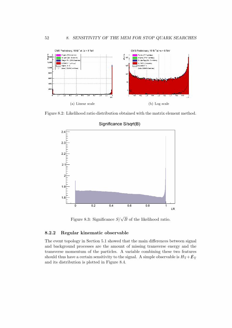
52 8. SENSITIVITY OF THE MEM FOR STOP QUARK SEARCHES
(a) Linear scale (b) Log scale
Figure 8.2: Likelihood ratio distribution obtained with the matrix element method.
Figure 8.3: Significance S/√B of the likelihood ratio.
8.2.2 Regular kinematic observable
The event topology in Section 5.1 showed that the main differences between signaland background processes are the amount of missing transverse energy and thetransverse momentum of the particles. A variable combining these two featuresshould thus have a certain sensitivity to the signal. A simple observable is HT+ /ET
and its distribution is plotted in Figure 8.4.
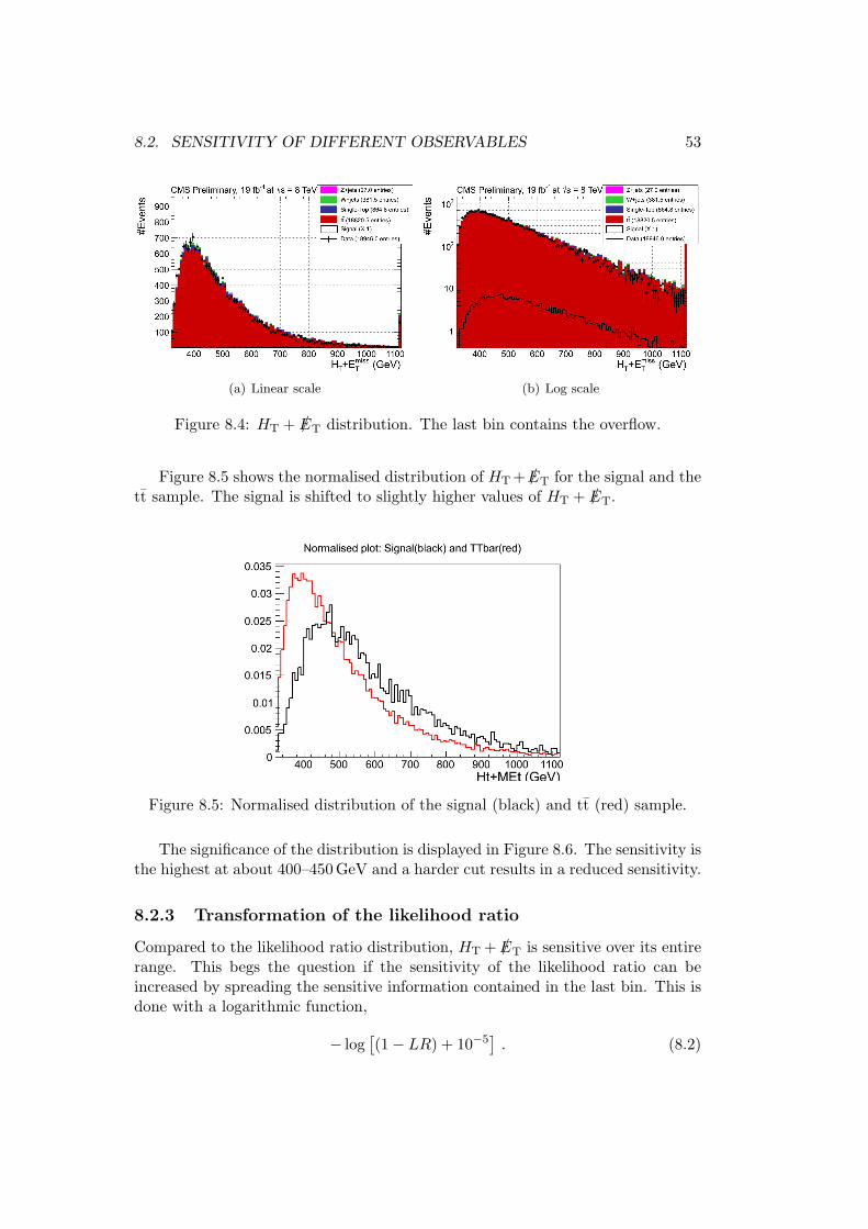
8.2. SENSITIVITY OF DIFFERENT OBSERVABLES 53
(a) Linear scale (b) Log scale
Figure 8.4: HT + /ET distribution. The last bin contains the overflow.
Figure 8.5 shows the normalised distribution of HT + /ET for the signal and thett sample. The signal is shifted to slightly higher values of HT + /ET.
Figure 8.5: Normalised distribution of the signal (black) and tt (red) sample.
The significance of the distribution is displayed in Figure 8.6. The sensitivity isthe highest at about 400–450 GeV and a harder cut results in a reduced sensitivity.
8.2.3 Transformation of the likelihood ratio
Compared to the likelihood ratio distribution, HT + /ET is sensitive over its entirerange. This begs the question if the sensitivity of the likelihood ratio can beincreased by spreading the sensitive information contained in the last bin. This isdone with a logarithmic function,
− log[(1− LR) + 10−5
]. (8.2)
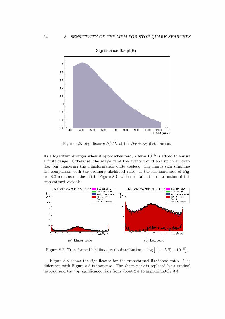
54 8. SENSITIVITY OF THE MEM FOR STOP QUARK SEARCHES
Figure 8.6: Significance S/√B of the HT + /ET distribution.
As a logarithm diverges when it approaches zero, a term 10−5 is added to ensurea finite range. Otherwise, the majority of the events would end up in an over-flow bin, rendering the transformation quite useless. The minus sign simplifiesthe comparison with the ordinary likelihood ratio, as the left-hand side of Fig-ure 8.2 remains on the left in Figure 8.7, which contains the distribution of thistransformed variable.
(a) Linear scale (b) Log scale
Figure 8.7: Transformed likelihood ratio distribution, − log[(1− LR) + 10−5
].
Figure 8.8 shows the significance for the transformed likelihood ratio. Thedifference with Figure 8.3 is immense. The sharp peak is replaced by a gradualincrease and the top significance rises from about 2.4 to approximately 3.3.
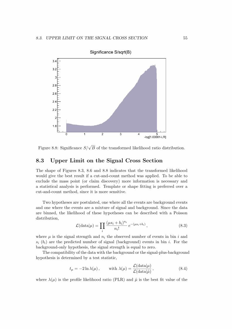
8.3. UPPER LIMIT ON THE SIGNAL CROSS SECTION 55
Figure 8.8: Significance S/√B of the transformed likelihood ratio distribution.
8.3 Upper Limit on the Signal Cross Section
The shape of Figures 8.3, 8.6 and 8.8 indicates that the transformed likelihoodwould give the best result if a cut-and-count method was applied. To be able toexclude the mass point (or claim discovery) more information is necessary anda statistical analysis is performed. Template or shape fitting is preferred over acut-and-count method, since it is more sensitive.
Two hypotheses are postulated, one where all the events are background eventsand one where the events are a mixture of signal and background. Since the dataare binned, the likelihood of these hypotheses can be described with a Poissondistribution,
L(data|µ) =∏i
(µsi + bi)ni
ni!e−(µsi+bi) , (8.3)
where µ is the signal strength and ni the observed number of events in bin i andsi (bi) are the predicted number of signal (background) events in bin i. For thebackground-only hypothesis, the signal strength is equal to zero.
The compatibility of the data with the background or the signal-plus-backgroundhypothesis is determined by a test statistic,
tµ = −2 lnλ(µ) , with λ(µ) =L(data|µ)L(data|µ)
, (8.4)
where λ(µ) is the profile likelihood ratio (PLR) and µ is the best fit value of the
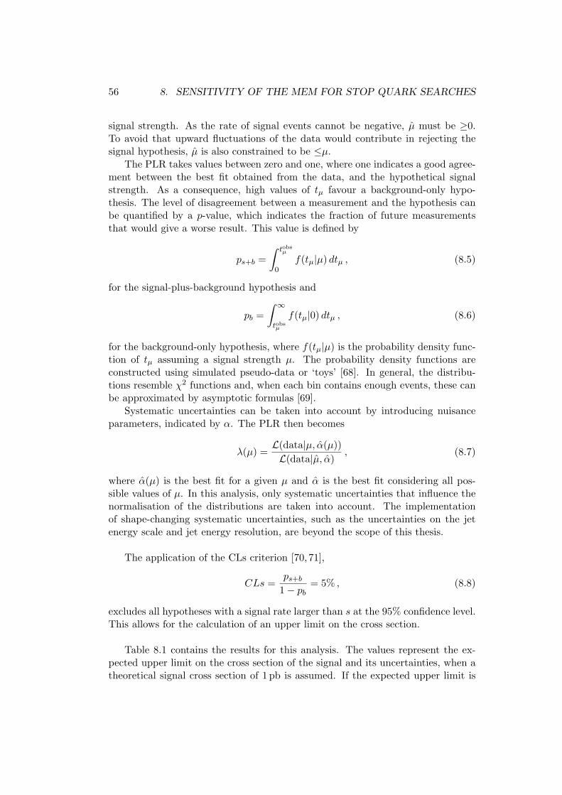
56 8. SENSITIVITY OF THE MEM FOR STOP QUARK SEARCHES
signal strength. As the rate of signal events cannot be negative, µ must be ≥0.To avoid that upward fluctuations of the data would contribute in rejecting thesignal hypothesis, µ is also constrained to be ≤µ.
The PLR takes values between zero and one, where one indicates a good agree-ment between the best fit obtained from the data, and the hypothetical signalstrength. As a consequence, high values of tµ favour a background-only hypo-thesis. The level of disagreement between a measurement and the hypothesis canbe quantified by a p-value, which indicates the fraction of future measurementsthat would give a worse result. This value is defined by
ps+b =∫ tobs
µ
0f(tµ|µ) dtµ , (8.5)
for the signal-plus-background hypothesis and
pb =∫ ∞tobsµ
f(tµ|0) dtµ , (8.6)
for the background-only hypothesis, where f(tµ|µ) is the probability density func-tion of tµ assuming a signal strength µ. The probability density functions areconstructed using simulated pseudo-data or ‘toys’ [68]. In general, the distribu-tions resemble χ2 functions and, when each bin contains enough events, these canbe approximated by asymptotic formulas [69].
Systematic uncertainties can be taken into account by introducing nuisanceparameters, indicated by α. The PLR then becomes
λ(µ) =L(data|µ, α(µ))L(data|µ, α)
, (8.7)
where α(µ) is the best fit for a given µ and α is the best fit considering all pos-sible values of µ. In this analysis, only systematic uncertainties that influence thenormalisation of the distributions are taken into account. The implementationof shape-changing systematic uncertainties, such as the uncertainties on the jetenergy scale and jet energy resolution, are beyond the scope of this thesis.
The application of the CLs criterion [70,71],
CLs =ps+b
1− pb= 5% , (8.8)
excludes all hypotheses with a signal rate larger than s at the 95% confidence level.This allows for the calculation of an upper limit on the cross section.
Table 8.1 contains the results for this analysis. The values represent the ex-pected upper limit on the cross section of the signal and its uncertainties, when atheoretical signal cross section of 1 pb is assumed. If the expected upper limit is
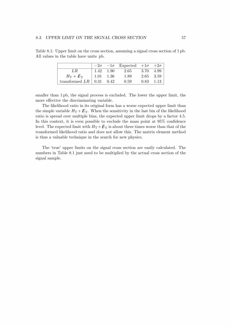
8.3. UPPER LIMIT ON THE SIGNAL CROSS SECTION 57
Table 8.1: Upper limit on the cross section, assuming a signal cross section of 1 pb.All values in the table have units pb.
−2σ −1σ Expected +1σ +2σLR 1.42 1.90 2.65 3.70 4.99
HT + /ET 1.01 1.36 1.89 2.65 3.59transformed LR 0.31 0.42 0.59 0.83 1.13
smaller than 1 pb, the signal process is excluded. The lower the upper limit, themore effective the discriminating variable.
The likelihood ratio in its original form has a worse expected upper limit thanthe simple variable HT + /ET. When the sensitivity in the last bin of the likelihoodratio is spread over multiple bins, the expected upper limit drops by a factor 4.5.In this context, it is even possible to exclude the mass point at 95% confidencelevel. The expected limit with HT + /ET is about three times worse than that of thetransformed likelihood ratio and does not allow this. The matrix element methodis thus a valuable technique in the search for new physics.
The ‘true’ upper limits on the signal cross section are easily calculated. Thenumbers in Table 8.1 just need to be multiplied by the actual cross section of thesignal sample.

58 8. SENSITIVITY OF THE MEM FOR STOP QUARK SEARCHES

9
Conclusions & Perspectives
In this thesis, the matrix element method was examined as an alternative tech-nique to multivariate analyses for new-physics searches. Its performance was testedwith respect to that of a simple kinematic variable, HT + /ET, by calculating theupper limit on the cross section of the production of a stop quark pair decayingto a top quark and a neutralino. To simplify the interpretation of the results,the theoretical cross section of this process was assumed to be 1 pb. Whereas thesimple likelihood ratio of the probabilities obtained by the matrix element methodrecorded a worse performance than the variable HT + /ET, returning an expectedupper limit of 2.65+1.05
−0.74 pb on the signal cross section compared to 1.89+0.76−0.54 pb for
HT + /ET, a transformation of the likelihood ratio yielded an expected upper limitof 0.59+0.24
−0.17 pb. This is about a factor three better than the upper limit obtainedby HT + /ET and proves that the matrix element technique is a valuable additionto the current analysis techniques searching for new physics and processes with alow signal-to-background ratio in general.
In the set-up of this analysis, the investigated mass point, having a stop quarkmass of 350 GeV and a neutralino mass of 100 GeV, can be excluded at 95% con-fidence level, as was to be expected from the general CMS and ATLAS resultsdisplayed in Figures 2.5 and 2.6. This remark has to be treated with caution,however. As not all systematic uncertainties were included in this analysis, acomparison with other CMS and ATLAS results is not possible. Therefore, a com-parison with a simple kinematic variable, treated on the same level as the matrixelement method, was included in this analysis.
The results of this analysis can be improved on multiple levels. Firstly, a cor-rection of the normalisation factors will allow a probabilistic interpretation of thequantities obtained by Equation (7.1). To this purpose, the transfer functionshave to be normalised and the normalising cross section needs to be calculatedat leading-order level. Even better results could be obtained if, instead of down-grading the precision of the cross section, the matrix element was calculated at
59
60 9. CONCLUSIONS & PERSPECTIVES
NLO level. Also more transfer functions can be added to include a more precisedescription of the detector effects. Of course, a balance between speed and ac-curacy has to be made. In any case, an upgrade to the new MadWeight version isrecommended, as the time performance is tremendously improved. Efforts to makefurther improvements definitely have an impact on the precision of the analysis,as a quicker processing will reflect itself in the inclusion of more accurate transferfunctions and higher-order matrix elements.
Secondly, the addition of shape-changing systematic uncertainties, such as theuncertainties on the jet energy scale, the jet energy resolutions, the b-tag scalefactors and the pile-up reweighting, will give a more realistic value of the upperlimit on the cross section and allow a comparison with other measurements.
Note that an increase in the collected integrated luminosity, which reducesthe statistical uncertainty, is not always the best road to a better result. Forthis analysis, for example, the processing time is tremendously dependent on thenumber of events. Small improvements in accuracy, like the ones mentioned above,could yield a better result for a smaller subset of events in less time.
10
Summary
This analysis has successfully established that the matrix element method is asuitable technique for new physics searches. The investigated new physics wasrepresented by a simplified supersymmetric model with direct stop quark produc-tion, where a stop quark of 350 GeV decayed into a top quark and a neutralino of100 GeV.
The signal and its main backgrounds—tt production, single top and W/Z+jets—were simulated to correctly estimate the contributions of each process. Only eventswith a semi-muonic decay were selected in this analysis. Additional selection cri-teria require, amongst others, exactly one isolated muon with a transverse mo-mentum larger than 25 GeV, at least four jets with a pT > 30 GeV, of whichtwo are identified as b jets, a missing transverse energy larger than 70 GeV andHT > 250 GeV.
The selected events from the simulated tt sample were then used to estimatethe mass of the W boson and the top quark. To this purpose, the observed jetswere matched with the generated quarks. A χ2 method that makes use of thesemasses then determined the optimal jet combination, without explicitly using theparton information. This ensured that the observed data events were treated onthe same level as the simulated events. For the tt events, the χ2 method had anefficiency of 74% for choosing the correct jet-quark assignment.
The matrix element method reflects the probability that an event is producedand observed assuming a certain theoretical model. Detector effects are taken intoaccount by transfer functions. For each event there are two model hypotheses.The first is that it is a signal event, i.e. a stop quark pair, the second that it isa background event, which will be represented by a top quark pair, as this is themost abundant background process. The probabilities are calculated for both casesand then combined into a discriminating variable, i.e. the transformed likelihoodratio − log [1− P(S) /(P(S) + P(B))].
The performance of the matrix element method is quantified by an upper limiton the production cross section of the signal. With the aid of a statistical methodbased on the profile likelihood ratio and the CLs criterion that is used for searches
61

62 10. SUMMARY
at the LHC, an expected upper limit of 0.59+0.24−0.17 pb is obtained for the transformed
likelihood ratio, where the theoretical signal cross section is assumed to be 1 pb.This means that the exclusion of the signal point under study is expected.
To be able to compare this result with other CMS studies, a full systematicinvestigation is necessary. This is beyond the scope of this thesis and, instead, acomparison with a simple kinematic variable, HT + /ET, is made. Using the samestatistical method, an upper limit of 1.89+0.76
−0.54 pb is obtained, which is about threetimes higher. This proves that the matrix element method is more sensitive to thesignal than this simple kinematic variable and that this technique is viable to lookfor new physics.
Samenvatting
Deze analyse toont aan dat de matrix element methode geschikt is om naar nieuwefysica te zoeken. Om dit na te gaan werd een vereenvoudigd supersymmetrischmodel met de rechtstreekse productie van een stop quark paar onderzocht. Enkelhet geval waar een stop quark met een massa van 350 GeV in een top quark eneen neutralino van 100 GeV vervalt werd beschouwd.
Het signaal en de voornaamste achtergrondprocessen—top quark paarproductie,enkelvoudige top quark productie en W- of Z+jets—werden gesimuleerd om debijdrage van elk proces correct te kunnen inschatten. Enkel gebeurtenissen dievoldeden aan de bepaalde voorwaarden werden beschouwd. De geselecteerde ge-beurtenissen hadden exact een geısoleerd muon met een transversaal impuls pT
groter dan 25 GeV en ten minste vier jets met een pT > 30 GeV, waarvan er tweeals b-jet geıdentificeerd werden. Verder moest de ontbrekende transversale energie/ET groter zijn dan 70 GeV en de scalaire som van de transversale impulsen van devier hardste jets HT > 250 GeV.
De geselecteerde tt-gebeurtenissen werden gebruikt om de massa van het W-boson en de top quark te schatten. Hiervoor werden de geselecteerde jets gepaardmet de gegenereerde quarks. Een χ2-methode die deze massa’s aanwendt, be-paalde de optimale jet-quark associatie, evenwel zonder expliciet de informatievan de gegenereerde quarks te gebruiken. Dit garandeerde dat de geobserveerdegebeurtenissen op gelijke voet behandeld werden als de gesimuleerde gebeurtenis-sen. Voor de tt-gebeurtenissen koos de χ2-methode de juiste jet-quark combinatiein 74% van de gevallen.
De matrix element methode geeft de waarschijnlijkheid weer dat een gebeurt-enis geproduceerd en geobserveerd wordt wanneer een bepaald theoretisch modelwordt ondersteld. Detectoreffecten worden in rekening gebracht door het gebruikvan transferfuncties. Er zijn twee hypotheses voor elke gebeurtenis, ofwel is degebeurtenis afkomstig van signaal, nl. een stop quark paar, ofwel van een achter-grondproces. Het achtergrondproces wordt voorgesteld als een top quark paar,aangezien dit de meest voorkomende achtergrondgebeurtenis is. Met behulp vande matrix element methode werden de waarschijnlijkheden berekend voor beide
63
64 SAMENVATTING
hypotheses en dan gecombineerd in een variabele die gevoelig is voor het signaal,nl. de getransformeerde likelihood ratio − log [1− P(S) /(P(S) + P(B))].
De performantie van de matrix element methode werd gekwantificeerd dooreen bovenlimiet op de werkzame doorsnede van het signaal. Met behulp vanstatistische methoden gebaseerd op de ‘profile likelihood ratio’ en het ‘CLs cri-terium’ dat gebruikt wordt voor het zoeken naar nieuwe fysica aan de Large Had-ron Collider, werd een verwachte bovenlimiet van 0.59+0.24
−0.17 pb verkregen voor degetransformeerde likelihood ratio wanneer verondersteld werd dat de theoretischewerkzame doorsnede van het signaal 1 pb is.
Om dit resultaat te kunnen vergelijken met andere zoektochten naar stop quarkproductie in de CMS collaboratie is een grondige studie van alle systematische ef-fecten nodig. Dit behoort niet tot de doelstelling van deze thesis. In plaats daarvanwerd een vergelijking met een simpele kinematische variabele, HT + /ET, gemaakt.Met dezelfde statistische methode werd een verwachte bovenlimiet van 1.89+0.76
−0.54 pbverkregen. Dit ligt ongeveer drie keer hoger dan de bovenlimiet bekomen met degetransformeerde likelihood ratio en bewijst dat de matrix element methode ge-voeliger is voor het signaal dan deze kinematische variabele. Deze methode is dusnuttig in de zoektocht naar nieuwe fysica.
Acknowledgements
First of all, I want to thank my promotor Jorgen D’Hondt and the Inter-universityInstitute for High-Energies (IIHE) for giving me the opportunity to make an inter-esting thesis. The world of particle physics is a fascinating one, with many roadsto travel. The endless possibilities make it easy to lose the overview, but yourguidance kept me on track.
I am greatly indebted to Dr. Petra Van Mulders, who was always there to helpme and bravely defied the—in my eyes—endless stream of questions.
Many thanks to Annik Olbrechts who introduced me to MadWeight/MadGraph,Stijn Blyweert and Michael Maes for helping me to solve some of my programmingissues and Olivier Devroede for sorting out my priority on the cluster.
Additional thanks to all PhD students and post-docs in our cosy greenhousefor their kind words of consolation in times of need, their offers of help and, notin the least, the amazing lunchtime conversations.
During my studies I met some amazing people. Thank you, Isabelle, Isis,Kevin, Ivo, Mathias, Bert, ... for making life just a little more pleasurable.
Though mentioned before, special thanks are needed for Isis Van Parijs, who,even in her gloomiest moments, gave me the courage to go on, these last hecticweeks. Many a lonely hour was spent at the office with frantic working and asprinkle of synchronised sighing concertos.
Further, I want to thank Tom Bauwens for reminding me that there is also alife next to the thesis (and hopefully also afterwards) and my parents for offeringto proofread my text and the many gestures of mental support (thunderstorms!)
65

66 ACKNOWLEDGEMENTS
References
[1] S. P. Martin, A Supersymmetry Primer, arXiv:hep-ph/9709356.
[2] The University of Tennessee, Knoxville, Department of Physics andAstronomy, http://electron6.phys.utk.edu/phys250/modules/module%206/particle_classification.htm.
[3] Particle Data Group, http://pdg.lbl.gov/.
[4] E. Fiorini, Neutrino: Dirac or Majorana?, in Ettore Majorana’s legacy andthe Physics of the XXI century. Catania, Italy, October, 2006.PoS(EMC2006)007.
[5] D. J. Griffiths, Introduction to Elementary Particles. Wiley-VCH, 2 ed.,2011.
[6] F. Englert and R. Brout, Phys. Rev. Lett. 13 (1964) 321–322.
[7] P. Higgs, Phys. Rev. Lett. 13 (1964) 508–509.
[8] G. Guralnik, C. Hagen, and T. Kibble, Phys. Rev. Lett. 13 (1964) 585–587.
[9] N. Polonsky, Supersymmetry: Structure and Phenomena,arXiv:hep-ph/0108236.
[10] D. Bailin, G. V. Kraniotis, and A. Love, Phys.Lett. B414 (1997) 269–276.
[11] The CMS Collaboration, Interpretation of searches for supersymmetry withsimplified models, Tech. Rep. arXiv:1301.2175. CMS-SUS-11-016.CERN-PH-EP-2012-351, CERN, Geneva, Jan, 2013. Comments: Submittedto Phys. Rev. D.
[12] The CMS Collaboration, Search for top-squark pair production in the singlelepton final state in pp collisions at 8 TeV, Tech. Rep.CMS-PAS-SUS-13-011, CERN, Geneva, 2013.
[13] The ATLAS Collaboration, ATLAS Physics Summary Plots,https://twiki.cern.ch/twiki/bin/view/AtlasPublic/CombinedSummaryPlots#SusyDirectStopSummary.
67
68 REFERENCES
[14] CERN, Cryogenics: Low temperatures, high performance,http://home.web.cern.ch/about/engineering/cryogenics-low-temperatures-high-performance.
[15] CERN, LHC, the guide, http://cds.cern.ch/record/1165534/files/CERN-Brochure-2009-003-Eng.pdf, 2009.
[16] M. Della Negra, L. Foa, A. Herve, and A. Ball, CMS physics TechnicalDesign Report. Technical Design Report CMS. CERN, Geneva, 2006.
[17] The ALICE Collaboration, JINST 3 S08002 (2008).
[18] The ATLAS Collaboration, JINST 3 S08003 (2008).
[19] The CMS Collaboration, JINST 3 S08004 (2008).
[20] The LHCb Collaboration, JINST 3 S08005 (2008).
[21] The LHCf Collaboration, JINST 3 S08006 (2008).
[22] The TOTEM Collaboration, JINST 3 S08007 (2008).
[23] The CMS Collaboration, C. Mariotti, Recent results on Higgs studies atCMS, http://indico.cern.ch/getFile.py/access?contribId=1&resId=0&materialId=slides&confId=245795, April, 2013.
[24] The CMS Collaboration, Detector overview: Superconducting Magnet,http://cms.web.cern.ch/news/superconducting-magnet.
[25] The University of Tennessee, Knoxville, High Energy Physics Group,http://hep.phys.utk.edu/~spanier/CMS/CMS_3D_Detector_50.gif.
[26] The CMS Collaboration, Detector overview: Tracker detector,http://cms.web.cern.ch/news/tracker-detector.
[27] M. Chen, Scintillation and Light Sensitive Detectors, http://neutron.physics.ucsb.edu/docs/scintillation_presentation_info.pdf.
[28] The CMS Collaboration, Detector overview: Hadron Calorimeter,http://cms.web.cern.ch/news/hadron-calorimeter.
[29] M. Della Negra and E. Radermacher, CMS: The Hadron Calorimeter.Technical Design Report CMS. CERN, Geneva, 1997.
[30] The CMS Collaboration, Detector overview: Crystal Calorimeter,http://cms.web.cern.ch/news/crystal-calorimeter.
[31] The CMS Collaboration, Detector overview: Electromagnetic Calorimeter,http://cms.web.cern.ch/news/electromagnetic-calorimeter.
REFERENCES 69
[32] M. Della Negra and E. Radermacher, CMS: The Muon Project, pp. 249–309.Technical Design Report CMS. CERN, Geneva, 1997.
[33] The CMS Collaboration, Detector overview: Resistive Plate Chambers,http://cms.web.cern.ch/news/resistive-plate-chambers.
[34] P. Zotto, CMS Muon System Overview, 5th International Workshop onB-Physics at Hadron Machines,http://www.pd.infn.it/~zotto/beauty97/rpc.html, 1997.
[35] The CMS Collaboration, Detector overview: Muon Drift Tubes,http://cms.web.cern.ch/news/muon-drift-tubes.
[36] The CMS Collaboration, Detector overview: Cathode Strip Chambers,http://cms.web.cern.ch/news/cathode-strip-chambers.
[37] M. Della Negra, A. Herve, S. Cittolin, W. H. Smith, and J. Varela, TheTriDAS Project Technical Design Report, Volume 1: The Trigger Systems,.
[38] The CMS Collaboration, Particle-Flow Event Reconstruction in CMS andPerformance for Jets, Taus, and MET, Tech. Rep. CMS-PAS-PFT-09-001,CERN, Geneva, 2009.
[39] The CMS Collaboration, D. Barney, Animated CMS slice for Powerpoint,https://cms-docdb.cern.ch/cgi-bin/PublicDocDB/ShowDocument?docid=5581.
[40] W. Adam, B. Mangano, T. Speer, and T. Todorov, Track reconstruction inthe CMS Tracker, CMS NOTE-2006/041.
[41] S. Cucciarelli, M. Konecki, D. Kotlinski, and T. Todorov, Trackreconstruction, primary vertex finding and seed generation with the PixelDetector, CMS NOTE-2006/026.
[42] R. Fruhwirth, Nuclear Instruments and Methods in Physics ResearchSection A: Accelerators, Spectrometers, Detectors and AssociatedEquipment 262 (1987), no. 23, 444 – 450. http://www.sciencedirect.com/science/article/pii/0168900287908874.
[43] G. Abbiendi, A. Adam, J. Alcaraz, et al., Muon Reconstruction in the CMSDetector, CMS AN-2008/097.
[44] The CMS Collaboration, Commissioning of the Particle-flow EventReconstruction with the first LHC collisions recorded in the CMS detector,Tech. Rep. CMS-PAS-PFT-10-001, CERN, Geneva, 2010.
[45] W. Adam, R. Fruhwirth, A. Strandlie, and T. Todor, Reconstruction ofElectrons with the Gaussian-Sum Filter in the CMS Tracker at the LHC,Tech. Rep. CMS-NOTE-2005-001, CERN, Geneva, 2005.
70 REFERENCES
[46] S. Baffioni, C. Charlot, F. Ferri, et al., Electron Reconstruction in CMS,CMS NOTE 2006/40.
[47] M. Pioppi, Electron Pre-identification in the Particle Flow framework, CMSAN-2008/032.
[48] M. Cacciari, G. P. Salam, and G. Soyez, JHEP 2008 (2008), no. 04, 063.
[49] The CMS Collaboration, J. Instrum. 8 P04013 (Nov, 2012) P04013. 67 p.arXiv:hep-ex/1211.4462. CMS-BTV-12-001. CERN-PH-EP-2012-262.
[50] J. Alwall, M. Herquet, F. Maltoni, et al., JHEP 2011 (2011), no. 06, 128.
[51] P. Nason, JHEP 2004 (2004), no. 11, 040.
[52] S. Frixione, P. Nason, and C. Oleari, JHEP 2007 (2007), no. 11, 070.
[53] S. Alioli, P. Nason, C. Oleari, and E. Re, JHEP 2009 (2009), no. 09, 111.
[54] T. Sjostrand, P. Eden, C. Friberg, et al., Computer Physics Communications135 (2001), no. 2, 238 – 259.
[55] B. Andersson, The Lund Model, vol. 7 of Cambridge Monographs on ParticlePhysics, Nuclear Physics and Cosmology. Cambridge University Press, 2005.
[56] S. Agostinelli, J. Allison, K. Amako, et al., Nuclear Instruments andMethods in Physics Research Section A: Accelerators, Spectrometers,Detectors and Associated Equipment 506 (2003), no. 3, 250 – 303.
[57] J. Allison, K. Amako, J. Apostolakis, et al., Nuclear Science, IEEETransactions on 53 (2006), no. 1, 270–278.
[58] N. Kidonakis, NNLL threshold resummation for top-pair and single-topproduction, 1210.7813.
[59] R. Gavin, Y. Li, F. Petriello, and S. Quackenbush, W physics at the LHCwith FEWZ 2.1, ANL-HEP-PR-11-83, NUHEP-TH/12-01, PSI-PR-12-01,arXiv:hep-ph/1201.5896.
[60] R. Gavin, Y. Li, F. Petriello, and S. Quackenbush, Computer PhysicsCommunications 182 (2011), no. 11, 2388 – 2403.
[61] The ATLAS Collaboration, M. Bianco, E. Gorini, M. Primavera, andA. Ventura, Scale Factors for Muon Trigger Efficiency on 2012 ATLASdata, http://annualreport.dmf.unisalento.it/2012/experiment/ScaleFactors_ventura.pdf.
REFERENCES 71
[62] J. C. Estrada Vigil, Maximal Use of the Kinematic Information for theExtraction of the Mass of the Top Quark in Single-lepton tt Events at DØ.PhD thesis, University of Rochester, Rochester, New York, 2001.http://www-d0.fnal.gov/results/publications_talks/thesis/estrada/thesis.ps.
[63] The DØ Collaboration, Nature 429 (June, 2004) 638–642.
[64] O. Mattelaer, A new approach to matrix element reweighting. PhD thesis,Universite Catholique de Louvain, Louvain-la-Neuve, 2011.http://cp3.irmp.ucl.ac.be/upload/theses/phd/mattelaer.pdf.
[65] P. Artoisenet and O. Mattelaer, MadWeight: automatic event reweightingwith matrix elements, in Prospects for Charged Higgs Discovery at Colliders.Uppsala, Sweden, September, 2008. PoS(CHARGED2008)025.
[66] P. Artoisenet, V. Lemaıtre, F. Maltoni, and O. Mattelaer, MadWeight Wiki,https://cp3.irmp.ucl.ac.be/projects/madgraph/wiki/MadWeight.
[67] J. Thaler, LHCO format,http://madgraph.phys.ucl.ac.be/Manual/lhco.html.
[68] Procedure for the LHC Higgs boson search combination in summer 2011,Tech. Rep. ATL-PHYS-PUB-2011-011, CERN, Geneva, Aug, 2011.
[69] G. Cowan, K. Cranmer, E. Gross, and O. Vitells, The European PhysicalJournal C 71 (2011), no. 2, 1–19. arXiv:1007.1727.
[70] A. L. Read, J. Phys. G28 (2002) 2693.
[71] T. Junk, Nucl. Instrum. Meth. A434 (1999) 435.
[72] G. P. Salam, Towards Jetography, arXiv:hep-ph/09061833.

72 REFERENCES

List of Abbreviations
ALICE A Large Ion Collider Experiment
APD Avalanche photodiode
ATLAS A Toroidal LHC ApparatuS
BR Branching ratio
BSM Beyond the standard model
CERN European Organization for Nuclear Research (Conseil Europeen pourla Recherche Nucleaire)
CMS Compact Muon Solenoid
cMSSM Constrained MSSM or minimal supergravity (mSUGRA)
CP Charge conjugation and Parity
CSC Cathode strip chamber
CSV Combined Secondary Vertex algorithm for b-tagging
CSVM Combined Secondary Vertex algorithm with medium working point.This allows a mistagging rate of about 1% at pT values of 80 GeV.
DAQ Data aquisition system
DT Drift tube
ECAL Electromagnetic calorimeter
FEWZ Fully Exclusive W and Z Production, for the calculation of cross sec-tions
GEANT4 GEometry ANd Tracking, version 4
GUT Grand unified theory
HCAL Hadron calorimeter
73

74 LIST OF ABBREVIATIONS
HLT High-level trigger
HPD Hybrid photodiodes
IRC Infrared and collinear safety of a jet algorithm
L1 Level-1 trigger
LEIR Low Energy Ion Ring
LHC Large Hadron Collider
LHCb Large Hadron Collider beauty
LHCf Large Hadron Collider forward
LO Leading order
LR Likelihood ratio
LSP Lightest supersymmetric particle
MC Monte Carlo simulation
MEM Matrix element method
MSSM Minimal Supersymmetric Standard Model
mSUGRA Minimal supergravity or constrained MSSM (cMSSM)
MVA Multivariate analysis technique
NLO Next-to-leading order
PF Particle Flow algorithm
PLR Profile likelihood ratio
pMSSM Phenomenological MSSM
POWHEG POsitive Weight Hardest Emission Generator
PS Proton Synchrotron
PU Pile-up
PV Primary vertex
relIso Relative isolation (of a lepton)
RMS Root-mean-square
RPC Resistive plate chamber

LIST OF ABBREVIATIONS 75
SM Standard model
SPS Super Proton Synchrotron
ST Single top
SUSY Supersymmetry
SV Secondary vertex
TOTEM TOTal Elastic and diffractive cross section Measurement
VPT Vacuum phototriode

76 LIST OF ABBREVIATIONS
Appendix A
Jet Reconstruction Algorithms
Quarks have a natural tendency to form colourless combinations. When they areproduced in particle collisions, they will first fragment and consequently hadronise.The produced showers of particles will be organised into well-defined jets thatrepresent the original quark. The properties of this jet give a good indication ofwhat the properties of the quark would have been.
There are several methods to organise particles into jets, which can be classifiedinto iterative cone algorithms and sequential recombination algorithms. The firstuses a top-down approach, while the latter is a bottom-up algorithm.
A.1 Iterative Cone Algorithms
Cone algorithms start from a seed particle, usually that with the highest transversemomentum. Then an imaginary cone with a radius R around the seed is taken andall particles within this cone are included in the jet. This procedure is iterativelyrepeated. Several possibilities exist to avoid overlaps between different jets. Theprogressive removal approach (IC-PR) removes all particles contained in the jetfrom the event before it will search a new seed. The split-merge approach (IC-SM)will first construct all cones, called protojets. Depending on the extent of sharedtransverse momentum, i.e. particles, between the protojets, they will be mergedinto one jet or split into separate jets. The problem of the latter technique is thatit suffers from infrared unsafety. This means that soft particle radiation can alterthe set of jets and is illustrated in Figure A.1 [72]. Whereas the soft radiation inFigure A.1(b) has no effect, in Figure A.1(c) only one jet is reconstructed.
77
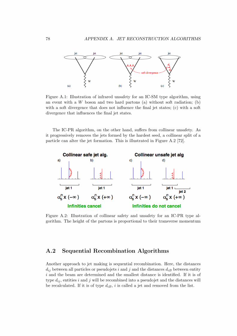
78 APPENDIX A. JET RECONSTRUCTION ALGORITHMS
Figure A.1: Illustration of infrared unsafety for an IC-SM type algorithm, usingan event with a W boson and two hard partons (a) without soft radiation; (b)with a soft divergence that does not influence the final jet states; (c) with a softdivergence that influences the final jet states.
The IC-PR algorithm, on the other hand, suffers from collinear unsafety. Asit progressively removes the jets formed by the hardest seed, a collinear split of aparticle can alter the jet formation. This is illustrated in Figure A.2 [72].
Figure A.2: Illustration of collinear safety and unsafety for an IC-PR type al-gorithm. The height of the partons is proportional to their transverse momentum
A.2 Sequential Recombination Algorithms
Another approach to jet making is sequential recombination. Here, the distancesdij between all particles or pseudojets i and j and the distances diB between entityi and the beam are determined and the smallest distance is identified. If it is oftype dij , entities i and j will be recombined into a pseudojet and the distances willbe recalculated. If it is of type diB, i is called a jet and removed from the list.

A.2. SEQUENTIAL RECOMBINATION ALGORITHMS 79
The distances are defined as
diB = k2pT,i ,
dij = min(k2p
T,i, k2pT,j
)∆2ij
R2, ∆2
ij = (yi − yj)2 + (φi − φj)2 ,(A.1)
where kT,i is the transverse momentum, φi is the azimuthal angle and yi ≡ 12 ln E+pz
E−pzis the rapidity of particle i. R is a radius parameter of the same sort as the oneused for iterative cone algorithms, while p controls the relative power of the energycompared to the geometrical scale ∆ij . When p = 1 the algorithm is called the(inclusive) kT algorithm, when p = 0 it is called the Cambridge/Aachen algorithmand when p = −1 the anti-kT algorithm.

80 APPENDIX A. JET RECONSTRUCTION ALGORITHMS
Appendix B
b-tag Scale Factors
Due to the properties of B hadrons, b jets can be differentiated from other jets.As algorithms are never perfect, there is always a chance that non-b jets areaccidentally identified or ‘tagged’ as b jets. This mistag rate is different for jetsoriginating from c quarks, which can produce hadrons with a medium lifetime,and light jets, which originate from u, d or s quarks and gluons. The efficiency totag jets of flavour i is defined as the ratio of the number of tagged jets to the totalnumber of jets of that flavour, i.e.
εi =Number of tagged jets of flavour iTotal number of jets of flavour i
. (B.1)
As the tagging efficiency is different in data and simulation, scale factors SFiwere measured by the CMS collaboration. These scale factors depend on the jetflavour, pT and η. Also the efficiency in simulation is obtained as a function ofthese quantities. This is visualised in Figure B.1.
The probability to tag a number of jets in events in simulation is defined as
P(MC) =∏i
tagged
εi∏j
not tagged
(1− εj) , (B.2)
while in data this probability becomes
P(data) =∏i
tagged
SFiεi∏j
not tagged
(1− SFjεj) , (B.3)
where i and j are elements of the collections of tagged and non-tagged jets re-spectively.
The b-tag weight assigned to a simulated event is then
w =P(data)P(MC)
. (B.4)
81
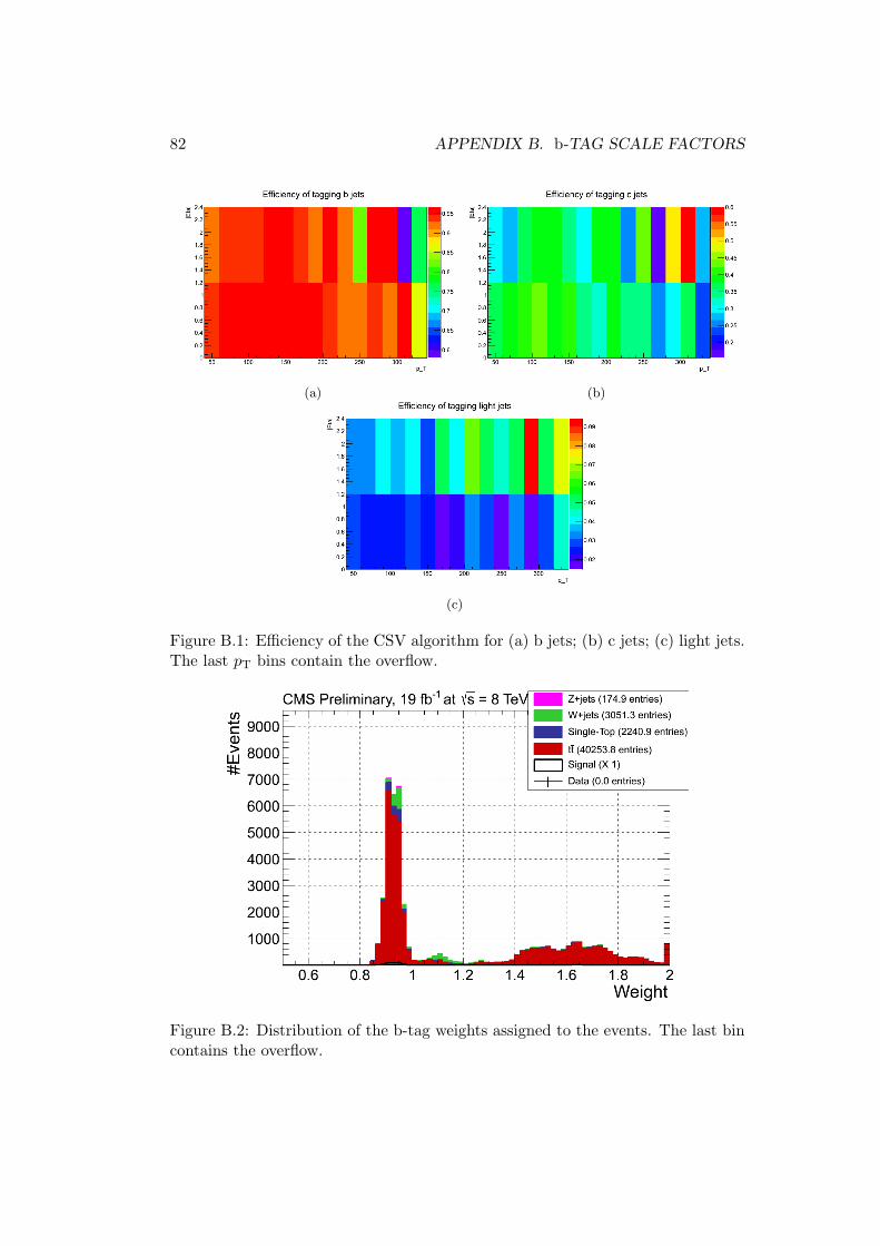
82 APPENDIX B. b-TAG SCALE FACTORS
(a) (b)
(c)
Figure B.1: Efficiency of the CSV algorithm for (a) b jets; (b) c jets; (c) light jets.The last pT bins contain the overflow.
Figure B.2: Distribution of the b-tag weights assigned to the events. The last bincontains the overflow.
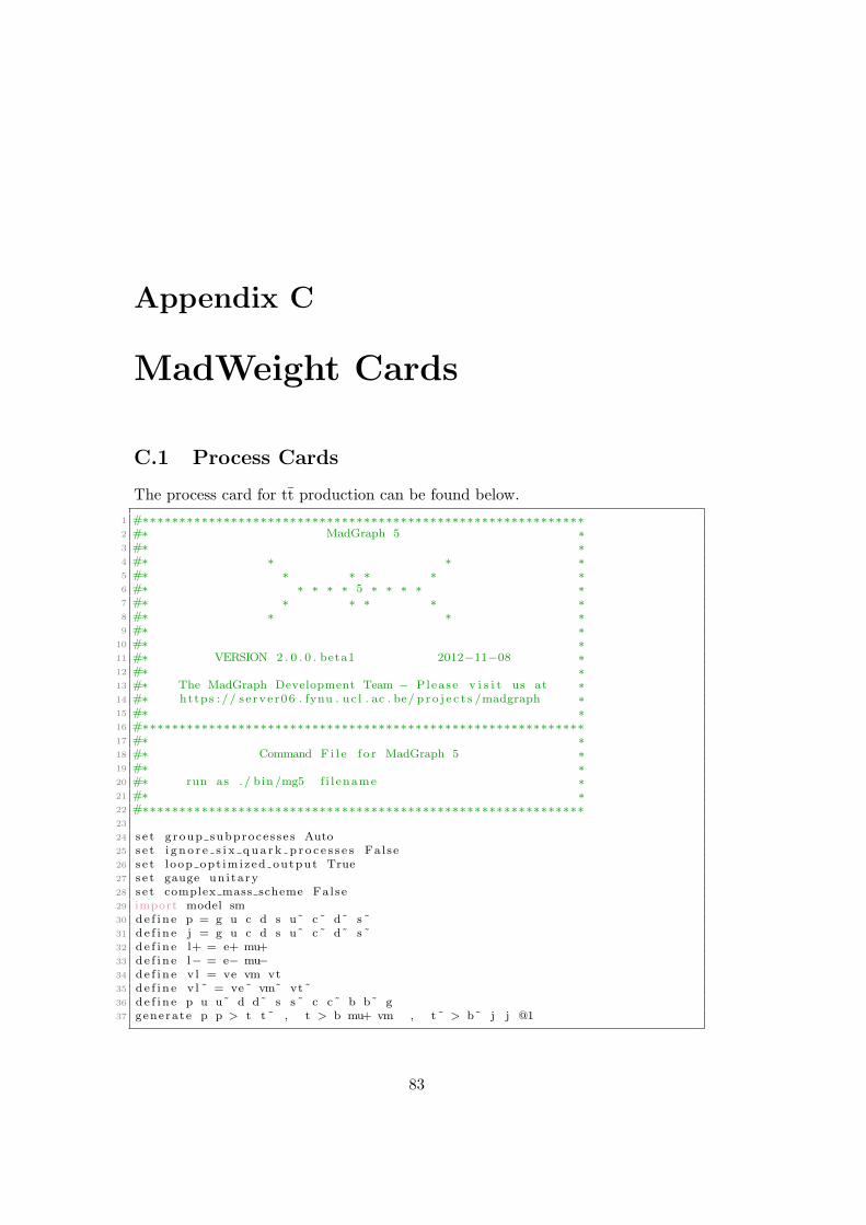
Appendix C
MadWeight Cards
C.1 Process Cards
The process card for tt production can be found below.1 #∗∗∗∗∗∗∗∗∗∗∗∗∗∗∗∗∗∗∗∗∗∗∗∗∗∗∗∗∗∗∗∗∗∗∗∗∗∗∗∗∗∗∗∗∗∗∗∗∗∗∗∗∗∗∗∗∗∗∗∗2 #∗ MadGraph 5 ∗3 #∗ ∗4 #∗ ∗ ∗ ∗5 #∗ ∗ ∗ ∗ ∗ ∗6 #∗ ∗ ∗ ∗ ∗ 5 ∗ ∗ ∗ ∗ ∗7 #∗ ∗ ∗ ∗ ∗ ∗8 #∗ ∗ ∗ ∗9 #∗ ∗
10 #∗ ∗11 #∗ VERSION 2 . 0 . 0 . beta1 2012−11−08 ∗12 #∗ ∗13 #∗ The MadGraph Development Team − Please v i s i t us at ∗14 #∗ https : // s e rve r06 . fynu . uc l . ac . be/ p r o j e c t s /madgraph ∗15 #∗ ∗16 #∗∗∗∗∗∗∗∗∗∗∗∗∗∗∗∗∗∗∗∗∗∗∗∗∗∗∗∗∗∗∗∗∗∗∗∗∗∗∗∗∗∗∗∗∗∗∗∗∗∗∗∗∗∗∗∗∗∗∗∗17 #∗ ∗18 #∗ Command F i l e f o r MadGraph 5 ∗19 #∗ ∗20 #∗ run as . / bin /mg5 f i l ename ∗21 #∗ ∗22 #∗∗∗∗∗∗∗∗∗∗∗∗∗∗∗∗∗∗∗∗∗∗∗∗∗∗∗∗∗∗∗∗∗∗∗∗∗∗∗∗∗∗∗∗∗∗∗∗∗∗∗∗∗∗∗∗∗∗∗∗23
24 s e t g roup subproce s s e s Auto25 s e t i g n o r e s i x q u a r k p r o c e s s e s Fa l se26 s e t l oop opt imized output True27 s e t gauge un i ta ry28 s e t complex mass scheme Fal se29 import model sm30 d e f i n e p = g u c d s u˜ c˜ d˜ s ˜31 d e f i n e j = g u c d s u˜ c˜ d˜ s ˜32 d e f i n e l+ = e+ mu+33 d e f i n e l− = e− mu−34 d e f i n e v l = ve vm vt35 d e f i n e v l ˜ = ve˜ vm˜ vt ˜36 d e f i n e p u u˜ d d˜ s s ˜ c c˜ b b˜ g37 generate p p > t t ˜ , t > b mu+ vm , t ˜ > b˜ j j @1
83
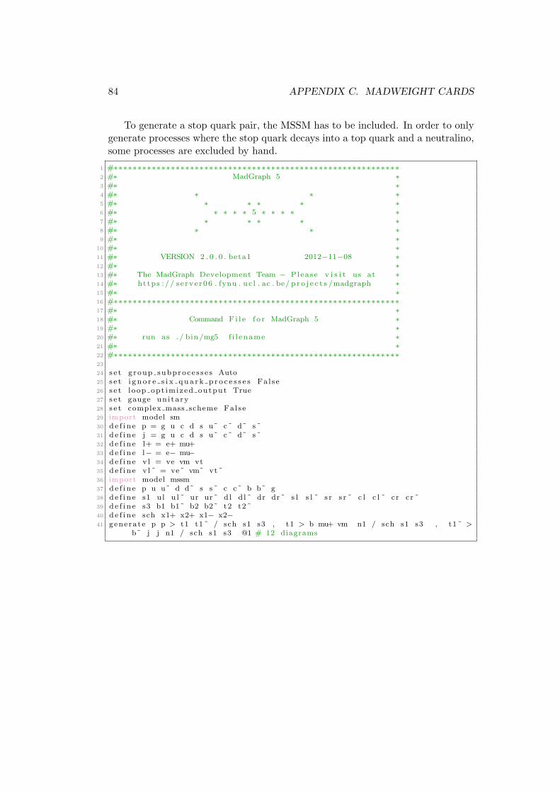
84 APPENDIX C. MADWEIGHT CARDS
To generate a stop quark pair, the MSSM has to be included. In order to onlygenerate processes where the stop quark decays into a top quark and a neutralino,some processes are excluded by hand.
1 #∗∗∗∗∗∗∗∗∗∗∗∗∗∗∗∗∗∗∗∗∗∗∗∗∗∗∗∗∗∗∗∗∗∗∗∗∗∗∗∗∗∗∗∗∗∗∗∗∗∗∗∗∗∗∗∗∗∗∗∗2 #∗ MadGraph 5 ∗3 #∗ ∗4 #∗ ∗ ∗ ∗5 #∗ ∗ ∗ ∗ ∗ ∗6 #∗ ∗ ∗ ∗ ∗ 5 ∗ ∗ ∗ ∗ ∗7 #∗ ∗ ∗ ∗ ∗ ∗8 #∗ ∗ ∗ ∗9 #∗ ∗
10 #∗ ∗11 #∗ VERSION 2 . 0 . 0 . beta1 2012−11−08 ∗12 #∗ ∗13 #∗ The MadGraph Development Team − Please v i s i t us at ∗14 #∗ https : // s e rve r06 . fynu . uc l . ac . be/ p r o j e c t s /madgraph ∗15 #∗ ∗16 #∗∗∗∗∗∗∗∗∗∗∗∗∗∗∗∗∗∗∗∗∗∗∗∗∗∗∗∗∗∗∗∗∗∗∗∗∗∗∗∗∗∗∗∗∗∗∗∗∗∗∗∗∗∗∗∗∗∗∗∗17 #∗ ∗18 #∗ Command F i l e f o r MadGraph 5 ∗19 #∗ ∗20 #∗ run as . / bin /mg5 f i l ename ∗21 #∗ ∗22 #∗∗∗∗∗∗∗∗∗∗∗∗∗∗∗∗∗∗∗∗∗∗∗∗∗∗∗∗∗∗∗∗∗∗∗∗∗∗∗∗∗∗∗∗∗∗∗∗∗∗∗∗∗∗∗∗∗∗∗∗23
24 s e t g roup subproce s s e s Auto25 s e t i g n o r e s i x q u a r k p r o c e s s e s Fa l se26 s e t l oop opt imized output True27 s e t gauge un i ta ry28 s e t complex mass scheme Fal se29 import model sm30 d e f i n e p = g u c d s u˜ c˜ d˜ s ˜31 d e f i n e j = g u c d s u˜ c˜ d˜ s ˜32 d e f i n e l+ = e+ mu+33 d e f i n e l− = e− mu−34 d e f i n e v l = ve vm vt35 d e f i n e v l ˜ = ve˜ vm˜ vt ˜36 import model mssm37 d e f i n e p u u˜ d d˜ s s ˜ c c˜ b b˜ g38 d e f i n e s1 u l u l ˜ ur ur˜ d l d l ˜ dr dr˜ s l s l ˜ s r s r ˜ c l c l ˜ cr cr ˜39 d e f i n e s3 b1 b1˜ b2 b2˜ t2 t2 ˜40 d e f i n e sch x1+ x2+ x1− x2−41 generate p p > t1 t1 ˜ / sch s1 s3 , t1 > b mu+ vm n1 / sch s1 s3 , t1 ˜ >
b˜ j j n1 / sch s1 s3 @1 # 12 diagrams
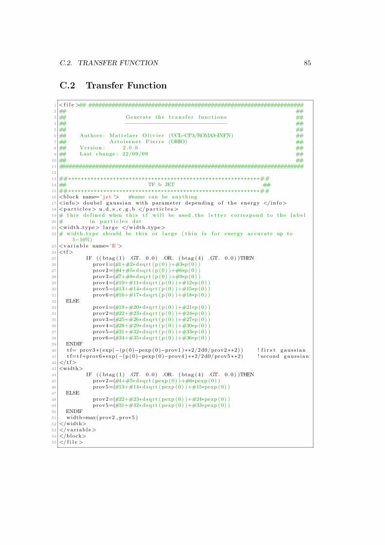
C.2. TRANSFER FUNCTION 85
C.2 Transfer Function
1 < f i l e >## #################################################################2 ## ##3 ## Generate the t r a n s f e r f u n c t i o n s ##4 ## −−−−−−−−−−−−−−−−−−−−−−−−−−−−−−− ##5 ## ##6 ## Authors : Matte laer O l i v i e r (UCL−CP3/ROMA3−INFN) ##7 ## Arto i s ene t P i e r r e (OHIO) ##8 ## Vers ion : 2 . 0 . 0 ##9 ## Last change : 22/09/09 ##
10 ## ##11 ##########################################################################12
13 ##∗∗∗∗∗∗∗∗∗∗∗∗∗∗∗∗∗∗∗∗∗∗∗∗∗∗∗∗∗∗∗∗∗∗∗∗∗∗∗∗∗∗∗∗∗∗∗∗∗∗∗∗∗∗∗∗∗∗∗∗##14 ## TF b JET ##15 ##∗∗∗∗∗∗∗∗∗∗∗∗∗∗∗∗∗∗∗∗∗∗∗∗∗∗∗∗∗∗∗∗∗∗∗∗∗∗∗∗∗∗∗∗∗∗∗∗∗∗∗∗∗∗∗∗∗∗∗∗##16 <block name=’ j e t ’> #name can be anything17 <i n fo> doubel gauss ian with parameter depending o f the energy </in fo>18 <p a r t i c l e s> u , d , s , c , g , b </p a r t i c l e s>19 # t h i s de f ined when t h i s t f w i l l be used . the l e t t e r correspond to the l a b e l20 # in p a r t i c l e s . dat21 <width type> l a r g e </width type>22 # width type should be th in or l a r g e ( th in i s f o r energy accurate up to
5−10%)23 <v a r i a b l e name=’E ’>24 <t f>25 IF ( ( btag (1 ) .GT. 0 . 0 ) .OR. ( btag (4 ) .GT. 0 . 0 ) )THEN26 prov1=(#1+#2∗dsqrt (p (0 ) )+#3∗p (0) )27 prov2=(#4+#5∗dsqrt (p (0 ) )+#6∗p (0) )28 prov3=(#7+#8∗dsqrt (p (0 ) )+#9∗p (0) )29 prov4=(#10+#11∗dsqrt (p (0 ) )+#12∗p (0) )30 prov5=(#13+#14∗dsqrt (p (0 ) )+#15∗p (0) )31 prov6=(#16+#17∗dsqrt (p (0 ) )+#18∗p (0) )32 ELSE33 prov1=(#19+#20∗dsqrt (p (0 ) )+#21∗p (0) )34 prov2=(#22+#23∗dsqrt (p (0 ) )+#24∗p (0) )35 prov3=(#25+#26∗dsqrt (p (0 ) )+#27∗p (0) )36 prov4=(#28+#29∗dsqrt (p (0 ) )+#30∗p (0) )37 prov5=(#31+#32∗dsqrt (p (0 ) )+#33∗p (0) )38 prov6=(#34+#35∗dsqrt (p (0 ) )+#36∗p (0) )39 ENDIF40 t f= prov3 ∗( exp(−(p (0 )−pexp (0)−prov1 ) ∗∗2/2d0/prov2 ∗∗2) ) ! f i r s t gauss ian41 t f=t f+prov6∗exp(−(p (0 )−pexp (0)−prov4 ) ∗∗2/2d0/prov5 ∗∗2) ! second gauss ian42 </t f>43 <width>44 IF ( ( btag (1 ) .GT. 0 . 0 ) .OR. ( btag (4 ) .GT. 0 . 0 ) )THEN45 prov2=(#4+#5∗dsqrt ( pexp (0) )+#6∗pexp (0) )46 prov5=(#13+#14∗dsqrt ( pexp (0) )+#15∗pexp (0) )47 ELSE48 prov2=(#22+#23∗dsqrt ( pexp (0) )+#24∗pexp (0) )49 prov5=(#31+#32∗dsqrt ( pexp (0) )+#33∗pexp (0) )50 ENDIF51 width=max( prov2 , prov5 )52 </width>53 </var i ab l e>54 </block>55 </ f i l e >
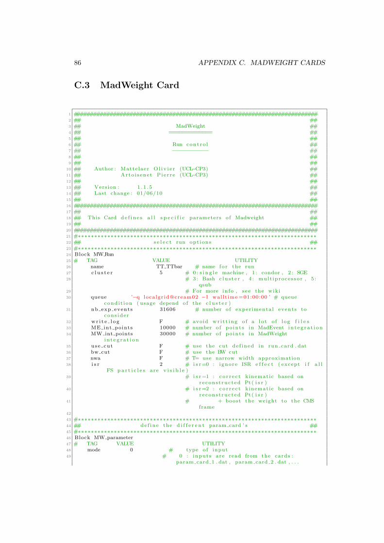
86 APPENDIX C. MADWEIGHT CARDS
C.3 MadWeight Card
1 ##########################################################################2 ## ##3 ## MadWeight ##4 ## ============= ##5 ## ##6 ## Run c o n t r o l ##7 ## −−−−−−−−−−− ##8 ## ##9 ## ##
10 ## Author : Matte laer O l i v i e r (UCL−CP3) ##11 ## Arto i s ene t P i e r r e (UCL−CP3) ##12 ## ##13 ## Vers ion : 1 . 1 . 5 ##14 ## Last change : 01/06/10 ##15 ## ##16 ##########################################################################17 ## ##18 ## This Card d e f i n e s a l l s p e c i f i c parameters o f Madweight ##19 ## ##20 ##########################################################################21 #∗∗∗∗∗∗∗∗∗∗∗∗∗∗∗∗∗∗∗∗∗∗∗∗∗∗∗∗∗∗∗∗∗∗∗∗∗∗∗∗∗∗∗∗∗∗∗∗∗∗∗∗∗∗∗∗∗∗∗∗∗∗∗∗∗∗∗∗∗∗∗∗∗22 ## s e l e c t run opt ions ##23 #∗∗∗∗∗∗∗∗∗∗∗∗∗∗∗∗∗∗∗∗∗∗∗∗∗∗∗∗∗∗∗∗∗∗∗∗∗∗∗∗∗∗∗∗∗∗∗∗∗∗∗∗∗∗∗∗∗∗∗∗∗∗∗∗∗∗∗∗∗∗∗∗∗24 Block MW Run25 # TAG VALUE UTILITY26 name TT TTbar # name f o r the run27 c l u s t e r 5 # 0 : s i n g l e machine , 1 : condor , 2 : SGE28 # 3 : Bash c l u s t e r , 4 : mu l t ip roce s so r , 5 :
qsub29 # For more in fo , s e e the wik i30 queue ’−q loca lgr id@cream02 − l wa l l t ime =01:00:00 ’ # queue
cond i t i on ( usage depend o f the c l u s t e r )31 nb exp events 31606 # number o f exper imenta l events to
con s id e r32 w r i t e l o g F # avoid w r i t t i n g o f a l o t o f l og f i l e s33 ME int points 10000 # number o f po in t s in MadEvent i n t e g r a t i o n34 MW int points 30000 # number o f po in t s in MadWeight
i n t e g r a t i o n35 use cut F # use the cut de f ined in run card . dat36 bw cut F # use the BW cut37 nwa F # T= use narrow width approximation38 i s r 2 # i s r =0 : i gno re ISR e f f e c t ( except i f a l l
FS p a r t i c l e s are v i s i b l e )39 # i s r =1 : c o r r e c t k inemat ic based on
r e con s t ruc t ed Pt ( i s r )40 # i s r =2 : c o r r e c t k inemat ic based on
r e con s t ruc t ed Pt ( i s r )41 # + boost the weight to the CMS
frame42
43 #∗∗∗∗∗∗∗∗∗∗∗∗∗∗∗∗∗∗∗∗∗∗∗∗∗∗∗∗∗∗∗∗∗∗∗∗∗∗∗∗∗∗∗∗∗∗∗∗∗∗∗∗∗∗∗∗∗∗∗∗∗∗∗∗∗∗∗∗∗∗∗∗∗44 ## d e f i n e the d i f f e r e n t param card ’ s ##45 #∗∗∗∗∗∗∗∗∗∗∗∗∗∗∗∗∗∗∗∗∗∗∗∗∗∗∗∗∗∗∗∗∗∗∗∗∗∗∗∗∗∗∗∗∗∗∗∗∗∗∗∗∗∗∗∗∗∗∗∗∗∗∗∗∗∗∗∗∗∗∗∗∗46 Block MW parameter47 # TAG VALUE UTILITY48 mode 0 # type o f input49 # 0 : inputs are read from the cards :
param card 1 . dat , param card 2 . dat , . . .
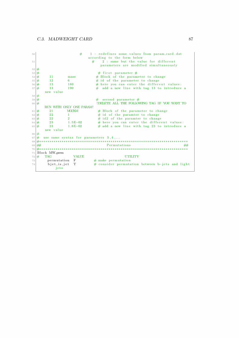
C.3. MADWEIGHT CARD 87
50 # 1 : r e d e f i n e s some va lue s from param card . dataccord ing to the form below
51 # 2 : same but the value f o r d i f f e r e n tparameters are modi f i ed s imu l taneous ly
52 #53 # # f i r s t parameter #54 # 11 mass # Block o f the parameter to change55 # 12 6 # id o f the parameter to change56 # 13 180 # here you can ente r the d i f f e r e n t va lue s :57 # 13 190 # add a new l i n e with tag 13 to int roduce a
new value58 #59 # # second parameter #60 # !DELETE ALL THE FOLLOWING TAG IF YOU WANT TO
RUN WITH ONLY ONE PARAM!61 # 21 MGCKM # Block o f the parameter to change62 # 22 1 # id o f the paramter to change63 # 22 2 # id2 o f the paramter to change64 # 23 1 .5E−02 # here you can ente r the d i f f e r e n t va lue s :65 # 23 1 .8E−02 # add a new l i n e with tag 23 to in t roduce a
new value66 #67 # use same syntax f o r parameters 3 , 4 , . . .68 #∗∗∗∗∗∗∗∗∗∗∗∗∗∗∗∗∗∗∗∗∗∗∗∗∗∗∗∗∗∗∗∗∗∗∗∗∗∗∗∗∗∗∗∗∗∗∗∗∗∗∗∗∗∗∗∗∗∗∗∗∗∗∗∗∗∗∗∗∗∗∗∗∗69 ## Permutations ##70 #∗∗∗∗∗∗∗∗∗∗∗∗∗∗∗∗∗∗∗∗∗∗∗∗∗∗∗∗∗∗∗∗∗∗∗∗∗∗∗∗∗∗∗∗∗∗∗∗∗∗∗∗∗∗∗∗∗∗∗∗∗∗∗∗∗∗∗∗∗∗∗∗∗71 Block MW perm72 # TAG VALUE UTILITY73 permutation F # make permutation74 b j e t i s j e t T # cons id e r permutation between b−j e t s and l i g h t
j e t s

88 APPENDIX C. MADWEIGHT CARDS
Een nieuwe aanpak van de zoektocht naar stop quarks aan de LargeHadron Collider met behulp van de matrixelementmethode
Sinds de ontdekking van het Higgs deeltje in 2012 is het standaard model derdeeltjes weer op het voorplan verschenen. Ondanks zijn opmerkelijke overeenkomstmet experimentele resultaten kan dit model niet alles verklaren. Een mogelijkeoplossing voor tal van onopgeloste vragen is de introductie van een nieuwe sym-metrie, “supersymmetrie”, die deeltjes en krachten op gelijke voet behandelt. Dezetheorie voorspelt een heleboel nieuwe deeltjes, maar die zijn tot op heden nog nietgeobserveerd. Indien ze bestaan, worden deze deeltjes slechts zeer zelden gepro-duceerd, zo zelden dat ze lijken te verdrinken in een achtergrond van standaardmodel processen. Er is dus nood aan technieken die dit kleine signaal uit deachtergrond kunnen filteren. Een nieuwe methode die hiertoe kan bijdragen is dematrixelementmethode.
Wanneer twee deeltjes botsen in de Large Hadron Collider (LHC) worden ernieuwe deeltjes gecreeerd, die op hun beurt weer vervallen naar andere deeltjes.Alle informatie over zo’n proces, zoals de energie en massa van de deeltjes, zitvervat in een zogenoemd matrixelement. Aangezien een detector niet perfect is,zijn de gemeten energieen vaak verschillend van de echte energieen van de deeltjes.Dit wordt in rekening gebracht door transferfuncties, die het verband geven tussende geobserveerde en de echte energieen van de deeltjes. Als er rekening gehoudenwordt met hoe vaak een bepaald proces geproduceerd wordt, ook wel werkzamedoorsnede genoemd, geeft de matrixelementmethode de waarschijnlijkheid weerdat het geobserveerde proces signaal of achtergrond is.
Op deze manier kan een bovengrens voor de werkzame doorsnede van de sig-naalprocessen bepaald worden. Hoe strenger deze bovenlimiet, des te gevoeliger isde methode voor het signaal. Met de matrixelementmethode werd een bovengrensbekomen die ongeveer driemaal kleiner is dan deze verkregen met andere tech-nieken, die slechts een gedeelte van de informatie van het proces gebruiken. Ditbetekent dat de matrixelementmethode uitermate nuttig is in de zoektocht naarnieuwe fysica.