Modelling the influence of the Abu Nakhla pond on the ...
173
FACULTEIT WETENSCHAPPEN Opleiding Master of Science in de geologie Academiejaar 2014–2015 Scriptie voorgelegd tot het behalen van de graad Van Master of Science in de geologie Promotor: Prof. Dr. L. Lebbe Leescommissie: J. Claus, Prof. Dr. V. Cnudde Modelling the influence of the Abu Nakhla pond on the phreatic aquifer in Qatar: present and future scenarios Joren De Tollenaere
Transcript of Modelling the influence of the Abu Nakhla pond on the ...
FACULTEIT WETENSCHAPPEN
Opleiding Master of Science in de geologie
Academiejaar 2014–2015
Scriptie voorgelegd tot het behalen van de graad
Van Master of Science in de geologie
Promotor: Prof. Dr. L. Lebbe
Leescommissie: J. Claus, Prof. Dr. V. Cnudde
Modelling the influence of the Abu Nakhla pond
on the phreatic aquifer in Qatar:
present and future scenarios
Joren De Tollenaere

i
VOORWOORD
Eerst en vooral wil ik m’n promotor prof. dr. Lebbe bedanken voor de mogelijkheid om dit
onderwerp als masterproef te doen. Ook wil ik hem bedanken voor zijn verhelderende
uitleg over de resultaten van de modellen en over de hydrogeologie. Ik wil ook Jasper
Claus bedanken voor het gebruik van zijn python scripts om de input van de modellen te
maken alsook voor zijn inzicht en aanpassingen aan het model. Gert-Jan Devriese wil ik
bedanken voor de morele steun en voor het gebruik van zijn bureau waar we vele leuke
uren hebben doorgebracht. En als laatste wil ik Devlin Depret bedanken voor zijn rationele
benadering in het steunen bij het schrijven van deze masterproef en zijn kritisch inzicht
inzake de resultaten.

ii
iii
Table of contents
1. INTRODUCTION ......................................................................................................... 1
2. STUDY AREA ............................................................................................................. 3
3. GEOLOGY .................................................................................................................. 5
3.1 Structural geology .................................................................................................. 5
3.2 Surface geology ..................................................................................................... 5
3.3 Stratigraphy ........................................................................................................... 6
3.3.1 Umm er Radhuma Formation .......................................................................... 7
3.3.2 Rus Formation ................................................................................................. 7
3.3.3 Dammam Formation ...................................................................................... 10
3.3.4 Dam Formation ............................................................................................. 11
3.3.5 Hofuf Formation ............................................................................................ 11
3.3.6 Sabkhas ........................................................................................................ 12
4. HYDROGEOLOGY ................................................................................................... 13
4.1 General hydrogeology .......................................................................................... 13
4.2 Head distribution .................................................................................................. 14
4.3 Hydrogeological parameters ................................................................................ 19
4.4 Fresh and salt water distribution .......................................................................... 20
5. CLIMATE AND HYDROLOGY .................................................................................. 23
6. MODELLING SOFTWARE ....................................................................................... 29
6.1 Evolution of the modelling software ...................................................................... 29
6.2 MODFLOW .......................................................................................................... 29
6.2.1 Code concepts .............................................................................................. 30
6.2.2 Discretisation of the groundwater reservoir .................................................... 30
6.2.3 Finite difference approximation of the groundwater flow ................................ 32
6.2.4 Iteration with the Strongly Implicit Procedure ................................................. 34
6.2.5 Cell and boundary types ................................................................................ 35
6.3 MOC3D................................................................................................................ 36
6.4 MOCDENS3D ...................................................................................................... 37
iv
6.5 Packages............................................................................................................. 38
6.5.1 MODFLOW packages ................................................................................... 38
6.5.1.1 Basic package (.bas-file) ........................................................................................ 38
6.5.1.2 Block-Centred-Flow package (.bcf-file) .................................................................. 39
6.5.1.3 Well package (.wel-file) .......................................................................................... 40
6.5.1.4 Evapotranspiration package (.evt-file) ................................................................... 41
6.5.1.5 Strongly Implicit Procedure package (.sip-file)....................................................... 41
6.5.1.6 Name file (Infile.nam) ............................................................................................. 41
6.5.2 MOCDENS3D packages ............................................................................... 42
6.5.2.1 MOC package (.moc-file) ....................................................................................... 42
6.5.2.2 Densin.dat-file ........................................................................................................ 42
6.5.2.3 Name file (moc.nam) .............................................................................................. 42
7. MODEL CONSTRUCTION ....................................................................................... 43
7.1 Base model ......................................................................................................... 43
7.1.1 Location and discretisation of the study area ................................................. 43
7.1.2 Hydrogeological parameters ......................................................................... 46
7.1.3 Boundary conditions and initial head values .................................................. 48
7.1.4 Fresh and salt water distribution .................................................................... 51
7.1.5 Recharge ...................................................................................................... 53
7.1.6 Evapotranspiration ........................................................................................ 53
7.1.7 Time discretisation and closure criterion ....................................................... 54
7.2 Adding the pond into the base model ................................................................... 54
7.2.1 Sub-model one: Steady state flow with pond ................................................. 55
7.2.1.1 Discretisation of the Abu Nakhla pond ................................................................... 55
7.2.2 Sub-model two: Mimicking steady state with an unsteady state model .......... 57
7.2.2.1 Hydrogeological parameters .................................................................................. 58
7.2.2.2 Time discretisation and closure criterion ................................................................ 60
7.2.3 Sub-model three: From mimicking steady state to full unsteady state ........... 61
7.2.3.1 Boundary conditions and storage factors ............................................................... 61
7.2.3.2 Time discretisation and closure criterion ................................................................ 61
7.2.4 Sub-model four: Desiccation and dissipation of the Abu Nakhla pond ........... 62
7.2.4.1 Boundary conditions and hydrogeological parameters .......................................... 62
v
7.2.4.2 Time discretisation and closure criterion ................................................................ 62
7.3 Sensitivity analysis ............................................................................................... 63
7.3.1 Horizontal conductivity of the upper aquifer ................................................... 63
7.3.2 Vertical conductivity of the gypsiferous Rus Formation .................................. 63
7.3.3 Storage factors .............................................................................................. 64
8. RESULTS AND DISCUSSION .................................................................................. 65
8.1 Base model .......................................................................................................... 65
8.1.1 Steady state flow ........................................................................................... 65
8.1.2 Unsteady state flow ....................................................................................... 66
8.2 Desiccation of the Abu Nakhla pond .................................................................... 68
8.2.1 Sub-model one: Steady state flow with pond ................................................. 68
8.2.2 Sub-model two: Mimicking steady state with an unsteady state model .......... 69
8.2.3 Sub-model three: From mimicking steady state to full unsteady state ............ 71
8.2.4 Sub-model four: Desiccation and dissipation of the Abu Nakhla pond ........... 73
8.3 Sensitivity analyses ............................................................................................. 79
8.3.1 Horizontal conductivity of the upper aquifer ................................................... 79
8.3.2 Vertical conductivity of the gypsiferous Rus Formation .................................. 88
8.3.3 Storage factors .............................................................................................. 97
8.3.3.1 Storage factor near the water table ........................................................................ 97
8.3.3.2 Storage factor of the aquifer ................................................................................. 106
8.4 Discussion ......................................................................................................... 114
9. CONCLUSION ........................................................................................................ 123
10. NEDERLANDSTALIGE SAMENVATTING ........................................................... 127
11. REFERENCES ...................................................................................................... 133
APPENDIX A: BOREHOLE LOGS ............................................................................. 137
APPENDIX B: TIME DISCRETISATION ..................................................................... 154

vi
vii
List of figures
Figure 1: Location of Abu Nakhla in Qatar (Google Earth) ............................................... 3
Figure 2: Evolution of the Abu Nakhla pond from 1972 to 2009 (ESC Archives). ............. 4
Figure 3: Location of geological structures and surface geology in Qatar (Al-Saad, 2005).
........................................................................................................................................ 5
Figure 4: Stratigraphy and lithology of the Eocene sediments in Qatar (Al-Saad, 2005). . 6
Figure 5: The depositional facies of the Rus Formation in Qatar (Eccleston, et al., (1981)
modified by Elobaid) ........................................................................................................ 9
Figure 6: Head distribution in the Umm er Radhuma Formation aquifer of Qatar (Lloyd, et
al., 1987). ...................................................................................................................... 15
Figure 7: Head distribution in the Rus Formation aquifer of Qatar (Lloyd, et al., 1987). . 16
Figure 8: Head distribution in the Dammam Formation aquifer of Qatar (Alsharhan, et al.,
2001). ............................................................................................................................ 17
Figure 9: Potentiometric surface map in meter amsl of Qatar based on results from April
2009 (Schlumberger, 2009). .......................................................................................... 18
Figure 10: Total Dissolved Solids (TDS) isoconcentration map in ppm (Schlumberger,
2009). ............................................................................................................................ 21
Figure 11: Total annual rainfall (mm yr-1) of Qatar from 1972 to 2005 (Amer, et al., 2008).
...................................................................................................................................... 23
Figure 12: Average annual total rainfall (mm yr-1) between 1989 and 2007 (Schlumberger,
2009). ............................................................................................................................ 24
Figure 13: A hypothetical discretised aquifer system with five rows, nine columns and five
layers (McDonald & Harbaugh, 1988). .......................................................................... 31
Figure 14: Block-centred finite difference cells (McDonald & Harbaugh, 1988). ............. 31
Figure 15: Flow into cell i, j, k from cell i, j-1, k (McDonald & Harbaugh, 1988). ............. 33
Figure 16: Discretised aquifer showing boundaries and cell designations (McDonald &
Harbaugh, 1988). .......................................................................................................... 35
Figure 17: Discretisation of the simulation time in stress periods and time steps including
the formulas to calculate the first time step and the following steps (McDonald & Harbaugh,
1988). ............................................................................................................................ 39
Figure 18: Volumetric evapotranspiration QET, as a function of head h, in a cell where d is
the extinction depth and hs the ET surface elevation (McDonald & Harbaugh, 1988). ... 41
Figure 19: A georeferenced Google Earth image visualising the study area with a large
grid (1 km x 1 km cells) and the normal grid (100 m x 100 m cells). .............................. 44
viii
Figure 20: Potentiometric surface map of Qatar with the study area visualised as the black
rectangle (Schlumberger, 2009). ................................................................................... 48
Figure 21: Cross-section through Qatar with the different hydrogeological units with their
respectively TDS values (Harhash & Yousif, 1985). ...................................................... 52
Figure 22: Overview of the different sub-models with the input and output used. .......... 55
Figure 23: Picture of the water level of the Abu Nakhla pond on 8 May 2015 measuring
35.10 m amsl. ............................................................................................................... 56
Figure 24: Boundary conditions for sub-model one. 1 are the active cells, -1 are the
constant-head cells with TDS 3,000 ppm from the Dammam and upper Rus Formation
aquifer and -4 are the constant-head cells with TDS 2,000 ppm from the Abu Nakhla pond.
..................................................................................................................................... 56
Figure 25: Interpolated initial heads of each layer of sub-model one. ............................ 57
Figure 26: Visualisation of the raster file with the bathymetry of the Abu Nakhla pond with:
(1) Light green is the A basin with interpolated values, (2) Dark blue is the B basin with
interpolated values, (3) Red is the C Basin with no direct measurements and is put at 33
m, (4) Light blue are manually interpolated cells with their neighbour and (5) Purple are
the cells surrounding the pond with values set at 32 m. ................................................ 59
Figure 27: Visualisation of the measured bathymetry lines with their spatial variability, used
for the interpolation for the bottom of the Abu Nakhla pond. .......................................... 60
Figure 28: Horizontal cross-section of the groundwater head (m) through layer five of the
steady state flow base model, stress period five. .......................................................... 66
Figure 29: Horizontal cross-section of the groundwater head (m) through layer five of the
unsteady state base model, stress period fifteen. The dark red colour in the upper left
corner represents inactive cells. .................................................................................... 67
Figure 30: Vertical cross-section of the groundwater head (m) along row 10 of the unsteady
state base model, stress period fifteen. The dark red colour represents inactive cells. .. 67
Figure 31: Vertical cross-section of the groundwater head (m) along row 71 of the unsteady
state base model, stress period fifteen. The dark red colour represents inactive cells. .. 68
Figure 32: Horizontal cross-section of the groundwater head (m) through layer one of sub-
model one, stress period five. ....................................................................................... 69
Figure 33: Vertical cross-section of the groundwater head (m) along row 71 of sub-model
one, stress period five. .................................................................................................. 69
Figure 34: Horizontal cross-section of the groundwater head (m) through layer one of sub-
model two, stress period fifteen. The blue colour represents dry cells. .......................... 70
Figure 35: Horizontal cross-section of the groundwater head (m) through layer five of sub-
model two, stress period fifteen. The dark blue colour in the upper left corner represents
dry cells......................................................................................................................... 71
ix
Figure 36: Vertical cross-section of the groundwater head (m) through layer five of sub-
model two, stress period fifteen. The dark blue colour represents dry cells. .................. 71
Figure 37: Horizontal cross-section of the groundwater head (m) through layer five of sub-
model three, stress period fifteen. The dark red colour in the upper left corner represents
inactive cells. ................................................................................................................. 72
Figure 38: Vertical cross-section of the groundwater head (m) along row 10 of sub-model
three, stress period fifteen. The dark red colour represents inactive cells. ..................... 72
Figure 39: Vertical cross-section of the groundwater head (m) along row 71 of sub-model
three, stress period fifteen. The dark red colour represents inactive cells. ..................... 73
Figure 40: Difference figure of the groundwater head (m) through layer five of sub-model
four, stress period ten minus stress period one. ............................................................ 73
Figure 41: Horizontal cross-section of the groundwater head (m) through layer five of sub-
model four, stress periods three, five, eight and ten (upper left to lower right). The dark red
colour in the upper left corners represent inactive cells. ................................................ 74
Figure 42: Vertical cross-section of the groundwater head (m) along row 71 of sub-model
four, stress periods three, five, eight and ten. The dark red colour represents inactive cells.
...................................................................................................................................... 75
Figure 43: Head (m) versus time (d) of layer one and layer five of a cell at the centre of the
Abu Nakhla pond (sub-model four). ............................................................................... 76
Figure 44: Head (m) versus time (d) of layer five of a cell at the centre of the Abu Nakhla
pond (dark blue) and of a cell 2 km in westward (green), eastward (red), northward (light
blue) and southward (purple) directions (sub-model four). ............................................. 77
Figure 45: Head (m) versus time (d) of layer five of a cell at the centre of the Abu Nakhla
pond (dark blue) and of a cell 5 km in westward (green), eastward (red), northward (light
blue) and southward (purple) directions (sub-model four). ............................................. 77
Figure 46: Head (m) versus depth (expressed as layers) of the ten stress periods (sub-
model four). When the head of a cell drops to 0 m, it represents a dry cell. ................... 78
Figure 47: Horizontal cross-section of the groundwater head (m) through layer five with
max Kh, stress periods three, five, eight and ten (upper left to lower right). The dark red
colour in the upper left corners represent inactive cells. ................................................ 80
Figure 48: Vertical cross-section of the groundwater head (m) along row 71 with max Kh,
stress periods three, five, eight and ten. The dark red colour represents inactive cells. . 81
Figure 49: Head (m) versus time (d) of layer one and five of a cell at the centre of the Abu
Nakhla pond (max Kh). .................................................................................................. 81
Figure 50: Head (m) versus time (d) of layer five of a cell at the centre of the Abu Nakhla
pond (dark blue) and of a cell 2 km in westward (green), eastward (red), northward (light
blue) and southward (purple) directions (max Kh). ......................................................... 82
x
Figure 51: Head (m) versus time (d) of layer five of a cell at the centre of the Abu Nakhla
pond (dark blue) and of a cell 5 km in westward (green), eastward (red), northward (light
blue) and southward (purple) directions (max Kh). ......................................................... 83
Figure 52: Head (m) versus depth (expressed in layers) of the ten stress periods (max Kh).
When the head of a cell drops to 0 m, it represents a dry cell. ...................................... 83
Figure 53: Horizontal cross-section of the groundwater head (m) through layer five with
min Kh, stress periods three, five, eight and ten (upper left to lower right). The dark red
colour in the upper left corners represent inactive cells. ................................................ 84
Figure 54: Vertical cross-section of the groundwater head (m) along row 71 with min Kh,
stress periods three, five, eight and ten. The dark red colour represents inactive cells. . 85
Figure 55: Head (m) versus time (d) of layer one and five of a cell at the centre of the Abu
Nakhla pond (min Kh). ................................................................................................... 86
Figure 56: Head (m) versus time (d) of layer five of a cell at the centre of the Abu Nakhla
pond (dark blue) and of a cell 2 km in westward (green), eastward (red), northward (light
blue) and southward (purple) directions (min Kh) ........................................................... 87
Figure 57: Head (m) versus time (d) of layer five of a cell at the centre of the Abu Nakhla
pond (dark blue) and of a cell 5 km in westward (green), eastward (red), northward (light
blue) and southward (purple) directions (min Kh). .......................................................... 87
Figure 58: Head (m) versus depth (expressed in layers) of the ten stress periods (min Kh).
..................................................................................................................................... 88
Figure 59: Horizontal cross-section of the groundwater head (m) through layer five with
max Kv, stress periods three, five, eight and ten (upper left to lower right). The dark red
colour in the upper left corners represent inactive cells. ................................................ 89
Figure 60: Vertical cross-section of the groundwater head (m) along row 71 with max Kv,
stress periods three, five, eight and ten. The dark red colour represents inactive cells.
Continued on the next page. ......................................................................................... 90
Figure 61: Head (m) versus time (d) of layer one and five of a cell at the centre of the Abu
Nakhla pond (max Kv). .................................................................................................. 90
Figure 62: Head (m) versus time (d) of layer five of a cell at the centre of the Abu Nakhla
pond (dark blue) and of a cell 2 km in westward (green), eastward (red), northward (light
blue) and southward (purple) directions (max Kv). ......................................................... 91
Figure 63: Head (m) versus time (d) of layer five of a cell at the centre of the Abu Nakhla
pond (dark blue) and of a cell 5 km in westward (green), eastward (red), northward (light
blue) and southward (purple) directions (max Kv). ......................................................... 92
Figure 64: Head (m) versus depth (expressed in layers) of the ten stress periods (max Kv).
When the head of a cell drops to 0 m, it represents a dry cell. ...................................... 93
xi
Figure 65: Horizontal cross-section of the groundwater head (m) through layer five with
min Kv, stress periods three, five, eight and ten (upper left to lower right). The dark red
colour in the upper left corners represent inactive cells. ................................................ 94
Figure 66: Vertical cross-section of the groundwater head (m) along row 71 with min Kv,
stress periods three, five, eight and ten. The dark red colour represents inactive cells.
Continued on the next page .......................................................................................... 94
Figure 67: Head (m) vs time (d) of layer one and five of a cell at the centre of the Abu
Nakhla pond (min Kv). ................................................................................................... 95
Figure 68: Head (m) versus time (d) of layer five of a cell at the centre of the Abu Nakhla
pond (dark blue) and of a cell 2 km in westward (green), eastward (red), northward (light
blue) and southward (purple) directions (min Kv). .......................................................... 96
Figure 69: Head (m) versus time (d) of layer five of a cell at the centre of the Abu Nakhla
pond (dark blue) and of a cell 5 km in westward (green), eastward (red), northward (light
blue) and southward (purple) directions (min Kv). .......................................................... 96
Figure 70: Head (m) versus depth (expressed in layers) of the ten stress periods (min Kv).
When the head of a cell drops to 0 m, it represents a dry cell. ....................................... 97
Figure 71: Horizontal cross-section of the groundwater head (m) through layer five with
max SF[1], stress periods three, five, eight and ten (upper left to lower right). The dark red
colour in the upper left corners represent inactive cells. ................................................ 98
Figure 72: Vertical cross-section of the groundwater head (m) along row 71 with max SF[1],
stress periods three, five, eight and ten. The dark red colour represents inactive cells.
Continued on the next page. ......................................................................................... 98
Figure 73: Head (m) versus time (d) of layer one and five of a cell at the centre of the Abu
Nakhla pond (max SF[1])............................................................................................... 99
Figure 74: Head (m) versus time (d) of layer five of a cell at the centre of the Abu Nakhla
pond (dark blue) and of a cell 2 km in westward (green), eastward (red), northward (light
blue) and southward (purple) directions (max SF[1]). .................................................. 100
Figure 75: Head (m) versus time (d) of layer five of a cell at the centre of the Abu Nakhla
pond (dark blue) and of a cell 5 km in westward (green), eastward (red), northward (light
blue) and southward (purple) directions (max SF[1]). .................................................. 100
Figure 76: Head (m) versus depth (expressed in layers) of the ten stress periods (max
SF[1]). ......................................................................................................................... 101
Figure 77: Horizontal cross-section of the groundwater head (m) through layer five with
min SF[1], stress periods three, five, eight and ten (upper left to lower right). The dark red
colour in the upper left corners represent inactive cells. .............................................. 102
xii
Figure 78: Vertical cross-section of the groundwater head (m) along row 71 with min SF[1],
stress periods three, five, eight and ten. The dark red colour represents inactive cells.
Continued on the next page. ....................................................................................... 102
Figure 79: Head (m) versus time (d) of layer one and five of a cell at the centre of the Abu
Nakhla pond (min SF[1]). ............................................................................................ 103
Figure 80: Head (m) versus time (d) of layer five of a cell at the centre of the Abu Nakhla
pond (dark blue) and of a cell 2 km in westward (green), eastward (red), northward (light
blue) and southward (purple) directions (min SF[1]). ................................................... 104
Figure 81: Head (m) versus time (d) of layer five of a cell at the centre of the Abu Nakhla
pond (dark blue) and of a cell 5 km in westward (green), eastward (red), northward (light
blue) and southward (purple) directions (min SF[1]). ................................................... 105
Figure 82: Head (m) versus depth (expressed in layers) of the ten stress periods (min
SF[1]). When the head of a cell drops to 0 m, it represents a dry cell. ......................... 105
Figure 83: Horizontal cross-section of the groundwater head (m) through layer five with
max SF[2], stress periods three, five, eight and ten (upper left to lower right). The dark red
colour in the upper left corners represent inactive cells. .............................................. 106
Figure 84: Vertical cross-section of the groundwater head (m) along row 71 with max SF[2],
stress periods three, five, eight and ten. The dark red colour represents inactive cells.107
Figure 85: Head (m) versus time (d) of layer one and five of a cell at the centre of the Abu
Nakhla pond (max SF[2]). ........................................................................................... 108
Figure 86: Head (m) versus time (d) of layer five of a cell at the centre of the Abu Nakhla
pond (dark blue) and of a cell 2 km in westward (green), eastward (red), northward (light
blue) and southward (purple) directions (max SF[2]). .................................................. 108
Figure 87: Head (m) versus time (d) of layer five of a cell at the centre of the Abu Nakhla
pond (dark blue) and of a cell 5 km in westward (green), eastward (red), northward (light
blue) and southward (purple) directions (max SF[2]). .................................................. 109
Figure 88: Head (m) versus depth (expressed in layers) of the ten stress periods (max
SF[2]). ......................................................................................................................... 109
Figure 89: Horizontal cross-section of the groundwater head (m) through layer five with
min SF[2], stress periods three, five, eight and ten (upper left to lower right). The dark red
colour in the upper left corners represent inactive cells. .............................................. 110
Figure 90: Vertical cross-section of the groundwater head (m) along row 71 with min SF[2],
stress periods three, five, eight and ten. The dark red colour represents inactive cells.111
Figure 91: Head (m) versus time (d) of layer one and five of a cell at the centre of the Abu
Nakhla pond (min SF[2]). ............................................................................................ 112
xiii
Figure 92: Head (m) versus time (d) of layer five of a cell at the centre of the Abu Nakhla
pond (dark blue) and of a cell 2 km in westward (green), eastward (red), northward (light
blue) and southward (purple) directions (min SF[2]). ................................................... 112
Figure 93: Head (m) versus time (d) of layer five of a cell at the centre of the Abu Nakhla
pond (dark blue) and of a cell 5 km in westward, eastward northward and southward
directions (min SF[2]). ................................................................................................. 113
Figure 94: Head (m) versus depth (expressed in layers) of the ten stress periods (min
SF[2]). When the head of a cell drops to 0 m, it represents a dry cell. ......................... 114
Figure 95: Difference figure of the groundwater head (m) through layer five of the last
stress period from sub-model one minus the last stress period from the steady state base
model. ......................................................................................................................... 115
Figure 96: Difference figure of the groundwater head (m) through layer five of the last
stress period from sub-model three minus the last stress period from the unsteady state
base model. ................................................................................................................ 116
Figure 97: Difference figure of the groundwater head (m) through layer five of the last
stress period from sub-model four minus the last stress period from the unsteady state
base model. ................................................................................................................ 116
Figure 98: Overview the head (m) versus time (d) of a cell in the centre of the pond in layer
five of sub-model four and the sensitivity analyses. ..................................................... 118

xiv
xv
List of tables
Table 1: Surface runoff estimates for Qatar (Schlumberger, 2009). ............................... 26
Table 2: Direct and indirect recharge area with the percentage of the direct and indirect
recharge of the total annual rainfall (Eccleston, et al., 1981). ........................................ 26
Table 3: The vertical discretisation of the modelled area with the number of layers,
thickness of the layers and the geology and lithology they represent. ........................... 45
Table 4: Overview of the transmissivity, storage factor and vert (reciprocal of the hydraulic
resistance) of each layer. .............................................................................................. 47
Table 5: Overview of the heads of the constant-head cells for the western boundary (north
to south direction), eastern boundary (north to south direction), northern boundary (west
to east direction) and southern boundary (west to east direction). ................................. 49
Table 6: TDS values and salt water concentrations used in the models. ....................... 53
Table 7: Extinction depths for different soil types and land covers (Shah, et al., 2007). . 54
Table 8: The hydraulic conductivities, storage factors, TOP, BOT and verts for the six
layers with LAYCON set at three. .................................................................................. 59
Table 9: The hydraulic conductivities, storage factors, TOP, BOT and verts for the six
layers with LAYCON set at three. .................................................................................. 62
Table 10: Minimum and maximum horizontal conductivity for each of the six layers
including the transmissivity. ........................................................................................... 63
Table 11: Minimum and maximum vert for each of the eleven layers of the gypsiferous Rus
Formation. ..................................................................................................................... 64
Table 12: Minimum and maximum storage factor near the water table and storage factor
of the aquifer. ................................................................................................................ 64
Table 13: Volume difference between sub-model three and the unsteady state base model
with the corresponding infiltrated water column over the pond area. ........................... 117
Table 14: On the left: the head (m) of stress period (SP) five to ten of sub-model four and
the sensitivity analyses of layer five; On the right: the difference in head of the sensitivity
analyses compared to sub-model four expressed as a percentage (%) of stress period
(SP) five to ten of layer five. ........................................................................................ 120
Table 15: The duration of each of the fifteen stress periods in days with their cumulative
duration expressed in days and years. ........................................................................ 154
Table 16: The incrementally increasing time steps (d) of the fifteen stress periods used in
sub-model two and three. Sub-model four only uses ten of the fifteen stress periods while
sub-model two uses the same values but 100 times smaller. ...................................... 155

1. INTRODUCTION 1
1. INTRODUCTION
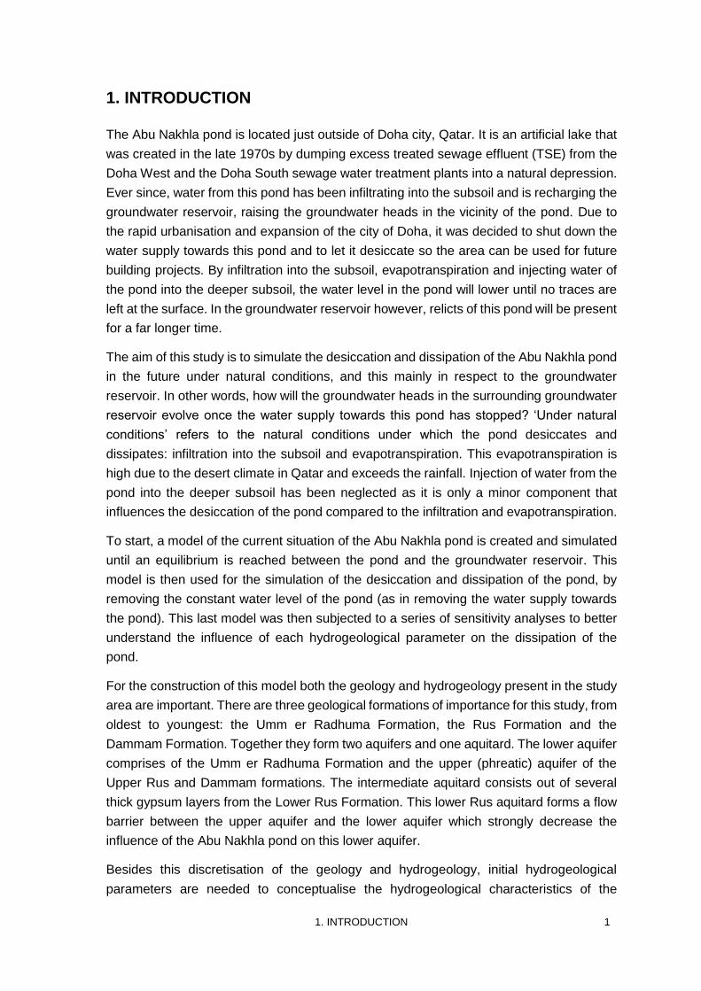
The Abu Nakhla pond is located just outside of Doha city, Qatar. It is an artificial lake that
was created in the late 1970s by dumping excess treated sewage effluent (TSE) from the
Doha West and the Doha South sewage water treatment plants into a natural depression.
Ever since, water from this pond has been infiltrating into the subsoil and is recharging the
groundwater reservoir, raising the groundwater heads in the vicinity of the pond. Due to
the rapid urbanisation and expansion of the city of Doha, it was decided to shut down the
water supply towards this pond and to let it desiccate so the area can be used for future
building projects. By infiltration into the subsoil, evapotranspiration and injecting water of
the pond into the deeper subsoil, the water level in the pond will lower until no traces are
left at the surface. In the groundwater reservoir however, relicts of this pond will be present
for a far longer time.
The aim of this study is to simulate the desiccation and dissipation of the Abu Nakhla pond
in the future under natural conditions, and this mainly in respect to the groundwater
reservoir. In other words, how will the groundwater heads in the surrounding groundwater
reservoir evolve once the water supply towards this pond has stopped? ‘Under natural
conditions’ refers to the natural conditions under which the pond desiccates and
dissipates: infiltration into the subsoil and evapotranspiration. This evapotranspiration is
high due to the desert climate in Qatar and exceeds the rainfall. Injection of water from the
pond into the deeper subsoil has been neglected as it is only a minor component that
influences the desiccation of the pond compared to the infiltration and evapotranspiration.
To start, a model of the current situation of the Abu Nakhla pond is created and simulated
until an equilibrium is reached between the pond and the groundwater reservoir. This
model is then used for the simulation of the desiccation and dissipation of the pond, by
removing the constant water level of the pond (as in removing the water supply towards
the pond). This last model was then subjected to a series of sensitivity analyses to better
understand the influence of each hydrogeological parameter on the dissipation of the
pond.
For the construction of this model both the geology and hydrogeology present in the study
area are important. There are three geological formations of importance for this study, from
oldest to youngest: the Umm er Radhuma Formation, the Rus Formation and the
Dammam Formation. Together they form two aquifers and one aquitard. The lower aquifer
comprises of the Umm er Radhuma Formation and the upper (phreatic) aquifer of the
Upper Rus and Dammam formations. The intermediate aquitard consists out of several
thick gypsum layers from the Lower Rus Formation. This lower Rus aquitard forms a flow
barrier between the upper aquifer and the lower aquifer which strongly decrease the
influence of the Abu Nakhla pond on this lower aquifer.
Besides this discretisation of the geology and hydrogeology, initial hydrogeological
parameters are needed to conceptualise the hydrogeological characteristics of the
2 1. INTRODUCTION
aquifers and the aquitard into the model. The base hydrogeological parameters, to form
the basis of the desiccation and dissipation model of the Abu Nakhla pond, are obtained
from literature. To simulate this model, specialised software is used which is based on the
MODFLOW-code and is called MOCDENS3D. With this software it is possible to model
density dependant flow in three-dimensions.
The study is divided in several chapters. First of all, chapter 2 will give a more in depth
overview of the study area and the history of the Abu Nakhla pond. Then, an overview of
the stratigraphy, including the surface and structural geology, will be given in chapter 3. A
detailed discussion of the hydrogeology is given in chapter 4 followed by a literature study
of the climate and hydrology in chapter 5. A technical discussion of the software is given
in chapter 6. Chapter 7 discusses the conceptualisation of the aquifers and aquitard into
the model and includes a quantification of the initial and hydrogeological parameters. The
results and discussion are elucidated in chapter 8 and a conclusion can be found in
chapter 9. Last but not least, a Dutch summary is presented in chapter 10.
2. STUDY AREA 3
2. STUDY AREA
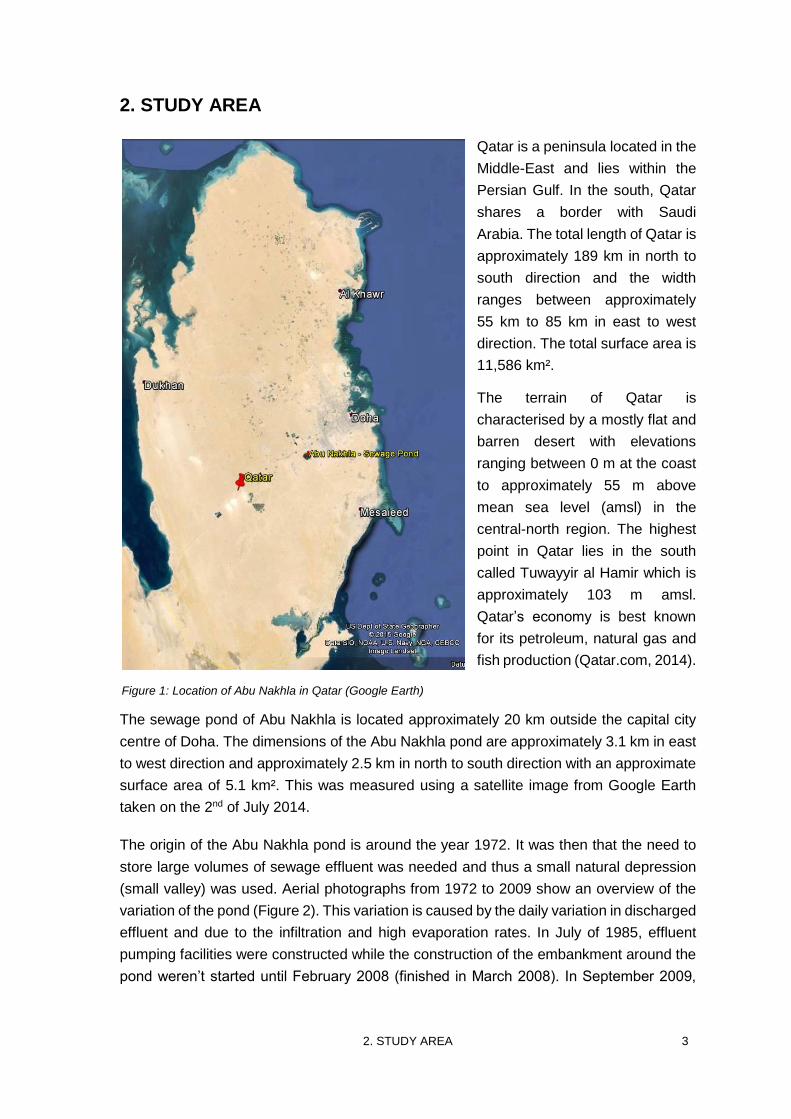
Qatar is a peninsula located in the
Middle-East and lies within the
Persian Gulf. In the south, Qatar
shares a border with Saudi
Arabia. The total length of Qatar is
approximately 189 km in north to
south direction and the width
ranges between approximately
55 km to 85 km in east to west
direction. The total surface area is
11,586 km².
The terrain of Qatar is
characterised by a mostly flat and
barren desert with elevations
ranging between 0 m at the coast
to approximately 55 m above
mean sea level (amsl) in the
central-north region. The highest
point in Qatar lies in the south
called Tuwayyir al Hamir which is
approximately 103 m amsl.
Qatar’s economy is best known
for its petroleum, natural gas and
fish production (Qatar.com, 2014).
The sewage pond of Abu Nakhla is located approximately 20 km outside the capital city
centre of Doha. The dimensions of the Abu Nakhla pond are approximately 3.1 km in east
to west direction and approximately 2.5 km in north to south direction with an approximate
surface area of 5.1 km². This was measured using a satellite image from Google Earth
taken on the 2nd of July 2014.
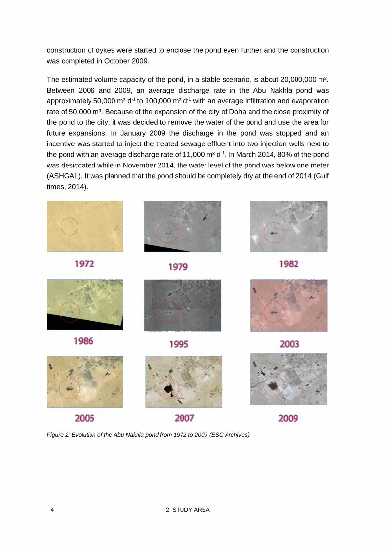
The origin of the Abu Nakhla pond is around the year 1972. It was then that the need to
store large volumes of sewage effluent was needed and thus a small natural depression
(small valley) was used. Aerial photographs from 1972 to 2009 show an overview of the
variation of the pond (Figure 2). This variation is caused by the daily variation in discharged
effluent and due to the infiltration and high evaporation rates. In July of 1985, effluent
pumping facilities were constructed while the construction of the embankment around the
pond weren’t started until February 2008 (finished in March 2008). In September 2009,
Figure 1: Location of Abu Nakhla in Qatar (Google Earth)
4 2. STUDY AREA
construction of dykes were started to enclose the pond even further and the construction
was completed in October 2009.
The estimated volume capacity of the pond, in a stable scenario, is about 20,000,000 m³.
Between 2006 and 2009, an average discharge rate in the Abu Nakhla pond was
approximately 50,000 m³ d-1 to 100,000 m³ d-1 with an average infiltration and evaporation
rate of 50,000 m³. Because of the expansion of the city of Doha and the close proximity of
the pond to the city, it was decided to remove the water of the pond and use the area for
future expansions. In January 2009 the discharge in the pond was stopped and an
incentive was started to inject the treated sewage effluent into two injection wells next to
the pond with an average discharge rate of 11,000 m³ d-1. In March 2014, 80% of the pond
was desiccated while in November 2014, the water level of the pond was below one meter
(ASHGAL). It was planned that the pond should be completely dry at the end of 2014 (Gulf
times, 2014).
Figure 2: Evolution of the Abu Nakhla pond from 1972 to 2009 (ESC Archives).
3. GEOLOGY 5
3. GEOLOGY
3.1 Structural geology
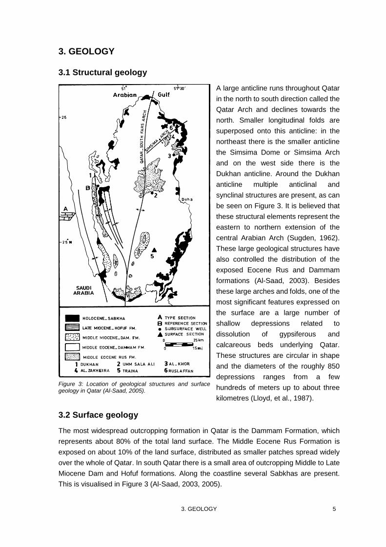
A large anticline runs throughout Qatar
in the north to south direction called the
Qatar Arch and declines towards the
north. Smaller longitudinal folds are
superposed onto this anticline: in the
northeast there is the smaller anticline
the Simsima Dome or Simsima Arch
and on the west side there is the
Dukhan anticline. Around the Dukhan
anticline multiple anticlinal and
synclinal structures are present, as can
be seen on Figure 3. It is believed that
these structural elements represent the
eastern to northern extension of the
central Arabian Arch (Sugden, 1962).
These large geological structures have
also controlled the distribution of the
exposed Eocene Rus and Dammam
formations (Al-Saad, 2003). Besides
these large arches and folds, one of the
most significant features expressed on
the surface are a large number of
shallow depressions related to
dissolution of gypsiferous and
calcareous beds underlying Qatar.
These structures are circular in shape
and the diameters of the roughly 850
depressions ranges from a few
hundreds of meters up to about three
kilometres (Lloyd, et al., 1987).
3.2 Surface geology
The most widespread outcropping formation in Qatar is the Dammam Formation, which
represents about 80% of the total land surface. The Middle Eocene Rus Formation is
exposed on about 10% of the land surface, distributed as smaller patches spread widely
over the whole of Qatar. In south Qatar there is a small area of outcropping Middle to Late
Miocene Dam and Hofuf formations. Along the coastline several Sabkhas are present.
This is visualised in Figure 3 (Al-Saad, 2003, 2005).
Figure 3: Location of geological structures and surface geology in Qatar (Al-Saad, 2005).
6 3. GEOLOGY
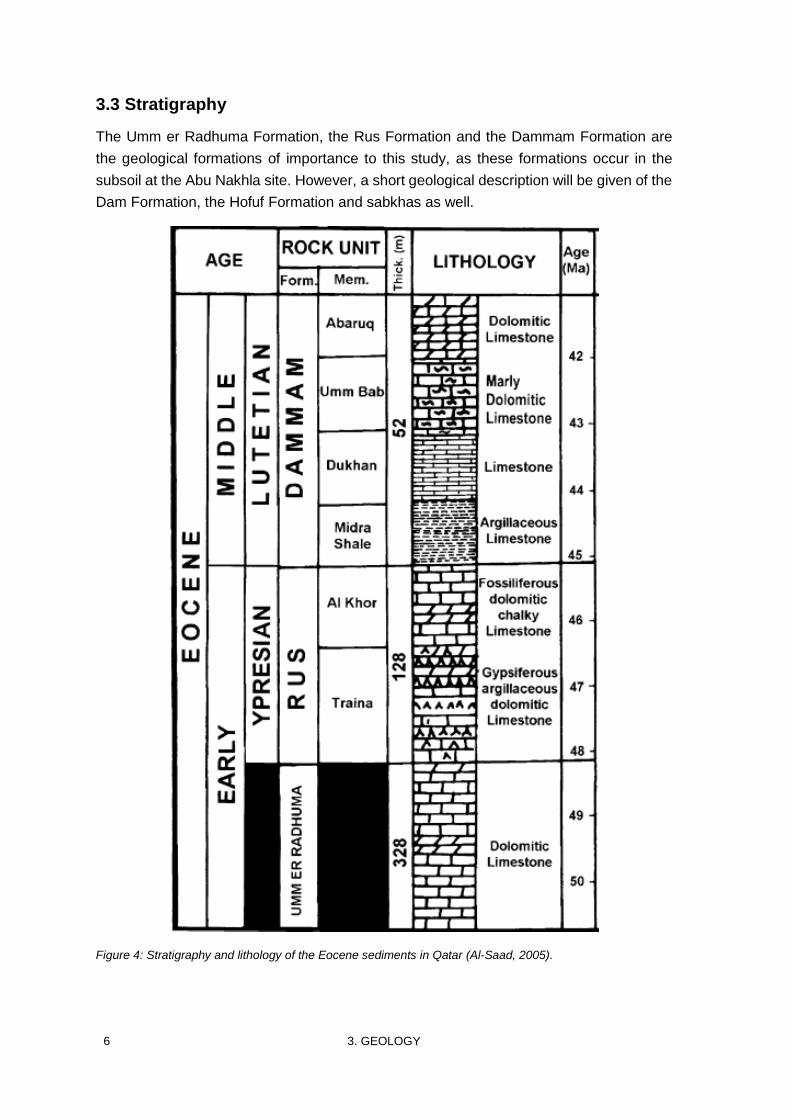
3.3 Stratigraphy
The Umm er Radhuma Formation, the Rus Formation and the Dammam Formation are
the geological formations of importance to this study, as these formations occur in the
subsoil at the Abu Nakhla site. However, a short geological description will be given of the
Dam Formation, the Hofuf Formation and sabkhas as well.
Figure 4: Stratigraphy and lithology of the Eocene sediments in Qatar (Al-Saad, 2005).
3. GEOLOGY 7
3.3.1 Umm er Radhuma Formation
The oldest formation of the Palaeogene or early Eocene is the Umm er Radhuma
Formation (UER). Unlike the other Eocene and Miocene formations, the UER has no
outcrops in Qatar. The UER is conformably overlying the Aruma Formation, the uppermost
Cretaceous unit, which is a hard marine crystalline limestone. The sedimentation process
of the UER is characterised by a marine transgression over the Persian Gulf area at the
beginning of the Palaeocene to Lower Eocene where it was deposited in a shallow marine
(neritic) environment (Mukhopadhyay, et al., 1996). The transition of the Aruma Formation
and the basal section of the UER can be lithological identified by the occurrence of dark
coloured shales and marl beds with the presence of local anhydrite layers (Lloyd, et al.,
1987).
The lithology of the Umm er Radhuma Formation is dominated by calcareous facies
depositions consisting of dolomites and limestones. The thickness ranges from 270 m to
370 m. Even though the UER underlying Qatar consists of a well-bedded calcareous
sequence, some silicified zones do occur in the form of chert and silicified limestone or
dolomite. This zone is present at about 18 m to 20 m below the top of the formation and
constrains the hydraulic continuity between the upper UER and lower UER where the part
of the UER above the siliceous limestone has a higher permeability and the part of the
UER below the siliceous limestone has a lower permeability (Lloyd, et al., 1987).
3.3.2 Rus Formation
The Rus Formation conformably lies on top of the Umm er Radhuma Formation. The
contact between the two formations is not always obvious because the lithologies of both
formations are rather similar. In some places however, evidence of dissolution and
dolomitization can be noticed on the boundary (Al-Hajari & Kendall, 1992). According to
Eccleston & Harhash (1982) the contact between the UER Formation and the Rus
Formation is characterised by a general facies change and the disappearance of marine
fauna. This abrupt facies change from the UER Formation depositional character to the
Rus Formation depositional character over a large part of the area suggest a possible
sedimentary hiatus after the deposition of the UER Formation. It is deposited in a shallow
marine environment and the hiatus can be associated with uplift and land emergence in
some positive structurally controlled areas (Lloyd, et al., 1987).
The Rus Formation deposits are the oldest outcropping rocks in Qatar. Because of scarcity
of fossils in the Rus Formation some dispute exists on the dating of the formation. Based
on the presence of planktonic foraminifera in the underlying Umm er Radhuma Formation,
the Rus Formation was dated as Lutetian in Al-Saad (2003), but the same author changed
the age to Ypresian in Al-Saad (2005). The thickness in Qatar ranges between 33 m and
128 m. It is subdivided into two members: (1) the lower Traina Member and (2) the upper
Al-Khor Member (Al-Saad, 2003).
8 3. GEOLOGY
The Traina Member has a thickness up to 78 m. The lithology consists of a white to light
grey gypsiferous, marly, clayey, dolomitic limestone with thin yellow beds. The boundary
between the Traina Member and the Umm er Radhuma Formation can be characterised
by a change from the dolomitic limestone of the UER Formation to the gypsiferous
limestone of the Traina Member. The upper boundary is defined by the contact between
the grey gypsiferous dolomitic limestone from the Traina member and the white chalky
limestone from the Al-Khor Member. No significant fauna is found within the Traina
Member. Gypsum represents the thickest facies in this member and towards the north of
Qatar, this facies gradually changes to a dolomitic cherty limestone. It was believed to be
deposited in a restricted lagoon to supratidal setting (Al-Saad, 2003).
The Al-Khor Member has a thickness up to 50 m. The lithology consists of a white to light
grey, yellowish dolomitic chalky limestone with some gypsum, marls and clay intercalation.
The top of the Al-Khor Member is placed at the contact between the grey dolomitic
limestone of the Al-Khor Member and the yellowish shale of the overlying Dammam
Formation. Shark teeth, foraminifera, Mollusca and echinoid fragments can very rarely be
found. It was believed to be deposited in an open marine tidal to subtidal zone (Al-Saad,
2003).
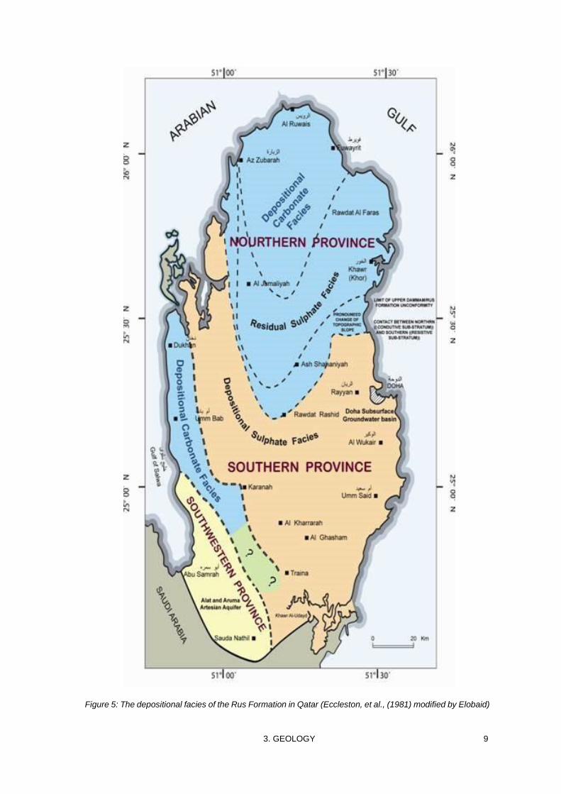
The Rus Formation is subdivided into two major provinces: A northern province
characterised by the occurrence of a depositional carbonate facies (dolomitic limestone)
and a residual gypsum facies and a southern province characterised by the occurrence of
a depositional sulphate facies (evaporitic, argillaceous, gypsiferous dolomitic limestone).
This has been visualised in Figure 5. The boundary between the two provinces is clearly
reflected as a V-shaped line with its apex at the Qatar Arch. The distribution and thickness
of the different facies in the provinces are influenced by the structural elements such as
the Simsima Arch and Qatar Arch. The basic lithology of both provinces is the same,
dolomitic limestone, but the gypsum present in the northern region was eliminated due to
post-depositional dissolution effects (present in the Traina member as discussed above).
This results in the depositional sulphate facies, which is present at the study area,
containing more gypsum than the residual sulphate facies, making it less permeable for
groundwater to flow. North of the residual sulphate facies the gypsum is completely
eliminated and a depositional carbonate facies remains.
Looking at the depositional setting of the Rus Formation it is believed that the southern
province was deposited in a relatively deep environment while the northern province was
deposited in a shallower environment (Al-Saad, 2003). Even though a clear dissimilarity
exists between the two facies, the dissolution of gypsum has complicated the identification
of the boundary. Collapse features due to this dissolution process also occurs in both
facies (Lloyd, et al., 1987).
In the southwest of Qatar, another small band of a depositional carbonate facies can be
depicted which runs along the Dukhan anticline.
3. GEOLOGY 9
Figure 5: The depositional facies of the Rus Formation in Qatar (Eccleston, et al., (1981) modified by Elobaid)
10 3. GEOLOGY
3.3.3 Dammam Formation
The Dammam Formation is subdivided into four members, from eldest to youngest: the
Midra Shale Member, the Dukhan Member, the Umm Bab Member and the Abaruq
Member. The thickness of the formation ranges between 30 m to 52 m and the boundary
between the Dammam Formation and the Rus Formation appears to be conformable on
the regional scale, as the light grey marly limestone of the Rus Formation gradually
changes into the light yellow or green claystone of the Dammam Formation. However, the
contact between the two formations represents the boundary between the Ypresian and
Lutetian which is considered to be a disconformity. In the northeast of Qatar an abrupt
facies change is present as the Umm Bab Member there lies disconformaby on top of the
Rus Formation while the Midra Shale and Dukhan members are missing. This is probably
related to the activation of paleohighs in the northern part of Qatar, such as the Simsima
Dome (Al-Saad, 2005; Holail, et al., 2005).
The Midra Shale Member is only exposed in southwest and central Qatar as explained in
the previous paragraph. In southwest Qatar, the Midra Shale Member consists of a soft,
grey to light green, fossiliferous, fissile, calcareous and gypsiferous shale with two thin
beds of marl ranging between 0.3 m and 0.5 m in thickness. The thickness of the Midra
Shale Member ranges here between 2 m and 6 m. In central Qatar the Midra Shale
Member consists of compact, massive, hard, grey to light green fossiliferous, partially
gypsiferous, calcareous claystone interbedded with two beds of argillaceous limestone at
the base and in the middle. Thin bands of marl, with a thickness ranging from 2 cm to 4 cm,
are intercalated within this facies. The thickness of the Midra Shale Member ranges here
between 4 m and 9 m. The boundary between the base of the Midra Shale Member and
the Rus Formation is characterised by the presence of shark teeth, while in the upper part
Mollusca fossils can be depicted. In some beds of the Midra Shale Member some ironstone
nodules can occur.
Above the Midra Shale Member lies the Dukhan Member. This member is also only
exposed in southwest and central Qatar. It consists of a massive, nodular grey to light
yellow to brown limestone and is abundant in fauna such as Nummulites and Alveolina.
The base of the Dukhan Member is characterised by mudstone facies because of a
shallowing upward cycle due to transgression of the Eocene Sea, while wackestone and
packstone textures become abundant towards the top. This member is the thinnest unit
within the Dammam Formation with a thickness ranging between 1 m and 2 m.
The Umm Bab Member is exposed in whole of Qatar. It consists of a hard, massive light
grey to creamy dolomitic limestone including a very thin marly bed at the base and a thin
cherty lens at the top. The boundary between the Dukhan Member and the Umm Bab
Member is characterised by a yellowish, fossiliferous marly limestone of about a 0.3 m
thickness, which contains Alveolines, molds of pelecypods and gastropods. The total
thickness of this member ranges between 15 m to 30 m.
3. GEOLOGY 11
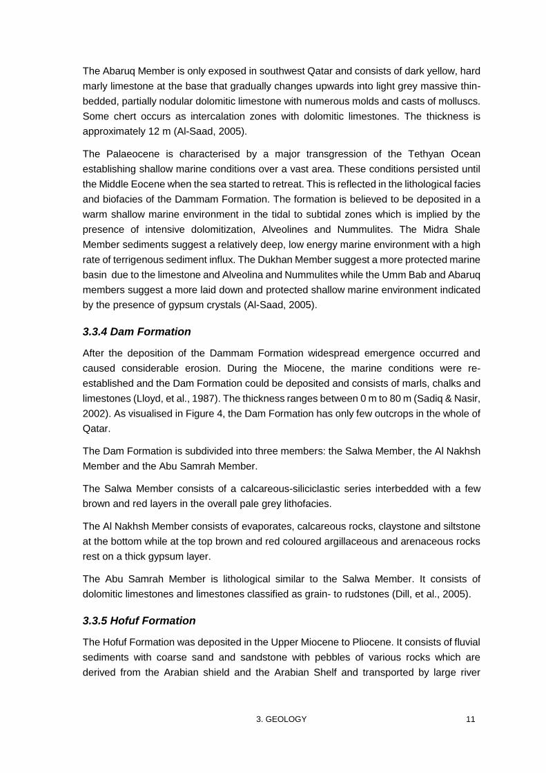
The Abaruq Member is only exposed in southwest Qatar and consists of dark yellow, hard
marly limestone at the base that gradually changes upwards into light grey massive thin-
bedded, partially nodular dolomitic limestone with numerous molds and casts of molluscs.
Some chert occurs as intercalation zones with dolomitic limestones. The thickness is
approximately 12 m (Al-Saad, 2005).
The Palaeocene is characterised by a major transgression of the Tethyan Ocean
establishing shallow marine conditions over a vast area. These conditions persisted until
the Middle Eocene when the sea started to retreat. This is reflected in the lithological facies
and biofacies of the Dammam Formation. The formation is believed to be deposited in a
warm shallow marine environment in the tidal to subtidal zones which is implied by the
presence of intensive dolomitization, Alveolines and Nummulites. The Midra Shale
Member sediments suggest a relatively deep, low energy marine environment with a high
rate of terrigenous sediment influx. The Dukhan Member suggest a more protected marine
basin due to the limestone and Alveolina and Nummulites while the Umm Bab and Abaruq
members suggest a more laid down and protected shallow marine environment indicated
by the presence of gypsum crystals (Al-Saad, 2005).
3.3.4 Dam Formation
After the deposition of the Dammam Formation widespread emergence occurred and
caused considerable erosion. During the Miocene, the marine conditions were re-
established and the Dam Formation could be deposited and consists of marls, chalks and
limestones (Lloyd, et al., 1987). The thickness ranges between 0 m to 80 m (Sadiq & Nasir,
2002). As visualised in Figure 4, the Dam Formation has only few outcrops in the whole of
Qatar.
The Dam Formation is subdivided into three members: the Salwa Member, the Al Nakhsh
Member and the Abu Samrah Member.
The Salwa Member consists of a calcareous-siliciclastic series interbedded with a few
brown and red layers in the overall pale grey lithofacies.
The Al Nakhsh Member consists of evaporates, calcareous rocks, claystone and siltstone
at the bottom while at the top brown and red coloured argillaceous and arenaceous rocks
rest on a thick gypsum layer.
The Abu Samrah Member is lithological similar to the Salwa Member. It consists of
dolomitic limestones and limestones classified as grain- to rudstones (Dill, et al., 2005).
3.3.5 Hofuf Formation
The Hofuf Formation was deposited in the Upper Miocene to Pliocene. It consists of fluvial
sediments with coarse sand and sandstone with pebbles of various rocks which are
derived from the Arabian shield and the Arabian Shelf and transported by large river

12 3. GEOLOGY
systems. The Hofuf Formation is approximately 18 m thick (Sadiq & Nasir, 2002; Al-Saad,
et al., 2002).
3.3.6 Sabkhas
Sabkhas are saline planes developed in the Holocene. Two types of sabkhas exist: inland
sabkhas and coastal sabkhas. Combined, they cover approximately 7% of the land surface
with coastal sabkhas being the most widespread type covering an area of 590 km².
Sabkhas are silty soils with high salinities and contain mainly quartz grains, mud and
evaporites. Their thickness ranges from 0 m to 20 m (Ashour, 2013).
4. HYDROGEOLOGY 13
4. HYDROGEOLOGY
4.1 General hydrogeology
Qatar has two major aquifers which are dominated by dissolution induced permeability:
the Umm er Radhuma Formation and the Rus Formation (Lloyd, et al., 1987). Both aquifers
have very different characteristics due to their different geologies. The main outcropping
Dammam Formation is only considered to be a small aquifer.
Below the Umm er Radhuma Formation the Aruma Group is present. The basal shales of
the UER act as aquitards separating the Aruma Group sediments from the overlying
calcareous facies of the UER aquifer. The middle part of the UER consists of calcareous
limestone with many fissures and is the most permeable aquifer layer. The top part of the
UER aquifer is dolomitic and karstified, infilled with argillaceous sediments. The aquifer
properties are rather moderate where these dolomitic zones with fissures occur
(Mukhopadhyay, et al., 1996). A siliceous limestone zone occurring near the top of the
UER (at about 20 m) constrains the continuity between the UER aquifer and the Rus
aquifer. Water in the UER aquifer is mainly transported through secondary porosity
induced by dissolution processes as intergranular permeability is rather low (Sharaf,
2001).
The Rus Formation has two different provinces with characteristic facies. The north
contains a depositional carbonate facies and a residual sulphate facies, the south contains
a depositional sulphate facies (Figure 5). Pleistocene groundwater flow mainly occurred
during pluvial periods leading to post-depositional permeability development, i.e.
dissolution of the evaporites. During such periods, the northern province acted as a
discharge zone for the UER aquifer with groundwater flowing from this aquifer through the
depositional carbonate facies of the Rus Formation. In the south, groundwater is mainly
present in fissures and cavernous parts in the depositional sulphate facies created by
dissolution of the evaporites, but where the Midra Shale Member is present, the dissolution
of the evaporites is retarded (Schlumberger, 2009). It can be concluded that hydraulic
continuity exists between the UER and Rus aquifer which is only constrained by the
siliceous limestone in the upper part of the UER, illuminated in previous paragraph, and
due to some shales present in the lower Rus Formation. When the depositional sulphate
facies overlies the UER, the hydraulic continuity between the two aquifers diminishes
rapidly away from the depositional calcareous facies because of the presence of basal
shales. A transition can be depicted from hydraulic continue aquifers in the north to two
distinct aquifers in the south (Lloyd, et al., 1987).
The Dammam Formation is considered to be a shallow aquifer. The dolomitic and chalky
limestone part forms the most important aquifer while the shaly and marly limestones of
the basal member acts as an aquitard (Mukhopadhyay, et al., 1996).
Karstification occurs near the surface aquifers of Qatar. Sinkholes created by the
karstification penetrate the Dammam Formation and links the surface with the Rus
14 4. HYDROGEOLOGY
Formation. During rainfall events, the water level in the sinkholes will rise as the regional
water table rises and they can be flooded by the surface water runoff. The depressions
found over the whole of Qatar are former sinkholes filled with autochthonous material
which explains the high storage coefficient and transmissivity measured around the
margins (Sadiq & Nasir, 2002).
4.2 Head distribution
The head distribution of the main aquifers, the Umm er Radhuma and Rus aquifer, and
the head of the Dammam aquifer are visualised in respectively Figure 6, Figure 7 and
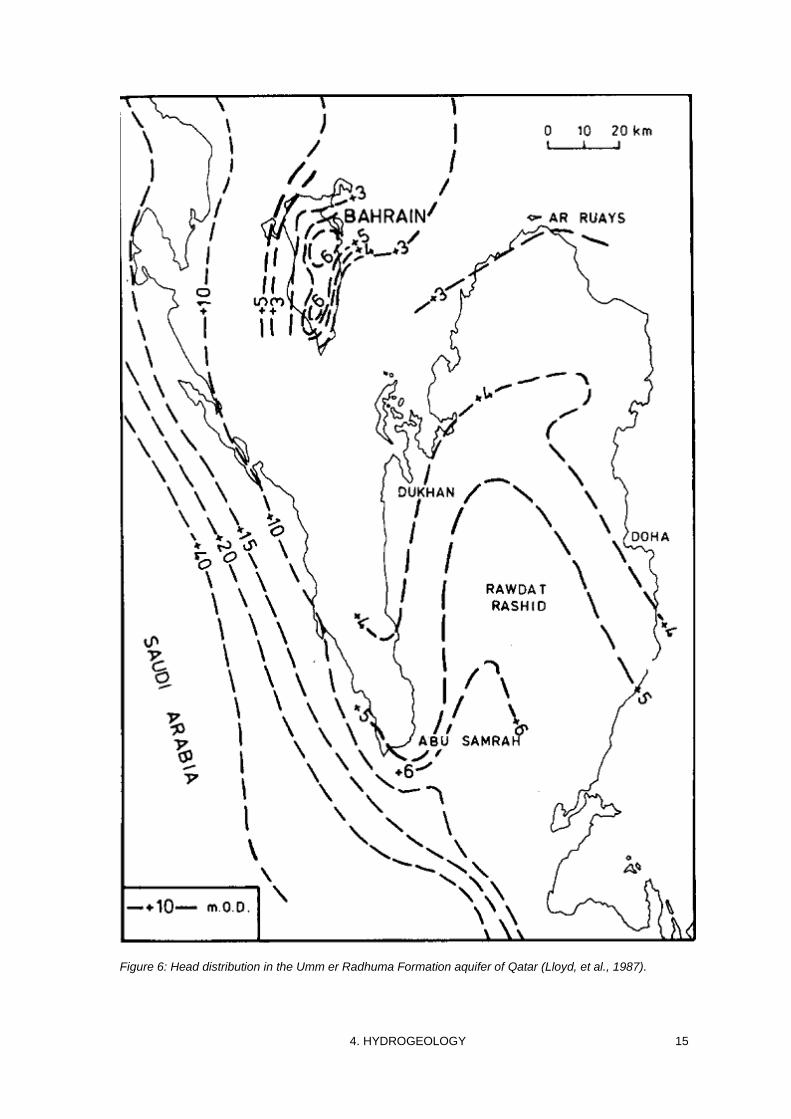
Figure 8. The distribution of the heads of the Umm er Radhuma Formation aquifer is quite
uniform as it shows a regional scale distribution, visualised on Figure 7. The head ranges
from about 6 m amsl in the south of Qatar to 3 m amsl in the north of Qatar.
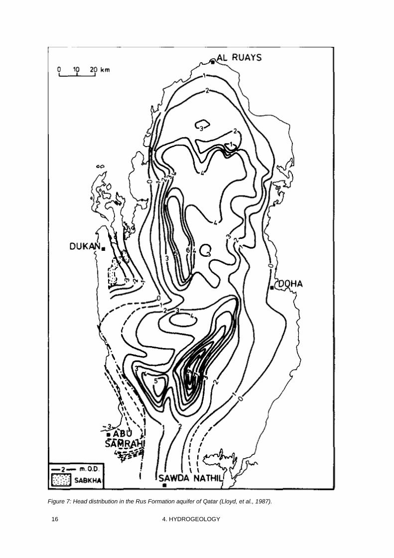
The head of the Rus Formation at the lateral boundaries is controlled by the sea. A change
in head relationship between the Umm er Radhuma and Rus aquifer across the peninsula
can be seen. In the calcareous part of the Rus Formation in the north of Qatar, the head
of the Rus Formation exceeds the head of the underlying UER, resulting in downward flow
in the central part where recharge occurs. Towards the sea, the heads decrease and the
difference in head between the Rus and the UER is reversed, thus the head of the UER
exceeds the head of the Rus Formation (Lloyd, et al., 1987). The head of the Rus
Formation clearly follows the Qatar Arch, with the highest values being located on the
southern part in the depositional sulphate facies. At the western side of Qatar, near the
Dukhan anticline, a big drop in head can be depicted. A sabkha which forms an
evaporative discharge area for the Rus Formation aquifer is situated there. Heads can be
as low as -3 m amsl in this area (Lloyd, et al., 1987).
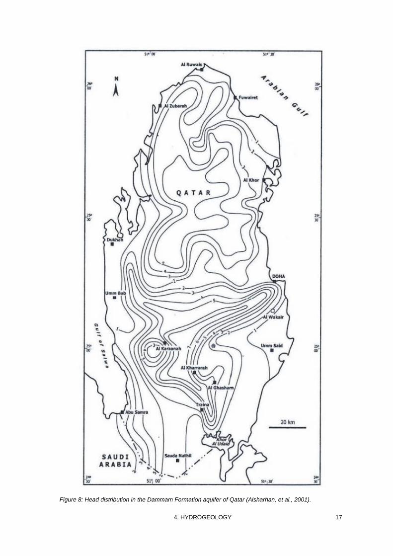
In the Dammam Formation aquifer (Figure 8) a similar trend can be noticed as in the Rus
Formation aquifer in central and southern Qatar. The heads show a high in the Qatar Arch
in the southern part and decrease towards the edges of the peninsula. In northern Qatar
a more gradual distribution can be depicted, the heads are lower than in the south and
never exceed the Rus Formation aquifer heads.
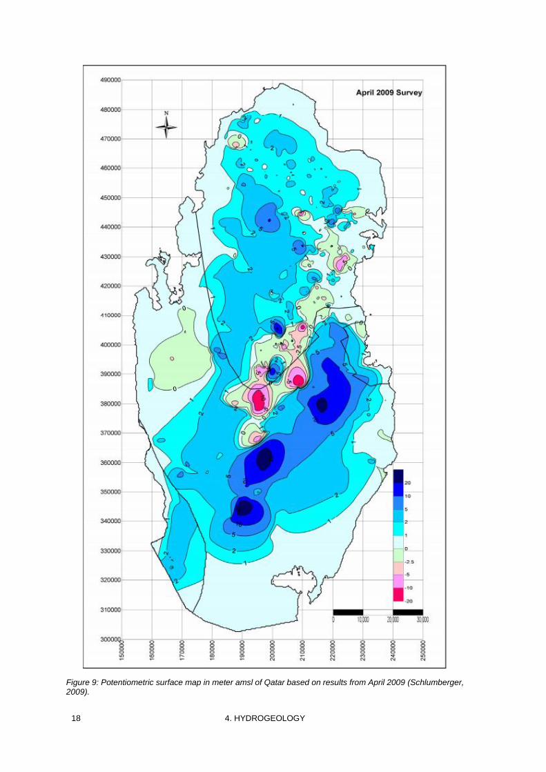
A more recent potentiometric surface map is presented by Schlumberger (2009) in Figure
9. The map represents the heads of the upper aquifer system (Dammam and upper Rus
formations). The largest heads mostly occur along the central axis of Qatar while the heads
decrease towards the sea. Starting in the centre and going towards the northeast, a zone
of depression cones can be depicted. These depression cones have heads as low as -20
m amsl. These depressions are induced by extensive pumping by farmers (irrigation,
cattle) or by municipal wells.
4. HYDROGEOLOGY 15
Figure 6: Head distribution in the Umm er Radhuma Formation aquifer of Qatar (Lloyd, et al., 1987).
16 4. HYDROGEOLOGY
Figure 7: Head distribution in the Rus Formation aquifer of Qatar (Lloyd, et al., 1987).
4. HYDROGEOLOGY 17
Figure 8: Head distribution in the Dammam Formation aquifer of Qatar (Alsharhan, et al., 2001).
18 4. HYDROGEOLOGY
Figure 9: Potentiometric surface map in meter amsl of Qatar based on results from April 2009 (Schlumberger, 2009).
4. HYDROGEOLOGY 19
4.3 Hydrogeological parameters
In the Umm er Radhuma aquifer, groundwater is mainly transmitted through the secondary
porosity. This makes an estimation of the average permeability and transmissivity
complicated. This is reflected in the many different values and wide ranges found in
literature. The average permeability found in previous studies show values of 3.46 m d-1
to 864 m d-1 and average transmissivity values range between 6.05 m² d-1 to
53568 m² d-1. The large variation seen in the permeability and the transmissivity can be
attributed to the increasing permeability as a result of dolomitisation. For the vertical
permeability, an average value of 2747.5 m d-1 can be noted while for the horizontal
permeability an average value of 3.84 x 10⁻³ m d-1 is depicted. The large anisotropy of the
UER aquifer system can easily be seen due to the large differences in the vertical and
horizontal permeability. The average storativity can be estimated in the range between
10-5 to 10-3, which are values that can be expected for a confined aquifer (Sharaf, 2001).
Similar values are described in a paper of a study in eastern Saudi Arabia (Rasheeduddin,
et al., 1989). Values described for the transmissivity of the UER are between 2000 m d-1
and 55296 m d-1 and values found for the storativity are between 2.50 x 10⁻⁵ to
1.50 x 10⁻². Values for the dispersivity of the UER range from 10 m to 150 m, the effective
porosity is approximately 0.2 m (Streetly & Kotoub, 1998).
El-Sayed (1986) researched the formation parameters of the Rus Formation in Qatar.
Thirteen samples of the upper part of the Rus Formation were taken thus the derived
parameters only represent the upper part of the Rus Formation. By analysis in the
laboratory, values for hydraulic conductivity were measured between 2.25 x 10⁻⁴ m d-1 to
0.355 m d-1. These values represent the upper part of the Rus Formation in the residual
sulphate facies (Figure 5). There are no direct measurements for the depositional sulphate
facies of the Rus Formation available in literature. Therefore an estimation can be made,
based on Domenico & Schwartz (1998), where the hydraulic conducitivies found in
anhydritic layers are described: horizontal hydraulic conducitivity values range from
3.456 * 10-8 m d-1 to 1.728 * 10-3 m d-1. Dispersivity values are in the range of 0.5 m to 5 m
and the effective porosity is approximately 0.2 m, the same value as the UER (Streetly &
Kotoub, 1998).
For the Dammam Formation, no studies of direct measuraments of the horizontal hydraulic
conductivity or transmissivity are avaible. As elucidated in part 3.3.3, the Dammam
Formation is a calcareous dolomitic limestone with an abundance in karst features such
as fissures and sinkholes (Sadiq & Nasir, 2002). If looked at the literature for
hydrogeological parameters of dolomitic limestone aquifers, a vast range of horizontal
hydraulic conductivities can be found. However, most studies indicate a similar range for
the horizontal hydraulic conductivity of a limestone aquifer matrix which varies between
8.64 x 10⁻⁶ m d-1 and 0.0216 m d-1. The horizontal hydraulic conductivity for karstified
dolomitic limestone aquifers vary between 1 m d-1 and 8.64 m d-1 (Dar, et al., 2014; Perrin,
et al., 2011). Higher values for the horizontal hydraulic conductivity can occur if the aquifer
has even more fissures and cracks, but this is not the case for the Dammam Formation.
20 4. HYDROGEOLOGY
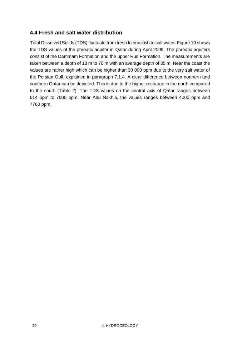
4.4 Fresh and salt water distribution
Total Dissolved Solids (TDS) fluctuate from fresh to brackish to salt water. Figure 10 shows
the TDS values of the phreatic aquifer in Qatar during April 2009. The phreatic aquifers
consist of the Dammam Formation and the upper Rus Formation. The measurements are
taken between a depth of 13 m to 70 m with an average depth of 35 m. Near the coast the
values are rather high which can be higher than 30 000 ppm due to the very salt water of
the Persian Gulf, explained in paragraph 7.1.4. A clear difference between northern and
southern Qatar can be depicted. This is due to the higher recharge in the north compared
to the south (Table 2). The TDS values on the central axis of Qatar ranges between
514 ppm to 7000 ppm. Near Abu Nakhla, the values ranges between 4000 ppm and
7760 ppm.
4. HYDROGEOLOGY 21
Figure 10: Total Dissolved Solids (TDS) isoconcentration map in ppm (Schlumberger, 2009).

22 4. HYDROGEOLOGY
5. CLIMATE AND HYDROLOGY 23
5. CLIMATE AND HYDROLOGY
Qatar has a desert climate with sporadic rainfall, mainly occurring during November to
March. The Persian Gulf affects the climate in terms of temperature and humidity but also
in terms of the occurrence and distribution of rainfall. Due to these climatic conditions the
summer temperatures can climb up to more than 40°C and persist throughout most of the
year. During winter, the temperatures can be as low as 4°C but they generally are between
10°C to 20°C (Lloyd, et al., 1987).
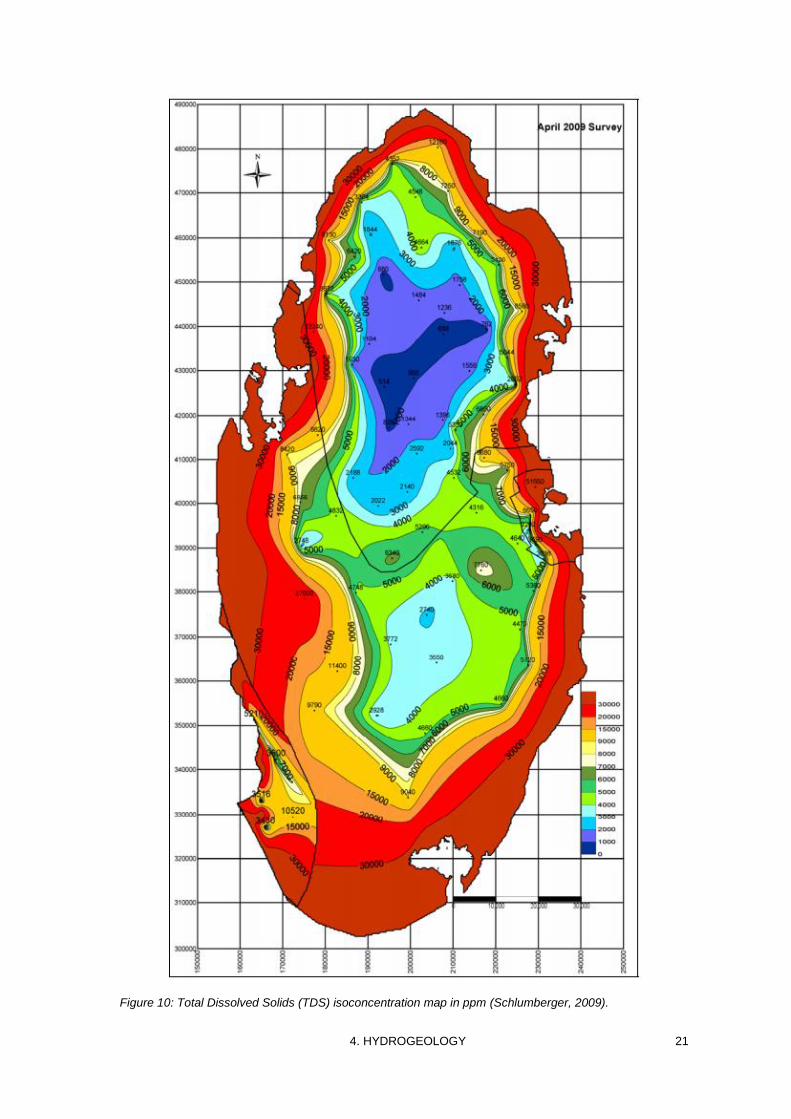
The mean annual total rainfall for the period from 1972 to 2005 is 80.2 mm yr-1 (Amer, et
al., 2008). As depicted on Figure 11, a big variation in annual rainfall can be noticed with
an absolute high in 1995 with a total annual rainfall of 276.8 mm. The annual evaporation
rate is around 2200 mm yr-1 with the daily evaporation rate varying from 2.5 mm d-1 during
winter months and 11.5 mm d-1 during summer months (Shomar, et al., 2014; Lloyd, et al.,
1987). Only a part of the precipitation will infiltrate into the soil, while the other part will
runoff or evaporate. Due to the high evaporation rate, recharge will only occur during storm
events when larger volumes of surface runoff occur. The annual natural recharge in Qatar
is estimated on 58 Mm³ yr-1 or approximately 5 mm yr-1 (Shomar, et al., 2014).
Figure 11: Total annual rainfall (mm yr-1) of Qatar from 1972 to 2005 (Amer, et al., 2008).
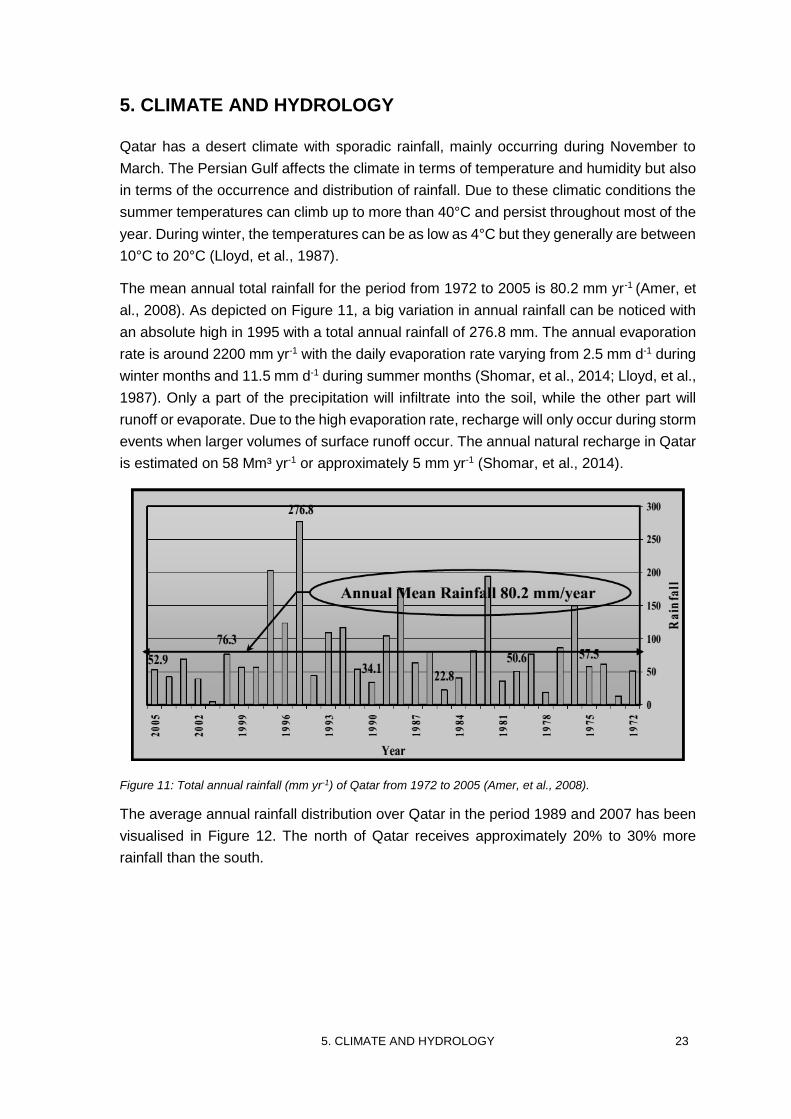
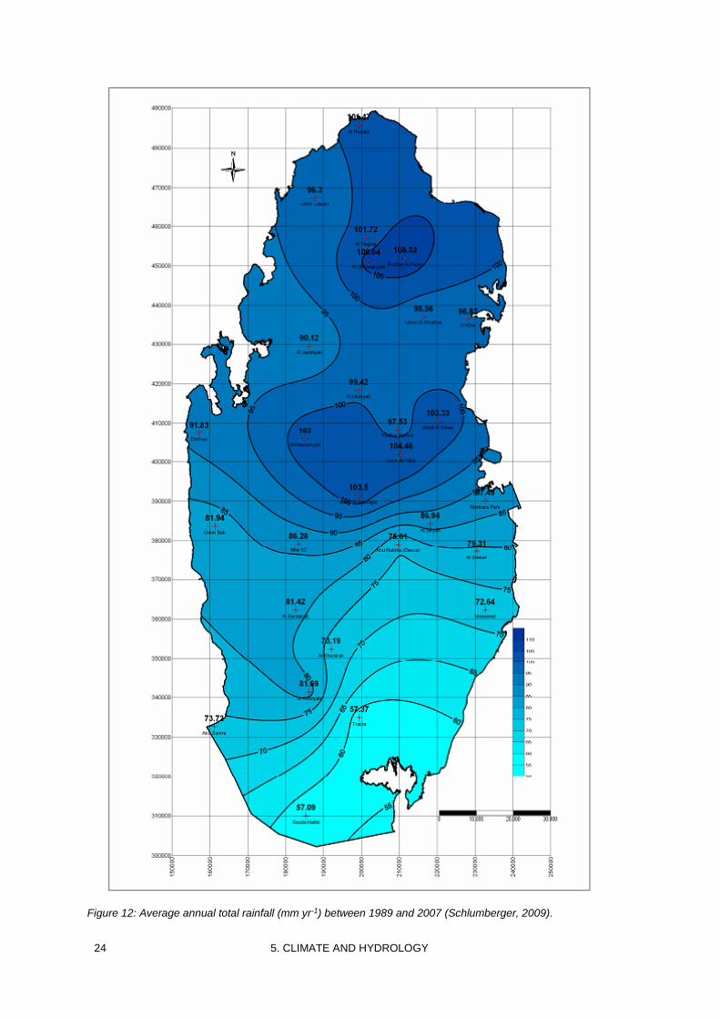
The average annual rainfall distribution over Qatar in the period 1989 and 2007 has been
visualised in Figure 12. The north of Qatar receives approximately 20% to 30% more
rainfall than the south.
24 5. CLIMATE AND HYDROLOGY
Figure 12: Average annual total rainfall (mm yr-1) between 1989 and 2007 (Schlumberger, 2009).
5. CLIMATE AND HYDROLOGY 25
Numerous studies have been made to estimate the surface runoff in Qatar because of its
importance to the indirect recharge of the groundwater reservoir, which will be discussed
later on. Table 1 lists a selection of available estimations, where runoff is given as a
percentage of the total rainfall. All these estimations of surface runoff are based on mass
balance calculations since no direct observations of surface runoff are made. From these
studies it can be concluded that rainfall over relatively small catchment areas is likely to
be evenly distributed. This causes short flow paths of surface water towards depressions
which result in less infiltration and evaporation loss and increases the potential surface
runoff. Soil moisture conditions prior to a rainfall event is another important factor. When
soils are close to their field capacity, infiltration will come to a halt and more runoff is
produced. Gemmel (1976) suggested that runoff is most likely to occur when a rainfall
event exceeds 10 mm. Pike et al. (1975) concluded that if rainfall exceeds 10 mm per day,
surface runoff can be estimated to be between 15% and 25%. Detailed analysis of rainfall
events and their resulting surface runoff showed that the distribution of rainfall over the
catchment area is of greater importance than the total amount of rainfall. This is based on
two storm events observed on the 5th and 12th of February 1976 in the Ghuwairayah
catchment area (central part of northern Qatar). Both storms produced a mean rainfall of
19 mm over the catchment area and yet the runoff was different in both cases: 18% and
8% respectively. The largest volume of runoff was produced by the storm event on the 5th
of February, which was the most intense with a mean rainfall of 13 mm predominantly over
the area with depressions and less rainfall at the boundary of the depressions. The storm
on the 12th of February produced a more evenly distributed rainfall across the catchment
area with an average rainfall of 10 mm. Even though the soil conditions were considered
to be more favourable for surface runoff generation (they were already wetted by the
previous storm), less than half of the runoff volume was generated by the second storm
(Gemmel, 1976; Eccleston, et al., 1981). However, it should be noted that no account has
been taken of the effect of the infiltration capacity of the soils. The first storm is said to be
more intense so it is possible that the rainfall rate exceeded the infiltration rate of the soils
in the catchment area producing more surface runoff compared to a less intense storm
which does not exceed the infiltration capacity of the soil. No data is given related to the
intensity of the storm but it can be noted that calculated hydraulic conductivities of the soils,
based on observed soil textural properties, are in the range of 9 mm h-1 to 18 mm h-1.
In a recent study by Schlumberger (2009) measurements revealed that surface runoff can
already occur with a total rainfall of only 5.9 mm without previous wetting of the soil, which
is in contrast with the minimum 8 mm to 10 mm described in previous studies. This lead
to the conclusion that rainfall intensity is of more importance to the surface runoff than the
total amount of rainfall as the soils only have a limited permeability. When rainfall intensity
exceeds the permeability of the soil, runoff will be generated even if the total amount of
rainfall is rather small (Schlumberger, 2009).
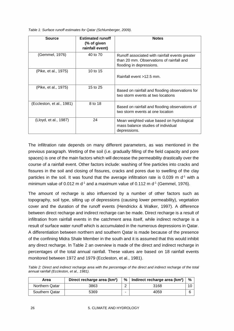
26 5. CLIMATE AND HYDROLOGY
Table 1: Surface runoff estimates for Qatar (Schlumberger, 2009).
Source Estimated runoff
(% of given
rainfall event)
Notes
(Gemmel, 1976) 40 to 70 Runoff associated with rainfall events greater
than 20 mm. Observations of rainfall and
flooding in depressions.
(Pike, et al., 1975) 10 to 15
Rainfall event >12.5 mm.
(Pike, et al., 1975) 15 to 25 Based on rainfall and flooding observations for
two storm events at two locations
(Eccleston, et al., 1981) 8 to 18 Based on rainfall and flooding observations of
two storm events at one location
(Lloyd, et al., 1987) 24 Mean weighted value based on hydrological
mass balance studies of individual
depressions.
The infiltration rate depends on many different parameters, as was mentioned in the
previous paragraph. Wetting of the soil (i.e. gradually filling of the field capacity and pore
spaces) is one of the main factors which will decrease the permeability drastically over the
course of a rainfall event. Other factors include: washing of fine particles into cracks and
fissures in the soil and closing of fissures, cracks and pores due to swelling of the clay
particles in the soil. It was found that the average infiltration rate is 0.039 m d-1 with a
minimum value of 0.012 m d-1 and a maximum value of 0.112 m d-1 (Gemmel, 1976).
The amount of recharge is also influenced by a number of other factors such as
topography, soil type, silting up of depressions (causing lower permeability), vegetation
cover and the duration of the runoff events (Hendrickx & Walker, 1997). A difference
between direct recharge and indirect recharge can be made. Direct recharge is a result of
infiltration from rainfall events in the catchment area itself, while indirect recharge is a
result of surface water runoff which is accumulated in the numerous depressions in Qatar.
A differentiation between northern and southern Qatar is made because of the presence
of the confining Midra Shale Member in the south and it is assumed that this would inhibit
any direct recharge. In Table 2 an overview is made of the direct and indirect recharge in
percentages of the total annual rainfall. These values are based on 18 rainfall events
monitored between 1972 and 1979 (Eccleston, et al., 1981).
Table 2: Direct and indirect recharge area with the percentage of the direct and indirect recharge of the total annual rainfall (Eccleston, et al., 1981).
Area Direct recharge area (km²) % Indirect recharge area (km²) %
Northern Qatar 3863 2 3168 10
Southern Qatar 5369 - 4059 6

5. CLIMATE AND HYDROLOGY 27
With an average total annual rainfall of 80.2 mm yr-1, as described by Amer et al. (2008),
recharge in the southern part would be about 4.8 mm yr-1 if the above mentioned 6% from
Table 2 is applied. This estimatation coincides with the value of 5 mm yr-1 as mentioned in
the study by Shomar, et al., (2014).

28 5. CLIMATE AND HYDROLOGY
6. MODELLING SOFTWARE 29
6. MODELLING SOFTWARE
6.1 Evolution of the modelling software
Two- and three-dimensional finite difference models existed long before the creation of
MODFLOW by the U.S. Geological Survey (USGS). These older models are described in
Trescott (1975), Trescott & Larson (1976) and Trescott et al. (1976). These models have
been extensively used by the USGS and others for the computer simulation of
groundwater flow. MODFLOW was created with the intention to be modular and it should
be easy to expand so it can be adjusted to any problem. Due to the modular build new
functions can be added without the necessity to change existing modules and subroutines
and due to the lower memory usage, because only modules are used which are necessary,
it could run on most computers (McDonald & Harbaugh, 1988).
To be able to simulate solute transport, the Method-of-Characteristics Solute Transport
Model (MOC) was created by Konikow & Bredehoeft (1978). With MOC, the solute
transport in a horizontal layer could be simulated. Lebbe (1983) adjusted the MOC code
so it could simulate density dependant flow in a vertical plain and the potentials are
expressed as freshwater heads. Sanford & Konikow (1985) made further adjustments to
MOC so that different densities and viscosities could also be simulated and the potentials
are expressed here as pressures. Later on, Konikow et al. (1996) created the successor
of MOC, named MOC3D, which can simulate solute transport in three-dimensions. Oude
Essink (1998) made adjustments to MOC3D so density dependent flow could be simulated
and named the software package MOCDENS3D. Here, the potentials are expressed as
freshwater heads.
6.2 MODFLOW
The flow equation which is used in MODFLOW is based on the law of Darcy and on the
continuity equation. Both equations will be used to simulate groundwater flow in a finite
difference network. MODFLOW can calculate steady state or unsteady state flow, i.e. time
independent and time dependant flow, in one-, two- or three-dimensions. MODFLOW
simulates in “real” three-dimensions or quasi-three-dimensions. If opted for the quasi-
three-dimensions, the aquitards will be represented by the horizon between the aquifers
so only the aquifers will be calculated as real layers, while the aquitards will be calculated
as the boundary between two aquifers. In the “real” three-dimensional simulation, the
aquitards will be discretised in multiple layers which will make it possible to accurately
simulate the head evolution in the aquitards on a specified level within a specified
timeframe. MODFLOW is created as modular simulation software, as elucidated in part
6.1, and exists out of a main module with a set of subroutines and a bunch of independent
modules with independent subroutines which are not mandatory but can be used if needed
(McDonald & Harbaugh, 1988).
30 6. MODELLING SOFTWARE
6.2.1 Code concepts
To convert a real physical groundwater system to a mathematical model, some
assumptions and conjectures need to be made. These conjectures include: (1)
schematisation of the groundwater system which can be discretised in a finite difference
grid, (2) no flow beyond the boundary of the model, (3) the modelled groundwater reservoir
can be heterogeneous and anisotropic, (4) the groundwater flow can be calculated in “real”
three-dimensions or as quasi-three-dimensional, (5) the simulated periods of both steady
state and unsteady state can be divided further into a series of time steps and (6) in
MODFLOW the density of the water is considered to be constant and cannot be changed
(McDonald & Harbaugh, 1988).
6.2.2 Discretisation of the groundwater reservoir
The spatial discretisation of an aquifer system into a finite difference grid is visualised in
Figure 13. Each different block is a cell and the location of all these cells is described with
three indices called rows, columns and layers. The indexation system used is i, j, k. For a
system consisting of “nrow” rows, “ncol” columns and “nlay” layers, the index for the row
will be i = 1, 2, 3, …, nrow, for the column the index will be j = 1, 2, 3, …, ncol, and for the
layer the index will be k = 1, 2, 3, …, nlay. A system with five rows, nine columns and five
layers is represented on Figure 13. In formulating the equations of the model, an
assumption is made that the layers generally correspond to horizontal hydrogeological
units or intervals. In terms of Cartesian coordinates this means that the k index denotes
changes along the vertical axis, z, since the followed convention of this discretisation is
that the layer numbers increase from the top down. In other words, an increase in the k
index corresponds with an increase in depth or a decrease in elevation. Rows would be
considered to be parallel to the x-axis meaning an increase in the row index i, corresponds
to a decrease in the y-value. Similarly for the columns, they are considered to be parallel
to the y-axis meaning an increase in the column index j corresponds with an increase in
the x-value (McDonald & Harbaugh, 1988).
Following the same convention used in Figure 13, the width of the cells along the row
direction at a given column j is ∆rj, the width of the cells along the column direction at a
given row i is ∆ci and the thickness of the cells in a given layer k is ∆vk.
In the centre of each cell there is a point called a node. In this node, the head will be
calculated. There are two conventions to define the configuration of cells with respect to
the location of the nodes: the block-centred formulation and the point-centred formulation.
Only the block-centred formulation will be discussed as it is the only one presently used in
the model. As visualised in Figure 14, the blocks or cells are formed by sets of parallel
lines and the nodes are situated in the centre of each cell. The assumption is made that
within a finite difference cell the groundwater reservoir is homogeneous and that the head
calculated in the node is representative for the cell (McDonald & Harbaugh, 1988).
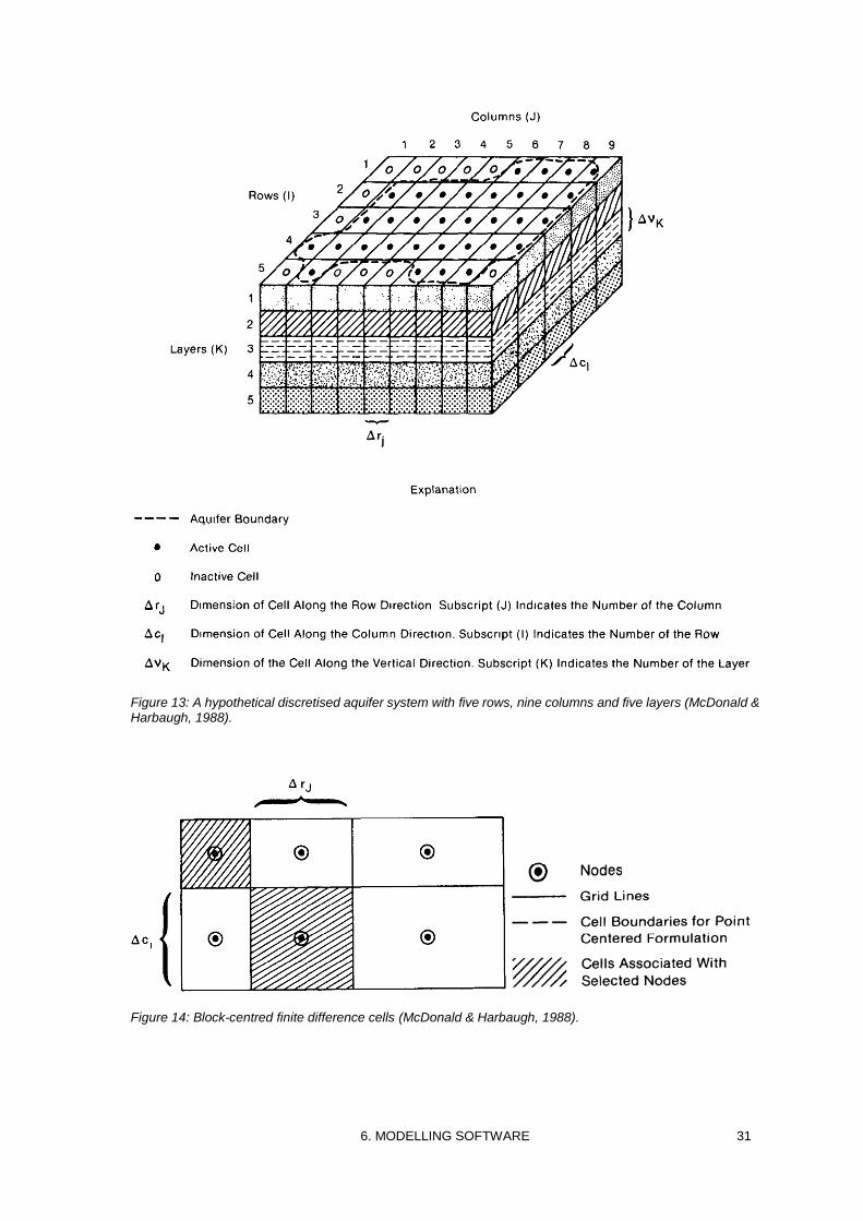
6. MODELLING SOFTWARE 31
Figure 13: A hypothetical discretised aquifer system with five rows, nine columns and five layers (McDonald & Harbaugh, 1988).
Figure 14: Block-centred finite difference cells (McDonald & Harbaugh, 1988).
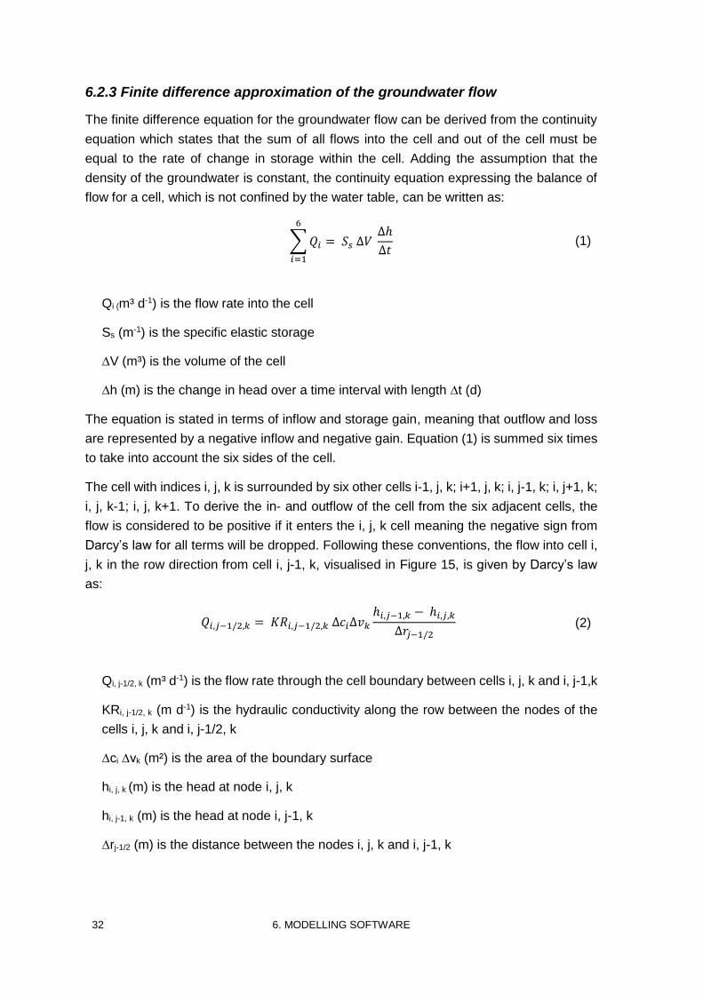
32 6. MODELLING SOFTWARE
6.2.3 Finite difference approximation of the groundwater flow
The finite difference equation for the groundwater flow can be derived from the continuity
equation which states that the sum of all flows into the cell and out of the cell must be
equal to the rate of change in storage within the cell. Adding the assumption that the
density of the groundwater is constant, the continuity equation expressing the balance of
flow for a cell, which is not confined by the water table, can be written as:
∑ 𝑄𝑖
6
𝑖=1
= 𝑆𝑠 ∆𝑉 ∆ℎ
∆𝑡 (1)
Qi (m³ d-1) is the flow rate into the cell
Ss (m-1) is the specific elastic storage
∆V (m³) is the volume of the cell
∆h (m) is the change in head over a time interval with length ∆t (d)
The equation is stated in terms of inflow and storage gain, meaning that outflow and loss
are represented by a negative inflow and negative gain. Equation (1) is summed six times
to take into account the six sides of the cell.
The cell with indices i, j, k is surrounded by six other cells i-1, j, k; i+1, j, k; i, j-1, k; i, j+1, k;
i, j, k-1; i, j, k+1. To derive the in- and outflow of the cell from the six adjacent cells, the
flow is considered to be positive if it enters the i, j, k cell meaning the negative sign from
Darcy’s law for all terms will be dropped. Following these conventions, the flow into cell i,
j, k in the row direction from cell i, j-1, k, visualised in Figure 15, is given by Darcy’s law
as:
𝑄𝑖,𝑗−1/2,𝑘 = 𝐾𝑅𝑖,𝑗−1/2,𝑘 ∆𝑐𝑖∆𝑣𝑘
ℎ𝑖,𝑗−1,𝑘 − ℎ𝑖,𝑗,𝑘
∆𝑟𝑗−1/2 (2)
Qi, j-1/2, k (m³ d-1) is the flow rate through the cell boundary between cells i, j, k and i, j-1,k
KRi, j-1/2, k (m d-1) is the hydraulic conductivity along the row between the nodes of the
cells i, j, k and i, j-1/2, k
∆ci ∆vk (m²) is the area of the boundary surface
hi, j, k (m) is the head at node i, j, k
hi, j-1, k (m) is the head at node i, j-1, k
∆rj-1/2 (m) is the distance between the nodes i, j, k and i, j-1, k
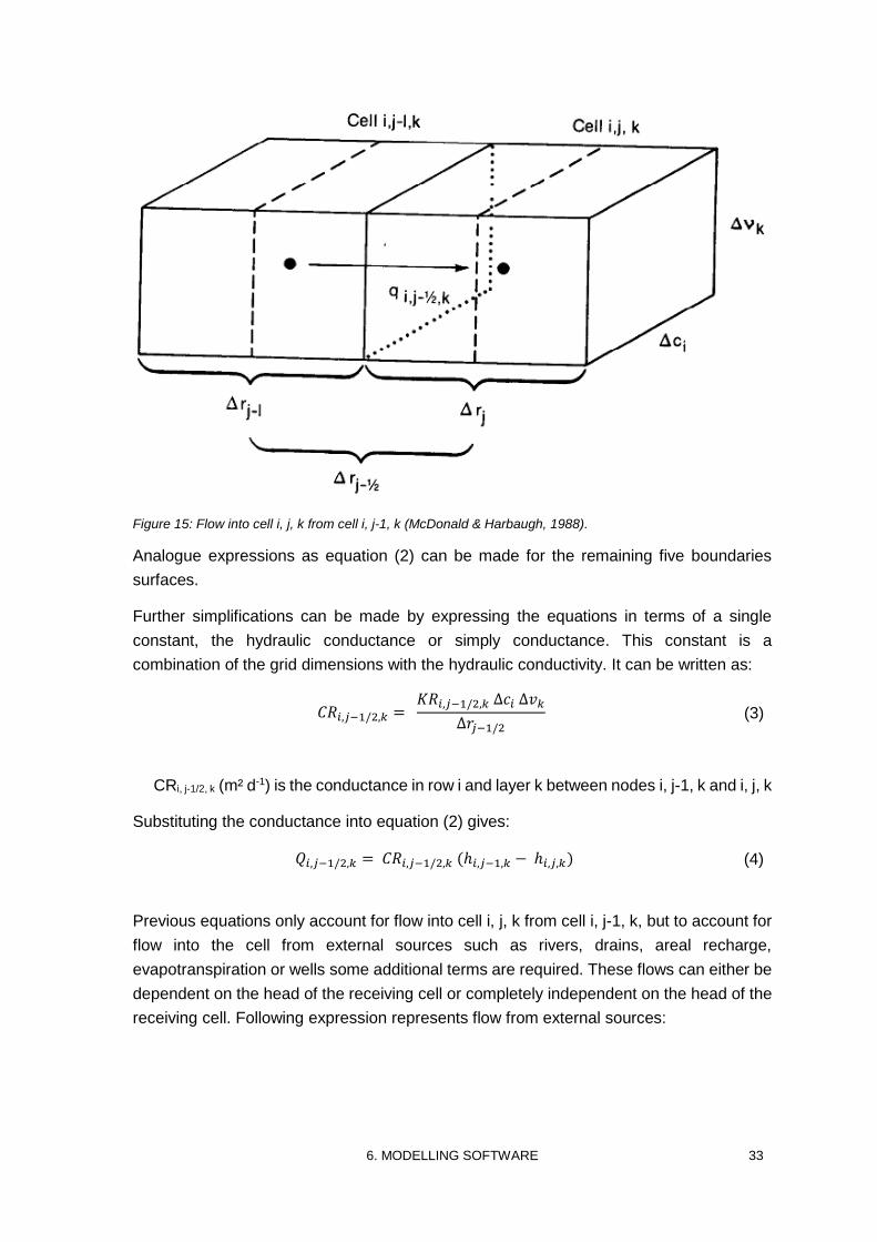
6. MODELLING SOFTWARE 33
Figure 15: Flow into cell i, j, k from cell i, j-1, k (McDonald & Harbaugh, 1988).
Analogue expressions as equation (2) can be made for the remaining five boundaries
surfaces.
Further simplifications can be made by expressing the equations in terms of a single
constant, the hydraulic conductance or simply conductance. This constant is a
combination of the grid dimensions with the hydraulic conductivity. It can be written as:
𝐶𝑅𝑖,𝑗−1/2,𝑘 =
𝐾𝑅𝑖,𝑗−1/2,𝑘 ∆𝑐𝑖 ∆𝑣𝑘
∆𝑟𝑗−1/2 (3)
CRi, j-1/2, k (m² d-1) is the conductance in row i and layer k between nodes i, j-1, k and i, j, k
Substituting the conductance into equation (2) gives:
𝑄𝑖,𝑗−1/2,𝑘 = 𝐶𝑅𝑖,𝑗−1/2,𝑘 (ℎ𝑖,𝑗−1,𝑘 − ℎ𝑖,𝑗,𝑘) (4)
Previous equations only account for flow into cell i, j, k from cell i, j-1, k, but to account for
flow into the cell from external sources such as rivers, drains, areal recharge,
evapotranspiration or wells some additional terms are required. These flows can either be
dependent on the head of the receiving cell or completely independent on the head of the
receiving cell. Following expression represents flow from external sources:
34 6. MODELLING SOFTWARE
𝑎𝑖,𝑗,𝑘,𝑛 = 𝑝𝑖,𝑗,𝑘,𝑛 ℎ𝑖,𝑗,𝑘 + 𝑄𝑖,𝑗,𝑘,𝑛 (5)
ai, j, k (m³ d-1) is the flow from the nth external source into cell i, j, k
hi, j, k (m) head in node i, j, k
pi, j, k, n (m² d-1) and Qi, j, k, n (m³ d-1) are constants
By summing all the equations from the flow between the boundary surfaces (equation (4)
and the five other analogue equations) and adding the flow of all the nth external sources
into one formula, the finite difference approximation for cell i, j, k can be given by:
𝐶𝑅𝑖,𝑗−
12
,𝑘 (ℎ𝑖,𝑗−1,𝑘 − ℎ𝑖,𝑗,𝑘) + 𝐶𝑅
𝑖,𝑗+12
,𝑘 (ℎ𝑖,𝑗+1,𝑘 − ℎ𝑖,𝑗,𝑘)
+ 𝐶𝐶𝑖−
12𝑗
,𝑘 (ℎ𝑖,−1𝑗,𝑘 − ℎ𝑖,𝑗,𝑘) + 𝐶𝐶
𝑖+12
,𝑗,𝑘 (ℎ𝑖,+1𝑗,𝑘 − ℎ𝑖,𝑗,𝑘)
+ 𝐶𝑉𝑖,𝑗,𝑘−
12
(ℎ𝑖,𝑗,𝑘−1 − ℎ𝑖,𝑗,𝑘) + 𝐶𝑉𝑖,𝑗,𝑘+
12
(ℎ𝑖,𝑗,𝑘+1 − ℎ𝑖,𝑗,𝑘)
+ 𝑃𝑖,𝑗,𝑘 ℎ𝑖,𝑗,𝑘 + 𝑄𝑇𝑖,𝑗,𝑘 = 𝑆𝑠 𝑖,𝑗,𝑘 (∆𝑟𝑗 ∆𝑐𝑖 ∆𝑣𝑘)∆ℎ𝑖,𝑗,𝑘
𝑚 − ∆ℎ𝑖,𝑗,𝑘𝑚−1
𝑡𝑚 − 𝑡𝑚−1
(6)
Pi, j, k is equal to ∑ 𝑝𝑖,𝑗,𝑘,𝑛𝑁𝑛=1
QTi, j, k is equal to ∑ 𝑄𝑖,𝑗,𝑘,𝑛𝑁𝑛=1
hi,j,km
is the head at time step m
hi,j,km-1
is the head at time step m-1
tm is the time at the end of time step m
tm-1 is the time at the end of time step m-1
6.2.4 Iteration with the Strongly Implicit Procedure
An iterative method is used to obtain the solution to the finite difference equations for each
time step. The calculation of the head in the nodes for the end of a given time step is
started by assigning an estimated (or a known) value for the head at each node at the
beginning of that time step. A procedure of calculation, in this case the Strongly Implicit
Procedure or SIP, is then used to calculate a new set of heads which are closer in
agreement with the finite difference equations. These new calculated heads replace the
initial head values and the procedure is repeated. The iteration continues until the
maximum difference of head between two consecutive iterations for all respective cells of
the grid is lower than a specified closure criterion (McDonald & Harbaugh, 1988).
The Strongly Implicit Procedure or SIP is a method of solving a large system of
simultaneous linear equations by iteration (McDonald & Harbaugh, 1988). As can be seen
in equation (6), the number of unknown variables can be up to seven: the head in the node
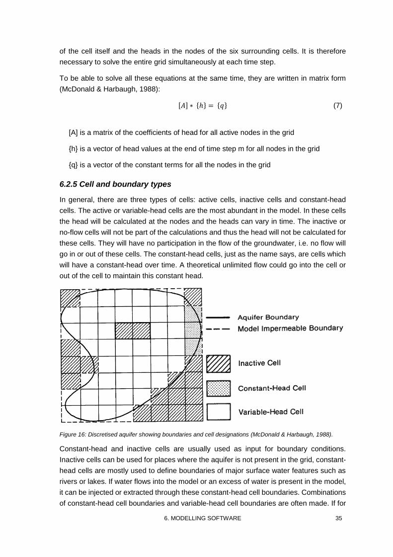
6. MODELLING SOFTWARE 35
of the cell itself and the heads in the nodes of the six surrounding cells. It is therefore
necessary to solve the entire grid simultaneously at each time step.
To be able to solve all these equations at the same time, they are written in matrix form
(McDonald & Harbaugh, 1988):
[𝐴] ∗ {ℎ} = {𝑞} (7)
[A] is a matrix of the coefficients of head for all active nodes in the grid
{h} is a vector of head values at the end of time step m for all nodes in the grid
{q} is a vector of the constant terms for all the nodes in the grid
6.2.5 Cell and boundary types
In general, there are three types of cells: active cells, inactive cells and constant-head
cells. The active or variable-head cells are the most abundant in the model. In these cells
the head will be calculated at the nodes and the heads can vary in time. The inactive or
no-flow cells will not be part of the calculations and thus the head will not be calculated for
these cells. They will have no participation in the flow of the groundwater, i.e. no flow will
go in or out of these cells. The constant-head cells, just as the name says, are cells which
will have a constant-head over time. A theoretical unlimited flow could go into the cell or
out of the cell to maintain this constant head.
Figure 16: Discretised aquifer showing boundaries and cell designations (McDonald & Harbaugh, 1988).
Constant-head and inactive cells are usually used as input for boundary conditions.
Inactive cells can be used for places where the aquifer is not present in the grid, constant-
head cells are mostly used to define boundaries of major surface water features such as
rivers or lakes. If water flows into the model or an excess of water is present in the model,
it can be injected or extracted through these constant-head cell boundaries. Combinations
of constant-head cell boundaries and variable-head cell boundaries are often made. If for
36 6. MODELLING SOFTWARE
example the eastern and western boundary are constant-head cells and the northern and
southern boundary are variable-head cells, the variable-head cell boundaries will act as
impervious boundaries as the exchange of water will preferentially flow through the
constant-head cell boundaries. This will result in a flow along the variable-head boundaries
and a flow perpendicular on the constant-head boundaries. An example of the different
possible boundary types can be seen in Figure 16 where inactive cells represent parts
where the aquifer is not present in the model (McDonald & Harbaugh, 1988).
6.3 MOC3D
MOC3D development started from the existing two-dimensional MOC code documented
by Konikow & Bredehoeft, (1978). MOC was developed to simulate solute transport in a
horizontal plane and MOC3D made it possible to simulate the solute transport in three-
dimensions. MOC3D is developed as a module for MODFLOW and is therefore compatible
with it.
MOC3D simulates the concentration evolution of a single solute in a three-dimensional
groundwater flow system. The calculations are done by simultaneous numerical solving of
two partial differential equations. The first one is the groundwater flow equation which
describes the head distribution in the aquifer while the second one is the solute transport
equation which describes the solute concentration within the flow system. By coupling the
flow equation with the solute transport equation, the model can be applied to both steady-
state and unsteady-state groundwater flow problems (Konikow, et al., 1996).
The purpose of the model is to simulate the concentration of a dissolved chemical species
in an aquifer at any specified place and time. Changes in concentration of the solute can
primarily be described by four destinct processes: (1) advective transport, (2)
hydrodynamic dispersion, (3) fluid sources where water of one composition is introduced
to water with a different composition and (4) reactions which can remove or add to the
solute by physical, chemical or biological processes in the water or between the water and
the aquifer matrix (Konikow, et al., 1996).
Advective transport is a process which is dependent of the flow velocity of the groundwater.
These flow velocities are derived from the heads calculated with MODFLOW and by
applying Darcy’s law, Darcian velocities can be derrived. Dividing the Darcian velocities
with the effective porosity, the average interstitial velocities are found. In essence, the
dissolved particles will be carried by the flowing groundwater (Konikow, et al., 1996).
Hydrodynamic dispersion is also dependant on the flow velocity of the groundwater. It
consists of mocelcular and ionic diffusion together with mechanical dispersion which is
related mostly to variations in fluid velocity through the porous media. These processes
cause the dissolved molecules and ions to diverge from the average direction of the
groundwater flow (Konikow, et al., 1996).
It should be noted that types of reactions incorporated into MOC3D are restricted to only
those that can be represented by first-order rate reactions such as radioactive decay or by
6. MODELLING SOFTWARE 37
a retardation factor such as instantaneous reversible sorption-desorption reactions written
as a linear isotherm with a constant distribution coefficient Kd (Konikow, et al., 1996).
The solute transport equation comprising of advective transport, hydrodynamic disperion,
injection or extraction of external sources, reversible adsorption/desorption and
radioactive decay can be written as:
𝛿𝐶
𝛿𝑡= − 𝑉𝑖
𝛿𝐶
𝛿𝑥𝑗 +
𝛿
𝛿𝑥𝑗 (𝐷𝑖𝑗
𝛿𝐶
𝛿𝑥𝑗) +
∑(𝑅 (𝐶′ − 𝐶)
𝑛−
𝛿 [𝜌𝑏 𝐶̅
𝑛 ]
𝛿𝑡− 𝜆 (𝐶 +
𝜌𝑏 𝐶̅
𝑛)
(8)
C (kg m-3) is the volumetric concentration
Vi (m d-1) is the interstitial velocity
Dij is the dispersion coefficient
R (m³ d-1) is the flow rate from the external source
C’ (kg m-3) is the concentration from the external source
ρb (kg m-3) is the bulk density
C̅ (kg m-3) is the adsorbed concentration
n is the effective porosity
λ (d-1) is the decay constant
6.4 MOCDENS3D
Oude Essink, (1998) adapted the MOC3D model and created MOCDENS3D which can
simulate density dependent groundwater flow. The code is able to simulate both steady
and unsteady state groundwater flow of fresh, brackish and saline groundwater. In
addition, it is still possible to simulate “ordinary” solute transport without density
differences, such as displacement of contaminants in the subsoil.
MOCDENS3D comprises of two modules: a solute transport module to displace the
density field and a groundwater flow module adapted to simulate density dependent
groundwater flows induced by density differences. This is possible by inserting a buoyancy
term in the basic groundwater flow equation. Viscosity differences are usually very small
and can be neglected in normal hydrogeological systems (Oude Essink, 1998).
In hydrogeological studies it is common to express the potentials in fresh water heads.
The fresh water head can be defined as:
38 6. MODELLING SOFTWARE
ℎ𝑓 = ℎ𝑧 + 𝑝
𝜌𝑓 𝑔 (9)
hf (m) is the fresh water head
hz (m) is the height of the filter of the observation well
p (kg m-1 s-2) is the pressure around the observation well filter
ρf (kg m-3) is the density of fresh water
g (m s-2) is the gravitational acceleration
The density dependant Darcian velocity, expressed as fresh water head, can be given by
following formula in the z-direction:
𝑞𝑧 = −𝐾𝑓𝑧
𝜇𝑓
𝜇𝑖 (
𝛿ℎ𝑓
𝛿𝑧+
𝜌𝑖 − 𝜌𝑓
𝜌𝑓) (10)
qz (m d-1) is the Darcian velocity in the z-direction
Kfz (m d-1) is the hydraulic conductivity of porous medium for freshwater
μf
μi
is the viscosity of freshwater divided by the viscosity of saltwater
ρi - ρf
ρ𝑓
is the buoyancy factor with the density of the aquifer water ρi and the density of
freshwater ρf
From this formula, it can be deducted that the groundwater flow velocities are a function
of the fresh-, brackish-, and saltwater distribution. At every time step the groundwater flow
will be recalculated with a new distribution of fresh-, brackish-, and saltwater (Oude Essink,
1998). If a steady state flow occurs with invariant boundary conditions, the groundwater
flow velocity and the freshwater heads will vary as a function of the fresh-, brackish-, and
saltwater distribution (Lebbe, 1983).
6.5 Packages
Both MODFLOW and MOCDENS3D are build up modularly. Different packages can be
used where some are mandatory while others are optional. The input file of each package
is in the form of a text file. In this section the different packages are elucidated.
6.5.1 MODFLOW packages
6.5.1.1 Basic package (.bas-file)
In this package the number of rows, columns, layers and stress periods (including the time
unit) are defined. The boundary condition grid for each layer is also defined here where a
cell with number smaller than zero is a constant-head cell, a cell with a zero is an inactive
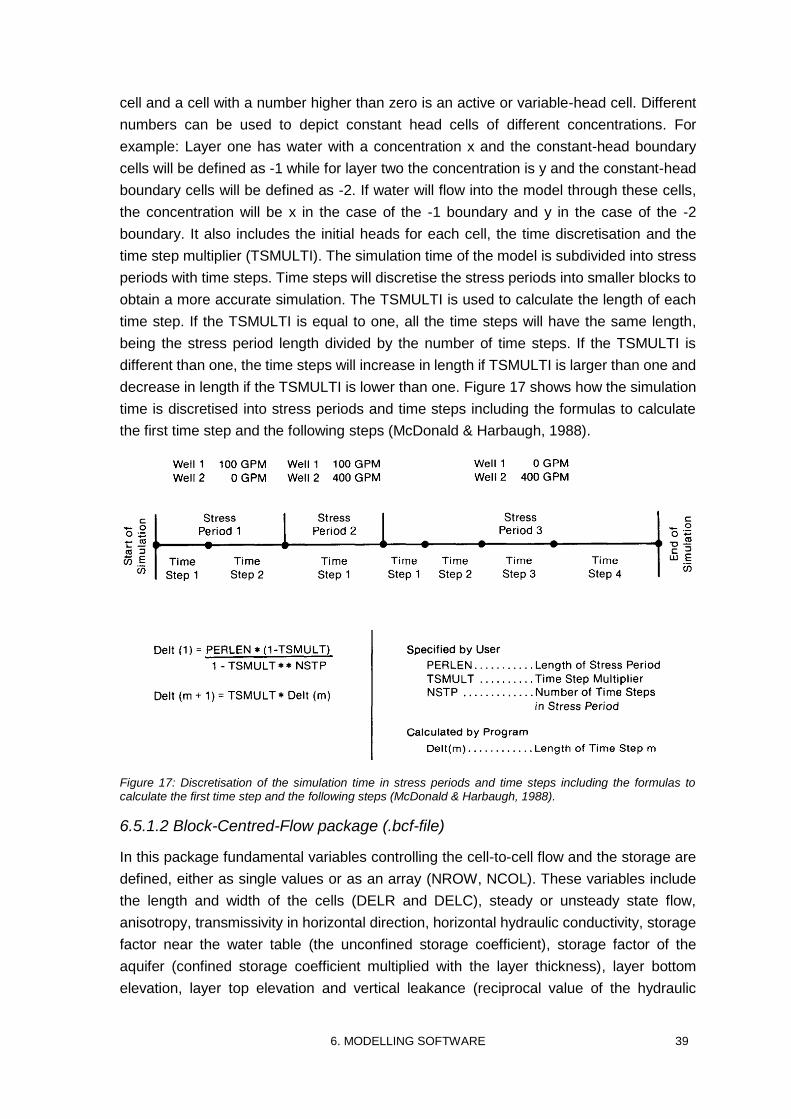
6. MODELLING SOFTWARE 39
cell and a cell with a number higher than zero is an active or variable-head cell. Different
numbers can be used to depict constant head cells of different concentrations. For
example: Layer one has water with a concentration x and the constant-head boundary
cells will be defined as -1 while for layer two the concentration is y and the constant-head
boundary cells will be defined as -2. If water will flow into the model through these cells,
the concentration will be x in the case of the -1 boundary and y in the case of the -2
boundary. It also includes the initial heads for each cell, the time discretisation and the
time step multiplier (TSMULTI). The simulation time of the model is subdivided into stress
periods with time steps. Time steps will discretise the stress periods into smaller blocks to
obtain a more accurate simulation. The TSMULTI is used to calculate the length of each
time step. If the TSMULTI is equal to one, all the time steps will have the same length,
being the stress period length divided by the number of time steps. If the TSMULTI is
different than one, the time steps will increase in length if TSMULTI is larger than one and
decrease in length if the TSMULTI is lower than one. Figure 17 shows how the simulation
time is discretised into stress periods and time steps including the formulas to calculate
the first time step and the following steps (McDonald & Harbaugh, 1988).
Figure 17: Discretisation of the simulation time in stress periods and time steps including the formulas to calculate the first time step and the following steps (McDonald & Harbaugh, 1988).
6.5.1.2 Block-Centred-Flow package (.bcf-file)
In this package fundamental variables controlling the cell-to-cell flow and the storage are
defined, either as single values or as an array (NROW, NCOL). These variables include
the length and width of the cells (DELR and DELC), steady or unsteady state flow,
anisotropy, transmissivity in horizontal direction, horizontal hydraulic conductivity, storage
factor near the water table (the unconfined storage coefficient), storage factor of the
aquifer (confined storage coefficient multiplied with the layer thickness), layer bottom
elevation, layer top elevation and vertical leakance (reciprocal value of the hydraulic
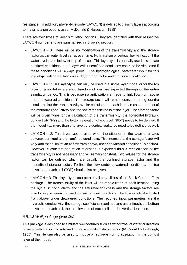
40 6. MODELLING SOFTWARE
resistance). In addition, a layer-type code (LAYCON) is defined to classify layers according
to the simulation options used (McDonald & Harbaugh, 1988).
There are four types of layer simulation options. They are identified with their respective
LAYCON number and are summarised in following section:
LAYCON = 0: There will be no modification of the transmissivity and the storage
factor as the water level varies over time. No limitation of vertical flow will occur if the
water level drops below the top of the cell. This layer-type is normally used to simulate
confined conditions, but a layer with unconfined conditions can also be simulated if
these conditions will always prevail. The hydrogeological parameter input for this
layer-type will be the transmissivity, storage factor and the vertical leakance.
LAYCON = 1: This layer-type can only be used in a single layer model or for the top
layer of a model where unconfined conditions are expected throughout the entire
simulation period. This is because no anticipation is made to limit flow from above
under dewatered conditions. The storage factor will remain constant throughout the
simulation but the transmissivity will be calculated at each iteration as the product of
the hydraulic conductivity and the saturated thickness of the layer. The storage factor
will be given while for the calculation of the transmissivity, the horizontal hydraulic
conductivity (HY) and the bottom elevation of each cell (BOT) needs to be defined. If
the model has more than one layer, the vertical leakance need to be defined as well.
LAYCON = 2: This layer-type is used when the situation in the layer alternates
between confined and unconfined conditions. This means that the storage factor will
vary and that a limitation of flow from above, under dewatered conditions, is desired.
However, a constant saturation thickness is expected thus a recalculation of the
transmissivity is not necessary and will remain constant. Two values for the storage
factor can be defined which are usually the confined storage factor and the
unconfined storage factor. To limit the flow under dewatered conditions, the top
elevation of each cell (TOP) should also be given.
LAYCON = 3: This layer-type incorporates all capabilities of the Block-Centred-Flow
package. The transmissivity of the layer will be recalculated at each iteration using
the hydraulic conductivity and the saturated thickness and the storage factors are
able to vary between confined and unconfined conditions. The flow will also be limited
from above under dewatered conditions. The required input parameters are the
hydraulic conductivity, the storage coefficients (confined and unconfined), the bottom
elevation of each cell, the top elevation of each cell and the vertical leakance.
6.5.1.3 Well package (.wel-file)
This package is designed to simulate well features such as withdrawal of water or injection
of water with a specified rate and during a specified stress period (McDonald & Harbaugh,
1988). This file can also be used to induce a recharge from precipitation in the upmost
layer of the model.
6. MODELLING SOFTWARE 41
6.5.1.4 Evapotranspiration package (.evt-file)
The evapotranspiration package is created to simulate the effects of plant transpiration
and direct evaporation by removing water from the saturated ground water regime.
Following assumptions forms the basis of the package: (1) when the water table is above
or at the evapotranspiration (ET) surface (specified elevation) the evapotranspiration loss
will be at a maximum rate, (2) when the depth of the water table is below the ET surface
but above the extinction depth (i.e. the depth where no water loss will occur due to
evapotranspiration) the evapotranspiration rate will decrease linearly with depth and (3)
when the water table drops below the extinction depth, no evapotranspiration will occur. A
graph of the three distinct zones is plotted in Figure 18 (McDonald & Harbaugh, 1988).
Figure 18: Volumetric evapotranspiration QET, as a function of head h, in a cell where d is the extinction depth and hs the ET surface elevation (McDonald & Harbaugh, 1988).
6.5.1.5 Strongly Implicit Procedure package (.sip-file)
In the .sip-file the maximum number of iterations is given that the model can do. A second
parameter that is given in the .sip-file is the closure criterion. If the closure criterion is not
reached after the maximum iterations, the model will be terminated (McDonald &
Harbaugh, 1988).
6.5.1.6 Name file (Infile.nam)
This file consists of a list of all the different files that MODFLOW should read to calculate
the groundwater flow and includes the name of the output file. If MOCDENS3D is used, it
also refers to the name file for the solute transport (Vandenbohede, 2008).
(1)
(2)
(3)
42 6. MODELLING SOFTWARE
6.5.2 MOCDENS3D packages
6.5.2.1 MOC package (.moc-file)
The MOC file, which stands for Method-Of-Characteristics, contains all information to
simulate the solute transport. The first and last layer, row and column are given for which
solute transport should be calculated. On the next line flags are defined for if dispersion,
decay or diffusion is/are present. It also includes the number of particles present in each
cell. Other parameters include the concentration in no-flow cells (or inactive cells) and a
grid of the concentration for each cell. Finally, the longitudinal dispersion and both
transversal dispersions, the retardation factors, thicknesses and porosities are defined
(Vandenbohede, 2008).
6.5.2.2 Densin.dat-file
This file contains the information regarding the density driven transport. Two parameters
are defined that will introduce the density difference to the different concentrations. A
certain concentration is given along with its density difference in regard to a reference state
of concentration equal to 0 (buoyancy factor). Densities for all other concentrations are
calculated proportionally to these two values (Vandenbohede, 2008).
6.5.2.3 Name file (moc.nam)
This file is similar to the infile.nam file in the sense that it also lists the different files needed
for MOCDENS3D to run and calculate the solute transport. An output file is also defined
here (Vandenbohede, 2008).
7. MODEL CONSTRUCTION 43
7. MODEL CONSTRUCTION
The study of the influence of the Abu Nakhla pond on the phreatic aquifer has been
subdivided into two parts. The first part comprises of the simulation of the present state
and the dissipation and desiccation of the Abu Nakhla pond. For this simulation, a base
model is constructed which represents the phreatic aquifer in equilibrium with the hydraulic
and climatic conditions, without the presence of the Abu Nakhla pond. Next, the Abu
Nakhla pond is added to the numerical model and is simulated until equilibrium with the
groundwater reservoir is obtained. This is a simplification of the reality as it hasn’t been
verified yet whether the pond is in equilibrium with the aquifer. However, for the scope of
this study it is justified to make this assumption. The last step of the first part is the
simulation of the desiccation of the pond. The volume of the pond slowly diminishes, due
to the evaporation and infiltration, and the influence of this on the evolution of the
groundwater reservoir is followed. The second part of the study comprises of a sensitivity
analysis to check which hydrogeological parameters have the most influence on the
dissipation of the pond, under constant evaporation conditions.
7.1 Base model
This base model represents the groundwater reservoir in equilibrium with its surroundings
if the Abu Nakhla pond would not be present. This base model includes all hydraulic
parameters that are independent of the presence of the Abu Nakhla pond and thus all
parameters that will remain constant throughout the models.
7.1.1 Location and discretisation of the study area
To investigate the extend of the influence of the Abu Nakhla pond on the phreatic aquifer,
a rectangular study area is chosen with a length from west to east of 18 km and a width
from north to south of 15 km with the pond in the centre (Figure 19). The lower left corner
has the coordinates x = 206200 and y = 370500 and the upper right corner has the
coordinates x = 224200 and y = 385500, expressed in the Qatar 1974 reference system.
Square cells with dimensions of 100 m x 100 m are used which results in a grid of 150
rows and 180 columns.
To be able to make a sound vertical discretisation in layers, a detailed understanding of
the geology is necessary. An interpretation of the upper 31 m is made with corings taken
around the Abu Nakhla pond (Appendix A). The Umm Bab Member 1 is the only member
present of the Dammam Formation. It is up to 21.9 m thick and consists of off-white to light
grey limestone. Below the Umm Bab Member the Midra Shale Member is present. It
reaches a depth of 26.55 m which results in a thickness of 4.65 m. It is followed by the
upper Rus Formation which consists of pale brown limestones and is considered as a part
of the upper southern aquifer. The Rus Formation changes to a depositional sulphate
1 Formerly known as the Simsima Member. It was changed to stop the confusion with the Simsima Formation present in Cretaceous deposits.

44 7. MODEL CONSTRUCTION
deposit with the presence of thick gypsum layers at a depth of approximately 47 m. The
depositional sulphate Rus facies extend to a depth of about 97 m where it changes into
the more permeable Umm er Radhuma Formation. The bottom of the model is put at 117
m where the silicified limestone layer is present which represents the transition of a
relatively good permeable UER to a relatively bad permeable UER. Three hydrogeological
units are defined: (1) Dammam Formation + upper Rus Formation aquifer, (2) Gypsiferous
Rus Formation aquitard and (3) UER Formation aquifer.
Figure 19: A georeferenced Google Earth image visualising the study area with a large grid (1 km x 1 km cells) and the normal grid (100 m x 100 m cells).
Based on the local geology, the model is subdivided into 21 layers, each layer being five
meter in thickness with the base of the first layer at 18 m amsl and the base of the model
at -77 m amsl. As simplification, the Midra Shale Member is represented by a five meter
thick layer between a depth of 22 m and 27 m. An overview of the vertical discretisation
with the corresponding geology is given in Table 3.
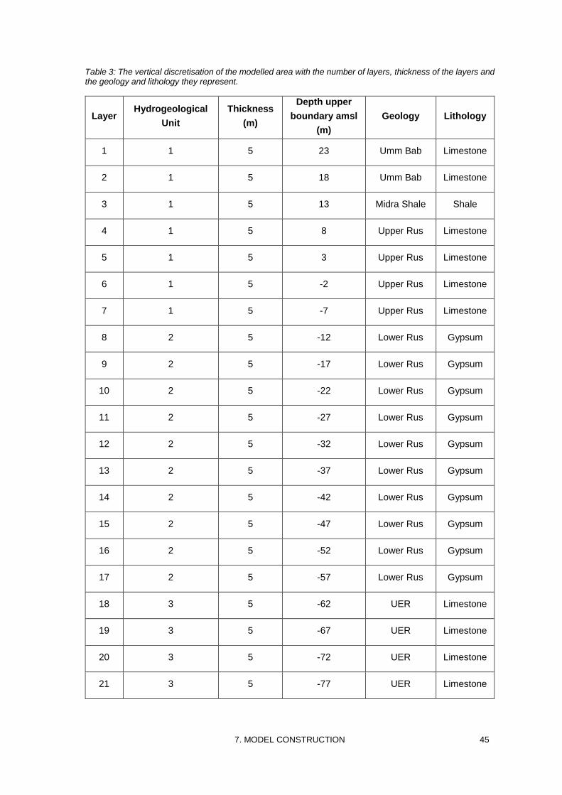
7. MODEL CONSTRUCTION 45
Table 3: The vertical discretisation of the modelled area with the number of layers, thickness of the layers and the geology and lithology they represent.
Layer Hydrogeological
Unit
Thickness
(m)
Depth upper
boundary amsl
(m)
Geology Lithology
1 1 5 23 Umm Bab Limestone
2 1 5 18 Umm Bab Limestone
3 1 5 13 Midra Shale Shale
4 1 5 8 Upper Rus Limestone
5 1 5 3 Upper Rus Limestone
6 1 5 -2 Upper Rus Limestone
7 1 5 -7 Upper Rus Limestone
8 2 5 -12 Lower Rus Gypsum
9 2 5 -17 Lower Rus Gypsum
10 2 5 -22 Lower Rus Gypsum
11 2 5 -27 Lower Rus Gypsum
12 2 5 -32 Lower Rus Gypsum
13 2 5 -37 Lower Rus Gypsum
14 2 5 -42 Lower Rus Gypsum
15 2 5 -47 Lower Rus Gypsum
16 2 5 -52 Lower Rus Gypsum
17 2 5 -57 Lower Rus Gypsum
18 3 5 -62 UER Limestone
19 3 5 -67 UER Limestone
20 3 5 -72 UER Limestone
21 3 5 -77 UER Limestone
46 7. MODEL CONSTRUCTION
7.1.2 Hydrogeological parameters
Steady state and unsteady state flow models use the same basic hydraulic parameters
but unsteady state flow models need an extra set of parameters, the storage factors. While
the storage factors will be discussed in this part, only unsteady state flow models will use
them.
The transmissivity is the horizontal conductivity multiplied with the thickness of the layer it
represents. The transmissivity of the upper layer is 68 m² d-1 (calculated for a layer
thickness of 8.5 m, which is a rough estimation) while the other Dammam layer (layer two)
has a transmissivity of 40 m² d-1. The Midra Shale Member, which is an aquitard, is
estimated to have a transmissivity of 1 m² d-1 which is 40 times lower than the surrounding
layers. The upper Rus Formation has the same 40 m² d-1 transmissivity of the Dammam
Formation as it is part of the upper aquifer system. The gypsiferous Rus Formation has a
very low transmissivity due to the depositional sulphate present. Based on the parameters
illuminated in part 4.3 for gypsiferous and anhydritic deposits, a transmissivity is estimated
of 0.01 m² d-1. The transmissivity used for the Umm er Radhuma Formation is 42 m² d-1
which is based on the fact that the formation can be extensively karstified and thus a
slightly higher value, compared to the Dammam and upper Rus formations, is used.
The vertical conductivity is expressed as the reciprocal value of the hydraulic resistance,
i.e. vertical conductivity divided by the thickness of the layers and expressed in d-1. For the
ease of use, this parameter is abbreviated as ‘vert’ further on. The estimation of the initial
vertical conductivity is done by assuming an anisotropy of 25. This means that the vertical
hydraulic conductivity (Kv) is 25 times smaller than the horizontal hydraulic conductivity
(Kh) of the layer. When the vert gets smaller, the hydraulic resistance of the layer will get
higher and thus less water will be able to flow between the layers. The vert is a value
representative for the boundary between two layers so only 20 verts are defined for the 21
layers in the model. The same principle is used as with the hydraulic conductance, where
the vert is defined by half of the layer above the boundary and half of the layer below the
boundary. The vert for the bottom boundary of the top layer will have a different value due
to the fact that it will have an influence of the whole top and bottom layer compared to the
rest which will only have half the influence. The vert for the first layer is thus 0.0427 d-1
(calculated for a layer thickness of 5 m). Both at the top and bottom of the Midra Shale
Member the vert is 0.0032 d-1 and is mainly influenced by the Midra Shale itself. For the
upper Rus Formation the vert is 0.064 d-1. The top and bottom of the gypsiferous Rus
Formation will mostly be influenced by the low conductive gypsum and thus the influence
of the high conductive upper Rus and UER layer can be neglected. A value of
0.000032 d-1 is defined and inside the gypsiferous Rus Formation a vert of 0.000016 d-1 is
used. The UER vert is estimated at 0.0672 d-1.
Data of storage coefficients are scarce and reasoning is used to obtain an estimated value.
The storage factor for the layer confined by the water table is equal to the specific elastic
storage (Ss) multiplied by the thickness (D) plus the storage coefficient near the water table
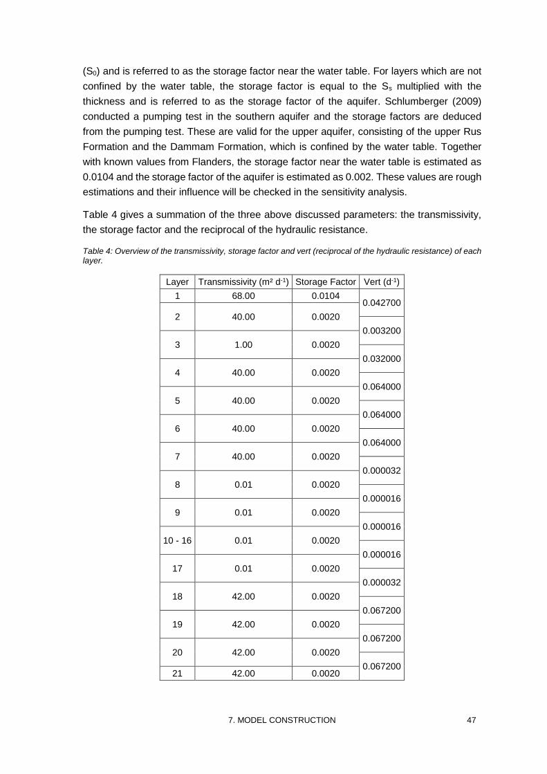
7. MODEL CONSTRUCTION 47
(S0) and is referred to as the storage factor near the water table. For layers which are not
confined by the water table, the storage factor is equal to the Ss multiplied with the
thickness and is referred to as the storage factor of the aquifer. Schlumberger (2009)
conducted a pumping test in the southern aquifer and the storage factors are deduced
from the pumping test. These are valid for the upper aquifer, consisting of the upper Rus
Formation and the Dammam Formation, which is confined by the water table. Together
with known values from Flanders, the storage factor near the water table is estimated as
0.0104 and the storage factor of the aquifer is estimated as 0.002. These values are rough
estimations and their influence will be checked in the sensitivity analysis.
Table 4 gives a summation of the three above discussed parameters: the transmissivity,
the storage factor and the reciprocal of the hydraulic resistance.
Table 4: Overview of the transmissivity, storage factor and vert (reciprocal of the hydraulic resistance) of each layer.
Layer Transmissivity (m² d-1) Storage Factor Vert (d-1)
1 68.00 0.0104 0.042700
2 40.00 0.0020
0.003200
3 1.00 0.0020
0.032000
4 40.00 0.0020
0.064000
5 40.00 0.0020
0.064000
6 40.00 0.0020
0.064000
7 40.00 0.0020
0.000032
8 0.01 0.0020
0.000016
9 0.01 0.0020
0.000016
10 - 16 0.01 0.0020
0.000016
17 0.01 0.0020
0.000032
18 42.00 0.0020
0.067200
19 42.00 0.0020
0.067200
20 42.00 0.0020
0.067200 21 42.00 0.0020
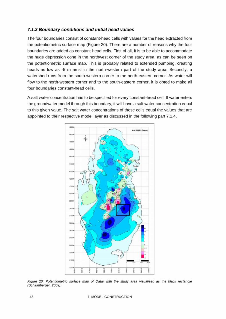
48 7. MODEL CONSTRUCTION
7.1.3 Boundary conditions and initial head values
The four boundaries consist of constant-head cells with values for the head extracted from
the potentiometric surface map (Figure 20). There are a number of reasons why the four
boundaries are added as constant-head cells. First of all, it is to be able to accommodate
the huge depression cone in the northwest corner of the study area, as can be seen on
the potentiometric surface map. This is probably related to extended pumping, creating
heads as low as -5 m amsl in the north-western part of the study area. Secondly, a
watershed runs from the south-western corner to the north-eastern corner. As water will
flow to the north-western corner and to the south-eastern corner, it is opted to make all
four boundaries constant-head cells.
A salt water concentration has to be specified for every constant-head cell. If water enters
the groundwater model through this boundary, it will have a salt water concentration equal
to this given value. The salt water concentrations of these cells equal the values that are
appointed to their respective model layer as discussed in the following part 7.1.4.
Figure 20: Potentiometric surface map of Qatar with the study area visualised as the black rectangle (Schlumberger, 2009).
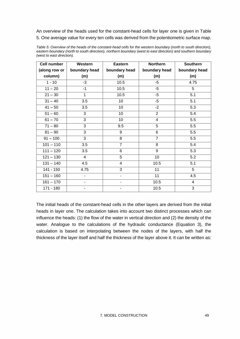
7. MODEL CONSTRUCTION 49
An overview of the heads used for the constant-head cells for layer one is given in Table
5. One average value for every ten cells was derived from the potentiometric surface map.
Table 5: Overview of the heads of the constant-head cells for the western boundary (north to south direction), eastern boundary (north to south direction), northern boundary (west to east direction) and southern boundary (west to east direction).
Cell number
(along row or
column)
Western
boundary head
(m)
Eastern
boundary head
(m)
Northern
boundary head
(m)
Southern
boundary head
(m)
1 - 10 -3 10.5 -5 4.75
11 – 20 -1 10.5 -5 5
21 – 30 1 10.5 -5 5.1
31 – 40 3.5 10 -5 5.1
41 – 50 3.5 10 -2 5.3
51 – 60 3 10 2 5.4
61 – 70 3 10 4 5.5
71 – 80 3 9.5 5 5.5
81 – 90 3 9 6 5.5
91 – 100 3 8 7 5.5
101 – 110 3.5 7 8 5.4
111 – 120 3.5 6 9 5.3
121 – 130 4 5 10 5.2
131 – 140 4.5 4 10.5 5.1
141 - 150 4.75 3 11 5
151 – 160 - - 11 4.5
161 – 170 - - 10.5 4
171 - 180 - - 10.5 3
The initial heads of the constant-head cells in the other layers are derived from the initial
heads in layer one. The calculation takes into account two distinct processes which can
influence the heads: (1) the flow of the water in vertical direction and (2) the density of the
water. Analogue to the calculations of the hydraulic conductance (Equation 3), the
calculation is based on interpolating between the nodes of the layers, with half the
thickness of the layer itself and half the thickness of the layer above it. It can be written as:
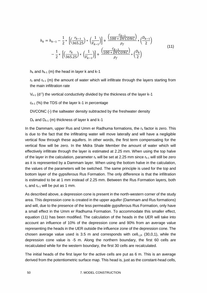
50 7. MODEL CONSTRUCTION
ℎ𝑘 = ℎ𝑘−1 − 1
2∗ [(
𝑟𝑘−1
365.25) ∗ (
1
𝑉𝑘−1)] +
(𝑐𝑘−1
100 ∗ 𝐷𝑉𝐶𝑂𝑁𝐶)
𝜌𝑓∗ (
𝐷𝑘−1
2)
− 1
2∗ [(
𝑟𝑘
365.25) ∗ (
1
𝑉𝑘−1)] +
(𝑐𝑘−1
100 ∗ 𝐷𝑉𝐶𝑂𝑁𝐶)
𝜌𝑓∗ (
𝐷𝑘
2)
(11)
hk and hk-1 (m) the head in layer k and k-1
rk and rk-1 (m) the amount of water which will infiltrate through the layers starting from
the main infiltration rate
Vk-1 (d-1) the vertical conductivity divided by the thickness of the layer k-1
ck-1 (%) the TDS of the layer k-1 in percentage
DVCONC (-) the saltwater density subtracted by the freshwater density
Dk and Dk-1 (m) thickness of layer k and k-1
In the Dammam, upper Rus and Umm er Radhuma formations, the rk factor is zero. This
is due to the fact that the infiltrating water will move laterally and will have a negligible
vertical flow through these aquifers. In other words, the first term compensating for the
vertical flow will be zero. In the Midra Shale Member the amount of water which will
effectively infiltrate through the layer is estimated at 2.25 mm. When using the top halve
of the layer in the calculation, parameter rk will be set at 2.25 mm since rk-1 will still be zero
as it is represented by a Dammam layer. When using the bottom halve in the calculation,
the values of the parameters will be switched. The same principle is used for the top and
bottom layer of the gypsiferous Rus Formation. The only difference is that the infiltration
is estimated to be at 1 mm instead of 2.25 mm. Between the Rus Formation layers, both
rk and rk-1 will be put as 1 mm.
As described above, a depression cone is present in the north-western corner of the study
area. This depression cone is created in the upper aquifer (Dammam and Rus formations)
and will, due to the presence of the less permeable gypsiferous Rus Formation, only have
a small effect in the Umm er Radhuma Formation. To accommodate this smaller effect,
equation (11) has been modified. The calculation of the heads in the UER will take into
account an influence of 10% of the depression cone and 90% from an average value
representing the heads in the UER outside the influence zone of the depression cone. The
chosen average value used is 3.5 m and corresponds with celli,,j,k (30,0,1), while the
depression cone value is -5 m. Along the northern boundary, the first 60 cells are
recalculated while for the western boundary, the first 30 cells are recalculated.
The initial heads of the first layer for the active cells are put as 6 m. This is an average
derived from the potentiometric surface map. This head is, just as the constant-head cells,
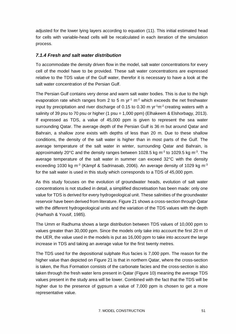
7. MODEL CONSTRUCTION 51
adjusted for the lower lying layers according to equation (11). This initial estimated head
for cells with variable-head cells will be recalculated in each iteration of the simulation
process.
7.1.4 Fresh and salt water distribution
To accommodate the density driven flow in the model, salt water concentrations for every
cell of the model have to be provided. These salt water concentrations are expressed
relative to the TDS value of the Gulf water, therefor it is necessary to have a look at the
salt water concentration of the Persian Gulf.
The Persian Gulf contains very dense and warm salt water bodies. This is due to the high
evaporation rate which ranges from 2 to 5 m yr-1 m-2 which exceeds the net freshwater
input by precipitation and river discharge of 0.15 to 0.30 m yr-1m-2 creating waters with a
salinity of 39 psu to 70 psu or higher (1 psu = 1,000 ppm) (Elhakeem & Elshorbagy, 2013).
If expressed as TDS, a value of 45,000 ppm is given to represent the sea water
surrounding Qatar. The average depth of the Persian Gulf is 36 m but around Qatar and
Bahrain, a shallow zone exists with depths of less than 20 m. Due to these shallow
conditions, the density of the salt water is higher than in most parts of the Gulf. The
average temperature of the salt water in winter, surrounding Qatar and Bahrain, is
approximately 20°C and the density ranges between 1028.5 kg m-3 to 1029.5 kg m-3. The
average temperature of the salt water in summer can exceed 32°C with the density
exceeding 1030 kg m-3 (Kämpf & Sadrinasab, 2006). An average density of 1029 kg m-3
for the salt water is used in this study which corresponds to a TDS of 45,000 ppm.
As this study focuses on the evolution of groundwater heads, evolution of salt water
concentrations is not studied in detail, a simplified discretisation has been made: only one
value for TDS is derived for every hydrogeological unit. These salinities of the groundwater
reservoir have been derived from literature. Figure 21 shows a cross-section through Qatar
with the different hydrogeological units and the variation of the TDS values with the depth
(Harhash & Yousif, 1985).
The Umm er Radhuma shows a large distribution between TDS values of 10,000 ppm to
values greater than 30,000 ppm. Since the models only take into account the first 20 m of
the UER, the value used in the models is put as 16,000 ppm to take into account the large
increase in TDS and taking an average value for the first twenty metres.
The TDS used for the depositional sulphate Rus facies is 7,000 ppm. The reason for the
higher value than depicted on Figure 21 is that in northern Qatar, where the cross-section
is taken, the Rus Formation consists of the carbonate facies and the cross-section is also
taken through the fresh water lens present in Qatar (Figure 10) meaning the average TDS
values present in the study area will be lower. Combined with the fact that the TDS will be
higher due to the presence of gypsum a value of 7,000 ppm is chosen to get a more
representative value.
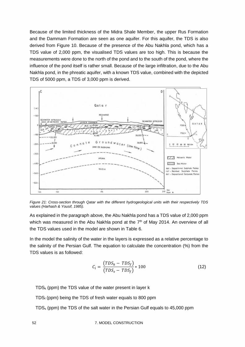
52 7. MODEL CONSTRUCTION
Because of the limited thickness of the Midra Shale Member, the upper Rus Formation
and the Dammam Formation are seen as one aquifer. For this aquifer, the TDS is also
derived from Figure 10. Because of the presence of the Abu Nakhla pond, which has a
TDS value of 2,000 ppm, the visualised TDS values are too high. This is because the
measurements were done to the north of the pond and to the south of the pond, where the
influence of the pond itself is rather small. Because of the large infiltration, due to the Abu
Nakhla pond, in the phreatic aquifer, with a known TDS value, combined with the depicted
TDS of 5000 ppm, a TDS of 3,000 ppm is derived.
Figure 21: Cross-section through Qatar with the different hydrogeological units with their respectively TDS values (Harhash & Yousif, 1985).
As explained in the paragraph above, the Abu Nakhla pond has a TDS value of 2,000 ppm
which was measured in the Abu Nakhla pond at the 7th of May 2014. An overview of all
the TDS values used in the model are shown in Table 6.
In the model the salinity of the water in the layers is expressed as a relative percentage to
the salinity of the Persian Gulf. The equation to calculate the concentration (%) from the
TDS values is as followed:
𝐶𝑖 =
(𝑇𝐷𝑆𝑘 − 𝑇𝐷𝑆𝑓)
(𝑇𝐷𝑆𝑠 − 𝑇𝐷𝑆𝑓)∗ 100 (12)
TDSk (ppm) the TDS value of the water present in layer k
TDSf (ppm) being the TDS of fresh water equals to 800 ppm
TDSs (ppm) the TDS of the salt water in the Persian Gulf equals to 45,000 ppm
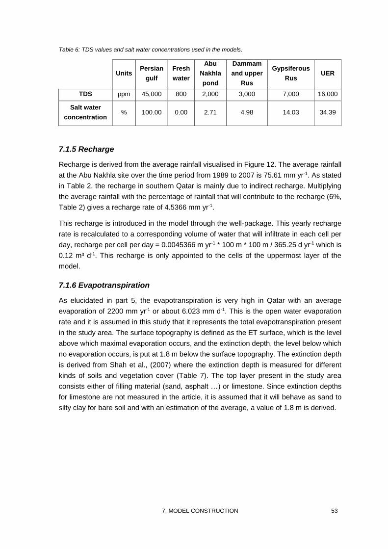
7. MODEL CONSTRUCTION 53
Table 6: TDS values and salt water concentrations used in the models.
Units Persian
gulf
Fresh
water
Abu
Nakhla
pond
Dammam
and upper
Rus
Gypsiferous
Rus UER
TDS ppm 45,000 800 2,000 3,000 7,000 16,000
Salt water
concentration % 100.00 0.00 2.71 4.98 14.03 34.39
7.1.5 Recharge
Recharge is derived from the average rainfall visualised in Figure 12. The average rainfall
at the Abu Nakhla site over the time period from 1989 to 2007 is 75.61 mm yr-1. As stated
in Table 2, the recharge in southern Qatar is mainly due to indirect recharge. Multiplying
the average rainfall with the percentage of rainfall that will contribute to the recharge (6%,
Table 2) gives a recharge rate of 4.5366 mm yr-1.
This recharge is introduced in the model through the well-package. This yearly recharge
rate is recalculated to a corresponding volume of water that will infiltrate in each cell per
day, recharge per cell per day = 0.0045366 m yr-1 * 100 m * 100 m / 365.25 d yr-1 which is
0.12 m³ d-1. This recharge is only appointed to the cells of the uppermost layer of the
model.
7.1.6 Evapotranspiration
As elucidated in part 5, the evapotranspiration is very high in Qatar with an average
evaporation of 2200 mm yr-1 or about 6.023 mm d-1. This is the open water evaporation
rate and it is assumed in this study that it represents the total evapotranspiration present
in the study area. The surface topography is defined as the ET surface, which is the level
above which maximal evaporation occurs, and the extinction depth, the level below which
no evaporation occurs, is put at 1.8 m below the surface topography. The extinction depth
is derived from Shah et al., (2007) where the extinction depth is measured for different
kinds of soils and vegetation cover (Table 7). The top layer present in the study area
consists either of filling material (sand, asphalt …) or limestone. Since extinction depths
for limestone are not measured in the article, it is assumed that it will behave as sand to
silty clay for bare soil and with an estimation of the average, a value of 1.8 m is derived.
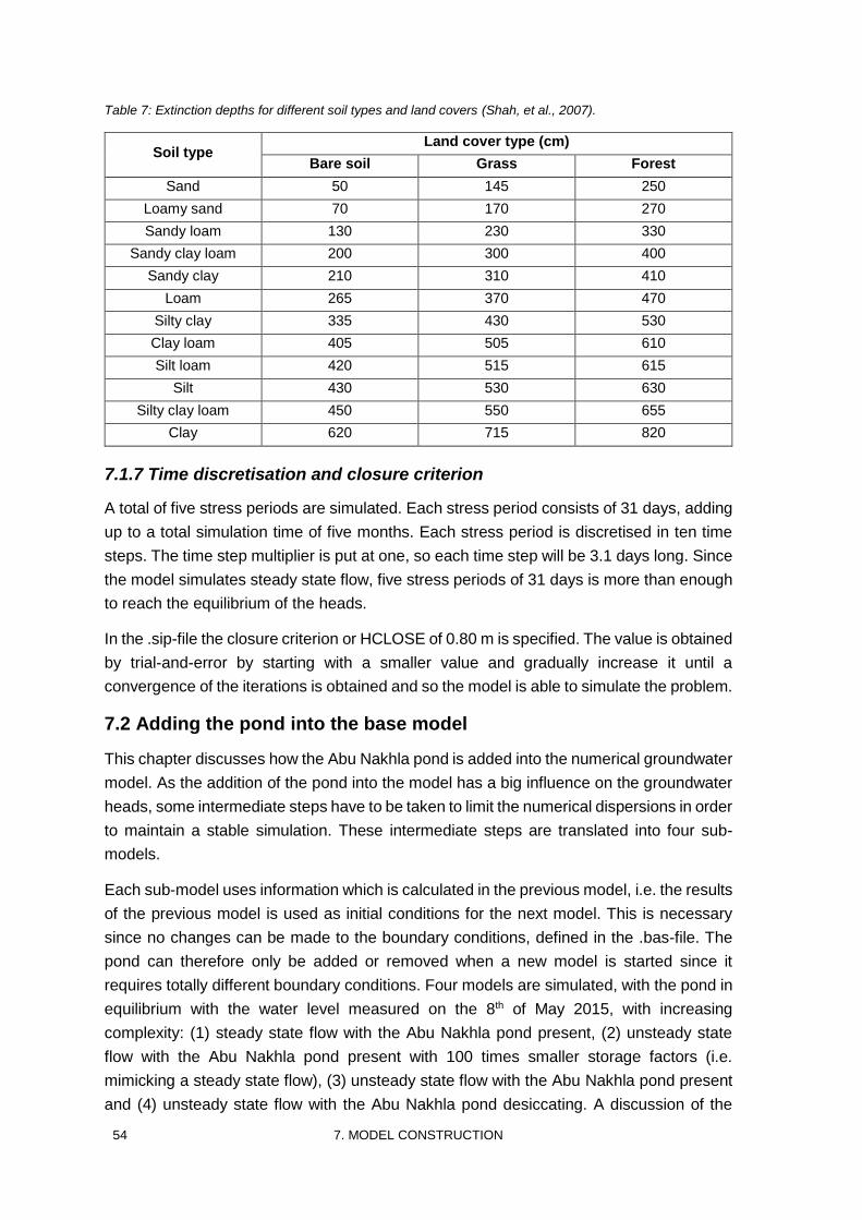
54 7. MODEL CONSTRUCTION
Table 7: Extinction depths for different soil types and land covers (Shah, et al., 2007).
Soil type Land cover type (cm)
Bare soil Grass Forest
Sand 50 145 250
Loamy sand 70 170 270
Sandy loam 130 230 330
Sandy clay loam 200 300 400
Sandy clay 210 310 410
Loam 265 370 470
Silty clay 335 430 530
Clay loam 405 505 610
Silt loam 420 515 615
Silt 430 530 630
Silty clay loam 450 550 655
Clay 620 715 820
7.1.7 Time discretisation and closure criterion
A total of five stress periods are simulated. Each stress period consists of 31 days, adding
up to a total simulation time of five months. Each stress period is discretised in ten time
steps. The time step multiplier is put at one, so each time step will be 3.1 days long. Since
the model simulates steady state flow, five stress periods of 31 days is more than enough
to reach the equilibrium of the heads.
In the .sip-file the closure criterion or HCLOSE of 0.80 m is specified. The value is obtained
by trial-and-error by starting with a smaller value and gradually increase it until a
convergence of the iterations is obtained and so the model is able to simulate the problem.
7.2 Adding the pond into the base model
This chapter discusses how the Abu Nakhla pond is added into the numerical groundwater
model. As the addition of the pond into the model has a big influence on the groundwater
heads, some intermediate steps have to be taken to limit the numerical dispersions in order
to maintain a stable simulation. These intermediate steps are translated into four sub-
models.
Each sub-model uses information which is calculated in the previous model, i.e. the results
of the previous model is used as initial conditions for the next model. This is necessary
since no changes can be made to the boundary conditions, defined in the .bas-file. The
pond can therefore only be added or removed when a new model is started since it
requires totally different boundary conditions. Four models are simulated, with the pond in
equilibrium with the water level measured on the 8th of May 2015, with increasing
complexity: (1) steady state flow with the Abu Nakhla pond present, (2) unsteady state
flow with the Abu Nakhla pond present with 100 times smaller storage factors (i.e.
mimicking a steady state flow), (3) unsteady state flow with the Abu Nakhla pond present
and (4) unsteady state flow with the Abu Nakhla pond desiccating. A discussion of the
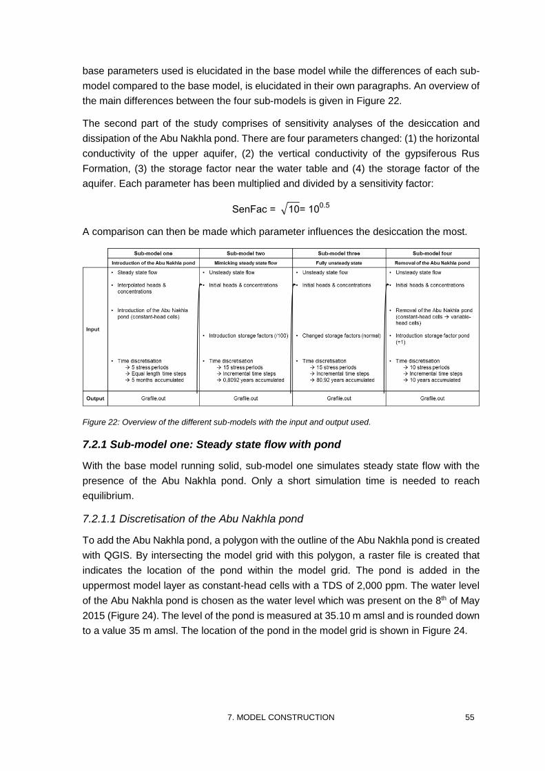
7. MODEL CONSTRUCTION 55
base parameters used is elucidated in the base model while the differences of each sub-
model compared to the base model, is elucidated in their own paragraphs. An overview of
the main differences between the four sub-models is given in Figure 22.
The second part of the study comprises of sensitivity analyses of the desiccation and
dissipation of the Abu Nakhla pond. There are four parameters changed: (1) the horizontal
conductivity of the upper aquifer, (2) the vertical conductivity of the gypsiferous Rus
Formation, (3) the storage factor near the water table and (4) the storage factor of the
aquifer. Each parameter has been multiplied and divided by a sensitivity factor:
SenFac = √10= 100.5
A comparison can then be made which parameter influences the desiccation the most.
Figure 22: Overview of the different sub-models with the input and output used.
7.2.1 Sub-model one: Steady state flow with pond
With the base model running solid, sub-model one simulates steady state flow with the
presence of the Abu Nakhla pond. Only a short simulation time is needed to reach
equilibrium.
7.2.1.1 Discretisation of the Abu Nakhla pond
To add the Abu Nakhla pond, a polygon with the outline of the Abu Nakhla pond is created
with QGIS. By intersecting the model grid with this polygon, a raster file is created that
indicates the location of the pond within the model grid. The pond is added in the
uppermost model layer as constant-head cells with a TDS of 2,000 ppm. The water level
of the Abu Nakhla pond is chosen as the water level which was present on the 8th of May
2015 (Figure 24). The level of the pond is measured at 35.10 m amsl and is rounded down
to a value 35 m amsl. The location of the pond in the model grid is shown in Figure 24.
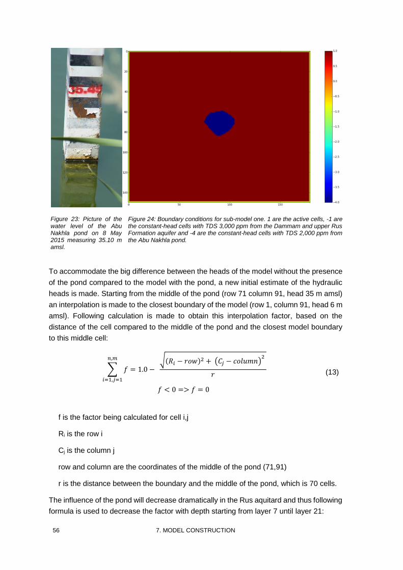
56 7. MODEL CONSTRUCTION
Figure 24: Boundary conditions for sub-model one. 1 are the active cells, -1 are the constant-head cells with TDS 3,000 ppm from the Dammam and upper Rus Formation aquifer and -4 are the constant-head cells with TDS 2,000 ppm from the Abu Nakhla pond.
To accommodate the big difference between the heads of the model without the presence
of the pond compared to the model with the pond, a new initial estimate of the hydraulic
heads is made. Starting from the middle of the pond (row 71 column 91, head 35 m amsl)
an interpolation is made to the closest boundary of the model (row 1, column 91, head 6 m
amsl). Following calculation is made to obtain this interpolation factor, based on the
distance of the cell compared to the middle of the pond and the closest model boundary
to this middle cell:
∑ 𝑓
𝑛,𝑚
𝑖=1,𝑗=1
= 1.0 − √(𝑅𝑖 − 𝑟𝑜𝑤)2 + (𝐶𝑗 − 𝑐𝑜𝑙𝑢𝑚𝑛)
2
𝑟
𝑓 < 0 => 𝑓 = 0
(13)
f is the factor being calculated for cell i,j
Ri is the row i
Cj is the column j
row and column are the coordinates of the middle of the pond (71,91)
r is the distance between the boundary and the middle of the pond, which is 70 cells.
The influence of the pond will decrease dramatically in the Rus aquitard and thus following
formula is used to decrease the factor with depth starting from layer 7 until layer 21:
Figure 23: Picture of the water level of the Abu Nakhla pond on 8 May 2015 measuring 35.10 m amsl.
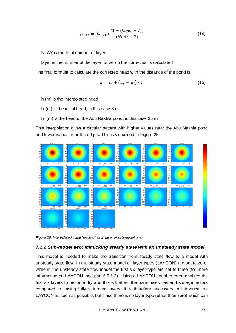
7. MODEL CONSTRUCTION 57
𝑓7→21 = 𝑓7→21 ∗
(1 − (𝑙𝑎𝑦𝑒𝑟 − 7))
(𝑁𝐿𝐴𝑌 − 7) (14)
NLAY is the total number of layers
layer is the number of the layer for which the correction is calculated
The final formula to calculate the corrected head with the distance of the pond is:
ℎ = ℎ𝑖 + (ℎ𝑝 − ℎ𝑖) ∗ 𝑓 (15)
h (m) is the interpolated head
hi (m) is the initial head, in this case 6 m
hp (m) is the head of the Abu Nakhla pond, in this case 35 m
This interpolation gives a circular pattern with higher values near the Abu Nakhla pond
and lower values near the edges. This is visualised in Figure 25.
Figure 25: Interpolated initial heads of each layer of sub-model one.
7.2.2 Sub-model two: Mimicking steady state with an unsteady state model
This model is needed to make the transition from steady state flow to a model with
unsteady state flow. In the steady state model all layer-types (LAYCON) are set to zero,
while in the unsteady state flow model the first six layer-type are set to three (for more
information on LAYCON, see part 6.5.1.2). Using a LAYCON equal to three enables the
first six layers to become dry and this will affect the transmissivities and storage factors
compared to having fully saturated layers. It is therefore necessary to introduce the
LAYCON as soon as possible, but since there is no layer-type (other than zero) which can
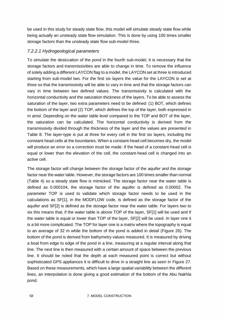
58 7. MODEL CONSTRUCTION
be used in this study for steady state flow, this model will simulate steady state flow while
being actually an unsteady state flow simulation. This is done by using 100 times smaller
storage factors than the unsteady state flow sub-model three.
7.2.2.1 Hydrogeological parameters
To simulate the desiccation of the pond in the fourth sub-model, it is necessary that the
storage factors and transmissivities are able to change in time. To remove the influence
of solely adding a different LAYCON flag to a model, the LAYCON set at three is introduced
starting from sub-model two. For the first six layers the value for the LAYCON is set at
three so that the transmissivity will be able to vary in time and that the storage factors can
vary in time between two defined values. The transmissivity is calculated with the
horizontal conductivity and the saturation thickness of the layers. To be able to assess the
saturation of the layer, two extra parameters need to be defined: (1) BOT, which defines
the bottom of the layer and (2) TOP, which defines the top of the layer, both expressed in
m amsl. Depending on the water table level compared to the TOP and BOT of the layer,
the saturation can be calculated. The horizontal conductivity is derived from the
transmissivity divided through the thickness of the layer and the values are presented in
Table 8. The layer-type is put at three for every cell in the first six layers, including the
constant-head cells at the boundaries. When a constant-head cell becomes dry, the model
will produce an error so a correction must be made: If the head of a constant-head cell is
equal or lower than the elevation of the cell, the constant-head cell is changed into an
active cell.
The storage factor will change between the storage factor of the aquifer and the storage
factor near the water table. However, the storage factors are 100 times smaller than normal
(Table 4) so a steady state flow is mimicked. The storage factor near the water table is
defined as 0.000104, the storage factor of the aquifer is defined as 0.00002. The
parameter TOP is used to validate which storage factor needs to be used in the
calculations as SF[1], in the MODFLOW code, is defined as the storage factor of the
aquifer and SF[2] is defined as the storage factor near the water table. For layers two to
six this means that, if the water table is above TOP of the layer, SF[1] will be used and if
the water table is equal or lower than TOP of the layer, SF[2] will be used. In layer one it
is a bit more complicated. The TOP for layer one is a matrix where the topography is equal
to an average of 32 m while the bottom of the pond is added in detail (Figure 26). The
bottom of the pond is derived from bathymetry values measured. It is measured by driving
a boat from edge to edge of the pond in a line, measuring at a regular interval along that
line. The next line is then measured with a certain amount of space between the previous
line. It should be noted that the depth at each measured point is correct but without
sophisticated GPS appliances it is difficult to drive in a straight line as seen in Figure 27.
Based on these measurements, which have a large spatial variability between the different
lines, an interpolation is done giving a good estimation of the bottom of the Abu Nakhla
pond.
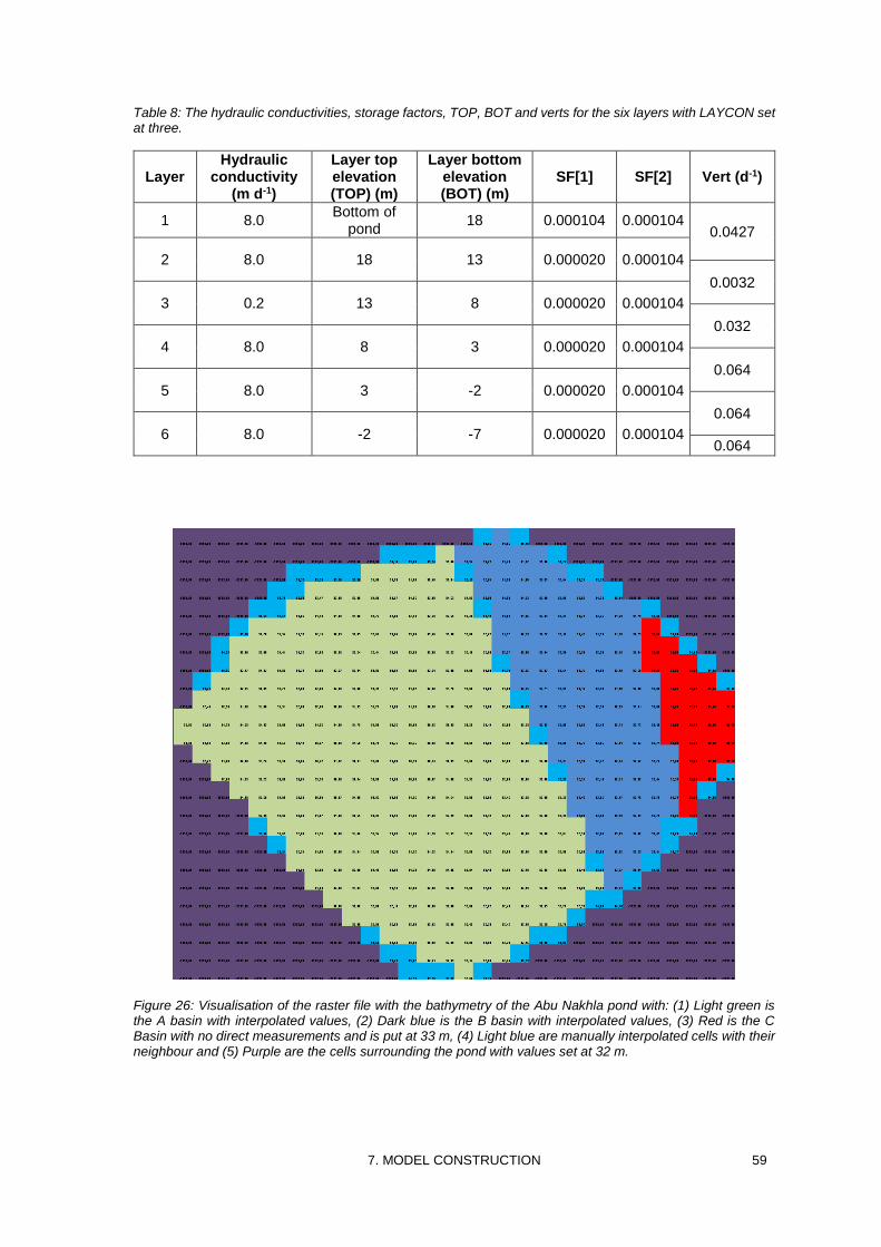
7. MODEL CONSTRUCTION 59
Table 8: The hydraulic conductivities, storage factors, TOP, BOT and verts for the six layers with LAYCON set at three.
Figure 26: Visualisation of the raster file with the bathymetry of the Abu Nakhla pond with: (1) Light green is the A basin with interpolated values, (2) Dark blue is the B basin with interpolated values, (3) Red is the C Basin with no direct measurements and is put at 33 m, (4) Light blue are manually interpolated cells with their neighbour and (5) Purple are the cells surrounding the pond with values set at 32 m.
Layer Hydraulic
conductivity (m d-1)
Layer top elevation (TOP) (m)
Layer bottom elevation (BOT) (m)
SF[1] SF[2] Vert (d-1)
1 8.0 Bottom of
pond 18 0.000104 0.000104
0.0427
2 8.0 18 13 0.000020 0.000104
0.0032
3 0.2 13 8 0.000020 0.000104
0.032
4 8.0 8 3 0.000020 0.000104
0.064
5 8.0 3 -2 0.000020 0.000104
0.064
6 8.0 -2 -7 0.000020 0.000104 0.064
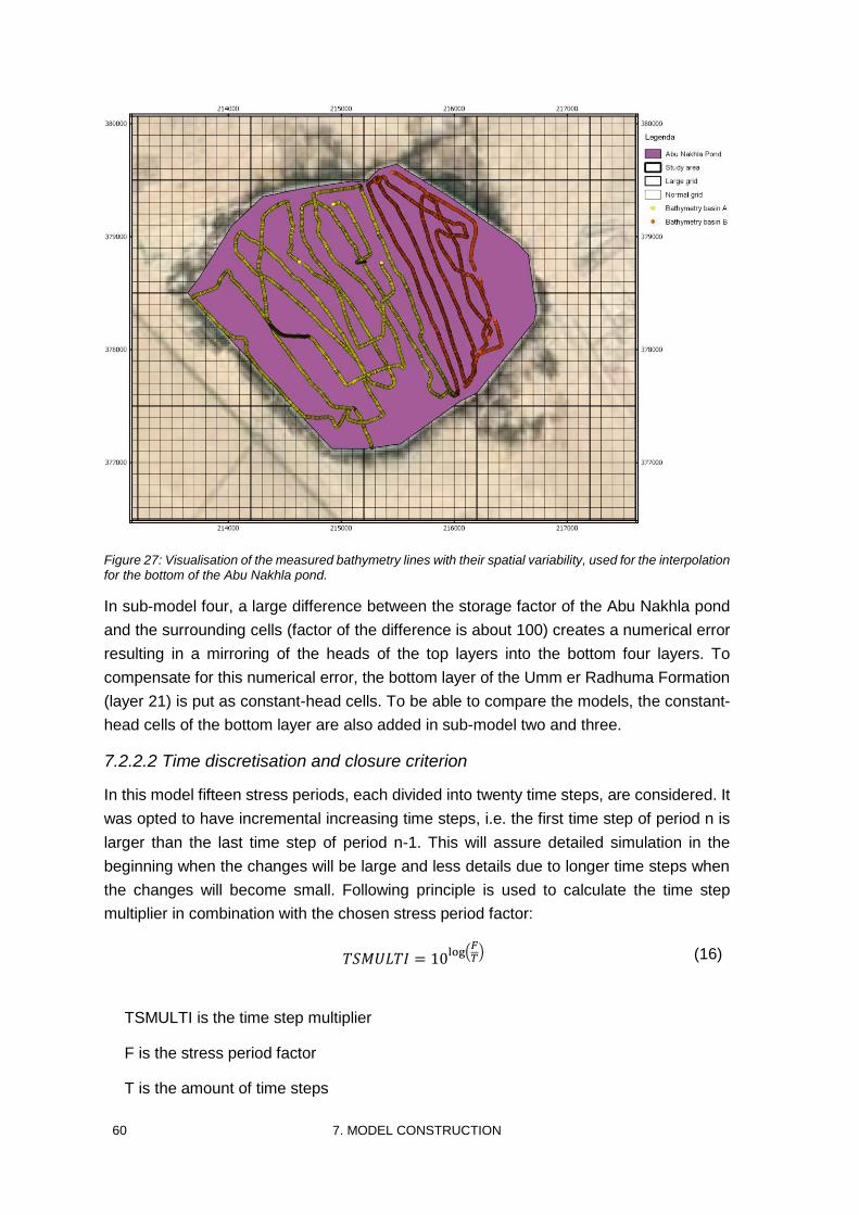
60 7. MODEL CONSTRUCTION
Figure 27: Visualisation of the measured bathymetry lines with their spatial variability, used for the interpolation for the bottom of the Abu Nakhla pond.
In sub-model four, a large difference between the storage factor of the Abu Nakhla pond
and the surrounding cells (factor of the difference is about 100) creates a numerical error
resulting in a mirroring of the heads of the top layers into the bottom four layers. To
compensate for this numerical error, the bottom layer of the Umm er Radhuma Formation
(layer 21) is put as constant-head cells. To be able to compare the models, the constant-
head cells of the bottom layer are also added in sub-model two and three.
7.2.2.2 Time discretisation and closure criterion
In this model fifteen stress periods, each divided into twenty time steps, are considered. It
was opted to have incremental increasing time steps, i.e. the first time step of period n is
larger than the last time step of period n-1. This will assure detailed simulation in the
beginning when the changes will be large and less details due to longer time steps when
the changes will become small. Following principle is used to calculate the time step
multiplier in combination with the chosen stress period factor:
𝑇𝑆𝑀𝑈𝐿𝑇𝐼 = 10
log(𝐹𝑇
) (16)
TSMULTI is the time step multiplier
F is the stress period factor
T is the amount of time steps
7. MODEL CONSTRUCTION 61
The stress period factor will define the increase in length of the stress periods. A factor F
equal to 1.515 is used with a starting stress period length of 30 days for stress period one.
Combined with twenty time steps, a value of 1.021 for TSMULTI is derived. An overview
of the length of the stress periods (Table 15) and the length of the time steps is presented
in Table 16 (Appendix B).
This model mimics steady state flow with an unsteady state model, so only small changes
in head are expected to occur. Due to the small storage factors a very fast equilibrium
should be obtained. Therefor short stress periods are used, 100 times shorter than
presented in Appendix B. If normal stress periods would be used, small numerical errors
will start to occur at each calculation because no water flows in or out of the storage. These
errors will accumulate and cause a faulty simulation.
The closure criterion is set very strict at 0.005 m. This is possible since the only difference
between the first and the second sub-model is the change from steady state to unsteady
state with adjusted LAYCONs. Only changes due to the addition of LAYCON are expected
and thus a strict HCLOSE can be used.
7.2.3 Sub-model three: From mimicking steady state to full unsteady state
This model represents the step from a mimicked steady state flow model to a full unsteady
state flow model. In essence, the model parameter input is exactly the same as the
previous model, except for the storage factors which now have normal values. So only a
small correction is needed in comparison with the previous sub-model.
7.2.3.1 Boundary conditions and storage factors
The boundary conditions are the same compared to sub-model two, but a correction is
needed due to the way MODFLOW is written in respect to the layer-types. When a head
drops below the bottom of the layer, the cell will become dry and the head is put at 0.0 m
by the MODFLOW code. No problems arise for the first four layers, but the bottom of layer
five is at -2 m amsl, when the heads from the previous sub-model are read and used as
the new initial heads for sub-model three, these dry cells are considered as active cells as
their heads (0.0m amsl) are above the base of the model layer five. This creates a large
numerical error after simulation. To fix this error, all active cells with a head of 0.0 m are
converted to inactive cells. By doing so, no calculations will happen in the dry cells which
eliminates the arisen problem.
Storage factors are already introduced in the previous sub-model, however they were set
100 times smaller than their normal values. In this sub-model the storage factors are
changed to their normal values. The storage factors used can be found in Table 4 and the
reasoning why these storage factors are used is extensively discussed in part 7.1.2.
7.2.3.2 Time discretisation and closure criterion
The time discretisation used is, just like with the storage factors, equal to sub-model two
but 100 times larger. Fifteen stress periods, which accumulate to a total of 80.92 years
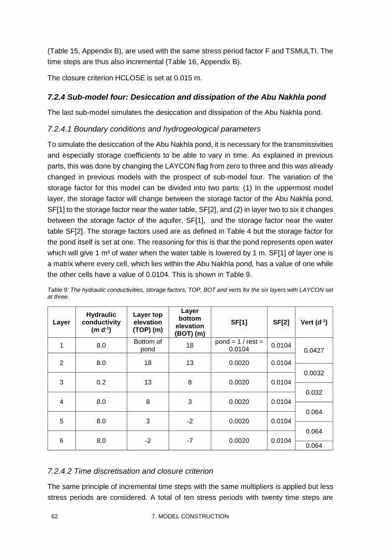
62 7. MODEL CONSTRUCTION
(Table 15, Appendix B), are used with the same stress period factor F and TSMULTI. The
time steps are thus also incremental (Table 16, Appendix B).
The closure criterion HCLOSE is set at 0.015 m.
7.2.4 Sub-model four: Desiccation and dissipation of the Abu Nakhla pond
The last sub-model simulates the desiccation and dissipation of the Abu Nakhla pond.
7.2.4.1 Boundary conditions and hydrogeological parameters
To simulate the desiccation of the Abu Nakhla pond, it is necessary for the transmissivities
and especially storage coefficients to be able to vary in time. As explained in previous
parts, this was done by changing the LAYCON flag from zero to three and this was already
changed in previous models with the prospect of sub-model four. The variation of the
storage factor for this model can be divided into two parts: (1) In the uppermost model
layer, the storage factor will change between the storage factor of the Abu Nakhla pond,
SF[1] to the storage factor near the water table, SF[2], and (2) in layer two to six it changes
between the storage factor of the aquifer, SF[1], and the storage factor near the water
table SF[2]. The storage factors used are as defined in Table 4 but the storage factor for
the pond itself is set at one. The reasoning for this is that the pond represents open water
which will give 1 m³ of water when the water table is lowered by 1 m. SF[1] of layer one is
a matrix where every cell, which lies within the Abu Nakhla pond, has a value of one while
the other cells have a value of 0.0104. This is shown in Table 9.
Table 9: The hydraulic conductivities, storage factors, TOP, BOT and verts for the six layers with LAYCON set at three.
7.2.4.2 Time discretisation and closure criterion
The same principle of incremental time steps with the same multipliers is applied but less
stress periods are considered. A total of ten stress periods with twenty time steps are
Layer Hydraulic
conductivity (m d-1)
Layer top elevation (TOP) (m)
Layer bottom
elevation (BOT) (m)
SF[1] SF[2] Vert (d-1)
1 8.0 Bottom of
pond 18
pond = 1 / rest = 0.0104
0.0104 0.0427
2 8.0 18 13 0.0020 0.0104
0.0032
3 0.2 13 8 0.0020 0.0104
0.032
4 8.0 8 3 0.0020 0.0104
0.064
5 8.0 3 -2 0.0020 0.0104
0.064
6 8.0 -2 -7 0.0020 0.0104 0.064
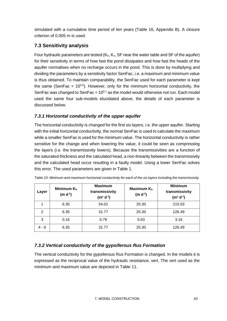
7. MODEL CONSTRUCTION 63
simulated with a cumulative time period of ten years (Table 16, Appendix B). A closure
criterion of 0.005 m is used.
7.3 Sensitivity analysis
Four hydraulic parameters are tested (Kh, Kv, SF near the water table and SF of the aquifer)
for their sensitivity in terms of how fast the pond dissipates and how fast the heads of the
aquifer normalises when no recharge occurs in the pond. This is done by multiplying and
dividing the parameters by a sensitivity factor SenFac, i.e. a maximum and minimum value
is thus obtained. To maintain comparability, the SenFac used for each parameter is kept
the same (SenFac = 100.5). However, only for the minimum horizontal conductivity, the
SenFac was changed to SenFac = 100.1 as the model would otherwise not run. Each model
used the same four sub-models elucidated above, the details of each parameter is
discussed below.
7.3.1 Horizontal conductivity of the upper aquifer
The horizontal conductivity is changed for the first six layers, i.e. the upper aquifer. Starting
with the initial horizontal conductivity, the normal SenFac is used to calculate the maximum
while a smaller SenFac is used for the minimum value. The horizontal conductivity is rather
sensitive for the change and when lowering the value, it could be seen as compressing
the layers (i.e. the transmissivity lowers). Because the transmissivities are a function of
the saturated thickness and the calculated head, a non-linearity between the transmissivity
and the calculated head occur resulting in a faulty model. Using a lower SenFac solves
this error. The used parameters are given in Table 1.
Table 10: Minimum and maximum horizontal conductivity for each of the six layers including the transmissivity.
Layer Minimum Kh
(m d-1)
Maximum
transmissivity
(m² d-1)
Maximum Kh
(m d-1)
Minimum
transmissivity
(m² d-1)
1 6.35 54.01 25.30 215.03
2 6.35 31.77 25.30 126.49
3 0.16 0.79 0.63 3.16
4 - 6 6.35 31.77 25.30 126.49
7.3.2 Vertical conductivity of the gypsiferous Rus Formation
The vertical conductivity for the gypsiferous Rus Formation is changed. In the models it is
expressed as the reciprocal value of the hydraulic resistance, vert. The vert used as the
minimum and maximum value are depicted in Table 11.
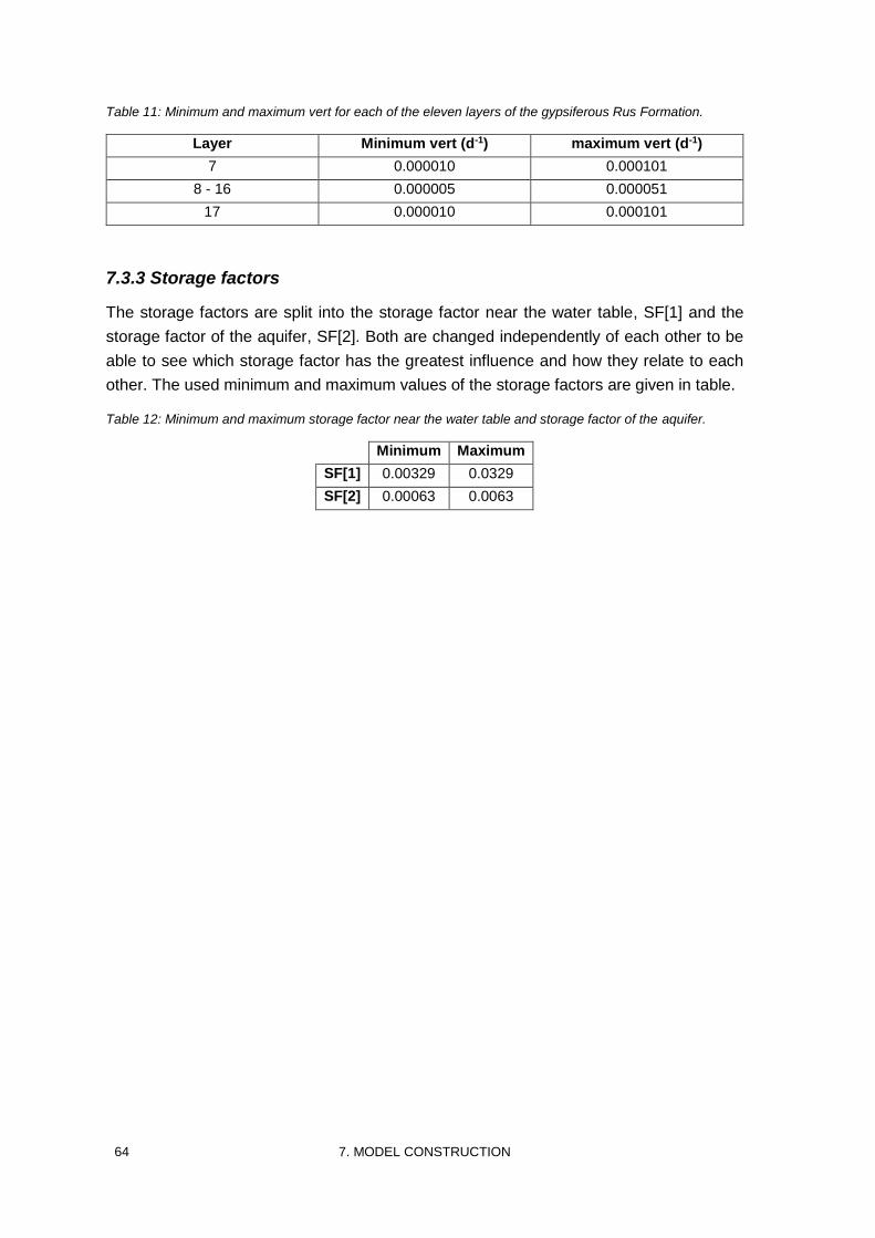
64 7. MODEL CONSTRUCTION
Table 11: Minimum and maximum vert for each of the eleven layers of the gypsiferous Rus Formation.
Layer Minimum vert (d-1) maximum vert (d-1)
7 0.000010 0.000101
8 - 16 0.000005 0.000051
17 0.000010 0.000101
7.3.3 Storage factors
The storage factors are split into the storage factor near the water table, SF[1] and the
storage factor of the aquifer, SF[2]. Both are changed independently of each other to be
able to see which storage factor has the greatest influence and how they relate to each
other. The used minimum and maximum values of the storage factors are given in table.
Table 12: Minimum and maximum storage factor near the water table and storage factor of the aquifer.
Minimum Maximum
SF[1] 0.00329 0.0329
SF[2] 0.00063 0.0063
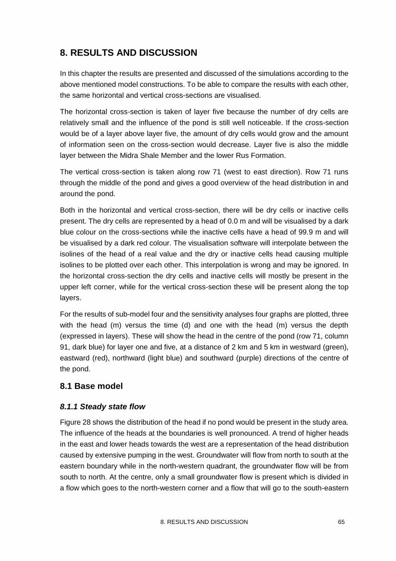
8. RESULTS AND DISCUSSION 65
8. RESULTS AND DISCUSSION
In this chapter the results are presented and discussed of the simulations according to the
above mentioned model constructions. To be able to compare the results with each other,
the same horizontal and vertical cross-sections are visualised.
The horizontal cross-section is taken of layer five because the number of dry cells are
relatively small and the influence of the pond is still well noticeable. If the cross-section
would be of a layer above layer five, the amount of dry cells would grow and the amount
of information seen on the cross-section would decrease. Layer five is also the middle
layer between the Midra Shale Member and the lower Rus Formation.
The vertical cross-section is taken along row 71 (west to east direction). Row 71 runs
through the middle of the pond and gives a good overview of the head distribution in and
around the pond.
Both in the horizontal and vertical cross-section, there will be dry cells or inactive cells
present. The dry cells are represented by a head of 0.0 m and will be visualised by a dark
blue colour on the cross-sections while the inactive cells have a head of 99.9 m and will
be visualised by a dark red colour. The visualisation software will interpolate between the
isolines of the head of a real value and the dry or inactive cells head causing multiple
isolines to be plotted over each other. This interpolation is wrong and may be ignored. In
the horizontal cross-section the dry cells and inactive cells will mostly be present in the
upper left corner, while for the vertical cross-section these will be present along the top
layers.
For the results of sub-model four and the sensitivity analyses four graphs are plotted, three
with the head (m) versus the time (d) and one with the head (m) versus the depth
(expressed in layers). These will show the head in the centre of the pond (row 71, column
91, dark blue) for layer one and five, at a distance of 2 km and 5 km in westward (green),
eastward (red), northward (light blue) and southward (purple) directions of the centre of
the pond.
8.1 Base model
8.1.1 Steady state flow
Figure 28 shows the distribution of the head if no pond would be present in the study area.
The influence of the heads at the boundaries is well pronounced. A trend of higher heads
in the east and lower heads towards the west are a representation of the head distribution
caused by extensive pumping in the west. Groundwater will flow from north to south at the
eastern boundary while in the north-western quadrant, the groundwater flow will be from
south to north. At the centre, only a small groundwater flow is present which is divided in
a flow which goes to the north-western corner and a flow that will go to the south-eastern
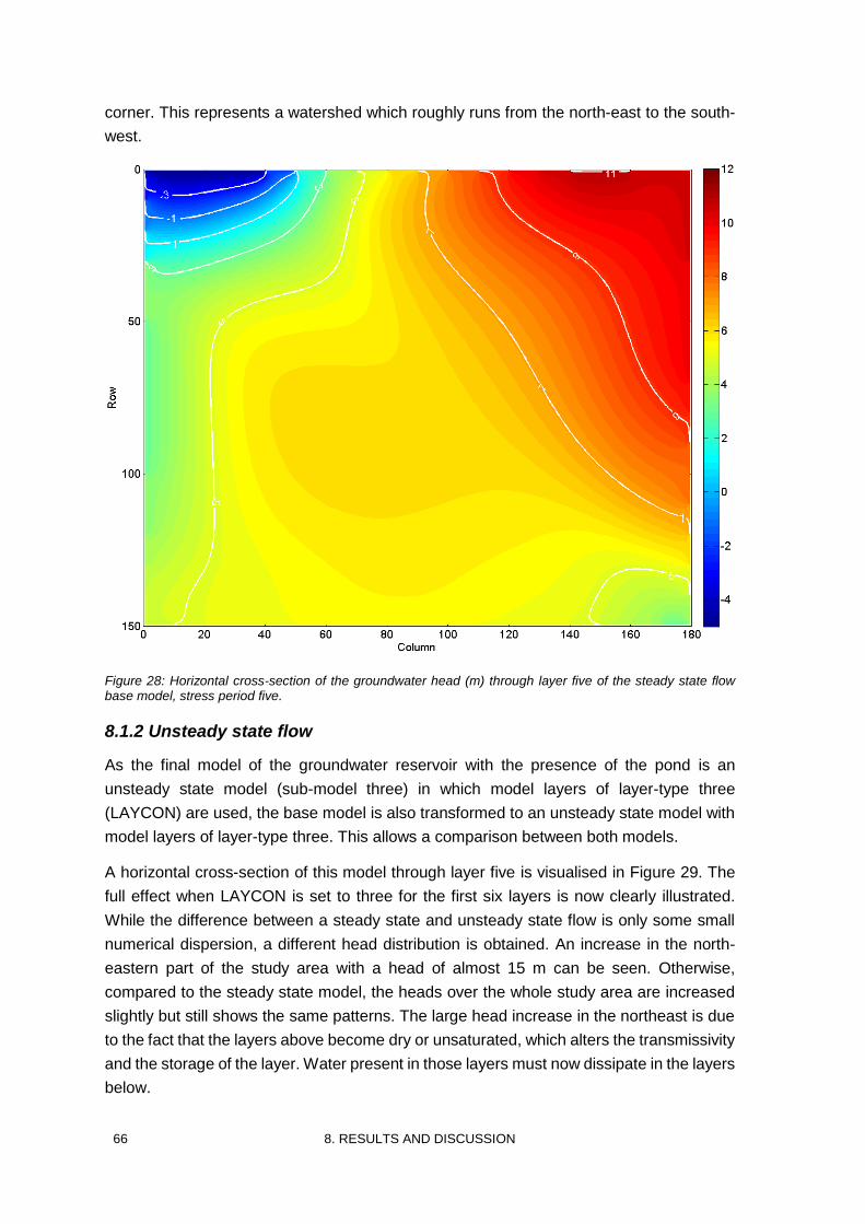
66 8. RESULTS AND DISCUSSION
corner. This represents a watershed which roughly runs from the north-east to the south-
west.
Figure 28: Horizontal cross-section of the groundwater head (m) through layer five of the steady state flow base model, stress period five.
8.1.2 Unsteady state flow
As the final model of the groundwater reservoir with the presence of the pond is an
unsteady state model (sub-model three) in which model layers of layer-type three
(LAYCON) are used, the base model is also transformed to an unsteady state model with
model layers of layer-type three. This allows a comparison between both models.
A horizontal cross-section of this model through layer five is visualised in Figure 29. The
full effect when LAYCON is set to three for the first six layers is now clearly illustrated.
While the difference between a steady state and unsteady state flow is only some small
numerical dispersion, a different head distribution is obtained. An increase in the north-
eastern part of the study area with a head of almost 15 m can be seen. Otherwise,
compared to the steady state model, the heads over the whole study area are increased
slightly but still shows the same patterns. The large head increase in the northeast is due
to the fact that the layers above become dry or unsaturated, which alters the transmissivity
and the storage of the layer. Water present in those layers must now dissipate in the layers
below.
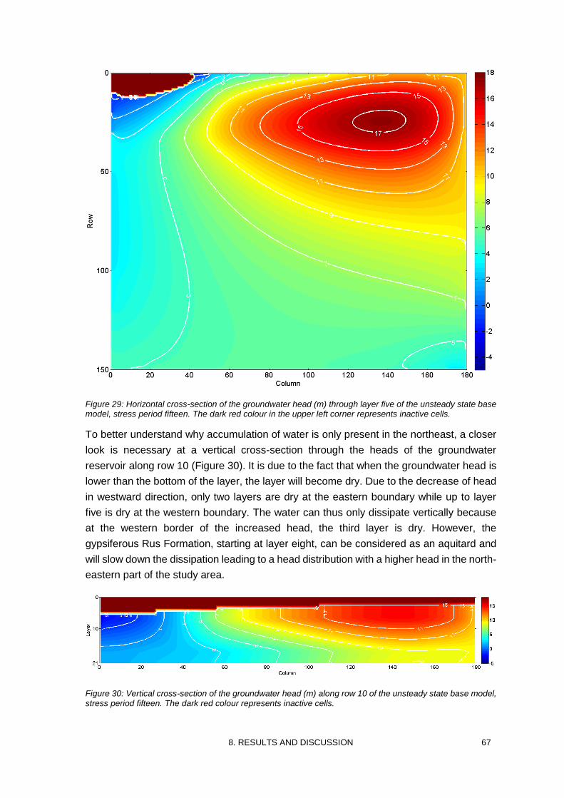
8. RESULTS AND DISCUSSION 67
Figure 29: Horizontal cross-section of the groundwater head (m) through layer five of the unsteady state base model, stress period fifteen. The dark red colour in the upper left corner represents inactive cells.
To better understand why accumulation of water is only present in the northeast, a closer
look is necessary at a vertical cross-section through the heads of the groundwater
reservoir along row 10 (Figure 30). It is due to the fact that when the groundwater head is
lower than the bottom of the layer, the layer will become dry. Due to the decrease of head
in westward direction, only two layers are dry at the eastern boundary while up to layer
five is dry at the western boundary. The water can thus only dissipate vertically because
at the western border of the increased head, the third layer is dry. However, the
gypsiferous Rus Formation, starting at layer eight, can be considered as an aquitard and
will slow down the dissipation leading to a head distribution with a higher head in the north-
eastern part of the study area.
Figure 30: Vertical cross-section of the groundwater head (m) along row 10 of the unsteady state base model, stress period fifteen. The dark red colour represents inactive cells.
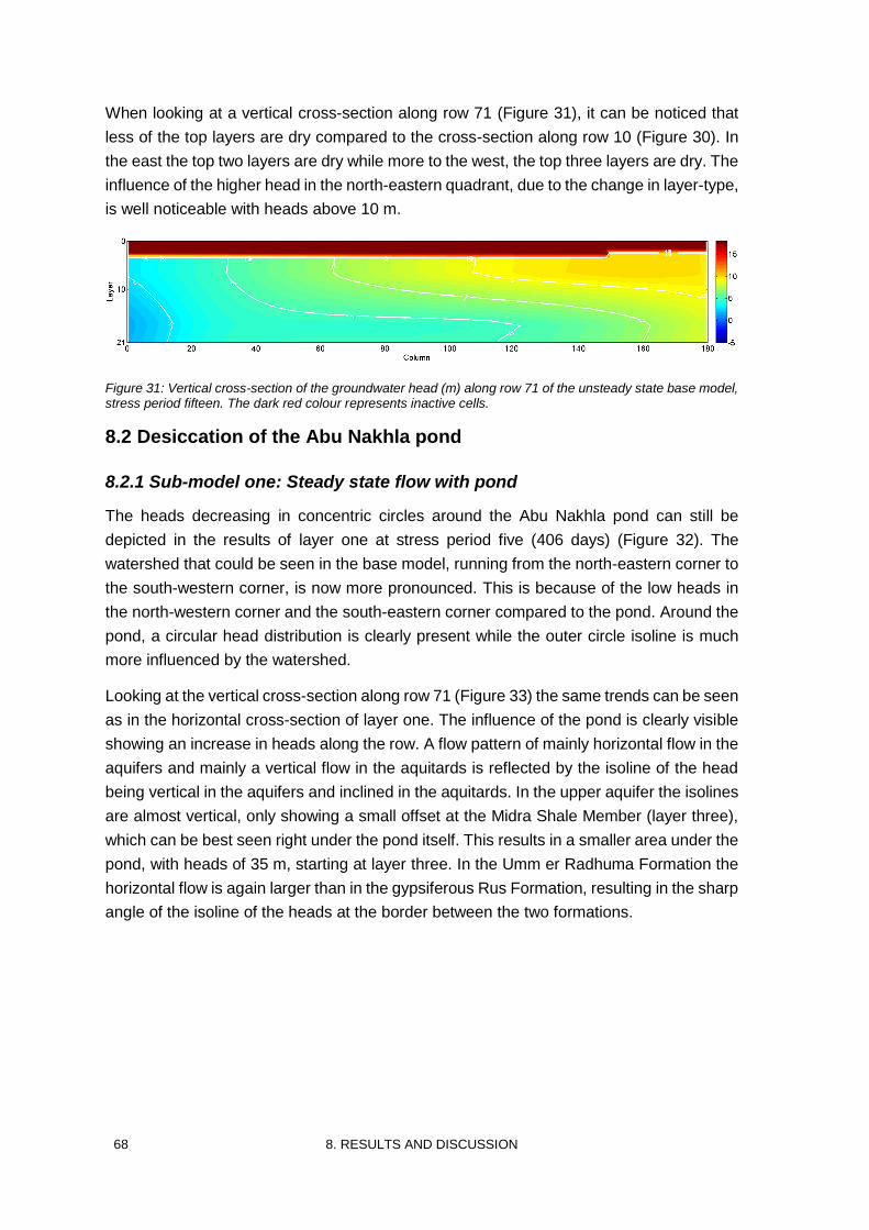
68 8. RESULTS AND DISCUSSION
When looking at a vertical cross-section along row 71 (Figure 31), it can be noticed that
less of the top layers are dry compared to the cross-section along row 10 (Figure 30). In
the east the top two layers are dry while more to the west, the top three layers are dry. The
influence of the higher head in the north-eastern quadrant, due to the change in layer-type,
is well noticeable with heads above 10 m.
Figure 31: Vertical cross-section of the groundwater head (m) along row 71 of the unsteady state base model, stress period fifteen. The dark red colour represents inactive cells.
8.2 Desiccation of the Abu Nakhla pond
8.2.1 Sub-model one: Steady state flow with pond
The heads decreasing in concentric circles around the Abu Nakhla pond can still be
depicted in the results of layer one at stress period five (406 days) (Figure 32). The
watershed that could be seen in the base model, running from the north-eastern corner to
the south-western corner, is now more pronounced. This is because of the low heads in
the north-western corner and the south-eastern corner compared to the pond. Around the
pond, a circular head distribution is clearly present while the outer circle isoline is much
more influenced by the watershed.
Looking at the vertical cross-section along row 71 (Figure 33) the same trends can be seen
as in the horizontal cross-section of layer one. The influence of the pond is clearly visible
showing an increase in heads along the row. A flow pattern of mainly horizontal flow in the
aquifers and mainly a vertical flow in the aquitards is reflected by the isoline of the head
being vertical in the aquifers and inclined in the aquitards. In the upper aquifer the isolines
are almost vertical, only showing a small offset at the Midra Shale Member (layer three),
which can be best seen right under the pond itself. This results in a smaller area under the
pond, with heads of 35 m, starting at layer three. In the Umm er Radhuma Formation the
horizontal flow is again larger than in the gypsiferous Rus Formation, resulting in the sharp
angle of the isoline of the heads at the border between the two formations.
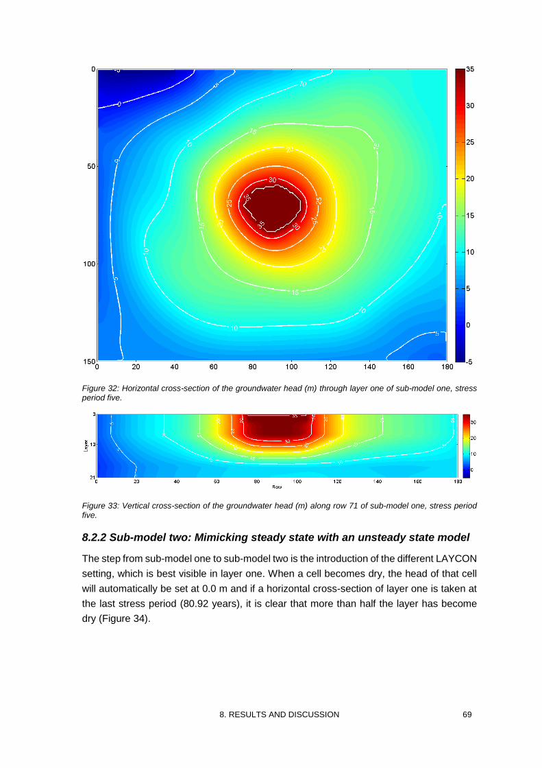
8. RESULTS AND DISCUSSION 69
Figure 32: Horizontal cross-section of the groundwater head (m) through layer one of sub-model one, stress period five.
Figure 33: Vertical cross-section of the groundwater head (m) along row 71 of sub-model one, stress period five.
8.2.2 Sub-model two: Mimicking steady state with an unsteady state model
The step from sub-model one to sub-model two is the introduction of the different LAYCON
setting, which is best visible in layer one. When a cell becomes dry, the head of that cell
will automatically be set at 0.0 m and if a horizontal cross-section of layer one is taken at
the last stress period (80.92 years), it is clear that more than half the layer has become
dry (Figure 34).
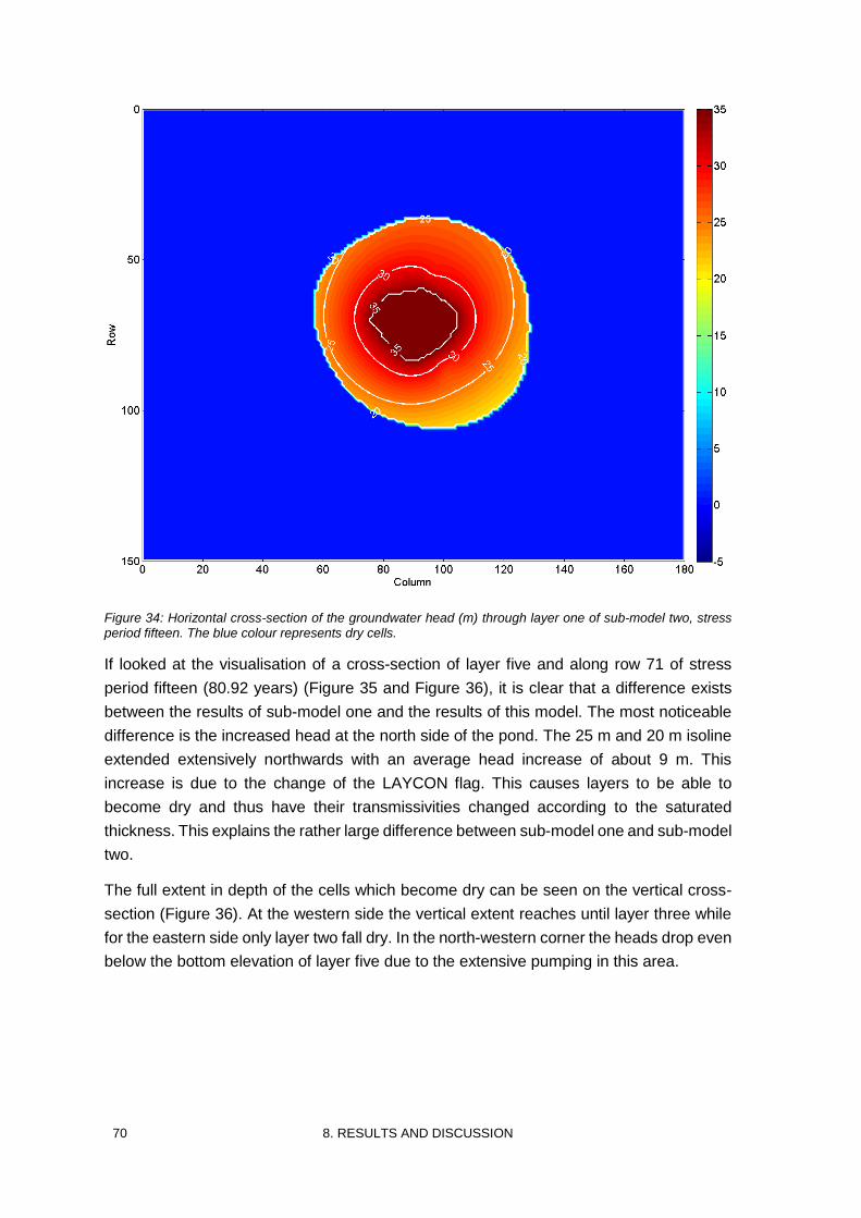
70 8. RESULTS AND DISCUSSION
Figure 34: Horizontal cross-section of the groundwater head (m) through layer one of sub-model two, stress period fifteen. The blue colour represents dry cells.
If looked at the visualisation of a cross-section of layer five and along row 71 of stress
period fifteen (80.92 years) (Figure 35 and Figure 36), it is clear that a difference exists
between the results of sub-model one and the results of this model. The most noticeable
difference is the increased head at the north side of the pond. The 25 m and 20 m isoline
extended extensively northwards with an average head increase of about 9 m. This
increase is due to the change of the LAYCON flag. This causes layers to be able to
become dry and thus have their transmissivities changed according to the saturated
thickness. This explains the rather large difference between sub-model one and sub-model
two.
The full extent in depth of the cells which become dry can be seen on the vertical cross-
section (Figure 36). At the western side the vertical extent reaches until layer three while
for the eastern side only layer two fall dry. In the north-western corner the heads drop even
below the bottom elevation of layer five due to the extensive pumping in this area.
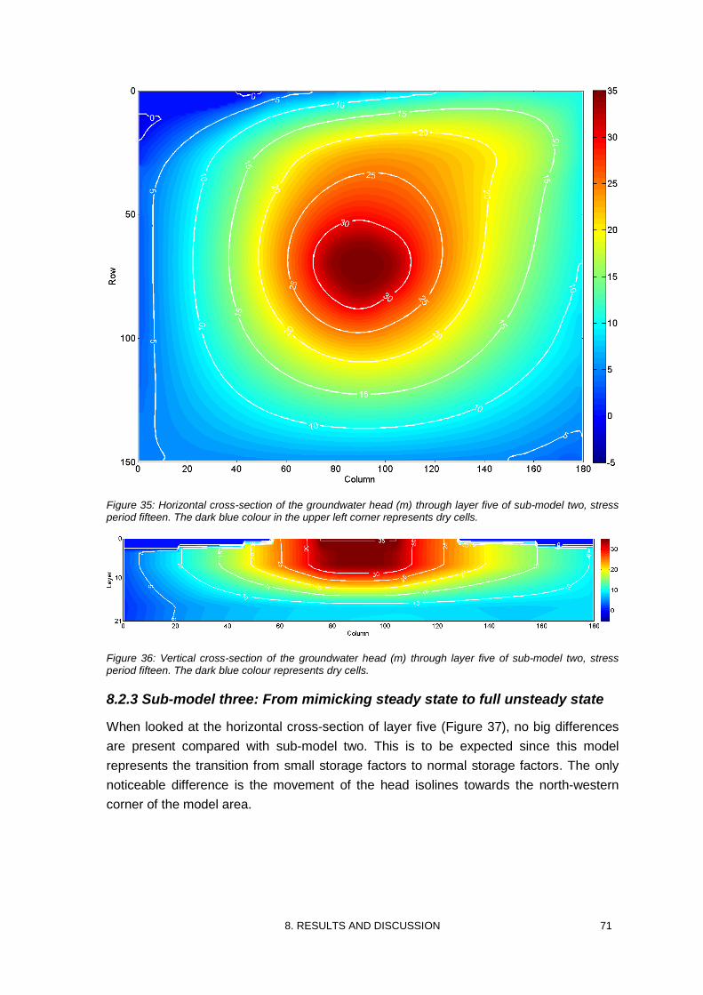
8. RESULTS AND DISCUSSION 71
Figure 35: Horizontal cross-section of the groundwater head (m) through layer five of sub-model two, stress period fifteen. The dark blue colour in the upper left corner represents dry cells.
Figure 36: Vertical cross-section of the groundwater head (m) through layer five of sub-model two, stress period fifteen. The dark blue colour represents dry cells.
8.2.3 Sub-model three: From mimicking steady state to full unsteady state
When looked at the horizontal cross-section of layer five (Figure 37), no big differences
are present compared with sub-model two. This is to be expected since this model
represents the transition from small storage factors to normal storage factors. The only
noticeable difference is the movement of the head isolines towards the north-western
corner of the model area.
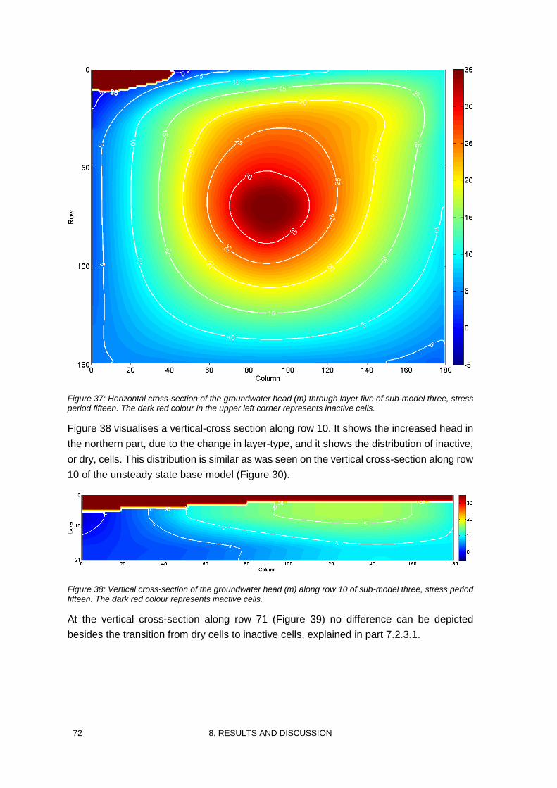
72 8. RESULTS AND DISCUSSION
Figure 37: Horizontal cross-section of the groundwater head (m) through layer five of sub-model three, stress period fifteen. The dark red colour in the upper left corner represents inactive cells.
Figure 38 visualises a vertical-cross section along row 10. It shows the increased head in
the northern part, due to the change in layer-type, and it shows the distribution of inactive,
or dry, cells. This distribution is similar as was seen on the vertical cross-section along row
10 of the unsteady state base model (Figure 30).
Figure 38: Vertical cross-section of the groundwater head (m) along row 10 of sub-model three, stress period fifteen. The dark red colour represents inactive cells.
At the vertical cross-section along row 71 (Figure 39) no difference can be depicted
besides the transition from dry cells to inactive cells, explained in part 7.2.3.1.
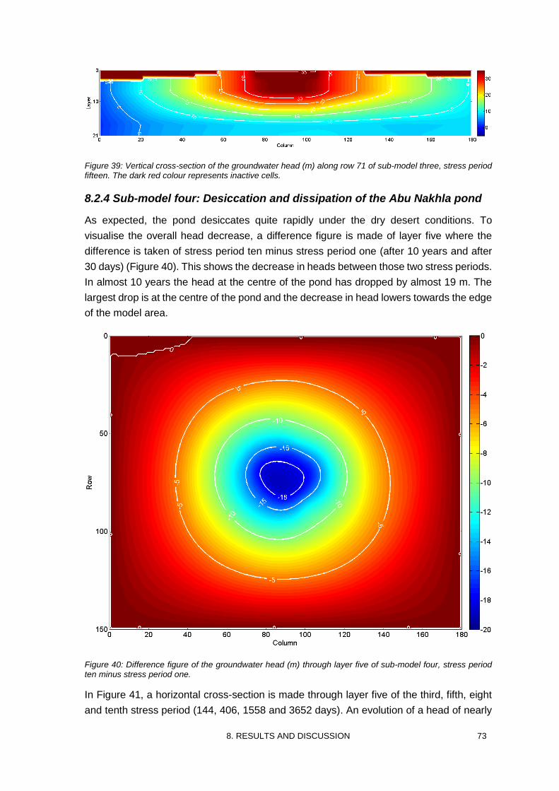
8. RESULTS AND DISCUSSION 73
Figure 39: Vertical cross-section of the groundwater head (m) along row 71 of sub-model three, stress period fifteen. The dark red colour represents inactive cells.
8.2.4 Sub-model four: Desiccation and dissipation of the Abu Nakhla pond
As expected, the pond desiccates quite rapidly under the dry desert conditions. To
visualise the overall head decrease, a difference figure is made of layer five where the
difference is taken of stress period ten minus stress period one (after 10 years and after
30 days) (Figure 40). This shows the decrease in heads between those two stress periods.
In almost 10 years the head at the centre of the pond has dropped by almost 19 m. The
largest drop is at the centre of the pond and the decrease in head lowers towards the edge
of the model area.
Figure 40: Difference figure of the groundwater head (m) through layer five of sub-model four, stress period ten minus stress period one.
In Figure 41, a horizontal cross-section is made through layer five of the third, fifth, eight
and tenth stress period (144, 406, 1558 and 3652 days). An evolution of a head of nearly
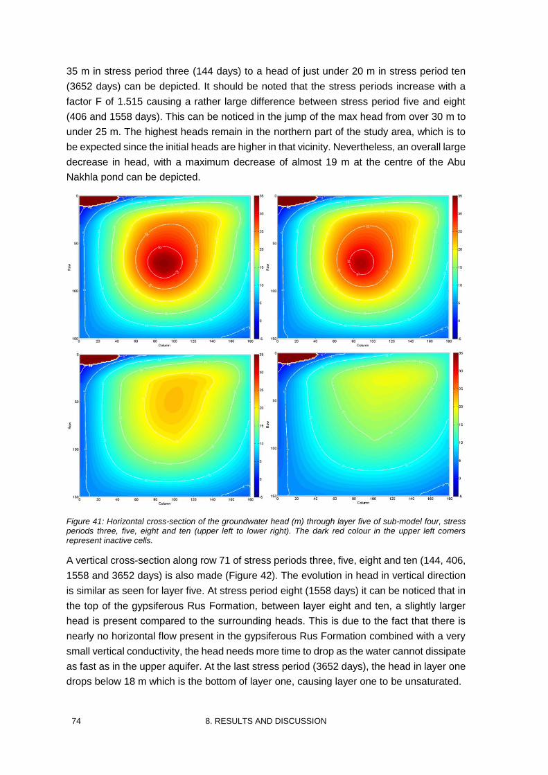
74 8. RESULTS AND DISCUSSION
35 m in stress period three (144 days) to a head of just under 20 m in stress period ten
(3652 days) can be depicted. It should be noted that the stress periods increase with a
factor F of 1.515 causing a rather large difference between stress period five and eight
(406 and 1558 days). This can be noticed in the jump of the max head from over 30 m to
under 25 m. The highest heads remain in the northern part of the study area, which is to
be expected since the initial heads are higher in that vicinity. Nevertheless, an overall large
decrease in head, with a maximum decrease of almost 19 m at the centre of the Abu
Nakhla pond can be depicted.
Figure 41: Horizontal cross-section of the groundwater head (m) through layer five of sub-model four, stress periods three, five, eight and ten (upper left to lower right). The dark red colour in the upper left corners represent inactive cells.
A vertical cross-section along row 71 of stress periods three, five, eight and ten (144, 406,
1558 and 3652 days) is also made (Figure 42). The evolution in head in vertical direction
is similar as seen for layer five. At stress period eight (1558 days) it can be noticed that in
the top of the gypsiferous Rus Formation, between layer eight and ten, a slightly larger
head is present compared to the surrounding heads. This is due to the fact that there is
nearly no horizontal flow present in the gypsiferous Rus Formation combined with a very
small vertical conductivity, the head needs more time to drop as the water cannot dissipate
as fast as in the upper aquifer. At the last stress period (3652 days), the head in layer one
drops below 18 m which is the bottom of layer one, causing layer one to be unsaturated.
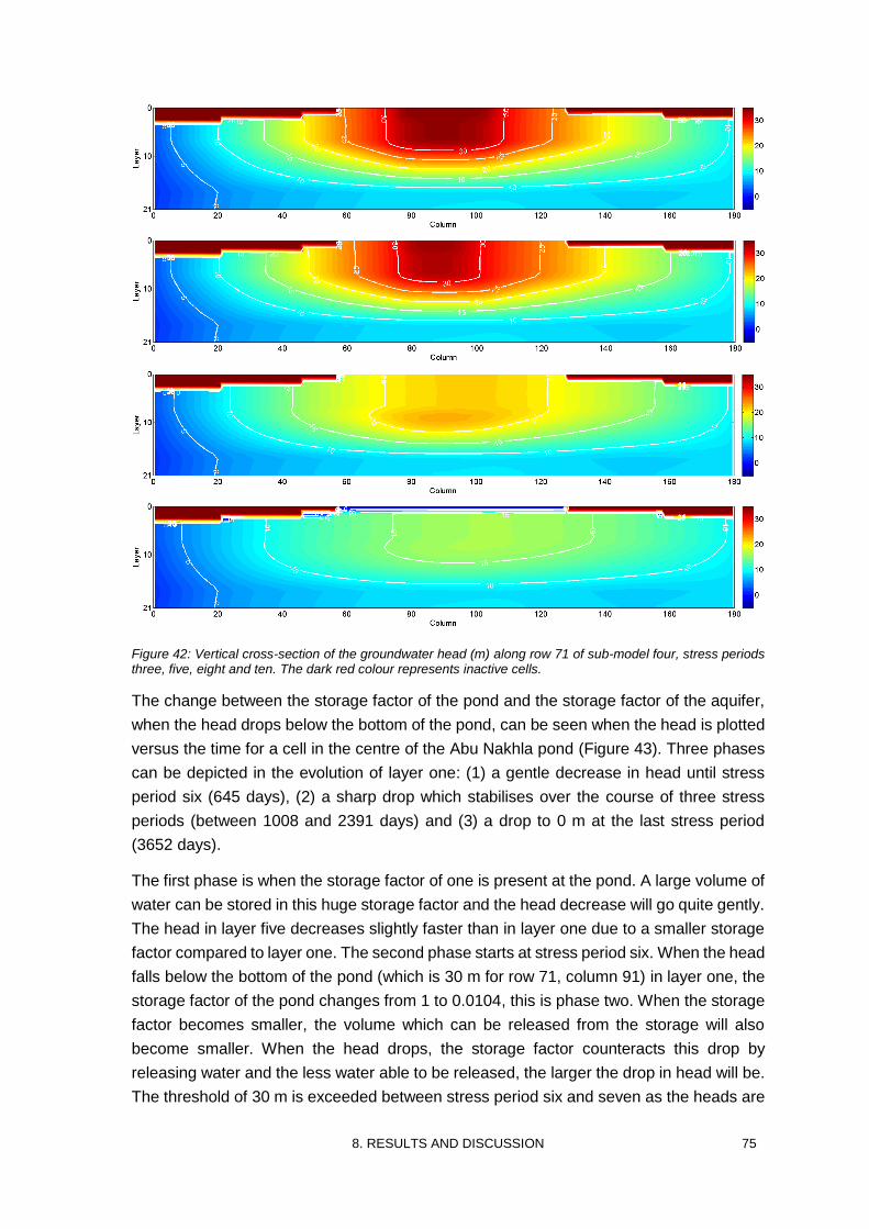
8. RESULTS AND DISCUSSION 75
Figure 42: Vertical cross-section of the groundwater head (m) along row 71 of sub-model four, stress periods three, five, eight and ten. The dark red colour represents inactive cells.
The change between the storage factor of the pond and the storage factor of the aquifer,
when the head drops below the bottom of the pond, can be seen when the head is plotted
versus the time for a cell in the centre of the Abu Nakhla pond (Figure 43). Three phases
can be depicted in the evolution of layer one: (1) a gentle decrease in head until stress
period six (645 days), (2) a sharp drop which stabilises over the course of three stress
periods (between 1008 and 2391 days) and (3) a drop to 0 m at the last stress period
(3652 days).
The first phase is when the storage factor of one is present at the pond. A large volume of
water can be stored in this huge storage factor and the head decrease will go quite gently.
The head in layer five decreases slightly faster than in layer one due to a smaller storage
factor compared to layer one. The second phase starts at stress period six. When the head
falls below the bottom of the pond (which is 30 m for row 71, column 91) in layer one, the
storage factor of the pond changes from 1 to 0.0104, this is phase two. When the storage
factor becomes smaller, the volume which can be released from the storage will also
become smaller. When the head drops, the storage factor counteracts this drop by
releasing water and the less water able to be released, the larger the drop in head will be.
The threshold of 30 m is exceeded between stress period six and seven as the heads are
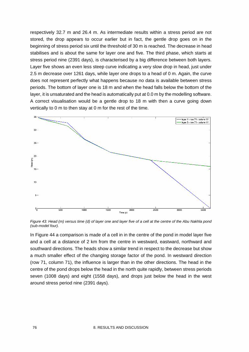
76 8. RESULTS AND DISCUSSION
respectively 32.7 m and 26.4 m. As intermediate results within a stress period are not
stored, the drop appears to occur earlier but in fact, the gentle drop goes on in the
beginning of stress period six until the threshold of 30 m is reached. The decrease in head
stabilises and is about the same for layer one and five. The third phase, which starts at
stress period nine (2391 days), is characterised by a big difference between both layers.
Layer five shows an even less steep curve indicating a very slow drop in head, just under
2.5 m decrease over 1261 days, while layer one drops to a head of 0 m. Again, the curve
does not represent perfectly what happens because no data is available between stress
periods. The bottom of layer one is 18 m and when the head falls below the bottom of the
layer, it is unsaturated and the head is automatically put at 0.0 m by the modelling software.
A correct visualisation would be a gentle drop to 18 m with then a curve going down
vertically to 0 m to then stay at 0 m for the rest of the time.
Figure 43: Head (m) versus time (d) of layer one and layer five of a cell at the centre of the Abu Nakhla pond (sub-model four).
In Figure 44 a comparison is made of a cell in in the centre of the pond in model layer five
and a cell at a distance of 2 km from the centre in westward, eastward, northward and
southward directions. The heads show a similar trend in respect to the decrease but show
a much smaller effect of the changing storage factor of the pond. In westward direction
(row 71, column 71), the influence is larger than in the other directions. The head in the
centre of the pond drops below the head in the north quite rapidly, between stress periods
seven (1008 days) and eight (1558 days), and drops just below the head in the west
around stress period nine (2391 days).
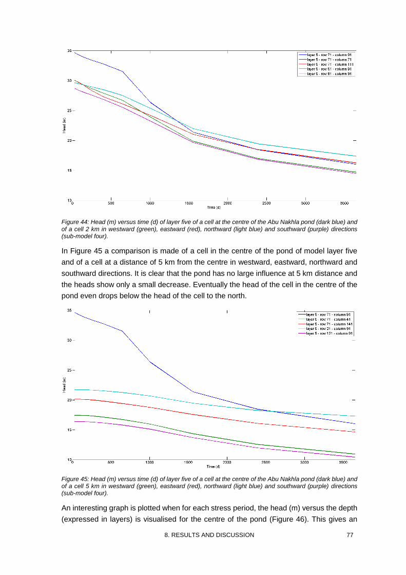
8. RESULTS AND DISCUSSION 77
Figure 44: Head (m) versus time (d) of layer five of a cell at the centre of the Abu Nakhla pond (dark blue) and of a cell 2 km in westward (green), eastward (red), northward (light blue) and southward (purple) directions (sub-model four).
In Figure 45 a comparison is made of a cell in the centre of the pond of model layer five
and of a cell at a distance of 5 km from the centre in westward, eastward, northward and
southward directions. It is clear that the pond has no large influence at 5 km distance and
the heads show only a small decrease. Eventually the head of the cell in the centre of the
pond even drops below the head of the cell to the north.
Figure 45: Head (m) versus time (d) of layer five of a cell at the centre of the Abu Nakhla pond (dark blue) and of a cell 5 km in westward (green), eastward (red), northward (light blue) and southward (purple) directions (sub-model four).
An interesting graph is plotted when for each stress period, the head (m) versus the depth
(expressed in layers) is visualised for the centre of the pond (Figure 46). This gives an
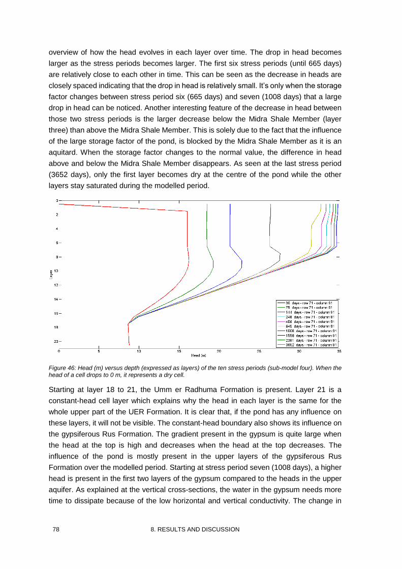
78 8. RESULTS AND DISCUSSION
overview of how the head evolves in each layer over time. The drop in head becomes
larger as the stress periods becomes larger. The first six stress periods (until 665 days)
are relatively close to each other in time. This can be seen as the decrease in heads are
closely spaced indicating that the drop in head is relatively small. It’s only when the storage
factor changes between stress period six (665 days) and seven (1008 days) that a large
drop in head can be noticed. Another interesting feature of the decrease in head between
those two stress periods is the larger decrease below the Midra Shale Member (layer
three) than above the Midra Shale Member. This is solely due to the fact that the influence
of the large storage factor of the pond, is blocked by the Midra Shale Member as it is an
aquitard. When the storage factor changes to the normal value, the difference in head
above and below the Midra Shale Member disappears. As seen at the last stress period
(3652 days), only the first layer becomes dry at the centre of the pond while the other
layers stay saturated during the modelled period.
Figure 46: Head (m) versus depth (expressed as layers) of the ten stress periods (sub-model four). When the head of a cell drops to 0 m, it represents a dry cell.
Starting at layer 18 to 21, the Umm er Radhuma Formation is present. Layer 21 is a
constant-head cell layer which explains why the head in each layer is the same for the
whole upper part of the UER Formation. It is clear that, if the pond has any influence on
these layers, it will not be visible. The constant-head boundary also shows its influence on
the gypsiferous Rus Formation. The gradient present in the gypsum is quite large when
the head at the top is high and decreases when the head at the top decreases. The
influence of the pond is mostly present in the upper layers of the gypsiferous Rus
Formation over the modelled period. Starting at stress period seven (1008 days), a higher
head is present in the first two layers of the gypsum compared to the heads in the upper
aquifer. As explained at the vertical cross-sections, the water in the gypsum needs more
time to dissipate because of the low horizontal and vertical conductivity. The change in
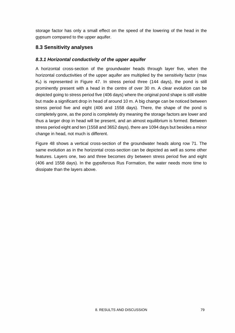
8. RESULTS AND DISCUSSION 79
storage factor has only a small effect on the speed of the lowering of the head in the
gypsum compared to the upper aquifer.
8.3 Sensitivity analyses
8.3.1 Horizontal conductivity of the upper aquifer
A horizontal cross-section of the groundwater heads through layer five, when the
horizontal conductivities of the upper aquifer are multiplied by the sensitivity factor (max
Kh) is represented in Figure 47. In stress period three (144 days), the pond is still
prominently present with a head in the centre of over 30 m. A clear evolution can be
depicted going to stress period five (406 days) where the original pond shape is still visible
but made a significant drop in head of around 10 m. A big change can be noticed between
stress period five and eight (406 and 1558 days). There, the shape of the pond is
completely gone, as the pond is completely dry meaning the storage factors are lower and
thus a larger drop in head will be present, and an almost equilibrium is formed. Between
stress period eight and ten (1558 and 3652 days), there are 1094 days but besides a minor
change in head, not much is different.
Figure 48 shows a vertical cross-section of the groundwater heads along row 71. The
same evolution as in the horizontal cross-section can be depicted as well as some other
features. Layers one, two and three becomes dry between stress period five and eight
(406 and 1558 days). In the gypsiferous Rus Formation, the water needs more time to
dissipate than the layers above.
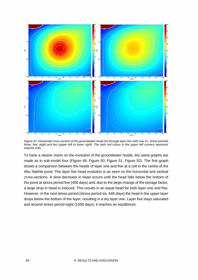
80 8. RESULTS AND DISCUSSION
Figure 47: Horizontal cross-section of the groundwater head (m) through layer five with max Kh, stress periods three, five, eight and ten (upper left to lower right). The dark red colour in the upper left corners represent inactive cells.
To have a clearer vision on the evolution of the groundwater heads, the same graphs are
made as in sub-model four (Figure 49, Figure 50, Figure 51, Figure 52). The first graph
shows a comparison between the heads of layer one and five at a cell in the centre of the
Abu Nakhla pond. The layer five head evolution is as seen on the horizontal and vertical
cross-sections. A slow decrease in head occurs until the head falls below the bottom of
the pond at stress period five (406 days) and, due to the large change of the storage factor,
a large drop in head is induced. This results in an equal head for both layer one and five.
However, in the next stress period (stress period six, 645 days) the head in the upper layer
drops below the bottom of the layer, resulting in a dry layer one. Layer five stays saturated
and around stress period eight (1558 days), it reaches an equilibrium.
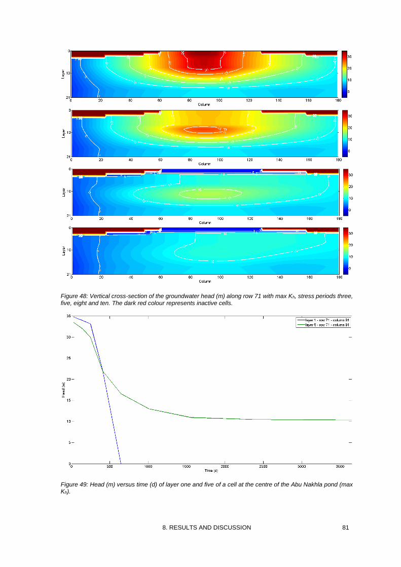
8. RESULTS AND DISCUSSION 81
Figure 48: Vertical cross-section of the groundwater head (m) along row 71 with max Kh, stress periods three, five, eight and ten. The dark red colour represents inactive cells.
Figure 49: Head (m) versus time (d) of layer one and five of a cell at the centre of the Abu Nakhla pond (max Kh).
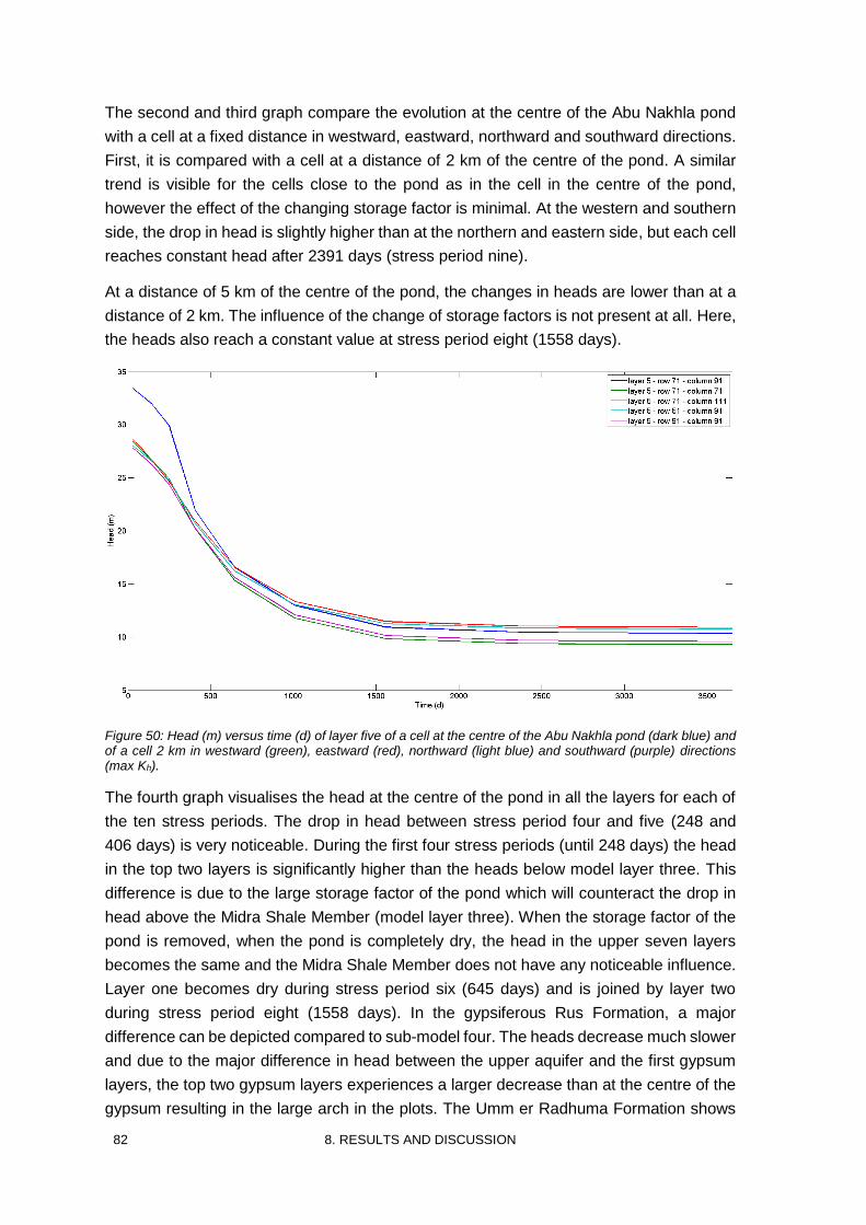
82 8. RESULTS AND DISCUSSION
The second and third graph compare the evolution at the centre of the Abu Nakhla pond
with a cell at a fixed distance in westward, eastward, northward and southward directions.
First, it is compared with a cell at a distance of 2 km of the centre of the pond. A similar
trend is visible for the cells close to the pond as in the cell in the centre of the pond,
however the effect of the changing storage factor is minimal. At the western and southern
side, the drop in head is slightly higher than at the northern and eastern side, but each cell
reaches constant head after 2391 days (stress period nine).
At a distance of 5 km of the centre of the pond, the changes in heads are lower than at a
distance of 2 km. The influence of the change of storage factors is not present at all. Here,
the heads also reach a constant value at stress period eight (1558 days).
Figure 50: Head (m) versus time (d) of layer five of a cell at the centre of the Abu Nakhla pond (dark blue) and of a cell 2 km in westward (green), eastward (red), northward (light blue) and southward (purple) directions (max Kh).
The fourth graph visualises the head at the centre of the pond in all the layers for each of
the ten stress periods. The drop in head between stress period four and five (248 and
406 days) is very noticeable. During the first four stress periods (until 248 days) the head
in the top two layers is significantly higher than the heads below model layer three. This
difference is due to the large storage factor of the pond which will counteract the drop in
head above the Midra Shale Member (model layer three). When the storage factor of the
pond is removed, when the pond is completely dry, the head in the upper seven layers
becomes the same and the Midra Shale Member does not have any noticeable influence.
Layer one becomes dry during stress period six (645 days) and is joined by layer two
during stress period eight (1558 days). In the gypsiferous Rus Formation, a major
difference can be depicted compared to sub-model four. The heads decrease much slower
and due to the major difference in head between the upper aquifer and the first gypsum
layers, the top two gypsum layers experiences a larger decrease than at the centre of the
gypsum resulting in the large arch in the plots. The Umm er Radhuma Formation shows
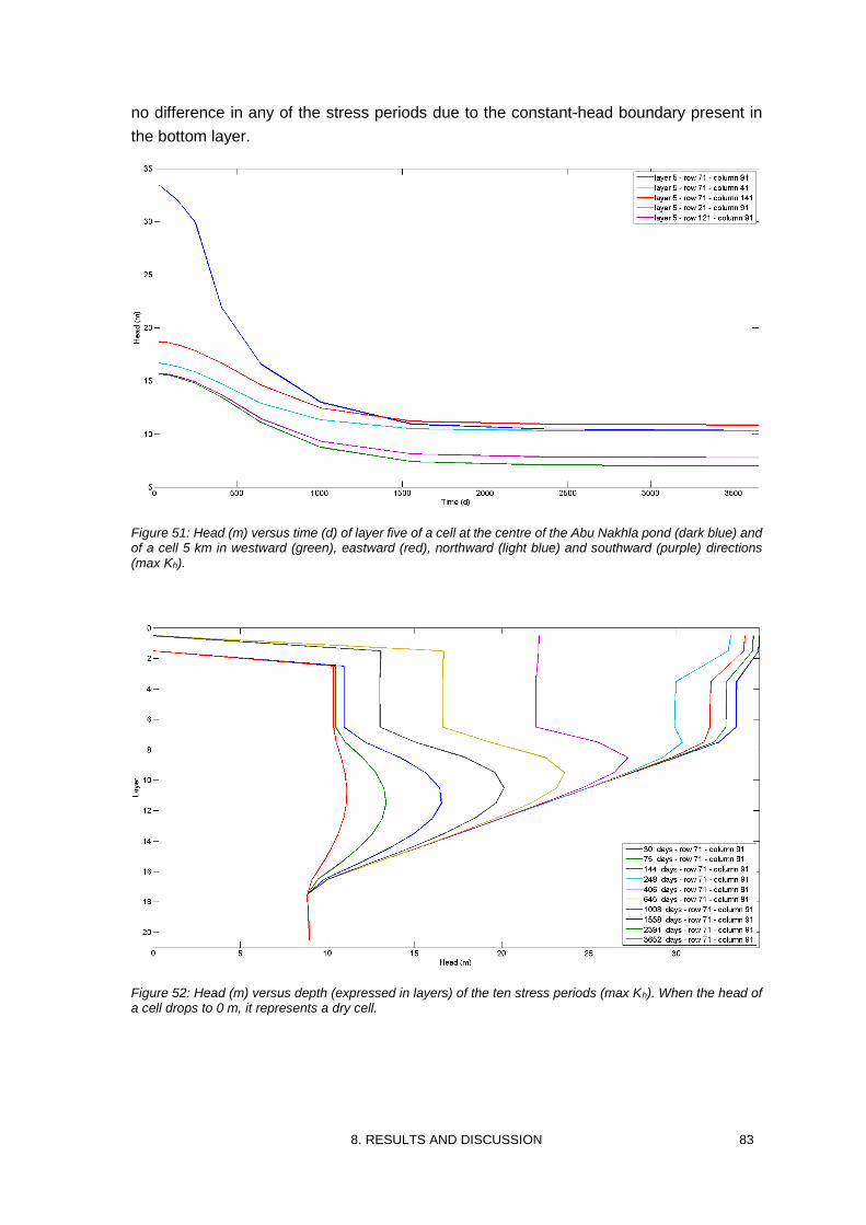
8. RESULTS AND DISCUSSION 83
no difference in any of the stress periods due to the constant-head boundary present in
the bottom layer.
Figure 51: Head (m) versus time (d) of layer five of a cell at the centre of the Abu Nakhla pond (dark blue) and of a cell 5 km in westward (green), eastward (red), northward (light blue) and southward (purple) directions (max Kh).
Figure 52: Head (m) versus depth (expressed in layers) of the ten stress periods (max Kh). When the head of a cell drops to 0 m, it represents a dry cell.
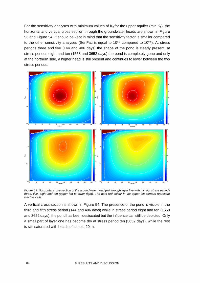
84 8. RESULTS AND DISCUSSION
For the sensitivity analyses with minimum values of Kh for the upper aquifer (min Kh), the
horizontal and vertical cross-section through the groundwater heads are shown in Figure
53 and Figure 54. It should be kept in mind that the sensitivity factor is smaller compared
to the other sensitivity analyses (SenFac is equal to 100.1 compared to 100.5). At stress
periods three and five (144 and 406 days) the shape of the pond is clearly present, at
stress periods eight and ten (1558 and 3652 days) the pond is completely gone and only
at the northern side, a higher head is still present and continues to lower between the two
stress periods.
Figure 53: Horizontal cross-section of the groundwater head (m) through layer five with min Kh, stress periods three, five, eight and ten (upper left to lower right). The dark red colour in the upper left corners represent inactive cells.
A vertical cross-section is shown in Figure 54. The presence of the pond is visible in the
third and fifth stress period (144 and 406 days) while in stress period eight and ten (1558
and 3652 days), the pond has been desiccated but the influence can still be depicted. Only
a small part of layer one has become dry at stress period ten (3652 days), while the rest
is still saturated with heads of almost 20 m.
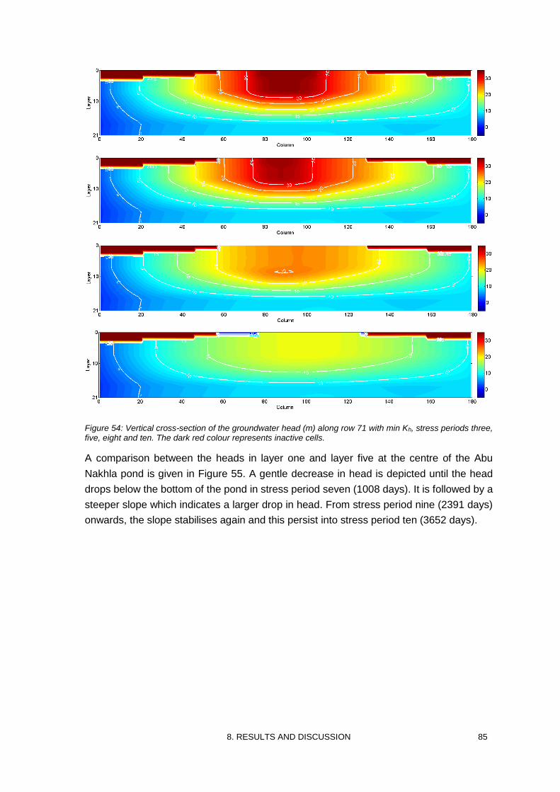
8. RESULTS AND DISCUSSION 85
Figure 54: Vertical cross-section of the groundwater head (m) along row 71 with min Kh, stress periods three, five, eight and ten. The dark red colour represents inactive cells.
A comparison between the heads in layer one and layer five at the centre of the Abu
Nakhla pond is given in Figure 55. A gentle decrease in head is depicted until the head
drops below the bottom of the pond in stress period seven (1008 days). It is followed by a
steeper slope which indicates a larger drop in head. From stress period nine (2391 days)
onwards, the slope stabilises again and this persist into stress period ten (3652 days).
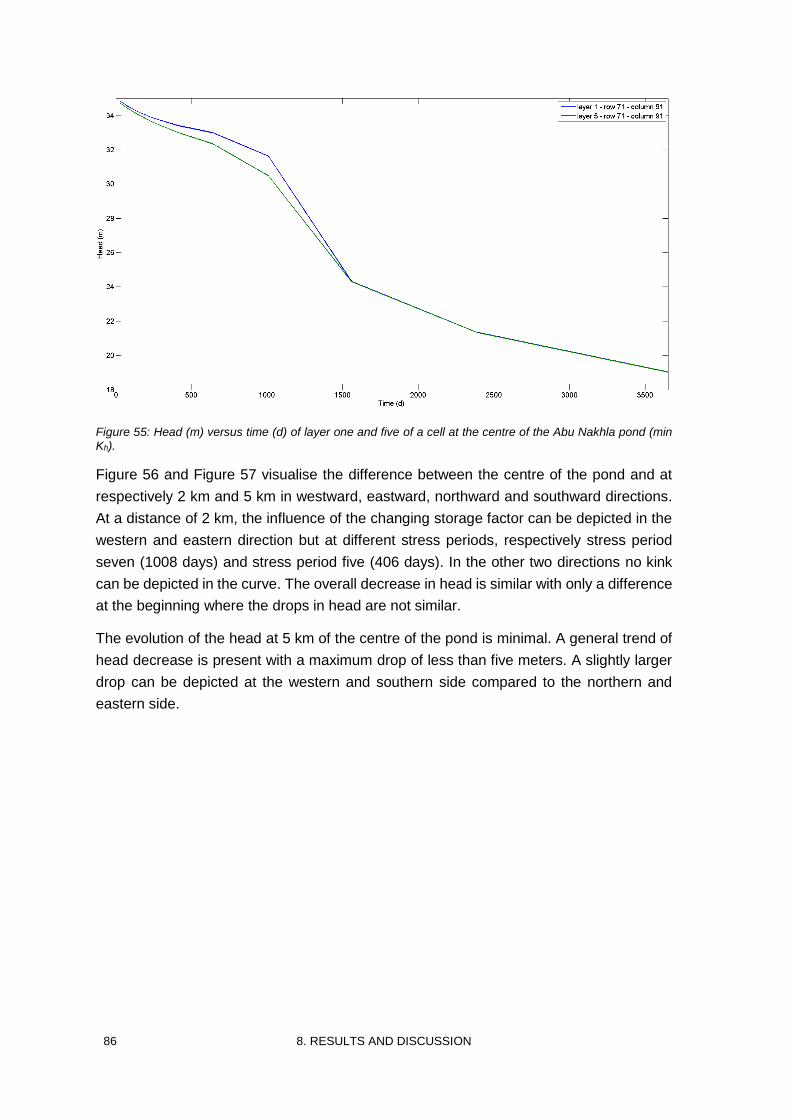
86 8. RESULTS AND DISCUSSION
Figure 55: Head (m) versus time (d) of layer one and five of a cell at the centre of the Abu Nakhla pond (min Kh).
Figure 56 and Figure 57 visualise the difference between the centre of the pond and at
respectively 2 km and 5 km in westward, eastward, northward and southward directions.
At a distance of 2 km, the influence of the changing storage factor can be depicted in the
western and eastern direction but at different stress periods, respectively stress period
seven (1008 days) and stress period five (406 days). In the other two directions no kink
can be depicted in the curve. The overall decrease in head is similar with only a difference
at the beginning where the drops in head are not similar.
The evolution of the head at 5 km of the centre of the pond is minimal. A general trend of
head decrease is present with a maximum drop of less than five meters. A slightly larger
drop can be depicted at the western and southern side compared to the northern and
eastern side.
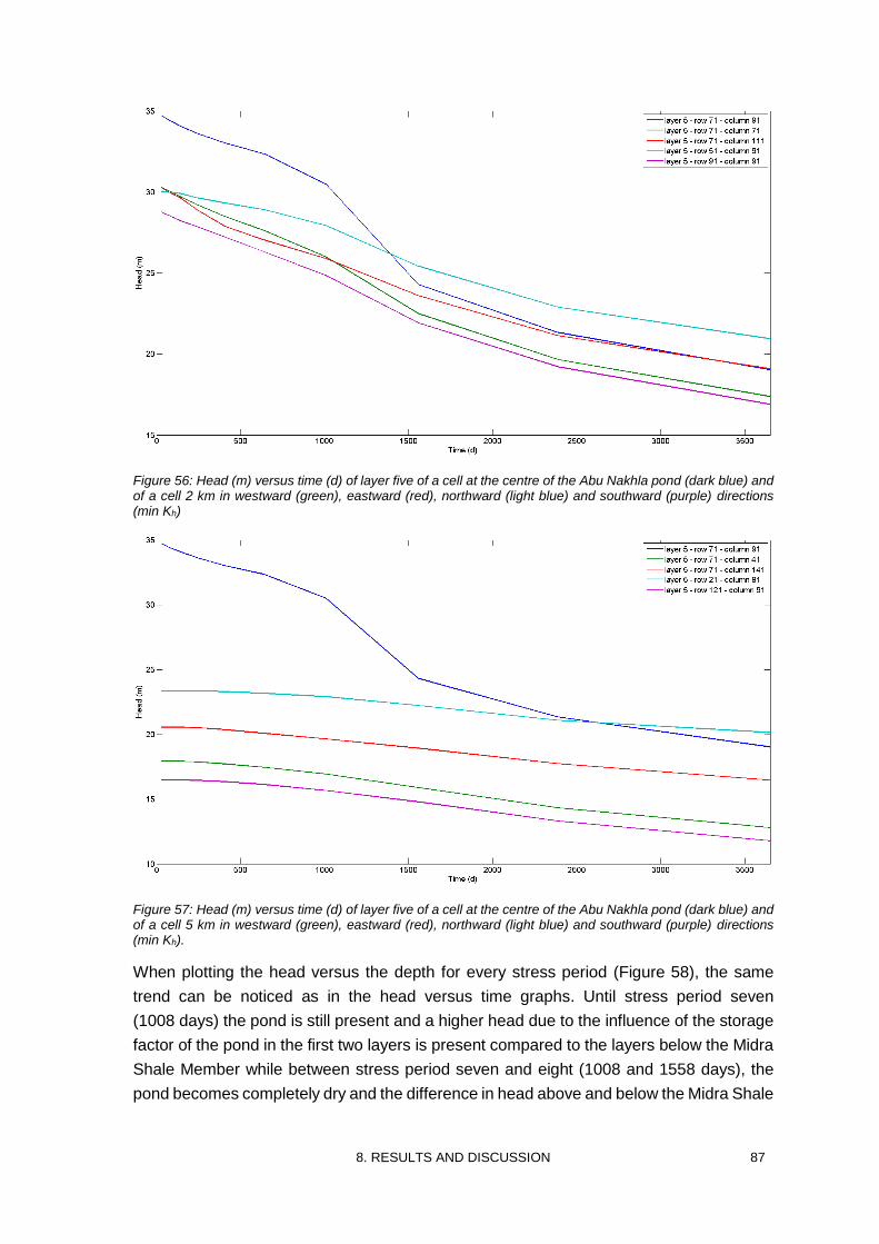
8. RESULTS AND DISCUSSION 87
Figure 56: Head (m) versus time (d) of layer five of a cell at the centre of the Abu Nakhla pond (dark blue) and of a cell 2 km in westward (green), eastward (red), northward (light blue) and southward (purple) directions (min Kh)
Figure 57: Head (m) versus time (d) of layer five of a cell at the centre of the Abu Nakhla pond (dark blue) and of a cell 5 km in westward (green), eastward (red), northward (light blue) and southward (purple) directions (min Kh).
When plotting the head versus the depth for every stress period (Figure 58), the same
trend can be noticed as in the head versus time graphs. Until stress period seven
(1008 days) the pond is still present and a higher head due to the influence of the storage
factor of the pond in the first two layers is present compared to the layers below the Midra
Shale Member while between stress period seven and eight (1008 and 1558 days), the
pond becomes completely dry and the difference in head above and below the Midra Shale
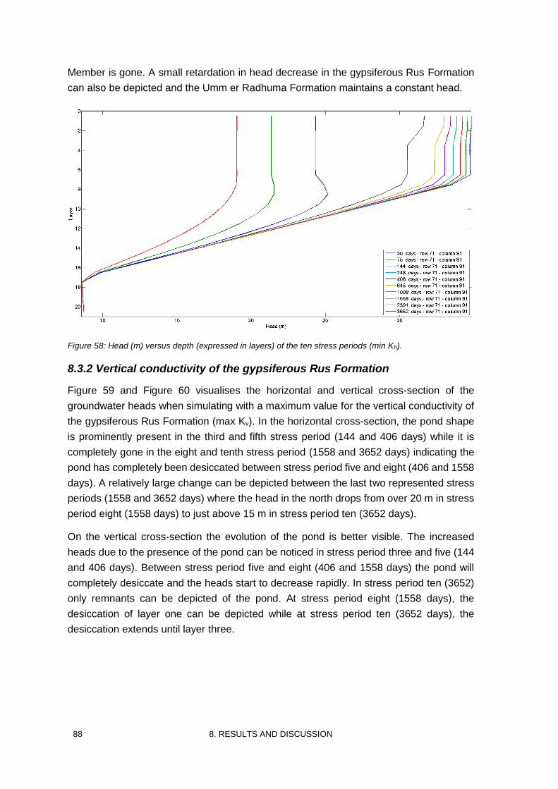
88 8. RESULTS AND DISCUSSION
Member is gone. A small retardation in head decrease in the gypsiferous Rus Formation
can also be depicted and the Umm er Radhuma Formation maintains a constant head.
Figure 58: Head (m) versus depth (expressed in layers) of the ten stress periods (min Kh).
8.3.2 Vertical conductivity of the gypsiferous Rus Formation
Figure 59 and Figure 60 visualises the horizontal and vertical cross-section of the
groundwater heads when simulating with a maximum value for the vertical conductivity of
the gypsiferous Rus Formation (max Kv). In the horizontal cross-section, the pond shape
is prominently present in the third and fifth stress period (144 and 406 days) while it is
completely gone in the eight and tenth stress period (1558 and 3652 days) indicating the
pond has completely been desiccated between stress period five and eight (406 and 1558
days). A relatively large change can be depicted between the last two represented stress
periods (1558 and 3652 days) where the head in the north drops from over 20 m in stress
period eight (1558 days) to just above 15 m in stress period ten (3652 days).
On the vertical cross-section the evolution of the pond is better visible. The increased
heads due to the presence of the pond can be noticed in stress period three and five (144
and 406 days). Between stress period five and eight (406 and 1558 days) the pond will
completely desiccate and the heads start to decrease rapidly. In stress period ten (3652)
only remnants can be depicted of the pond. At stress period eight (1558 days), the
desiccation of layer one can be depicted while at stress period ten (3652 days), the
desiccation extends until layer three.
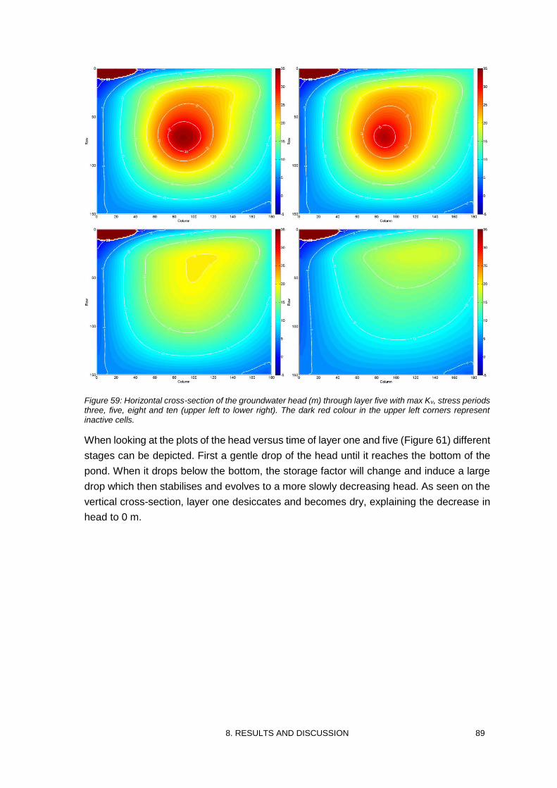
8. RESULTS AND DISCUSSION 89
Figure 59: Horizontal cross-section of the groundwater head (m) through layer five with max Kv, stress periods three, five, eight and ten (upper left to lower right). The dark red colour in the upper left corners represent inactive cells.
When looking at the plots of the head versus time of layer one and five (Figure 61) different
stages can be depicted. First a gentle drop of the head until it reaches the bottom of the
pond. When it drops below the bottom, the storage factor will change and induce a large
drop which then stabilises and evolves to a more slowly decreasing head. As seen on the
vertical cross-section, layer one desiccates and becomes dry, explaining the decrease in
head to 0 m.
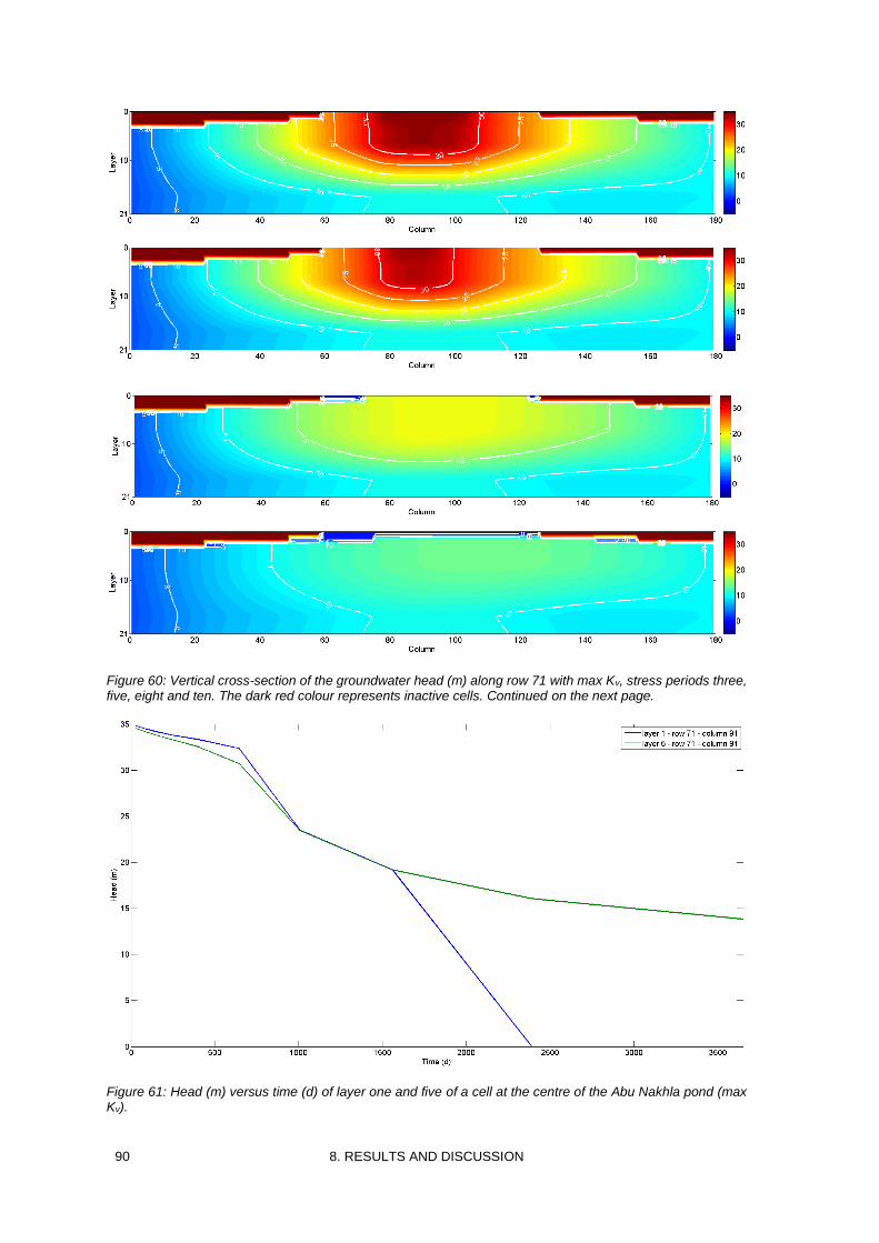
90 8. RESULTS AND DISCUSSION
Figure 60: Vertical cross-section of the groundwater head (m) along row 71 with max Kv, stress periods three, five, eight and ten. The dark red colour represents inactive cells. Continued on the next page.
Figure 61: Head (m) versus time (d) of layer one and five of a cell at the centre of the Abu Nakhla pond (max Kv).
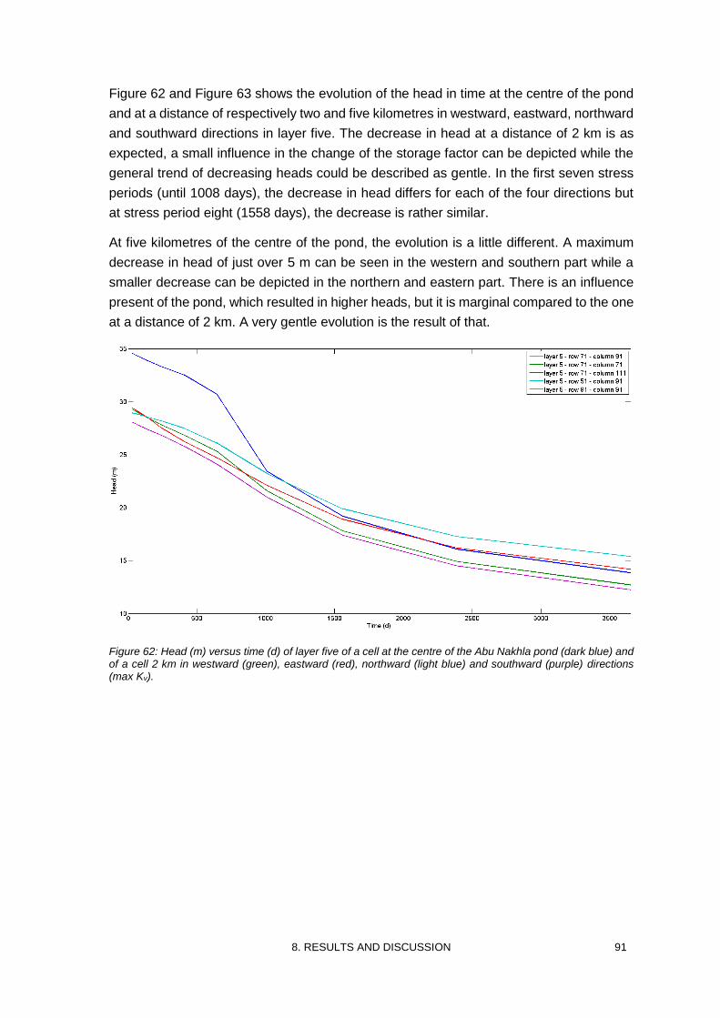
8. RESULTS AND DISCUSSION 91
Figure 62 and Figure 63 shows the evolution of the head in time at the centre of the pond
and at a distance of respectively two and five kilometres in westward, eastward, northward
and southward directions in layer five. The decrease in head at a distance of 2 km is as
expected, a small influence in the change of the storage factor can be depicted while the
general trend of decreasing heads could be described as gentle. In the first seven stress
periods (until 1008 days), the decrease in head differs for each of the four directions but
at stress period eight (1558 days), the decrease is rather similar.
At five kilometres of the centre of the pond, the evolution is a little different. A maximum
decrease in head of just over 5 m can be seen in the western and southern part while a
smaller decrease can be depicted in the northern and eastern part. There is an influence
present of the pond, which resulted in higher heads, but it is marginal compared to the one
at a distance of 2 km. A very gentle evolution is the result of that.
Figure 62: Head (m) versus time (d) of layer five of a cell at the centre of the Abu Nakhla pond (dark blue) and of a cell 2 km in westward (green), eastward (red), northward (light blue) and southward (purple) directions (max Kv).
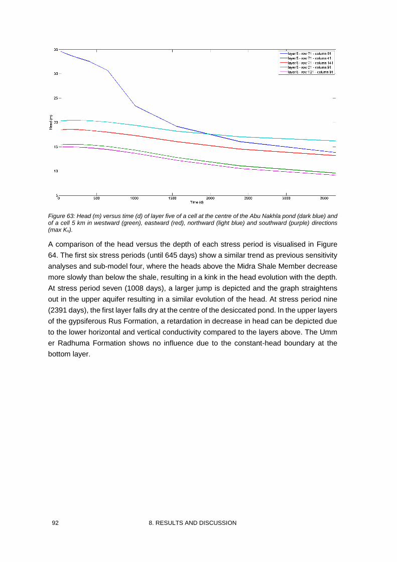
92 8. RESULTS AND DISCUSSION
Figure 63: Head (m) versus time (d) of layer five of a cell at the centre of the Abu Nakhla pond (dark blue) and of a cell 5 km in westward (green), eastward (red), northward (light blue) and southward (purple) directions (max Kv).
A comparison of the head versus the depth of each stress period is visualised in Figure
64. The first six stress periods (until 645 days) show a similar trend as previous sensitivity
analyses and sub-model four, where the heads above the Midra Shale Member decrease
more slowly than below the shale, resulting in a kink in the head evolution with the depth.
At stress period seven (1008 days), a larger jump is depicted and the graph straightens
out in the upper aquifer resulting in a similar evolution of the head. At stress period nine
(2391 days), the first layer falls dry at the centre of the desiccated pond. In the upper layers
of the gypsiferous Rus Formation, a retardation in decrease in head can be depicted due
to the lower horizontal and vertical conductivity compared to the layers above. The Umm
er Radhuma Formation shows no influence due to the constant-head boundary at the
bottom layer.
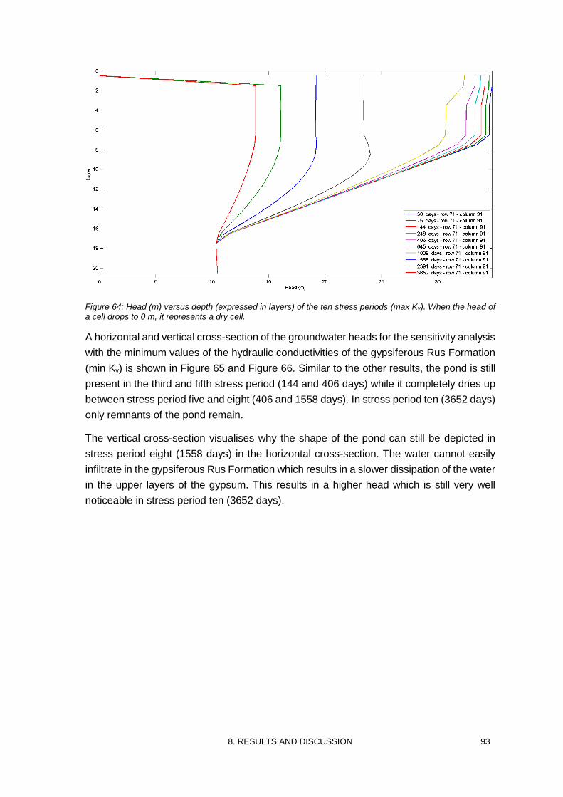
8. RESULTS AND DISCUSSION 93
Figure 64: Head (m) versus depth (expressed in layers) of the ten stress periods (max Kv). When the head of a cell drops to 0 m, it represents a dry cell.
A horizontal and vertical cross-section of the groundwater heads for the sensitivity analysis
with the minimum values of the hydraulic conductivities of the gypsiferous Rus Formation
(min Kv) is shown in Figure 65 and Figure 66. Similar to the other results, the pond is still
present in the third and fifth stress period (144 and 406 days) while it completely dries up
between stress period five and eight (406 and 1558 days). In stress period ten (3652 days)
only remnants of the pond remain.
The vertical cross-section visualises why the shape of the pond can still be depicted in
stress period eight (1558 days) in the horizontal cross-section. The water cannot easily
infiltrate in the gypsiferous Rus Formation which results in a slower dissipation of the water
in the upper layers of the gypsum. This results in a higher head which is still very well
noticeable in stress period ten (3652 days).
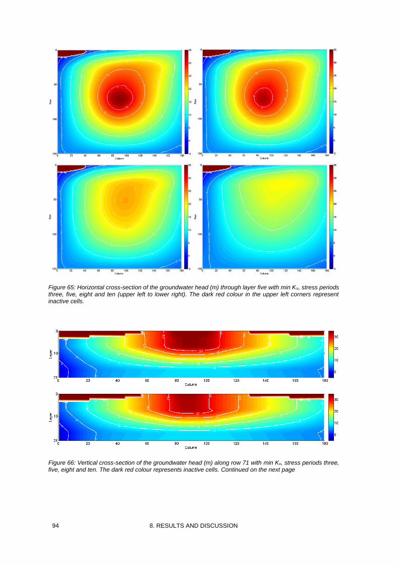
94 8. RESULTS AND DISCUSSION
Figure 65: Horizontal cross-section of the groundwater head (m) through layer five with min Kv, stress periods three, five, eight and ten (upper left to lower right). The dark red colour in the upper left corners represent inactive cells.
Figure 66: Vertical cross-section of the groundwater head (m) along row 71 with min Kv, stress periods three, five, eight and ten. The dark red colour represents inactive cells. Continued on the next page
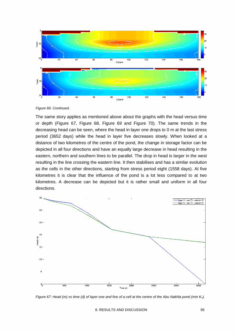
8. RESULTS AND DISCUSSION 95
Figure 66: Continued.
The same story applies as mentioned above about the graphs with the head versus time
or depth (Figure 67, Figure 68, Figure 69 and Figure 70). The same trends in the
decreasing head can be seen, where the head in layer one drops to 0 m at the last stress
period (3652 days) while the head in layer five decreases slowly. When looked at a
distance of two kilometres of the centre of the pond, the change in storage factor can be
depicted in all four directions and have an equally large decrease in head resulting in the
eastern, northern and southern lines to be parallel. The drop in head is larger in the west
resulting in the line crossing the eastern line. It then stabilises and has a similar evolution
as the cells in the other directions, starting from stress period eight (1558 days). At five
kilometres it is clear that the influence of the pond is a lot less compared to at two
kilometres. A decrease can be depicted but it is rather small and uniform in all four
directions.
Figure 67: Head (m) vs time (d) of layer one and five of a cell at the centre of the Abu Nakhla pond (min Kv).
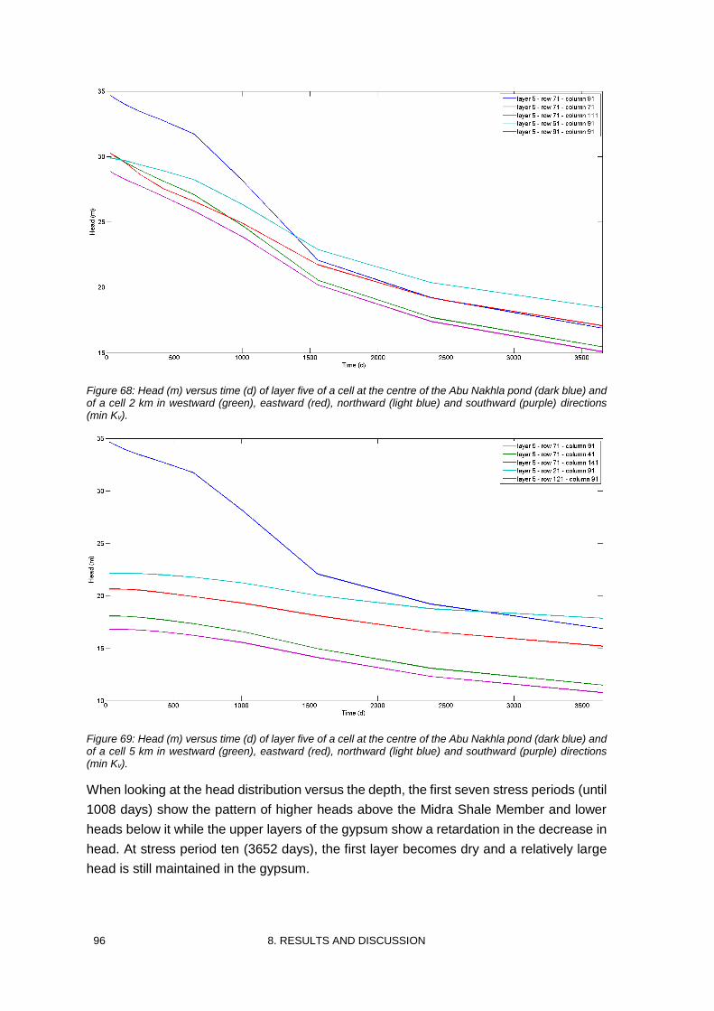
96 8. RESULTS AND DISCUSSION
Figure 68: Head (m) versus time (d) of layer five of a cell at the centre of the Abu Nakhla pond (dark blue) and of a cell 2 km in westward (green), eastward (red), northward (light blue) and southward (purple) directions (min Kv).
Figure 69: Head (m) versus time (d) of layer five of a cell at the centre of the Abu Nakhla pond (dark blue) and of a cell 5 km in westward (green), eastward (red), northward (light blue) and southward (purple) directions (min Kv).
When looking at the head distribution versus the depth, the first seven stress periods (until
1008 days) show the pattern of higher heads above the Midra Shale Member and lower
heads below it while the upper layers of the gypsum show a retardation in the decrease in
head. At stress period ten (3652 days), the first layer becomes dry and a relatively large
head is still maintained in the gypsum.
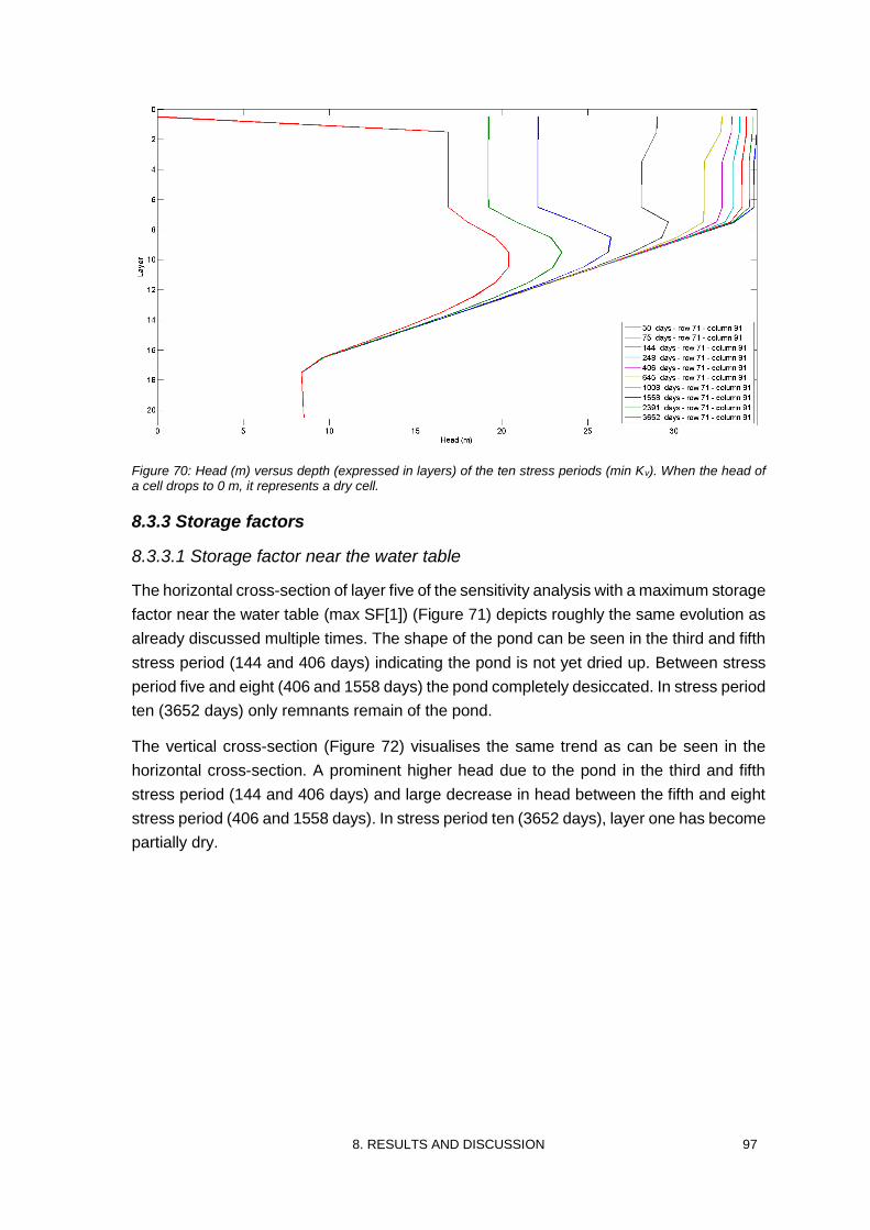
8. RESULTS AND DISCUSSION 97
Figure 70: Head (m) versus depth (expressed in layers) of the ten stress periods (min Kv). When the head of a cell drops to 0 m, it represents a dry cell.
8.3.3 Storage factors
8.3.3.1 Storage factor near the water table
The horizontal cross-section of layer five of the sensitivity analysis with a maximum storage
factor near the water table (max SF[1]) (Figure 71) depicts roughly the same evolution as
already discussed multiple times. The shape of the pond can be seen in the third and fifth
stress period (144 and 406 days) indicating the pond is not yet dried up. Between stress
period five and eight (406 and 1558 days) the pond completely desiccated. In stress period
ten (3652 days) only remnants remain of the pond.
The vertical cross-section (Figure 72) visualises the same trend as can be seen in the
horizontal cross-section. A prominent higher head due to the pond in the third and fifth
stress period (144 and 406 days) and large decrease in head between the fifth and eight
stress period (406 and 1558 days). In stress period ten (3652 days), layer one has become
partially dry.
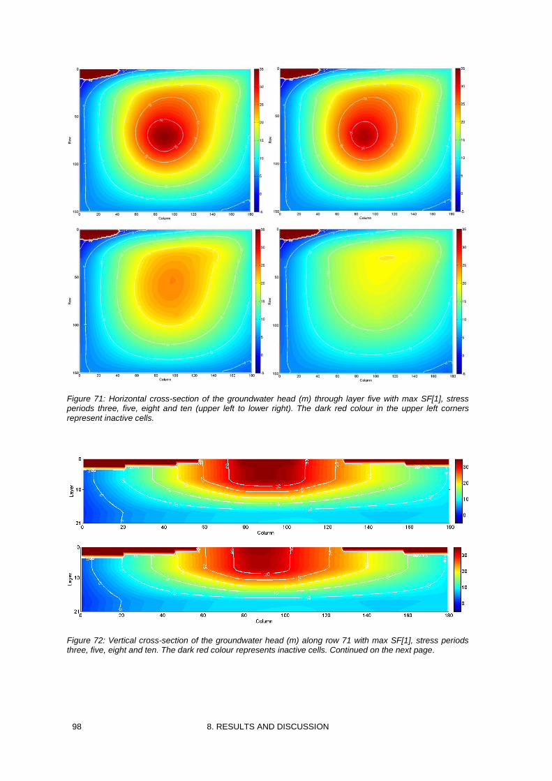
98 8. RESULTS AND DISCUSSION
Figure 71: Horizontal cross-section of the groundwater head (m) through layer five with max SF[1], stress periods three, five, eight and ten (upper left to lower right). The dark red colour in the upper left corners represent inactive cells.
Figure 72: Vertical cross-section of the groundwater head (m) along row 71 with max SF[1], stress periods three, five, eight and ten. The dark red colour represents inactive cells. Continued on the next page.
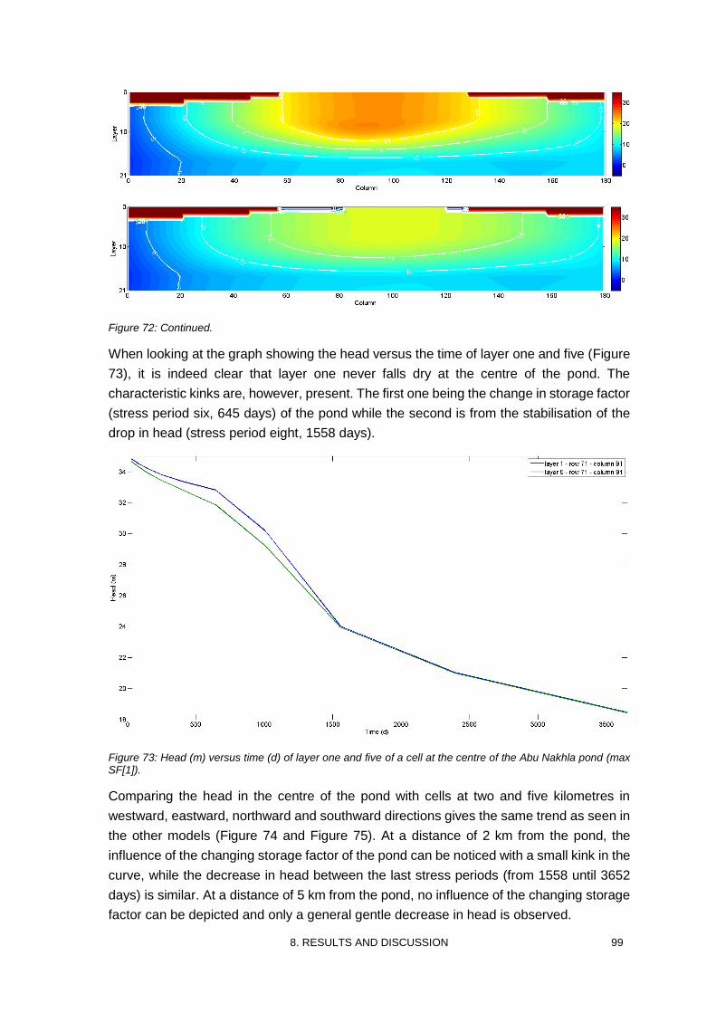
8. RESULTS AND DISCUSSION 99
Figure 72: Continued.
When looking at the graph showing the head versus the time of layer one and five (Figure
73), it is indeed clear that layer one never falls dry at the centre of the pond. The
characteristic kinks are, however, present. The first one being the change in storage factor
(stress period six, 645 days) of the pond while the second is from the stabilisation of the
drop in head (stress period eight, 1558 days).
Figure 73: Head (m) versus time (d) of layer one and five of a cell at the centre of the Abu Nakhla pond (max SF[1]).
Comparing the head in the centre of the pond with cells at two and five kilometres in
westward, eastward, northward and southward directions gives the same trend as seen in
the other models (Figure 74 and Figure 75). At a distance of 2 km from the pond, the
influence of the changing storage factor of the pond can be noticed with a small kink in the
curve, while the decrease in head between the last stress periods (from 1558 until 3652
days) is similar. At a distance of 5 km from the pond, no influence of the changing storage
factor can be depicted and only a general gentle decrease in head is observed.
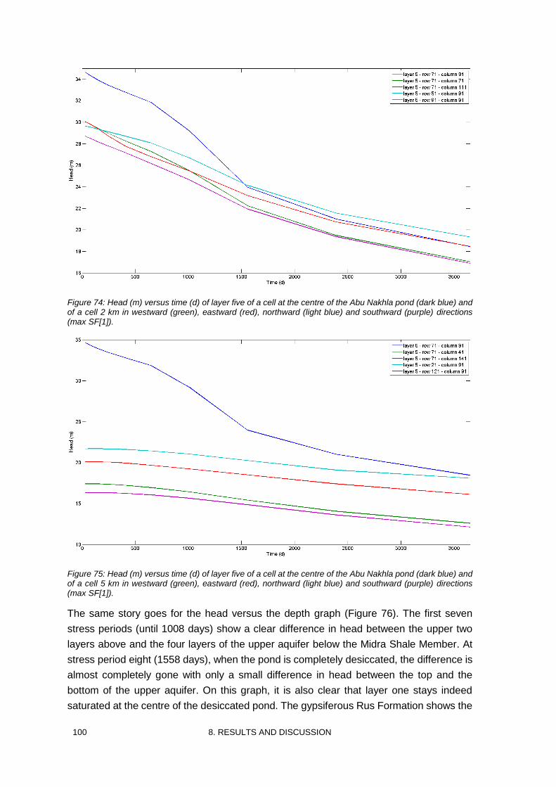
100 8. RESULTS AND DISCUSSION
Figure 74: Head (m) versus time (d) of layer five of a cell at the centre of the Abu Nakhla pond (dark blue) and of a cell 2 km in westward (green), eastward (red), northward (light blue) and southward (purple) directions (max SF[1]).
Figure 75: Head (m) versus time (d) of layer five of a cell at the centre of the Abu Nakhla pond (dark blue) and of a cell 5 km in westward (green), eastward (red), northward (light blue) and southward (purple) directions (max SF[1]).
The same story goes for the head versus the depth graph (Figure 76). The first seven
stress periods (until 1008 days) show a clear difference in head between the upper two
layers above and the four layers of the upper aquifer below the Midra Shale Member. At
stress period eight (1558 days), when the pond is completely desiccated, the difference is
almost completely gone with only a small difference in head between the top and the
bottom of the upper aquifer. On this graph, it is also clear that layer one stays indeed
saturated at the centre of the desiccated pond. The gypsiferous Rus Formation shows the
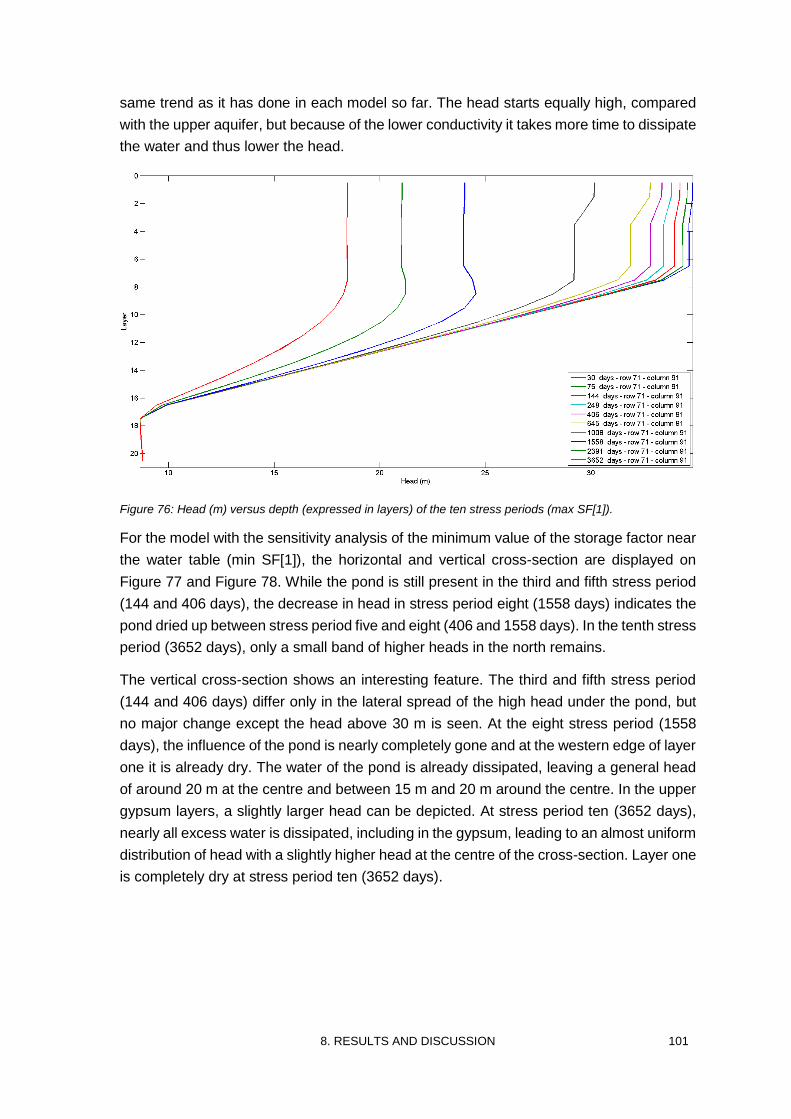
8. RESULTS AND DISCUSSION 101
same trend as it has done in each model so far. The head starts equally high, compared
with the upper aquifer, but because of the lower conductivity it takes more time to dissipate
the water and thus lower the head.
Figure 76: Head (m) versus depth (expressed in layers) of the ten stress periods (max SF[1]).
For the model with the sensitivity analysis of the minimum value of the storage factor near
the water table (min SF[1]), the horizontal and vertical cross-section are displayed on
Figure 77 and Figure 78. While the pond is still present in the third and fifth stress period
(144 and 406 days), the decrease in head in stress period eight (1558 days) indicates the
pond dried up between stress period five and eight (406 and 1558 days). In the tenth stress
period (3652 days), only a small band of higher heads in the north remains.
The vertical cross-section shows an interesting feature. The third and fifth stress period
(144 and 406 days) differ only in the lateral spread of the high head under the pond, but
no major change except the head above 30 m is seen. At the eight stress period (1558
days), the influence of the pond is nearly completely gone and at the western edge of layer
one it is already dry. The water of the pond is already dissipated, leaving a general head
of around 20 m at the centre and between 15 m and 20 m around the centre. In the upper
gypsum layers, a slightly larger head can be depicted. At stress period ten (3652 days),
nearly all excess water is dissipated, including in the gypsum, leading to an almost uniform
distribution of head with a slightly higher head at the centre of the cross-section. Layer one
is completely dry at stress period ten (3652 days).
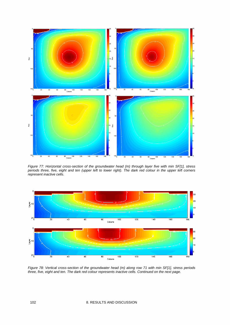
102 8. RESULTS AND DISCUSSION
Figure 77: Horizontal cross-section of the groundwater head (m) through layer five with min SF[1], stress periods three, five, eight and ten (upper left to lower right). The dark red colour in the upper left corners represent inactive cells.
Figure 78: Vertical cross-section of the groundwater head (m) along row 71 with min SF[1], stress periods three, five, eight and ten. The dark red colour represents inactive cells. Continued on the next page.
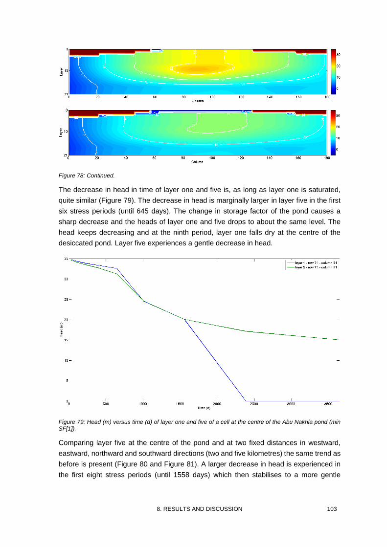
8. RESULTS AND DISCUSSION 103
Figure 78: Continued.
The decrease in head in time of layer one and five is, as long as layer one is saturated,
quite similar (Figure 79). The decrease in head is marginally larger in layer five in the first
six stress periods (until 645 days). The change in storage factor of the pond causes a
sharp decrease and the heads of layer one and five drops to about the same level. The
head keeps decreasing and at the ninth period, layer one falls dry at the centre of the
desiccated pond. Layer five experiences a gentle decrease in head.
Figure 79: Head (m) versus time (d) of layer one and five of a cell at the centre of the Abu Nakhla pond (min SF[1]).
Comparing layer five at the centre of the pond and at two fixed distances in westward,
eastward, northward and southward directions (two and five kilometres) the same trend as
before is present (Figure 80 and Figure 81). A larger decrease in head is experienced in
the first eight stress periods (until 1558 days) which then stabilises to a more gentle
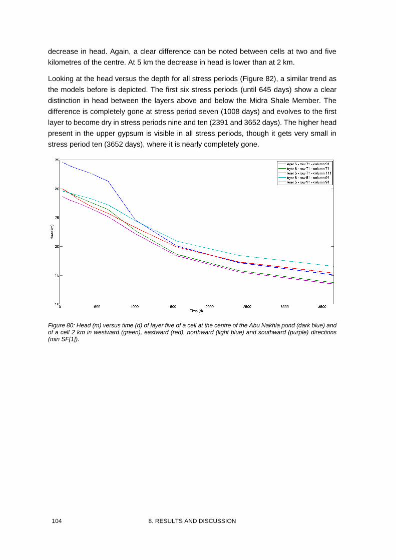
104 8. RESULTS AND DISCUSSION
decrease in head. Again, a clear difference can be noted between cells at two and five
kilometres of the centre. At 5 km the decrease in head is lower than at 2 km.
Looking at the head versus the depth for all stress periods (Figure 82), a similar trend as
the models before is depicted. The first six stress periods (until 645 days) show a clear
distinction in head between the layers above and below the Midra Shale Member. The
difference is completely gone at stress period seven (1008 days) and evolves to the first
layer to become dry in stress periods nine and ten (2391 and 3652 days). The higher head
present in the upper gypsum is visible in all stress periods, though it gets very small in
stress period ten (3652 days), where it is nearly completely gone.
Figure 80: Head (m) versus time (d) of layer five of a cell at the centre of the Abu Nakhla pond (dark blue) and of a cell 2 km in westward (green), eastward (red), northward (light blue) and southward (purple) directions (min SF[1]).
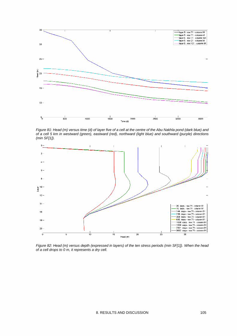
8. RESULTS AND DISCUSSION 105
Figure 81: Head (m) versus time (d) of layer five of a cell at the centre of the Abu Nakhla pond (dark blue) and of a cell 5 km in westward (green), eastward (red), northward (light blue) and southward (purple) directions (min SF[1]).
Figure 82: Head (m) versus depth (expressed in layers) of the ten stress periods (min SF[1]). When the head of a cell drops to 0 m, it represents a dry cell.
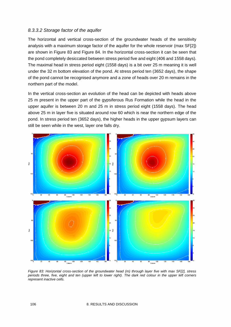
106 8. RESULTS AND DISCUSSION
8.3.3.2 Storage factor of the aquifer
The horizontal and vertical cross-section of the groundwater heads of the sensitivity
analysis with a maximum storage factor of the aquifer for the whole reservoir (max SF[2])
are shown in Figure 83 and Figure 84. In the horizontal cross-section it can be seen that
the pond completely desiccated between stress period five and eight (406 and 1558 days).
The maximal head in stress period eight (1558 days) is a bit over 25 m meaning it is well
under the 32 m bottom elevation of the pond. At stress period ten (3652 days), the shape
of the pond cannot be recognised anymore and a zone of heads over 20 m remains in the
northern part of the model.
In the vertical cross-section an evolution of the head can be depicted with heads above
25 m present in the upper part of the gypsiferous Rus Formation while the head in the
upper aquifer is between 20 m and 25 m in stress period eight (1558 days). The head
above 25 m in layer five is situated around row 60 which is near the northern edge of the
pond. In stress period ten (3652 days), the higher heads in the upper gypsum layers can
still be seen while in the west, layer one falls dry.
Figure 83: Horizontal cross-section of the groundwater head (m) through layer five with max SF[2], stress periods three, five, eight and ten (upper left to lower right). The dark red colour in the upper left corners represent inactive cells.
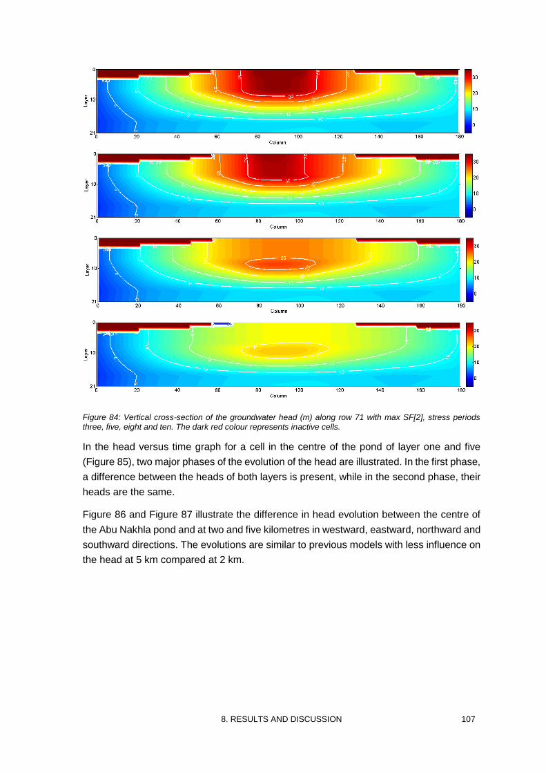
8. RESULTS AND DISCUSSION 107
Figure 84: Vertical cross-section of the groundwater head (m) along row 71 with max SF[2], stress periods three, five, eight and ten. The dark red colour represents inactive cells.
In the head versus time graph for a cell in the centre of the pond of layer one and five
(Figure 85), two major phases of the evolution of the head are illustrated. In the first phase,
a difference between the heads of both layers is present, while in the second phase, their
heads are the same.
Figure 86 and Figure 87 illustrate the difference in head evolution between the centre of
the Abu Nakhla pond and at two and five kilometres in westward, eastward, northward and
southward directions. The evolutions are similar to previous models with less influence on
the head at 5 km compared at 2 km.
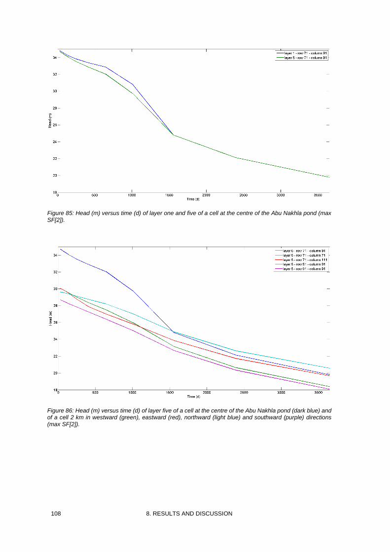
108 8. RESULTS AND DISCUSSION
Figure 85: Head (m) versus time (d) of layer one and five of a cell at the centre of the Abu Nakhla pond (max SF[2]).
Figure 86: Head (m) versus time (d) of layer five of a cell at the centre of the Abu Nakhla pond (dark blue) and of a cell 2 km in westward (green), eastward (red), northward (light blue) and southward (purple) directions (max SF[2]).
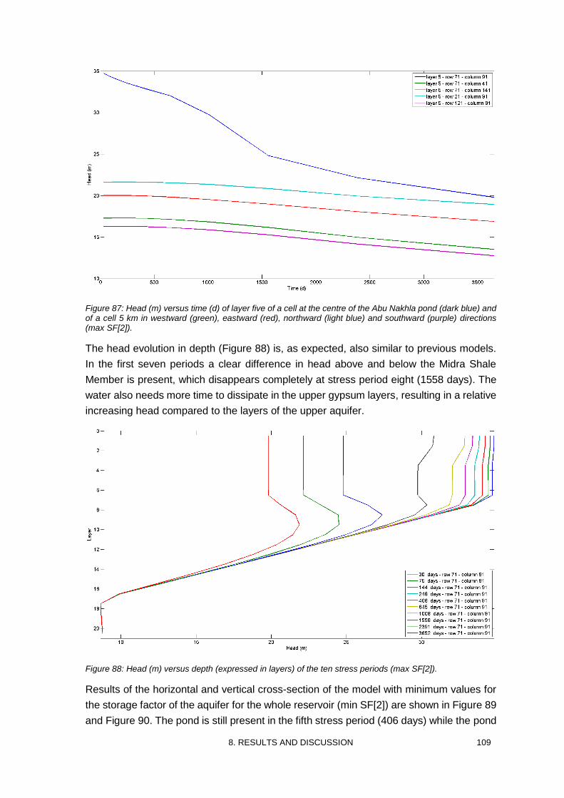
8. RESULTS AND DISCUSSION 109
Figure 87: Head (m) versus time (d) of layer five of a cell at the centre of the Abu Nakhla pond (dark blue) and of a cell 5 km in westward (green), eastward (red), northward (light blue) and southward (purple) directions (max SF[2]).
The head evolution in depth (Figure 88) is, as expected, also similar to previous models.
In the first seven periods a clear difference in head above and below the Midra Shale
Member is present, which disappears completely at stress period eight (1558 days). The
water also needs more time to dissipate in the upper gypsum layers, resulting in a relative
increasing head compared to the layers of the upper aquifer.
Figure 88: Head (m) versus depth (expressed in layers) of the ten stress periods (max SF[2]).
Results of the horizontal and vertical cross-section of the model with minimum values for
the storage factor of the aquifer for the whole reservoir (min SF[2]) are shown in Figure 89
and Figure 90. The pond is still present in the fifth stress period (406 days) while the pond
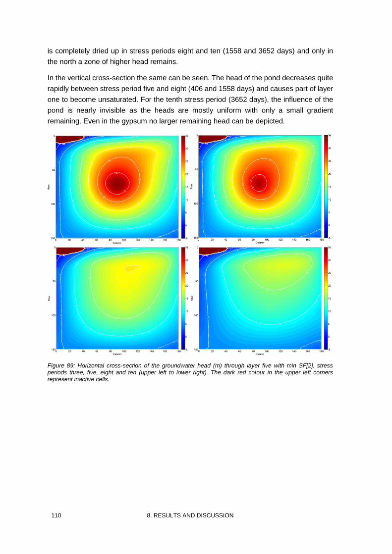
110 8. RESULTS AND DISCUSSION
is completely dried up in stress periods eight and ten (1558 and 3652 days) and only in
the north a zone of higher head remains.
In the vertical cross-section the same can be seen. The head of the pond decreases quite
rapidly between stress period five and eight (406 and 1558 days) and causes part of layer
one to become unsaturated. For the tenth stress period (3652 days), the influence of the
pond is nearly invisible as the heads are mostly uniform with only a small gradient
remaining. Even in the gypsum no larger remaining head can be depicted.
Figure 89: Horizontal cross-section of the groundwater head (m) through layer five with min SF[2], stress periods three, five, eight and ten (upper left to lower right). The dark red colour in the upper left corners represent inactive cells.
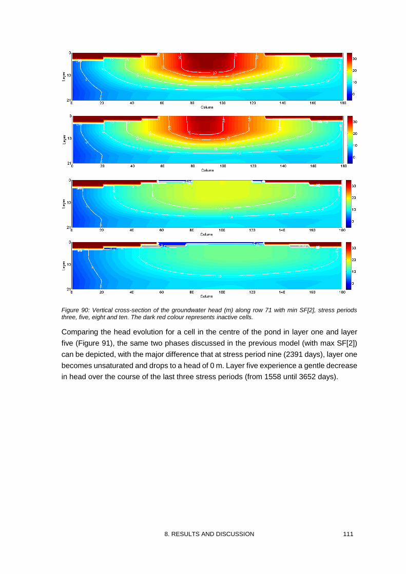
8. RESULTS AND DISCUSSION 111
Figure 90: Vertical cross-section of the groundwater head (m) along row 71 with min SF[2], stress periods three, five, eight and ten. The dark red colour represents inactive cells.
Comparing the head evolution for a cell in the centre of the pond in layer one and layer
five (Figure 91), the same two phases discussed in the previous model (with max SF[2])
can be depicted, with the major difference that at stress period nine (2391 days), layer one
becomes unsaturated and drops to a head of 0 m. Layer five experience a gentle decrease
in head over the course of the last three stress periods (from 1558 until 3652 days).
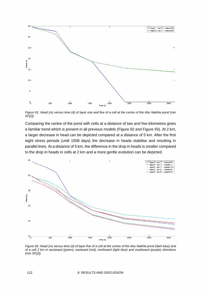
112 8. RESULTS AND DISCUSSION
Figure 91: Head (m) versus time (d) of layer one and five of a cell at the centre of the Abu Nakhla pond (min SF[2]).
Comparing the centre of the pond with cells at a distance of two and five kilometres gives
a familiar trend which is present in all previous models (Figure 92 and Figure 93). At 2 km,
a larger decrease in head can be depicted compared at a distance of 5 km. After the first
eight stress periods (until 1558 days) the decrease in heads stabilise and resulting in
parallel lines. At a distance of 5 km, the difference in the drop in heads is smaller compared
to the drop in heads in cells at 2 km and a more gentle evolution can be depicted.
Figure 92: Head (m) versus time (d) of layer five of a cell at the centre of the Abu Nakhla pond (dark blue) and of a cell 2 km in westward (green), eastward (red), northward (light blue) and southward (purple) directions (min SF[2]).
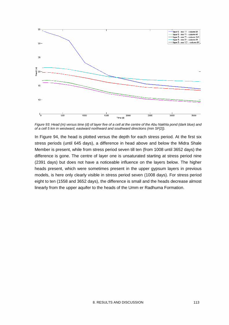
8. RESULTS AND DISCUSSION 113
Figure 93: Head (m) versus time (d) of layer five of a cell at the centre of the Abu Nakhla pond (dark blue) and of a cell 5 km in westward, eastward northward and southward directions (min SF[2]).
In Figure 94, the head is plotted versus the depth for each stress period. At the first six
stress periods (until 645 days), a difference in head above and below the Midra Shale
Member is present, while from stress period seven till ten (from 1008 until 3652 days) the
difference is gone. The centre of layer one is unsaturated starting at stress period nine
(2391 days) but does not have a noticeable influence on the layers below. The higher
heads present, which were sometimes present in the upper gypsum layers in previous
models, is here only clearly visible in stress period seven (1008 days). For stress period
eight to ten (1558 and 3652 days), the difference is small and the heads decrease almost
linearly from the upper aquifer to the heads of the Umm er Radhuma Formation.
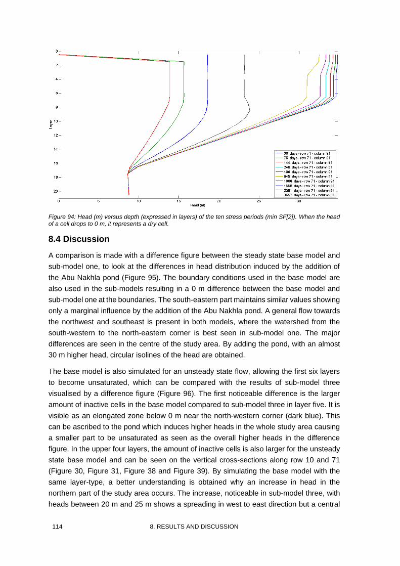
114 8. RESULTS AND DISCUSSION
Figure 94: Head (m) versus depth (expressed in layers) of the ten stress periods (min SF[2]). When the head of a cell drops to 0 m, it represents a dry cell.
8.4 Discussion
A comparison is made with a difference figure between the steady state base model and
sub-model one, to look at the differences in head distribution induced by the addition of
the Abu Nakhla pond (Figure 95). The boundary conditions used in the base model are
also used in the sub-models resulting in a 0 m difference between the base model and
sub-model one at the boundaries. The south-eastern part maintains similar values showing
only a marginal influence by the addition of the Abu Nakhla pond. A general flow towards
the northwest and southeast is present in both models, where the watershed from the
south-western to the north-eastern corner is best seen in sub-model one. The major
differences are seen in the centre of the study area. By adding the pond, with an almost
30 m higher head, circular isolines of the head are obtained.
The base model is also simulated for an unsteady state flow, allowing the first six layers
to become unsaturated, which can be compared with the results of sub-model three
visualised by a difference figure (Figure 96). The first noticeable difference is the larger
amount of inactive cells in the base model compared to sub-model three in layer five. It is
visible as an elongated zone below 0 m near the north-western corner (dark blue). This
can be ascribed to the pond which induces higher heads in the whole study area causing
a smaller part to be unsaturated as seen as the overall higher heads in the difference
figure. In the upper four layers, the amount of inactive cells is also larger for the unsteady
state base model and can be seen on the vertical cross-sections along row 10 and 71
(Figure 30, Figure 31, Figure 38 and Figure 39). By simulating the base model with the
same layer-type, a better understanding is obtained why an increase in head in the
northern part of the study area occurs. The increase, noticeable in sub-model three, with
heads between 20 m and 25 m shows a spreading in west to east direction but a central
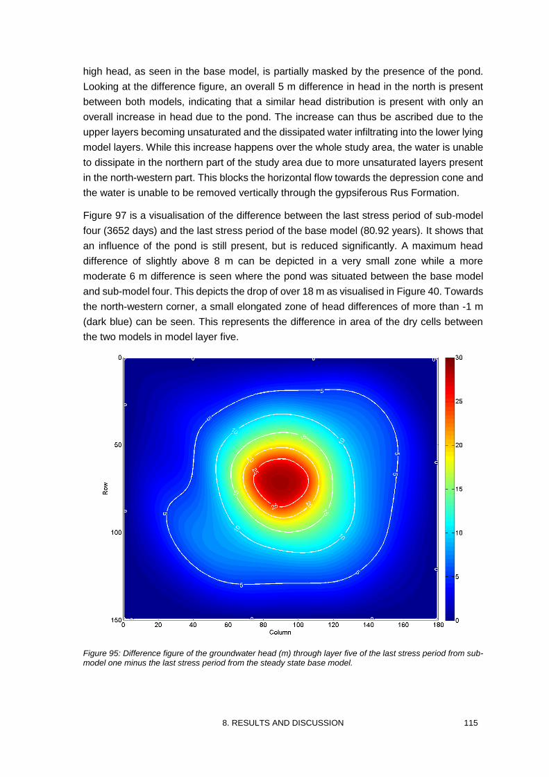
8. RESULTS AND DISCUSSION 115
high head, as seen in the base model, is partially masked by the presence of the pond.
Looking at the difference figure, an overall 5 m difference in head in the north is present
between both models, indicating that a similar head distribution is present with only an
overall increase in head due to the pond. The increase can thus be ascribed due to the
upper layers becoming unsaturated and the dissipated water infiltrating into the lower lying
model layers. While this increase happens over the whole study area, the water is unable
to dissipate in the northern part of the study area due to more unsaturated layers present
in the north-western part. This blocks the horizontal flow towards the depression cone and
the water is unable to be removed vertically through the gypsiferous Rus Formation.
Figure 97 is a visualisation of the difference between the last stress period of sub-model
four (3652 days) and the last stress period of the base model (80.92 years). It shows that
an influence of the pond is still present, but is reduced significantly. A maximum head
difference of slightly above 8 m can be depicted in a very small zone while a more
moderate 6 m difference is seen where the pond was situated between the base model
and sub-model four. This depicts the drop of over 18 m as visualised in Figure 40. Towards
the north-western corner, a small elongated zone of head differences of more than -1 m
(dark blue) can be seen. This represents the difference in area of the dry cells between
the two models in model layer five.
Figure 95: Difference figure of the groundwater head (m) through layer five of the last stress period from sub-model one minus the last stress period from the steady state base model.
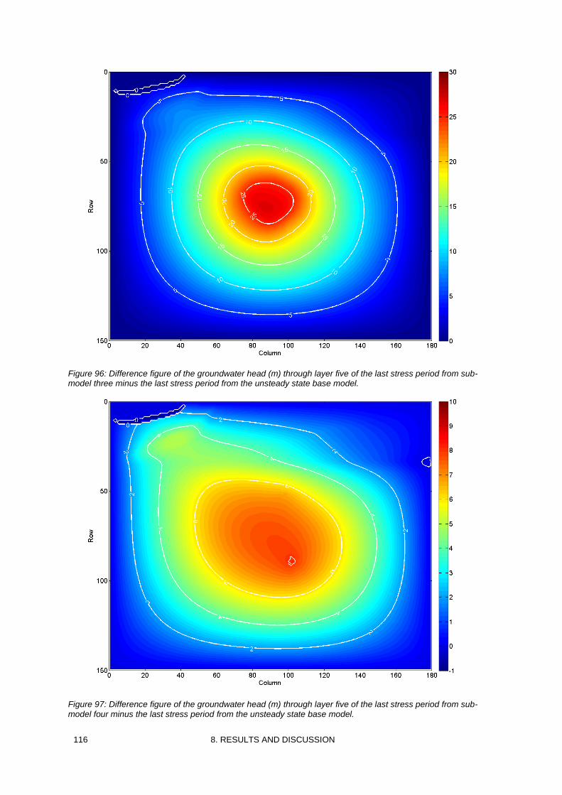
116 8. RESULTS AND DISCUSSION
Figure 96: Difference figure of the groundwater head (m) through layer five of the last stress period from sub-model three minus the last stress period from the unsteady state base model.
Figure 97: Difference figure of the groundwater head (m) through layer five of the last stress period from sub-model four minus the last stress period from the unsteady state base model.
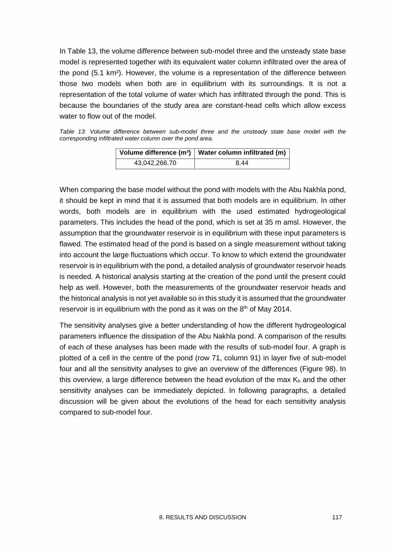
8. RESULTS AND DISCUSSION 117
In Table 13, the volume difference between sub-model three and the unsteady state base
model is represented together with its equivalent water column infiltrated over the area of
the pond (5.1 km²). However, the volume is a representation of the difference between
those two models when both are in equilibrium with its surroundings. It is not a
representation of the total volume of water which has infiltrated through the pond. This is
because the boundaries of the study area are constant-head cells which allow excess
water to flow out of the model.
Table 13: Volume difference between sub-model three and the unsteady state base model with the corresponding infiltrated water column over the pond area.
Volume difference (m³) Water column infiltrated (m)
43,042,266.70 8.44
When comparing the base model without the pond with models with the Abu Nakhla pond,
it should be kept in mind that it is assumed that both models are in equilibrium. In other
words, both models are in equilibrium with the used estimated hydrogeological
parameters. This includes the head of the pond, which is set at 35 m amsl. However, the
assumption that the groundwater reservoir is in equilibrium with these input parameters is
flawed. The estimated head of the pond is based on a single measurement without taking
into account the large fluctuations which occur. To know to which extend the groundwater
reservoir is in equilibrium with the pond, a detailed analysis of groundwater reservoir heads
is needed. A historical analysis starting at the creation of the pond until the present could
help as well. However, both the measurements of the groundwater reservoir heads and
the historical analysis is not yet available so in this study it is assumed that the groundwater
reservoir is in equilibrium with the pond as it was on the 8th of May 2014.
The sensitivity analyses give a better understanding of how the different hydrogeological
parameters influence the dissipation of the Abu Nakhla pond. A comparison of the results
of each of these analyses has been made with the results of sub-model four. A graph is
plotted of a cell in the centre of the pond (row 71, column 91) in layer five of sub-model
four and all the sensitivity analyses to give an overview of the differences (Figure 98). In
this overview, a large difference between the head evolution of the max Kh and the other
sensitivity analyses can be immediately depicted. In following paragraphs, a detailed
discussion will be given about the evolutions of the head for each sensitivity analysis
compared to sub-model four.
118 8. RESULTS AND DISCUSSION
Figure 98: Overview the head (m) versus time (d) of a cell in the centre of the pond in layer five of sub-model four and the sensitivity analyses.
When the horizontal conductivity is increased for the first seven model layers (upper
aquifer, max Kh), it can be expected that water will be able to dissipate faster. The rapid
decrease in head is present throughout the whole study area. The influence of the large
storage factor of the pond is larger and the difference in head above and below the Midra
Shale Member is also more pronounced. A big contrast exists between the upper aquifer
and the gypsiferous Rus Formation. The retardation of the dissipation of the water is much
larger compared to sub-model four.
When decreasing the horizontal conductivity (min Kh), the decrease in head slows down.
Even though the rate of decrease in head is a lot different than sub-model four, it should
be kept in mind that the sensitivity factor is smaller compared to the other sensitivity
analyses.
When the vertical conductivity of the gypsiferous Rus Formation is increased (max Kv),
only a relatively small change in decrease rate is obtained. The excess water is able to
penetrate more easily into the gypsum, causing the head to be lowered faster. However,
the change in decrease rate is rather low compared to the large sensitivity factor used.
After the jump in head due to the change of the storage factor of the pond in the upper
aquifer, only one stress period is needed to obtain an equilibrium between the head in the
upper aquifer and the head in the gypsum. This is much faster than sub-model four where
a slight increased head can still be depicted after three stress periods. Another difference
is that the heads in the Umm er Radhuma Formation are larger than in sub-model four. In
sub-model four it is below ten meters, while with the higher vertical conductivity it is above
ten meters. This is because more water is able to flow through the gypsum leading to a
higher head in the underlying UER in the steady state flow model (sub-model one). The
8. RESULTS AND DISCUSSION 119
bottom layer of the UER is then set as constant-head cells for the unsteady state flow
models (sub-model two, three and four) with these higher heads.
When decreasing the vertical conductivity of the gypsum layers (min Kv), the effect of the
slower dissipation of the water in the gypsum is increased. Besides the larger remaining
head in the gypsum layers, the head of the upper aquifer is similar and is only slightly
larger than the upper aquifer heads of sub-model four. However, the pond does desiccate
slower since the change in storage factor of the pond happens between stress periods
seven and eight (1008 and 1558 days), while it happens between stress periods six and
seven (645 and 1008 days) in sub-model four.
The storage factor near the water table (SF[1]) and the storage factor of the aquifer (SF[2])
are changed independently. This makes it possible to determine which one has the largest
influence on the dissipation of the pond. When increasing the storage factor near the water
table (max SF[1]), the drop in head is smaller compared to sub-model four. This is as to
be expected because a larger storage factor results in more water able to be stored which
is able to counteract the decrease in head more extensively. The decrease in head is
indeed smaller and the difference between the head of the upper aquifer and of the
gypsum is noticeably smaller than in sub-model four. It is, of course, relative as the heads
in the upper aquifer are higher thus reducing the difference.
Lowering the storage factor near the water table (min SF[1]) induces a larger decrease in
head compared to sub-model four. A larger drop happens when the storage factor of the
pond changes and due to the smaller storage factor, only a small volume of water is able
to be released from the storage to counteract this drop. A larger difference in head between
the upper aquifer and the gypsum layers when the storage factor is decreased is present.
When the storage factor of the aquifer over the whole reservoir (max SF[2]) is increased,
a similar trend is seen as with the increase of the storage factor near the water table. Due
to the increase in storage capacity, the head decrease is lower compared with sub-model
four due to the larger counteraction against the decrease in head. Looking at cells away
from the centre, the decrease in head remains lower and at five kilometres of the centre
of the pond, the decrease in head is minimal and stays nearly constant in the northward
direction. When the heads versus the depths are compared, a noticeable difference in
head distribution between the upper aquifer and the gypsiferous Rus Formation is present.
In sub-model four the head difference between the gypsum and the upper aquifer is almost
completely gone in the last stress period (3652 days), while it is still clearly present in the
model with increased storage factors of the aquifer. This is because the larger storage
factor can strongly counteract the decrease in head by releasing large volumes of water
and thus a higher head can be maintained.
Lowering the storage factor of the aquifer (min SF[2]) results in a faster decrease in head
compared to sub-model four. Even at two and five kilometres of the pond, the difference
is quite extensive but, as in the other models, the trend is rather similar. Looking at the
head versus depth, the major difference is, again, in the gypsiferous Rus Formation. Only
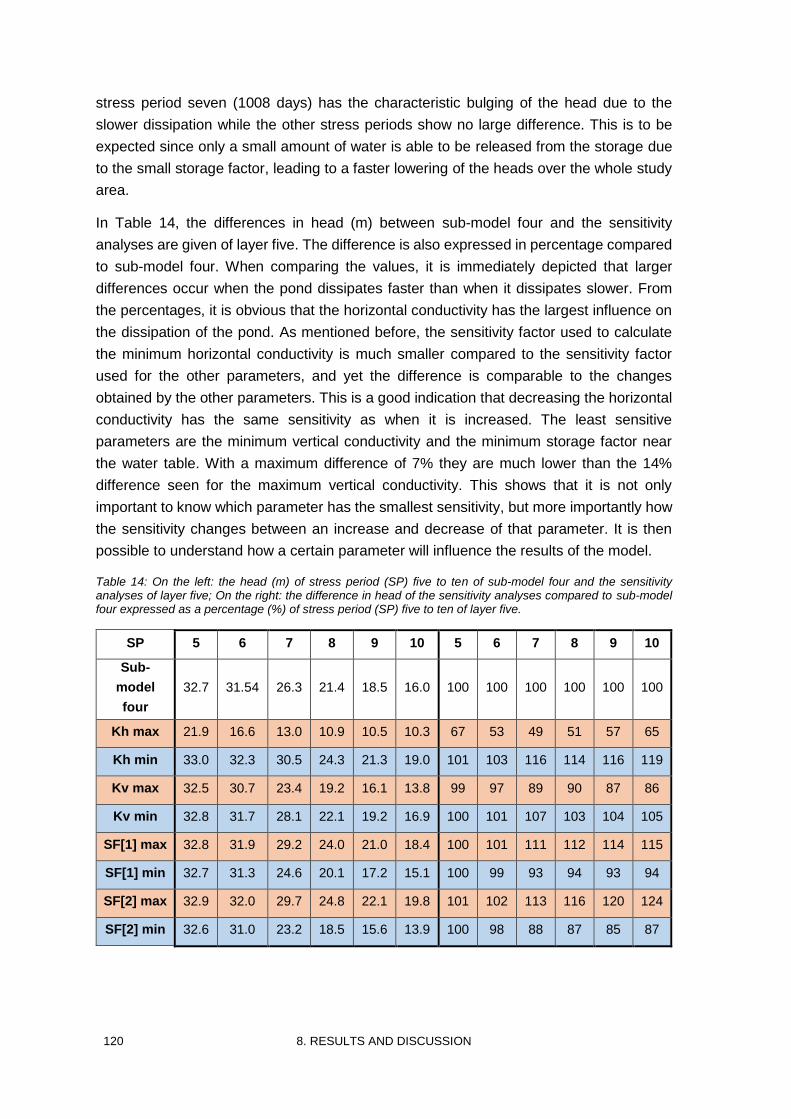
120 8. RESULTS AND DISCUSSION
stress period seven (1008 days) has the characteristic bulging of the head due to the
slower dissipation while the other stress periods show no large difference. This is to be
expected since only a small amount of water is able to be released from the storage due
to the small storage factor, leading to a faster lowering of the heads over the whole study
area.
In Table 14, the differences in head (m) between sub-model four and the sensitivity
analyses are given of layer five. The difference is also expressed in percentage compared
to sub-model four. When comparing the values, it is immediately depicted that larger
differences occur when the pond dissipates faster than when it dissipates slower. From
the percentages, it is obvious that the horizontal conductivity has the largest influence on
the dissipation of the pond. As mentioned before, the sensitivity factor used to calculate
the minimum horizontal conductivity is much smaller compared to the sensitivity factor
used for the other parameters, and yet the difference is comparable to the changes
obtained by the other parameters. This is a good indication that decreasing the horizontal
conductivity has the same sensitivity as when it is increased. The least sensitive
parameters are the minimum vertical conductivity and the minimum storage factor near
the water table. With a maximum difference of 7% they are much lower than the 14%
difference seen for the maximum vertical conductivity. This shows that it is not only
important to know which parameter has the smallest sensitivity, but more importantly how
the sensitivity changes between an increase and decrease of that parameter. It is then
possible to understand how a certain parameter will influence the results of the model.
Table 14: On the left: the head (m) of stress period (SP) five to ten of sub-model four and the sensitivity analyses of layer five; On the right: the difference in head of the sensitivity analyses compared to sub-model four expressed as a percentage (%) of stress period (SP) five to ten of layer five.
SP 5 6 7 8 9 10 5 6 7 8 9 10
Sub-
model
four
32.7 31.54 26.3 21.4 18.5 16.0 100 100 100 100 100 100
Kh max 21.9 16.6 13.0 10.9 10.5 10.3 67 53 49 51 57 65
Kh min 33.0 32.3 30.5 24.3 21.3 19.0 101 103 116 114 116 119
Kv max 32.5 30.7 23.4 19.2 16.1 13.8 99 97 89 90 87 86
Kv min 32.8 31.7 28.1 22.1 19.2 16.9 100 101 107 103 104 105
SF[1] max 32.8 31.9 29.2 24.0 21.0 18.4 100 101 111 112 114 115
SF[1] min 32.7 31.3 24.6 20.1 17.2 15.1 100 99 93 94 93 94
SF[2] max 32.9 32.0 29.7 24.8 22.1 19.8 101 102 113 116 120 124
SF[2] min 32.6 31.0 23.2 18.5 15.6 13.9 100 98 88 87 85 87
8. RESULTS AND DISCUSSION 121
In the case of the minimum vertical conductivity of the gypsiferous Rus Formation it can
be deducted that the small difference, compared to sub-model four, is because the normal
vertical conductivity value is already small. Decreasing this small value results in changing
from nearly no water being infiltrated in the gypsum to even less water infiltrating into the
gypsum. An increase of this parameter has more influence because more water is able to
infiltrate into the gypsum. The gypsum is a thick layer and a large amount of water can
suddenly be stored and transported through this gypsum resulting in a much higher
sensitivity.
To understand the low sensitivity when lowering the storage factor near the water table, a
closer look must be taken to the total storage of the study area. A simplification is made
since the concept is more important than the exact calculation. The total storage could
then be written as:
𝑇𝑜𝑡𝑎𝑙 𝑠𝑡𝑜𝑟𝑎𝑔𝑒 = 𝑆𝑠𝐷 + 𝑆0 (17)
Total storage is the total storage of the reservoir
Ss (m-1) is the specific elastic storage (storage coefficient of the aquifer)
D (m) is the thickness of the reservoir
S0 (-) is the storage coefficient near the water table
The storage coefficient near the water table only depends on the change in head of the
water table while the elastic storage coefficient is dependent on the change in head over
the whole reservoir. The specific elastic storage is multiplying by the thickness of the whole
reservoir resulting in the storage factor of the aquifer for the whole reservoir. When the
normal values of the storage factors are used, the storage factor of the aquifer is then
about two times larger than the storage factor near the water table. When the storage
factor near the water table is then divided by the sensitivity factor, the sensitivity will be
low because the absolute difference of the total storage is much smaller than when the
storage factor near the water table is multiplied by the sensitivity factor. In other words,
when the total storage is only slightly smaller, the difference in head, compared with sub-
model four, will only be slightly different.

122 8. RESULTS AND DISCUSSION
9. CONCLUSION 123
9. CONCLUSION
The influence of the Abu Nakhla pond on the phreatic aquifer was studied by use of
numerical models based on the MODFLOW-code. To discuss the model construction and
results more easily, the study has been subdivided into two parts: (1) the simulation of the
present state and the desiccation and dissipation of the Abu Nakhla pond and (2) the
sensitivity analysis to check which hydrogeological parameters have the most influence
on the dissipation of the Abu Nakhla pond under the same constant climatic conditions
(evaporation and recharge).
To simulate the first part, a base model was created. The horizontal and vertical
discretisation comprised of 150 rows, 180 columns and 21 layers. This base model was
constructed with all hydraulic parameters which are independent of the Abu Nakhla pond.
These hydraulic parameters comprise of the transmissivity, storage factors and the
reciprocal value of the hydraulic resistance. The hydraulic parameters, the initial heads
and the initial concentrations were estimated based on values found in literature or from
field measurements. This base model allowed to evaluate the base input parameters and
to have a stable model where the pond can be added later on. The base model represents
the head distribution of the groundwater reservoir in equilibrium with the climatic conditions
when no pond is present. This equilibrium mainly depends on the estimated hydraulic
parameters together with the constant head of the boundaries, estimated from the
potentiometric surface map. A watershed running from the south-western corner to the
north-eastern corner can be depicted. When allowing cells to become dry (a model-
technical option, layer-type), a different head distribution was obtained. A large increase
in head in the north-eastern quadrant can be ascribed to the top layers becoming dry and
holding the water in place. The Abu Nakhla pond was then added to the stable base model,
using the same horizontal and vertical discretisation and boundary conditions. To simulate
the desiccation and dissipation of the Abu Nakhla pond, it was assumed that an equilibrium
exists between the pond, with a head of 35 m amsl, and the groundwater reservoir. Four
sub-models were introduced, each using results obtained from the previous sub-model.
These sub-models were: (1) a steady state flow where the pond is introduced, (2) a model
mimicking steady state flow but using an unsteady state flow model, (3) a full unsteady
state flow model and (4) the simulation of the desiccation and dissipation of the Abu Nakhla
pond. The pond was added with constant-head cells with a head equal to 35 m amsl, which
was the level measured on the 8th of May 2015. By adding the Abu Nakhla pond into the
model, the watershed was expressed more explicit. Similar to the base model, an increase
in the north-eastern quadrant can be depicted when allowing cells to become dry. When
plotting the head versus time and depth, as the pond was desiccating under constant
climatic conditions and was dissipating into the phreatic aquifer, three major features can
be depicted. The first and most important feature being the switch between the storage
factor of the pond (=1) to the storage factor near the water table (=0.0104). It was
associated with a sudden drop of the head because a small storage factor can only release
a small volume of water compared to a large storage factor which can release a large
124 9. CONCLUSION
volume of water to counteract a drop in head. In other words, the drop in head will be lower
when the volume of water able to be released by the storage factor is larger. A similar
trend can be depicted at a distance of 2 km from the centre of the pond but it cannot be
depicted at a distance of 5 km, where only a small drop in head is present. The second
feature is the difference in head above and below the Midra Shale Member. This can be
ascribed to the lower vertical conductivity of the Midra Shale Member, which acts as a flow
barrier that the higher heads, due to the influence of the large storage factor of the pond,
will not dissipate into the underlying layers. When the storage factor of the pond is
removed, the higher heads disappears. The third feature is the slower dissipation of the
water in the upper layers of the gypsiferous Rus Formation. When the constant level of the
pond is removed, the water in the upper aquifer dissipates quickly, resulting in a fast
decrease in head while the dissipation of water in the gypsum is much slower, resulting in
a slow decrease in head. The different decrease rates result in a large difference in head
between the upper aquifer and the gypsiferous Rus Formation and when the decrease in
head stabilises for the upper aquifer, the difference in head will become smaller.
A calculation of the volume difference between the base model and sub-model three was
made to illustrate the influence of the pond on the groundwater reservoir in the study area.
A volume of 43,042,266.70 m³ was found which corresponds to an infiltrated water column
of 8.44 m over the area of the Abu Nakhla pond (5.1 km²). This is, however, not the total
amount of water infiltrated but reflects the difference in volume in the study area with the
groundwater reservoir in equilibrium without the pond and in equilibrium with a pond with
a head of 35 m amsl because excess water will be removed at the constant-head
boundaries. A simulation of the historical evolution of the pond would allow to calculate the
total infiltrated volume since the creation of the pond.
After the simulation of the base model and the model of the dissipation and desiccation of
the pond, it was subjected to a series of sensitivity analyses. A total of four hydraulic
parameters were subjected to a sensitivity analysis in which the hydraulic parameters were
multiplied and divided by a sensitivity factor of 100.5, resulting in a total of eight sensitivity
analyses. The hydraulic parameters which were subjected to a sensitivity analysis are: the
horizontal conductivity of the upper aquifer, the vertical conductivity of the gypsiferous Rus
Formation, the storage factor near the water table and the storage factor of the aquifer (for
the whole reservoir). The sensitivity analyses show the same three features as described
above, when plotting the head versus the time and depth. Depending on which parameter
was subjected to the sensitivity analysis and if it was increased or decreased, one or more
feature(s) were more or less pronounced. Comparing the differences in head between the
sensitivity analyses and sub-model four reveals which parameters were the most sensitive
in terms of the dissipation of the Abu Nakhla pond. The horizontal conductivity of the upper
seven layers was by far the most sensitive parameter. Both an increase and decrease of
the parameter shows an equal relative increase or decrease of the head, keeping in mind
that the sensitivity factor used for decreasing the horizontal conductivity is smaller (factor
100.1). The least sensitive parameters were decreasing the vertical conductivity of the
9. CONCLUSION 125
gypsiferous Rus Formation and decreasing the storage factor near the water table. The
low sensitivity of the vertical conductivity can be ascribed to the fact that the normal vertical
conductivity is already so low that only a very small amount of water will penetrate into the
gypsiferous Rus Formation and decreasing this low value will only have a small additional
effect. For the decreased storage factor near the water table, the low sensitivity can be
ascribed to the large influence of the storage factor of the aquifer. When calculating the
total storage, the sum of the storage factor near the water table and the storage factor of
the aquifer, the whole reservoir must be taken into account resulting in the normal value
for the storage factor of the aquifer of the whole reservoir being roughly two times larger
than the storage factor near the water table. When this relatively small value is then
lowered, the absolute value of the total storage will only decrease slightly. When increasing
the value, the absolute value of the total storage will have a much larger increase
compared to the decrease. This is the cause of the non-linear behaviour of the sensitivity.
The aim of this study comprised of modelling present and future scenarios of the Abu
Nakhla pond in respect to the influence on the phreatic aquifer and this aim has been
achieved. The influence of the pond on the phreatic aquifer can be seen in the volume
difference between the base model and sub-model three. It shows the infiltrated volume
in the study area due to the presence of the pond when an equilibrium exists between the
pond and the groundwater reservoir. The future scenarios comprise of a dissipation of the
pond with a set of chosen base parameters and sensitivity analyses which check the
influence of the estimated parameters on the dissipation.
It can be concluded that the pond does have a clear influence in the study area, but that
the influence rapidly disappears when going beyond 5 km from the centre of the pond. It
was also clear that quite some time will pass until the influence of the pond is completely
gone and that the rate of the dissipation is mainly influenced by the horizontal conductivity
of the upper aquifer.
Further research could be a simulation of the historical evolution of the pond which, on the
one hand, could be used to calculate the effective volume of water which has been
infiltrated and on the other hand check if the groundwater reservoir is truly in equilibrium
with a pond with a head of 35 m amsl . Measurements of the effective hydraulic parameters
present in the study area and adding the injection of the pond water could improve the
model so that a clearer understanding of the dissipation of the pond can be made.

126 9. CONCLUSION
10. NEDERLANDSTALIGE SAMENVATTING 127
10. NEDERLANDSTALIGE SAMENVATTING
Het Abu Nakhla meer is gelegen in Qatar, net buiten de hoofdstad Doha. Het meer is in
de jaren ’70 ontstaan uit noodzaak om het overtollige afvalwater, afkomstig van de stad,
op te vangen. Het ontvangt behandeld afvalwater afkomstig uit twee
afvalwaterzuiveringsinstallaties: Doha West en Doha South. Door de snelle expansie van
de stad Doha is er beslist om het meer te laten droogvallen zodanig dat het gebied ook
kan aangewend worden voor bouwprojecten. Deze studie heeft als doel om een numeriek
grondwater stromingsmodel op te stellen die de huidige toestand (8 mei 2014) modelleert,
waarbij uitgegaan wordt van de veronderstelling dat het meer in evenwicht is met het
grondwaterreservoir, om daarna de uitdroging en de verspreiding van het water in het
grondwaterreservoir van het meer te modelleren. Daarnaast is er ook een
gevoeligheidsanalyse uitgevoerd, waarbij onderzocht werd welke hydrogeologische
parameters de grootste invloed uitoefenen op deze verspreiding van het water in het
grondwaterreservoir.
Het schiereiland Qatar heeft een lengte van 189 km in noord-zuid richting en een breedte
die schommelt tussen de 55 km en 85 km in oost-west richting. De totale oppervlakte van
het land bedraagt 11 586 km² en wordt gekenmerkt door zijn woestijn karakter. Het reliëf
is relatief vlak met een maximale hoogte tot 103 m. De economie bestaat voornamelijk uit
de ontginning van hun natuurlijk gas en olie en de visvangst.
Het Abu Nakhla meer is ongeveer 3,1 km in oost-west richting en ongeveer 2,5 km in
noord-zuid richting en heeft een oppervlak van 5,1 km. Een volume van ongeveer 50 000
m³ tot 100 000 m³ wordt dagelijks geloosd in het Abu Nakhla meer. Het meer kan een
totaal volume van ongeveer 20 miljoen m³ aan water bevatten. De gemiddelde dagelijkse
infiltratie en evaporatie bedraagt samen ongeveer 50 000 m³.
Om de numerieke modellen van het grondwaterreservoir op te stellen is een gedetailleerde
studie nodig van de ondergrond. De aanwezige structurele geologie van Qatar bestaat uit
een grote anticline die van noord naar zuid loopt doorheen het midden van Qatar. Deze
wordt de Qatar Arch genoemd en heeft een declinatie in de noordelijke richting.
Verscheidene kleinere longitudinale plooien liggen boven op deze anticline: de Simsima
Dome/Arch in het noordoosten en de Dukhan anticline in het westen. Rondom deze
Dukhan anticline liggen verscheidene anticlinale en synclinale structuren. Aan het
oppervlak dagzoomt voornamelijk de Dammam Formatie. Deze representeert ongeveer
80% van de totale landoppervlakte. De Midden-Eocene Rus Formatie dagzoomt ongeveer
op 10% van het landoppervlak en is verspreid in kleinere zones. Kijkende naar de
stratigrafie, dan zijn er drie belangrijke formaties die van belang zijn voor deze studie: de
Umm er Radhuma Formatie (UER), de Rus Formatie en de Dammam Formatie.
De UER is de oudste formatie van het vroeg-Eoceen. De UER heeft een dikte tussen de
270 m en 370 m en de lithologie is gedomineerd door een carbonaat facies met dolomiet
128 10. NEDERLANDSTALIGE SAMENVATTING
en kalksteen. Op 20 m onder de top is een silicieuze kalksteenlaag aanwezig die de
hydraulische connectiviteit tussen de bovenste UER en onderste UER beperkt.
De Rus Formatie ligt bovenop de UER en is gedateerd als Ieperiaan. De formatie is
onderverdeeld in twee leden: het Traina lid en het Al-Khor lid. De totale dikte van de Rus
Formatie bedraagt ongeveer 128 m en de lithologie is voornamelijk (dolomitische)
kalksteen. De formatie kan onderverdeeld worden in twee provincies: de noordelijke
provincie, gekenmerkt door de aanwezigheid van een depositioneel carbonaat facies en
een residueel sulfaat facies, en de zuidelijke provincie, gekenmerkt door de aanwezigheid
van een depositioneel sulfaat facies. Het studiegebied ligt in de zuidelijke provincie en het
depositioneel sulfaat facies gedraagt zich als aquitard.
De Dammam Formatie is van midden-Eoceen ouderdom en is onderverdeeld in vier leden,
van oud naar jong: het Midra Shale lid, het Dukhan lid, het Umm Bab lid en het Abaruq lid.
De dikte van de formatie varieert tussen de 30 m en 52 m. De lithologie bestaat
voornamelijk uit (dolomitische) kalksteen behalve voor het Midra Shale lid dat een schalie
is.
Naast de geologie is ook de hydrogeologie van belang bij het opstellen van het model.
Hierbij worden er twee aquifers beschouwd en één aquitard. De aquifers bestaan uit de
“upper aquifer” en de “lower” aquifer. De upper aquifer is een combinatie van de Dammam
Formatie het bovenste gedeelte van en Rus Formatie. De lower aquifer bestaat uit de
Umm er Radhuma Formatie. Deze bovenste Rus Formatie bestaat uit een carbonaat
facies. Het Midra Shale lid is ook aanwezig in deze upper aquifer en acteert als een dunne
ondoorlatende laag binnenin de upper aquifer, maar zal door zijn geringe dikte eerder
weinig invloed uitoefenen. De aquitard, die uit de “upper” van de “lower” aquifer scheidt,
bestaat uit de onderste Rus Formatie. Deze is opgebouwd uit het depositioneel sulfaat
facies en bevat verscheidene dikke gipspakketten. Onder deze aquitard ligt de UER
aquifer waarbij, zoals eerder vermeld, het bovenste gedeelte van de aquifer van het
onderste gedeelte gescheiden wordt door de aanwezigheid van een silicieuze
kalksteenlaag.
De stijghoogte distributie zoals deze teruggevonden wordt in de literatuur geeft een
algemeen beeld voor zowel de UER, Rus en Dammam formaties. De stijghoogte distributie
van de UER is aanwezig op regionale schaal over het Arabische schiereiland. In Qatar,
een daling in de UER van 6 m boven het zeeniveau in het zuiden tot 3 m boven het
zeeniveau in het noorden is aanwezig. De stijghoogte distributie van de Rus Formatie
wordt aan de grenzen van Qatar door de zee beïnvloed wat leidt tot een daling tot 0 m.
Een verschil tussen de noordelijke en de zuidelijke provincie is aanwezig worden waarbij
in de noordelijke provincie de stijghoogtes hoger zijn dan de stijghoogtes van de
onderliggende UER en dit is niet het geval in de zuidelijke provincie. Voornamelijk in het
centrale noordelijk deel is er een neerwaartse grondwaterstroming aanwezig, waarbij er
een heropvulling van de “lower” aquifer plaatsvindt. Langs de kustvlakte is deze relatie
omgekeerd waarbij de UER stijghoogtes hoger zijn dan deze in de bovenliggende Rus
10. NEDERLANDSTALIGE SAMENVATTING 129
Formatie. De Dammam Formatie toont een gelijkaardige trend als de Rus Formatie. Meer
recentere metingen van het potentiometrisch oppervlak tonen een grote depressie aan de
noordgrens van het modelgebied. Daar wordt vermoedelijk dichtbij grondwater
opgepompt. Een hogere stijghoogte is aanwezig waar het Abu Nakhla meer is gelegen.
Gegevens over de hydrogeologische parameters van de verschillende hydrogeologische
lagen is schaars in de literatuur. Dit komt door de grote variatie van de parameters, daar
deze vaak door de secundaire porositeit worden bepaald. Zo zijn er waarden voor de
transmissiviteit in de UER teruggevonden tussen de 6,05 m²/d en 53 568 m²/d. Dit komt
omdat deze transmissiviteit bepaald wordt door de aanwezige karst en dolomitisatie,
resulterend in deze grote verschillen. Voor de Rus Formatie zijn er geen metingen van de
hydraulische conductiviteiten voor het depositioneel sulfaat facies beschikbaar in de
literatuur. Een inschatting gebaseerd op waarden gevonden voor gelijkaardige
anhydrietlagen levert waarden op tussen de 3,456 * 10-8 m/d tot 1,728 * 10-3 m/d. Ook voor
de Dammam Formatie bestaan er geen gemeten waarden en deze worden geschat aan
de hand van gelijkaardige waarden voor dolomitische kalksteen met karst, die tussen de
1 m/d en 8.64 m/d variëren.
Qatar wordt gekenmerkt door een woestijnklimaat. De gemiddelde jaarlijkse neerslag
bedraagt 80 mm/jaar en de gemiddelde evaporatie bedraagt 2200 mm/jaar. Van deze
neerslag zal maar een klein deel effectief infiltreren in de bodem en zo de aquifers
heropvullen. Uit de literatuur blijkt dat ongeveer 6% van de totale jaarlijkse neerslag zal
infiltreren.
De software die gebruikt wordt om het numerieke grondwatermodel te simuleren is
MOCDENS3D. Deze code is gebaseerd op MODFLOW, met als additie de mogelijkheid
om densiteitsafhankelijke stroming te simuleren in 3D. De input bestaat uit tekstbestanden
waarin alle hydraulische parameters verwerkt zijn, evenals de initiële stijfhoogtes en
concentraties. De output bestaat eveneens uit tekstbestanden die geanalyseerd kunnen
worden met de postprocessor VisualMOCDENS3D, om zo de resultaten ook visueel te
kunnen weergeven.
Om het eerste deel van de studie, de uitdroging en verspreiding van het water van het Abu
Nakhla meer, te simuleren werd er eerst een basis model opgebouwd dat de huidige
situatie van het grondwaterreservoir simuleert zonder dat het meer reeds aanwezig is. Het
bevat dus alle hydraulische parameters die onafhankelijk zijn van het meer en geeft in feite
de toestand van het grondwaterreservoir weer indien het meer niet aanwezig zou geweest
zijn. Het modelgebied werd zo gekozen dat het een gebied van 18 km in west-oost richting
en 15 km in noord-zuid richting beslaat. Het bestaat uit cellen van 100 m x 100 m en een
grid van 180 x 150 cellen is verkregen. De verticale discretisatie is gebaseerd op
lithologische boorbeschrijvingen die in de onmiddellijke omgeving van het meer werden
opgesteld (ondiepe geologie). Voor de diepere verticale discretisatie werd gesteund op
gegevens beschikbaar in de literatuur. Op basis hiervan is het model onderverdeeld in 21
lagen met een uniforme dikte van 5 m. Drie hydrogeologische parameters die
130 10. NEDERLANDSTALIGE SAMENVATTING
onafhankelijk zijn van het meer zijn: de transmissiviteit, het omgekeerde van de
hydraulische weerstand en de bergingsfactoren (zowel de bergingsfactor nabij de
watertafel en de bergingsfactor van de aquifer). Een overzicht van de waarden voor deze
parameters is gegeven in Table 4. De vier randen van het studiegebied zijn gedefinieerd
als constante stijghoogte cellen en de waarde voor de stijghoogte is afgeleid uit de
potentiometrische oppervlaktekaart, waarbij telkens een gemiddelde waarde voor tien
cellen gekozen werd. De zoet-zout distributie is afgeleid uit de literatuur waarbij iedere
hydrogeologische eenheid (upper aquifer, Rus aquitard, lower aquifer) verondersteld werd
een uniforme waarde te hebben over het volledige interval van de eenheid, uitgedrukt in
ppm. Ook de heropvulling en evapotranspiratie is toegevoegd aan dit basis model en deze
klimatologische factoren blijven constant in ieder volgend gesimuleerd model.
Nadat een stabiel basis model verkregen werd, kon het meer aan het numerieke model
worden toegevoegd. Om de uitdroging en verspreiding van het water te modelleren
werden vier sub-modellen opgesteld. Deze zijn: (1) een permanente grondwaterstroming
met aanwezigheid van het meer, (2) het nabootsen van permanente stroming aan de hand
van een niet-permanent stromingsmodel, (3) een model met volledig niet-permanente
stroming en (4) de uitdroging en verspreiding van het water van het meer. Ieder model
gebruikt hierbij de resultaten van het voorgaande sub-model. In sub-model 1 wordt het
meer toegevoegd aan het model aan de hand van constante stijghoogte cellen met een
stijghoogte van 35 m, dit is de stijghoogte zoals deze op 8 Mei 2014 werd opgemeten.
Door middel van een lineaire interpolatie tussen het centrum van het pond en de randen
werd een initiële inschatting de stijghoogten voor de overige cellen berekend. Omdat
verschillende laag-types nodig zijn om de verspreiding van het water van het Abu Nakhla
meer te simuleren, werden deze reeds geïntroduceerd in sub-model 2. Om een vlotte
overgang mogelijk te maken tussen het permanente en niet-permanente stromingsmodel
wordt er, door gebruik te maken van 100 keer kleinere bergingsfactoren, een permanente
stroming gesimuleerd aan de hand van een niet-permanent model, waarbij voor de
bovenste zes lagen een aangepast laag-type werd ingevoerd. Sub-model 3 is analoog aan
sub-model 2, maar gebruikt normale bergingsfactoren. Enkel numerieke dispersies
worden verwacht tussen deze twee modellen. Sub-model 4 simuleert de uitdroging en het
verspreiden van het water van het meer. Hierbij worden de cellen van het meer omgezet
naar variabele stijghoogte cellen. Om de volledige saturatie van de cellen (100% gevuld
met water) te bekomen, werden deze ingevoerd met een bergingsfactor gelijk aan 1, zo
wordt een open watervlakte gecreëerd. Eenmaal het peil van het meer onder de bodem
daalt, dan valt de bergingsfactor voor deze respectievelijke cel terug naar zijn normale
waarde.
Het tweede deel van het onderzoek bestaat uit een gevoeligheidsanalyse van het eerder
opgestelde model. Vier hydraulische parameters werden onderworpen aan deze
gevoeligheidsanalyse: (1) de horizontale conductiviteit van de upper aquifer, (2) de
verticale conductiviteit van de Rus aquitard, (3) de bergingsfactor nabij de watertafel en
(4) de bergingsfactor van de aquifer. Deze parameters zijn allen vermenigvuldigd en
10. NEDERLANDSTALIGE SAMENVATTING 131
gedeeld door een sensitiviteitsfactor van 100.5, zo wordt een totaal van acht
gevoeligheidsanalyses bekomen.
De resultaten van het basis model maken duidelijk dat het veranderen van het laag-type
een verandering teweeg brengt in de distributie van de stijghoogte. Door deze te
vergelijken met de resultaten van de sub-modellen kan de invloed van dit laag-type
duidelijk gezien worden in beide modellen.
Wanneer het volume verschil wordt berekend tussen het model zonder meer (het
basismodel) en het model met het Abu Nakhla meer erin, dan wordt een volume van
ongeveer 43 miljoen m³ berekent. Omgerekend naar een hoogte van een waterkolom komt
dit neer op een hoogte van 8,44 m over het oppervlakte van het meer. Dit is niet
noodzakelijker wijs het totaal volume geïnfiltreerd water maar is het verschil tussen de
situatie in evenwicht zonder meer en het evenwicht met het meer die een stijghoogte van
35 m heeft.
Bij het verdwijnen van het meer kunnen drie zaken opgemerkt worden. Het eerste treedt
op bij de omzetting van de bergingsfactor van het meer naar de bergingsfactor nabij de
watertafel als de stijghoogte van het meer onder de bodem van het meer daalt. Dit kan
gezien worden door een sterke daling in stijghoogte, doordat een groot volume water plots
niet meer kan geborgen worden in de kleinere bergingsfactor nabij de watertafel. Het
tweede kenmerk is het verschil in stijghoogte boven en onder het Midra Shale lid. Dit komt
doordat deze laag als een kleine aquitard werkt en er dus minder invloed is van de grote
bergingsfactor van het meer onder deze laag. Het derde is de relatief trage verspreiding
van het water in de bovenste lagen van de onderste Rus Formatie waardoor een relatief
groot verschil ontstaat met de upper aquifer. Verder werd opgemerkt dat er op 2 km
afstand van het midden van het meer nog een relatief grote invloed aanwezig is op de
stijghoogte maar dat deze bijna volledig weg is bij 5 km van het midden van het meer.
Bij de gevoeligheidsanalyses komen deze zelfde drie kenmerken terug, maar afhankelijk
van welke parameter is aangepast, zal het ene kenmerk er meer uitspringen dan de
andere. Wanneer deze gevoeligheidsanalyses worden vergeleken met het model van de
uitdroging en verspreiding van het water en de andere gevoeligheidsanalyses, dan vallen
enkele zaken op. Zo is de horizontale conductiviteit van de bovenste zeven lagen duidelijk
de meest gevoelige parameter. Indien deze wordt vergroot is er een versnelling in daling
te zien en als deze wordt verkleint dan gebeurt het omgekeerde. De minst gevoelige
parameters zijn de minimale waarde voor de verticale conductiviteit en de verlaging van
de bergingsfactor nabij de watertafel. Voor de verticale conductiviteit komt dit doordat de
normale waarde reeds zo klein is, zodat er bijna geen water meer zal infiltreren. Een
verlaging van deze waarde zal dan ook weinig effect hebben. Voor de bergingsfactor nabij
de watertafel kan dit toegeschreven worden aan het absoluut verschil in totale berging
(berging nabij de watertafel + berging van het volledige grondwaterreservoir). De berging
van het volledige grondwaterreservoir is bij de normale waarden al ongeveer 2 maal zo
groot. Wanneer de relatief kleinere berging nabij de watertafel verkleind wordt, zal dit maar

132 10. NEDERLANDSTALIGE SAMENVATTING
een klein verschil geven in totale berging ten opzichte van een vergroting van deze
waarde.
Het doel van deze studie, het modelleren van de huidige toestand en mogelijke
toekomstige scenario’s, is behaald. Er kan geconcludeerd worden dat de invloed van het
meer niet veel verder reikt dan 5 km ten opzichte van het midden van het meer en dat de
snelheid van de verspreiding van het water voornamelijk afhangt van de horizontale
conductiviteit van de upper aquifer.
Verder onderzoek zou een meer gedetailleerde berekening kunnen inhouden van het
effectief geïnfiltreerd volume water, door de modellering van de volledige historiek van het
meer. Ook is er nood aan meer gedetailleerde informatie omtrent de hydraulische
parameters rondom het Abu Nakhla meer.
11. REFERENCES 133
11. REFERENCES
Al-Hajari, S. A. & Kendall, C. G. S. C., 1992. The sedimentology of the Lower Eocene Rus
Formation of Qatar and neighboring regions. J. Univ. Kuwait (Sci.), Issue 19, pp. 153-172.
Al-Saad, H., 2003. Facies analysis, cyclic sedimentation and paleoenvironment of the
middle Eocene Rus formation in Qatar and adjoining areas. Carbonates and Evaporites,
Issue 1, pp. 41-50.
Al-Saad, H., 2005. Lithostratigraphy of the Middle Eocene Dammam Formation in Qatar,
Arabian Gulf: effects of sea-level fluctuations along a tidal environment. Journal of Asian
Earthscience, Issue 25, pp. 781-789.
Al-Saad, H., Nasir, S., Sadooni, F. & Al-Sharhan, A., 2002. Stratigrapy and sedimentology
of the Hofuf Formation in the State of Qatar, in relation to the tectonic evolution of the
Eastern Arabian Block. Neues Jahrbuch fuer Geologie und Palaeontologie, Issue 7, pp.
426-448.
Alsharhan, A. S. et al., 2001. Hydrogeology of an arid region: the Arabian Gulf and
adjoining areas. sl:Elsevier.
Amer, K. M., Aziz Al-Muraikhi, A. A. & Rashid, N., 2008. Management of Coastal Aquifers
- The Case of a Peninsula - State of Qatar. Naples, Florida, USA, 20th Salt Water Intrusion
Meeting.
ASHGAL, sd sl:sn
Ashour, M. M., 2013. Sabkhas in Qatar Peninsula. Landscape and Geodiversity, Issue 1,
pp. 10-15.
Dar, F. A., Perrin, J. & Ahmed, S., 2014. Review: Carbonate aquifers and future
perspectives of karst hydrogeology in India. Hydrogeology Journal, Issue 22, pp. 1493-
1506.
Dill, H. G. et al., 2005. Sedimentary facies, mineralogy, and geochemistry of the sulphate-
bearing Miocene Dam Formation in Qatar. Sedimentary Geology, Issue 174, pp. 63-96.
Domenico, P. A. & Schwartz, F. W., 1998. Physical and chemical hydrogeology. New York:
Wiley.
Eccleston, B. & Harhash, I., 1982. The hydrogeology of Qatar. Water Resources and
Agricultural Development Project, p. 173.
Eccleston, B. L., Pike, J. G. & Harhash, I., 1981. The water resources of Qatar and their
development, Qatar: Ministry of Industry and Agriculture.
Elhakeem, A. & Elshorbagy, W., 2013. Evaluation of the long-term variability of seawater
salinity and temperature in response to natural and anthropogenic stressors in the Arabian
Gulf. Marine Pollution Bulletin, Issue 76, pp. 355-359.
134 11. REFERENCES
El-Sayed, A. A., 1986. Formation parameters of the lower Eocene rocks in Qatar. Qatar
Univ. Sci. Bull., Issue 6, pp. 329-345.
ESC Archives, sd Environmental Study Centre Archives of the Qatar University. sl:sn
Gemmel, B., 1976. Rainfall/run off, infiltration and recharge data obtained from flooded
depressions in Qatar, February and March, sl: Project for water and soil investigations for
Agricultural Development.
Gulf times, 2014. [Online]
Available at: http://www.gulf-times.com/qatar/178/details/383620/abu-nakhla-lagoon-to-
be--drained-by-end-of-this-year
[Geopend 30 09 2014].
Harhash, I. E. & Yousif, A. M., 1985. Groundwater recharge estimates for the period 1972-
1983, Qatar: Ministry of Industry and Agriculture.
Hendrickx, J. M. & Walker, G. R., 1997. Recharge from precipitation. Rotterdam,
International Association of Hydrogeologists.
Holail, H., Shaaban, M., Mansour, A. S. & Rifai, R., 2005. Diagenesis of the middle eocene
upper dammam subformation, Qatar: etrographic and isotopic evidence. Carbonates and
Evaporites, I(20), pp. 72-81.
Kämpf, J. & Sadrinasab, M., 2006. The circulation of the Persian Gulf: a numerical study.
Ocean Science, Issue 2, pp. 27-41.
Konikow, L. F. & Bredehoeft, J. D., 1978. Computer model of two-dimensional solute
transport and dispersion in ground-water. In: Techniques of Water-Resources
Investigations. Book 7: Chapter C2, p. 90.
Konikow, L. F., Goode, D. J. & Hornberger, G. Z., 1996. A Three-Dimensional Method-of-
Characteristics Solute-Transport Model (MOC3D), USGS: Water-Resources
Investigations Report 96-4267.
Lebbe, L., 1983. Mathematical model of the evolution of the fresh water lens under the
dunes and the beach with semi-diurnal tides. Geologia Applicata e Idrogeologia, 18(2), pp.
211-226.
Lloyd, J. W., Pike, J. G., Eccleston, B. L. & Chidley, T. R., 1987. The hydrogeology of
complex lens conditions in Qatar. Journal of Hydrology, 89(3-4), pp. 239-258.
McDonald, M. G. & Harbaugh, A. W., 1988. A modular three-dimensional finite-difference
ground-water flow model. In: Techniques of Water-Resources Investigations of the United
States Geological Survey. 1e red. Book 6: Chapter A1, p. 588.
Mukhopadhyay, A., Al-Sulaimi, J., Al-Awadi, E. & Al-Ruwaih, F., 1996. An overview of the
Tertiary geology and hydrogeology of the northern part of the Arabian Gulf region with
special reference to Kuwait. Earth-Science Reviews, Issue 40, pp. 259-295.
11. REFERENCES 135
Oude Essink, G. H., 1998. MOC3D adapted to simulate 3D density-dependant
groundwater flow. Colorado, U.S.A., Proc. of MODFLOW'98 Conference.
Perrin, J., Parker, B. L. & Cherry, J. A., 2011. Assessing the flow regime in a contaminated
fractured and karstic dolostone aquifer supplying municipal water. Journal of Hydrology,
Issue 400, pp. 396-410.
Pike, J. G., Harhash, I. & Gemmell, B. A., 1975. Rainfall and groundwater recharge-Qatar.,
State of Qatar: Ministry of Industry and Agriculture.
Qatar.com, 2014. Geography of Qatar. [Online]
Available at: http://www.qatar.com
[Geopend 03 02 2015].
Rasheeduddin, M., Yazicigil, H. & Al-Layla, R., 1989. Numerical modeling of a mutli-aquifer
system in eastern Saudi Arabia. Journal of Hydrology, Issue 107, pp. 193-222.
Sadiq, A. M. & Nasir, S. J., 2002. Middle Pleistocene karst evolution in the state of Qatar,
Arabian Gulf. Journal of Cave and Karst Studies, II(64), pp. 132-139.
Sanford, W. E. & Konikow, L. F., 1985. A two constituent solute-transport model for
groundwater having variable density, USGS: Water-Resources Investigation Report 85-
4276.
Schlumberger, 2009. Studying & developing the natural & artificial recharge of the
groundwater aquifer in the State of Qatar, Qatar: Ministry of Environment.
Shah, N., Nachabe, M. & Ross, M., 2007. Extinction Depth and Evapotranspiration from
Ground Water under Selected Land Covers. Ground Water, 45(3), pp. 329-338.
Sharaf, M., 2001. Review of the hydrogeological and hydrochemical aspects of
groundwater in the Umm-Er-Radhuma aquifer system, Arabian Peninsula. Journal of
African Earth Science, XXXIII(2), pp. 349-362.
Shomar, B., Darwish, M. & Rowell, C., 2014. What does Integrated Water Resources
Management from Local to Global Perspective Mean? Qatar as a Case Stuyd, the Very
Rich Country With No Water. Water Resour Manage, Issue 28, pp. 2781-2791.
Streetly, M. J. & Kotoub, S., 1998. Determination of aquifer properties in northern Qatar
for application to artificial recharge. Quaterly Journal of Engineering Geology, Issue 31,
pp. 199-209.
Sugden, W., 1962. Structural analysis and geometrical prediction for change form with
depth, of some Arabian plain-type folds. American Association of Petroleum Geologists
Bulletin, Issue 46, pp. 2213-2228.
Trescott, P. C., 1975. Documentatiopn of finite-difference model for simulation of three-
dimensional ground-water flow: U.S. Geological Survey, Open-File Report 75-438: 32 p.
136 11. REFERENCES
Trescott, P. C. & Larson, S. P., 1976. Supplement to Open-File Report 75-438,
Documentation of finite-difference model of three-dimensional ground-water flow, Open-
FIle Report 76-591: 21 p.
Trescott, P. C., Pinder, G. F. & Larson, S. P., 1976. Finite-difference model for aquifer
simulation in two dimensions with results of numerical experiments. In: U.S. Geological
Survey Techniques of Water-Resources Invistigations. Book 7: Chapter C1, p. 116.
Vandenbohede, A., 2008. Visual MOCDENS3D - Visualisation and processing software
for MOCDENS3D, a 3D density dependent groundwater flow and solute transport model,
Ghent University: Reasearch unit groundwater modelling.
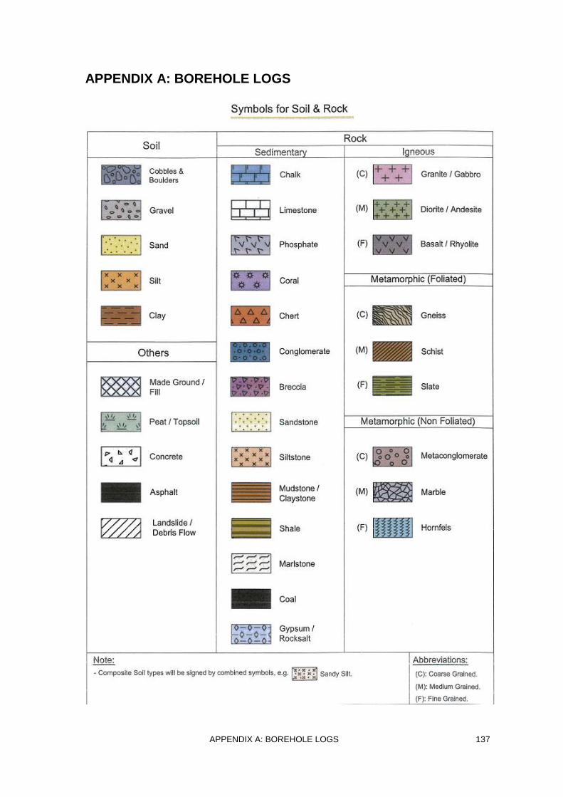
APPENDIX A: BOREHOLE LOGS 137
APPENDIX A: BOREHOLE LOGS
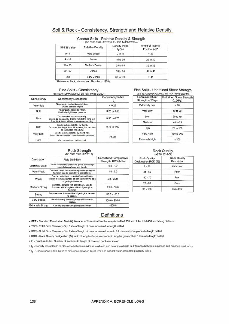
138 APPENDIX A: BOREHOLE LOGS
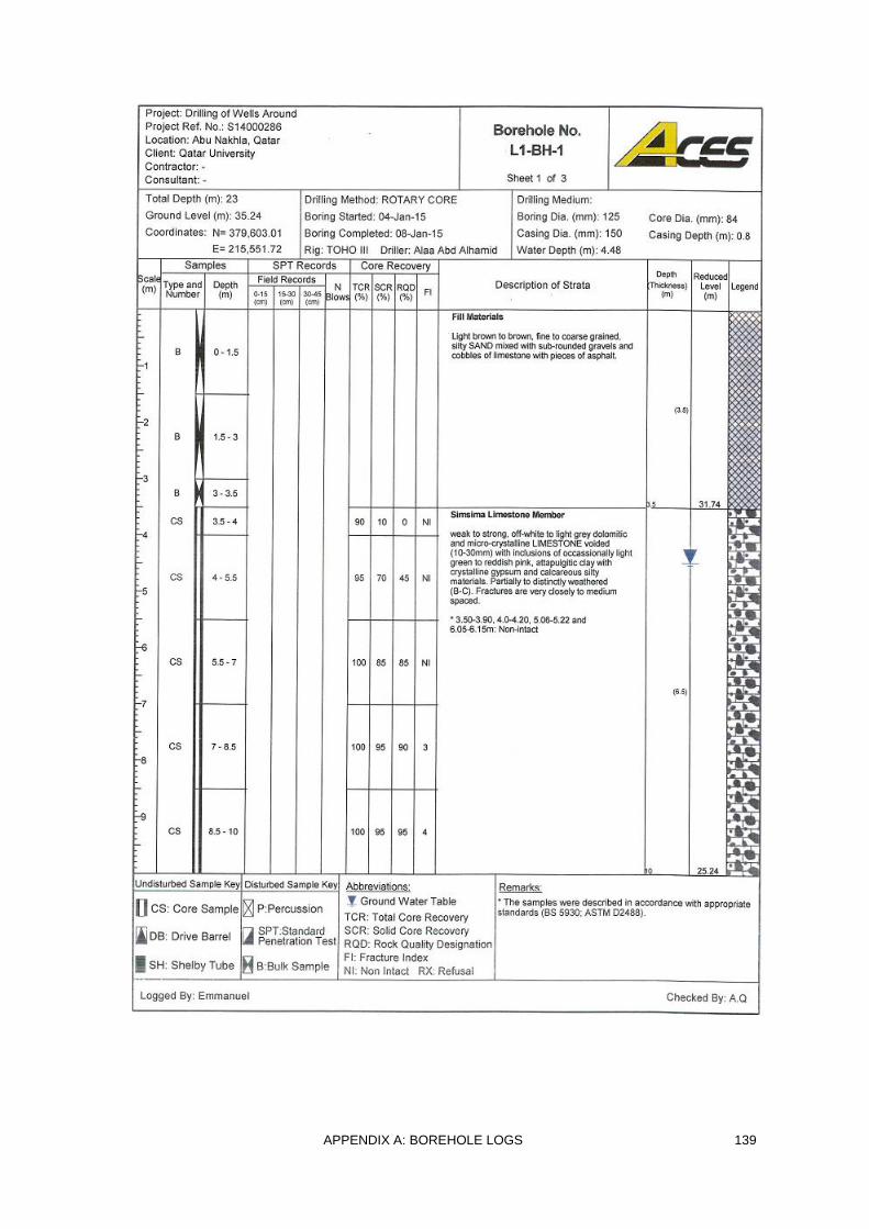
APPENDIX A: BOREHOLE LOGS 139
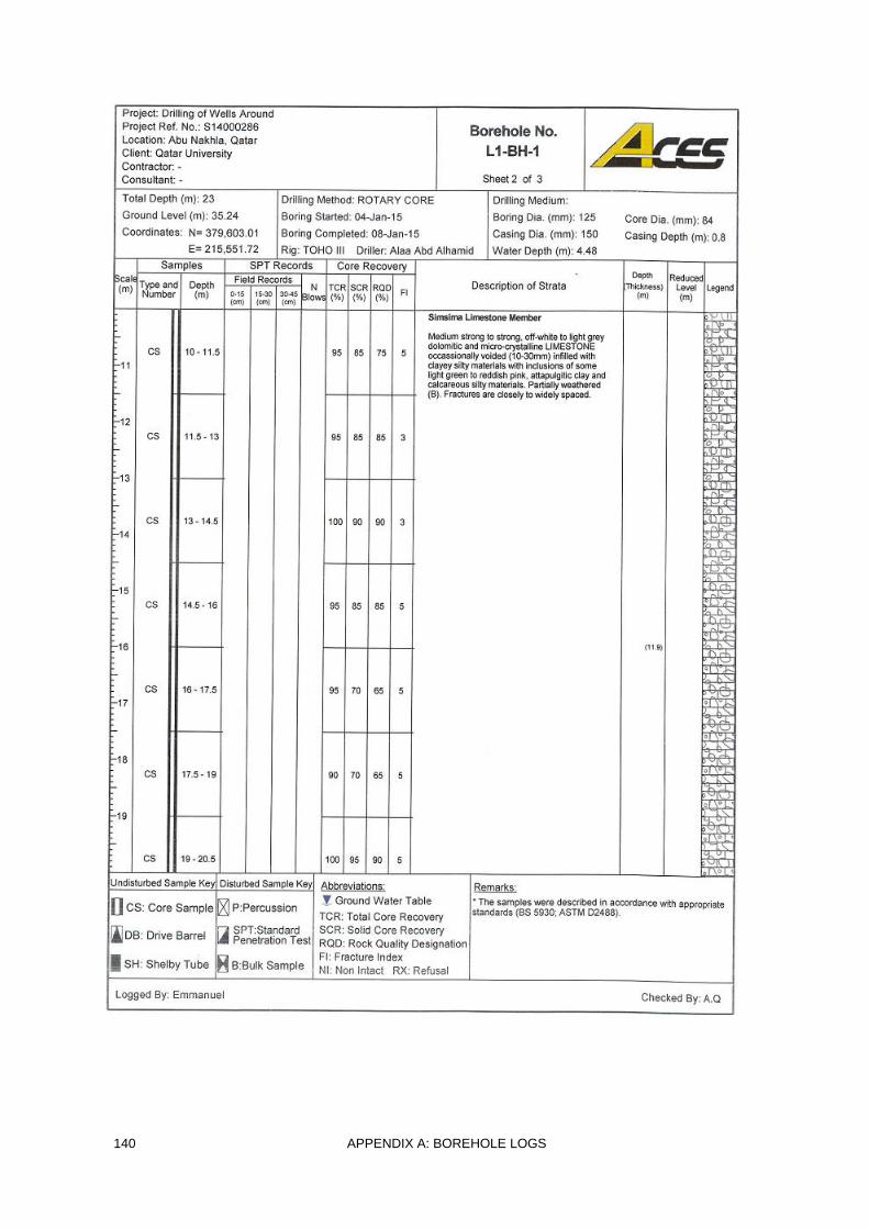
140 APPENDIX A: BOREHOLE LOGS
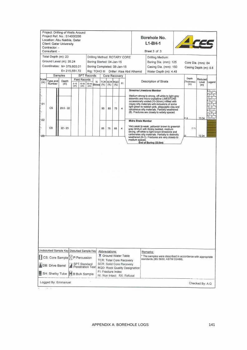
APPENDIX A: BOREHOLE LOGS 141
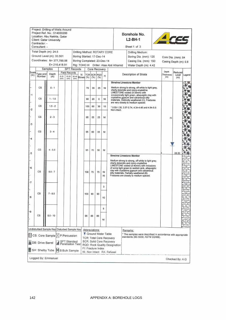
142 APPENDIX A: BOREHOLE LOGS
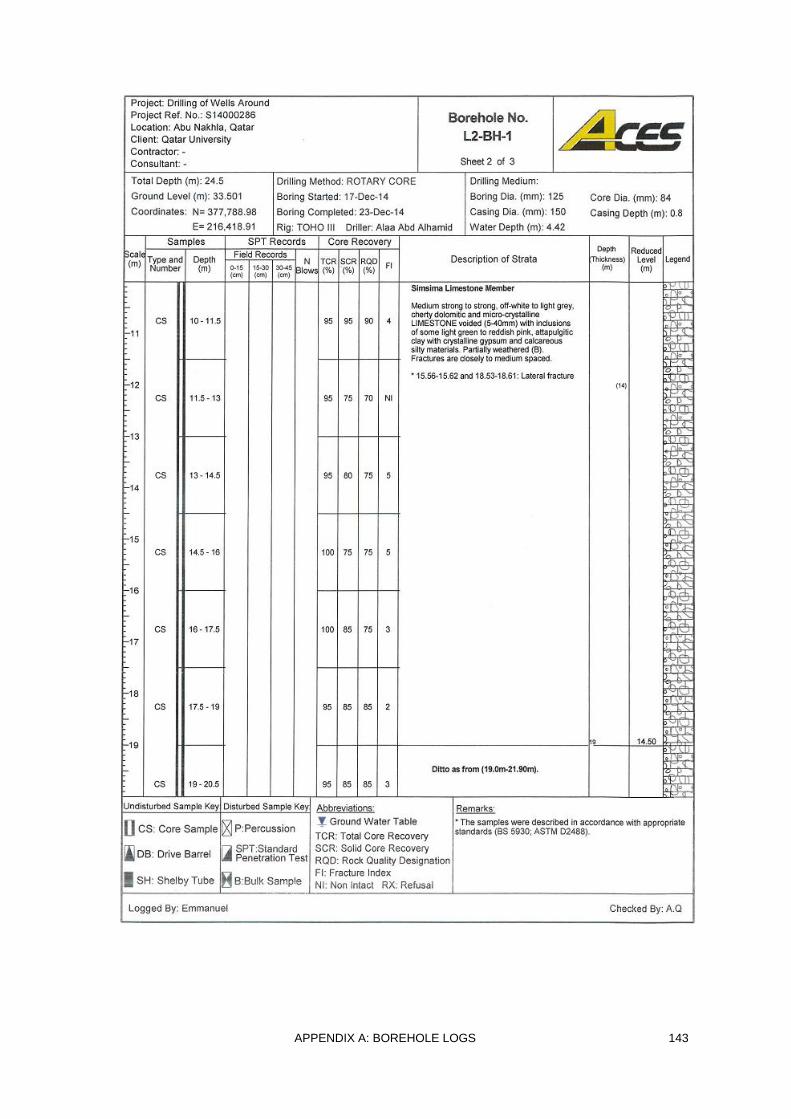
APPENDIX A: BOREHOLE LOGS 143
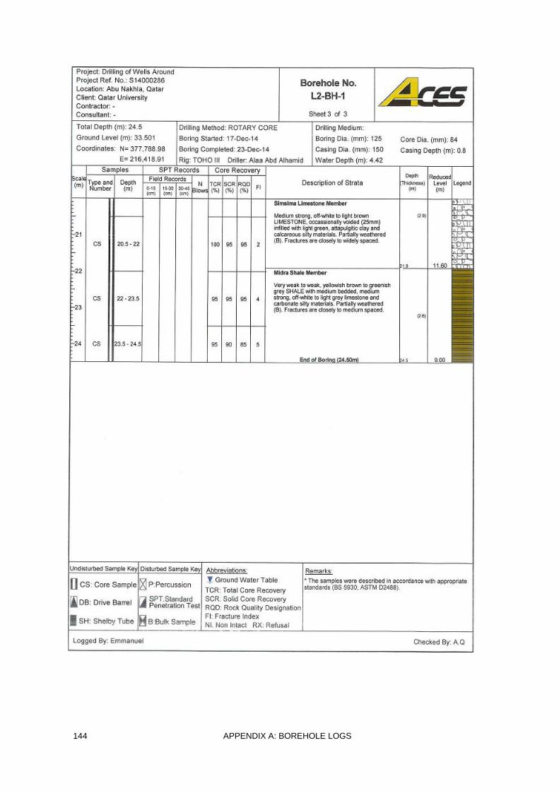
144 APPENDIX A: BOREHOLE LOGS
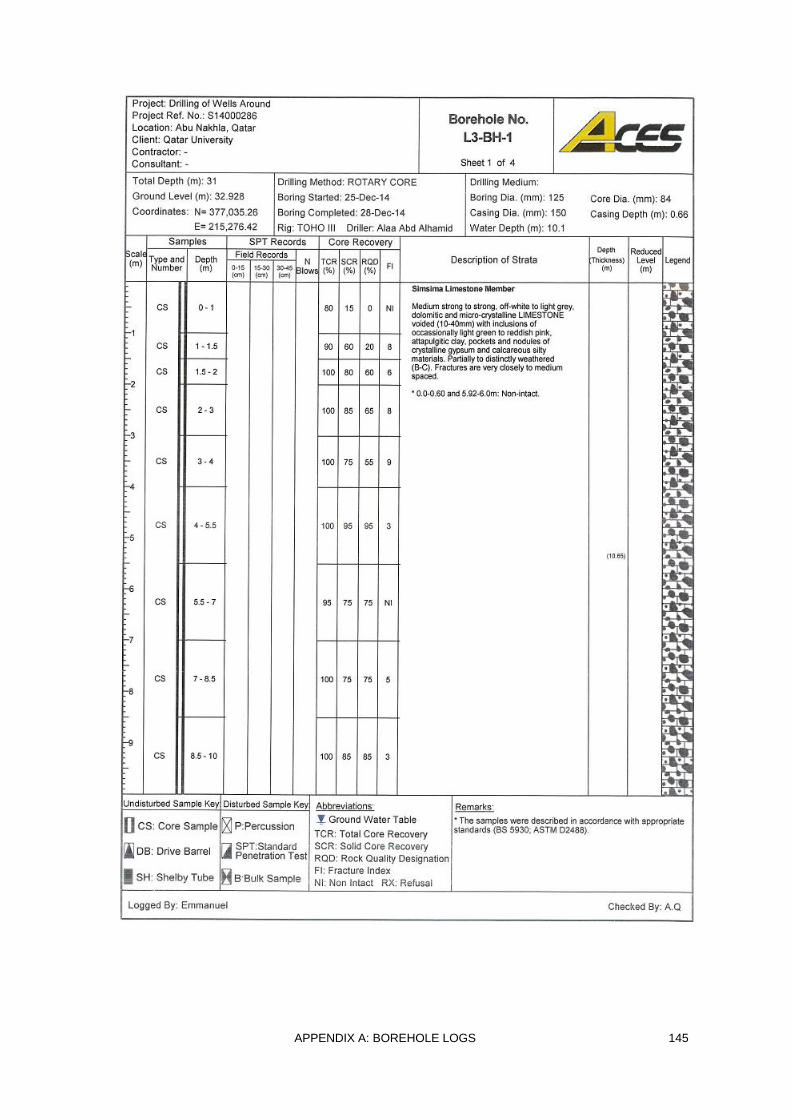
APPENDIX A: BOREHOLE LOGS 145
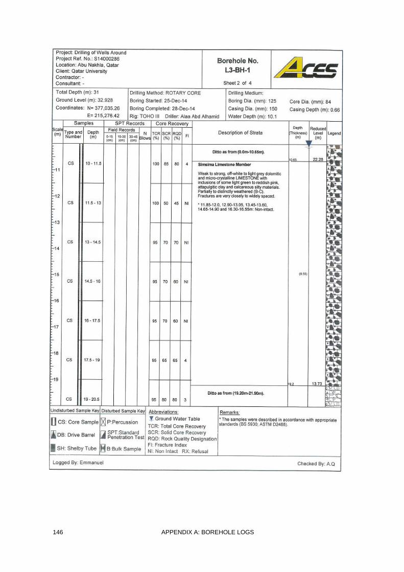
146 APPENDIX A: BOREHOLE LOGS
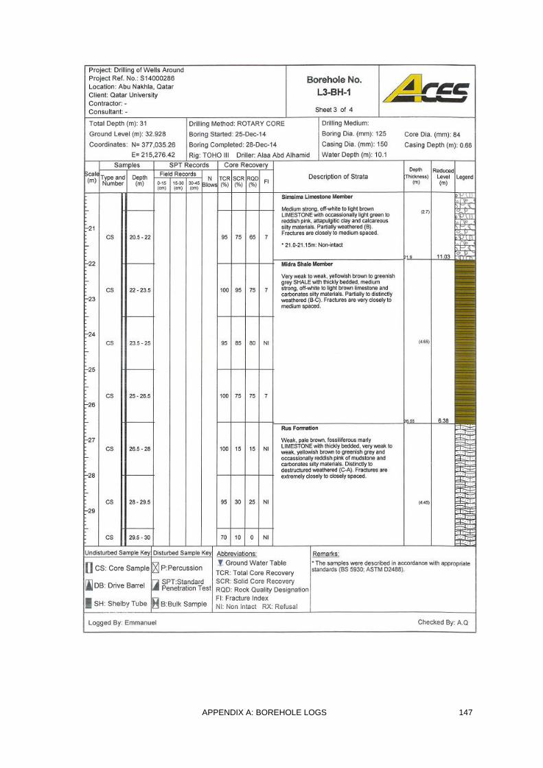
APPENDIX A: BOREHOLE LOGS 147

148 APPENDIX A: BOREHOLE LOGS
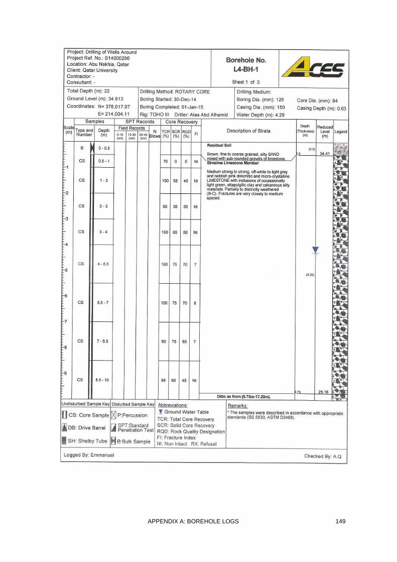
APPENDIX A: BOREHOLE LOGS 149
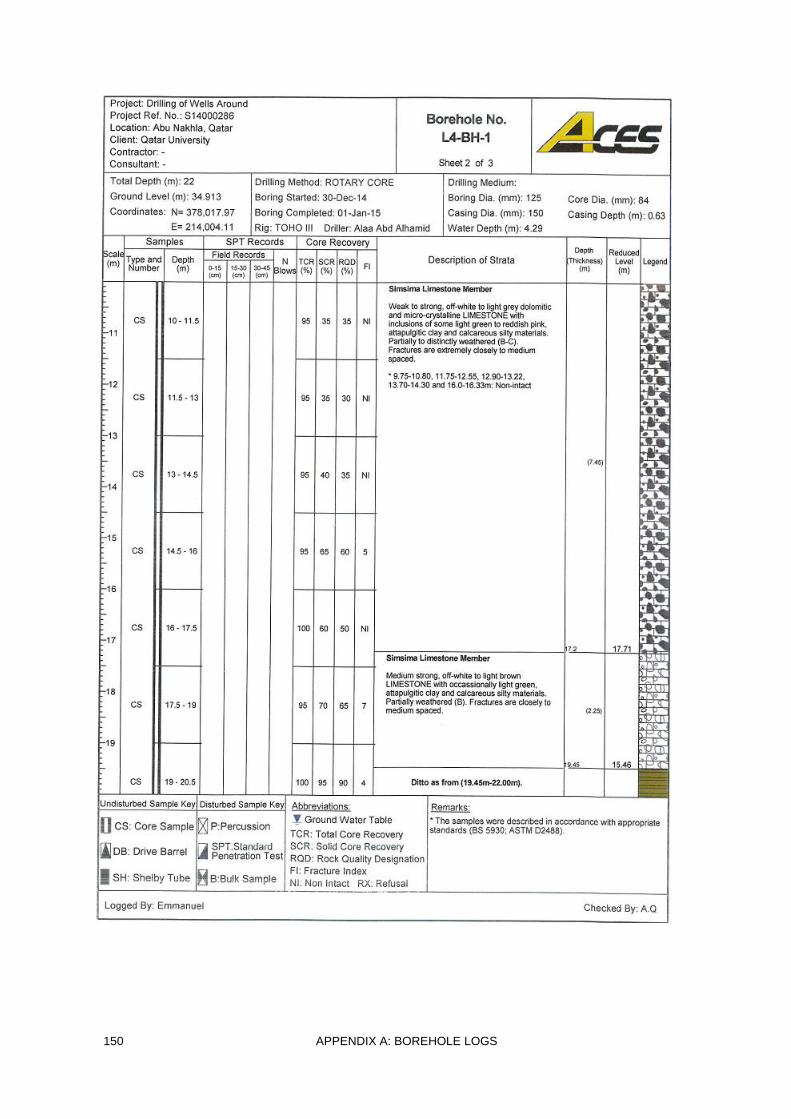
150 APPENDIX A: BOREHOLE LOGS

APPENDIX A: BOREHOLE LOGS 151
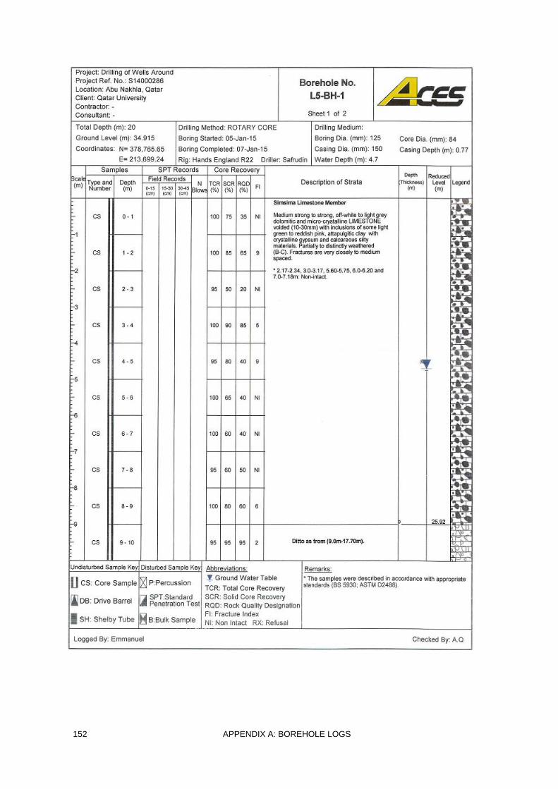
152 APPENDIX A: BOREHOLE LOGS
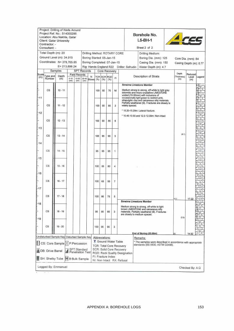
APPENDIX A: BOREHOLE LOGS 153
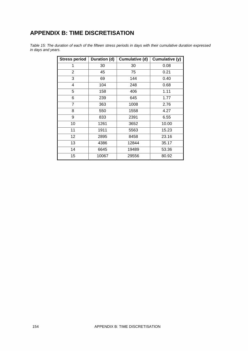
154 APPENDIX B: TIME DISCRETISATION
APPENDIX B: TIME DISCRETISATION
Table 15: The duration of each of the fifteen stress periods in days with their cumulative duration expressed in days and years.
Stress period Duration (d) Cumulative (d) Cumulative (y)
1 30 30 0.08
2 45 75 0.21
3 69 144 0.40
4 104 248 0.68
5 158 406 1.11
6 239 645 1.77
7 363 1008 2.76
8 550 1558 4.27
9 833 2391 6.55
10 1261 3652 10.00
11 1911 5563 15.23
12 2895 8458 23.16
13 4386 12844 35.17
14 6645 19489 53.36
15 10067 29556 80.92
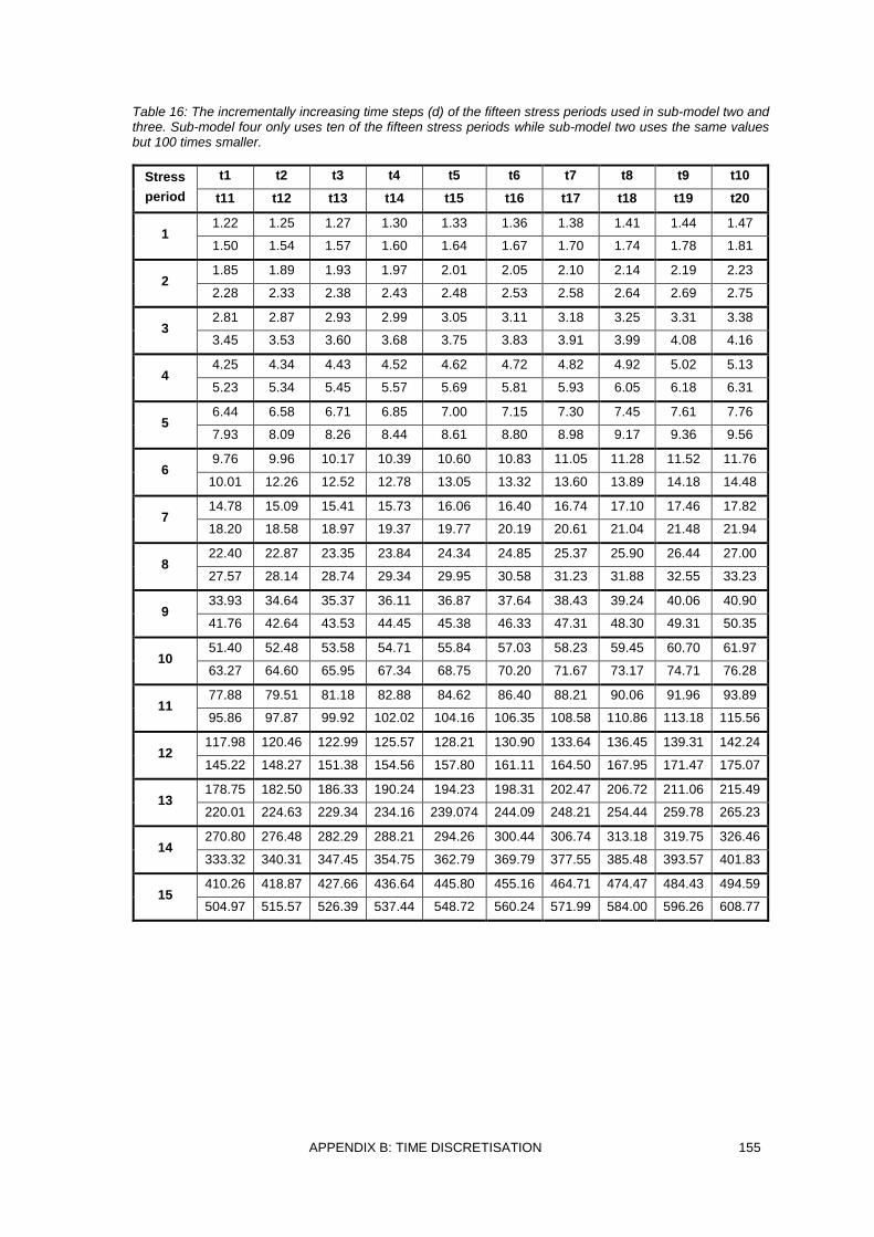
APPENDIX B: TIME DISCRETISATION 155
Table 16: The incrementally increasing time steps (d) of the fifteen stress periods used in sub-model two and three. Sub-model four only uses ten of the fifteen stress periods while sub-model two uses the same values but 100 times smaller.
Stress
period
t1 t2 t3 t4 t5 t6 t7 t8 t9 t10
t11 t12 t13 t14 t15 t16 t17 t18 t19 t20
1 1.22 1.25 1.27 1.30 1.33 1.36 1.38 1.41 1.44 1.47
1.50 1.54 1.57 1.60 1.64 1.67 1.70 1.74 1.78 1.81
2 1.85 1.89 1.93 1.97 2.01 2.05 2.10 2.14 2.19 2.23
2.28 2.33 2.38 2.43 2.48 2.53 2.58 2.64 2.69 2.75
3 2.81 2.87 2.93 2.99 3.05 3.11 3.18 3.25 3.31 3.38
3.45 3.53 3.60 3.68 3.75 3.83 3.91 3.99 4.08 4.16
4 4.25 4.34 4.43 4.52 4.62 4.72 4.82 4.92 5.02 5.13
5.23 5.34 5.45 5.57 5.69 5.81 5.93 6.05 6.18 6.31
5 6.44 6.58 6.71 6.85 7.00 7.15 7.30 7.45 7.61 7.76
7.93 8.09 8.26 8.44 8.61 8.80 8.98 9.17 9.36 9.56
6 9.76 9.96 10.17 10.39 10.60 10.83 11.05 11.28 11.52 11.76
10.01 12.26 12.52 12.78 13.05 13.32 13.60 13.89 14.18 14.48
7 14.78 15.09 15.41 15.73 16.06 16.40 16.74 17.10 17.46 17.82
18.20 18.58 18.97 19.37 19.77 20.19 20.61 21.04 21.48 21.94
8 22.40 22.87 23.35 23.84 24.34 24.85 25.37 25.90 26.44 27.00
27.57 28.14 28.74 29.34 29.95 30.58 31.23 31.88 32.55 33.23
9 33.93 34.64 35.37 36.11 36.87 37.64 38.43 39.24 40.06 40.90
41.76 42.64 43.53 44.45 45.38 46.33 47.31 48.30 49.31 50.35
10 51.40 52.48 53.58 54.71 55.84 57.03 58.23 59.45 60.70 61.97
63.27 64.60 65.95 67.34 68.75 70.20 71.67 73.17 74.71 76.28
11 77.88 79.51 81.18 82.88 84.62 86.40 88.21 90.06 91.96 93.89
95.86 97.87 99.92 102.02 104.16 106.35 108.58 110.86 113.18 115.56
12 117.98 120.46 122.99 125.57 128.21 130.90 133.64 136.45 139.31 142.24
145.22 148.27 151.38 154.56 157.80 161.11 164.50 167.95 171.47 175.07
13 178.75 182.50 186.33 190.24 194.23 198.31 202.47 206.72 211.06 215.49
220.01 224.63 229.34 234.16 239.074 244.09 248.21 254.44 259.78 265.23
14 270.80 276.48 282.29 288.21 294.26 300.44 306.74 313.18 319.75 326.46
333.32 340.31 347.45 354.75 362.79 369.79 377.55 385.48 393.57 401.83
15 410.26 418.87 427.66 436.64 445.80 455.16 464.71 474.47 484.43 494.59
504.97 515.57 526.39 537.44 548.72 560.24 571.99 584.00 596.26 608.77