Meta-mathematical aspects of Martin-Löf's type theory
173
Meta-mathematical aspects of Martin-L¨of’s type theory
Transcript of Meta-mathematical aspects of Martin-Löf's type theory
Meta-mathematical aspects of
Martin-Lof’s type theory

CIP-DATA KONINKLIJKE BIBLIOTHEEK, DEN HAAG
Valentini, Silvio
Meta-mathematical aspects of Martin-Lof’s type theoryS. Valentini – [S.l. : s.n.]. – Ill.Thesis Nijmegen – With ref. – With summary.ISBN: 90-9013777-7Subject headings: constructive type theory
c©Silvio Valentini, Padova, Italia, 2000
Meta-mathematical aspects ofMartin-Lof’s type theory
een wetenschappelijke proeve op het gebied van deNatuurwetenschappen, Wiskunde en Informatica
PROEFSCHRIFT
ter verkrijging van de graad van doctoraan de Katholieke Universiteit Nijmegen,
volgens besluit van het College van Decanenin het openbaar te verdedigenop donderdag 22 juni 2000,
des namiddags om 1.30 uur precies
door
Silvio Luigi Maria Valentini
geboren op 6 january 1953 te Padova, Italia
Promotor: prof. dr. H.P. Barendregt
Manuscript commissie:
prof. dr. Peter Aczel (University of Manchester, UK)prof. dr. Dirk van Dalen (Utrecht University, NL)dr. Herman Geuvers (University of Nijmegen, NL)
Contents
1 Introduction 11.1 Introduction . . . . . . . . . . . . . . . . . . . . . . . . . . . . . . . . . . . . . . . . 11.2 Outline of the thesis . . . . . . . . . . . . . . . . . . . . . . . . . . . . . . . . . . . 1
1.2.1 General Introduction . . . . . . . . . . . . . . . . . . . . . . . . . . . . . . . 11.2.2 Canonical form theorem . . . . . . . . . . . . . . . . . . . . . . . . . . . . . 21.2.3 Properties of type theory . . . . . . . . . . . . . . . . . . . . . . . . . . . . 21.2.4 Subset theory . . . . . . . . . . . . . . . . . . . . . . . . . . . . . . . . . . . 31.2.5 Program development . . . . . . . . . . . . . . . . . . . . . . . . . . . . . . 31.2.6 Forbidden constructions . . . . . . . . . . . . . . . . . . . . . . . . . . . . . 41.2.7 Appendices . . . . . . . . . . . . . . . . . . . . . . . . . . . . . . . . . . . . 4
2 Introduction to Martin-Lof’s type theory 52.1 Introduction . . . . . . . . . . . . . . . . . . . . . . . . . . . . . . . . . . . . . . . . 52.2 Judgments and Propositions . . . . . . . . . . . . . . . . . . . . . . . . . . . . . . . 62.3 Different readings of the judgments . . . . . . . . . . . . . . . . . . . . . . . . . . . 6
2.3.1 On the judgment A set . . . . . . . . . . . . . . . . . . . . . . . . . . . . . . 72.3.2 On the judgment A prop . . . . . . . . . . . . . . . . . . . . . . . . . . . . . 7
2.4 Hypothetical judgments . . . . . . . . . . . . . . . . . . . . . . . . . . . . . . . . . 82.5 The logic of types . . . . . . . . . . . . . . . . . . . . . . . . . . . . . . . . . . . . . 92.6 Some programs . . . . . . . . . . . . . . . . . . . . . . . . . . . . . . . . . . . . . . 10
2.6.1 The sum of natural numbers . . . . . . . . . . . . . . . . . . . . . . . . . . 102.6.2 The product of natural numbers . . . . . . . . . . . . . . . . . . . . . . . . 11
2.7 All types are similar . . . . . . . . . . . . . . . . . . . . . . . . . . . . . . . . . . . 112.8 Some applications . . . . . . . . . . . . . . . . . . . . . . . . . . . . . . . . . . . . 13
2.8.1 A computer memory . . . . . . . . . . . . . . . . . . . . . . . . . . . . . . . 132.8.2 A Turing machine on a two symbols alphabet . . . . . . . . . . . . . . . . . 15
3 The canonical form theorem 173.1 Summary . . . . . . . . . . . . . . . . . . . . . . . . . . . . . . . . . . . . . . . . . 173.2 Introduction . . . . . . . . . . . . . . . . . . . . . . . . . . . . . . . . . . . . . . . . 183.3 Assumptions of high level arity variables . . . . . . . . . . . . . . . . . . . . . . . . 193.4 Modifications due to the new assumptions . . . . . . . . . . . . . . . . . . . . . . . 233.5 Some observations on type theory . . . . . . . . . . . . . . . . . . . . . . . . . . . . 23
3.5.1 Associate judgements . . . . . . . . . . . . . . . . . . . . . . . . . . . . . . 233.5.2 Substituted judgements . . . . . . . . . . . . . . . . . . . . . . . . . . . . . 24
3.6 The evaluation tree . . . . . . . . . . . . . . . . . . . . . . . . . . . . . . . . . . . . 263.7 Computability . . . . . . . . . . . . . . . . . . . . . . . . . . . . . . . . . . . . . . 263.8 The lemmas . . . . . . . . . . . . . . . . . . . . . . . . . . . . . . . . . . . . . . . . 303.9 Computability of the rules . . . . . . . . . . . . . . . . . . . . . . . . . . . . . . . . 34
3.9.1 The substitution rules . . . . . . . . . . . . . . . . . . . . . . . . . . . . . . 343.9.2 U-elimination rules . . . . . . . . . . . . . . . . . . . . . . . . . . . . . . . . 363.9.3 The structural rules . . . . . . . . . . . . . . . . . . . . . . . . . . . . . . . 373.9.4 The assumption rules . . . . . . . . . . . . . . . . . . . . . . . . . . . . . . 463.9.5 The logical rules . . . . . . . . . . . . . . . . . . . . . . . . . . . . . . . . . 48
iii
iv CONTENTS
3.10 The computability theorem . . . . . . . . . . . . . . . . . . . . . . . . . . . . . . . 55
4 Properties of Type Theory 574.1 Summary . . . . . . . . . . . . . . . . . . . . . . . . . . . . . . . . . . . . . . . . . 574.2 Decidability is functionally decidable . . . . . . . . . . . . . . . . . . . . . . . . . . 57
4.2.1 The main result . . . . . . . . . . . . . . . . . . . . . . . . . . . . . . . . . 594.3 An intuitionistic Cantor’s theorem . . . . . . . . . . . . . . . . . . . . . . . . . . . 61
4.3.1 Cantor’s theorem . . . . . . . . . . . . . . . . . . . . . . . . . . . . . . . . . 614.4 The forget-restore principle . . . . . . . . . . . . . . . . . . . . . . . . . . . . . . . 63
4.4.1 The multi-level typed lambda calculus . . . . . . . . . . . . . . . . . . . . . 644.4.2 The judgment A true . . . . . . . . . . . . . . . . . . . . . . . . . . . . . . . 654.4.3 Final remarks . . . . . . . . . . . . . . . . . . . . . . . . . . . . . . . . . . . 67
5 Set Theory 695.1 Summary . . . . . . . . . . . . . . . . . . . . . . . . . . . . . . . . . . . . . . . . . 695.2 Introduction . . . . . . . . . . . . . . . . . . . . . . . . . . . . . . . . . . . . . . . . 69
5.2.1 Foreword . . . . . . . . . . . . . . . . . . . . . . . . . . . . . . . . . . . . . 705.2.2 Contents . . . . . . . . . . . . . . . . . . . . . . . . . . . . . . . . . . . . . 715.2.3 Philosophical motivations . . . . . . . . . . . . . . . . . . . . . . . . . . . . 71
5.3 Reconstructing subset theory . . . . . . . . . . . . . . . . . . . . . . . . . . . . . . 725.3.1 The notion of subset . . . . . . . . . . . . . . . . . . . . . . . . . . . . . . . 725.3.2 Elements of a subset . . . . . . . . . . . . . . . . . . . . . . . . . . . . . . . 745.3.3 Inclusion and equality between subsets . . . . . . . . . . . . . . . . . . . . . 755.3.4 Subsets as images of functions . . . . . . . . . . . . . . . . . . . . . . . . . 775.3.5 Singletons and finite subsets . . . . . . . . . . . . . . . . . . . . . . . . . . . 785.3.6 Finitary operations on subsets . . . . . . . . . . . . . . . . . . . . . . . . . 805.3.7 Families of subsets and infinitary operations . . . . . . . . . . . . . . . . . . 815.3.8 The power of a set . . . . . . . . . . . . . . . . . . . . . . . . . . . . . . . . 825.3.9 Quantifiers relative to a subset . . . . . . . . . . . . . . . . . . . . . . . . . 845.3.10 Image of a subset and functions defined on a subset . . . . . . . . . . . . . 85
6 Development of non-trivial programs 876.1 Summary . . . . . . . . . . . . . . . . . . . . . . . . . . . . . . . . . . . . . . . . . 876.2 Introduction . . . . . . . . . . . . . . . . . . . . . . . . . . . . . . . . . . . . . . . . 876.3 Basic Definitions . . . . . . . . . . . . . . . . . . . . . . . . . . . . . . . . . . . . . 88
6.3.1 The set Seq(A) . . . . . . . . . . . . . . . . . . . . . . . . . . . . . . . . . . 886.3.2 The set Tree(A) . . . . . . . . . . . . . . . . . . . . . . . . . . . . . . . . . . 906.3.3 Expanding a finite tree . . . . . . . . . . . . . . . . . . . . . . . . . . . . . . 916.3.4 Finitary Graphs . . . . . . . . . . . . . . . . . . . . . . . . . . . . . . . . . 92
6.4 Games and Games trees . . . . . . . . . . . . . . . . . . . . . . . . . . . . . . . . . 976.4.1 Game description . . . . . . . . . . . . . . . . . . . . . . . . . . . . . . . . . 976.4.2 Potential Moves . . . . . . . . . . . . . . . . . . . . . . . . . . . . . . . . . 986.4.3 The set of game trees. . . . . . . . . . . . . . . . . . . . . . . . . . . . . . . 996.4.4 Some general game problems . . . . . . . . . . . . . . . . . . . . . . . . . . 996.4.5 Some general solutions . . . . . . . . . . . . . . . . . . . . . . . . . . . . . . 100
6.5 Examples . . . . . . . . . . . . . . . . . . . . . . . . . . . . . . . . . . . . . . . . . 1016.5.1 The knight’s tour problem . . . . . . . . . . . . . . . . . . . . . . . . . . . . 1016.5.2 A game with two players . . . . . . . . . . . . . . . . . . . . . . . . . . . . 103
6.6 Generality . . . . . . . . . . . . . . . . . . . . . . . . . . . . . . . . . . . . . . . . . 1046.7 Some type and functions we use . . . . . . . . . . . . . . . . . . . . . . . . . . . . . 105
6.7.1 The type N<(a) . . . . . . . . . . . . . . . . . . . . . . . . . . . . . . . . . . 1056.7.2 The function append2(s1, s2) . . . . . . . . . . . . . . . . . . . . . . . . . . 1066.7.3 The
∨-function . . . . . . . . . . . . . . . . . . . . . . . . . . . . . . . . . . 106
6.7.4 The∧
-function . . . . . . . . . . . . . . . . . . . . . . . . . . . . . . . . . . 1066.7.5 The max-function. . . . . . . . . . . . . . . . . . . . . . . . . . . . . . . . . 1066.7.6 The sets used in the games description and solutions . . . . . . . . . . . . . 107
CONTENTS v
7 What should be avoided 1097.1 Summary . . . . . . . . . . . . . . . . . . . . . . . . . . . . . . . . . . . . . . . . . 1097.2 Introduction . . . . . . . . . . . . . . . . . . . . . . . . . . . . . . . . . . . . . . . . 1097.3 iTTP = iTT + power-sets . . . . . . . . . . . . . . . . . . . . . . . . . . . . . . . . 1107.4 iTTP is consistent . . . . . . . . . . . . . . . . . . . . . . . . . . . . . . . . . . . . 1147.5 iTTP is classical . . . . . . . . . . . . . . . . . . . . . . . . . . . . . . . . . . . . . 1167.6 Some remarks on the proof . . . . . . . . . . . . . . . . . . . . . . . . . . . . . . . 1217.7 Other dangerous set constructions . . . . . . . . . . . . . . . . . . . . . . . . . . . 121
7.7.1 The collection of the finite subsets . . . . . . . . . . . . . . . . . . . . . . . 1227.7.2 The quotient set constructor . . . . . . . . . . . . . . . . . . . . . . . . . . 1237.7.3 The two-subset set . . . . . . . . . . . . . . . . . . . . . . . . . . . . . . . . 123
A Expressions theory 125A.1 The Expressions with arity . . . . . . . . . . . . . . . . . . . . . . . . . . . . . . . 125
A.1.1 Introduction . . . . . . . . . . . . . . . . . . . . . . . . . . . . . . . . . . . 125A.2 Basic definitions . . . . . . . . . . . . . . . . . . . . . . . . . . . . . . . . . . . . . 126
A.2.1 Abbreviating definitions . . . . . . . . . . . . . . . . . . . . . . . . . . . . . 126A.3 Some properties of the expressions system . . . . . . . . . . . . . . . . . . . . . . . 129A.4 Decidability of “to be an expression” . . . . . . . . . . . . . . . . . . . . . . . . . . 131
A.4.1 New rules to form expressions . . . . . . . . . . . . . . . . . . . . . . . . . . 131A.4.2 A hierarchy of definitions . . . . . . . . . . . . . . . . . . . . . . . . . . . . 132A.4.3 The algorithm . . . . . . . . . . . . . . . . . . . . . . . . . . . . . . . . . . 133
A.5 Abstraction and normal form . . . . . . . . . . . . . . . . . . . . . . . . . . . . . . 135A.5.1 α, β, η and ξ conversion . . . . . . . . . . . . . . . . . . . . . . . . . . . . . 138A.5.2 Normal form . . . . . . . . . . . . . . . . . . . . . . . . . . . . . . . . . . . 140
A.6 Relation with typed λ-calculus . . . . . . . . . . . . . . . . . . . . . . . . . . . . . 141
B The complete rule system 145B.1 The forms of judgements . . . . . . . . . . . . . . . . . . . . . . . . . . . . . . . . . 145B.2 The structural rules . . . . . . . . . . . . . . . . . . . . . . . . . . . . . . . . . . . 145
B.2.1 Weakening . . . . . . . . . . . . . . . . . . . . . . . . . . . . . . . . . . . . 145B.2.2 Assumptions rules . . . . . . . . . . . . . . . . . . . . . . . . . . . . . . . . 146B.2.3 Equality rules . . . . . . . . . . . . . . . . . . . . . . . . . . . . . . . . . . . 146B.2.4 Equal types rules . . . . . . . . . . . . . . . . . . . . . . . . . . . . . . . . . 146B.2.5 Substitution rules . . . . . . . . . . . . . . . . . . . . . . . . . . . . . . . . 147
B.3 The logical rules . . . . . . . . . . . . . . . . . . . . . . . . . . . . . . . . . . . . . 148B.3.1 Π-rules . . . . . . . . . . . . . . . . . . . . . . . . . . . . . . . . . . . . . . 148B.3.2 Σ-rules . . . . . . . . . . . . . . . . . . . . . . . . . . . . . . . . . . . . . . 149B.3.3 +-rules . . . . . . . . . . . . . . . . . . . . . . . . . . . . . . . . . . . . . . 150B.3.4 Eq-rules . . . . . . . . . . . . . . . . . . . . . . . . . . . . . . . . . . . . . . 151B.3.5 Id-rules . . . . . . . . . . . . . . . . . . . . . . . . . . . . . . . . . . . . . . 152B.3.6 S(A)-rules . . . . . . . . . . . . . . . . . . . . . . . . . . . . . . . . . . . . . 153B.3.7 Nn-rules . . . . . . . . . . . . . . . . . . . . . . . . . . . . . . . . . . . . . . 154B.3.8 N-rules . . . . . . . . . . . . . . . . . . . . . . . . . . . . . . . . . . . . . . . 155B.3.9 W-rules . . . . . . . . . . . . . . . . . . . . . . . . . . . . . . . . . . . . . . 156B.3.10 U-rules . . . . . . . . . . . . . . . . . . . . . . . . . . . . . . . . . . . . . . . 157
vi CONTENTS
Samenvatting
Vanaf de 70-er jaren heeft Martin-Lof in een aantal opeenvolgende varianten de intuitionistischetypetheorie ontwikkeld. (Zie [Mar84, NPS90].) Het oorspronkelijke doel was om een formeelsysteem voor constructieve wiskunde te definieren, maar al snel werd ook het belang van de theorievoor de informatica ingezien.
In dit proefschrift geven we eerst een algemene inleiding in Martin-Lofs typetheorie. Vervol-gens bespreken we een aantal van de belangrijkste meta-mathematische eigenschappen. Daarnabehandelen we enkele toepassingen van de theorie binnen de constructieve wiskunde en de theo-retische informatica. Tot slot analyseren we een aantal mogelijke uitbreidingen van de theorie metimpredicatieve verzamelingsconstructies.
In hoofdstuk 3 worden de belangrijkste meta-mathematische eigenschappen bewezen. Dit hoofd-stuk bevat een volledig bewijs van de ‘canonieke vorm stelling’ (canonical form theorem), waaruitde bekende corollaria van een normalisatie stelling volgen, zoals de consistentie van de theorie, dedisjunctie en existentie eigenschappen en de totale correctheid van partieel correcte programma’s.We beschouwen de theorie zoals die gepresenteerd is in [Mar84], die universa en extensionele geli-jkheid bevat en waarvoor een normalisatie stelling in zijn standaard vorm niet geldt. Het bewezenresultaat in dit hoofdstuk zegt dat iedere gesloten welgetypeerde term in een aantal stappen gere-duceerd kan worden naar een term in canonieke vorm.
In hoofdstuk 4 worden een aantal meta-mathematische eigenschappen geanalyseerd. We lateneerst zien dat de bekende intuitionistische karakterisering van de beslisbaarheid van predikatenequivalent is aan het bestaan van een beslissingsfunctie. Daarna bewijzen we een intuitionistis-che versie van de stelling van Cantor. Preciezer: we laten zien dat er geen surjectieve functiebestaat van de verzameling van natuurlijke getallen naar de verzameling van functies van natu-urlijke getallen naar natuurlijke getallen. Tenslotte illustreren we het ‘vergeet-herstel principe’forget-restore principle dat in [SV98] werd geıntroduceerd om uit te leggen wat abstractie in con-structieve zin betekent. We doen dit door een eenvoudig voorbeeld in Martin-Lofs typetheorie tebeschouwen, namelijk uitspraken van de vorm A true. De betekenis van A true is dat er een elementa is waarvoor a ∈ A geldt, maar het maakt niet uit welke specifieke a het is. De overgang van deuitspraak a ∈ A naar de uitspraak A true is een duidelijk voorbeeld van een vergeet proces. In dithoofdstuk laten we zien dat dit een vergeet proces in constructieve zin is, daar we uit een bewijsvan de uitspraak A true, een element a kunnen reconstrueren waarvoor a ∈ A.
In hoofdstuk 5 laten we zien hoe een predicatieve lokale verzamelingenleer kan worden on-twikkeld binnen Martin-Lofs typetheorie. In de literatuur vindt men verschillende voorstellen vooreen ontwikkeling van verzamelingenleer, binnen Martin-Lofs typetheorie of zodanig dat ze binnenMartin-Lofs typetheorie geınterpreteerd zouden kunnen worden. Het voornaamste verschil tussende benaderingen in de literatuur en de benadering die we hier kiezen is dat wij niet eisen dateen deelverzameling zelf weer een verzameling is. In de andere benaderingen is het doel om debekende basis constructoren uit de typetheorie toe te passen op een algemeen verzamelingsbegrip,inclusief verzamelingen verkregen met comprehensie (over een bestaande verzameling), of om eenaxiomatische verzamelingenleer te definieren waarvan de axioma’s een constructieve interpretatiehebben. De theorie van deelverzamelingen die wij hier voorstellen is een soort ‘typeloze’ verza-melingenleer, gelokaliseerd binnen een verzameling. We bewijzen dat de gehele ontwikkeling binnentypetheorie gedaan kan worden. Uiteraard zijn niet alle axioma’s van de klassieke verzamelingen-leer geldig in deze benadering. In het bijzonder is het onmogelijk om de axioma’s af te leiden diegeen constructieve betekenis hebben, zoals de machtsverzamelingsconstructie.
Hoofdstuk 6 behandelt de ontwikkeling van een aantal niet-triviale programma’s in Martin-Lofstypetheorie. Dit kan gezien worden als een studie naar abstractie in functioneel programmeren.Door de zeer krachtige type-constructies en het ingebouwde ‘proposities-als-types’ principe, onder-steunt Martin-Lofs typetheorie de ontwikkeling van bewijsbaar-correcte programma’s. In plaatsvan te werken aan specifieke problemen, specificeren we in dit hoofdstuk klassen van problemen enwe ontwikkelen algemene oplossingen voor deze klassen.
Tot slot is er hoofdstuk 7, waar we een uitbreiding bestuderen van Martin-Lofs intensioneletypetheorie met een verzamelingsconstructor P , zodat de elementen van P(S) de deelverzamelin-gen van S zijn. Als we voor zo’n uitbreiding een vorm van extensionaliteit op de gelijkheid vandeelverzamelingen eisen (wat natuurlijk is), blijkt deze uitbreiding klassiek te zijn. Het hoofd-
CONTENTS vii
stuk wordt afgesloten door te laten zien dat het voornaamste probleem met de definitie van eenmachtsverzamelingsconstructie hem zit in de vereiste extensionele gelijkheid tussen deelverzamelin-gen. Om precies te zijn: we laten zien dat niet alleen de machtsverzamelingsconstructie de logicaklassiek maakt, maar dat klassieke logica al een gevolg is van de mogelijkheid om een verzamelingte definieren waarvan de elementen precies de eindige verzamelingen van een gegeven verzamelingzijn. Zelfs is klassieke logica al een gevolg van de mogelijkheid om quotientverzamelingen te makenen tevens al van de mogelijkheid om een extensionele verzameling te definieren wier elementen tweedeelverzamelingen zijn.
De eerste appendix bevat de ‘theorie van expressies’ expression theory, een soort getypeerdeλ-calculus waar een definitiemechanisme wordt gebruikt in plaats van λ-abstractie. Deze theorieis nodig om de syntax van Martin-Lofs constructieve typetheorie in uit te drukken. De tweedeappendix bevat alle regels van de theorie. Deze kan door het proefschrift heen gebruikt wordenals een referentie. Modulo kleine variaties zijn dit de standaard regels die op veel plaatsen in deliteratuur gevonden kunnen worden. Het leek ons een goed idee om ze te bij te voegen in hetproefschrift.
viii CONTENTS
Curriculum vitae
Silvio Valentini was born on January 6th 1953 in Padova, Italy. He lives in via Vittor Pisani n.14, in Padova, Italy (tel. +39 049 802 44 86).
He attended the corso di laurea in Mathematics at the University of Padova and obtainedthe laurea in Mathematics on July 8th 1977, with the thesis ‘L’uso del calcolo dei predicati perla scrittura di algoritmi’ (in Italian) under the direction of Professor Giovanni Sambin of theMathematical Department of the University of Padova and Professor Enrico Pagello of L.A.D.S.E.B.of C.N.R., the National Council for Researches.
Starting October 1st 1977, he won a grant of C.N.R., that he used at the Mathematical Instituteof the University of Siena, headed by Professor Roberto Magari.
After November 1st 1980, he became a Ricercatore Universitario Confermato at the Mathemat-ical Institute of the University of Siena.
After April 2nd 1984, he was a Ricercatore Universitario Confermato at the MathematicalDepartment of the University of Padova.
Then, after October 25th 1987, he has become an Associate Professor in Mathematical Logicat the Computer Science Department of the University of Milan.
Now, after November 1st 1991, he is an Associate Professor in Mathematical Logic at theMathematical Department of the University of Padova.
Chapter 1
Introduction
1.1 Introduction
Since the 70s Martin-Lof has developed, in a number of successive variants, an Intuitionistic The-ory of Types [Mar84, NPS90]. The initial aim was to provide a formal system for constructivemathematics but the relevance of the theory also in computer science was soon recognized. In fact,from an intuitionistic perspective, to define a constructive set theory is completely equivalent todefine a logical calculus [How80] or a language for problem specification [Kol32], and hence thetopic is of immediate relevance both to mathematicians, logicians and computer scientists. More-over, since an element of a set can also be seen as a proof of the corresponding proposition oras a program which solves the corresponding problem, the intuitionistic theory of types is also afunctional programming language with a very rich type structure and an integrated system to de-rive correct programs from their specification [PS86]. These pleasant properties of the theory havecertainly contributed to the interest for it arisen in the computer science community, especiallyamong those people who believe that program correctness is a major concern in the programmingactivity [BCMS89].
1.2 Outline of the thesis
In this thesis we will first give a general introduction to Martin-Lof’s Type theory and then we willdiscuss some of its main meta-mathematical properties. Some applications of the theory both toconstructive mathematics development and theoretical computer science will follow. Finally someextensions of the theory with impredicative set constructors will be analyzed.
1.2.1 General Introduction
In chapter 2 we will give an introduction to Martin-Lof’s type theory by presenting the main ideason which the theory is based and by showing some examples.
No theorem will be proved in this chapter, but we think that a general explanation of theideas on which the theory is built on is necessary in order to have a feeling for the theory beforebeginning the meta-mathematical study. We think that this chapter is going to be useful to anyreader which does not know Martin-Lof’s type theory. In fact, only after a basic comprehensionof the general approach to set construction and proposition definition will be achieved, it will bepossible to understand the meaning of the technical mathematical results in the next chapters.Indeed, these results are consequences of such a basic philosophical attitude even if sometime themathematical subtle details of their proofs can hide the intuitive content of the statements of thetheorems; moreover their relevance can be undertaken if it is not clear that they are important inshowing how the basic ideas are working and having effects which can be explained in mathematicalterms.
For this reason in this chapter we will introduce the theory by analyzing its syntax and ex-plaining its semantics in term of computations. Then, the general idea of inductive set will be
1
2 CHAPTER 1. INTRODUCTION
introduced and some simple example of program development will be shown. Finally two lesstivial examples will be developed with some details: a computer memory and a Turing machine.
Most of the content of this chapter was presented in [Val96a].
1.2.2 Canonical form theorem
In chapter 3, the main meta-mathematical properties of the theory will be proved. Here, you willfind the complete proof of the canonical form theorem that allows to obtain most of the standardconsequence of a normalization theorem that is, the consistency of the theory, the disjunction andexistential properties and the total correctness of any partially correct program.
In this chapter we will consider the theory presented in [Mar84] which contains both universesand extensional equality; it is well know that a standard normalization theorem does not hold forsuch a theory (see the introduction of the chapter for a proof of this result). On the other handthis theory is often the most useful in developing constructive mathematics and hence some kindof normal form result is useful for it.
The result that we will prove in this chapter states that any closed typed term, whose derivationhas no open assumption, can be reduced by a sequence of reductions into an equivalent one incanonical form, that is, a sort of external normal form, and that the proof of any provable judgementcan be transformed into an equivalent one in introductory form. These facts are sufficient to obtainmost of the usual consequence of a standard normalization theorem.
It is easy to extend the proof to a theory which contains both intensional and extensionalequality and it is even possible to prove a strong normalization theorem if only intensional equalityis present, nevertheless we think that the theory that we presented and the technique that we usedto prove the canonical form theorem are interesting enough to deserve a deep study in a case wherethe full normalization theorem does not hold.
The content of this chapter is mainly contained in [BV92].
1.2.3 Properties of type theory
In chapter 4 some meta-mathematical properties of the theory will be analyzed.
We will first show that the usual intuitionistic characterization of the decidability of the propo-sitional function B(x) prop [x : A], that is, to require that the predicate (∀x ∈ A) B(x) ∨ ¬B(x)is provable, is equivalent to require that there exists a decision function, that is a functionφ : A → Boole such that (∀x ∈ A) (φ(x) =Boole true) ↔ B(x). This result turns out to bevery useful in many applications of Martin-Lof’s type theory and its proof is interesting since itrequire to use some of the peculiarities of the theory, namely the presence of universes and thefact that an intuitionistic axiom of choice is provable because of the strong elimination rule for theexistential quantifier.
The results of this section can be found in [Val96].
Then, we will prove that an intutionistic version of Cantor’s theorem holds. In fact, we willshow that there exists no surjective function from the set of the natural numbers N into the setN → N of the functions from N into N. As the matter of fact a similar result can be proved forany not-empty set A such that there exists a function from A into A which has no fixed point, asis the case of the successor function for the set N.
This theorem was first presented in [MV96].
Finally, the “forget-restore” principle, introduced in [SV98] in order to explain what can beconsidered a constructive way to operate an abstraction, will be illustrated by analyzing a simplecase in Martin-Lof’s type theory. Indeed, type theory offers many ways of “forgetting” information;what will be analyzed in this section is the form of judgment A true. The meaning of A true is thatthere exists an element a such that a ∈ A holds but it does not matter which particular elementa is (one should compare this approach with the notion of proof irrelevance in [Bru80]). Thus, topass from the judgment a ∈ A to the judgment A true is a clear example of the forgetting process.
In this section we will show that it is a constructive way of forgetting since, provided that thereis a proof of the judgment A true, an element a such that a ∈ A can be re-constructed.
The results of this section have been presented in [Val98].
1.2. OUTLINE OF THE THESIS 3
1.2.4 Subset theory
In chapter 5 we will show how a predicative local set theory can be developed within Martin-Lof’stype theory.
In fact, a few years’ experience in developing constructive topology in the framework of typetheory has taught us that a more liberal treatment of subsets is needed than what could be achievedby remaining literally inside type theory and its traditional notation. To be able to work freelywith subsets in the usual style of mathematics one must come to conceive them like any othermathematical object and have access to their usual apparatus.
Many approaches were proposed for the development of a set theory within Martin-Lof’s typetheory or in such a way that they can be interpreted in Martin-Lof’s type theory (see for instance[NPS90], [Acz78], [Acz82], [Acz86], [Hof94], [Hof97] and [HS95]).
The main difference between our approach and these other ones stays on the fact that we donot require to a subset to be a set while in general in the other approaches the aim is to apply theusual set-constructors of basic type theory to a wider notion of set, which includes sets obtained bycomprehension over a given set (see [NPS90], [Hof94], [Hof97] and [HS95]) or to define an axiomaticset theory whose axioms have a constructive interpretation (see [Acz78], [Acz82], [Acz86]); hencethe justification of the validity of the rules and axioms for sets must be given anew and a newjustification must be furnished each time the basic type theory or the basic axioms are modified.On the other hand the subset theory that we proposed here is a sort of type-less set theory localizedto a set and we prove that all of its development can be done within type theory without losingcontrol, that is by “forgetting” only information which can be restored at will. This is reduced tothe single fact that, for any set A, the judgment A true holds if and only if there exists a such thata ∈ A, and it can be proved once and for all, see [Val98].
In this chapter we will provide with all the main definitions for a subset theory; in particular,we will state the basic notion of subset U of a set S, that is we will identify U with a propositionalfunction over S. Hence a subset can never be a set and thus no membership relation is definedbetween U and the elements of S. This is the reason why our next step will be the introduction ofa new membership relation between an element a of S and a subset U of S, which will turn out tohold if and only if the proposition U(a) is true. Then the full theory will be developed based onthese ideas, that is, the usual set-theoretic operations will be defined in terms of logical operations.Of course not all of the classical set theoretic axioms are satisfied in this approach. In particular itis not possible to validate the axioms which do not have a constructive meaning like, for instance,the power-set construction.
The topics of this section were first presented in [SV98].
1.2.5 Program development
Chapter 6 is devoted to the development of some non-trivial program within Martin-Lof’s typetheory and it can be considered like a sort of case study in abstraction in functional programming.
In fact, as regards computing science, through very powerful type-definitions facilities and theembedded principle of “propositions as types”, Martin-Lof’s type theory primarily supplies meansto support the development of proved-correct programs, that is, it furnishes both the sufficientexpressive power to allows general problem descriptions by means of type definitions and meanwhilea powerful deductive system where a formal proof that a type representing a problem is inhabitedis ipso facto a functional program which solves such a problem. Indeed here type checking achievesits very aim, namely that of avoiding logical errors.
There are a lot of works (see for instance [Nor81, PS86]) stressing how it is possible to writedown, within the framework of type theory, the formal specification of a problem and then develop aprogram meeting this specification. Actually, examples often refer to a single, well-known algorithmwhich is formally derived within the theory. The analogy between a mathematical constructiveproof and the process of deriving a correct program is emphasized. Formality is necessary, but it iswell recognized that the master-key to overcome the difficulties of formal reasoning, in mathematicsas well as in computer science, is abstraction and generality. Abstraction mechanisms are very welloffered by type theory by means of assumptions and dependent types.
4 CHAPTER 1. INTRODUCTION
In this chapter we want to emphasize this characteristic of the theory. Thus, instead of speci-fying a single problem we will specify classes of problems and we will develop general solutions forthem.
The content of this section can also be found in [Val96b].
1.2.6 Forbidden constructions
To end with, there is chapter 7 where it will be analyzed an extension of Martin-Lof’s intensionaltype theory by means of a set constructor P such that the elements of P(S) are the subsets ofthe set S. Since it seems natural to require some kind of extensionality on the equality amongsubsets, it turns out that such an extension cannot be constructive. In fact we will prove that thisextension is classic, that is (A ∨ ¬A) true holds for any proposition A.
In the literature there are examples of intuitionistic set theories with some kind of power-setconstructor. For instance, one can think to a topos, where a sort of “generalized set theory”is obtained by associating with any topos its internal language (see [Bel88]), or to the Calculusof Constructions by Coquand and Huet, where the power of a set S can be identified with thecollection of the functions from S into prop. But in the first case problems arise because of theimpredicativity of the theory and in the second because prop cannot be a set from a constructiveperspective and hence also the collection of the functions from a set S into prop cannot be a set.Of course, there is no reason to expect that a second order construction becomes constructive onlybecause it is added to a theory which is constructive. Indeed, we will prove that even the fragmentiTT of Martin-Lof’s type theory, which contains only the basic set constructors, i.e. no universeand no well-orders, and the intensional equality, cannot be extended with a power-set constructorin a way compatible with the usual explanation of the meaning of the connectives, if the power-setis the collection of all the subsets of a given set equipped with some kind of extensional equality.In fact, by using the so called intuitionistic axiom of choice, it is possible to prove that, givenany power-set constructor, which satisfies the conditions that we will illustrate, classical logic isobtained. A crucial point in carrying on our proof is the uniformity of the equality conditionexpressing extensionality on the power-set.
The chapter is completed by showing that the main problem in the definition of the power-setconstructor is the required extensionality among subsets. In fact it will be proved that not onlythe power-set constructor allows to obtain classical logic but that it is a consequence also of thepossibility to define a set whose elements are the finite subsets of a given set, of the possibility todefine quotient sets and even of the possibility to define an extensional set whose elements are twosubsets.
The proofs in this chapter were first presented in [MV99] and [Val00].
1.2.7 Appendices
Finally, two appendices follow. The first contains expression theory, that is, a sort of typed lambda-calculus where abbreviating definitions are used instead that λ-abstraction, which is necessary tohave a formal theory where the syntax for Martin-Lof’s constructive type theory can be expressed.
Expression theory was first presented in [BV89].The second appendix contains all of the rules of the theory and it can be used like a reference
along all the thesis. With some small variants, such rules can be found in many printed papers(see for instance [Mar84, NPS90, BV92] and others), but we thought that it could be handy tohave them within the thesis.
Chapter 2
Introduction to Martin-Lof’s type
theory
2.1 Introduction
Since the 70s Martin-Lof has developed, in a number of successive variants, an Intuitionistic The-ory of Types [Mar84, NPS90] (ITT for short in the following). The initial aim was to providea formal system for constructive mathematics but the relevance of the theory also in computerscience was soon recognized. In fact, from an intuitionistic perspective, to define a constructive settheory is completely equivalent to define a logical calculus [How80] or a language for problem spec-ification [Kol32], and hence the topic is of immediate relevance both to mathematicians, logiciansand computer scientists. Moreover, since an element of a set can also be seen as a proof of thecorresponding proposition or as a program which solves the corresponding problem, ITT is also afunctional programming language with a very rich type structure and an integrated system to de-rive correct programs from their specification [PS86]. These pleasant properties of the theory havecertainly contributed to the interest for it arisen in the computer science community, especiallyamong those people who believe that program correctness is a major concern in the programmingactivity [BCMS89].
To develop ITT one has to pass through four steps:
• The first step is the definition of a theory of expressions which both allows to abstract onvariables and has a decidable equality theory; indeed the first requirement is inevitable to gainthe needed expressive power while the last is essential in order to guarantee a mechanicalverification of the correct application of the rules used to present ITT. Here the naturalcandidate is a sort of simple typed lambda calculus which can be found in the appendix A.
• The second step is the definition of the types (respectively sets, propositions or problems) oneis interested in; here the difference between the classical and the intuitionistic approach isessential: in fact a proposition is not merely an expression supplied with a truth value butrather an expression such that one knows what counts as one of its verifications (respectivelyone of its elements or one of the programs which solves the problem).
• The third step is the choice of the judgments one can express on the types introduced in theprevious step. Four forms of judgment are considered in ITT:
1. the first form of judgment is obviously the judgment which asserts that an expression isa type;
2. the second form of judgment states that two types are equal;
3. the third form of judgment asserts that an expression is an element of a type;
4. the fourth form of judgment states that two elements of a type are equal.
• The fourth step is the definition of the computation rules which allow to execute the programsdefined in the previous point.
5
6 CHAPTER 2. INTRODUCTION TO MARTIN-LOF’S TYPE THEORY
In this chapter we will show some of the standard sets and propositions in [Mar84] and someexamples of application of the theory to actual cases, while for the study of the main meta-mathematical results on ITT the reader is asked to wait for the next chapters.
2.2 Judgments and Propositions
In a classical approach to the development of a formal theory one usually takes care to definea formal language only to specify the syntax (s)he wants to use while as regard to the intendedsemantics no a priori tie on the used language is required. Here the situation is quite different; infact we want to develop a constructive set theory and hence we can assume no external knowledgeon sets; then we do not merely develop a suitable syntax to describe something which existssomewhere. Hence we have “to put our cards on the table” at the very beginning of the game andto declare the kind of judgments on sets we are going to express. Let us consider the followingexample: let A be a set,then
a ∈ A
which means that a is an element of A, is one of the form of judgment we are interested in (butalso the previous “A is a set” is already a form of judgment!). It is important to note that alogical calculus is meaningful only if it allows to derive judgments. Hence one should try to defineit only after the choice of the judgments (s)he is interested in. A completely different problem isthe definition of the suitable notation to express such a logical calculus; in this case it is probablymore correct to speak of a well-writing theory instead of a logical calculus (see appendix A to seea well-writing theory suitable for ITT).
Let us show the form of the judgments that we are going to use to develop our constructive settheory. The first is
(type-ness) A type
(equivalently A set, A prop and A prob) which reads “A is a type” (respectively “A is a set”, “A isa proposition” and “A is a problem”) and states that A is a type. The second form of judgment is
(equal types) A = B
which, provided that A and B are types, states that they are equal types. The next judgment is
(membership) a ∈ A
which states that a is an element of the type A. Finally
(equal elements) a = b ∈ A
which, provided that a and b are elements of the type A, states that a and b are equal elements ofthe type A.
2.3 Different readings of the judgments
Here we can see a peculiar aspect of a constructive set theory: we can give many different readingsfor the same judgment. Let us show some of them
A type a ∈ A
A is a set a is an element of A
A is a proposition a is a proof of A
A is a problem a is a method which solves A
The first reading conforms to the definition of a constructive set theory. The second one, whichlinks type theory with intuitionistic logic, is due to Heyting [Hey56, How80]: it is based on the iden-tification of a proposition with the set of its proofs. Finally the third reading, due to Kolmogorov[Kol32], consists on the identification of a problem with the set of its solutions.
2.3. DIFFERENT READINGS OF THE JUDGMENTS 7
2.3.1 On the judgment A set
Let us explain the meaning of the various forms of judgment; to this aim we may use many differentphilosophical approaches: here it is convenient to commit to an epistemological one.
What is a set? A set is defined by prescribing how its elements are formed.
Let us work out an example: the set N of natural numbers. We state that natural numbersform a set since we know how to construct its elements.
0 ∈ Na ∈ N
s(a) ∈ N
i.e. 0 is a natural number and the successor of any natural number is a natural number.Of course in this way we only construct the typical elements, we will call them the canonical
elements, of the set of the natural numbers and we say nothing on elements like 3 + 2. We canrecognize also this element as a natural number if we understand that the operation + is justa method such that, given two natural numbers, provides us, by means of a calculation, with anatural number in canonical form, i.e. 3+2 = s(2+2); this is the reason why, besides the judgmenton membership, we also need the equal elements judgment. For the type of the natural numberswe put
0 = 0 ∈ Na = b ∈ N
s(a) = s(b) ∈ N
In order to make clear the meaning of the judgment A set let us consider another example. Supposethat A and B are sets, then we can construct the type A×B, which corresponds to the cartesianproduct of the sets A and B, since we know what are its canonical elements:
a ∈ A b ∈ B
〈a, b〉 ∈ A×B
a = c ∈ A b = d ∈ B
〈a, b〉 = 〈c, d〉 ∈ A×B
So we explained the meaning of the judgment A set but meanwhile we also explained themeaning of two other forms of judgment.
What is an element of a set? An element of a set A is a method which, when executed, yields acanonical element of A as result.
When are two elements equal? Two elements a, b of a set A are equal if, when executed, they yieldequal canonical elements of A as results.
It is interesting to note that one cannot construct a set if (s)he does not know how to produceits elements: for instance the subset of the natural numbers whose elements are the code numbersof the recursive functions which do not halt when applied to 0 is not a type in ITT, due to thehalting problem. Of course it is a subset, since there is a way to describe it, and a suitable subsettheory is usually sufficient in order to develop a great deal of standard mathematics (see chapter5 or [SV98]).
2.3.2 On the judgment A prop
We can now immediately explain the meaning of the second way of reading the judgment A type,i.e. to answer to the question:What is a proposition?
Since we want to identify a proposition with the set of its proofs, in order to answer to thisquestion we have only to repeat for proposition what we said for sets: a proposition is defined bylaying down what counts as a proof of the proposition.
This approach is completely different from the classical one; in the classical case a propositionis an expression provided with a truth value, while here to state that an expression is a propositionone has to clearly state what (s)he is willing to accept as one of its proofs. Consider for instancethe proposition A&B: supposing A and B are propositions, then A&B is a proposition since wecan state what is one of its proofs: a proof of A&B consists of a proof of A together with a proofof B, and so we can state
a ∈ A b ∈ B〈a, b〉 ∈ A&B
but then A&B ≡ A×B and, more generally, we can identify sets and propositions.
8 CHAPTER 2. INTRODUCTION TO MARTIN-LOF’S TYPE THEORY
A lot of propositions
Since we identify sets and propositions, we can construct a lot of new sets if we know how toconstruct new propositions, i.e. if we can explain what is one of their proofs. Even if theirintended meaning is completely different with respect to the classical case, we can recognize thefollowing propositions.
a proof of consists of
A&B 〈a, b〉, where a is a proof of A and b is a proof of B
A ∨B inl(a), where a is a proof of A orinr(b), where b is a proof of B
A→ B λ(b), where b(x) is a proof of Bprovided that x is a proof of A
(∀x ∈ A) B(x) λ(b), where b(x) is a proof of B(x)provided that x is an element of A
(∃x ∈ A) B(x) 〈a, b〉, where a is an element of A and b is a proof of B(a)
⊥ nothing
It is worth noting that the intuitionistic meaning of the logical connectives allows to recognize thatthe connective → is just a special case of the quantifier ∀, provided the proposition B(x) does notdepend on the variable x, and the connective & is a special case of the quantifier ∃ under the sameassumption.
Let us see which sets correspond to the propositions we have defined so far.
The proposition corresponds to the set
A&B A×B, the cartesian product of the sets A and B
A ∨B A + B, the disjoint union of the sets A and B
A→ B A→ B, the set of the functions from A to B
(∀x ∈ A) B(x) Π(A, B), the cartesian product of a familyB(x) of types indexed on the type A
(∃x ∈ A) B(x) Σ(A, B), the disjoint union of a familyB(x) of types indexed on the type A
⊥ ∅, the empty set
2.4 Hypothetical judgments
So far we have explained the basic ideas of ITT; now we want to introduce a formal system. Tothis aim we must introduce the notion of hypothetical judgment: a hypothetical judgment is ajudgment expressed under assumptions. Let us explain what is an assumption; here we only givesome basic ideas while a formal approach can be found in the next chapter 3 or in [BV92]. Let Abe a type; then the assumption
x : A
means both:
1. a variable declaration: the variable x has type A
2. a logical assumption: x is a hypothetical proof of A.
The previous is just the simplest form of assumption, but we can also use
y : (x : A) B
which means that y is a function which maps an element a ∈ A into the element y(a) ∈ B, and soon, by using assumptions of arbitrary complexity (see appendix A to find some explanation on thenotation we use).
2.5. THE LOGIC OF TYPES 9
Let us come back to hypothetical judgments. We start with the simplest example of hypotheticaljudgment; suppose A type then we can state that B is a propositional function on the elements ofA by putting
B(x) prop [x : A]
provided that we know what it counts as a proof of B(a) for each element a ∈ A. For instance,one could consider the hypothetical judgment
x 6= 0→ (3
x∗ x = 3) prop [x : N]
whose meaning is obvious.Of course, we also have:
B(x) = D(x) [x : A]b(x) ∈ B(x) [x : A]
b(x) = d(x) ∈ B(x) [x : A]
The previous are just the simplest forms of hypothetical judgments and in general, supposing
A1 type, A2(x1) type [x1 : A1], . . . , An(x1, . . . , xn−1) type [x1 : A1, . . . , xn−1 : An−1]
we can introduce the hypothetical judgment
J [x1 : A1, . . . , xn : An(x1, . . . , xn−1)]
where J is one of the four forms of judgment that we have considered that can contain the variablesx1, . . . , xn.
2.5 The logic of types
We can now describe the full set of rules needed to describe one type. We will consider fourkinds of rules: the first rule states the conditions required in order to form the type, the secondone introduces the canonical elements of the type, the third rule explains how to use, and henceeliminate, the elements of the type and the last one how to compute using the elements of the type.For each kind of rules we will first give an abstract explanation and then we will show the actualrules for the cartesian product of two types.
Formation. How to form a new type (possibly by using some previously defined types) and whentwo types constructed in this way are equal.
Example:A type B type
A×B typeA = C B = DA×B = C ×D
which state that the cartesian product of two types is a type.
Introduction. What are the canonical elements of the type and when two canonical elements areequal.
Example:a ∈ A b ∈ B〈a, b〉 ∈ A×B
a = c ∈ A b = d ∈ B〈a, b〉 = 〈c, d〉 ∈ A×B
which state that the canonical elements of the cartesian product A×B are the couples whose firstelement is in A and second element is in B.
Elimination. How to define functions on the elements of the type defined by the introductionrules.
Example:c ∈ A×B d(x, y) ∈ C(〈x, y〉) [x : A, y : B]
E(c, d) ∈ C(c)
which states that to define a function on all the elements of the type A×B it is sufficient to explainhow it works on the canonical elements.
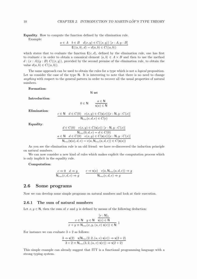
10 CHAPTER 2. INTRODUCTION TO MARTIN-LOF’S TYPE THEORY
Equality. How to compute the function defined by the elimination rule.Example:
a ∈ A b ∈ B d(x, y) ∈ C(〈x, y〉) [x : A, y : B]
E(〈a, b〉, d) = d(a, b) ∈ C(〈a, b〉)
which states that to evaluate the function E(c, d), defined by the elimination rule, one has firstto evaluate c in order to obtain a canonical element 〈a, b〉 ∈ A × B and then to use the methodd : (x : A)(y : B) C(〈x, y〉), provided by the second premise of the elimination rule, to obtain thevalue d(a, b) ∈ C(〈a, b〉).
The same approach can be used to obtain the rules for a type which is not a logical proposition.Let us consider the case of the type N. It is interesting to note that there is no need to changeanything with respect to the general pattern in order to recover all the usual properties of naturalnumbers.
Formation:N set
Introduction:
0 ∈ Na ∈ N
s(a) ∈ N
Elimination:c ∈ N d ∈ C(0) e(x, y) ∈ C(s(x))[x : N, y : C(x)]
Nrec(c, d, e) ∈ C(c)
Equality:d ∈ C(0) e(x, y) ∈ C(s(x)) [x : N, y : C(x)]
Nrec(0, d, e) = d ∈ C(0)a ∈ N d ∈ C(0) e(x, y) ∈ C(s(x))[x : N, y : C(x)]
Nrec(s(a), d, e) = e(a, Nrec(a, d, e)) ∈ C(s(a))
As you see the elimination rule is an old friend: we have re-discovered the induction principleon natural numbers.
We can now consider a new kind of rules which makes explicit the computation process whichis only implicit in the equality rule.
Computation:
c⇒ 0 d⇒ g
Nrec(c, d, e)⇒ g
c⇒ s(a) e(a, Nrec(a, d, e))⇒ g
Nrec(c, d, e)⇒ g
2.6 Some programs
Now we can develop some simple programs on natural numbers and look at their execution.
2.6.1 The sum of natural numbers
Let x, y ∈ N, then the sum of x and y is defined by means of the following deduction:
x ∈ N y ∈ N
[v : N]1
s(v) ∈ N
x + y ≡ Nrec(x, y, (u, v) s(v)) ∈ N1
For instance we can evaluate 3 + 2 as follows:
3⇒ s(2) s(Nrec(2, 2, (u, v) s(v))⇒ s(2 + 2)
3 + 2 ≡ Nrec(3, 2, (u, v) s(v))⇒ s(2 + 2)
This simple example can already suggest that ITT is a functional programming language with astrong typing system.
2.7. ALL TYPES ARE SIMILAR 11
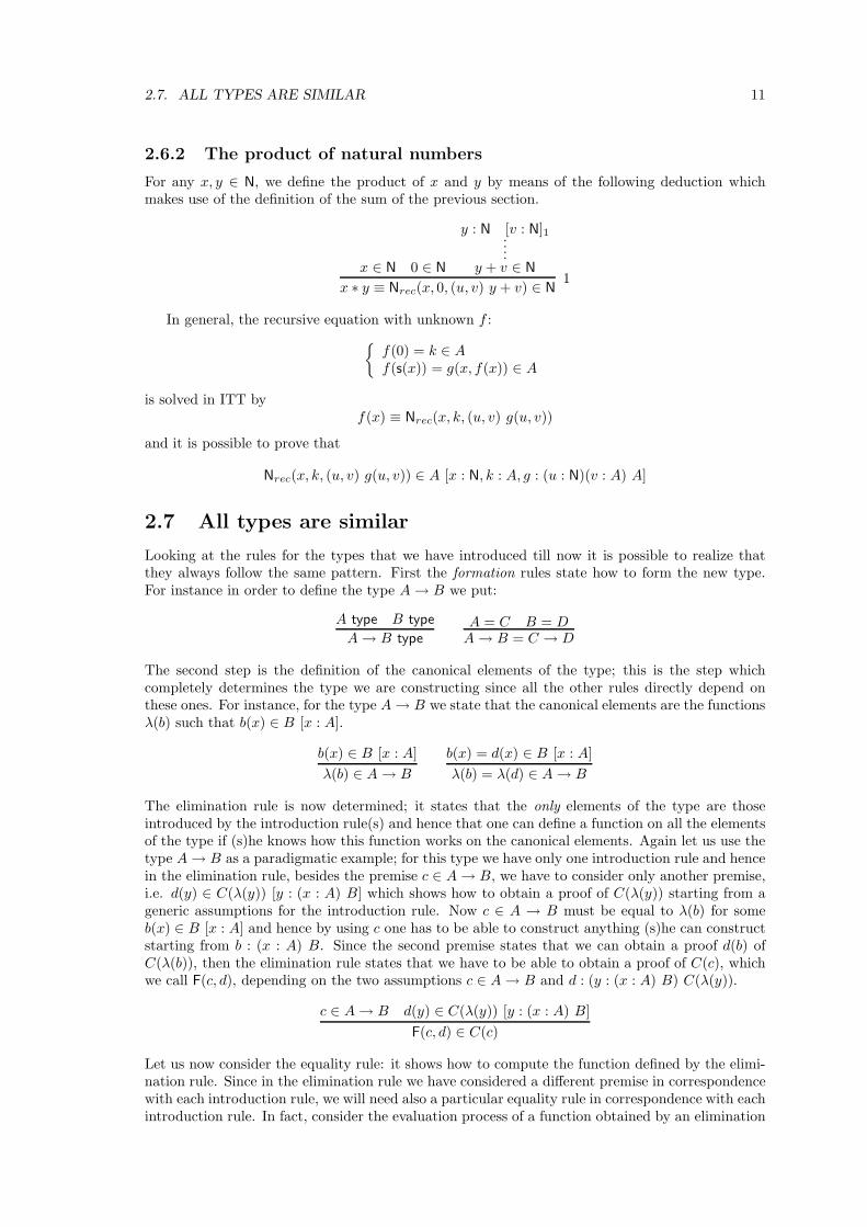
2.6.2 The product of natural numbers
For any x, y ∈ N, we define the product of x and y by means of the following deduction whichmakes use of the definition of the sum of the previous section.
x ∈ N 0 ∈ N
y : N [v : N]1....y + v ∈ N
x ∗ y ≡ Nrec(x, 0, (u, v) y + v) ∈ N1
In general, the recursive equation with unknown f :
f(0) = k ∈ Af(s(x)) = g(x, f(x)) ∈ A
is solved in ITT byf(x) ≡ Nrec(x, k, (u, v) g(u, v))
and it is possible to prove that
Nrec(x, k, (u, v) g(u, v)) ∈ A [x : N, k : A, g : (u : N)(v : A) A]
2.7 All types are similar
Looking at the rules for the types that we have introduced till now it is possible to realize thatthey always follow the same pattern. First the formation rules state how to form the new type.For instance in order to define the type A→ B we put:
A type B type
A→ B typeA = C B = D
A→ B = C → D
The second step is the definition of the canonical elements of the type; this is the step whichcompletely determines the type we are constructing since all the other rules directly depend onthese ones. For instance, for the type A→ B we state that the canonical elements are the functionsλ(b) such that b(x) ∈ B [x : A].
b(x) ∈ B [x : A]
λ(b) ∈ A→ B
b(x) = d(x) ∈ B [x : A]
λ(b) = λ(d) ∈ A→ B
The elimination rule is now determined; it states that the only elements of the type are thoseintroduced by the introduction rule(s) and hence that one can define a function on all the elementsof the type if (s)he knows how this function works on the canonical elements. Again let us use thetype A→ B as a paradigmatic example; for this type we have only one introduction rule and hencein the elimination rule, besides the premise c ∈ A→ B, we have to consider only another premise,i.e. d(y) ∈ C(λ(y)) [y : (x : A) B] which shows how to obtain a proof of C(λ(y)) starting from ageneric assumptions for the introduction rule. Now c ∈ A → B must be equal to λ(b) for someb(x) ∈ B [x : A] and hence by using c one has to be able to construct anything (s)he can constructstarting from b : (x : A) B. Since the second premise states that we can obtain a proof d(b) ofC(λ(b)), then the elimination rule states that we have to be able to obtain a proof of C(c), whichwe call F(c, d), depending on the two assumptions c ∈ A→ B and d : (y : (x : A) B) C(λ(y)).
c ∈ A→ B d(y) ∈ C(λ(y)) [y : (x : A) B]
F(c, d) ∈ C(c)
Let us now consider the equality rule: it shows how to compute the function defined by the elimi-nation rule. Since in the elimination rule we have considered a different premise in correspondencewith each introduction rule, we will need also a particular equality rule in correspondence with eachintroduction rule. In fact, consider the evaluation process of a function obtained by an elimination
12 CHAPTER 2. INTRODUCTION TO MARTIN-LOF’S TYPE THEORY
rule for the type A. First the element of the type A which appears in the leftmost premise isevaluated into a canonical element of A in correspondence to a suitable introduction rule; then thepremise(s) of this introduction rule can be substituted for the assumption(s) of the correspondingpremise of the elimination rule. Let us consider the case of the type A → B: we have only oneintroduction rule and hence we have to define one equality rule which explains how to evaluatea function F(z, d) ∈ C(z) [z : A → B] when it is used on the canonical element λ(b); the secondpremise of the elimination rule states that we obtain a proof d(b) of C(λ(b)) simply by substitutingb for y and hence we put F(λ(b), d) = d(b).
b(x) ∈ B [x : A] d(y) ∈ C(λ(y)) [y : (x : A) B]
F(λ(b), d) = d(b) ∈ C(λ(b))
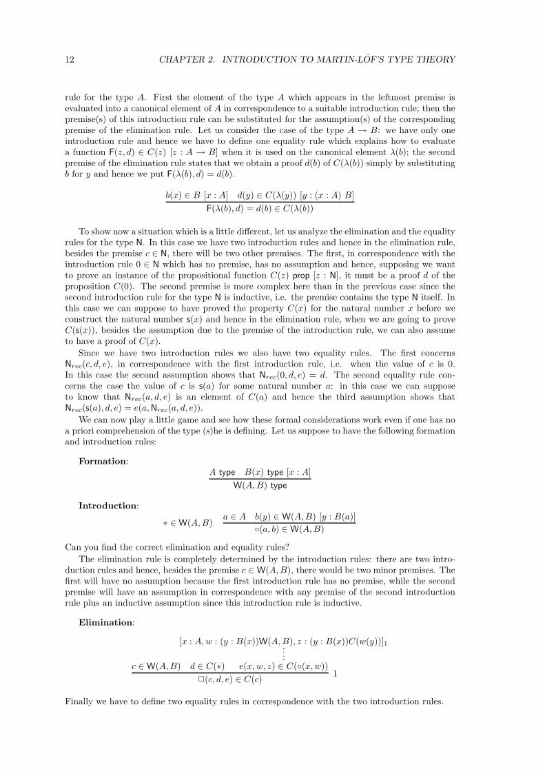
To show now a situation which is a little different, let us analyze the elimination and the equalityrules for the type N. In this case we have two introduction rules and hence in the elimination rule,besides the premise c ∈ N, there will be two other premises. The first, in correspondence with theintroduction rule 0 ∈ N which has no premise, has no assumption and hence, supposing we wantto prove an instance of the propositional function C(z) prop [z : N], it must be a proof d of theproposition C(0). The second premise is more complex here than in the previous case since thesecond introduction rule for the type N is inductive, i.e. the premise contains the type N itself. Inthis case we can suppose to have proved the property C(x) for the natural number x before weconstruct the natural number s(x) and hence in the elimination rule, when we are going to proveC(s(x)), besides the assumption due to the premise of the introduction rule, we can also assumeto have a proof of C(x).
Since we have two introduction rules we also have two equality rules. The first concernsNrec(c, d, e), in correspondence with the first introduction rule, i.e. when the value of c is 0.In this case the second assumption shows that Nrec(0, d, e) = d. The second equality rule con-cerns the case the value of c is s(a) for some natural number a: in this case we can supposeto know that Nrec(a, d, e) is an element of C(a) and hence the third assumption shows thatNrec(s(a), d, e) = e(a, Nrec(a, d, e)).
We can now play a little game and see how these formal considerations work even if one has noa priori comprehension of the type (s)he is defining. Let us suppose to have the following formationand introduction rules:
Formation:A type B(x) type [x : A]
W(A, B) type
Introduction:
∗ ∈W(A, B)a ∈ A b(y) ∈ W(A, B) [y : B(a)]
(a, b) ∈ W(A, B)
Can you find the correct elimination and equality rules?
The elimination rule is completely determined by the introduction rules: there are two intro-duction rules and hence, besides the premise c ∈ W(A, B), there would be two minor premises. Thefirst will have no assumption because the first introduction rule has no premise, while the secondpremise will have an assumption in correspondence with any premise of the second introductionrule plus an inductive assumption since this introduction rule is inductive.
Elimination:
c ∈W(A, B) d ∈ C(∗)
[x : A, w : (y : B(x))W(A, B), z : (y : B(x))C(w(y))]1....e(x, w, z) ∈ C((x, w))
2(c, d, e) ∈ C(c)1
Finally we have to define two equality rules in correspondence with the two introduction rules.
2.8. SOME APPLICATIONS 13
∗
t1 RRRRRRRRRRRRRRR ∗
t2
∗
t3qqqqqqqqqqq
∗
u1 KKKKKKKKKKK ∗
u2
b1[u3] ≡ (a2, b2)
u3
lllllllllllll
∗
v1
WWWWWWWWWWWWWWWWWWWWWWWWWWW b[v2] ≡ (a1, b1)
v2
RRRRRRRRRRRRR∗
v3
∗
v4
rrrrrrrrrrr∗
v5
kkkkkkkkkkkkkkkkk
(a, b)
B(a) ≡ v1, v2, v3, v4, v5 B(a1) ≡ u1, u2, u3 B(a2) ≡ t1, t2, t3
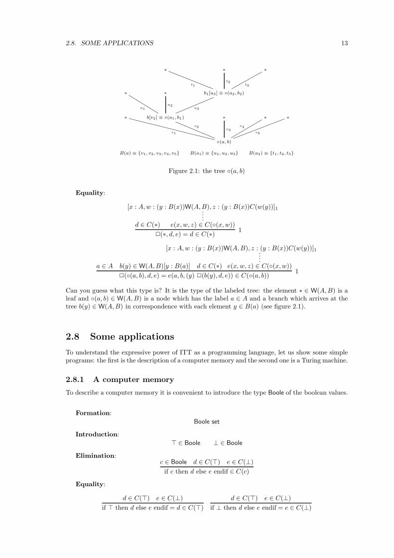
Figure 2.1: the tree (a, b)
Equality:
d ∈ C(∗)
[x : A, w : (y : B(x))W(A, B), z : (y : B(x))C(w(y))]1....e(x, w, z) ∈ C((x, w))
2(∗, d, e) = d ∈ C(∗)1
a ∈ A b(y) ∈W(A, B)[y : B(a)] d ∈ C(∗)
[x : A, w : (y : B(x))W(A, B), z : (y : B(x))C(w(y))]1....e(x, w, z) ∈ C((x, w))
2((a, b), d, e) = e(a, b, (y) 2(b(y), d, e)) ∈ C((a, b))1
Can you guess what this type is? It is the type of the labeled tree: the element ∗ ∈ W(A, B) is aleaf and (a, b) ∈ W(A, B) is a node which has the label a ∈ A and a branch which arrives at thetree b(y) ∈W(A, B) in correspondence with each element y ∈ B(a) (see figure 2.1).
2.8 Some applications
To understand the expressive power of ITT as a programming language, let us show some simpleprograms: the first is the description of a computer memory and the second one is a Turing machine.
2.8.1 A computer memory
To describe a computer memory it is convenient to introduce the type Boole of the boolean values.
Formation:
Boole set
Introduction:
⊤ ∈ Boole ⊥ ∈ Boole
Elimination:c ∈ Boole d ∈ C(⊤) e ∈ C(⊥)
if c then d else e endif ∈ C(c)
Equality:
d ∈ C(⊤) e ∈ C(⊥)
if ⊤ then d else e endif = d ∈ C(⊤)
d ∈ C(⊤) e ∈ C(⊥)
if ⊥ then d else e endif = e ∈ C(⊥)
14 CHAPTER 2. INTRODUCTION TO MARTIN-LOF’S TYPE THEORY
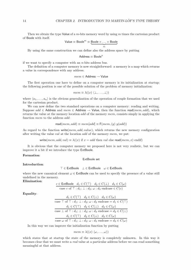
Then we obtain the type Value of a m-bits memory word by using m times the cartesian productof Boole with itself.
Value ≡ Boolem ≡ Boole× . . .× Boole︸ ︷︷ ︸
m
By using the same construction we can define also the address space by putting
Address ≡ Boolen
if we want to specify a computer with an n-bits address bus.The definition of a computer memory is now straightforward: a memory is a map which returns
a value in correspondence with any address.
mem ∈ Address→ Value
The first operation one have to define on a computer memory is its initialization at startup;the following position is one of the possible solution of the problem of memory initialization:
mem ≡ λ((x) 〈⊥, . . . ,⊥〉)
where 〈a1, . . . , an〉 is the obvious generalization of the operation of couple formation that we usedfor the cartesian product.
We can now define the two standard operations on a computer memory: reading and writing.Suppose add ∈ Address and mem ∈ Address → Value, then the function read(mem, add), whichreturns the value at the memory location add of the memory mem, consists simply in applying thefunction mem to the address add:
read(mem, add) ≡ mem[add] ≡ F(mem, (y) y(add))
As regard to the function write(mem, add, value), which returns the new memory configurationafter writing the value val at the location add of the memory mem, we put:
write(mem, add, val) ≡ λ((x) if x = add then val else read(mem, x) endif)
It is obvious that the computer memory we proposed here is not very realistic, but we canimprove it a bit if we introduce the type ExtBoole.
Formation:ExtBoole set
Introduction:⊤ ∈ ExtBoole ⊥ ∈ ExtBoole ω ∈ ExtBoole
where the new canonical element ω ∈ ExtBoole can be used to specify the presence of a value stillundefined in the memory.Elimination:
c ∈ ExtBoole d1 ∈ C(⊤) d2 ∈ C(⊥) d3 ∈ C(ω)
case c of ⊤ : d1; ⊥ : d2; ω : d3 endcase ∈ C(c)
Equality:d1 ∈ C(⊤) d2 ∈ C(⊥) d3 ∈ C(ω)
case ⊤ of ⊤ : d1; ⊥ : d2; ω : d3 endcase = d1 ∈ C(⊤)
d1 ∈ C(⊤) d2 ∈ C(⊥) d3 ∈ C(ω)
case ⊥ of ⊤ : d1; ⊥ : d2; ω : d3 endcase = d2 ∈ C(⊥)
d1 ∈ C(⊤) d2 ∈ C(⊥) d3 ∈ C(ω)
case ω of ⊤ : d1; ⊥ : d2; ω : d3 endcase = d3 ∈ C(ω)
In this way we can improve the initialization function by putting
mem ≡ λ((x) 〈ω, . . . , ω〉)
which states that at startup the state of the memory is completely unknown. In this way itbecomes clear that we must write a real value at a particular address before we can read somethingmeaningful at that address.
2.8. SOME APPLICATIONS 15
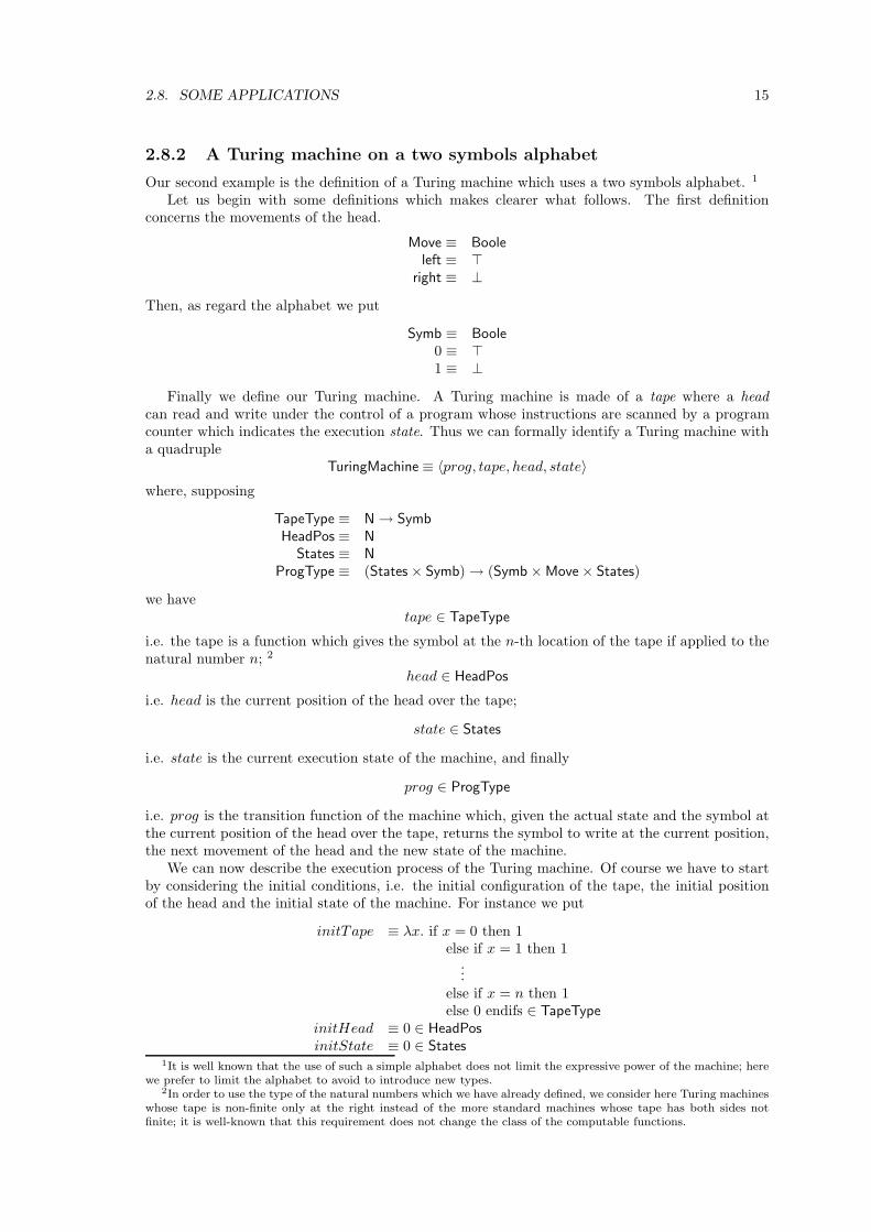
2.8.2 A Turing machine on a two symbols alphabet
Our second example is the definition of a Turing machine which uses a two symbols alphabet. 1
Let us begin with some definitions which makes clearer what follows. The first definitionconcerns the movements of the head.
Move ≡ Boole
left ≡ ⊤right ≡ ⊥
Then, as regard the alphabet we put
Symb ≡ Boole
0 ≡ ⊤1 ≡ ⊥
Finally we define our Turing machine. A Turing machine is made of a tape where a headcan read and write under the control of a program whose instructions are scanned by a programcounter which indicates the execution state. Thus we can formally identify a Turing machine witha quadruple
TuringMachine ≡ 〈prog, tape, head, state〉
where, supposing
TapeType ≡ N→ Symb
HeadPos ≡ N
States ≡ N
ProgType ≡ (States× Symb)→ (Symb×Move× States)
we havetape ∈ TapeType
i.e. the tape is a function which gives the symbol at the n-th location of the tape if applied to thenatural number n; 2
head ∈ HeadPos
i.e. head is the current position of the head over the tape;
state ∈ States
i.e. state is the current execution state of the machine, and finally
prog ∈ ProgType
i.e. prog is the transition function of the machine which, given the actual state and the symbol atthe current position of the head over the tape, returns the symbol to write at the current position,the next movement of the head and the new state of the machine.
We can now describe the execution process of the Turing machine. Of course we have to startby considering the initial conditions, i.e. the initial configuration of the tape, the initial positionof the head and the initial state of the machine. For instance we put
initTape ≡ λx. if x = 0 then 1else if x = 1 then 1
...else if x = n then 1else 0 endifs ∈ TapeType
initHead ≡ 0 ∈ HeadPos
initState ≡ 0 ∈ States1It is well known that the use of such a simple alphabet does not limit the expressive power of the machine; here
we prefer to limit the alphabet to avoid to introduce new types.2In order to use the type of the natural numbers which we have already defined, we consider here Turing machines
whose tape is non-finite only at the right instead of the more standard machines whose tape has both sides notfinite; it is well-known that this requirement does not change the class of the computable functions.
16 CHAPTER 2. INTRODUCTION TO MARTIN-LOF’S TYPE THEORY
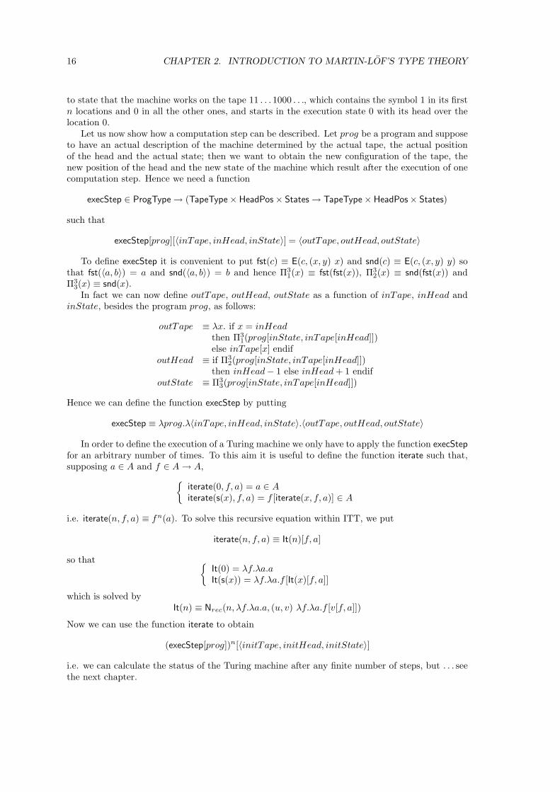
to state that the machine works on the tape 11 . . . 1000 . . ., which contains the symbol 1 in its firstn locations and 0 in all the other ones, and starts in the execution state 0 with its head over thelocation 0.
Let us now show how a computation step can be described. Let prog be a program and supposeto have an actual description of the machine determined by the actual tape, the actual positionof the head and the actual state; then we want to obtain the new configuration of the tape, thenew position of the head and the new state of the machine which result after the execution of onecomputation step. Hence we need a function
execStep ∈ ProgType→ (TapeType× HeadPos× States→ TapeType× HeadPos× States)
such that
execStep[prog][〈inTape, inHead, inState〉] = 〈outTape, outHead, outState〉
To define execStep it is convenient to put fst(c) ≡ E(c, (x, y) x) and snd(c) ≡ E(c, (x, y) y) sothat fst(〈a, b〉) = a and snd(〈a, b〉) = b and hence Π3
1(x) ≡ fst(fst(x)), Π32(x) ≡ snd(fst(x)) and
Π33(x) ≡ snd(x).
In fact we can now define outTape, outHead, outState as a function of inTape, inHead andinState, besides the program prog, as follows:
outTape ≡ λx. if x = inHeadthen Π3
1(prog[inState, inTape[inHead]])else inTape[x] endif
outHead ≡ if Π32(prog[inState, inTape[inHead]])
then inHead− 1 else inHead + 1 endifoutState ≡ Π3
3(prog[inState, inTape[inHead]])
Hence we can define the function execStep by putting
execStep ≡ λprog.λ〈inTape, inHead, inState〉.〈outTape, outHead, outState〉
In order to define the execution of a Turing machine we only have to apply the function execStep
for an arbitrary number of times. To this aim it is useful to define the function iterate such that,supposing a ∈ A and f ∈ A→ A,
iterate(0, f, a) = a ∈ Aiterate(s(x), f, a) = f [iterate(x, f, a)] ∈ A
i.e. iterate(n, f, a) ≡ fn(a). To solve this recursive equation within ITT, we put
iterate(n, f, a) ≡ It(n)[f, a]
so that It(0) = λf.λa.aIt(s(x)) = λf.λa.f [It(x)[f, a]]
which is solved byIt(n) ≡ Nrec(n, λf.λa.a, (u, v) λf.λa.f [v[f, a]])
Now we can use the function iterate to obtain
(execStep[prog])n[〈initTape, initHead, initState〉]
i.e. we can calculate the status of the Turing machine after any finite number of steps, but . . . seethe next chapter.
Chapter 3
The canonical form theorem
3.1 Summary
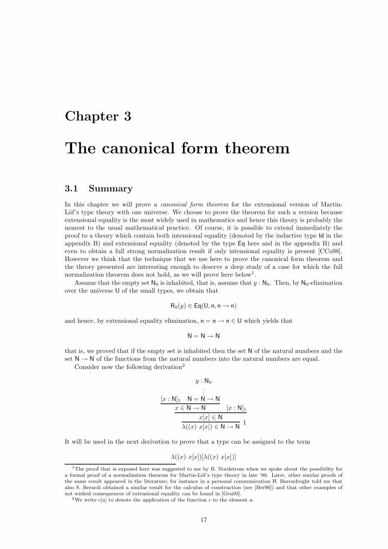
In this chapter we will prove a canonical form theorem for the extensional version of Martin-Lof’s type theory with one universe. We choose to prove the theorem for such a version becauseextensional equality is the most widely used in mathematics and hence this theory is probably thenearest to the usual mathematical practice. Of course, it is possible to extend immediately theproof to a theory which contain both intensional equality (denoted by the inductive type Id in theappendix B) and extensional equality (denoted by the type Eq here and in the appendix B) andeven to obtain a full strong normalization result if only intensional equality is present [CCo98].However we think that the technique that we use here to prove the canonical form theorem andthe theory presented are interesting enough to deserve a deep study of a case for which the fullnormalization theorem does not hold, as we will prove here below1.
Assume that the empty set N0 is inhabited, that is, assume that y : N0. Then, by N0-eliminationover the universe U of the small types, we obtain that
R0(y) ∈ Eq(U, n, n→ n)
and hence, by extensional equality elimination, n = n→ n ∈ U which yields that
N = N→ N
that is, we proved that if the empty set is inhabited then the set N of the natural numbers and theset N→ N of the functions from the natural numbers into the natural numbers are equal.
Consider now the following derivation2
[x : N]1
y : N0
...N = N→ N
x ∈ N→ N [x : N]1
x[x] ∈ N
λ((x) x[x]) ∈ N→ N1
It will be used in the next derivation to prove that a type can be assigned to the term
λ((x) x[x])[λ((x) x[x])]
1The proof that is exposed here was suggested to me by B. Nordstrom when we spoke about the possibility fora formal proof of a normalization theorem for Martin-Lof’s type theory in late ’80. Later, other similar proofs ofthe same result appeared in the literature; for instance in a personal communication H. Barendreght told me thatalso S. Berardi obtained a similar result for the calculus of construction (see [Ber90]) and that other examples ofnot wished consequences of extensional equality can be found in [Geu93].
2We write c[a] to denote the application of the function c to the element a.
17
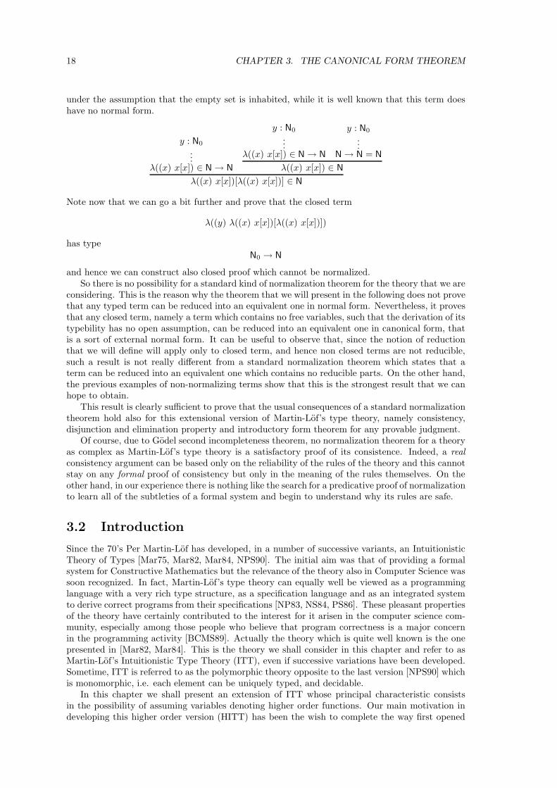
18 CHAPTER 3. THE CANONICAL FORM THEOREM
under the assumption that the empty set is inhabited, while it is well known that this term doeshave no normal form.
y : N0
...λ((x) x[x]) ∈ N→ N
y : N0
...λ((x) x[x]) ∈ N→ N
y : N0
...N→ N = N
λ((x) x[x]) ∈ N
λ((x) x[x])[λ((x) x[x])] ∈ N
Note now that we can go a bit further and prove that the closed term
λ((y) λ((x) x[x])[λ((x) x[x])])
has type
N0 → N
and hence we can construct also closed proof which cannot be normalized.So there is no possibility for a standard kind of normalization theorem for the theory that we are
considering. This is the reason why the theorem that we will present in the following does not provethat any typed term can be reduced into an equivalent one in normal form. Nevertheless, it provesthat any closed term, namely a term which contains no free variables, such that the derivation of itstypebility has no open assumption, can be reduced into an equivalent one in canonical form, thatis a sort of external normal form. It can be useful to observe that, since the notion of reductionthat we will define will apply only to closed term, and hence non closed terms are not reducible,such a result is not really different from a standard normalization theorem which states that aterm can be reduced into an equivalent one which contains no reducible parts. On the other hand,the previous examples of non-normalizing terms show that this is the strongest result that we canhope to obtain.
This result is clearly sufficient to prove that the usual consequences of a standard normalizationtheorem hold also for this extensional version of Martin-Lof’s type theory, namely consistency,disjunction and elimination property and introductory form theorem for any provable judgment.
Of course, due to Godel second incompleteness theorem, no normalization theorem for a theoryas complex as Martin-Lof’s type theory is a satisfactory proof of its consistence. Indeed, a realconsistency argument can be based only on the reliability of the rules of the theory and this cannotstay on any formal proof of consistency but only in the meaning of the rules themselves. On theother hand, in our experience there is nothing like the search for a predicative proof of normalizationto learn all of the subtleties of a formal system and begin to understand why its rules are safe.
3.2 Introduction
Since the 70’s Per Martin-Lof has developed, in a number of successive variants, an IntuitionisticTheory of Types [Mar75, Mar82, Mar84, NPS90]. The initial aim was that of providing a formalsystem for Constructive Mathematics but the relevance of the theory also in Computer Science wassoon recognized. In fact, Martin-Lof’s type theory can equally well be viewed as a programminglanguage with a very rich type structure, as a specification language and as an integrated systemto derive correct programs from their specifications [NP83, NS84, PS86]. These pleasant propertiesof the theory have certainly contributed to the interest for it arisen in the computer science com-munity, especially among those people who believe that program correctness is a major concernin the programming activity [BCMS89]. Actually the theory which is quite well known is the onepresented in [Mar82, Mar84]. This is the theory we shall consider in this chapter and refer to asMartin-Lof’s Intuitionistic Type Theory (ITT), even if successive variations have been developed.Sometime, ITT is referred to as the polymorphic theory opposite to the last version [NPS90] whichis monomorphic, i.e. each element can be uniquely typed, and decidable.
In this chapter we shall present an extension of ITT whose principal characteristic consistsin the possibility of assuming variables denoting higher order functions. Our main motivation indeveloping this higher order version (HITT) has been the wish to complete the way first opened
3.3. ASSUMPTIONS OF HIGH LEVEL ARITY VARIABLES 19
by Per Martin-Lof. Indeed in the preface of [Mar84], while referring to a series of lectures given inMunich (October 1980), he writes: “The main improvement of the Munich lectures, compared withthose given in Padova, was the adoption of a systematic higher level notation . . . ”. This notationis called expressions with arity and yields a more uniform and compact writing of the rules of thetheory. An expression with arity is built up starting from primitive constants and variables witharity, by means of abstractions and applications. The arity associated to an expression specifiesits functionality and constrains the applications, analogously to what the type does for typedlambda-calculus. In our opinion, in order to fully exploit this approach and be able to establishformal properties of the system, it is necessary to extend the formalization of the contexts as givenin [Mar84] to assumptions of variables of higher arity. Therefore we have defined this extensionthat, even if conservative, supplies increased expressive power, advantageous especially when thetheory is viewed as a programming and a specification language. In fact, assuming a variable ofhigher arity corresponds to assuming the possibility of putting together pieces of programs, thussupporting a modular approach in program development [BV87].
Some properties of HITT are also proved, the principal ones are the consistency of HITT,which also implies the consistency of ITT, and the computability of any judgement derived withinHITT. Besides we proved a canonical form theorem: to any derivable judgement we can associatea canonical one whose derivation ends with an introductory rule. This result, even if weakerthan a standard normalization theorem [Pra65], suffices to obtain all the useful consequencestypical of a normal form theorem, mainly the consistency of the theory. Moreover, by using thecomputational interpretation of types (i.e. types as problem descriptions and their elements asprograms to solve those problems) it immediately follows that the execution of any proved correctprogram terminates. We assume the reader is familiar with the Intuitionistic Theory of Types aspresented in [Mar82, Mar84] and with typed lambda calculus [Bar84], or enjoyably, with the theoryof expressions with arity (see appendix A or [BV89, NPS90]).
The following is the outline of the chapter. In section 2. our characterization of assumptionsof variables of any arity is presented and some consequences of this are briefly sketched. We areextremely grateful to Prof. Aczel for his suggestions on the notation to be used for the new kindof assumptions. Further comments on the properties of our system are given in section 3. Section4. deals with computability. The definition of computable judgement, which is the basis for thecomputability theorem, is first given. The rest of the section is devoted to prove that each rule ofthe theory preserves this property. The computability theorem, as well as some relevant corollaries,is presented in the concluding section 5. All of the rules of HITT are listed in the appendix B.Compared with ITT, besides the changes concerning the assumptions of higher level variables,there are also changes in the notation and in the fact that we explicitly added to the premises ofa rule all the requirements that were only informally expressed in ITT.
3.3 Assumptions of high level arity variables
We assume the theory of expressions with arity (see appendix A and [Bee85, BV89, NPS90])developed by Martin Lof in order to give an uniform and compact presentation of his theory oftypes. The theory has many similarities with typed lambda-calculus [Bar84] and some familiaritywith this system should be sufficient to understand what follows. An expression with arity isbuilt up starting from primitive constants and variables with arity, by means of abstractions andapplications. The arity associated to an expression fully specifies its functionality, i.e. it indicatesthe number and the arity of the expressions to which it can be applied, analogously to what thetype does for typed lambda-calculus.
The Intuitionistic Theory of Types [Mar82] consists of a language of constant symbols, each ofsome arity, a system of computation rules and a system of rules of inference for deriving judgements.Each instance of a rule of inference has the form
J1 . . . Jn
J
where J1,. . . ,Jn,J are judgements. A derivation is a tree of judgements built up in the usual way
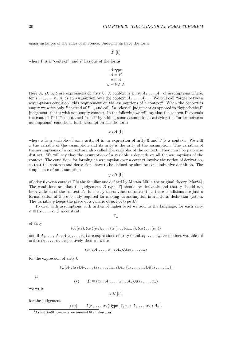
20 CHAPTER 3. THE CANONICAL FORM THEOREM
using instances of the rules of inference. Judgements have the form
F [Γ]
where Γ is a “context”, and F has one of the forms
A type
A = Ba ∈ A
a = b ∈ A
Here A, B, a, b are expressions of arity 0. A context is a list A1, . . . , An of assumptions where,for j = 1, . . . , n, Aj is an assumption over the context A1, . . . , Aj−1. We will call “order betweenassumptions condition” this requirement on the assumptions of a context3. When the context isempty we write only F instead of F [], and call J a “closed” judgement as opposed to “hypothetical”judgement, that is with non-empty context. In the following we will say that the context Γ′ extendsthe context Γ if Γ′ is obtained from Γ by adding some assumptions satisfying the “order betweenassumptions” condition. Each assumption has the form
x : A [Γ]
where x is a variable of some arity, A is an expression of arity 0 and Γ is a context. We callx the variable of the assumption and its arity is the arity of the assumption. The variables ofthe assumptions of a context are also called the variables of the context. They must be pair-wisedistinct. We will say that the assumption of a variable x depends on all the assumptions of thecontext. The conditions for forming an assumption over a context involve the notion of derivation,so that the contexts and derivations have to be defined by simultaneous inductive definition. Thesimple case of an assumption
y : B [Γ]
of arity 0 over a context Γ is the familiar one defined by Martin-Lof in the original theory [Mar84].The conditions are that the judgement B type [Γ] should be derivable and that y should notbe a variable of the context Γ. It is easy to convince ourselves that these conditions are just aformalization of those usually required for making an assumption in a natural deduction system.The variable y keeps the place of a generic object of type B.
To deal with assumptions with arities of higher level we add to the language, for each arityα ≡ (α1, . . . , αn), a constant
Tα
of arity(0, (α1), (α1)(α2), . . . , (α1) . . . (αn−1), (α1) . . . (αn))
and if A1, . . . , An, A(x1, . . . , xn) are expressions of arity 0 and x1, . . . , xn are distinct variables ofarities α1, . . . , αn respectively then we write
(x1 : A1, . . . , xn : An)A(x1, . . . , xn)
for the expression of arity 0
Tα(A1, (x1)A2, . . . , (x1, . . . , xn−1)An, (x1, . . . , xn)A(x1, . . . , xn))
If(∗) B ≡ (x1 : A1, . . . , xn : An)A(x1, . . . , xn)
we write: B [Γ]
for the judgement(∗∗) A(x1, . . . , xn) type [Γ, x1 : A1, . . . , xn : An].
3As in [Bru91] contexts are inserted like ‘telescopes’.
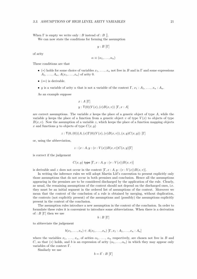
3.3. ASSUMPTIONS OF HIGH LEVEL ARITY VARIABLES 21
When Γ is empty we write only : B instead of : B [].We can now state the conditions for forming the assumption
y : B [Γ]
of arityα ≡ (α1, . . . , αn)
These conditions are that
• (∗) holds for some choice of variables x1, . . . , xn not free in B and in Γ and some expressionsA1, . . . , An, A(x1, . . . , xn) of arity 0.
• (∗∗) is derivable.
• y is a variable of arity α that is not a variable of the context Γ, x1 : A1, . . . , xn : An.
As an example suppose
x : A [Γ]
y : T(0)(V (x), (v)B(x, v)) [Γ, x : A]
are correct assumptions. The variable x keeps the place of a generic object of type A, while thevariable y keeps the place of a function from a generic object v of type V (x) to objects of typeB(x, v). Now the assumption of a variable z, which keeps the place of a function mapping objectsx and functions y to objects of type C(x, y)
z : T(0, (0))(A, (x)T (0)(V (x), (v)B(x, v)), (x, y)C(x, y)) [Γ]
or, using the abbreviation,
z : (x : A, y : (v : V (x))B(x, v))C(x, y)[Γ]
is correct if the judgement
C(x, y) type [Γ, x : A, y : (v : V (x))B(x, v)]
is derivable and z does not occur in the context [Γ, x : A, y : (v : V (x))B(x, v)].In writing the inference rules we will adopt Martin Lof’s convention to present explicitly only
those assumptions that do not occur in both premises and conclusion. Hence all the assumptionsappearing in the premises are to be considered discharged by the application of the rule. Clearly,as usual, the remaining assumptions of the context should not depend on the discharged ones, i.e.they must be an initial segment in the ordered list of assumptions of the context. Moreover wemean that the context of the conclusion of a rule is obtained by merging, without duplication,the contexts (not explicitly present) of the assumptions and (possibly) the assumptions explicitlypresent in the context of the conclusion.
The assumption rules introduce a new assumption in the context of the conclusion. In order toformulate these rules it is convenient to introduce some abbreviations. When there is a derivationof : B [Γ] then we use
b : B [Γ]
to abbreviate the judgement
b(x1, . . . , xn) ∈ A(x1, . . . , xn) [Γ, x1 : A1, . . . , xn : An]
where the variables x1, . . . , xn, of arities α1, . . . , αn respectively, are chosen not free in B andC, so that (∗) holds, and b is an expression of arity (α1, . . . , αn) in which they may appear onlyvariables of the context Γ.
Similarly we useb = b′ : B [Γ]
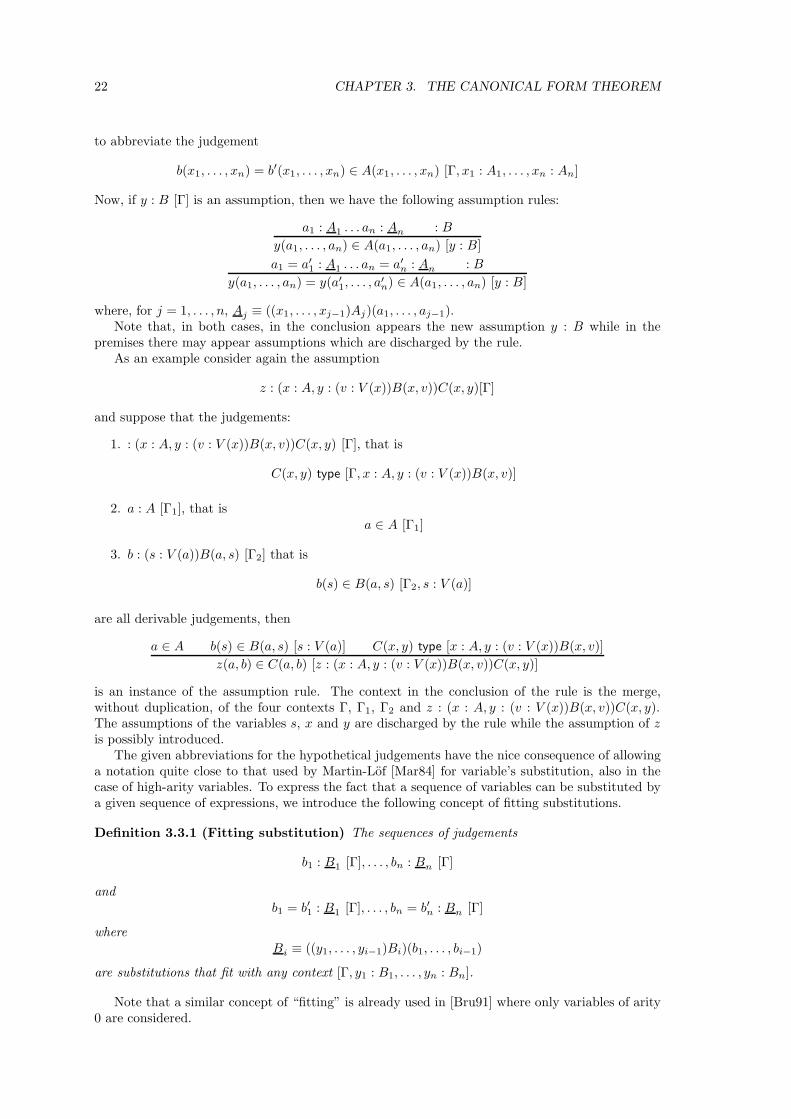
22 CHAPTER 3. THE CANONICAL FORM THEOREM
to abbreviate the judgement
b(x1, . . . , xn) = b′(x1, . . . , xn) ∈ A(x1, . . . , xn) [Γ, x1 : A1, . . . , xn : An]
Now, if y : B [Γ] is an assumption, then we have the following assumption rules:
a1 : A1 . . . an : An : B
y(a1, . . . , an) ∈ A(a1, . . . , an) [y : B]
a1 = a′1 : A1 . . . an = a′
n : An : B
y(a1, . . . , an) = y(a′1, . . . , a
′n) ∈ A(a1, . . . , an) [y : B]
where, for j = 1, . . . , n, Aj ≡ ((x1, . . . , xj−1)Aj)(a1, . . . , aj−1).Note that, in both cases, in the conclusion appears the new assumption y : B while in the
premises there may appear assumptions which are discharged by the rule.As an example consider again the assumption
z : (x : A, y : (v : V (x))B(x, v))C(x, y)[Γ]
and suppose that the judgements:
1. : (x : A, y : (v : V (x))B(x, v))C(x, y) [Γ], that is
C(x, y) type [Γ, x : A, y : (v : V (x))B(x, v)]
2. a : A [Γ1], that isa ∈ A [Γ1]
3. b : (s : V (a))B(a, s) [Γ2] that is
b(s) ∈ B(a, s) [Γ2, s : V (a)]
are all derivable judgements, then
a ∈ A b(s) ∈ B(a, s) [s : V (a)] C(x, y) type [x : A, y : (v : V (x))B(x, v)]
z(a, b) ∈ C(a, b) [z : (x : A, y : (v : V (x))B(x, v))C(x, y)]
is an instance of the assumption rule. The context in the conclusion of the rule is the merge,without duplication, of the four contexts Γ, Γ1, Γ2 and z : (x : A, y : (v : V (x))B(x, v))C(x, y).The assumptions of the variables s, x and y are discharged by the rule while the assumption of zis possibly introduced.
The given abbreviations for the hypothetical judgements have the nice consequence of allowinga notation quite close to that used by Martin-Lof [Mar84] for variable’s substitution, also in thecase of high-arity variables. To express the fact that a sequence of variables can be substituted bya given sequence of expressions, we introduce the following concept of fitting substitutions.
Definition 3.3.1 (Fitting substitution) The sequences of judgements
b1 : B1 [Γ], . . . , bn : Bn [Γ]
andb1 = b′1 : B1 [Γ], . . . , bn = b′n : Bn [Γ]
whereBi ≡ ((y1, . . . , yi−1)Bi)(b1, . . . , bi−1)
are substitutions that fit with any context [Γ, y1 : B1, . . . , yn : Bn].
Note that a similar concept of “fitting” is already used in [Bru91] where only variables of arity0 are considered.
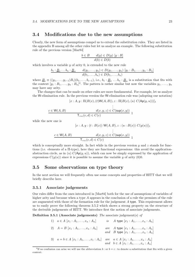
3.4. MODIFICATIONS DUE TO THE NEW ASSUMPTIONS 23
3.4 Modifications due to the new assumptions
Clearly, the new form of assumptions compel us to extend the substitution rules. They are listed inthe appendix B among all the other rules but let us analyze an example. The following substitutionrule of the previous version [Mar84]
b ∈ B d(y) ∈ D(y) [y : B]
d(b) ∈ D(b)
which involves a variable y of arity 0, is extended to the new rule
b1 : B1 . . . bn : Bn d(y1, . . . , yn) ∈ D(y1, . . . , yn) [y1 : B1, . . . , yn : Bn]
d(b1, . . . , bn) ∈ D(b1, . . . , bn)
where Bi ≡ ((y1, . . . , yi−1)Bi)(b1, . . . , bi−1), i.e., b1 : B1 . . . bn : Bn is a substitution that fits withthe context [y1 : B1, . . . , yn : Bn]4. The pattern is rather similar but now the variables y1, . . . , yn
may have any arity.The changes that can be made on other rules are more fundamental. For example, let us analyze
the W-elimination rule. In the previous version the W-elimination rule was (adopting our notation)
c ∈W(A, B)
[x : A, y : Π(B(x), (t)W(A, B)), z : Π(B(x), (u) C(Ap(y, u)))]1...
d(x, y, z) ∈ C(sup(x, y))
Trec(c, d) ∈ C(c)1
while the new one is
c ∈W(A, B)
[x : A, y : (t : B(x)) W(A, B), z : (u : B(x)) C(y(u))]1...
d(x, y, z) ∈ C(sup(x, y))
Trec(c, d) ∈ C(c)1
which is conceptually more straight. In fact while in the previous version y and z stands for func-tions (i.e. elements of a Π-type), here they are functional expressions: this avoid the application-abstraction circle, as in (u) C(Ap(y, u)), which can now be simply expressed by the application ofexpressions C(y(u)) since it is possible to assume the variable y of arity (0)0.
3.5 Some observations on type theory
In the next section we will frequently often use some concepts and properties of HITT that we willbriefly describe here.
3.5.1 Associate judgements
Our rules differ from the ones introduced in [Mar84] both for the use of assumptions of variables ofhigher arity and because when a type A appears in the conclusion of a rule the premises of the ruleare augmented with those of the formation rule for the judgement A type. This requirement allowsus to easily prove the following theorem 3.5.2 which shows a strong property on the structure ofthe derivable judgements of HITT. We introduce first the notion of associate judgements.
Definition 3.5.1 (Associate judgements) The associate judgement(s) of
1) a ∈ A [x1 : A1, . . . , xn : An] is A type [x1 : A1, . . . , xn : An]
2) A = B [x1 : A1, . . . , xn : An] are A type [x1 : A1, . . . , xn : An]and B type [x1 : A1, . . . , xn : An]
3) a = b ∈ A [x1 : A1, . . . , x1 : An] are a ∈ A [x1 : A1, . . . , xn : An]and b ∈ A [x1 : A1, . . . , xn : An]
4If no confusion can arise we will use the abbreviation b : or b = c : to denote a substitution that fits with a givencontext.
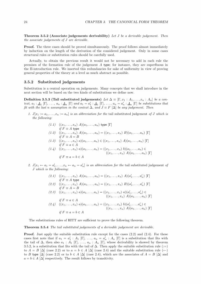
24 CHAPTER 3. THE CANONICAL FORM THEOREM
Theorem 3.5.2 (Associate judgements derivability) Let J be a derivable judgement. Thenthe associate judgements of J are derivable.
Proof. The three cases should be proved simultaneously. The proof follows almost immediatelyby induction on the length of the derivation of the considered judgement. Only in some casesstructural rules or substitution rules should be carefully used.
Actually, to obtain the previous result it would not be necessary to add in each rule thepremises of the formation rule of the judgement A type; for instance, they are superfluous inthe Π-introduction rule. We inserted this redundancies for sake of uniformity in view of provinggeneral properties of the theory at a level as much abstract as possible.
3.5.2 Substituted judgements
Substitution is a central operation on judgements. Many concepts that we shall introduce in thenext section will be based on the two kinds of substitutions we define now.
Definition 3.5.3 (Tail substituted judgements) Let ∆ ≡ [Γ, x1 : A1, . . . , xn : An] be a con-text, a1 : A1 [Γ], . . . , an : An [Γ] and a1 = a′
1 : A1 [Γ], . . . , an = a′n : An [Γ] be substitutions that
fit with the last n assumption in the context ∆, and J ≡ F [∆] be any judgement. Then
1. J [x1 := a1, . . . , xn := an] is an abbreviation for the tail substituted judgement of J which isthe following:
(1.1) ((x1, . . . , xn) A)(a1, . . . , an) type [Γ]if F ≡ A type
(1.2) ((x1, . . . , xn) A)(a1, . . . , an) = ((x1, . . . , xn) B)(a1, . . . , an) [Γ]if F ≡ A = B
(1.3) ((x1, . . . , xn) a)(a1, . . . , an) ∈ ((x1, . . . , xn) A)(a1, . . . , an) [Γ]if F ≡ a ∈ A
(1.4) ((x1, . . . , xn) a)(a1, . . . , an) = ((x1, . . . , xn) b)(a1, . . . , an) ∈((x1, . . . , xn) A)(a1, . . . , an) [Γ]
if F ≡ a = b ∈ A
2. J [x1 ← a1 = a′1, . . . , xn ← an = a′
n] is an abbreviation for the tail substituted judgement ofJ which is the following:
(2.1) ((x1, . . . , xn) A)(a1, . . . , an) = ((x1, . . . , xn) A)(a′1, . . . , a
′n) [Γ]
if F ≡ A type
(2.2) ((x1, . . . , xn) A)(a1, . . . , an) = ((x1, . . . , xn) B)(a′1, . . . , a
′n) [Γ]
if F ≡ A = B(2.3) ((x1, . . . , xn) a)(a1, . . . , an) = ((x1, . . . , xn) a)(a′
1, . . . , a′n) ∈
((x1, . . . , xn) A)(a1, . . . , an) [Γ]if F ≡ a ∈ A
(2.4) ((x1, . . . , xn) a)(a1, . . . , an) = ((x1, . . . , xn) b)(a′1, . . . , a
′n) ∈
((x1, . . . , xn) A)(a1, . . . , an) [Γ]if F ≡ a = b ∈ A
The substitutions rules of HITT are sufficient to prove the following theorem.
Theorem 3.5.4 The tail substituted judgements of a derivable judgement are derivable.
Proof. Just apply the suitable substitution rule except for the cases (2.2) and (2.4). For thesecases first note that if a1 = a′
1 : A1 [Γ], . . . , an = a′n : An [Γ] is a substitution that fits with
the tail of ∆, then also a1 : A1 [Γ], . . . , an : An [Γ], whose derivability is showed by theorem3.5.2, is a substitution that fits with the tail of ∆. Then apply the suitable substitution rule (:=)to A = B [∆] (case 2.2) or to a = b ∈ A [∆] (case 2.4) and the suitable substitution rule (←)to B type [∆] (case 2.2) or to b ∈ A [∆] (case 2.4), which are the associates of A = B [∆] anda = b ∈ A [∆] respectively. The result follows by transitivity.
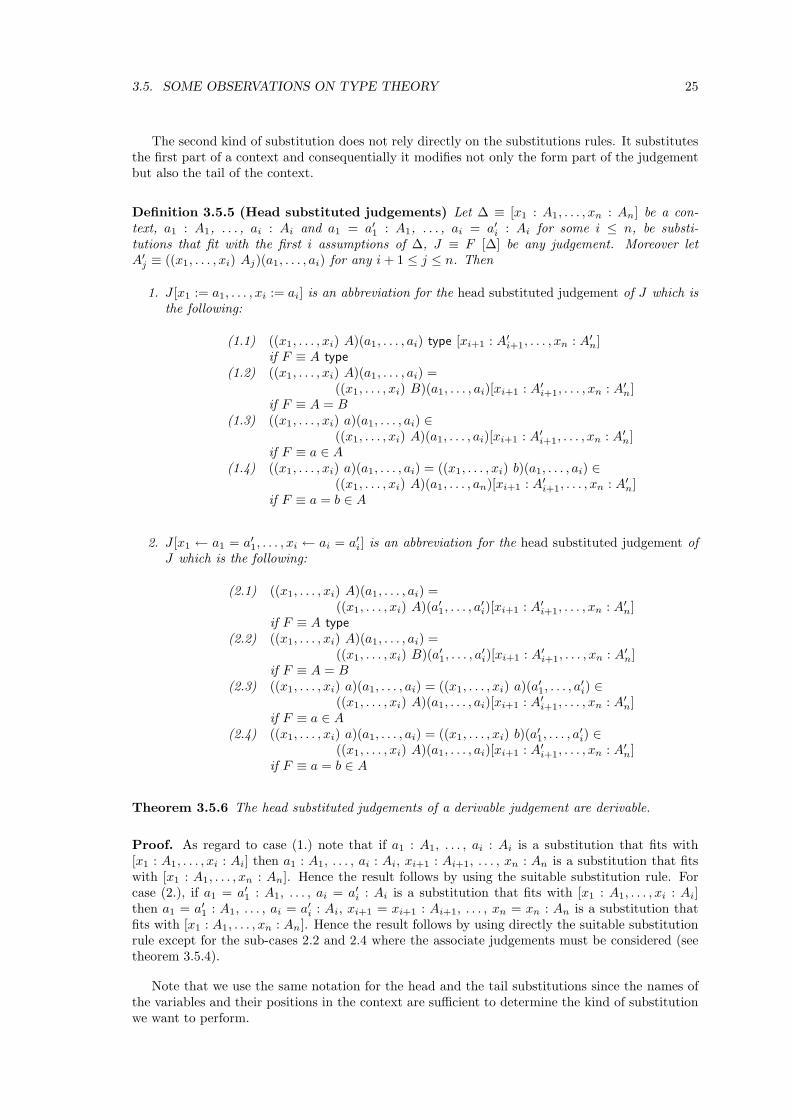
3.5. SOME OBSERVATIONS ON TYPE THEORY 25
The second kind of substitution does not rely directly on the substitutions rules. It substitutesthe first part of a context and consequentially it modifies not only the form part of the judgementbut also the tail of the context.
Definition 3.5.5 (Head substituted judgements) Let ∆ ≡ [x1 : A1, . . . , xn : An] be a con-text, a1 : A1, . . . , ai : Ai and a1 = a′
1 : A1, . . . , ai = a′i : Ai for some i ≤ n, be substi-
tutions that fit with the first i assumptions of ∆, J ≡ F [∆] be any judgement. Moreover letA′
j ≡ ((x1, . . . , xi) Aj)(a1, . . . , ai) for any i + 1 ≤ j ≤ n. Then
1. J [x1 := a1, . . . , xi := ai] is an abbreviation for the head substituted judgement of J which isthe following:
(1.1) ((x1, . . . , xi) A)(a1, . . . , ai) type [xi+1 : A′i+1, . . . , xn : A′
n]if F ≡ A type
(1.2) ((x1, . . . , xi) A)(a1, . . . , ai) =((x1, . . . , xi) B)(a1, . . . , ai)[xi+1 : A′
i+1, . . . , xn : A′n]
if F ≡ A = B(1.3) ((x1, . . . , xi) a)(a1, . . . , ai) ∈
((x1, . . . , xi) A)(a1, . . . , ai)[xi+1 : A′i+1, . . . , xn : A′
n]if F ≡ a ∈ A
(1.4) ((x1, . . . , xi) a)(a1, . . . , ai) = ((x1, . . . , xi) b)(a1, . . . , ai) ∈((x1, . . . , xi) A)(a1, . . . , an)[xi+1 : A′
i+1, . . . , xn : A′n]
if F ≡ a = b ∈ A
2. J [x1 ← a1 = a′1, . . . , xi ← ai = a′
i] is an abbreviation for the head substituted judgement ofJ which is the following:
(2.1) ((x1, . . . , xi) A)(a1, . . . , ai) =((x1, . . . , xi) A)(a′
1, . . . , a′i)[xi+1 : A′
i+1, . . . , xn : A′n]
if F ≡ A type
(2.2) ((x1, . . . , xi) A)(a1, . . . , ai) =((x1, . . . , xi) B)(a′
1, . . . , a′i)[xi+1 : A′
i+1, . . . , xn : A′n]
if F ≡ A = B(2.3) ((x1, . . . , xi) a)(a1, . . . , ai) = ((x1, . . . , xi) a)(a′
1, . . . , a′i) ∈
((x1, . . . , xi) A)(a1, . . . , ai)[xi+1 : A′i+1, . . . , xn : A′
n]if F ≡ a ∈ A
(2.4) ((x1, . . . , xi) a)(a1, . . . , ai) = ((x1, . . . , xi) b)(a′1, . . . , a
′i) ∈
((x1, . . . , xi) A)(a1, . . . , ai)[xi+1 : A′i+1, . . . , xn : A′
n]if F ≡ a = b ∈ A
Theorem 3.5.6 The head substituted judgements of a derivable judgement are derivable.
Proof. As regard to case (1.) note that if a1 : A1, . . . , ai : Ai is a substitution that fits with[x1 : A1, . . . , xi : Ai] then a1 : A1, . . . , ai : Ai, xi+1 : Ai+1, . . . , xn : An is a substitution that fitswith [x1 : A1, . . . , xn : An]. Hence the result follows by using the suitable substitution rule. Forcase (2.), if a1 = a′
1 : A1, . . . , ai = a′i : Ai is a substitution that fits with [x1 : A1, . . . , xi : Ai]
then a1 = a′1 : A1, . . . , ai = a′
i : Ai, xi+1 = xi+1 : Ai+1, . . . , xn = xn : An is a substitution thatfits with [x1 : A1, . . . , xn : An]. Hence the result follows by using directly the suitable substitutionrule except for the sub-cases 2.2 and 2.4 where the associate judgements must be considered (seetheorem 3.5.4).
Note that we use the same notation for the head and the tail substitutions since the names ofthe variables and their positions in the context are sufficient to determine the kind of substitutionwe want to perform.
26 CHAPTER 3. THE CANONICAL FORM THEOREM
3.6 The evaluation tree
In HITT, a set of computation rules is associated to each defined type such as Π, Σ, etc. Theyspecify a process for evaluating expressions denoting elements or types. They apply to variable-free and saturated expressions, that is, expressions of arity 0 in which no variable occurs free. The“normal form” theorem for expressions [BV89], assures us that a variable-free, saturated expressionis always definitionally equivalent to an expression of the form c(a1, . . . , an) where c is a constant.Hence, to evaluate an expression, we first consider its normal form and then detect the suitablecomputation rule. This can be done by looking at the outermost constant of the expression innormal form and, only in some cases, at the value of its first argument. Then each premise of theselected rule indicate how to continue the process recursively. Clearly, the process of evaluatingan expression denoting an element or a type using the computation rules naturally gives rise to afinitary tree: we will refer to it as the evaluation tree. Of course an expression evaluates if and onlyif its evaluation tree is finite. Hence if we know that an expression can be evaluated an inductionon the depth of its evaluation tree is a correct proof-method. It can be used to prove the followingtheorem.
Theorem 3.6.1 Let c and C be variable-free and saturated expressions. Then
1. If c ⇒ g then g is a canonical expression for an element, i.e. exactly one of the followingholds: g ≡ λ(b), g ≡ 〈a, b〉, g ≡ inl(a), g ≡ inr(b), g ≡ e, g ≡ mn, g ≡ 0, g ≡ s(a),g ≡ sup(a, b), g ≡ π(a, b), g ≡ σ(a, b), g ≡ +(a, b), g ≡ eq(a, b, d), g ≡ nn, g ≡ n, g ≡ w(a, b).
2. If C G then G is a canonical expression for a type, i.e. exactly one of the following holds:G ≡ Π(A, B), G ≡ Σ(A, B), G ≡ +(A, B), G ≡ Eq(A, b, d), G ≡ Nn, G ≡ N, G ≡ W(A, B),G ≡ U.
Note that the objects in the conclusion of a formation rule or an introduction rule are al-ways denoted by canonical expressions. We will call them canonical elements or canonical typesrespectively. However a canonical expression does not necessarily denote a canonical element ora canonical type. The successive canonical form theorem will certify this whenever we considerjudgements derived within the theory. More precisely, if the judgement a ∈ A (or A type) is derivedwithin the theory, then the canonical expression resulting from the evaluation of the expression a(or A) denotes a canonical element (or a canonical type). Moreover, under the same hypothesis,the evaluation process of the expression a (or A) always terminates.
Finally let us also observe that, since the computation rules do not “add” variables, it is obviousthat if no variable appears in a (respectively A) and a⇒ g (respectively A G), then no variableappears in g (respectively G).
3.7 Computability
In this section we introduce the main notions of the chapter: the definitions of computation treeand computable judgement.
To prove a canonical-form theorem for the system we are considering, and whose complete set ofrules is reported in the appendix B, we will follow a proof style similar to the one used by Martin-Lof in [Mar71] based on the method of Tait [Tai67] to prove normalization theorems. Therefore wewill introduce the notion of computable judgement. This notion applies both to closed judgementsand to hypothetical ones. Essentially, to express the computability of a judgement is equivalent toexpress what it is necessary to know in order to be allowed to formulate that judgement. Hence thedefinition formally summarizes the meaning of all the forms of judgements which can be obtainedby a derivation in type theory. Of course, it is directly inspired by the informal explanation ofthe rules given in [Mar84], but the needs of formalization make it a very long definition. We willbase it on the concept of computation tree which represents the full process needed to recognizethe computability of a given judgement. The nodes of a computation tree are labeled by derivablejudgements and if J is the label of a node then the labels of its sons are all the judgements whosecomputability is required in order to establish the computability of J .
3.7. COMPUTABILITY 27
As regards hypothetical judgements, their computability is referred to the computability of anyclosed judgement that can be obtained by substituting, in any possible way, computable judgementsto the open assumptions.
As regards closed judgements, the definition obviously differs when considering one form ofjudgement or another. Still there are some basic common points:
• any term appearing in the judgement must be (syntactically) valuable (evaluation) to acanonical term. This requirement is directly expressed for the two forms A type and a ∈ Aand indirectly, by requiring the computability of the associate judgements (associate), for theforms A = B and a = b ∈ A.
• the equality between a term and its corresponding evaluated form must be a provable judge-ment (correct evaluation)
• the computability of a judgement is recursively referred to the computability of the compo-nents (parts) of the judgement built up with the evaluated canonical terms.
Definition 3.7.1 (Computable judgement) The judgement J ≡ F [Γ] is computable if it isderivable andCase 1. There is no assumption, i.e. the context Γ is empty.
• Subcase 1.1: F ≡ A type. Then
– 1.1.1 (evaluation) A GA
– 1.1.2 (correct evaluation) the judgement A = GA is provable
– 1.1.3 (parts) the parts of GA are computable type(s), i.e.
∗ if GA ≡ Π(A1, A2) then the judgements A1 type and A2(x) type [x : A1] are com-putable
∗ if GA ≡ Σ(A1, A2) then the judgements A1 type and A2(x) type [x : A1] are com-putable
∗ if GA ≡ +(A1, A2) then the judgements A1 type and A2 type are computable
∗ if GA ≡ Eq(A1, b, d) then the judgements A1 type, b ∈ A1 and d ∈ A1 are computable
∗ if GA ≡ Nn then no condition
∗ if GA ≡ N then no condition
∗ if GA ≡ W(A1, A2) then the judgements A1 type and A2(x) type [x : A1] are com-putable
∗ if GA ≡ U, i.e. , A ≡ U, then no condition
• Subcase 1.2: F ≡ A = B then
– 1.2.1 (associate judgements) the associate judgements A type and B type are computable,and hence A GA and B GB .
– 1.2.2 (parts) GA and GB are equal computable types, i.e.
∗ GA ≡ Π(A1, A2) iff GB ≡ Π(B1, B2) and the judgements A1 = B1 andA2(x) = B2(x) [x : A1] are computable
∗ GA ≡ Σ(A1, A2) iff GB ≡ Σ(B1, B2) and the judgements A1 = B1 andA2(x) = B2(x) [x : A1] are computable
∗ GA ≡ +(A1, A2) iff GB ≡ +(B1, B2) and the judgements A1 = B1 andA2 = B2 are computable
∗ GA ≡ Eq(A1, a, c) iff GB ≡ Eq(B1, b, d) and the judgements A1 = B1,a = b ∈ A1 and c = d ∈ A1 are computable
∗ GA ≡ Nn iff GB ≡ Nn
∗ GA ≡ N iff GB ≡ N
∗ GA ≡W(A1, A2) iff GB ≡W(B1, B2) and the judgements A1 = B1 andA2(x) = B2(x) [x : A1] are computable
28 CHAPTER 3. THE CANONICAL FORM THEOREM
∗ GA ≡ U iff GB ≡ U
• Subcase 1.3: F ≡ c ∈ A then
– 1.3.1 (associate judgements) The associate judgement A type is computable, and henceA GA
– 1.3.2 (evaluation) c⇒ g
– 1.3.3 (correct evaluation) c = g ∈ A is provable
– 1.3.4 (parts) the parts of g are computable element(s) in GA, i.e.
∗ GA ≡ Π(A1, A2) iff g ≡ λ(b) and the judgementb(x) ∈ A2(x) [x : A1] is computable
∗ GA ≡ Σ(A1, A2) iff g ≡ 〈a, b〉 and the judgements a ∈ A1 and b ∈ A2(a) arecomputable
∗ GA ≡ +(A1, A2) iff either g ≡ inl(a) and the judgement a ∈ A1 is computable org ≡ inr(b) and the judgement b ∈ A2 is computable
∗ GA ≡ Eq(A1, b, d) iff g ≡ r and the judgement b = d ∈ A1 is computable
∗ GA ≡ Nn iff g ≡ mn for some 0 ≤ m ≤ n− 1
∗ GA ≡ N iff either g ≡ 0 or g ≡ s(a) and the judgement a ∈ N is computable
∗ GA ≡W(A1, A2) iff g ≡ sup(a, b) and the judgementsa ∈ A1 and b(x) ∈W(A1, A2) [x : A2(a)] are computable
∗ GA ≡ U iff
· either g ≡ π(a, b) and the judgements a ∈ U andb(x) ∈ U [x :< a >] are computable
· or g ≡ σ(a, b) and the judgements a ∈ U andb(x) ∈ U [x :< a >] are computable
· or g ≡ +(a, b) and the judgements a ∈ U and b ∈ U are computable
· or g ≡ eq(a, b, d) and the judgements a ∈ U, b ∈< a > and d ∈< a > arecomputable
· or g ≡ nn
· or g ≡ n
· or g ≡ w(a, b) and the judgements a ∈ U andb(x) ∈ U [x :< a >] are computable
• Subcase 1.4: F ≡ a = b ∈ A then
– 1.4.1 (associate judgements) the associate judgements a ∈ A and b ∈ A are computable,and hence a⇒ ga, b⇒ gb and A GA.
– 1.4.2 (parts) the parts of ga and gb are computable equal elements in GA, i.e.
∗ GA ≡ Π(A1, A2) iff ga ≡ λ(a′) and gb ≡ λ(b′) and the judgementa′(x) = b′(x) ∈ A2(x) [x : A1] is computable
∗ GA ≡ Σ(A1, A2) iff ga ≡ 〈a′, a′′〉 and gb ≡ 〈b′, b′′〉 and the judgementsa′ = b′ ∈ A1 and a′′ = b′′ ∈ A2(a
′) are computable
∗ GA ≡ +(A1, A2) iff either ga ≡ inl(a′) and gb ≡ inl(b′) and the judgementa′ = b′ ∈ A1 is computable or ga ≡ inr(a′′) and gb ≡ inr(b′′) and the judgementa′′ = b′′ ∈ A2 is computable
∗ GA ≡ Eq(A1, c, d) iff ga ≡ r and gb ≡ r and the judgement c = d ∈ A1 is computable
∗ GA ≡ Nn iff ga ≡ mn and gb ≡ mn for some 0 ≤ m ≤ n− 1
∗ GA ≡ N iff either ga ≡ 0 and gb ≡ 0 or ga ≡ s(a′) and gb ≡ s(b′) and the judgementa′ = b′ ∈ N is computable
∗ GA ≡ W(A1, A2) iff ga ≡ sup(a′, a′′) and gb ≡ sup(b′, b′′) and the judgementsa′ = b′ ∈ A1 anda′′(x) = b′′(x) ∈ W(A1, A2) [x : A2(a
′)] are computable
3.7. COMPUTABILITY 29
∗ GA ≡ U iff
· either ga ≡ π(a′, a′′) and gb ≡ π(b′, b′′) and the judgements a′ = b′ ∈ U anda′′(x) = b′′(x) ∈ U [x :< a′ >] are computable
· or ga ≡ σ(a′, a′′) and gb ≡ σ(b′, b′′) and the judgements a′ = b′ ∈ U anda′′(x) = b′′(x) ∈ U [x :< a′ >] are computable
· or ga ≡ +(a′, a′′) and gb ≡ +(b′, b′′) and the judgements a′ = b′ ∈ U anda′′ = b′′ ∈ U are computable
· or ga ≡ eq(a′, c, d) and gb ≡ eq(b′, e, f) and the judgements a′ = b′ ∈ U,c = e ∈< a′ > and d = f ∈< a′ > are computable
· or ga ≡ nn and gb ≡ nn
· or ga ≡ n and gbn
· or ga ≡ w(a′, a′′) and gb ≡ w(b′, b′′) and the judgements a′ = b′ ∈ U anda′′(x) = b′′(x) ∈ U [x :< a′ >] are computable
Case 2. There are assumptions, i.e. Γ ≡ x1 : A1, . . . , xn : An, for some n > 0. The judgement Jis computable if for any computable closed substitution (c.c.s.) a1 : A1, . . . , an : An (i.e. ai : Ai,for 1 ≤ i ≤ n, are computable judgements), and for any computable closed substitution (c.c.s.)a1 = c1 : A1, . . . , an = cn : An (i.e. ai = ci : Ai, for 1 ≤ i ≤ n, are computable judgements) thatfit with Γ
• Subcase 2.1: F ≡ B(x1, . . . , xn) type
– 2.1.1 (substitution :=) the judgementB(a1, . . . , an) type is computable
– 2.1.2 (substitution ←) the judgement B(a1, . . . , an) = B(c1, . . . , cn) is computable
• Subcase 2.2: F ≡ B(x1, . . . , xn) = D(x1, . . . , xn) then
– 2.2.1 (associate) the judgement B(x1, . . . , xn) type [Γ] is computable
– 2.2.2 (substitution :=) the judgement B(a1, . . . , an) = D(a1, . . . , an) is computable
– 2.2.3 (substitution ←) the judgement B(a1, . . . , an) = D(c1, . . . , cn) is computable
• Subcase 2.3: F ≡ b(x1, . . . , xn) ∈ B(x1, . . . , xn) then
– 2.3.1 (associate) the judgement B(x1, . . . , xn) type [Γ] is computable
– 2.3.2 (substitution :=) the judgement b(a1, . . . , an) ∈ B(a1, . . . , an) is computable
– 2.3.3 (substitution ←) the judgementb(a1, . . . , an) = b(c1, . . . , cn) ∈ B(a1, . . . , an) is computable
• Subcase 2.4: F ≡ b(x1, . . . , xn) = d(x1, . . . , xn) ∈ B(x1, . . . , xn) then
– 2.4.1 (associate) the judgement b(x1, . . . , xn) ∈ B(x1, . . . , xn) [Γ] is computable
– 2.4.2 (substitution :=) the judgementb(a1, . . . , an) = d(a1, . . . , an) ∈ B(a1, . . . , an) is computable
– 2.4.3 (substitution ←) the judgementb(a1, . . . , an) = d(c1, . . . , cn) ∈ B(a1, . . . , an) is computable
Note that the asymmetry in the conditions on associate judgements (point 2.2.1 and 2.4.1)reflects the asymmetry in the rules of the theory. Actually we will prove that also the other associatejudgement is computable but the reduced requirement simplifies the next inductive proofs.
By looking at the above definition as a “generalized process” to search for computability of ajudgement, a search tree is naturally associate to any derivable judgement. It is clear that wheneverJ is recognized to be a computable judgement its search tree is well founded. In such a case wegive the definition of computation tree.
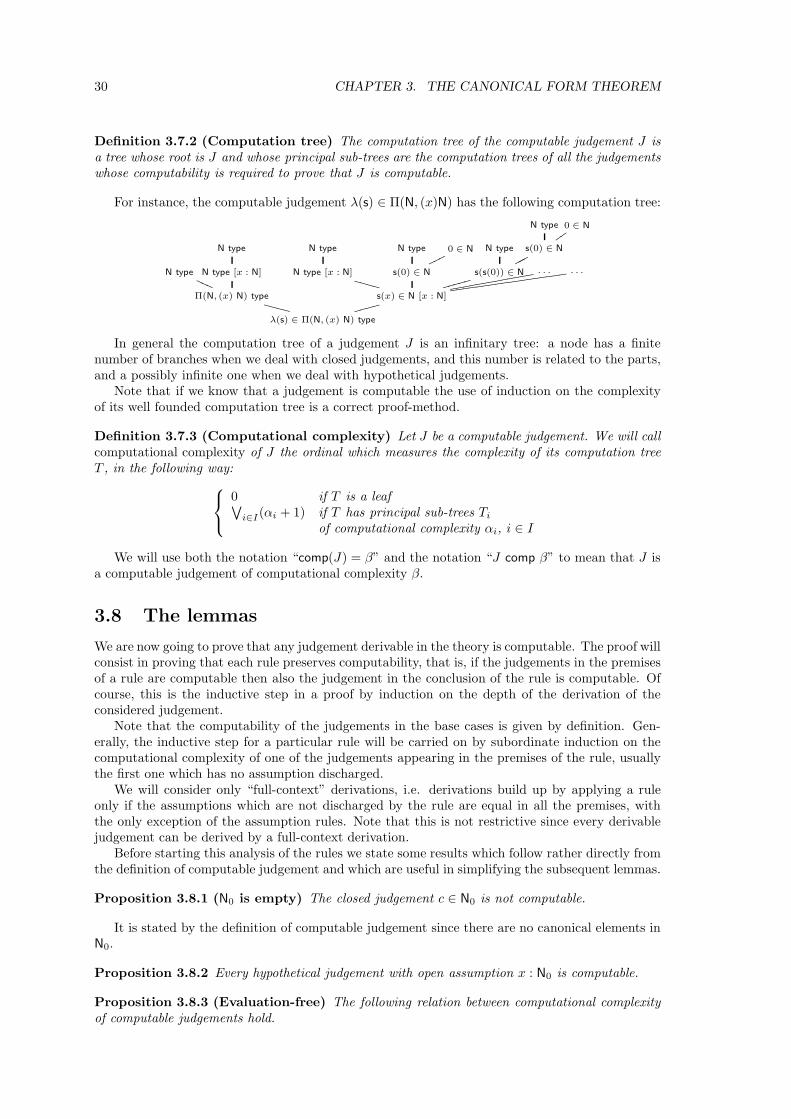
30 CHAPTER 3. THE CANONICAL FORM THEOREM
Definition 3.7.2 (Computation tree) The computation tree of the computable judgement J isa tree whose root is J and whose principal sub-trees are the computation trees of all the judgementswhose computability is required to prove that J is computable.
For instance, the computable judgement λ(s) ∈ Π(N, (x)N) has the following computation tree:
N type 0 ∈ N
vv
N type N type N type 0 ∈ N
oooN type s(0) ∈ N
ppp
N typePPP
N type [x : N] N type [x : N]VVVV
s(0) ∈ N s(s(0)) ∈ N
hhhhh. . .
eeeeeeeeeeeee . . .
dddddddddddddddddd
Π(N, (x) N) type
WWWWs(x) ∈ N [x : N]
hhhh
λ(s) ∈ Π(N, (x) N) type
In general the computation tree of a judgement J is an infinitary tree: a node has a finitenumber of branches when we deal with closed judgements, and this number is related to the parts,and a possibly infinite one when we deal with hypothetical judgements.
Note that if we know that a judgement is computable the use of induction on the complexityof its well founded computation tree is a correct proof-method.
Definition 3.7.3 (Computational complexity) Let J be a computable judgement. We will callcomputational complexity of J the ordinal which measures the complexity of its computation treeT , in the following way:
0 if T is a leaf∨
i∈I(αi + 1) if T has principal sub-trees Ti
of computational complexity αi, i ∈ I
We will use both the notation “comp(J) = β” and the notation “J comp β” to mean that J isa computable judgement of computational complexity β.
3.8 The lemmas
We are now going to prove that any judgement derivable in the theory is computable. The proof willconsist in proving that each rule preserves computability, that is, if the judgements in the premisesof a rule are computable then also the judgement in the conclusion of the rule is computable. Ofcourse, this is the inductive step in a proof by induction on the depth of the derivation of theconsidered judgement.
Note that the computability of the judgements in the base cases is given by definition. Gen-erally, the inductive step for a particular rule will be carried on by subordinate induction on thecomputational complexity of one of the judgements appearing in the premises of the rule, usuallythe first one which has no assumption discharged.
We will consider only “full-context” derivations, i.e. derivations build up by applying a ruleonly if the assumptions which are not discharged by the rule are equal in all the premises, withthe only exception of the assumption rules. Note that this is not restrictive since every derivablejudgement can be derived by a full-context derivation.
Before starting this analysis of the rules we state some results which follow rather directly fromthe definition of computable judgement and which are useful in simplifying the subsequent lemmas.
Proposition 3.8.1 (N0 is empty) The closed judgement c ∈ N0 is not computable.
It is stated by the definition of computable judgement since there are no canonical elements inN0.
Proposition 3.8.2 Every hypothetical judgement with open assumption x : N0 is computable.
Proposition 3.8.3 (Evaluation-free) The following relation between computational complexityof computable judgements hold.
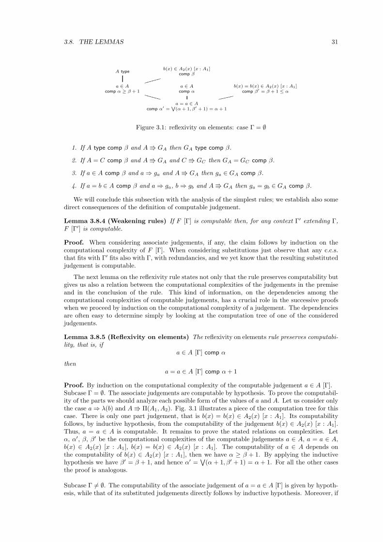
3.8. THE LEMMAS 31
A typeb(x) ∈ A2(x) [x : A1]
comp β
hhhhhh
a ∈ Acomp α ≥ β + 1
VVVVVV
a ∈ Acomp α
b(x) = b(x) ∈ A2(x) [x : A1]comp β′ = β + 1 ≤ α
fffff
a = a ∈ A
comp α′ =W
(α + 1, β′ + 1) = α + 1
Figure 3.1: reflexivity on elements: case Γ = ∅
1. If A type comp β and A GA then GA type comp β.
2. If A = C comp β and A GA and C GC then GA = GC comp β.
3. If a ∈ A comp β and a⇒ ga and A GA then ga ∈ GA comp β.
4. If a = b ∈ A comp β and a⇒ ga, b⇒ gb and A GA then ga = gb ∈ GA comp β.
We will conclude this subsection with the analysis of the simplest rules; we establish also somedirect consequences of the definition of computable judgement.
Lemma 3.8.4 (Weakening rules) If F [Γ] is computable then, for any context Γ′ extending Γ,F [Γ′] is computable.
Proof. When considering associate judgements, if any, the claim follows by induction on thecomputational complexity of F [Γ]. When considering substitutions just observe that any c.c.s.that fits with Γ′ fits also with Γ, with redundancies, and we yet know that the resulting substitutedjudgement is computable.
The next lemma on the reflexivity rule states not only that the rule preserves computability butgives us also a relation between the computational complexities of the judgements in the premiseand in the conclusion of the rule. This kind of information, on the dependencies among thecomputational complexities of computable judgements, has a crucial role in the successive proofswhen we proceed by induction on the computational complexity of a judgement. The dependenciesare often easy to determine simply by looking at the computation tree of one of the consideredjudgements.
Lemma 3.8.5 (Reflexivity on elements) The reflexivity on elements rule preserves computabi-lity, that is, if
a ∈ A [Γ] comp α
thena = a ∈ A [Γ] comp α + 1
Proof. By induction on the computational complexity of the computable judgement a ∈ A [Γ].Subcase Γ = ∅. The associate judgements are computable by hypothesis. To prove the computabil-ity of the parts we should analyze each possible form of the values of a and A. Let us consider onlythe case a⇒ λ(b) and A Π(A1, A2). Fig. 3.1 illustrates a piece of the computation tree for thiscase. There is only one part judgement, that is b(x) = b(x) ∈ A2(x) [x : A1]. Its computabilityfollows, by inductive hypothesis, from the computability of the judgement b(x) ∈ A2(x) [x : A1].Thus, a = a ∈ A is computable. It remains to prove the stated relations on complexities. Letα, α′, β, β′ be the computational complexities of the computable judgements a ∈ A, a = a ∈ A,b(x) ∈ A2(x) [x : A1], b(x) = b(x) ∈ A2(x) [x : A1]. The computability of a ∈ A depends onthe computability of b(x) ∈ A2(x) [x : A1], then we have α ≥ β + 1. By applying the inductivehypothesis we have β′ = β + 1, and hence α′ =
∨(α + 1, β′ + 1) = α + 1. For all the other cases
the proof is analogous.
Subcase Γ 6= ∅. The computability of the associate judgement of a = a ∈ A [Γ] is given by hypoth-esis, while that of its substituted judgements directly follows by inductive hypothesis. Moreover, if
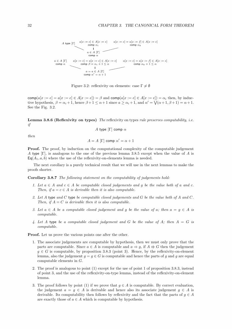
32 CHAPTER 3. THE CANONICAL FORM THEOREM
A type [Γ]
RRRRRRa[x := e] ∈ A[x := e]
comp αi
a[x := e] = a[x := f ] ∈ A[x := e]comp αk
ggggggggg
a ∈ A [Γ]comp α
a ∈ A [Γ]comp α
UUUUUU
a[x := e] = a[x := e] ∈ A[x := e]comp β = αi + 1 ≤ α
a[x := e] = a[x := f ] ∈ A[x := e]comp αk + 1 ≤ α
fffffffff
a = a ∈ A [Γ]comp α′ = α + 1
Figure 3.2: reflexivity on elements: case Γ 6= ∅
comp(a[x := e] = a[x := e] ∈ A[x := e]) = β and comp(a[x := e] ∈ A[x := e]) = αi then, by induc-tive hypothesis, β = αi +1, hence β +1 ≤ α+1 since a ≥ αi +1, and α′ =
∨(α+1, β +1) = α+1.
See the Fig. 3.2.
Lemma 3.8.6 (Reflexivity on types) The reflexivity on types rule preserves computability, i.e.if
A type [Γ] comp α
thenA = A [Γ] comp α′ = α + 1
Proof. The proof, by induction on the computational complexity of the computable judgementA type [Γ], is analogous to the one of the previous lemma 3.8.5 except when the value of A isEq(A1, a, b) where the use of the reflexivity-on-elements lemma is needed.
The next corollary is a purely technical result that we will use in the next lemmas to make theproofs shorter.
Corollary 3.8.7 The following statement on the computability of judgements hold:
1. Let a ∈ A and c ∈ A be computable closed judgements and g be the value both of a and c.Then, if a = c ∈ A is derivable then it is also computable.
2. Let A type and C type be computable closed judgements and G be the value both of A and C.Then, if A = C is derivable then it is also computable.
3. Let a ∈ A be a computable closed judgement and g be the value of a; then a = g ∈ A iscomputable.
4. Let A type be a computable closed judgement and G be the value of A; then A = G iscomputable.
Proof. Let us prove the various points one after the other.
1. The associate judgements are computable by hypothesis, then we must only prove that theparts are computable. Since a ∈ A is computable and a⇒ g, if A G then the judgementg ∈ G is computable, by proposition 3.8.3 (point 3). Hence, by the reflexivity-on-elementlemma, also the judgement g = g ∈ G is computable and hence the parts of g and g are equalcomputable elements in G.
2. The proof is analogous to point (1) except for the use of point 1 of proposition 3.8.3, insteadof point 3, and the use of the reflexivity-on-type lemma, instead of the reflexivity-on-elementlemma.
3. The proof follows by point (1) if we prove that g ∈ A is computable. By correct evaluation,the judgement a = g ∈ A is derivable and hence also its associate judgement g ∈ A isderivable. Its computability then follows by reflexivity and the fact that the parts of g ∈ Aare exactly those of a ∈ A which is computable by hypothesis.
3.8. THE LEMMAS 33
4. The proof is analogous to point (3) except for the use of point (2) instead of (1).
The following lemma does not concern one of the rules of the theory but states some propertiesof computable judgements which will be very often referred to in the following subsections.
Lemma 3.8.8 (Head substitution) Let Γ ≡ [x1 : A1, . . . , xn : An] be a context, J ≡ F [Γ] be acomputable judgement, a1 : A1, . . . , ai : Ai and a1 = a′
1 : A1, . . . , ai = a′i : Ai, for i < n, be c.c.s
that fit with the context [x1 : A1, . . . , xi : Ai]. Then
1. J [x1 := a1, . . . , xi := ai] is a computable judgement5.
2. J [x1 ← a1 = a′1, . . . , xi ← ai = a′
i] is a computable judgement.
Proof. The proof is by induction on the computational complexity of J .Let ∆ ≡ [xi+1 : A′
i+1, . . . , xn : A′n], where A′
j ≡ ((x1, . . . , xi) Aj)(a1, . . . , ai), for i + 1 ≤ j ≤ n,and let ai+1 : A′
i+1, . . . , an : A′n be a c.c.s. that fits with the context ∆.
To prove the computability of the head substituted judgements we will show that for any c.c.s.saturating J [x1 := a1, . . . , xi := ai] or J [x1 ← a1 = a′
1, . . . , xi ← ai = a′i] it is possible to find out
a c.c.s. saturating J and yielding the same judgement. First of all note that for i + 1 ≤ j ≤ n,
Aj ≡ ((x1, . . . , xj−1) Aj)(a1, . . . , aj−1)≡ ((xi+1, . . . , xj−1)(((x1, . . . , xi) Aj)(a1, . . . , ai))(ai+1, . . . , aj−1)≡ A′
j .
Case i.(associate judgements) The computability of the associate judgements, if any, follows by induc-
tive hypothesis.(substitution :=) For any c.c.s. ai+1 : A′
i+1, . . . , an : A′n we have that a1 : A1, . . . , an : An is a
c.c.s. that fits with Γ; hence
(J [x1 := a1, . . . , xi := ai])[xi+1 := ai+1, . . . , xn := an] ≡ J [x1 := a1, . . . , xn := an]
is computable.(substitution ←) For any c.c.s. ai+1 = a′
i+1 : A′i+1, . . . , an = a′
n : A′n that fits with the context
∆, we have that a1 = a1 : A1, . . . , ai = ai : Ai, ai+1 = a′i+1 : Ai+1, . . . , an = a′
n : An is a c.c.s.that fits with Γ. Note that the reflexivity-on-elements lemma must be used here. Hence
(J [x1 := a1, . . . , xi := ai])[xi+1 ← ai+1 = a′i+1, . . . , xn ← an = a′
n]≡ J [x1 ← a1 = a1, . . . , xi ← ai = ai, xi+1 ← ai+1 = a′
i+1, . . . , xn ← an = a′n]
is computable.Case ii.
(associate judgements) The computability of the associate judgements follows from case (i)since if a1 = a′
1 : A1, . . . , ai = a′i : Ai, for i < n, are computable then also a1 : A1, . . . , ai : Ai are
computable andJ [x1 := a1, . . . , xi := ai]
is the associate judgement of
J [x1 ← a1 = a′1, . . . , xi ← ai = a′
i]
whose computability is required.(substitution :=) For any c.c.s. ai+1 : A′
i+1, . . . , an : A′n that fits with the context ∆, we have
that a1 = a′1 : A1, . . . , ai = a′
i : Ai, ai+1 = ai+1 : Ai+1, . . . , an = an : An is a c.c.s. that fits withΓ; hence also
(J [x1 ← a1 = a′1, . . . , xi ← ai = a′
i])[xi+1 := ai+1, . . . , xn := an]≡ J [x1 ← a1 = a′
1, . . . , xi ← ai = a′i, xi+1 ← ai+1 = ai+1, , xn ← an = an]
5Note that for i=n the claim is true by definition of computable judgement.
34 CHAPTER 3. THE CANONICAL FORM THEOREM
is computable.(substitution ←) For any c.c.s. ai+1 = a′
i+1 : A′i+1, . . . , an = a′
n : A′n that fits with the context
∆, we have that a1 = a′1 : A1, . . . , ai = a′
i : Ai, ai+1 = a′i+1 : Ai+1, . . . , an = a′
n : An is a c.c.s.that fits with Γ; hence
(J [x1 ← a1 = a′1, . . . , xi ← ai = a′
i])[xi+1 ← ai+1 = a′i+1, . . . , xn ← an = a′
n]≡ J [x1 ← a1 = a′
1, . . . , xi ← ai = a′i, xi+1 ← ai+1 = a′
i+1, . . . , xn ← an = a′n]
is computable.
Remark 3.8.9 Let Γ ≡ [x1 : A1, . . . , xn : An] be a context, a1 : A1, . . . , an : An and a1 = a′1 : A1,
. . . , an = a′n : An be c.c.s.s that fit with Γ, and B ≡ (s1 : S1, . . . , sm : Sm) A(s1, . . . , sm), then
from the head substitution lemma we have that
• if : B [Γ] is computable then: B [Γ][x1 := a1, . . . , xn := an] and: B [Γ][x1 ← a1 = a′
1, . . . , xn ← an = a′n] are computable;
• if b : B [Γ] is computable thenb : B [Γ][x1 := a1, . . . , xn := an] andb : B [Γ][x1 ← a1 = a′
1, . . . , xn ← an = a′n] are computable;
• if b = b′ : B [Γ] is computable thenb = b′ : B [Γ][x1 := a1, . . . , xn := an] andb = b′ : B [Γ][x1 ← a1 = a′
1, . . . , xn ← an = a′n] are computable.
We will continue now by proving that each rule listed in the appendix B preserves computability,that is any judgement in the conclusion of that rule is computable whenever all the judgements inthe premises are computable. The ordering of the lemmas has been suitably chosen to allow us todeal separately with each rule, thus mastering the complexity of the computability proof.
3.9 Computability of the rules
In the following sections we will show that all of the rules of type theory preserve computability.
3.9.1 The substitution rules
The definition of computable judgement directly states that the substitution rules preserve com-putability in the special case of saturating substitutions. In the next lemma we will prove thatcomputability is preserved by substitution rules also in the general case of tail substitution. Sincethe different forms of judgement of the six substitution rules are not essential to prove the resultwe will compact the sentence as much as possible.
Lemma 3.9.1 (Substitution lemma) Let Γ be a context, ∆ ≡ [Γ, x1 : A1, . . . , xn : An] be acontext, J ≡ F [∆] be a computable judgement, a1 : B1 [Γ], . . . , an : Bn [Γ] and a1 = a′
1 : B1 [Γ],. . . , an = a′
n : Bn [Γ] be two lists of substitutions that fit with the context [x1 : A1, . . . , xn : An],that is, for any 1 ≤ j ≤ n, Bj ≡ ((x1, . . . , xj−1) Aj)(a1, . . . , aj−1). Then
1. J [x1 := a1, . . . , xn := an] is a computable judgement.
2. J [x1 ← a1 = a′1, . . . , xn ← an = a′
n] is a computable judgement.
Proof. If the context Γ is empty then the claim holds by definition. Thus, let us suppose thatΓ ≡ [s1 : S1, . . . , sm : Sm], for some m > 0. The proof is by induction on the computationalcomplexity of J .Case i.
(associate judgements) The computability of the associate judgements follows by inductivehypothesis.
3.9. COMPUTABILITY OF THE RULES 35
(substitution :=) For any c.c.s. c1 : S1, . . . , cm : Sm fitting with the context Γ, we define
di ≡ ((s1, . . . , sm) ai)(c1, . . . , cm) 1 ≤ i ≤ n
By remark 3.8.9
di : ((s1, . . . , sm) Bi)(c1, . . . , cm) ≡ ai : Bi [Γ][s1 := c1, . . . , sm := cm]
is computable. Moreover we have
≡ ((s1, . . . , sm) Bi)(c1, . . . , cm)≡ ((s1, . . . , sm)((x1, . . . , xi−1) Ai)(a1, . . . , ai−1))(c1, . . . , cm)≡ ((s1, . . . , sm, x1, . . . , xi−1) Ai)(c1, . . . , cm, d1, . . . , di−1)≡ Ai
Therefore c1 : S1, . . . , cm : Sm, d1 : A1, . . . , dn : An is a c.c.s. fitting with the context ∆. Hence
(J [x1 := a1, . . . , xn := an])[s1 := c1, . . . , sm := cm] ≡J [s1 := c1, . . . , sm := cm, x1 := d1, . . . , xn := dn]
is computable.(substitution ←) For any c.c.s. c1 = c′1 : S1, . . . , cm = c′m : Sm that fits with the context Γ, we
definedi ≡ ((s1, . . . , sm) ai)(c1, . . . , cm) 1 ≤ i ≤ n
andd′i ≡ ((s1, . . . , sm) ai)(c
′1, . . . , c
′m) 1 ≤ i ≤ n
By remark 3.8.9
di = d′i : ((s1, . . . , sm) Bi)(c1, . . . , cm) ≡ ai : Bi [Γ][s1 ← c1 = c′1, . . . , sm ← cm = c′m] 1 ≤ i ≤ n
is computable. Moreover from the previous point we have
Ai ≡ ((s1, . . . , sm) Bi)(c1, . . . , cm)
Then, c1 = c′1 : S1, . . . , cm = c′m : Sm, d1 = d′1 : A1, . . . , dn = d′n : An is a c.c.s. that fits with thecontext ∆. Hence
(J [x1 := a1, . . . , xn := an])[s1 ← c1 = c′1, . . . , sm ← cm = c′m] ≡J [s1 ← c1 = c′1, . . . , sm ← cm = c′m, x1 ← d1 = d′1, . . . , xn ← dn = d′n]
is computable.Case ii.
(associate judgements) The computability of the associate judgements follows from case (i).(substitution :=) For any c.c.s. c1 : S1, . . . , cm : Sm fitting with the context Γ, we define
di ≡ ((s1, . . . , sm) ai)(c1, . . . , cm)
andd′i ≡ ((s1, . . . , sm) a′
i)(c1, . . . , cm)
By remark 3.8.9
di = d′i : ((s1, . . . , sm) Bi)(c1, . . . , cm) ≡ ai = a′i : Bi [Γ][s1 := c1, . . . , sm := cm]
is computable. Then, since Ai ≡ ((s1, . . . , sm) Bi)(c1, . . . , cm), c1 = c1 : S1, . . . , cm = cm : Sm,d1 = d′1 : A1, . . . , dn = d′n : An is a c.c.s. fitting with the context ∆. Hence
(J [x1 ← a1 = a′1, . . . , xn ← an = a′
n])[s1 := c1, . . . , sm := cm] ≡J [s1 ← c1 = c1, . . . , sm ← cm = cm, x1 ← d1 = d′1, . . . , xn ← dn = d′n]
is computable.
36 CHAPTER 3. THE CANONICAL FORM THEOREM
(substitution ←) For any c.c.s. c1 = c′1 : S1, . . . , cm = c′m : Sm fitting with the context Γ, wedefine
di ≡ ((s1, . . . , sm) ai)(c1, . . . , cm)
andd′i ≡ ((s1, . . . , sm) ai)(c
′1, . . . , c
′m)
By remark 3.8.9
d1 = d′i : ((s1, . . . , sm) Bi)(c1, . . . , cm) ≡ ai = a′i : Bi [Γ][s1 ← c1 = c′1, . . . , sm ← cm = c′m]
is computable. Then, since Ai ≡ ((s1, . . . , sm) Bi)(c1, . . . , cm), c1 = c′1 : S1, . . . , cm = c′m : Sm,d1 = d′1 : A1, . . . , dn = d′n : An is a c.c.s. fitting with the context ∆. Hence
(J [x1 ← a1 = a′1, . . . , xn ← an = a′
n])[s1 ← c1 = c′1, . . . , sm ← cm = c′m] ≡J [s1 ← c1 = c′1, . . . , sm ← cm = c′m, x1 ← d1 = d′1, .., xn ← dn = d′n]
is computable.
3.9.2 U-elimination rules
The next lemma 3.9.2 deals with U-elimination rules. We need to know that they preserve bothcomputability and computational complexity to establish the next lemma 3.9.3 about computabilityof the remaining structural rules. For this reason their analysis precede so much that of all theother logical rules.
Lemma 3.9.2 (U-elimination) The U-elimination rules preserve computability and do not in-crease computational complexity, that is
1. If a ∈ U [Γ] comp β then < a > type [Γ] comp β′ ≤ β
2. If a = b ∈ U [Γ] comp β then < a >=< b > [Γ] comp β′ ≤ β
Proof. By induction on the computational complexity β.Case 1.Subcase Γ = ∅.
(evaluation) < a > G<a> immediately follows from the computability of the judgement a ∈ U
by using the suitable computation rule.(correct evaluation) the required derivation can be obtained by applying the suitable U-equality
rule to premises whose existence is guaranteed by the computability of the judgement a ∈ U. Forinstance, if a⇒ π(a′, a′′) the required proof is the following:
a = π(a′, a′′) ∈ U
< a >=< π(a′, a′′) >
a′ ∈ U a′′(x) ∈ U [x :< a′ >]
< π(a′, a′′) >= Π(< a′ >, (x) < a′′(x) >)
< a >= Π(< a′ >, (x) < a′′(x) >)
(parts) the parts of G<a> are computable type(s) with computational complexity less or equalof that one of the corresponding parts of the computable judgement a ∈ U. For instance, supposingG<a> ≡ Π(< a′ >, (x) < a′′(x) >), by inductive hypothesis, we obtain both that a′ ∈ U comp β′
implies that < a′ > type comp γ′ ≤ β′ and that a′′(x) ∈ U [x :< a′ >] comp β′′ implies that< a′′(x) > type [x :< a′ >] comp γ′′ ≤ β′′. The other cases are completely similar.Subcase Γ 6= ∅.
(substitution :=) immediately follows by inductive hypothesis (1)(substitution ←) immediately follows by inductive hypothesis (2)
Case 2.Subcase Γ = ∅.
(associate) from a = b ∈ U comp β we obtain a ∈ U comp β1 < β and b ∈ U comp β2 < β.Hence by inductive hypothesis, point 1,
< a > type comp β′1 ≤ β1
3.9. COMPUTABILITY OF THE RULES 37
and< b > type comp β′
2 ≤ β2
(parts) if < a > G<a> and < b > G<b> then the parts of G<a> and G<b> are equalcomputable types with the same computational complexity of the corresponding parts of the com-putable judgement a = b ∈ U. Let us analyze the case G<a> ≡ Π(< a′ >, (x) < a′′(x) >):
G<a> ≡ Π(< a′ >, (x) < a′′(x) >) iff a⇒ π(a′, a′′)iff b⇒ π(b′, b′′)iff G<b> ≡ Π(< b′ >, (x) < b′′(x) >)
Moreover, by inductive hypothesis, we obtain both that a′ = b′ ∈ U comp β3 implies that< a′ >=< b′ > comp β′
3 ≤ β3 and that a′′(x) = b′′(x) ∈ U [x :< a′ >] comp β4 implies that< a′′(x) >=< b′′(x) > [x :< a′ >] comp β′
4 ≤ β.Hence β′ =
∨(β′
1 + 1, β′2 + 1, β′
3 + 1, β′4 + 1) ≤
∨(β1 + 1, β2 + 1, β3 + 1, β4 + 1) = β. The other
cases are completely similar.Subcase Γ 6= ∅.
(associate) immediately follows by inductive hypothesis, point 1.(substitution :=) immediately follows by inductive hypothesis, point 2.(substitution ←) immediately follows by inductive hypothesis, point 2.
Note that the computational complexity of the judgements in the premise and in the conclusionare usually equal, but we may also have different complexities. For instance, the complexity of abasic judgement, like N type, is 0 while the complexity of the corresponding judgement, < n >∈ U,is 1 due to the requirement that the associate judgement U type is computable.
3.9.3 The structural rules
In the previous section we dealt with the reflexivity on elements and the reflexivity on types rule.All the other structural rules, that is the transitivity on elements, the transitivity on types, thesymmetry on elements, the symmetry on types, the equal elements and the equal types rules, areconsidered together in the next lemma 3.9.3. This lemma is a key point in the proof of computabil-ity since it establishes, besides the fact that structural rules preserve computability, other basicand important relationships among the computational complexities of related judgements. As wealready pointed out, these information are essential in the subsequent proof since they guaranteethe applicability of the inductive hypothesis when we proceed by induction on the computationalcomplexity of a judgement.
Lemma 3.9.3 (Structural rules) Let β be a computational complexity. Then
1. If a = c ∈ A [Γ] comp α1 < β, b = d ∈ A [Γ] comp α2 < β and a = b ∈ A [Γ] comp α then
• (i) α1 = α2 = α
• (ii) c = d ∈ A [Γ] comp α
• (1.1) (transitivity on elements) If a = b ∈ A [Γ] comp α1 < β andb = c ∈ A [Γ] comp α2 < β then a = c ∈ A [Γ] comp α = α1 = α2
2. If A = C [Γ] comp α1 < β, B = D [Γ] comp α2 < β and A = B [Γ] comp α then
• (i) α1 = α2 = α
• (ii) C = D [Γ] comp α
• (2.1) (transitivity on types) If A = B [Γ] comp α1 < β andB = C [Γ] comp α2 < β then A = C [Γ] comp α = α1 = α2
3. If A = C [Γ] comp β then
• (i.) (associate judgements) A type [Γ] comp α if and only if C type [Γ] comp α
• (ii.) (symmetry on types) C = A [Γ] comp β
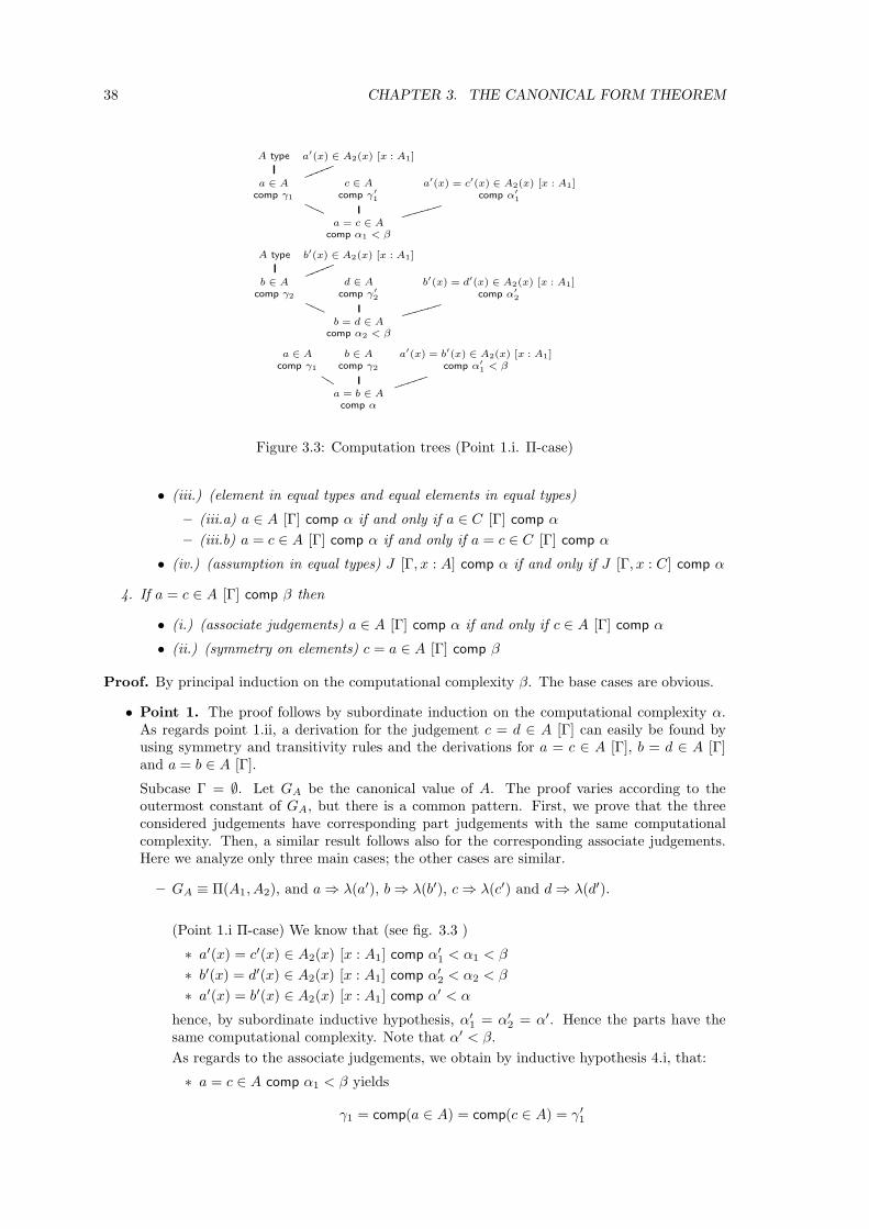
38 CHAPTER 3. THE CANONICAL FORM THEOREM
A type a′(x) ∈ A2(x) [x : A1]
lllll
a ∈ Acomp γ1
PPP
c ∈ A
comp γ′
1
a′(x) = c′(x) ∈ A2(x) [x : A1]comp α′
1
hhhhhh
a = c ∈ Acomp α1 < β
A type b′(x) ∈ A2(x) [x : A1]
lllll
b ∈ Acomp γ2
PPP
d ∈ A
comp γ′
2
b′(x) = d′(x) ∈ A2(x) [x : A1]comp α′
2
hhhhhh
b = d ∈ Acomp α2 < β
a ∈ Acomp γ1
JJ
b ∈ Acomp γ2
a′(x) = b′(x) ∈ A2(x) [x : A1]comp α′
1< β
jjjjj
a = b ∈ Acomp α
Figure 3.3: Computation trees (Point 1.i. Π-case)
• (iii.) (element in equal types and equal elements in equal types)
– (iii.a) a ∈ A [Γ] comp α if and only if a ∈ C [Γ] comp α
– (iii.b) a = c ∈ A [Γ] comp α if and only if a = c ∈ C [Γ] comp α
• (iv.) (assumption in equal types) J [Γ, x : A] comp α if and only if J [Γ, x : C] comp α
4. If a = c ∈ A [Γ] comp β then
• (i.) (associate judgements) a ∈ A [Γ] comp α if and only if c ∈ A [Γ] comp α
• (ii.) (symmetry on elements) c = a ∈ A [Γ] comp β
Proof. By principal induction on the computational complexity β. The base cases are obvious.
• Point 1. The proof follows by subordinate induction on the computational complexity α.As regards point 1.ii, a derivation for the judgement c = d ∈ A [Γ] can easily be found byusing symmetry and transitivity rules and the derivations for a = c ∈ A [Γ], b = d ∈ A [Γ]and a = b ∈ A [Γ].
Subcase Γ = ∅. Let GA be the canonical value of A. The proof varies according to theoutermost constant of GA, but there is a common pattern. First, we prove that the threeconsidered judgements have corresponding part judgements with the same computationalcomplexity. Then, a similar result follows also for the corresponding associate judgements.Here we analyze only three main cases; the other cases are similar.
– GA ≡ Π(A1, A2), and a⇒ λ(a′), b⇒ λ(b′), c⇒ λ(c′) and d⇒ λ(d′).
(Point 1.i Π-case) We know that (see fig. 3.3 )
∗ a′(x) = c′(x) ∈ A2(x) [x : A1] comp α′1 < α1 < β
∗ b′(x) = d′(x) ∈ A2(x) [x : A1] comp α′2 < α2 < β
∗ a′(x) = b′(x) ∈ A2(x) [x : A1] comp α′ < α
hence, by subordinate inductive hypothesis, α′1 = α′
2 = α′. Hence the parts have thesame computational complexity. Note that α′ < β.
As regards to the associate judgements, we obtain by inductive hypothesis 4.i, that:
∗ a = c ∈ A comp α1 < β yields
γ1 = comp(a ∈ A) = comp(c ∈ A) = γ′1
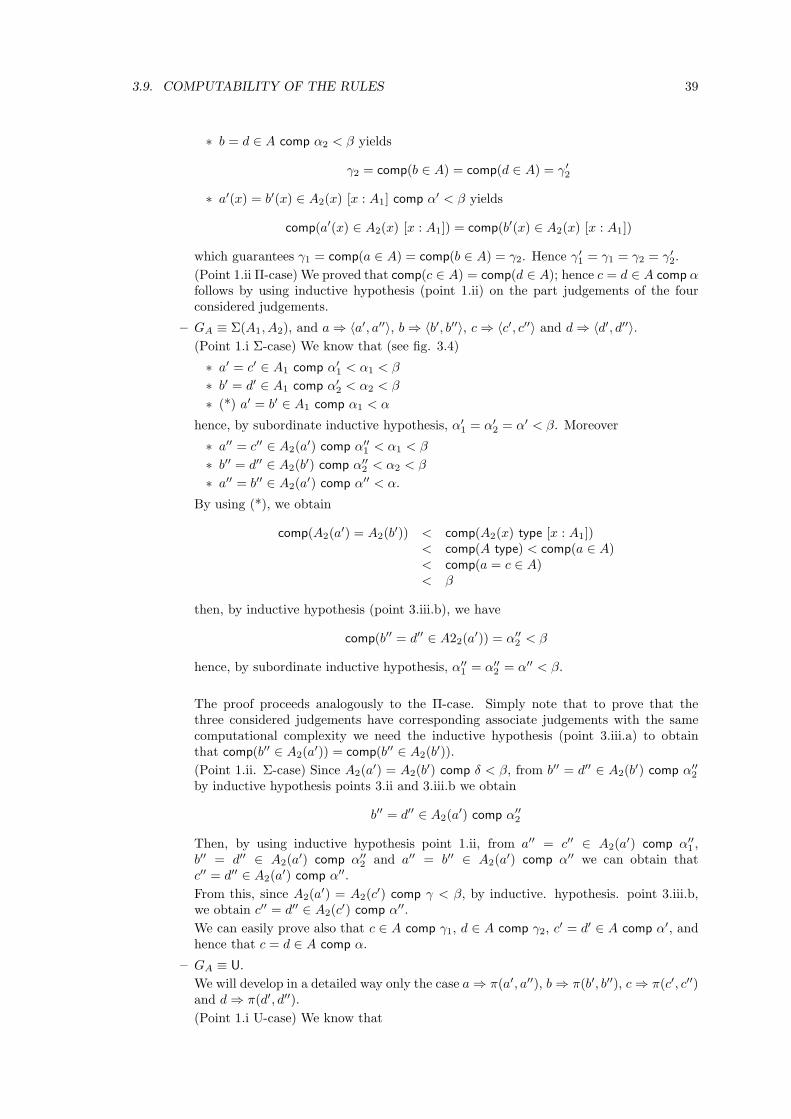
3.9. COMPUTABILITY OF THE RULES 39
∗ b = d ∈ A comp α2 < β yields
γ2 = comp(b ∈ A) = comp(d ∈ A) = γ′2
∗ a′(x) = b′(x) ∈ A2(x) [x : A1] comp α′ < β yields
comp(a′(x) ∈ A2(x) [x : A1]) = comp(b′(x) ∈ A2(x) [x : A1])
which guarantees γ1 = comp(a ∈ A) = comp(b ∈ A) = γ2. Hence γ′1 = γ1 = γ2 = γ′
2.
(Point 1.ii Π-case) We proved that comp(c ∈ A) = comp(d ∈ A); hence c = d ∈ A comp αfollows by using inductive hypothesis (point 1.ii) on the part judgements of the fourconsidered judgements.
– GA ≡ Σ(A1, A2), and a⇒ 〈a′, a′′〉, b⇒ 〈b′, b′′〉, c⇒ 〈c′, c′′〉 and d⇒ 〈d′, d′′〉.
(Point 1.i Σ-case) We know that (see fig. 3.4)
∗ a′ = c′ ∈ A1 comp α′1 < α1 < β
∗ b′ = d′ ∈ A1 comp α′2 < α2 < β
∗ (*) a′ = b′ ∈ A1 comp α1 < α
hence, by subordinate inductive hypothesis, α′1 = α′
2 = α′ < β. Moreover
∗ a′′ = c′′ ∈ A2(a′) comp α′′
1 < α1 < β
∗ b′′ = d′′ ∈ A2(b′) comp α′′
2 < α2 < β
∗ a′′ = b′′ ∈ A2(a′) comp α′′ < α.
By using (*), we obtain
comp(A2(a′) = A2(b
′)) < comp(A2(x) type [x : A1])< comp(A type) < comp(a ∈ A)< comp(a = c ∈ A)< β
then, by inductive hypothesis (point 3.iii.b), we have
comp(b′′ = d′′ ∈ A22(a′)) = α′′
2 < β
hence, by subordinate inductive hypothesis, α′′1 = α′′
2 = α′′ < β.
The proof proceeds analogously to the Π-case. Simply note that to prove that thethree considered judgements have corresponding associate judgements with the samecomputational complexity we need the inductive hypothesis (point 3.iii.a) to obtainthat comp(b′′ ∈ A2(a
′)) = comp(b′′ ∈ A2(b′)).
(Point 1.ii. Σ-case) Since A2(a′) = A2(b
′) comp δ < β, from b′′ = d′′ ∈ A2(b′) comp α′′
2
by inductive hypothesis points 3.ii and 3.iii.b we obtain
b′′ = d′′ ∈ A2(a′) comp α′′
2
Then, by using inductive hypothesis point 1.ii, from a′′ = c′′ ∈ A2(a′) comp α′′
1 ,b′′ = d′′ ∈ A2(a
′) comp α′′2 and a′′ = b′′ ∈ A2(a
′) comp α′′ we can obtain thatc′′ = d′′ ∈ A2(a
′) comp α′′.
From this, since A2(a′) = A2(c
′) comp γ < β, by inductive. hypothesis. point 3.iii.b,we obtain c′′ = d′′ ∈ A2(c
′) comp α′′.
We can easily prove also that c ∈ A comp γ1, d ∈ A comp γ2, c′ = d′ ∈ A comp α′, andhence that c = d ∈ A comp α.
– GA ≡ U.
We will develop in a detailed way only the case a⇒ π(a′, a′′), b⇒ π(b′, b′′), c⇒ π(c′, c′′)and d⇒ π(d′, d′′).
(Point 1.i U-case) We know that
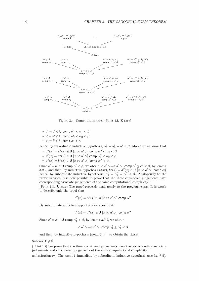
40 CHAPTER 3. THE CANONICAL FORM THEOREM
A2(a′) = A2(b′)comp δ
TTTTTTTT
. . . A2(a′) = A2(c′)comp γ
jjjjjjjj
A1 type
VVVVVVVVVVVV A2(x) type [x : A1]
A type
a ∈ Acomp γ1
VVVVVVVVVVVVVVVc ∈ A
comp γ′
1
NNNN
NN
a′ = c′ ∈ A1
comp α′
1< β
nnnnnn
a′′ = c′′ ∈ A2(a′)
comp α′′
1< β
ffffffffffffffffff
a = c ∈ Acomp α1 < β
b ∈ Acomp γ2
VVVVVVVVVVVVVVVd ∈ A
comp γ′
2
NNNN
NN
b′ = d′ ∈ A1
comp α′
1< β
nnnnnn
b′′ = d′′ ∈ A2(b′)
comp α′′
2< β
ffffffffffffffffff
b = d ∈ Acomp α2 < β
a ∈ Acomp γ1
UUUUUUUUUUUUUUUb ∈ A
comp γ2
LLLLL
a′ = b′ ∈ A1
comp α′ < β
oooooo
a′′ = b′′ ∈ A2(a′)comp α′′ < α
ffffffffffffffffff
a = b ∈ Acomp α
Figure 3.4: Computation trees (Point 1.i. Σ-case)
∗ a′ = c′ ∈ U comp α′1 < α1 < β
∗ b′ = d′ ∈ U comp α′2 < α2 < β
∗ a′ = b′ ∈ U comp α′ < α
hence, by subordinate inductive hypothesis, α′1 = α′
2 = α′ < β. Moreover we know that
∗ a′′(x) = c′′(x) ∈ U [x :< a′ >] comp α′′1 < α1 < β
∗ b′′(x) = d′′(x) ∈ U [x :< b′ >] comp α′′2 < α2 < β
∗ a′′(x) = b′′(x) ∈ U [x :< a′ >] comp α′′ < α.
Since a′ = b′ ∈ U comp α′ < β, we obtain < a′ >=< b′ > comp γ′ ≤ α′ < β, by lemma3.9.2, and then, by inductive hypothesis (3.iv), b′′(x) = d′′(x) ∈ U [x :< a′ >] comp α′′
2
hence, by subordinate inductive hypothesis, α′′1 = α′′
2 = α′′ < β. Analogously to theprevious cases, it is now possible to prove that the three considered judgements havecorresponding associate judgements of the same computational complexity .
(Point 1.ii. U-case) The proof proceeds analogously to the previous cases. It is worthto describe only the proof that
c′′(x) = d′′(x) ∈ U [x :< c′ >] comp α′′
By subordinate inductive hypothesis we know that
c′′(x) = d′′(x) ∈ U [x :< a′ >] comp α′′
Since a′ = c′ ∈ U comp α′1 < β, by lemma 3.9.2, we obtain
< a′ >=< c′ > comp γ′1 ≤ α′
1 < β
and then, by inductive hypothesis (point 3.iv), we obtain the thesis.
Subcase Γ 6= ∅
(Point 1.i) We prove that the three considered judgements have the corresponding associatejudgements and substituted judgements of the same computational complexity.
(substitution :=) The result is immediate by subordinate inductive hypothesis (see fig. 3.5).
3.9. COMPUTABILITY OF THE RULES 41
a[x := e] = a[x := e]∈ A[x := e] comp α∗
1
. . .
gggggggggggggg
a ∈ A [Γ]comp α′
1
WWWWWWWWWa[x := e] = c[x := e]∈ A[x := e] comp α′′
1
a[x := e] = c[x := f ]∈ A[x := e] comp α′′′
1
ggggg
a = c ∈ A [Γ]comp α1 < β
b[x := e] = b[x := f ]∈ A[x := e] comp α∗
2
. . .
gggggggggggggg
b ∈ A [Γ]comp α′
2
WWWWWWWWWb[x := e] = d[x := e]∈ A[x := e] comp α′′
2
b[x := e] = d[x := f ]∈ A[x := e] comp α′′′
2
ggggg
b = d ∈ A [Γ]comp α2 < β
a ∈ A [Γ]comp α′ = α′
1
WWWWWWW
a[x := e] = b[x := e] ∈ A[x := e]comp α′′
a[x := e] = b[x := f ] ∈ A[x := e]comp α′′′
eeeeeeeee
a = b ∈ A [Γ]comp α < β
Figure 3.5: Point 1.i (substitution :=)
(substitution←) First observe that, by subordinate inductive hypothesis (1.i) α′′ = α′′′1 = α′′′
2 .Moreover, if e = f : is a c.c.s. fitting with Γ this holds also for e :. Hence α∗
1 < β and α∗2 < β
and, by subordinate inductive hypothesis (points 1.i and 1.ii), α′′ = α∗1 = α∗
2 = α′′′. Henceα′′′ = α′′′
1 = α′′′2 .
(associate judgements) Since α′ = α′1, α′′ = α′′
1 and α′′′ = α′′′1 then α = α1 < β and, by
inductive hypothesis 4.i, comp(b ∈ A [Γ]) = α′2 = comp(a ∈ A [Γ]) = α′
1.
(Point 1.ii)
By inductive hypothesis (point 4.i) comp(c ∈ A [Γ]) = comp(a ∈ A [Γ]) = α′. Then, bysubordinate inductive hypothesis on substituted judgements, we obtain that, for any c.c.s.e :, comp(c[x := e] = d[x := e] ∈ A[x := e]) = α′′ holds and for any c.c.s. e = f :,comp(c[x := e] = d[x := f ] ∈ A[x := e]) = α′′ holds. Hence comp(c = d ∈ A [Γ]) = α.
Point 1.1
By inductive hypothesis (point 4.ii), from comp(a = b ∈ A [Γ]) = α1 < β we obtain thatcomp(b = a ∈ A [Γ]) = α1 < β. Hence b ∈ A [Γ] is computable and, by the reflexivity lemma3.8.5, b = b ∈ A [Γ] is computable. Then the result follows from the previous point 1.ii.
• Point 2.
The proof follows by subordinate induction on the computational complexity α. The proofof this case is analogous to the one of point 1. Just substitute the judgement ’equal ele-ments in a type’ with the judgement ’equal types’ and pay attention in analyzing the caseGA ≡ Eq(A1, e, f) where an obvious application of point 1. is required.
Point 2.1.
By using inductive hypothesis point 3.ii, from comp(A = B [Γ]) = α1 < β we obtain thatcomp(B = A [Γ]) = α1 < β. Hence B type [Γ] is computable and, by the reflexivity lemma3.8.6, B = B [Γ] is computable. Then the result follows from the previous point 2.ii.
• Point 3.
Point 3.i Subcase Γ = ∅.
Let A GA and C GC we must prove that the parts of GA and GC have the samecomputational complexity. The proof varies according to the outermost constant of GA. Weanalyze only two significant cases; the other cases are similar.
42 CHAPTER 3. THE CANONICAL FORM THEOREM
– GA ≡ Π(A1, A2) hence, since A = C is a computable judgement, GC ≡ Π(C1, C2) andwe know that
(∗) comp(A1 = C1) < β
and hence, by inductive hypothesis point 3.i, comp(A1 type) = comp(C1 type);
(∗∗) comp(A2(x) = C2(x) [x : A1]) < β
and hence comp(A2(x) type [x : A1]) = comp(C2(x) type [x : A1]), by inductive hypoth-esis point 3.i, and finally comp(A2(x) type [x : A1]) = comp(C2(x) type [x : C1]) byusing inductive hypothesis point 3.iv.
– GA ≡ Eq(A1, a′, a′′) and GC ≡ Eq(C1, c
′, c′′) and we know that
(∗) comp(A1 = C1) < β
then, by inductive hypothesis point 3.i, comp(A1 type) = comp(C1 type);
(∗∗) comp(a′ = c′ ∈ A1) < β
hence, by inductive hypothesis point 4.i, comp(a′ ∈ A1) = comp(c′ ∈ A1) and then, byinductive hypothesis point 3.iii.a, comp(a′ ∈ A1) = comp(c′ ∈ C1);
(∗ ∗ ∗) comp(a′′ = c′′ ∈ A1) < β
hence, by inductive hypothesis point 4.i, comp(a′′ ∈ A1) = comp(c′′ ∈ A1) and then, byinductive hypothesis point 3.iii.a, comp(a′′ ∈ A1) = comp(c′′ ∈ C1).
Point 3.i. Subcase Γ 6= ∅
For any c.c.s. e :, since comp(A[x := e] = C[x := e]) < β, by inductive hypothesis 3.i, itimmediately follows that
comp(A[x := e] type) = comp(C[x := e] type)
For any c.c.s. e = f : we know that e : and, by reflexivity, e = e : are c.c.s fitting with Γ.Hence,
comp(A[x := e] = A[x := e]) = comp(A[x := e] = A[x := f ])
by inductive hypothesis 2.i, and
comp(A[x := e] = A[x := e]) = comp(C[x := e] = C[x := f ])
by inductive hypothesis 2.ii. Hence
comp(A[x := e] = A[x := f ]) = comp(C[x := e] = C[x := f ])
and thus comp(A type [Γ]) = comp(C type [Γ])
Point 3.ii
(associate judgements) We must prove that the associate judgements of the derivable judge-ment C = A [Γ] are computable and their computational complexities are equal to thecomputational complexities of the corresponding associate of the judgement A = C [Γ]. Thisresult is obvious by the previous point 3.i.
Point 3.ii. Subcase Γ = ∅.
We must prove that the parts of C = A have the same computational complexity of the partsof A = C. Let us show only two cases
– GA ≡ Π(A1, A2) and hence GC ≡ Π(C1, C2).
The parts of A = C are A1 = C1 comp α1 and A2(x) = C2(x) [x : A1] comp α2 andthe parts of C = A are C1 = A1 comp α′
1 and C2(x) = A2(x) [x : C1] comp α′2. Now
α1 = α′1, by inductive hypothesis point 3.ii, because α1 < β and, since, by inductive
hypothesis point 3.v,comp(C2(x) = A2(x) [x : A1]) = α′
2
it follows that α2 = α′2, again by using the inductive hypothesis point 3.ii, because
α2 < β.
3.9. COMPUTABILITY OF THE RULES 43
– GA ≡ Eq(A1, a′, a′′) and hence GC ≡ Eq(C1, c
′, c′′).
The parts of the judgement A = C are A1 = C1 comp α1, a′ = c′ ∈ A1 comp α2
and a′′ = c′′ ∈ A1 comp α3 while the parts of C = A are C1 = A1 comp α′1,
c′ = a′ ∈ C1 comp α′2 and c′′ = a′′ ∈ C1 comp α′
3. Now α1 = α′1 by inductive hy-
pothesis point 3.ii because α1 < β. Moreover, since, by inductive hypothesis point4.ii, both comp(c′ = a′ ∈ A1) = α2 and comp(c′′ = a′′ ∈ A1) = α3, we obtaincomp(c′ = a′ ∈ C1) = α2 and comp(c′′ = a′′ ∈ C1) = α3 by using inductive hypothesispoint 3.iv.
Point 3.ii. Subcase Γ 6= ∅.
We have to prove that the two considered judgements have substituted judgements with thesame computational complexity.
(substitution :=) Immediate by inductive hypothesis 3.ii.
(substitution ←) For any c.c.s. e = f : fitting with Γ also e : is a c.c.s. fitting with Γ. Henceby inductive hypothesis (2.i and 2.ii)
comp(A[x := e] = C[x := e]) = comp(A[x := e] = A[x := f ])= comp(A[x := e] = A[x := e])= comp(C[x := e] = A[x := f ])
comp(A[x := e] = C[x := e]) = comp(A[x := e] = C[x := f ])= comp(A[x := e] = A[x := e])= comp(C[x := e] = C[x := f ])
Hence comp(C[x := e] = A[x := f ]) = comp(A[x := e] = C[x := f ]).
Point 3.iii.a.
Let us prove the if-part (the proof of the only-if part is completely similar) by subordinate in-duction on the computational complexity α. Note that, by point 3.i, the associate judgementsof a ∈ A [Γ] and a ∈ C [Γ] are computable judgements with the same complexity.
Point 3.iii.a. Subcase Γ = ∅.
(evaluation) a⇒ ga, by hypothesis
(correct evaluation) a = ga ∈ C is provable, immediate
(parts) Let us analyze here only three cases according to the form of GC .
– GC ≡ Σ(C1, C2) and hence GA ≡ Σ(A1, A2) and ga ≡ 〈a′, a′′〉 and we know that
∗ A1 = C1 comp α1 < β,
∗ A2(x) = C2(x) [x : A1] comp α2 < β,
∗ a′ ∈ A1 comp α′ < α and
∗ a′′ ∈ A2(a′) comp α′′ < α
and hence comp(a′ ∈ C1) = α′, by inductive hypothesis point 3.iii.a, and, since
comp(A2(a′) = C2(a
′)) < comp(A2(x) = C2(x) [x : A1])< comp(A = C)< β
we obtaina′′ ∈ C2(a
′) comp α′′
by using inductive hypothesis point 3.iii.a.
– GC ∈ Eq(C1, c′, c′′) and hence GA ≡ Eq(A1, a
′, a′′) and ga ≡ e and we know that
∗ a′ = c′ ∈ A1 comp α2 < β,
∗ a′′ = c′′ ∈ A1 comp α3 < β and
∗ a′ = a′′ ∈ A1 comp α′ < α
44 CHAPTER 3. THE CANONICAL FORM THEOREM
and, by point 1., we obtain c′ = c′′ ∈ A1 comp α′ then, since A1 = C1 comp α1 < β, byusing inductive hypothesis point 3.iii.b,
comp(c′ = c′′ ∈ C1) = α′
– GC ≡ W(C1, C2) and hence GA ≡ W(A1, A2) and ga ≡ sup(a′, a′′) and we know thatA1 = C1 comp α1 < β and a′ ∈ A1 comp α′ < α; then, by inductive hypothesis 3.iii.a,a′ ∈ C1 comp α′. Moreover we know that a′′(y) ∈ W(A1, A2) [y : A2(a
′)] comp α′′ < αand A2(x) = C2(x) [x : A1] comp α2 < β.
Finally also a′′(y) ∈ W(A1, A2) [y : C2(a′)] comp α′′ < α holds, by inductive hypothesis
point 3.iv, since comp(A2(a′) = C2(a
′)) < comp(A2(x) = C2(x) [x : A1]) < β. Now toprove
a′′(y) ∈W(C1, C2) [y : C2(a′)] comp α′′
we must consider the associate judgements. Since
comp(W(A1, A2) type) = comp(W(C1, C2) type)
and
comp(W(A1, A2) = W(A1, A2)) = comp(W(C1, C2) = W(C1, C2))
then
comp(W(A1, A2) type [y : C2(a′)]) = comp(W(C1, C2) type [y : C2(a
′)])
(substitutions) By subordinate inductive hypothesis 3.iii.a and 3.iii.b, for any c.c.s.e ∈ C2(a
′) and e = f ∈ C2(a′) we have
comp(a′′(e) ∈W(A1, A2)) = comp(a′′(e) ∈ W(C1, C2))
and
comp(a′′(e) = a′′(f) ∈W(A1, A2)) = comp(a′′(e) = a′′(f) ∈W(C1, C2))
Point 3.iii.a. Subcase Γ 6= ∅.
(substitution :=) The result immediately follows by using the inductive hypothesis point3.iii.a.
(substitution ←) The result immediately follows by using the inductive hypothesis point3.iii.b.
Point 3.iii.b.
The proof of this case is similar to the previous point 3.iii.a. Just note that, by point 3.iii.a,the associate judgements of a = c ∈ A [Γ] and c = a ∈ C [Γ] are computable with the samecomplexity.
Point 3.iv.
The proof is by subordinate induction on the computational complexity α. Let us prove theif-part (the proof of the only if-part is completely similar).
(associate judgements) By subordinate inductive hypothesis the associate judgements ofJ [Γ, x : C] are computable with the same complexity of those of J [Γ, x : A].
(substitutions) In order to analyse the substituted judgements, suppose Γ is the context[y1 : B1, . . . , yn : Bn]. Since A = C [Γ] comp β then for any c.c.s. a1 : B1, . . . , an : Bn,e : C (or a1 = a′
1 : B1, . . . , an = a′n : Bn, e = e′ : C) fitting with [Γ, x : C], we have
comp(A[y := a] = C[y := a]) < β hence, by point 3.iii.a (or 3.iii.b), e : A (or e = e′ : A) isa computable judgement and thus the same substitution fits also with [Γ, x : A]. Hence thesubstituted judgements are computable with the same complexity.
3.9. COMPUTABILITY OF THE RULES 45
• Point 4.
Point 4.i.
Let us prove the if-part (the proof of the only if-part is completely similar).
(associate judgements) The associate judgement of both judgements is A type.
Point 4.i. Subcase Γ = ∅.
We must prove only that the parts of c ∈ A have the same computational complexity of thecorresponding parts of a ∈ A. According to the values of A and a we show here only threecases:
– A Σ(A1, A2) and a⇒ 〈a′, a′′〉.
We know that c ⇒ 〈c′, c′′〉, comp(a′ = c′ ∈ A1) < β and comp(a′′ = c′′ ∈ A2(a′)) < β;
therefore comp(a′ ∈ A1) = comp(c′ ∈ A1) by inductive hypothesis 4.i; and, since
comp(A2(a′) = A2(c
′)) < comp(A2(x) type [x : A1])< comp(A type) < comp(a ∈ A)< comp(a = c ∈ A)= β
we obtaincomp(a′′ ∈ A2(a
′)) = comp(c′′ ∈ A2(c′))
by using inductive hypothesis point 4.i and point 3.iii.a.
– A W(A1, A2) and a⇒ sup(a′, a′′).
We know that c⇒ sup(c′, c′′), and that comp(a′ = c′ ∈ A1) < β; therefore
comp(a′ ∈ A1) = comp(c′ ∈ A1)
by using inductive hypothesis point 4.i. We know also that
comp(a′′(x) = c′′(x) ∈W(A1, A2) [x : A2(a′)]) < β
andcomp(A2(a
′) = A2(c′)) < comp(A2(x) = A2(x) [x : A1])
< comp(A2(x) type [x : A1]< β
by inductive hypothesis point 4.i and point 3.iv, then we obtain
comp(a′′(x) ∈ W(A1, A2) [x : A2(a′)]) = comp(c′′(x) ∈ W(A1, A2) [x : A2(a
′)])= comp(c′′(x) ∈ W(A1, A2) [x : A2(c
′)])
– A U and a⇒ π(a′, a′′), and therefore c⇒ π(c′, c′′).
We know both that comp(a′ = c′ ∈ U) < β and comp(a′′(x) = c′′(x) ∈ U[x :< a′ >]) < β.Therefore, by inductive hypothesis (4.i), we obtain both comp(a′ ∈ U) = comp(c′ ∈ U)and comp(a′′(x) ∈ U [x :< a′ >]) = comp(c′′(x) ∈ U [x :< a′ >]).
Moreover, comp(a′ = c′ ∈ U) < β. Then, by using lemma 3.9.2, we obtain thatcomp(< a′ >=< c′ >) < β, and we obtain, by using inductive hypothesis (3.iv),
comp(c′′(x) ∈ U [x :< a′ >]) = comp(c′′(x) ∈ U [x :< c′ >])
Point 4.i. Subcase Γ 6= ∅.
(substitution :=) The result immediately follows by inductive hypothesis 4.i.
(substitution ←) The result follows by inductive hypothesis point 1 using the fact that ife = f : is a c.c.s fitting with Γ so is e :.
Point 4.ii.
Point 4.ii. Subcase Γ = ∅.
46 CHAPTER 3. THE CANONICAL FORM THEOREM
Since the associate judgement of a = c ∈ A are exactly those of c = a ∈ A, we must prove onlythat the parts of c = a ∈ A have the same computational complexity of the correspondingparts of a = c ∈ A. The proof is similar to that of the previous point 4.i; let us analyze justone case:
– A Σ(A1, A2) and a ⇒ 〈a′, a′′〉. We know that c ⇒ 〈c′, c′′〉, comp(a′ = c′ ∈ A1) < βand comp(a′′ = c′′ ∈ A2(a
′)) < β; therefore comp(a′ = c′ ∈ A1) = comp(c′ = a′ ∈ A1),by inductive hypothesis 4.ii; and, since
comp(A2(a′) = A2(c
′)) < comp(A2(x) type [x : A1])< comp(A type)< comp(a ∈ A)< comp(a = c ∈ A)= β
we obtaincomp(a′′ = c′′ ∈ A2(a
′)) = comp(c′′ = a′′ ∈ A2(c′))
by using inductive hypothesis point 4.ii and point 3.iii.b.
Point 4.ii. Subcase Γ 6= ∅.
As for the previous case the result follows by inductive hypothesis (4.i. and 4.ii) by usinginductive hypothesis (point 1.1) and the fact that if e = f : is a c.c.s fitting with Γ so is e :.
It is worth noting that, the computability of the associate judgements which were left out fromthe definition 3.7.1 of computable judgement (points 2.2.1 and 2.4.1) is now established by thesymmetry rules.
3.9.4 The assumption rules
In section 3.3 we presented the assumption rules of our system; they introduce variables of anyarity. The new assumption appears in the context Γ of the conclusion of the rule and for thisreason only the case Γ 6= ∅ has to be considered in order to prove that assumption rules preservecomputability.
Lemma 3.9.4 (First assumption rule) Let ai : Ai [Γi], for any 1 ≤ i ≤ n, be n computablejudgements and : B [Γ] ≡ A(x1, . . . , xn) type [Γ, x1 : A1, . . . , xn : An] be a computable judgement.Then the judgement
y(a1, . . . , an) ∈ A(a1, . . . , an) [Γ′]
where Γ′ is the merge without duplication of the contexts Γ1, . . . , Γn, Γ, [y : B], is computable.
Proof. Let Γ′ ≡ s1 : S1, . . . , sk : Sk, y : B, z1 : C1, . . . , zm : Cm, for k ≥ 0 and m ≥ 0, wherez1 : C1, . . . , zm : Cm strictly depend on y : B. First note that, since the context Γ′ extends boththe contexts Γ and all the contexts Γi, for 1 ≤ i ≤ n, by the weakening lemma, we have that
A(x1, . . . , xn) type [Γ′, x1 : A1, . . . , xn : An]
andai : Ai [Γ′] 1 ≤ i ≤ n
are computable judgements.(associate judgement) The computability of the judgement
A(a1, . . . , an) type [Γ′]
follows by the substitution lemma.(substitution :=) Consider any c.c.s. fitting with the context Γ′ : d1 : S1, . . . , dk : Sk, b : B,
c1 : C1, . . . , cm : Cm. Note that, if A′i ≡ ((s1, . . . , sk) Ai)(d1, . . . , dk) then b : B abbreviates:
b : B[s1 := d1, . . . , sk := dk] ≡ b(x1, . . . , xn) ∈ ((s1, . . . , sk) A)(d1, . . . , dk) [x1 : A′1, . . . , xn : A′
n]
3.9. COMPUTABILITY OF THE RULES 47
Moreover, for any 1 ≤ i ≤ n, ai : Ai [Γ′] is a computable judgement; then, by the head substitutionlemma 3.8.8,
ai : Ai [Γ′][s1 := d1, . . . , sk := dk, y := b, z1 := c1, . . . , zm := cm]
is also computable, and
≡ ((s1, . . . , sk, y, z1, . . . , zm) Ai)(d1, . . . , dk, b, c1, . . . , cm)≡ ((s1, . . . , sk) Ai)(d1, . . . , dk)≡ A′
i
Let, for any 1 ≤ i ≤ n, ei ≡ ((s1, . . . , sk, y, z1, . . . , zm) ai)(d1, . . . , dk, b, c1, . . . , cm) then also thejudgement b : B[x1 := e1, . . . , xn := en] is computable.
But y : B, z1 : C1, . . . , zm : Cm cannot appear in the context [Γ, x1 : A1, . . . , xn : An]; then
((s1, . . . , sk, y, z1, . . . , zm) A)(d1, . . . , dk, b, c1, . . . , cm) ≡ ((s1, . . . , sk) A)(d1, . . . , dk)
and therefore
≡ b : B[x1 := e1, . . . , xn := en]≡ y(a1, . . . , an) ∈ A(a1, . . . , an) [Γ′][s1 := d1, . . . , sk := dk, y := b, z1 := c1, . . . , zm := cm]
(substitution ←) Consider any c.c.s. d1 = d′1 : S1, . . . , dk = d′k : Sk, b = b′ : B, c1 = c′1 : C1,. . . , cm = c′m : Cm fitting with Γ′. The, the proof proceeds as before after noting that, for any1 ≤ i ≤ n, the judgement
ai : Ai [Γ′][s1 ← d1 = d′1, . . . , sk ← dk = d′k, y ← b = b′, z1 ← c1 = c′1, . . . , zm ← cm = c′m]
is computable and can be substituted for xi in b = b′ : B obtaining a computable judgement whichis exactly
y(a1, . . . , an) ∈ A(a1, . . . , an) [Γ′][s1 ← d1 = d′1, . . . , sk ← dk = d′k,y ← b = b′, z1 ← c1 = c′1, . . . , zm ← cm = c′m]
Lemma 3.9.5 (Second assumption rule) Let ai = a′i : Ai [Γi] for any 1 ≤ i ≤ n, be n com-
putable judgements and : B [Γ] ≡ A(x1, . . . , xn) type [Γ, x1 : A1, . . . , xn : An] be a computablejudgement. Then the judgement
y(a1, . . . , an) = y(a′1, . . . , a
′n) ∈ A(a1, . . . , an) [Γ′]
where Γ′ is the merge without duplication of the contexts Γ1, . . . , Γn, Γ, [y : B] is computable.
Proof. Let Γ′ ≡ s1 : S1, . . . , sk : Sk, y : B, z1 : C1, . . . , zm : Cm, for k ≥ 0, m ≥ 0, wherez1 : C1, . . . , zm : Cm strictly depend on y : B.
(associate judgement) By hypothesis, for any 1 ≤ i ≤ n, ai = a′i : Ai [Γi] is a computable
judgement; then also its associate judgements ai : Ai [Γi] is computable. Hence, by the previouslemma, the judgement
y(a1, . . . , an) ∈ A(a1, . . . , an) [Γ′]
is computable.(substitution :=) Consider any c.c.s. d1 : S1, . . . , dk : Sk, b : B, c1 : C1, . . . , cm : Cm fitting
with Γ′. The proof proceeds as before after noting that b = b : B is computable by the reflexivitylemma 3.8.5 and that, for any 1 ≤ i ≤ n,
ai = a′i : Ai [Γ′][s1 := d1, . . . , sk := dk, y := b, z1 := c1, . . . , zm := cm]
is a computable judgement which can be substituted for xi in b = b : B obtaining a computablejudgement which is exactly
y(a1, . . . , an) = y(a′1, . . . , a
′n) ∈ A(a1, . . . , an) [Γ′]
[s1 := d1, . . . , sk := dk, y := b, z1 := c1, . . . , zm := cm]
48 CHAPTER 3. THE CANONICAL FORM THEOREM
(substitution ←) Consider any c.c.s. d1 = d′1 : S1, . . . , dk = d′k : Sk, b = b′ : B, c1 = c′1 : C1,. . . , cm = c′m : Cm fitting with Γ′. The proof proceeds as before by noting that, for any 1 ≤ i ≤ n,
ai = a′i : Ai [Γ′][s1 ← d1 = d′1, . . . , sk ← dk = d′k, y ← b = b′, z1 ← c1 = c′1, . . . , zm ← cm = c′m]
are computable judgements which can be substituted for xi in b = b′ : B obtaining a computablejudgement which is exactly
y(a1, . . . , an) = y(a′1, . . . , a
′n) ∈ A(a1, . . . , an) [Γ′][s1 ← d1 = d′1, . . . ,
. . . , sk ← dk = d′k, y ← b = b′, z1 ← c1 = c′1, . . . , zm ← cm = c′m]
3.9.5 The logical rules
We have now to analyze the rules that we call “logical” since they can be used to interpret a logicalintuitionistic first order calculus or a logical theory of natural numbers. An informal discussion onthe computability of these rules is usually depicted in many of the descriptions of the intuitionistictype theory and we follow the same ideas. Nevertheless, we want to note that in our experience acomplete formal proof of computability for these rules cannot be carried on without a substantialuse of lemma 3.9.3 on structural rules.
Lemma 3.9.6 (Π-formation rules) The Π-formation rules preserve computability. That is
1. If J1 ≡ A type [Γ] and J2 ≡ B(x) type [Γ, x : A] are computable judgements then thejudgement
Π(A, B) type [Γ]
is computable
2. If J1 ≡ A = C [Γ] and J2 ≡ B(x) = D(x) [Γ, x : A] are computable judgements then thejudgement
Π(A, B) = Π(C, D) [Γ]
is computable.
Proof By induction on the computational complexity α of J1.Case 1.Subcase Γ = ∅.
(evaluation) Π(A, B) Π(A, B) holds(correct evaluation) Π(A, B) = Π(A, B) is derivable by using first the Π-formation rule and
then the reflexivity on types rule.(parts) The parts are J1 and J2 which are assumed to be computable.
Subcase Γ 6= ∅.(substitution :=) Consider any c.c.s. a1 : A1, . . . , an : An fitting with Γ ≡ [x1 : A1, . . . , xn : An],
thenA type [Γ][x1 := a1, . . . , xn := an]
is computable with computational complexity lower then α;
B(x) type [Γ, x : A][x1 := a1, . . . , xn := an]
is computable, by head substitution lemma 3.8.8, hence the result follows by inductive hypothesis(case 1).
(substitution ←) Consider any c.c.s. a1 = a′1 : A1, . . . , an = a′
n : An fitting with the contextΓ ≡ [x1 : A1, . . . , xn : An]. Then
A type [Γ][x1 ← a1 = a′1, . . . , xn ← an = a′
n]
is computable with computational complexity lower then α;
B(x) type [Γ, x : A][x1 ← a1 = a′1, . . . , xn ← an = a′
n]
3.9. COMPUTABILITY OF THE RULES 49
is computable, by head substitution lemma, hence the result follows by inductive hypothesis (case2).Case 2.Subcase Γ = ∅.
(associate judgements) The judgements A type and B(x) type [x : A], associate of J1 and J2 arecomputable by assumption, and, by point (3.i) of lemma 3.9.3 also C type and D(x) type [x : A] arecomputable with the same computational complexity. By point 3.iv of the same lemma, we knowthat also D(x) type [x : C] is computable and hence the result follows by inductive hypothesis (case1).
(parts) They are J1 and J2 which are assumed to be computable.Subcase Γ 6= ∅.
(associate judgement) The judgements A type [Γ] and B(x) type [Γ, x : A] associate respectivelyof J1 and J2 are computable. Hence the result follows by inductive hypothesis (case 1) since thecomputational complexity of the judgement A type [Γ] is lower than that of J1.
(substitution :=) and (substitution ←) Similar to the previous case 1 by using inductive hy-pothesis (case 2).
Lemma 3.9.7 (Π-introduction rules) The Π-introduction rules preserve computability. Thatis
1. If J1 ≡ b(x) ∈ B(x) [Γ, x : A], J2 ≡ A type [Γ] and J3 ≡ B(x) type [Γ, x : A] are computablejudgements then
λ(b) ∈ Π(A, B) [Γ]
is computable.
2. If J1 ≡ b(x) = d(x) ∈ B(x) [Γ, x : A], J2 ≡ A type[Γ] and J3 ≡ B(x) type [Γ, x : A] arecomputable judgements then the judgement
λ(b) = λ(d) ∈ Π(A, B) [Γ]
is computable.
Proof. By induction on the computational complexity α of J2.Case 1.
(associate judgement) The computability of the associate judgements is immediate by the pre-vious lemma 3.9.6 on Π-formation rules.Subcase Γ = ∅.
(evaluation) λ(b)⇒ λ(b) holds.(correct evaluation) The judgement λ(b) = λ(b) ∈ Π(A, B) is derivable by using first the Π-
introduction rule and then the reflexivity on elements rule.(parts) The part is J1 which is assumed to be computable.
Subcase Γ 6= ∅.(substitution :=) Consider any c.c.s. a1 : A1, . . . , an : An fitting with Γ ≡ [x1 : A1, . . . , xn : An],
then
A type [Γ][x1 := a1, . . . , xn := an]
is computable with computational complexity lower then α;
B(x) type [Γ, x : A][x1 := a1, . . . , xn := an]
is computable, by head substitution lemma 3.8.8,
b(x) ∈ B(x) [Γ, x : A][x1 := a1, . . . , xn := an]
is computable, by head substitution lemma 3.8.8, hence the result follows by inductive hypothesis(case 1).
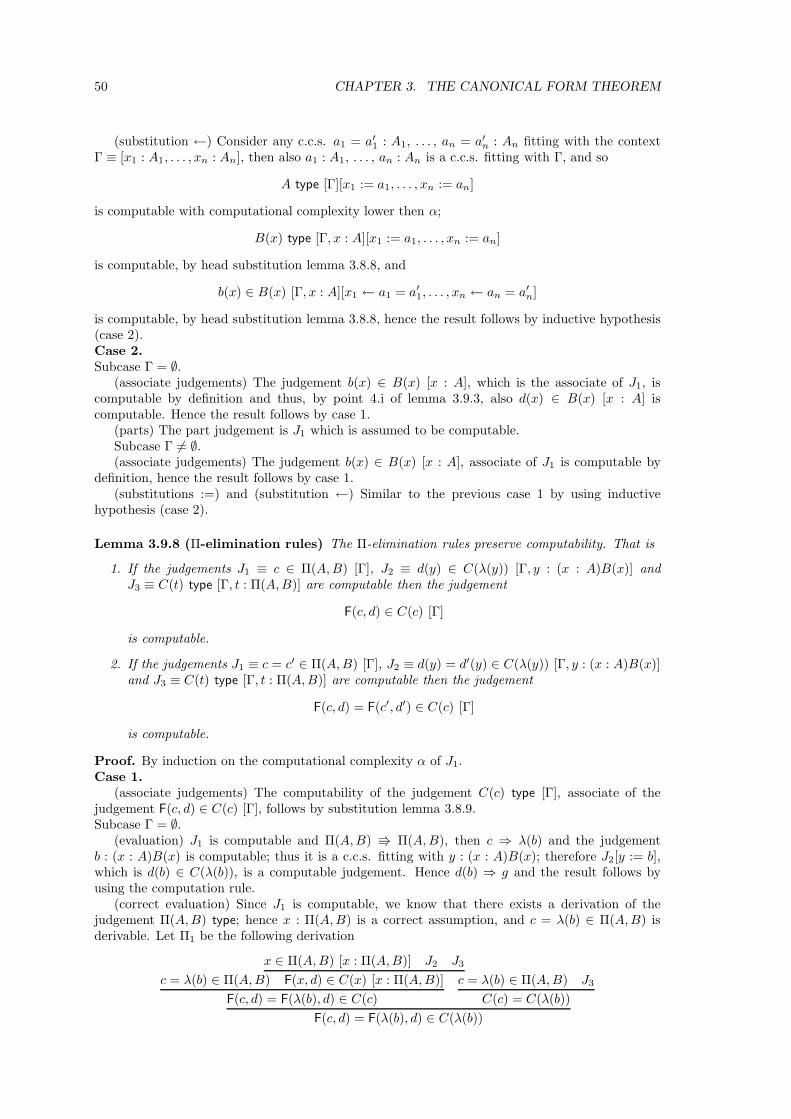
50 CHAPTER 3. THE CANONICAL FORM THEOREM
(substitution ←) Consider any c.c.s. a1 = a′1 : A1, . . . , an = a′
n : An fitting with the contextΓ ≡ [x1 : A1, . . . , xn : An], then also a1 : A1, . . . , an : An is a c.c.s. fitting with Γ, and so
A type [Γ][x1 := a1, . . . , xn := an]
is computable with computational complexity lower then α;
B(x) type [Γ, x : A][x1 := a1, . . . , xn := an]
is computable, by head substitution lemma 3.8.8, and
b(x) ∈ B(x) [Γ, x : A][x1 ← a1 = a′1, . . . , xn ← an = a′
n]
is computable, by head substitution lemma 3.8.8, hence the result follows by inductive hypothesis(case 2).Case 2.Subcase Γ = ∅.
(associate judgements) The judgement b(x) ∈ B(x) [x : A], which is the associate of J1, iscomputable by definition and thus, by point 4.i of lemma 3.9.3, also d(x) ∈ B(x) [x : A] iscomputable. Hence the result follows by case 1.
(parts) The part judgement is J1 which is assumed to be computable.Subcase Γ 6= ∅.(associate judgements) The judgement b(x) ∈ B(x) [x : A], associate of J1 is computable by
definition, hence the result follows by case 1.(substitutions :=) and (substitution ←) Similar to the previous case 1 by using inductive
hypothesis (case 2).
Lemma 3.9.8 (Π-elimination rules) The Π-elimination rules preserve computability. That is
1. If the judgements J1 ≡ c ∈ Π(A, B) [Γ], J2 ≡ d(y) ∈ C(λ(y)) [Γ, y : (x : A)B(x)] andJ3 ≡ C(t) type [Γ, t : Π(A, B)] are computable then the judgement
F(c, d) ∈ C(c) [Γ]
is computable.
2. If the judgements J1 ≡ c = c′ ∈ Π(A, B) [Γ], J2 ≡ d(y) = d′(y) ∈ C(λ(y)) [Γ, y : (x : A)B(x)]and J3 ≡ C(t) type [Γ, t : Π(A, B)] are computable then the judgement
F(c, d) = F(c′, d′) ∈ C(c) [Γ]
is computable.
Proof. By induction on the computational complexity α of J1.Case 1.
(associate judgements) The computability of the judgement C(c) type [Γ], associate of thejudgement F(c, d) ∈ C(c) [Γ], follows by substitution lemma 3.8.9.Subcase Γ = ∅.
(evaluation) J1 is computable and Π(A, B) Π(A, B), then c ⇒ λ(b) and the judgementb : (x : A)B(x) is computable; thus it is a c.c.s. fitting with y : (x : A)B(x); therefore J2[y := b],which is d(b) ∈ C(λ(b)), is a computable judgement. Hence d(b) ⇒ g and the result follows byusing the computation rule.
(correct evaluation) Since J1 is computable, we know that there exists a derivation of thejudgement Π(A, B) type; hence x : Π(A, B) is a correct assumption, and c = λ(b) ∈ Π(A, B) isderivable. Let Π1 be the following derivation
c = λ(b) ∈ Π(A, B)
x ∈ Π(A, B) [x : Π(A, B)] J2 J3
F(x, d) ∈ C(x) [x : Π(A, B)]
F(c, d) = F(λ(b), d) ∈ C(c)
c = λ(b) ∈ Π(A, B) J3
C(c) = C(λ(b))
F(c, d) = F(λ(b), d) ∈ C(λ(b))
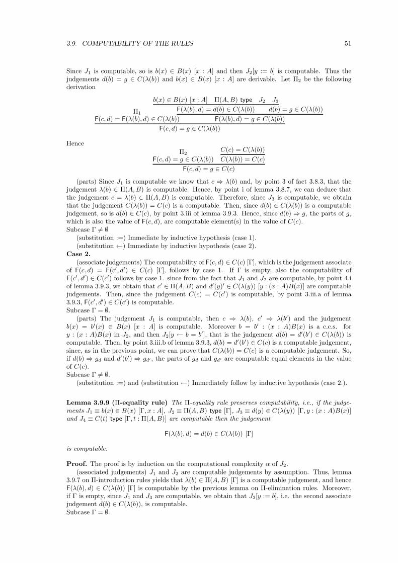
3.9. COMPUTABILITY OF THE RULES 51
Since J1 is computable, so is b(x) ∈ B(x) [x : A] and then J2[y := b] is computable. Thus thejudgements d(b) = g ∈ C(λ(b)) and b(x) ∈ B(x) [x : A] are derivable. Let Π2 be the followingderivation
Π1
F(c, d) = F(λ(b), d) ∈ C(λ(b))
b(x) ∈ B(x) [x : A] Π(A, B) type J2 J3
F(λ(b), d) = d(b) ∈ C(λ(b)) d(b) = g ∈ C(λ(b))
F(λ(b), d) = g ∈ C(λ(b))
F(c, d) = g ∈ C(λ(b))
Hence
Π2
F(c, d) = g ∈ C(λ(b))
C(c) = C(λ(b))
C(λ(b)) = C(c)
F(c, d) = g ∈ C(c)
(parts) Since J1 is computable we know that c ⇒ λ(b) and, by point 3 of fact 3.8.3, that thejudgement λ(b) ∈ Π(A, B) is computable. Hence, by point i of lemma 3.8.7, we can deduce thatthe judgement c = λ(b) ∈ Π(A, B) is computable. Therefore, since J3 is computable, we obtainthat the judgement C(λ(b)) = C(c) is a computable. Then, since d(b) ∈ C(λ(b)) is a computablejudgement, so is d(b) ∈ C(c), by point 3.iii of lemma 3.9.3. Hence, since d(b) ⇒ g, the parts of g,which is also the value of F(c, d), are computable element(s) in the value of C(c).Subcase Γ 6= ∅
(substitution :=) Immediate by inductive hypothesis (case 1).(substitution ←) Immediate by inductive hypothesis (case 2).
Case 2.(associate judgements) The computability of F(c, d) ∈ C(c) [Γ], which is the judgement associate
of F(c, d) = F(c′, d′) ∈ C(c) [Γ], follows by case 1. If Γ is empty, also the computability ofF(c′, d′) ∈ C(c′) follows by case 1. since from the fact that J1 and J2 are computable, by point 4.iof lemma 3.9.3, we obtain that c′ ∈ Π(A, B) and d′(y)′ ∈ C(λ(y)) [y : (x : A)B(x)] are computablejudgements. Then, since the judgement C(c) = C(c′) is computable, by point 3.iii.a of lemma3.9.3, F(c′, d′) ∈ C(c′) is computable.Subcase Γ = ∅.
(parts) The judgement J1 is computable, then c ⇒ λ(b), c′ ⇒ λ(b′) and the judgementb(x) = b′(x) ∈ B(x) [x : A] is computable. Moreover b = b′ : (x : A)B(x) is a c.c.s. fory : (x : A)B(x) in J2, and then J2[y ← b = b′], that is the judgement d(b) = d′(b′) ∈ C(λ(b)) iscomputable. Then, by point 3.iii.b of lemma 3.9.3, d(b) = d′(b′) ∈ C(c) is a computable judgement,since, as in the previous point, we can prove that C(λ(b)) = C(c) is a computable judgement. So,if d(b) ⇒ gd and d′(b′) ⇒ gd′ , the parts of gd and gd′ are computable equal elements in the valueof C(c).Subcase Γ 6= ∅.
(substitution :=) and (substitution ←) Immediately follow by inductive hypothesis (case 2.).
Lemma 3.9.9 (Π-equality rule) The Π-equality rule preserves computability, i.e., if the judge-ments J1 ≡ b(x) ∈ B(x) [Γ, x : A], J2 ≡ Π(A, B) type [Γ], J3 ≡ d(y) ∈ C(λ(y)) [Γ, y : (x : A)B(x)]and J4 ≡ C(t) type [Γ, t : Π(A, B)] are computable then the judgement
F(λ(b), d) = d(b) ∈ C(λ(b)) [Γ]
is computable.
Proof. The proof is by induction on the computational complexity α of J2.(associated judgements) J1 and J2 are computable judgements by assumption. Thus, lemma
3.9.7 on Π-introduction rules yields that λ(b) ∈ Π(A, B) [Γ] is a computable judgement, and henceF(λ(b), d) ∈ C(λ(b)) [Γ] is computable by the previous lemma on Π-elimination rules. Moreover,if Γ is empty, since J1 and J3 are computable, we obtain that J3[y := b], i.e. the second associatejudgement d(b) ∈ C(λ(b)), is computable.Subcase Γ = ∅.
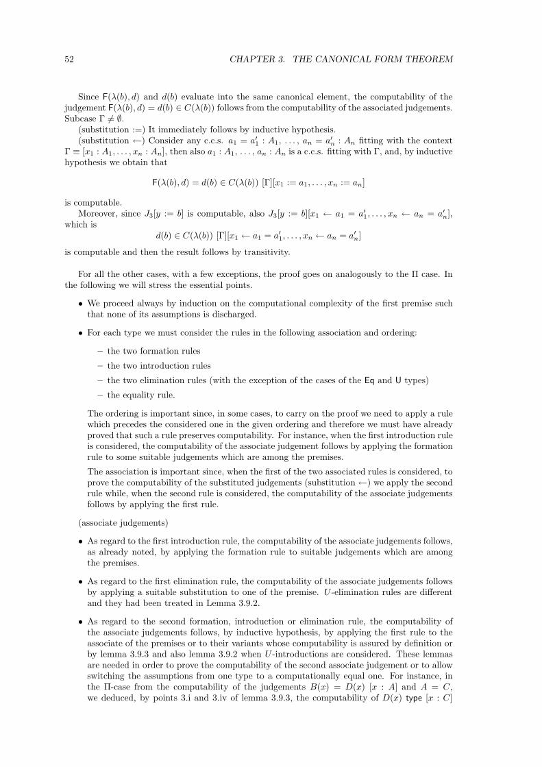
52 CHAPTER 3. THE CANONICAL FORM THEOREM
Since F(λ(b), d) and d(b) evaluate into the same canonical element, the computability of thejudgement F(λ(b), d) = d(b) ∈ C(λ(b)) follows from the computability of the associated judgements.Subcase Γ 6= ∅.
(substitution :=) It immediately follows by inductive hypothesis.(substitution ←) Consider any c.c.s. a1 = a′
1 : A1, . . . , an = a′n : An fitting with the context
Γ ≡ [x1 : A1, . . . , xn : An], then also a1 : A1, . . . , an : An is a c.c.s. fitting with Γ, and, by inductivehypothesis we obtain that
F(λ(b), d) = d(b) ∈ C(λ(b)) [Γ][x1 := a1, . . . , xn := an]
is computable.Moreover, since J3[y := b] is computable, also J3[y := b][x1 ← a1 = a′
1, . . . , xn ← an = a′n],
which isd(b) ∈ C(λ(b)) [Γ][x1 ← a1 = a′
1, . . . , xn ← an = a′n]
is computable and then the result follows by transitivity.
For all the other cases, with a few exceptions, the proof goes on analogously to the Π case. Inthe following we will stress the essential points.
• We proceed always by induction on the computational complexity of the first premise suchthat none of its assumptions is discharged.
• For each type we must consider the rules in the following association and ordering:
– the two formation rules
– the two introduction rules
– the two elimination rules (with the exception of the cases of the Eq and U types)
– the equality rule.
The ordering is important since, in some cases, to carry on the proof we need to apply a rulewhich precedes the considered one in the given ordering and therefore we must have alreadyproved that such a rule preserves computability. For instance, when the first introduction ruleis considered, the computability of the associate judgement follows by applying the formationrule to some suitable judgements which are among the premises.
The association is important since, when the first of the two associated rules is considered, toprove the computability of the substituted judgements (substitution←) we apply the secondrule while, when the second rule is considered, the computability of the associate judgementsfollows by applying the first rule.
(associate judgements)
• As regard to the first introduction rule, the computability of the associate judgements follows,as already noted, by applying the formation rule to suitable judgements which are amongthe premises.
• As regard to the first elimination rule, the computability of the associate judgements followsby applying a suitable substitution to one of the premise. U -elimination rules are differentand they had been treated in Lemma 3.9.2.
• As regard to the second formation, introduction or elimination rule, the computability ofthe associate judgements follows, by inductive hypothesis, by applying the first rule to theassociate of the premises or to their variants whose computability is assured by definition orby lemma 3.9.3 and also lemma 3.9.2 when U -introductions are considered. These lemmasare needed in order to prove the computability of the second associate judgement or to allowswitching the assumptions from one type to a computationally equal one. For instance, inthe Π-case from the computability of the judgements B(x) = D(x) [x : A] and A = C,we deduced, by points 3.i and 3.iv of lemma 3.9.3, the computability of D(x) type [x : C]
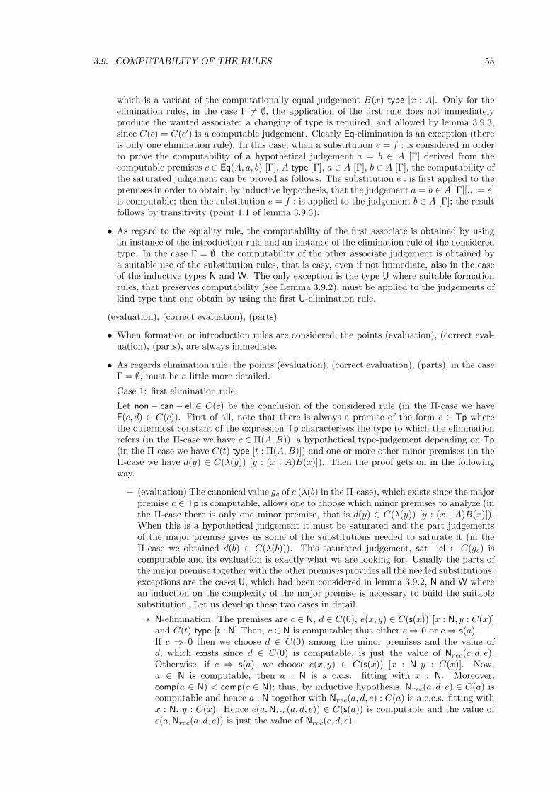
3.9. COMPUTABILITY OF THE RULES 53
which is a variant of the computationally equal judgement B(x) type [x : A]. Only for theelimination rules, in the case Γ 6= ∅, the application of the first rule does not immediatelyproduce the wanted associate: a changing of type is required, and allowed by lemma 3.9.3,since C(c) = C(c′) is a computable judgement. Clearly Eq-elimination is an exception (thereis only one elimination rule). In this case, when a substitution e = f : is considered in orderto prove the computability of a hypothetical judgement a = b ∈ A [Γ] derived from thecomputable premises c ∈ Eq(A, a, b) [Γ], A type [Γ], a ∈ A [Γ], b ∈ A [Γ], the computability ofthe saturated judgement can be proved as follows. The substitution e : is first applied to thepremises in order to obtain, by inductive hypothesis, that the judgement a = b ∈ A [Γ][.. := e]is computable; then the substitution e = f : is applied to the judgement b ∈ A [Γ]; the resultfollows by transitivity (point 1.1 of lemma 3.9.3).
• As regard to the equality rule, the computability of the first associate is obtained by usingan instance of the introduction rule and an instance of the elimination rule of the consideredtype. In the case Γ = ∅, the computability of the other associate judgement is obtained bya suitable use of the substitution rules, that is easy, even if not immediate, also in the caseof the inductive types N and W. The only exception is the type U where suitable formationrules, that preserves computability (see Lemma 3.9.2), must be applied to the judgements ofkind type that one obtain by using the first U-elimination rule.
(evaluation), (correct evaluation), (parts)
• When formation or introduction rules are considered, the points (evaluation), (correct eval-uation), (parts), are always immediate.
• As regards elimination rule, the points (evaluation), (correct evaluation), (parts), in the caseΓ = ∅, must be a little more detailed.
Case 1: first elimination rule.
Let non− can− el ∈ C(c) be the conclusion of the considered rule (in the Π-case we haveF(c, d) ∈ C(c)). First of all, note that there is always a premise of the form c ∈ Tp wherethe outermost constant of the expression Tp characterizes the type to which the eliminationrefers (in the Π-case we have c ∈ Π(A, B)), a hypothetical type-judgement depending on Tp
(in the Π-case we have C(t) type [t : Π(A, B)]) and one or more other minor premises (in theΠ-case we have d(y) ∈ C(λ(y)) [y : (x : A)B(x)]). Then the proof gets on in the followingway.
– (evaluation) The canonical value gc of c (λ(b) in the Π-case), which exists since the majorpremise c ∈ Tp is computable, allows one to choose which minor premises to analyze (inthe Π-case there is only one minor premise, that is d(y) ∈ C(λ(y)) [y : (x : A)B(x)]).When this is a hypothetical judgement it must be saturated and the part judgementsof the major premise gives us some of the substitutions needed to saturate it (in theΠ-case we obtained d(b) ∈ C(λ(b))). This saturated judgement, sat− el ∈ C(gc) iscomputable and its evaluation is exactly what we are looking for. Usually the parts ofthe major premise together with the other premises provides all the needed substitutions;exceptions are the cases U, which had been considered in lemma 3.9.2, N and W wherean induction on the complexity of the major premise is necessary to build the suitablesubstitution. Let us develop these two cases in detail.
∗ N-elimination. The premises are c ∈ N, d ∈ C(0), e(x, y) ∈ C(s(x)) [x : N, y : C(x)]and C(t) type [t : N] Then, c ∈ N is computable; thus either c⇒ 0 or c⇒ s(a).If c ⇒ 0 then we choose d ∈ C(0) among the minor premises and the value ofd, which exists since d ∈ C(0) is computable, is just the value of Nrec(c, d, e).Otherwise, if c ⇒ s(a), we choose e(x, y) ∈ C(s(x)) [x : N, y : C(x)]. Now,a ∈ N is computable; then a : N is a c.c.s. fitting with x : N. Moreover,comp(a ∈ N) < comp(c ∈ N); thus, by inductive hypothesis, Nrec(a, d, e) ∈ C(a) iscomputable and hence a : N together with Nrec(a, d, e) : C(a) is a c.c.s. fitting withx : N, y : C(x). Hence e(a, Nrec(a, d, e)) ∈ C(s(a)) is computable and the value ofe(a, Nrec(a, d, e)) is just the value of Nrec(c, d, e).
54 CHAPTER 3. THE CANONICAL FORM THEOREM
∗ W-elimination. Note that the judgment c ∈ W(A, B) is computable by assump-tion; then c ⇒ sup(a, b) and a ∈ A and b(x) ∈ W(A, B) [x : B(a)], that isb : (x : B(a)) W(A, B), are computable judgements. Hence we obtaind that a : A,b : (x : B(a)) W(A, B) is a c.c.s. fitting with z : A, y : (x : B(z)) W(A, B). Then, byapplying a W-elimination rule on b(x) ∈ W(A, B)[x : B(a)] instead of c ∈ W(A, B)we obtain by inductive hypothesis that Trec(b(x), d) ∈ C(b(x)) [x : B(a)] is acomputable judgement, because the computational complexity of the judgementb(x) ∈W(A, B) [x : B(a)] is lower than the computational complexity of the judge-ment c ∈ W(A, B). Now, note that the judgement Trec(b(x), d) ∈ C(b(x)) [x : B(a)]is equivalent by definition to (x) Trec(b(x), d) : (x : B(a)) C(b(x)) and hence itis a c.c.s. fitting with t : (x : B(a)) C(b(x)). Then, by substituting, we ob-tain that d(a, b, (x) Trec(b(x), d)) ∈ C(sup(a, b)) is computable and the value ofd(a, b, (x) Trec(b(x), d)) is exactly the value of Trec(c, d) we are looking for.
– (correct evaluation) For each canonical value of the major premise a derivation can beconstructed analogously to what we did in the Π-case. It is sufficient to substituteany application of Π-elimination and Π-equality rules by the corresponding one for theconsidered type.
– (parts) The computability of the major premise c ∈ Tp guarantees, by lemma 3.8.3 andpoint i of lemma 3.8.7, the computability of the judgement c = gc ∈ Tp (in the Π-case wehad c = λ(b) ∈ Π(A, B)). This fact yields that the type equality judgement C(c) = C(gc)is computable (in the Π-case we proved that C(c) = C(λ(b)) is computable). Now, ifwe consider the computable judgement built up to prove the previous evaluation point,sat− el ∈ C(gc) (in the Π-case we had d(b) ∈ C(λ(b))), by point 3.iii of lemma 3.9.3, weobtain that sat− el ∈ C(c) is computable (in the Π-case we had d(b) ∈ C(c)). Hence ifsat− el⇒ can− el and C(c)⇒ canC , then also non− can− el⇒ can− el and the partsof can− el are computable elements in canC .
Case 2: second elimination rule.
Let non− can− el1 = non− can− el2 ∈ C(c) be the conclusion of the rule.
(parts) First of all, note that the computability of the first associate of the major premise,c = c′ ∈ Tp, guarantees the computability of the judgement C(c) = C(gc). Then, analo-gously to the case 1 of the first elimination rule, we can choose the suitable minor premiseand saturate it by using ← instead of :=. By the computability of the resulting judge-ment sat− el1 = sat− el2 ∈ C(gc) together with that of C(c) = C(gc), we will obtain thecomputability of sat− el1 = sat− el2 ∈ C(c). From this the result is immediate.
• For the equality rule, the point (parts), follow easily since, by point i of lemma 3.8.7 (or pointii when the type U is considered), the computability of the associate judgements together withthe definition of the evaluation process⇒, guarantees the computability of the judgement inthe conclusion.
(substitution :=)
• The point (substitution :=) always follows, by induction, by first applying the same substi-tution to the premises and next applying again the same rule to the resulting judgements.Note that when a rule which discharges assumptions is considered, we must apply a headsubstitution which preserves computability.
(substitution ←)
• For the first formation, introduction or elimination rule, the point (substitution←) follows, byinductive hypothesis, by applying the second rule in the association to judgements obtainedby properly substituting the given premises. In some cases, when a rule which dischargesassumptions is considered, the computability of the suitably substituted premises is statedby the head substitution lemma 3.8.8.
3.10. THE COMPUTABILITY THEOREM 55
• For the second formation, introduction or elimination rule, the proof of the point (substitution←) follows by applying the same rule to judgements obtained by wisely applying the samesubstitution e = f : or its associate e : to the given premises.
• For the equality rule, when the substitution e = f : is considered in proving the point (sub-stitution ←), we will proceed as follows. On one side we apply the same rule to judgementsobtained by applying the associate substitution e : to the premises. On the other side, weapply the substitution e = f : to a judgement built up by applying a suitable head substi-tution to the minor premise analogously to what done for the (evaluation) point. The resultthen follows by transitivity (consider again the Π-case as a typical example). For the U-casewe must build up a first judgement by applying the same rule to judgements obtained byapplying the substitution e : to the given premises, and a second one by applying a formationrule to the result of applying the U-elimination to the premises. The result then follows bytransitivity. Note that all the rules used in the construction preserve computability.
3.10 The computability theorem
Now we can state our main theorem: it shows that any derivable judgement is computable andhence that all the properties we ask for a judgement to be computable hold for any derivablejudgement.
Theorem 3.10.1 (Computability theorem) Let J be any derivable judgement. Then J is com-putable.
From a proof-theoretical point of view the main meta-theoretical result on a deductive system innatural deduction style as ours, is a normal form theorem, i.e. a theorem that states that any proofcan be transformed in a new one with the same conclusion but enjoying stronger structure prop-erties. These properties generally allow in turn to deduce important properties on the considereddeduction system such as its consistency. Our computability theorem does not regard derivationsbut still is strongly related to normal form theorems as the following definitions will clarify.
Definition 3.10.2 (Canonical proof) A proof Π of a judgement J is canonical if
1. J ≡ A type or J ≡ A = B and the last inference step in Π is a formation rule.
2. J ≡ a ∈ A or J ≡ a = b ∈ A and the last inference step in Π is an introduction rule.
A canonical proof might be also called “normal at the end”. Clearly not every closed judgementcan be derived by a canonical proof. This holds only for the judgements which, according to thefollowing definition, are in canonical form.
Definition 3.10.3 (Canonical form) Let J be a closed judgement. Then
• if J ≡ A type and A GA then the canonical form of J is GA type;
• if J ≡ A = B and A GA and B GB then the canonical form of J is GA = GB ;
• if J ≡ a ∈ A and a⇒ ga and A GA then the canonical form of J is ga ∈ GA;
• if J ≡ a = b ∈ A and a ⇒ ga and b ⇒ gb and A GA then the canonical form of J isga = gb ∈ GA.
Corollary 3.10.4 (Canonical-form theorem) Let J be a derivable closed judgement then thereexists a canonical proof of the canonical form of J .
Proof. Since J is derivable then it is computable and hence there exist a derivation of its partsjudgements since they also are computable. By putting them together with a formation or anintroduction rule we obtain a canonical proof of the canonical form of J .
It is easy to see that if J is a derivable closed judgement then its computability implies that itscanonical form is a judgement equivalent to J , in fact:
56 CHAPTER 3. THE CANONICAL FORM THEOREM
• if J ≡ A type and A GA then the canonical form of J is GA type and the computabilityof J assures that A = GA is derivable.
• if J ≡ A = B and A GA and B GB then the canonical form of J is GA = GB and thecomputability of J assures that A = GA and B = GB are derivable judgements.
• if J ≡ a ∈ A and a ⇒ ga and A GA then the canonical form of J is ga ∈ GA and thecomputability of J yields that A = GA and a = ga ∈ A are derivable judgements.
• if J ≡ a = b ∈ A and a ⇒ ga, b ⇒ gb and A GA then the canonical form of J isga = gb ∈ GA and the computability of J assures that A = GA, a = ga ∈ A and b = gb ∈ Aare derivable judgements.
Then the previous canonical form theorem is, in our system, the counterpart of a standardnormal form theorem since it guarantees that if J is a closed derivable judgement then we canconstruct a canonical proof for a judgement equivalent to J . Moreover it allows us to deduce mostof the results usually obtained by a normal form theorem such as, for instance, consistency.
Corollary 3.10.5 (Consistency of HITT) The Higher order Intuitionistic Theory of Type isconsistent.
Proof. Since the judgement c ∈ N0 is not computable and then it cannot be derivable.
Note that this result establishes also the consistency of the original ITT. As we could expect,the minimal properties, which are usually asked for a logical system to be considered constructive,immediately follow just by reading the definition of computable judgement.
Corollary 3.10.6 (Disjunction property) If the judgement c ∈ +(A, B) is derivable then eitherthere exists an element a such that a ∈ A is derivable or there exists an element b such that b ∈ Bis derivable.
Proof. If c ∈ +(A, B) is derivable then it is computable and hence either c⇒ inl(a) and a ∈ A isderivable or c⇒ inr(b) and b ∈ B is derivable.
Corollary 3.10.7 (Existential property) If the judgement c ∈ Σ(A, B) is derivable then thereexists an element b such that the judgement b ∈ B(a) is derivable for some a ∈ A.
Proof. If c ∈ Σ(A, B) is derivable then it is computable and hence c ⇒ 〈a, b〉 and a ∈ A andb ∈ B(a) are derivable judgements.
Other consequences of the computability theorem can be stated when the Intuitionistic Theoryof Type is viewed as a formal system to derive programs, that is when a type is interpreted as thespecification of a problem and an element in this type as the program which meets this specification.In this environment an expression denoting an element in a type is thought as a program written ina functional language whose operational semantics is given by the computation rules and hence toexecute a program corresponds to evaluating it. The computability theorem shows that wheneverwe prove that a program a is partially correct with respect to its specification A, i.e. we derive thejudgement a ∈ A, then we know also that it is totally correct, that is its evaluation terminates.
Corollary 3.10.8 (Evaluation theorem) Any provable expression can be evaluated, that is
1. If A type is a provable judgement then A has a canonical value.
2. If a ∈ A is a provable judgement, then a has a canonical value.
Thus any program whose evaluation does not terminate, such as the famous Church’s non-terminating function, cannot be typed in HITT.
Related works. We should like to thank the referee for his comments and suggestions and forpointing out to us related works, in particular [All86] and [All87] where similar results are provedby a realizability-like semantics.
Chapter 4
Properties of Type Theory
4.1 Summary
In this chapter some meta-mathematical properties of Martin-Lof’s type theory will be presented.
In the first part we will show that decidability of a property over elements of a set A can bereduced to the problem of finding a suitable function from A into the set Boole (≡ N2).
Then an intuitionistic version of Cantor’s theorem will be shown which proves that there isno bijection between the set N of the natural numbers and the set N → N of the functions fromnatural numbers into natural numbers.
Finally, the “forget-restore” principle will be illustrated by analyzing a simple case in Martin-Lof’s type theory. Indeed, type theory offers a way of “forgetting” information, that is, supposingA set, the form of judgment A true. The meaning of A true is that there exists an element asuch that a ∈ A but it does not matter which particular element a is (see also the notion of proofirrelevance in [Bru80]). Thus to pass from the judgment a ∈ A to the judgment A true is a clearexample of the forgetting process. In this section we will show that it is a constructive way toforget since, provided that there is a proof of the judgment A true, an element a such that a ∈ Acan be re-constructed.
4.2 Decidability is functionally decidable
Introduction and basic lemmas
In this section we show that the usual intuitionistic characterization of the decidability of thepropositional function B(x) prop [x : A], that is to require that the predicate (∀x ∈ A) B(x)∨¬B(x)is provable, is equivalent, when working within the framework of Martin-Lof’s Intuitionistic TypeTheory, to require that there exists a decision function φ : A→ Boole such that
(∀x ∈ A) (φ(x) =Boole true)↔ B(x)
Since we will also show that the proposition x =Boole true [x : Boole] is decidable, we can alter-natively say that the main result of this section is a proof that the decidability of the predicateB(x) prop [x : A] can be effectively reduced by a function φ ∈ A → Boole to the decidability ofthe predicate φ(x) =Boole true [x : A]. All the proofs are carried out within the Intuitionistic TypeTheory and hence the decision function φ, together with a proof of its correctness, is effectivelyconstructed as a function of the proof of (∀x ∈ A) B(x) ∨ ¬B(x).
This result may not be completely new (for instance in a personal communication Martin-Lofsaid that he already knew it) but since, to my knowledge, there is no published material on thistopic this note may be useful to a wider audience. In fact, apart from its intrinsic relevance, thisresult is also a good exercise in ITT since in order to be able to obtain its proof one has to usesome of the most interesting properties of ITT. In this paragraph we will recall these properties,and their proofs, to the reader who is not familiar with ITT, but to avoid to bore the reader who
57
58 CHAPTER 4. PROPERTIES OF TYPE THEORY
is familiar with ITT we will not recall all the basic definitions which can be found in [Mar84] or[NPS90].
Since in most of the results the type Boole plays a central role, let us begin by recalling someof its properties. First of all recall that the canonical elements of the type Boole are true and false
and that, supposing C(x) prop [x : Boole], the Boole-elimination rule allows to obtain
if c then d else e ∈ C(c)
provided c ∈ Boole, d ∈ C(true) and e ∈ C(false).
Lemma 4.2.1 Let P (x) prop [x : Boole] and c ∈ Boole; then
P (c)→ P (true) ∨ P (false)
Proof. The proof is just an application of the Boole-elimination rule. In fact if c ∈ Boole then
if c then λx.inl(x) else λy.inr(y) ∈ P (c)→ P (true) ∨ P (false)
since λx.inl(x) ∈ P (true)→ P (true) ∨ P (false) and λy.inr(y) ∈ P (false)→ P (true) ∨ P (false).
Let us recall that, supposing c, d ∈ Boole, by c =Boole d we mean the intensional equalityproposition for elements of Boole, denoted in the appendix B by the type Id. Its main propertiesare that
• if c = d ∈ Boole then c =Boole d is true,
• if c =Boole d is true and A(x) prop [x : Boole] is a proposition on elements of Boole such thata ∈ A(c) then move(c, a) ∈ A(d),
• if c =Boole d is true, a(x) ∈ A [x : Boole] and y =A z prop [y, z : A] is the intensional equalityproposition for elements of the type A then a(c) =A a(d) is true.
Hence the following corollary is immediate.
Corollary 4.2.2 Let c ∈ Boole; then (c =Boole true) ∨ (c =Boole false).
Proof. Suppose P (x) ≡ c =Boole x [x : Boole], then the previous lemma shows that
(c =Boole c)→ (c =Boole true) ∨ (c =Boole false)
Now the statement is obvious since c =Boole c is straightforward.
We have then proved that in Boole there are at most two elements; by means of the universeof the small types U, whose elements are (the codes of) the basic types, we can show that in Boole
there are exactly two elements. To obtain this result it is convenient to use the equality propositionA =U B prop [A, B : U] for elements of the type U. Besides the properties analogous to those abovefor the equality proposition for the elements of the type Boole, in this case one can also prove thatif A =U B is true and a ∈ A then shift(a) ∈ B.
Lemma 4.2.3 ¬(true =Boole false)
Proof. Assume that y : Boole. Then a Boole-elimination can be used to shows that
if y then ⊤ else ⊥ ∈ U
where ⊤ is the one-element type and ⊥ is the empty type.Let us now assume that x : true =Boole false, i.e. let us assume that true =Boole false is true.
Then we obtain thatif true then ⊤ else ⊥ =U if false then ⊤ else ⊥
and hence ⊤ =U ⊥ since the equality proposition is transitive and ⊤ =U if true then ⊤ else ⊥and if false then ⊤ else ⊥ =U ⊥ hold; hence, supposing ∗ is the only element of the type ⊤,
4.2. DECIDABILITY IS FUNCTIONALLY DECIDABLE 59
shift(∗) ∈ ⊥, that is we have found an element in the empty type; so, by discharging the assumptionx : true =Boole false, we finally obtain λx. shift(∗) ∈ ¬(true =Boole false).
We showed a full detailed proof of this lemma to stress the fact that it is completely carriedout within ITT with the universe U of the small types.
By using lemma 4.2.3 and a little of intuitionistic logic one can prove the following not verysurprising result.
Lemma 4.2.4 (c =Boole false) if and only if ¬(c =Boole true).
Even if the previous lemma is straightforward when we combine it with 4.2.2 we obtain aninteresting result: the predicate x =Boole true [x : Boole] is decidable.
Corollary 4.2.5 For all c ∈ Boole, (c =Boole true) ∨ ¬(c =Boole true).
There is another property that we need to recall because of its relevance in the following: thanksto the constructive meaning of the logical connectives a sort of Axiom of Choice holds in ITT (herewe show a statement which is not the strongest one that can be proved but it is sufficient for us).
Lemma 4.2.6 Let A, B be two types and C(x, y) prop [x : A, y : B]; then
((∀x ∈ A)(∃y ∈ B) C(x, y))→ ((∃f ∈ A→ B)(∀x ∈ A) C(x, f(x)))
Proof. A complete proof can be found in [Mar84] where a choice function f ∈ A→ B is constructedtogether with a formal proof that for any x ∈ A, C(x, f(x)) holds; anyhow the basic intuition toobtain the proof is rather simple: suppose h is (the code for) a proof of (∀x ∈ A)(∃y ∈ B) C(x, y)then, for any x ∈ A, (the value of) h(x) is a couple whose first element fst(h(x)) belongs to B whilethe second element is a proof of C(x, fst(h(x))); the choice function is then λx.fst(h(x)) ∈ A→ B.
Also in this case we want to observe that the proof explicitly shows how to construct a choicefunction in A→ B provided that we have a proof of (∀x ∈ A)(∃y ∈ B) C(x, y).
4.2.1 The main result
This paragraph is completely devoted to the proof of the following theorem.
Theorem 4.2.7 Let B(x) prop [x : A]; then the following statements are equivalent:(1) There exists a decision function φ : A→ Boole such that, for all x ∈ A, φ(x) =Boole true if
and only if B(x) is true.(2) for all x ∈ A, B(x) ∨ ¬B(x).
We can straight away prove that (1) implies (2). In fact, let us suppose that φ : A → Boole
is a decision function for the proposition B(x) prop [x : A] and let us assume that x ∈ A. Then,because of corollary 4.2.5, we know that
(φ(x) =Boole true) ∨ ¬(φ(x) =Boole true)
and hence we can concludeB(x) ∨ ¬B(x)
by ∨-elimination. In fact φ(x) =Boole true immediately implies that B(x) is true, and hence thatB(x) ∨ ¬B(x) is true, since φ is a decision function. On the other hand the same conclusion canbe obtained from the assumption ¬(φ(x) =Boole true) by using the following derivation which againmakes use of the fact that φ is a decision function:
[B(x)]1
φ(x) =Boole true ¬(φ(x) =Boole true)
⊥¬B(x)
1
B(x) ∨ ¬B(x)
60 CHAPTER 4. PROPERTIES OF TYPE THEORY
Let us now show that (2) implies (1); we do not only have to provide a function φ : A→ Boole,which would be easy, but we have also to show that it is a decision function. This is the reasonwhy we need some preliminary lemmas.
Lemma 4.2.8 Let B(x) prop [x : A]; then
(∀x ∈ A) B(x) ∨ ¬B(x)→(∀x ∈ A)(∃y ∈ Boole)(y =Boole true→ B(x)) & (y =Boole false→ ¬B(x))
Proof. The proof is just an application of the ∨-elimination rule. In fact let us suppose that(∀x ∈ A) B(x) ∨ ¬B(x) holds and assume that x ∈ A, then we have to show
(∃y ∈ Boole) (y =Boole true→ B(x)) & (y =Boole false→ ¬B(x))
from B(x) ∨ ¬B(x) and hence all we need are the following deductions:
B(x)
true =Boole true→ B(x)
¬(true =Boole false)
true =Boole false→ ¬B(x)
(true =Boole true→ B(x)) & (true =Boole false→ ¬B(x))
(∃y ∈ Boole) (y =Boole true→ B(x)) & (y =Boole false→ ¬B(x))
and¬(false =Boole true)
false =Boole true→ B(x)
¬B(x)
false =Boole false→ ¬B(x)
(false =Boole true→ B(x)) & (false =Boole false→ ¬B(x))
(∃y ∈ Boole) (y =Boole true→ B(x)) & (y =Boole false→ ¬B(x))
Thanks to lemma 4.2.8, we are in the position to take advantage of the axiom of choice in orderto obtain the following corollary.
Corollary 4.2.9 Let B(x) prop [x : A]; then
(∀x ∈ A) B(x) ∨ ¬B(x)→(∃φ ∈ A→ Boole)(∀x ∈ A)(φ(x) =Boole true→ B(x))&(φ(x) =Boole false→ ¬B(x))
Hence we have obtained the proof of the main theorem; in fact this corollary shows that if wehave a proof of (∀x ∈ A) B(x) ∨ ¬B(x) then both
(†) there exists a function φ : A → Boole, and since all the proofs were developed within ITTwe can effectively construct it, and
(‡) such a function is a decision function for B(x); in fact if φ(x) =Boole true then B(x) istrue and, on the other hand, if B(x) is true we can use the following derivation to show thatφ(x) =Boole true:
φ(x) =Boole true ∨ φ(x) =Boole false
[φ(x) =Boole false]1 φ(x) =Boole false→ ¬B(x)
¬B(x) B(x)
⊥¬(φ(x) =Boole false)
1
φ(x) =Boole true
We can save a curious reader the trouble of doing some work if we say that, supposingh ∈ (∀x ∈ A) B(x) ∨ ¬B(x), the decision function which we obtain (after some unessential simpli-fication) is
φ ≡ λx. fst(D( h(x),(z) < true, < λw. z, λu. R0(shift(∗)) >>,(z) < false, < λu. R0(shift(∗)), λw. z >>)).
4.3. AN INTUITIONISTIC CANTOR’S THEOREM 61
We can simplify it by far if we disregard all the parts which do not have a computational contentand which appear in φ only because of the way we obtained it; in fact the function
φ′ ≡ λx.D(h(x), (z) true, (z) false)
has obviously the same computational behavior as φ; the drawback is that we lack a formal proofthat φ′ is a decision function for B(x). Of course we can obtain such a proof by using the factthat φ is a decision function for B(x). In fact we can prove that (∀x ∈ A) φ(x) =Boole φ′(x)is true, because in general, supposing A, B, C, D are types, c ∈ A + B, d(z) ∈ C × D [z : A],e(z) ∈ C ×D [z : B], the equality proposition
fst(D(c, (z) d(z), (z) e(z)) =C D(c, (z) fst(d(z)), (z) fst(e(z)))
holds.
4.3 An intuitionistic Cantor’s theorem
Introduction
An intuitionistic version of Cantor’s theorem, which shows that there is no surjective function fromthe type of the natural numbers N into the type N→ N of the functions from N into N, is provedwithin Martin-Lof’s Intuitionistic Type Theory with the universe of the small types.
4.3.1 Cantor’s theorem
In this section we show that within Martin-Lof’s Intuitionistic Type Theory with the universe ofthe small types [Mar84, NPS90] (ITT for short in the following) a version of Cantor’s theoremholds, which shows that there is no surjective function from the type of the natural numbers N
into the type N → N of the functions from N into N. As the matter of fact a similar result canbe stated for any not-empty type A such that there exists a function from A into A which has nofixed point, as is the case of the successor function for the type N. In order to express Cantor’stheorem within ITT we need the intensional equality proposition: let A be a type and a, c ∈ A,then by a =A c we mean the intensional equality proposition for elements of type A (see the typedenoted by Id in the appendix B or [NPS90]).
Theorem 4.3.1 (ITT Cantor’s theorem) Let N be the type of the natural numbers; then
¬(∃f ∈ N→ (N→ N))(∀y ∈ N→ N)(∃x ∈ N) f(x) =N→N y
To prove this theorem some lemmas are useful. Indeed we need to obtain a contradiction fromthe assumption
(∃f ∈ N→ (N→ N))(∀y ∈ N→ N)(∃x ∈ N) f(x) =N→N y
i.e. from the two assumptions f ∈ N→ (N→ N) and (∀y ∈ N→ N)(∃x ∈ N) f(x) =N→N y.By using the basic idea of the classic proof of Cantor’s theorem, from the first assumption we
can prove λx.s(f(x)(x)) ∈ N → N, where s : (x : N)N is the successor function, by the followingdeduction:
[x : N]1
[x : N]1 f ∈ N→ (N→ N)
f(x) : N→ N
f(x)(x) ∈ N
s(f(x)(x)) ∈ N
λx.s(f(x)(x)) ∈ N→ N1
We can now use this function in the second assumption in order to obtain
(∃x ∈ N) f(x) =N→N λx.s(f(x)(x)).
So our problem becomes to obtain a contradiction from the two assumptions x : N andf(x) =N→N λx.s(f(x)(x)). We can use these assumptions to prove, by transitivity of the equality
62 CHAPTER 4. PROPERTIES OF TYPE THEORY
proposition, that f(x)(x) =N s(f(x)(x)) is true since in general if A and B are types and a =A cand f =A→B g then f(a) =B g(c) and obviously (λx.s(f(x)(x)))(x) =N s(f(x)(x)) is true.
We can thus re-state our aim by saying that we have to prove that ITT is not consistent withthe assumption that the successor function has a fixed point. To prove this result we can transposea well known categorical arguments within ITT [Law69, HP90]. Let us recall that we can solve theusual recursive definition of the sum between two natural numbers
n + 0 = n : N
n + s(x) = s(n + x) : N
by putting n + x ≡ Nrec(x, n, (u, v) s(v)). Then the following lemma can be proved by induction.
Lemma 4.3.2 For any n, x ∈ N, n + s(x) =N s(n) + x.
As for the sum, we can solve the recursive equation for the predecessor function
p(0) = 0 : N
p(s(x)) = x : N
by putting p(x) ≡ Nrec(x, 0, (u, v) u), and then that for the subtraction
n− 0 = n : N
n− s(x) = p(n− x) : N
by putting n− x ≡ Nrec(x, n, (u, v) p(v)).
Lemma 4.3.3 For any x ∈ N, (∀n ∈ N) (n + x) − x =N n.
Proof. By induction on x. If x = 0 then (n + 0) − 0 =N n + 0 =N n. On the other hand,if we assume by inductive hypothesis that (∀n ∈ N) (n + x) − x =N n, then we obtain that(n + s(x)) − s(x) =N p((n + s(x))− x) =N p((s(n) + x) − x) =N p(s(n)) =N n. 2
We can apply this lemma to the case n = 0 and obtain the following corollary.
Corollary 4.3.4 For any x ∈ N, x− x =N 0.
Proof. Immediate, since 0 + x =N x holds for each x ∈ N. 2
Now we conclude our proof. Let us write ω to mean the fixed point of the successor function,i.e. ω =N s(ω). Then the following lemma holds.
Lemma 4.3.5 For any x ∈ N, ω − x =N ω.
Proof. Again a proof by induction on x. If x = 0 then ω − 0 =N ω and, supposing ω − x =N ω,we obtain ω − s(x) =N p(ω − x) =N p(ω) =N p(s(ω)) =N ω. 2
So we proved that ω − ω =N 0 by corollary 4.3.4 and also that ω − ω =N ω by lemma 4.3.5;hence 0 =N ω =N s(ω). Finally we reach a contradiction.
Theorem 4.3.6 For any x ∈ N, ¬(0 =N s(x))
Proof. By using an elimination rule for the type N, from the assumption y : N, we obtainNrec(y,⊥, (u, v) ⊤) ∈ U, where U is the universe of the small types, ⊥ is the empty type and⊤ is the one-element type. Now let us assume that x ∈ N and that 0 =N s(x) is true, thenNrec(0,⊥, (u, v) ⊤) =U Nrec(s(x),⊥, (u, v) ⊤) since in general if A and B are types and a =A cis true and b(x) ∈ B [x : A] then b(a) =B b(c) is true. Hence, by transitivity of the equalityproposition, ⊥ =U ⊤ since ⊥ =U Nrec(0,⊥, (u, v) ⊤) and Nrec(s(x),⊥, (u, v) ⊤) =U ⊤. Then,because of one of the properties of the equality proposition for the elements of the type U, ⊥is inhabited since ⊤ is and hence, by discharging the assumption 0 =N s(x), we obtain that¬(0 =N s(x)) is true. 2
4.4. THE FORGET-RESTORE PRINCIPLE 63
Thus the proof of theorem 4.3.1 is finished since we have obtained the contradiction we werelooking for. Anyhow we stress on the fact that a similar result holds for any type A such that thereexists a function from A into A with no fixed point. In fact, in this hypothesis, we can prove thatthere exists a function g from A→ (A → A) into A→ A which supplies, for any function h fromA into A→ A, a function g(h) ∈ A→ A which is not in the image of h.
Theorem 4.3.7 Let A be a type; then
(∃f ∈ A→ A)(∀x ∈ A) ¬(f(x) =A x)→(∃g ∈ (A→ (A→ A))→ (A→ A))(∀h ∈ A→ (A→ A))(∀x ∈ A) ¬(g(h) =A→A h(x))
The proof of this theorem is similar to the first part of the proof of theorem 4.3.1. In factwe only have to use the function f ∈ A → A, instead of the successor function, to construct thefunction
g ≡ λk.λy.f(k(y)(y)) ∈ (A→ (A→ A))→ (A→ A)
such that, for any h ∈ A→ (A→ A) and any x ∈ A, allows to prove h(x)(x) =A f(h(x)(x)), whichis contrary to the assumption that the function f has no fixed point.
4.4 The forget-restore principle
Introduction
The aim of this section is to give a simple but instructive example of the forget-restore principle,conceived by Giovanni Sambin as a discipline for a constructive development of mathematics andfirst appeared in print in the introduction of [SV98]. The best way to explain such a philosophicalposition is to quote from that paper: “To build up an abstract concept from a raw flow of data,one must disregard inessential details . . . this is obtained by forgetting some information. To forgetinformation is the same as to destroy something, in particular if there is no possibility of restoringthat information . . . our principle is that an abstraction is constructive . . . when information . . . isforgotten in such a way that it can be restored at will in any moment.”
The example we want to show here refers to Martin-Lof’s intuitionistic type theory (just typetheory from now on). We assume knowledge of the main peculiarities of type theory, as formulatedin [Mar84] or [NPS90].
Type theory is a logical calculus which adopts those notions and rules which keep total controlof the amount of information contained in the different forms of judgment. However, type theoryoffers a way of “forgetting” information, that is, supposing A set, the form of judgment A true.
The meaning of A true is that there exists an element a such that a ∈ A but it does not matterwhich particular element a is (see also the notion of proof irrelevance in [Bru80]). Thus to passfrom the judgment a ∈ A to the judgment A true is a clear example of the forgetting process.
We will show that it is a constructive way to forget since, provided that there is a proof of thejudgment A true, an element a such that a ∈ A can be re-constructed.
Of course the simple solution of adding only the rule
a ∈ A
A true
allows to obtain such a result but is completely useless in practice. In fact, it does not allowto operate with judgments of the form A true and, in our experience, judgments of this formare essential in developing constructive mathematics, like for instance in formal topology, and indeveloping meta-mathematical arguments (see for instance [SV98] and [MV99]).
To obtain the same result, but avoiding this limitation, we provide a general calculus for ex-pressions, directly inspired by Martin-Lof’s Siena lectures in April 1983 (see [BV89]). This calculuswas first published in [Val96a] and is similar for instance to that in [NPS90]. The advantage of ourcalculus with respect to the other ones present in the literature is that its rules, besides to allowto express all of the judgments of basic type theory, also permit a rigorous treatment of judgmentsof the form A true.
64 CHAPTER 4. PROPERTIES OF TYPE THEORY
4.4.1 The multi-level typed lambda calculus
The first idea for the definition of our calculus is to use a sort of simple typed λ-calculus (see[Bar92]). In this way it is possible both to abstract on variables and to preserve a decidable theoryof equality, which is an essential feature to describe any logical system since decidability is necessaryin order to recognize the correct application of the inference rules. On the other hand, to describetype theory a simple typed λ-calculus is not sufficient. Thus we define the following multi-leveltyped λ-calculus: the intuitive idea is to construct a tower of dependent typed λ-calculi, each oneover another, marked by a level. Hence the rules of the multi-level typed λ-calculus are those of asimple typed λ-calculus enriched by a label which specifies the level.
(assumption)Γ ⊢ N :i M
Γ, x :i−1 N ⊢ x :i−1 Ni ≥ 1
(weakening)Γ ⊢ N :i M Γ ⊢ K :j L
Γ, x :i−1 N ⊢ K :j Li ≥ 1
(abstraction)Γ, x :j N ⊢ K :i L
Γ ⊢ ((x :j N)K) :i ((x :j N)L)
(application)Γ ⊢ N :i ((x :j L)M) Γ ⊢ K :j L
Γ ⊢ N(K) :i M [x := K]
The assumption rule tells that, if N is an expression of level greater than zero, then we may assumeit to be inhabited. The weakening rule tells that we may add assumptions of the form x :i−1 Nprovided that the level of N is greater than zero. Abstraction and application are like usual, exceptthat they apply to any level; note that they do not change the level of an expression.
These rules by themselves are not sufficient to develop any logical calculus since no expressioncan be assigned a type because to prove the conclusion of a rule one should have already provedits premise(s). So, in order to start, one needs some axioms. The first thing one has to do is tosettle the maximum level m needed to describe a particular theory; to this aim we will introducethe symbol ∗ to indicate the only type of the highest level. One can then define all the other typesdownward from ∗ by means of axioms of the form ⊢ c :m ∗ for some constant c. Note that the onlyelements of ∗ are constants. Then, all the other axioms will have the form Γ ⊢ c :j−1 M for someconstant c provided that j > 0 and there exists a type N such that Γ ⊢M :j N . It is not difficultto recognize here some analogies with the approach to typed lambda-calculi used in the Pure TypeSystems approach (see [Bar92]).
In the case of type theory, we define a chain
a :0 A :1 set :2 ∗
to mean that a is an element of A which is a set, i.e. an element of set, which is the only elementof ∗. Thus our first axiom is:
⊢ set :2 ∗
We can now begin our description of type theory; to this aim we will follow the informalexplanation by Martin-Lof in [Mar84]. We start by stating an axiom which introduces a constantfor each set-constructor in correspondence with each formation rule of type theory. For instance,suppose we want to describe the set Π(A, B); to this aim we add the axiom
⊢ Π :1 (X :1 set)(Y :1 (x :0 X) set) set
which means that Π is a set-constructor constant which gives a new set when applied to the set Xand to the propositional function Y on elements of X . It is straightforward to verify that this is acorrect axiom since
⊢ (X :1 set)(Y :1 (x :0 X) set) set :2 (X :1 set)(Y :1 (x :0 X) set) ∗
The next step corresponds to the introduction rule(s): we add a new axiom for each kind ofcanonical element. Let us consider again the case of the set Π(A, B); then we put
⊢ λ :0 (X :1 set)(Y :1 (x :0 X) set)(y :0 (x :0 X) Y (x)) Π(X, Y )
4.4. THE FORGET-RESTORE PRINCIPLE 65
which states that, if X is a set, Y is a propositional function on elements of X and y is a functionwhich gives a proof of Y (x) for any x in X , then λ(X, Y, y) is an element of the set Π(X, Y ). Thusthis axiom is just a rephrasing of the Π-introduction rule in [Mar84].
Also the elimination rule becomes a new axiom. In fact, it defines the term-constructor con-stant introduced by the elimination rule. For instance for the set Π(A, B), following the standardelimination rule (see the introduction of [Mar84]), we put
⊢ F :0 (X :1 set)(Y :1 (x :0 X) set)(Z :1 (z :0 Π(X, Y )) set)(c :0 Π(X, Y ))(d :0 (y :0 (x :0 X) Y (x)) Z(λ(X, Y, y))) Z(c)
which states that, if X is a set, Y is a propositional function on elements of X , Z is a propositionalfunction on elements of Π(X, Y ), c is an element of Π(X, Y ) and d is a method which maps anyfunction y from x in X to Y (x) into an element of Z(λ(X, Y, y)), then F (X, Y, c, d) is an elementof Z(c).
In a similar way all of the rules of type theory become axioms of the multi-level typed λ-calculus.The notion of level will not be necessary to prove the main theorem in this section but it is
useful to prove that the multi-level typed lambda-calculus is normalizing. In fact, because of thepresence of the levels, the multi-level typed lambda-calculus is obtained just putting together manydependent typed lambda-calculi with constants which cannot interact one with the other. Henceone can adapt to this framework any normalization proof for a dependent typed lambda calculuspresent in the literature (for instance see [CV98]). Anyway, in order to simplify the notation, inthe following we will not write all the indexes of the levels whenever they are not necessary.
4.4.2 The judgment A true
The main novelty of our approach with respect to a standard simple typed lambda calculus, besidesthe notion of level, is that, besides the judgments of the form N : M together with their rules,we can introduce here also the new form of judgment “M true”, whose intended meaning is thatthe type M is inhabited. The rules we require on this form of judgment are completely similar tothose for the judgment N : M in the previous section. This fact will be crucial in the proof of thenext theorem 4.4.1 which links the judgments of the form N : M with those of the form M true.
(assumption)Γ ⊢ N :i M
Γ, x :i−1 N ⊢ N truei ≥ 1
(weakening)Γ ⊢ N :i M Γ ⊢ L true
Γ, x :i−1 N ⊢ L truei ≥ 1
(abstraction)Γ, x :j N ⊢ L true
Γ ⊢ ((x :j N)L) true
(application)Γ ⊢ ((x :j L)M) true Γ ⊢ K :j L
Γ ⊢M [x := K] true
It may be useful to note that in most of the previous rules, besides judgments of the formM true, it is necessary to use also those of the form N : M and thus this calculus cannot beexpressed independently from the previous one.
Like for the judgments of the form N : M in the previous section, no type M can be proved tobe inhabited, i.e. ⊢ M true, unless some specific axioms are added. The intended meaning of thejudgment M true suggests to add the axiom Γ ⊢M true whenever an axiom of the form Γ ⊢ c : Mis present for some constant c. For instance, when we consider the set Π(A, B) we will add thefollowing two axioms:
⊢ (X : set)(Y : (x : X) set)(y : (x : X) Y (x)) Π(X, Y ) true
which states that the type (X : set)(Y : (x : X) set)(y : (x : X) Y (x)) Π(X, Y ) is inhabited;by using it, one can prove for instance that Γ ⊢ Π(A, B) true, provided that Γ ⊢ A : set andΓ, x : A ⊢ B(x) : set and Γ, x : A ⊢ B(x) true hold, since if Γ, x : A ⊢ B(x) true holds then, by thenext theorem 4.4.1, it is possible to construct an expression b such that Γ, x : A ⊢ b(x) : B(x);
⊢ (X : set)(Y : (x : X) set)(Z : (z : Π(X, Y )) set)(c : Π(X, Y ))(d : (y : (x : X) Y (x)) Z(λ(X, Y, y))) Z(c) true
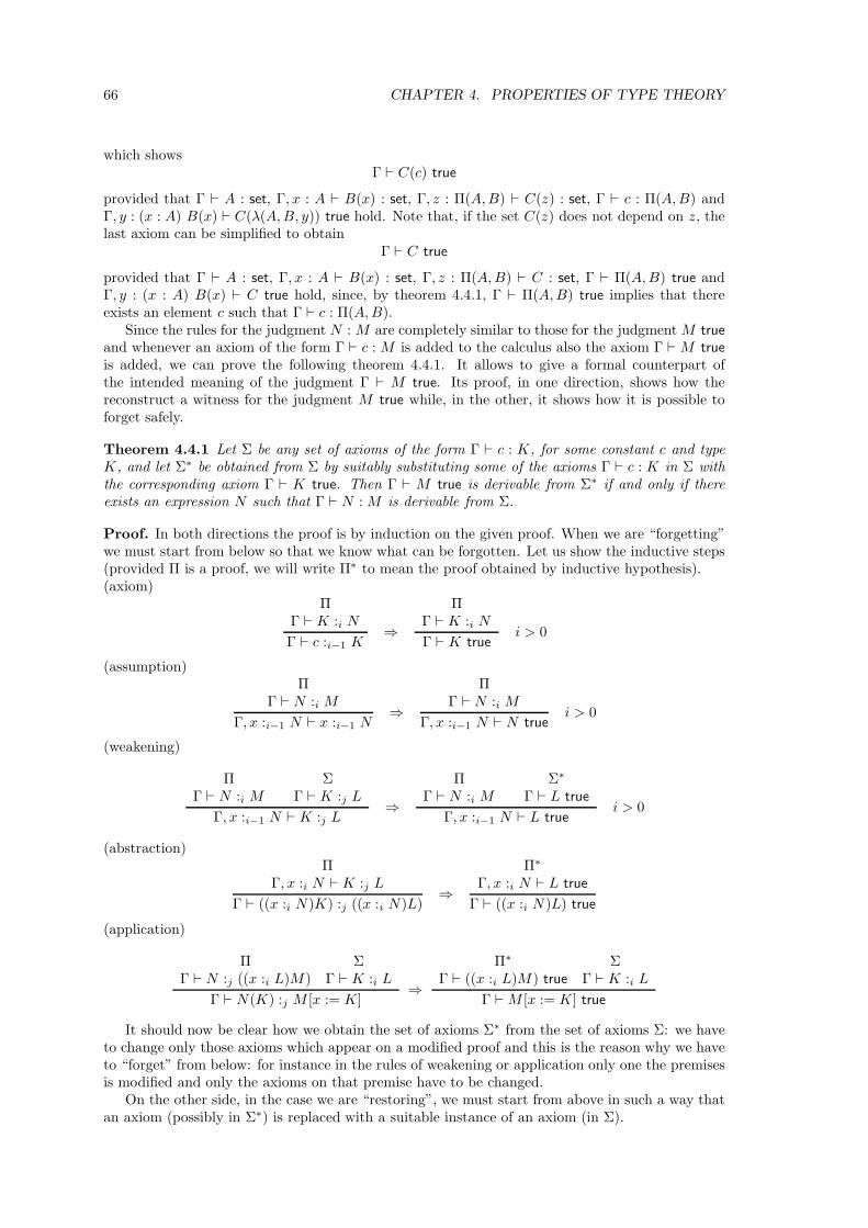
66 CHAPTER 4. PROPERTIES OF TYPE THEORY
which showsΓ ⊢ C(c) true
provided that Γ ⊢ A : set, Γ, x : A ⊢ B(x) : set, Γ, z : Π(A, B) ⊢ C(z) : set, Γ ⊢ c : Π(A, B) andΓ, y : (x : A) B(x) ⊢ C(λ(A, B, y)) true hold. Note that, if the set C(z) does not depend on z, thelast axiom can be simplified to obtain
Γ ⊢ C true
provided that Γ ⊢ A : set, Γ, x : A ⊢ B(x) : set, Γ, z : Π(A, B) ⊢ C : set, Γ ⊢ Π(A, B) true andΓ, y : (x : A) B(x) ⊢ C true hold, since, by theorem 4.4.1, Γ ⊢ Π(A, B) true implies that thereexists an element c such that Γ ⊢ c : Π(A, B).
Since the rules for the judgment N : M are completely similar to those for the judgment M true
and whenever an axiom of the form Γ ⊢ c : M is added to the calculus also the axiom Γ ⊢M true
is added, we can prove the following theorem 4.4.1. It allows to give a formal counterpart ofthe intended meaning of the judgment Γ ⊢ M true. Its proof, in one direction, shows how thereconstruct a witness for the judgment M true while, in the other, it shows how it is possible toforget safely.
Theorem 4.4.1 Let Σ be any set of axioms of the form Γ ⊢ c : K, for some constant c and typeK, and let Σ∗ be obtained from Σ by suitably substituting some of the axioms Γ ⊢ c : K in Σ withthe corresponding axiom Γ ⊢ K true. Then Γ ⊢ M true is derivable from Σ∗ if and only if thereexists an expression N such that Γ ⊢ N : M is derivable from Σ.
Proof. In both directions the proof is by induction on the given proof. When we are “forgetting”we must start from below so that we know what can be forgotten. Let us show the inductive steps(provided Π is a proof, we will write Π∗ to mean the proof obtained by inductive hypothesis).(axiom)
ΠΓ ⊢ K :i N
Γ ⊢ c :i−1 K⇒
ΠΓ ⊢ K :i N
Γ ⊢ K truei > 0
(assumption)Π
Γ ⊢ N :i M
Γ, x :i−1 N ⊢ x :i−1 N⇒
ΠΓ ⊢ N :i M
Γ, x :i−1 N ⊢ N truei > 0
(weakening)
ΠΓ ⊢ N :i M
ΣΓ ⊢ K :j L
Γ, x :i−1 N ⊢ K :j L⇒
ΠΓ ⊢ N :i M
Σ∗
Γ ⊢ L true
Γ, x :i−1 N ⊢ L truei > 0
(abstraction)Π
Γ, x :i N ⊢ K :j L
Γ ⊢ ((x :i N)K) :j ((x :i N)L)⇒
Π∗
Γ, x :i N ⊢ L true
Γ ⊢ ((x :i N)L) true
(application)
Π ΣΓ ⊢ N :j ((x :i L)M) Γ ⊢ K :i L
Γ ⊢ N(K) :j M [x := K]⇒
Π∗ ΣΓ ⊢ ((x :i L)M) true Γ ⊢ K :i L
Γ ⊢M [x := K] true
It should now be clear how we obtain the set of axioms Σ∗ from the set of axioms Σ: we haveto change only those axioms which appear on a modified proof and this is the reason why we haveto “forget” from below: for instance in the rules of weakening or application only one the premisesis modified and only the axioms on that premise have to be changed.
On the other side, in the case we are “restoring”, we must start from above in such a way thatan axiom (possibly in Σ∗) is replaced with a suitable instance of an axiom (in Σ).
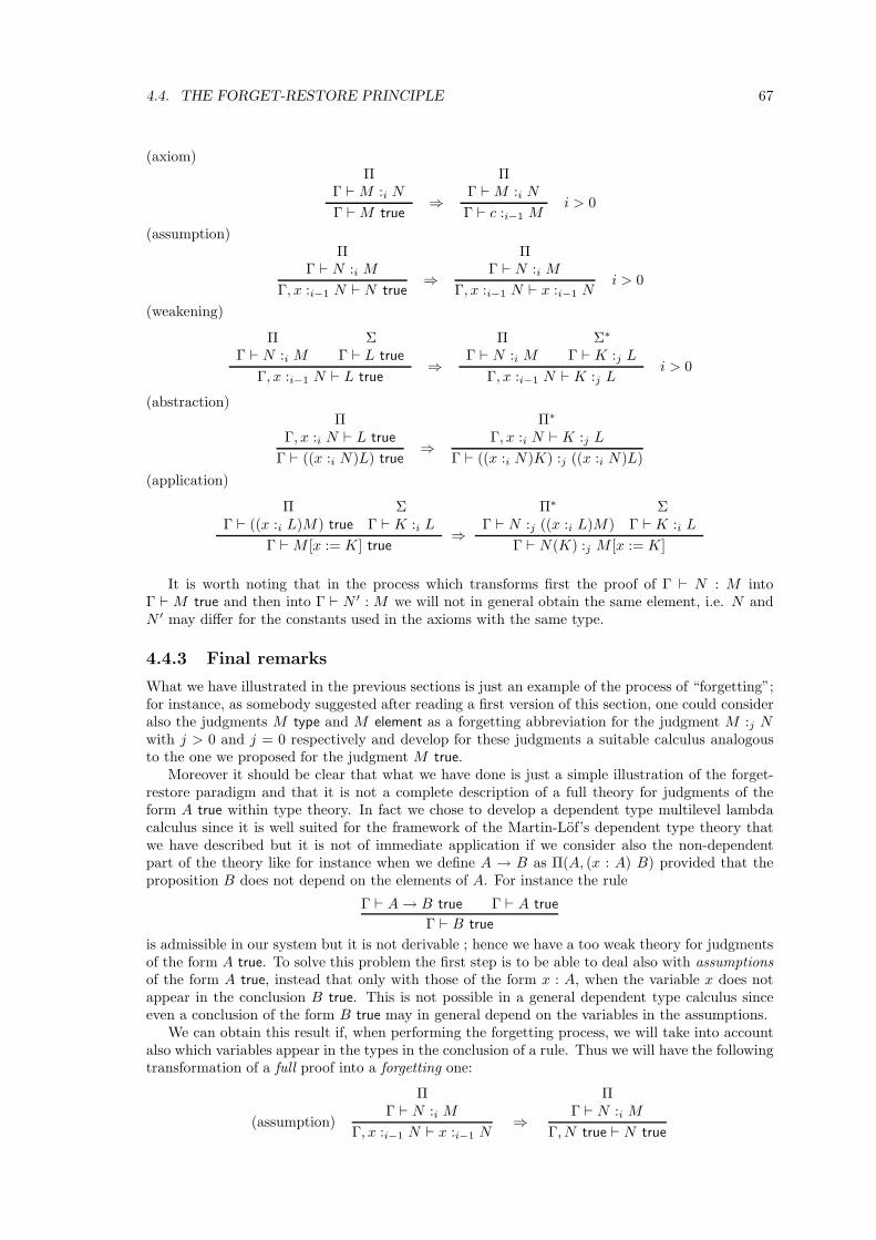
4.4. THE FORGET-RESTORE PRINCIPLE 67
(axiom)Π
Γ ⊢M :i N
Γ ⊢M true⇒
ΠΓ ⊢M :i N
Γ ⊢ c :i−1 Mi > 0
(assumption)Π
Γ ⊢ N :i M
Γ, x :i−1 N ⊢ N true⇒
ΠΓ ⊢ N :i M
Γ, x :i−1 N ⊢ x :i−1 Ni > 0
(weakening)
ΠΓ ⊢ N :i M
ΣΓ ⊢ L true
Γ, x :i−1 N ⊢ L true⇒
ΠΓ ⊢ N :i M
Σ∗
Γ ⊢ K :j L
Γ, x :i−1 N ⊢ K :j Li > 0
(abstraction)Π
Γ, x :i N ⊢ L true
Γ ⊢ ((x :i N)L) true⇒
Π∗
Γ, x :i N ⊢ K :j L
Γ ⊢ ((x :i N)K) :j ((x :i N)L)
(application)
Π ΣΓ ⊢ ((x :i L)M) true Γ ⊢ K :i L
Γ ⊢M [x := K] true⇒
Π∗ ΣΓ ⊢ N :j ((x :i L)M) Γ ⊢ K :i L
Γ ⊢ N(K) :j M [x := K]
It is worth noting that in the process which transforms first the proof of Γ ⊢ N : M intoΓ ⊢ M true and then into Γ ⊢ N ′ : M we will not in general obtain the same element, i.e. N andN ′ may differ for the constants used in the axioms with the same type.
4.4.3 Final remarks
What we have illustrated in the previous sections is just an example of the process of “forgetting”;for instance, as somebody suggested after reading a first version of this section, one could consideralso the judgments M type and M element as a forgetting abbreviation for the judgment M :j Nwith j > 0 and j = 0 respectively and develop for these judgments a suitable calculus analogousto the one we proposed for the judgment M true.
Moreover it should be clear that what we have done is just a simple illustration of the forget-restore paradigm and that it is not a complete description of a full theory for judgments of theform A true within type theory. In fact we chose to develop a dependent type multilevel lambdacalculus since it is well suited for the framework of the Martin-Lof’s dependent type theory thatwe have described but it is not of immediate application if we consider also the non-dependentpart of the theory like for instance when we define A → B as Π(A, (x : A) B) provided that theproposition B does not depend on the elements of A. For instance the rule
Γ ⊢ A→ B true Γ ⊢ A true
Γ ⊢ B true
is admissible in our system but it is not derivable ; hence we have a too weak theory for judgmentsof the form A true. To solve this problem the first step is to be able to deal also with assumptionsof the form A true, instead that only with those of the form x : A, when the variable x does notappear in the conclusion B true. This is not possible in a general dependent type calculus sinceeven a conclusion of the form B true may in general depend on the variables in the assumptions.
We can obtain this result if, when performing the forgetting process, we will take into accountalso which variables appear in the types in the conclusion of a rule. Thus we will have the followingtransformation of a full proof into a forgetting one:
(assumption)
ΠΓ ⊢ N :i M
Γ, x :i−1 N ⊢ x :i−1 N⇒
ΠΓ ⊢ N :i M
Γ, N true ⊢ N true
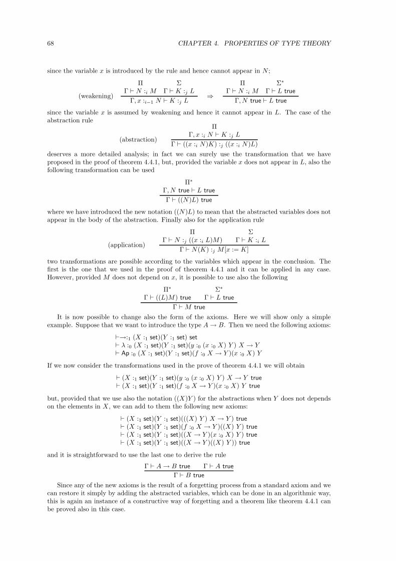
68 CHAPTER 4. PROPERTIES OF TYPE THEORY
since the variable x is introduced by the rule and hence cannot appear in N ;
(weakening)
Π ΣΓ ⊢ N :i M Γ ⊢ K :j L
Γ, x :i−1 N ⊢ K :j L⇒
Π Σ∗
Γ ⊢ N :i M Γ ⊢ L true
Γ, N true ⊢ L true
since the variable x is assumed by weakening and hence it cannot appear in L. The case of theabstraction rule
(abstraction)
ΠΓ, x :i N ⊢ K :j L
Γ ⊢ ((x :i N)K) :j ((x :i N)L)
deserves a more detailed analysis; in fact we can surely use the transformation that we haveproposed in the proof of theorem 4.4.1, but, provided the variable x does not appear in L, also thefollowing transformation can be used
Π∗
Γ, N true ⊢ L true
Γ ⊢ ((N)L) true
where we have introduced the new notation ((N)L) to mean that the abstracted variables does notappear in the body of the abstraction. Finally also for the application rule
(application)
ΠΓ ⊢ N :j ((x :i L)M)
ΣΓ ⊢ K :i L
Γ ⊢ N(K) :j M [x := K]
two transformations are possible according to the variables which appear in the conclusion. Thefirst is the one that we used in the proof of theorem 4.4.1 and it can be applied in any case.However, provided M does not depend on x, it is possible to use also the following
Π∗
Γ ⊢ ((L)M) true
Σ∗
Γ ⊢ L true
Γ ⊢M true
It is now possible to change also the form of the axioms. Here we will show only a simpleexample. Suppose that we want to introduce the type A→ B. Then we need the following axioms:
⊢→:1 (X :1 set)(Y :1 set) set
⊢ λ :0 (X :1 set)(Y :1 set)(y :0 (x :0 X) Y ) X → Y⊢ Ap :0 (X :1 set)(Y :1 set)(f :0 X → Y )(x :0 X) Y
If we now consider the transformations used in the prove of theorem 4.4.1 we will obtain
⊢ (X :1 set)(Y :1 set)(y :0 (x :0 X) Y ) X → Y true
⊢ (X :1 set)(Y :1 set)(f :0 X → Y )(x :0 X) Y true
but, provided that we use also the notation ((X)Y ) for the abstractions when Y does not dependson the elements in X , we can add to them the following new axioms:
⊢ (X :1 set)(Y :1 set)(((X) Y ) X → Y ) true
⊢ (X :1 set)(Y :1 set)(f :0 X → Y )((X) Y ) true
⊢ (X :1 set)(Y :1 set)((X → Y )(x :0 X) Y ) true
⊢ (X :1 set)(Y :1 set)((X → Y )((X) Y )) true
and it is straightforward to use the last one to derive the rule
Γ ⊢ A→ B true Γ ⊢ A true
Γ ⊢ B true
Since any of the new axioms is the result of a forgetting process from a standard axiom and wecan restore it simply by adding the abstracted variables, which can be done in an algorithmic way,this is again an instance of a constructive way of forgetting and a theorem like theorem 4.4.1 canbe proved also in this case.
Chapter 5
Set Theory
5.1 Summary
In this chapter we will show how a local set theory can be developed within Martin-Lof’s typetheory. In particular, we will show how to develop a predicative theory of subsets within typetheory. In fact, a few years’ experience in developing constructive topology in the framework oftype theory has taught us that a more liberal treatment of subsets is needed than what could beachieved by remaining literally inside type theory and its traditional notation. To be able to workfreely with subsets in the usual style of mathematics one must come to conceive them like any othermathematical object (which technically means for instance that the judgment that something is asubset can be taken as assumption) and have access to their usual apparatus (for instance, unionand intersection).
Many approaches were proposed for the development of a set theory within Martin-Lof’s typetheory or in such a way that they can be interpreted in Martin-Lof’s type theory (see for instance[NPS90], [Acz78], [Acz82], [Acz86], [Hof94], [Hof97] and [HS95]).
The main difference between our approach and these other ones stays in the fact that we donot require a subset to be a set while in general in the other approaches the aim is to apply theusual set-constructors of basic type theory to a wider notion of set, which includes sets obtained bycomprehension over a given set (see [NPS90], [Hof94], [Hof97] and [HS95]) or to define an axiomaticset theory whose axioms have a constructive interpretation (see [Acz78], [Acz82], [Acz86]); hencethe justification of the validity of the rules and axioms for sets must be given anew and a newjustification must be furnished each time the basic type theory or the basic axioms are modified.
In this chapter we will provide all the main definitions for a subset theory; in particular, wewill state the basic notion of subset U of a set S, that is we will identify U with a propositionalfunction over S and hence we will require that a subset is never a set; then we will introduce themembership relation between an element a of S and a subset U of S, which will turn out to holdif and only if the proposition U(a) is true. Then the full theory will be developed based on thesesimple ideas, that is the usual set-theoretic operations will be defined in terms of logical operations.Of course not all of the classical set theoretic axioms are satisfied in this approach. In particularit is not possible to validate the axioms which do not have a constructive explanation like, forinstance, the power-set construction.
5.2 Introduction
The present work originates from the need of subsets in the practical development of a constructiveapproach to topology (see [Sam87] and [Sam97] and references therein) and most of what wepresent here is the answer to problems actually encountered. The solution we arrived at is inspiredby a philosophical attitude, and this too has become clear along the way. Thus the aim of thisIntroduction is to explain such attitude and to make the resulting principles explicit, which mighthelp to understand better some of the technical choices.
69
70 CHAPTER 5. SET THEORY
5.2.1 Foreword
Beginning in 1970, Per Martin-Lof has developed an intuitionistic type theory (henceforth typetheory tout-court) as a constructive alternative to the usual foundation of mathematics based onclassical set theory. We assume the reader is aware at least of the main peculiarities of type theory,as formulated in [Mar84] or [NPS90]; here we recall some of them to be able to introduce our pointof view.
The form of type theory is that of a logical calculus, where inference rules to derive judgments areat the same time set theoretic constructions, because of the “propositions-as-sets”1 interpretation.The spirit of type theory - expressing our interpretation in a single sentence - is to adopt thosenotions and rules which keep total control of the amount of information contained in the differentforms of judgment. We now briefly justify this claim.
First of all, the judgment asserting the truth of a proposition A, which from an intuitionisticpoint of view means the existence of a verification of A, in type theory is replaced by the judgmenta ∈ A which explicitly exhibits a verification a of A. In fact, it would be unwise, for a constructivist,to throw away the specific verification of A which must be known to be able to assert the existenceof a verification!
The judgment that A is a set, which from an intuitionistic point of view means that there existsan inductive presentation of A, is treated in type theory in a quite similar way (even if in this caseno notation analogous to a ∈ A is used) since the judgment A set in type theory becomes explicitknowledge of the specific inductive presentation of A. In fact, the rules for primitive types and fortype constructors are so devised that whenever a judgment A set is proved, it means that one hasalso complete information on the rules which describe how canonical elements of A are formed.Such property, which might look like a peculiarity of type theory, is as a matter of fact necessaryin order to give a coherent constructive treatment of quantifiers. Consider for instance universalquantification, and take for granted that an intuitionistically meaningful explanation of universalquantification is possible only for domains with an inductive presentation, that is for what havebeen called sets above (by the way, this is the reason why the distinction between sets and typesis so basic in type theory, see [Mar84]). Then the pure knowledge that A is a set is sufficient tosay that universal quantification over A gives rise to propositions; however, it would be unwise toforget which specific rules generate A inductively, since, in general, a method verifying a universallyquantified proposition over A can be produced, by means of an elimination rule, only by directreference to the method by which A is generated.
Summing up, we see not only that type theory is inspired by the principle of control of infor-mation, but also that the same principle should be at the base of any coherent treatment of setsand propositions, if it has to be both intuitionistic and free of wastes.
Coming back to the formalism in which type theory is expressed, one can see that the principleof keeping control of information is revealed also at the level of syntax, since most inference rulesare formulated in a fully analytic style, i.e. everything which appears in the premises is presentsomehow also in the conclusion. A consequence is, for instance, that the derivation of a judgmenta ∈ A is so detailed that a is ipso facto a program which satisfies the requirements specified by A.This is why type theory is particularly interesting for computer science.
However, our experience in developing pieces of actual mathematics within type theory has ledus to believe that “orthodox” type theory is not suitable because its control of information is toostrict for this purpose. In fact, the fully analytic character of type theory becomes a burden whendealing with the synthetic methods of mathematics, which “forget” or take for granted most of thedetails. This, in our opinion, could be the reason why type theory has collected, up to now, moreinterest among logicians and computer scientists as a formal system than among mathematiciansas a foundational theory.
We claim that there is no intrinsic reason why it should remain so, and that actually it is only amatter of developing a stock of “utilities”, that is, of building up a toolbox which covers the territorybetween the basic formalism and mathematical practice; after all, this happened for classical settheory ZF long ago. In other words, the situation seems analogous to that of a programmer who,maybe because of a particular skill with the machine language, has not yet developed those higher
1Called “formulae-as-types” in [How80]. A little warning on terminology is necessary here: we use “set” exactlyas in [Mar84], while “category” of [Mar84] is here replaced with “type”as in [NPS90].
5.2. INTRODUCTION 71
level constructs and languages which allow him to save time and mental energy, and thus in theend are necessary to free the mind for a common human, i.e. abstract, comprehension.
So our general aim is to build up those tools, that is definitions and rules, which “forget” someinformation, and thus allow a higher level of abstraction, which can make type theory more handyand suitable to work out (intuitionistic) mathematics basing on mathematical intuition, as it hasbeen and should be.
5.2.2 Contents
Here, completing the work first announced in [SV93], we make a substantial step in the directionstated above and show how to develop a predicative theory of subsets within type theory.2 A fewyears’ experience in developing topology in the framework of type theory has taught us that a moreliberal treatment of subsets is needed than what could be achieved by remaining literally insidetype theory and its traditional notation. In fact, to be able to work freely with subsets in theusual style of mathematics one must come to conceive them like any other mathematical object(which technically means for instance that the judgment that something is a subset can be takenas assumption) and have access to their usual apparatus (for instance, union and intersection).
Subset theory as developed in [NPS90] does not meet the above demands since, being motivatedby programming, its aim is different. We could say, in fact, that the aim of [NPS90] is to apply theusual set-constructors of basic type theory to a wider notion of set, which includes sets obtained bycomprehension over a given set; the price they have to pay is that the justification of the validityof rules for sets must be given anew. The same price must be paid whenever the basic type theoryis modified; another example is the recent [Tur97].
The way out is to adopt the simple idea that it is not compulsory that a subset be a set.Then one is free to define subsets in a natural way as propositional functions (as first suggestedin [Mar84], page 64, and explicitly adopted in [Sam87]), and then to introduce the new notion ofelement of a subset, in terms of which also the other standard notions, like inclusion and extensionalequality, arbitrary unions and intersections, singletons and finite subsets, quantifiers and functionsdefined on subsets can be defined. The resulting subset theory is a sort of type-less set theorylocalized to a set and we have experienced that it is sufficient for instance for the development oftopology. We prove that all of this can be done in type theory without losing control, that is by“forgetting” only information which can be restored at will. This is reduced to the single fact that,for any set A, the judgment A true holds if and only if there exists a such that a ∈ A, and it canbe proved once and for all, see [Val98]; this is the price we have to pay to justify our approach.
Since for all notions related to subsets we adopt essentially the standard notation, the result isthat at first sight a page of mathematics written using subset theory looks like a page of standardmathematical writing, and one might easily overlook or forget the underlying substantial novelty,namely that everything is directly formalized in type theory. Far from being a drawback, this isin a sense our main intention, since it would show that one can develop an intuition free from theunderlying formalism.
5.2.3 Philosophical motivations
The attitude illustrated so far in this introduction can be seen as the specific outcome of a moregeneral philosophical position (see [Sam91]) when applied to type theory, and the results we provecan be seen as fragments of a general program (see [PV93]) not necessarily bound to type theory.Here we describe briefly both the philosophical position and the general program in the form ofsome principles, just enough to be able to state the connection with the problem of foundations.
To build up an abstract concept from a raw flow of data, one must disregard inessential details;in other words, to simplify the complexity of concrete reality one must idealize over it, and thisis obtained by “forgetting” some information. To forget information is the same as to destroysomething, in particular if there is no possibility of restoring that information, like when themagnetic memory of a disk is erased. So to abstract involves a certain amount of destruction; ourprinciple is that an abstraction is constructive, that is, a reliable tool in getting knowledge which
2The second step should be on quotient sets, or abstract data types, or setoids.
72 CHAPTER 5. SET THEORY
is faithful to reality, not when information is kept as much as possible, but when it is “forgotten”in such a way that it can be restored at will in any moment. This after all is the test to show thatan abstraction does not lead astray from reality, that is, that it preserves truth.
It is clear that the first step, and often the only one, to be able to restore what has been“forgotten” is to know, to be aware of, what has been forgotten, and to keep control of it. Sothe second principle is that constructivism does not consist of a a priori self-limitation to fullinformation, which would tie constructivism with reluctance to abstraction (as was the case aroundthe twenties when finitism and intuitionism were somehow identified), but rather in the awarenessof the destruction which has been operated to build up a certain abstract concept.
When it comes to mathematical terms, awareness of what has been destroyed or forgotten cansometimes be put in objective terms, and then it takes the form of a method by which the previousstate can be restored. If T ′ is a theory obtained from a more basic theory T by adding some moreabstract constructs and their rules, then a method must be supplied which allows us to transformwhatever proof in T ′ into a proof within T with the same computational content. This allows us to“forget safely”, since it guarantees that faithfulness to the more concrete level of T is not lost bythe more abstract concepts of T ′.
This, we believe, is the only reasonable way for a constructivist to extract a philosophical andmathematical value out of Hilbert’s program. To obtain a foundation which justifies itself, inHilbert’s view it is necessary to rely on a part of mathematics, called real mathematics, which hasto be safe beyond any doubt and without any proof. In Hilbert’s conception this is identified withfinitistic mathematics, that is manipulation of concrete objects; here instead real mathematics isidentified with type theory, which is of course far richer than finitistic mathematics but still servesthe purpose. In fact, on the one hand the contextual explanation of judgments and rules and on theother hand its interpretation as a programming language (the modern “manipulation of concreteobjects”) indeed make it reliable beyond doubt and without any proof.
Hilbert was right, of course, in saying that mathematics cannot be restricted to real mathe-matics; in fact, even the most radical constructivist certainly uses more abstract notions or ideas,even if they do not appear in his communications. But which abstract notions can be accepted?We propose an answer here. It is well known that Hilbert’s view puts no limitation, as long asthe consistency of the formalism in which ideal mathematics is expressed is proven within realmathematics. This cannot be accepted by a constructivist, since a consistency proof is not enoughto restore, once and for all, the constructive meaning, i.e. faithfulness to the concrete reality ofcomputations. After all, even classical logic is consistent, and with a finitistic proof! So the pro-gram is to analyze, case by case, how a certain abstract notion is linked with real mathematics;when it is clear which concrete aspects are forgotten and how they can be restored by a suitablemethod, then that abstract notion can be used freely and safely. In this chapter we show howthis is possible for the theory of subsets, and thus we accomplish a fragment of the constructiveversion of Hilbert’s program, which we have called the Camerino program from the place wherewe spoke about it for the first time (see [PV93]). The aim is, paradoxically, to save the intuitionof an intuitionist from the rigidity of formal systems by supplying safe bridges between intuitionand computation.
5.3 Reconstructing subset theory
5.3.1 The notion of subset
In classical mathematics a subset U of a set S is usually defined to be a set such that if a ∈ Uthen a ∈ S. Importing in type theory this definition as it stands, however, would give a notionof subset not general enough to include all examples of what is undoubtedly to be considered asubset. In fact, if S is a set and U : (x : S) prop is a propositional function3 over S, then wesurely want the collection of elements of S satisfying U , usually written x ∈ S| U(x), to be asubset of S. In ZF, x ∈ S| U(x) would be a set, by the separation principle; in type theory,however, no form of the separation principle is justified, since in general there are no rules tellinghow the canonical elements of the collection x ∈ S| U(x) are formed. In fact, a is an element of
3Which means that U applied to x, for x ∈ S, is a proposition, written U(x) prop [x : S].
5.3. RECONSTRUCTING SUBSET THEORY 73
x ∈ S| U(x) if a ∈ S and U(a) is true, that is, if there exists b such that b ∈ U(a), but this formof judgment is not one of the four forms of judgments considered in type theory and hence there isno canonical way to reach the conclusion that such b exists. For example, if U(x) is the property“the Turing machine with index x does not stop on input x”, then there are no effective rules togenerate x ∈ N| U(x). Thus, the conclusion is that we want x ∈ S| U(x) to be a subset of Sfor any property U , but also that it does not need to be a set.
A second observation is that in ordinary mathematics, operations like union and intersectionare freely defined on the class of all sets, while at the opposite extreme in type theory there is nooperation of union or intersection in the ordinary sense available on sets. In fact, the result of anyoperation of set-formation gives rise to a set whose elements are specific of the constructed set,and thus, for instance, we could not have a common statement like a ∈ S ∩ T iff a ∈ S and a ∈ T ,because if ∩ were a set-constructor then S∩T would be a set different from S and T , and hence itselements could not be in common with S and T . As we will soon see, however, such set-theoreticoperations can easily be defined on subsets of a set, as soon as we do not require a subset to be aset. We are thus led to take the step of relaxing the requirement that a subset be a set. Thereforea subset will not have canonical elements, nor rules of elimination or of equality.
Two ways of defining subsets are traditionally available which do not require a subset to be aset. The first is that a subset of S is given by a property U(x) with x ranging over S; while in aclassical perspective it can be conceived that there are many more subsets than properties, froma constructive point of view there is no sense in assuming the existence of a subset unless we canspecify it, namely by a property. Thus the conclusion would be that a subset U of S is nothingbut a propositional function U over S.
The second conception of subset of S, namely as a function f : S → 0, 1 usually calledcharacteristic function, brings in the end to the same conclusion, as we now see. Classically, anyfunction f : S → 0, 1 gives rise to a property over S, namely the property f(x) = 1, and, givena property U(x) over S, the associated function is
fU (x) =
1 if U(x) true
0 otherwise
If we transfer this as it stands into type theory, we obtain a notion of subset which is too narrow. Infact, due to the different notion of function, the above argument, when properly translated in typetheory, gives a bijective correspondence between functions S → 0, 1 and decidable propositionalfunctions over S (for a detailed proof, see for instance section 4.2 or [Val96]).
However, in the classical conception the above definition of fU can be seen just as a differentway of denoting the propositional function U itself. In fact, classically a proposition is just a way todenote a truth value (see [Fre1892]), so 0, 1 can be identified with the set of values of propositions.Under this reading, the intuitionistic analogue of a characteristic function is a function from S intothe type of intuitionistic propositions, i.e. a propositional function over S.
So both traditional approaches lead to the same intuitionistic version. We thus put:
Definition 5.3.1 (Definition of subset) For any set S, a propositional function U with argu-ment ranging in S is called a subset of S, and is written U ⊆ S.
Thus we can think that a subset U of S is obtained by abstracting the variable x in thejudgment U(x) prop [x : S], i.e. U ≡ (x : S) U(x). The same effect is usually expressed with thebrace notation to form a subset x ∈ S| U(x), which does not depend on x any longer. So weput:
x ∈ S| U(x) ≡ U ≡ (x : S) U(x)
However, it must be said explicitly that, even if we adopt the common expression x ∈ S| U(x)for a subset, it remains true that a subset is a propositional function and hence a subset can nevercoincide with a set, for the simple reason that propositional functions are of a type different fromthat of sets.
By similar reasons, the notion of subset is not automatically accompanied by that of elementof a subset: writing a ∈ x ∈ S| U(x), for a ∈ S, does never give a well formed expression and,on the other hand, writing u : U would mean (x : S) u(x) : (x : S) U(x), which corresponds to the
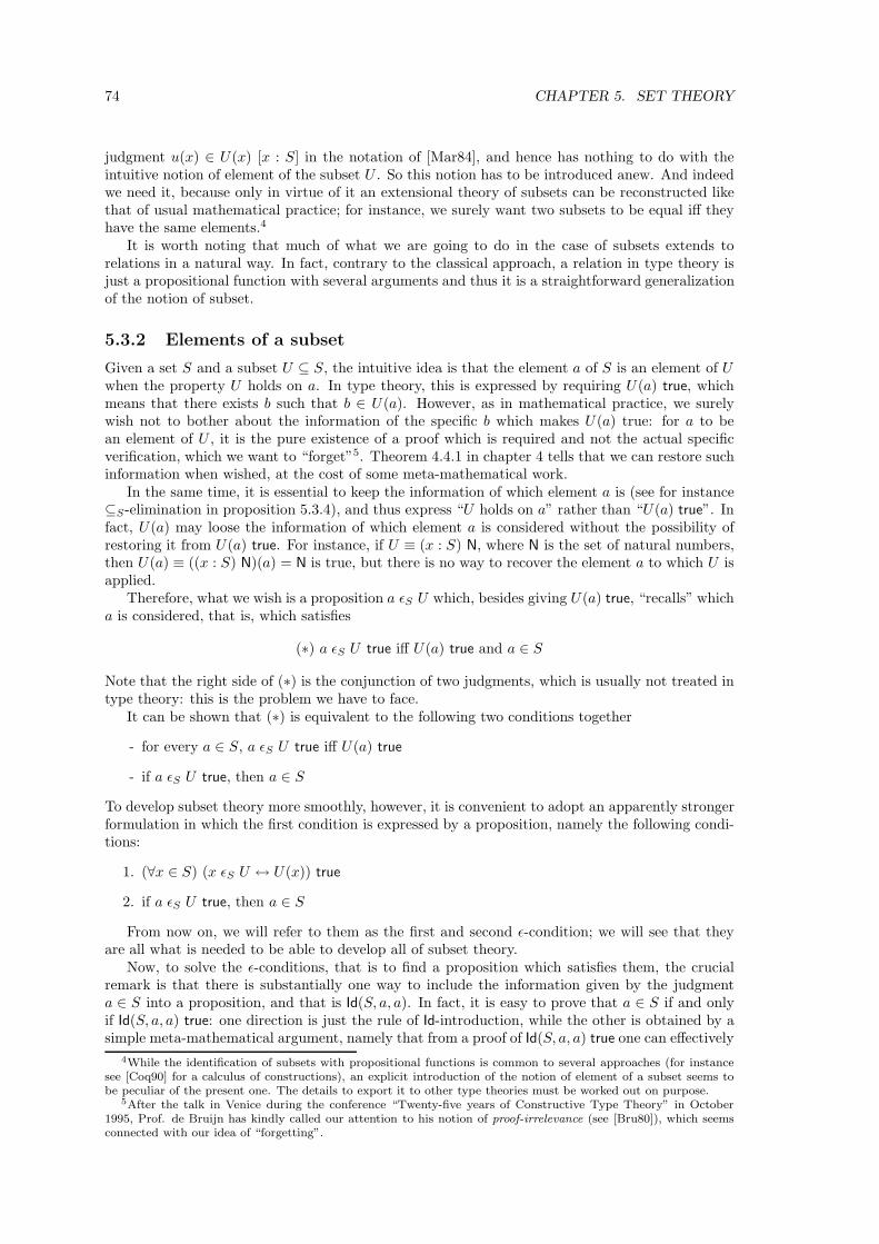
74 CHAPTER 5. SET THEORY
judgment u(x) ∈ U(x) [x : S] in the notation of [Mar84], and hence has nothing to do with theintuitive notion of element of the subset U . So this notion has to be introduced anew. And indeedwe need it, because only in virtue of it an extensional theory of subsets can be reconstructed likethat of usual mathematical practice; for instance, we surely want two subsets to be equal iff theyhave the same elements.4
It is worth noting that much of what we are going to do in the case of subsets extends torelations in a natural way. In fact, contrary to the classical approach, a relation in type theory isjust a propositional function with several arguments and thus it is a straightforward generalizationof the notion of subset.
5.3.2 Elements of a subset
Given a set S and a subset U ⊆ S, the intuitive idea is that the element a of S is an element of Uwhen the property U holds on a. In type theory, this is expressed by requiring U(a) true, whichmeans that there exists b such that b ∈ U(a). However, as in mathematical practice, we surelywish not to bother about the information of the specific b which makes U(a) true: for a to bean element of U , it is the pure existence of a proof which is required and not the actual specificverification, which we want to “forget”5. Theorem 4.4.1 in chapter 4 tells that we can restore suchinformation when wished, at the cost of some meta-mathematical work.
In the same time, it is essential to keep the information of which element a is (see for instance⊆S-elimination in proposition 5.3.4), and thus express “U holds on a” rather than “U(a) true”. Infact, U(a) may loose the information of which element a is considered without the possibility ofrestoring it from U(a) true. For instance, if U ≡ (x : S) N, where N is the set of natural numbers,then U(a) ≡ ((x : S) N)(a) = N is true, but there is no way to recover the element a to which U isapplied.
Therefore, what we wish is a proposition a ǫS U which, besides giving U(a) true, “recalls” whicha is considered, that is, which satisfies
(∗) a ǫS U true iff U(a) true and a ∈ S
Note that the right side of (∗) is the conjunction of two judgments, which is usually not treated intype theory: this is the problem we have to face.
It can be shown that (∗) is equivalent to the following two conditions together
- for every a ∈ S, a ǫS U true iff U(a) true
- if a ǫS U true, then a ∈ S
To develop subset theory more smoothly, however, it is convenient to adopt an apparently strongerformulation in which the first condition is expressed by a proposition, namely the following condi-tions:
1. (∀x ∈ S) (x ǫS U ↔ U(x)) true
2. if a ǫS U true, then a ∈ S
From now on, we will refer to them as the first and second ǫ-condition; we will see that theyare all what is needed to be able to develop all of subset theory.
Now, to solve the ǫ-conditions, that is to find a proposition which satisfies them, the crucialremark is that there is substantially one way to include the information given by the judgmenta ∈ S into a proposition, and that is Id(S, a, a). In fact, it is easy to prove that a ∈ S if and onlyif Id(S, a, a) true: one direction is just the rule of Id-introduction, while the other is obtained by asimple meta-mathematical argument, namely that from a proof of Id(S, a, a) true one can effectively
4While the identification of subsets with propositional functions is common to several approaches (for instancesee [Coq90] for a calculus of constructions), an explicit introduction of the notion of element of a subset seems tobe peculiar of the present one. The details to export it to other type theories must be worked out on purpose.
5After the talk in Venice during the conference “Twenty-five years of Constructive Type Theory” in October1995, Prof. de Bruijn has kindly called our attention to his notion of proof-irrelevance (see [Bru80]), which seemsconnected with our idea of “forgetting”.
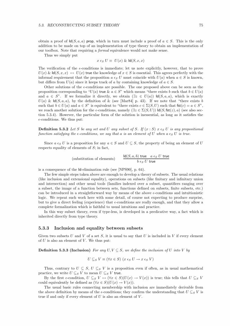
5.3. RECONSTRUCTING SUBSET THEORY 75
obtain a proof of Id(S, a, a) prop, which in turn must include a proof of a ∈ S. This is the onlyaddition to be made on top of an implementation of type theory to obtain an implementation ofour toolbox. Note that requiring a formal equivalence would not make sense.
Thus we simply put
x ǫS U ≡ U(x) & Id(S, x, x)
The verification of the ǫ-conditions is immediate; let us note explicitly, however, that to proveU(x) & Id(S, x, x) ↔ U(x) true the knowledge of x ∈ S is essential. This agrees perfectly with theinformal requirement that the proposition a ǫS U must coincide with U(a) when a ∈ S is known,but differs from U(a) since it keeps track of a by containing knowledge of a ∈ S.
Other solutions of the ǫ-conditions are possible. The one proposed above can be seen as theproposition corresponding to “U(a) true & a ∈ S” which means “there exists b such that b ∈ U(a)and a ∈ S”. If we formalize it directly, we obtain (∃z ∈ U(a)) Id(S, a, a), which is exactlyU(a) & Id(S, a, a), by the definition of & (see [Mar84] p. 43). If we note that “there exists bsuch that b ∈ U(a) and a ∈ S” is equivalent to “there exists c ∈ Σ(S, U) such that fst(c) = a ∈ S”,we reach another solution for the ǫ-conditions, namely (∃z ∈ Σ(S, U)) Id(S, fst(z), a) (see also sec-tion 5.3.4). However, the particular form of the solution is inessential, as long as it satisfies theǫ-conditions. We thus put:
Definition 5.3.2 Let S be any set and U any subset of S. If (x : S) x ǫS U is any propositionalfunction satisfying the ǫ-conditions, we say that a is an element of U when a ǫS U is true.
Since a ǫS U is a proposition for any a ∈ S and U ⊆ S, the property of being an element of Urespects equality of elements of S; in fact,
(substitution of elements)Id(S, a, b) true a ǫS U true
b ǫS U true
is a consequence of the Id-elimination rule (see [NPS90], p. 64).
The few simple steps taken above are enough to develop a theory of subsets. The usual relations(like inclusion and extensional equality), operations on subsets (like finitary and infinitary unionand intersection) and other usual tools (families indexed over a subset, quantifiers ranging overa subset, the image of a function between sets, functions defined on subsets, finite subsets, etc.)can be introduced in a straightforward way by means of the above ǫ-conditions and intuitionisticlogic. We repeat such work here with some detail, of course not expecting to produce surprise,but to give a direct feeling (experience) that ǫ-conditions are really enough, and that they allow acomplete formalization which is faithful to usual intuitions and practice.
In this way subset theory, even if type-less, is developed in a predicative way, a fact which isinherited directly from type theory.
5.3.3 Inclusion and equality between subsets
Given two subsets U and V of a set S, it is usual to say that U is included in V if every elementof U is also an element of V . We thus put:
Definition 5.3.3 (Inclusion) For any U, V ⊆ S, we define the inclusion of U into V by
U ⊆S V ≡ (∀x ∈ S) (x ǫS U → x ǫS V )
Thus, contrary to U ⊆ S, U ⊆S V is a proposition even if often, as in usual mathematicalpractice, we write U ⊆S V to mean U ⊆S V true.
By the first ǫ-condition, U ⊆S V ↔ (∀x ∈ S)(U(x) → V (x)) is true; this tells that U ⊆S Vcould equivalently be defined as (∀x ∈ S)(U(x)→ V (x)).
The usual basic rules connecting membership with inclusion are immediately derivable fromthe above definition by means of the ǫ-conditions; they confirm the understanding that U ⊆S V istrue if and only if every element of U is also an element of V .
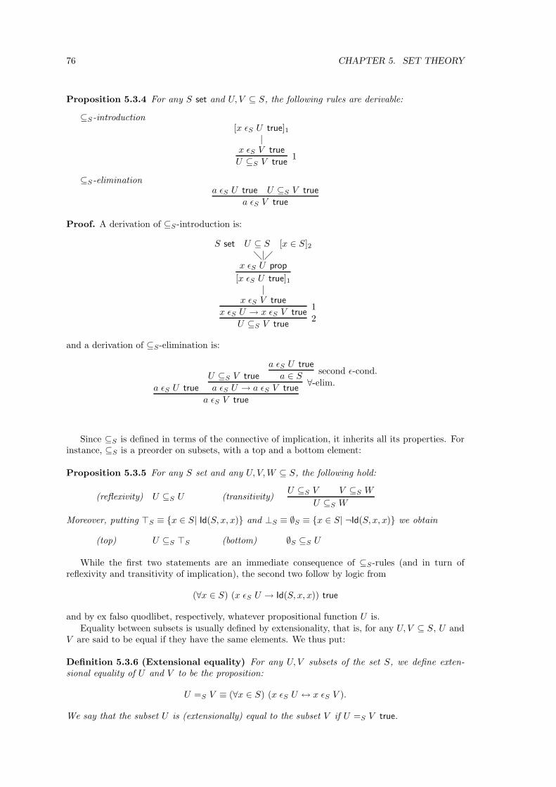
76 CHAPTER 5. SET THEORY
Proposition 5.3.4 For any S set and U, V ⊆ S, the following rules are derivable:
⊆S-introduction[x ǫS U true]1
|x ǫS V true
U ⊆S V true1
⊆S-eliminationa ǫS U true U ⊆S V true
a ǫS V true
Proof. A derivation of ⊆S-introduction is:
S set U ⊆ S [x ∈ S]2|
x ǫS U prop
[x ǫS U true]1|
x ǫS V true
x ǫS U → x ǫS V true1
U ⊆S V true2
and a derivation of ⊆S-elimination is:
a ǫS U true
U ⊆S V true
a ǫS U true
a ∈ Ssecond ǫ-cond.
a ǫS U → a ǫS V true∀-elim.
a ǫS V true
Since ⊆S is defined in terms of the connective of implication, it inherits all its properties. Forinstance, ⊆S is a preorder on subsets, with a top and a bottom element:
Proposition 5.3.5 For any S set and any U, V, W ⊆ S, the following hold:
(reflexivity) U ⊆S U (transitivity)U ⊆S V V ⊆S W
U ⊆S W
Moreover, putting ⊤S ≡ x ∈ S| Id(S, x, x) and ⊥S ≡ ∅S ≡ x ∈ S| ¬Id(S, x, x) we obtain
(top) U ⊆S ⊤S (bottom) ∅S ⊆S U
While the first two statements are an immediate consequence of ⊆S-rules (and in turn ofreflexivity and transitivity of implication), the second two follow by logic from
(∀x ∈ S) (x ǫS U → Id(S, x, x)) true
and by ex falso quodlibet, respectively, whatever propositional function U is.
Equality between subsets is usually defined by extensionality, that is, for any U, V ⊆ S, U andV are said to be equal if they have the same elements. We thus put:
Definition 5.3.6 (Extensional equality) For any U, V subsets of the set S, we define exten-sional equality of U and V to be the proposition:
U =S V ≡ (∀x ∈ S) (x ǫS U ↔ x ǫS V ).
We say that the subset U is (extensionally) equal to the subset V if U =S V true.
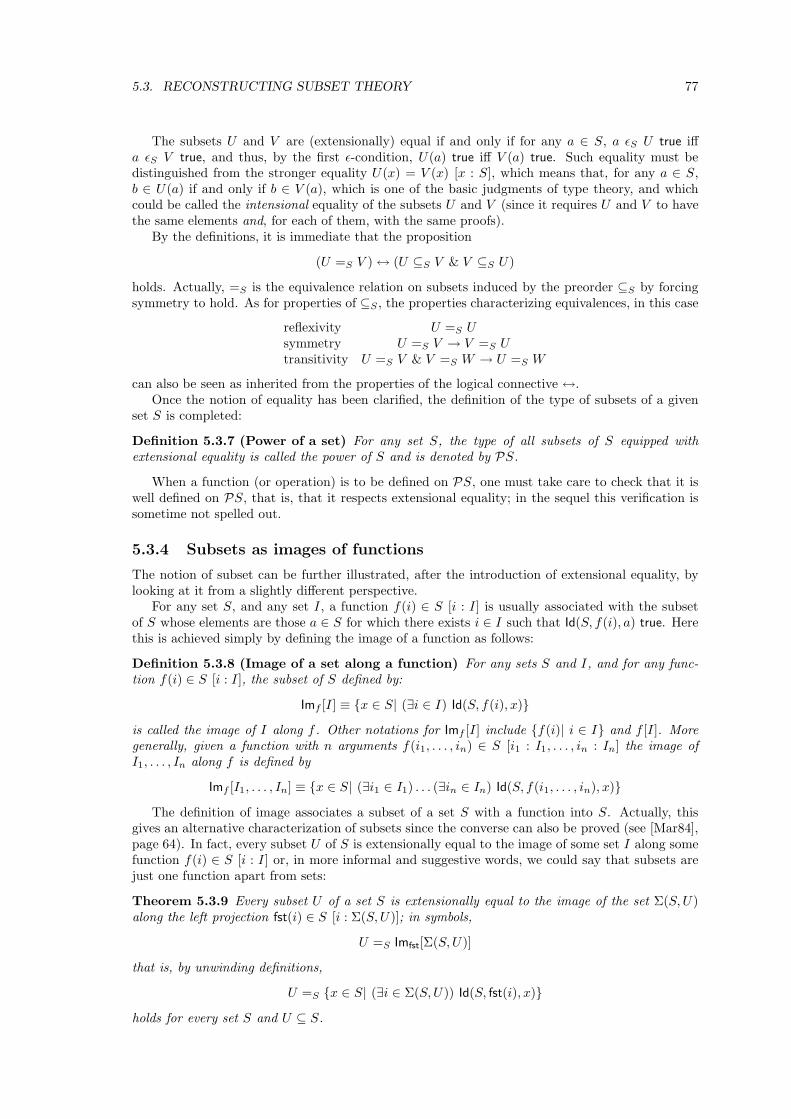
5.3. RECONSTRUCTING SUBSET THEORY 77
The subsets U and V are (extensionally) equal if and only if for any a ∈ S, a ǫS U true iffa ǫS V true, and thus, by the first ǫ-condition, U(a) true iff V (a) true. Such equality must bedistinguished from the stronger equality U(x) = V (x) [x : S], which means that, for any a ∈ S,b ∈ U(a) if and only if b ∈ V (a), which is one of the basic judgments of type theory, and whichcould be called the intensional equality of the subsets U and V (since it requires U and V to havethe same elements and, for each of them, with the same proofs).
By the definitions, it is immediate that the proposition
(U =S V )↔ (U ⊆S V & V ⊆S U)
holds. Actually, =S is the equivalence relation on subsets induced by the preorder ⊆S by forcingsymmetry to hold. As for properties of ⊆S , the properties characterizing equivalences, in this case
reflexivity U =S Usymmetry U =S V → V =S Utransitivity U =S V & V =S W → U =S W
can also be seen as inherited from the properties of the logical connective ↔.Once the notion of equality has been clarified, the definition of the type of subsets of a given
set S is completed:
Definition 5.3.7 (Power of a set) For any set S, the type of all subsets of S equipped withextensional equality is called the power of S and is denoted by PS.
When a function (or operation) is to be defined on PS, one must take care to check that it iswell defined on PS, that is, that it respects extensional equality; in the sequel this verification issometime not spelled out.
5.3.4 Subsets as images of functions
The notion of subset can be further illustrated, after the introduction of extensional equality, bylooking at it from a slightly different perspective.
For any set S, and any set I, a function f(i) ∈ S [i : I] is usually associated with the subsetof S whose elements are those a ∈ S for which there exists i ∈ I such that Id(S, f(i), a) true. Herethis is achieved simply by defining the image of a function as follows:
Definition 5.3.8 (Image of a set along a function) For any sets S and I, and for any func-tion f(i) ∈ S [i : I], the subset of S defined by:
Imf [I] ≡ x ∈ S| (∃i ∈ I) Id(S, f(i), x)
is called the image of I along f . Other notations for Imf [I] include f(i)| i ∈ I and f [I]. Moregenerally, given a function with n arguments f(i1, . . . , in) ∈ S [i1 : I1, . . . , in : In] the image ofI1, . . . , In along f is defined by
Imf [I1, . . . , In] ≡ x ∈ S| (∃i1 ∈ I1) . . . (∃in ∈ In) Id(S, f(i1, . . . , in), x)
The definition of image associates a subset of a set S with a function into S. Actually, thisgives an alternative characterization of subsets since the converse can also be proved (see [Mar84],page 64). In fact, every subset U of S is extensionally equal to the image of some set I along somefunction f(i) ∈ S [i : I] or, in more informal and suggestive words, we could say that subsets arejust one function apart from sets:
Theorem 5.3.9 Every subset U of a set S is extensionally equal to the image of the set Σ(S, U)along the left projection fst(i) ∈ S [i : Σ(S, U)]; in symbols,
U =S Imfst[Σ(S, U)]
that is, by unwinding definitions,
U =S x ∈ S| (∃i ∈ Σ(S, U)) Id(S, fst(i), x)
holds for every set S and U ⊆ S.
78 CHAPTER 5. SET THEORY
Proof. By the definitions and the ǫ-conditions, the claim U =S fst[Σ(S, U)] becomes
(∀x ∈ S) (U(x)↔ (∃y ∈ Σ(S, U)) Id(S, fst(y), x))
To prove it, assume that a is an arbitrary element of S, and that z ∈ U(a). Then 〈a, z〉 ∈ Σ(S, U),thus fst(〈a, z〉) = a ∈ S, hence r(a) ∈ Id(S, fst(〈a, z〉), a), and therefore
〈〈a, z〉, r(a)〉 ∈ (∃y ∈ Σ(S, U)) Id(S, fst(y), a)
This proves that λz.〈〈a, z〉, r(a)〉 is the term making U(a)→ (∃y ∈ Σ(S, U)) Id(S, fst(y), a) true.To prove the converse, assume z ∈ (∃y ∈ Σ(S, U)) Id(S, fst(y), a). Then fst(z) ∈ Σ(S, U) and
hence snd(fst(z)) ∈ U(fst(fst(z))) which, together with the fact that snd(z) ∈ Id(S, fst(fst(z)), a),gives subst(snd(fst(z)), snd(z)) ∈ U(a), as wished (see [NPS90], p. 64).
The theorem above gives further evidence to the fact that the notion of being an element of asubset is the result of disregarding some information. Given a function f(i) : S [i : I], the subsetImf [I] can be seen as the result of a process with two different abstraction steps. First, we realizethat to know that a is an element in Imf [I] we can abstract on the particular argument i such thatId(S, f(i), a) true and prove only c ∈ (∃i : I) Id(S, f(i), a) for some c. Note however that, due tothe constructive meaning of existential quantification in type theory, a specific element i ∈ I suchthat Id(S, f(i), a) true can immediately be obtained from c. So, the second step, where we reallyforget some information, is to say that a is in Imf (I) if and only if (∃i : I) Id(S, f(i), a) true.
Now let us consider the case of the function fst(z) ∈ S [z : Σ(S, U)], for some subset U ⊆ S.Then the above considerations bring to the conclusion that a is in Imfst[Σ(S, U)] if and only if(∃z : Σ(S, U)) Id(S, fst(z), a) true. By the theorem above, a ǫS U true is equivalent to a isin Imfst[Σ(S, U)], and hence also to (∃z : Σ(S, U)) Id(S, fst(z), a) true. It is then interesting toobserve that to pass from a given verification of (∃z : Σ(S, U)) Id(S, fst(z), a) to the judgment(∃z : Σ(S, U)) Id(S, fst(z), a) true means to forget the verification making U(a) true without for-getting a, since a appears explicitly in the proposition itself. To supply all the details we left outamounts to find a proof of (∃z : Σ(S, U)) Id(S, fst(z), a) ↔ U(a) & Id(S, a, a) true..
It is interesting to note that, since U(a) & Id(S, a, a) is the “canonical” solution of the ǫ-conditions, the above equivalence gives an alternative, and more formal, proof of the fact that alsothe proposition (∃z : Σ(S, U)) Id(S, fst(z), a) is a solution of the ǫ-conditions, as we already statedin section 5.3.2.
5.3.5 Singletons and finite subsets
Every element a of a set S is equal to any element b of the same set S making the propositionalfunction (x : S) Id(S, x, a) true at b; such triviality means that for any a ∈ S we can intuitivelyform the singleton a by putting
a ≡ x ∈ S| Id(S, x, a)
And then the idea is that a finite subset is the union of a finite number of singletons; so ifa0, . . . , an−1 ∈ S, for some natural number n, we put
a0, . . . , an−1 ≡ a0 ∪ a1 ∪ . . . ∪ an−1≡ x ∈ S| Id(S, x, a0) ∨ . . . ∨ Id(S, x, an−1)
But what does it mean, more precisely, to give a0, . . . , an−1 ∈ S? It means that a is a functionfrom N(n), a set with n elements, into S, and a0, . . . , an−1 are its values.
It is easy to define a family of sets N(n) set [n : N] such that N(0) has no elements and, forn > 0, the elements of N(n) are 0n, . . . , (n − 1)n. Then a singleton is the image of a functiona : N(1) → S, and a finite subset of S with n elements is the image of a function a : N(n) → S.We thus put:
Definition 5.3.10 (Singletons and finite subsets) For every set S, a subset U of S is said tobe finite if U is extensionally equal to the image of some function a ∈ N(n)→ S, for some n ∈ N
and in particular it is called a singleton if n = 1; more formally U is finite if
(∃z ∈ Σ(N, (n) N(n)→ S)) (U =S Imsnd(z)[N(fst(z))]) true
5.3. RECONSTRUCTING SUBSET THEORY 79
In particular, the empty subset of S is also finite, being equal to the image of a function fromN(0) into S.
Given the above definition, the assertion “U is finite” is just a proposition with parameter U .This allows for instance to express rigorously in type theory a statement of the form “there existsa finite subset U0 of U such that . . . U0 . . .” by
(∃z ∈ Σ(N, (n) N(n)→ S)) Imsnd(z)[N(fst(z))] ⊆S U & . . . Imsnd(z)[N(fst(z))] . . .
(a typical example is the definition of Stone cover in [Sam87]).
Proposition 5.3.11 For any set S, if U is a finite subset of S, then either U is empty or thereexist a natural number n > 0 and a0, . . . , an−1 ∈ S such that U =S a0, . . . , an−1.
Proof. The proof is nothing but working out definitions, using properties of finite sets, and fixingnotation. U finite means that
(∃z ∈ Σ(N, (n) N(n)→ S)) (U =S Imsnd(z)[N(fst(z))]) true
If w is one of its verifications then fst(w) ∈ Σ(N, (n) N(n)→ S)), and so n ≡ fst(fst(w)) is a naturalnumber and a ≡ snd(fst(w)) is a function in N(n)→ S. Then U =S Ima[N(n)] holds. If n is zero wehave finished since Ima[N(n)] is empty. Otherwise, by definition of image, x ǫS Ima[N(n)] true if andonly if (∃i ∈ N(n)) Id(S, a(i), x) true. Then, writing ai for a(in), by the rule of N(n)-eliminationwe have
(x ǫS Ima[N(n)])↔ (Id(S, x, a0) ∨ Id(S, x, a1) ∨ . . . ∨ Id(S, x, an−1)) true
as wished.
Set theoretic operations can be defined among finite subsets which give a finite subset as result.For instance, suppose that U and V are finite subsets determined by the elements c and d inΣ(N, (n) N(n)→ S), i.e. U =S Imsnd(c)[N(fst(c))] and V =S Imsnd(d)[N(fst(d))]. Then the union ofU and V is the finite subset determined by
〈fst(c) + fst(d), λx. if x < fst(c) then snd(c)(x) else snd(d)(x − fst(c))〉
On the other hand, intersection between the finite subsets U and V , determined by c and d,cannot be determined by an element in Σ(N, (n) N(n) → S) unless equality among elements of Sis decidable. In fact, suppose that there exists a function g such that g(c, d) ∈ Σ(N, (n) N(n)→ S)determines the finite subset which corresponds to the intersection of U and V . Then consider thecase in which U and V are the singletons a and b for a, b ∈ S, i.e. U and V are determinedby 〈1, λx. a〉 and 〈1, λx. b〉 in Σ(N, (n) N(n) → S) respectively. Then the subset determined byg(〈1, λx. a〉, 〈1, λx. b〉) is either a singleton or empty according to whether Id(S, a, b) is true or not.Hence fst(g(〈1, λx. a〉, 〈1, λx. b〉)) ∈ N is equal to 1 if and only if Id(S, a, b) true, which allows todecide on the equality of a and b since equality in N is decidable6.
Many usual properties of singletons and finite subsets are obtained by intuitionistic logic fromthe above definitions. We give the following proposition as a sample:
Proposition 5.3.12 For any S set, U ⊆ S and a ∈ S,
a ǫS U true iff a ⊆S U true
Proof. Assume a ǫS U true and let x ǫS a true; then Id(S, x, a) true, and hence by the rule ofsubstitution on elements x ǫS U true, so that, by ⊆S-introduction a ⊆S U true. Conversely ifa ⊆S U true then, by ⊆S-elimination, a ǫS U true because obviously a ǫS a true.
However, some other common properties require new definitions to be expressed. An exampleis for instance U =S
⋃
aǫSUa, where the notion of union indexed over a subset is necessary (seesection 5.3.9).
6A solution to the problem of intersection exists, but it requires a more complex definition of finite subset, forwhich proposition 5.3.11 fails. The intuitive idea is that, given a finite set J and, for any j ∈ J , a finite set I(j), asubset is finite if it is extensionally equal to the subset x ∈ S|
W
j∈J (V
i∈I(j) x = aji). More formally, the finite
subsets are determined by the elements of the set Σ(N, (n) Σ(N(n) → N, (k) Π(N(n), (x) N(k(x)) → S))). It can beshown that this definition reduces to the one in the main text if the equality of S is decidable.
80 CHAPTER 5. SET THEORY
5.3.6 Finitary operations on subsets
One of the main reasons for the definition of subsets as propositional functions is that it allows todefine operations on subsets with a subset as value. We begin with usual set-theoretic operations.
Definition 5.3.13 (Finitary operations on subsets) For any U, V ⊆ S, we define
intersection : U ∩ V ≡ x ∈ S| U(x) & V (x)union : U ∪ V ≡ x ∈ S| U(x) ∨ V (x)implication : U ⇒ V ≡ x ∈ S| U(x)→ V (x)opposite : −U ≡ x ∈ S| ¬U(x)
Note the common pattern of the above definitions: an operation on subsets, i.e. propositionalfunctions, is obtained by lifting (through abstraction) a connective acting on propositions. Moreformally, if • is a given connective, then the corresponding operation on subsets is defined by
≡ (S : set)(U : (x : S) prop)(V : (x : S) prop)(x : S)(U(x) • V (x))
and hence : (S : set)(U : (x : S) prop)(V : (x : S) prop)(x : S) prop. This is the direct linkbetween “subset-theoretic” operations and intuitionistic logical connectives. It is also clear thatall of the above operations on subsets respect extensional equality, by the logical meta-theorem ofreplacement of equivalent propositions.
The following proposition tells that each of them can be characterized in terms of elements inthe expected, traditional way:
Proposition 5.3.14 For any U, V ⊆ S and any a ∈ S, the following hold
a ǫS U ∩ V true iff a ǫS U & a ǫS V true
a ǫS U ∪ V true iff a ǫS U ∨ a ǫS V true
a ǫS U ⇒ V true iff a ǫS U → a ǫS V true
a ǫS −U true iff ¬(a ǫS U) true
Proof. Under the assumption a ∈ S, the judgment a ǫS U ∩ V true is equivalent to the judge-ment ((x : S) U(x) & V (x))(a) true, that is U(a) & V (a) true, which in turn is equivalent toa ǫS U & a ǫS V true by the first ǫ-condition.
Exactly the same argument applies to all other operations.
Even if a ǫS U and U(a) are logically equivalent under the assumption that a ∈ S, note thatit is the use of the ǫ-notation which allows to make evident an intuitive content which otherwisewould be completely hidden in the syntactic rule of reduction by which for instance (U&V )(a) andU(a) & V (a) are just equal expressions. This is one of the main reasons for introducing it.
As for inclusion and equality, the properties of operations on subsets are an immediate conse-quence of the properties of the corresponding logical connective used to define them.
The logical rules of &-elimination say that
U ∩ V ⊆S U and U ∩ V ⊆S V
while by &-introduction it is immediate that
W ⊆S U W ⊆S V
W ⊆S U ∩ V
and thus U ∩ V is the infimum of U and V with respect to the partial order ⊆S.Similarly, by the ∨-rules, we have
U ⊆S U ∪ V and V ⊆S U ∪ V
andU ⊆S W V ⊆S W
U ∪ V ⊆S W
5.3. RECONSTRUCTING SUBSET THEORY 81
which say that U ∪ V is the supremum of U and V .If instead of rules we consider logical truths, then it is immediate that
associativity (U ∩ V ) ∩W =S U ∩ (V ∩W )commutativity U ∩ V =S V ∩ Uidempotency U ∩ U =S U
hold, and that the same properties hold for ∪.The link between ⇒ and ⊆S , is given by
(U ⇒ V ) =S ⊤S iff U ⊆S V
that is (∀x ∈ S) ((x ǫS U → x ǫS V ) ↔ ⊤) iff (∀x ∈ S) (x ǫS U → x ǫS V ), which is obviousbecause (A→ B)↔ ⊤ is logically equivalent to A→ B, for any propositions A and B.
In general, the usual informal argument to prove a certain property of set-theoretic operationsis perfectly reflected into a rigorous proof through intuitionistic logic.
5.3.7 Families of subsets and infinitary operations
We now turn to infinitary operations on subsets. The order of conceptual priority, however, isto deal before with families of subsets. The traditional notion of family of subsets has a simpledefinition in the present approach:
Definition 5.3.15 (Set-indexed family of subsets) A family of subsets of S indexed by a setI is a propositional function U : (i : I)(x : S) prop with two arguments, one in I and one in S.Applying U to an element i of I we obtain a propositional function U(i) on elements of S, i.e.U(i) ⊆ S. Following traditional notation, given any i ∈ I, we put
Ui ≡ U(i)
Hence the usual notation (Ui)i∈I can be used for a set-indexed family of subsets.Two families of subsets U, V , indexed by I, are said to be equal if for any index i ∈ I it is
Ui =S Vi, that is we put
((Ui)i∈I =S (Vi)i∈I) ≡ (∀i ∈ I) (Ui =S Vi)
In other terms, U and V are equal if they are extensionally equal as binary relations between I andS, i.e. (∀i ∈ I)(∀x ∈ S) (U(i, x)↔ V (i, x)).
Infinitary operations are easily defined on set-indexed families of subsets. Just as propositionalconnectives were used to define unary and binary operations, now quantifiers are used to defineinfinitary operations.
Definition 5.3.16 (Infinitary operations) Let (Ui)i∈I be a set-indexed family of subsets of S.Then we put:
⋃
i∈I Ui ≡ x ∈ S| (∃i ∈ I) U(i, x) ≡ (x : S)(∃i ∈ I) U(i, x)
⋂
i∈I Ui ≡ x ∈ S| (∀i ∈ I) U(i, x) ≡ (x : S)(∀i ∈ I) U(i, x)
Clearly⋃
i∈I Ui and⋂
i∈I Ui are subsets of S. Moreover, they behave in the expected way withrespect to elements:
Proposition 5.3.17 For any set-indexed family (Ui)i∈I of subsets of S, and any a ∈ S:
a ǫS
⋃
i∈I Ui true iff (∃i ∈ I) (a ǫS Ui) true
a ǫS
⋂
i∈I Ui true iff (∀i ∈ I) (a ǫS Ui) true
82 CHAPTER 5. SET THEORY
Proof. The proof is perfectly similar to the proof of proposition 5.3.14.
The standard properties of union are obtained, as expected, from logical properties of the exis-tential quantifier. Given any set-indexed family of subsets (Ui)i∈I , for any j ∈ I the ∃-introductionrule gives (∀x ∈ S) (x ǫS Uj → (∃i ∈ I) x ǫS Ui) true, which says that
for all j ∈ I, Uj ⊆S
⋃
i∈I
Ui (5.1)
Note that, since Uj ⊆S
⋃
i∈I Ui is a proposition and not a judgment, we could, more formally ,express the above as (∀j ∈ I) (Uj ⊆S
⋃
i∈I Ui).Similarly, for any x ∈ S and W ⊆ S, the rule of ∃-elimination
(∃i ∈ I) x ǫS Ui true
[i ∈ I, x ǫS Ui true]|
x ǫS W true
x ǫS W true
can be put in the form(∀i ∈ I) (x ǫS Ui → x ǫS W )
((∃i ∈ I) x ǫS Ui)→ x ǫS W
which says thatUi ⊆W for all i ∈ I
⋃
i∈I Ui ⊆W(5.2)
Of course, the above two properties (5.1) and (5.2) say that union is the supremum of set-indexedfamilies w.r.t. the order ⊆S .
An equivalent formulation of (5.1) and (5.2) together is
⋃
i∈I
Ui ⊆W iff for all i ∈ I, Ui ⊆W
which corresponds to
(∀x ∈ S) ((∃i ∈ I) x ǫS Ui)→ x ǫS W iff (∀i ∈ I)(∀x ∈ S) (x ǫS Ui → x ǫS W )
which is true by the intuitionistic laws of permutation of quantifiers with implication. One canactually prove a somewhat stronger statement, namely
(∀x ∈ S) (((∃i ∈ I) (x ǫS Ui)→ x ǫS W )↔ (∀i ∈ I) (x ǫS Ui → x ǫS W ))
which can also be expressed in terms of subsets, as
(⋃
i∈I
Ui ⇒W ) =S
⋂
i∈I
(Ui ⇒W )
and shows the use of the subset operation ⇒.Quite similarly, from the rules for ∀, one obtains that intersection is the infimum of a set-indexed
family (Ui)i∈I .
5.3.8 The power of a set
In this section some facts specific of the type of subsets of a set S, equipped with extensionalequality, will be illustrated. Let us stress that the type we are considering is not the type ofthe propositional functions over S, even if a subset of S is the same as a propositional functionover S. In fact, a type is determined both by its elements and its equality relation, and we donot consider intensional equality between propositional functions as in [Mar84], but extensionalequality as defined in definition 5.3.6.
5.3. RECONSTRUCTING SUBSET THEORY 83
First of all, we want to analyze the structure of PS, equipped with finitary and infinitaryoperations, in algebraic terms. The fact that PS is equipped with extensional equality gives as aconsequence that inclusion ⊆S is a partial order on PS.
Moreover, (PS,∩) and (PS,∪) are semi-lattices7 because of the results in section 5.3.6. Toshow that (PS,∩,∪) is a lattice, we have to check that ⊆S is the partial order induced by thesemi-lattice operations ∩ and ∪, i.e.
U ∩ V =S U iff U ⊆S V iff U ∪ V =S V
The first equivalence is immediate by logic (and proposition 5.3.14) once we expand definitionsinto (∀x ∈ S) (x ǫS U ∩ V ↔ x ǫS U) if and only if (∀x ∈ S) (x ǫS U → x ǫS V ). Similarly, thesecond equivalence holds because A ∨B ↔ B iff A→ B, for any propositions A and B.
The next step is to show that PS is a complete lattice with respect to infinitary union andintersection. The traditional definition is that a lattice L is complete if any family (fi)i∈I , whereI is a set, of elements of L has a supremum. To express this inside type theory, we lack only thedefinition of set-indexed family of elements in a type (or in a set):
Definition 5.3.18 (set-indexed family of elements) Let C be any type or set. A set-indexedfamily of elements of C is a function f defined on a set I with values in C. As usual, the notation,(fi)i∈I , where fi ≡ f(i), is used.
We already used set-indexed family of elements of a type within this chapter in section 5.3.7,where we introduced the notion of set-indexed family of subsets of a set. In general, the foundationalreason for introducing set-indexed families of elements of a type is that they allow to give a meaningto quantification over the elements of some sub-types. In fact, given a function f from the set Iinto the type C, the quantification over the image of f is reduced to a quantification over the setof indexes I. An example coming from mathematical practice is in [SVV96], where we introducedset-based Scott domains, i.e. Scott domains such that the type of compact elements can be indexedby a set.
Now, the definition of complete lattice in our approach is literally as above, but one must becareful that it has a different meaning according to the foundational attitude. In the classical view,any sub-type of PS can be indexed by a set, while we expect this to be false in type theory. Webelieve, however, that from a computational point of view it is necessary, but in the same timesufficient, to consider only families of subsets which are set-indexed.
Hence PS is a complete lattice because we have shown in section 5.3.7 that any set-indexedfamily of subsets has both supremum and infimum. It is now easy to prove also:
Theorem 5.3.19 For any set S, PS = 〈PS,∩,⋃
,⊤S ,⊥S〉 is a frame (alias locale, completeHeyting algebra).
Proof. After the preceding results, it remains to be proved only that infinitary union distributesover intersection, that is:
(⋃
i∈I
Ui ∩W ) =S
⋃
i∈I
(Ui ∩W )
It is immediate to see that this correspond exactly to a logical law of quantifier shifting, namely
(∀x ∈ S) ((∃i ∈ I) x ǫS Ui & x ǫS W ↔ (∃i ∈ I) (x ǫS Ui & x ǫS W ))
As an example of how a classical theorem is rendered in our notion of power of a set, we givehere a constructive version of Cantor’s diagonalization theorem:
Theorem 5.3.20 (Cantor’s diagonalization) Let S be any set. Then for any set-indexed fam-ily (Fx)x∈S of subsets of S, there is a subset DF ⊆ S which is extensionally different from Fx forany x ∈ S.
7Here and in the whole chapter we adhere to the principle of adopting standard algebraic terminology for struc-tures (A, f1, . . . , fn), where A is a type, and not necessarily a set.
84 CHAPTER 5. SET THEORY
Proof. Given the family (Fx)x∈S, i.e. F (x, y) prop [x : S, y : S], put DF ≡ (y : S) ¬F (y, y), thatis, DF (y) ≡ ¬F (y, y). For any x ∈ S, DF =S Fx would mean that (∀y ∈ S) ¬F (y, y) ↔ F (x, y),which for y = x would give ¬F (x, x) ↔ F (x, x), which is a contradiction. So for any x ∈ S, it is¬(DF =S Fx)
Another example, inspired by topos theory, is the bi-univocal correspondence between PS andS → PN1, the collection of families of subsets of the one-element set N1 equipped with equality asdefined in 5.3.15. We leave the details.
5.3.9 Quantifiers relative to a subset
The meaning of quantification over a subset U of a set S is that the range of quantification isrestricted to elements of U , rather than all elements of S. A common definition in pure logic isthat of quantifiers relative to a property; the idea is to adapt it to type theory in such a way tomake it visible that U is considered as the domain of quantification.
Definition 5.3.21 (Quantifiers relative to a subset) Let S be a set and U ⊆ S. Then, forany propositional function A(x) prop [x : S, x ǫS U true] we put:
(∀x ǫS U) A(x) ≡ (∀x ∈ S) (x ǫS U → A(x))(∃x ǫS U) A(x) ≡ (∃x ∈ S) (x ǫS U & A(x))
The operators (∀x ǫS U) and (∃xS ǫS U) are called, respectively, the universal and existentialquantifier relative to U .
Note that the above definition makes use of the fact, specific to type theory, that A → Band A & B are propositions provided that A is a proposition and B is a proposition under theassumption that A is true.
It is an easy matter now to check that quantifiers relative to a subset U obey to rules completelysimilar to those for quantifiers in intuitionistic logic, but with explicit mention of the domain ofquantification, as in [Mar84]:
∀-introduction[x ǫS U true]
|A(x) true
(∀x ǫS U) A(x) true
∀-eliminationa ǫS U true (∀x ǫS U) A(x) true
A(a) true
∃-introductiona ǫS U true A(a) true
(∃x ǫS U) A(x) true
∃-elimination
(∃x ǫS U) A(x) true
[x ǫS U true, A(x) true]|
C true
C true
Such rules are only abbreviations for deductions in type theory. For instance, the ∀-introduction
rule relativized to U is an abbreviation of
S set U ⊆ S [x ∈ S]2|
x ǫS U prop
[x ǫS U true]1|
A(x) true
x ǫS U → A(x) true1
(∀x ǫS U)A(x) true2
5.3. RECONSTRUCTING SUBSET THEORY 85
Once we have access to quantifiers relative to subsets, many of the notions defined on setscan be extended to subsets in a straightforward way; we now see the case of arbitrary unionsand intersections. Before that, the notion of set-indexed family of subsets must be generalized tosubset-indexed families.
Definition 5.3.22 (Subset-indexed family of subsets) Let S and I be two sets and U be asubset of I. Then a propositional function
V : (i : I)(y : U(i))(x : S) prop
is said to be a family of subsets of S indexed on the subset U if the truth of V (i, y, x) does notdepend on y, i.e. V (i, y1) =S V (i, y2) for any y1, y2 ∈ U(i); then one can hide the variable y andwrite
Vi ⊆ S [i ǫI U true].
The infinitary operations of union and intersection are immediately extended to subset-indexedfamilies of subsets, simply by replacing quantifiers with quantifiers relative to a subset. So, ifVi ⊆ S [i ǫI U true], we put
⋃
iǫIU
Vi ≡ x : S| (∃i ǫI U) x ǫS Vi ≡ (x : S)(∃i ∈ I) (i ǫI U & x ǫS Vi)
and ⋂
iǫIU
Vi ≡ x : S| (∀i ǫI U) x ǫS Vi ≡ (x : S)(∀i ∈ I) (i ǫI U → x ǫS Vi)
As an exercise, we can prove here the property we left out in section 5.3.5.
Proposition 5.3.23 For any S set and U ⊆ S,
U =S
⋃
iǫSU
i
Proof. The subset-indexed family is of course i ⊆ S [i ǫS U ]. In fact, for any x ∈ S, we havex ǫS
⋃
iǫSUi true if and only if (∃i ǫS U) x ǫS i true if and only if (∃i ǫS U) Id(S, x, i) true ifand only if (∃i ∈ S) i ǫS U & Id(S, x, i) true if and only if x ǫS U true.
We propose a second exercise: prove that if U ⊆I W and Vi ⊆ S [i : I], then⋃
iǫIU
Vi ⊆S
⋃
iǫIW
Vi
A similar result holds also in the weaker assumption Vi ⊆ S [i ǫI W ], but with a more complicatedstatement and proof.
5.3.10 Image of a subset and functions defined on a subset
The idea of relativized quantifiers, makes it natural to extend to subsets also the notion of imageof a set:
Definition 5.3.24 (Image of a subset) Let S and I be sets. Then, given any function
f(i) ∈ S [i : I]
and any subset U of I, the subset of S defined by:
f [U ] ≡ x ∈ S| (∃i ǫI U) Id(S, f(i), x) ≡ (x : S)(∃i ∈ I) (i ǫI U & Id(S, f(i), x))
is called the image of U along f . An alternative notation for the image of U along f is f(x)| U(x).More generally, given a function f(x1, . . . , xn) ∈ S [x1 : I1, . . . , xn : In] and a relation
R(x1, . . . , xn) prop [x1 : I1, . . . , xn : In] both with n arguments, the image of R along f is de-fined by
Imf [R] ≡ (x : S)(∃i1 ∈ I1) . . . (∃in ∈ In) (R(i1, . . . , in) & Id(S, f(i1, . . . , in), x))
Alternative notations for Imf [R] are f [R] and f(x1, . . . , xn)| R(x1, . . . , xn).
86 CHAPTER 5. SET THEORY
Of course, if U is the trivial subset ⊤I , then f [⊤i] =S Imf [I]. In general, all the expectedproperties can easily be checked. For instance, for any U, V ⊆ I,
U ⊆I V
f [U ] ⊆S f [V ]
follows immediately from definitions by intuitionistic logic. Another instructive exercise is to realizethat f [U ] ≡ ∪iǫIUf(i).
It is also worthwhile to notice that the image f [U ] is always extensionally equal to the im-age Img[J ] of some set J along some function g: it is enough to consider J ≡ Σ(I, U) andg ≡ λx. f(fst(x)).
If n subsets U1 ⊆ I1, . . . , Un ⊆ In are given, then the image of U1, . . . , Un under f is obtainedas a special case, by putting
R(i1, . . . , in) ≡ i1 ǫI1 U1 & . . . & in ǫInUn
For instance, given an operation · : S2 → S, and writing as usual b · c for ·(b, c), the image of thetwo subsets U, V ⊆ S is the subset
(x : S)(∃b, c ∈ S) (b ǫS U & c ǫS V & Id(S, x, b · c))
that is(x : S)(∃b ǫS U)(∃c ǫS V ) Id(S, x, b · c)
which, following the above conventions, is written also b · c| b ǫS U, c ǫS V or ·[U, V ]; it is thelatter notation which gives raise to U · V , which is the standard notation for such subset used inalgebra to mean, for instance, the product of ideals I ·J or of subgroups H ·K, and which we founduseful in formal topology.
The notion of function itself can be relativized to a subset in the following sense:
Definition 5.3.25 (Function defined on a subset) If S is a set, I is a set and U ⊆ I, afunction of two arguments f(i, y) ∈ S [i : I, y : U(i)] is said to be a function from U to S, if thevalue f(i, y) does not depend on y, that is if (∀y, y′ ∈ U(i))Id(S, f(i, y), f(i, y′)) true; then one canhide the variable y and write simply
f(i) ∈ S [i ǫI U true].
The intuitive content of such definition is that, just like the notion of element of a subset Uis obtained by “forgetting” the witness y of U(i), so a function f relativized to U is obtained by“forgetting” the second argument of the input. This of course can be done only when the specificvalue of y is irrelevant for the computation of f(i, y), i.e. when f(i, y) and f(i, y′) have the samevalue for any y, y′ ∈ U(i) as required above.
A similar definition can be given also when f is a function from I and U(i) set [i : I] into a typeC. In this case, to express the fact that f does not depend on the second argument, the equalityin C must be used instead of propositional equality, and thus, in general, the condition can not beexpressed by a proposition.
Extending the previous terminology to functions defined on subsets, a function f(i) ∈ C [i ǫI U ]is also called a subset-indexed family of elements of C. The remark following definition 5.3.18 applieshere equally well. Again, examples are to be found in [SVV96].
Chapter 6
Development of non-trivial
programs
6.1 Summary
In this chapter we will show how a non-trivial program schema can be formally developed withinMartin-Lof’s type theory. With respect to the other chapters we will use here also some types thatare not described in appendix B but can be found in [NPS90].
6.2 Introduction
Since the 70s Martin-Lof has developed, in a number of successive variants, an Intuitionistic Theoryof Types [Mar84, NPS90] (ITT for short in the following). The initial aim was to provide aformal system for constructive mathematics but the relevance of the theory also in computerscience was soon recognized. In fact, from an intuitionistic perspective, defining a constructive settheory is equivalent to defining a logical calculus [How80] or a language for problem specification[Kol32]. Hence the topic is of immediate relevance both to mathematicians, logicians and computerscientists. Moreover, since an element of a set can also be seen as a proof of the correspondingproposition or as a program which solves the corresponding problem, ITT is also a functionalprogramming language with a very rich type structure and an integrated system to derive correctprograms from their specification [PS86]. These pleasant properties of the theory have certainlycontributed to the interest for it arisen in the computer science community, especially amongthose people who believe that program correctness is a major concern in the programming activity[BCMS89]. Many are the peculiarities of the theory which justify this wide concern. As regardscomputing science, through very powerful type-definition facilities and the embedded principle of“propositions as types” it primarily supplies means to support the development of proved-correctprograms. Indeed here type checking achieves its very aim, namely that of avoiding logical errors.There are a lot of works (see for instance [Nor81, PS86]) stressing how it is possible to write down,within the framework of type theory, the formal specification of a problem and then develop aprogram meeting this specification. Actually, examples often refer to a single, well-known algorithmwhich is formally derived within the theory. The analogy between a mathematical constructiveproof and the process of deriving a correct program is emphasized. Formality is necessary, but it iswell recognized that the master-key to overcome the difficulties of formal reasoning, in mathematicsas well as in computer science, is abstraction and generality. Abstraction mechanisms are very welloffered by type theory by means of assumptions and dependent types. In this chapter we want toemphasize this characteristic of the theory.
Instead of specifying a single problem we specify classes of problems and develop general so-lutions for them. Correctness of any specific instance is clearly assured by the theory. Anotheraspect we think of some interest in the chapter is the introduction of some new dependent types;especially the type Tree(A) of finite trees labeled by elements of A. This type has been defined bymeans of the W -type: the type of well-orderings.
87
88 CHAPTER 6. DEVELOPMENT OF NON-TRIVIAL PROGRAMS
Let us simply recall that if B is a type and C(x) is a family of types, where x ranges on B,then W(B, C) can be thought of as the set of all well-founded trees with labels in B and branchesdetermined by C(x). More precisely if a node is labeled by b ∈ B then the branches coming outfrom that node correspond to the elements of C(b). Transfinite induction gives us the eliminationrule for elements of this type: if, from the assumption that a proposition holds for the predecessors(sub-trees) of an element t ∈ W(B, C) it is possible to derive that it holds for t, then it holds forany element in W(B, C).
The chapter is organized as follows. In section 6.3, we begin the description of the types whichallow to express the following game problems within type theory. First the type Seq(A), of finitesequences of elements in A, the type Tree(A) and some general functions defined on them arepresented. Then Graph(A), the type of finitary directed graphs is introduced and it is shown howits elements can be viewed as laws for building up finite trees. Theorems characterizing this classof trees follow. In section 6.4 the problems we deal with are defined and their solutions developed.They are problems on “games” and clearly their specification strongly depends on how we describea game. Finally two simple examples, based on the knight’s tour problem are considered anddiscussed. Finally, in section 6.7 there are most of the details on the constructions we use.
6.3 Basic Definitions
In this section we will introduce some general types we will use in the next of the chapter. Let usrecall that in section 6.7.1 you will find the definition of the type N<(a), that is, given a ∈ N, thetype of all the natural number less than a, that is 0, . . . , a− 1, and such that N<(0) = ∅ holds.
6.3.1 The set Seq(A)
Instead of introducing the type of the lists on A directly, we will implement them as pairs sincethis approach makes the following easier. The first component of a pair is the length n ∈ N of thelist and the second a function mapping an element i ∈ N<(n) to the i-th element of the list. Thus,we put
Seq(A) ≡ (∃x ∈ N) N<(x)→ A
and, supposing a ∈ A and s ∈ Seq(A), we make the following definitions:
nil ≡ 〈0, λx. R0(x)〉a • s ≡ 〈s(fst(s)), λx. if x <N fst(s) then snd(s)[x] else a〉
which implies that, if
C(x) prop [x : Seq(A)]d ∈ C(nil)e(x, y, z) ∈ C(x • y) [x : A, y : Seq(A), z : C(y)],
thenListrec(s, d, e) ≡ E(s, (n, f) Nrec(n, d, (u, v) e(f [u], 〈u, f〉, v)))
is a correct proof-method to find a proof of C(s).We will use the abbreviations
♯s ≡ fst(s) for the length of s andsi ≡ snd(s)[i] for the i-th element of s
If a ∈ A and s ∈ Seq(A) then the proposition a InSeq s holds if and only if a is an element ofthe sequence s. The following equations hold:
a InSeq nil = ⊥a InSeq b • t = (a =A b) ∨ (a InSeq t)
where a =A b is a shorthand for Id(A, a, b) (see sppendix B). The solution is
a InSeq s ≡ Listrec(s,⊥, (x, y, z) (a =A x) ∨ z)
6.3. BASIC DEFINITIONS 89
To filter out, from a given sequence s, all the elements which do not satisfy a given conditionf(x) ∈ Boole [x : A] we define the function
filter(f, s) ∈ Seq(A) [f : (x : A) Boole, s : Seq(A)]
such that, for all a ∈ A, a InSeq filter(f, s) if and only if both f(a) =Boole true and a InSeq s. Therecursive equations for the function filter are
filter(f, nil) = nil
filter(f, a • s) = if f(a) then a • filter(f, s) else filter(f, s)
and they can be solved by making the explicit definition
filter(f, s) ≡ Listrec(s, nil, (x, y, z) if f(x) then x • z else z)
Theorem 6.3.1 Ifa ∈ As ∈ Seq(A)f(x) ∈ Boole [x : A]
thena InSeq filter(f, s) is true if and only if (f(a) =Boole true) & (a InSeq s)
Proof. The proof is by list-induction over s. In the base case
a InSeq filter(f, nil)⇐⇒ (f(a) =Boole true) & (a InSeq nil)
must be proven. But this is obvious, since
filter(f, nil) = nil ∈ Seq(A) and a InSeq nil = ⊥.
In the induction step, assume that
a InSeq filter(f, s)⇐⇒ (f(a) =Boole true) & (a InSeq s);
the goal is to prove
a InSeq filter(f, b • s)⇐⇒ (f(a) =Boole true) & (a InSeq b • s).
The proof will proceed by a Boole-elimination on f(b). Suppose f(b) =Boole true, then we mustprove
a InSeq b • filter(f, s)⇐⇒ (f(a) =Boole true) & ((a =A b) ∨ (a InSeq s)),
that is:
(a =A b) ∨ (a InSeq filter(f, s))⇐⇒ (a =A b) ∨ ((f(a) =Boole true) & (a InSeq s))
that obviously holds by induction hypothesis.In the second case, if f(b) =Boole false, we must prove
a InSeq filter(f, s)⇐⇒ (f(a) =Boole true) & ((a =A b) ∨ (a InSeq s))
that is, by inductive hypothesis, our goal is to prove
(f(a) =Boole true) & (a InSeq s)⇐⇒(f(a) =Boole true) & ((a =A b) ∨ (a InSeq s)).
One implication is obvious. To obtain the proof of the other one, assume
(f(a) =Boole true) & ((a =A b) ∨ (a InSeq s)),
then we have(a =A b) ∨ (a InSeq s)
by &-elimination. Then the result follows by ∨-elimination since (a =A b) yields f(a) =Boole f(b), byextensionality, and hence true = false ∈ Boole; but then one obtains (f(a) =Boole true) & (a InSeq s),by ⊥-elimination; on the other hand, if (a InSeq s) then (f(a) =Boole true) & (a InSeq s), followsby &-introduction.
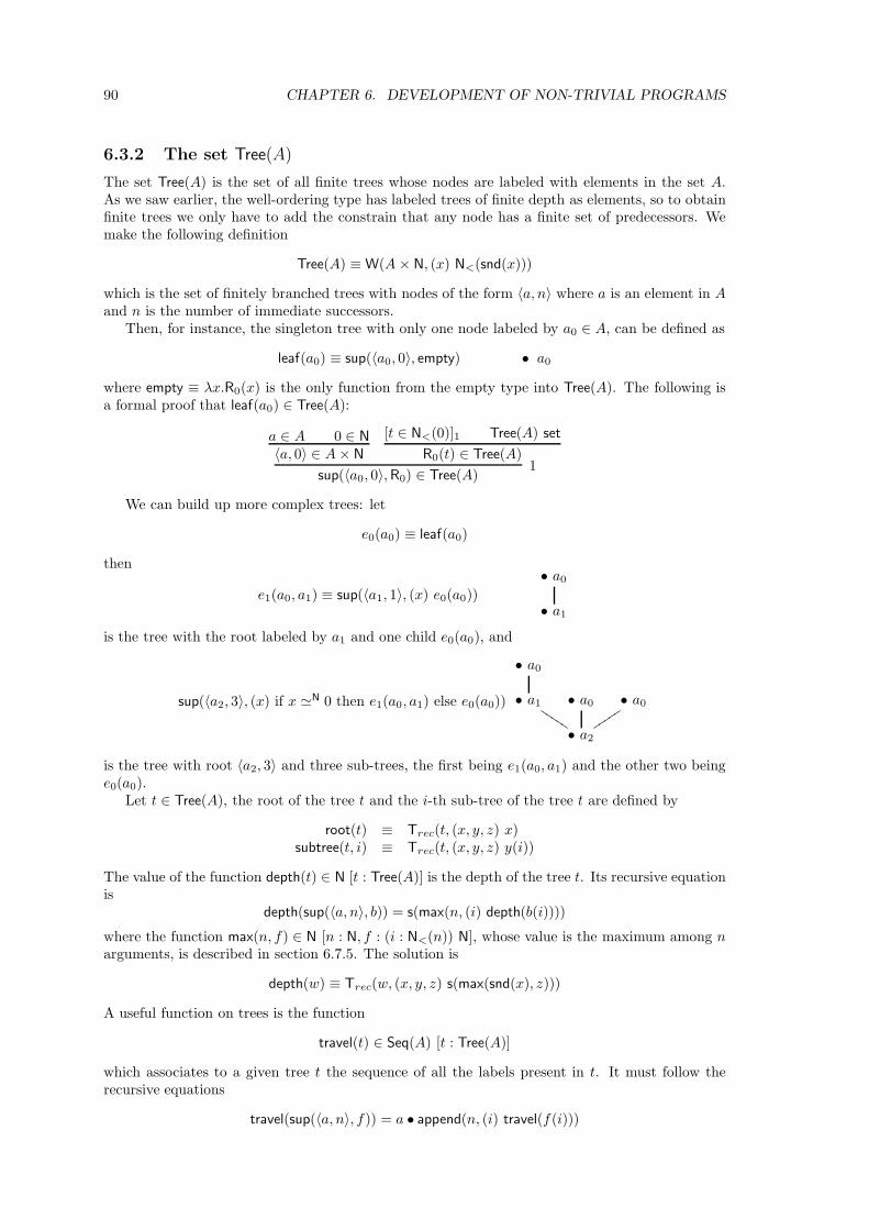
90 CHAPTER 6. DEVELOPMENT OF NON-TRIVIAL PROGRAMS
6.3.2 The set Tree(A)
The set Tree(A) is the set of all finite trees whose nodes are labeled with elements in the set A.As we saw earlier, the well-ordering type has labeled trees of finite depth as elements, so to obtainfinite trees we only have to add the constrain that any node has a finite set of predecessors. Wemake the following definition
Tree(A) ≡W(A × N, (x) N<(snd(x)))
which is the set of finitely branched trees with nodes of the form 〈a, n〉 where a is an element in Aand n is the number of immediate successors.
Then, for instance, the singleton tree with only one node labeled by a0 ∈ A, can be defined as
leaf(a0) ≡ sup(〈a0, 0〉, empty) • a0
where empty ≡ λx.R0(x) is the only function from the empty type into Tree(A). The following isa formal proof that leaf(a0) ∈ Tree(A):
a ∈ A 0 ∈ N
〈a, 0〉 ∈ A× N
[t ∈ N<(0)]1 Tree(A) set
R0(t) ∈ Tree(A)
sup(〈a0, 0〉, R0) ∈ Tree(A)1
We can build up more complex trees: let
e0(a0) ≡ leaf(a0)
then
e1(a0, a1) ≡ sup(〈a1, 1〉, (x) e0(a0))
• a0
• a1
is the tree with the root labeled by a1 and one child e0(a0), and
sup(〈a2, 3〉, (x) if x ≃N 0 then e1(a0, a1) else e0(a0))
• a0
• a1
JJJJ
J• a0 • a0
tttt
t
• a2
is the tree with root 〈a2, 3〉 and three sub-trees, the first being e1(a0, a1) and the other two beinge0(a0).
Let t ∈ Tree(A), the root of the tree t and the i-th sub-tree of the tree t are defined by
root(t) ≡ Trec(t, (x, y, z) x)subtree(t, i) ≡ Trec(t, (x, y, z) y(i))
The value of the function depth(t) ∈ N [t : Tree(A)] is the depth of the tree t. Its recursive equationis
depth(sup(〈a, n〉, b)) = s(max(n, (i) depth(b(i))))
where the function max(n, f) ∈ N [n : N, f : (i : N<(n)) N], whose value is the maximum among narguments, is described in section 6.7.5. The solution is
depth(w) ≡ Trec(w, (x, y, z) s(max(snd(x), z)))
A useful function on trees is the function
travel(t) ∈ Seq(A) [t : Tree(A)]
which associates to a given tree t the sequence of all the labels present in t. It must follow therecursive equations
travel(sup(〈a, n〉, f)) = a • append(n, (i) travel(f(i)))
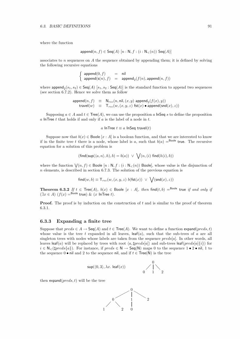
6.3. BASIC DEFINITIONS 91
where the function
append(n, f) ∈ Seq(A) [n : N, f : (i : N<(n)) Seq(A)]
associates to n sequences on A the sequence obtained by appending them; it is defined by solvingthe following recursive equations
append(0, f) = nil
append(s(n), f) = append2(f(n), append(n, f))
where append2(s1, s2) ∈ Seq(A) [s1, s2 : Seq(A)] is the standard function to append two sequences(see section 6.7.2). Hence we solve them as follow
append(n, f) ≡ Nrec(n, nil, (x, y) append2(f(x), y))travel(w) ≡ Trec(w, (x, y, z) fst(x) • append(snd(x), z))
Supposing a ∈ A and t ∈ Tree(A), we can use the proposition a InSeq s to define the propositiona InTree t that holds if and only if a is the label of a node in t.
a InTree t ≡ a InSeq travel(t)
Suppose now that b(x) ∈ Boole [x : A] is a boolean function, and that we are interested to knowif in the finite tree t there is a node, whose label is a, such that b(a) =Boole true. The recursiveequation for a solution of this problem is
(find(sup(〈a, n〉, h), b) = b(a)) ∨∨
(n, (i) find(h(i), b))
where the function∨
(n, f) ∈ Boole [n : N, f : (i : N<(n)) Boole], whose value is the disjunction ofn elements, is described in section 6.7.3. The solution of the previous equation is
find(w, b) ≡ Trec(w, (x, y, z) b(fst(x)) ∨∨
(snd(x), z))
Theorem 6.3.2 If t ∈ Tree(A), b(x) ∈ Boole [x : A], then find(t, b) =Boole true if and only if(∃x ∈ A) (f(x) =Boole true) & (x InTree t).
Proof. The proof is by induction on the construction of t and is similar to the proof of theorem6.3.1.
6.3.3 Expanding a finite tree
Suppose that preds ∈ A→ Seq(A) and t ∈ Tree(A). We want to define a function expand(preds, t)whose value is the tree t expanded in all leaves, leaf(a), such that the sub-trees of a are allsingleton trees with nodes whose labels are taken from the sequence preds[a]. In other words, allleaves leaf(a) will be replaced by trees with root 〈a, ♯preds[a]〉 and sub-trees leaf(preds[a]i) fori ∈ N<(♯predsa). For instance, if preds ∈ N → Seq(N) maps 0 to the sequence 1 • 2 • nil, 1 tothe sequence 0 • nil and 2 to the sequence nil, and if t ∈ Tree(N) is the tree
sup(〈0, 3〉, λx. leaf(x))0
0
1 2
====
then expand(preds, t) will be the tree
0
0
pppppppp1 2
LLLLLLL
1
2
====
0
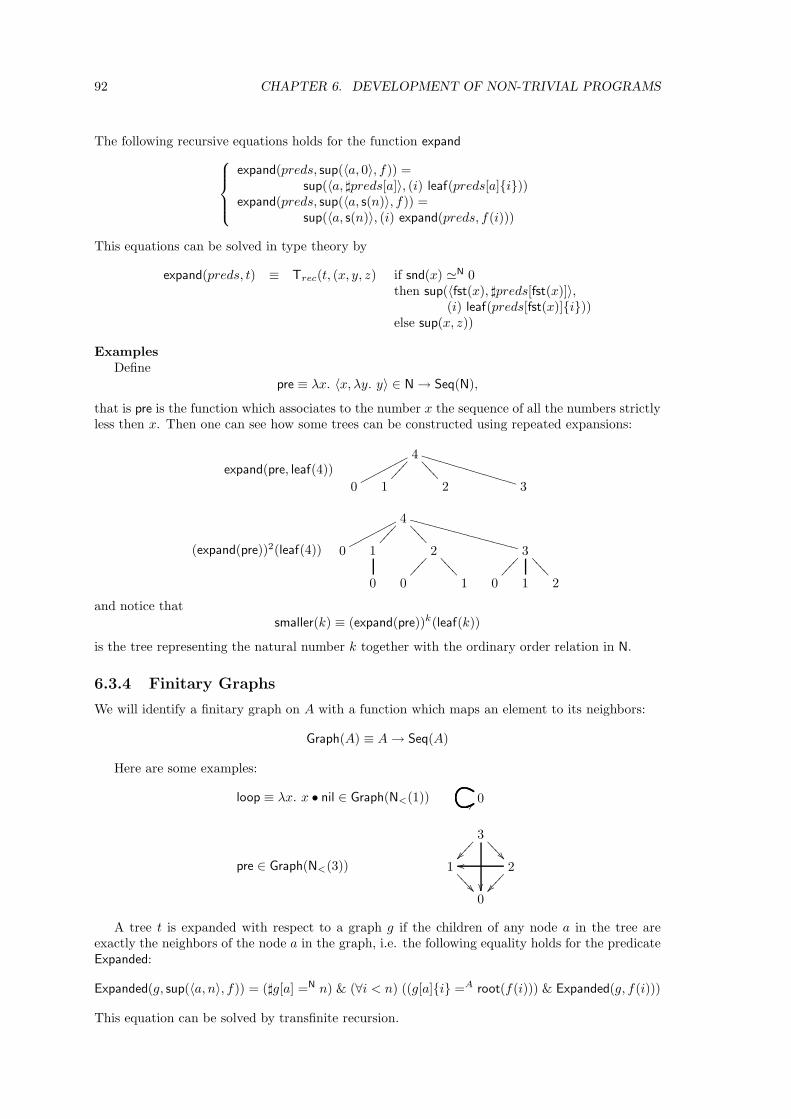
92 CHAPTER 6. DEVELOPMENT OF NON-TRIVIAL PROGRAMS
The following recursive equations holds for the function expand
expand(preds, sup(〈a, 0〉, f)) =sup(〈a, ♯preds[a]〉, (i) leaf(preds[a]i))
expand(preds, sup(〈a, s(n)〉, f)) =sup(〈a, s(n)〉, (i) expand(preds, f(i)))
This equations can be solved in type theory by
expand(preds, t) ≡ Trec(t, (x, y, z) if snd(x) ≃N 0then sup(〈fst(x), ♯preds[fst(x)]〉,
(i) leaf(preds[fst(x)]i))else sup(x, z))
ExamplesDefine
pre ≡ λx. 〈x, λy. y〉 ∈ N→ Seq(N),
that is pre is the function which associates to the number x the sequence of all the numbers strictlyless then x. Then one can see how some trees can be constructed using repeated expansions:
expand(pre, leaf(4))4
0
pppppppp1
2
====
3
UUUUUUUUUUUUUUU
(expand(pre))2(leaf(4))
4
0
pppppppp1
2
====
3
WWWWWWWWWWWWWWWWW
0 0
1
====
0
1 2
====
and notice thatsmaller(k) ≡ (expand(pre))k(leaf(k))
is the tree representing the natural number k together with the ordinary order relation in N.
6.3.4 Finitary Graphs
We will identify a finitary graph on A with a function which maps an element to its neighbors:
Graph(A) ≡ A→ Seq(A)
Here are some examples:
loop ≡ λx. x • nil ∈ Graph(N<(1)) 0::
pre ∈ Graph(N<(3))
3
===
=
1
===
= 2oo
0
A tree t is expanded with respect to a graph g if the children of any node a in the tree areexactly the neighbors of the node a in the graph, i.e. the following equality holds for the predicateExpanded:
Expanded(g, sup(〈a, n〉, f)) = (♯g[a] =N n) & (∀i < n) ((g[a]i =A root(f(i))) & Expanded(g, f(i)))
This equation can be solved by transfinite recursion.
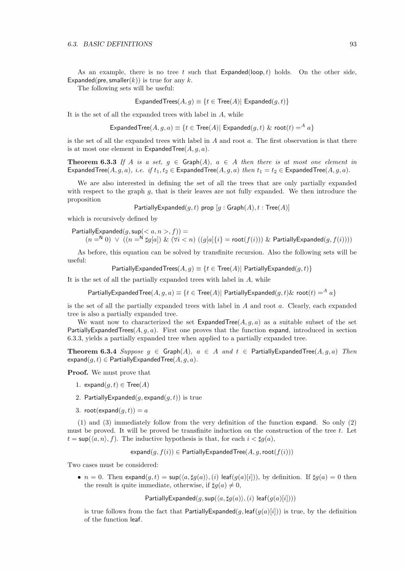
6.3. BASIC DEFINITIONS 93
As an example, there is no tree t such that Expanded(loop, t) holds. On the other side,Expanded(pre, smaller(k)) is true for any k.
The following sets will be useful:
ExpandedTrees(A, g) ≡ t ∈ Tree(A)| Expanded(g, t)
It is the set of all the expanded trees with label in A, while
ExpandedTree(A, g, a) ≡ t ∈ Tree(A)| Expanded(g, t) & root(t) =A a
is the set of all the expanded trees with label in A and root a. The first observation is that thereis at most one element in ExpandedTree(A, g, a).
Theorem 6.3.3 If A is a set, g ∈ Graph(A), a ∈ A then there is at most one element inExpandedTree(A, g, a), i.e. if t1, t2 ∈ ExpandedTree(A, g, a) then t1 = t2 ∈ ExpandedTree(A, g, a).
We are also interested in defining the set of all the trees that are only partially expandedwith respect to the graph g, that is their leaves are not fully expanded. We then introduce theproposition
PartiallyExpanded(g, t) prop [g : Graph(A), t : Tree(A)]
which is recursively defined by
PartiallyExpanded(g, sup(< a, n >, f)) =(n =N 0) ∨ ((n =N ♯g[a]) & (∀i < n) ((g[a]i = root(f(i))) & PartiallyExpanded(g, f(i))))
As before, this equation can be solved by transfinite recursion. Also the following sets will beuseful:
PartiallyExpandedTrees(A, g) ≡ t ∈ Tree(A)| PartiallyExpanded(g, t)
It is the set of all the partially expanded trees with label in A, while
PartiallyExpandedTree(A, g, a) ≡ t ∈ Tree(A)| PartiallyExpanded(g, t)& root(t) =A a
is the set of all the partially expanded trees with label in A and root a. Clearly, each expandedtree is also a partially expanded tree.
We want now to characterized the set ExpandedTree(A, g, a) as a suitable subset of the setPartiallyExpandedTrees(A, g, a). First one proves that the function expand, introduced in section6.3.3, yields a partially expanded tree when applied to a partially expanded tree.
Theorem 6.3.4 Suppose g ∈ Graph(A), a ∈ A and t ∈ PartiallyExpandedTree(A, g, a) Thenexpand(g, t) ∈ PartiallyExpandedTree(A, g, a).
Proof. We must prove that
1. expand(g, t) ∈ Tree(A)
2. PartiallyExpanded(g, expand(g, t)) is true
3. root(expand(g, t)) = a
(1) and (3) immediately follow from the very definition of the function expand. So only (2)must be proved. It will be proved be transfinite induction on the construction of the tree t. Lett = sup(〈a, n〉, f). The inductive hypothesis is that, for each i < ♯g(a),
expand(g, f(i)) ∈ PartiallyExpandedTree(A, g, root(f(i)))
Two cases must be considered:
• n = 0. Then expand(g, t) = sup(〈a, ♯g(a)〉, (i) leaf(g(a)[i])), by definition. If ♯g(a) = 0 thenthe result is quite immediate, otherwise, if ♯g(a) 6= 0,
PartiallyExpanded(g, sup(〈a, ♯g(a)〉, (i) leaf(g(a)[i])))
is true follows from the fact that PartiallyExpanded(g, leaf(g(a)[i])) is true, by the definitionof the function leaf.
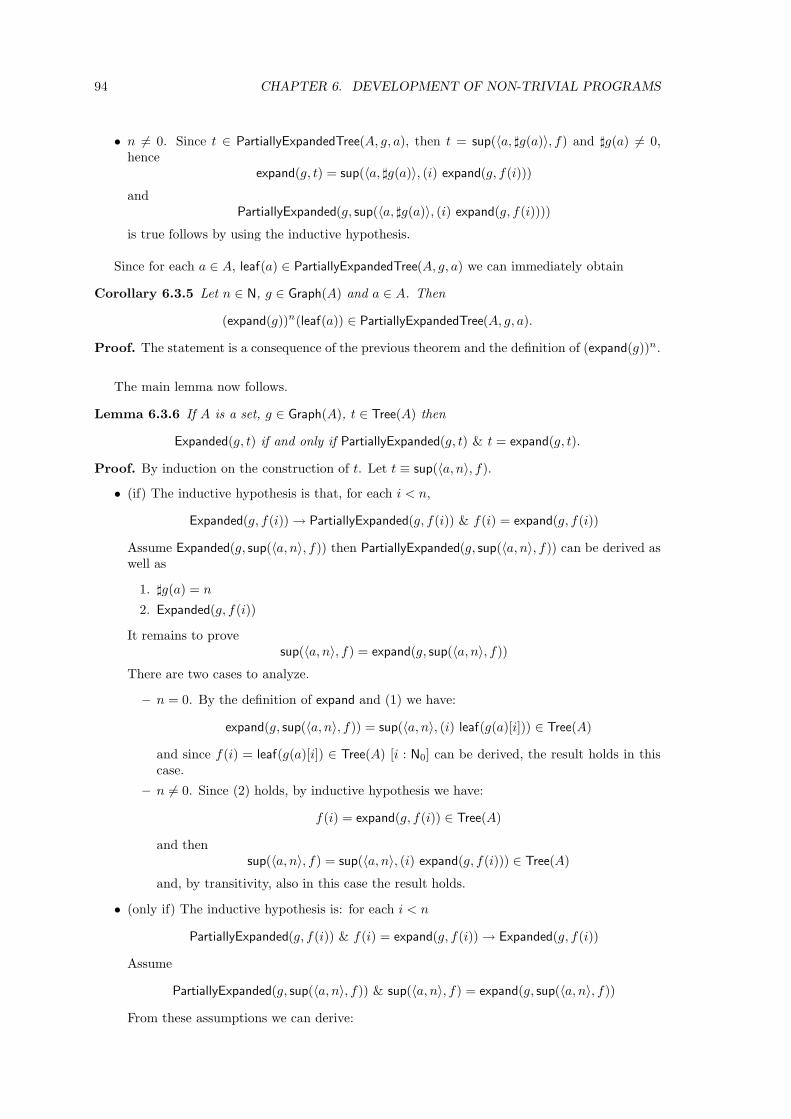
94 CHAPTER 6. DEVELOPMENT OF NON-TRIVIAL PROGRAMS
• n 6= 0. Since t ∈ PartiallyExpandedTree(A, g, a), then t = sup(〈a, ♯g(a)〉, f) and ♯g(a) 6= 0,hence
expand(g, t) = sup(〈a, ♯g(a)〉, (i) expand(g, f(i)))
andPartiallyExpanded(g, sup(〈a, ♯g(a)〉, (i) expand(g, f(i))))
is true follows by using the inductive hypothesis.
Since for each a ∈ A, leaf(a) ∈ PartiallyExpandedTree(A, g, a) we can immediately obtain
Corollary 6.3.5 Let n ∈ N, g ∈ Graph(A) and a ∈ A. Then
(expand(g))n(leaf(a)) ∈ PartiallyExpandedTree(A, g, a).
Proof. The statement is a consequence of the previous theorem and the definition of (expand(g))n.
The main lemma now follows.
Lemma 6.3.6 If A is a set, g ∈ Graph(A), t ∈ Tree(A) then
Expanded(g, t) if and only if PartiallyExpanded(g, t) & t = expand(g, t).
Proof. By induction on the construction of t. Let t ≡ sup(〈a, n〉, f).
• (if) The inductive hypothesis is that, for each i < n,
Expanded(g, f(i))→ PartiallyExpanded(g, f(i)) & f(i) = expand(g, f(i))
Assume Expanded(g, sup(〈a, n〉, f)) then PartiallyExpanded(g, sup(〈a, n〉, f)) can be derived aswell as
1. ♯g(a) = n
2. Expanded(g, f(i))
It remains to provesup(〈a, n〉, f) = expand(g, sup(〈a, n〉, f))
There are two cases to analyze.
– n = 0. By the definition of expand and (1) we have:
expand(g, sup(〈a, n〉, f)) = sup(〈a, n〉, (i) leaf(g(a)[i])) ∈ Tree(A)
and since f(i) = leaf(g(a)[i]) ∈ Tree(A) [i : N0] can be derived, the result holds in thiscase.
– n 6= 0. Since (2) holds, by inductive hypothesis we have:
f(i) = expand(g, f(i)) ∈ Tree(A)
and thensup(〈a, n〉, f) = sup(〈a, n〉, (i) expand(g, f(i))) ∈ Tree(A)
and, by transitivity, also in this case the result holds.
• (only if) The inductive hypothesis is: for each i < n
PartiallyExpanded(g, f(i)) & f(i) = expand(g, f(i))→ Expanded(g, f(i))
Assume
PartiallyExpanded(g, sup(〈a, n〉, f)) & sup(〈a, n〉, f) = expand(g, sup(〈a, n〉, f))
From these assumptions we can derive:
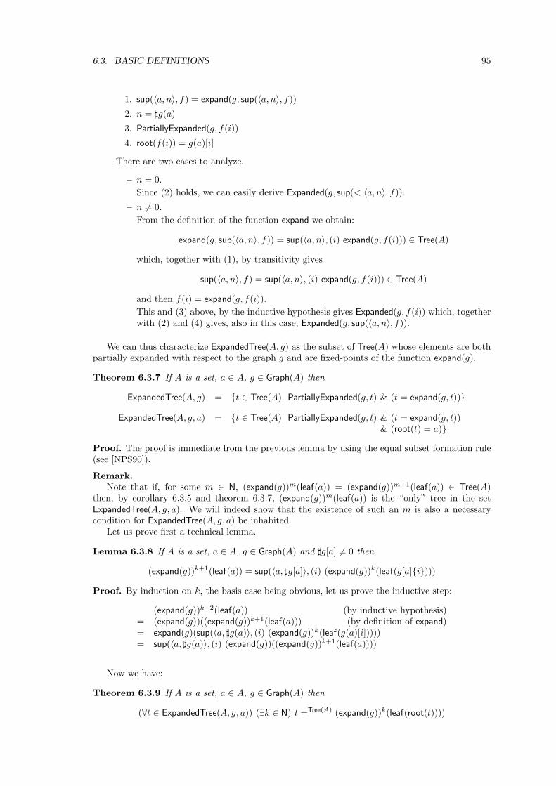
6.3. BASIC DEFINITIONS 95
1. sup(〈a, n〉, f) = expand(g, sup(〈a, n〉, f))
2. n = ♯g(a)
3. PartiallyExpanded(g, f(i))
4. root(f(i)) = g(a)[i]
There are two cases to analyze.
– n = 0.
Since (2) holds, we can easily derive Expanded(g, sup(< 〈a, n〉, f)).
– n 6= 0.
From the definition of the function expand we obtain:
expand(g, sup(〈a, n〉, f)) = sup(〈a, n〉, (i) expand(g, f(i))) ∈ Tree(A)
which, together with (1), by transitivity gives
sup(〈a, n〉, f) = sup(〈a, n〉, (i) expand(g, f(i))) ∈ Tree(A)
and then f(i) = expand(g, f(i)).
This and (3) above, by the inductive hypothesis gives Expanded(g, f(i)) which, togetherwith (2) and (4) gives, also in this case, Expanded(g, sup(〈a, n〉, f)).
We can thus characterize ExpandedTree(A, g) as the subset of Tree(A) whose elements are bothpartially expanded with respect to the graph g and are fixed-points of the function expand(g).
Theorem 6.3.7 If A is a set, a ∈ A, g ∈ Graph(A) then
ExpandedTree(A, g) = t ∈ Tree(A)| PartiallyExpanded(g, t) & (t = expand(g, t))
ExpandedTree(A, g, a) = t ∈ Tree(A)| PartiallyExpanded(g, t) & (t = expand(g, t))& (root(t) = a)
Proof. The proof is immediate from the previous lemma by using the equal subset formation rule(see [NPS90]).
Remark.Note that if, for some m ∈ N, (expand(g))m(leaf(a)) = (expand(g))m+1(leaf(a)) ∈ Tree(A)
then, by corollary 6.3.5 and theorem 6.3.7, (expand(g))m(leaf(a)) is the “only” tree in the setExpandedTree(A, g, a). We will indeed show that the existence of such an m is also a necessarycondition for ExpandedTree(A, g, a) be inhabited.
Let us prove first a technical lemma.
Lemma 6.3.8 If A is a set, a ∈ A, g ∈ Graph(A) and ♯g[a] 6= 0 then
(expand(g))k+1(leaf(a)) = sup(〈a, ♯g[a]〉, (i) (expand(g))k(leaf(g[a]i)))
Proof. By induction on k, the basis case being obvious, let us prove the inductive step:
(expand(g))k+2(leaf(a)) (by inductive hypothesis)= (expand(g))((expand(g))k+1(leaf(a))) (by definition of expand)= expand(g)(sup(〈a, ♯g(a)〉, (i) (expand(g))k(leaf(g(a)[i]))))= sup(〈a, ♯g(a)〉, (i) (expand(g))((expand(g))k+1(leaf(a))))
Now we have:
Theorem 6.3.9 If A is a set, a ∈ A, g ∈ Graph(A) then
(∀t ∈ ExpandedTree(A, g, a)) (∃k ∈ N) t =Tree(A) (expand(g))k(leaf(root(t))))
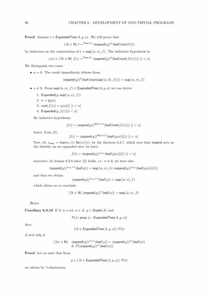
96 CHAPTER 6. DEVELOPMENT OF NON-TRIVIAL PROGRAMS
Proof. Assume t ∈ ExpandedTree(A, g, a). We will prove that
(∃k ∈ N) t =Tree(A) (expand(g))k(leaf(root(t))))
by induction on the construction of t = sup(〈a, n〉, f). The inductive hypothesis is:
x(i) ∈ (∃k ∈ N) f(i) =Tree(A) (expand(g))k(leaf(root(f(i))))) [i < n]
We distinguish two cases.
• n = 0. The result immediately follows from:
(expand(g))0(leaf(root(sup(〈a, 0〉, f)))) = sup(〈a, n〉, f)
• n 6= 0. From sup(〈a, n〉, f) ∈ ExpandedTree(A, g, a) we can derive:
1. Expanded(g, sup(〈a, n〉, f))
2. n = ♯g(a)
3. root(f(i)) = g(a)[i] [i < n]
4. Expanded(g, f(i))[i < n]
By inductive hypothesis:
f(i) = (expand(g))fst(x(i))(leaf(root(f(i)))) [i < n]
hence, from (3):f(i) = (expand(g))fst(x(i))(leaf(g(a)[i])) [i < n]
Now, let xmax = max(n, (i) fst(x(i))), by the theorem 6.3.7, which says that expand acts asthe identity on an expanded tree, we have:
f(i) = (expand(g))xmax(leaf(g(a)[i])) [i < n]
moreover, by lemma 6.3.8 since (2) holds, i.e. n 6= 0, we have also
(expand(g))xmax+1(leaf(a)) = sup(〈a, n〉, (i) (expand(g))xmax(leaf(g(a)[i])))
and then we obtain(expand(g))xmax+1(leaf(a)) = sup(〈a, n〉, f)
which allows us to conclude:
(∃k ∈ N) (expand(g))k(leaf(a)) = sup(〈a, n〉, f)
Hence
Corollary 6.3.10 If A is a set, a ∈ A, g ∈ Graph(A) and
P (x) prop [x : ExpandedTree(A, g, a)]
then(∃t ∈ ExpandedTree(A, g, a)) P (t)
if and only if
(∃m ∈ N) (expand(g))m+1(leaf(a)) = (expand(g))m(leaf(a))& P ((expand(g))m(leaf(a)))
Proof. Let us note that from
y ∈ (∃t ∈ ExpandedTree(A, g, a)) P (t)
we obtain by ∃-elimination
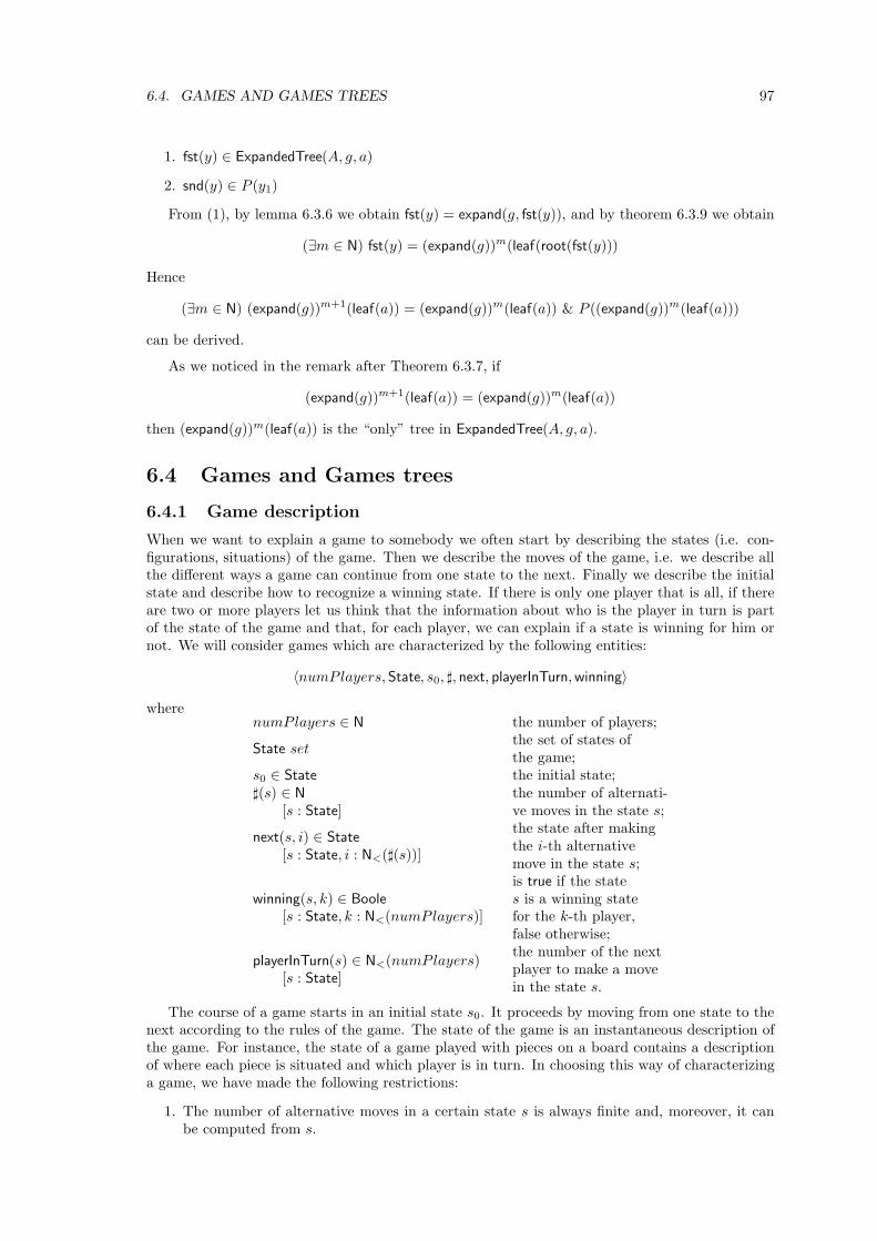
6.4. GAMES AND GAMES TREES 97
1. fst(y) ∈ ExpandedTree(A, g, a)
2. snd(y) ∈ P (y1)
From (1), by lemma 6.3.6 we obtain fst(y) = expand(g, fst(y)), and by theorem 6.3.9 we obtain
(∃m ∈ N) fst(y) = (expand(g))m(leaf(root(fst(y)))
Hence
(∃m ∈ N) (expand(g))m+1(leaf(a)) = (expand(g))m(leaf(a)) & P ((expand(g))m(leaf(a)))
can be derived.
As we noticed in the remark after Theorem 6.3.7, if
(expand(g))m+1(leaf(a)) = (expand(g))m(leaf(a))
then (expand(g))m(leaf(a)) is the “only” tree in ExpandedTree(A, g, a).
6.4 Games and Games trees
6.4.1 Game description
When we want to explain a game to somebody we often start by describing the states (i.e. con-figurations, situations) of the game. Then we describe the moves of the game, i.e. we describe allthe different ways a game can continue from one state to the next. Finally we describe the initialstate and describe how to recognize a winning state. If there is only one player that is all, if thereare two or more players let us think that the information about who is the player in turn is partof the state of the game and that, for each player, we can explain if a state is winning for him ornot. We will consider games which are characterized by the following entities:
〈numPlayers, State, s0, ♯, next, playerInTurn, winning〉
wherenumPlayers ∈ N the number of players;
State setthe set of states ofthe game;
s0 ∈ State the initial state;♯(s) ∈ N
[s : State]the number of alternati-ve moves in the state s;
next(s, i) ∈ State
[s : State, i : N<(♯(s))]
the state after makingthe i-th alternativemove in the state s;
winning(s, k) ∈ Boole
[s : State, k : N<(numPlayers)]
is true if the states is a winning statefor the k-th player,false otherwise;
playerInTurn(s) ∈ N<(numPlayers)[s : State]
the number of the nextplayer to make a movein the state s.
The course of a game starts in an initial state s0. It proceeds by moving from one state to thenext according to the rules of the game. The state of the game is an instantaneous description ofthe game. For instance, the state of a game played with pieces on a board contains a descriptionof where each piece is situated and which player is in turn. In choosing this way of characterizinga game, we have made the following restrictions:
1. The number of alternative moves in a certain state s is always finite and, moreover, it canbe computed from s.
98 CHAPTER 6. DEVELOPMENT OF NON-TRIVIAL PROGRAMS
2. All possible next states can be computed from the current state.
3. It is decidable if a state is winning for a player or not.
The reasons for choosing the first two restrictions is that we want to have a general algorithmwhich decides if it is possible to reach a winning position or not. The third restriction is not asevere restriction; it is just a concrete way of expressing that there should be no doubt if a gameis won or not.
6.4.2 Potential Moves
To describe the rules for making a move, it is often more convenient to first describe all potentialmoves and then disallow some of them as illegal. For instance in chess, we describe how each piececan potentially move and then disallow the illegal ones, for instance it is impossible to move a pieceoutside the board or to put a piece on already occupied fields. It is often convenient to define theconstants State, next, and ♯ in the following way:
• Define a set of “extended states”, a set which contains illegal as well as legal states of thegame:
ExtendedState set
• Define, for each extended state s, a boolean which says if s describes a legal state of the gameor not:
legal(s) ∈ Boole [s : ExtendedState]
• Give the upper bound of the number of alternative potential moves in the state s:
maxMoves(s) ∈ N [s : State]
• Define, for each state s and each potential move i (0 ≤ i < maxMoves(s)) the extended stateobtained by performing the i-th potential move from s:
try(s, i) ∈ ExtendedState [s : State, i : N<(maxMoves(s))]
We can show that in this case we can give the description of the game in terms of the entitiesState, ♯ and next. The states of the game are the subset of the legal extended states, i.e.
State ≡ s ∈ ExtendedState| legal(s) =Boole true
We can define ♯(s) and next(s, i) by using a general filtering technique in the following way. Wewill first build up for each state s the finite sequence of all extended states associated with s:
potentialMoves(s) ≡ 〈maxMoves(s), λi. try(s, i)〉 ∈ Seq(ExtendedState)
Then we will filter out the illegal states, by means of the function filter defined in section 6.3.1.
legalMoves(s) ≡ filter(potentialMoves(s), legal)
and finally we define
♯(s) ≡ ♯legalMoves(s)next(s, i) ≡ legalMoves(s)i
6.4. GAMES AND GAMES TREES 99
6.4.3 The set of game trees.
Let
Game ≡ 〈numPlayers, State, s0, ♯, next, playerInTurn, winning〉
be a given game. We notice that the functions ♯ and next define a graph, namely
g0 ≡ λs. 〈♯(s), λi. next(s, i)〉
This is the graph which defines the rules of the game in the sense that the neighbors of anynode s in the graph are exactly all possible states immediately following s in the game. In section6.3.4 we saw how to associate a tree with a graph. For instance, the set
ExpandedTree(State, g0, s0)
contains at most one element, the game tree associated with Game. This is a tree with a gamestate in each node and the initial state s0 in the root. Furthermore, for each node s in the tree,the i-th child of s is the resulting state after choosing the i-th alternative move from s. We sawalso, in section 6.3.4, that if there is a game tree, it can be written as (expand(g0))
m(leaf(s0)) forsome m ∈ N.
6.4.4 Some general game problems
Given a game there are many different questions we could ask. For instance, let us consider thefollowing ones:
1. Is it possible for the k-th player to win the game?
2. Is there a winning strategy for the k-th player?
3. Let s be a situation. Give me the list of all the winning moves for the k-th player.
It should be clear that all of these questions can be formalized within type theory by using theset ExpandedTree(State, g0, s0).
As a first example, let us consider the question: “Is it possible for the k-th player to win thegame?” We have to find a boolean function which associates to the k-th player true if and onlyif there exists the game tree and it has a node labeled with a state which is winning for the k-thplayer. The problem can be expressed by the following type:
(∀k < numPlayers) x ∈ Boole| (x = true)↔(∃g ∈ ExpandedTree(State, g0, s0))HasWinning(g, k)
where
HasWinning(g, k) ≡ (∃a ∈ State) (a InTree g) & (winning(a, k) = true).
To solve the second problem: “Is there a winning strategy for the k-th player?”, we have tofind a boolean function which associates to the k-th player true if and only if there exists the gametree and it is winning for the k-th player. A game tree is winning for the player k if:
1. k is in turn
• and the situation of the game is winning for k or
• there exists a move for k to a tree that is winning for k
2. k is not in turn
• and the situation of the game is winning for k or
• the situation is not terminal and every move that the player in turn can do turns outin a game tree that is winning for k.
100 CHAPTER 6. DEVELOPMENT OF NON-TRIVIAL PROGRAMS
Then the recursive equation defining the proposition
IsWinningTree(t, k) [t : Tree(State), k < numPlayers]
is:
IsWinningTree(sup(〈a, n〉, f), k) = if (playerInTurn(a) = k)then (winning(a, k) = true) ∨ (∃i < n) IsWinningTree(f(i), k))else (winning(a, k) = true) ∨ ((n 6= 0) & (∀i < n) IsWinningTree(f(i), k))
This recursive equation can be solved in type theory by a standard technique (see section 6.7.6);then the second problem can be expressed as:
(∀k < numPlayers) x ∈ Boole| (x = true)↔(∃t ∈ ExpandedTree(State, g0, s0))IsWinningTree(t, k)
To solve the problem “Give me the list of all the winning moves for the k-th player in a situations” we have to find a function which associates to a player k and a state s the sequence of the winningmoves for the k-th player from the state s. This is an element w of Seq(N<(♯s)) which satisfies thecondition:
(∃t ∈ ExpandedTree(State, g0, s))(∀i < ♯s) (i InSeq w)↔ IsWinningTree(subtree(t, i), k)
Now the problem is expressed by the type:
(∀k < numPlayers)(∀s ∈ State) w ∈ Seq(N<(♯s))|(∃t ∈ ExpandedTree(State, g0, s))(∀i < ♯s) (i InSeq w)↔ IsWinningTree(subtree(t, i), k)
6.4.5 Some general solutions
We can observe that in the types expressing the three considered problems there is always aconstruction of the form:
(∃t ∈ ExpandedTree(State, g0, s)) Q(t)
for a suitable proposition Q(t) prop [t : ExpandedTree(State, g0, s)].By corollary 6.3.10:
(∃t ∈ ExpandedTree(State, g0, s)) Q(t)↔(∃m ∈ N) (expand(g0))
m+1(leaf(s)) = (expand(g0))m(leaf(s)) & Q((expand(g0))
m(leaf(s)))
holds; hence whenever
(expand(g0))m+1(leaf(s)) = (expand(g0))
m(leaf(s))
holds we can give equivalent formalizations of the problems given in the previous section.
1. (∀k < numPlayers)x ∈ Boole| (x = true)↔ HasWinning((expand(g0))m(leaf(s0)), k)
2. (∀k < numPlayers)x ∈ Boole| (x = true)↔ IsWinningTree((expand(g0))m(leaf(s0)), k)
3.(∀k < numPlayers)(∀s ∈ State)w ∈ Seq(N<(♯s))| (∀i < ♯s) (i InSeq w)↔
IsWinningTree(subtree((expand(g0))m(leaf(s)), i), k)
A general solution of the problem (1) is then given by the function
λk. find((expand(g0))m(leaf(s0)), (s) winning(s, k))
since we proved (see theorem 6.3.2) that
find(t, p) ∈ x ∈ Boole| (x = true)↔ (∃a ∈ State) (a InTree g) & (p(a) = true)
6.5. EXAMPLES 101
For the problem (2) we can easily find a function
winningTree(t, k) ∈ Boole [t : Tree(State), k < numPlayers]
satisfying the condition:
(winningTree(t, k) =Boole true)↔ IsWinningTree(t, k).
Its recursive definition mimics the definition of the type IsWinningTree and can be solved in asimilar way (see section 6.7.6). Hence
λk. winningTree((expand(g0))m(leaf(s0)), k)
is a general solution of the problem (2).Finally, a general solution for the problem (3) is
λk. filter((i) winningTree(subtree(t, i), k), 〈♯a, λx. x〉)
whose correctness follows from Theorem 6.3.1.
6.5 Examples
6.5.1 The knight’s tour problem
We have an n × n board with n2 fields and a knight placed on an initial field. The problem is tofind out if there exists a covering of the entire board, i.e. a sequence of moves such that every fieldof the board is visited exactly once. This is a game with only one player; let us describe it followingsection 6.4. First, note that there is a fixed number of potential moves: maxMoves(s) = 8, for anystate s of the game. A state of this game can be characterized by a current field (the position ofthe knight) together with the necessary information about the history of the game, i.e., we needto know all the fields visited by the knight before the current one. Clearly, for this game
numPlayers ≡ 1;playerInTurn(s) ≡ 1.
We represent a field by a pair of natural numbers:
Field ≡ N× N
Since we are considering a chess board of a certain dimension n, let us identify the limits of ann× n board as in fig. 6.1, and, given f ∈ Field and n ∈ N, define the proposition:
WithinLimits(f, n) ≡ (2 ≤ fst(f) ≤ n + 1) & (2 ≤ snd(f) ≤ n + 1)
Let us define a field to be busy if it is outside the board or if it has already been visited by theknight; otherwise it is free. A marked-board is a function which associates to each field a booleansaying if the field is free or busy:
MarkedBoard ≡ Field→ Boole
We will use the abbreviations:free ≡ true
busy ≡ false
Clearly, in a legal state the current field must be free, but we relax this condition in definingthe set:
ExtendedState ≡ Field× (∃n ∈ N) MarkedBoardSize(n)
where
MarkedBoardSize(n) ≡ m ∈ MarkedBoard| (∀f ∈ Field) Free(f, m)→WithinLimits(f, n)
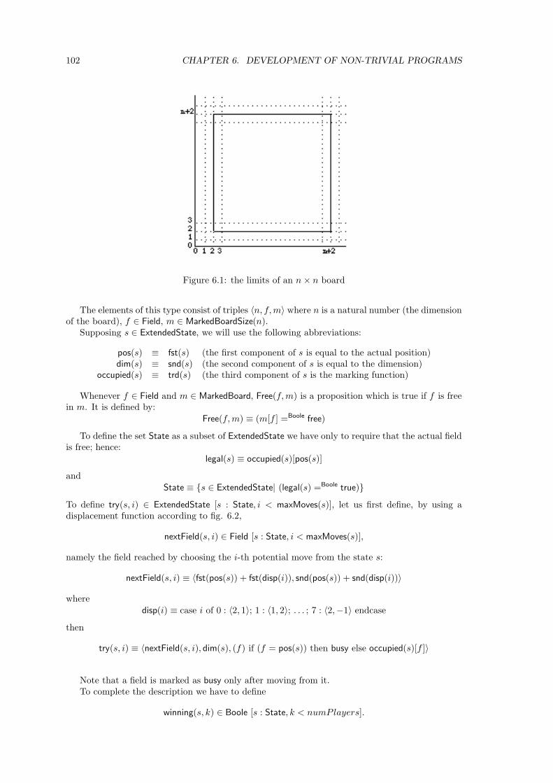
102 CHAPTER 6. DEVELOPMENT OF NON-TRIVIAL PROGRAMS
Figure 6.1: the limits of an n× n board
The elements of this type consist of triples 〈n, f, m〉 where n is a natural number (the dimensionof the board), f ∈ Field, m ∈ MarkedBoardSize(n).
Supposing s ∈ ExtendedState, we will use the following abbreviations:
pos(s) ≡ fst(s) (the first component of s is equal to the actual position)dim(s) ≡ snd(s) (the second component of s is equal to the dimension)
occupied(s) ≡ trd(s) (the third component of s is the marking function)
Whenever f ∈ Field and m ∈ MarkedBoard, Free(f, m) is a proposition which is true if f is freein m. It is defined by:
Free(f, m) ≡ (m[f ] =Boole free)
To define the set State as a subset of ExtendedState we have only to require that the actual fieldis free; hence:
legal(s) ≡ occupied(s)[pos(s)]
and
State ≡ s ∈ ExtendedState| (legal(s) =Boole true)
To define try(s, i) ∈ ExtendedState [s : State, i < maxMoves(s)], let us first define, by using adisplacement function according to fig. 6.2,
nextField(s, i) ∈ Field [s : State, i < maxMoves(s)],
namely the field reached by choosing the i-th potential move from the state s:
nextField(s, i) ≡ 〈fst(pos(s)) + fst(disp(i)), snd(pos(s)) + snd(disp(i))〉
where
disp(i) ≡ case i of 0 : 〈2, 1〉; 1 : 〈1, 2〉; . . . ; 7 : 〈2,−1〉 endcase
then
try(s, i) ≡ 〈nextField(s, i), dim(s), (f) if (f = pos(s)) then busy else occupied(s)[f ]〉
Note that a field is marked as busy only after moving from it.To complete the description we have to define
winning(s, k) ∈ Boole [s : State, k < numPlayers].
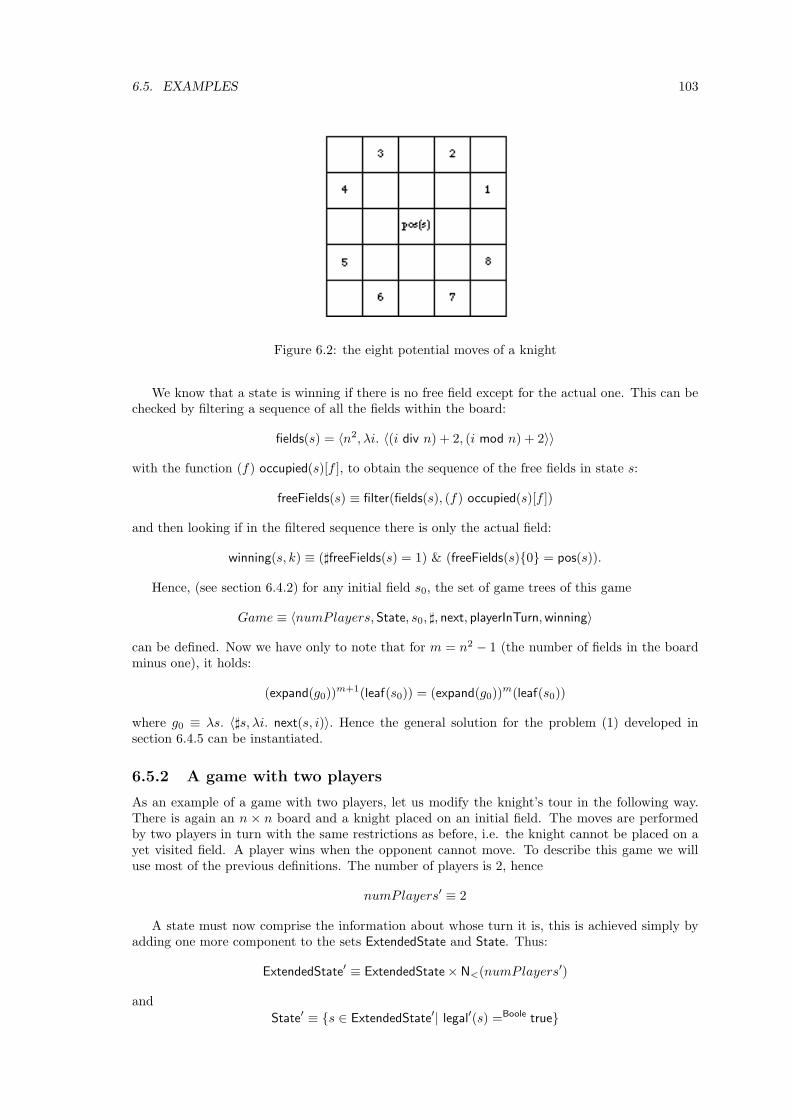
6.5. EXAMPLES 103
Figure 6.2: the eight potential moves of a knight
We know that a state is winning if there is no free field except for the actual one. This can bechecked by filtering a sequence of all the fields within the board:
fields(s) = 〈n2, λi. 〈(i div n) + 2, (i mod n) + 2〉〉
with the function (f) occupied(s)[f ], to obtain the sequence of the free fields in state s:
freeFields(s) ≡ filter(fields(s), (f) occupied(s)[f ])
and then looking if in the filtered sequence there is only the actual field:
winning(s, k) ≡ (♯freeFields(s) = 1) & (freeFields(s)0 = pos(s)).
Hence, (see section 6.4.2) for any initial field s0, the set of game trees of this game
Game ≡ 〈numPlayers, State, s0, ♯, next, playerInTurn, winning〉
can be defined. Now we have only to note that for m = n2 − 1 (the number of fields in the boardminus one), it holds:
(expand(g0))m+1(leaf(s0)) = (expand(g0))
m(leaf(s0))
where g0 ≡ λs. 〈♯s, λi. next(s, i)〉. Hence the general solution for the problem (1) developed insection 6.4.5 can be instantiated.
6.5.2 A game with two players
As an example of a game with two players, let us modify the knight’s tour in the following way.There is again an n × n board and a knight placed on an initial field. The moves are performedby two players in turn with the same restrictions as before, i.e. the knight cannot be placed on ayet visited field. A player wins when the opponent cannot move. To describe this game we willuse most of the previous definitions. The number of players is 2, hence
numPlayers′ ≡ 2
A state must now comprise the information about whose turn it is, this is achieved simply byadding one more component to the sets ExtendedState and State. Thus:
ExtendedState′ ≡ ExtendedState× N<(numPlayers′)
and
State′ ≡ s ∈ ExtendedState′| legal′(s) =Boole true
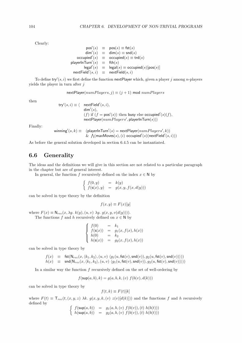
104 CHAPTER 6. DEVELOPMENT OF NON-TRIVIAL PROGRAMS
Clearly:pos′(s) ≡ pos(s) ≡ fst(s)dim′(s) ≡ dim(s) ≡ snd(s)
occupied′(s) ≡ occupied(s) ≡ trd(s)playerInTurn′(s) ≡ fth(s)
legal′(s) ≡ legal(s) ≡ occupied(s)[pos(s)]nextField′(s, i) ≡ nextField(s, i)
To define try′(s, i) we first define the function nextPlayer which, given a player j among n-playersyields the player in turn after j
nextPlayer(numPlayers, j) ≡ (j + 1) mod numPlayers
thentry′(s, i) ≡ 〈 nextField′(s, i),
dim′(s),(f) if (f = pos′(s)) then busy else occupied′(s)(f),nextPlayer(numPlayers′, playerInTurn(s))〉
Finally:winning′(s, k) ≡ (playerInTurn′(s) = nextPlayer(numPlayers′, k))
&∧
(maxMoves(s), (i) occupied′(s)(nextField′(s, i)))
As before the general solution developed in section 6.4.5 can be instantiated.
6.6 Generality
The ideas and the definitions we will give in this section are not related to a particular paragraphin the chapter but are of general interest.
In general, the function f recursively defined on the index x ∈ N by
f(0, y) = k(y)f(s(x), y) = g(x, y, f(x, d(y)))
can be solved in type theory by the definition
f(x, y) ≡ F (x)[y]
where F (x) ≡ Nrec(x, λy. k(y), (u, v) λy. g(x, y, v(d(y)))).The functions f and h recursively defined on x ∈ N by
f(0) = k1
f(s(x)) = g1(x, f(x), h(x))h(0) = k2
h(s(x)) = g2(x, f(x), h(x))
can be solved in type theory by
f(x) ≡ fst(Nrec(x, 〈k1, k2〉, (u, v) 〈g1(u, fst(v), snd(v)), g2(u, fst(v), snd(v))〉))h(x) ≡ snd(Nrec(x, 〈k1, k2〉, (u, v) 〈g1(u, fst(v), snd(v)), g2(u, fst(v), snd(v))〉))
In a similar way the function f recursively defined on the set of well-ordering by
f(sup(a, b), k) = g(a, b, k, (v) f(b(v), d(k)))
can be solved in type theory byf(t, k) ≡ F (t)[k]
where F (t) ≡ Trec(t, (x, y, z) λk. g(x, y, k, (v) z(v)[d(k)])) and the functions f and h recursivelydefined by
f(sup(a, b)) = g1(a, b, (v) f(b(v)), (t) h(b(t)))h(sup(a, b)) = g2(a, b, (v) f(b(v)), (t) h(b(t)))
6.7. SOME TYPE AND FUNCTIONS WE USE 105
can be solved in type theory by
f(c) ≡ fst(F (c))h(c) ≡ snd(F (c))
where
F (c) ≡ Trec(c, (x, y, z) 〈 g1(x, y, (v) fst(z(y(v))), (t) snd(z(y(t)))),g2(x, y, (v) fst(z(y(v))), (t) snd(z(y(t))))〉)
In the chapter we will use the following abbreviating definitions:
R0(x) ≡ Rec0(x) if x then y else z ≡ Rec2(x, z, y)fst(x) ≡ E(x, (u, v) u) snd(x) ≡ E(x, (u, v) v)⊥ ≡ ∅ ¬A ≡ A→ ⊥
a =A b ≡ Eq(A, a, b) a 6=A b ≡ ¬Eq(A, a, b)
where we omit the superscript A when the type is clear from the context.
6.7 Some type and functions we use
6.7.1 The type N<(a)
Let a ∈ N, we want to define a new type N<(a) whose canonical elements are all the naturalnumbers less than a, i.e. 0, . . . , a − 1; moreover we want that N<(0) = ∅ holds. This can beaccomplished by solving the following equations:
N<(0) = ∅N<(s(a)) = y ∈ N| y < s(a)
where the proposition x <N a, if x ∈ N and a ∈ N, defined by
x <N a ≡ Nrec(a, ∅, (u, v) (x =N u) ∨ v)
is the type resulting from the solution of the following equations:
x <N 0 = ∅x <N s(a) = (x =N a) ∨ (x <N a)
Hence,
N<(a) ≡ Nrec(a, ∅, (t, z) y ∈ N| y <N s(t))
Let us give you some examples
N<(0) = Nrec(0, ∅, (t, z) y ∈ N| y <N s(t))= ∅
N<(2) = Nrec(2, ∅, (t, z) y ∈ N| y <N s(t))= y ∈ N| y <N 2= y ∈ N| Nrec(2, ∅, (u, v) (y =N u) ∨ v)= y ∈ N| (y =N 1) ∨ (y <N 1)= y ∈ N| (y =N 1) ∨ (y =N 0) ∨ ⊥
In the chapter we have used both the notation (∀i ∈ N<(n)) B(i) and (∀i < n) B(i) to meanthe type Π(N<(n), B) and (∃i ∈ N<(n)) B(i) and (∃i < n) B(i) to mean the type Σ(N<(n), B);moreover, with the same intention, sometime we denoted the assumption of the variable k ∈ N<(n)by k < n.
106 CHAPTER 6. DEVELOPMENT OF NON-TRIVIAL PROGRAMS
6.7.2 The function append2(s1, s2)
The recursive equations for the function
append2(s1, s2) ∈ Seq(A) [s1, s2 : Seq(A)]
whose value is the sequence obtained by appending the sequence s2 to the sequence s1, are
append2(nil, s2) = s2
append2(a • s1, s2) = a • append2(s1, s2)
that are solved by putting
append2(s1, s2) ≡ Listrec(s1, s2, (x, y, z) x • z)
6.7.3 The∨
-function
Let us suppose that f(x) ∈ Boole [x : A]. We want to define the function
∨
(n, (i) f(t(i))) ∈ Boole [n : N, t : (x : N) A]
whose value is true if and only if at least one among f(t(0)),. . . , f(t(n)) is true; then the followingequations must hold
∨(0, (i) f(t(i))) = false
∨(s(n), (i) f(t(i))) = f(t(s(n))) or
∨(n, (i) f(t(i)))
where x or y ≡ if x then true else y. We can solve them by the definition
∨
(n, (i) f(t(i))) ≡ Nrec(n, false, (u, v) f(t(s(u))) or v).
6.7.4 The∧
-function
Let us suppose that f(x) ∈ Boole [x : A]. We want to define the function
∧
(n, (i) f(t(i))) ∈ Boole [n : N, t : (x : N) A]
whose value is true if and only if f(t(0)),. . . , f(t(n)) are all true; then the following equations musthold ∧
(0, (i) f(t(i))) = true∧
(s(n), (i) f(t(i))) = f(t(s(n))) and∧
(n, (i) f(t(i)))
where x and y ≡ if x then y else false. So
∧
(n, (i) f(t(i))) ≡ Nrec(n, true, (u, v) f(t(s(u))) and v).
6.7.5 The max-function.
We define a function to compute the greatest value among the value in the set f(0), . . . , f(n),where n ∈ N and f(x) ∈ B [x : N] where B is a type where a binary order relation <B is defined.Then we are looking for a function max(n, f) ∈ B [n : N, f : (u : N) B] such that
max(0, f) = f(0)max(s(x), f) = max2(f(s(x)), max(x, f))
and hencemax(n, f) ≡ Nrec(n, f(0), (u, v) max2(f(s(u)), v))
where max2(x, y) ∈ B [x, y : B] is the function to obtain the greatest value among x and y thatcan be defined by
max2(x, y) ≡ if x >B y then x else y
6.7. SOME TYPE AND FUNCTIONS WE USE 107
As an example, we can define the usual order relation among two natural numbers as follow
x <N y ≡ apply( Nrec(x,λt. Nrec(t, false, (u, v) true),(u, v) λt. Nrec(t, false, (h, k) apply(v, Nrec(t, 0, (n, m) n)))),
y)
and
x ≤N y ≡ apply(Nrec(x, λt. true, (u, v) λt. Nrec(t, false, (h, k) apply(v, Nrec(t, 0, (n, m) n)))), y)
Note that in a similar way the usual difference among two natural numbers can be derived (warning:0− x = 0 ∈ N [x : N])
x− y ≡ apply(Nrec(x, λt. 0, (u, v) λt. Nrec(t, s(u), (h, k) apply(v, Nrec(t, 0, (n, m) n)))), y)
6.7.6 The sets used in the games description and solutions
Along this section we will use concepts and ideas related with the universes [Mar84, NPS90]. LetT (x1, . . . , xn) set [x1 : A1, . . . , xn : An] be the type defined by
T (x1, . . . , xn) ≡ t(x1, . . . , xn)
where t(x1, . . . , xn) is an element of a universe where the types A1, . . . , An have a code, constructedby the use of &, ∨, (∀i < k) B(i), (∃i < k) B(i), starting from ⊥ and a =Ai b, possibly by usingrecursion. Then, if for each 1 ≤ i ≤ n, one can define the function x ≃Ai y ∈ Boole [x, y : Ai]such that x ≃Ai y has true as a value if and only if x =Ai y is true, it is possible to define afunction f(x1, . . . , xn) ∈ Boole [x1 : A1, . . . , xn : An] such that f(x1, . . . , xn) =Boole true if and onlyif T (x1, . . . , xn) is true.
To obtain f one must only follow the definition of t and use the translation
(⊥)∗ = false (a =Ai b)∗ = a ≃Ai b(&)∗ = and (∨)∗ = or(¬)∗ = not((∀i < n) B(i))∗ =
∧(n, (i) (B(i))∗) (∃i < n) B(i))∗ =
∨(n, (i) (B(i))∗)
For instance, we can introduce a boolean function x ≃N y ∈ Boole [x, y : N], whose value is true
if and only if x and y have the same value and hence if and only if x =N y, by solving the followingrecursive equations
0 ≃N 0 = true
s(x) ≃N 0 = false
0 ≃N s(y) = false
s(x) ≃N s(y) = x ≃N y
The solution, that is obtained by using the ideas of the previous sections, is
x ≃N y≡ apply( Nrec(x,
λt. Nrec(t, true, (u, v) false),(u, v) λt. Nrec(t, false, (h, k) apply(v, Nrec(t, 0, (n, m) n)))),
y)
Much easier is to define the boolean function
x ≃Boole y ∈ Boole [x, y : Boole],
whose value is true if and only if x and y have the same value:
x ≃Boole y ≡ if x then y else not(y)
where the boolean functionnot(x) ∈ Boole [x : Boole]
is defined bynot(x) ≡ if x then false else true
108 CHAPTER 6. DEVELOPMENT OF NON-TRIVIAL PROGRAMS
The set Expanded(g, t)
We must solve in type theory the following equation
Expanded(g, sup(〈a, n〉, f)) =(♯g(a) =N n) & (∀i < n) (g(a))[i] =Tree(A) root(f(i)) & Expanded(g, f(i))
The solution can be obtained by transfinite induction in a universe U where the type A has acode. In this case we must solve the following equation
Expanded(g, sup(〈a, n〉, f)) =
(♯g(a) =N n) &∧
(n, (i) g(a))[i] =Tree(A) root(f(i)) & Expanded(g, f(i)))
and hence to obtain the code for Expanded(g, t) we make the definition
Expanded(g, t) ≡ Trec(t, (x, y, z) ♯g(fst(x)) =N snd(x) &∧
(snd(x), (i) g(a))[i] =Tree(A) root(y(i)) & Expanded(g, y(i)))
The proposition IsWinningTree(t, k)
Now, let us analyze the definition of the proposition
IsWinningTree(t, k) [t : Tree(State), k < numPlayers];
This proposition must satisfy the equation
IsWinningTree(sup(〈a, n〉, f), k) =if (playerInTurn(a) ≃N k)then (winning(a, k) =Boole true) ∨
(∃i < n) IsWinningTree(f(i), k)else (winning(a, k) =Boole true) ∨
((n 6=N 0) & (∀i < n) IsWinningTree(f(i), k))
This equation can be solved by the definition
IsWinningTree(t, k) ≡ (isWinningTree(t, k) =Boole true)
whereisWinningTree(t, k) ≡
apply( Trec( t,(x, y, z) λk. if (playerInTurn(fst(x)) ≃N k)
then winning(fst(x), k) =Boole true
∨(∃i < n) z(i)[k]else winning(fst(x), k) =Boole true
∨(¬(snd(x) =N 0)&(∀i < n) z(i)[k])),
k)
Then the set IsWinningTree(t, k) is inhabited if and only if the following function
winningTree(t, k) ∈ Boole [t : Tree(State), k < numPlayers]
has true as value:
winningTree(t, k) ≡apply( Trec( t,
(x, y, z) λk. if (playerInTurn(fst(x)) ≃N k)then (winning(fst(x), k) ≃Boole true)
or∨
(snd(x), (i) z(i)[k])else (winning(fst(x), k) ≃Boole true)
or (not(snd(x) ≃N 0) and∧
(snd(x), (i) z(i)[k]))),k)
Chapter 7
What should be avoided
7.1 Summary
In this chapter we will analyze an extension of Martin-Lof’s intensional type theory by means of aset constructor P such that the elements of P(S) are the subsets of the set S.
Since it seems natural to require some kind of extensionality on the equality among subsets, itturns out that such an extension cannot be constructive. In fact we will prove that this extensionis classic, that is (A ∨ ¬A) true holds for any proposition A.
7.2 Introduction
In [GR94] it is shown that the proof theoretic strength of Martin-Lof’s set theory [Mar84, NPS90]with restricted well-orders and the universe of the small sets is that of a subsystem of second orderarithmetic with ∆1
2 comprehension and bar-induction. Thus, it is natural to wonder whether it ispossible to enforce it to a theory with the strength of the full comprehension schema by adding apower-set constructor; in fact, this extension is necessary if we want to quantify over the subsetsof a given set since in Martin-Lof’s set theory quantification is meaningful only on elements of aset.
In the literature there are already examples of constructive set theories with some kind of power-set constructor. For instance, one can think of a topos as a “generalized set theory” by associatingwith any topos its internal language (see [Bel88]). The logic underlying such a set theory is theintuitionistic predicate calculus and so any topos can be thought of as an intuitionistic universeof sets. Then, the lack of the rule of excluded middle seems to assure the constructivity of anyproof developed within topos theory. The problem of adapting the topos theoretic approach toMartin-Lof’s set theory is due to the impredicativity of the former. Indeed, Martin-Lof’s set theoryis predicative and provides a fully algorithmic way to construct the elements of the sets and theproofs of the propositions over these sets.
Another approach which should be considered is the Calculus of Constructions by Coquand andHuet, where the power of a set S can be identified with the collection of the functions from S intoprop. But, if we identify sets and propositions, which is basic for a constructive explanation of themeaning of Martin-Lof’s set theory, the power-set so obtained is not a set, since prop cannot be aset and hence also the collection of the functions from a set S to prop cannot be a set. Thus, thereis no chance to give a constructive, i.e. intuitionistic and predicative, meaning to quantificationover its elements. A second problem with this approach is that in this way we would obtain anintensional notion of power-set, which is not the intended one since we think that equality amongsubsets has to be understood extensionally. Finally, it can be proved that the strong sum type,which is characteristic in Martin-Lof’s set theory, cannot consistently be added to the Calculusof Constructions at the level of propositions (see [Coq90]); thus, this approach cannot have thefull strong sum on propositions (see for instance [Luo90]) and hence it cannot be considered anextension of Martin-Lof’s set theory.
Of course, there is no reason to expect that a second order construction becomes constructive
109
110 CHAPTER 7. WHAT SHOULD BE AVOIDED
only because it is added to a theory which is constructive. Indeed, we will prove that even theweaker fragment iTT, which contains only the basic set constructors, i.e. no universes and nowell-orders, and the intensional equality, cannot be extended with a power-set constructor in away compatible with the usual semantical explanation of the connectives, if the power-set is thecollection of all the subsets of a given set equipped with extensional equality expressed in a uniformway at the propositional level. In fact, by using the so called intuitionistic axiom of choice, it ispossible to prove that, given any power-set constructor, which satisfies the conditions that we willillustrate in the next section, classical logic arises (see also [Hof95] page 170, where it is suggestedthat a similar result holds in the setoid model built upon the Calculus of Constructions). A crucialpoint in carrying on our proof is the uniformity of the equality condition expressing extensionalityon the power-set. This is to be contrasted with the proofs of similar results already proposed inthe literature, after Diaconescu’s original proof in [Dia75], where proof-irrelevance of propositions,which does not hold in constructive type theory, is used.
7.3 iTTP = iTT + power-sets
To express the rules and the conditions that we are going to require on the power-set we need touse judgements of the form A true (see [Mar84]) and hence it is convenient to recall their mainproperty: A true holds if and only if there exists a proof-element a such that a ∈ A holds (for aformal approach to this topic see [Val98]). In particular, the following rule is admissible
(True Introduction)a ∈ A
A true
as well as all the rules of the intuitionistic predicative calculus with equality, where the judgementA true is the type theoretic interpretation of ⊢ A (see [Mar84] for the definition of the embeddingof the intuitionistic predicative calculus within iTT). Here, we only recall the rules for the set ofthe intensional propositional equality Id (see [NPS90], page 61) which plays a central role in thischapter (for sake of clearness, supposing A is a set and a, b ∈ A, we will write a =A b to meanId(A, a, b)). The formation and introduction rules are
A set a ∈ A b ∈ A
a =A b set
A = C a = c ∈ A b = d ∈ A
(a =A b) = (c =A d)
A set a ∈ A
r(a) ∈ a =A a
A set a = b ∈ A
r(a) = r(b) ∈ a =A a
whereas the elimination rule is
c ∈ a =A b
[x : A]1|
d(x) ∈ C(x, x, r(x))
[x : A, y : A, z : x =A y]1|
C(x, y, z) set
K(c, d) ∈ C(a, b, c)1
and, if C(x, y, z) set [x : A, y : A, z : x =A y] and D(x, y) set [x : A, y : A], it yields the admissibilityof the following two rules:
c ∈ a =A b
[x : A]|
C(x, x, r(x)) true
C(a, b, c) true
a =A b true
[x : A]|
D(x, x) true
D(a, b) true
The rules for the set P(S) depend on the definition of what a subset is within iTT. Followinga long tradition, we identify a subset of S with a propositional function on S, i.e., provided thatU(x) set [x : S], we say that U ≡ (x : S) U(x) is a subset of S, and hence, we say that an elementa ∈ S is an element of U if U(a) is inhabited, i.e. the judgement U(a) true holds (see [Bru80] and[SV98] for a detailed discussion on this topic).
7.3. ITTP = ITT + POWER-SETS 111
Thus, provided that we want to have an extensional equality between subsets, we are forcedto consider equal two subsets U and V of S if and only if they have the same elements, i.e.U(x)↔ V (x) true [x : S].
The will to construct a set out of the collection of the propositional functions over a set equippedwith an equality relation between propositional functions based on equi-provability is the pointwhere classical logic breaks into the system.
Inspired by the previous explanations, here we propose the following formation and introductionrules for P(S):
FormationS set
P(S) set
S = T
P(S) = P(T )
IntroductionU(x) set [x : S]
(x : S) U(x) ∈ P(S)
Now, we should formulate the next rules for the set P(S), i.e. the equality introduction rule,the elimination rule and the equality rule. But the aim of this chapter is to show that it is actuallyimpossible to formulate any rules which make valid the conditions that we are going to discuss inthe following and that seem to be necessary to make P(S) the power-set of S, because otherwisewe would obtain a Heyting semantics for classical logic.
As already said, it is necessary to formalize the fact that the equality between subsets isextensional; otherwise, P(S) would not be the set of the subsets of S but the collection of thepropositional functions over S, and to add this collection as a set is not consistent (see [Jac89]).Thus, one seems to be forced to require that, whenever the two subsets U and V of S are equal,that is if U(x) ↔ V (x) true [x : S] then (x : S) U(x) = (x : S) V (x) ∈ P(S). However, asnoted by Peter Aczel after reading a preliminary version of this work, this should not be a formalrule for the set P(S) since the use of an extensional equality rule for power-sets does not fit withthe idea of treating the judgmental equalities as definitional, which is basic in iTT. To avoid thisproblem, we require here a weaker condition, which is a consequence of the judgmental equalityabove.
Equality introduction conditionLet U(x)↔ V (x) true [x : S]. Then there exists a proof-term c(U, V ) such that
c(U, V ) ∈ (x : S) U(x) =P(S) (x : S) V (x)
Also this condition does not follow completely the general approach used in Martin-Lof’s settheory since some information is lost in the path from the premise to the conclusion, that is theproof term which testifies that
U(x)↔ V (x) true [x : S]
For this reason we do not want to consider it a formal rule. In the following we will prove thatthis lack of information is one of the main point in obtaining classical logic by adding the power-set constructor and this fact suggests that there is still some hope to be able to add a power-setconstructor to constructive set-theory. For instance, one could consider the following rule
f(x) ∈ U(x)↔ V (x) [x : S]
c(U, V, f) ∈ (x : S) U(x) =P(S) (x : S) V (x)
and in this case it would be no more possible to carry on our proof to its end. In any caseit is worth noting that even this approach is not sufficient to avoid classical logic in most ofthe actual implementations of constructive set theory (see for instance [Mag92]). Indeed, suchimplementations use pattern-matching instead of elimination rules and thus they validate strongerconditions, as the uniqueness of equality proofs [HS95] which allows to obtain classical logic alsowith this rule if an extensional power-set would be added. Moreover, this rule seems not to satisfythe condition that any element in a propositional equality set is of the form r(−), i.e. we loose theadequacy property of the calculus.
112 CHAPTER 7. WHAT SHOULD BE AVOIDED
Before going on, it is worth noting that the previous equality condition, even if reasonable, canalready be pretty dangerous. In fact, if we try to follow the same approach within a calculus whichallows to quantify over the collection of all the propositions, then we would obtain proof-unicity.And note that to allow to quantify over the collection of all the propositions is not really differentthan to allow to quantify over the collection P(⊤) of the subsets of the one-element set ⊤.
To prove this result first observe that the following lemma holds.
Lemma 7.3.1 The intensional equality proposition is equivalent to the Leibniz equality proposition.
Proof. Recall that the Leibniz equality is defined as follows by using a quantification over thecollection of the propositional functions.
LEq(A, a, b) ≡ (∀P ∈ A→ prop) P (a)→ P (b)
that is, those things which cannot be distinguished by means of a proposition are equal.Now, we want to show that, for any set A, and elements a and b in A, a =A b if and only
if LEq(A, a, b). Thus, let us suppose that c ∈ a =A b, P : A → prop, w : P (a), and putQ(x, y, z) ≡ P (x) → P (y). Then, supposing x is any element in A, Q(x, x, r(x)) ≡ P (x) → P (x)and hence, λ((y) y) ∈ Q(x, x, r(x)). So, by using the elimination rule for intensional equality, weobtain K(c, λ((y) y)) ∈ P (a)→ P (b) and hence, by discharging the assumptions P : A→ prop andw : P (a),
λ((P ) λ((w) K(c, λ((y) y))[w])) ∈ LEq(A, a, b)
On the other hand, suppose c ∈ LEq(A, a, b), that is
c ∈ (∀P ∈ A→ prop) P (a)→ P (b),
and put P ≡ (x : A) a =A x. Then c[P ] ∈ (a =A a)→ (a =A b). But we know that r(a) ∈ a =A aand hence
c[P ][r(a)] ∈ a =A b
Now, we can prove the following theorem.
Theorem 7.3.2 Extensionality yields proof-unicity, that is, if
(extensionality) (∀P, Q ∈ prop) (P ↔ Q)→ P =prop Qthen
(proof-unicity) (∀P ∈ prop)(∀x, y ∈ P ) x =P y
Proof. Let P be any proposition and put Q ≡ ⊤, that is Q is the one-proof proposition inductivelygenerated by the following introduction and elimination rules.
∗ ∈ ⊤c ∈ ⊤ C(x) prop [x : ⊤] d ∈ C(∗)
R1(c, d) ∈ C(c)
Suppose now that x and y are proofs of P . Then P is true and hence P ↔ ⊤ holds (for instance onecan consider the proof-elements λ((z) ∗) ∈ P → ⊤ and λ((w) x) ∈ ⊤ → P ). Then extensionalityyields P =prop ⊤. Consider now the following property on propositions:
OneEl(A) ≡ (∀x, y ∈ A) x =A y
which states that the proposition A has at most one proof-element. It is easy to show that OneEl(⊤)holds. In fact, let us put C(x) ≡ x =⊤ ∗ and use the ⊤-elimination rule in order to obtain, forany x and y in ⊤, that R1(x, r(∗)) ∈ x =⊤ ∗ and R1(y, r(∗)) ∈ y =⊤ ∗. Hence it is sufficient touse the fact that for the intensional equality proposition symmetry and transitivity hold to obtainthat x =⊤ y holds.
But then P =prop ⊤ yields, by the previous lemma, that P and ⊤ satisfy the same propositionsand hence also OneEl(P ) holds, that is, we obtained proof-unicity.
Now we have an immediate corollary.
7.3. ITTP = ITT + POWER-SETS 113
Corollary 7.3.3 Extensionality is not consistent with inductive propositions and strong elimina-tion1.
Proof. The proof is straightforward since by using strong elimination it is possible to prove thatthere are inductive propositions with more then one proof (see next lemma 7.5.2 for a proof whichdoes not use strong elimination).
The elimination and the equality rules are even more problematic. In fact it is difficult to givea plain application of the standard approach that requires to obtain the elimination rule out of theintroduction rule(s) (see [Mar71]). In fact, the introduction rule does not act over elements of aset but over elements of the collection ((x : S) set)↔. Thus, if one wants to follow for P(S) thegeneral pattern for a quotient set, he could look for a rule similar to the following:
c ∈ P(S)
[Y : (x : S) set]|
d(Y ) ∈ C(Y )
[Y, Z : (x : S) set, Y (x)↔ Z(x) true [x : S]]|
d(Y ) = d(Z) ∈ C(Y )
Prec(c, d) ∈ C(c)
But this rule requires the use of variables for propositional functions, which are difficult to justifysince prop is not a set.
Moreover, a standard equality rule should be something similar to the following
[x : S]|
U(x) set
[Y : (x : S) set]|
d(Y ) ∈ C(Y )
[Y, Z : (x : S) set, Y (x)↔ Z(x) true [x : S]]|
d(Y ) = d(Z) ∈ C(Y )
Prec((x : S) U(x), d) = d((x : S) U(x)) ∈ C((x : S) U(x))
These rules are a direct consequence of the introduction rule and the equality introductioncondition and they are already not completely within standard Martin-Lof’s set theory. But, theproblem is that, as they stand, they are not sufficient to make P(S) the set of the subsets of S.For instance, there is no way to obtain a proposition out of an element of P(S) and this does notfit with the introduction rule. Thus, to deal with the set P(S), one should add some rules whichlinks its elements both with the elements of the type set and with those of the collection set↔,whose elements are propositions but whose equality is induced by the logical equivalence.
Again, we don’t want to propose any particular rule since we are going to show that there canbe no suitable rule, but we simply require that two conditions, which should be a consequence ofsuch rules, are satisfied. The first condition is:
Elimination conditionLet c ∈ P(S) and a ∈ S. Then there exists a proposition aεc.
This condition is suggested by the elimination rule that we have considered. In fact, a free useof the elimination rule with C(z) ≡ set↔ allows to obtain that Prec(c, (Y ) Y (a)) is an element ofset↔ and hence that it is a proposition and we can identify such a proposition with aεc. Of course,the above condition is problematic because it requires the existence of a proposition but it givesno knowledge about it; in particular it is not clear if one has to require a new proposition (whichare its canonical elements? which are its introduction and elimination rules?) or an old one (whichproposition should one choose?).
As a consequence of the suggested equality rule, we require the following equality condition.
Equality conditionSuppose U(x) set [x : S] and a : S then aε(x : S) U(x) ↔ U(a) true.
This condition can be justified in a way similar to the justification of the elimination condition,but using the equality rule instead of the elimination rule; in fact, supposing U(x) set [x : S] anda : S, the equality rule allows to obtain that aε(x : S) U(x) and U(a) are equal elements of set↔which yields our condition. This condition cannot be justified from a semantical point of view since
1Strong elimination corresponds to the elimination rule for the universe U in the appendix B.
114 CHAPTER 7. WHAT SHOULD BE AVOIDED
we have no way to recover the proof element for its conclusion; this is the requirement which allowsus to develop our proof in the next section without furnishing term constructors for classical logic.
It is worth noting that no form of η-equality, like
c ∈ P(S)
(x : S) xεc = c ∈ P(S)x 6∈ V F (c),
is required on P(S), but its validity is a consequence of the suggested elimination rule for P(S) atleast within the extensional version of Martin-Lof’s set theory eTT. This theory is obtained fromiTT by substituting the intensional equality proposition by the extensional equality propositionEq(A, a, b) which allows to deduce a = b ∈ A from a proof of Eq(A, a, b). The problem withextensional equality is that it causes the lack of decidability of the equality judgement; for thisreason it is usually rejected in the present version of the theory. To prove the η-equality in eTT letus assume that Y is a subset of S and that x : S, then Y (x) set and hence xεY ↔ Y (x) true holdsbecause of the equality condition and it yields Eq(PS, (x : S) xεY , Y ); thus, if c ∈ PS, byusing the elimination rule one obtains Eq(PS, (x : S) xεc, c) and hence (x : S) xεc = c ∈ PS.Note that the last step is not allowed in iTTP .
It is interesting to note that also this kind of extensionality is dangerous if we are workingwithin a framework which allows to quantify over the collection of all the propositions. In factin this case we can argue like in [Coq90] (or also [Jac89]) where it is proved that if there exists aproposition B and two elements code ∈ prop→ B and decode ∈ B → prop such that
(∀A ∈ prop) A↔ decode(code(A))
then we obtain an inconsistent theory since the inconsistent PTS λU (see [Bar92] for its definition)can be embedded into it.
Now, note that the possibility to build the power-set of the one-element set, together with therequired logical equivalence condition for the membership proposition, allow us to define a set Band the necessary elements by putting
B ≡ P(⊤)code(U) ≡ w ∈ ⊤| Udecode(c) ≡ ∗εc
In fact, the required equivalence condition yields that, for any proposition U ,
∗εw ∈ ⊤| U ↔ U
that is
decode(code(U))↔ U
Then it is clear that we have to avoid to use this kind of power-set constructor together withimpredicative quantification.
7.4 iTTP is consistent
It is well known that by adding as a set to iTT the collection P(⊤), whose elements are (the codefor) the non-dependent sets, but using an equality between its elements induced by the intensionalequality between sets, one obtains an inconsistent extension of iTT [Jac89]. On the contrary, wewill prove that any extension of iTT with a power-set as proposed in the previous section, i.e.where the equality between two elements of a power-set is induced by the provability equivalence,is consistent or at least it is not inconsistent because of the rules we proposed on the power-setsand the conditions we required.
The easiest way to prove such a result is to show first that iTTP can be embedded in theextensional theory eTTΩ, which is an extension of the extensional version of type theory eTT onlywith the power-set Ω ≡ P(⊤) of all the subsets of the one element set ⊤. Then we will prove thatsuch a theory is consistent.
7.4. ITTPIS CONSISTENT 115
Thus we have the following formation and introduction rules
Ω set Ω = ΩU(x) set [x : ⊤]
(x : ⊤) U(x) ∈ Ω
Moreover, we require that the introduction equality condition holds, i.e. if U(x)↔ V (x) true [x : ⊤]then there exists a proof-term c(U, V ) such that
c(U, V ) ∈ (x : ⊤) U(x) =Ω (x : ⊤) V (x)
where if x, y : Ω then x =Ω y is the abbreviation for the extensional propositional equality setEq(Ω, x, y).
Now, the condition on the existence of a proposition aεc set [a : ⊤, c : Ω] can be satisfied byputting, for any c ∈ Ω,
aεc ≡ (c =Ω ⊤⊤)
where ⊤⊤ ≡ (x : ⊤) x =⊤ x; here, any reference to the element a disappears in the definiensbecause all the elements in ⊤ are equal. Finally, we require that
if U(x) set [x : ⊤] then ((x : ⊤) U(x) =Ω ⊤⊤)↔ U(w) true [w : ⊤]
Now, any power-set can be defined by putting
P(S) ≡ S → Ω
since, for any proposition U(x) set [x : S], one obtains an element in P(S) by putting
(x : S) U(x) ≡ λ((x : S) (w : ⊤) U(x))
where we suppose that w does not appear free in U(x), which is in fact an element in S → Ω.Then the equality introduction condition holds provided that the propositional equality on
functions is at least weakly extensional, i.e. for f, g : A→ B,
(∀x ∈ A) (f(x) =B g(x)) → (λx.f(x) =A→B λx.g(x))
is inhabited, as it happens when the extensional version of type theory is considered.Moreover, for any element c ∈ P(S), i.e. a function from S into Ω, and any element a ∈ S, one
obtains a proposition by puttingaεc ≡ (c(a) =Ω ⊤⊤)
which indeed satisfies the required equality condition.Thus, any proof of c ∈ ⊥ in iTTP , i.e. any inconsistency in iTTP , can be reconstructed in eTTΩ.
Hence, it is sufficient to show that this new theory is consistent and this will be done by definingan interpretation I of this theory into Zermelo-Fraenkel set theory with the axiom of choice ZFC.
The basic idea is to interpret any non-dependent set A into a set I(A) of ZFC and, providedthatI(A1) is a set of ZFC,I(A2) is a map from I(A1) into the collection of all sets of ZFC,. . . ,I(An) is a map from the disjoint union
⊎
α1∈I(A1),...,αn−2∈I(An−2)(〈α1,...,αn−3〉)
I(An−1)(〈α1, . . . , αn−2〉)
into the collection of all sets of ZFC, then the dependent set
A(x1, . . . , xn) set [x1 : A1, . . . , xn : An(x1, . . . , xn−1)],
i.e. the propositional function A : (x1 : A1) . . . (xn : An(x1, . . . , xn−1)) set, is interpreted into amap from the disjoint union
⊎
α1∈I(A1),...,αn−1∈I(An−1)(〈α1,...,αn−2〉)
I(An)(〈α1, . . . , αn−1〉)
116 CHAPTER 7. WHAT SHOULD BE AVOIDED
into the collection of all sets of ZFC.Since the axiom of replacement allows to avoid the use of maps into the collection of all sets,
which can be substituted by indexed families of sets, all the interpretation can be explained withinbasic ZFC, but we think that the approach we use here is more perspicuous and well suited for theinterpretation of a theory like eTTΩ where propositional functions have to be considered.
The interpretation I(a) of a closed term a ∈ A, where A is a non-dependent set, will be anelement of the set I(A) whereas the interpretation of a not-closed term
a(x1, . . . , xn) ∈ A(x1, . . . , xn) [x1 : A1, . . . , xn : An(x1, . . . , xn−1)],
i.e. the function-element a : (x1 : A1) . . . (xn : An(x1, . . . , xn−1)) A(x1, . . . , xn), is a function I(a)which, when applied to the element
α ∈⊎
α1∈I(A1),...,αn−1∈I(An−1)(〈α1,...,αn−2〉)
I(An)(〈α1, . . . , αn−1〉)
gives the element I(a)(α) of the set I(A)(α).Now, for the basic sets we put:
I(⊥) ≡ ∅I(⊤) ≡ ∅I(Boole) ≡ ∅, ∅
and there is an obvious interpretation of their elements. Moreover, the sets Σ(A, B) and Π(A, B)(or, equivalently, the propositions (∃x ∈ A) B(x) and (∀x ∈ A) B(x)) are interpreted respectivelyin the disjoint union and the indexed product of the interpretation of B(x) indexed on the elementsof the interpretation of A. The disjoint sum set A + B is interpreted in the disjoint union of theinterpretation of A and B and the interpretation of the extensional equality proposition a =A b isthe characteristic function of the equality of the interpretation of a and b.
Finally, the interpretation of the set Ω is the set ∅, ∅.Moreover, the judgement A(x1, . . . , xn) true [Γ] is interpreted in I(A)(γ) 6= ∅ for every γ ∈ I(Γ),
which gives I(A) 6= ∅ when A is a non-dependent set.The interpretation of all the terms is straightforward; thus, here we only illustrate the inter-
pretation of the elements related to the set Ω:
I((x : ⊤) U(x)) ≡
∅ if I(U(∗)) = ∅∅ if I(U(∗)) 6= ∅
and I(c(U, V )) ≡ ∅.After these definitions, for any subset U of ⊤,
I(((x : ⊤) U(x) =Ω ⊤⊤)↔ U(∗)) 6= ∅
by the axiom of choice and hence the equality condition is valid.It is tedious, but straightforward, to check that all the rules of eTTΩ are valid in this interpreta-
tion and hence that any proof of the judgement a ∈ ⊥ within eTTΩ, i.e. any form of inconsistency,would result in a proof that there is some element in ∅, that is, an inconsistency in ZFC.
7.5 iTTP is classical
We are going to prove that iTTP gives rise to classical logic, that is, for any proposition A thejudgement A∨¬A true holds. Even if iTTP is not a topos, the proof that we show here is obtainedby adapting to our framework an analogous result stating that any topos satisfying the axiom ofchoice is boolean. Among the various proofs of this result (see for instance [LS86] and [Bel88]),which goes back to Diaconescu’s work showing that one obtains ZF by adding the axiom of choiceto IZF (see [Dia75]), we choose to translate the proof of Bell [Bel88], because it is very well suitedto work in iTTP since it is almost completely developed within local set theory instead of topostheory, except for the use of a choice rule.
7.5. ITTPIS CLASSICAL 117
In iTTP the result is a consequence of the strong elimination rule for disjoint union which allowsto prove the so called intuitionistic axiom of choice, i.e.
((∀x ∈ A)(∃y ∈ B) C(x, y))→ ((∃f ∈ A→ B)(∀x ∈ A) C(x, f(x))) true
Let us recall the proof [Mar84]. Assume that h ∈ (∀x ∈ A)(∃y ∈ B) C(x, y) and that x ∈ A. Thenh(x) ∈ (∃y ∈ B) C(x, y). Let fst(−) and snd(−) be the first and the second projection respectively;then the elimination rule for the set of the disjoint union allows to prove that
fst(h(x)) ∈ B
andsnd(h(x)) ∈ C(x, fst(h(x)))
Hence, by putting f ≡ λx.fst(h(x)) we obtain both
f ∈ A→ B
andsnd(h(x)) ∈ C(x, f(x))
since, by β-equality, f(x) ≡ (λx.fst(h(x)))(x) = fst(h(x)). Finally, we conclude by using thetrue-introduction rule.
Now, in the sequel, we will first show the structure of the proof skipping the formalizationdetails and then we will formalize it inside Martin-Lof’s type theory.
First note that for any U, V ∈ P(⊤), if decode(U)∨decode(V ) holds then there exists an elementx ∈ Boole such that
(x =Boole true→ decode(U)) ∧ (x =Boole false→ decode(V ))
because ¬(true =Boole false) is provable in Martin-Lof’s type theory with one universe. Then,by the axiom of choice, there exists a function f such that, for any U, V ∈ P(⊤) such thatdecode(U) ∨ decode(V ) holds,
(f(〈U, V 〉) =Boole true→ decode(U)) ∧ (f(〈U, V 〉) =Boole false→ decode(V ))
Now, let A be any proposition. Then 〈code(A), code(⊤)〉 and 〈code(⊤), code(A)〉 are two couplessuch that
decode(code(A)) ∨ decode(code(⊤))
anddecode(code(⊤)) ∨ decode(code(A))
hold because decode(code(⊤))↔ ⊤. Then, with a bit of intuitionistic logic, we can obtain both
f(〈code(A), code(⊤)〉) =Boole true→ decode(code(A))
andf(〈code(⊤), code(A)〉) =Boole false→ decode(code(A))
and hencef(〈code(A), code(⊤)〉) =Boole true→ A
andf(〈code(⊤), code(A)〉) =Boole false→ A
because decode(code(A))↔ A.But we know that the set Boole is decidable (see [NPS90]) and hence
f(〈code(A), code(⊤)〉) =Boole true ∨ f(〈code(A), code(⊤)〉) =Boole false
holds. Thus we can argue by ∨-elimination as follows. If
f(〈code(A), code(⊤)〉) =Boole true
118 CHAPTER 7. WHAT SHOULD BE AVOIDED
then f(〈code(A), code(⊤)〉) =Boole true→ A yields A and hence
A ∨ f(〈code(A), code(⊤)〉) =Boole false
holds. On the other hand f(〈code(A), code(⊤)〉) =Boole false yields directly
A ∨ f(〈code(A), code(⊤)〉) =Boole false
Similarly we can obtainA ∨ f(〈code(⊤), code(A)〉) =Boole true
Hence, by distributivity, we have
A ∨ (f(〈code(A), code(⊤)〉) =Boole false ∧ f(〈code(⊤), code(A)〉) =Boole true)
and we can argue by ∨-elimination to prove that A ∨ ¬A holds.In fact, assuming that A holds yields directly that A ∨ ¬A holds.On the other hand, let us suppose that
f(〈code(A), code(⊤)〉) =Boole false
andf(〈code(⊤), code(A)〉) =Boole true
and assume that A is true. Then A ↔ ⊤ holds, and hence code(A) =P(⊤) code(⊤) by equalityintroduction. Thus
〈code(A), code(⊤)〉 =P(⊤)×P(⊤) 〈code(⊤), code(A)〉
and hence
false =Boole f(〈code(A), code(⊤)〉) =Boole f(〈code(⊤), code(A)〉) =Boole true
So we are arrived to a contradiction starting from the assumption that A holds, and thus ¬A holdswhich gives also in this case that A ∨ ¬A holds.
Thus we proved that classical logic is yielded by our two conditions. Of course we did notfurnish a proof element for A ∨ ¬A since we only required that for any a ∈ S and U ⊆ S,aεx ∈ S| U(x) ↔ U(a) holds but we could not furnish a proof element for this judgement, thatis we destroyed the correspondence between the judgements A true and the fact that there existsa proof-term a such that a ∈ A (see [Val98]).
Let us now show how the previous argument can be completely formalized inside Martin-Lof’stype theory.
Since in the following we will mainly use the power-set P(⊤), we introduce some abbreviationsbesides of Ω ≡ P(⊤) and ⊤⊤ ≡ (w : ⊤) w =⊤ w already used in section 7.4; let us supposethat U is any proposition and w : ⊤ is a variable which does not appear free in U , then we put[U ] ≡ (w : ⊤) U and, supposing p ∈ Ω, we put p ≡ ∗εp. Moreover, following a standard practice,supposing A is a proposition, sometimes we will simply write A to assert the judgement A true.
It is convenient to state here all the properties of the intensional equality proposition Id thatwe need in the following. First, we recall two well known results: Id is an equivalence relation, andif A and B are sets and a =A c and f =A→B g then f(a) =B g(c) (for a proof see [NPS90], page64).
Moreover, the following properties of Id are specific of the new set Ω. They are similar to theproperties that the set Id enjoys when it is used on elements of the set U, i.e. the universe of thesmall sets, which we will not use at all. In fact, Ω resembles this set, but it also differs because ofthe considered equality and because a code for each set is present in Ω whereas only the codes forthe small sets can be found in U.
Lemma 7.5.1 If p =Ω q then p↔ q.
Proof. Let x ∈ Ω; then x↔ x and hence p↔ q is a consequence of p =Ω q by Id-elimination. 2
7.5. ITTPIS CLASSICAL 119
Lemma 7.5.2 ¬(true =Boole false).
Proof. Let x ∈ Boole; then if x then [⊤] else [⊥] ∈ Ω. Now, suppose that true =Boole false, thenif true then [⊤] else [⊥] =Ω if false then [⊤] else [⊥] which yields [⊤] =Ω [⊥] by boole-equality andtransitivity. Thus, by the previous lemma [⊤] ↔ [⊥], but [⊤] ↔ ⊤ and [⊥] ↔ ⊥ by the equalitycondition; hence ⊥ true and thus, by discharging the assumption true =Boole false, we obtain theresult. 2
Now, we will start the proof of the main result of this section. The trick to internalize the proofin [Bel88] within iTTP is stated in the following lemma.
Lemma 7.5.3 For any proposition A, if A true then
c((w : ⊤) A, (w : ⊤) w =⊤ w) ∈ [A] =Ω ⊤⊤
and hence [A] =Ω ⊤⊤ true; moreover, if [A] =Ω ⊤⊤ true then A true.
Proof. If A true then A ↔ (w =⊤ w) true [w : ⊤]; hence, by the equality introduction condition,c((w : ⊤) A, (w : ⊤) w =⊤ w) ∈ [A] =Ω ⊤⊤, and thus [A] =Ω ⊤⊤ true by true-introduction; on theother hand, if [A] =Ω ⊤⊤ true then [A] ↔ ⊤⊤ by lemma 7.5.1, but [A] ↔ A and ∗ =⊤ ∗ ↔ ⊤⊤
by the equality condition, and hence A true since ∗ =⊤ ∗ true. 2
After this lemma, for any proposition A it is possible to obtain a logically equivalent proposition,i.e. [A] =Ω ⊤⊤, such that, if A true, the proof element c((w : ⊤) A, (w : ⊤) w =⊤ w) of[A] =Ω ⊤⊤ has no memory of the proof element which testifies the truth of A. We will seethat this property is crucial to get the main result. We will use the above lemma immediatelyin the next one where, instead of the proposition fst(w) ∨ snd(w) set [w : Ω × Ω], we write[fst(w) ∨ snd(w)] =Ω ⊤⊤ set [w : Ω × Ω] in order to avoid that the proof-term in the mainstatement depends on the truth of the first or of the second disjunct.
Proposition 7.5.4 In iTTP the following proposition
(∀z ∈ Σ(Ω× Ω, (w) [fst(w) ∨ snd(w)] =Ω ⊤⊤))
(∃x ∈ Boole) (x =Boole true → fst(fst(z))) ∧
(x =Boole false → snd(fst(z)))
is true.
Proof. Suppose z ∈ Σ(Ω× Ω, (w) [fst(w) ∨ snd(w)] =Ω ⊤⊤) then fst(z) ∈ Ω× Ω and snd(z) is aproof of [fst(fst(z)) ∨ snd(fst(z))] =Ω ⊤⊤. Thus, by lemma 7.5.3, fst(fst(z)) ∨ snd(fst(z)). Now,the result can be proved by ∨-elimination. In fact, if
fst(fst(z)) true
then
true =Boole true→ fst(fst(z))
Moreover, ¬(true =Boole false) by lemma 7.5.2 and hence
true =Boole false→ snd(fst(z))
Thus we obtain that
(∃x ∈ Boole) (x =Boole true→ fst(fst(z))) ∧ (x =Boole false→ snd(fst(z)))
On the other hand, by a similar proof we reach the same conclusion starting from the assumptionsnd(fst(z)) true. 2
Thus, we can use the intuitionistic axiom of choice to obtain:
120 CHAPTER 7. WHAT SHOULD BE AVOIDED
Proposition 7.5.5 In iTTP the following proposition
(∃f ∈ Σ(Ω× Ω, (w) [fst(w) ∨ snd(w)] =Ω ⊤⊤)→ Boole)
(∀z ∈ Σ(Ω× Ω, (w) [fst(w) ∨ snd(w)] =Ω ⊤⊤))
(f(z) =Boole true → fst(fst(z))) ∧ (f(z) =Boole false → snd(fst(z)))
is true.
Now, suppose that A is any proposition; then
〈〈[A],⊤⊤〉, k([A],⊤⊤)〉 ∈ Σ(Ω× Ω, (w) [fst(w) ∨ snd(w)] =Ω ⊤⊤)
where k(x, y) is short for c((w : ⊤) fst(〈x, y〉) ∨ snd(〈x, y〉), (w : ⊤) w =⊤ w).In fact, 〈[A],⊤⊤〉 ∈ Ω× Ω and ⊤⊤ true, hence fst(〈[A],⊤⊤〉) ∨ snd(〈[A],⊤⊤〉); thus the result
follows by lemma 7.5.3.Now, let f be the choice function in the proposition 7.5.5; then
f(〈〈[A],⊤⊤〉, k([A],⊤⊤)〉) =Boole true → [A]
But(f(〈〈[A],⊤⊤〉, k([A],⊤⊤)〉) =Boole true) ∨ (f(〈〈[A],⊤⊤〉, k([A],⊤⊤)〉) =Boole false)
since the set Boole is decidable (for a proof see [NPS90], page 177), and hence, by ∨-eliminationand a little of intuitionistic logic, one obtains that
(1) [A] ∨ (f(〈〈[A],⊤⊤〉, k([A],⊤⊤)〉) =Boole false)
Analogously one can prove that
(2) [A] ∨ (f(〈〈⊤⊤, [A]〉, k(⊤⊤, [A])〉) =Boole true)
Thus, by using distributivity on the conjunction of (1) and (2), one finally obtains
Proposition 7.5.6 For any proposition A in iTTP the following proposition
(∃f ∈ Σ(Ω× Ω, (w) [fst(w) ∨ snd(w)] =Ω ⊤⊤)→ Boole)
[A] ∨ ((f(〈〈[A],⊤⊤〉, k([A],⊤⊤)〉) =Boole false)∧(f(〈〈⊤⊤, [A]〉, k(⊤⊤, [A])〉) =Boole true))
is true.
Now, let us assume [A] true; then [A] =Ω ⊤⊤ true by lemma 7.5.3 and hence
〈〈[A],⊤⊤〉, k([A],⊤⊤)〉 =Σ(Ω×Ω,...) 〈〈⊤⊤,⊤⊤〉, k(⊤⊤,⊤⊤)〉
sinceλx.〈〈x,⊤⊤〉, k(x,⊤⊤)〉 ∈ Ω→ Σ(Ω× Ω, (w) [fst(w) ∨ snd(w)] =Ω ⊤⊤)
Thusf(〈〈[A],⊤⊤〉, k([A],⊤⊤)〉) =Boole f(〈〈⊤⊤,⊤⊤〉, k(⊤⊤,⊤⊤)〉)
where f is the function whose existence is stated by the proposition 7.5.6.With the same assumption, also
f(〈〈⊤⊤, [A]〉, k(⊤⊤, [A])〉) =Boole f(〈〈⊤⊤,⊤⊤〉, k(⊤⊤,⊤⊤)〉)
can be proved in a similar way; hence, by transitivity of the equality proposition,
f(〈〈[A],⊤⊤〉, k([A],⊤⊤)〉) =Boole f(〈〈⊤⊤, [A]〉, k(⊤⊤, [A])〉)
It is worth noting that this result depends mainly on lemma 7.5.3, and hence on the equalityintroduction condition whose premise is a “true judgement”. Indeed, λx.〈〈x,⊤⊤〉, k(x,⊤⊤)〉 and
7.6. SOME REMARKS ON THE PROOF 121
λx.〈〈⊤⊤, x〉, k(⊤⊤, x)〉 yield equal results when applied to ⊤⊤ since they do not depend on theproof-terms used to derive the two judgements
(x ∨⊤⊤)↔ (w =⊤ w) true [x : Ω, w : ⊤]
and(⊤⊤ ∨ x)↔ (w =⊤ w) true [x : Ω, w : ⊤]
In the case we admit dependency on the proof-terms in the equality introduction condition we canredo the whole proof if we assume that uniqueness of equality proofs (see the rules in [HS95] or[Hof95]) holds and we replace a with a =Ω ⊤⊤, where a ∈ Ω, everywhere in the proof in order toget an actual proof-term at this point.
Now, by assuming both [A] true and
(f(〈〈[A],⊤⊤〉, k([A],⊤⊤)〉) =Boole false) ∧ (f(〈〈⊤⊤, [A]〉, k(⊤⊤, [A])〉) =Boole true)
one can conclude true =Boole false.On the other hand, we know that ¬(true =Boole false) holds by lemma 7.5.2. Hence ⊥ follows
and so we obtain that the judgement ¬[A] true holds by discharging the assumption [A] true. Then,by using proposition 7.5.6 and a little of intuitionistic logic, we can conclude ([A] ∨ ¬[A]) true
which, by the equality condition, yields (A ∨ ¬A) true. Thus, if we could give suitable rules forthe power-sets that allow our conditions to hold and follow the usual meaning for the judgementC true, i.e. C true holds if and only if there exists a proof element for the proposition C, then wewould have a proof element for the proposition A ∨ ¬A, which is expected to fail.
7.6 Some remarks on the proof
To help the reader who knows the proof in [Bel88], it may be useful to explain the differencesbetween the original proof and that presented in the previous section. Our proof is not the plainapplication of Bell’s result to iTTP since iTTP is not a topos. It is possible to build a topos out ofthe extensional theory eTTP obtained by adding a power-set constructor to eTT, if one adds to italso the rule of η-equality for power-sets, like in the end of section 7.3. However, we showed that itis not necessary to be within a topos to reconstruct Diaconescu’s result and that a weaker theoryis sufficient.
This fact suggests that it is not possible to extend Martin-Lof’s set theory, where sets andpropositions are identified and proof-elements can be provided for any provable proposition, toan intuitionistic theory of sets fully equipped with power-sets satisfying the conditions discussedin section 7.3, provided that we want to preserve the constructive meaning of the connectives.However, observe that the requirement of uniformity in the extensional equality condition is crucialto carry on our proof. Therefore, it seems that there is still some hope to get power-sets inconstructive type theory by dropping uniformity. But, it is worth recalling that an analogousproof of excluded middle can be performed also without uniformity if the uniqueness of equalityproofs holds. Thus, no constructive power-set can be added if type theory is endowed with patternmatching, which is usually used in most of its actual implementations.
7.7 Other dangerous set constructions
In the previous sections we proved that by adding an extensional set constructor to Martin-Lof’stype theory, which satisfies some vary natural conditions, classical logic is obtained. In the nextsections we will show that the problem is not due to the power set constructor but mainly to therequired extesionality.
The need for the addition of extensional set constructors to Martin-Lof’s type theory appearsimmediately as soon as one tries to develop within such a framework a piece of actual mathematics,as we did with constructive topology (see the introductory sections in [CSSV]). In fact, if oneworks on constructive topology, and hence within the set theoretical framework of Martin-Lof’sconstructive type theory, it is very likely that he is going to wonder on the reason way one wants to
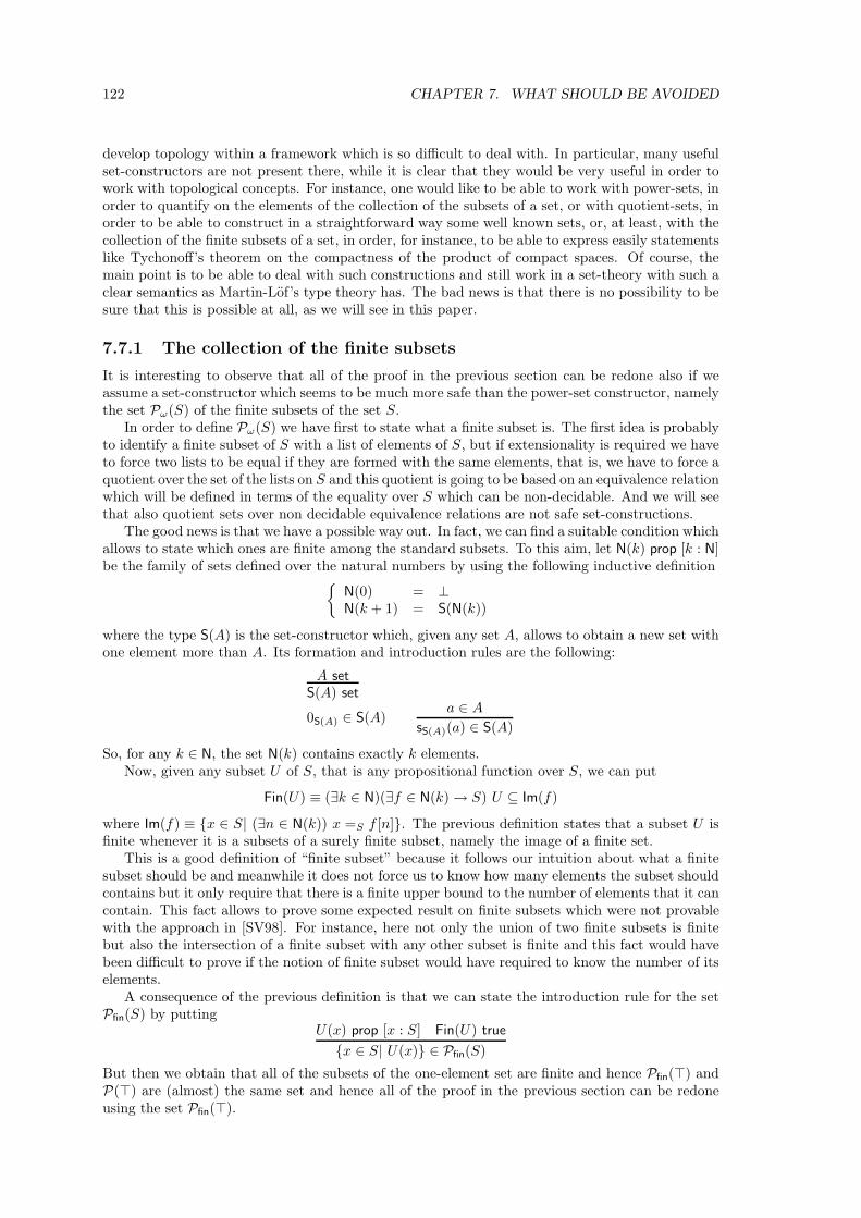
122 CHAPTER 7. WHAT SHOULD BE AVOIDED
develop topology within a framework which is so difficult to deal with. In particular, many usefulset-constructors are not present there, while it is clear that they would be very useful in order towork with topological concepts. For instance, one would like to be able to work with power-sets, inorder to quantify on the elements of the collection of the subsets of a set, or with quotient-sets, inorder to be able to construct in a straightforward way some well known sets, or, at least, with thecollection of the finite subsets of a set, in order, for instance, to be able to express easily statementslike Tychonoff’s theorem on the compactness of the product of compact spaces. Of course, themain point is to be able to deal with such constructions and still work in a set-theory with such aclear semantics as Martin-Lof’s type theory has. The bad news is that there is no possibility to besure that this is possible at all, as we will see in this paper.
7.7.1 The collection of the finite subsets
It is interesting to observe that all of the proof in the previous section can be redone also if weassume a set-constructor which seems to be much more safe than the power-set constructor, namelythe set Pω(S) of the finite subsets of the set S.
In order to define Pω(S) we have first to state what a finite subset is. The first idea is probablyto identify a finite subset of S with a list of elements of S, but if extensionality is required we haveto force two lists to be equal if they are formed with the same elements, that is, we have to force aquotient over the set of the lists on S and this quotient is going to be based on an equivalence relationwhich will be defined in terms of the equality over S which can be non-decidable. And we will seethat also quotient sets over non decidable equivalence relations are not safe set-constructions.
The good news is that we have a possible way out. In fact, we can find a suitable condition whichallows to state which ones are finite among the standard subsets. To this aim, let N(k) prop [k : N]be the family of sets defined over the natural numbers by using the following inductive definition
N(0) = ⊥N(k + 1) = S(N(k))
where the type S(A) is the set-constructor which, given any set A, allows to obtain a new set withone element more than A. Its formation and introduction rules are the following:
A set
S(A) set
0S(A) ∈ S(A)a ∈ A
sS(A)(a) ∈ S(A)
So, for any k ∈ N, the set N(k) contains exactly k elements.Now, given any subset U of S, that is any propositional function over S, we can put
Fin(U) ≡ (∃k ∈ N)(∃f ∈ N(k)→ S) U ⊆ Im(f)
where Im(f) ≡ x ∈ S| (∃n ∈ N(k)) x =S f [n]. The previous definition states that a subset U isfinite whenever it is a subsets of a surely finite subset, namely the image of a finite set.
This is a good definition of “finite subset” because it follows our intuition about what a finitesubset should be and meanwhile it does not force us to know how many elements the subset shouldcontains but it only require that there is a finite upper bound to the number of elements that it cancontain. This fact allows to prove some expected result on finite subsets which were not provablewith the approach in [SV98]. For instance, here not only the union of two finite subsets is finitebut also the intersection of a finite subset with any other subset is finite and this fact would havebeen difficult to prove if the notion of finite subset would have required to know the number of itselements.
A consequence of the previous definition is that we can state the introduction rule for the setPfin(S) by putting
U(x) prop [x : S] Fin(U) true
x ∈ S| U(x) ∈ Pfin(S)
But then we obtain that all of the subsets of the one-element set are finite and hence Pfin(⊤) andP(⊤) are (almost) the same set and hence all of the proof in the previous section can be redoneusing the set Pfin(⊤).
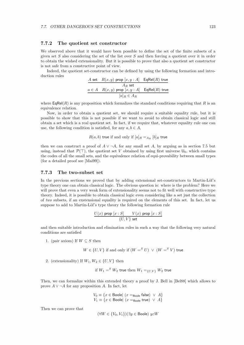
7.7. OTHER DANGEROUS SET CONSTRUCTIONS 123
7.7.2 The quotient set constructor
We observed above that it would have been possible to define the set of the finite subsets of agiven set S also considering the set of the list over S and then forcing a quotient over it in orderto obtain the wished extensionality. But it is possible to prove that also a quotient set constructoris not safe from a constructive point of view.
Indeed, the quotient set-constructor can be defined by using the following formation and intro-duction rules
A set R(x, y) prop [x, y : A] EqRel(R) true
AR seta ∈ A R(x, y) prop [x, y : A] EqRel(R) true
[a]R ∈ AR
where EqRel(R) is any proposition which formalizes the standard conditions requiring that R is anequivalence relation.
Now, in order to obtain a quotient set, we should require a suitable equality rule, but it ispossible to show that this is not possible if we want to avoid to obtain classical logic and stillobtain a set which is a real quotient set. In fact, if we require that, whatever equality rule one canuse, the following condition is satisfied, for any a, b ∈ A,
R(a, b) true if and only if [a]R =AR[b]R true
then we can construct a proof of A ∨ ¬A, for any small set A, by arguing as in section 7.5 butusing, instead that P(⊤), the quotient set V obtained by using first universe U0, which containsthe codes of all the small sets, and the equivalence relation of equi-provability between small types(for a detailed proof see [Mai99]).
7.7.3 The two-subset set
In the previous sections we proved that by adding extensional set-constructors to Martin-Lof’stype theory one can obtain classical logic. The obvious question is: where is the problem? Here wewill prove that even a very weak form of extensionality seems not to fit well with constructive typetheory. Indeed, it is possible to obtain classical logic even considering like a set just the collectionof two subsets, if an exstensional equality is required on the elements of this set. In fact, let ussuppose to add to Martin-Lof’s type theory the following formation rule
U(x) prop [x : S] V (x) prop [x : S]
U, V set
and then suitable introduction and elimination rules in such a way that the following very naturalconditions are satisfied
1. (pair axiom) If W ⊆ S then
W ∈ U, V if and only if (W =S U) ∨ (W =S V ) true
2. (extensionality) If W1, W2 ∈ U, V then
if W1 =S W2 true then W1 =U,V W2 true
Then, we can formalize within this extended theory a proof by J. Bell in [Bel88] which allows toprove A ∨ ¬A for any proposition A. In fact, let
V0 ≡ x ∈ Boole| (x =Boole false) ∨ AV1 ≡ x ∈ Boole| (x =Boole true) ∨ A
Then we can prove that
(∀W ∈ V0, V1)(∃y ∈ Boole) yεW
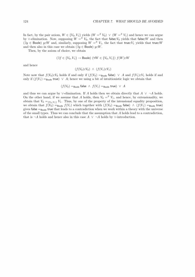
124 CHAPTER 7. WHAT SHOULD BE AVOIDED
In fact, by the pair axiom, W ∈ V0, V1 yields (W =S V0) ∨ (W =S V1) and hence we can argueby ∨-elimination. Now, supposing W =S V0, the fact that falseεV0 yields that falseεW and then(∃y ∈ Boole) yεW and, similarly, supposing W =S V1, the fact that trueεV1 yields that trueεWand then also in this case we obtain (∃y ∈ Boole) yεW .
Then, by the axiom of choice, we obtain
(∃f ∈ V0, V1 → Boole) (∀W ∈ V0, V1) f(W )εW
and hence(f(V0)εV0) ∧ (f(V1)εV1)
Note now that f(V0)εV0 holds if and only if (f(V0) =Boole false) ∨ A and f(V1)εV1 holds if andonly if (f(V1) =Boole true) ∨ A; hence we using a bit of intuitionistic logic we obtain that
(f(V0) =Boole false ∧ f(V1) =Boole true) ∨ A
and thus we can argue by ∨-elimination. If A holds then we obtain directly that A ∨ ¬A holds.On the other hand, if we assume that A holds, then V0 =S V1, and hence, by extensionality, weobtain that V0 =V0,V1 V1. Thus, by one of the property of the intensional equality proposition,we obtain that f(V0) =Boole f(V1) which together with (f(V0) =Boole false) ∧ (f(V1) =Boole true)gives false =Boole true that leads to a contradiction when we work within a theory with the universeof the small types. Thus we can conclude that the assumption that A holds lead to a contradiction,that is ¬A holds and hence also in this case A ∨ ¬A holds by ∨-introduction.
Appendix A
Expressions theory
A.1 The Expressions with arity
A.1.1 Introduction
Martin Lof’s type theory [Mar84, NPS90] has been exposed by giving, besides the conceptualmotivations, also a set of formal rules where types and their elements are denoted by expressionsbuild up from variables and constants by means of application (notation: b(a)) and abstraction(notation: ((x) b)). Moreover, the operational semantics of type theory is given by expressionmanipulations.
Since, in order to verify the correctness of the application of a rule we need, almost always, bothto recognize definitional equality between textual different expressions (that is, different denotationsof the same type) and to reduce expressions into equivalent ones (e.g a ⇒ ((x) a)(x)), we need aformal theory for expressions which deals with these problems at a level underlying type theory.Clearly pure lambda-calculus cannot be considered because of the undecidability of definitionalequality due to the possibility of self-application [Chu36]. Historically, to solve this problem, typedlambda-calculus [Bar84, CF74] has been introduced.
A similar approach has been followed by Martin-Lof [Mar83, NPS90] where an arity is asso-ciated to any expression in order to specify its functionality. The main difference with respectto standard typed lambda-calculus is in the use of abbreviating definitions which extend the lin-guistic expressiveness of expressions instead of lambda-abstraction. Definitions seem necessary tointroduce derived rules in type theory and their power is manifested by the ability to emulateabstraction.
Our approach is strongly related to Martin Lof’s one, but we give a different treatment ofdefinitions both to make them suitable for a mechanical treatment and to be able to analyze theconditions under which it is possible to develop a provable correct parsing algorithm for expressions.As a consequence other changes were needed and, for this reason, Martin-Lof has no responsibilityfor the following.
The chapter is organized as follows. In section A.2 you can find the definition of arity, thecharacterization of abbreviating definitions, the definition of the rules to form expressions witharity and the rules to prove that two expressions are definitionally equal.
In section A.3 some properties of the expression system previously defined are proved. In thissystem is easy to deal with both normal form and decidability of expressions: the notion of normalform is introduced very naturally and an algorithm to reduce any expression into an equivalentone in normal form is easy to develop and to prove correct.
In section A.4 we introduce new rules to form expressions and we prove that they are sufficientto form all of the expressions without introducing new ones. The new rules are introduced to meetthe requirements to obtain decidability of the predicate ‘to be an expression’.
Then, in section A.5, abstraction is introduced as a schema of abbreviating definitions and theconcepts of normal form and its principal properties are given.
Finally the relationships between the expression theory and the standard typed lambda-calculuswith α, β, η and ξ reductions is dealt with in section A.6.
125
126 APPENDIX A. EXPRESSIONS THEORY
A.2 Basic definitions
The formal definition of arity is the following.
Definition A.2.1 (Arity) An arity α is defined by induction as follows:
1. 0 is an arity
2. If α and β are two arities then (α)β is an arity.
0 will be the arity of expressions which cannot be applied, that is the saturated expressions. Weshall subsequently usually omit the rightmost 0 of an arity since this will not lead to ambiguity.
Arities are naturally ordered by the usual ordering on construction complexity and two aritiesare equal if and only if they are textually identical.
In the following we assume to have a set (possibly empty) of primitive constants with arityc− α and, for any arity α, an enumerable set of variables x1 − α, x2 − α, . . . Since we want thatany variable and any constant is recognizable with its unique arity we assume the decidability ofthe two predicates x − α var and c − α const whose reading is “x is a variable of arity α” and “cis a primitive constant of arity α” respectively. Moreover we assume the ability to recognize theoccurrences of a variable and of a primitive constant within a string.
We shall use the notation dx1, . . . , xn to stress that x1, . . . , xn are all the variables occurringwithin the string d.
A.2.1 Abbreviating definitions
The notion of abbreviating definition plays a central role in what follows. An abbreviating definitionis a binary relation on strings:
definiendum =def definiens
where the first element is called definiendum (what we are defining on) and the second one is calleddefiniens (what we assume to already have). We can think of the definiendum as a new denotationfor the object denoted by the definiens. The general form of a definiendum is
dx1, . . . , xn(y1) . . . (ym) n, m ≥ 0
where distinguishable, and declared, occurrences of the variables x1, . . . , xn (the name parameters)of arity α1, . . . , αn may appear inside the string d (the parametric name) and y1, . . . , ym (thearguments) are variables of arity β1, . . . , βm respectively.
We shall call definition skeleton the result of the substitution, within a parametric name, ofthe name-parameters by place-holders with arity; note that no variable appears inside a definitionskeleton.
Definitions must obey the following conditions:
1. (variables condition) The variables x1, . . . , xn, y1, . . . , ym are distinct from one another andcomprise all of the variables appearing in the definiens; moreover each xi occurs only once ind.
2. (non overlapping clause) If
dx1, . . . , xn(y1) . . . (ym) =def e1
where xi − αi var and yj − βj var, for i = 1, . . . , n and j = 1, . . . , m, and
dz1, . . . , zn(w1) . . . (ws) =def e2
where zi − αi var and wj − γj var, for i = 1, . . . , n and j = 1, . . . , s, are two definitions withthe same definition skeleton then
• s = m
• βj = γj for any j = 1, . . . , m
A.2. BASIC DEFINITIONS 127
• e2 is e1[z1, . . . , zn, w1, . . . , ws/x1, . . . , xn, y1, . . . , ym] where e[s1, . . . , sk/t1, . . . , tk] is theresult of the simultaneous textual substitution of the variables t1, . . . , tk of arities δ1,. . . , δk respectively, by the variables s1, . . . , sk of correspondent arities.
3. (recognizability) The occurrence of a definition skeleton within a string is recognizable.
Remarks
• Condition 2 does not avoid having “duplicate definitions” provided no ambiguity may arise.
• Condition 3 implies the ability to single out within a string all the sub-strings which havebeen substituted for the place-holders inside the definition skeleton.
• Since in a definition skeleton no variable appears a textual substitution of variables does notmodify it.
Examples:
1. Let x− 0 var, f − (0) 0 var, g − (0) 0 var then
[f ] [g](x) =def f(g(x))
is a definition: [f ] [g] is the parametric name, f and g are the name-parameters, [.] [.] is thedefinition skeleton and x the argument. The intention is to define the function “compositionof f and g”.
2. Let t− 0 var, x− 0 var, y − 0 var then
exchange[t](x)(y) =def begin t := x; x := y; y := t end
is the definition for a procedure performing the exchange between x and y.
Now we can formally define what an expression of arity α is by giving the rules to form ex-pressions. In the definition we will introduce the predicate a − α exp whose reading is “a is anexpression of arity α”. A fixed set D of abbreviating definition is assumed; to stress the dependencyon D the notation a− α expD may as well be used.
Definition A.2.2 (Expression of arity α)
1.x− (α1) . . . (αn)0 var a1 − α1 exp . . . an − αn exp
x(a1) . . . (an)− 0 expn ≥ 0
2.c− (α1) . . . (αn) 0 const a1 − α1 exp . . . an − αn exp
c(a1) . . . (an)− 0 expn ≥ 0
3.
dx1, . . . , xn(y1) . . . (ym) =def e e− 0 exp e[a, b/x, y]− 0 exp
xi − αi var yj − βj var ai − αi exp bj − βj exp
d[a1, . . . , an](b1) . . . (bm)− 0 expn ≥ 0, i = 1, . . . , n, m ≥ 0, j = 1, . . . , m
4.b(x)− β exp x− α var
b− (α) β expwhere the only occurrence of x in b(x) is the manifested one
Notations
• a abbreviates a1, . . . , an.
• e[a/x] is the result of the simultaneous textual substitution of the variables x by the expres-sions a within the expression e.
• d[a1, . . . , an] is a notation to denote the result of the simultaneous textual substitution ofthe variables x by the expressions a within the parametric name dx1, . . . , xn. We use thisnotation to stress that the expressions a must be recognizable inside the parametric name.
128 APPENDIX A. EXPRESSIONS THEORY
• d[a1, . . . , an] and d[a1, . . . , an](b1) . . . (bm) will be referred to as instance of a parametric nameand instance of a definiendum, respectively.
The notions of derivation and theorem are standard. We shall call depth of a derivation thelength of the longest branch in the derivation tree.
Remarks
• Rule 4. in the definition A.2.2 requires the ability to recognize where a variable occurs withina string b: we have always supposed to have it. Note that we can inductively define the setof variables that appears inside an expression following the formation rules:
V(x(a1) . . . (an)) = x ∪ V(a1) ∪ . . . ∪ V(an)
V(c(a1) . . . (an)) = V(a1) ∪ . . . ∪ V(an)
V(d[a1, . . . , an](b1) . . . (bm)) = V(a1) ∪ . . . ∪ V(an) ∪ V(b1) ∪ . . . ∪ V(bm)
V(b) = V(b(x))/x
In our approach we never introduce the notion of free and bound variables but we alwaysdeal with variables.
• An expression has one of the following shape
x(a1) . . . (ak) k ≥ 0
c(a1) . . . (ak) k ≥ 0
d[a1, . . . , an](b1) . . . (bk) k ≥ 0
• The derivation of an expression according to definition A.2.2 is uniquely determinable exceptfor the name of the variable (if rule 4. is applied) and the choice among duplicate definitions.This derives because of the demand to distinguish the occurrences of variables, primitiveconstants and definition skeletons within a string and, if rule 3. applies, the non overlappingclause assures that an instance of a parametric name always uniquely determines its definition.
• It is easy to see that rules 1. and 2. produce expressions, from old ones, by the use of appli-cation under the constrain of correct arity; rule 3. allows the use of abbreviating definition,under the condition that the definiens is an expression; rule 4. is the way to obtain a trueabstraction: here this system is different from a typed lambda-calculus where the abstractionis indicated; anyhow in section A.5 we will introduce a set of abbreviating definitions thatallow to indicated abstraction.
Expressions are just a syntactic vehicle to denote objects. A definiendum and its definiens mustclearly denote the same object and in this sense they have to be considered ‘equal’. To achieve thisresult we extend the textual identity on strings to an equality on expressions of the same arity.
Definition A.2.3 (Definitional equality)
1= x− (α1) . . . (αn)0 var a1 = b1 − α1 . . . an = bn − αn
x(a1) . . . (an) = x(b1) . . . (bn)− 0n ≥ 0
2= c− (α1) . . . (αn)0 const a1 = b1 − α1 . . . an = bn − αn
c(a1) . . . (an) = c(b1) . . . (bn)− 0n ≥ 0
3=i
dx1, . . . , xn(y1) . . . (ym) =def e e− 0 exp e[a, b/x, y] = c− 0xi − αi var yj − βj var ai − αi exp bj − βj exp
d[a1, . . . , an](b1) . . . (bm) = c− 0n ≥ 0, i = 1, . . . , n, m ≥ 0, j = 1, . . . , m
3=ii
dx1, . . . , xn(y1) . . . (ym) =def e e− 0 exp e[a, b/x, y] = c− 0x1 − αi var yj − βj var ai − αi exp bj − βj exp
c = d[a1, . . . , an](b1) . . . (bm)− 0n ≥ 0, i = 1, . . . , n, m ≥ 0, j = 1, . . . , m
4= b(x) = d(x) − β x− α var
b = d− (α) βwhere the only occurrence of x in b(x) and d(x) is the manifested one
A.3. SOME PROPERTIES OF THE EXPRESSIONS SYSTEM 129
Remarks
• If we have a derivation of a = b− α then it is possible to prove that a− α exp and b− α exp
(the proof is by induction on the depth of the derivation of a = b− α)
• It is meaningless to ask for equality between two strings unless they are known to be expres-sions of the same arity.
• The derivation of definitional equality between two expressions a and b is unique, but for thechoice of the name of the variable if rule 4= applies and for the choice of (i) or (ii) in rule3= if two instances of a definiendum are considered. This fact can be proved by induction onthe ‘sum’ of the depths of the derivations of a and b.
• It is easy to prove by induction on the depth of the derivation that = is an equivalencerelation. Now, by 3=
i , from a =def b it immediately follows a = b− 0.
Theorem A.2.4 (Decidability of the definitional equality) Let a and b be two expressionsof arity α, then the predicate a = b− α is decidable.
Proof. The proof readily follows by induction on the ‘sum’ of the depth of the derivations ofa− α exp and b− α exp.
Note that the same result could indirectly derive from the existence and unicity of normal formfor expressions (see section A.5).
A.3 Some properties of the expressions system
In this section some properties of the system of rules introduced in section A.2 are proved. Themain result is theorem A.3.4 which states its closure under substitution.
Theorem A.3.1 The following property holds for expressions with arity:
1. If x− α var then x− α exp.
2. If c− α const then c− α exp.
Proof. The proof of the first point is obtained by induction on the arity of the variable x. Afterthe first point has been proved, the proof of the second point is immediate.
Now we can prove that the system to form expressions is closed under textual substitution.First we will prove a stronger result in the case of substitution of a variable by a variable.
Lemma A.3.2 If c−γ exp, z−α var and y−α var then c[z/y]−γ exp is provable with a derivationof the same depth than the derivation of c− γ exp.
Proof. The proof can be obtained by induction on the depth of the derivation of c−γ exp. Anyhow,this lemma only states that we can obtain a derivation of c[z/y]−γ exp just by substituting all theoccurrences of y in the derivation of c− γ exp by z: the only condition required is that y and z arevariables of the same arity. Attention is required if c is of higher arity (γ1)γ2, that is it is obtained,by using rule 4., from c(x) − γ2 exp and x− γ1 var under the condition that x does not appear inc, and c indeed contains y. In this case it is necessary to avoid x being z: for this reason a renameof x in the derivation of c(x)− γ2 exp may be required (allowed by inductive hypothesis).
To obtain the proof of next theorem we need a new definition:
Definition A.3.3 (Arity of a substitution) Let b − β exp, ai − αi exp and xi − αi var, fori = 1, . . . , n. Then b[a/x] is obtained from b by a substitution of arity (α1) . . . (αn).
Now the main theorem on substitution follows.
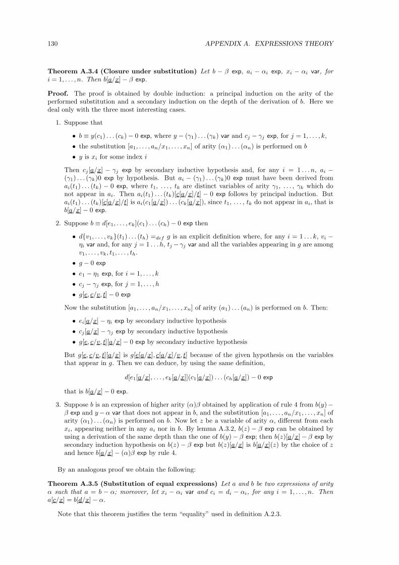
130 APPENDIX A. EXPRESSIONS THEORY
Theorem A.3.4 (Closure under substitution) Let b − β exp, ai − αi exp, xi − αi var, fori = 1, . . . , n. Then b[a/x]− β exp.
Proof. The proof is obtained by double induction: a principal induction on the arity of theperformed substitution and a secondary induction on the depth of the derivation of b. Here wedeal only with the three most interesting cases.
1. Suppose that
• b ≡ y(c1) . . . (ck)− 0 exp, where y − (γ1) . . . (γk) var and cj − γj exp, for j = 1, . . . , k,
• the substitution [a1, . . . , an/x1, . . . , xn] of arity (α1) . . . (αn) is performed on b
• y is xi for some index i
Then cj [a/x] − γj exp by secondary inductive hypothesis and, for any i = 1 . . . n, ai −(γ1) . . . (γk)0 exp by hypothesis. But ai − (γ1) . . . (γk)0 exp must have been derived fromai(t1) . . . (tk) − 0 exp, where t1, . . . , tk are distinct variables of arity γ1, . . . , γk which donot appear in ai. Then ai(t1) . . . (tk)[c[a/x]/t] − 0 exp follows by principal induction. Butai(t1) . . . (tk)[c[a/x]/t] is ai(c1[a/x]) . . . (ck[a/x]), since t1, . . . , tk do not appear in ai, that isb[a/x]− 0 exp.
2. Suppose b ≡ d[e1, . . . , ek](c1) . . . (ch)− 0 exp then
• dv1, . . . , vk(t1) . . . (th) =def g is an explicit definition where, for any i = 1 . . . k, vi −ηi var and, for any j = 1 . . . h, tj − γj var and all the variables appearing in g are amongv1, . . . , vk, t1, . . . , th.
• g − 0 exp
• e1 − η1 exp, for i = 1, . . . , k
• cj − γj exp, for j = 1, . . . , h
• g[e, c/v, t]− 0 exp
Now the substitution [a1, . . . , an/x1, . . . , xn] of arity (a1) . . . (an) is performed on b. Then:
• ei[a/x]− ηi exp by secondary inductive hypothesis
• cj [a/x]− γj exp by secondary inductive hypothesis
• g[e, c/v, t][a/x]− 0 exp by secondary inductive hypothesis
But g[e, c/v, t][a/x] is g[e[a/x], c[a/x]/v, t] because of the given hypothesis on the variablesthat appear in g. Then we can deduce, by using the same definition,
d[e1[a/x], . . . , ek[a/x]](c1[a/x]) . . . (ch[a/x])− 0 exp
that is b[a/x]− 0 exp.
3. Suppose b is an expression of higher arity (α)β obtained by application of rule 4 from b(y)−β exp and y−α var that does not appear in b, and the substitution [a1, . . . , an/x1, . . . , xn] ofarity (α1) . . . (αn) is performed on b. Now let z be a variable of arity α, different from eachxi, appearing neither in any ai nor in b. By lemma A.3.2, b(z) − β exp can be obtained byusing a derivation of the same depth than the one of b(y)− β exp; then b(z)[a/x]− β exp bysecondary induction hypothesis on b(z)− β exp but b(z)[a/x] is b[a/x](z) by the choice of zand hence b[a/x]− (α)β exp by rule 4.
By an analogous proof we obtain the following:
Theorem A.3.5 (Substitution of equal expressions) Let a and b be two expressions of arityα such that a = b − α; moreover, let xi − αi var and ci = di − αi, for any i = 1, . . . , n. Thena[c/x] = b[d/x]− α.
Note that this theorem justifies the term “equality” used in definition A.2.3.
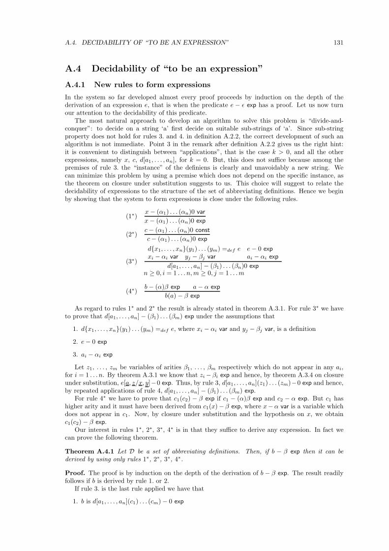
A.4. DECIDABILITY OF “TO BE AN EXPRESSION” 131
A.4 Decidability of “to be an expression”
A.4.1 New rules to form expressions
In the system so far developed almost every proof proceeds by induction on the depth of thederivation of an expression e, that is when the predicate e − ǫ exp has a proof. Let us now turnour attention to the decidability of this predicate.
The most natural approach to develop an algorithm to solve this problem is “divide-and-conquer”: to decide on a string ‘a’ first decide on suitable sub-strings of ‘a’. Since sub-stringproperty does not hold for rules 3. and 4. in definition A.2.2, the correct development of such analgorithm is not immediate. Point 3 in the remark after definition A.2.2 gives us the right hint:it is convenient to distinguish between “applications”, that is the case k > 0, and all the otherexpressions, namely x, c, d[a1, . . . , an], for k = 0. But, this does not suffice because among thepremises of rule 3. the “instance” of the definiens is clearly and unavoidably a new string. Wecan minimize this problem by using a premise which does not depend on the specific instance, asthe theorem on closure under substitution suggests to us. This choice will suggest to relate thedecidability of expressions to the structure of the set of abbreviating definitions. Hence we beginby showing that the system to form expressions is close under the following rules.
(1∗)x− (α1) . . . (αn)0 var
x− (α1) . . . (αn)0 exp
(2∗)c− (α1) . . . (αn)0 const
c− (α1) . . . (αn)0 exp
(3∗)
dx1, . . . , xn(y1) . . . (ym) =def e e− 0 exp
xi − αi var yj − βj var ai − αi exp
d[a1, . . . , an]− (β1) . . . (βn)0 expn ≥ 0, i = 1 . . . n, m ≥ 0, j = 1 . . .m
(4∗)b− (α)β exp a− α exp
b(a)− β exp
As regard to rules 1∗ and 2∗ the result is already stated in theorem A.3.1. For rule 3∗ we haveto prove that d[a1, . . . , an]− (β1) . . . (βm) exp under the assumptions that
1. dx1, . . . , xn(y1) . . . (ym) =def e, where xi − αi var and yj − βj var, is a definition
2. e− 0 exp
3. ai − αi exp
Let z1, . . . , zm be variables of arities β1, . . . , βm respectively which do not appear in any ai,for i = 1 . . . n. By theorem A.3.1 we know that zi− βi exp and hence, by theorem A.3.4 on closureunder substitution, e[a, z/x, y]−0 exp. Thus, by rule 3, d[a1, . . . , an](z1) . . . (zm)−0 exp and hence,by repeated applications of rule 4, d[a1, . . . , an]− (β1) . . . (βm) exp.
For rule 4∗ we have to prove that c1(c2) − β exp if c1 − (α)β exp and c2 − α exp. But c1 hashigher arity and it must have been derived from c1(x)− β exp, where x−α var is a variable whichdoes not appear in c1. Now, by closure under substitution and the hypothesis on x, we obtainc1(c2)− β exp.
Our interest in rules 1∗, 2∗, 3∗, 4∗ is in that they suffice to derive any expression. In fact wecan prove the following theorem.
Theorem A.4.1 Let D be a set of abbreviating definitions. Then, if b − β exp then it can bederived by using only rules 1∗, 2∗, 3∗, 4∗.
Proof. The proof is by induction on the depth of the derivation of b − β exp. The result readilyfollows if b is derived by rule 1. or 2.
If rule 3. is the last rule applied we have that
1. b is d[a1, . . . , an](c1) . . . (cm)− 0 exp
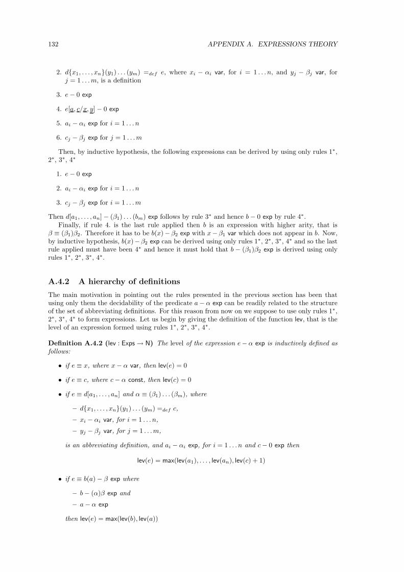
132 APPENDIX A. EXPRESSIONS THEORY
2. dx1, . . . , xn(y1) . . . (ym) =def e, where xi − αi var, for i = 1 . . . n, and yj − βj var, forj = 1 . . .m, is a definition
3. e− 0 exp
4. e[a, c/x, y]− 0 exp
5. ai − αi exp for i = 1 . . . n
6. cj − βj exp for j = 1 . . .m
Then, by inductive hypothesis, the following expressions can be derived by using only rules 1∗,2∗, 3∗, 4∗
1. e− 0 exp
2. ai − αi exp for i = 1 . . . n
3. cj − βj exp for i = 1 . . .m
Then d[a1, . . . , an]− (β1) . . . (bm) exp follows by rule 3∗ and hence b− 0 exp by rule 4∗.Finally, if rule 4. is the last rule applied then b is an expression with higher arity, that is
β ≡ (β1)β2. Therefore it has to be b(x)− β2 exp with x− β1 var which does not appear in b. Now,by inductive hypothesis, b(x)−β2 exp can be derived using only rules 1∗, 2∗, 3∗, 4∗ and so the lastrule applied must have been 4∗ and hence it must hold that b − (β1)β2 exp is derived using onlyrules 1∗, 2∗, 3∗, 4∗.
A.4.2 A hierarchy of definitions
The main motivation in pointing out the rules presented in the previous section has been thatusing only them the decidability of the predicate a− α exp can be readily related to the structureof the set of abbreviating definitions. For this reason from now on we suppose to use only rules 1∗,2∗, 3∗, 4∗ to form expressions. Let us begin by giving the definition of the function lev, that is thelevel of an expression formed using rules 1∗, 2∗, 3∗, 4∗.
Definition A.4.2 (lev : Exps→ N) The level of the expression e− α exp is inductively defined asfollows:
• if e ≡ x, where x− α var, then lev(e) = 0
• if e ≡ c, where c− α const, then lev(c) = 0
• if e ≡ d[a1, . . . , an] and α ≡ (β1) . . . (βm), where
– dx1, . . . , xn(y1) . . . (ym) =def c,
– xi − αi var, for i = 1 . . . n,
– yj − βj var, for j = 1 . . .m,
is an abbreviating definition, and ai − αi exp, for i = 1 . . . n and c− 0 exp then
lev(e) = max(lev(a1), . . . , lev(an), lev(c) + 1)
• if e ≡ b(a)− β exp where
– b− (α)β exp and
– a− α exp
then lev(e) = max(lev(b), lev(a))
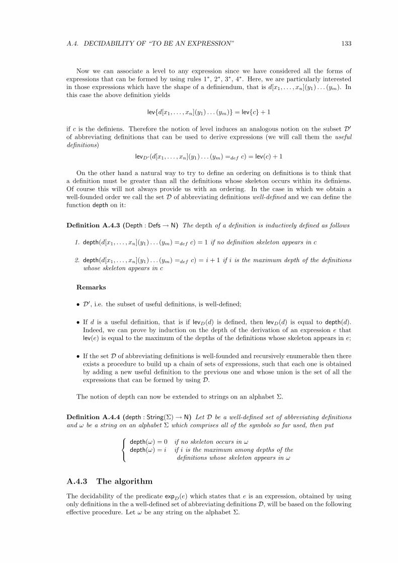
A.4. DECIDABILITY OF “TO BE AN EXPRESSION” 133
Now we can associate a level to any expression since we have considered all the forms ofexpressions that can be formed by using rules 1∗, 2∗, 3∗, 4∗. Here, we are particularly interestedin those expressions which have the shape of a definiendum, that is d[x1, . . . , xn](y1) . . . (ym). Inthis case the above definition yields
levd[x1, . . . , xn](y1) . . . (ym) = levc+ 1
if c is the definiens. Therefore the notion of level induces an analogous notion on the subset D′
of abbreviating definitions that can be used to derive expressions (we will call them the usefuldefinitions)
levD′(d[x1, . . . , xn](y1) . . . (ym) =def c) = lev(c) + 1
On the other hand a natural way to try to define an ordering on definitions is to think thata definition must be greater than all the definitions whose skeleton occurs within its definiens.Of course this will not always provide us with an ordering. In the case in which we obtain awell-founded order we call the set D of abbreviating definitions well-defined and we can define thefunction depth on it:
Definition A.4.3 (Depth : Defs→ N) The depth of a definition is inductively defined as follows
1. depth(d[x1, . . . , xn](y1) . . . (ym) =def c) = 1 if no definition skeleton appears in c
2. depth(d[x1, . . . , xn](y1) . . . (ym) =def c) = i + 1 if i is the maximum depth of the definitionswhose skeleton appears in c
Remarks
• D′, i.e. the subset of useful definitions, is well-defined;
• If d is a useful definition, that is if levD(d) is defined, then levD(d) is equal to depth(d).Indeed, we can prove by induction on the depth of the derivation of an expression e thatlev(e) is equal to the maximum of the depths of the definitions whose skeleton appears in e;
• If the set D of abbreviating definitions is well-founded and recursively enumerable then thereexists a procedure to build up a chain of sets of expressions, such that each one is obtainedby adding a new useful definition to the previous one and whose union is the set of all theexpressions that can be formed by using D.
The notion of depth can now be extended to strings on an alphabet Σ.
Definition A.4.4 (depth : String(Σ)→ N) Let D be a well-defined set of abbreviating definitionsand ω be a string on an alphabet Σ which comprises all of the symbols so far used, then put
depth(ω) = 0 if no skeleton occurs in ωdepth(ω) = i if i is the maximum among depths of the
definitions whose skeleton appears in ω
A.4.3 The algorithm
The decidability of the predicate expD(e) which states that e is an expression, obtained by usingonly definitions in the a well-defined set of abbreviating definitions D, will be based on the followingeffective procedure. Let ω be any string on the alphabet Σ.
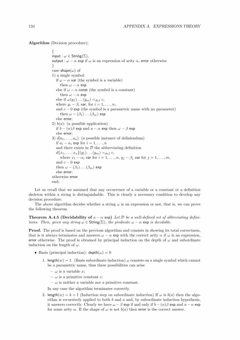
134 APPENDIX A. EXPRESSIONS THEORY
Algorithm (Decision procedure);
input : ω ∈ String(Σ),output : ω − α exp if ω is an expression of arity α, error otherwisecase shape(ω) of1) a single symbol:
if ω − α var (the symbol is a variable)then ω − α exp
else if ω − α const (the symbol is a constant)then ω − α exp
else if ω(y1) . . . (ym) =def c,where yi − βi var, for i = 1, . . . , n,and c− 0 exp (the symbol is a parametric name with no parameter)
then ω − (β1) . . . (βm) exp
else error;2) b(a): (a possible application)
if b− (α)β exp and a− α exp then ω − β exp
else error;3) d[a1, . . . , an]: (a possible instance of definiendum)
if ai − αi exp for i = 1, . . . , nand there exists in D the abbreviating definitiondx1, . . . , xn(y1) . . . (ym) =def c,
where x1 − αi var for i = 1, . . . , n, yj − βj var for j = 1, . . . , m,and c− 0 exp
then ω − (β1) . . . (βm) exp
else error;otherwise error
end;
Let us recall that we assumed that any occurrence of a variable or a constant or a definitionskeleton within a string is distinguishable. This is clearly a necessary condition to develop anydecision procedure.
The above algorithm decides whether a string ω is an expression or not, that is, we can provethe following theorem.
Theorem A.4.5 (Decidability of a− α exp) Let D be a well-defined set of abbreviating defini-tions. Then, given any string ω ∈ String(Σ), the predicate ω − α exp is decidable.
Proof. The proof is based on the previous algorithm and consists in showing its total correctness,that is it always terminates and answers ω − α exp with the correct arity α if ω is an expression,error otherwise. The proof is obtained by principal induction on the depth of ω and subordinateinduction on the length of ω.
• Basis (principal induction): depth(ω) = 0
1. length(w) = 1. (Basis subordinate induction) ω consists on a single symbol which cannotbe a parametric name, thus three possibilities can arise
– ω is a variable x;
– ω is a primitive constant c;
– ω is neither a variable nor a primitive constant.
In any case the algorithm terminates correctly.
2. length(w) = k + 1 (Induction step on subordinate induction) If ω is b(a) then the algo-rithm is recursively applied to both b and a and, by subordinate induction hypothesis,it answers correctly. Clearly we have ω− β exp if and only if b− (α)β exp and a−α exp
for some arity α. If the shape of ω is not b(a) then error is the correct answer.
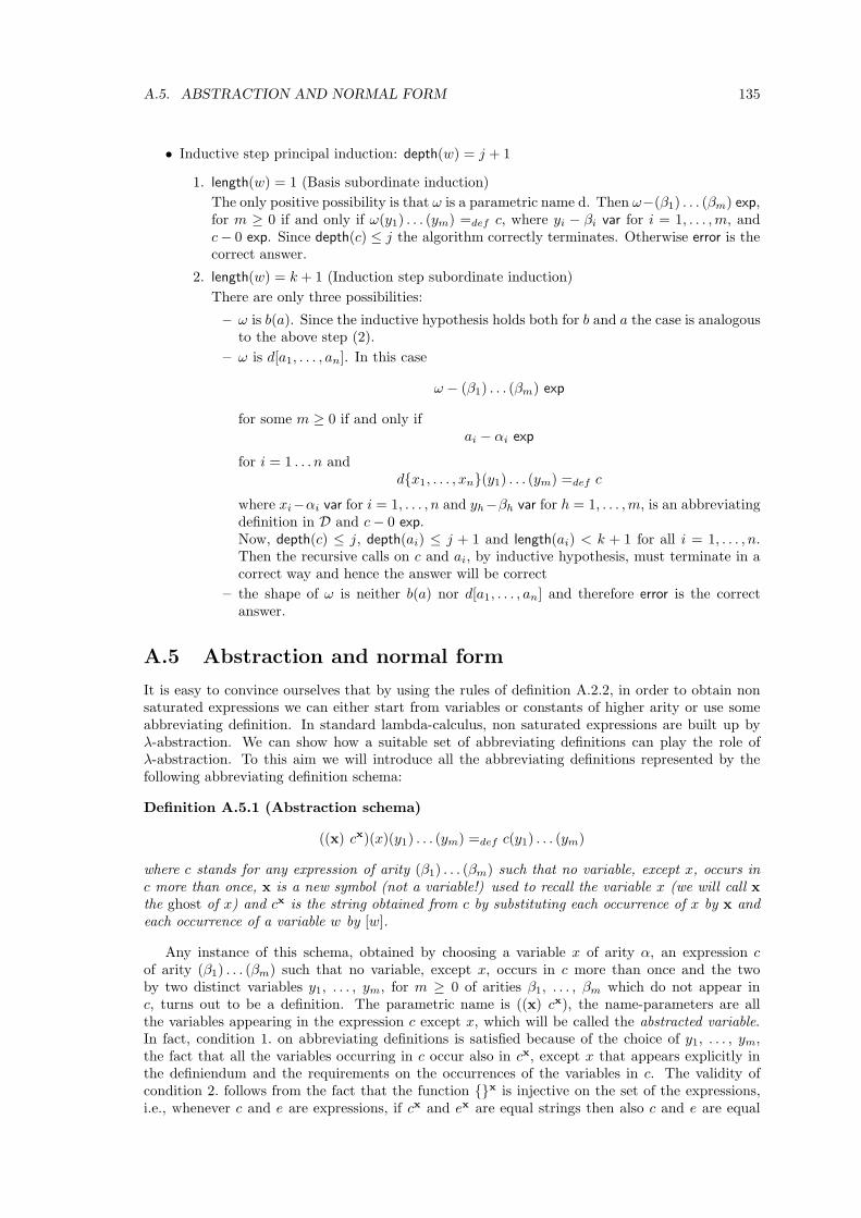
A.5. ABSTRACTION AND NORMAL FORM 135
• Inductive step principal induction: depth(w) = j + 1
1. length(w) = 1 (Basis subordinate induction)
The only positive possibility is that ω is a parametric name d. Then ω−(β1) . . . (βm) exp,for m ≥ 0 if and only if ω(y1) . . . (ym) =def c, where yi − βi var for i = 1, . . . , m, andc− 0 exp. Since depth(c) ≤ j the algorithm correctly terminates. Otherwise error is thecorrect answer.
2. length(w) = k + 1 (Induction step subordinate induction)
There are only three possibilities:
– ω is b(a). Since the inductive hypothesis holds both for b and a the case is analogousto the above step (2).
– ω is d[a1, . . . , an]. In this case
ω − (β1) . . . (βm) exp
for some m ≥ 0 if and only ifai − αi exp
for i = 1 . . . n anddx1, . . . , xn(y1) . . . (ym) =def c
where xi−αi var for i = 1, . . . , n and yh−βh var for h = 1, . . . , m, is an abbreviatingdefinition in D and c− 0 exp.Now, depth(c) ≤ j, depth(ai) ≤ j + 1 and length(ai) < k + 1 for all i = 1, . . . , n.Then the recursive calls on c and ai, by inductive hypothesis, must terminate in acorrect way and hence the answer will be correct
– the shape of ω is neither b(a) nor d[a1, . . . , an] and therefore error is the correctanswer.
A.5 Abstraction and normal form
It is easy to convince ourselves that by using the rules of definition A.2.2, in order to obtain nonsaturated expressions we can either start from variables or constants of higher arity or use someabbreviating definition. In standard lambda-calculus, non saturated expressions are built up byλ-abstraction. We can show how a suitable set of abbreviating definitions can play the role ofλ-abstraction. To this aim we will introduce all the abbreviating definitions represented by thefollowing abbreviating definition schema:
Definition A.5.1 (Abstraction schema)
((x) cx)(x)(y1) . . . (ym) =def c(y1) . . . (ym)
where c stands for any expression of arity (β1) . . . (βm) such that no variable, except x, occurs inc more than once, x is a new symbol (not a variable!) used to recall the variable x (we will call xthe ghost of x) and cx is the string obtained from c by substituting each occurrence of x by x andeach occurrence of a variable w by [w].
Any instance of this schema, obtained by choosing a variable x of arity α, an expression cof arity (β1) . . . (βm) such that no variable, except x, occurs in c more than once and the twoby two distinct variables y1, . . . , ym, for m ≥ 0 of arities β1, . . . , βm which do not appear inc, turns out to be a definition. The parametric name is ((x) cx), the name-parameters are allthe variables appearing in the expression c except x, which will be called the abstracted variable.In fact, condition 1. on abbreviating definitions is satisfied because of the choice of y1, . . . , ym,the fact that all the variables occurring in c occur also in cx, except x that appears explicitly inthe definiendum and the requirements on the occurrences of the variables in c. The validity ofcondition 2. follows from the fact that the function x is injective on the set of the expressions,i.e., whenever c and e are expressions, if cx and ex are equal strings then also c and e are equal
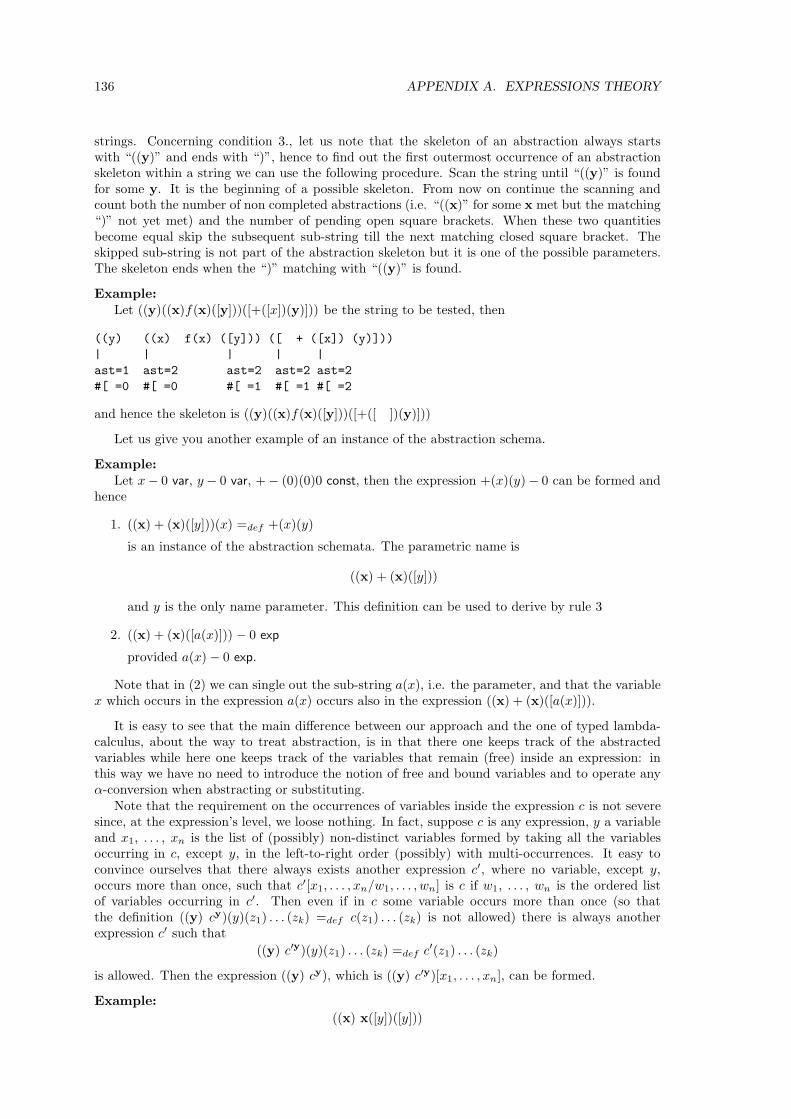
136 APPENDIX A. EXPRESSIONS THEORY
strings. Concerning condition 3., let us note that the skeleton of an abstraction always startswith “((y)” and ends with “)”, hence to find out the first outermost occurrence of an abstractionskeleton within a string we can use the following procedure. Scan the string until “((y)” is foundfor some y. It is the beginning of a possible skeleton. From now on continue the scanning andcount both the number of non completed abstractions (i.e. “((x)” for some x met but the matching“)” not yet met) and the number of pending open square brackets. When these two quantitiesbecome equal skip the subsequent sub-string till the next matching closed square bracket. Theskipped sub-string is not part of the abstraction skeleton but it is one of the possible parameters.The skeleton ends when the “)” matching with “((y)” is found.
Example:Let ((y)((x)f(x)([y]))([+([x])(y)])) be the string to be tested, then
((y) ((x) f(x) ([y])) ([ + ([x]) (y)]))
| | | | |
ast=1 ast=2 ast=2 ast=2 ast=2
#[ =0 #[ =0 #[ =1 #[ =1 #[ =2
and hence the skeleton is ((y)((x)f(x)([y]))([+([ ])(y)]))
Let us give you another example of an instance of the abstraction schema.
Example:Let x− 0 var, y − 0 var, +− (0)(0)0 const, then the expression +(x)(y)− 0 can be formed and
hence
1. ((x) + (x)([y]))(x) =def +(x)(y)
is an instance of the abstraction schemata. The parametric name is
((x) + (x)([y]))
and y is the only name parameter. This definition can be used to derive by rule 3
2. ((x) + (x)([a(x)])) − 0 exp
provided a(x)− 0 exp.
Note that in (2) we can single out the sub-string a(x), i.e. the parameter, and that the variablex which occurs in the expression a(x) occurs also in the expression ((x) + (x)([a(x)])).
It is easy to see that the main difference between our approach and the one of typed lambda-calculus, about the way to treat abstraction, is in that there one keeps track of the abstractedvariables while here one keeps track of the variables that remain (free) inside an expression: inthis way we have no need to introduce the notion of free and bound variables and to operate anyα-conversion when abstracting or substituting.
Note that the requirement on the occurrences of variables inside the expression c is not severesince, at the expression’s level, we loose nothing. In fact, suppose c is any expression, y a variableand x1, . . . , xn is the list of (possibly) non-distinct variables formed by taking all the variablesoccurring in c, except y, in the left-to-right order (possibly) with multi-occurrences. It easy toconvince ourselves that there always exists another expression c′, where no variable, except y,occurs more than once, such that c′[x1, . . . , xn/w1, . . . , wn] is c if w1, . . . , wn is the ordered listof variables occurring in c′. Then even if in c some variable occurs more than once (so thatthe definition ((y) cy)(y)(z1) . . . (zk) =def c(z1) . . . (zk) is not allowed) there is always anotherexpression c′ such that
((y) c′y)(y)(z1) . . . (zk) =def c′(z1) . . . (zk)
is allowed. Then the expression ((y) cy), which is ((y) c′y)[x1, . . . , xn], can be formed.
Example:
((x) x([y])([y]))
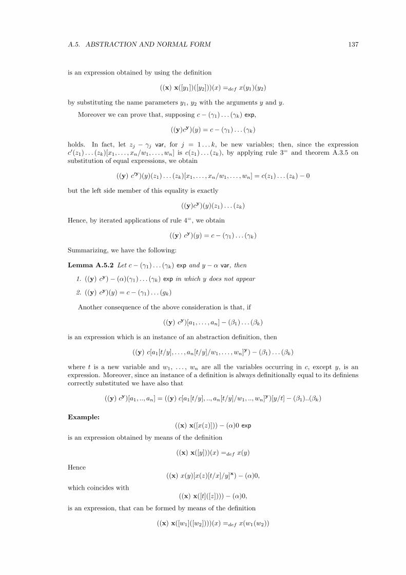
A.5. ABSTRACTION AND NORMAL FORM 137
is an expression obtained by using the definition
((x) x([y1])([y2]))(x) =def x(y1)(y2)
by substituting the name parameters y1, y2 with the arguments y and y.
Moreover we can prove that, supposing c− (γ1) . . . (γk) exp,
((y)cy)(y) = c− (γ1) . . . (γk)
holds. In fact, let zj − γj var, for j = 1 . . . k, be new variables; then, since the expressionc′(z1) . . . (zk)[x1, . . . , xn/w1, . . . , wn] is c(z1) . . . (zk), by applying rule 3= and theorem A.3.5 onsubstitution of equal expressions, we obtain
((y) c′y)(y)(z1) . . . (zk)[x1, . . . , xn/w1, . . . , wn] = c(z1) . . . (zk)− 0
but the left side member of this equality is exactly
((y)cy)(y)(z1) . . . (zk)
Hence, by iterated applications of rule 4=, we obtain
((y) cy)(y) = c− (γ1) . . . (γk)
Summarizing, we have the following:
Lemma A.5.2 Let c− (γ1) . . . (γk) exp and y − α var, then
1. ((y) cy)− (α)(γ1) . . . (γk) exp in which y does not appear
2. ((y) cy)(y) = c− (γ1) . . . (gk)
Another consequence of the above consideration is that, if
((y) cy)[a1, . . . , an]− (β1) . . . (βk)
is an expression which is an instance of an abstraction definition, then
((y) c[a1[t/y], . . . , an[t/y]/w1, . . . , wn]y)− (β1) . . . (βk)
where t is a new variable and w1, . . . , wn are all the variables occurring in c, except y, is anexpression. Moreover, since an instance of a definition is always definitionally equal to its definienscorrectly substituted we have also that
((y) cy)[a1, .., an] = ((y) c[a1[t/y], .., an[t/y]/w1, .., wn]y)[y/t]− (β1)..(βk)
Example:((x) x([x(z)])) − (α)0 exp
is an expression obtained by means of the definition
((x) x([y]))(x) =def x(y)
Hence((x) x(y)[x(z)[t/x]/y]x)− (α)0,
which coincides with((x) x([t]([z]))) − (α)0,
is an expression, that can be formed by means of the definition
((x) x([w1]([w2])))(x) =def x(w1(w2))
138 APPENDIX A. EXPRESSIONS THEORY
Then
((x) x([t(z)])) = ((x) x([t]([z])))− (α)0
since
x(y)[x(z), s/y, x] ≡ x(w1(w2))[x, z, s/w1, w2, x]
where s− (α)0 var is a new variable.
From now on, we assume to derive expressions within a system on a set D of definitions whichcomprises all of the instances of the abstraction schema, unless otherwise stated.
RemarkThe use of the above schema of abbreviating definition does not affect the decidability of the
predicate a − α exp. In fact, the only problem can derive from the fact that at point 3 of thedecision algorithm we require the ability to recognize an instance of a definiendum. So, let ussuppose that ((x) b) is the string which must be analyzed. We already showed how to single outthe definition skeleton. The possible parameter a1, . . . , an are just the sub-strings skipped in thatprocess. They must be first substituted inside the skeleton by new variables x1, . . . , xn whosearity is determined by the arity of the expressions a1, . . . , an. Then, to single out the definition(indeed we will find out one definition among a set of duplicate definitions) we have first to invertthe function x. This can be done by cutting off the square brackets immediately around the newvariables and by substituting x, that is the ghost of x, by x unless it occurs within the skeletonof an inner abstraction with the same ghost. Secondly we have to decide on the resulting stringwhich is “simpler” than the initial one. If it is an expression a of arity (β1) . . . (βm) the definitionwe were looking for is ((x) b)(x)(y1) . . . (ym) =def a(y1) . . . (ym).
Example:Suppose that x − 0 var, f − (0)((0)) const, + − (0)(0) const and that we want to analyze the
string
((x) ((x) f(x)([((x) + (x)([x]))]))).
First we look for the skeleton of the outermost abstraction “((x) . . .)”: it is the entire string
((x) ((x) f(x)([((x) + (x)([x]))])))
Now, we must invert the function x on
((x) f(x)([((x) + (x)([x]))]))
and we obtain the string((x) f(x)([((x) + (x)([x]))]))
Then we recursively continue by analyzing this resulting string and finally we obtain
((x) f(x)([((x) + (x)([x]))])) − (0) exp
Therefore the definition we are looking for is
((x) ((x) f(x)([((x) + (x)([x]))])))(x)(s) =def ((x) f(x)([((x) + (x)([x]))]))(s)
A.5.1 α, β, η and ξ conversion
When all the instances of the abstraction schema had been introduced, we can prove the validityof equality analogous to those introduced by α, β, η, ξ reductions of lambda-calculus. In fact,after lemma A.5.2, we know that, for any expression c of arity γ and any variable x of arity α,((x) cx)(x) = c− γ. Hence
Theorem A.5.3 (α-equality) Suppose c−γ exp and y−α var is a variable which does not appearin c. Then
(α-equality) ((x) cx) = ((y) c[y/x]y)− (α)γ
A.5. ABSTRACTION AND NORMAL FORM 139
Proof. By lemma A.5.2
((y) c[y/x]y)(y) = c[y/x]− γ
Then by the theorem on substitution of equal expressions
((y) c[y/x]y)(y)[x/y] = c[y/x][x/y]− γ
which yields
((y) c[y/x]y)(x) = c− γ
since y appears neither in ((y) c[y/x]y) nor in c.
But c = ((x) cx)(x)− γ and hence ((y) c[y/x]y)(x) = ((x) cx)(x)− γ by transitivity. Thus wefinally obtain
((y) c[y/x]y) = ((x) cx)− (α)γ
by rule 4=, since x appears neither in ((x) cx) nor in ((y) c[y/x]y).
Theorem A.5.4 (β-equality) Suppose c− γ exp and a− α exp. Then
(β-equality) ((x) cx)(a) = c[a/x]− γ
Proof. The result follows directly from lemma A.5.2 and theorem A.3.5.
Theorem A.5.5 (η-equality) Let c− (α)γ exp and x− α var which does not appear in c. Then
(η-equality) ((x) c(x)x) = c− (α)γ
Proof. By lemma A.5.2 we obtain that
((x) c(x)x)(x) = c(x) − γ
Hence by rule 4=
((x) c(x)x) = c− (α)γ
since x appears neither in c nor in ((x) c(x)x).
Theorem A.5.6 (ξ-equality) Suppose that b − γ exp, d − γ exp, x − α var and that b = d − γ.Then
(ξ-equality) ((x) bx) = ((x) dx)− (α)γ
Proof. By lemma A.5.2
((x) bx)(x) = b − γ
and
((x) dx)(x) = d− γ
Thus, by transitivity,
((x) bx)(x) = ((x) dx)(x) − γ
and finally
((x) bx) = ((x) dx)− (α)γ
by rule 4= since x appears neither in ((x) bx) nor in ((x) dx).
140 APPENDIX A. EXPRESSIONS THEORY
A.5.2 Normal form
Let us introduce the concept of normal form for an expression. The definition will be given byinduction on the construction of the expression.
Definition A.5.7 (Normal form) Let a be an expression. Then
1. If a has arity 0 then it is in normal form if its shape is
f(b1) . . . (bm)
where f is a variable or a primitive constant of arity (β1) . . . (βm)0 and, for any j = 1 . . .m,bj is an expression in normal form of arity βj.
2. If a has arity (α)β then it is in normal form if its shape is
((x) cx)
where x− α var and c is an expression of arity β in normal form.
Note that, given any expression e, there always exists at least an expression nf(e) in normalform which is definitional equivalent to e. The following algorithm can be used to find it out.
Algorithm (Normalization algorithm)
1. Suppose that the arity of e is (α)β. Then it has been obtained by an application of rule 4.Now, let x be a variable of arity α which does not appear in e. Then
nf(e) ≡ ((x) nf(e(x))x)
2. Suppose that the arity of e is 0 and that it has been obtained by using rule 3, that is
e ≡ d[a1, . . . , an](b1) . . . (bm)
for some abbreviating definition dx1, . . . , xn(y1) . . . (ym) =def c. Then
nf(e) ≡ nf(c[a, b/x, y])
3. Suppose that the arity of e is 0 and that it has been obtained by using the rule 1 or 2, thatis, e ≡ f(b1) . . . (bm), where f is a variable or a primitive constant of arity (β1) . . . (βm) andbj − βj exp, for j = 1 . . .m. Then
nf(e) ≡ f(nf(b1)) . . . (nf(bm))
The proof that this algorithm preserves definitional equality is obtained by induction on thedepth of the derivation of the expression e. A sketch of the proof is the following:
Case 1. By theorem A.5.2((x) nf(e(x))x)(x) = nf(e(x)) − β
But, by inductive hypothesis, nf(e(x)) = e(x)− β and so, by transitivity and rule 4,
((x) nf(e(x))x) = e− (α)β
Case 2. By inductive hypothesisnf(c[a, b/x, y]) = c[a, b/x, y]− 0
but, by rule 3=i ,
c[a, b/x, y] = d[a1, . . . , an](b1) . . . (bm)− 0
Case 3. Immediate by inductive hypothesis.
A.6. RELATION WITH TYPED λ-CALCULUS 141
Moreover the algorithm always terminates because at each step a ‘simpler’ (with respect toderivation) expression is considered. Finally it is straightforward to check that the final shape isthe required one.
It is easy to see that an expression in normal form contain no definition, a part abstraction,hence we can state the following theorem about definition elimination.
Theorem A.5.8 (Definition elimination) Let a be any expression. Then, there exists an ex-pression nf(a), equivalent to a, in which no definition appears, except abstraction.
We can also prove that the normal form is a good representative for the class of definitionalequivalent expressions. Let us first prove the following lemma.
Lemma A.5.9 If Π is the proof of ((x) cx) = ((y) ey) − (α)β then there is a proof Π∗ ofc[t/x] = e[t/y]− β, whose depth is less that the depth of Π.
The proof consist just in constructing Π∗, by analyzing the proof Π.
Theorem A.5.10 (Unicity of normal form) Let a and b be two expressions in normal form.Then a = b − α implies that a and b have the same pattern, that is, they differ only for the nameof the abstracted variables.
Proof. The proof proceeds by induction on the depth of the derivation of a = b − α, using theprevious lemma in the case two abstractions are considered. Now the following corollary easilyfollows.
Corollary A.5.11 Two expressions are definitionally equivalent if and only if they have the samenormal form (except for the name of abstracted variables).
A.6 Relation with typed λ-calculus
In this section we examine the relationship between our expressions and standard typed lambda-calculus. We will consider expressions on a set of abbreviating definitions which comprise only allthe instances of the abstraction schema. We will not give complete proofs of the stated theoremssince they are standard or can easily be reconstructed.
Since a lot of slightly different formulations of typed lambda-calculus can be found in theliterature, here we expose the one that we will use and some of its properties we are interested in.
Definition A.6.1 (Systemλ) We will call Systemλ the set of strings which we obtain by the fol-lowing inductive definition:
1λ
x− (α1) . . . (αn) var
x− (α1) . . . (αn) expλFV(x) = x
2λ
c− (α1) . . . (αn) const
c− (α1) . . . (αn) expλFV(c) = ∅
3λ
b− (α)β expλ a− α expλ
b(a)− α expλFV(b(a)) = FV(b) ∪ FV(a)
4λ
b− β expλ x− α var
((x) b)− (α)β expλFV(((x)b)) = FV(b)− x
We will use the convention to use different names for different variables: by this convention wewill avoid to say “let x− α var and y − α var and x 6= y . . .”.
The substitution of a variable with a λ-expression within a λ-expression is defined in the usualway.
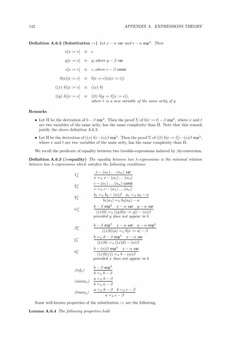
142 APPENDIX A. EXPRESSIONS THEORY
Definition A.6.2 (Substitution :=) Let x− α var and e− α expλ. Then
x[x := e] ≡ e
y[x := e] ≡ y,where y − β var
c[x := e] ≡ c,where c− β const
b(a)[x := e] ≡ b[x := e](a[x := e])
((x) b)[x := e] ≡ ((x) b)
((y) b)[x := e] ≡ ((t) b[y := t][x := e]),where t is a new variable of the same arity of y
Remarks
• Let Π be the derivation of b− β expλ. Then the proof Σ of b[x := t]− β expλ, where x and tare two variables of the same arity, has the same complexity than Π. Note that this remarkjustify the above definition A.6.2.
• Let Π be the derivation of ((x) b)−(α)β expλ. Then the proof Σ of ((t) b[x := t])−(α)β expλ,where x and t are two variables of the same arity, has the same complexity than Π.
We recall the predicate of equality between two lambda-expressions induced by βη-conversion.
Definition A.6.3 (λ-equality) The equality between two λ-expressions is the minimal relationbetween two λ-expressions which satisfies the following conditions:
1=λ
x− (α1) . . . (αn) var
x =λ x− (α1) . . . (αn)
2=λ
c− (α1) . . . (αn) const
c =λ c− (α1) . . . (αn)
3=λ
b1 =λ b2 − (α)β a1 =λ a2 − α
b1(a1) =λ b2(a2)− α
α=λ
b− β expλ x− α var y − α var
((x)b) =λ ((y)b[x := y])− (α)βprovided y does not appear in b
β=λ
b− β expλ x− α var a− α expλ
((x)b)(a) =λ b[x := a]− β
ξ=λ
b =λ d− β expλ x− α var
((x)b) =λ ((x)d) − (α)β
η=λ
b− (α)β expλ x− α var
((x)b(x)) =λ b− (α)βprovided x does not appear in b
(refλ)b− β expλ
b =λ b− β
(simmλ)a =λ b− β
b =λ a− β
(transλ)a =λ b− β b =λ c− β
a =λ c− β
Some well-known properties of the substitution := are the following.
Lemma A.6.4 The following properties hold
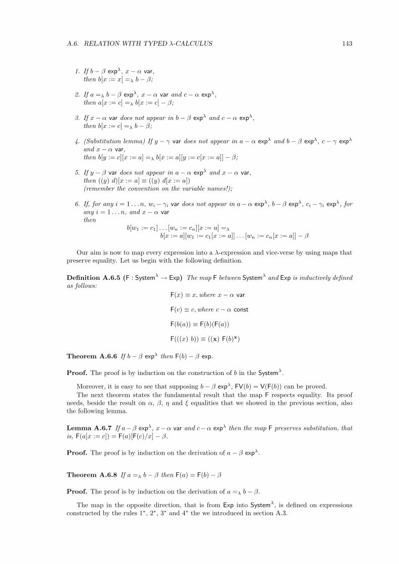
A.6. RELATION WITH TYPED λ-CALCULUS 143
1. If b − β expλ, x− α var,then b[x := x] =λ b− β;
2. If a =λ b− β expλ, x− α var and c− α expλ,then a[x := c] =λ b[x := c]− β;
3. If x− α var does not appear in b − β expλ and c− α expλ,then b[x := c] =λ b− β;
4. (Substitution lemma) If y − γ var does not appear in a− α expλ and b − β expλ, c− γ expλ
and x− α var,then b[y := c][x := a] =λ b[x := a][y := c[x := a]]− β;
5. If y − β var does not appear in a− α expλ and x− α var,then ((y) d)[x := a] ≡ ((y) d[x := a])(remember the convention on the variable names!);
6. If, for any i = 1 . . . n, wi− γi var does not appear in a−α expλ, b− β expλ, ci− γi expλ, forany i = 1 . . . n, and x− α var
thenb[w1 := c1] . . . [wn := cn][x := a] =λ
b[x := a][w1 := c1[x := a]] . . . [wn := cn[x := a]]− β
Our aim is now to map every expression into a λ-expression and vice-verse by using maps thatpreserve equality. Let us begin with the following definition.
Definition A.6.5 (F : Systemλ → Exp) The map F between Systemλ and Exp is inductively definedas follows:
F(x) ≡ x,where x− α var
F(c) ≡ c,where c− α const
F(b(a)) ≡ F(b)(F(a))
F(((x) b)) ≡ ((x) F(b)x)
Theorem A.6.6 If b− β expλ then F(b)− β exp.
Proof. The proof is by induction on the construction of b in the Systemλ.
Moreover, it is easy to see that supposing b− β expλ, FV(b) = V(F(b)) can be proved.
The next theorem states the fundamental result that the map F respects equality. Its proofneeds, beside the result on α, β, η and ξ equalities that we showed in the previous section, alsothe following lemma.
Lemma A.6.7 If a−β expλ, x−α var and c−α expλ then the map F preserves substitution, thatis, F(a[x := c]) = F(a)[F(c)/x] − β.
Proof. The proof is by induction on the derivation of a− β expλ.
Theorem A.6.8 If a =λ b− β then F(a) = F(b)− β
Proof. The proof is by induction on the derivation of a =λ b − β.
The map in the opposite direction, that is from Exp into Systemλ, is defined on expressionsconstructed by the rules 1∗, 2∗, 3∗ and 4∗ the we introduced in section A.3.
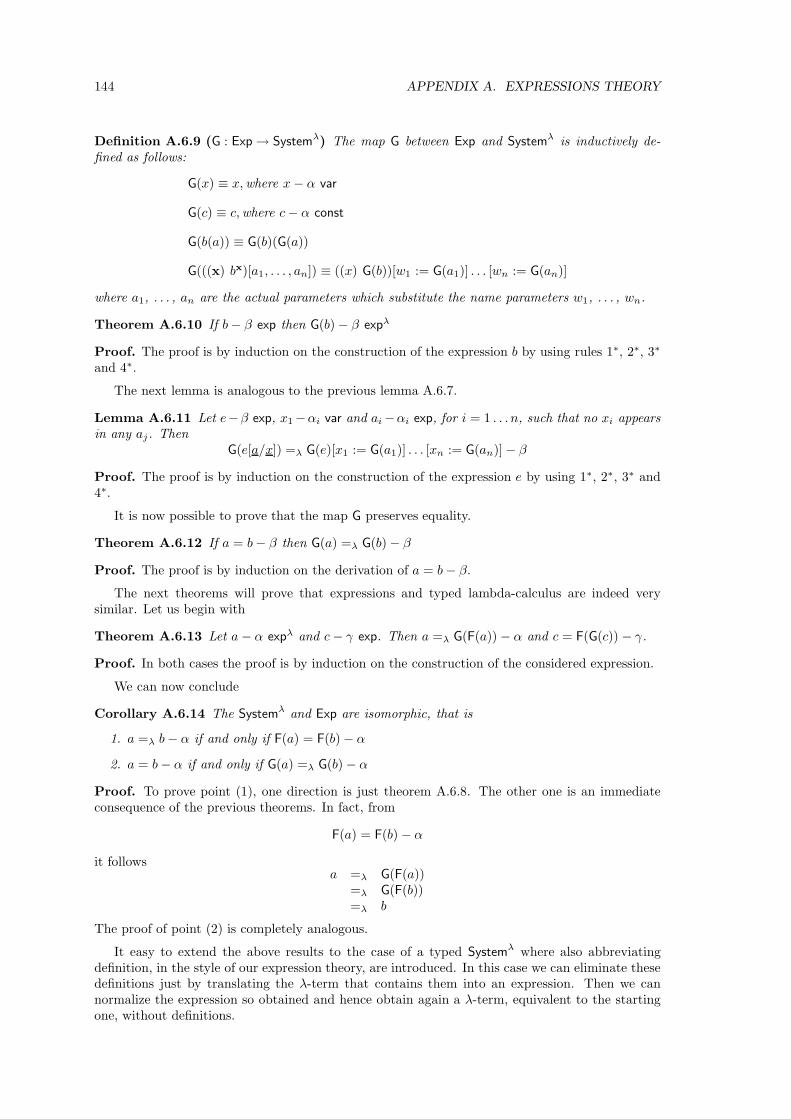
144 APPENDIX A. EXPRESSIONS THEORY
Definition A.6.9 (G : Exp→ Systemλ) The map G between Exp and Systemλ is inductively de-fined as follows:
G(x) ≡ x,where x− α var
G(c) ≡ c,where c− α const
G(b(a)) ≡ G(b)(G(a))
G(((x) bx)[a1, . . . , an]) ≡ ((x) G(b))[w1 := G(a1)] . . . [wn := G(an)]
where a1, . . . , an are the actual parameters which substitute the name parameters w1, . . . , wn.
Theorem A.6.10 If b− β exp then G(b)− β expλ
Proof. The proof is by induction on the construction of the expression b by using rules 1∗, 2∗, 3∗
and 4∗.
The next lemma is analogous to the previous lemma A.6.7.
Lemma A.6.11 Let e−β exp, x1−αi var and ai−αi exp, for i = 1 . . . n, such that no xi appearsin any aj. Then
G(e[a/x]) =λ G(e)[x1 := G(a1)] . . . [xn := G(an)]− β
Proof. The proof is by induction on the construction of the expression e by using 1∗, 2∗, 3∗ and4∗.
It is now possible to prove that the map G preserves equality.
Theorem A.6.12 If a = b− β then G(a) =λ G(b)− β
Proof. The proof is by induction on the derivation of a = b− β.
The next theorems will prove that expressions and typed lambda-calculus are indeed verysimilar. Let us begin with
Theorem A.6.13 Let a− α expλ and c− γ exp. Then a =λ G(F(a)) − α and c = F(G(c)) − γ.
Proof. In both cases the proof is by induction on the construction of the considered expression.
We can now conclude
Corollary A.6.14 The Systemλ and Exp are isomorphic, that is
1. a =λ b− α if and only if F(a) = F(b)− α
2. a = b− α if and only if G(a) =λ G(b)− α
Proof. To prove point (1), one direction is just theorem A.6.8. The other one is an immediateconsequence of the previous theorems. In fact, from
F(a) = F(b)− α
it followsa =λ G(F(a))
=λ G(F(b))=λ b
The proof of point (2) is completely analogous.
It easy to extend the above results to the case of a typed Systemλ where also abbreviatingdefinition, in the style of our expression theory, are introduced. In this case we can eliminate thesedefinitions just by translating the λ-term that contains them into an expression. Then we cannormalize the expression so obtained and hence obtain again a λ-term, equivalent to the startingone, without definitions.
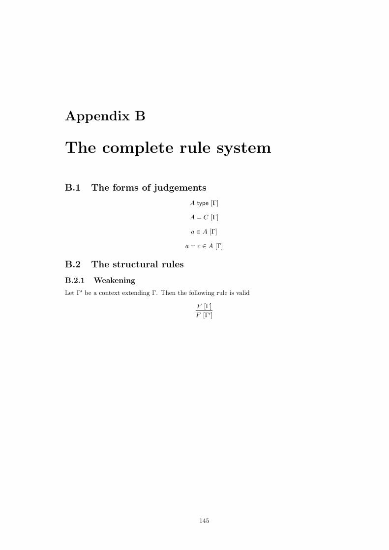
Appendix B
The complete rule system
B.1 The forms of judgements
A type [Γ]
A = C [Γ]
a ∈ A [Γ]
a = c ∈ A [Γ]
B.2 The structural rules
B.2.1 Weakening
Let Γ′ be a context extending Γ. Then the following rule is valid
F [Γ]
F [Γ′]
145
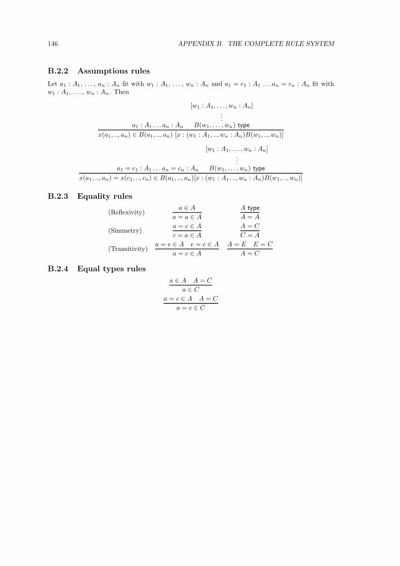
146 APPENDIX B. THE COMPLETE RULE SYSTEM
B.2.2 Assumptions rules
Let a1 : A1, . . . , an : An fit with w1 : A1, . . . , wn : An and a1 = c1 : A1 . . . an = cn : An fit withw1 : A1, . . . , wn : An. Then
a1 : A1 . . . an : An
[w1 : A1, . . . , wn : An]...
B(w1, . . . , wn) type
x(a1, .., an) ∈ B(a1, .., an) [x : (w1 : A1, .., wn : An)B(w1, .., wn)]
a1 = c1 : A1 . . . an = cn : An
[w1 : A1, . . . , wn : An]...
B(w1, . . . , wn) type
x(a1, .., an) = x(c1, .., cn) ∈ B(a1, .., an)[x : (w1 : A1, .., wn : An)B(w1, .., wn)]
B.2.3 Equality rules
(Reflexivity)a ∈ A
a = a ∈ A
A type
A = A
(Simmetry)a = c ∈ A
c = a ∈ A
A = C
C = A
(Transitivity)a = e ∈ A e = c ∈ A
a = c ∈ A
A = E E = C
A = C
B.2.4 Equal types rules
a ∈ A A = C
a ∈ C
a = c ∈ A A = C
a = c ∈ C
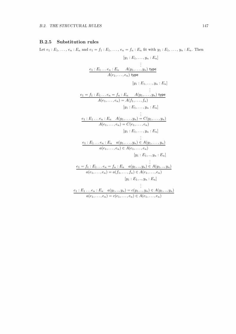
B.2. THE STRUCTURAL RULES 147
B.2.5 Substitution rules
Let e1 : E1, . . . , en : En and e1 = f1 : E1, . . . , en = fn : En fit with y1 : E1, . . . , yn : En. Then
e1 : E1 . . . en : En
[y1 : E1, . . . , yn : En]...
A(y1, . . . , yn) type
A(e1, . . . , en) type
e1 = f1 : E1 . . . en = fn : En
[y1 : E1, . . . , yn : En]...
A(y1, . . . , yn) type
A(e1, . . . , en) = A(f1, . . . , fn)
e1 : E1 . . . en : En
[y1 : E1, . . . , yn : En]...
A(y1, . . . , yn) = C(y1, . . . , yn)
A(e1, . . . , en) = C(e1, . . . , en)
e1 : E1 . . . en : En
[y1 : E1, . . . , yn : En]...
a(y1, . . . , yn) ∈ A(y1, . . . , yn)
a(e1, . . . , en) ∈ A(e1, . . . , en)
e1 = f1 : E1 . . . en = fn : En
[y1 : E1, .., yn : En]...
a(y1, .., yn) ∈ A(y1, .., yn)
a(e1, . . . , en) = a(f1, . . . , fn) ∈ A(e1, . . . , en)
e1 : E1 . . . en : En
[y1 : E1, .., yn : En]...
a(y1, .., yn) = c(y1, .., yn) ∈ A(y1, .., yn)
a(e1, . . . , en) = c(e1, . . . , en) ∈ A(e1, . . . , en)
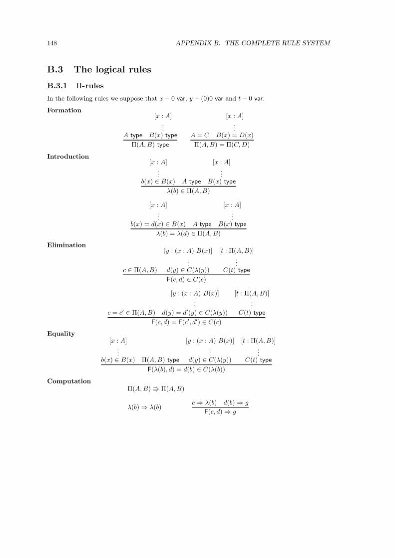
148 APPENDIX B. THE COMPLETE RULE SYSTEM
B.3 The logical rules
B.3.1 Π-rules
In the following rules we suppose that x− 0 var, y − (0)0 var and t− 0 var.
Formation
A type
[x : A]...
B(x) type
Π(A, B) type
A = C
[x : A]...
B(x) = D(x)
Π(A, B) = Π(C, D)
Introduction[x : A]
...b(x) ∈ B(x) A type
[x : A]...
B(x) type
λ(b) ∈ Π(A, B)
[x : A]...
b(x) = d(x) ∈ B(x) A type
[x : A]...
B(x) type
λ(b) = λ(d) ∈ Π(A, B)
Elimination
c ∈ Π(A, B)
[y : (x : A) B(x)]...
d(y) ∈ C(λ(y))
[t : Π(A, B)]...
C(t) type
F(c, d) ∈ C(c)
c = c′ ∈ Π(A, B)
[y : (x : A) B(x)]...
d(y) = d′(y) ∈ C(λ(y))
[t : Π(A, B)]...
C(t) type
F(c, d) = F(c′, d′) ∈ C(c)
Equality[x : A]
...b(x) ∈ B(x) Π(A, B) type
[y : (x : A) B(x)]...
d(y) ∈ C(λ(y))
[t : Π(A, B)]...
C(t) type
F(λ(b), d) = d(b) ∈ C(λ(b))
ComputationΠ(A, B) Π(A, B)
λ(b)⇒ λ(b)c⇒ λ(b) d(b)⇒ g
F(c, d)⇒ g
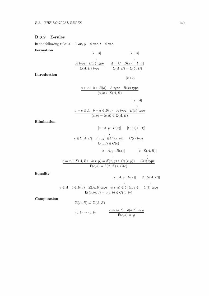
B.3. THE LOGICAL RULES 149
B.3.2 Σ-rules
In the following rules x− 0 var, y − 0 var, t− 0 var.
Formation
A type
[x : A]...
B(x) type
Σ(A, B) type
A = C
[x : A]...
B(x) = D(x)
Σ(A, B) = Σ(C, D)
Introduction
a ∈ A b ∈ B(a) A type
[x : A]...
B(x) type
〈a, b〉 ∈ Σ(A, B)
a = c ∈ A b = d ∈ B(a) A type
[x : A]...
B(x) type
〈a, b〉 = 〈c, d〉 ∈ Σ(A, B)
Elimination
c ∈ Σ(A, B)
[x : A, y : B(x)]...
d(x, y) ∈ C(〈x, y〉)
[t : Σ(A, B)]...
C(t) type
E(c, d) ∈ C(c)
c = c′ ∈ Σ(A, B)
[x : A, y : B(x)]...
d(x, y) = d′(x, y) ∈ C(〈x, y〉)
[t : Σ(A, B)]...
C(t) type
E(c, d) = E(c′, d′) ∈ C(c)
Equality
a ∈ A b ∈ B(a) Σ(A, B)type
[x : A, y : B(x)]...
d(x, y) ∈ C(〈x, y〉)
[t : S(A, B)]...
C(t) type
E(〈a, b〉, d) = d(a, b) ∈ C(〈a, b〉)
ComputationΣ(A, B) Σ(A, B)
〈a, b〉 ⇒ 〈a, b〉c⇒ 〈a, b〉 d(a, b)⇒ g
E(c, d)⇒ g
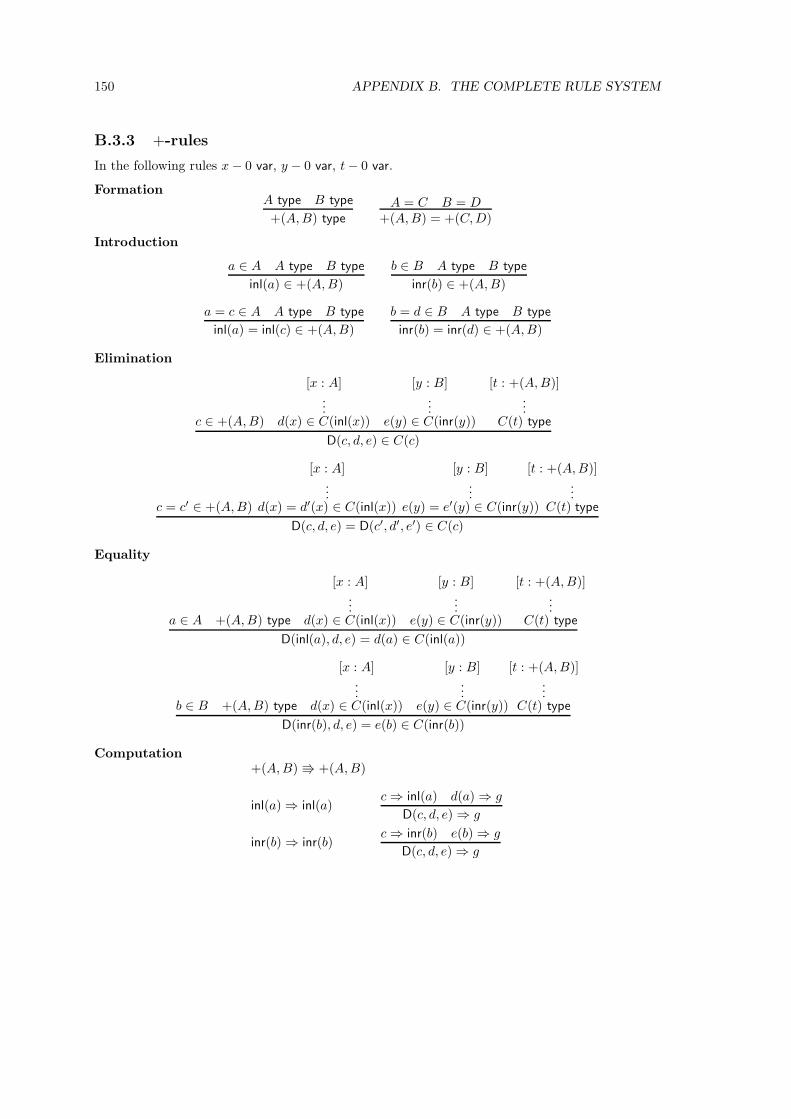
150 APPENDIX B. THE COMPLETE RULE SYSTEM
B.3.3 +-rules
In the following rules x− 0 var, y − 0 var, t− 0 var.
FormationA type B type
+(A, B) type
A = C B = D+(A, B) = +(C, D)
Introduction
a ∈ A A type B type
inl(a) ∈ +(A, B)
b ∈ B A type B type
inr(b) ∈ +(A, B)
a = c ∈ A A type B type
inl(a) = inl(c) ∈ +(A, B)
b = d ∈ B A type B type
inr(b) = inr(d) ∈ +(A, B)
Elimination
c ∈ +(A, B)
[x : A]...
d(x) ∈ C(inl(x))
[y : B]...
e(y) ∈ C(inr(y))
[t : +(A, B)]...
C(t) type
D(c, d, e) ∈ C(c)
c = c′ ∈ +(A, B)
[x : A]...
d(x) = d′(x) ∈ C(inl(x))
[y : B]...
e(y) = e′(y) ∈ C(inr(y))
[t : +(A, B)]...
C(t) type
D(c, d, e) = D(c′, d′, e′) ∈ C(c)
Equality
a ∈ A +(A, B) type
[x : A]...
d(x) ∈ C(inl(x))
[y : B]...
e(y) ∈ C(inr(y))
[t : +(A, B)]...
C(t) type
D(inl(a), d, e) = d(a) ∈ C(inl(a))
b ∈ B +(A, B) type
[x : A]...
d(x) ∈ C(inl(x))
[y : B]...
e(y) ∈ C(inr(y))
[t : +(A, B)]...
C(t) type
D(inr(b), d, e) = e(b) ∈ C(inr(b))
Computation+(A, B) +(A, B)
inl(a)⇒ inl(a)c⇒ inl(a) d(a)⇒ g
D(c, d, e)⇒ g
inr(b)⇒ inr(b)c⇒ inr(b) e(b)⇒ g
D(c, d, e)⇒ g
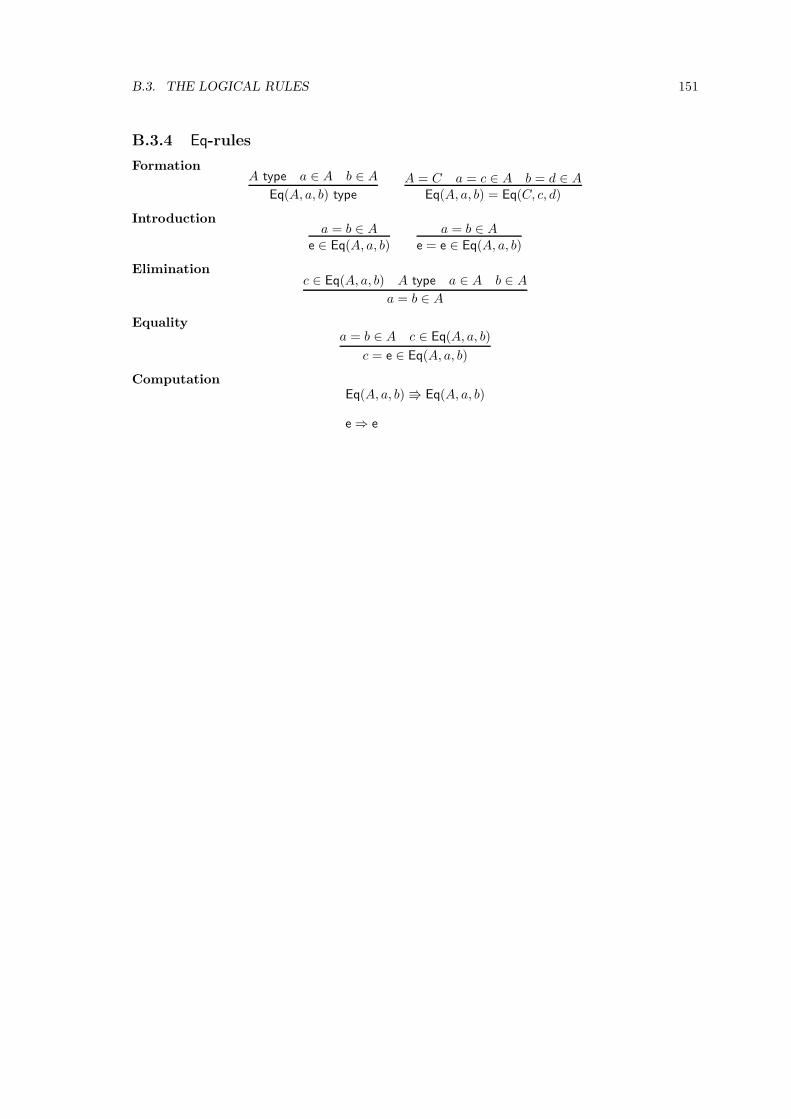
B.3. THE LOGICAL RULES 151
B.3.4 Eq-rules
FormationA type a ∈ A b ∈ A
Eq(A, a, b) type
A = C a = c ∈ A b = d ∈ AEq(A, a, b) = Eq(C, c, d)
Introductiona = b ∈ A
e ∈ Eq(A, a, b)a = b ∈ A
e = e ∈ Eq(A, a, b)
Eliminationc ∈ Eq(A, a, b) A type a ∈ A b ∈ A
a = b ∈ A
Equalitya = b ∈ A c ∈ Eq(A, a, b)
c = e ∈ Eq(A, a, b)
ComputationEq(A, a, b) Eq(A, a, b)
e⇒ e
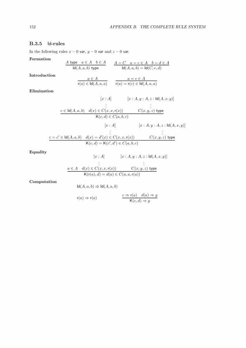
152 APPENDIX B. THE COMPLETE RULE SYSTEM
B.3.5 Id-rules
In the following rules x− 0 var, y − 0 var and z − 0 var.
FormationA type a ∈ A b ∈ A
Id(A, a, b) type
A = C a = c ∈ A b = d ∈ AId(A, a, b) = Id(C, c, d)
Introductiona ∈ A
r(a) ∈ Id(A, a, a)a = c ∈ A
r(a) = r(c) ∈ Id(A, a, a)
Elimination
c ∈ Id(A, a, b)
[x : A]...
d(x) ∈ C(x, x, r(x))
[x : A, y : A, z : Id(A, x, y)]...
C(x, y, z) type
K(c, d) ∈ C(a, b, c)
c = c′ ∈ Id(A, a, b)
[x : A]...
d(x) = d′(x) ∈ C(x, x, r(x))
[x : A, y : A, z : Id(A, x, y)]...
C(x, y, z) type
K(c, d) = K(c′, d′) ∈ C(a, b, c)
Equality
a ∈ A
[x : A]...
d(x) ∈ C(x, x, r(x))
[x : A, y : A, z : Id(A, x, y)]...
C(x, y, z) type
K(r(a), d) = d(a) ∈ C(a, a, r(a))
ComputationId(A, a, b) Id(A, a, b)
r(a)⇒ r(a)c⇒ r(a) d(a)⇒ g
K(c, d)⇒ g
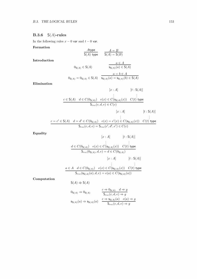
B.3. THE LOGICAL RULES 153
B.3.6 S(A)-rules
In the following rules x− 0 var and t− 0 var.
FormationAtype
S(A) type
A = BS(A) = S(B)
Introduction
0S(A) ∈ S(A)a ∈ A
sS(A)(a) ∈ S(A)
0S(A) = 0S(A) ∈ S(A)a = b ∈ A
sS(A)(a) = sS(A)(b) ∈ S(A)
Elimination
c ∈ S(A) d ∈ C(0S(A))
[x : A]...
e(x) ∈ C(sS(A)(x))
[t : S(A)]...
C(t) type
Srec(c, d, e) ∈ C(c)
c = c′ ∈ S(A) d = d′ ∈ C(0S(A))
[x : A]...
e(x) = e′(x) ∈ C(sS(A)(x))
[t : S(A)]...
C(t) type
Srec(c, d, e) = Srec(c′, d′, e′) ∈ C(c)
Equality
d ∈ C(0S(A))
[x : A]...
e(x) ∈ C(sS(A)(x))
[t : S(A)]...
C(t) type
Srec(0S(A), d, e) = d ∈ C(0S(A))
a ∈ A d ∈ C(0S(A))
[x : A]...
e(x) ∈ C(sS(A)(x))
[t : S(A)]...
C(t) type
Srec(sS(A)(a), d, e) = e(a) ∈ C(sS(A)(a))
ComputationS(A) S(A)
0S(A) ⇒ 0S(A)
c⇒ 0S(A) d⇒ g
Srec(c, d, e)⇒ g
sS(A)(a)⇒ sS(A)(a)c⇒ sS(A)(a) e(a)⇒ g
Srec(c, d, e)⇒ g
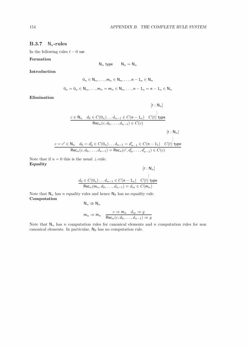
154 APPENDIX B. THE COMPLETE RULE SYSTEM
B.3.7 Nn-rules
In the following rules t− 0 var.
FormationNn type Nn = Nn
Introduction
0n ∈ Nn, . . . , mn ∈ Nn, . . . , n− 1n ∈ Nn
0n = 0n ∈ Nn, . . . , mn = mn ∈ Nn, . . . , n− 1n = n− 1n ∈ Nn
Elimination
c ∈ Nn d0 ∈ C(0n) . . . dn−1 ∈ C(n− 1n)
[t : Nn]...
C(t) type
Recn(c, d0, . . . , dn−1) ∈ C(c)
c = c′ ∈ Nn d0 = d′0 ∈ C(0n) . . . dn−1 = d′n−1 ∈ C(n− 11)
[t : Nn]...
C(t) type
Recn(c, d0, . . . , dn−1) = Recn(c′, d′0, . . . , d′n−1) ∈ C(c)
Note that if n = 0 this is the usual ⊥-rule.Equality
d0 ∈ C(0n) . . . dn−1 ∈ C(n− 1n)
[t : Nn]...
C(t) type
Recn(mn, d0, . . . , dn−1) = dm ∈ C(mn)
Note that Nn has n equality rules and hence N0 has no equality rule.Computation
Nn Nn
mn ⇒ mn
c⇒ mn dm ⇒ g
Recn(c, d0, . . . , dn−1)⇒ g
Note that Nn has n computation rules for canonical elements and n computation rules for noncanonical elements. In particular, N0 has no computation rule.
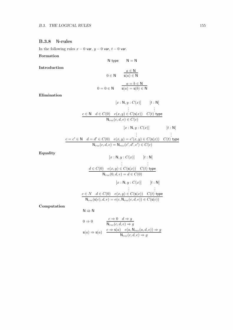
B.3. THE LOGICAL RULES 155
B.3.8 N-rules
In the following rules x− 0 var, y − 0 var, t− 0 var.
FormationN type N = N
Introduction
0 ∈ N
a ∈ N
s(a) ∈ N
0 = 0 ∈ N
a = b ∈ N
s(a) = s(b) ∈ N
Elimination
c ∈ N d ∈ C(0)
[x : N, y : C(x)]...
e(x, y) ∈ C(s(x))
[t : N]...
C(t) type
Nrec(c, d, e) ∈ C(c)
c = c′ ∈ N d = d′ ∈ C(0)
[x : N, y : C(x)]...
e(x, y) = e′(x, y) ∈ C(s(x))
[t : N]...
C(t) type
Nrec(c, d, e) = Nrec(c′, d′, e′) ∈ C(c)
Equality
d ∈ C(0)
[x : N, y : C(x)]...
e(x, y) ∈ C(s(x))
[t : N]...
C(t) type
Nrec(0, d, e) = d ∈ C(0)
c ∈ N d ∈ C(0)
[x : N, y : C(x)]...
e(x, y) ∈ C(s(x))
[t : N]...
C(t) type
Nrec(s(c), d, e) = e(c, Nrec(c, d, e)) ∈ C(s(c))
ComputationN N
0⇒ 0c⇒ 0 d⇒ g
Nrec(c, d, e)⇒ g
s(a)⇒ s(a)c⇒ s(a) e(a, Nrec(a, d, e))⇒ g
Nrec(c, d, e)⇒ g
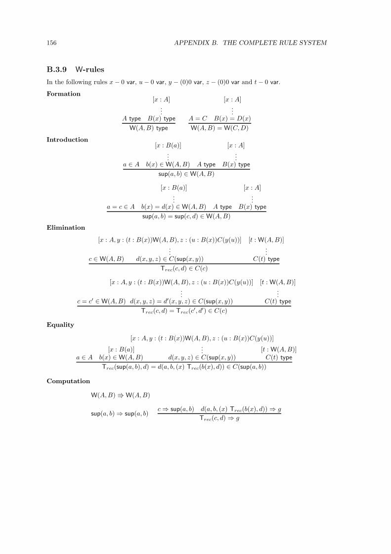
156 APPENDIX B. THE COMPLETE RULE SYSTEM
B.3.9 W-rules
In the following rules x− 0 var, u− 0 var, y − (0)0 var, z − (0)0 var and t− 0 var.
Formation
A type
[x : A]...
B(x) type
W(A, B) type
A = C
[x : A]...
B(x) = D(x)
W(A, B) = W(C, D)
Introduction
a ∈ A
[x : B(a)]...
b(x) ∈W(A, B) A type
[x : A]...
B(x) type
sup(a, b) ∈ W(A, B)
a = c ∈ A
[x : B(a)]...
b(x) = d(x) ∈W(A, B) A type
[x : A]...
B(x) type
sup(a, b) = sup(c, d) ∈W(A, B)
Elimination
c ∈ W(A, B)
[x : A, y : (t : B(x))W(A, B), z : (u : B(x))C(y(u))]...
d(x, y, z) ∈ C(sup(x, y))
[t : W(A, B)]...
C(t) type
Trec(c, d) ∈ C(c)
c = c′ ∈W(A, B)
[x : A, y : (t : B(x))W(A, B), z : (u : B(x))C(y(u))]...
d(x, y, z) = d′(x, y, z) ∈ C(sup(x, y))
[t : W(A, B)]...
C(t) type
Trec(c, d) = Trec(c′, d′) ∈ C(c)
Equality
a ∈ A[x : B(a)]
b(x) ∈W(A, B)
[x : A, y : (t : B(x))W(A, B), z : (u : B(x))C(y(u))]...
d(x, y, z) ∈ C(sup(x, y))[t : W(A, B)]
C(t) type
Trec(sup(a, b), d) = d(a, b, (x) Trec(b(x), d)) ∈ C(sup(a, b))
Computation
W(A, B) W(A, B)
sup(a, b)⇒ sup(a, b)c⇒ sup(a, b) d(a, b, (x) Trec(b(x), d))⇒ g
Trec(c, d)⇒ g
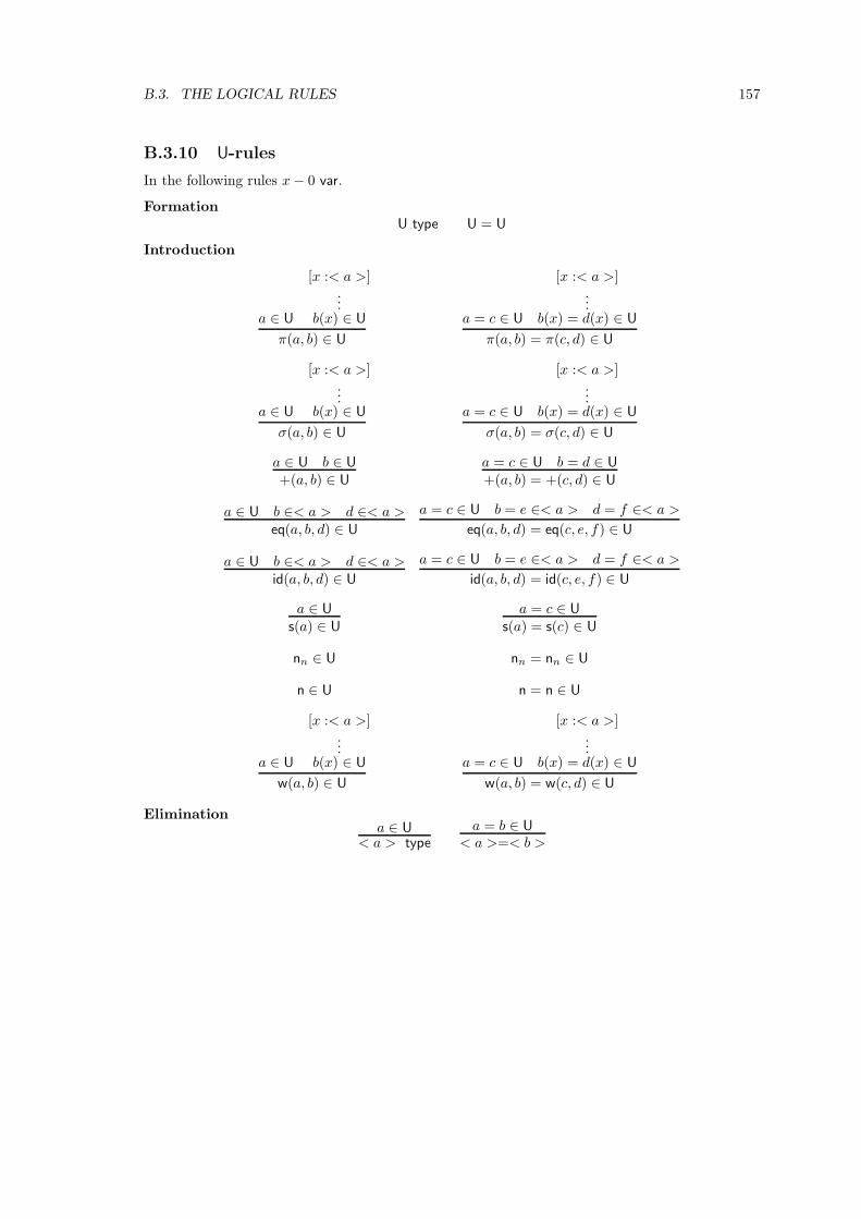
B.3. THE LOGICAL RULES 157
B.3.10 U-rules
In the following rules x− 0 var.
FormationU type U = U
Introduction
a ∈ U
[x :< a >]...
b(x) ∈ U
π(a, b) ∈ U
a = c ∈ U
[x :< a >]...
b(x) = d(x) ∈ U
π(a, b) = π(c, d) ∈ U
a ∈ U
[x :< a >]...
b(x) ∈ U
σ(a, b) ∈ U
a = c ∈ U
[x :< a >]...
b(x) = d(x) ∈ U
σ(a, b) = σ(c, d) ∈ U
a ∈ U b ∈ U
+(a, b) ∈ U
a = c ∈ U b = d ∈ U
+(a, b) = +(c, d) ∈ U
a ∈ U b ∈< a > d ∈< a >eq(a, b, d) ∈ U
a = c ∈ U b = e ∈< a > d = f ∈< a >
eq(a, b, d) = eq(c, e, f) ∈ U
a ∈ U b ∈< a > d ∈< a >id(a, b, d) ∈ U
a = c ∈ U b = e ∈< a > d = f ∈< a >
id(a, b, d) = id(c, e, f) ∈ U
a ∈ U
s(a) ∈ U
a = c ∈ U
s(a) = s(c) ∈ U
nn ∈ U nn = nn ∈ U
n ∈ U n = n ∈ U
a ∈ U
[x :< a >]...
b(x) ∈ U
w(a, b) ∈ U
a = c ∈ U
[x :< a >]...
b(x) = d(x) ∈ U
w(a, b) = w(c, d) ∈ U
Eliminationa ∈ U
< a > type
a = b ∈ U
< a >=< b >
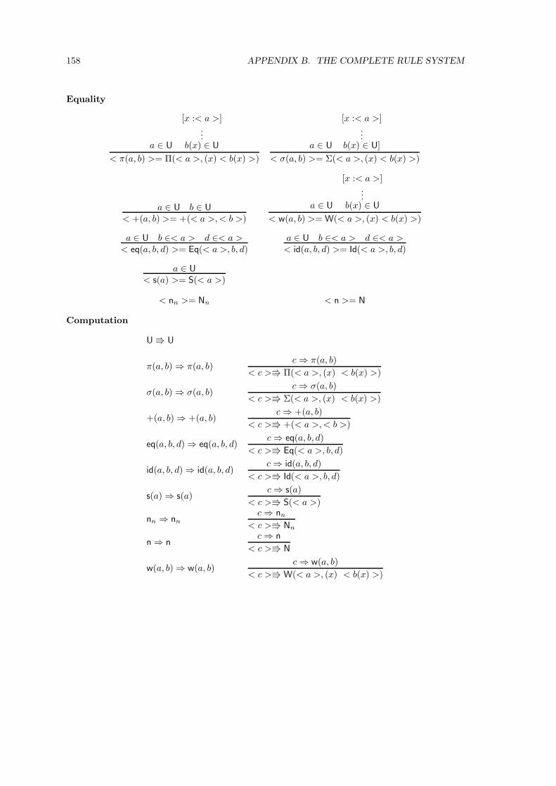
158 APPENDIX B. THE COMPLETE RULE SYSTEM
Equality
a ∈ U
[x :< a >]...
b(x) ∈ U
< π(a, b) >= Π(< a >, (x) < b(x) >)
a ∈ U
[x :< a >]...
b(x) ∈ U]
< σ(a, b) >= Σ(< a >, (x) < b(x) >)
a ∈ U b ∈ U
< +(a, b) >= +(< a >, < b >)
a ∈ U
[x :< a >]...
b(x) ∈ U
< w(a, b) >= W(< a >, (x) < b(x) >)
a ∈ U b ∈< a > d ∈< a >< eq(a, b, d) >= Eq(< a >, b, d)
a ∈ U b ∈< a > d ∈< a >< id(a, b, d) >= Id(< a >, b, d)
a ∈ U
< s(a) >= S(< a >)
< nn >= Nn < n >= N
Computation
U U
π(a, b)⇒ π(a, b)c⇒ π(a, b)
< c > Π(< a >, (x) < b(x) >)
σ(a, b)⇒ σ(a, b)c⇒ σ(a, b)
< c > Σ(< a >, (x) < b(x) >)
+(a, b)⇒ +(a, b)c⇒ +(a, b)
< c > +(< a >, < b >)
eq(a, b, d)⇒ eq(a, b, d)c⇒ eq(a, b, d)
< c > Eq(< a >, b, d)
id(a, b, d)⇒ id(a, b, d)c⇒ id(a, b, d)
< c > Id(< a >, b, d)
s(a)⇒ s(a)c⇒ s(a)
< c > S(< a >)
nn ⇒ nn
c⇒ nn
< c > Nn
n⇒ nc⇒ n
< c > N
w(a, b)⇒ w(a, b)c⇒ w(a, b)
< c > W(< a >, (x) < b(x) >)
Bibliography
[Acz78] Aczel, P., The type theoretic interpretation of constructive set theory, in “Logic Colloquium’77”, MacIntyre, A., Pacholski, L., Paris, J. eds., North Holland, Amsterdam, 1978.
[Acz82] Aczel, P., The type theoretic interpretation of constructive set theory: choice principles, in“The L.E.J. Brouwer Centenary Symposium”, Troelstra, S.S., van Dalen, D. eds., North Holland,Amsterdam, 1982.
[Acz86] Aczel, P., The type theoretic interpretation of constructive set theory; inductive definitions,in “Logic, Metodology and Philosophy of Science VII”, Marcus, R.B. et al. (eds.), North Holland,Amsterdam, 1986.
[All86] Allen, S.F., A non-type-theoretic definition of Martin-Lof ’s types, Proceedings of “The 1stAnnual Symposium on Logic in Computer Science”, IEEE, 1986, pp. 215-221.
[All87] Allen, S.F., A non-type-theoretic semantics for a type-theoretic language, PhD Thesis, Cor-nell University, 1987.
[BCMS89] Backhouse, R., Chisholm, P., Malcom, G. and Saaman, E., Do-it-yourself type theory,Formal Aspects of Computing 1, 1989, pp.19-84.
[BC85] Bates, J.L. and Constable, R.L., Proofs as Programs, ACM Transactions on ProgrammingLanguages and Systems 7, N.1, 1985, pp. 94-117.
[Bar84] Barendregt, H.P., The Lambda Calculus, its Syntax and Semantics, North–Holland, Ams-terdam, 1984.
[Bar92] Barendregt, H.P., Lambda-calculi with types, in “Handbook of logic and computer science”,vol. 2, S. Abramski, D.M. Gabbay and T.S. Maibaum eds., Oxford University Press, 1992, pp.118-309.
[Bee85] Beeson, M.J., Foundation of Constructive Mathematics, Lecture Notes in Computer Sci-ence, Springer-Verlag, 1985.
[Bel88] Bell, J.L., Toposes and local set theory: an introduction. Clarendon Press, Oxford, 1988.
[Ber90] Berardi, S., Type dependence and constructive mathematics, PhD thesis, Dipartimento diMatematica, Universita di Torino, 1990.
[BV87] Bossi, A. and Valentini, S., Assunzioni di arieta superiore nella teoria intuizionistica deitipi, in Italian, in “Atti secondo convegno nazionale sulla Programmazione Logica”, Torino 1987,B. Demo ed., pp. 81-92.
[BV89] Bossi, A. and Valentini, S., The expressions with arity, internal report of “Dipartimento diScienze dell’Informazione”, University of Milan, 1989, 61/89.
[BV92] Bossi, A. and Valentini, S., An intuitionistic theory of types with assumptions of high-arityvariables, Annals of Pure and Applied Logic 57, North Holland, 1992, pp. 93-149.
[Coq90] Coquand, T., Metamathematical investigations of a calculus of constructions, in “Logicand Computer Science”, P. Odifreddi ed., Academic Press, London, 1990, pp. 91-122.
159
160 BIBLIOGRAPHY
[Coq96] Coquand, T., An Algorithm for Type-Checking Dependent Types, Science of ComputerProgramming 26 (1–3), 1996, pp. 167-177.
[CCo98] Coquand, C., A realizability interpretation of Martin-Lof ’s type theory, In “Twenty fiveyears of Constructive Type Theory”, J. Smith and G. Sambin eds., Oxford Logic Guides (36),Clarendon Press, Oxford, 1998, pp. 73-82.
[CSSV] Coquand, T., G. Sambin, J. Smith and S. Valentini, Inductive generation of formal topolo-gies, to appear.
[CV98] Capretta, V. and Valentini, S., A general method to prove the normalization theorem forfirst and second order typed λ-calculi Mathematical Structures in Computer Science, 1998, pp.719-739.
[Chu36] Church, A. An unsolvable problem of elementary number theory, American Journal ofMathematics, 58 (1936), pp. 345-363.
[CF74] Curry, H.B., Feys, R., Combinatory Logic, North-Holland, Amsterdam, 1974.
[Bru80] de Bruijn, N.G., A survey of the project Automath, in “To H. B. Curry: Essays on Combi-natory Logic, Lambda Calculus and Formalism”, J.P. Seldin and J.R. Hyndley eds., AcademicPress, London, 1980, pp. 589-606.
[Bru91] de Bruijn, N.G., Telescopic mappings in typed lambda calculus, Information and Compu-tation, 91(2), April 1991, pp. 189-204.
[Dia75] Diaconescu, R., Axiom of choice and complementation, Proc. American MathematicalSociety, 51, 1975, pp. 176-178.
[Fre1892] Frege, G., Uber Sinn und Bedeutung, Zeitschrift fur Philosophie und philosophische Kri-tik, 1892, pp. 25-50.
[Gal90] Gallier, J.H., On Girard’s “Candidats de Reductibilite”, in “Logic and Computer Science”,P. Odifreddi ed., Academic Press, London, 1990, pp. 123-203.
[Gan80] Gandy, R.O., An early proof of normalization by A. M. Turing, in “To H. B. Curry: Essayson Combinatory Logic, Lambda Calculus and Formalism”, S. P. Seldin and J. R. Hindley eds.,Academic Press, London, 1980, pp. 453-455.
[Geu93] Geuvers, H., Logics and type systems, PhD thesis, Katholieke Universiteit Nijmegen, TheNetherlands, 1993.
[Gir71] Girard, J.Y., Une extension de l’interpretation de Godel a l’analyse, et son application al’elimination des coupures dans l’analyse et la theorie des types, in “Proceedings of 2nd Scandi-navian Logic Symposium”, J. E. Fenstad ed., North–Holland, Amsterdam, 1971, pp. 63-92.
[Gir86] Girard, J.Y., The system F of variable types, fifteen years later, Theoretical ComputerScience 45, North–Holland, Amsterdam, 1986, pp 159-192.
[GLT89] Girard, J.Y., Lafont, Y. and Taylor, P., Proofs and Types, Cambridge University Press,1989.
[GR94] Griffor, E. and Rathjen, M., The strength of some Martin-Lof ’s type theories, ArchiveMathematical Logic, 33, 1994, pp. 347-385.
[Hey56] Heyting, A., Intuitionism, an introduction, North-Holland, Amsterdam, 1956.
[Hof94] Hofmann, M., Elimination of extensionality and quotient types in Martin-Lof type theory.in “Proceedings of the International Workshop on Types for Proofs and Programs, Nijmegen,The Netherlands”, H. Barendregt and T. Nipkow eds., Lecture Notes in Computer Science (806),Springer Verlag, Berlin and New York, 1994, pp. 166-190.
BIBLIOGRAPHY 161
[Hof95] Hofmann, M., Extensional concepts in intensional type theory. PhD Thesis, University ofEdinburgh, 1995.
[Hof97] Hofmann, M., A simple model for quotient types. in “Typed lambda calculi and applica-tions”, Lecture Notes in Computer Science, Springer Verlag, Berlin and New York, 1997, pp.216–234.
[HS95] Hofmann, M. and Streicher, T., The groupoid interpretation of type theory, In “Twenty fiveyears of Constructive Type Theory”, J. Smith and G. Sambin eds., Oxford Logic Guides (36),Clarendon Press, Oxford, 1998, pp. 83-111.
[How80] Howard, W.A., The formula-as-types notion of construction, To “H.B. Curry: Essays oncombinatory Logic, Lambda Calculus and Formalism” R. Hindley and J.P. Seldin eds., AcademicPress, London, 1980, pp. 479-490.
[HP90] Huwig, H. and Poigne, A., A note on inconsistencies caused by fixpoints in a cartesianclosed category, Theoretical Computer Scince, 75, 1990, pp. 101-112.
[Jac89] Jacobs, B., The inconsistency of higher order extensions of Martin-Lof ’s type theory, Jour-nal of Philosophical Logic, 18, 1989, pp. 399-422.
[Kol32] Kolmogorov, A.N., Zur Deutung der intuitionistischen Logik, Mathematische Zeitschrift,vol. 35, 1932, pp. 58-65.
[Kri93] Krivine, J. L., Lambda-Calculus, Types and Models Masson, Paris, Ellis Horwood, HemelHempstead, 1993.
[LS86] Lambek, J. and Scott, P.J., An introduction to higher order categorical logic., volume 7 of“Studies in Advanced Mathematics”, Cambridge University Press, 1986.
[Law69] Lawvere, F.W., Diagonal arguments and cartesian closed categories, in “Category Theory,Homology Theory and their Applications II”, Lecture Notes in Mathematics, n.92, Springer 1969,pp. 134-145.
[Luo90] Luo, Z. An extended calculus of constructions. PhD Thesis, University of Edinburgh, 1990.
[MV96] Maguolo, D. and Valentini, S., An intuitionistic version of Cantor’s theorem, MathematicalLogic Quarterly 42, 1996, pp. 446-448.
[MV99] Maietti, M.E. and Valentini, S., Can you add power-set to Martin-Lof intuitionistic settheory? Mathematical Logic Quarterly 45, 1999, pp. 521-532.
[Mai99] Maietti, M.E., About effective quotients in constructive type theory, in “Types for Proofsand Programs”, International Workshop “Types’98”, Altenkirch T., Naraschewski W. and ReusB. eds., Lecture Notes in Computer Science 1657, Springer Verlag, 1999, pp. 164-178.
[Mag92] Magnusson, L., The new implementation of ALF, in proceedings of the “1992 Workshopon Types for Proofs and Programs”, Nordstrom B., Petersson K. and Plotkin G. eds.
[Mat98] Matthes, R., Extensions of SystemF by Iteration and Primitive Recursion on MonotoneInductive Types, PhD thesis, Department of Mathematics and Informatics, University of Munich,1998.
[MJ98] Matthes, R. and Joachimski, F. Short proofs of normalization for the simply-typed lambda-calculus, permutative conversions and Godel’s T, submitted to the Archive for MathematicalLogic.
[Mar71] Martin-Lof, P. Hauptsatz for the intuitionistic theory of iterated inductive definitions, in“Proceedings of the second Scandinavian logic symposium”, J.E. Fenstad ed., North-Holland,Amsterdam, 1971, pp. 179-216.
[Mar75] Martin-Lof, P. An Intuitionistic Theory of Types: Predicative Part, in “Logic Colloquium1973”, H. E. Rose and J. C. Shepherdson eds., North-Holland, Amsterdam, 1975, pp. 73-118.
162 BIBLIOGRAPHY
[Mar82] Martin-Lof, P. Constructive Mathematics and Computer Programming, in “Proceedings ofthe 6th International Congress for Logic, Methodology and Philosophy of Science”, Cohen, L.J.Los, J. Pfeiffer, H. and Podewski, K. P. eds., IV, Hannover 1979, North-Holland, Amsterdam(1982), pp.153-175.
[Mar83] Martin-Lof, P. Siena Lectures, handwritten notes of a series of lectures given in Siena,April 1983.
[Mar84] P. Martin-Lof, Intuitionistic type theory, notes by Giovanni Sambin of a series of lecturesgiven in Padua, June 1980, Bibliopolis, Napoli, 1984.
[MNPS91] Miller, D., Nadathur, G., Pfenning, F. and Scedrov, A., Uniform proofs as a foundationfor logic programming, Annals of Pure and Applied Logic, 51, 1991, pp. 125-157.
[MR86] Mayer, A. R. and Reinhold, M. B. ‘Type’ is not a type: preliminary report, ACM, 1986,pp. 287–295.
[Nor81] Nordstrom, B., Programming in Constructive Set Theory: some examples, in proceeding of“ACM Conference on Functional Programming Languages and Computer Architecture”, 1981,pp. 141-153.
[NP83] Nordstrom, B. and Petersson, K, Types and Specifications, in “Proceedings IFIP ’83”,R.E.A. Mason ed., Paris, Elsevier Science Publishers (North-Holland), Amsterdam 1983.
[NPS90] Nordstrom, B., Petersson, K. and Smith, J.M., Programming in Martin-Lof ’s Type The-ory, an introduction, Oxford Univ. Press, Oxford, 1990.
[NS84] Nordstrom, B. and Smith, J.M., Propositions, Types and Specifications of Programs inMartin-Lof ’s Type Theory, BIT, 24, N.3 (October 1984), pp. 288-301.
[PV93] Paulus Venetus (1993) (alias Sambin, G. and Valentini, S.). Propositum Cameriniense, siveetiam itinera certaminis . . . (in italian), in “Atti degli Incontri di Logica Matematica vol. viii(XV Incontro)”, G. Gerla, C. Toffalori and S. Tulipani eds., Camerino, pp. 115-143.
[PS86] Petersson, K. and Smith, J.M., Program derivation in type theory: a partitioning problem,Comput. Languages 11 (3/4), 1986, pp.161-172.
[Pot80] Pottinger, G., A type assignment for strongly normalizable λ-terms, in “To H.B. Curry,Essay on Combinatory Logic, Lambda Calculus and Formalism”, Academic Press, New York,1980, pp. 561-577.
[Pra65] Prawitz, D., Natural Deduction: A Proof-Theoretical Study, Almquist and Wiksell, Stock-olm, 1965.
[Sam87] Sambin, G.. Intuitionistic formal spaces - a first communication, in “Mathematical Logicand its Applications”, D. Skordev ed., Plenum, New York, 1987, pp. 187-204.
[Sam91] Sambin, G., Per una dinamica nei fondamenti (in italian), in “Atti del Congresso: Nuoviproblemi della logica e della filosofia della scienza”, vol. II, G. Corsi and G. Sambin eds., CLUEB,Bologna, 1991, pp. 163-210.
[Sam97] Sambin, G., Developing topology in a type theoretic setting, to appear.
[SV93] Sambin, G. and Valentini, S., Building up a tool-box for Martin-Lof ’s type theory (abstract),in “Computational Logic and Proof Theory. Proceedings of the Third Kurt Godel Colloquium,KGC’93”, G. Gottlob, A. Leitsch and D. Mundici eds., Lecture Notes in Computer Science,Springer, Berlin-Heidelberg-New York, 1993, pp. 69-70.
[SV98] Sambin, G. and Valentini, S., Building up a tool-box for Martin-Lof intuitionistic typetheory, in “Twenty five years of Constructive Type Theory”, J. Smith and G. Sambin eds.,Oxford Logic Guides (36), Clarendon Press, Oxford, 1998, pp. 221-244.
BIBLIOGRAPHY 163
[SVV96] Sambin, G., Valentini, S. and Virgili, P., Constructive Domain Theory as a branch ofIntuitionistic Pointfree Topology, Theoretical Computer Science, 159, 1996, pp. 319-341.
[Tai67] Tait, W.W., Intensional interpretation of functionals of finite type I, Journal of SymbolicLogic, 32, 1967, pp. 198-212.
[Tro87] Troelstra, A. S., On the Syntax of Martin Lof ’s Type Theories Theoretical ComputerScience, 51, 1987, pp. 1-26.
[Tur97] Turner, R., Reading between the lines in constructive type theory, Journal Logic Compu-tation, 7-2, 1997, pp. 229-250.
[Val94] Valentini, S., A note on a straightforward proof of normal form theorem for simply typedλ-calculi, Bollettino dell’Unione Matematica Italiana, 8-A, 1994, pp. 207-213.
[Val95] Valentini, S., On the decidability of the equality theory of simply typed lambda-calculi,Bollettino dell’Unione Matematica Italiana, 9-A, 1995, pp. 83-93.
[Val95a] Valentini, S., The multi-level typed λ-calculus, in preparation.
[Val96] Valentini, S., Decidability in Intuitionistic Type Theory is functionally decidable, Mathe-matical Logic Quarterly, 42, 1996, pp. 300-304.
[Val96a] Valentini, S., Another introduction to Martin-Lof ’s Type Theory, in “Trends in Theoret-ical Informatics”, R. Albrecht and H. Herre eds., Schriftenreihe der Osterreichischen ComputerGesellscaft, Bd. 89, Munchen, 1996.
[Val96b] Valentini, S., The formal development of non-trivial programs in constructive type the-ory, in “Proceedings of the Second International Conference on Massively Parellel ComputingSystems”, Ischia, maggio 1996, pp. 570-577
[Val98] Valentini, S., The forget-restore principle: a paradigmatic example, in “Twenty five years ofConstructive Type Theory”, J. Smith and G. Sambin eds., Oxford Logic Guide (36), ClarendonPress, Oxford, 1998, pp. 275-283.
[Val00] Valentini, S., Extensionality versus constructivity, to appear.