Ind 43978502

8/8/2019 Ind 43978502

http://slidepdf.com/reader/full/ind-43978502 1/8

A GIS framework for surface-layer soil moisture estimationcombining satellite radar measurements and land surface

modeling with soil physical property estimation

M. Tischler a, M. Garcia b, C. Peters-Lidard c, M.S. Moran d,*,S. Miller e, D. Thoma d, S. Kumar b, J. Geiger c

a U.S. Army Corps of Engineers, Engineering Research and Development Center, Topographic Engineering Center,

7701 Telegraph Rd, Alexandria, VA 22312, USAb University of Maryland e Baltimore County, NASA Goddard Space Flight Center, Code 614.3, Greenbelt, MD 20771, USA

c NASA, NASA Goddard Space Flight Center, Code 614.3, Greenbelt, MD 20771, USAd USDA Agricultural Research Service, Walnut Gulch Experimental Watershed, Southwest Watershed Research Center,

2000 East Allen Rd., Tucson, AZ 85719, USAe Department of Renewable Resources, University of Wyoming, Box 3354, 1000 E. University Dr, Laramie, WY 82071, USA

Received 2 November 2005; received in revised form 9 May 2006; accepted 26 May 2006

Available online 1 August 2006

Abstract

A GIS framework, the Army Remote Moisture System (ARMS), has been developed to link the Land Information System (LIS), a high per-

formance land surface modeling and data assimilation system, with remotely sensed measurements of soil moisture to provide a high resolution

estimation of soil moisture in the near surface. ARMS uses available soil (soil texture, porosity, K sat), land cover (vegetation type, LAI, Fraction

of Greenness), and atmospheric data (Albedo) in standardized vector and raster GIS data formats at multiple scales, in addition to climatologicalforcing data and precipitation. PEST (Parameter EStimation Tool) was integrated into the process to optimize soil porosity and saturated

hydraulic conductivity ( K sat), using the remotely sensed measurements, in order to provide a more accurate estimate of the soil moisture.

The modeling process is controlled by the user through a graphical interface developed as part of the ArcMap component of ESRI ArcGIS.

Published by Elsevier Ltd.

Keywords: GIS; ARMS; Model integration; Soil moisture; Land Information System; Parameter estimation

1. Introduction

The Army Remote Moisture System (ARMS) was con-ceived out of the need for a better understanding and estimation

of profile soil moisture in environmentally diverse, potentially

hostile, data poor, or physically inaccessible areas. Such knowl-

edge is particularly useful to the Army with respect to traffic-

ability modeling and construction engineering, in addition to

a variety of other applications. The project was intended to de-

vise a method by which profile soil moisture over watershed-

size areas (1000e

25 000 km2

) could be characterized andpredicted down to the tactical scale (<100 m). Furthermore,

the system is intended be applicable over any area of interest,

regardless of the amount of existing data or resolution.

The solution was to develop a combination system relying

heavily on land-surface modeling, but additionally using re-

motely sensed estimates of surface soil moisture to provide

more accurate results by employing parameter estimation.

The final requirements were that the system reside within

a Geographic Information System, specifically ArcGIS, and

be usable by persons with little or no hydrology, soil science,

* Corresponding author. Tel.:þ1 520 670 6380x171; fax: þ1 520 670 5550.

E-mail addresses: [email protected] (M. Tischler),

[email protected] (M.S. Moran).

1364-8152/$ - see front matter Published by Elsevier Ltd.

doi:10.1016/j.envsoft.2006.05.022

Environmental Modelling & Software 22 (2007) 891e898www.elsevier.com/locate/envsoft

mailto:[email protected]


http://www.elsevier.com/locate/envsoft

http://www.elsevier.com/locate/envsoft



8/8/2019 Ind 43978502


or remote sensing background. Therefore, the individual com-

ponents of ARMS were linked using ArcObjects, Visual Basic

for Applications (VBA), and external executables and were all

controlled within the ArcGIS framework.

The user friendly nature, spatial data analysis tools, and

visualization capabilities of a Geographic Information System

(GIS) provide a good framework to which models relying on orpredicting spatial data can be appended. The most popular GIS

is the Arc series of software tools developed by ESRI,

including ArcInfo, ArcView, and most recently, ArcGIS.

Alternatively, the GRASS GIS (Neteler and Mitasova, 2005) ex-

ists as an open source choice, particularly when runningon UNIX

platforms. The popularity of integrating hydrologic models into

a GIS in fact prompted the creation of the ArcHydro data model

and tools by ESRI for ArcGIS (Morehouse, 2002). Catchment-

Sim, an open source standalone GIS package was developed spe-

cifically for hydrologic model integration (Ryan and Boyd,

2003). Similar to ARMS, Hydrological Simulation Program e

FORTRAN (HSPF) was created using a windows interface

with integrated GIS tools to model and visualize point sourceand non-point source pollution (Shen et al., 2005).

For more than 10 years several different types of watershed

models have been integrated with a GIS (Ogden et al., 2001).

The complexity of such model integration varies with the pro-

ject, however. Xu et al. (2001) used a fairly loose integration

by relying on the GIS to provide input data for the PDTank

model. Miller et al. (2002) used a tighter coupling by scripting

GIS functionality to perform hydrologic functions and provide

input to the KINEROS and SWAT models in their AGWA Arc-

View extension. Storck et al. (1998) also used a tightly cou-

pled approach in their analysis of stream flow in the Pacific

Northwest using DHSVM (Wigmosta et al., 1994). Franken-berger et al. (1999) present the most extreme case of GIS cou-

pling, where the SMR model is written into the GRASS code

rather than being compiled and called externally.

However, in most cases the GIS is used to process and dis-

play inputs and outputs to an external model that can be started

automatically via scripting, or manually. This allows flexibility

in the modeling language, and does not require a model to be

rewritten, only simply modified to process the model inputs

and outputs. ARMS uses this approach by scripting ArcGIS

to provide a Graphical User Interface (GUI), process and con-

vert input data, communicate between external modules, write

metadata, and display output data. Similarly, Jeong and Liang

(2005) developed a data retrieval, analysis, and visualization

system that use GIS tools to accomplish particular tasks, and

requires little scientific knowledge of the user.

2. Background

2.1. Remote sensing of soil moisture

Airborne microwave radiometers have been used for over

three decades to measure surface soil moisture (Jackson and

Schmugge, 1989). Due to the large contrast in the dielectric

constant that naturally exists between water and non-saturated

soil, this technology has been successful for measuring soil

moisture. Water, with a dielectric constant of 80, is vastly dif-

ferent than dry soil, which typically has a dielectric constant

<5. In the field, a water-dry soil mixture exists, yielding a di-

electric constant somewhere between the two values that can

be determined by measuring the soils’ emissivity at micro-

wave frequencies (Schmugge et al., 2002).

Given soil texture and vegetation information, proven andaccurate methods exist to convert the measured emissivity to

volumetric soil moisture (Jackson and Schmugge, 1991). The

actual sampling depth over which the soil moisture can be de-

termined is variable, depending on the soil moisture condition

and radar properties. Most studies agree that the penetration

depth for microwave sensing is between 0.1 to 0.3 times the

wavelength, where the longest wavelengths (L-band) are about

21 cm (Schmugge et al., 2002), which equates to an effective

sampling depth of approximately 2e6 cm. For example, several

large-scale field experiments have been conducted that used mi-

crowave remote sensing to map soil moisture on a watershed

scale, including Monsoon ’90 (Kustas and Goodrich, 1994),

Southern Great Plains 1997 (Jackson et al., 2002), SouthernGreat Plains 1999 (Jackson and Hsu, 2001), Soil Moisture Ex-

periment (SMEX) 2002 (Jackson et al., 2003), SMEX 2003

(Jackson et al., 2004), SMEX 2004, and SMEX 2005.

However, active microwave sensors such as Synthetic Ap-

erture Radar (SAR) currently represent the best approach for

obtaining spatially distributed surface soil moisture at scales

of 10e100 m for watersheds ranging from 1000 to

25 000 km2. The magnitude of the SAR backscatter coefficient

(so) is related to volumetric surface soil moisture (ms) through

the contrast of the dielectric constants of dry bare soil and wa-

ter. The perturbing factors affecting the accuracy of ms

estima-

tion are soil surface roughness and vegetation biomass.Studies, particularly in the past decade, have generated

a multitude of methods, algorithms, and models relating satel-

lite-based images of SAR backscatter to surface soil moisture

(Table 1). However, no operational algorithm exists using

SAR data acquired by existing spaceborne sensors (Borgeaud

and Saich, 1999). A significant limitation of SAR for watershed

scale applications is that the sun synchronous satellites can pro-

vide only weekly repeat coverage, and even longer for the same

orbital path (generally around 35 days). Moran et al. (2004)

identified a number of priorities in research, validation and de-

velopment to improve the accuracy of SAR-derived ms

estima-

tions, including further studies to interpret the effects of surface

roughness and vegetation on the SAR signal, investing in in situ

soil moisture measurement networks, launching new sensors,

and decreasing the price of SAR imagery.

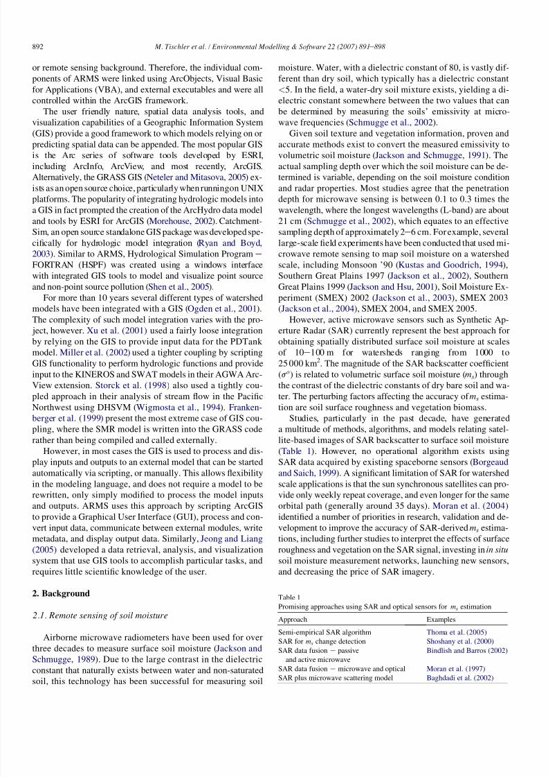
Table 1

Promising approaches using SAR and optical sensors for ms

estimation

Approach Examples

Semi-empirical SAR algorithm Thoma et al. (2005)

SAR for ms change detection Shoshany et al. (2000)

SAR data fusion e passive

and active microwave

Bindlish and Barros (2002)

SAR data fusion e microwave and optical Moran et al. (1997)

SAR plus microwave scattering model Baghdadi et al. (2002)

892 M. Tischler et al. / Environmental Modelling & Software 22 (2007) 891e898

8/8/2019 Ind 43978502


8/8/2019 Ind 43978502


either spatially explicit characterizations of the AOI, as in

a landcover classification raster layer, or the user can set a pa-

rameter to be uniform across the AOI. The same method is

used for setting required initial conditions. For example, if

a raster layer representing the initial soil moisture of the sur-

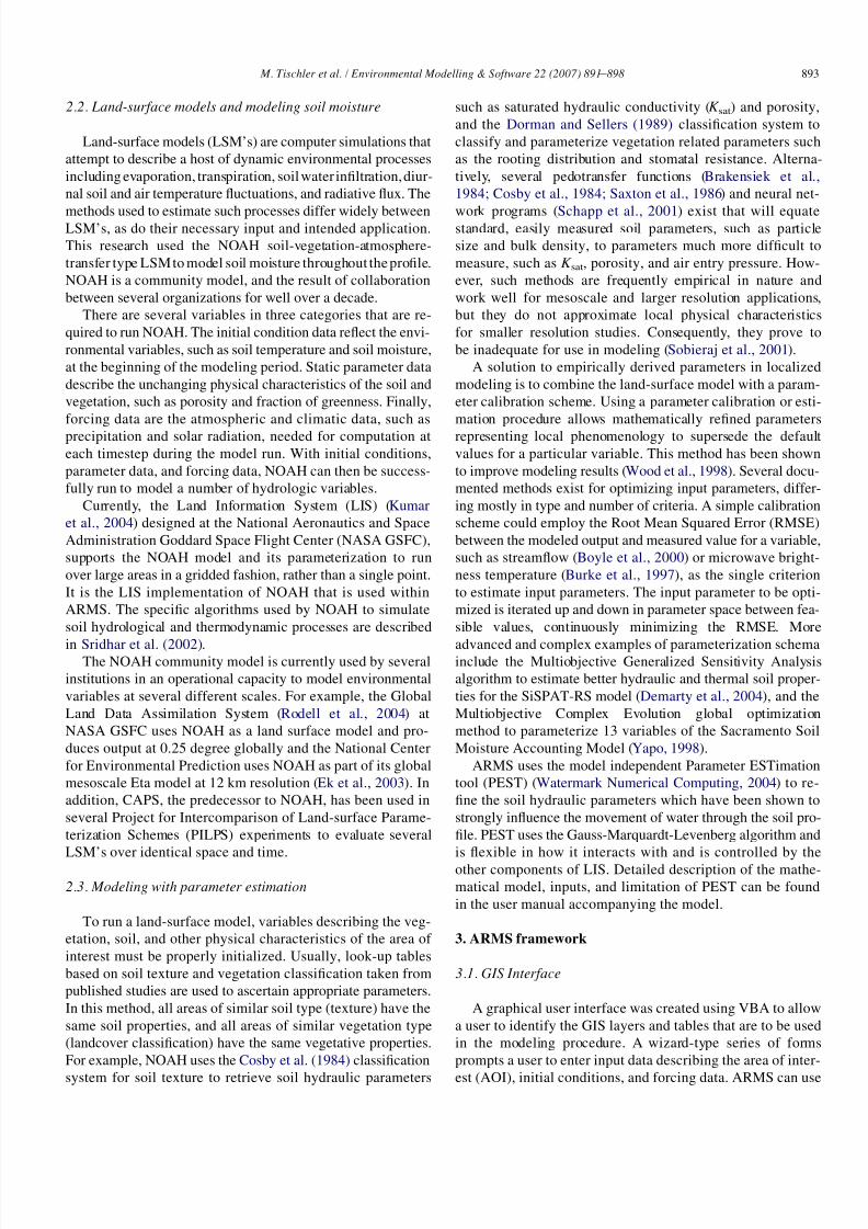
face layer exists, a user can choose that layer. Alternatively,

a user can specify that the initial soil moisture is constant(e.g., 25% soil moisture) across the domain, as in Fig. 1.

Soil classification, landcover classification, saturated hydraulic

conductivity, porosity, fraction of greenness, initial soil mois-

ture for the profile, initial soil temperature for the profile, skin

temperature, and albedo may all be designated in one of the

above methods. At a minimum, the user must have a spatially

explicit representation of soil type and landcover type. It is as-

sumed that a user would at least have these data for their AOI.

If no other characteristics of the domain are known but soil

and landcover, necessary parameters can be calculated from

just these two inputs through internal look-up tables derived

from pedotransfer functions. At a maximum, all of the above

mentioned parameters may be represented by GIS layers.Control parameters for LIS and NOAH are also set using the

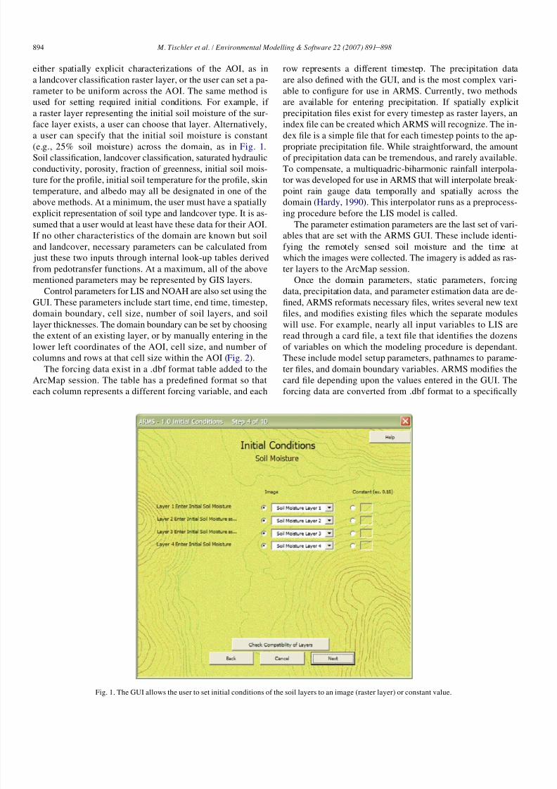
GUI. These parameters include start time, end time, timestep,

domain boundary, cell size, number of soil layers, and soil

layer thicknesses. The domain boundary can be set by choosing

the extent of an existing layer, or by manually entering in the

lower left coordinates of the AOI, cell size, and number of

columns and rows at that cell size within the AOI (Fig. 2).

The forcing data exist in a .dbf format table added to the

ArcMap session. The table has a predefined format so that

each column represents a different forcing variable, and each

row represents a different timestep. The precipitation data

are also defined with the GUI, and is the most complex vari-

able to configure for use in ARMS. Currently, two methods

are available for entering precipitation. If spatially explicit

precipitation files exist for every timestep as raster layers, an

index file can be created which ARMS will recognize. The in-

dex file is a simple file that for each timestep points to the ap-propriate precipitation file. While straightforward, the amount

of precipitation data can be tremendous, and rarely available.

To compensate, a multiquadric-biharmonic rainfall interpola-

tor was developed for use in ARMS that will interpolate break-

point rain gauge data temporally and spatially across the

domain (Hardy, 1990). This interpolator runs as a preprocess-

ing procedure before the LIS model is called.

The parameter estimation parameters are the last set of vari-

ables that are set with the ARMS GUI. These include identi-

fying the remotely sensed soil moisture and the time at

which the images were collected. The imagery is added as ras-

ter layers to the ArcMap session.

Once the domain parameters, static parameters, forcingdata, precipitation data, and parameter estimation data are de-

fined, ARMS reformats necessary files, writes several new text

files, and modifies existing files which the separate modules

will use. For example, nearly all input variables to LIS are

read through a card file, a text file that identifies the dozens

of variables on which the modeling procedure is dependant.

These include model setup parameters, pathnames to parame-

ter files, and domain boundary variables. ARMS modifies the

card file depending upon the values entered in the GUI. The

forcing data are converted from .dbf format to a specifically

Fig. 1. The GUI allows the user to set initial conditions of the soil layers to an image (raster layer) or constant value.


8/8/2019 Ind 43978502


formatted text file to be read by LIS during runtime. All raster

files that are chosen as inputs are also converted to a text for-

mat for access by the separate modules. Once all the input data

are converted, and the appropriate control files written, param-

eter estimation and modeling can begin.

3.2. Parameter estimation

The parameter estimation routine in ARMS uses the 1-di-

mensional version of NOAH and is controlled by the ParameterEStimation Tool (PEST) (Watermark Numerical Computing,

2004). The PEST module jointly optimizes K sat and porosity

for the AOI. Running PEST over the entire domain is not feasi-

ble for several reasons, though mainly computational time and

power. Instead, stratified samples of cells from across the AOI

are chosen for the procedure. The cells are chosen by determin-

ing the total number of unique combinations of soil and land-

cover types in the domain. A file is created identifying the

combination to which each cell in the domain belongs. PEST

is run for a specified number of cells that represent each unique

combination. Currently, PEST is hard coded to run for up to 8

cells in each unique combination of landcover and soil types.

If the total number of cells for a particular combination is less

than 8, then PEST will run on as many as are present.

For each cell that is to be used in PEST, the initial condi-

tions, static parameters, forcing data, and remotely sensed

soil moisture values are extracted from the appropriate parent

files, and written to text files that PEST will read. Then, 1-D

NOAH is run by PEST until optimized parameters are con-

verged upon. The detailed process by which this happens is

described in the PEST User Manual (Watermark Numerical

Computing, 2004). Once optimized parameters exist for each

chosen cell, those optimized values are averaged within each

unique combination. Optimized K sat and porosity raster layers

are created from the average values for each unique

combination across the domain by using the reference file

that tracks to which combination each cell belongs. These op-

timized parameters can supersede the original K sat and poros-

ity estimations for use in LIS.

3.3. LIS and NOAH

The modeling kernel of ARMS is the NOAH LSM accessible

through LIS. LIS resides as an external Windows executable file

compiled using Compaq Visual Fortran v6.6. The model isa modified version of the standard LIS software package de-

signed to work with the files which ARMS provides. Any spa-

tially explicit LIS inputs the user may have are added to the

ArcMap session as raster layers. These can be either data avail-

able for the area, or the result of parameter estimation. ARMS

reformats the raster layers into text files that LIS can then read

and process. The modification of a card file communicates to

LIS how the model will be run, and with which parameters.

LIS will process all the inputs given to it by ARMS, define

a domain, and then rely on NOAH to perform the actual mod-

eling at each timestep for each cell in the domain. The compu-

tations performed by NOAH are outlined and explained in

Sridhar et al. (2002). After NOAH has completed calculations

across the domain at a particular timestep, LIS will write out-

put files summarizing the calculations. In addition, a text file

of the output profile soil moisture is written that can easily

be imported to ArcGIS for display.

4. Field study

The ARMS system has been tested using data from the

Monsoon ’90 field experiment (Kustas and Goodrich, 1994)

at the Walnut Gulch Experimental Watershed in southern Ari-

zona. During Monsoon’90, daily gravimetric soil moisture

data were collected at eight micrometeorological-energy flux

Fig. 2. Domain attributes and control variables for the modeling run are set in the GUI.


8/8/2019 Ind 43978502


(Metflux) sites, in addition to standard meteorological vari-

ables and surface fluxes. In addition, an airborne L-band

Push Broom Microwave Radiometer (PBMR) mounted on

a NASA C-130 aircraft was flown at an altitude of 600 m

above the ground to yield soil moisture products derived

from measured microwave brightness temperature (Tb)

(Schmugge et al., 1994). Tb data were collected over an ap-proximately 8 Â 20 km area with a 40 m horizontal resolution

for six days: 212 (Jul. 31), 214 (Aug. 2), 216 (Aug. 4), 217

(Aug. 5), 220 (Aug. 8), and 221 (Aug. 9).

The Metflux data in combination with a network of 88 rain

gauges provided the forcing data necessary to use ARMS. To

test the effectiveness of the system, two model runs were per-

formed. First, the model was run with the best possible soil pa-

rameters (Run 1). This included soil texture, porosity, and K satvalues derived from the Soil Survey Geographic Database

(SSURGO). This dataset is available only for the United States,

and provides the most detailed estimates of soil property infor-

mation. Next, the model was run for the Monsoon ’90 period

using soil textures derived from the Food and Agricultural Or-ganization (FAO) Digital Soil Map of the World (Run 2). This

dataset provides very course, but globally available data cover-

age. Porosity and K sat values initially used in this model run

were derived from the default tables within LIS, which are

based on Cosby et al. (1984). For the first model run (Run 1)

with SSURGO data, no parameter estimation was used. PEST

was used in the second run (Run 2) to optimize porosity and

K sat, based on the comparison between the model output and

PBMR derived soil moisture values collected in the modeling

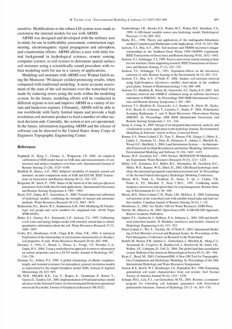
period. Fig. 3 compares the watershed averages of K sat and po-

rosity for the different soil data sources, and pest.

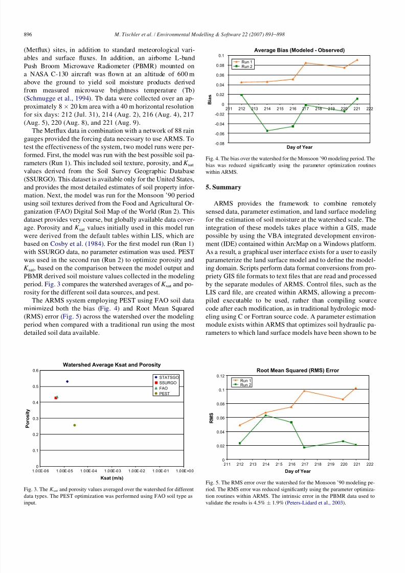
The ARMS system employing PEST using FAO soil dataminimized both the bias (Fig. 4) and Root Mean Squared

(RMS) error (Fig. 5) across the watershed over the modeling

period when compared with a traditional run using the most

detailed soil data available.

5. Summary

ARMS provides the framework to combine remotelysensed data, parameter estimation, and land surface modeling

for the estimation of soil moisture at the watershed scale. The

integration of these models takes place within a GIS, made

possible by using the VBA integrated development environ-

ment (IDE) contained within ArcMap on a Windows platform.

As a result, a graphical user interface exists for a user to easily

parameterize the land surface model and to define the model-

ing domain. Scripts perform data format conversions from pro-

priety GIS file formats to text files that are read and processed

by the separate modules of ARMS. Control files, such as the

LIS card file, are created within ARMS, allowing a precom-

piled executable to be used, rather than compiling sourcecode after each modification, as in traditional hydrologic mod-

eling using C or Fortran source code. A parameter estimation

module exists within ARMS that optimizes soil hydraulic pa-

rameters to which land surface models have been shown to be

Watershed Average Ksat and Porosity

0

0.1

0.2

0.3

0.4

0.5

0.6

1.00E-06 1.00E-05 1.00E-04 1.00E-03 1.00E-02 1.00E-01 1.00E+00

Ksat (m/s)

P o r o s i t y

STATSGO

SSURGO

FAO

PEST

Fig. 3. The K sat and porosity values averaged over the watershed for different

data types. The PEST optimization was performed using FAO soil type as

input.

Average Bias (Modeled - Observed)

-0.08

-0.06

-0.04

-0.02

0

0.02

0.04

0.06

0.08

0.1

211 212 213 214 215 216 217 218 219 220 221 222

Day of Year

B i a s

Run 1

Run 2

Fig. 4. The bias over the watershed for the Monsoon ’90 modeling period. The

bias was reduced significantly using the parameter optimization routines

within ARMS.

Root Mean Squared (RMS) Error

0

0.02

0.04

0.06

0.08

0.1

0.12

211 212 213 214 215 216 217 218 219 220 221 222

Day of Year

R M S

Run 1

Run 2

Fig. 5. The RMS error over the watershed for the Monsoon ’90 modeling pe-

riod. The RMS error was reduced significantly using the parameter optimiza-

tion routines within ARMS. The intrinsic error in the PBMR data used to

validate the results is 4.5% Æ 1.9% (Peters-Lidard et al., 2003).


8/8/2019 Ind 43978502


sensitive. Modifications to the robust LIS system were made to

customize the internal models for use with ARMS.

ARMS was designed and developed with the military user

in mind, for use in trafficability assessment, construction engi-

neering, electromagnetic signal propagation and adsorption,

and countermine efforts. ARMS allows a user with little for-

mal background in hydrological sciences, remote sensing,computer science, or soil science to determine spatial surface

soil moisture using a scientifically sound procedure with ro-

bust modeling tools for use in a variety of applications.

Modeling soil moisture with ARMS over Walnut Gulch us-

ing the Monsoon ’90 dataset yielded promising results, when

compared with traditional modeling. A more accurate assess-

ment of the state of the soil moisture over the watershed was

made by reducing errors using the tools within the modeling

system. In the future, modeling efforts will be conducted in

different regions to test and improve ARMS in a variety of ter-

rain and landcover regimes. Ultimately, ARMS will be able to

run worldwide with fairly limited inputs and provide a high

resolution soil moisture product to feed a number of other tac-tical decision aids. Currently, the system is not yet operational.

In the future, information regarding ARMS and the release of

software can be directed to the United States Army Corps of

Engineers Topographic Engineering Center.

References

Baghdadi, N., King, C., Chanzy, A., Wingneron, J.P., 2002. An empirical

calibration of IEM model based on SAR data and measurements of soil

moisture and surface roughness over bare soils. International Journal of

Remote Sensing 23 (20), 4325e4340.

Bindlish, R., Barros, A.P., 2002. Subpixel variability of remotely sensed soilmoisture: an inter-comparison study of SAR and ESTAR. IEEE Transac-

tions on Geoscience and Remote Sensing 40 (2), 326e337.

Borgeaud, M., Saich, P., 1999. Status of the retrieval of bio and geo-physical

parameters from SAR data for land applications. International Geoscience

and Remote Sensing Symposium 4, 1901e1903.

Boyle, D.P., Gupta, H.V., Sorooshian, S., 2000. Toward improved calibration

of hydrologic models: combining the strengths of manual and automatic

methods. Water Resources Research 36 (12), 3663e3674.

Brakensiek, D.L., Rawls, W.J., Stephenson, G.R. 1984. Modifying SCS hydro-

logic soil groups and curve numbers for rangeland soils. ASAE Paper

(PNR-84203).

Burke, E.J., Gurney, R.J., Simmonds, L.P., Jackson, T.J., 1997. Calibrating

a soil water and energy budget model with remotely sensed data to obtain

quantitative information about the soil. Water Resources Research 33 (7),

1689e

1697.Cosby, B.J., Hornberger, G.M., Clapp, R.B., Ginn, T.R., 1984. A statistical

Exploration of the relationships of soil moisture characteristics to the phys-

ical properties of soils. Water Resources Research 20 (6), 682e690.

Demarty, J., Ottle, C., Braud, I., Olioso, A., Frangi, J.P., Bastidas, L.A.,

Gupta, H.V., 2004. Using a multiobjective approach to retrieve information

on surface properties used in a SVAT model. Journal of Hydrology 287,

214e236.

Dorman, J.L., Sellers, P.J., 1989. A global climatology of albedo, roughness

length, and stomatal resistance for atmospheric general circulation models

as represented by the simple biosphere model (SiB). Journal of Applied

Meteorology 28, 833e855.

Ek, M.B., Mitchell, K.E., Lin, Y., Rogers, E., Grunmann, P., Koren, V.,

Gayno, G., Tarpley, J.D., 2003. Implementation of Noah land surface model

advances in the National Centers for Environmental Prediction operational

mesoscale Eta model. Journal of Geophysical Research 108 (D22).

Frankenberger, J.R., Brooks, E.S., Walter, M.T., Walter, M.F., Steenhuis, T.S.,

1999. A GIS-based variable source area hydrology model. Hydrological

Processes 13 (6), 805e822.

Hardy, R.L., 1990. Theory and applications of the multiquadric-biharmonic

method.Computersand Mathematics with Applications. 19 (8e9), 163e208.

Jackson, T.J., Hsu, A.Y., 2001. Soil moisture and TRMM microwave imager

relationships in the Southern Great Plains 1999 (SGP99) experiment.

IEEE Transactions on Geoscience and Remote Sensing 39 (8), 1632e1642.

Jackson, T.J., Schmugge, T.J., 1989. Passive microwave remote sensing system

for soil moisture: Some supporting research. IEEE Transactions on Geosci-

ence and Remote Sensing 27 (2), 225e235.

Jackson, T.J., Schmugge, T.J., 1991. Vegetation effects on the microwave

emission of soils. Remote Sensing of the Environment 36 (3), 203e212.

Jackson, T.J., Hsu, A.Y., O’Neill, P., 2002. Surface soil moisture retrieval

using high-frequency microwave satellite observations in the southern

great plains. Journal of Hydrometeorology 3 (6), 688e698.

Jackson, T.J., Bindlish, R., Klein, M., Gasiewski, A.J., Njoku, E.G. 2003. Soil

moisture retrieval and AMSR-E validation using an airborne microwave

radiometer in SMEX02. In: Proceedings 2003 IEEE International Geosci-

ence and Remote Sensing Symposium 1, 401e403.

Jackson, T.J., Bindlish, R., Gasiewski, A.J., Stankov, B., Klein, M., Njoku,

E.G., Bosch, D., Coleman, T., Laymon, C., Starks, P. 2004., Polarimetric

Scanning Radiometer C and X Band Microwave Observations During

SMEX03. In: Proceedings 2004 IEEE International Geoscience and

Remote Sensing Symposium 1, 321e324.

Jeong, S., Liang, X., 2005. Design of an integrated data retrieval, analysis, and

visualization system: application in the hydrology domain. Environmental

Modelling & Software: Article in Press, Corrected Proof.

Kumar, S.V., Peters-Lidard, C.D., Tian, Y., Houser, P.R., Geiger, J., Olden, S.,

Lighty, L., Eastman, J.L., Doty, B., Dirmeyer, P., Adams, J., Mitchell, K.,

Wood, E.F., Sheffield, J., 2004. Land Information System e An Interoper-

able Framework for High Resolution Land Surface Modeling. Submitted to

Environmental Modeling and Software 21 (10), 1402e1415.

Kustas, W.P., Goodrich, D.C., 1994. Preface. MONSOON’90 Multidisciplin-

ary Experiment. Water Resources Research 30 (5), 1211e1225.

Miller, S.N., Semmens, D.J., Miller, R.C., Hernandez, M., Goodrich, D.C.,

Miller, W.P., Kepner, W.G., Ebert, D., 2002. GIS-Based hydrologic mod-

eling: the automated geospatial watershed assessment tool. In: Proceedingsof the Second Federal Interagency Hydrologic Modeling Conference.

Moran, M.S., Vidal, A., Troufleau, D., Inoue, Y., Qi, J., Clarke, T.R.,

Pinter Jr., P.J., Mitchell, T., Neal, C.M.U., 1997. Combining multi-

frequency microwave and optical data for crop management. Remote Sens-

ing of Environment 61 (1), 96e109.

Moran, M.S., Peters-Lidard, C.D., Watts, J.M., McElroy, S., 2004. Estimating

soil moisture at the watershed scale with satellite-based radar and land sur-

face models. Canadian Journal of Remote Sensing 30 (5), 1e22.

Morehouse, S., 2002. Arc Hydro: GIS for Water Resources. ESRI Press.

Neteler, M., Mitasova, H., 2005. Open Source GIS: A GRASS GIS Approach.

Kluwer Academic Publishers.

Ogden, F.L., Garbrecht, J., DeBarry, P.A., Johnson, L., 2001. GIS and distrib-

uted watershed models. II: Modules, interfaces, and models. Journal of

Hydrologic Engineering 6 (6), 515e523.

Peters-Lidard, C., Wu, Y., Tischler, M., O’Neill, P., 2003. Operational Model-ing of Soil Moisture at Local and Regional Scales. In: Proceedings of the

First Interagency Conference on Research in the Watersheds.

Rodell, M., Houser, P.R., Jambor, U., Gottschalck, J., Mitchell, K., Meng, C.J.,

Aresenault, K., Cosgrove, B., Radakovich, J., Bosilovich, M., Entin, J.K.,

Walker, J.P., Lohmann, D., Toll, D., 2004. The global land data assimilation

system. Bulletin of the American Meteorological Sociey 85 (3), 381e394.

Ryan, C., Boyd, M., 2003. CatchmentSIM: A New GIS Tool for Topographic

Geo-Computation and Hydrologic Modeling. In: Proceedings of the 28th

International Hydrology and Water Resources Symposium.

Saxton, K.E., Rawls, W.J., Romberger, J.S., Pependick, R.I., 1986. Estimating

generalized soil water characteristics from soil texture. Soil Science

Society of America Journal 50 (4), 1231e1238.

Schapp, M.G., Leij, F.J., van Genuchten, M.Th., 2001. Rosetta: a computer

program for estimating soil hydraulic parameters with hierarchical

pedotransfer functions. Journal of Hydrology 251 (3e

4), 163e

176.


8/8/2019 Ind 43978502


Ind 43978502

Documents

Transcript of Ind 43978502