Hans Bloemen, Stefan Hochguertel and Jochem Zweerink Joint ... · Hans Bloemen, Stefan Hochguertel...
32
Hans Bloemen, Stefan Hochguertel and Jochem Zweerink Joint Retirement of Couples Evidence from a Natural Experiment DP 06/2014-087
Transcript of Hans Bloemen, Stefan Hochguertel and Jochem Zweerink Joint ... · Hans Bloemen, Stefan Hochguertel...
Hans Bloemen, Stefan Hochguertel and Jochem Zweerink
Joint Retirement of Couples Evidence from a Natural Experiment
DP 06/2014-087
Joint Retirement of Couples:
Evidence from a natural experiment
Hans Bloemen𝑎,𝑏, Stefan Hochguertel𝑎 and Jochem Zweerink𝑎
a VU University Amsterdam, Tinbergen Institute, Netspar b IZA Bonn
June 10, 2014
Abstract We estimate and explain the impact of early retirement of husbands on the wives’ probability to retire within one year, using administrative micro panel data that cover the whole Dutch population. We employ an instrumental variable approach in which retirement choice of husbands is instrumented with eligibility rules for generous early retirement benefits that were temporarily and unexpectedly available. The empirical model explains wives’ probability to retire within one year. We find that early retirement opportunity of husbands increased the wives’ probability to retire within one year by 25.4 percentage points. This is a strong effect. Our results are robust to several sensitivity tests.
JEL classification: C26, J26, J120, J140
Keywords: instruments, retirement, couples
Acknowledgements. This paper is part of the Netspar research theme "Pensions, savings and retirement decisions (II)," subproject "Retirement decisions: financial incentives, wealth and flexibility". We thank Adriaan Kalwij and the seminar audience of the “Pensions, retirement, and the financial position of the elderly” theme meeting of Netspar for helpful and constructive comments. Correspondence to: Jochem Zweerink, Department of Economics, Faculty of Economics and Business Administration, VU University Amsterdam, De Boelelaan 1105, 1081 HV Amsterdam, The Netherlands. E-mail: [email protected].
1
1. Introduction
Large changes across OECD countries are being observed in terms of labor force participation of older
workers and retirement patterns. In particular, older workers retire later. These patterns have partly
been ascribed to changes in institutions such as restricted access to early retirement (ER).
Understanding the way individuals make labor supply and retirement decisions is crucial for designing
effective policies that are meant to change behavior. Traditional microeconomic retirement models that
can guide policy makers in policy and parameter choice typically focus on individual decisions in isolation
and study the decision process as a function of age, income, health, wealth, and financial or tax
incentives (Gustman and Steinmeier (1986), Berkovec and Stern (1991), Lumsdaine, Stock and Wise
(1992) and Rust and Phelan (1997)). As a recent strand of literature has emphasized, however,
important spillover effects can plausibly be at work when household labor supply and retirement
choices are being considered because spousal decisions depend on each other in various ways. Ignoring
such effects may have direct implications for the evaluation of policy measures (Blau and Gilleskie
(2006) and Van der Klaauw and Wolpin (2008)).
Reverse causality typically makes it challenging to identify the effect of, say, the husband’s retirement
choice on the labor market status of the wife using observational data, since both spouses’ labor supply
choices may be linked directly and indirectly through both observables and correlated unobservables, or
shocks. Using Dutch administrative micro data and relying on identification through a quasi-natural
experiment, we find robust evidence for important spillovers from husbands’ retirement decisions on
their wives’ retirement status emanating from husbands’ changed financial incentives to retire early.
The policy change that we exploit became effective in 2005 for certain birth cohorts of civil servants
employed for more than ten years by the Dutch central government. These individuals were offered the
opportunity to retire during the year 2005, by a temporary reduction of the ER eligibility age. For our
empirical work, we focus on dual-earner couples in which the husband does and the wife does not work
in the public sector, such as to rule out coincidental treatment of wives through the same reform.1
1 We do not estimate the effect of retirement of the wife on retirement status of the husband because of a lack of observations. There are too few wives induced to retire by the introduction of the early retirement arrangement we use. This may have to do with the fact that labor market attachment of women in the Netherlands is not uniformly strong.
2
The wife’s probability to retire is the dependent variable in our model. We employ the mentioned
policy change as an instrument for husband’s retirement status, and control for both observable
characteristics and unobservables. We use an individual fixed effects specification for the latter. Fixed
effects also control non-parametrically for cohort effects that may arguably be important. In addition,
we control for year fixed effects and nonlinear age effects. Since couples are stable dyads in our sample,
we thus identify an effect over and above fixed differences in ages.
According to our central estimates, retirement of male civil servants led to a jump in the probability of
their wives to retire within one year by 25.4 percentage points. This is a large effect, given that wives
pursue their own careers and have a strong labor market attachment and a sector affiliation of at least
10 consecutive years. Further investigation reveals the effect to be driven by observations on couples
with a husband aged 60 and a wife aged 59 or 60. This suggests that the interaction between the ER
arrangement for civil servants and private sector ER may play an important role in retirement decisions
of couples.
There are two related literatures that our work speaks to. One focuses on joint retirement using
structural models. These models assume that husbands and wives make separate retirement decisions
and have their own preferences. Appropriate modelling of the relevant financial incentives and suitable
parameterization of individual preferences are some of the main challenges in this literature. Papers
such as Blau and Gilleskie (2006) and Van der Klaauw and Wolpin (2008) carefully model the incentives
provided by social security rules, and specify stochastic processes for wages, health and survival. The
main effect of husbands on wives’ retirement choices runs through the household budget constraint in
those papers. The household budget constraint is not the only channel inducing dependence, however.
Spouses enjoy spending time together, i.e. there are leisure complementarities in preferences. Gustman
and Steinmeier (2000) study leisure complementarities assuming that there is no uncertainty. They find
that spouses coordinate retirement decisions and that coordination of retirement decisions is motivated
by leisure complementarities rather than financial incentives provided by the household budget
constraint. Casanova Rivas (2010) does take into account uncertainty regarding future income, health
and survival. In line with Gustman and Steinmeier (2000), she finds that leisure complementarities are
present and account for up to eight percent of observed joint retirements.
3
We directly contribute to a second strand of very recent empirical literature that estimates the effect of
retirement of one partner on retirement status of the spouse. The identification methods used in this
literature do not rely on distributional assumptions, but rather on exogenous sources of variation in the
retirement rates. Hospido and Zamarro (2013), Banks, Blundell and Casanova Rivas (2010) and Goux,
Maurin and Petrongolo (2011) are the survey data studies most comparable to ours. All of them find
that spousal decisions can be influenced by retirement shifts of their partners.
Our first contribution is to use strong instruments that provide exogenous (unanticipated) variation in
retirement rates of husbands, as explained above. Second, we use administrative data at annual
frequency that include end dates of jobs and that allow us to observe the precise within-couple
sequencing of retirement. This is critical in order to rule out that our estimates are influenced by
behavior of wives that actually retire earlier than their husbands. The latter effect cannot be ruled out in
other studies that are based on biennial survey data, posing a potential threat to identification. Third, as
we have access to data covering the entire population, we can focus on a sample of particular interest,
namely individuals from a very narrow age range where we can (to some degree) control for historical
labor market attachment.
The rest of the paper is set up as follows. Section 2 reviews the literature and Section 3 describes the
institutional environment, including the policy change that we exploit. Section 4 explains and describes
the data. Section 5 delineates the identification strategy we use for estimating the causal effect of
husband’s retirement on wife’s retirement. Section 6 discusses the results and Section 7 concludes.
2. Literature review
Hospido and Zamarro (2013) employ a fuzzy Regression Discontinuity design using the eligibility age for
early retirement benefits as discontinuity in the probability to retire. They use data from the Survey on
Health, Ageing and Retirement in Europe (SHARE) covering eleven European countries and find that
induced retirement of husbands increases the probability that their wives retire in the same two-year
interval between survey waves by 16-18 percentage points. Banks, Blundell and Casanova Rivas (2010)
employ a before-after difference-in-difference approach, exploiting the difference in eligibility age for
public pensions between the UK and US as a source of variation on retirement status. They use data
from the 2002 and 2004 waves of the Health and Retirement Study (HRS) for the US and from the

4
English Longitudinal Study of Ageing (ELSA) for the UK. The eligibility age for public pensions was 62 in
the US and 60 in the UK. American husbands whose wives turned 60 during the time between the two
survey waves form the control group and the treatment group consists of British husbands whose wives
turned 60 during the time between the two survey waves. They find that men in the UK are 14-20
percentage points more likely to retire when their wife reaches state pension age than comparable men
in the US. They find a similar effect after employing instrumental variable estimation, using the state
pension age as a source of exogenous variation for retirement status of the wife.
Stancanelli (2012) employs a fuzzy Regression Discontinuity design, using age 60, the youngest early
retirement age in France, as the discontinuity in the probability to retire. She uses data from the French
Labour Force Surveys (LFS). She finds a positive effect of retirement on the partner’s hours worked, both
for male and female partners. Goux, Maurin and Petrongolo (2011) employ an instrumental variables
approach, using an hours worked reduction per working week in large firms in France as a source of
exogenous variation in the retirement probability. They combine individual level data from the French
LFS with firm level information on the implementation of the shorter workweek from the French
“DARES-URSSAF” dataset. They find that men reduce their working hours if their wives reduce working
hours. They find no effect of a reduction in working hours of the husband on working hours of the wife.
Zweimueller, Winter-Ebmer and Falkinger (1996) estimate a bivariate probit model, where the
dependent variables are the retirement statuses of the husband and the wife. The retirement status of
each of the partners depends on the social security variables applicable to him- or herself and on the
social security variables applicable to the partner. Using data from the Austrian Microzensus, the
authors find that husbands respond to a change in the minimum retirement age of their wives whereas
wives do not respond to a change in minimum retirement age of their husbands. Baker (2002) estimates
the effect of a decrease in the eligibility age for age-related income security benefits for spouses in
Canada on labor force participation of workers. He uses data from the Canadian Survey of Consumer
Finances. The author finds that eligibility for the age-related benefits is associated with a six to seven
percentage point decrease in labor force participation of men.2 He does not find an association between
eligibility for the age related benefits and labor force participation for women.
2 This is the effect for men whose wives have reached the eligibility age for age related income security benefits for spouses.
5
3. Institutional background and policy change
We study the case of the Netherlands. We exploit temporary age-specific retirement incentives for civil
servants as a source of exogenous variation in retirement rates. At the time of the policy change, the
normal retirement age was 65, for both men and women. Actual retirement ages have been
substantially lower, due to the use of early retirement arrangements being widespread in almost all
sectors.3 The average age at which workers aged 55 and older retired in 2005 was 61 for both men and
women (Statistics Netherlands, 2014).
The Netherlands has a pension system that rests on three pillars (Bovenberg and Meijdam, 2001). The
first pillar consists of universal flat-rate benefit public old-age pensions, financed on a pay-as-you-go
basis. The second pillar concerns occupational pensions. These are funded. Coverage rates are in the
order of magnitude of 90% for employees. The third pillar includes private provisions. We study the
period 2000-2005, with special attention for 2005, i.e. the year of the policy change we exploit. During
the period we study, most occupational pension funds offered early retirement arrangements. So did
the public sector pension fund. Its early retirement arrangements typically offered retirement as of the
ages 61 or 62 onwards. We exploit a temporary decrease in the ER eligibility age for civil servants as a
source of exogenous variation in husbands’ retirement probability to estimate the impact of early
retirement of husbands on their wives’ probability to retire within one year.
The Dutch central government announced a temporary decrease in ER eligibility age for its workers in
April 2004. This decrease is referred to as `the early retirement window’ in the remainder of this paper.
As a part of a reorganization of the central government, certain civil servants employed at central
government organizations were allowed to be offered possibilities for early retirement in the year 2005
at lower than common ages. Central government organizations only had permission to offer early
retirement if this would save existing jobs of younger civil servants at the level of the organization.4 In
practice, each of the central government organizations offered early retirement collectively to its eligible
workers, so to either all or none of them (Dutch Government, 2004). This aspect prevents that the early
retirement window is targeted at workers whose wives have a relatively low or high probability to retire
3 A detailed description of the Dutch pension system and early retirement arrangements specifically available to civil servants can be found in the Appendix. 4 Saving existing jobs refers to preventing forced layoff due to reorganization.
6
in the year to come.5 The gross retirement benefits offered by the early retirement window were
equally generous as those associated with regular ER programs and could be up to 70 percent of
workers’ average wage.6
Civil servants could only enter the early retirement window if they satisfied several eligibility criteria
(Dutch Government, 2004, 2005). First, civil servants had to be aged 55 or older on the day of early
retirement. Second and third, they were required to have had a continuous employment tenure as a civil
servant of at least ten years prior to early retirement and to have contributed to the public sector
pension fund continuously during the ten years prior to early retirement.7 The second and third
requirement are important for our identification strategy, because they prevent self-selection into the
public sector of workers who would plan to retire early. Central government employers had to decide
before 1 January 2005 whether to open the early retirement window and entering civil servants had to
retire on or before 1 December 2005. The early retirement window offered early retirement benefits to
workers until they reached the age of 65 and with a duration of no longer than eight years. This implies
that civil servants aged 57 or older at the day of early retirement were entitled to retirement benefits
for the full period until their normal retirement at age 65. Civil servants who were born before 1 January
1948 could let the employer pay for 50 percent of the pension accrual for at most four years. The early
retirement window thus provided strong incentives to retire for civil servants aged 58 or older,8 slightly
weaker incentives to retire for civil servants aged 57 and much weaker incentives to retire for civil
servants aged 55 or 56.
5 If early retirement would have been offered to workers individually, employers may have offered early retirement only to ill health workers or workers with a low productivity due to having a poor health. This might bias the estimate of the treatment effect of interest upwards. 6 The average wage refers to the average wage earned during working life. The replacement rate depended among others on the birth date of an individual. The early retirement window was not actuarially fair, but rather quite advantageous for the worker. 7 Interruption of employment and pension contribution of at most two months was allowed, although interruption of employment and pension contribution in the half year prior to early retirement would have led to loss of eligibility. 8 The early retirement window offer was “an offer they could not refuse” for workers aged 57 and older.
7
4. Data
We use administrative data collected and prepared for research purposes by Statistics Netherlands. The
data cover the period 1999-2008 and include variables on job and personal characteristics.9 The job
characteristics data provide information on all jobs any individual has been employed in during 1999-
2005. The job information includes start and end date, the industry code and the annual wage. The
personal characteristics data contain information on demographic characteristics for the whole Dutch
population. The demographic characteristics include nationality, marital status, birth year and birth
month. The personal characteristics data also include a partner identifier that allows us to link partners
to each other.
For our analysis we select observations on different-sex couples for which both members aged 53-60
during 2000-2005.10 We exclude observations on couples that include at least one individual without a
Dutch citizenship during 2000-2005. We also exclude observations for which either husband or wife has
not been continuously employed for the ten years prior to January 1st of the year of observation. We
make this selection for the following reasons. First, for wives, because having been employed
continuously for the ten years prior to the year of observation ensures that the wife has a strong labor
market attachment. Second, for husbands, because one of the eligibility criteria for entering the early
retirement window for civil servants is that civil servants have been continuously employed as a civil
servant for the ten years prior to early retirement. For the same reason, observations on husbands who
switched between the public sector and any other sector are excluded from the analysis as well.
Observations on couples that include at least one worker who died in 2000-2005 or stayed in the
hospital somewhere between 1998 and the final year of observation are also excluded from our
analysis. By making this selection we aim to limit the endogeneity of retirement status of wives and
husbands to health. We also drop observations for the years after the year in which at least one
9 The original file names are Doodsoorzaken (2000-2005), Landelijke Medische Registratie (LMR, 1998-2004), SSB Banen (1999-2008), SSB Personen (2000-2005) and PARTNERBUS (2010). Unfortunately, for the years we are interested in, there are no data available on e.g. financial wealth. 10 We do not use the observations for 1999, because we need the 1999 observations to generate one-year lagged wage income and one-year lagged wage income of the partner in 2000. We use observations on couples who are married or have a registered partnership. Registered partnership refers to partnerships enjoying legal status similar to marriage. Being married excludes cohabitation without being married or without having a registered partnership.
8
member of the couple has retired.11 We use about 4,500 observations on couples for which the husband
worked as a civil servant.
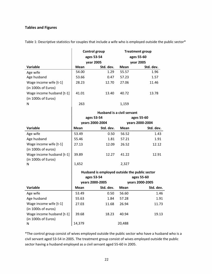
Table 1 shows descriptive statistics for couples that include a husband who is a civil servant. Age of the
wife and age of the husband are measured on December 31st of the respective year. Wage income of
the wife and wage income of the husband (at t-1) indicate the total wage income a worker and her
husband earned in the year prior to the year of observation. The income variables are measured in
thousands of deflated euros.
The control group in our instrumental variable model includes wives whose husband is a civil servant
aged 53-54 in 2005, i.e. wives with a husband who could not be offered early retirement. The treatment
group includes wives with a husband who is a civil servants aged 55-60 in 2005, i.e. women partnered
with those civil servants who could be offered early retirement. Table 1 shows that wives in the control
group have a similar lagged wage income as wives in the treatment group. Wage income for husbands
and wives is also similar for the treatment group as for similarly selected couples in the years before the
early retirement window was opened. For the external validity of our study, it is important to notice that
couples that include a husband who is a civil servant are in general comparable, in terms of observables,
to couples that include a husband who is employed outside the public sector.12
The early retirement window was opened for civil servants employed by the central government. We
use an industry code to identify civil servants employed by the central government. However, groups of
civil servants not employed by the central government have the same industry code as civil servants
employed by the central government. Hence, when we refer to civil servants, we in fact refer to civil
servants employed by the central government plus some groups of other civil servants who were not
eligible for entering the early retirement window. Another data issue concerns the lack of data on early
retirement window offers. Because we do not observe to which civil servants the early retirement
window was offered, we cannot observe whether a civil servant who does not retire rejected the early
retirement offer or simply was not offered the early retirement window. This implies that the
11 We define retirement as leaving the job without entering any new job afterwards. We discuss this in more detail later in this section. 12 The husbands employed outside the public sector are selected in a similar way (tenure in industry) as the husbands employed as a civil servant.
9
“treatment” group as observed in our data is somewhat larger than the “true” treatment group.13
Important to notice is that the early retirement window was offered to workers in departments or
organizations within the central government collectively rather than to individual workers. This makes it
unlikely that there was selection in offering the early retirement window to workers. The final data
imperfection is the absence of data on whether individuals receive retirement benefits. We cope with
this issue by basing our definition of retirement on whether a worker has left his or her job and has not
entered another job afterwards but before January 1st, 2009.
A remaining important concern is that if spouses retire in the same year, but wives retire earlier than
their husbands, this may be considered as wives being induced to retire by retirement of their husbands.
To prevent this, we define retirement status in the following way. We define retirement as having quit a
job and not having worked in any other job after, but before January 1st, 2009. However, if spouses
retire in the same year, but the wife retires before the husband, we consider the husband to have
continued working rather than having retired in this year.14 If the husband retires in a particular year,
and the wife retires within 365 days after the husband, we consider the wife as having retired in the
same calendar year.
5. Methodology
We employ an instrumental variable approach to estimate the impact of early retirement of the
husband on retirement status of the wife. We instrument the retirement choice of the husband using
dummy variables for the ages at which husbands were eligible for entering the early retirement window
interacted with a dummy variable for the year 2005, i.e. the year of the policy change.15 We estimate
our model using only observations on wives employed outside the public sector who have a husband
who is a civil servant. We use wives whose husband is aged 53 or 54 in 2005 as the control group and
wives whose husband is aged 55-60 in 2005 as the treatment group. The model controls for time-
invariant heterogeneity. The treatment effect we estimate is a Local Average Treatment Effect (LATE),
i.e. the effect of early retirement of the husband on the wife’s probability to retire within one year for
those couples for whom the husband was induced to retire early by variation in the eligibility conditions.
13 We do not know how much smaller the “true” treatment group is than the observed treatment group. 14 If at least one member of the couple retires in a year, we will use no observations for this couple in later years. 15 Bloemen, Hochguertel and Zweerink (2013) employ a similar identification strategy to estimate the effect of retirement on the probability to die within five years.

10
5.1 Instrument validity
The validity of our instruments hinges on the satisfaction of two conditions. First, the instruments have
an impact on the probability that husbands retire. Second, the instruments do not correlate with
unobserved factors having an impact on the probability that wives retire. We use dummies for eligibility
for retirement benefits for husbands due to the opening of the early retirement window for civil
servants in 2005 as instruments for husband’s retirement status.
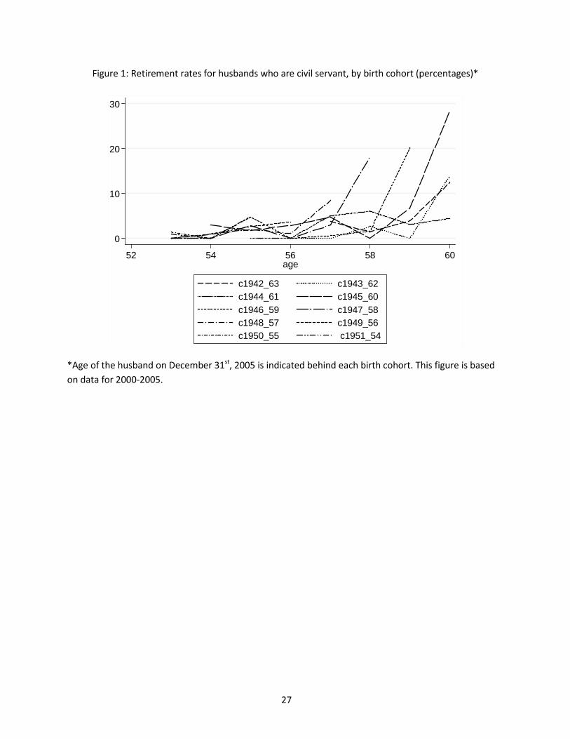
Figure 1 shows retirement rates for husbands who are civil servant. Husbands aged 56-60 have higher
retirement rates in 2005 than in earlier years. The difference in retirement rates between 2005 and
earlier years is especially large for husbands aged 58-60. Husbands aged 53-54 have similar retirement
rates in 2005 as in earlier years. This is all in line with the age-specific incentives as provided by the
temporary decrease in eligibility age in early retirement benefits, as discussed in Section 3. This supports
our hypothesis that our instruments are relevant.16
To our knowledge, there were in 2005 no similar early retirement windows in sectors other than the
public sector. We thus do not expect the opening of the early retirement window to have had a direct
impact on the probability that the wives of the male civil servants retire. We are also not aware of any
event other than the opening of the early retirement window, that may have affected the probability to
retire for husbands being civil servant and aged 55-60 in 2005. We expect that our instruments are not
correlated with unobserved factors that influenced wives’ probability to retire.17 Wives’ unobserved
health, number of hours worked or stress levels associated with work are among the unobserved factors
that may have influenced wives’ probability to retire. Correlation due to anticipation of the opening of
the early retirement window is not expected to be an issue. This is because the opening of the early
retirement window was only announced by the government in April 2004 and central government
employers only decided after that time whether and to whom they would actually open the early
retirement window. We also do not expect selection into public sector jobs by husbands or wives after
the announcement of the opening of the early retirement window to be an issue. The reason for this is
that eligibility for the early retirement window required individuals to have been employed as a civil
16 The Appendix describes pension related policy changes in the period around the introduction of the early retirement arrangement we exploit, and discusses its possible effects on retirement rates. 17 Wives were employed outside the public sector.
11
servant continuously for the ten years prior to early retirement and to have contributed to the public
sector pension fund during the ten years prior to early retirement.
Another possible threat to the exogeneity of our instruments is that factors other than the opening of
the early retirement window may have boosted retirement rates for civil servants in 2005. Changes in
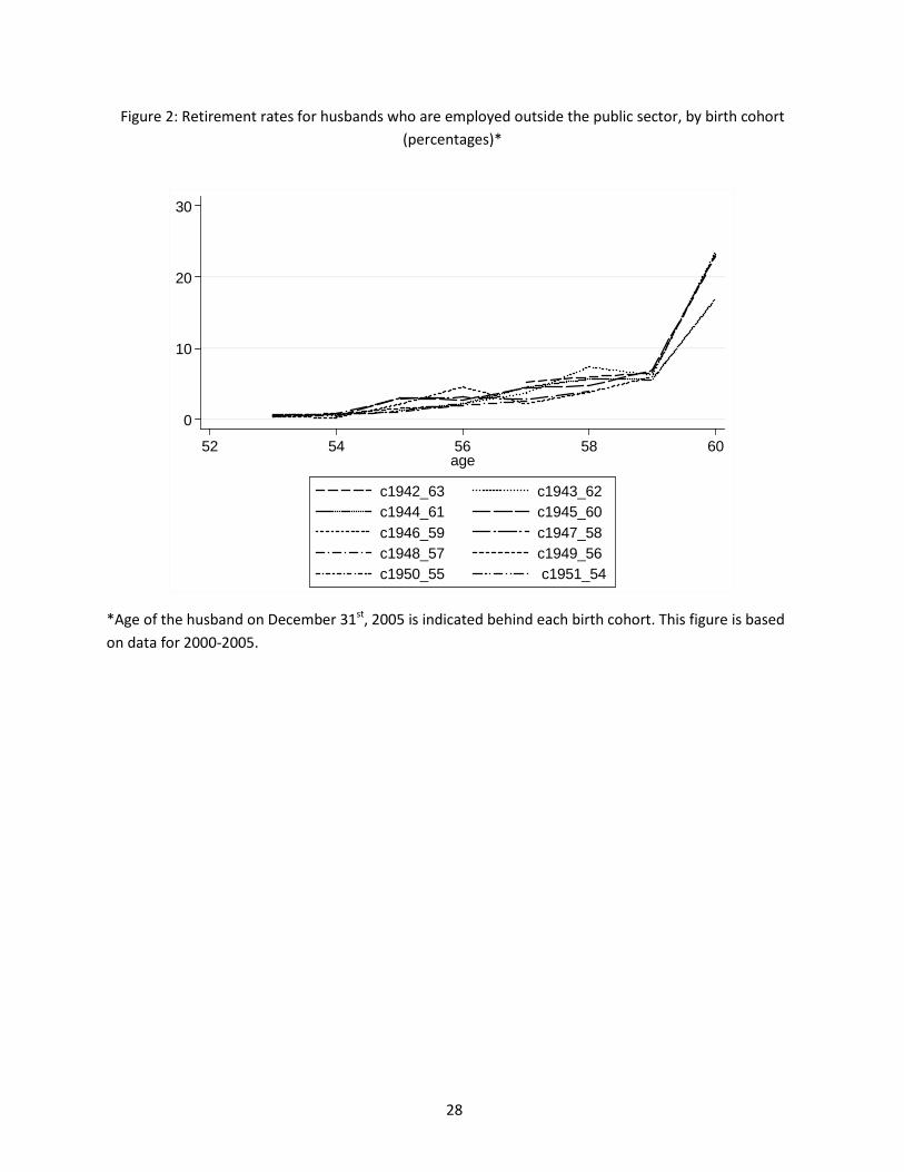
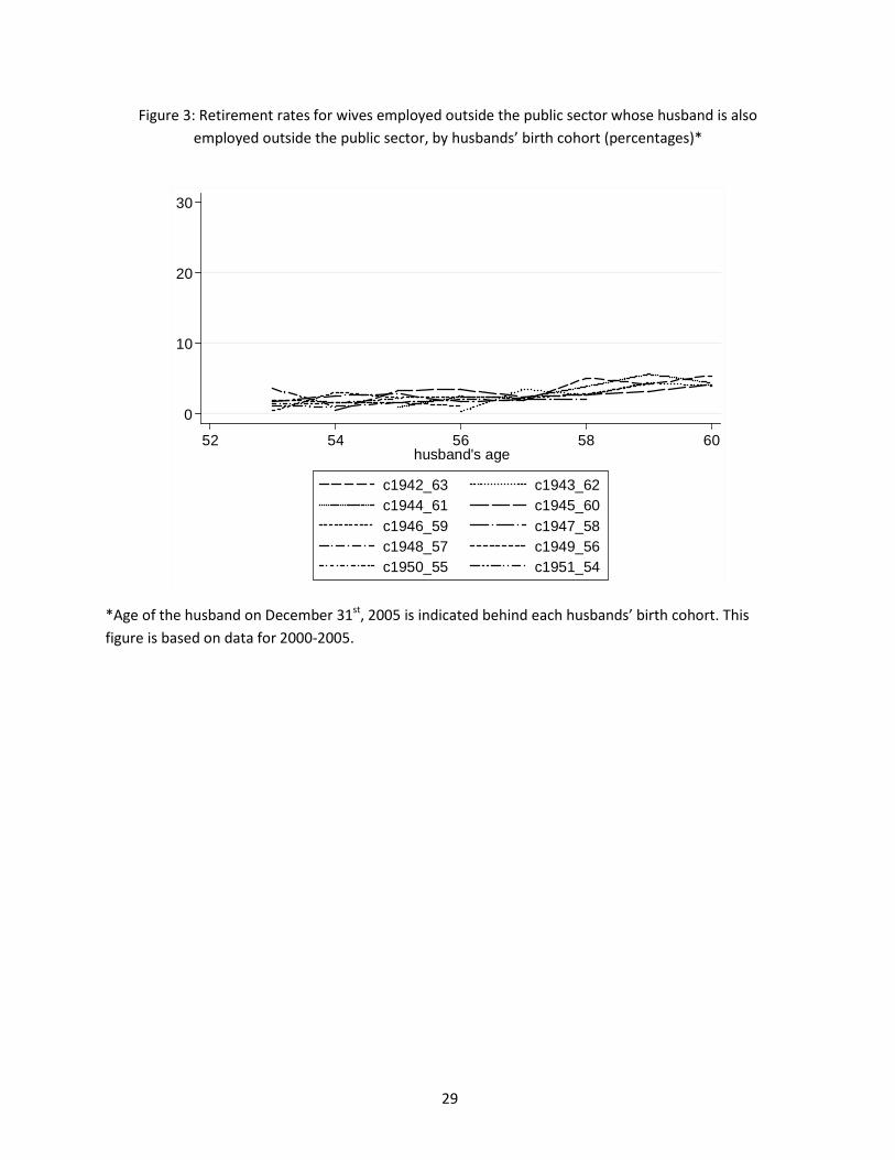
disability insurance may, for instance, have affected retirement rates of civil servants.18 Figure 2 shows
that retirement rates for husbands aged 55-60 employed outside the public sector were not higher in
2005 than in other years. This indicates that factors affecting retirement rates of all husbands aged 55-
60 were not responsible for the increase in retirement rates of husbands employed as a civil servant
aged 55-60 in 2005. It could also be that retirement rates for wives whose husband is aged 55-60 were
higher in 2005 than in earlier years, irrespective of the sector the husband was employed in. The
introduction of a policy that provides wives with an incentive to retire if the husband is aged 55-60, for
instance, may have caused such a deviation. Figure 3 shows that retirement rates for wives employed
outside the public sector whose husband is aged 55-60 and also employed outside the public sector
were not higher in 2005 than in earlier years.
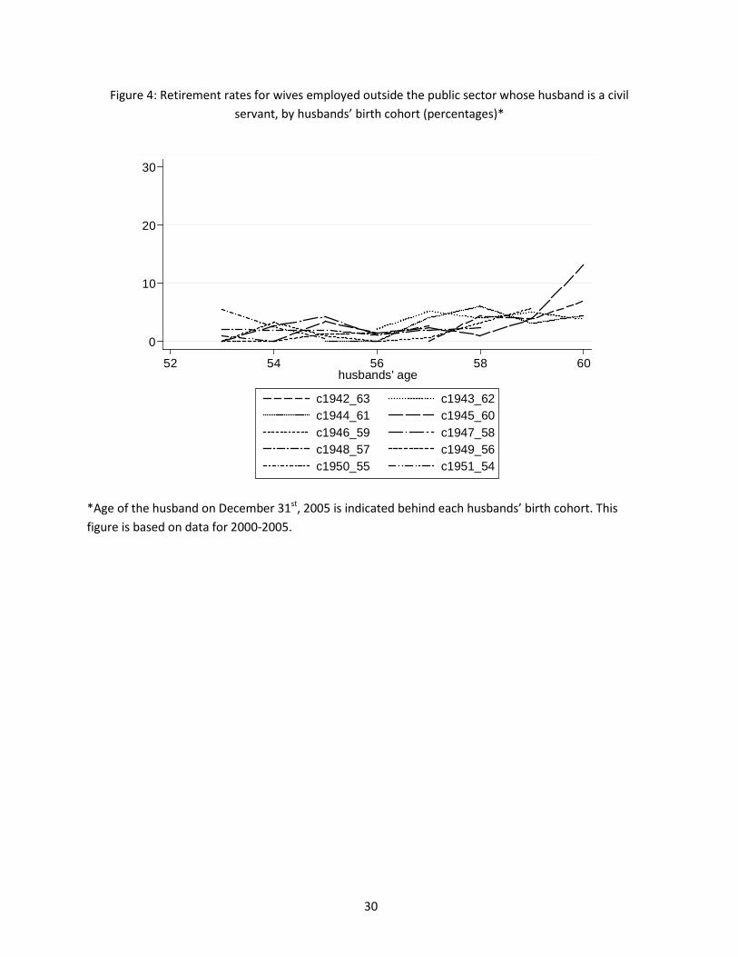
Figure 4 shows retirement rates for wives by husbands’ age and birth cohort when the husband is a civil
servant. Wives’ retirement rates show a clear jump for husbands aged 60 in 2005, though there is no
such jump present for wives with younger husbands in 2005. This may suggest that if we find an effect
of retirement of the husband on retirement status of the wife, this effect may be driven by wives who
have a husband aged 60 in 2005. The wives who retired in 2005 and have a husband aged 60 in 2005,
are all 59 or 60 years old. Especially the wives aged 60 in 2005 may have been eligible for regular early
retirement benefits. This could explain why they retired, though wives of younger husbands, who were
on average also younger themselves, may not have retired in 2005.
5.2 Model specification
We employ a two-stage-least-squares fixed effects instrumental variable model to estimate the LATE. In
the first stage, retirement status of the husband is estimated and in the second stage, the impact of
predicted retirement of the husband on the wife’s probability to retire is estimated. As we use a fixed
effects model, our model has the advantage that it controls for effects of time-invariant individual 18 Disability insurance and its relation to early retirement are discussed in the Appendix. Disability insurance is a universal social insurance scheme and not sector-specific.
12
characteristics and allows individual fixed effects and observed characteristics to be correlated with
each other. We control for year effects and for differences in wife’s and husband’s probability to retire
across age. We specify the first stage of our model as follows:
(1) 𝐻𝑖𝑡 = 𝑒0 + ∑ 𝑏𝑗𝐷𝑗𝑡𝑗=2004𝑗=2000 + ∑ 𝑐𝑘𝐴𝑘𝑖𝑡𝑘=3
𝑘=2 + ∑ 𝑐𝑘𝑝𝐴𝑘𝑖𝑡𝑝𝑘=3𝑘=2 + ∑ 𝑑05𝑙𝑝𝐷05,𝑡𝐸𝑙𝑖𝑡𝑙=60
𝑙=55 + 𝑔𝑖𝑡−1′ 𝑚
+ 𝑒𝑖 + 𝑣𝑖𝑡
where 𝐻𝑖𝑡 is a dummy that is 1 if the husband of couple i is aged 55 or older in year t and the husband of
couple i retired in year t. 𝐻𝑖𝑡 is 0 otherwise. 𝐷𝑗𝑡 is a year dummy that is 1 in year j and 0 otherwise. 𝐴𝑘𝑖𝑡
(𝐴𝑘𝑖𝑡𝑝) denotes the difference between the age of the wife (husband) in couple i in year t and 53, taken
to the kth power.19 𝐸𝑙𝑖𝑡 is an age dummy that is 1 if the husband in couple i reaches age l in year t and 0
otherwise. 𝑔𝑖𝑡−1 includes one-year lagged wage income of the wife and one-year lagged wage income of
the husband. 𝑣𝑖𝑡 is an error term. 𝑒𝑖 is an individual fixed effect that is allowed to be arbitrarily
correlated with all covariates.
The second stage is specified as follows:
(2) 𝑊𝑖𝑡 = 𝛼0 + ∑ 𝛾𝑗𝐷𝑗𝑡𝑗=2004𝑗=2000 + ∑ 𝛿𝑘𝐴𝑘𝑖𝑡𝑘=3
𝑘=2 +∑ 𝛿𝑘𝑝𝐴𝑘𝑖𝑡𝑝𝑘=3𝑘=2 + 𝑔𝑖𝑡−1′ 𝜑 + 𝜔𝐻�𝑖𝑡 + 𝛼𝑖 + 𝑢𝑖𝑡
where 𝑊𝑖𝑡 is a dummy that is 1 if the wife in couple i retires in year t and 0 otherwise. 𝜔 indicates the
LATE. 𝛼𝑖is allowed to be correlated with all covariates. 𝛼𝑖 and 𝑒𝑖 are also allowed to be correlated. 𝑢𝑖𝑡
and 𝑣𝑖𝑡 are allowed to be correlated.
6. Results
6.1 The uninstrumented case
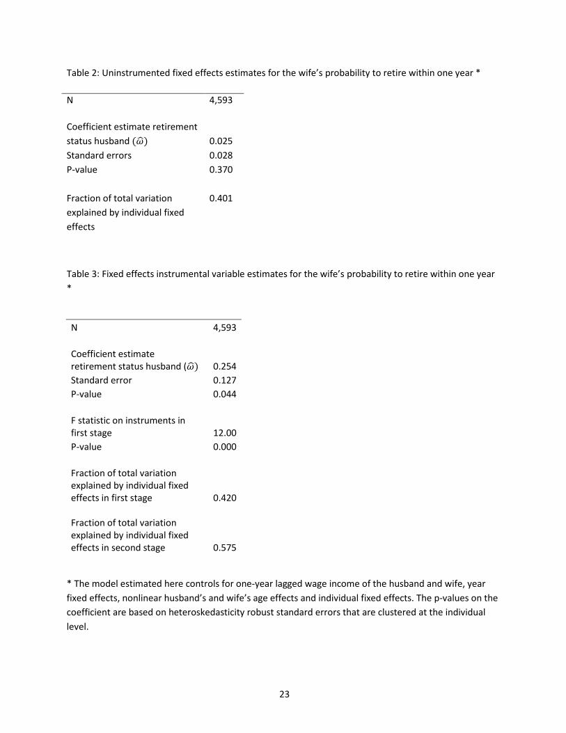
We shall instrument retirement status of the husband because of the potential endogeneity of
retirement status of the husband to the retirement status of the wife. For comparison, Table 2 shows
the coefficient estimates on retirement status of the husband 𝐻𝑖𝑡 for the specification (2) for the case in
which retirement status 𝐻𝑖𝑡 is not instrumented. The coefficient estimate on retirement status of the
husband is insignificant at the ten percent significance level. If retirement status of the husband would
be exogenous to retirement status of the wife, the coefficient estimate on retirement status of the 19 We do not include 𝐴1𝑖𝑡 and/or 𝐴1𝑖𝑡𝑝 in our models. Including 𝐴1𝑖𝑡 and/or 𝐴1𝑖𝑡𝑝 is not possible due to multicollinearity caused by the presence of the year dummies.
13
husband in the fixed effects model without instruments would be similar to the one in the instrumental
variable model with fixed effects.
6.2 Instrumental variable estimates
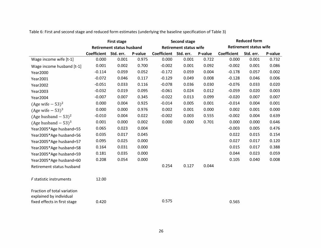
Table 3 shows the instrumental variable fixed effects estimates.20 The estimates show that retirement of
husbands induced by the early retirement window increased their wives’ probability to retire within one
year by 25.4 percentage points. This is effect is significant at the five percent significance level. The
effect is slightly larger than the effects found by Hospido and Zamarro (2013) and Banks, Blundell and
Casanova Rivas (2010). Hospido and Zamarro (2013) and Banks, Blundell and Casanova Rivas (2010) find
a positive effect of 16-18 percentage points and 14-20 percentage points of retirement of the husband
on wives’ probability to retire within the same two-year time interval.
The F statistics in the first stage show that our instruments are relevant at the one percent significance
level. The coefficients on the instruments in the first stage are positive, indicating that the opening of
the early retirement window did induce eligible male civil servants to retire.
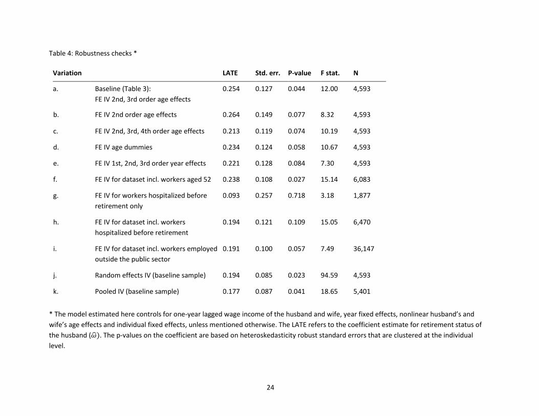
6.3 Robustness checks
Age dummies and nonlinear age and year terms
Our statements concerning the probability to retire are to be understood conditional on age and age of
the husband. Age is an important determinant of retirement status of the wife, so is age of the husband
an important determinant of retirement status of the husband. This may make our result sensitive to
the way age and age of the husband enter our model. We control for second and third order age and
husband’s age effects in our instrumental variable model. This baseline estimate is redisplayed as
variation a in Table 4. As a robustness check, we estimate the instrumental variable model once
controlling for second order age and husband’s age effects only and once controlling for a fourth-degree
polynomial in husband’s age. Table 4 shows that the LATE estimates for the alternative models are
similar to the LATE estimate for the baseline model. This indicates that our instrumental variable result
is robust to controlling for age and husband’s age effects of one order lower or one order higher
(variations b and c). Our instrumental variable result is robust to controlling for age and husband’s age
20 Table 6 shows the first and second stage estimates.
14
fixed effects rather than nonlinear age effects (variation d) and non-linear year effects rather than year
fixed effects (variation e) as well.21
Extended control group: workers aged 52-54 in 2005
Given the selection of our dataset, the control group consists of wives with a husband who is either 53
or 54 in 2005. Because we use fixed effects models, the control group effectively consists of wives who
have a husband who is aged 54 in 2005 only. We include observations on wives and husbands aged 52
for all years and extend our control group to wives who have a husband aged 52-54 in 2005 to verify
whether our result is not driven by particular characteristics of either male civil servants aged 54 in
2005, or their wives’ characteristics. Table 4, variation f, shows that our result is robust to including
wives and husbands aged 52 in our dataset.
Extended dataset: hospitalized workers
Ill-health workers may have a higher probability to retire early than healthy workers. We have tried to
limit bias due to the potential endogeneity of retirement status to health by dropping observations on
workers who have not been hospitalized between 1998 and retirement. We can verify how sensitive our
result is to initial health status by estimating the instrumental variable models using observations on
workers who have been hospitalized between 1998 and retirement and those who have not been
hospitalized between 1998 and retirement. Table 4, variation g, shows that the LATE estimated using
observations on hospitalized workers only is much smaller in magnitude than the LATE estimated using
observations on nonhospitalized workers only. The intuition for this finding is that previously
hospitalized husbands are induced to retire by health problems rather than financial incentives
compared to husbands who were not hospitalized before. Similarly, previously hospitalized wives are
induced to retire by health problems rather than by retirement of their husband. Because the number of
observations on nonhospitalized civil servants is small, the LATE estimates based on observations of
hospitalized and nonhospitalized workers differ only slightly from the LATE based on observations of
nonhospitalized workers only (variation h).
21 Husbands’/wives’ age fixed effects enter the model through husbands’/wives’ age dummies and the non-linear year effects are controlled for in the model by including the terms (𝑦𝑒𝑎𝑟 − 1999)2 and (𝑦𝑒𝑎𝑟 − 1999)3.
15
Extended dataset: workers employed outside the public sector
The dataset used for the estimation of the LATE consists of observations on wives with a husband who is
civil servant only. Our result may depend on civil servant-specific retirement rates of husbands across
age and years. As a robustness check, we estimate a modified version of the model using data on wives
with husbands who are either civil servant or employed outside the public sector. The model we
estimate is the model specified in (1) and (2), except that the instruments, i.e. the interactions between
the dummy for the year 2005 and the dummies for the ages 55-60, are multiplied by a dummy for being
a civil servant. Table 4, variation i, shows that our LATE estimate is robust to correcting for civil servant
specific retirement patterns.
Individual effects: random effects and no individual effects
We also estimate the instrumental variable models with individual random effects (RE); variation in
estimates may point to individual effects being correlated with covariates. We estimate the RE
instrumental variable model using the baseline specification as in (1) and (2). Table 4, variation j, shows
that the LATE estimated using the RE model is significant at the five percent level and that it is slightly
smaller than the LATE estimated using the FE model.22 The difference between the fixed effects and
random effects LATE estimate indicates that individual effects are correlated with at least some
covariates. Individual effects may, for instance, be correlated with lagged wage income. Wives or their
husbands with a higher wage income in the previous year may have time-invariant characteristics that
make them more or less likely to retire. As individual effects and at least some covariates are correlated,
the instrumental variable model with individual fixed effects is preferred over the instrumental variable
model with random effects. Lastly, we estimate the instrumental variable model without individual
effects to verify how sensitive our result is to not controlling for unobserved heterogeneity. Table 4,
variation k, shows that the LATE estimate without individual fixed effects is a bit smaller than the one
with individual fixed effects, but stays significant at the conventional five percent level. Interestingly, the
effect is similar to the effect found by Hospido and Zamarro (2013) and Banks, Blundell and Casanova
Rivas (2010), who also do not control for unobserved heterogeneity.
22 Performing a Hausman test on the differences between coefficient estimates in the random effects and fixed effects model tells us that the differences between coefficient estimates in the two models are significant at the one percent significance level.
16
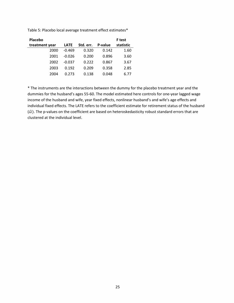
Placebo treatment effects
We have estimated placebo treatment effects to check whether the treatment effects we find might be
spurious. We estimate effects for placebo treatments in any of the years 2000-2004. Six instruments are
used. These instruments are the interactions between the dummy for the placebo treatment year and
the dummy for every age of the husband in the age range 55-60. Table 5 shows that the placebo LATE is
insignificant at the ten percent level for all years, except 2004. The placebo LATE for the year 2004 could
simply be significant at the ten percent level due to chance. By chance, we would expect placebo LATEs
to be significant at the ten percent level in ten percent of the cases if we would estimate a large number
of placebo LATEs. We find that the placebo LATEs are significant in one out of five times, i.e. in 20
percent of the times. This is not a large deviation from the expected ten percent given the small number
of LATEs estimated.
7. Conclusions
This paper has studied the effect of induced retirement of the husband on retirement status of the wife.
The population we studied includes couples with wives who have a strong labor force attachment. We
benefited from having administrative data from the Netherlands and having a strong and exogenous
source of variation in retirement status of the husband to our disposal. We have found that induced
retirement of husbands increases the probability that the wife retires within one year by 25.4
percentage points. This result, which is robust, indicates that the temporary decrease of the eligibility
age for early retirement benefits had strong spillovers to their spouse for male civil servants. The effect
was driven by husbands aged 60 who had a wife aged 59 of 60. This is interesting, because in sectors
other than the public sector, age 60 was a common eligibility age for early retirement benefits.
Interactions between the early retirement window under review and regular early retirement
arrangements in other sectors may thus play a role in the couples’ decision to retire. This is relevant,
also when considering the spillovers of the introduction of age specific retirement incentives to
retirement status of spouses in contexts and countries other than the ones currently studied.
17
References
Baker, M. (2002), “The Retirement Behavior of Married Couples: Evidence from the Spouse's Allowance”, Journal of Human Resources 37: 1-34 Banks, J., R. Blundell and M. Casanova Rivas (2010), “The dynamics of retirement behavior in couples: Reduced-form evidence from England and the US”, preliminary version Berkovec, J. and S. Stern (1991), “Job Exit Behavior of Older Men", Econometrica 59: 189-210 Blau, D.M. and D.B. Gilleskie (2006), “Health insurance and retirement of married couples”, Journal of Applied Econometrics 21: 935-953 Bloemen, H., S. Hochguertel and J. Zweerink (2013), “The Causal Effect of Retirement on Mortality Evidence from Targeted Incentives to retire early”, Tinbergen Institute Discussion Paper No. 2013-119/V Bovenberg, A.L. and L. Meijdam (2001), “The Dutch pension system”, in: A.H. Börsch-Supan and M. Miegel (eds.), ”Pension reform in six countries. What can we learn from each other?”, Berlin: Springer Casanova Rivas, M. (2010), “Happy Together: A Structural Model of Couples' Joint Retirement Choices”, work in progress Dutch Government (2004), “Sociaal flankerend beleid sector Rijk”, Staatscourant 115, 21 June 2004 Dutch Government (2005), “Besluit van 31 december 2004, houdende vaststelling van een aantal tijdelijke rechtspositionele voorzieningen van sociaal flankerend beleid voor de sector Rijk die gelden van 1 maart 2004 tot 1 januari 2008”, Staatsblad 29, 25 January 2005 Goux, D., E. Maurin and B. Petrongolo (2011), “Worktime Regulations and Spousal Labour Supply”, IZA Discussion Paper No. 5639 Gustman, A.L. and T.L. Steinmeier (1986), “A Structural Retirement Model", Econometrica 54: 555-584 Gustman, A.L. and T.L. Steinmeier (2000), “Retirement in Dual-Career Families: A Structural Model”, Journal of Labor Economics 18: 503-545 Hospido, L. and G. Zamarro (2013), “Retirement Patterns of Couples in Europe”, CESR Working Paper No. 2013-006 Hurd, M. (1990), “The Joint Retirement Decisions of Husbands and Wives", in Issues in the Economics of Aging, ed. by D. A. Wise. Chicago: University of Chicago Press.
18
Lumsdaine, R., J. Stock and D. Wise (1992), “Three Models of Retirement: Computational Complexity vs. Predictive Validity", in D. Wise (ed.) Topics in the Economics of Aging, Chicago: University of Chicago Press, 1992 Rust, J. and C. Phelan (1997), “How Social Security and Medicare Affect Retirement Behavior in a World of Incomplete Markets", Econometrica 65: 781-831 Stancanelli, E. (2012), “Spouses’ Retirement and Hours of Work Outcomes: Evidence from Twofold Regression Discontinuity”, CES Working paper No. 2012.74 Statistics Netherlands (2006), “Groei aandeel arbeidsongeschikte vrouwen voorbij”, Webmagazine, October 9th, 2006 Statistics Netherlands (2014), data retrieved on April 16th, 2014 from http://statline.cbs.nl/StatWeb/publication/?DM=SLNL&PA=80396NED&D1=1,9&D2=1-2&D3=0&D4=0-2&D5=1-2&D6=0-2,8,15&D7=0&D8=5&HDR=G1,G2,G3,G6,T,G7&STB=G4,G5&VW=T Van der Klaauw, W. and K.I. Wolphin (2008), “Social security and the retirement and savings behavior of low-income households”, Journal of Econometrics: 145: 21-42 Zweimueller, J., R. Winter-Ebmer and J. Falkinger (1996), “Retirement of Spouses and Social Security Reform”, European Economic Review 40: 449-472

19
Appendix23
The Dutch pension system
The Dutch pension system rests on three pillars (Bovenberg and Meijdam, 2001). The first pillar is the
public old-age pension. The public old-age pension is financed on a pay-as-you-go basis.
Contributions stem from workers and employers. All residents registered in the Netherland accrue
public old-age pension rights. Public old-age pension benefits are flat. For couples they equal the
minimum wage. Singles receive 70 percent of the minimum wage. For every year between the ages 15
and 65 that an individual did not reside in the Netherlands, public old-age benefits are cut by two
percentage points. The second pillar consists of occupational pensions. Occupational pensions are
funded pensions and are generally managed on the sector level.24 About 90 percent of the workers
participate in an occupational pension plan. Occupational pension schemes receive contributions from
workers and employers. Workers who participate in a pension plan pay contributions over the
difference between their wage and a nominal threshold called the “franchise”. As every firm or sector
has its own pension plan and pension conditions, there is a large heterogeneity among occupational
pensions. At the time at which the early retirement window under review was opened, there was also a
large heterogeneity in early retirement arrangements. The third pillar consists of private provisions.
Private provisions include amongst others annuity insurance.
Regular early retirement arrangements for civil servants
As of April 1st, 1997, early retirement benefits for civil servants consisted of two parts. The first part was
in general 70 percent of the “franchise” for civil servants who had worked full-time during their working
life.25 The first part intended to compensate early retirees for the lack of old-age pension benefits for
the period between early retirement and normal retirement. Civil servants were eligible for the first part
if they satisfied two conditions. First, they had to have been employed as a civil servant continuously
during the ten years prior to early retirement. Second, they had to have contributed continuously to the
public pension fund during the ten years preceding early retirement. The first part of early retirement
benefits was in general higher when a civil servant retired at a later age. The first part was financed on a
pay-as-you-go-basis. Workers and employers contributed to the early retirement benefit scheme. Part 23 The Appendix is obtained from Bloemen, Hochguertel and Zweerink (2013). 24 Various large employers have their own pension fund. 25 This replacement rate is based on retirement at the ER eligibility age. The ER eligibility age depends on the birth date of an individual.
20
two of early retirement benefits was funded. Workers and employers contributed to the accrual of
benefits in the second part. When a civil servant would have accrued benefits for 40 years, the sum of
the first and second part would have been 70 percent of the final wage.26 The replacement rate was
reduced by 1.75 percentage points for every year a civil servant would have accrued benefits less than
40 years. Civil servants were allowed to do paid work after early retirement. However, total income of a
retired civil servant was not allowed to exceed 100 percent of the final gross wage.27 Otherwise, early
retirement benefits were cut to bring the total income earned on 100 percent of the final gross wage
(means test).
Other policy changes
On January 1st, 2004, the public sector pension fund switched from a final wage pension system to an
average wage pension system.28 However, due to a transition arrangement, civil servants born before
January 1st, 1954 were hardly affected by the switch.
On January 1st, 2006, the so-called fiscal facilitation of early retirement benefits for individuals born
January 1st, 1950 or later was terminated.29 This implied that most early retirement arrangements for
the affected individuals disappeared. Early retirement among civil servants usually occurred at age 61 or
62. The termination of the fiscal facilitation of early retirement benefits could have been anticipated as
of 2003 and may have induced anticipation effects of civil servants aged 53-55 in 2005.
Early retirement via disability insurance
Workers may facilitate an early withdrawal from the labor force by starting to receive disability
insurance (DI) benefits. Workers could start receiving DI benefits if they would be judged to be disabled
by a medical examiner of the social insurance institute. DI benefits amounted to up to 70 percent of the
final earned gross wage. The DI system was financed by workers and employers. In the context of this
paper, it is important to notice that civil servants faced the same generosity of and eligibility criteria for
26 This replacement rate is based on retirement at the ER eligibility age. The ER eligibility age depends on the birth date of an individual. 27 Income does not only include wage income here, but also some other specified sources of income. 28 The pension fund for the health care sector also switched from a final wage system to an average wage system on January 1st, 2004. Many other pension funds also switched in the years before or after January 1st, 2004. 29 The fiscal facilitation of the early retirement contributions implied that the early retirement benefits were taxed, and that the early retirement contributions paid by workers and employers were exempted from taxation. As effectively less tax was paid, the fiscal facilitation made early retirement very attractive for eligible workers and employers.
21
DI benefits as workers employed in other sectors, and that there were no major changes in DI in 2005
except one on December 29th.
From that day on, eligibility criteria for starting to receive disability benefits have been tightened and
disability benefits have been made less generous for workers who are only partially disabled. One year
earlier, another change in disability insurance had taken place. Since January 1st, 2004, workers could
only start receiving DI benefits after having been ill during employment continuously for two years. We
hardly observe any civil servants who are induced to retire in 2005 to start receiving disability benefits.
Moreover, the inflow into DI for men in all ages decreased smoothly from 53,000 in 2001 to 36,000 in
2004 and dropped to 17,000 in 2005. It is thus unlikely that the retirement rates in 2005 were boosted
by changed incentives in DI (Statistics Netherlands, 2006).
22
Tables and Figures
Table 1: Descriptive statistics for couples that include a wife who is employed outside the public sector*
Control group Treatment group ages 53-54 ages 55-60 year 2005 year 2005 Variable Mean Std. dev. Mean Std. dev. Age wife 54.00 1.29 55.57 1.96 Age husband 53.66 0.47 57.23 1.57 Wage income wife [t-1] (in 1000s of Euros)
28.23
12.70
27.06
11.46
Wage income husband [t-1] (in 1000s of Euros)
41.01
13.40
40.72
13.78
N 263 1,159
Husband is a civil servant
ages 53-54 ages 55-60 years 2000-2004 years 2000-2004
Variable Mean Std. dev. Mean Std. dev. Age wife 53.49 0.50 56.52 1.43 Age husband 55.46 1.81 57.21 1.91 Wage income wife [t-1] 27.13
12.09
26.52
12.12
(in 1000s of euros) Wage income husband [t-1] 39.89
1,652
12.27
41.22
2,327
12.91
(in 1000s of Euros) N
Husband is employed outside the public sector
ages 53-54 ages 55-60
years 2000-2005 years 2000-2005 Variable Mean Std. dev. Mean Std. dev. Age wife 53.49 0.50 56.60 1.46 Age husband 55.63 1.84 57.28 1.91 Wage income wife [t-1] 27.03
11.68
26.94
11.73
(in 1000s of euros) Wage income husband [t-1] 39.68
14,379
18.23
40.94
20,488
19.13
(in 1000s of Euros) N
*The control group consist of wives employed outside the public sector who have a husband who is a civil servant aged 53-54 in 2005. The treatment group consist of wives employed outside the public sector having a husband employed as a civil servant aged 55-60 in 2005.
23
Table 2: Uninstrumented fixed effects estimates for the wife’s probability to retire within one year * N 4,593 Coefficient estimate retirement status husband (𝜔�) Standard errors P-value
0.025 0.028 0.370
Fraction of total variation explained by individual fixed effects
0.401
Table 3: Fixed effects instrumental variable estimates for the wife’s probability to retire within one year *
N 4,593 Coefficient estimate retirement status husband (𝜔�) 0.254 Standard error 0.127 P-value 0.044 F statistic on instruments in first stage 12.00 P-value 0.000 Fraction of total variation explained by individual fixed effects in first stage 0.420 Fraction of total variation explained by individual fixed effects in second stage
0.575
* The model estimated here controls for one-year lagged wage income of the husband and wife, year fixed effects, nonlinear husband’s and wife’s age effects and individual fixed effects. The p-values on the coefficient are based on heteroskedasticity robust standard errors that are clustered at the individual level.
24
Table 4: Robustness checks *
Variation LATE Std. err. P-value F stat. N
a. Baseline (Table 3): FE IV 2nd, 3rd order age effects
0.254 0.127 0.044 12.00 4,593
b. FE IV 2nd order age effects 0.264 0.149 0.077 8.32 4,593
c. FE IV 2nd, 3rd, 4th order age effects 0.213 0.119 0.074 10.19 4,593
d. FE IV age dummies 0.234 0.124 0.058 10.67 4,593
e. FE IV 1st, 2nd, 3rd order year effects 0.221 0.128 0.084 7.30 4,593
f. FE IV for dataset incl. workers aged 52 0.238 0.108 0.027 15.14 6,083
g. FE IV for workers hospitalized before retirement only
0.093 0.257 0.718 3.18 1,877
h. FE IV for dataset incl. workers hospitalized before retirement
0.194 0.121 0.109 15.05 6,470
i. FE IV for dataset incl. workers employed outside the public sector
0.191 0.100 0.057 7.49 36,147
j. Random effects IV (baseline sample) 0.194 0.085 0.023 94.59 4,593
k. Pooled IV (baseline sample) 0.177 0.087 0.041 18.65 5,401
* The model estimated here controls for one-year lagged wage income of the husband and wife, year fixed effects, nonlinear husband’s and wife’s age effects and individual fixed effects, unless mentioned otherwise. The LATE refers to the coefficient estimate for retirement status of the husband (𝜔�). The p-values on the coefficient are based on heteroskedasticity robust standard errors that are clustered at the individual level.
25
Table 5: Placebo local average treatment effect estimates*
Placebo treatment year LATE Std. err. P-value
F test statistic
2000 -0.469 0.320 0.142 1.60 2001 -0.026 0.200 0.896 3.60 2002 -0.037 0.222 0.867 3.67 2003 0.192 0.209 0.358 2.85 2004 0.273 0.138 0.048 6.77
* The instruments are the interactions between the dummy for the placebo treatment year and the dummies for the husband’s ages 55-60. The model estimated here controls for one-year lagged wage income of the husband and wife, year fixed effects, nonlinear husband’s and wife’s age effects and individual fixed effects. The LATE refers to the coefficient estimate for retirement status of the husband (𝜔�). The p-values on the coefficient are based on heteroskedasticity robust standard errors that are clustered at the individual level.
26
Table 6: First and second stage and reduced form estimates (underlying the baseline specification of Table 3)
First stage Second stage Reduced form
Retirement status husband Retirement status wife Retirement status wife
Coefficient Std. err. P-value Coefficient Std. err. P-value Coefficient Std. err. P-value
Wage income wife [t-1] 0.000 0.001 0.975 0.000 0.001 0.722 0.000 0.001 0.732
Wage income husband [t-1] 0.001 0.002 0.700 -0.002 0.001 0.092 -0.002 0.001 0.086 Year2000 -0.114 0.059 0.052 -0.172 0.059 0.004 -0.178 0.057 0.002 Year2001 -0.072 0.046 0.117 -0.129 0.049 0.008 -0.128 0.046 0.006
Year2002 -0.051 0.033 0.116 -0.078 0.036 0.030 -0.076 0.033 0.020 Year2003 -0.032 0.019 0.095 -0.061 0.024 0.012 -0.059 0.020 0.003 Year2004 -0.007 0.007 0.345 -0.022 0.013 0.099 -0.020 0.007 0.007
(Age wife − 53)2 0.000 0.004 0.925 -0.014 0.005 0.001 -0.014 0.004 0.001
(Age wife − 53)3 0.000 0.000 0.976 0.002 0.001 0.000 0.002 0.001 0.000
(Age husband− 53)2 -0.010 0.004 0.022 -0.002 0.003 0.555 -0.002 0.004 0.639
(Age husband− 53)3 0.001 0.000 0.002 0.000 0.000 0.701 0.000 0.000 0.646 Year2005*Age husband=55 0.065 0.023 0.004 -0.003 0.005 0.476 Year2005*Age husband=56 0.035 0.017 0.045 0.022 0.015 0.154
Year2005*Age husband=57 0.095 0.025 0.000 0.027 0.017 0.120
Year2005*Age husband=58 0.164 0.031 0.000 0.015 0.017 0.388 Year2005*Age husband=59 0.181 0.035 0.000 0.044 0.023 0.059
Year2005*Age husband=60 0.208 0.054 0.000 0.105 0.040 0.008
Retirement status husband
0.254 0.127 0.044
F statistic instruments 12.00
Fraction of total variation explained by individual fixed effects in first stage 0.420
0.575
0.565
27
Figure 1: Retirement rates for husbands who are civil servant, by birth cohort (percentages)*
*Age of the husband on December 31st, 2005 is indicated behind each birth cohort. This figure is based on data for 2000-2005.
0
10
20
30
52 54 56 58 60age
c1942_63 c1943_62 c1944_61 c1945_60 c1946_59 c1947_58 c1948_57 c1949_56 c1950_55 c1951_54
28
Figure 2: Retirement rates for husbands who are employed outside the public sector, by birth cohort (percentages)*
*Age of the husband on December 31st, 2005 is indicated behind each birth cohort. This figure is based on data for 2000-2005.
0
10
20
30
52 54 56 58 60age
c1942_63 c1943_62 c1944_61 c1945_60 c1946_59 c1947_58 c1948_57 c1949_56 c1950_55 c1951_54
29
Figure 3: Retirement rates for wives employed outside the public sector whose husband is also employed outside the public sector, by husbands’ birth cohort (percentages)*
*Age of the husband on December 31st, 2005 is indicated behind each husbands’ birth cohort. This figure is based on data for 2000-2005.
0
20
30
10
52 54 56 58 60husband's age
c1942_63 c1943_62c1944_61 c1945_60c1946_59 c1947_58c1948_57 c1949_56c1950_55 c1951_54
30
Figure 4: Retirement rates for wives employed outside the public sector whose husband is a civil servant, by husbands’ birth cohort (percentages)*
*Age of the husband on December 31st, 2005 is indicated behind each husbands’ birth cohort. This figure is based on data for 2000-2005.
0
10
20
30
52 54 56 58 60husbands' age
c1942_63 c1943_62c1944_61 c1945_60c1946_59 c1947_58c1948_57 c1949_56c1950_55 c1951_54