Flow Separation on Wind Turbine Blades - Universiteit Utrecht · 2020-02-26 · Flow Separation on...
170
Transcript of Flow Separation on Wind Turbine Blades - Universiteit Utrecht · 2020-02-26 · Flow Separation on...


Flow Separation on Wind Turbine Blades
Het Loslaten van Stroming over Windturbinebladen

Pagina leeg
Flow Separation on Wind Turbine Blades
Het Loslaten van Stroming over Windturbinebladen
(met een samenvatting in het Nederlands)
Proefschrift
ter verkrijging van de graad van doctor aan de Universiteit Utrecht, op gezag van de Rector Magnificus, Prof. Dr. H.O. Voorma,
ingevolge het besluit van het College voor Promotiesin het openbaar te verdedigen op maandag 8 januari 2001 des middags te 16:15 uur
door
Gustave Paul Corten
geboren op 8 september 1968, te Rotterdam

promotor: Prof. dr. ir. C.D. Andriesseverbonden aan de Faculteit Natuur- en Sterrenkundevan de Universiteit Utrecht
leescommissie:Prof. W.C. SinkeIr. H. SnelProf. dr. ir. G.A.M. van KuikProf. dr. W.F. van der Weg
examencommissie:voorzitter: Prof. dr. H.J.G.L.M. Lamersgasten: Ir. H.J.M. Beurskens
Prof. dr. ir. G.A.M. van KuikIng. O. de Vries
hoogleraren: Prof. dr. ir. W. LourensProf. dr. F. W. SarisProf. dr. W. C. SinkeProf. dr. P. van de StratenProf. dr. W.F. van der Weg
dit proefschrift werd mede mogelijk gemaakt met financiële steun van EnergieonderzoekCentrum Nederland
on januari 16, 2001 some corrections were made
ISBN 90-393-2582-0 , NUGI 837

‘What is needed now is a new era of economicgrowth - growth that is forceful and at the sametime socially and environmentally sustainable.’
‘Sustainable development is development thatmeets the needs of the present withoutcompromising the ability of future generations tomeet their own needs.’
Brundtland, G.H., Our Common Future, 1987


vii
Summary
In the year 2000, 15GW of wind power was installed throughout the world, producing 100PJof energy annually. This contributes to the total electricity demand by only 0.2%. Both theinstalled power and the generated energy are increasing by 30% per year world-wide. If theairflow over wind turbine blades could be controlled fully, the generation efficiency and thusthe energy production would increase by 9%.
Power Control
To avoid damage to wind turbines, they are cut out above 10 Beaufort (25 m/s) on the windspeed scale. A turbine could be designed in such a way that it converts as much power aspossible in all wind speeds, but then it would have to be to heavy. The high costs of such adesign would not be compensated by the extra production in high winds, since such winds arerare. Therefore turbines usually reach maximum power at a much lower wind speed: the ratedwind speed, which occurs at about 6 Beaufort (12.5 m/s). Above this rated speed, the powerintake is kept constant by a control mechanism. Two different mechanisms are commonlyused. Active pitch control, where the blades pitch to vane if the turbine maximum is exceededor, passive stall control, where the power control is an implicit property of the rotor.
Stall ControlThe flow over airfoils is called ‘attached’ when it flows over the surface from the leadingedge to the trailing edge. However, when the angle of attack of the flow exceeds a certaincritical angle, the flow does not reach the trailing edge, but leaves the surface at the separationline. Beyond this line the flow direction is reversed, i.e. it flows from the trailing edgebackward to the separation line. A blade section extracts much less energy from the flowwhen it separates. This property is used for stall control.Stall controlled rotors always operate at a constant rotation speed. The angle of attack of theflow incident to the blades is determined by the blade speed and the wind speed. Since thelatter is variable, it determines the angle of attack. The art of designing stall rotors is to makethe separated area on the blades extend in such a way, that the extracted power remainsprecisely constant, independent of the wind speed, while the power in the wind at cut-outexceeds the maximum power of the turbine by a factor of 8. Since the stall behaviour isinfluenced by many parameters, this demand cannot be easily met. However, if it can be met,the advantage of stall control is its passive operation, which is reliable and cheap.
Flow Separation on Wind Turbine Blades
viii
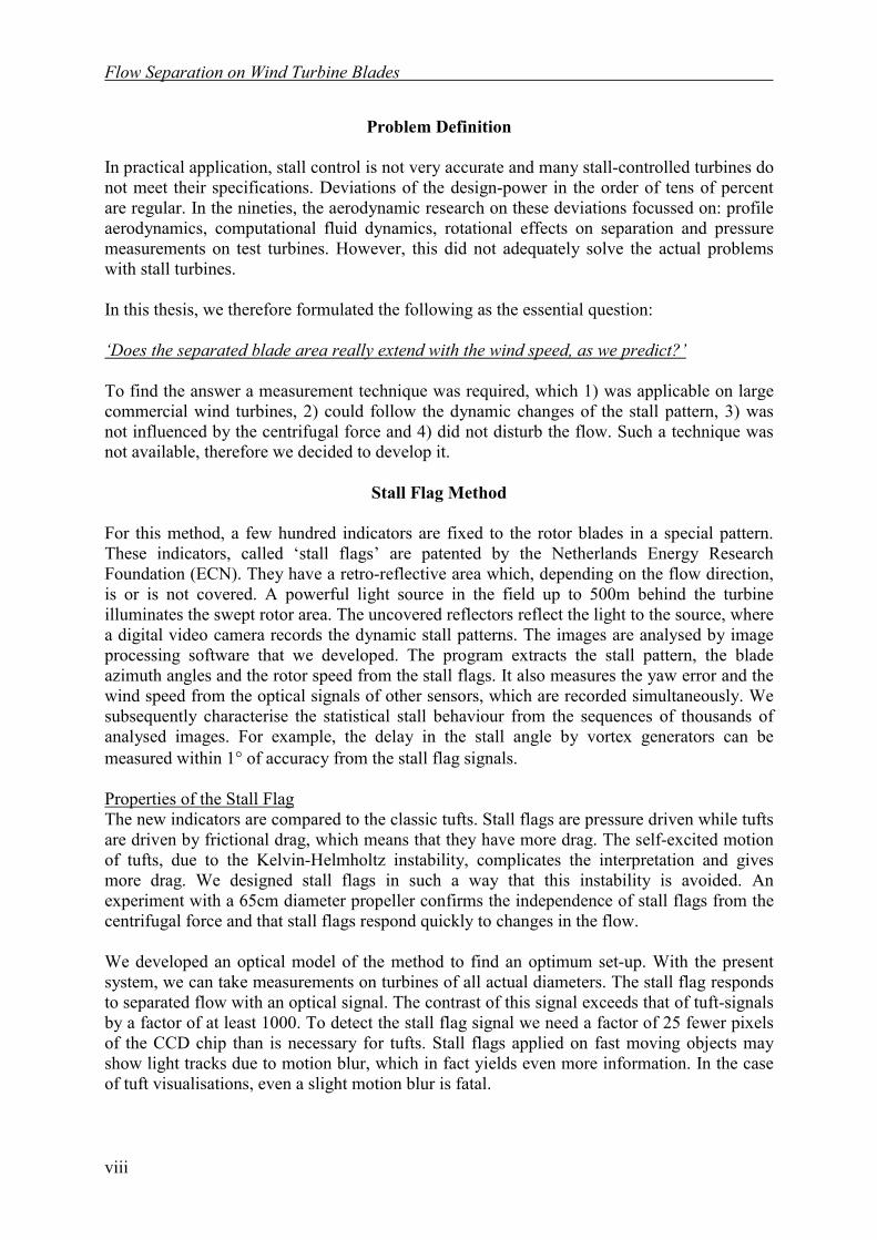
Problem Definition
In practical application, stall control is not very accurate and many stall-controlled turbines donot meet their specifications. Deviations of the design-power in the order of tens of percentare regular. In the nineties, the aerodynamic research on these deviations focussed on: profileaerodynamics, computational fluid dynamics, rotational effects on separation and pressuremeasurements on test turbines. However, this did not adequately solve the actual problemswith stall turbines.
In this thesis, we therefore formulated the following as the essential question:
‘Does the separated blade area really extend with the wind speed, as we predict?’
To find the answer a measurement technique was required, which 1) was applicable on largecommercial wind turbines, 2) could follow the dynamic changes of the stall pattern, 3) wasnot influenced by the centrifugal force and 4) did not disturb the flow. Such a technique wasnot available, therefore we decided to develop it.
Stall Flag Method
For this method, a few hundred indicators are fixed to the rotor blades in a special pattern.These indicators, called ‘stall flags’ are patented by the Netherlands Energy ResearchFoundation (ECN). They have a retro-reflective area which, depending on the flow direction,is or is not covered. A powerful light source in the field up to 500m behind the turbineilluminates the swept rotor area. The uncovered reflectors reflect the light to the source, wherea digital video camera records the dynamic stall patterns. The images are analysed by imageprocessing software that we developed. The program extracts the stall pattern, the bladeazimuth angles and the rotor speed from the stall flags. It also measures the yaw error and thewind speed from the optical signals of other sensors, which are recorded simultaneously. Wesubsequently characterise the statistical stall behaviour from the sequences of thousands ofanalysed images. For example, the delay in the stall angle by vortex generators can bemeasured within 1° of accuracy from the stall flag signals.
Properties of the Stall FlagThe new indicators are compared to the classic tufts. Stall flags are pressure driven while tuftsare driven by frictional drag, which means that they have more drag. The self-excited motionof tufts, due to the Kelvin-Helmholtz instability, complicates the interpretation and givesmore drag. We designed stall flags in such a way that this instability is avoided. Anexperiment with a 65cm diameter propeller confirms the independence of stall flags from thecentrifugal force and that stall flags respond quickly to changes in the flow.
We developed an optical model of the method to find an optimum set-up. With the presentsystem, we can take measurements on turbines of all actual diameters. The stall flag respondsto separated flow with an optical signal. The contrast of this signal exceeds that of tuft-signalsby a factor of at least 1000. To detect the stall flag signal we need a factor of 25 fewer pixelsof the CCD chip than is necessary for tufts. Stall flags applied on fast moving objects mayshow light tracks due to motion blur, which in fact yields even more information. In the caseof tuft visualisations, even a slight motion blur is fatal.

Summary
ix
Principal Results
In dealing with the fundamental theory of wind turbines, we found a new aspect of theconversion efficiency of a wind turbine, which also concerns the stall behaviour. Another newaspect concerns the effects of rotation on stall. By using the stall flag method, we were able toclear up two practical problems that seriously threatened the performance of stall turbines.These topics will be described briefly.
1. Inherent Heat GenerationThe classic result for an actuator disk representing a wind turbine is that the power extractedequals the kinetic power transferred. This is a consequence of disregarding the flow aroundthe disk. When this flow is included, we need to introduce a heat generation term in theenergy balance. This has the practical consequence that an actuator disk at the Lanchester-Betz limit transfers 50% more kinetic energy than it extracts. This surplus is dissipated inheat.Using this new argument, together with a classic argument on induction, we see no reason tointroduce the concept of edge-forces on the tips of the rotor blades (Van Kuik, 1991). Werather recommend following the ideas of Lanchester (1915) on the edge of the actuator diskand on the wind speed at the disc. We analyse the concept induction, and show that correctingfor the aspect ratio, for induced drag and application of Blade Element Momentum Theory allhave the same significance for a wind turbine. Such corrections are sometimes made twice(Viterna & Corrigan, 1981).
2. Rotational Effects on Flow SeparationIn designing wind turbine rotors, one uses the aerodynamic characteristics measured in thewind tunnel on fixed aerodynamic profiles. These characteristics are corrected for the effectsof rotation and subsequently used for wind turbine rotors. Such a correction was developed bySnel (1990-1999). This correction is based on boundary layer theory, the validity of which wequestion in regard to separated flow.We estimated the effects of rotation on flow separation by arguing that the separation layer isthick so the velocity gradients are small and viscosity can be neglected. We add the argumentthat the chord-wise speed and its derivative normal to the wall is zero at the separation line,which causes the terms with the chord-wise speed or accelerations to disappear. Theconclusion is that the chord-wise pressure gradient balances the Coriolis force. By doing sowe obtain a simple set of equations that can be solved analytically. Subsequently, our modelpredicts that the convective term with the radial velocity (vr∂vr/∂r) is dominant in the equationfor the r-direction, precisely the term that was neglected in Snel’s analysis.
3. Multiple Power LevelsSeveral large commercial wind turbines demonstrate drops in maximum power levels up to45%, under apparently equal conditions. Earlier studies attempting to explain this effect bytechnical malfunctioning, aerodynamic instabilities and blade contamination effects estimatedwith computational fluid dynamics, have not yet yielded a plausible result.
We formulated many hypotheses, three of which were useful. By taking stall flagmeasurements and making two other crucial experiments, we could confirm one of those threehypotheses: the insect hypothesis. Insects only fly in low wind, impacting upon the blades atspecific locations. In these conditions, the insectual remains are located at positions whereroughness has little influence on the profile performance, so that the power is not affected. Inhigh winds however, the flow around the blades has changed. As a result, the positions at
Flow Separation on Wind Turbine Blades
x
which the insects have impacted at low winds are very sensitive to contamination. So thecontamination level changes at low wind when insects fly and this level determines the powerin high winds when insects do not fly. As a consequence we get discrete power levels in highwinds.
The other two hypotheses, which did not cause the multiple power levels for the case westudied, gave rise to two new insights. First, we expect the power to depend on the winddirection at sites where the shape of the terrain concentrates the wind. In this case the powerlevel of all turbine types, including pitch regulated ones, will be affected. Second, we inferheuristically that the stalled area on wind turbine blades will adapt continuously to windvariations. Therefore, the occurrence of strong bi-stable stall-hysteresis, which most bladesections demonstrate in the wind tunnel, is lost. This has been confirmed by taking specialstall flag measurements.
4. Deviation of SpecificationsThe maximum power of stall controlled wind turbines often shows large systematic deviationsfrom the design. We took stall flag measurements on a rotor, the maximum power of whichwas 30% too high, so that the turbine had to be cut out far below the designed cut-out windspeed. We immediately observed the blade areas with deviating stall behaviour. Some areasthat should have stalled did not and caused the excessive power. We adapted those areas byshifting the vortex generators. In this way we obtained a power curve that met the designmuch more closely and we realised a production increase of 8%.

xi
Contents
Summary . . . . . . . . . . . . . . . . . .
Contents . . . . . . . . . . . . . . . . . .
1. Introduction . . . . . . . . . . . . . . . .
2. Energy Extraction . . . . . . . . . . . . . . .List of Symbols . . . . . . . . . . . . . . . .2.1 Maximum Energy Transfer . . . . . . . . . . . .
2.1.1 The Lanchester-Betz Limit . . . . . . . . .2.1.2 Heat Generation . . . . . . . . . . .
2.2 Induction . . . . . . . . . . . . . . .2.2.1 Prandtl Finite Airfoil Induction . . . . . . . . .2.2.2 Induction for a Wind Turbine . . . . . . . . . .2.2.3 Blade Element Momentum Theory . . . . . . . .
2.3 Tip Correction . . . . . . . . . . . . . . .2.3.1 Prandtl Tip Correction . . . . . . . . . . .2.3.2 Tip Correction for an Actuator Disk . . . . . . . .
2.4 Blade Aerodynamics . . . . . . . . . . . . . .2.4.1 The Angle of Attack . . . . . . . . . . . .2.4.2 Lift and Drag . . . . . . . . . . . .2.4.3 Stall . . . . . . . . . . . . . . .
2.5 Rotational Effects . . . . . . . . . . . . . .2.5.1 Fundamental Equations in a Rotating Frame of Reference . . .2.5.2 Boundary Layer Assumptions. . . . . . . . . .2.5.3 Attached Flow on a Rotating Blade . . . . . . . .2.5.4 Rotational Effects on Flow Separation; Snel’s Analysis . . . .2.5.5 Rotational Effects on Flow Separation; Our Analysis . . . .2.5.6 Extension of the Heuristics with θ-z Rotation . . . . . .
vii
xi
1
5799
11171819202222232525262730303132343841
Flow Separation on Wind Turbine Blades
xii
3. The Stall Flag Method . . . . . . . . . . . . . .List of Symbols . . . . . . . . . . . . . . . .3.1 The Stall Flag . . . . . . . . . . . . . .
3.1.1 Controlled Evolutionary Development . . . . . . .3.1.2 List of Recommendations. . . . . . . . . . .
3.2 Interpretation of Signals . . . . . . . . . . . .3.2.1 Aerodynamic Forces on the Stall Flag . . . . . . .3.2.2 External Forces . . . . . . . . . . . . .3.2.3 Sensitivity . . . . . . . . . . . . . .3.2.4 Response Time . . . . . . . . . . . . .3.2.5 Hystersis and the h/2h-Model . . . . . . . . . .3.2.6 Kelvin-Helmholtz Instability . . . . . . . . . .3.2.7 Observations . . . . . . . . . . . . .
3.3 Flow Disturbance . . . . . . . . . . . . . .3.3.1 Transition . . . . . . . . . . . . . .3.3.2 Drag Increase . . . . . . . . . . . . .3.3.3 Influence to Pressure Distributions . . . . . . . .
3.4 Tufts and Stall Flags Compared . . . . . . . . . . .
4. Optical Aspects of Stall Flags . . . . . . . . . . . .List of symbols . . . . . . . . . . . . . . . .4.1 Principles of Detection . . . . . . . . . . . .
4.1.1 Detectable or Visible . . . . . . . . . . .4.1.2 Active or Passive . . . . . . . . . . . .4.1.3 Stall Flag Positioning . . . . . . . . . . .4.1.4 Type and Locus of Contrasting Area . . . . . . . .4.1.5 Retro-reflection . . . . . . . . . . . . .4.1.6 Differential Detection . . . . . . . . . . .
4.2 Quantifying Stall Flag Signals . . . . . . . . . .4.2.1 Sources of Radiation . . . . . . . . . . . .4.2.2 Intensity of Stall Flag Signals . . . . . . .4.2.3 Stall Flag Image Size. . . . . . . . . . . .4.2.4 Image Spectral Irradiance. . . . . . . . . . .4.2.5 Image Spectral Exposure . . . . . . . . . . .4.2.6 The Absolute Demand . . . . . . . . . . .4.2.7 The Relative Demand . . . . . . . . . . .4.2.8 Visibility . . . . . . . . . . . . . .
4.3 Optimisation . . . . . . . . . . . . . . .4.3.1 Diffuse Reflection . . . . . . . . . . . .4.3.2 Retro-reflection . . . . . . . . . . . . .4.3.3. Summary . . . . . . . . . . . . .
4.4 Application on a Wind Turbine . . . . . . . . . . .4.5 Tufts Signals . . . . . . . . . . . . . . .
454648485253535556565760626464656668
697072727273737475777777797980818282848485868790
Contents
xiii
5. Stall Flag Experiments . . . . . . . . . . . . . .5.1 The Standard Procedure . . . . . . . . . . . .
5.1.1 Instrumentation of the Turbine . . . . . . . . .5.1.2 The Stall Flag Pattern . . . . . . . . . . .5.1.3 The Measurements . . . . . . . . . . .5.1.4 Image Analysis . . . . . . . . . . . . .5.1.5 Experimental Data . . . . . . . . . . . .
5.2 Proof of Concept Using a 25mHAT . . . . . . . . . .5.3 Multiple Power Levels . . . . . . . . . . . . .
5.3.1 The Tip Commands Hypothesis . . . . . . . . .5.3.2 The Insect Hypothesis . . . . . . . . . . .5.3.3 Experience with a 44m HAT . . . . . . . . . .5.3.4 Validation of the Tip Commands Hypothesis . . . . . .5.3.5 Validation of the Insect Hypothesis . . . . . . . .5.3.6 The Terrain Concentration Hypothesis . . . . . . . .5.3.7 Conclusion on Multiple Power Levels . . . . . . . .
5.4 Comparison with Theory . . . . . . . . . . . . .
6. Conclusions. . . . . . . . . . . . . . . . .
References . . . . . . . . . . . . . . . . . .
A: The Aerpac 43m Rotor . . . . . . . . . . . . . .A.1 First Stall Flag Measurement . . . . . . . . . . . .A.2 Second Stall Flag Measurement . . . . . . . . . . .A.3 Vortex Generator Modelling . . . . . . . . . . . .
B: Propeller Experiment . . . . . . . . . . . . . .
C: Stall Flag Patent . . . . . . . . . . . . . . .
Samenvatting . . . . . . . . . . . . . . . . .
Curriculum Vitae . . . . . . . . . . . . . . . .
Dankwoord . . . . . . . . . . . . . . . . .
93949495979899
101105105107108109110112114115
117
121
125125129130
133
135
145
149
151

Flow Separation on Wind Turbine Blades
xiv
1
1. Introduction
This thesis deals with flow separation on wind turbine blades. When air flows over an airfoilit may not follow the surface from the leading edge towards the trailing edge, but may turnaway and break loose from that surface. This phenomenon is called flow separation. It spoilsthe performance of the blades. When separation occurs, the lift, which normally is rapidlyincreasing with the angle of attack, stops rising and the drag, which normally is very small,becomes comparable to the lift.An aircraft that suddenly stalls slows down due to the large drag and loses lift, due to bothstalling and due to the decrease in speed. Therefore, flow separation is to be avoided inaviation, unless braking firmly is intended.
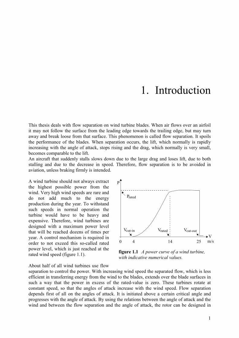
A wind turbine should not always extractthe highest possible power from thewind. Very high wind speeds are rare anddo not add much to the energyproduction during the year. To withstandsuch speeds in normal operation theturbine would have to be heavy andexpensive. Therefore, wind turbines aredesigned with a maximum power levelthat will be reached dozens of times peryear. A control mechanism is required inorder to not exceed this so-called ratedpower level, which is just reached at therated wind speed (figure 1.1).
About half of all wind turbines use flowseparation to control the power. With increasing wind speed the separated flow, which is lessefficient in transferring energy from the wind to the blades, extends over the blade surfaces insuch a way that the power in excess of the rated-value is zero. These turbines rotate atconstant speed, so that the angles of attack increase with the wind speed. Flow separationdepends first of all on the angles of attack. It is initiated above a certain critical angle andprogresses with the angle of attack. By using the relations between the angle of attack and thewind and between the flow separation and the angle of attack, the rotor can be designed in
figure 1.1 A power curve of a wind turbine,with indicative numerical values.
V m/s
Vrated
P
Vcut-in Vcut-out
Prated
0 4 14 25

Flow Separation on Wind Turbine Blades
2
such a way that the maximum power captured is limited by the rotor geometry. The constantrotation speed and the passive power control lead to a simple but efficient design of theturbine, which is therefore relatively cheap.
The other half of the wind turbines turn their blades actively to vane position at high windspeeds, so that the smaller angles of attack limit the transfer of energy. This principle is moreexpensive since it requires a mechanism to turn the blades. Here one needs to understand lessof the physics of flow separation, however. The angles of attack approach the conditions offlow separation only around rated wind speed.
Flow separation depends in a complex way on many parameters. When the inflow approachesthe separation angle, any parameter, no matter how small, can have a decisive role. Therefore,the separation behaviour cannot be predicted. In practice one relies on empirical studies ofairfoil sections in a wind tunnel. However, the same airfoils in different wind tunnels oftendemonstrate different stall properties. When the airfoils characterised in a tunnel are used aspart of a wind turbine blade and rotate in the field one observes further deviations. Thephenomenon of separation is very sensitive to surface roughness, turbulence level andimperfections of the airfoil contour.
Turbine power control based on passive stall is often inaccurate up to +/- 15%, but in theworst case it can deviate as much as 45%. Overpower leads to overheating of the generator ofthe turbine, so that the latter has to be stopped and an economic loss is suffered. Largedeviations become unacceptable for the increasing investments in wind energy generation.Pitch-controlled turbines may produce about 15% less power near the rated wind speed due topremature separation, but they are more predictable.
Poor control of flow separation leads to economic losses of 15% for stall-regulated turbinesand 2.5% for pitch-regulated turbines. Every GW wind power installed loses 22GWh perpercent annually due to flow separation. Presently, in August 2000, the wind power installedworld-wide is 15GW, so that for an average separation loss of 9%, the present losses are3GWh or 10 PJ per year. This corresponds to about 3% of the electricity consumption in theNetherlands.
In chapter 2 of this thesis the process of energy extraction by a rotor is described. We firstreproduce the classic result for the maximum power that a wind turbine can extract from aflow. We stress - and this is not new but often overlooked - that energy extraction by a windturbine is inherently coupled to turbulent mixing and viscous shear behind the turbine, whichcauses that a large amount of kinetic energy dissipates in heat. The amount is about 1/3 of thetotal decrease of the kinetic energy in the flow. This clarifies the peculiar situation that thepower required to drive a force D with speed U in air is -D·U, while the same force atstandstill in a wind of speed U can extract maximally -2/3D·U. Then we deal with induction.We discuss the corrections for angles of attack, for induced drag and for the finite aspectratios. These three corrections address the same physical effect, however. This is not wellknown so that sometimes more than one of these corrections is applied.
The remainder of chapter 2 is devoted to the effects of rotation on flow separation. Thediscussion is focused on relevant approximations of the Navier-Stokes equation. We estimatethe radial component of the flow in the separated area to be the largest, precisely the one thathas been neglected so far. In our physical model of the separated flow, the chord-wise
Introduction
3
pressure gradient just balances the Coriolis force. Furthermore, in separated flow viscousforces will be so small that they can be neglected. Thus, we arrive at Euler equations, whichcan be solved analytically.In chapters 3 and 4 we present a flow visualisation technique, based on a new detector, the so-called stall flag. This stall flag has been patented in European Countries and in the UnitedStates. The uncertainties associated with flow separation were an incentive for measuring theproperties of stall in practice, but there appeared to be no good method of doing so. We havedeveloped a method with which the separated area on any wind turbine can be visualised fromhalf a kilometre distance. By this method, the fast dynamic variations in the separated flowcan be followed. The very thin and very light wireless stall flags, that only need to be pastedon the surface of the airfoil, have a negligible influence on the flow. Chapter 3 deals with theaerodynamic aspects of the stall flag, and addresses the influence of external forces. Thesignals of the stall flags are optical. The development and modelling of the stall flagobservation system are described in chapter 4.
Chapter 5 describes the actual stall flag experiments. It first gives an impression of the fieldwork and continues with proofs of the value of stall flag measurements (The application ofstall flags to improve the power curve of an 43m diameter rotor and a proof with a rotatingpropeller of 65cm diameter are described in appendices). Chapter 6 presents the conclusions.

Flow Separation on Wind Turbine Blades
4
5
2. Energy Extraction
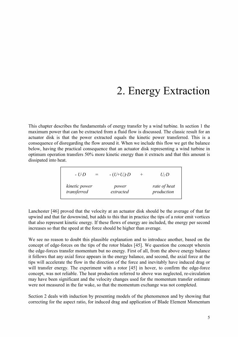
This chapter describes the fundamentals of energy transfer by a wind turbine. In section 1 themaximum power that can be extracted from a fluid flow is discussed. The classic result for anactuator disk is that the power extracted equals the kinetic power transferred. This is aconsequence of disregarding the flow around it. When we include this flow we get the balancebelow, having the practical consequence that an actuator disk representing a wind turbine inoptimum operation transfers 50% more kinetic energy than it extracts and that this amount isdissipated into heat.
Lanchester [46] proved that the velocity at an actuator disk should be the average of that farupwind and that far downwind, but adds to this that in practice the tips of a rotor emit vorticesthat also represent kinetic energy. If these flows of energy are included, the energy per secondincreases so that the speed at the force should be higher than average.
We see no reason to doubt this plausible explanation and to introduce another, based on theconcept of edge-forces on the tips of the rotor blades [45]. We question the concept whereinthe edge-forces transfer momentum but no energy. First of all, from the above energy balanceit follows that any axial force appears in the energy balance, and second, the axial force at thetips will accelerate the flow in the direction of the force and inevitably have induced drag orwill transfer energy. The experiment with a rotor [45] in hover, to confirm the edge-forceconcept, was not reliable. The heat production referred to above was neglected, re-circulationmay have been significant and the velocity changes used for the momentum transfer estimatewere not measured in the far wake, so that the momentum exchange was not completed.
Section 2 deals with induction by presenting models of the phenomenon and by showing thatcorrecting for the aspect ratio, for induced drag and application of Blade Element Momentum
- U·D = - (U+Ui)·D + Ui·D
kinetic powertransferred
power extracted
rate of heatproduction
Flow Separation on Wind Turbine Blades
6
Theory all have the same significance for a wind turbine. This is not generally known, andmay lead to double corrections as proposed in [26] or to the idea that the aspect ratiocorrection includes the tip correction [45].
Section 3 deals with tip corrections. Prandtl’s tip correction addresses the azimuthal non-uniformity of disk loading, but does not correct for the flow around the tips or for the flowaround the edges of an actuator disk. Lanchester [46] stated ‘At the disk edge, it is manifestlyimpossible to maintain any finite pressure difference between the front and the rear faces.’ Soin fact a concept for a second tip correction is proposed that affects even an actuator disk.
Section 4 briefly reviews airfoil aerodynamics. They are basic for the detailed treatment of theaerodynamics on rotating blades given in section 5.Here we estimated the effects of rotation on flow separation by arguing that the separationlayer is thick, therefore the velocity gradients are small and viscosity can be neglected. Withthe argument that the chord-wise speed and its derivative normal to the wall is 0 at theseparation line, the terms with the chord-wise speed or accelerations disappear and we mustconclude that the chord-wise pressure gradient balances the Coriolis force. By doing so we geta simple set of equations that can be solved analytically. We oppose the classic model of Snel[52,53]. He uses boundary layer theory, which is invalid in separated flow [51,64]. As aconsequence he neglects precisely those terms which we estimate to be dominant.

Energy Extraction
7
List of Symbols
a [-] axial induction factora' [-] tangential induction factorA [m2] surface of the actuator diskb [m] half of the span of the airfoilc [m] chordCD [-] axial force coefficientCH [-] total pressure head coefficientCheat [-] dissipated heat coefficientcsep [m] separated length of the chordcdi [-] induced drag coefficientcl [-] lift coefficient L/(½ρv2c)CP [-] power coefficientcp [-] pressure coefficient p/(½ρv2)D [N/m] drag force per unit spanDax [N] axial force exerted by the actuator diskDi [N/m] induced drag force per unit spanDN [N] normalisation for axial force ½ρAU2
f [-] stalled fraction of the chord csep/cdτ [m3] infinitely small element of volumeF [N/kg] external force per unit of massFr [N/kg] external force per unit of mass in the r-directionFθ [N/kg] external force per unit of mass in the θ-directionFz [N/kg] external force per unit of mass in the z-directioni [rad] induced angle of attackL [N/m] lift force per unit spanm [kg/s] mass flow of the wind, in section 2.2.2 it is the mass flow per unit span in
kg/ms to which the momentum transfer per unit span is confined.P [W] powerPflow [W/m] kinetic power extracted from the flow per unit airfoil spanPN [W] normalisation power ½ρAU3
p [N/m2] pressurep0 [N/m2] atmospheric pressurep+ [N/m2] pressure on upwind site of the actuator diskp- [N/m2] pressure on downwind side of the actuator diskpd [N/m2] dynamic pressure ½ρU2
r [m] radial positionR [m] radius of the turbine rotors [-] location of the separation pointt [s] timeU [m/s] wind speedUD [m/s] wind speed at the diskUi [m/s] induced velocity

Flow Separation on Wind Turbine Blades
8
UW [m/s] wind speed in the far wakeV [m/s] wind speed in the very far wakev [m/s] velocity of the airfoilvr [m/s] flow velocity in the r-direction in the rotating frame of referencevθ [m/s] flow velocity in the θ-direction in the rotating frame of referencevz [m/s] flow velocity in the z-direction in the rotating frame of referenceW [m/s] resultant inflow velocityx [m] position in the direction of the chordy [m] position in the direction of the spanz [m] position normal to the blade surface
α [rad] angle of attackα0 [rad] zero lift angle of attackβ [rad] local pitch angle including twistΓ [m2/s] circulationδ [m] boundary layer thickness∆U [m/s] velocity change in very far wake due to actuator disk.∆Ps [W] kinetic power extracted from the flow through the stream tube.∆P [W] kinetic power extracted from the total flow.ε [-] fraction of the total mass flow m through the actuator disk∇ [m-1] nabla-operator (∂ /∂x, ∂ /∂y, ∂ /∂z)ρ [kg/m3] air density ≈ 1.25 kg/m3
µ [Ns/m2] dynamic viscosity of air ≈ 17.1·10-6 Ns/m2
τ [N/m2] shear stressη [-] efficiency of kinetic energy transferϕ [rad] geometric angle of attackθ [rad] position in chord-wise directionλ [-] tip speed ratio ΩR/Uλ [-] aspect ratio (2b2)/bcλr [-] local speed ratio Ωr/UΣ [m] cross section of inflow per unit span to which momentum change is
confinedω [s-1] vorticityΩ [rad/s] rotor angular frequency
Energy Extraction
9
2.1 Maximum Energy Transfer
The theory predicting the maximum useful power that can be extracted from a fluid flow wasfirst published by F.W. Lanchester [46] in 1915. In most cases however, this theory isattributed to A. Betz, who published the same argument in 1920 [7]. To do justice to the firstauthor, we will speak of the 'Lanchester-Betz' limit. The first subsection briefly describes themodel, in which Lanchester analyses the actuator disk introduced by Froude in 1889 [32]. Thesecond subsection adds a new aspect to the classic model: the inherent viscous losses of anactuator disk. It will be shown that an actuator disk operating in wind turbine mode extractsmore energy from the fluid than can be transferred into useful energy. At the Lanchester-Betzlimit the decrease of the kinetic energy in the wind is converted by 2/3 into useful power andby 1/3 into heat. The heat is produced by the viscous force of the outer flow on the stream tubethat just encloses the flow through the actuator disk. The analysis shows that there is nonecessity to add edge-forces to the actuator disk model [45].
2.1.1 The Lanchester-Betz Limit
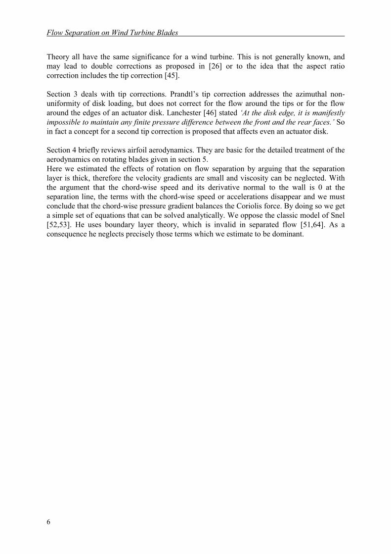
This section summarises a text written by Glauert [34], to which physical arguments areadded. First the actual wind turbine will be replaced by a so-called actuator disk which wasintroduced by Froude (see figure 2.1). This actuator disk is an abstract theoretical analogue ofa wind turbine being used in momentum theory. The disk has a surface A, equal to the sweptarea of the wind turbine, and it is oriented perpendicular to the wind. The disk does notconsist of several rotor blades but has a homogeneous structure. The undisturbed wind speedis U, at the actuator disk it is UD=(1-a)U and in the far wake it is (1-2a)U. The parameter a iscalled the induction factor which takes into account the decrease of the wind speed when itpasses through the permeableactuator disk. The mass flowthrough this disk is ρA(1-a)Uand it is driven by thedifference in pressure p+ on theupwind side of the disk and p-
on the downwind side. So thepressure at the disk isdiscontinuous and the disk issubject to a net axial force Dax= A(p+-p-). This force is alsoexerted on the fluid and thus itshould be equal to the changeof the flow of momentum.From conservation of mass itfollows that the stream tube justenclosing the flow through theactuator disk has a constant
far ahead actuator disk far wake
U a(1- )
Actuator disk,surface A
DaxU a(1-2 )
U
U
U
U
p-
p0
p+
figure 2.1 Froude’s actuator model. The stream tubeconsists of a slipstream behind the disk, but has novelocity discontinuity in front of the disk.

Flow Separation on Wind Turbine Blades
10
mass flow ρA(1-a)U at all cross sections from far upstream to far downstream. The figureshows this stream tube and its expansion. Behind the actuator we have a clear slipstream, butin front of it such a boundary does not exist, therefore we dashed the slip stream contour here.As this mass flow is constant, the change of momentum should be attributed to a velocitydifference between the flow in the far wake and the undisturbed wind speed far upstream:
.)w-+ U-a)U(U-(1=p-p ρ (2.1)
Upwind and downwind of the actuator disk, the kinetic energy in the flow is transferred into'pressure' energy. So the actuator disk does not directly extract kinetic energy. The disk slowsdown the flow which causes a pressure difference over the disk. The extracted energy comesfrom the product of the pressure difference and the volume flow through the disk. Applicationof Bernoulli's relation that p+½ρU2 = constant along a streamline (when no power isextracted), yields for the flow upwind and downwind respectively:
,)1( 2221
21 p+Ua=p+U +
o2 −ρρ (2.2)
,)1( 2221
21 p+Ua=p+U -
ow2 −ρρ (2.3)
where po is the undisturbed atmospheric pressure. By subtracting equations 2.2 and 2.3 itfollows that:
.)2221
w-+ U-(U=p-p ρ (2.4)
The combination of equations 2.1 and 2.4 demonstrates that the velocity decrease in front ofthe disk equals that behind the disk:
.)1(, UaU2a)U-(1=U Dw −= (2.5)
The remarkable fact that half the acceleration must take place in front of the disk and halfbehind it will be discussed in sections 2.1.2 and 2.2. The absolute values for p+ and p- arefound to be:
,)2()2( 2221 aap+paaU+p=p dyno
2o
+ −=−ρ (2.6)
,)32()32( 2221 aap-p=aaU-p=p dyno
2o
- −−ρ (2.7)
where the free stream dynamic pressure pd = ½ρU2 is used. It should be noted that the increaseof the pressure on the upwind side is larger than the decrease of the pressure on the downwindside. This suggests that the pressure field far from the turbine can be modelled as the sum of adipole and a monopole or source.The extracted power is equal to the difference of the kinetic energy in the flow far upstream,minus the kinetic energy in the flow far downstream, multiplied by the mass flow ρA(1-a)U.Far upstream the velocity is U and far downstream it is (1-2a)U. Thus we find for the power:
,)1(4)1(4 23212
NPaaAUaaP −=−= ρ (2.8)
Energy Extraction
11
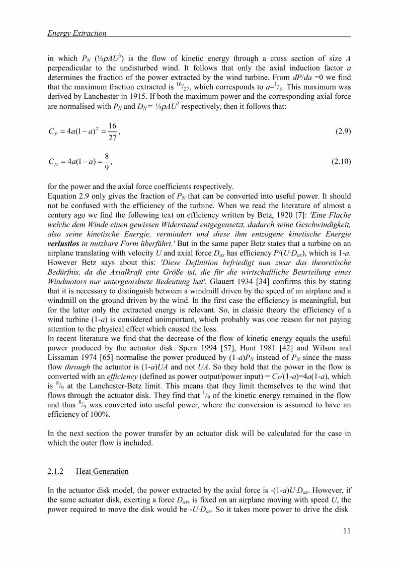
in which PN (½ρAU3) is the flow of kinetic energy through a cross section of size Aperpendicular to the undisturbed wind. It follows that only the axial induction factor adetermines the fraction of the power extracted by the wind turbine. From dP/da =0 we findthat the maximum fraction extracted is 16/27, which corresponds to a=1/3. This maximum wasderived by Lanchester in 1915. If both the maximum power and the corresponding axial forceare normalised with PN and DN = ½ρAU2 respectively, then it follows that:
,2716
)1(4 2 =−= aaCP (2.9)
,98)1(4 =−= aaCD (2.10)
for the power and the axial force coefficients respectively.Equation 2.9 only gives the fraction of PN that can be converted into useful power. It shouldnot be confused with the efficiency of the turbine. When we read the literature of almost acentury ago we find the following text on efficiency written by Betz, 1920 [7]: 'Eine Flachewelche dem Winde einen gewissen Widerstand entgegensetzt, dadurch seine Geschwindigkeit,also seine kinetische Energie, vermindert und diese ihm entzogene kinetische Energieverlustlos in nutzbare Form überführt.' But in the same paper Betz states that a turbine on anairplane translating with velocity U and axial force Dax has efficiency P/(U·Dax), which is 1-a.However Betz says about this: 'Diese Definition befriedigt nun zwar das theoretischeBedürfnis, da die Axialkraft eine Größe ist, die für die wirtschaftliche Beurteilung einesWindmotors nur untergeordnete Bedeutung hat'. Glauert 1934 [34] confirms this by statingthat it is necessary to distinguish between a windmill driven by the speed of an airplane and awindmill on the ground driven by the wind. In the first case the efficiency is meaningful, butfor the latter only the extracted energy is relevant. So, in classic theory the efficiency of awind turbine (1-a) is considered unimportant, which probably was one reason for not payingattention to the physical effect which caused the loss. In recent literature we find that the decrease of the flow of kinetic energy equals the usefulpower produced by the actuator disk. Spera 1994 [57], Hunt 1981 [42] and Wilson andLissaman 1974 [65] normalise the power produced by (1-a)PN instead of PN since the massflow through the actuator is (1-a)UA and not UA. So they hold that the power in the flow isconverted with an efficiency (defined as power output/power input) = CP/(1-a)=4a(1-a), whichis 8/9 at the Lanchester-Betz limit. This means that they limit themselves to the wind thatflows through the actuator disk. They find that 1/9 of the kinetic energy remained in the flowand thus 8/9 was converted into useful power, where the conversion is assumed to have anefficiency of 100%.
In the next section the power transfer by an actuator disk will be calculated for the case inwhich the outer flow is included.
2.1.2 Heat Generation
In the actuator disk model, the power extracted by the axial force is -(1-a)U·Dax. However, ifthe same actuator disk, exerting a force Dax, is fixed on an airplane moving with speed U, thepower required to move the disk would be -U·Dax. So it takes more power to drive the disk
Flow Separation on Wind Turbine Blades
12
than the maximum power that can be generated by the disk. This difference is understoodwhen the flow around the actuator is also included in the analysis. It then follows that theenergy conversion by an actuator disk has an inherent dissipation of kinetic energy into heat.
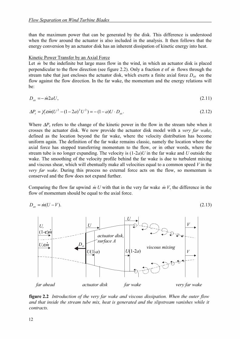
Kinetic Power Transfer by an Axial ForceLet m be the indefinite but large mass flow in the wind, in which an actuator disk is placedperpendicular to the flow direction (see figure 2.2). Only a fraction ε of m flows through thestream tube that just encloses the actuator disk, which exerts a finite axial force Dax on theflow against the flow direction. In the far wake, the momentum and the energy relations willbe:
,2aUmDax −= (2.11)
.)1())21(( 2222
1axs DUaUaUmP ⋅−−=−−= ε∆ (2.12)
Where ∆Ps refers to the change of the kinetic power in the flow in the stream tube when itcrosses the actuator disk. We now provide the actuator disk model with a very far wake,defined as the location beyond the far wake, where the velocity distribution has becomeuniform again. The definition of the far wake remains classic, namely the location where theaxial force has stopped transferring momentum to the flow, or in other words, where thestream tube is no longer expanding. The velocity is (1-2a)U in the far wake and U outside thewake. The smoothing of the velocity profile behind the far wake is due to turbulent mixingand viscous shear, which will ebentually make all velocities equal to a common speed V in thevery far wake. During this process no external force acts on the flow, so momentum isconserved and the flow does not expand further.
Comparing the flow far upwind m U with that in the very far wake m V, the difference in theflow of momentum should be equal to the axial force.
).( VUmDax −= (2.13)
figure 2.2 Introduction of the very far wake and viscous dissipation. When the outer flowand that inside the stream tube mix, heat is generated and the slipstream vanishes while itcontracts.
U a(1- )DaxU, mε
U
U a(1-2 ) V
UV
viscous mixing
far ahead actuator disk far wake very far wake
U,m(1-ε).
.actuator disk,surface A
Energy Extraction
13
We can express V in U, a and ε by using the momentum balance between the far wake and thevery far wake. The momentum in the outer flow of the far wake is (1-ε) m U, and in the streamtube it is ε m (1-2a)U, which together should be equal to m V to conserve momentum, or
.)21()21()1( UaUaUV εεε −=−+−= (2.14)
The velocity change obtained from the momentum relation 2.13 is connected to the change ofthe kinetic power in the wind, by
.)1()( 222
1axDUaVUmP ⋅−−=−= ε∆ (2.15)
To clarify: this is the change of the kinetic power in the flow due to the axial force when theouter flow is included, whereas equation 2.12 expresses that change when the outer flow isexcluded. In practice the mass flow m is large but finite, so that the fraction of m going throughthe disk, ε, is much smaller than 1 and ∆P is close to -Dax·U. So, the decrease of flow ofkinetic energy by a force Dax approaches the scalar product of the undisturbed wind speed -Uand Dax and not the often used product of the local velocity -(1-a)U and the force Dax. Thelatter corresponds to the power extracted from the flow.
Dissipation into HeatIn the process of mixing between the far wake and the very far wake, the kinetic power in theflow will not be conserved, but it will be partially converted into heat. This heat is generatedby the viscous force that accelerates the flow in the stream tube to the velocity V in the veryfar wake. In this process the flow inside the stream tube gains less kinetic energy than theouter flow loses. In the far wake the kinetic power inside the stream tube is ½ε m (1-2a)2U2
and in the outer flow it is ½(1-ε) m U2. In the very far wake the kinetic power is ½ m V2. Thedifference has to be the heat generated;
.)1(])1()21([ 22222
1axheat DaUVUUamP ⋅−−=−−+−= εεε (2.16)
Of course, this is also equal to ∆P-∆Ps.
If we want to normalise to PN= ½ρAU3, as in the previous section, the mass flow through theactuator disk (1-a)ρAU has to be replaced by ε m . So we use PN = ½ε m U2/(1-a) =-DaxU/(4a(1-a)). Since the mass flow through the actuator disk is much smaller than the flowoutside the wake, we take the limit ε→0, and find the following power coefficients,
,)1(4 aaP
PCN
H −≈=∆
(2.17)
,)1(4 2aaPP
CN
sP −==
∆(2.18)
Flow Separation on Wind Turbine Blades
14
.)1(4 2 aaP
PC
N
heatheat −≈= (2.19)
Here CH refers to the transferred kinetic power, CP to the kinetic power actually extracted andCheat to the power in the viscous heating. CP is the commonly used (classic) power coefficient.
It follows that the maximum efficiency for the process of transfer of kinetic energy into usefulpower by an actuator disk η is:
,1 aCC
H
P −≈=η (2.20)
which is in agreement with Betz’s result [7]. Our calculation makes clear that an actuator diskdoes not convert all transferred kinetic energy into useful energy. The energy balance reads:
.heatPH CCC += (2.21)
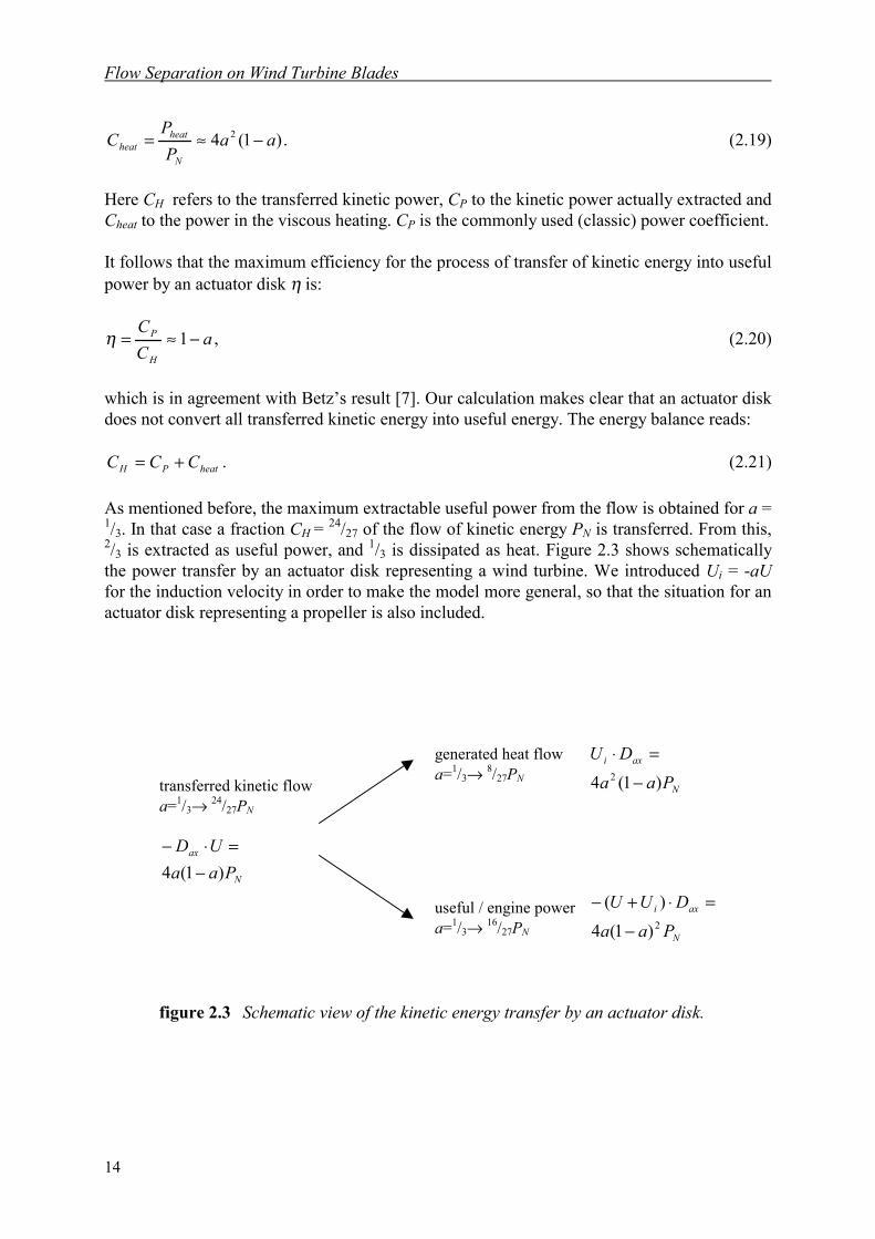
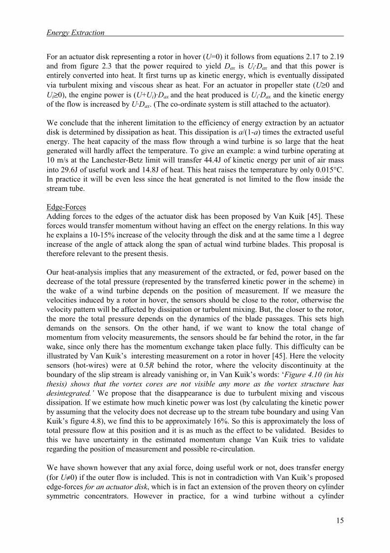
As mentioned before, the maximum extractable useful power from the flow is obtained for a =1/3. In that case a fraction CH = 24/27 of the flow of kinetic energy PN is transferred. From this,2/3 is extracted as useful power, and 1/3 is dissipated as heat. Figure 2.3 shows schematicallythe power transfer by an actuator disk representing a wind turbine. We introduced Ui = -aUfor the induction velocity in order to make the model more general, so that the situation for anactuator disk representing a propeller is also included.
transferred kinetic flowa=1/3→ 24/27PN
N
ax
PaaUD
)1(4 −=⋅−
N
axi
PaaDU
)1(4 2 −
=⋅
N
axi
PaaDUU
2)1(4
)(
−
=⋅+−
generated heat flowa=1/3→ 8/27PN
useful / engine powera=1/3→ 16/27PN
figure 2.3 Schematic view of the kinetic energy transfer by an actuator disk.
Energy Extraction
15
For an actuator disk representing a rotor in hover (U=0) it follows from equations 2.17 to 2.19and from figure 2.3 that the power required to yield Dax is Ui·Dax and that this power isentirely converted into heat. It first turns up as kinetic energy, which is eventually dissipatedvia turbulent mixing and viscous shear as heat. For an actuator in propeller state (U≥0 andUi≥0), the engine power is (U+Ui)·Dax and the heat produced is Ui·Dax and the kinetic energyof the flow is increased by U·Dax. (The co-ordinate system is still attached to the actuator).
We conclude that the inherent limitation to the efficiency of energy extraction by an actuatordisk is determined by dissipation as heat. This dissipation is a/(1-a) times the extracted usefulenergy. The heat capacity of the mass flow through a wind turbine is so large that the heatgenerated will hardly affect the temperature. To give an example: a wind turbine operating at10 m/s at the Lanchester-Betz limit will transfer 44.4J of kinetic energy per unit of air massinto 29.6J of useful work and 14.8J of heat. This heat raises the temperature by only 0.015°C.In practice it will be even less since the heat generated is not limited to the flow inside thestream tube.
Edge-ForcesAdding forces to the edges of the actuator disk has been proposed by Van Kuik [45]. Theseforces would transfer momentum without having an effect on the energy relations. In this wayhe explains a 10-15% increase of the velocity through the disk and at the same time a 1 degreeincrease of the angle of attack along the span of actual wind turbine blades. This proposal istherefore relevant to the present thesis.
Our heat-analysis implies that any measurement of the extracted, or fed, power based on thedecrease of the total pressure (represented by the transferred kinetic power in the scheme) inthe wake of a wind turbine depends on the position of measurement. If we measure thevelocities induced by a rotor in hover, the sensors should be close to the rotor, otherwise thevelocity pattern will be affected by dissipation or turbulent mixing. But, the closer to the rotor,the more the total pressure depends on the dynamics of the blade passages. This sets highdemands on the sensors. On the other hand, if we want to know the total change ofmomentum from velocity measurements, the sensors should be far behind the rotor, in the farwake, since only there has the momentum exchange taken place fully. This difficulty can beillustrated by Van Kuik’s interesting measurement on a rotor in hover [45]. Here the velocitysensors (hot-wires) were at 0.5R behind the rotor, where the velocity discontinuity at theboundary of the slip stream is already vanishing or, in Van Kuik’s words: ‘Figure 4.10 (in histhesis) shows that the vortex cores are not visible any more as the vortex structure hasdesintegrated.’ We propose that the disappearance is due to turbulent mixing and viscousdissipation. If we estimate how much kinetic power was lost (by calculating the kinetic powerby assuming that the velocity does not decrease up to the stream tube boundary and using VanKuik’s figure 4.8), we find this to be approximately 16%. So this is approximately the loss oftotal pressure flow at this position and it is as much as the effect to be validated. Besides tothis we have uncertainty in the estimated momentum change Van Kuik tries to validateregarding the position of measurement and possible re-circulation.
We have shown however that any axial force, doing useful work or not, does transfer energy(for U≠0) if the outer flow is included. This is not in contradiction with Van Kuik’s proposededge-forces for an actuator disk, which is in fact an extension of the proven theory on cylindersymmetric concentrators. However in practice, for a wind turbine without a cylinder
Flow Separation on Wind Turbine Blades
16
symmetric concentrator or tip-vanes [41], when we have a select number of blades, possibleaxial edge-forces at the blade tips acting on a certain span-wise flow would bend this flow inthe direction of the forces according to state of the art induction theory (next section). So theflow aligns with the forces to some extent and subsequently the forces transfer energy, whichis in contradiction with Van Kuik’s concept. For this reason we used classic momentumtheory (without edge-forces) in our simulations of rotor behaviour.
The ½ FactorThe velocity at the actuator disk is assumed to be half the sum of that far upwind and fardownwind (eq. 2.5). Only then were both the momentum and energy balance met. But in thisenergy balance only the kinetic energy was considered, while in fact all types of energy shouldbe included. In the classic stream tube theory we assumed a uniform disk, which may not betrue in practice. Near the centre of rotation, and near the tips, the velocity distributionimmediately downwind of the rotor will not be uniform. Velocity differences will surely leadto viscous dissipation, in this case also between the rotor and the far wake. This heat shouldbe included in the energy balance, otherwise the velocity at the location of the force, whencalculated from the relation - force times local speed equals change of kinetic energy - will betoo low. Lanchester [46] analysed the situation of a real rotor, where the tips are emittingvortices that contain kinetic energy, which will not remain in the fluid far downstream. Butthis energy had to be produced, so the transfer of kinetic energy is larger than eq. 2.12 for anactuator disk without tips. When the speed at the disk is calculated so that it includes theenergy emitted by the vortices it should be higher than ½ of the sum of the velocity far upwindand far downwind. We did not include this argument in our further analysis, because it wasnot yet available in a quantitative form.
PracticeThe above analysis does not put the Lanchester-Betz limit in a different light, since themaximum extractable useful energy of a wind turbine remains unchanged. But for a windturbine park as a whole (present park optimisation studies are based on momentum balancesand thus deal correctly with the dissipated heat), our model clarifies what determines the loss.And we conclude that the maximum extractable useful energy shall not occur when allturbines operate individually at maximum output. By choosing the induction factor 10%below the optimum, the power coefficient decreases less than 1%, while the efficiency risesmore than 3%. In the turbulent wake state in particular, when a is approximately 0.4-0.5, theefficiency (1-a) becomes rather low, thus other wind turbines in the wake get a lower powerinput. This could be reason to operate turbines at the upwind side of a park below theoptimum for a, and certainly not in the turbulent wake state, so that the production of the parkas a whole increases.
Energy Extraction
17
2.2 Induction
In this section the concept 'induction' will be discussed. Induction takes the differencesbetween a three-dimensional steady or unsteady situation of practice and the two-dimensionaltest situation in a wind tunnel into account. The concept is also used to derive the potentialtheoretical contribution to the drag force, which is the induced drag. It is useful therefore tostart with definitions concerning induction in aerodynamics. Section 1 then deals with theinduced velocities which were proposed by Prandtl for a finite airfoil. Section 2 discussesinduction related to a wind turbine. Section 3 involves the classic blade element momentumtheory.
Induced velocities and vorticityThe velocity field around an aerodynamic object, which experiences forces perpendicular tothe flow direction (lift forces), can be described mathematically by a vorticity distribution.But, vorticity is only a way to describe a velocity field, it is not the cause of the velocity field.Vortices do not induce velocities; they are equivalent to certain velocity patterns.
Pressure distribution and velocity fieldIn inviscid flow, the flow field is determined by the Euler equation which describes theinteraction between pressure distribution, external forces and velocity field and assumes thatno internal friction (viscosity) exists. When an aerodynamic object is placed in a fluid inmotion a pressure distribution over the surface of the object comes into being. This pressuredistribution is in agreement with the velocity field around the object. The words ‘in agreementwith’ were used to emphasise the mutual interaction between pressure distribution on theobject and velocity field around the object instead of a causal connection. In summary: anobject in combination with a flow causes a combination of a velocity field and a pressuredistribution. The resulting velocity field can be described as the sum of the undisturbed fluidmotion and the motion described by a vorticity distribution.
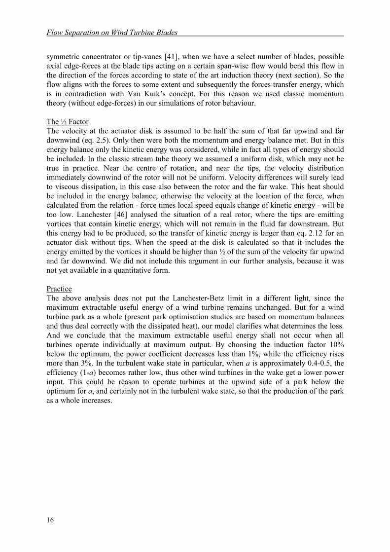
Induced velocities in 'Prandtl-terms'Vortices describe induced velocities, butonly a specific portion of them are‘induction velocities’ in Prandtl-terms.This portion accounts for the differencebetween the three-dimensional steady orunsteady practical situations and the 'two-dimensional steady' wind tunnelsituation. The difference consists ingeneral of three types of vortices, shownin figure 2.4. The first is the trailingvorticity of the tips of a finite airfoil(what BT induces at BB); the second thevorticity shed from the airfoil when the bound circulation changes over time (what PP inducesat BB); and the third is the absence of the (shed) vorticity outside the span of the airfoil (what
AB
A
T
B
S
T
P
S
P
figure 2.4 Prandtl’s induction velocities.
Flow Separation on Wind Turbine Blades
18
SP, which is the shed vorticity of AB, induces at BB. This contribution does not exist in the3d-situation, but is present in the 2d-situation. So the difference has to be corrected). For aprecise definition of the third contribution we refer to Van Holten [41]. It is especiallyimportant for helicopter rotors with their strong variations in circulation with azimuth. In thecase of a wind turbine it is normally sufficient to account for the tip vortices only. It should benoted that the velocity pattern described by the bound vorticity that was present in the windtunnel is excluded from the induction velocities in 'Prandtl terms'.
2.2.1 Prandtl Finite Airfoil Induction
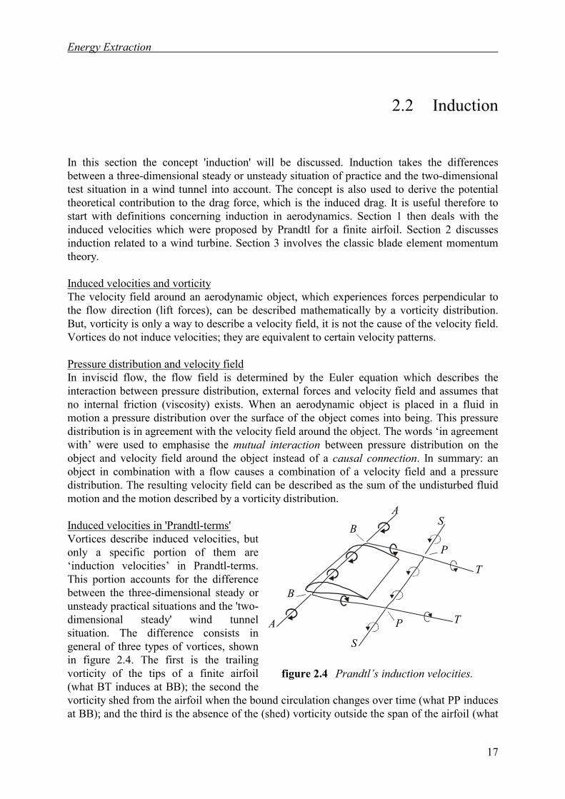
This section gives a summary of Prandtl's reasoning for obtaining a general expression for theinduced drag of finite airfoils. The fact that lift is necessarily accompanied by induced dragwas first pointed out by Lanchester; later Prandtl developed a rigorous system of mathematicalequations which will be explained below. The text is based on the contribution of von Karmánand Burgers in [44].
When a finite airfoil of span 2b exertsa lift force per unit span L on the flow,this force is balanced by an equalmomentum change. If this change ofmomentum is confined to a certainarea Σ per unit span perpendicular tothe flow direction then it results in adownward velocity u0 which equalsL/ρvΣ (see figure 2.5). The downwardmotion is associated with a flow ofkinetic energy per unit span.
.2
2202
1 vDv
LuvP iflow ===Σρ
Σρ (2.22)
This power per unit span is produced by the so-called induced resistance of the airfoil Di perunit span. The power loss due to the motion of the airfoil times Di equals the flow of kineticenergy of the downward flow per unit span, as was shown in equation 2.22. (We know that weshould in fact account for the total power loss, thus also static pressure changes, kineticenergy changes in any direction and possibly heat produced.) It can be derived (see [44]) thatΣ has the maximum value πb, when 2b is the span of the airfoil. It follows that:
.0 bvLuπρ
= (2.23)
This maximum corresponds to a minimum induced drag. The minimum drag and minimumdrag coefficient read respectively:
,,2
2
2
2
πλπρl
diic
cbv
LD == (2.24)
Figure 2.4 Prandtl finite airfoil induction..
u0
i
u0
chordline
induced drag D i
v
α φ lift force L
12
figure 2.5 Prandtl’s finite airfoil.
Energy Extraction
19
in which cl = L/(½ρv2c) is the lift coefficient, c is the chord of the airfoil and λ = (2b)2/bc isthe aspect ratio. It is assumed that half of the downward velocity is imparted to the air beforeit reaches the airfoil and half is imparted after it has passed the airfoil. The same relation wasfound for the entire rotor (see equation 2.5). Lanchester explains this using the followingargument for a fluid which is initially at rest:
‘Let m = the mass of fluid per second, and V its ultimate velocity; then mV2/2 is the energy orwork done per second. And the momentum per second of the stream = mV, which is also theforce by which the flow is impelled. And this force must (to comply with the energy condition)move through a distance per second, in other words act with a velocity U such that:’
,2
,2
2 VUormVUmV == (2.25)
Lanchester also proves the validity for any nonzero initial velocity; the change of the velocitywhere the force acts is given by half of the total change. It follows that the downward velocityat the airfoil u= ½u0. If we combine this velocity with the undisturbed velocity v we obtain theresultant velocity √(v2+u2) which is inclined under an angle tan(i) = v/u. In practice u is muchsmaller than v, therefore the approximation i=v/u is acceptable. The conclusion is that theeffective angle of incidence α differs from the geometric angle of attack ϕ by the angle i:
.i−= ϕα (2.26)
In summary: the inflow direction is inclined by an angle i compared to the geometrical inflowdirection and thus the lift force has a component in the backward direction. This componentequals the induced drag. The induced drag times the velocity of the airfoil equals the flow ofkinetic energy in the downstream.
2.2.2 Induction for a Wind Turbine
This section deals with the induction of a wind turbine rotor and relates it to the above for afinite airfoil. It will be shown that the induced drag of wind turbine blades is implicitly takeninto account in momentum theory.
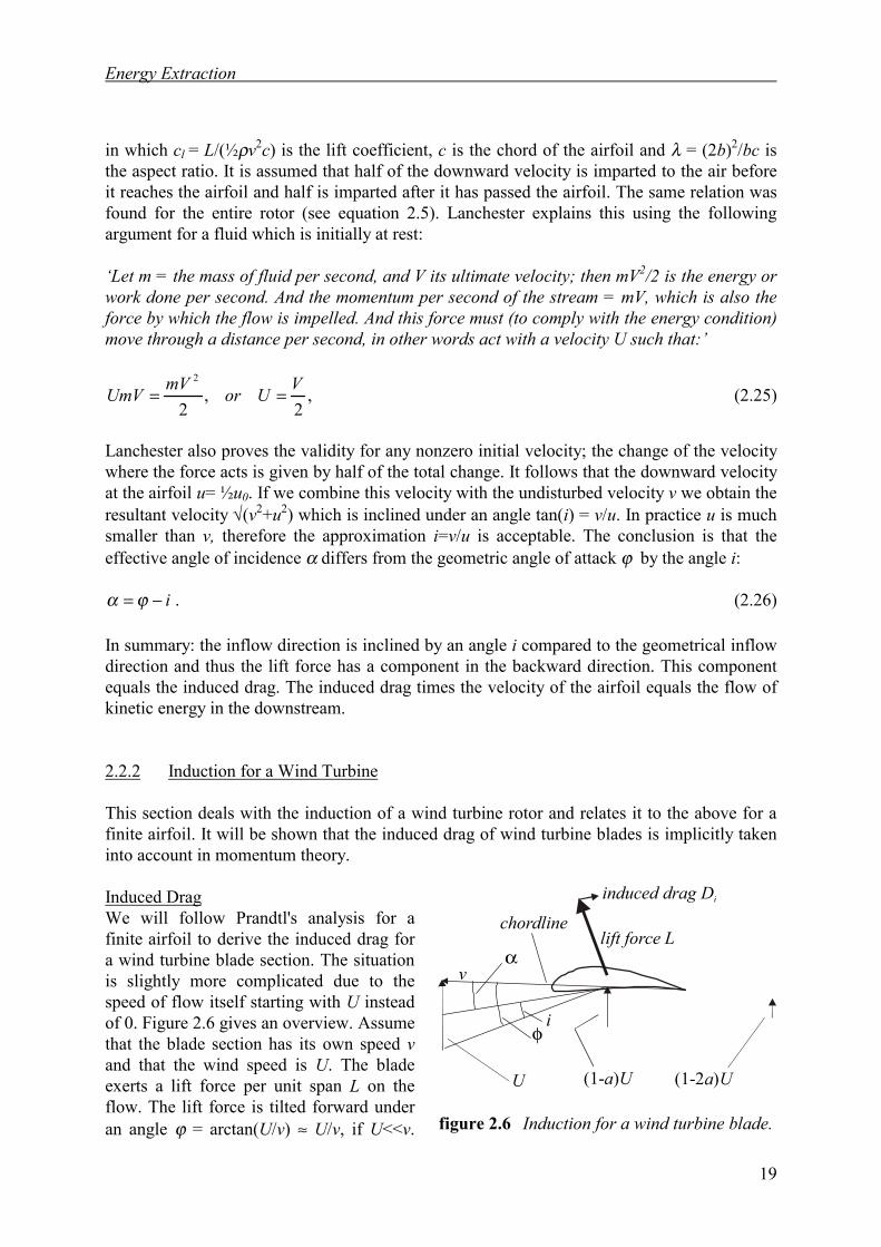
Induced DragWe will follow Prandtl's analysis for afinite airfoil to derive the induced drag fora wind turbine blade section. The situationis slightly more complicated due to thespeed of flow itself starting with U insteadof 0. Figure 2.6 gives an overview. Assumethat the blade section has its own speed vand that the wind speed is U. The bladeexerts a lift force per unit span L on theflow. The lift force is tilted forward underan angle ϕ = arctan(U/v) ≈ U/v, if U<<v. figure 2.6 Induction for a wind turbine blade.
(1-2 )a U
i
chordline
induced drag D i
v α
φ
lift force L
U (1- )a U
Flow Separation on Wind Turbine Blades
20
Thus the power extracted from the flow in this initial situation is L·U, which has to becompared with 0 for Prandtl's finite airfoil. The lift force will be balanced by the change ofmomentum of the mass flow per unit span. This mass flow m refers to the mass flow throughthe cross section Σ (and not to the indefinite flow referred to in 2.1.2). The resulting velocitychange will be ∆U=L/ m . The kinetic power of the inflow was ½ m U2 and decreased to½ m (U-∆U)2 when passing the airfoil. Thus the kinetic power extracted from the flow per unitspan Pflow is:
.22
)( 22
mLULUmUUmPflow −=−=
∆∆ (2.27)
The expression on the right hand side follows after a substitution of ∆U by L/ m . So, thepower extracted by the lift force U·L exceeds the power extracted from the flow by L2/(2 m ).This error will be corrected by the introduction of the induced angle of attack i. The inducedangle should tilt the lift force backwards until the power generated by the lift is decreased withthe power surplus. Thus if we assume that i is small, then Lvi should equal L2/(2 m ), or:
.22 vU
vmLi ∆
== (2.28)
It follows that the induced angle of attack decreases the geometric angle of attack by means ofhalf the induced velocity in the far wake, in agreement with equation 2.5 of section 2.1.1 andwith the argument of Lanchester. So the introduction of Prandtl's induced drag via the inducedangle of attack i is equivalent to the effect of the induction factors in blade elementmomentum theory, which is described in the next section. This is not generally known.Reference is often made to Viterna and Corrigan [62] who propose a correction for theinduced drag in addition to the effect of induction velocities calculated using blade elementmomentum theory. This means that they correct for induction twice.
Aspect RatioThe performance of a finite airfoil diminishes by a decreasing aspect ratio. The smaller theaspect ratio the larger the ratio of the lift force and the mass flow on which the force isexerted. So the velocity in the down flow increases and thus the induced drag. We shouldemphasise that the aspect ratio correction is equivalent to a correction for induction velocities.In fact the aspect ratio is just the geometric factor that determines the induced drag viacdi=cl
2/(πλ). Thus it is already part of blade element momentum theory.
2.2.3 Blade Element Momentum Theory
This theory, sometimes referred to as strip theory, is W. Froude’s [33]. It differs frommomentum theory in that the forces on the flow are produced by the blades of a propeller, orwind turbine rotor, instead of an actuator disk. The theory, found in much of the literature [34,63, 65], is based on the assumption that no interference exists between successive bladeelements. In short, the theory offers a calculation scheme that iteratively brings the forces onthe airfoil sections at a certain radial position into agreement with the momentum changes of
Energy Extraction
21
the flow through the annulus at that radial position. It yields both the forces and the axial andtangential induction factors a and a’. The axial force causes the flow to slow down by aU atthe rotor disk and 2aU in the far wake. The torque exerted by the flow on the rotor will causethe flow to rotate in the opposite direction with rotation speed a’Ω at the rotor and 2a’Ω in thefar wake.One assumes a rotor with N blades and airfoil sections at radial position r with chord c. Whenthe rotor speed is Ω and the undisturbed wind speed U, the velocity component at the bladesections are:
.)'1(,)1( tan raUUaUax Ω+=−= (2.29)
The axial and tangential induction factors a and a’ first get an initial value, for example 0.From these velocities the inflow conditions are obtained, namely the resultant velocity W andthe angle of attack α with
,arctan,tan
2tan
2 βα −=+=UU
UUW axax (2.30)
where β is the blade pitch angle. Using tables for cl(α) and cd(α), the lift L and the drag forceD are found,
,, 22
122
1 rNccWDrNccWL dl ∆=∆= ρρ (2.31)
which can be expressed as an axial and tangential force
.cossin,sincos tan αααα DLFDLFax −=+= (2.32)
These forces should balance the axial and change of tangential momentum of the mass flowthrough an annulus of cross section 2πr∆r:
.'2)1(2,2)1(2 tanFraarUrFaUarUr ax =−=− Ω∆π∆π (2.33)
In this way one can find a new estimate for a and a’, but these values are still based on thecondition of undisturbed inflow. One has to go through this procedure a number of times tofind more correct values for the forces and induction factors. By doing so for many radialpositions and many wind speeds, the rotor performance can be calculated. The geometry cansubsequently be changed until optimum performance is obtained. Relevant changes includethe local pitch angle β, the chord c, the airfoil that determines the tables for cl and cd and therotor speed.
Strip theory cannot deal with yawed conditions and wind shear, which often do occur inpractice. It is therefore common practice to extend the calculation scheme by dividing theswept area not only in radial, but also in k azimuthal sections. The mass flow will decrease by1/k and the number of blades in an azimuthal section becomes N/k. Now the wind speed inputcan vary with altitude, to represent shear, and the relative direction of motion of the bladesand the wind can be accounted for, to represent yaw.
Flow Separation on Wind Turbine Blades
22
2.3 Tip Correction
The flow through an actuator disk does not depend on azimuth. This disk is a theoreticalconcept, whereas in practice one has 2 or 3 blades on which the force is exerted. That forcewill therefore vary with time at any fixed azimuthal position. The smaller the ratio of the tipvelocity and the wind velocity, ΩR/U, and the fewer the blades, the greater becomes the pitchof the tip vortices and thus the variation of the induced velocities with azimuth. A correctionfor the non-uniform disk loading was proposed by Prandtl in 1919. It will be explained in thefirst section. The second section deals qualitatively with another tip correction that is requiredeven in the case of the actuator disk.
2.3.1 Prandtl Tip Correction
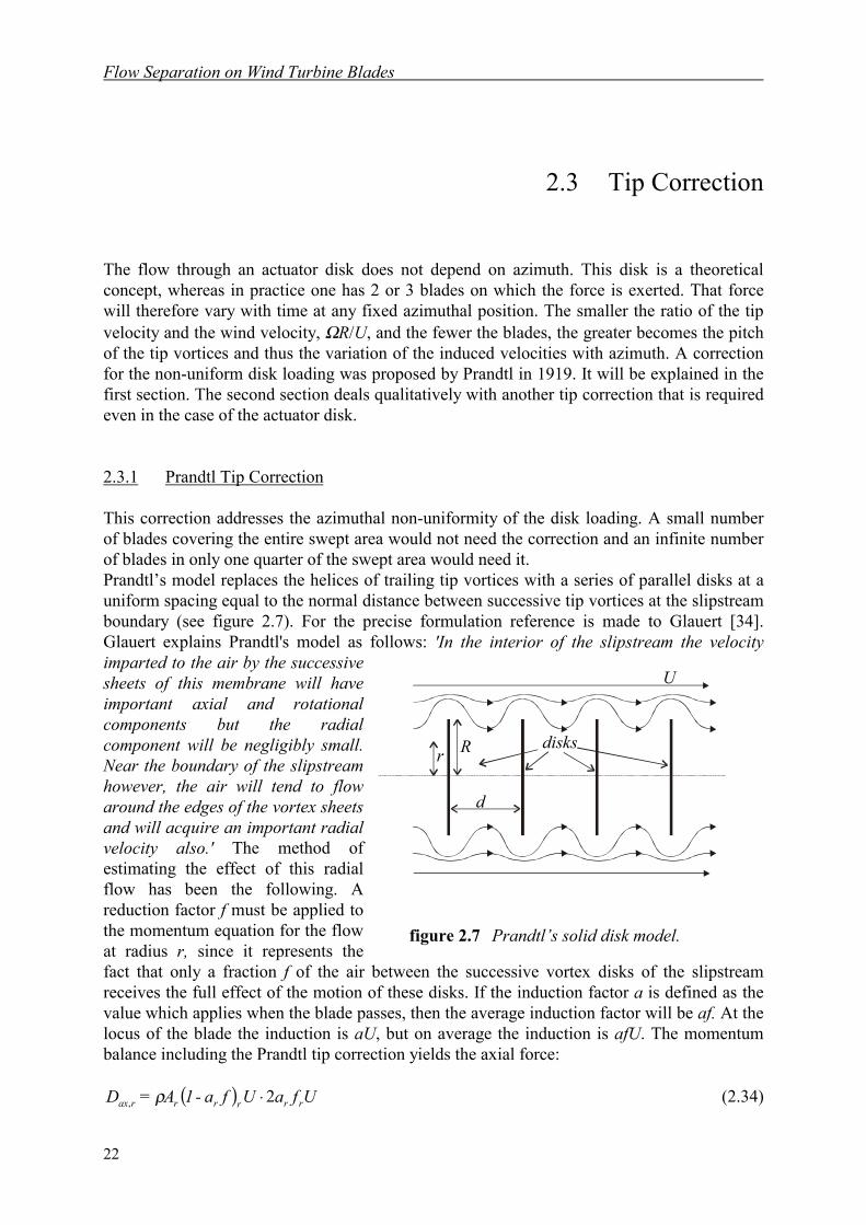
This correction addresses the azimuthal non-uniformity of the disk loading. A small numberof blades covering the entire swept area would not need the correction and an infinite numberof blades in only one quarter of the swept area would need it.Prandtl’s model replaces the helices of trailing tip vortices with a series of parallel disks at auniform spacing equal to the normal distance between successive tip vortices at the slipstreamboundary (see figure 2.7). For the precise formulation reference is made to Glauert [34].Glauert explains Prandtl's model as follows: 'In the interior of the slipstream the velocityimparted to the air by the successivesheets of this membrane will haveimportant axial and rotationalcomponents but the radialcomponent will be negligibly small.Near the boundary of the slipstreamhowever, the air will tend to flowaround the edges of the vortex sheetsand will acquire an important radialvelocity also.' The method ofestimating the effect of this radialflow has been the following. Areduction factor f must be applied tothe momentum equation for the flowat radius r, since it represents thefact that only a fraction f of the air between the successive vortex disks of the slipstreamreceives the full effect of the motion of these disks. If the induction factor a is defined as thevalue which applies when the blade passes, then the average induction factor will be af. At thelocus of the blade the induction is aU, but on average the induction is afU. The momentumbalance including the Prandtl tip correction yields the axial force:
( ) UfaUfa-1A=D rrrrrrax 2, ⋅ρ (2.34)
U
r R disks
d
Figur 2.5 Prandtl's solid disk model.e . figure 2.7 Prandtl’s solid disk model.
Energy Extraction
23
Here the index 'r' is added to the variables Dax, A, a and f, in order to denote that they refer toan annulus and not to the entire rotor. The reduction factor f is found to be:
,arccos2 )(
=
−−d
rR
r efπ
π(2.35)
with
,)1(2
)()(UaR
NWrRd
rR−
−=−π (2.36)
in which R is the blade radius and r is the radial position, d is the spacing between the soliddisks, N is the number of blades and W is the resultant velocity. It can be seen that fr, the tipcorrection, vanishes when N, the number of blades, becomes very large and we approach thetheoretical concept of the actuator disk.
2.3.2 Tip Correction for an Actuator Disk
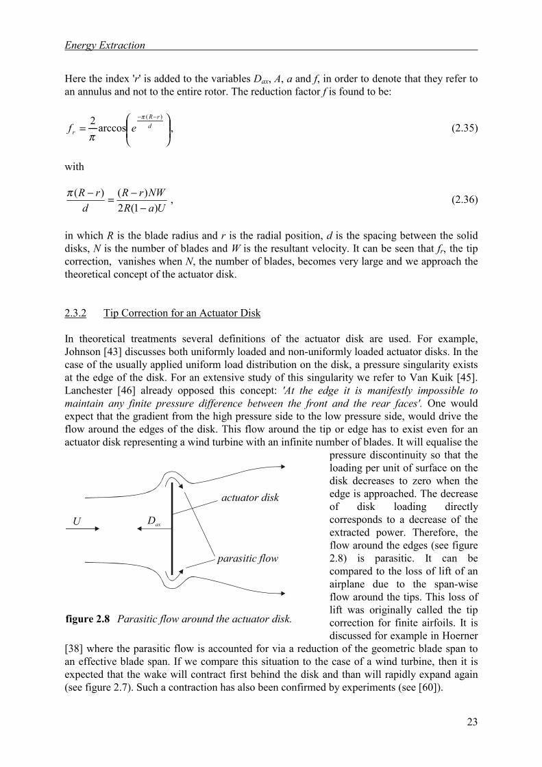
In theoretical treatments several definitions of the actuator disk are used. For example,Johnson [43] discusses both uniformly loaded and non-uniformly loaded actuator disks. In thecase of the usually applied uniform load distribution on the disk, a pressure singularity existsat the edge of the disk. For an extensive study of this singularity we refer to Van Kuik [45].Lanchester [46] already opposed this concept: 'At the edge it is manifestly impossible tomaintain any finite pressure difference between the front and the rear faces'. One wouldexpect that the gradient from the high pressure side to the low pressure side, would drive theflow around the edges of the disk. This flow around the tip or edge has to exist even for anactuator disk representing a wind turbine with an infinite number of blades. It will equalise the
pressure discontinuity so that theloading per unit of surface on thedisk decreases to zero when theedge is approached. The decreaseof disk loading directlycorresponds to a decrease of theextracted power. Therefore, theflow around the edges (see figure2.8) is parasitic. It can becompared to the loss of lift of anairplane due to the span-wiseflow around the tips. This loss oflift was originally called the tipcorrection for finite airfoils. It isdiscussed for example in Hoerner
[38] where the parasitic flow is accounted for via a reduction of the geometric blade span toan effective blade span. If we compare this situation to the case of a wind turbine, then it isexpected that the wake will contract first behind the disk and than will rapidly expand again(see figure 2.7). Such a contraction has also been confirmed by experiments (see [60]).
figure 2.8 Parasitic flow around the actuator disk.
U
actuator disk
Dax
parasitic flow
Flow Separation on Wind Turbine Blades
24
It should be mentioned that the tip correction for rotors is, in the existing literature, entirelyattributed to the effect of the finite number of blades. For example Johnson [43], Spera [57]and Glauert [34] attribute the tip correction wholly to the effect of a finite number of blades.In their theory the actuator disk has no loss of lift at the edges. A loss of lift at the tips of rotorblades is mentioned by Freris, but not worked out in his formulas for the tip correction [31].
So, two corrections for the tip of wind turbine blades can be distinguished. First that byPrandtl for the azimuthal variation of the induced velocity. Second a correction for the loss oflift and thus a loss of transferred power due to the span-wise/axial flow around the blade tips.The latter correction is also required for an actuator disk. It has been stated that the correctionfor the aspect ratio includes the tip correction [45], but this is not correct. The aspect ratiocorrects for the induced drag, while the flow around the tips means that the geometric aspectratio should itself be corrected to obtain a smaller effective aspect ratio. For a wind turbinethis means that the physical diameter should be corrected to a somewhat smaller effectivediameter.
Energy Extraction
25
2.4 Blade Aerodynamics
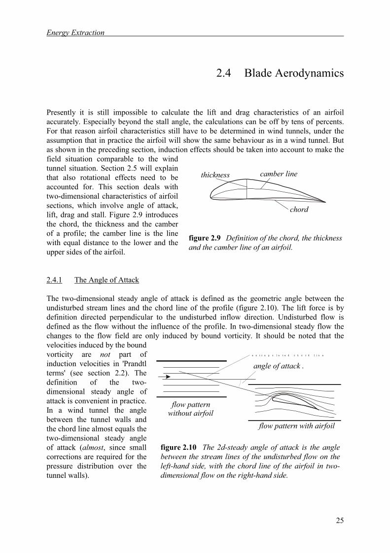
Presently it is still impossible to calculate the lift and drag characteristics of an airfoilaccurately. Especially beyond the stall angle, the calculations can be off by tens of percents.For that reason airfoil characteristics still have to be determined in wind tunnels, under theassumption that in practice the airfoil will show the same behaviour as in a wind tunnel. Butas shown in the preceding section, induction effects should be taken into account to make thefield situation comparable to the windtunnel situation. Section 2.5 will explainthat also rotational effects need to beaccounted for. This section deals withtwo-dimensional characteristics of airfoilsections, which involve angle of attack,lift, drag and stall. Figure 2.9 introducesthe chord, the thickness and the camberof a profile; the camber line is the linewith equal distance to the lower and theupper sides of the airfoil.
2.4.1 The Angle of Attack
The two-dimensional steady angle of attack is defined as the geometric angle between theundisturbed stream lines and the chord line of the profile (figure 2.10). The lift force is bydefinition directed perpendicular to the undisturbed inflow direction. Undisturbed flow isdefined as the flow without the influence of the profile. In two-dimensional steady flow thechanges to the flow field are only induced by bound vorticity. It should be noted that thevelocities induced by the boundvorticity are not part ofinduction velocities in 'Prandtlterms' (see section 2.2). Thedefinition of the two-dimensional steady angle ofattack is convenient in practice.In a wind tunnel the anglebetween the tunnel walls andthe chord line almost equals thetwo-dimensional steady angleof attack (almost, since smallcorrections are required for thepressure distribution over thetunnel walls).
Figure 2.7 Definition of the chord, the thicknessand the camber line of an airfoil.
.
thickness
chord
camber line
figure 2.9 Definition of the chord, the thicknessand the camber line of an airfoil.
figure 2.10 The 2d-steady angle of attack is the anglebetween the stream lines of the undisturbed flow on theleft-hand side, with the chord line of the airfoil in two-dimensional flow on the right-hand side.
flow patternwithout airfoil
angle of attack a
flow pattern with airfoil
e x t r a p o l a t e d c h o r d l i n e

Flow Separation on Wind Turbine Blades
26
2.4.2 Lift and Drag
In two-dimensional steady flow the force exerted on an object consists of a component,perpendicular to the undisturbed flow, which is by definition the lift, and a component parallelto that flow which is by definition the drag. In the unsteady three-dimensional situations thatoccur in practice, these definitions refer to the direction of the sum of the undisturbed flowvelocity and the induction velocities in Prandtl's terms. Lift is described in theory as the forceexerted by a fluid flow on a bound vortex, given that the fluid flows perpendicular to thevorticity vector. The vorticity is defined as ωωωω= ∇∇∇∇×v. The total vorticity or circulation ΓΓΓΓ in asurface S is the integral of the local vorticity over S:
∫∫∫ ⋅=⋅= dCvdSωΓ (2.37)
The equivalence of the integral over the surface S and the integral along the closed curve Cfollows from Stokes' theorem. The difference between vorticity and circulation is, thatvorticity is a property of an infinitesimalelement of fluid, while circulation is anintegral property. The physical meaningof circulation becomes clear when a line(hence a 2d-situation) of constantvorticity ωωωω is considered. If C is a circleof radius r perpendicular to the line ofvorticity in the centre, it follows that v =ΓΓΓΓ/(2πr). The lift force per unit length isrelated to the circulation and the inflowvelocity via Joukowski’s theorem:
,Γρ ×= vL (2.38)
According to Joukowski's hypothesis, theeffect of viscosity in the boundary layer isto cause precisely that circulation so thatthe stagnation point at the rear of the airfoil corresponds to the sharp trailing edge of theairfoil. For a description of this process reference is made to Batchelor [6]. Joukowski'shypothesis implies that the circulation around an airfoil under small inflow angles is almostproportional to this inflow angle. Airfoils have camber since it yields a slightly betterperformance regarding the lift over drag ratio. The camber also causes the lift curve of theairfoil to shift over a certain angle α0, which is the angle of attack at zero lift (see figure 2.11).Both the lift and drag per unit of span are conventionally given as dimensionless quantitiesafter normalisation by the product of dynamic pressure and the chord c of the airfoil. The liftand drag coefficient are respectively defined by:
,),(2 22
1022
1 cvDc
cvLc dl ρ
ααπρ
=−≈= (2.39)
−5 0 5 10 15
1.0 0.2
α0
Cl
Cd
0.5 0.1
0
1.5 0.3
stall
α [ ]
Cl
Cd
2π(α−α )0
Figure 2.10 Airfoil characteristicsas function of the angle of attack ( ).
. α
0
figure 2.11 Airfoil characteristics asfunction of the angle of attack (α).
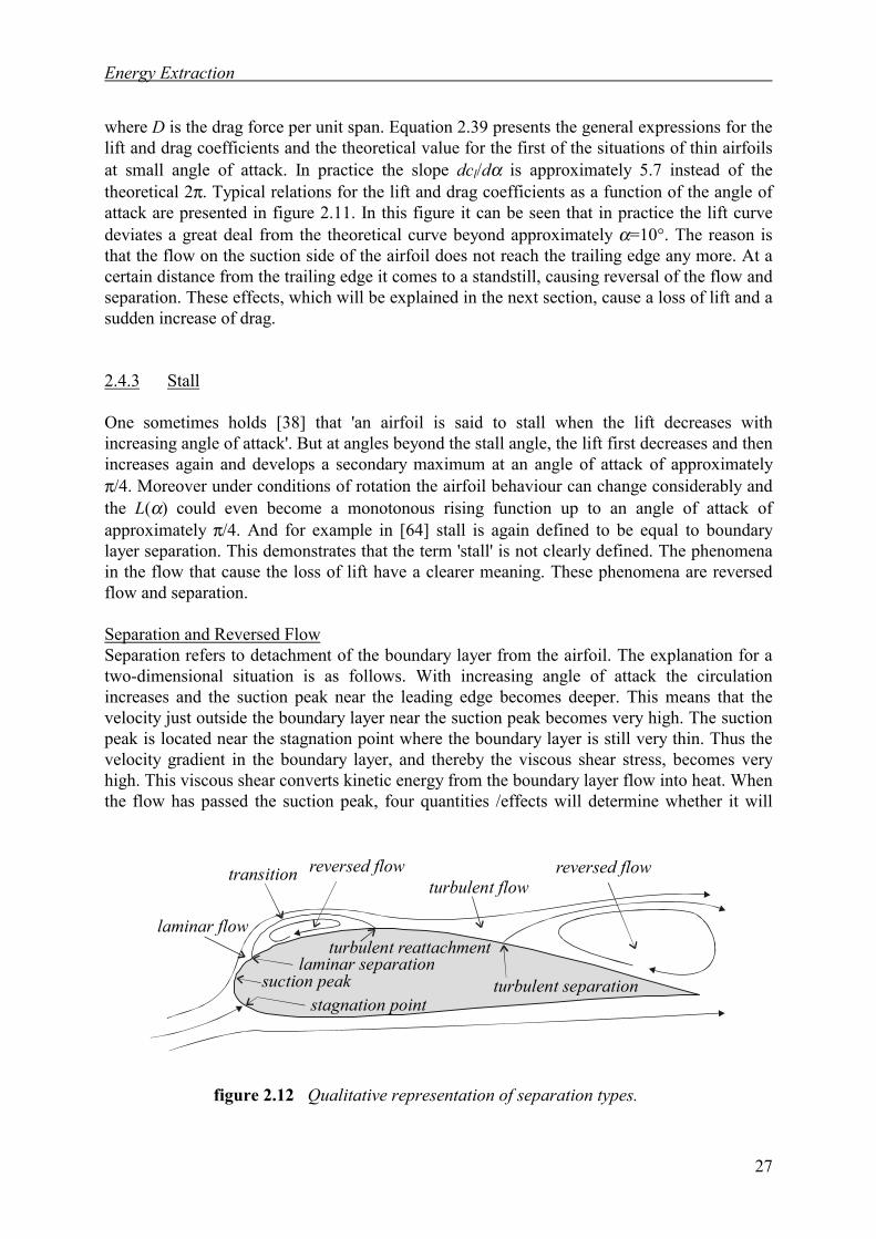
Energy Extraction
27
where D is the drag force per unit span. Equation 2.39 presents the general expressions for thelift and drag coefficients and the theoretical value for the first of the situations of thin airfoilsat small angle of attack. In practice the slope dcl/dα is approximately 5.7 instead of thetheoretical 2π. Typical relations for the lift and drag coefficients as a function of the angle ofattack are presented in figure 2.11. In this figure it can be seen that in practice the lift curvedeviates a great deal from the theoretical curve beyond approximately α=10°. The reason isthat the flow on the suction side of the airfoil does not reach the trailing edge any more. At acertain distance from the trailing edge it comes to a standstill, causing reversal of the flow andseparation. These effects, which will be explained in the next section, cause a loss of lift and asudden increase of drag.
2.4.3 Stall
One sometimes holds [38] that 'an airfoil is said to stall when the lift decreases withincreasing angle of attack'. But at angles beyond the stall angle, the lift first decreases and thenincreases again and develops a secondary maximum at an angle of attack of approximatelyπ/4. Moreover under conditions of rotation the airfoil behaviour can change considerably andthe L(α) could even become a monotonous rising function up to an angle of attack ofapproximately π/4. And for example in [64] stall is again defined to be equal to boundarylayer separation. This demonstrates that the term 'stall' is not clearly defined. The phenomenain the flow that cause the loss of lift have a clearer meaning. These phenomena are reversedflow and separation.
Separation and Reversed FlowSeparation refers to detachment of the boundary layer from the airfoil. The explanation for atwo-dimensional situation is as follows. With increasing angle of attack the circulationincreases and the suction peak near the leading edge becomes deeper. This means that thevelocity just outside the boundary layer near the suction peak becomes very high. The suctionpeak is located near the stagnation point where the boundary layer is still very thin. Thus thevelocity gradient in the boundary layer, and thereby the viscous shear stress, becomes veryhigh. This viscous shear converts kinetic energy from the boundary layer flow into heat. Whenthe flow has passed the suction peak, four quantities /effects will determine whether it will
figure 2.12 Qualitative representation of separation types.
turbulent reattachment laminar flow
transition
laminar separation turbulent separation
stagnation point
reversed flow turbulent flow
reversed flow
suction peak
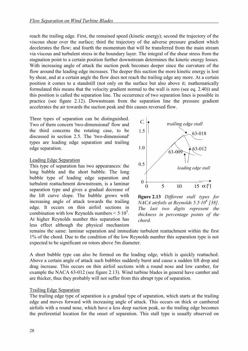
Flow Separation on Wind Turbine Blades
28
reach the trailing edge. First, the remained speed (kinetic energy); second the trajectory of theviscous shear over the surface; third the trajectory of the adverse pressure gradient whichdecelerates the flow; and fourth the momentum that will be transferred from the main streamvia viscous and turbulent stress in the boundary layer. The integral of the shear stress from thestagnation point to a certain position further downstream determines the kinetic energy losses.With increasing angle of attack the suction peek becomes deeper since the curvature of theflow around the leading edge increases. The deeper this suction the more kinetic energy is lostby shear, and at a certain angle the flow does not reach the trailing edge any more. At a certainposition it comes to a standstill (not only on the surface but also above it; mathematicallyformulated this means that the velocity gradient normal to the wall is zero (see eq. 2.40)) andthis position is called the separation line. The occurrence of two separation lines is possible inpractice (see figure 2.12). Downstream from the separation line the pressure gradientaccelerates the air towards the suction peak and this causes reversed flow.
Three types of separation can be distinguished.Two of them concern 'two-dimensional' flow andthe third concerns the rotating case, to bediscussed in section 2.5. The 'two-dimensional'types are leading edge separation and trailingedge separation.
Leading Edge SeparationThis type of separation has two appearances: thelong bubble and the short bubble. The longbubble type of leading edge separation andturbulent reattachment downstream, is a laminarseparation type and gives a gradual decrease ofthe lift curve slope. The bubble grows withincreasing angle of attack towards the trailingedge. It occurs on thin airfoil sections incombination with low Reynolds numbers < 5·105.At higher Reynolds number this separation hasless effect although the physical mechanismremains the same: laminar separation and immediate turbulent reattachment within the first1% of the chord. Due to the condition of the low Reynolds number this separation type is notexpected to be significant on rotors above 5m diameter.
A short bubble type can also be formed on the leading edge, which is quickly reattached.Above a certain angle of attack such bubbles suddenly burst and cause a sudden lift drop anddrag increase. This occurs on thin airfoil sections with a round nose and low camber, forexample the NACA 63-012 (see figure 2.13). Wind turbine blades in general have camber andare thicker, thus they probably will not suffer from this abrupt type of separation.
Trailing Edge SeparationThe trailing edge type of separation is a gradual type of separation, which starts at the trailingedge and moves forward with increasing angle of attack. This occurs on thick or camberedairfoils with a round nose, which have a less deep suction peak, so the trailing edge becomesthe preferential location for the onset of separation. This stall type is usually observed on
figure 2.13 Different stall types forNACA airfoils at Reynolds 5.5·106 [38].The last two digits represent thethickness in percentage points of thechord.
0 5 10 15
1.0
0.5
0
1.5
α [ ]
Cl trailing edge stall
63-018
63-009
leading edge stall
63-012
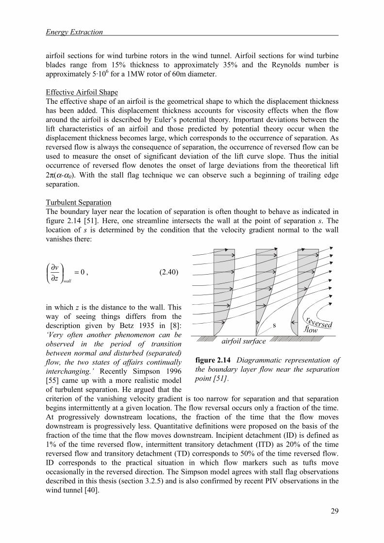
Energy Extraction
29
airfoil sections for wind turbine rotors in the wind tunnel. Airfoil sections for wind turbineblades range from 15% thickness to approximately 35% and the Reynolds number isapproximately 5·106 for a 1MW rotor of 60m diameter.
Effective Airfoil ShapeThe effective shape of an airfoil is the geometrical shape to which the displacement thicknesshas been added. This displacement thickness accounts for viscosity effects when the flowaround the airfoil is described by Euler’s potential theory. Important deviations between thelift characteristics of an airfoil and those predicted by potential theory occur when thedisplacement thickness becomes large, which corresponds to the occurrence of separation. Asreversed flow is always the consequence of separation, the occurrence of reversed flow can beused to measure the onset of significant deviation of the lift curve slope. Thus the initialoccurrence of reversed flow denotes the onset of large deviations from the theoretical lift2π(α-α0). With the stall flag technique we can observe such a beginning of trailing edgeseparation.
Turbulent SeparationThe boundary layer near the location of separation is often thought to behave as indicated infigure 2.14 [51]. Here, one streamline intersects the wall at the point of separation s. Thelocation of s is determined by the condition that the velocity gradient normal to the wallvanishes there:
,0=
∂∂
wallzv (2.40)
in which z is the distance to the wall. Thisway of seeing things differs from thedescription given by Betz 1935 in [8]:‘Very often another phenomenon can beobserved in the period of transitionbetween normal and disturbed (separated)flow, the two states of affairs continuallyinterchanging.’ Recently Simpson 1996[55] came up with a more realistic modelof turbulent separation. He argued that thecriterion of the vanishing velocity gradient is too narrow for separation and that separationbegins intermittently at a given location. The flow reversal occurs only a fraction of the time.At progressively downstream locations, the fraction of the time that the flow movesdownstream is progressively less. Quantitative definitions were proposed on the basis of thefraction of the time that the flow moves downstream. Incipient detachment (ID) is defined as1% of the time reversed flow, intermittent transitory detachment (ITD) as 20% of the timereversed flow and transitory detachment (TD) corresponds to 50% of the time reversed flow.ID corresponds to the practical situation in which flow markers such as tufts moveoccasionally in the reversed direction. The Simpson model agrees with stall flag observationsdescribed in this thesis (section 3.2.5) and is also confirmed by recent PIV observations in thewind tunnel [40].
figure 2.14 Diagrammatic representation ofthe boundary layer flow near the separationpoint [51].
s
airfoil surface wolf deev srer
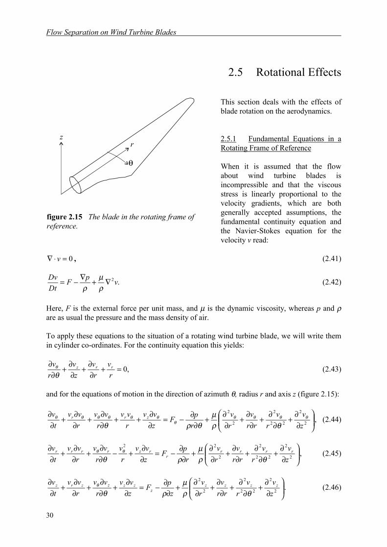
Flow Separation on Wind Turbine Blades
30
2.5 Rotational Effects
This section deals with the effects ofblade rotation on the aerodynamics.
2.5.1 Fundamental Equations in aRotating Frame of Reference
When it is assumed that the flowabout wind turbine blades isincompressible and that the viscousstress is linearly proportional to thevelocity gradients, which are bothgenerally accepted assumptions, thefundamental continuity equation andthe Navier-Stokes equation for thevelocity v read:
0=⋅∇ v , (2.41)
.2vpFDtDv ∇+∇−=
ρµ
ρ(2.42)
Here, F is the external force per unit mass, and µ is the dynamic viscosity, whereas p and ρare as usual the pressure and the mass density of air.
To apply these equations to the situation of a rotating wind turbine blade, we will write themin cylinder co-ordinates. For the continuity equation this yields:
,0=+∂∂+
∂∂+
∂∂
rv
rv
zv
rv rrz
θθ (2.43)
and for the equations of motion in the direction of azimuth θ, radius r and axis z (figure 2.15):
,2
2
22
2
2
2
∂∂
+∂
∂+
∂∂
+∂∂
+∂
∂−=∂∂
++∂∂
+∂∂
+∂
∂zv
rv
rrv
rv
rpF
zvv
rvv
rvv
rvv
tv zrr θθθθ
θθθθθθθ
θρµ
θρθ(2.44)
,2
2
22
2
2
22
∂∂+
∂∂+
∂∂+
∂∂+
∂∂−=
∂∂+−
∂∂
+∂∂+
∂∂
zv
rv
rrv
rv
rpF
zvv
rv
rvv
rvv
tv rrrr
rrzrrrr
θρµ
ρθθθ (2.45)
.2
2
22
2
2
2
∂∂
+∂
∂+
∂∂
+∂∂
+∂
∂−=∂∂
+∂∂
+∂∂
+∂
∂zv
rv
rrv
rv
zpF
zvv
rvv
rvv
tv zzzz
zzzzzrz
θρµ
ρθθ (2.46)
r
θ
z
Figure 2.13 The blade in the rotating frame of reference.
. figure 2.15 The blade in the rotating frame ofreference.
Energy Extraction
31
Forces in the Rotating Frame of ReferenceFor an incompressible fluid with only one phase, the external forces in the inertial (non-rotating) reference system are usually zero. In practice the only external force is gravitational,but that force is balanced by the hydrostatic pressure gradient, so that both are left out of theequations. In a rotating frame the centrifugal and Coriolis forces appear. An observer on theblade notices radial and azimuthal accelerations on passing air elements dτ. Therefore thecentrifugal and Coriolis forces are real forces in the rotating frame of reference. If the angularvelocity of the frame of reference is Ω then the centrifugal force equals ρdτ Ω2r. When theparticle is moving in the rotating reference system with velocity vector v, then the Coriolisforce equals 2ρdτΩΩΩΩ×v. The vector ΩΩΩΩ only has a z-component, and thus the Coriolisaccelerations are: 2vrΩθθθθ1 - 2vθΩr1, in which θθθθ1 and r1 are the unit vectors in the θ and r-direction respectively. They act on the mass element in addition to other inertial forces, which,however can be left out, as explained above. So, the Coriolis force acts in the θ-direction andr-direction, and thus the first term on the right-hand side of equation 2.44 can be replaced by2Ωvr. As the centrifugal force works in the r-direction, the first term on the right-hand side ofequation 2.45 can be replaced by a centrifugal contribution rΩ2 and a Coriolis contribution-2vθΩ. In the above, it is assumed that the wing rotates in the r,θ-plane given by z=0. But inpractice the rotor blades have a small cone angle and therefore the tip rotates at a slightlynegative value of z. The centrifugal and Coriolis force are thus assumed to work in the planeof the boundary layer. In short, the relevant external forces per unit of mass are:
rvF Ωθ 2= , θΩΩ vrFr 22 −= and 0=zF . (2.47)
2.5.2 Boundary Layer Assumptions
In the flow about rotating wind turbine blades the rate of downstream convection (in theθ-direction) is much larger than the rate of transverse viscous diffusion, which means thatviscosity only plays a significant role in a thin so-called boundary layer around the object.This insight will be used to estimate the order of magnitude of terms in equations 2.43-2.46.Terms of small order will then be neglected.The thickness of the boundary layer can be estimated as follows. At the wall the velocity is 0and at a certain distance, say δ, perpendicular to the wall the flow velocity will be vθ. Thevelocity gradient perpendicular to the wall is therefore approximately vθ/δ and the shear stressτ ≈ -µvθ/δ. The derivative of this stress ∂τ/∂y equals the convective deceleration of the flowρvθ/r(∂vθ/∂θ), where ∂vθ/∂θ ≈ vθ/(c/r) and c is the chord of the airfoil. Thus ∂τ/∂y= -µvθ/δ 2 ≈ρvθ
2/c, or δ ≈ √(µc/ρvθ), which is very small since µair ≈ 17.1·10-6 Pa·s.
It follows that the shear layer of thickness δ is small compared to the chord c=rθ. Thez-direction is perpendicular to the boundary layer where most velocity changes take place. Thevelocity derivatives in the z-direction are therefore relatively large: ∂vθ/∂z is of the order vθ/δ.Outside the boundary layer the second derivative of vθ in the z-direction is zero. Thus insidethe boundary layer the second derivative equals the change of the first derivative, which wasof the order vθ/δ. Therefore the second derivative ∂ 2vθ/∂z2 is of the order vθ/δ 2. These resultswill be used to find the significant terms which yield the boundary layer equations.
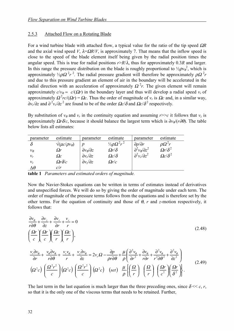
Flow Separation on Wind Turbine Blades
32
2.5.3 Attached Flow on a Rotating Blade
For a wind turbine blade with attached flow, a typical value for the ratio of the tip speed ΩRand the axial wind speed V, λ=ΩR/V, is approximately 7. That means that the inflow speed isclose to the speed of the blade element itself being given by the radial position times theangular speed. This is true for radial positions r>R/λ, thus for approximately 0.3R and larger.In this range the pressure distribution on the blade is roughly proportional to ½ρvθ
2, which isapproximately ½ρΩ 2r 2. The radial pressure gradient will therefore be approximately ρΩ 2rand due to this pressure gradient an element of air in the boundary will be accelerated in theradial direction with an acceleration of approximately Ω 2r. The given element will remainapproximately c/vθ ≈ c/(Ωr) in the boundary layer and thus will develop a radial speed vr ofapproximately Ω 2rc/(Ωr) = Ωc. Thus the order of magnitude of vr is Ωc and, in a similar way,∂vr/∂z and ∂ 2vr/∂z 2 are found to be of the order Ωc/δ and Ωc/δ 2 respectively.
By substitution of vθ and vr in the continuity equation and assuming r>>c it follows that vz isapproximately Ωrδ/c, because it should balance the largest term which is ∂vθ/(r∂θ). The tablebelow lists all estimates:
parameter estimate parameter estimate parameter estimateδ √(µc/ρvθ) p ½ρΩ 2r 2 ∂p/∂r ρΩ 2rvθ Ωr ∂vθ/∂z Ωr/δ ∂2vθ/∂z2 Ωr/δ 2
vr Ωc ∂vr/∂z Ωc/δ ∂2vr/∂z2 Ωc/δ 2
vz Ωrδ/c ∂vz/∂z Ωr/c∆θ c/r
table 1 Parameters and estimated orders of magnitude.
Now the Navier-Stokes equations can be written in terms of estimates instead of derivativesand unspecified forces. We will do so by giving the order of magnitude under each term. Theorder of magnitude of the pressure terms follows from the equations and is therefore set by theother terms. For the equation of continuity and those of θ, r and z-motion respectively, itfollows that:
,
0
=+∂∂
+∂∂
+∂
∂
rc
rc
cr
cr
rv
rv
zv
rv rrz
ΩΩΩΩθθ
(2.48)
( ) ( ) ( ) ( ) .
2
222
222
222
2
2
22
2
2
2
∂∂+
∂∂+
∂∂+
∂∂+
∂∂−=
∂∂++
∂∂+
∂∂
δΩΩΩΩ
ρµΩΩΩΩΩ
θρµ
θρΩ
θθθθθθθθθθ
rc
rrr
setccrc
crc
zv
rv
rrv
rv
rpv
zvv
rvv
rvv
rvv
rzrr
(2.49)
The last term in the last equation is much larger than the three preceding ones, since δ << c, r,so that it is the only one of the viscous terms that needs to be retained. Further,
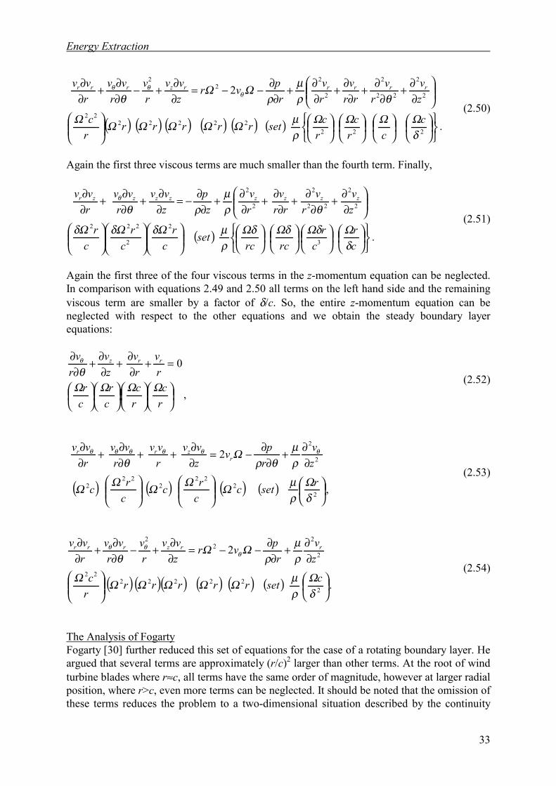
Energy Extraction
33
( ) ( ) ( ) ( ) ( ) ( ) .
2
22222222
22
2
2
22
2
2
22
2
∂∂+
∂∂+
∂∂+
∂∂+
∂∂−−=
∂∂+−
∂∂+
∂∂
δΩΩΩΩ
ρµΩΩΩΩΩΩ
θρµ
ρΩΩ
θ θθθ
ccr
cr
csetrrrrrrc
zv
rv
rrv
rv
rpvr
zvv
rv
rvv
rvv rrrrrzrrr
(2.50)
Again the first three viscous terms are much smaller than the fourth term. Finally,
( ) .3
2
2
222
2
2
22
2
2
2
∂∂+
∂∂+
∂∂+
∂∂+
∂∂−=
∂∂+
∂∂+
∂∂
cr
cr
rcrcset
cr
cr
cr
zv
rv
rrv
rv
zp
zvv
rvv
rvv zzzzzzzzr
δΩδΩδΩδΩ
ρµΩδΩδΩδ
θρµ
ρθθ
(2.51)
Again the first three of the four viscous terms in the z-momentum equation can be neglected.In comparison with equations 2.49 and 2.50 all terms on the left hand side and the remainingviscous term are smaller by a factor of δ/c. So, the entire z-momentum equation can beneglected with respect to the other equations and we obtain the steady boundary layerequations:
,
0
=+∂∂+
∂∂+
∂∂
rc
rc
cr
cr
rv
rv
zv
rv rrz
ΩΩΩΩθθ
(2.52)
( ) ( ) ( ) ( ) ,
2
22
222
222
2
2
∂∂+
∂∂−=
∂∂++
∂∂+
∂∂
δΩ
ρµΩΩΩΩΩ
ρµ
θρΩ
θθθθθθθ
rsetccrc
crc
zv
rpv
zvv
rvv
rvv
rvv
rzrr
(2.53)
( )( )( ) ( ) ( ) ( ) .
2
222222
22
2
22
2
∂∂+
∂∂−−=
∂∂+−
∂∂+
∂∂
δΩ
ρµΩΩΩΩΩΩ
ρµ
ρΩΩ
θ θθθ
csetrrrrrrc
zv
rpvr
zvv
rv
rvv
rvv rrzrrr
(2.54)
The Analysis of FogartyFogarty [30] further reduced this set of equations for the case of a rotating boundary layer. Heargued that several terms are approximately (r/c)2 larger than other terms. At the root of windturbine blades where r≈c, all terms have the same order of magnitude, however at larger radialposition, where r>c, even more terms can be neglected. It should be noted that the omission ofthese terms reduces the problem to a two-dimensional situation described by the continuity
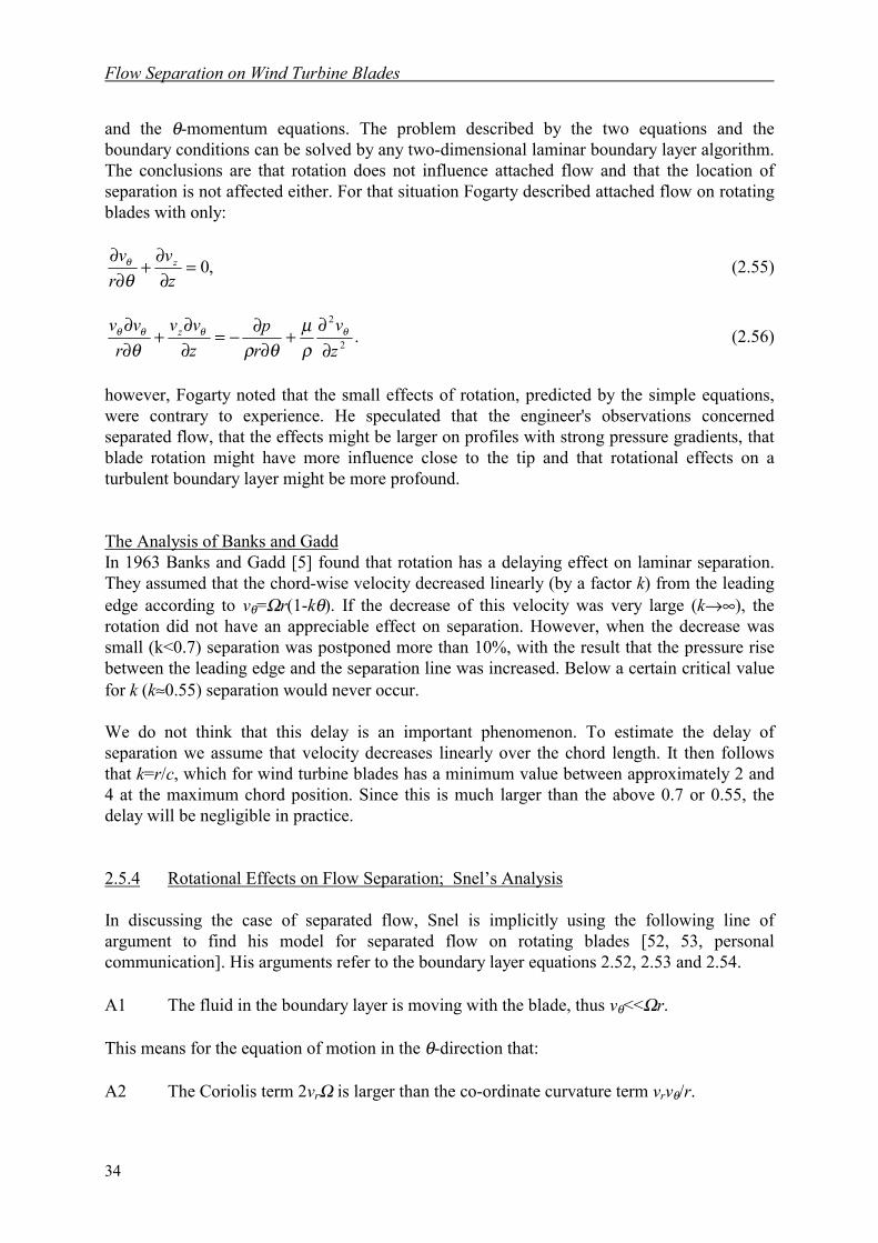
Flow Separation on Wind Turbine Blades
34
and the θ-momentum equations. The problem described by the two equations and theboundary conditions can be solved by any two-dimensional laminar boundary layer algorithm.The conclusions are that rotation does not influence attached flow and that the location ofseparation is not affected either. For that situation Fogarty described attached flow on rotatingblades with only:
,0=∂∂+
∂∂
zv
rv z
θθ (2.55)
.2
2
zv
rp
zvv
rvv z
∂∂
+∂
∂−=∂∂
+∂∂ θθθθ
ρµ
θρθ(2.56)
however, Fogarty noted that the small effects of rotation, predicted by the simple equations,were contrary to experience. He speculated that the engineer's observations concernedseparated flow, that the effects might be larger on profiles with strong pressure gradients, thatblade rotation might have more influence close to the tip and that rotational effects on aturbulent boundary layer might be more profound.
The Analysis of Banks and GaddIn 1963 Banks and Gadd [5] found that rotation has a delaying effect on laminar separation.They assumed that the chord-wise velocity decreased linearly (by a factor k) from the leadingedge according to vθ=Ωr(1-kθ). If the decrease of this velocity was very large (k→∞), therotation did not have an appreciable effect on separation. However, when the decrease wassmall (k<0.7) separation was postponed more than 10%, with the result that the pressure risebetween the leading edge and the separation line was increased. Below a certain critical valuefor k (k≈0.55) separation would never occur.
We do not think that this delay is an important phenomenon. To estimate the delay ofseparation we assume that velocity decreases linearly over the chord length. It then followsthat k=r/c, which for wind turbine blades has a minimum value between approximately 2 and4 at the maximum chord position. Since this is much larger than the above 0.7 or 0.55, thedelay will be negligible in practice.
2.5.4 Rotational Effects on Flow Separation; Snel’s Analysis
In discussing the case of separated flow, Snel is implicitly using the following line ofargument to find his model for separated flow on rotating blades [52, 53, personalcommunication]. His arguments refer to the boundary layer equations 2.52, 2.53 and 2.54.
A1 The fluid in the boundary layer is moving with the blade, thus vθ<<Ωr.
This means for the equation of motion in the θ-direction that:
A2 The Coriolis term 2vrΩ is larger than the co-ordinate curvature term vrvθ/r.

Energy Extraction
35
A3 The viscous stress and the pressure gradient are small compared to the case ofattached flow. The Coriolis term is dominant and should be balanced by theconvective terms on the left-hand side.
And for the r-direction:
A4 The centrifugal force Ω 2r is dominant along with the radial pressure gradient, sincethe pressure is of the order Ω 2r2.
A5 The convective term with vr again is smaller then the other two convective terms;from the continuity equation it follows that the remaining terms with vz and vθ are ofthe same order.
A6 The convective terms should balance the terms on the right-hand side, thus(vθ/r)(∂vr/∂θ) ≈ Ω 2r and it follows that vr ≈ Ω 2rc/vθ.
Returning to the θ-direction Snel argues that:
A7 The convective term vr∂vθ/∂r should be much smaller than the Coriolis term.A8 The remaining convective terms are of the same order. This is implied by the
continuity equation. Since, if the terms with vr are smaller than the other terms, theseother terms yield vθ/c ≈ vz/δ ; and by substituting vz ≈ vθδ /c in the convective termwith vz of equation 2.53 we see that the statement holds.
A9 It follows that vθ∂vθ/(r∂θ) is of the order Ωvr, and vθ2 is of the order Ωcvr.
And for the r-direction Snel finds finally:
A10 By substituting the relation found in A9 in the r-momentum equation, it follows thatvθ ≈ Ωc2/3r1/3 and vr ≈ Ωc1/3r2/3.
A11 vr/vθ ≈ (r/c)1/3 , which agrees with A7.A12 If c ≈ r, then it follows that vθ ≈ vr; when vr ≈ Ωc1/3r2/3 ≈ Ωr thus vθ ≈ Ωr which is in
contradiction with the primary assumption; so the approximations are only valid forr/c >>1.
A13 vz ≈ δΩc1/3r -1/3; this follows from the substitution of vr for vθ in the continuityequation, which yields Ωc2/3r -2/3+Ωr -1/3c1/3 +vz/δ = 0.
parameter estimate parameter estimate parameter estimatevθ Ωc2/3r1/3 p ½ρΩ 2r 2 ∂p/∂r ρΩ 2rvr Ωc1/3r2/3 ∂vθ/∂z vθ/δ ∂ 2vθ/∂z 2 vθ/δ 2
vz δΩc-1/3r1/3 ∂vr/∂z vr/δ ∂ 2vr/∂z 2 vr/δ 2
∂θ c/r ∂vz/∂z vz/δtable 2 Parameters and orders of magnitude for separated flow according to Snel.
The estimated parameters are listed in table 2. They are used in equations 2.57, 2.58 and 2.59for the boundary layer to find the order of magnitude for each term.
( )( )( )( )3/13/13/13/13/13/13/13/1
0
−−−− ΩΩΩΩ
=+∂∂+
∂∂+
∂∂
rcrcrcrcrv
rv
zv
rv rrz
θθ
(2.57)
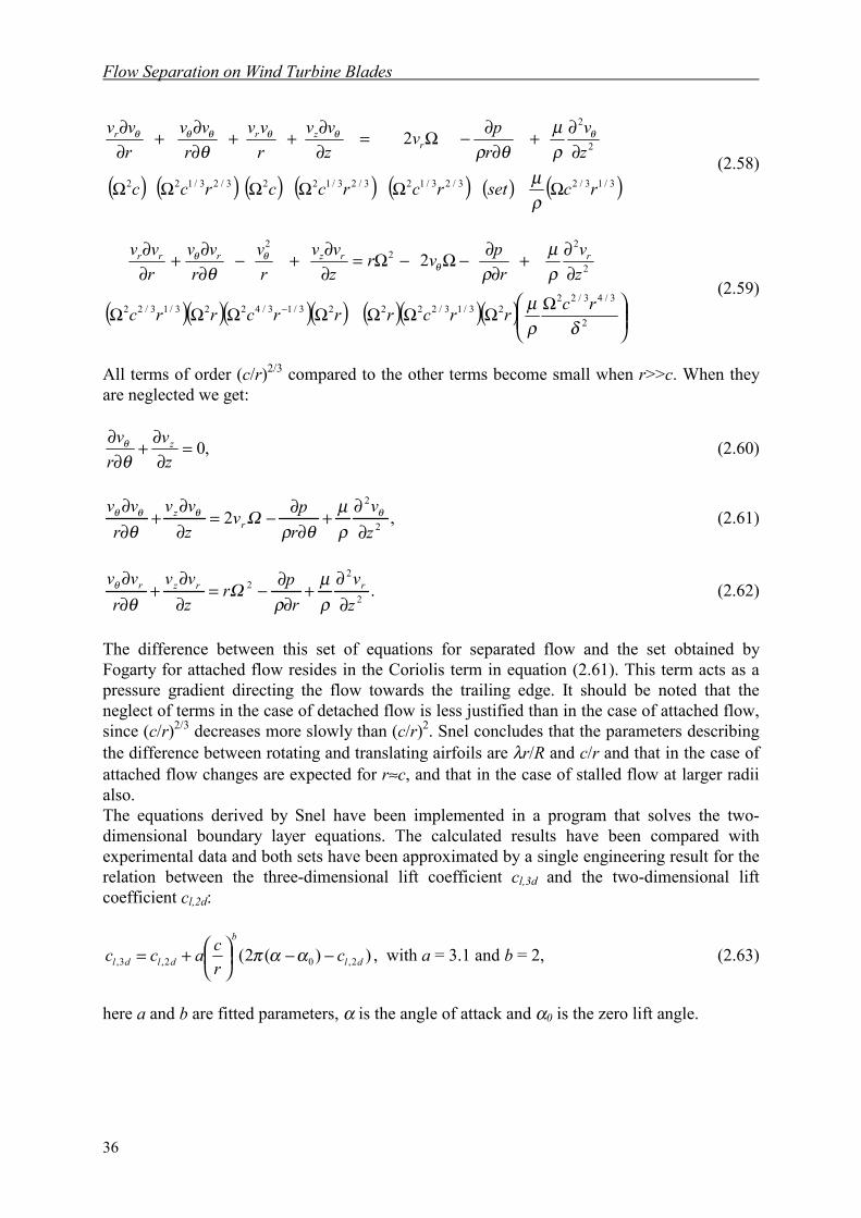
Flow Separation on Wind Turbine Blades
36
( ) ( ) ( ) ( ) ( ) ( ) ( )3/13/23/23/123/23/1223/23/122
2
2
2
rcsetrcrccrcc
zv
rpv
zvv
rvv
rvv
rvv
rzrr
ΩΩΩΩΩΩ
∂∂+
∂∂−Ω=
∂∂++
∂∂+
∂∂
ρµ
ρµ
θρθθθθθθθ
(2.58)
( )( )( )( ) ( )( )( )
ΩΩΩΩΩΩΩΩ
∂∂+
∂∂−Ω−Ω=
∂∂+−
∂∂+
∂∂
−2
3/43/2223/13/22223/13/4223/13/22
2
22
2
2
δρµ
ρµ
ρθ θθθ
rcrrcrrrcrrc
zv
rpvr
zvv
rv
rvv
rvv rrzrrr
(2.59)
All terms of order (c/r)2/3 compared to the other terms become small when r>>c. When theyare neglected we get:
,0=∂∂+
∂∂
zv
rv z
θθ (2.60)
,2 2
2
zv
rpv
zvv
rvv
rz
∂∂
+∂
∂−=
∂∂
+∂∂ θθθθ
ρµ
θρΩ
θ(2.61)
.2
22
zv
rpr
zvv
rvv rrzr
∂∂
+∂
∂−=
∂∂
+∂∂
ρµ
ρΩ
θθ (2.62)
The difference between this set of equations for separated flow and the set obtained byFogarty for attached flow resides in the Coriolis term in equation (2.61). This term acts as apressure gradient directing the flow towards the trailing edge. It should be noted that theneglect of terms in the case of detached flow is less justified than in the case of attached flow,since (c/r)2/3 decreases more slowly than (c/r)2. Snel concludes that the parameters describingthe difference between rotating and translating airfoils are λr/R and c/r and that in the case ofattached flow changes are expected for r≈c, and that in the case of stalled flow at larger radiialso. The equations derived by Snel have been implemented in a program that solves the two-dimensional boundary layer equations. The calculated results have been compared withexperimental data and both sets have been approximated by a single engineering result for therelation between the three-dimensional lift coefficient cl,3d and the two-dimensional liftcoefficient cl,2d:
))(2( 2,02,3, dl
b
dldl crcacc −−
+= ααπ , with a = 3.1 and b = 2, (2.63)
here a and b are fitted parameters, α is the angle of attack and α0 is the zero lift angle.
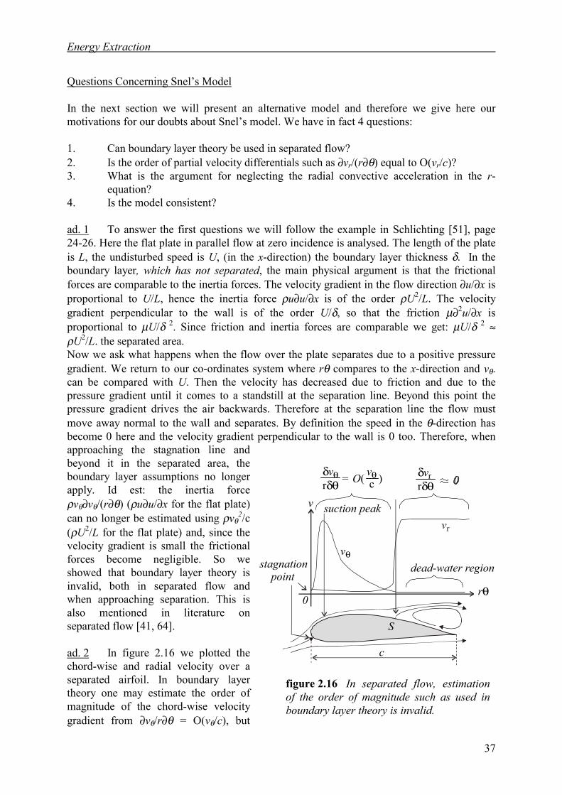
Energy Extraction
37
Questions Concerning Snel’s Model
In the next section we will present an alternative model and therefore we give here ourmotivations for our doubts about Snel’s model. We have in fact 4 questions:
1. Can boundary layer theory be used in separated flow?2. Is the order of partial velocity differentials such as ∂vr/(r∂θ) equal to O(vr/c)?3. What is the argument for neglecting the radial convective acceleration in the r-
equation?4. Is the model consistent?
ad. 1 To answer the first questions we will follow the example in Schlichting [51], page24-26. Here the flat plate in parallel flow at zero incidence is analysed. The length of the plateis L, the undisturbed speed is U, (in the x-direction) the boundary layer thickness δ. In theboundary layer, which has not separated, the main physical argument is that the frictionalforces are comparable to the inertia forces. The velocity gradient in the flow direction ∂u/∂x isproportional to U/L, hence the inertia force ρu∂u/∂x is of the order ρU2/L. The velocitygradient perpendicular to the wall is of the order U/δ, so that the friction µ∂2u/∂x isproportional to µU/δ 2. Since friction and inertia forces are comparable we get: µU/δ 2 ≈ρU2/L. the separated area.Now we ask what happens when the flow over the plate separates due to a positive pressuregradient. We return to our co-ordinates system where rθ compares to the x-direction and vθ.can be compared with U. Then the velocity has decreased due to friction and due to thepressure gradient until it comes to a standstill at the separation line. Beyond this point thepressure gradient drives the air backwards. Therefore at the separation line the flow mustmove away normal to the wall and separates. By definition the speed in the θ-direction hasbecome 0 here and the velocity gradient perpendicular to the wall is 0 too. Therefore, whenapproaching the stagnation line andbeyond it in the separated area, theboundary layer assumptions no longerapply. Id est: the inertia forceρvθ∂vθ/(r∂θ) (ρu∂u/∂x for the flat plate)can no longer be estimated using ρvθ
2/c(ρU2/L for the flat plate) and, since thevelocity gradient is small the frictionalforces become negligible. So weshowed that boundary layer theory isinvalid, both in separated flow andwhen approaching separation. This isalso mentioned in literature onseparated flow [41, 64].
ad. 2 In figure 2.16 we plotted thechord-wise and radial velocity over aseparated airfoil. In boundary layertheory one may estimate the order ofmagnitude of the chord-wise velocitygradient from ∂vθ/r∂θ = O(vθ/c), but
figure 2.16 In separated flow, estimationof the order of magnitude such as used inboundary layer theory is invalid.
rθ
c
dead-water regionstagnation point
v
S
δδθ vr
r= O( )vθ
cδδθ vθ
r
0
suction peak
S
c
vθ
Flow Separation on Wind Turbine Blades
38
only in attached flow. In separated flow this may give errors. For example the order of thepartial velocity gradient ∂vr/(r∂θ) cannot be estimated by O(vr/c), with the argument that theradial speed is approximately vr inside the separated area and approximately 0 outside theseparated area. Snel’s analysis uses such estimates for the second and fourth term of equation2.59. In fact, when the partial derivative is estimated inside the dead-water region, we find∂vr/(r∂θ) ≈ 0.
One might come up with the statement that the order of the partial derivatives in the dead-water region is still equal to that in the attached region, although the magnitudes are verydifferent. However to reduce the Navier-Stokes equations we assume that the smaller termscan be neglected. The order of a term is not only decisive for its magnitude, the coefficient isalso important. Snel’s analysis is based on orders only.
ad. 3 In Snel’s model the convective term with vr is smaller than the other terms (A5), butthe argument for this is lacking. In our model this term appears to be dominant.
ad. 4 In Snel’s model θ-equation leads to vθ2=O(Ωcvr) (A9). Then from the r-equation he
has no reason (see ad. 3) to assume that any acceleration term is off smaller order than O(Ω2r)so that vr∂vr/∂r=O(Ω2r) and thus vr=O(Ωr). If we substitute this in the term vθ∂vr/(r∂θ) of theθ-equation, it follows that vθ=O(Ωc). However, the group of estimates obtained, vr=O(Ωr),vθ=O(Ωc) and vθ
2=O(Ωcvr), is inconsistent.
2.5.5 Rotational Effects on Flow Separation; Our Analysis
Snel's model gave the first estimate of three-dimensional effects in stall, which have beenvaluable understanding rotor behaviour. The reason for an alternative model was to includethe often observed and intuitively expected radial flow, which is not dominant Snel’s model.Our model is valid in the separated flow and shows that the separated air flows in a radialstream with vr as the dominant velocity. Furthermore, the new model is not based on theboundary layer theory: we use the full set of equations and do not use the property ofboundary layers in which partial velocity gradients can be estimated with the ratio ofdifferences, such as ∂vr/(r∂θ) ≈ (vr/c), which is invalid in separated flow. The model describesthe separated flow on rotating blades without any effect of viscosity, which seems to be aparadox. However by studying the physics of flow separation this becomes clear. Separationoccurs because the air is coming to a standstill in the main flow direction due to friction andthe positive pressure gradient. Then in 2d-flow, beyond the point of separation, a dead-waterregion is formed. Here the frictional forces are negligible and the accelerations and thepressure gradients are small, which is illustrated by figure 3.20. Some back-flow will causethe flow to move normal to the wall at the separation line. In 3d-flow however, we have stillthe situation that the flow comes to a standstill in the chord-wise direction and separates dueto the back-flow at a slightly larger chord-wise position. As in 2d-flow, near and beyond thestagnation line, the gradient of the chord-wise velocity normal to the wall is very small oreven zero, so viscous effects and chord-wise accelerations are negligible, otherwise separationwould not have occurred. This means that the pressure gradient and the Coriolis force mustbalance in the 3d-separated area. The difference with the 2d-situation is that a radial pressuregradient and a radial external force are also present and accelerate the separated flow in theradial direction.
Energy Extraction
39
Heuristics of Flow Separation about Rotating BladesB1 Due to viscous drag and the positive pressure gradient some air in the boundary layer
will be decelerated in the chord-wise direction so that it becomes detached. B2 In the separated area the 'boundary layer is thick', so that the velocity gradients are
small. In this case the role of viscosity becomes less important and the equationsbecome of the Euler type.
B3 When the flow has separated, it has come to a standstill in the chord-wise direction,and the chord-wise velocity and velocity gradient normal to the wall are small. So thechord-wise acceleration and the frictional forces are small too. Since other largechord-wise forces exist, namely the chord-wise pressure gradient and the Coriolisforces, they must be balancing.
B4 In the absence of a thin layer with large velocity gradients, partial derivatives in the z-direction will not be much different from those in the other directions.
B5 The centrifugal acceleration and the radial pressure gradient drive the separated air inthe radial direction. The first acceleration is Ω 2r and the second depends on the span-wise variation of the angle of attack and of λr, but will be of the same order.
B6 Separated air moving over the blade in the radial direction can enter attached flow ata larger radial position and thereby advances stall to a certain extent, but eventually itwill leave the blade in the θ-direction (figure 2.17).
B7 The above radial flow experiences three chord-wise forces: the Coriolis force actingtowards the trailing edge, the chord-wise pressure gradient acting towards the leadingedge and a turbulent mixing stress as a result of the interaction of the chord-wiseflow above the boundary layer with the radial flow. The latter effect forces the flowtowards the trailing edge.
B8 The turbulent mixing shear on the upper side of the separated flow is comparable tothat of the two-dimensional case. And in that case it is negligible since the pressuredistribution is flat in the separated area (see for example figure 3.20).
B9 The remaining counteracting chord-wise forces (Coriolis and pressure gradient) arestabilising pure radial outflow, otherwise the flow could not have separated (B3).
B10 The chord-wise Coriolis acceleration is constant over the chord, which means that thechord-wise pressure gradient should be constant. This predicts a triangular shape forthe pressure distribution in the separated area, as observed in experiments [9].
B11 The radial flow of separated air is fed at the blade root but also from both the leadingedge and trailing edge. These sources are hard to quantify but their effect will belarge. For this reason we cannot neglect any term in the continuity equation.
B12 In this model the z-direction is only relevant for the control of the chord-wisepressure gradient via the displacement thickness and thus vz remains small.
Mathematical Description of the ModelThe stream of separated air is of the order of the chord in the θ- and z-direction and as long asthe blade in the radial direction. Its flux can therefore not be described by the boundary layerequations. We have to start with the complete set of fundamental equations 2.43 to 2.46. B2suggests that terms with viscosity can be neglected. B3 implies that the chord-wise velocitycan be neglected in the separated area, which is reason to neglect all terms with vθ except thatin the continuity equation. B4 is reason to neglect the remaining z-derivatives in equations2.45 and 2.46. We further assume that the flow is steady and that the external mass forcesgiven by equation 2.47 are relevant. Using these approximations it follows that in equation2.46, the term vr∂vz/∂r is the only convective term left and the entire equations is of smaller
Flow Separation on Wind Turbine Blades
40
order than the continuity equation and equations 2.44 and 2.45. The latter two remain in amuch reduced form:
,0=+∂∂
+∂∂
+∂
∂rv
rv
zv
rv rrz
θθ (2.64)
.2 Ωθρ rv
rp
=∂
∂ (2.65)
It follows from equation 2.65 that the chord-wise pressure gradient is a constant in the chord-wise direction if the radial velocity is constant in this area. This explains the often observedtriangularly shaped pressure distributions.
)2
1(22
rc
rcrr
prrvv p
prr
∂
∂−−=
∂∂
−=∂∂
Ωρ
Ω (2.66)
It should be noted that equation 2.66 for the motion in the r-direction retains precisely theterm vr∂vr/∂r that was neglected in Snel’s model (see equation 2.62). Moreover Snel'scontinuity equation does not contain the terms with vr, which are thought to be relevant in thepresent model.
This extremely simple model is useful for identifying the leading terms. To obtain a firstestimate, p was substituted by ½ρΩ2r2cp in equation 2.66. Coefficient cp will vary from almost0 at the trailing edge to a value if cp,sep at the separation line. (cp,sep ≈ -3 estimated frompressure distributions in reference [3]). We assume that ∂cp/∂r = 0 and that separation isinitiated at the trailing edge and find that:
,21 rvrcrv rpr ΩΩΩ <<⇒−= (2.67)
so vr is approximately Ωr at the trailing edge to approximately 2Ωr at the separation line.This can be substituted in the equation for the θ-direction in which p is also substituted by½ρΩ2r2cp. If the air is separated over a fraction f of the chord, the chord-wise pressuregradient and the increase of the pressure coefficient at the stagnation line are restricted by:
rrc
rp 84 <
∂∂
<θ
or .84r
fccr
fcp
−>>
− ∆ (2.68)
This equation describes the decrease of the pressure from the trailing edge towards theseparation line. If we assume that the pressure coefficient is 0 at the trailing edge, it equalsapproximately ∆cp at the separation line. In case of two-dimensional stall the pressurecoefficient remains almost constant between the trailing edge and the stagnation line. Thusdue to rotation the pressure coefficient in the separated area is on the average ∆cp/2 higher andthe lift coefficient of the section increases by:
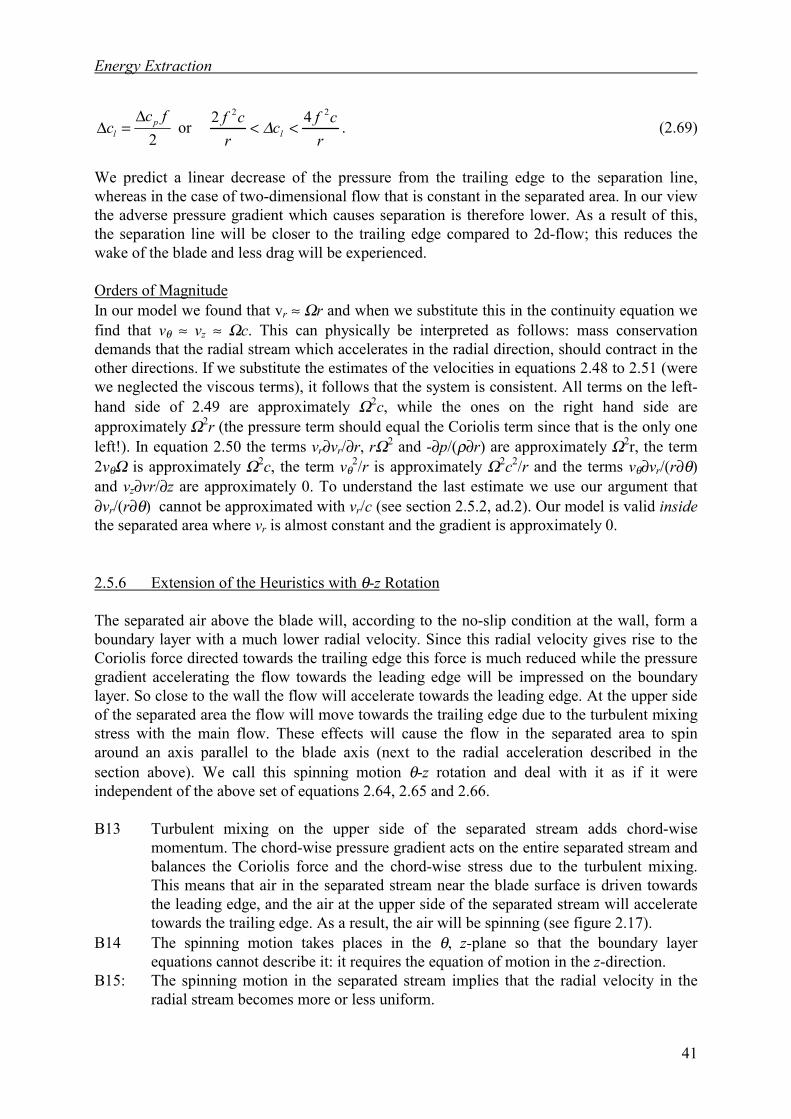
Energy Extraction
41
2fc
c pl
∆=∆ or .
42 22
rcfc
rcf
l << ∆ (2.69)
We predict a linear decrease of the pressure from the trailing edge to the separation line,whereas in the case of two-dimensional flow that is constant in the separated area. In our viewthe adverse pressure gradient which causes separation is therefore lower. As a result of this,the separation line will be closer to the trailing edge compared to 2d-flow; this reduces thewake of the blade and less drag will be experienced.
Orders of MagnitudeIn our model we found that vr ≈ Ωr and when we substitute this in the continuity equation wefind that vθ ≈ vz ≈ Ωc. This can physically be interpreted as follows: mass conservationdemands that the radial stream which accelerates in the radial direction, should contract in theother directions. If we substitute the estimates of the velocities in equations 2.48 to 2.51 (werewe neglected the viscous terms), it follows that the system is consistent. All terms on the left-hand side of 2.49 are approximately Ω2c, while the ones on the right hand side areapproximately Ω2r (the pressure term should equal the Coriolis term since that is the only oneleft!). In equation 2.50 the terms vr∂vr/∂r, rΩ2 and -∂p/(ρ∂r) are approximately Ω2r, the term2vθΩ is approximately Ω2c, the term vθ
2/r is approximately Ω2c2/r and the terms vθ∂vr/(r∂θ)and vz∂vr/∂z are approximately 0. To understand the last estimate we use our argument that∂vr/(r∂θ) cannot be approximated with vr/c (see section 2.5.2, ad.2). Our model is valid insidethe separated area where vr is almost constant and the gradient is approximately 0.
2.5.6 Extension of the Heuristics with θ-z Rotation
The separated air above the blade will, according to the no-slip condition at the wall, form aboundary layer with a much lower radial velocity. Since this radial velocity gives rise to theCoriolis force directed towards the trailing edge this force is much reduced while the pressuregradient accelerating the flow towards the leading edge will be impressed on the boundarylayer. So close to the wall the flow will accelerate towards the leading edge. At the upper sideof the separated area the flow will move towards the trailing edge due to the turbulent mixingstress with the main flow. These effects will cause the flow in the separated area to spinaround an axis parallel to the blade axis (next to the radial acceleration described in thesection above). We call this spinning motion θ-z rotation and deal with it as if it wereindependent of the above set of equations 2.64, 2.65 and 2.66.
B13 Turbulent mixing on the upper side of the separated stream adds chord-wisemomentum. The chord-wise pressure gradient acts on the entire separated stream andbalances the Coriolis force and the chord-wise stress due to the turbulent mixing.This means that air in the separated stream near the blade surface is driven towardsthe leading edge, and the air at the upper side of the separated stream will acceleratetowards the trailing edge. As a result, the air will be spinning (see figure 2.17).
B14 The spinning motion takes places in the θ, z-plane so that the boundary layerequations cannot describe it: it requires the equation of motion in the z-direction.
B15: The spinning motion in the separated stream implies that the radial velocity in theradial stream becomes more or less uniform.
Flow Separation on Wind Turbine Blades
42
B16: A negative pressure gradient towards the centre of the spinning motion is alsorequired to produce the required centripetal forces.
Mathematical Model for θ-z RotationThe spinning motion can be described with the pressure gradients responsible for thecentripetal force and the balancing convective acceleration terms. If we restrict ourselves tothe terms required for spinning motion, we get for continuity and the θ and the z-equations ofmotion respectively:
,0=∂∂+
∂∂
zv
rv z
θθ (2.70)
,θρ
θ
∂∂−=
∂∂
rp
zvvz (2.71)
.z
pr
vv z
∂∂−=
∂∂
ρθθ (2.72)
The θ-z rotation is a mechanism that is assumed to be insignificant compared to the radialflow effects described by equations 2.64 and 2.66. However, in this thesis the existence of theθ-z rotation is important because this phenomenon is responsible for the signal of stall flagswith hinges parallel to the blade axis.
root
θ -z rotation
radial flow movesfrom the blade
stream with separated flow
attached flow inflow over leading edge
tip
3d-stall
inflow from blade root
Figure 2.14 Heuristic model on the stream of separated air and -z rotation.. θfigure 2.17 Heuristic model on the stream of separated air and the θ-z rotation.
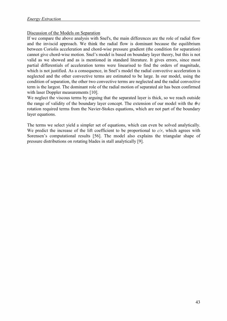
Energy Extraction
43
Discussion of the Models on SeparationIf we compare the above analysis with Snel's, the main differences are the role of radial flowand the inviscid approach. We think the radial flow is dominant because the equilibriumbetween Coriolis acceleration and chord-wise pressure gradient (the condition for separation)cannot give chord-wise motion. Snel’s model is based on boundary layer theory, but this is notvalid as we showed and as is mentioned in standard literature. It gives errors, since mostpartial differentials of acceleration terms were linearised to find the orders of magnitude,which is not justified. As a consequence, in Snel’s model the radial convective acceleration isneglected and the other convective terms are estimated to be large. In our model, using thecondition of separation, the other two convective terms are neglected and the radial convectiveterm is the largest. The dominant role of the radial motion of separated air has been confirmedwith laser Doppler measurements [10].We neglect the viscous terms by arguing that the separated layer is thick, so we reach outsidethe range of validity of the boundary layer concept. The extension of our model with the θ-zrotation required terms from the Navier-Stokes equations, which are not part of the boundarylayer equations.
The terms we select yield a simpler set of equations, which can even be solved analytically.We predict the increase of the lift coefficient to be proportional to c/r, which agrees withSorensen’s computational results [56]. The model also explains the triangular shape ofpressure distributions on rotating blades in stall analytically [9].

Flow Separation on Wind Turbine Blades
44
45
3. The Stall Flag Method
The stall flag method is a newly developed technique by which the flow direction over anaerodynamic object can be visualised. The method is particularly useful for the visualisationof flow separation. It is comparable to flow visualisation with tufts, the tufts being replacedby the so-called stall flags. Figure 3.1 shows the application of the stall flags to a commercialwind turbine. The figure demonstrates the most relevant difference between flow visualisationwith stall flags and with tufts: the visibility of stall flags is orders of magnitude better. Thestall flag is a detector with a binary output signal. An optically contrasting surface (in mostcases a retro-reflector) can be either visible or invisible depending on the flow direction overthe stall flag. A bright light source illuminates the entire swept area of the turbine and allexposed retro-reflectors return the light to the source. An observer or (video) camera can seeor record the signals even from a kilometre’s distance. In practical application the stallbehaviour of large commercial wind turbines can be analysed with approximately 200 stallflags installed on the rotor blades. The signals are recorded while operational conditions suchas rotation speed and yaw angleare varied. From theserecordings the stall behaviour ofa wind turbine rotor can bedetermined in detail.This chapter will deal with themethod from an aerodynamicpoint of view in conjunction tothe technical development of thestall flag. We begin with thatdevelopment. In section 2 weconsider the interpretation ofstall flag behaviour, in section 3the flow disturbance by that stallflag. Then in section 4 the stallflag will be compared to thetuft. For all the optical aspectsof the method we refer to thenext chapter.
figure 3.1 Application of the stall flag method to theNEG Micon 700/44m at Tehachapi, Ca. USA.

Flow Separation on Wind Turbine Blades
46
List of Symbols
a [m] amplitude of the sinusoidal flap deformationb [m] widthc [m] chordcd [-] drag coefficientcl [-] lift coefficientcl,max [-] first maximum of lift coefficientct [-] tangential force coefficientct,TES [-] average tangential force coefficient during trailing edge separationd [m] height of separated air above surfaceD [m] rotor diameterE [N/m2] Hooke modus of elasticity for flap materialf [rad] flap opening angleF1 [N] force on flap due to reversed flowF2 [N] force on flap due to main flowF3 [N] thrust force due to stall flagFcp [N] centrifugal force on the flapf [m] vector in flap plane perpendicular to the hinge lineg [m/s2] gravitational accelerationh [m] height of the flaph [m] hinge vectori [m] inflow direction vectork [-] dimensionless stall flag responseI [kgm2] moment of inertia of the flapIa [m3] second moment of area per unit width of the flapl [m] tuft lengthma [kg/m2] mass per unit area of the flapMa [Nm] aerodynamic turning momentMcf [Nm] turning moment due to centrifugal forcesME [N] turning moment per unit width due to material stiffnessMg [Nm] turning moment due to gravityMp [N] turning moment per unit width due to the pressure distributionn [-] integern [m] vector normal to flapp0 [N/m2] undisturbed static pressurepx [N/m2] static pressure at position xr [m] radial positionRe [-] chord based Reynolds numbers [m] location of stagnation pointS [-] stall flag sensitivityScf [-] stall flag sensitivity with respect to centrifugal forcesSg [-] stall flag sensitivity with respect to gravitationT [m] period of deformationt [rad] angle between flow and hinge linetf [m] thickness of flap

The Stall Flag Method
47
v [m/s] flow velocityv0 [m/s] undisturbed flow velocityvx [m/s] velocity at position xx [m] position in flow direction along the flap or chord-wise position of stall flagy [m] span-wise positionz [m] position above surface
α [rad] angle of attackβ [rad] local pitch angleγ [rad] hinge angle∆t [s] turn-over time of a stall flagχ [rad] angle between vertical and hinge vectorρ [kg/m3] air densityω [rad/s] angular velocity of switching flap or of the rotorω& [rad/s2] angular acceleration dω/dt of switching flap
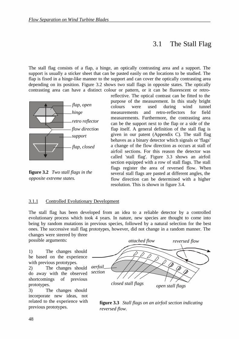
Flow Separation on Wind Turbine Blades
48
3.1 The Stall Flag
The stall flag consists of a flap, a hinge, an optically contrasting area and a support. Thesupport is usually a sticker sheet that can be pasted easily on the locations to be studied. Theflap is fixed in a hinge-like manner to the support and can cover the optically contrasting areadepending on its position. Figure 3.2 shows two stall flags in opposite states. The opticallycontrasting area can have a distinct colour or pattern, or it can be fluorescent or retro-
reflective. The optical contrast can be fitted to thepurpose of the measurement. In this study brightcolours were used during wind tunnelmeasurements and retro-reflectors for fieldmeasurements. Furthermore, the contrasting areacan be the support next to the flap or a side of theflap itself. A general definition of the stall flag isgiven in our patent (Appendix C). The stall flagbehaves as a binary detector which signals or 'flags'a change of the flow direction as occurs at stall ofairfoil sections. For this reason the detector wascalled 'stall flag'. Figure 3.3 shows an airfoilsection equipped with a row of stall flags. The stallflags register the area of reversed flow. Whenseveral stall flags are pasted at different angles, theflow direction can be determined with a higherresolution. This is shown in figure 3.4.
3.1.1 Controlled Evolutionary Development
The stall flag has been developed from an idea to a reliable detector by a controlledevolutionary process which took 4 years. In nature, new species are thought to come intobeing by random mutations in previous species, followed by a natural selection for the bestones. The successive stall flag prototypes, however, did not change in a random manner. Thechanges were steered by threepossible arguments:
1) The changes shouldbe based on the experiencewith previous prototypes.2) The changes shoulddo away with the observedshortcomings of previousprototypes.3) The changes shouldincorporate new ideas, notrelated to the experience withprevious prototypes.
figure 3.2 Two stall flags in theopposite extreme states.
flap, open
flow direction
hinge
support
retro reflector
flap, closed
reversed flowattached flow
closed stall flags open stall flags
aerfoilsection
figure 3.3 Stall flags on an airfoil section indicatingreversed flow.
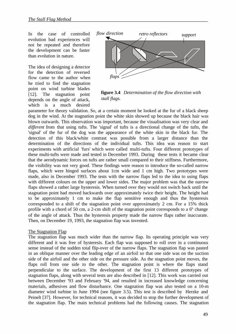
The Stall Flag Method
49
In the case of controlledevolution bad experiences willnot be repeated and thereforethe development can be fasterthan evolution in nature.
The idea of designing a detectorfor the detection of reversedflow came to the author whenhe tried to find the stagnationpoint on wind turbine blades[12]. The stagnation pointdepends on the angle of attack,which is a much desiredparameter for theory validation. So, at a certain moment he looked at the fur of a black sheepdog in the wind. At the stagnation point the white skin showed up because the black hair wasblown outwards. This observation was important, because the visualisation was very clear anddifferent from that using tufts. The 'signal' of tufts is a directional change of the tufts, the'signal' of the fur of the dog was the appearance of the white skin in the black fur. Thedetection of this black/white contrast was possible from a larger distance than thedetermination of the directions of the individual tufts. This idea was reason to startexperiments with artificial 'furs' which were called multi-tufts. Four different prototypes ofthese multi-tufts were made and tested in December 1993. During these tests it became clearthat the aerodynamic forces on tufts are rather small compared to their stiffness. Furthermore,the visibility was not very good. These findings were reason to introduce the so-called narrowflaps, which were hinged surfaces about 1cm wide and 1 cm high. Two prototypes weremade, also in December 1993. The tests with the narrow flaps led to the idea to using flapswith different colours on the upper and lower sides. The major problem was that the narrowflaps showed a rather large hysteresis. When turned over they would not switch back until thestagnation point had moved backwards over approximately twice their height. The height hadto be approximately 1 cm to make the flap sensitive enough and thus the hysteresiscorresponded to a shift of the stagnation point over approximately 2 cm. For a 15% thickprofile with a chord of 50 cm, a 2-cm shift of the stagnation point corresponds to a 6° changeof the angle of attack. Thus the hysteresis property made the narrow flaps rather inaccurate.Then, on December 19, 1993, the stagnation flap was invented.
The Stagnation FlapThe stagnation flap was much wider than the narrow flap. Its operating principle was verydifferent and it was free of hysteresis. Each flap was supposed to roll over in a continuoussense instead of the sudden total flip-over of the narrow flaps. The stagnation flap was pastedin an oblique manner over the leading edge of an airfoil so that one side was on the suctionside of the airfoil and the other side on the pressure side. As the stagnation point moves, theflaps roll from one side to the other. The stagnation point is where the flaps standperpendicular to the surface. The development of the first 13 different prototypes ofstagnation flaps, along with several tests are also described in [12]. This work was carried outbetween December '93 and February '94, and resulted in increased knowledge concerningmaterials, adhesives and flow disturbance. One stagnation flap was also tested on a 10-mdiameter wind turbine in June 1994 (see figure 3.5). This test is described by Herzke andPeinelt [37]. However, for technical reasons, it was decided to stop the further development ofthe stagnation flap. The main technical problems had the following causes. The stagnation
figure 3.4 Determination of the flow direction withstall flags.
flaps
flow direction support retro reflectors
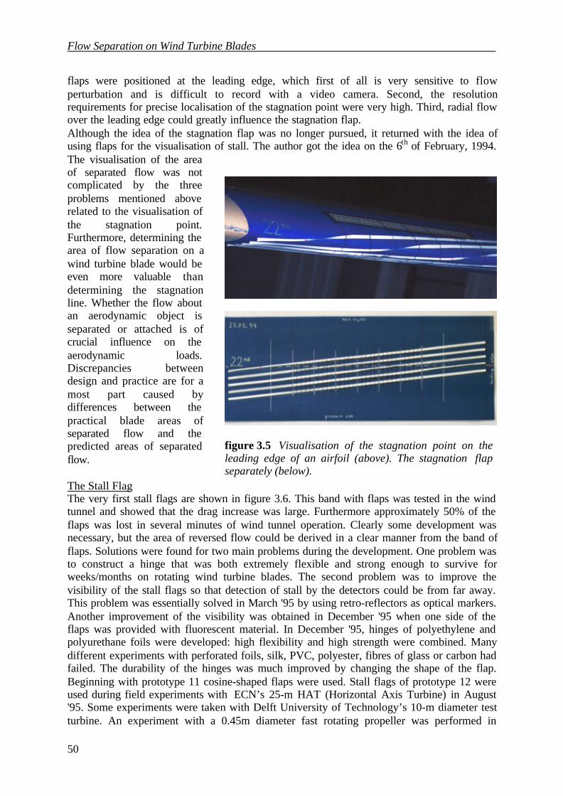
Flow Separation on Wind Turbine Blades
50
flaps were positioned at the leading edge, which first of all is very sensitive to flowperturbation and is difficult to record with a video camera. Second, the resolutionrequirements for precise localisation of the stagnation point were very high. Third, radial flowover the leading edge could greatly influence the stagnation flap.Although the idea of the stagnation flap was no longer pursued, it returned with the idea ofusing flaps for the visualisation of stall. The author got the idea on the 6th of February, 1994.The visualisation of the areaof separated flow was notcomplicated by the threeproblems mentioned aboverelated to the visualisation ofthe stagnation point.Furthermore, determining thearea of flow separation on awind turbine blade would beeven more valuable thandetermining the stagnationline. Whether the flow aboutan aerodynamic object isseparated or attached is ofcrucial influence on theaerodynamic loads.Discrepancies betweendesign and practice are for amost part caused bydifferences between thepractical blade areas ofseparated flow and thepredicted areas of separatedflow.
The Stall FlagThe very first stall flags are shown in figure 3.6. This band with flaps was tested in the windtunnel and showed that the drag increase was large. Furthermore approximately 50% of theflaps was lost in several minutes of wind tunnel operation. Clearly some development wasnecessary, but the area of reversed flow could be derived in a clear manner from the band offlaps. Solutions were found for two main problems during the development. One problem wasto construct a hinge that was both extremely flexible and strong enough to survive forweeks/months on rotating wind turbine blades. The second problem was to improve thevisibility of the stall flags so that detection of stall by the detectors could be from far away.This problem was essentially solved in March '95 by using retro-reflectors as optical markers.Another improvement of the visibility was obtained in December '95 when one side of theflaps was provided with fluorescent material. In December '95, hinges of polyethylene andpolyurethane foils were developed: high flexibility and high strength were combined. Manydifferent experiments with perforated foils, silk, PVC, polyester, fibres of glass or carbon hadfailed. The durability of the hinges was much improved by changing the shape of the flap.Beginning with prototype 11 cosine-shaped flaps were used. Stall flags of prototype 12 wereused during field experiments with ECN’s 25-m HAT (Horizontal Axis Turbine) in August'95. Some experiments were taken with Delft University of Technology’s 10-m diameter testturbine. An experiment with a 0.45m diameter fast rotating propeller was performed in
figure 3.5 Visualisation of the stagnation point on theleading edge of an airfoil (above). The stagnation flapseparately (below).
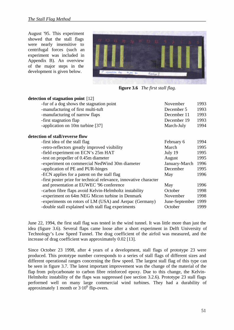
The Stall Flag Method
51
August '95. This experimentshowed that the stall flagswere nearly insensitive tocentrifugal forces (such anexperiment was included inAppendix B). An overviewof the major steps in thedevelopment is given below.
detection of stagnation point [12]-fur of a dog shows the stagnation point November 1993-manufacturing of first multi-tuft December 5 1993-manufacturing of narrow flaps December 11 1993-first stagnation flap December 19 1993-application on 10m turbine [37] March-July 1994
detection of stall/reverse flow-first idea of the stall flag February 6 1994-retro-reflectors greatly improved visibility March 1995-field experiment on ECN’s 25m HAT July 19 1995-test on propeller of 0.45m diameter August 1995-experiment on commercial NedWind 30m diameter January-March 1996-application of PE and PUR-hinges December 1995-ECN applies for a patent on the stall flag May 1996-first poster prize for technical relevance, innovative character and presentation at EUWEC '96 conference May 1996-carbon fibre flaps avoid Kelvin-Helmholtz instability October 1998-experiment on 64m NEG Micon turbine in Denmark November 1998-experiments on rotors of LM (USA) and Aerpac (Germany) June-September 1999-double stall explained with stall flag experiments October 1999
June 22, 1994, the first stall flag was tested in the wind tunnel. It was little more than just theidea (figure 3.6). Several flaps came loose after a short experiment in Delft University ofTechnology’s Low Speed Tunnel. The drag coefficient of the airfoil was measured, and theincrease of drag coefficient was approximately 0.02 [13].
Since October 23 1998, after 4 years of a development, stall flags of prototype 23 wereproduced. This prototype number corresponds to a series of stall flags of different sizes anddifferent operational ranges concerning the flow speed. The largest stall flag of this type canbe seen in figure 3.7. The latest important improvement was the change of the material of theflap from polycarbonate to carbon fibre reinforced epoxy. Due to this change, the Kelvin-Helmholtz instability of the flaps was suppressed (see section 3.2.6). Prototype 23 stall flagsperformed well on many large commercial wind turbines. They had a durability ofapproximately 1 month or 3·106 flip-overs.
figure 3.6 The first stall flag.
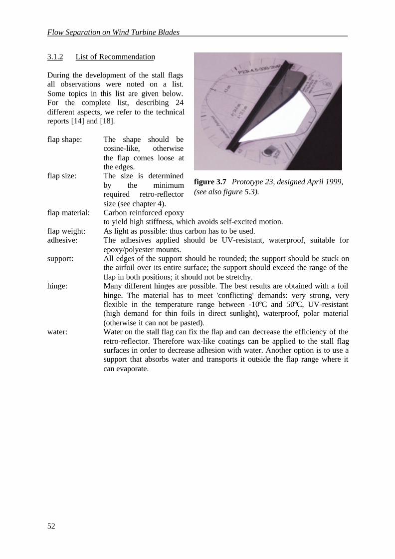
Flow Separation on Wind Turbine Blades
52
3.1.2 List of Recommendation
During the development of the stall flagsall observations were noted on a list.Some topics in this list are given below.For the complete list, describing 24different aspects, we refer to the technicalreports [14] and [18].
flap shape: The shape should becosine-like, otherwisethe flap comes loose atthe edges.
flap size: The size is determinedby the minimumrequired retro-reflectorsize (see chapter 4).
flap material: Carbon reinforced epoxyto yield high stiffness, which avoids self-excited motion.
flap weight: As light as possible: thus carbon has to be used.adhesive: The adhesives applied should be UV-resistant, waterproof, suitable for
epoxy/polyester mounts.support: All edges of the support should be rounded; the support should be stuck on
the airfoil over its entire surface; the support should exceed the range of theflap in both positions; it should not be stretchy.
hinge: Many different hinges are possible. The best results are obtained with a foilhinge. The material has to meet 'conflicting' demands: very strong, veryflexible in the temperature range between -10ºC and 50ºC, UV-resistant(high demand for thin foils in direct sunlight), waterproof, polar material(otherwise it can not be pasted).
water: Water on the stall flag can fix the flap and can decrease the efficiency of theretro-reflector. Therefore wax-like coatings can be applied to the stall flagsurfaces in order to decrease adhesion with water. Another option is to use asupport that absorbs water and transports it outside the flap range where itcan evaporate.
figure 3.7 Prototype 23, designed April 1999,(see also figure 5.3).
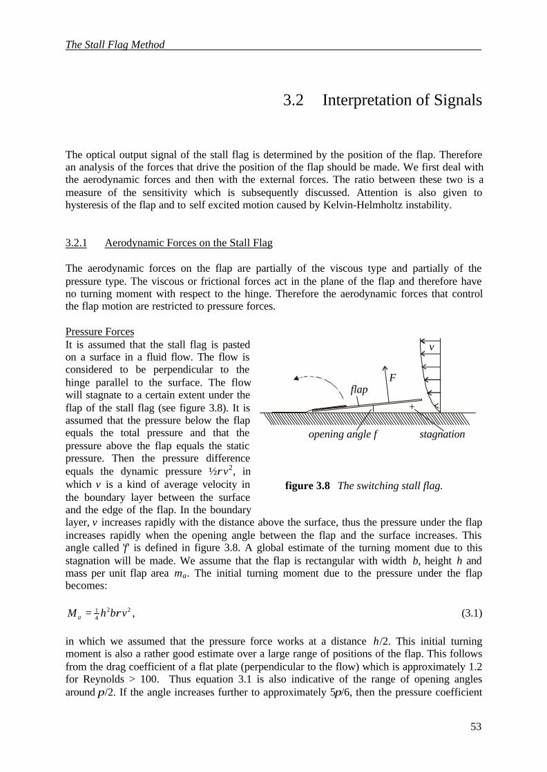
The Stall Flag Method
53
3.2 Interpretation of Signals
The optical output signal of the stall flag is determined by the position of the flap. Thereforean analysis of the forces that drive the position of the flap should be made. We first deal withthe aerodynamic forces and then with the external forces. The ratio between these two is ameasure of the sensitivity which is subsequently discussed. Attention is also given tohysteresis of the flap and to self excited motion caused by Kelvin-Helmholtz instability.
3.2.1 Aerodynamic Forces on the Stall Flag
The aerodynamic forces on the flap are partially of the viscous type and partially of thepressure type. The viscous or frictional forces act in the plane of the flap and therefore haveno turning moment with respect to the hinge. Therefore the aerodynamic forces that controlthe flap motion are restricted to pressure forces.
Pressure ForcesIt is assumed that the stall flag is pastedon a surface in a fluid flow. The flow isconsidered to be perpendicular to thehinge parallel to the surface. The flowwill stagnate to a certain extent under theflap of the stall flag (see figure 3.8). It isassumed that the pressure below the flapequals the total pressure and that thepressure above the flap equals the staticpressure. Then the pressure differenceequals the dynamic pressure ½ρv2, inwhich v is a kind of average velocity inthe boundary layer between the surfaceand the edge of the flap. In the boundarylayer, v increases rapidly with the distance above the surface, thus the pressure under the flapincreases rapidly when the opening angle between the flap and the surface increases. Thisangle called 'f' is defined in figure 3.8. A global estimate of the turning moment due to thisstagnation will be made. We assume that the flap is rectangular with width b, height h andmass per unit flap area ma. The initial turning moment due to the pressure under the flapbecomes:
,2241 vbhM a ρ= (3.1)
in which we assumed that the pressure force works at a distance h/2. This initial turningmoment is also a rather good estimate over a large range of positions of the flap. This followsfrom the drag coefficient of a flat plate (perpendicular to the flow) which is approximately 1.2for Reynolds > 100. Thus equation 3.1 is also indicative of the range of opening anglesaround π/2. If the angle increases further to approximately 5π/6, then the pressure coefficient
+
opening angle f
F
v
flap
stagnation
figure 3.8 The switching stall flag.
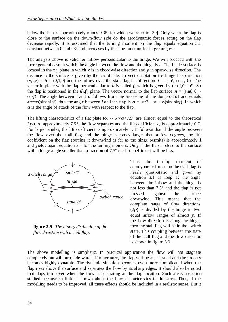
Flow Separation on Wind Turbine Blades
54
below the flap is approximately minus 0.35, for which we refer to [39]. Only when the flap isclose to the surface on the down-flow side do the aerodynamic forces acting on the flapdecrease rapidly. It is assumed that the turning moment on the flap equals equation 3.1constant between 0 and π/2 and decreases by the sine function for larger angles.
The analysis above is valid for inflow perpendicular to the hinge. We will proceed with themore general case in which the angle between the flow and the hinge is t. The blade surface islocated in the x,y plane in which x is in chord-wise direction and y in span-wise direction. Thedistance to the surface is given by the z-ordinate. In vector notation the hinge has direction(x,y,z) = h = (0,1,0) and the inflow over the stall flag has direction i = (sint, cost, 0). Thevector in-plane with the flap perpendicular to h is called f, which is given by (cosf,0,sinf). Sothe flap is positioned in the (h,f) plane. The vector normal to the flap surface n = (sinf, 0, -cosf). The angle between i and n follows from the arccosine of the dot product and equalsarccos(sint sinf), thus the angle between i and the flap is α = π/2 - arccos(sint sinf), in whichα is the angle of attack of the flow with respect to the flap.
The lifting characteristics of a flat plate for -7.5°<α<7.5° are almost equal to the theoretical2πα. At approximately 7.5°, the flow separates and the lift coefficient cl is approximately 0.7.For larger angles, the lift coefficient is approximately 1. It follows that if the angle betweenthe flow over the stall flag and the hinge becomes larger than a few degrees, the liftcoefficient on the flap (forcing it downwind as far as the hinge permits) is approximately 1and yields again equation 3.1 for the turning moment. Only if the flap is close to the surfacewith a hinge angle smaller than a fraction of 7.5° the lift coefficient will be less.
Thus the turning moment ofaerodynamic forces on the stall flag isnearly quasi-static and given byequation 3.1 as long as the anglebetween the inflow and the hinge isnot less than 7.5° and the flap is notpressed against the surfacedownwind. This means that thecomplete range of flow directions(2π) is divided by the hinge in twoequal inflow ranges of almost π. Ifthe flow direction is along the hinge,then the stall flag will be in the switchstate. This coupling between the stateof the stall flag and the flow directionis shown in figure 3.9.
The above modelling is simplistic. In practical application the flow will not stagnatecompletely but will turn side-wards. Furthermore, the flap will be accelerated and the processbecomes highly dynamic. The dynamic situation becomes even more complicated when theflap rises above the surface and separates the flow by its sharp edges. It should also be notedthat flaps turn over when the flow is separating at the flap location. Such areas are oftenstudied because so little is known about the flow characteristics in this area. Thus, if themodelling needs to be improved, all these effects should be included in a realistic sense. But it
figure 3.9 The binary distinction of theflow direction with a stall flag.
hinge
state '0'
state '1' switch range
switch range
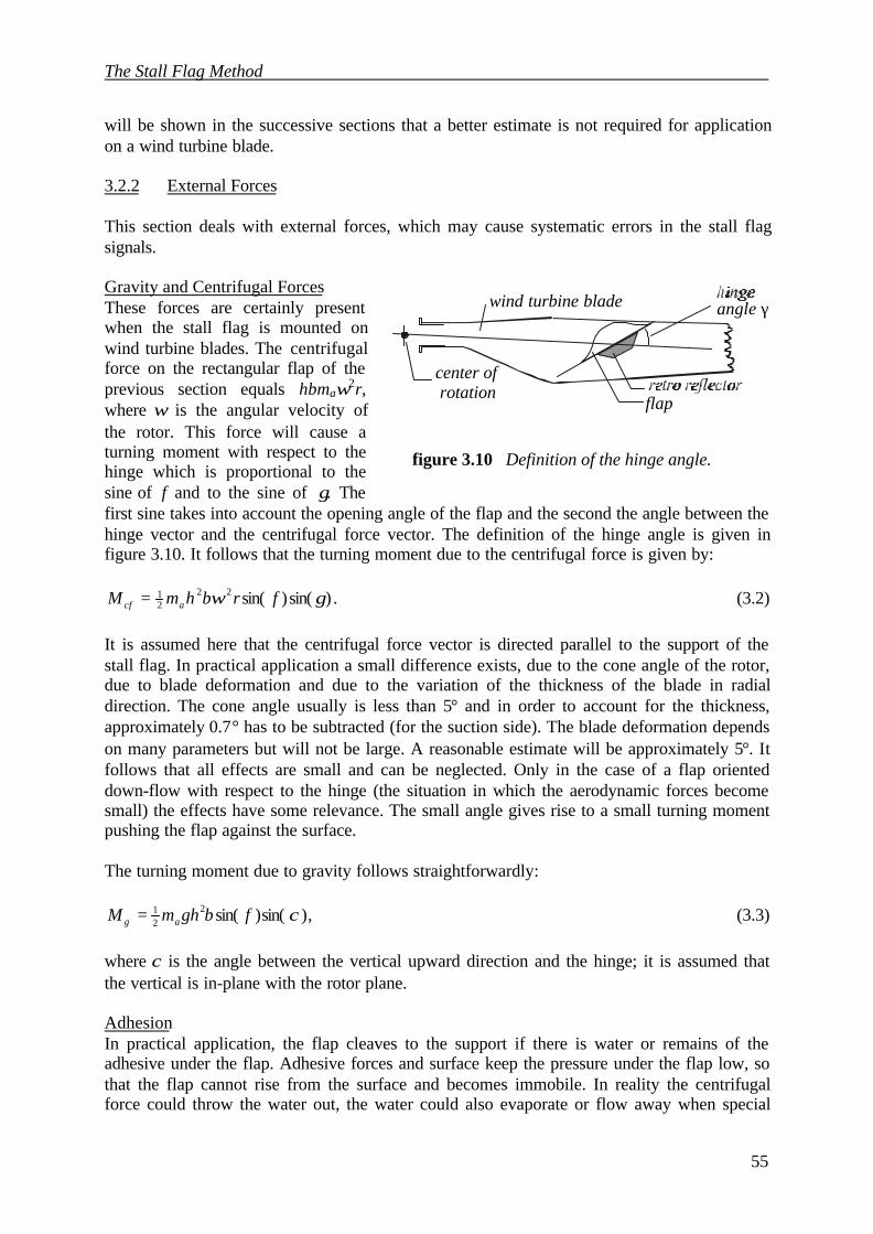
The Stall Flag Method
55
will be shown in the successive sections that a better estimate is not required for applicationon a wind turbine blade.
3.2.2 External Forces
This section deals with external forces, which may cause systematic errors in the stall flagsignals.
Gravity and Centrifugal ForcesThese forces are certainly presentwhen the stall flag is mounted onwind turbine blades. The centrifugalforce on the rectangular flap of theprevious section equals hbmaω2r,where ω is the angular velocity ofthe rotor. This force will cause aturning moment with respect to thehinge which is proportional to thesine of f and to the sine of γ. Thefirst sine takes into account the opening angle of the flap and the second the angle between thehinge vector and the centrifugal force vector. The definition of the hinge angle is given infigure 3.10. It follows that the turning moment due to the centrifugal force is given by:
.)sin()sin(2221 γω frbhmM acf = (3.2)
It is assumed here that the centrifugal force vector is directed parallel to the support of thestall flag. In practical application a small difference exists, due to the cone angle of the rotor,due to blade deformation and due to the variation of the thickness of the blade in radialdirection. The cone angle usually is less than 5° and in order to account for the thickness,approximately 0.7° has to be subtracted (for the suction side). The blade deformation dependson many parameters but will not be large. A reasonable estimate will be approximately 5°. Itfollows that all effects are small and can be neglected. Only in the case of a flap orienteddown-flow with respect to the hinge (the situation in which the aerodynamic forces becomesmall) the effects have some relevance. The small angle gives rise to a small turning momentpushing the flap against the surface.
The turning moment due to gravity follows straightforwardly:
,)sin()sin(221 χfbghmM ag = (3.3)
where χ is the angle between the vertical upward direction and the hinge; it is assumed thatthe vertical is in-plane with the rotor plane.
AdhesionIn practical application, the flap cleaves to the support if there is water or remains of theadhesive under the flap. Adhesive forces and surface keep the pressure under the flap low, sothat the flap cannot rise from the surface and becomes immobile. In reality the centrifugalforce could throw the water out, the water could also evaporate or flow away when special
angle γ
center of rotation
flap
wind turbine blade
figure 3.10 Definition of the hinge angle.
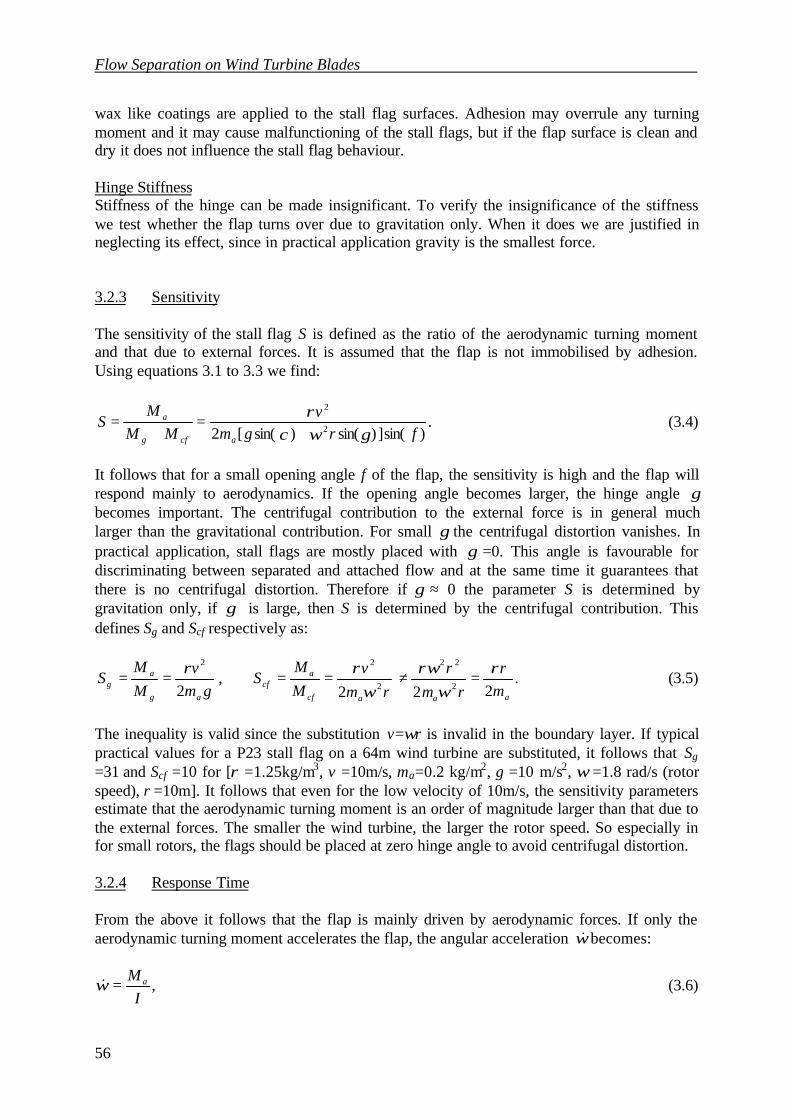
Flow Separation on Wind Turbine Blades
56
wax like coatings are applied to the stall flag surfaces. Adhesion may overrule any turningmoment and it may cause malfunctioning of the stall flags, but if the flap surface is clean anddry it does not influence the stall flag behaviour.
Hinge StiffnessStiffness of the hinge can be made insignificant. To verify the insignificance of the stiffnesswe test whether the flap turns over due to gravitation only. When it does we are justified inneglecting its effect, since in practical application gravity is the smallest force.
3.2.3 Sensitivity
The sensitivity of the stall flag S is defined as the ratio of the aerodynamic turning momentand that due to external forces. It is assumed that the flap is not immobilised by adhesion.Using equations 3.1 to 3.3 we find:
.)sin(])sin()sin([2 2
2
frgmv
MMM
Sacfg
a
γωχρ
+=
+= (3.4)
It follows that for a small opening angle f of the flap, the sensitivity is high and the flap willrespond mainly to aerodynamics. If the opening angle becomes larger, the hinge angle γbecomes important. The centrifugal contribution to the external force is in general muchlarger than the gravitational contribution. For small γ the centrifugal distortion vanishes. Inpractical application, stall flags are mostly placed with γ =0. This angle is favourable fordiscriminating between separated and attached flow and at the same time it guarantees thatthere is no centrifugal distortion. Therefore if γ ≈ 0 the parameter S is determined bygravitation only, if γ is large, then S is determined by the centrifugal contribution. Thisdefines Sg and Scf respectively as:
.222
,2 2
22
2
22
aaacf
acf
ag
ag m
r
rm
r
rm
vM
MS
gmv
M
MS
ρω
ρωω
ρρ =≠==== (3.5)
The inequality is valid since the substitution v=ωr is invalid in the boundary layer. If typicalpractical values for a P23 stall flag on a 64m wind turbine are substituted, it follows that Sg
=31 and Scf =10 for [ρ =1.25kg/m3, v =10m/s, ma=0.2 kg/m2, g =10 m/s2, ω =1.8 rad/s (rotorspeed), r =10m]. It follows that even for the low velocity of 10m/s, the sensitivity parametersestimate that the aerodynamic turning moment is an order of magnitude larger than that due tothe external forces. The smaller the wind turbine, the larger the rotor speed. So especially infor small rotors, the flags should be placed at zero hinge angle to avoid centrifugal distortion.
3.2.4 Response Time
From the above it follows that the flap is mainly driven by aerodynamic forces. If only theaerodynamic turning moment accelerates the flap, the angular acceleration ω& becomes:
,I
M a=ω& (3.6)
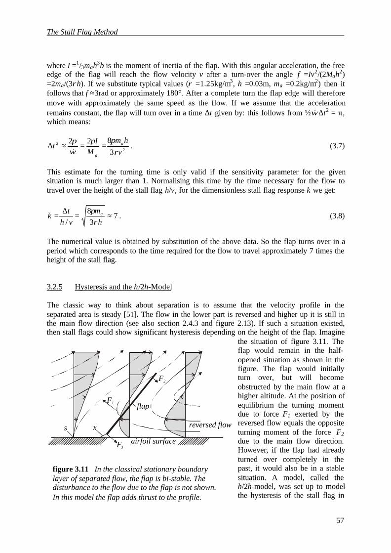
The Stall Flag Method
57
where I =1/3mah3b is the moment of inertia of the flap. With this angular acceleration, the freeedge of the flag will reach the flow velocity v after a turn-over the angle f =Iv2/(2Mah2)=2ma/(3ρh). If we substitute typical values (ρ =1.25kg/m3, h =0.03m, ma =0.2kg/m2) then itfollows that f ≈3rad or approximately 180°. After a complete turn the flap edge will thereforemove with approximately the same speed as the flow. If we assume that the accelerationremains constant, the flap will turn over in a time ∆t given by: this follows from ½ω& ∆t2 = π,which means:
.3
8222
2
v
hmM
It a
a ρππ
ωπ ==≈∆&
(3.7)
This estimate for the turning time is only valid if the sensitivity parameter for the givensituation is much larger than 1. Normalising this time by the time necessary for the flow totravel over the height of the stall flag h/v, for the dimensionless stall flag response k we get:
.73
8/
≈=∆=h
mvht
k a
ρπ
(3.8)
The numerical value is obtained by substitution of the above data. So the flap turns over in aperiod which corresponds to the time required for the flow to travel approximately 7 times theheight of the stall flag.
3.2.5 Hysteresis and the h/2h-Model
The classic way to think about separation is to assume that the velocity profile in theseparated area is steady [51]. The flow in the lower part is reversed and higher up it is still inthe main flow direction (see also section 2.4.3 and figure 2.13). If such a situation existed,then stall flags could show significant hysteresis depending on the height of the flap. Imagine
the situation of figure 3.11. Theflap would remain in the half-opened situation as shown in thefigure. The flap would initiallyturn over, but will becomeobstructed by the main flow at ahigher altitude. At the position ofequilibrium the turning momentdue to force F1 exerted by thereversed flow equals the oppositeturning moment of the force F2due to the main flow direction.However, if the flap had alreadyturned over completely in thepast, it would also be in a stablesituation. A model, called theh/2h-model, was set up to modelthe hysteresis of the stall flag in
flap F1
airfoil surface
reversed flow
F3
x s
F2
figure 3.11 In the classical stationary boundarylayer of separated flow, the flap is bi-stable. Thedisturbance to the flow due to the flap is not shown.In this model the flap adds thrust to the profile.
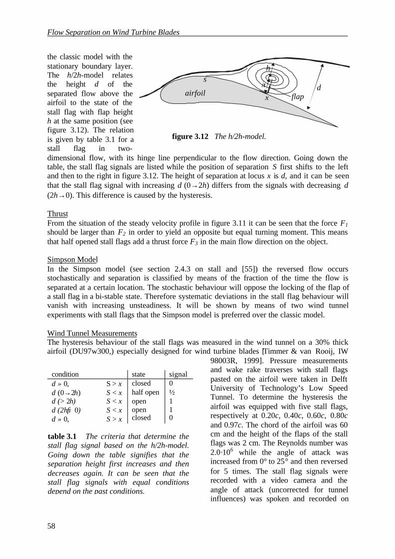
Flow Separation on Wind Turbine Blades
58
the classic model with thestationary boundary layer.The h/2h-model relatesthe height d of theseparated flow above theairfoil to the state of thestall flag with flap heighth at the same position (seefigure 3.12). The relationis given by table 3.1 for astall flag in two-dimensional flow, with its hinge line perpendicular to the flow direction. Going down thetable, the stall flag signals are listed while the position of separation S first shifts to the leftand then to the right in figure 3.12. The height of separation at locus x is d, and it can be seenthat the stall flag signal with increasing d (0→2h) differs from the signals with decreasing d(2h→0). This difference is caused by the hysteresis.
ThrustFrom the situation of the steady velocity profile in figure 3.11 it can be seen that the force F1should be larger than F2 in order to yield an opposite but equal turning moment. This meansthat half opened stall flags add a thrust force F3 in the main flow direction on the object.
Simpson ModelIn the Simpson model (see section 2.4.3 on stall and [55]) the reversed flow occursstochastically and separation is classified by means of the fraction of the time the flow isseparated at a certain location. The stochastic behaviour will oppose the locking of the flap ofa stall flag in a bi-stable state. Therefore systematic deviations in the stall flag behaviour willvanish with increasing unsteadiness. It will be shown by means of two wind tunnelexperiments with stall flags that the Simpson model is preferred over the classic model.
Wind Tunnel MeasurementsThe hysteresis behaviour of the stall flags was measured in the wind tunnel on a 30% thickairfoil (DU97w300,) especially designed for wind turbine blades [Timmer & van Rooij, IW
98003R, 1999]. Pressure measurementsand wake rake traverses with stall flagspasted on the airfoil were taken in DelftUniversity of Technology’s Low SpeedTunnel. To determine the hysteresis theairfoil was equipped with five stall flags,respectively at 0.20c, 0.40c, 0.60c, 0.80cand 0.97c. The chord of the airfoil was 60cm and the height of the flaps of the stallflags was 2 cm. The Reynolds number was2.0·106 while the angle of attack wasincreased from 0° to 25° and then reversedfor 5 times. The stall flag signals wererecorded with a video camera and theangle of attack (uncorrected for tunnelinfluences) was spoken and recorded on
condition state signald ≈ 0, S > x closed 0d (0→2h) S < x half open ½d (> 2h) S < xd (2h→0) S < xd ≈ 0, S > x
openopenclosed
110
table 3.1 The criteria that determine thestall flag signal based on the h/2h-model.Going down the table signifies that theseparation height first increases and thendecreases again. It can be seen that thestall flag signals with equal conditionsdepend on the past conditions.
figure 3.12 The h/2h-model.
airfoil
s
flap
h
d x

The Stall Flag Method
59
the audio channel of the camera. The angle of attack changes at a constant rate of 0.875°/s.Because the time between successive frames of the video was precisely 40 ms, the changes ofangle of attack between changes of the stall flag signals could be determined rather preciselyby counting the number of video frames. Figure 3.13 shows the results averaged over the 5sweeps. In steady conditions, thus without pitching, the stall flag signals were not steady inseparated flow. They could close for several seconds and then suddenly flip over and back ina fraction of a second. During the measurements, it was observed that several stall flags
0
20
40
60
80
100
8 12 16 20 24 28 32angle of attack [ o ]
chor
dwis
e po
sitio
n [%
]
0.78 h-tunnel
0.47 h-tunnel
0
20
40
60
80
100
8 12 16 20 24 28 32angle of attack [ o ]
chor
dwis
e po
sitio
n [%
] 4 cm
3 cm
figure 3.13 Hysteresis ofthe airfoil and the stallflags. The curves are passedclockwise. The averagehysteresis is approximately1.5° angle of attack.
figure 3.14 Equal rows ofstall flags (1 cm high) atdifferent span-wiselocations show largedifferences caused by three-dimensional flow. All loopsabove 22.5° are clockwise,all loops below this angleare counter clockwise.
figure 3.15 Hysteresis ofstall flags with flaps of 3and 4 cm height atrespectively 39% and 56%of the height of the tunnel.All loops are clockwise.
0
20
40
60
80
100
8 10 12 14 16 18 20 22 24 26
angle of attack [ o ]
chor
dwis
e po
sitio
n [%
] stall flags
p-distribution
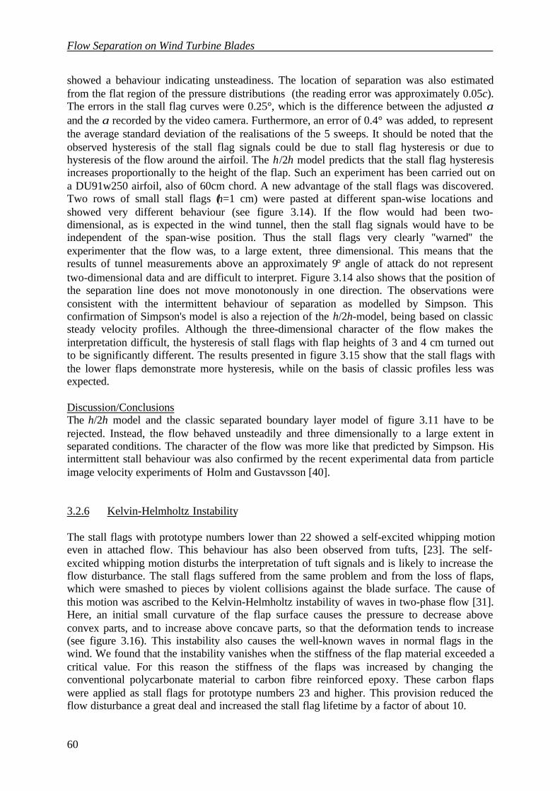
Flow Separation on Wind Turbine Blades
60
showed a behaviour indicating unsteadiness. The location of separation was also estimatedfrom the flat region of the pressure distributions (the reading error was approximately 0.05c).The errors in the stall flag curves were 0.25°, which is the difference between the adjusted αand the α recorded by the video camera. Furthermore, an error of 0.4° was added, to representthe average standard deviation of the realisations of the 5 sweeps. It should be noted that theobserved hysteresis of the stall flag signals could be due to stall flag hysteresis or due tohysteresis of the flow around the airfoil. The h/2h model predicts that the stall flag hysteresisincreases proportionally to the height of the flap. Such an experiment has been carried out ona DU91w250 airfoil, also of 60cm chord. A new advantage of the stall flags was discovered.Two rows of small stall flags (h=1 cm) were pasted at different span-wise locations andshowed very different behaviour (see figure 3.14). If the flow would had been two-dimensional, as is expected in the wind tunnel, then the stall flag signals would have to beindependent of the span-wise position. Thus the stall flags very clearly ''warned'' theexperimenter that the flow was, to a large extent, three dimensional. This means that theresults of tunnel measurements above an approximately 9° angle of attack do not representtwo-dimensional data and are difficult to interpret. Figure 3.14 also shows that the position ofthe separation line does not move monotonously in one direction. The observations wereconsistent with the intermittent behaviour of separation as modelled by Simpson. Thisconfirmation of Simpson's model is also a rejection of the h/2h-model, being based on classicsteady velocity profiles. Although the three-dimensional character of the flow makes theinterpretation difficult, the hysteresis of stall flags with flap heights of 3 and 4 cm turned outto be significantly different. The results presented in figure 3.15 show that the stall flags withthe lower flaps demonstrate more hysteresis, while on the basis of classic profiles less wasexpected.
Discussion/ConclusionsThe h/2h model and the classic separated boundary layer model of figure 3.11 have to berejected. Instead, the flow behaved unsteadily and three dimensionally to a large extent inseparated conditions. The character of the flow was more like that predicted by Simpson. Hisintermittent stall behaviour was also confirmed by the recent experimental data from particleimage velocity experiments of Holm and Gustavsson [40].
3.2.6 Kelvin-Helmholtz Instability
The stall flags with prototype numbers lower than 22 showed a self-excited whipping motioneven in attached flow. This behaviour has also been observed from tufts, [23]. The self-excited whipping motion disturbs the interpretation of tuft signals and is likely to increase theflow disturbance. The stall flags suffered from the same problem and from the loss of flaps,which were smashed to pieces by violent collisions against the blade surface. The cause ofthis motion was ascribed to the Kelvin-Helmholtz instability of waves in two-phase flow [31].Here, an initial small curvature of the flap surface causes the pressure to decrease aboveconvex parts, and to increase above concave parts, so that the deformation tends to increase(see figure 3.16). This instability also causes the well-known waves in normal flags in thewind. We found that the instability vanishes when the stiffness of the flap material exceeded acritical value. For this reason the stiffness of the flaps was increased by changing theconventional polycarbonate material to carbon fibre reinforced epoxy. These carbon flapswere applied as stall flags for prototype numbers 23 and higher. This provision reduced theflow disturbance a great deal and increased the stall flag lifetime by a factor of about 10.
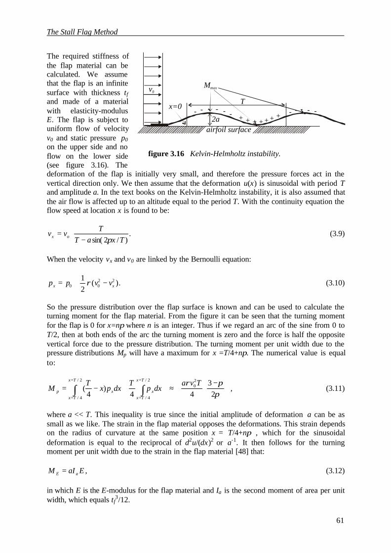
The Stall Flag Method
61
The required stiffness ofthe flap material can becalculated. We assumethat the flap is an infinitesurface with thickness tfand made of a materialwith elasticity-modulusE. The flap is subject touniform flow of velocityv0 and static pressure p0on the upper side and noflow on the lower side(see figure 3.16). Thedeformation of the flap is initially very small, and therefore the pressure forces act in thevertical direction only. We then assume that the deformation u(x) is sinusoidal with period Tand amplitude a. In the text books on the Kelvin-Helmholtz instability, it is also assumed thatthe air flow is affected up to an altitude equal to the period T. With the continuity equation theflow speed at location x is found to be:
.)/2sin( TxaT
Tvv ox π−
= (3.9)
When the velocity vx and v0 are linked by the Bernoulli equation:
.)(21 22
00 xx vvpp −+= ρ (3.10)
So the pressure distribution over the flap surface is known and can be used to calculate theturning moment for the flap material. From the figure it can be seen that the turning momentfor the flap is 0 for x=nπ where n is an integer. Thus if we regard an arc of the sine from 0 toT/2, then at both ends of the arc the turning moment is zero and the force is half the oppositevertical force due to the pressure distribution. The turning moment per unit width due to thepressure distributions Mp will have a maximum for x =T/4+nπ. The numerical value is equalto:
,2
344
)4
(20
2/
4/
2/
4/
−
≈+−= ∫∫=
=
=
= ππρ Tva
dxpT
dxpxT
MTx
Txxx
Tx
Txp (3.11)
where a << T. This inequality is true since the initial amplitude of deformation a can be assmall as we like. The strain in the flap material opposes the deformations. This strain dependson the radius of curvature at the same position x = T/4+nπ , which for the sinusoidaldeformation is equal to the reciprocal of d2u/(dx)2 or a-1. It then follows for the turningmoment per unit width due to the strain in the flap material [48] that:
,EaIM aE = (3.12)
in which E is the E-modulus for the flap material and Ia is the second moment of area per unitwidth, which equals tf
3/12.
figure 3.16 Kelvin-Helmholtz instability.
airfoil surface
v0
+
Mmax
+ + + + + -
+ - - - - - - - - - -
2a
x=0 T
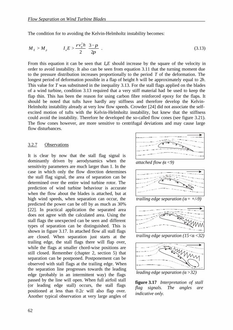
Flow Separation on Wind Turbine Blades
62
The condition for to avoiding the Kelvin-Helmholtz instability becomes:
.2
32
20
−>⇔>
ππρ hv
EIMM apE (3.13)
From this equation it can be seen that IaE should increase by the square of the velocity inorder to avoid instability. It also can be seen from equation 3.11 that the turning moment dueto the pressure distribution increases proportionally to the period T of the deformation. Thelongest period of deformation possible in a flap of height h will be approximately equal to 2h.This value for T was substituted in the inequality 3.13. For the stall flags applied on the bladesof a wind turbine, condition 3.13 required that a very stiff material had be used to keep theflap thin. This has been the reason for using carbon fibre reinforced epoxy for the flaps. Itshould be noted that tufts have hardly any stiffness and therefore develop the Kelvin-Helmholtz instability already at very low flow speeds. Crowder [24] did not associate the self-excited motion of tufts with the Kelvin-Helmholtz instability, but knew that the stiffnesscould avoid the instability. Therefore he developed the so-called flow cones (see figure 3.21).The flow cones however, are more sensitive to centrifugal deviations and may cause largeflow disturbances.
3.2.7 Observations
It is clear by now that the stall flag signal isdominantly driven by aerodynamics when thesensitivity parameters are much larger than 1. In thecase in which only the flow direction determinesthe stall flag signal, the area of separation can bedetermined over the entire wind turbine rotor. Theprediction of wind turbine behaviour is accuratewhen the flow about the blades is attached, but athigh wind speeds, when separation can occur, thepredicted the power can be off by as much as 30%[22]. In practical application the separated areadoes not agree with the calculated area. Using thestall flags the unexpected can be seen and differenttypes of separation can be distinguished. This isshown in figure 3.17. In attached flow all stall flagsare closed. When separation just starts at thetrailing edge, the stall flags there will flap over,while the flags at smaller chord-wise positions arestill closed. Remember (chapter 2, section 5) thatseparation can be postponed. Postponement can beobserved with stall flags at the trailing edge. Whenthe separation line progresses towards the leadingedge (probably in an intermittent way) the flagspassed by the line will open. When full airfoil stall(or leading edge stall) occurs, the stall flagspositioned at less than 0.2c will also flap over.Another typical observation at very large angles of
figure 3.17 Interpretation of stallflag signals. The angles areindicative only.
leading edge separation ( >32)α
attached flow ( <9)α
trailing edge separation (15< <32)α
trailing edge separation ( = +/-9)α
The Stall Flag Method
63
attack (>32°) is that stall flags downstream 0.8c can close again because of the vortex at thetrailing edge (see figure 3.17).
The signals of the stall flags were compared to pressure measurements in the wind tunnel fortwo different airfoils used in wind turbine blades: the DU91w250 and the DU97w300. Fromthese measurements, a semi-quantitative relation was derived between the flow types given bythe stall flags and pressures measured (see figure 3.20). Stall flags positioned in the 'flat' partof the pressure distribution were always open and in other parts were always closed. When thestall flag at 0.90c was open and the one at 0.80c was closed, the airfoil operated at the firstmaximum of the lift coefficient cl,max. This could be a general phenomenon, since these stallflag signals mean that significant decambering ‘just started’ at the trailing edge. When thisstarts the drag coefficient cd also increases rapidly. The tangential force coefficient ct =clsin(α+β)-cdcos(α+β) is added to table 3.2, in which various cases of the stall flag signals arelisted. The stall flag indicate when separation of the trailing edge is initiated. Then we definethe tangential force coefficient to be ct,TES, and this value remains nearly constant (+/-0.05)when the separation line moves forward. When the flow on the leading edge also separates,however, ct suddenly drops by approximately 0.2. This means that the tangential force on ablade section remains approximately constant in trailing edge stall, so the power produced bythe rotor is constant. But when the flow at the leading edge separates, the tangential forcesdrops and can even become slightly negative, thus the power of the rotor is reduced.
stall flag signalx/c<0.2 rest x/c>0.8
coefficient flow type
0 0 00 0 1
cl= 2πα,cd< 0.02cl= cl,max,cd> 0.1
attached flowinitial separation
0 1 1/0 ct≈ct,TES trailing edge separation1 1/0 1/01 1/0 0
ct≈ct,TES-0.2ct≈ct,TES-0.2
full airfoil separationdeep stall
table 3.2 Indicative correspondence of stall flag signals and aerodynamiccoefficients.

Flow Separation on Wind Turbine Blades
64
3.3 Flow Disturbance
The stall flags are meant to detect the areas of flow separation on aerodynamic objects. Theyshould not disturb the separation phenomenon to a large extent. Although wind tunnelexperiments show that this is the case, one should always be suspicious about possibledisturbances. It can easily be checked whether certain stall flags change the separationphenomenon. One should install other stall flags downstream from the ones suspected. If theirsignals are independent from the ones upstream, it can be concluded that the latter do notcause significant disturbance. After this general remark, the possible flow disturbance due tothe stall flags will be discussed in more detail. First the influence of the stall flag on transitionwill be discussed, then the drag increase is measured and finally the influence on the pressuredistribution will be described.
3.3.1 Transition
Transition depends on roughness, pressure gradient, turbulence and fluid properties such asthe Reynolds number. Not much is known in detail about the factors controlling thismechanism [1,51], and therefore only semi-theoretical or empirical models exist to analysethe influence of roughness. Transition involves a change in the skin friction. In laminar flowthe skin friction is approximately proportional to v1.5, but in turbulent flow it is v1.85. Thepresence of stall flags may therefore introduce additional viscous drag. Early transition couldalso postpone separation and thereby reduce the drag an order of magnitude. Thus, if the stallflags do affect the location of transition, both drag and lift characteristics may be affected.
Expected Influence on TransitionAbbott gives the minimum height of a cylindrical disturbance (0.9 mm diameter at 0.05c, withits axis normal to the surface) necessary to cause premature transition [1]. This heightbecomes less when the (chord based) Reynolds number increases (to 0.75mm for Re = 2.5·106
and 0.38mm for Re = 5·106). The position of lowest pressure in Abbott's figure was 0.7c.Wind turbine blades rarely operate at Reynolds numbers larger than 5·106, and this wouldimply that our stall flag height (0.3 mm) is too low to affect transition. However, the shape ofthe object causing flow disturbance is also important, and the stall flag has surface roughness.Furthermore, in Abbott's case, the position of lowest pressure was far behind the disturbance,which stabilised the flow. At conditions more comparable to wind turbine aerodynamicsnearby or in separation, the lowest pressure will be located near the leading edge (<0.1c), sothat transition will take place much sooner. This explains why wind tunnel measurementsshowed that stall flags caused transition when located in areas of laminar flow (see figure3.20). So stall flags cause transition when placed in laminar flow. However, when stall flagsshow separation, the flow has become turbulent far upstream if the stall flag position and thusno flow disturbance via transition takes place.
Influence on Transition in Practical ApplicationCommercial wind turbine blades often already have a leading edge roughness ofapproximately 0.5mm due to the manufacturing process [22]. Blades produced with verysmooth leading edges will become contaminated by insects within a few months (depending
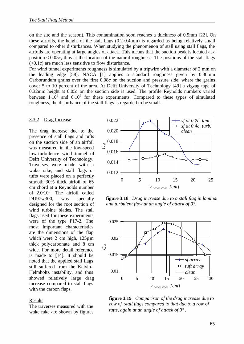
The Stall Flag Method
65
on the site and the season). This contamination soon reaches a thickness of 0.5mm [22]. Onthese airfoils, the height of the stall flags (0.2-0.4mm) is regarded as being relatively smallcompared to other disturbances. When studying the phenomenon of stall using stall flags, theairfoils are operating at large angles of attack. This means that the suction peak is located at aposition < 0.05c, thus at the location of the natural roughness. The positions of the stall flags(>0.1c) are much less sensitive to flow disturbance.For wind tunnel experiments roughness is simulated by a tripwire with a diameter of 2 mm onthe leading edge [58]. NACA [1] applies a standard roughness given by 0.30mmCarborundum grains over the first 0.08c on the suction and pressure side, where the grainscover 5 to 10 percent of the area. At Delft University of Technology [49] a zigzag tape of0.32mm height at 0.05c on the suction side is used. The profile Reynolds numbers variedbetween 1·106 and 6·106 for these experiments. Compared to these types of simulatedroughness, the disturbance of the stall flags is regarded to be small.
3.3.2 Drag Increase
The drag increase due to thepresence of stall flags and tuftson the suction side of an airfoilwas measured in the low-speedlow-turbulence wind tunnel ofDelft University of Technology.Traverses were made with awake rake, and stall flags ortufts were placed on a perfectlysmooth 30% thick airfoil of 65cm chord at a Reynolds numberof 2.0·106. The airfoil calledDU97w300, was speciallydesigned for the root section ofwind turbine blades. The stallflags used for these experimentswere of the type P17-2. Themost important characteristicsare the dimensions of the flapwhich were 2 cm high, 125µmthick polycarbonate and 8 cmwide. For more detail referenceis made to [14]. It should benoted that the applied stall flagsstill suffered from the Kelvin-Helmholtz instability, and thusshowed relatively large dragincrease compared to stall flagswith the carbon flaps.
ResultsThe traverses measured with thewake rake are shown by figures
figure 3.18 Drag increase due to a stall flag in laminarand turbulent flow at an angle of attack of 9°.
0.012
0.014
0.016
0.018
0.020
0.022
0 5 10 15 20 25y wake rake [cm]
Cd
sf at 0.2c, lam.sf at 0.4c, turb.clean
figure 3.19 Comparison of the drag increase due torow of stall flags compared to that due to a row oftufts, again at an angle of attack of 9° .
0.01
0.015
0.02
0.025
0 5 10 15 20 25 30
y wake rake [cm]
Cd
sf arraytuft arrayclean
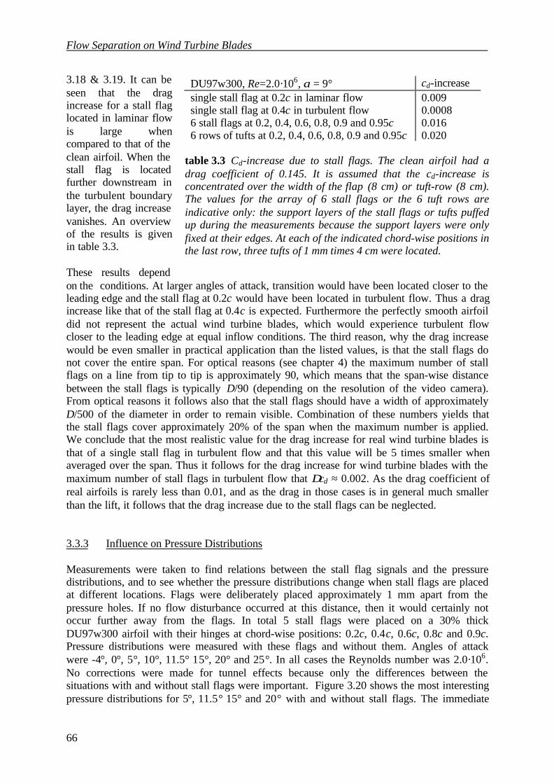
Flow Separation on Wind Turbine Blades
66
3.18 & 3.19. It can beseen that the dragincrease for a stall flaglocated in laminar flowis large whencompared to that of theclean airfoil. When thestall flag is locatedfurther downstream inthe turbulent boundarylayer, the drag increasevanishes. An overviewof the results is givenin table 3.3.
These results dependon the conditions. At larger angles of attack, transition would have been located closer to theleading edge and the stall flag at 0.2c would have been located in turbulent flow. Thus a dragincrease like that of the stall flag at 0.4c is expected. Furthermore the perfectly smooth airfoildid not represent the actual wind turbine blades, which would experience turbulent flowcloser to the leading edge at equal inflow conditions. The third reason, why the drag increasewould be even smaller in practical application than the listed values, is that the stall flags donot cover the entire span. For optical reasons (see chapter 4) the maximum number of stallflags on a line from tip to tip is approximately 90, which means that the span-wise distancebetween the stall flags is typically D/90 (depending on the resolution of the video camera).From optical reasons it follows also that the stall flags should have a width of approximatelyD/500 of the diameter in order to remain visible. Combination of these numbers yields thatthe stall flags cover approximately 20% of the span when the maximum number is applied.We conclude that the most realistic value for the drag increase for real wind turbine blades isthat of a single stall flag in turbulent flow and that this value will be 5 times smaller whenaveraged over the span. Thus it follows for the drag increase for wind turbine blades with themaximum number of stall flags in turbulent flow that ∆cd ≈ 0.002. As the drag coefficient ofreal airfoils is rarely less than 0.01, and as the drag in those cases is in general much smallerthan the lift, it follows that the drag increase due to the stall flags can be neglected.
3.3.3 Influence on Pressure Distributions
Measurements were taken to find relations between the stall flag signals and the pressuredistributions, and to see whether the pressure distributions change when stall flags are placedat different locations. Flags were deliberately placed approximately 1 mm apart from thepressure holes. If no flow disturbance occurred at this distance, then it would certainly notoccur further away from the flags. In total 5 stall flags were placed on a 30% thickDU97w300 airfoil with their hinges at chord-wise positions: 0.2c, 0.4c, 0.6c, 0.8c and 0.9c.Pressure distributions were measured with these flags and without them. Angles of attackwere -4°, 0°, 5°, 10°, 11.5° 15°, 20° and 25°. In all cases the Reynolds number was 2.0·106.No corrections were made for tunnel effects because only the differences between thesituations with and without stall flags were important. Figure 3.20 shows the most interestingpressure distributions for 5°, 11.5° 15° and 20° with and without stall flags. The immediate
DU97w300, Re=2.0·106, α = 9° cd-increasesingle stall flag at 0.2c in laminar flow 0.009single stall flag at 0.4c in turbulent flow 0.00086 stall flags at 0.2, 0.4, 0.6, 0.8, 0.9 and 0.95c 0.0166 rows of tufts at 0.2, 0.4, 0.6, 0.8, 0.9 and 0.95c 0.020
table 3.3 Cd-increase due to stall flags. The clean airfoil had adrag coefficient of 0.145. It is assumed that the cd-increase isconcentrated over the width of the flap (8 cm) or tuft-row (8 cm).The values for the array of 6 stall flags or the 6 tuft rows areindicative only: the support layers of the stall flags or tufts puffedup during the measurements because the support layers were onlyfixed at their edges. At each of the indicated chord-wise positions inthe last row, three tufts of 1 mm times 4 cm were located.
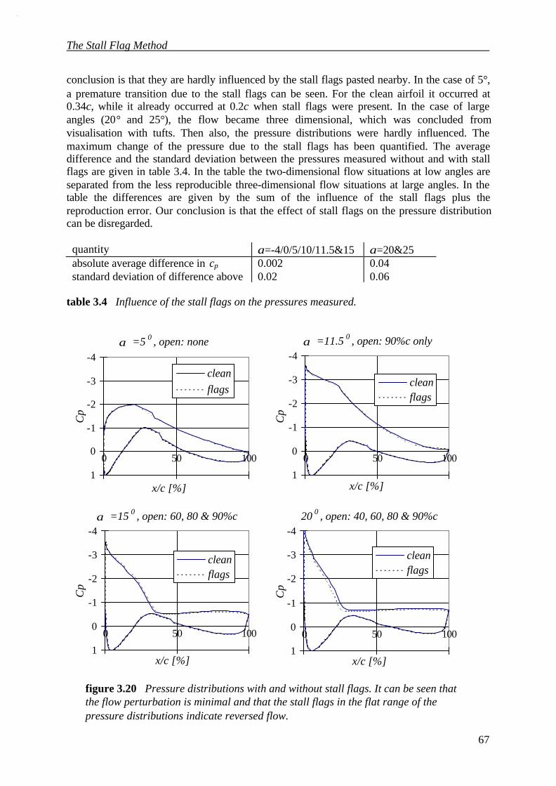
The Stall Flag Method
67
conclusion is that they are hardly influenced by the stall flags pasted nearby. In the case of 5°,a premature transition due to the stall flags can be seen. For the clean airfoil it occurred at0.34c, while it already occurred at 0.2c when stall flags were present. In the case of largeangles (20° and 25°), the flow became three dimensional, which was concluded fromvisualisation with tufts. Then also, the pressure distributions were hardly influenced. Themaximum change of the pressure due to the stall flags has been quantified. The averagedifference and the standard deviation between the pressures measured without and with stallflags are given in table 3.4. In the table the two-dimensional flow situations at low angles areseparated from the less reproducible three-dimensional flow situations at large angles. In thetable the differences are given by the sum of the influence of the stall flags plus thereproduction error. Our conclusion is that the effect of stall flags on the pressure distributioncan be disregarded.
quantity α=-4/0/5/10/11.5&15 α=20&25absolute average difference in cp 0.002 0.04standard deviation of difference above 0.02 0.06
table 3.4 Influence of the stall flags on the pressures measured.
figure 3.20 Pressure distributions with and without stall flags. It can be seen thatthe flow perturbation is minimal and that the stall flags in the flat range of thepressure distributions indicate reversed flow.
α =5 0 , open: none-4
-3
-2
-1
0
1
0 50 100
x/c [%]
Cp
cleanflags
α =11.5 0 , open: 90%c only-4
-3
-2
-1
0
1
0 50 100
x/c [%]
Cp
cleanflags
α =15 0 , open: 60, 80 & 90%c -4
-3
-2
-1
0
1
0 50 100
x/c [%]
Cp
cleanflags
20 0 , open: 40, 60, 80 & 90%c-4
-3
-2
-1
0
1
0 50 100
x/c [%]
Cp
cleanflags
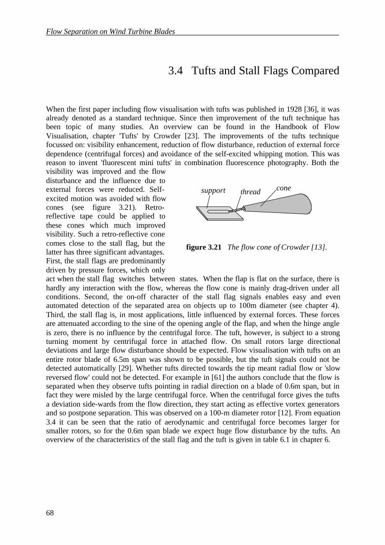
Flow Separation on Wind Turbine Blades
68
3.4 Tufts and Stall Flags Compared
When the first paper including flow visualisation with tufts was published in 1928 [36], it wasalready denoted as a standard technique. Since then improvement of the tuft technique hasbeen topic of many studies. An overview can be found in the Handbook of FlowVisualisation, chapter 'Tufts' by Crowder [23]. The improvements of the tufts techniquefocussed on: visibility enhancement, reduction of flow disturbance, reduction of external forcedependence (centrifugal forces) and avoidance of the self-excited whipping motion. This wasreason to invent 'fluorescent mini tufts' in combination fluorescence photography. Both thevisibility was improved and the flowdisturbance and the influence due toexternal forces were reduced. Self-excited motion was avoided with flowcones (see figure 3.21). Retro-reflective tape could be applied tothese cones which much improvedvisibility. Such a retro-reflective conecomes close to the stall flag, but thelatter has three significant advantages.First, the stall flags are predominantlydriven by pressure forces, which onlyact when the stall flag switches between states. When the flap is flat on the surface, there ishardly any interaction with the flow, whereas the flow cone is mainly drag-driven under allconditions. Second, the on-off character of the stall flag signals enables easy and evenautomated detection of the separated area on objects up to 100m diameter (see chapter 4).Third, the stall flag is, in most applications, little influenced by external forces. These forcesare attenuated according to the sine of the opening angle of the flap, and when the hinge angleis zero, there is no influence by the centrifugal force. The tuft, however, is subject to a strongturning moment by centrifugal force in attached flow. On small rotors large directionaldeviations and large flow disturbance should be expected. Flow visualisation with tufts on anentire rotor blade of 6.5m span was shown to be possible, but the tuft signals could not bedetected automatically [29]. Whether tufts directed towards the tip meant radial flow or 'slowreversed flow' could not be detected. For example in [61] the authors conclude that the flow isseparated when they observe tufts pointing in radial direction on a blade of 0.6m span, but infact they were misled by the large centrifugal force. When the centrifugal force gives the tuftsa deviation side-wards from the flow direction, they start acting as effective vortex generatorsand so postpone separation. This was observed on a 100-m diameter rotor [12]. From equation3.4 it can be seen that the ratio of aerodynamic and centrifugal force becomes larger forsmaller rotors, so for the 0.6m span blade we expect huge flow disturbance by the tufts. Anoverview of the characteristics of the stall flag and the tuft is given in table 6.1 in chapter 6.
conesupport thread
figure 3.21 The flow cone of Crowder [13].

69
4. Optical Aspects of Stall Flags
We have seen that the detection of separated areas on the blades of wind turbines is crucial forthe understanding of the stall behaviour. We also showed that our new indicator, the stall flag,is very well suitable for responding to flow separated by the change of the position of the flap.But still the state of a stall flag should be read out somehow. In fact the optical and contact-less read out of the stall flag state is one of its principal benefits. In this chapter we deal withmany options that can be made. Where should we put the retro-reflector. Underneath the flapor on the flap? And how large should the reflector be and what type should we use?We then model the stall flag and the recording system for the most beneficial options. Ourmodel is based on basic optical theory [25] in conjunction with experimental data. The modelis subsequently used to calculate the optimum configuration and we finally compare theoptical properties of the stall flag to those of tufts.

Flow Separation on Wind Turbine Blades
70
List of Symbols
a [-] apertureA [m2] size of contrasting areaAD [-] Absolute Demand on visibilityc [m] blade chordd [m] distance between camera/light source and contrasting areade [m] effective diameter of image of a contrasting areadh [m] horizontal distance to turbinedL [m] diameter of the camera lensdR [m] diameter of the contrasting area of the stall flagdλa [m] diameter of first order maximum of diffraction image of a pointD [m] diameter of the rotorDCCD [m] diameter of the CCD-chipDmin [J/m2] minimum detectable exposureEi [W/m3] spectral irradiance of image of contrasting areaEsun [W/m3] spectral irradiance from the sun assuming an air mass of 1.5ES [W/m3] spectral irradiance from the artificial sourcef [m] focal lengthfL,B [-] Lambertian reflected fraction of the blade areafL [-] Lambertian reflected fraction of contrasting stall flag areafR,θ [-] retro-reflected fraction of irradiance under angle θfR,ζ [-] retro-reflected fraction of irradiance under angle ζh [m] hub heightIL,θ [W/msr] Lambertian spectral intensity of contrasting area as secondary sourceIR [W/msr] spectral radiant intensity of the retro-reflector acting as secondary sourceIS [W/msr] spectral radiant intensity of the source Isf [W/msr] spectral radiant intensity of contrasting area of the stall flag as secondary
sourcek [sr] (space angle per unit cross section) per square distance to the sourceM [-] magnificationNCCD [-] resolution of CCD-chip expressed in # pixels on a liner [m] radial positionR [m] rotor radiusRD [-] Relative Demand on visibilityvi [m/s] velocity of the image over the detector areavtip [m/s] tip speedβ [°] pitch angleβt [°] total pitch angleδ [rad] half maximum cone angle of retro-reflected flux∆tL [s] illumination time of Lambertian reflective image of contrasting area∆tp [s] pulse duration of artificial source∆tR [s] illumination time of retro-reflective image of contrasting area∆ts [s] shutter timeεBi [J/m2] exposure of the blade images

Optical Aspects of Stall Flags
71
εRi [J/m2] exposure of the reflector imagesηD [-] spectral sensitivity of the detectorηF [-] filter spectral transmissionηL [-] lens transmissionηS [-] bundle efficiency of the sourceθ [rad] entrance angle between irradiance and normal to contrasting areaϕ [rad] half maximum cone angle of the bundle of the artificial sourceΦD [W/m] spectral radiant flux from contrasting area incident to the detector lensΦi,S [W/m] spectral radiant flux of the source incident to the contrasting areaΦi,sun [W/m] spectral radiant flux of the sun incident to the contrasting areaΦS [W/m] spectral radiant flux of the sourceΦD,B [W/m] spectral radiant flux from the blade surface incident to the detector lensλ [m] wavelength of radiationζ [rad] angle between solar irradiance and normal to contrasting area
Flow Separation on Wind Turbine Blades
72
4.1 Principles of Detection
The stall flag has two optically different states that are assumed to correspond to ranges offlow direction (see figure 4.1 and 3.9). When a contrasting area is visible, the signal will becalled ‘1’ and otherwise ‘0’, so the stall flag is a binary detector. The principle for detection iswhether the contrasting area shows up or not. A tuft in comparison shows up all the time, andthe detector should read the direction inwhich the tuft is pointing, which is muchless clear (see figure 4.1). The text belowdiscusses many ways to detect the binarystall flag signals.
4.1.1 Detectable or Visible
The stall flag signals can be observed by adetector (e.g. a video camera) or by thehuman eye. In the first case we speak aboutdetection and in the second case aboutvisibility. Detection is expressed inradiometric units and visibility inphotometric units. We start the analysis by aradiometric analysis and derive thenphotometric results by multiplication by the spectral sensitivity of the detector or the humaneye. Depending on the results, the signals will be concluded to be detectable or visible.Detection is more important because the human eye cannot follow the signals of hundreds ofstall flags simultaneously. However, it is beneficial if the signals are visible too. Visibilityallows an immediate check of the signals and draws the attention to uncommon events thatmay prompt the experimenter to adapt the measuring scheme.
4.1.2 Active or Passive
The stall flags are passively responding by the optical signal they give, but they may be madeactive to signal their turning over. One could connect an electric switch or optical sensor toeach flag for example, and detect the state of that flag through a direct electric signal, fed intoa computer via a data bus. This would require wires to each stall flag, however. We knowfrom experience that this complicates instrumentation so much that the technique becomesprohibitive for application on a commercial wind turbine. Moreover, the computer wouldhave to rotate with the turbine rotor or, if one wants to put the computer on the ground,electronic / optical slip rings or radio transmission techniques would be needed. This addseven more complexity.Another option is to give each flag its own power supply so that it can send an active optic orradio signal to the ground and does not need wires. A battery, possibly in combination with asolar cell, can be used. It may be difficult however, to keep the flag then thin enough to notdisturb the flow. The device should also be durably resistant to high centrifugal loads and to
figure 4.1 Stall flags and tufts at equalconditions. On the left-hand side the flowsmoves upward, on the right-hand side it isreversed.
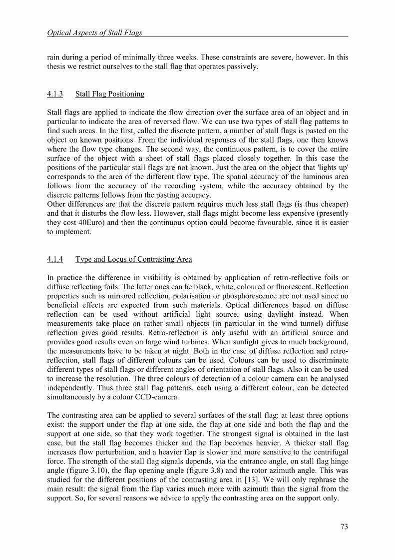
Optical Aspects of Stall Flags
73
rain during a period of minimally three weeks. These constraints are severe, however. In thisthesis we restrict ourselves to the stall flag that operates passively.
4.1.3 Stall Flag Positioning
Stall flags are applied to indicate the flow direction over the surface area of an object and inparticular to indicate the area of reversed flow. We can use two types of stall flag patterns tofind such areas. In the first, called the discrete pattern, a number of stall flags is pasted on theobject on known positions. From the individual responses of the stall flags, one then knowswhere the flow type changes. The second way, the continuous pattern, is to cover the entiresurface of the object with a sheet of stall flags placed closely together. In this case thepositions of the particular stall flags are not known. Just the area on the object that 'lights up'corresponds to the area of the different flow type. The spatial accuracy of the luminous areafollows from the accuracy of the recording system, while the accuracy obtained by thediscrete patterns follows from the pasting accuracy.Other differences are that the discrete pattern requires much less stall flags (is thus cheaper)and that it disturbs the flow less. However, stall flags might become less expensive (presentlythey cost 40Euro) and then the continuous option could become favourable, since it is easierto implement.
4.1.4 Type and Locus of Contrasting Area
In practice the difference in visibility is obtained by application of retro-reflective foils ordiffuse reflecting foils. The latter ones can be black, white, coloured or fluorescent. Reflectionproperties such as mirrored reflection, polarisation or phosphorescence are not used since nobeneficial effects are expected from such materials. Optical differences based on diffusereflection can be used without artificial light source, using daylight instead. Whenmeasurements take place on rather small objects (in particular in the wind tunnel) diffusereflection gives good results. Retro-reflection is only useful with an artificial source andprovides good results even on large wind turbines. When sunlight gives to much background,the measurements have to be taken at night. Both in the case of diffuse reflection and retro-reflection, stall flags of different colours can be used. Colours can be used to discriminatedifferent types of stall flags or different angles of orientation of stall flags. Also it can be usedto increase the resolution. The three colours of detection of a colour camera can be analysedindependently. Thus three stall flag patterns, each using a different colour, can be detectedsimultaneously by a colour CCD-camera.
The contrasting area can be applied to several surfaces of the stall flag: at least three optionsexist: the support under the flap at one side, the flap at one side and both the flap and thesupport at one side, so that they work together. The strongest signal is obtained in the lastcase, but the stall flag becomes thicker and the flap becomes heavier. A thicker stall flagincreases flow perturbation, and a heavier flap is slower and more sensitive to the centrifugalforce. The strength of the stall flag signals depends, via the entrance angle, on stall flag hingeangle (figure 3.10), the flap opening angle (figure 3.8) and the rotor azimuth angle. This wasstudied for the different positions of the contrasting area in [13]. We will only rephrase themain result: the signal from the flap varies much more with azimuth than the signal from thesupport. So, for several reasons we advice to apply the contrasting area on the support only.
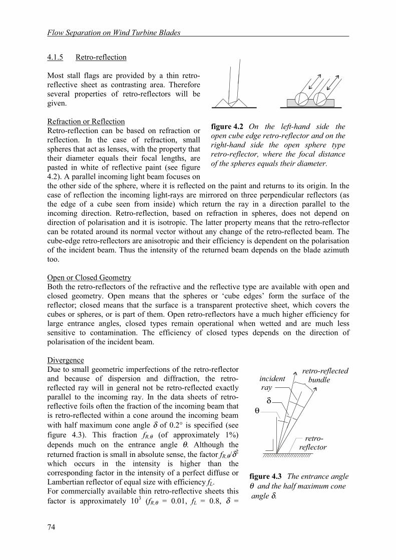
Flow Separation on Wind Turbine Blades
74
4.1.5 Retro-reflection
Most stall flags are provided by a thin retro-reflective sheet as contrasting area. Thereforeseveral properties of retro-reflectors will begiven.
Refraction or ReflectionRetro-reflection can be based on refraction orreflection. In the case of refraction, smallspheres that act as lenses, with the property thattheir diameter equals their focal lengths, arepasted in white of reflective paint (see figure4.2). A parallel incoming light beam focuses onthe other side of the sphere, where it is reflected on the paint and returns to its origin. In thecase of reflection the incoming light-rays are mirrored on three perpendicular reflectors (asthe edge of a cube seen from inside) which return the ray in a direction parallel to theincoming direction. Retro-reflection, based on refraction in spheres, does not depend ondirection of polarisation and it is isotropic. The latter property means that the retro-reflectorcan be rotated around its normal vector without any change of the retro-reflected beam. Thecube-edge retro-reflectors are anisotropic and their efficiency is dependent on the polarisationof the incident beam. Thus the intensity of the returned beam depends on the blade azimuthtoo.
Open or Closed GeometryBoth the retro-reflectors of the refractive and the reflective type are available with open andclosed geometry. Open means that the spheres or ‘cube edges’ form the surface of thereflector; closed means that the surface is a transparent protective sheet, which covers thecubes or spheres, or is part of them. Open retro-reflectors have a much higher efficiency forlarge entrance angles, closed types remain operational when wetted and are much lesssensitive to contamination. The efficiency of closed types depends on the direction ofpolarisation of the incident beam.
DivergenceDue to small geometric imperfections of the retro-reflectorand because of dispersion and diffraction, the retro-reflected ray will in general not be retro-reflected exactlyparallel to the incoming ray. In the data sheets of retro-reflective foils often the fraction of the incoming beam thatis retro-reflected within a cone around the incoming beamwith half maximum cone angle δ of 0.2° is specified (seefigure 4.3). This fraction fR,θ (of approximately 1%)depends much on the entrance angle θ. Although thereturned fraction is small in absolute sense, the factor fR,θ/δ2
which occurs in the intensity is higher than thecorresponding factor in the intensity of a perfect diffuse orLambertian reflector of equal size with efficiency fL.For commercially available thin retro-reflective sheets thisfactor is approximately 103 (fR,θ = 0.01, fL = 0.8, δ =
figure 4.2 On the left-hand side theopen cube edge retro-reflector and on theright-hand side the open sphere typeretro-reflector, where the focal distanceof the spheres equals their diameter.
θ
incident ray
retro-reflector
δ
retro-reflected bundle
figure 4.3 The entrance angleθ and the half maximum cone angle δ.
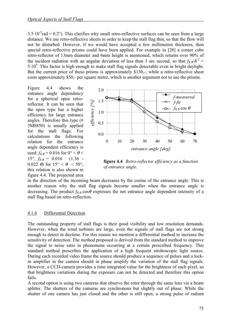
Optical Aspects of Stall Flags
75
3.5·10-3rad = 0.2°). This clarifies why small retro-reflective surfaces can be seen from a largedistance. We use retro-reflective sheets in order to keep the stall flag thin, so that the flow willnot be disturbed. However, if we would have accepted a few millimetres thickness, thenspecial retro-reflective prisms could have been applied. For example in [28] a corner cuberetro-reflector of 13mm diameter and 6mm height is mentioned, which returns over 90% ofthe incident radiation with an angular deviation of less than 3 arc second, so that fR,θ/δ 2 =5·109. This factor is high enough to make stall flag signals detectable even in bright daylight.But the current price of these prisms is approximately $130,-, while a retro-reflective sheetcosts approximately $50,- per square metre, which is another argument not to use the prisms.
Figure 4.4 shows theentrance angle dependencyfor a spherical open retro-reflector. It can be seen thatthe open type has a higherefficiency for large entranceangles. Therefore this type (#3M8850) is usually appliedfor the stall flags. Forcalculations the followingrelation for the entranceangle dependent efficiency isused: fR,θ = 0.016 for 0° < θ <15°, fR,θ
= 0.016 · (1.36 -0.022 θ) for 15° < θ < 50°;this relation is also shown infigure 4.4. The projected areain the direction of the incoming beam decreases by the cosine of the entrance angle. This isanother reason why the stall flag signals become smaller when the entrance angle isdecreasing. The product fR,θ cosθ expresses the net entrance angle dependent intensity of astall flag based on retro-reflection.
4.1.6 Differential Detection
The outstanding property of stall flags is their good visibility and low resolution demands.However, when the wind turbines are large, even the signals of stall flags are not strongenough to detect in daytime. For this reason we mention a differential method to increase thesensitivity of detection. The method proposed is derived from the standard method to improvethe signal to noise ratio in phenomena occurring at a certain prescribed frequency. Thisstandard method prescribes the application of a high frequent stroboscopic light source.During each recorded video frame the source should produce a sequence of pulses and a lock-in amplifier in the camera should in phase amplify the variation of the stall flag signals.However, a CCD-camera provides a time integrated value for the brightness of each pixel, sothat brightness variations during the exposure can not be detected and therefore this optionfails.A second option is using two cameras that observe the rotor through the same lens via a beamsplitter. The shutters of the cameras are synchronous but slightly out of phase. While theshutter of one camera has just closed and the other is still open, a strong pulse of radiant
0.0
0.5
1.0
1.5
2.0
0 10 20 30 40 50 60 70
entrance angle [deg]
effic
ienc
y [%
]
figure 4.4 Retro-reflector efficiency as a functionof entrance angle.
f-measuredf-fitfR,θ cos θ

Flow Separation on Wind Turbine Blades
76
energy from an artificial source is supplied. Subsequently both images are subtracted and onlythe influence of the artificial source remains. Application of this difference method wouldhowever much increase the experimental complexity, which is fatal for field experiments.During the night the signals appear to be easily detectable without taking resource to adifferential method. In practice this turns out not to be a severe restriction, so it was decidedto maintain the method of direct detection.
Optical Aspects of Stall Flags
77
4.2 Quantifying Stall Flag Signals
We will calculate the detection and visibility of the contrasting area of the stall flag byfollowing the radiation from the source to the stall flag and from there to the CCD-chip or thehuman eye. The primary sources of radiant energy are the sun and the artificial source. Thecontrasting area acts as a secondary source that reflects a part of the incident radiant flux ofwhich again a part is received by a camera or by an observer behind the turbine. We canmodel it as a disk of diameter dR=√(4A/π), when A is the area, since the image of a stall flag isso small that the precise geometry is lost. It will be shown that the strength of stall flag signalscan be described by two numbers: the absolute (AD), in which the sensitivity of detection istaken into account and the relative (RD) which accounts for the background. If both numbersare larger than 1 then the stall flag signals are detectable.
4.2.1 Sources of Radiation
The exposure of the stall flag image will be calculated by assuming that we have two sources:the sun and an artificial source. The spectral irradiance from the sun Esun is shown by figure4.6. It is roughly equivalent to the radiation of a black body of 6000K. The spectral radiantintensity of the artificial source IS depends on the type. When that artificial source has a totalradiant spectral flux ΦS, of which a fraction ηS is bundled isotropically with half-maximumangle ϕ, its spectral intensity and irradiance are:
,cos )-(12
= I SSS ϕπ
Φη (4.1)
,2dkI = E S
S (4.2)
where d is the distance of the source, and k = 1 unit space angle.
4.2.2 Intensity of Stall Flag Signals
The reflective properties of the contrasting area depend on the wavelength of the radiation λand the angle θ between the normal of the contrasting area and the irradiance. To include boththe diffuse and retro-reflective properties, we assume that the area reflects a spectral fractionfL as a Lambertian source and a fraction fR,θ as a retro-reflector. Both fractions are functions ofthe wavelength. The fraction fR,θ also depends on the entrance angle θ. It is assumed that fR,θis retro-reflected isotropically within a bundle with divergence δ, which also is a function ofλ. Stall flags with optical differences due to diffuse or retro-reflective properties can bemodelled by changing the fractions.
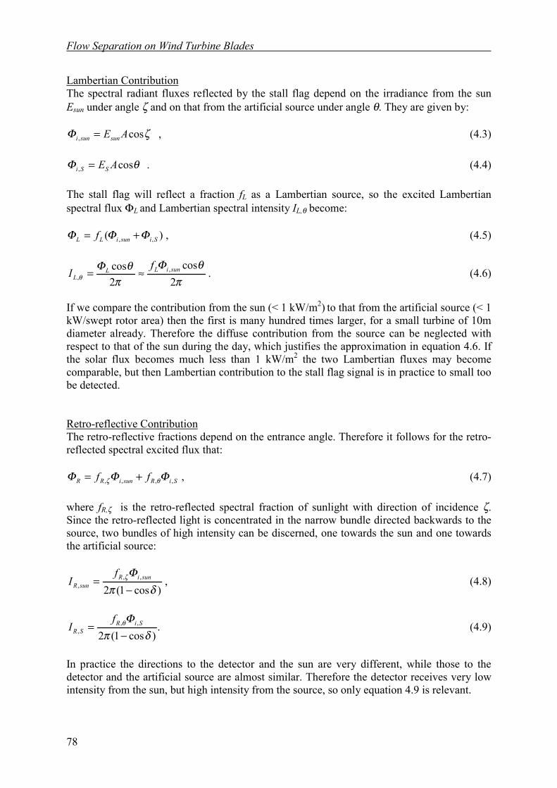
Flow Separation on Wind Turbine Blades
78
Lambertian ContributionThe spectral radiant fluxes reflected by the stall flag depend on the irradiance from the sunEsun under angle ζ and on that from the artificial source under angle θ. They are given by:
,cos, ζΦ AEsunsuni = (4.3)
.cos, θΦ AESSi = (4.4)
The stall flag will reflect a fraction fL as a Lambertian source, so the excited Lambertianspectral flux ΦL and Lambertian spectral intensity IL,θ become:
,)( ,, SisuniLL f ΦΦΦ += (4.5)
.2
cos2cos ,
, πθΦ
πθΦ
θsuniLL
L
fI ≈= (4.6)
If we compare the contribution from the sun (< 1 kW/m2) to that from the artificial source (< 1kW/swept rotor area) then the first is many hundred times larger, for a small turbine of 10mdiameter already. Therefore the diffuse contribution from the source can be neglected withrespect to that of the sun during the day, which justifies the approximation in equation 4.6. Ifthe solar flux becomes much less than 1 kW/m2 the two Lambertian fluxes may becomecomparable, but then Lambertian contribution to the stall flag signal is in practice to small toobe detected.
Retro-reflective ContributionThe retro-reflective fractions depend on the entrance angle. Therefore it follows for the retro-reflected spectral excited flux that:
,,,,, SiRsuniRR ff ΦΦΦ θζ += (4.7)
where fR,ζ is the retro-reflected spectral fraction of sunlight with direction of incidence ζ.Since the retro-reflected light is concentrated in the narrow bundle directed backwards to thesource, two bundles of high intensity can be discerned, one towards the sun and one towardsthe artificial source:
,)cos1(2
,,, δπ
Φζ
−= suniR
sunR
fI (4.8)
.)cos1(2
,,, δπ
Φθ
−= SiR
SR
fI (4.9)
In practice the directions to the detector and the sun are very different, while those to thedetector and the artificial source are almost similar. Therefore the detector receives very lowintensity from the sun, but high intensity from the source, so only equation 4.9 is relevant.
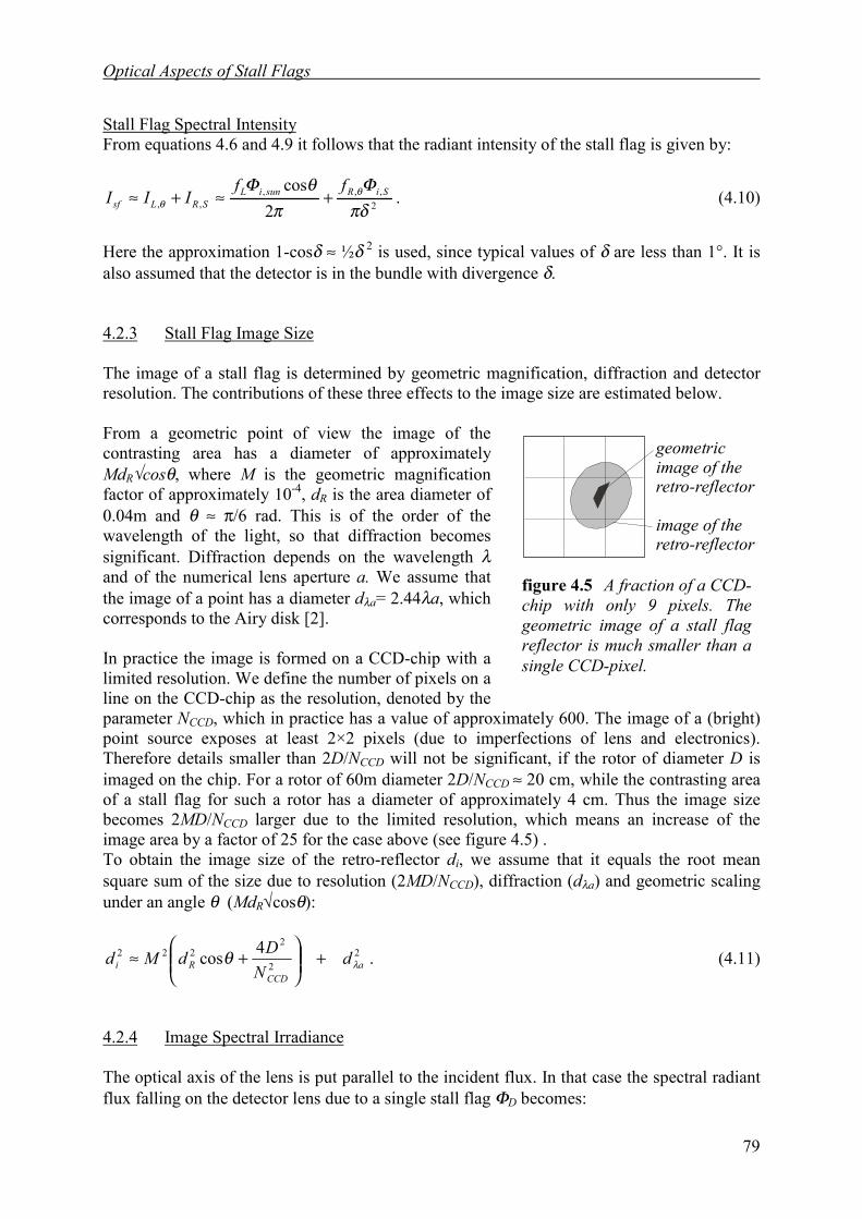
Optical Aspects of Stall Flags
79
Stall Flag Spectral IntensityFrom equations 4.6 and 4.9 it follows that the radiant intensity of the stall flag is given by:
.2
cos2
,,,,, πδ
Φπ
θΦ θθ
SiRsuniLSRLsf
ffIII +≈+≈ (4.10)
Here the approximation 1-cosδ ≈ ½δ 2 is used, since typical values of δ are less than 1°. It isalso assumed that the detector is in the bundle with divergence δ.
4.2.3 Stall Flag Image Size
The image of a stall flag is determined by geometric magnification, diffraction and detectorresolution. The contributions of these three effects to the image size are estimated below.
From a geometric point of view the image of thecontrasting area has a diameter of approximatelyMdR√cosθ, where M is the geometric magnificationfactor of approximately 10-4, dR is the area diameter of0.04m and θ ≈ π/6 rad. This is of the order of thewavelength of the light, so that diffraction becomessignificant. Diffraction depends on the wavelength λand of the numerical lens aperture a. We assume thatthe image of a point has a diameter dλa= 2.44λa, whichcorresponds to the Airy disk [2].
In practice the image is formed on a CCD-chip with alimited resolution. We define the number of pixels on aline on the CCD-chip as the resolution, denoted by theparameter NCCD, which in practice has a value of approximately 600. The image of a (bright)point source exposes at least 2×2 pixels (due to imperfections of lens and electronics).Therefore details smaller than 2D/NCCD will not be significant, if the rotor of diameter D isimaged on the chip. For a rotor of 60m diameter 2D/NCCD ≈ 20 cm, while the contrasting areaof a stall flag for such a rotor has a diameter of approximately 4 cm. Thus the image sizebecomes 2MD/NCCD larger due to the limited resolution, which means an increase of theimage area by a factor of 25 for the case above (see figure 4.5) .To obtain the image size of the retro-reflector di, we assume that it equals the root meansquare sum of the size due to resolution (2MD/NCCD), diffraction (dλa) and geometric scalingunder an angle θ (MdR√cosθ):
.4cos 22
2222
aCCD
Ri dN
DdMd λθ +
+≈ (4.11)
4.2.4 Image Spectral Irradiance
The optical axis of the lens is put parallel to the incident flux. In that case the spectral radiantflux falling on the detector lens due to a single stall flag ΦD becomes:
figure 4.5 A fraction of a CCD-chip with only 9 pixels. Thegeometric image of a stall flagreflector is much smaller than asingle CCD-pixel.
geometricimage of theretro-reflector
image of theretro-reflector

Flow Separation on Wind Turbine Blades
80
,4 2
22
42 aMkI
d d
kI = sf
Lsf
D
πΦ π = (4.12)
if dL is the diameter of the lens. The expression on the right-hand side follows from thesubstitutions a=f/dL and f≈Md, in which f is the focal length of the lens. M approaches f/dwhen f becomes much smaller than the object distance d. Since typical values for f and d arerespectively 3cm and 100m, the approximation is valid. The flux ΦD will be filtered by a filterwith spectral transmission ηF and subsequently a fraction ηL (the transmission of the lens) isdistributed over the effective image size of the contrasting area.The irradiance Ei at the effective image of the contrasting area follows from the ratio of theflux that passed the lens and the effective image size, assuming that the spectral radiant flux ishomogeneously distributed over the effective image area:
.22
2
4 i
sfLF
2i
DLFi da
MIk =
d = E
ηηπ
Φηηπ
(4.13)
4.2.5 Image Spectral Exposure
The exposure, the product of the irradiance and the exposure time, is not a trivial factor, sincethe exposure time depends on many parameters.
Exposure TimeThe exposure time is determined by three time intervals: the shutter time of the detector ∆ts,the pulse duration of the artificial source ∆tp and the time it takes for the image of the stallflag to move over approximately di /2. We will explain that it can differ for the diffuse andretro-reflective part of the flux. In practice the magnification is adjusted so that the rotor fillsthe entire field of view of the detector. The speed of a stall flag on radial position r on aturbine of radius R, which is rotating with angular velocity Ω, is Ωr=ΩR r/R = vtipr/R. So thespeed of its image on the detector becomes vi = vtipMr/R. The image travels over di/2 in a timeinterval di/2vi = ½diR/(rMvtip). Thus the exposure time of the diffuse reflected part (from solarorigin) of the stall flag signal is determined by the minimum of di/2vi and ∆ts, while theexposure time of the retro-reflected part (from artificial origin) of the intensity of the stall flagsignal is determined by the minimum of di/2vi , ∆ts and ∆tp.
Contrasting AreaFor the exposure εR,i of the effective image of the contrasting area we get:
,)(4
,,22
2
, RSRLLi
LFiR tItI
da Mk
= ∆∆ηη
ε θ + (4.14)
with ∆tL = min(di/2vi, ∆ts) and ∆tR = min(di/2vi, ∆ts, ∆tp )

Optical Aspects of Stall Flags
81
BackgroundWe assume that the background is formed by white wind turbine blades, which only reflectsunlight in a Lambertian manner. In this case the image of the object (the blades) is largecompared to a CCD-pixel and to the wavelength, so that both the camera-resolution anddiffraction do not significantly enlarge the geometrical image size. Therefore an area of theturbine blades of diameter dB at an angle θ is imaged as an area of diameter MdB√cosθ. Thismeans that the spectral irradiance of the image of the blades EB,i is:
,8
coscos 2
,22
4
,, a
EfkdM
E sunBLLF
B
BDLFiB
ζηηθ
Φηηπ
== (4.15)
where ΦD,B is the spectral flux, incident on the detector lens from the area of the turbineblades, and fL,B is the fraction of solar radiation that is Lambertian reflected by the whiteblades. The derivation of 4.15 from equations 4.12, 4.6 and 4.3 is straightforward. Thespectral exposure of the white blades equals the product of EB,i and the shutter time ∆ts.
siBiB tE ∆= ,,ε (4.16)
4.2.6 The Absolute Demand
We now derive the minimum incident radiant energy per unit area that can be detected, that is:the minimum exposure of the stall flag image. To this end the product of the spectral exposureof the image of the contrasting area and the spectral sensitivity of the detector should beintegrated over the sensitive detector range, limited by λmin and λmax, and then needs to exceeda certain threshold. This ratio, which should be larger than 1 is called AD. For example: theimage of a stall flag on a photograph should expose the film above its minimum exposurelevel. In equation form the absolute demand yields:
,1
d
min
,
max
min D
ADDiR
>=∫
λ
λ
ληε(4.17)
in which ηD is the spectral detector sensitivity and Dmin is the minimum integrated detectorexposure that provides a detector response above noise level.
To optimise stall flag signals based on retro-reflection, we use the analysis above to rewritethe relation for the absolute demand as a function of the independent parameters. We assumethat the stall flag image size di, the divergence angle of the retro-reflected radiation δ, and thereflected fractions fR,θ and fL, the efficiency of the source ηS do not depend much on thewavelength and obtain:
.d)cos1(cos2 max
minmin22222
,22
λΦηηϕδπ
θ∆ηη λ
λ
θSFD
i
RRSL Ddda
AtfMk AD ∫−= (4.18)
Flow Separation on Wind Turbine Blades
82
In practice the bundle of the source (with half maximum cone angle ϕ) is adjusted in such away that most of the radiant flux is homogeneously distributed over the swept area of therotor (¼πD2). Therefore we replace 2π(1-cosϕ)d2 by ¼πD2. This means that the optics of theartificial source is adapted in such a way that the irradiance of the swept area of the turbinedoes not change with distance between source and turbine. We also replace M=f/d by DCCD/Dand dλa by 2.44λa and obtain a useful expression for the optimisation of the stall flagdetection system:
.d)44.2(4cos
cos4 max
minmin22
2
222422
,2
λΦηηλθδπ
θ∆ηη λ
λ
θSFD
RCCDCCDR
RRSL D
dDa
NdDDa
tfk AD ∫
++
= (4.19)
4.2.7 The Relative Demand
The image formation in the detector will be affected by scattering on particles in the air,internal reflections of the lens, dispersion, diffraction and other effects. As a result there willbe a background. So, the ratio of the stall flag image and the background, which we call therelative demand or RD, should be larger than unity:
,1d
d
max
min
max
min
,
,
>=
∫
∫
RD
DiB
DiR
λ
λ
λ
λ
ληε
ληε(4.21)
where εB,i is the spectral exposure of the blade image. When the differential recordingprinciple described in section 4.1.6 is used the factor can be much less than 1.
Using similar substitutions as in the calculation of AD, RD is found to be:
1d
d
)44.2(4coscos
cos32max
min
max
min
22
2
22242
,
, >
++
=
∫
∫
E
dDa
NdDDtf
tfkRD
sunFD
SFD
RCCDCCDRsBL
RRSλ
λ
λ
λθ
ληη
λΦηη
λθζδ∆π
θ∆η(4.22)
4.2.8 Visibility
The above relations for detection can be converted to relations for visibility for the averagehuman eye by replacing the resolution NCCD by NH, ηD by ηH and Dmin by Hmin. The parameterNH is the resolution of the retina of the human eye, ηH represents the spectral sensitivity of thehuman eye and Hmin is the minimum luminous exposure that can be clearly seen. The human
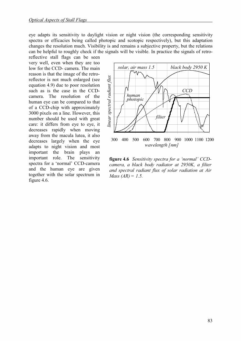
Optical Aspects of Stall Flags
83
eye adapts its sensitivity to daylight vision or night vision (the corresponding sensitivityspectra or efficacies being called photopic and scotopic respectively), but this adaptationchanges the resolution much. Visibility is and remains a subjective property, but the relationscan be helpful to roughly check if the signals will be visible. In practice the signals of retro-reflective stall flags can be seenvery well, even when they are toolow for the CCD- camera. The mainreason is that the image of the retro-reflector is not much enlarged (seeequation 4.9) due to poor resolutionsuch as is the case in the CCD-camera. The resolution of thehuman eye can be compared to thatof a CCD-chip with approximately3000 pixels on a line. However, thisnumber should be used with greatcare: it differs from eye to eye, itdecreases rapidly when movingaway from the macula lutea, it alsodecreases largely when the eyeadapts to night vision and mostimportant the brain plays animportant role. The sensitivityspectra for a ‘normal’ CCD-cameraand the human eye are giventogether with the solar spectrum infigure 4.6.
figure 4.6 Sensitivity spectra for a ‘normal’ CCD-camera, a black body radiator at 2950K, a filterand spectral radiant flux of solar radiation at AirMass (AR) = 1.5.
0.0
0.2
0.4
0.6
0.8
1.0
1.2
1.4
1.6
1.8
300 400 500 600 700 800 900 1000 1100 1200wavelength [nm]
linea
r spe
ctra
l rad
iant
flux
filter
solar, air mass 1.5
CCDhumanphotopic
black body 2950 K
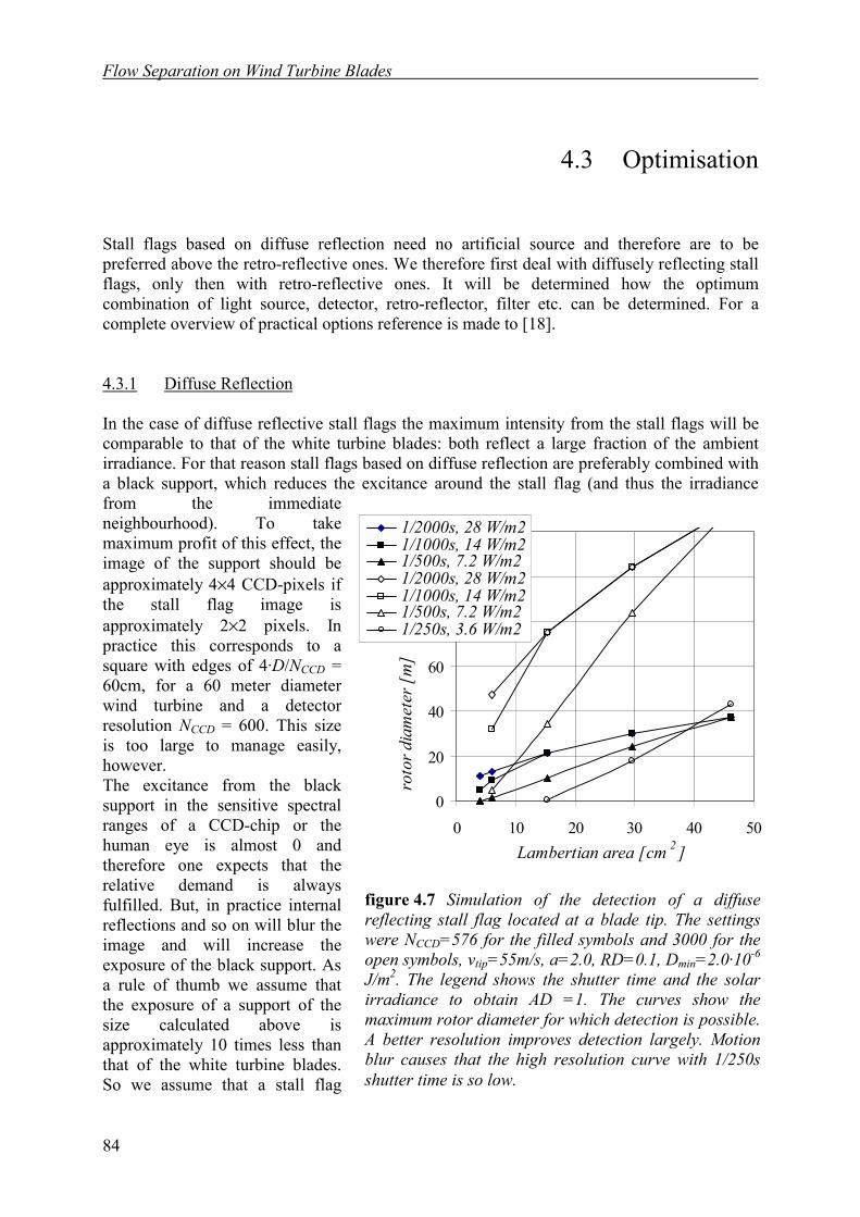
Flow Separation on Wind Turbine Blades
84
4.3 Optimisation
Stall flags based on diffuse reflection need no artificial source and therefore are to bepreferred above the retro-reflective ones. We therefore first deal with diffusely reflecting stallflags, only then with retro-reflective ones. It will be determined how the optimumcombination of light source, detector, retro-reflector, filter etc. can be determined. For acomplete overview of practical options reference is made to [18].
4.3.1 Diffuse Reflection
In the case of diffuse reflective stall flags the maximum intensity from the stall flags will becomparable to that of the white turbine blades: both reflect a large fraction of the ambientirradiance. For that reason stall flags based on diffuse reflection are preferably combined witha black support, which reduces the excitance around the stall flag (and thus the irradiancefrom the immediateneighbourhood). To takemaximum profit of this effect, theimage of the support should beapproximately 4×4 CCD-pixels ifthe stall flag image isapproximately 2×2 pixels. Inpractice this corresponds to asquare with edges of 4·D/NCCD =60cm, for a 60 meter diameterwind turbine and a detectorresolution NCCD = 600. This sizeis too large to manage easily,however.The excitance from the blacksupport in the sensitive spectralranges of a CCD-chip or thehuman eye is almost 0 andtherefore one expects that therelative demand is alwaysfulfilled. But, in practice internalreflections and so on will blur theimage and will increase theexposure of the black support. Asa rule of thumb we assume thatthe exposure of a support of thesize calculated above isapproximately 10 times less thanthat of the white turbine blades.So we assume that a stall flag
figure 4.7 Simulation of the detection of a diffusereflecting stall flag located at a blade tip. The settingswere NCCD=576 for the filled symbols and 3000 for theopen symbols, vtip=55m/s, a=2.0, RD=0.1, Dmin=2.0·10-6
J/m2. The legend shows the shutter time and the solarirradiance to obtain AD =1. The curves show themaximum rotor diameter for which detection is possible.A better resolution improves detection largely. Motionblur causes that the high resolution curve with 1/250sshutter time is so low.
0
20
40
60
80
100
120
0 10 20 30 40 50Lambertian area [cm 2 ]
roto
r dia
met
er [
m]
1/2000s, 28 W/m21/1000s, 14 W/m21/500s, 7.2 W/m21/2000s, 28 W/m21/1000s, 14 W/m21/500s, 7.2 W/m21/250s, 3.6 W/m2
Optical Aspects of Stall Flags
85
based on diffuse reflection is detectable/visible if the AD-value > 1 and the RD-value > 0.1.The contrasting area of the diffuse reflective stall flags is more than twice as large as that ofretro-reflective stall flags, since both the flap and the support under the flap in stall flag state‘0’ can be covered with reflective foil.Using the relations for the absolute and relative demand derived above, simulations werecarried out for typical stall flags on wind turbines of varying diameter. The results are shownin figure 4.7. The signals detected for a digital consumer video camera (1998) and by thehuman eye (which approximately equals that of a 24×36mm2 slide) were simulated. For thisreason NCCD was set to 576 and 3000 respectively. The figure shows that stall flags of acontrasting area of 15cm2 can be applied on turbines of 20m diameter requiring a backgroundirradiance of 14W/m2 or more. During the day such a background level is usually available(the irradiance from the sun in the Netherlands is approximately 1kW/m2 at noon in thesummer). A turbine of 40m diameter already requires stall flags with contrasting areas of50cm2, which is rather large. Thus even in theory diffuse reflective stall flags are onlydetectable on small wind turbines. The figure shows that in the case of a much higherresolution, detection can be obtained even for turbines of 80m diameter with stall flags of30cm2 only. So, with the high resolution, diffuse reflective stall flags are detectable even onlarge wind turbines, which seems an interesting option for the future, but in practice we willhave severe disadvantages. The sun can be roughly in front of the turbine, so that it is a blacksilhouette in the bright sky for the camera behind the turbine. Or when the blades turnoccasionally in the shadow areas the automatic image analysis would become verycomplicated. Furthermore light conditions change continuously due to passing clouds, andobviously measurements can not take place at night.
4.3.2 Retro-reflection
From the integrals in formula 4.22, we see that spectral filtering can increase RD orders ofmagnitude. The filter can be chosen in such a way that the transmission is high at wavelengthwhere the source spectral intensity is high and low where the sun has high spectral intensity.The source should emit most flux in narrow bandwidths, located in the sensitive spectralrange of the detector and at wavelengths of low solar flux.From both the relation for AD and RD it can be seen that they do hardly depend on thedistance between detector and turbine: the only implicit dependency is that the retro-reflectorefficiency increases by the distance because the entrance angle decreases. Furthermore it canbe seen that AD drops by the second power of the rotor diameter D and for larger rotors evenby the fourth power of D. The switch-over from second to fourth power (equal contributions)takes place for D= 6.7m for usual detector settings (a= 2.0, θ= 20°, dR= 2.8cm, DCCD= 8mm,NCCD= 576, λ= 700nm). For a photo camera with 24×36mm slides the switch-over occurs forD≈ 42m, in which case the settings were (a= 2.0, θ= 20°, dR= 3.6cm, DCCD= 24mm, NCCD=3000, λ= 700nm). We conclude that the retro-reflective stall flag signals are very easy todetect for small rotor diameters. Stall flags based on diffuse reflection can only be applied tosmall rotors and have even in those cases several disadvantages. Thus, also for small rotorsretro-reflective stall flags are recommended. Only when all sources of radiation can becontrolled, for example in a wind tunnel, diffuse reflection might be preferred. Then thesignals become less entrance angle dependent and the sources do not need to be located closeto the detector.
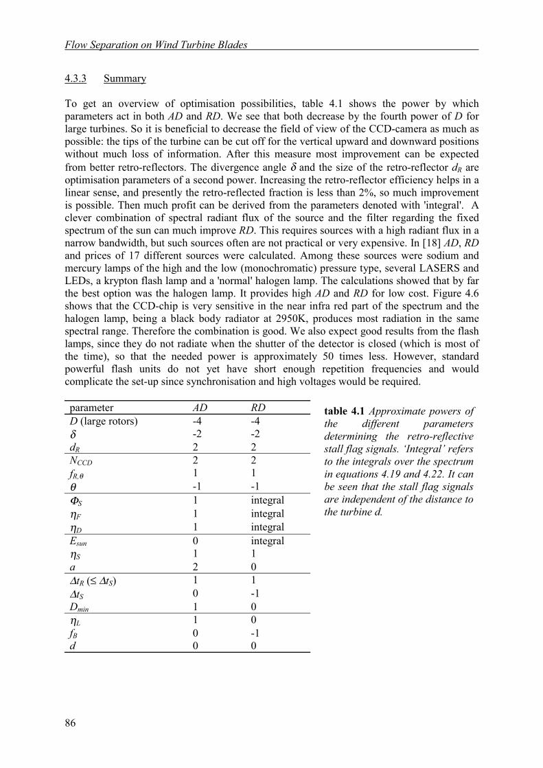
Flow Separation on Wind Turbine Blades
86
4.3.3 Summary
To get an overview of optimisation possibilities, table 4.1 shows the power by whichparameters act in both AD and RD. We see that both decrease by the fourth power of D forlarge turbines. So it is beneficial to decrease the field of view of the CCD-camera as much aspossible: the tips of the turbine can be cut off for the vertical upward and downward positionswithout much loss of information. After this measure most improvement can be expectedfrom better retro-reflectors. The divergence angle δ and the size of the retro-reflector dR areoptimisation parameters of a second power. Increasing the retro-reflector efficiency helps in alinear sense, and presently the retro-reflected fraction is less than 2%, so much improvementis possible. Then much profit can be derived from the parameters denoted with 'integral'. Aclever combination of spectral radiant flux of the source and the filter regarding the fixedspectrum of the sun can much improve RD. This requires sources with a high radiant flux in anarrow bandwidth, but such sources often are not practical or very expensive. In [18] AD, RDand prices of 17 different sources were calculated. Among these sources were sodium andmercury lamps of the high and the low (monochromatic) pressure type, several LASERS andLEDs, a krypton flash lamp and a 'normal' halogen lamp. The calculations showed that by farthe best option was the halogen lamp. It provides high AD and RD for low cost. Figure 4.6shows that the CCD-chip is very sensitive in the near infra red part of the spectrum and thehalogen lamp, being a black body radiator at 2950K, produces most radiation in the samespectral range. Therefore the combination is good. We also expect good results from the flashlamps, since they do not radiate when the shutter of the detector is closed (which is most ofthe time), so that the needed power is approximately 50 times less. However, standardpowerful flash units do not yet have short enough repetition frequencies and wouldcomplicate the set-up since synchronisation and high voltages would be required.
parameter AD RDD (large rotors) -4 -4δ -2 -2dR 2 2NCCD 2 2fR,θ 1 1θ -1 -1ΦS 1 integralηF 1 integralηD 1 integralEsun 0 integralηS 1 1a 2 0∆tR (≤ ∆tS) 1 1∆tS 0 -1Dmin 1 0ηL 1 0fB 0 -1d 0 0
table 4.1 Approximate powers ofthe different parametersdetermining the retro-reflectivestall flag signals. ‘Integral’ refersto the integrals over the spectrumin equations 4.19 and 4.22. It canbe seen that the stall flag signalsare independent of the distance tothe turbine d.
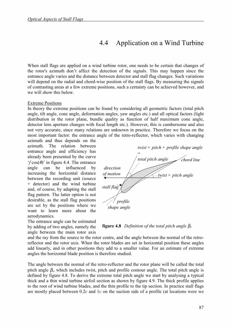
Optical Aspects of Stall Flags
87
4.4 Application on a Wind Turbine
When stall flags are applied on a wind turbine rotor, one needs to be certain that changes ofthe rotor's azimuth don’t affect the detection of the signals. This may happen since theentrance angle varies and the distance between detector and stall flag changes. Such variationswill depend on the radial and chord-wise position of the stall flags. By measuring the signalsof contrasting areas at a few extreme positions, such a certainty can be achieved however, andwe will show this below.
Extreme PositionsIn theory the extreme positions can be found by considering all geometric factors (total pitchangle, tilt angle, cone angle, deformation angles, yaw angles etc.) and all optical factors (lightdistribution in the rotor plane, bundle quality as function of half maximum cone angle,detector lens aperture changes with focal length etc.). However, this is cumbersome and alsonot very accurate, since many relations are unknown in practice. Therefore we focus on themost important factor: the entrance angle of the retro-reflector, which varies with changingazimuth and thus depends on theazimuth. The relation betweenentrance angle and efficiency hasalready been presented by the curve‘f cos(θ)’ in figure 4.4. The entranceangle can be influenced byincreasing the horizontal distancebetween the recording unit (source+ detector) and the wind turbineand, of course, by adapting the stallflag pattern. The latter option is notdesirable, as the stall flag positionsare set by the positions where wewant to learn more about theaerodynamics.The entrance angle can be estimatedby adding of two angles, namely theangle between the main rotor axisand the ray from the source to the rotor centre, and the angle between the normal of the retro-reflector and the rotor axis. When the rotor blades are set in horizontal position these anglesadd linearly, and in other positions they add to a smaller value. For an estimate of extremeangles the horizontal blade position is therefore studied.
The angle between the normal of the retro-reflector and the rotor plane will be called the totalpitch angle βt, which includes twist, pitch and profile contour angle. The total pitch angle isdefined by figure 4.8. To derive the extreme total pitch angle we start by analysing a typicalthick and a thin wind turbine airfoil section as shown by figure 4.9. The thick profile appliesto the root of wind turbine blades, and the thin profile to the tip section. In practice stall flagsare mostly placed between 0.2c and 1c on the suction side of a profile (at locations were we
figure 4.8 Definition of the total pitch angle βt.
profileshape angle
twist + pitch angle
chord line
directionof motion
twist + pitch + profile shape angle=total pitch angle
stall flag
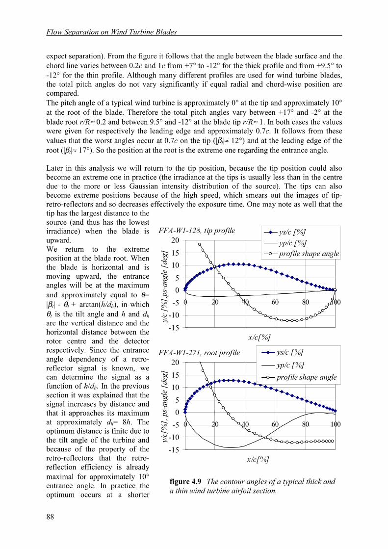
Flow Separation on Wind Turbine Blades
88
expect separation). From the figure it follows that the angle between the blade surface and thechord line varies between 0.2c and 1c from +7° to -12° for the thick profile and from +9.5° to-12° for the thin profile. Although many different profiles are used for wind turbine blades,the total pitch angles do not vary significantly if equal radial and chord-wise position arecompared.The pitch angle of a typical wind turbine is approximately 0° at the tip and approximately 10°at the root of the blade. Therefore the total pitch angles vary between +17° and -2° at theblade root r/R≈ 0.2 and between 9.5° and -12° at the blade tip r/R≈ 1. In both cases the valueswere given for respectively the leading edge and approximately 0.7c. It follows from thesevalues that the worst angles occur at 0.7c on the tip (|βt|≈ 12°) and at the leading edge of theroot (|βt|≈ 17°). So the position at the root is the extreme one regarding the entrance angle.
Later in this analysis we will return to the tip position, because the tip position could alsobecome an extreme one in practice (the irradiance at the tips is usually less than in the centredue to the more or less Gaussian intensity distribution of the source). The tips can alsobecome extreme positions because of the high speed, which smears out the images of tip-retro-reflectors and so decreases effectively the exposure time. One may note as well that thetip has the largest distance to thesource (and thus has the lowestirradiance) when the blade isupward.We return to the extremeposition at the blade root. Whenthe blade is horizontal and ismoving upward, the entranceangles will be at the maximumand approximately equal to θ=|βt| - θt + arctan(h/dh), in whichθt is the tilt angle and h and dhare the vertical distance and thehorizontal distance between therotor centre and the detectorrespectively. Since the entranceangle dependency of a retro-reflector signal is known, wecan determine the signal as afunction of h/dh. In the previoussection it was explained that thesignal increases by distance andthat it approaches its maximumat approximately dh= 8h. Theoptimum distance is finite due tothe tilt angle of the turbine andbecause of the property of theretro-reflectors that the retro-reflection efficiency is alreadymaximal for approximately 10°entrance angle. In practice theoptimum occurs at a shorter
figure 4.9 The contour angles of a typical thick anda thin wind turbine airfoil section.
FFA-W1-128, tip profile
-15-10-505
101520
0 20 40 60 80 100
x/c[%]
y/c
[%],
ps-a
ngle
[de
g]
ys/c [%]yp/c [%]profile shape angle
FFA-W1-271, root profile
-15-10-505
101520
0 20 40 60 80 100
x/c[%]
y/c[
%],
ps-
angl
e [d
eg]
ys/c [%]yp/c [%]profile shape angle

Optical Aspects of Stall Flags
89
horizontal distance for reasons already mentioned (the aperture usually decreases by focallength and the bundle efficiency of the source armature decreases by decreasing bundledivergence). We recommend a horizontal distance between 3h and 6h.
Practical Proof for Detection:The detection of the stall flags depends on many parameters of which some are unknown.Calculations can help to optimise stall flag signals and to predict the performance of manydifferent sources of radiation, but detection in practice is never guaranteed by our formulas.We therefore recommend to past retro-reflectors (stall flags without flaps) of the size that isused for a stall flag on the trailing edge of the tip (r/R=1, |βt|≈12°) and at the leading edge ofthe root (r/R=0.2, |βt|≈17°). If they are detectable over the entire azimuth range, then any stallflag signal on positions (r/R<1, 0.2<x/c<1.0) is also guaranteed to be detectable.
Flow Separation on Wind Turbine Blades
90
4.5 Tufts Signals
Signal StrengthWe define the signal strength as the ratio of radiant intensities excited by a flow indicator forattached and separated flow. For a retro-reflective stall flag this typically is as high as 103.Tufts do not display intensity differences and therefore have signal strength 1. The signal oftufts has to be derived from the direction in which they are pointing and this sets highdemands on the detector resolution.
ResolutionA rather precise image of the tuft needs to be formed to distinguish its direction. The image ofthe tuft has to cover at least 10 × 2 CCD-pixels, and since the tuft can turn in all directions, anarea of approximately 20 × 20 pixels is required. For a CCD-chip of approximately 600 pixelson a line, the maximum number of tufts on a line is approximately 30. However, the numberof stall flags on a line, which each only need 4 × 4 pixels, can be 150, so that the resolutionrequirements are (20 × 20)/(4 × 4)=25 times less. The image of the tuft is 10 pixels long, thusthe real tuft should be 10pixels/600pixels × rotor diameter long. For a 60m diameter windturbine this gives a length of approximately 1 meter, which is not realistic. For realistic tufts(2mm × 5cm) the maximum diameter of the turbine would have to be between 1.2 and 3m,much smaller than current commercial rotors are. For such small rotors one should expectflow disturbance and a high centrifugal deviation.To solve this resolution problem, one can think of a rotating camera that follows only a singleblade. In that case special engineering is required to fix the camera vibration free to the rotorand to transfer the signals without loss of quality to the ground. One should also protect thecamera(lens) against contamination, moisture, high accelerations and lightning. Automaticimage processing would become almost impossible, since the exposure varies much withazimuth: one moment the camera looks into the sky and a moment later to the ground. Itwould also be difficult to program a computer to automatically follow the tufts and read theirdirections. In our opinion tufts in combination with a rotating camera on a commercial windturbine are not a realistic option. However, some tuft experiments on small wind turbineshave been carried out.
Crowder [23] describes experiments with thousands of flow cones on the MOD II windturbine of 100m diameter. Such cones are mentioned in section 3.4 and shown by figure 3.21.Although the centrifugal deviation decreases when the turbine becomes larger, he stillobserved a deviation of approximately 20º, which was initially considered to be acceptable.Later, wind tunnel experiments showed that the filaments acted as very effective vortexgenerators due to this sideward deviation and that the flow behaviour was alteredsubstantially. Crowder used a large photo camera with an effective resolution ofapproximately 6000 times 9000 points. He had difficulties with motion blur but solved thatlater with a powerful flash lamp. Using this set-up he could takes pictures of approximatelyhalf a rotor blade. The dynamic behaviour could not be followed and image analysis could notbe done automatically. He concluded that the utility of flow cones for such rotatingapplications is limited considerably by their relatively high mass.
Optical Aspects of Stall Flags
91
We stress that even with Crowder's very high resolution imaging, only a part of a blade couldbe observed. The flow on a wind turbine, especially at separated flow is highly dynamic.What one sees at one particular moment is not very interesting. Hundreds of images need tobe analysed to find the dynamics of the flow. Therefore visualisation of a part of a rotor bladein a few instants does not give the information we are looking for. We need visualisation ofthe entire swept area during a considerable period with a sufficiently high image rate.Analysis of the obtained sequences of hundreds or thousands of frames is only possible withthe aid of a computer. And then we take much advantage of the binary signals of the stallflags.
Motion BlurFor stall flag signals motion blur is not a problem and even an advantage. This blur causeslight tracks where detector is in state '1' and darkness (nothing) in state '0', so that states canbe derived from the images. This enables the application to fast rotating propellers in quasisteady operation: the average stall pattern can be obtained from a picture that is exposed formany revolutions (see the propeller experiment in appendix B).For tufts however, motion blur over a fraction of the tuft length completely destroys theinformation. Even when the camera follows the object under study, or when the object doesnot move, information vanishes due to motion blur. This is due to the self-excited motion(Kevin-Helmholtz instability) of tufts, which was described in chapter 3.

Flow Separation on Wind Turbine Blades
92
93
5. Stall Flag Experiments
We begin by explaining the way stall flag experiments are set-up, carried out and analysed.The focus was initially on the solution of practical problems such as hinge durability and lightsource optimisation, but after about 10 experiments on wind turbines, the focus was shifted toaerodynamic questions. However, the development of the technique has not stopped. Recentnovelties are a retro-reflective sphere on a line fixed to the nacelle to optically measure theyaw error, and an anemometer with retro-reflector, placed on the nacelle, that sends a windspeed signal to the video camera. Section 5.2 presents the first field experiment on a turbineof considerable size. We show the extent of the stall area and how the stall behaviour of thisturbine was seriously disturbed by the sensors applied to measure the angle of attack. Section5.3 deals with the peculiar stall behaviour of wind turbines in California, which will bediscussed in light of chapter 2. For two additional experiments we refer to appendices A andB. The first aims at improvement of the power curve of a commercial rotor; the seconddemonstrates the fast response of the stall flag, the independence of centrifugal force and theadvantage the method can gain from motion blur.

Flow Separation on Wind Turbine Blades
94
5.1 The Standard Procedure
5.1.1 Instrumentation of the Turbine
During the instrumentation four types of devicesare installed on the wind turbine: the stall flags,the reference reflectors, a wind directionindicator and a wind speed indicator. It takesabout 12 hours to install everything on theturbine if the work is done by two people in thebasket of a crane. The instrumentation is non-intrusive and it can be easily removed. Pastingthe stall flags on a 64m diameter turbine has alsobeen tried by absailers; two men were fixed withropes to the main shaft and sailed down alongthe blade, but the wind caught them and theywere moving too quickly to stick anything onthe blades accurately. Another possibility is tolift a person with a small multi-compartmenthelium filled balloon (see figure 5.1). The manand the balloon are fixed to a weight and theconnecting rope is also used to control thealtitude. We have only used a crane toinstrument the blades. The method is as follows.One blade is put in a downward vertical positionand the people in the basket move towards theblade tip. There they attach a measuring ropethat will indicate the distance to the tip. Theythen move to the blade root fixing the rope everytwo metres. At the blade root they start pastingthe stall flags and reference reflectors (and flowmanipulators like vortex generators) while using
a second measuring rope to determine the chord-wise position. They continue movingdownward and remove the rope that measures the tip distance. The orientation angle of thestall flags is adjusted by eye, or if accuracy demands it, a line fixed to the rotor shaft is usedas reference. This procedure is repeated for each blade. The stall behaviour is largelydependent on the yaw error and the wind speed, therefore two devices are applied to recordthese signals with the video camera too.
Retro-reflective SphereA retro-reflector is pasted at the centre of the rear end of the nacelle and here also a thin lineof about one blade radius length is also attached, see figure 5.2. At its other end we attach aretro-reflective sphere of foam, which simply moves freely with the wind. When the videocamera in the field behind the rotor detects the foam sphere vertically below the rear of thenacelle, the wind is directed straight. This gives a reliable indication of any yaw error.
figure 5.1 Possibility toinstrument the turbine.
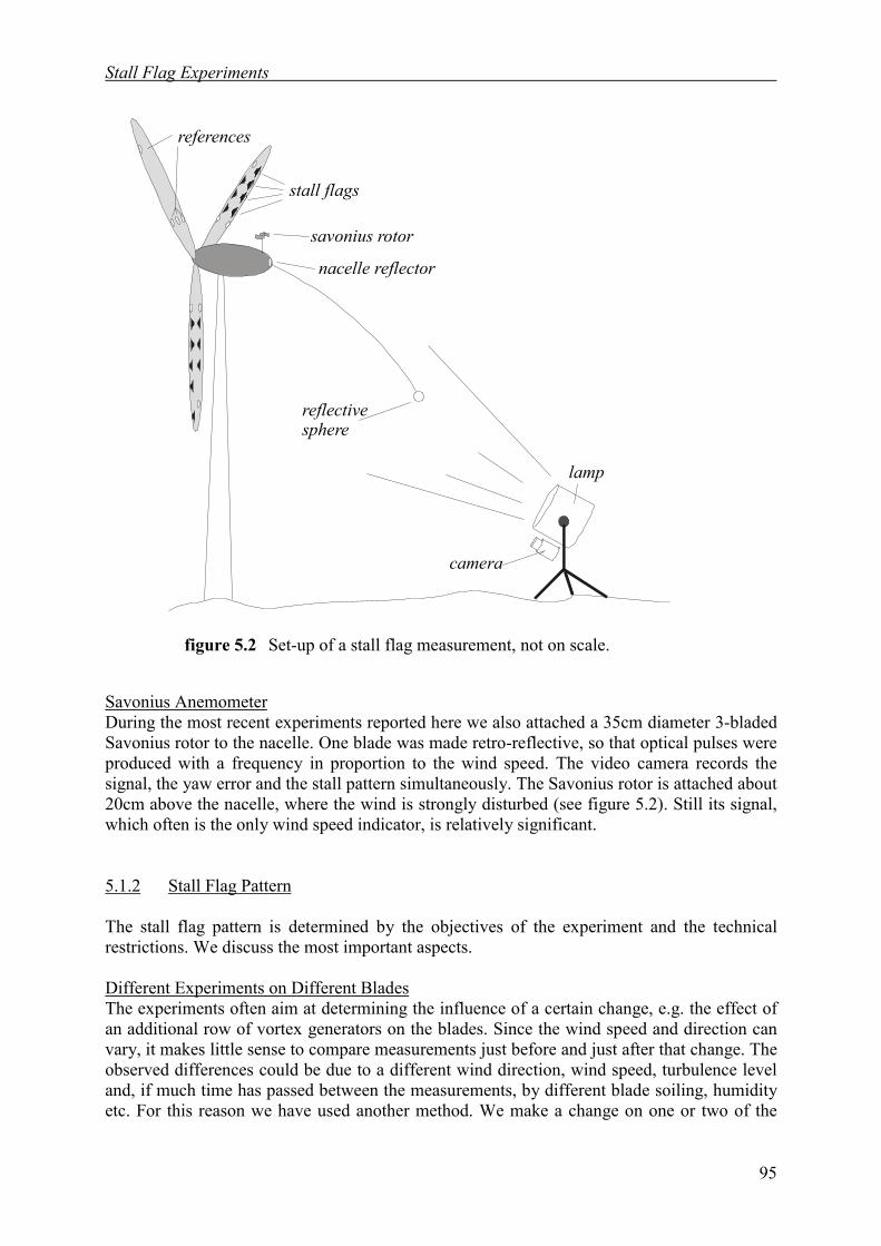
Stall Flag Experiments
95
Savonius AnemometerDuring the most recent experiments reported here we also attached a 35cm diameter 3-bladedSavonius rotor to the nacelle. One blade was made retro-reflective, so that optical pulses wereproduced with a frequency in proportion to the wind speed. The video camera records thesignal, the yaw error and the stall pattern simultaneously. The Savonius rotor is attached about20cm above the nacelle, where the wind is strongly disturbed (see figure 5.2). Still its signal,which often is the only wind speed indicator, is relatively significant.
5.1.2 Stall Flag Pattern
The stall flag pattern is determined by the objectives of the experiment and the technicalrestrictions. We discuss the most important aspects.
Different Experiments on Different BladesThe experiments often aim at determining the influence of a certain change, e.g. the effect ofan additional row of vortex generators on the blades. Since the wind speed and direction canvary, it makes little sense to compare measurements just before and just after that change. Theobserved differences could be due to a different wind direction, wind speed, turbulence leveland, if much time has passed between the measurements, by different blade soiling, humidityetc. For this reason we have used another method. We make a change on one or two of the
figure 5.2 Set-up of a stall flag measurement, not on scale.
savonius rotor
reflectivesphere
stall flags
lamp
camera
references
nacelle reflector
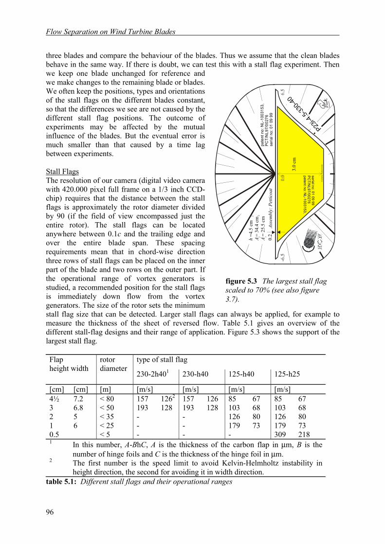
Flow Separation on Wind Turbine Blades
96
three blades and compare the behaviour of the blades. Thus we assume that the clean bladesbehave in the same way. If there is doubt, we can test this with a stall flag experiment. Thenwe keep one blade unchanged for reference andwe make changes to the remaining blade or blades.We often keep the positions, types and orientationsof the stall flags on the different blades constant,so that the differences we see are not caused by thedifferent stall flag positions. The outcome ofexperiments may be affected by the mutualinfluence of the blades. But the eventual error ismuch smaller than that caused by a time lagbetween experiments.
Stall FlagsThe resolution of our camera (digital video camerawith 420.000 pixel full frame on a 1/3 inch CCD-chip) requires that the distance between the stallflags is approximately the rotor diameter dividedby 90 (if the field of view encompassed just theentire rotor). The stall flags can be locatedanywhere between 0.1c and the trailing edge andover the entire blade span. These spacingrequirements mean that in chord-wise directionthree rows of stall flags can be placed on the innerpart of the blade and two rows on the outer part. Ifthe operational range of vortex generators isstudied, a recommended position for the stall flagsis immediately down flow from the vortexgenerators. The size of the rotor sets the minimumstall flag size that can be detected. Larger stall flags can always be applied, for example tomeasure the thickness of the sheet of reversed flow. Table 5.1 gives an overview of thedifferent stall-flag designs and their range of application. Figure 5.3 shows the support of thelargest stall flag.
type of stall flagFlapheight width
rotordiameter
230-2h401 230-h40 125-h40 125-h25
[cm] [cm] [m] [m/s] [m/s] [m/s] [m/s]4½ 7.2 < 80 157 1262 157 126 85 67 85 673 6.8 < 50 193 128 193 128 103 68 103 682 5 < 35 - - 126 80 126 801 6 < 25 - - 179 73 179 730.5 < 5 - - - 309 2181 In this number, A-BhC, A is the thickness of the carbon flap in µm, B is the
number of hinge foils and C is the thickness of the hinge foil in µm.2 The first number is the speed limit to avoid Kelvin-Helmholtz instability in
height direction, the second for avoiding it in width direction.table 5.1: Different stall flags and their operational ranges
figure 5.3 The largest stall flagscaled to 70% (see also figure3.7).
Inve
nted
by:
Gus
tave
Cor
ten
Inve
nted
by:
Gus
tave
Cor
ten
A f= 34
.4 c
m2
0.2
h =4
.5 c
m
3.0
cm
Inve
nted
by:
Gus
tave
Cor
ten
Inve
nted
by:
Gus
tave
Cor
ten
Inve
nted
by:
Gus
tave
Cor
ten
patent no: NL-1003153,
PC
T/NL97/00276
serial no: 01 09 99
pate
nt n
o: N
L-10
0315
3,PC
T/N
L97/
0027
6 se
rial n
o: 0
1 09
99
Asse
mbl
y: P
ettic
oat
A r= 25
.5 c
m2
P23i-4
.5-33
0-40
Stall Flag Experiments
97
The type of stall flag is determined by the local flow speed expected. The higher the speed thestiffer the flap of the stall flags needs to be (see section 3.2.6). So we use for example type230-2h40 at the tip and 125-h40 at the root.The angle γ (defined in figure 3.10) under which the stall flag is installed is 0° in most cases.This choice makes a clear distinction of flow from leading edge towards the trailing edge or inthe reverse direction possible; in this case the flap position is not influenced by the centrifugalforce. Other angles are used if more resolution in flow direction is required.
Reference MarkersThese markers (which are retro-reflectors without flaps and thus are always visible) are usedby the image processing software to follow the blades and to find the positions of the stallflags. The size of the reference marker should be twice the retro-reflective area of the stallflags, which size is set by the rotor diameter (chapter 4). The references also serve torecognise the different blades by placing them in different ways on the different blades. Forthe most recent experiments we used 3 references per blade and one more on one blade foridentification (figure 5.2). The three references define the blade co-ordinate system for theimage processing software. Therefore they should have a large mutual spacing in chord-wisedirection and in radial direction; for this we use two markers near the largest chord and onemarker at the tip.The nacelle gets a reference marker at its rear end. This marker is used for determining theyaw angle (in combination with the reflective sphere) and to detect vibrations of the camera ornacelle.
5.1.3 The Measurements
After the instrumentation of the turbine, we wait for twilight. Then we position the cameraand light source down-wind at a distance of about 4 times the height of the nacelle behind theturbine. The source has to be adjusted until it homogeneously illuminates the swept area andthe camera has to cover that arc completely (a few tip chords may be cut off at the upper andlower side). We prefer a recording of the stall behaviour while the wind speed is slowlyincreasing from about 5 to 25 m/s, but we cannot control the wind. Therefore we have to workwith a few different mean wind speeds over several evenings of taking measurements. Suchrecordings of ‘steady’ operation at a constant wind speed give the most reliable information,but often the interesting wind speeds do not occur during the ‘short’ measuring period.Therefore we experimented with recordings while starting and stopping the wind turbine tosimulate wind speed variations.
Starts and StopsThe idea is that we simulate a wind speed variation at constant rotation speed with a rotationspeed variation at constant wind speed. In both cases we can get the same range of λ = vtip/U= ΩR/U values. The highest λ is obtained when the turbine reaches the maximum (nominal)rotation speed. So the wind speed should not be too high, say less than 10 m/s, to get theentire λ-range of interest. This procedure has one drawback: the induction of the turbine willnot be in equilibrium with its operational state. When it starts, the induction will increase witha significant delay, and vice versa, there will be too much induction during a stop. The slowerthe change of the rotation speed of the rotor the smaller this error will be.Its maximum value can be estimated by comparing the cases of steady induction and noinduction. Since the start torque is much less than the brake torque, a start is slower than a

Flow Separation on Wind Turbine Blades
98
stop. So we prefer starts. Stops are also inconvenient since the tips are often deployed (turnedover 90°) to serve as aerodynamic brakes. Turbines with a two speed drive train can be forcedin low speed at relatively low wind to obtain a second interesting λ-value.
YawingOne can turn the turbine during the recordings to see the effect of a variation of the angle ofattack on azimuth. This can be helpful in analysing dynamic effects (how fast do stall areascome and go). Using the yaw error and our extended blade element momentum theory(section 2.2.3), we can estimate the variation of the angle of attack along the blade onazimuth, and we can see its influence from the stall flag signals. Such measurements aredifficult to interpret, but they turn out to be of great value in understanding the phenomenonof ‘double stall’.
5.1.4 Image Analysis
The image analysis starts with a fast assessment of the applicability of video recordings. Afew interesting shots (often starts) are transferred over a firewire 1394 data bus from thedigital video camera to a hard disk. These shots incorporate about 1500 frames, which isabout one minute of video (although they sometimes take 10 minutes). Then the video file isconverted into a sequence of separated video frames, each stored as a jpg-file. These files aresuccessively opened by an image analysis program especially written for the application. Thisprogram starts with a conversion to 8-bit (256 values) black and white scale and subsequentlysharpens the images. The process of data extraction is explained below.
User InteractionEach frame can be described as a black surface with about 10 to 300 bright spots from thevisible reflectors. It turned out to be difficult to program a computer so that it wouldautomatically find which spot refers to which stall flag or reference marker or other object.The user has to assist the computer in the interpretation of the first two frames, after which itwill process the successive thousands. He has to point with a mouse to each referencereflector, the reflective sphere, the nacelle reflector and the anemometer. The computer readsthe stall flag positions from an input file and finds them since it knows the positions of thereference reflectors. This procedure has been implemented with success. We will explain afew important aspects of the image analysis.
Reference ReflectorsAfter two frames of user interaction the computer has the co-ordinates of the referencereflectors in two successive frames. From this it estimates the rotation speed and centre ofrotation so that it can estimate the positions of the reference reflectors in the next frame. Itwill search for each reflector within a circle around the estimated position. All pixels above acertain threshold in the circle are used (weighted average) to find the measured position. Theerror between estimated and measured position is stored for each reference reflectorseparately as a moving average. The reference positions in all remaining frames are estimatedby rotating the reflector around the rotor centre and adding the partly systematic error. Thisprocedure implicitly corrects for perspective (the reflectors do not follow circular paths sincethe camera monitors from below), lens errors and low frequency vibrations. When a rotorblade disappears behind the tower it can remain invisible for 20 frames or so. In this periodthe estimated positions are based on the preceding estimates and the reference reflector will
Stall Flag Experiments
99
only be found when it re-appears, when the procedure is very accurate. In practice it wasproven that the program could find the blade after it disappeared for dozens of frames andsequences of thousands of frames could be processed automatically. This enabled statisticalanalysis of the dynamic stall patterns.
Stall FlagsThe computer should get the positions of the stall flags relative to the reference reflectorsfrom an input file or by user interaction. Using this data it can precisely search for stall flagsignals at the locations of stall flags. This procedure very effectively avoids the computermistaking passing insects, rain droplets or sand particles for stall flag signals. When an insectflies over a stall flag in state ‘0’, the computer sets the signal incorrectly to ‘1’, but this is arare event which only slightly affects the statistics.
Reflective Sphere and AnemometerSpecial subroutines follow the retro-reflective sphere and the Savonius rotor anemometer. Thepositions of these objects in each new frame are also estimated by extrapolating their tracks.The Savonius rotor on the nacelle can move through the frame because of camera vibrations,turbine yawing and tower bending. The extrapolation procedure only allows for small andslow movements of the Savonius rotor and much faster variations of speed and direction ofthe sphere. These differences are used to distinguish the objects when they come very close toeach other or even completely overlap. The retro-reflective sphere in particular often crossesother sensitive positions (where the computer calculates positions of references or stall flags)without causing problems for a correct continuation.
VibrationsMeasurements are sometimes carried out during high wind speeds. Then the tripod holdingthe lamp and the camera vibrates in the wind. Our video camera has an optical imagestabiliser which filters most of these vibrations, so the recordings are stabilised to someextent. But sometimes, when severe vibrations occur, the image analysis may miss a referencereflector. These situations can be avoided when the retro-reflector on the nacelle is alsofollowed. The translation made by this reflector should be added to the estimates for all otherreflectors. Such a procedure can deal with most vibrations. However, when the cameravibrates in a rotational way around an axis parallel to its optical axis, this procedure will nothelp.
5.1.5 Experimental Data
Presenting graphs of the angle of attack α , when stall sets in, or the tip speed ratio λ as afunction of radial position r/R is valuable. These will be discussed in section 5.3 and inappendix A. Here we will give only a list of the data that become available from the videorecordings.
a. The frame number representing time.b. The state of each stall flag (0= closed, 1= open, t= behind tower, m = outside field of
view).c. The rotation speed of the Savonius rotor by which the wind speed is estimated.d. The co-ordinates of the reflective sphere relative to the rotation centre.e. The yaw error as obtained from the nacelle reflector and the reflective sphere.f. The azimuth angle of each blade independently.

Flow Separation on Wind Turbine Blades
100
g. The rotation speed from the derivative of the azimuth.h. The in-plane blade bending and from this eventually lead-lag vibrations.
Using these data we will try to find answers to the following questions:
1. What is the effect of vortex generators or stall strips? In which angle of attack rangeare they operational and how large is the blade area they influence.
2. Does the rotor stall before rated wind speed?3. If overpower occurs, which rotor areas are still attached?4. Is stall occurring at the leading edge or at the trailing edge?5. How does the separated area extend with increasing wind speed?6. How is the separated area influenced by shear, yaw, tower passage?7. How are separated areas affected by turbulence, transition, blade contamination, rain
etc?8. What is the thickness of the separated area? (This can be measured with different
flap heights.)9. What kind of lead-lag modes do occur and what are their amplitudes?10. Does the tower display side-ward bending?
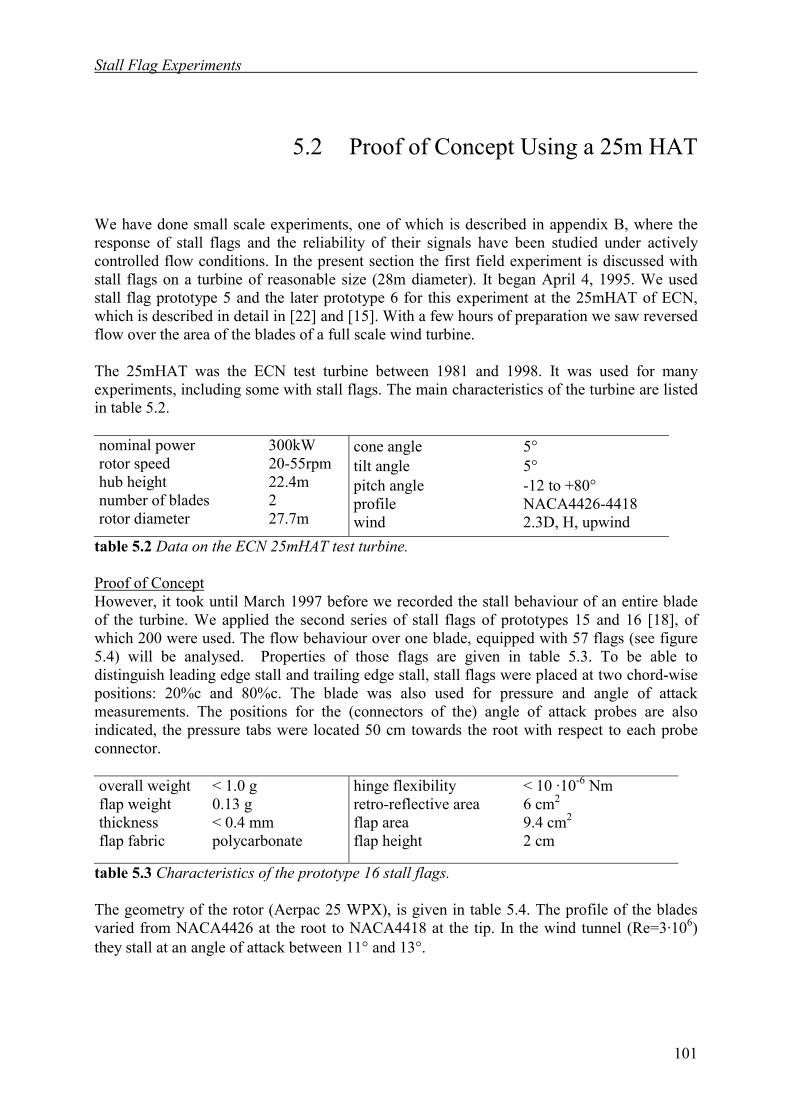
Stall Flag Experiments
101
5.2 Proof of Concept Using a 25m HAT
We have done small scale experiments, one of which is described in appendix B, where theresponse of stall flags and the reliability of their signals have been studied under activelycontrolled flow conditions. In the present section the first field experiment is discussed withstall flags on a turbine of reasonable size (28m diameter). It began April 4, 1995. We usedstall flag prototype 5 and the later prototype 6 for this experiment at the 25mHAT of ECN,which is described in detail in [22] and [15]. With a few hours of preparation we saw reversedflow over the area of the blades of a full scale wind turbine.
The 25mHAT was the ECN test turbine between 1981 and 1998. It was used for manyexperiments, including some with stall flags. The main characteristics of the turbine are listedin table 5.2.
nominal power 300kWrotor speed 20-55rpmhub height 22.4mnumber of blades 2rotor diameter 27.7m
cone angle 5°tilt angle 5°pitch angle -12 to +80°profile NACA4426-4418wind 2.3D, H, upwind
table 5.2 Data on the ECN 25mHAT test turbine.
Proof of ConceptHowever, it took until March 1997 before we recorded the stall behaviour of an entire bladeof the turbine. We applied the second series of stall flags of prototypes 15 and 16 [18], ofwhich 200 were used. The flow behaviour over one blade, equipped with 57 flags (see figure5.4) will be analysed. Properties of those flags are given in table 5.3. To be able todistinguish leading edge stall and trailing edge stall, stall flags were placed at two chord-wisepositions: 20%c and 80%c. The blade was also used for pressure and angle of attackmeasurements. The positions for the (connectors of the) angle of attack probes are alsoindicated, the pressure tabs were located 50 cm towards the root with respect to each probeconnector.
overall weight < 1.0 gflap weight 0.13 gthickness < 0.4 mmflap fabric polycarbonate
hinge flexibility < 10 ·10-6 Nmretro-reflective area 6 cm2
flap area 9.4 cm2
flap height 2 cm
table 5.3 Characteristics of the prototype 16 stall flags.
The geometry of the rotor (Aerpac 25 WPX), is given in table 5.4. The profile of the bladesvaried from NACA4426 at the root to NACA4418 at the tip. In the wind tunnel (Re=3·106)they stall at an angle of attack between 11° and 13°.
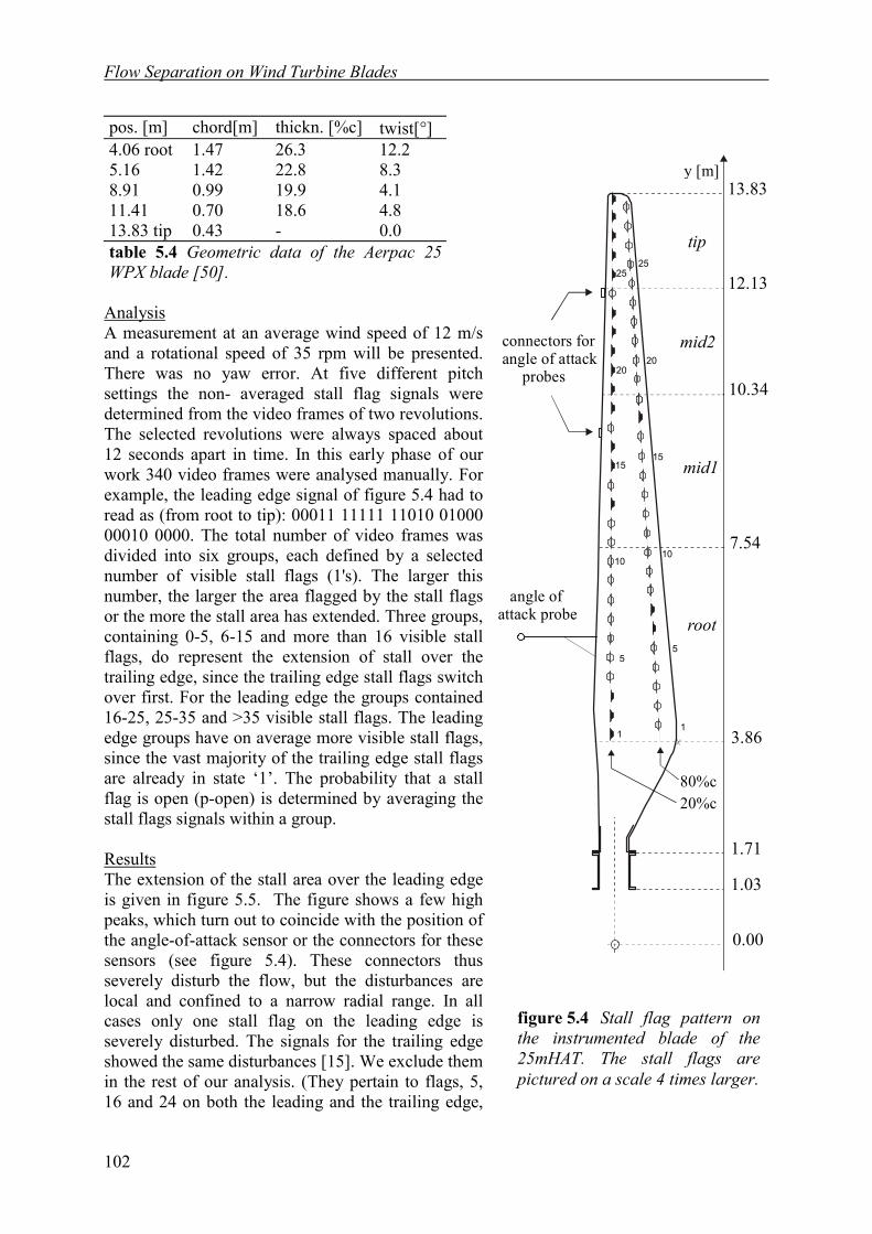
Flow Separation on Wind Turbine Blades
102
pos. [m] chord[m] thickn. [%c] twist[°]4.06 root5.168.9111.4113.83 tip
1.471.420.990.700.43
26.322.819.918.6-
12.28.34.14.80.0
table 5.4 Geometric data of the Aerpac 25WPX blade [50].
AnalysisA measurement at an average wind speed of 12 m/sand a rotational speed of 35 rpm will be presented.There was no yaw error. At five different pitchsettings the non- averaged stall flag signals weredetermined from the video frames of two revolutions.The selected revolutions were always spaced about12 seconds apart in time. In this early phase of ourwork 340 video frames were analysed manually. Forexample, the leading edge signal of figure 5.4 had toread as (from root to tip): 00011 11111 11010 0100000010 0000. The total number of video frames wasdivided into six groups, each defined by a selectednumber of visible stall flags (1's). The larger thisnumber, the larger the area flagged by the stall flagsor the more the stall area has extended. Three groups,containing 0-5, 6-15 and more than 16 visible stallflags, do represent the extension of stall over thetrailing edge, since the trailing edge stall flags switchover first. For the leading edge the groups contained16-25, 25-35 and >35 visible stall flags. The leadingedge groups have on average more visible stall flags,since the vast majority of the trailing edge stall flagsare already in state ‘1’. The probability that a stallflag is open (p-open) is determined by averaging thestall flags signals within a group.
ResultsThe extension of the stall area over the leading edgeis given in figure 5.5. The figure shows a few highpeaks, which turn out to coincide with the position ofthe angle-of-attack sensor or the connectors for thesesensors (see figure 5.4). These connectors thusseverely disturb the flow, but the disturbances arelocal and confined to a narrow radial range. In allcases only one stall flag on the leading edge isseverely disturbed. The signals for the trailing edgeshowed the same disturbances [15]. We exclude themin the rest of our analysis. (They pertain to flags, 5,16 and 24 on both the leading and the trailing edge,
figure 5.4 Stall flag pattern onthe instrumented blade of the25mHAT. The stall flags arepictured on a scale 4 times larger.
1
5
10
angle ofattack probe
80%c
connectors forangle of attack probes
20%c
mid2
mid1
root
12.13
10.34
7.54
3.86
1.71
1.03
0.00
y [m]13.83
tip25
15
10
20
15
25
20
5
1
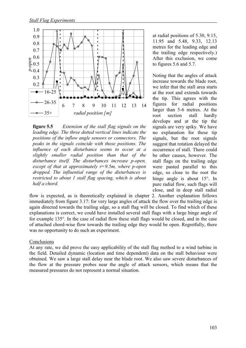
Stall Flag Experiments
103
at radial positions of 5.30, 9.15,11.95 and 5.48, 9.33, 12.13metres for the leading edge andthe trailing edge respectively.)After this exclusion, we cometo figures 5.6 and 5.7.
Noting that the angles of attackincrease towards the blade root,we infer that the stall area startsat the root and extends towardsthe tip. This agrees with thefigures for radial positionslarger than 5-6 metres. At theroot section stall hardlydevelops and at the tip thesignals are very spiky. We haveno explanation for these tipsignals, but the root signalssuggest that rotation delayed theoccurrence of stall. There couldbe other causes, however. Thestall flags on the trailing edgewere pasted parallel to thisedge, so close to the root thehinge angle is about 15°. Inpure radial flow, such flags willclose, and in deep stall radial
flow is expected, as is theoretically explained in chapter 2. Another explanation followsimmediately from figure 3.17: for very large angles of attack the flow over the trailing edge isagain directed towards the trailing edge, so a stall flag will be closed. To find which of theseexplanations is correct, we could have installed several stall flags with a large hinge angle offor example 135°. In the case of radial flow these stall flags would be closed, and in the caseof attached chord-wise flow towards the trailing edge they would be open. Regretfully, therewas no opportunity to do such an experiment.
ConclusionsAt any rate, we did prove the easy applicability of the stall flag method to a wind turbine inthe field. Detailed dynamic (location and time dependent) data on the stall behaviour wereobtained. We saw a large stall delay near the blade root. We also saw severe disturbances ofthe flow at the pressure probes near the angle of attack sensors, which means that themeasured pressures do not represent a normal situation.
figure 5.5 Extension of the stall flag signals on theleading edge. The three dotted vertical lines indicate thepositions of the inflow angle sensors or connectors. Thepeaks in the signals coincide with those positions. Theinfluence of each disturbance seems to occur at aslightly smaller radial position than that of thedisturbance itself. The disturbances increase p-open,except of that at approximately r=9.5m, where p-opendropped. The influential range of the disturbances isrestricted to about 1 stall flag spacing, which is abouthalf a chord.
0.00.10.20.30.40.50.60.70.80.91.0
4 5 6 7 8 9 10 11 12 13 14radial position [m]
p-op
en
16-25
26-35
35+
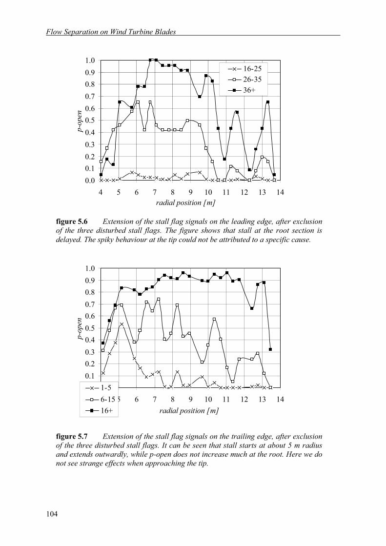
Flow Separation on Wind Turbine Blades
104
figure 5.6 Extension of the stall flag signals on the leading edge, after exclusionof the three disturbed stall flags. The figure shows that stall at the root section isdelayed. The spiky behaviour at the tip could not be attributed to a specific cause.
figure 5.7 Extension of the stall flag signals on the trailing edge, after exclusionof the three disturbed stall flags. It can be seen that stall starts at about 5 m radiusand extends outwardly, while p-open does not increase much at the root. Here we donot see strange effects when approaching the tip.
0.00.10.20.30.40.50.60.70.80.91.0
4 5 6 7 8 9 10 11 12 13 14radial position [m]
p-op
en16-2526-3536+
0.00.10.20.30.40.50.60.70.80.91.0
4 5 6 7 8 9 10 11 12 13 14radial position [m]
p-op
en
1-56-1516+
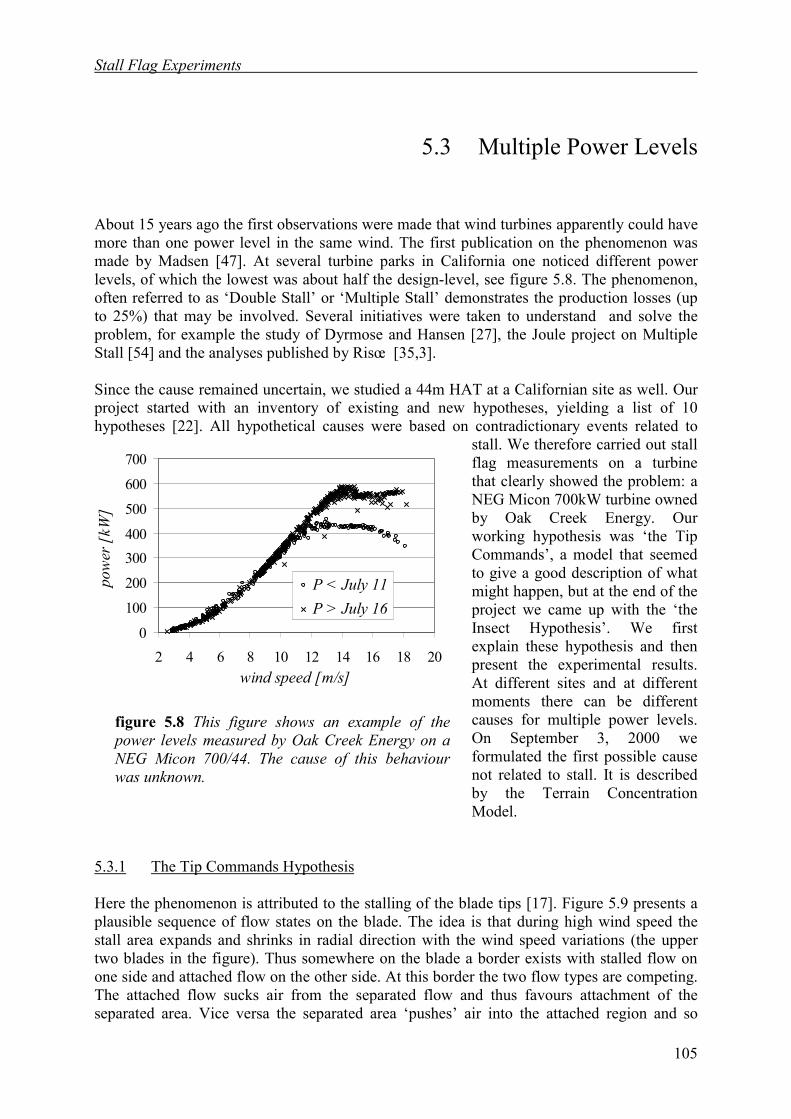
Stall Flag Experiments
105
5.3 Multiple Power Levels
About 15 years ago the first observations were made that wind turbines apparently could havemore than one power level in the same wind. The first publication on the phenomenon wasmade by Madsen [47]. At several turbine parks in California one noticed different powerlevels, of which the lowest was about half the design-level, see figure 5.8. The phenomenon,often referred to as ‘Double Stall’ or ‘Multiple Stall’ demonstrates the production losses (upto 25%) that may be involved. Several initiatives were taken to understand and solve theproblem, for example the study of Dyrmose and Hansen [27], the Joule project on MultipleStall [54] and the analyses published by Risœ [35,3].
Since the cause remained uncertain, we studied a 44m HAT at a Californian site as well. Ourproject started with an inventory of existing and new hypotheses, yielding a list of 10hypotheses [22]. All hypothetical causes were based on contradictionary events related to
stall. We therefore carried out stallflag measurements on a turbinethat clearly showed the problem: aNEG Micon 700kW turbine ownedby Oak Creek Energy. Ourworking hypothesis was ‘the TipCommands’, a model that seemedto give a good description of whatmight happen, but at the end of theproject we came up with the ‘theInsect Hypothesis’. We firstexplain these hypothesis and thenpresent the experimental results.At different sites and at differentmoments there can be differentcauses for multiple power levels.On September 3, 2000 weformulated the first possible causenot related to stall. It is describedby the Terrain ConcentrationModel.
5.3.1 The Tip Commands Hypothesis
Here the phenomenon is attributed to the stalling of the blade tips [17]. Figure 5.9 presents aplausible sequence of flow states on the blade. The idea is that during high wind speed thestall area expands and shrinks in radial direction with the wind speed variations (the uppertwo blades in the figure). Thus somewhere on the blade a border exists with stalled flow onone side and attached flow on the other side. At this border the two flow types are competing.The attached flow sucks air from the separated flow and thus favours attachment of theseparated area. Vice versa the separated area ‘pushes’ air into the attached region and so
figure 5.8 This figure shows an example of thepower levels measured by Oak Creek Energy on aNEG Micon 700/44. The cause of this behaviourwas unknown.
0
100
200
300400
500
600
700
2 4 6 8 10 12 14 16 18 20wind speed [m/s]
pow
er [
kW]
P < July 11P > July 16
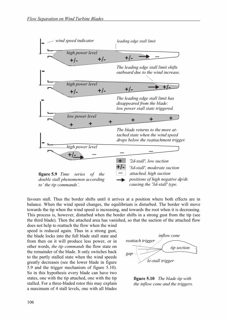
Flow Separation on Wind Turbine Blades
106
favours stall. Thus the border shifts until it arrives at a position where both effects are inbalance. When the wind speed changes, the equilibrium is disturbed. The border will movetowards the tip when the wind speed is increasing, and towards the root when it is decreasing.This process is, however, disturbed when the border shifts in a strong gust from the tip (seethe third blade). Then the attached area has vanished, so that the suction of the attached flowdoes not help to reattach the flow when the windspeed is reduced again. Thus in a strong gust,the blade locks into the full blade stall state andfrom then on it will produce less power, or inother words, the tip commands the flow state onthe remainder of the blade. It only switches backto the partly stalled state when the wind speedsgreatly decreases (see the lower blade in figure5.9 and the trigger mechanism of figure 5.10).So in this hypothesis every blade can have twostates, one with the tip attached, one with the tipstalled. For a three-bladed rotor this may explaina maximum of 4 stall levels, one with all blades
figure 5.9 Time series of thedouble stall phenomenon accordingto’ the tip commands’.
wind speed indicator
positions of high negative dp/dr,causing the '3d-stall' type.
'3d-stall', moderate suctionattached, high suction
The blade returns to the more at-tached state when the wind speeddrops below the reattachment trigger.
leading edge stall limit
The leading edge stall limit shiftsoutboard due to the wind increase.
The leading edge stall limit hasdisappeared from the blade: low power stall state triggered.
+/-
+/-
_
+++++
+
+
+/-
+/- +/-
+/-
+/-
+/-
_ __
+/-
_'2d-stall', low suction
low power level
high power level
high power level
high power level
figure 5.10 The blade tip withthe inflow cone and the triggers.
inflow cone
le-stall trigger
reattach triggertip section
gap
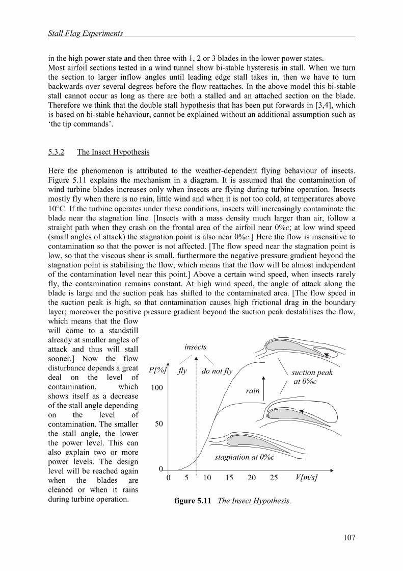
Stall Flag Experiments
107
in the high power state and then three with 1, 2 or 3 blades in the lower power states.Most airfoil sections tested in a wind tunnel show bi-stable hysteresis in stall. When we turnthe section to larger inflow angles until leading edge stall takes in, then we have to turnbackwards over several degrees before the flow reattaches. In the above model this bi-stablestall cannot occur as long as there are both a stalled and an attached section on the blade.Therefore we think that the double stall hypothesis that has been put forwards in [3,4], whichis based on bi-stable behaviour, cannot be explained without an additional assumption such as‘the tip commands’.
5.3.2 The Insect Hypothesis
Here the phenomenon is attributed to the weather-dependent flying behaviour of insects.Figure 5.11 explains the mechanism in a diagram. It is assumed that the contamination ofwind turbine blades increases only when insects are flying during turbine operation. Insectsmostly fly when there is no rain, little wind and when it is not too cold, at temperatures above10°C. If the turbine operates under these conditions, insects will increasingly contaminate theblade near the stagnation line. [Insects with a mass density much larger than air, follow astraight path when they crash on the frontal area of the airfoil near 0%c; at low wind speed(small angles of attack) the stagnation point is also near 0%c.] Here the flow is insensitive tocontamination so that the power is not affected. [The flow speed near the stagnation point islow, so that the viscous shear is small, furthermore the negative pressure gradient beyond thestagnation point is stabilising the flow, which means that the flow will be almost independentof the contamination level near this point.] Above a certain wind speed, when insects rarelyfly, the contamination remains constant. At high wind speed, the angle of attack along theblade is large and the suction peak has shifted to the contaminated area. [The flow speed inthe suction peak is high, so that contamination causes high frictional drag in the boundarylayer; moreover the positive pressure gradient beyond the suction peak destabilises the flow,which means that the flowwill come to a standstillalready at smaller angles ofattack and thus will stallsooner.] Now the flowdisturbance depends a greatdeal on the level ofcontamination, whichshows itself as a decreaseof the stall angle dependingon the level ofcontamination. The smallerthe stall angle, the lowerthe power level. This canalso explain two or morepower levels. The designlevel will be reached againwhen the blades arecleaned or when it rainsduring turbine operation. figure 5.11 The Insect Hypothesis.
V[m/s]
P[%]
100
50
00 5 10 15 20 25
insects
fly
stagnation at 0%c
suction peak at 0%c
rain
do not fly

Flow Separation on Wind Turbine Blades
108
5.3.3 Experiment with a 44m HAT
This section presents the experimental validation of the multiple-power-level hypotheses. Infact the above insect hypothesis was made half-way the experiments. It gave rise to furtherexperiments to make sure that it was correct.
Set-upIn the project several stall flag measurements were performed with three different patterns ofvortex generators, stall flags etc. on the rotor. We only present the most importantmeasurements. Thecorrespondingconfiguration is shown infigure 5.12. The leadingedge of blade 1 wascleaned from root to tipbetween -20%c (pressureside) and 20%c. Artificialroughness was applied onblade 2 from root to tip at0%c. For the roughness azigzag tape (0.5mmperiod) with a maximumthickness of 1.15mm andsurface roughness of0.8mm was used. The tapewas 0.5cm wide between0.7-1.0R and 1.5cmbetween 0.2-0.7R. Allvortex generators of blade3 were removed. Thisblade was not cleaned.The leading edges ofblades 2 and 3 werecontaminated with insectsto a depth of about0.3mm. The roughnesswas about the same overthe entire span and waslocated at chord-wisepositions smaller than5%c on both the suctionand the pressure side. Thedensity of thesedisturbances was about100 insects per squaremetre.
figure 5.12 Configuration of the second measurement. Theleading edge of blade1 was cleaned. Zigzag tape was put onthat of blade 2. The vortex generators of blade 3 were takenoff.
c2, b1, leading edge cleaned
0.00.51.01.5
0.2 0.3 0.4 0.5 0.6 0.7 0.8 0.9 1.0
radial position r/R
chor
d [m
]stall flagvortex generatorsreference marker
c2, b2, zigzag tape at 0%c
0.0
0.5
1.0
1.5
0.2 0.3 0.4 0.5 0.6 0.7 0.8 0.9 1.0radial position r/R
chor
d [m
]
stall flagvortex generatorsreference markerroughness 0%c
c2, b3, vg's removed
0.0
0.5
1.0
1.5
0.2 0.3 0.4 0.5 0.6 0.7 0.8 0.9 1.0radial position r/R
chor
d [m
]
stall flagreference marker

Stall Flag Experiments
109
5.3.4 Validation of The Tip Commands Hypothesis
This hypothesis implies that the tip may lock into a stable stalled state in high wind speed. Wetook measurements at 18 m/s average wind speed and we even yawed the turbine over 35°.Under these conditions the tip angle of attack varies between about 13° and 18° depending onthe azimuth. Figure 5.13 shows two revolutions of the rough stall flag signals. Theserevolutions are representativeof the results of some hours oftesting, but do not show anysign of locking behaviour. Thestall pattern ‘continuously’follows the changing inflowconditions, although theremight be some delay. This wasthe reason to believe that thedouble stall mechanismsuggested by ‘the TipCommands’ was notresponsible for the multiplepower levels of practice. Infact the command-mechanismwas not yet triggered, since asfigure 5.13 shows, the leadingedges (0.2c) of the tips werestill in attached flow.But part of the model isconfirmed: the blade did notshow bi-stable hysteresis but acontinuous behaviour as wasexpected from the model. Thisimplies that the hypothesis in[3,4], which is based on bi-stable behaviour, is an unlikelycandidate.
The figure shows anotherresult: the stall flag pattern atthe leading edges movestowards the tip with about 13m/s. This observationindirectly confirms the that theradial flow speed in the stallarea can be large (section2.5.4). It is indirect, since wesee the movement of theborders between separated andattached areas, not the radialmotion of the air inside theseparated areas.
leading edge trailing edge, flags at 0.95cvortex range flags at 0.2c vortex range
tt t t tt t t t t t t t t t t t t tt t t t t t t t t t t t t t t t t t t t t t t t t t t t t t t t t t t t t t t t t t t t t t t t t t t t t tt t t t t t t t t t t t t t t t t t t t t t tt t t t t
t t tt t t t t t t t tt t t t t t t t t t t t t t t t t t t t t t t t t t t t t t t t t t t t t t t t t t t t t t t t t t t t t tt t t t t t t t t t t t t t t t t t t t t t t t t t t t t t t t t t t t t t t t t t t t t t tt t t t t t t t tt t
Azim
uth
→
radial position →root tip
radial position →root tip
figure 5.13 Two revolution of the rough stall flagsignals (25 Hz) of blade 1. The grey area is where thestall flag indicates reversed flow, the white area isattached flow, the tower passage is black. The rotor speedis 27 rpm, the wind speed 18 m/s and the yaw error 35°.The radial speed of the stall areas is about 13 m/s.
radialmotion

Flow Separation on Wind Turbine Blades
110
5.3.5 Validation of the Insect Hypothesis
The video with the stall flag signals was analysed with the image processing program. Aftersorting out the frames on tip speed ratio λ = ΩR/U, the λ-value at which the stall flagswitched between its two states was statistically determined. The variation of λ was caused bychanges of Ω during starting and stopping the turbine. Figure 5.14 shows plots of the artificialwind speed ΩR/λ versus radial position. The speeds are called artificial since it was not thewind that was changing but the rotation speed.
Stall Flag ResultsWe see in figure 5.14 thatmost stall flags on theleading edge of the roughblade switch over at 17 m/son average, while those onthe clean blade switch over at21 m/s on average. It followsfrom this and other figures[22], that the roughnesscauses a large advance ofstall in the wind speed rangeof 11 m/s to 25 m/s. As theinfluence extends over theentire span of all blades it caneasily affect the power bydozens of percentage points.Therefore it can explain themultiple power levels.
Time series of PV-dataTime series of the power Pand the wind speed V of fourdifferent turbines werestudied in detail in order tovalidate the InsectHypothesis [22]. The powerlevels appeared to becomelower after each period oflow wind speed. Thisconfirms the Insect
leading edge
1315171921232527293133
0,20 0,30 0,40 0,50 0,60 0,70 0,80 0,90 1,00radial position r/R
win
d sp
eed
[m/s]
b1, cleanb2, roughb3, all vg's removed
trailing edge
13
14
15
16
17
18
19
20
0,20 0,30 0,40 0,50 0,60 0,70 0,80 0,90 1,00radial position r/R
win
d sp
eed
[m/s]
b1, cleanb2, roughb3, all vg's removed
figure 5.14 Plots of the wind speed against the radial position. The important observationis the large difference of the leading edge signals of blade 2 with roughness, compared to theother blades. Between 0.65R and the tip blade 2 stalls at about 18 m/s while blades 1 and 3stall at about 25 m/s neglecting the peak in the signal of blade 2. This advance of leadingedge stall corresponds to power losses of dozens of percents. The peak at about 0.92Rcorresponds to the first stall flag at larger radial position than the tip division. The centre ofthis stall flag is about 22 centimetre apart from the slit. The flow is largely influenced by thetransient or the leakage though the slit. The trailing edge signals clearly show the delay ofstall due to the vortex generators.
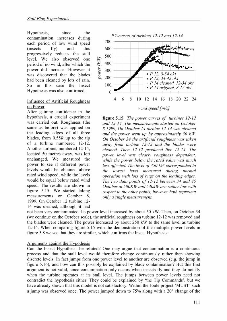
Stall Flag Experiments
111
Hypothesis, since thecontamination increases duringeach period of low wind speed(insects fly) and thisprogressively reduces the stalllevel. We also observed oneperiod of no wind, after which thepower did increase. However itwas discovered that the bladeshad been cleaned by lots of rain.So in this case the InsectHypothesis was also confirmed.
Influence of Artificial Roughnesson PowerAfter gaining confidence in thehypothesis, a crucial experimentwas carried out. Roughness (thesame as before) was applied onthe leading edges of all threeblades, from 0.55R up to the tipof a turbine numbered 12-12.Another turbine, numbered 12-14,located 50 metres away, was leftunchanged. We measured thepower to see if different powerlevels would be obtained aboverated wind speed, while the levelswould be equal below rated windspeed. The results are shown infigure 5.15. We started takingmeasurements on October 8,1999. On October 12 turbine 12-14 was cleaned, although it hadnot been very contaminated. Its power level increased by about 50 kW. Then, on October 34(we continue on the October scale), the artificial roughness on turbine 12-12 was removed andthe blades were cleaned. The power increased by about 250 kW to the same level as turbine12-14. When comparing figure 5.15 with the demonstration of the multiple power levels infigure 5.8 we see that they are similar, which confirms the Insect Hypothesis.
Arguments against the HypothesisCan the Insect Hypothesis be refuted? One may argue that contamination is a continuousprocess and that the stall level would therefore change continuously rather than showingdiscrete levels. In fact jumps from one power level to another are observed (e.g. the jump infigure 5.16), and how can this possibly be explained by blade contamination? But this firstargument is not valid, since contamination only occurs when insects fly and they do not flywhen the turbine operates at its stall level. The jumps between power levels need notcontradict the hypothesis either. They could be explained by ‘the Tip Commands’, but wehave already shown that this model is not satisfactory. Within the Joule project ‘MUST’ sucha jump was observed once. The power jumped down to 75% along with a 20° change of the
figure 5.15 The power curves of turbines 12-12and 12-14. The measurements started on October8 1999, On October 14 turbine 12-14 was cleanedand the power went up by approximately 50 kW.On October 34 the artificial roughness was takenaway from turbine 12-12 and the blades werecleaned. Then 12-12 produced like 12-14. Thepower level was clearly roughness dependent,while the power below the rated value was muchless affected. The level of 350 kW corresponded tothe lowest level measured during normaloperation with lots of bugs on the leading edges.The two data points of 12-12 between 34 and 45October at 500KW and 530kW are rather low withrespect to the other points, however both representonly a single measurement.
PV-curves of turbines 12-12 and 12-14
0100200300400500600700
4 6 8 10 12 14 16 18 20 22 24
wind speed [m/s]
pow
er [
kW]
P 12, 8-34 oktP 12, 34-45 oktP 14 cleaned, 12-34 oktP 14 original, 8-12 okt
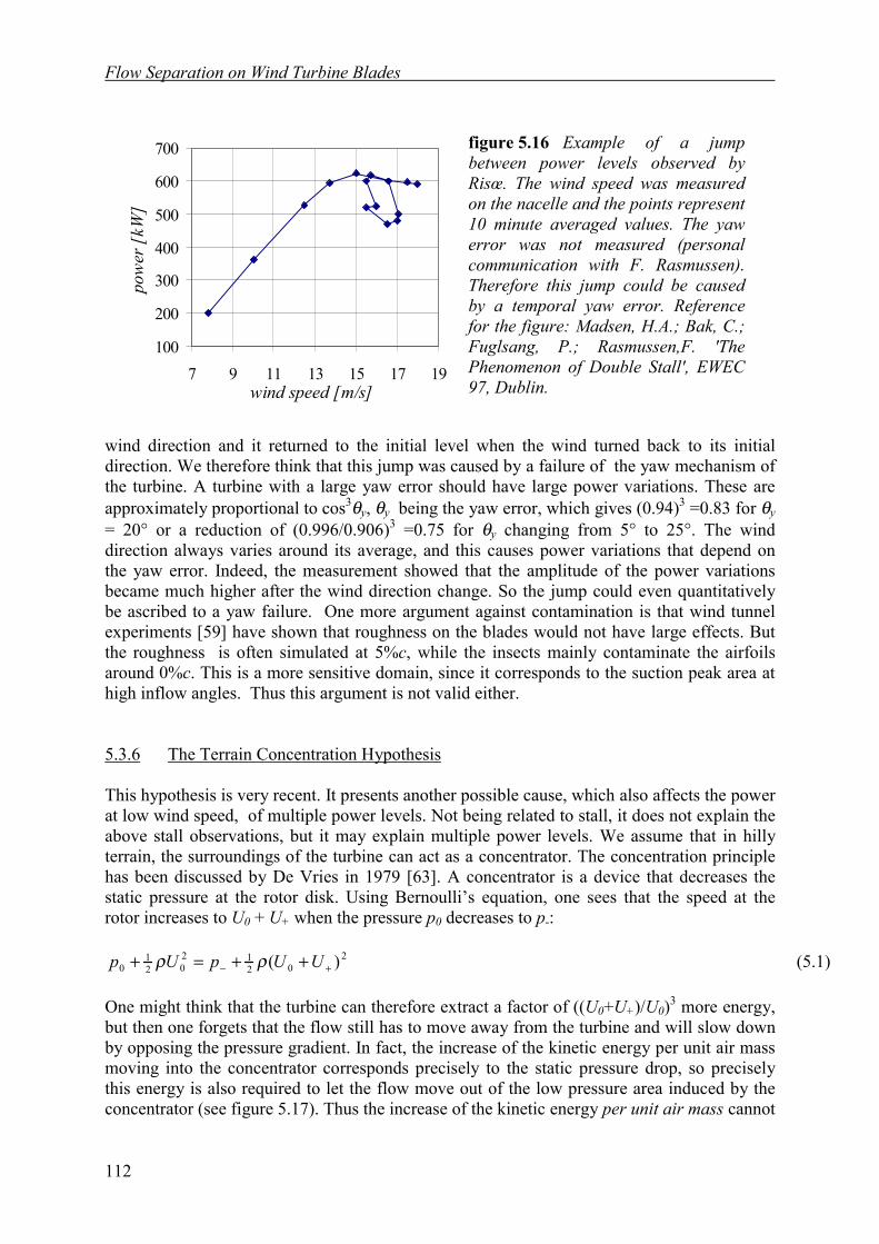
Flow Separation on Wind Turbine Blades
112
wind direction and it returned to the initial level when the wind turned back to its initialdirection. We therefore think that this jump was caused by a failure of the yaw mechanism ofthe turbine. A turbine with a large yaw error should have large power variations. These areapproximately proportional to cos3θy, θy being the yaw error, which gives (0.94)3 =0.83 for θy= 20° or a reduction of (0.996/0.906)3 =0.75 for θy changing from 5° to 25°. The winddirection always varies around its average, and this causes power variations that depend onthe yaw error. Indeed, the measurement showed that the amplitude of the power variationsbecame much higher after the wind direction change. So the jump could even quantitativelybe ascribed to a yaw failure. One more argument against contamination is that wind tunnelexperiments [59] have shown that roughness on the blades would not have large effects. Butthe roughness is often simulated at 5%c, while the insects mainly contaminate the airfoilsaround 0%c. This is a more sensitive domain, since it corresponds to the suction peak area athigh inflow angles. Thus this argument is not valid either.
5.3.6 The Terrain Concentration Hypothesis
This hypothesis is very recent. It presents another possible cause, which also affects the powerat low wind speed, of multiple power levels. Not being related to stall, it does not explain theabove stall observations, but it may explain multiple power levels. We assume that in hillyterrain, the surroundings of the turbine can act as a concentrator. The concentration principlehas been discussed by De Vries in 1979 [63]. A concentrator is a device that decreases thestatic pressure at the rotor disk. Using Bernoulli’s equation, one sees that the speed at therotor increases to U0 + U+ when the pressure p0 decreases to p-:
202
1202
10 )( +− ++=+ UUpUp ρρ (5.1)
One might think that the turbine can therefore extract a factor of ((U0+U+)/U0)3 more energy,but then one forgets that the flow still has to move away from the turbine and will slow downby opposing the pressure gradient. In fact, the increase of the kinetic energy per unit air massmoving into the concentrator corresponds precisely to the static pressure drop, so preciselythis energy is also required to let the flow move out of the low pressure area induced by theconcentrator (see figure 5.17). Thus the increase of the kinetic energy per unit air mass cannot
figure 5.16 Example of a jumpbetween power levels observed byRisœ. The wind speed was measuredon the nacelle and the points represent10 minute averaged values. The yawerror was not measured (personalcommunication with F. Rasmussen).Therefore this jump could be causedby a temporal yaw error. Referencefor the figure: Madsen, H.A.; Bak, C.;Fuglsang, P.; Rasmussen,F. 'ThePhenomenon of Double Stall', EWEC97, Dublin.
100
200
300
400
500
600
700
7 9 11 13 15 17 19wind speed [m/s]
pow
er [
kW]
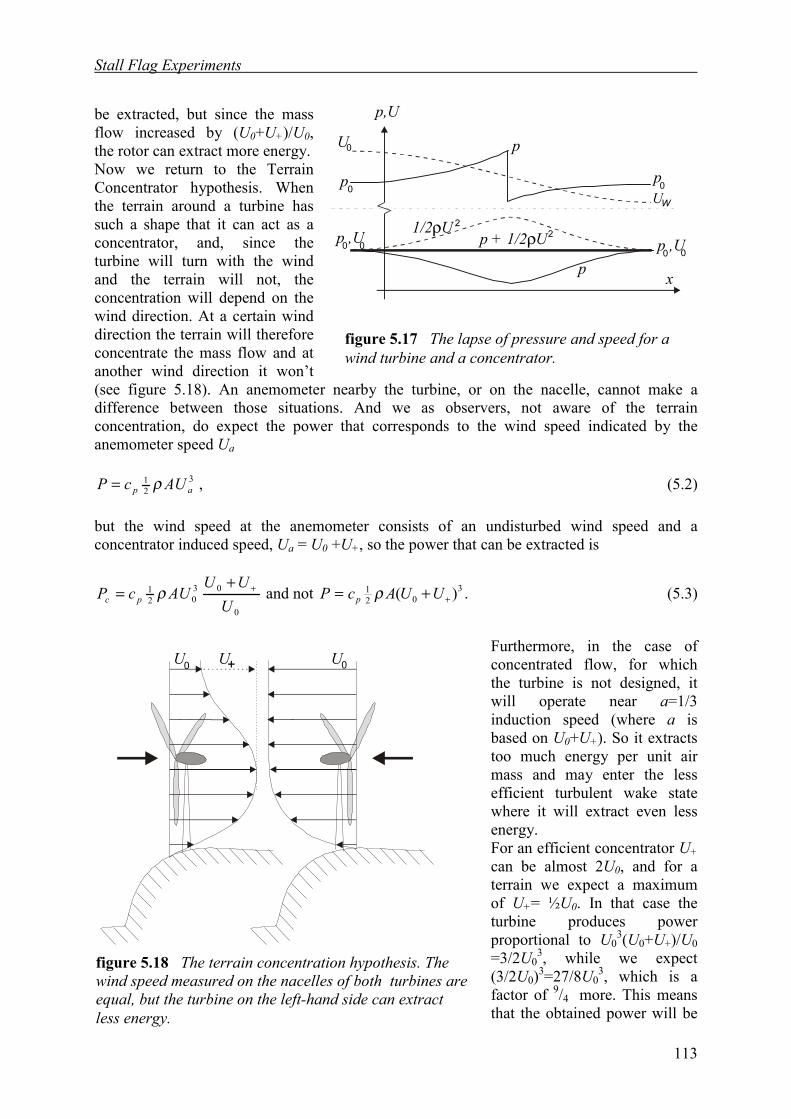
Stall Flag Experiments
113
be extracted, but since the massflow increased by (U0+U+)/U0,the rotor can extract more energy.Now we return to the TerrainConcentrator hypothesis. Whenthe terrain around a turbine hassuch a shape that it can act as aconcentrator, and, since theturbine will turn with the windand the terrain will not, theconcentration will depend on thewind direction. At a certain winddirection the terrain will thereforeconcentrate the mass flow and atanother wind direction it won’t(see figure 5.18). An anemometer nearby the turbine, or on the nacelle, cannot make adifference between those situations. And we as observers, not aware of the terrainconcentration, do expect the power that corresponds to the wind speed indicated by theanemometer speed Ua
,321
ap AUcP ρ= (5.2)
but the wind speed at the anemometer consists of an undisturbed wind speed and aconcentrator induced speed, Ua = U0 +U+, so the power that can be extracted is
0
0302
1
UUU
AUcP pc++
= ρ and not .)( 302
1++= UUAcP p ρ (5.3)
Furthermore, in the case ofconcentrated flow, for whichthe turbine is not designed, itwill operate near a=1/3induction speed (where a isbased on U0+U+). So it extractstoo much energy per unit airmass and may enter the lessefficient turbulent wake statewhere it will extract even lessenergy.For an efficient concentrator U+can be almost 2U0, and for aterrain we expect a maximumof U+= ½U0. In that case theturbine produces powerproportional to U0
3(U0+U+)/U0=3/2U0
3, while we expect(3/2U0)3=27/8U0
3, which is afactor of 9/4 more. This meansthat the obtained power will be
figure 5.18 The terrain concentration hypothesis. Thewind speed measured on the nacelles of both turbines areequal, but the turbine on the left-hand side can extractless energy.
UU+U 00
p
2
x
p
p,U
21/2 Uρp + 1/2 Uρ
p 0
p ,U00
U0
p ,U00
UWp
0
figure 5.17 The lapse of pressure and speed for awind turbine and a concentrator.
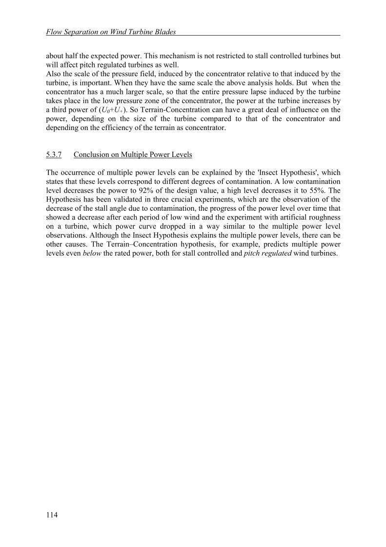
Flow Separation on Wind Turbine Blades
114
about half the expected power. This mechanism is not restricted to stall controlled turbines butwill affect pitch regulated turbines as well.Also the scale of the pressure field, induced by the concentrator relative to that induced by theturbine, is important. When they have the same scale the above analysis holds. But when theconcentrator has a much larger scale, so that the entire pressure lapse induced by the turbinetakes place in the low pressure zone of the concentrator, the power at the turbine increases bya third power of (U0+U+). So Terrain-Concentration can have a great deal of influence on thepower, depending on the size of the turbine compared to that of the concentrator anddepending on the efficiency of the terrain as concentrator.
5.3.7 Conclusion on Multiple Power Levels
The occurrence of multiple power levels can be explained by the 'Insect Hypothesis', whichstates that these levels correspond to different degrees of contamination. A low contaminationlevel decreases the power to 92% of the design value, a high level decreases it to 55%. TheHypothesis has been validated in three crucial experiments, which are the observation of thedecrease of the stall angle due to contamination, the progress of the power level over time thatshowed a decrease after each period of low wind and the experiment with artificial roughnesson a turbine, which power curve dropped in a way similar to the multiple power levelobservations. Although the Insect Hypothesis explains the multiple power levels, there can beother causes. The Terrain–Concentration hypothesis, for example, predicts multiple powerlevels even below the rated power, both for stall controlled and pitch regulated wind turbines.
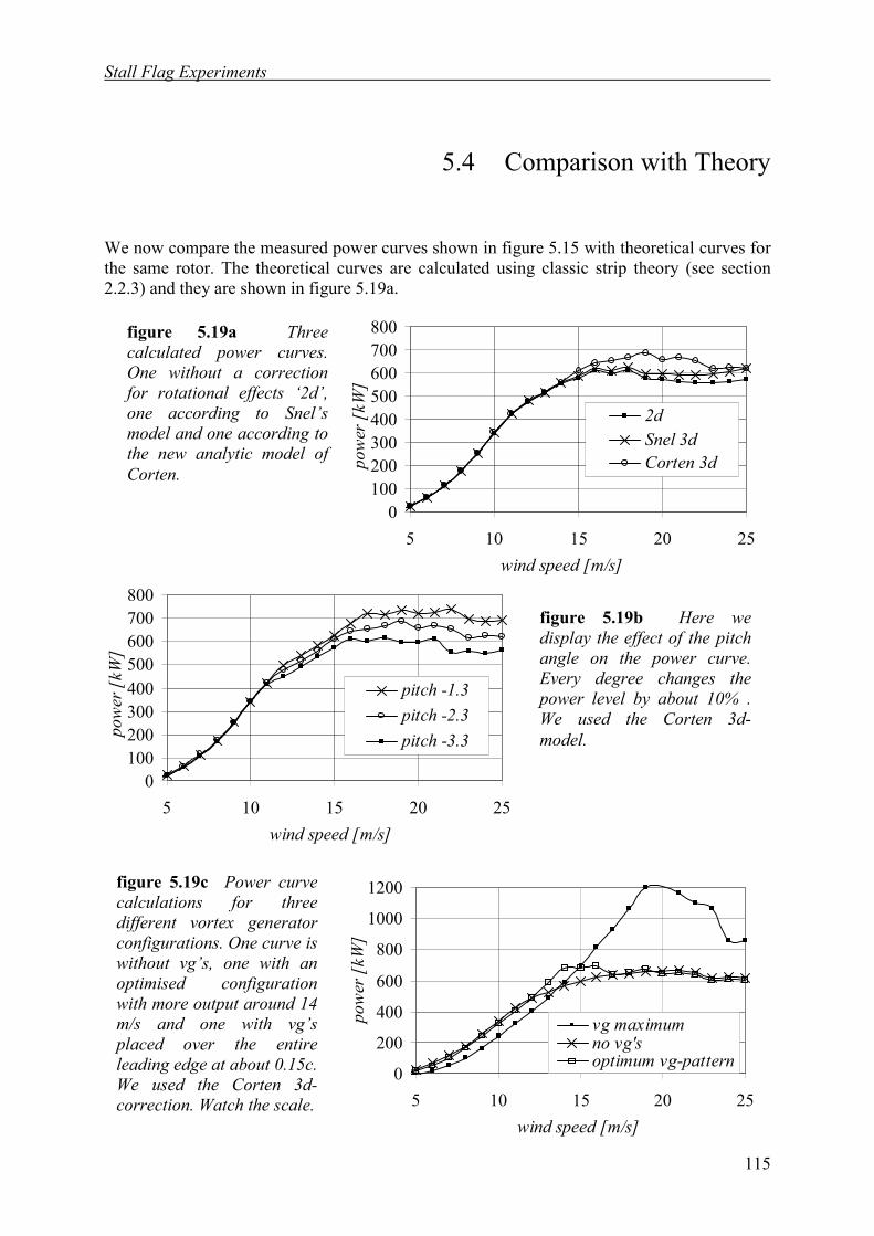
Stall Flag Experiments
115
5.4 Comparison with Theory
We now compare the measured power curves shown in figure 5.15 with theoretical curves forthe same rotor. The theoretical curves are calculated using classic strip theory (see section2.2.3) and they are shown in figure 5.19a.
figure 5.19a Threecalculated power curves.One without a correctionfor rotational effects ‘2d’,one according to Snel’smodel and one according tothe new analytic model ofCorten.
figure 5.19b Here wedisplay the effect of the pitchangle on the power curve.Every degree changes thepower level by about 10% .We used the Corten 3d-model.
figure 5.19c Power curvecalculations for threedifferent vortex generatorconfigurations. One curve iswithout vg’s, one with anoptimised configurationwith more output around 14m/s and one with vg’splaced over the entireleading edge at about 0.15c.We used the Corten 3d-correction. Watch the scale.
0100200300400500600700800
5 10 15 20 25wind speed [m/s]
pow
er [
kW]
2dSnel 3dCorten 3d
0100200300400500600700800
5 10 15 20 25wind speed [m/s]
pow
er [
kW]
pitch -1.3pitch -2.3pitch -3.3
0
200
400
600
800
1000
1200
5 10 15 20 25wind speed [m/s]
pow
er [
kW]
vg maximumno vg's optimum vg-pattern
Flow Separation on Wind Turbine Blades
116
We also show the curves predicted by the approximations discussed in section 2.5. Accordingto Snel’s theory the stall level would shift by 5% and according to Corten’s theory by 10%.Since both shifts are smaller than the spread shown in figure 5.15, it cannot be decided whichof the two is superior. Even the 2d-strip theory is useful. Differences in the theories appear tobe less important than differences in the experimental conditions.This is illustrated in figure 5.19b, where the effect is shown of a change of the pitch angle,being no less than 10% per degree. One should know that this angle can hardly be determinedto a precision of 1°, and that the twist also varies on the order of 1°, from blade to blade.Small deviations from the ideal blade shape (as pursued in production) can have importantconsequences; we have noticed, for instance, that a minute ridge near the leading edge of theairfoil did act as a stall strip. Another illustration is given in figure 5.19c, where the strongeffect of vortex generators is shown. These can double the turbine power level.
Without further illustrations we recall the effects of fly-induced roughness. Even a littlecontamination can lower the power by 10%, and a lot of contamination can halve it. We alsorecall the yaw error of 20°, which reduced the power by 20%. Yaw errors of that magnitudemay be expected in complex, hilly terrain. Even larger effects can be expected when theterrain has a concentrating effect at the turbine. Turbines are often put in locations whereprofit can be taken of the natural concentration. This may effect the power, even below rated,by as much as 100%, although we will use 25% as possible value in our conclusion. For thesake of completeness, we finally mention effects of air density and, perhaps turbulence. Thedensity of air, which linearly enters the transfer of momentum and power, varies only by afew percent (at most 10% when a storm depression passes), so the effect is mostly small andmay be neglected. However, at some turbine sites in Canada the density can rise to 1.47kg/m3, while the mean value is 1.28, with an effect on the power level of 15%. Turbulence hasbeen invoked to explain the multiple power levels [54] without making clear how this canpossibly work. We propose not to neglect the effects of turbulence, but to ignore them.
Our conclusion must be that the theoretical modelling in chapter 2 falls short in thedescription of the stall phenomena. Irrespective of the choice of approximations in thesolution of the Navier-Stokes equation, the theory addresses only a small part of the complexprocess of flow separation.
117
6. Conclusions
Let us summarise. Wind turbines need a control mechanism to limit the power to a designedmaximum, which is reached at a certain rated wind speed. Designers therefore tried tocombine a constant rotor speed with a clever rotor geometry that inherently controls its powervia flow separation. In this way, the power control becomes an intrinsic property of the rotor.About 50% of all turbines use this mechanism called stall control. However, in practice thepower level can deviate tens of percent both above and below the design level.
Models on Stall BehaviourTo design rotors with a more accurate power levelling one needs precise models on theseparation behaviour. The heuristic model we propose considers rotational effects on the flowseparation. We use Euler equations, since the separation layer is thick. We find an analyticsolution wherein the contribution of the radial velocity, which is neglected in other models, isstressed. Present models on flow separation yield corrections for rotation that influence thepower level of wind turbines by about 10%. Regrettably, none of the models addresses themajor effects on the power of vortex generators (+100%), stall strips (-50%) andcontamination (-50%). The first two affect only a part of the rotor, so the uncertaintiesintroduced are approximately 20% and 10% respectively. Furthermore, flow separationfollows from an instability, so that small disturbances can have large effects. However, in themodels all small terms were neglected, in order to simplify the equations. Of course one mayretain all the terms of the Navier-Stokes equations and solve them numerically. It should berealised however, that the computer code needs the precise rotor geometry as input, includingthe vortex generators and even the roughness caused by the insects on the blades. And thelatter is one of the relevant dependencies that change with time. Therefore, we have quite aproblem with the input data. Even if this problem could be overcome, one would need a greatdeal of computing time. So far, only the separation properties of airfoil sections, simplified toa two-dimensional set-up have been correctly computed, but only for the case of attachedflow. Sometimes entire wind turbine blades were simulated [56], but in these cases, themodelling of turbulence had to be adapted until some correlation with the observations wasreached. However, those observations did not include the real separation behaviour of theblades, so the correlation with practice was in fact unknown. Moreover, even if the stallcharacteristics of a rotor could be calculated precisely, it would still be impossible to designthe rotor so that it had a constant stall level.
Flow Separation on Wind Turbine Blades
118
Systematic and Time-Dependent DeviationsWe have in fact found many reasons for the deviation between the designed power level andthat of practice. A perfect design should account for the effects mentioned above, and manymore. We have an influence of the power of 10% per degree blade pitch, and about 5% for thetwist uncertainty. Vortex generators and stall strips account for 20% and 10% uncertaintyrespectively. A yaw error of 20° can cause a power decrease of 20%t, the terrain shape canalso influence by 25%t. Density affects the power by 10%t. Other effects are changes of theblade surface roughness from ageing of the coating, wind shear, rain and ice sedimentation.For those, we estimate 20%t uncertainty. Blade contamination can differ from a few percent to45%t. Differences between the blades produced and the airfoils tested in the wind tunnel alsogive about 20% uncertainty. Rotational effects add 10% uncertainty. The root-mean squareeffect on the power level is about 35% due to systematic deviations. Due to time-dependentdeviations (superscript t) we estimate deviations of 20% if we neglect the yaw error, terrainconcentration and contamination problems and we estimate a deviation of up to 60% whenthese effects are included.
Stall Flag Visualisation TechniqueLet us return to the main subject of this thesis. We developed a flow visualisation techniquethat has many advantages over the use of tufts. Stall is a highly dynamic process, which onlycan be studied with a technique that has a fast response and the possibility of evaluating theoutput signals automatically. Both characteristics are met by the stall flag technique. Inparticular on rotating objects, tufts are severely influenced by the centrifugal force andtherefore display erroneous signals, while disturbing the flow. Stall flags are hardly affectedby the centrifugal force (and in their most favourable positions, not at all), so that systematicerrors and flow disturbances are avoided. The pressure driven stall flag will in most cases,introduce much less drag than the frictional-drag driven tufts. Disturbance is also caused bythe self-excited flapping motion displayed by tufts, even in attached flow. The first stall flagshad the same problem, but the later ones, with higher stiffness, remained stable and so thedisturbance was avoided. Finally, stall flag signals can benefit from motion blur, while tuftsignals become useless. Thanks to this property, we can visualise the flow on rapidly movingobjects. In particular we can visualise the separation behaviour of full-scale wind turbines indetail. A summary of the stall flag characteristics compared to tufts is given in table 6.1.
Correcting Systematic DeviationsIf the actual power level of a stall-controlled turbine does not correlate with the designedvalue, the reason can be found by observing stall flags on that turbine. Stall flags which wedeveloped and learned to use, are a unique tool for this purpose, and possibly also for otherpurposes. Once the cause of the deviation is known, adaptations are possible. Stall areaswhere the wind is below the rated value can be provided with vortex generators, and areaswhere the flow is still attached although the rated power has been surpassed can be providedwith stall strips; in the latter case a small blade pitch adjustment is also possible.With these adaptations, we can shift the power level up and down by about a factor of 2. Fromthe stall flag signals we can determine the stall delay of vortex generators as a function oftheir chord-wise and radial position. So we have sufficient possibilities of correcting the errorin the power level but we cannot correct for influence on the power caused by time-dependentblade contamination, by fluctuations in the air density, by terrain concentration or by verticalyaw. In short, we can avoid the systematic error of about 35%, but the time-variant error of20-60% remains.
Conclusions
119
Changing Ambient ConditionsCan the stall behaviour be made independent of changes in the environment? No. Stall is theconsequence of frictional drag in the boundary layer and roughness such as caused by insectsimmediately influences this frictional drag. One can search for airfoils that are relativelyinsensitive to roughness. This dependency is often measured in the tunnel by pasting a zigzagtape at 5%c. A better impression of this effect will be obtained by using zigzag tape where theroughness is located in practice: at about 0%c. One may further try to avoid contamination byusing special coatings, and by regular cleaning, but that will not solve the problem. A severeimpact of insects can halve the power level, as we have seen, but a small number of impactswill bring the power down by many percentage points already.The variation of the air density with time may even be more cumbersome. Separation is notmuch dependent on the density, but the power produced is affected in a linear sense. So thepower control based on stall is passively shifting up and down with the air density. Besidesthese two, we have time-dependent effects on the power by yaw errors, of which the verticalcomponents cannot be avoided, and by concentration of the wind by the terrain.
Blade and Turbine RequirementsA good stall design requires precision in the yaw mechanism and especially in the blades. Theturbine should always be in line with the wind. The shape of the blades should be well definedand be manufactured with very small tolerances. Even when systematic deviations in theactual stall power are corrected with the stall flag method, the inaccuracies in themanufacturing should be small. Otherwise one would need a stall flag experiment per turbine.So stall control sets high production standards, which will rise the price and could take awayone of the main arguments for stall control.
Predicting Stall BehaviourOne cannot yet produce, cost-effective, blades precise enough to meet a designed stallbehaviour. We should add that there are no models to predict that behaviour, and even withsuch models, we can not make an accurate stall regulation. With the stall flags systematicdeviations can be corrected, but the time-dependent effects remain a source of trouble. Takingall these things together, we conclude that power control by passive stall cannot be moreaccurate than +/-20% (the remaining time-dependent variation). We estimate that theproduction loss is about 13% in the case of a 20% surplus power (turbine stops 10% aboverated) and 6% less for a 20% lower power level. We assumed that the level changedpermanently, so this is an estimate for the production losses (10% average) when thesystematic errors are not corrected. For the time-dependent effects, we roughly estimate thatthey act 50% of the time so the losses become on average 5% (the average of the half of 13%and of 6%). Active stall control can remove this uncertainty but will add complexity, therebyremoving a major argument for stall control. We conclude that the effects on the energyproduction are not so large if we correct for systematic errors. Pitch-controlled wind turbinesmay also stall around rated wind speed. If we assume an average power loss due to separationof 5% from 12 to 16 m/s, it affects the production by 2.5%.
Inherent Heat GenerationA final point should be made. We showed that when the flow outside the stream tube throughthe actuator is included in the analysis, the energy conversion process has an inherentdissipation of kinetic energy in heat. The heat produced in the flow is about half the energyextracted.

Flow Separation on Wind Turbine Blades
120
no. property stall flag tufts1. purpose 1. detection of separated area
2. detection of separationheight
detection of separated area
2. visibility:-signal-resolution-motion blur
≈1000 times tuft visibilitybinary, clear detection4×4 pixelsadvantage
tuft visibilitycontinuous, not easy to detect20×20 pixelsfatal
3. response speed 7h/v, with h = flap height unknown, but comparable
4. flow disturbance 1. cause transition2. drag increase in laminar
flow
1. cause transition2. drag increase in all flow
types3. act as vortex generators
and delay stall4. self-excitation gives drag
5. centrifugal forcedependence
zero for hinge angle zero,which is the most usefulangle.
large, comparable toaerodynamic force on rotors
6. Kelvin-Helmholtzinstability
avoided not avoided (except with flowcones, but these haveproblems with aspects 2, 4, 5,8 and 9)
7. operating principle pressure forces only duringflip-over
always frictional drag
8. data-acquisition automated by imageprocessing
manual
9. applicability objects up to 100m·100m objects up to 10m·10m
10. construction hinge, flap, support, reflector thread, support, (reflector)
table 6.1 Comparison of stall flag and tuft.
121
References
1 Abbott, H. and von Doenhoff, A.E., ‘Theory of Wing Sections’, Dover Publications,New York, 1959.
2 Adrian; R.J., 'Scattering Particle Characteristics and their effect on Pulsed LaserMeasurements of Fluid Flow: speckle velocimetry vs. particle image velocimetry',Applied Optics 24 (1985), pages 44-52.
3 Bak, C.; Madsen, H.A.; Fuglsang, P.; Rasmussen, F., 'Double Stall', Risoe-R-1043(EN), June 1998.
4 Bak, C., Madsen, H.A., Fuglsang, P., Rasmussen, F.,’Observations and Hypothesis ofDouble Stall’, Wind Energy, Wiley, Vol 2, No 4 Oct-Dec 1999.
5 Banks, W.H.H., Gadd, G.E.; 'Delaying Effect of Rotation on Laminar Separation',AIAA J., Volume 1, No 4, April 1963, pp.941-942.
6 Batchelor, G.K., An Introduction to Fluid Dynamics', Cambridge University Press,ISBN 0 521 098173, 1967.
7 Betz, A., 'Das Maximum der Theoretisch Möglichen Ausnützung des Windes durchWindmotoren', Zeitschrift für das gesamte Turbinewesen, Sept. 20th 1920, page 307-209.
8 Betz, A. 'Applied Airfoil Theory' Volume IV, Division J in Durand, W.F.'Aerodynamic Theory, A General Review of Progress', 1935.
9 Brand, A.J.; Dekker, J.W.M.;Groot, de C.M.; Späth, M., 'Field Rotor Aerodynamics:the Rotating Case'.
10 Bunnes, P. and Fiddes, S., Laser Doppler Results Contributed to 'Dynamic Stall andThree Dimensional Effects', Joule II contractors meeting 8-10 feb 1995, NEL,Glasgow, U.K.
11 Corten, G. P., 'Parameterising Particle Image Velocimetry, The Feasibility Study toVisualise the Flow Around the 28 [m] Wind Turbine at ECN.`, IW-95091R, Aug. '95.
12 Corten, G.P., ‘The Stagnation Flap, an Instrument to Visualise and LocateStagnation’, November 1996, IW-96107R
13 Corten, G.P., 'The Stall Flag, Prior Development and First Results', Delft Faculty ofAerospace Engineering, Memorandum M774, Delft, February 1997.
14 Corten, G.P., ‘Technical Development of the Stall Flag Method’, ECN-CX--97-036,August 1997.
Flow Separation on Wind Turbine Blades
122
15 Corten, G.P., ‘The Stall Flag Method: Proof of Concept’, ECN-RX—98-001, JointASME, AIAA Wind Energy Symposium, Reno, USA, January 12-15, 1998.
16 Corten, G.P. & Vronsky, T, ’Stall Regulated Wood Epoxy Blades’, IEA Symposiumon the Aerodynamic of Wind Turbines, Lyngby Denmark, 3-4 December 1998.
17 Corten, G.P., 'The Tip Commands', ECN-RX--99-029, September 1999, presented atthe BWEA 21, 1-3 September 1999, Cambridge, UK.
18 Corten, G.P., ‘Technical Development of the Stall Flag Method, Prototypes 14-19,second report’, ECN-CX--99-114, October 1999.
19 Corten, G.P., 'Insects Cause Double Stall', 13th IEA symposion Nov. 29-30 1999,Stockholm.
20 Corten, G.P., 'Optimisation of Vortex Generator Locations', 13th IEA symposionNov. 29-30 1999, Stockholm.
21 Corten, G.P., 'Inviscid Stall Model', 13th IEA symposion Nov. 29-30 1999,Stockholm
22 Corten, G.P., ‘Insects Cause Double Stall’, ECN-CX—00-018, February 2000.23 Crowder, J.P., 'Tufts', Chapter 9 of Handbook of Flow Visualisation, edited by Yang,
W.Y., Hemisphere Publishing Corporation, 1989.24 Crowder, J.P., 'Flow Direction and State Indicator', United States Patent 4,567,760,
Febr. 4 1986.25 Driscroll, W.G.; Vaughan, W., 'Handbook op Optics' Optical Society of America
ISBN: 0-07 -047710-8, 1978.26 Du, A.; Selig, M.S., 'A 3D Stall Delay Model for Horizontal Axis Wind turbine
Performance Prediction', in 'A collection of the 1998 ASME Wind EnergySymposion', AIAA-98-0021, 36th AIAA Aerospace Meeting and Exhibit, Reno,January 1998.
27 Dyrmose, S.Z., Hansen, P.,'The Double Stall Phenomenon and how to Avoid it', IEAJoint Action Aerodynamics of Wind Turbines, Lyngby, December 3-4 1998.
28 Edmund Scientific Catalog, Industrial Optics, Barrington USA.29 Eggleston, D.M. and Starcher, K., 'Comparative Study of Aerodynamics of Several
Wind Turbines Using Flow Visualisation', 8th ASME Wind energy Symposion, NewYork, 1989.
30 Fogarty, L.E., 'The Laminar Boundary Layer on a Rotating Blade', Journal ofAeronautical Sciences, April, 1951.
31 Freris, L.L., 'Wind energy Conversion Systems', ISBN 0-13-960527-4 Prentice HallInternational UK, 1990.
32 Froude, R.E., Transactions, Institute of naval Architects, Vol 30, p.390, 1889.33 Froude, W., Transactions, Institute of Naval Architects, Vol. 19, p.47, 1878.34 Glauert, H. 'Airplane Propellors' Volume IV, Division L in Durand, W.F.
'Aerodynamic Theory, A General Review of Progress', 1934.35 Grabau, P., 'Double Stall', LM Glasfiber A/S, February 1996.36 Haslam, Flt., 'Wool Tufts: a Direct Method of Visually Discriminating between
Steady and Turbulent Flow over the Wing Surfaces of Aircraft in Flight', Rep. Mem.Aeronaut. Res. Council 1209, 1928.
37 Herzke, U., Peinelt, I., 'Visualisation of the Stagnation Point: First Results of a NewMethod', IW-94079 R, August '94.
38 Hoerner, S.F. and Borst, H.V., 'Fluid Dynamic Lift', Published by Mrs. Hoerner, L.A.,Hoerner Fluid Dynamics, Vancouver, WA , USA, 1985.
References
123
39 Hoerner, S.F., 'Fluid Dynamic Drag', Hoerner Fluid Dynamics, P.O. Box 65283,Vancouver, WA 98665, USA, 1965.
40 Holm, R and Gustavsson, J., 'A PIV Study of Separated Flow around a 2D Airfoil atHigh Angles of Attack in a Low Speed Wind Tunnel', in proceedings of IEA AnnexXI, 'Aerodynamics of Wind Turbines', 13th symposium, November 1999, Stockholm.
41 Holten, van Th., 'On the Validity of Lifting line Concepts in Rotor Analysis', Vertica,Vol. 1 pp. 239-254, 1976.
41 Holten, van Th.,’Concentrator Systems for Wind energy, with Emphasis on TipVanes’, Wind Engineering, Vol 5, no.1, p.29, 1981.
42 Hunt, V.D., 'Windpower', ISBN 0-442-27389-4, Litton Educational Publishing Inc.,New York, 1981.
43 Johnson, W., 'Helicopter Theory', Princeton University Press, Princeton, New Jersey,USA, 1980.
44 Karman, Th. von; and Burgers, J.M., 'General Aerodynamic Theory Perfect Fluids',Volume II, Division E in Durand, W.F. 'Aerodynamic Theory, A General Review ofProgress', 1934.
45 Kuik, G.A.M. van, ‘On the Limitations of Froude’s Actuator Disk Concept’, ph.d.thesis 1991.
46 Lanchester, F.W., 'A Contribution to the Theory of Propulsion and the ScrewPropeller', Trans. Institution of Naval Architects, Vol. XXX p. 330, March 25th,1915.
47 Madsen, H.A., 'Aerodynamics of a Horizontal Axis Wind Turbine in NaturalConditions', Riso M 2903 1991.
48 Mönch, E., 'Technische Mechanik', ISBN 3-486-38766-9, 1986.49 Schepers, J.G. en Snel, H., 'Aerodynamisch herontwerp NedWind 40 rotor' ECN-C--
95-108, November ‘95, blz 9 3.1 ‘Beschikbare profielen’.50 Schepers, J.G., Brand, A.J. e.a., 'Final Report of IEA Annex XIV: Field Rotor
Aerodynamics', June 1997, ECN-C--97-02751 Schlichting, H., 'Boundary Layer Theory', McGraw Hill Book company, ISBN 0 07
055334-3, 1979.52 Snel, H., 'Scaling Laws for the Boundary Layer Flow on Rotating Wind Turbine
Blades', proceedings of th fourth IEA Symposion on the Aerodynamics of windTurbines, Rome 20-21 November 1990, ETSU-N-118, January 1991, ETSU, Dept. ofEnergy, UK.
53 Snel, H., Houwink, R. and Piers, W.J.; 'Sectional Prediction of 3D Effects forSeparated Flow on rotating blades', 18th European Rotorcraft Forum, Avignon France15-18 September 1992.
54 Snel, H.; Corten, G.P.; Dekker, J.W.M.; Boer, J.de; Chaviaropoulos, P.K., Voutsinas,S., 'Progress in the Joule Project: Multiple Stall Levels', presented at the EUWECconference, March 1999, Nice, France.
55 Simpson, R.L., 'Aspects of Turbulent Boundary Layer Separation', Prog. AerospaceSci., Vol. 32, pp. 457-521, 1996.
56 Sørensen, J.N., 'VISCWIND, Viscous Effects on Wind Turbine Blades', ET-AFM-9902, Department of Energy engineering, Technical University of Denmark, June1999.
57 Spera, D.A., Wind Turbine Technology', ASME Press New York, 1994.58 Tangler, J.L. and Somers, D.M. 'Status of the special purpose airfoil families',
Proceedings IEA-symposion on the aerodynamics of Wind Turbines.
Flow Separation on Wind Turbine Blades
124
59 Timmer, W.A.,’Nieuwe profielen voor windturbines, een literatuurstudie’, IW-92056R, TUDelft, 1992.
60 Vermeer, L.J.,'Measurements on the Properties of the Tip Vortex of a Rotor Model',proceedings of EWEC '94, volume 1, page 805-808, 10-14 Oct. '94.
61 Vermeer, L.J. and Timmer, W.A., 'Identification of Operational Aerofoil State bymeans of Velocity Measurements', EWEC 1-5 March 1999, Nice, France.
62 Viterna, L.A. and Corrigan, R.D., 'Fixed Pitch Rotor Performance of LargeHorizontal Axis Wind Turbines', presented at DOE/NASA workshop on LargeHAWT's, Cleveland, Ohio, 1981.
63 Vries, O. de ' Fluid Dynamic Aspects of Wind Energy Conversion' AGARD -AG-243, ISBN 92-835-1326-6, July 1979.
64 White, F.M., ‘Viscous Fluid Flow’, McGraw-Hill, ISBN 0-07-100995-7,International Edition, 1991.
65 Wilson, R.E., Lissaman, P.B.S., Walker, S.N., 'Aerodynamic Performance of WindTurbines', Oregan State University, June 1976

125
Appendix A: The Aerpac 43m Rotor
The Dutch blade manufacturer Aerpac requested the author in the beginning of 1999 toimprove the stall behaviour of their APX43 rotor. Figure A.1 shows several power curves ofthe rotor. If we look at the intended curve ‘design’ and measured curve ‘initial’, then we seethe discrepancy at the start of the project. The turbine of 600 kW rated power couldmaximally produce 660kW, but, above 16 m/s, when the rotor captures even more than 700kW, the turbine will be halted.This is needed to prevent theturbine from overloading oroverheating, but the penalty isof course a production loss.We also see that the rotorproduces less than predictedbelow rated and in particularat approximately 10 m/s. Thisagain represents productionlosses. Both deviations causeda loss of approximately 10%relative to the design. We willtry to change the passivepower control by adaptation ofthe stall behaviour, which webase on stall flag diagnostics.Two series of stall flagmeasurements were carriedout, one in July 1999 and onein March 2000.
A.1 First Stall Flag Measurement
During the first measurement for Aerpac we had periods of low wind and periods of rain,causing the flaps to stick to the blade surface. Only one measurement could be made. Wepresent the most valuable result, namely for the APX43 blade in standard layout with some
figure A.1 The predicted power curve of the APX43‘design’ (1.86 GWh), the measured curve before theproject started ‘initial’ (1.65 GWh), and the measuredcurve after the first stall flag measurement ‘ECN’ (1.79GWh). The scale on the right-hand side refers to thedifference between the two measured curves.
0100200300400500600700800
6 8 10 12 14 16 18 20 22 24wind speed [m/s]
P [k
W]
-120-100-80-60-40-2002040
delta
P [
kW]
designinitialECNdifference

Flow Separation on Wind Turbine Blades
126
adaptations. Delft University of Technology, who had an important input in the aerodynamicdesign of the APX43, proposed to install stall strips at approximately 0.85R to avoidoverpower, and to extend the line of vortex generators from 0.52R to 0.58R to increase thepower below rated. The powercurve ‘initial’ refers to thislayout. The pattern of stallflags and vortex generatorsduring the first measurement isshown in figure A.2.After installation of the stallflags, we started the turbineseveral times, while recordingthe stall flags signalsresponding to the increasingrotation speed, and thus theincreasing tip speed ratio λ.The video frames wereanalysed by the image-processing program. Theframes were binned on tipspeed ratios and we obtained table A.1 as output. The table displays the average signals ofeach pair of adjacent trailing edge stall flags. The second row shows the radial positions fromthe tip to the root of the blade. The first column shows the value for λ for each bin and thesecond column shows the number of video frames in each bin. Therefore, the first row of datashows that 57 video frames were analysed for the λ=2.0 bin, and the first two stall flags on thetip were open during a fraction 0.3 of the 57 frames. The column with the heading ‘strip’shows the signal of the pair of stall flags behind the stall strip. We see that this strip causes
stall for λ< 7.5. The tip speedof this rotor is 61.5 m/s, sostall occurred above 8 m/s,which is much too soon. Thecolumns in the vortexgenerator area show that thesegenerators effectively delaystall.
We see that the switching overof a stall flag is gradual. Theλ-values in the table areobtained from ΩR/U. For Uwe used the average of theanemometer signal, obtained athub height from a mastupwind, for R the known rotordimension and for the angularfrequency Ω the rather preciseresult of the image processing.Although the error in U makesλ somewhat uncertain, there is
figure A.3 Trailing edge λ-stall values for the firstmeasurement. The turbine reaches rated power forλ≈4.5, so the blade surface near the stall strip stallsmuch too soon and the surface between 0.45R and0.55R is too late.
23456789
10
0.1 0.2 0.3 0.4 0.5 0.6 0.7 0.8 0.9 1.0radial position r/R
lam
bda-
stal
l
0.000.050.100.150.200.250.300.350.40
vg p
ositi
on x
/c
0.2-0.6ctrailing edgevortex
figure A.2 The pattern during the first measurement.The vertical line at 0.86R is the tip division and the stallstrip is located just to the left of it at the leading edge.
0.0
0.5
1.0
1.5
0.1 0.2 0.3 0.4 0.5 0.6 0.7 0.8 0.9 1.0
radial position r/R
chor
d [m
]
flags 0 dgvortexreferenceflags 60 dg
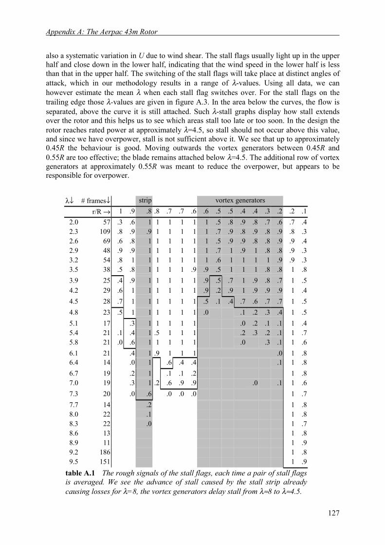
Appendix A: The Aerpac 43m Rotor
127
also a systematic variation in U due to wind shear. The stall flags usually light up in the upperhalf and close down in the lower half, indicating that the wind speed in the lower half is lessthan that in the upper half. The switching of the stall flags will take place at distinct angles ofattack, which in our methodology results in a range of λ-values. Using all data, we canhowever estimate the mean λ when each stall flag switches over. For the stall flags on thetrailing edge those λ-values are given in figure A.3. In the area below the curves, the flow isseparated, above the curve it is still attached. Such λ-stall graphs display how stall extendsover the rotor and this helps us to see which areas stall too late or too soon. In the design therotor reaches rated power at approximately λ=4.5, so stall should not occur above this value,and since we have overpower, stall is not sufficient above it. We see that up to approximately0.45R the behaviour is good. Moving outwards the vortex generators between 0.45R and0.55R are too effective; the blade remains attached below λ=4.5. The additional row of vortexgenerators at approximately 0.55R was meant to reduce the overpower, but appears to beresponsible for overpower.
λ↓ # frames↓ strip vortex generatorsr/R → 1 .9 .8 .8 .7 .7 .6 .6 .5 .5 .4 .4 .3 .2 .2 .1
2.0 57 .3 .6 1 1 1 1 1 1 .5 .8 .9 .8 .7 .6 .7 .42.3 109 .8 .9 .9 1 1 1 1 1 .7 .9 .8 .9 .8 .9 .8 .32.6 69 .6 .8 1 1 1 1 1 1 .5 .9 .9 .8 .8 .9 .9 .42.9 48 .9 .9 1 1 1 1 1 1 .7 1 .9 1 .8 .8 .9 .33.2 54 .8 1 1 1 1 1 1 1 .6 1 1 1 1 .9 .9 .33.5 38 .5 .8 1 1 1 1 .9 .9 .5 1 1 1 .8 .8 1 .83.9 25 .4 .9 1 1 1 1 1 .9 .5 .7 1 .9 .8 .7 1 .54.2 29 .6 1 1 1 1 1 1 .9 .2 .9 1 .9 .9 .9 1 .44.5 28 .7 1 1 1 1 1 1 .5 .1 .4 .7 .6 .7 .7 1 .54.8 23 .5 1 1 1 1 1 1 .0 .1 .2 .3 .4 1 .55.1 17 .3 1 1 1 1 1 .0 .2 .1 .1 1 .45.4 21 .1 .4 1 .5 1 1 1 .2 .3 .2 .1 1 .75.8 21 .0 .6 1 1 1 1 1 .0 .3 .1 1 .66.1 21 .4 1 .9 1 1 1 .0 1 .86.4 14 .0 1 .6 .4 .4 .1 1 .86.7 19 .2 1 .1 .1 .2 1 .87.0 19 .3 1 .2 .6 .9 .9 .0 .1 1 .67.3 20 .0 .6 .0 .0 .0 1 .77.7 14 .2 1 .88.0 22 .1 1 .88.3 22 .0 1 .78.6 13 1 .88.9 11 1 .99.2 186 1 .89.5 151 1 .9
table A.1 The rough signals of the stall flags, each time a pair of stall flagsis averaged. We see the advance of stall caused by the stall strip alreadycausing losses for λ=8, the vortex generators delay stall from λ≈8 to λ≈4.5.

Flow Separation on Wind Turbine Blades
128
The stall flags placed undera hinge angle of 60°correspond to the lowervalues of the zigzag linelabelled ‘0.2-0.6c’ in figureA.3, so they close soonerduring a start. This indicatesthat, with decreasing angleof attack, the separated flowover the blade changesdirection from the reversedto the radial direction. Thisis as expected, since at largeangles of attack (at low tipspeed ratios) rotation haslittle effect on a reversedflow, which then behaves asa 2-dimensional separatedflow.Between 0.6R and 0.9R theblade stalls much too soon,especially in the stall striparea. This clearly is thereason for the losses belowrated. Another observation isthat the stall strip has onlyeffect on the stall flagsbehind it, so its influence isrestricted to its physicaldimensions. Finally, we seethat the tip is a bit late installing.We come to the remarkableconclusion that bothmeasures proposed tocorrect the stall behaviourmade the problems worse!Using stall flags, we couldclear up what reallyhappened, why thecorrections didn’t help, and
most importantly, what had to be done: Remove the stall strips, since the blade stalls too soonin this range even without them. Install vortex generators up to much larger radial positions,say 0.8R. Reduce the effectiveness of the vortex generators between 0.45R and 0.6R bymoving them to a larger chord-wise position, and maybe, make the tip stall sooner. So wedesigned a new vortex generator pattern (see figure A.7). The power curve was measuredagain with this pattern and figure A.1 shows the result. We see that the overpower problemhas disappeared. While the turbine had to be halted above 15m/s in the initial situation, itcould now operate up in its full design range. The difference of the two power curves (also
figure A.4 The pattern of the second measurement.Blade 1 has the pattern according to the first advice ofECN. Blade 2 has a second new pattern. The vortexgenerators of blade 3 were removed, while the blade hasthe same stall flag pattern as blade 2, except of thesmaller number on the trailing edge.
blade 1, unchanged
0.00.51.01.52.0
0.1 0.2 0.3 0.4 0.5 0.6 0.7 0.8 0.9 1.0radial position [r/R]
chor
d [m
]
stall flagvortex generatorsreference marker
blade 2, vg's >.55r/R at 0.39x/c, vg's for .32<r/R<.55 backwards
0.00.51.01.52.0
0.1 0.2 0.3 0.4 0.5 0.6 0.7 0.8 0.9 1.0radial position [r/R]
chor
d [m
]
stall flagvortex generatorsreference markerstall strip -30 deg
blade 3, all vg's removed
0.00.51.01.52.0
0.1 0.2 0.3 0.4 0.5 0.6 0.7 0.8 0.9 1.0radial position [r/R]
chor
d [m
]
stall flagvortex generatorsreference markerstall strip -45 deg
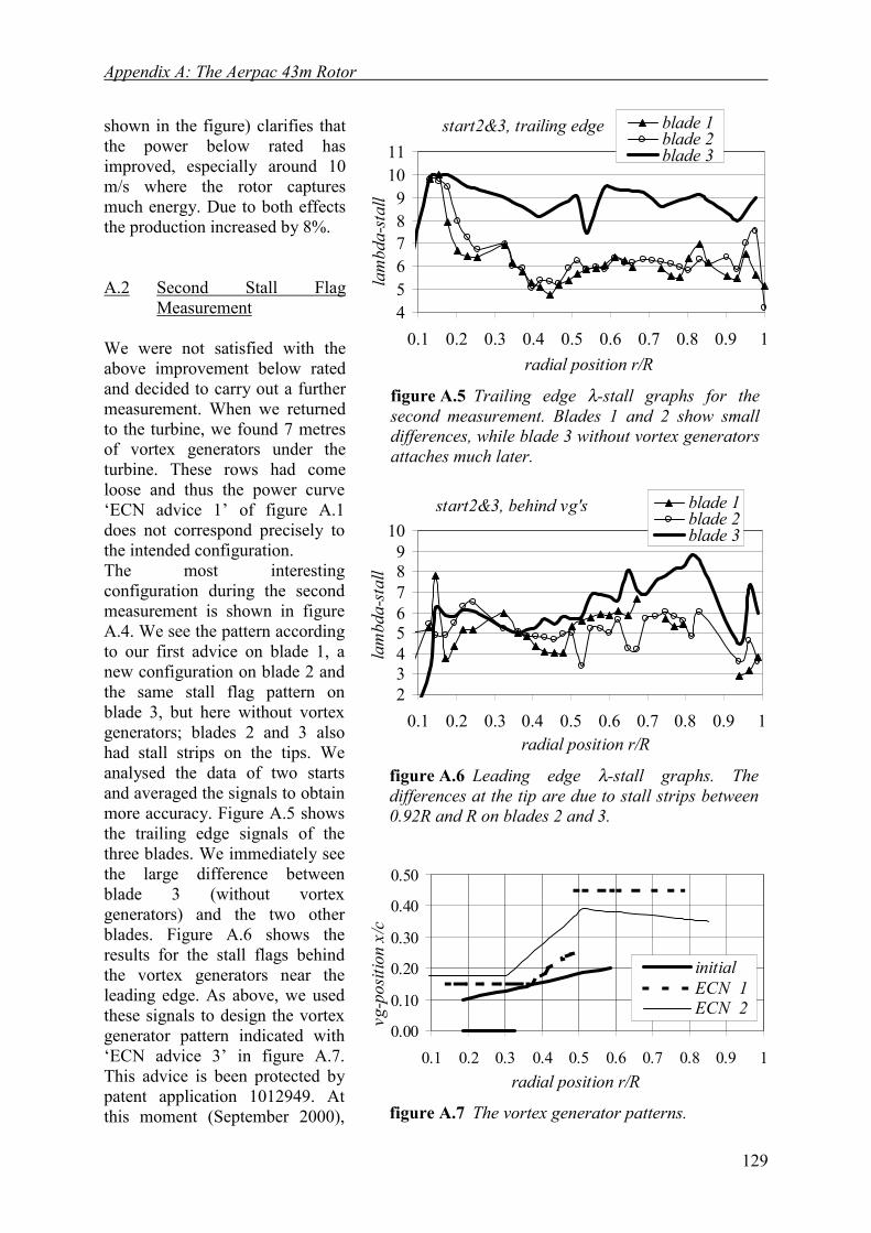
Appendix A: The Aerpac 43m Rotor
129
shown in the figure) clarifies thatthe power below rated hasimproved, especially around 10m/s where the rotor capturesmuch energy. Due to both effectsthe production increased by 8%.
A.2 Second Stall FlagMeasurement
We were not satisfied with theabove improvement below ratedand decided to carry out a furthermeasurement. When we returnedto the turbine, we found 7 metresof vortex generators under theturbine. These rows had comeloose and thus the power curve‘ECN advice 1’ of figure A.1does not correspond precisely tothe intended configuration.The most interestingconfiguration during the secondmeasurement is shown in figureA.4. We see the pattern accordingto our first advice on blade 1, anew configuration on blade 2 andthe same stall flag pattern onblade 3, but here without vortexgenerators; blades 2 and 3 alsohad stall strips on the tips. Weanalysed the data of two startsand averaged the signals to obtainmore accuracy. Figure A.5 showsthe trailing edge signals of thethree blades. We immediately seethe large difference betweenblade 3 (without vortexgenerators) and the two otherblades. Figure A.6 shows theresults for the stall flags behindthe vortex generators near theleading edge. As above, we usedthese signals to design the vortexgenerator pattern indicated with‘ECN advice 3’ in figure A.7.This advice is been protected bypatent application 1012949. Atthis moment (September 2000),
figure A.5 Trailing edge λ-stall graphs for thesecond measurement. Blades 1 and 2 show smalldifferences, while blade 3 without vortex generatorsattaches much later.
start2&3, trailing edge
456789
1011
0.1 0.2 0.3 0.4 0.5 0.6 0.7 0.8 0.9 1radial position r/R
lam
bda-
stal
l
blade 1blade 2blade 3
figure A.6 Leading edge λ-stall graphs. Thedifferences at the tip are due to stall strips between0.92R and R on blades 2 and 3.
start2&3, behind vg's
23456789
10
0.1 0.2 0.3 0.4 0.5 0.6 0.7 0.8 0.9 1radial position r/R
lam
bda-
stal
l
blade 1blade 2blade 3
figure A.7 The vortex generator patterns.
0.00
0.10
0.20
0.30
0.40
0.50
0.1 0.2 0.3 0.4 0.5 0.6 0.7 0.8 0.9 1radial position r/R
vg-p
ositi
on x
/c
initialECN 1ECN 2
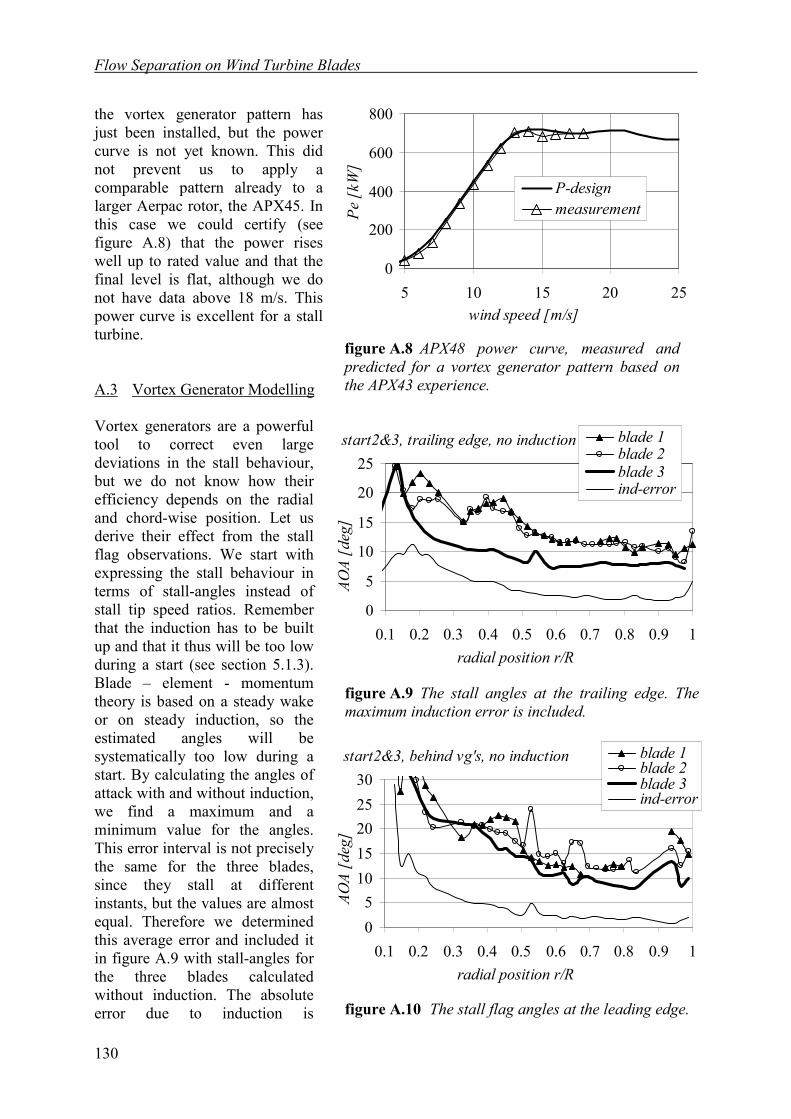
Flow Separation on Wind Turbine Blades
130
the vortex generator pattern hasjust been installed, but the powercurve is not yet known. This didnot prevent us to apply acomparable pattern already to alarger Aerpac rotor, the APX45. Inthis case we could certify (seefigure A.8) that the power riseswell up to rated value and that thefinal level is flat, although we donot have data above 18 m/s. Thispower curve is excellent for a stallturbine.
A.3 Vortex Generator Modelling
Vortex generators are a powerfultool to correct even largedeviations in the stall behaviour,but we do not know how theirefficiency depends on the radialand chord-wise position. Let usderive their effect from the stallflag observations. We start withexpressing the stall behaviour interms of stall-angles instead ofstall tip speed ratios. Rememberthat the induction has to be builtup and that it thus will be too lowduring a start (see section 5.1.3).Blade – element - momentumtheory is based on a steady wakeor on steady induction, so theestimated angles will besystematically too low during astart. By calculating the angles ofattack with and without induction,we find a maximum and aminimum value for the angles.This error interval is not preciselythe same for the three blades,since they stall at differentinstants, but the values are almostequal. Therefore we determinedthis average error and included itin figure A.9 with stall-angles forthe three blades calculatedwithout induction. The absoluteerror due to induction is
0
200
400
600
800
5 10 15 20 25wind speed [m/s]
Pe [
kW]
P-designmeasurement
figure A.8 APX48 power curve, measured andpredicted for a vortex generator pattern based onthe APX43 experience.
figure A.9 The stall angles at the trailing edge. Themaximum induction error is included.
start2&3, trailing edge, no induction
0
5
10
15
20
25
0.1 0.2 0.3 0.4 0.5 0.6 0.7 0.8 0.9 1radial position r/R
AOA
[deg
]
blade 1blade 2blade 3ind-error
figure A.10 The stall flag angles at the leading edge.
start2&3, behind vg's, no induction
05
1015202530
0.1 0.2 0.3 0.4 0.5 0.6 0.7 0.8 0.9 1radial position r/R
AOA
[deg
]
blade 1blade 2blade 3ind-error
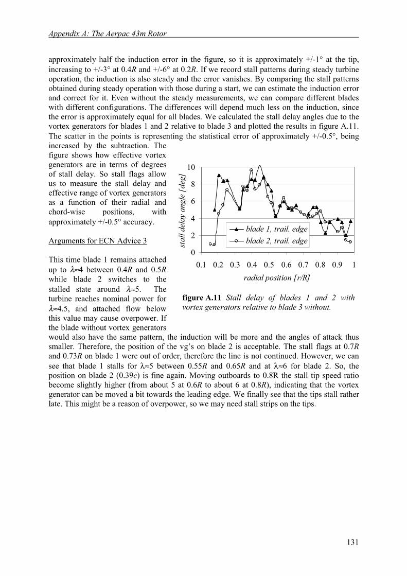
Appendix A: The Aerpac 43m Rotor
131
approximately half the induction error in the figure, so it is approximately +/-1° at the tip,increasing to +/-3° at 0.4R and +/-6° at 0.2R. If we record stall patterns during steady turbineoperation, the induction is also steady and the error vanishes. By comparing the stall patternsobtained during steady operation with those during a start, we can estimate the induction errorand correct for it. Even without the steady measurements, we can compare different bladeswith different configurations. The differences will depend much less on the induction, sincethe error is approximately equal for all blades. We calculated the stall delay angles due to thevortex generators for blades 1 and 2 relative to blade 3 and plotted the results in figure A.11.The scatter in the points is representing the statistical error of approximately +/-0.5°, beingincreased by the subtraction. Thefigure shows how effective vortexgenerators are in terms of degreesof stall delay. So stall flags allowus to measure the stall delay andeffective range of vortex generatorsas a function of their radial andchord-wise positions, withapproximately +/-0.5° accuracy.
Arguments for ECN Advice 3
This time blade 1 remains attachedup to λ≈4 between 0.4R and 0.5Rwhile blade 2 switches to thestalled state around λ≈5. Theturbine reaches nominal power forλ≈4.5, and attached flow belowthis value may cause overpower. Ifthe blade without vortex generatorswould also have the same pattern, the induction will be more and the angles of attack thussmaller. Therefore, the position of the vg’s on blade 2 is acceptable. The stall flags at 0.7Rand 0.73R on blade 1 were out of order, therefore the line is not continued. However, we cansee that blade 1 stalls for λ≈5 between 0.55R and 0.65R and at λ≈6 for blade 2. So, theposition on blade 2 (0.39c) is fine again. Moving outboards to 0.8R the stall tip speed ratiobecome slightly higher (from about 5 at 0.6R to about 6 at 0.8R), indicating that the vortexgenerator can be moved a bit towards the leading edge. We finally see that the tips stall ratherlate. This might be a reason of overpower, so we may need stall strips on the tips.
figure A.11 Stall delay of blades 1 and 2 withvortex generators relative to blade 3 without.
0
2
4
6
8
10
0.1 0.2 0.3 0.4 0.5 0.6 0.7 0.8 0.9 1radial position [r/R]
stal
l del
ay a
ngle
[de
g]
blade 1, trail. edgeblade 2, trail. edge

Flow Separation on Wind Turbine Blades
132
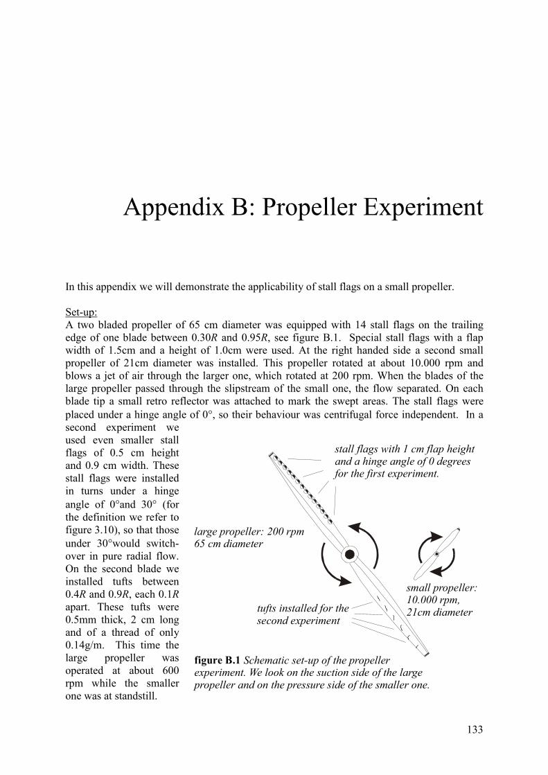
133
Appendix B: Propeller Experiment
In this appendix we will demonstrate the applicability of stall flags on a small propeller.
Set-up:A two bladed propeller of 65 cm diameter was equipped with 14 stall flags on the trailingedge of one blade between 0.30R and 0.95R, see figure B.1. Special stall flags with a flapwidth of 1.5cm and a height of 1.0cm were used. At the right handed side a second smallpropeller of 21cm diameter was installed. This propeller rotated at about 10.000 rpm andblows a jet of air through the larger one, which rotated at 200 rpm. When the blades of thelarge propeller passed through the slipstream of the small one, the flow separated. On eachblade tip a small retro reflector was attached to mark the swept areas. The stall flags wereplaced under a hinge angle of 0°, so their behaviour was centrifugal force independent. In asecond experiment weused even smaller stallflags of 0.5 cm heightand 0.9 cm width. Thesestall flags were installedin turns under a hingeangle of 0°and 30° (forthe definition we refer tofigure 3.10), so that thoseunder 30°would switch-over in pure radial flow.On the second blade weinstalled tufts between0.4R and 0.9R, each 0.1Rapart. These tufts were0.5mm thick, 2 cm longand of a thread of only0.14g/m. This time thelarge propeller wasoperated at about 600rpm while the smallerone was at standstill.
large propeller: 200 rpm65 cm diameter
figure B.1 Schematic set-up of the propeller experiment. We look on the suction side of the largepropeller and on the pressure side of the smaller one.
small propeller: 10.000 rpm,21cm diameter tufts installed for the
second experiment
stall flags with 1 cm flap heightand a hinge angle of 0 degreesfor the first experiment.
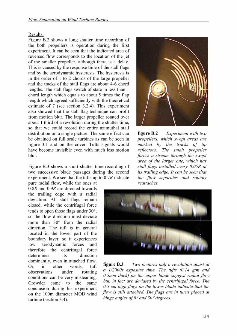
Flow Separation on Wind Turbine Blades
134
Results:Figure B.2 shows a long shutter time recording ofthe both propellers is operation during the firstexperiment. It can be seen that the indicated area ofreversed flow corresponds to the location of the jetof the smaller propeller, although there is a delay.This is caused by the response time of the stall flagsand by the aerodynamic hysteresis. The hysteresis isin the order of 1 to 2 chords of the large propellerand the tracks of the stall flags are about 4-6 chordlengths. The stall flags switch of state in less than 1chord length which equals to about 5 times the flaplength which agreed sufficiently with the theoreticalestimate of 7 (see section 3.2.4). This experimentalso showed that the stall flag technique can profitfrom motion blur. The larger propeller rotated overabout 1 third of a revolution during the shutter time,so that we could record the entire azimuthal stalldistribution on a single picture. The same effect canbe obtained on full scale turbines as can be seen infigure 3.1 and on the cover. Tufts signals wouldhave become invisible even with much less motionblur.
Figure B.3 shows a short shutter time recording oftwo successive blade passages during the secondexperiment. We see that the tufts up to 0.7R indicatepure radial flow, while the ones at0.8R and 0.9R are directed towardsthe trailing edge with a radialdeviation. All stall flags remainclosed, while the centrifugal forcetends to open those flags under 30°,so the flow direction must deviatemore than 30° from the radialdirection. The tuft is in generallocated in the lower part of theboundary layer, so it experienceslow aerodynamic forces andtherefore the centrifugal forcedetermines its directiondominantly, even in attached flow.Or, in other words, tuftobservations under rotatingconditions can be very misleading.Crowder came to the sameconclusion during his experimenton the 100m diameter MOD windturbine (section 3.4).
figure B.2 Experiment with twopropellers, which swept areas aremarked by the tracks of tipreflectors. The small propellerforces a stream through the sweptarea of the larger one, which hasstall flags installed every 0.05R atits trailing edge. It can be seen thatthe flow separates and rapidlyreattaches.
figure B.3 Two pictures half a revolution apart ata 1/2000s exposure time. The tufts (0.14 g/m and0.5mm thick) on the upper blade suggest radial flowbut, in fact are deviated by the centrifugal force. The0.5 cm high flags on the lower blade indicate that theflow is still attached. The flags are in turns placed athinge angles of 0° and 30° degrees.

135
Appendix C: Stall Flag Patent
At ECN the stall flag was regarded to be a valuable new instrument and therefore it wasdecided to apply for a patent. The procedure started with a Dutch patent no. OA 1003153Ned., which was applied May 17, 1996 and granted November 11, 1997. It was also decidedto extend the application to Europe and the Unites States of America. The application inEurope is still running, while that in the USA has just been granted. The latter is includedhere.

Flow Separation on Wind Turbine Blades
136
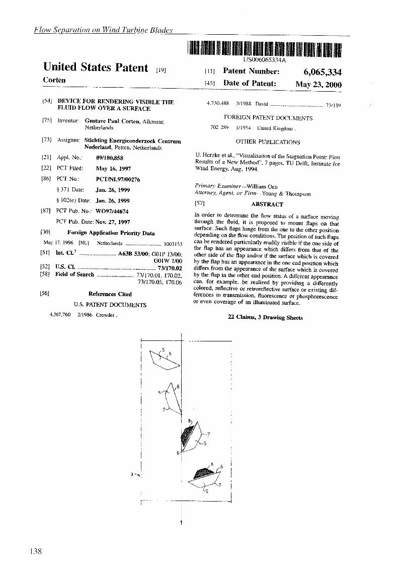

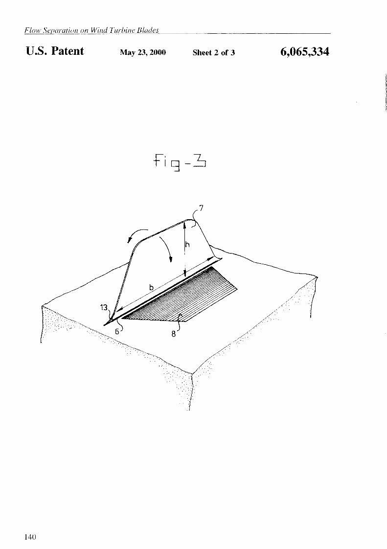
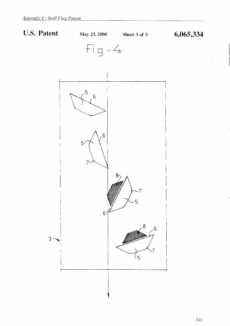
145
Samenvatting
Op dit moment is wereldwijd 15GW aan windvermogen opgesteld en daarmee wordt per jaarongeveer 100PJ elektriciteit opgewekt. Dit is slechts 0.2% van de wereldelektriciteits-produktie, maar zowel het opgestelde vermogen als de opgewekte energie nemen met circa30% per jaar toe. Er zou nog 9% meer energie kunnen worden opgewekt als het fenomeen vanstromingsloslating (overtrek) goed beheersbaar zou zijn.
Vermogensregeling
Om schade aan windturbines te voorkomen, worden ze gewoonlijk boven windkracht 10(25m/s) stilgezet. Het vermogen in de wind is dan ongeveer 8 keer hoger dan de turbine kanverwerken. Om te zorgen dat het turbinemaximum niet overschreden wordt, is hetnoodzakelijk om het opgenomen vermogen te kunnen regelen. Het is niet zinvol om deturbine zo te ontwerpen dat ook uit deze harde wind zo veel mogelijk energie kan wordengewonnen, omdat de zeer hoge windsnelheden zelden voorkomen. Een goed regelsysteem iswel zinvol en verhoogt dus de kosteneffectiviteit van de turbine. Globaal zijn er twee typenregelingen: actieve bladhoekverstelling (hierbij worden de bladen om hun as naar vaanstandgedraaid als het maximale vermogen overschreden wordt) en passieve overtrekregeling(waarbij de rotor op constant toerental draait en het opgenomen vermogen passief bepaaldwordt door de rotorgeometrie).
OvertrekregelingOvertrek is het verschijnsel dat de luchtstroming die van de voorrand naar de achterrand overde bladen stroomt, boven een bepaalde kritische invalshoek voortijdig loslaat van hetvleugeloppervlak (flow separation). Na het loslaatpunt stroomt de lucht zelfs terug, dat wilzeggen van de achterrand van de vleugel naar de voorrand. De energieopname van het deelvan de vleugel dat overtrekt neemt sterk af.De kunst van het ontwerpen van een overtrekgeregelde turbine is de rotorgeometrie zo tekiezen dat naarmate de windkracht toeneemt, het gebied van overtrek op de bladen, zodanigtoeneemt, dat het opgenomen vermogen constant blijft. Dit moet gelden in het bereik vanongeveer windkracht 6 of 12.5 m/s (als het maximum vermogen net bereikt wordt), totongeveer windkracht 10 (als de turbine stopt). Het voordeel van deze regeling is dat hetpassief werkt, dus niet kwetsbaar is voor mankementen en goedkoop is in uitvoering.
Flow Separation on Wind Turbine Blades
146
Probleemstelling
In de praktijk blijkt de overtrekregeling echter slecht beheersbaar en voldoen veel turbinesniet aan de specificaties. Afwijkingen van het ontwerpvermogen tot tientallen procenten teveel of te weinig zijn niet ongewoon.
In de jaren ’90 spitste het aërodynamische onderzoek zich toe op drie hoofdonderwerpen, teweten profielonderzoek in de windtunnel, de theorie van rotatie-effecten en drukmetingen optestturbines. Actuele problemen met het overtrekgedrag van commerciële windturbineskonden daarmee echter niet voldoende onderzocht en begrepen worden.
Wij hebben daarom in deze dissertatie als kernvraag gekozen:
‘Verloopt de stromingsloslating over de bladen met de windsnelheid wel zoals wij denken?’
Om dit vast te stellen is een meetmethode nodig die op grote commerciële turbines toepasbaaris, die het dynamische karakter van overtrek kan registreren, die ongevoelig is voor de sterkecentrifugale kracht, en die natuurlijk geen significante verstoring geeft. Een dergelijkemethode bestond niet. Daarom hebben wij een nieuwe techniek ontwikkeld.
‘Stall flag’-methode
Bij deze methode worden op een gerichte wijze honderden detectoren, verspreid over de rotor,in de vorm van stickers aangebracht. De detectoren (stall flags), die door ECN zijngeoctrooieerd, hebben een reflecterende laag die afhankelijk van de luchtstromingsrichting aldan niet zichtbaar wordt. Door een krachtige schijnwerper in het veld op te stellen, lichten allezichtbare reflectoren op, en kunnen we het veranderlijke overtrekpatroon registreren met eendigitale videocamera, zelfs op 500m afstand. De ‘stall flag’-signalen worden automatisch, metdoor ons ontwikkelde beeldbewerkingprogrammatuur opgemeten. De video camera registreertnaast het stallpatroon de bladazimuthoeken en het rotortoerental en uit de optische signalenvan andere sensoren ook nog de actuele windsnelheid en de windrichting. Uit de veleduizenden beelden karakteriseren we zo het stochastische overtrekgedrag.
Eigenschappen van de stall flagDe nieuwe detectortjes worden met de klassieke woldraadjes (tufts) vergeleken. Ze blijkenminder weerstand te geven doordat ze werken op dynamische druk en niet, zoals tufts, opwrijvingsweerstand. Tufts vertonen een zelfgeëxciteerde klappergedrag (door de Kelvin-Helmholtzinstabiliteit) dat wij met een zorgvuldig ontwerp van de stall flag kunnenvoorkomen. In de meest voorkomende opstelling zijn de stall flags bovendien ongevoeligvoor de centrifugale kracht. Een experiment met een 65cm diameter propeller bewijst dat destall flags onder draaiende omstandigheden blijven werken, terwijl tufts door de centrifugalekracht naar buiten slingeren, ook bij aanliggende stroming. Verder blijkt hieruit de zeer snellerespons van de stall flag.
Na het modelleren van het optisch gedrag, hebben wij het meetsysteem zodanig kunnenoptimaliseren dat het toepasbaar is op turbines van alle voorkomende diameters. Vergelekenmet tufts constateren we naast de eerder genoemde voordelen een minstens 1000 keer hogercontrast en 25 keer lagere resolutie-eisen aan de camera. Verder kunnen we vanbewegingsonscherpte profiteren terwijl die voor tuftsignalen fataal is.
Samenvatting
147
Belangrijkste resultaten
In het kader van de fundamentele theorie over windturbines ontwikkelen wij twee nieuwetheoretische inzichten die betrekking hebben op het overtrekgedrag. Aansluitend analyserenwe twee praktijkproblemen met de nieuwe meetmethode. Deze vier onderdelen wordenhieronder kort besproken.
1. Inherente warmteontwikkelingAls bij de energie-extractie door een windturbine ook de stroming om de rotor wordtmeegenomen, blijkt dat er een inherente warmteontwikkeling in het zog ver achter de turbineoptreedt. Bij optimaal turbinebedrijf is dat maar liefst de helft van het opgewekte vermogen.Hierdoor en door een argument met betrekking tot geïnduceerde weerstand zien wij geenaanleiding om de fundamentele theorie over energie-extractie aan te passen met de door VanKuik (1991) voorgestelde ‘edge-forces’. Wel bevelen wij aan om het door Lanchester (1915)ontwikkelde gedachtegoed over deze theorie verder uit te werken. Binnen de fundamenteletheorie analyseren we het begrip inductie en vinden we dat de impulstheorie,slankheidcorrecties en geïnduceerde weerstand alle drie hetzelfde fysische effect in rekeningbrengen. Onbekendheid hiermee kan leiden tot dubbele correcties (Viterna & Corrigan, 1981).
2. De invloed van rotatie op het overtrekgedragBij het ontwerp van windturbines baseert men zich op aërodynamische karakteristieken,bepaald voor vast opgestelde profielsecties in een windtunnel. Om deze te vertalen naar hetpraktijkgedrag van draaiende rotorbladen zijn correctiemethoden ontwikkeld (Snel, 1990-1999). De daarbij gehanteerde aanname, dat de grenslaagtheorie geldig is in en nabij hetlosgelaten-stromingsgebied, onderschrijven wij niet.
In plaats daarvan gaan wij uit van de Navier-Stokesvergelijkingen, die we reduceren op basisvan fysische argumenten. We verwaarlozen viscositeit, met het argument dat de losgelatenlaag dik is. Uit de condities van loslating, leiden wij af dat de drukgradiënt en deCorioliskracht elkaar balanceren in koorderichting. Dan volgt dat de lucht in het losgelatengebied door de radiale drukgradiënt en de centrifugale kracht naar de tip versnelt. Zo ontstaateen analytisch oplosbaar stelsel, waarin de convectieve term vr∂vr/∂r in de vergelijking voorde radiale richting (verwaarloosd in andere modellen) dominant is.
3. Meervoudige VermogensniveausBij verschillende grote commerciële windmolens worden af en toe vermogensdalingen tot45% waargenomen bij schijnbaar gelijkblijvende omstandigheden. Eerder onderzoek naarmogelijke oorzaken, zoals technische gebreken, aërodynamische instabiliteiten en vervuilinghad geen afdoende verklaring opgeleverd.
Wij formuleren drie hypothetische oorzaken. Door middel van ‘stall flag’-metingen en tweeandere cruciale experimenten kregen wij bevestiging voor één van de drie: deinsectenhypothese. Insecten vliegen alleen bij lage windsnelheden en slaan in op specifiekeplekken op de rotorbladen. Gebleken is, dat dit nu juist de plekken zijn die het vermogen bijhoge windsnelheden, als insecten niet vliegen, sterk beïnvloeden.
De andere, verworpen hypothesen, geven wel twee nieuwe inzichten. Ten eerste verwachtenwe meerdere vermogensniveaus indien de vorm van het terrein de wind concentreert. Deniveaus worden dan bepaald door de windrichting en zullen optreden op alle typenwindturbines, ook de bladhoekgeregelden. Ten tweede stellen we met de stall flags vast dat

Flow Separation on Wind Turbine Blades
148
het overtrokken deel van het blad zich op een continue wijze aanpast aan de aanstroming. Hetsterke bi-stabiele hysteresegedrag van een overtrokken bladsectie in de windtunnel gaat in hetveld dus verloren.
4. Afwijkingen van OntwerpspecificatiesHet vermogen van overtrekgeregelde turbines vertoont in de praktijk vaak forse systematischeafwijkingen van het ontwerp. Wij onderzochten met de stall flags een geval waarbij hetvermogen 30% te hoog was (en de turbine overbelast werd). De gebieden op de rotor met eenafwijkend gedrag werden onmiddellijk zichtbaar en het gedrag aldaar kon aangepast wordenmet grenslaagmanipulatoren zoals vortexgeneratoren. Zo ontstond een vermogenscurve, dieaanzienlijk dichter bij de ontwerpspecificaties lag en realiseerden wij eenopbrengstverbetering van 8%.
149
Curriculum Vitae
Gustave Paul Corten werd geboren in Rotterdam op 8 september 1968. Hij doorliep hetMerletcollege te Cuijk, waar hij op 4 juni 1986 het diploma Atheneum behaalde. Daarnastudeerde hij aan de Technische Universiteit Delft aan de faculteit Technische Natuurkunde.In 1990 verkoos hij af te studeren op het onderwerp ‘tweefase stroming in een kokend-waterreactor’ bij de vakgroep kernreactorkunde. Het doctoraal examen werd afgelegd op 24november 1992.
Tijdens het afstuderen verschoof zijn interesse in de richting van duurzame energie. Daarombegon hij een promotieonderzoek bij het Instituut voor Windenergie aan dezelfde universiteit.Deze promotieplaats werd gefinancierd door het Energieonderzoek Centrum Nederland, waarhij op 1 mei 1997 een baan kreeg aangeboden. Tot op heden bekleedt hij daar eenonderzoeksfunctie binnen de Unit Windenergie.
Al vanaf zijn tiende jaar was fotografie één van de voornaamste hobby’s Zo blies hij in zijnstudententijd nieuw leven in de fotoclub van DSV St-Jansbrug. Vervolgens speelde defotografie een belangrijke rol in zowel zijn afstudeerwerk als in het daarop volgendepromotieonderzoek. Een andere voorname hobby is watersport in de vorm van roeien, kanoënen zeilen, waarbij nauwe relaties bestaan tussen de optimalisatie van de catamaran en die vande windturbine.
In 1998 ging hij samenwonen met Lies de Jong en op 21 April 2000 ontstond hun nieuwehobby: hun kindje Veerle.

Flow Separation on Wind Turbine Blades
150
151
Dankwoord
Het is af! Zeven jaar werk was nodig om te komen van de eerste ideeën over het zichtbaarmaken van overtrek op windturbines tot een effectieve methodiek die inmiddels standaard isgeworden. Het onderzoek heeft de eerste 3 jaar in Delft plaatsgevonden bij het Instituut voorWindenergie, daarna heb ik het bij het ECN voortgezet. Dit werk, de meettechniek en denieuwe theorie zouden niet tot stand hebben kunnen komen zonder de steun en medewerkingvan een groot aantal mensen die ik hier bedanken wil.
Dank gaat uit naar Jan Dragt en Theo van Holten voor hun inzet en bijdragen als promotorenin de eerste fase van dit promotieonderzoek. Verder naar Arno Brand en Herman Snel, alsnaaste collega’s. Arno voor de zorgvuldige wijze waarmee hij de contacten vanuit ECNonderhield en omdat hij de nieuwe methode het voordeel van de twijfel gaf. Herman, die - alseen van eerste theoretici - het belang van ‘stall flag’-methode onderschreef en zo moreelsteunde. De vele discussies met hem over stromingsloslating en andere theoretischeonderwerpen waren af en toe heftig, maar altijd verhelderend. Speciaal wil ik Otto de Vriesbedanken, zowel voor de controles van delen van dit werk als voor zijn waardevolleAgardograph publicatie uit 1979. Dan Toon de Vries, voor het uren samenwerken in weer enwind in de werkbak van een hoogwerker, om honderden stall flags op windturbinebladen teplakken. Hij dacht als geen ander mee over het ontwerp van de stall flag, dat pas na jarenonderzoek voldoende bestand bleek tegen de omstandigheden op een windturbineblad. OokCees de Groot wil ik bedanken voor het bedienen van de 25mHAT tijdens diverse nachtelijkeexperimenten.
Bijzonder veel dank gaat uit naar Kees Andriesse. Pas in oktober 1999 heb ik hem benaderdmet dit onderzoek. Hij was onmiddellijk gecharmeerd van de kracht van de eenvoud van destall flag. Ik was zeer verheugd dat hij na zorgvuldige bestudering van mijn werk bereid wasals promotor op te treden. Hij bracht het gestagneerde promotieonderzoek in eenstroomversnelling. Ingestuurde hoofdstukken kwamen binnen een week terug voorzien vanzorgvuldig commentaar en schaduwberekeningen. Onder zijn leiding konden de nieuwetheorieën over warmteontwikkeling en rotatie-effecten ontstaan. Kortom: dit proefschrift hadzonder zijn enorme inzet en zijn wetenschappelijke toewijding niet kunnen ontstaan.
Flow Separation on Wind Turbine Blades
152
Dank gaat ook uit naar de mensen die dit onderzoek financieel mogelijk hebben gemaakt. JosBeurskens en Harry van Grol hebben alles geïnitieerd door mijn promotieonderzoek, ook deperiode in Delft, te financieren. In de fase dat de mogelijkheden van de methode nog onzekerwaren, was Frits Verheij van NOVEM bereid om een groot project over de ‘stall flag’-methode voor 80% mee te financieren. Door dit project werd de methode enorm verbeterd.We kunnen nu meten op elke commerciële turbine, ook als de diameter 80m is. Daardoorvolgden opdrachten vanuit de industrie. Jaap de Boer en Henk Heerkes van Aerpac bedank ikvoor hun opdracht om een Aerpac rotor met de stall flags te optimaliseren. Dick Veldkampvoor de opdracht van NEG Micon om het stallgedrag van turbines met meervoudigevermogensniveaus te onderzoeken. Ook wil ik hem bedanken voor de samenwerking binnendit project in de VS. Then I thank Thomas Vronsky and Mark Hancock for including themethod in a Joule-project to diagnose the stall behaviour of a 64m diameter Aerolaminatesrotor installed in Denmark. Binnen het Joule-project ‘MUST’, waarbinnen eveneens demeervoudige vermogensniveaus onderzocht werden, zijn ook een aantal ‘stall flag’-metingenopgenomen. Deze financieringen, althans het deel voor het ‘stall flag’-werk, hadden sameneen omvang van ongeveer 700kEuro. Mijn dank gaat ook uit naar ECN voor het vergoedenvan de drukkosten van dit proefschrift.
Al zeg ik het zelf, er is best wat bereikt. En dat is allemaal niet bepaald zonder slag of stoot totstand gekomen. Ik heb dan ook veel morele steun nodig gehad. Er was voor mijn gevoel eenonuitputtelijk doorzettingsvermogen nodig om de techniek te krijgen waar hij is. De stall flagwas onbegrijpelijk simpel. Het was in de eerste fase in Delft onmogelijk om uitleggen watermee kon. Dat ik dat toentertijd gered heb is te danken aan een groot aantal vrienden,vriendinnen en gezinsleden. Een aantal mensen wil ik hiervoor speciaal bedanken: CarienKuperus, Roosmarijn Sweers, Ella van Buuren, Camiel en Sigrun Heffels, Hans de Nivelle, ende paranimfen Guido van Geelen en Iegte de Jong. Zij voerden met mij veel relativerende enopbeurende gesprekken.
De meeste dank ben ik echter verschuldigd aan mijn partner Lies de Jong. Voor haar morelesteun én voor haar tolerantie. Promoveren is namelijk asociaal: ’s avonds en in het weekendwas ik vaak aan het schrijven, vakanties werden meestal opgeofferd. Ook de woonkamermoest het ontgelden. Hier werden experimenten met kleine windturbines uitgevoerd. Somsassisteerde Lies daarbij met gevaar voor eigen leven. De plank op het achterwiel van deSuzuki waarop stall flags getest werden, vond ze aanvankelijk eng en later overigens bestleuk. Veerle bedank ik voor haar voorbeeldfunctie: ze was altijd alleen met hoofdzaken bezig.
Tot slot wil ik mijn familie bedanken. Mijn ouders hebben tot op de dag van vandaag eenomgeving gecreëerd waarin diverse activiteiten met grote diepgang centraal stonden. Hungalerie voor moderne kunst en architectuur is zo’n activiteit, de medische (ethische)wetenschap, de omgang met de natuur, de humanistische kijk op de wereld. Deze omgevingvan doorzetten en nadenken is waarschijnlijk de bron geweest voor dit werk. Zowel mijnvader, moeder en broers wil ik bovendien bedanken voor de morele steun die tijdens mijnonderzoek regelmatig nodig was en voor hun concrete bijdragen: Het ontwerp van de kaftkomt van mijn ouders, de samenvatting is gebaseerd op een interview door broer Frans enmijn broer Paul heeft essentieel bijgedragen aan het ontwerp van debeeldbewerkingalgoritmen. Laat ik tenslotte Heer Ollie B. Bommel-3 niet vergeten. Tijdenshet uitlaten toonden zijn zwarte vachtharen bij veel wind soms ineens zijn spierwitte vel. Datwas de inspiratie voor het heldere signaal van de hedendaagse stall flag.

Stellingen behorende bij het proefschrift
Flow Separation on Wind Turbine Blades
Gustave Paul Corten
1. Een windturbine in bedrijf op de Lanchester-Betzlimiet haalt, in tegenstelling tot heersendeopvattingen, 50% meer kinetische energie uit de stroming dan de nuttige arbeid die hij levert. Ditmeerdere komt vrij als warmte (dit proefschrift).
2. Onbekendheid over het moment waarop en de gebieden waar de rotorbladen van windturbinesovertrekken leidt tot grote economische schade. Met de in dit proefschrift ontwikkelde 'stall flag'-meetmethode kan de ontbrekende informatie voor elke turbine verkregen worden.
3. Indien een windturbine op de Lanchester-Betzlimiet met de windsnelheid tegen de wind in beweegten het hiervoor benodigde vermogen in rekening wordt gebracht, dan verdubbelt zijn opbrengst.
4. De acceptatie van windturbines verbetert als ze 4 of 5 in plaats van 3 bladen hebben. Ze kunnendan langzamer draaien bij gelijke opbrengst. Dit geeft minder onrust in het landschap, een sterkegeluidsreductie en een bladsnelheid die vogels meer tijd geeft om uit te wijken.
5. Het vertuien van grote windturbinerotoren kan trillingen voorkomen, de rotormassa verminderen ende opbrengst verhogen.
6. De beste gebruikers van de aërodynamica snappen er het minste van: vogels.
7. De stall flag is onbegrijpelijk simpel (dit proefschrift).
8. Het verspreiden van kernafval boven een stad, bijvoorbeeld door een terrorist, kan tot groterecontaminatie leiden dan een kernexplosie. Dit afval dient daarom onder het non-proliferatieverdragte vallen.
9. Alleen aan je eigen auto zitten overwegend voordelen.
10. Subsidiëren van onderzoek verlaagt de kans op kwaliteit.
11. Kernafval kan het beste in proefschriften worden opgeslagen: die verdwijnen meestal voor eeuwigin bureaulades.
12. Een proefschrift is als een kunstwerk: de tijd zal leren of het waardevol is.