Electronic autocollimation

Citation for published version (APA):Vloet, R. E. J. M. (1995). Electronic autocollimation. (TU Eindhoven. Fac. Werktuigbouwkunde, Vakgroep WPA :rapporten). Eindhoven: Technische Universiteit Eindhoven.

Document status and date:Published: 01/01/1995

Document Version:Publisher’s PDF, also known as Version of Record (includes final page, issue and volume numbers)

Please check the document version of this publication:

• A submitted manuscript is the version of the article upon submission and before peer-review. There can beimportant differences between the submitted version and the official published version of record. Peopleinterested in the research are advised to contact the author for the final version of the publication, or visit theDOI to the publisher's website.• The final author version and the galley proof are versions of the publication after peer review.• The final published version features the final layout of the paper including the volume, issue and pagenumbers.Link to publication

General rightsCopyright and moral rights for the publications made accessible in the public portal are retained by the authors and/or other copyright ownersand it is a condition of accessing publications that users recognise and abide by the legal requirements associated with these rights.

• Users may download and print one copy of any publication from the public portal for the purpose of private study or research. • You may not further distribute the material or use it for any profit-making activity or commercial gain • You may freely distribute the URL identifying the publication in the public portal.

If the publication is distributed under the terms of Article 25fa of the Dutch Copyright Act, indicated by the “Taverne” license above, pleasefollow below link for the End User Agreement:

www.tue.nl/taverne

Take down policyIf you believe that this document breaches copyright please contact us at:

openaccess@tue.nl

providing details and we will investigate your claim.

Download date: 06. Jan. 2020

Traineeship report

Electronic autocollimation

R.E.J.M. Vloet

Eindhoven, The Netherlands March 1995

WPA Report 310021

Attendants: Dr. Ir. Carsten Schlewitt, Moller-Wedel Ing. K. G. Struik, TU Eindhoven

Eindhoven University of Technology Faculty Mechanical Engineering Devision Mechanical Productiontechnology and -automation Section Precision Engineering

Preface

Looking back at my stay in Wedel, I can say that I had a good time there, at the company as well as in Hamburg during leisure time. I want to thank Prof. Schellekens and Mr. Struik for arranging this traineeship, and all the people I've worked with at Moller-Wedel and at Blohm, for their fine co-operation and good care. Special thanks go to Carsten Schlewitt for his personal accompaniment. And above all I want to thank may parents for all their support.

Task

My task was to describe the measuring methods for the different applications of electronic autocollimators, and methods to expand and improve their applications.

Summary

Electronic autocollimation has become an important measuring principle in various parts of the industry and in laboratories. This report gives the descriptions of the measuring methods for the different applications of electronic autocollimators. Also methods to expand and improve the applications are discussed. Especially the possibility to measure twist with the autocollimator deserves further research, because twist is a very common problem which is still problematic to be measured. I also acquired some practical experience in working with the ELCOMA T 2000 in an industrial environment at Blohm, Hamburg which can be read in the appendix.

Contents

1. Introduction ................................................................................................................. 6 1 .1. Autocollimation principle ................................................................................ 6 1.2. Moller-Wedel autocollimators ........................................................................ 8

2. Applications ................................................................................................................. 9 2.1. Measuring the straightness of machine components .................................... 9 2.2. Measuring flatness ........................................................................................ 12 2.3. Checking of parallelism ................................................................................. 13

2.3.1. Checking parallelism by means of a mirror strip ............................. 13 2.3.2. Checking parallelism by means of a pentaprism ............................. 14 2.3.3. Comparison .................................................................................... 15 2.3.4. Deviations in parallelism of cylindrical bore holes and axes ........... 15

2.3.4.1. Holes or shafts in a straight line behind each other .......... 15 2.3.4.2. Holes or shafts in parallels next to each other .................. 16 2.3.4.3. Holes or shafts in parallels above each other ................... 18

2.3.5. Deviations in parallelism of planes .................................................. 18 2.3.5.1. Planes at the same height behind each other ................... 18 2.3.5.2. Planes at the same height next to each other ................... 19 2.3.5.3. Planes above each other .................................................. 19

2.4. Measuring squareness .................................................................................. 21 2.4.1. Squareness between planes .......................................................... 22 2.4.2. Examples ........................................................................................ 23

2.4.2.1. Squareness between a vertical spindle and a machine bed ..................................................................... 23

2.4.2.2. Squareness of a spindle to a matrix-axis .......................... 23 2.4.2.3. Squareness between a spindle column and a

machine bed ..................................................................... 24 2.4.2.4. Squareness between a spindle and a movement

direction ............................................................................ 24 2.5. Measuring the wedge deviation of parallel planes ......................................... 26

2.5.1. Outer planes ................................................................................... 26 2.5.1.1. Transparent. non-reflecting objects ................................... 26

2.5.2. I nner planes .................................................................................... 27 2.6. Checking of measuring and manufacturing machines ................................... 29

2.6.1. Pitching and yawing ........................................................................ 29 2.6.2. Deformation of machine parts ......................................................... 30

2.6.2.1. Deformation of support and machine bed during support movement ............................................................ 30

2.6.2.2. Deformation of a measuring head, during changing of force direction ............................................................... 31

2.6.3. Turning errors of spindles ............................................................... 32 2.6.4. Further examples ............................................................................ 33

2.6.4.1. Angle measurement in the structural components of photo scanners ................................................................. 33

2.6.4.2. Testing the ram movement on 3D-coordinate measuring machines ......................................................... 34

2.7. Checking of polygons and circular dividing heads ......................................... 35 2.7.1. Determination of the table error ...................................................... 36

2.7.1.1. Determination of the table error with known polygon error ........................................................................... 36

2.7.1.2. Determination of the table error with unknown polygon error ..................................................................... 36

2.7.1.3. Determination of the backlash ........................................... 37 2.7.2. Determination of the inclining error of the table and the

relative pyramidal error of the polygon ............................................ 37 2.8. Checking of prisms ........................................................................................ 39

2.8.1. Comparison with an etalon ............................................................. 39 2.8.2. Relative measurement of facet angles of prisms ............................ 40 2.8.3. Checking a pentaprism with help of plane mirrors .......................... 40

2.9. Calibration applications ................................................................................. 42 2.9.1. Calibration of autocollimators .......................................................... 42 2.9.2. Self-calibrating polygon construction .............................................. 42 2.9.3. Calibration of arbitrary angular normals .......................................... 43 2.9.4. Calibration of small-angle angular normals ..................................... 43 2.9.5. Calibration of slope-meters ............................................................. 44

2.10. Other application examples ........................................................................... 45 2.10.1. Adjusting high precision elements with mechanical impulses ........ .45 2.1 0.2. Integration in automatic assembly lines .......................................... 45 2.10.3. Long-term drift and stability studies ................................................ 47

3. Research ..................................................................................................................... 48 3.1. Measurement of twist .................................................................................... 48

3.1.1. Discussion ...................................................................................... 51 3.2. Possibilities in application expansion by changes in control unit and

computer ....................................................................................................... 53 3.3. Constructive aspects ..................................................................................... 54

3.3.1. Ultra-stable holder for the ELCOMAT 2000 .................................... 54 3.3.2. Pentaprism with level and adjustable feeL ..................................... 54 3.3.3. Mirror strips ..................................................................................... 55

4. Conclusion ............................................................................................................. 56 Literature ........................................................................................................................... 57 Appendices ....................................................................................................................... 58

Appendix 1: Autocollimation mirrors ...................................................................... 59 Appendix 2: The pentagon prism .............................................. , ............................ 61 Appendix 3: Polygons ............................................................................................ 64 Appendix 4: Determination of table and polygon errors ......................................... 65 Appendix 5: Calculation of pentaprism deflection error after measurement of

four 90° angles .............................................................................................. 71 Appendix 6: Measuring resolution of Moller-Wedel electronic autocollimators

ELCOMAT 2000 and ELCOMAT HR ............................................................. 73 Appendix 7: Moller-Wedel ..................................................................................... 75 Appendix 8: Blohm Maschinenbau GmbH ............................................................. 76

Introduction

1 . Introduction

In many areas of professional metrology, precise and contactless measurement of small angles and angle deviations, or the accurate alignment of components is required. The electronic autocollimator is a high precision angle measurement apparatus, which can measure angles with an accuracy of fractions of an arcsecond. It can be used in a wide range of applications. In industry it can be used for example for measurements of parts of the machining equipment, like the slideways of precision machines, or for angle measurement during assembly. Applications in the laboratory can be long-term angle measurement or calibration of angle standards and other measuring equipment Because measuring with an electronic autocollimator is a fast, easy, accurate, and relatively cheap measuring method, it's a very interesting method which application possibilities are worth investigating and, if possible, expanding. This will be done in this report on electronic autocollimation applications.

1 .1 . Autocollimation principle

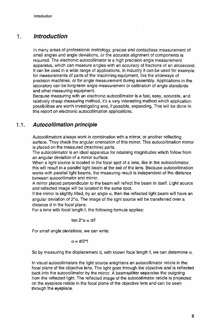
Autocollimators always work in combination with a mirror, or another reflecting surface. They check the angular orientation of this mirror. This autocollimation mirror is placed on the measured (machine) parts. The autocollimator is an ideal apparatus for retaining magnitudes which follow from an angular deviation of a mirror surface. When a light source is located in the focal spot of a lens, like in the autocollimator, this will result in a parallel light beam at the exit of the lens. Because autocollimation works with parallel light beams, the measuring result is independent of the distance between autocollimator and mirror. A mirror placed perpendicular to the beam will reflect the beam in itself. Light source and reflected image will be located in the same spot. If the mirror is slightly tilted, by an angle a, then the reflected light beam will have an angular deviation of 2*a. The image of the light source will be transferred over a distance d in the focal plane. For a lens with focal length f, the following formula applies:

tan 2*a = d/f

For small angle deviations, we can write:

u = d/2"'f

So by measuring the displacement d, with known focal length f, we can determine u.

In visual autocol/imators the light source enlightens an autocollimator reticle in the focal plane of the objective lens. The light goes through the objective and is reflected back into the autocollimator by the mirror. A beam splitter separates the outgoing from the reflected light. The reflected image of the autocollimator reticle is projected on the eyepiece reticle in the focal plane of the objective lens and can be seen through the eyepiece.

6

Introduction

Illuminator Collimator

Condenser _---t-'=

Eyepiece reticle Objective

Figure 1: visual autocollimator

In the electronic autocollimator the light source enlightens a slit in the focal plane of the objective lens. The reflected light slit is projected on a light sensitive detector, located exactly in the focal plane of the objective. In the Moller-Wedel ELCOMAT this sensors a linear CCD-array. This CCD-array measures the distance d. In the bi­directional autocollimators, there are separate measuring systems for both the X and the Y direction. The measured signals will be translated electronically into an angle deviation. By connecting the autocollimator control unit to a computer, many applications in modern measuring and controlling systems are possible.

Ob

-~-.-- .1+-_. -- - II---t-+

T lED l \oil

Figure 2: electronic autocollimator: ELCOMAT 2000

The electronic autocollimator is fit for very accurate quantitative angle measurement. This in contrast to visual ones, which are less accurate, but can be used for qualitative checking of surfaces, like the testing of image quality, focal distance or the determination of radii of curvature of spherical surfaces. For these procedures, visual autocollimators must be used which can be adjusted to a certain distance.

7

Introduction

1.2. Moller-Wedel autocollimators

Different types of autocollimators have different measuring range and different accuracy. This depends on focal length, as seen in the above formula, construction and, in electronic autocollimators, on the detection principle and the calculation algorithm in the autocollimator's control unit. A description of the acquisition of the high resolution of Moller-Wedel electronic autocollimators is given in appendix . The differences in measuring range and accuracy of the different types of Moller­Wedel autocollimators will be illustrated in the following table (lit. 1).

table 1: comparison of autocollimator types

The electronic autocollimators

Moller-Wedel has two types of electronic autocollimators: the ELCOMAT 2000 and the ELCOMAT HR:

The ELCOMAT HR is used in calibration institutes and metrology laboratories, all over the world. It is built on an ultra-stable structure made of Zerodur. The ELCOMAT 2000 is meant for measuring under normal, industrial circumstances, and must be clamped in an adjustable holder.

The ELCOMAT is connected to a control unit which can be connected to a computer so that the measuring instrument can be directly integrated in a bigger system.

8

Applications

2. Applications

2.1. Measuring the straightness of machine components

Principle

The straightness of machine components, like guide ways, or the straightness of lines of motion of machine components, can be checked with the autocollimator and a base mirror (lit. 2,3).

AK B B

J II.~'\

Figure 3: measurement principle (lit. 1)

--------L----------~

-.--

L : total length F : foot spacing n : number of meas. positions

Linear data :

j

y. = F· !. tan (l. J j _ a I

-.-~ -'-Yn

Devialion from straighlness

(l : inclination angle y : axis of measurement x : axis of travel

Deviations from straightness:

dSy{Xy =Yj' ~ • j

Figure 4: measuring straightness deviations using the angular mode (lit. 2)

9

Applications

The base mirror is moved step by step along the guide way which is to be measured. The distance between the successive positions equals the nominal span of the mirror base. When the mirror base is tilted, caused by unstraightness of the slideway, the angle of tilt will be measured by the autocollimator. With this angle a and the known base length b, the difference in height, .6h, can be calculated:

.6h = b * tan a

The slope of the line through the first and last point of the slideway depends on how the autocollimator has been set up. Therefore the measured values are usually related to a base line which has zero departure at each end. The measuring accuracy depends on the number of measuring points along the line. Many measuring pOints cause a lower accuracy. The number of measuring points is determined by the base length of the mirror. For long guide ways a longer base length is preferred. Furthermore, the accuracy can be increased by repeating the measurements. The crosshair-axes of the autocollimator should be parallel to the horizontal and vertical directions of the plane where the measured line is in. This can be approximated by slightly rotating the mirror in the horizontal plane and rotating the autocollimator round its axis, until the measured angle in vertical direction only changes very little when the mirror is rotated in the horizontal plane. It will never be reached that the vertical angle value won't change at all with mirror rotations in the horizontal plane. However, the caused measuring error will be negligible, because it's only of second order.

Figure 5: measuring the straightness of a guideway

Procedure

1. The autocollimator is placed on one end of the guide way. When this isn't possible it can be placed on a tripod, but this option could enable extra relative movements between autocollimator and mirror, which could influence the accuracy of the measurement in a negative way. With an extra deflection mirror the pOSitioning freedom of the autocollimator is even bigger.

10

Applications

2. The base mirror must be guided along a straight line. If necessary, a straightedge must be secured along the guide way. Intervals by the length of the mirror base must be marked off along the guide way.

3. The base mirror is placed on the guide way to be measured, in the position closest to the autocollimator. The autocollimator is adjusted to the mirror so that the signal is measured in the middle of the measuring range. The autocollimator light beam must be aimed at the centre of the mirror. Then the mirror is moved to the end of the guide way. The signal should still be measured. If not, then the autocollimator is adjusted so that the signal is measured in the middle of the measuring range again. After that the mirror is placed at the beginning of the guide way again, to see if the signal is still measured now. When the surface quality is questionable, one or more positions between beginning and end point are checked too. The autocollimator is adjusted until it can measure the reflected signal in all mirror positions.

4. Now measurements are made in every interval, after which the computer calculates the straightness deviations. The following example with a base length of 100 mm and a guide way length of 1000 mm illustrates the calculation.

autocollimator difference rise(-) or fall(+) cumulative adjustment error position mean from first in rise or required of

reading reading 100mm fall straightness mm seconds seconds Ilm Jlm Jlm Jlm

0 0 0 0 0 0-100 +10 0 0 0 +2 +2

100-200 +8 -2 -1 -1 +4- +3 200-300 +6 -4 -2 -3 +6 +3 300-400 0 -10 -5 -8 +8 0 400-500 +4 -6 -3 -11 +10 -1 500-600 +14 +4 +2 -9 +12 +3 600-700 +12 +2 +1 -8 +14 +6 700-800 +8 -2 -1 -9 +16 +7 800-900 0 -10 -5 -14 +18 +4

900-1000 -2 -12 -6 -20 +20 0

table 2: example of a straightness measurement (lit. 3)

11

Applications

2.2. Measuring flatness

Measuring the flatness of large surfaces is usually done by measuring the straightness in the relevant direction of a series of lines in the surface plane in a certain pattern, like the 'Union Jack' (lit. 3,4).

G

Figure 6: measuring flatness In the 'Union Jack' pattern (lit. 1)

The procedure for each line is the same as for single straightness measurements. By using an extra deflection mirror, all the lines of the pattern can be measured, while the autocollimator only needs to be placed in a few different positions. By correlating the straightness results, obtained along the lines, it is possible to determine the errors of flatness of the plane, related to a reference plane. The linking of the measurement lines at certain reference pOints (corners, centre point of the pattern) and the calculation of the reference plane are all done by the computer software.

I I I

I j I ,

FLATNESS

1600 [lIIlll

. Flatness Dev.: 17.6 ~m Ntn: (1600.999 mm / aBe.Bee mm) Max: (1333.320 ~ / 1:0.008 mm)

Figure 7: flatness diagram of a grid pattern (lit. 4)

Record :2

12

Applications

2.3. Checking of parallelism

In order to check the parallelism between two lines, two straightness measurements must always be performed. For example, these lines can be guide ways or lines of motion.

2.3.1. Checking parallelism by means of a mirror strip

Principle

A mirror strip, laid on the guide ways to be checked, serves as the reference to which the individual straightness measurements of the guide ways will be related. This way their parallelism can be checked (lit. 5).

~ 'd gUI ewey

utocollimotion mirror

ri I I

r L J

mirrQr strip

Figure 8: checking parallelism by means of a mirror strip

Procedure

1. On the ends of the guide ways to be measured, a suitable flat mirror with a surface shape deviation less than 60 nm is laid, with its reflecting side in the direction of the guide ways.

2. At the beginning of the first guide way a base mirror is positioned and the autocollimator is aligned to it. Then the base mirror is removed and the mirror strip is adjusted to the autocollimator. The measured absolute angles are noted down.

3. Then the base mirror is placed in the light beam again, and the straightness of the first guide way is measured. This measurement will be related to the mirror strip angle measurement.

4. After measuring the first guide way, the autocollimator is positioned in front of the second guide way and adjusted to the mirror strip. The absolute measured angles are noted down again, and the difference d with the mirror strip angle measurements of the first guide way is calculated. This way the positions of the autocollimator during the two straightness measurements are related.

5. The base mirror is placed on the second guide way, and the straightness of this guide way is measured.

6. The angle between the reference straight lines of the straightness normal and the datum lines formed by calculation is evaluated for each guide way. The difference between these angles or slopes is the deviation from parallelism:

13

Applications

where Ap: deviation from parallelism (11: slope of the datum line of axis 1 (12: slope of the datum line of axis 2

2.3.2. Checking parallelism by means of a pentaprism

Principle

The autocollimator is placed perpendicular to the lines to be measured (lit. 2,3). A pentaprism (see appendix 2) with known deflection error, is used for the deflection of the autocollimator light beam by 90°. This way the autocollimator can stay in the same position during the measurements of the different guide ways. Thus the measured guide ways can be related to each other, at least if the pentaprism is adjusted correctly before each guide way measurement!

nn LLLJ

mirror

guideway

pentaprism

Figure 9: checking parallelism by means of a pentaprism

Procedure

1. The pentaprism must be adjusted, so that the measured angle does not change when the pentaprism is slightly rotated round the vertical axis. This checking is very important because the pentaprism only deflects invariantly to its horizontal rotation if the plane formed by the deflected light beams is perpendicular to the secant of the pentaprism's sides. Otherwise another deflection error will be introduced.

2. After adjusting the pentaprism and the autocollimator, the first guide way is measured.

3. Then the pentaprism is moved and adjusted to the second guide way, after which the guide way is measured.

4. The angle between the reference straight lines of the straightness normal and the datum lines formed by calculation is evaluated for each guide way. The difference between these angles or slopes is the deviation from parallelism:

where Ap: deviation from parallelism (11: slope of the datum line of axis 1 <l2: slope of the datum line of axis 2

14

Applications

2.3.3. Comparison

The method with the mirror strip has the advantage that parallelism in two directions can be checked at the same time. Also the precise adjustment of the pentaprism for each guide way can be omitted. A disadvantage is the need of a long mirror strip when the guide ways are not close to each other. A long mirror with sufficient surface quality is expensive and only available to a limited length.

2.3.4. Deviations in parallelism of cylindrical bore holes and axes

Three different situations for the relative position of bore holes or axes can be distinguished (lit. 3):

• Holes or shafts are in a straight line behind each other • Holes or shafts are in parallels next to each other • Holes or shafts are in parallels above each other

These situations will be described separately.

2.3.4.1 . Holes or shafts in a straight line behind each other

Bore holes

Principle

With a mirror, attached to the head side of a spine, the deviation in parallelism between the holes can be measured. When holes with different diameters must be compared, you need a spine with different diameters or several different spines. In the last case the mirrors must all be adjusted perpendicularly to their spines. When you use one spine it just has to be oriented in the same way in all the holes, which can be easily done with mark lines on spine and holes.

Procedure

The spine is placed in the first hole and the autocollimator is adjusted until the image is reflected in the middle of the measuring range. The measured values must be registered, and the spine is placed in the next hole. Again the values must be registered, and this must be done for each hole. The differences show the angles between the bore hole axis.

Shafts

When the parallelism of shafts is to be measured, the shafts must have cylindrical parts, with the same axis as the shafts. Besides, within some distance from the shafts, there must be open space for the autocollimator light beam. On the spines, mirrors with prismatic bases are placed, high enough to put the mirror in the autocollimator light beam.

15

Applications

2.3.4.2. Holes or shafts in parallels next to each other

Bore holes

The autocollimator is placed in the plane through the holes, perpendicularly to their axis. Again the above mentioned spines with mirrors are used. The autocollimator light beam is deviated to the mirror by a pentaprism with a level. This level is needed to place the pentaprism in the same position in the vertical plane through the concerning axis, during every measurement. In the horizontal plane, the pentaprism always deviates the incoming autocollimator light beam under an angle of 90° , as a result of its optical properties, without being exactly aligned to the autocollimator.

~ I

AKF

Figure 10: checking bore holes next to each other (lit. 3)

Thus the measured angles of the bore hole axis can be compared both in the horizontal plane and in the vertical plane through the axis. Note that the accuracy of the measurement in the vertical plane also depends on the accuracy of the level.

Shafts

For checking the parallelism of shafts in parallels next to each other, a cylindrical part of the shafts, with the same axis as the shafts, can be used to place a mirror with prismatic base on it, so that the angles can be measured with autocollimator and pentaprism.

16

Applications

AK

Figure 11: checking rolls next to each other (lit. 1)

It is also possible to attach mirrors to the head sides of the shafts, which must be aligned perpendicularly to the shaft axis, and use these mirrors to measure the angles, in combination with autocollimator and pentaprism.

Figure 12: checking rolls with mirrors on head sides (lit. 6)

17

Applications

2.3.4.3. Holes or shafts in parallels above each other

When the bore holes or the shafts are in parallels above each other, parallelism in the vertical plane can be checked with the autocollimator in combination with a pentaprism.

D

Figure 13: checking bore holes above each other (lit. 1)

2.3.5. Deviations in parallelism of planes

2.3.5.1 . Planes at the same height behind each other

F

AKF

Figure 14: checking planes at the same height behind each other (lit. 3)

The autocollimator is positioned so that its light beam goes in the direction in which the planes are behind each other, in which their parallelism must be checked (lit. 3). A plane mirror is placed in the light beam on the first plane and, if there is no

18

Applications

straightedge available, adjusted to the autocollimator. The horizontal autocollimator­axis must be adjusted parallel to the plane. This can be checked by rotating the mirror with very small angles in the horizontal plane. The angular values measured by the autocollimator in the vertical direction then should only change a little bit. It would be perfect if they would not change at all, but the error made by not being parallel of autocollimator-axis to measured axis is only of second order, so it will be negligible when there are small parallelism errors between these axis. The angle in the relevant direction, perpendicular to the plane, must be measured. The mirror is placed on the next plane and adjusted to the autocollimator again, and again the angle must be measured. This must be repeated for all the planes which must be checked.

2.3.5.2. Planes at the same height next to each other

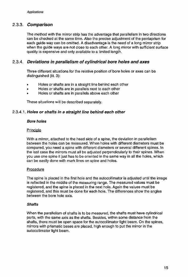
In this case the pentaprism with level must be used again, and the principle is the same as for checking parallelism of guide ways (lit. 3). The mirror is placed on a base like in the figure. The relative rotation and translation of the mirror, in the plane perpendicular to the measuring direction, between the measurements in the different planes, don't introduce extra errors. The autocollimator is placed perpendicularly to the measured planes, and the pentaprism is placed on the first plane to be measured, adjusted with the level. Then the mirror is adjusted to the autocollimator, and the autocollimator values are measured. This is repeated for each plane. The differences between the values show the deviations in parallelism.

m n I

5

I y

PP L AKF Figure 15: checking planes next to each other (lit. 3)

2.3.5.3. Planes above each other

When the planes to be checked are above each other, a mirror on a protuberance can be used. The light beam is deviated by a deviation mirror (lit. 3). When it isn't possible to use a protuberance, the pentaprism must be used again. In that case, only parallelism errors in the plane, perpendicular to the autocollimator­axis, can be measured.

19

Applications

,---- --.., E2 [L--_'_-...Jli. ... ,,··;;i

r-------, E3l,--: _' _----lll.;;;;;;;;.i

AKF u~~ ____ ~ ____ ~

Figure 16: checking by means 01 a protuberance (lit. 3)

5 d

q I ~

,.._J...1_ .,

E{tt....-_'_ '---," AKF

U ,...-L-~-L....-...--""'"

Figure 17: checking by means 01 a pentaprism (lit. 3)

20

Applications

2.4. Measuring squareness

Principle

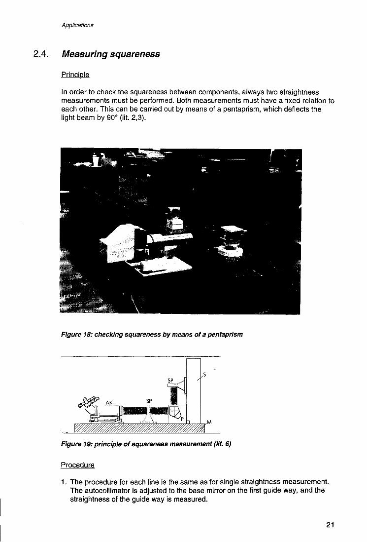
In order to check the squareness between components, always two straightness measurements must be performed. Both measurements must have a fixed relation to each other. This can be carried out by means of a pentaprism, which deflects the light beam by 900 (lit. 2,3).

Figure 18: checking squareness by means of a pentaprism

s

Figure 19: principle of squareness measurement (lit. 6)

Procedure

1. The procedure for each line is the same as for single straightness measurement. The autocollimator is adjusted to the base mirror on the first guide way, and the straightness of the guide way is measured.

21

Applications

2. The pentaprism, with known deflection error, is placed in the autocollimator light beam, so that the by 90° deflected beam is directed at the base mirror which is moved to the second guide way.

3. The second guide way is measured. 4. The evaluation follows as in the manual. In the straightness evaluation, the angle

between the reference lines of the straightness normal and the datum lines formed by calculation. This angle is printed out as slope of the line. By linking the angles (slopes <lx,<ly) in accordance with the formula shown in figure 20, the squareness deviation is obtained. Using this formula the following applies to the relation between the slope values (<lx,<ly) and the number of the axis (1 or 2)

Ct ,Ct : Slope of reference line x y

6.g0 : Squareness error

6 N : Error of reference square

e = 90° - Ct - Ct x y

1\ =6 -0: -0: "-'90 N x Y

.......

Figure 20: definition of the prefix when evaluating squareness deviations (lit. 2)

If the angle between the lines of motion is smaller than 90°, a negative squareness deviation is outputted. An angle bigger than 90° is characterised by a positive deviation. When calculating the square ness error, the angle error of the reference square, in this measurement this is the pentaprism deflection error, must be taken into account.

2.4.1. Squareness between planes

Principle

When the squareness between two planes is to be measured, the directions perpendicular to the secant of the two planes must be found. This can be achieved by placing a planparallel mirror against the plane facing the autocollimator, and adjusting the autocollimator to it (lit. 3). Then the base mirror is placed in the light beam on the first plane, and adjusted to the autocollimator. After that, the straightness of the line in the first plane is measured. A straightedge can be used to guide the base mirror along a straight line. After the measurement of the first plane,

22

Applications

the base mirror is placed on the second plane and adjusted to the autocollimator by means of the pentaprism. Then the second line can be measured just like the first one.

2.4.2. Examples

2.4.2.1. Squareness between a vertical spindle and a machine bed

With an adjustable planparallel mirror as a reference for the spindle axis and a planparallel mirror for adjusting the autocollimatorto·the machine bed M, the square ness between the spindle and the bed can be checked (lit. 6).

Figure 21: squareness between a vertical spindle and a machine bed (lit. 6)

Procedure

1. The autocollimator is aligned to the spindle mirror S2: it is aimed at one mirror surface and set to zero. Then the mirror is turned over, and the angle is measured. This angular value is divided by two and both the mirror and the autocollimator are adjusted by this value so that the measured angle is zero.

2. Now mirror S1 is placed on the bed. The squareness deviation is the difference between the angles measured on the two mirrors, but because 82 was set to zero, it is the angle measured on mirror S1. Instead of taking only this one position of 81, it would be better to measure a whole line on the bed, and compare this to the spindle mirror, but mostly one position of 81 will do.

2.4.2.2. Squareness of a spindle to a matrix-axis.

With adjustable flat mirrors as references for the spindle axis and the matrix axis and a pentaprism, the squareness between the spindle and the matrix-axis can be checked (lit. 6).

Procedure

1. The mirrors S are adjusted perpendicular to their axes Sd and H. 2. The autocollimator is adjusted to the mirror on Sd. 3. With a pentaprism the mirror on H is checked. 4. Squareness can be determined, with notice of the pentaprism deflection error.

23

Applications

Figure 22: squareness of a spindle to a matrix-axis (lit. 6)

2.4.2.3. Squareness between a spindle column and a machine bed

With a adjustable flat mirror as a reference for the spindle axis, a base mirror as a reference for the machine bed, an adjustable mirror, clamped under 90°, as a reference for the spindle movement, and a pentaprism, the squareness between the machine bed and a spindle column and -movement can be checked (lit. 6).

Figure 23: squareness between a spindle column and a machine bed (lit. 6)

Procedure

1. Mirror 51 is adjusted perpendicular to the spindle axis 5d. 2. The autocollimator is adjusted to 52 on the machine bed and set to zero. 3. 52 is removed so that 51 is measured. 4. The measured angle is the squareness deviation. 5. With a pentaprism and mirror 53 the straightness of the spindle movement, and

the squareness between this movement and the bed can be checked ..

2.4.2.4. Squareness between a spindle and a movement direction

On a machine bed M a support F with a column B is moved. The column B carries a spindle A, which rotational axis should make a right angle with the movement direction of the column (figure 24). This angle can be checked as follows (lit. 3):

24

Applications

Procedure

1. A planparallel mirror 81 is adjusted parallel to the rotational axis, by turning it over to the autocollimator.

2. Mirror 82 is adjusted parallel to the movement direction, with a microcator. 3. The autocollimator measures the angle on mirror 81. 4. Mirror 82 is measured with the pentaprism. 5. The squareness deviation is determined with regard of the pentaprism deflection

error:

Where

s

A

A

Aa= aS2-aSl+S

Ila:= the squareness deviation (lS1= angle measured on mirror 81 (lS2= angle measured on mirror 81 0= deflection error of the pentaprism

I

S,

Figure 24: squareness between a spindle and a movement direction (lit. 3)

25

Applications

2.5. Measuring the wedge deviation of parallel planes

2.5.1. Outer planes

Principle

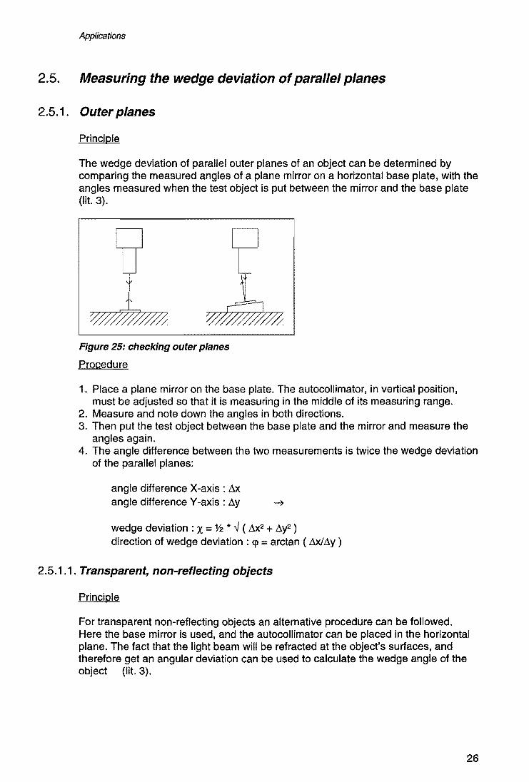
The wedge deviation of parallel outer planes of an object can be determined by comparing the measured angles of a plane mirror on a horizontal base plate, with the angles measured when the test object is put between the mirror and the base plate (lit. 3).

Figure 25: checking outer planes

Procedure

1. Place a plane mirror on the base plate. The autocollimator, in vertical position, must be adjusted so that it is measuring in the middle of its measuring range.

2. Measure and note down the angles in both directions. 3. Then put the test object between the base plate and the mirror and measure the

angles again. 4. The angle difference between the two measurements is twice the wedge deviation

of the parallel planes:

angle difference X-axis : ~ angle difference Y-axis : ~y ----7

wedge deviation: X = Y2 * ....j ( ~2 + ~y2 ) direction of wedge deviation: <p = arctan (ilXI~y)

2.5.1.1. Transparent, non-reflecting objects

Principle

For transparent non-reflecting objects an alternative procedure can be followed. Here the base mirror is used, and the autocollimator can be placed in the horizontal plane. The fact that the light beam will be refracted at the object's surfaces, and therefore get an angular deviation can be used to calculate the wedge angle of the object (lit. 3).

26

Applications

au tacall imator object bose mirror

Figure 26: checking transparent objects

Procedure

1. First a measurement is taken with only the base mirror in front of the autocollimator. The angles are noted down.

2. Then the object is placed between the autocollimator and the base mirror, and another measurement is taken.

3. For small angle deviations 0, the following formula applies:

0=x*(n-1)

where n is the refraction index. So in this case we can write:

x == { Y2 * ..J ( ffi(2 + Ay2 ) ) I ( n - 1 )

2.5.2. Inner planes

Principle

For measuring the wedge error of inner planes a pentaprism is needed (lit. 3). This prism deflects the autocollimator beam of the autocollimator which is placed with his axis parallel to the surfaces to be compared.

Figure 27: checking inner planes

27

Applications

Procedure

1. The autocollimator is placed with the autocollimation axis parallel to the planes to be measured, and is adjusted to its level. It doesn't need to be adjusted exactly in the horizontal plane.

2. The pentaprism is placed between the planes, and adjusted horizontally with a level. It is placed so that it deflects the autocollimation beam on one of the surfaces to be measured.

3. The first measurement is noted down. 4. The pentaprism is repositioned, so that it deflects the beam on the other plane,

and is adjusted again. 5. The second measurement is noted down. 6. The wedge error of the planes simply follows by subtracting the two measured

angles, with noticing the pentaprism's deflection error (see appendix 5).

28

Applications

2.6. Checking of measuring and manufacturing machines

Besides the already mentioned general methods there are some more specific procedures (lit. 3) for the checking of machines, like the checking of

• pitching and yawing of parts • deformation of parts • errors of spindles

2.6.1. Pitching and yawing

Principle

In the construction of machine axes the principle of Abbe can't always be met. Especially when measuring table or support can move in several perpendicular directions. The measured distances of ruler and measured object are not on the same line but in parallels next to or under each other. pitching and yawing will cause first order errors, but can be measured very accurately with the electronic autocollimator. with these and the relevant distances between ruler and measured object, it is possible to see if the resulting errors are negligible.

z· I yaw

CD I ,rx-'V

XJ. pitch

Figure 28: rotary motions of a machine carriage (lit. 2)

Procedure

1. A plane mirror is placed on the table, perpendicular to the table movement, the autocollimator is placed on the machine itself. Or the autocollimator is placed on the table and the plane mirror on the machine. The autocollimator can also be placed on a tripod next to the machine. For very accurate measurement, a measurement of the machine movement could be made, at the same time, to check the relevant movement of machine and table, in that case. Therefore a second mirror is attached to the machine. A second autocollimator is used, so that the two autocollimator synchronously measure with one mirror each.

2. Adjust the autocollimators so that angle deviation is measured in the middle of the measuring range.

3. The table is moved in steps, of which the size depends on the standards of the measured machine and the desired number of measuring points. Rotations in both directions can be measured at the same time with the two axes

29

Applications

autocollimator. When the machine ruler is below the measured distance of the measured or manufactured object, then the vertical deviations are relevant. Is it besides of it, in the horizontal plane, then the horizontal deviations are relevant to determine if the resulting errors are negligible or not. When there are rulers in both directions, both horizontal en vertical deviations are relevant.

4. To separate accidental errors, caused by dust or irregularities of the table bearings, from the systematic errors, measurements must be repeated. The systematic errors can be caused by guide way errors or deformations of the machine.

5. When relative measurements, with more mirrors, are made, it's not necessary to start at a certain zero level, because only the differences between the two mirrors are important.

6. It can be wise to read the autocollimator values while changing the table movement direction. Because of the different positioning forces, the table could take different positions.

7. The angle deviations should also be checked during the movements of the table from one measuring position to another to see if extreme or unexpected values occur between the measured pOints.

2.6.2. Deformation of machine parts

Some typical deformation situations are described here:

2.6.2.1. Deformation of support and machine bed during support movement

Principle

When a support or table is moved on a machine bed, the bed can deform, but the support itself can also deform, if it is not moving on fixed rolls, but on loose ones, which can change their position in relation to the support. These deformations can change with the load, carried by the support.

s /

T

M

Figure 29: checking with autocollimator placed on the machine (lit. 3)

Procedure

1. With bigger machines the autocollimator can be placed on one end of the slideway, a mirror on the other. During movement of the slide, the change in angle between mirror and autocollimator are measured. With smaller machines the autocollimator is placed next to the machine, and two mirrors are used, each attached to one end of the machine bed, to measure its deformations during slide movement.

30

Applications

2. Two measurement series have to be made; one with each mirror. This can be done with one autocommator in successive series, or synchronously with two autocollimators.

3. Angular differences between the measurement results on the first and the second mirror indicate deformations of the bed during table movement.

For checking of the table or support deformations during it's own movement, the mirrors should be attached to the ends of the table or support and the same procedure as for the bed is repeated.

I I

m

I I

T

•

I ____

n ,

I I , G

[CtL}~-----

I

Ii

Figure 30: checking with autocollimator placed next to the machine (lit. 3)

2.6.2.2. Deformation of a measuring head, during changing of force direction

Principle

Changing of the force direction during measurement with a coordinate measuring machine can cause various deformations in the bearings of the measuring head and in the measuring head itself. These deformations can result in measuring errors. The location of these deformations within the measuring head can be determined with help of the autocollimator: by putting small mirrors on several parts of the measuring head, relative angle measurements can be made by comparing the results from the different mirrors. This can be done with one autocollimator, using several mirrors successively, or more autocollimators (one for each mirror) for faster and more comfortable measurement (figure 31).

Procedure

1. Attach several mirrors to the different parts of the measuring head. 2. A measuring surface is moved from one side against the head, until it measures

zero. 3. The autocollimator is set to zero. 4. Measuring direction of the head is reversed. 5. Now another measuring surface approaches the head from the opposite side.

31

Applications

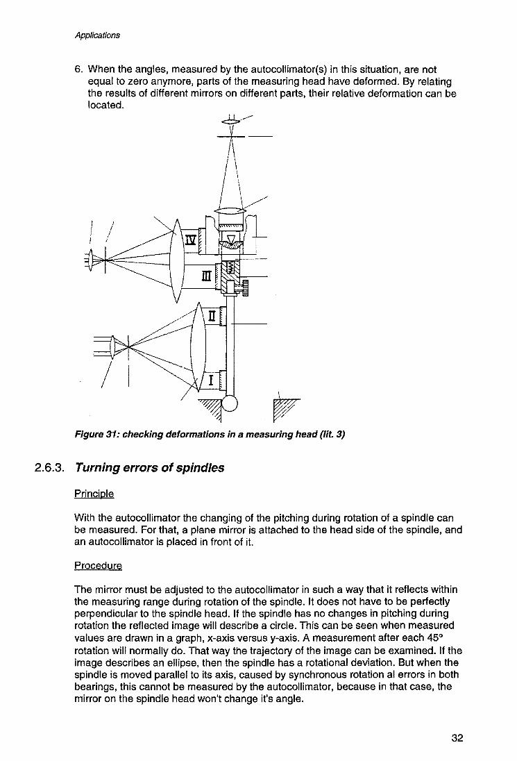
6. When the angles, measured by the autocollimator(s) in this situation, are not equal to zero anymore, parts of the measuring head have deformed. By relating the results of different mirrors on different parts, their relative deformation can be located.

~

iI-I \

\

Figure 31: checking deformations in a measuring head (lit. 3)

2.6.3. Turning errors of spindles

Principle

With the autocollimator the changing of the pitching during rotation of a spindle can be measured. For that, a plane mirror is attached to the head side of the spindle, and an autocollimator is placed in front of it.

Procedure

The mirror must be adjusted to the autocollimator in such a way that it reflects within the measuring range during rotation of the spindle. It does not have to be perfectly perpendicular to the spindle head. If the spindle has no changes in pitching during rotation the reflected image will describe a circle. This can be seen when measured values are drawn in a graph, x-axis versus y-axis. A measurement after each 45° rotation will normally do. That way the trajectory of the image can be examined. If the image describes an ellipse, then the spindle has a rotational deviation. But when the spindle is moved parallel to its axis, caused by synchronous rotation al errors in both bearings, this cannot be measured by the autocollimator, because in that case, the mirror on the spindle head won't change it's angle.

32

Applications

t--

AKF

t--

5 J L

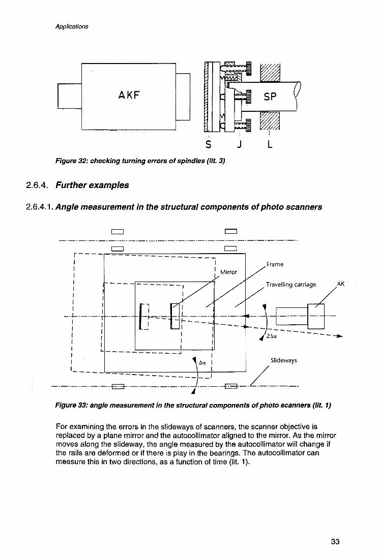
Figure 32: checking turning errors of spindles (lit. 3)

2.6.4. Further examples

2.6.4.1 . Angle measurement in the structural components of photo scanners

c:::::J r - - - -r--""=-=-'"'=_="_=-=_:-:_:::-=-_-_-_-_-_-_-_-_-_-_----, I I I I I ----------I I

-.L.---.: --.-. E',~-=-, L. ___ _ I I ~---~ I, I, I, I, 'I I I I L--- ________

J

Frame

Travelling carriage

I I , "ACt I Slideways

1------ I L ---------------, -.-.-.-.----~.------------~-----~--. ---------

Figure 33: angle measurement in the structural components of photo scanners (lit. 1)

For examining the errors in the slideways of scanners, the scanner objective is replaced by a plane mirror and the autocollimator aligned to the mirror. As the mirror moves along the slideway, the angle measured by the autocollimator will change if the rails are deformed or if there is play in the bearings. The autocollimator can measure this in two directions, as a function of time (lit. 1).

AK

33

Applications

2.6.4.2. Testing the ram movement on 3D-coordinate measuring machines

Mirror strip

Precision guide

-. - Ram

51'

AK

Figure 34: testing of the ram movement on 3D-coordinate measuring machines (lit. 1)

The electronic autocollimator can test the pitch and roll movement of a ram, with help of a mirror strip. The accuracy depends on the flatness of the mirror strip (lit. 1). However, these mirror strips are very expensive, and can only be produced to a certain length with the demanded accuracy. It would be much better if a method could be developed where the roll-angle is directly measured by the autocollimator. More on this is written in chapter 3.1.

34

Applications

2.7. Checking of polygons and circular dividing heads

Principle

With one autocollimator and a polygon with known polygon error, the table error of circular dividing heads and other rotation tables can be checked. It is also possible to check a polygon with unknown polygon error with a table with known error. With an extended procedure a polygon and a table, both with unknown errors, can, be checked, also with only one autocollimator. Another method, which will not be discussed extensively here, is to use two autocollimators, where the errors are determined in one measurement series. This method requires approximately the same calculation algorithm as the method here described. But because of the need of a second autocollimator this method is much more expensive(lit. 3).

The table error is comprised of radial and axial movements, the inClining error and the actual table error. We can determine the following parameters (see appendix 4)(lit. 7):

• angular table error • inclining error of the table • polygon error • pyramidal polygon error relative to the polygon reference surface

If the polygon error is known, then it doesn't need to be determined.

I

.-s)I". Figure 35: checking a polygon (lit. 6)

Procedure

For all the error measurement types mentioned above, the following preparations are required (lit. 8):

The polygon is mounted on the table axis. Make sure to check the numbering of the polygon surfaces and of the table positions. The table is rotated to its initial position. The polygon surface 1 is now in autocollimation position to the autocollimator. The rotation axes of the polygon and the table are aligned parallel to each other. The polygon doesn't have to be centred to the rotation axis of the table. The autocollimator is aligned to the first polygon mirror. The measured absolute value is set to zero. Then the table is rotated over 1800

, for an even number of mirror

35

Applications

surfaces, so that the mirror opposite of the first one is in autocollimation position. Now the angle deviation between the polygon axis and the table axis is measured. This value is divided by 2. Both the autocollimator and the polygon are tilted by this value so that the measured tilt is zero. After that the table is returned to the first position, and the described procedure is repeated until the measured tilt remains approximately zero, also after rotation of the table. It's recommendable to execute this procedure not only in 1800 steps, but also in 900

steps. After this alignment, the measurement can start.

2.7.1 . Determination of the table error

2.7.1.1. Determination of the table error with known polygon error

The measurements begin with table position '1' and then continue successively to the n-th position (n stands for the number of polygon surfaces). The last measurement in a series is again table position '1'. There are two measurements for the reference position: 0° and 360°. For table error determination with a polygon with known error, only one measurement series need to be executed (lit. 3,7,8). However, when more measurement series are made, the measuring uncertainty will be smaller. If more measurement series are made, do not rotate the polygon relative to the table, for each new series of measurements.

2.7.1.2. Determination of the table error with unknown polygon error

For determining the table error with a polygon with unknown error, there are two measuring methods (see appendix 4) (lit. 7):

• The Rosette method • The setting up of a linear equation system

Rosette method

In this method, for a polygon with n mirror surfaces, n measurement series are executed. Rotate the polygon exactly one position relative to the circular dividing head for each individual series of measurements. No special order of rotation is required, but errors which can impair the results are made more easily when the surfaces are not rotated in successive order. Therefore it is best to first have surface 1 in the preliminary alignment, then surfaces 2, 3, etc. until the last surface coincides with original position 1 of table position '0'.

The advantages of this method are high statistical accuracy, because of the high number of measurement series, and the exact determination of the polygon error. This method can also be used when the polygon error is known. Even when a wrong foolish error value is taken in, still the correct results will be obtained. If the polygon error is not known, it will automatically be determined.

36

Applications

A disadvantage is that much work is involved, for example a polygon with 12 surfaces requires 12 measurement series with 12 individual measurements each, these are 144 measurements altogether.

Setting up and solving an equation system

For a polygon with n surfaces, [n -1] table errors and [n - 1] polygon errors need to be determined. For example, a total of 11 table errors and 11 polygon errors have to be determined for a polygon with 12 surfaces. Therefore a minimum of 22 independent linear equations have to be set up, which must be derived from at least 2 measurement series. The polygon has to be rotated at least exactly one position relative to the dividing head. Otherwise a solution for the equations cannot be found.

Only 2 measurement series are needed to mathematically determine the polygon error and the table error: then there is always an exact solution for the equation system (see appendix 4). Therefore measurement errors will go undetected. With only two measurement series, acceptable results will only be obtained with a very high accuracy of the autocollimator and a high accuracy of adjustment of the table. So, for higher measuring certainty, it is wise to execute more then two measuring series. However, the polygon errors can be determined by calculation and then automatically correct the data of the table error.

This method is more effective than the rosette method, because only a few measurement series are needed to automatically determine the polygon errors and incorporate them.

2.7.1 .3. Determination of the backlash

The backlash of a specific dividing head position is obtained by subtracting the deviations of all positions. These are obtained by either rotating the dividing head one position in the positive and in the negative direction respectively (lit. 7). The more effective method is by executing the measurements clockwise and counter clockwise for the measurement series.

2.7.2. Determination of the inclining error of the table and the relative pyramidal error of the polygon

Information of the inclining error of the table, can only be obtained with a two axial autocollimator. The inclining error for table pOSition '0' is set to zero. All errors will refer to this position. This procedure well defines the inclining error (lit. 7). However, when the pyramidal error of the polygon is not known, this procedure is not very helpful in determining this pyramidal polygon error; polygon surface 1 has its own individual pyramidal error, which is fairly complicated to determine. In order to do so the y-axis of the autocollimator has to be aligned exactly parallel to the theoretical axis of rotation of the polygon, and no displacement, would be allowed to occur when the polygon is rotated relative to the table.

37

Applications

However, if the absolute pyramidal error of at least one surface is known (can be determined with a different method of measurement, see appendix 4) the absolute values of the other surfaces can be determined by using the relative values. Here too, a minimum of two independent measurement series are necessary to determine an unknown pyramidal error, between which the polygon has to be rotated at least one position relative to the table (see appendix 4).

38

Applications

2.8. Checking of prisms

Nowadays prisms are mostly checked with a goniometer (lit. 5). This is a measuring instrument with a turntable, a collimator and a visual autocollimator. The accuracy of the visual autocollimator is high enough to measure in combination with the turntable. The accuracy of the turntable is about 1 n. Therefore it's not necessary to use an electronic autocollimator for this measurement; it would be much more expensive, and apart from that, the electronic autocollimator is much heavier than a visual one, so a heavier construction would be necessary.

Nevertheless, there are some methods for checking prisms, in which electronic autocollimators are applied. Some will be explained shortly here.

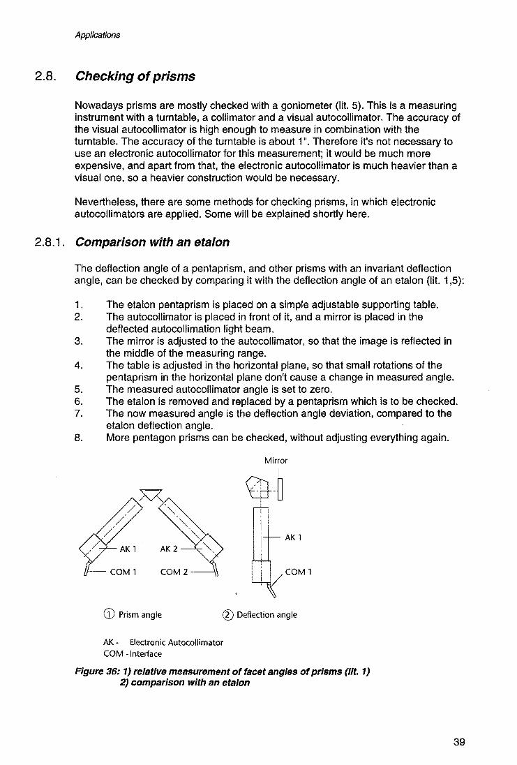
2.8.1. Comparison with an eta/on

The deflection angle of a pentaprism, and other prisms with an invariant deflection angle, can be checked by comparing it with the deflection angle of an etalon (lit. 1,5):

1. The etalon pentaprism is placed on a simple adjustable supporting table. 2. The autocollimator is placed in front of it, and a mirror is placed in the

deflected autocollimation light beam. 3. The mirror is adjusted to the autocollimator, so that the image is reflected in

the middle of the measuring range. 4. The table is adjusted in the horizontal plane, so that small rotations of the

pentaprism in the horizontal plane don't cause a change in measured angle. 5. The measured autocollimator angle is set to zero. 6. The etalon is removed and replaced by a pentaprism which is to be checked. 7. The now measured angle is the deflection angle deviation, compared to the

etalon deflection angle. 8. More pentagon prisms can be checked, without adjusting everything again.

Mirror

AK 1

COM 1

CD Prism angle CD Deflection angle

AK - Electronic Autocollimator COM -Interface

Figure 36: 1) relative measurement of facet angles of prisms (lit. 1) 2) comparison with an eta/on

39

Applications

2.8.2. Relative measurement of facet angles of prisms

Relative measurement of facet angles of prismatic specimens with specular reflecting surfaces can be performed by means of two autocollimators (figure 36, lit. 1,5). This method has the advantage that no precise adjustment has to be done, and can therefore be done very quickly:

1. Two autocollimators are placed in front of supporting table. 2. A prism is placed on the table. 3. Each autocollimator is adjusted to one prism surface. 4. The measured autocollimator angles are set to zero. 5. Another prism can be placed on the table without precise adjusting, and the

autocollimator angles are read. 6. The facet angle can be compared to the facet angle of the other prism, simply

by subtracting the angles, measured by the two autocollimators. The result is the difference between the compared facet angles.

7. More prisms can follow.

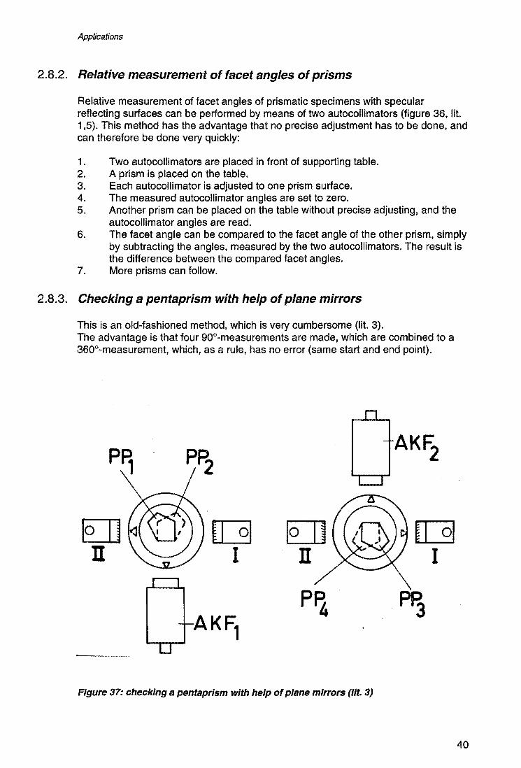
2.8.3. Checking a pentaprism with help of plane mirrors

This is an old-fashioned method, which is very cumbersome (lit. 3). The advantage is that four gOo-measurements are made, which are combined to a 360°-measurement, which, as a rule, has no error (same start and end point).

Pf2

[Jl [[] OJ [[g n I n I

AKF, PF4 Pf3

--~---~""

Figure 37: checking a pentaprism with help of plane mirrors (lit. 3)

40

Applications

Procedure

1. A planparallel base mirror is placed on a simple turntable, and the autocollimator is aligned to it.

2. The pentaprism is placed on the turntable in stead of the two-sided mirror, and two plane mirrors are placed at both sides of the turntable, parallel to the autocollimator-axis.

3. The pentaprism is rotated with the turntable so that the light beam is deflected on mirror 1. This mirror is adjusted to the autocollimator. The measured x­angle value is noted down.

4. The pentaprism is rotated over 900 so that its previous exit plane now becomes entrance plane. The light beam is now deflected on mirror 2, which is adjusted so that the measured angles are approximately the same as the ones measured with mirror 1. The angle in x-direction is noted down again.

5. Now the autocollimator is placed on the opposite side of the turntable, or a second autocollimator is used. The use of two autocollimators is recommended when serial measurements must be made.

6. The pentaprism is rotated over another 900, still deflecting on mirror 2.

7. Now the autocollimator is adjusted to it, and the x-angle is measured. 8. Another rotation of the pentaprism over 900 follows, and a measurement is

made. 9. Calculation of the deflection error deviation follows as in appendix 5.

41

Applications

2.9. Calibration applications

The electronic autocollimator is used for many different calibrations where accurate angular checkings are required. Examples of calibration methods where electronic autocollimators are involved, follow here.

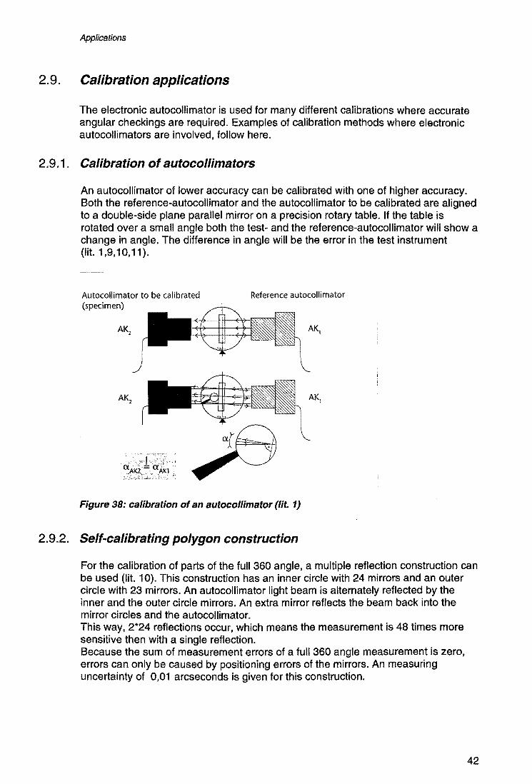
2.9.1. Calibration of autocollimators

An autocollimator of lower accuracy can be calibrated with one of higher accuracy. Both the reference-autocollimator and the autocollimator to be calibrated are aligned to a double-side plane parallel mirror on a precision rotary table. If the table is rotated over a small angle both the test- and the reference-autocollimator will show a change in angle. The difference in angle will be the error in the test instrument (lit. 1,9,10,11).

Autocollimator to be calibrated (specimen)

Reference autocollimator

AKl

AKl

Figure 38: calibration of an autocollimator (lit. 1)

2.9.2. Self-calibrating polygon construction

For the calibration of parts of the full 360 angle, a multiple reflection construction can be used (lit. 10). This construction has an inner circle with 24 mirrors and an outer circle with 23 mirrors. An autocollimator light beam is alternately reflected by the inner and the outer circle mirrors. An extra mirror reflects the beam back into the mirror circles and the autocollimator. This way, 2*24 reflections occur, which means the measurement is 48 times more sensitive then with a single reflection. Because the sum of measurement errors of a full 360 angle measurement is zero, errors can only be caused by positioning errors of the mirrors. An measuring uncertainty of 0,01 arcseconds is given for this construction.

42

Applications

AuBenspiegel

Zusatzspiegel

Figure 39: principle of multiple reflection (lit. 10)

2.9.3. Calibration of arbitrary angular normals

The autocollimator is used for calibration in the direct method, of angular normals, in combination with an indexing-table (lit. 10). This means that an angular normal is paced on the table, and before and after a table rotation of the normal's angle the an autocollimator measurement is made. The normal's error can be directly determined.

2.9.4. Calibration of small-angle angular normals

II

'f-e'=a=~---I A KF 1

""I Figure 40: calibration of small-angle angular normals (lit. 10)

The autocollimator is used for the calibration of angular normals with angles smaller than 20 arcseconds (lit. 10). Two autocollimators are needed in combination with a rotation-table. One autocollimator is aimed at a plane mirror, which is placed on the rotation-table. This autocollimator is only for checking that the table doesn't rotate during the measurements. The other autocollimator is aimed at the angular normal, which is placed against fixations on the rotation-table. The angle is measured before and

43

Applications

after turning over the angular normal, after which the deviation of the normal's angle can be determined. If the normal has an error d, the reflected image has an error 2d. In two measurements, an error 4d is measured.

2.9.5. Calibration of slope-meters.

In coordinate-measurement slope-meters are used increasingly for the automatic measurement of rotational guideway errors. For the calibration of such meters, a vertically rotatable, precisely adjustable table is used, where an autocollimator, with adequate accuracy according to its calibration certificate, can serve as angle-embodiment (lit. 10).

3

4

l

5

.2

Funktionsschema'eines Neigungsmessers

1 Rahmengehause, 2 Wegaufnehmer, 3 Blattfeder (Kunststoff),

4 Pendelstab, 5 Pendelgewicht mit MeGflache, 6 Dampfungselement,

7 Silikonol

Figure 41: slope meter (lit. 10)

44

Applications

2.10. Other application examples

2.10.1. Adjusting high precision elements with mechanical impulses

The autocollimator can be used in an automatic adjustment construction, which enables an exact adjusting of high precision and optical construction-elements, with the following procedure (lit. 12):

1. The construction-element to be adjusted are fixed with definite fixation force. 2. Mechanical impulses are transmitted to the element by means of beating

magnets. 3. Stepwise adjusting-movements are generated in the form of small angular

changes by the stick-slip effect. 4. The positioning-optimisation follows by means of a computer and an

autocollimator, which checks the position of the construction- element.

Positionserkennungssystem %. B. M<:F

~.-.-.-~.'-~.~.-.---''F-.

Schlagwerk mttllier

Zuf1l1agne1tn

Steuergerat N1I manuellen und

l!lJ!<lmdschen Betrieb

Figure 42: set-up for adjusting high precision elements with mechanical impulses (lit. 12)

This principle guarantees a cheap, simple and fast solution for adjusting problems, the automatizability and the remote-controllability of adjusting procedures. Applications in industry can be thought in internal positioning-optimising in instruments. In the laboratory it can be used for rotating or centring mirror-optics and fine construction-elements.

2.10.2. Integration in automatic assembly lines

Via standard interfaces the electronic autocollimator can be integrated in monitoring and assembly systems (lit. 1). A computer can compare the actual angle values of several autocollimators with the nominal values and compensate the deviations by suitable adjustment and control devices:

• Monitoring the position of a mUlti-axis system

45

Applications

Figure 43: monitoring the position of a multi-axis system (lit. 1)

• Automatic mirror adjusting during assembly

AK.Display

o

Figure 44: adjusting a mirror to the optical autocollimator-axis (lit. 1) SM: stepping motor ASE: control unit

Autocollimator /

SM

AK·Head

AK-Display o Control unit ASE

Figure 45: adjustment of an optical set-up using an electronic autocollimator (lit. 1) SM: stepping motor ASE: control unit

46

Applications

2.10.3. Long-term drift and stability studies

arcsec

o

By connecting the control unit of the electronic autocollimator to a computer, it is possible to make long-term studies on the stability and drift properties of equipment to develop angle scanning units, etc. (lit. 1).

Autocollimator

i

AK-Display

Figure 46: long-term drift and stability studies (lit. 1) SM: stepping motor ASE: control unit S: mirror

-D,S .............................................................................................................................................................................................................. .

-, o 10 20 30 40 50 60 h

Figure 47: long term drift studies of a positioning set-up with stepping motor (lit. 1)

47

Research

3. Research

3.1. Measurement of twist

In manufacturing machines, a very important source of error is the rolling of slide ways, that's the rotation around the axis in the direction of movement. Unfortunately this is a very difficult thing to measure with acceptable accuracy. Therefore it would put the autocollimator in a preferable position in machine measurement, if it could be adapted to measure pitch, yaw and roll of a slide way at the same time in one measurement series (lit. 13,14,15). The advantages would be the high resolution and the large working distance, characteristic for the autocollimator, and the use of simple, common, relatively cheap components. Until now methods for roll measurement in which autocollimators have been used, always needed further instruments like an additional single or dual-axis autocollimator mounted on the Z-axis and directed toward an additional reflector. This could be a plane mirror mounted adjacent to the roof prism, or an aluminised area on the hypotenuse face of the latter. Gr the off-axis autocollimator is replaced by single-function instruments: a projector, placed in the XZ plane on one side of the Z axis, directs a collimated light beam at a roof prism, placed with its roof edge parallel to the X-axis, which reflects the beam to a receiver on the opposite side of the Z-axis (lit. 13).

Figure 48: separate collimator and sensor (lit. 13)

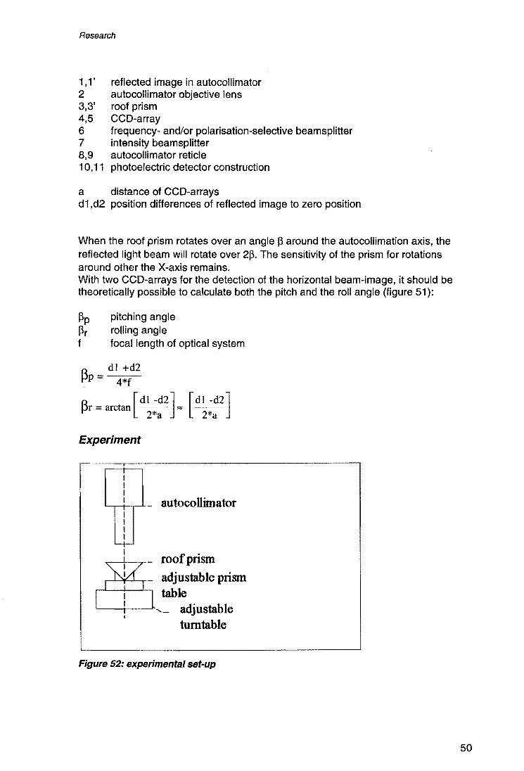
When pitch, yaw and roll need to be measured simultaneously with only an autocollimator, a conceptual change in the autocollimator construction seems to be necessary. An idea for different detector configuration, in combination with separation of the horizontal and vertical light beam at the reflector is explained here (lit. 14,16).

Principle

The idea is to use an autocollimator with a roof prism as reflector (figure 49). The reflected image will change its location when the prism is rotated round the autocollimator axis: the roll angle would be half the angle by which the reflected beam changes direction relative to the primary beam (figure 50).

48

Research

When a roof prism is used as reflector, rotation about the "roof" edge (the intersection of the reflecting surfaces) has no effect on the direction of the reflected beam. Therefore a different reflection method must be used to measure this rotation. To measure these rotations about the V-axis, the vertical beam of the light cross must be reflected separately. at the front surface of the roof prism. The horizontal beam of the light cross should be used for measuring roll and rotation round the X-axis.

:<2..11

--P.··=-1SJ __ i ! ~

10 : -r r 7 FZr: 6 /';;2

. .l.r ..... _ .. E2J ..... _. :""~,,-,,,-,~,,,,,: . __ ........ ..... 1..\ ..... _ -- .. . U ' I '\ \'

I 'I \ I n 8 \

I I

Figure 49 (lit. 14)

11 I 11

II I i

~L~ __~_1LjT I 1

4 ~ 5 ! a I i~<----~)I

Figure 50 (lit. 14) Figure 51 (lit. 14)

In the figures 49-51:

49

Research

1,1' reflected image in autocollimator 2 autocollimator objective lens 3,3' roof prism 4,5 CCD-array 6 frequency- and/or polarisation-selective beamsplitter 7 intensity beamsplitter 8,9 autocollimator reticle 10,11 photoelectric detector construction

a distance of CCD-arrays d1 ,d2 position differences of reflected image to zero position

When the roof prism rotates over an angle p around the autocoliimation axis, the reflected light beam will rotate over 2p. The sensitivity of the prism for rotations around other the X-axis remains. With two CCD-arrays for the detection of the horizontal beam-image, it should be theoretically possible to calculate both the pitch and the roll angle (figure 51):

Pp pitching angle Pr rOiling angle f focal length of optical system

A _ dl +d2 tJP - 4*f

~r = arctan [dl -d2]= [dl -d2] 2*a 2*a

Experiment

autocollimator

~-+---,-_ roof prism

r--'--"I'-'-..-- adjustable prism table

'------1----", _ adjustab Ie turntable

Figure 52: experimental set-up

50

Research

In an experimental set-up where a roof prism with a non-reflecting top surface on a small adjustable table, was placed on a bigger adjustable turntable, the situation of roll measurement is simulated (see figure ), the movements of the image of the autocollimation signal are observed with a visual autocollimator. Depending of the way the prism is adjusted to the autocollimator, the image describes different curves:

1. When the turntable is adjusted first to the autocollimator, by means of a flat mirror on the table surface, and after that the prism with its table is adjusted, a situation is simulated where only roll occurs, when the turntable is rotated round its axis. Then the image cross hair rotates with double turntable frequency.

2. When the turntable is adjusted and the prism is not, the image describes the same rotation around his on mid point, but also a circular track round the ocular middle.

3. When the turntable and the prism are both adjusted, and after that the whole is disturbed by pitching the turntable, the circular track is described round another as the ocular middle point.

4. When nothing is adjusted, a very strange curve is described, of which the relations of shape, radius and frequency change dependent of the relative pitching of the different axis.

I I I I

I I I I I I I I !

~ I

~/ I

@l !~ I I I I I I I I / I I

/ I I I I I I / I I I

~ I I I I f I v> W I I I W 1/ I I

I I I I } I I I I I 1 / I /

I I / I I I I I I I I I / I / I I 1/ 1/ I I r t I I I 1 I I 1 I I I 1 I I I I I

Figure 53: different adjusting situations

The last situation occurs when pitching, yawing and rolling happen at the same time. The question is how the different rotations influence the movements of the autocollimation image. The rotation of the image-crosshair round his own middle should only be caused by roll, and always keeps the double frequency of the roll-angle of the roof prism. The circular track of the image should then be caused by prism rotation round the other axis, perpendicular to the roof edge.

3.1 .1 . Discussion

In the experiment we see that a very strange curve occurs, when the roof prism is rolled over large angles, without adjustment to the autocollimation axis, the way it happens in normal pitch, yaw and roll measurement on machines over small roll

51

Research

angles. Now the problem is to determine the influence of this strange curve on the translation of the image, caused by rotation round the axis perpendicular to the roof edge. If the curve can be simplified to a straight line, for small rotations, the above principle could theoretically work. If this works, the questions will be if a practical solution can be found for satisfactory separation of the horizontal and vertical light beam and if a detector configuration with acceptable accuracy will be realisable.

52

Research

3.2. Possibilities in application expansion by changes in control unit and computer

The electronic autocollimator applicability and performance could possibly improved by shifting more functions from the autocollimator control unit to the computer. That way the user can have more influence on the measurement procedure, and can use his own insight (lit. 9).

The translation of the received CCD signal into an angular deviation of the autocollimation mirror is executed by the interior of the autocollimator control unit. When these calculations could be done on a computer, it would be possible to change certain calculation parameters manually, used for the translation of the signal into angular values. These parameters are now programmed in a processing part of the control unit, with a fixed value. When they can be changed by means of a computer keyboard, after judging the measuring situation, they can be attuned more accurate to the specific, individual situation.

When more than one image of different intensity are projected on the CGD-array at the same time, the control unit automatically takes the strongest signal in the current situation. If the intensity-pattern of the detectors could be shown on the computer screen, it could be made possible to choose which part of the information from the detectors is taken for further working up. This could make the electronic autocollimator fit for applications where more images reflected back into the autocollimator at the same time. These tasks can now only be fulfilled by visual autocollimators, because human beings can judge what the eye sees in the ocular and decide which information is relevant.

53

Research

3.3. Constructive aspects

3.3.1. Ultra-stable holder for the ELCOMAT 2000

A problem of the ELCOMAT 2000 seems to be that it doesn't meet the desired stability during long-term measurement under laboratory circumstances, using his regular holder (lit. 5,9,16). This holder has three feet of which two are adjustable: the holder can be rotated around the x-axis or the z-axis separately and independently. The desired stability of the whole set-up should be corresponding to the ELCOMAT measurement accuracy, under these ideal circumstances. The construction of an ultra-stable holder will have my attention during engineering exam task.

Figure 54: adjustable holder

3.3.2. Pentaprism with level and adjustable feet

When a pentaprism is used in accurate measurements, it must always be aligned with a level. Therefore it could be comfortable to make the level part of the pentaprism's housing, so that no loose level is needed. For the adjustment, also an adjustment table is needed. When the pentaprism would have adjustable feet of itself, this table wouldn't be needed anymore (lit. 5).

This way only the pentaprism itself is needed, without extra adjusting instruments. I realise that it will make the pentaprism more specialised for measurement only the horizontal plane, but this is the most common application.

54

Research

3.3.3. Mirror strips

The checking of parallelism can be executed by means of a mirror strip. The manufacturing of long strips, with long re'flecting surfaces of high quality is very expensive. For the use in parallelism measurement, a strip with planparallel reflecting areas at the necessary positions would do just as well (lit. 5). The production of such strips is probably a lot cheaper, and can therefore be suggested.

55

Conclusion

4. Conclusion

During this traineeship I've learned that the electronic autocollimator is used in a very large variety of applications, varying from industrial measurement to measurement in laboratories and in calibration. Also I had some practical experience in working with the ELCOMAT 2000, and learned about the manufacturing of high precision measuring instruments.

The different applications require very different specifications of the autocollimator and his accessories. In most cases these specifications can be met, but improvements can still be made. Changes in the control unit and the software can make the measuring control easier and more efficient, and can improve the autocollimator's performance. For high precision measurements the ELCOMAT 2000 needs to be equipped with a more stable holder, so that it can be applied under circumstances where the ELCOMAT HR can't be used. The importance of an accurate and easy method to measure twist makes it interesting to investigate the possibilities of the electronic autocollimator to fulfil this task.

The construction of the holder for the ELCOMAT 2000 will be the major subject of my exam for mechanical engineering, and perhaps there will be time to pay attention to the twist measuring problem.

56

Literature

Literature

1. Brochure 'autocollimators'l Moller-Wedell 1993

2. User's manual 'Straightness PC_GER'I GFM Aachen/1992

3. MeBmethoden zum autokollimationsfernrohrl Martin Peglow/lnstitut fur Technische Optik der TH Stuttgart

4. User's manual 'Flatness PC_EBE'I GFM Aachenl1992

5. Discussions with Mr. Schlewitt! Moller-Wedel, Wedell during traineeship 6-'94/9-'94

6. Brochure 'autocoilimators'l Moller-Wedell 1989

7. Programm Beschreibung Teiltischvermessung TTMI Moller-Wedel

8. User's manual 'Positioning Uncertainty PC_POS'I GFM Aachen/1993

9. Discussions with Mr. Duisl Moller-Wedel, Wedell during traineeship 6-'941 9-'94

1 O.lndustrielle WinkelmeBtechnik Lehrgang Nr 9515/41.1681 Prazision­WinkelmeBverfahren und -meBgeratel W. Beyer/6-1987

11.1ndustrielle WinkelmeBtechnik Lehrgang Nr 9515/41.1681 Neue Verfahren zur Winkelmessungl D. Ullrich! 6-1987

12.Justierbewegungen durch Obertragung mechanischer Impulsel Dipl.-Ing. Ch. Damml Frauenhofer Einrichtung fUr Angewandte Optik und Feinmechanik IOF Jena

13.Measurement of twist by autocollimation 1 P.W. Collyer I Optical Spectra I Fourth Quarter 1967 (p. 30-35)

14.Patentmeldung zur Rollwinkelmessung! Dr.-Ing. Martin Schrock! Esslingen 113-5-1993

15.Fax 'from Derel Ben-Zion (ROGO Israel) to Mr. DumitresclJ (Moller-Wedel)

16.Discussions with Mr. Tredel Moller-Wedel, Wedell during traineeship 6-'94/9-'94

17.SPIE Vol. 1167 Precision Engineering and Optomechanics: Design and performance of a high accuracy automatic autocollimatorl W. Duis a.o.l1989

18.Documentation Moller-Wedell Wedell during traineeship 6-'94/9-'94

19.Discussions with Mr. Tietbohl and other employees at Blohml Hamburgl during traineeship 6-'941 9-'94

20.Brochure 'Plan- und Profilschleifen, BLOHM Lieferprogramml Hamburg/9-'94

57

Appendices

Appendices

58

Appendices

Appendix 1: Autocoilimation mirrors

The autocollimator always works in combination with some kind of reflecting surface (lit. 3). This is necessary to reflect the outgoing light beam back into the autocollimator. The most common reflecting object for this purpose is the base mirror. This is a plane mirror with a three point support of three pins. Mostly the mirror is double-sided and planparallel, so that it can be used on both sides, which is necessary for some applications, like some calibration methods.

Figure 55: base mirror (lit. 1)

Figure 57: magnetic base mirror (lit. 1)

Figure 56: base mirror with side-guide (lit. 1)

Figure 58: mirror with magne­tic clamp (lit. 1)

The chosen type of mirror base depends on the quality and the size of the measured surfaces.

59

Appendices

On rough surfaces you can't use a base on feet with point shaped contact areas, but line shaped or plane shaped contact areas should be used there. For longer surfaces or guide ways, longer bases are chosen. When the surfaces have too much slope, so that normal mirrors can't stand one them, or when no straight edge is available, along which the mirror can be guided, a magnetic plane base can be used. Such a base will always be plane shaped. The mirror can be clamped on a carriage with the magnetic base, while the carriage is moved along his own guide way. Another type of mirror is only one~side and has a magnetic, adjustable clamp on the backside, so that it can be attached to spindle heads etcetera.

Figure 59: deflection mirror (lit. 1)

60

Appendices

Appendix 2: The pentagon prism

The pentagonal prism (pentaprism) is a special prism which is very often used in combination with an autocollimator. The pentaprism quality that it always deflects an incoming light beam over an angle of 90°, without being exactly aligned in the measuring-plane. The deflection angle of 90° can be met within an accuracy of 2" (lit. 1). However the pentaprism must meet some adjusting conditions for a correct deflection angle (lit. 3,18). The following figures 55,56a,b,c, show the measuring errors that are made, when certain adjustment errors are made. This means that, if the pentaprism deflects by an angle bigger or smaller than 90°, the deflection error must be reckoned with in the calculations. If the light beam is deflected over an angle of less than 90° by the pentaprism, the error has a negative prefix. For an angle bigger than 90°, the error has a positive prefix.

MUST BE 90"

TELESCOPE L.O.S.

",. ~.O S

_ -71

---- / I // I

/ I

/ /

/

I I I

/

Pentagonal Prism; condition for accurate 90' angle, plane of line of sight perpendicular to vertex.

Pentagonal Prism; condition of inaccurate deflection, plane of line of sight not perpendicular to vertex.

Figure 60 (lit. 18)

0;" " "-

/~~~, ,~- 90·

Both lines of sight normal to faces of prism.

Figure 61a (lit. 18)

61

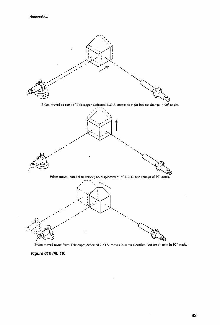
Appendices

Prism moved to right of Telescope; deflected L.O.S. moves to right but no change in 90' angle.

'I': Prism moved parallel to vertex; no displacement of LO.S. nor change of 90' angle.

, , .. , I " I ,

Prism moved away from Telescope; deflected LO.S. moves in same direction. but no change in 90' angle.

Figure 61b (lit. 18)

62

Appendices

Prism rotated about the Telescope axis; deflected L.O.S. moves in the same direction and the image itself rotates, but no change in 90° angle.

Prism rotated through small angle about an axis parallel to vertex; deflected L.O.S. is displaced but no change in 90° angle.

i

, 0

Nor 90

Prism tilted by raising vertex: deflected L.O.S. moves in plane of rotation and image rotates. Angle no longer 90°

Figure 61c (lit. 18)

63

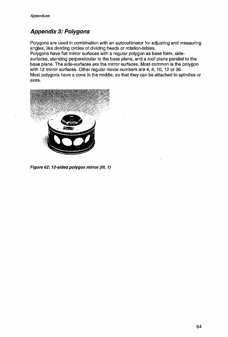
Appendices

Appendix 3: Polygons

Polygons are used in combination with an autocollimator for adjusting and measuring angles, like dividing circles of dividing heads or rotation-tables. Polygons have flat mirror surfaces with a regular polygon as base form, side­surfaces, standing perpendicular to the base plane, and a roof plane parallel to the base plane. The side-surfaces are the mirror surfaces. Most common is the polygon with 12 mirror surfaces. Other regular mirror numbers are 4, 8, 10, 12 or 36. Most polygons have a cone in the middle, so that they can be attached to spindles or axes.

Figure 62: 12-sided polygon mirror (lit. 1)

64

Appendices

Appendix 4: Determination of table and polygon errors

Determination of the table error and the polygon error with two measurement series (lit. 7)

Terminology

The preliminary alignment of the rotating table is defined as position zero, the reference surface of the polygon as '0'. Polygons with 6 surfaces are numbered 0 ... 5 (0 ... n-1). The table error refers to table position zero or the polygon surface '0' respectively. For n surfaces there are n-1 table errors. Table error 'n' is zero (rotation of 360°). The table errors are referred to as O'j , the polygon errors as cPj • In a measurement series the polygon surface '0' coincides with table position zero. The resulting table error values are derived from the equation:

If an autocollimator measures the value MO when beginning a measurement series

(table in preliminary alignment). then 'Vi = Mi - Mo. Mi is the value for the i-angle position. In, for example, another measurement series, polygon surface 'k' coincides with the preliminary position of the table. It follows that:

for i+k < n

for i+k = n

for i+k> n

(with: CPo: CPn : 0; 0'0: O'n =O)

An example for a polygon with 3 surfaces:

Each measurement series is comprised of the measuring data Mo, M1. M2' In the first measurement series the polygon surface '0' coincides with table position '0'. In the second measurement series you will find polygon surface '1' in table position zero. For the first measurement series:

Zero position: Mo 1. position: M1 2. position: M2

Insert the values in the following equations:

'V11 : M11-M10 'V12 = M12-M1 0

(1a)

Where the first index indicates the preliminary polygon surface, and the second index indicates the angle position.

65

Appendices

Analogous for the second measurement series:

'1121 = M21 - M20 '1122 = M22 - M20

Now an equation system can be established:

0"1 + <1>1 = '1111 0"2 + <1>2 = '1112 0"1 + (<1>2-<1>1) = '1121 0"2 - <1>1 = '1122

There are 4 equations with 4 unknown variables:0"1. 0"2. <1>1. <1>2 The equation for the system in matrix is as follows

AX=L

1 0 1 0 0"11 'II" l o 1 0 1 0"2

'II" j * -1 0 -1 1 <PI "'21 o 1 -1 0 <P2 "'22

(1b)

(2a) (2b) (2c) (2d)

(3)

(4)

A solution is obtained with the Gauss-Jordan-algorithm. A new matrix system is derived by subtracting equation (3) from equation (1) and equation (4) from equation (2).

101 0 0"1 <PII o 1 0 -1 0"2 <P12

* 002 1 <PI "'ll -"'21 (5)

o 0 1 1 <P2 "'12 - "'22

Equation (4) is set up with equations (3) and (4). then follows:

11 0 1 0 0"1 "'11 lO 1 0 1

0"2 "'12 * o 0 2-1 <PI "'11 - "'21 (6)

o 0 0-3 <P2 "'11 - "'21 - 2(",12 - "'22)

Now a solution can be specified:

<1>2 = - ( <1>11 - <1>21 - 2 (<1>12-<1>22»/3 (7) Other numbers result by substituting and transforming the equation system.

66

Appendices

For a solution algorithm it is important that no equation vanishes. Then the equation system is not indeterminated or singular. The procedure can be extended to any number of surfaces (angle positions). It is of no relevance which surface is in the preliminary alignment. However, for the second measurement series, it is important to rotate the polygon only one position relative to the table (Le. first measurement series: Surface 3 in preliminary alignment, second measurement series: Surface 2 or 4 in preliminary alignment). The same data results are obtained when executing 3, 4, or 6 measurement series.

Note: There is no solution for the equation system when not applying the above mentioned.

Under ideal conditions and for a known polygon error only one measurement series is necessary. When executing several measurement series the relative position of the polygon to the table need not be altered then. If the accuracy of the table and the accuracy of the autocollimator is much larger than expected the table error, the dividing head, and/or the polygon measurement can be executed with one or two measurement series. To reduce measurement errors repeat measurements several times.

Determination of table and polygon error with several measurement series (lit. 7)

Again, execute at least 2 independent measurement series. The polygon should be rotated only one surface relative to the former position (Le. first surface 9 in the preliminary alignment, then surface 10).Additional measurement series can be executed.

The rosette method is the alternative measuring method. The measuring principle is that each polygon surface is in the preliminary alignment at least once. The advantage of this method is that the polygon error is eliminated regardless whether the polygon errors were known or determined. When executing two or more measurement series you get more equations than there are unknown variables.

For the above mentioned example for a polygon with 3 surfaces, the matrix of coefficients can be extended as follows:

3 measurement series are executed in which polygon surface '2' coincides with table position '0'.

rl 0 1 0 1 o 1 0 1 I 1 0 -1 1

A= 0 1 1 0

1 0 0-1

lo 1 I-d An exact solution is obtained when all AX = L equations are satisfiable. This does not strictly apply for executed measurements.

67

Appendices

An over-determined equation system is solved by multiplying matrix of coefficients, transporting each figure for the equation to the other side. Begin on the left. Then the Gauss standard form is obtained.

(9)

Now there is the same number of equations and variables. Should the measurements be erroneous, use equation (9) which supplies a solution vector. The mean square root deviation gives optimum results. If the values are reconstructed with equation AX, they differ from the actually measured. The mean square of these differences are minimal.

~L= L-AX (10)

The standard deviation a can be calculated with the elements of L. This is an indication of the quality of the measurements. Three measurement series and 6 surfaces require 15 equations. A second backward calculation follows with correct results even if the polygon has an incorporated error. The table error results when subtracting the polygon errors from the measured values \jIi(4). Find the mean average and calculate the standard deviation. The average values are identical with the calculated table errors from (9). Now a standard deviation is assigned to each table error. These give information about the accuracy of the positioning of the table. Standard deviations are determined during the measurement series. The measured data are related to the table error. If the accuracy of measurement of the autocollimator is high compared to the expected accuracy of the adjustment of the revolving table the error can entirely be attributed to the dividing head. If this first requirement cannot be met, then the accuracy of position is best estimated with the following equation:

stt = -J sm-sak

sm: Standard deviation according to the measurement protocol sak: Accuracy of the autocollimator under concrete measurement

conditions Stt: Standard deviation of the circular dividing head

Inclining error and pyramidal error (lit. 7)

In principle the same method is applied as for the table error. The main difference is that the polygon surface also has a pyramidal error.

Note: The pyramidal error of the polygon reference surface cannot be determined this way. For the other surfaces there are no absolute values for pyramidal errors. Therefore there are only relative pyramidal errors (relative to the reference surface).

The inclining error is relative to the reference surface of the table. The pivot axis can be used as a reference if its exact position is known. The inclining error can only be regarded relative to the reference surface of the table. The inclining error can be used as a reference if the exact position of the pivot axis is known. With the deviations from the reference position and reference surface an equation system can be set up the same way as for the table error.

68

Appendices

In general 2 independent measurement series suffice in which the polygon is rotated one position relative to the table.

If the absolute pyramidal deviation of a polygon surface is known, then other absolute values can be calculated with the corresponding relative values.

Determination of the absolute pyramidal error (lit. 3)

The determination of the absolute pyramidal error of a polygon can be done by using a second autocollimator. This second autocollimator is placed opposite of the first one. The mirror surfaces, used for adjusting the polygon, are now used for determination of their absolute pyramidal error. The absolute errors of the other mirror surfaces can all be determined with their relative errors, related to the first mirror.

The first mirror is turned in autocollimation position for the first autocollimator, and the second autocollimator is adjusted to the mirror opposite the first one. Then the measured values are noted down, the polygon is rotated over 180°, and the measured values are noted down again. After that the polygon is taken away, so that one autocollimator pictures his image in the other autocollimator. These values are also noted down.

Two opposite mirrors of a polygon can be seen as a planparallel, double-sided mirror with a wedge error. Therefore the sum of their measured values is diminished by the sum of their positions. The resulting differences are the wedge errors of the opposite mirror surfaces and therefore the sum of their absolute pyramidal errors. They repeat within the measuring uncertainty after 180° rotation. Because the polygon is adjusted so that opposite mirror surfaces have the same angle to the rotation axis, these opposite mirrors must have the same absolute pyramidal error. So the value must be divided by 2 to get the absolute pyramidal error of these surfaces.

For example, for a 12-sided polygon:

measured value of autocollimator 1 on mirror 1: £1 measured value of autocollimator 2 on mirror 7: £2 image of autocollimator 1 in autocollimator 2: 112 image of autocollimator 2 in autocollimator 1: 111

£ = £1+£2

11 = 111 +112

X=£-l1 00= XI2

Now we have the absolute pyramidal error 00 of mirror 1 to which all the other mirrors can be related.

69

Appendices

Determination of the polygon sum- and group-error (fit. 3)

The polygon sum error

For most applications of the polygon, not the polygon error of the single polygon mirrors, but the sum-error 'Y is important. The sum-error 'Y of the m-th mirror surface, is the deviation of the ideal angle between the perpendiculars on the first and the m­th mirror surface in a plane perpendicular to the polygon axis. The perpendicular on the first mirror surface is the starting-point for the sum-error. The sum-error of the second mirror plane 'Y2 equals the first polygon error cp1' "13 equals cp1 +cp2, and in general:

"tm = <\>1 + <\>2+ ••• +<\>m -1 =!$ i=l

This means that the sum-error should be zero for the first mirror surface after adding all the polygon errors.

The polygon group error

When the angular deviations are measured of the angle between the perpendiculars of mirror surfaces that are not in successive positions but with one or more mirror surfaces between them, these errors are called group errors ~. For example, the 60°-angle deviations between the perpendiculars on the uneven mirror surfaces of a 12-sided polygon are determined by aiming the autocollimator at these mirrors and skipping the even mirrors. The six 60-angle measurements add up to 360. With 150-group errors of a12-sided polygon, twelve 150-angles can be added to 1800 which is 5 times 360. These group errors are measured to check the sum error "I, because in the calculation of "I with the polygon errors cp, the measuring uncertainty propagates, so that the sum error is pretty uncertain for a high number of mirror surfaces. Therefore the group errors of 36-mirror polygons of the 30°·, gOo-and 180°·angles are measured, and 'fit into each other.

70

Appendices

Appendix 5: Calculation of pentaprism deflection error after measurement of four 90° angles

In each of the two autocollimator positions, the deviation in parallelism of the two plane mirrors is measured two times (lit. 3). In every 900 "measurement the deflection error a, of the 90° deflection angle, is propagating double. That means in the four 90°-measurements that form the 360°­measurement, a is in eight times. Because the autocollimator measures mirror rotations instead of the angle between primary and reflected light beam, division by two has already taken place (so 4*a remains in the measured angle). So the calculation is as follows:

~1: parallelism error of plane mirror 1 relative to the direction of prOjection of the autocollimator

~2 : parallelism error of plane mirror 2 relative to the direction of projection of the autocollimator

~ 1 and ~2 are positive when they are turned towards the autocollimator in its first position. The angle deviation of the light beam at the mirror behind the pentaprism, with the autocollimator in its first position will be:

in the first pentaprism position: in the second pentaprism position:

The difference of the two readings will be:

r11 = ( " a + ~ 1 ) r12 = ( " a + ~2 )

The angle deviation of the light beam at the mirror behind the pentaprism, with the autocollimator in its first position will be:

in the first pentaprism position: in the second pentaprism position:

The difference of the two readings will be:

When L11 and L12 are added, it shows that:

r21 = ( " a - ~2 ) r22 == ( - a " ~1 )

L11 + L12 = ( r11 + r12) + ( r21 + r22 ) = - 4. a

The deflection error of the pentaprism can now be calculated as follows:

0= rll+r12+r21+r22 -4

To acquire the right sign for a, check the sign of the autocollimator measurements, the sequence and the direction of the measurements.

71

Appendices

The second autocollimator position doesn't need to be parallel to the first one; when they are not parallel, ~1 and ~2 will have different values for the two autocollimator positions, but their sum (~1 + ~2) will be the same.

As a side-effect the parallelism of the two mirrors can also be determined:

wedge error = ~ 1 + ~2 = ( ~ 1 -~ ) / 2

72

Appendices

Appendix 6: Measuring resolution of Moller-Wedel electronic autocollimators ELCOMA T 2000 and ELCOMA T HR

For both autocollimators the same techniques for detection are used, but because of a different focal length and a different number of slits in the reticle the resolutions of the ELCOMAT 2000 and the HR are different. Because of its higher resolution, the ELCOMAT HR will be described from here.

As locally sensitive detector Moller-Wedel uses a specially selected CCO-array with 1728 elements which have a distance of 10 microns each (lit. 9,17). This results in a linear detection range of 17,28 mm. With the formula:

a = d/2*f

and a focal length of 1100 mm, we find that a maximum detection range of ±81 0 arcsec is possible for one measuring axis. In praxis, for a version with two measuring axes, it is preliminary limited to 150 arcsec for the ELCOMAT HR. In order to facilitate a simple alignment of the autocollimator, the detecting and acquisition range is extended to around 600 arcsec. Regarding these geometrical premises, it is easily seen from the distance between two individual adjacent detector elements (pixels) that a spatial resolution of only 0,94 arcsec can be achieved, which is much to low. Moller-Wedel has developed several methods for increasing the resolution. The subpixel resolution method works on a purely digital basis. Each light slit image detected from the CCO-array is electronically filtered and read out at a pre-given clock frequency. Because of separate systems for X and Y measurement, one direction can be calculated while the other is measured, so that there is constantly one measured and one calculated direction. The integration-time can be varied, and is approximately 35 ms, which results in a frequency of 25-30 Hz. One light slit has a width of 100 micron, which equals a range of approximately ten pixels.

image ofligbt slit on CCD-array

Figure 63

Steps in resolution increase (lit. 9):

1. The processing unit can find this range of enlightened detecting pixels, and the signal is read out. The integration curve is calculated. When the digital intensity values are integrated into an integration-curve, the intensity will vary within the length of a pixel. This varying value is read out so on 16 places of the integration-

73

Appendices

curve within every pixel-length, which leads to a 16-fold resolution increase, because a different intensity-value is found now for every 1/16-th pixel-length.

>..

I ~

'iii c curve multiple 2

,S fitting >

pixel reading

Figure 64: multiple pixel reading

2. Mathematically, a sub-pixel resolution is carried out by a numerical calculation of the point of concentration:

The pOint of concentration is calculated from the amplitude A of the individual pixel i.

3. Then a further increase of the resolution is acquired by the use of a multiple light slit. This is caused by an overlapping of the intensity-curves. In the ELCOMAT HR four light slits are used for each measuring direction. When the images of these light slits are mutually shifted over a distance of (x+1/4) times the pixel-length, this makes the resolution approximately four times better. In the ELCOMAT 2000 with a double light slit, a two times better resolution is reached, with a distance of (x+ 1/2) times the pixel-length, between the two light slits.

CCD ELCOMAT 2000 ELCOMATHR resolution f= 300 mm f = 1100 mm

pixelwidth 10 ,lm 3.44" 0.94" step 1:

resolution increase 0.625 ~m 0.22" 0.06" by hardware (patent)

factor 16 step 2:

resolution increase 0.04 ~m 0.013" 0.004" by software

factor 16 step 3: 0.02 ~m 0.006" 0.001" multiple reticle

0.01 ~m (double reticle) (fourfold reticle)

table 3: internal AC resolution for a single measurement (lit. 18)

74

Appendices

Appendix 7: Moller-Wedel

The Moller works are located in Wedel near Hamburg, and have begun as Johann Dietrich Moller started a small handicraft workshop for optical elements and microscopes. Until 1985 it stayed a family-company, in the fourth generation. Now Moller-Wedel is part of the Swiss Haag-Streit Group. Moller-Wedel manufactures medical instruments for ophthalmology and microchurgery (ophthalmologic and neurological), and technical optics, like optical measuring instruments, optical construction elements and reticles. The firm has about 230 employees, divided over production, sales management, financial management, staff management, technology, construction and marketing. Moller-Wedel doesn't practice mass-production. They work with small series and single production.

During my traineeship I was stationed on the sales-department, where I was attended by Carsten Schlewitt, who is the product-manager of the measuring instruments.

During a few days of assistance in the assembly of visual optical measuring equipment (autocollimators, diopter telescopes) one of the things I learned was that their assembly time is not exactly predictable. For example the time needed for the cleaning of an autocollimator reticle can even influenced by the weather.

75

Appendices

Appendix 8: Blohm Maschinenbau GmbH

Blohm Maschinenbau GmbH is a company of the international Schleifring-Group, and is located in Hamburg. Blohm manufactures grinding-machines for various applications, like plane- and profile-grinding, round-grinding, precision grinding and specialised applications, like in turbine industry. .

At Blohm I worked for two weeks, to get practical experience in measuring with the ELCOMA T 2000 in an industrial environment. Beside that I have instructed Blohm employees in handling the ELCOMAT 2000. During my work, I found out that the GFM-software, delivered with the ELCOMAT, can use some improvements to make it more fit for the use in an industrial environment, where it is important that measurements can be made quickly, with few action steps and that a simple print-out with sufficient information is produced (lit. 19).

Figure 65: grinding machine: Blohm PLANOMAT (lit. 20)

76