
Dissertation 5 : Zamberi Jamaludin
189
DISTURBANCE COMPENSATION FOR MACHINE TOOLS WITH LINEAR MOTOR DRIVES Promotoren: Prof. Dr. ir. H. Van Brussel Prof. Dr. ir. J. Swevers 2008D09 September 2008 Proefschrift voorgedragen tot het bekomen van de graad van Doctor in de Ingenieurswetenschappen door Zamberi JAMALUDIN
-
Upload
mat-jibrud -
Category
Documents
-
view
391 -
download
0
description
Disturbance Compensation for Machine Tools with Linear Motor Drives.
Transcript of Dissertation 5 : Zamberi Jamaludin
eri
DISTURBANCE COMPENSATION FOR MACHINE TOOLS WITH LINEAR MOTOR DRIVES
Promotoren: Prof. Dr. ir. H. Van Brussel Prof. Dr. ir. J. Swevers
2008D09 September 2008
Proefschrift voorgedragen tot het bekomen van de graad van Doctor in de Ingenieurswetenschappen door
Zamberi JAMALUDIN

DISTURBANCE COMPENSATION FOR MACHINE TOOLS WITH LINEAR MOTOR DRIVES
Jury: Prof. Dr. ir. A. Haegemans, voorzitter Prof. Dr. ir. H. Van Brussel, promotor Prof. Dr. ir. J. Swevers, promotor Prof. Dr. ir. J. De Schutter Prof. Dr. ir. H. Ramon Prof. Dr. ir. P. Sas Prof. Dr. ir. G. Pritschow (University of Stuttgart)
2008D09 September 2008
Proefschrift voorgedragen tot het bekomen van de graad van Doctor in de Ingenieurswetenschappen door
Zamberi JAMALUDIN

© Katholieke Universiteit Leuven Faculteit Ingenieurswetenschappen Arenbergkasteel, B-3001 Heverlee (Leuven), Belgium Alle rechten voorbehouden. Niets uit deze uitgave mag worden verveelvoudigd en/of openbaar gemaakt worden door middel van druk, fotokopie, microfilm, elektronisch of op welke andere wijze ook zonder voorafgaandelijke schriftelijke toestemming van de uitgever. All rights reserved. No part of this publication may be reproduced in any form, by print, photoprint, microfilm or any other means without written permission from the publisher. D/2008/7515/85 ISBN 978-90-5682-975-9 U.D.C. 681.5

My Parents
My Wife

The beginning of knowledge is the intention, then listening, then understanding, then action, then preservation, and then spreading it.

i
Acknowledgements This journey begins in 2003. The common question at that time is “Why Belgium?” This is apparent especially because of the weak link in the educational relationship between Malaysia and Belgium. A nice and encouraging introduction by Dr. Indra Tanaya (a graduate of K.U.Leuven and who was once my colleague in Malacca) about PMA, its strong lists of academicians and researchers with dedicated research activities and the beautiful and peaceful city of Leuven have motivate me enough to begin this new chapter of my life here in PMA, Leuven. I am grateful that I have made this important choice because after these five wonderful and challenging years, both PMA and Leuven have never failed to contribute positively to my academic and personal development. There are two very important persons that have been very influential to my academic development here in Leuven. First and foremost, I would like to express my deepest gratitude to Prof. Van Brussel for accepting me into the PMA community and for the trust that he has put on me in realising this work. It is a great honour and pleasure to be able to work with him, a person of great mechatronics background, experience, success, ideas, and stature. It is certainly be a great challenge to me to emulate your success and to be as good as you are. Your kind advice, time, attention, and dedication towards realising this work are greatly appreciated. Finally, I would like to extend my deepest appreciation for your kind attentions on the well-being of myself (visiting me in the hospital on just my third week in Belgium) and my wife and your warm hospitality towards my parents. Secondly, I would like to express my special gratitude to Prof. Swevers – the control specialist, for nurturing me into the challenging world of control. Your knowledge in advanced control theory certainly amazed me and I wish that there is somebody of your calibre in Malacca (there is none at the moment) so that I can keep learning from the best mind in this field. Your guidance, attention, and time are greatly appreciated. I would like to thank you, your wife and family for being such a great and wonderful host during your yearly summer bbq sessions. I would like to extend my deepest gratitude to the thesis jury committee members; Prof. Dr ir. Herman Ramon, Prof. Dr ir. Joris De Schutter, Prof. Dr ir. Paul Sas, and Prof Dr ir. Gunther Pritshow of the Stuttgart University. Thank you for your valuable time, suggestions, comments, and critical

Acknowledgements
ii
thoughts that have enable me to improve the quality of this manuscript. I would also like to express my thanks to Prof. Dr Ann Haegemans for being the chairperson. I admired the great knowledge and experience of Prof. Vanherck, a person whom I regard as a walking technical library. Your help, assistance, teachings, and explanation on many technical issues have helped me tremendously throughout my work in PMA. Thank you for your dreams (I will always remember you saying this when there are problems with the xy table and the Ferraris sensor). I would like to extend my special thanks to the administrators of PMA - Luc Haine, Lieve Notre, Karin Dewit, Carine Coosemans, and Ann Letelier for their support, assistance and warm hearts. I am also grateful to all the technical personnel at the workshop, the electronic and the IT department for making my life easier at the workshop. My special thanks to Dirk Bastiaensen, Eddy Smets, Paul Van Cauwenbergh, Luc De Simpelaere, Bertram Van Soom, Jean Pierre Merkcx, Ronny Moreas, and Jan Thielemans. My life here at PMA is made easier by Dr T. Tjahjowidodo who has given me a nice introduction to life at PMA, its surrounding and its research environment. I still remember the confusions and funs that we had during my early days in PMA trying to understand each other in Bahasa Melayu (some similar Malaysian and Indonesian words can have totally different meanings). I would also like to express my appreciation for your time and assistance in explaining the world of friction to me. The nice explanations have certainly helped in my work on friction compensation. It is a great pleasure to be in the environment of the control group people and of my office colleagues – Bram, Christophe, David Vaes, Bart Paijmans, Kris Smolders, Goele, Jan De Caigny, Dimitri, Lieboud, Diederick, Bert Stalleart, Myriam, Leopoldo, Marnix and Maarten. Thank you for the company, assistance, and fruitful discussions. I would like to express my special thanks to Goele Pipeleers for assisting me in the design of the repetitive controller. The mechatronics group meetings have exposed me to many wonderful people. It is a pleasure to be in the company of these distinguished colleagues of various backgrounds and origins - Prof. Farid Al-Bender, Wim Symens, Brecht, Hsiao-Wei.Tang, Emmanuel Vander Poorten, Wim van de

Acknowledgements
iii
Vijver, Tri, Gorka, Mohamed El-Said (also Neny and Zaharah for your kindness and warm hearts), Maira, Thierry, Kris, Pauwel, Bert, and Agusmian. Life in Belgium for a Malaysian can be a lonely experience (there are not many of us here). However, since the last two years, the students community has grown with the arrival of other Malaysian students and families (although there are all not in Leuven). I would like to extend my sincere appreciation to: Zaini and Ros, Saifullah, Yeong and family, Helmi and Natrah, Am and Nurul, Dr Razak and family, abang Zam, kak Zu and family, and Kelvin and family. Thank you for the friendship and hospitalities. I would also like to thank Akmal and Zura for their warm heart and hospitality towards me and my wife and for all the trips that you have taken us to. Finally, to the Embassy of Malaysia in Brussels, thank you for all the nice receptions and your kind treatment of myself and my wife for all the five years that we are in Belgium. I am also grateful to have known many kind and warm hearted Indonesian friends and families especially Pak Oemar, Mbak Leen and Esti, Gandjar and family, Tegoeh, Ira and family, Singgih, Uly and the kids, Arie and Sarah, and Freddy, Novita and family. This work is made possible with the financial supports of the Ministry of Higher Education Malaysia (SLAB) and the University Technical of Malaysia-Malacca (UTeM). These financial supports are greatly appreciated and indebted. I also wish to express my sincere gratitude towards the International Student Office of K.U.Leuven for the financial support that I have received during the final three months of my stay in Leuven. This financial support has enabled me to complete my study here uninterruptedly and successfully. Finally and most importantly, I wish to express my deepest gratitude to both my parents, Hj. Jamaludin and Hjh Khatijah Bee, my brother Saifullah, and the families in Kedah and Singapore for their prayers, loves, cares, and support. I am greatly indebted to them and may God repay all their deeds and sacrifices. To my wife Zila, there are no words to describe how grateful I am for your company during both the easy and the difficult times of this journey. I salute your patient, dedication, love, and care that have brought happiness and serenity to our life.
Zamberi Jamaludin
Leuven, Sept. 2008.

iv
v
Abstract
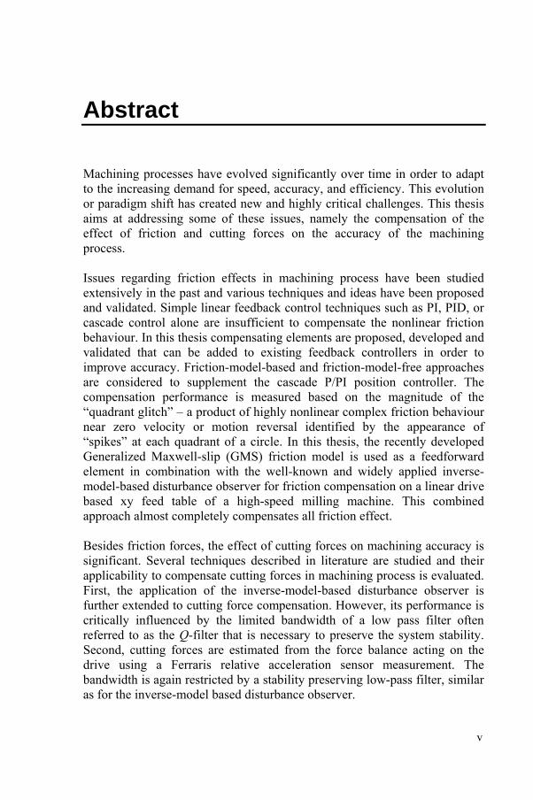
Machining processes have evolved significantly over time in order to adapt to the increasing demand for speed, accuracy, and efficiency. This evolution or paradigm shift has created new and highly critical challenges. This thesis aims at addressing some of these issues, namely the compensation of the effect of friction and cutting forces on the accuracy of the machining process. Issues regarding friction effects in machining process have been studied extensively in the past and various techniques and ideas have been proposed and validated. Simple linear feedback control techniques such as PI, PID, or cascade control alone are insufficient to compensate the nonlinear friction behaviour. In this thesis compensating elements are proposed, developed and validated that can be added to existing feedback controllers in order to improve accuracy. Friction-model-based and friction-model-free approaches are considered to supplement the cascade P/PI position controller. The compensation performance is measured based on the magnitude of the “quadrant glitch” – a product of highly nonlinear complex friction behaviour near zero velocity or motion reversal identified by the appearance of “spikes” at each quadrant of a circle. In this thesis, the recently developed Generalized Maxwell-slip (GMS) friction model is used as a feedforward element in combination with the well-known and widely applied inverse-model-based disturbance observer for friction compensation on a linear drive based xy feed table of a high-speed milling machine. This combined approach almost completely compensates all friction effect. Besides friction forces, the effect of cutting forces on machining accuracy is significant. Several techniques described in literature are studied and their applicability to compensate cutting forces in machining process is evaluated. First, the application of the inverse-model-based disturbance observer is further extended to cutting force compensation. However, its performance is critically influenced by the limited bandwidth of a low pass filter often referred to as the Q-filter that is necessary to preserve the system stability. Second, cutting forces are estimated from the force balance acting on the drive using a Ferraris relative acceleration sensor measurement. The bandwidth is again restricted by a stability preserving low-pass filter, similar as for the inverse-model based disturbance observer.

Abstract
vi
Finally, a method that is renown for its excellent compensation of periodic disturbance signals is applied, namely, the repetitive controller (RC). A repetitive controller is developed for the considered linear drive based xy feed table. To validate the performance of this RC, an actual cutting process is performed on the test setup. It is shown that the developed RC is able to compensate almost completely the tracking errors introduced by the cutting forces. The repetitive controller, when combined with the previous friction compensation elements such as the GMS friction model feedfoward and the disturbance observer, almost completely removed the cutting forces during an actual cutting process. This thesis has successfully demonstrated that the tracking performance of a machine tool can be increased significantly by adding dedicated compensation elements to the simple and widely used cascade P/PI position controller. However, further studies are desired to include adaptive measures in both friction and cutting forces compensation using the advanced GMS friction model and the RC. This will ensure a robust friction compensation approach to changing friction behaviour and characteristics over time due to the influence of lubrication, heating and etc. An adaptive RC will compensate against changes in the cutting conditions, for example, changes in the spindle speed, tools diameter, tracking speed, and etc.

vii
BBeekknnooppttee SSaammeennvvaattttiinngg
De technologische evolutie van conventionele materiaalbewerkingsmachines wordt gedreven door de vraag naar steeds hogere snelheden, nauwkeurigheden en efficiëntie. Deze evolutie creëert nieuwe uitdagingen. Deze thesis richt zich op enkele van deze uitdagingen, namelijk de actieve compensatie van de effecten van wrijving en snijkrachten op de nauwkeurigheid van het bewerkingsproces. Het effect van wrijving op de nauwkeurigheid van bewerkingsprocessen werd in het verleden reeds uitgebreid onderzocht. Verschillende technieken om het effect van wrijving te compenseren werden ontwikkeld en experimenteel gevalideerd. Eenvoudige lineaire regelaars op basis van terugkoppeling, zoals de PI-, PID-, en de cascaderegelaars voldoen niet om het effect van het niet-lineaire wrijvingsgedrag te compenseren. Deze thesis stelt een aantal wrijvingscompensatietechnieken voor die kunnen toegevoegd worden aan bestaande (lineaire) sturingen. Zowel technieken gebaseerd op een wrijvingsmodel als technieken die geen wrijvingsmodel vereisen, worden beschouwd. De performantie van deze technieken wordt gemeten aan de hand van de grootte van de “quadrant glitch”, het resultaat van het sterk niet-lineair gedrag van wrijving dat optreedt bij omkering van de bewegingrichting en bij zeer lage bewegingssnelheden, en dat zich uit als spikes in de volgfout. De compensatietechnieken die werden onderzocht worden ook experimenteel gevalideerd op een met lineaire motoren aangedreven XY voedingstafel van een hoge-snelheidsfreesmachine. De combinatie van voorwaartse koppeling aan de hand van het recent ontwikkelde “Generalized Maxwell-slip (GMS)” wrijvingsmodel en de gekende en vaak toegepaste storingsschatter op basis van een invers systeemmodel resulteert in de grootste verbetering van de volgnauwkeurigheid: wrijvingseffecten bij elke kwadrant van een circulaire baan worden bijna volledig gecompenseerd. Naast wrijving kunnen ook de snijkrachten een belangrijke invloed hebben op de bewerkingsnauwkeurigheid van de machine. Verschillende compensatietechnieken beschreven in de literatuur worden bestudeerd en hun toepasbaarheid om snijkrachten te compenseren wordt onderzocht en

Beknopte Samenvetting
viii
experimenteel gevalideerd. Eerst wordt de storingsschatter op basis van een invers systeemmodel verder uitgebreid voor snijkrachtcompensatie. De performantie van deze storingsschatter wordt kritisch beïnvloed door de beperkte bandbreedte van de laagdoorlaatfilter (Q-filter) die aanwezig is in deze schatter om de systeemstabiliteit te vrijwaren. Daarnaast wordt een snijkrachtschatter bestudeerd die gebruik maakt van metingen van de relatieve versnelling van de lineaire motor op basis van een Ferraris sensor. Ook voor deze schatter gelden dezelfde beperkingen met betrekking tot bandbreedte en performantie. Tenslotte wordt de repetitieve regelaar bestudeerd. Deze regelaar richt zich uitsluitend op periodische storingen waarvan de periode gekend is of kan geschat worden. Deze regelaar maakt gebruik van niet-causale filters waardoor een aanzienlijk hogere bandbreedte kan bereikt worden. Een repetitieve regelaar wordt ontworpen en toegepast op de beschouwde testopstelling. Om de performantie van de ontwikkelde repetitieve regelaar te valideren wordt een freesbewerking uitgevoerd op de testopstelling. De testen tonen aan dat de ontworpen repetitieve regelaar in staat is om volgfout ten gevolge van het freesproces bijna volledig te elimineren. Deze repetitieve regelaar wordt toegepast in combinatie met de ontwikkelde wrijvingscompensatie op basis van het GMS model en de storingsonderdrukker zodat ook wrijving tijdens deze bewerking gecompenseerd wordt. De overblijvende volgfout is verwaarloosbaar. Deze thesis heeft met succes aangetoond dat de volgnauwkeurigheid van een werktuigmachine significant kan verbeterd worden door gerichte compensatietechnieken toe te voegen aan de eenvoudige klassieke cascade P/PI positiesturing van de machine. Echter, verder onderzoek is vereist om deze compensatie adaptief te maken om zo efficiënt te kunnen inspelen op veranderingen in de tijd van de wrijvingskarakteristieken, die beïnvloed worden door smering, temperatuur, en slijtage, en van de snijkarakteristieken, die o.a. beïnvloed worden door de spilsnelheid en de freesdiameter.
ix
Symbols and Abbreviations
Symbols
Control:
d(t) disturbance force signal [N] ( )td~ estimated disturbance force [N]
ep(t) position tracking error signal [µm] ev(t) velocity tracking error signal [µm/s]
f frequency [Hz] γp,∆ robust periodic performance index γnp Non-periodic performance index kf motor force constant [N/V] kp proportional gain controller in velocity loop [volt·s/µm] ki integral gain controller in velocity loop [volt/µm] kv velocity gain factor, or the Proportional gain
controller in cascade position loop [1/s]
n(t) noise u(t) control command signal [volt] vref desired reference velocity [µm/s] z(t) Output position signal [µm]
zref(t) Desired reference position signal [µm] ωo Undamped natural frequency [rad/s] ζ damping ratio F Force acting on linear motor [N] G considered system Ĝ FRF of the considered system Gm system model transfer function Gn nominal model system transfer function Gm’ system model with GMS friction term M mass of the sliding table [kg]
N(s) notch filter S sensitivity function T complementary sensitivity function T0 sampling period [s] Td time delay [s]
Vest(s) estimated velocity signal [µm/s]

Symbols & Abbreviations
x
Friction:
δ Stribeck function shape factor σ viscous friction force [N·s] αi elementary normalized friction force [N] ki elementary spring constant of the Maxwell slip
blocks element [N/m]
s(v) Stribeck function Ff total friction force [N] Fc Coulomb friction force [N] Fs static friction force [N] Vs Stribeck velocity [µm/s] Wi maximum elementary friction force [N]
Abbreviations
rms root mean square rpm revolution per minute
DOB disturbance observer FRF frequency response function FF feedforward
GMS Generalized Maxwell-slip H∞ H-infinity I/O input-output PI proportional plus integrator
PID proportional plus integrator plus differentiator RC repetitive controller
RHP right half plane SISO single input single output SMC sliding mode control
xi
Table of Contents
Acknowledgements i Abstract v Beknopte Samenvetting vii Symbols and Abbreviations ix Table of Contents xi List of Figures xv List of Tables xxiii
1 Introduction 1 1.1 Motivation ……………………………………………... 1
1.2 State of the Art on Motion Control ……………………. 3
1.2.1 Mechanical Drive Systems ……………………. 3
1.2.2 Disturbance Forces and Compensation Methods 6
1.3 Scope, Objective and Approaches ………….…………. 9
1.4 Contributions …………………………………………... 10
1.5 Outlines ………………………………………………... 11
2 Classical Motion Control 13 2.1 Introduction ……………………………………………. 13
2.2 High-Speed XY Milling Machine ……………………... 14
2.3 System Identification ………………………………….. 17
2.4 Cascade Control Structure and Analysis …………….. 20
2.4.1 Cascade Controller Structure and Configuration 20
2.4.2 Analysis of the Closed Loops Behaviour with Proportional (P) Velocity Loop ……………….. 22
Table of Contents
xii
2.4.3 Analysis of the Closed Loops Behaviour with Proportional (P) and Integrator (I) Velocity Loop …………………….……………………... 25
2.5 Design and Validation of Cascade P/PI Controller Based on Measured FRFs ……………………….….…. 27
2.5.1 Design and Analysis of the Velocity Loop...….. 27
2.5.2 Design and Analysis of the Position Loop ….… 34
2.5.3 Tracking Performance Numerical Validation … 39
2.5.4 Cascade P/PI with Feedforward …………...….. 40
2.6 Correlation between Velocity and Position Closed Loop Characteristics …………………………………………. 41
2.6 Summary ………………………………………………. 44
3 Disturbance Forces in Servo Drives System 45 3.1 Introduction ………………………………………….… 45
3.2 Friction Characterization and Model Structures ………. 45
3.3 The Dahl Model ……………………………………….. 46
3.4 The LuGre Model ……………………………………… 47
3.5 Static Friction Model ……………………………….…. 48
3.2.1 Model Structure ………………………….…..... 48
3.2.2 Identification of Static Friction Model ………... 49
3.6 Generalized Maxwell-slip Model (GMS) ……………... 50
3.2.1 Model Structure ……………………………….. 50
3.2.2 Identification of GMS friction model …………. 52
3.7 Cutting Forces …………………………………………. 56
3.7.1 Cutting Force Measurements and Analysis ….... 56
3.7.2 Artificial Cutting Force ……………….………. 60
3.8 Summary ………………………………………………. 62
Table of Contents
xiii
4 Friction Forces Compensation 63 4.1 Introduction ……………………………………………. 63
4.2 Friction Model-Based Feedforward ………………...…. 64
4.2.1 System Transfer Function with a GMS Friction Term for Friction Simulation ……………… 64
4.2.2 Friction Feedforward: Numerical Results …… 67
4.2.3 Friction Feedforward: Experimental Results 69
4.3 Inverse-Model Based Disturbance Observer ……...…... 73
4.3.1 Q-filter Design and Stability Analysis ……...… 75
4.3.2 Loops Characteristic with Disturbance Observer 78
4.3.3 Numerical Validations……………………......... 87
4.3.4 Experimental Validations………...……………. 90
4.4 Summary ………………………………………………. 94
5 Cutting Force Compensation 97 5.1 Introduction ………………………………………….… 97
5.2 Inverse-Model-Based Disturbance Observer ………….. 98
5.2.1 Numerical Validations…...…………………….. 98
5.2.2 Experimental Validations...…….……...………. 100
5.3 Explicit Estimation of Cutting Force using Ferraris Relative Acceleration Sensor Measurements ………….. 103
5.3.1 The Ferraris Principle ……………….………… 104
5.3.2 Cutting Force Estimator ………………………. 105
5.3.3 Experimental Validations...……………………. 106
5.4 Repetitive Controller …………………………………... 112
5.4.1 Design Structure of a Repetitive Controller…… 112
5.4.2 Experimental Validations...……………………. 116

Table of Contents
xiv
5.5 Cutting Force Compensation during Actual Cutting Process ……………………………………………….... 120
5.6 Summary ……………………….……………………… 123
6 Conclusions and Future Studies 125 7 Bibliography 129 8 Curriculum Vitae 135 9 List of Publications 137 10 Appendices 139 A System Dynamic Analysis 139
B Calibration of Ferraris Sensor 140
C Cutting Force Estimation from Ferraris Acceleration Sensor Measurement 143
D General State Force Observer Design 147
xv
List of Figures Chapter 1
1.1 Quadrant glitches in circular test ………………………... 2
1.2 Electromechanical ball-screw drive structure…………… 4
1.3 Structure of an iron-core linear motor…………………… 5
1.4 Schematic diagram for friction compensation techniques. 6
Chapter 2
2.1 A linear-driven xy feed table of a high-speed milling machine …………………………………………………. 14
2.2 Schematic diagram of the xy table ….………………….. 15
2.3 Motion controller structure of a xy feed table with three linear drives for high speed milling application…………. 17
2.4 FRFs measurement of the x and y axes………………….. 18
2.5 X-axis: FRF measurement and proposed model………… 19
2.6 Y-axis: FRF measurement and proposed model………… 19
2.7 General scheme of a cascade control structure………….. 20
2.8 Schematic diagram of the open loop system for force constant estimation………………………………………. 21
2.9 An ideal cascade control structure for a linear motor position control…………………………………………... 22
2.10 Frequency domain scheme of the cascade P/PI controller for control of a linear motor drive……………………….. 28
2.11 Bode diagram of Vest(s)………………………………….. 28
2.12 X-axis: Bode diagram of a notch filter N(s) for frequency between 320 Hz and 340 Hz…………………………….. 29
2.13 X-axis: Theoretical bode of the velocity open loop transfer function based on measured FRF of the system... 31

List of Figures
xvi
2.14 Y-axis: X-axis: Theoretical bode of the velocity open loop transfer function based on measured FRF of the system……………………………………………………. 31
2.15 Nyquist plots of the x-axis (left) and the y-axis (right) velocity open loop transfer functions based on measured FRFs of the system………………………………………. 32
2.16 Sensitivity function of x (left) and y (right) axes for the velocity loop……………………………………………... 33
2.17 Velocity closed loop transfer function for (a) x-axis and (b) y-axis ………………………………………………... 34
2.18 Position open loop transfer function for (a) x-axis and (b) y-axis based on measured FRF of the system ………...… 36
2.19 Nyquist plots of the x-axis (left) and the y-axis (right) of the position open loop transfer functions………………... 37
2.20 Sensitivity function of x (left) and y (right) axes for the position loop……………………………………………... 37
2.21 Position closed loop transfer functions for x and y axes… 38
2.22 Measured dynamic stiffness of x (left) and y (right) axes using cascade P/P and cascade P/PI controller………….. 39
2.23 Simulated tracking error of the x-axis (left) and the y- axis (right) for sinusoidal reference signal of an amplitude of 1mm and frequency of 10Hz……………… 39
2.24 Position error transfer functions of the x-axis (left) and the y-axis (right)…………………………………………. 40
2.25 Cascade P/PI with feedforward for improved tracking performance……………………………………………… 40
2.26 Simulated tracking error of the x-axis (left) and the y- axis (right) for sinusoidal reference signal of amplitude 1mm and frequency of 10Hz…………………………….. 41
2.27 Schematic diagram of a velocity closed loop……………. 42
2.28 Y-axis: Simulated speed closed loop based on measured system FRF ………............................................................ 43
List of Figures
xvii
2.29 Measured FRF of the y-axis position closed loop with kv =150 s-1………………………………………………... 44
Chapter 3
3.1 Pre-sliding and sliding friction regimes…………………. 46
3.2 Friction components in static friction model (3.5)………. 48
3.3 Friction force from control command signals at constant velocity motion of 2.0 mm/s (y-axis)……………………. 49
3.4 Friction force-velocity mapping and the manually fitted static friction model using equation (3.5) ……………..... 50
3.5 N-elementary configuration of the Maxwell-slip structure 51
3.6 Y-axis: Friction force and position for sinusoidal reference signal of 0.1Hz and amplitudes of (a) 15µm and (b) 450µm………………………………………….... 53
3.7 Y-axis: (a) virgin curve and (b) virgin curve with selected knots and slopes………………………………... 53
3.8 Y-axis GMS model parameters identification…………… 54
3.9 X-axis: Friction force and position for sinusoidal reference signal of 0.1Hz and amplitudes of (a) 15µm and (b) 450µm…………………………………………… 55
3.10 X-axis: (a) virgin curve (b) virgin curve with selected knots and slopes (right)………………………………….. 55
3.11 X-axis: GMS model parameters identification………….. 56
3.12 Cutting force in x and y direction for cutting depth 1mm.. 57
3.13 Cutting force in x and y direction for cutting depth of 3mm …………………………………………………….. 58
3.14 Cutting force measurements on a work-piece using Kistler dynamometer force sensor along the x-axis……... 58
3.15 Spectral of cutting force along x and y direction, for cutting depth of 1mm……………………………………. 59
3.16 Spectral of cutting force along x and y direction, for cutting depth of 3mm……………………………………. 59
List of Figures
xviii
3.17 X-axis: Comparison between the measured cutting force and the synthesized cutting force for 1mm depth of cut… 62
Chapter 4
4.1 Friction compensation scheme using friction model- based feedforward (kf is the force constant)……………... 64
4.2 System transfer function with a GMS friction model to characterize the complex friction behaviour…………….. 65
4.3 System model parameters adjustment for system structure that includes the GMS friction term: (a) using the original model parameters and (b) using updated model parameters………………………………………... 66
4.4 Y-axis: Simulated position, velocity and tracking error for three different cases of friction compensation techniques (a) no friction feedforward, (b) Stribeck friction model feedforward, (c) GMS model feedforward. 67
4.5 Y-axis: Simulated tracking error using GMS model feedforward for (a) system model with delay and (b) with the delay removed.…………….………………………… 68
4.6 Y-axis: Simulated tracking error using (a) modified GMS model feedforward and (b) matched GMS model for system both without delay……………………………….. 69
4.7 Y-axis: Measured position and tracking error for (a) no friction feedforward, (b) static friction model feedforward, (c) GMS feedforward …...………………… 70
4.8 X-axis: Measured quadrant glitches for maximum tracking velocity of 10mm/s: (a) static friction model feedforward and (b) GMS model feedforward…………... 71
4.9 Y-axis: Measured quadrant glitches for maximum tracking velocity of 10mm/s: (a) static friction model feedforward and (b) GMS model feedforward…………... 71
4.10 Measured contour and radial tracking error at tangential tracking velocity of 100mm/s: (a) no friction feedforward, (b) static friction model feedforward, (c) GMS model feedforward………………………………… 72
List of Figures
xix
4.11 Measured contour and radial tracking errors for tangential tracking velocity of 10mm/s: (a) static friction model feedforward and (b) GMS model feedforward…… 73
4.12 Block diagram of a system with an inverse-model- based disturbance observer……………………………………... 74
4.13 Equivalent block diagram of a system with an inverse model-based disturbance observer………………………. 74
4.14 Bandwidth limitation of the filter Q for (a) x-axis and (b) y-axis…………………………………………………….. 77
4.15 Cascade P/PI position control with inverse model-based disturbance observer …...................................................... 78
4.16 Cascade P/PI position control with equivalent block diagram of the inverse model-based disturbance observer
78
4.17 Velocity open loop transfer function for (a) x-axis and (b) y-axis for system with and without a disturbance observer…………………………………………………..
80
4.18 Velocity closed loop transfer functions for (a) x-axis and (b) y-axis for system with and without a disturbance observer………………………………………………….. 81
4.19 Effect of the disturbance observer on the sensitivity function of the velocity loop for x-axis (left) and y-axis (right) …………………………………………….……… 82
4.20 Nyquist plots of the velocity loops with and without the disturbance observer……………………………………... 82
4.21 Position open loop transfer function for (a) x-axis and (b) y-axis for system with and without a disturbance observer………………………………………………….. 84
4.22 Position closed loop transfer functions for (a) x-axis and (b) y-axis for system with and without a disturbance observer………………………………………………….. 85
4.23 Effect of the disturbance observer on the sensitivity function of the position loop for the (a) x-axis and (b) y-axis …..………………………………………………….. 86

List of Figures
xx
4.24 Nyquist plots of the position loops with and without the disturbance observer……………………………………... 87
4.25 Simulated control scheme for friction compensation using friction model feedforward and a disturbance observer………………………………………………….. 88
4.26 Y-axis: Simulated position and tracking error for configuration (a), (b) and (c)…………………………….. 89
4.27 X-axis: Measured position and tracking errors for configuration (a), (b) and (c)…………………………….. 90
4.28 X-axis: Measured position and tracking errors for slower reference trajectory of 10mm/s for configuration (a) and (b)………………………………………………………... 91
4.29 Y-axis: Measured position and tracking errors for configuration (a), (b) and (c)…………………………….. 92
4.30 Measured contours and radial errors for configuration (a), (b) and (c)…………………………………………… 93
4.31 Circular tracking tests at tangential tracking velocity of 10mm/s…………………………………………………... 93
4.32 Position and radial tracking error for different friction compensation approaches………………………………... 94
Chapter 5
5.1 MATLAB/Simulink diagram of a cascade P/PI controller and a disturbance observer with a sinusoidal based disturbance input signal………………………………….. 98
5.2 Y-axis: The effect of a disturbance observer on tracking errors for disturbance input frequencies of (i) 1 Hz, (ii) 58 Hz, and (iii) 100 Hz…………………………………... 99
5.3 Y-axis: Position errors for system with and without a disturbance observer……………………………………... 100
5.4 Cutting force compensation using inverse-model-based disturbance observer……………………………………... 101
List of Figures
xxi
5.5 Y-axis: Measured position errors with inverse model-based disturbance observer for synthesized cutting forces disturbance with different harmonics component……….. 101
5.6 Y-axis: Spectral analysis of the position errors without the disturbance observer (top) and with the disturbance observer (bottom) for disturbance force signals with different harmonic contents……………………………… 102
5.7 Measured contours and radial errors for circular tests with (right) and without (left) the inverse model based disturbance observer …………………………………….. 103
5.8 Schematic diagram of the Ferraris principle and the actual sensor used in measurement……………………… 104
5.9 Schematic diagram of a cascade P/PI position control with cutting force estimator (without feedback)………… 107
5.10 Reference and estimated cutting forces…………………. 107
5.11 Schematic diagram of a cascade P/PI position control with cutting force estimator (with feedback)……………. 108
5.12 Position errors for different cutting force harmonic components using estimator…………………………….. 108
5.13 Spectral analysis of the position errors for different cutting force harmonic components using estimator……. 109
5.14 Tracking errors for different cutting force harmonic contents for cases with and without the estimator………. 110
5.15 Spectral analysis of the tracking errors for different cutting force harmonic components for cases with and without the estimator…………………………………….. 110
5.16 Cutting Forces Estimation Analysis (without reference trajectory)………………………………………………... 111
5.17 Standard RC as an add-on module to a closed loop control scheme ……………………………..…………… 113
5.18 Standard memory loop with periodic signal generator with period T0[s] …………………………….…………... 113
5.19 Discrete time implementation of a typical RC…………... 114
List of Figures
xxii
5.20 Schematic diagram of (a) nth order RC, (b) 2nd order RC …………………………………………………….. 115
5.21 Y-axis: Bode plots of (a) the loop gain, (b) sensitivity function and (c) complementary sensitivity function of the second order RC …………………………………….. 116
5.22 A schematic diagram of a cascade P/PI controller with a RC module and friction compensation elements ...…….. 117
5.23 Y-axis: Measured position tracking errors with and without the RC for different harmonic component of the cutting forces…………………………………………….. 118
5.24 X-axis: Measured position tracking errors with and without the RC for different harmonic components of the cutting forces. …………………………………….……... 118
5.25 Circle tests: Measured position and radial tracking errors for cases (i), (ii), and (iii) ………………..……………… 119
5.26 Cutting force compensation during actual cutting process 121
5.27 Measured position tracking errors and spectral analyses for control configurations (i), (ii), and (iii) ...…………… 122
5.28 Contour tracking measurement and radial tracking errors for control configurations (i), (ii), and (iii) …………… 122
xxiii
List of Tables Chapter 2
2.1 System model parameters for x and y axes. ……………. 19
2.2 Velocity loop PI controller parameters of x and y axes … 30
2.3 Gain margin and phase margin of x and y axes velocity open loop………………………………………………… 32
2.4 Bandwidths of the velocity loop………………………… 33
2.5 Gain margin and phase margin of x and y axes position open loop………………………………………………… 35
2.6 Bandwidths of the position loop………………………… 37
Chapter 3
3.1 Static friction model parameters for x and y axes……….. 49
3.2 GMS slip-blocks model parameters for the y-axis………. 54
3.3 GMS slip-blocks model parameters for the x-axis………. 55
3.4 Cutting process parameters……………………………… 57
3.5 X-axis: Harmonic contents of the measured cutting force for 1mm depth of cut……………………………………. 60
3.6 Y-axis: Harmonic contents of the measured cutting force for 1mm depth of cut……………………………………. 61
Chapter 4
4.1 Original and revised system transfer function parameters. 65
4.2 Simulated friction compensation performance for reference sinusoidal signal with an amplitude of 30mm and a maximum tracking velocity of 100mm/s………….. 68
4.3a Y-axis: Original GMS slip-blocks model parameters…… 69
4.3b Y-axis: Adjusted GMS slip-blocks model parameters…... 69
List of Tables
xxiv
4.4 Measured friction compensation performance for reference sinusoidal signal with an amplitude of 30mm and a maximum tracking velocity of 100mm/s………….. 70
4.5 Characteristics of the low pass filter Q…………………... 77
4.6 Gain margin and phase margin of x and y axes velocity open loop………………………………………………… 80
4.7 Gain margin and phase margin of x and y axes position open loop………………………………………………… 83
4.8 Bandwidth of x and y axes position loops………………. 86
4.9 Simulated friction compensation performance for reference sinusoidal signal with an amplitude of 30mm and a maximum tracking velocity of 100mm/s………….. 89
4.10 Measured friction compensation performance for reference sinusoidal signal with an amplitude of 30mm and a maximum tracking velocity of 100mm/s………….. 92
4.11 Magnitude of the quadrant glitches for reference sinusoidal signal with an amplitude of 30mm and a maximum tracking velocity of 100mm/s………………... 95
Chapter 5
5.1 rms of position errors for different cutting force harmonics content using inverse-model-based disturbance observer ……………………………………. 102
5.2 rms of position errors for different cutting force harmonics rms of position errors for different cutting force harmonics content using the explicit estimation of cutting force technique…………………………………... 109
5.3 rms of tracking errors for different cutting force harmonics content using the explicit estimation of cutting force technique…………………………………………... 111
5.4 rms of the radial tracking errors for cases (i), (ii),and (iii) 119
5.5 Cutting test characteristics used in cutting force compensation…………………………………………….. 120
5.6 rms of the radial tracking errors for cases (i), (ii), and (iii) during actual cutting process 123

1
Chapter 1
Introduction
1.1 Motivation
The constant demand for higher speed and accuracy in machine tools stimulates the development of machine tool technology and design methodologies. An integrated part of this technology and design is the machine tool controller. A coordinated and concurrent development of the different technology fields and a good knowledge and understanding of the factors that contribute to the machine speed and accuracy are essential. One of the factors that contribute to the accuracy of a machine tool is the tracking performance of its drive system, which is critically influenced by the following factors: • The Mechanical structure can limit the system tracking
performance. Mechanical resonances influence the dynamic and frequency response function (FRF) of a system. The resonances can be excited during motion and can limit the potential bandwidth and reduce the stability margins of the control system. The excitation of the system resonances is often accompanied by mechanical vibration of the moving structure which can then influence the tracking accuracy. This vibration can be damped with a good control design but this will result in a more complex control structure. The influence of mechanical structural vibration and mechanical resonance on positioning and tracking performances can be limited by a well-balanced and integrated mechanical design and good control design strategies – a mechatronics approach.
Introduction
2
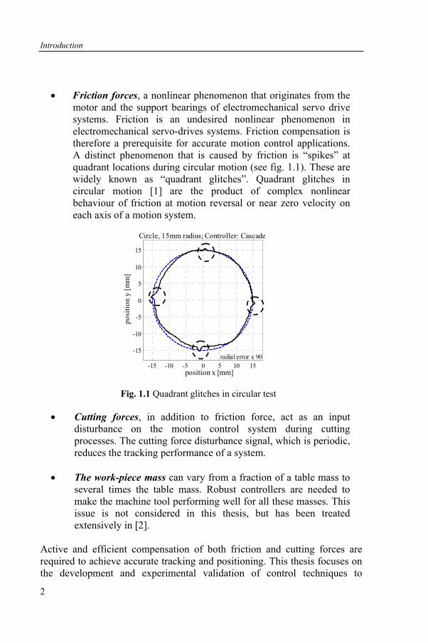
• Friction forces, a nonlinear phenomenon that originates from the motor and the support bearings of electromechanical servo drive systems. Friction is an undesired nonlinear phenomenon in electromechanical servo-drives systems. Friction compensation is therefore a prerequisite for accurate motion control applications. A distinct phenomenon that is caused by friction is “spikes” at quadrant locations during circular motion (see fig. 1.1). These are widely known as “quadrant glitches”. Quadrant glitches in circular motion [1] are the product of complex nonlinear behaviour of friction at motion reversal or near zero velocity on each axis of a motion system.
-15 -10 -5 0 5 10 15
-15
-10
-5
0
5
10
15
position x [mm]
posi
tion
y [m
m]
Circle, 15mm radius; Controller: Cascade
radial error x 90
Fig. 1.1 Quadrant glitches in circular test
• Cutting forces, in addition to friction force, act as an input disturbance on the motion control system during cutting processes. The cutting force disturbance signal, which is periodic, reduces the tracking performance of a system.
• The work-piece mass can vary from a fraction of a table mass to
several times the table mass. Robust controllers are needed to make the machine tool performing well for all these masses. This issue is not considered in this thesis, but has been treated extensively in [2].
Active and efficient compensation of both friction and cutting forces are required to achieve accurate tracking and positioning. This thesis focuses on the development and experimental validation of control techniques to

Introduction
3
actively compensate the influence of friction at motion reversal and cutting forces on the tracking error of drive systems. Both friction feedforward compensation based on the advanced nonlinear Generalized Maxwell Slip (GMS) friction model and various simple and advanced linear control techniques are added to a conventional machine tool controller. Compensation techniques that are highly practical and simple in their application are desired.
1.2 State of the Art on Motion Control
Mechanical drive systems have evolved to meet the present demands for high speed (i.e. shorter transient response time) and high accuracy applications. This evolution however has created a new challenge to the control community with regard to the complexity in effectively rejecting disturbance forces and achieving the best possible tracking accuracy. This section presents a discussion of the paradigm shift in mechatronic drive system technology and a literature review on disturbance forces and their compensation techniques.
1.2.1 Mechanical Drive Systems
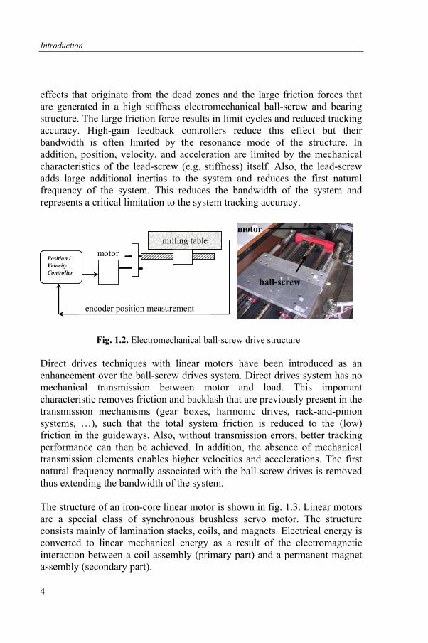
Mechanical drives system technology has seen a shift from electromechanical drive systems to direct drive systems. The emergence of direct drive systems over conventional electromechanical drive systems has provided the industry with their speed and high tracking performance requirements while eliminating some disadvantages of electromechanical drives systems, as discussed in the following paragraph. Pritschow [3] discusses the principle differences between linear motors and the more conventional and still widely used ball-screw drives, and explains that a shift to linear motors is required to further increase the productivity level of machine tools. Fig 1.2 shows a schematic diagram of the conventional ball-screw drive system. The main characteristic of a conventional ball-screw drives structure is the transmission mechanism that converts rotary motion of the motor to linear motion. The transmission mechanism includes the gearing elements and the lead-screw. The lead-screw element contributes negatively to the drives’ performance. The pitch tolerances of the lead-screw generate transmission errors that reduce the tracking accuracy. Tracking accuracy is also compromised by the backlash
Introduction
4
effects that originate from the dead zones and the large friction forces that are generated in a high stiffness electromechanical ball-screw and bearing structure. The large friction force results in limit cycles and reduced tracking accuracy. High-gain feedback controllers reduce this effect but their bandwidth is often limited by the resonance mode of the structure. In addition, position, velocity, and acceleration are limited by the mechanical characteristics of the lead-screw (e.g. stiffness) itself. Also, the lead-screw adds large additional inertias to the system and reduces the first natural frequency of the system. This reduces the bandwidth of the system and represents a critical limitation to the system tracking accuracy.
encoder position measurement
motormilling table
Position / Velocity Controller
encoder position measurement
motormilling table
Position / Velocity Controller
Position / Velocity Controller
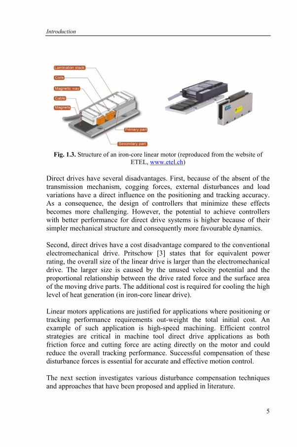
Fig. 1.2. Electromechanical ball-screw drive structure Direct drives techniques with linear motors have been introduced as an enhancement over the ball-screw drives system. Direct drives system has no mechanical transmission between motor and load. This important characteristic removes friction and backlash that are previously present in the transmission mechanisms (gear boxes, harmonic drives, rack-and-pinion systems, …), such that the total system friction is reduced to the (low) friction in the guideways. Also, without transmission errors, better tracking performance can then be achieved. In addition, the absence of mechanical transmission elements enables higher velocities and accelerations. The first natural frequency normally associated with the ball-screw drives is removed thus extending the bandwidth of the system. The structure of an iron-core linear motor is shown in fig. 1.3. Linear motors are a special class of synchronous brushless servo motor. The structure consists mainly of lamination stacks, coils, and magnets. Electrical energy is converted to linear mechanical energy as a result of the electromagnetic interaction between a coil assembly (primary part) and a permanent magnet assembly (secondary part).
ball-screw
motor
Introduction
5
Fig. 1.3. Structure of an iron-core linear motor (reproduced from the website of ETEL, www.etel.ch)
Direct drives have several disadvantages. First, because of the absent of the transmission mechanism, cogging forces, external disturbances and load variations have a direct influence on the positioning and tracking accuracy. As a consequence, the design of controllers that minimize these effects becomes more challenging. However, the potential to achieve controllers with better performance for direct drive systems is higher because of their simpler mechanical structure and consequently more favourable dynamics. Second, direct drives have a cost disadvantage compared to the conventional electromechanical drive. Pritschow [3] states that for equivalent power rating, the overall size of the linear drive is larger than the electromechanical drive. The larger size is caused by the unused velocity potential and the proportional relationship between the drive rated force and the surface area of the moving drive parts. The additional cost is required for cooling the high level of heat generation (in iron-core linear drive). Linear motors applications are justified for applications where positioning or tracking performance requirements out-weight the total initial cost. An example of such application is high-speed machining. Efficient control strategies are critical in machine tool direct drive applications as both friction force and cutting force are acting directly on the motor and could reduce the overall tracking performance. Successful compensation of these disturbance forces is essential for accurate and effective motion control. The next section investigates various disturbance compensation techniques and approaches that have been proposed and applied in literature.
Introduction
6
1.2.2 Disturbance Forces and Compensation Methods
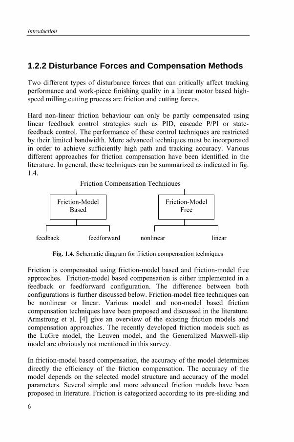
Two different types of disturbance forces that can critically affect tracking performance and work-piece finishing quality in a linear motor based high-speed milling cutting process are friction and cutting forces. Hard non-linear friction behaviour can only be partly compensated using linear feedback control strategies such as PID, cascade P/PI or state-feedback control. The performance of these control techniques are restricted by their limited bandwidth. More advanced techniques must be incorporated in order to achieve sufficiently high path and tracking accuracy. Various different approaches for friction compensation have been identified in the literature. In general, these techniques can be summarized as indicated in fig. 1.4.
Fig. 1.4. Schematic diagram for friction compensation techniques
Friction is compensated using friction-model based and friction-model free approaches. Friction-model based compensation is either implemented in a feedback or feedforward configuration. The difference between both configurations is further discussed below. Friction-model free techniques can be nonlinear or linear. Various model and non-model based friction compensation techniques have been proposed and discussed in the literature. Armstrong et al. [4] give an overview of the existing friction models and compensation approaches. The recently developed friction models such as the LuGre model, the Leuven model, and the Generalized Maxwell-slip model are obviously not mentioned in this survey. In friction-model based compensation, the accuracy of the model determines directly the efficiency of the friction compensation. The accuracy of the model depends on the selected model structure and accuracy of the model parameters. Several simple and more advanced friction models have been proposed in literature. Friction is categorized according to its pre-sliding and
Friction-Model Based
Friction-Model Free
feedback feedforward nonlinear linear
Friction Compensation Techniques

Introduction
7
sliding regimes, and the most simple friction models consider the sliding regime only. These models are a static map between friction force and velocity, e.g. viscous, Coulomb and Stribeck effect friction models. A first attempt in describing the more complex friction behaviour in pre-sliding regime was accomplished by Dahl [5]. The Dahl model was applied extensively for systems with ball-bearing friction. In 1995, Canudas et al. [6] have proposed a new improved friction model, the LuGre model, for control of systems with friction. The model captures most of the observed frictional behaviours that include Coulomb friction, Stribeck effect, and hysteresis. The LuGre friction model is widely applied and accepted for its simplicity and relatively good performance. However, the LuGre friction model fails to describe the hysteresis non-local memory behaviour of friction force in pre-sliding regime. Swevers et al. [7] have improved the LuGre model yielding the Leuven integrated friction model, which is further modified by Lampaert et al. [8]. Recently, Al-Bender et al. [9] developed the so-called Generalized Maxwell-slip (GMS) friction model and illustrate the superiority of the model with respect to simulation of friction behaviour in both the pre-sliding and sliding regimes. The main disadvantage of the GMS model is its complexity and large number of parameters, which complicates its application in control. In a feedback configuration, the measured position signal is used to generate a friction compensation force based on the available friction model. In a feedforward configuration, the reference position is used instead of the measured position signal. The feedback approach is generally designed on the basis of the Coulomb model and the Maxwell-slip model [10]. A careful design strategy is necessary to avoid instability problems. In this thesis, feedforward friction compensation is applied: friction forces predicted by the applied friction model are added to the control command signal to compensate friction forces in the system. The effectiveness of this approach, however, depends on the accuracy of the friction models. Changes in the system environment and structure (lubrication, wear, etc.) could change the friction behaviour and re-identification of the friction model will be necessary to avoid deterioration in the friction compensation performance. Besides model based friction compensation, various friction-model free compensation methods have been suggested and discussed in the literature. These include linear and non-linear control strategies. In a linear control approach, Tung, Anwar, and Tomizuka [11] have demonstrated the effectiveness of a repetitive controller, first introduced by Hara et al. [12], in improving tracking performance and quadrant glitches compensation.
Introduction
8
In addition, Lampaert et al. [13] have proposed a control approach that includes a disturbance observer based on a Kalman filter using a second order random walk model. Since friction is a highly nonlinear phenomenon it can be expected that nonlinear control approaches are more appropriate. Several nonlinear control strategies have been adapted for friction compensation. Tjahjowidodo et al. [14] have shown that a Maxwell-slip-model-based nonlinear gain scheduling controller yields fast response and low steady-state error for friction compensation in electro-mechanical systems. Sliding mode control (SMC) [15, 16] is an example of an important robust control design approach for linear and nonlinear systems. Two main features of SMC are the finite reaching time and the complete disturbance rejection of matched uncertainties. In SMC applications, the system states approach the switching line (or surface) and slide along this line to reach the final states. During sliding, the control behaviour is independent of the system dynamics and hence is independent of the influence of the acting disturbance forces. Altintas [17] has described the SMC design for high-speed feed drives. A tracking performance comparison between SMC and the classical cascade controller is discussed in [18]. SMC however, is widely known for its “chattering” problem [19, 20], a high-frequency switching of the SMC that is a result of the imperfect switching mechanism and discontinuous control signal around the switching surface. Chattering is highly undesirable since it involves large control activity and possible excitation of the resonance frequencies of the system. Many different techniques have been proposed in literature to eliminate chattering in SMC related applications [21, 22]. Besides friction force compensation, attenuation of other external disturbance forces, such as the cutting force that acts on a motion control system, is of equal importance. Various compensation methods for different applications have been proposed in literature. A repetitive controller is ideal for periodic reference command signals and disturbance inputs. The repetitive controller is only active in small frequency ranges around the harmonics and system phase lag is compensated for in its design [23]. The performance of a repetitive controller is highly influenced by the accuracy of the period of the harmonics signal. Disturbances can also be compensated using a robust control approach such as the H-infinity control [24] and SMC. Van Brussel and Van den Braembussche have investigated the robustness of both H∞ and SMC in linear motor systems [25].
Introduction
9
Ohnishi et al. present an inverse model-based disturbance observer [26, 27] control structure that can be applied for any type of input disturbance. It adds a high gain loop to an existing control configuration, thereby improving the disturbance rejection with its bandwidth, which depends on the accuracy of the available system model. The tuning of this bandwidth is a trade-off between performance and stability margin. Kempf et al. [28] have added the disturbance observer into an existing control system structure and have shown enhanced disturbance attenuation performance of a track following optical disk drive system against shock and vibration influence. The disturbance attenuation property is removed from the design specifications of the feedback controller resulting in simplified control design and greater stability. This approach can be applied to any disturbance and is effective up to a specified bandwidth which depends on the accuracy of the available system model. An explicit estimation of the cutting force has been attempted by Pritschow et al. [29]. The estimation is based on the balance of forces acting on the system and uses a relative acceleration sensor measurement. A reduced order state observer estimates the velocity and the cutting force. However, to the best of our knowledge, no report on the application of this estimator to effectively compensate the influence of the cutting force is available.
1.3 Scope, Objective, and Approaches
Effective compensation of friction forces and cutting forces are a prerequisite for accurate tracking performance in machine tool drive applications. Classical motion controllers (discussed in chapter 2) are not able to fully reduce the effect of these disturbances sufficiently. Various other techniques have been reported as discussed in the previous section. However, very limited knowledge on the application of some of these techniques for friction and cutting forces compensation in high-speed milling machine direct drives is available. The objective of this research can be summarized as follow:
“Improve the positioning and tracking accuracy of motion systems controlled by the classical cascade P/PI feedback control structure by adding simple but effective friction and cutting force compensation mechanisms.”
Introduction
10
These compensation mechanisms are developed for a linear drive based xy-table of a high-speed milling machine. The modelling and experimental identification of this system, the design of the cascade P/PI feedback controller and various compensation mechanisms and their simulation-based and experimental validation are discussed in detail in this thesis. Friction forces are compensated using both friction-model based feedforward and the inverse-model-based disturbance observer. These techniques have been selected because of their simplicity. Feedforward is preferred over feedback in order to avoid stability issues. Two friction models are compared: a static friction model and the recent and more advanced Generalised Maxwell-slip model. The inverse model based disturbance observer [26, 27] is selected because of its simple structure and design methodology that accounts for model uncertainty. To compensate cutting forces, several techniques are implemented and compared. These include: the inverse model based disturbance observer, a repetitive controller, a force disturbance observer, and Pritschow’s explicit estimation of cutting forces using the Ferraris relative acceleration sensor measurement.
1.4 Contributions
The thesis attempts to enrich the understanding and knowledge regarding accurate motion control of machine tool feed drive systems. The following contributions are presented:
i. Development of simple motion control structure based on the classical cascade P/PI controller combined with modules to improve the friction and cutting forces compensation.
ii. Application of a simple identification procedure for the Generalized Maxwell-slip (GMS) friction model that produces superior friction compensation performance, especially at lower tracking velocity
iii. Application of an inverse model based disturbance observer in combination with feedforward of the GMS friction model for efficient friction compensation.
iv. Comparison of the tracking performance of different cutting force compensation techniques during actual circular cutting tests.
Introduction
11
1.5 Outline
This thesis focuses on friction and cutting forces compensation of a linear-motor based xy feed drive system. The above mentioned friction feedforward, inverse model based disturbance observer, and repetitive controller are add-on devices, implying that they are added to an existing feedback control system, which is a classical cascade P/PI controller. The structure, design procedures, and analysis of a classical cascade P/PI position controller that is widely applied in many mechatronic systems are discussed first in Chapter 2. The minimization of the effect of disturbance forces on the system position and tracking performance requires precise knowledge and complete understanding of the characteristics of these disturbance forces. Chapter 3 discusses the modelling and identification of friction, and the spectral analysis of cutting force measurements of an actual milling cutting process. Chapter 4 discusses the implementation of the friction force compensation based on the feedforward of friction models. Simulations and experimental validations of friction compensation performances using a simple static friction model and the more advanced and recent GMS friction model are performed and compared. An inverse model-based disturbance observer module is introduced in combination with feedforward of the friction models and its influence on the magnitude of the quadrant glitches from circular tests are studied and analysed. Chapter 5 describes and discusses compensation of the cutting force using various selected control techniques. The experimental validation of the different compensation techniques are performed first using artificial cutting force synthesized from actual milling cutting force measurements and second during actual circular cutting processes. The practical implementation of friction and cutting forces compensation during these cutting tests and the tracking performances of the different techniques are discussed and compared. Finally, Chapter 6 presents the conclusions regarding the design of the cascade P/PI controller, the performance of friction and cutting forces compensation and some recommendations of future work.

12
13
Chapter 2
Classical Motion Control
2.1 Introduction
Motion tracking controllers are designed with the objective of achieving maximal tracking accuracy and robustness against disturbances and plant uncertainties. The size of the tracking errors and actuator input signals are important indicators to validate a control system design. A good control design ensures that these indicators remain below some pre-specified conditions and hence exploiting the system to its fullest potential. Feedback control strategy is the basic principle of many control systems. The desired reference signals are compared with the actual output of the system and corrective measures are implemented to compensate these errors. Feedback control linearizes nonlinear elements and partly compensates the effects of disturbances and system variations. Due to its simplicity, PI and PID control form 90% of the practical control applications. Feedforward control strategies are normally introduced to compliment feedback control [30]. A combined feedforward and feedback control strategy improves tracking performance especially in systems with pre-knowledge of the inputs reference and disturbance signals. A prominent and classical tracking controller that exists in the majority of servo motion control systems is the classical cascade controller. Cascade control is widely applied for its simple structure and transparent design. In addition, the loop controllers are based on the familiar classical proportional P, and integrator I controllers. Various modifications to this controller have been suggested in literature with the aim of improving its tracking performance. For example, Doenitz [31] analysed the tracking error of a combination of a cascade controller with a disturbance observer. In addition,
Classical Motion Control
14
Boucher et al. [32] have presented a generalized predictive cascade control for control of machine tool drives. This chapter discusses the analysis and design of a classical cascade P/PI controller for position control of a linear drive based xy feed table. First, a detailed description of the experimental setup, that is, a high-speed xy milling machine is presented.
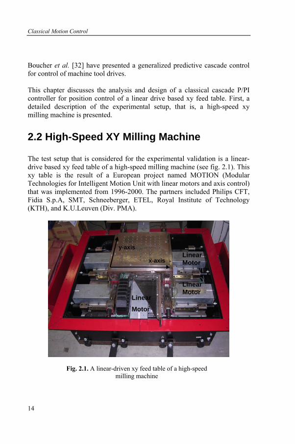
2.2 High-Speed XY Milling Machine
The test setup that is considered for the experimental validation is a linear-drive based xy feed table of a high-speed milling machine (see fig. 2.1). This xy table is the result of a European project named MOTION (Modular Technologies for Intelligent Motion Unit with linear motors and axis control) that was implemented from 1996-2000. The partners included Philips CFT, Fidia S.p.A, SMT, Schneeberger, ETEL, Royal Institute of Technology (KTH), and K.U.Leuven (Div. PMA).
Fig. 2.1. A linear-driven xy feed table of a high-speed milling machine
Linear Motor
Linear Motor
Linear
Motor
x-axis
y-axis
Classical Motion Control
15
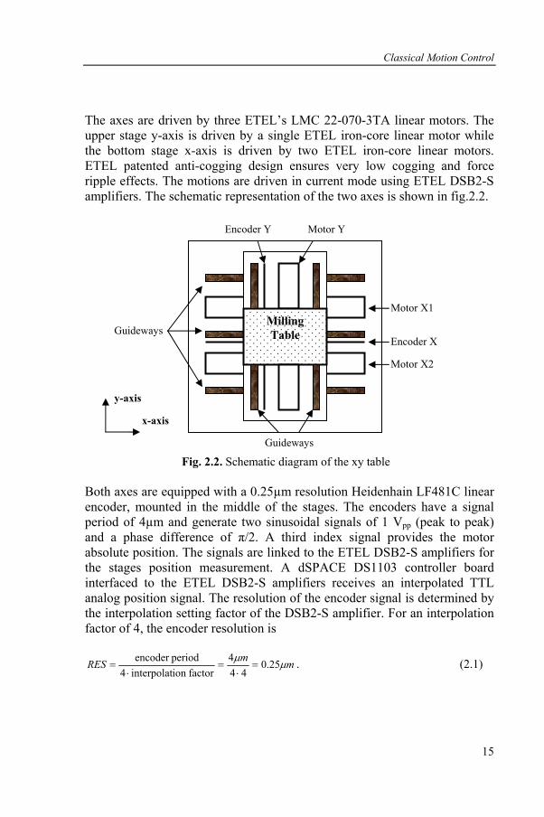
The axes are driven by three ETEL’s LMC 22-070-3TA linear motors. The upper stage y-axis is driven by a single ETEL iron-core linear motor while the bottom stage x-axis is driven by two ETEL iron-core linear motors. ETEL patented anti-cogging design ensures very low cogging and force ripple effects. The motions are driven in current mode using ETEL DSB2-S amplifiers. The schematic representation of the two axes is shown in fig.2.2.
Fig. 2.2. Schematic diagram of the xy table
Both axes are equipped with a 0.25µm resolution Heidenhain LF481C linear encoder, mounted in the middle of the stages. The encoders have a signal period of 4µm and generate two sinusoidal signals of 1 Vpp (peak to peak) and a phase difference of π/2. A third index signal provides the motor absolute position. The signals are linked to the ETEL DSB2-S amplifiers for the stages position measurement. A dSPACE DS1103 controller board interfaced to the ETEL DSB2-S amplifiers receives an interpolated TTL analog position signal. The resolution of the encoder signal is determined by the interpolation setting factor of the DSB2-S amplifier. For an interpolation factor of 4, the encoder resolution is
mmRES μμ 25.044
4factorion interpolat4
periodencoder =
⋅=
⋅= . (2.1)
Encoder Y
Guideways
Motor Y
Motor X1
Encoder X
Motor X2
x-axis
y-axis
Milling Table Guideways
Classical Motion Control
16
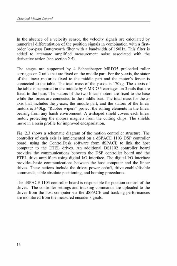
In the absence of a velocity sensor, the velocity signals are calculated by numerical differentiation of the position signals in combination with a first-order low-pass Butterworth filter with a bandwidth of 150Hz. This filter is added to attenuate amplified measurement noise associated with the derivative action (see section 2.5). The stages are supported by 4 Schneeberger MRD35 preloaded roller carriages on 2 rails that are fixed on the middle part. For the y-axis, the stator of the linear motor is fixed to the middle part and the motor’s forcer is connected to the table. The total mass of the y-axis is 170kg. The x-axis of the table is supported in the middle by 6 MRD35 carriages on 3 rails that are fixed to the base. The stators of the two linear motors are fixed to the base while the forces are connected to the middle part. The total mass for the x-axis that includes the y-axis, the middle part, and the stators of the linear motors is 340kg. “Rubber wipers” protect the rolling elements in the linear bearing from any harsh environment. A u-shaped shield covers each linear motor, protecting the motors magnets from the cutting chips. The shields move in a resin profile for improved encapsulation. Fig. 2.3 shows a schematic diagram of the motion controller structure. The controller of each axis is implemented on a dSPACE 1103 DSP controller board, using the ControlDesk software from dSPACE to link the host computer to the ETEL drives. An additional DS1102 controller board provides the communications between the DSP controller board and the ETEL drive amplifiers using digital I/O interface. The digital I/O interface provides basic communications between the host computer and the linear drives. These actions include the drives power on/off, drive enable/disable commands, table absolute positioning, and homing procedures. The dSPACE 1103 controller board is responsible for position control of the drives. The controller settings and tracking commands are uploaded to the drives from the host computer via the dSPACE and tracking performances are monitored from the measured encoder signals.
Classical Motion Control
17
Fig. 2.3. Motion controller structure of a xy feed table with three linear drives for high speed milling application
The system identification is described in the next section.
2.3 System Identification
A linear time-invariant model of the dynamic behaviour of each axis is obtained from frequency response function (FRF) measurements of the system. The dynamic coupling between both axes is negligible and the system dynamics can be described by two single-input single-output (SISO) models. In order to measure the two SISO FRFs of the system, the system is excited with band-limited white noise signals. The output encoder measurements and the excitation signal, that is the signal that is sent to the ETEL drive amplifiers, are recorded. The sampling frequency is 2000Hz and the total duration of the measurement is 5 min. A Hanning window is applied. The number of samples per window is 2048. This yields a sampling resolution of 1Hz. The SISO FRFs of the system are estimated using the H1 estimator [33].
Classical Motion Control
18
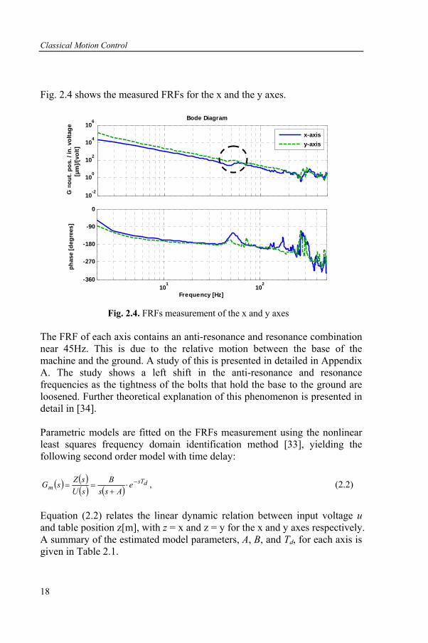
Fig. 2.4 shows the measured FRFs for the x and the y axes.
10-2
100
102
104
106
101
102
-360
-270
-180
-90
0
Frequency [Hz]
phas
e [d
egre
es]
G =
out.
pos.
/ in
. vol
tage
[
µm]/[
volt]
Bode Diagram
x-axisy-axis
Fig. 2.4. FRFs measurement of the x and y axes
The FRF of each axis contains an anti-resonance and resonance combination near 45Hz. This is due to the relative motion between the base of the machine and the ground. A study of this is presented in detailed in Appendix A. The study shows a left shift in the anti-resonance and resonance frequencies as the tightness of the bolts that hold the base to the ground are loosened. Further theoretical explanation of this phenomenon is presented in detail in [34]. Parametric models are fitted on the FRFs measurement using the nonlinear least squares frequency domain identification method [33], yielding the following second order model with time delay:
( ) ( )( ) ( ) ,dsT
m eAss
BsUsZsG −⋅
+== (2.2)
Equation (2.2) relates the linear dynamic relation between input voltage u and table position z[m], with z = x and z = y for the x and y axes respectively. A summary of the estimated model parameters, A, B, and Td, for each axis is given in Table 2.1.
Classical Motion Control
19
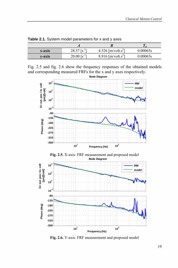
Table 2.1. System model parameters for x and y axes A B Td
x-axis 28.57 [s-1] 4.526 [m/volt.s2] 0.00065s y-axis 20.00 [s-1] 8.916 [m/volt.s2] 0.00065s
Fig. 2.5 and fig. 2.6 show the frequency responses of the obtained models and corresponding measured FRFs for the x and y axes respectively.
Bode Diagram
Frequency (Hz)
Phas
e (d
eg)
G=
out.
pos
/ in.
vol
t [µ
m]/[
volt]
10-2
100
102
104
101 102-360
-315
-270
-225
-180
-135
-90
FRFmodel
Fig. 2.5. X-axis: FRF measurement and proposed model
Bode Diagram
Frequency (Hz)
Phas
e (d
eg)
G=
out.
pos
/ in.
vol
t [µ
m]/[
volt]
10-2
100
102
104
101 102-360
-315
-270
-225
-180
-135
-90
FRFmodel
Fig. 2.6. Y-axis: FRF measurement and proposed model
Classical Motion Control
20
The parametric model (2.2) estimates the models as a mass line with damping characteristic at lower frequency range. These models do not include the resonance and anti-resonance peaks at frequencies beyond 40Hz as shown in fig. 2.5 (e.g. the anti-resonance frequency at 47Hz for the x-axis, and at 44 Hz for the y-axis). The next section discusses the control analysis and design of a cascade controller that is applied for position control of the xy table. Analysis of the cascade controller based on an ideal configuration of the system is first considered.
2.4 Cascade Control Structure & Analysis
2.4.1 Cascade Controller Structure & Configuration
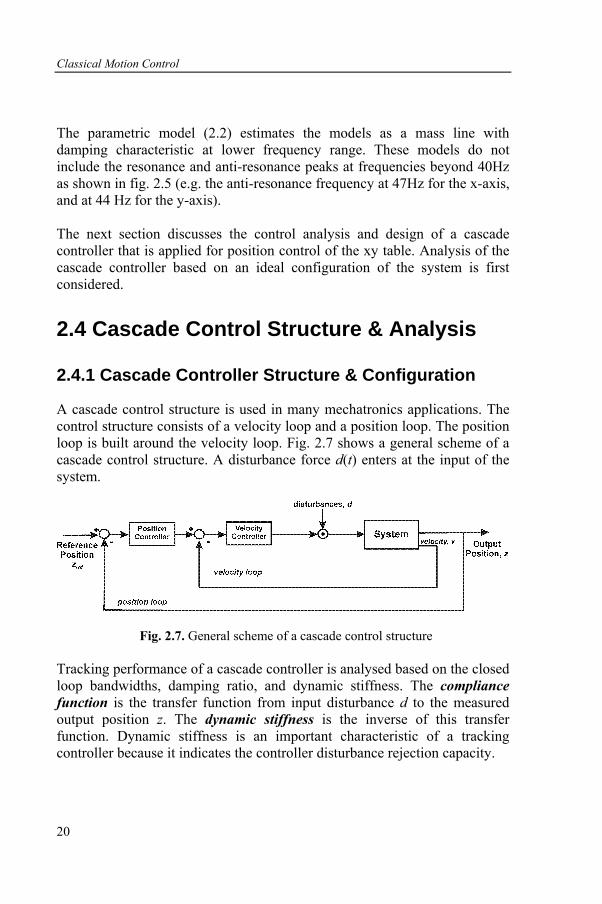
A cascade control structure is used in many mechatronics applications. The control structure consists of a velocity loop and a position loop. The position loop is built around the velocity loop. Fig. 2.7 shows a general scheme of a cascade control structure. A disturbance force d(t) enters at the input of the system.
Fig. 2.7. General scheme of a cascade control structure Tracking performance of a cascade controller is analysed based on the closed loop bandwidths, damping ratio, and dynamic stiffness. The compliance function is the transfer function from input disturbance d to the measured output position z. The dynamic stiffness is the inverse of this transfer function. Dynamic stiffness is an important characteristic of a tracking controller because it indicates the controller disturbance rejection capacity.
Classical Motion Control
21
This section analyses the characteristics of the cascade P/PI controller by first considering an ideal theoretical design configuration. The following idealized configuration is considered:
the system behaves as an ideal rigid body system without friction,
velocity v and position signals z are assumed to be available,
measurement noise n(t) is only present on the velocity signal, not on the position signal,
disturbances d(t) enter at the input of the system, that is, these disturbances are forces.
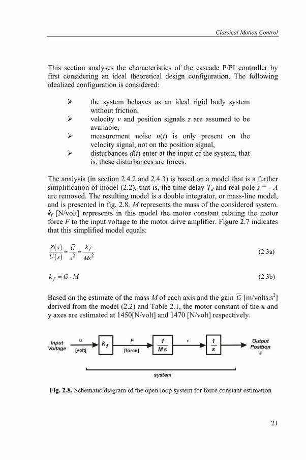
The analysis (in section 2.4.2 and 2.4.3) is based on a model that is a further simplification of model (2.2), that is, the time delay Td and real pole s = - A are removed. The resulting model is a double integrator, or mass-line model, and is presented in fig. 2.8. M represents the mass of the considered system. kf [N/volt] represents in this model the motor constant relating the motor force F to the input voltage to the motor drive amplifier. Figure 2.7 indicates that this simplified model equals:
( )( ) 2 2
fkZ s GU s s Ms
= = (2.3a)
MGk f ⋅= (2.3b)
Based on the estimate of the mass M of each axis and the gain G [m/volts.s2] derived from the model (2.2) and Table 2.1, the motor constant of the x and y axes are estimated at 1450[N/volt] and 1470 [N/volt] respectively.
Fig. 2.8. Schematic diagram of the open loop system for force constant estimation
Classical Motion Control
22
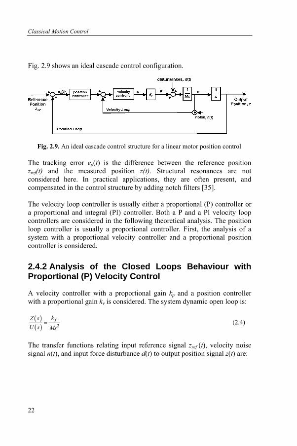
Fig. 2.9 shows an ideal cascade control configuration.
Fig. 2.9. An ideal cascade control structure for a linear motor position control The tracking error ep(t) is the difference between the reference position zref(t) and the measured position z(t). Structural resonances are not considered here. In practical applications, they are often present, and compensated in the control structure by adding notch filters [35]. The velocity loop controller is usually either a proportional (P) controller or a proportional and integral (PI) controller. Both a P and a PI velocity loop controllers are considered in the following theoretical analysis. The position loop controller is usually a proportional controller. First, the analysis of a system with a proportional velocity controller and a proportional position controller is considered.
2.4.2 Analysis of the Closed Loops Behaviour with Proportional (P) Velocity Control
A velocity controller with a proportional gain kp and a position controller with a proportional gain kv is considered. The system dynamic open loop is:
( )( ) 2
fkZ sU s Ms
= (2.4)
The transfer functions relating input reference signal zref (t), velocity noise signal n(t), and input force disturbance d(t) to output position signal z(t) are:
Classical Motion Control
23
( ) ( )
( )
( )
2
2
2
1
v p fref
p f v p f
p f
p f v p f
p f v p f
k k kZ s Z s
Ms k k s k k k
k k + N s
Ms k k s k k k
+ D sMs k k s k k k
= ⋅+ +
⋅+ +
⋅+ +
(2.5)
The dynamic stiffness of the controller, which is the inverse of ( )( )
Z sD s
in (2.5),
is
( )( )
2p f v p f
D sMs k k s k k k .
Z s= + + (2.6)
The position error ep(t) can be expressed as a function of the reference signal zref (t), velocity noise signal n(t), and the input disturbance d(t),
( ) ( ) ( )
( ) ( )
( )
( )
2
2
2
21
p ref
p fp ref
p f v p f
p f
p f v p f
p f v p f
E s Z s Z s
Ms k k sE s Z s
Ms k k s k k k
k k - N s
Ms k k s k k k
- D s .Ms k k s k k k
= −
+= ⋅
+ +
⋅+ +
⋅+ +
(2.7)
The undamped natural frequency ω0 and the damping ratio ς of the system are obtained from the transfer function ( )
( )sZsZ
refin (2.5),
Mkkk fpv=0ω (2.8)
v
fp
Mkkk
21
=ς . (2.9)
Classical Motion Control
24
The tracking performance of the cascade P/P controller is analysed as follows: For a reference signal with a constant velocity,
( ) 2svsZref = , (2.10)
the steady-state tracking error obtained using the final-value theorem to equation (2.7) (ignoring noise signal n(t) and input disturbance d(t)) equals:
( )pv
vek
∞ = (2.11)
The steady-state error is inversely proportional to the proportional gain kv and is directly proportional to the constant tracking velocity v. Next, the positioning performance is analysed for a step reference input signal zref(t)=k and for a static disturbance signal d(t) = k. The steady state position error for a step reference input signal and for a static disturbance signal, obtained by applying the final value theorem to equation (2.7) are:
0pz _ stepe = (2.12a)
pd _ step v p f
ke .k k k
= − (2.12b)
The steady-state error is proportional to the static disturbance force k (equation 2.12b) and will always be a non-zero value. This also means that, in the absence of a disturbance signal, the steady-state error is zero (equation 2.12a).
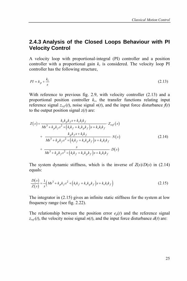
Classical Motion Control
25
2.4.3 Analysis of the Closed Loops Behaviour with PI Velocity Control
A velocity loop with proportional-integral (PI) controller and a position controller with a proportional gain kv is considered. The velocity loop PI controller has the following structure,
skkPI i
p += (2.13)
With reference to previous fig. 2.9, with velocity controller (2.13) and a proportional position controller kv, the transfer functions relating input reference signal zref (t), noise signal n(t), and the input force disturbance f(t) to the output position signal z(t) are:
( ) ( ) ( )
( ) ( )
( ) ( )
3 2
3 2
3 2
v p f v i fref
p f i f v p f v i f
p f i f
p f i f v p f v i f
p f i f v p f v i f
k k k s k k kZ s Z s
Ms k k s k k k k k s k k k
k k s k k + N s
Ms k k s k k k k k s k k k
s + D sMs k k s k k k k k s k k k
+= ⋅
+ + + +
+⋅
+ + + +
⋅+ + + +
(2.14)
The system dynamic stiffness, which is the inverse of Z(s)/D(s) in (2.14) equals:
( )( ) ( )( )3 21
= + + + +p f i f v p f v i fD s
Ms k k s k k k k k s k k kZ s s
(2.15)
The integrator in (2.15) gives an infinite static stiffness for the system at low frequency range (see fig. 2.22). The relationship between the position error ep(t) and the reference signal zref (t), the velocity noise signal n(t), and the input force disturbance d(t) are:
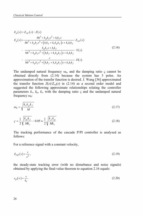
Classical Motion Control
26
( ) ( ) ( )
( ) ( ) ( )
( ) ( )
( ) ( )
3 2
3 2
3 2
3 2
p ref
p f i fp ref
p f i f v p f v i f
p f i f
p f i f v p f v i f
p f i f v p f v i f
E s Z s Z s
Ms k k s k k sE s Z s
Ms k k s k k k k k s k k k
k k s k k - N s
Ms k k s k k k k k s k k k
s - D s .Ms k k s k k k k k s k k k
= −
+ += ⋅
+ + + +
+⋅
+ + + +
⋅+ + + +
(2.16)
The undamped natural frequency ω0, and the damping ratio ς cannot be obtained directly from (2.14) because the system has 3 poles. An approximation of the transfer function is desired. J. Wang [36] approximated the transfer function Z(s)/Zref(s) in (2.14) as a second order model and suggested the following approximate relationships relating the controller parameters kv, kp, ki, with the damping ratio ς and the undamped natural frequency ω0:
Mkkk fpv=0ω (2.17)
v
pf
v
fp
Mkkk
Mkkk
2105.0
21
≈−=ς (2.18)
The tracking performance of the cascade P/PI controller is analysed as follows: For a reference signal with a constant velocity,
( ) 2refvZ ss
= , (2.19)
the steady-state tracking error (with no disturbance and noise signals) obtained by applying the final-value theorem to equation 2.16 equals:
( )pv
ve .k
∞ = (2.20)
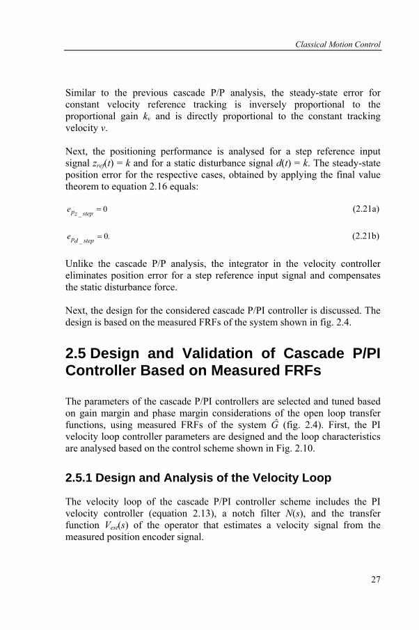
Classical Motion Control
27
Similar to the previous cascade P/P analysis, the steady-state error for constant velocity reference tracking is inversely proportional to the proportional gain kv and is directly proportional to the constant tracking velocity v. Next, the positioning performance is analysed for a step reference input signal zref(t) = k and for a static disturbance signal d(t) = k. The steady-state position error for the respective cases, obtained by applying the final value theorem to equation 2.16 equals:
0pz _ stepe = (2.21a)
0pd _ stepe .= (2.21b)
Unlike the cascade P/P analysis, the integrator in the velocity controller eliminates position error for a step reference input signal and compensates the static disturbance force. Next, the design for the considered cascade P/PI controller is discussed. The design is based on the measured FRFs of the system shown in fig. 2.4.
2.5 Design and Validation of Cascade P/PI Controller Based on Measured FRFs
The parameters of the cascade P/PI controllers are selected and tuned based on gain margin and phase margin considerations of the open loop transfer functions, using measured FRFs of the system Ĝ (fig. 2.4). First, the PI velocity loop controller parameters are designed and the loop characteristics are analysed based on the control scheme shown in Fig. 2.10.
2.5.1 Design and Analysis of the Velocity Loop
The velocity loop of the cascade P/PI controller scheme includes the PI velocity controller (equation 2.13), a notch filter N(s), and the transfer function Vest(s) of the operator that estimates a velocity signal from the measured position encoder signal.
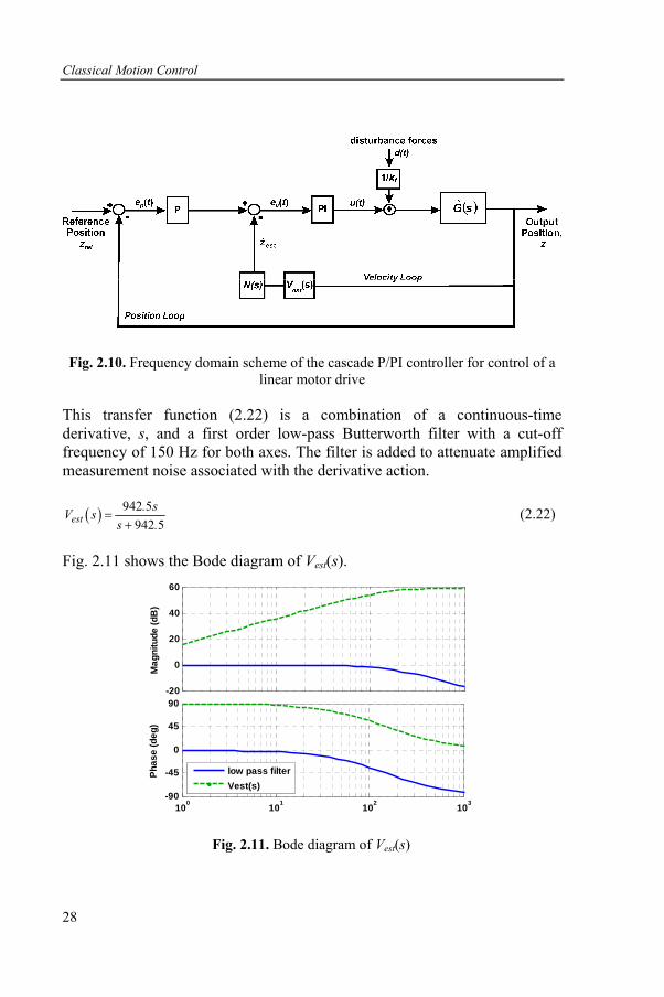
Classical Motion Control
28
Fig. 2.10. Frequency domain scheme of the cascade P/PI controller for control of a linear motor drive
This transfer function (2.22) is a combination of a continuous-time derivative, s, and a first order low-pass Butterworth filter with a cut-off frequency of 150 Hz for both axes. The filter is added to attenuate amplified measurement noise associated with the derivative action.
( ) 942 5942 5est
. sV ss .
=+
(2.22)
Fig. 2.11 shows the Bode diagram of Vest(s).
-20
0
20
40
60
Mag
nitu
de (d
B)
100 101 102 103-90
-45
0
45
90
Phas
e (d
eg)
low pass filterVest(s)
Fig. 2.11. Bode diagram of Vest(s)
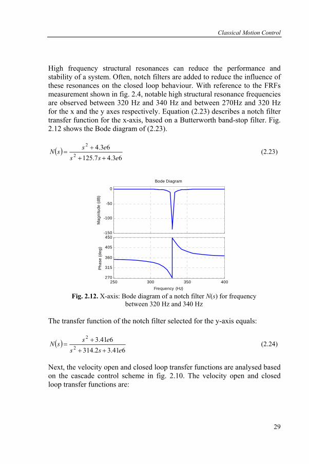
Classical Motion Control
29
High frequency structural resonances can reduce the performance and stability of a system. Often, notch filters are added to reduce the influence of these resonances on the closed loop behaviour. With reference to the FRFs measurement shown in fig. 2.4, notable high structural resonance frequencies are observed between 320 Hz and 340 Hz and between 270Hz and 320 Hz for the x and the y axes respectively. Equation (2.23) describes a notch filter transfer function for the x-axis, based on a Butterworth band-stop filter. Fig. 2.12 shows the Bode diagram of (2.23).
( )63.47.125
63.42
2
essessN++
+= (2.23)
-150
-100
-50
0
Mag
nitu
de (d
B)
250 300 350 400270
315
360
405
450
Phas
e (d
eg)
Bode Diagram
Frequency (Hz) Fig. 2.12. X-axis: Bode diagram of a notch filter N(s) for frequency
between 320 Hz and 340 Hz The transfer function of the notch filter selected for the y-axis equals:
( )641.32.314
641.32
2
essessN
++
+= (2.24)
Next, the velocity open and closed loop transfer functions are analysed based on the cascade control scheme in fig. 2.10. The velocity open and closed loop transfer functions are:
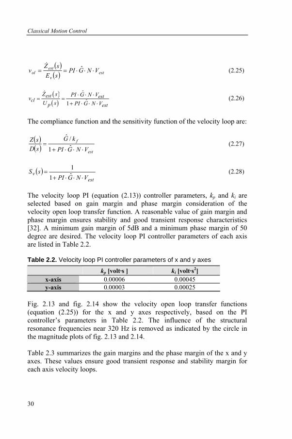
Classical Motion Control
30
( )( ) est
v
estol VNGPI
sEsZ
v ⋅⋅⋅== ˆ&
(2.25)
( )( ) 1
est estcl
p est
ˆZ s PI G N Vv ˆU s PI G N V⋅ ⋅ ⋅
= =+ ⋅ ⋅ ⋅
& (2.26)
The compliance function and the sensitivity function of the velocity loop are:
( )( ) est
f
VNGPI
kGsDsZ
⋅⋅⋅+= ˆ1
/ˆ (2.27)
( )est
vVNGPI
sS⋅⋅⋅+
= ˆ11 (2.28)
The velocity loop PI (equation (2.13)) controller parameters, kp and ki are selected based on gain margin and phase margin consideration of the velocity open loop transfer function. A reasonable value of gain margin and phase margin ensures stability and good transient response characteristics [32]. A minimum gain margin of 5dB and a minimum phase margin of 50 degree are desired. The velocity loop PI controller parameters of each axis are listed in Table 2.2.
Table 2.2. Velocity loop PI controller parameters of x and y axes kp [volt·s ] ki [volt·s2]
x-axis 0.00006 0.00045 y-axis 0.00003 0.00025
Fig. 2.13 and fig. 2.14 show the velocity open loop transfer functions (equation (2.25)) for the x and y axes respectively, based on the PI controller’s parameters in Table 2.2. The influence of the structural resonance frequencies near 320 Hz is removed as indicated by the circle in the magnitude plots of fig. 2.13 and 2.14. Table 2.3 summarizes the gain margins and the phase margin of the x and y axes. These values ensure good transient response and stability margin for each axis velocity loops.
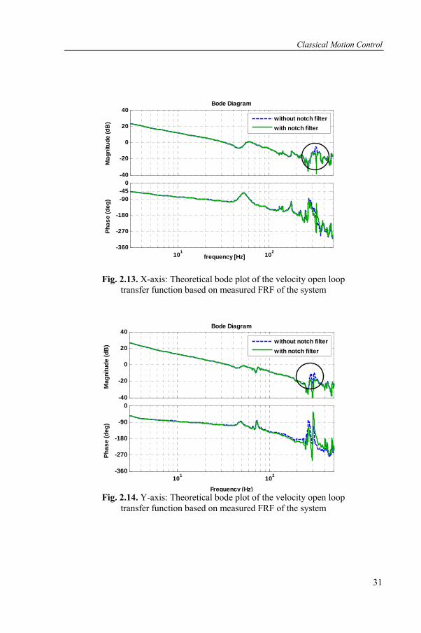
Classical Motion Control
31
Bode DiagramPh
ase
(deg
)M
agni
tude
(dB
)
-40
-20
0
20
40
101 102-360
-270
-180
-90-45
0
frequency [Hz]
without notch filterwith notch filter
Fig. 2.13. X-axis: Theoretical bode plot of the velocity open loop
transfer function based on measured FRF of the system
Bode Diagram
Frequency (Hz)
Phas
e (d
eg)
Mag
nitu
de (d
B)
-40
-20
0
20
40
101 102-360
-270
-180
-90
0
without notch filterwith notch filter
Fig. 2.14. Y-axis: Theoretical bode plot of the velocity open loop
transfer function based on measured FRF of the system
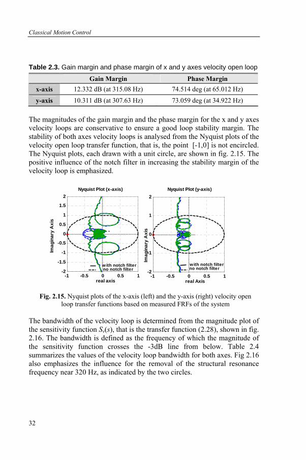
Classical Motion Control
32
Table 2.3. Gain margin and phase margin of x and y axes velocity open loop Gain Margin Phase Margin
x-axis 12.332 dB (at 315.08 Hz) 74.514 deg (at 65.012 Hz)
y-axis 10.311 dB (at 307.63 Hz) 73.059 deg (at 34.922 Hz) The magnitudes of the gain margin and the phase margin for the x and y axes velocity loops are conservative to ensure a good loop stability margin. The stability of both axes velocity loops is analysed from the Nyquist plots of the velocity open loop transfer function, that is, the point [-1,0] is not encircled. The Nyquist plots, each drawn with a unit circle, are shown in fig. 2.15. The positive influence of the notch filter in increasing the stability margin of the velocity loop is emphasized.
Imag
inar
y A
xis
-1 -0.5 0 0.5 1-2
-1.5
-1
-0.5
0
0.5
1
1.5
2
real Axis
Imag
inar
y A
xis
-1 -0.5 0 0.5 1-2
-1
0
1
2
real axis
no notch filter w ith notch filter
Nyquist Plot (x-axis) Nyquist Plot (y-axis)
with notch filter no notch filter
Fig. 2.15. Nyquist plots of the x-axis (left) and the y-axis (right) velocity open loop transfer functions based on measured FRFs of the system
The bandwidth of the velocity loop is determined from the magnitude plot of the sensitivity function Sv(s), that is the transfer function (2.28), shown in fig. 2.16. The bandwidth is defined as the frequency of which the magnitude of the sensitivity function crosses the -3dB line from below. Table 2.4 summarizes the values of the velocity loop bandwidth for both axes. Fig 2.16 also emphasizes the influence for the removal of the structural resonance frequency near 320 Hz, as indicated by the two circles.
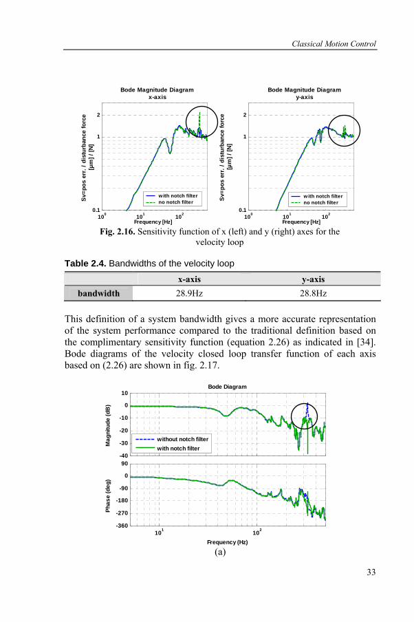
Classical Motion Control
33
Bode Magnitude Diagramx-axis
Sv=p
os e
rr. /
dis
turb
ance
forc
e[µ
m] /
[N]
100 101 1020.1
1
2
with notch filterno notch filter
Bode Magnitude Diagramy-axis
Sv=
pos
err.
/ dis
turb
ance
forc
e[µ
m] /
[N]
100 101 1020.1
1
2
with notch filterno notch filter
Frequency [Hz] Frequency [Hz] Fig. 2.16. Sensitivity function of x (left) and y (right) axes for the
velocity loop
Table 2.4. Bandwidths of the velocity loop x-axis y-axis
bandwidth 28.9Hz 28.8Hz This definition of a system bandwidth gives a more accurate representation of the system performance compared to the traditional definition based on the complimentary sensitivity function (equation 2.26) as indicated in [34]. Bode diagrams of the velocity closed loop transfer function of each axis based on (2.26) are shown in fig. 2.17.
Bode Diagram
Frequency (Hz)
Phas
e (d
eg)
Mag
nitu
de (d
B)
-40
-30
-20
-10
0
10
101 102-360
-270
-180
-90
0
90
without notch filterwith notch filter
(a)
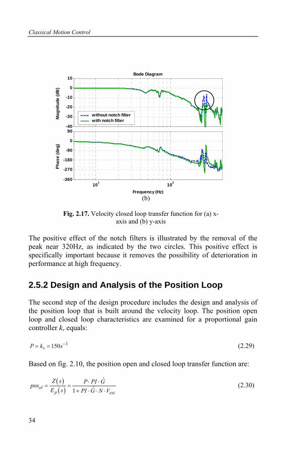
Classical Motion Control
34
Bode Diagram
Frequency (Hz)
Phas
e (d
eg)
Mag
nitu
de (d
B)
-40
-30
-20
-10
0
10
without notch filterwith notch filter
101 102-360
-270
-180
-90
0
90
(b)
Fig. 2.17. Velocity closed loop transfer function for (a) x-
axis and (b) y-axis The positive effect of the notch filters is illustrated by the removal of the peak near 320Hz, as indicated by the two circles. This positive effect is specifically important because it removes the possibility of deterioration in performance at high frequency.
2.5.2 Design and Analysis of the Position Loop
The second step of the design procedure includes the design and analysis of the position loop that is built around the velocity loop. The position open loop and closed loop characteristics are examined for a proportional gain controller kv equals:
1150vP k s−= = (2.29)
Based on fig. 2.10, the position open and closed loop transfer function are:
( )( ) 1ol
p est
ˆZ s P PI Gpos ˆE s PI G N V⋅ ⋅
= =+ ⋅ ⋅ ⋅
(2.30)
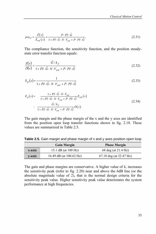
Classical Motion Control
35
( )( ) 1cl
ref est
ˆZ s P PI Gpos .ˆ ˆZ s PI G N V P PI G⋅ ⋅
= =+ ⋅ ⋅ ⋅ + ⋅ ⋅
(2.31)
The compliance function, the sensitivity function, and the position steady-state error transfer function equals:
( )( ) GPIPVNGPI
kG
sDsZ
est
fˆˆ1
/ˆ
⋅⋅+⋅⋅⋅+= (2.32)
( )GPIPVNGPI
sSest
p ˆˆ11
⋅⋅+⋅⋅⋅+= (2.33)
( ) ( )
( )
11
1
estp ref
est
f
est
ˆPI G N VE s Z sˆ ˆPI G N V P PI G
G / k - D s .ˆ ˆPI G N V P PI G
+ ⋅ ⋅ ⋅=
+ ⋅ ⋅ ⋅ + ⋅ ⋅
+ ⋅ ⋅ ⋅ + ⋅ ⋅
(2.34)
The gain margin and the phase margin of the x and the y axes are identified from the position open loop transfer functions shown in fig. 2.18. These values are summarized in Table 2.5.
Table 2.5. Gain margin and phase margin of x and y axes position open loop Gain Margin Phase Margin
x-axis 15.1 dB (at 100 Hz) 68 deg (at 21.4 Hz)
y-axis 16.49 dB (at 100.62 Hz) 67.18 deg (at 22.47 Hz)
The gain and phase margins are conservative. A higher value of kv increases the sensitivity peak (refer to fig. 2.20) near and above the 6dB line (or the absolute magnitude value of 2), that is the normal design criteria for the sensitivity peak value. Higher sensitivity peak value deteriorates the system performance at high frequencies.

Classical Motion Control
36
x-axis
Phas
e (d
eg)
Mag
nitu
de (d
B)
-60-40-20
02040
101 102-360
-270
-180
-90
Frequency [Hz] (a)
y-axis
Phas
e (d
eg)
Mag
nitu
de (d
B)
-60-40-20
02040
101 102-360
-270
-180
-90
Frequency [Hz] (b)
Fig. 2.18. Position open loop transfer function for (a) x-axis and (b) y-axis based on measured FRF of the system
The stability of the x-axis and the y-axis position loops is analysed from the Nyquist plots of the position open loop transfer function, that is, the point [-1,0] is not encircled. Fig. 2.19 shows the Nyquist plots, each drawn with a unit circle. In both cases, the [-1, 0] point is not encircled, thus ensuring system stability.
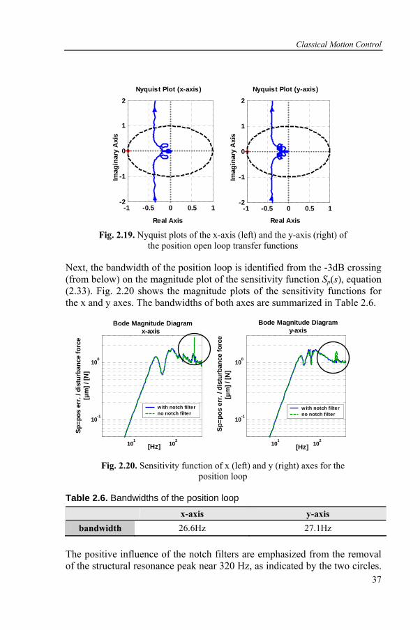
Classical Motion Control
37
-1 -0.5 0 0.5 1-2
-1
0
1
2Nyquist Plot (x-axis)
Real Axis
Imag
inar
y A
xis
-1 -0.5 0 0.5 1-2
-1
0
1
2Nyquist Plot (y-axis)
Real Axis
Imag
inar
y A
xis
Fig. 2.19. Nyquist plots of the x-axis (left) and the y-axis (right) of
the position open loop transfer functions
Next, the bandwidth of the position loop is identified from the -3dB crossing (from below) on the magnitude plot of the sensitivity function Sp(s), equation (2.33). Fig. 2.20 shows the magnitude plots of the sensitivity functions for the x and y axes. The bandwidths of both axes are summarized in Table 2.6.
Bode Magnitude Diagramy-axis
Sp=p
os e
rr. /
dis
turb
ance
forc
e[µ
m] /
[N]
Bode Magnitude Diagramx-axis
Sp=p
os e
rr. /
dis
turb
ance
forc
e[µ
m] /
[N]
101 102
10-1
100
with notch filterno notch filter
101 102
10-1
100
with notch filterno notch filter
[Hz] [Hz]
Fig. 2.20. Sensitivity function of x (left) and y (right) axes for the position loop
Table 2.6. Bandwidths of the position loop x-axis y-axis
bandwidth 26.6Hz 27.1Hz The positive influence of the notch filters are emphasized from the removal of the structural resonance peak near 320 Hz, as indicated by the two circles.
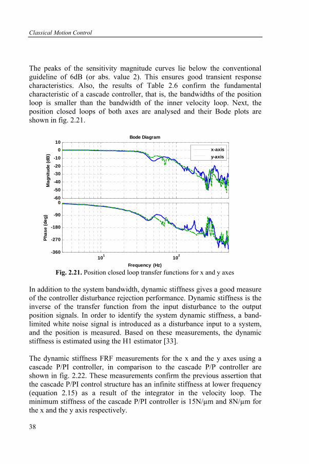
Classical Motion Control
38
The peaks of the sensitivity magnitude curves lie below the conventional guideline of 6dB (or abs. value 2). This ensures good transient response characteristics. Also, the results of Table 2.6 confirm the fundamental characteristic of a cascade controller, that is, the bandwidths of the position loop is smaller than the bandwidth of the inner velocity loop. Next, the position closed loops of both axes are analysed and their Bode plots are shown in fig. 2.21.
-60
-50
-40
-30-20
-10
010
Mag
nitu
de (d
B)
101 102-360
-270
-180
-90
0
Phas
e (d
eg)
Bode Diagram
Frequency (Hz)
x-axisy-axis
Fig. 2.21. Position closed loop transfer functions for x and y axes
In addition to the system bandwidth, dynamic stiffness gives a good measure of the controller disturbance rejection performance. Dynamic stiffness is the inverse of the transfer function from the input disturbance to the output position signals. In order to identify the system dynamic stiffness, a band-limited white noise signal is introduced as a disturbance input to a system, and the position is measured. Based on these measurements, the dynamic stiffness is estimated using the H1 estimator [33]. The dynamic stiffness FRF measurements for the x and the y axes using a cascade P/PI controller, in comparison to the cascade P/P controller are shown in fig. 2.22. These measurements confirm the previous assertion that the cascade P/PI control structure has an infinite stiffness at lower frequency (equation 2.15) as a result of the integrator in the velocity loop. The minimum stiffness of the cascade P/PI controller is 15N/µm and 8N/µm for the x and the y axis respectively.
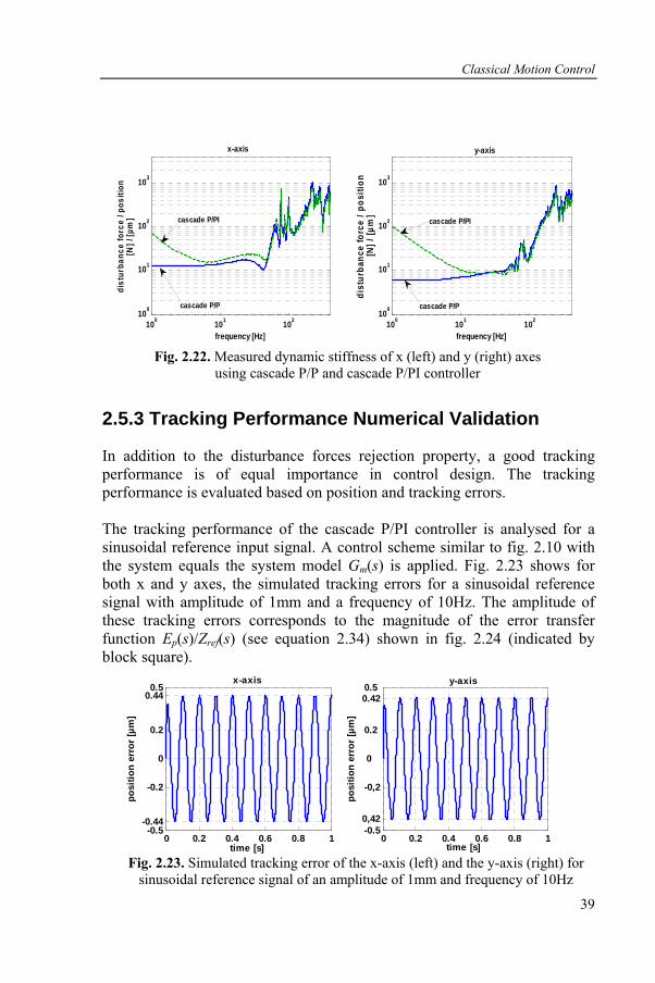
Classical Motion Control
39
100 101 102100
101
102
103
frequency [Hz]
dist
urba
nce
forc
e / p
ositi
on[N
] / [µ
m]
100 101 102100
101
102
103
frequency [Hz]
dist
urba
nce
forc
e / p
ositi
on[N
] / [µ
m]
cascade P/PI
cascade P/P
cascade P/PI
cascade P/P
x-axis y-axis
Fig. 2.22. Measured dynamic stiffness of x (left) and y (right) axes
using cascade P/P and cascade P/PI controller
2.5.3 Tracking Performance Numerical Validation
In addition to the disturbance forces rejection property, a good tracking performance is of equal importance in control design. The tracking performance is evaluated based on position and tracking errors. The tracking performance of the cascade P/PI controller is analysed for a sinusoidal reference input signal. A control scheme similar to fig. 2.10 with the system equals the system model Gm(s) is applied. Fig. 2.23 shows for both x and y axes, the simulated tracking errors for a sinusoidal reference signal with amplitude of 1mm and a frequency of 10Hz. The amplitude of these tracking errors corresponds to the magnitude of the error transfer function Ep(s)/Zref(s) (see equation 2.34) shown in fig. 2.24 (indicated by block square).
0 0.2 0.4 0.6 0.8 1-0.5
-0.44
-0.2
0
0.2
0.440.5
time [s]
posi
tion
erro
r [µm
]
x-axis
0 0.2 0.4 0.6 0.8 1-0.50,42
-0,2
0
0.2
0.420.5 y-axis
time [s]
posi
tion
erro
r [µm
]
Fig. 2.23. Simulated tracking error of the x-axis (left) and the y-axis (right) for
sinusoidal reference signal of an amplitude of 1mm and frequency of 10Hz
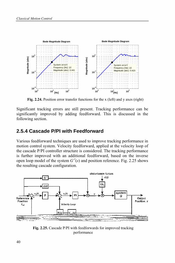
Classical Motion Control
40
Bode Magnitude Diagram
[Hz]
Mag
nitu
de (a
bs)
Bode Magnitude Diagram
[Hz]
Mag
nitu
de (a
bs)
100 101 10210-2
10-1
100
System: errorX Frequency [Hz]: 10 Magnitude (abs): 0.441
100 101 10210-2
10-1
100
System: errorY Frequency [Hz]: 10 Magnitude (abs): 0.423
Fig. 2.24. Position error transfer functions for the x (left) and y axes (right)
Significant tracking errors are still present. Tracking performance can be significantly improved by adding feedforward. This is discussed in the following section.
2.5.4 Cascade P/PI with Feedforward
Various feedforward techniques are used to improve tracking performance in motion control system. Velocity feedforward, applied at the velocity loop of the cascade P/PI controller structure is considered. The tracking performance is further improved with an additional feedforward, based on the inverse open loop model of the system G-1(s) and position reference. Fig. 2.25 shows the resulting cascade configuration.
Fig. 2.25. Cascade P/PI with feedforwards for improved tracking performance
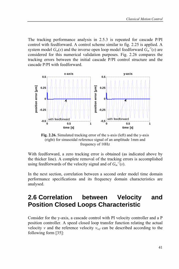
Classical Motion Control
41
The tracking performance analysis in 2.5.3 is repeated for cascade P/PI control with feedforward. A control scheme similar to fig. 2.25 is applied. A system model Gm(s) and the inverse open loop model feedforward Gm
-1(s) are considered for this numerical validation purposes. Fig. 2.26 compares the tracking errors between the initial cascade P/PI control structure and the cascade P/PI with feedforward.
0 0.5 1-0,5
-0,25
0
0.25
0.5
time [s]
posi
tion
erro
r [µm
]
y-axis
0 0.5 1-0.5
-0.25
0
0.25
0.5
time [s]
posi
tion
erro
r [µm
]
x-axis
with feedforward with feedforward
Fig. 2.26. Simulated tracking error of the x-axis (left) and the y-axis (right) for sinusoidal reference signal of an amplitude 1mm and
frequency of 10Hz With feedforward, a zero tracking error is obtained (as indicated above by the thicker line). A complete removal of the tracking errors is accomplished using feedforwards of the velocity signal and of Gm
-1(s). In the next section, correlation between a second order model time domain performance specifications and its frequency domain characteristics are analysed.
2.6 Correlation between Velocity and Position Closed Loops Characteristic
Consider for the y-axis, a cascade control with PI velocity controller and a P position controller. A speed closed loop transfer function relating the actual velocity v and the reference velocity vref can be described according to the following form [35]:
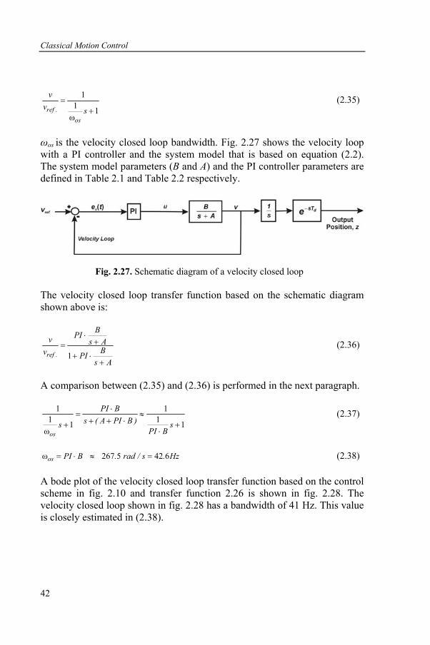
Classical Motion Control
42
11 1ω
ref .os
vv s
=+
(2.35)
ωos is the velocity closed loop bandwidth. Fig. 2.27 shows the velocity loop with a PI controller and the system model that is based on equation (2.2). The system model parameters (B and A) and the PI controller parameters are defined in Table 2.1 and Table 2.2 respectively.
Fig. 2.27. Schematic diagram of a velocity closed loop The velocity closed loop transfer function based on the schematic diagram shown above is:
1ref .
BPIv s ABv PI
s A
⋅+=
+ ⋅+
(2.36)
A comparison between (2.35) and (2.36) is performed in the next paragraph.
1 11 11 1ωos
PI Bs ( A PI B )s s
PI B
⋅= ≈
+ + ⋅+ +⋅
(2.37)
ω 267 5 42 6os PI B . rad / s . Hz= ⋅ ≈ = (2.38)
A bode plot of the velocity closed loop transfer function based on the control scheme in fig. 2.10 and transfer function 2.26 is shown in fig. 2.28. The velocity closed loop shown in fig. 2.28 has a bandwidth of 41 Hz. This value is closely estimated in (2.38).
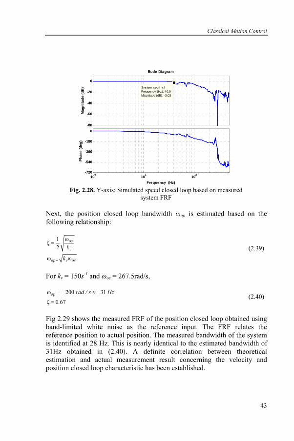
Classical Motion Control
43
100 101 102-720
-540
-360
-180
0
Phas
e (d
eg)
Bode Diagram
Frequency (Hz)
-80
-60
-40
-20
0M
agni
tude
(dB) System: spdtf_cl
Frequency (Hz): 40.9Magnitude (dB): -3.03
Fig. 2.28. Y-axis: Simulated speed closed loop based on measured
system FRF Next, the position closed loop bandwidth ωop is estimated based on the following relationship:
ω1ζ2
ω ω
os
v
op v os
k
k=
= (2.39)
For kv = 150s-1 and ωos = 267.5rad/s,
ω 200 31
ζ 0 67op rad / s Hz
.
= ≈
= (2.40)
Fig 2.29 shows the measured FRF of the position closed loop obtained using band-limited white noise as the reference input. The FRF relates the reference position to actual position. The measured bandwidth of the system is identified at 28 Hz. This is nearly identical to the estimated bandwidth of 31Hz obtained in (2.40). A definite correlation between theoretical estimation and actual measurement result concerning the velocity and position closed loop characteristic has been established.
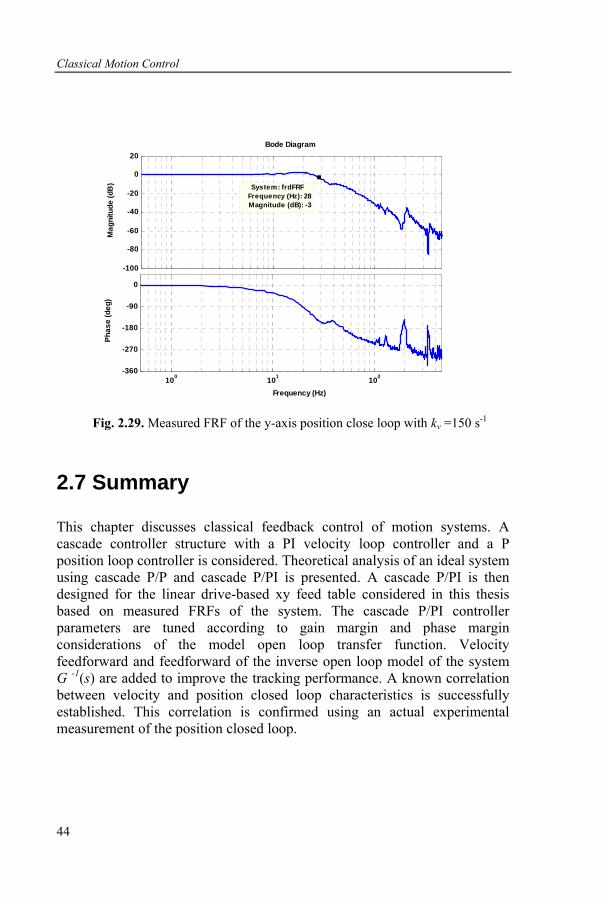
Classical Motion Control
44
Bode Diagram
Frequency (Hz)
Phas
e (d
eg)
Mag
nitu
de (d
B)
100 101 102-360
-270
-180
-90
0
-100
-80
-60
-40
-20
0
20
System: frdFRF Frequency (Hz): 28 Magnitude (dB): -3
Fig. 2.29. Measured FRF of the y-axis position close loop with kv =150 s-1
2.7 Summary
This chapter discusses classical feedback control of motion systems. A cascade controller structure with a PI velocity loop controller and a P position loop controller is considered. Theoretical analysis of an ideal system using cascade P/P and cascade P/PI is presented. A cascade P/PI is then designed for the linear drive-based xy feed table considered in this thesis based on measured FRFs of the system. The cascade P/PI controller parameters are tuned according to gain margin and phase margin considerations of the model open loop transfer function. Velocity feedforward and feedforward of the inverse open loop model of the system G -1(s) are added to improve the tracking performance. A known correlation between velocity and position closed loop characteristics is successfully established. This correlation is confirmed using an actual experimental measurement of the position closed loop.
45
Chapter 3
Disturbance Forces in Servo Drives System
3.1 Introduction
Disturbance forces directly affect the positioning and tracking accuracy of linear drive systems because of the lack of transmission. Two important disturbance forces are the highly nonlinear friction forces and cutting forces that occur during milling operation. Effective reduction of the effects of these disturbances is highly desirable. This requires a deep and detailed knowledge of the characteristics of these disturbances. This chapter focuses on the understanding, characterization and modelling of friction behaviour and cutting forces. Two different friction models are considered and the identification of the parameters of these models is discussed. A frequency domain analysis of the spectrum of cutting forces based on a sequence of cutting force measurements on a milling machine is provided. First, the friction force characterization and model structures are discussed and explained in the next section.
3.2 Friction Characterization and Model Structures
Friction, by definition, refers to the resistance to motion during sliding of two opposing objects against one another. Friction is present in various applications and influences many aspects of our daily life. It brings benefit in various forms. Braking systems and clutches are two examples of friction effects that benefit us. However, friction is highly undesirable in most
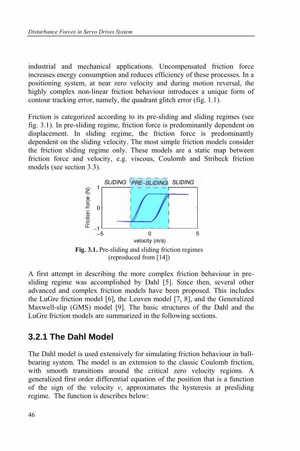
Disturbance Forces in Servo Drives System
46
industrial and mechanical applications. Uncompensated friction force increases energy consumption and reduces efficiency of these processes. In a positioning system, at near zero velocity and during motion reversal, the highly complex non-linear friction behaviour introduces a unique form of contour tracking error, namely, the quadrant glitch error (fig. 1.1). Friction is categorized according to its pre-sliding and sliding regimes (see fig. 3.1). In pre-sliding regime, friction force is predominantly dependent on displacement. In sliding regime, the friction force is predominantly dependent on the sliding velocity. The most simple friction models consider the friction sliding regime only. These models are a static map between friction force and velocity, e.g. viscous, Coulomb and Stribeck friction models (see section 3.3).
Fig. 3.1. Pre-sliding and sliding friction regimes
(reproduced from [14]) A first attempt in describing the more complex friction behaviour in pre-sliding regime was accomplished by Dahl [5]. Since then, several other advanced and complex friction models have been proposed. This includes the LuGre friction model [6], the Leuven model [7, 8], and the Generalized Maxwell-slip (GMS) model [9]. The basic structures of the Dahl and the LuGre friction models are summarized in the following sections.
3.2.1 The Dahl Model
The Dahl model is used extensively for simulating friction behaviour in ball-bearing system. The model is an extension to the classic Coulomb friction, with smooth transitions around the critical zero velocity regions. A generalized first order differential equation of the position that is a function of the sign of the velocity v, approximates the hysteresis at presliding regime. The function is describes below:
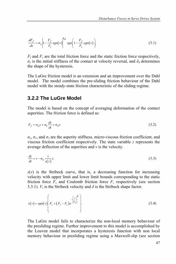
Disturbance Forces in Servo Drives System
47
( ) ( )δ
σ 1 1d
f f fo
s s
dF F Fsgn v sgn sgn v .
dx F F⎛ ⎞
= − −⎜ ⎟⎜ ⎟⎝ ⎠
(3.1)
Ff and Fs are the total friction force and the static friction force respectively, σo is the initial stiffness of the contact at velocity reversal, and δd determines the shape of the hysteresis. The LuGre friction model is an extension and an improvement over the Dahl model. The model combines the pre-sliding friction behaviour of the Dahl model with the steady-state friction characteristic of the sliding regime.
3.2.2 The LuGre Model
The model is based on the concept of averaging deformation of the contact asperities. The friction force is defined as:
1 2σ σ σf odzF z v.dt
= + + (3.2)
σo, σ1, and σ2 are the asperity stiffness, micro-viscous friction coefficient, and viscous friction coefficient respectively. The state variable z represents the average deflection of the asperities and v is the velocity.
( )σo
dz vv z.dt s v
= − (3.3)
s(v) is the Stribeck curve, that is, a decreasing function for increasing velocity with upper limit and lower limit bounds corresponding to the static friction force Fs and Coulomb friction force Fc respectively (see section 3.3.1). Vs is the Stribeck velocity and δ is the Stribeck shape factor.
( ) ( ) ( )
δv
Vsc s cs v sgn v F F F e .
−⎛ ⎞⎜ ⎟⎜ ⎟= + −⎜ ⎟⎜ ⎟⎝ ⎠
(3.4)
The LuGre model fails to characterize the non-local memory behaviour of the presliding regime. Further improvement to this model is accomplished by the Leuven model that incorporates a hysteresis function with non local memory behaviour in presliding regime using a Maxwell-slip (see section
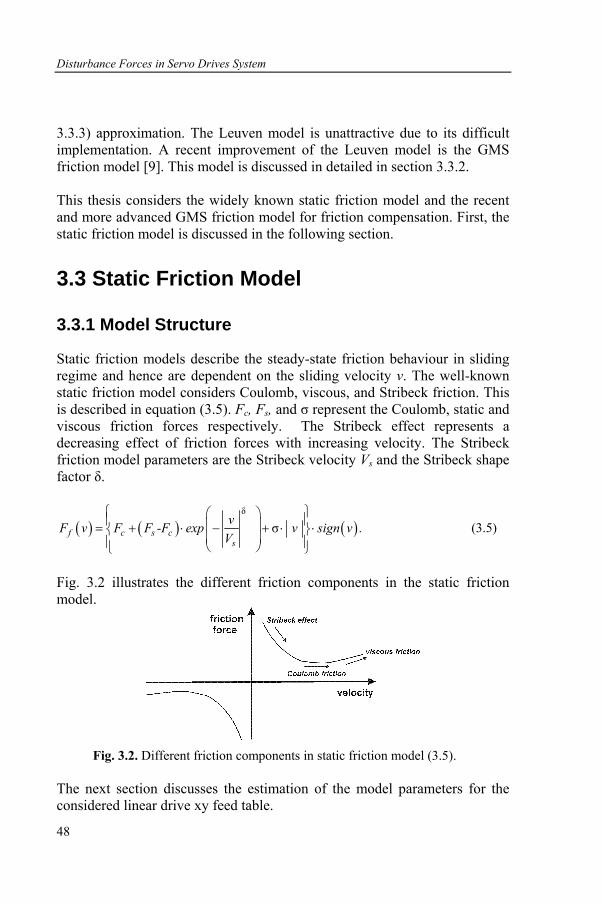
Disturbance Forces in Servo Drives System
48
3.3.3) approximation. The Leuven model is unattractive due to its difficult implementation. A recent improvement of the Leuven model is the GMS friction model [9]. This model is discussed in detailed in section 3.3.2. This thesis considers the widely known static friction model and the recent and more advanced GMS friction model for friction compensation. First, the static friction model is discussed in the following section.
3.3 Static Friction Model
3.3.1 Model Structure
Static friction models describe the steady-state friction behaviour in sliding regime and hence are dependent on the sliding velocity v. The well-known static friction model considers Coulomb, viscous, and Stribeck friction. This is described in equation (3.5). Fc, Fs, and σ represent the Coulomb, static and viscous friction forces respectively. The Stribeck effect represents a decreasing effect of friction forces with increasing velocity. The Stribeck friction model parameters are the Stribeck velocity Vs and the Stribeck shape factor δ.
( ) ( ) ( )δ
σf c s cs
vF v F F -F exp v sign v .V
⎧ ⎫⎛ ⎞⎪ ⎪⎜ ⎟= + ⋅ − + ⋅ ⋅⎨ ⎬⎜ ⎟⎪ ⎪⎝ ⎠⎩ ⎭
(3.5)
Fig. 3.2 illustrates the different friction components in the static friction model.
Fig. 3.2. Different friction components in static friction model (3.5). The next section discusses the estimation of the model parameters for the considered linear drive xy feed table.
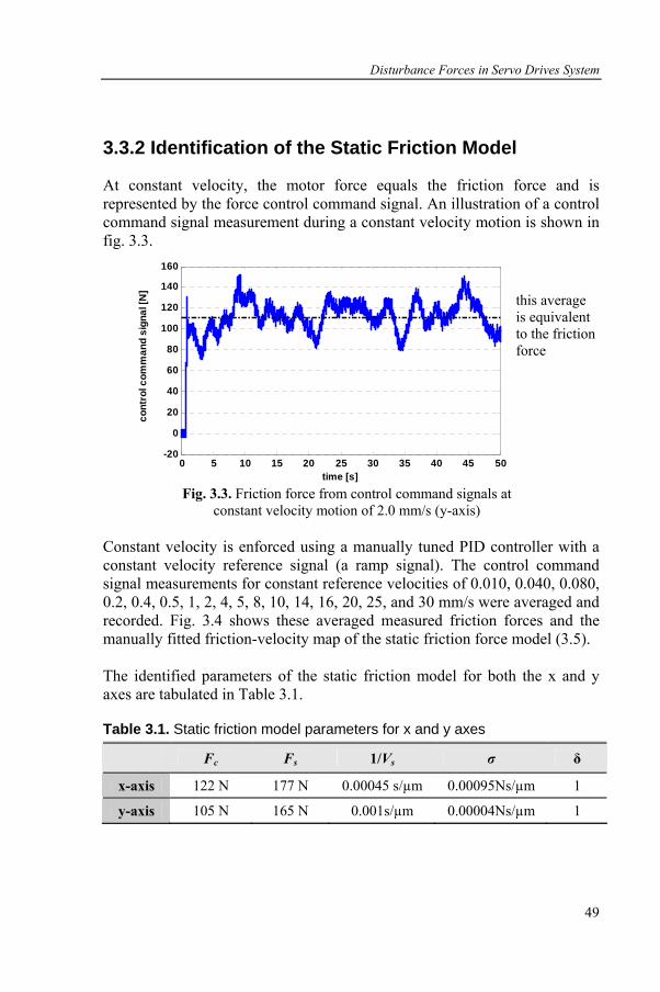
Disturbance Forces in Servo Drives System
49
3.3.2 Identification of the Static Friction Model
At constant velocity, the motor force equals the friction force and is represented by the force control command signal. An illustration of a control command signal measurement during a constant velocity motion is shown in fig. 3.3.
0 5 10 15 20 25 30 35 40 45 50-20
0
20
40
60
80
100
120
140
160
time [s]
cont
rol c
omm
and
sign
al [N
]
Fig. 3.3. Friction force from control command signals at
constant velocity motion of 2.0 mm/s (y-axis) Constant velocity is enforced using a manually tuned PID controller with a constant velocity reference signal (a ramp signal). The control command signal measurements for constant reference velocities of 0.010, 0.040, 0.080, 0.2, 0.4, 0.5, 1, 2, 4, 5, 8, 10, 14, 16, 20, 25, and 30 mm/s were averaged and recorded. Fig. 3.4 shows these averaged measured friction forces and the manually fitted friction-velocity map of the static friction force model (3.5). The identified parameters of the static friction model for both the x and y axes are tabulated in Table 3.1.
Table 3.1. Static friction model parameters for x and y axes Fc Fs 1/Vs σ δ
x-axis 122 N 177 N 0.00045 s/µm 0.00095Ns/µm 1
y-axis 105 N 165 N 0.001s/µm 0.00004Ns/µm 1
this average is equivalent to the friction force
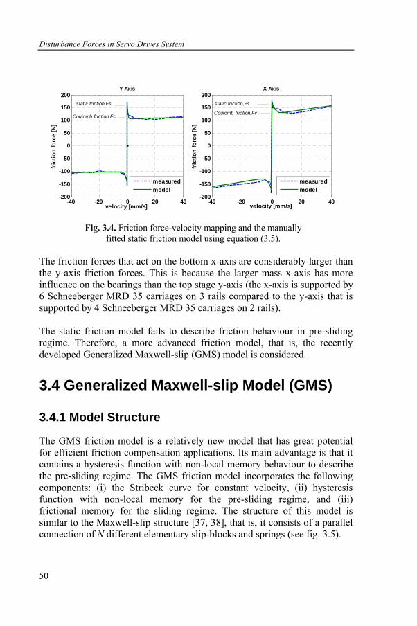
Disturbance Forces in Servo Drives System
50
-40 -20 0 20 40-200
-150
-100
-50
0
50
100
150
200Y-Axis
velocity [mm/s]
fric
tion
forc
e [N
]
-40 -20 0 20 40-200
-150
-100
-50
0
50
100
150
200X-Axis
velocity [mm/s]
fric
tion
forc
e [N
]
static friction,Fs
Coulomb friction,Fc
static friction,Fs
Coulomb friction,Fc
measuredmodel
measuredmodel
Fig. 3.4. Friction force-velocity mapping and the manually fitted static friction model using equation (3.5).
The friction forces that act on the bottom x-axis are considerably larger than the y-axis friction forces. This is because the larger mass x-axis has more influence on the bearings than the top stage y-axis (the x-axis is supported by 6 Schneeberger MRD 35 carriages on 3 rails compared to the y-axis that is supported by 4 Schneeberger MRD 35 carriages on 2 rails). The static friction model fails to describe friction behaviour in pre-sliding regime. Therefore, a more advanced friction model, that is, the recently developed Generalized Maxwell-slip (GMS) model is considered.
3.4 Generalized Maxwell-slip Model (GMS)
3.4.1 Model Structure
The GMS friction model is a relatively new model that has great potential for efficient friction compensation applications. Its main advantage is that it contains a hysteresis function with non-local memory behaviour to describe the pre-sliding regime. The GMS friction model incorporates the following components: (i) the Stribeck curve for constant velocity, (ii) hysteresis function with non-local memory for the pre-sliding regime, and (iii) frictional memory for the sliding regime. The structure of this model is similar to the Maxwell-slip structure [37, 38], that is, it consists of a parallel connection of N different elementary slip-blocks and springs (see fig. 3.5).
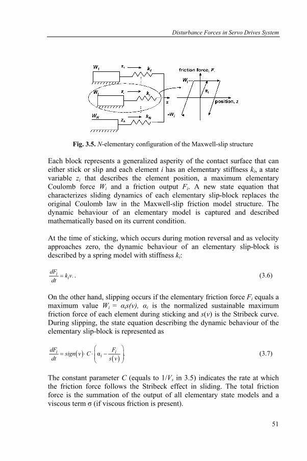
Disturbance Forces in Servo Drives System
51
Fig. 3.5. N-elementary configuration of the Maxwell-slip structure Each block represents a generalized asperity of the contact surface that can either stick or slip and each element i has an elementary stiffness ki, a state variable zi that describes the element position, a maximum elementary Coulomb force Wi and a friction output Fi. A new state equation that characterizes sliding dynamics of each elementary slip-block replaces the original Coulomb law in the Maxwell-slip friction model structure. The dynamic behaviour of an elementary model is captured and described mathematically based on its current condition. At the time of sticking, which occurs during motion reversal and as velocity approaches zero, the dynamic behaviour of an elementary slip-block is described by a spring model with stiffness ki:
ii
dF k v.dt
= . (3.6)
On the other hand, slipping occurs if the elementary friction force Fi equals a maximum value Wi = αis(v), αi is the normalized sustainable maximum friction force of each element during sticking and s(v) is the Stribeck curve. During slipping, the state equation describing the dynamic behaviour of the elementary slip-block is represented as
( ) ( )αi i
idF Fsign v C .dt s v
⎛ ⎞= ⋅ ⋅ −⎜ ⎟⎜ ⎟
⎝ ⎠ (3.7)
The constant parameter C (equals to 1/Vs in 3.5) indicates the rate at which the friction force follows the Stribeck effect in sliding. The total friction force is the summation of the output of all elementary state models and a viscous term σ (if viscous friction is present).
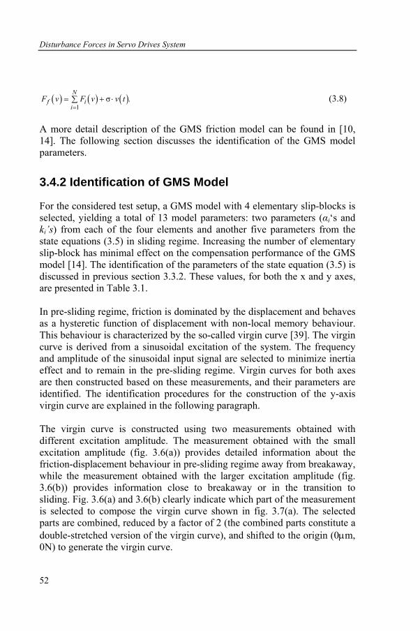
Disturbance Forces in Servo Drives System
52
( ) ( ) ( )1
σN
f ii
F v F v v t .=
= + ⋅∑ (3.8)
A more detail description of the GMS friction model can be found in [10, 14]. The following section discusses the identification of the GMS model parameters.
3.4.2 Identification of GMS Model
For the considered test setup, a GMS model with 4 elementary slip-blocks is selected, yielding a total of 13 model parameters: two parameters (αi‘s and ki’s) from each of the four elements and another five parameters from the state equations (3.5) in sliding regime. Increasing the number of elementary slip-block has minimal effect on the compensation performance of the GMS model [14]. The identification of the parameters of the state equation (3.5) is discussed in previous section 3.3.2. These values, for both the x and y axes, are presented in Table 3.1. In pre-sliding regime, friction is dominated by the displacement and behaves as a hysteretic function of displacement with non-local memory behaviour. This behaviour is characterized by the so-called virgin curve [39]. The virgin curve is derived from a sinusoidal excitation of the system. The frequency and amplitude of the sinusoidal input signal are selected to minimize inertia effect and to remain in the pre-sliding regime. Virgin curves for both axes are then constructed based on these measurements, and their parameters are identified. The identification procedures for the construction of the y-axis virgin curve are explained in the following paragraph. The virgin curve is constructed using two measurements obtained with different excitation amplitude. The measurement obtained with the small excitation amplitude (fig. 3.6(a)) provides detailed information about the friction-displacement behaviour in pre-sliding regime away from breakaway, while the measurement obtained with the larger excitation amplitude (fig. 3.6(b)) provides information close to breakaway or in the transition to sliding. Fig. 3.6(a) and 3.6(b) clearly indicate which part of the measurement is selected to compose the virgin curve shown in fig. 3.7(a). The selected parts are combined, reduced by a factor of 2 (the combined parts constitute a double-stretched version of the virgin curve), and shifted to the origin (0μm, 0N) to generate the virgin curve.
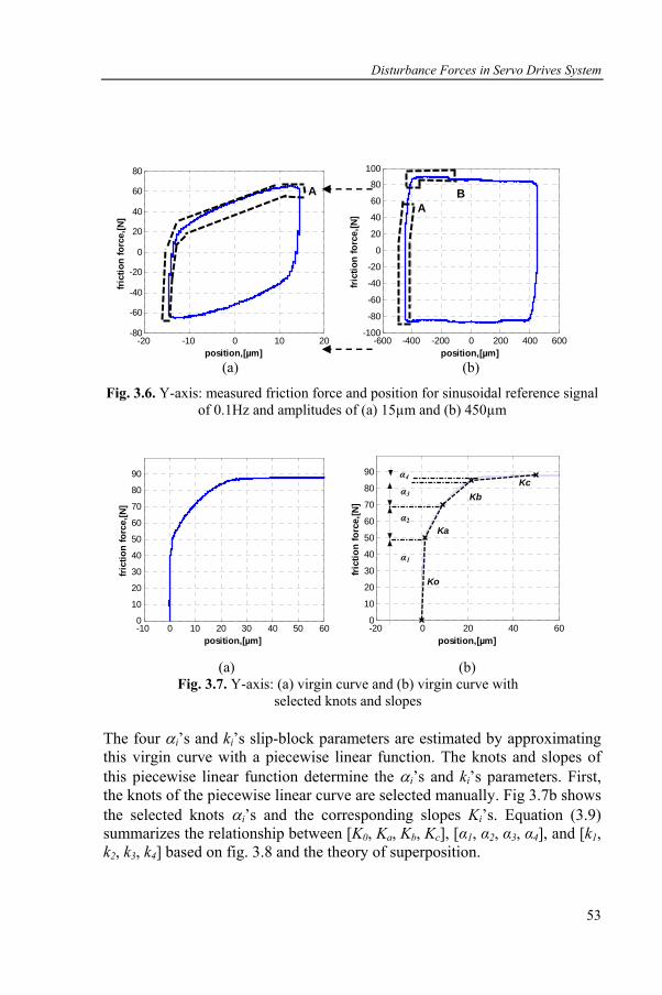
Disturbance Forces in Servo Drives System
53
(a) (b)
Fig. 3.6. Y-axis: measured friction force and position for sinusoidal reference signal of 0.1Hz and amplitudes of (a) 15µm and (b) 450µm
(a) (b) Fig. 3.7. Y-axis: (a) virgin curve and (b) virgin curve with
selected knots and slopes The four αi’s and ki’s slip-block parameters are estimated by approximating this virgin curve with a piecewise linear function. The knots and slopes of this piecewise linear function determine the αi’s and ki’s parameters. First, the knots of the piecewise linear curve are selected manually. Fig 3.7b shows the selected knots αi’s and the corresponding slopes Ki’s. Equation (3.9) summarizes the relationship between [K0, Ka, Kb, Kc], [α1, α2, α3, α4], and [k1, k2, k3, k4] based on fig. 3.8 and the theory of superposition.
-10 0 10 20 30 40 50 600
10
20
30
40
50
60
70
80
90
position,[µm]
fric
tion
forc
e,[N
]
-20 0 20 40 600
10
20
30
40
50
60
70
80
90
position,[µm]
frict
ion
forc
e,[N
]
Ka
Kb Kc
Ko
α4
α3
α2
α1
-20 -10 0 10 20-80
-60
-40
-20
0
20
40
60
80
position,[µm]
fric
tion
forc
e,[N
]
-600 -400 -200 0 200 400 600-100
-80
-60
-40
-20
0
20
40
60
80
100
position,[µm]fri
ctio
n fo
rce,
[N]
B A A
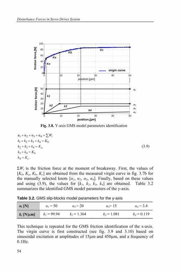
Disturbance Forces in Servo Drives System
54
0 10 20 30 40 500
20
40
60
80
100
position,[µm]
frict
ion
forc
e,[N
]
0 10 20 30 40 500
10
20
30
40
50
position,[µm]
frict
ion
forc
e,[N
]
Ko
Ka
Kb Kc
virgin curve
k1
k2 k3 k4
Fig. 3.8. Y-axis GMS model parameters identification
1 2 3 4
1 2 3 4 0
2 3 4
3 4
4
α α α α i
a
b
c
Wk k k k Kk k k Kk k Kk K .
+ + + =
+ + + =
+ + =
+ =
=
∑
(3.9)
ΣWi is the friction force at the moment of breakaway. First, the values of [K0, Ka, Kb, Kc] are obtained from the measured virgin curve in fig. 3.7b for the manually selected knots [α1, α2, α3, α4]. Finally, based on these values and using (3.9), the values for [k1, k2, k3, k4] are obtained. Table 3.2 summarizes the identified GMS model parameters of the y-axis.
Table 3.2. GMS slip-blocks model parameters for the y-axis
αi [N] α1 = 50 α2 = 20 α3= 15 α4 = 3.4
ki [N/μm] k1 = 99.94 k2 = 1.364 k3 = 1.081 k4 = 0.119
This technique is repeated for the GMS friction identification of the x-axis. The virgin curve is first constructed (see fig. 3.9 and 3.10) based on sinusoidal excitation at amplitudes of 15µm and 450µm, and a frequency of 0.1Hz.
α1
α2
α3
α4
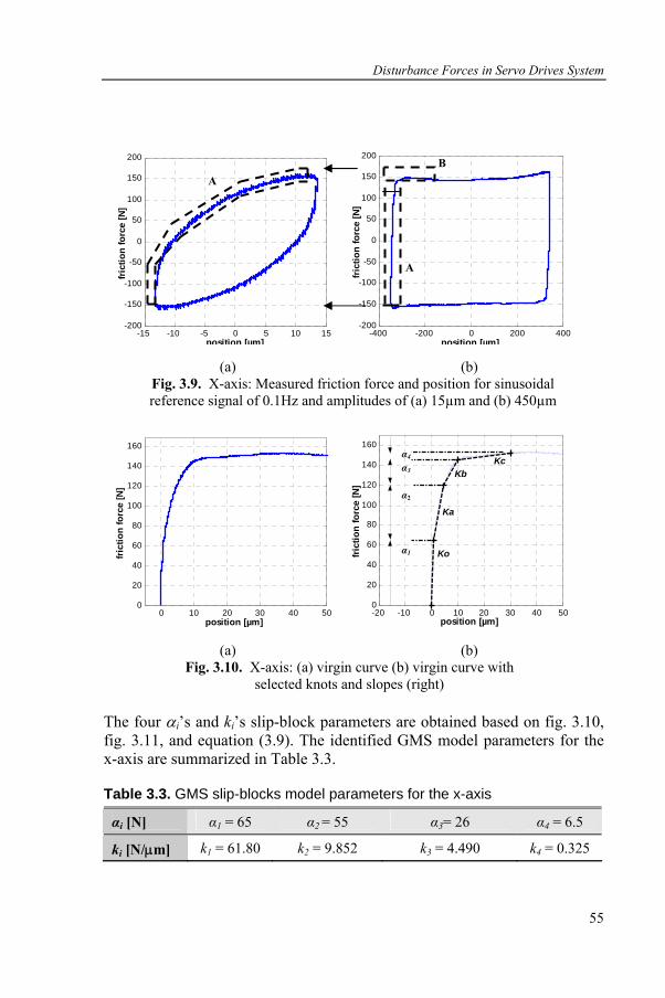
Disturbance Forces in Servo Drives System
55
(a) (b)
Fig. 3.9. X-axis: Measured friction force and position for sinusoidal reference signal of 0.1Hz and amplitudes of (a) 15µm and (b) 450µm
(a) (b)
Fig. 3.10. X-axis: (a) virgin curve (b) virgin curve with selected knots and slopes (right)
The four αi’s and ki’s slip-block parameters are obtained based on fig. 3.10, fig. 3.11, and equation (3.9). The identified GMS model parameters for the x-axis are summarized in Table 3.3.
Table 3.3. GMS slip-blocks model parameters for the x-axis
αi [N] α1 = 65 α2 = 55 α3= 26 α4 = 6.5
ki [N/μm] k1 = 61.80 k2 = 9.852 k3 = 4.490 k4 = 0.325
-15 -10 -5 0 5 10 15-200
-150
-100
-50
0
50
100
150
200
position [µm]
fric
tion
forc
e [N
]
-400 -200 0 200 400-200
-150
-100
-50
0
50
100
150
200
position [µm]fr
ictio
n fo
rce
[N]
0 10 20 30 40 500
20
40
60
80
100
120
140
160
position [µm]
fric
tion
forc
e [N
]
-20 -10 0 10 20 30 40 500
20
40
60
80
100
120
140
160
position [µm]
fric
tion
forc
e [N
]
Ko
Ka
Kb Kc
α4
α3
α2
α1
A
A B
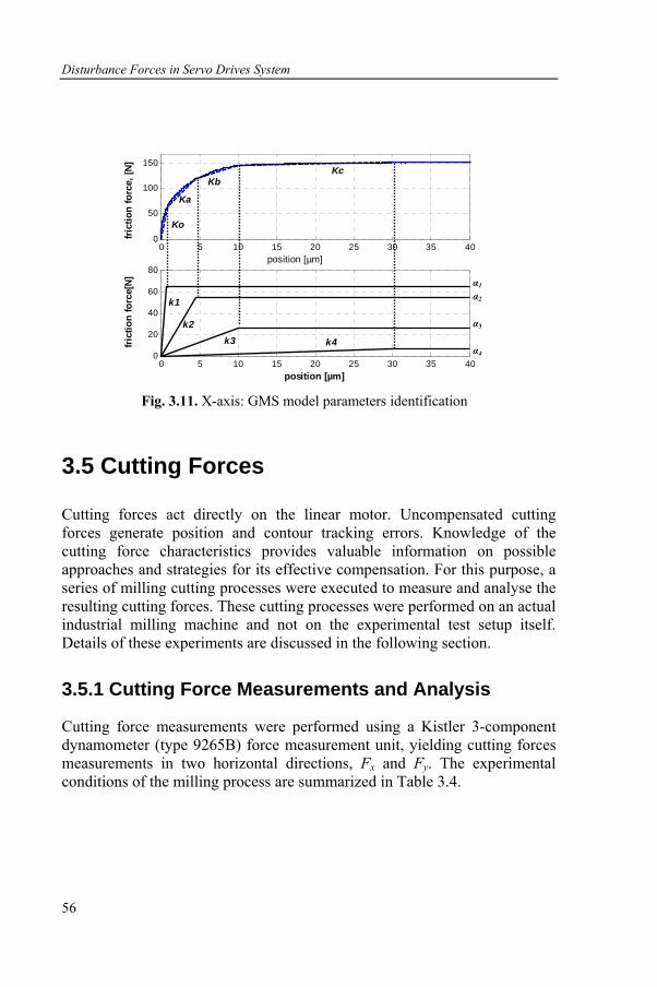
Disturbance Forces in Servo Drives System
56
0 5 10 15 20 25 30 35 400
50
100
150
position [µm]
frict
ion
forc
e, [N
]
0 5 10 15 20 25 30 35 400
20
40
60
80
position [µm]
frict
ion
forc
e[N]
Ko
Ka
Kb Kc
k1
k2 k3 k4
Fig. 3.11. X-axis: GMS model parameters identification
3.5 Cutting Forces
Cutting forces act directly on the linear motor. Uncompensated cutting forces generate position and contour tracking errors. Knowledge of the cutting force characteristics provides valuable information on possible approaches and strategies for its effective compensation. For this purpose, a series of milling cutting processes were executed to measure and analyse the resulting cutting forces. These cutting processes were performed on an actual industrial milling machine and not on the experimental test setup itself. Details of these experiments are discussed in the following section.
3.5.1 Cutting Force Measurements and Analysis
Cutting force measurements were performed using a Kistler 3-component dynamometer (type 9265B) force measurement unit, yielding cutting forces measurements in two horizontal directions, Fx and Fy. The experimental conditions of the milling process are summarized in Table 3.4.
α1
α2
α3
α4
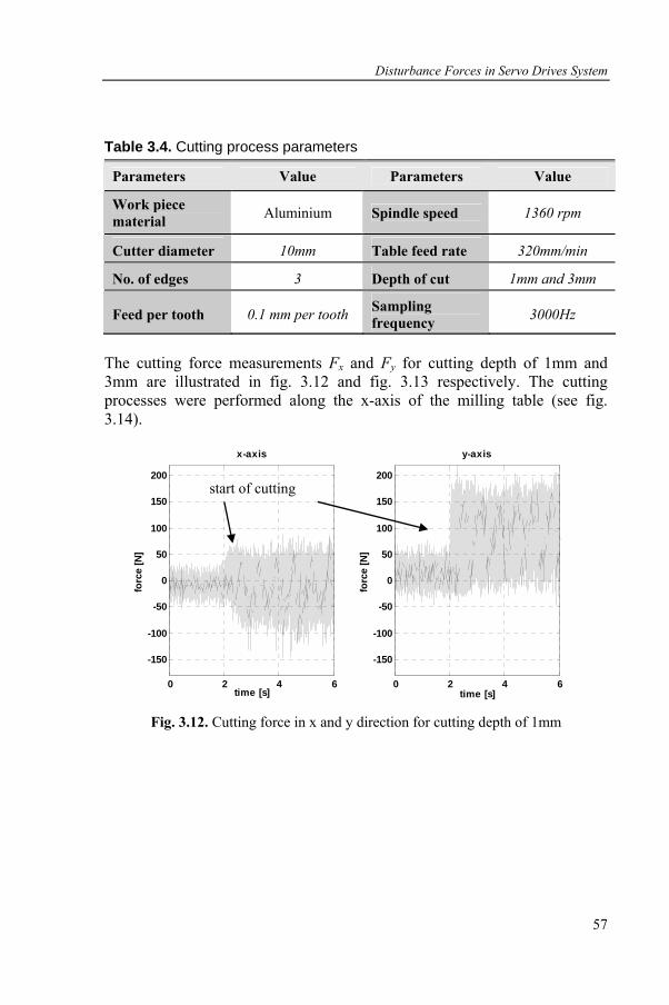
Disturbance Forces in Servo Drives System
57
Table 3.4. Cutting process parameters
Parameters Value Parameters Value
Work piece material Aluminium Spindle speed 1360 rpm
Cutter diameter 10mm Table feed rate 320mm/min
No. of edges 3 Depth of cut 1mm and 3mm
Feed per tooth 0.1 mm per tooth Sampling frequency 3000Hz
The cutting force measurements Fx and Fy for cutting depth of 1mm and 3mm are illustrated in fig. 3.12 and fig. 3.13 respectively. The cutting processes were performed along the x-axis of the milling table (see fig. 3.14).
0 2 4 6
-150
-100
-50
0
50
100
150
200
x-axis
time [s]
forc
e [N
]
0 2 4 6
-150
-100
-50
0
50
100
150
200
y-axis
time [s]
forc
e [N
]
Fig. 3.12. Cutting force in x and y direction for cutting depth of 1mm
start of cutting
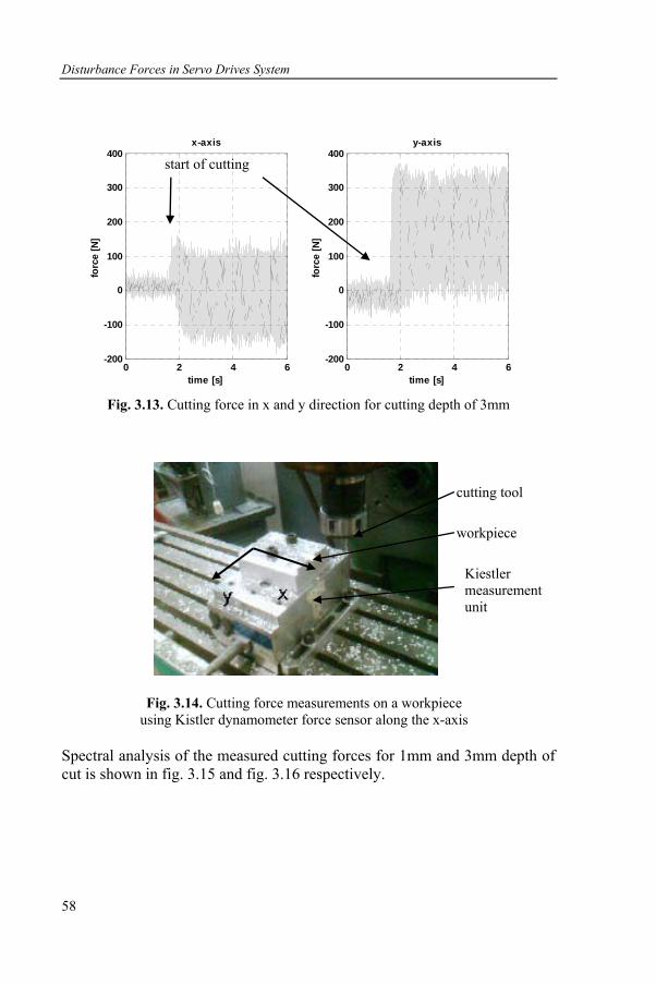
Disturbance Forces in Servo Drives System
58
0 2 4 6-200
-100
0
100
200
300
400x-axis
time [s]
forc
e [N
]
0 2 4 6-200
-100
0
100
200
300
400y-axis
time [s]
forc
e [N
]
Fig. 3.13. Cutting force in x and y direction for cutting depth of 3mm
Fig. 3.14. Cutting force measurements on a workpiece using Kistler dynamometer force sensor along the x-axis
Spectral analysis of the measured cutting forces for 1mm and 3mm depth of cut is shown in fig. 3.15 and fig. 3.16 respectively.
start of cutting
workpiece
Kiestler measurement unit
cutting tool
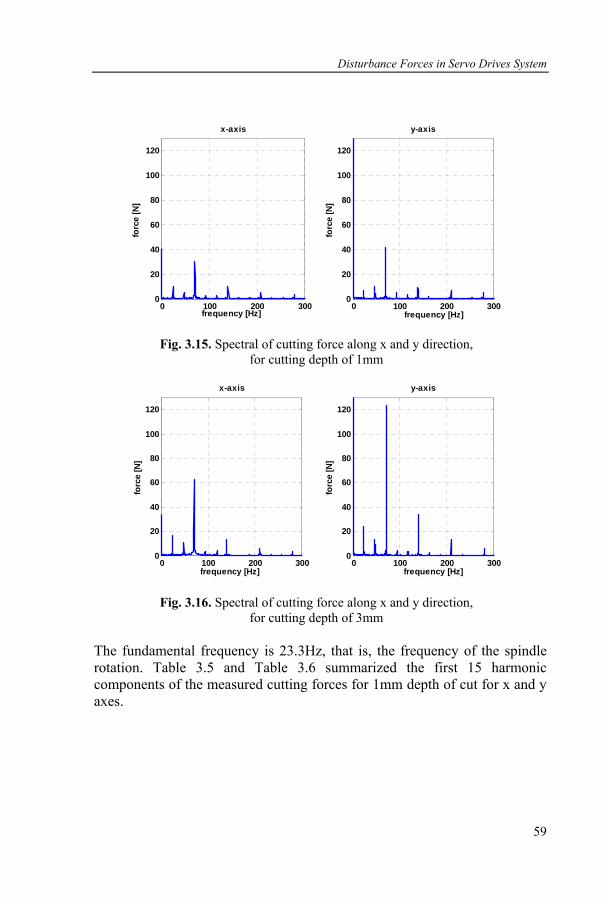
Disturbance Forces in Servo Drives System
59
0 100 200 3000
20
40
60
80
100
120
frequency [Hz]fo
rce
[N]
y-axis
0 100 200 3000
20
40
60
80
100
120
frequency [Hz]
forc
e [N
]x-axis
Fig. 3.15. Spectral of cutting force along x and y direction, for cutting depth of 1mm
0 100 200 3000
20
40
60
80
100
120
x-axis
frequency [Hz]
forc
e [N
]
0 100 200 3000
20
40
60
80
100
120
y-axis
frequency [Hz]
forc
e [N
]
Fig. 3.16. Spectral of cutting force along x and y direction, for cutting depth of 3mm
The fundamental frequency is 23.3Hz, that is, the frequency of the spindle rotation. Table 3.5 and Table 3.6 summarized the first 15 harmonic components of the measured cutting forces for 1mm depth of cut for x and y axes.
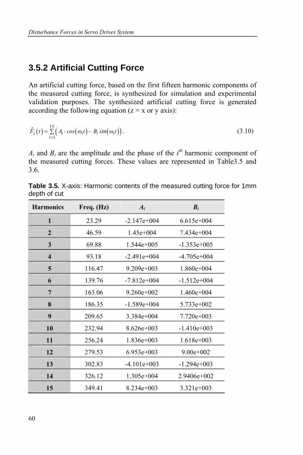
Disturbance Forces in Servo Drives System
60
3.5.2 Artificial Cutting Force
An artificial cutting force, based on the first fifteen harmonic components of the measured cutting force, is synthesized for simulation and experimental validation purposes. The synthesized artificial cutting force is generated according the following equation (z = x or y axis):
( ) ( ) ( )( )15
1ω ωz i i i i
iF t A cos t B sin t
== ⋅ −∑% . (3.10)
Ai and Bi are the amplitude and the phase of the ith harmonic component of the measured cutting forces. These values are represented in Table3.5 and 3.6.
Table 3.5. X-axis: Harmonic contents of the measured cutting force for 1mm depth of cut
Harmonics Freq. (Hz) Ai Bi
1 23.29 -2.147e+004 6.615e+004
2 46.59 1.45e+004 7.434e+004
3 69.88 1.544e+005 -1.353e+005
4 93.18 -2.491e+004 -4.705e+004
5 116.47 9.209e+003 1.860e+004
6 139.76 -7.812e+004 -1.512e+004
7 163.06 9.260e+002 1.460e+004
8 186.35 -1.589e+004 5.733e+002
9 209.65 3.384e+004 7.720e+003
10 232.94 8.626e+003 -1.410e+003
11 256.24 1.836e+003 1.618e+003
12 279.53 6.953e+003 9.00e+002
13 302.83 -4.101e+003 -1.294e+003
14 326.12 1.305e+004 2.9406e+002
15 349.41 8.234e+003 3.321e+003
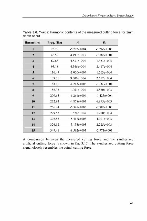
Disturbance Forces in Servo Drives System
61
Table 3.6. Y-axis: Harmonic contents of the measured cutting force for 1mm depth of cut
Harmonics Freq. (Hz) Ai Bi
1 23.29 -6.792e+004 -1.263e+005
2 46.59 4.497e+003 -7.883e+004
3 69.88 4.833e+004 1.453e+005
4 93.18 4.546e+004 2.417e+004
5 116.47 -1.020e+004 1.563e+004
6 139.76 9.306e+004 2.657e+004
7 163.06 -4.213e+003 -1.180e+004
8 186.35 1.061e+004 3.850e+003
9 209.65 -6.261e+004 -1.425e+004
10 232.94 -4.878e+003 6.895e+003
11 256.24 -6.341e+003 -2.983e+003
12 279.53 1.574e+004 1.280e+004
13 302.83 -5.417e+003 4.901e+003
14 326.12 -3.133e+003 2.225e+003
15 349.41 -8.592e+003 -2.971e+003 A comparison between the measured cutting force and the synthesized artificial cutting force is shown in fig. 3.17. The synthesized cutting force signal closely resembles the actual cutting force.
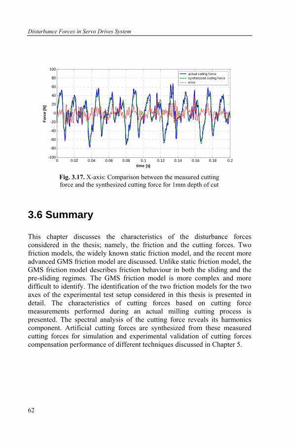
Disturbance Forces in Servo Drives System
62
0 0.02 0.04 0.06 0.08 0.1 0.12 0.14 0.16 0.18 0.2-100
-80
-60
-40
-20
0
20
40
60
80
100
time [s]
Forc
e [N
]
actual cutting forcesynthesized cutting forceerror
Fig. 3.17. X-axis: Comparison between the measured cutting force and the synthesized cutting force for 1mm depth of cut
3.6 Summary
This chapter discusses the characteristics of the disturbance forces considered in the thesis; namely, the friction and the cutting forces. Two friction models, the widely known static friction model, and the recent more advanced GMS friction model are discussed. Unlike static friction model, the GMS friction model describes friction behaviour in both the sliding and the pre-sliding regimes. The GMS friction model is more complex and more difficult to identify. The identification of the two friction models for the two axes of the experimental test setup considered in this thesis is presented in detail. The characteristics of cutting forces based on cutting force measurements performed during an actual milling cutting process is presented. The spectral analysis of the cutting force reveals its harmonics component. Artificial cutting forces are synthesized from these measured cutting forces for simulation and experimental validation of cutting forces compensation performance of different techniques discussed in Chapter 5.
63
Chapter 4
Friction Force Compensation Design
4.1 Introduction
Friction forces reduce the positioning and tracking accuracy in mechanical systems. Various friction compensation techniques have been described and presented in literature and have been highlighted in section 1.2.2. This chapter focuses on the application of two compensation techniques on the considered test setup: friction model feedforward and a disturbance observer that does not rely on a friction model. Feedforward friction compensation is validated for two different friction models: a static friction model (section 3.3) and a Generalized Maxwell-slip model (section 3.4). The disturbance observer is based on the inverse-model based disturbance observer design by Ohnishi [26]. The design and the analysis of this disturbance observer for the considered system are presented. The model applied in the disturbance observer is an approximate second order linear model of the considered system (equation 2.2). Finally, both techniques are combined and the friction compensation performances are compared [40]. Both numerical and experimental validations are performed. The magnitude of the quadrant glitch that appears near zero velocity or during motion reversal becomes the basis of performance comparison.

Friction Force Compensation Design
64
4.2 Friction Model-Based Feedforward
The performance of feedforward friction compensation based on a static and a GMS friction model is evaluated numerically and experimentally. The general control scheme is shown in fig. 4.1 and is based on the control structure presented in section 2.5.4 (fig. 2.25). The control scheme of each individual axis consists of a cascade P/PI position controller that includes a proportional (P) position and a PI velocity feedback controllers, a notch filter N(s), a first order velocity estimator Vest(s) (2.22), a velocity feedforward, and a feedforward Gm
-1 based on the inverse system model Gm (equation 2.2) and reference position. The friction model feedforward is inserted at the input of the plant.
Fig. 4.1. Friction compensation scheme using friction model-based feedforward (kf is the force constant).
The following section discusses the numerical validation of friction feedforward compensation using two different friction models.
4.2.1 System Transfer Function with a GMS Friction Term for Friction Simulation
The friction compensation performance is validated numerically in MATLAB/ Simulink. The system model Gm’ (see figure 4.1) consists of a linear second order model with delay (equation 2.2) in combination with the GMS friction model. Fig. 4.2 shows this system model in detail.
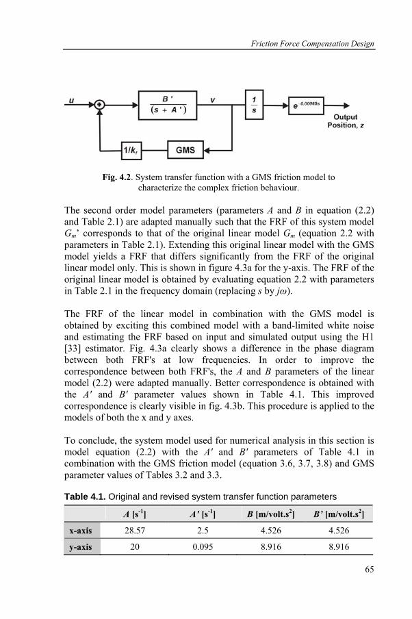
Friction Force Compensation Design
65
Fig. 4.2. System transfer function with a GMS friction model to characterize the complex friction behaviour.
The second order model parameters (parameters A and B in equation (2.2) and Table 2.1) are adapted manually such that the FRF of this system model Gm’ corresponds to that of the original linear model Gm (equation 2.2 with parameters in Table 2.1). Extending this original linear model with the GMS model yields a FRF that differs significantly from the FRF of the original linear model only. This is shown in figure 4.3a for the y-axis. The FRF of the original linear model is obtained by evaluating equation 2.2 with parameters in Table 2.1 in the frequency domain (replacing s by jω). The FRF of the linear model in combination with the GMS model is obtained by exciting this combined model with a band-limited white noise and estimating the FRF based on input and simulated output using the H1 [33] estimator. Fig. 4.3a clearly shows a difference in the phase diagram between both FRF's at low frequencies. In order to improve the correspondence between both FRF's, the A and B parameters of the linear model (2.2) were adapted manually. Better correspondence is obtained with the A' and B' parameter values shown in Table 4.1. This improved correspondence is clearly visible in fig. 4.3b. This procedure is applied to the models of both the x and y axes. To conclude, the system model used for numerical analysis in this section is model equation (2.2) with the A' and B' parameters of Table 4.1 in combination with the GMS friction model (equation 3.6, 3.7, 3.8) and GMS parameter values of Tables 3.2 and 3.3.
Table 4.1. Original and revised system transfer function parameters
A [s-1] A’ [s-1] B [m/volt.s2] B’ [m/volt.s2]
x-axis 28.57 2.5 4.526 4.526
y-axis 20 0.095 8.916 8.916
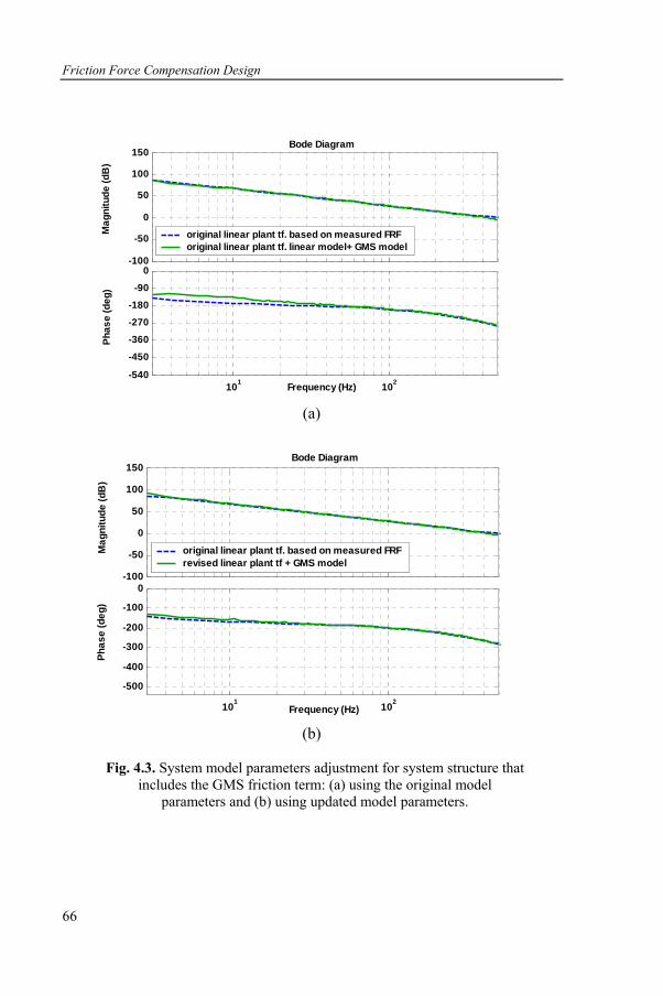
Friction Force Compensation Design
66
Bode Diagram
Frequency (Hz)
Phas
e (d
eg)
Mag
nitu
de (d
B)
-100
-50
0
50
100
150
original linear plant tf. based on measured FRForiginal linear plant tf. linear model+ GMS model
101 102-540
-450
-360
-270
-180
-90
0
(a)
Bode Diagram
Frequency (Hz)
Phas
e (d
eg)
Mag
nitu
de (d
B)
-100
-50
0
50
100
150
original linear plant tf. based on measured FRFrevised linear plant tf + GMS model
101 102
-500
-400
-300
-200
-100
0
(b)
Fig. 4.3. System model parameters adjustment for system structure that
includes the GMS friction term: (a) using the original model parameters and (b) using updated model parameters.
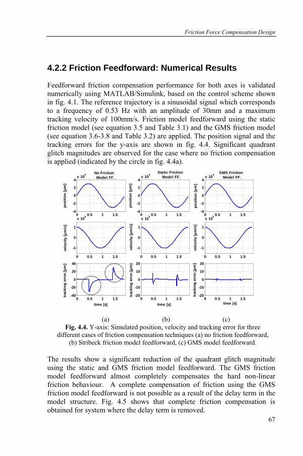
Friction Force Compensation Design
67
4.2.2 Friction Feedforward: Numerical Results
Feedforward friction compensation performance for both axes is validated numerically using MATLAB/Simulink, based on the control scheme shown in fig. 4.1. The reference trajectory is a sinusoidal signal which corresponds to a frequency of 0.53 Hz with an amplitude of 30mm and a maximum tracking velocity of 100mm/s. Friction model feedforward using the static friction model (see equation 3.5 and Table 3.1) and the GMS friction model (see equation 3.6-3.8 and Table 3.2) are applied. The position signal and the tracking errors for the y-axis are shown in fig. 4.4. Significant quadrant glitch magnitudes are observed for the case where no friction compensation is applied (indicated by the circle in fig. 4.4a).
0 0.5 1 1.5-4
-2
0
2
4x 10⁴
posi
tion
[µm
]
0 0.5 1 1.5
-1
0
1
x 105
velo
city
[µm
/s]
0 0.5 1 1.5-40
-20
0
20
40
time [s]
0 0.5 1 1.5-4
-2
0
2
4x 10⁴
0 0.5 1 1.5
-1
0
1
x 105
0 0.5 1 1.5-20
-10
0
10
20
0 0.5 1 1.5-4
-2
0
2
4x 10⁴
0 0.5 1 1.5
-1
0
1
x 105
0 0.5 1 1.5-20
-10
0
10
20
GMS Friction Model FF.
posi
tion
[µm
]
posi
tion
[µm
]
velo
city
[µm
/s]
velo
city
[µm
/s]
track
ing
erro
r,[µ
m]
trac
king
err
or,[µ
m]
track
ing
erro
r,[µ
m]
Static Friction Model FF.
No Friction Model FF.
time [s] time [s]
(a) (b) (c)
Fig. 4.4. Y-axis: Simulated position, velocity and tracking error for three different cases of friction compensation techniques (a) no friction feedforward,
(b) Stribeck friction model feedforward, (c) GMS model feedforward. The results show a significant reduction of the quadrant glitch magnitude using the static and GMS friction model feedforward. The GMS friction model feedforward almost completely compensates the hard non-linear friction behaviour. A complete compensation of friction using the GMS friction model feedforward is not possible as a result of the delay term in the model structure. Fig. 4.5 shows that complete friction compensation is obtained for system where the delay term is removed.
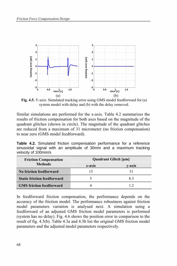
Friction Force Compensation Design
68
0 0.5 1 1.5-3
-2
-1
0
1
2
3
0 0.5 1 1.5-3
-2
-1
0
1
2
3
trac
king
err
or [µ
m]
trac
king
err
or [µ
m]
time [s]time [s] (a) (b) Fig. 4.5. Y-axis: Simulated tracking error using GMS model feedforward for (a)
system model with delay and (b) with the delay removed. Similar simulations are performed for the x-axis. Table 4.2 summarizes the results of friction compensation for both axes based on the magnitude of the quadrant glitches (shown in circle). The magnitude of the quadrant glitches are reduced from a maximum of 31 micrometer (no friction compensation) to near zero (GMS model feedforward).
Table 4.2. Simulated friction compensation performance for a reference sinusoidal signal with an amplitude of 30mm and a maximum tracking velocity of 100mm/s
Quadrant Glitch [µm] Friction Compensation Methods x-axis y-axis
No friction feedforward 15 31
Static friction feedforward 5 8.3
GMS friction feedforward 4 1.2 In feedforward friction compensation, the performance depends on the accuracy of the friction model. The performance robustness against friction model parameters variation is analysed next. A simulation using a feedforward of an adjusted GMS friction model parameters is performed (system has no delay). Fig. 4.6 shows the position error in comparison to the result of fig. 4.5(b). Table 4.3a and 4.3b list the original GMS friction model parameters and the adjusted model parameters respectively.
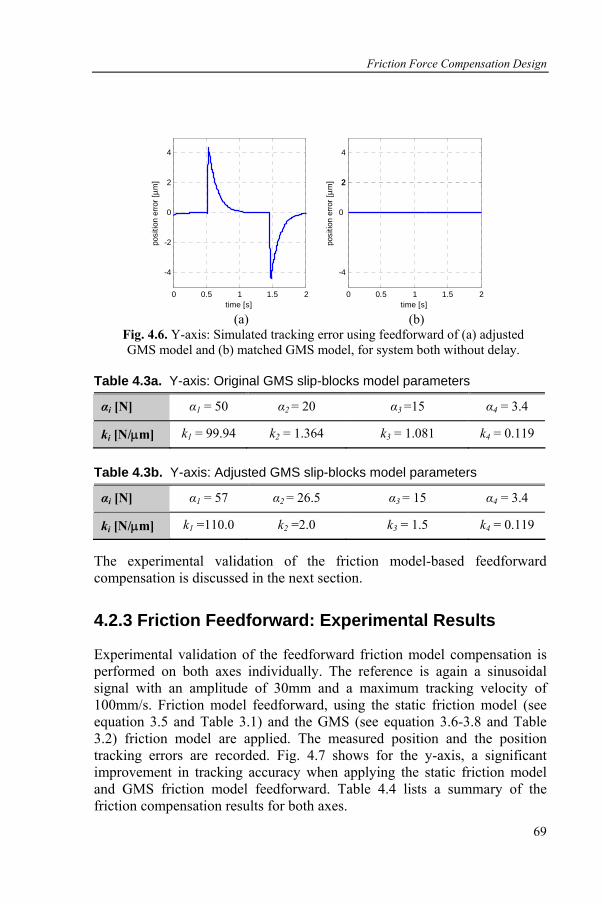
Friction Force Compensation Design
69
0 0.5 1 1.5 2
-4
2
0
2
4
time [s]
posi
tion
erro
r [µm
]
0 0.5 1 1.5 2
-4
-2
0
2
4po
sitio
n er
ror [
µm]
time [s] (a) (b)
Fig. 4.6. Y-axis: Simulated tracking error using feedforward of (a) adjusted GMS model and (b) matched GMS model, for system both without delay.
Table 4.3a. Y-axis: Original GMS slip-blocks model parameters
αi [N] α1 = 50 α2 = 20 α3 =15 α4 = 3.4
ki [N/μm] k1 = 99.94 k2 = 1.364 k3 = 1.081 k4 = 0.119
Table 4.3b. Y-axis: Adjusted GMS slip-blocks model parameters
αi [N] α1 = 57 α2 = 26.5 α3 = 15 α4 = 3.4
ki [N/μm] k1 =110.0 k2 =2.0 k3 = 1.5 k4 = 0.119 The experimental validation of the friction model-based feedforward compensation is discussed in the next section.
4.2.3 Friction Feedforward: Experimental Results
Experimental validation of the feedforward friction model compensation is performed on both axes individually. The reference is again a sinusoidal signal with an amplitude of 30mm and a maximum tracking velocity of 100mm/s. Friction model feedforward, using the static friction model (see equation 3.5 and Table 3.1) and the GMS (see equation 3.6-3.8 and Table 3.2) friction model are applied. The measured position and the position tracking errors are recorded. Fig. 4.7 shows for the y-axis, a significant improvement in tracking accuracy when applying the static friction model and GMS friction model feedforward. Table 4.4 lists a summary of the friction compensation results for both axes.
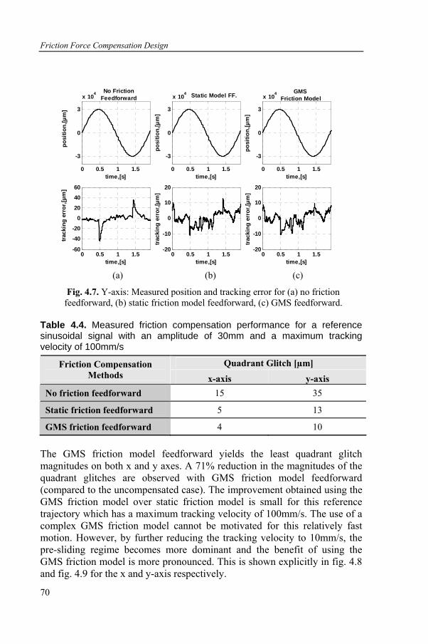
Friction Force Compensation Design
70
0 0.5 1 1.5
-3
0
3
x 104 No Friction Feedforward
time,[s]
posi
tion,
[µm
]
0 0.5 1 1.5-60
-40
-20
0
20
40
60
time,[s]
track
ing
erro
r,[µm
]
0 0.5 1 1.5
-3
0
3
x 104 GMS Friction Model
time,[s]
posi
tion,
[µm
]0 0.5 1 1.5
-20
-10
0
10
20
time,[s]
track
ing
erro
r,[µ
m]
0 0.5 1 1.5
-3
0
3
x 104 Static Model FF.
time,[s]
posi
tion,
[µm
]
0 0.5 1 1.5-20
-10
0
10
20
time,[s]
track
ing
erro
r,[µ
m]
(a) (b) (c)
Fig. 4.7. Y-axis: Measured position and tracking error for (a) no friction feedforward, (b) static friction model feedforward, (c) GMS feedforward.
Table 4.4. Measured friction compensation performance for a reference sinusoidal signal with an amplitude of 30mm and a maximum tracking velocity of 100mm/s
Quadrant Glitch [µm] Friction Compensation Methods x-axis y-axis
No friction feedforward 15 35
Static friction feedforward 5 13
GMS friction feedforward 4 10 The GMS friction model feedforward yields the least quadrant glitch magnitudes on both x and y axes. A 71% reduction in the magnitudes of the quadrant glitches are observed with GMS friction model feedforward (compared to the uncompensated case). The improvement obtained using the GMS friction model over static friction model is small for this reference trajectory which has a maximum tracking velocity of 100mm/s. The use of a complex GMS friction model cannot be motivated for this relatively fast motion. However, by further reducing the tracking velocity to 10mm/s, the pre-sliding regime becomes more dominant and the benefit of using the GMS friction model is more pronounced. This is shown explicitly in fig. 4.8 and fig. 4.9 for the x and y-axis respectively.
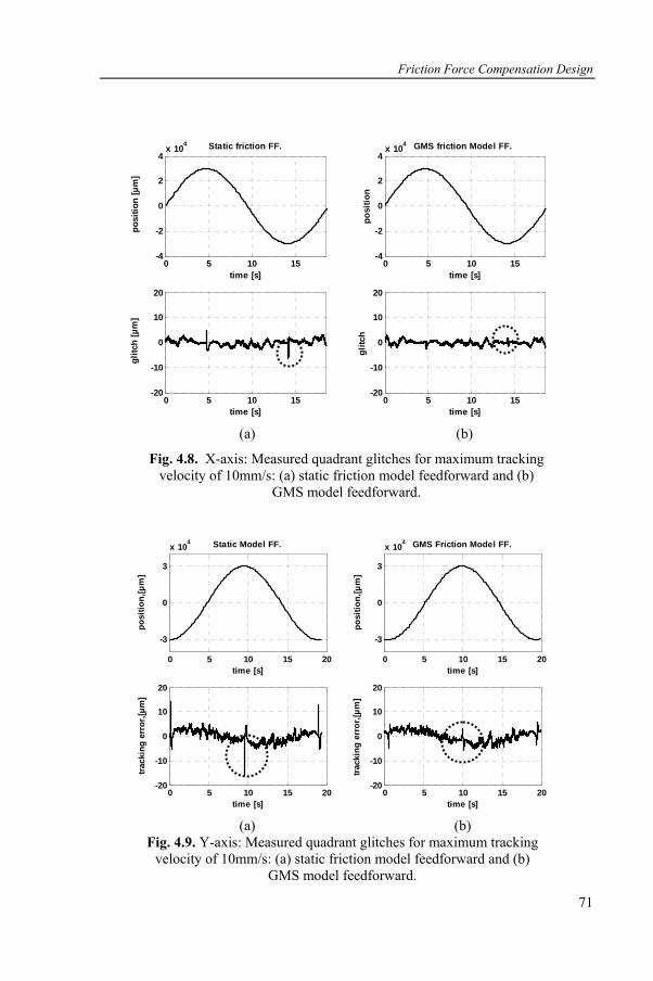
Friction Force Compensation Design
71
0 5 10 15-4
-2
0
2
4x 10⁴
time [s]
posi
tion
[µm
]Static friction FF.
0 5 10 15
20
10
0
-10
-20
time [s]
glitc
h [µ
m]
0 5 10 15-4
-2
0
2
4x 10⁴ GMS friction Model FF.
time [s]
posi
tion
0 5 10 15-20
-10
0
10
20
time [s]
glitc
h
(a) (b)
Fig. 4.8. X-axis: Measured quadrant glitches for maximum tracking velocity of 10mm/s: (a) static friction model feedforward and (b)
GMS model feedforward.
0 5 10 15 20-20
-10
0
10
20
time [s]
track
ing
erro
r,[µm
]
0 5 10 15 20
-3
0
3
x 104
time [s]
posi
tion,
[µm
]
0 5 10 15 20-20
-10
0
10
20
time [s]
track
ing
erro
r,[µm
]
0 5 10 15 20
-3
0
3
x 104 GMS Friction Model FF.
time [s]
posi
tion,
[µm
]
Static Model FF.
(a) (b)
Fig. 4.9. Y-axis: Measured quadrant glitches for maximum tracking velocity of 10mm/s: (a) static friction model feedforward and (b)
GMS model feedforward.
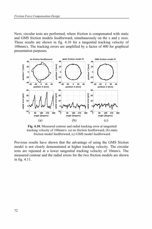
Friction Force Compensation Design
72
Next, circular tests are performed, where friction is compensated with static and GMS friction models feedforward, simultaneously on the x and y axes. These results are shown in fig. 4.10 for a tangential tracking velocity of 100mm/s. The tracking errors are amplified by a factor of 400 for graphical presentation purposes.
-40 -20 0 20 40-40
-20
0
20
40no friction feedforward
position X [mm]
posi
tion
Y [m
m]
0 90 180 270 360-10
0
10
20
30
angle [degree]
radi
al e
rror
[µm
]
-40 -20 0 20 40-40
-20
0
20
40static friction model ff.
position X [mm]
posi
tion
Y [m
m]
0 90 180 270 360-10
0
10
20
30
angle [degree]
radi
al e
rror
[µm
]
-40 -20 0 20 40-40
-20
0
20
40GMS friction model ff.
position X [mm]po
sitio
n Y
[mm
]
0 90 180 270 360-10
0
10
20
30
angle [degree]
radi
al e
rror
[µm
]
(a) (b) (c)
Fig. 4.10. Measured contour and radial tracking error at tangential tracking velocity of 100mm/s: (a) no friction feedforward, (b) static
friction model feedforward, (c) GMS model feedforward. Previous results have shown that the advantage of using the GMS friction model is not clearly demonstrated at higher tracking velocity. The circular tests are repeated at a lower tangential tracking velocity of 10mm/s. The measured contour and the radial errors for the two friction models are shown in fig. 4.11.
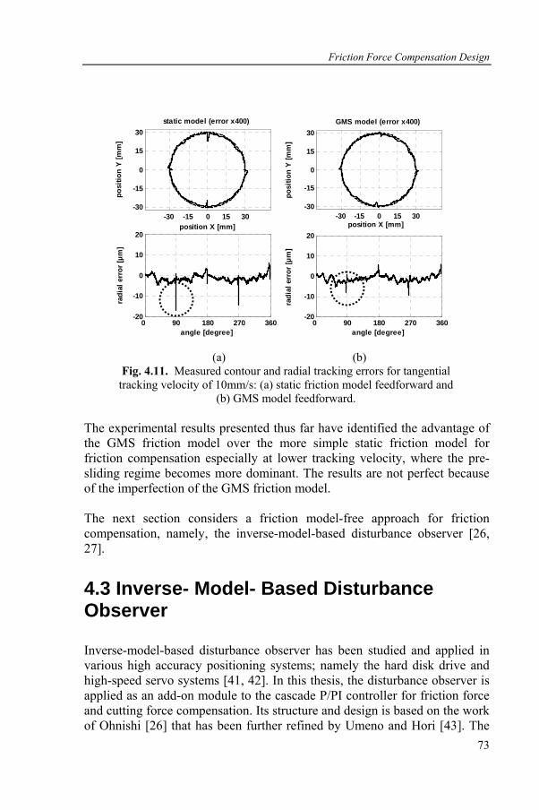
Friction Force Compensation Design
73
-30 -15 0 15 30-30
-15
0
15
30static model (error x400)
position X [mm]
posi
tion
Y [m
m]
0 90 180 270 360-20
-10
0
10
20
angle [degree]
radi
al e
rror
[µm
]
-30 -15 0 15 30-30
-15
0
15
30GMS model (error x400)
position X [mm]
posi
tion
Y [m
m]
0 90 180 270 360-20
-10
0
10
20
angle [degree]
radi
al e
rror
[µm
]
(a) (b)
Fig. 4.11. Measured contour and radial tracking errors for tangential tracking velocity of 10mm/s: (a) static friction model feedforward and
(b) GMS model feedforward. The experimental results presented thus far have identified the advantage of the GMS friction model over the more simple static friction model for friction compensation especially at lower tracking velocity, where the pre-sliding regime becomes more dominant. The results are not perfect because of the imperfection of the GMS friction model. The next section considers a friction model-free approach for friction compensation, namely, the inverse-model-based disturbance observer [26, 27].
4.3 Inverse- Model- Based Disturbance Observer
Inverse-model-based disturbance observer has been studied and applied in various high accuracy positioning systems; namely the hard disk drive and high-speed servo systems [41, 42]. In this thesis, the disturbance observer is applied as an add-on module to the cascade P/PI controller for friction force and cutting force compensation. Its structure and design is based on the work of Ohnishi [26] that has been further refined by Umeno and Hori [43]. The
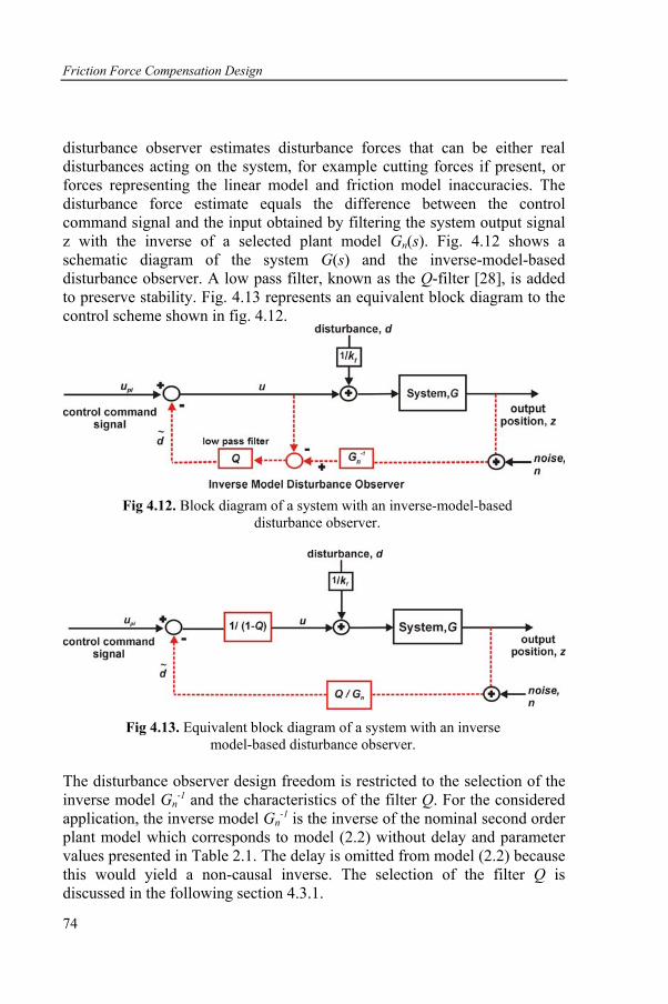
Friction Force Compensation Design
74
disturbance observer estimates disturbance forces that can be either real disturbances acting on the system, for example cutting forces if present, or forces representing the linear model and friction model inaccuracies. The disturbance force estimate equals the difference between the control command signal and the input obtained by filtering the system output signal z with the inverse of a selected plant model Gn(s). Fig. 4.12 shows a schematic diagram of the system G(s) and the inverse-model-based disturbance observer. A low pass filter, known as the Q-filter [28], is added to preserve stability. Fig. 4.13 represents an equivalent block diagram to the control scheme shown in fig. 4.12.
Fig 4.12. Block diagram of a system with an inverse-model-based disturbance observer.
Fig 4.13. Equivalent block diagram of a system with an inverse model-based disturbance observer.
The disturbance observer design freedom is restricted to the selection of the inverse model Gn
-1 and the characteristics of the filter Q. For the considered application, the inverse model Gn
-1 is the inverse of the nominal second order plant model which corresponds to model (2.2) without delay and parameter values presented in Table 2.1. The delay is omitted from model (2.2) because this would yield a non-causal inverse. The selection of the filter Q is discussed in the following section 4.3.1.
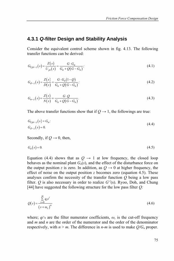
Friction Force Compensation Design
75
4.3.1 Q-filter Design and Stability Analysis
Consider the equivalent control scheme shown in fig. 4.13. The following transfer functions can be derived:
( ) ( )( ) ( )
nUpi z
pi n n
Z s G GG s ;U s G Q G G−
⋅= =
+ − (4.1)
( ) ( )( )
( )( )
1nd z
n n
Z s G G QG s ;
D s G Q G G−⋅ −
= =+ −
(4.2)
( ) ( )( ) ( )n z
n n
Z s G QG s .N s G Q G G−
⋅= =
+ − (4.3)
The above transfer functions show that if Q → 1, the followings are true:
( )( ) 0
Upi z n
d z
G s G ;
G s .−
−
=
= (4.4)
Secondly, if Q → 0, then,
( ) 0nG s .= (4.5)
Equation (4.4) shows that as Q → 1 at low frequency, the closed loop behaves as the nominal plant Gn(s), and the effect of the disturbance force on the output position z is zero. In addition, as Q → 0 at higher frequency, the effect of noise on the output position z becomes zero (equation 4.5). These analyses confirm the necessity of the transfer function Q being a low pass filter. Q is also necessary in order to realize G-1(s). Ryoo, Doh, and Chung [44] have suggested the following structure for the low pass filter Q:
( )( )
0
ω
m ii
in
c
q sQ s
s=∑
=+
(4.6)
where; qi’s are the filter numerator coefficients, ωc is the cut-off frequency and m and n are the order of the numerator and the order of the denominator respectively, with n > m. The difference in n-m is used to make Q/Gn proper.
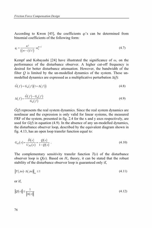
Friction Force Compensation Design
76
According to Kwon [45], the coefficients qi’s can be determined from binomial coefficients of the following form:
( )( )ωn i
i cn!q
n i !i!−= ⋅
− (4.7)
Kempf and Kobayashi [24] have illustrated the significance of ωc on the performance of the disturbance observer. A higher cut-off frequency is desired for better disturbance attenuation. However, the bandwidth of the filter Q is limited by the un-modelled dynamics of the system. These un-modelled dynamics are expressed as a multiplicative perturbation Δ(f):
( ) ( ) ( )( )1 ΔnG f G f f= + (4.8)
( ) ( ) ( )( )
Δ n
n
G f G ff
G f−
= (4.9)
Ĝ(f) represents the real system dynamics. Since the real system dynamics are nonlinear and the expression is only valid for linear systems, the measured FRF of the system, presented in fig. 2.4 for the x and y axes respectively, are used for G(f) in equation (4.9). In the absence of any un-modelled dynamics, the disturbance observer loop, described by the equivalent diagram shown in fig. 4.13, has an open loop transfer function equal to:
( ) ( )( )
( )( )1ol
PI
D s Q sG s .
U s Q s= =
−
%. (4.10)
The complementary sensitivity transfer function T(s) of the disturbance observer loop is Q(s). Based on H∞ theory, it can be stated that the robust stability of the disturbance observer loop is guaranteed only if,
( ) ( )ω Δ ω 1T j j∞
⋅ ≤ (4.11)
or if,
( )( )1
ΔQ s
s≤ (4.12)
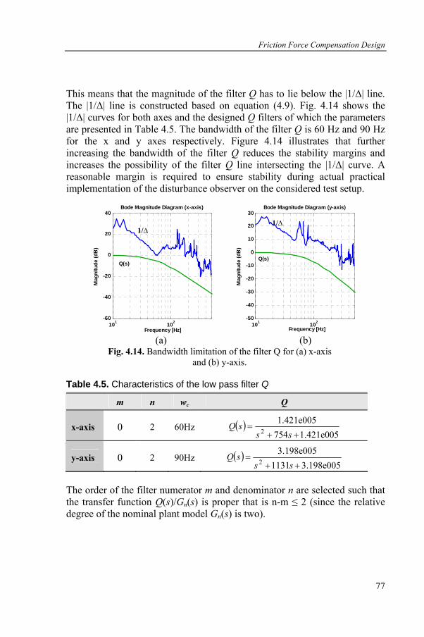
Friction Force Compensation Design
77
This means that the magnitude of the filter Q has to lie below the |1/Δ| line. The |1/Δ| line is constructed based on equation (4.9). Fig. 4.14 shows the |1/Δ| curves for both axes and the designed Q filters of which the parameters are presented in Table 4.5. The bandwidth of the filter Q is 60 Hz and 90 Hz for the x and y axes respectively. Figure 4.14 illustrates that further increasing the bandwidth of the filter Q reduces the stability margins and increases the possibility of the filter Q line intersecting the |1/Δ| curve. A reasonable margin is required to ensure stability during actual practical implementation of the disturbance observer on the considered test setup.
Bode Magnitude Diagram (y-axis)
Mag
nitu
de (d
B)
101 102-50
-40
-30
-20
-10
0
10
20
30Bode Magnitude Diagram (x-axis)
Mag
nitu
de (d
B)
101 102-60
-40
-20
0
20
40
Q(s) Q(s)
Frequency [Hz] Frequency [Hz] (a) (b)
Fig. 4.14. Bandwidth limitation of the filter Q for (a) x-axis and (b) y-axis.
Table 4.5. Characteristics of the low pass filter Q
m n wc Q
x-axis 0 2 60Hz ( )1.421e005754
1.421e0052 ++
=ss
sQ
y-axis 0 2 90Hz ( )3.198e0051131
3.198e0052 ++
=ss
sQ
The order of the filter numerator m and denominator n are selected such that the transfer function Q(s)/Gn(s) is proper that is n-m ≤ 2 (since the relative degree of the nominal plant model Gn(s) is two).
1/∆ 1/∆
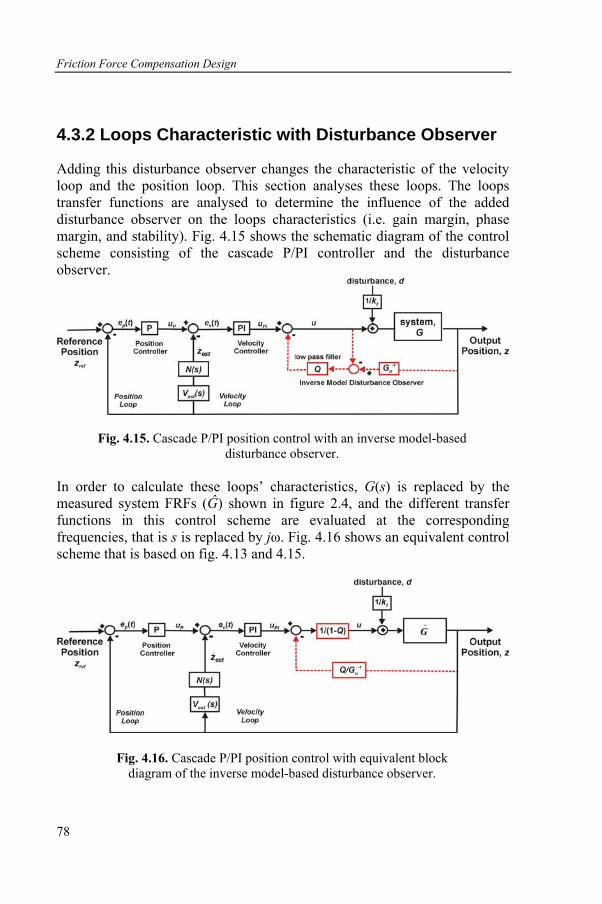
Friction Force Compensation Design
78
4.3.2 Loops Characteristic with Disturbance Observer
Adding this disturbance observer changes the characteristic of the velocity loop and the position loop. This section analyses these loops. The loops transfer functions are analysed to determine the influence of the added disturbance observer on the loops characteristics (i.e. gain margin, phase margin, and stability). Fig. 4.15 shows the schematic diagram of the control scheme consisting of the cascade P/PI controller and the disturbance observer.
Fig. 4.15. Cascade P/PI position control with an inverse model-based disturbance observer.
In order to calculate these loops’ characteristics, G(s) is replaced by the measured system FRFs (Ĝ) shown in figure 2.4, and the different transfer functions in this control scheme are evaluated at the corresponding frequencies, that is s is replaced by jω. Fig. 4.16 shows an equivalent control scheme that is based on fig. 4.13 and 4.15.
Fig. 4.16. Cascade P/PI position control with equivalent block diagram of the inverse model-based disturbance observer.

Friction Force Compensation Design
79
First, the velocity loop with the added disturbance observer is considered. The velocity open loop, closed loop, and sensitivity transfer functions equal:
( )( )
( ) ( )( )
n estdob _ ol
v n n
ˆZ s PI G G V s N sV ,ˆE s Q G G G
⋅ ⋅ ⋅ ⋅= =
− +
& (4.13)
( )( )
( ) ( )( ) ( ) ( )
n estdob _ cl
p n n n est
ˆZ s PI G G V s N sV ,ˆ ˆU s G Q G G PI G G V s N s
⋅ ⋅ ⋅ ⋅= =
+ − + ⋅ ⋅ ⋅ ⋅
& (4.14)
( ) ( ) ( ) ( )1
v _ dobn n n est
S s .ˆ ˆG Q G G PI G G V s N s=
+ − + ⋅ ⋅ ⋅ ⋅ (4.15)
Fig. 4.17 and 4.18 illustrate the influence of the disturbance observer on the velocity open loop and closed loop characteristics for the x and y axes respectively.
Frequency (Hz)
Phas
e (d
eg)
Mag
nitu
de (d
B)
-60
-40
-20
0
20
40
101
102
-360
-270
-180
-90
0
90
no observerwith observer
x-axis
(a)
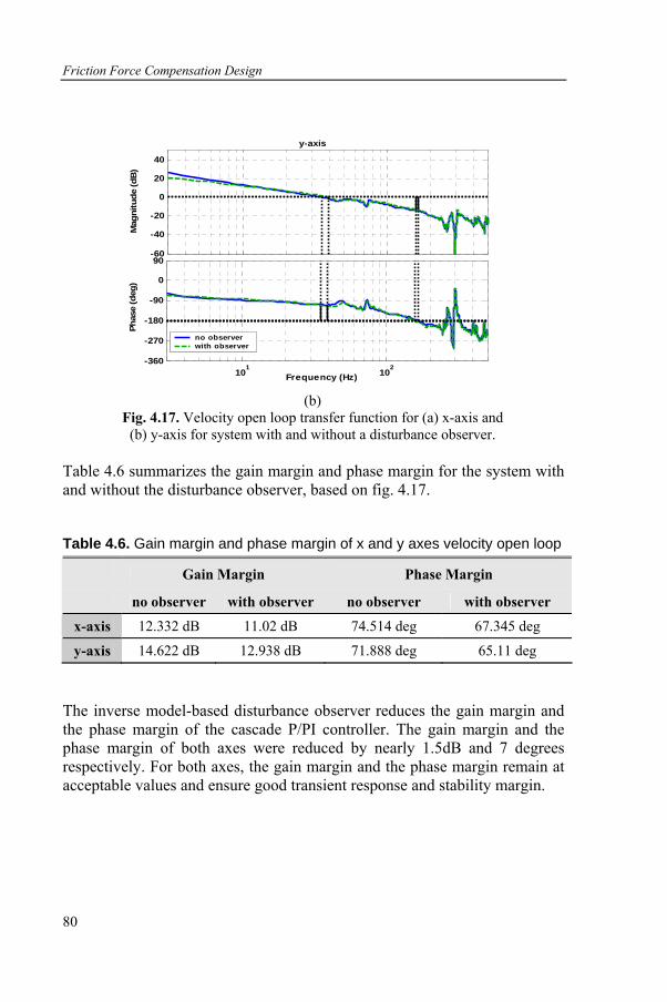
Friction Force Compensation Design
80
Frequency (Hz)
Phas
e (d
eg)
Mag
nitu
de (d
B)
-60
-40
-20
0
20
40
101
102
-360
-270
-180
-90
0
90
no observerwith observer
y-axis
(b)
Fig. 4.17. Velocity open loop transfer function for (a) x-axis and (b) y-axis for system with and without a disturbance observer.
Table 4.6 summarizes the gain margin and phase margin for the system with and without the disturbance observer, based on fig. 4.17.
Table 4.6. Gain margin and phase margin of x and y axes velocity open loop Gain Margin Phase Margin
no observer with observer no observer with observer
x-axis 12.332 dB 11.02 dB 74.514 deg 67.345 deg
y-axis 14.622 dB 12.938 dB 71.888 deg 65.11 deg The inverse model-based disturbance observer reduces the gain margin and the phase margin of the cascade P/PI controller. The gain margin and the phase margin of both axes were reduced by nearly 1.5dB and 7 degrees respectively. For both axes, the gain margin and the phase margin remain at acceptable values and ensure good transient response and stability margin.
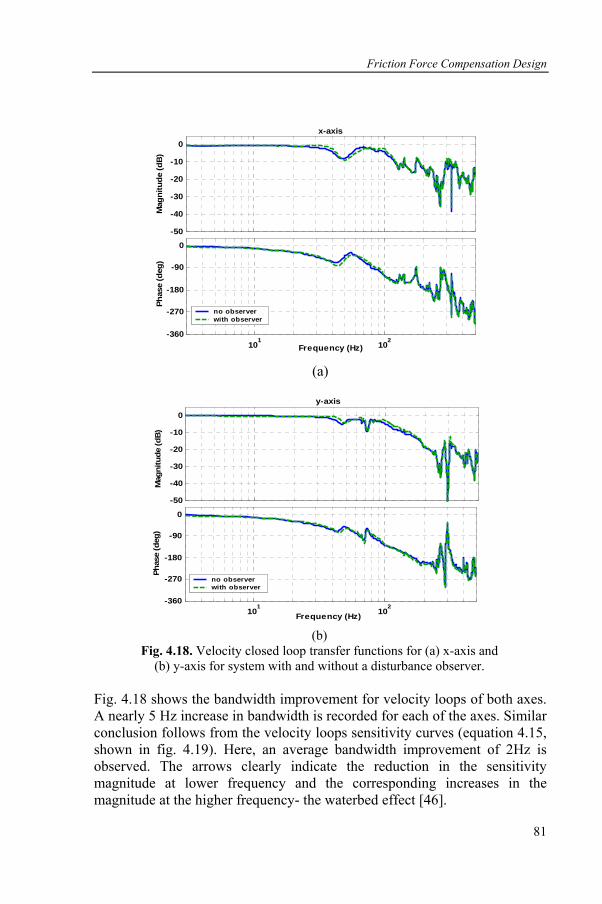
Friction Force Compensation Design
81
x-axis
Frequency (Hz)
Phas
e (d
eg)
Mag
nitu
de (d
B)
101
102
-360
-270
-180
-90
0
no observerwith observer
-50
-40
-30
-20
-10
0
(a)
y-axis
-50
-40
-30
-20
-10
0
101
102
-360
-270
-180
-90
0
no observerwith observer
Frequency (Hz)
Phas
e (d
eg)
Mag
nitu
de (d
B)
(b)
Fig. 4.18. Velocity closed loop transfer functions for (a) x-axis and (b) y-axis for system with and without a disturbance observer.
Fig. 4.18 shows the bandwidth improvement for velocity loops of both axes. A nearly 5 Hz increase in bandwidth is recorded for each of the axes. Similar conclusion follows from the velocity loops sensitivity curves (equation 4.15, shown in fig. 4.19). Here, an average bandwidth improvement of 2Hz is observed. The arrows clearly indicate the reduction in the sensitivity magnitude at lower frequency and the corresponding increases in the magnitude at the higher frequency- the waterbed effect [46].
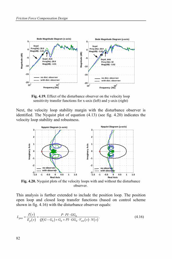
Friction Force Compensation Design
82
Bode Magnitude Diagram (x-axis)
Mag
nitu
de (d
B)
Bode Magnitude Diagram (y-axis)
Mag
nitu
de (d
B)
101 102-20
-15
-10
-5
0
5
Sspd_dob Freq(Hz): 29.9 Mag(dB): -3.01
Sspd Freq(Hz): 28.9 Mag(dB): -3.01
101 102-20
-15
-10
-5
0
5
Sspd Freq (Hz): 28.9 Mag(dB): -3.02
Sspd_dob Freq (Hz): 32 Mag(dB): -3.02
Frequency [Hz] Frequency [Hz]
no dist. observer w ith dist. observer
no dist. observer w ith dist. observer
Fig. 4.19. Effect of the disturbance observer on the velocity loop sensitivity transfer functions for x-axis (left) and y-axis (right)
Next, the velocity loop stability margin with the disturbance observer is identified. The Nyquist plot of equation (4.13) (see fig. 4.20) indicates the velocity loop stability and robustness.
Nyquist Diagram (y-axis)
Real Axis
Imag
inar
y A
xis
-1.5 -1 -0.5 0 0.5 1 1.5-3
-2
-1
0
1
2
3
Real Axis
Imag
inar
y A
xis
-1.5 -1 -0.5 0 0.5 1 1.5-3
-2
-1
0
1
2
3
no observer with observer
no observer with observer
Nyquist Diagram (x-axis)
Fig. 4.20. Nyquist plots of the velocity loops with and without the disturbance
observer. This analysis is further extended to include the position loop. The position open loop and closed loop transfer functions (based on control scheme shown in fig. 4.16) with the disturbance observer equals:
( )( ) ( ) ( ) ( )
npos
p n n n est
Z s P PI GGL ,E s Q G G G PI GG V s N s
⋅ ⋅= =
− + + ⋅ ⋅ ⋅ (4.16)
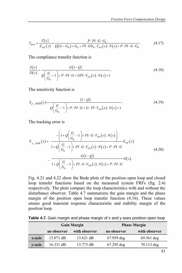
Friction Force Compensation Design
83
( )( ) ( ) ( ) ( )
npos
ref n n n est n
Z s P PI G GT .Z s Q G G G PI GG V s N s P PI G G
⋅ ⋅ ⋅= =
− + + ⋅ ⋅ ⋅ + ⋅ ⋅ ⋅ (4.17)
The compliance transfer function is
( )( )
( )
( ) ( )
1
1 1estn
Z s G Q.
D s GQ P PI G GPI V s N sG
−=
⎛ ⎞− + ⋅ ⋅ + ⋅ ⋅ +⎜ ⎟
⎝ ⎠
(4.18)
The sensitivity function is
( ) ( )
( ) ( )
1
1 1p _ DOB
estn
QS s .
GQ P PI G G PI V s N sG
−=
⎛ ⎞− + ⋅ ⋅ + ⋅ ⋅ ⋅ +⎜ ⎟
⎝ ⎠
(4.19)
The tracking error is
( )( ) ( )
( ) ( )( )
( )
( ) ( )( )
1 1
1 1
1
1 1
p _ DOB
estn
ref
estn
estn
GQ PI G V s N sG
E s Z sGQ PI G V s N s P PI GG
G Q _ D s .
GQ PI G V s N s P PI GG
⎛ ⎞⎛ ⎞− + − + ⋅ ⋅ ⋅⎜ ⎟⎜ ⎟⎜ ⎟⎝ ⎠⎝ ⎠=⎛ ⎞
+ − + ⋅ ⋅ ⋅ + ⋅ ⋅⎜ ⎟⎝ ⎠
−
⎛ ⎞+ − + ⋅ ⋅ ⋅ + ⋅ ⋅⎜ ⎟
⎝ ⎠
(4.20)
Fig. 4.21 and 4.22 show the Bode plots of the position open loop and closed loop transfer functions based on the measured system FRFs (fig. 2.4) respectively. The plots compare the loop characteristics with and without the disturbance observer. Table 4.7 summarizes the gain margin and the phase margin of the position open loop transfer function (4.16). These values ensure good transient response characteristic and stability margin of the position loop.
Table 4.7. Gain margin and phase margin of x and y axes position open loop
Gain Margin Phase Margin
no observer with observer no observer with observer
x-axis 15.071 dB 13.621 dB 67.959 deg 69.561 deg
y-axis 16.331 dB 13.773 dB 67.295 deg 70.113 deg
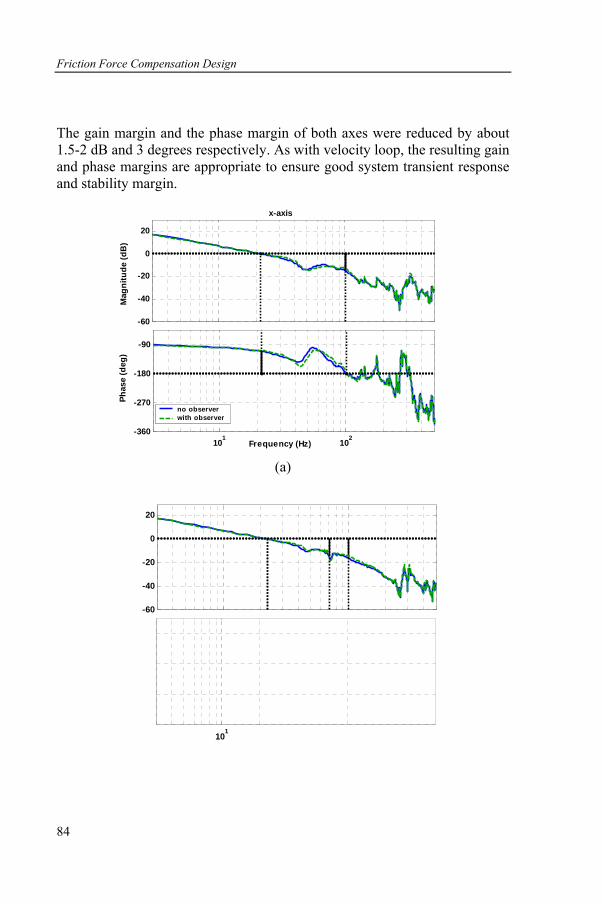
Friction Force Compensation Design
84
The gain margin and the phase margin of both axes were reduced by about 1.5-2 dB and 3 degrees respectively. As with velocity loop, the resulting gain and phase margins are appropriate to ensure good system transient response and stability margin.
Frequency (Hz)
Phas
e (d
eg)
Mag
nitu
de (d
B)
-60
-40
-20
0
20
101
102
-360
-270
-180
-90
no observerwith observer
x-axis
(a)
-60
-40
-20
0
20
101
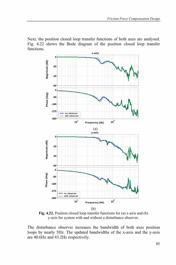
Friction Force Compensation Design
85
Next, the position closed loop transfer functions of both axes are analysed. Fig. 4.22 shows the Bode diagram of the position closed loop transfer functions.
x-axis
Frequency (Hz)
Phas
e (d
eg)
Mag
nitu
de (d
B)
-60
-40
-20
0
101
102
-360
-270
-180
-90
0
no observerwth observer
(a)
y-axis
-60
-40
-20
0
101
102
-360
-270
-180
-90
0
no observerwith observer
Frequency (Hz)
Phas
e (d
eg)
Mag
nitu
de (d
B)
(b)
Fig. 4.22. Position closed loop transfer functions for (a) x-axis and (b) y-axis for system with and without a disturbance observer.
The disturbance observer increases the bandwidth of both axes position loops by nearly 5Hz. The updated bandwidths of the x-axis and the y-axis are 40.6Hz and 43.2Hz respectively.
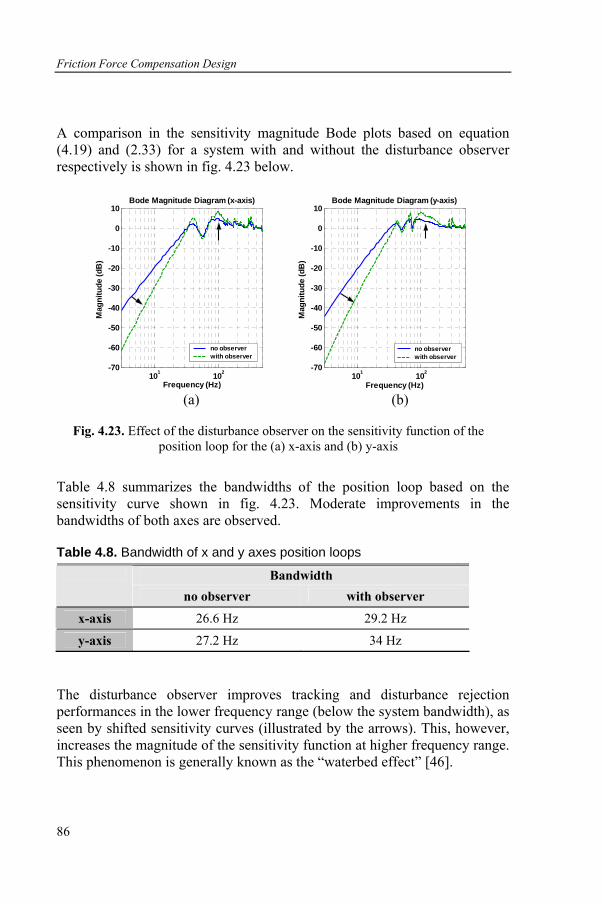
Friction Force Compensation Design
86
A comparison in the sensitivity magnitude Bode plots based on equation (4.19) and (2.33) for a system with and without the disturbance observer respectively is shown in fig. 4.23 below.
Bode Magnitude Diagram (y-axis)
Frequency (Hz)
Mag
nitu
de (d
B)
101 102-70
-60
-50
-40
-30
-20
-10
0
10
no observerwith observer
Bode Magnitude Diagram (x-axis)
Frequency (Hz)
Mag
nitu
de (d
B)
101 102-70
-60
-50
-40
-30
-20
-10
0
10
no observerwith observer
(a) (b)
Fig. 4.23. Effect of the disturbance observer on the sensitivity function of the
position loop for the (a) x-axis and (b) y-axis
Table 4.8 summarizes the bandwidths of the position loop based on the sensitivity curve shown in fig. 4.23. Moderate improvements in the bandwidths of both axes are observed.
Table 4.8. Bandwidth of x and y axes position loops
Bandwidth
no observer with observer
x-axis 26.6 Hz 29.2 Hz
y-axis 27.2 Hz 34 Hz The disturbance observer improves tracking and disturbance rejection performances in the lower frequency range (below the system bandwidth), as seen by shifted sensitivity curves (illustrated by the arrows). This, however, increases the magnitude of the sensitivity function at higher frequency range. This phenomenon is generally known as the “waterbed effect” [46].
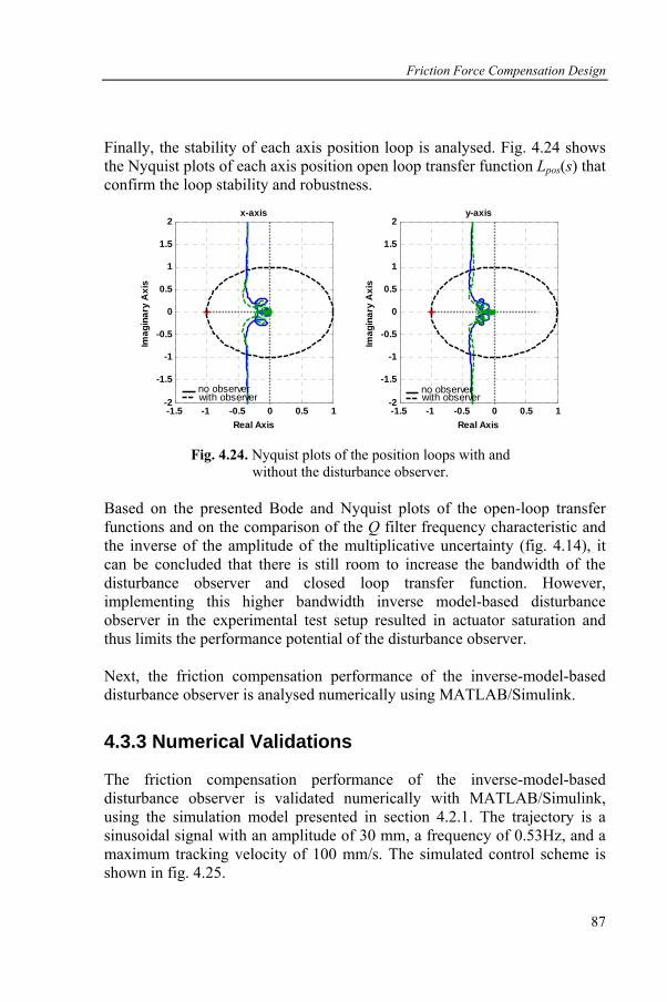
Friction Force Compensation Design
87
Finally, the stability of each axis position loop is analysed. Fig. 4.24 shows the Nyquist plots of each axis position open loop transfer function Lpos(s) that confirm the loop stability and robustness.
x-axis
Real Axis
Imag
inar
y A
xis
-1.5 -1 -0.5 0 0.5 1-2
-1.5
-1
-0.5
0
0.5
1
1.5
2y-axis
Real Axis
Imag
inar
y A
xis
-1.5 -1 -0.5 0 0.5 1-2
-1.5
-1
-0.5
0
0.5
1
1.5
2
no observer with observer
no observer with observer
Fig. 4.24. Nyquist plots of the position loops with and without the disturbance observer.
Based on the presented Bode and Nyquist plots of the open-loop transfer functions and on the comparison of the Q filter frequency characteristic and the inverse of the amplitude of the multiplicative uncertainty (fig. 4.14), it can be concluded that there is still room to increase the bandwidth of the disturbance observer and closed loop transfer function. However, implementing this higher bandwidth inverse model-based disturbance observer in the experimental test setup resulted in actuator saturation and thus limits the performance potential of the disturbance observer. Next, the friction compensation performance of the inverse-model-based disturbance observer is analysed numerically using MATLAB/Simulink.
4.3.3 Numerical Validations
The friction compensation performance of the inverse-model-based disturbance observer is validated numerically with MATLAB/Simulink, using the simulation model presented in section 4.2.1. The trajectory is a sinusoidal signal with an amplitude of 30 mm, a frequency of 0.53Hz, and a maximum tracking velocity of 100 mm/s. The simulated control scheme is shown in fig. 4.25.
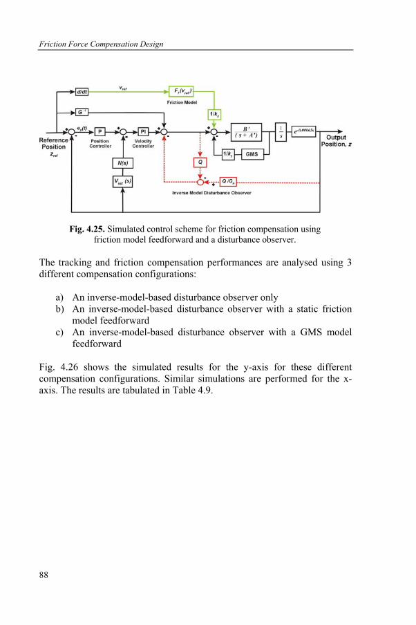
Friction Force Compensation Design
88
Fig. 4.25. Simulated control scheme for friction compensation using friction model feedforward and a disturbance observer.
The tracking and friction compensation performances are analysed using 3 different compensation configurations:
a) An inverse-model-based disturbance observer only b) An inverse-model-based disturbance observer with a static friction
model feedforward c) An inverse-model-based disturbance observer with a GMS model
feedforward Fig. 4.26 shows the simulated results for the y-axis for these different compensation configurations. Similar simulations are performed for the x-axis. The results are tabulated in Table 4.9.
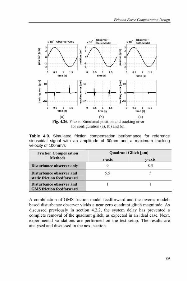
Friction Force Compensation Design
89
0 0.5 1 1.5
-3-2
0
23
x 104 Observer Onlypo
sitio
n [µ
m]
time [s]0 0.5 1 1.5
-3-2
0
23
x 104
posi
tion
[µm
]
time [s]
Observer + Static Model
0 0.5 1 1.5
-3-2
0
23
x 104
posi
tion
[µm
]
time [s]
Observer +GMS Model
0 0.5 1 1.5
-10
0
10
0 0.5 1 1.5
-10
0
10
0 0.5 1 1.5
-10
0
10tra
ckin
g er
ror
[µm
]
track
ing
erro
r [µ
m]
track
ing
erro
r [µ
m]
time [s]time [s]time [s] (a) (b) (c)
Fig. 4.26. Y-axis: Simulated position and tracking error for configuration (a), (b) and (c).
Table 4.9. Simulated friction compensation performance for reference sinusoidal signal with an amplitude of 30mm and a maximum tracking velocity of 100mm/s
Quadrant Glitch [µm] Friction Compensation Methods x-axis y-axis
Disturbance observer only 9 8.5
Disturbance observer and static friction feedforward
5.5 5
Disturbance observer and GMS friction feedforward
1 1
A combination of GMS friction model feedforward and the inverse model-based disturbance observer yields a near zero quadrant glitch magnitude. As discussed previously in section 4.2.2, the system delay has prevented a complete removal of the quadrant glitch, as expected in an ideal case. Next, experimental validations are performed on the test setup. The results are analysed and discussed in the next section.
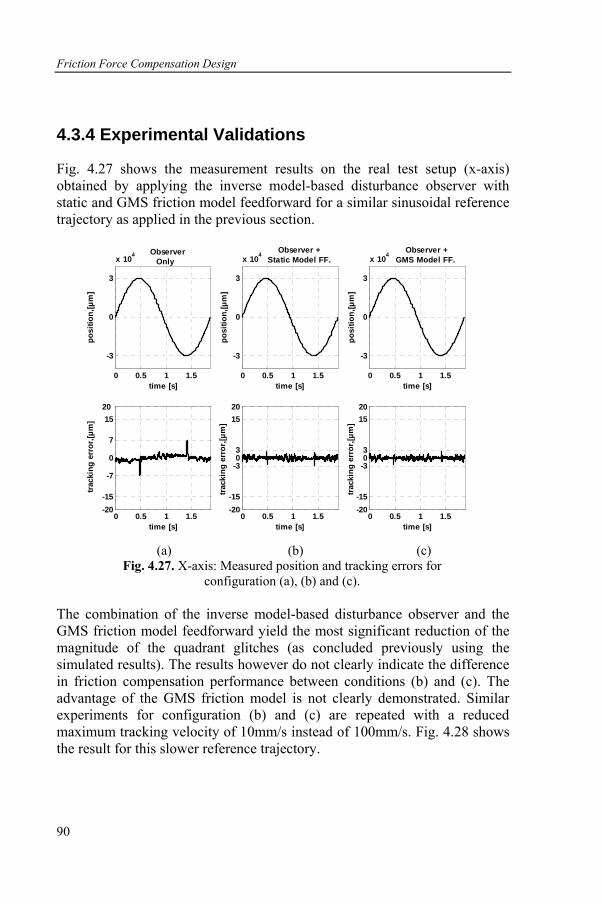
Friction Force Compensation Design
90
4.3.4 Experimental Validations
Fig. 4.27 shows the measurement results on the real test setup (x-axis) obtained by applying the inverse model-based disturbance observer with static and GMS friction model feedforward for a similar sinusoidal reference trajectory as applied in the previous section.
0 0.5 1 1.5
-3
0
3
x 104 Observer Only
time [s]
posi
tion,
[µm
]
0 0.5 1 1.5-20-15
-7
0
7
1520
time [s]
track
ing
erro
r,[µm
]
0 0.5 1 1.5
-3
0
3
x 104 Observer +
Static Model FF.
time [s]
posi
tion,
[µm
]
0 0.5 1 1.5-20-15
-303
1520
time [s]
track
ing
erro
r,[µm
]
0 0.5 1 1.5
-3
0
3
x 104 Observer +
GMS Model FF.
time [s]
posi
tion,
[µm
]
0 0.5 1 1.5-20-15
-303
1520
time [s]
track
ing
erro
r,[µm
]
(a) (b) (c)
Fig. 4.27. X-axis: Measured position and tracking errors for configuration (a), (b) and (c).
The combination of the inverse model-based disturbance observer and the GMS friction model feedforward yield the most significant reduction of the magnitude of the quadrant glitches (as concluded previously using the simulated results). The results however do not clearly indicate the difference in friction compensation performance between conditions (b) and (c). The advantage of the GMS friction model is not clearly demonstrated. Similar experiments for configuration (b) and (c) are repeated with a reduced maximum tracking velocity of 10mm/s instead of 100mm/s. Fig. 4.28 shows the result for this slower reference trajectory.
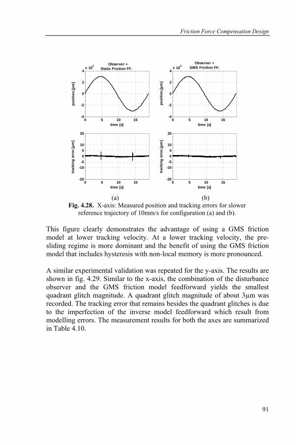
Friction Force Compensation Design
91
0 5 10 15-4
-2
0
2
4x 10⁴ Observer +
Static Friction FF.
time [s]
posi
tion,
[µm
]
0 5 10 15-20
-10-505
10
20
time [s]
track
ing
erro
r,[µm
]
0 5 10 15-4
-2
0
2
4x 10⁴
Observer + GMS Friction FF.
time [s]
posi
tion,
[µm
]
0 5 10 15-20
-10-505
10
20
time [s]
track
ing
erro
r,[µm
]
(a) (b)
Fig. 4.28. X-axis: Measured position and tracking errors for slower reference trajectory of 10mm/s for configuration (a) and (b).
This figure clearly demonstrates the advantage of using a GMS friction model at lower tracking velocity. At a lower tracking velocity, the pre-sliding regime is more dominant and the benefit of using the GMS friction model that includes hysteresis with non-local memory is more pronounced. A similar experimental validation was repeated for the y-axis. The results are shown in fig. 4.29. Similar to the x-axis, the combination of the disturbance observer and the GMS friction model feedforward yields the smallest quadrant glitch magnitude. A quadrant glitch magnitude of about 3µm was recorded. The tracking error that remains besides the quadrant glitches is due to the imperfection of the inverse model feedforward which result from modelling errors. The measurement results for both the axes are summarized in Table 4.10.
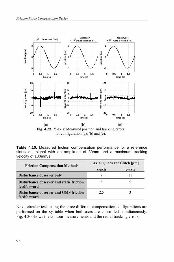
Friction Force Compensation Design
92
0 0.5 1 1.5
-3
0
3
x 104 Observer Only
time [s]
posi
tion
[µm
]
0 0.5 1 1.5-20
-10
0
10
20
time [s]
track
ing
erro
r [µm
]
0 0.5 1 1.5
-3
0
3
x 104 Observer +GMS Friction FF.
time [s]
posi
tion
[µm
]
0 0.5 1 1.5-20
-10
-303
10
20
time [s]
track
ing
erro
r [µm
]
0 0.5 1 1.5
-3
0
3
x 104 Observer +Static Friction FF.
time [s]
posi
tion
[µm
]
0 0.5 1 1.5-20
-10-505
10
20
time [s]
track
ing
erro
r [µm
]
(a) (b) (c)
Fig. 4.29. Y-axis: Measured position and tracking errors for configuration (a), (b) and (c).
Table 4.10. Measured friction compensation performance for a reference sinusoidal signal with an amplitude of 30mm and a maximum tracking velocity of 100mm/s
Axial Quadrant Glitch [µm] Friction Compensation Methods
x-axis y-axis Disturbance observer only 7 11
Disturbance observer and static friction feedforward
3 5
Disturbance observer and GMS friction feedforward
2.5 3
Next, circular tests using the three different compensation configurations are performed on the xy table when both axes are controlled simultaneously. Fig. 4.30 shows the contour measurements and the radial tracking errors.
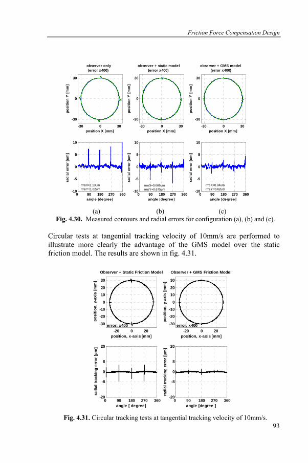
Friction Force Compensation Design
93
-30 0 30
-30
0
30
observer only (error x400)
position X [mm]
posi
tion
Y [m
m]
0 90 180 270 360-10
-5
0
5
10
angle [degree]
radi
al e
rror
[um
]
-30 0 30
-30
0
30
observer + static model (error x400)
position X [mm]po
sitio
n Y
[mm
]
0 90 180 270 360-10
-5
0
5
10
angle [degree]
radi
al e
rror
[um
]-30 0 30
-30
0
30
observer + GMS model (error x400)
position X [mm]
posi
tion
Y [m
m]
0 90 180 270 360-10
-5
0
5
10
angle [degree]
radi
al e
rror
[um
]rmsX=1.13umrmsY=1.02um
rmsX=0.666umrmsY=0.675um
rmsX=0.84umrmsY=0.62um
(a) (b) (c)
Fig. 4.30. Measured contours and radial errors for configuration (a), (b) and (c). Circular tests at tangential tracking velocity of 10mm/s are performed to illustrate more clearly the advantage of the GMS model over the static friction model. The results are shown in fig. 4.31.
-20 0 20
-30
-20
-10
0
10
20
30
Observer + Static Friction Model
position, x-axis [mm]
posi
tion,
y-a
xis
[mm
]
0 90 180 270 360-20
-8
0
8
20
angle [ degree]
radi
al tr
acki
ng e
rror
[µm
]
-20 0 20
-30
-20
-10
0
10
20
30
Observer + GMS Friction Model
position, x-axis [mm]
posi
tion,
y-a
xis
[mm
]
0 90 180 270 360-20
-8
0
8
20
angle [degree ]
radi
al tr
acki
ng e
rror
[µm
]
error: x400 error: x400
Fig. 4.31. Circular tracking tests at tangential tracking velocity of 10mm/s.
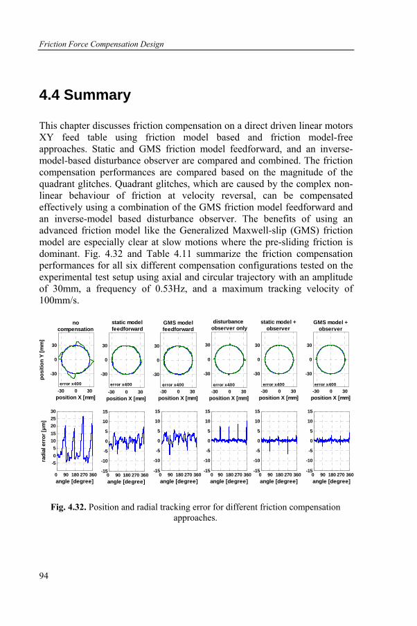
Friction Force Compensation Design
94
4.4 Summary
This chapter discusses friction compensation on a direct driven linear motors XY feed table using friction model based and friction model-free approaches. Static and GMS friction model feedforward, and an inverse-model-based disturbance observer are compared and combined. The friction compensation performances are compared based on the magnitude of the quadrant glitches. Quadrant glitches, which are caused by the complex non-linear behaviour of friction at velocity reversal, can be compensated effectively using a combination of the GMS friction model feedforward and an inverse-model based disturbance observer. The benefits of using an advanced friction model like the Generalized Maxwell-slip (GMS) friction model are especially clear at slow motions where the pre-sliding friction is dominant. Fig. 4.32 and Table 4.11 summarize the friction compensation performances for all six different compensation configurations tested on the experimental test setup using axial and circular trajectory with an amplitude of 30mm, a frequency of 0.53Hz, and a maximum tracking velocity of 100mm/s.
-30 0 30
-30
0
30
nocompensation
position X [mm]
posi
tion
Y [m
m]
0 90 180 270 360
-505
1015202530
radi
al e
rror
[µm
]
angle [degree]
-30 0 30
-30
0
30
static modelfeedforward
position X [mm]
0 90 180 270 360-15
-10
-5
0
5
10
15
angle [degree]
-30 0 30
-30
0
30
GMS modelfeedforward
position X [mm]
0 90 180 270 360-15
-10
-5
0
5
10
15
angle [degree]
-30 0 30
-30
0
30
disturbance observer only
position X [mm]
0 90 180 270 360-15
-10
-5
0
5
10
15
angle [degree]
-30 0 30
-30
0
30
static model +observer
position X [mm]
0 90 180 270 360-15
-10
-5
0
5
10
15
angle [degree]
-30 0 30
-30
0
30
GMS model +observer
position X [mm]
0 90 180 270 360-15
-10
-5
0
5
10
15
angle [degree]
error x400 error x400 error x400 error x400 error x400 error x400
Fig. 4.32. Position and radial tracking error for different friction compensation approaches.
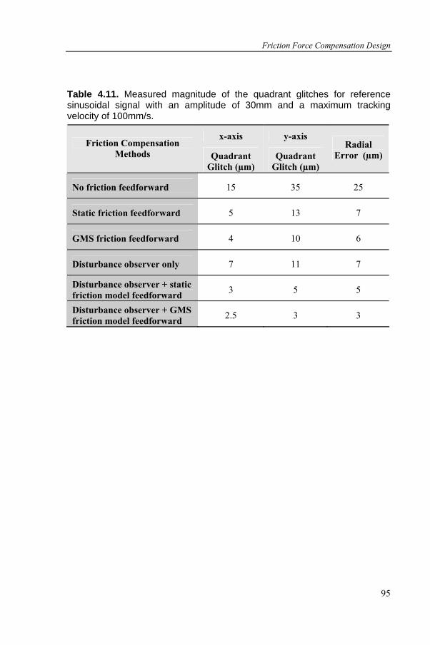
Friction Force Compensation Design
95
Table 4.11. Measured magnitude of the quadrant glitches for reference sinusoidal signal with an amplitude of 30mm and a maximum tracking velocity of 100mm/s.
x-axis y-axis Friction Compensation
Methods Quadrant Glitch (µm)
Quadrant Glitch (µm)
Radial Error (µm)
No friction feedforward 15 35 25
Static friction feedforward 5 13 7
GMS friction feedforward 4 10 6
Disturbance observer only 7 11 7
Disturbance observer + static friction model feedforward 3 5 5
Disturbance observer + GMS friction model feedforward 2.5 3 3

96
97
Chapter 5
Cutting Force Compensation Design
5.1 Introduction
Friction force compensation alone is insufficient to obtain high tracking accuracy in high-speed linear drive based milling processes. Cutting forces generated by the cutting tool and work-piece interaction act directly on the linear motors and influence positioning and tracking accuracy. Cutting force compensation is essential and is traditionally accomplished with high gain feedback control yielding high dynamic stiffness. High dynamic stiffness means high disturbance rejection capacity. High controller gain however reduces the stability margins. This chapter analyses several disturbance compensation methods that have been proposed in literature for various applications but limited knowledge is available with regards to their application and performance for compensation of cutting forces. The different compensation methods will supplement the existing cascade P/PI position controller in a modular based approach. Three compensation methods are considered, namely; (i) an inverse-model-based disturbance observer (section 5.2), (ii) an explicit estimation of cutting force using relative acceleration measurement (section 5.3), and (iii) a repetitive controller (section 5.4). First, the performance of the inverse-model-based disturbance observer is analysed for cutting force compensation, an extension from its previous friction force compensation.
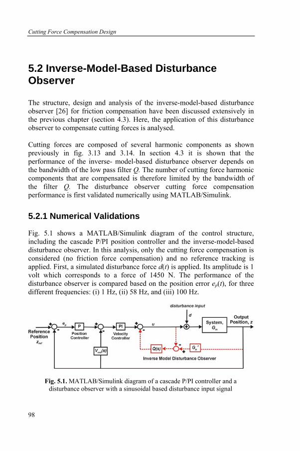
Cutting Force Compensation Design
98
5.2 Inverse-Model-Based Disturbance Observer
The structure, design and analysis of the inverse-model-based disturbance observer [26] for friction compensation have been discussed extensively in the previous chapter (section 4.3). Here, the application of this disturbance observer to compensate cutting forces is analysed. Cutting forces are composed of several harmonic components as shown previously in fig. 3.13 and 3.14. In section 4.3 it is shown that the performance of the inverse- model-based disturbance observer depends on the bandwidth of the low pass filter Q. The number of cutting force harmonic components that are compensated is therefore limited by the bandwidth of the filter Q. The disturbance observer cutting force compensation performance is first validated numerically using MATLAB/Simulink.
5.2.1 Numerical Validations
Fig. 5.1 shows a MATLAB/Simulink diagram of the control structure, including the cascade P/PI position controller and the inverse-model-based disturbance observer. In this analysis, only the cutting force compensation is considered (no friction force compensation) and no reference tracking is applied. First, a simulated disturbance force d(t) is applied. Its amplitude is 1 volt which corresponds to a force of 1450 N. The performance of the disturbance observer is compared based on the position error ep(t), for three different frequencies: (i) 1 Hz, (ii) 58 Hz, and (iii) 100 Hz.
Fig. 5.1. MATLAB/Simulink diagram of a cascade P/PI controller and a disturbance observer with a sinusoidal based disturbance input signal
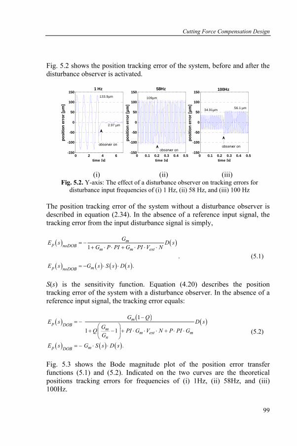
Cutting Force Compensation Design
99
Fig. 5.2 shows the position tracking error of the system, before and after the disturbance observer is activated.
0 2 4 6-150
-100
-50
0
50
100
150
posi
tion
erro
r [µm
]
1 Hz
time [s]0 0.1 0.2 0.3 0.4 0.5
-150
-100
-50
0
50
100
150100Hz
posi
tion
erro
r [µm
]
time [s]0 0.1 0.2 0.3 0.4 0.5
-150
-100
-50
0
50
100
15058Hz
posi
tion
erro
r [µm
]
time [s]
observer onobserver on
observer on
133.9µm
2.97 µm
109µm
34.91µm 56.1 µm
(i) (ii) (iii)
Fig. 5.2. Y-axis: The effect of a disturbance observer on tracking errors for disturbance input frequencies of (i) 1 Hz, (ii) 58 Hz, and (iii) 100 Hz
The position tracking error of the system without a disturbance observer is described in equation (2.34). In the absence of a reference input signal, the tracking error from the input disturbance signal is simply,
( ) ( )
( ) ( ) ( ) ( )
1m
p noDOBm m est
p mnoDOB
GE s D sG P PI G PI V N
E s G s S s D s .
= −+ ⋅ ⋅ + ⋅ ⋅ ⋅
= − ⋅ ⋅
. (5.1)
S(s) is the sensitivity function. Equation (4.20) describes the position tracking error of the system with a disturbance observer. In the absence of a reference input signal, the tracking error equals:
( ) ( ) ( )
( ) ( ) ( )
1
1 1
mp DOB
mm est m
n
p mDOB
G QE s D s
GQ PI G V N P PI GG
E s G S s D s .
−= −
⎛ ⎞+ − + ⋅ ⋅ ⋅ + ⋅ ⋅⎜ ⎟
⎝ ⎠= − ⋅ ⋅
(5.2)
Fig. 5.3 shows the Bode magnitude plot of the position error transfer functions (5.1) and (5.2). Indicated on the two curves are the theoretical positions tracking errors for frequencies of (i) 1Hz, (ii) 58Hz, and (iii) 100Hz.

Cutting Force Compensation Design
100
Bode Magnitude Diagram
Frequency (Hz)
Mag
nitu
de (a
bs)
10-1 100 101 102 10310-2
10-1
100
101
102
103
Freq (Hz): 58.2 Mag (abs): 112
Freq (Hz): 100 Mag (abs): 57.8
Freq (Hz): 1 Mag(abs): 2.96
Freq (Hz): 58 Mag (abs): 109
Freq (Hz): 100 Mag (abs): 36.4
Freq (Hz): 1 Mag(abs): 133
no observerw ith observer
Fig 5.3. Y-axis: Position errors for system with and without a disturbance observer
Fig. 5.3 shows an almost exact match of position errors for each of the three different frequencies, for cases with and without the disturbance observer, when compared to the simulated position errors shown in fig. 5.2. The system is able to partly compensate the purely sinusoidal signal until a frequency of nearly 60Hz. The position error is amplified beyond this frequency, as shown in fig. 5.2 (iii) and fig. 5.3.
5.2.2 Experimental Validations
Experimental validation is performed on the test setup using a synthesized cutting force with different harmonic contents. Fig. 5.4 shows the control scheme that includes the cascade P/PI controller, GMS friction model feedforward, the inverse-model reference feedforward, and the inverse-model-based disturbance observer. First, a synthesized cutting force described in section 3.4.2 is applied at the input of the system with no reference trajectory motion. The position errors for a synthesized cutting force with 1, 2, 3, and 15 harmonics content is shown in fig. 5.5 (the fundamental frequency is 23.3Hz, see Table 3.5).
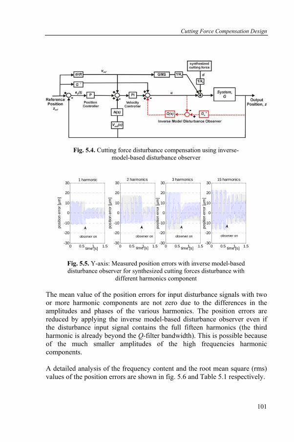
Cutting Force Compensation Design
101
Fig. 5.4. Cutting force disturbance compensation using inverse-model-based disturbance observer
0 0.5 1 1.5-30
-20
-10
0
10
20
3015 harmonics
time [s]
posi
tion
erro
r [µm
]
0 0.5 1 1.5-30
-20
-10
0
10
20
303 harmonics
time [s]
posi
tion
erro
r [µm
]
0 0.5 1 1.5-30
-20
-10
0
10
20
302 harmonics
time [s]
posi
tion
erro
r [µm
]
0 0.5 1 1.5-30
-20
-10
0
10
20
301 harmonic
time [s]
posi
tion
erro
r [µm
]
observer on observer on observer on observer on
Fig. 5.5. Y-axis: Measured position errors with inverse model-based disturbance observer for synthesized cutting forces disturbance with
different harmonics component The mean value of the position errors for input disturbance signals with two or more harmonic components are not zero due to the differences in the amplitudes and phases of the various harmonics. The position errors are reduced by applying the inverse model-based disturbance observer even if the disturbance input signal contains the full fifteen harmonics (the third harmonic is already beyond the Q-filter bandwidth). This is possible because of the much smaller amplitudes of the high frequencies harmonic components. A detailed analysis of the frequency content and the root mean square (rms) values of the position errors are shown in fig. 5.6 and Table 5.1 respectively.
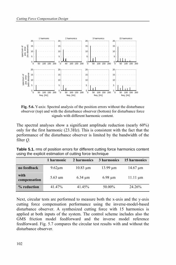
Cutting Force Compensation Design
102
0 50 100 150 2000
5
10
15
20
spec
trum
of
pos.
erro
r(n
o ob
serv
er)
1 harmonic
0 50 100 150 2000
5
10
15
20
freq. [Hz]
spec
trum
of
pos.
erro
r(w
ith o
bse)
rver
0 50 100 150 2000
5
10
15
202 harmonics
0 50 100 150 2000
5
10
15
20
freq. [Hz]
0 50 100 150 2000
5
10
15
203 harmonics
0 50 100 150 2000
5
10
15
20
freq. [Hz]
0 50 100 150 2000
5
10
15
2015 harmonics
0 50 100 150 2000
5
10
15
20
freq. [Hz]
Fig. 5.6. Y-axis: Spectral analysis of the position errors without the disturbance observer (top) and with the disturbance observer (bottom) for disturbance force
signals with different harmonic content.
The spectral analyses show a significant amplitude reduction (nearly 60%) only for the first harmonic (23.3Hz). This is consistent with the fact that the performance of the disturbance observer is limited by the bandwidth of the filter Q.
Table 5.1. rms of position errors for different cutting force harmonics content using the explicit estimation of cutting force technique 1 harmonic 2 harmonics 3 harmonics 15 harmonics
no feedback 9.62µm 10.83 µm 13.99 µm 14.67 µm
with compensation 5.63 um 6.34 µm 6.98 µm 11.11 µm
% reduction 41.47% 41.45% 50.00% 24.26%
Next, circular tests are performed to measure both the x-axis and the y-axis cutting force compensation performance using the inverse-model-based disturbance observer. A synthesized cutting force with 15 harmonics is applied at both inputs of the system. The control scheme includes also the GMS friction model feedforward and the inverse model reference feedforward. Fig. 5.7 compares the circular test results with and without the disturbance observer.
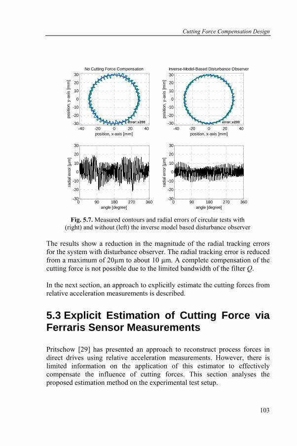
Cutting Force Compensation Design
103
-40 -20 0 20 40-30
-20
-10
0
10
20
30
position, x-axis [mm]
posi
tion,
y-a
xis
[mm
]No Cutting Force Compensation
0 90 180 270 360-30
-20
-10
0
10
20
30
angle [degree]
radi
al e
rror [
µm]
-40 -20 0 20 40-30
-20
-10
0
10
20
30
position, x-axis [mm]
posi
tion,
y-a
xis
[mm
]
Inverse-Model-Based Disturbance Observer
0 90 180 270 360-30
-20
-10
0
10
20
30
angle [degree]
radi
al e
rror [
µm]
error: x200 error: x200
Fig. 5.7. Measured contours and radial errors of circular tests with
(right) and without (left) the inverse model based disturbance observer The results show a reduction in the magnitude of the radial tracking errors for the system with disturbance observer. The radial tracking error is reduced from a maximum of 20µm to about 10 µm. A complete compensation of the cutting force is not possible due to the limited bandwidth of the filter Q. In the next section, an approach to explicitly estimate the cutting forces from relative acceleration measurements is described.
5.3 Explicit Estimation of Cutting Force via Ferraris Sensor Measurements
Pritschow [29] has presented an approach to reconstruct process forces in direct drives using relative acceleration measurements. However, there is limited information on the application of this estimator to effectively compensate the influence of cutting forces. This section analyses the proposed estimation method on the experimental test setup.
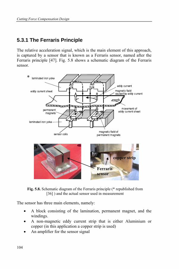
Cutting Force Compensation Design
104
5.3.1 The Ferraris Principle
The relative acceleration signal, which is the main element of this approach, is captured by a sensor that is known as a Ferraris sensor, named after the Ferraris principle [47]. Fig. 5.8 shows a schematic diagram of the Ferraris sensor.
Fig. 5.8. Schematic diagram of the Ferraris principle (* republished from
[36] ) and the actual sensor used in measurement
The sensor has three main elements, namely:
• A block consisting of the lamination, permanent magnet, and the windings.
• A non-magnetic eddy current strip that is either Aluminium or copper (in this application a copper strip is used)
• An amplifier for the sensor signal
*
copper strip
Ferraris sensor
Cutting Force Compensation Design
105
The eddy current strip that lies within the slot of the block is attached to the moving object while the other parts are fixed to the frame. A relative motion between the eddy current strip and the block generates eddy current in the eddy current strip due to the permanent magnet that induces a voltage. The resulting eddy current generates magnetic fields and the strength of this field changes as the velocity of motion changes. This results in a voltage being induced in the winding. This voltage is proportional to the change of velocity, that is, the acceleration of the motion. The amplifier then amplifies the signal. A Ferraris sensor is attractive in mechatronic application because it provides an alternative method for generating a velocity signal from the acceleration signal [48]. Noise amplification and quantization of velocity signals that are generated by numerically differentiating position encoder signals can be avoided. J. Wang [36] has described the effect of eddy current strip characteristics, placement, and structure on the quality of the sensor signals. The disadvantage of this sensor is that, it has to be calibrated on-site. This is because the installation of the sensor part can affect the sensor sensitivity. The calibration of the sensor is based on the comparison between the position encoder measurement and the position signal that is generated from the Ferraris sensor measurements. The calibration of the Ferraris sensor sensitivity and offset value are described in Appendix B.
5.3.2 Cutting Force Estimator
The Pritschow’s cutting force estimator [29] is designed based on a reduced order observer [35] that estimates state variables that cannot be measured directly. The observer is designed by considering the following model equation that describes the balance between forces that acts on a direct drive system (here, the x&& term refers to absolute acceleration).
( ) ( ) ( ) ( )1 1ff
kx t u t d t F v
M M M= + −&& (5.3)
x is the position, d is the disturbance force, kf is the motor force constant, M is the mass, Ff is the friction force, and u is the voltage to the drive amplifier. The state space representations of the system and the measurement equation are:
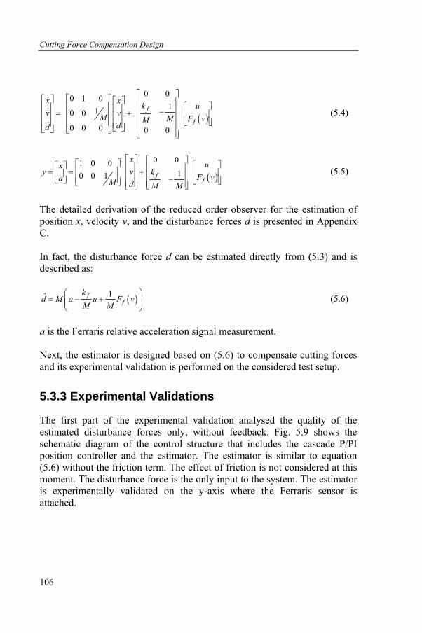
Cutting Force Compensation Design
106
( )
0 00 1 0110 0
0 0 0 0 0
f
f
x xuk
v v M M F vMdd
⎡ ⎤⎡ ⎤⎡ ⎤ ⎡ ⎤ ⎢ ⎥ ⎡ ⎤⎢ ⎥⎢ ⎥ ⎢ ⎥ ⎢ ⎥−= + ⎢ ⎥⎢ ⎥⎢ ⎥ ⎢ ⎥ ⎢ ⎥ ⎢ ⎥⎢ ⎥ ⎣ ⎦⎢ ⎥ ⎢ ⎥ ⎢ ⎥⎣ ⎦⎣ ⎦ ⎣ ⎦ ⎢ ⎥⎣ ⎦
&
&
&
(5.4)
( )
0 01 0 010 0 1 f
f
xux
y v k F va M d M M
⎡ ⎤ ⎡ ⎤⎡ ⎤ ⎡ ⎤⎡ ⎤ ⎢ ⎥ ⎢ ⎥⎢ ⎥= = + ⎢ ⎥⎢ ⎥ ⎢ ⎥ ⎢ ⎥−⎢ ⎥ ⎢ ⎥⎣ ⎦ ⎣ ⎦⎣ ⎦ ⎢ ⎥ ⎢ ⎥⎣ ⎦⎣ ⎦
(5.5)
The detailed derivation of the reduced order observer for the estimation of position x, velocity v, and the disturbance forces d is presented in Appendix C. In fact, the disturbance force d can be estimated directly from (5.3) and is described as:
( )1ff
kd M a u F v
M M⎛ ⎞
= − +⎜ ⎟⎜ ⎟⎝ ⎠
(5.6)
a is the Ferraris relative acceleration signal measurement. Next, the estimator is designed based on (5.6) to compensate cutting forces and its experimental validation is performed on the considered test setup.
5.3.3 Experimental Validations
The first part of the experimental validation analysed the quality of the estimated disturbance forces only, without feedback. Fig. 5.9 shows the schematic diagram of the control structure that includes the cascade P/PI position controller and the estimator. The estimator is similar to equation (5.6) without the friction term. The effect of friction is not considered at this moment. The disturbance force is the only input to the system. The estimator is experimentally validated on the y-axis where the Ferraris sensor is attached.
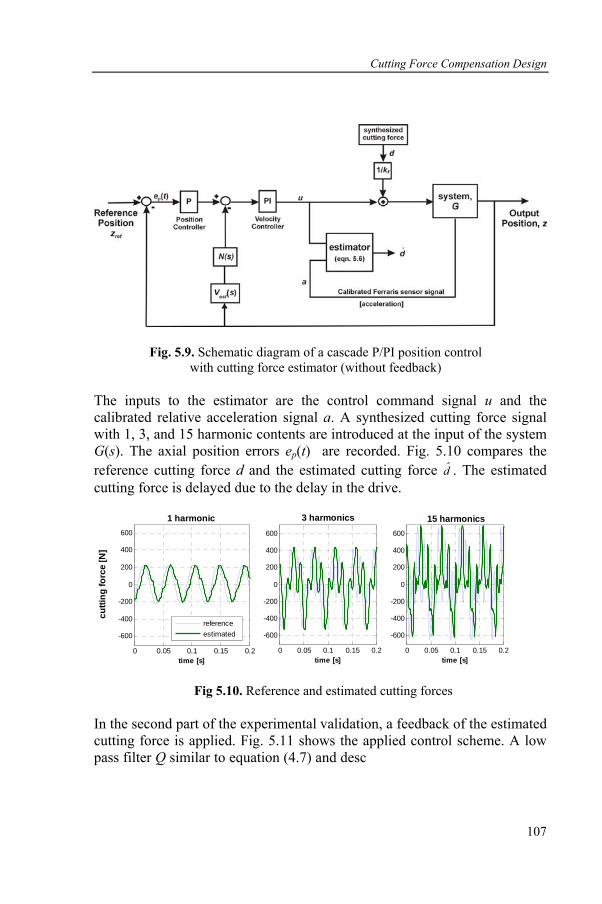
Cutting Force Compensation Design
107
Fig. 5.9. Schematic diagram of a cascade P/PI position control with cutting force estimator (without feedback)
The inputs to the estimator are the control command signal u and the calibrated relative acceleration signal a. A synthesized cutting force signal with 1, 3, and 15 harmonic contents are introduced at the input of the system G(s). The axial position errors ep(t) are recorded. Fig. 5.10 compares the reference cutting force d and the estimated cutting force d . The estimated cutting force is delayed due to the delay in the drive.
0 0.05 0.1 0.15 0.2
-600
-400
-200
0
200
400
600
time [s]
cutti
ng fo
rce
[N]
1 harmonic
0 0.05 0.1 0.15 0.2
-600
-400
-200
0
200
400
600
time [s]
3 harmonics
0 0.05 0.1 0.15 0.2
-600
-400
-200
0
200
400
600
time [s]
15 harmonics
referenceestimated
Fig 5.10. Reference and estimated cutting forces In the second part of the experimental validation, a feedback of the estimated cutting force is applied. Fig. 5.11 shows the applied control scheme. A low pass filter Q similar to equation (4.7) and desc
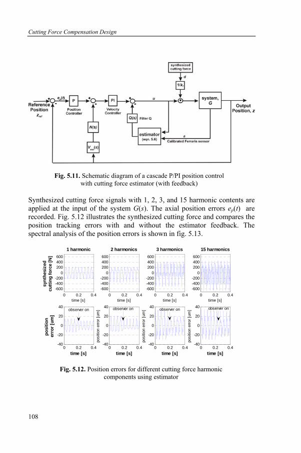
Cutting Force Compensation Design
108
Fig. 5.11. Schematic diagram of a cascade P/PI position control with cutting force estimator (with feedback)
Synthesized cutting force signals with 1, 2, 3, and 15 harmonic contents are applied at the input of the system G(s). The axial position errors ep(t) are recorded. Fig. 5.12 illustrates the synthesized cutting force and compares the position tracking errors with and without the estimator feedback. The spectral analysis of the position errors is shown in fig. 5.13.
0 0.2 0.4-600-400-200
0200400600
time [s]
synt
hesi
zed
cutti
ng fo
rce
[N]
1 harmonic
0 0.2 0.4-40
-20
0
20
40
time [s]
posi
tion
erro
r [um
]
0 0.2 0.4-600-400-200
0200400600
time [s]
2 harmonics
0 0.2 0.4-40
-20
0
20
40
time [s]
posi
tion
erro
r [um
]
0 0.2 0.4-600-400-200
0200400600
time [s]
3 harmonics
0 0.2 0.4-40
-20
0
20
40
time [s]
posi
tion
erro
r [um
]
0 0.2 0.4-600-400-200
0200400600
time [s]
15 harmonics
0 0.2 0.4-40
-20
0
20
40
time [s]
posi
tion
erro
r [um
]observer on observer on observer on observer on
Fig. 5.12. Position errors for different cutting force harmonic components using estimator
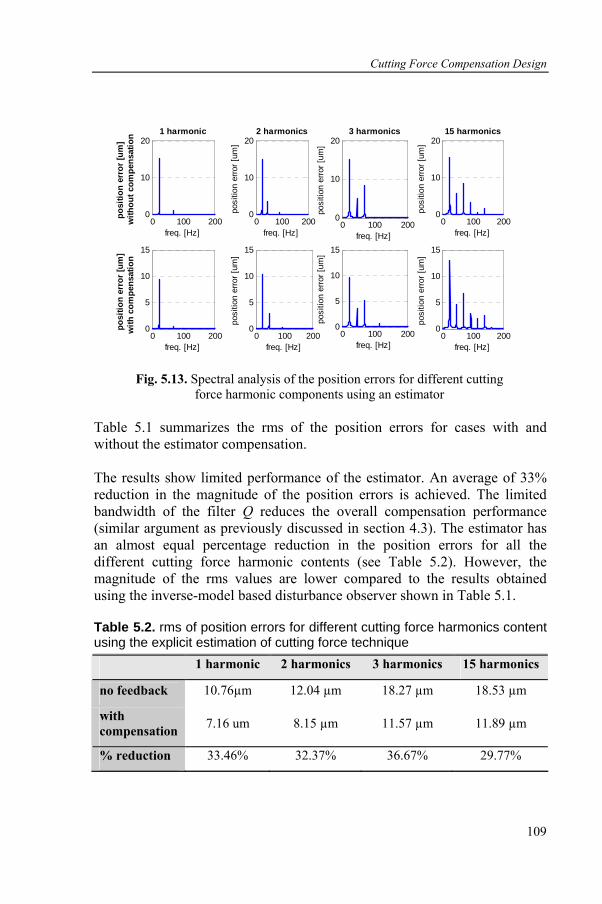
Cutting Force Compensation Design
109
0 100 2000
10
20
freq. [Hz]
posi
tion
erro
r [um
] w
ithou
t com
pens
atio
n 1 harmonic
0 100 2000
5
10
15
freq. [Hz]
posi
tion
erro
r [um
] w
ith c
ompe
nsat
ion
0 100 2000
10
20
freq. [Hz]po
sitio
n er
ror [
um]
2 harmonics
0 100 2000
5
10
15
freq. [Hz]
posi
tion
erro
r [um
]0 100 200
0
10
20
freq. [Hz]
posi
tion
erro
r [um
]
15 harmonics
0 100 2000
5
10
15
freq. [Hz]
posi
tion
erro
r [um
]
0 100 2000
10
20
freq. [Hz]
posi
tion
erro
r [um
]
3 harmonics
0 100 2000
5
10
15
freq. [Hz]
posi
tion
erro
r [um
]
Fig. 5.13. Spectral analysis of the position errors for different cutting force harmonic components using an estimator
Table 5.1 summarizes the rms of the position errors for cases with and without the estimator compensation. The results show limited performance of the estimator. An average of 33% reduction in the magnitude of the position errors is achieved. The limited bandwidth of the filter Q reduces the overall compensation performance (similar argument as previously discussed in section 4.3). The estimator has an almost equal percentage reduction in the position errors for all the different cutting force harmonic contents (see Table 5.2). However, the magnitude of the rms values are lower compared to the results obtained using the inverse-model based disturbance observer shown in Table 5.1.
Table 5.2. rms of position errors for different cutting force harmonics content using the explicit estimation of cutting force technique 1 harmonic 2 harmonics 3 harmonics 15 harmonics
no feedback 10.76µm 12.04 µm 18.27 µm 18.53 µm
with compensation 7.16 um 8.15 µm 11.57 µm 11.89 µm
% reduction 33.46% 32.37% 36.67% 29.77%
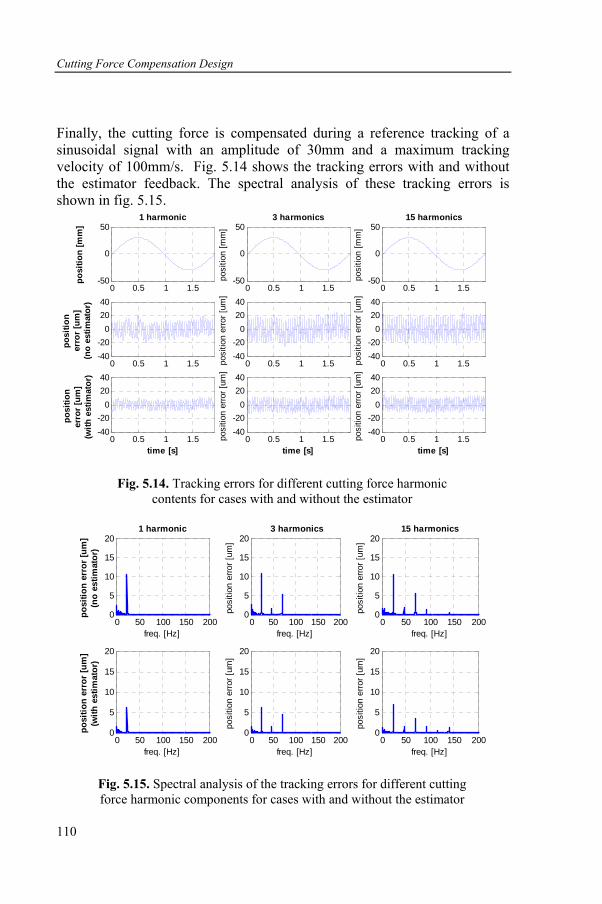
Cutting Force Compensation Design
110
Finally, the cutting force is compensated during a reference tracking of a sinusoidal signal with an amplitude of 30mm and a maximum tracking velocity of 100mm/s. Fig. 5.14 shows the tracking errors with and without the estimator feedback. The spectral analysis of these tracking errors is shown in fig. 5.15.
0 0.5 1 1.5-50
0
501 harmonic
posi
tion
[mm
]
0 0.5 1 1.5-40-20
02040
posi
tion
erro
r [u
m]
(no
estim
ator
)
0 0.5 1 1.5-40-20
02040
time [s]
posi
tion
erro
r [u
m]
(with
est
imat
or)
0 0.5 1 1.5-50
0
503 harmonics
posi
tion
[mm
]
0 0.5 1 1.5-40-20
02040
posi
tion
erro
r [um
]
0 0.5 1 1.5-40-20
02040
time [s]
posi
tion
erro
r [um
]
0 0.5 1 1.5-50
0
5015 harmonics
posi
tion
[mm
]0 0.5 1 1.5
-40-20
02040
posi
tion
erro
r [um
]
0 0.5 1 1.5-40-20
02040
time [s]
posi
tion
erro
r [um
]
Fig. 5.14. Tracking errors for different cutting force harmonic contents for cases with and without the estimator
0 50 100 150 2000
5
10
15
20
freq. [Hz]
posi
tion
erro
r [u
m]
(no
estim
ator
)
1 harmonic
0 50 100 150 2000
5
10
15
20
freq. [Hz]
posi
tion
erro
r [u
m]
(with
est
imat
or)
0 50 100 150 2000
5
10
15
20
freq. [Hz]
posi
tion
erro
r [um
]
3 harmonics
0 50 100 150 2000
5
10
15
20
freq. [Hz]
posi
tion
erro
r [um
]
0 50 100 150 2000
5
10
15
20
freq. [Hz]
posi
tion
erro
r [um
]
15 harmonics
0 50 100 150 2000
5
10
15
20
freq. [Hz]
posi
tion
erro
r [um
]
Fig. 5.15. Spectral analysis of the tracking errors for different cutting force harmonic components for cases with and without the estimator
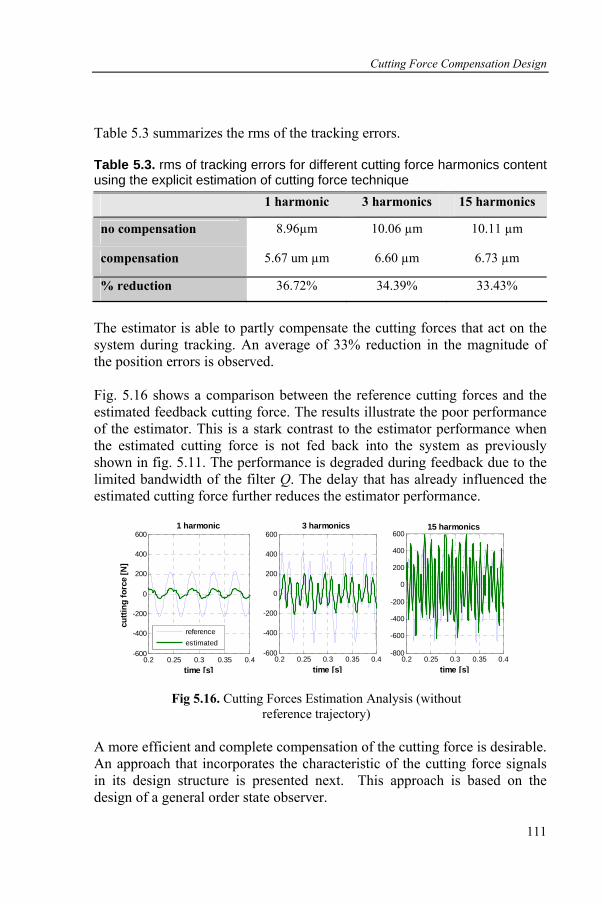
Cutting Force Compensation Design
111
Table 5.3 summarizes the rms of the tracking errors.
Table 5.3. rms of tracking errors for different cutting force harmonics content using the explicit estimation of cutting force technique 1 harmonic 3 harmonics 15 harmonics
no compensation 8.96µm 10.06 µm 10.11 µm
compensation 5.67 um µm 6.60 µm 6.73 µm
% reduction 36.72% 34.39% 33.43%
The estimator is able to partly compensate the cutting forces that act on the system during tracking. An average of 33% reduction in the magnitude of the position errors is observed. Fig. 5.16 shows a comparison between the reference cutting forces and the estimated feedback cutting force. The results illustrate the poor performance of the estimator. This is a stark contrast to the estimator performance when the estimated cutting force is not fed back into the system as previously shown in fig. 5.11. The performance is degraded during feedback due to the limited bandwidth of the filter Q. The delay that has already influenced the estimated cutting force further reduces the estimator performance.
0.2 0.25 0.3 0.35 0.4-600
-400
-200
0
200
400
600
time [s]
cutti
ng fo
rce
[N]
1 harmonic
0.2 0.25 0.3 0.35 0.4-600
-400
-200
0
200
400
600
time [s]
3 harmonics
0.2 0.25 0.3 0.35 0.4-800
-600
-400
-200
0
200
400
600
time [s]
15 harmonics
referenceestimated
Fig 5.16. Cutting Forces Estimation Analysis (without reference trajectory)
A more efficient and complete compensation of the cutting force is desirable. An approach that incorporates the characteristic of the cutting force signals in its design structure is presented next. This approach is based on the design of a general order state observer.
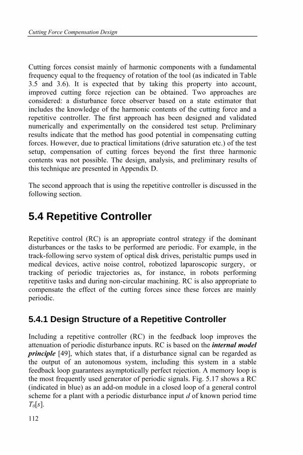
Cutting Force Compensation Design
112
Cutting forces consist mainly of harmonic components with a fundamental frequency equal to the frequency of rotation of the tool (as indicated in Table 3.5 and 3.6). It is expected that by taking this property into account, improved cutting force rejection can be obtained. Two approaches are considered: a disturbance force observer based on a state estimator that includes the knowledge of the harmonic contents of the cutting force and a repetitive controller. The first approach has been designed and validated numerically and experimentally on the considered test setup. Preliminary results indicate that the method has good potential in compensating cutting forces. However, due to practical limitations (drive saturation etc.) of the test setup, compensation of cutting forces beyond the first three harmonic contents was not possible. The design, analysis, and preliminary results of this technique are presented in Appendix D. The second approach that is using the repetitive controller is discussed in the following section.
5.4 Repetitive Controller
Repetitive control (RC) is an appropriate control strategy if the dominant disturbances or the tasks to be performed are periodic. For example, in the track-following servo system of optical disk drives, peristaltic pumps used in medical devices, active noise control, robotized laparoscopic surgery, or tracking of periodic trajectories as, for instance, in robots performing repetitive tasks and during non-circular machining. RC is also appropriate to compensate the effect of the cutting forces since these forces are mainly periodic.
5.4.1 Design Structure of a Repetitive Controller
Including a repetitive controller (RC) in the feedback loop improves the attenuation of periodic disturbance inputs. RC is based on the internal model principle [49], which states that, if a disturbance signal can be regarded as the output of an autonomous system, including this system in a stable feedback loop guarantees asymptotically perfect rejection. A memory loop is the most frequently used generator of periodic signals. Fig. 5.17 shows a RC (indicated in blue) as an add-on module in a closed loop of a general control scheme for a plant with a periodic disturbance input d of known period time T0[s].
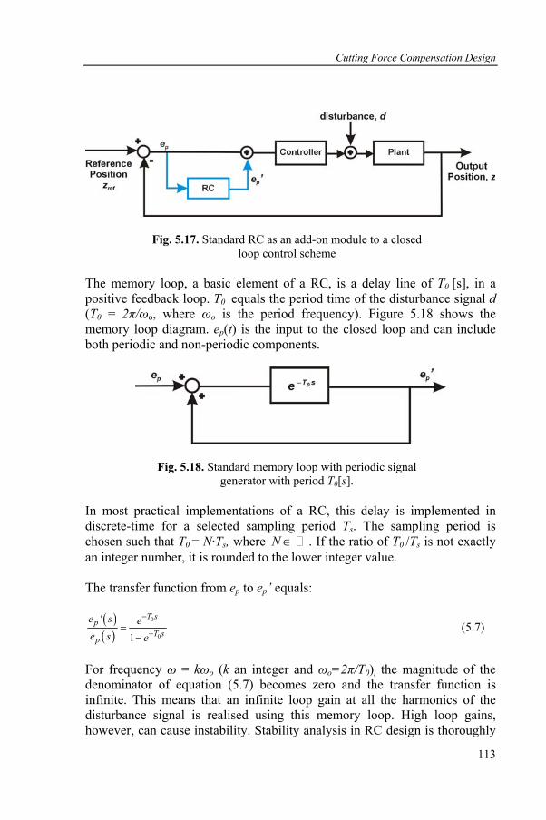
Cutting Force Compensation Design
113
Fig. 5.17. Standard RC as an add-on module to a closed loop control scheme
The memory loop, a basic element of a RC, is a delay line of T0 [s], in a positive feedback loop. T0 equals the period time of the disturbance signal d (T0 = 2π/ωo, where ωo is the period frequency). Figure 5.18 shows the memory loop diagram. ep(t) is the input to the closed loop and can include both periodic and non-periodic components.
Fig. 5.18. Standard memory loop with periodic signal generator with period T0[s].
In most practical implementations of a RC, this delay is implemented in discrete-time for a selected sampling period Ts. The sampling period is chosen such that T0 = N·Ts, where ∈N . If the ratio of T0 /Ts is not exactly an integer number, it is rounded to the lower integer value. The transfer function from ep to ep’ equals:
( )( )
0
01
T sp
T sp
e ' s ee s e
−
−=−
(5.7)
For frequency ω = kωo (k an integer and ωo=2π/T0), the magnitude of the denominator of equation (5.7) becomes zero and the transfer function is infinite. This means that an infinite loop gain at all the harmonics of the disturbance signal is realised using this memory loop. High loop gains, however, can cause instability. Stability analysis in RC design is thoroughly
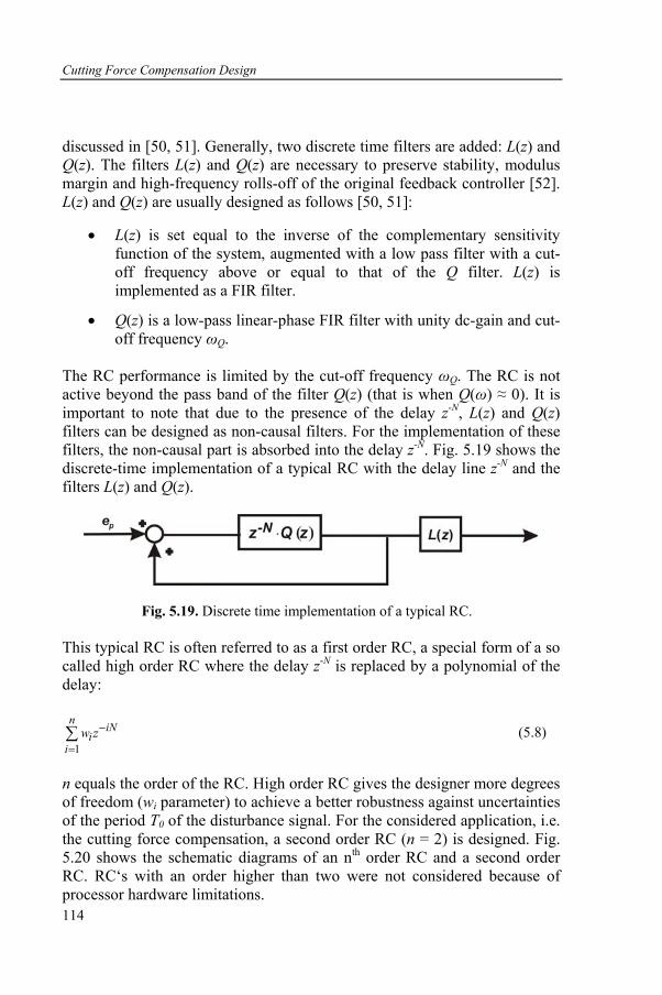
Cutting Force Compensation Design
114
discussed in [50, 51]. Generally, two discrete time filters are added: L(z) and Q(z). The filters L(z) and Q(z) are necessary to preserve stability, modulus margin and high-frequency rolls-off of the original feedback controller [52]. L(z) and Q(z) are usually designed as follows [50, 51]:
• L(z) is set equal to the inverse of the complementary sensitivity function of the system, augmented with a low pass filter with a cut-off frequency above or equal to that of the Q filter. L(z) is implemented as a FIR filter.
• Q(z) is a low-pass linear-phase FIR filter with unity dc-gain and cut-off frequency ωQ.
The RC performance is limited by the cut-off frequency ωQ. The RC is not active beyond the pass band of the filter Q(z) (that is when Q(ω) ≈ 0). It is important to note that due to the presence of the delay z-N, L(z) and Q(z) filters can be designed as non-causal filters. For the implementation of these filters, the non-causal part is absorbed into the delay z-N. Fig. 5.19 shows the discrete-time implementation of a typical RC with the delay line z-N and the filters L(z) and Q(z).
Fig. 5.19. Discrete time implementation of a typical RC. This typical RC is often referred to as a first order RC, a special form of a so called high order RC where the delay z-N is replaced by a polynomial of the delay:
1
n iNi
iw z−
=∑ (5.8)
n equals the order of the RC. High order RC gives the designer more degrees of freedom (wi parameter) to achieve a better robustness against uncertainties of the period T0 of the disturbance signal. For the considered application, i.e. the cutting force compensation, a second order RC (n = 2) is designed. Fig. 5.20 shows the schematic diagrams of an nth order RC and a second order RC. RC‘s with an order higher than two were not considered because of processor hardware limitations.

Cutting Force Compensation Design
115
Fig. 5.20. Schematic diagram of (a) nth order RC, (b) 2nd order RC
The two parameters w1 and w2 of the second order RC were designed using the method developed by G.Pipeleers et. al. [52, 53] as a trade-off between periodic performance considering a relative uncertainty of 1% on the period of the disturbance and non-periodic performance degradation, that is the amplification of non-periodic disturbances such as measurement noise that are present between the harmonics of the cutting force. The periodic and non-periodic performances of a RC are quantified by the robust periodic and non-periodic performance indices respectively [51]. The robust periodic performance index γp,∆ [51] is defined as the smallest reduction of the sensitivity function over all considered harmonics of the disturbance and over all potential frequencies within the specified (in this case 1%) relative uncertainty interval. Attenuation of the periodic disturbances corresponds to γp,∆ < 1, where γp,∆ = 0 indicates perfect rejection. The non-periodic performance index γnp [51] is defined as the highest amplification of the sensitivity function over all frequencies within the bandwidth of the RC. The RC is designed to have a bandwidth of 200 Hz (ωQ =200Hz), such that the first eight harmonics (the fundamental frequency is 23.3 Hz, for a spindle speed of 1360rpm) of the synthesised cutting force are compensated. This bandwidth is chosen due to the model accuracy limitation beyond a frequency of 200Hz. This limitation will have a minimal effect on the controller compensation performance because the influence of the 8th or higher harmonic components of the cutting forces is not significant (Table 3.5 and 3.6). The designed RC has a periodic performance index γp,∆ of 0.063 and a non-periodic performance index γnp of 6dB.
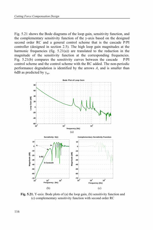
Cutting Force Compensation Design
116
Fig. 5.21 shows the Bode diagrams of the loop gain, sensitivity function, and the complementary sensitivity function of the y-axis based on the designed second order RC and a general control scheme that is the cascade P/PI controller (designed in section 2.5). The high loop gain magnitudes at the harmonic frequencies (fig. 5.21(a)) are translated to the reduction in the magnitude of the sensitivity function at the corresponding frequencies. Fig. 5.21(b) compares the sensitivity curves between the cascade P/PI control scheme and the control scheme with the RC added. The non-periodic performance degradation is identified by the arrows A, and is smaller than 6dB as predicted by γnp.
100 101 102-60
-40
-20
0
20
40
60
80
Loop
Gai
n [d
B]
Bode Plot of Loop Gain
frequency (Hz) (a)
100 101 102-70
-60
-50
-40
-30
-20
-10
0
10
Frequency (Hz)
Mag
nitu
de [d
B]
Complementary Sensitivity Function
100 101 102-70
-60
-50
-40
-30
-20
-10
0
10
Mag
nitu
de (d
B)
Sensitivity: S(z)
Frequency (Hz)
A
S-RC
S-Cascade
(b) (c)
Fig. 5.21. Y-axis: Bode plots of (a) the loop gain, (b) sensitivity function and (c) complementary sensitivity function with second order RC
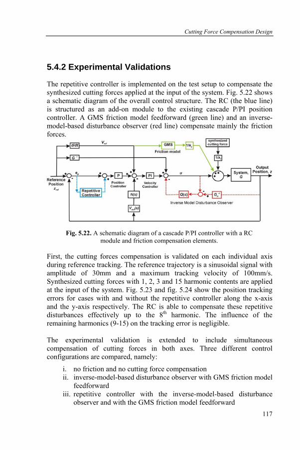
Cutting Force Compensation Design
117
5.4.2 Experimental Validations
The repetitive controller is implemented on the test setup to compensate the synthesized cutting forces applied at the input of the system. Fig. 5.22 shows a schematic diagram of the overall control structure. The RC (the blue line) is structured as an add-on module to the existing cascade P/PI position controller. A GMS friction model feedforward (green line) and an inverse-model-based disturbance observer (red line) compensate mainly the friction forces.
Fig. 5.22. A schematic diagram of a cascade P/PI controller with a RC module and friction compensation elements.
First, the cutting forces compensation is validated on each individual axis during reference tracking. The reference trajectory is a sinusoidal signal with amplitude of 30mm and a maximum tracking velocity of 100mm/s. Synthesized cutting forces with 1, 2, 3 and 15 harmonic contents are applied at the input of the system. Fig. 5.23 and fig. 5.24 show the position tracking errors for cases with and without the repetitive controller along the x-axis and the y-axis respectively. The RC is able to compensate these repetitive disturbances effectively up to the 8th harmonic. The influence of the remaining harmonics (9-15) on the tracking error is negligible. The experimental validation is extended to include simultaneous compensation of cutting forces in both axes. Three different control configurations are compared, namely:
i. no friction and no cutting force compensation ii. inverse-model-based disturbance observer with GMS friction model
feedforward iii. repetitive controller with the inverse-model-based disturbance
observer and with the GMS friction model feedforward

Cutting Force Compensation Design
118
0 0.1 0.2-400
-200
0
200
4001 harmonic
cutti
ng fo
rce
[N]
0 1 2-20
-10
0
10
20
posi
tion
erro
r [µm
]
no
RC
0 1 2-20
-10
0
10
20
time [s]
posi
tion
erro
r [µm
]
with
RC
0 0.1 0.2-400
-200
0
200
4002 harmonics
0 1 2-20
-10
0
10
20
0 1 2-20
-10
0
10
20
time [s]
0 0.1 0.2-400
-200
0
200
4003 harmonics
0 1 2-20
-10
0
10
20
0 1 2-20
-10
0
10
20
time [s]
0 0.1 0.2-400
-200
0
200
40015 harmonics
0 1 2-20
-10
0
10
20
0 1 2-20
-10
0
10
20
time [s]
Fig. 5.23. Y-axis: Measured position tracking errors with and without the RC for different harmonic component of the cutting forces.
0 0.1 0.2-400
-200
0
200
4001 harmonic
cutti
ng fo
rce
[N]
0 1 2-20
-10
0
10
20
posi
tion
erro
r [µm
]
n
o R
C
0 1 2-20
-10
0
10
20
time [s]
posi
tion
erro
r [µm
]
w
ith R
C
0 0.1 0.2-400
-200
0
200
4002 harmonic
0 1 2-20
-10
0
10
20
0 1 2-20
-10
0
10
20
time [s]
0 0.1 0.2-400
-200
0
200
4003 harmonic
0 1 2-20
-10
0
10
20
0 1 2-20
-10
0
10
20
time [s]
0 0.1 0.2-400
-200
0
200
40015 harmonics
0 1 2-20
-10
0
10
20
0 1 2-20
-10
0
10
20
time [s]
Fig. 5.24. X-axis: Measured position tracking errors with and without the RC for different harmonic components of the cutting forces.
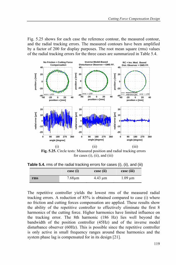
Cutting Force Compensation Design
119
Fig. 5.25 shows for each case the reference contour, the measured contour, and the radial tracking errors. The measured contours have been amplified by a factor of 200 for display purposes. The root mean square (rms) values of the radial tracking errors for the three cases are summarized in Table 5.4.
-40 -20 0 20 40-40
-20
0
20
40
RC + Inv. Mod. Based Dist. Observer + GMS FF.
position x [mm]
posi
tion
y [m
m]
0 90 180 270 360
-20
-10
0
10
20
radi
al e
rror
[µm
]
angle [degree]
-40 -20 0 20 40-40
-20
0
20
40
Inverse-Model-Based Disturbance Observer + GMS FF.
position x [mm]
posi
tion
y [m
m]
0 90 180 270 360
-20
-10
0
10
20
radi
al e
rror
[µm
]
angle [degree]
-40 -20 0 20 40-40
-20
0
20
40
position x [mm]
posi
tion
y [m
m]
No Friction + Cutting Force Compensation
0 90 180 270 360
-20
-10
0
10
20
angle [degree]
radi
al e
rror
[µm
]
measured pos.reference pos.error = x200 error = x200 error = x200
(i) (ii) (iii)
Fig. 5.25. Circle tests: Measured position and radial tracking errors for cases (i), (ii), and (iii)
Table 5.4. rms of the radial tracking errors for cases (i), (ii), and (iii) case (i) case (ii) case (iii)
rms 7.68µm 4.43 µm 1.09 µm
The repetitive controller yields the lowest rms of the measured radial tracking errors. A reduction of 85% is obtained compared to case (i) where no friction and cutting forces compensation are applied. These results show the ability of the repetitive controller to effectively eliminate the first 8 harmonics of the cutting force. Higher harmonics have limited influence on the tracking error. The 8th harmonic (186 Hz) lies well beyond the bandwidth of the position controller (45Hz) and of the inverse model disturbance observer (60Hz). This is possible since the repetitive controller is only active in small frequency ranges around these harmonics and the system phase lag is compensated for in its design [21].

Cutting Force Compensation Design
120
The disturbance observer performance is limited by its inherent phase lag. A higher bandwidth is possible with a more accurate model, but will always be lower than the bandwidth of the repetitive controller due to uncompensated system delay.
In the next section, actual cutting operations are performed on the considered test setup. Because of the superior performance of the RC, only this technique is implemented and validated.
5.5 Cutting Forces Compensation during an Actual Cutting Process
Actual cutting tests are performed on the test setup. The cutting test characteristics are summarized in Table 5.5.
Table 5.5. Cutting test characteristics used in cutting force compensation
Cutting conditions Descriptions
Work piece material Aluminium
Cutter diameter 16mm
No. of edges 4
Feed per tooth 0.1mm/tooth
Spindle speed 1360rpm
Axial depth of cut 4mm
Radial depth of cut 1mm
Sampling frequency 2000Hz
The following control configurations are considered for the evaluation of the cutting force compensation:
(i) no friction and no cutting force compensation
(ii) inverse-model-based disturbance observer + GMS friction model feedforward
(iii) inverse-model-based disturbance observer and GMS friction model feedforward with cutting force compensation using a second order repetitive controller
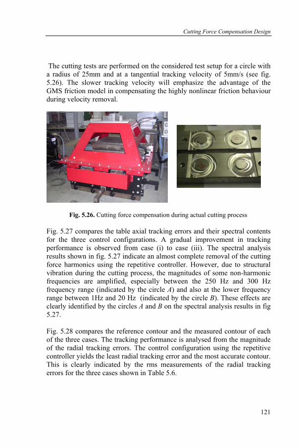
Cutting Force Compensation Design
121
The cutting tests are performed on the considered test setup for a circle with a radius of 25mm and at a tangential tracking velocity of 5mm/s (see fig. 5.26). The slower tracking velocity will emphasize the advantage of the GMS friction model in compensating the highly nonlinear friction behaviour during velocity removal.
Fig. 5.26. Cutting force compensation during actual cutting process Fig. 5.27 compares the table axial tracking errors and their spectral contents for the three control configurations. A gradual improvement in tracking performance is observed from case (i) to case (iii). The spectral analysis results shown in fig. 5.27 indicate an almost complete removal of the cutting force harmonics using the repetitive controller. However, due to structural vibration during the cutting process, the magnitudes of some non-harmonic frequencies are amplified, especially between the 250 Hz and 300 Hz frequency range (indicated by the circle A) and also at the lower frequency range between 1Hz and 20 Hz (indicated by the circle B). These effects are clearly identified by the circles A and B on the spectral analysis results in fig 5.27. Fig. 5.28 compares the reference contour and the measured contour of each of the three cases. The tracking performance is analysed from the magnitude of the radial tracking errors. The control configuration using the repetitive controller yields the least radial tracking error and the most accurate contour. This is clearly indicated by the rms measurements of the radial tracking errors for the three cases shown in Table 5.6.
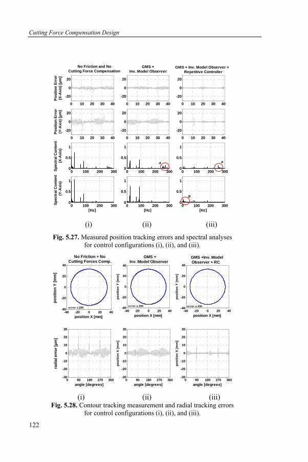
Cutting Force Compensation Design
122
0 10 20 30 40
-20
0
20
Posi
tion
Erro
r(X
-Axi
s) [µ
m]
No Friction and No Cutting Force Compensation
0 10 20 30 40
-20
0
20
Posi
tion
Erro
r
(Y
-Axi
s) [µ
m]
0 100 200 3000
0.5
1
Spec
tral
Con
tent
(X-A
xis)
0 100 200 3000
0.5
1
[Hz]
Spec
tral
Con
tent
(Y-
Axi
s)
0 10 20 30 40
-20
0
20
GMS + Inv. Model Observer
0 10 20 30 40
-20
0
20
0 100 200 3000
0.5
1
[Hz]
0 100 200 3000
0.5
1
0 10 20 30 40
-20
0
20
GMS + Inv. Model Observer + Repetitive Controller
0 10 20 30 40
-20
0
20
0 100 200 3000
0.5
1
0 100 200 3000
0.5
1
[Hz]
AA
B
(i) (ii) (iii)
Fig. 5.27. Measured position tracking errors and spectral analyses for control configurations (i), (ii), and (iii).
-40 -20 0 20 40-40
-20
0
20
40
position X [mm]
posi
tion
Y [m
m]
No Friction + No Cutting Forces Comp.
0 90 180 270 360-30
-20
-10
0
10
20
30
angle [degrees]
radi
al e
rror
[µm
]
-40 -20 0 20 40-40
-20
0
20
40
position X [mm]
posi
tion
Y [m
m]
GMS + Inv. Model Observer
0 90 180 270 360-30
-20
-10
0
10
20
30
posi
tion
X [m
m]
angle [degrees]
-40 -20 0 20 40-40
-20
0
20
40
position X [mm]
posi
tion
Y [m
m]
GMS +Inv. Model Observer + RC
0 90 180 270 360-30
-20
-10
0
10
20
30
posi
tion
X [m
m]
angle [degrees]
error x 200 error x 200 error x 200
(i) (ii) (iii)
Fig. 5.28. Contour tracking measurement and radial tracking errors for control configurations (i), (ii), and (iii).
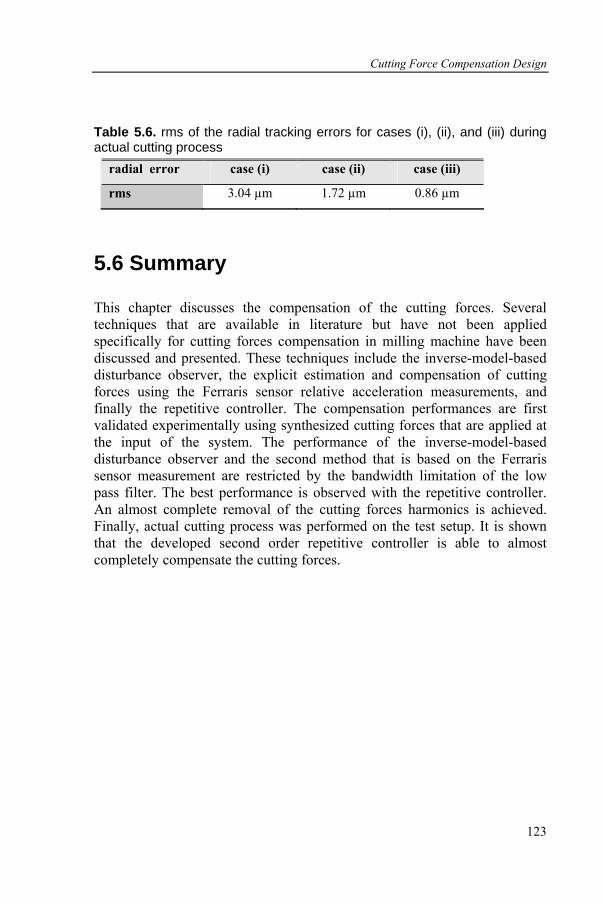
Cutting Force Compensation Design
123
Table 5.6. rms of the radial tracking errors for cases (i), (ii), and (iii) during actual cutting process
radial error case (i) case (ii) case (iii)
rms 3.04 µm 1.72 µm 0.86 µm
5.6 Summary
This chapter discusses the compensation of the cutting forces. Several techniques that are available in literature but have not been applied specifically for cutting forces compensation in milling machine have been discussed and presented. These techniques include the inverse-model-based disturbance observer, the explicit estimation and compensation of cutting forces using the Ferraris sensor relative acceleration measurements, and finally the repetitive controller. The compensation performances are first validated experimentally using synthesized cutting forces that are applied at the input of the system. The performance of the inverse-model-based disturbance observer and the second method that is based on the Ferraris sensor measurement are restricted by the bandwidth limitation of the low pass filter. The best performance is observed with the repetitive controller. An almost complete removal of the cutting forces harmonics is achieved. Finally, actual cutting process was performed on the test setup. It is shown that the developed second order repetitive controller is able to almost completely compensate the cutting forces.

124
125
Chapter 6
Conclusions & Future Study
This thesis investigates friction and cutting forces compensation in a linear drive xy feed table based on several techniques that have been discussed in literature. A simple and highly practical cascade control configuration is selected as the primary controller. The design of a cascade P/PI controller is first discussed. Careful attention is given during the design steps to minimize the influence of the system natural resonance frequencies on system stability and tracking behavior of the drives. A PI velocity controller and a P position controller for each axis are chosen. The system bandwidth of each axis is limited by the first anti-resonance and resonance frequency at 40 Hz and 45 Hz for x and y axes respectively. These anti-resonance and resonance frequencies have been shown to be caused by the relative motion between the base of the machine and the floor. During the design analysis, notch filters are added to suppress the high resonance frequencies. The advantages of adding the notch filters have been clearly demonstrated in the design analysis discussed in Chapter 2. Velocity feedforward and an inverse model position feedforward compliment the cascade P/PI structure in order to eliminate the reference tracking errors. Compensation of disturbance forces acting on the linear drives is critical for high tracking performance. The non-linear friction behaviour is compensated using both friction model-based and friction model-free approaches. The friction compensation performances of these methods are compared based on the magnitude of the quadrant glitches – that are “spikes” at each quadrant of a circle, resulting from the high and complex nonlinear friction behaviour during velocity reversal. The combination of friction feedforward based on the recently developed Generalized Maxwell-slip (GMS) friction model and the inverse-model-based disturbance observer yields the smallest quadrant glitch magnitudes. The magnitude of the quadrant glitches were reduced from a maximum of 27 µm to only 3µm. This thesis has demonstrated the
Conclusions and Future Study
126
effectiveness of the GMS friction model especially at lower tracking velocity. This can be explained from the model’s ability to accurately describe the friction pre-sliding regime that is dominant at slower motion. In addition, the accuracy of the friction model especially in describing the pre-sliding behaviour of the friction regime determines the degree of performance. This thesis does not consider an adaptive friction model that will be necessary to improve the robustness of this approach. Further study on the application of such technique is desired. On the other hand, the performance of the inverse-model-based disturbance observer is limited by the bandwidth of the applied low pass filter Q. The filter Q is necessary for system stability. A low pass filter Q with a bandwidth of 60 Hz and 90 Hz are designed for the x and y axes. These bandwidths are selected to ensure a reasonable stability margin and are restricted by the unmodeled system dynamics. The inverse-model-based disturbance observer is able to compliment the GMS friction model feedforward approach because it estimates the disturbance forces for example cutting forces if present, or forces representing the linear model and friction model inaccuracies that cannot be explained by the system output and the available system model. Several different techniques are studied for cutting force compensation. The application of the inverse-model-based disturbance observer is further extended to include cutting forces compensation. As discussed earlier, the performance is again limited by the bandwidth of the low pass filter Q. Next, a method that is based on explicit estimation of the cutting forces from relative acceleration measurement using the Ferraris sensor is applied. The compensation performance is negatively influenced by the delay in the estimator caused by the delay in the drive. In addition, this thesis has shown that the application of a low pass filter in the feedback loop degrades the compensation performance. A successful compensation of the synthesized cutting forces is observed using a repetitive controller. The spectral analysis of the tracking errors shows complete removal of the cutting force up to its eighth harmonic. However, due to the waterbed effect, an improvement in the performance at the harmonic frequencies has yielded the degradation of performance in other frequencies.

Conclusions and Future Study
127
A study on other compensation techniques is desirable. This could include the application of the nonlinear sliding mode control (SMC) or the robust H∞ approach. The application of a sliding mode controller is attractive because SMC is widely known for its robustness against matched disturbances, which means that the disturbance forces are completely rejected once sliding has occurred. An actual cutting process was performed on the test setup. The performance of the inverse-model-based disturbance observer and the repetitive controller are compared. Analysis of the drive position tracking errors indicates a successful compensation of the cutting forces using the repetitive controller. However, the roundness measurements of the finished product (a circular shape work-piece) indicate some structural problem of the test setup. An additional study is necessary to clearly identify the cause of this deficiency. In addition, a surface roughness analysis on the finished products (circles) is desired in order to establish the effect of the high frequencies component of the cutting forces on surface finish quality. In the test setup, the tracking performance is highly influenced by the high friction and actuator saturation. It is believed that the full potential of these techniques has not yet been fully explored. Also, a future study on the application of adaptive repetitive controller is desired to compensate changing frequencies of the cutter drive because of the changes in the set-point reference and also due to the cutting tools and work-piece interactions.

128
129
Bibliography [1] T. Prajogo, “Experimental study of pre-rolling friction for motion-
reversal error compensation on machine tool drive systems”, PhD thesis, Department of Werktuigkunde, Katholieke Universiteit Leuven, Belgium, 1999.
[2] P. Van den Braembussche, Robust motion control of high-performance
machine tools with linear motors, PhD thesis, Department of Werktuigkunde, Katholieke Universiteit Leuven, Belgium, 1998.
[3] G. Pritschow, “A comparison of linear and conventional
electromechanical drives”, Annals of the CIRP, vol. 47, no2, pp. 541- 548, 1998.
[4] B. P. Armstrong-Hélouvry, Dupont and C. Canudas de Wit, “A survey of models, analysis tools, and compensation methods for the control of machines with friction,” Automatica, vol. 30(7), pp. 1083-1138, 1994. [5] P.R. Dahl, “Measurement of solid friction parameters of ball bearings,” Proc. of 6th Annual Symp. on Incremental Motion, Control System and Devices, 1977. [6] Canudas de Wit, C., H. Olsson, K. Astrom, and P. Lishinsky. “A new model for control system with friction”, IEEE Trans. on Automatic Control, 40, 5, pp. 419-425. 1995. [7] J. Swevers, F. Al Bender, C. Ganseman and T. Prajogo, “An integrated friction model structure with improved pre-sliding behaviour for accurate friction compensation,” IEEE Trans. on Automatic Control, vol. 45, no. 4, pp. 675-686, 2000. [8] Lampaert, V., J. Swevers, F. Al Bender, C. Ganseman and T. Prajogo, “Modification of the Leuven integrated friction model structure”, IEEE Trans. on Automatic Control, 47, 4, pp. 683-687. 2002. [9] F. Al Bender, V. Lampaert and J. Swevers, “The generalized Maxwell- slip friction model: a novel model for friction simulation and
Bibliography
130
compensation,” IEEE Trans. on Automatic Control, vol. 50, no. 11, pp. 1883-1887, 2005. [10] T. Tjahjowidodo, F. Al Bender, H. Van Brussel, and W. Symens, “Friction characterization and compensation in electro-mechanical systems,” Journal of Sound and Vibration. Article in press, 2007. [11] E.D. Tung, G. Anwar and M. Tomizuka, “Low-velocity friction compensation and feedforward solution based on repetitive control”, Journal Dynamics System Measurement and Control, vol. 115, pp. 279-284. 1993. [12] S. Hara., , Y. Yamamoto, T. Omata, , M. Nakano, “Repetitive control system: a new type servo system for periodic exogenous signals”, IEEE Transactions on Automatic Control, Vol. 33, No. 7, pp. 659- 668, 1988. [13] V. Lampaert, J. Swevers, F. Al Bender, “Comparison of model and non-model based friction compensation techniques in the neighbourhood of pre-sliding regime,” Proc. of the 2004 American Control Conference, Boston. pp. 1121-1126, 2004. [14] T. Tjahjowidodo, Characterization, modelling and control of mechanical systems comprising material and geometrical nonlinearities, PhD thesis, Department of Werktuigkunde, Katholieke Universiteit Leuven, Belgium, 2006. [15] V.I. Utkin, “Variable structure system with sliding mode”, IEEE Trans. on Automatic Control, 22, pp 212-222, 1977. [16] K.D. Young, V.I. Utkin, U. Ozguner, “A control engineer’s guide to sliding mode control”, IEEE Transactions on Control Systems Technology, vol 7, no.3, May 1999. [17] Y. Altintas, “Sliding mode controller design for high-speed feed drives”, Annals of the CIRP, 49 (1), pp 265-270, 2000. [18] Z. Jamaludin, H. Van Brussel, J. Swevers, “Classical cascade and sliding mode control tracking performances for a x-y feed table of a high-speed machine tools”, Int. J. Precision Technology, vol.1/1, pp. 65-74, 2007.
Bibliography
131
[19] V.I. Utkin, “Sliding mode control in discrete-time and difference systems”, Variable Structure and Lyapunov Control, London, UK, Springer-Verlag, 1993. [20] S.K. Spurgeon, C. Edwards, Sliding Mode Control, Taylor and France, London, pp 15-16, 1998. [21] V.I. Utkin, J. Guldner, J. Shi, Sliding Mode Control in Electro- Mechanical Systems, Taylor & Francis, London, 1999. [22] J.J. Slotine, “Sliding controller design for non-linear systems”, Int. Journal for Control, 40, pp. 421-434, 1984. [23] M. Steinbuch, “Repetitive control for systems with uncertain period- time”, Automatica, 38, pp. 2103-2109, 2002. [24] H. Kwakernaak, “Robust control and H∞ Optimization”, Automatica, vol 29, pp. 255-273, 1993. [25] H. Van Brussel, and P. Van den Braembussche, “Robust control of feed
drives with linear motors”, Annals of CIRP, 47 (1), PP 325-328, 1998. [26] K. Ohnishi, “Advanced motion control in robotics”, Proc. IEEE IECON89, Philadelphia, PA, 1989. [27] T. Murakami, K. Ohnishi, “Advanced motion control in mechatronics – A tutorial”, Proc. IEEE Int. Workshop Intelligent Control, vol. 1, Istanbul Turkey, pp 9-17, Aug. 1990. [28] C.J. Kempf, S. Kobayashi, “Disturbance observer and feedforward design for a high-speed direct drive positioning table”, IEEE Trans. on Control System Tech., vol. 7, no. 5, pp 513-526, 1999. [29] G.Pritschow, S. Fritz, P. Pruschek, “Reconstruction of process forces of direct drives using the Ferraris sensor”, Proceedings of the VIIth Int. Conference on Monitoring and Automatic Supervision in Manufacturing AC 04, Zakopane, Poland, 19-21 August 2004.
Bibliography
132
[30] G. Pritschow, W. Phillip, “Research on the efficiency of feedforward controllers on machine direct drives”, Annals of the CIRP, vol. 41, no1, pp. 411-415, 1992. [31] S. Doenitz, “Comparison of disturbance suppression for servo drives”, 8th European Conference on Power Electronics and Applications, Lausanne (1999). [32] P. Boucher, D. Dumur, K.F. Rahmani, “ Generalized predictive cascade
control (GPCC) for machine tool drives”, Annals of the CIRP, vol. 39, no1, pp. 357-360, 1990.
[33] R. Pintelon and J. Schoukens, “System identification – a frequency domain approach”, IEEE Press, New Jersey, pp. 199-227, 2000. [34] A.M. Rankers, Machine dynamics in mechatronic systems – an
engineering approach, PhD Dissertation, Universiteit Twente, 1997. [35] G.F. Franklin, J.D. Powell, A.E. Naeni, “Feedback control of dynamic system”, 4ed., Addison-Wesley, New Jersey, 2002. [36] J. Wang, “Robust tracking controller design with application to the motion control of an x-y feed table for high-speed machining”, PhD Thesis, Faculty of Engineering, Department of Mechanical, Division of Production, Machine Design and Automation (P.M.A), Katholieke Universiteit Leuven, Belgium, 2004. [37] W.D. Iwan, “A Distributed-element model for hysteresis and its steady-state dynamic response”, Journal of Appl. Mech, 33, pp. 893- 900, 1966. [38] F. Al Bender, V. Lampaert, S.D. Fassois, D.D. Rizos, K. Worden, D. Engster, A. Hornstein, and U. Parlitz, “Measurement and identification of pre-sliding friction dynamics”, Nonlinear Dynamics of Production Processes, Wiley-VCH, 2003. [39] F. Al Bender, W. Symens, J. Swevers, and H. Van Brussel, “Theoretical analysis of the dynamic behaviour of hysteresis elements in mechanical system,” Int . Journal of Nonlinear Mechanics, vol. 39, pp. 1721-1735, 2004.
Bibliography
133
[40] Z. Jamaludin, H. Van Brussel, J. Swevers, “Quadrant glitch compensation using friction model-based feedforward and an inverse-model-based disturbance observer”, Proc. Advanced Motion Control, Trento, Italy, 2008. [41] H.S. Lee and M. Tomizuka, “Robust motion controller design for high-accuracy positioning systems”, IEEE Trans. on Ind. Electronics, vol. 43, 1, pp. 48-55, 1996. [42] L. Yi and M. Tomizuka, “Two-degree-of-freedom control with robust feedback control for hard disk servo systems”, IEEE Trans. on Mechatronics, vol. 4, 1, pp. 17-24, 1999. [43] T. Umeno, Y. Hori, “Robust speed control of DC servomotors using modern two-degree-of freedom controller design”, IEEE Trans. of Ind. Electronic, vol. 38, pp 363-368, 1991. [44] J.R. Ryoo, T.Y. Doh, M.J. Chung, “Robust disturbance observer for the track-following control system of an optical disk drive”, Control Engineering Practice, 12, pp. 577-585. 2004. [45] S.J. Kwon, “Robust tracking control and state estimation of mechanical systems: a pertubation compensator based approach”, PhD Dissertation, POSTECH, (2002). [46] S. Skogestad, I. Posletthwaite, Multivariable Feedback Control - Analysis and Design, John Wiley & Sons, Chichester, West Sessex, England, 2005. [47] B. Hiller, “Ferraris acceleration sensor –Principle and field of application in servo drive”, Hübner and Elektromaschinen AG, Berlin, Germany. [48] G. Pritschow, “Ferraris sensor – the key for advanced dynamic drives”, Institute for Control Engineering for Machine Tool and Manufacturing Units, University of Stuttgart, Germany. [49] B.A. Francis and W.M. Wonham, “The internal model principle for linear multivariable regulators”, Applied Mathematics and Optics, 2, pp. 170-194, 1975.
Bibliography
134
[50] M. Tomizuka, T.C. Tsao, and K.K. Chew, “Discrete-time domain analysis and synthesis of repetitive controllers”, Proc. of the 1998 American Control Conference, pp. 860-868, 1988. [51] G. Hillerström, “Adaptive suppression of vibration – a repetitive control approach”, IEEE Trans. on Control Systems Technology, 4(1), pp. 72-77, 1996. [52] G. Pipeleers, B. Demeulenaere, J. De Schutter, and J. Swevers, “Robust
high-order repetitive control”, accepted for the 2008 American Control Conference, Seattle, June 11-13, 2008.
[53] G. Pipeleers, B. Demeulenaere, J. De Schutter, and J. Swevers, “Robust High-Order Repetitive Control: Optimal Performance Trade-Offs”, Accepted for Automatica. 2008.

135
Curriculum Vitae Name : Zamberi Jamaludin Date of Birth : 4th September 1972 Place of Birth : Malacca, Malaysia Nationality : Malaysian Home Address : 22 Jalan Burung Pikau,
Taman Bukit Maluri, 52100 Kepong, Kuala Lumpur,
Malaysia. Telephone No. : (60) 12-3911912 Position : Lecturer Office Address : Faculty of Manufacturing Engineering,
Department of Robotics and Automation, P.O.Box 1200, 75450 Ayer Keroh, Malacca, Malaysia
Office Tel. No. : (60) 6-233 2421 Email Address : [email protected]
Academic Backgrounds
1. Bachelor of Engineering (Chemical Engineering) Lakehead University (Department of Chemical Engineering), 955 Oliver Road, Thunder Bay, Ontario, Canada. 1993-1997. Thesis: Study on Optimal Parameters for Pulp and Paper Sludge Dewatering Process Using Polymer Based Material. Supervisor: Prof. Dr. Robert Rosehart
2. Master Engineering (Manufacturing Eng.) National University of Malaysia (U.K.M) Bangi, Selangor, Malaysia. 1999-2001. Thesis: Analysis for Optimal Parameters For Filling Process In Metal Injection Molding Utilising the Moldflow Flow Simulation Software. Supervisor: Associate Prof. Dr. Norhamidi Muhammad

Curriculum Vitae
136
Working Experiences 1. Japan-Malaysia Technical Institute, Vocational Training Officer, Manpower Dept., Ministry of Human Resources. 01/08/1997 – 09/06/2002
2. Malaysia-Malacca Technical University (UTeM) Lecturer, Ministry of Higher Education. 10/06/2002 - present
Awards
1. Malaysian Federal Government Scholarship High School and Bachelor Studies in Canada 1990-1997.
2. Japan Int. Cooperation Agency (JICA) Scholarship Malaysian-Japanese Counterpart Training in Japan 27/10/1997 – 08/02/1998.
3. Japan Int. Cooperation Agency (JICA) Scholarship Seminar on Enhancing Vocational Training, Japan 23/10/2000 – 08/12/2000.
4. Malaysian Ministry of Higher Education Scholarship PhD Studies at K.U.Leuven, Belgium 29 Sept. 2003 – 28 Sept. 2008.
137
List of Publications Journals
1. Z. Jamaludin, H. Van Brussel, J. Swevers, “Friction Compensation of a XY Feed Table using Friction Model-Based Feedforward and an Inverse-Model-Based Disturbance Observer”, Submitted for publication in IEEE Trans. on Industrial Electronics- Advances in Motion Control . 2008.
2. Z. Jamaludin, H. Van Brussel (1), G. Pipeleers, J. Swevers, “Accurate Motion Control of XY High-Speed Linear Drives using Friction Model Feedforward and Cutting Forces Estimation”, Annals of the CIRP-Manufacturing Technology, vol. 57/1, pp 403-406, 2008.
3. Z. Jamaludin, H. Van Brussel, J. Swevers, “Classical Cascade and Sliding Mode Control Tracking Performances for a X-Y Feed Table of a High-Speed Machine Tools”, Int. J. Precision Technology, vol.1/1, pp. 65-74, 2007.
Proceedings
1. Z. Jamaludin, H. Van Brussel, J. Swevers, "Design of a Disturbance Observer and Model-Based Friction Feedforward to Compensate Quadrant Glitches", The 9th International Conference on Motion and Vibration Control - MOVIC, Munich, Sept. 15-18, accepted, 2008.
2. Z. Jamaludin, H. Van Brussel, J. Swevers, “Quadrant Glitch Compensation using Friction Model-based Feedforward and an Inverse-Model-Based Disturbance Observer”, Proc. of the 10th International Workshop on Advanced Motion Control, Trento, Italy, pp. 212-217, 2008.
3. Z. Jamaludin, H. Van Brussel, J. Swevers, “Tracking Performances
of Cascade and Sliding Mode Controllers with Application to a XY Milling Table”, Proc. on Int. Conference on Noise and Vibration Engineering, Leuven, Belgium, Sept. 18-20, 2006.

List of Publications
138
4. Z. Jamaludin, H. Van Brussel, J. Swevers, “Comparison of Classical Cascade and Sliding Mode Control of a X-Y Feed Table of a High-Speed Machine Tools”, Proc. of Int. Conf. on Manufacturing Science and Technology-ICOMAST, August 28-30, Malacca, Malaysia, 2006.
5. Z. Jamaludin, H. Van Brussel, J. Swevers, “Comparison of Classical Cascade and Sliding Mode Control for a X-Y Feed Table of a High-Speed Machine Tools”, Book of Abstracts - 25th Benelux Meeting on System and Control, March 15-18, Heeze, The Netherlands, 2006.
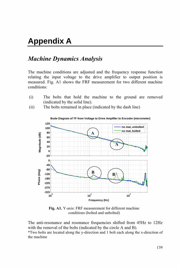
139
Appendix A Machine Dynamics Analysis The machine conditions are adjusted and the frequency response function relating the input voltage to the drive amplifier to output position is measured. Fig. A1 shows the FRF measurement for two different machine conditions: (i) The bolts that hold the machine to the ground are removed
(indicated by the solid line). (ii) The bolts remained in place (indicated by the dash line)
Bode Diagram of TF from Voltage to Drive Amplifier to Encoder (micrometer)
Frequency (Hz)
Phas
e (d
eg)
Mag
nitu
de (d
B)
-200
20406080
100120
100
101
102
-315-270-225-180-135
-90-45
0
no mat, unboltedno mat, bolted
Fig. A1. Y-axis: FRF measurement for different machine
conditions (bolted and unbolted) The anti-resonance and resonance frequencies shifted from 45Hz to 12Hz with the removal of the bolts (indicated by the circle A and B). *Two bolts are located along the y-direction and 1 bolt each along the x-direction of the machine
A
A
B B

140
Appendix B
Ferraris Acceleration Sensor Calibration This section describes the procedures and the results of the identification of the Ferraris relative acceleration sensor. The sensor gain sensitivity and offset values are determined. The Ferraris sensor is graphically shown in fig. B.1.
Fig B.1: Ferraris relative acceleration sensor Procedures
The milling table was excited with sinusoidal signals at selected frequencies between 0.2-100Hz.
Large gain was applied at lower frequencies (until 25Hz for
displacement of ~10mm) and the gain was reduced for higher frequencies excitation to avoid saturation effect.
The encoder measurement and the Ferraris sensor signals were
recorded using the dSPACE. Gain Sensitivity and Zero Offset Determination The calibrated relative acceleration signal, a(t) is defined as follow:
( ) ( ) ZGtmta +⋅= (B.1)
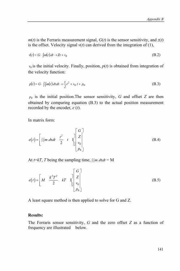
Appendix B
141
m(t) is the Ferraris measurement signal, G(t) is the sensor sensitivity, and z(t) is the offset. Velocity signal v(t) can derived from the integration of (1),
( ) ( ) 0vZtdt tmGtv ++⋅⋅= ∫ (B.2)
0v is the initial velocity. Finally, position, p(t) is obtained from integration of the velocity function:
( ) ( ) 002 pt vt
2zdtd tmGtp +++⋅τ⋅= ∫ ∫ (B.3)
0p is the initial position.The sensor sensitivity, G and offset Z are then obtained by comparing equation (B.3) to the actual position measurement recorded by the encoder, e (t).
In matrix form:
( )0
0
τ 12
2
GZte t m d dt tvp
∫ ∫
⎡ ⎤⎢ ⎥⎡ ⎤ ⎢ ⎥= ⎢ ⎥ ⎢ ⎥⎢ ⎥⎣ ⎦ ⎢ ⎥⎣ ⎦
(B.4)
At t=kT, T being the sampling time, τm d dt∫ ∫ = M
( )0
0
12
2 2
GZk Te t M kTvp
⎡ ⎤⎢ ⎥⎡ ⎤ ⎢ ⎥= ⎢ ⎥ ⎢ ⎥⎢ ⎥⎣ ⎦ ⎢ ⎥⎣ ⎦
(B.5)
A least square method is then applied to solve for G and Z.
Results:
The Ferraris sensor sensitivity, G and the zero offset Z as a function of frequency are illustrated below.
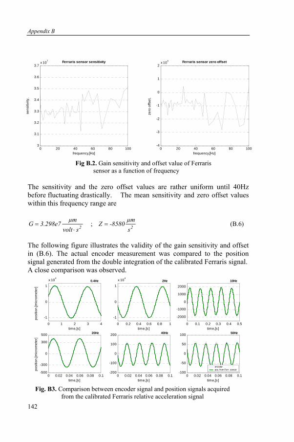
Appendix B
142
0 1 2 3 4
-1
0
1
x 104
time,[s]
posi
tion,
[mic
rom
eter
]
0 0.2 0.4 0.6 0.8 1
-1
0
1
x 104
time,[s]0 0.1 0.2 0.3 0.4 0.5
-2000
-1000
0
1000
2000
time,[s]
0 0.02 0.04 0.06 0.08 0.1-500
-300
0
300
500
time,[s]
posi
tion,
[mic
rom
eter
]
0 0.02 0.04 0.06 0.08 0.1-200
-100
0
100
200
time,[s]0 0.02 0.04 0.06 0.08 0.1
-100
-50
0
50
100
time,[s]
encoderpos. from Ferr. sensor
0.4Hz 2Hz 10Hz
20Hz 40Hz 50Hz
Fig B.2. Gain sensitivity and offset value of Ferraris sensor as a function of frequency
The sensitivity and the zero offset values are rather uniform until 40Hz before fluctuating drastically. The mean sensitivity and zero offset values within this frequency range are
2µmG 3.298e7
volt s=
⋅ ; 2
µmZ -8580s
= (B.6)
The following figure illustrates the validity of the gain sensitivity and offset in (B.6). The actual encoder measurement was compared to the position signal generated from the double integration of the calibrated Ferraris signal. A close comparison was observed.
Fig. B3. Comparison between encoder signal and position signals acquired from the calibrated Ferraris relative acceleration signal
0 20 40 60 80 1003
3.1
3.2
3.3
3.4
3.5
3.6
3.7x 10⁷
frequency,[Hz]
sens
itivi
ty,
Ferraris sensor sensitivity
0 20 40 60 80 100-4
-3
-2
-1
0
1
2x 10⁴
frequency,[Hz]ze
ro o
ffset
,
Ferraris sensor zero offset

143
Appendix C
Cutting Force Estimation from Ferraris Acceleration Sensor Measurement The state space representations of the system, including the measurement equation are:
( )⎥⎦⎤
⎢⎣
⎡
⎥⎥⎥⎥
⎦
⎤
⎢⎢⎢⎢
⎣
⎡
−+⎥⎥⎥
⎦
⎤
⎢⎢⎢
⎣
⎡
⎥⎥⎥
⎦
⎤
⎢⎢⎢
⎣
⎡=
⎥⎥⎥
⎦
⎤
⎢⎢⎢
⎣
⎡
vFu
MM
k
dvx
Mdvx
friction
f
00
100
000
/100010
&&
&
(C.1)
( )⎥⎦⎤
⎢⎣
⎡
⎥⎥
⎦
⎤
⎢⎢
⎣
⎡
−+
⎥⎥⎥
⎦
⎤
⎢⎢⎢
⎣
⎡
⎥⎦
⎤⎢⎣
⎡=⎥
⎦
⎤⎢⎣
⎡=
vFu
MM
k
dvx
Max
yfriction
f 100
/100001
(C.2)
Next, a reduced order observer is designed. Consider a general state equation of the form:
x Ax Buy Cx, C = E 0= +
= ⎡ ⎤⎣ ⎦
&
(C.3)
E is a unit matrix. A state of the system that contains a combination of the measured variable y and the non-measured state variable w are:
yx
w
⎡ ⎤= ⎢ ⎥⎢ ⎥⎣ ⎦
(C.4)
The system equation then becomes,
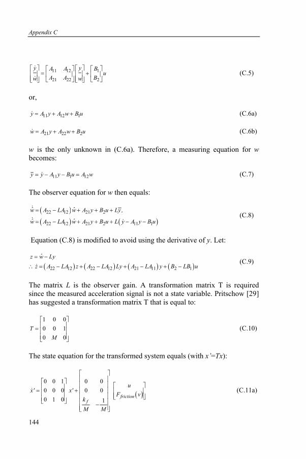
Appendix C
144
11 12 1
21 22 2
y yA A Bu
A A Bw w
⎡ ⎤ ⎡ ⎤⎡ ⎤ ⎡ ⎤= +⎢ ⎥ ⎢ ⎥⎢ ⎥ ⎢ ⎥
⎢ ⎥ ⎢ ⎥⎣ ⎦ ⎣ ⎦⎣ ⎦ ⎣ ⎦
&
& (C.5)
or,
11 12 1y A y A w B u= + +& (C.6a)
21 22 2w A y A w B u= + +& (C.6b)
w is the only unknown in (C.6a). Therefore, a measuring equation for w becomes:
11 1 12y y A y B u A w= − − =& (C.7)
The observer equation for w then equals:
( )( ) ( )
22 12 21 2
22 12 21 2 11 1
ˆ ˆw A LA w A y B u Ly ,
ˆ ˆw A LA w A y B u L y A y B u
= − + + +
= − + + + − −
&
& & (C.8)
Equation (C.8) is modified to avoid using the derivative of y. Let:
( ) ( ) ( ) ( )22 12 22 12 21 11 2 1
ˆz w Lyz A LA z A LA Ly A LA y B LB u= −
∴ = − + − + − + −& (C.9)
The matrix L is the observer gain. A transformation matrix T is required since the measured acceleration signal is not a state variable. Pritschow [29] has suggested a transformation matrix T that is equal to:
1 0 00 0 10 0
TM
⎡ ⎤⎢ ⎥= ⎢ ⎥⎢ ⎥⎣ ⎦
(C.10)
The state equation for the transformed system equals (with x’=Tx):
( )
0 0 1 0 00 0 0 0 00 1 0 1
frictionf
ux' x'
F vkM M
⎡ ⎤⎢ ⎥⎡ ⎤ ⎢ ⎥ ⎡ ⎤⎢ ⎥= + ⎢ ⎥ ⎢ ⎥⎢ ⎥ ⎢ ⎥⎢ ⎥ ⎣ ⎦⎢ ⎥⎣ ⎦ ⎢ ⎥−⎢ ⎥⎣ ⎦
& (C.11a)

Appendix D
145
( )⎥⎦⎤
⎢⎣
⎡
⎥⎥
⎦
⎤
⎢⎢
⎣
⎡
−+⎥
⎦
⎤⎢⎣
⎡=⎥
⎦
⎤⎢⎣
⎡=
vFu
MM
kxax
yfriction
f 100
' 010001
(C.11b)
By definition,
( )⎥⎥
⎦
⎤
⎢⎢
⎣
⎡
+−=⎥
⎦
⎤⎢⎣
⎡=−=⎥
⎦
⎤⎢⎣
⎡= vF
Mu
Mk
a
xxDuy
yy
yfriction
f 1' 010001
''
2
1 (C.12a)
and,
1
2
3
x 'x' x '
x '
⎡ ⎤⎢ ⎥= ⎢ ⎥⎢ ⎥⎣ ⎦
(C.12b)
The matrices A11, A12, A21, A22, B1, B2 (based on (B.11a) and the observer gain L for the designed of the reduced order observer of the transformed system are:
[ ] [ ]
[ ]0
;1 ;0000
;0 ;10 ;01
;0000
1
21
22211211
lL
MMk
BB
AAAA
f
=
⎥⎦
⎤⎢⎣
⎡−=⎥
⎦
⎤⎢⎣
⎡=
==⎥⎦
⎤⎢⎣
⎡=⎥
⎦
⎤⎢⎣
⎡=
(C.13)
Substituting (C.13) into the reduced order observer of equation (C.9) yields,
[ ] ( )⎥⎦⎤
⎢⎣
⎡
⎥⎥⎦
⎤
⎢⎢⎣
⎡−+⎥
⎦
⎤⎢⎣
⎡−+−=
vFu
MM
kyy
lzlzfriction
f 1''
1ˆ2
1211 &&
& (C.14a)
11 1 1
20
y 'ˆ ˆ ˆw z l z l y 'y '⎡ ⎤
= + = +⎡ ⎤ ⎢ ⎥⎣ ⎦⎣ ⎦
(C.14b)
1 13 3ˆ ˆ ˆ ˆy ' x, x w, x ' z l x= = ∴ = + (C.14c)
Based on y
x ,w
⎡ ⎤= ⎢ ⎥⎢ ⎥⎣ ⎦

Appendix C
146
1 1 11
2 2 22
3 1 1 1
0 1 00 0 11 0
x y ' y 'y 'ˆ ˆx y ' z y 'y 'ˆ ˆx w l z l y '
⎡ ⎤ ⎡ ⎤ ⎡ ⎤ ⎡ ⎤ ⎡ ⎤⎡ ⎤⎢ ⎥ ⎢ ⎥ ⎢ ⎥ ⎢ ⎥ ⎢ ⎥= = + =⎢ ⎥⎢ ⎥ ⎢ ⎥ ⎢ ⎥ ⎢ ⎥ ⎢ ⎥⎣ ⎦⎢ ⎥ ⎢ ⎥ ⎢ ⎥ ⎢ ⎥ ⎢ ⎥+⎣ ⎦ ⎣ ⎦ ⎣ ⎦ ⎣ ⎦⎣ ⎦
(C.15)
Equations (C.14a) and (C.15) can be simplified as follows:
1 2
1 2
ˆ ˆz A' z B ' y' B ' uˆ ˆx' D ' z D ' y'= + += +
& (C.16)
Next, re-transformation into original physical states are accomplished, using the transformation matrix T and by replacing y’ with y:
( )( )
1 2
1 2
ˆ ˆz A' z B ' y Du B ' uˆ ˆx T D ' z D ' y'
= + − +
= +
& (C.17)
or,
[ ] ( ) ( )⎥⎦⎤
⎢⎣
⎡⎥⎦
⎤⎢⎣
⎡−+
⎥⎥
⎦
⎤
⎢⎢
⎣
⎡
+−−+−=vF
uMM
kvF
Mu
Mk
a
xlzlz
friction
f
frictionf 11 1ˆ 2
11 &&& (C.18a)
( ) ⎥⎥⎥
⎦
⎤
⎢⎢⎢
⎣
⎡=
⎥⎥⎥⎥⎥⎥
⎦
⎤
⎢⎢⎢⎢⎢⎢
⎣
⎡
⎟⎟⎠
⎞⎜⎜⎝
⎛+−
+=⎥⎥⎥
⎦
⎤
⎢⎢⎢
⎣
⎡
⎥⎥⎥
⎦
⎤
⎢⎢⎢
⎣
⎡=
dvx
vFM
uM
kaM
xlzx
xxx
Mx
frictionf ˆ
ˆˆ
1ˆ
'''
00100001
ˆ 1
3
2
1 (C.18b)
Fig. C.1 shows the structure of this reduced order observer based on (C.16)
Fig. C.1. Schematic diagram of the cutting forces estimator
147
Appendix D
General State Force Observer Cutting forces contain harmonic components (as shown in Table 3.5 and 3.6) 3.4). A cutting force state observer estimates and compensates the cutting forces based on these harmonic frequencies. The fundamental frequency equals the frequency of the spindle speed (1360Hz).
Structure of a Disturbance Force Observer
Consider a sinusoidal disturbance force input d (t), its first derivative ( )d t& , and the second derivative ( )d t&& :
( ) ( )( ) ( )( ) ( )
1
1 22 2
2 1
ω θ
ω ω θ
ω ω θ ω
d t q A' sin t
d t q q A' cos t
d t q A' sin t q
= = +
= = = +
= = − + = −
& &
&& &
(D.1)
A’ is the amplitude of the sinusoidal signal, t is the time, ω and θ are the signal frequency and offset respectively. Equation D.1 shows that the second derivative of the reference disturbance force is directly proportional to the reference signal itself. A force disturbance observer can then be designed according to this observation. The following is the state space representation of a general order state observer:
( )ˆ ˆx Fx Gu L y yy Hx= + + −
=
& (D.2)
x is the state variable matrix, y is the output, and L is the observer gain matrix. Equation (D.2) is extended based on the system transfer function (2.2) for cutting force compensation of a single harmonic content.
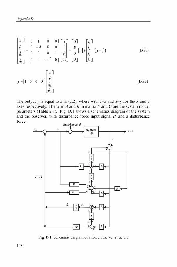
Appendix D
148
[ ] ( )1
2
1 312
2 42
0 1 0 0 00 00 0 0 1 0
00 0 ω 0
x x lˆ A B ˆv v lB ˆu y y
q lqq lq
⎡ ⎤ ⎡ ⎤ ⎡ ⎤ ⎡ ⎤⎡ ⎤⎢ ⎥ ⎢ ⎥ ⎢ ⎥ ⎢ ⎥⎢ ⎥−⎢ ⎥ ⎢ ⎥ ⎢ ⎥ ⎢ ⎥⎢ ⎥= + + −⎢ ⎥ ⎢ ⎥ ⎢ ⎥ ⎢ ⎥⎢ ⎥⎢ ⎥ ⎢ ⎥ ⎢ ⎥ ⎢ ⎥⎢ ⎥⎢ ⎥ −⎢ ⎥ ⎣ ⎦⎣ ⎦ ⎣ ⎦⎣ ⎦⎣ ⎦
&
&
&
&&
(D.3a)
[ ]1
2
1 0 0 0
xv
y qq
⎡ ⎤⎢ ⎥⎢ ⎥=⎢ ⎥⎢ ⎥⎣ ⎦
(D.3b)
The output y is equal to z in (2.2), where with z=x and z=y for the x and y axes respectively. The term A and B in matrix F and G are the system model parameters (Table 2.1). Fig. D.1 shows a schematics diagram of the system and the observer, with disturbance force input signal d, and a disturbance force.
Fig. D.1. Schematic diagram of a force observer structure
Appendix D
149
The fundamental equation (D.3) can be further extended to include other cutting forces harmonic contents. The following is an example of a disturbance force observer structure for compensation of cutting forces with three harmonics components:
( ) ( )( ) ( )( ) ( )
1 1 1 1 1
1 1 2 1 1 1 12 2
1 2 1 1 1 1 1 1
ω θ
ω ω θ
ω ω θ ω
d t q A ' sin t
d t q q A ' cos t
d t q A ' sin t q
= = +
= = = +
= = − + = −
& &
&& &
(D.4a)
( ) ( )( ) ( )( ) ( )
2 3 2 2 2
2 3 4 2 2 2 22 2
2 4 2 2 2 2 2 3
ω θ
ω ω θ
ω ω θ ω
d t q A ' sin t
d t q q A ' cos t
d t q A ' sin t q
= = +
= = = +
= = − + = −
& &
&& &
(D.4b)
( ) ( )( ) ( )( ) ( )
3 5 3 3 3
3 5 6 3 3 3 32 2
3 6 3 3 3 3 3 5
ω θ
ω ω θ
ω ω θ ω
d t q A ' sin t
d t q q A ' cos t
d t q A ' sin t q
= = +
= = = +
= = − + = −
& &
&& &
(D.4c)
The total forces equal:
1 2 3
1 3 5
total
total
or
d d d d
d q q q .
= + +
= + + (D.5)
The structure of this observer is an extension to the fundamental structure shown in fig. D.1. The disturbance observer design is based on the selection of the design parameters, that is, the observer gains l1, l2, l3, l4. Large LHP poles results in faster response but with reduced stability margin while small LHP poles have slower response but better stability margin.
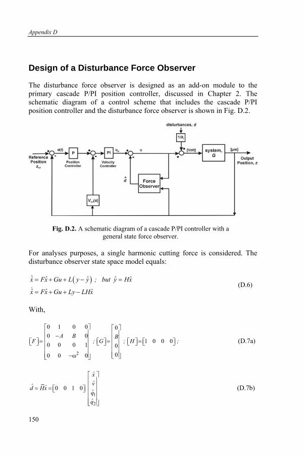
Appendix D
150
Design of a Disturbance Force Observer
The disturbance force observer is designed as an add-on module to the primary cascade P/PI position controller, discussed in Chapter 2. The schematic diagram of a control scheme that includes the cascade P/PI position controller and the disturbance force observer is shown in Fig. D.2.
Fig. D.2. A schematic diagram of a cascade P/PI controller with a general state force observer.
For analyses purposes, a single harmonic cutting force is considered. The disturbance observer state space model equals:
( )ˆ ˆ ˆ ˆ ˆx Fx Gu L y y ; but y Hx
ˆ ˆ ˆx Fx Gu Ly LHx
= + + − =
= + + −
&
& (D.6)
With,
2
0 1 0 0 00 0
1 0 0 00 0 0 1 000 0 ω 0
A B BF ; G ; H ;
⎡ ⎤ ⎡ ⎤⎢ ⎥ ⎢ ⎥−⎢ ⎥ ⎢ ⎥= = =⎡ ⎤ ⎡ ⎤ ⎡ ⎤ ⎡ ⎤⎣ ⎦ ⎣ ⎦ ⎣ ⎦ ⎣ ⎦⎢ ⎥ ⎢ ⎥⎢ ⎥ ⎢ ⎥
⎢ ⎥⎢ ⎥− ⎣ ⎦⎣ ⎦
(D.7a)
1
2
0 0 1 0
xvˆ ˆd Hx qq
⎡ ⎤⎢ ⎥⎢ ⎥= = ⎡ ⎤⎣ ⎦ ⎢ ⎥⎢ ⎥⎢ ⎥⎣ ⎦
(D.7b)

Appendix D
151
Taking the Laplace Transform,
( ) ( ) ( ) ( ) ( )ˆ ˆ ˆsX s FX s GU s LY s LHX s= + + − (D.8)
However,
( ) ( ) ( )( ) ( )
PI
ref est
ˆU s U s HX sˆU s P PI Z Y PI V Y HX
= −
= ⋅ − − ⋅ ⋅ − (D.9)
Substituting (D.9) into (D.8),
( ) ( ) ( )( ) ( ) ( )ref estˆ ˆ ˆ ˆsX s FX s G P PI Z Y PI V Y HX LY s LHX s= + ⋅ − − ⋅ ⋅ − + − (D.10)
( ) ( ) ( ) ( )estref
L G P PI G PI VG P PIX s Z s Y ssI F GH LH sI F GH LH
− ⋅ ⋅ − ⋅ ⋅⋅ ⋅= +
− + + − + + (D.11)
Also, (let the system be Gsys)
( ) ( )sysY s G U D= + (D.12)
( ) ( )( )sys ref estˆY s G P PI Z Y PI V Y HX D= ⋅ − − ⋅ ⋅ − + (D.13)
Substituting (D.11) into (D.13) and with further simplification,
( ) ( )
( )
1
1
syssys
refest
sys sys est sys
p
estsys sys est sys
G H GP PIG PPI
sI F GH LHY s Z sL GPPI G PI VG PPI G PI V G H
sI F GH LHG
D sL G P PI G PI VG PPI G PI V G HsI F GH LH
⎛ ⎞⋅ ⋅⎜ ⎟⋅ −⎜ ⎟− + +⎝ ⎠=
− − ⋅ ⋅+ + ⋅ +
− + +
+− ⋅ ⋅ − ⋅ ⋅
+ + ⋅ +− + +
(D.14)
The sensitivity function, S(s) equals:
( ) 1
1 estsys sys est sys
S s L G P PI G PI VG P PI G PI V G HsI F GH LH
=− ⋅ ⋅ − ⋅ ⋅
+ ⋅ + ⋅ +− + +
(D.15)
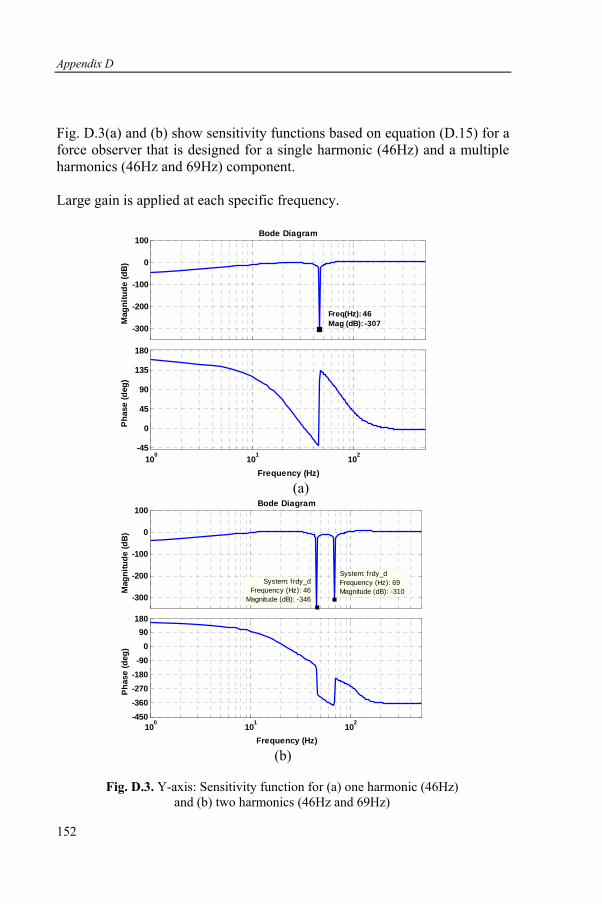
Appendix D
152
Fig. D.3(a) and (b) show sensitivity functions based on equation (D.15) for a force observer that is designed for a single harmonic (46Hz) and a multiple harmonics (46Hz and 69Hz) component. Large gain is applied at each specific frequency.
Bode Diagram
Frequency (Hz)
Phas
e (d
eg)
Mag
nitu
de (d
B)
100 101 102-45
0
45
90
135
180
-300
-200
-100
0
100
Freq(Hz): 46 Mag (dB): -307
(a)
Bode Diagram
Frequency (Hz)
Phas
e (d
eg)
Mag
nitu
de (d
B)
100 101 102-450-360-270-180-90
090
180
-300
-200
-100
0
100
System: frdy_d Frequency (Hz): 46
Magnitude (dB): -346
System: frdy_d Frequency (Hz): 69 Magnitude (dB): -310
(b)
Fig. D.3. Y-axis: Sensitivity function for (a) one harmonic (46Hz)
and (b) two harmonics (46Hz and 69Hz)

Appendix D
153
Next, the transfer function (D.14) and (D.15) are validated numerically using MATLAB/Simulink based on the control scheme in fig. D.2. Fig. D.4(a) shows the simulated position error for sinusoidal disturbance signal at 23Hz. Fig. D.4(b) shows the estimated position error obtained using the sensitivity function (D.15).
2 2.02 2.04 2.06 2.08 2.1-1000
-782
0
782
1000
time,[s]
posi
tion
erro
r, [µ
m]
(a)
Bode Magnitude Diagram
Frequency (Hz)
Posi
tion
erro
r (ab
s)[µ
m]
100
101
102
10-20
10-15
10-10
10-5
100
105
Freq (Hz): 23
Mag (abs): 783
(b)
Fig. D.4. Y-axis: (a) Simulated position error and (b) estimated position error for force observer designed for 46Hz and 69Hz
harmonics
An exact match between the simulated position error and the estimated position error are observed.. This confirms the transfer functions (D.14) and (D.15).
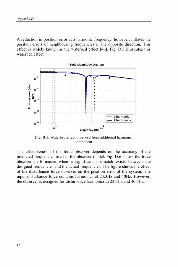
Appendix D
154
A reduction in position error at a harmonic frequency, however, inflates the position errors of neighbouring frequencies in the opposite direction. This effect is widely known as the waterbed effect [46]. Fig. D.5 illustrates this waterbed effect.
Bode Magnitude Diagram
Frequency (Hz)
Posi
tion
erro
r (ab
s)[µ
m]
101
102
10-20
10-15
10-10
10-5
100
1 harmonic2 harmonics
Fig. D.5. Waterbed effect observed from additional harmonic
component The effectiveness of the force observer depends on the accuracy of the predicted frequencies used in the observer model. Fig. D.6 shows the force observer performance when a significant mismatch exists between the designed frequencies and the actual frequencies. The figure shows the effect of the disturbance force observer on the position error of the system. The input disturbance force contains harmonics at 23.3Hz and 40Hz. However, the observer is designed for disturbance harmonics at 23.3Hz and 46.6Hz.
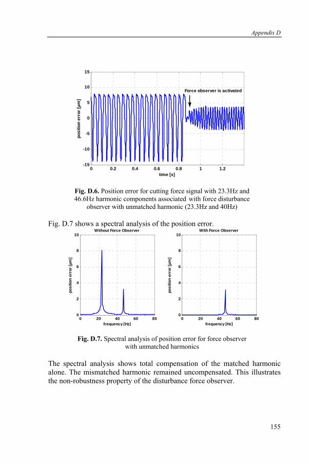
Appendix D
155
0 0.2 0.4 0.6 0.8 1 1.2-15
-10
-5
0
5
10
15
time [s]
posi
tion
erro
r [µm
]
Force observer is activated
Fig. D.6. Position error for cutting force signal with 23.3Hz and 46.6Hz harmonic components associated with force disturbance
observer with unmatched harmonic (23.3Hz and 40Hz) Fig. D.7 shows a spectral analysis of the position error.
0 20 40 60 800
2
4
6
8
10Without Force Observer
frequency [Hz]
posi
tion
erro
r [µm
]
0 20 40 60 800
2
4
6
8
10With Force Observer
frequency [Hz]
posi
tion
erro
r [µm
]
Fig. D.7. Spectral analysis of position error for force observer with unmatched harmonics
The spectral analysis shows total compensation of the matched harmonic alone. The mismatched harmonic remained uncompensated. This illustrates the non-robustness property of the disturbance force observer.
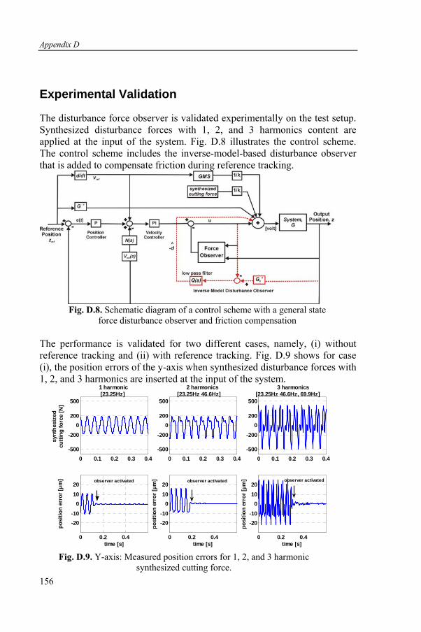
Appendix D
156
Experimental Validation
The disturbance force observer is validated experimentally on the test setup. Synthesized disturbance forces with 1, 2, and 3 harmonics content are applied at the input of the system. Fig. D.8 illustrates the control scheme. The control scheme includes the inverse-model-based disturbance observer that is added to compensate friction during reference tracking.
Fig. D.8. Schematic diagram of a control scheme with a general state
force disturbance observer and friction compensation The performance is validated for two different cases, namely, (i) without reference tracking and (ii) with reference tracking. Fig. D.9 shows for case (i), the position errors of the y-axis when synthesized disturbance forces with 1, 2, and 3 harmonics are inserted at the input of the system.
0 0.2 0.4
-20-10
010
20
time [s]
posi
tion
erro
r [µm
]
0 0.1 0.2 0.3 0.4-500
-200
0200
500
sy
nthe
size
d
cu
tting
forc
e [N
]
0 0.2 0.4
-20-10
010
20
time [s]
posi
tion
erro
r [µm
]
0 0.1 0.2 0.3 0.4-500
-200
0200
500
0 0.2 0.4
-20-10
010
20
time [s]
posi
tion
erro
r [µm
]
0 0.1 0.2 0.3 0.4-500
-200
0200
500
1 harmonic [23.25Hz]
2 harmonics [23.25Hz 46.6Hz]
3 harmonics [23.25Hz 46.6Hz, 69.9Hz]
observer activated observer activated observer activated
Fig. D.9. Y-axis: Measured position errors for 1, 2, and 3 harmonic
synthesized cutting force.

Appendix D
157
The above results indicate a complete removal of the cutting forces influence on the position errors. Fig. D.10 shows the compensation results during reference tracking.
0 0.5 1 1.5-4
-2
0
2
4x 10⁴
refe
renc
e [µ
m]
1 harmonic
time [s]
0 0.5 1 1.5-20
-10
0
10
20
time [s]
posi
tion
erro
r [µm
]
n
o ob
serv
er
0 0.5 1 1.5
-10
0
10
time [s]
posi
tion
erro
r [µm
]
with
obs
erve
r
0 0.5 1 1.5-4
-2
0
2
4x 10⁴ 3 harmonics
time [s]
refe
renc
e [µ
m]
0 0.5 1 1.5-20
-10
0
10
20
posi
tion
erro
r [µm
]
n
o ob
serv
er
0 0.5 1 1.5
-10
0
10
time [s]
posi
tion
erro
r [µm
]
w
ith o
bser
ver
rms = 0.66µm
rms = 7.12µm
rms = 3.90µm
rms =3.1µm
Fig. D.10. Y-axis: Measured tracking errors for synthesized cutting
force with 1 (left) and 3 (right) harmonics. Fig. D.11 shows the spectral content of the tracking errors.
0 20 40 60 80 1000
2
4
6
8
101 harmonic
frequency [hz]
posi
tion
erro
r [µm
]
n
o ob
serv
er
0 20 40 60 80 1000
2
4
6
8
10
frequency [hz]
posi
tion
erro
r [µm
]
no
obs
erve
r
3 harmonics
0 20 40 60 80 1000
2
4
6
8
10
frequency [hz]
posi
tion
erro
r [µm
]
with
obs
erve
r
0 20 40 60 80 1000
2
4
6
8
10
frequency [hz]
posi
tion
erro
r [µm
]
with
obs
erve
r
Fig. D.11. Spectral analysis of the tracking error for synthesized
cutting force with 1 harmonic (left) and 3 harmonics (right).
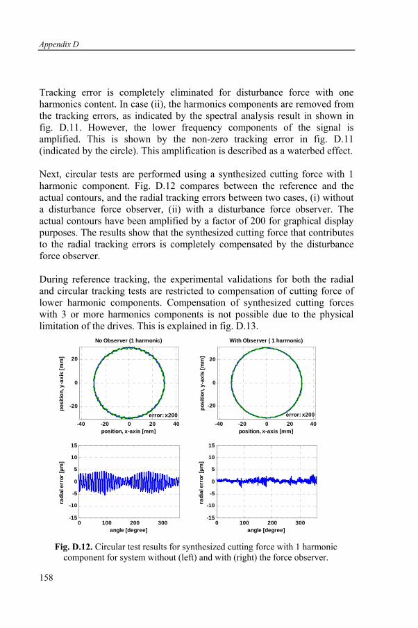
Appendix D
158
Tracking error is completely eliminated for disturbance force with one harmonics content. In case (ii), the harmonics components are removed from the tracking errors, as indicated by the spectral analysis result in shown in fig. D.11. However, the lower frequency components of the signal is amplified. This is shown by the non-zero tracking error in fig. D.11 (indicated by the circle). This amplification is described as a waterbed effect. Next, circular tests are performed using a synthesized cutting force with 1 harmonic component. Fig. D.12 compares between the reference and the actual contours, and the radial tracking errors between two cases, (i) without a disturbance force observer, (ii) with a disturbance force observer. The actual contours have been amplified by a factor of 200 for graphical display purposes. The results show that the synthesized cutting force that contributes to the radial tracking errors is completely compensated by the disturbance force observer. During reference tracking, the experimental validations for both the radial and circular tracking tests are restricted to compensation of cutting force of lower harmonic components. Compensation of synthesized cutting forces with 3 or more harmonics components is not possible due to the physical limitation of the drives. This is explained in fig. D.13.
-40 -20 0 20 40
-20
0
20
No Observer (1 harmonic)
position, x-axis [mm]
posi
tion,
y-a
xis
[mm
]
0 100 200 300-15
-10
-5
0
5
10
15
angle [degree]
radi
al e
rror
[µm
]
-40 -20 0 20 40
-20
0
20
With Observer ( 1 harmonic)
position, x-axis [mm]
posi
tion,
y-a
xis
[mm
]
0 100 200 300-15
-10
-5
0
5
10
15
angle [degree]
radi
al e
rror
[µm
]
error: x200 error: x200
Fig. D.12. Circular test results for synthesized cutting force with 1 harmonic
component for system without (left) and with (right) the force observer.
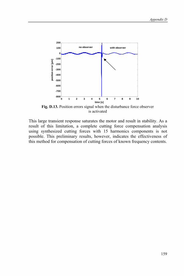
Appendix D
159
0 1 2 3 4 5 6 7 8 9 10-800
-700
-600
-500
-400
-300
-200
-100
0
100
200
posi
tion
erro
r [µm
]
time [s]
no observer with observer
Fig. D.13. Position errors signal when the disturbance force observer
is activated
This large transient response saturates the motor and result in stability. As a result of this limitation, a complete cutting force compensation analysis using synthesized cutting forces with 15 harmonics components is not possible. This preliminary results, however, indicates the effectiveness of this method for compensation of cutting forces of known frequency contents.