A LEARNED PERFORMANCE MODEL FOR TENSOR PROCESSING UNITS

Samuel J. Kaufman 1 2 * Phitchaya Mangpo Phothilimthana 1 * Yanqi Zhou 1 Charith Mendis 1 Sudip Roy 1

Amit Sabne 1 Mike Burrows 1

ABSTRACTAccurate hardware performance models are critical to efficient code generation. They can be used by compilersto make heuristic decisions, by superoptimizers as a minimization objective, or by autotuners to find an optimalconfiguration for a specific program. However, they are difficult to develop because contemporary processorsare complex, and the recent proliferation of deep learning accelerators has increased the development burden.We demonstrate a method of learning performance models from a corpus of tensor computation graph programsfor Tensor Processing Unit (TPU) instances. We show that our learned model outperforms a heavily-optimizedanalytical performance model on two tasks—tile-size selection and operator fusion—and that it helps an autotunerdiscover faster programs in a setting where access to TPUs is limited or expensive.

1 INTRODUCTION

Compilers often rely on performance models for solvingoptimization problems because collecting performance mea-surements from a real machine can be expensive, limited byhardware availability, or infeasible (such as during ahead-of-time compilation). For example, LLVM’s loop vectorizeruses a performance model to compute the optimal vectoriza-tion and unroll factors (LLVM), and GCC uses a model todecide when to apply loop-peeling, loop-versioning, outer-loop vectorization, and intra-iteration vectorization (GCC,2019). In addition, a performance model can be used bya compiler autotuner to evaluate candidate configurationsin a search space (Chen et al., 2018; Adams et al., 2019;Narayanan et al., 2019; Jia et al., 2020).

Developing an accurate analytical model of program per-formance on a modern processor is challenging and cantake months of engineering effort. Program performance istightly coupled with the underlying processor architectureas well as the optimization decisions that are made duringcompilation (Berry et al., 2006). Developers of analyticalmodels are often unaware of detailed features of the pro-cessor or effects from all compiler passes. Furthermore,architectural features and the underlying compiler code gen-eration interact in extremely complex ways; manually im-plementing these interactions and their effects on program

*Equal contribution 1Google, Mountain View, CA 2PaulG. Allen School of Computer Science & Engineering, Univer-sity of Washington, Seattle, WA. Correspondence to: Samuel J.Kaufman <kaufmans@cs.washington.edu>, Phitchaya MangpoPhothilimthana <mangpo@google.com>.

Proceedings of the 4 th MLSys Conference, San Jose, CA, USA,2021. Copyright 2021 by the author(s).

performance is tedious and error-prone. The recent prolif-eration of deep learning accelerators has only exacerbatedthis problem by demanding rapid, repeated development ofperformance models targeting new accelerators.

This paper addresses these problems by applying ma-chine learning techniques to produce a performance model.In particular, we are interested in learning a model forpredicting execution time of tensor programs on TPUs,which are widely-used accelerators for deep learning work-loads (Jouppi et al., 2017; 2020). We aim to develop alearned approach to performance modeling that satisfiesthe following key criteria for the ease of development anddeployment. First, the approach must be general enoughto handle non-trivial constructs in tensor programs (e.g.,multi-level loop nests common in programs involving high-dimensional tensors). Second, it must generalize acrossprograms of different application domains as well as to pro-grams unseen at training time. Third, it should not rely onwell-crafted features that require significant domain exper-tise and effort to develop and tune. Finally, the approachshould be retargetable to different optimization tasks withminimal effort.

While there has been some prior work (Adams et al.,2019; Chen et al., 2018; Mendis et al., 2019a) proposinglearned approaches to performance modeling, to the bestof our knowledge, none of them satisfy the four criteriastated above. For instance, Ithemal (Mendis et al., 2019a)does not handle complex multi-level loop nests. WhileHalide’s learned performance model can handle tensor pro-grams (Adams et al., 2019), it requires heavy feature en-gineering. Although AutoTVM’s models do not rely en-tirely on manually-engineered features (Chen et al., 2018),

arX

iv:2

008.

0104

0v2

[cs

.PF]

18

Mar

202

1

A Learned Performance Model for Tensor Processing Units

Configs for Various Optimizations:- data/model parallelism- layout assignment- operator fusion- remateralization- memory assignment- tiling etc.

Compiler Autotuner

input program

config cost

best config

exe

Evaluator

ML Compiler

Hardware

ML Compiler

Learned Cost Model

IROR

Various Search Strategies:random, genetic,simulated annealing, MCMC, MCTS, RL, etc.

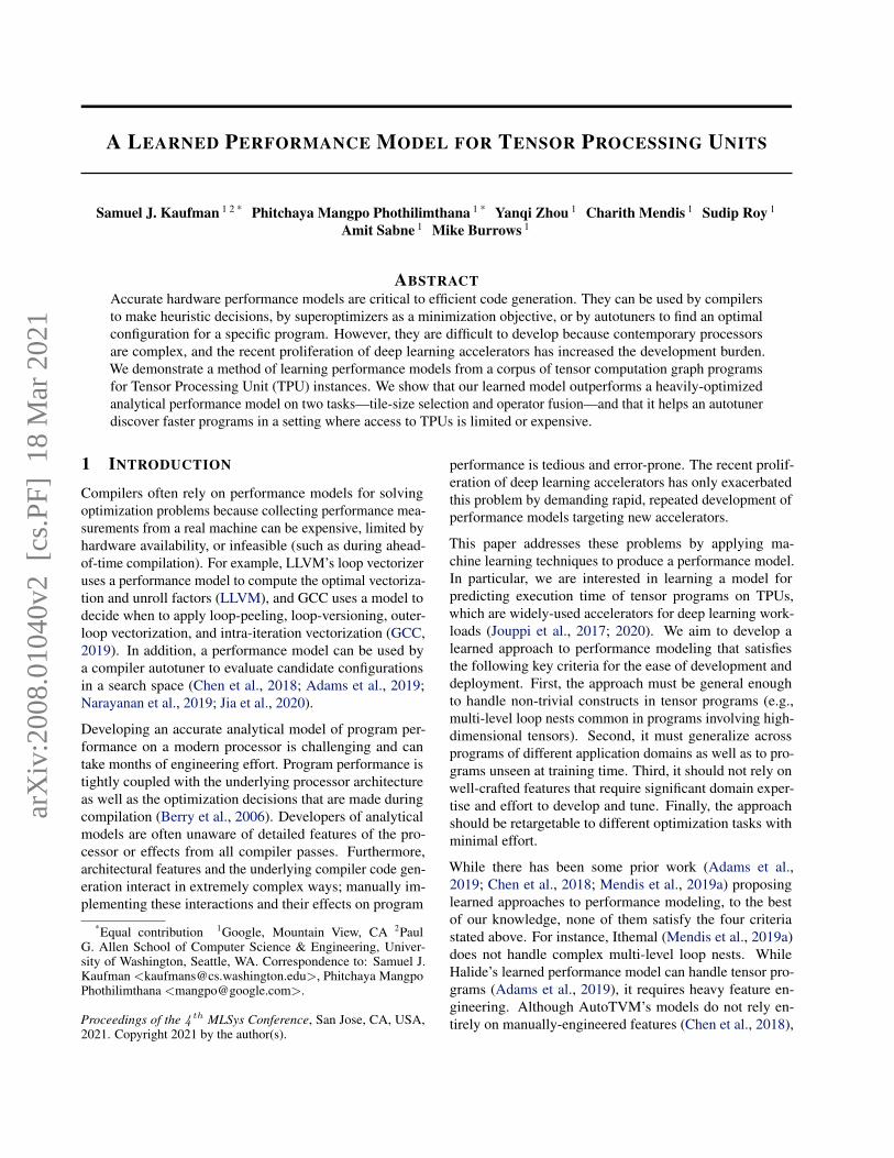
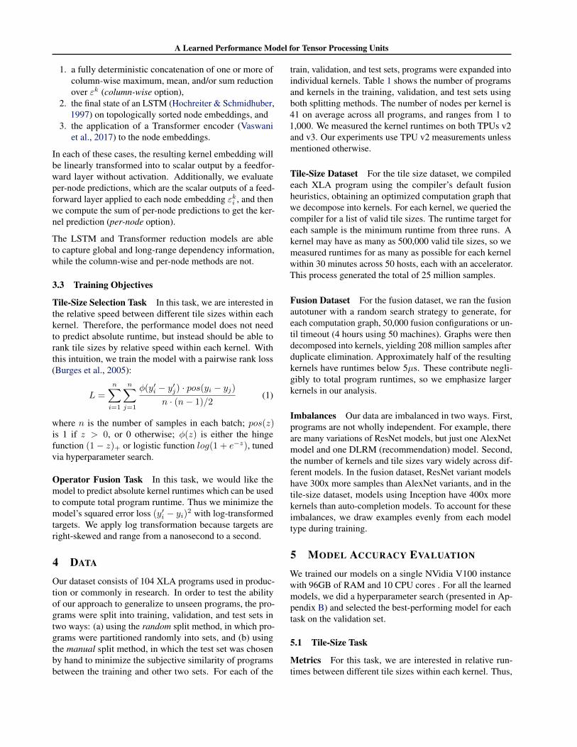
Figure 1. A compiler autotuner typically relies on real hardware to evaluate theperformance of generated code. We propose a learned performance model as acheaper alternative to obtain reward signals.

conv

param.2param.1 param.3

mult

broadcast

param.1

exp

reduce

reshape

kernel 1 kernel 2

kernel 3output

output

output

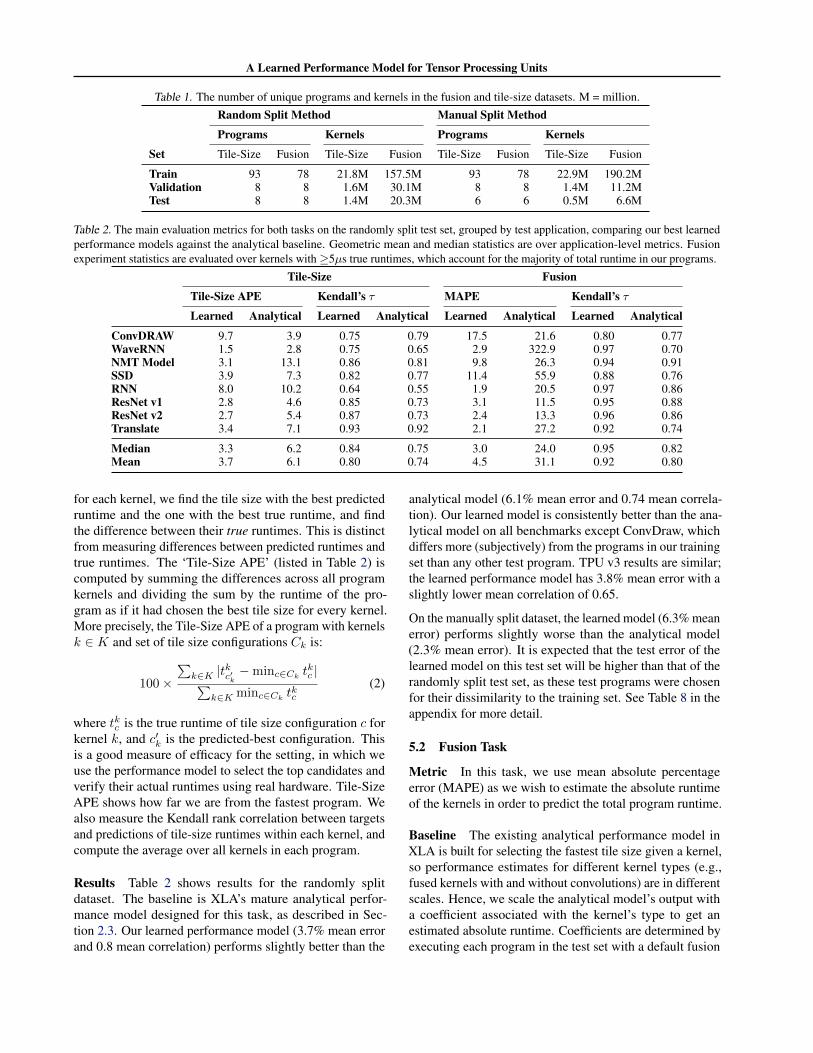
Figure 2. An optimized tensor computation graphconsists of multiple kernels (gray blobs). Each ker-nel in turn contains a graph of nodes correspondingto primitive operations.

it shows limited ability to generalize across kernels.

Like prior work, we formulate the runtime estimation prob-lem as a regression task. However, we make specific archi-tectural choices to satisfy the desiderata. First, our approachrepresents tensor programs as data flow graphs with nodesthat represent operations and edges that represent tensorflows between nodes. Second, we use a graph-based neu-ral network optionally coupled with a sequence model; thegraph model ensures generalizability across different pro-grams, while the sequence model is used to capture longrange dependencies within a graph. Third, we directly en-code operation properties to generate a feature vector for anode in the graph. While our approach does not require anyprogram analyses, adding manually engineered features asadditional features is trivial. Our approach is retargetable todifferent tensor graph optimization tasks. We evaluate ourperformance model on its ability to predict runtimes for twotasks: tile-size selection and operator fusion. The model isapplied to evaluate program configurations generated by anautotuner for the Accelerated Linear Algebra (XLA) com-piler (TensorFlow) as depicted in Fig. 1.

In summary, we make the following contributions:• We develop a learned performance model for tensor

programs that does not require feature engineering,generalizes to unseen programs, and is retargetable fordifferent compiler optimization tasks.

• We show that our learned models achieve 96.3% and95.5% accuracy with respect to true measurements; and2.4% and 26.6% better accuracy than the best hand-tuned model for tile-size and fusion tasks, respectively.

• We conduct a comprehensive set of ablation studiesover modeling choices.

• We integrate our learned performance model into anXLA autotuner, and demonstrate that it helps in discov-ering faster programs when access to real hardware islimited or expensive, which is often true in practice.

2 TARGET HARDWARE AND TASKS

Our approach to learning a performance model is applicableto any target processor executing tensor programs. A tensorprogram can be represented as a computation graph, whichis acyclic and directed. A node in a computation graphrepresents a tensor operation, processing one or more inputtensors into a single output, and an edge connects an outputtensor from one node to an input tensor of another node.

To evaluate our method, we build a learned model to pre-dict runtimes of XLA programs on a TPU. XLA is a ma-chine learning compiler for multiple hardware targets, andis used by various machine learning programming frame-works. XLA first performs high-level optimizations at thewhole-program level. During this stage, some nodes (primi-tive operations) in the original computation graph may bemerged into a fused node, called a kernel, as illustrated inFig. 2. After that, XLA lowers each kernel into a low-levelrepresentation, which is then further optimized and com-piled to machine code. In this paper, we evaluate on twooptimization tasks: tile-size selection (a kernel-level opti-mization applied during lowering) and operator fusion (aprogram-level optimization).

2.1 Tensor Processing Unit

Tensor Processing Units (Jouppi et al., 2020) are fast,energy-efficient machine learning accelerators. Theyachieve high performance by employing systolic array-based matrix multiplication units. The architecture incor-porates a vector processing unit, a VLIW instruction set,2D vector registers, and a transpose reduction permute unit.Programs can access the High Bandwidth Memory (HBM)or the faster but smaller on-chip scratchpad memory that issoftware-managed. While a TPU has no out-of-order execu-tion, it relies heavily on instruction-level parallelism—doneby the compiler backend across several passes includingcritical path scheduling and register allocation—making it

A Learned Performance Model for Tensor Processing Units

challenging for performance modeling. TPUs do not supportmulti-threading; one kernel is executed at a time.

The design of a TPU allows us to compute the runtime of anentire program by summing the runtimes of its kernel execu-tions. We expect our approach to work best for targets wherethe runtime of one kernel is independent of others (e.g., nooverlapping kernel executions and no inter-kernel caching).For example, prior work has shown that this approach issufficiently accurate for autotuning graph rewrites (Jia et al.,2019a) and parallelization configurations (Jia et al., 2019b;Narayanan et al., 2019) on GPUs.

We evaluate our approach on TPUs v2 and v3 to demonstrateits generalizability across different generations of hardware.TPU v3 has higher memory bandwidth and twice as manymatrix multiplier units compared to TPU v2.

2.2 Optimization Tasks

Tile-Size Selection To generate efficient code, XLA uti-lizes the fast scratchpad to store data. Because of the limitedscratchpad memory, a kernel cannot consume its whole in-put or compute its entire output at once. Instead, it computesone piece of its output at a time from one or more piecesof its inputs. These pieces are called tiles. An output tile iscopied to the slower HBM before the next tile is computed.The goal of tile-size selection is to choose a tile size thatminimizes kernel runtime.

Operator Fusion Operator fusion merges multiple opera-tions into a single unit. Before this pass, a node in a compu-tation graph is a primitive tensor operation (e.g., convolu-tion, element-wise add, etc.). When producer and consumernodes are fused, intermediate data is stored in scratchpadmemory, without transferring it to/from HBM, thereby re-ducing data communication. After the fusion pass, a nodein a computation graph is either a single primitive operationor a fused operation with many primitive operations.

2.3 Existing Analytical Model

For tile-size selection, XLA enumerates all possible tilesizes and selects the best according to a heavily hand-tunedanalytical performance model. This model estimates thekernel’s data transfer time and computation time, and takesthe maximum of the two. Tile-size selection happens priorto the code generation, so the model relies on several heuris-tics that may cause inaccuracy. While the model works wellin practice, the approach has the following demerits: (a) thelack of some execution behaviors due to poorly understoodarchitectural characteristics implies missed opportunities;(b) changes in the code generation result in a constant needto update the heuristics; and (c) each new hardware genera-tion requires not only tuning of existing heuristics but alsoadditional modeling. Details can be found in Appendix A.

Unlike tile-size selection, XLA does not use a precise per-formance model for the fusion task. Instead, it relies onestimates of whether including each node into a fused groupwill save memory space and access time. It then prioritizefusion decisions according to these estimates.

2.4 Autotuning

Instead of relying on the compiler’s heuristics and analyticalperformance model, an XLA autotuner has been developedto search for the fastest tile size for each kernel, and thefastest fusion configuration of each XLA program. Theautotuner found up to 25% speedup over the compiler’s de-fault on some production deep learning models. However,the autotuning process involves exhaustively running eachkernel with all valid tile sizes (ranging from 2 to 500,000options) and exploration in an exponentially large space ofup to 240,000 fusion configurations per each program. Thisrequires many evaluations, where each evaluation is slowdue to the time spent in compilation and execution. An ac-curate performance model can provide a cheap and reliableestimate of the runtime, and can significantly reduce thetime and resource requirements of the autotuning process.

3 MODEL DESIGN

Our approach decomposes an XLA program into smallercomputation subgraphs (kernels) whose runtimes are pre-dicted with a neural network. The estimated program run-time is the sum of its kernel runtimes. Predicting kernelruntimes instead of the whole program’s runtime has multi-ple benefits. First, this decomposition is general enough thatwe can apply the neural network model to various tasks, in-cluding both program- and kernel-level optimizations. Sec-ond, predicting runtime at a low-level representation shouldbe more accurate as the model does not have to capturewhat happens inside the high-level compiler. Additionally,kernels are smaller than whole programs, simplifying themodel’s domain. The rest of this section focuses on the threemain components for predicting a kernel runtime: modelinputs, model architecture, and training objectives.

3.1 Model Inputs

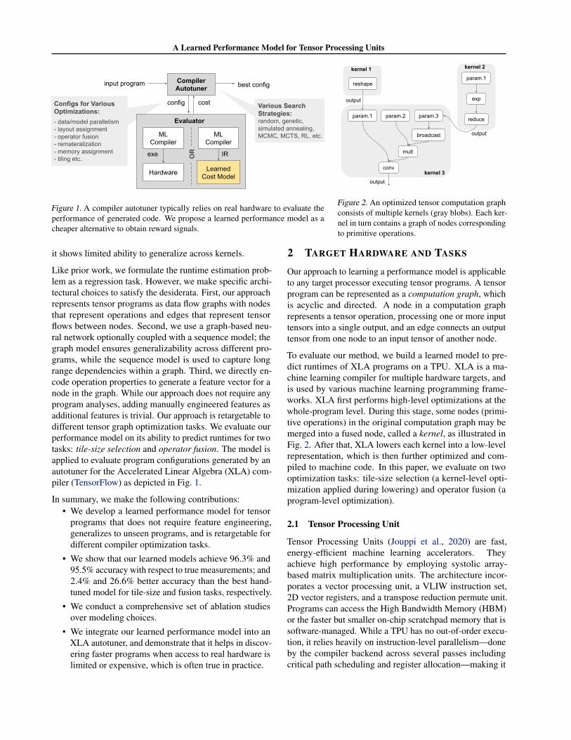
A model input is a kernel represented as node features,whole-kernel features, and an adjacency matrix (highlightedyellow, red, and blue respectively in Fig. 3). Node featuresinclude the integer-valued type of the operation (opcode),as well as scalar features which further describe the node’sbehavior, such as output tensor shape, tensor layout, strid-ing, padding, and when applicable, convolution filter size.1

1Integers are cast to reals. Features are independently scaled tobe in the range [0, 1] using the minimum and maximum observedin the training set.

A Learned Performance Model for Tensor Processing Units

*11

HPEHG�RSFRGH

RSFRGHLGV

RSFRGH�HPEHGGLQJV

NHUQHO�IHDWXUHV�RSWLRQ���

QRGH�IHDWXUHV

UHSHDW

NHUQHO�IHDWXUHV�RSWLRQ���

QRGH�HPEHGGLQJV

__

__

UHGXFWLRQ��

IHHGIRUZDUG

NHUQHO�HPEHGGLQJV

UXQWLPH�SUHGLFWLRQ

__

DGMDFHQF\�PDWUL[

3OHDVH�NHHS�UHG��EOXH��\HOORZ�FRORUV�DV�ZH�UHIHU�WR�WKHP�LQ�WKH�SDSHU�

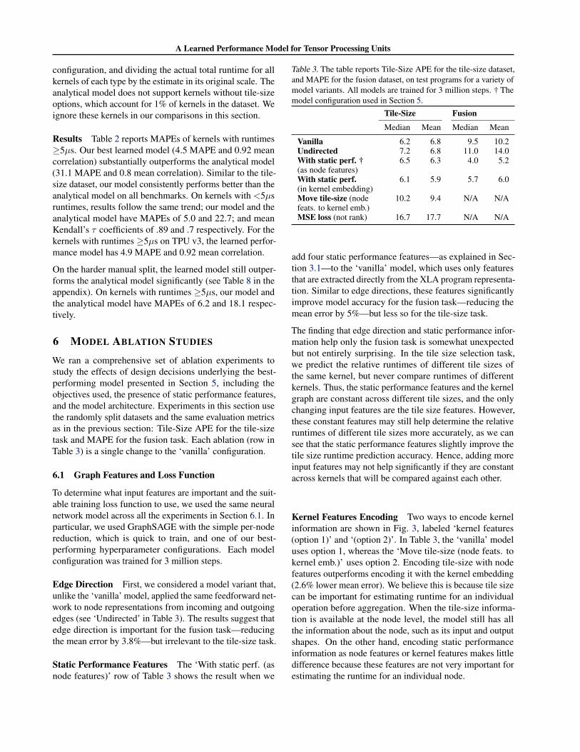
Figure 3. Overview of our model. Model inputs are an adjacencymatrix representing graph structure (red), node information (blue),and kernel information (yellow). Kernel features can be fed intothe model in two ways: (1) appending to the node features or (2)appending to kernel embedding.

Kernel’s inputs are expressed by nodes with the parame-ter opcode, and outputs are expressed via an extra featureassociated with the output nodes. Kernel features includetile size (only for the tile-size selection task) and optionalstatic performance information. The adjacency matrix cap-tures data-flow dependencies between nodes in the kernel,as shown in Fig. 2.

Optional Static Performance Features The XLA com-piler has static analyses that determine high-level perfor-mance metrics of a given kernel. In addition to the featuresextracted directly from the program representation, we con-sider providing information from these analyses as addi-tional inputs to the model. These features are optional, butmay improve the model’s accuracy. We consider four suchkernel features: (1) number of floating point operations,(2) amount of data read in bytes, (3) amount of data beingwritten in bytes, and (4) number of instructions executingon a special functional unit. These are estimates becausethe static analyses do not precisely model the compiler’sbackend code generation. The static performance featuresof the same kernel with different tile-sizes are the same.

Variable-Sized Features Many node and kernel featuresare naturally interpreted as variable-length lists of numbers.This is because tensors are n-dimensional arrays and somefeatures describe individual tensor dimensions. For example,tile size is encoded as a vector of length n, in which eachcomponent corresponds to a tensor dimension. We encodethese features as fixed-size sub-vectors, padded or truncatedas necessary. Additionally, we include the sum and product

of all the values. Including the product is critical as itusually represents the volume of a tensor, and can be morepredictive in cases where the sub-feature has been truncatedand so the product could not be recovered by the model.

3.2 Model Architecture

Figure 3 depicts the architecture of our model. We applya Graph Neural Network (GNN) to capture local structuralinformation and then apply a reduction over node embed-dings to generate a kernel embedding, which is in turn usedto predict the final runtime. We explore different choicesfor the reduction, including sequence and attention modelsthat can capture global graph information.

Node and Kernel Features The opcode xoi of an oper-ation is categorical, so we follow best practices and mapit to a vector of parameters called an opcode embedding.Opcode embeddings are concatenated with node featuresbefore being passed, along with the adjacency matrix, to aGNN. Kernel features are duplicated and concatenated withnode feature vectors (‘option 1’ in Fig. 3).

Node Embedding We use a GNN to combine informationfrom the node and its neighbors to generate a node repre-sentation. We use a GNN because (i) a tensor computationkernel is naturally represented as a graph, and (ii) learningnode representations conditioned only on their own featuresand local neighborhoods has shown to improve generaliza-tion in other settings. We believe that local neighborhoodscapture information that is important for estimating runtime.For a example, node features include an output tensor shapebut not input tensors’ shape because operations can havevariable numbers of inputs. With a GNN, the model canreceive input shape information from node’s neighbors.

Our model builds on the GraphSAGE architecture (Hamiltonet al., 2017). We selected GraphSAGE since it is one of thesimpler GNN formulations that has been used successfullyin inductive tasks. The GraphSAGE embedding of node iconsidering k-hop neighbors can be computed as follows:

εki = l2

(fk3

(concat

(εk−1i ,

∑j∈neighbors(i)

fk2 (εk−1j

)))

for all k > 0, and ε0i = f1(Xi) otherwise. Here: fk2...3denote feedforward layers specific to depth k. l2 denotesL2 normalization. neighbors(i) is the set of immediateneighbors of node i.

∑is a reduction chosen during hyper-

parameter search.

Kernel Embedding & Prediction We combine the nodeembeddings εk to create the embedding κ of the kernel. Wetreat the exact method of calculating κ as a hyperparameter,choosing from the following methods, including:

A Learned Performance Model for Tensor Processing Units

1. a fully deterministic concatenation of one or more ofcolumn-wise maximum, mean, and/or sum reductionover εk (column-wise option),

2. the final state of an LSTM (Hochreiter & Schmidhuber,1997) on topologically sorted node embeddings, and

3. the application of a Transformer encoder (Vaswaniet al., 2017) to the node embeddings.

In each of these cases, the resulting kernel embedding willbe linearly transformed into to scalar output by a feedfor-ward layer without activation. Additionally, we evaluateper-node predictions, which are the scalar outputs of a feed-forward layer applied to each node embedding εki , and thenwe compute the sum of per-node predictions to get the ker-nel prediction (per-node option).

The LSTM and Transformer reduction models are ableto capture global and long-range dependency information,while the column-wise and per-node methods are not.

3.3 Training Objectives

Tile-Size Selection Task In this task, we are interested inthe relative speed between different tile sizes within eachkernel. Therefore, the performance model does not needto predict absolute runtime, but instead should be able torank tile sizes by relative speed within each kernel. Withthis intuition, we train the model with a pairwise rank loss(Burges et al., 2005):

L =

n∑i=1

n∑j=1

φ(y′i − y′j) · pos(yi − yj)n · (n− 1)/2

(1)

where n is the number of samples in each batch; pos(z)is 1 if z > 0, or 0 otherwise; φ(z) is either the hingefunction (1− z)+ or logistic function log(1 + e−z), tunedvia hyperparameter search.

Operator Fusion Task In this task, we would like themodel to predict absolute kernel runtimes which can be usedto compute total program runtime. Thus we minimize themodel’s squared error loss (y′i − yi)2 with log-transformedtargets. We apply log transformation because targets areright-skewed and range from a nanosecond to a second.

4 DATA

Our dataset consists of 104 XLA programs used in produc-tion or commonly in research. In order to test the abilityof our approach to generalize to unseen programs, the pro-grams were split into training, validation, and test sets intwo ways: (a) using the random split method, in which pro-grams were partitioned randomly into sets, and (b) usingthe manual split method, in which the test set was chosenby hand to minimize the subjective similarity of programsbetween the training and other two sets. For each of the

train, validation, and test sets, programs were expanded intoindividual kernels. Table 1 shows the number of programsand kernels in the training, validation, and test sets usingboth splitting methods. The number of nodes per kernel is41 on average across all programs, and ranges from 1 to1,000. We measured the kernel runtimes on both TPUs v2and v3. Our experiments use TPU v2 measurements unlessmentioned otherwise.

Tile-Size Dataset For the tile size dataset, we compiledeach XLA program using the compiler’s default fusionheuristics, obtaining an optimized computation graph thatwe decompose into kernels. For each kernel, we queried thecompiler for a list of valid tile sizes. The runtime target foreach sample is the minimum runtime from three runs. Akernel may have as many as 500,000 valid tile sizes, so wemeasured runtimes for as many as possible for each kernelwithin 30 minutes across 50 hosts, each with an accelerator.This process generated the total of 25 million samples.

Fusion Dataset For the fusion dataset, we ran the fusionautotuner with a random search strategy to generate, foreach computation graph, 50,000 fusion configurations or un-til timeout (4 hours using 50 machines). Graphs were thendecomposed into kernels, yielding 208 million samples afterduplicate elimination. Approximately half of the resultingkernels have runtimes below 5µs. These contribute negli-gibly to total program runtimes, so we emphasize largerkernels in our analysis.

Imbalances Our data are imbalanced in two ways. First,programs are not wholly independent. For example, thereare many variations of ResNet models, but just one AlexNetmodel and one DLRM (recommendation) model. Second,the number of kernels and tile sizes vary widely across dif-ferent models. In the fusion dataset, ResNet variant modelshave 300x more samples than AlexNet variants, and in thetile-size dataset, models using Inception have 400x morekernels than auto-completion models. To account for theseimbalances, we draw examples evenly from each modeltype during training.

5 MODEL ACCURACY EVALUATION

We trained our models on a single NVidia V100 instancewith 96GB of RAM and 10 CPU cores . For all the learnedmodels, we did a hyperparameter search (presented in Ap-pendix B) and selected the best-performing model for eachtask on the validation set.

5.1 Tile-Size Task

Metrics For this task, we are interested in relative run-times between different tile sizes within each kernel. Thus,

A Learned Performance Model for Tensor Processing Units

Table 1. The number of unique programs and kernels in the fusion and tile-size datasets. M = million.Random Split Method Manual Split Method

Programs Kernels Programs Kernels

Set Tile-Size Fusion Tile-Size Fusion Tile-Size Fusion Tile-Size Fusion

Train 93 78 21.8M 157.5M 93 78 22.9M 190.2MValidation 8 8 1.6M 30.1M 8 8 1.4M 11.2MTest 8 8 1.4M 20.3M 6 6 0.5M 6.6M

Table 2. The main evaluation metrics for both tasks on the randomly split test set, grouped by test application, comparing our best learnedperformance models against the analytical baseline. Geometric mean and median statistics are over application-level metrics. Fusionexperiment statistics are evaluated over kernels with≥5µs true runtimes, which account for the majority of total runtime in our programs.

Tile-Size Fusion

Tile-Size APE Kendall’s τ MAPE Kendall’s τ

Learned Analytical Learned Analytical Learned Analytical Learned Analytical

ConvDRAW 9.7 3.9 0.75 0.79 17.5 21.6 0.80 0.77WaveRNN 1.5 2.8 0.75 0.65 2.9 322.9 0.97 0.70NMT Model 3.1 13.1 0.86 0.81 9.8 26.3 0.94 0.91SSD 3.9 7.3 0.82 0.77 11.4 55.9 0.88 0.76RNN 8.0 10.2 0.64 0.55 1.9 20.5 0.97 0.86ResNet v1 2.8 4.6 0.85 0.73 3.1 11.5 0.95 0.88ResNet v2 2.7 5.4 0.87 0.73 2.4 13.3 0.96 0.86Translate 3.4 7.1 0.93 0.92 2.1 27.2 0.92 0.74

Median 3.3 6.2 0.84 0.75 3.0 24.0 0.95 0.82Mean 3.7 6.1 0.80 0.74 4.5 31.1 0.92 0.80

for each kernel, we find the tile size with the best predictedruntime and the one with the best true runtime, and findthe difference between their true runtimes. This is distinctfrom measuring differences between predicted runtimes andtrue runtimes. The ‘Tile-Size APE’ (listed in Table 2) iscomputed by summing the differences across all programkernels and dividing the sum by the runtime of the pro-gram as if it had chosen the best tile size for every kernel.More precisely, the Tile-Size APE of a program with kernelsk ∈ K and set of tile size configurations Ck is:

100×∑

k∈K |tkc′k −minc∈Cktkc |∑

k∈K minc∈Cktkc

(2)

where tkc is the true runtime of tile size configuration c forkernel k, and c′k is the predicted-best configuration. Thisis a good measure of efficacy for the setting, in which weuse the performance model to select the top candidates andverify their actual runtimes using real hardware. Tile-SizeAPE shows how far we are from the fastest program. Wealso measure the Kendall rank correlation between targetsand predictions of tile-size runtimes within each kernel, andcompute the average over all kernels in each program.

Results Table 2 shows results for the randomly splitdataset. The baseline is XLA’s mature analytical perfor-mance model designed for this task, as described in Sec-tion 2.3. Our learned performance model (3.7% mean errorand 0.8 mean correlation) performs slightly better than the

analytical model (6.1% mean error and 0.74 mean correla-tion). Our learned model is consistently better than the ana-lytical model on all benchmarks except ConvDraw, whichdiffers more (subjectively) from the programs in our trainingset than any other test program. TPU v3 results are similar;the learned performance model has 3.8% mean error with aslightly lower mean correlation of 0.65.

On the manually split dataset, the learned model (6.3% meanerror) performs slightly worse than the analytical model(2.3% mean error). It is expected that the test error of thelearned model on this test set will be higher than that of therandomly split test set, as these test programs were chosenfor their dissimilarity to the training set. See Table 8 in theappendix for more detail.

5.2 Fusion Task

Metric In this task, we use mean absolute percentageerror (MAPE) as we wish to estimate the absolute runtimeof the kernels in order to predict the total program runtime.

Baseline The existing analytical performance model inXLA is built for selecting the fastest tile size given a kernel,so performance estimates for different kernel types (e.g.,fused kernels with and without convolutions) are in differentscales. Hence, we scale the analytical model’s output witha coefficient associated with the kernel’s type to get anestimated absolute runtime. Coefficients are determined byexecuting each program in the test set with a default fusion

A Learned Performance Model for Tensor Processing Units

configuration, and dividing the actual total runtime for allkernels of each type by the estimate in its original scale. Theanalytical model does not support kernels without tile-sizeoptions, which account for 1% of kernels in the dataset. Weignore these kernels in our comparisons in this section.

Results Table 2 reports MAPEs of kernels with runtimes≥5µs. Our best learned model (4.5 MAPE and 0.92 meancorrelation) substantially outperforms the analytical model(31.1 MAPE and 0.8 mean correlation). Similar to the tile-size dataset, our model consistently performs better than theanalytical model on all benchmarks. On kernels with <5µsruntimes, results follow the same trend; our model and theanalytical model have MAPEs of 5.0 and 22.7; and meanKendall’s τ coefficients of .89 and .7 respectively. For thekernels with runtimes ≥5µs on TPU v3, the learned perfor-mance model has 4.9 MAPE and 0.92 mean correlation.

On the harder manual split, the learned model still outper-forms the analytical model significantly (see Table 8 in theappendix). On kernels with runtimes ≥5µs, our model andthe analytical model have MAPEs of 6.2 and 18.1 respec-tively.

6 MODEL ABLATION STUDIES

We ran a comprehensive set of ablation experiments tostudy the effects of design decisions underlying the best-performing model presented in Section 5, including theobjectives used, the presence of static performance features,and the model architecture. Experiments in this section usethe randomly split datasets and the same evaluation metricsas in the previous section: Tile-Size APE for the tile-sizetask and MAPE for the fusion task. Each ablation (row inTable 3) is a single change to the ‘vanilla’ configuration.

6.1 Graph Features and Loss Function

To determine what input features are important and the suit-able training loss function to use, we used the same neuralnetwork model across all the experiments in Section 6.1. Inparticular, we used GraphSAGE with the simple per-nodereduction, which is quick to train, and one of our best-performing hyperparameter configurations. Each modelconfiguration was trained for 3 million steps.

Edge Direction First, we considered a model variant that,unlike the ‘vanilla’ model, applied the same feedforward net-work to node representations from incoming and outgoingedges (see ‘Undirected’ in Table 3). The results suggest thatedge direction is important for the fusion task—reducingthe mean error by 3.8%—but irrelevant to the tile-size task.

Static Performance Features The ‘With static perf. (asnode features)’ row of Table 3 shows the result when we

Table 3. The table reports Tile-Size APE for the tile-size dataset,and MAPE for the fusion dataset, on test programs for a variety ofmodel variants. All models are trained for 3 million steps. † Themodel configuration used in Section 5.

Tile-Size Fusion

Median Mean Median Mean

Vanilla 6.2 6.8 9.5 10.2Undirected 7.2 6.8 11.0 14.0With static perf. † 6.5 6.3 4.0 5.2(as node features)With static perf. 6.1 5.9 5.7 6.0(in kernel embedding)Move tile-size (node 10.2 9.4 N/A N/Afeats. to kernel emb.)MSE loss (not rank) 16.7 17.7 N/A N/A

add four static performance features—as explained in Sec-tion 3.1—to the ‘vanilla’ model, which uses only featuresthat are extracted directly from the XLA program representa-tion. Similar to edge directions, these features significantlyimprove model accuracy for the fusion task—reducing themean error by 5%—but less so for the tile-size task.

The finding that edge direction and static performance infor-mation help only the fusion task is somewhat unexpectedbut not entirely surprising. In the tile size selection task,we predict the relative runtimes of different tile sizes ofthe same kernel, but never compare runtimes of differentkernels. Thus, the static performance features and the kernelgraph are constant across different tile sizes, and the onlychanging input features are the tile size features. However,these constant features may still help determine the relativeruntimes of different tile sizes more accurately, as we cansee that the static performance features slightly improve thetile size runtime prediction accuracy. Hence, adding moreinput features may not help significantly if they are constantacross kernels that will be compared against each other.

Kernel Features Encoding Two ways to encode kernelinformation are shown in Fig. 3, labeled ‘kernel features(option 1)’ and ‘(option 2)’. In Table 3, the ‘vanilla’ modeluses option 1, whereas the ‘Move tile-size (node feats. tokernel emb.)’ uses option 2. Encoding tile-size with nodefeatures outperforms encoding it with the kernel embedding(2.6% lower mean error). We believe this is because tile sizecan be important for estimating runtime for an individualoperation before aggregation. When the tile-size informa-tion is available at the node level, the model still has allthe information about the node, such as its input and outputshapes. On the other hand, encoding static performanceinformation as node features or kernel features makes littledifference because these features are not very important forestimating the runtime for an individual node.

A Learned Performance Model for Tensor Processing Units

Table 4. Model ablation study results. The table reports Tile-Size APE for the tile-size dataset, and MAPE for the fusion dataset, on testprograms. Standard deviations of the errors across test applications are in parentheses. Reductions (rows) are defined in Section 3. Boldindicates the selected models used in Section 5. All models are trained until 5 million steps.

Tile-Size Fusion

Reduction \ Graph No GNN GraphSAGE GAT No GNN GraphSAGE GAT

per-node 10.7 (5.3) 6.0 (3.8) 9.2 (6.4) 16.6 (132.7) 7.3 (34.6) 15.1 (4.0)column-wise 9.3 (3.3) 6.9 (3.0) 8.4 (4.2) 6.6 (9.1) 5.1 (3.6) 8.5 (3.8)LSTM 7.1 (3.7) 3.7 (2.8) 7.7 (4.2) 3.9 (7.5) 5.0 (4.3) 7.4 (4.5)Transformer 10.8 (7.4) 4.6 (2.6) 8.2 (3.8) 7.3 (10.1) 4.5 (5.8) 14.6 (11.3)

MSE vs. Rank Loss For the tile-size dataset, we compareusing MSE and rank loss as the training objective. The‘vanilla’ model is trained using rank loss, while the ‘MSEloss (not rank)’ in Table 3 uses MSE loss. The effect issignificant, using rank loss is 10.9% more accurate. Thisresult confirms our intuition that training a model to predictrelative speeds is easier than absolute runtimes.

6.2 Neural Network Model

Once we determined the best set of graph features to in-clude and the suitable loss function for each task from theexperiment in Section 6.1, we performed a comprehensivecomparison between different modeling choices to answer:

1. Does a GNN outperform models that treat programs assequences?

2. Do we need an additional model to capture long-rangedependencies in a kernel beyond a GNN?

3. How does GraphSAGE compare to a more sophisti-cated GNN: Graph Attention Network (GAT)?

To answer these questions, we explore different combi-nations of modeling choices for a GNN (GraphSAGE,GAT, and no GNN) and node reduction methods (per-node,column-wise, LSTM, and Transformer).

For all the models in this experiment, we train to five mil-lion steps and use the best settings from Section 6.1: distin-guishing edge direction, and including static performanceinformation (and tile-size) as node features.

Q1: Graphs vs. Sequences Prior work proposesan LSTM-based performance model for x86 basicblocks (Mendis et al., 2019a). To understand the effectof representing program examples as graphs rather than se-quences, we compare GraphSAGE with the simple column-wise reduction to LSTM and Transformer (with no GNN).LSTM and Transformer models are trained over topologi-cally sorted sequences of nodes, whose embeddings are thesame per-node representations fed into GNNs.

According to Table 4, GraphSAGE with the column-wisereduction is more accurate than using LSTM or Transformerwithout a GNN on the tile-size dataset. On the fusion dataset,LSTM is slightly better than GraphSAGE, but LSTM has a

higher error variance across test applications. Since we wantthe performance model to be consistently accurate acrossall programs, we conclude that GraphSAGE is a crucialcomponent to achieve that. Another interesting finding isthat Transformer alone is worse than the simple column-wise reduction even without GraphSAGE.

Q2: Most Effective Global Reduction GNNs capture lo-cal graph structural information but not the global structure.To consider some global information and long-range depen-dencies in a kernel, we apply a sequence model (LSTM) anda global attention model (Transformer) to generate kernelembeddings from node embeddings produced by a GNN.

As seen in Table 4, applying either LSTM or Transformeron top of GraphSAGE improves the model accuracy overGraphSAGE with a non-model-based reduction (per-nodeor column-wise). This result suggests that in order toachieve the best accuracy, the model indeed needs to cap-ture more than local dependencies. GraphSAGE-LSTMand GraphSAGE-Transformer perform equally well onboth tile-size and fusion datasets. However, GraphSAGE-Transformer is much faster to train.

Nevertheless, GraphSAGE with the simple column-wisereduction already works reasonably well. If one prefers amodel with fast inference time, we recommend such a com-bination. While GraphSAGE with the per-node reductionis slightly better than GraphSAGE with the column-wisereduction on the tile-size task, it is significantly worse onthe fusion task with a high variance across applications.

Q3: Most Effective GNN We compared our choice ofGraphSAGE to GAT, which found state-of-the-art perfor-mance on a number of benchmarks (Yun et al., 2019). Weuse GAT with multiple attention heads per each layer. Ac-cording to Table 4, GraphSAGE consistently exhibits bettertest accuracy compared to GAT. We noticed that trainingGATs was especially sensitive to hyperparameter choices.For example, GraphSAGE was less sensitive to learning ratechanges than GATs. Therefore, we conclude that Graph-SAGE with roughly the same number of learnable param-eters compared to GAT generalizes better for our cost pre-diction regression task. Additionally, we observed that GATwith LSTM/Transformer is worse than LSTM/Transformer

A Learned Performance Model for Tensor Processing Units

alone. We hypothesize that training a compounded complexmodel further increases the training difficulty.

7 XLA TOOLCHAIN INTEGRATION

In this section, we integrated the learned model into theXLA compiler and autotuner.

7.1 Tile-Size Compiler Integration

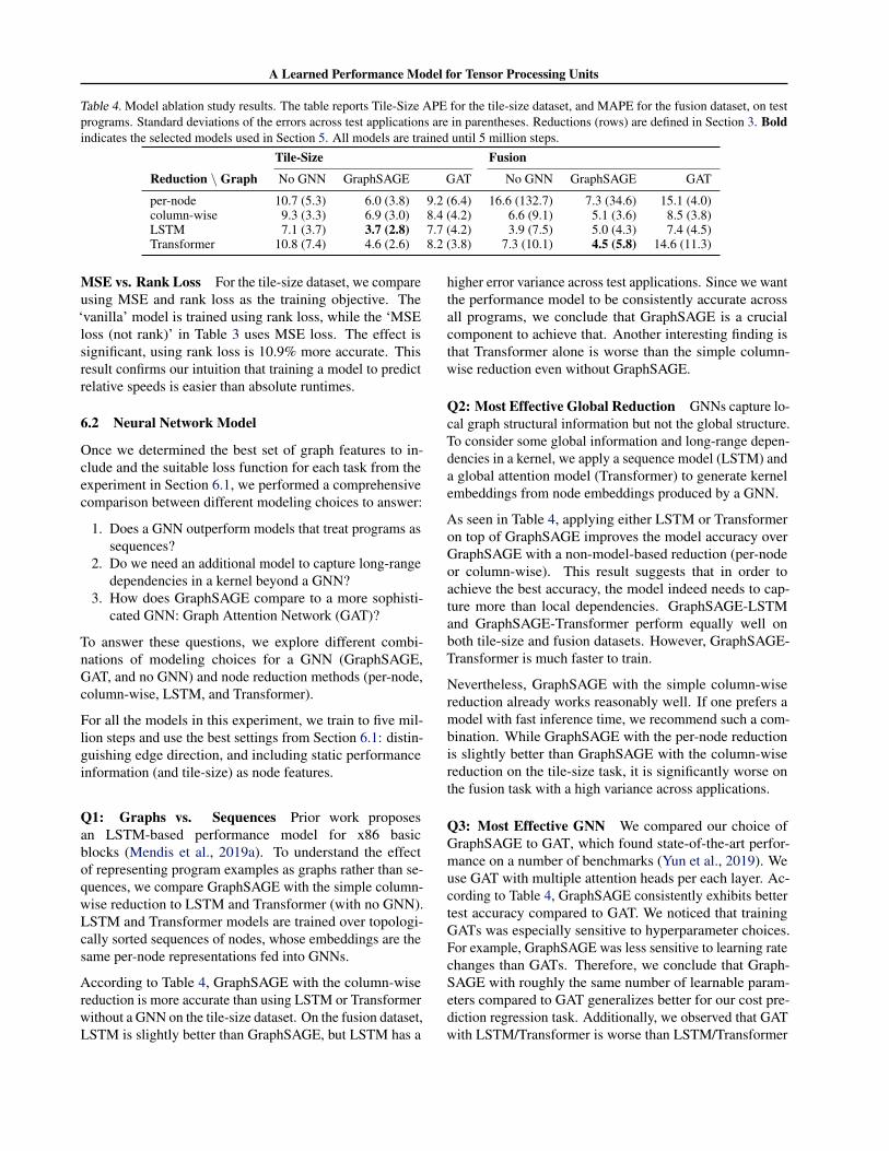
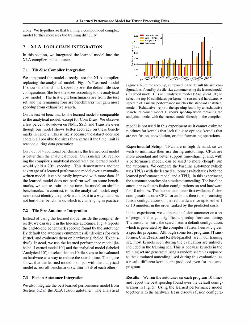
We integrated the model directly into the XLA compiler,replacing the analytical model. Fig. 4’s ‘Learned model1’ shows the benchmark speedup over the default tile-sizeconfigurations (the best tile-sizes according to the analyticalcost model). The first eight benchmarks are from the testset, and the remaining four are benchmarks that gain mostspeedup from exhaustive search.

On the test set benchmarks, the learned model is comparableto the analytical model, except for ConvDraw. We observea few percent slowdown on NMT, SSD, and Translate eventhough our model shows better accuracy on these bench-marks in Table 2. This is likely because the dataset does notcontain all possible tile sizes for a kernel if the time limit isreached during data generation.

On 3 out of 4 additional benchmarks, the learned cost modelis better than the analytical model. On Translate (3), replac-ing the compiler’s analytical model with the learned modelwould yield a 20% speedup. This demonstrates anotheradvantage of a learned performance model over a manually-written model: it can be easily improved with more data. Ifthe learned model does not perform well on some bench-marks, we can re-train or fine-tune the model on similarbenchmarks. In contrast, to fix the analytical model, engi-neers must identify the problem and fix it in a way that doesnot hurt other benchmarks, which is challenging in practice.

7.2 Tile-Size Autotuner Integration

Instead of using the learned model inside the compiler di-rectly, we can use it in the tile-size autotuner. Fig. 4 reportsthe end-to-end benchmark speedup found by the autotuner.By default the autotuner enumerates all tile-sizes for eachkernel, and evaluates them on hardware (labeled ‘Exhaus-tive’). Instead, we use the learned performance model (la-beled ‘Learned model 10’) and the analytical model (labeled‘Analytical 10’) to select the top 10 tile-sizes to be evaluatedon hardware as a way to reduce the search time. The figureshows that the learned model is on par with the analyticalmodel across all benchmarks (within 1-3% of each other).

7.3 Fusion Autotuner Integration

We also integrate the best learned performance model fromSection 5.2 in the XLA fusion autotuner. The analytical

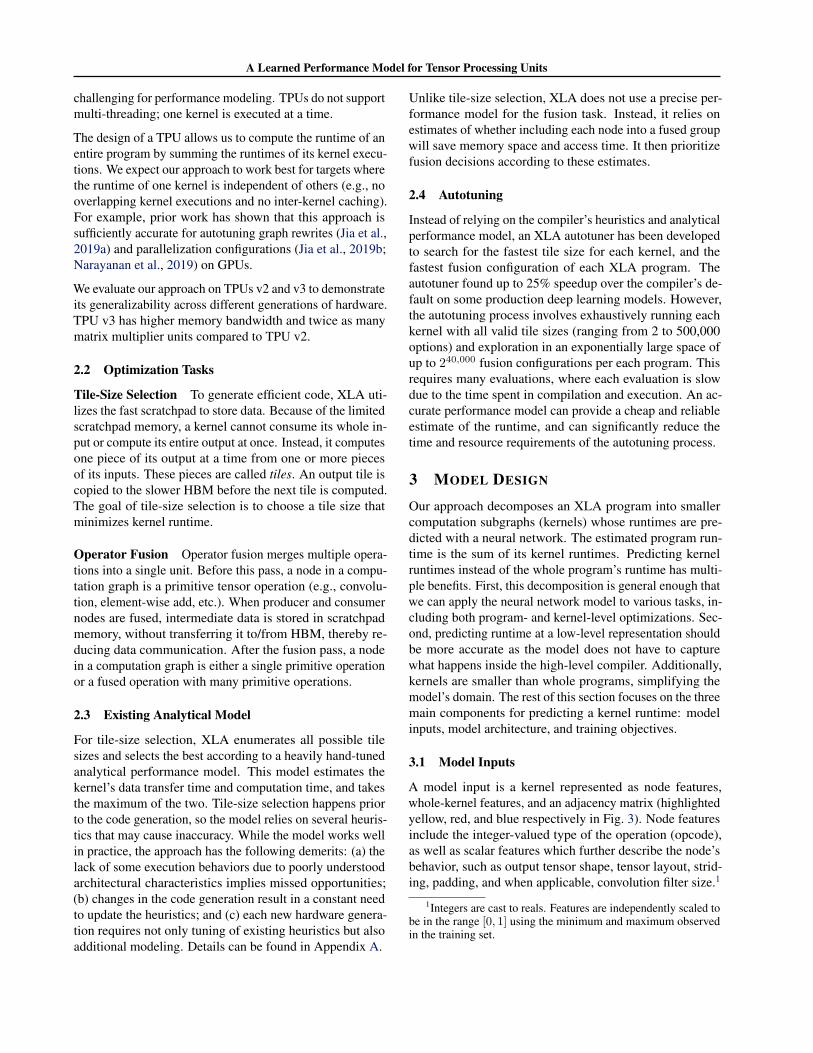
Figure 4. Runtime speedup, compared to the default tile size con-figurations, found by the tile-size autotuner using the learned model(‘Learned model 10’) and analytical model (‘Analytical 10’) toselect the top 10 candidates per kernel to run on real hardware. Aspeedup of 1 means performance matches the standard analyticalmodel. ‘Exhaustive’ reports the speedup found by an exhaustivesearch. ‘Learned model 1’ shows speedup when replacing theanalytical model with the learned model directly in the compiler.

model is not used in this experiment as it cannot estimateruntimes for kernels that lack tile-size options; kernels thatare not fusion, convolution, or data formatting operations.

Experimental Setup TPUs are in high demand, so wewish to minimize their use during autotuning. CPUs aremore abundant and better support time-sharing, and, witha performance model, can be used to more cheaply runthe autotuner. We compare the baseline autotuner (whichuses TPUs) with the learned autotuner (which uses both thelearned performance model and a TPU). In this experiment,the autotuner searches via simulated annealing. The baselineautotuner evaluates fusion configurations on real hardwarefor 10 minutes. The learned autotuner first evaluates fusionconfigurations on a CPU for an hour, then runs promisingfusion configurations on the real hardware for up to either 1or 10 minutes, in the order ranked by the predicted costs.

In this experiment, we compare the fusion autotuner on a setof programs that gain significant speedup from autotuning.The autotuner starts the search from a default configuration,which is generated by the compiler’s fusion heuristic givena specific program. Although some test programs (Trans-former, Char2Feats, and ResNet-parallel) are in our trainingset, most kernels seen during the evaluation are unlikelyincluded in the training set. This is because kernels in thetraining set are generated using a random search as opposedto the simulated annealing used during this evaluation; asa result, different kernels are produced even for the sameprogram.

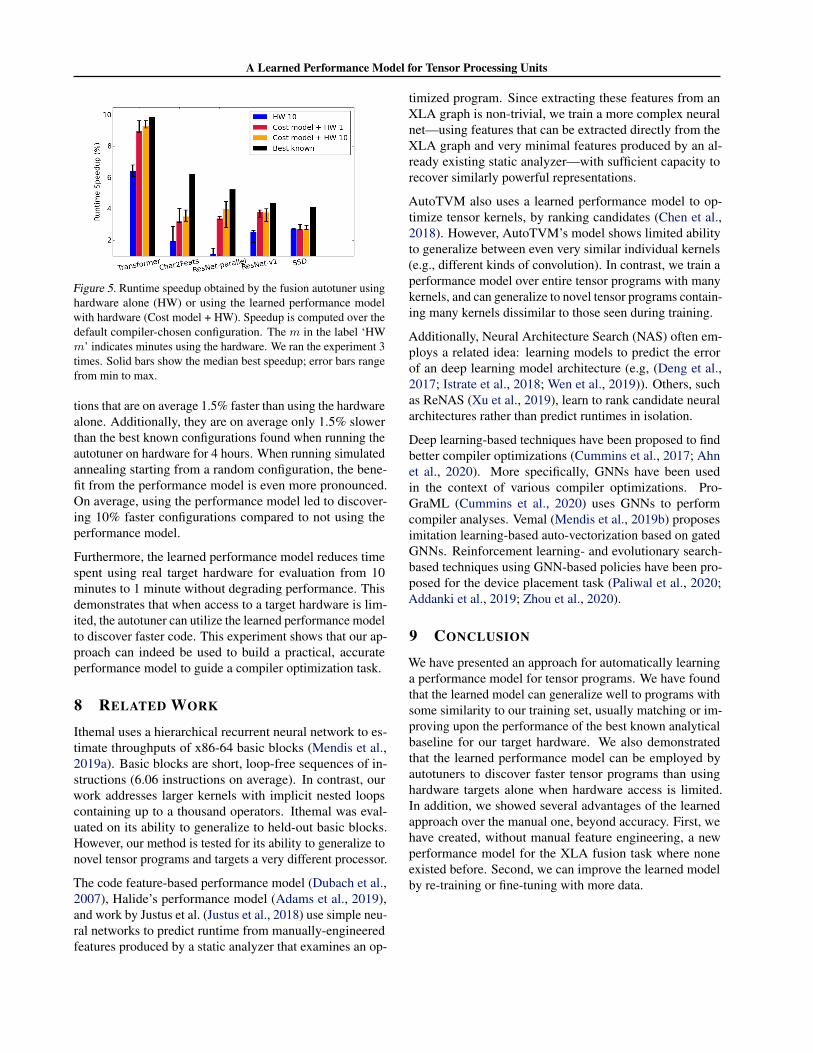
Results We run the autotuner on each program 10 timesand report the best speedup found over the default config-uration in Fig. 5. Using the learned performance modeltogether with the hardware let us discover fusion configura-

A Learned Performance Model for Tensor Processing Units

Figure 5. Runtime speedup obtained by the fusion autotuner usinghardware alone (HW) or using the learned performance modelwith hardware (Cost model + HW). Speedup is computed over thedefault compiler-chosen configuration. The m in the label ‘HWm’ indicates minutes using the hardware. We ran the experiment 3times. Solid bars show the median best speedup; error bars rangefrom min to max.

tions that are on average 1.5% faster than using the hardwarealone. Additionally, they are on average only 1.5% slowerthan the best known configurations found when running theautotuner on hardware for 4 hours. When running simulatedannealing starting from a random configuration, the bene-fit from the performance model is even more pronounced.On average, using the performance model led to discover-ing 10% faster configurations compared to not using theperformance model.

Furthermore, the learned performance model reduces timespent using real target hardware for evaluation from 10minutes to 1 minute without degrading performance. Thisdemonstrates that when access to a target hardware is lim-ited, the autotuner can utilize the learned performance modelto discover faster code. This experiment shows that our ap-proach can indeed be used to build a practical, accurateperformance model to guide a compiler optimization task.

8 RELATED WORK

Ithemal uses a hierarchical recurrent neural network to es-timate throughputs of x86-64 basic blocks (Mendis et al.,2019a). Basic blocks are short, loop-free sequences of in-structions (6.06 instructions on average). In contrast, ourwork addresses larger kernels with implicit nested loopscontaining up to a thousand operators. Ithemal was eval-uated on its ability to generalize to held-out basic blocks.However, our method is tested for its ability to generalize tonovel tensor programs and targets a very different processor.

The code feature-based performance model (Dubach et al.,2007), Halide’s performance model (Adams et al., 2019),and work by Justus et al. (Justus et al., 2018) use simple neu-ral networks to predict runtime from manually-engineeredfeatures produced by a static analyzer that examines an op-

timized program. Since extracting these features from anXLA graph is non-trivial, we train a more complex neuralnet—using features that can be extracted directly from theXLA graph and very minimal features produced by an al-ready existing static analyzer—with sufficient capacity torecover similarly powerful representations.

AutoTVM also uses a learned performance model to op-timize tensor kernels, by ranking candidates (Chen et al.,2018). However, AutoTVM’s model shows limited abilityto generalize between even very similar individual kernels(e.g., different kinds of convolution). In contrast, we train aperformance model over entire tensor programs with manykernels, and can generalize to novel tensor programs contain-ing many kernels dissimilar to those seen during training.

Additionally, Neural Architecture Search (NAS) often em-ploys a related idea: learning models to predict the errorof an deep learning model architecture (e.g, (Deng et al.,2017; Istrate et al., 2018; Wen et al., 2019)). Others, suchas ReNAS (Xu et al., 2019), learn to rank candidate neuralarchitectures rather than predict runtimes in isolation.

Deep learning-based techniques have been proposed to findbetter compiler optimizations (Cummins et al., 2017; Ahnet al., 2020). More specifically, GNNs have been usedin the context of various compiler optimizations. Pro-GraML (Cummins et al., 2020) uses GNNs to performcompiler analyses. Vemal (Mendis et al., 2019b) proposesimitation learning-based auto-vectorization based on gatedGNNs. Reinforcement learning- and evolutionary search-based techniques using GNN-based policies have been pro-posed for the device placement task (Paliwal et al., 2020;Addanki et al., 2019; Zhou et al., 2020).

9 CONCLUSION

We have presented an approach for automatically learninga performance model for tensor programs. We have foundthat the learned model can generalize well to programs withsome similarity to our training set, usually matching or im-proving upon the performance of the best known analyticalbaseline for our target hardware. We also demonstratedthat the learned performance model can be employed byautotuners to discover faster tensor programs than usinghardware targets alone when hardware access is limited.In addition, we showed several advantages of the learnedapproach over the manual one, beyond accuracy. First, wehave created, without manual feature engineering, a newperformance model for the XLA fusion task where noneexisted before. Second, we can improve the learned modelby re-training or fine-tuning with more data.

A Learned Performance Model for Tensor Processing Units

ACKNOWLEDGEMENTS

We would like to thank the XLA team, especially BjarkeRoune, for feedback and help during development, Hyeon-taek Lim for code review and writing feedback, and RishabhSingh for guidance.

REFERENCES

Adams, A., Ma, K., Anderson, L., Baghdadi, R., Li, T.-M., Gharbi, M., Steiner, B., Johnson, S., Fatahalian, K.,Durand, F., and Ragan-Kelley, J. Learning to OptimizeHalide with Tree Search and Random Programs. ACMTrans. Graph., 38(4):121:1–121:12, July 2019. ISSN0730-0301. doi: 10.1145/3306346.3322967. URL http://doi.acm.org/10.1145/3306346.3322967.

Addanki, R., Bojja Venkatakrishnan, S., Gupta, S.,Mao, H., and Alizadeh, M. Learning generalizabledevice placement algorithms for distributed machinelearning. In Wallach, H., Larochelle, H., Beygelz-imer, A., d’Alche Buc, F., Fox, E., and Garnett, R.(eds.), Advances in Neural Information ProcessingSystems, volume 32, pp. 3981–3991. Curran Asso-ciates, Inc., 2019. URL https://proceedings.neurips.cc/paper/2019/file/71560ce98c8250ce57a6a970c9991a5f-Paper.pdf.

Ahn, B. H., Pilligundla, P., Yazdanbakhsh, A., and Es-maeilzadeh, H. Chameleon: Adaptive code optimiza-tion for expedited deep neural network compilation. InInternational Conference on Learning Representations,2020. URL https://openreview.net/forum?id=rygG4AVFvH.

Berry, H., Gracia Perez, D., and Temam, O. Chaos inComputer Performance. Chaos (Woodbury, N.Y.), 16:013110, 2006.

Burges, C., Shaked, T., Renshaw, E., Lazier, A., Deeds,M., Hamilton, N., and Hullender, G. Learning to rankusing gradient descent. In Proceedings of the 22nd In-ternational Conference on Machine Learning, ICML’05, pp. 89–96, New York, NY, USA, 2005. Associ-ation for Computing Machinery. ISBN 1595931805.doi: 10.1145/1102351.1102363. URL https://doi.org/10.1145/1102351.1102363.

Chen, T., Zheng, L., Yan, E., Jiang, Z., Moreau, T., Ceze,L., Guestrin, C., and Krishnamurthy, A. Learning toOptimize Tensor Programs. In Proceedings of the 32NdInternational Conference on Neural Information Process-ing Systems, NIPS’18, 2018.

Cummins, C., Petoumenos, P., Wang, Z., and Leather, H.End-to-end deep learning of optimization heuristics. In

2017 26th International Conference on Parallel Architec-tures and Compilation Techniques (PACT), pp. 219–232.IEEE, 2017.

Cummins, C., Fisches, Z. V., Ben-Nun, T., Hoefler, T., andLeather, H. Programl: Graph-based deep learning forprogram optimization and analysis, 2020.

Deng, B., Yan, J., and Lin, D. Peephole: Predict-ing network performance before training. CoRR,abs/1712.03351, 2017. URL http://arxiv.org/abs/1712.03351.

Dubach, C., Cavazos, J., Franke, B., Fursin, G., O’Boyle,M. F., and Temam, O. Fast Compiler Optimisation Evalu-ation Using Code-Feature Based Performance Prediction.In Proceedings of the 4th International Conference onComputing Frontiers, CF ’07, 2007.

GCC. Auto-Vectorization in GCC.https://www.gnu.org/software/gcc/projects/tree-ssa/vectorization.html, August 2019. [Online; lastmodified 18-August-2019].

Hamilton, W. L., Ying, Z., and Leskovec, J. InductiveRepresentation Learning on Large Graphs. In Advancesin Neural Information Processing Systems, 2017.

Hochreiter, S. and Schmidhuber, J. Long short-term memory.Neural Computation, 9:1735–1780, 1997.

Istrate, R., Scheidegger, F., Mariani, G., Nikolopoulos, D.,Bekas, C., and Malossi, A. C. I. Tapas: Train-less accu-racy predictor for architecture search, 2018.

Jia, Z., Thomas, J., Warszawski, T., Gao, M., Zaharia, M.,and Aiken, A. Optimizing dnn computation with relaxedgraph substitutions. In 2nd SysML Conference, 2019a.

Jia, Z., Zaharia, M., and Aiken, A. Beyond data and modelparallelism for deep neural networks. In 2nd SysMLConference, 2019b.

Jia, Z., Lin, S., Gao, M., Zaharia, M., and Aiken, A.Improving the accuracy, scalability, and performanceof graph neural networks with roc. In Dhillon, I.,Papailiopoulos, D., and Sze, V. (eds.), Proceedingsof Machine Learning and Systems, volume 2, pp.187–198, 2020. URL https://proceedings.mlsys.org/paper/2020/file/fe9fc289c3ff0af142b6d3bead98a923-Paper.pdf.

Jouppi, N. P., Young, C., Patil, N., Patterson, D., Agrawal,G., Bajwa, R., Bates, S., Bhatia, S., Boden, N., Borchers,A., Boyle, R., Cantin, P.-l., Chao, C., Clark, C., Coriell, J.,Daley, M., Dau, M., Dean, J., Gelb, B., Ghaemmaghami,T. V., Gottipati, R., Gulland, W., Hagmann, R., Ho, C. R.,

A Learned Performance Model for Tensor Processing Units

Hogberg, D., Hu, J., Hundt, R., Hurt, D., Ibarz, J., Jaffey,A., Jaworski, A., Kaplan, A., Khaitan, H., Killebrew, D.,Koch, A., Kumar, N., Lacy, S., Laudon, J., Law, J., Le,D., Leary, C., Liu, Z., Lucke, K., Lundin, A., MacKean,G., Maggiore, A., Mahony, M., Miller, K., Nagarajan, R.,Narayanaswami, R., Ni, R., Nix, K., Norrie, T., Omernick,M., Penukonda, N., Phelps, A., Ross, J., Ross, M., Salek,A., Samadiani, E., Severn, C., Sizikov, G., Snelham, M.,Souter, J., Steinberg, D., Swing, A., Tan, M., Thorson,G., Tian, B., Toma, H., Tuttle, E., Vasudevan, V., Walter,R., Wang, W., Wilcox, E., and Yoon, D. H. In-DatacenterPerformance Analysis of a Tensor Processing Unit. InProceedings of the 44th Annual International Symposiumon Computer Architecture, ISCA ’17, 2017.

Jouppi, N. P., Yoon, D. H., Kurian, G., Li, S., Patil, N.,Laudon, J., Young, C., and Patterson, D. A domain-specific supercomputer for training deep neural networks.Commun. ACM, 63(7):67–78, June 2020. ISSN 0001-0782. doi: 10.1145/3360307. URL https://doi.org/10.1145/3360307.

Justus, D., Brennan, J., Bonner, S., and McGough, A. S.Predicting the computational cost of deep learning mod-els. In 2018 IEEE International Conference on Big Data(Big Data), pp. 3873–3882, 2018. doi: 10.1109/BigData.2018.8622396.

LLVM. Auto-Vectorization in LLVM. https://bcain-llvm.readthedocs.io/projects/llvm/en/latest/Vectorizers.[Online; accessed 03-Feb-2020].

Mendis, C., Renda, A., Amarasinghe, S. P., and Carbin,M. Ithemal: Accurate, Portable and Fast Basic BlockThroughput Estimation using Deep Neural Networks. InProceedings of the 36th International Conference on Ma-chine Learning, ICML, 2019a.

Mendis, C., Yang, C., Pu, Y., Amarasinghe, S., and Carbin,M. Compiler auto-vectorization with imitation learning.In Advances in Neural Information Processing Systems,pp. 14625–14635, 2019b.

Narayanan, D., Harlap, A., Phanishayee, A., Seshadri, V.,Devanur, N. R., Ganger, G. R., Gibbons, P. B., andZaharia, M. Pipedream: Generalized pipeline paral-lelism for dnn training. In Proceedings of the 27thACM Symposium on Operating Systems Principles, SOSP’19, pp. 1–15, New York, NY, USA, 2019. Associa-tion for Computing Machinery. ISBN 9781450368735.doi: 10.1145/3341301.3359646. URL https://doi.org/10.1145/3341301.3359646.

Paliwal, A., Gimeno, F., Nair, V., Li, Y., Lubin, M., Kohli, P.,and Vinyals, O. Reinforced genetic algorithm learning for

optimizing computation graphs. In International Confer-ence on Learning Representations, 2020. URL https://openreview.net/forum?id=rkxDoJBYPB.

TensorFlow. XLA: Optimizing Compiler for TensorFlow.https://www.tensorflow.org/xla. [Online; accessed 19-September-2019].

Vaswani, A., Shazeer, N., Parmar, N., Uszkoreit, J., Jones,L., Gomez, A. N., Kaiser, u., and Polosukhin, I. Attentionis all you need. In Proceedings of the 31st InternationalConference on Neural Information Processing Systems,NIPS’17, pp. 6000–6010, Red Hook, NY, USA, 2017.Curran Associates Inc. ISBN 9781510860964.

Wen, W., Liu, H., Li, H., Chen, Y., Bender, G., and Kin-dermans, P.-J. Neural predictor for neural architecturesearch, 2019.

Xu, Y., Wang, Y., Han, K., Jui, S., Xu, C., Tian, Q., andXu, C. Renas:relativistic evaluation of neural architecturesearch, 2019.

Yun, S., Jeong, M., Kim, R., Kang, J., and Kim, H. J. Graphtransformer networks. In Advances in Neural InformationProcessing Systems, pp. 11983–11993, 2019.

Zhou, Y., Roy, S., Abdolrashidi, A., Wong, D., Ma, P. C., Xu,Q., Liu, H., Phothilimtha, P., Wang, S., Goldie, A., Mirho-seini, A., and Laudon, J. Transferable graph optimizersfor ml compilers. In Advances in Neural InformationProcessing Systems, 2020.

A Learned Performance Model for Tensor Processing Units

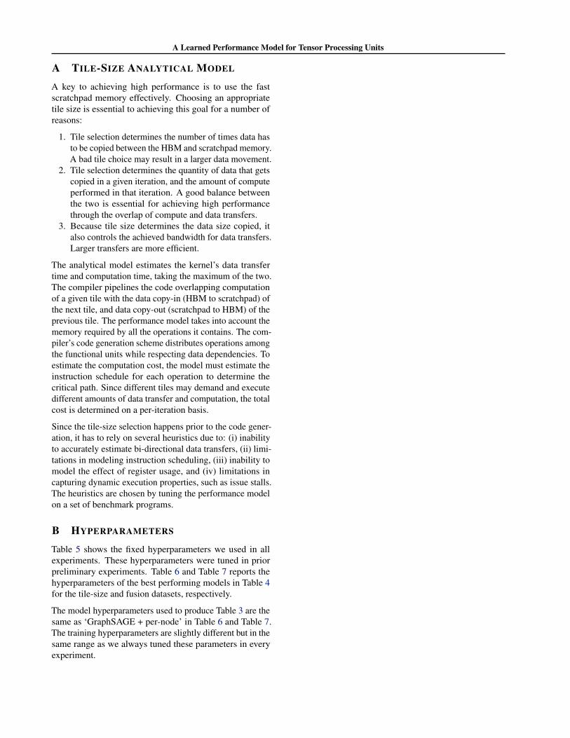
A TILE-SIZE ANALYTICAL MODEL

A key to achieving high performance is to use the fastscratchpad memory effectively. Choosing an appropriatetile size is essential to achieving this goal for a number ofreasons:

1. Tile selection determines the number of times data hasto be copied between the HBM and scratchpad memory.A bad tile choice may result in a larger data movement.

2. Tile selection determines the quantity of data that getscopied in a given iteration, and the amount of computeperformed in that iteration. A good balance betweenthe two is essential for achieving high performancethrough the overlap of compute and data transfers.

3. Because tile size determines the data size copied, italso controls the achieved bandwidth for data transfers.Larger transfers are more efficient.

The analytical model estimates the kernel’s data transfertime and computation time, taking the maximum of the two.The compiler pipelines the code overlapping computationof a given tile with the data copy-in (HBM to scratchpad) ofthe next tile, and data copy-out (scratchpad to HBM) of theprevious tile. The performance model takes into account thememory required by all the operations it contains. The com-piler’s code generation scheme distributes operations amongthe functional units while respecting data dependencies. Toestimate the computation cost, the model must estimate theinstruction schedule for each operation to determine thecritical path. Since different tiles may demand and executedifferent amounts of data transfer and computation, the totalcost is determined on a per-iteration basis.

Since the tile-size selection happens prior to the code gener-ation, it has to rely on several heuristics due to: (i) inabilityto accurately estimate bi-directional data transfers, (ii) limi-tations in modeling instruction scheduling, (iii) inability tomodel the effect of register usage, and (iv) limitations incapturing dynamic execution properties, such as issue stalls.The heuristics are chosen by tuning the performance modelon a set of benchmark programs.

B HYPERPARAMETERS

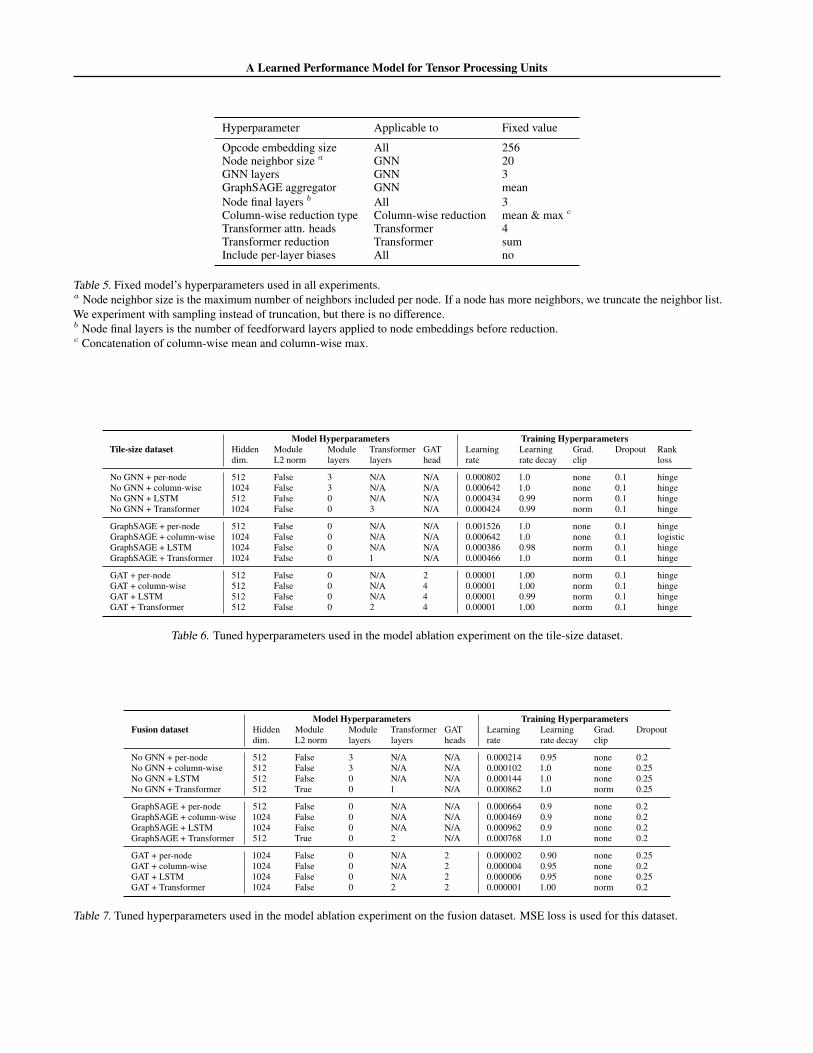
Table 5 shows the fixed hyperparameters we used in allexperiments. These hyperparameters were tuned in priorpreliminary experiments. Table 6 and Table 7 reports thehyperparameters of the best performing models in Table 4for the tile-size and fusion datasets, respectively.

The model hyperparameters used to produce Table 3 are thesame as ‘GraphSAGE + per-node’ in Table 6 and Table 7.The training hyperparameters are slightly different but in thesame range as we always tuned these parameters in everyexperiment.

A Learned Performance Model for Tensor Processing Units

Hyperparameter Applicable to Fixed value

Opcode embedding size All 256Node neighbor size a GNN 20GNN layers GNN 3GraphSAGE aggregator GNN meanNode final layers b All 3Column-wise reduction type Column-wise reduction mean & max c

Transformer attn. heads Transformer 4Transformer reduction Transformer sumInclude per-layer biases All no

Table 5. Fixed model’s hyperparameters used in all experiments.a Node neighbor size is the maximum number of neighbors included per node. If a node has more neighbors, we truncate the neighbor list.We experiment with sampling instead of truncation, but there is no difference.b Node final layers is the number of feedforward layers applied to node embeddings before reduction.c Concatenation of column-wise mean and column-wise max.

Model Hyperparameters Training HyperparametersTile-size dataset Hidden

dim.ModuleL2 norm

Modulelayers

Transformerlayers

GAThead

Learningrate

Learningrate decay

Grad.clip

Dropout Rankloss

No GNN + per-node 512 False 3 N/A N/A 0.000802 1.0 none 0.1 hingeNo GNN + column-wise 1024 False 3 N/A N/A 0.000642 1.0 none 0.1 hingeNo GNN + LSTM 512 False 0 N/A N/A 0.000434 0.99 norm 0.1 hingeNo GNN + Transformer 1024 False 0 3 N/A 0.000424 0.99 norm 0.1 hinge

GraphSAGE + per-node 512 False 0 N/A N/A 0.001526 1.0 none 0.1 hingeGraphSAGE + column-wise 1024 False 0 N/A N/A 0.000642 1.0 none 0.1 logisticGraphSAGE + LSTM 1024 False 0 N/A N/A 0.000386 0.98 norm 0.1 hingeGraphSAGE + Transformer 1024 False 0 1 N/A 0.000466 1.0 norm 0.1 hinge

GAT + per-node 512 False 0 N/A 2 0.00001 1.00 norm 0.1 hingeGAT + column-wise 512 False 0 N/A 4 0.00001 1.00 norm 0.1 hingeGAT + LSTM 512 False 0 N/A 4 0.00001 0.99 norm 0.1 hingeGAT + Transformer 512 False 0 2 4 0.00001 1.00 norm 0.1 hinge

Table 6. Tuned hyperparameters used in the model ablation experiment on the tile-size dataset.

Model Hyperparameters Training HyperparametersFusion dataset Hidden

dim.ModuleL2 norm

Modulelayers

Transformerlayers

GATheads

Learningrate

Learningrate decay

Grad.clip

Dropout

No GNN + per-node 512 False 3 N/A N/A 0.000214 0.95 none 0.2No GNN + column-wise 512 False 3 N/A N/A 0.000102 1.0 none 0.25No GNN + LSTM 512 False 0 N/A N/A 0.000144 1.0 none 0.25No GNN + Transformer 512 True 0 1 N/A 0.000862 1.0 norm 0.25

GraphSAGE + per-node 512 False 0 N/A N/A 0.000664 0.9 none 0.2GraphSAGE + column-wise 1024 False 0 N/A N/A 0.000469 0.9 none 0.2GraphSAGE + LSTM 1024 False 0 N/A N/A 0.000962 0.9 none 0.2GraphSAGE + Transformer 512 True 0 2 N/A 0.000768 1.0 none 0.2

GAT + per-node 1024 False 0 N/A 2 0.000002 0.90 none 0.25GAT + column-wise 1024 False 0 N/A 2 0.000004 0.95 none 0.2GAT + LSTM 1024 False 0 N/A 2 0.000006 0.95 none 0.25GAT + Transformer 1024 False 0 2 2 0.000001 1.00 norm 0.2

Table 7. Tuned hyperparameters used in the model ablation experiment on the fusion dataset. MSE loss is used for this dataset.

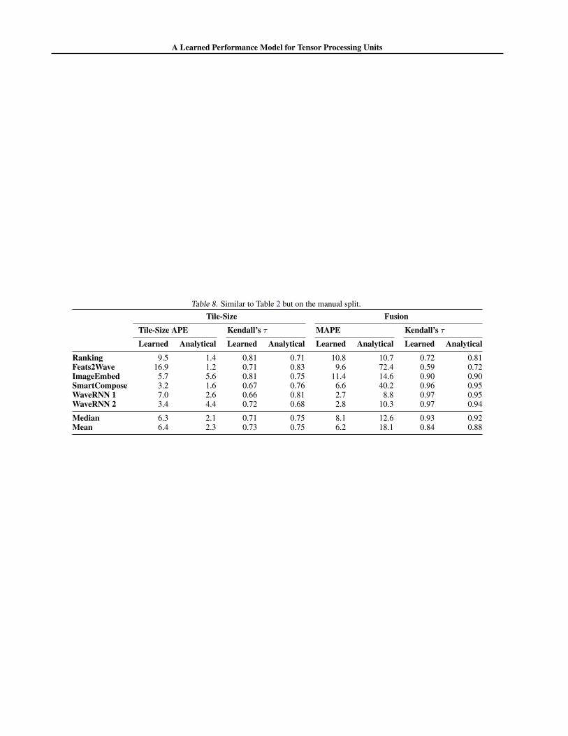
A Learned Performance Model for Tensor Processing Units

Table 8. Similar to Table 2 but on the manual split.Tile-Size Fusion

Tile-Size APE Kendall’s τ MAPE Kendall’s τ

Learned Analytical Learned Analytical Learned Analytical Learned Analytical

Ranking 9.5 1.4 0.81 0.71 10.8 10.7 0.72 0.81Feats2Wave 16.9 1.2 0.71 0.83 9.6 72.4 0.59 0.72ImageEmbed 5.7 5.6 0.81 0.75 11.4 14.6 0.90 0.90SmartCompose 3.2 1.6 0.67 0.76 6.6 40.2 0.96 0.95WaveRNN 1 7.0 2.6 0.66 0.81 2.7 8.8 0.97 0.95WaveRNN 2 3.4 4.4 0.72 0.68 2.8 10.3 0.97 0.94

Median 6.3 2.1 0.71 0.75 8.1 12.6 0.93 0.92Mean 6.4 2.3 0.73 0.75 6.2 18.1 0.84 0.88