
RXU KRPH - Ipsos › sites › default › files › ct › news › ...('8&$7,21 7(185( ',6$%,/,7
02'(//,1*�2)�(;75(0(�35(&,3,7$7,21�,1�%(/*,80
Kwinten Van Weverberg
Dissertation presented in partial fulfillment of the requirements for the degree of Doctor of Science
May 2010
Supervisor: Prof. Dr. N. P. M. van Lipzig Members of the Examination Committee: Prof. Dr. A. P. Siebesma Prof. Dr. P. Termonia Dr. L. Delobbe Prof. Dr. P. Willems Prof. Dr. G. Govers Prof. Dr. J. Poesen

2
© 2010 Katholieke Universiteit Leuven, Groep Wetenschap & Technologie, Arenberg Doctoraatsschool, W. de Croylaan 6, 3001 Heverlee, België Foto omslag © 2004 Peter Vancoillie Alle rechten voorbehouden. Niets uit deze uitgave mag worden vermenigvuldigd en/of openbaar gemaakt worden door middel van druk, fotokopie, microfilm, elektronisch of op welke andere wijze ook zonder voorafgaandelijke schriftelijke toestemming van de uitgever. All rights reserved. No part of the publication may be reproduced in any form by print, photoprint, microfilm, electronic or any other means without written permission from the publisher. ISBN 978-90-8649-327-2 D/2010/10.705/20

�������µ:RUN�RQ�FORXG�SDUDPHWHUL]DWLRQV��«��EHJDQ�DERXW����\HDUV�DJR��&ROOHFWLYHO\��ZH��WKH�DXWKRUV�RI�WKLV�SDSHU��KDYH�EHHQ�ZRUNLQJ�RQ�WKH�SUREOHP�IRU�DOPRVW�D�FHQWXU\��$UH�ZH�KDYLQJ�IXQ�\HW"�'HILQLWHO\�\HV��&ORXG�SDUDPHWHUL]DWLRQ�LV�D�EHDXWLIXO��LPSRUWDQW��LQILQLWHO\�FKDOOHQJLQJ�SUREOHP��DQG�ZH�FRQWLQXH�WR�EH�
IDVFLQDWHG�DQG�H[FLWHG�E\�LW��:H�DQG�RWKHU�PHPEHUV�RI�RXU�UHVHDUFK�JURXS�KDYH�PDGH�LPSRUWDQW�SURJUHVV��RI�ZKLFK�ZH�VKRXOG�EH�SURXG��DQG�ZH�KDYH�QR�GRXEW�WKDW�SURJUHVV�ZLOO�FRQWLQXH��1HYHUWKHOHVV��D�VREHU�DVVHVVPHQW�VXJJHVWV�WKDW�ZLWK�FXUUHQW�DSSURDFKHV�WKH�FORXG�SDUDPHWHUL]DWLRQ�SUREOHP�ZLOO�QRW�EH�µVROYHG¶�LQ�
DQ\�RI�RXU�OLIHWLPHV¶�(Randall et al. 2003)���������������
��

4
�������������������������������������������
����������
3UHIDFH������
Een jaartje of acht moet ik zijn geweest, toen ik voor het eerst ongeduldig een boekje over weer- en klimaat kon uitpakken als verjaardagsgeschenk. Sindsdien is alles wat met klimatologie, stormen en extreem weer te maken heeft, uitgegroeid tot een echte passie. Al snel begon ik nauwgezet de dagelijkse temperatuurs- en neerslagevolutie te noteren, tekende ik de ideale weerkaarten voor hitte-onweders en sneeuwstormen en uiteraard kon ik geen weerbericht op tv missen. Groot was het enthousiasme wanneer een zwaar onweer de pluviometer in de tuin net niet stukhagelde, even groot de teleurstelling wanneer het gewoon droog bleef ondanks aangekondigd noodweer. Vijftien jaar na dat eerste boekje stelde Koen De Ridder, als promotor van mijn masterthesis, me voor om me achter een doctoraatsvoorstel van Nicole van Lipzig te scharen over evaluatie van neerslag in atmosfeermodellen. Dit was een unieke kans om een passie voor de atmosfeer te laten ontbloeien in een vierjarig onderzoek en ik was dan ook snel overtuigd van de in te slagen weg. Na enige tijd bleek echter dat het maken van een doctoraat niet gestaag, maar eerder grillig als de atmosfeer verloopt. Lange perioden van nevelige windstilte werden afgewisseld door een stevige vaart en helder zicht. Zonnige momenten werden gevolgd door stormachtige dagen met flinke tegenwind. Dat er uiteindelijk, na vier jaren onderzoek, wetenschappelijke resultaten werden geboekt die zijn samengevat in voorliggende dissertatie is uiteraard niet enkel mijn verdienste. Velen hebben me de afgelopen tijd moreel of wetenschappelijk gesteund. Die mensen wil ik graag van harte danken. In de eerste plaats gaat oneindig veel dank naar Nicole van Lipzig, die me vier jaar lang met raad bijstond. Haar deur stond altijd open, ze stimuleerde

3UHIDFH�
6
verschillende leerzame bezoeken aan buitenlandse instituten en regelmatig wist ze me uit het moeras van Fortrancode en gedetaileerde modelresultaten te trekken. I also would like to thank a number of scientists who played a crucial role in both my personal evolution as a scientist and the scientific results that were obtained over the past four years. Laurent Delobbe from the Royal Meteorological Institute of Belgium explained me what one can learn and more important, what one cannot learn from radar. Thanks for all your technical and scientific assistance in exploring the Wideumont radar observations. I’m also very grateful to Axel Seifert (Deutscher Wetterdienst), who received my work with enthusiasm on the many Quest meetings and conferences and with whom I had stimulating discussions on microphysics and the difficult task to properly forecast precipitation. Gunther Haase very hospitably welcomed me for a short stay at the Swedish Meteorological and Hydrological Institute and explained me how to work with the Radar Simulation Model. Although we decided in the end not to use this tool for model evaluation, this stay at SMHI provided me with sound insight in the complicated task of implementing a forward operator for model evaluation. I also definitely would like to acknowledge Ming Xue, Keith Brewster and Daniel Dawson from the Oklahoma University with whom I had very stimulating discussions on the Advanced Regional Prediction System and who helped me with the set up of a number of relevant sensitivity experiments during a visit to the Oklahoma University. I encountered many other scientists during conferences and symposia which I’d like to thank cordially for stimulating discussions. Especially, I would like to thank all people involved in the 48(67-project: Susanne Crewell, Felix Ament, George Craig, Christian Keil, Thorsten Reinhardt, Christoph Selbach, Sonja Eikenberg, Stefan Stapelberg, Tim Böhme, Suraj Polade, Jürgen Fischer and Anja Ludwig. I would also like to thank Marcus Paulat and Heini Wernli who provided me with the SAL verification score and Britta Thies and Nathalie Selbach from the CM-SAF who provided me with huge amounts of MSG-SEVIRI satellite data. I would also like to thank the people from the IT Service Centre for their support for the work on the HPC supercluster of the K.U.Leuven, especially Wim Obbels, Martijn Oldenhof and Geertjan Bex for their help in getting the ARPS model installed properly and optimizing the speed to integrate a large number of experiments. A dissertation on in depth-evaluation of atmospheric models would be impossible without institutes providing free access to high quality data and support. Those institutes should be acknowledged accordingly. First, I ‘d like to
3UHIDFH�
7
thank the Center for Analysis and Prediction of Storms (CAPS) of the Oklahoma University for providing the ARPS source code online. I am also grateful to the European Environment Agency for making available the CORINE land cover data, the US Geological Survey for the GTOPO30 terrain height dataset, the Deutsches Zentrum für Luft und Raumfahrt (DLR) for the processed AVHRR imagery for sea surface temperature and the Flemish Institute for Technological Research (VITO) for the SPOT vegetation NDVI imagery. I also acknowledge the European Soil Bureau Network and the European Commission for providing spatially distributed soil texture data and the European Commission Joint Research Centre DESERT action for providing spatially distributed soil moisture data. I ‘d also like to thank the Deutscher Wetterdienst (DWD) and the ICSU/WMO World Data Center for Remote Sensing of the Atmosphere for providing the Satellite Application Facility on Climate Monitoring (CM-SAF) and APOLLO satellite derived cloud properties respectively. Atmospheric sounding data were provided by the Department of Atmospheric Science of the University of Wyoming. Natuurlijk draaiden de afgelopen jaren niet enkel rond wetenschap, maar werden ook vriendschappen gesmeed en bevestigd. Matthias leerde ik kennen bij de eerste passen door de wereld van het postprocessen tijdens m’ n masterthesis en al gauw werd duidelijk dat we vele interesses deelden: het klimaat, het buitenland en de Leuvense terrasjes om er maar een paar te noemen. Die laatste interesse delen Matthias en ik ook met Toon, met wie ik de afgelopen negen jaar veel plezier heb beleefd. Hopelijk blijven deze vriendschappen nog lang in stand. De meeste tijd heb ik de afgelopen jaren natuurlijk met de bureaugenoten doorgebracht. Dirk leerde me niet alleen wat je buiten de haren uittrekken nog kan doen als je model crasht na een zoveelste VHJPHQWDWLRQ�IDXOW, maar vergezelde me ook op een erg geslaagd bezoek aan de VS. Wim was niet alleen al die tijd een bureaugenoot, maar ook lange tijd een toffe huisgenoot. Altijd had hij een luisterend oor klaar wanneer het even minder ging en deelde hij in het enthousiasme op succesvolle momenten. Voor leerzame discussies over maatschappij en wetenschap kon ik dan weer altijd terecht bij Christoph, die wat later op onze bureau aanbelandde. Daarom ook een dikke merci jullie drie voor de leuke jaren op bureau 03.254. Ook de andere collega’ s van onze afdeling wil ik graag bedanken voor de fijne jaren. Iedereen kon het steeds goed met elkaar vinden tijdens de koffiepauzes en middagpauzes, de sportieve events en de afdelingsfeestjes. Specifically I would like to thank all members of the Weather and Climate Group for the nice atmosphere during the past years: Thanks a lot Erwan, Irina, Praveen, Tim, Tom, Annemarie, Clemence. Veel dank ook aan alle vrienden die van veraf of dichtbij de evolutie van dit doctoraat hebben gevolgd. In het bijzonder dank ik mijn huisgenoten Katrien, Anne en Tine. Steeds hadden jullie een luisterend oor
3UHIDFH�
8
en vaak zelfs een volledige maaltijd klaar wanneer ik na een lange dag thuiskwam, vooral gedurende het laatste half jaar. Ook veel dank aan alle andere vrienden, Daan, Joeri, Tjarda, Klaar, Fré, Steve, Kim, Tim, Floris en vele anderen voor de leuke ontspanningsmomenten de afgelopen jaren. Als laatste, maar niet in het minst, wil ik erg graag mijn ouders, mijn zus en broer en mijn meter en peter bedanken voor hun onvoorwaardelijke steun in wat ik doe. Van kleins af aan hebben jullie mijn interesses gestimuleerd en gemotiveerd. Zonder jullie zou ik niet zijn wie ik ben. Een dikke merci daarvoor.
��������������������������������
9
����������
$EVWUDFW�����
Precipitation is probably the single most difficult feature to forecast by any atmospheric model, due to the many scales involved and the amalgam of interacting processes eventually leading to precipitation at the surface. With increasing computing power and a better understanding and representation of the physical processes in atmospheric models, it is now possible to operationally forecast individual storm systems. However, progress in the simulation of precipitation has been disappointing. Simulated storm systems are often too intense and appear at wrong locations and timings. Many aspects of such convection-resolving models have been subject to detailed studies with respect to the quantitative precipitation forecast, but none of them was able to point to a single model deficiency responsible for poor precipitation forecasts. The main objective of this dissertation is to use a broad number of recently available spatially distributed observational data to evaluate as much as possible of the interacting processes aloft leading to surface precipitation. By performing numerous sensitivity studies to soil moisture initialization, precipitation size distribution assumptions, horizontal resolution and even numerical inaccuracies for case studies and large composites it is believed that knowledge on the relevance of each of those processes for surface precipitation will be improved. For two cases of intense convection it was found that the gain of using spatially distributed initial soil properties as opposed to homogeneous soil properties over the domain was small, although it was found important to have the mean soil moisture content right for a realistic simulation of cold pool intensity, storm structure and surface precipitation. Furthermore, a mechanism was proposed to explain the inverse relation between surface precipitation and
$EVWUDFW�
10
soil moisture content found in our simulations, but also in other studies using convection-resolving models. Increasing soil moisture leads to enhanced thermodynamic conditions, but this effect is counterbalanced by a weakening of the storms as a consequence of weaker cold pools associated with decreased evaporative cooling in the moister boundary layer. Issues with the parameterized sub-grid turbulent motions emerged when turning to smaller grid spacings. Too excessive motions on the resolved scale occurred in the boundary layer, which easily propagated upward during a shear-driven case and led to the occurrence of grid-scale storms. During a buoyancy-driven case, the effect was much smaller due to the less important vertical momentum exchange as a driver for convection. A large number of sensitivity experiments were performed on the size distributions of the precipitating hydrometeors (rain, snow and hail) for three cases of intense precipitation and intensively evaluated against remotely sensed observational data. Satellite-derived cloud optical thickness distribution could only be realistically represented when large hail was replaced by small graupel. This could be related to a strong overestimation of snow amounts in experiments with large hail. The vertical radar reflectivity profile was significantly improved during the simulation of a stratiform event by the inclusion of small graupel. During convective events however, large hail was necessary in order to simulate the strong reflective cores. Furthermore, when large hail was replaced by small graupel, the vertical storm structure and the surface precipitation field deteriorated significantly. Therefore, it was concluded that for an operational model, both hail and graupel should be included in the microphysics parameterization. Surface precipitation however, was found to be rather insensitive to any of the size distribution modifications proposed. During the simulation of a low-topped supercell it was found that when only replacing hail by small graupel, surface precipitation slightly increased, in contrast to findings of many previous studies. It was found that this was due to contrasting effects of on the one hand decreased precipitation efficiency (associated with intense graupel sublimation) and on the other hand enhanced thermodynamic conditions (associated with riming processes). We showed that the response of storms to modifications of the largest precipitating ice species strongly depends on storm depth as deeper storms have more graupel sublimation and hence smaller precipitation efficiencies as compared to shallow graupel-containing storms. Furthermore, we showed that while including more realistic snow size distribution assumptions did not affect storm characteristics at all, more realistic rain size distribution assumptions improved the accumulated surface precipitation by decreasing the cold pool area and hence the precipitation area. This was due to decreased rain evaporative cooling near
$EVWUDFW�
11
the storm edges. At last it was found that the contribution of clipping of negative mixing ratios, originating from inaccuracies in the finite-difference representation of the moisture advection process, is non-negligible and adds significant amounts (up to over 30 %) of artificial water to the model. An experiment forcing the model to conserve water revealed significantly improved simulation of the surface precipitation quantities. For two composites containing 15 stratiform and 15 convective cases respectively, we confirmed many of the findings made above for single case studies. Graupel was found necessary for correct simulation of the cloud radiative properties, while surface precipitation was insensitive to any of the size distribution experiments implemented. The positive surface precipitation bias was greatly improved by forcing the model to conserve water. The gain of turning to higher resolution convection-resolving scales for precipitation simulation is that the representation of storm structure and the physics of the convective systems is improved, although little gain was found as far as precipitation amounts were concerned.
��������������������������
12
����������
6DPHQYDWWLQJ������
Neerslag is wellicht het meest problematische aspect van de weersvoorspelling in elk atmosfeermodel, omwille van de verschillende schalen waarop de neerslagvorming speelt en het amalgaam van interagerende processen die uiteindelijk tot neerslag aan het oppervlak leiden. Dankzij toenemende rekenkracht van computers en een beter begrip en voorstelling van de fysische processen in atmosfeermodellen, is het vandaag technisch mogelijk om individuele buiensystemen operationeel te voorspellen. De vooruitgang in de simulatie van neerslag is totnogtoe echter eerder teleurstellend. Gemodelleerde systemen zijn vaak te intens en verschijnen op verkeerde plaatsen en op verkeerde momenten. Vele aspecten van zulke convectie-oplossende modellen zijn onderwerp geweest van gedetailleerde studies m.b.t. de kwantitatieve neerslagvoorspelling, maar geen enkele was in staat één enkel facet van de modellen aan te duiden dat verantwoordelijk was voor de slechte neerslagvoorspelling. Het belangrijkste doel van deze dissertatie is om een groot aantal recent beschikbare ruimtelijk verdeelde observatiegegevens te gebruiken om zo veel mogelijk van de relevante gesimuleerde interagerende processen in de atmosfeer te evalueren. Via het uitvoeren van een groot aantal gevoeligheidsstudies naar bodemvochtinitialisatie, de grootteverdelingen van de verschillende neerslagtypes, de ruimtelijke resolutie en zelfs numerieke onnauwkeurigheden voor intense neerslagevents, wordt verwacht dat de kennis over de relevantie van elk van deze aspecten voor oppervlakteneerslag verbeterd zal kunnen worden. Voor twee situaties met intense convectie werd gevonden dat het voordeel van ruimtelijk verdeelde bodemeigenschappen in atmosfeermodellen (tegenover
6DPHQYDWWLQJ�
13
ruimtelijk homogene bodemeigenschappen) erg klein was, hoewel het belangrijk is om het gemiddelde bodemvochtgehalte correct te initialiseren voor een realistische simulatie van koudepoelintensiteit, buienstructuur en oppervlakteneerslag. Verder werd een mechanisme voorgesteld om de omgekeerde relatie te verklaren tussen oppervlakteneerslag en bodemvochtgehalte, die gevonden werd in onze simulaties maar ook in eerdere studies. Een hoger bodemvochtgehalte leidt tot gunstigere thermodynamische omstandigheden voor buienvorming, maar aan de andere kant zwakkere koudepoelen onder de buien, omwille van beperkte verdampingskoeling in vochtige grenslagen. Voor vele buiensystemen zijn zowel de thermodynamische omstandigheden als de koudepoelkarakteristieken van groot belang voor de intensiteit. Wanneer de horizontale resolutie verder verhoogd werd, bleek de geparameterizeerde turbulentie in de grenslaag te beperkt te worden waardoor te veel turbulente bewegingen werden opgelost door het modelgrid zelf. Deze buitensporige turbulenties werder vlot opwaarts getranporteerd in een situatie met sterke windschering, wat aanleiding gaf tot intense buien ter grootte van slechts één enkele grid cell Een groot aantal gevoeligheidsexperimenten naar de grootteverdeling van de neerslaande hydrometeoren (regen, sneeuw en hagel) werden uitgevoerd voor drie situaties met intense neerslag en deze werden rigoreus ge-evalueerd aan de hand van ruimtelijk verdeelde teledetectiedata (satelliet en radar). De frequentieverdeling van de wolken-optische dikte kon enkel realistisch gesimuleerd worden wanneer hagel vervangen werd door korrelhagel. Dit kon worden gerelateerd aan overmatige hoeveelheden sneeuw in experimenten met hagel. Het verticale radar reflectiviteitsprofiel verbeterde significant tijdens de simulatie van stratiforme neerslag wanneer hagel vervangen werd door korrelhagel. Tijdens convectieve neerslag echter, was hagel noodzakelijk om de sterk reflectieve neerslagkernen te simuleren. Verder verslechterde de verticale buienstructuur en de oppervlakteneerslagstructuur sterk wanneer hagel vervangen werd door korrelhagel. Daarom werd geconcludeerd dat in een operationeel model zowel hagel als korrelhagel zouden moeten inbegrepen zijn in de microfysica parameterisatie. Oppervlakteneerslag was veel minder gevoelig aan de voorgestelde modificaties. Tijdens de simulatie van een ondiepe supercell over België werd bevonden dat wanneer hagel vervangen werd door korrelhagel, de oppervlakteneerslag licht toenam, in tegenstrijd tot vele eerdere studies. Er werd aangetoond dat deze toename te wijten was aan contrasterende effecten van aan de ene kant verminderde neerslagefficiëntie (gerelateerd aan intense korrelhagelsublimatie) en aan de andere kant gunstigere thermodynamische omstandigheden (gerelateerd aan rijmingprocessen). We toonden aan dat de gevoeligheid van gesimuleerde buien voor veranderingen aan de grootteverdeling van de grootste

6DPHQYDWWLQJ�
14
ijshydrometeoor in modellen sterk afhangt van de diepte van de buien. In diepe buien treedt namelijk veel meer sublimatie van korrelhagel op en bijgevolgd is de neerslagefficiëntie er lager in vergelijking met ondiepe buien die korrelhagel bevatten. Verder toonden we aan dat terwijl het implementeren van meer realistische sneeuwgrootteverdelingen geen invloed had op de buienkarakteristieken, meer realistische regengrootteverdelingen de geaccumuleerde opppervlakteneerslag duidelijk verbeteren. Dit kwam door het verkleinen van de koudepoel aangezien er minder verdamping van regen optrad aan de randen van koudepoelen onder buien. Hierdoor werd de neerslagoppervlakte van de buien typisch verkleind. Tenslotte werd ontdekt dat de bijdrage van het kunstmatig toevoegen van water aan het model in verband met numerieke onnauwkeurigheden in het vochttranport van het model niet verwaarloosbaar is en belangrijke hoevelheden water toevoegt aan het model (tot meer dan 30 %). Bij een experiment waarin het model geforceerd werd om de totale hoeveelheid water te behouden, werd de oppervlakteneerslag duidelijk beter gesimuleerd. Voor twee composieten die respectievelijk 15 stratiforme en 15 convectieve weersituaties bevatten, konden we de meeste van de bevindingen hierboven gemaakt werden, bevestigen. Korrelhagel werd noodzakelijk bevonden om de stralingseigenschappen van wolken correct te simuleren, terwijl oppervlakteneerslag ongevoelig was voor elk van de experimenten met variabele grootteverdelingen. De positieve neerslagafwijking kon sterk verbeterd worden door het model te dwingen om de totale hoeveelheid water in het model te behouden. Het grote voordeel van het integreren van atmosfeermodellen met een hogere resolutie op dit moment is dat de voorstelling van de structuur van buien en de fysica van de convectieve systemen is verbeterd, hoewel weinig verbetering werd gevonden in de neerslaghoeveelheden.�
�������������
�
15
7DEOH�RI�FRQWHQWV�
Table of contents _______________________________________________ 15
List of symbols and abbreviations __________________________________ 19
Chapter 1: Introduction __________________________________________ 23
1.1. Quantitative forecast of intense precipitation___________________ 23 1.2. Remote sensing of intense precipitation_______________________ 27 1.3. Research goals __________________________________________ 28 1.4. Outline ________________________________________________ 29
Chapter 2: Observed precipitation characteristics ______________________ 33
2.1. Dynamical aspects of precipitation __________________________ 33 ������ 6WUDWLIRUP�SUHFLSLWDWLRQ BBBBBBBBBBBBBBBBBBBBBBBBBBBBBBBBB �� ������ &RQYHFWLYH�SUHFLSLWDWLRQBBBBBBBBBBBBBBBBBBBBBBBBBBBBBBBBB ��
2.2. Microphysical aspects of precipitation________________________ 35 ������ 3UHFLSLWDWLRQ�IRUPDWLRQ�SURFHVVHV BBBBBBBBBBBBBBBBBBBBBBBBB �� ������ 6L]H�GLVWULEXWLRQ�FKDUDFWHULVWLFV BBBBBBBBBBBBBBBBBBBBBBBBBBB ��
2.2.2.1. Size distribution characteristics of rain __________________ 36 2.2.2.2. Size distribution characteristics of snow _________________ 38 2.2.2.3. Size distribution characteristics of hail and graupel_________ 40
Chapter 3: Modelling of precipitation _______________________________ 43
3.1. Nonhydrostatic modelling of precipitation_____________________ 43 3.2. The Advanced Regional Prediction System____________________ 47 3.3. Parameterization of surface processes ________________________ 50 3.4. Parameterization of microphysical processes___________________ 52 3.5. Case description_________________________________________ 56 ������ ���1RYHPEHU�������VWUDWLIRUP�FDVH BBBBBBBBBBBBBBBBBBBBBBBB ��

7DEOH�RI�FRQWHQWV�
16
������ ���2FWREHU�������VKHDU�GULYHQ�FRQYHFWLYH�FDVHBBBBBBBBBBBBBBB �� ������ ���-XO\�������EXR\DQF\�GULYHQ�FRQYHFWLYH�FDVHBBBBBBBBBBBBBBB ��
Chapter 4: Sensitivity of quantitative precipitation forecast to soil moisture initialization, microphysics parameterization and horizontal resolution _____ 61
4.1. Introduction ____________________________________________ 61 4.2. Model setup and case description ___________________________ 63 4.3. Experiments design ______________________________________ 63 4.4. Observational data and SAL _______________________________ 67 4.5. Results ________________________________________________ 69 ������ 6HQVLWLYLW\�WR�VRLO�PRLVWXUH�LQLWLDOL]DWLRQBBBBBBBBBBBBBBBBBBBBB ��
4.5.1.1. Shear-driven case___________________________________ 69 4.5.1.2. Buoyancy-driven case _______________________________ 75
������ 6HQVLWLYLW\�WR�PLFURSK\VLFV�SDUDPHWHUL]DWLRQ BBBBBBBBBBBBBBBBB �� 4.5.2.1. Shear-driven case___________________________________ 80 4.5.2.2. Buoyancy-driven case _______________________________ 83
������ 6HQVLWLYLW\�WR�KRUL]RQWDO�JULG�VSDFLQJ BBBBBBBBBBBBBBBBBBBBBBB �� 4.5.3.1. Shear-driven case___________________________________ 87 4.5.3.2. Buoyancy-driven case _______________________________ 90
4.6. Discussion and conclusions ________________________________ 91
Chapter 5: Evaluation of moist processes in km-scale NWP models using remote sensing and in-situ data: impact of microphysics size distribution assumptions 95
5.1. Introduction ____________________________________________ 95 5.2. Model setup and observational data__________________________ 97 ������ 0RGHO�VHWXS�DQG�H[SHULPHQWV�GHVLJQ BBBBBBBBBBBBBBBBBBBBBBB �� ������ 2EVHUYDWLRQDO�GDWD BBBBBBBBBBBBBBBBBBBBBBBBBBBBBBBBBBBBB ��
5.2.2.1. Sounding data _____________________________________ 99 5.2.2.2. Satellite data _____________________________________ 100 5.2.2.3. Volume radar data _________________________________ 101 5.2.2.4. Radar-rain gauge merging product ____________________ 102
5.3. Results _______________________________________________ 103 ������ 6RXQGLQJ�GHULYHG�LQWHJUDWHG�ZDWHU�YDSRXUBBBBBBBBBBBBBBBBBB ���
5.3.1.1. Stratiform case____________________________________ 103 5.3.1.2. Convective cases __________________________________ 105
������ 06*�GHULYHG�FORXG�RSWLFDO�WKLFNQHVV BBBBBBBBBBBBBBBBBBBBBB ��� 5.3.2.1. Stratiform case____________________________________ 107 5.3.2.2. Convective cases __________________________________ 110
������ 5DGDU�UHIOHFWLYLW\ BBBBBBBBBBBBBBBBBBBBBBBBBBBBBBBBBBBBB ��� 5.3.3.1. Stratiform case____________________________________ 114 5.3.3.2. Convective cases __________________________________ 116
������ 6XUIDFH�SUHFLSLWDWLRQ BBBBBBBBBBBBBBBBBBBBBBBBBBBBBBBBBB ��� 5.3.4.1. Stratiform case____________________________________ 119

7DEOH�RI�FRQWHQWV�
17
5.3.4.2. Convective cases __________________________________ 120 5.4. Summary and conclusions ________________________________ 122
Chapter 6: The impact of size distribution assumptions in a simple microphysics scheme on surface precipitation and storm dynamics during a low-topped supercell case_________________________________________________ 125
6.1. Introduction ___________________________________________ 125 6.2. Model and experimental design ____________________________ 127 6.3. Results _______________________________________________ 131 ������ ,QIOXHQFH�RI�JUDXSHO��KDLO�VL]H�GLVWULEXWLRQ BBBBBBBBBBBBBBBBBB ��� ������ ,QIOXHQFH�RI�VQRZ�DQG�UDLQ�VL]H�GLVWULEXWLRQBBBBBBBBBBBBBBBBB ��� ������ ,QIOXHQFH�RI�QHJDWLYH�PL[LQJ�UDWLRVBBBBBBBBBBBBBBBBBBBBBBBB ���
6.4. Summary and conclusion_________________________________ 145
Chapter 7: Improvement of clouds and quantitative precipitation forecast during convective and stratiform intense precipitation events on convection-resolving scales _______________________________________________________ 149
7.1. Introduction ___________________________________________ 149 7.2. Model setup and experiments design ________________________ 151 7.3. Case description and observational data _____________________ 152 7.4. Results _______________________________________________ 154 ������ &ORXG�RSWLFDO�WKLFNQHVVBBBBBBBBBBBBBBBBBBBBBBBBBBBBBBBBB ��� ������ 6XUIDFH�SUHFLSLWDWLRQ BBBBBBBBBBBBBBBBBBBBBBBBBBBBBBBBBB ��� �������� 7UDGLWLRQDO�YHULILFDWLRQ�VFRUHV BBBBBBBBBBBBBBBBBBBBBBBBB ��� �������� 6$/ BBBBBBBBBBBBBBBBBBBBBBBBBBBBBBBBBBBBBBBBBBBBBB ��� �������� &RPSDULVRQ�DJDLQVW���NP�H[SHULPHQWV BBBBBBBBBBBBBBBBBBB ��� ������ ([DPSOHV BBBBBBBBBBBBBBBBBBBBBBBBBBBBBBBBBBBBBBBBBBB ���
7.5. Conclusions ___________________________________________ 172
Chapter 8: General conclusions and future prospects __________________ 175
8.1. General conclusions_____________________________________ 175 8.2. Prospects for future research ______________________________ 182
Appendix A: Glossary __________________________________________ 185
A.1 General Terms___________________________________________ 185 A.2 Microphysics conversion terms______________________________ 191
Appendix B: Microphysics conversion equations _____________________ 193
Appendix C: SAL verification score _______________________________ 197
C.1 Identification of objects____________________________________ 197 C.2 The amplitude component A ________________________________ 198 C.3 The location component L__________________________________ 198 C.4 The structure component S _________________________________ 199

7DEOH�RI�FRQWHQWV�
18
Appendix D: Influence of inaccuracies in the moisture transport during a shear-driven convective case, a buoyancy-driven convective and a stratiform case 201
References ___________________________________________________ 205
�����������������

19
����������
/LVW�RI�V\PEROV�DQG�DEEUHYLDWLRQV����
6\PERO�$EEUHYLDWLRQ� ([SODQDWLRQ� ax Coefficient of the mass-diameter relationship
of the precipitating hydrometeor x (where x is rain, hail or snow)
A Amplitude component of SAL analysis ABL Atmospheric Boundary Layer AGL Above Ground Level ARPS Advanced Regional Prediction System br Slope of the retention curve in the surface
parameterization bx Power of the mass-diameter relationship of the
precipitating hydrometeor x (where x is rain, hail or snow)
CAPE Convective Available Potential Energy CD Drag coefficient in the hail fall speed
formulation CFAD Contoured Frequency by Altitude Diagram CGsat Soil thermal coefficient at saturation CH Drag coefficient in the sensible heat flux
formulation CIN Convective Inhibition CORINE Coordination of Information on the
Environment COT Cloud Optical Thickness cp Specific heat of air at constant pressure
/LVW�RI�V\PEROV�DQG�DEEUHYLDWLRQV�
20
cx Coefficient of the velocity-diameter relationship of the precipitating hydrometeor x (where x is rain, hail or snow)
C1 Coefficient in the Deardorff (1977) formulation to prognose wg
C1sat Value of C1 at saturation C2 Coefficient in the Deardorff (1977) formulation
to prognose wg C2ref Value of C2 for w2 = 0.5 wsat dx Power of the velocity-diameter relationship of
the precipitating hydrometeor x (where x is rain, hail or snow)
D0x Equivalent diameter of hydrometeor x (where x is rain, hail or snow)
d1 Skin soil layer depth d2 Deep soil layer depth E Latent heat flux ECMWF European Centre for Medium-Range Weather
Forecasting Eg Soil surface evaporation ESDB European Soil Database Etr Transpiration ETS Equitable Threat Score Ev Evapotranspiration g Gravitational acceleration G Heat storage rate hu Relative humidity at the ground surface hv Halstead coefficient IWV Integrated Water Vapour Ki Dielectric factor for ice Kw Dielectric factor for water L Location component of the SAL analysis LAI Leaf Area Index LCL Lifting Condensation Level LFC Level of Free Convection LNB Level of Neutral Buoyancy MSG Meteosat Second Generation
/LVW�RI�V\PEROV�DQG�DEEUHYLDWLRQV�
21
MSL Mean Sea Level mx Mass of hydrometeor x (where x is rain, hail or
snow) n(D0x) Number concentration of hydrometeor x
(where x is rain, hail or snow) NDVI Normalized Difference Vegetation Index N0x Intercept parameter of the exponential size
distribution of hydrometeor x (where x is rain, hail or snow)
OMB One-Moment Bulk microphysics Pv Precipitation rate at the top of the vegetation PE Precipitation Efficiency PSD Particle Size Distribution qa Atmospheric specific humidity of the air QPF Quantitative Precipitation Forecast qsat Saturated specific humidity qx Mixing ratio of hydrometeor x (where x is
cloud water, cloud ice, rain, hail or snow) qv Mixing ratio of water vapour RA Incoming atmospheric infrared radiation Rex Effective radius of hydrometeor x (where x is
cloud water, cloud ice, rain, hail or snow) RG Incoming solar radiation RMI Royal Meteorological Institute of Belgium RMSE Root Mean Square Error Rn Net radiation at the surface RSmin Minimum surface resistance S Structure component of the SAL analysis SEVIRI Spinning Enhanced Visible and Infrared
Radiometer SPOT Satellite Pour l’ Observation de la Terre T Air temperature TKE Turbulent Kinetic Energy TS Skin soil temperature T0 Melting temperature T2 Deep soil temperature ULL Upper Level Low
/LVW�RI�V\PEROV�DQG�DEEUHYLDWLRQV�
22
Va Scalar wind speed veg Fraction of vegetation Vx Mass weighted mean terminal velocity of
hydrometeor x (where x is rain, hail or snow) wg Skin soil layer volumetric water content wsat Saturated volumetric soil moisture content wwilt Wilting point volumetric water content w2 Deep soil layer volumetric water content Ze Equivalent radar reflectivity factor Zx Radar reflectivity factor of hydrometeor x
(where x is rain, hail or snow) z0 Roughness length
Albedo Gamma function Emissivity x Slope parameter of the exponential size
distribution of hydrometeor x (where x is rain, hail or snow)
Air density x Density of hydrometeor x (where x is rain, hail
or snow) Stefan-Botlzmann constant x Optical thickness hydrometeor x (where x is
cloud water, cloud ice, rain, hail or snow) ���������������
23
����������
&KDSWHU������
,QWURGXFWLRQ�
������4XDQWLWDWLYH�IRUHFDVW�RI�LQWHQVH�SUHFLSLWDWLRQ�
Flash floods, caused by severe convective precipitation events in the warm season, pose a major threat to public and private infrastructure in densely populated areas like Western Europe (Vanneuville et al. 2006). An ever increasing built-up area and a larger number of dwellings built in areas prone to flash flooding urge the need for better prevention. Significant progress in weather forecasting plays a major role in taking precautious measures on short time scales and in issuing warnings to the public. Numerical atmospheric models have been a tool for forecasting precipitation ever since the 1960s, although it is only during the last decade that storm-scale simulations have become operationally feasible. Continuously increasing computer power permitted operational models to be integrated at continuously smaller grid spacings. Today, using grid spacings up to only a few kilometres, it has become operationally feasible to simulate individual storm systems.
Results with FRQYHFWLRQ�UHVROYLQJ models (i.e. able to explicitly simulate individual storm updrafts and downdrafts) have been promising in some case studies. Weisman et al. (1997) simulated mid-latitude thunderstorms at horizontal grid spacing ranging from 1 to 12 km and found that their development became more realistic as resolution increased, and that 4-km grid spacing successfully duplicated much of the observed mesoscale structure and evolution. Nielson-Gammon and Strack (2000) examined the effects of
&KDSWHU���
24
horizontal grid spacing (36 – 4 km) on maximum precipitation during three extreme rainfall events over Texas. They found that a grid spacing of 6 km or smaller was necessary to consistently achieve the observed rainfall rates.
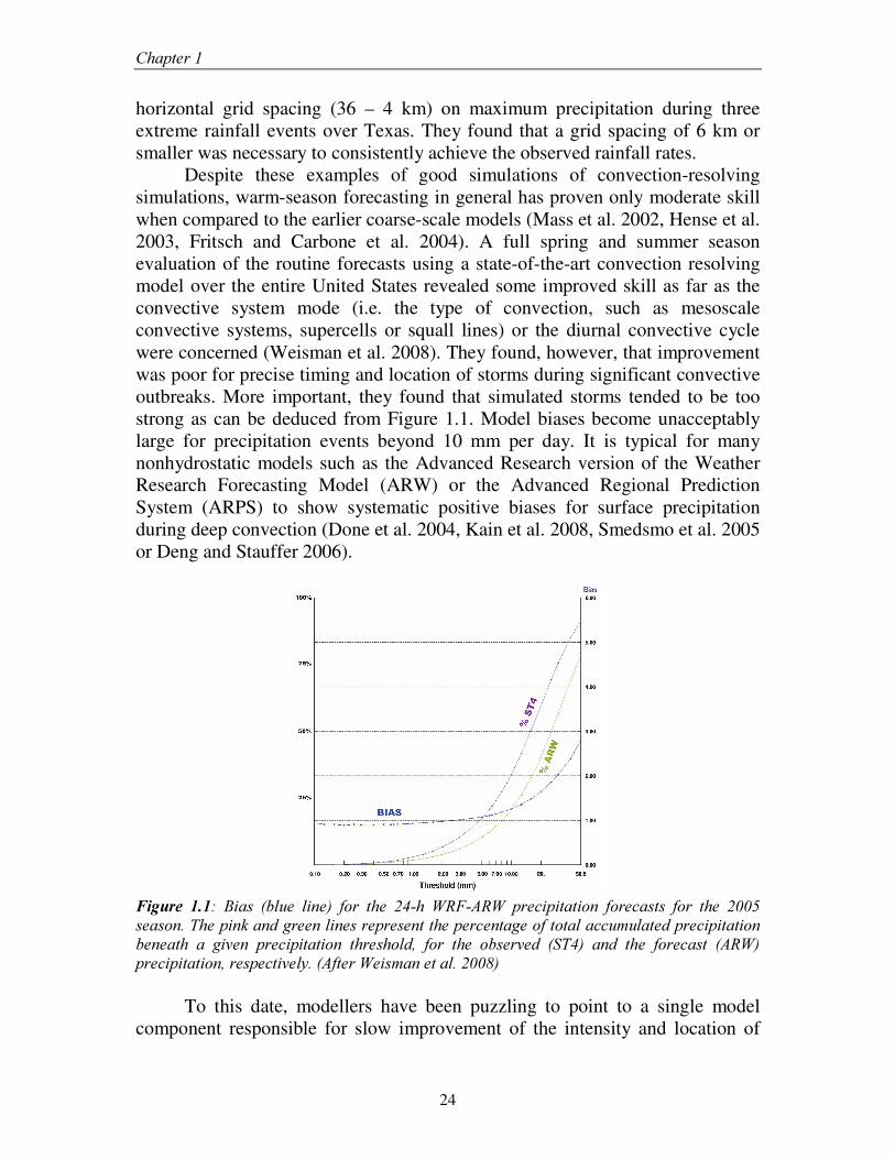
Despite these examples of good simulations of convection-resolving simulations, warm-season forecasting in general has proven only moderate skill when compared to the earlier coarse-scale models (Mass et al. 2002, Hense et al. 2003, Fritsch and Carbone et al. 2004). A full spring and summer season evaluation of the routine forecasts using a state-of-the-art convection resolving model over the entire United States revealed some improved skill as far as the convective system mode (i.e. the type of convection, such as mesoscale convective systems, supercells or squall lines) or the diurnal convective cycle were concerned (Weisman et al. 2008). They found, however, that improvement was poor for precise timing and location of storms during significant convective outbreaks. More important, they found that simulated storms tended to be too strong as can be deduced from Figure 1.1. Model biases become unacceptably large for precipitation events beyond 10 mm per day. It is typical for many nonhydrostatic models such as the Advanced Research version of the Weather Research Forecasting Model (ARW) or the Advanced Regional Prediction System (ARPS) to show systematic positive biases for surface precipitation during deep convection (Done et al. 2004, Kain et al. 2008, Smedsmo et al. 2005 or Deng and Stauffer 2006).
)LJXUH� ����� %LDV� �EOXH� OLQH�� IRU� WKH� ���K� :5)�$5:� SUHFLSLWDWLRQ� IRUHFDVWV� IRU� WKH� �����VHDVRQ��7KH�SLQN�DQG�JUHHQ�OLQHV�UHSUHVHQW�WKH�SHUFHQWDJH�RI�WRWDO�DFFXPXODWHG�SUHFLSLWDWLRQ�EHQHDWK� D� JLYHQ� SUHFLSLWDWLRQ� WKUHVKROG�� IRU� WKH� REVHUYHG� �67��� DQG� WKH� IRUHFDVW� �$5:��SUHFLSLWDWLRQ��UHVSHFWLYHO\���$IWHU�:HLVPDQ�HW�DO��������
To this date, modellers have been puzzling to point to a single model component responsible for slow improvement of the intensity and location of
,QWURGXFWLRQ�
25
simulated storms within convection-resolving atmospheric models. Some authors have suggested that KRUL]RQWDO� RU� YHUWLFDO� JULG� VSDFLQJ is still insufficient to fully resolve convection, hence forcing the convection on coarser-than-natural scales (e.g. Deng and Stauffer 2006). Adlerman and Droegemeier (2002) showed that simulated storms did not produce observed cyclic cell regeneration until grid spacing dropped below 1.5 km. Bernadet et al (2000) found that a 2 km grid spacing was necessary to capture convection explicitly. Bryan et al. (2003) analyzed energy spectra of sub-grid energy and water fluxes and concluded that model grid spacing up to 1 km is still insufficient to faithfully simulate deep convection, although the quantitative and qualitative differences between their 1 km and 125 m simulations were still much less than the differences Weisman et al (1997) noted between their experiments using 4 km and 12 km horizontal grid spacing.
Other authors point to the VXE�JULG� VFDOH� PRGHO� SK\VLFV as a main candidate for model improvement. Many of the processes that cannot be resolved by the model grid itself, such as precipitation formation or small turbulent eddies, are too important to be neglected and need to be parameterized. Many authors have investigated the influence of the form of the precipitation size distribution in the precipitation formation parameterization (microphysics parameterization). Mainly concerning the largest precipitation species, hail or graupel, considerable difference exists among different studies. While Gilmore et al. (2004) found differences in accumulated surface precipitation up to 380 % varying the characteristics of the largest precipitation species from small graupel to large hail, McCumber et al. (1991), van den Heever and Cotton (2004) and Cohen and McCaul (2006) found much smaller sensitivities ranging from 0 to 30 %. The vertical distribution of precipitation types (snow, hail or rain) changed significantly in all studies. Milbrandt and Yau (2006) found a strong reduction in surface precipitation using a more advanced representation of the size distribution characteristics in the simulation of a hail storm, but did not verify their results against observational data. Lynn et al. (2001) have shown that a more advanced representation of sub-grid scale turbulence within a convection-resolving model was the only way to realistically represent an observed mesoscale convective system over Florida. Wisse and de Arellano (2004) showed for a severe convective storm over Spain that the positive bias of the surface precipitation remained in all three simulations using different approaches to represent sub-grid scale turbulence although differences up to 20 % in accumulated surface precipitation could be found between the different simulations.
Yet another candidate for errors in the representation of moist convection mentioned by many studies is the representation of ODQG�VXUIDFH�SURFHVVHV�DQG�LQLWLDO�VRLO�YDULDEOHV. Holt et al. (2006) stated that a more detailed representation of land surface processes should be included in weather forecasting models, particularly for severe storm forecasting where local-scale information is
&KDSWHU���
26
important. Cheng and Cotton (2004) performed simulations of a mesoscale convective system using initial soil moisture datasets with varying detail and found that soil moisture datasets with 40-km grid spacing are sufficient to initialize their convection-resolving model. Trier et al. (2008) investigated the importance of both land surface-atmosphere feedback processes and the initial land surface conditions on precipitation during a 12-day period over the mid-west United States. They found that although systematic differences occurred in regional precipitation frequencies in the different simulations, no single simulation most accurately reproduced the observed diurnal cycle of precipitation at all times.
Some authors have speculated on the influence of inaccuracies in the QXPHULFDO� WHFKQLTXHV employed to solve the prognostic equations on the representation of moist processes in atmospheric models. Braun (2006) performed a water budget analysis of hurricane Bonnie and found out that due to inaccuracies in the advection process, total water mass in the model was not conserved and about 15-20 % artificial water was created. Skamarock and Weisman (2009) found out that surface precipitation was increased by about 30 % for the same reason during the simulation of two severe convective events.
At last, part of the explanation of slow progress in km-scale modelling of intense convection might be related to FRQFHSWXDO�SUREOHPV�LQ�FRQYHFWLRQ�PRGHO�SK\VLFV. Currently, numerical models of the atmosphere have a modular structure in which the individual physical processes are coupled with the dynamical core and hence interacting through the model’ s prognostic variables. Hence, small-scale interactions between those processes (e.g. between microphysics and small-scale turbulence) are missing. Moreover, numerical models artificially separate the spectrum of processes at different scales in a resolved and an unresolved part. As the model physics to deal with this separation is specifically designed and tuned for a certain range of resolutions, the model solution does not naturally converge to the solution of the real atmosphere as the resolution is refined (Arakawa 2004). First efforts to improve interactions between different physical processes and to make the treatment of processes more consistent at various resolutions from fully sub-grid to fully explicit are on the way. Piriou et al. (2007) for instance, proposed a Microphysics and Transport Convective Scheme (MTCS), enabling more direct interaction between convective processes and microphysics. Gerard et al. (2009) developed an integrated sequential treatment of resolved condensation, deep convection and microphysics, using prognostic variables and allowing consistent results from tens of kilometres up to 2 km. Such approaches seem to be promising but operational forecasting is still far from a unification of all physical parameterizations as proposed by Arakawa (2004).
From the overview above it is clear that when turning to the km-scales,
we enter a multifaceted problem which we currently do not quite understand. In
,QWURGXFWLRQ�
27
fact, this has led to a spirited debate whether increased computational resources should be primarily used to continue the trend to higher resolution and more advanced physics in operational weather forecasting or to integrate large ensembles of forecasts at lesser resolution to produce probabilistic forecasts (Mass et al. 2002). On the short term, most gain in the precipitation forecast will probably originate from such improved probabilistic techniques and data assimilation. Probabilistic ensemble forecasts are based on multiple integrations of the same model, using different initial conditions, boundary conditions or even model physics and are at this moment even performed for high resolution models (e.g. Schwartz et al., 2010). Data assimilation techniques try to combine the observed and simulated variable fields in order to obtain a ‘best estimate’ of the current state. Ongoing progress is made in both the applied statistical techniques (e.g. Caumont et al. 2010) and in the available data to be used for assimilation, such as radar (e.g. Chung et al. 2009) or satellite (e.g. Stengel et al. 2009). Although it is possible to increase forecast skill through application of statistical techniques alone (e.g. Gebhardt 2008), without new understanding of the (micro)physics of precipitation or a better implementation of known physical relations, the overall improvement on the longer term will remain limited and will likely remain below the practical limits of predictability (Fritsch and Carbone 2004).
������5HPRWH�VHQVLQJ�RI�LQWHQVH�SUHFLSLWDWLRQ� A major problem for the improvement of the quantitative precipitation
forecast is that it is an end-product of an enormously vast number of processes at different scales, hard to trace in complex models and hard to evaluate against sparse observational data. Recently, more and more spatially distributed observational data, sensed by airborne or ground-based devices, became available to the modelling community for model evaluation. Weather radar is able to sense the precipitation phase at very high temporal (up to 5 minutes) and spatial (up to 500 m) resolution, although it is still not always straightforward to relate the returned radar signal to quantitative information on the precipitation phase. Cloud satellites provide detailed information on the cloud phase over large domains and at high spatial resolution (up to a few kilometres). Temporal resolution is typically somewhat lower as compared to weather radar and ranges from once a day for polar-orbiting satellites to a one hour interval for geo-stationary satellites. Over the past decade, many institutes have developed increasingly reliable methods to derive quantitative information from satellite observations on cloud properties, such as cloud optical thickness, cloud top height and integrated water quantities.
Newly emerging spatially distributed observational datasets, such as weather radar and cloud satellite, allow for a detailed quantitative comparison
&KDSWHU���
28
against simulated moisture fields from convection-resolving models. Previous studies on improvement of the quantitative precipitation forecast have been often based on idealized model experiments (i.e. initialized from a horizontally homogeneous atmosphere without observed or forecast large-scale atmospheric or surface data ingestion), allowing for unambiguous interpretation. However, only by performing real-case experiments (i.e. initialized from observed or forecast large-scale atmospheric data ingestion and applying real surface characteristics) and in depth-evaluation against all available observational data, it can be understood if models improve for the right reasons.
������5HVHDUFK�JRDOV�
In this research, three severe precipitation case studies observed over Belgium were selected to perform a broad number of sensitivity experiments dealing with aspects mentioned in the previous paragraphs as candidates for introducing uncertainty in the quantitative precipitation forecast. The focus of this thesis is on extreme events as the context of this work is the problematic forecasting of precipitation for purposes controlled by the intense precipitation events, such as erosion modelling and hydrology and flood forecasting. Subsequently, it was investigated if the main conclusions from these case studies could be consolidated for two samples of events (further referred to as composites) containing a larger number of stratiform and convective cases respectively. Case studies have the advantage over long-term simulations (or composites of many cases) that they can be investigated in a much more detailed physical way, leading to the development of physically based hypotheses which can be evaluated against observational data. Long-term simulations on the other hand can indicate if hypotheses set up from the case studies can be generalized.
The ultimate research goal of this dissertation is to determine which of a number of investigated processes can be held responsible for deficiencies in the simulation of moist processes and surface precipitation during intense precipitation events using a convection-resolving atmospheric model over Belgium. It should be stressed that the aim is not to directly propose clear model improvements in terms of the convective precipitation forecast, but to assess the sensitivity of the model to certain important aspects of the precipitation formation process. Such research is crucial in order to gain understanding of the complex problem of convection-resolving precipitation forecasting. More specifically, six research questions will be answered:
- ���� +RZ� GR� XQFHUWDLQWLHV� GXH� WR� ODQG� VXUIDFH� SURFHVVHV��
KRUL]RQWDO� JULG� VSDFLQJ� DQG� PLFURSK\VLFDO� VL]H� GLVWULEXWLRQ�DVVXPSWLRQV� LQWHUUHODWH" Many of the aforementioned studies have been dedicated to a one of these issues, but it has been rarely
,QWURGXFWLRQ�
29
investigated how uncertainties introduced to these processes interrelate during the same atmospheric conditions.
- ����'R�PRUH�UHDOLVWLF�SUHFLSLWDWLRQ�VL]H�GLVWULEXWLRQ�DVVXPSWLRQV�LQ� D� EXON� PLFURSK\VLFV� VFKHPH� \LHOG� D� PRUH� UHDOLVWLF�UHSUHVHQWDWLRQ� RI� WKH� PRLVW� SURFHVVHV� LQ� FRQYHFWLRQ� UHVROYLQJ�PRGHOV"�&DQ�QHZO\�DYDLODEOH�KLJK�UHVROXWLRQ�REVHUYDWLRQDO�GDWD�EULQJ� QHZ� LQVLJKWV� LQ� WKH� UHSUHVHQWDWLRQ� RI� PRLVW� SURFHVVHV� LQ�WKRVH�PRGHOV"��
- ����+RZ�FDQ�FRQWUDGLFWLQJ�UHVXOWV��UHSRUWHG� LQ� OLWHUDWXUH�RI�ERWK�WKH� LQIOXHQFH� RI� LQLWLDO� VRLO� PRLVWXUH� DQG� PLFURSK\VLFDO� VL]H�GLVWULEXWLRQ�DVVXPSWLRQV��EH� H[SODLQHG"�$UH� WKHVH�SULPDULO\�GXH�WR�GLIIHUHQFHV�LQ�H[SHULPHQWDO�GHVLJQV��DWPRVSKHULF�FRQGLWLRQV�RU�PRGHO�FRPSOH[LW\"�
- ����+RZ�GR�WKH�DUWLILFLDO�VRXUFH�WHUPV�IRU�FORXG�DQG�SUHFLSLWDWLRQ�PDVV��DVVRFLDWHG�ZLWK�WKH�VHWWLQJ�WR�]HUR�RI�QHJDWLYH�PL[LQJ�UDWLRV�WKDW� DULVH� IURP� QXPHULFDO� DGYHFWLRQ� HUURUV�� DIIHFW� WKH� ZDWHU�EDODQFH�DQG�WKH�VXUIDFH�SUHFLSLWDWLRQ�LQ�WKH�PRGHO"�
- ����:KLFK�RI�WKH�LQYHVWLJDWHG�SURFHVVHV�KDV�WKH�ODUJHVW�SRWHQWLDO�WR� LPSURYH� TXDQWLWDWLYH� SUHFLSLWDWLRQ� IRUHFDVW� LQ� WKH� WKUHH� FDVH�VWXGLHV"� 'R� WKHVH� LPSURYHPHQWV� VWLOO� KROG� IRU� D� ORQJ�WHUP�VLPXODWLRQ"��
- ���� :KDW� FDQ� EH� JDLQHG� IURP� SHUIRUPLQJ� FRQYHFWLRQ�UHVROYLQJ�VLPXODWLRQV� RI� H[WUHPH� SUHFLSLWDWLRQ� HYHQWV� DV� FRPSDUHG� WR�FRDUVHU�UHVROXWLRQ�VLPXODWLRQV"�
�����2XWOLQH�
This dissertation is structured in two main parts. A first part (including chapters 1 to 3) reviews a number of observational and modelling aspects of the precipitation process, relevant for interpreting the results of a number of sensitivity experiments evaluated in the second part (consisting of chapters 4 to 8). Each chapter of the second part of this thesis has been written as research paper and was published or submitted to international scientific journals, apart from chapter 7. At the beginning of each of the chapters which are based on submitted or published work, a footnote indicates the paper on which they are based and mentions the current status of the paper. Since each of the papers was intended to read independently, some overlap may occur between the various chapters. The current chapter provides a general background introducing concepts and research goals discussed in the forthcoming chapters.
&KDSWHU���
30
Chapter 2 gives an overview of current insights in the observed dynamical and microphysical aspects of the precipitation process. First, the dynamical aspects of convective and stratiform precipitation are discussed. This is followed by an overview of observed microphysical aspects of precipitation, providing a basis upon which numerical models build to simulate the precipitation formation processes.
Chapter 3 introduces the concept of nonhydrostatic modelling and provides a short review on the apparent contradictions found in literature on the influence of two parameterizations on the quantitative precipitation forecast, namely the land surface-atmosphere interaction and the microphysics parameterization. Furthermore, the model details and setup used in this dissertation are explained, followed by an overview of how the surface and microphysical processes are parameterized in this model. Finally, synoptic and mesoscale aspects of three case studies are described.
Chapter 4 answers research question 1 and a part of research question 3. It is investigated how uncertainties in the quantitative precipitation forecast due to moist surface properties, assumptions on precipitation particle size distributions in the bulk microphysics scheme, and horizontal grid spacing interrelate. Furthermore, it is discussed if and why these modifications have potential of bringing significant improvements in the numerical representation of the moist processes during extreme convective cases.
Chapter 5 answers research question 2 and determines whether more realistic assumptions of the precipitation particle size distributions in the model bulk microphysics scheme result in a more realistic representation of the simulated moist processes, using a broad number of high resolution observational data.
Chapter 6 answers research questions 3 and 4. It is investigated whether the degree of sophistication between previously conducted studies to particle size distributions are responsible for differences found in literature. Furthermore, it is estimated to what extent artificial water due to inaccuracies in the model advection scheme leads to non-conserved water mass in the model and what the consequences are for the simulated surface precipitation.
Chapter 7 answers research questions 5 and 6 and deals with the analysis of a large composite of extreme precipitation events performed to understand if hypotheses posed by the previous chapters are still valid during other cases.
Finally, Chapter 8 summarizes the results in a general conclusion and prospects for further research.

,QWURGXFWLRQ�
31
Within this dissertation, an attempt has been made to gradually introduce certain aspects (i.e. the precipitation formation process and size distributions) of observed precipitation and how these are implemented in models. It is, however, not always feasible to give a full understanding of all terms or concepts within each chapter, so a glossary of terms used in this dissertation can be found in Appendix A.
������������������������������������

32
�������������������������������������������
33
����������
&KDSWHU������
2EVHUYHG�SUHFLSLWDWLRQ�FKDUDFWHULVWLFV�
Generally, precipitation is classified as stratiform, associated with large
scale air mass uplift due to baroclinic instability or as convective, associated with localized updrafts in conditionally unstable air. Both types of precipitation eventually originate from condensation processes due to cooling of moist air. Hence the precipitation process involves condensation associated with G\QDPLFDO� DVSHFWV and precipitation formation associated with PLFURSK\VLFDO�DVSHFWV, such as conversions of non-precipitating hydrometeors (i.e. type of condensed water – cloud water, cloud ice …) to downward sedimenting hydrometeors (e.g. rain, snow, graupel, hail …). Both aspects will be discussed in more detail in the following sections. Much of this chapter is meant to provide a solid background for non-specialists in atmospheric sciences, necessary for the interpretation of the remainder of this thesis. Section 2.2.2 is intended as a review chapter on observed size distribution characteristics.
������'\QDPLFDO�DVSHFWV�RI�SUHFLSLWDWLRQ�
2.1.1. Stratiform precipitation
Stratiform precipitation at mid-latitudes is mostly associated with large-scale extra-tropical cyclones embedded in baroclinic waves (Wallace and Hobbs 2006). These waves develop easily in the mid-latitudes as instabilities due to the strong meridional temperature gradient in these areas and are visible on 500 hPa
&KDSWHU���
34
pressure maps as successive ridges and troughs. Areas in the upward branch of such troughs are associated with upper-level divergence and hence favour cyclogenesis at the surface. Sharp horizontal gradients, denoted as fronts, develop in the surface cyclones as warm moist air is gradually rising over the colder airmasses. As air masses are dynamically forced to rise, they decompress and cool, leading to massive condensation.
2.1.2. Convective precipitation
Deep moist convection occurs as localized phenomena associated with conditionally unstable atmospheres. In contrast to frontal stratiform precipitation, the horizontal scale of convection is much smaller than that of baroclinic waves and its timescale much shorter (Wallace and Hobbs 2006). Only two environmental parameters are particularly important for the storm evolution and its structure (Weisman and Klemp 1982), being the buoyancy (vertical motions associated with thermodynamic instability) and the vertical wind shear (change of direction and speed of wind with height).
Necessary ingredients for strong buoyancy are the existence of conditionally unstable lapse rates (indicating that the vertical temperature gradient of the atmosphere is between the dry adiabatic gradient (9.8 × 10⁻³ K m-1) and the moist adiabatic gradient (6.0 × 10⁻³ K m-1)), substantial boundary-layer moisture and sufficient lifting (e.g. due to surface wind and moisture convergence) to release the instability (Wallace and Hobbs 2006). The total amount of buoyant energy available for a particular air parcel is called the convective available potential energy (CAPE), which provides a measure of the maximum possible kinetic energy that a statically unstable air parcel can acquire (neglecting effects of water vapour and condensed water on the buoyancy), assuming that the parcel ascends without mixing with the environment and adjusts instantaneously with the local environmental pressure (Holton 2004). It can be shown that CAPE is equal to the integral:
G]777J&$3(
������������������ �
�����������
−= ∫ (2.1),
where zLFC is the level of free convection, zLNB is the level of neutral buoyancy, g is the gravitation acceleration, Tparcel is the parcel temperature (following the adiabatic lapse rate) and Tenv is the temperature of the environment. The higher CAPE becomes the more energy for vertical motions and hence decompression, cooling and condensation is available to the rising parcel. In case of an atmosphere without significant changes of wind speed or direction with height (i.e. vertical wind shear), a rain-evaporation induced cold
2EVHUYHG�SUHFLSLWDWLRQ�FKDUDFWHULVWLFV�
35
surface outflow develops within the hour and spreads axisymmetrically away from the storm. This effectively cuts off the warm inflow to the updraft and quickly leads to the decline of the storm (Weismand and Klemp 1982). When strong wind shear exists however, the updraft is tilted and is effectively separated from the downdraft. A symbiotic relationship develops in which updraft and downdraft develop into a clear circulating cell which leads to longer lived storms capable of producing large hail and strong surface winds (Wallace and Hobbs 2006). Based upon the characteristics of buoyancy and vertical wind shear, storms can be classified in several types. Conditions with moderate buoyancy and no shear favour the development of single-cell or pulse storms. As soon as rain-evaporative cooling becomes large enough to induce a downdraft, the updraft is effectively cut-off from the surface and storms decay quickly. Hence they are short-lived and rarely produce destructive winds or hail. When moderate vertical wind shear is present, multi-cell storms develop. New cells are continuously initiated at the outflow boundary of older cells, leading to the development of a longer-lived entity of clustered storms. Due to the longer lifetime of these storms, high accumulations of surface precipitation might occur. Supercells develop in strongly sheared conditions and have the tendency to develop a rotating mesocylone from an initially non-rotating environment. This is due to the fact that horizontal vorticity (associated with the vertical wind shear) is tilted by a strong updraft and converted into vertical vorticity, leading to a rotating updraft. Supercells last many hours and are associated with severe wind phenomena and large hail. All of these thunderstorm types occur in mid-latitudes in Europe and the United States. In Western Europe, which is the main area of interest of the forthcoming study, tornado-producing supercells are associated with strong low-level wind shear and moderate amounts of CAPE (Groenemeijer and van Delden, 2007).
������0LFURSK\VLFDO�DVSHFWV�RI�SUHFLSLWDWLRQ�
2.2.1. Precipitation formation processes
Not all condensate precipitates towards the surface. Most condensed water even re-evaporates to the vapour phase. In a typical thunderstorm, only 19 % of all condensed water which is ingested in the storm eventually ends up as surface precipitation (Braham 1952).
Two mechanisms exist to turn condensed water to precipitation. The collision and coalescence process is believed to be the main process of precipitation formation in warm clouds (having a temperature above freezing at all levels). This process originates from differential fall velocities of cloud droplets with different sizes (e.g. due to different sizes of condensation nuclei).
&KDSWHU���
36
Larger drops grow larger by overtaking smaller drops. Warm clouds typically need to be thicker than 500 m to produce any measurable surface precipitation.
Most mid-latitude precipitating clouds are so-called cold clouds, having cloud tops well below freezing. In such cold clouds liquid water droplets are still much more numerous than ice crystals at air temperatures above -20 °C. Only at temperatures below -40 °C almost all water occurs as crystals. Ice crystals initiate by direct deposition of vapour on deposition nuclei or by homogeneous freezing of liquid droplets and might grow initially by further deposition of vapour or by contact freezing of supercooled droplets. This leads to the co-existence of ice crystals and supercooled cloud droplets mainly at air temperatures between -30 °C and -10 °C. Saturation vapour pressure above a water surface is greater than de saturation vapour pressure above an ice surface however. In a saturated environment, such as a cloud, this difference causes the water molecules to diffuse naturally from the droplets to the ice crystals leading to crystal growth. As the uptake of vapour from the droplet by the crystal causes subsaturation around the droplet, additional evaporation of the droplet occurs. This process provides a continuous source of moisture for the ice crystal yielding the ice crystals to grow larger at the expense of surrounding water droplets. This process is the main precipitation formation process in cold clouds and is often called the Bergeron process (Ahrens, 2003).
2.2.2. Size distribution characteristics
The coalescence and the ice crystal growth process described above lead to the occurrence of a mixture of cloud droplets, rain drops, ice crystals and snow flakes with a broad range of sizes in cold clouds. Typically, these particles can be characterized by three quantities (Pruppacher and Klett 2003): their equivalent drop diameter ' ��� , size distribution Q�' ��� � (expressed as the number of drops per volume) and the precipitation intensity 5. Most relevant for the parameterization of precipitation processes is the size distribution of each hydrometeor.
2.2.2.1. Size distribution characteristics of rain The rain size distribution has typically been represented by a negative
exponential size distribution (Marshall and Palmer 1948, Okita 1958, Müller 1966, Sekhorn and Srivastava 1971, Beard et al. 1986, Rauber et al. 1991 and Willis and Hallett 1991) yielding:
)exp()( 0 ���� '1'1 λ−= , (2.2)
2EVHUYHG�SUHFLSLWDWLRQ�FKDUDFWHULVWLFV�
37
where 1R is the number of particles per unit volume per unit size range, '0R is the equivalent drop diameter and 10R and R are the intercept and slope of the exponential size distribution, respectively. Other fitting functions have been proposed, such as gamma distributions (Ulbrich 1983, Willis 1984 or Willis and Tattelman 1989) or lognormal distributions (Bradley and Stow 1974 or Markowiz 1976).
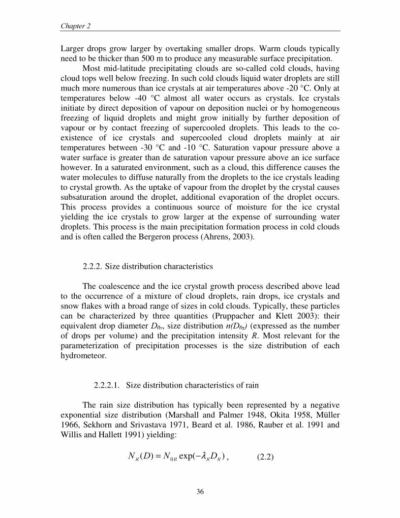
Rain size distributions tend to vary strongly between different types of precipitation or even within a single storm. Zhang et al. (2008) presented disdrometer-derived rain size distributions for a number of storms in Oklahoma (US). They found significant differences between the size distributions of different storms (Figure 2.1). Brandes et al. (2006) showed that initially strong convective rain usually contains both large and small drops, and hence has a broad size distribution. In its decaying phase, size distributions of storms are dominated by small drops. Stratiform rain usually has larger drops, but has lower number concentration for a given rain rate.
Marshall and Palmer (1948) found N0R to be constant at 8 × 10⁶ m-4. Waldvogel (1974) however, was the first one to show order of magnitude variations in N0R. Recent observational studies, e.g. by Zhang et al. (2008) could relate the N0R to the mixing ratio of rain.
)LJXUH������5DLQGURS�VL]H�GLVWULEXWLRQV�DQG�WKHLU�ILW�WR�WKH�H[SRQHQWLDO�GLVWULEXWLRQ�IRU�VWURQJ�FRQYHFWLRQ��ZHDN�FRQYHFWLRQ�DQG�VWUDWLIRUP�UDLQ�GHULYHG�IURP�GLVGURPHWHU�PHDVXUHPHQWV�LQ�2NODKRPD��86���=KDQJ�HW�DO�������
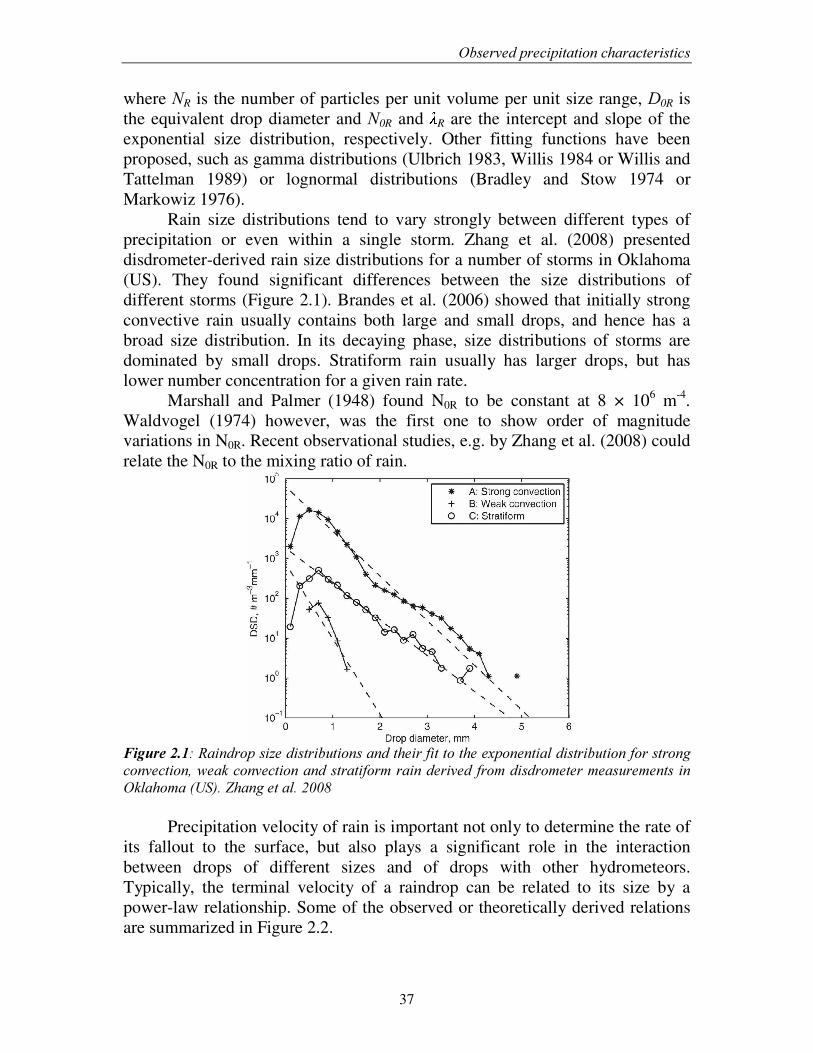
Precipitation velocity of rain is important not only to determine the rate of its fallout to the surface, but also plays a significant role in the interaction between drops of different sizes and of drops with other hydrometeors. Typically, the terminal velocity of a raindrop can be related to its size by a power-law relationship. Some of the observed or theoretically derived relations are summarized in Figure 2.2.
&KDSWHU���
38
)LJXUH� ����� 5DLQGURS� WHUPLQDO� YHORFLWLHV� YHUVXV� GURS� GLDPHWHU� DFFRUGLQJ� WR� GLIIHUHQW�REVHUYDWLRQDO�VWXGLHV��
2.2.2.2. Size distribution characteristics of snow
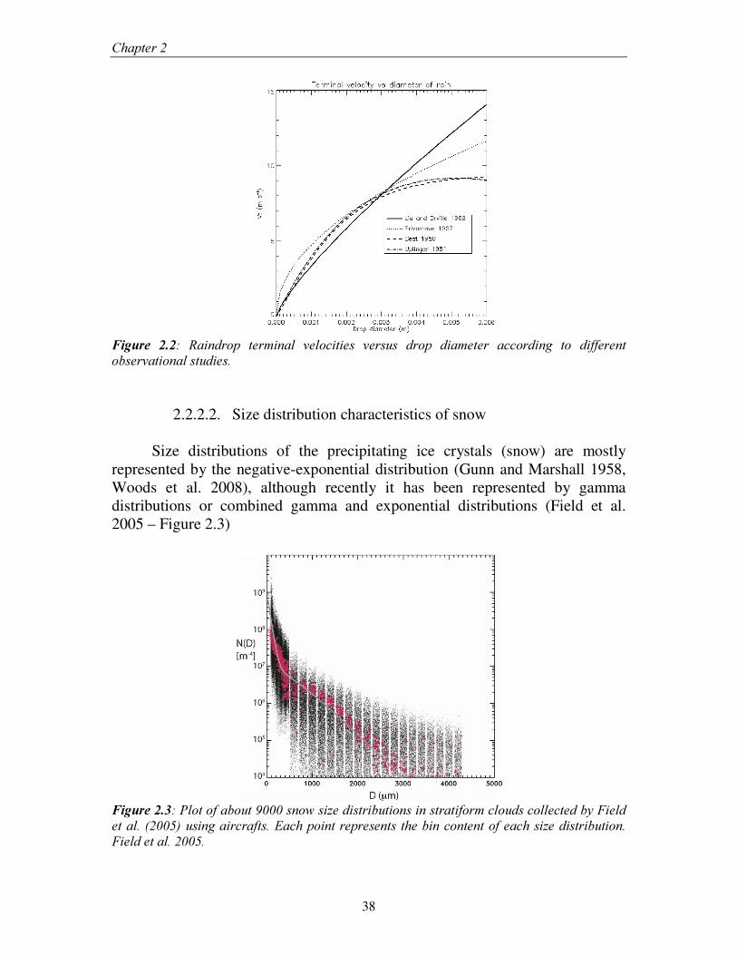
Size distributions of the precipitating ice crystals (snow) are mostly represented by the negative-exponential distribution (Gunn and Marshall 1958, Woods et al. 2008), although recently it has been represented by gamma distributions or combined gamma and exponential distributions (Field et al. 2005 – Figure 2.3)
)LJXUH������3ORW�RI�DERXW������VQRZ�VL]H�GLVWULEXWLRQV�LQ�VWUDWLIRUP�FORXGV�FROOHFWHG�E\�)LHOG�HW�DO���������XVLQJ�DLUFUDIWV��(DFK�SRLQW�UHSUHVHQWV�WKH�ELQ�FRQWHQW�RI�HDFK�VL]H�GLVWULEXWLRQ��)LHOG�HW�DO��������
2EVHUYHG�SUHFLSLWDWLRQ�FKDUDFWHULVWLFV�
39
From Figure 2.3 it is clear that, as for the rain size distribution, large variations can be found in the snow size distribution. Houze et al. (1979) and Field (1999) found large variations with height (and hence temperature) within clouds. At cloud tops, particles were small, while they became progressively larger with decreasing height. For cloud regions warmer than -15 °C aggregation of snow flakes becomes a main growth mechanism, leading to rapidly increasing average crystal diameters (Field 1999). Early observational studies (e.g. Gun and Marshall 1958) proposed a constant value of 3 × 10⁶ m-4 for the intercept parameter of the snow size distribution. Houze et al. (1979) however showed that the intercept tends to vary with the temperature, yielding smaller intercepts at warmer temperatures due to aggregation growth of the snow, while Sekhon and Srivastava (1970) found N0S to be proportional to the snow precipitation rate.
Density of precipitating ice crystals, unlike the constant rain density, tends to vary from 5 to 500 kg m-3, depending on snow habit, size or degree of riming (Pruppacher and Klett 2003). Many authors have derived relations between mass and diameter and velocity and diameter for different snow types around the world. Mostly, these relations can be represented by a power law of the form:
����� 'DP = , (2.3)
�� 'F9 = , (2.4)
where mS is the snow mass (kg), DS is the characteristic diameter (m), VS is the terminal fall velocity (m s-1) and aS, bS, cS and dS are constants.
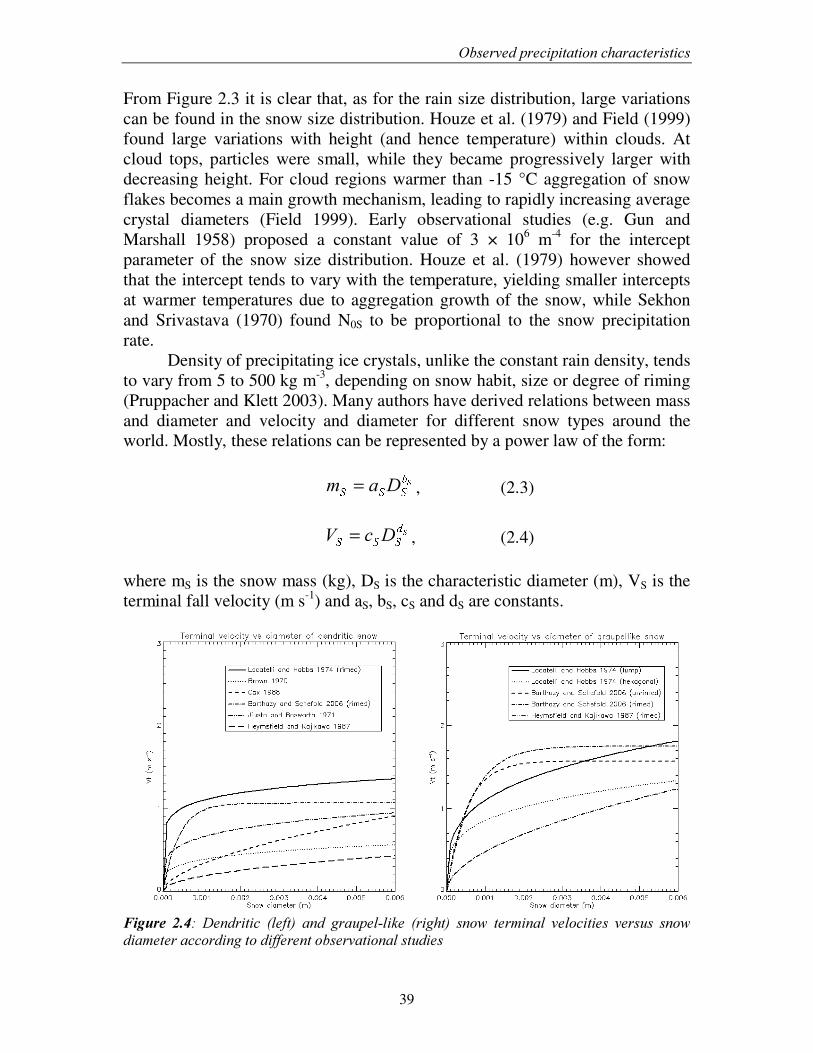
)LJXUH� ����� 'HQGULWLF� �OHIW�� DQG� JUDXSHO�OLNH� �ULJKW�� VQRZ� WHUPLQDO� YHORFLWLHV� YHUVXV� VQRZ�GLDPHWHU�DFFRUGLQJ�WR�GLIIHUHQW�REVHUYDWLRQDO�VWXGLHV�
&KDSWHU���
40
Terminal fall velocity of snow flakes depends strongly on the shape and habit characteristics of the snow. A number of commonly used VS-DS relations for dendritic snow and graupel-like snow are summarized in Figure 2.4. Graupel-like snow on average falls about twice as fast when compared to dendritic snow flakes.
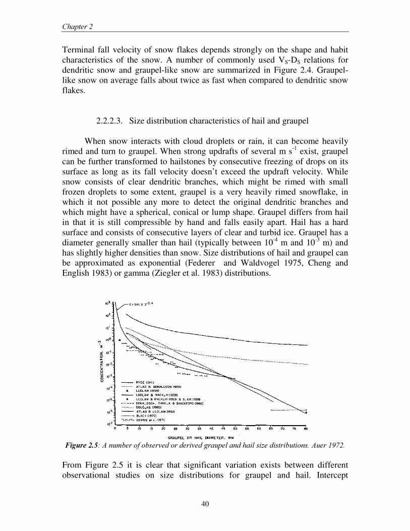
2.2.2.3. Size distribution characteristics of hail and graupel When snow interacts with cloud droplets or rain, it can become heavily rimed and turn to graupel. When strong updrafts of several m s-1 exist, graupel can be further transformed to hailstones by consecutive freezing of drops on its surface as long as its fall velocity doesn’ t exceed the updraft velocity. While snow consists of clear dendritic branches, which might be rimed with small frozen droplets to some extent, graupel is a very heavily rimed snowflake, in which it not possible any more to detect the original dendritic branches and which might have a spherical, conical or lump shape. Graupel differs from hail in that it is still compressible by hand and falls easily apart. Hail has a hard surface and consists of consecutive layers of clear and turbid ice. Graupel has a diameter generally smaller than hail (typically between 10-4 m and 10-3 m) and has slightly higher densities than snow. Size distributions of hail and graupel can be approximated as exponential (Federer and Waldvogel 1975, Cheng and English 1983) or gamma (Ziegler et al. 1983) distributions.
)LJXUH������$�QXPEHU�RI�REVHUYHG�RU�GHULYHG�JUDXSHO�DQG�KDLO�VL]H�GLVWULEXWLRQV��$XHU������� From Figure 2.5 it is clear that significant variation exists between different observational studies on size distributions for graupel and hail. Intercept
2EVHUYHG�SUHFLSLWDWLRQ�FKDUDFWHULVWLFV�
41
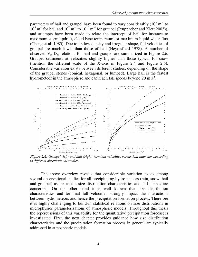
parameters of hail and graupel have been found to vary considerably (103 m-4 to 105 m-4 for hail and 107 m-4 to 1010 m-4 for graupel (Pruppacher and Klett 2003)), and attempts have been made to relate the intercept of hail for instance to maximum storm updraft, cloud base temperature or maximum liquid water flux (Cheng et al. 1985). Due to its low density and irregular shape, fall velocities of graupel are much lower than those of hail (Heymsfield 1978). A number of observed VH-DH relations for hail and graupel are summarized in Figure 2.6. Graupel sediments at velocities slightly higher than those typical for snow (mention the different scale of the X-axis in Figure 2.4 and Figure 2.6). Considerable variation exists between different studies, depending on the shape of the graupel stones (conical, hexagonal, or lumped). Large hail is the fastest hydrometeor in the atmosphere and can reach fall speeds beyond 20 m s-1.
)LJXUH������*UDXSHO��OHIW��DQG�KDLO��ULJKW��WHUPLQDO�YHORFLWLHV�YHUVXV�KDLO�GLDPHWHU�DFFRUGLQJ�WR�GLIIHUHQW�REVHUYDWLRQDO�VWXGLHV��
��
The above overview reveals that considerable variation exists among several observational studies for all precipitating hydrometeors (rain, snow, hail and graupel) as far as the size distribution characteristics and fall speeds are concerned. On the other hand it is well known that size distribution characteristics and terminal fall velocities strongly impact the interactions between hydrometeors and hence the precipitation formation process. Therefore it is highly challenging to build-in statistical relations on size distributions in microphysics parameterizations of atmospheric models. Throughout this thesis the repercussions of this variability for the quantitative precipitation forecast is investigated. First, the next chapter provides guidance how size distribution characteristics and the precipitation formation process in general are typically addressed in atmospheric models.�
�

42
�������������������������������������������
43
�������� �
&KDSWHU������
0RGHOOLQJ�RI�SUHFLSLWDWLRQ�
������1RQK\GURVWDWLF�PRGHOOLQJ�RI�SUHFLSLWDWLRQ�
�Atmospheric models are designed to simulate the dynamical evolution of
the global or regional atmosphere, based on the fundamental set of conservation principles. Any atmospheric model should conserve mass, heat, motion, water and other gaseous or aerosol materials (Pielke 2002). These principles form a coupled set of relations that must be satisfied simultaneously and that include sources and sinks in the individual expressions. Typically, these equations are solved on a discretized grid with spatial resolutions of 1 to 100 km. Coarse-scale models, such as climate models or global forecasting models mostly replace the vertical momentum equation by the hydrostatic approximation, which states that the vertical pressure gradient is always equal to the product of density and the gravitational acceleration (Pielke 2002). This means that vertical accelerations are neglected compared to vertical pressure gradients and vertical buoyancy forces. This might be a good approximation for synoptic-scale systems but for a proper simulation of convective storms, in which as much of the internal circulations (discussed in section 2.1.2) as possible should be resolved, this hydrostatic approximation is not valid any more and the vertical momentum equation should be included. Therefore, such models are called QRQK\GURVWDWLF models. This dissertation aims at providing insight in the reasons for model deficiencies of the quantitative precipitation forecast as soon grid spacing becomes small enough to resolve internal storm circulations and hence we implement the Advanced Regional Prediction System (ARPS), a state-of-the-art
&KDSWHU���
44
nonhydrostatic research model developed by the Oklahoma University and discussed in section 3.2, during the remainder of this dissertation.
The conservation equations of any atmospheric model contain terms that represent effects processes of scales smaller than the grid resolution. Therefore, parameterizations should be added to this set of equations to represent the effects of the smaller-scale processes in terms of the large-scale state. Parameterizations are theories that involve idealizations as well as “closure assumptions” that are, at best, only approximately valid and hence introduce uncertainty in all atmospheric models (Randall et al. 2003). At least two of these parameterizations have been held responsible for deficiencies in the quantitative precipitation forecast before, namely the land surface-atmosphere interaction and the parameterization of microphysical processes.
As far as the land surface-atmosphere interaction is concerned, an
important source of uncertainty is introduced by the initial states of soil moisture and other variables and simple assumptions about these initial states have to be made. Soil moisture availability for instance strongly affects the soil heat capacity (Entekhabi et al. 1996) and the partitioning of surface latent and sensible heat fluxes, boundary layer evolution and convective stability. A long-standing debate on the influence of soil moisture availability on the development of convection in atmospheric models is still present to this date.
On the one hand, many authors find enhanced convection and increasing surface precipitation as initial soil moisture amounts increase. The mechanism proposed by these studies is that higher moisture levels near the surface enhance the CAPE amounts, directly feeding more intense storms. Gallus and Segal (2000) for instance varied the initial volumetric soil moisture content from 60 % drier to 30 % wetter than a control simulation, and found an increase in surface precipitation with increasing soil moisture in Midwest United States. Wetter soils led to more than 50 % more surface precipitation compared to the very dry soils for this strong convective case. Using a one-dimensional model to study the impact of soil moisture on the development of deep cumulus convection, Clark and Arritt (1995) indicated that the onset of precipitation was somewhat delayed in moist soils, although precipitation amounts increased.
On the other hand, many authors find an inverse relationship between initial soil moisture and surface precipitation. The responsible mechanism in this case is not very clear, although some authors point to a reduced surface heating, reducing the convection amplitude (Martin and Xue 2006). Also Cheng and Cotton (2004) found wetter soils suppressing convection for the development of a mesoscale convective system in Texas. Total accumulated surface precipitation across the domain was reduced by as much as 60 % when the homogeneous initial volumetric soil moisture field was increased from 30 % to 50 % of saturation.
0RGHOOLQJ�RI�SUHFLSLWDWLRQ�
45
Yet other authors did not find any influence of initial soil moisture content on the quantities of surface precipitation, but found significant redistributions of surface precipitation. Xu et al. (2004) applied a wet soil moisture anomaly to the North American monsoon area and found a redistribution of convection, although the overall average precipitation was not affected. Cheng and Cotton (2004) however, found small differences in surface precipitation, timing and location among soil moisture datasets with different horizontal resolution and heterogeneity, but similar average amounts, although convection tended to preferentially occur on wet soil moisture peripheries.
It is clear that no unambiguous mechanism can be dedicated of the influence of moisture content or its spatial variation in soils on moist convection. As mentioned in section 1.3, it was one of the main research questions of this thesis to explain apparent contradictions between different studies on soil moisture influence on convection. In Chapter 4 we propose a mechanism explaining the different nature of response to soil moisture initialization found in different studies. When soil moisture increases, CAPE is increased on the one hand, leading to more vigorous storms. On the other hand we showed that internal circulation of storms weakens as soil and boundary layer moisture increase due to the development of much weaker cold pools. Depending on the nature of storms, one or the other effect gets the upper hand. All previously mentioned studies finding an significantly increased surface precipitation when soil moisture is increased have parameterized convection, known to poorly represent cold pool development and internal circulation (Davis 2003). Hence, model simulations using parameterized convection are found to be poorly suited to investigate the soil moisture impact on moist convection.
Microphysical processes play a key role not only in the precipitation
formation, but also in the thermodynamics and dynamics of the atmosphere through e.g. their impact on latent heating or radiative properties (Khain et al. 2000). From section 2.2.2 (Figures 2.1, 2.3 and 2.5) it became clear that significant variability exists in observed size distributions and fall speeds of hydrometeors which makes it a challenge to build-in simplified bulk statistical relations in bulk-microphysical parameterization schemes (see section 3.4). Therefore, many authors have pointed to the parameterized microphysical processes as a potential source of quantitative precipitation biases in atmospheric models.
During VWUDWLIRUP events, there is a rather solid consensus that realistic modifications in the size distribution assumptions affect surface precipitation fairly little and that more realistic assumptions generally cannot improve positive model precipitation biases (e.g. Serafin and Ferretti 2007, Thompson et al. 2004, Colle et al. 2005). The vertical distribution of hydrometeors and the general representation of moist processes however, are very sensitive to the applied assumptions. Reisner et al. (1998) and Thompson et al. (2004) e.g.
&KDSWHU���
46
found a significant impact on the degree of glaciation in models, depending on the implemented snow size distributions. Relating the intercept parameter of the exponential snow size distribution to the snow mixing ratio or air temperature, as compared to a fixed constant value, resulted in increased ice amounts in the model and deteriorated a general underestimation of liquid water aloft. Applying more realistic mass-diameter relations of the snow size distribution, Woods et al. (2007) found an increase in surface precipitation, which was in the opposite direction of the recurring finding that their model generally overpredicts surface precipitation.
Consensus on the impact of microphysics size distribution assumptions is less clear in FRQYHFWLYH environments. Typically, one has mainly investigated the influence of the largest precipitating ice species (graupel or hail), while the influence of the snow and rain variable has been mostly overlooked. Most studies report an increase of accumulated surface precipitation as the size of hail or graupel increases. The precise magnitude of this sensitivity varies considerably however. Cohen and McCaul (2006) found almost no sensitivity to increasing the size of graupel in their microphysics parameterization during an idealized simulation of deep convection. McCumber et al. (1991) and van den Heever and Cotton (2004) found somewhat more significant sensitivities. Replacing the small graupel formulation by large hail in their simulations led to an increase in surface precipitation up to 30 %. Similar experiments by Gilmore et al. (2004) suggested a much larger sensitivity however. They found up to four times much accumulated surface precipitation when large hail was present as compared to small graupel.
This literature review learns that the precise influence of the assumptions made in bulk one-moment microphysics schemes on surface precipitation in still not well-known*. Many authors find contradicting results and it is not clear whether these are related to case-specific issues or different experimental setups. Furthermore, little research has been done on the influence of snow and rain size distribution characteristics in convective cases, while in stratiform cases most studies were limited to the snow species (although some authors looked at the influence of rain auto-conversion or graupel-snow interactions, e.g. Thompson et al. 2004). Furthermore, convective sensitivity studies have been mainly performed for idealized experiments, assuming the model to have homogeneous thermodynamic conditions in the atmosphere and initiating convection by applying a warm thermal bubble. It is inherent to such approaches that it is impossible to thoroughly evaluate these experiments against observed data.
* It should be mentioned that some of the microphysical issues raised in the previous paragraphs are (partly) solved using newly developed microphysics schemes which not only prognose the third moment (mixing ratio), but also the zeroth moment (number concentration – Seifert and Beheng 2005, Ferrier 1994) and even the sixth moment (reflectivity – Milbrandt and Yau 2005). These models are however not yet implemented in operational models as they still require a considerably larger computational cost.
0RGHOOLQJ�RI�SUHFLSLWDWLRQ�
47
Chapter 5 provides an in depth evaluation of a number of real-case microphysics sensitivity experiments against spatially observational data, while Chapter 6 answers the question as to whether differences in precipitation sensitivity to the largest precipitating ice species in idealized convective studies are mainly due to differences in experimental design or to differences in atmospheric conditions applied.
The remainder of this dissertation discusses the influence of the initial
volumetric soil moisture and the representation of the microphysical size distribution assumptions in the nonhydrostatic ARPS model. The next section discusses model characteristics of ARPS and the particular set up implemented in the remained of this thesis. Sections 3.3 and 3.4 provide more details on how land surface-atmosphere interactions and microphysical processes are parameterized in ARPS and section 3.5 gives more details on the synoptic and mesoscale aspects case studies used throughout this thesis.
������7KH�$GYDQFHG�5HJLRQDO�3UHGLFWLRQ�6\VWHP��
ARPS is a state-of-the art nonhydrostatic mesoscale meteorological model developed at the University of Oklahoma and specifically designed for storm-scale simulations for both atmospheric research and operational numeric weather prediction (Xue et al. 2000 and Xue et al. 2001). Its governing equations include conservation equations for momentum, heat, mass, water substance (vapour, liquid and ice), subgrid scale turbulent kinetic energy and the equation of state of moist air. Two of the three state variables are prognosed, being temperature and pressure, while the third state variable, density, is diagnosed from the equation of state. All finite-difference prognostic equations of the model are discretized on an Arakawa C-grid, employing a terrain-following coordinate in the vertical direction. The main prognostic equation of importance for this thesis is the conservation equation of water substance:
( )ρρ
T9]3T.TWT !"
∂∂++∇⋅∇+∇⋅−=
∂∂ 19 , (3.1)
where q denotes the mixing ratio of the hydrometeor, Km is the momentum eddy coefficient, Vq� LV� WKH� WHUPLQDO� IDOO�YHORFLW\�RI� WKH�K\GURPHWHRU�DQG� � LV� WKH�DLU�density. The first term on the right-hand side denotes the advection of the hydrometeor through the domain, which is solved for water and all other advected variables with a fourth-order central differencing scheme with a leapfrog time stepping. The second term denotes the contribution from diffusion processes, which includes both physical sub-grid scale turbulence and
&KDSWHU���
48
computational diffusion, necessary to control the small-scale numerical noise introduced by numerical dispersion, nonlinear instability, discontinuous physical processes or external forcing (Xue 2000). Turbulence for water and all other relevant variables was represented by the 1.5-order turbulent kinetic energy (TKE) model, and Sun and Chang (1986) paramerization for the convective boundary layer, while computational diffusion was represented by a fourth order monotonic scheme in both the vertical and horizontal (Xue 2000). The third term in equation (3.1) denotes the time evolution of the hydrometeor quantity due to microphysical processes (Lin et al. 1983) described in detail in section 3.4. The last term on the right-hand side is the fallout term of the hydrometeor to underlying grid boxes due to its terminal velocity. Land surface processes are parameterized following Noilhan and Planton (1989).
In order to initiate the model equations, the initial state of the atmosphere and the surface should be known a priori. ,GHDOL]HG simulations make certain assumptions on this state and initialize the model with a single atmospheric profile, homogeneous across the domain, and a warm thermal bubble at the surface to initiate a perturbation. When UHDO� FDVH simulations are performed however, this initial state can be derived more accurately from global analysis datasets. These analysis datasets provide an optimal interpolation of all available synoptic station data, sounding information, shipping and buoy data and satellite information using e.g. a four-dimensional variational analysis (4DVAR). We initialized the model using the operational analysis data on a 0.25° horizontal grid spacing from the European Centre for Medium-Range Weather Forecasts (ECMWF). We provided this information gradually to a high resolution (3 km grid spacing) domain of 540 km × 540 km area centered over Belgium using an intermediate step of a larger domain of 1620 km × 1620 km with a horizontal grid spacing of 9 km. This procedure is called a one-way nesting of successive model domains and the domains applied in the remainder of this thesis can be found in Figure 3.1.
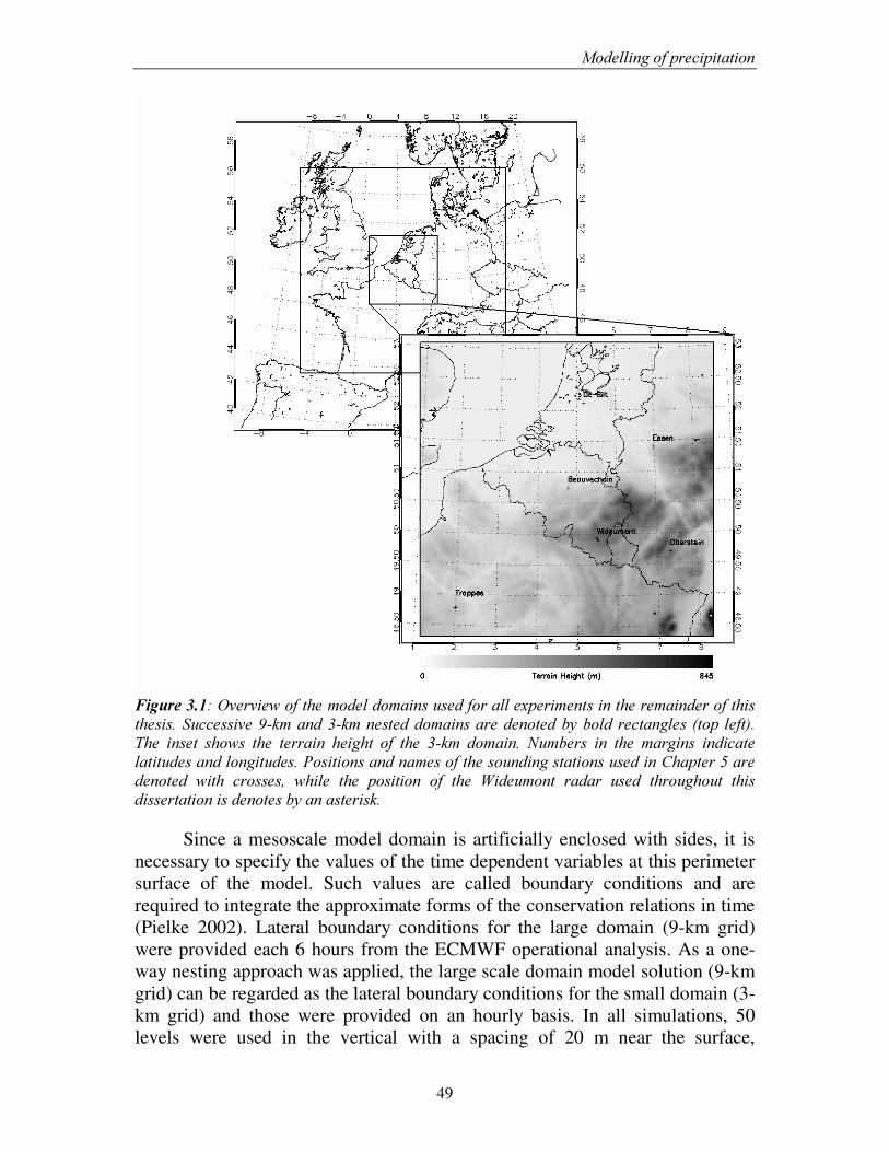
0RGHOOLQJ�RI�SUHFLSLWDWLRQ�
49
)LJXUH������2YHUYLHZ�RI�WKH�PRGHO�GRPDLQV�XVHG�IRU�DOO�H[SHULPHQWV�LQ�WKH�UHPDLQGHU�RI�WKLV�WKHVLV��6XFFHVVLYH���NP�DQG���NP�QHVWHG�GRPDLQV�DUH�GHQRWHG�E\�EROG�UHFWDQJOHV� �WRS� OHIW���7KH� LQVHW� VKRZV� WKH� WHUUDLQ� KHLJKW� RI� WKH� ��NP� GRPDLQ�� 1XPEHUV� LQ� WKH� PDUJLQV� LQGLFDWH�ODWLWXGHV�DQG�ORQJLWXGHV��3RVLWLRQV�DQG�QDPHV�RI�WKH�VRXQGLQJ�VWDWLRQV�XVHG�LQ�&KDSWHU���DUH�GHQRWHG� ZLWK� FURVVHV�� ZKLOH� WKH� SRVLWLRQ� RI� WKH� :LGHXPRQW� UDGDU� XVHG� WKURXJKRXW� WKLV�GLVVHUWDWLRQ�LV�GHQRWHV�E\�DQ�DVWHULVN��
�Since a mesoscale model domain is artificially enclosed with sides, it is
necessary to specify the values of the time dependent variables at this perimeter surface of the model. Such values are called boundary conditions and are required to integrate the approximate forms of the conservation relations in time (Pielke 2002). Lateral boundary conditions for the large domain (9-km grid) were provided each 6 hours from the ECMWF operational analysis. As a one-way nesting approach was applied, the large scale domain model solution (9-km grid) can be regarded as the lateral boundary conditions for the small domain (3-km grid) and those were provided on an hourly basis. In all simulations, 50 levels were used in the vertical with a spacing of 20 m near the surface,
&KDSWHU���
50
increasing to 1 km near the upper-model boundary, which was located at a 20-km altitude. As we focus on case studies of approximately one day, all simulations were initialized with a 12 hour spin-up period, beginning at 1200 UTC on the previous day. It should be mentioned that while in the 3-km grid domain convection was explicitly simulated (resolved by the model dynamics itself), this could not be done in the large scale domain with a coarse grid spacing of 9 km. Here, deep convection was parameterized following Kain-Fritsch (1993).
������3DUDPHWHUL]DWLRQ�RI�VXUIDFH�SURFHVVHV�
One of the important processes to be parameterized as it occurs on scales smaller than the typical scale of atmospheric models, are the processes coupling the soil surface and the atmosphere. Surface-atmosphere exchanges are important for precipitation initiation, mainly in convective situations, where they determine the rate at which moisture from the surface becomes available for condensation aloft due to latent heat fluxes from the surface. In the Advanced Regional Prediction System (ARPS) land surface processes are parameterized following Noihan and Planton (1989). This model is based on two main classes of parameters. The spatial distribution of primary parameters, i.e. the dominant types of soil and vegetation within each grid cell, are derived from existing data sets. Secondary parameters, describing the physical properties of each type of soil and vegetation (summarized in Table 3.1), are inferred from previous observational studies. The model assumes two soil layers – a skin soil layer (d1) with a depth of 10 cm and a deep soil layer (d2) with a depth of 1 m – and the scheme includes prognostic equations for the surface temperature Ts, representative of both canopy and soil surface, the temperature of the deep soil layer T2, the surface volumetric water content wg, the volumetric water content of the deep soil layer w2 and the interception water store Wr for the canopy.
Prognostic equations for skin and deep soil temperature and skin and deep soil moisture are based on a force restore method proposed by Bhumralkar (1975) and Blackadar (1976). This implies that each prognostic equation consists of a forcing term (associated with the net all-wave radiation at the soil surface (i.e. net incoming shortwave solar radiation minus net outgoing longwave radiation)) and a restore term exponentially restoring the skin soil temperature or moisture to a mean value as soon as the external forcing is removed. An additional prognostic equation determines the rainfall and dew intercepted by the foliage following Deardorff (1978), leading to a total of five prognostic equations.
0RGHOOLQJ�RI�SUHFLSLWDWLRQ�
51
7DEOH������5HOHYDQW� VHFRQGDU\�VRLO�DQG�YHJHWDWLRQ�SDUDPHWHUV� LQ� WKH� ODQG�VXUIDFH�PRGHO�RI�1RLOKDQ�DQG�3ODQWRQ��������DQG�W\SLFDO�YDOXHV�IRU�D�ORDP\�VRLO�FRYHUHG�ZLWK�JUDVV�DV�XVHG�LQ�$536�
Saturated volumetric moisture content wsat 43.9 % Wilting point volumetric water content wwilt 6.6 % Slope of the retention curve br 5.39 Soil thermal coefficient at saturation CGsat 4.111 × 10⁻⁶ K m2 J-1 Depth of the soil column d2 1.0 m Fraction of vegetation veg 'HULYHG�IURP�1'9,�Minimum surface resistance RSmin 80.0 s m-1 Leaf Area Index LAI 4.0 Roughness length z0 0.010 m Albedo 'HSHQGHQW�RQ�VRLO�PRLVWXUH�DQG�
]HQLWK�KHLJKW�Emissivity 0.995
� From these five prognostic equations, the surface heat balance can be determined at each time step. In order to conserve heat, net all-wave radiation at the surface should be balanced by the surface heat fluxes towards the atmosphere or deeper soil layers. Net radiation (Rn) at the surface is the sum of the absorbed fraction of the incoming solar radiation RG and of the atmospheric infrared radiation RA, reduced by the emitted infrared radiation:
( ) ( )41 #$%& 7555 σεα −+−= , (3.2) ZKHUH� WKH� DOEHGR� � LV� FDOFXODWHG� IURP� WKH� VRODU� ]HQLWK� DQJOH� DQG� WKH� VRLO�PRLVWXUH�� � LV� WKH� HPLVVLYLW\� DQG� � LV� WKH�6WHIDQ-Boltzmann constant. Sensible heat flux (H) is calculated as:
( )'(')*' 779&F+ −= ρ , (3.3) where cp� LV� WKH�VSHFLILF�KHDW�� a, Va and Ta are the air density, wind speed and temperature respectively and CH is the drag coefficient. Latent heat flux (E) is the sum of the soil surface evaporation (Eg) and the evapotranspiration (Ev) from the vegetation:
( ) ( )( )+,-�+./+0+1 T7TK9&YHJ( −−= ρ1 , (3.4)
( )( )234�2�562726 T7TK9&YHJ( −= ρ , (3.5) where qsat(TS) is the saturated specific humidity at the temperature TS and qa is the atmospheric specific humidity of the air. hu is the relative humidity at the ground surface, related to the superficial soil moisture and hv is the Halstead
&KDSWHU���
52
coefficient, taking into account direct evaporation from the intercepted water on the foliage as well as the evaporation. The ground heat flux is determined as the residual difference between 5n on the one hand and +, (g and (v on the other hand.
������3DUDPHWHUL]DWLRQ�RI�PLFURSK\VLFDO�SURFHVVHV�
Given certain conditions in terms of moisture and temperature, determined by the model dynamical equations and the parameterized processes, the ultimate process of transformation of water vapour to condensed water and surface precipitation occurs via the microphysics parameterization. As mentioned earlier, a parameterization scheme describes sub-grid scale processes by statistical and empirically-derived relations of the time-evolving variables of the conservation equations and certain sub-grid scale aspects relevant for the large scale. Precipitation parameterization for instance, typically applies conversion equations between water vapour and the different species of hydrometeors to the bulk of their size distribution (i.e. bulk microphysics schemes – e.g. Lin et al. 1983, Rutledge and Hobbs 1983, Cotton et al. 1986), using empirical statistical relations described in section 2.2.2. More advanced ways of representing those conversions have been proposed, calculating conversions between hydrometeors for discrete size bins (i.e. bin or spectral microphysics schemes – e.g. Kogan 1991, Khain et al. 1999, Ovtchinnikov and Kogan 2000), but due to their computational cost are not routinely implemented in operational atmospheric models.
In the remainder of this thesis, a bulk microphysics scheme including five hydrometeor types will be used, based on the formulations of Lin et al. (1983). Two of these hydrometeor types, cloud water and cloud ice, are suspended in the air and form part of the cloud phase. They are assumed to have a monodisperse size distribution. The three precipitating hydrometeor types (snow, hail and rain) all are assumed to have a negative exponential size distribution of the form:
)exp()( 0 8888 '1'1 λ−= , (3.6)
where Nx(D) is the number concentration of the hydrometeor, N0x is the intercept parDPHWHU�� x is the slope parameter and Dx is the particle diameter. These hydrometeors are able to precipitate towards lower grid boxes due to gravitational forces.
Mathematically, a distribution function, such as the size distribution of a hydrometeor, can be described in terms of its PRPHQWV. In a negative exponential distribution each moment Q corresponds to a variable that can be related to the QWK power of the independent variable (particle size D). Hence, the zeroth moment can be related to D0 and can be shown to be the equal to the
0RGHOOLQJ�RI�SUHFLSLWDWLRQ�
53
number concentration NTx (Straka 2009). The first moment is related to D1 and is hence equal to the characteristic particle diameter itself. The second moment, proportional to D2, can be shown to be the total surface area Ax of the hydrometeors. The third moment, proportional to D3, can be shown to be the volume, which for constant density and spherical hydrometeors is related in turn to the mixing ratio qx (Straka 2009).
The more of these moments of the size distribution can be prognosed by a microphysics scheme, the more accurate the nature of the distribution and hence of the microphysical conversion between the hydrometeors can be described. In most parameterizations, such as the one described in Lin et al. (1983), only one moment is explicitly predicted, being the mixing ratio (third moment). Such models are therefore called RQH�PRPHQW� VFKHPHV. The exact relation between the third moment and the particle diameter of a hydrometeor can be described as follows (Straka 2009):
( )9:�; <
=9>�?99 E'1DT@
+Γ= 1ρ , (3.7)
where ax and bx are the coefficient and power of the mass-diameter relationship (equation 2.3)� DQG� � LV� WKH� FRPSOHWH� *DPPD� IXQFWLRQ�� 7KH� SUHUHTXLVLWH� RI�defining the mixing ratio as the third moment of the size distribution is that all particles are constant density spheres, yielding for the mass-density relation that:
3
6AAA 'P
= πρ , (3.8)
As mentioned in section 2.2.2, this spherical relation is a good approximation for rain and hailstones, but might be problematic for snow and graupel as observations point more to a relation in the order of power 2 instead of 3. The implications of these assumptions will be explored in the forthcoming chapters of this dissertation. As most of the microphysical conversion processes between the different hydrometeors are most easily described in terms of the slope pDUDPHWHU� x and the intercept parameter N0x of the negative exponential size distribution, equation 3.6 is multiplied with the mass-diameter relationship (equation 2.3) and integrated over all sizes (Woods et al. 2007) yielding:
( ) ( )11
0 1 +
+Γ=BC
DE�F GDDDD TE1D
ρλ , (3.9)
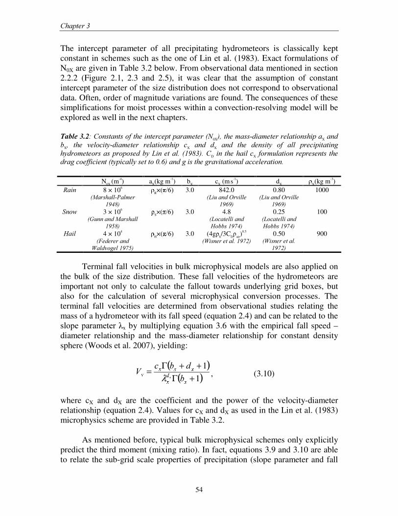
&KDSWHU���
54
The intercept parameter of all precipitating hydrometeors is classically kept constant in schemes such as the one of Lin et al. (1983). Exact formulations of N0X are given in Table 3.2 below. From observational data mentioned in section 2.2.2 (Figure 2.1, 2.3 and 2.5), it was clear that the assumption of constant intercept parameter of the size distribution does not correspond to observational data. Often, order of magnitude variations are found. The consequences of these simplifications for moist processes within a convection-resolving model will be explored as well in the next chapters. 7DEOH������&RQVWDQWV�RI�WKH�LQWHUFHSW�SDUDPHWHU��10X���WKH�PDVV�GLDPHWHU�UHODWLRQVKLS�DX�DQG�EX�� WKH� YHORFLW\�GLDPHWHU� UHODWLRQVKLS� FX� DQG� GX� DQG� WKH� GHQVLW\� RI� DOO� SUHFLSLWDWLQJ�K\GURPHWHRUV�DV�SURSRVHG�E\�/LQ�HW�DO����������&D� LQ� WKH�KDLO�FX� IRUPXODWLRQ�UHSUHVHQWV� WKH�GUDJ�FRHIILFLHQW��W\SLFDOO\�VHW�WR������DQG�J�LV�WKH�JUDYLWDWLRQDO�DFFHOHUDWLRQ��
N0X (m-4) aX(kg m-1) bX cX (m s-1) dX X(kg m-3)
5DLQ� 8 × 10⁶
�0DUVKDOO�3DOPHU������
R×( ��� 3.0 842.0 �/LX�DQG�2UYLOOH�
����� 0.80
�/LX�DQG�2UYLOOH������
1000
6QRZ� 3 × 10⁶
�*XQQ�DQG�0DUVKDOO������
S×( ��� 3.0 4.8 �/RFDWHOOL�DQG�+REEV������
0.25 �/RFDWHOOL�DQG�+REEV������
100
+DLO� 4 × 10⁴
�)HGHUHU�DQG�:DOGYRJHO������
H×( ��� 3.0 (4g h/3CD air)0.5
�:LVQHU�HW�DO������� 0.50
�:LVQHU�HW�DO��������
900
� Terminal fall velocities in bulk microphysical models are also applied on the bulk of the size distribution. These fall velocities of the hydrometeors are important not only to calculate the fallout towards underlying grid boxes, but also for the calculation of several microphysical conversion processes. The terminal fall velocities are determined from observational studies relating the mass of a hydrometeor with its fall speed (equation 2.4) and can be related to the VORSH�SDUDPHWHU� x by multiplying equation 3.6 with the empirical fall speed – diameter relationship and the mass-diameter relationship for constant density sphere (Woods et al. 2007), yielding:
( )( )1
1+Γ
++Γ=H
IH
HHHH EGEF9 J
λ , (3.10)
where cX and dX are the coefficient and the power of the velocity-diameter relationship (equation 2.4). Values for cX and dX as used in the Lin et al. (1983) microphysics scheme are provided in Table 3.2. As mentioned before, typical bulk microphysical schemes only explicitly predict the third moment (mixing ratio). In fact, equations 3.9 and 3.10 are able to relate the sub-grid scale properties of precipitation (slope parameter and fall
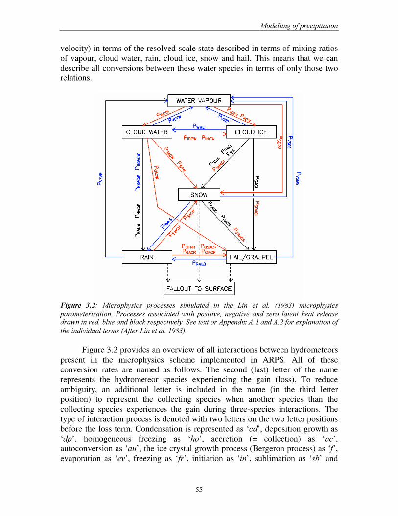
0RGHOOLQJ�RI�SUHFLSLWDWLRQ�
55
velocity) in terms of the resolved-scale state described in terms of mixing ratios of vapour, cloud water, rain, cloud ice, snow and hail. This means that we can describe all conversions between these water species in terms of only those two relations.
)LJXUH� ����� 0LFURSK\VLFV� SURFHVVHV� VLPXODWHG� LQ� WKH� /LQ� HW� DO�� ������� PLFURSK\VLFV�SDUDPHWHUL]DWLRQ�� 3URFHVVHV� DVVRFLDWHG�ZLWK� SRVLWLYH�� QHJDWLYH� DQG� ]HUR� ODWHQW� KHDW� UHOHDVH�GUDZQ�LQ�UHG��EOXH�DQG�EODFN�UHVSHFWLYHO\��6HH�WH[W�RU�$SSHQGL[�$���DQG�$���IRU�H[SODQDWLRQ�RI�WKH�LQGLYLGXDO�WHUPV��$IWHU�/LQ�HW�DO��������� Figure 3.2 provides an overview of all interactions between hydrometeors present in the microphysics scheme implemented in ARPS. All of these conversion rates are named as follows. The second (last) letter of the name represents the hydrometeor species experiencing the gain (loss). To reduce ambiguity, an additional letter is included in the name (in the third letter position) to represent the collecting species when another species than the collecting species experiences the gain during three-species interactions. The type of interaction process is denoted with two letters on the two letter positions before the loss term. Condensation is represented as ‘FG’ , deposition growth as ‘GS’ , homogeneous freezing as ‘KR’ , accretion (= collection) as ‘DF’ , autoconversion as ‘DX’ , the ice crystal growth process (Bergeron process) as ‘I’ , evaporation as ‘HY’ , freezing as ‘IU’ , initiation as ‘LQ’ , sublimation as ‘VE’ and
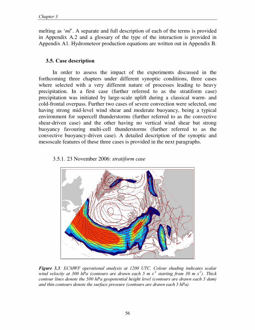
&KDSWHU���
56
melting as ‘PO’ . A separate and full description of each of the terms is provided in Appendix A.2 and a glossary of the type of the interaction is provided in Appendix A1. Hydrometeor production equations are written out in Appendix B.
������&DVH�GHVFULSWLRQ�
In order to assess the impact of the experiments discussed in the
forthcoming three chapters under different synoptic conditions, three cases where selected with a very different nature of processes leading to heavy precipitation. In a first case (further referred to as the stratiform case) precipitation was initiated by large-scale uplift during a classical warm- and cold-frontal overpass. Further two cases of severe convection were selected, one having strong mid-level wind shear and moderate buoyancy, being a typical environment for supercell thunderstorms (further referred to as the convective shear-driven case) and the other having no vertical wind shear but strong buoyancy favouring multi-cell thunderstorms (further referred to as the convective buoyancy-driven case). A detailed description of the synoptic and mesoscale features of these three cases is provided in the next paragraphs.
3.5.1. 23 November 2006: VWUDWLIRUP�FDVH �
)LJXUH� ����� (&0:)� RSHUDWLRQDO� DQDO\VLV� DW� ����� 87&�� &RORXU� VKDGLQJ� LQGLFDWHV� VFDODU�ZLQG� YHORFLW\� DW� ���� K3D� �FRQWRXUV� DUH� GUDZQ�HDFK� ��P� V-1� VWDUWLQJ� IURP� ���P� V-1��� 7KLFN�FRQWRXU�OLQHV�GHQRWH�WKH�����K3D�JHRSRWHQWLDO�KHLJKW�OHYHO��FRQWRXUV�DUH�GUDZQ�HDFK���GDP��DQG�WKLQ�FRQWRXUV�GHQRWH�WKH�VXUIDFH�SUHVVXUH��FRQWRXUV�DUH�GUDZQ�HDFK���K3D���
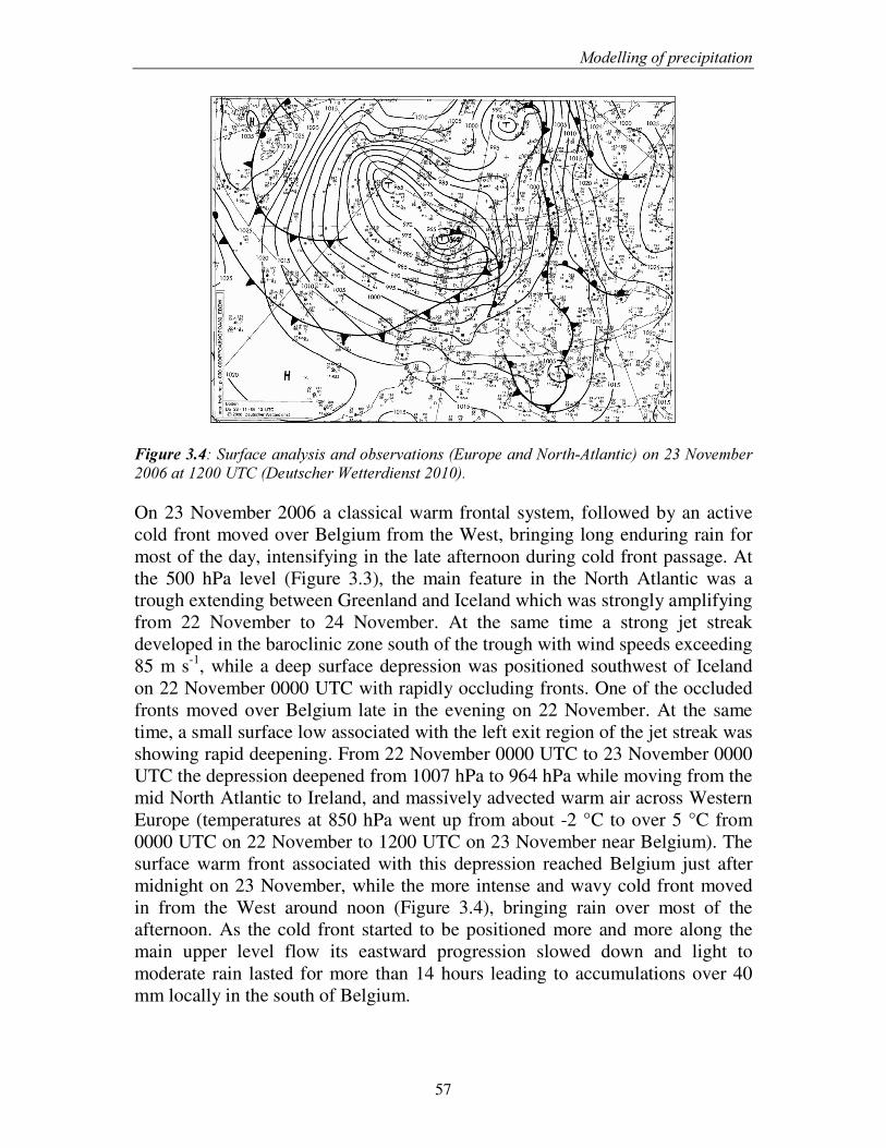
0RGHOOLQJ�RI�SUHFLSLWDWLRQ�
57
)LJXUH������6XUIDFH�DQDO\VLV�DQG�REVHUYDWLRQV��(XURSH�DQG�1RUWK�$WODQWLF��RQ����1RYHPEHU������DW������87&��'HXWVFKHU�:HWWHUGLHQVW���������On 23 November 2006 a classical warm frontal system, followed by an active cold front moved over Belgium from the West, bringing long enduring rain for most of the day, intensifying in the late afternoon during cold front passage. At the 500 hPa level (Figure 3.3), the main feature in the North Atlantic was a trough extending between Greenland and Iceland which was strongly amplifying from 22 November to 24 November. At the same time a strong jet streak developed in the baroclinic zone south of the trough with wind speeds exceeding 85 m s-1, while a deep surface depression was positioned southwest of Iceland on 22 November 0000 UTC with rapidly occluding fronts. One of the occluded fronts moved over Belgium late in the evening on 22 November. At the same time, a small surface low associated with the left exit region of the jet streak was showing rapid deepening. From 22 November 0000 UTC to 23 November 0000 UTC the depression deepened from 1007 hPa to 964 hPa while moving from the mid North Atlantic to Ireland, and massively advected warm air across Western Europe (temperatures at 850 hPa went up from about -2 °C to over 5 °C from 0000 UTC on 22 November to 1200 UTC on 23 November near Belgium). The surface warm front associated with this depression reached Belgium just after midnight on 23 November, while the more intense and wavy cold front moved in from the West around noon (Figure 3.4), bringing rain over most of the afternoon. As the cold front started to be positioned more and more along the main upper level flow its eastward progression slowed down and light to moderate rain lasted for more than 14 hours leading to accumulations over 40 mm locally in the south of Belgium.
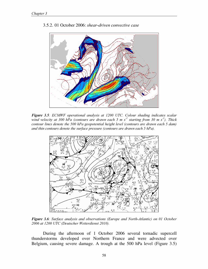
&KDSWHU���
58
3.5.2. 01 October 2006: VKHDU�GULYHQ�FRQYHFWLYH�FDVH �
)LJXUH� ����� (&0:)� RSHUDWLRQDO� DQDO\VLV� DW� ����� 87&�� &RORXU� VKDGLQJ� LQGLFDWHV� VFDODU�ZLQG� YHORFLW\� DW� ���� K3D� �FRQWRXUV� DUH� GUDZQ�HDFK� ��P� V-1� VWDUWLQJ� IURP� ���P� V-1��� 7KLFN�FRQWRXU�OLQHV�GHQRWH�WKH�����K3D�JHRSRWHQWLDO�KHLJKW�OHYHO��FRQWRXUV�DUH�GUDZQ�HDFK���GDP��DQG�WKLQ�FRQWRXUV�GHQRWH�WKH�VXUIDFH�SUHVVXUH��FRQWRXUV�DUH�GUDZQ�HDFK���K3D���
)LJXUH� ����� 6XUIDFH�DQDO\VLV�DQG�REVHUYDWLRQV� �(XURSH� DQG�1RUWK�$WODQWLF�� RQ����2FWREHU������DW������87&��'HXWVFKHU�:HWWHUGLHQVW�������
During the afternoon of 1 October 2006 several tornadic supercell
thunderstorms developed over Northern France and were advected over Belgium, causing severe damage. A trough at the 500 hPa level (Figure 3.5)
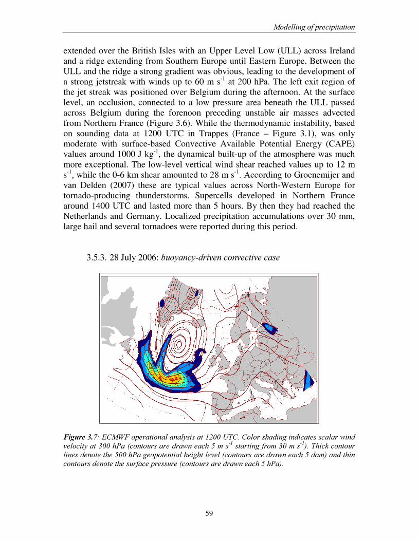
0RGHOOLQJ�RI�SUHFLSLWDWLRQ�
59
extended over the British Isles with an Upper Level Low (ULL) across Ireland and a ridge extending from Southern Europe until Eastern Europe. Between the ULL and the ridge a strong gradient was obvious, leading to the development of a strong jetstreak with winds up to 60 m s-1 at 200 hPa. The left exit region of the jet streak was positioned over Belgium during the afternoon. At the surface level, an occlusion, connected to a low pressure area beneath the ULL passed across Belgium during the forenoon preceding unstable air masses advected from Northern France (Figure 3.6). While the thermodynamic instability, based on sounding data at 1200 UTC in Trappes (France – Figure 3.1), was only moderate with surface-based Convective Available Potential Energy (CAPE) values around 1000 J kg-1, the dynamical built-up of the atmosphere was much more exceptional. The low-level vertical wind shear reached values up to 12 m s-1, while the 0-6 km shear amounted to 28 m s-1. According to Groenemijer and van Delden (2007) these are typical values across North-Western Europe for tornado-producing thunderstorms. Supercells developed in Northern France around 1400 UTC and lasted more than 5 hours. By then they had reached the Netherlands and Germany. Localized precipitation accumulations over 30 mm, large hail and several tornadoes were reported during this period.
3.5.3. 28 July 2006: EXR\DQF\�GULYHQ�FRQYHFWLYH�FDVH �
)LJXUH������(&0:)�RSHUDWLRQDO�DQDO\VLV�DW������87&��&RORU�VKDGLQJ�LQGLFDWHV�VFDODU�ZLQG�YHORFLW\�DW�����K3D��FRQWRXUV�DUH�GUDZQ�HDFK���P�V-1�VWDUWLQJ�IURP����P�V-1���7KLFN�FRQWRXU�OLQHV�GHQRWH�WKH�����K3D�JHRSRWHQWLDO�KHLJKW�OHYHO��FRQWRXUV�DUH�GUDZQ�HDFK���GDP��DQG�WKLQ�FRQWRXUV�GHQRWH�WKH�VXUIDFH�SUHVVXUH��FRQWRXUV�DUH�GUDZQ�HDFK���K3D���
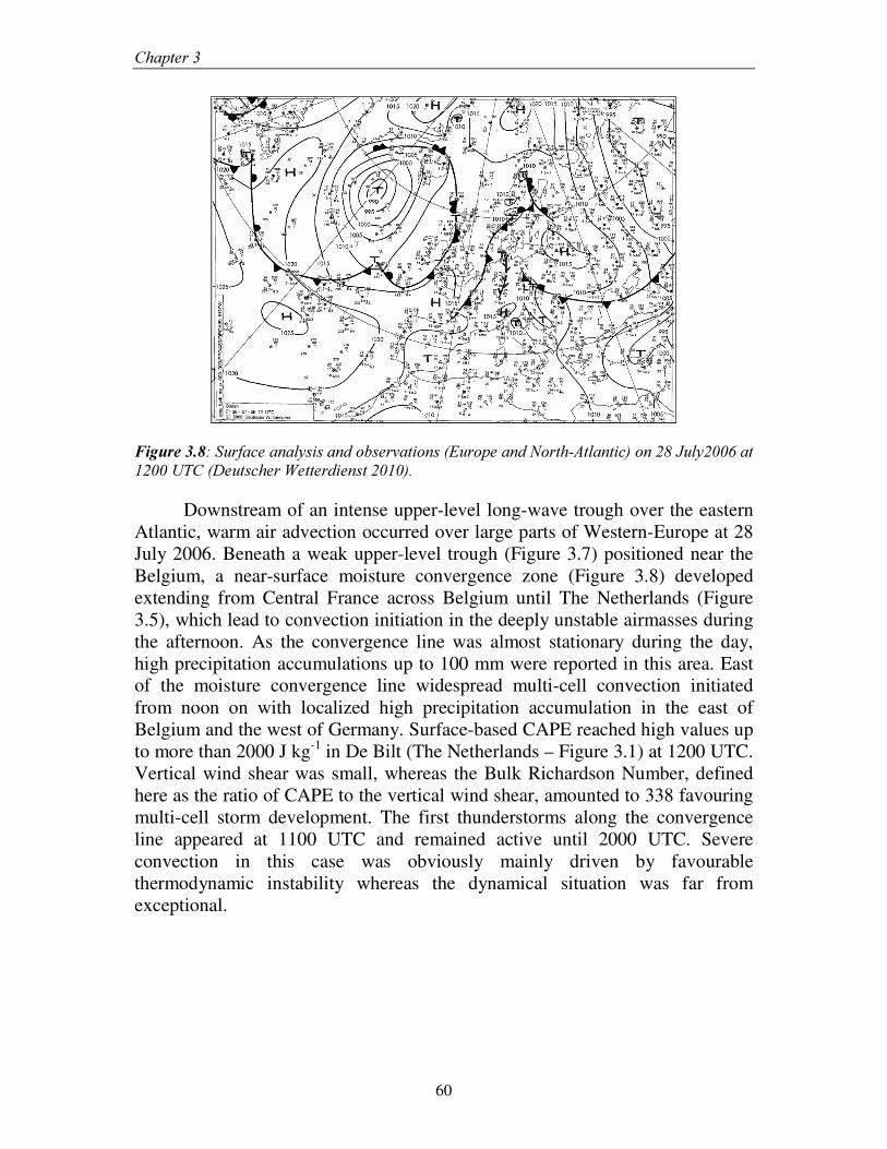
&KDSWHU���
60
�)LJXUH������6XUIDFH�DQDO\VLV�DQG�REVHUYDWLRQV��(XURSH�DQG�1RUWK�$WODQWLF��RQ����-XO\�����DW������87&��'HXWVFKHU�:HWWHUGLHQVW���������
Downstream of an intense upper-level long-wave trough over the eastern Atlantic, warm air advection occurred over large parts of Western-Europe at 28 July 2006. Beneath a weak upper-level trough (Figure 3.7) positioned near the Belgium, a near-surface moisture convergence zone (Figure 3.8) developed extending from Central France across Belgium until The Netherlands (Figure 3.5), which lead to convection initiation in the deeply unstable airmasses during the afternoon. As the convergence line was almost stationary during the day, high precipitation accumulations up to 100 mm were reported in this area. East of the moisture convergence line widespread multi-cell convection initiated from noon on with localized high precipitation accumulation in the east of Belgium and the west of Germany. Surface-based CAPE reached high values up to more than 2000 J kg-1 in De Bilt (The Netherlands – Figure 3.1) at 1200 UTC. Vertical wind shear was small, whereas the Bulk Richardson Number, defined here as the ratio of CAPE to the vertical wind shear, amounted to 338 favouring multi-cell storm development. The first thunderstorms along the convergence line appeared at 1100 UTC and remained active until 2000 UTC. Severe convection in this case was obviously mainly driven by favourable thermodynamic instability whereas the dynamical situation was far from exceptional.
61
������
&KDSWHU������
6HQVLWLYLW\�RI�TXDQWLWDWLYH�SUHFLSLWDWLRQ�IRUHFDVW�WR�VRLO�PRLVWXUH�LQLWLDOL]DWLRQ��PLFURSK\VLFV�SDUDPHWHUL]DWLRQ�DQG�KRUL]RQWDO�
UHVROXWLRQ �
������,QWURGXFWLRQ� Quantitative precipitation forecast of extreme convective events remains a
challenging task, often involving significant positive precipitation biases (Weisman et al. 2008). The causes of deficient precipitation forecasts are many and a debate is going on in the scientific community which of these causes prevails over others. The representation of initial soil moisture contents, microphysics parameterization and the horizontal grid spacing are three often mentioned candidates for significant model improvement. A literature review in section 3.1 of this thesis reveals that despite numerous attempts to quantify the influence of these aspects on the quantitative precipitation forecast, contradictory results are often found.
Studies on the impact of initial soil moisture fields on intense convection can be by and large subdivided in two groups. On the one hand, many studies find enhanced surface precipitation and more vigorous storms as soil moisture increases, due to more a favourable thermodynamic environment as the lower troposphere moistens. Many other studies find an inverse relationship between
* Van Weverberg, K., N.P.M. van Lipzig, L. Delobbe, D. Lauwaet, 2010: Sensitivity of quantitative precipitation forecast to soil moisture initialization and microphysics parameterization. Quarterly Journal of the Royal Meteorological Society, LQ�SUHVV.
&KDSWHU���
62
soil moisture and convective activity however. As soil moisture amounts increase, surface precipitation decreases. Often, cooler surface conditions when soils are wetter are designated as the reason for this behaviour. It is a challenge to understand how these contradictory studies are compatible to each other.
Similar contradictory results are found as far as the representation of size distribution assumptions in microphysics parameterizations is concerned. Some authors found considerable sensitivity of the surface precipitation to the representation of mainly the largest precipitating ice particles in idealized studies to severe convection (e.g. Gilmore et al. 2004). Other studies, having similar experimental designs, found a much smaller impact on surface precipitation, while the vertical distribution of hydrometeors was found to vary significantly (McCumber et al. 1991, van den Heever and Cotton 2004). Only few investigations have been performed to the sensitivity of extreme convection to other hydrometeor size distributions, such as the rain and snow species and mostly find small perturbations of surface precipitation (Serafin and Ferretti 2007, Gilmore et al. 2004).
Typically it has been found that grid spacings up to a few kilometres are sufficient to resolve most of the mesoscale structure of intense storms (Weisman et al. 1997). Bryan et al. (2003) however, analyzed energy spectra of subgrid energy and water fluxes and concluded that model grid spacings up to 1 km are still insufficient to faithfully simulate deep convection.
While continuous research in these fields has been devoted to investigate their single influence on precipitation formation, it is still under debate how the surface precipitation is affected by combinations of these processes. A major gap of knowledge remains as to how the different processes contributing to uncertainty in the precipitation forecasts compare to each other. Many of the aforementioned studies have been carried out for idealized simulations initialized with a single sounding and a temperature perturbation. The main advantage of these studies is that processes can be simplified so that interpretation is less ambiguous. The question arises however if the same sensitivities as occurring in those idealized simulations could be expected in real-case simulations. Further, a general drawback of idealized simulations is the lack of a ‘ground truth’ available to compare the model results with. Many studies take the most complex physics parameterization as such a ground truth, but there is no solid ground to assume that each further sophistication leads to a model improvement. Real case simulations can be compared with observations and hence have a more reliable ground-truth available.
The scope of the present chapter hence is to gain further insight in how modifications in three potential sources of error in the quantitative precipitation forecast interrelate and if current insights from idealized model integrations can be confirmed for real case simulations of severe convection across North-Western Europe. Currently, operational numerical weather prediction models use a grid spacing up to only a few kilometers. In this study we focus on a model
6HQVLWLYLW\�RI�43)�WR�VRLO�PRLVWXUH��PLFURSK\VLFV�DQG�KRUL]RQWDO�UHVROXWLRQ�
63
with such an operationally applied set up. Hence a number of sensitivity studies was devised using the Advanced Regional Prediction System (ARPS). The model was integrated for two convective events in Belgium, with changes in soil moisture initialization, model microphysical parameterization and horizontal grid spacing. The main objective of this chapter is to understand if and why these modifications have potential of bringing significant improvements in the numerical representation of the moist processes during extreme convective cases. As in many idealized case studies wind shear is included as an important degree of freedom, we selected two cases with very different environmental wind shear profiles. An overview of the ARPS model and the selected cases is given in section 4.2. The experiment design is described in more detail in section 4.3. Results are given in section 4.4 and a discussion of the results and the conclusions are presented in section 4.5.
������0RGHO�VHWXS�DQG�FDVH�GHVFULSWLRQ��
The model setup of ARPS was as described in section 3.2 in order to simulate two convective cases. Integrations were performed on a 540 km × 540 km domain with 3-km horizontal grid spacing. All experiments covered a 36 hour period, starting at 1200 UTC the day before. All analysis discussed in the forthcoming paragraphs deals with the 0000 UTC – 0000 UTC period, omitting the 12 hours spin-up time, unless stated otherwise. As Weisman and Klemp (1982) point to the important influence of both vertical wind shear and buoyancy on convective storm structure, two different environments regarding these two parameters have been selected. A first case is having moderate buoyancy but strong wind shear, typical for supercell development (shear-driven case described in section 3.5.2) and the second is having no wind shear but high buoyancy, favouring multi-cell development (buoyancy-driven case described in section 3.5.3).
������'HVLJQ�RI�PRGHO�VHQVLWLYLW\�H[SHULPHQWV�
4.3.1 Soil moisture initialization sensitivity experiments
As discussed in section 3.2, land surface processes are parameterized following Noilhan and Planton (1989). The two primary parameters of the model are dominant type of vegetation, which is derived from the Coordination Information Environment (CORINE) land cover data (Heymann et al. 1994) and the soil texture which is assumed to be loamy soil texture, homogeneous across the domain. Among the secondary parameters of the land surface model,
&KDSWHU���
64
vegetation fraction is based on the normalized difference vegetation index (NDVI) from the Satellite Pour l’ Observation de la Terre (SPOT) vegetation satellite imagery, with a resolution of 1 km.
Four model sensitivity experiments (further referred to as H[SHULPHQWV) were designed in order to assess the influence of soil moisture initialization on the moist processes in the simulated cases. The CONTROL experiment had a homogeneous loamy soil texture and homogeneous soil moisture content, which was set to 29.0 % for the deep soil layer and 26.0 % for the skin soil layer, which are mean data for a surface and deep soil horizon, monitored over one year in a Belgian loam area by Nachtergaele and Poesen (2002). The loamy soil which was used across the domain has a saturated volumetric soil moisture content of 43.9 %. This saturated moisture content was used as model initialization during the high soil moisture sensitivity experiment (Expsoil+) for both the skin soil layer and the deep soil layer of the surface parameterization scheme. The low soil moisture sensitivity experiment (Expsoil-) was initialized using a soil moisture content of only 10.0 % in the skin soil layer and 15.0 % in the deep soil layer, which were the lowest values monitored by Nachtergaele and Poesen (2002). A last experiment (Expsoilvar) explored the influence of initializing the model using spatially distributed soil texture and soil moisture data, instead of applying homogeneous fields. Soil texture data were obtained from the European Soil Database (ESDB; European Soil Bureau Network and the European Commission, 2004; see http://eusoils.jrc.it/ESDB_Archive/ESDBv2/index.htm) at a 1 km horizontal resolution and actual soil moisture data for both cases were provided by the European Commission Joint Research Centre DESERT action at a 5 km horizontal resolution. These data were obtained from the daily integrated LISFLOOD hydrological model (De Roo et al. 2000). Domain average surface soil moisture derived from this model was 25.8 % during the shear-driven case and 21.6 % during the buoyancy-driven case.
4.3.2 Microphysics sensitivity experiments
In section 3.3 it was explored how observed size distribution
characteristics, discussed in section 2.2, are routinely implemented in the widely used one-moment bulk microphysical schemes in numerical atmospheric models. By applying the microphysical conversions between the hydrometeors on the bulk of the size distribution, however, inevitably many simplifications have to be made. Some of those assumptions and simplifications introduce large uncertainty in the quantitative precipitation forecast. Therefore a number of microphysics size distribution experiments were designed.
The control simulation, further referred to as ([S+, had an identical setup as the default Lin et al. (1983) scheme available in ARPS, described in detail in
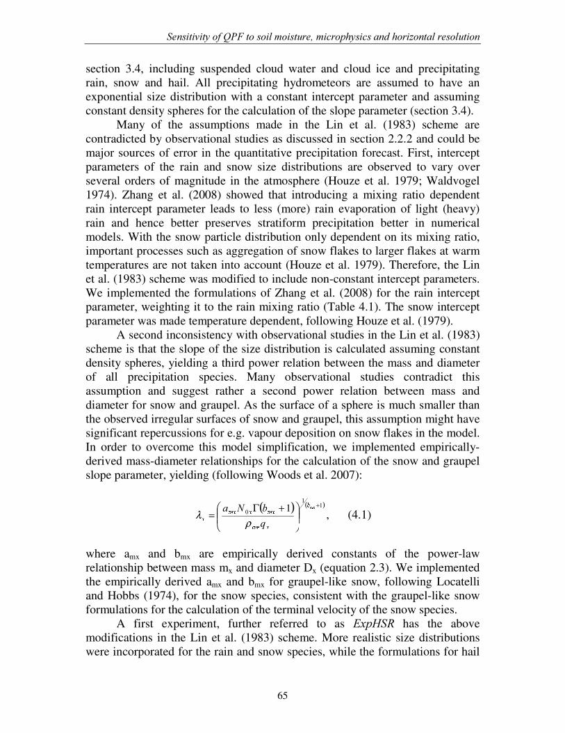
6HQVLWLYLW\�RI�43)�WR�VRLO�PRLVWXUH��PLFURSK\VLFV�DQG�KRUL]RQWDO�UHVROXWLRQ�
65
section 3.4, including suspended cloud water and cloud ice and precipitating rain, snow and hail. All precipitating hydrometeors are assumed to have an exponential size distribution with a constant intercept parameter and assuming constant density spheres for the calculation of the slope parameter (section 3.4). Many of the assumptions made in the Lin et al. (1983) scheme are contradicted by observational studies as discussed in section 2.2.2 and could be major sources of error in the quantitative precipitation forecast. First, intercept parameters of the rain and snow size distributions are observed to vary over several orders of magnitude in the atmosphere (Houze et al. 1979; Waldvogel 1974). Zhang et al. (2008) showed that introducing a mixing ratio dependent rain intercept parameter leads to less (more) rain evaporation of light (heavy) rain and hence better preserves stratiform precipitation better in numerical models. With the snow particle distribution only dependent on its mixing ratio, important processes such as aggregation of snow flakes to larger flakes at warm temperatures are not taken into account (Houze et al. 1979). Therefore, the Lin et al. (1983) scheme was modified to include non-constant intercept parameters. We implemented the formulations of Zhang et al. (2008) for the rain intercept parameter, weighting it to the rain mixing ratio (Table 4.1). The snow intercept parameter was made temperature dependent, following Houze et al. (1979). A second inconsistency with observational studies in the Lin et al. (1983) scheme is that the slope of the size distribution is calculated assuming constant density spheres, yielding a third power relation between the mass and diameter of all precipitation species. Many observational studies contradict this assumption and suggest rather a second power relation between mass and diameter for snow and graupel. As the surface of a sphere is much smaller than the observed irregular surfaces of snow and graupel, this assumption might have significant repercussions for e.g. vapour deposition on snow flakes in the model. In order to overcome this model simplification, we implemented empirically-derived mass-diameter relationships for the calculation of the snow and graupel slope parameter, yielding (following Woods et al. 2007):
( ) ( )11
0 1 +
+Γ=
K�LMNO�P QRNNRNN TE1D
ρλ , (4.1)
where amx and bmx are empirically derived constants of the power-law relationship between mass mx and diameter Dx (equation 2.3). We implemented the empirically derived amx and bmx for graupel-like snow, following Locatelli and Hobbs (1974), for the snow species, consistent with the graupel-like snow formulations for the calculation of the terminal velocity of the snow species. A first experiment, further referred to as ([S+65 has the above modifications in the Lin et al. (1983) scheme. More realistic size distributions were incorporated for the rain and snow species, while the formulations for hail
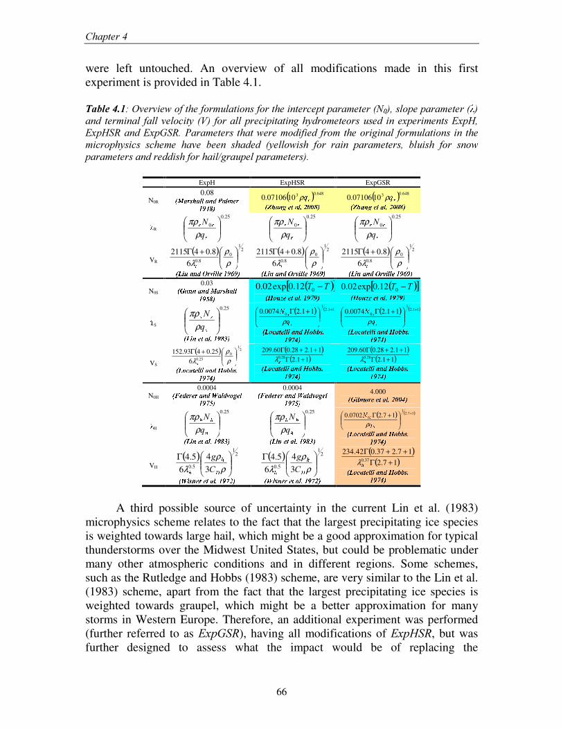
&KDSWHU���
66
were left untouched. An overview of all modifications made in this first experiment is provided in Table 4.1. 7DEOH������2YHUYLHZ�RI�WKH�IRUPXODWLRQV�IRU�WKH�LQWHUFHSW�SDUDPHWHU��1 S ���VORSH�SDUDPHWHU�� ��DQG� WHUPLQDO� IDOO�YHORFLW\� �9�� IRU�DOO�SUHFLSLWDWLQJ�K\GURPHWHRUV�XVHG� LQ�H[SHULPHQWV�([S+��([S+65�DQG�([S*65��3DUDPHWHUV�WKDW�ZHUH�PRGLILHG� IURP�WKH�RULJLQDO�IRUPXODWLRQV� LQ�WKH�PLFURSK\VLFV� VFKHPH� KDYH� EHHQ� VKDGHG� �\HOORZLVK� IRU� UDLQ� SDUDPHWHUV�� EOXLVK� IRU� VQRZ�SDUDPHWHUV�DQG�UHGGLVK�IRU�KDLO�JUDXSHO�SDUDPHWHUV����
ExpH ExpHSR ExpGSR
N0R 08.0 T UWVYX[Z�\�V�] ]^V�_�`bacV�] dfe�XgYhjijk l ( ) 648.031007106.0 mnρ T oc\�V�_�pqe�r^VY] sjt�u�u k[l ( ) 648.031007106.0 mnρ T ov\V�_�pqe�r^VY] sjt�u�u k[l
R
25.0
0
www
T1
ρπρ
25.0
0
www
T1
ρπρ
25.0
0
xxx
T1
ρπρ
VR ( ) 2
1
08.06
8.042115
+Γρρ
λ yT z|{ }~V�_�`���X���{ ] ] e gYh^��h�l( ) 2
1
08.06
8.042115
+Γρρ
λ yT zv{ }qV�_`���X���{ ] ] e gYh^��h�l
( ) 21
08.06
8.042115
+Γρρ
λ y T z|{ }~V�_�`���X���{ ] ] e g�h���h�l
N0S 0.03 T ��}�_^_~V�_`bU�VYX[Z�\VY] ]gYh���k l ( )[ ]77 −012.0exp02.0 T �~��}^��e�e�r^VY] s gYh���h�l ( )[ ]77 −012.0exp02.0 T �~��}^��e�e�r^VY] s gYh���h�l
S
25.0
���
T1
ρπρ
T z|{ _~e�r^V�] s gYhjk���l( ) ( )11.2
1
0 11.20074.0 +
+���
�ρ
T zc�j��VYr e�] ] {^V�_�`b�~���j��Z[sg�h���i�l
( ) ( )11.21
0 11.20074.0 +
+���
�ρ
� �c�j���Y� �� ¡^��¢^£b¤~��¥j¥�¦�§¨�©�ª�«�¬
VS
( ) 21
025.06
25.0493.152
+Γρρ
λ
� �c�j����� �� ¡^��¢�£®¤q��¥j¥�¦[§¨Y©�ª�«[¬
( )( )11.2
11.228.060.20928.0 +Γ
++Γ¯λ
� �c�j����� �� ¡���¢�£®¤q��¥j¥�¦�§¨�©�ª�«�¬
( )( )11.2
11.228.060.20928.0 +Γ
++Γ¯λ
� �v�j����� �� ¡^��¢�£®¤q��¥j¥�¦[§¨�©�ª�«�¬
N0H 0.0004 � °���£���±���±c��¢�£~²q�� £�³���´^�� ¨Y©�ª�µ ¶
0.0004 � °���£���±���±c��¢�£~²f�� £j³���´^�� ¨�©�ª�µ ¶
4.000 � ·�¡ ¸q�Y±��������� §j¹�ºjº «�¬
H
25.0
»»»
T1
ρπρ
� �|¡ ¢~���^�� § ¨Y©j¼�½�¬
25.0
»»»
T1
ρπρ
� �v¡ ¢~���^�� § ¨Y©j¼�½�¬
( ) ( )17.21
0 17.20702.0 +
+Γ¾¾¿Àρ
� �v�j����� �� ¡^��¢�£®¤q��¥j¥�¦[§¨�©�ª�«�¬
VH ( ) 2
1
5.0 34
65.4
Γρ
ρλ Á
ÂÂ &
J
��²f¡ ¦�¢��±c���^�� § ¨Y©�ª ¹ ¬( ) 2
1
5.0 34
65.4
Γρ
ρλ Á
ÂÂ &
J
�[²q¡ ¦�¢��±����^�� § ¨Y©�ª ¹ ¬
( )( )17.2
17.237.042.23437.0 +Γ
++ΓÃλ
� �v�j����� �� ¡^��¢�£®¤q��¥j¥�¦[§¨�©�ª�«�¬
A third possible source of uncertainty in the current Lin et al. (1983) microphysics scheme relates to the fact that the largest precipitating ice species is weighted towards large hail, which might be a good approximation for typical thunderstorms over the Midwest United States, but could be problematic under many other atmospheric conditions and in different regions. Some schemes, such as the Rutledge and Hobbs (1983) scheme, are very similar to the Lin et al. (1983) scheme, apart from the fact that the largest precipitating ice species is weighted towards graupel, which might be a better approximation for many storms in Western Europe. Therefore, an additional experiment was performed (further referred to as ([S*65), having all modifications of ([S+65, but was further designed to assess what the impact would be of replacing the
6HQVLWLYLW\�RI�43)�WR�VRLO�PRLVWXUH��PLFURSK\VLFV�DQG�KRUL]RQWDO�UHVROXWLRQ�
67
formulations of large hail in the Lin et al. (1983) scheme with those typical for graupel. In order to do so, we implemented the empirical mass-diameter relations of lump graupel for the calculation of the slope parameter (equation 4.1), following Locatelli and Hobbs (1974) and their empirically derived velocity-diameter relations for lump graupel to calculate the terminal fall velocity (Vx), following Woods et al. (2007):
( )( )1
1+Γ
++Γ= ÄÅÆ
ÇÄÇÆ EEED9 È
λ , (4.2) Further, the constant intercept parameter for large hail was increased to weight it more towards the small particle fraction, and the graupel density was decreased, following Gilmore et al. (2004). A detailed overview of all modifications made in this last experiment is given in Table 4.1.
4.3.3 Grid spacing experiments
In order to investigate the influence of the horizontal grid spacing, the number of grid points in the model domain, as specified in section 3.1, was doubled to 360 points in both the X- and Y-directions, resulting in a grid spacing of 1.5 km (further referred to as Expgdsp-). This domain was directly fed by the 9 km grid spacing domain in order to keep the model setting as near as possible to the CONTROL experiment, apart from the model grid spacing. In order to make a fair comparison between the experiments, all results discussed in this chapter have been aggregated to the 3 km grid spacing.
������2EVHUYDWLRQDO�GDWD�DQG�6$/�
The main advantage of integrating real-case simulations is to have observational data available to evaluate the model results. Precipitation observations are obtained from the C-band weather radar in Wideumont (indicated by the asterisk in Figure 3.2) operated by the Royal Meteorological Institute of Belgium and from a dense network of rain gauges (1 per 135 km²) operated by the hydrological service of the Walloon region. Although a second radar exists in Belgium (Zaventem radar, operated by the air traffic safety agency Belgocontrol), its data are generally not used for quantitative precipitation estimation due to excessive clutter filtering at short range which partially removes precipitation. However, as no strong occultation effects were present in any of the simulated cases, precipitation patterns observed by both radars were very similar, so sufficient information could be obtained by using data only from the Wideumont radar.
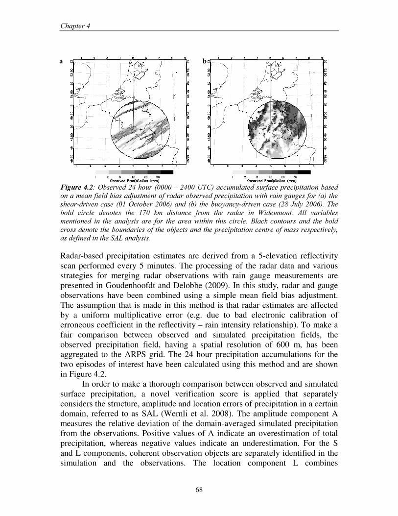
&KDSWHU���
68
)LJXUH������2EVHUYHG����KRXU�������±������87&��DFFXPXODWHG�VXUIDFH�SUHFLSLWDWLRQ�EDVHG�RQ�D�PHDQ�ILHOG�ELDV�DGMXVWPHQW�RI�UDGDU�REVHUYHG�SUHFLSLWDWLRQ�ZLWK�UDLQ�JDXJHV�IRU��D��WKH�VKHDU�GULYHQ�FDVH�����2FWREHU�������DQG��E�� WKH�EXR\DQF\�GULYHQ�FDVH�����-XO\��������7KH�EROG� FLUFOH� GHQRWHV� WKH� ���� NP� GLVWDQFH� IURP� WKH� UDGDU� LQ� :LGHXPRQW�� $OO� YDULDEOHV�PHQWLRQHG� LQ� WKH� DQDO\VLV� DUH� IRU� WKH� DUHD�ZLWKLQ� WKLV� FLUFOH�� %ODFN� FRQWRXUV� DQG� WKH� EROG�FURVV�GHQRWH�WKH�ERXQGDULHV�RI�WKH�REMHFWV�DQG�WKH�SUHFLSLWDWLRQ�FHQWUH�RI�PDVV�UHVSHFWLYHO\��DV�GHILQHG�LQ�WKH�6$/�DQDO\VLV���Radar-based precipitation estimates are derived from a 5-elevation reflectivity scan performed every 5 minutes. The processing of the radar data and various strategies for merging radar observations with rain gauge measurements are presented in Goudenhoofdt and Delobbe (2009). In this study, radar and gauge observations have been combined using a simple mean field bias adjustment. The assumption that is made in this method is that radar estimates are affected by a uniform multiplicative error (e.g. due to bad electronic calibration of erroneous coefficient in the reflectivity – rain intensity relationship). To make a fair comparison between observed and simulated precipitation fields, the observed precipitation field, having a spatial resolution of 600 m, has been aggregated to the ARPS grid. The 24 hour precipitation accumulations for the two episodes of interest have been calculated using this method and are shown in Figure 4.2.
In order to make a thorough comparison between observed and simulated surface precipitation, a novel verification score is applied that separately considers the structure, amplitude and location errors of precipitation in a certain domain, referred to as SAL (Wernli et al. 2008). The amplitude component A measures the relative deviation of the domain-averaged simulated precipitation from the observations. Positive values of A indicate an overestimation of total precipitation, whereas negative values indicate an underestimation. For the S and L components, coherent observation objects are separately identified in the simulation and the observations. The location component L combines
D� E�
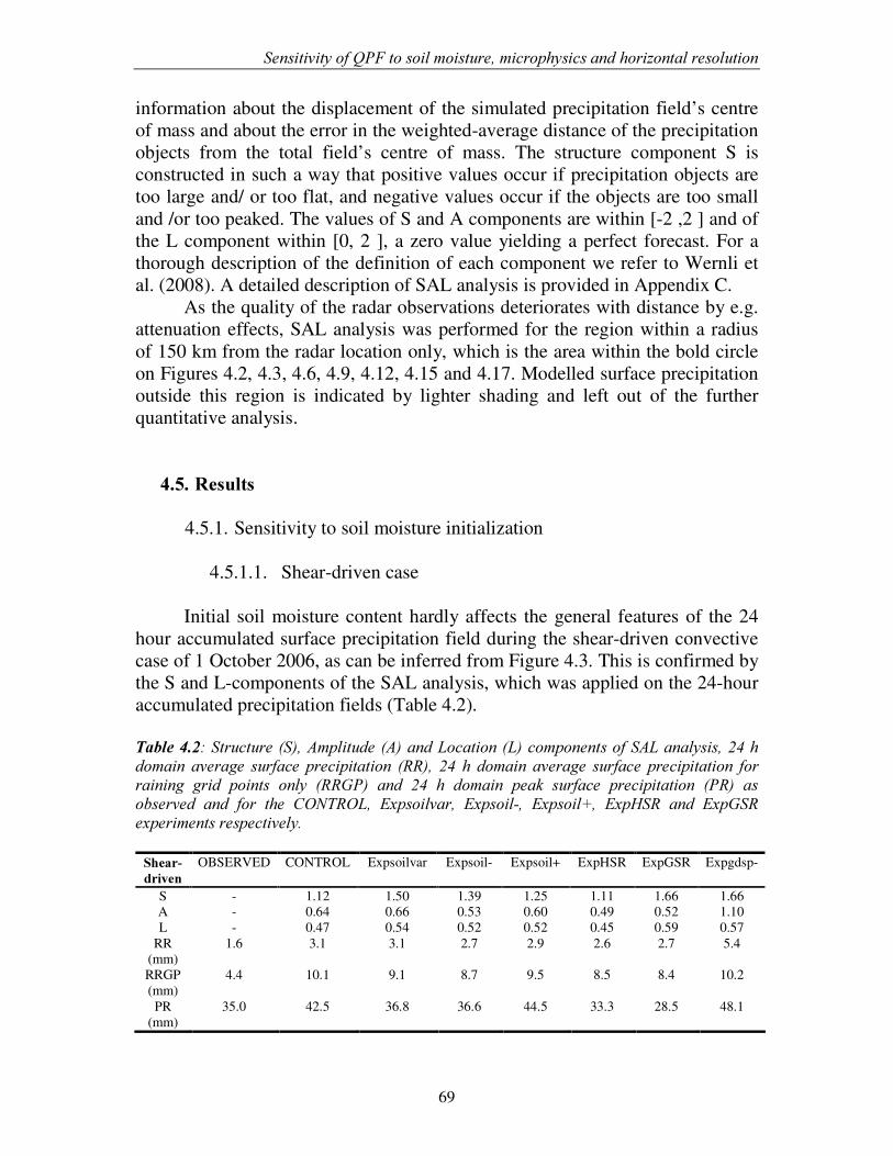
6HQVLWLYLW\�RI�43)�WR�VRLO�PRLVWXUH��PLFURSK\VLFV�DQG�KRUL]RQWDO�UHVROXWLRQ�
69
information about the displacement of the simulated precipitation field’ s centre of mass and about the error in the weighted-average distance of the precipitation objects from the total field’ s centre of mass. The structure component S is constructed in such a way that positive values occur if precipitation objects are too large and/ or too flat, and negative values occur if the objects are too small and /or too peaked. The values of S and A components are within [-2 ,2 ] and of the L component within [0, 2 ], a zero value yielding a perfect forecast. For a thorough description of the definition of each component we refer to Wernli et al. (2008). A detailed description of SAL analysis is provided in Appendix C.
As the quality of the radar observations deteriorates with distance by e.g. attenuation effects, SAL analysis was performed for the region within a radius of 150 km from the radar location only, which is the area within the bold circle on Figures 4.2, 4.3, 4.6, 4.9, 4.12, 4.15 and 4.17. Modelled surface precipitation outside this region is indicated by lighter shading and left out of the further quantitative analysis.
������5HVXOWV�
4.5.1. Sensitivity to soil moisture initialization
4.5.1.1. Shear-driven case
Initial soil moisture content hardly affects the general features of the 24 hour accumulated surface precipitation field during the shear-driven convective case of 1 October 2006, as can be inferred from Figure 4.3. This is confirmed by the S and L-components of the SAL analysis, which was applied on the 24-hour accumulated precipitation fields (Table 4.2).
7DEOH������6WUXFWXUH��6���$PSOLWXGH��$��DQG�/RFDWLRQ��/��FRPSRQHQWV�RI�6$/�DQDO\VLV�����K�GRPDLQ� DYHUDJH� VXUIDFH� SUHFLSLWDWLRQ� �55��� ��� K� GRPDLQ� DYHUDJH� VXUIDFH� SUHFLSLWDWLRQ� IRU�UDLQLQJ� JULG� SRLQWV� RQO\� �55*3�� DQG� ��� K� GRPDLQ� SHDN� VXUIDFH� SUHFLSLWDWLRQ� �35�� DV�REVHUYHG� DQG� IRU� WKH� &21752/�� ([SVRLOYDU�� ([SVRLO��� ([SVRLO��� ([S+65� DQG� ([S*65�H[SHULPHQWV�UHVSHFWLYHO\��
�6KHDU�GULYHQ�
OBSERVED CONTROL Expsoilvar Expsoil- Expsoil+ ExpHSR ExpGSR Expgdsp-
S - 1.12 1.50 1.39 1.25 1.11 1.66 1.66 A - 0.64 0.66 0.53 0.60 0.49 0.52 1.10 L - 0.47 0.54 0.52 0.52 0.45 0.59 0.57
RR (mm)
1.6 3.1 3.1 2.7 2.9 2.6 2.7 5.4
RRGP (mm)
4.4 10.1 9.1 8.7 9.5 8.5 8.4 10.2
PR (mm)
35.0 42.5 36.8 36.6 44.5 33.3 28.5 48.1
�
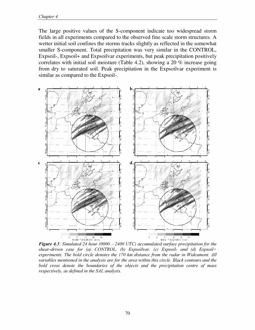
&KDSWHU���
70
The large positive values of the S-component indicate too widespread storm fields in all experiments compared to the observed fine scale storm structures. A wetter initial soil confines the storms tracks slightly as reflected in the somewhat smaller S-component. Total precipitation was very similar in the CONTROL, Expsoil-, Expsoil+ and Expsoilvar experiments, but peak precipitation positively correlates with initial soil moisture (Table 4.2), showing a 20 % increase going from dry to saturated soil. Peak precipitation in the Expsoilvar experiment is similar as compared to the Expsoil-.
)LJXUH������6LPXODWHG����KRXU�������±������87&��DFFXPXODWHG�VXUIDFH�SUHFLSLWDWLRQ�IRU�WKH�VKHDU�GULYHQ� FDVH� IRU� �D�� &21752/�� �E�� ([SVRLOYDU�� �F�� ([SVRLO�� DQG� �G�� ([SVRLO��H[SHULPHQWV��7KH�EROG�FLUFOH�GHQRWHV�WKH�����NP�GLVWDQFH�IURP�WKH�UDGDU�LQ�:LGHXPRQW��$OO�YDULDEOHV�PHQWLRQHG�LQ�WKH�DQDO\VLV�DUH�IRU�WKH�DUHD�ZLWKLQ�WKLV�FLUFOH��%ODFN�FRQWRXUV�DQG�WKH�EROG� FURVV� GHQRWH� WKH� ERXQGDULHV� RI� WKH� REMHFWV� DQG� WKH� SUHFLSLWDWLRQ� FHQWUH� RI� PDVV�UHVSHFWLYHO\��DV�GHILQHG�LQ�WKH�6$/�DQDO\VLV�������
D� E�
F� G�
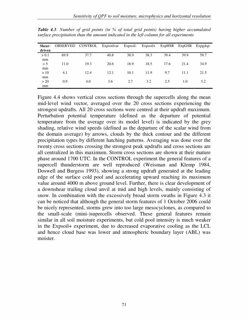
6HQVLWLYLW\�RI�43)�WR�VRLO�PRLVWXUH��PLFURSK\VLFV�DQG�KRUL]RQWDO�UHVROXWLRQ�
71
7DEOH� ����� 1XPEHU� RI� JULG� SRLQWV� �LQ� �� RI� WRWDO� JULG� SRLQWV�� KDYLQJ� KLJKHU� DFFXPXODWHG�VXUIDFH�SUHFLSLWDWLRQ�WKDQ�WKH�DPRXQW�LQGLFDWHG�LQ�WKH�OHIW�FROXPQ�IRU�DOO�H[SHULPHQWV��6KHDU�GULYHQ�
OBSERVED CONTROL Expsoilvar Expsoil- Expsoil+ ExpHSR ExpGSR Expgdsp-
> 0.1 mm
69.9 37.7 40.8 38.9 38.3 39.4 39.9 59.7
> 5 mm
11.0 19.3 20.6 18.9 18.5 17.6 21.4 34.9
> 10 mm
4.1 12.4 12.1 10.1 11.9 9.7 11.1 21.5
> 20 mm
0.9 4.0 3.6 2.7 3.2 2.5 1.0 5.2
�Figure 4.4 shows vertical cross sections through the supercells along the mean mid-level wind vector, averaged over the 20 cross sections experiencing the strongest updrafts. All 20 cross sections were centred at their updraft maximum. Perturbation potential temperature (defined as the departure of potential temperature from the average over its model level) is indicated by the grey shading, relative wind speeds (defined as the departure of the scalar wind from the domain average) by arrows, clouds by the thick contour and the different precipitation types by different hatching patterns. Averaging was done over the twenty cross sections crossing the strongest peak updrafts and cross sections are all centralized in this maximum. Storm cross sections are shown at their mature phase around 1700 UTC. In the CONTROL experiment the general features of a supercell thunderstorm are well reproduced (Weisman and Klemp 1984, Doswell and Burgess 1993), showing a strong updraft generated at the leading edge of the surface cold pool and accelerating upward reaching its maximum value around 4000 m above ground level. Further, there is clear development of a downshear trailing cloud anvil at mid and high levels, mainly consisting of snow. In combination with the excessively broad storm swaths in Figure 4.3 it can be noticed that although the general storm features of 1 October 2006 could be nicely represented, storms grew into too large mesocyclones, as compared to the small-scale (mini-)supercells observed. These general features remain similar in all soil moisture experiments, but cold pool intensity is much weaker in the Expsoil+ experiment, due to decreased evaporative cooling as the LCL and hence cloud base was lower and atmospheric boundary layer (ABL) was moister.
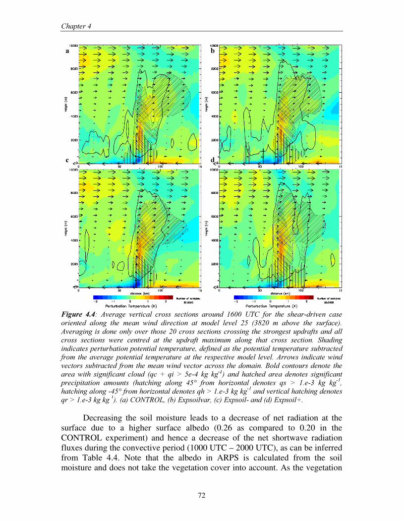
&KDSWHU���
72
)LJXUH� ����� $YHUDJH� YHUWLFDO� FURVV� VHFWLRQV� DURXQG� ����� 87&� IRU� WKH� VKHDU�GULYHQ� FDVH�RULHQWHG� DORQJ� WKH� PHDQ� ZLQG� GLUHFWLRQ� DW� PRGHO� OHYHO� ��� ������ P� DERYH� WKH� VXUIDFH���$YHUDJLQJ�LV�GRQH�RQO\�RYHU� WKRVH����FURVV�VHFWLRQV�FURVVLQJ� WKH�VWURQJHVW�XSGUDIWV�DQG�DOO�FURVV� VHFWLRQV� ZHUH� FHQWUHG� DW� WKH� XSGUDIW� PD[LPXP� DORQJ� WKDW� FURVV� VHFWLRQ�� 6KDGLQJ�LQGLFDWHV�SHUWXUEDWLRQ�SRWHQWLDO�WHPSHUDWXUH��GHILQHG�DV�WKH�SRWHQWLDO�WHPSHUDWXUH�VXEWUDFWHG�IURP� WKH�DYHUDJH�SRWHQWLDO� WHPSHUDWXUH�DW� WKH�UHVSHFWLYH�PRGHO� OHYHO��$UURZV� LQGLFDWH�ZLQG�YHFWRUV�VXEWUDFWHG� IURP�WKH�PHDQ�ZLQG�YHFWRU�DFURVV�WKH�GRPDLQ��%ROG�FRQWRXUV�GHQRWH� WKH�DUHD�ZLWK� VLJQLILFDQW� FORXG� �TF��� TL� !� �H��� NJ� NJ É Ê �� DQG� KDWFKHG� DUHD� GHQRWHV� VLJQLILFDQW�SUHFLSLWDWLRQ� DPRXQWV� �KDWFKLQJ� DORQJ� ���� IURP� KRUL]RQWDO� GHQRWHV� TV� !� ��H��� NJ� NJ É Ê ��KDWFKLQJ�DORQJ������IURP�KRUL]RQWDO�GHQRWHV�TK�!���H���NJ�NJ É Ê �DQG�YHUWLFDO�KDWFKLQJ�GHQRWHV�TU�!���H���NJ�NJ É Ê ����D��&21752/���E��([SVRLOYDU���F��([SVRLO��DQG��G��([SVRLO�����
Decreasing the soil moisture leads to a decrease of net radiation at the surface due to a higher surface albedo (0.26 as compared to 0.20 in the CONTROL experiment) and hence a decrease of the net shortwave radiation fluxes during the convective period (1000 UTC – 2000 UTC), as can be inferred from Table 4.4. Note that the albedo in ARPS is calculated from the soil moisture and does not take the vegetation cover into account. As the vegetation
D� E�
F� G�
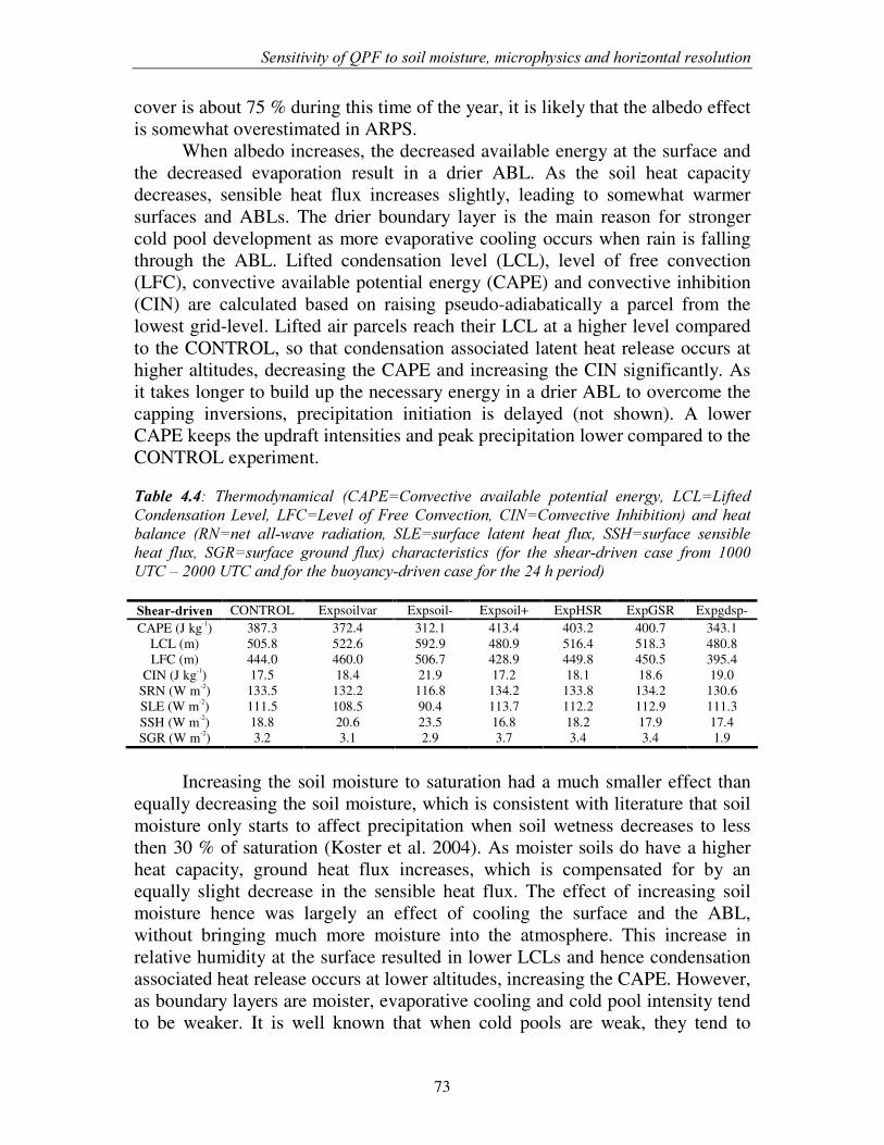
6HQVLWLYLW\�RI�43)�WR�VRLO�PRLVWXUH��PLFURSK\VLFV�DQG�KRUL]RQWDO�UHVROXWLRQ�
73
cover is about 75 % during this time of the year, it is likely that the albedo effect is somewhat overestimated in ARPS.
When albedo increases, the decreased available energy at the surface and the decreased evaporation result in a drier ABL. As the soil heat capacity decreases, sensible heat flux increases slightly, leading to somewhat warmer surfaces and ABLs. The drier boundary layer is the main reason for stronger cold pool development as more evaporative cooling occurs when rain is falling through the ABL. Lifted condensation level (LCL), level of free convection (LFC), convective available potential energy (CAPE) and convective inhibition (CIN) are calculated based on raising pseudo-adiabatically a parcel from the lowest grid-level. Lifted air parcels reach their LCL at a higher level compared to the CONTROL, so that condensation associated latent heat release occurs at higher altitudes, decreasing the CAPE and increasing the CIN significantly. As it takes longer to build up the necessary energy in a drier ABL to overcome the capping inversions, precipitation initiation is delayed (not shown). A lower CAPE keeps the updraft intensities and peak precipitation lower compared to the CONTROL experiment.
7DEOH� ����� 7KHUPRG\QDPLFDO� �&$3( &RQYHFWLYH� DYDLODEOH� SRWHQWLDO� HQHUJ\�� /&/ /LIWHG�&RQGHQVDWLRQ�/HYHO�� /)& /HYHO�RI�)UHH�&RQYHFWLRQ��&,1 &RQYHFWLYH� ,QKLELWLRQ�� DQG�KHDW�EDODQFH� �51 QHW� DOO�ZDYH� UDGLDWLRQ�� 6/( VXUIDFH� ODWHQW� KHDW� IOX[�� 66+ VXUIDFH� VHQVLEOH�KHDW� IOX[�� 6*5 VXUIDFH� JURXQG� IOX[�� FKDUDFWHULVWLFV� �IRU� WKH� VKHDU�GULYHQ� FDVH� IURP� �����87&�±������87&�DQG�IRU�WKH�EXR\DQF\�GULYHQ�FDVH�IRU�WKH����K�SHULRG���6KHDU�GULYHQ� CONTROL Expsoilvar Expsoil- Expsoil+ ExpHSR ExpGSR Expgdsp- CAPE (J kg-1) 387.3 372.4 312.1 413.4 403.2 400.7 343.1
LCL (m) 505.8 522.6 592.9 480.9 516.4 518.3 480.8 LFC (m) 444.0 460.0 506.7 428.9 449.8 450.5 395.4
CIN (J kg-1) 17.5 18.4 21.9 17.2 18.1 18.6 19.0 SRN (W m-2) 133.5 132.2 116.8 134.2 133.8 134.2 130.6 SLE (W m-2) 111.5 108.5 90.4 113.7 112.2 112.9 111.3 SSH (W m-2) 18.8 20.6 23.5 16.8 18.2 17.9 17.4 SGR (W m-2) 3.2 3.1 2.9 3.7 3.4 3.4 1.9
Increasing the soil moisture to saturation had a much smaller effect than
equally decreasing the soil moisture, which is consistent with literature that soil moisture only starts to affect precipitation when soil wetness decreases to less then 30 % of saturation (Koster et al. 2004). As moister soils do have a higher heat capacity, ground heat flux increases, which is compensated for by an equally slight decrease in the sensible heat flux. The effect of increasing soil moisture hence was largely an effect of cooling the surface and the ABL, without bringing much more moisture into the atmosphere. This increase in relative humidity at the surface resulted in lower LCLs and hence condensation associated heat release occurs at lower altitudes, increasing the CAPE. However, as boundary layers are moister, evaporative cooling and cold pool intensity tend to be weaker. It is well known that when cold pools are weak, they tend to
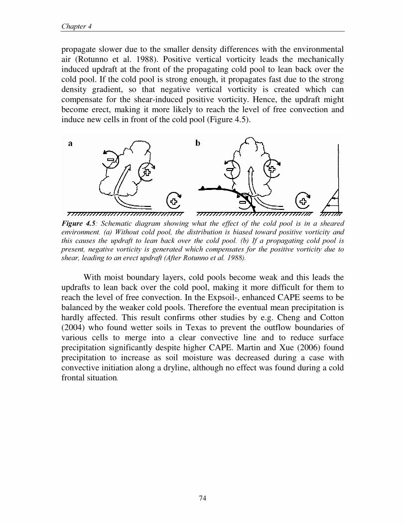
&KDSWHU���
74
propagate slower due to the smaller density differences with the environmental air (Rotunno et al. 1988). Positive vertical vorticity leads the mechanically induced updraft at the front of the propagating cold pool to lean back over the cold pool. If the cold pool is strong enough, it propagates fast due to the strong density gradient, so that negative vertical vorticity is created which can compensate for the shear-induced positive vorticity. Hence, the updraft might become erect, making it more likely to reach the level of free convection and induce new cells in front of the cold pool (Figure 4.5).
)LJXUH� ����� 6FKHPDWLF� GLDJUDP� VKRZLQJ� ZKDW� WKH� HIIHFW� RI� WKH� FROG� SRRO� LV� LQ� D� VKHDUHG�HQYLURQPHQW�� �D��:LWKRXW� FROG� SRRO�� WKH� GLVWULEXWLRQ� LV� ELDVHG� WRZDUG�SRVLWLYH�YRUWLFLW\� DQG�WKLV� FDXVHV� WKH� XSGUDIW� WR� OHDQ� EDFN� RYHU� WKH� FROG� SRRO�� �E�� ,I� D� SURSDJDWLQJ� FROG� SRRO� LV�SUHVHQW�� QHJDWLYH� YRUWLFLW\� LV� JHQHUDWHG�ZKLFK�FRPSHQVDWHV� IRU� WKH� SRVLWLYH� YRUWLFLW\� GXH� WR�VKHDU��OHDGLQJ�WR�DQ�HUHFW�XSGUDIW��$IWHU�5RWXQQR�HW�DO���������
With moist boundary layers, cold pools become weak and this leads the
updrafts to lean back over the cold pool, making it more difficult for them to reach the level of free convection. In the Expsoil-, enhanced CAPE seems to be balanced by the weaker cold pools. Therefore the eventual mean precipitation is hardly affected. This result confirms other studies by e.g. Cheng and Cotton (2004) who found wetter soils in Texas to prevent the outflow boundaries of various cells to merge into a clear convective line and to reduce surface precipitation significantly despite higher CAPE. Martin and Xue (2006) found precipitation to increase as soil moisture was decreased during a case with convective initiation along a dryline, although no effect was found during a cold frontal situation����
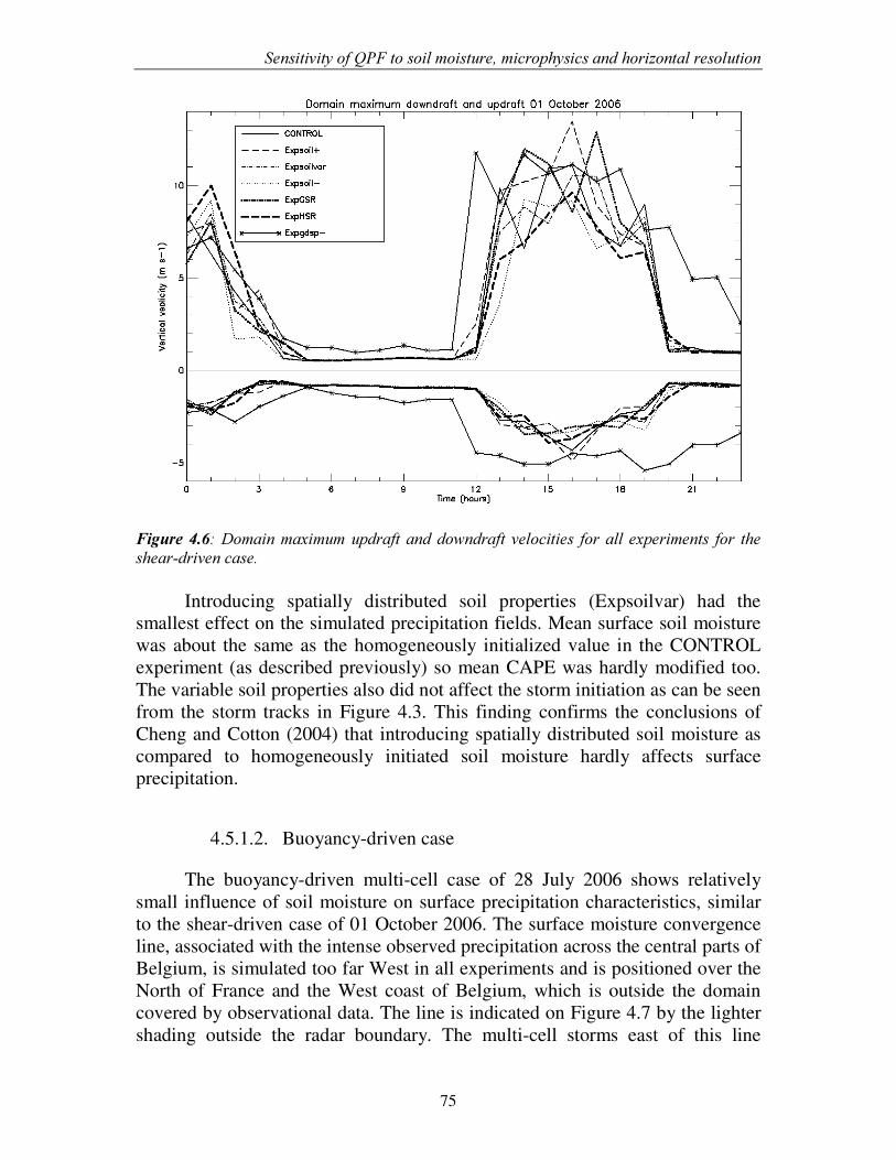
6HQVLWLYLW\�RI�43)�WR�VRLO�PRLVWXUH��PLFURSK\VLFV�DQG�KRUL]RQWDO�UHVROXWLRQ�
75
��)LJXUH������'RPDLQ�PD[LPXP�XSGUDIW�DQG�GRZQGUDIW� YHORFLWLHV� IRU�DOO�H[SHULPHQWV� IRU� WKH�VKHDU�GULYHQ�FDVH�
Introducing spatially distributed soil properties (Expsoilvar) had the
smallest effect on the simulated precipitation fields. Mean surface soil moisture was about the same as the homogeneously initialized value in the CONTROL experiment (as described previously) so mean CAPE was hardly modified too. The variable soil properties also did not affect the storm initiation as can be seen from the storm tracks in Figure 4.3. This finding confirms the conclusions of Cheng and Cotton (2004) that introducing spatially distributed soil moisture as compared to homogeneously initiated soil moisture hardly affects surface precipitation.
4.5.1.2. Buoyancy-driven case
The buoyancy-driven multi-cell case of 28 July 2006 shows relatively small influence of soil moisture on surface precipitation characteristics, similar to the shear-driven case of 01 October 2006. The surface moisture convergence line, associated with the intense observed precipitation across the central parts of Belgium, is simulated too far West in all experiments and is positioned over the North of France and the West coast of Belgium, which is outside the domain covered by observational data. The line is indicated on Figure 4.7 by the lighter shading outside the radar boundary. The multi-cell storms east of this line
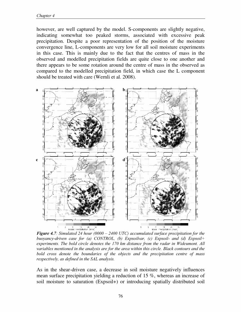
&KDSWHU���
76
however, are well captured by the model. S-components are slightly negative, indicating somewhat too peaked storms, associated with excessive peak precipitation. Despite a poor representation of the position of the moisture convergence line, L-components are very low for all soil moisture experiments in this case. This is mainly due to the fact that the centres of mass in the observed and modelled precipitation fields are quite close to one another and there appears to be some rotation around the centre of mass in the observed as compared to the modelled precipitation field, in which case the L component should be treated with care (Wernli et al. 2008).
)LJXUH������6LPXODWHG����KRXU�������±������87&��DFFXPXODWHG�VXUIDFH�SUHFLSLWDWLRQ�IRU�WKH�EXR\DQF\�GULYHQ� FDVH� IRU� �D�� &21752/�� �E�� ([SVRLOYDU�� �F�� ([SVRLO�� DQG� �G�� ([SVRLO��H[SHULPHQWV��7KH�EROG�FLUFOH�GHQRWHV�WKH�����NP�GLVWDQFH�IURP�WKH�UDGDU�LQ�:LGHXPRQW��$OO�YDULDEOHV�PHQWLRQHG�LQ�WKH�DQDO\VLV�DUH�IRU�WKH�DUHD�ZLWKLQ�WKLV�FLUFOH��%ODFN�FRQWRXUV�DQG�WKH�EROG� FURVV� GHQRWH� WKH� ERXQGDULHV� RI� WKH� REMHFWV� DQG� WKH� SUHFLSLWDWLRQ� FHQWUH� RI� PDVV�UHVSHFWLYHO\��DV�GHILQHG�LQ�WKH�6$/�DQDO\VLV���As in the shear-driven case, a decrease in soil moisture negatively influences mean surface precipitation yielding a reduction of 15 %, whereas an increase of soil moisture to saturation (Expsoil+) or introducing spatially distributed soil
D� E�
F� G�
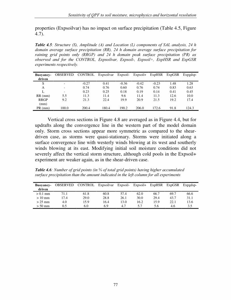
6HQVLWLYLW\�RI�43)�WR�VRLO�PRLVWXUH��PLFURSK\VLFV�DQG�KRUL]RQWDO�UHVROXWLRQ�
77
properties (Expsoilvar) has no impact on surface precipitation (Table 4.5, Figure 4.7).
7DEOH������6WUXFWXUH��6���$PSOLWXGH��$��DQG�/RFDWLRQ��/��FRPSRQHQWV�RI�6$/�DQDO\VLV�����K�GRPDLQ� DYHUDJH� VXUIDFH� SUHFLSLWDWLRQ� �55��� ��� K� GRPDLQ� DYHUDJH� VXUIDFH� SUHFLSLWDWLRQ� IRU�UDLQLQJ� JULG� SRLQWV� RQO\� �55*3�� DQG� ��� K� GRPDLQ� SHDN� VXUIDFH� SUHFLSLWDWLRQ� �35�� DV�REVHUYHG� DQG� IRU� WKH� &21752/�� ([SVRLOYDU�� ([SVRLO��� ([SVRLO��� ([S+65� DQG� ([S*65�H[SHULPHQWV�UHVSHFWLYHO\��
�%XR\DQF\�GULYHQ�
OBSERVED CONTROL Expsoilvar Expsoil- Expsoil+ ExpHSR ExpGSR Expgdsp-
S - -0.27 0.41 -0.36 -0.42 -0.23 1.48 1.28 A - 0.74 0.76 0.60 0.76 0.74 0.83 0.63 L - 0.23 0.25 0.18 0.19 0.14 0.41 0.45
RR (mm) 5.5 11.3 11.4 9.6 11.4 11.3 12.6 10.0 RRGP (mm)
9.2 21.3 22.4 19.9 20.9 21.5 19.2 17.4
PR (mm) 100.0 200.4 180.4 190.2 206.0 172.6 91.8 124.3
Vertical cross sections in Figure 4.8 are averaged as in Figure 4.4, but for
updrafts along the convergence line in the western part of the model domain only. Storm cross sections appear more symmetric as compared to the shear-driven case, as storms were quasi-stationary. Storms were initiated along a surface convergence line with westerly winds blowing at its west and southerly winds blowing at its east. Modifying initial soil moisture conditions did not severely affect the vertical storm structure, although cold pools in the Expsoil+ experiment are weaker again, as in the shear-driven case.
7DEOH������1XPEHU�RI�JULG�SRLQWV��LQ���RI�WRWDO�JULG�SRLQWV��KDYLQJ�KLJKHU�DFFXPXODWHG�VXUIDFH�SUHFLSLWDWLRQ�WKDQ�WKH�DPRXQW�LQGLFDWHG�LQ�WKH�OHIW�FROXPQ�IRU�DOO�H[SHULPHQWV�
�%XR\DQF\�GULYHQ�
OBSERVED CONTROL Expsoilvar Expsoil- Expsoil+ ExpHSR ExpGSR Expgdsp-
> 0.1 mm 71.1 61.8 60.8 57.4 62.0 66.7 69.7 66.6 > 10 mm 17.4 29.0 28.8 26.1 30.0 29.4 43.7 31.1 > 25 mm 4.0 15.9 16.4 13.0 16.2 15.9 22.1 13.6 > 50 mm 0.5 6.0 6.9 4.7 5.7 5.6 4.6 3.5
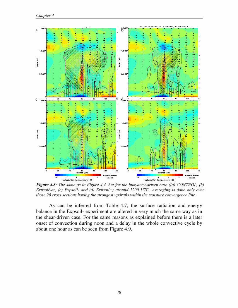
&KDSWHU���
78
)LJXUH������7KH�VDPH�DV�LQ�)LJXUH������EXW�IRU�WKH�EXR\DQF\�GULYHQ�FDVH���D��&21752/���E��([SVRLOYDU�� �F�� ([SVRLO�� DQG� �G�� ([SVRLO��� DURXQG� �����87&�� $YHUDJLQJ� LV� GRQH� RQO\� RYHU�WKRVH����FURVV�VHFWLRQV�KDYLQJ�WKH�VWURQJHVW�XSGUDIWV�ZLWKLQ�WKH�PRLVWXUH�FRQYHUJHQFH�OLQH���
As can be inferred from Table 4.7, the surface radiation and energy balance in the Expsoil- experiment are altered in very much the same way as in the shear-driven case. For the same reasons as explained before there is a later onset of convection during noon and a delay in the whole convective cycle by about one hour as can be seen from Figure 4.9.
D� E�
F� G�
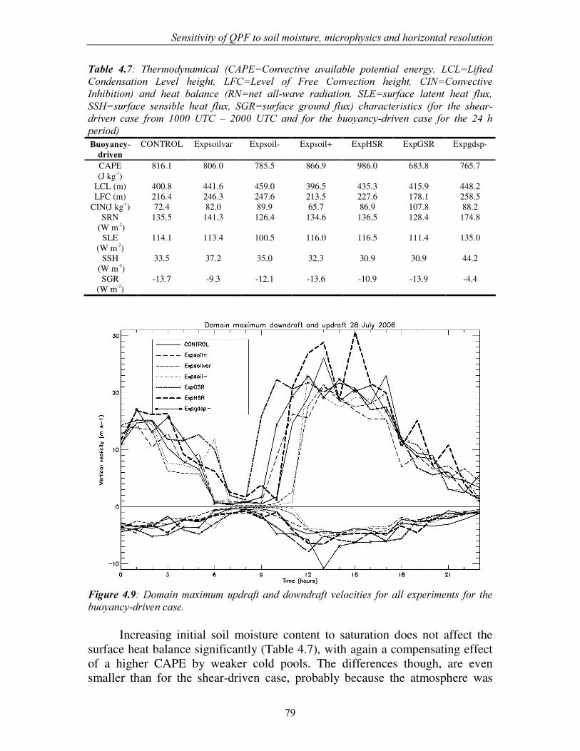
6HQVLWLYLW\�RI�43)�WR�VRLO�PRLVWXUH��PLFURSK\VLFV�DQG�KRUL]RQWDO�UHVROXWLRQ�
79
7DEOH� ����� 7KHUPRG\QDPLFDO� �&$3( &RQYHFWLYH� DYDLODEOH� SRWHQWLDO� HQHUJ\�� /&/ /LIWHG�&RQGHQVDWLRQ� /HYHO� KHLJKW�� /)& /HYHO� RI� )UHH� &RQYHFWLRQ� KHLJKW�� &,1 &RQYHFWLYH�,QKLELWLRQ�� DQG� KHDW� EDODQFH� �51 QHW� DOO�ZDYH� UDGLDWLRQ�� 6/( VXUIDFH� ODWHQW� KHDW� IOX[��66+ VXUIDFH� VHQVLEOH� KHDW� IOX[�� 6*5 VXUIDFH� JURXQG� IOX[�� FKDUDFWHULVWLFV� �IRU� WKH� VKHDU�GULYHQ� FDVH� IURP� ����� 87&� ±� ����� 87&� DQG� IRU� WKH� EXR\DQF\�GULYHQ� FDVH� IRU� WKH� ��� K�SHULRG��%XR\DQF\�GULYHQ
CONTROL Expsoilvar Expsoil- Expsoil+ ExpHSR ExpGSR Expgdsp-
CAPE (J kg-1)
816.1 806.0 785.5 866.9 986.0 683.8 765.7
LCL (m) 400.8 441.6 459.0 396.5 435.3 415.9 448.2 LFC (m) 216.4 246.3 247.6 213.5 227.6 178.1 258.5
CIN(J kg-1) 72.4 82.0 89.9 65.7 86.9 107.8 88.2 SRN
(W m-2) 135.5 141.3 126.4 134.6 136.5 128.4 174.8
SLE (W m-2)
114.1 113.4 100.5 116.0 116.5 111.4 135.0
SSH (W m-2)
33.5 37.2 35.0 32.3 30.9 30.9 44.2
SGR (W m-2)
-13.7 -9.3 -12.1 -13.6 -10.9 -13.9 -4.4
)LJXUH������'RPDLQ�PD[LPXP�XSGUDIW�DQG�GRZQGUDIW� YHORFLWLHV� IRU�DOO�H[SHULPHQWV� IRU� WKH�EXR\DQF\�GULYHQ�FDVH�
Increasing initial soil moisture content to saturation does not affect the
surface heat balance significantly (Table 4.7), with again a compensating effect of a higher CAPE by weaker cold pools. The differences though, are even smaller than for the shear-driven case, probably because the atmosphere was
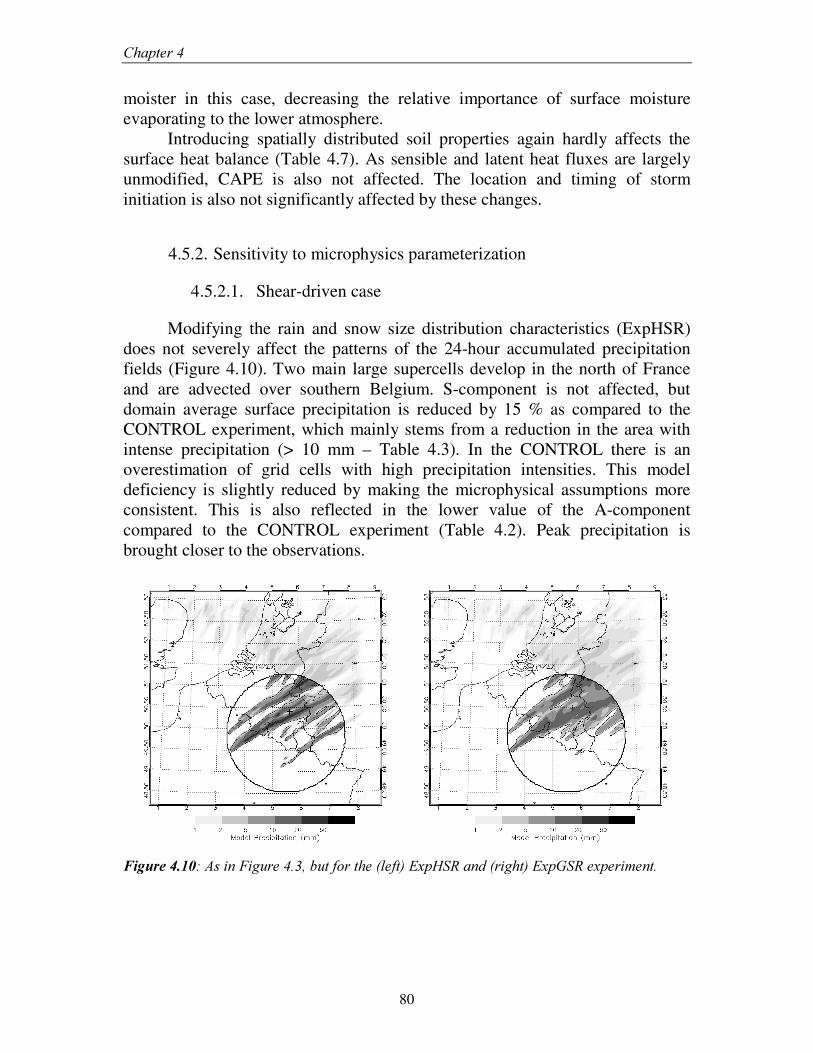
&KDSWHU���
80
moister in this case, decreasing the relative importance of surface moisture evaporating to the lower atmosphere.
Introducing spatially distributed soil properties again hardly affects the surface heat balance (Table 4.7). As sensible and latent heat fluxes are largely unmodified, CAPE is also not affected. The location and timing of storm initiation is also not significantly affected by these changes.
4.5.2. Sensitivity to microphysics parameterization
4.5.2.1. Shear-driven case
Modifying the rain and snow size distribution characteristics (ExpHSR) does not severely affect the patterns of the 24-hour accumulated precipitation fields (Figure 4.10). Two main large supercells develop in the north of France and are advected over southern Belgium. S-component is not affected, but domain average surface precipitation is reduced by 15 % as compared to the CONTROL experiment, which mainly stems from a reduction in the area with intense precipitation (> 10 mm – Table 4.3). In the CONTROL there is an overestimation of grid cells with high precipitation intensities. This model deficiency is slightly reduced by making the microphysical assumptions more consistent. This is also reflected in the lower value of the A-component compared to the CONTROL experiment (Table 4.2). Peak precipitation is brought closer to the observations.
)LJXUH�������$V�LQ�)LJXUH������EXW�IRU�WKH��OHIW��([S+65�DQG��ULJKW��([S*65�H[SHULPHQW���
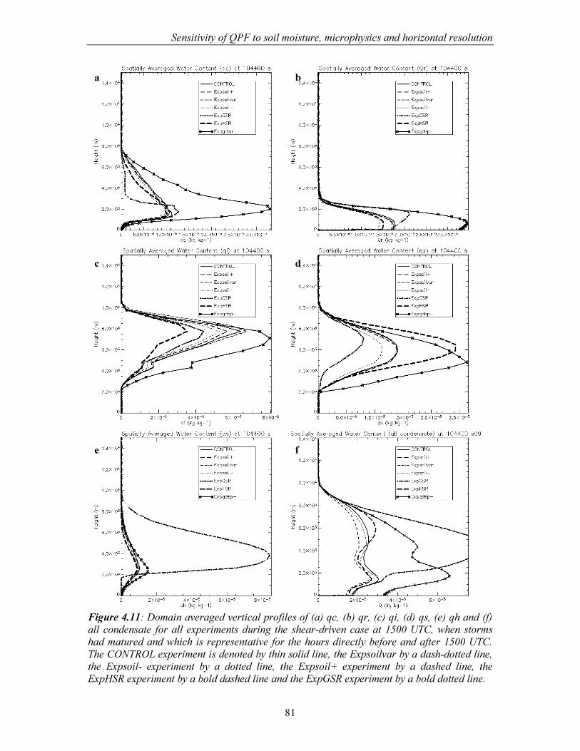
6HQVLWLYLW\�RI�43)�WR�VRLO�PRLVWXUH��PLFURSK\VLFV�DQG�KRUL]RQWDO�UHVROXWLRQ�
81
)LJXUH�������'RPDLQ�DYHUDJHG�YHUWLFDO�SURILOHV�RI��D��TF���E��TU���F��TL���G��TV���H��TK�DQG��I��DOO�FRQGHQVDWH� IRU�DOO�H[SHULPHQWV�GXULQJ� WKH�VKHDU�GULYHQ�FDVH�DW������87&��ZKHQ�VWRUPV�KDG�PDWXUHG�DQG�ZKLFK�LV�UHSUHVHQWDWLYH�IRU�WKH�KRXUV�GLUHFWO\�EHIRUH�DQG�DIWHU������87&��7KH�&21752/�H[SHULPHQW�LV�GHQRWHG�E\�WKLQ�VROLG�OLQH��WKH�([SVRLOYDU�E\�D�GDVK�GRWWHG�OLQH��WKH� ([SVRLO�� H[SHULPHQW� E\� D� GRWWHG� OLQH�� WKH� ([SVRLO�� H[SHULPHQW� E\� D� GDVKHG� OLQH�� WKH�([S+65�H[SHULPHQW�E\�D�EROG�GDVKHG�OLQH�DQG�WKH�([S*65�H[SHULPHQW�E\�D�EROG�GRWWHG�OLQH��
D� E�
F� G�
H� I�
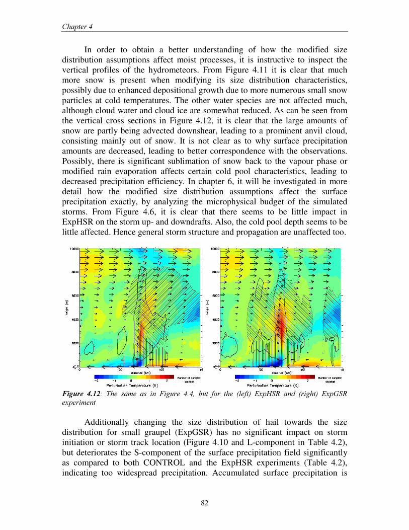
&KDSWHU���
82
In order to obtain a better understanding of how the modified size distribution assumptions affect moist processes, it is instructive to inspect the vertical profiles of the hydrometeors. From Figure 4.11 it is clear that much more snow is present when modifying its size distribution characteristics, possibly due to enhanced depositional growth due to more numerous small snow particles at cold temperatures. The other water species are not affected much, although cloud water and cloud ice are somewhat reduced. As can be seen from the vertical cross sections in Figure 4.12, it is clear that the large amounts of snow are partly being advected downshear, leading to a prominent anvil cloud, consisting mainly out of snow. It is not clear as to why surface precipitation amounts are decreased, leading to better correspondence with the observations. Possibly, there is significant sublimation of snow back to the vapour phase or modified rain evaporation affects certain cold pool characteristics, leading to decreased precipitation efficiency. In chapter 6, it will be investigated in more detail how the modified size distribution assumptions affect the surface precipitation exactly, by analyzing the microphysical budget of the simulated storms. From Figure 4.6, it is clear that there seems to be little impact in ExpHSR on the storm up- and downdrafts. Also, the cold pool depth seems to be little affected. Hence general storm structure and propagation are unaffected too.
)LJXUH� ������ 7KH� VDPH� DV� LQ� )LJXUH� ����� EXW� IRU� WKH� �OHIW�� ([S+65� DQG� �ULJKW�� ([S*65�H[SHULPHQW�
Additionally changing the size distribution of hail towards the size distribution for small graupel (ExpGSR) has no significant impact on storm initiation or storm track location (Figure 4.10 and L-component in Table 4.2), but deteriorates the S-component of the surface precipitation field significantly as compared to both CONTROL and the ExpHSR experiments (Table 4.2), indicating too widespread precipitation. Accumulated surface precipitation is
6HQVLWLYLW\�RI�43)�WR�VRLO�PRLVWXUH��PLFURSK\VLFV�DQG�KRUL]RQWDO�UHVROXWLRQ�
83
decreased by 12 % compared to the CONTROL experiment. The decrease is due to a very strong reduction in the area with very intense precipitation (> 20 mm) as can be inferred from Table 4.3, which is more in agreement with the observations. Peak precipitation drops well below the observed value, however.
The much slower and lighter graupel strongly redistributes the water in the atmosphere between the precipitating hydrometeors (Figure 4.11). Much more graupel is being formed as the smaller particles collect more cloud ice, cloud water, snow and rain. Further, graupel fallout is reduced as its fallspeed is much lower. These processes lead the domain total amount of graupel to grow five times as much as compared to the CONTROL experiment. As can be inferred from the vertical cross sections in Figure 4.12, this results in cloud water and ice being limited to the updrafting cores as they are much more accreted by graupel. As graupel is hardly sublimating and falling slowly towards the surface, diffusion of graupel both upshear and downshear lead precipitating cells to grow larger. Once the graupel reaches the melting level, it melts almost instantaneously inducing a much broader area with intense surface rain (> 5 mm), which leads to a stronger overestimation in this precipitation bin (Table 4.3). Including graupel hence leads to a deterioration of the surface precipitation structure and the vertical distribution of the hydrometeors, as the clear supercell signature tends to get lost in the vertical cross sections.
4.5.2.2. Buoyancy-driven case
Including more realistic assumptions for the rain and snow size distribution (ExpHSR) hardly affects the general features of the surface precipitation field in the buoyancy-driven case. The S-component of the SAL analysis is again hardly affected and the L component remains small. Although peak precipitation is decreased, total precipitation accumulation is not affected (Table 4.5 and Figure 4.13).
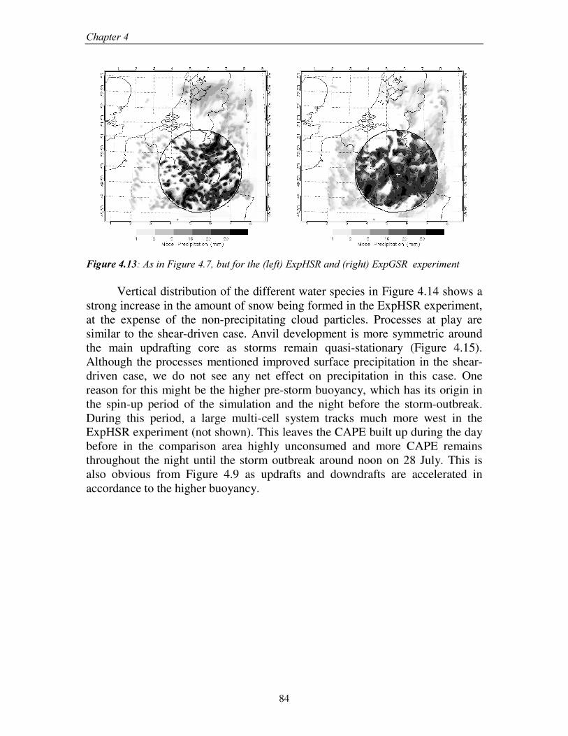
&KDSWHU���
84
)LJXUH�������$V�LQ�)LJXUH������EXW�IRU�WKH��OHIW��([S+65�DQG��ULJKW��([S*65��H[SHULPHQW�
Vertical distribution of the different water species in Figure 4.14 shows a strong increase in the amount of snow being formed in the ExpHSR experiment, at the expense of the non-precipitating cloud particles. Processes at play are similar to the shear-driven case. Anvil development is more symmetric around the main updrafting core as storms remain quasi-stationary (Figure 4.15). Although the processes mentioned improved surface precipitation in the shear-driven case, we do not see any net effect on precipitation in this case. One reason for this might be the higher pre-storm buoyancy, which has its origin in the spin-up period of the simulation and the night before the storm-outbreak. During this period, a large multi-cell system tracks much more west in the ExpHSR experiment (not shown). This leaves the CAPE built up during the day before in the comparison area highly unconsumed and more CAPE remains throughout the night until the storm outbreak around noon on 28 July. This is also obvious from Figure 4.9 as updrafts and downdrafts are accelerated in accordance to the higher buoyancy.
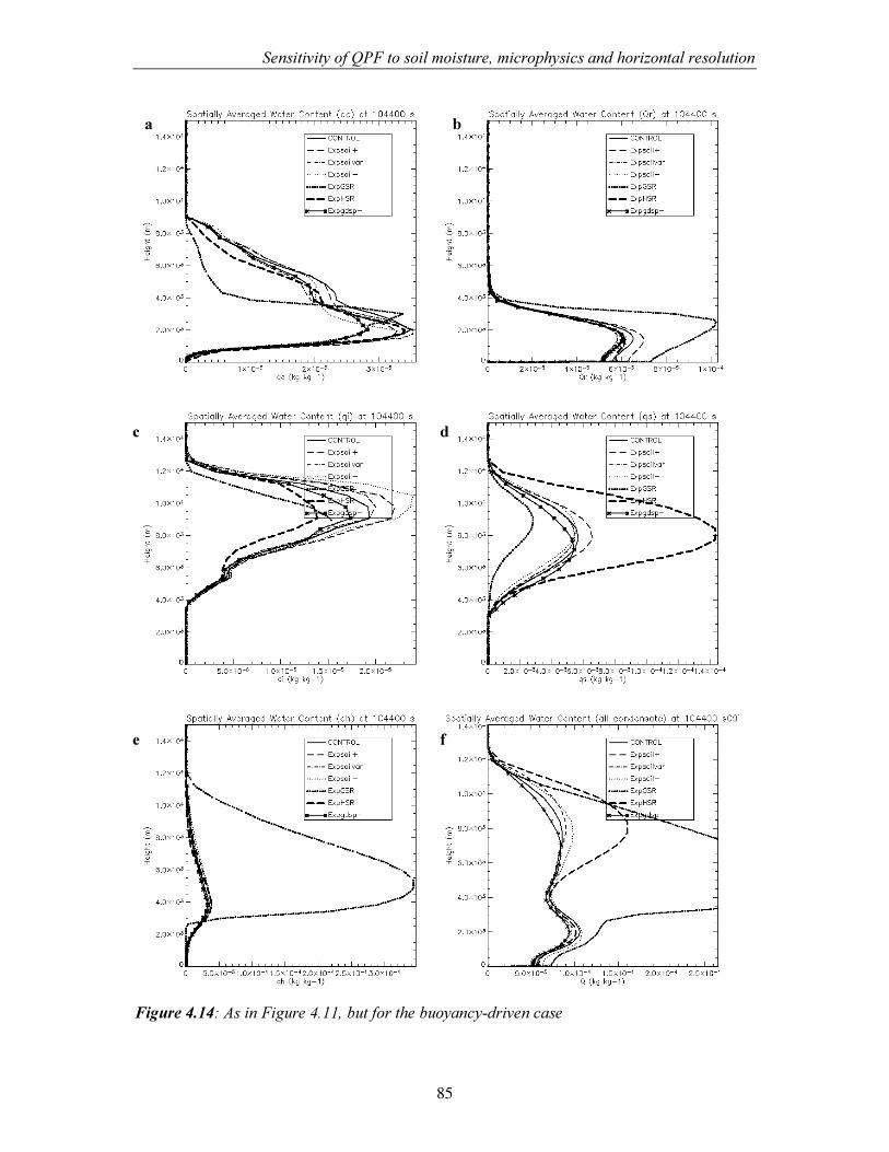
6HQVLWLYLW\�RI�43)�WR�VRLO�PRLVWXUH��PLFURSK\VLFV�DQG�KRUL]RQWDO�UHVROXWLRQ�
85
)LJXUH�������$V�LQ�)LJXUH�������EXW�IRU�WKH�EXR\DQF\�GULYHQ�FDVH��
D� E�
F� G�
H� I�
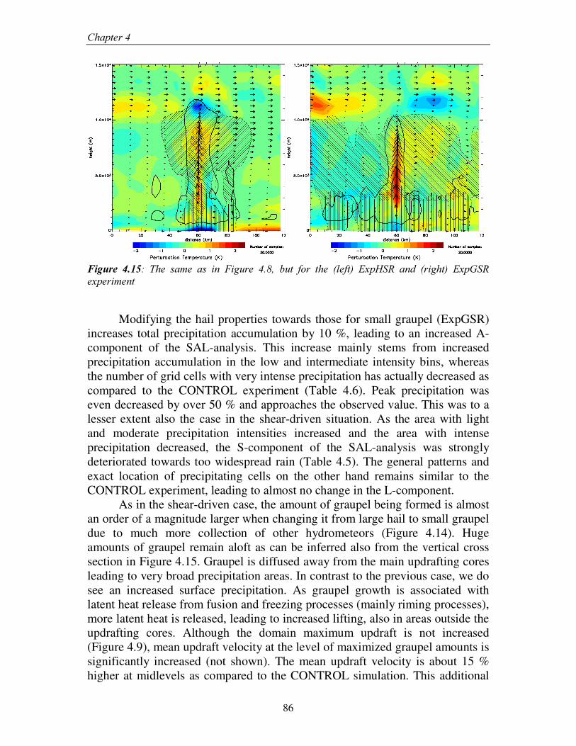
&KDSWHU���
86
�)LJXUH� ������ 7KH� VDPH� DV� LQ� )LJXUH� ����� EXW� IRU� WKH� �OHIW�� ([S+65� DQG� �ULJKW�� ([S*65�H[SHULPHQW���
Modifying the hail properties towards those for small graupel (ExpGSR) increases total precipitation accumulation by 10 %, leading to an increased A-component of the SAL-analysis. This increase mainly stems from increased precipitation accumulation in the low and intermediate intensity bins, whereas the number of grid cells with very intense precipitation has actually decreased as compared to the CONTROL experiment (Table 4.6). Peak precipitation was even decreased by over 50 % and approaches the observed value. This was to a lesser extent also the case in the shear-driven situation. As the area with light and moderate precipitation intensities increased and the area with intense precipitation decreased, the S-component of the SAL-analysis was strongly deteriorated towards too widespread rain (Table 4.5). The general patterns and exact location of precipitating cells on the other hand remains similar to the CONTROL experiment, leading to almost no change in the L-component.
As in the shear-driven case, the amount of graupel being formed is almost an order of a magnitude larger when changing it from large hail to small graupel due to much more collection of other hydrometeors (Figure 4.14). Huge amounts of graupel remain aloft as can be inferred also from the vertical cross section in Figure 4.15. Graupel is diffused away from the main updrafting cores leading to very broad precipitation areas. In contrast to the previous case, we do see an increased surface precipitation. As graupel growth is associated with latent heat release from fusion and freezing processes (mainly riming processes), more latent heat is released, leading to increased lifting, also in areas outside the updrafting cores. Although the domain maximum updraft is not increased (Figure 4.9), mean updraft velocity at the level of maximized graupel amounts is significantly increased (not shown). The mean updraft velocity is about 15 % higher at midlevels as compared to the CONTROL simulation. This additional
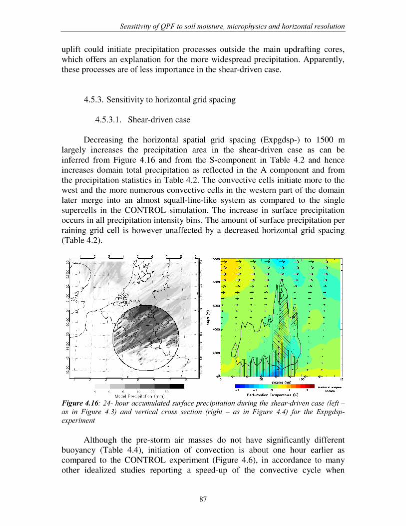
6HQVLWLYLW\�RI�43)�WR�VRLO�PRLVWXUH��PLFURSK\VLFV�DQG�KRUL]RQWDO�UHVROXWLRQ�
87
uplift could initiate precipitation processes outside the main updrafting cores, which offers an explanation for the more widespread precipitation. Apparently, these processes are of less importance in the shear-driven case.
4.5.3. Sensitivity to horizontal grid spacing
4.5.3.1. Shear-driven case
Decreasing the horizontal spatial grid spacing (Expgdsp-) to 1500 m largely increases the precipitation area in the shear-driven case as can be inferred from Figure 4.16 and from the S-component in Table 4.2 and hence increases domain total precipitation as reflected in the A component and from the precipitation statistics in Table 4.2. The convective cells initiate more to the west and the more numerous convective cells in the western part of the domain later merge into an almost squall-line-like system as compared to the single supercells in the CONTROL simulation. The increase in surface precipitation occurs in all precipitation intensity bins. The amount of surface precipitation per raining grid cell is however unaffected by a decreased horizontal grid spacing (Table 4.2).
)LJXUH�����������KRXU�DFFXPXODWHG�VXUIDFH�SUHFLSLWDWLRQ�GXULQJ�WKH�VKHDU�GULYHQ�FDVH��OHIW�±�DV� LQ� )LJXUH� ����� DQG� YHUWLFDO� FURVV� VHFWLRQ� �ULJKW� ±� DV� LQ� )LJXUH� ����� IRU� WKH� ([SJGVS��H[SHULPHQW�
Although the pre-storm air masses do not have significantly different buoyancy (Table 4.4), initiation of convection is about one hour earlier as compared to the CONTROL experiment (Figure 4.6), in accordance to many other idealized studies reporting a speed-up of the convective cycle when
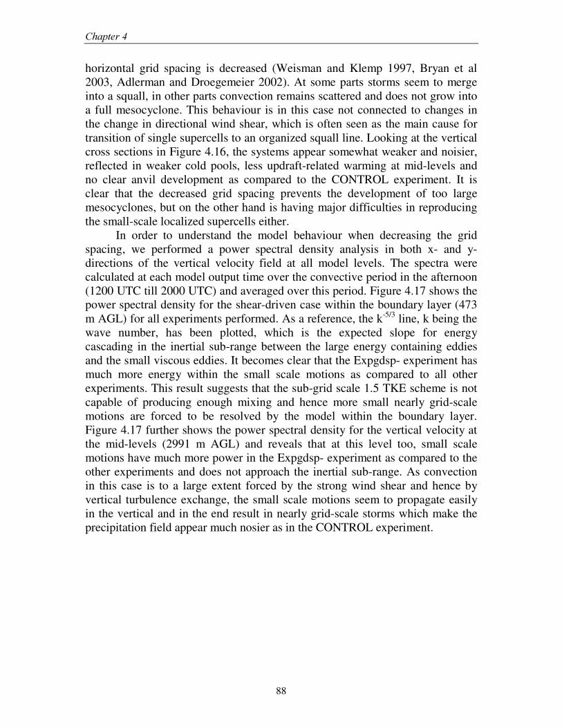
&KDSWHU���
88
horizontal grid spacing is decreased (Weisman and Klemp 1997, Bryan et al 2003, Adlerman and Droegemeier 2002). At some parts storms seem to merge into a squall, in other parts convection remains scattered and does not grow into a full mesocyclone. This behaviour is in this case not connected to changes in the change in directional wind shear, which is often seen as the main cause for transition of single supercells to an organized squall line. Looking at the vertical cross sections in Figure 4.16, the systems appear somewhat weaker and noisier, reflected in weaker cold pools, less updraft-related warming at mid-levels and no clear anvil development as compared to the CONTROL experiment. It is clear that the decreased grid spacing prevents the development of too large mesocyclones, but on the other hand is having major difficulties in reproducing the small-scale localized supercells either.
In order to understand the model behaviour when decreasing the grid spacing, we performed a power spectral density analysis in both x- and y-directions of the vertical velocity field at all model levels. The spectra were calculated at each model output time over the convective period in the afternoon (1200 UTC till 2000 UTC) and averaged over this period. Figure 4.17 shows the power spectral density for the shear-driven case within the boundary layer (473 m AGL) for all experiments performed. As a reference, the k-5/3 line, k being the wave number, has been plotted, which is the expected slope for energy cascading in the inertial sub-range between the large energy containing eddies and the small viscous eddies. It becomes clear that the Expgdsp- experiment has much more energy within the small scale motions as compared to all other experiments. This result suggests that the sub-grid scale 1.5 TKE scheme is not capable of producing enough mixing and hence more small nearly grid-scale motions are forced to be resolved by the model within the boundary layer. Figure 4.17 further shows the power spectral density for the vertical velocity at the mid-levels (2991 m AGL) and reveals that at this level too, small scale motions have much more power in the Expgdsp- experiment as compared to the other experiments and does not approach the inertial sub-range. As convection in this case is to a large extent forced by the strong wind shear and hence by vertical turbulence exchange, the small scale motions seem to propagate easily in the vertical and in the end result in nearly grid-scale storms which make the precipitation field appear much nosier as in the CONTROL experiment.
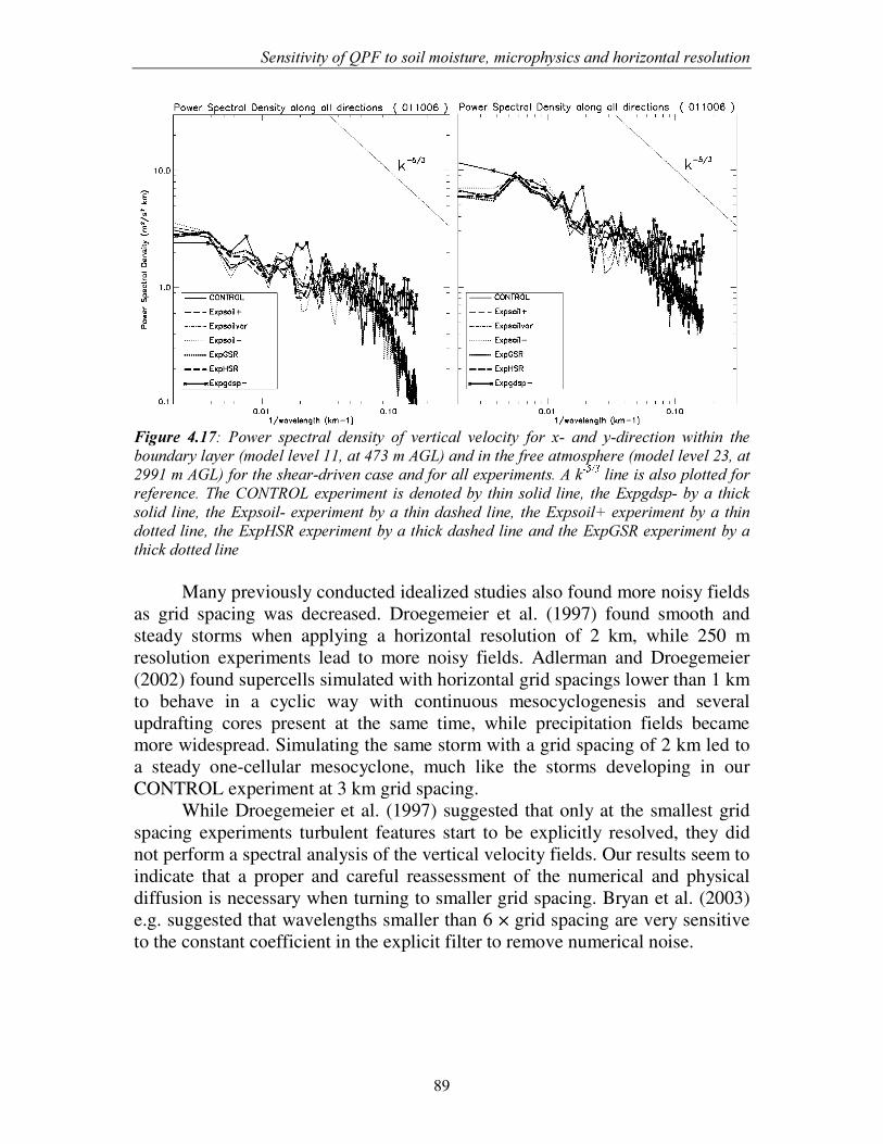
6HQVLWLYLW\�RI�43)�WR�VRLO�PRLVWXUH��PLFURSK\VLFV�DQG�KRUL]RQWDO�UHVROXWLRQ�
89
)LJXUH� ������ 3RZHU� VSHFWUDO� GHQVLW\� RI� YHUWLFDO� YHORFLW\� IRU� [�� DQG� \�GLUHFWLRQ� ZLWKLQ� WKH�ERXQGDU\�OD\HU��PRGHO�OHYHO�����DW�����P�$*/��DQG�LQ�WKH�IUHH�DWPRVSKHUH��PRGHO�OHYHO�����DW������P�$*/��IRU�WKH�VKHDU�GULYHQ�FDVH�DQG�IRU�DOO�H[SHULPHQWV��$�N É Ë�Ì Í �OLQH�LV�DOVR�SORWWHG�IRU�UHIHUHQFH��7KH�&21752/�H[SHULPHQW� LV�GHQRWHG�E\� WKLQ�VROLG�OLQH�� WKH�([SJGVS��E\�D� WKLFN�VROLG� OLQH��WKH�([SVRLO��H[SHULPHQW�E\�D� WKLQ�GDVKHG� OLQH�� WKH�([SVRLO��H[SHULPHQW�E\�D� WKLQ�GRWWHG�OLQH��WKH�([S+65�H[SHULPHQW�E\�D�WKLFN�GDVKHG�OLQH�DQG�WKH�([S*65�H[SHULPHQW�E\�D�WKLFN�GRWWHG�OLQH��
Many previously conducted idealized studies also found more noisy fields as grid spacing was decreased. Droegemeier et al. (1997) found smooth and steady storms when applying a horizontal resolution of 2 km, while 250 m resolution experiments lead to more noisy fields. Adlerman and Droegemeier (2002) found supercells simulated with horizontal grid spacings lower than 1 km to behave in a cyclic way with continuous mesocyclogenesis and several updrafting cores present at the same time, while precipitation fields became more widespread. Simulating the same storm with a grid spacing of 2 km led to a steady one-cellular mesocyclone, much like the storms developing in our CONTROL experiment at 3 km grid spacing.
While Droegemeier et al. (1997) suggested that only at the smallest grid spacing experiments turbulent features start to be explicitly resolved, they did not perform a spectral analysis of the vertical velocity fields. Our results seem to indicate that a proper and careful reassessment of the numerical and physical diffusion is necessary when turning to smaller grid spacing. Bryan et al. (2003) e.g. suggested that wavelengths smaller than 6 × grid spacing are very sensitive to the constant coefficient in the explicit filter to remove numerical noise.
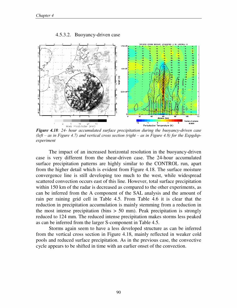
&KDSWHU���
90
4.5.3.2. Buoyancy-driven case
)LJXUH� ������ ���� KRXU� DFFXPXODWHG� VXUIDFH� SUHFLSLWDWLRQ� GXULQJ� WKH� EXR\DQF\�GULYHQ� FDVH��OHIW�±�DV�LQ�)LJXUH������DQG�YHUWLFDO�FURVV�VHFWLRQ��ULJKW�±�DV�LQ�)LJXUH������IRU�WKH�([SJGVS��H[SHULPHQW�
The impact of an increased horizontal resolution in the buoyancy-driven case is very different from the shear-driven case. The 24-hour accumulated surface precipitation patterns are highly similar to the CONTROL run, apart from the higher detail which is evident from Figure 4.18. The surface moisture convergence line is still developing too much to the west, while widespread scattered convection occurs east of this line. However, total surface precipitation within 150 km of the radar is decreased as compared to the other experiments, as can be inferred from the A component of the SAL analysis and the amount of rain per raining grid cell in Table 4.5. From Table 4.6 it is clear that the reduction in precipitation accumulation is mainly stemming from a reduction in the most intense precipitation (bins > 50 mm). Peak precipitation is strongly reduced to 124 mm. The reduced intense precipitation makes storms less peaked as can be inferred from the larger S-component in Table 4.5.
Storms again seem to have a less developed structure as can be inferred from the vertical cross section in Figure 4.18, mainly reflected in weaker cold pools and reduced surface precipitation. As in the previous case, the convective cycle appears to be shifted in time with an earlier onset of the convection.
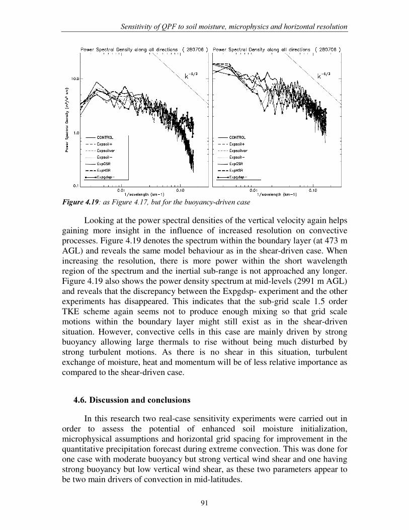
6HQVLWLYLW\�RI�43)�WR�VRLO�PRLVWXUH��PLFURSK\VLFV�DQG�KRUL]RQWDO�UHVROXWLRQ�
91
)LJXUH�������DV�)LJXUH�������EXW�IRU�WKH�EXR\DQF\�GULYHQ�FDVH�
Looking at the power spectral densities of the vertical velocity again helps gaining more insight in the influence of increased resolution on convective processes. Figure 4.19 denotes the spectrum within the boundary layer (at 473 m AGL) and reveals the same model behaviour as in the shear-driven case. When increasing the resolution, there is more power within the short wavelength region of the spectrum and the inertial sub-range is not approached any longer. Figure 4.19 also shows the power density spectrum at mid-levels (2991 m AGL) and reveals that the discrepancy between the Expgdsp- experiment and the other experiments has disappeared. This indicates that the sub-grid scale 1.5 order TKE scheme again seems not to produce enough mixing so that grid scale motions within the boundary layer might still exist as in the shear-driven situation. However, convective cells in this case are mainly driven by strong buoyancy allowing large thermals to rise without being much disturbed by strong turbulent motions. As there is no shear in this situation, turbulent exchange of moisture, heat and momentum will be of less relative importance as compared to the shear-driven case.
������'LVFXVVLRQ�DQG�FRQFOXVLRQV�
�In this research two real-case sensitivity experiments were carried out in
order to assess the potential of enhanced soil moisture initialization, microphysical assumptions and horizontal grid spacing for improvement in the quantitative precipitation forecast during extreme convection. This was done for one case with moderate buoyancy but strong vertical wind shear and one having strong buoyancy but low vertical wind shear, as these two parameters appear to be two main drivers of convection in mid-latitudes.
&KDSWHU���
92
The gain of spatially distributed soil moisture and texture information was small in our simulations, but it is important to have at least the mean soil moisture content right for a realistic simulation of cold pool intensity, storm structure and surface precipitation. We propose a mechanism to explain the inverse relation between surface precipitation and soil moisture content found here but also in some other studies (Martin and Xue 2006, Cheng and Cotton 2004). Increasing soil moisture content enhances the thermodynamic conditions for storm development. However, this effect is counterbalanced by a weakening of the storms as a consequence of a weakening of the cold pools due to less evaporative cooling within the boundary layer. There are also some studies that contradict these results and where surface precipitation was found to increase with increasing soil moisture, such as Gallus and Segal (2000). These studies make use of rather coarse scale modeling, requiring convection to be parameterized. Davis (2003) showed that these convective parameterization schemes (CPS) fail in many circumstances to correctly simulate storm propagation characteristics. They speculated that cold pools produced by CPSs were insufficiently cold to permit propagation. Therefore in models that use CPSs, the effect of enhancement of the storms due to thermodynamic conditions is not counterbalanced by a weakening of the storm evolution by weaker cold pools. This implies that coarse scale models with a CPS are missing an important mechanism for storm development and are therefore less suitable to study the effect of soil moisture anomalies on storm intensity than high-resolution models that do not depend on a CPS. An aspect we did not investigate, but would be worthwhile for further study, is the impact of soil moisture on the lifecycle (storm initiation to storm decay) and life time of storms. It might be that due to more vigorous cold pools, storms live longer when soils are dry, mainly in the shear-driven case.
Changing the size distribution assumptions of the precipitating hydrometeors in the microphysics parameterization scheme had a larger impact on the hydrometeor distribution than on surface precipitation. Unfortunately, no polarimetric radar was present within our study area in order to determine which of the microphysics experiments led to a better representation of the hydrometeor distribution. From comparison against observed precipitation fields it is clear however that including more realistic rain and snow size distributions slightly improved the surface precipitation in a shear-driven case, while there was no change in a buoyancy-driven situation. Weighting the size distribution assumptions of the large hail to small graupel led to a very poor representation of the general storm structure, reflected in high S-components of the SAL analysis. Large amounts of graupel were precipitating outside the convective cores, leading to widespread and, mainly in the buoyancy-driven case, unrealistic precipitation fields. As mentioned by e.g. McCumber et al. (1991) and Cohen and McCaul (2006) including both hail and graupel as prognostic
6HQVLWLYLW\�RI�43)�WR�VRLO�PRLVWXUH��PLFURSK\VLFV�DQG�KRUL]RQWDO�UHVROXWLRQ�
93
variables would avoid tuning a single variable representing both hail and graupel.
Increasing the horizontal grid spacing apparently led to issues with parameterized sub-grid turbulent motions in the boundary layer. Power spectral density analysis revealed that the 1.5 TKE scheme could not produce enough small-scale turbulence, leading to excessive motions on the resolved scale. In a shear-driven situation, where vertical momentum exchanges are important mechanisms to enhance convection, those small-scale turbulent motions easily propagated upward in the atmosphere leading to the development of numerous grid-scale storms popping up and excessive surface precipitation. In a buoyancy-driven case, where convective development is dominated by the rise of large thermals from the surface, those excessive small-scale motions did not propagate upward easily in the atmosphere and the influence on surface precipitation was found to be small. These results suggest that a proper and careful assessment of the numerical and physical diffusion coefficients is necessary when turning to smaller grid spacings.
It should further be stressed that our study only investigated three aspects of QPF. Many more model components influence the simulation of deep convection, such e.g. parameterization of boundary-layer processes, (shallow) convection parameterization and even the applied numerical techniques. Wisse et al. (2004) and Deng and Stauffer (2006), simulating deep convection at similar horizontal grid spacing as in our study, both found the Medium-Range Forecast (MRF) boundary-layer scheme to enhance vertical mixing significantly. This mostly led to too widespread precipitation as compared to e.g. the Eta-Mellor-Yamada (ETA) or the Gayno-Seaman (GS) boundary layer schemes. Deng and Stauffer (2006) found largest improvement in their simulation of a convective case over the Great Lake area in the northern United States at a 4 km horizontal grid spacing when applying a convection parameterization, suggesting that such grid spacing is still not able to resolve deep convection sufficiently. Actually, sensitivities they found were in the same order of magnitude as sensitivities found in our experiments on soil moisture and microphysics parameterization.
In summary we can conclude that the experiments we carried out mainly affected the storm intensity and more realistic size distribution assumptions as well as initial soil moisture assumptions can improve simulated precipitation intensity during extreme convection as compared to observations. On the other hand, we found a minor impact on the position of convective initiation and the eventual storm structure development. More research in these fields is needed but we are convinced that the set up of a large number of sensitivity studies for real cases, which can be compared to the observed situation, provides much added value to the mostly idealized experiments carried out so far for which it is not possible to judge whether a model modification is actually a model improvement.

94
�������������������������������������������
95
����������
&KDSWHU������
(YDOXDWLRQ�RI�PRLVW�SURFHVVHV�LQ�NP�VFDOH�1:3�PRGHOV�XVLQJ�UHPRWH�VHQVLQJ�DQG�LQ�VLWX�GDWD��LPSDFW�RI�PLFURSK\VLFV�VL]H�
GLVWULEXWLRQ�DVVXPSWLRQV �
������,QWURGXFWLRQ�
A proper simulation of severe precipitation within numerical weather prediction models requires that moist processes in the atmosphere are adequately represented. An indispensable part in the turnover of water vapour to clouds and precipitation is the parameterization of microphysical cloud processes. Due to the small scales of processes involved, a large number of simplifications and assumptions on e.g. size distributions of the several hydrometeors have to be made.
Typically, microphysical processes have been represented in numerical models by one-moment bulk (OMB) microphysical schemes, representing a single size distribution on the bulk of the hydrometeor species within a model grid cell and predicting only one moment of a hydrometeor’ s size distribution, being its mixing ratio (third moment – e.g. Lin et al. 1983, Rutledge and Hobbs 1983, Cotton et al. 1986). Current advances in microphysics can be subdivided in at least three main directions. A first sophistication involves a higher number of predicted moments, such as the number concentration (zeroth moment – e.g.
* Van Weverberg, K., N. P. M. van Lipzig, L. Delobbe, 2010: Evaluation of moist processes during intense precipitation in km-scale NWP models using remote sensing and in-situ data: impact of microphysics size distribution assumptions. Atmospheric Research (submitted).
&KDSWHU���
96
Ferrier 1994, Seifert and Beheng 2005) or the radar reflectivity (sixth moment – e.g. Milbrandt and Yau 2005). A second direction consists of separating the mass contents in several size categories (bin or spectral microphysical schemes, e.g. Kogan 1991, Khain et al. 1999, Ovtchinnikov and Kogan 2000). At last, it is investigated whether improvements in the bulk size distribution assumptions of the OMB microphysics schemes are capable of better representing microphysical cloud processes (Woods et al. 2007, Cohen and McCaul 2006). While the two former approaches have definitely a higher degree of sophistication, the computational cost of the latter is much smaller, as it does not involve a higher number of prognostic variables. Furthermore, it remains unclear how many processes are influenced by the way size distributions in OMB schemes are represented. Hence OMB microphysics schemes remain the workhorse in numerical weather prediction to this day.
Many of the studies to OMB microphysical parameterizations over the past decade were conducted for either warm season convection or frontal stratiform precipitation and had a focus on a single microphysical parameter only. Often that parameter was concerned with hail/ graupel in studies on convection (Gilmore et al. 2004, McCumber et al. 1991, Smedsmo et al. 2005) and with snow in studies on frontal stratiform precipitation (Colle et al. 2005, Woods et al. 2007). In operational weather forecasting a single model set up is needed which is providing good simulation for both convective and stratiform situations. For that reason it is interesting to understand what impact a model modification made to improve the moist processes under a certain synoptic situation has in other synoptic situations. Furthermore, most of the studies to the influence of microphysical processes on convective storms have been conducted for idealized conditions, initializing the model with a single sounding. While such studies are more straightforward to interpret, they have the disadvantage that they cannot be easily verified against observational data. In recent years, many efforts have been done to obtain spatially distributed observational data with high temporal resolution from spaceborne and ground-based remote sensors, such as satellite and weather radar, largely increasing knowledge on the three-dimensional atmospheric conditions during intense precipitation events.
This chapter discusses a number of experiments in which size distribution assumptions of a typical OMB microphysical scheme have been more realistically represented for both stratiform and convective intense precipitation situations. Using a broad range of high resolution observational data this research wants to gain more insight in to what extent a more realistic representation of the size distribution assumptions also leads to a model improvement of the representation of moist processes during intense precipitation events. A description of the model setup, the cases studied and the available observational data products is given in section 5.2. Section 5.3 provides an overview of the microphysics experiments and results of these
(YDOXDWLRQ�RI�PRLVW�SURFHVVHV�LQ�NP�VFDOH�1:3�PRGHOV��
97
experiments are compared against observational data in section 5.4. Conclusions and issues for further research are discussed in section 5.5.
������0RGHO�VHWXS�DQG�REVHUYDWLRQDO�GDWD�
5.2.1. Model setup and experiments design The model setup of ARPS was as described in section 3.2. A number of sensitivity experiments are implemented in order to understand if more realistic size distribution assumptions yield a more realistic representation of moist processes and surface precipitation. These experiments were applied on the shear-driven of 01 October 20006, buoyancy-driven convective case of 28 July 2006 and the stratiform case of 23 November 2006, described in detail in section 3.5. For both the stratiform and the convective cases, the control experiment is identical to ExpH discussed in Chapter 4, having the default Lin et al. (1983) microphysical setup. During the FRQYHFWLYH cases, the implemented sensitivity experiments are the ExpHSR and ExpGSR, described in Chapter 4. ExpHSR and ExpGSR include more realistic rain and snow size distribution assumptions and the ExpGSR additionally has its largest precipitating ice species weighted to small graupel as compared to large hail in ExpH and ExpHSR. Sensitivity experiments for the VWUDWLIRUP case are as ExpHSR and ExpGSR apart from the mass-diameter and mass-velocity diameter implemented for the snow species. Instead of implementing the formulations for graupel-like snow of Locatelli and Hobbs (1974), we assumed that formulations for slowly falling dendritic snow, as observed by Cox (1988) more realistically represent the conditions during large-scale gentle uplift in a frontal stratiform situation. The latter two experiments are referred to as ExpGSRstrat and ExpHSRstrat. An overview all experiments used in this chapter is given in Table 5.1.

&KDSWHU���
98
7DEOH������2YHUYLHZ�RI�WKH�IRUPXODWLRQV�IRU�WKH�LQWHUFHSW�SDUDPHWHU��1 ���VORSH�SDUDPHWHU�� ��DQG� WHUPLQDO� IDOO�YHORFLW\� �9�� IRU�DOO�SUHFLSLWDWLQJ�K\GURPHWHRUV�XVHG� LQ�H[SHULPHQWV�([S+��([S+65�� ([S*65�� ([S+65strat� DQG� ([S*65strat�� 3DUDPHWHUV� WKDW� ZHUH� PRGLILHG� IURP� WKH�RULJLQDO� IRUPXODWLRQV� LQ� WKH� PLFURSK\VLFV� VFKHPH� KDYH� EHHQ� VKDGHG� �\HOORZLVK� IRU� UDLQ�SDUDPHWHUV��EOXLVK�IRU�VQRZ�SDUDPHWHUV�DQG�UHGGLVK�IRU�KDLO�JUDXSHO�SDUDPHWHUV���
ExpH ExpHSR ExpGSR ExpHSRstrat ExpGSRstrat
N0
R
08.0 Ï ÐWÑYÒ[Ó�Ô�Ñ�Õ Õ^Ñ�Ö×bØvÑ�Õ ÙfÚ�ÒÛ�Ü�ÝjÞ[ß ( ) 648.031007106.0 àáρ Ï âcÔÑYÖ�ãqÚ�ä^ÑYÕ åjæ�ç�ç Þ[ß ( ) 648.031007106.0 èéρ
Appendix·B:·Microphysics·conversion·equations____________________193¶
(Zhang et al. 2008) (Zhang et al. 2008) •R VR (Liu and Orville 1969) (Liu and Orville 1969) (Liu and Orville 1969) (Liu and Orville 1969) (Liu and Orville 1969) N0S 0.03 (Gunn and Marshall 1958) (Houze et al. 1979) (Houze et al. 1979) (Houze et al. 1979) (Houze et al. 1979) •S (Lin et al. 1983) (Locatelli and Hobbs. 1974) (Locatelli and Hobbs. 1974) (Cox 1988) (Cox 1988) VS (Locatelli and Hobbs. 1974)
(Locatelli and Hobbs. 1974) (Locatelli and Hobbs. 1974) (Cox 1988) (Cox 1988) N0H 0.0004 (Federer and Waldvogel 1975) 0.0004 (Federer and Waldvogel 1975) 4.000 (Gilmore et al. 2004) 0.0004 (Federer and Waldvogel 1975) 4.000 (Gilmore et al. 2004) •H (Lin et al. 1983) (Lin et al. 1983) (Locatelli and Hobbs. 1974) (Lin et al. 1983) (Locatelli and Hobbs. 1974) VH (Wisner et al. 1972) (Wisner et al. 1972) (Locatelli and Hobbs. 1974) (Wisner et al. 1972) (Locatelli and Hobbs. 1974) Figure 5.1 provides an overview of the consequences of the modifications in the microphysics size distribution assumptions in all experiments for the hydrometeor fall speed formulations. It is clear that experiments including a mixing ratio dependent rain intercept parameter have faster rain at mixing ratios below 1 g kg-1, but decreased rain fall speeds as compared to the original formulation at higher mixing ratios. In the ExpHSRstrat and ExpGSRstrat, including dendritic snow, snow fall speeds are only half the original fall speeds at cold temperatures, increasing towards the original snow fall speed in the Lin et al. (1983) scheme at warm temperatures. This increase of snow fall speed with temperature is also obvious in ExpHSR and ExpGSR, including graupellike snow, although fall speeds are considerably higher as compared to the original fall speed formulation at warm temperatures. Fall speeds of graupel in experiments ExpGSR and ExpGSRstrat are considerably smaller than those of large hail.
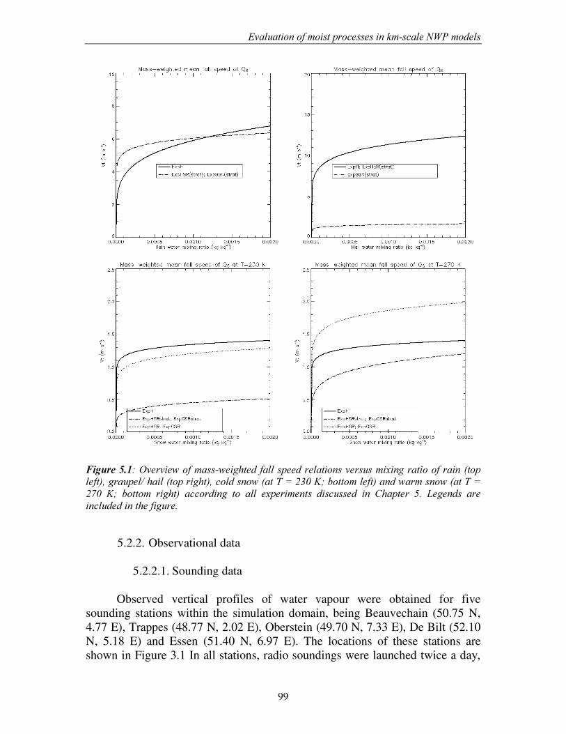
(YDOXDWLRQ�RI�PRLVW�SURFHVVHV�LQ�NP�VFDOH�1:3�PRGHOV��
99
�)LJXUH������2YHUYLHZ�RI�PDVV�ZHLJKWHG�IDOO�VSHHG�UHODWLRQV�YHUVXV�PL[LQJ�UDWLR�RI�UDLQ��WRS�OHIW���JUDXSHO��KDLO��WRS�ULJKW���FROG�VQRZ��DW�7� �����.��ERWWRP�OHIW��DQG�ZDUP�VQRZ��DW�7� ����� .�� ERWWRP� ULJKW�� DFFRUGLQJ� WR� DOO� H[SHULPHQWV� GLVFXVVHG� LQ� &KDSWHU� ��� /HJHQGV� DUH�LQFOXGHG�LQ�WKH�ILJXUH�
5.2.2. Observational data
5.2.2.1. Sounding data
Observed vertical profiles of water vapour were obtained for five sounding stations within the simulation domain, being Beauvechain (50.75 N, 4.77 E), Trappes (48.77 N, 2.02 E), Oberstein (49.70 N, 7.33 E), De Bilt (52.10 N, 5.18 E) and Essen (51.40 N, 6.97 E). The locations of these stations are shown in Figure 3.1 In all stations, radio soundings were launched twice a day,
&KDSWHU���
100
at 0000 UTC and at 1200 UTC, except for Beauvechain where only one sounding was launched at 0000 UTC. Vertically integrated water vapour at these stations is compared against the modelled vertically integrated water vapour at the grid cell located closest to the station position.
5.2.2.2. Satellite data
In order to evaluate simulated cloud hydrometeors (cloud water, cloud ice and snow), cloud optical thickness (COT) was used, derived from SEVIRI (Spinning Enhanced Visible and Infrared Radiometer) onboard the geostationary METEOSAT satellites (Meteosat-8, -9). COT was derived by the EUMETSAT Satellite Application Facility on Climate Monitoring (CM-SAF – Schulz et al. 2009), using the algorithms described in Roebeling et al. (2006), for the buoyancy-driven convective and the stratiform case. During the shear-driven convective case Meteosat-8 entered sleeping mode and hence we used the COT derived by the World Data Center for Remote Sensing of the Atmosphere (WDC-RSAT) using the AVHRR Processing scheme Over cLouds, Land and Ocean (APOLLO, discussed in Saunders and Kriebel (1988)) applied on Meteosat-9 SEVIRI. COT calculation is applied to each grid cell of a satellite scene and is available on a 3 km × 6 km horizontal resolution in our study area with an image repeat cycle of 60 minutes. As the visual channel is used for COT calculation, only daytime hours (0900 – 1300 UTC) are included in the further analysis. Considerable uncertainty exists in the COT retrieval from satellite. From a two weeks validation against pyranometer data in Cabauw, Karlsson et al. (2005) found a good correlation of 0.85 of the daily average COT, although, at certain times large differences could be found due to mismatches in collocation and the sensitivity of the pyranometer retrieval to inhomogeneities in the cloud properties. In order to avoid mismatches due to mislocations we decided to perform model evaluation only by means of integrated methods, such as by comparing the daily integrated simulated and observed frequency distribution.
COT in ARPS is calculated for each hydrometeor separately, following a routine developed at the National Aeronautics and Space Administration (NASA) Goddard Cumulus Ensemble Modelling Group (Tao et al. 2003). For liquid (water) clouds and hail, COT in the visible region is parameterized based on Sui et al. (1998) following Fu and Liou (1993), assuming spherical droplets:
∫= G]5Tê[ëëë
23τ , (5.1)
∫= G]5Tì ííí
23τ , (5.2)
(YDOXDWLRQ�RI�PRLVW�SURFHVVHV�LQ�NP�VFDOH�1:3�PRGHOV��
101
∫= G]5Tî ïïï
23τ , (5.3)
where qc, qr and qh are the mixing ratios (in kg kg-1) of cloud water, rain and hail
respectively and effective radii (in cm) 0015.0=ð[ñ5 , ( ) 25.0
0
.3òòòó ò T15
ρρπ= and
( ) 25.00
.3ôôôõ ô T15
ρρπ= . For cloud ice and snow, COT is parameterized based on
formula derived for cirrus ice crystals by Fu and Liou (1993):
( ) G]5TT ö[÷ øø÷÷ ø∫
×+−×+×=−4
4 10686.3006656.010τ , (5.4)
where qi and qs are the mixing ratio (in kg kg-1) of cloud ice and snow respectively and 0125.0=ù[ú û5 if temperature (T) is above 243.16 K, 0025.0=ü[ý þ5 if temperature is below 223.16 K and ( ) 0005.0*16.2430125.0 −+= 75 ÿ�� � if temperature is between 223.16 and 243.16 K. Total COT is defined as the sum of all components described in equations 5.1 to 5.4. The empirical coefficients -0.006656 and 3.3686 × 10⁻⁴ are determined by Fu and Liou (1993) from fitting different numerical scattering and absorption programs to observed snow size distribution data.
5.2.2.3. Volume radar data
Three-dimensional fields of precipitating hydrometeors can be compared using radar-derived reflectivity values. Volume radar data from the C-band weather radar of Wideumont were derived from a 10-elevation reflectivity scan performed every 15 minutes and interpolated to the ARPS grid. It is well known that C-band radars suffer from attenuation already at moderate rain rates. During and shortly after rainfall on the radar radome, attenuation might become even more of a problem. Therefore, it was chosen to only include data from within a radius of 150 km from the radar position in all further analysis and to perform evaluation using time-integrated methods, rather than comparing individual snap shots. Equivalent reflectivity data, Ze, in mm6 m-3, in ARPS were calculated following Tong and Xue (2008), based on formulations by Smith et al. (1975) assuming Rayleigh scattering for rain, dry snow, wet snow, dry hail and wet hail, yielding:
70
1810720�
�� 1=λ
×= , (5.5)
&KDSWHU���
102
7220
1822 10720���
���� � .1.=
λρρ ×
= , (5.6)
70
1810720�
�� 1=λ
×= , (5.7)
70
181072019.0
�� 1=λ
××= , (5.8)
95.0
70
1810720
×=
�� 1=λ
, (5.9)
where Zr, Zsd, Zsw, Zhd and Zhw are reflectivity factors for rain, dry snow, wet snow, dry hail and wet hail respectively, Nor, Nos, Noh,� r�� s� DQG� h are the intercept and slope parameters of the exponential size distributions of rain, snow and hail respectively. Total Ze is the sum of each of the components described above (equations 5.5 to 5.9). Reflectivity Z, is calculated from Ze by
( )�== 10log10= , (5.10)
The reflectivity data in ARPS were calculated for each model level. Data beyond 150 km from the location of the Wideumont radar and below the lowest beam elevation were omitted from the further analysis.
5.2.2.4. Radar-rain gauge merging product
Surface precipitation observations are obtained from the C-band weather radar in Wideumont (Denoted by the asterisk in Figure 3.1) operated by the Royal Meteorological Institute of Belgium and from a dense network of rain gauges (1 per 135 km²) operated by the hydrological service of the Walloon region. Radar-based precipitation estimates are derived from a 5-elevation reflectivity scan performed every 5 minutes. The processing of the radar data and various strategies for merging radar observations with rain gauge measurements are presented in Goudenhoofdt and Delobbe (2009). In this study, radar and gauge observations have been combined using a simple mean field bias adjustment. Mean bias and mean absolute error using this method was found to be in the order of 0.039 dB and 1.5 mm respectively during a four-year verification against an independent set of rain gauge stations (Goudenhoofdt and Delobbe 2009). The 24h precipitation accumulations for the three cases have been calculated using this method and were aggregated to the ARPS grid. As radar suffers from many issues regarding the quality of its returned power (e.g. attenuation), mainly at large distances from the radar itself, data from beyond 150 km from the radar position were omitted from the further analysis in both the observed and the simulated fields.
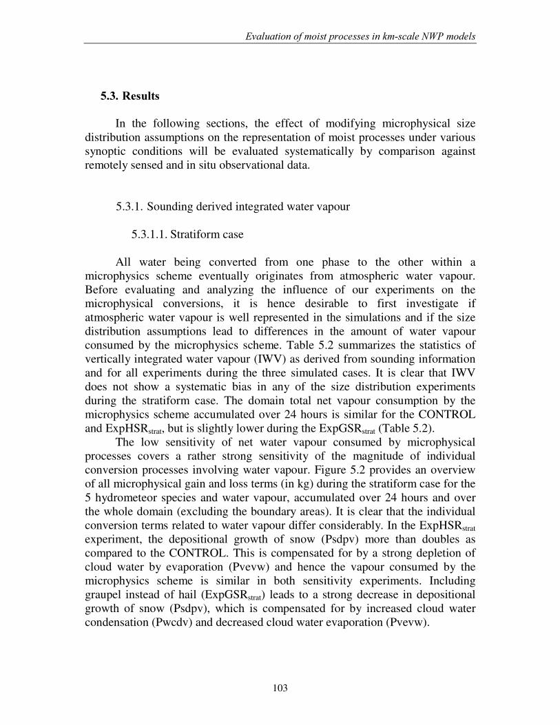
(YDOXDWLRQ�RI�PRLVW�SURFHVVHV�LQ�NP�VFDOH�1:3�PRGHOV��
103
�������5HVXOWV�
In the following sections, the effect of modifying microphysical size distribution assumptions on the representation of moist processes under various synoptic conditions will be evaluated systematically by comparison against remotely sensed and in situ observational data.
5.3.1. Sounding derived integrated water vapour
5.3.1.1. Stratiform case All water being converted from one phase to the other within a
microphysics scheme eventually originates from atmospheric water vapour. Before evaluating and analyzing the influence of our experiments on the microphysical conversions, it is hence desirable to first investigate if atmospheric water vapour is well represented in the simulations and if the size distribution assumptions lead to differences in the amount of water vapour consumed by the microphysics scheme. Table 5.2 summarizes the statistics of vertically integrated water vapour (IWV) as derived from sounding information and for all experiments during the three simulated cases. It is clear that IWV does not show a systematic bias in any of the size distribution experiments during the stratiform case. The domain total net vapour consumption by the microphysics scheme accumulated over 24 hours is similar for the CONTROL and ExpHSRstrat, but is slightly lower during the ExpGSRstrat (Table 5.2).
The low sensitivity of net water vapour consumed by microphysical processes covers a rather strong sensitivity of the magnitude of individual conversion processes involving water vapour. Figure 5.2 provides an overview of all microphysical gain and loss terms (in kg) during the stratiform case for the 5 hydrometeor species and water vapour, accumulated over 24 hours and over the whole domain (excluding the boundary areas). It is clear that the individual conversion terms related to water vapour differ considerably. In the ExpHSRstrat experiment, the depositional growth of snow (Psdpv) more than doubles as compared to the CONTROL. This is compensated for by a strong depletion of cloud water by evaporation (Pvevw) and hence the vapour consumed by the microphysics scheme is similar in both sensitivity experiments. Including graupel instead of hail (ExpGSRstrat) leads to a strong decrease in depositional growth of snow (Psdpv), which is compensated for by increased cloud water condensation (Pwcdv) and decreased cloud water evaporation (Pvevw).
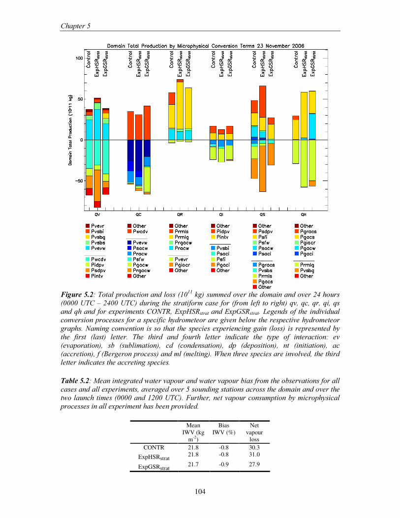
&KDSWHU���
104
)LJXUH������7RWDO�SURGXFWLRQ�DQG�ORVV����11�NJ��VXPPHG�RYHU�WKH�GRPDLQ�DQG�RYHU����KRXUV�������87&�±������87&��GXULQJ�WKH�VWUDWLIRUP�FDVH�IRU��IURP�OHIW�WR�ULJKW��TY��TF��TU��TL��TV�DQG�TK�DQG�IRU�H[SHULPHQWV�&2175��([S+65strat�DQG�([S*65strat��/HJHQGV�RI�WKH�LQGLYLGXDO�FRQYHUVLRQ�SURFHVVHV�IRU�D�VSHFLILF�K\GURPHWHRU�DUH�JLYHQ�EHORZ�WKH�UHVSHFWLYH�K\GURPHWHRU�JUDSKV��1DPLQJ�FRQYHQWLRQ� LV�VR� WKDW� WKH�VSHFLHV�H[SHULHQFLQJ�JDLQ��ORVV�� LV�UHSUHVHQWHG�E\�WKH� ILUVW� �ODVW�� OHWWHU�� 7KH� WKLUG� DQG� IRXUWK� OHWWHU� LQGLFDWH� WKH� W\SH� RI� LQWHUDFWLRQ�� HY��HYDSRUDWLRQ��� VE� �VXEOLPDWLRQ��� FG� �FRQGHQVDWLRQ��� GS� �GHSRVLWLRQ��� QW� �LQLWLDWLRQ��� DF��DFFUHWLRQ���I��%HUJHURQ�SURFHVV��DQG�PO��PHOWLQJ���:KHQ�WKUHH�VSHFLHV�DUH�LQYROYHG��WKH�WKLUG�OHWWHU�LQGLFDWHV�WKH�DFFUHWLQJ�VSHFLHV���
7DEOH������0HDQ�LQWHJUDWHG�ZDWHU�YDSRXU�DQG�ZDWHU�YDSRXU�ELDV�IURP�WKH�REVHUYDWLRQV�IRU�DOO�FDVHV�DQG�DOO�H[SHULPHQWV��DYHUDJHG�RYHU���VRXQGLQJ�VWDWLRQV�DFURVV�WKH�GRPDLQ�DQG�RYHU�WKH�WZR�ODXQFK�WLPHV�������DQG������87&���)XUWKHU��QHW�YDSRXU�FRQVXPSWLRQ�E\�PLFURSK\VLFDO�SURFHVVHV�LQ�DOO�H[SHULPHQW�KDV�EHHQ�SURYLGHG��
� Mean
IWV (kg m-2)
Bias IWV (%)
Net vapour
loss CONTR 21.8 -0.8 30.3
ExpHSRstrat 21.8 -0.8 31.0
ExpGSRstrat 21.7 -0.9 27.9
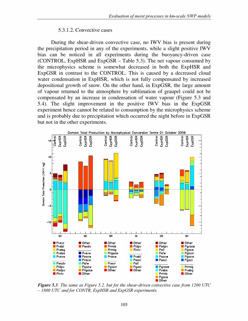
(YDOXDWLRQ�RI�PRLVW�SURFHVVHV�LQ�NP�VFDOH�1:3�PRGHOV��
105
5.3.1.2. Convective cases
During the shear-driven convective case, no IWV bias is present during the precipitation period in any of the experiments, while a slight positive IWV bias can be noticed in all experiments during the buoyancy-driven case (CONTROL, ExpHSR and ExpGSR – Table 5.3). The net vapour consumed by the microphysics scheme is somewhat decreased in both the ExpHSR and ExpGSR in contrast to the CONTROL. This is caused by a decreased cloud water condensation in ExpHSR, which is not fully compensated by increased depositional growth of snow. On the other hand, in ExpGSR, the large amount of vapour returned to the atmosphere by sublimation of graupel could not be compensated by an increase in condensation of water vapour (Figure 5.3 and 5.4). The slight improvement in the positive IWV bias in the ExpGSR experiment hence cannot be related to consumption by the microphysics scheme and is probably due to precipitation which occurred the night before in ExpGSR but not in the other experiments.
)LJXUH������7KH�VDPH�DV�)LJXUH������EXW�IRU�WKH�VKHDU�GULYHQ�FRQYHFWLYH�FDVH�IURP������87&�±������87&�DQG�IRU�&2175��([S+65�DQG�([S*65�H[SHULPHQWV��
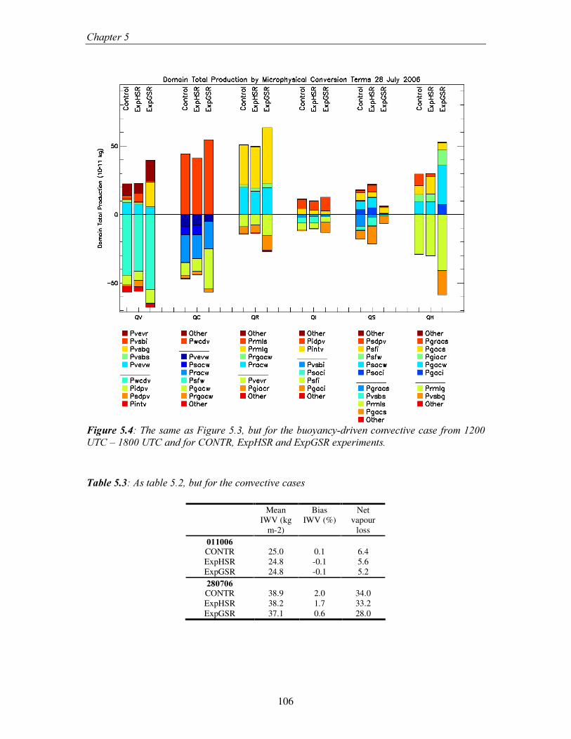
&KDSWHU���
106
)LJXUH������7KH�VDPH�DV�)LJXUH������EXW�IRU�WKH�EXR\DQF\�GULYHQ�FRQYHFWLYH�FDVH�IURP������87&�±������87&�DQG�IRU�&2175��([S+65�DQG�([S*65�H[SHULPHQWV�� 7DEOH������$V�WDEOH������EXW�IRU�WKH�FRQYHFWLYH�FDVHV�
� Mean IWV (kg
m-2)
Bias IWV (%)
Net vapour
loss ������� CONTR 25.0 0.1 6.4 ExpHSR 24.8 -0.1 5.6 ExpGSR 24.8 -0.1 5.2 ������� CONTR 38.9 2.0 34.0 ExpHSR 38.2 1.7 33.2 ExpGSR 37.1 0.6 28.0
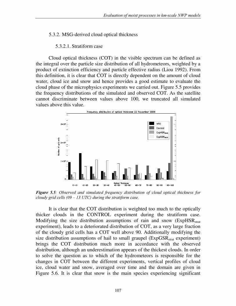
(YDOXDWLRQ�RI�PRLVW�SURFHVVHV�LQ�NP�VFDOH�1:3�PRGHOV��
107
5.3.2. MSG-derived cloud optical thickness
5.3.2.1. Stratiform case
Cloud optical thickness (COT) in the visible spectrum can be defined as
the integral over the particle size distribution of all hydrometeors, weighted by a product of extinction efficiency and particle effective radius (Liou 1992). From this definition, it is clear that COT is directly dependent on the amount of cloud water, cloud ice and snow and hence provides a good estimate to evaluate the cloud phase of the microphysics experiments we carried out. Figure 5.5 provides the frequency distributions of the simulated and observed COT. As the satellite cannot discriminate between values above 100, we truncated all simulated values above this value.
)LJXUH� ����� 2EVHUYHG� DQG� VLPXODWHG� IUHTXHQF\� GLVWULEXWLRQ� RI� FORXG� RSWLFDO� WKLFNQHVV� IRU�FORXG\�JULG�FHOOV�����±����87&��GXULQJ�WKH�VWUDWLIRUP�FDVH��
It is clear that the COT distribution is weighted too much to the optically
thicker clouds in the CONTROL experiment during the stratiform case. Modifying the size distribution assumptions of rain and snow (ExpHSRstrat
experiment), leads to a deteriorated distribution of COT, as a very large fraction of the cloudy grid cells has a COT well above 90. Additionally modifying the size distribution assumptions of hail to small graupel (ExpGSRstrat experiment) brings the COT distribution much more in accordance with the observed distribution, although an underestimation appears of the thickest clouds. In order to solve the question as to which of the hydrometeors is responsible for the changes in COT between the different experiments, vertical profiles of cloud ice, cloud water and snow, averaged over time and the domain are given in Figure 5.6. It is clear that snow is the main species experiencing significant
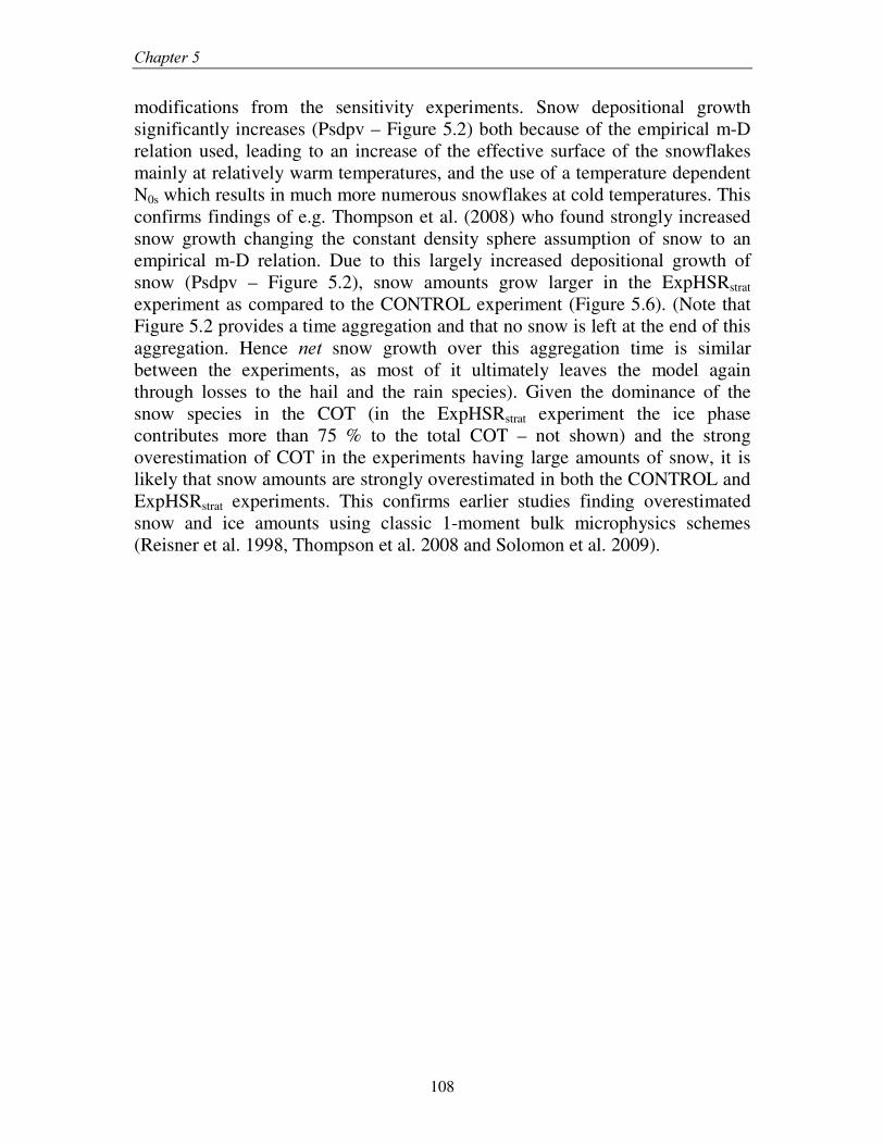
&KDSWHU���
108
modifications from the sensitivity experiments. Snow depositional growth significantly increases (Psdpv – Figure 5.2) both because of the empirical m-D relation used, leading to an increase of the effective surface of the snowflakes mainly at relatively warm temperatures, and the use of a temperature dependent N0s which results in much more numerous snowflakes at cold temperatures. This confirms findings of e.g. Thompson et al. (2008) who found strongly increased snow growth changing the constant density sphere assumption of snow to an empirical m-D relation. Due to this largely increased depositional growth of snow (Psdpv – Figure 5.2), snow amounts grow larger in the ExpHSRstrat experiment as compared to the CONTROL experiment (Figure 5.6). (Note that Figure 5.2 provides a time aggregation and that no snow is left at the end of this aggregation. Hence QHW snow growth over this aggregation time is similar between the experiments, as most of it ultimately leaves the model again through losses to the hail and the rain species). Given the dominance of the snow species in the COT (in the ExpHSRstrat experiment the ice phase contributes more than 75 % to the total COT – not shown) and the strong overestimation of COT in the experiments having large amounts of snow, it is likely that snow amounts are strongly overestimated in both the CONTROL and ExpHSRstrat experiments. This confirms earlier studies finding overestimated snow and ice amounts using classic 1-moment bulk microphysics schemes (Reisner et al. 1998, Thompson et al. 2008 and Solomon et al. 2009).
(YDOXDWLRQ�RI�PRLVW�SURFHVVHV�LQ�NP�VFDOH�1:3�PRGHOV��
109
)LJXUH������'RPDLQ�DYHUDJHG�YHUWLFDO�SURILOHV�RI�FORXG�ZDWHU��UDLQ��FORXG�LFH��VQRZ��DQG�KDLO�IURP����±����87&�GXULQJ�WKH�VWUDWLIRUP�FDVH�IRU�DOO�H[SHULPHQWV��
&KDSWHU���
110
Snow amounts strongly decrease when applying the graupel formulations
instead of hail formulations (ExpGSRstrat experiment), which brings the COT distribution much closer to the observations. Snow depositional growth (Psdpv) decreases as less snow is available. Indeed, as soon as snow appears, it is collected by graupel (Pgacs), which is also lofted to higher altitudes in the atmosphere. As graupel deposition growth is not parameterized in the Lin et al. (1983) scheme, cloud water condensation (Pwcdv) will be enhanced in order to convert vapour to condensate. As most of this additional cloud water is collected by graupel (Pgacw), total cloud water remains unaffected. Although the total amount of frozen hydrometeors remains similar as in the CONTROL and ExpHSRstrat experiments, COT decreases as graupel is optically much thinner as compared to snow.
It can be noticed that cloud ice and cloud water are not much affected by any of the modifications made (Figure 5.6). Again, this could be due to compensating effects (Figure 5.2). In the ExpGSRstrat experiment more cloud water is lost by riming growth of graupel (Pgacw), which is compensated for by increased condensation (Pwcdv) in ExpHSRstrat. More cloud water evaporates (Pvevw), which is compensated by decreased riming growth of snow (Psacw) and accretion by rain (Pracw).
5.3.2.2. Convective cases
During the shear-driven convective case, the model tends to underestimate the number of grid cells having low COT values, while too many thick clouds occur (Figure 5.7). Differences between the different experiments are small in this case, although less optically thick clouds are present in the ExpGSR.
Vertical hydrometeor profiles are given in Figure 5.8. While cloud water seems to be somewhat more affected in the ExpHSR as compared to similar size distribution modifications in the stratiform case, it is again mainly the snow content which is significantly altered when compared to the CONTROL experiment. Due to its slower fall speed (Figure 5.1) at cold temperatures and its larger number concentration, Psdpv increases in the upper tropospheric levels (Figure 5.3). Cloud water in the ExpHSR experiment is slightly reduced above the freezing level due to increased Psdpv (Figure 5.3). Below the freezing level, snow sedimentation becomes faster with increasing temperature and hence snow amounts quickly converge to the amounts in the CONTROL experiment in the lower troposphere. In the ExpGSR experiment, cloud water is dramatically depleted above the freezing level, which is mainly due to strongly increased accretion by graupel (Pgacw - Figure 5.3). As the enormous amounts of graupel produced in this experiment are lofted to much higher altitudes (Figure 5.8), accretion of snow by graupel (Pgacs) takes place at higher altitudes, depleting
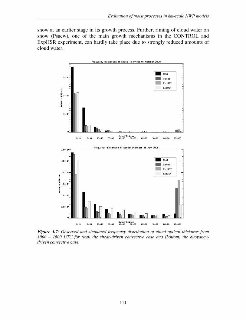
(YDOXDWLRQ�RI�PRLVW�SURFHVVHV�LQ�NP�VFDOH�1:3�PRGHOV��
111
snow at an earlier stage in its growth process. Further, riming of cloud water on snow (Psacw), one of the main growth mechanisms in the CONTROL and ExpHSR experiment, can hardly take place due to strongly reduced amounts of cloud water.
)LJXUH� �����2EVHUYHG�DQG� VLPXODWHG� IUHTXHQF\�GLVWULEXWLRQ�RI� FORXG�RSWLFDO� WKLFNQHVV� IURP������ ±� ����� 87&� IRU� �WRS�� WKH� VKHDU�GULYHQ� FRQYHFWLYH� FDVH� DQG� �ERWWRP�� WKH� EXR\DQF\�GULYHQ�FRQYHFWLYH�FDVH��
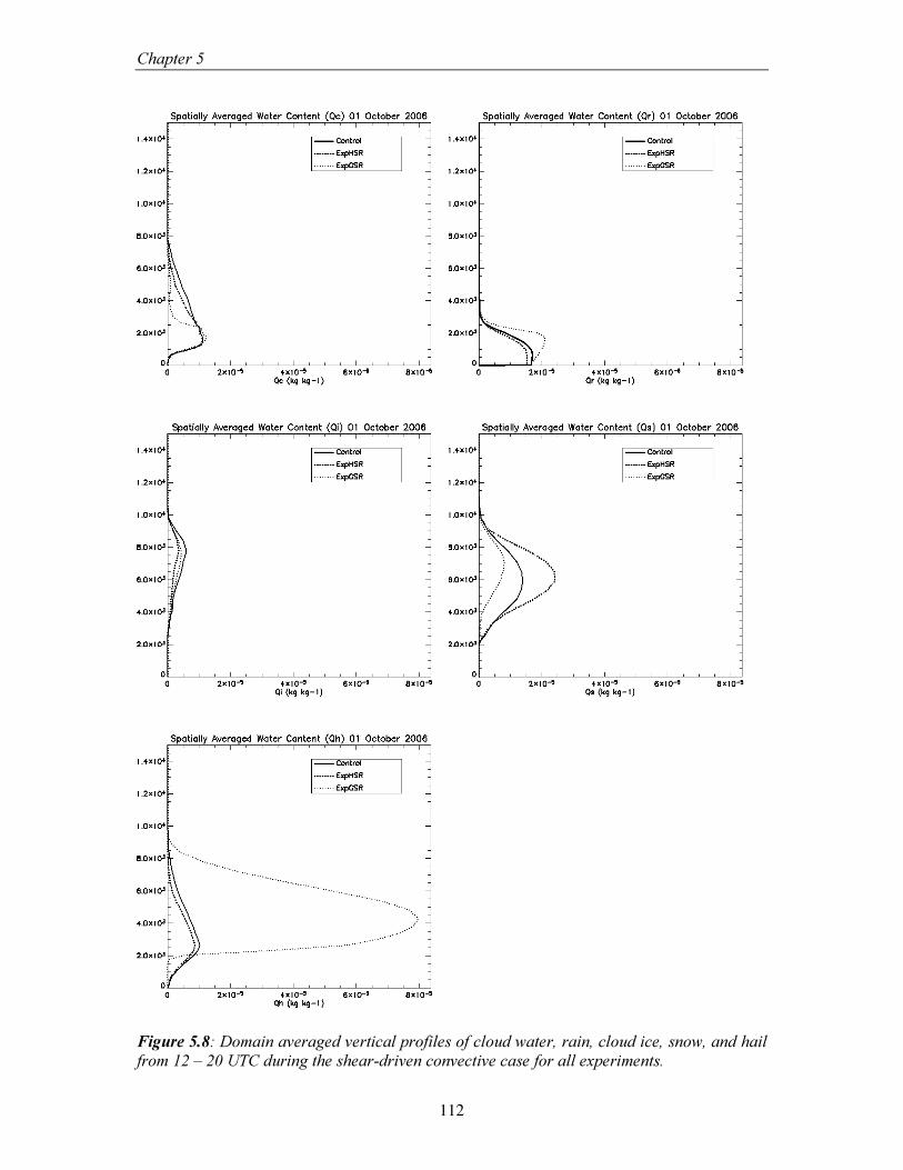
&KDSWHU���
112
)LJXUH������'RPDLQ�DYHUDJHG�YHUWLFDO�SURILOHV�RI�FORXG�ZDWHU��UDLQ��FORXG�LFH��VQRZ��DQG�KDLO�IURP����±����87&�GXULQJ�WKH�VKHDU�GULYHQ�FRQYHFWLYH�FDVH�IRU�DOO�H[SHULPHQWV��
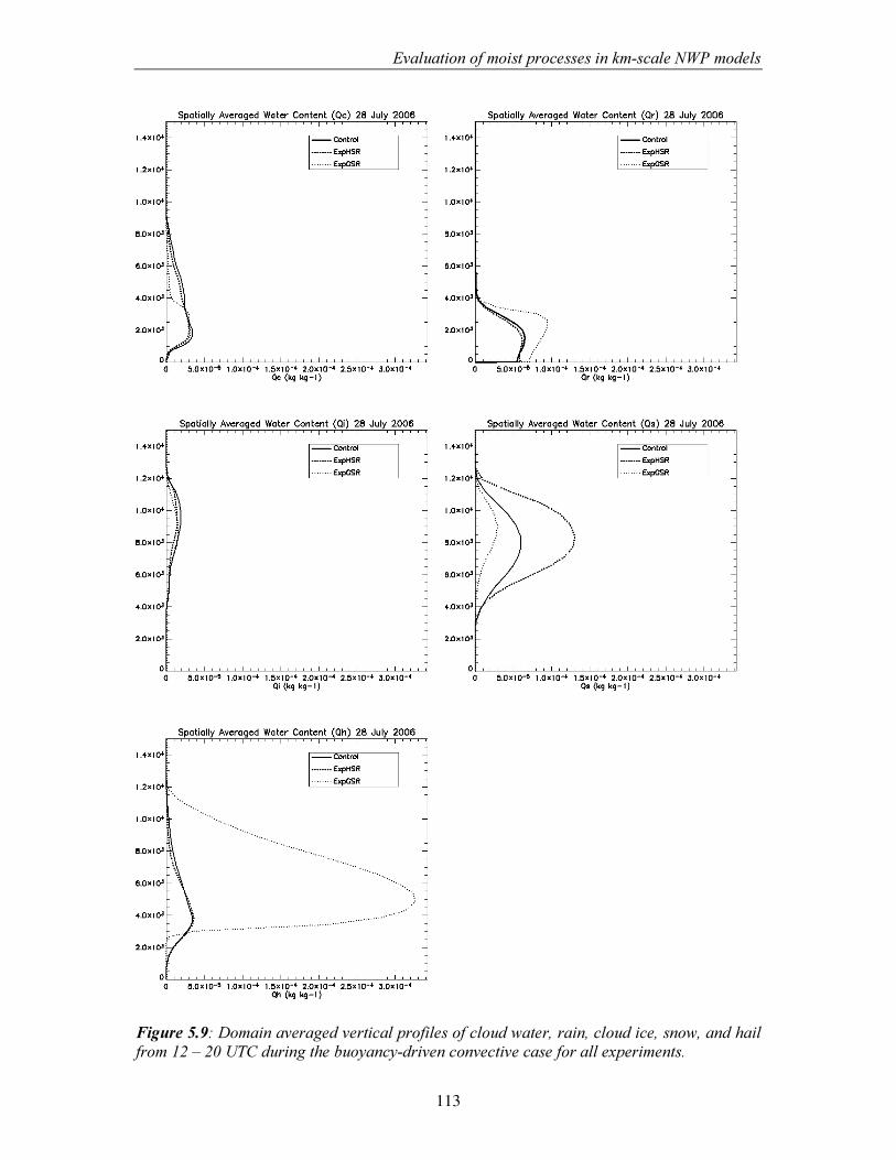
(YDOXDWLRQ�RI�PRLVW�SURFHVVHV�LQ�NP�VFDOH�1:3�PRGHOV��
113
)LJXUH������'RPDLQ�DYHUDJHG�YHUWLFDO�SURILOHV�RI�FORXG�ZDWHU��UDLQ��FORXG�LFH��VQRZ��DQG�KDLO�IURP����±����87&�GXULQJ�WKH�EXR\DQF\�GULYHQ�FRQYHFWLYH�FDVH�IRU�DOO�H[SHULPHQWV��
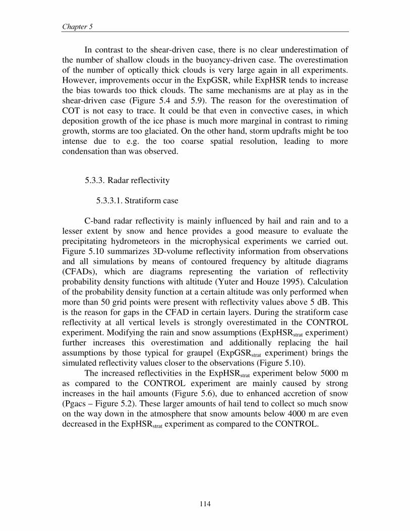
&KDSWHU���
114
In contrast to the shear-driven case, there is no clear underestimation of the number of shallow clouds in the buoyancy-driven case. The overestimation of the number of optically thick clouds is very large again in all experiments. However, improvements occur in the ExpGSR, while ExpHSR tends to increase the bias towards too thick clouds. The same mechanisms are at play as in the shear-driven case (Figure 5.4 and 5.9). The reason for the overestimation of COT is not easy to trace. It could be that even in convective cases, in which deposition growth of the ice phase is much more marginal in contrast to riming growth, storms are too glaciated. On the other hand, storm updrafts might be too intense due to e.g. the too coarse spatial resolution, leading to more condensation than was observed.
�
5.3.3. Radar reflectivity
5.3.3.1. Stratiform case
C-band radar reflectivity is mainly influenced by hail and rain and to a lesser extent by snow and hence provides a good measure to evaluate the precipitating hydrometeors in the microphysical experiments we carried out. Figure 5.10 summarizes 3D-volume reflectivity information from observations and all simulations by means of contoured frequency by altitude diagrams (CFADs), which are diagrams representing the variation of reflectivity probability density functions with altitude (Yuter and Houze 1995). Calculation of the probability density function at a certain altitude was only performed when more than 50 grid points were present with reflectivity values above 5 dB. This is the reason for gaps in the CFAD in certain layers. During the stratiform case reflectivity at all vertical levels is strongly overestimated in the CONTROL experiment. Modifying the rain and snow assumptions (ExpHSRstrat experiment) further increases this overestimation and additionally replacing the hail assumptions by those typical for graupel (ExpGSRstrat experiment) brings the simulated reflectivity values closer to the observations (Figure 5.10).
The increased reflectivities in the ExpHSRstrat experiment below 5000 m as compared to the CONTROL experiment are mainly caused by strong increases in the hail amounts (Figure 5.6), due to enhanced accretion of snow (Pgacs – Figure 5.2). These larger amounts of hail tend to collect so much snow on the way down in the atmosphere that snow amounts below 4000 m are even decreased in the ExpHSRstrat experiment as compared to the CONTROL.
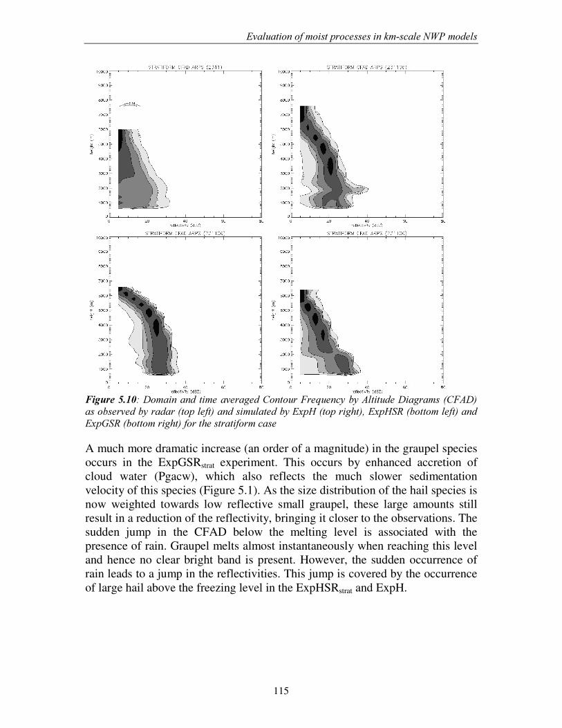
(YDOXDWLRQ�RI�PRLVW�SURFHVVHV�LQ�NP�VFDOH�1:3�PRGHOV��
115
)LJXUH�������'RPDLQ�DQG�WLPH�DYHUDJHG�&RQWRXU�)UHTXHQF\�E\�$OWLWXGH�'LDJUDPV��&)$'��DV�REVHUYHG�E\�UDGDU��WRS�OHIW��DQG�VLPXODWHG�E\�([S+��WRS�ULJKW���([S+65��ERWWRP�OHIW��DQG�([S*65��ERWWRP�ULJKW��IRU�WKH�VWUDWLIRUP�FDVH�
�A much more dramatic increase (an order of a magnitude) in the graupel species occurs in the ExpGSRstrat experiment. This occurs by enhanced accretion of cloud water (Pgacw), which also reflects the much slower sedimentation velocity of this species (Figure 5.1). As the size distribution of the hail species is now weighted towards low reflective small graupel, these large amounts still result in a reduction of the reflectivity, bringing it closer to the observations. The sudden jump in the CFAD below the melting level is associated with the presence of rain. Graupel melts almost instantaneously when reaching this level and hence no clear bright band is present. However, the sudden occurrence of rain leads to a jump in the reflectivities. This jump is covered by the occurrence of large hail above the freezing level in the ExpHSRstrat and ExpH.
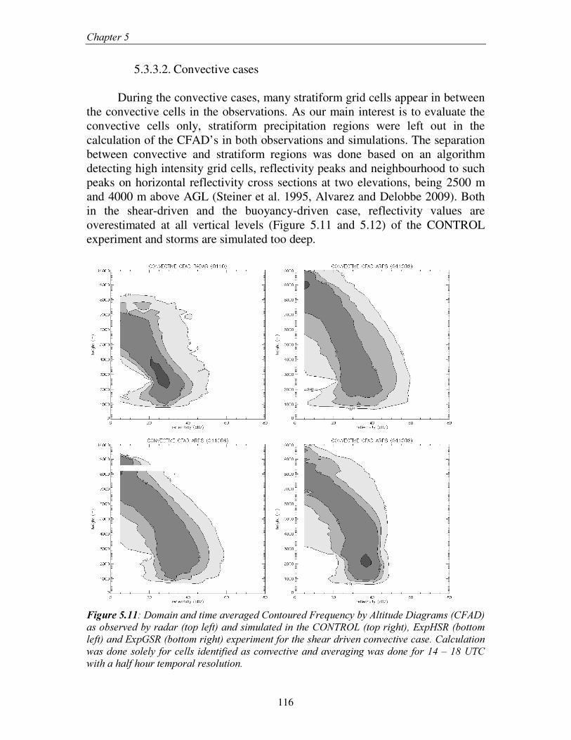
&KDSWHU���
116
5.3.3.2. Convective cases
During the convective cases, many stratiform grid cells appear in between the convective cells in the observations. As our main interest is to evaluate the convective cells only, stratiform precipitation regions were left out in the calculation of the CFAD’ s in both observations and simulations. The separation between convective and stratiform regions was done based on an algorithm detecting high intensity grid cells, reflectivity peaks and neighbourhood to such peaks on horizontal reflectivity cross sections at two elevations, being 2500 m and 4000 m above AGL (Steiner et al. 1995, Alvarez and Delobbe 2009). Both in the shear-driven and the buoyancy-driven case, reflectivity values are overestimated at all vertical levels (Figure 5.11 and 5.12) of the CONTROL experiment and storms are simulated too deep.
)LJXUH�������'RPDLQ�DQG�WLPH�DYHUDJHG�&RQWRXUHG�)UHTXHQF\�E\�$OWLWXGH�'LDJUDPV��&)$'��DV�REVHUYHG�E\�UDGDU��WRS�OHIW��DQG�VLPXODWHG�LQ�WKH�&21752/��WRS�ULJKW���([S+65��ERWWRP�OHIW��DQG�([S*65��ERWWRP�ULJKW��H[SHULPHQW�IRU�WKH�VKHDU�GULYHQ�FRQYHFWLYH�FDVH��&DOFXODWLRQ�ZDV�GRQH�VROHO\�IRU�FHOOV�LGHQWLILHG�DV�FRQYHFWLYH�DQG�DYHUDJLQJ�ZDV�GRQH�IRU����±����87&�ZLWK�D�KDOI�KRXU�WHPSRUDO�UHVROXWLRQ���
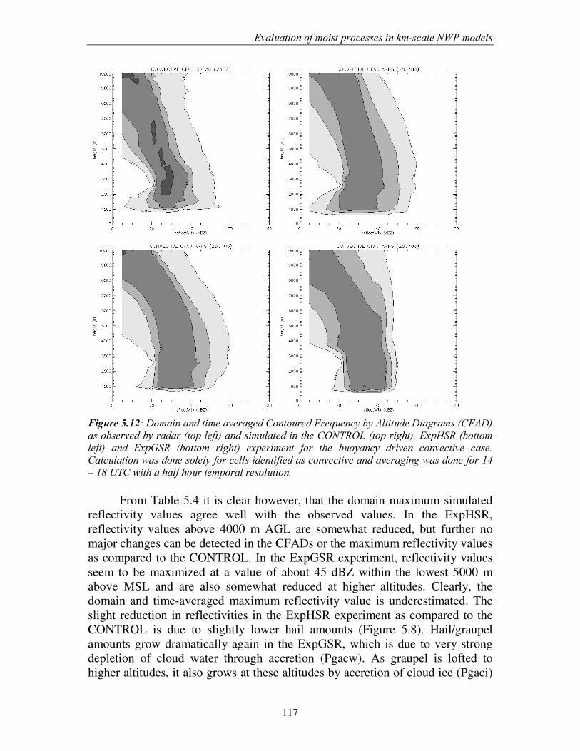
(YDOXDWLRQ�RI�PRLVW�SURFHVVHV�LQ�NP�VFDOH�1:3�PRGHOV��
117
)LJXUH�������'RPDLQ�DQG�WLPH�DYHUDJHG�&RQWRXUHG�)UHTXHQF\�E\�$OWLWXGH�'LDJUDPV��&)$'��DV�REVHUYHG�E\�UDGDU��WRS�OHIW��DQG�VLPXODWHG�LQ�WKH�&21752/��WRS�ULJKW���([S+65��ERWWRP�OHIW�� DQG� ([S*65� �ERWWRP� ULJKW�� H[SHULPHQW� IRU� WKH� EXR\DQF\� GULYHQ� FRQYHFWLYH� FDVH��&DOFXODWLRQ�ZDV�GRQH�VROHO\�IRU�FHOOV�LGHQWLILHG�DV�FRQYHFWLYH�DQG�DYHUDJLQJ�ZDV�GRQH�IRU����±����87&�ZLWK�D�KDOI�KRXU�WHPSRUDO�UHVROXWLRQ��
From Table 5.4 it is clear however, that the domain maximum simulated reflectivity values agree well with the observed values. In the ExpHSR, reflectivity values above 4000 m AGL are somewhat reduced, but further no major changes can be detected in the CFADs or the maximum reflectivity values as compared to the CONTROL. In the ExpGSR experiment, reflectivity values seem to be maximized at a value of about 45 dBZ within the lowest 5000 m above MSL and are also somewhat reduced at higher altitudes. Clearly, the domain and time-averaged maximum reflectivity value is underestimated. The slight reduction in reflectivities in the ExpHSR experiment as compared to the CONTROL is due to slightly lower hail amounts (Figure 5.8). Hail/graupel amounts grow dramatically again in the ExpGSR, which is due to very strong depletion of cloud water through accretion (Pgacw). As graupel is lofted to higher altitudes, it also grows at these altitudes by accretion of cloud ice (Pgaci)
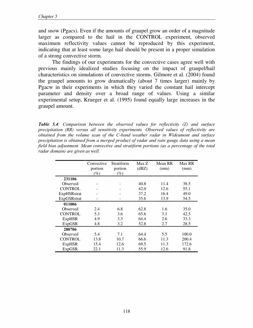
&KDSWHU���
118
and snow (Pgacs). Even if the amounts of graupel grow an order of a magnitude larger as compared to the hail in the CONTROL experiment, observed maximum reflectivity values cannot be reproduced by this experiment, indicating that at least some large hail should be present in a proper simulation of a strong convective storm.
The findings of our experiments for the convective cases agree well with previous mainly idealized studies focusing on the impact of graupel/hail characteristics on simulations of convective storms. Gilmore et al. (2004) found the graupel amounts to grow dramatically (about 7 times larger) mainly by Pgacw in their experiments in which they varied the constant hail intercept parameter and density over a broad range of values. Using a similar experimental setup, Krueger et al. (1995) found equally large increases in the graupel amount.
7DEOH� ����� &RPSDULVRQ� EHWZHHQ� WKH� REVHUYHG� YDOXHV� IRU� UHIOHFWLYLW\� �=�� DQG� VXUIDFH�SUHFLSLWDWLRQ� �55�� YHUVXV� DOO� VHQVLWLYLW\� H[SHULPHQWV�� 2EVHUYHG� YDOXHV� RI� UHIOHFWLYLW\� DUH�REWDLQHG� IURP� WKH� YROXPH� VFDQ� RI� WKH� &�EDQG� ZHDWKHU� UDGDU� LQ� :LGHXPRQW� DQG� VXUIDFH�SUHFLSLWDWLRQ�LV�REWDLQHG�IURP�D�PHUJHG�SURGXFW�RI�UDGDU�DQG�UDLQ�JDXJH�GDWD�XVLQJ�D�PHDQ�ILHOG�ELDV�DGMXVWPHQW��0HDQ�FRQYHFWLYH�DQG�VWUDWLIRUP�SRUWLRQV��DV�D�SHUFHQWDJH�RI�WKH�WRWDO�UDGDU�GRPDLQ��DUH�JLYHQ�DV�ZHOO��
� Convective portion
(%)
Stratiform portion
(%)
Max Z (dBZ)
Mean RR (mm)
Max RR (mm)
������ Observed - - 40.8 11.4 38.5
CONTROL - - 42.0 12.6 55.1 ExpHSRstrat - - 37.2 16.4 49.0 ExpGSRstrat - - 35.6 13.9 54.5
������� Observed 2.4 6.8 62.8 1.6 35.0
CONTROL 5.3 3.6 65.6 3.1 42.5 ExpHSR 4.9 3.3 64.4 2.6 33.3 ExpGSR 4.8 3.2 52.8 2.7 28.5 �������
Observed 5.4 7.1 64.4 5.5 100.0 CONTROL 13.8 10.7 66.6 11.3 200.4
ExpHSR 15.4 12.6 69.5 11.3 172.6 ExpGSR 22.1 11.3 55.9 12.6 91.8
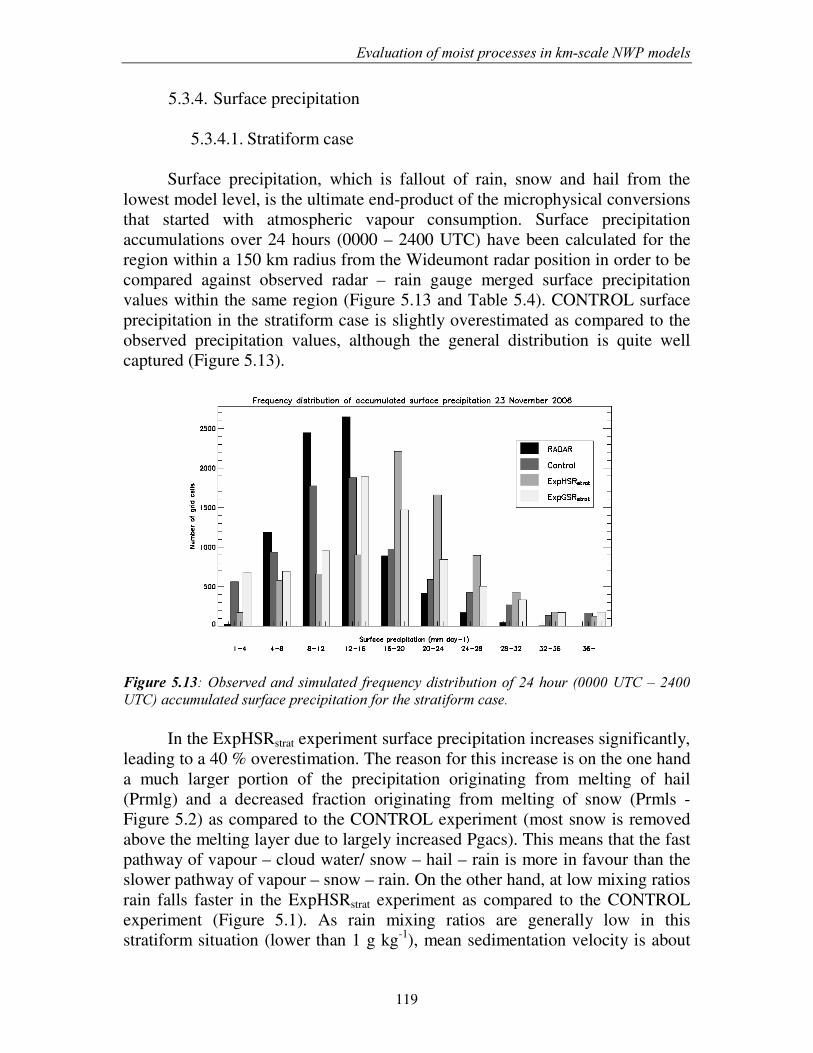
(YDOXDWLRQ�RI�PRLVW�SURFHVVHV�LQ�NP�VFDOH�1:3�PRGHOV��
119
5.3.4. Surface precipitation
5.3.4.1. Stratiform case
Surface precipitation, which is fallout of rain, snow and hail from the lowest model level, is the ultimate end-product of the microphysical conversions that started with atmospheric vapour consumption. Surface precipitation accumulations over 24 hours (0000 – 2400 UTC) have been calculated for the region within a 150 km radius from the Wideumont radar position in order to be compared against observed radar – rain gauge merged surface precipitation values within the same region (Figure 5.13 and Table 5.4). CONTROL surface precipitation in the stratiform case is slightly overestimated as compared to the observed precipitation values, although the general distribution is quite well captured (Figure 5.13).
)LJXUH�������2EVHUYHG�DQG�VLPXODWHG� IUHTXHQF\�GLVWULEXWLRQ�RI����KRXU�������87&�±������87&��DFFXPXODWHG�VXUIDFH�SUHFLSLWDWLRQ�IRU�WKH�VWUDWLIRUP�FDVH��
In the ExpHSRstrat experiment surface precipitation increases significantly,
leading to a 40 % overestimation. The reason for this increase is on the one hand a much larger portion of the precipitation originating from melting of hail (Prmlg) and a decreased fraction originating from melting of snow (Prmls - Figure 5.2) as compared to the CONTROL experiment (most snow is removed above the melting layer due to largely increased Pgacs). This means that the fast pathway of vapour – cloud water/ snow – hail – rain is more in favour than the slower pathway of vapour – snow – rain. On the other hand, at low mixing ratios rain falls faster in the ExpHSRstrat experiment as compared to the CONTROL experiment (Figure 5.1). As rain mixing ratios are generally low in this stratiform situation (lower than 1 g kg-1), mean sedimentation velocity is about
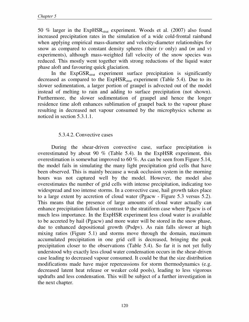
&KDSWHU���
120
50 % larger in the ExpHSRstrat experiment. Woods et al. (2007) also found increased precipitation rates in the simulation of a wide cold-frontal rainband when applying empirical mass-diameter and velocity-diameter relationships for snow as compared to constant density spheres (their (Y only) and (P and Y) experiments), although mass-weighted fall velocity of the snow species was reduced. This mostly went together with strong reductions of the liquid water phase aloft and favouring quick glaciation.
In the ExpGSRstrat experiment surface precipitation is significantly decreased as compared to the ExpHSRstrat experiment (Table 5.4). Due to its slower sedimentation, a larger portion of graupel is advected out of the model instead of melting to rain and adding to surface precipitation (not shown). Furthermore, the slower sedimentation of graupel and hence the longer residence time aloft enhances sublimation of graupel back to the vapour phase resulting in decreased net vapour consumed by the microphysics scheme as noticed in section 5.3.1.1.
5.3.4.2. Convective cases
During the shear-driven convective case, surface precipitation is overestimated by about 90 % (Table 5.4). In the ExpHSR experiment, this overestimation is somewhat improved to 60 %. As can be seen from Figure 5.14, the model fails in simulating the many light precipitation grid cells that have been observed. This is mainly because a weak occlusion system in the morning hours was not captured well by the model. However, the model also overestimates the number of grid cells with intense precipitation, indicating too widespread and too intense storms. In a convective case, hail growth takes place to a large extent by accretion of cloud water (Pgacw - Figure 5.3 versus 5.2). This means that the presence of large amounts of cloud water actually can enhance precipitation fallout in contrast to the stratiform case where Pgacw is of much less importance. In the ExpHSR experiment less cloud water is available to be accreted by hail (Pgacw) and more water will be stored in the snow phase, due to enhanced depositional growth (Psdpv). As rain falls slower at high mixing ratios (Figure 5.1) and storms move through the domain, maximum accumulated precipitation in one grid cell is decreased, bringing the peak precipitation closer to the observations (Table 5.4). So far it is not yet fully understood why exactly less cloud water condensation occurs in the shear-driven case leading to decreased vapour consumed. It could be that the size distribution modifications made have major repercussions for storm thermodynamics (e.g. decreased latent heat release or weaker cold pools), leading to less vigorous updrafts and less condensation. This will be subject of a further investigation in the next chapter.
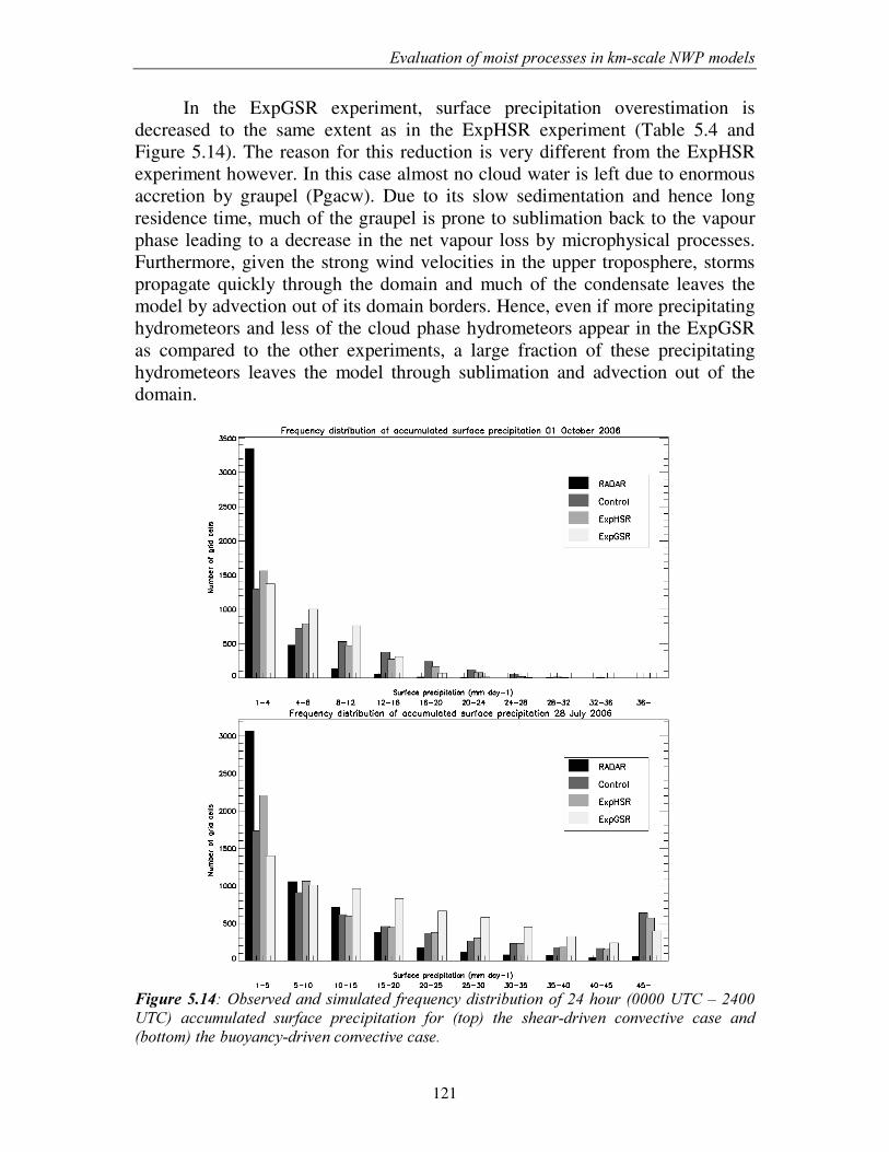
(YDOXDWLRQ�RI�PRLVW�SURFHVVHV�LQ�NP�VFDOH�1:3�PRGHOV��
121
In the ExpGSR experiment, surface precipitation overestimation is decreased to the same extent as in the ExpHSR experiment (Table 5.4 and Figure 5.14). The reason for this reduction is very different from the ExpHSR experiment however. In this case almost no cloud water is left due to enormous accretion by graupel (Pgacw). Due to its slow sedimentation and hence long residence time, much of the graupel is prone to sublimation back to the vapour phase leading to a decrease in the net vapour loss by microphysical processes. Furthermore, given the strong wind velocities in the upper troposphere, storms propagate quickly through the domain and much of the condensate leaves the model by advection out of its domain borders. Hence, even if more precipitating hydrometeors and less of the cloud phase hydrometeors appear in the ExpGSR as compared to the other experiments, a large fraction of these precipitating hydrometeors leaves the model through sublimation and advection out of the domain.
)LJXUH�������2EVHUYHG�DQG�VLPXODWHG� IUHTXHQF\�GLVWULEXWLRQ�RI����KRXU�������87&�±������87&�� DFFXPXODWHG� VXUIDFH� SUHFLSLWDWLRQ� IRU� �WRS�� WKH� VKHDU�GULYHQ� FRQYHFWLYH� FDVH� DQG��ERWWRP��WKH�EXR\DQF\�GULYHQ�FRQYHFWLYH�FDVH��
&KDSWHU���
122
In the buoyancy-driven case surface precipitation is altered in a somewhat
different way as compared to the shear-driven case. In the CONTROL experiment both domain average surface precipitation and peak precipitation are about double the amount observed. In contrast to the shear-driven case, no change in domain average surface precipitation takes place in the ExpHSR experiment, although peak precipitation is somewhat reduced. While in the shear-driven case cloud water condensation was strongly decreased, this is not the case in the buoyancy-driven case and hence no large difference in the net vapour consumed by the microphysical processes is present.
During the ExpGSR, surface precipitation is surprisingly increased, despite a lower net vapour consumption as compared to the other experiments. Sublimation back to the vapour phase is of the same order of importance as compared to the shear-driven case. The main difference with the shear-driven case is that upper level winds are very weak in this case and hence storms hardly propagate through the domain. Instead, they develop, mature and decay at about the same location without precipitation being advected out of the domain. As seen in the previous chapter, storms tend to be too widespread. Graupel sediments out of the convective cores and massively collects cloud water, releasing latent heat due to freezing and hence broadening the storm area. This would also explain while the total cloud water condensation is so much increased when graupel is included, as this might be a thermodynamic effect. This should be further investigated.
������6XPPDU\�DQG�FRQFOXVLRQV�
The main objective of this chapter was to determine how moist processes and mainly surface precipitation in a nonhydrostatic mesoscale model are affected by modifications in the size distribution assumptions of a simple 1-moment bulk microphysics scheme. A number of sensitivity experiments on the size distribution assumptions of the rain, snow and hail variables was set up for three extreme precipitation cases very different in nature. The vapour phase, cloud phase, precipitation phase and surface precipitation were rigorously evaluated against remotely sensed and surface observational data in order to understand if the modifications made in the microphysics scheme brought the simulations closer to the observations or not.
While the net vapour consumption was not much altered by including more realistic rain and snow size distributions in both the stratiform and convective cases, replacing the hail formulations by graupel strongly decreased the net vapour consumed by the microphysics scheme. It was shown that this is probably related to strongly increased sublimation of graupel back to the vapour
(YDOXDWLRQ�RI�PRLVW�SURFHVVHV�LQ�NP�VFDOH�1:3�PRGHOV��
123
phase, associated with its long residence time aloft as it is precipitating much slower than hail.
Cloud optical thickness distribution could only be realistically represented in during the stratiform case when large hail was replaced by small graupel. This could be related to a strong overestimation of the snow amounts in experiments with large hail. Including graupel led to significantly reduced snow depositional growth and snow collection by graupel, leading to decreased amounts of optically thick snow. In convective cases, cloud optical thickness was also brought closer to the observations by inclusion of graupel, related both to decreased amounts of snow and cloud water. This finding has significant relevance for the radiation budget in numerical models, as the radiative forcing is likely to be better represented in experiments including some graupel.
From comparison of observed and simulated radar reflectivity, it was found that rain and snow size distributions do not affect the vertical radar reflectivity profile significantly. However, a proper representation of reflectivity during the stratiform case was impossible without the inclusion of small graupel. During the convective cases however, the experiments including small graupel are not capable of reproducing realistically the highest reflective cores associated with large hail.
Surface precipitation was found to be far less sensitive to modifications to the size distribution assumptions than cloud optical thickness and radar reflectivity. In all cases, none of the experiments was able to significantly improve a positive surface precipitation bias. Faster rain fall speeds and more rain originating from fast falling hail as compared to slowly falling snow as compared to a control simulation resulted in increased surface precipitation during the stratiform case when rain and snow size distribution assumptions were more realistically represented. This effect was smaller when additionally graupel replaced large hail. During the convective cases, the reasons for modified surface precipitation characteristics in the microphysics experiments were not easy to trace. A slight decrease of surface precipitation was found by both microphysics experiments in a shear-driven case, while little effect was found in the buoyancy-driven case. It could be that the microphysics experiments inferred thermodynamic effects which will be further investigated in the next chapter for the shear-driven case. On the other hand, a decrease in the peak precipitation in all experiments is probably related with the slower rain fall speeds.
From the conclusions above we could summarize that it was found highly advisable to apply graupel formulations when simulating moist processes during a frontal stratiform situation, as both COT and reflectivity could not be simulated properly without. During convective cases, large hail was necessary to capture the very reflective convective cores, although the COT was negatively affected. In general we would advise to include both hail and graupel in an RSHUDWLRQDO numerical weather prediction model, confirming the suggestions of

&KDSWHU���
124
e.g. McCumber et al. (1991) and Cohen and McCaul (2006) to increase the number of ice categories in microphysical schemes. While the cloud phase and vertical reflectivity profiles could be enhanced by modifications presented in the above analysis, important to e.g. realistically represent the surface radiation characteristics, surface rainfall overestimation found in all cases could not be solved by any of the modifications made. While many studies found similarly low sensitivities as found in our experiments, e.g. Gilmore et al. (2004) found surface precipitation to be four times smaller in a simulation having small graupel as compared to large hail. While the vertical wind profile they applied was comparable to the one in our shear-driven convective case, their storms were much more vigorous and deeper. On the other hand their simulations were rather short (2 hours) and their domain was smaller than the one used in our simulations. In the next chapter we investigate whether the difference in the sensitivities found by Gilmore et al. (2004) and in this research are mainly related to a different experiments design or to different atmospheric conditions.
125
����������
&KDSWHU������
7KH�LPSDFW�RI�VL]H�GLVWULEXWLRQ�DVVXPSWLRQV�LQ�D�VLPSOH�PLFURSK\VLFV�VFKHPH�RQ�VXUIDFH�SUHFLSLWDWLRQ�DQG�VWRUP�
G\QDPLFV�GXULQJ�D�ORZ�WRSSHG�VXSHUFHOO�FDVH �
������,QWURGXFWLRQ�
Proper simulation of deep moist convection in mid-latitude regions is still
a difficult task, despite continuously improved physics and numerics over the past decades. Generally, the simulation of deep convection is associated with positive biases of the precipitation amounts and too vigorous updrafts (Weisman et al. 2008, Kain et al. 2008, Deng and Stauffer 2006). It remains challenging to point to a single model deficiency responsible for this bias. As parameterized microphysical processes affect both the precipitation formation process and the (thermo)dynamics of convective systems, they have been thought to be a main contributor to overestimated surface rainfall.
Over the past decades, idealized studies suggested that mainly the largest precipitating hydrometeor type (graupel or hail) is having an influence on both the surface precipitation and the (thermo)dynamic processes within deep convective systems. Most studies were conducted for deep convection and all found surface precipitation to increase as the size of hail or graupel increased. The precise nature of the impact was found to vary a lot among different studies
* Van Weverberg, K., N. P. M. van Lipzig, L. Delobbe, 2010: The impact of size distribution assumptions in a simple microphysics scheme on surface precipitation and storm dynamics during a low-topped supercell case. Monthly Weather Review (submitted).
&KDSWHU���
126
however. Some studies found a small impact on the accumulated surface precipitation. McCumber et al. (1991) e.g. found for idealized cases of tropical convection that while the effect on the vertical reflectivity profiles was very large, total surface precipitation varied by about 30 % when replacing the large hail formulation in the Lin et al. (1983) microphysics scheme by small graupel. Van den Heever and Cotton (2004) and Cohen and McCaul (2006) found small sensitivity to the amounts of precipitation reaching the surface, but the rainfall was spread over a larger area when the size of hail stones was decreased. In contrast, Gilmore et al. (2004) found the surface precipitation to decrease enormously by a factor of 3-4 when the largest precipitating ice species was weighted towards small graupel instead of large hail for idealized cases of mid-latitude supercell and multi-cell convection.
Also the influence on storm dynamics was found to be significantly different among different studies. Some found stronger near-surface downdrafts and enhanced low-level cooling as the size of hail or graupel decreased, such as Cohen and McCaul (2006) or van den Heever and Cotton (2004). Gilmore et al. (2004) however, found low-level downdrafts and cold pools to be weaker in experiments including small graupel instead of large hail.
It should be mentioned that differences exist in the design of the experiments and in the microphysical schemes used among previously mentioned studies. Gilmore et al. (2004) only varied the constant intercept and density of the hail variable, while McCumber et al. (1991) also varied the coefficients associated with the fall speed relations and hence had a somewhat more sophisticated experimental design. Furthermore, very few studies were conducted to investigate the impact of modifying PSD characteristics of other precipitating hydrometeors, being rain or snow, on the simulation of severe convection.
Apart from microphysical size distribution characteristics, it has been recently pointed out by some authors that issues exist with the advection of moisture in typical operational atmospheric models. The finite-difference representation of advection processes often creates negative mixing ratios near cloud edges. Before the microphysics parameterization is called by the model, all these negative mixing ratios are zeroed, resulting in an artificial source of water. Although this source is generally assumed to be small and insignificant, e.g. Braun (2006) found that this source might contribute as much as 20 % to the precipitation during a high resolution simulation of a hurricane. Skamarock and Weisman (2009) even found decreased surface precipitation by over 30 % during two simulations of convection when a applying an advection scheme avoiding the occurrence of negative mixing ratios.
In this chapter a systematic setup has been chosen to gradually introduce more sophisticated modifications to the size distribution assumptions of a simple one-moment bulk microphysical scheme. All experiments are carried out for a case of extreme convection over Belgium, driven by strong shear conditions
,PSDFW�RI�VL]H�GLVWULEXWLRQ�DVVXPSWLRQV�RQ�VXSHUFHOO�SUHFLSLWDWLRQ�DQG�G\QDPLFV��
127
leading to a long-lived low-topped supercell. The main rationale for conducting this study is to understand if the differences in sensitivity found by previous research are caused by differences in the experimental design or different synoptic conditions and what kind of sensitivities can be expected from real case simulations. While interpretation of the mainly idealized studies conducted so far is more unambiguous, real case simulations have the advantage that it can be better estimated if a model modification is actually a model improvement through a comparison against observed surface precipitation estimates. A further goal of this research is to investigate the sensitivity of moist processes to similar modifications to the snow and rain size distribution assumptions. At last we quantified the influence of the artificial water source due to inaccuracies in the advection process and assessed to what extent this contributes to the surface rain. An overview of the model set up and the experimental design is given in section 6.2. In section 6.3 an overview of the results is given, discussing the storm dynamics and the microphysical budgets of each of the experiments performed. Concluding remarks are made in section 6.4.
������0RGHO�DQG�H[SHULPHQWDO�GHVLJQ�
The model setup of ARPS was as described in section 3.2. Default settings of the Lin et al. (1983) scheme, as discussed in section 3.3 are used in the ExpH. Apart from the experiments ExpHSR and ExpGSR discussed in the previous two chapters, four additional microphysics experiments were carried out in order to address the specific research questions posed in this chapter.
First of all, Gilmore et al. (2004) found quantitative precipitation to be very sensitive to the way the largest hydrometeor type (hail/graupel) is represented in the microphysical parameterizations. Therefore, a set of two additional experiments was designed to understand if the sensitivities found in idealized experiments RQO\ modifying the intercept parameter and density of the hail/graupel species could be reproduced for our real case experiments. In a first approach to do so, we followed the experiment’ s design of Gilmore et al. (2004), implementing a larger intercept parameter and lower density of the hail/graupel species, identical to the values for small graupel in Gilmore et al. (2004), further referred to as ExpG1.
Two inconsistencies exist in the ExpG1�KRZHYHU��)LUVW��FDOFXODWLRQ�RI� H is done assuming constant density spheres, which is contradicted by observational studies summarized in Figure 2.5 of this dissertation (e.g. Locatelli and Hobbs 1974). Second, fall speed calculation of qh in experiment ExpG1 is still done according the original formulations in the Lin scheme, following Wisner et al. (1972) for large hail. In order to understand the impact of these inconsistencies on the simulation results, a more advanced setup of the graupel weighted experiment was designed. This experiment (ExpG2) has an identical intercept
&KDSWHU���
128
parameter and density as in ExpG1, but slope parameter for a constant density sphere and fall speed for large hail were not retained. Instead, the empirically derived coefficient a and power b of the mass – diameter relationship for dense lump graupel of Locatelli and Hobbs (1974) were used in equation 3.9 for the calculation of the slope parameter. The empirically derived coefficient c and power d of the terminal velocity – diameter relation for dense lump graupel were used in equation 3.10 to calculate the terminal fall velocity of the graupel. An additional research question in this chapter was how the snow and rain size distribution each influence the representation of moist processes during an event of low-topped supercells. As experiments ExpHSR and ExpGSR have both modified snow and rain size distributions, it is hard to separate effects due to the snow species and the rain species. Therefore we implemented an experiment in which the setup was identical to ExpHSR and ExpGSR, except that the rain size distribution assumptions were kept as the original formulations in Lin et al. (1983), having a constant intercept parameter. This yielded in two additional experiments ExpHS and ExpGS. Comparing ExpHS and ExpGS against ExpH and ExpG2 provides understanding of the influence of more realistic representation of the snow species only, while comparison of ExpHS and ExpGS against ExpHSR and ExpGSR reveals how moist processes are affected by a more realistic representation of the rain species only. An overview of all microphysics experiments implemented in this chapter is provided in Table 6.1 while Figure 6.1 gives an overview of the influence of all modifications to the hydrometeor terminal fall velocities.
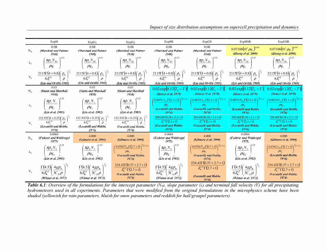
,PSDFW�RI�VL]H�GLVWULEXWLRQ�DVVXPSWLRQV�RQ�VXSHUFHOO�SUHFLSLWDWLRQ�DQG�G\QDPLFV��
ExpH ExpG1 ExpG2 ExpHS ExpGS ExpHSR ExpGSR
N0R 08.0 � ���� � � � � �� �� � ��� ���� !
08.0 � � ��� � � � � � � �� � ��� ���� !
08.0 � ���� � � � � � � �� � ��� ��� � !
08.0 � � ��� � � � � � � �� � ��� ���� !
08.0 � �� �� � � � � � � �� � ��� ���� !
( ) 648.031007106.0 "#ρ �$ � � � %� & � �(' )* * ! ( ) 648.031007106.0 "#ρ �$ � � � %� & � �(' )* * !
R
25.0
0
+++
T1
ρπρ
25.0
0
,,,
T1
ρπρ
25.0
0
,,,
T1
ρπρ
25.0
0
,,,
T1
ρπρ
25.0
0
,,,
T1
ρπρ
25.0
0
,,,
T1
ρπρ
25.0
0
,,,
T1
ρπρ
VR ( ) 2
1
08.06
8.042115
+Γρρ
λ -�. /0 �� �1 � 2 / � �� ��3 � !
( ) 21
08.06
8.042115
+Γρρ
λ 4
�. /0 � � � 1 � 2 / � �� ��3 � !
( ) 21
08.06
8.042115
+Γρρ
λ -� . /0 � � �1 � 2 / � �� ��3 � !
( ) 21
08.06
8.042115
+Γρρ
λ -� . /0 � � �1 � 2 / � �� ��3 � !
( ) 21
08.06
8.042115
+Γρρ
λ -�. /0 � � � 1 � 2 / � �� ��3 � !
( ) 21
08.06
8.042115
+Γρρ
λ -�. /0 �� �1 � 2 / � �� ��3 � !
( ) 21
08.06
8.042115
+Γρρ
λ -
� . /0 � � � 1 � 2 / � �� ��3 � !
N0S 0.03 �5 0 � � � � � ���� � � � ���6 !
0.03 � 5 0 � � � � � ���� � � � ���6 !
0.03 � 5 0 � � � � � ���� � � � ��� 6 !
( )[ ]77 −012.0exp02.0 �78 09 � � & � �(' ��: � !
( )[ ]77 −012.0exp02.0 �78 0 9 � � & � �(' ��: � !
( )[ ]77 −012.0exp02.0 �78 0 9 � � & � �(' ��: � !
( )[ ]77 −012.0exp02.0 ;<= >? @ @ AB C(D EFG F H
S
25.0
III
T1
ρπρ
;J KL @ AB C(D EFM N H
25.0
OOO
T1
ρπρ
;J KL @ AB C(D EFM N H
25.0
OOO
T1
ρπρ
;J KL @ AB C(D EFM N H
( ) ( )11.21
0 11.20074.0 +
+Γ
PPRQS
ρ
;J= TB A @ C C KB L U < = V VW DE FG X H
( ) ( )11.21
0 11.20074.0 +
+Γ
YYRZ[
ρ
;J= TB A @ C C KB L U < = V VW DE FG X H
( ) ( )11.21
0 11.20074.0 +
+Γ
\\^]
_
ρ
;J= TB A @ C C KB L U < = V VW DE FG X H
( ) ( )11.21
0 11.20074.0 +
+Γ
``^ab
ρ
;J= TB A @ C C KB L U <= V VW DE FG X H
VS
( ) 21
025.06
25.0493.152
+Γρρ
λ c
;J= TB A @ C C KB L U <= V VW DE FG X H
( ) 21
025.06
25.0493.152
+Γρρ
λd
efg hi jk l lm in op g q qrstuv w x
( ) 21
025.06
25.0493.152
+Γρρ
λ y
efg h i j k l lm in op g q qr stu v w x
( )( )11.2
11.228.060.20928.0 +Γ
++Γzλ
efg h i jk l lm in op g q qr stuv w x
( )( )11.2
11.228.060.20928.0 +Γ
++Γzλ
efg hi jk l lm in op g q qrstuv w x
( )( )11.2
11.228.060.20928.0 +Γ
++Γzλ
ef g hi jk l lm in op g q qr stuv w x
( )( )11.2
11.228.060.20928.0 +Γ
++Γzλ
efg h i jk l lm in op g q qrstuv w x
N0H 0.0004 e{ k ok| k | in o} i l o~g �k ltuv � �
4.000 e� m l� g | k k j i ls �� � w x
4.000 e� m l� g | k k j i ls �� � w x
0.0004 e { k ok| k | in o} i l o~g �k ltuv � � 4.000 e� m l� g | k k j i ls �� � w x
0.0004 e{ k ok| k | in o} i l o~g � k ltuv � �
4.000 e� m l� g | k k j i ls �� � w x
H
25.0
���
T1
ρπρ
ef mn k j i ls tu� � x
25.0
���
T1
ρπρ
ef mn k j i ls tu� � x
( ) ( )17.21
0 17.20702.0 +
+�����
ρefg h i j k l lm in op g q qr stu v w x
25.0
���
T1
ρπρ
ef mn k j i ls tu� � x( ) ( )17.2
1
0 17.20702.0 +
+�����
ρ
ef g hi j k l lm in op g q qr stuv w x
25.0
���
T1
ρπρ
ef mn k j i ls tu� � x
( ) ( )17.21
0 17.20702.0 +
+�����
ρ
efg h i jk l lm in op g q qrstuv w x
VH ( ) 2
1
5.0 34
65.4
Γρ
ρλ �
�
� &J
e} m rn k| k j i ls tuv � x
( ) 21
5.0 34
65.4
Γρ
ρλ �
�
� &J
�� ��� �� � �� �( ¡¢£ ¤ ¥
( )( )17.2
17.237.042.23437.0 +Γ
++Γ
¦λ
�§¨ ©� � � � � � � � ª« ¨ ¬ ¬ � ¡¢ £ ¥
( ) 21
5.0 34
65.4
Γρ
ρλ �
�
� &J
�� � �� �� � � � � ¡ ¢£ ¤ ¥
( )( )17.2
17.237.042.23437.0 +Γ
++Γ
®λ � §¨ ©� � � � � � � � ª« ¨ ¬ ¬ � ¡ ¢£ ¥
( ) 21
5.0 34
65.4
Γρ
ρλ �
�
� &J
�� � �� �� � � � �( ¡¢£ ¤ ¥
( )( )17.2
17.237.042.23437.0 +Γ
++Γ
¯λ
� §¨ ©� � � � � � � � ª« ¨ ¬ ¬ � ¡ ¢£ ¥
7DEOH������2YHUYLHZ�RI�WKH�IRUPXODWLRQV�IRU�WKH�LQWHUFHSW�SDUDPHWHU��1 °���VORSH�SDUDPHWHU�� ��DQG�WHUPLQDO�IDOO�YHORFLW\��9��IRU�DOO�SUHFLSLWDWLQJ�K\GURPHWHRUV� XVHG� LQ� DOO� H[SHULPHQWV�� 3DUDPHWHUV� WKDW�ZHUH�PRGLILHG� IURP� WKH� RULJLQDO� IRUPXODWLRQV� LQ� WKH�PLFURSK\VLFV� VFKHPH� KDYH�EHHQ�VKDGHG��\HOORZLVK�IRU�UDLQ�SDUDPHWHUV��EOXLVK�IRU�VQRZ�SDUDPHWHUV�DQG�UHGGLVK�IRU�KDLO�JUDXSHO�SDUDPHWHUV����
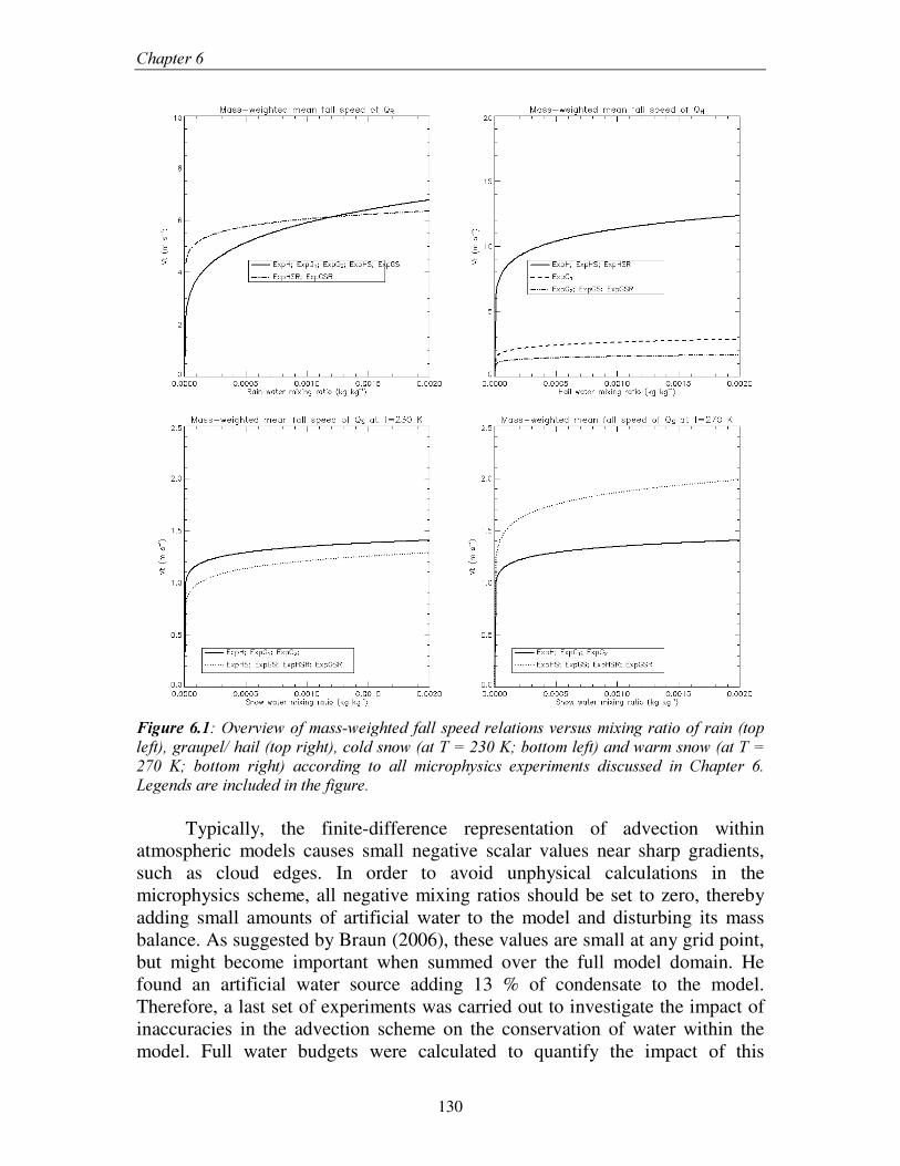
&KDSWHU���
130
)LJXUH������2YHUYLHZ�RI�PDVV�ZHLJKWHG�IDOO�VSHHG�UHODWLRQV�YHUVXV�PL[LQJ�UDWLR�RI�UDLQ��WRS�OHIW���JUDXSHO��KDLO��WRS�ULJKW���FROG�VQRZ��DW�7� �����.��ERWWRP�OHIW��DQG�ZDUP�VQRZ��DW�7� ����� .�� ERWWRP� ULJKW�� DFFRUGLQJ� WR� DOO� PLFURSK\VLFV� H[SHULPHQWV� GLVFXVVHG� LQ� &KDSWHU� ���/HJHQGV�DUH�LQFOXGHG�LQ�WKH�ILJXUH�
Typically, the finite-difference representation of advection within
atmospheric models causes small negative scalar values near sharp gradients, such as cloud edges. In order to avoid unphysical calculations in the microphysics scheme, all negative mixing ratios should be set to zero, thereby adding small amounts of artificial water to the model and disturbing its mass balance. As suggested by Braun (2006), these values are small at any grid point, but might become important when summed over the full model domain. He found an artificial water source adding 13 % of condensate to the model. Therefore, a last set of experiments was carried out to investigate the impact of inaccuracies in the advection scheme on the conservation of water within the model. Full water budgets were calculated to quantify the impact of this
,PSDFW�RI�VL]H�GLVWULEXWLRQ�DVVXPSWLRQV�RQ�VXSHUFHOO�SUHFLSLWDWLRQ�DQG�G\QDPLFV��
131
artificial water source for each of the hydrometeors. For each hydrometeor, the conservation equation can be written as:
( ) ±±±±±±± =T9]3'LIITWT
+∂∂+++∇⋅−=
∂∂ ρ
ρ19 , (6.1)
The first term on the right-hand side is the advection term, the second is the parameterized numerical and physical diffusion term, Px represents the contribution by microphysical production, the fourth term represents the fallout term (which is zero for cloud water and cloud ice as they are considered suspended in the air) and Zx represents the artificial water source from zeroing of negative mixing ratios. In order to assess the influence of artificially added water to surface precipitation, two additional experiments were carried out. The model was forced to conserve water mass at each grid box and each time step by subtracting the total amount of total artificially added water from the vapour mixing ratio within the respective grid box and at each time step (ExpHSRconserved and ExpGSRconserved). This was done as water vapour mixing ratios never drop to values close to zero and hence can be regarded as a major source of water within each grid box to subtract the artificially added water amounts from in order to keep water mass conserved.
������5HVXOWV�
6.3.1. Influence of graupel/ hail size distribution
Table 6.2 summarizes the 0000 UTC – 0000 UTC surface precipitation characteristics for all experiments and as observed. Precipitation observations are obtained from the C-band weather radar in Wideumont (indicated by the asterisk in Figure 3.1) operated by the Royal Meteorological Institute of Belgium and from a dense network of rain gauges ( 1 per 135 km²) operated by the hydrological service of the Walloon region. Radar-based precipitation estimates are derived from a 5-elelvation reflectivity scan performed every 5 minutes and radar and rain gauge observations have been combined using a simple mean field bias adjustment. To make a fair comparison between observed and simulated precipitation fields, the observed precipitation field, having a spatial resolution of 600 m, has been aggregated to the ARPS grid. All simulated and observed 24-hour accumulated surface precipitation estimates in the following paragraphs are for the region within a radius of 150 km from the radar location. Uncertainties on precipitation observations are discusses in more detail in section 5.2.2.4. It is clear that 24-hour accumulated surface precipitation is largely overestimated in the ExpH. Surface precipitation tends to increase as the largest frozen precipitation species is weighted towards small graupel. When
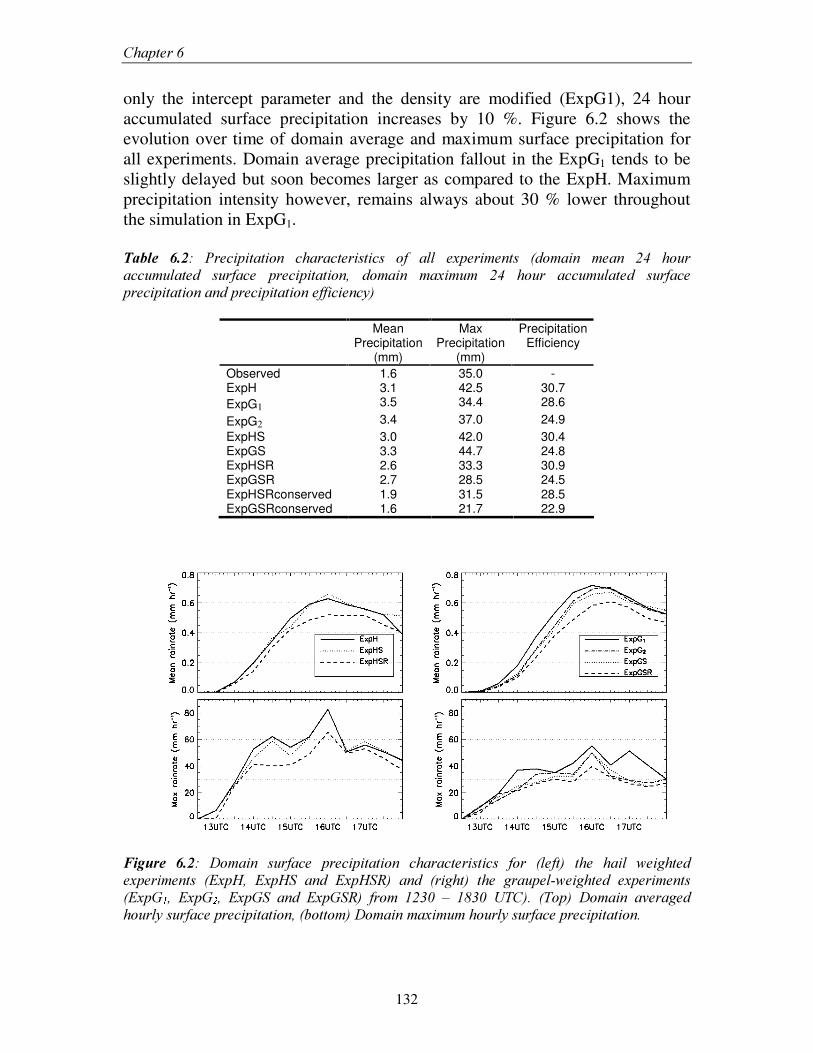
&KDSWHU���
132
only the intercept parameter and the density are modified (ExpG1), 24 hour accumulated surface precipitation increases by 10 %. Figure 6.2 shows the evolution over time of domain average and maximum surface precipitation for all experiments. Domain average precipitation fallout in the ExpG1 tends to be slightly delayed but soon becomes larger as compared to the ExpH. Maximum precipitation intensity however, remains always about 30 % lower throughout the simulation in ExpG1.
7DEOH� ����� 3UHFLSLWDWLRQ� FKDUDFWHULVWLFV� RI� DOO� H[SHULPHQWV� �GRPDLQ� PHDQ� ��� KRXU�DFFXPXODWHG� VXUIDFH� SUHFLSLWDWLRQ�� GRPDLQ� PD[LPXP� ��� KRXU� DFFXPXODWHG� VXUIDFH�SUHFLSLWDWLRQ�DQG�SUHFLSLWDWLRQ�HIILFLHQF\��
Mean Precipitation
(mm)
Max Precipitation
(mm)
Precipitation Efficiency
Observed 1.6 35.0 - ExpH 3.1 42.5 30.7 ExpG1 3.5 34.4 28.6
ExpG2 3.4 37.0 24.9 ExpHS 3.0 42.0 30.4 ExpGS 3.3 44.7 24.8 ExpHSR 2.6 33.3 30.9 ExpGSR 2.7 28.5 24.5 ExpHSRconserved 1.9 31.5 28.5 ExpGSRconserved 1.6 21.7 22.9
)LJXUH� ����� 'RPDLQ� VXUIDFH� SUHFLSLWDWLRQ� FKDUDFWHULVWLFV� IRU� �OHIW�� WKH� KDLO� ZHLJKWHG�H[SHULPHQWV� �([S+�� ([S+6� DQG� ([S+65�� DQG� �ULJKW�� WKH� JUDXSHO�ZHLJKWHG� H[SHULPHQWV��([S* ² �� ([S*³ �� ([S*6� DQG� ([S*65�� IURP� ����� ±� ����� 87&��� �7RS�� 'RPDLQ� DYHUDJHG�KRXUO\�VXUIDFH�SUHFLSLWDWLRQ���ERWWRP��'RPDLQ�PD[LPXP�KRXUO\�VXUIDFH�SUHFLSLWDWLRQ��
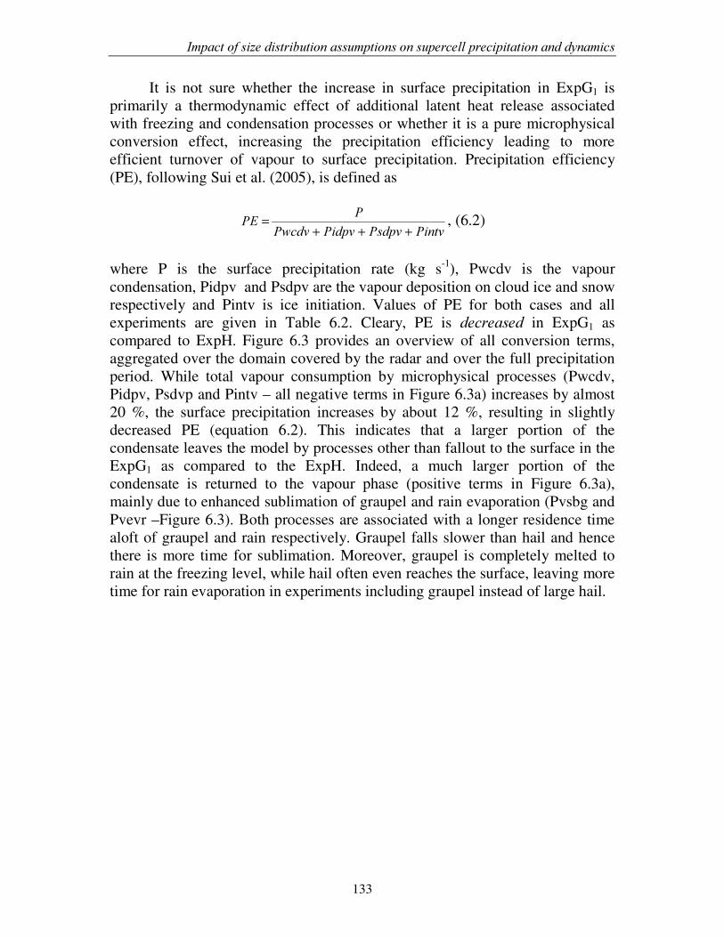
,PSDFW�RI�VL]H�GLVWULEXWLRQ�DVVXPSWLRQV�RQ�VXSHUFHOO�SUHFLSLWDWLRQ�DQG�G\QDPLFV��
133
It is not sure whether the increase in surface precipitation in ExpG1 is primarily a thermodynamic effect of additional latent heat release associated with freezing and condensation processes or whether it is a pure microphysical conversion effect, increasing the precipitation efficiency leading to more efficient turnover of vapour to surface precipitation. Precipitation efficiency (PE), following Sui et al. (2005), is defined as
3LQWY3VGSY3LGSY3ZFGY33(
+++= , (6.2)
where P is the surface precipitation rate (kg s-1), Pwcdv is the vapour condensation, Pidpv and Psdpv are the vapour deposition on cloud ice and snow respectively and Pintv is ice initiation. Values of PE for both cases and all experiments are given in Table 6.2. Cleary, PE is GHFUHDVHG in ExpG1 as compared to ExpH. Figure 6.3 provides an overview of all conversion terms, aggregated over the domain covered by the radar and over the full precipitation period. While total vapour consumption by microphysical processes (Pwcdv, Pidpv, Psdvp and Pintv – all negative terms in Figure 6.3a) increases by almost 20 %, the surface precipitation increases by about 12 %, resulting in slightly decreased PE (equation 6.2). This indicates that a larger portion of the condensate leaves the model by processes other than fallout to the surface in the ExpG1 as compared to the ExpH. Indeed, a much larger portion of the condensate is returned to the vapour phase (positive terms in Figure 6.3a), mainly due to enhanced sublimation of graupel and rain evaporation (Pvsbg and Pvevr –Figure 6.3). Both processes are associated with a longer residence time aloft of graupel and rain respectively. Graupel falls slower than hail and hence there is more time for sublimation. Moreover, graupel is completely melted to rain at the freezing level, while hail often even reaches the surface, leaving more time for rain evaporation in experiments including graupel instead of large hail.
�
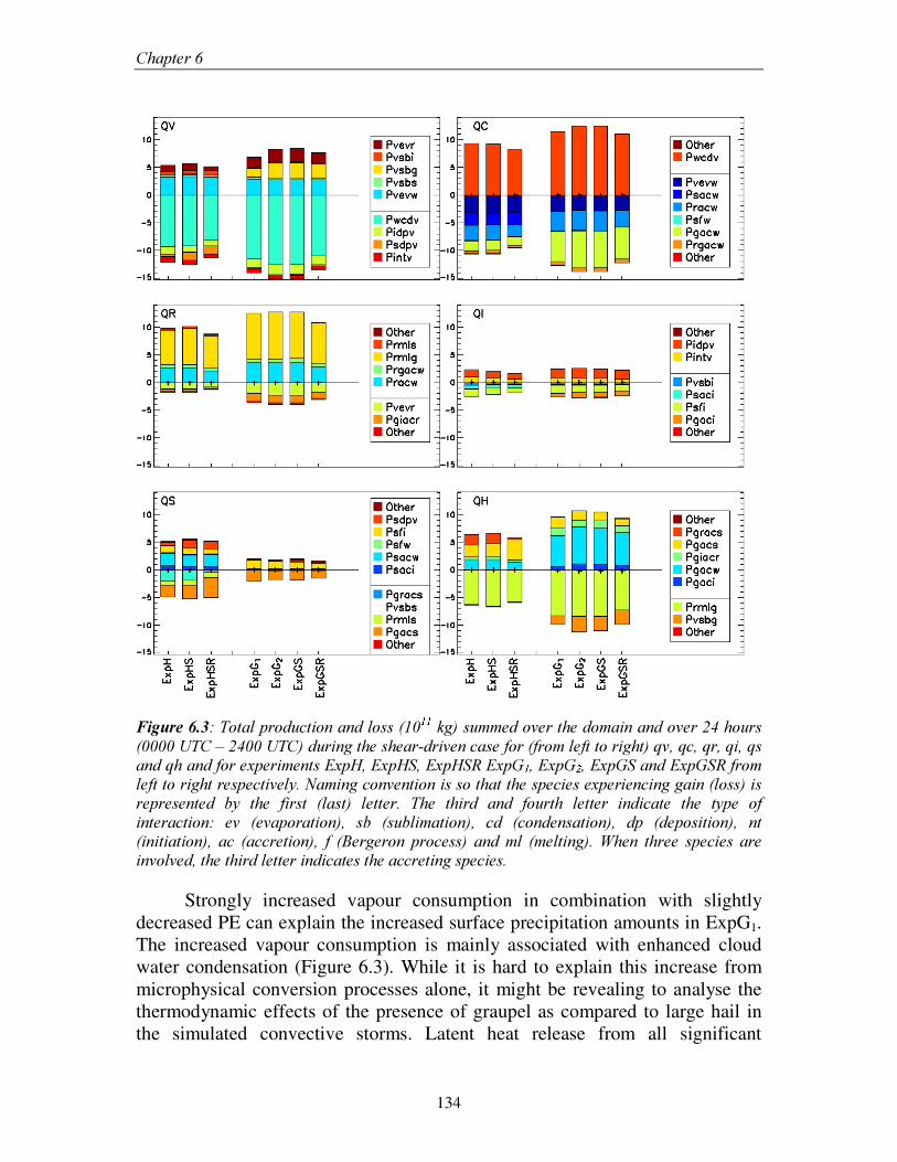
&KDSWHU���
134
)LJXUH������7RWDO�SURGXFWLRQ�DQG�ORVV���� ²´² �NJ��VXPPHG�RYHU�WKH�GRPDLQ�DQG�RYHU����KRXUV�������87&�±������87&��GXULQJ�WKH�VKHDU�GULYHQ�FDVH�IRU��IURP�OHIW�WR�ULJKW��TY��TF��TU��TL��TV�DQG�TK�DQG�IRU�H[SHULPHQWV�([S+��([S+6��([S+65�([S* ² ��([S*³ ��([S*6�DQG�([S*65�IURP�OHIW�WR�ULJKW�UHVSHFWLYHO\��1DPLQJ�FRQYHQWLRQ�LV�VR�WKDW�WKH�VSHFLHV�H[SHULHQFLQJ�JDLQ��ORVV��LV�UHSUHVHQWHG� E\� WKH� ILUVW� �ODVW�� OHWWHU�� 7KH� WKLUG� DQG� IRXUWK� OHWWHU� LQGLFDWH� WKH� W\SH� RI�LQWHUDFWLRQ�� HY� �HYDSRUDWLRQ��� VE� �VXEOLPDWLRQ��� FG� �FRQGHQVDWLRQ��� GS� �GHSRVLWLRQ��� QW��LQLWLDWLRQ��� DF� �DFFUHWLRQ��� I� �%HUJHURQ� SURFHVV�� DQG�PO� �PHOWLQJ���:KHQ� WKUHH� VSHFLHV� DUH�LQYROYHG��WKH�WKLUG�OHWWHU�LQGLFDWHV�WKH�DFFUHWLQJ�VSHFLHV���
�Strongly increased vapour consumption in combination with slightly
decreased PE can explain the increased surface precipitation amounts in ExpG1. The increased vapour consumption is mainly associated with enhanced cloud water condensation (Figure 6.3). While it is hard to explain this increase from microphysical conversion processes alone, it might be revealing to analyse the thermodynamic effects of the presence of graupel as compared to large hail in the simulated convective storms. Latent heat release from all significant
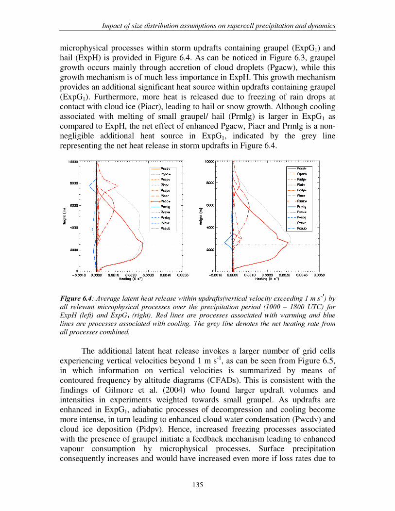
,PSDFW�RI�VL]H�GLVWULEXWLRQ�DVVXPSWLRQV�RQ�VXSHUFHOO�SUHFLSLWDWLRQ�DQG�G\QDPLFV��
135
microphysical processes within storm updrafts containing graupel (ExpG1) and hail (ExpH) is provided in Figure 6.4. As can be noticed in Figure 6.3, graupel growth occurs mainly through accretion of cloud droplets (Pgacw), while this growth mechanism is of much less importance in ExpH. This growth mechanism provides an additional significant heat source within updrafts containing graupel (ExpG1). Furthermore, more heat is released due to freezing of rain drops at contact with cloud ice (Piacr), leading to hail or snow growth. Although cooling associated with melting of small graupel/ hail (Prmlg) is larger in ExpG1 as compared to ExpH, the net effect of enhanced Pgacw, Piacr and Prmlg is a non-negligible additional heat source in ExpG1, indicated by the grey line representing the net heat release in storm updrafts in Figure 6.4.
)LJXUH������$YHUDJH�ODWHQW�KHDW�UHOHDVH�ZLWKLQ�XSGUDIWV�YHUWLFDO�YHORFLW\�H[FHHGLQJ���P�V µ ² ��E\�DOO� UHOHYDQW�PLFURSK\VLFDO� SURFHVVHV� RYHU� WKH� SUHFLSLWDWLRQ� SHULRG� ������ ±� �����87&�� IRU�([S+� �OHIW�� DQG� ([S* ² �ULJKW��� 5HG� OLQHV� DUH� SURFHVVHV� DVVRFLDWHG�ZLWK�ZDUPLQJ� DQG� EOXH�OLQHV�DUH�SURFHVVHV�DVVRFLDWHG�ZLWK�FRROLQJ��7KH�JUH\�OLQH�GHQRWHV�WKH�QHW�KHDWLQJ�UDWH�IURP�DOO�SURFHVVHV�FRPELQHG��
The additional latent heat release invokes a larger number of grid cells
experiencing vertical velocities beyond 1 m s-1, as can be seen from Figure 6.5, in which information on vertical velocities is summarized by means of contoured frequency by altitude diagrams (CFADs). This is consistent with the findings of Gilmore et al. (2004) who found larger updraft volumes and intensities in experiments weighted towards small graupel. As updrafts are enhanced in ExpG1, adiabatic processes of decompression and cooling become more intense, in turn leading to enhanced cloud water condensation (Pwcdv) and cloud ice deposition (Pidpv). Hence, increased freezing processes associated with the presence of graupel initiate a feedback mechanism leading to enhanced vapour consumption by microphysical processes. Surface precipitation consequently increases and would have increased even more if loss rates due to
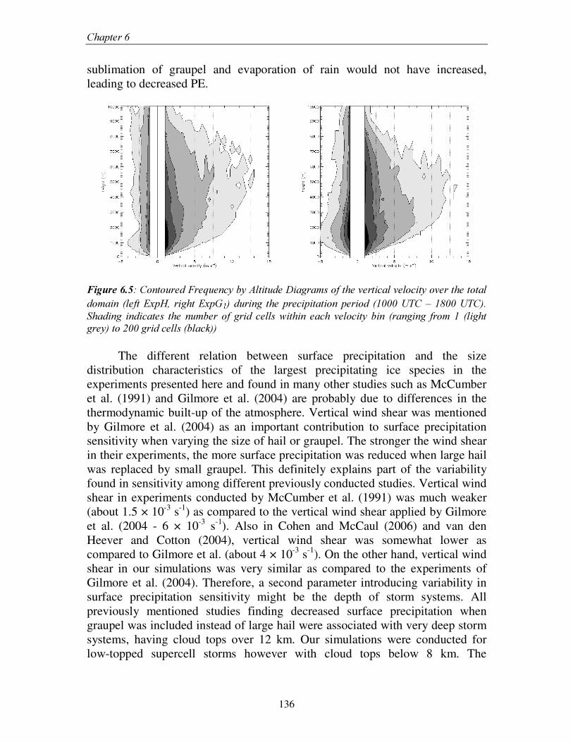
&KDSWHU���
136
sublimation of graupel and evaporation of rain would not have increased, leading to decreased PE.
)LJXUH������&RQWRXUHG�)UHTXHQF\�E\�$OWLWXGH�'LDJUDPV�RI�WKH�YHUWLFDO�YHORFLW\�RYHU�WKH�WRWDO�GRPDLQ� �OHIW�([S+�� ULJKW�([S* ¶ ��GXULQJ� WKH�SUHFLSLWDWLRQ�SHULRG� ������87&�±������87&���6KDGLQJ� LQGLFDWHV� WKH� QXPEHU� RI� JULG� FHOOV�ZLWKLQ� HDFK� YHORFLW\� ELQ� �UDQJLQJ� IURP� �� �OLJKW�JUH\��WR�����JULG�FHOOV��EODFN���
The different relation between surface precipitation and the size distribution characteristics of the largest precipitating ice species in the experiments presented here and found in many other studies such as McCumber et al. (1991) and Gilmore et al. (2004) are probably due to differences in the thermodynamic built-up of the atmosphere. Vertical wind shear was mentioned by Gilmore et al. (2004) as an important contribution to surface precipitation sensitivity when varying the size of hail or graupel. The stronger the wind shear in their experiments, the more surface precipitation was reduced when large hail was replaced by small graupel. This definitely explains part of the variability found in sensitivity among different previously conducted studies. Vertical wind shear in experiments conducted by McCumber et al. (1991) was much weaker (about 1.5 × 10⁻³ s-1) as compared to the vertical wind shear applied by Gilmore et al. (2004 - 6 × 10⁻³ s-1). Also in Cohen and McCaul (2006) and van den Heever and Cotton (2004), vertical wind shear was somewhat lower as compared to Gilmore et al. (about 4 × 10⁻³ s-1). On the other hand, vertical wind shear in our simulations was very similar as compared to the experiments of Gilmore et al. (2004). Therefore, a second parameter introducing variability in surface precipitation sensitivity might be the depth of storm systems. All previously mentioned studies finding decreased surface precipitation when graupel was included instead of large hail were associated with very deep storm systems, having cloud tops over 12 km. Our simulations were conducted for low-topped supercell storms however with cloud tops below 8 km. The
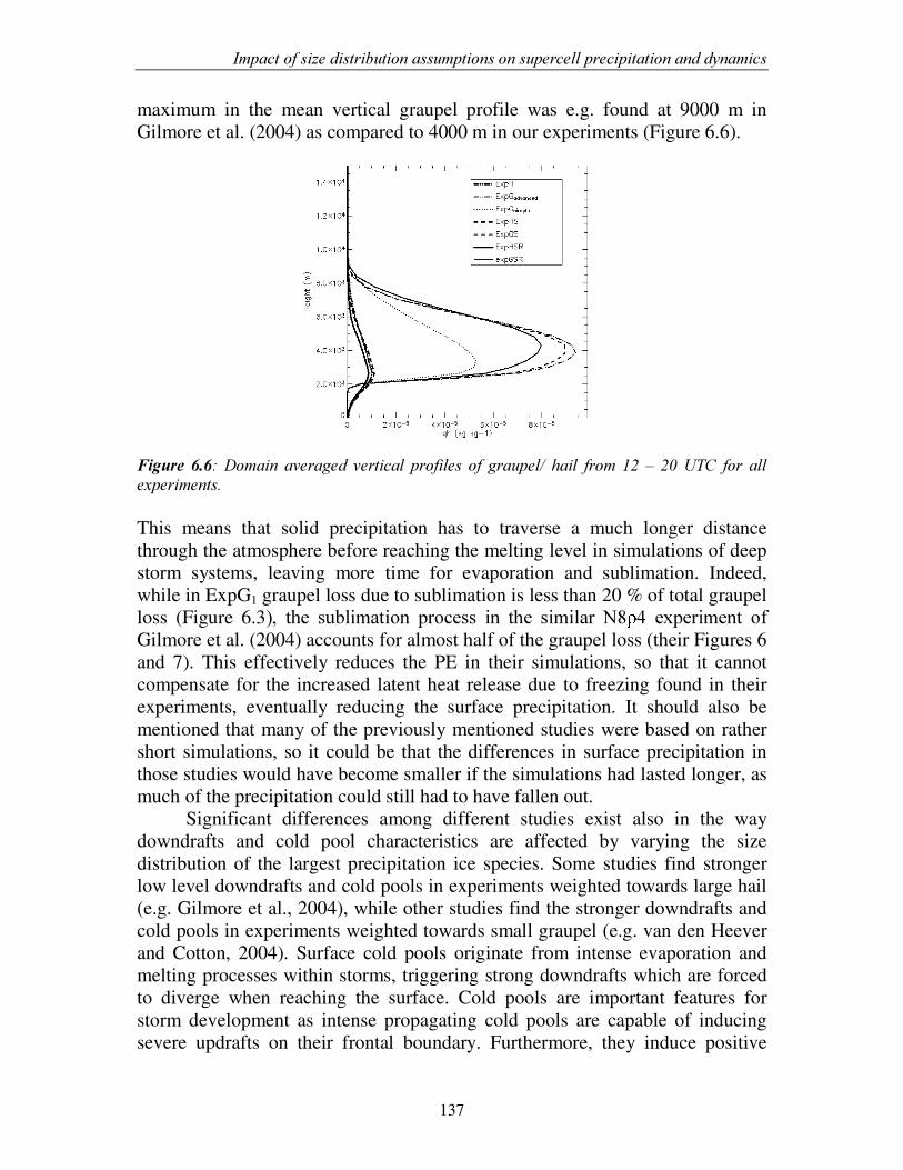
,PSDFW�RI�VL]H�GLVWULEXWLRQ�DVVXPSWLRQV�RQ�VXSHUFHOO�SUHFLSLWDWLRQ�DQG�G\QDPLFV��
137
maximum in the mean vertical graupel profile was e.g. found at 9000 m in Gilmore et al. (2004) as compared to 4000 m in our experiments (Figure 6.6).
)LJXUH� �����'RPDLQ� DYHUDJHG� YHUWLFDO� SURILOHV� RI� JUDXSHO�� KDLO� IURP� ��� ±� ���87&� IRU� DOO�H[SHULPHQWV�� This means that solid precipitation has to traverse a much longer distance through the atmosphere before reaching the melting level in simulations of deep storm systems, leaving more time for evaporation and sublimation. Indeed, while in ExpG1 graupel loss due to sublimation is less than 20 % of total graupel loss (Figure 6.3��� WKH� VXEOLPDWLRQ� SURFHVV� LQ� WKH� VLPLODU� 1� �� H[SHULPHQW� RI�Gilmore et al. (2004) accounts for almost half of the graupel loss (their Figures 6 and 7). This effectively reduces the PE in their simulations, so that it cannot compensate for the increased latent heat release due to freezing found in their experiments, eventually reducing the surface precipitation. It should also be mentioned that many of the previously mentioned studies were based on rather short simulations, so it could be that the differences in surface precipitation in those studies would have become smaller if the simulations had lasted longer, as much of the precipitation could still had to have fallen out.
Significant differences among different studies exist also in the way downdrafts and cold pool characteristics are affected by varying the size distribution of the largest precipitation ice species. Some studies find stronger low level downdrafts and cold pools in experiments weighted towards large hail (e.g. Gilmore et al., 2004), while other studies find the stronger downdrafts and cold pools in experiments weighted towards small graupel (e.g. van den Heever and Cotton, 2004). Surface cold pools originate from intense evaporation and melting processes within storms, triggering strong downdrafts which are forced to diverge when reaching the surface. Cold pools are important features for storm development as intense propagating cold pools are capable of inducing severe updrafts on their frontal boundary. Furthermore, they induce positive
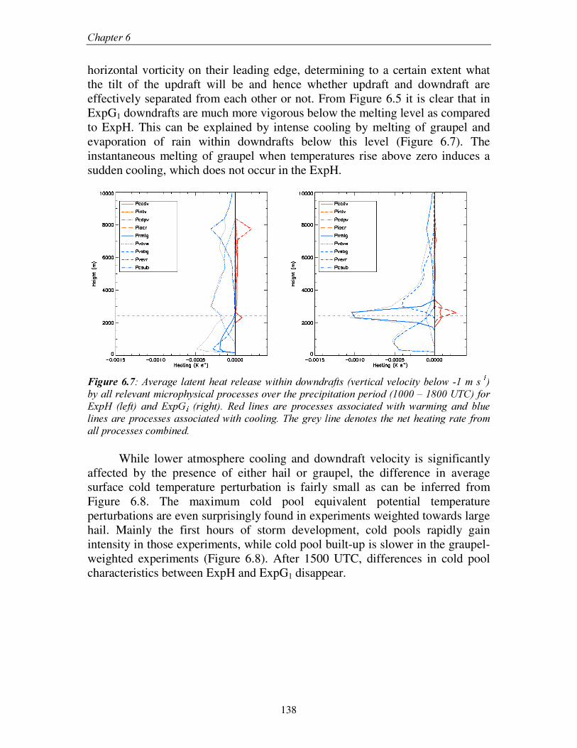
&KDSWHU���
138
horizontal vorticity on their leading edge, determining to a certain extent what the tilt of the updraft will be and hence whether updraft and downdraft are effectively separated from each other or not. From Figure 6.5 it is clear that in ExpG1 downdrafts are much more vigorous below the melting level as compared to ExpH. This can be explained by intense cooling by melting of graupel and evaporation of rain within downdrafts below this level (Figure 6.7). The instantaneous melting of graupel when temperatures rise above zero induces a sudden cooling, which does not occur in the ExpH.
)LJXUH������$YHUDJH�ODWHQW�KHDW�UHOHDVH�ZLWKLQ�GRZQGUDIWV��YHUWLFDO�YHORFLW\�EHORZ����P�V µ ² ��E\�DOO�UHOHYDQW�PLFURSK\VLFDO�SURFHVVHV�RYHU�WKH�SUHFLSLWDWLRQ�SHULRG�������±������87&��IRU�([S+� �OHIW�� DQG� ([S* ² �ULJKW��� 5HG� OLQHV� DUH� SURFHVVHV� DVVRFLDWHG�ZLWK�ZDUPLQJ� DQG� EOXH�OLQHV�DUH�SURFHVVHV�DVVRFLDWHG�ZLWK�FRROLQJ��7KH�JUH\�OLQH�GHQRWHV�WKH�QHW�KHDWLQJ�UDWH�IURP�DOO�SURFHVVHV�FRPELQHG��
While lower atmosphere cooling and downdraft velocity is significantly affected by the presence of either hail or graupel, the difference in average surface cold temperature perturbation is fairly small as can be inferred from Figure 6.8. The maximum cold pool equivalent potential temperature perturbations are even surprisingly found in experiments weighted towards large hail. Mainly the first hours of storm development, cold pools rapidly gain intensity in those experiments, while cold pool built-up is slower in the graupel-weighted experiments (Figure 6.8). After 1500 UTC, differences in cold pool characteristics between ExpH and ExpG1 disappear.
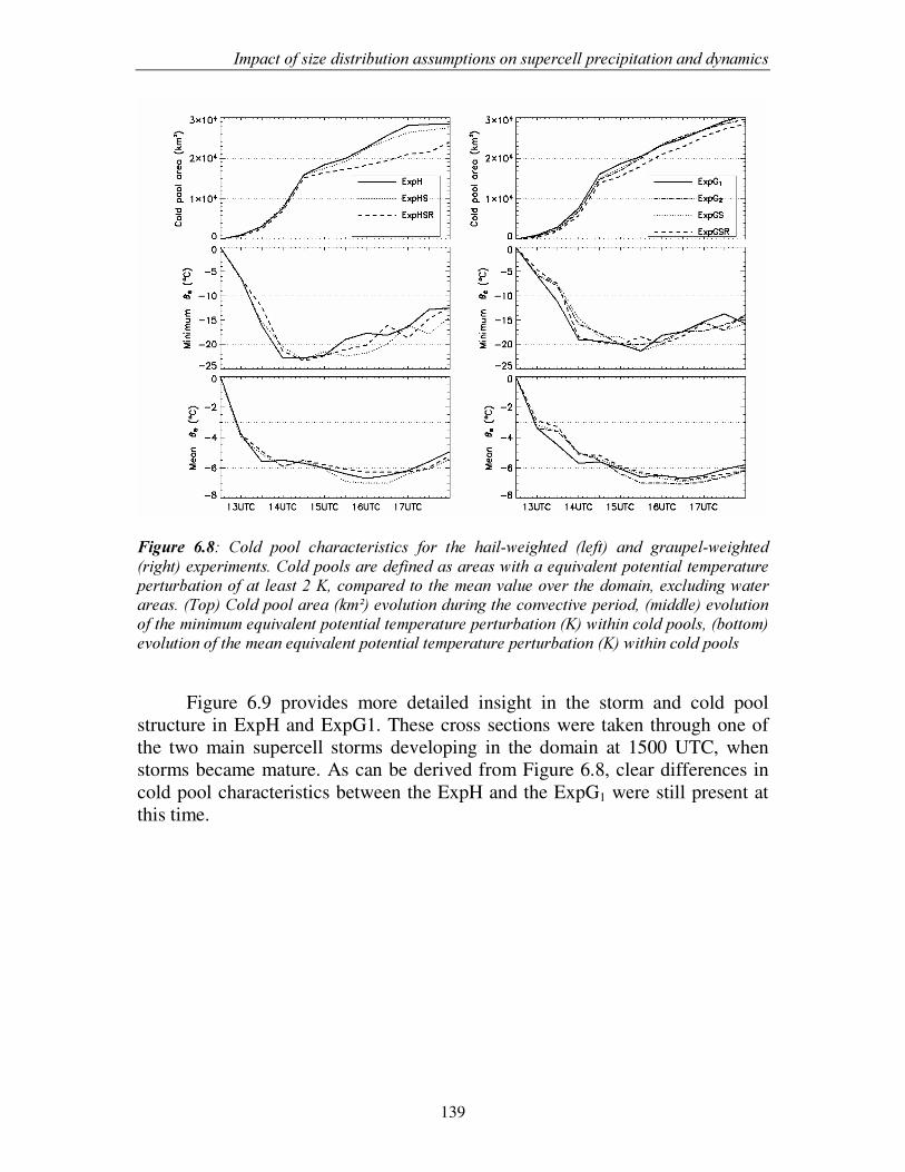
,PSDFW�RI�VL]H�GLVWULEXWLRQ�DVVXPSWLRQV�RQ�VXSHUFHOO�SUHFLSLWDWLRQ�DQG�G\QDPLFV��
139
��)LJXUH� ����� &ROG� SRRO� FKDUDFWHULVWLFV� IRU� WKH� KDLO�ZHLJKWHG� �OHIW�� DQG� JUDXSHO�ZHLJKWHG��ULJKW��H[SHULPHQWV��&ROG�SRROV�DUH�GHILQHG�DV�DUHDV�ZLWK�D�HTXLYDOHQW�SRWHQWLDO�WHPSHUDWXUH�SHUWXUEDWLRQ�RI�DW�OHDVW���.��FRPSDUHG�WR�WKH�PHDQ�YDOXH�RYHU�WKH�GRPDLQ��H[FOXGLQJ�ZDWHU�DUHDV���7RS��&ROG�SRRO�DUHD��NPð��HYROXWLRQ�GXULQJ�WKH�FRQYHFWLYH�SHULRG���PLGGOH��HYROXWLRQ�RI�WKH�PLQLPXP�HTXLYDOHQW�SRWHQWLDO�WHPSHUDWXUH�SHUWXUEDWLRQ��.��ZLWKLQ�FROG�SRROV���ERWWRP��HYROXWLRQ�RI�WKH�PHDQ�HTXLYDOHQW�SRWHQWLDO�WHPSHUDWXUH�SHUWXUEDWLRQ��.��ZLWKLQ�FROG�SRROV� Figure 6.9 provides more detailed insight in the storm and cold pool structure in ExpH and ExpG1. These cross sections were taken through one of the two main supercell storms developing in the domain at 1500 UTC, when storms became mature. As can be derived from Figure 6.8, clear differences in cold pool characteristics between the ExpH and the ExpG1 were still present at this time.
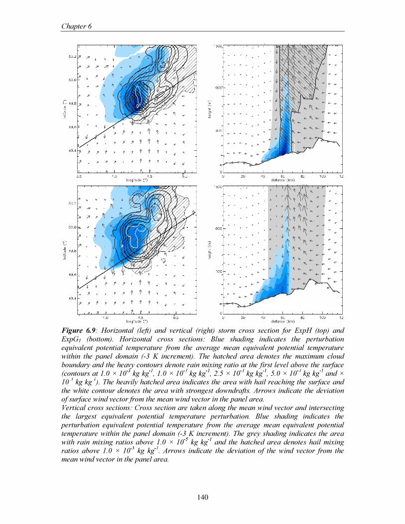
&KDSWHU���
140
)LJXUH� ����� +RUL]RQWDO� �OHIW�� DQG� YHUWLFDO� �ULJKW�� VWRUP� FURVV� VHFWLRQ� IRU� ([S+� �WRS�� DQG ([S* ² � �ERWWRP��� +RUL]RQWDO� FURVV� VHFWLRQV�� %OXH� VKDGLQJ� LQGLFDWHV� WKH� SHUWXUEDWLRQ�HTXLYDOHQW� SRWHQWLDO� WHPSHUDWXUH� IURP� WKH� DYHUDJH� PHDQ� HTXLYDOHQW� SRWHQWLDO� WHPSHUDWXUH�ZLWKLQ� WKH� SDQHO� GRPDLQ� ���� .� LQFUHPHQW��� 7KH� KDWFKHG� DUHD� GHQRWHV� WKH� PD[LPXP� FORXG�ERXQGDU\�DQG�WKH�KHDY\�FRQWRXUV�GHQRWH�UDLQ�PL[LQJ�UDWLR�DW�WKH�ILUVW�OHYHO�DERYH�WKH�VXUIDFH��FRQWRXUV�DW�����î��� µ · �NJ�NJ µ ² ������î��� µ ¸ �NJ�NJ µ ² ������î��� µ ¸ �NJ�NJ µ ² ������î��� µ ¸ �NJ�NJ µ ² �DQG�î��� µ ¹ �NJ�NJ µ ² ���7KH�KHDYLO\�KDWFKHG�DUHD�LQGLFDWHV�WKH�DUHD�ZLWK�KDLO�UHDFKLQJ�WKH�VXUIDFH�DQG�WKH�ZKLWH�FRQWRXU�GHQRWHV�WKH�DUHD�ZLWK�VWURQJHVW�GRZQGUDIWV��$UURZV�LQGLFDWH�WKH�GHYLDWLRQ�RI�VXUIDFH�ZLQG�YHFWRU�IURP�WKH�PHDQ�ZLQG�YHFWRU�LQ�WKH�SDQHO�DUHD���9HUWLFDO�FURVV�VHFWLRQV��&URVV�VHFWLRQ�DUH�WDNHQ�DORQJ�WKH�PHDQ�ZLQG�YHFWRU�DQG�LQWHUVHFWLQJ�WKH� ODUJHVW� HTXLYDOHQW� SRWHQWLDO� WHPSHUDWXUH� SHUWXUEDWLRQ�� %OXH� VKDGLQJ� LQGLFDWHV� WKH�SHUWXUEDWLRQ� HTXLYDOHQW� SRWHQWLDO� WHPSHUDWXUH� IURP� WKH� DYHUDJH� PHDQ� HTXLYDOHQW� SRWHQWLDO�WHPSHUDWXUH�ZLWKLQ�WKH�SDQHO�GRPDLQ�����.�LQFUHPHQW���7KH�JUH\�VKDGLQJ�LQGLFDWHV�WKH�DUHD�ZLWK�UDLQ�PL[LQJ� UDWLRV�DERYH�����î��� µ · � NJ�NJ µ ² � DQG� WKH�KDWFKHG�DUHD�GHQRWHV�KDLO�PL[LQJ�UDWLRV� DERYH� ����î� �� µ · � NJ� NJ µ ² ��$UURZV� LQGLFDWH� WKH� GHYLDWLRQ�RI� WKH�ZLQG� YHFWRU� IURP� WKH�PHDQ�ZLQG�YHFWRU�LQ�WKH�SDQHO�DUHD��
,PSDFW�RI�VL]H�GLVWULEXWLRQ�DVVXPSWLRQV�RQ�VXSHUFHOO�SUHFLSLWDWLRQ�DQG�G\QDPLFV��
141
From the horizontal cross sections, it is clear that intense cold pool areas are associated with the most vigorous downdrafts in the storms (denoted by the white contour). Both horizontal and vertical cross sections show that the most intense surface cold pools are found in the hail weighted experiment, despite the more vigorous downdrafts in the graupel-weighted experiments discussed earlier. Those intense cold pool areas in the hail-weighted experiments are associated with intensively melting large hail reaching the surface (Figure 6.9). It is likely that downdrafts initiated at mid-tropospheric levels diffuse on their way down, resulting in somewhat broader but less intense cold pool areas, while it is the low-level cooling (within the lowest km of the troposphere or so), associated with hail melt and rain evaporation, which is responsible for the most intense cold pools. Although mid-level cooling processes are most vigorous in ExpG1, near surface cooling is dominant in ExpH leading to intense but localized cold pools, associated with hail melt. This is also consistent with differences found in literature among different studies. Indeed, in van den Heever and Cotton, some graupel reaches the surface in all experiments, contributing to cooling due to melting down to the surface. In experiments by Gilmore et al. (2004) as well as in our experiments, having the weaker cold pools in the graupel-weighted experiments, all graupel is melted well above the surface. Hence cooling due to melting ceases at a few kilometres above the surface, leading to smaller minimum cold pool perturbation temperatures in those experiments.
So far we only investigated the impact of modifying the hail intercept parameter and its density (ExpG1). However, this leads to an inconsistency as the fall speed calculation is still based on the large hail formulation of Wisner et al. (1972). As graupel tends to fall slower than hail of the same size (as it is not a constant density sphere), we applied an additional experiment to understand the impact of applying more consistent fall speed and size distribution assumptions (ExpG2). Surface precipitation in this experiment is almost unaffected as compared to ExpG1 (Table 6.2 and Figure 6.2). From Figure 6.1 it is clear that in the ExpG2, graupel is falling even slower as compared to ExpG1, which leads the graupel amount to grow even larger (Figure 6.6). As the graupel sediments slowly, more of it will sublimate (Pvsbg – Figure 6.3) to the vapour phase instead of falling towards the surface and melting to rain (Prmlg – Figure 6.3), which further decreases the precipitation efficiency (Table 6.2). However, even more condensation occurs in response to the increased latent heat release associated with the riming growth of graupel (Pgacw – Figure 6.3). The combination of both mechanisms yields almost no change of the surface precipitation.
&KDSWHU���
142
6.3.2. Influence of snow and rain size distribution
In most bulk microphysics schemes, snow has been represented as a constant density sphere and having a constant intercept parameter. It has been rarely investigated what the impact would be of more realistic size distribution assumptions of snow on deep moist convection. Therefore we further modified the set up of the experiments ExpH and ExpG2 to introduce a temperature dependent snow intercept parameter and assuming graupellike snow instead of a constant density sphere for the slope parameter calculation (ExpHS and ExpGS). Accumulated surface precipitation in both experiments is very similar to their respective counterparts with the original snow size distribution formulations (Figure 6.2 and Table 6.2). Impact of these experiments on both precipitation efficiency and thermodynamics (not shown) are virtually non-existing.
As for the snow variable, the intercept parameter of rain is kept constant in most bulk microphysical schemes, while it is known to vary significantly from observational data. Therefore, experiments ExpHS and ExpGS were further modified to include a mixing ratio dependent rain intercept parameter (ExpHSR and ExpGSR). This modification leads to a significant reduction (about 15 %) in the accumulated surface precipitation and maximum rain rate (Figure 6.2 and Table 6.2). From Figure 6.1 it is clear that at high rain mixing ratios, the mixing ratio dependent rain fall speeds are reduced by about 20 %. This explains why maximum rain rates are reduced in this case. However, it is odd that the accumulated total precipitation is also reduced, as there is no change in PE (Table 6.2) and updraft intensity is not clearly diminished (Figure 6.10). Taking a look at the cold pool characteristics reveals the likely reason for the decreased surface rain amounts, however (Figure 6.8). Cold pools in the experiments having a diagnosed rain intercept are consistently smaller than cold pools in the other experiments. From Figure 6.1, it is clear that rain sedimentation velocities are significantly increased for small mixing ratios and decreased for large mixing ratios, leaving less time for evaporation near the edges of storms and more time for evaporation in the high intensity cores. This effectively shrinks the cold pool areas, while the inner parts remain as cold as compared to the experiments with constant rain intercepts (Figure 6.8). As updrafts are forced on the frontal outflow boundary of propagating storms and the outflow area shrinks, storms tend to shrink too, eventually leading to storms having a similar intensity but smaller size as compared to the other experiments.
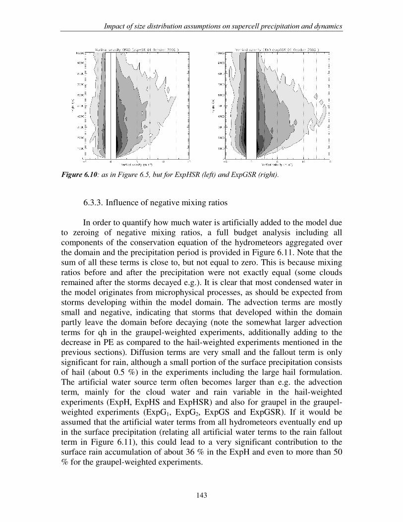
,PSDFW�RI�VL]H�GLVWULEXWLRQ�DVVXPSWLRQV�RQ�VXSHUFHOO�SUHFLSLWDWLRQ�DQG�G\QDPLFV��
143
)LJXUH�������DV�LQ�)LJXUH������EXW�IRU�([S+65��OHIW��DQG�([S*65��ULJKW���
6.3.3. Influence of negative mixing ratios In order to quantify how much water is artificially added to the model due
to zeroing of negative mixing ratios, a full budget analysis including all components of the conservation equation of the hydrometeors aggregated over the domain and the precipitation period is provided in Figure 6.11. Note that the sum of all these terms is close to, but not equal to zero. This is because mixing ratios before and after the precipitation were not exactly equal (some clouds remained after the storms decayed e.g.). It is clear that most condensed water in the model originates from microphysical processes, as should be expected from storms developing within the model domain. The advection terms are mostly small and negative, indicating that storms that developed within the domain partly leave the domain before decaying (note the somewhat larger advection terms for qh in the graupel-weighted experiments, additionally adding to the decrease in PE as compared to the hail-weighted experiments mentioned in the previous sections). Diffusion terms are very small and the fallout term is only significant for rain, although a small portion of the surface precipitation consists of hail (about 0.5 %) in the experiments including the large hail formulation. The artificial water source term often becomes larger than e.g. the advection term, mainly for the cloud water and rain variable in the hail-weighted experiments (ExpH, ExpHS and ExpHSR) and also for graupel in the graupel-weighted experiments (ExpG1, ExpG2, ExpGS and ExpGSR). If it would be assumed that the artificial water terms from all hydrometeors eventually end up in the surface precipitation (relating all artificial water terms to the rain fallout term in Figure 6.11), this could lead to a very significant contribution to the surface rain accumulation of about 36 % in the ExpH and even to more than 50 % for the graupel-weighted experiments.
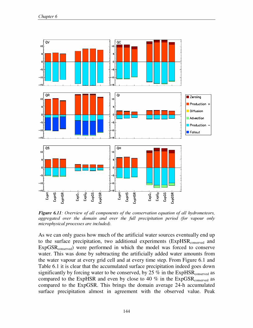
&KDSWHU���
144
)LJXUH�������2YHUYLHZ�RI�DOO�FRPSRQHQWV�RI� WKH�FRQVHUYDWLRQ�HTXDWLRQ�RI�DOO�K\GURPHWHRUV��DJJUHJDWHG� RYHU� WKH� GRPDLQ� DQG� RYHU� WKH� IXOO� SUHFLSLWDWLRQ� SHULRG� �IRU� YDSRXU� RQO\�PLFURSK\VLFDO�SURFHVVHV�DUH�LQFOXGHG�����As we can only guess how much of the artificial water sources eventually end up to the surface precipitation, two additional experiments (ExpHSRconserved and ExpGSRconserved) were performed in which the model was forced to conserve water. This was done by subtracting the artificially added water amounts from the water vapour at every grid cell and at every time step. From Figure 6.1 and Table 6.1 it is clear that the accumulated surface precipitation indeed goes down significantly by forcing water to be conserved, by 25 % in the ExpHSRconserved as compared to the ExpHSR and even by close to 40 % in the ExpGSRconserved as compared to the ExpGSR. This brings the domain average 24-h accumulated surface precipitation almost in agreement with the observed value. Peak
,PSDFW�RI�VL]H�GLVWULEXWLRQ�DVVXPSWLRQV�RQ�VXSHUFHOO�SUHFLSLWDWLRQ�DQG�G\QDPLFV��
145
precipitation in ExpHSRconserved is only slightly decreased as compared to ExpHSR, while it is significantly decreased in the ExpGSRconserved, deviating this model characteristic more from the observations. It should also be stressed however, that the method proposed to force the model to conserve water leads to non-conserved energy. Artificially added water indeed partially re-evaporates to add up to the decreased vapour mixing ratios, cooling down the atmosphere. We therefore would not advise to implement this method routinely in atmospheric models, but we do advise to implement more sophisticated moisture advection schemes for proper quantitative precipitation forecast*.
������6XPPDU\�DQG�FRQFOXVLRQ�
In this research, a systematic setup was followed to investigate the influence of gradually introducing more sophistication within a bulk one-moment microphysics scheme on microphysical and thermodynamical aspects of deep moist convection. The impact of modifying the size distribution assumptions of the largest precipitating ice (hail/graupel) species, snow and rain has been explored for a long-lived low-topped supercell case over Belgium. An additional experiment was performed to understand the implications of inaccuracies in the finite-difference representation of the advection process, resulting in negative mixing ratios. The elimination of these negative mixing ratios by setting them to zero leads to artificial water added to the model water balance. Implementing an intercept parameter and density typical for graupel instead of those typical for large-hail in the microphysics scheme leads to increased surface precipitation, in contrast to earlier findings by e.g. Gilmore et al. (2004). It was found that although precipitation efficiency is decreased in the graupel-weighted experiment, thermodynamical heating due to enhanced freezing processes yields stronger updrafts, more condensation and more intense storms. Implementing a more sophisticated formulation for the graupel variable, taking into account the empirical relations found by Locatelli and Hobbs (1974) for the calculation of the slope parameter and the fall velocity yields in even lower precipitation efficiencies, but also more vigorous updrafts. In the end, surface precipitation was only slightly diminished by the more advanced representation of graupel, showing that experimental design is probably not the main reason for different responses found in previous studies. While Gilmore et al. (2004) suggested that the decrease of surface precipitation with decreasing * We also applied the method to conserve water mass to the stratiform event of 23 November 2006 and the buoyancy-driven convective event of 28 July 2006, discussed in the previous chapters. Here too it was found that forcing the model to conserve water was having a large positive effect on quantitative precipitation forecast. A short description of the analysis on these cases is provided in Appendix D, as well as Figures showing the spatial distribution of surface precipitation during the shear-driven case discussed in this chapter and the buoyancy-driven and stratiform case.
&KDSWHU���
146
graupel size could be related to the strength of the vertical wind shear, we could show that this response is also strongly dependent on storm depth. The thermodynamic atmospheric conditions in our simulations provoked the development of low-topped, rather shallow supercell storms, while much deeper storms were simulated in most previously conducted studies. This left much more time for graupel sublimation and effectively reducing the precipitation efficiency in our simulations. In simulations by e.g. Gilmore et al. (2004), more favourable thermodynamics due to additional latent heating could not catch up with the decreased precipitation efficiency, while this was obviously the case in our simulations Experiments implementing more realistic size distribution assumptions for the snow species, including a temperature dependent intercept parameter and the use of empirical mass-diameter relations for the calculation of the slope parameter did not affect moist processes or surface precipitation significantly. Somewhat more snow was present in the simulations with more advanced size distribution assumptions, but this was not sufficient to impact precipitation efficiency or thermodynamics of the storms. Implementing a mixing ratio dependent intercept parameter of the rain size distribution led to the most significant decrease in surface precipitation, although still modest (15 %) and without solving the positive precipitation bias. This could not be related to changes in the precipitation efficiency or thermodynamics, but a mechanism was proposed by which surface cold pools strongly shrunk due to weaker rain evaporation at the cold pool boundaries. As updrafts were forced on the frontal edge of propagating evaporative cold pools, storm size tended to shrink as well, leading to decreased accumulated surface precipitation amounts. At last it was found that the contribution of zeroing of negative mixing ratios in the model, originating from inaccuracies in the finite-difference representation of the moisture advection process, is non-neglectible and strongly adds artificial water amounts to the model. Contributions of artificial water were mainly large for cloud water and rain species, but also for graupel in the graupel-weighted experiments. In order to estimate what a possible effect on surface precipitation could be, an additional experiment with conserved water mass was carried out. It was found this experiment brought the domain average surface precipitation close the observed value. It should be stressed however, that the method we propose to conserve water in the model violates the conservation of energy and hence we do not advise to implement this method routinely in atmospheric models. This study does suggest on the other hand that the artificially added water due to zeroing of negative mixing ratios becomes problematic in high resolution simulations of moist convection and there is potential for model improvement by an advanced representation of the advection process, avoiding the occurrence of negative mixing ratios, than a more advanced microphysical parameterization. This was recently also suggested by Skamarock and Weisman (2009). They found that implementing a new positive-

,PSDFW�RI�VL]H�GLVWULEXWLRQ�DVVXPSWLRQV�RQ�VXSHUFHOO�SUHFLSLWDWLRQ�DQG�G\QDPLFV��
147
definite transport scheme for moisture, avoiding the occurrence of negative mixing ratios could significantly reduce the large positive precipitation bias, mainly at high precipitation thresholds.
���������������������������

148
�������������������������������������������
149
����������
&KDSWHU������
,PSURYHPHQW�RI�FORXGV�DQG�TXDQWLWDWLYH�SUHFLSLWDWLRQ�IRUHFDVW�GXULQJ�FRQYHFWLYH�DQG�VWUDWLIRUP�LQWHQVH�SUHFLSLWDWLRQ�HYHQWV�RQ�
FRQYHFWLRQ�UHVROYLQJ�VFDOHV�
������,QWURGXFWLRQ�
In the previous chapters it was investigated for three cases of intense
precipitation over Belgium which aspects of the moist processes and surface precipitation were influenced by improved initial soil properties, enhanced spatial resolution, improved representation of the microphysical size distribution assumptions and an alternative way to deal with negative mixing ratios associated with the finite-difference representation of the advection process. The latter two modifications were found to be most promising for improvement of the quantitative precipitation forecast and the representation of moist processes.
Bringing the size distribution formulations of the largest precipitating ice species to those typical for small graupel significantly improved the cloud optical properties and the vertical radar reflectivity profile during a stratiform intense precipitation event, while surface precipitation tended to slightly increase. A better representation of mainly the rain size distribution was found to have important consequences for the representation of storm dynamics in a case of shear-driven severe convection, while impact was low in a case of buoyancy-driven convection. Total accumulated surface precipitation decreased as cold pools shrunk due to altered rain evaporation characteristics. Most significant reduction of the surface precipitation bias was found when it was
&KDSWHU���
150
avoided to add artificial water to the model by setting negative mixing ratios to zero.
While an in depth evaluation of three case studies allowed to set up clear hypotheses as to how exactly the proposed modifications affect moist processes and surface precipitation, it remains challenging to extrapolate the conclusions from these cases studies to a more general formulation on quantitative precipitation forecast of convection resolving atmospheric models. Only by repeating the most important sensitivity experiments for a large composite of cases it can be understood if conclusions drawn from the individual case studies can be generalized or not. Very few studies so far were associated with long-term verification of moist processes in numerical models with explicit convection, mainly due to the lack of real case experiments and observation scarcity. Recently, more reliable high resolution satellite-derived cloud properties are becoming available. Matsui et al. (2009) for instance, showed that simulated deep convective clouds produce too abundant frozen condensate, based on a full summer month evaluation of the high resolution Goddard Cumulus Ensemble model against satellite-derived reflectivities in China. A larger number of studies evaluating the surface precipitation of long-term convection-resolving simulations have been performed in recent years. Most of them find little gain in performing simulations with explicit convection as far as quantitative precipitation forecast is concerned, but find a more accurate depiction of the physics of convective systems and hence of the type of convection (e.g. Done et al. 2004, Kain et al. 2008). Weisman et al. (2008) inspected the 36-h real time convective forecasts of the Advance Research Weather Research and Forecasting Model (WRF-ARW) during the warm seasons of 2003 to 2005 and found consistently large overestimations of the surface precipitation. Their sensitivity studies including enhanced model resolution and improved physics were unable to explain the larger forecast errors, while they suggested that the source of many poor forecasts might be related to initial atmospheric conditions. Skamarock and Weisman (2009) compared the real-time forecast seasons of 2005 and 2007 using the same model. In 2007, a new formulation of moisture advection was implemented, avoiding the occurrence of negative mixing ratios and hence conserving water mass as no zeroing of negative mixing ratios needed to be performed. In 2005 this was not yet the case. They found significantly smaller precipitation biases in the 2007 warm season as compared to the 2005 warm season.
In order to further investigate whether hypotheses set up in the last chapters still hold for other high precipitation events, we selected a large number of intense convective and stratiform precipitation events from the warm seasons (May to October) of the years 2006, 2007 and 2008, so that a total composite of 15 convective cases and 15 stratiform cases was obtained. Both conventional verification tools (such as grid point based categorical scores) and the novel error score SAL (Wernli et al. 2008) were applied in order to assess how
,PSURYHPHQW�RI�FORXGV�DQG�43)�RQ�FRQYHFWLRQ�UHVROYLQJ�VFDOHV�
151
quantitative precipitation forecast was affected by the implemented modifications. The motivation to apply the SAL tool is that it is capable of considering the structure, amplitude and location of precipitation forecasts separately and hence does not overly penalizes mislocation of storms as many traditional verification scores do. In order to assess to what extent there is gain in performing convection-resolving simulations of intense precipitation events as compared to the coarser scale simulations, a comparison of model performance was made between high resolution convection resolving simulations and their respective driving coarser scale simulations, having parameterized convection. A description of the ARPS model setup and the sensitivity experiments carried out for the convective and stratiform composites is provided in section 7.2. Section 7.3 gives an overview of the convective and stratiform events and the observational data used for model evaluation. Results are given in section 7.4 and a summary is provided in section 7.5.
������0RGHO�VHWXS�DQG�H[SHULPHQWV�GHVLJQ�
The model setup of ARPS used in the control simulation of this research chapter was as described in section 3.2 and hence was identical to experiment ExpH described in the previous chapters. Apart from this control simulation, a microphysics size distribution experiment was conducted for each of the events in the convective and stratiform composite. The design of these experiments was identical to ExpHSR (as described in Chapter 4) for the convective composite, as this microphysics experiment was found to have a positive influence on QPF during convective case study of 01 October. The ExpGSRstrat was chosen (as described in Chapter 5) for the stratiform composite, as this experiment was found to have the better influence on moist processes in the stratiform case of 23 November 2006. A detailed overview of all experiments implemented in this chapter can be found in Table 7.1. Furthermore, as they were found to have the most positive impact on surface precipitation in all three case studies, as suggested by Chapter 6 and Appendix D, experiments ExpHSRconserved and ExpGSRstratconserved (described in detail in Chapter 6) were repeated for the convective and stratiform composites respectively.
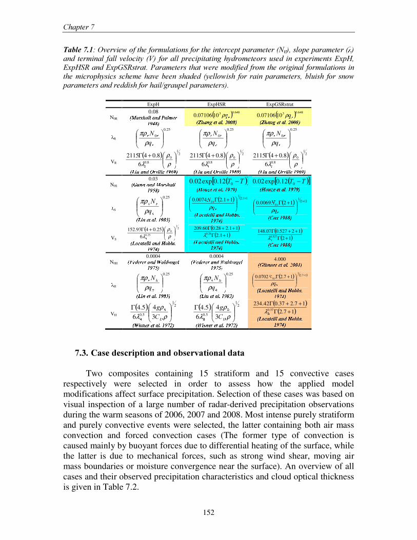
&KDSWHU���
152
7DEOH������2YHUYLHZ�RI�WKH�IRUPXODWLRQV�IRU�WKH�LQWHUFHSW�SDUDPHWHU��1 º ���VORSH�SDUDPHWHU�� ��DQG� WHUPLQDO� IDOO�YHORFLW\� �9�� IRU�DOO�SUHFLSLWDWLQJ�K\GURPHWHRUV�XVHG� LQ�H[SHULPHQWV�([S+��([S+65�DQG�([S*65VWUDW��3DUDPHWHUV�WKDW�ZHUH�PRGLILHG�IURP�WKH�RULJLQDO�IRUPXODWLRQV�LQ�WKH�PLFURSK\VLFV�VFKHPH�KDYH�EHHQ�VKDGHG� �\HOORZLVK� IRU�UDLQ�SDUDPHWHUV��EOXLVK� IRU�VQRZ�SDUDPHWHUV�DQG�UHGGLVK�IRU�KDLO�JUDXSHO�SDUDPHWHUV��
ExpH ExpHSR ExpGSRstrat
N0R 08.0 » ¼¾½À¿�ÁÃÂ(½ÅÄ ÄƽÅÇ(ÈÊÉ˽ÅÄ ÌÎÍÿÏÀÐ´Ñ´Ò Ó ( ) 648.031007106.0 ÔÕρ » ÖËÂ(½ÅÇØ×ÙÍ�ÚƽÀÄ Û´ÜØÝÅÝ Ò�Ó ( ) 648.031007106.0 ÔÕρ » ÖÞÂß½ÅÇØ×ÙÍ�ÚƽÀÄ Û´ÜØÝÅÝ Ò�Ó
R
25.0
0
ààà
T1
ρπρ
25.0
0
ààà
T1
ρπρ
25.0
0
ááá
T1
ρπρ
VR ( ) 2
1
08.06
8.042115
+Γρρ
λ â» ãåä æç½ÅÇ(Èéèê¿ÃëÃä Ä Ä Í ÏÀÐÆìíÐîÓ( ) 2
1
08.06
8.042115
+Γρρ
λ â» ãÞä æÙ½ÅÇßÈéèï¿�ëÃä Ä Ä Í ÏÀÐÆìíÐîÓ
( ) 21
08.06
8.042115
+Γρρ
λ â » ãåä æç½ÅÇ(Èðèï¿îë�ä Ä Ä Í ÏÅÐØìíÐîÓ
N0S 0.03 » ñïæ(ÇÆÇç½ÅÇßÈʼò½À¿�ÁÃÂß½ÀÄ ÄÏÀÐØóÅÒ Ó ( )[ ]77 −012.0exp02.0 » ôçõÅæÆöÃÍêÍ�ÚƽÀÄ Û ÏÀÐø÷îÐîÓ ( )[ ]77 −012.0exp02.0 » ôçõÅæÆö�ÍêÍ�ÚƽÀÄ Û ÏÀÐø÷îÐîÓ
S
25.0
ùùù
T1
ρπρ
» ãåä ÇçÍ�ÚƽÅÄ Û ÏÀдÒÅúîÓ( ) ( )11.2
1
0 11.20074.0 +
+Γûûü
ýρ
» ãËõ´þ�½ÀÚ ÍÃÄ Ä äƽÅÇ(ÈÊôçõÅÿ´ÿíÁ�ÛÏÅÐ ÷îÑîÓ
( ) ( )121
0 120069.0 +
+���
�ρ� ����� ��� ���
VS
( ) 21
025.06
25.0493.152
+Γρρ
λ �
� ������� � �� � ��� ��� ��� !�!#"�$%�'&)(��
( )( )11.2
11.228.060.20928.0 +Γ
++Γ*λ
� ������� � �� � �+� ��� ��� !�!#")$ �,&)()�
( )( )12
12527.007.148527.0 +Γ
++Γ-λ
� ����� ��� ���
N0H 0.0004 � ./��� �10�10�� ���32�� � � 4��#5���%�'&16 7
0.0004 � ./�#� �101�0�� ���328� � ��4�#5���� �,&16 7
4.000 � 9:� � ;��%0)�/���+� � $�<+=�=#()�
H
25.0
>>>
T1
ρπρ
� �?� �3���� � $+%��� @)�
25.0
>>>
T1
ρπρ
� �A� �3���� � $+%��� @)�
( ) ( )17.21
0 17.20702.0 +
+ΓBBC
Dρ
� �A����� � �� � ��� ��� ��� !�!#"�$ �,&)()�
VH ( ) 2
1
5.0 34
65.4
Γρ
ρλ E
FF &
J
�)28� "1�G�0��1��� � $+%�,&1<)�( ) 2
1
5.0 34
65.4
Γρ
ρλ E
FF &
J
��2�� "1�G�10:�1��� � $+%�,&1<)�
( )( )17.2
17.237.042.23437.0 +Γ
++ΓHλ
� �A����� � �� � ��� ��� ��� !�!#"�$ �,&)()�
������&DVH�GHVFULSWLRQ�DQG�REVHUYDWLRQDO�GDWD�
Two composites containing 15 stratiform and 15 convective cases
respectively were selected in order to assess how the applied model modifications affect surface precipitation. Selection of these cases was based on visual inspection of a large number of radar-derived precipitation observations during the warm seasons of 2006, 2007 and 2008. Most intense purely stratiform and purely convective events were selected, the latter containing both air mass convection and forced convection cases (The former type of convection is caused mainly by buoyant forces due to differential heating of the surface, while the latter is due to mechanical forces, such as strong wind shear, moving air mass boundaries or moisture convergence near the surface). An overview of all cases and their observed precipitation characteristics and cloud optical thickness is given in Table 7.2.
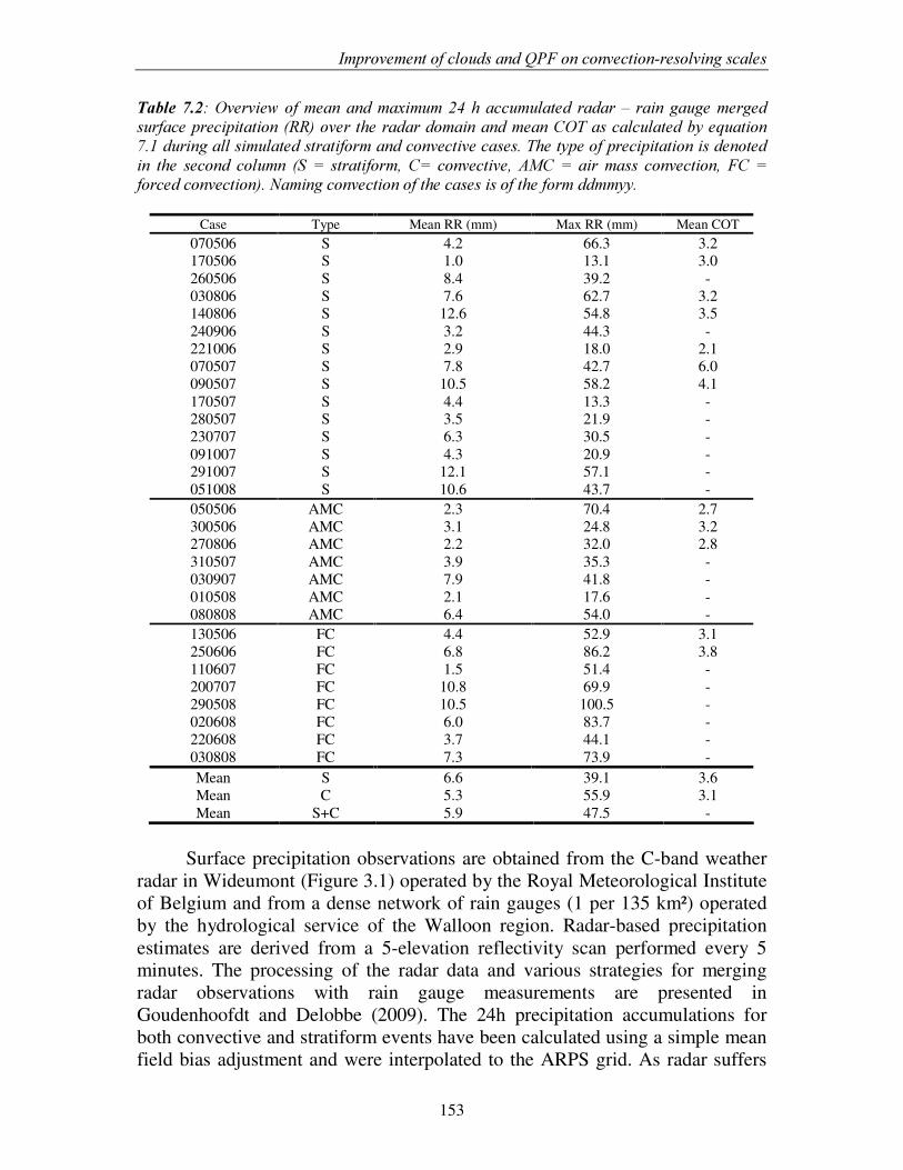
,PSURYHPHQW�RI�FORXGV�DQG�43)�RQ�FRQYHFWLRQ�UHVROYLQJ�VFDOHV�
153
7DEOH������2YHUYLHZ�RI�PHDQ�DQG�PD[LPXP����K�DFFXPXODWHG� UDGDU�±�UDLQ�JDXJH�PHUJHG�VXUIDFH�SUHFLSLWDWLRQ��55��RYHU�WKH�UDGDU�GRPDLQ�DQG�PHDQ�&27�DV�FDOFXODWHG�E\�HTXDWLRQ�����GXULQJ�DOO�VLPXODWHG�VWUDWLIRUP�DQG�FRQYHFWLYH�FDVHV��7KH�W\SH�RI�SUHFLSLWDWLRQ�LV�GHQRWHG�LQ� WKH� VHFRQG� FROXPQ� �6� � VWUDWLIRUP��& � FRQYHFWLYH�� $0&� � DLU�PDVV� FRQYHFWLRQ�� )&� �IRUFHG�FRQYHFWLRQ���1DPLQJ�FRQYHFWLRQ�RI�WKH�FDVHV�LV�RI�WKH�IRUP�GGPP\\��
�Case Type Mean RR (mm) Max RR (mm) Mean COT
070506 S 4.2 66.3 3.2 170506 S 1.0 13.1 3.0 260506 S 8.4 39.2 - 030806 S 7.6 62.7 3.2 140806 S 12.6 54.8 3.5 240906 S 3.2 44.3 - 221006 S 2.9 18.0 2.1 070507 S 7.8 42.7 6.0 090507 S 10.5 58.2 4.1 170507 S 4.4 13.3 - 280507 S 3.5 21.9 - 230707 S 6.3 30.5 - 091007 S 4.3 20.9 - 291007 S 12.1 57.1 - 051008 S 10.6 43.7 - 050506 AMC 2.3 70.4 2.7 300506 AMC 3.1 24.8 3.2 270806 AMC 2.2 32.0 2.8 310507 AMC 3.9 35.3 - 030907 AMC 7.9 41.8 - 010508 AMC 2.1 17.6 - 080808 AMC 6.4 54.0 - 130506 FC 4.4 52.9 3.1 250606 FC 6.8 86.2 3.8 110607 FC 1.5 51.4 - 200707 FC 10.8 69.9 - 290508 FC 10.5 100.5 - 020608 FC 6.0 83.7 - 220608 FC 3.7 44.1 - 030808 FC 7.3 73.9 - Mean S 6.6 39.1 3.6 Mean C 5.3 55.9 3.1 Mean S+C 5.9 47.5 -
Surface precipitation observations are obtained from the C-band weather
radar in Wideumont (Figure 3.1) operated by the Royal Meteorological Institute of Belgium and from a dense network of rain gauges (1 per 135 km²) operated by the hydrological service of the Walloon region. Radar-based precipitation estimates are derived from a 5-elevation reflectivity scan performed every 5 minutes. The processing of the radar data and various strategies for merging radar observations with rain gauge measurements are presented in Goudenhoofdt and Delobbe (2009). The 24h precipitation accumulations for both convective and stratiform events have been calculated using a simple mean field bias adjustment and were interpolated to the ARPS grid. As radar suffers
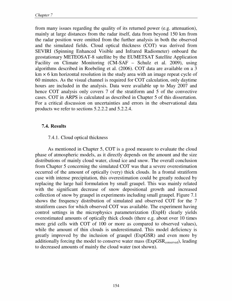
&KDSWHU���
154
from many issues regarding the quality of its returned power (e.g. attenuation), mainly at large distances from the radar itself, data from beyond 150 km from the radar position were omitted from the further analysis in both the observed and the simulated fields. Cloud optical thickness (COT) was derived from SEVIRI (Spinning Enhanced Visible and Infrared Radiometer) onboard the geostationary METEOSAT-8 satellite by the EUMETSAT Satellite Application Facility on Climate Monitoring (CM-SAF – Schulz et al. 2009), using algorithms described in Roebeling et al. (2006). COT data are available on a 3 km × 6 km horizontal resolution in the study area with an image repeat cycle of 60 minutes. As the visual channel is required for COT calculation, only daytime hours are included in the analysis. Data were available up to May 2007 and hence COT analysis only covers 7 of the stratiform and 5 of the convective cases. COT in ARPS is calculated as described in Chapter 5 of this dissertation. For a critical discussion on uncertainties and errors in the observational data products we refer to sections 5.2.2.2 and 5.2.2.4.
������5HVXOWV�
7.4.1. Cloud optical thickness
As mentioned in Chapter 5, COT is a good measure to evaluate the cloud
phase of atmospheric models, as it directly depends on the amount and the size distributions of mainly cloud water, cloud ice and snow. The overall conclusion from Chapter 5 concerning the simulated COT was that a severe overestimation occurred of the amount of optically (very) thick clouds. In a frontal stratiform case with intense precipitation, this overestimation could be greatly reduced by replacing the large hail formulation by small graupel. This was mainly related with the significant decrease of snow depositional growth and increased collection of snow by graupel in experiments including small graupel. Figure 7.1 shows the frequency distribution of simulated and observed COT for the 7 stratiform cases for which observed COT was available. The experiment having control settings in the microphysics parameterization (ExpH) clearly yields overestimated amounts of optically thick clouds (there e.g. about over 10 times more grid cells with COT of 100 or more as compared to observed values), while the amount of thin clouds is underestimated. This model deficiency is greatly improved by the inclusion of graupel (ExpGSR) and even more by additionally forcing the model to conserve water mass (ExpGSRconserved), leading to decreased amounts of mainly the cloud water (not shown).
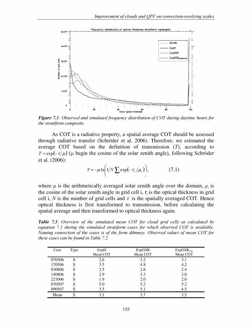
,PSURYHPHQW�RI�FORXGV�DQG�43)�RQ�FRQYHFWLRQ�UHVROYLQJ�VFDOHV�
155
)LJXUH������2EVHUYHG�DQG�VLPXODWHG�IUHTXHQF\�GLVWULEXWLRQ�RI�&27�GXULQJ�GD\WLPH�KRXUV�IRU�WKH�VWUDWLIRUP�FRPSRVLWH�
As COT is a radiative property, a spatial average COT should be assessed through radiative transfer (Schröder et al. 2006). Therefore, we estimated the average COT based on the definition of transmission (7), according to
( )µτ−= exp7 �� �EHJLQ�WKH�FRVLQH�RI�WKH�VRODU�]HQLWK�DQJOH���IROORZLQJ�6FKUöder et al. (2006):
( )
−−= ∑I II1 µτµτ exp1ln , (7.1)
where is the arithmetically averaged solar zenith angle over the domain, i is the cosine of the solar zenith angle in grid cell i, i is the optical thickness in grid cell i, 1 is the number of grid cells and τ is the spatially averaged COT. Hence optical thickness is first transformed to transmission, before calculating the spatial average and then transformed to optical thickness again. 7DEOH� ����� 2YHUYLHZ� RI� WKH� VLPXODWHG� PHDQ� &27� IRU� FORXG� JULG� FHOOV� DV� FDOFXODWHG� E\�HTXDWLRQ� ���� GXULQJ� WKH� VLPXODWHG� VWUDWLIRUP� FDVHV� IRU� ZKLFK� REVHUYHG� &27� LV� DYDLODEOH��1DPLQJ�FRQYHFWLRQ�RI� WKH�FDVHV� LV�RI� WKH� IRUP�GGPP\\��2EVHUYHG�YDOXHV�RI�PHDQ�&27� IRU�WKHVH�FDVHV�FDQ�EH�IRXQG�LQ�7DEOH�����
Case Type ExpH ExpGSR ExpGSRcon Mean COT Mean COT Mean COT
070506 S 2.6 3.2 3.1 170506 S 3.5 4.8 4.2 030806 S 2.5 2.6 2.4 140806 S 2.9 3.3 3.0 221006 S 1.9 2.0 2.0 070507 S 5.0 5.2 5.2 090507 S 3.5 5.1 4.5 Mean S 3.1 3.7 3.5
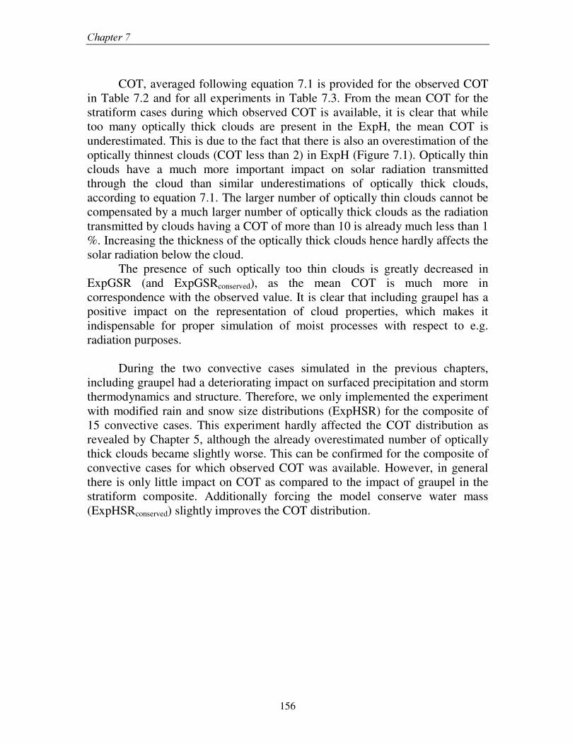
&KDSWHU���
156
COT, averaged following equation 7.1 is provided for the observed COT
in Table 7.2 and for all experiments in Table 7.3. From the mean COT for the stratiform cases during which observed COT is available, it is clear that while too many optically thick clouds are present in the ExpH, the mean COT is underestimated. This is due to the fact that there is also an overestimation of the optically thinnest clouds (COT less than 2) in ExpH (Figure 7.1). Optically thin clouds have a much more important impact on solar radiation transmitted through the cloud than similar underestimations of optically thick clouds, according to equation 7.1. The larger number of optically thin clouds cannot be compensated by a much larger number of optically thick clouds as the radiation transmitted by clouds having a COT of more than 10 is already much less than 1 %. Increasing the thickness of the optically thick clouds hence hardly affects the solar radiation below the cloud.
The presence of such optically too thin clouds is greatly decreased in ExpGSR (and ExpGSRconserved), as the mean COT is much more in correspondence with the observed value. It is clear that including graupel has a positive impact on the representation of cloud properties, which makes it indispensable for proper simulation of moist processes with respect to e.g. radiation purposes.
During the two convective cases simulated in the previous chapters, including graupel had a deteriorating impact on surfaced precipitation and storm thermodynamics and structure. Therefore, we only implemented the experiment with modified rain and snow size distributions (ExpHSR) for the composite of 15 convective cases. This experiment hardly affected the COT distribution as revealed by Chapter 5, although the already overestimated number of optically thick clouds became slightly worse. This can be confirmed for the composite of convective cases for which observed COT was available. However, in general there is only little impact on COT as compared to the impact of graupel in the stratiform composite. Additionally forcing the model conserve water mass (ExpHSRconserved) slightly improves the COT distribution.
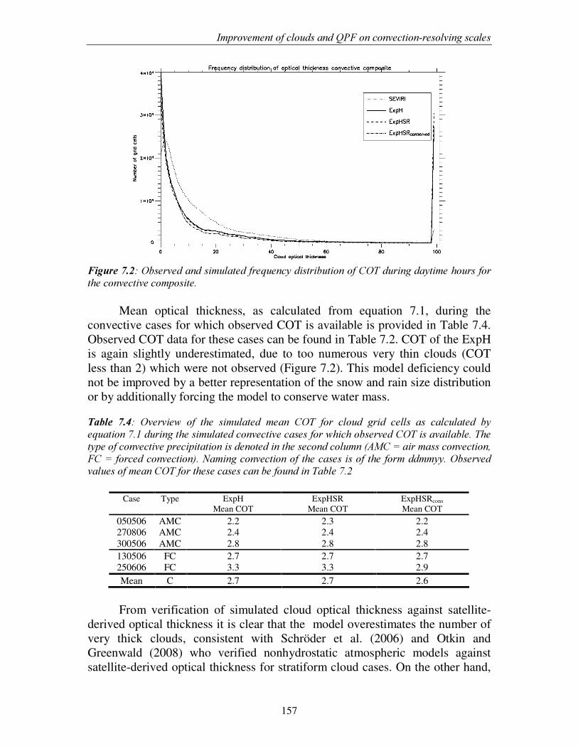
,PSURYHPHQW�RI�FORXGV�DQG�43)�RQ�FRQYHFWLRQ�UHVROYLQJ�VFDOHV�
157
)LJXUH������2EVHUYHG�DQG�VLPXODWHG�IUHTXHQF\�GLVWULEXWLRQ�RI�&27�GXULQJ�GD\WLPH�KRXUV�IRU�WKH�FRQYHFWLYH�FRPSRVLWH�
Mean optical thickness, as calculated from equation 7.1, during the convective cases for which observed COT is available is provided in Table 7.4. Observed COT data for these cases can be found in Table 7.2. COT of the ExpH is again slightly underestimated, due to too numerous very thin clouds (COT less than 2) which were not observed (Figure 7.2). This model deficiency could not be improved by a better representation of the snow and rain size distribution or by additionally forcing the model to conserve water mass. �7DEOH� ����� 2YHUYLHZ� RI� WKH� VLPXODWHG� PHDQ� &27� IRU� FORXG� JULG� FHOOV� DV� FDOFXODWHG� E\�HTXDWLRQ�����GXULQJ�WKH�VLPXODWHG�FRQYHFWLYH�FDVHV�IRU�ZKLFK�REVHUYHG�&27�LV�DYDLODEOH��7KH�W\SH�RI�FRQYHFWLYH�SUHFLSLWDWLRQ�LV�GHQRWHG�LQ�WKH�VHFRQG�FROXPQ��$0&� �DLU�PDVV�FRQYHFWLRQ��)&� �IRUFHG�FRQYHFWLRQ���1DPLQJ�FRQYHFWLRQ�RI�WKH�FDVHV�LV�RI�WKH�IRUP�GGPP\\��2EVHUYHG�YDOXHV�RI�PHDQ�&27�IRU�WKHVH�FDVHV�FDQ�EH�IRXQG�LQ�7DEOH�����
Case Type ExpH ExpHSR ExpHSRcons Mean COT Mean COT Mean COT
050506 AMC 2.2 2.3 2.2 270806 AMC 2.4 2.4 2.4 300506 AMC 2.8 2.8 2.8 130506 FC 2.7 2.7 2.7 250606 FC 3.3 3.3 2.9 Mean C 2.7 2.7 2.6
From verification of simulated cloud optical thickness against satellite-
derived optical thickness it is clear that the model overestimates the number of very thick clouds, consistent with Schröder et al. (2006) and Otkin and Greenwald (2008) who verified nonhydrostatic atmospheric models against satellite-derived optical thickness for stratiform cloud cases. On the other hand,
&KDSWHU���
158
as also more numerous thin clouds are simulated, too much solar radiation reaches the surface. Including graupel in stratiform cases improves both the occurrence of excessively thick clouds and the averaged COT values. Hence, including graupel in model microphysics parameterizations has potential to improve the representation of moist processes and the surface radiative forcing in atmospheric models.
7.4.2. Surface precipitation
7.4.2.1. Traditional verification scores
First, traditional verification scores will be used to evaluate the surface precipitation characteristics in both composites and during all experiments. Table 7.5 provides an overview of mean and maximum 24 hour accumulated surface precipitation all experiments and Table 7.2 contains observed precipitation estimates as derived from combining radar and rain gauge information. Colour shading in Table 7.5 indicates the deviation from the observations and hence it is clear that precipitation overestimation prevails throughout most of the cases and all experiments. This is also clear from the precipitation bias, which is the mean of the differences between the model and respective observations at each grid point (Table 7.6) and which is positive in all experiments and for both composites. Table 7.6 also provides the Root Mean Square Error (RMSE), defined as the square root of the mean square differences between the model and respective observations at each grid point. The lower the RMSE, the more accurate the simulation is. Due to the square of the difference in the RMSE, it is much more sensitive to large model errors as compared to the bias. The bias and RMSE are significantly larger in the convective composite as compared the stratiform composite.
From Table 7.5 and Table 7.6 it is clear that none of the experiments performed completely removes the positive precipitation bias. In the stratiform composite, precipitation bias actually deteriorates by experiment ExpGSR, although the maximum precipitation amounts are somewhat better represented. In ExpGSRconserved precipitation bias is strongly improved. RMSE is also decreased, but to a lesser extent while maximum precipitation accumulation is brought close the observations. During convective events, there is no clear difference in the mean precipitation accumulation between the ExpH and the ExpHSR, although bias and RMSE are somewhat improved in ExpHSR. This is mainly due to a better representation of the maximum precipitation amounts. Significant improvement in the mean surface precipitation is found in ExpHSRconserved, mainly during the forced convection experiments.
�
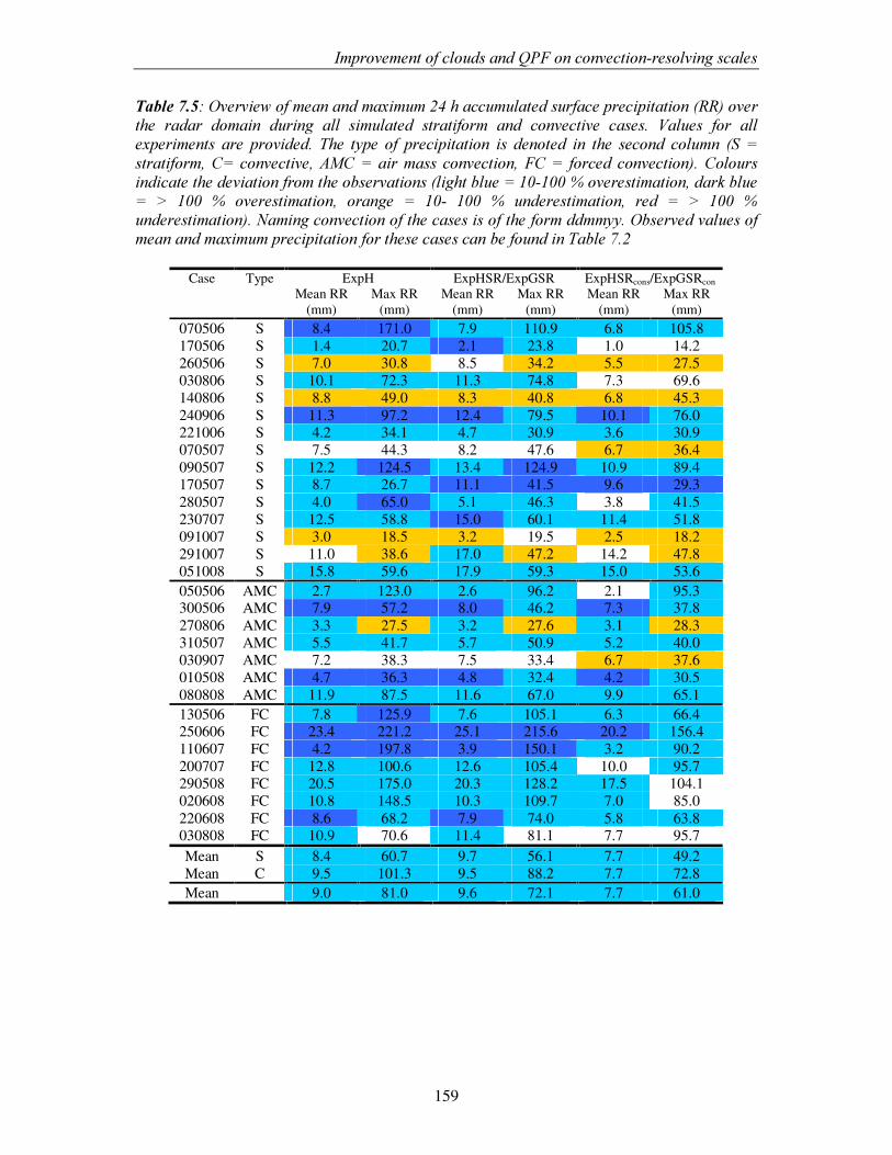
,PSURYHPHQW�RI�FORXGV�DQG�43)�RQ�FRQYHFWLRQ�UHVROYLQJ�VFDOHV�
159
7DEOH������2YHUYLHZ�RI�PHDQ�DQG�PD[LPXP����K�DFFXPXODWHG�VXUIDFH�SUHFLSLWDWLRQ��55��RYHU�WKH� UDGDU� GRPDLQ� GXULQJ� DOO� VLPXODWHG� VWUDWLIRUP� DQG� FRQYHFWLYH� FDVHV�� 9DOXHV� IRU� DOO�H[SHULPHQWV� DUH� SURYLGHG�� 7KH� W\SH� RI� SUHFLSLWDWLRQ� LV� GHQRWHG� LQ� WKH� VHFRQG� FROXPQ� �6� �VWUDWLIRUP��& �FRQYHFWLYH��$0&� �DLU�PDVV� FRQYHFWLRQ��)&� � IRUFHG�FRQYHFWLRQ���&RORXUV�LQGLFDWH�WKH�GHYLDWLRQ�IURP�WKH�REVHUYDWLRQV��OLJKW�EOXH� ����������RYHUHVWLPDWLRQ��GDUN�EOXH� � !� ���� �� RYHUHVWLPDWLRQ�� RUDQJH� � ���� ���� �� XQGHUHVWLPDWLRQ�� UHG� � !� ���� ��XQGHUHVWLPDWLRQ���1DPLQJ�FRQYHFWLRQ�RI�WKH�FDVHV�LV�RI�WKH�IRUP�GGPP\\��2EVHUYHG�YDOXHV�RI�PHDQ�DQG�PD[LPXP�SUHFLSLWDWLRQ�IRU�WKHVH�FDVHV�FDQ�EH�IRXQG�LQ�7DEOH������
Case Type ExpH ExpHSR/ExpGSR ExpHSRcons/ExpGSRcon Mean RR
(mm) Max RR
(mm) Mean RR
(mm) Max RR
(mm) Mean RR
(mm) Max RR
(mm) 070506 S 8.4 171.0 7.9 110.9 6.8 105.8 170506 S 1.4 20.7 2.1 23.8 1.0 14.2 260506 S 7.0 30.8 8.5 34.2 5.5 27.5 030806 S 10.1 72.3 11.3 74.8 7.3 69.6 140806 S 8.8 49.0 8.3 40.8 6.8 45.3 240906 S 11.3 97.2 12.4 79.5 10.1 76.0 221006 S 4.2 34.1 4.7 30.9 3.6 30.9 070507 S 7.5 44.3 8.2 47.6 6.7 36.4 090507 S 12.2 124.5 13.4 124.9 10.9 89.4 170507 S 8.7 26.7 11.1 41.5 9.6 29.3 280507 S 4.0 65.0 5.1 46.3 3.8 41.5 230707 S 12.5 58.8 15.0 60.1 11.4 51.8 091007 S 3.0 18.5 3.2 19.5 2.5 18.2 291007 S 11.0 38.6 17.0 47.2 14.2 47.8 051008 S 15.8 59.6 17.9 59.3 15.0 53.6 050506 AMC 2.7 123.0 2.6 96.2 2.1 95.3 300506 AMC 7.9 57.2 8.0 46.2 7.3 37.8 270806 AMC 3.3 27.5 3.2 27.6 3.1 28.3 310507 AMC 5.5 41.7 5.7 50.9 5.2 40.0 030907 AMC 7.2 38.3 7.5 33.4 6.7 37.6 010508 AMC 4.7 36.3 4.8 32.4 4.2 30.5 080808 AMC 11.9 87.5 11.6 67.0 9.9 65.1 130506 FC 7.8 125.9 7.6 105.1 6.3 66.4 250606 FC 23.4 221.2 25.1 215.6 20.2 156.4 110607 FC 4.2 197.8 3.9 150.1 3.2 90.2 200707 FC 12.8 100.6 12.6 105.4 10.0 95.7 290508 FC 20.5 175.0 20.3 128.2 17.5 104.1 020608 FC 10.8 148.5 10.3 109.7 7.0 85.0 220608 FC 8.6 68.2 7.9 74.0 5.8 63.8 030808 FC 10.9 70.6 11.4 81.1 7.7 95.7 Mean S 8.4 60.7 9.7 56.1 7.7 49.2 Mean C 9.5 101.3 9.5 88.2 7.7 72.8 Mean 9.0 81.0 9.6 72.1 7.7 61.0
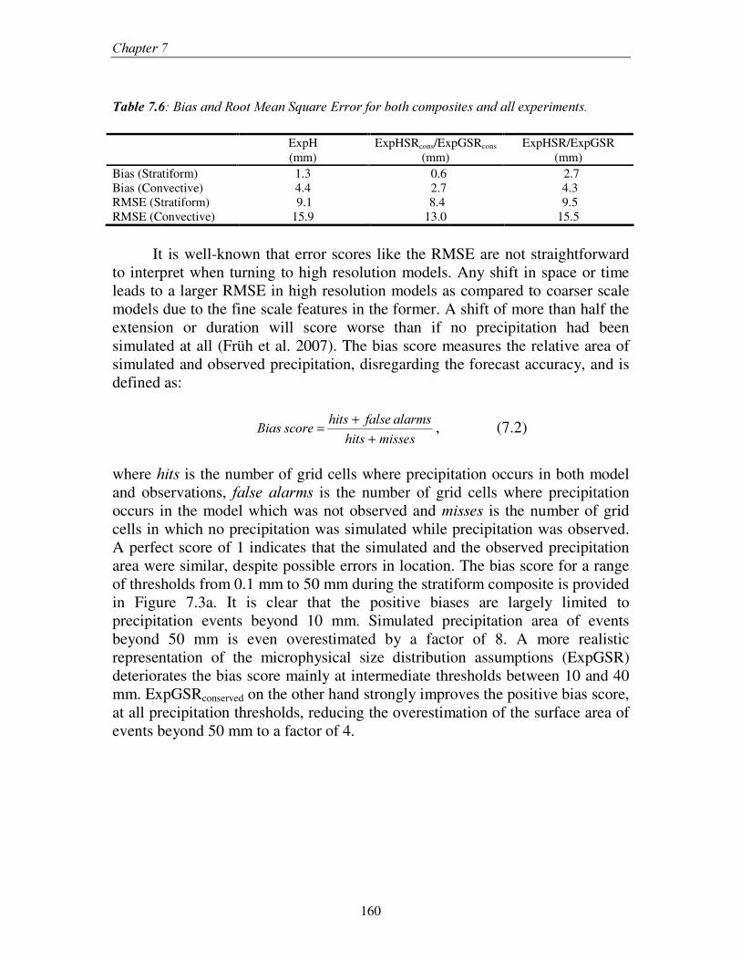
&KDSWHU���
160
7DEOH������%LDV�DQG�5RRW�0HDQ�6TXDUH�(UURU�IRU�ERWK�FRPSRVLWHV�DQG�DOO�H[SHULPHQWV��
ExpH (mm)
ExpHSRcons/ExpGSRcons
(mm) ExpHSR/ExpGSR
(mm) Bias (Stratiform) 1.3 0.6 2.7 Bias (Convective) 4.4 2.7 4.3 RMSE (Stratiform) 9.1 8.4 9.5 RMSE (Convective) 15.9 13.0 15.5
It is well-known that error scores like the RMSE are not straightforward
to interpret when turning to high resolution models. Any shift in space or time leads to a larger RMSE in high resolution models as compared to coarser scale models due to the fine scale features in the former. A shift of more than half the extension or duration will score worse than if no precipitation had been simulated at all (Früh et al. 2007). The bias score measures the relative area of simulated and observed precipitation, disregarding the forecast accuracy, and is defined as:
PLVVHVKLWVDODUPVIDOVHKLWVVFRUH%LDV
++= , (7.2)
where KLWV is the number of grid cells where precipitation occurs in both model and observations, IDOVH� DODUPV is the number of grid cells where precipitation occurs in the model which was not observed and PLVVHV is the number of grid cells in which no precipitation was simulated while precipitation was observed. A perfect score of 1 indicates that the simulated and the observed precipitation area were similar, despite possible errors in location. The bias score for a range of thresholds from 0.1 mm to 50 mm during the stratiform composite is provided in Figure 7.3a. It is clear that the positive biases are largely limited to precipitation events beyond 10 mm. Simulated precipitation area of events beyond 50 mm is even overestimated by a factor of 8. A more realistic representation of the microphysical size distribution assumptions (ExpGSR) deteriorates the bias score mainly at intermediate thresholds between 10 and 40 mm. ExpGSRconserved on the other hand strongly improves the positive bias score, at all precipitation thresholds, reducing the overestimation of the surface area of events beyond 50 mm to a factor of 4.
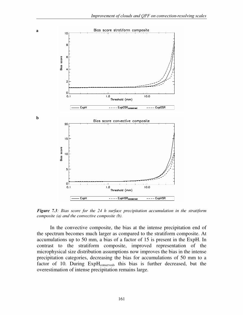
,PSURYHPHQW�RI�FORXGV�DQG�43)�RQ�FRQYHFWLRQ�UHVROYLQJ�VFDOHV�
161
)LJXUH� ����� %LDV� VFRUH� IRU� WKH� ��� K� VXUIDFH� SUHFLSLWDWLRQ� DFFXPXODWLRQ� LQ� WKH� VWUDWLIRUP�FRPSRVLWH��D��DQG�WKH�FRQYHFWLYH�FRPSRVLWH��E��
In the convective composite, the bias at the intense precipitation end of the spectrum becomes much larger as compared to the stratiform composite. At accumulations up to 50 mm, a bias of a factor of 15 is present in the ExpH. In contrast to the stratiform composite, improved representation of the microphysical size distribution assumptions now improves the bias in the intense precipitation categories, decreasing the bias for accumulations of 50 mm to a factor of 10. During ExpHconserved, this bias is further decreased, but the overestimation of intense precipitation remains large.
D�
E�
&KDSWHU���
162
7.4.2.2. SAL
Most traditional verification scores typically overly penalize the mislocation of precipitation events (Ebert and Mcbride 2000). Whether an event is simulated at a significant distance or in the neighbouring grid cell makes no difference in scores like the RMSE. Furthermore, high resolution convection resolving simulations are capable of producing individual storm systems with fine-scale structure and strong gradients, which are not rated by any of the previous verification measures. Therefore, a novel object-based verification score, SAL (Wernli et al. 2008), was applied which can discriminate between errors due to structure, amplitude and location in the precipitation field. The amplitude component A measures the relative deviation of the domain-averaged simulated precipitation from the observations. Positive values of A indicate an overestimation of total precipitation, whereas negative values indicate an underestimation. For the S and L components, coherent observation objects are separately identified in the simulation and the observations. The location component L combines information about the displacement of the simulated precipitation field’ s centre of mass and about the error in the weighted-average distance of the precipitation objects from the total field’ s centre of mass. The structure component S is constructed in such a way that positive values occur if precipitation objects are too large and/ or too flat, and negative values occur if the objects are too small and /or too peaked. The values of S and A components are within [-2 ,2 ] and of the L component within [0, 2 ], a zero value yielding a perfect forecast. As the quality of the radar observations deteriorates with distance by e.g. attenuation effects, SAL analysis was performed for the region within a radius of 150 km from the radar location only. A thorough description of SAL is provided in Appendix C of this dissertation.
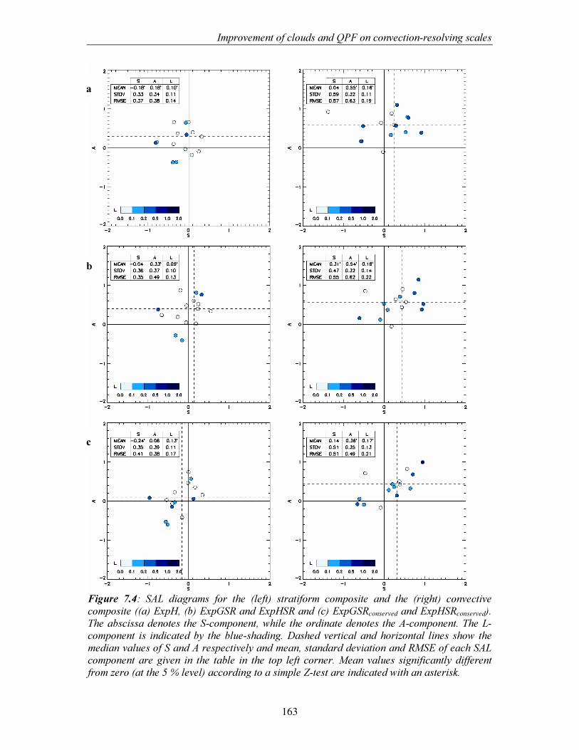
,PSURYHPHQW�RI�FORXGV�DQG�43)�RQ�FRQYHFWLRQ�UHVROYLQJ�VFDOHV�
163
)LJXUH� ����� 6$/� GLDJUDPV� IRU� WKH� �OHIW�� VWUDWLIRUP� FRPSRVLWH� DQG� WKH� �ULJKW�� FRQYHFWLYH�FRPSRVLWH���D��([S+���E��([S*65�DQG�([S+65�DQG��F��([S*65conserved�DQG�([S+65conserved���7KH�DEVFLVVD�GHQRWHV�WKH�6�FRPSRQHQW��ZKLOH�WKH�RUGLQDWH�GHQRWHV�WKH�$�FRPSRQHQW��7KH�/�FRPSRQHQW� LV� LQGLFDWHG�E\� WKH�EOXH�VKDGLQJ��'DVKHG�YHUWLFDO�DQG�KRUL]RQWDO� OLQHV� VKRZ� WKH�PHGLDQ�YDOXHV�RI�6�DQG�$�UHVSHFWLYHO\�DQG�PHDQ��VWDQGDUG�GHYLDWLRQ�DQG�506(�RI�HDFK�6$/�FRPSRQHQW�DUH� JLYHQ� LQ� WKH� WDEOH� LQ� WKH� WRS� OHIW� FRUQHU��0HDQ�YDOXHV� VLJQLILFDQWO\� GLIIHUHQW�IURP�]HUR��DW�WKH�����OHYHO��DFFRUGLQJ�WR�D�VLPSOH�=�WHVW�DUH�LQGLFDWHG�ZLWK�DQ�DVWHULVN��
D�
E�
F�
&KDSWHU���
164
�SAL diagrams, relating S, A and L components as proposed by Wernli et
al. (2008) were constructed for the stratiform and convective composites and for all experiments separately (Figure 7.4). In Figure 7.4 also a number of statistical measures on each of the components are provided. Asterisks denote whether the mean of a SAL-component is significantly different from zero or not (at the 5 % significance level), based on a simple Z-test. In the stratiform composite, the structure (S) component is slightly below zero in ExpH and ExpGSRconserved and hence precipitation fields tend to be somewhat too peaked or too small. Due to a decreased peak precipitation while intermediate precipitation values are increased, S-component in the ExpGSR is improved (Table 7.5 and Figure 7.3). The amplitude (A) component is always positive, but becomes close to zero during the ExpGSRconserved, while it is largest in ExpGSR. Precise location (L-component) is not much affected by any of the modifications applied.
Deviations from a perfect forecast (values of zero for all components) are larger in the convective composite (Figure 7.4). Precipitation overestimation (A) is largest in ExpH, but only slightly lower in ExpHSR. ExpHSRconserved again yields the best score of the A-component. The model also tends to produce too widespread precipitation or too large storms, reflected in positive S-components. This component is only significantly different from zero in the ExpHSR however. Again, the location of storms is highly unaffected by any of the modifications made in the convective composite, but is generally represented quite properly.
7.4.2.3. Comparison against 9 km experiments
The question arises which aspects of the quantitative precipitation forecast actually gain from turning to higher resolution models allowing the explicit representation of convection. Therefore, we repeated part of the above analysis for the coarse resolution (9 km) experiments. To do so, radar – rain gauge merged imagery was aggregated to the 9 km grid and precipitation estimates were compared for the same region as for the 3 km experiments discussed earlier. Comparing the bias score in the stratiform composite for the 9 km experiments (Figure 7.5a) and the 3 km experiments (Figure 7.3a) reveals that the positive precipitation bias disappears when going to coarser resolution. At precipitation accumulations of over 30 mm, even a significant underestimation occurs in the model. The model hence is not capable of reproducing the most intensive precipitation events at a horizontal spatial resolution of 9 km, while a significant overestimation occurs in the 3 km experiments.
In the convective composite, the precipitation bias is strongly improved in the coarse resolution experiments (Figure 7.5b). Overestimation of the precipitation bin of 50 mm is twice as low as in the 3 km experiments. It is
,PSURYHPHQW�RI�FORXGV�DQG�43)�RQ�FRQYHFWLRQ�UHVROYLQJ�VFDOHV�
165
furthermore remarkable that differences between the implemented experiments become smaller when turning to coarser resolution. The impact of adding artificial water to the model in order to get rid of the negative mixing ratios is much smaller at coarse resolution. Indeed, inaccuracies in the advection scheme leading to these negative mixing ratios occur mainly near strong gradients, which are typical for high-resolution simulations. Hence, as far as the precipitation amount is concerned and using traditional verification scores, little gain is found in turning to convection resolving scales. This confirms earlier studies such as Weisman et al. (2008), indicating that traditional verification scores usually perform better at coarse resolutions as compared to convection resolving scales.
However, SAL is designed specifically to evaluate high resolution precipitation simulations, avoiding the drawbacks of traditional scores mentioned earlier. Hence, SAL analysis was repeated for the 9 km experiments for both the stratiform and convective composite. SAL – diagrams for these coarse scale experiments are provided in Figure 7.6. It is clear that the A-component in the stratiform composite now indicates an underestimation of surface precipitation in all experiments, although this underestimation is only significant in the ExpGSRconserved. As could be expected form large scale models, not representing fine-scale structure, S-components become larger in all experiments when turning to coarser resolution, yielding good scores of the S-components in all experiments. L-components are not much affected by the resolution.
During the convective precipitation events, it is clear that the gain of higher resolution is non-existent when the A-component is considered. The surface precipitation overestimation is clearly lower in the coarse-scale experiments as can be derived from mean A-components and the RMSE. A significant overestimation only remains in the ExpHSR. On the other hand, the coarse scale model is having definite difficulties in representing the fine-scale structure of the storms, resulting in high S-component values. Precipitation tends to be too widespread instead of simulating small individual storms in all experiments. Precise location of the storm systems is not much affected by the higher resolution, indicating that the mislocation of big storms systems is often related to inaccuracies in the large-scale environment. This analysis suggests that the gain of turning to explicit convection permitting scales is mainly in a better representation of storm structure, rather than improved integrated precipitation quantities. While the representation of the size distribution assumptions in the microphysics parameterization does not have a large effect on the overestimation of precipitation, forcing the model to conserve water when dealing with negative mixing ratios originating from the finite difference representation of the advection process clearly improves domain average precipitation estimates when turning to explicit convection.
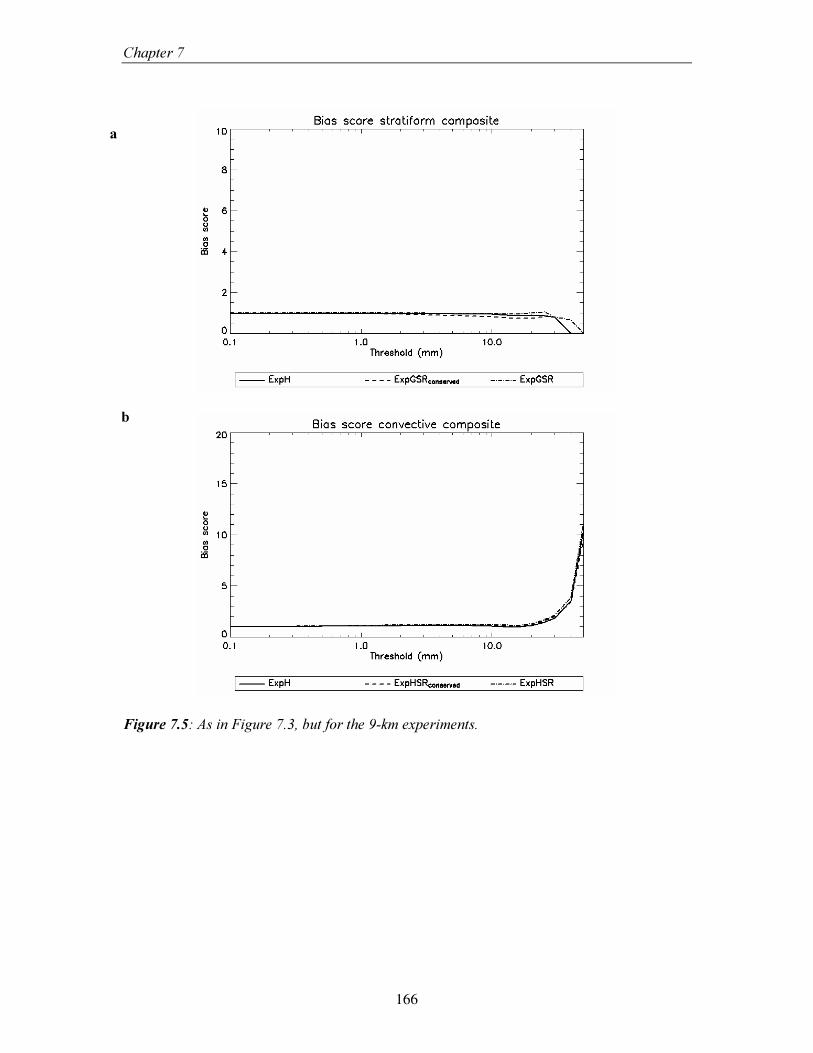
&KDSWHU���
166
)LJXUH������$V�LQ�)LJXUH������EXW�IRU�WKH���NP�H[SHULPHQWV�
D�
E�
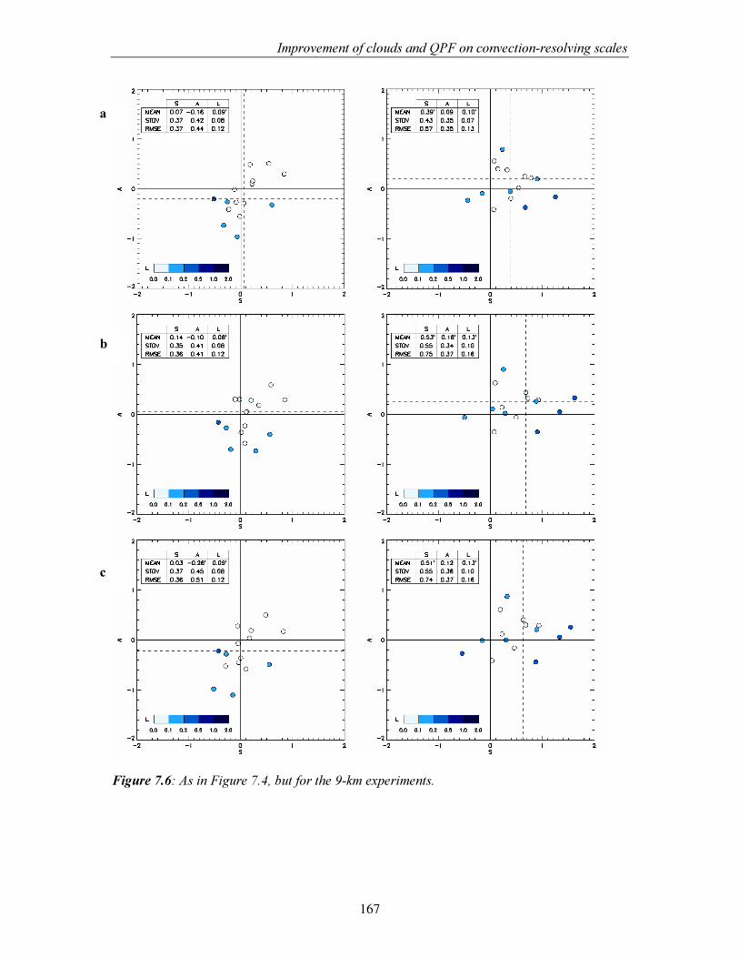
,PSURYHPHQW�RI�FORXGV�DQG�43)�RQ�FRQYHFWLRQ�UHVROYLQJ�VFDOHV�
167
�)LJXUH������$V�LQ�)LJXUH������EXW�IRU�WKH���NP�H[SHULPHQWV�
D�
E�
F�
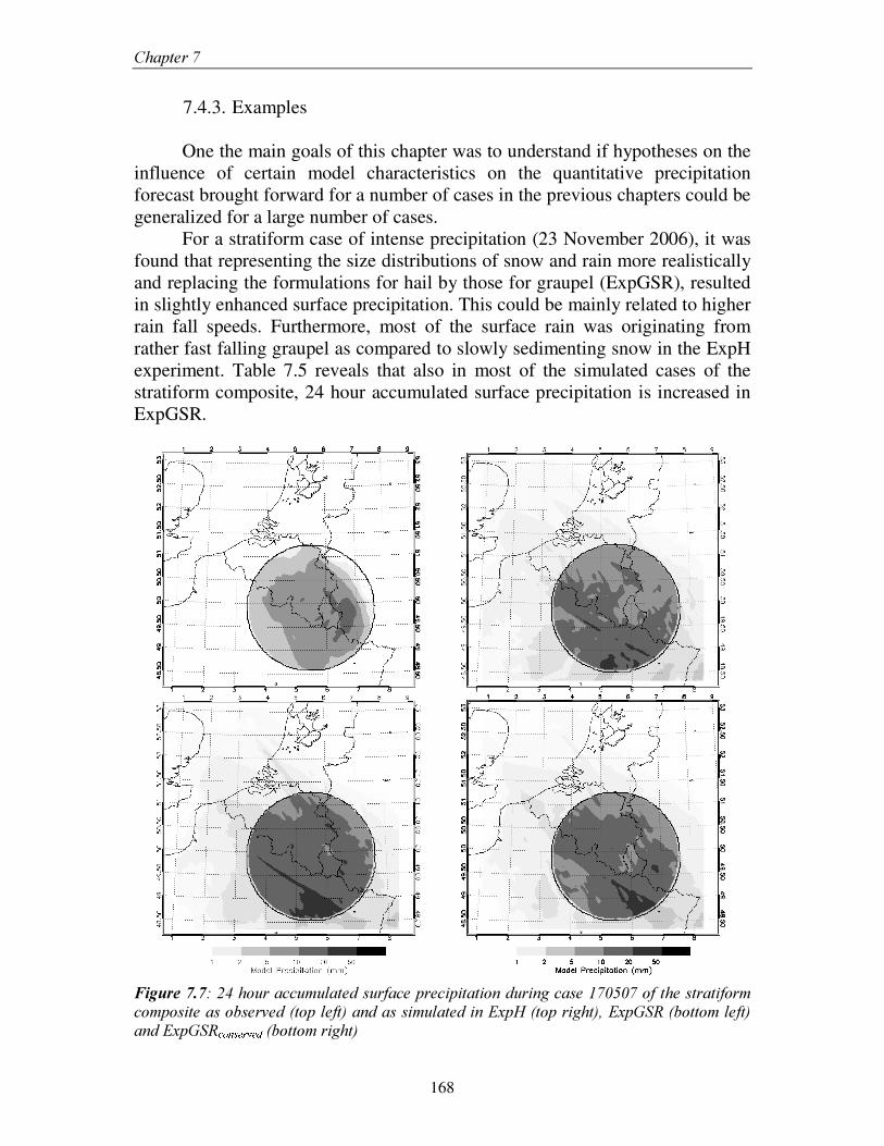
&KDSWHU���
168
7.4.3. Examples
One the main goals of this chapter was to understand if hypotheses on the influence of certain model characteristics on the quantitative precipitation forecast brought forward for a number of cases in the previous chapters could be generalized for a large number of cases.
For a stratiform case of intense precipitation (23 November 2006), it was found that representing the size distributions of snow and rain more realistically and replacing the formulations for hail by those for graupel (ExpGSR), resulted in slightly enhanced surface precipitation. This could be mainly related to higher rain fall speeds. Furthermore, most of the surface rain was originating from rather fast falling graupel as compared to slowly sedimenting snow in the ExpH experiment. Table 7.5 reveals that also in most of the simulated cases of the stratiform composite, 24 hour accumulated surface precipitation is increased in ExpGSR.
)LJXUH���������KRXU�DFFXPXODWHG�VXUIDFH�SUHFLSLWDWLRQ�GXULQJ�FDVH��������RI�WKH�VWUDWLIRUP�FRPSRVLWH�DV�REVHUYHG��WRS�OHIW��DQG�DV�VLPXODWHG�LQ�([S+��WRS�ULJKW���([S*65��ERWWRP�OHIW��DQG�([S*65 J�K%L MN1O)P#N1Q ��ERWWRP�ULJKW��
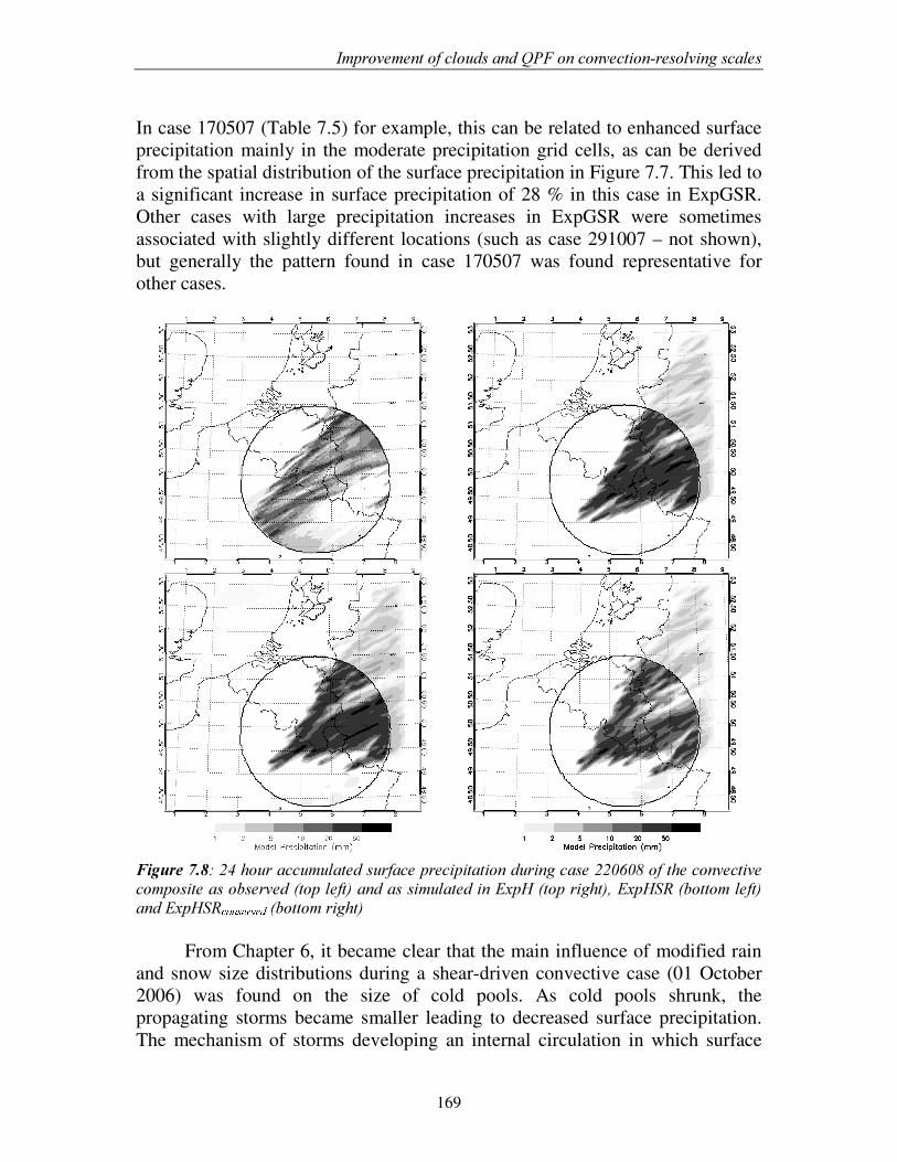
,PSURYHPHQW�RI�FORXGV�DQG�43)�RQ�FRQYHFWLRQ�UHVROYLQJ�VFDOHV�
169
�In case 170507 (Table 7.5) for example, this can be related to enhanced surface precipitation mainly in the moderate precipitation grid cells, as can be derived from the spatial distribution of the surface precipitation in Figure 7.7. This led to a significant increase in surface precipitation of 28 % in this case in ExpGSR. Other cases with large precipitation increases in ExpGSR were sometimes associated with slightly different locations (such as case 291007 – not shown), but generally the pattern found in case 170507 was found representative for other cases.
)LJXUH���������KRXU�DFFXPXODWHG�VXUIDFH�SUHFLSLWDWLRQ�GXULQJ�FDVH��������RI�WKH�FRQYHFWLYH�FRPSRVLWH�DV�REVHUYHG��WRS�OHIW��DQG�DV�VLPXODWHG�LQ�([S+��WRS�ULJKW���([S+65��ERWWRP�OHIW��DQG�([S+65 J�K%L MN1O)P#N1Q ��ERWWRP�ULJKW���
From Chapter 6, it became clear that the main influence of modified rain and snow size distributions during a shear-driven convective case (01 October 2006) was found on the size of cold pools. As cold pools shrunk, the propagating storms became smaller leading to decreased surface precipitation. The mechanism of storms developing an internal circulation in which surface
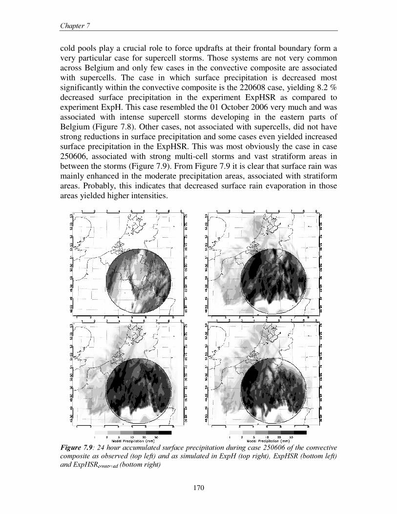
&KDSWHU���
170
cold pools play a crucial role to force updrafts at their frontal boundary form a very particular case for supercell storms. Those systems are not very common across Belgium and only few cases in the convective composite are associated with supercells. The case in which surface precipitation is decreased most significantly within the convective composite is the 220608 case, yielding 8.2 % decreased surface precipitation in the experiment ExpHSR as compared to experiment ExpH. This case resembled the 01 October 2006 very much and was associated with intense supercell storms developing in the eastern parts of Belgium (Figure 7.8). Other cases, not associated with supercells, did not have strong reductions in surface precipitation and some cases even yielded increased surface precipitation in the ExpHSR. This was most obviously the case in case 250606, associated with strong multi-cell storms and vast stratiform areas in between the storms (Figure 7.9). From Figure 7.9 it is clear that surface rain was mainly enhanced in the moderate precipitation areas, associated with stratiform areas. Probably, this indicates that decreased surface rain evaporation in those areas yielded higher intensities. �
�)LJXUH���������KRXU�DFFXPXODWHG�VXUIDFH�SUHFLSLWDWLRQ�GXULQJ�FDVH��������RI�WKH�FRQYHFWLYH�FRPSRVLWH�DV�REVHUYHG��WRS�OHIW��DQG�DV�VLPXODWHG�LQ�([S+��WRS�ULJKW���([S+65��ERWWRP�OHIW��DQG�([S+65 J�K%L MN1O)P#N1Q ��ERWWRP�ULJKW��
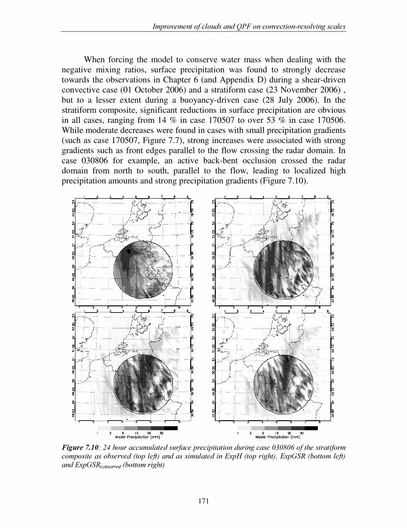
,PSURYHPHQW�RI�FORXGV�DQG�43)�RQ�FRQYHFWLRQ�UHVROYLQJ�VFDOHV�
171
�When forcing the model to conserve water mass when dealing with the
negative mixing ratios, surface precipitation was found to strongly decrease towards the observations in Chapter 6 (and Appendix D) during a shear-driven convective case (01 October 2006) and a stratiform case (23 November 2006) , but to a lesser extent during a buoyancy-driven case (28 July 2006). In the stratiform composite, significant reductions in surface precipitation are obvious in all cases, ranging from 14 % in case 170507 to over 53 % in case 170506. While moderate decreases were found in cases with small precipitation gradients (such as case 170507, Figure 7.7), strong increases were associated with strong gradients such as front edges parallel to the flow crossing the radar domain. In case 030806 for example, an active back-bent occlusion crossed the radar domain from north to south, parallel to the flow, leading to localized high precipitation amounts and strong precipitation gradients (Figure 7.10).
�)LJXUH����������KRXU�DFFXPXODWHG�VXUIDFH�SUHFLSLWDWLRQ�GXULQJ�FDVH��������RI�WKH�VWUDWLIRUP�FRPSRVLWH�DV�REVHUYHG��WRS�OHIW��DQG�DV�VLPXODWHG�LQ�([S+��WRS�ULJKW���([S*65��ERWWRP�OHIW��DQG�([S*65 J�K%L MN1O)P#N1Q ��ERWWRP�ULJKW���
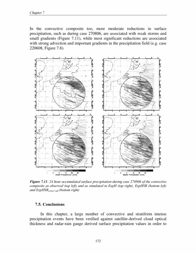
&KDSWHU���
172
�In the convective composite too, more moderate reductions in surface precipitation, such as during case 270806, are associated with weak storms and small gradients (Figure 7.11), while most significant reductions are associated with strong advection and important gradients in the precipitation field (e.g. case 220608, Figure 7.8). �
�)LJXUH����������KRXU�DFFXPXODWHG�VXUIDFH�SUHFLSLWDWLRQ�GXULQJ�FDVH��������RI�WKH�FRQYHFWLYH�FRPSRVLWH�DV�REVHUYHG��WRS�OHIW��DQG�DV�VLPXODWHG�LQ�([S+��WRS�ULJKW���([S+65��ERWWRP�OHIW��DQG�([S+65 J�K%L MN1O)P#N1Q ��ERWWRP�ULJKW��
��������&RQFOXVLRQV��
In this chapter, a large number of convective and stratiform intense
precipitation events have been verified against satellite-derived cloud optical thickness and radar-rain gauge derived surface precipitation values in order to
,PSURYHPHQW�RI�FORXGV�DQG�43)�RQ�FRQYHFWLRQ�UHVROYLQJ�VFDOHV�
173
assess if hypotheses derived for the case studies performed in the previous chapters still hold for other intense precipitation events.
We revealed that adding graupel to stratiform precipitation events greatly improves both the cloud optical thickness distribution and the mean transmission of solar radiation through the clouds and hence yields a better representation of the moist processes and the surface solar radiation forcing. It should be mentioned that many more mutual interactions between microphysics and radiation effects exist, which have not been subject of this study. Latent heat release associated with microphysical processes could affect cloud top cooling by infrared radiation emission or entrainment of dry air above a stratiform cloud. It would be worthwhile to investigate such interactions for our sensitivity experiments in future studies. Surface precipitation estimates could only be improved by this modification when it went together with a method to conserve water mass when negative mixing ratios were zeroed. If not, the positive surface precipitation bias was deteriorated.
In the convective composite, no clear influence was found of modifying the rain and snow size distribution characteristics on cloud optical thickness. Too many very thick clouds and very thin clouds were simulated, resulting in underestimated spatially average cloud optical thickness and leading to too much solar radiation reaching the surface underneath clouds. The positive surface precipitation bias was not affected much neither. Only when conditions led to the development of supercells, significantly reduced precipitation amounts were simulated. This further confirms the hypothesis brought forward in Chapter 6 that propagating cold pools shrink leading to smaller storm systems which are driven by such cold pool propagation, a situation typical for supercells. In other convective systems, cold pool size does not matter, either because convection is organized along lines, leading to cold pools merged side by side (e.g. squall lines or convergence lines) or because storm motion is mainly driven by environmental winds as cold pools are weak (e.g. typical air mass convection systems). Peak precipitation was mostly improved in this experiment however, due to lower peak rain fall velocities, but as storms generally were also too extended, this had a negative impact on the S-component of the SAL analysis. Forcing the model to conserve water mass again yielded clear improvements in peak precipitation and the surface precipitation bias, although the bias remained positive.
In order to answer the question as to what can be gained from performing high spatial resolution precipitation simulations, we compared a number of verification scores in the 3 km experiments and the 9 km experiments. The results of this analysis were different for the stratiform composite and the convective composite. No clear gain was found in turning to higher resolution in the stratiform composite. Both A and S components were fairly well represented already in the 9-km experiments and did not further improve in the 3-km experiments. During convective events the coarse scale model typically had the
&KDSWHU���
174
better scores as far as precipitation amounts were concerned. However, the S-component generally became much worse, indicating too widespread precipitation in any single experiment. This research hence confirms earlier studies to the gain of explicit convection simulations (e.g. Weisman et al. 2008, Done et al. 2004, Kain et al. 2008) showing little gain as far as the point-specific precipitation forecast is concerned, while a clear gain is present in the representation of storm structure and the depiction of the physics of convective systems.
175
���������
&KDSWHU������
*HQHUDO�FRQFOXVLRQV�DQG�IXWXUH�SURVSHFWV�
������*HQHUDO�FRQFOXVLRQV� Over the past decade, increasing computational resources have allowed for the operational forecasting of storm systems at convection resolving scales. However, while many aspects of the forecasts have clearly gained from the higher detail in such simulations, progress of quantitative precipitation forecast has been rather disappointing. Generally, mainly intense storm systems show a tendency to be too strong, yielding unacceptably high precipitation biases (e.g. Weisman et al. 2008) while the simulation of the precise location of large storm systems remains challenging. A long-standing debate on the origins of this persistent model failure has so far not led to consensus. Many aspects of convection-resolving models, such as spatial resolution, sub-grid scale physics, initial conditions or numerical techniques have been subject to detailed studies with respect to the quantitative precipitation forecast. However, none of those studies was able to point to a single model deficiency responsible for positive precipitation biases. One of the key problems related to the precipitation forecast is that surface precipitation is an end-product of a complex amalgam of interacting processes which are difficult to trace throughout atmospheric models and hard to verify against sparse observational data. The philosophy of this thesis is that by performing an in-depth evaluation of as much as possible of interacting processes aloft it can be understood why exactly surface precipitation and moist processes respond the way they do when performing sensitivity experiments to several relevant modelling aspects. Only recently, spatially
&KDSWHU���
176
distributed observational data from air- and spaceborne and ground-based remote sensing devices have acquired sufficient quality for model verification of the full chain of processes involved in quantitative precipitation forecast. The leading thread running through this dissertation has been the understanding of how moist processes and surface precipitation are affected by a number of proposed model modifications. We now revisit each of the six specific research questions which were posed in the general introduction of this dissertation and summarize the key findings this research brought to light. ����+RZ�GR�XQFHUWDLQWLHV�GXH�WR�ODQG�VXUIDFH�SURFHVVHV��KRUL]RQWDO�JULG�VSDFLQJ�DQG�PLFURSK\VLFDO�VL]H�GLVWULEXWLRQ�DVVXPSWLRQV�LQWHUUHODWH"
In &KDSWHU� � it was shown that the gain of implementing spatially distributed soil moisture was small for both a shear-driven and a buoyancy-driven case of severe convection as far as daily accumulated precipitation is concerned in convection-resolving models with limited domain sizes (540 km × 540 km in our simulations). On the other hand, it was found to be important to have at least the mean soil moisture content right for a realistic simulation of cold pool intensity, storm structure and surface precipitation. An inverse relation was found between surface precipitation and soil moisture content (the mechanism of which is discussed in the next paragraph), but still variation in domain averaged surface precipitation was found to be of the order of only 10 - 15 %.
Changing the size distribution assumptions of the precipitating hydrometeors in the microphysics parameterization scheme had a larger impact on the hydrometeor distribution than on surface precipitation. Snow amounts grew larger when applying more realistic snow size distribution assumptions, while much more graupel was present when additionally replacing large hail by small graupel. Adding graupel greatly deteriorated the structure of the surface precipitation fields and the vertical storm cross sections. Storms almost entirely consisted of precipitating graupel, which is generally not observed. However, influence on surface precipitation was low in each of these experiments and was mostly in the order of 15 – 20 %. Largest decreases of surface precipitation were found in the shear-driven case when snow and rain size distributions were represented more realistically.
Increasing the horizontal grid spacing apparently led to issues with parameterized sub-grid turbulent motions in the boundary layer. It was shown that the 1.5 TKE scheme could not produce enough small-scale turbulence, leading to excessive motions on the resolved scale. In a shear-driven situation, where vertical momentum exchanges are important mechanisms to enhance convection, those small-scale turbulent motions easily propagated upward in the
*HQHUDO�FRQFOXVLRQV�DQG�IXWXUH�SURVSHFWV�
177
atmosphere leading to the development of numerous grid-scale storms popping up and a large increase in surface precipitation. In the buoyancy-driven case, where convective development is dominated by the rise of large thermals from the surface, those excessive small-scale motions did not propagate upward easily in the atmosphere and the influence on surface precipitation was found to be small. These results suggested that a proper and careful assessment of the numerical and physical diffusion coefficients is necessary when turning to smaller grid spacings.
While none of the three sensitivity experiments conducted in &KDSWHU�� were able to profoundly improve the large precipitation bias, moist processes were found to be highly affected by the hydrometeor’ s microphysics size distribution assumptions. Research question 2 provides more insight into which of the size distribution experiments yields most realistic fields as compared to spatially distributed observations. ���� 'R� PRUH� UHDOLVWLF� SUHFLSLWDWLRQ� VL]H� GLVWULEXWLRQ� DVVXPSWLRQV� LQ� WKH�PLFURSK\VLFV�VFKHPH�\LHOG�D�PRUH�UHDOLVWLF�UHSUHVHQWDWLRQ�RI�WKH�PRLVW�SURFHVVHV�LQ� FRQYHFWLRQ� UHVROYLQJ� PRGHOV"� &DQ� QHZO\� DYDLODEOH� KLJK�UHVROXWLRQ�REVHUYDWLRQDO�GDWD�EULQJ�QHZ�LQVLJKWV�LQ�WKH�UHSUHVHQWDWLRQ�RI�PRLVW�SURFHVVHV�LQ�WKRVH�PRGHOV"���
In CKDSWHU� �, a large number of spatially distributed and in situ-observational data was used for in depth model evaluation of a number of microphysics sensitivity experiments during three cases of extreme precipitation. No significant bias of the integrated water vapour was found as compared to sounding derived values in any of the experiments in all cases. While the net vapour consumption was not much altered by including more realistic rain and snow size distributions in both the stratiform and convective cases, replacing the hail formulations by graupel strongly decreased the net vapour consumed by the microphysics scheme. It was shown that this was probably related to strongly increased sublimation of graupel back to the vapour phase, associated with its long residence time aloft as it is precipitating much slower than hail.
In &KDSWHU�� and &KDSWHU��, it was clearly shown that the spatial average and the frequency distribution of cloud optical thickness could only be realistically represented in experiments including graupel. As seen in &KDSWHU��, this was due to reduced amounts of the likely overestimated and optically thick snow species in these experiments, due to decreased snow depositional growth and enhanced collection of snow flakes by the more numerous graupel particles. This means that a proper simulation of the surface radiation balance is likely to be improved by adding graupel to the microphysics parameterization. More realistically representing the snow size distribution resulted in enhanced
&KDSWHU���
178
snow depositional growth and hence increased and deteriorated optical thickness. It is only by the additional inclusion of graupel that this model characteristic could be improved.
From comparison of observed and simulated radar reflectivity, it was found that rain and snow size distributions do not affect the vertical radar reflectivity profile significantly. However, a proper representation of reflectivity during the stratiform case required the inclusion of graupel. During the convective cases, the experiments including small graupel are not capable of reproducing realistically the high reflective cores associated with large hail. Adding to the evidence from &KDSWHU� � that surface precipitation fields and vertical storm structure were poorly represented when replacing large hail by small graupel leads us to conclude that this modification yields a poor representation of the physical processes in a simulation of severe convection.
From the above conclusions it is clear that, as far as the physical moist processes are concerned, it is needed to include both hail and graupel in an operational weather prediction model, as graupel was found indispensable to realistically simulate the vertical cloud precipitation distribution during a stratiform situation, while having RQO\ graupel in a convective case led to model failure as far as the strong reflective cores and storm structure were concerned. This confirmed the suggestions of e.g. McCumber et al. (1991) and Cohen and McCaul (2006) to increase the number of ice categories in microphysical schemes.
Despite significant improvements in the vertical cloud and precipitation distribution, surface precipitation was found far less sensitive to modifications in the size distribution. As shown in &KDSWHU� �, surface precipitation in a stratiform case was found to be increased when the rain and snow size distribution characteristics were represented more realistically due to faster rain fall speed and enhanced hail growth. Additionally replacing large hail by small graupel also consistently led to slightly enhanced surface precipitation for 15 simulations of stratiform precipitation (&KDSWHU��). Less clear effects on surface precipitation were found as far as the convective cases were concerned. Only when convection was maintained by propagating isolated surface cold pools, inducing updrafts at their frontal edges, significant reductions in surface precipitation were found when more realistic size distributions were applied. This could mainly be related to decreased evaporative cooling at the cold pool edges due to enhanced rain size distributions and hence smaller propagating cold pools and smaller storms. Other convective cases, as was shown in &KDSWHU���DQG��, do not experience much sensitivity to these modifications as they were not dominated by cold pool size (e.g. convergence lines, air mass convection of squall lines with cold pools merged side by side). Including graupel in convective cases had deteriorating impact on the structure of the surface precipitation fields in a buoyancy-driven and a shear-driven convective case
*HQHUDO�FRQFOXVLRQV�DQG�IXWXUH�SURVSHFWV�
179
(&KDSWHU��) and led to enhanced surface precipitation in the buoyancy-driven case.
At last, this research showed that many knowledge gaps might be filled by deriving additional algorithms to derive more cloud and precipitation properties from satellite and radar. Polarimetric radar e.g. is useful to determine the precipitation species, while retrievals of cloud liquid or ice water in mixed-phase clouds would be highly informative to determine if models tend to be too glaciated.
��
����+RZ�FDQ�FRQWUDGLFWLQJ�UHVXOWV�UHSRUWHG�LQ�OLWHUDWXUH�RI�ERWK�WKH�LQIOXHQFH�RI�LQLWLDO� VRLO� PRLVWXUH� DQG� PLFURSK\VLFDO� VL]H� GLVWULEXWLRQ� DVVXPSWLRQV� EH�H[SODLQHG"� $UH� WKHVH� SULPDULO\� GXH� WR� GLIIHUHQFHV� LQ� H[SHULPHQWDO� GHVLJQV��DWPRVSKHULF�FRQGLWLRQV�RU�PRGHO�FRPSOH[LW\"��
In &KDSWHU� � we propose a mechanism to explain the inverse relation between surface precipitation and soil moisture content found in our but also in some other studies (Martin and Xue 2006, Cheng and Cotton 2004). Increasing soil moisture content enhanced the thermodynamic conditions for storm development. However, this effect was counterbalanced by a weakening of the storms as a consequence of a weakening of the cold pools due to less evaporative cooling within the boundary layer. There are also some studies that contradict these results and where surface precipitation was found to increase with increasing soil moisture, such as Gallus and Segal (2000). These studies make use of rather coarse scale modelling, requiring convection to be parameterized. Davis (2003) showed that these convective parameterization schemes (CPS) fail in many circumstances to correctly simulate storm propagation characteristics. They speculated that cold pools produced by CPSs were insufficiently cold to permit propagation. Therefore, in models that use CPSs, the effect of enhancement of the storms due to thermodynamic conditions is not counterbalanced by a weakening of the storm evolution by weaker cold pools. This implies that coarse scale models with a CPS are missing an important mechanism for storm development and are therefore less suitable to study the effect of soil moisture anomalies on storm intensity than high-resolution models that do not depend on a CPS. A second contradiction in literature which has been addressed was discussed in &KDSWHU��. A number of mainly idealized studies have been conducted over the past decades on the influence of the largest precipitating ice species in bulk one-moment microphysics schemes. While some authors found small sensitivity of surface precipitation to swapping large hail and small graupel in the model (e.g. McCumber et al. 1991, van den Heever and Cotton 2004), others found significant decreases when applying size distribution assumptions of graupel instead of large hail (Gilmore et al. 2004). We could show that little difference
&KDSWHU���
180
exists between simple or more sophisticated graupel size distribution experiments. Differences found in literature could hence not be due to differences that exist in experiment design. Hence, as mentioned by Gilmore et al. (2004), differences in environmental vertical wind shear explain lot of the differences found among previous studies. However, we could show that significant sensitivity of the surface precipitation response to modifications in the graupel size distribution exist to the simulated storm depth. We found that although precipitation efficiency was decreased in the graupel-weighted experiment, thermodynamical heating due to enhanced freezing processes yielded stronger updrafts, more condensation and more intense storms. The thermodynamic atmospheric conditions in our simulations provoked the development of low-topped, rather shallow supercell storms. In simulations by Gilmore et al. (2004), storms were much deeper, leaving much more time for graupel sublimation and effectively reducing the precipitation efficiency. In their simulations, more favourable thermodynamics due to additional latent heating could not catch up with the decreased precipitation efficiency, while this was obviously the case in our simulations. ����� +RZ� GR� WKH� DUWLILFLDO� VRXUFH� WHUPV� IRU� FORXG� DQG� SUHFLSLWDWLRQ� PDVV��DVVRFLDWHG� ZLWK� WKH� VHWWLQJ� WR� ]HUR� RI� QHJDWLYH� PL[LQJ� UDWLRV� WKDW� DULVH� IURP�QXPHULFDO� DGYHFWLRQ� HUURUV�� DIIHFW� WKH� ZDWHU� EDODQFH� DQG� WKH� VXUIDFH�SUHFLSLWDWLRQ�LQ�WKH�PRGHO"��
In &KDSWHU�� we showed that a significant amount of water is added to the model by setting negative mixing ratios, originating from inaccuracies in the finite-difference representation of the moisture advection scheme, to zero. The artificial water added to the model was mainly large for the cloud water and rain species, and in the graupel-weighted experiment also for the graupel species. It was found that this numerical inaccuracy in total adds up over 50 % of water over the full model time integration in a shear-driven convective case. Total water mass is hence not conserved at all when applying this technique to high resolution experiments having strong gradients in moisture fields. As an attempt to quantify the impact of the artificially added water on surface precipitation, a simple method was proposed in which the model was forced to conserve water. Negative mixing ratios of cloud water, cloud ice, rain, snow and graupel were subtracted from the water vapour mixing ratio (which does not drop below zero) at every grid point and every time step, before setting them to zero. It was found that mainly during cases associated with significant advection of storms and strong moisture gradients, this method indeed yielded strong decreases of the positive precipitation bias and in some cases brought the surface precipitation in accordance with the observed value. It should be stressed that the method we proposed to conserve water in the model, violates the
*HQHUDO�FRQFOXVLRQV�DQG�IXWXUH�SURVSHFWV�
181
conservation of energy and hence we would not advise to implement this method routinely in atmospheric models. However, this study clearly shows that proper quantitative precipitation forecast in this case would profit more from an advanced representation of the advection process, avoiding the occurrence of negative mixing ratios, than a more advanced microphysical parameterization. As these problems of non-conservation of water mass are typical for most models using split-explicit time integration techniques, many other (operational) models might profit from improved quantitative precipitation forecast by a more accurate representation of the advection process (e.g. the Coupled Ocean-Atmosphere Mesoscale Prediction System (Hodur 1997) or the Regional Atmospheric Modeling System (Pielke et al. 1992)). ����� :KLFK� RI� WKH� LQYHVWLJDWHG� SURFHVVHV� KDV� WKH� ODUJHVW� SRWHQWLDO� WR� LPSURYH�TXDQWLWDWLYH� SUHFLSLWDWLRQ� IRUHFDVW� LQ� WKH� WKUHH� FDVH� VWXGLHV"� 'R� WKHVH�LPSURYHPHQWV�VWLOO�KROG�IRU�D�ORQJ�WHUP�VLPXODWLRQ"�� Running through the answers of the previous four research questions, it is clear that the main improvement in the quantitative precipitation forecast was found by forcing the model to conserve water when dealing with negative mixing ratios. All other sensitivity experiments, including improved initialization of soil properties, more realistic size distribution assumptions and enhanced horizontal resolution, did have a low impact on the accumulated surface rain in all cases. Significant deteriorations even occurred when enhancing grid spacing during a shear-driven convective case and when applying graupel instead of large hail in a buoyancy-driven convective case.
However, as the previous research questions were addressed using only one or a number of intense precipitation cases, it was hard to extrapolate the conclusions to a more general formulation on quantitative precipitation forecast of convection resolving atmospheric models. Only by repeating the most important sensitivity experiments for a large composite of cases it could be understood if conclusions drawn from the individual case studies could be generalized or not. Therefore, a large number of convective and stratiform intense precipitation events have been verified against radar-rain gauge derived surface precipitation values in &KDSWHU� � in order to assess if hypotheses derived for the case studies still hold for other intense precipitation events.
Analysis of these composites confirmed that a more realistic representation of the microphysics size distribution did have fairly little effect on the quantitative precipitation forecast. Surface precipitation could be significantly improved however by forcing the model to conserve water mass. This improvement was mainly visible in situations with strong moisture advection through the model domain and with strong moisture gradients.
&KDSWHU���
182
However, in many cases the positive precipitation bias was not completely removed.
���� :KDW� FDQ� EH� JDLQHG� IURP� SHUIRUPLQJ� FRQYHFWLRQ�UHVROYLQJ� VLPXODWLRQV� RI�H[WUHPH�SUHFLSLWDWLRQ�HYHQWV�DV�FRPSDUHG�WR�FRDUVHU�UHVROXWLRQ�VLPXODWLRQV"�
The last research question that was answered throughout this dissertation
was what could be the gain from performing high spatial resolution convection-resolving simulations of extreme precipitation events. Therefore, in &KDSWHU��, we compared the convective and stratiform composite of intense precipitation in the 3 km experiments and the 9 km experiments. The results of this analysis were different for the stratiform composite and the convective composite. The gain of turning to higher resolution in stratiform situation is small, as both the amplitudes and structure of the precipitation field were already fairly well simulated on the 9 km grid. During convective events the gain of turning to higher resolution was not in the quantitative precipitation forecast, but mainly in the simulated storm structure and the type of convection. Only at 3-km grid spacing the convective mode is clearly distinguishable, which might be of important relevance to forecasters.
������3URVSHFWV�IRU�IXWXUH�UHVHDUFK�
Although most of the specific research questions mentioned in the introduction of this dissertation have been addressed throughout the past 8 chapters, the complex puzzle of quantitative precipitation forecast remains far from finished. Still, this dissertation has raised many starting points for further research to enhance knowledge of how the representation of moist processes in convection-resolving models could be further improved.
(1) First of all, while a large number of aspects of the convection-resolving models have been subject to investigation with respect to the quantitative precipitation forecast throughout this dissertation, many other aspects were not. It would be worthwhile to study the influence of similar modifications to the parameterization of boundary layer processes, shallow convection and other numerical issues possibly being of relevance for the quantitative precipitation forecast. Even within the microphysics parameterization, the way of representing certain processes (for instance, no graupel deposition growth is included in the Lin et al. (1983) scheme) might be worthwhile to investigate. Performing real-cases in doing so has the clear advantage of the availability of observational data for
*HQHUDO�FRQFOXVLRQV�DQG�IXWXUH�SURVSHFWV�
183
verification of the moist processes. Wisse et al. (2004) and Deng and Stauffer (2006), simulating deep convection at similar horizontal grid spacing as in our study, both found the Medium-Range Forecast (MRF) boundary-layer scheme to enhance vertical mixing significantly. This mostly led to too widespread precipitation as compared to e.g. the Eta-Mellor-Yamada (ETA) or the Gayno-Seaman (GS) boundary layer schemes. Deng and Stauffer (2006) found largest improvement in their simulation of a convective case over the Great Lake area in the northern United States at a 4 km horizontal grid spacing when applying a convection parameterization, suggesting that such grid spacing is still not able to resolve deep convection sufficiently.
(2) Second, while some sensitivity was found of the accumulated rainfall amounts and the peak precipitation intensities by the modifications we implemented, it was found that the precise location of storm initiation and tracks was remarkably insensitive. It should be further investigated which processes could possibly improve mislocations of the storm systems. Although it is often thought that storm initiation is highly stochastic, it is believed that a better simulation of the broader area were storms initiate might be attained by improved boundary-layer processes, more advanced land surface – atmosphere interaction or even initial and boundary conditions driving the convection-resolving model.
(3) From Chapter 5, it was suggested that in an operational setting, convection-resolving forecasts might profit from including an additional prognostic ice species in the microphysics parameterization. This was because it was found indispensable to have hail in the simulation of extreme convective storms, while graupel was needed to correctly represent cloud and reflectivity profiles in the simulation of stratiform precipitation. It would be highly interesting to investigate whether long-term simulations would gain from including both ice species in a one-moment bulk microphysics scheme, but possibly also in more sophisticated schemes.
(4) In many cases of both the stratiform and the convective composite simulated in Chapter 7, a major improvement of the precipitation forecast was found by forcing the model to conserve water when dealing with negative mixing ratios originating from inaccuracies in the moisture transport through the model. This was done by subtracting the negative mixing ratios from the water vapour mixing ratio (which never becomes negative) at every grid point and every time step. While this modification indeed forces the model to conserve water, it violates the conservation of energy as part of the
&KDSWHU���
184
still added condensate will evaporate leading to artificial cooling in the model. Hence, the positive impact we found might be to certain extent an exaggeration of the real influence of the artificially added water. Therefore, newly developed advection schemes preventing the mixing ratios from dropping below zero should be implemented and compared with currently used advection schemes. Such new schemes are available (e.g. Skamarock and Weisman 2009), but it has been rarely investigated what the gain from such approaches is in quantitative precipitation forecast.
(5) The work presented in this dissertation mainly dealt with the analysis of 24 hour integrated precipitation fields. However, many applications, such as flood forecasting (e.g. Sangati et al. 2009) or urban hydrology (e.g. Willems 2001) require a temporal resolution up to the minute scale. It would therefore be valuable in future studies to evaluate how well the short duration extremes (up to a few minutes) are represented in current convection-resolving models by means of, for instance comparison of probability density functions of 15-minutes accumulated radar-observed and simulated surface precipitation extremes.
(6) At last, while we have found recently available spatially distributed observational data highly useful for model evaluation, a large number of key processes in the precipitation formation can still not be sufficiently verified to understand how well they are actually represented in convection-resolving models. Therefore, an ongoing effort should be maintained to obtain more sophisticated satellite and radar products and algorithms. Among them an operational network of polarimetric radars would be highly desirable to obtain 3D information on the hydrometeor types occurring within storms. Furthermore, quantitative information on liquid and ice water path within mixed phase clouds would be highly useful to determine whether storms tend to glaciate excessively as this might be a reason for too high precipitation efficiencies due to enhanced turnover from suspended to precipitating hydrometeors.
�������
185
����������
$SSHQGL[�$����
*ORVVDU\� $���0LVFHOODQHRXV�PHWHRURORJLFDO�WHUPV R � $FFUHWLRQ� Growth of a hydrometeor by collision with other hydrometeors. The accreted hydrometeors freeze to or merge with the collecting hydrometeor. �$GYHFWLRQ� The process of transport of an atmospheric property solely by mass motion (velocity field) of the atmosphere. $XWRFRQYHUVLRQ� The initial stage of the collision – coalescence process whereby small particles collide and coalescence to form larger particles �%DURFOLQLFLW\� A state of stratification within a fluid in which surfaces of constant pressure intersect surfaces of constant density. %RXQGDU\�OD\HU: The bottom layer of the troposphere that is in contact with the surface of the earth. %XR\DQF\� The upward force exerted upon a parcel of fluid in a gravitational field by virtue of the density difference between the parcel and that of the surrounding fluid.
* Most of the definitions in this glossary are based on definitions provided by the American Meteorological Society glossary of meteorology (http://amsglossary.allenpress.com/glossary).
$SSHQGLFHV�
186
&�EDQG�UDGDU: The radar frequency band in the range of 4 – 8 GHz (3.75 – 7.5 cm wavelength). It is typically used for precipitation measurements. &ORVXUH�DVVXPSWLRQ: approximations made to the Reynolds-averaged equations of turbulence to allow solutions for flow and turbulence variables. &ORXG�RSWLFDO�WKLFNQHVV: The degree to which a cloud modifies the light passing through it. It depends on the physical constitution (ice crystals, droplets, drops) and the form of the cloud. The overall effect depends on the scatter parameter for the particles as well as their concentration and the vertical extent of the cloud. &ROG�SRRO: Pocket of dense cold air at the surface underneath intense convective systems, fed by strong evaporative cooling within downdrafts reaching the surface. &RQYHFWLYH�DYDLODEOH�SRWHQWLDO�HQHUJ\ (CAPE): The maximum energy available to an ascending parcel, according to parcel theory. On a thermodynamic diagram it is called the positive area, and can be seen as the region between the lifted parcel process curve and the environmental sounding, from the parcel’ s level of free convection to its level of neutral buoyancy. &RQYHFWLYH� LQKLELWLRQ (CIN): The energy needed to lift an air parcel vertically and pseudoadiabatically from its originating level to its level of free convection. For an air parcel possessing positive CAPE, the CIN represents the negative area on a thermodynamic diagram. The negative area typically arises from the presence of lid. &RQYHUJHQFH� OLQH: A line along which horizontal convergence is taking place near the surface. Hence the air must be rising at the convergence line and it is often associated with the development of convective clouds. &\FORJHQHVLV� Any development or strengthening of cyclonic circulation in the atmosphere. 'HSRVLWLRQDO� JURZWK� The process of phase transition from vapour directly to solid in the absence of condensation (the inverse of sublimation). �'LVGURPHWHU� An instrument that measures and records the sizes of raindrops. 'LIIXVLRQ: The process of mixing fluid properties by molecular and turbulent motions. The process in turbulent flow is called turbulent or eddy diffusion. Diffusion by turbulence is much more rapid that diffusion by molecular motions.
$SSHQGLFHV�
187
�'LYHUJHQFH: The expansion of spreading out of a vector field. 'RZQGUDIW: Small-scale downward moving air current in a convective cloud. (TXLYDOHQW� GURS� GLDPHWHU� diameter of a sphere with the same volume as an observed drop. (TXLYDOHQW�SRWHQWLDO�WHPSHUDWXUH: potential temperature of a parcel of air when all the water vapour has condensed so that its saturation mixing ratio becomes zero. It can be found as follows. The air is lifted pseudoadiabatically until all the vapour has condensed, released its heat, and fallen out. The air is then compressed dry adiabatically to the standard pressure of 1000 hPa, at which point it will attain its equivalent potential temperature. (TXLYDOHQW�UDGDU�UHIOHFWLYLW\�IDFWRU: The concentration of uniformly distributed small water particles that would return the amount of power received. It is expressed in mm6 m-3 ([SOLFLW�FRQYHFWLRQ: In atmospheric models with sufficiently small grid spacing, convection can be resolved on the grid instead of being parameterized. This implies strong coupling between the model dynamics and microphysics parameterization and explicitly simulated updrafts strong enough to lift hydrometeors up to the equilibrium level and explicitly simulated downdrafts and their accompanying gustfronts. ([WUD�WURSLFDO�F\FORQH: any cyclonic-scale storm that is not a tropical cyclone. *UDXSHO� �OXPS��FRQLFDO��«�� Heavily rimed snow particles, often called snow pellets. It resembles very small soft hail, but is smaller than 5 mm. It is distinguished by shape into conical, hexagonal and lump (irregular) graupel. +RPRJHQHRXV� IUHH]LQJ� Direct freezing of liquid drops without direct contact with other ice or aerosol particles �+\GURPHWHRU: Any product of condensation or deposition of atmospheric water vapour whether formed in the free atmosphere or at the earth’ s surface. ,QHUWLDO�VXEUDQJH: An intermediate range of turbulent scales or wavelengths that is smaller than the energy-containing eddies but larger than viscous eddies. In the inertial subrange, the net energy coming from the energy-containing eddies is in equilibrium with the net energy cascading to smaller eddies where it is
$SSHQGLFHV�
188
dissipated. Thus the slope of the energy spectrum remains constant in this range. Kolmogorov showed that the slope is -5/3 based on dimensional arguments. -HW�VWUHDN: The region in the jet stream axis with the greatest winds /DSVH�UDWH: The rate of decrease of temperature with height of a parcel of dry air lifted by a reversible adiabatic process through an atmosphere in hydrostatic equilibrium. For dry air this lapse rate is approximately 9.8 °C km-1, while it depends strongly with temperature for saturated air (typically around 5 °C km-1). /DWHQW�KHDW� IOX[: The flux of heat from the earth’ s surface to the atmosphere that is associated with evaporation or transpiration of water at the surface. /HDI�DUHD�LQGH[: The leaf area subtended per unit area of land /HDSIURJ� WLPH�VWHSSLQJ: A finite-difference approximation to a time evolution equation in which the time derivative is approximated with values one time step before and one time step ahead of the values that specify other terms of the equation. /HYHO� RI� IUHH� FRQYHFWLRQ: The level at which a parcel of air lifted dry-adiabatically until saturated and saturation-adiabatically thereafter would first become warmer that its surroundings in a conditionally unstable atmosphere. /LIWHG�FRQGHQVDWLRQ� OHYHO: The level at which a parcel of moist air lifted dry-adiabatically would become saturated. 0HVR�VFDOH�: Pertaining to atmospheric phenomena having horizontal scales ranging from a few to several hundred kilometres, including thunderstorms, squall lines, fronts, mountain waves and sea breezes. 0L[LQJ�UDWLR: The ratio of the mass of a variable atmospheric constituent to the mass of dry air
0XOWL�FHOO�VWRUP: A convective storm system composed of a cluster of ordinary convective cells at various stages of their life cycle. New cells within the convective system are generated primarily by either low-level convergence along a pre-existing boundary, or by lifting at the leading edge of the system-scale cold pool that was produced by the previous cells. A multi-cell storm may have a lifetime of several hours and may have supercells incorporated as a part of the system as well.

$SSHQGLFHV�
189
3DUDPHWHUL]DWLRQ: The representation in a dynamic model, of physical effects in terms of admittedly oversimplified parameters, rather than realistically requiring such effects to be consequences of the dynamics of the system. 3RODULPHWULF�UDGDU: A radar capable of measuring any or all of the polarization-dependent attributes of a target. Typical polarimetric radars are dual-polarimetric radars, capable of transmitting and receiving two orthogonal (horizontal and vertical) polarizations. They hence can measure both the horizontal and vertical dimensions of cloud and precipitation particles. 3RWHQWLDO�WHPSHUDWXUH: The temperature that a parcel of air would have if it were lifted (expanded) or descended (compressed) adiabatically from its existing pressure and temperature to 1000 hPa. �3UHVVXUH� ULGJH: An elongated area of relatively high atmospheric pressure, almost always associated with and most clearly identified as an area of maximum anticyclonic curvature of wind flow. 3UHVVXUH�WURXJK: An elongated area of relatively low atmospheric pressure. 3URJQRVWLF� HTXDWLRQ: Any equation governing a system that contains a time derivative of a quantity and therefore can be used to determine the value of that quantity at a later time when the other terms in the equation are known. 3XOVH�VWRUP: A single cell thunderstorm that is usually not very strong and not associated with severe wind events. They ordinarily form in environments exhibiting relatively low vertical wind shear. 5DGDU� DWWHQXDWLRQ: The reduction with distance from the radar of the signal propagating through the atmosphere, caused by the interaction of the signal with gaseous constituents of the atmosphere, aerosols or hydrometeors. 5DGDU� UHIOHFWLYLW\: A measure of the efficiency of precipitation in intercepting and returning the radio energy. It depends on the dielectric properties and the size distribution of the precipitation and includes effects of reflection, scattering and diffraction. 5DGDU�UHIOHFWLYLW\�IDFWRU: A quantity determined by the drop-size distribution of precipitation, proportional to the radar reflectivity. Given the drop-size distribution of a sample of precipitation, the radar reflectivity factor may be computed by summing the sixth-powers of the diameters of all drops contained in a unit volume of space.
$SSHQGLFHV�
190
5D\OHLJK� VFDWWHULQJ: Scattering by spherical particles whose radii are smaller than about one-tenth of the radar wavelength. 5LPLQJ: The growth of an ice hydrometeor by collision with supercooled cloud drops that freeze wholly or partially upon contact. 6DWXUDWLRQ�YDSRXU�SUHVVXUH: The vapour pressure of a system that has attained saturation, but not supersaturation. 6HQVLEOH�KHDW�IOX[: The flux of heat from the earth’ s surface to the atmosphere, without evaporation of liquid involved. 6RXQGLQJ: Measurement, from the ground, an airborne platform or a satellite, of atmospheric parameters at various height or pressure levels 6TXDOO� OLQH: A line of active thunderstorms, either continuous or with breaks, including contiguous precipitation areas. It is a type of mesoscale convective system, distinguished from other types by a larger length-to-width ratio. 6WDWH�YDULDEOH: A term for pressure, temperature and specific volume. The other variables are often referred to as thermodynamic functions of state. 6XEOLPDWLRQ� The process of phase transition from solid directly to vapour in the absence of melting �6XSHUFHOO�VWRUP: A severe convective storm that consists primarily of a single, quasi-steady rotating updrafts, which persists for a period of time much longer than it takes an air parcel to rise from the base of the updraft to its summit. A supercell typically has very organized internal structure that enables it to propagate continuously. It may exist for several hours an usually forms in an environment with strong vertical wind shear. 7XUEXOHQFH: Random and continuously changing air motions that are superposed on the mean motion of the air. 8SGUDIW� Small-scale upward moving air current in a convective cloud 9ROXPHWULF�ZDWHU�FRQWHQW: Volume of water per unit total volume of soil. 9RUWLFLW\: A vector measure of local rotation in a fluid flow, defined as the curl of the velocity vector.

$SSHQGLFHV�
191
:LQG�VKHDU: The local variation of the wind vector or any of its components (i.e. scalar wind speed and/ or direction) in a given direction
�$���0LFURSK\VLFV�FRQYHUVLRQ�WHUPV�
In all conversion terms below naming convection is so that the hydrometeor species experiencing the gain (loss) is represented by the first (last) letter. The third and the fourth letter indicate the type of interaction: ev (evaporation), sb (sublimation), cd (condensation), dp (depositional growth), nt (initiation), ac (accretion / collection), f (Bergeron process) and ml (melting). When three species are involved, the third letter indicates the accreting species.
Pvevr Rain evaporation Pvsbi Cloud ice sublimation Pvsbg Hail / graupel sublimation Pvsbs Snow sublimation Pvevw Cloud water evaporation Pwcdv Cloud water condensation Pidpv Cloud ice depositional growth at the expense of water
vapour Psdpv Snow depositional growth Pintv Initiation of cloud ice at the expense of water vapour Pidpw Cloud ice depositional growth at the expense of cloud
water Pihow Homogeneous freezing of cloud water to cloud ice Psaui Autoconversion of cloud ice to snow P(g)(s)raci Collection of cloud ice by rain adding to hail / graupel
or snow (loss term for cloud ice) P(g)(s)iacr Collection of rain by cloud ice adding to hail / graupel
or snow (loss term for rain) Psfi Depositional growth of snow at the expense of cloud
ice due to the Bergeron process Pgaci Collection of cloud ice by hail / graupel Pwmli Melting of cloud ice to cloud water Prauw Autoconversion of cloud water to rain P(r)sacw Collection of cloud water by snow adding to rain or
snow Pracw Collection of cloud water by rain Pgacw Collection of cloud water by hail / graupel Prgacw Collection of cloud water by hail / graupel adding to
rain Psfw Depositional growth of snow at the expense of cloud

$SSHQGLFHV�
192
water due to the Bergeron process Psaci Collection of cloud ice by snow Ps(g)acr Collection of rain by snow adding to hail / graupel or
snow Pgacs Collection of snow by hail / graupel Pgaus Autoconversion of snow to hail / graupel Pgracs Collection of snow by rain adding to hail / graupel Prmls Melting of snow to rain Pgacr Collection of rain by hail / graupel Pgfrr Homogeneous freezing of rain to hail / graupel Prmlg Melting of hail / graupel to rain �����������������
���
���������
$SSHQGLFHV�
193
����������
$SSHQGL[�%����
0LFURSK\VLFV�FRQYHUVLRQ�HTXDWLRQV�����
�In this appendix, microphysical conversions between different
hydrometeors (rain, snow, hail, cloud water and cloud ice) and water vapour, summarized in Figure 3.2, are given in their full form. For all hydrometeors two separate temperature regimes are used for the conversions. In the following all conversion process abbreviations are designed as follows. The second (last) letter of the name represents the hydrometeor species experiencing the gain (loss). To reduce ambiguity, an additional letter is included in the name (in the third letter position) to represent the collecting species when another species than the collecting species experiences the gain during three-species interactions. The type of interaction process is denoted with two letters on the two letter positions before the loss term. Condensation is represented as ‘FG’ , deposition growth as ‘GS’ , homogeneous freezing as ‘KR’ , accretion (= collection) as ‘DF’ , autoconversion as ‘DX’ , the ice crystal growth process (Bergeron process) as ‘I’ , evaporation as ‘HY’ , freezing as ‘IU’ , initiation as ‘LQ’ , sublimation as ‘VE’ and melting as ‘PO’ . A more detailed description of all terms separately can be found in Appendix A.2.
Cloud water can only be initiated by condensation of water vapour or by melting of cloud ice, but can be scavenged by hail, snow or water (also called accretion or – in case of snow and hail – riming growth). It can also evaporate back to the vapour phase or gradually diffuse to the ice phase by the Bergeron process. Total production term for cloud water may be written for two
$SSHQGLFHV�
194
temperature regimes as (A complete description of each of these terms is provided in the List of commonly used symbols and abbreviations) If temperature is below 0 °C:
3YHYZ3JDFZ3VIZ3UDFZ3UDXZ3VDFZ3LKRZ3LGZ3ZFGYW
T S
−−
−−−−−−=∂
∂
, (B.1)
If temperature is above 0 °C:
3YHYZ3UDFZ3UDXZ3ZPOL3ZFGYWT T
−−−+=∂
∂, (B.2)
Rain initially grows by auto-conversion from cloud water. It further grows by collection of cloud droplets and at above zero temperature also by collection of hail and by melting of hail and snow. It again disappears from the model by evaporation or by different freezing processes at below zero temperatures. Rain total production terms are defined as follows
If temperature is below 0 °C:
3YHYU3JIUU3JDFU3VDFU3LDFU3UDFZ3UDXZWT U −−−−−+=∂
∂, (B.3)
If temperature is above 0 °C:
3YHYU3UPOV3UPOJ3UJDFZ3UDFZ3UDXZWT V −++++=∂
∂, (B.4)
Cloud ice is initially forms by homogeneous freezing of droplets or by direct sublimation on nuclei. It then further grows by deposition of vapour on these ice particles, but gets dissipated again by sublimation to the vapour phase, collection by snow flakes or hailstones, or melts instantaneously if temperature rises above 0°C. The full production term equation of cloud ice is given by: If temperature is below 0 °C:
$SSHQGLFHV�
195
3VDFL3YVEL3JDFLSVIL3LDFU3UDFL3VDXL3LGSZ3LKRZ3LLQY3LGSYW
T W
−−−
−−−−+++=∂
∂
, (B.5)
If temperature is above 0 °C:
3FPOLWT X −=∂
∂, (B.6)
As for rain, snow initially grows by auto-conversion from cloud ice particles. It further grows by collision and aggregation of the smaller cloud ice particles, contact freezing of small raindrops, depositional growth and riming of ice crystals or drops. Sublimation, melting and scavenging by graupel or rain can reduce the snow content. Full equations are defined as: If temperature is below 0 °C:
3YVEV3JUDFV3JDXV3JDFVSVGSY3VDFU3VLDFU3VUDFL3VIL3VIZ3VDFZ3VDFL3VDXLW
T Y
−−−−+
+++++++=∂
∂
, (B.7)
If temperature is above 0 °C:
3JDFV3UPOVWT Z −−=∂
∂, (B.8)
At last, hail can initially be initiated by auto-conversion from the snow-phase or by freezing of drops. It further can grow by wet or dry growth processes and can only be lost eventually by melting to raindrops or by sublimating back to the vapour phase, yielding: If temperature is below 0 °C:
3YVEJ3JDFZ3JDFL3UDFV3KLDFU3KUDFL3JIUU3JVDFU3JDFV3JDFU3JDXVW
T [
−+++
++++++=∂
∂
, (B.9)
If temperature is above 0 °C:

$SSHQGLFHV�
196
3JDFV3UPOJWT \ +−=∂
∂, (B.10)
����������
������������������������
$SSHQGLFHV�
197
����������
$SSHQGL[�&����
6$/�YHULILFDWLRQ�VFRUH������
SAL is a novel verification score, developed by Wernli et al. (2008). It separately considers aspects of the structure (S), amplitude (A) and location (L) of a precipitation forecast or simulation. It is specifically designed to address precipitation accumulation periods of 1 to 24 hours and has the advantage over other object-based verification scores that it does not require one-to-one matching between the identified objects in the observed and simulated fields. In the forthcoming sections it will be explained what the detailed characteristics are for a SAL analysis of an observed precipitation field (Robs) and a simulated precipitation field (Rmod) over a domain Dom represented by N grid points. � &���,GHQWLILFDWLRQ�RI�REMHFWV�
For the calculation of the S and L components of the SAL verification score, individual precipitation objects need to be identified within the observed and simulated domain separately. Therefore, first a threshold value is determined given by
max* I55 = , (C.1)
where Rmax denotes the maximum value of accumulated precipitation anywhere in dom and f is a subjective factor equal to 0.1. Starting from all grid points
$SSHQGLFHV�
198
exceeding threshold R*, neighbouring grid points are included in the object as long as the grid point values are larger than R*. � &���7KH�DPSOLWXGH�FRPSRQHQW�$�
The amplitude component A corresponds to the normalized difference of the domain averaged precipitation values of the simulated and observed precipitation field:
( ) ( )( ) ( )[ ]]�^1_
]�^1_5'5'5'5'$
+−
=mod
mod
5.0, (C.2)
where D(R) denotes the domain average of R:
( )( )
∑∈
= `ba�cde e d515'),
1 , (C.3)
Rij being the gridpoint values. Values of A reside within the [-2, +2] interval and a 0 value denotes a perfect forecast in terms of the domain accumulated precipitation quantity. A value of +1 (-1) indicates that the model overestimates (underestimates) the domain-accumulated precipitation by a factor of 3. Overestimations by factors of 1.5 and 2 lead to values of A = 0.4 and 0.67 respectively. � &���7KH�ORFDWLRQ�FRPSRQHQW�/�
The location component of SAL consists of two separate scores ( 21 /// += ). The first score measures the normalized distance between the centres of mass of the simulated and observed precipitation fields,
( ) ( )G
55/ f�gh[[ −= mod
1 , (C.4)
where d is the largest possible distance within the considered domain and [(5) denotes the centre of mass of the precipitation field R. Values of /1 are within the interval [0, 1]. In case of 01 =/ , the centres of mass of the simulated and observed precipitation field are identical. As different spatial distributions of the precipitation field can have identical centres of mass however, 01 =/ does not necessarily indicates a perfect forecast.
$SSHQGLFHV�
199
Therefore, a second part, /2, aims to distinguish between such forecasts with identical centres of mass but different spatial distributions around this centre. It considers the averaged spatial distance between the centre of mass of the total precipitation field and the individual precipitation objects, which are identified, based the method described in C.1.,
∑
∑
=
=
−= i
j j
i
j jj
5
5U
1
1
[[, (C.5)
where r is the weighted average distance between the centres of mass of the individual objects, [n, and the centre of mass of the total precipitation field, [. 5n denotes the integrated amount of precipitation calculated for every object. The maximum value of r is d/2 (i.e. half the maximum distance between two grid points in the domain). Now /2 can be calculated as the difference of r calculated for the observed and simulated precipitation fields,
( ) ( )
−= G
5U5U/ k�lmmod2 2 , (C.6)
The factor of 2 is used to scale /2 to the range [0, 1], so that the total location component can reach values between [0, 2], and the value of 0 can only be obtained in a simulated where both the centre of mass and the averaged distance between the objects and the centre of mass agree with the observations. � &���7KH�VWUXFWXUH�FRPSRQHQW�6�
The basic idea in the definition of the structure component 6 is to compare the volume of the normalized precipitation objects. For every object, a scaled volume, 9n is calculated as
maxnnn 559 = , (C.7)
where maxo5 denotes the maximum precipitation value within the object. This scaling is necessary to make the S component independent from the amplitude component A. The scaled volume is calculated separately for all objects in the observational and simulated datasets. Then, the weighted mean of all objects’ scaled precipitation volume, referred to as V, is determined in both datasets yielding,
$SSHQGLFHV�
200
( )∑
∑
=
== p
q q
p
q qq
5
9559
1
1 , (C.8)
where Rn denotes the objects’ integrated amount of precipitation. The component S is then defined as the normalized difference in V,
( ) ( )( ) ( )[ ]r�st
r�st595959596
+−
=mod
mod
5.0, (C.9)
S becomes large if the model predicts for instance widespread precipitation in a situation of small convective events. The possibility to identify these kinds of errors is one of the key characteristics of SAL. Negative values of S occur for too small precipitation objects, too peaked objects or a combination of both.
������������������������
$SSHQGLFHV�
201
����������
$SSHQGL[�'����
,QIOXHQFH�RI�LQDFFXUDFLHV�LQ�WKH�PRLVWXUH�WUDQVSRUW�GXULQJ�D�VKHDU�GULYHQ�FRQYHFWLYH�FDVH��D�EXR\DQF\�GULYHQ�FRQYHFWLYH�DQG�D�
VWUDWLIRUP�FDVH�����
In this appendix, an analysis is provided to understand the influence of inaccuracies in the finite difference representation of moisture advection on the quantitative precipitation forecast during the three cases investigated in Chapter 4, 5 and 6. These inaccuracies tend to cause the occurrence of negative mixing ratios near strong gradients which need to be set to zero in order to avoid unphysical calculations in the microphysics parameterization. This consistently adds small amounts of artificial water to the model and hence disturbs the model’ s water mass conservation. In order to force the model to conserve water mass, a method is proposed in which the amount of artificial water added to each hydrometeor by setting negative mixing ratios to zero, is subtracted from the water vapour at each grid point and at each time step. This is done as water vapour is the only species never dropping below zero.
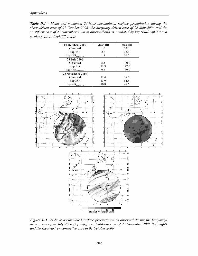
$SSHQGLFHV�
202
7DEOH� '��� �� 0HDQ� DQG� PD[LPXP� ���KRXU� DFFXPXODWHG� VXUIDFH� SUHFLSLWDWLRQ� GXULQJ� WKH�VKHDU�GULYHQ� FDVH� RI� ���2FWREHU� ������ WKH� EXR\DQF\�GULYHQ� FDVH� RI� ���-XO\� ����� DQG� WKH�VWUDWLIRUP�FDVH�RI����1RYHPEHU������DV�REVHUYHG�DQG�DV�VLPXODWHG�E\�([S+65�([S*65�DQG�([S+65 u�v%w x1yz�{#y1| �([S*65 u�v w x)y1z1{�y| ��
����2FWREHU������ Mean RR Max RR
Observed 1.6 35.0 ExpHSR 2.6 33.3
ExpHSRconserved 1.8 31.5 ���-XO\�����
Observed 5.5 100.0 ExpHSR 11.3 172.6
ExpHSRconserved 9.8 139.0 ���1RYHPEHU�����
Observed 11.4 38.5 ExpGSR 13.9 54.5
ExpGSRconserved 10.8 47.6
)LJXUH�'���� ���KRXU� DFFXPXODWHG� VXUIDFH� SUHFLSLWDWLRQ� DV� REVHUYHG� GXULQJ� WKH� EXR\DQF\�GULYHQ�FDVH�RI����-XO\�������WRS�OHIW��� WKH�VWUDWLIRUP�FDVH�RI����1RYHPEHU�������WRS�ULJKW��DQG�WKH�VKHDU�GULYHQ�FRQYHFWLYH�FDVH�RI����2FWREHU�������
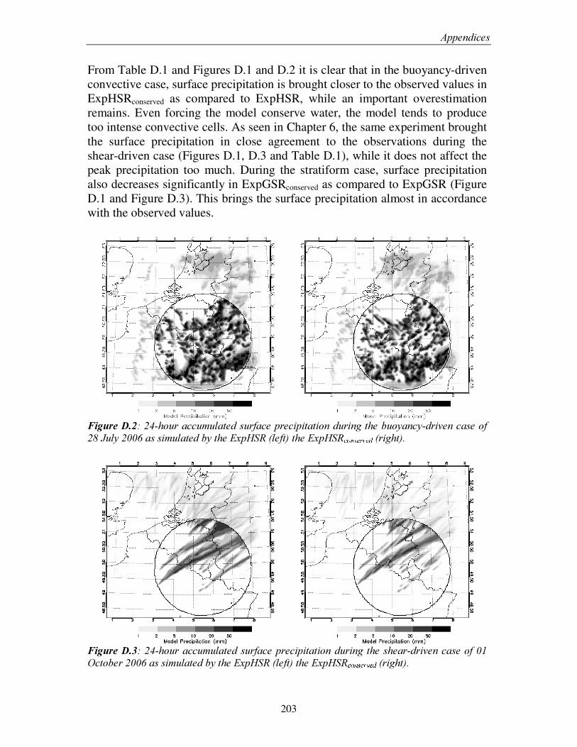
$SSHQGLFHV�
203
From Table D.1 and Figures D.1 and D.2 it is clear that in the buoyancy-driven convective case, surface precipitation is brought closer to the observed values in ExpHSRconserved as compared to ExpHSR, while an important overestimation remains. Even forcing the model conserve water, the model tends to produce too intense convective cells. As seen in Chapter 6, the same experiment brought the surface precipitation in close agreement to the observations during the shear-driven case (Figures D.1, D.3 and Table D.1), while it does not affect the peak precipitation too much. During the stratiform case, surface precipitation also decreases significantly in ExpGSRconserved as compared to ExpGSR (Figure D.1 and Figure D.3). This brings the surface precipitation almost in accordance with the observed values.
)LJXUH�'�������KRXU�DFFXPXODWHG�VXUIDFH�SUHFLSLWDWLRQ�GXULQJ�WKH�EXR\DQF\�GULYHQ�FDVH�RI����-XO\������DV�VLPXODWHG�E\�WKH�([S+65��OHIW��WKH�([S+65 uv%w x1yz){�y| ��ULJKW����
)LJXUH�'�������KRXU�DFFXPXODWHG�VXUIDFH�SUHFLSLWDWLRQ�GXULQJ� WKH�VKHDU�GULYHQ�FDVH�RI����2FWREHU������DV�VLPXODWHG�E\�WKH�([S+65��OHIW��WKH�([S+65 uv%w x1y1z1{�y1| ��ULJKW���
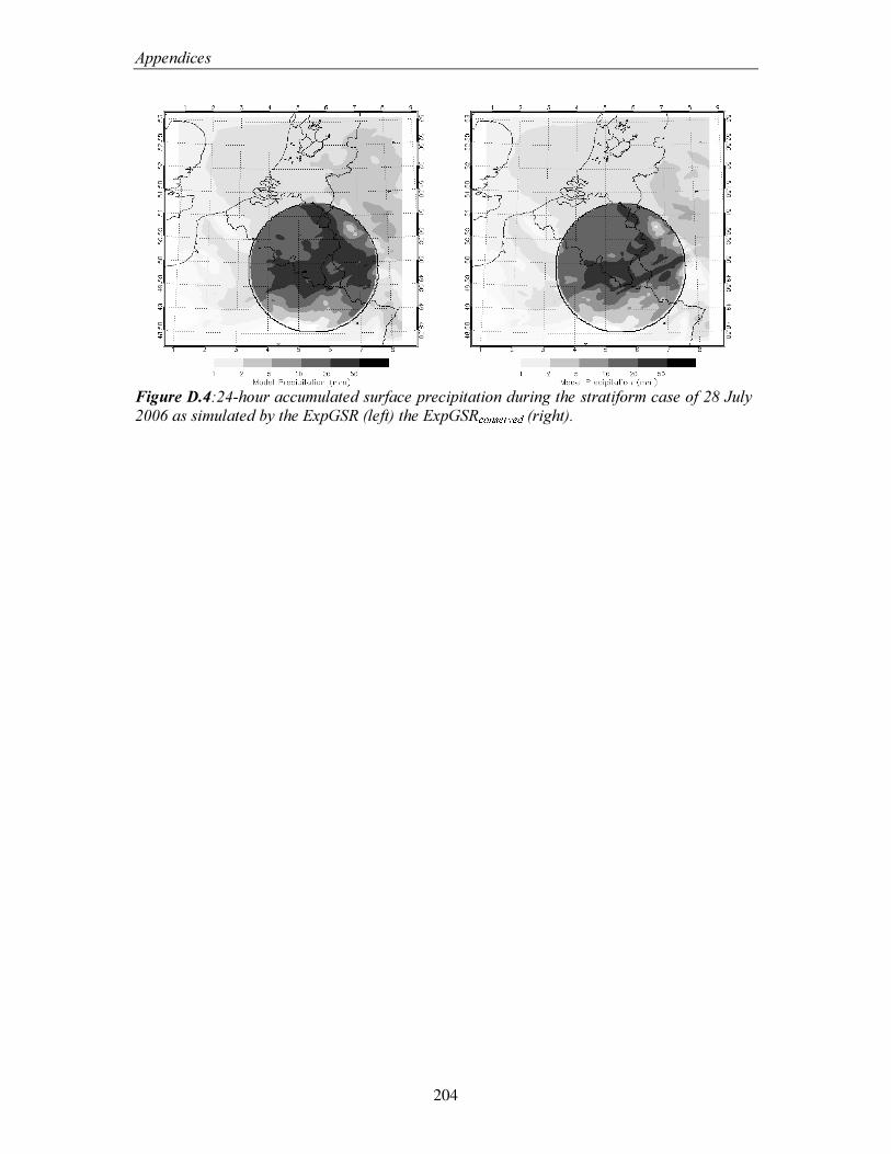
$SSHQGLFHV�
204
)LJXUH�'������KRXU�DFFXPXODWHG�VXUIDFH�SUHFLSLWDWLRQ�GXULQJ�WKH�VWUDWLIRUP�FDVH�RI����-XO\������DV�VLPXODWHG�E\�WKH�([S*65��OHIW��WKH�([S*65 u�v%w x1yz�{#y| ��ULJKW���
����������������������
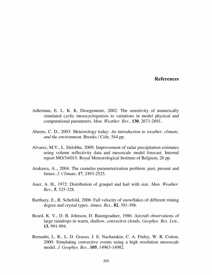
205
����������
5HIHUHQFHV������
Adlerman, E. J., K. K. Droegemeier, 2002: The sensitivity of numerically simulated cyclic mesocyclogenisis to variations in model physical and computational parameters. 0RQ��:HDWKHU��5HY., ���, 2671-2691.
Ahrens, C. D., 2003: Meteorology today: $Q�LQWURGXFWLRQ�WR�ZHDWKHU��FOLPDWH��
DQG�WKH�HQYLURQPHQW. Brooks / Cole, 544 pp. Alvarez, M.V., L. Delobbe, 2009: Improvement of radar precipitation estimates
using volume reflectivity data and mesoscale model forecast. Internal report MO/34/015. Royal Meteorological Institute of Belgium, 28 pp.
Arakawa, A.., 2004: The cumulus parameterization problem: past, present and
future. -��&OLPDWH, ��, 2493-2525. Auer, A. H., 1972: Distribution of graupel and hail with size. 0RQ��:HDWKHU��
5HY., �, 325-328. Barthazy, E., R. Schefold, 2006: Fall velocity of snowflakes of different riming
degree and crystal types. $WPRV��5HV�,���, 391-398. Beard, K. V., D. B. Johnson, D. Baumgradner, 1986: Aircraft observations of
large raindrops in warm, shallow, convective clouds. *HRSK\V��5HV��/HWW., ��, 991-994.
Bernadet, L. R., L. D. Grasso, J. E. Nachamkin, C. A. Finley, W. R. Cotton,
2000: Simulating convective events using a high resolution mesoscale model. -��*HRSK\V��5HV�, ���, 14963-14982.
5HIHUHQFHV�
206
Best, A. C., 1950: Empirical formulae for the terminal velocity of water drops
falling through the atmosphere. 4��-��5��0HWHRURO��6RF�, ��, 302-311. Bhumralkar, C. M., 1975: Numerical experiments on computation of ground
surface-temperature in an atmospheric general circulation model. -��$SSO��0HWHRU., ��, 1246-1258.
Blackadar, A. K., 1976: Modeling the nocturnal boundary layer. Proceedings,
7KLUG� 6\PS�� RQ� $WPRVSKHULF� 7XUEXOHQFH�� 'LIIXVLRQ� DQG� $LU� 4XDOLW\, Boston, Amer. Meteor. Soc., 46-49.
Bradley, S. G., C. D. Stow, 1974: The measurement of charge and size of rain
drops: Part II: Results and analysis at ground level. -��$SSO��0HWHRU., ��, 131-147.
Brandes, E. A., G. Zhang, J. Sun, 2006: On the influence of assumed drop size
distribution form on radar-retrieved thunderstorm microphysics. -��$SSO��0HWHRURO��DQG�&OLPDWRORJ\, ��, 259-268.
Braun, S. A., 2006: High-resolution simulation of hurricane Bonnie (1998). Part
II: Water budget. -��$WPRV��6FL�, ��, 43-64 Braham, R. R., 1952: The water and energy budgets of the thunderstorm and
their relation to thunderstorm development. -��0HWHRU., �, 227-242. Brown, S. R., 1970: Terminal velocities of ice particles. Atmospheric Science
Research Paper 170, Colorado State University, 52 pp. Bryan, G. H., Wyngaard, J. C., and Fritsch J. M., 2003: Resolution
requirements for the simulation of deep moist convection. 0RQ��:HDWKHU��5HY., ���, 2394-2416.
Caumont, O., V. Ducrocq, E. Wattrelot, G. Jaubert, S. Pradier-Vabre, 2010:
1D+3DVar assimilation of radar reflectivity data: a proof of concept. 7HOOXV� 6HULHV� $� ±� '\QDPLF�0HWHRURORJ\� DQG� 2FHDQRJUDS\, ��$, 173-187.
Cheng, L., M. English, 1983: A relationship between hailstone concentration
and size. -�$WPRV��6FL., ��, 204-213.
5HIHUHQFHV�
207
, M. English, R. Wong, 1985: Hailstone size distributions and their relationship to storm thermodynamics. -�� &OLP�� $SSO�� 0HWHRURO�, ��, 1059-1066.
Cheng, W. Y. Y., Cotton, W. R., 2004: Sensitivity of a cloud-resolving
simulation of the genesis of a mesoscale convective system to horizontal heterogeneities in soil moisture initialization. -�� +\GURPHWHRU�� �, 934-958.
Chung, K.S., I. Zawadzki, M.K. Yau, L. Fillion, 2009: Short-term forecasting
of a midlatitude convective storm by the assimilation of single-doppler radar observations. 0RQ��:HDWKHU��5HY., ���, 4115-4135.
Clark, C. A., R. W. Arritt, 1995: Numerical simulations of the effect of soil-
moisture and vegetation cover on the development of deep convection. -��$SSO��0HWHRU., ��, 2029-2045.
Cohen, C., McCaul Jr., E. W., 2006: The sensitivity of simulated convective
storms to variations in prescribed single-moment microphysics parameters that describe particle distribution sizes and numbers. 0RQ��:HDWKHU��5HY., ���, 2547-2565.
Colle, B.A., M.F. Garvert, J.B. Wolfe, C.F. Mass, C.P. Woods, 2005: The 13-
14 December 2001 IMPROVE-2 event. Part III: Simulated microphysical budgets and sensitivity analysis. -��$WPRV��6FL�, ��, 3535-3558.
Cotton, W.G., G.J. Tripoli, R.M. Rauber, E.A. Mulvihill, 1986: Numerical
simulation of the effects of varying ice crystal nucleation rates and aggregation processes on orographic snowfall. -�� $SSO�� 0HWHRU., ��, 1658-1680.
Cox. G.P., 1988: Modelling precipitation in frontal rainbands. 4�� -�� 5��
0HWHRURO��6RF�� ���, 115-127. Davis, C. A., Manning, K. W., Carbone, R. E., Trier, S. B., Tuttle, J. D., 2003:
Coherence of warm-season continental rainfall in numerical weather prediction models. 0RQ��:HDWKHU��5HY., ���, 2667-2679.
Deardorff, J. W., 1977: A parameterization of ground surface moisture content
for use in atmospheric prediction models. -�� $SSO�� 0HWHRU., ��, 1182-1185.
5HIHUHQFHV�
208
, 1978: Efficient prediction of ground surface temperature and moisture with inclusion of a layer of vegetation. -��*HRSK\V��5HV�, ��, 1889-1903.
Deng, A., Stauffer, D. R., 2006: On improving 4-km mesoscale model
simulations. -��$SSO��0HWHRURO��DQG�&OLPDWRORJ\, ��, 361-381. De Roo, A. P. J., Wesseling, C. G., Van Deurzen, W. P. A, 2000: Physically
based river basin modelling within a GIS: the LISFLOOD model. +\GURO��3URFHVV�, ��, 1981–1992.
Done. J., C. A. Davis, M. L. Weisman, 2004: The next generation of NWP:
Explicit forecasts of convection using the Weather Research and Forecast (WRF) model. $WPRV��6FL��/HWW., �, 110-117, doi:10.1002/asl.72.
Doswell, C. A. and Burgess, D. W., 1993: Tornadoes and tornadic storms: A
review of conceptual models. 7KH� 7RUQDGR�� ,WV� 6WUXFWXUH�� '\QDPLFV��3UHGLFWLRQ��DQG�+D]DUGV. Amer. Geophys. Union, *HRSK\V��0RQRJU. ��, 161-172.
Douglas, R. H., 1964: Hail size distribution, Proceedings, �� } ~ �:HDWKHU�5DGDU�
&RQIHUHQFH, Boston, Amer. Meteor. Soc., 146-149. Ebert, E. E., J. L. McBride, 2000: Verification of precipitation in weather
systems: Determination of systematic errors. -��+\GURO�, ���, 179-202. Entekhabi, D., Rodriguezlturbe, I., Castelli, F., 1996: Mutual interaction of soil
moisture state and atmospheric processes. -��+\GURO�, ���, 3-17. European Soil Bureau Network and the European Commission, 2004: European
Soil Database (v 2.0), EUR 19945 EN. Federer, B. and A. Waldvogel, 1975: Hail and raindrop size distributions from a
Swiss multicell storm. -��$SSO��0HWHRURO., ��, 91-97. Ferrier, B. S., 1994: A double-moment multiple-phase four-class bulk ice
scheme, Part I: description. -��$WPRV��6FL�, ��, 249-280. Field, P. R., 1999: Aircraft observations of ice crystal evolution in an altostratus
cloud. -��$WPRV��6FL�, ��, 1925-1941. , R. J. Hogan, P. R. A. Brown, A. J. Illingworth, T. W. Choularton, R. J.
Cotton, 2005: Parameterization of ice-particle size distributions for mid-latitude stratiform cloud. 4��-��5��0HWHRURO��6RF�, ���, 1997-2017.
5HIHUHQFHV�
209
, A.J. Heymsfield, A. Bansemer, C.H. Twohy, 2008: Determination of the
combined ventilation factor and capacitance for ice crystal aggregates from airborne observations in a tropical anvil cloud. -��$WPRV��6FL�, ��, 376-191.
Franklin, C. N., G. J. Holland, P. T. May, 2005: Sensitivity of tropical cyclone
rainbands to ice-phase microphysics. 0RQ�� :HDWKHU�� 5HY., ���, 2473-2493.
Fritsch, J. M., R. E. Carbone, 2004: Improving the quantitative precipitation
forecast in the warm season. %XOO��$PHU��0HWHRU��6RF�, ��, 955-965. Früh, B., J. Bendix, T. Nauss, M. Paulat, A. Pfeiffer, B. Thies, H. Wernli, 2007:
Verification of precipitation from regional climate simulations and remote-sensing observations with respect to ground-based observations in the upper Danube catchment. 0HWHRURORJLVFKH�=HLWVFKULIW, ��, 1-19.
Fu, Q., K.-N. Liou, 1993: Parameterization of the radiative properties of cirrus
clouds. -��$WPRV��6FL�, ��, 2008-2025. Gallus Jr, W. A., Segal, M., 2000: Sensitivity of forecast rainfall in a Texas
convective system to soil moisture and convective parameterization. :HDWKHU��)RUHFDVW. ��, 509-525.
Garvert, M.F., C.P. Woods, B.A. Colle, C.F. Mass, P.V. Hobbs, M.P. Stoelinga,
J.B. Wolfe, 2005: The 13-14 December 2001 IMPROVE-2 event. Part II: Comparison of MM5 model simulations of clouds and precipitation with observations. -��$WPRV��6FL�, ��, 3520-3534.
Gebhardt, C., S. Theis, P. Krahe, V. Renner, 2008: Experimental ensemble
forecasts of precipitation based on a convection-resolving model. $WPRV��6FL��/HWW., �, 67-72, doi:10.1002/asl.177.
Gerard, L., J.-M. Piriou, R. Brozkova, J.-F. Geleyn, D. Banciu, 2009: Cloud and
precipitation parameterization in a meso-gamma-scale operational weather prediction model.�0RQ��:HDWKHU��5HY�, ���, 3960-3977.
Gilmore, M. S., Straka, J. M., Rasmussen, E. N., 2004: Precipitation uncertainty
due to variations in precipitation particle parameters within a simple microphysics scheme. 0RQ��:HDWKHU��5HY�, ���, 2610-2627.
5HIHUHQFHV�
210
Goudenhoofdt, E., L. Delobbe, 2009: Evaluation of radar-gauge merging methods for quantitative precipitation estimates. +\GURO��(DUWK�6\VW��6F., ��, 195-203.
Groenemeijer, P.H., A. van Delden, 2007: Sounding-derived parameters
associated with large hail and tornadoes in the Netherlands. $WPRV��5HV�, ��, 473-487.
Gunn, K. L. S., J. S. Marshall, 1958: The distribution with size of aggregate
snowflakes. -��0HWHRU�, ��, 452-461. Hense, A., Adrian, G., Kottmeier, C., Simmer, C., Wulfmeyer, V., 2003: Das
Schwerpunktprogramm SPP 1167 der Deutschen Forschungsgemeinschaft „Quantitatieve Niederschlagvorhersage“ (Priority programm SPP 1167 from the German research community „Quantitative Precipitation Forecast“). ,QWHUQDO� GRFXPHQW, University of Bonn, [Available online at http://www.meteo.uni-bonn.de/projekte/SPPMeteo/reports/DMG_SPP1167.pdf], 9 pp.
Heymann, Y., Steenmans, C., Croisille, G., Bossard, M., 1994: CORINE land
cover technical guide. 2IILFH� IRU� 2IILFLDO� 3XEOLFDWLRQV� RI� WKH� (XURSHDQ�&RPPXQLWLHV, 136 pp.
Heymsfield, A. J., 1978: The characteristics of graupel particles in northeast
Colorado cumulus congestus clouds. -��$WPRV��6FL., ��, 284-295. , M. Kajikawa, 1987: An improved approach to calculating terminal
velocities of plate-like crystals and graupel. -� $WPRV��6FL., ��, 1088-1099. Holt, T. R., D. Niyogi, F. Chen, K. Manning, M. LeMone, A. Qureshi, 2006:
Effect of lan-atmosphere interactions on the IHOP 24-25 May 2002 convection case. 0RQ��:HDWKHU��5HY., ���, 113-133.
Holton, J. R., 2004: $Q�LQWURGXFWLRQ�WR�G\QDPLF�PHWHRURORJ\. Elsevier, 535 pp. Houze, R. A., Hobbs, P. V., Herzegh, P. H., Parsons, D. B., 1979: Size
distributions of precipitation particles in frontal clouds��-��$WPRV��6FL�, ��, 156-162.
Jiusto, J. E., G. E. Bosworth, 1971: Fall velocity of snowflakes. -�� $SSO��
0HWHRU., ��, 1352-1354.
5HIHUHQFHV�
211
Kain, J. S., J. M. Fritsch, 1993: Convective parameterization for mesoscale models: The Kain-Fritsch scheme. The Representation of Cumulus Convection in Numerical Models. 0HWHRURO��0RQRJU�, ��, 165-170.
Karlsson, K.-G., E. Wolters, P. Albert, A. Tetzlaff, R. Roebeling, W. Thomas, S.
Johnston, 2005: Initial validation of CM-SAF cloud products using MSG/SEVIRI data. Scientific report, Satellite Application Facility on Climate Monitoring, SAF/CM/DWD/SMHI/KNMI/SR/CLOUDS/1, 39 pp.
Kain, J. S., S. J. Weiss, D. R. Bright, M. E. Baldwin, J. J. Levit, G. W. Carbin,
C. S. Schwartz, M. L. Weisman, K. K. Droegemeier, D. B. Weber, K. W. Thomas, 2008: Some practical considerations regarding horizontal resolution in the first generation of operation convection-allowing NWP. :HDWKHU��)RUHFDVW� ��, 931-952.
Khain, A., A. Pokrovsky, I. Sednev, 1999: Some effects of cloud-aerosol
interaction on cloud microphysics structure and precipitation formation: Numerical experiments with a spectral microphysics cloud ensemble model. $WPRV��5HV., ��, 195-220.
., Ovtchinnikov, M., Pinsky, M., Pokrovsky, A., Krugliak, H., 2000: Notes
on the state-of-the-art numerical modeling of cloud microphysics. $WPRV��5HV�,���, 159-224.
Kogan, Y.L., 1991: The simulation of a convective coud in a 3D model with
explicit microphysics. Part I: Model description and sensitivity experiments. -��$WPRV��6FL�, ��, 1160-1189.
Koster, R.D., Dirmeyer, P.A., Guo, Z., Bonan, G., Chan, E., Cox, P., Gordon, C.
T., Kanae, S., Kowalczyk, E., Lawrence, D., Liu, P., Lu, C.-H., Malyshev, S., McAvaney, B., Mitchell, K., Mocko, D., Oki, T., Oleson, K., Pitman, A., Sud, Y. C., Taylor, C. M., Verseghy, D., Vasic, R., Xue, Y., Yamada, T., 2004: Regions of strong coupling between soil moisture and precipitation. 6FLHQFH, ���, 1138-1140.
Lin, Y.- L., Farley, R. D., Orville, H. D., 1983: Bulk parameterization of the
snow field in a cloud model. -��&OLP��$SSO��0HWHRURO�, ��, 1065-1092. Liu, J. Y., H. D. Orville, 1969: Numerical modeling of precipitation and cloud
shadow effects on mountain-induced cumuli. -�� $WPRV�� 6FL., ��, 1283-1298.
5HIHUHQFHV�
212
Liou, K. N., 1992: Radiation and cloud processes in the atmosphere. Oxford University Press, New York, NJ, USA.
Locatelli, J. D., Hobbs, P. V., 1974: Fall speeds and masses of solid
precipitation particles. -� *HRSK\V��5HV., ��, 2185-2197. Lynn, B. H., D. R. Stauffer, P. J. Wetzel, W.- K. Tao, P. Alpert, N. Perlin, R. D.
Bakker, R. Muñoz, A. Boone, Y. Jia, 2001: Improved simulation of Florida summer convection using the PLACE land model and a 1.5-order turbulence parameterization coupled to the Penn state – NCAR mesoscale model. 0RQ��:HDWKHU��5HY., ���, 1441-1461.
Markowitz, A. H., 1976: Raindrop size distribution expressions. -�� $SSO��
0HWHRU., ��, 1029-1031. Martin, W. J., Xue, M., 2006: Sensitivity analysis of convection of the 24 May
2002 IHOP case using very large ensembles. 0RQ��:HDWKHU�� 5HY., ���, 192-207.
Mass, C. F., D. Ovens, K. Westrick, B. A. Colle, 2002: Does increasing
horizontal resolution produce more skillful forecasts? %XOO��$PHU��0HWHRU��6RF�, ��, 407-430.
Matson, R. J., A. W. Huggins, 1980: The direct measurements of the sizes,
shapes and kinematics of falling hailstones, -��$WPRV��6FL., ��, 1107-1125. Matsui, T., X. Zeng, W.- K. Tao, H. Masunaga, W. S. Olson, S. Lang, 2009:
Evaluation of long-term cloud-resolving model simulations using satellite radiance observations and multifrequency satellite simulators. -�� $WPRV��2FHDQ��7HFK�, ��, 1261-1274.
McCumber M., Tao, W.- T., Simpson, J., Penc, R., Soong, S.- T., 1991:
Comparison of ice-phase microphysical parameterization schemes using numerical simulations of tropical convection. -��$SSO��0HWHRURO., ��, 985-1004.
Milbrandt, J. A., Yau, M. K., 2005: A multimoment bulk microphysics
parameterization. Part II: A proposed three-moment closure and scheme description.�-��$WPRV��6FL., ��, 3065–3081.
, , 2006: A multimoment bulk microphysics parameterization. Part
III: Control simulation of a hailstorm. -��$WPRV��6FL., ��, 3077–3090.
5HIHUHQFHV�
213
Marshall, J. S., W. M. K. Palmer, 1948: The distribution of raindrops with size. -��0HWHRURO., �, 165-166.
Müller, E. A., 1966: Radar cross sections from drop size spectra. Doctoral
thesis, University of Illinois, Urbana-Champaign, 89 pp. Nachtergaele, J., Poesen, J., 2002: Spatial and temporal variations in resistance
of loess-derived soils to ephemeral gully erosion. (XU�� -�� 6RLO� 6FL�, ��, 449-463.
Nielsen-Gammon, J. W., J. Strack, 2000: Numerical simulations and forecasting
potential for extreme rainfall events in the southern United States. Proceedings, �� } ~ �&RQI��RQ�+\GURORJ\, 251-254.
Noilhan, J., Planton, S., 1989: A simple parameterization of land surface
processes for meteorological models. 0RQ��:HDWKHU��5HY., ���, 536-549. Okita, T., 1958: Observations on vertical change of raindrop size distribution,
Tohoku University Science Rep. 1, Geophysics Series 5, Vol. 10, 13 pp. Otkin, J. A., T. J. Greenwald, 2008: Comparison of WRF model-simulated and
MODIS-derived cloud data, 0RQ��:HD��5HY�, ���, 1957-1970. Ovtchinnikov, M., Y.L. Kogan, 2000: An investigation of ice production
mechanisms in small cumuliform clouds using a 3D model with explicit microphysics. Part I: Model description. -��$WPRV��6FL., ��, 2989-3003.
Pielke, R. A., 1992: 0HVRVFDOH� PHWHRURORJLFDO� PRGHOLQJ. ,QWHUQDWLRQDO�
*HRSK\VLFV�6HULHV, Academic Press, ��, 676 pp. Piriou, J.-M., J.-L. Redelsperger, J.-F. Geleyn, J.-P. Lafore, F. Guichard, 2007:
An approach for convective parameterization with memory, in separating microphysics and transport in grid-scale equations. -�� $WPRV�� 6FL., ��, 4127-4139.
Pruppacher, H., J. D. Klett, 2003: 0LFURSK\VLFV� RI� FORXGV� DQG� SUHFLSLWDWLRQ,
Kluwer Academic, 943 pp. Randall, D., M. Khairoutdinov, A. Arakawa, W. Gabowski, 2003: Breaking the
cloud parameterization deadlock. %XOO�� $PHU�� 0HWHRU�� 6RF�, ��, 1547-1564.
5HIHUHQFHV�
214
Ramaswamy, V. and A. Detwiler, 1986: Interdependence of radiation and microphysics in cirrus clouds. -��$WPRV��6FL., ��, 2289-2301.
Rauber, R. M., K. V. Beard, B. M. Andrews, 1991: A mechanism for giant
raindrop formation in warm, shallow convective clouds. -��$WPRV��6FL., ��, 1791-1797.
Reisner, J., Rasmussen, R. M., Bruintjes, R. T., 1998: Explicit forecasting of
supercooled liquid water in winter storms using the MM5 mesoscale model. 4��-��5��0HWHRURO��6RF�, ���, 1071-1107.
Roebeling, R.A., A. J. Feijt, P. Stammes, 2006: Cloud property retrievals for
climate monitoring: Implications of differences between Spinning Enhanced Visible and Infrared Imager (SEVIRI) on METEOSAT-8 and Advanced Very High Resolution Radiometer (AVHRR) on NOAA-17. -��*HRSK\V��5HV�, ���, D20210, doi:10.1029/2005JD006990.
Rotunno, R., J. B. Klemp, M. L. Weisman, 1988: A theory for strong, long-lived
squall lines. -��$WPRV��6FL., ��, 463-485. Rutledge, S. A., Hobbs, P. V., 1983: The mesoscale and microscale structure
and organization of clouds and precipitation in mid-latitude cyclones. Part VIII: A model for the “ seeder-feeder” process in warm-frontal rainbands. -��$WPRV��6FL., ��, 1185-1206.
Sangati, M., M. Borga, D. Rabuffetti, R. Bechini, 2009: Influence of rainfall and
soil properties spatial aggregation on extreme flash flood response modelling: An evaluation based on the Sesia river Basin, North Western Italy. $GY��:DWHU�5HV�, ��, 1090-1106.
Saunders, R.W., K.T. Kriebel, 1988: An improved method for detecting clear-
sky and cloudy radiances from AVHRR data. ,QW��-��5HP��6HQV�, �, 123-150.
Schröder, M., N. P. M. van Lipzig, F. Ament, J.- P. Chaboureau, S. Crewell, J.
Fischer, V. Matthias, E. van Meijgaard, A. Walther, U. Willén, 2006: Model predicted low-level cloud parameters. Part II: Comparison with satellite remote sensing observations during the BALTEX Bridge Campaigns. $WPRV��5HV., ��, 83-101.
Schulz, J., W. Thomas, R. Müller, H.-D. Behr, D. Caprion, H. Deneke, S.
Dewitte, B. Dürr, P. Fuchs, A. Gratzki, R. Hollmann, K.-G. Karlsson, T. Manninen, M. Reuter, A. Riihelä, R. Roebeling, N. Selbach, A. Tetzlaff,
5HIHUHQFHV�
215
E. Wolters, A. Zelenka, M. Werscheck , 2008: Operational climate monitoring from space: the EUMETSAT satellite application facility on climate monitoring (CM-SAF), $WPRV�� &KHP�� 3K\V�� 'LVFXVV�, �, 8517-8563, 2008
Schwartz, C.S., J.S. Kain, S.J. Weiss, M. Xue, D.R. Bright, F.Y. Kong, K.W.
Thomas, J.J. Levit, M.C. Coniglio, M.S. Wandishin, 2010: Toward improved convection-allowing ensembles: model physics sensitivities and optimizing probabilistic guidance with small ensemble membership. :HDWKHU��)RUHFDVW�. ��, 263-280.
Schwitalla, T., H.-S. Bauer, V. Wulfmeyer, G. Zängl, 2008: Systematic errors of
QPF in low-mountain regions as revealed by MM5 simulations. 0HWHRURORJLVFKH�=HLWVFKULIW, ��, 903-919.
Seifert, A., Beheng, K. D., 2006: A two-moment cloud microphysics
parameterization for mixed-phase clouds. Part 2: Maritime vs. continental deep convective storms. 0HWHRURO��$WPRV��3K\V., ��, 67-82.
Sekhon, R. S., R. C. Srivastava, 1970: Snow size spectra and radar reflectivity.
-� $WPRV��6FL., ��, 299-307. , , 1971: Doppler radar observations of drop size distributions in a
thunderstorm. -� $WPRV��6FL., ��, 983-994. Serafin, S., Ferretti, R., 2007: Sensitivity of a mesoscale model to microphysical
parameterizations in the MAP SOP events IOP2b and IOP8. -�� $SSO��0HWHRURO��DQG�&OLPDWRORJ\, ��, 1438-1454.
Skamarock, W. C., M. L. Weisman, 2009: The impact of positive-definite
moisture transport on NWP precipitation forecasts. 0RQ��:HD��5HY�, ���, 488-494.
Smedsmo, J.L., E.F. Foufoula-Georgiou, V. Vuruputur, F. Kong, K.
Droegemeier, 2005: On the vertical structure of modeled and observed deep convective storms: Insights for the precipitation retrieval and microphysical parameterization. -��$SSO��0HWHRU., ��, 1866-1884.
Smith, P.L., C.G. Myers, H.D. Orville, 1975: Radar reflectivity factor
calculations in numerical cloud models using bulk parameterization of precipitation, -��$SSO��0HWHRU., ��, 1156-1164.
5HIHUHQFHV�
216
Srivastava, R. C., 1967: On the role of coalescence between raindrops in shaping their size distribution. -��$WPRV��6FL., ��, 287-291.
Steiner, M., R.A. Houze, S.E. Yuter, 1995: Climatological characterization of
three-dimensional storm structure from operational radar and rain gauge data, -��$SSO��0HWHRU., ��, 1978-2006.
Stengel, M., P. Unden, M. Lindskog, P. Dahlgren, N. Gustafsson, R. Bennartz,
2009: Assimilation of SEVIRI infrared radiances with HIRLAM 4D-Var. 4��-��5��0HWHRURO��6RF�, ���, 2100-2109.
Straka, J. M., 2009: &ORXG� DQG� SUHFLSLWDWLRQ� PLFURSK\VLFV. Cambridge
University Press, 392 pp. Sui, C. H., K.- H. Lau, X. Li, 1998: Convective-radiative interaction in
simulated diurnal variations of tropical cumulus ensemble. -��$WPRV��6FL., ��, 637-655.
, X. Li, M.- J. Yang, 2007 : On the definition of precipitation efficiency. -��
$WPRV��6FL., ��, 4506-4513. Sun W.-Y., Chang C.-Z., 1986 : Diffusion model for a convective layer. Part I:
Numerical simulation of convective boundary layer. -�� &OLP�� $SSO��0HWHRURO., ��, 1445-1453.
Tao, W.-K., J. Simpson, D. Baker, S. Braun, M.-D. Chou, B. Ferrier, D.
Johnson, A. Khain, S. Lang, B. Lynn, C.-L. Shie, D. Starr, C.-H. Sui, Y. Wang, P. Wetzel, 2003: Microphysics, radiation and surface processes in the Goddard Cumulus Ensemble (GCE) model, 0HWHRURO��$WPRV��3K\V., ��, 97-137.
Thompson, G., R. Y. Rasmussen, K. M. Manning, 2004: Explicit forecasts of
winter precipitation using an improved bulk microphysics scheme. Part I: Description and sensitivity analysis. 0RQ��:HD��5HY�, ���, 519-542.
, P.R. Field, R.M. Rasmussen, W.D. Hall, 2008: Explicit forecasts of
winter precipitation using an improved bulk microphysics scheme. Part II: Implementation of a new snow parameterization. 0RQ��:HD��5HY�, ���, 5095-5115.
Tong, M. and M. Xue, 2008: Simultaneous estimation of microphysical
parameters and atmospheric state with simulated radar data and ensemble
5HIHUHQFHV�
217
square root Kalman filter. Part I: Sensitivity analysis and parameter identifiability. 0RQ��:HD��5HY�, ���, 1630-1648.
Trier, S. B., Chen, F., Manning, K. W., LeMone, M. A., Davis, C. A., 2008:
Sensitivity of the PBL and precipitation in 12-day simulations of warm-season convection using different land surface models and soil wetness conditions. 0RQ��:HDWKHU��5HY., ���, 2321-2343.
Ulbrich, C. W., 1983: Natural variations in the analytical form of the raindrop
size distribution. -��&OLPDWH�$SSO��0HWHRU., ��, 1764-1775. Uplinger, C. W., 1981: A new formula for raindrop terminal velocity. Preprints,
�� } ~ �&RQI��RQ�5DGDU�0HWHRURORJ\, Boston, MA, Amer. Meteor. Soc., 389-391.
van den Heever, S.C., W.R. Cotton, 2004: The impact of hail size on simulated
supercell storms, -� $WPRV��6FL., ��, 1596-1609. Vanneuville, W., Maddens, R., Collard, C., Bogaert, P., De Maeyer, P., Antrop,
M., 2006: Impact op mens en economie t.g.v. overstromingen bekeken in het licht van wijzigende hydraulische condities, omgevingsfactoren en klimatologische omstandigheden (Impact on man and economy by floods, studied in the light of changing hydraulic conditions, environmental factors and climatologic circumstances). MIRA report, Flemisch Environmental Agency (VMM), 120 pp.
Van Weverberg, K., N.P.M. van Lipzig, L. Delobbe, D. Lauwaet, 2010:
Sensitivity of quantitative precipitation forecast to soil moisture initialization and microphysics parameterization. 4��-��5��0HWHRURO��6RF�, (in press).
, , , 2010: Evaluation of moist processes during intense
precipitation in km-scale NWP models using remote sensing and in-situ data: impact of microphysics size distribution assumptions. $WPRV��5HV�� (submitted).
, , , 2010: The impact of size distribution assumptions in a
simple microphysics scheme on surface precipitation and storm dynamics during a low-topped supercell case. 0RQ��:HDWKHU��5HY.� (submitted).
Waldvogel, A., 1974: The N0 jump of raindrop spectra. -��$WPRV��6FL., ��, 1067-
1078.
5HIHUHQFHV�
218
Wallace, J. M., P. V. Hobbs, 2006: $WPRVSKHULF� VFLHQFH�� $Q� LQWURGXFWRU\�VXUYH\. Elsevier, 483 pp.
Weisman M. L., Klemp, J. B., 1982: The dependence of numerically simulated
convective storms on vertical wind shear and buoyancy. 0RQ��:HDWKHU��5HY., ���, 504-520.
, , 1984: The structure and classification of numerically simulated
convective storms in directionally varying wind shears. 0RQ�� :HDWKHU��5HY., ���, 2479-2498.
, Skamarock, W. C., Klemp, J. B., 1997: The resolution dependence of
explicitly modeled convective systems. 0RQ�� :HDWKHU�� 5HY., ���, 527-548.
, C. Davis, W. Wang, K. W. Manning, J. B. Klemp, 2008: Experiences
with 0-36 h explicit convective forecasts with the WRF-ARW model. :HDWKHU��)RUHFDVW�. ��, 407-437.
Wernli, H., Paulat, M., Hagen, M., Frei, C., 2008: SAL – A novel quality
measure for the verification of quantitative precipitation forecasts. 0RQ��:HDWKHU��5HY., ���, 4470-4487.
Willems, P., 2001: A spatial rainfall generator for small spatial scales. -��
+\GURO., ���, 126-144. Willis, P. T., 1984: Functional fits of some observed drop size distributions and
parameterization of rain, -��$WPRV��6FL., ��, 1648-1661. , P. Tattelman, 1989: Drop-size distributions associated with intense
rainfall, -��$SSO��0HWHRURO�, ��, 3-15. , J. Hallett, 1991: Microphysical measurements from an aircraft ascending
with a growing isolated maritime cumulus tower, -��$PWRV��6FL�, ��, 283-300.
Wisner, C., Orville, H. D., Myers, C., 1972: A numerical model of a hail-
bearing cloud��-� $WPRV��6FL., ��, 1160-1181. Wisse, J. S. P., de Arellano, J. V. G., 2004: Analysis of the role of the planetary
boundary layer schemes during a severe convective storm, $QQ��*HRSK\V�, ��, 1861-1874.
5HIHUHQFHV�
219
Woods, C. P., Stoelinga, M. T., Locatelli, J. D., 2007: The IMPROVE-1 storm of 1-2 February 2001. Part III: Sensitivity of a mesoscale model simulation to the representation of snow particle types and testing of a bulk microphysical scheme with snow habit prediction.�-��$WPRV��6FL., ��, 3927-3948.
Xu, J., X. Gao, S. Sorooshian, 2004: Model study on the soil-moisture influence
on the precipitation seesaw in the southern United States. 7HOOXV, ��$, 514-519.
Xue, M., 2000: High-order monotonic numerical diffusion and smoothing. 0RQ��
:HDWKHU��5HY., ���, 2853-2864. , Droegemeier, K. K., Wong, V., 2000: The Advanced Regional
Prediction System (ARPS) – A multi-scale nonhydrostatic atmospheric simulation and prediction model. Part I: Model dynamics and verification. 0HWHRURO��$WPRV��3K\V., ��, 161-193.
, , , Shapiro, A., Brewster, K., Carr, F., Weber, D., Liu, Y.,
Wang, D., 2001: The Advanced Regional Prediction System (ARPS) – A multi-scale nonhydrostatic atmospheric simulation and prediction tool. Part II: Model physics and applications. 0HWHRURO��$WPRV��3K\V., ��, 143-165.
Yuter, S. E., R. A. Houze, 1995: 3-dimensional kinematic and microphysical
evolution of Florida cumulonimbus. 1. Spatial-distribution of updrafts, downdrafts and precipitation. 0RQ��:HD��5HY., ���, 1941-1963.
Zängl, G., 2004: The sensitivity of simulated orographic precipitation to model
components other than cloud microphysics. 4��-��5��0HWHRURO��6RF., ���, 1857-1875.
Zhang, G., Xue, M., Cao, Q., Dawson, D., 2008: Diagnosing the intercept
parameter for exponential raindrop size distribution based on video disdrometer observations: model development. -�� $SSO�� 0HWHRURO�� DQG�&OLPDWRORJ\, ��, 2983-2992.
Ziegler, C. L., P. S. Ray, N. C. Knight, 1983: Hail growth in an Oklahoma
multicell storm, -��$WPRV��6FL., ��, 1768-1791.