
plasimo.phys.tue.nl · Transport and equilibrium in molecular plasmas: the sulfur lamp PROEFSCHRIFT...
158
Transport and equilibrium in molecular plasmas: the sulfur lamp PROEFSCHRIFT ter verkrijging van de graad van doctor aan de Technische Universiteit Eindhoven, op gezag van de Rector Magnificus, prof.dr. R.A. van Santen, voor een commissie aangewezen door het College voor Promoties in het openbaar te verdedigen op donderdag 13 maart 2003 om 16.00 uur door Colin William Johnston geboren te Dublin, Ierland
Transcript of plasimo.phys.tue.nl · Transport and equilibrium in molecular plasmas: the sulfur lamp PROEFSCHRIFT...
Transport and equilibrium in molecularplasmas: the sulfur lamp
PROEFSCHRIFT
ter verkrijging van de graad van doctor aan deTechnische Universiteit Eindhoven, op gezag van de
Rector Magnificus, prof.dr. R.A. van Santen, voor eencommissie aangewezen door het College voor
Promoties in het openbaar te verdedigenop donderdag 13 maart 2003 om 16.00 uur
door
Colin William Johnston
geboren te Dublin, Ierland
Dit proefschrift is goedgekeurd door de promotoren:
prof.dr.ir. D.C. Schramenprof.dr.ir. G.M.W. Kroesen
Copromotor:dr. J.J.A.M. van der Mullen
This research is sponsored by the Dutch Technology Foundation, STW, as project ETN.3892
CIP-DATA LIBRARY TECHNISCHE UNIVERSITEIT EINDHOVEN
Johnston, Colin William
Transport and equilibrium in molecular plasmas: the sulfur lamp / byColin William Johnston. - Eindhoven : Technische Universiteit Eindhoven, 2003. -Proefschrift.ISBN 90-386-1635-XNUR 924Trefw. : plasma / zwavel lamp / moleculen / transporteigenschappenSubject headings : plasma / sulfur lamp / molecules / transport propertiesPrinted by: Universiteitsdrukkerij Technische Universiteit EindhovenCover image: A quartz bulb containing sulfur. Photography by Jan-Willem Luiten.

To Phyl, Bill and Peter

Contents
1 General Introduction 7
2 A self consistent LTE model of a microwave driven, high-pressure sulfurlamp 132.1 Introduction . . . . . . . . . . . . . . . . . . . . . . . . . . . . . . . . . . . 142.2 Origin and operational trends in the spectrum . . . . . . . . . . . . . . . . 15
2.2.1 Origin of the spectrum . . . . . . . . . . . . . . . . . . . . . . . . . 152.2.2 Bulb characterization . . . . . . . . . . . . . . . . . . . . . . . . . . 162.2.3 Spectral trends . . . . . . . . . . . . . . . . . . . . . . . . . . . . . 17
2.3 State of the art . . . . . . . . . . . . . . . . . . . . . . . . . . . . . . . . . 172.4 The Model . . . . . . . . . . . . . . . . . . . . . . . . . . . . . . . . . . . . 17
2.4.1 Simplifications . . . . . . . . . . . . . . . . . . . . . . . . . . . . . . 172.4.2 The energy balance . . . . . . . . . . . . . . . . . . . . . . . . . . . 182.4.3 Electromagnetic module . . . . . . . . . . . . . . . . . . . . . . . . 182.4.4 Generation and transport of radiation . . . . . . . . . . . . . . . . . 192.4.5 Boundary conditions . . . . . . . . . . . . . . . . . . . . . . . . . . 212.4.6 Iteration procedure . . . . . . . . . . . . . . . . . . . . . . . . . . . 21
2.5 Material properties . . . . . . . . . . . . . . . . . . . . . . . . . . . . . . . 222.5.1 Reactions and species . . . . . . . . . . . . . . . . . . . . . . . . . . 222.5.2 Composition module . . . . . . . . . . . . . . . . . . . . . . . . . . 232.5.3 Thermal conductivity module . . . . . . . . . . . . . . . . . . . . . 242.5.4 Electrical Conductivity . . . . . . . . . . . . . . . . . . . . . . . . . 252.5.5 Species interactions . . . . . . . . . . . . . . . . . . . . . . . . . . . 26
2.6 Results . . . . . . . . . . . . . . . . . . . . . . . . . . . . . . . . . . . . . . 262.6.1 Temperature . . . . . . . . . . . . . . . . . . . . . . . . . . . . . . . 272.6.2 Power balance . . . . . . . . . . . . . . . . . . . . . . . . . . . . . . 272.6.3 Electric field strength . . . . . . . . . . . . . . . . . . . . . . . . . . 282.6.4 Spectra . . . . . . . . . . . . . . . . . . . . . . . . . . . . . . . . . 282.6.5 Sensitivity analysis . . . . . . . . . . . . . . . . . . . . . . . . . . . 30
2.7 Conclusions . . . . . . . . . . . . . . . . . . . . . . . . . . . . . . . . . . . 30
1
Contents
3 Operational trends in the characteristic temperature of a high pressuremicrowave powered sulfur lamp 333.1 Introduction . . . . . . . . . . . . . . . . . . . . . . . . . . . . . . . . . . . 343.2 Molecular spectrum and atomic lines . . . . . . . . . . . . . . . . . . . . . 353.3 Experimental setup . . . . . . . . . . . . . . . . . . . . . . . . . . . . . . . 35
3.3.1 Bulb characterization . . . . . . . . . . . . . . . . . . . . . . . . . . 363.4 Model results . . . . . . . . . . . . . . . . . . . . . . . . . . . . . . . . . . 38
3.4.1 Temperature profiles . . . . . . . . . . . . . . . . . . . . . . . . . . 383.5 Spectral line interpretation . . . . . . . . . . . . . . . . . . . . . . . . . . . 39
3.5.1 Boltzmann plot . . . . . . . . . . . . . . . . . . . . . . . . . . . . . 393.5.2 Dissociation degree . . . . . . . . . . . . . . . . . . . . . . . . . . . 403.5.3 Absolute line measurements . . . . . . . . . . . . . . . . . . . . . . 40
3.6 Results . . . . . . . . . . . . . . . . . . . . . . . . . . . . . . . . . . . . . . 423.6.1 Characteristic temperatures . . . . . . . . . . . . . . . . . . . . . . 423.6.2 Line intensities . . . . . . . . . . . . . . . . . . . . . . . . . . . . . 43
3.7 Conclusions . . . . . . . . . . . . . . . . . . . . . . . . . . . . . . . . . . . 43
4 An improved LTE model of a high pressure sulfur discharge 454.1 Introduction . . . . . . . . . . . . . . . . . . . . . . . . . . . . . . . . . . . 464.2 Model Review . . . . . . . . . . . . . . . . . . . . . . . . . . . . . . . . . . 474.3 Composition and transport properties . . . . . . . . . . . . . . . . . . . . . 494.4 Radiative contribution to the energy balance . . . . . . . . . . . . . . . . . 50
4.4.1 Radiation generation and transport . . . . . . . . . . . . . . . . . . 504.4.2 Heavier polymers . . . . . . . . . . . . . . . . . . . . . . . . . . . . 524.4.3 Additional S2 states . . . . . . . . . . . . . . . . . . . . . . . . . . 53
4.5 Results . . . . . . . . . . . . . . . . . . . . . . . . . . . . . . . . . . . . . . 544.5.1 Spectra . . . . . . . . . . . . . . . . . . . . . . . . . . . . . . . . . 544.5.2 Temperature . . . . . . . . . . . . . . . . . . . . . . . . . . . . . . . 56
4.6 Discussion . . . . . . . . . . . . . . . . . . . . . . . . . . . . . . . . . . . . 584.6.1 Energy balance . . . . . . . . . . . . . . . . . . . . . . . . . . . . . 584.6.2 Origin of the spectrum . . . . . . . . . . . . . . . . . . . . . . . . . 584.6.3 Species densities . . . . . . . . . . . . . . . . . . . . . . . . . . . . 584.6.4 Influence of the wall . . . . . . . . . . . . . . . . . . . . . . . . . . 59
4.7 Conclusions . . . . . . . . . . . . . . . . . . . . . . . . . . . . . . . . . . . 60
5 Measured and simulated response of a high pressure sulfur spectrumto power interruption 635.1 Introduction . . . . . . . . . . . . . . . . . . . . . . . . . . . . . . . . . . . 645.2 Experimental setup . . . . . . . . . . . . . . . . . . . . . . . . . . . . . . . 665.3 Typical responses . . . . . . . . . . . . . . . . . . . . . . . . . . . . . . . . 67
5.3.1 Non-LTE responses . . . . . . . . . . . . . . . . . . . . . . . . . . . 685.3.2 LTE responses . . . . . . . . . . . . . . . . . . . . . . . . . . . . . . 69
5.4 Results . . . . . . . . . . . . . . . . . . . . . . . . . . . . . . . . . . . . . . 715.4.1 Atomic lines . . . . . . . . . . . . . . . . . . . . . . . . . . . . . . . 715.4.2 Molecular bands . . . . . . . . . . . . . . . . . . . . . . . . . . . . 72
5.5 Characteristic decay times . . . . . . . . . . . . . . . . . . . . . . . . . . . 73
2
Contents
5.5.1 Signal decay time . . . . . . . . . . . . . . . . . . . . . . . . . . . . 745.6 Measured decay times . . . . . . . . . . . . . . . . . . . . . . . . . . . . . 75
5.6.1 Molecular response above 700 nm . . . . . . . . . . . . . . . . . . . 775.6.2 Atomic line response . . . . . . . . . . . . . . . . . . . . . . . . . . 77
5.7 Global study of the response of energy balances . . . . . . . . . . . . . . . 785.8 Electron temperature decay . . . . . . . . . . . . . . . . . . . . . . . . . . 795.9 Heavy particle temperature decay . . . . . . . . . . . . . . . . . . . . . . . 81
5.9.1 Gradient length . . . . . . . . . . . . . . . . . . . . . . . . . . . . . 815.9.2 Heat capacity . . . . . . . . . . . . . . . . . . . . . . . . . . . . . . 825.9.3 Conduction decay time . . . . . . . . . . . . . . . . . . . . . . . . . 84
5.10 Decay times including radiation transport . . . . . . . . . . . . . . . . . . 845.11 Conclusions . . . . . . . . . . . . . . . . . . . . . . . . . . . . . . . . . . . 86
6 A scaling rule for molecular electronic transition dipole moments: ap-plication to asymptotically allowed and forbidden transitions 936.1 Introduction . . . . . . . . . . . . . . . . . . . . . . . . . . . . . . . . . . . 946.2 Empirical methods . . . . . . . . . . . . . . . . . . . . . . . . . . . . . . . 95
6.2.1 Direct approach . . . . . . . . . . . . . . . . . . . . . . . . . . . . . 956.3 Scaling approach . . . . . . . . . . . . . . . . . . . . . . . . . . . . . . . . 966.4 Asymptotically correct scaling rule . . . . . . . . . . . . . . . . . . . . . . 97
6.4.1 Asymptotically allowed transitions . . . . . . . . . . . . . . . . . . 986.4.2 Asymptotically forbidden transitions . . . . . . . . . . . . . . . . . 100
6.5 Conclusions . . . . . . . . . . . . . . . . . . . . . . . . . . . . . . . . . . . 101
7 A power law scaling between the atomic dipole polarizabilities and thequadrupole and octupole values: application to molecules 1037.1 Introduction . . . . . . . . . . . . . . . . . . . . . . . . . . . . . . . . . . . 1047.2 Scaling in atomic polarizabilities . . . . . . . . . . . . . . . . . . . . . . . . 1047.3 Application to molecules . . . . . . . . . . . . . . . . . . . . . . . . . . . . 1057.4 Conclusions . . . . . . . . . . . . . . . . . . . . . . . . . . . . . . . . . . . 106
8 Born-Mayer parameters for arbitrary atomic and molecularinteractions 1078.1 Introduction . . . . . . . . . . . . . . . . . . . . . . . . . . . . . . . . . . . 1088.2 Definitions . . . . . . . . . . . . . . . . . . . . . . . . . . . . . . . . . . . . 1098.3 Tang and Toennies potential . . . . . . . . . . . . . . . . . . . . . . . . . . 1098.4 Potential parameters . . . . . . . . . . . . . . . . . . . . . . . . . . . . . . 110
8.4.1 Potential minimum: rm and εm . . . . . . . . . . . . . . . . . . . . 1108.4.2 The dispersion coefficient . . . . . . . . . . . . . . . . . . . . . . . . 111
8.5 Atomic and molecular polarizabilities . . . . . . . . . . . . . . . . . . . . . 1118.5.1 Atoms . . . . . . . . . . . . . . . . . . . . . . . . . . . . . . . . . . 1128.5.2 Molecules . . . . . . . . . . . . . . . . . . . . . . . . . . . . . . . . 112
8.6 Validation . . . . . . . . . . . . . . . . . . . . . . . . . . . . . . . . . . . . 1148.6.1 Noble gases . . . . . . . . . . . . . . . . . . . . . . . . . . . . . . . 1158.6.2 Neutral interactions . . . . . . . . . . . . . . . . . . . . . . . . . . . 1168.6.3 Neutral - ion interactions . . . . . . . . . . . . . . . . . . . . . . . . 118
3
Contents
8.7 Conclusions . . . . . . . . . . . . . . . . . . . . . . . . . . . . . . . . . . . 119
9 Influence of model potentials on the transport properties of reactingLTE plasma mixtures 1239.1 Introduction . . . . . . . . . . . . . . . . . . . . . . . . . . . . . . . . . . . 1249.2 Collision integrals . . . . . . . . . . . . . . . . . . . . . . . . . . . . . . . . 1269.3 Interactions . . . . . . . . . . . . . . . . . . . . . . . . . . . . . . . . . . . 126
9.3.1 Coulomb . . . . . . . . . . . . . . . . . . . . . . . . . . . . . . . . . 1279.3.2 Electron-Neutral . . . . . . . . . . . . . . . . . . . . . . . . . . . . 1279.3.3 Neutral-Neutral/Neutral-Ion . . . . . . . . . . . . . . . . . . . . . . 1289.3.4 Multi-channel collisions . . . . . . . . . . . . . . . . . . . . . . . . . 1299.3.5 Hard sphere . . . . . . . . . . . . . . . . . . . . . . . . . . . . . . . 129
9.4 Automatic calculation . . . . . . . . . . . . . . . . . . . . . . . . . . . . . 1309.5 Case studies . . . . . . . . . . . . . . . . . . . . . . . . . . . . . . . . . . . 131
9.5.1 Argon . . . . . . . . . . . . . . . . . . . . . . . . . . . . . . . . . . 1319.5.2 Oxygen . . . . . . . . . . . . . . . . . . . . . . . . . . . . . . . . . 1369.5.3 11 species Air . . . . . . . . . . . . . . . . . . . . . . . . . . . . . . 136
9.6 Conclusions . . . . . . . . . . . . . . . . . . . . . . . . . . . . . . . . . . . 137
10 General conclusions 143
Summary 147
Samenvatting 149
Acknowledgements 151
4


CHAPTER 1
General Introduction
Any technological advance is ultimately the result of the manipulation of matter. Theinitial progress of the human race is even characterized by its mastery over materials;from the stone through to the iron age. Over the last century or so, advances havebeen distinguished by the manipulation of matter on the microscopic scale. One of themore important developments has been our ability to artificially maintain the plasmastate. The exploitation of plasmas, facilitated by their ability to preserve local neutralitywhile free electrons are heated by an external source, is based on the access to the internalstates of atoms and molecules which they provide. The energy transfer to the surroundingenvironment via the excited states of various particles is the key to their usefulness. Thetremendous freedom afforded by the plasma state makes it ideal for many applicationssuch as spectrochemical analysis [1], material deposition [2], welding and cutting [3].However, the most important use of artificial plasmas is in the generation of visible light[4].
This thesis deals with a new medium for this purpose; a high pressure sulfur plasma.The discharge has the appealing property of producing a pleasant spectrum and doingso efficiently. Moreover, sulfur is more environmentally friendly than mercury, which isbiologically hazardous and environmentally persistent, and found in most contemporarygas discharge lamps. First discovered as such in 1980 by Michael Ury and Chuck Woodthe use of sulfur in lighting applications was the sole preserve of Fusion Lighting Systemswhich produced a system under the name Solar 1000 for several years from 1995 [5] to1999. The bulb used is simply a hollow quartz ball filled with several milligrams of sulfurpowder and argon gas (an example of which is shown on the cover of this thesis).
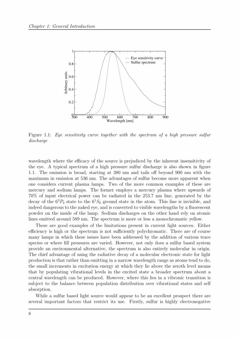
The human eye is sensitive to radiation in the 400-700 nm range and is most receptivearound 555 nm and less so at other wavelengths. First established as a standard in 1924by the international illumination society, the Commission Internationale de l’Eclairage,this sensitivity is quantified by the so-called eye sensitivity curve, which is shown in figure1.1. It is important that a lamp not only produce much light efficiently, but to do soat many wavelengths, i.e. be polychromatic. Furthermore, the distribution of power inthe spectrum should be centered as close to 555 nm as is possible rather than at another
7
Chapter 1: General Introduction
300 400 500 600 700 800 900Wavelength [nm]
0
0.2
0.4
0.6
0.8
1
Arb
itrar
y un
its
Eye sensitivity curveSulfur spectrum
Figure 1.1: Eye sensitivity curve together with the spectrum of a high pressure sulfurdischarge
wavelength where the efficacy of the source is prejudiced by the inherent insensitivity ofthe eye. A typical spectrum of a high pressure sulfur discharge is also shown in figure1.1. The emission is broad, starting at 380 nm and tails off beyond 900 nm with themaximum in emission at 536 nm. The advantages of sulfur become more apparent whenone considers current plasma lamps. Two of the more common examples of these aremercury and sodium lamps. The former employs a mercury plasma where upwards of70% of input electrical power can be radiated in the 253.7 nm line, generated by thedecay of the 63P2 state to the 61S0 ground state in the atom. This line is invisible, andindeed dangerous to the naked eye, and is converted to visible wavelengths by a fluorescentpowder on the inside of the lamp. Sodium discharges on the other hand rely on atomiclines emitted around 589 nm. The spectrum is more or less a monochromatic yellow.
These are good examples of the limitations present in current light sources. Eitherefficiency is high or the spectrum is not sufficiently polychromatic. There are of coursemany lamps in which these issues have been addressed by the addition of various tracespecies or where fill pressures are varied. However, not only does a sulfur based systemprovide an environmental alternative, the spectrum is also entirely molecular in origin.The chief advantage of using the radiative decay of a molecular electronic state for lightproduction is that rather than emitting in a narrow wavelength range as atoms tend to do,the small increments in excitation energy at which they lie above the zeroth level meansthat by populating vibrational levels in the excited state a broader spectrum about acentral wavelength can be produced. However, where this lies in a vibronic transition issubject to the balance between population distribution over vibrational states and selfabsorption.
While a sulfur based light source would appear to be an excellent prospect there areseveral important factors that restrict its use. Firstly, sulfur is highly electronegative
8
and in the plasma state destroys electrodes made from conventional materials. Secondly,pressures above three bar are required to produce visible light which in turn require highpower densities. Finally, in order to optimize light production the bulb has to be of acertain size such that it has be rotated in order that the effects of convection are overcomeand the necessary vapour pressure achieved. The most cost effective option for generatingthe required powers is to use a magnetron, very much like those in microwave ovens andindeed the Solar 1000 was so constructed. The bulb was rotated in a resonant cavityplaced on top of a magnetron. In this thesis the arrangement of a magnetron, waveguide,resonant cavity and rotating bulb is referred to as the sulfur lamp. Despite much initialfanfare and publicity the Solar 1000 is at this time no longer on the market. Nevertheless,what remains interesting is the basis of the lamp, the molecular spectrum produced byS2.
The most important step in studying a new lamp is to understand its energy balance.To achieve this a combined modelling/experimental approach is taken. The integratedenvironment for the construction and execution of plasma models plasimo [6, 7] is usedfor that aspect of the sulfur lamp that is of chief interest, i.e. the spectrum, the effect ofrotation is ignored and the plasma-electric field interaction is treated in the most straight-forward means possible. As is suitable for the first investigations into a new and previouslyunstudied system, the plasma will be modelled as if it were in local thermal equilibrium(LTE). Several atomic lines found in the spectrum were used for validation of the modeland the technique of power interruption was employed to expose any inconsistencies inthe LTE approach.
An issue that quickly arose in the course of the work was that of a lack of fundamentaldata. Not only is little known about sulfur in the plasma state but also the elementaryinteractions between species, that permit studies into more established plasmas for whichcan one rely upon several decades of literature, are also unavailable. This is not a problemrestricted to the current subject. In fact “the dearth of basic data for the simulation ofplasma generation and transport” [8] means that “the lack of fundamental data for themost important chemical species is the largest factor limiting the successful applicationof models of industrial interest” [9]. A secondary goal of this work is to address thislack of data as it applies to the production of radiation from diatomic molecules and thetransport properties of plasma mixtures. This is done in a general way which can beapplied to arbitrary systems and is not sulfur specific.
Thesis outline
In chapter 2 the first LTE model of the lamp is developed. Here, radiation generation istreated semi-classically and a single radiating transition in S2 is chosen. The efficiencyof the lamp due to that single transition is confirmed and the response of the spectrumto operational changes in pressure and power agree with experiment. In chapter 3 theabsolute measurement of several sulfur atomic lines found in the spectrum is used todetermine an effective central temperature. Again an LTE approach was used and theaverage value found of 4100 K agrees very well with the results of the models. In chapter4 the model of the energy balance is developed further and radiation generation is treatedquantum mechanically. The most important addition to the model is the inclusion of S3,UV absorption in which is shown to be responsible for the short wavelength behaviour of
9
Bibliography
the spectrum. In both models the simulated spectrum was deficient at longer wavelengthswhich even the inclusion of several extra radiating states in S2 could not remedy.
The response of the atomic and molecular spectra to an interruption of the suppliedpower are examined in chapter 5, experimentally, via global considerations and with sim-ulations. For the latter the model from chapter 4 was modified. The large inelastic lossesassociated with the production of the molecular states are shown to prevent a substantialdifference between electron and heavy particle temperatures from developing. Further-more, the simulated decay of the spectrum with the LTE model not only predicts thetimescale on which the spectrum decays but also the response as a function of wave-length. The observed decay of the molecular spectrum at longer wavelengths is found tobe too fast if the system were to be ruled by a single temperature. This indicates that theexcitation temperature over the vibrational states in the B state decreases with increasingvibrational quantum number.
Chapters 6 and 7 present two scaling laws. The former shows how the electronic tran-sition dipole moment for a molecular absorption, which is crucial for studying molecularradiation, can be found from that in a similar species while the latter reports a powerlaw in which the high order polarizabilities of atoms and molecules can be found fromthe dipole values. Chapter 8 shows that in conjunction with the results of chapter 7 apolarizability approach for molecular collisions leads to extremely accurate data for vander Waals potentials for a large class of interacting species. Chapter 9 prescribes an fixedset of model potentials that can be used to find the transport properties of LTE plasmamixtures. Several test case plasmas are treated with the approach. Given only informa-tion needed for the composition calculation and species data, which can be determinedfor any atom or molecule, the accuracy of the approach is shown to be high.
The thesis ends with general conclusions in chapter 10.
References
[1] Boumans P W J M, Inductively coupled plasma emission spectroscopy (John Wiley& Sons, New York, 1987)
[2] Liebermann M A and Lichtenberg A J, Principles of plasma discharges and materialsprocessing (John Wiley & Sons, New York, 1994)
[3] Boulos M I, Fauchais P, Pfender E, Thermal plasmas: fundamentals and applications(John Wiley & Sons, New York, 1994)
[4] Waymouth J F, 1971, Electric discharge lamps (The M.I.T. Press, Massachussets,1971)
[5] Ury M G, Wood C H, Dolan J T, Lamp including sulfur, USA Patent # 5,404,076(1995)
[6] Janssen G M, van Dijk J, Benoy D A, Tas M A, Burm K T A L, Goedheer W J, vander Mullen J J A M and Schram D C, Plasma Sources Sci. Technol. 8, 1 (1999)
10
Bibliography
[7] van Dijk J, Modelling of plasma light sources : an object-oriented approach, PhDThesis, Eindhoven University of Technology, The Netherlands, ISBN 90-386-1819-0(2001)
[8] National Research Council, Plasma Processing of Materials: Scientific Opportunitiesand Technological Challenges (National Academy Press, Washington, D.C., 1991)
[9] National Research Council, Database Needs for Modelling and Simulation of PlasmaProcessing (National Academy Press, Washington, D.C., 1996) ISBN 0-309-05591-1
11

CHAPTER 2
A self consistent LTE model of a microwave driven, high-pressure
sulfur lamp
A one dimensional LTE model of a microwave driven sulfur lamp is presented to aid ourunderstanding of the discharge. The energy balance of the lamp is determined by Ohmicinput on one hand and transport due to conductive heat transfer and molecular radiationon the other. We discuss the origin of, and operational trends in the spectrum, presentthe model and discuss how the material properties of the plasma are determined. Notonly are temperature profiles and electric field strengths simulated but also the spectrumof the lamp from 300 nm to 900 nm under various conditions of input power and lampfilling pressure. We show that simulated spectra demonstrate observed trends and thatradiated power increases linearly with input power as is also found from experiment.
C. W. Johnston, H. W. P. van der Heijden, G. M. Janssen,
J. van Dijk and J. J. A. M. van der Mullen
J. Phys. D: Appl. Phys. 35, 342-351 2002
13
Chapter 2: A self consistent LTE model . . .
2.1 Introduction
There are essentially three criteria that a lighting application should fulfill; good colouring,high efficiency and longevity. However, the first two of these are often mutually exclusive.A familiar example is the low pressure mercury lamp in which more than 70% of inputpower is converted into UV photons. The overall efficiency of the lamp is reduced by theneed to convert these quanta into visible photons via the fluorescent coating. The issue oflamp lifespan has been addressed in recent years by the use of electrode-less configurationssuch as Osram’s Endura and Philips’ QL lamp. However, the light emitting particleremains mercury. which brings us to a fourth criterion, of ever increasing importance,that lamp fillings should have little environmental impact. Mercury, present in mostplasma lamps, is a notorious pollutant.
Alongside the well known lamp fillings and power in-coupling techniques, Fusion Light-ing Systems produced the Solar 1000 in 1995, a microwave driven high pressure lamp withsulfur as the radiating medium. This lamp displays all of the properties listed above.Firstly it has excellent colouring; the spectrum of the lamp appears continuous and over-laps the eye-sensitivity curve very well. Little of the spectrum lies in the UV and no morethan a few percent of total spectral power is found in the infrared. Secondly its radiativeefficiency is very high; up to 70% of power coupled into the plasma can be emitted as(visible) light. Thirdly, since there are no electrodes in the bulb and the wall is unaffectedby the plasma, the bulb is expected to have a long lifetime. Finally, sulfur is much lessenvironmentally damaging than mercury.
Nevertheless, there are some disadvantages. Hot re-ignition is a problem due to thehigh vapour pressure during operation. Also the lifetime and efficiency of the magnetronpower supply are low which reduces the overall system efficacy and lifespan; in fact themagnetron would have to be replaced more often than the bulb. Another factor is thatthe lamp contains moving parts: the bulb itself needs to be rotated.
However, despite its striking difference to conventional lamps, its high plasma effi-ciency and good colouring are indisputable. Thus such a new lamp, with a radiatingmedium previously unknown as such, presents the challenge of identifying the phenomenathat result in its unique properties. Insight gained in studying the sulfur lamp couldsubsequently lead to the better understanding of other molecular lamps.
In the first instance an experimental approach to understanding the lamp is hamperedby several factors. A consequence of the lamps large spectral power density and the factthat the bulb rotates is that standard laser diagnostics would be rather involved. Alsoidentification of molecular vibrational/rotational structure in the spectrum is very difficultdue to the high operating pressure where there are ca. 106 overlapping lines. Therefore,in light of the many advantages associated with sulfur discharges, the lack of detailedinformation on its internal processes and the inherent difficulty of applying standarddiagnostics, we attempt to explain the discharge by constructing a numerical model forthe system. To facilitate the construction of the model we use the plasma simulationtoolkit plasimo [1, 2], which provides the framework for the plasma properties, such asthermal and electrical conductivity, used in the transport and energy balances which aresolved subject to user definable boundary conditions.
This paper is structured as follows: firstly, we examine the origin of the spectrum andoperational trends. After reviewing the state of the art, we concentrate on the model itself
14

2.2 Origin and operational trends in the spectrum
1.4 1.6 1.8 2.0 2.2 2.4 2.60
1
2
3
4
5
X3Σ-
g
B3Σ-
u
452 nm
1u
re=1.889
re=2.150
v'=9
v''=10
v''=20
v''=30
E [e
V]
r [Å]
1 2 3 4 5 60
1
2
3
4
5
6
7
8
B3Σ-
u
X3Σ-
g
r [Å]
E [e
V]
Figure 2.1: Left: potential curves for the ground and excited states [4]. The B excitedstate is pre-dissociated at v = 9 by the Π, an unbound state. Right: potential curvescompleted using an enhanced Morse potential to the available data.
and discuss the electromagnetic and radiation generation/transport approaches. Then wechoose which species to include in the model and demonstrate how we calculate the electri-cal and thermal conductivity of the plasma. Finally we present the results of simulations,examining the behaviour of various field variables as functions of power and pressure, andfinish with our conclusions.
2.2 Origin and operational trends in the spectrum
An apparatus used to ignite, maintain and measure the lamps spectrum has already beendescribed elsewhere [3]. Despite some differences with the Solar 1000 the two systems areessentially the same: a magnetron introduces EM radiation at 2.45 GHz into a waveguideto which a resonator is attached. The main difference between the two is the resonatorused. In our case it is a hemi-ellipse which supports a TM101 mode, while the Fusion lampemploys a cylindrical cavity that resonates in the TE111 mode.
2.2.1 Origin of the spectrum
Radiation produced by the sulfur lamp has been identified as primarily arising fromtransitions between the molecular excited state, B3Σ−
u , and the ground state, X3Σ−g [4].
There may also be a contribution to the spectrum from transitions between the 1Πu andthe ground state. However this is an unbound-bound transition which is excluded fromthe model.
Only part of the Potential Energy Curve (PEC) for the molecular ground state isknown. Given the dissociation energy and the energy spacing of the lowest vibrationallevels, there ought to be 60 vibrational states. However, only 30 have been measured.
15
Chapter 2: A self consistent LTE model . . .
300 400 500 600 700 800 900Wavelength [nm]
0
0.5
1
1.5
2
2.5
Pow
er [W
/nm
]
1000 W [658]810 W [580]720 W [500]630 W [400]540 W [317]450 W [222]360 W [131]
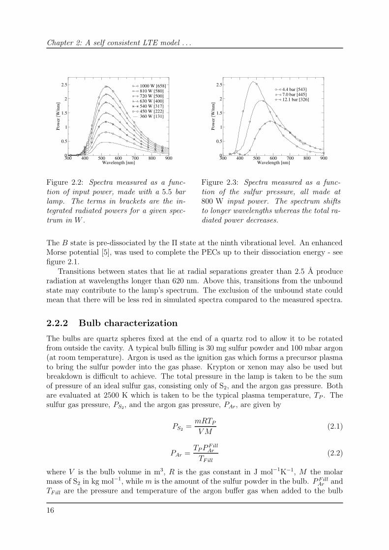
Figure 2.2: Spectra measured as a func-tion of input power, made with a 5.5 barlamp. The terms in brackets are the in-tegrated radiated powers for a given spec-trum in W .
300 400 500 600 700 800 900Wavelength [nm]
0
0.5
1
1.5
2
2.5
Pow
er [W
/nm
]
4.4 bar [543]7.0 bar [445]12.1 bar [326]
Figure 2.3: Spectra measured as a func-tion of the sulfur pressure, all made at800 W input power. The spectrum shiftsto longer wavelengths whereas the total ra-diated power decreases.
The B state is pre-dissociated by the Π state at the ninth vibrational level. An enhancedMorse potential [5], was used to complete the PECs up to their dissociation energy - seefigure 2.1.
Transitions between states that lie at radial separations greater than 2.5 A produceradiation at wavelengths longer than 620 nm. Above this, transitions from the unboundstate may contribute to the lamp’s spectrum. The exclusion of the unbound state couldmean that there will be less red in simulated spectra compared to the measured spectra.
2.2.2 Bulb characterization
The bulbs are quartz spheres fixed at the end of a quartz rod to allow it to be rotatedfrom outside the cavity. A typical bulb filling is 30 mg sulfur powder and 100 mbar argon(at room temperature). Argon is used as the ignition gas which forms a precursor plasmato bring the sulfur powder into the gas phase. Krypton or xenon may also be used butbreakdown is difficult to achieve. The total pressure in the lamp is taken to be the sumof pressure of an ideal sulfur gas, consisting only of S2, and the argon gas pressure. Bothare evaluated at 2500 K which is taken to be the typical plasma temperature, TP . Thesulfur gas pressure, PS2, and the argon gas pressure, PAr, are given by
PS2 =mRTP
VM(2.1)
PAr =TPP
FillAr
TFill
(2.2)
where V is the bulb volume in m3, R is the gas constant in J mol−1K−1, M the molarmass of S2 in kg mol−1, while m is the amount of the sulfur powder in the bulb. P Fill
Ar andTFill are the pressure and temperature of the argon buffer gas when added to the bulb
16
2.3 State of the art
(at room temperature). The typical operating pressure is 6 bar, 5 bar due to sulfur and1 bar due to argon. However, from now on when we refer to a lamp we do this by thesulfur pressure alone at TP . In our simulations the operating buffer gas pressure, PAr, isalways 1 bar and the lamp diameter 36 mm.
2.2.3 Spectral trends
In figures 2.2 and 2.3 spectra are shown as a function of input power and pressure. Thefollowing trends can be observed
• Power: at a fixed filling pressure, an increase in power causes a linear increase in thespectral radiant power (see figure 2.2) - there is almost no shift in the wavelengthof the spectral maximum.
• Pressure: the spectrum shifts to the red with increasing sulfur pressure as can beseen in figure 2.3. The radiated power also decreases above 4 bars.
2.3 State of the art
Most of what is reported concerning microwave powered high pressure sulfur lamps can befound in patent literature and is appropriate to that medium. As far as we are aware theonly quantitative information published, has been by van Dongen [3]. Here we summarizethe principal conclusions from these experiments.
The temperature on the bulb’s outer wall was measured with an infrared camera andwas found to be between 1000 K and 1200 K for most situations. An estimate of thecentral temperature was made by examining the spectrum at 676 nm, the wavelength atwhich atomic sulfur has a non self-absorbing line. Since this line could not be detectedabove the molecular background, the maximum temperature at the centre of the lampwas estimated to be 5500 K. The electric field at the cavity wall was measured by placinga metal probe just inside it and the field strength at the lamps position could then bedetermined. Under most operating conditions the electric field strength was found to be400 V/cm [3]. With this knowledge of the electric field, power losses in the cavity wereestimated and the power balance for the whole system was completed. The main resultwas that about 70% of power generated by the magnetron was coupled into the plasma.
2.4 The Model
2.4.1 Simplifications
In order to reduce the complexity and dimensionality of the model, we present here theassumptions and simplifications made in the description of the system. Firstly, we assumeLTE, which is a standard assertion applied to high pressure lamps. This may seem adrastic assumption given the huge radiation losses. However, the equilibrium restoringprocesses are extremely fast due the high pressure - the electron S2 collision frequency is
17
Chapter 2: A self consistent LTE model . . .
ca. 10 GHz. In the first instance we assume that this is sufficient to allow us to proceedas if the lamp were in LTE.
Secondly we discount convective transport as generated by rotation and gravity. Thusthe system is a closed one for which a Navier-Stokes approach is not needed. The assump-tion of LTE precludes the solution of particle balances and leaves us with a 1-D energyequation, which we discuss now.
2.4.2 The energy balance
The energy balance which describes the competition between Ohmic dissipation and theenergy transport due to conduction and radiation can be written as:
1
2σ(r)E(r)2 =
1
r2
∂
∂r(r2λ
∂
∂rT (r)) +
∫ ∞
04π[jν(r) −
1
4π
∫ ∞
0κν(r)IνdΩ
]dν (2.3)
The thermal conductivity, λ, and the electrical conductivity, σ, will be discussed in sec-tions 2.5.3 and 2.5.4. We will begin by detailing how we calculate the electric field strength,then discuss radiation generation and transport and finally illustrate the various steps inthe iterative process.
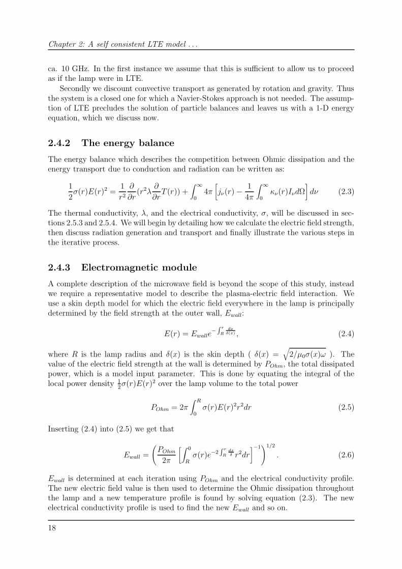
2.4.3 Electromagnetic module
A complete description of the microwave field is beyond the scope of this study, insteadwe require a representative model to describe the plasma-electric field interaction. Weuse a skin depth model for which the electric field everywhere in the lamp is principallydetermined by the field strength at the outer wall, Ewall:
E(r) = Ewalle−∫ r
R
dxδ(x) , (2.4)
where R is the lamp radius and δ(x) is the skin depth ( δ(x) =√
2/µ0σ(x)ω ). Thevalue of the electric field strength at the wall is determined by POhm, the total dissipatedpower, which is a model input parameter. This is done by equating the integral of thelocal power density 1
2σ(r)E(r)2 over the lamp volume to the total power
POhm = 2π∫ R
0σ(r)E(r)2r2dr (2.5)
Inserting (2.4) into (2.5) we get that
Ewall =
(POhm
2π
[∫ 0
Rσ(r)e−2
∫ r
R
dxδ r2dr
]−1)1/2
. (2.6)
Ewall is determined at each iteration using POhm and the electrical conductivity profile.The new electric field value is then used to determine the Ohmic dissipation throughoutthe lamp and a new temperature profile is found by solving equation (2.3). The newelectrical conductivity profile is used to find the new Ewall and so on.
18
2.4 The Model
2.4.4 Generation and transport of radiation
Since we are dealing with a plasma for which a considerable part of the input poweris converted into radiation (it is a lamp after all) it is extremely important to describethe generation and transport of radiation as well as possible. However, a full quantummechanical description of the origin of the spectrum is out of question. We have alreadymentioned that the spectrum is the result of the overlap of many thousands of lines thatresult from rovibrational transitions in the S2 molecule. This is an extremely complextask since the equation of radiative transport must be solved for the entire lamp, for about500,000 frequency intervals during each iteration of the energy balance.
Radiation generation
Our approach in overcoming the problem sketched above is to employ an approximatetechnique for the generation of molecular radiation. It is based on the Classical Franck-Condon Principle (CFCP), and is a means to determine jν and κν as smooth functionsof frequency. We present only an overview of the approach here, see [6] for a detaileddiscussion.
The generation of molecular radiation can be seen in analogy with that of atomic lineradiation for which the emission coefficient is given by
jν = n(Q)hν
4πA(Q,P )φν(ν) (2.7)
Here n(Q) is the density of the radiating upper state, A(Q,P ) the transition probabilityand φν(ν) is the line profile.
Classically, molecular radiation can be seen as a high pressure limit of atomic radiation,where the species density is sufficient for internuclear potentials to become relevant and theline-profile is subsequently connected to the distribution of molecular states. Transitionsbetween these states are dictated by the CFCP, in which there is no loss of atomic kineticenergy and bound atoms are stationary during a transition. Thus, the energy of an emittedphoton is determined solely by the change in potential energy where the transition takesplace at a fixed internuclear distance. Thus, the energy of a photon can be written interms of internuclear distance r;
hν(r) = VQ(r) − VP (r).
Here VQ and Vp are the potential energies of the upper and lower states. The line profileof radiation emitted in the range r . . . r + ∆r is therefore
φ(ν) =1
dν=
(∣∣∣∣∣dν(r)
dr
∣∣∣∣∣ dr)−1
(2.8)
Using equation (2.11) for the density of the molecular state in terms of its constituentatoms we get the molecular analog to equation (2.7)
jν(r) = ηAηB
(h√
2πµkBT
)1/3
exp
(VQ(r)
kBT
)hνAQP (ν(r))
4π
4πr2
|dν(r)/dr| (2.9)
19
Chapter 2: A self consistent LTE model . . .
1000.0 2000.0 3000.0 4000.0 5000.0 6000.0Temperature[K]
200
300
400
500
600
700
800
900
[nm
]
1
1
110
10
101x10 2
1x10²
1x10 31x103
5x10³
5x10³
5x1033x104
3x1048x104
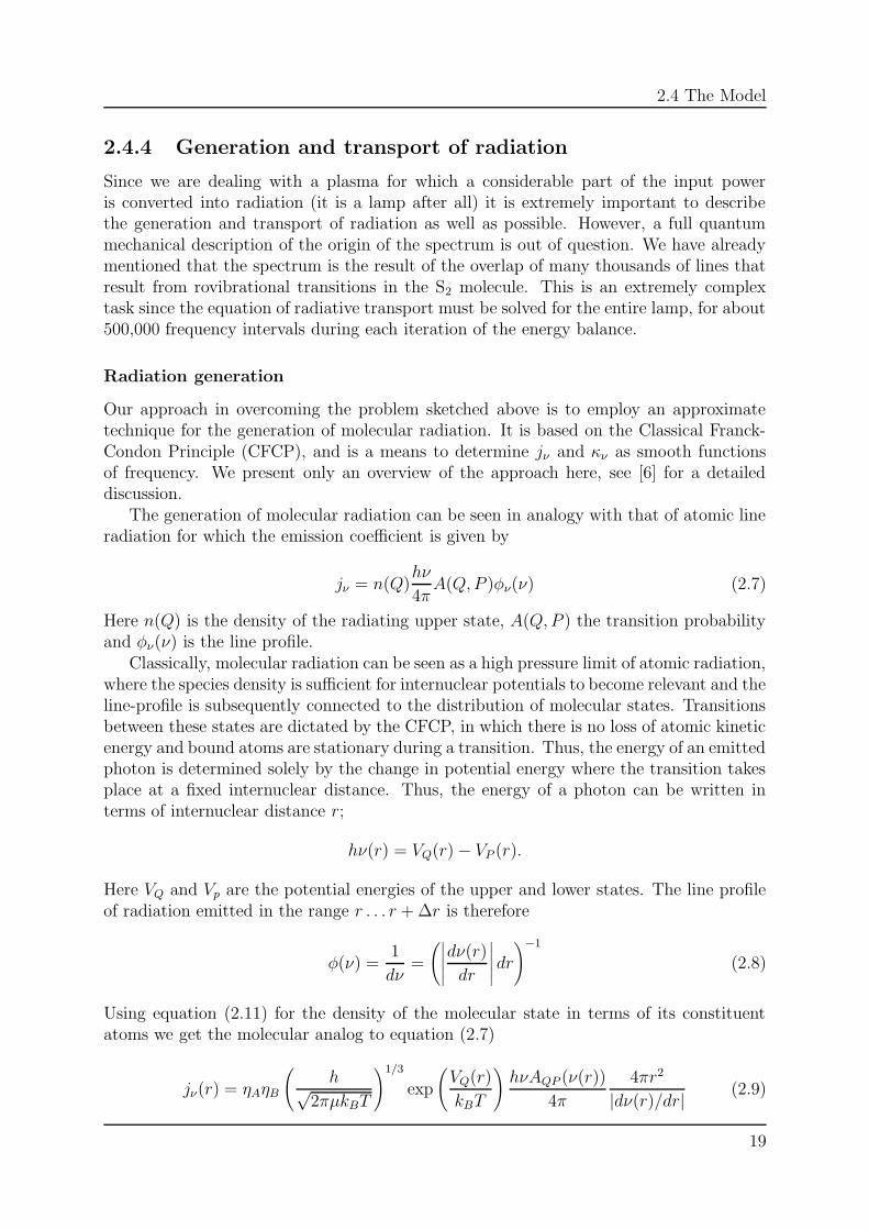
Figure 2.4: Spectral absorption coefficient, κ[m−1] for the B → X transition in the sulfurmolecule as a function of temperature and wavelength. The S2 densities are determinedfrom a full composition calculation (see figure 2.5). The plasma is optically thick between200 and 400 nm and almost fully transparent above 550 nm. As temperature increasesthere are less and less molecules in lower rovibrational states and hence the values for κabove 5000 K are lower.
The spectral absorption coefficient can be found via the Planck formula and is
κν(r) = ηAηBc2AQP (ν(r))
8πν2(r)
4πr2
|dν(r)/dr|
[exp
(−VP (r)
kBT
)], (2.10)
where we have omitted the stimulated emission term. The electronic transition probabilityis given by
A =16π3ν3
3ε0hc3|M(r)|2,
where M(r) is the electronic transition dipole moment as a function of internuclear sep-aration obtained from [8]. In figure 2.4 the spectral absorption coefficient is shown as afunction of temperature and wavelength for the BΣ−
u → XΣ−g transition calculated using
equation (2.10). The plasma is optically thick for quanta with wavelengths below 400nm and almost fully transparent for radiation above 600 nm. In between the opacity ofthe plasma is semi-thick, which has important consequences for the way in which we dealwith the transport of radiation. If the radiation produced by the lamp was completelyoptically open, then the radiative contribution to the energy balance could be treated as apure loss term. On the other hand, if the radiation was optically thick, the energy balancecontribution could be treated as a heat conduction term. However, neither of these is thecase and as such the local energy balance will be affected by the non-local production oflight and a special approach is needed.
20
2.4 The Model
Transport of radiation
Since the production of radiation is isotropic whereas the rate of local absorption isdependent on the direction from which the light came from equation (2.3), the transport ofradiation is three dimensional for the current case, two spatial coordinates and a frequencycoordinate.
In order to deal with this transport irrespective of opacity, we employ a ray tracingmethod. Rays enter the plasma with Iν = 0, and intensity along them increases due tolocal emission; transport is realized through absorption, exchanging energy from the rayto the plasma. In fact we integrate along the lines and solve the equation of radiationtransfer:
dIν = (jν − κνIν)ds.
The net accumulation of intensity along a ray allows the radiative term in the energybalance to be determined. The absorption term in the energy balance as given by∫v κ∫4π Iν(r)dΩ depends on the action of these rays. Since we have a finite number of
rays passing through the plasma, the integration over solid angles is approximated as:∫
4πIνdΩ ≈
∑
lines
Iν∆Ωline.
The subject of radiation generation and transfer is very involved and deserves a dedicatedforum. As such we have tried to demonstrate the essence of the techniques we have usedand direct the reader to more in-depth discussions on these topics [6, 7].
2.4.5 Boundary conditions
Two boundary conditions are applied in the model. Firstly there is no temperaturegradient at r = 0, i.e. ∂T/∂n = 0, where n is normal to the boundary in question.Secondly, a Neumann condition is applied stating that the heat flux at the wall volumeequals that through the wall, i.e.
λplasma∂T
∂n
∣∣∣∣∣wall
=λwall
δwall(Tinner − Touter)
where δwall, λwall, Tinner, and Touter are the wall thickness, thermal conductivity of thewall material and the temperature at the inner and outside wall respectively. We fix thewall temperature to the measured value of 1100 K and wall thickness to 2 mm for allsimulations.
2.4.6 Iteration procedure
As we have a non-local radiative energy term in the energy balance, the iteration procedurerequires an extra step to determine the local radiative contribution. The simulationsproceed as follows:
• Start with a temperature profile which fixes thermal and electrical conductivity.
• Determine the electric field.
21
Chapter 2: A self consistent LTE model . . .
1000 2000 3000 4000 5000 6000Temperature [K]
1018
1019
1020
1021
1022
1023
1024
1025
1026
Den
sity
[m-3
]S2Ar
S
S-
S2-
S2+
S+
e
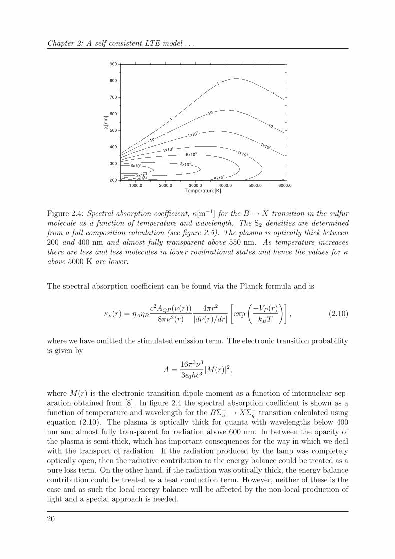
Figure 2.5: Composition of a 5 bar sulfur plasma with 1 bar of argon buffer gas. Below3700 K we have essentially a molecular plasma with a very low ionization degree ≈ 10−5.S+
2 is the dominant ion up to 5000 K.
• Compute j and κ
– perform ray tracing in several directions
– determine Iν at each point in the plasma, from a number of directions
– perform integration over all solid angles
• Determine net contribution of radiation to the energy balance for each control vol-ume
• Solve the energy balance equation itself which provides a new temperature profile
• Determine the electric field . . .
2.5 Material properties
Here we discuss how the calculation of the composition, thermal and electrical conduc-tivity of the plasma is carried out. However, we begin by discussing the choice of speciesand reactions that will be included in the model.
2.5.1 Reactions and species
The wall temperature has been measured with an infrared camera and is always around1100 K. We do not treat the sulfur trimer, S3, and work from the premise that theheaviest sulfur species is the dimer, S2, which it is the only species responsible for the
22
2.5 Material properties
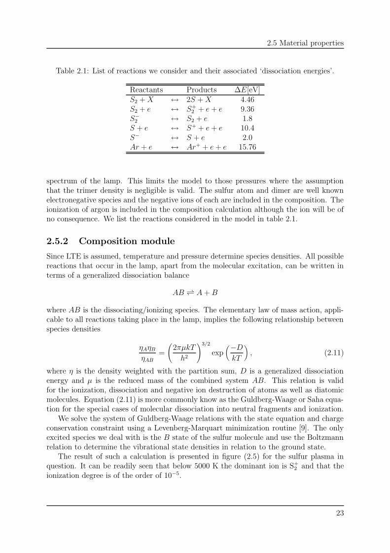
Table 2.1: List of reactions we consider and their associated ‘dissociation energies’.
Reactants Products ∆E[eV]S2 +X ↔ 2S +X 4.46S2 + e ↔ S+
2 + e+ e 9.36S−
2 ↔ S2 + e 1.8S + e ↔ S+ + e+ e 10.4S− ↔ S + e 2.0Ar + e ↔ Ar+ + e+ e 15.76
spectrum of the lamp. This limits the model to those pressures where the assumptionthat the trimer density is negligible is valid. The sulfur atom and dimer are well knownelectronegative species and the negative ions of each are included in the composition. Theionization of argon is included in the composition calculation although the ion will be ofno consequence. We list the reactions considered in the model in table 2.1.
2.5.2 Composition module
Since LTE is assumed, temperature and pressure determine species densities. All possiblereactions that occur in the lamp, apart from the molecular excitation, can be written interms of a generalized dissociation balance
AB A+B
where AB is the dissociating/ionizing species. The elementary law of mass action, appli-cable to all reactions taking place in the lamp, implies the following relationship betweenspecies densities
ηAηB
ηAB
=
(2πµkT
h2
)3/2
exp(−DkT
), (2.11)
where η is the density weighted with the partition sum, D is a generalized dissociationenergy and µ is the reduced mass of the combined system AB. This relation is validfor the ionization, dissociation and negative ion destruction of atoms as well as diatomicmolecules. Equation (2.11) is more commonly know as the Guldberg-Waage or Saha equa-tion for the special cases of molecular dissociation into neutral fragments and ionization.
We solve the system of Guldberg-Waage relations with the state equation and chargeconservation constraint using a Levenberg-Marquart minimization routine [9]. The onlyexcited species we deal with is the B state of the sulfur molecule and use the Boltzmannrelation to determine the vibrational state densities in relation to the ground state.
The result of such a calculation is presented in figure (2.5) for the sulfur plasma inquestion. It can be readily seen that below 5000 K the dominant ion is S+
2 and that theionization degree is of the order of 10−5.
23
Chapter 2: A self consistent LTE model . . .
1000 2000 3000 4000 5000 6000Temperature [K]
0
0.2
0.4
0.6
0.8
1
λ [W
/mK
]
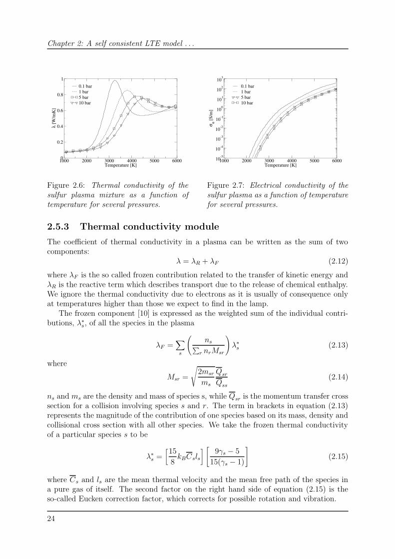
0.1 bar1 bar5 bar10 bar
Figure 2.6: Thermal conductivity of thesulfur plasma mixture as a function oftemperature for several pressures.
1000 2000 3000 4000 5000 6000Temperature [K]
10-5
10-4
10-3
10-2
10-1
100
101
102
103
σ e[S
/m]
0.1 bar1 bar5 bar10 bar
Figure 2.7: Electrical conductivity of thesulfur plasma as a function of temperaturefor several pressures.
2.5.3 Thermal conductivity module
The coefficient of thermal conductivity in a plasma can be written as the sum of twocomponents:
λ = λR + λF (2.12)
where λF is the so called frozen contribution related to the transfer of kinetic energy andλR is the reactive term which describes transport due to the release of chemical enthalpy.We ignore the thermal conductivity due to electrons as it is usually of consequence onlyat temperatures higher than those we expect to find in the lamp.
The frozen component [10] is expressed as the weighted sum of the individual contri-butions, λ∗s, of all the species in the plasma
λF =∑
s
(ns∑
r nrMsr
)λ∗s (2.13)
where
Msr =
√2msr
ms
Qsr
Qss
(2.14)
ns and ms are the density and mass of species s, while Qsr is the momentum transfer crosssection for a collision involving species s and r. The term in brackets in equation (2.13)represents the magnitude of the contribution of one species based on its mass, density andcollisional cross section with all other species. We take the frozen thermal conductivityof a particular species s to be
λ∗s =[15
8kBCsls
] [9γs − 5
15(γs − 1)
](2.15)
where Cs and ls are the mean thermal velocity and the mean free path of the species ina pure gas of itself. The second factor on the right hand side of equation (2.15) is theso-called Eucken correction factor, which corrects for possible rotation and vibration.
24
2.5 Material properties
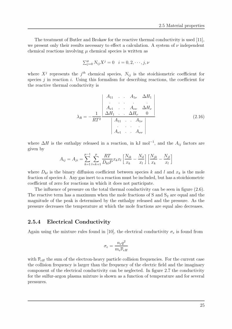
The treatment of Butler and Brokaw for the reactive thermal conductivity is used [11],we present only their results necessary to effect a calculation. A system of ν independentchemical reactions involving µ chemical species is written as
∑µj=0NijX
j = 0 i = 0, 2, · · · , j, ν
where Xj represents the jth chemical species, Nij is the stoichiometric coefficient forspecies j in reaction i. Using this formalism for describing reactions, the coefficient forthe reactive thermal conductivity is
λR = − 1
RT 2
∣∣∣∣∣∣∣∣∣
A11 . . A1ν ∆H1
. . . . .Aν1 . . Aνν ∆Hν
∆H1 . . ∆Hν 0
∣∣∣∣∣∣∣∣∣∣∣∣∣∣∣∣
A11 . . A1ν
. . . .Aν1 . . Aνν
∣∣∣∣∣∣∣
(2.16)
where ∆H is the enthalpy released in a reaction, in kJ mol−1, and the Aij factors aregiven by
Aij = Aji =µ−1∑
k=1
µ∑
l=k+1
RT
DklPxkxl
[Nik
xk
− Nil
xl
] [Njk
xk
− Njl
xl
]
where Dkl is the binary diffusion coefficient between species k and l and xk is the molefraction of species k. Any gas inert to a reaction must be included, but has a stoichiometriccoefficient of zero for reactions in which it does not participate.
The influence of pressure on the total thermal conductivity can be seen in figure (2.6).The reactive term has a maximum when the mole fractions of S and S2 are equal and themagnitude of the peak is determined by the enthalpy released and the pressure. As thepressure decreases the temperature at which the mole fractions are equal also decreases.
2.5.4 Electrical Conductivity
Again using the mixture rules found in [10], the electrical conductivity σe is found from
σe =neq
2
meνeH
with νeH the sum of the electron-heavy particle collision frequencies. For the current casethe collision frequency is larger than the frequency of the electric field and the imaginarycomponent of the electrical conductivity can be neglected. In figure 2.7 the conductivityfor the sulfur-argon plasma mixture is shown as a function of temperature and for severalpressures.
25
Chapter 2: A self consistent LTE model . . .
0 3 6 9 12 15 18Radius [mm]
1000
2000
3000
4000
Tem
pera
ture
[K]
400 W500 W800 W1000 W
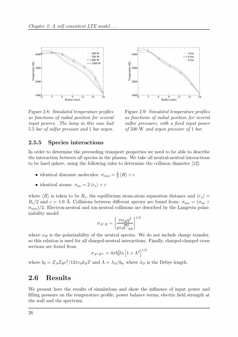
Figure 2.8: Simulated temperature profilesas functions of radial position for severalinput powers. The lamp in this case had5.5 bar of sulfur pressure and 1 bar argon.
0 3 6 9 12 15 18Radius [mm]
1000
2000
3000
4000
Tem
pera
ture
[K]
4 bar6 bar8 bar
Figure 2.9: Simulated temperature profilesas functions of radial position for severalsulfur pressures, with a fixed input powerof 500 W and argon pressure of 1 bar.
2.5.5 Species interactions
In order to determine the preceeding transport properties we need to be able to describethe interaction between all species in the plasma. We take all neutral-neutral interactionsto be hard sphere, using the following rules to determine the collision diameter [12]:
• identical diatomic molecules: σmm = 43〈R〉 + c
• identical atoms: σaa = 2 〈rx〉 + c
where 〈R〉 is taken to be Re, the equilibrium atom-atom separation distance and 〈rx〉 =Re/2 and c = 1.6 A. Collisions between different species are found from: σam = (σaa +σmm)/2. Electron-neutral and ion-neutral collisions are described by the Langevin polar-izability model
σA+B =
[παBq
2
µε0C2AB
]1/2
where αB is the polarizability of the neutral species. We do not include charge transfer,so this relation is used for all charged-neutral interactions. Finally, charged-charged crosssections are found from
σA+B+ = 4πb20ln[1 + Λ2
]1/2
where b0 = ZAZBe2/12πε0kBT and Λ = λD/b0, where λD is the Debye length.
2.6 Results
We present here the results of simulations and show the influence of input power andfilling pressure on the temperature profile, power balance terms, electric field strength atthe wall and the spectrum.
26
2.6 Results
0 3 6 9 12 15 18Radius [mm]
-0.5
0.0
0.5
1.0
1.5
Rad
ial p
ower
den
sity
[105 W
/m] POhm
PRadPThermal
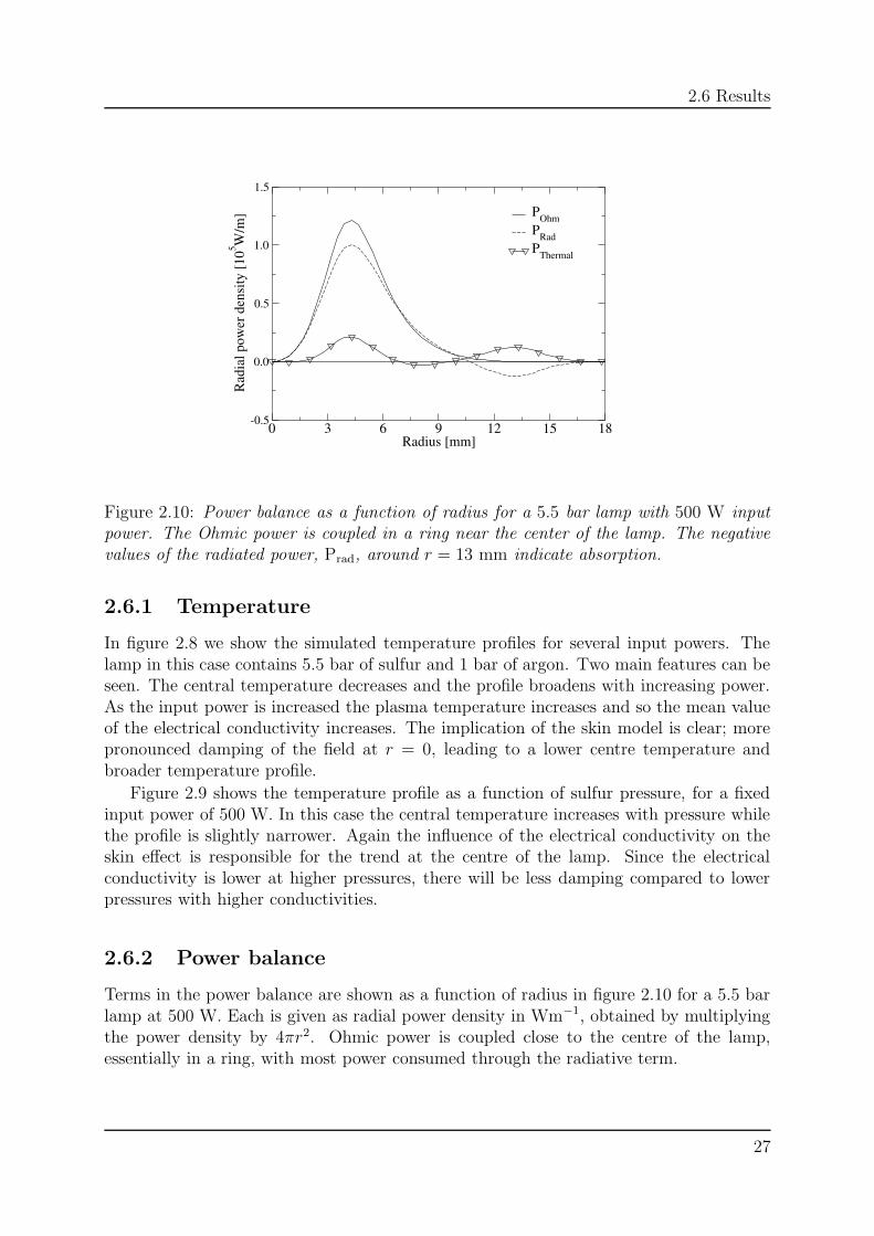
Figure 2.10: Power balance as a function of radius for a 5.5 bar lamp with 500 W inputpower. The Ohmic power is coupled in a ring near the center of the lamp. The negativevalues of the radiated power, Prad, around r = 13 mm indicate absorption.
2.6.1 Temperature
In figure 2.8 we show the simulated temperature profiles for several input powers. Thelamp in this case contains 5.5 bar of sulfur and 1 bar of argon. Two main features can beseen. The central temperature decreases and the profile broadens with increasing power.As the input power is increased the plasma temperature increases and so the mean valueof the electrical conductivity increases. The implication of the skin model is clear; morepronounced damping of the field at r = 0, leading to a lower centre temperature andbroader temperature profile.
Figure 2.9 shows the temperature profile as a function of sulfur pressure, for a fixedinput power of 500 W. In this case the central temperature increases with pressure whilethe profile is slightly narrower. Again the influence of the electrical conductivity on theskin effect is responsible for the trend at the centre of the lamp. Since the electricalconductivity is lower at higher pressures, there will be less damping compared to lowerpressures with higher conductivities.
2.6.2 Power balance
Terms in the power balance are shown as a function of radius in figure 2.10 for a 5.5 barlamp at 500 W. Each is given as radial power density in Wm−1, obtained by multiplyingthe power density by 4πr2. Ohmic power is coupled close to the centre of the lamp,essentially in a ring, with most power consumed through the radiative term.
27
Chapter 2: A self consistent LTE model . . .
0 3 6 9 12 15 18Radius [mm]
0
0.5
1
1.5
2
Rad
ial p
ower
den
sity
[W/m
] 400 W500 W800 W1000 W
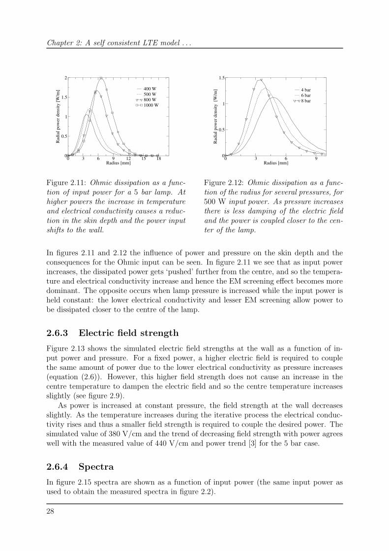
Figure 2.11: Ohmic dissipation as a func-tion of input power for a 5 bar lamp. Athigher powers the increase in temperatureand electrical conductivity causes a reduc-tion in the skin depth and the power inputshifts to the wall.
0 3 6 9Radius [mm]
0
0.5
1
1.5
Rad
ial p
ower
den
sity
[W
/m] 4 bar
6 bar8 bar
Figure 2.12: Ohmic dissipation as a func-tion of the radius for several pressures, for500 W input power. As pressure increasesthere is less damping of the electric fieldand the power is coupled closer to the cen-ter of the lamp.
In figures 2.11 and 2.12 the influence of power and pressure on the skin depth and theconsequences for the Ohmic input can be seen. In figure 2.11 we see that as input powerincreases, the dissipated power gets ‘pushed’ further from the centre, and so the tempera-ture and electrical conductivity increase and hence the EM screening effect becomes moredominant. The opposite occurs when lamp pressure is increased while the input power isheld constant: the lower electrical conductivity and lesser EM screening allow power tobe dissipated closer to the centre of the lamp.
2.6.3 Electric field strength
Figure 2.13 shows the simulated electric field strengths at the wall as a function of in-put power and pressure. For a fixed power, a higher electric field is required to couplethe same amount of power due to the lower electrical conductivity as pressure increases(equation (2.6)). However, this higher field strength does not cause an increase in thecentre temperature to dampen the electric field and so the centre temperature increasesslightly (see figure 2.9).
As power is increased at constant pressure, the field strength at the wall decreasesslightly. As the temperature increases during the iterative process the electrical conduc-tivity rises and thus a smaller field strength is required to couple the desired power. Thesimulated value of 380 V/cm and the trend of decreasing field strength with power agreeswell with the measured value of 440 V/cm and power trend [3] for the 5 bar case.
2.6.4 Spectra
In figure 2.15 spectra are shown as a function of input power (the same input power asused to obtain the measured spectra in figure 2.2).
28
2.6 Results
400 600 800 1000Power [W]
300
350
400
450
Ele
ctri
c fi
eld
stre
ngth
[V/c
m]
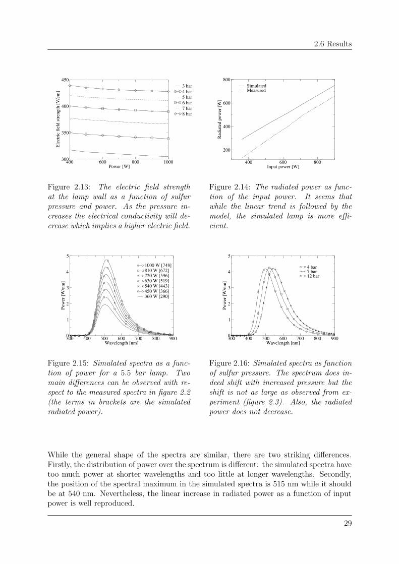
3 bar4 bar5 bar6 bar7 bar8 bar
Figure 2.13: The electric field strengthat the lamp wall as a function of sulfurpressure and power. As the pressure in-creases the electrical conductivity will de-crease which implies a higher electric field.
400 600 800Input power [W]
200
400
600
800
Rad
iate
d po
wer
[W]
Simulated Measured
Figure 2.14: The radiated power as func-tion of the input power. It seems thatwhile the linear trend is followed by themodel, the simulated lamp is more effi-cient.
300 400 500 600 700 800 900Wavelength [nm]
0
1
2
3
4
5
Pow
er [W
/nm
]
1000 W [748]810 W [672]720 W [596]630 W [519]540 W [443]450 W [366]360 W [290]
Figure 2.15: Simulated spectra as a func-tion of power for a 5.5 bar lamp. Twomain differences can be observed with re-spect to the measured spectra in figure 2.2(the terms in brackets are the simulatedradiated power).
300 400 500 600 700 800 900Wavelength [nm]
0
1
2
3
4
5
Pow
er [W
/nm
]
4 bar7 bar12 bar
Figure 2.16: Simulated spectra as functionof sulfur pressure. The spectrum does in-deed shift with increased pressure but theshift is not as large as observed from ex-periment (figure 2.3). Also, the radiatedpower does not decrease.
While the general shape of the spectra are similar, there are two striking differences.Firstly, the distribution of power over the spectrum is different: the simulated spectra havetoo much power at shorter wavelengths and too little at longer wavelengths. Secondly,the position of the spectral maximum in the simulated spectra is 515 nm while it shouldbe at 540 nm. Nevertheless, the linear increase in radiated power as a function of inputpower is well reproduced.
29
Chapter 2: A self consistent LTE model . . .
A further judge of the model is to examine the radiated power as a function of inputpower, which can be found in figure 2.14. While the general trend is followed the lampwe simulate is more efficient, producing consistently 100 - 150 W more light.
2.6.5 Sensitivity analysis
Since the spectral emission and absorption coefficients are fixed due to the radiationmodel we used, we may only vary the material properties in the energy balance (all wereincreased and decreased by a factor 2):
• electrical conductivity: only a 5% change in the energy balance was observed.
• reactive thermal conductivity: caused a 5% change in the radiated power.
• frozen thermal conductivity: responsible for a 10% change in radiated power.
The energy balance is most sensitive to λF due to its influence on heat flux through thelamp wall. Since this term was calculated on the basis of a hard sphere model, basingthe calculation on interaction potentials would certainly influence the magnitude of thethermal conductivity at the wall.
2.7 Conclusions
The high pressure sulfur lamp is an interesting subject for study, as it is not only anextremely efficient light source but also due to the molecular nature of the radiation.As a first step in understanding the various processes in the lamp, we have describeda simple model for the energy balance of such a lamp, which deals the generation ofmolecular radiation and the consequences of its transport. We validated the model bynot only comparing the simulated and experimental spectra but also by showing theradiative efficiency of a real and simulated lamp. Such comparisons are favourable: thesimulated spectra do not shift with increased power and the increase in radiated power islinear. The shift to longer wavelengths is also observed in the simulated spectra.
However there are three discrepancies. Firstly, the distribution of power in the spec-trum differs with experiment: too much is radiated below 500 nm and too little above 600nm. Secondly, the simulated radiated power does not decrease with increasing pressure- this may be a consequence of ignoring S3 and heavier sulfur polymers, as we have nomechanism for the creation of S3 as pressure increases. Thirdly, the radiated power istoo large - which after consideration of the sensitivity analysis may be rectified by animproved transport model.
The form of the spectrum is a more serious issue. We employed an approximatetechnique for the description of the production/destruction of molecular radiation in orderto reduce computational effort. The classical approach used has been applied successfullyto the determination of spectra produced by Na2. However, in that case the radiationoriginates from the wings of the internuclear potential and not deep in the well as thesituation is here. It may be the case that in the well the vibrational energy levels are too
30
Bibliography
separated to be considered continuous to allow the line profile to be written as equation(2.8). This would also have a significant influence on the power balance.
To conclude, the simplified energy balance we have presented can predict the trendsin spectral behaviour as well as absolute values for radiated power. In the future we willadd the presence of S3, improve the species interaction models we use for the transportcoefficients and further examine the classical approach to radiation generation used inorder to improve the models predictive range.
Acknowledgements
This work is part of the research program of the Dutch Technology Foundation (STW).The authors would like to thank Achim Korber and Johannes Baier of Philips researchlaboratories in Aachen, Germany for their assistance and provision of experimental spec-tra.
References
[1] Janssen G M, van Dijk J, Benoy D A, Tas M A, Burm K T A L, Goedheer W J, vander Mullen J J A M and Schram D C, Plasma Sources Sci. Technol. 8, 1 (1999)
[2] van Dijk J, Modelling of plasma light sources : an object-oriented approach, PhDThesis, Eindhoven University of Technology, The Netherlands, ISBN 90-386-1819-0(2001)
[3] van Dongen M, Korber A, van der Heijden H, Jonkers J, Scholl R and van der MullenJ J A M, J. Phys. D: Appl. Phys. 31, 3095 (1999)
[4] Peterson D A, Schlie L A, J. Chem. Phys. 73, 4 (1980)
[5] Herzberg G, Spectra of Diatomic molecules (Van Nostrand Reinhold Company, NewYork, 1950)
[6] van der Heijden H and van der Mullen J J A M, J. Phys. B: At. Mol. Opt. Phys. 34,4183 (2001)
[7] van der Heijden H , van der Mullen J J A M, Baier J and Korber A, J. Phys. B: At.Mol. Opt. Phys. 35, 3633 (2002)
[8] Pradhan A D, Partridge H, Chem. Phys. Lett. 255, 163 (1996)
[9] www.netlib.org/lapack/
[10] Mitchner M, Kruger C H, Partially ionized gases (Wiley, New York, 1973)
[11] Butler B N, Browkaw R S, J. Chem. Phys. 26, 6 (1955)
[12] Kang S H, Kunc J A, Phys. Rev. A 44, 3596 (1991)
31

CHAPTER 3
Operational trends in the characteristic temperature of a high
pressure microwave powered sulfur lamp
Temperatures have been measured in a high pressure microwave sulfur lamp using sulfuratomic lines found in the spectrum at 867, 920 and 1045 nm. The absolute intensity ofthese lines were determined for 3, 5 and 7 bar lamps at several input powers. Temperaturesare 4100 K on average and increase slightly with increasing pressure and input power.Direct changes in line intensities are used as conclusive evidence of these trends andthe measurements agree well with our simulations. However, the power trend found iscontrary to that demonstrated by the model. This might be an indication that the skindepth model for the electric field may be incomplete.
C. W. Johnston, J. Jonkers and J. J. A. M. van der Mullen
J. Phys. D: Appl. Phys. 35 2578 (2002)
33
Chapter 3: Operational trends . . .
3.1 Introduction
The microwave powered, high pressure sulfur lamp is an extremely interesting light sourcefor several reasons: it has good colouring, a long life span and high plasma efficiency. Tobe specific, its spectrum is molecular in origin and due to the high operational pressure isalmost continuous over the range 300 - 900 nm, overlapping well with the eye-sensitivitycurve. The plasma is also an efficient radiator - up to 70% of input power can be convertedto visible light. Also, in contrast to many contemporary lamps, it neither contains mercurynor requires a phosphor. Other major differences with existing lamps are the magnetronpower supply and that the bulb must be rotated.
However, it is precisely these excellent lighting properties and differences to standardlamps that hinder most diagnostic approaches. On one hand, identification of individualtransitions in the spectrum is impossible due to the overlap of many thousands of rovi-bronic lines. And on the other the high spectral radiance, ca. 1.5 W/nm at 532 nm,coupled with the curvature of the bulb and its rotation, effectively rules out active laserdiagnostics.
Motivated by these difficulties, we began our studies of the lamp by constructing anumerical model that included Ohmic input balanced by heat conduction and radiationtransport [1]. Our principal means of validating this work was through comparison ofsimulated and measured spectra under different operating conditions of power and pres-sure. We also compared measured and simulated electric field strengths. Absolute valuesof the field strengths and the spectral response to different operating conditions werewell reproduced. However, the position and magnitude of the spectral maximum werenot. Thus, the operational trends produced by the model are encouraging but we are leftwith several issues that need to be resolved, namely the reproduction of the measuredspectrum. Nevertheless, while we are making further studies to improve the model moredirect experimental verification of model results is crucial.
The solution to the previously mentioned experimental difficulties came with the dis-covery of three atomic triplets, all attributable to atomic sulfur. These lines were foundat 867, 920 and 1045 nm - all lying in the optically open part of the molecular spectrum.We have measured the absolute line intensities of these lines for several powers and lamppressures. Since we have limited optical access to the lamp in our current cavity, all suchmeasurements are spatially unresolved and as such we measure average quantities over aline of sight through the centre of the lamp.
The paper is organized as follows: firstly, the experimental setup used to ignite andmaintain the discharge is introduced. Secondly, we discuss the origin of the spectrumand how it responds to changes in external parameters such as power and pressure Thesimulated temperatures profiles from [1] are reviewed. We then present an overview of themeasurement procedure, defining the characteristic temperature, and finally we discussthe results and trends in the temperature, comparing them to our simulated values.
34
3.2 Molecular spectrum and atomic lines
300 400 500 600 700 800 900Wavelength [nm]
0
0.5
1
1.5
2
2.5
Pow
er [W
/nm
]
200 W
900 W
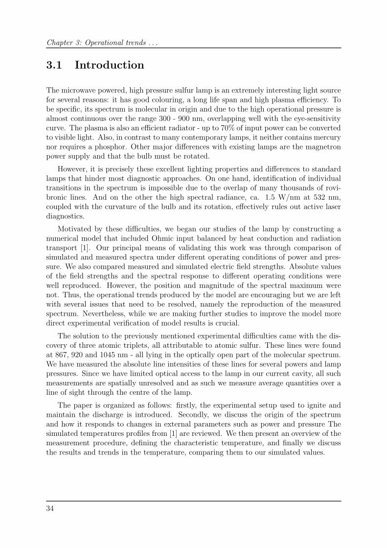
Figure 3.1: Measured spectra of a 5 barlamp are shown here for input powers from200 to 900 W.
300 400 500 600 700 800 900Wavelength[nm]
0
0.5
1
1.5
2
2.5
Pow
er [W
/nm
]
3 bar5 bar7 bar
Figure 3.2: Spectra measured at severaldifferent sulfur pressures for a fixed inputpower of 800 W.
3.2 Molecular spectrum and atomic lines
Typical lamp spectra are shown in figures 3.1 and 3.2. They arise from multitudinousrovibrational transitions between the BΣ−
u excited state and the XΣ−g ground state in
the S2 molecule. The spectrum is broad and continuous; ranging from 300 nm to morethan 900 nm. Radiated power increases linearly as a function of input power, as shownin figure 3.1, and the spectral maximum remains at 514 nm. Figure 3.2 shows thatfor increasing lamp pressure the spectrum shifts to longer wavelengths and the spectralmaximum decreases with respect to lower pressures. In all cases the spectra are extremelydense and identification of individual rovibronic transitions is impossible.
In fact, we have been fortunate enough to find several atomic triplets in the opticallyopen part of the molecular spectrum at 867, 920 and 1045 nm. Transition probabilities,energy level data and statistical weights of the transitions and states are listed in table3.1. These lines can be used to determine a temperature. However, since our opticalaccess to the lamp is restricted, we measure these along a line of sight through the centreof the lamp.
3.3 Experimental setup
The apparatus we use to ignite and maintain a sulfur discharge is similar to the onedescribed in [3] and shown in figure 3.4; a magnetron introduces EM radiation at afrequency of 2.45 GHz into a waveguide onto which a resonator is attached. The bulb isfixed on a rod which allows it to be rotated from outside the cavity. Tuning is facilitatedby stub tuners and a movable short. Despite some differences with the commercial systemfrom Fusion Lighting, the Solar 1000, the two systems are essentially the same, the maindifference being the resonator used. In our case it is a hemi-ellipse which supports aTM101 mode while the Fusion lamp employs a cylindrical cavity and resonates in theTE111 mode. Our cavity, shown in figure 3.4, is essentially a metal box with some holes
35
Chapter 3: Operational trends . . .
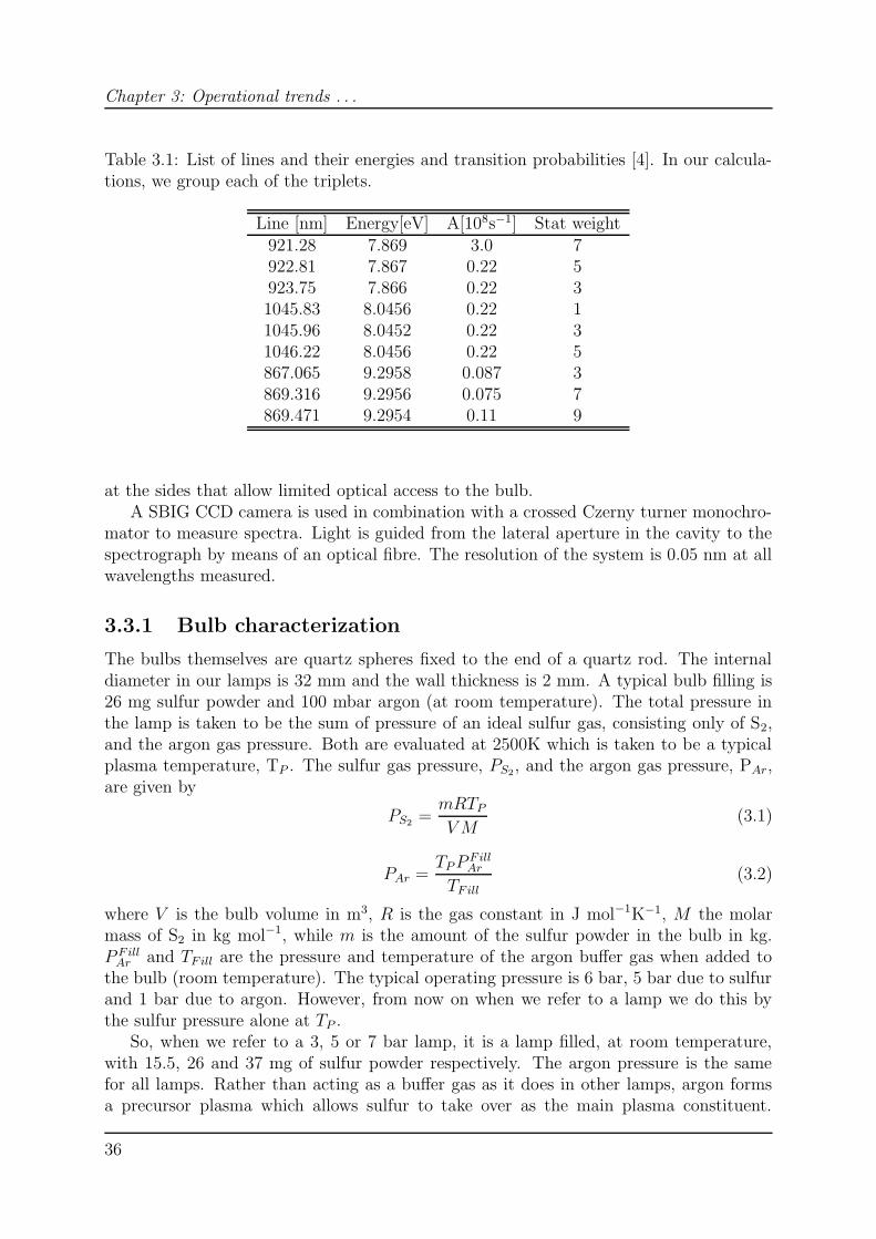
Table 3.1: List of lines and their energies and transition probabilities [4]. In our calcula-tions, we group each of the triplets.
Line [nm] Energy[eV] A[108s−1] Stat weight921.28 7.869 3.0 7922.81 7.867 0.22 5923.75 7.866 0.22 31045.83 8.0456 0.22 11045.96 8.0452 0.22 31046.22 8.0456 0.22 5867.065 9.2958 0.087 3869.316 9.2956 0.075 7869.471 9.2954 0.11 9
at the sides that allow limited optical access to the bulb.A SBIG CCD camera is used in combination with a crossed Czerny turner monochro-
mator to measure spectra. Light is guided from the lateral aperture in the cavity to thespectrograph by means of an optical fibre. The resolution of the system is 0.05 nm at allwavelengths measured.
3.3.1 Bulb characterization
The bulbs themselves are quartz spheres fixed to the end of a quartz rod. The internaldiameter in our lamps is 32 mm and the wall thickness is 2 mm. A typical bulb filling is26 mg sulfur powder and 100 mbar argon (at room temperature). The total pressure inthe lamp is taken to be the sum of pressure of an ideal sulfur gas, consisting only of S2,and the argon gas pressure. Both are evaluated at 2500K which is taken to be a typicalplasma temperature, TP . The sulfur gas pressure, PS2, and the argon gas pressure, PAr,are given by
PS2 =mRTP
VM(3.1)
PAr =TPP
FillAr
TFill(3.2)
where V is the bulb volume in m3, R is the gas constant in J mol−1K−1, M the molarmass of S2 in kg mol−1, while m is the amount of the sulfur powder in the bulb in kg.P Fill
Ar and TFill are the pressure and temperature of the argon buffer gas when added tothe bulb (room temperature). The typical operating pressure is 6 bar, 5 bar due to sulfurand 1 bar due to argon. However, from now on when we refer to a lamp we do this bythe sulfur pressure alone at TP .
So, when we refer to a 3, 5 or 7 bar lamp, it is a lamp filled, at room temperature,with 15.5, 26 and 37 mg of sulfur powder respectively. The argon pressure is the samefor all lamps. Rather than acting as a buffer gas as it does in other lamps, argon formsa precursor plasma which allows sulfur to take over as the main plasma constituent.
36
3.3 Experimental setup
920 nm
867 nm
1045 nm7.86 eV
6.53 eV
9.31 eV
3.95 eV
10.36 eV
9.29 eV
1.16 eV
1.67 eV
4.46 eV
X3Σ−g
S+
S
B3Σ−u
S+2
S2
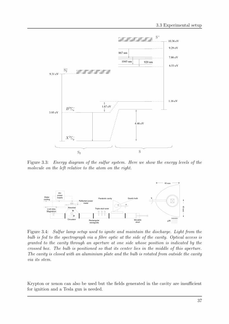
Figure 3.3: Energy diagram of the sulfur system. Here we show the energy levels of themolecule on the left relative to the atom on the right.
2.45 GHzMagnetron
Circulator
Triple stub tuner
Movableshort
Rectangularwaveguide
HV-powersupply
Reflected powermeter
Absorber
Watercooling Parabolic cavity Quartz bulb
60 mm
80 mm
Wµ
Figure 3.4: Sulfur lamp setup used to ignite and maintain the discharge. Light from thebulb is fed to the spectrograph via a fibre optic at the side of the cavity. Optical access isgranted to the cavity through an aperture at one side whose position is indicated by thecrossed box. The bulb is positioned so that its center lies in the middle of this aperture.The cavity is closed with an aluminium plate and the bulb is rotated from outside the cavityvia its stem.
Krypton or xenon can also be used but the fields generated in the cavity are insufficientfor ignition and a Tesla gun is needed.
37
Chapter 3: Operational trends . . .
0 3 6 9 12 15 18Radius [mm]
1000
2000
3000
4000
Tem
pera
ture
[K]
400 W500 W800 W1000 W
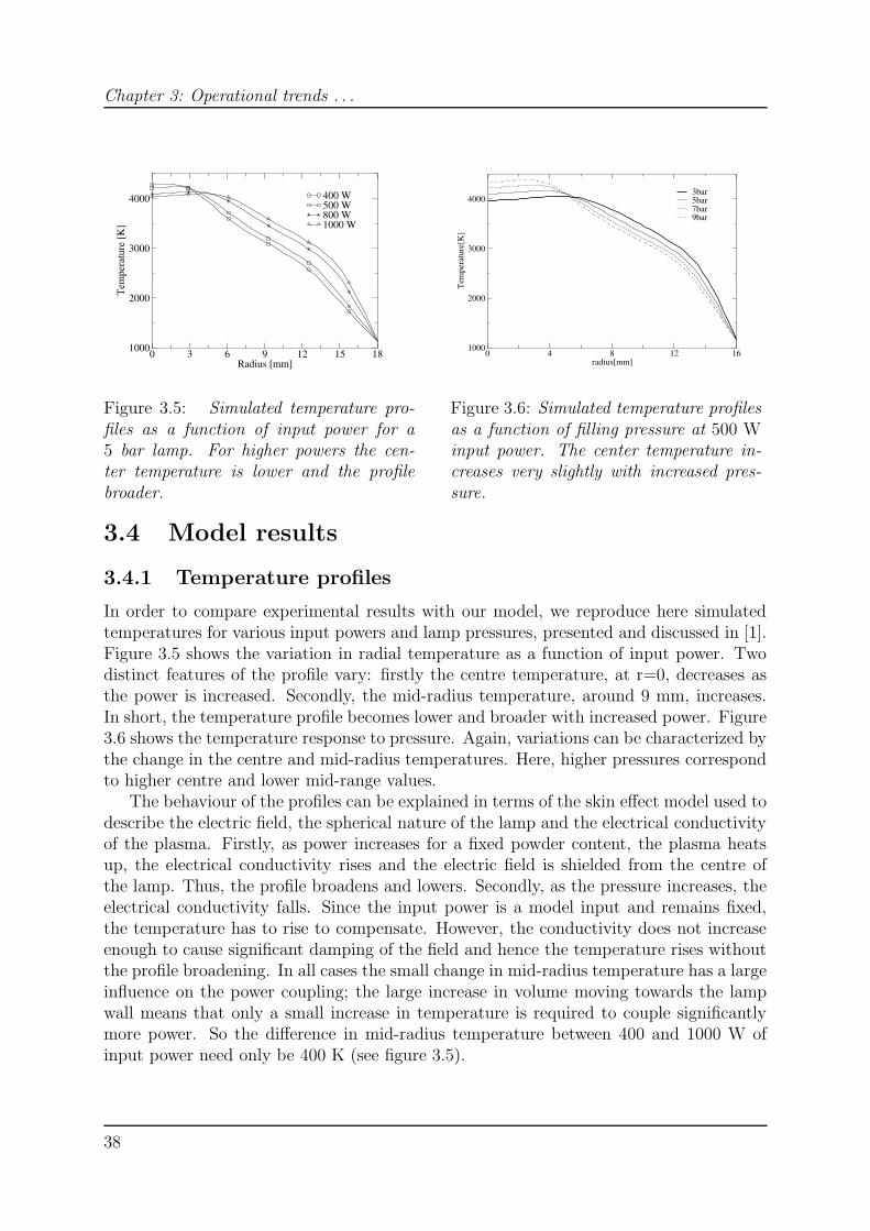
Figure 3.5: Simulated temperature pro-files as a function of input power for a5 bar lamp. For higher powers the cen-ter temperature is lower and the profilebroader.
0 4 8 12 16radius[mm]
1000
2000
3000
4000
Tem
pera
ture
[K]
3bar5bar7bar9bar
Figure 3.6: Simulated temperature profilesas a function of filling pressure at 500 Winput power. The center temperature in-creases very slightly with increased pres-sure.
3.4 Model results
3.4.1 Temperature profiles
In order to compare experimental results with our model, we reproduce here simulatedtemperatures for various input powers and lamp pressures, presented and discussed in [1].Figure 3.5 shows the variation in radial temperature as a function of input power. Twodistinct features of the profile vary: firstly the centre temperature, at r=0, decreases asthe power is increased. Secondly, the mid-radius temperature, around 9 mm, increases.In short, the temperature profile becomes lower and broader with increased power. Figure3.6 shows the temperature response to pressure. Again, variations can be characterized bythe change in the centre and mid-radius temperatures. Here, higher pressures correspondto higher centre and lower mid-range values.
The behaviour of the profiles can be explained in terms of the skin effect model used todescribe the electric field, the spherical nature of the lamp and the electrical conductivityof the plasma. Firstly, as power increases for a fixed powder content, the plasma heatsup, the electrical conductivity rises and the electric field is shielded from the centre ofthe lamp. Thus, the profile broadens and lowers. Secondly, as the pressure increases, theelectrical conductivity falls. Since the input power is a model input and remains fixed,the temperature has to rise to compensate. However, the conductivity does not increaseenough to cause significant damping of the field and hence the temperature rises withoutthe profile broadening. In all cases the small change in mid-radius temperature has a largeinfluence on the power coupling; the large increase in volume moving towards the lampwall means that only a small increase in temperature is required to couple significantlymore power. So the difference in mid-radius temperature between 400 and 1000 W ofinput power need only be 400 K (see figure 3.5).
38
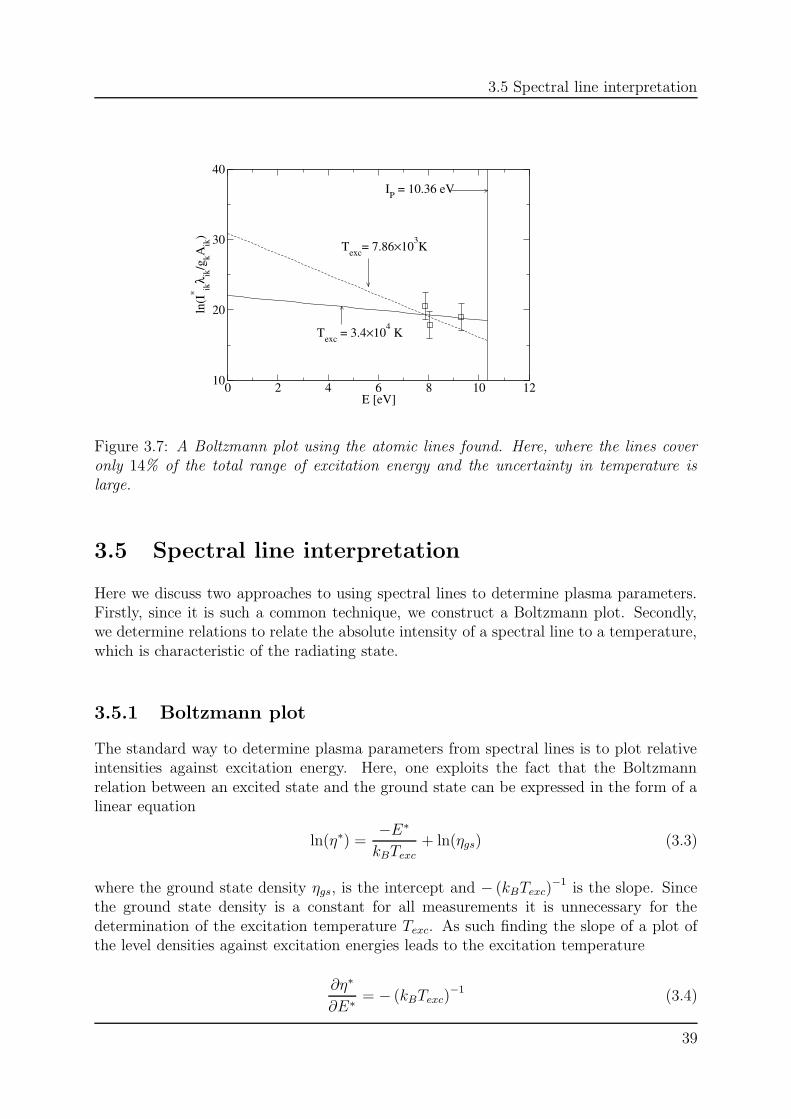
3.5 Spectral line interpretation
0 2 4 6 8 10 12E [eV]
10
20
30
40
ln(I
* ikλ ik
/gkA
ik)
Texc = 3.4×10⁴ K
Texc= 7.86×10³K
IP = 10.36 eV
Figure 3.7: A Boltzmann plot using the atomic lines found. Here, where the lines coveronly 14% of the total range of excitation energy and the uncertainty in temperature islarge.
3.5 Spectral line interpretation
Here we discuss two approaches to using spectral lines to determine plasma parameters.Firstly, since it is such a common technique, we construct a Boltzmann plot. Secondly,we determine relations to relate the absolute intensity of a spectral line to a temperature,which is characteristic of the radiating state.
3.5.1 Boltzmann plot
The standard way to determine plasma parameters from spectral lines is to plot relativeintensities against excitation energy. Here, one exploits the fact that the Boltzmannrelation between an excited state and the ground state can be expressed in the form of alinear equation
ln(η∗) =−E∗
kBTexc+ ln(ηgs) (3.3)
where the ground state density ηgs, is the intercept and − (kBTexc)−1 is the slope. Since
the ground state density is a constant for all measurements it is unnecessary for thedetermination of the excitation temperature Texc. As such finding the slope of a plot ofthe level densities against excitation energies leads to the excitation temperature
∂η∗
∂E∗= − (kBTexc)
−1 (3.4)
39
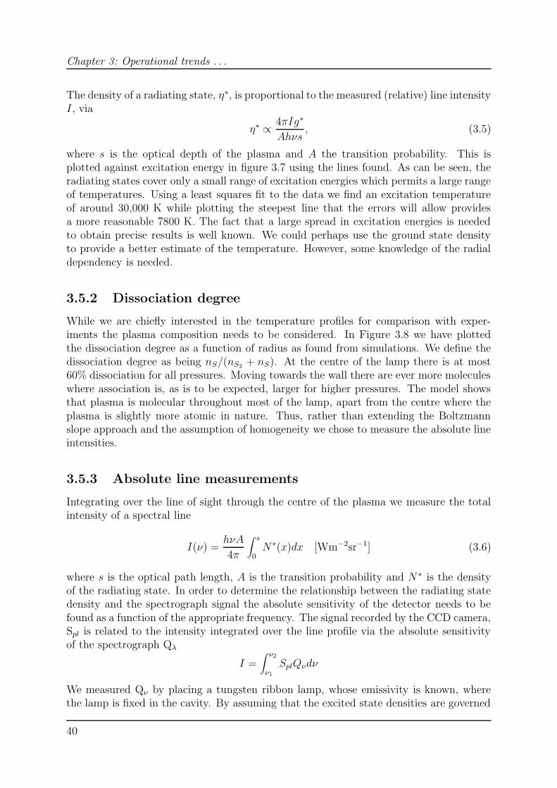
Chapter 3: Operational trends . . .
The density of a radiating state, η∗, is proportional to the measured (relative) line intensityI, via
η∗ ∝ 4πIg∗
Ahνs, (3.5)
where s is the optical depth of the plasma and A the transition probability. This isplotted against excitation energy in figure 3.7 using the lines found. As can be seen, theradiating states cover only a small range of excitation energies which permits a large rangeof temperatures. Using a least squares fit to the data we find an excitation temperatureof around 30,000 K while plotting the steepest line that the errors will allow providesa more reasonable 7800 K. The fact that a large spread in excitation energies is neededto obtain precise results is well known. We could perhaps use the ground state densityto provide a better estimate of the temperature. However, some knowledge of the radialdependency is needed.
3.5.2 Dissociation degree
While we are chiefly interested in the temperature profiles for comparison with exper-iments the plasma composition needs to be considered. In Figure 3.8 we have plottedthe dissociation degree as a function of radius as found from simulations. We define thedissociation degree as being nS/(nS2 + nS). At the centre of the lamp there is at most60% dissociation for all pressures. Moving towards the wall there are ever more moleculeswhere association is, as is to be expected, larger for higher pressures. The model showsthat plasma is molecular throughout most of the lamp, apart from the centre where theplasma is slightly more atomic in nature. Thus, rather than extending the Boltzmannslope approach and the assumption of homogeneity we chose to measure the absolute lineintensities.
3.5.3 Absolute line measurements
Integrating over the line of sight through the centre of the plasma we measure the totalintensity of a spectral line
I(ν) =hνA
4π
∫ s
0N∗(x)dx [Wm−2sr−1] (3.6)
where s is the optical path length, A is the transition probability and N ∗ is the densityof the radiating state. In order to determine the relationship between the radiating statedensity and the spectrograph signal the absolute sensitivity of the detector needs to befound as a function of the appropriate frequency. The signal recorded by the CCD camera,Spl is related to the intensity integrated over the line profile via the absolute sensitivityof the spectrograph Qλ
I =∫ ν2
ν1
SplQνdν
We measured Qν by placing a tungsten ribbon lamp, whose emissivity is known, wherethe lamp is fixed in the cavity. By assuming that the excited state densities are governed
40
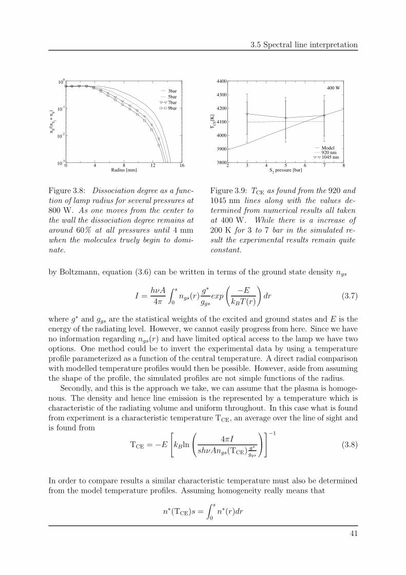
3.5 Spectral line interpretation
0 4 8 12 16Radius [mm]
10-3
10-2
10-1
100
n S/(n S 2+
n S)
3bar5bar7bar9bar
Figure 3.8: Dissociation degree as a func-tion of lamp radius for several pressures at800 W. As one moves from the center tothe wall the dissociation degree remains ataround 60% at all pressures until 4 mmwhen the molecules truely begin to domi-nate.
2 3 4 5 6 7 8S2 pressure [bar]
3800
3900
4000
4100
4200
4300
4400
TC
E[K
]
Model920 nm1045 nm
400 W
Figure 3.9: TCE as found from the 920 and1045 nm lines along with the values de-termined from numerical results all takenat 400 W. While there is a increase of200 K for 3 to 7 bar in the simulated re-sult the experimental results remain quiteconstant.
by Boltzmann, equation (3.6) can be written in terms of the ground state density ngs
I =hνA
4π
∫ s
0ngs(r)
g∗
ggs
exp
(−E
kBT (r)
)dr (3.7)
where g∗ and ggs are the statistical weights of the excited and ground states and E is theenergy of the radiating level. However, we cannot easily progress from here. Since we haveno information regarding ngs(r) and have limited optical access to the lamp we have twooptions. One method could be to invert the experimental data by using a temperatureprofile parameterized as a function of the central temperature. A direct radial comparisonwith modelled temperature profiles would then be possible. However, aside from assumingthe shape of the profile, the simulated profiles are not simple functions of the radius.
Secondly, and this is the approach we take, we can assume that the plasma is homoge-nous. The density and hence line emission is the represented by a temperature which ischaracteristic of the radiating volume and uniform throughout. In this case what is foundfrom experiment is a characteristic temperature TCE, an average over the line of sight andis found from
TCE = −EkBln
4πI
shνAngs(TCE) g∗
ggs
−1
(3.8)
In order to compare results a similar characteristic temperature must also be determinedfrom the model temperature profiles. Assuming homogeneity really means that
n∗(TCE)s =∫ s
0n∗(r)dr
41
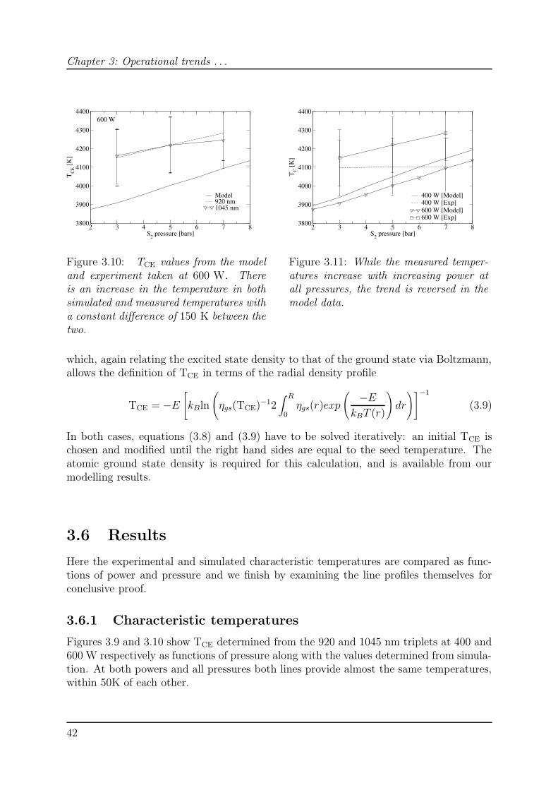
Chapter 3: Operational trends . . .
2 3 4 5 6 7 8S2 pressure [bars]
3800
3900
4000
4100
4200
4300
4400
TC
E [K
]
Model920 nm1045 nm
600 W
Figure 3.10: TCE values from the modeland experiment taken at 600 W. Thereis an increase in the temperature in bothsimulated and measured temperatures witha constant difference of 150 K between thetwo.
2 3 4 5 6 7 8S2 pressure [bar]
3800
3900
4000
4100
4200
4300
4400
TC [K
]
400 W [Model]400 W [Exp]600 W [Model]600 W [Exp]
Figure 3.11: While the measured temper-atures increase with increasing power atall pressures, the trend is reversed in themodel data.
which, again relating the excited state density to that of the ground state via Boltzmann,allows the definition of TCE in terms of the radial density profile
TCE = −E[kBln
(ηgs(TCE)−12
∫ R
0ηgs(r)exp
(−E
kBT (r)
)dr
)]−1
(3.9)
In both cases, equations (3.8) and (3.9) have to be solved iteratively: an initial TCE ischosen and modified until the right hand sides are equal to the seed temperature. Theatomic ground state density is required for this calculation, and is available from ourmodelling results.
3.6 Results
Here the experimental and simulated characteristic temperatures are compared as func-tions of power and pressure and we finish by examining the line profiles themselves forconclusive proof.
3.6.1 Characteristic temperatures
Figures 3.9 and 3.10 show TCE determined from the 920 and 1045 nm triplets at 400 and600 W respectively as functions of pressure along with the values determined from simula-tion. At both powers and all pressures both lines provide almost the same temperatures,within 50K of each other.
42
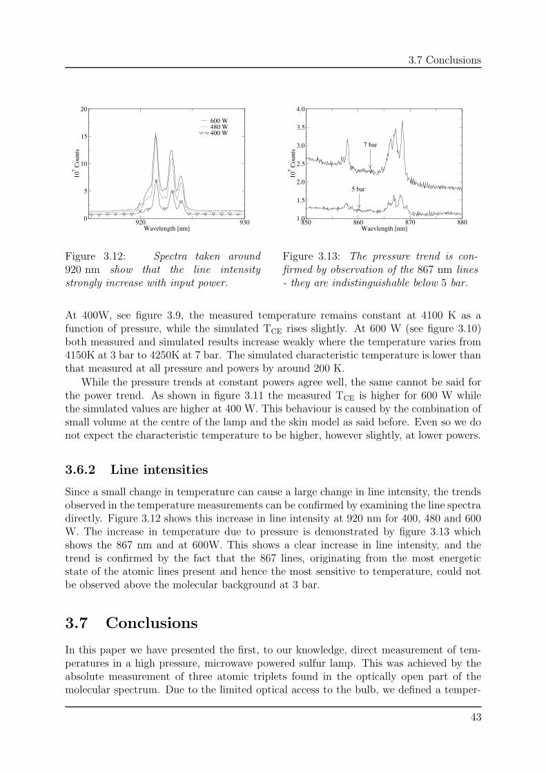
3.7 Conclusions
920 930Wavelength [nm]
0
5
10
15
20
105 C
ount
s
600 W480 W400 W
Figure 3.12: Spectra taken around920 nm show that the line intensitystrongly increase with input power.
850 860 870 880Waevlength [nm]
1.0
1.5
2.0
2.5
3.0
3.5
4.0
105 C
ount
s
7 bar
5 bar
Figure 3.13: The pressure trend is con-firmed by observation of the 867 nm lines- they are indistinguishable below 5 bar.
At 400W, see figure 3.9, the measured temperature remains constant at 4100 K as afunction of pressure, while the simulated TCE rises slightly. At 600 W (see figure 3.10)both measured and simulated results increase weakly where the temperature varies from4150K at 3 bar to 4250K at 7 bar. The simulated characteristic temperature is lower thanthat measured at all pressure and powers by around 200 K.
While the pressure trends at constant powers agree well, the same cannot be said forthe power trend. As shown in figure 3.11 the measured TCE is higher for 600 W whilethe simulated values are higher at 400 W. This behaviour is caused by the combination ofsmall volume at the centre of the lamp and the skin model as said before. Even so we donot expect the characteristic temperature to be higher, however slightly, at lower powers.
3.6.2 Line intensities
Since a small change in temperature can cause a large change in line intensity, the trendsobserved in the temperature measurements can be confirmed by examining the line spectradirectly. Figure 3.12 shows this increase in line intensity at 920 nm for 400, 480 and 600W. The increase in temperature due to pressure is demonstrated by figure 3.13 whichshows the 867 nm and at 600W. This shows a clear increase in line intensity, and thetrend is confirmed by the fact that the 867 lines, originating from the most energeticstate of the atomic lines present and hence the most sensitive to temperature, could notbe observed above the molecular background at 3 bar.
3.7 Conclusions
In this paper we have presented the first, to our knowledge, direct measurement of tem-peratures in a high pressure, microwave powered sulfur lamp. This was achieved by theabsolute measurement of three atomic triplets found in the optically open part of themolecular spectrum. Due to the limited optical access to the bulb, we defined a temper-
43
Bibliography
ature characteristic of the radiating state and determined it as a function of pressure for400 and 600 W input power.
This temperature was found to be 4100 K on average, increasing slightly with increasedpressure and power. Trends observed in the measurements were confirmed by the linespectra themselves since the radiating states are close to the ionization potential and alsovery sensitive. The increase in plasma temperature with increasing pressure is confirmedby the fact that the 867 nm lines could only be detected at 5 bar and above. Characteristictemperatures determined from our previous modelling efforts were found to be 150-200 Klower than those from experiment, but pressure trends were well reproduced. Despite theaveraging nature of the characteristic temperature approach, we have exposed a problemwith our model where the power trend is reversed. This is due to our use of a skin effectdescription of the electric field in our numerical model and requires further study.
Acknowledgements
This work is part of the research program of the Dutch Technology Foundation (STW).The authors would like to thank Achim Korber and Johannes Baier of Philips researchlaboratories in Aachen, Germany their assistance and provision of experimental spectra.
References
[1] Johnston C W, van der Heijden H, Janssen G M, van Dijk van der Mullen J J A M,J. Phys. D: Appl. Phys. 35, 342 (2002) Chapter 2 of this thesis
[2] van der Heijden H and van der Mullen J J A M, J. Phys. B: At. Mol. Opt. Phys. 34,4183 (2001)
[3] van Dongen M, Korber A, van der Heijden H, Jonkers J, Scholl R and van der MullenJ J A M, J. Phys. D: Appl. Phys. 31, 3095 (1999)
[4] Wiese W L, Smith M W and Miles B M, Atomic transition probabilities, Natl. Stand.Ref. Data Ser. Natl. Bur. Stad., Circ. 4 (U.S.GPO, Washington, D.C.,1966), Vol. 1.
44
CHAPTER 4
An improved LTE model of a high pressure sulfur discharge
An existing LTE model [1] of a high pressure sulfur discharge is improved upon by themore accurate and complete treatment of each term in the energy balance. The simulationprogram plasimo [2, 3], which is an integrated environment for the construction andexecution of plasma models, has been used to define and solve all aspects of the model.The electric field is treated as being DC and the temperature dependent nature of speciesinteractions is incorporated in the determination of transport coefficients. In addition tothe main radiative transition, the B3Σ−
u → X3Σ−g , several others in S2 are included. These
are B′′3Πu → X3Σ−g , B′3Πg → A3Σ+
u , A′3∆u and e1Πg → c1Σ−
u . The S3 molecule is alsoincluded in the composition as an absorbing particle. Furthermore, radiation productionis treated quantum mechanically. The principle improvement over the previous work isthat both the position of the spectral maximum and the pressure shift are quantitativelydescribed by the current model. Both are chiefly due to the presence of S3.
45
Chapter 4: An improved LTE model . . .
4.1 Introduction
The sulfur lamp is known mainly for its radiative efficiency and good colour rendering. Itis a high pressure discharge that produces white light without the need for a fluorescentpowder to convert UV photons into visible light.
The lamp is by any standard an unusual system. It is powered by microwaves andcomprises a rotating bulb, inside a resonant cavity, that uses a high pressure sulfur dis-charge as the radiating medium. We have chosen to study the system with the help of a1D LTE energy balance constructed with the help of plasimo [2, 3]. Rotation is ignoredin order that we might concentrate on the most important aspect of the lamp, namelythe spectrum.
The distribution of power in the spectrum, which matches the eye sensitivity curvevery well, is so important that any attempt to understand and model the lamp should notonly include the energy balance in global terms but also the relative power distributionin the emitted spectrum. In a previous article [1], referred to as paper I from now on,we presented a 1D LTE model of the lamp which was validated by comparison of thesimulated and measured spectra. In the present paper we improve upon this model byenhancing the treatment of each term in the energy balance and the influence of radiationgeneration from various species.
The reason that a high pressure sulfur plasma possesses such desirable lighting prop-erties is a result of several factors. Firstly the B3Σ−
u → X3Σ−g transition is very strong.
The transition probabilities for many of the vibronic transitions are large for a molecule,namely in the order of 105 s−1. Secondly, the high pressure and temperature ensures thatall vibrational states are substantially populated which allows them to contribute to thespectrum. The fact that only visible light is produced is due to the fortuitous position-ing of the B and X electronic states with respect to each other, which also determinesthe shape of the spectrum. A further property of sulfur is that the atomic transitionassociated with the molecular one is optically forbidden.
Paper I was based on a simplified energy balance comprising three terms: Ohmic inputbalanced by conductive and radiative losses. All species interactions were assumed to behard sphere and the transport coefficients were found using mean free path methods. Thegeneration of radiation was attributed to only one electronic transition — the B3Σ−
u →X3Σ−
g in S2 and the semiclassical Franck Condon approach was used to describe thespectral distribution. The plasma-electric field interaction was described with a skinmodel.
We found that at high pressure the single transition in the dimer was a good candidatewhen seeking to explain the spectrum and the high radiative efficiency. Furthermore thegeneral shape and extent of the spectrum were reproduced quite reasonably. Moreover,both the measured linear increase in radiated power with increasing input power and shiftof the spectrum to the red with increasing pressure were reproduced by the model. In ad-dition, the electric field strengths were found to be within a factor 2 of the experimentallydetermined values. However, there were three chief discrepancies. Firstly, the position ofthe spectral maximum lay too far to the blue, secondly there was too little light in the redpart of the spectrum and finally the decrease in radiated power as a function of increasingpressure was not reproduced.
In a subsequent article [4], referred to as paper II from now on, we measured a tem-
46
4.2 Model Review
perature from absolute measurements of several atomic lines we found at 920 and 1046nm. A temperature of 4100 K was found which agreed well with the value determinedfrom the model results. However, while the model predicted the measured increase intemperature as a function of pressure, it also predicted a decrease of the temperaturewith increasing power — contrary to the measurements. In conclusion: we have thusconstructed a picture of the sulfur lamp in which the B3Σ−
u → X3Σ−g transition does not
produce sufficient red light and self absorption at shorter wavelengths is too insubstantialto quantitatively explain either the position of the spectral maximum or the spectral shiftof the maximum with pressure.
In their series of articles on the generation and transport of molecular sulfur spectra[5, 6, 7] van der Heijden and van der Mullen have shown that one has to take fine structureinto account in order to correctly describe the transport of the spectrum. It was shownthat in comparison to the semiclassical treatment [5] a quantum-mechanical descriptionproduces less blue and more UV [6]. It has been known for some time already that S3
absorbs in the UV. Doll and Lapatovich [8] suggested that the former could be responsiblefor the spectral shift which was later demonstrated by Korber [9].
With respect to the deficiency in the red there are several excited states in S2, observedin emission, that may redress this. On the other hand van der Heijden et al advanced theidea that a departure from LTE may be responsible. Assuming LTE, the ionization degreeis 10−5 which can be too low to maintain Maxwell and Boltzmann equilibria. While itmay be ultimately necessary to investigate LTE departure we consider the previous LTEmodel presented in paper I to have performed well enough that the next step should beto improve it, add the trimer, and determine whether other states in S2 may contributeto the spectrum.
The article is laid out as follows: section 4.2 presents a brief review of the model andexplains the lamp nomenclature. Section 4.3 reports the plasma composition and thetransport property calculations. Section 4.4 deals with radiation transport and the extracontributions to spectrum calculation. The results of the model are presented in section4.5, discussed in 4.6 and we finish with our conclusions in section 4.7.
4.2 Model Review
In an LTE model plasma composition and material properties are established once quan-tity of material and temperature are known. There is then one equation that needs tobe solved for the temperature. As in paper I Ohmic input is balanced by conductive andradiative losses. Ignoring convection the steady state balance is
QOhm + ∇ · (λc∇T ) +Qrad = 0 (4.1)
where λc is the thermal conductivity and QOhm and Qrad are the power source terms forOhmic input and radiation. Since the plasma emits a significant proportion of the inputpower Qrad is typically negative. Positive values of this term indicate that absorptionoutweighs local emission.
In paper I the plasma-electric field interaction was treated with a skin effect model.This time however, the electric field will be treated as DC. There are three reasons forthis. Firstly, in paper II we observed trends in the simulated temperature profiles that
47
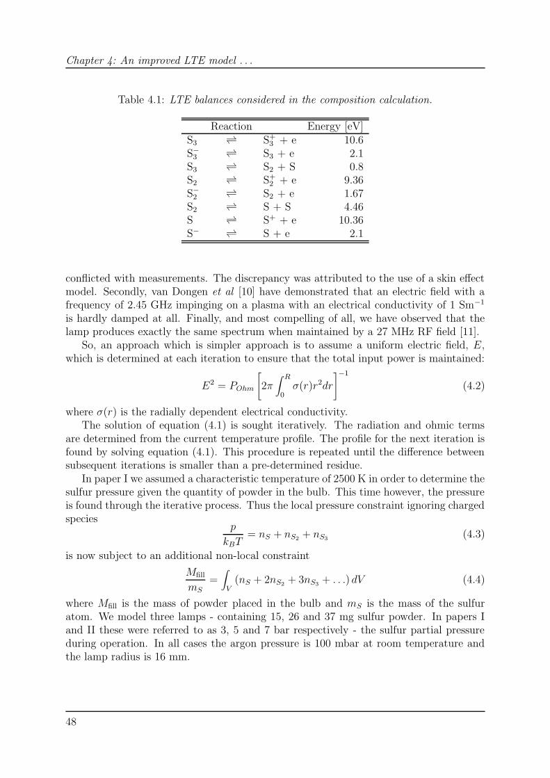
Chapter 4: An improved LTE model . . .
Table 4.1: LTE balances considered in the composition calculation.
Reaction Energy [eV]S3 S+
3 + e 10.6S−
3 S3 + e 2.1
S3 S2 + S 0.8S2 S+
2 + e 9.36S−
2 S2 + e 1.67
S2 S + S 4.46S S+ + e 10.36S− S + e 2.1
conflicted with measurements. The discrepancy was attributed to the use of a skin effectmodel. Secondly, van Dongen et al [10] have demonstrated that an electric field with afrequency of 2.45 GHz impinging on a plasma with an electrical conductivity of 1 Sm−1
is hardly damped at all. Finally, and most compelling of all, we have observed that thelamp produces exactly the same spectrum when maintained by a 27 MHz RF field [11].
So, an approach which is simpler approach is to assume a uniform electric field, E,which is determined at each iteration to ensure that the total input power is maintained:
E2 = POhm
[2π∫ R
0σ(r)r2dr
]−1
(4.2)
where σ(r) is the radially dependent electrical conductivity.The solution of equation (4.1) is sought iteratively. The radiation and ohmic terms
are determined from the current temperature profile. The profile for the next iteration isfound by solving equation (4.1). This procedure is repeated until the difference betweensubsequent iterations is smaller than a pre-determined residue.
In paper I we assumed a characteristic temperature of 2500 K in order to determine thesulfur pressure given the quantity of powder in the bulb. This time however, the pressureis found through the iterative process. Thus the local pressure constraint ignoring chargedspecies
p
kBT= nS + nS2 + nS3 (4.3)
is now subject to an additional non-local constraint
Mfill
mS
=∫
V(nS + 2nS2 + 3nS3 + . . .) dV (4.4)
where Mfill is the mass of powder placed in the bulb and mS is the mass of the sulfuratom. We model three lamps - containing 15, 26 and 37 mg sulfur powder. In papers Iand II these were referred to as 3, 5 and 7 bar respectively - the sulfur partial pressureduring operation. In all cases the argon pressure is 100 mbar at room temperature andthe lamp radius is 16 mm.
48
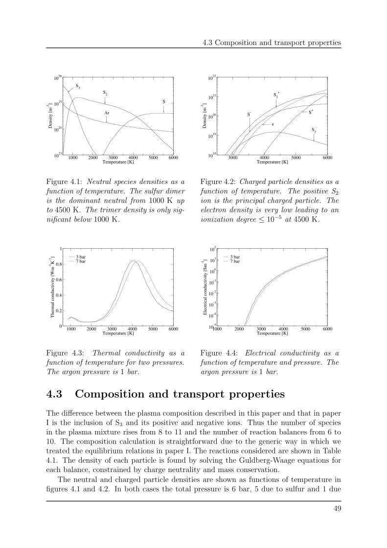
4.3 Composition and transport properties
1000 2000 3000 4000 5000 6000Temperature [K]
1023
1024
1025
1026
Den
sity
[m-3
]
S3S2
Ar
S
Figure 4.1: Neutral species densities as afunction of temperature. The sulfur dimeris the dominant neutral from 1000 K upto 4500 K. The trimer density is only sig-nificant below 1000 K.
3000 4000 5000 6000Temperature [K]
1018
1019
1020
1021
1022
Den
sity
[m-3
]
S2+
S2-
S+
e
S-
Figure 4.2: Charged particle densities as afunction of temperature. The positive S2
ion is the principal charged particle. Theelectron density is very low leading to anionization degree ≤ 10−5 at 4500 K.
1000 2000 3000 4000 5000 6000Temperature [K]
0
0.2
0.4
0.6
0.8
1
The
rmal
con
duct
ivity
[Wm
-1K
-1] 3 bar
7 bar
Figure 4.3: Thermal conductivity as afunction of temperature for two pressures.The argon pressure is 1 bar.
1000 2000 3000 4000 5000 6000Temperature [K]
10-5
10-4
10-3
10-2
10-1
100
101
102
Ele
ctri
cal c
ondu
ctiv
ity [S
m-1
] 3 bar7 bar
Figure 4.4: Electrical conductivity as afunction of temperature and pressure. Theargon pressure is 1 bar.
4.3 Composition and transport properties
The difference between the plasma composition described in this paper and that in paperI is the inclusion of S3 and its positive and negative ions. Thus the number of speciesin the plasma mixture rises from 8 to 11 and the number of reaction balances from 6 to10. The composition calculation is straightforward due to the generic way in which wetreated the equilibrium relations in paper I. The reactions considered are shown in Table4.1. The density of each particle is found by solving the Guldberg-Waage equations foreach balance, constrained by charge neutrality and mass conservation.
The neutral and charged particle densities are shown as functions of temperature infigures 4.1 and 4.2. In both cases the total pressure is 6 bar, 5 due to sulfur and 1 due
49
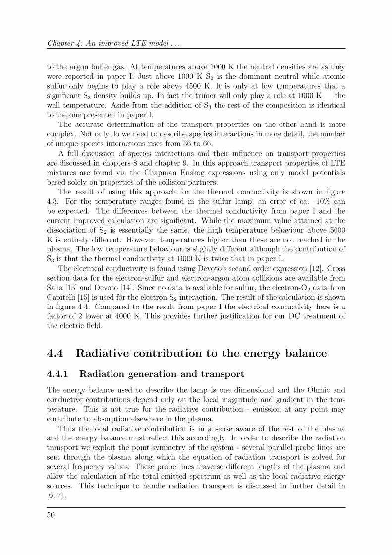
Chapter 4: An improved LTE model . . .
to the argon buffer gas. At temperatures above 1000 K the neutral densities are as theywere reported in paper I. Just above 1000 K S2 is the dominant neutral while atomicsulfur only begins to play a role above 4500 K. It is only at low temperatures that asignificant S3 density builds up. In fact the trimer will only play a role at 1000 K — thewall temperature. Aside from the addition of S3 the rest of the composition is identicalto the one presented in paper I.
The accurate determination of the transport properties on the other hand is morecomplex. Not only do we need to describe species interactions in more detail, the numberof unique species interactions rises from 36 to 66.
A full discussion of species interactions and their influence on transport propertiesare discussed in chapters 8 and chapter 9. In this approach transport properties of LTEmixtures are found via the Chapman Enskog expressions using only model potentialsbased solely on properties of the collision partners.
The result of using this approach for the thermal conductivity is shown in figure4.3. For the temperature ranges found in the sulfur lamp, an error of ca. 10% canbe expected. The differences between the thermal conductivity from paper I and thecurrent improved calculation are significant. While the maximum value attained at thedissociation of S2 is essentially the same, the high temperature behaviour above 5000K is entirely different. However, temperatures higher than these are not reached in theplasma. The low temperature behaviour is slightly different although the contribution ofS3 is that the thermal conductivity at 1000 K is twice that in paper I.
The electrical conductivity is found using Devoto’s second order expression [12]. Crosssection data for the electron-sulfur and electron-argon atom collisions are available fromSaha [13] and Devoto [14]. Since no data is available for sulfur, the electron-O2 data fromCapitelli [15] is used for the electron-S2 interaction. The result of the calculation is shownin figure 4.4. Compared to the result from paper I the electrical conductivity here is afactor of 2 lower at 4000 K. This provides further justification for our DC treatment ofthe electric field.
4.4 Radiative contribution to the energy balance
4.4.1 Radiation generation and transport
The energy balance used to describe the lamp is one dimensional and the Ohmic andconductive contributions depend only on the local magnitude and gradient in the tem-perature. This is not true for the radiative contribution - emission at any point maycontribute to absorption elsewhere in the plasma.
Thus the local radiative contribution is in a sense aware of the rest of the plasmaand the energy balance must reflect this accordingly. In order to describe the radiationtransport we exploit the point symmetry of the system - several parallel probe lines aresent through the plasma along which the equation of radiation transport is solved forseveral frequency values. These probe lines traverse different lengths of the plasma andallow the calculation of the total emitted spectrum as well as the local radiative energysources. This technique to handle radiation transport is discussed in further detail in[6, 7].
50
4.4 Radiative contribution to the energy balance
This method was used to treat radiation transport in paper I and is retained here.However, radiation generation will be treated in a different way. As argued before, afull quantum mechanical treatment of the spectrum is out of the question. There are 41vibrational levels in the B and 63 in the X state where all levels have rotational sublevels.
Performing radiation transport on the ca. 106 rovibrational lines that arise is compu-tationally expensive. Since we are more interested in the general shape of the spectrumand its overlap with the eye sensitivity curve rather than the ultra fine detail which a fullquantum mechanical treatment would eventually provide, we employed a semiclassicaltechnique in paper I. In that approach the radiation produced between electronic statesin a molecule is treated as a two level system — a single line profile was used to describethe transition. The line has a shape that is related to the transition frequency on theinternuclear distance r, as provided by the state potentials and reads
φ(ν(r)) ∝ r2exp
(−V (r)
kBT
) ∣∣∣∣∣dν
dr
∣∣∣∣∣
−1
,
where V (r) is the potential function of the lower electronic state. The radial change infrequency is found from the state potentials. The power of this approach is that only avery limited number of frequency points is needed, and it is thus computationally cheap.In addition the data demands are moderate.
However, applying this method in paper I we found that the self absorption in theB3Σ−
u → X3Σ−g system was insufficient to explain the observed position of the spectral
maximum. A detailed comparison of the semiclassical (SC) and quantum mechanical(QM) approaches as they apply to the sulfur spectrum shows that while on average theSC cross section for radiation absorption seems to agree with the QM value [5], theinfluence of fine structure increases absorption in the blue [6].
As a result the spectrum is shifted as required. So, while we are not interested infine structure it is necessary to include it. Nevertheless, the situation remains that we donot wish to include a full quantum mechanical radiation transport calculation inside aniterative model for the energy balance. Van der Heijden et al [7] have shown that a fullQM spectrum can be modelled to within 5% accuracy by taking 40 clusters throughoutthe frequency spectrum, each of which contains 250 frequency points. In this way thecorrect average of the absorption cross section is found at each frequency and the fullspectrum is found by interpolation.
The QM absorption cross section is first calculated for all possible transitions andthose that fall within our desired range are grouped to provide the cross section as afunction of frequency. Aside from potential and spectroscopic data two pieces of informa-tion are required: the Franck-Condon table and the electronic transition dipole moment(ETDM) for the transition. In order to calculate the vibrational wavefunctions we usethe SCHROED program [16] and employ the integration routines provided by the GNUScientific Library [17] to determine the overlap. The BX transition has been studiedextensively and its ETDM is available [18, 19, 20].
51
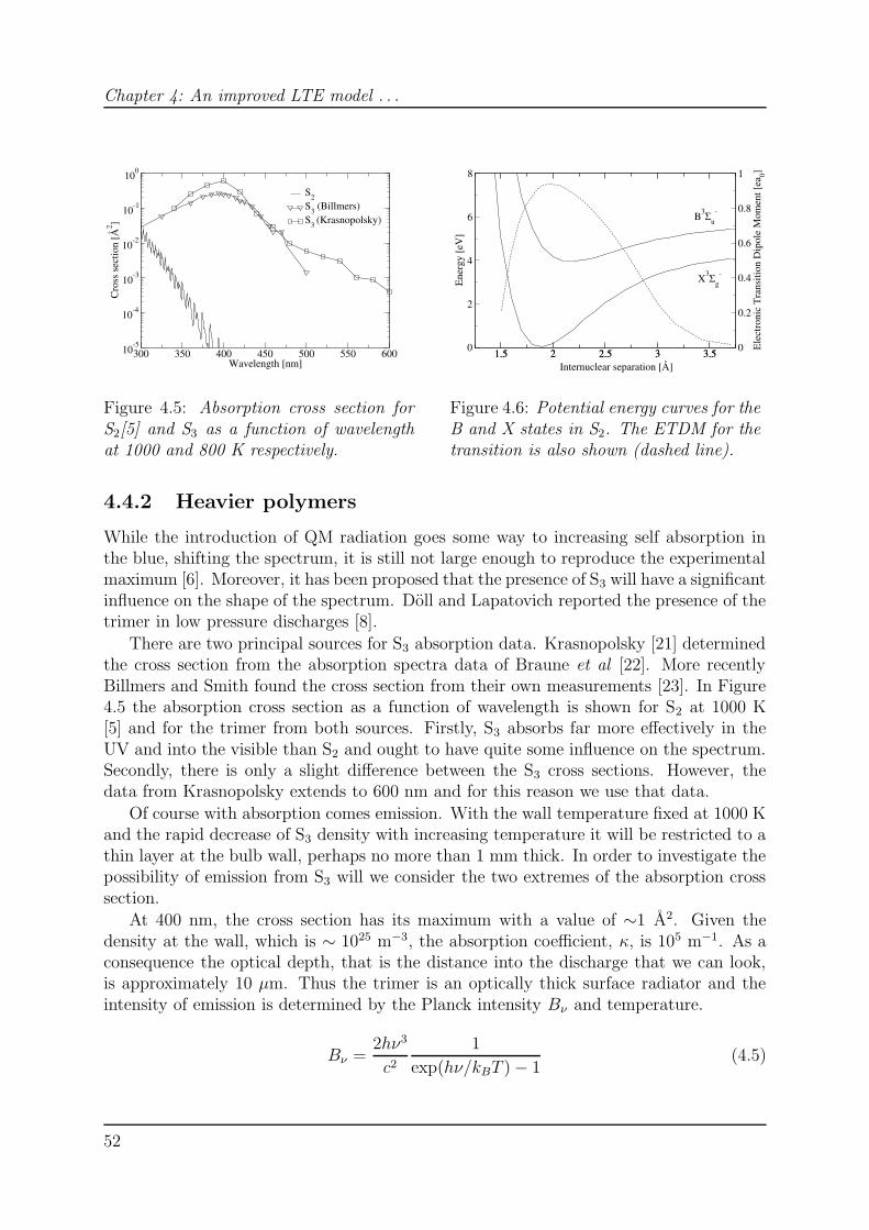
Chapter 4: An improved LTE model . . .
300 350 400 450 500 550 600Wavelength [nm]
10-5
10-4
10-3
10-2
10-1
100
Cro
ss s
ectio
n [Å
2 ]
S2S3 (Billmers)S3 (Krasnopolsky)
Figure 4.5: Absorption cross section forS2[5] and S3 as a function of wavelengthat 1000 and 800 K respectively.
1.5 2 2.5 3 3.50
2
4
6
8
Ene
rgy
[eV
]
1.5 2 2.5 3 3.5 0
0.2
0.4
0.6
0.8
1
Ele
ctro
nic
Tra
nsiti
on D
ipol
e M
omen
t [ea
0]
Internuclear separation [Å]
B3Σu-
X3Σg-
Figure 4.6: Potential energy curves for theB and X states in S2. The ETDM for thetransition is also shown (dashed line).
4.4.2 Heavier polymers
While the introduction of QM radiation goes some way to increasing self absorption inthe blue, shifting the spectrum, it is still not large enough to reproduce the experimentalmaximum [6]. Moreover, it has been proposed that the presence of S3 will have a significantinfluence on the shape of the spectrum. Doll and Lapatovich reported the presence of thetrimer in low pressure discharges [8].
There are two principal sources for S3 absorption data. Krasnopolsky [21] determinedthe cross section from the absorption spectra data of Braune et al [22]. More recentlyBillmers and Smith found the cross section from their own measurements [23]. In Figure4.5 the absorption cross section as a function of wavelength is shown for S2 at 1000 K[5] and for the trimer from both sources. Firstly, S3 absorbs far more effectively in theUV and into the visible than S2 and ought to have quite some influence on the spectrum.Secondly, there is only a slight difference between the S3 cross sections. However, thedata from Krasnopolsky extends to 600 nm and for this reason we use that data.
Of course with absorption comes emission. With the wall temperature fixed at 1000 Kand the rapid decrease of S3 density with increasing temperature it will be restricted to athin layer at the bulb wall, perhaps no more than 1 mm thick. In order to investigate thepossibility of emission from S3 will we consider the two extremes of the absorption crosssection.
At 400 nm, the cross section has its maximum with a value of ∼1 A2. Given thedensity at the wall, which is ∼ 1025 m−3, the absorption coefficient, κ, is 105 m−1. As aconsequence the optical depth, that is the distance into the discharge that we can look,is approximately 10 µm. Thus the trimer is an optically thick surface radiator and theintensity of emission is determined by the Planck intensity Bν and temperature.
Bν =2hν3
c21
exp(hν/kBT ) − 1(4.5)
52
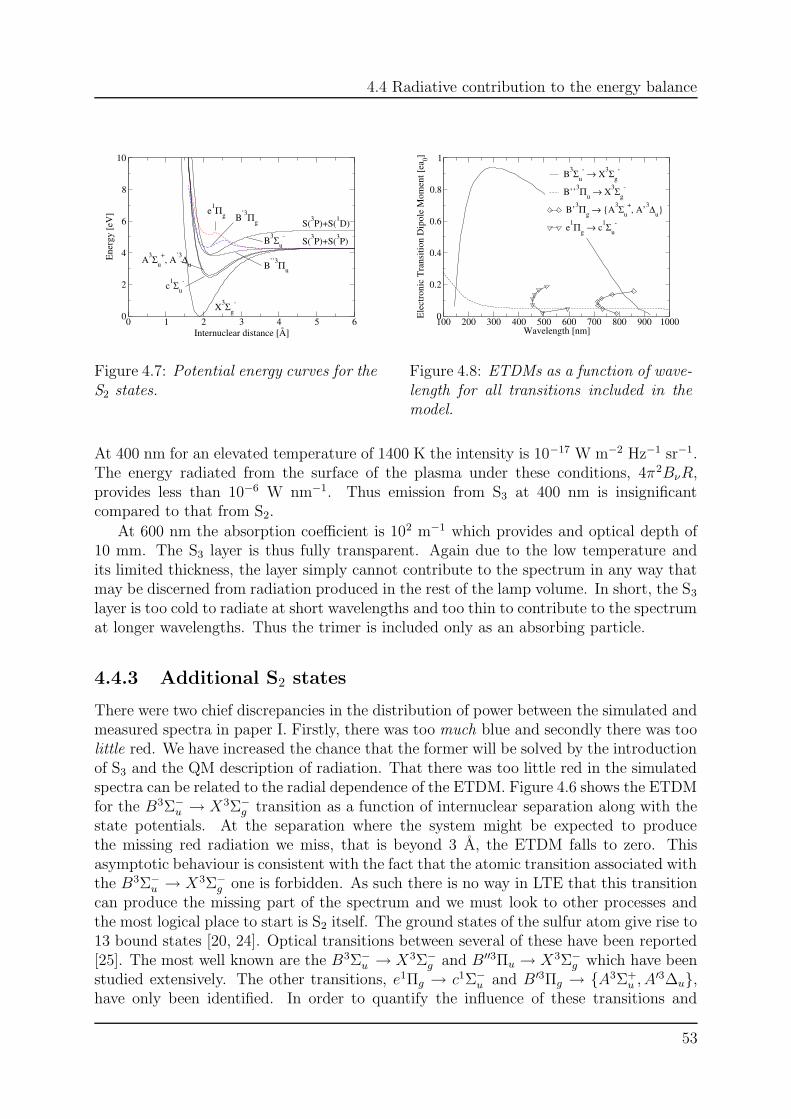
4.4 Radiative contribution to the energy balance
0 1 2 3 4 5 6Internuclear distance [Å]
0
2
4
6
8
10
Ene
rgy
[eV
]
A3Σu+, A’3∆u
X3Σg-
B’3Πg
B’’3Πu
c1Σu-
B3Σu-
e1Πg
S(3P)+S(3P)
S(3P)+S(1D)
Figure 4.7: Potential energy curves for theS2 states.
100 200 300 400 500 600 700 800 900 1000Wavelength [nm]
0
0.2
0.4
0.6
0.8
1
Ele
ctro
nic
Tra
nsiti
on D
ipol
e M
omen
t [ea
0]
B3Σu- → X3Σg
-
B’’3Πu → X3Σg-
B’3Πg → A3Σu+, A’3∆u
e1Πg → c1Σu-
Figure 4.8: ETDMs as a function of wave-length for all transitions included in themodel.
At 400 nm for an elevated temperature of 1400 K the intensity is 10−17 W m−2 Hz−1 sr−1.The energy radiated from the surface of the plasma under these conditions, 4π2BνR,provides less than 10−6 W nm−1. Thus emission from S3 at 400 nm is insignificantcompared to that from S2.
At 600 nm the absorption coefficient is 102 m−1 which provides and optical depth of10 mm. The S3 layer is thus fully transparent. Again due to the low temperature andits limited thickness, the layer simply cannot contribute to the spectrum in any way thatmay be discerned from radiation produced in the rest of the lamp volume. In short, the S3
layer is too cold to radiate at short wavelengths and too thin to contribute to the spectrumat longer wavelengths. Thus the trimer is included only as an absorbing particle.
4.4.3 Additional S2 states
There were two chief discrepancies in the distribution of power between the simulated andmeasured spectra in paper I. Firstly, there was too much blue and secondly there was toolittle red. We have increased the chance that the former will be solved by the introductionof S3 and the QM description of radiation. That there was too little red in the simulatedspectra can be related to the radial dependence of the ETDM. Figure 4.6 shows the ETDMfor the B3Σ−
u → X3Σ−g transition as a function of internuclear separation along with the
state potentials. At the separation where the system might be expected to producethe missing red radiation we miss, that is beyond 3 A, the ETDM falls to zero. Thisasymptotic behaviour is consistent with the fact that the atomic transition associated withthe B3Σ−
u → X3Σ−g one is forbidden. As such there is no way in LTE that this transition
can produce the missing part of the spectrum and we must look to other processes andthe most logical place to start is S2 itself. The ground states of the sulfur atom give rise to13 bound states [20, 24]. Optical transitions between several of these have been reported[25]. The most well known are the B3Σ−
u → X3Σ−g and B′′3Πu → X3Σ−
g which have beenstudied extensively. The other transitions, e1Πg → c1Σ−
u and B′3Πg → A3Σ+u , A
′3∆u,have only been identified. In order to quantify the influence of these transitions and
53
Chapter 4: An improved LTE model . . .
include them in the model we require both spectroscopic and ETDM data. The former isavailable for all the states although the ETDM is only available for the B3Σ−
u → X3Σ−g and
B′′3Πu → X3Σ−g . The quantum chemistry package molpro2000.3 was used to calculate
all state potentials and ETDMs for all radiating states [27]. Figure 4.7 shows the potentialenergy curves for the states involved in the optical transitions. These agree with publishedPECs [20, 24] except that the asymptotes of the e1Πg and B′3Πg lie at the 1D and 3Prather than the 1S and the 1D. The consequence is that these states are bound over asmaller range of separation than has been previously reported. In figure 4.8 the ETDMsof all the radiating states are shown as a function of wavelength. The B ′′3Πu → X3Σ−
g
transition will only contribute to the spectrum at very short wavelengths. The e1Πg →c1Σ−
u transition radiates only at 500 nm where the ETDM for the B3Σ−u → X3Σ−
g is fourtimes larger. Thus the only transitions that may generate additional radiation in the redare the B′3Πg → A3Σ+
u , A′3∆u. However, the ETDMs are no larger than that for the
B3Σ−u → X3Σ−
g . It is then doubtful whether these will greatly influence the spectrum.Nevertheless, we will include these states in the radiative transfer calculation.
4.5 Results
In this section the model output that can be validated is presented. The modelled spec-trum is compared to those measured and found previously in paper I. The effect of cal-culating the pressure is not so substantial - the sulfur partial pressures are found to be2.9, 5.1 and 7.2 bar for the 15, 26 and 37 mg lamps. Thus we will stick to the previousnomenclature when referring to lamps by the sulfur pressure as determined at 2500 K.The bulb radius remains 16 mm.
4.5.1 Spectra
In figure 4.9 simulated and experimental spectra are shown for the three main lamps thatwe have studied - the 3, 5, and 7 bar bulbs. In each case the input power is 800 W.The main result is that the position of the spectral maximum is in good agreement withmeasurement. This lies at 490, 510 and 536 nm for the 3, 5 and 7 bar lamps respectively.The model predicts the maximum exactly for the 3 and 5 bar bulbs but the 7 bar spectralies at a slightly shorter wavelength. Nevertheless, the results are far superior to theprevious model.
In paper I the simulated spectra were deficient in the red and there was a surplus ofradiated power in the blue. As can be seen in figures 4.9(a), 4.9(b) and 4.9(c) the reddeficit is still present but there is also less blue. This decrease was obtained by adding S3.The extra transitions in S2 that were added contribute little to the spectrum as predicted- the flat feature at 700 nm is due to the B ′3Πg → A3Σ+
u , A′3∆u transition. However,
in total the supplementary levels contribute less than 20 W to the radiated power whichis too little to raise the emission to the experimental level. In figure 4.9(d) the simulatedand measured radiated power is shown as a function of input power for the 3 and 7 barlamps. In paper I the simulated radiated power increased linearly with input power withthe same rate of increase as the experimental. The simulated lamp was more efficientthan the real one, radiating 20% too much.
54
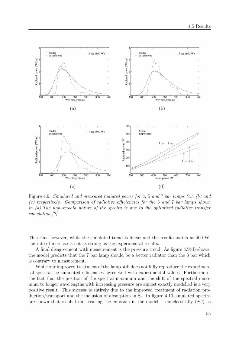
4.5 Results
300 400 500 600 700 800 900Wavelength[nm]
0
1
2
3
4
Rad
iate
d po
wer
[W/n
m]
modelexperiment
3 bar (800 W)
300 400 500 600 700 800 900Wavelength[nm]
0
1
2
3
4
Rad
iate
d po
wer
[W/n
m]
model experiment
5 bar (800 W)
(a) (b)
300 400 500 600 700 800 900Wavelength[nm]
0
1
2
3
4
Rad
iate
d po
wer
[W/n
m]
modelexperiment
7 bar (800 W)
200 300 400 500 600 700 800Input power [W]
0
100
200
300
400
500
600R
adia
ted
pow
er [W
]
ModelExperiment
3 bar 7 bar
3 bar 7 bar
(c) (d)
Figure 4.9: Simulated and measured radiated power for 3, 5 and 7 bar lamps (a), (b) and(c) respectively. Comparison of radiative efficiencies for the 3 and 7 bar lamps shownin (d).The non-smooth nature of the spectra is due to the optimized radiative transfercalculation [7].
This time however, while the simulated trend is linear and the results match at 400 W,the rate of increase is not as strong as the experimental results.
A final disagreement with measurement is the pressure trend. As figure 4.9(d) shows,the model predicts that the 7 bar lamp should be a better radiator than the 3 bar whichis contrary to measurement.
While our improved treatment of the lamp still does not fully reproduce the experimen-tal spectra the simulated efficiencies agree well with experimental values. Furthermore,the fact that the position of the spectral maximum and the shift of the spectral maxi-mum to longer wavelengths with increasing pressure are almost exactly modelled is a verypositive result. This success is entirely due to the improved treatment of radiation pro-duction/transport and the inclusion of absorption in S3. In figure 4.10 simulated spectraare shown that result from treating the emission in the model - semiclassically (SC) as
55
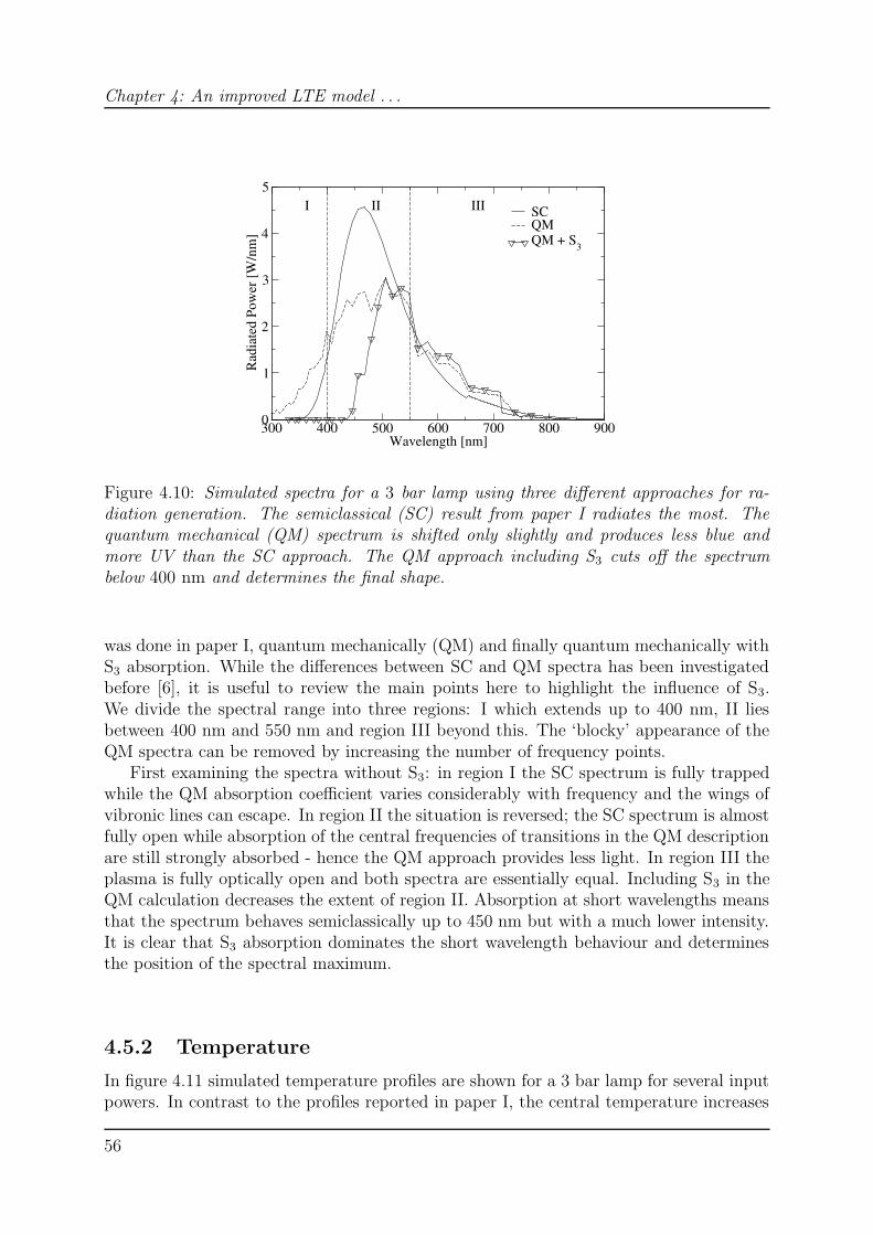
Chapter 4: An improved LTE model . . .
300 400 500 600 700 800 900Wavelength [nm]
0
1
2
3
4
5
Rad
iate
d Po
wer
[W/n
m]
SCQMQM + S3
I II III
Figure 4.10: Simulated spectra for a 3 bar lamp using three different approaches for ra-diation generation. The semiclassical (SC) result from paper I radiates the most. Thequantum mechanical (QM) spectrum is shifted only slightly and produces less blue andmore UV than the SC approach. The QM approach including S3 cuts off the spectrumbelow 400 nm and determines the final shape.
was done in paper I, quantum mechanically (QM) and finally quantum mechanically withS3 absorption. While the differences between SC and QM spectra has been investigatedbefore [6], it is useful to review the main points here to highlight the influence of S3.We divide the spectral range into three regions: I which extends up to 400 nm, II liesbetween 400 nm and 550 nm and region III beyond this. The ‘blocky’ appearance of theQM spectra can be removed by increasing the number of frequency points.
First examining the spectra without S3: in region I the SC spectrum is fully trappedwhile the QM absorption coefficient varies considerably with frequency and the wings ofvibronic lines can escape. In region II the situation is reversed; the SC spectrum is almostfully open while absorption of the central frequencies of transitions in the QM descriptionare still strongly absorbed - hence the QM approach provides less light. In region III theplasma is fully optically open and both spectra are essentially equal. Including S3 in theQM calculation decreases the extent of region II. Absorption at short wavelengths meansthat the spectrum behaves semiclassically up to 450 nm but with a much lower intensity.It is clear that S3 absorption dominates the short wavelength behaviour and determinesthe position of the spectral maximum.
4.5.2 Temperature
In figure 4.11 simulated temperature profiles are shown for a 3 bar lamp for several inputpowers. In contrast to the profiles reported in paper I, the central temperature increases
56
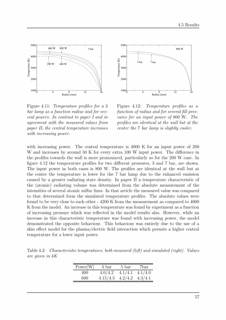
4.5 Results
0 4 8 12 16Radius [mm]
1000
2000
3000
4000
5000
Tem
pera
ture
[K]
200 W 400 W
600 W 800 W 3 bar
Figure 4.11: Temperature profiles for a 3bar lamp as a function radius and for sev-eral powers. In contrast to paper I and inagreement with the measured values frompaper II, the central temperature increaseswith increasing power.
0 4 8 12 16Radius [mm]
1000
2000
3000
4000
5000
Tem
pera
ture
[K]
3 bar 7 bar
800 W
Figure 4.12: Temperature profiles as afunction of radius and for several fill pres-sures for an input power of 800 W. Theprofiles are identical at the wall but at thecenter the 7 bar lamp is slightly cooler.
with increasing power. The central temperature is 4000 K for an input power of 200W and increases by around 50 K for every extra 100 W input power. The difference inthe profiles towards the wall is more pronounced, particularly so for the 200 W case. Infigure 4.12 the temperature profiles for two different pressures, 3 and 7 bar, are shown.The input power in both cases is 800 W. The profiles are identical at the wall but atthe centre the temperature is lower for the 7 bar lamp due to the enhanced emissioncaused by a greater radiating state density. In paper II a temperature characteristic ofthe (atomic) radiating volume was determined from the absolute measurement of theintensities of several atomic sulfur lines. In that article the measured value was comparedto that determined form the simulated temperature profiles. The absolute values werefound to be very close to each other - 4200 K from the measurement as compared to 4000K from the model. An increase in this temperature was found by experiment as a functionof increasing pressure which was reflected in the model results also. However, while anincrease in this characteristic temperature was found with increasing power, the modeldemonstrated the opposite behaviour. This behaviour was entirely due to the use of askin effect model for the plasma/electric field interaction which permits a higher centraltemperature for a lower input power.
Table 4.2: Characteristic temperatures, both measured (left) and simulated (right). Valuesare given in kK
Power[W] 3 bar 5 bar 7bar400 4.0/4.2 4.1/4.1 4.1/4.0600 4.15/4.3 4.2/4.2 4.3/4.1
57
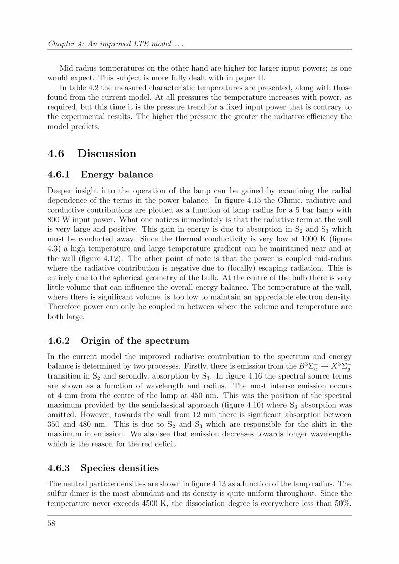
Chapter 4: An improved LTE model . . .
Mid-radius temperatures on the other hand are higher for larger input powers; as onewould expect. This subject is more fully dealt with in paper II.
In table 4.2 the measured characteristic temperatures are presented, along with thosefound from the current model. At all pressures the temperature increases with power, asrequired, but this time it is the pressure trend for a fixed input power that is contrary tothe experimental results. The higher the pressure the greater the radiative efficiency themodel predicts.
4.6 Discussion
4.6.1 Energy balance
Deeper insight into the operation of the lamp can be gained by examining the radialdependence of the terms in the power balance. In figure 4.15 the Ohmic, radiative andconductive contributions are plotted as a function of lamp radius for a 5 bar lamp with800 W input power. What one notices immediately is that the radiative term at the wallis very large and positive. This gain in energy is due to absorption in S2 and S3 whichmust be conducted away. Since the thermal conductivity is very low at 1000 K (figure4.3) a high temperature and large temperature gradient can be maintained near and atthe wall (figure 4.12). The other point of note is that the power is coupled mid-radiuswhere the radiative contribution is negative due to (locally) escaping radiation. This isentirely due to the spherical geometry of the bulb. At the centre of the bulb there is verylittle volume that can influence the overall energy balance. The temperature at the wall,where there is significant volume, is too low to maintain an appreciable electron density.Therefore power can only be coupled in between where the volume and temperature areboth large.
4.6.2 Origin of the spectrum
In the current model the improved radiative contribution to the spectrum and energybalance is determined by two processes. Firstly, there is emission from the B3Σ−
u → X3Σ−g
transition in S2 and secondly, absorption by S3. In figure 4.16 the spectral source termsare shown as a function of wavelength and radius. The most intense emission occursat 4 mm from the centre of the lamp at 450 nm. This was the position of the spectralmaximum provided by the semiclassical approach (figure 4.10) where S3 absorption wasomitted. However, towards the wall from 12 mm there is significant absorption between350 and 480 nm. This is due to S2 and S3 which are responsible for the shift in themaximum in emission. We also see that emission decreases towards longer wavelengthswhich is the reason for the red deficit.
4.6.3 Species densities
The neutral particle densities are shown in figure 4.13 as a function of the lamp radius. Thesulfur dimer is the most abundant and its density is quite uniform throughout. Since thetemperature never exceeds 4500 K, the dissociation degree is everywhere less than 50%.
58
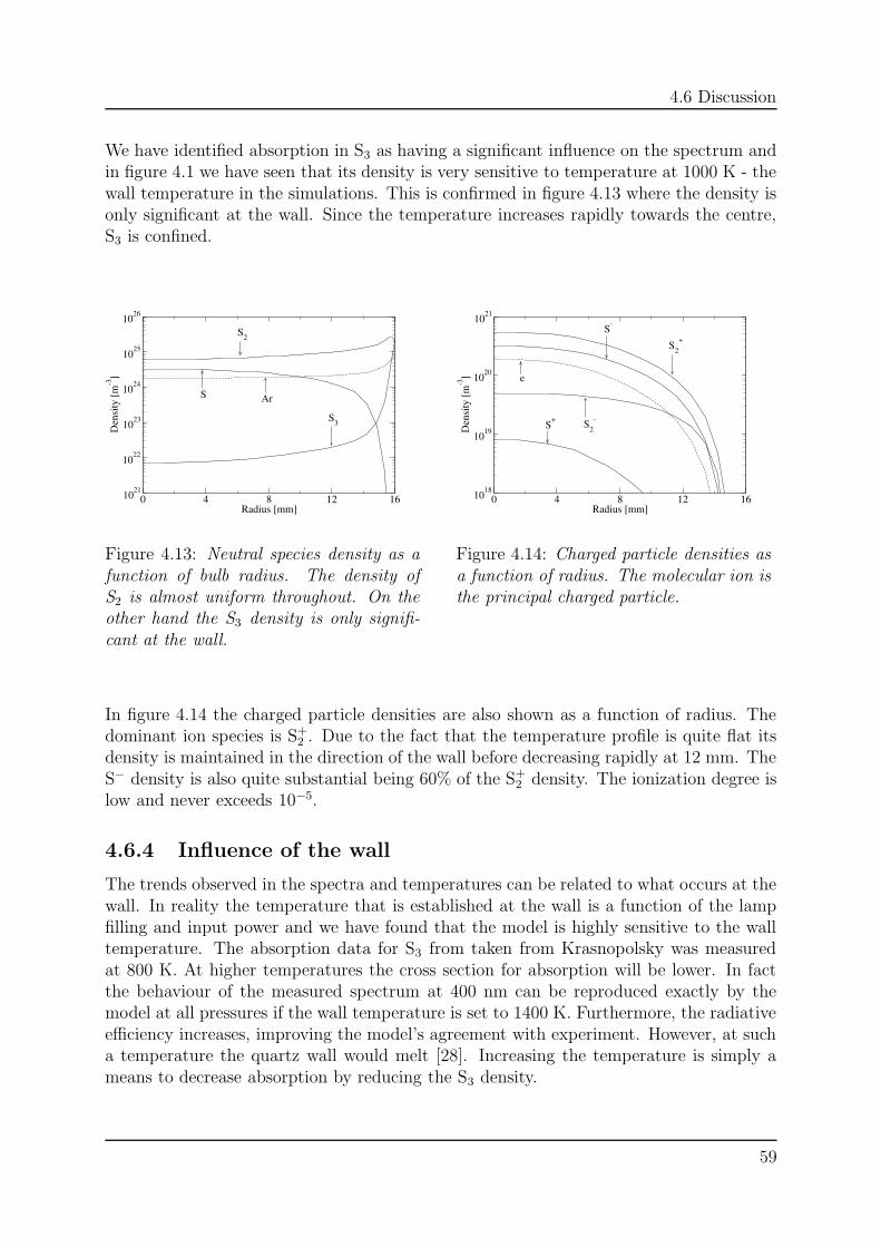
4.6 Discussion
We have identified absorption in S3 as having a significant influence on the spectrum andin figure 4.1 we have seen that its density is very sensitive to temperature at 1000 K - thewall temperature in the simulations. This is confirmed in figure 4.13 where the density isonly significant at the wall. Since the temperature increases rapidly towards the centre,S3 is confined.
0 4 8 12 16Radius [mm]
1021
1022
1023
1024
1025
1026
Den
sity
[m-3
]
S2
S
S3
Ar
Figure 4.13: Neutral species density as afunction of bulb radius. The density ofS2 is almost uniform throughout. On theother hand the S3 density is only signifi-cant at the wall.
0 4 8 12 16Radius [mm]
1018
1019
1020
1021
Den
sity
[m-3
]
S+
S2+
e
S2-
S-
Figure 4.14: Charged particle densities asa function of radius. The molecular ion isthe principal charged particle.
In figure 4.14 the charged particle densities are also shown as a function of radius. Thedominant ion species is S+
2 . Due to the fact that the temperature profile is quite flat itsdensity is maintained in the direction of the wall before decreasing rapidly at 12 mm. TheS− density is also quite substantial being 60% of the S+
2 density. The ionization degree islow and never exceeds 10−5.
4.6.4 Influence of the wall
The trends observed in the spectra and temperatures can be related to what occurs at thewall. In reality the temperature that is established at the wall is a function of the lampfilling and input power and we have found that the model is highly sensitive to the walltemperature. The absorption data for S3 from taken from Krasnopolsky was measuredat 800 K. At higher temperatures the cross section for absorption will be lower. In factthe behaviour of the measured spectrum at 400 nm can be reproduced exactly by themodel at all pressures if the wall temperature is set to 1400 K. Furthermore, the radiativeefficiency increases, improving the model’s agreement with experiment. However, at sucha temperature the quartz wall would melt [28]. Increasing the temperature is simply ameans to decrease absorption by reducing the S3 density.
59
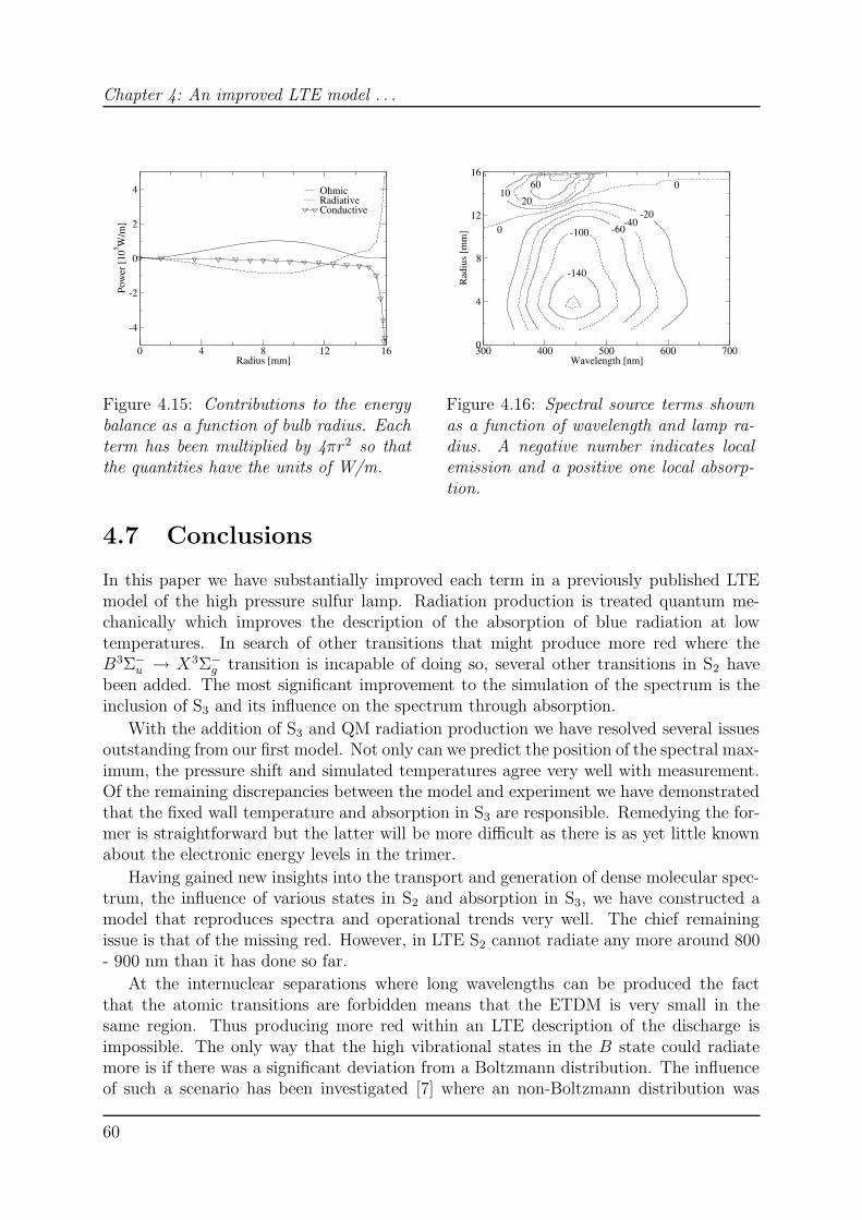
Chapter 4: An improved LTE model . . .
0 4 8 12 16Radius [mm]
-4
-2
0
2
4
Pow
er [1
05 W/m
]
OhmicRadiativeConductive
Figure 4.15: Contributions to the energybalance as a function of bulb radius. Eachterm has been multiplied by 4πr2 so thatthe quantities have the units of W/m.
300 400 500 600 700Wavelength [nm]
0
4
8
12
16
Rad
ius
[mm
]
-20-40
-60-100
-140
0
0
1020
60
Figure 4.16: Spectral source terms shownas a function of wavelength and lamp ra-dius. A negative number indicates localemission and a positive one local absorp-tion.
4.7 Conclusions
In this paper we have substantially improved each term in a previously published LTEmodel of the high pressure sulfur lamp. Radiation production is treated quantum me-chanically which improves the description of the absorption of blue radiation at lowtemperatures. In search of other transitions that might produce more red where theB3Σ−
u → X3Σ−g transition is incapable of doing so, several other transitions in S2 have
been added. The most significant improvement to the simulation of the spectrum is theinclusion of S3 and its influence on the spectrum through absorption.
With the addition of S3 and QM radiation production we have resolved several issuesoutstanding from our first model. Not only can we predict the position of the spectral max-imum, the pressure shift and simulated temperatures agree very well with measurement.Of the remaining discrepancies between the model and experiment we have demonstratedthat the fixed wall temperature and absorption in S3 are responsible. Remedying the for-mer is straightforward but the latter will be more difficult as there is as yet little knownabout the electronic energy levels in the trimer.
Having gained new insights into the transport and generation of dense molecular spec-trum, the influence of various states in S2 and absorption in S3, we have constructed amodel that reproduces spectra and operational trends very well. The chief remainingissue is that of the missing red. However, in LTE S2 cannot radiate any more around 800- 900 nm than it has done so far.
At the internuclear separations where long wavelengths can be produced the factthat the atomic transitions are forbidden means that the ETDM is very small in thesame region. Thus producing more red within an LTE description of the discharge isimpossible. The only way that the high vibrational states in the B state could radiatemore is if there was a significant deviation from a Boltzmann distribution. The influenceof such a scenario has been investigated [7] where an non-Boltzmann distribution was
60
Bibliography
shown to reproduce the measured spectra.We conclude from the results of the model in paper I, the measurements in paper
II and the improved model presented here that the power balance and response of thespectrum to operational parameters can be very adequately understood via LTE. However,we feel that any further refinement of our understanding of the discharge will require theconsideration of non-equilibrium processes.
Acknowledgements
This work is part of the research program of the Dutch Technology Foundation (STW).The authors would like to thank Achim Korber and Johannes Baier of Philips research lab-oratories in Aachen, Germany for their assistance and provision of experimental spectra.Also a special thanks to Toni Kiljunen of the Department of Chemistry at the UniversityJyaasklya, Finland, for providing the ETDMs of the supplementary S2 states included inthe model and our fruitful discussions.
References
[1] Johnston C W, van der Heijden H W P, Janssen G M, van Dijk J and van der MullenJ J A M, J. Phys. D: Appl. Phys. 35, 342 (2002), Chapter 2 of this thesis
[2] Janssen G M, van Dijk J, Benoy D A, Tas M A, Burm K T A L, Goedheer W J, vander Mullen J J A M and Schram D C, Plasma Sources Sci. Technol. 8, 1 (1999)
[3] van Dijk J, Modelling of plasma light sources : an object-oriented approach, PhDThesis, Eindhoven University of Technology, The Netherlands, ISBN 90-386-1819-0(2001)
[4] Johnston C W, Jonkers J and van der Mullen J J A M, J. Phys. D: Appl. Phys. 35,2578 (2002), Chapter 3 of this thesis
[5] van der Heijden H and van der Mullen J J A M, J. Phys. B: At. Mol. Opt. Phys. 34,4183 (2001)
[6] van der Heijden H, van der Mullen J J A M, Baier J and Korber A, J. Phys. B: At.Mol. Opt. Phys. 35, 3633 (2002)
[7] van der Heijden H and van der Mullen J A M J. Phys. D: Appl. Phys. 35, 2112(2002)
[8] Doll W P and Lapatovich W P, J. Phys. Chem. 95, 4242 (1991)
[9] Korber A, The physics of light emission from sulphur lamps, Master class on hottopics in Plasma Physics and Technology Socrates CLTPP-4, Eindhoven, (1999)
[10] van Dongen M, Korber A, van der Heijden H, Jonkers J, Scholl R and van der MullenJ J A M, J. Phys. D: Appl. Phys. 31, 3095, (1999)
61
Bibliography
[11] Johnston C W, Philips Trainee Report, CDL II 4007/96 (1996)
[12] Devoto R S, Phys. Fluids 9, 1230 (1966)
[13] Devoto R S, Phys. Rev. A 56, 1897 (1992)
[14] Devoto R S, Phys. Fluids 10, 354 (1967)
[15] Capitelli M, Colonna G, Gorse C, D’Angola A, Eur. Phys. J. D 11, 279 (2000)
[16] Pashov A, Jastrzebski W and Kowalcyzk P, Comput. Phys. Commun. 128, 622 (2000)
[17] http://sources.redhat.com/gsl/
[18] D A Pradhan and Partridge H, Chem. Phys. Lett. 255, 163 (1996)
[19] Wheeler M D, Newman S M and Orr-Ewing A J, J. Chem. Phys. 108, 6594 (1998)
[20] Kiljunen T, Eloranta J, Kunttu H, Khriachtchev L, Pettersson M, Rasa nen M J.Chem. Phys. 112, 163 (1996)
[21] Krasnopolsky V A Adv. Space Res. 7, 12 (1987)
[22] Braune H, Steinbacher E, Adv. Space Res. 7a, 486 (1952)
[23] Billmers R I, Smith A L, J. Phys. Chem. 95, 4242 (1991)
[24] Swope W C, Lee Y P, Schaefer III H F J. Chem. Phys. 70, 947 (1979)
[25] Pearse R W B Gaydon A G, Indentification of Molecular Spectra (Chapman and Hall,London, 1984)
[26] MOLPRO is a package of ab initio programs designed by Werner H J and KnowlesP J. The authors are Amos R D, Bernhardsson A, Berning A, Celani P, Cooper D L,Deegan M J O , Dobbyn A J, Eckert F, Hampel C, Hetzer G, Knowles P J, Korona T,Lindh R, Lloyd A W, McNicholas S J, Manby F R, Meyer W, Mura M E, NicklaßA,Palmieri P, Pitzer R, Rauhut G, Schtz M, Schumann U, Stoll H, Stone A J, TarroniR, Thorsteinsson T and Werner H J.
[27] T. Kiljunen, private communication
[28] van Dongen M, Graduation report, Eindhoven University of Technology, VDF/NT97-14 (1997)
62
CHAPTER 5
Measured and simulated response of a high pressure sulfur
spectrum to power interruption
The power supplied to a high pressure sulfur plasma sustained by microwaves is inter-rupted on short times scales. The response of the molecular spectrum between 400 and900 nm is measured during this interruption. Characteristic decay times of around 20ms are found and are due chiefly to the large heat capacity of the reacting mixture. Theresults of a time dependent LTE model of the interruption, including radiation transportof the entire molecular spectrum and heat conduction, are also presented. The simu-lated signal decay agrees with experiment not only in magnitude but also as a functionof wavelength.
63
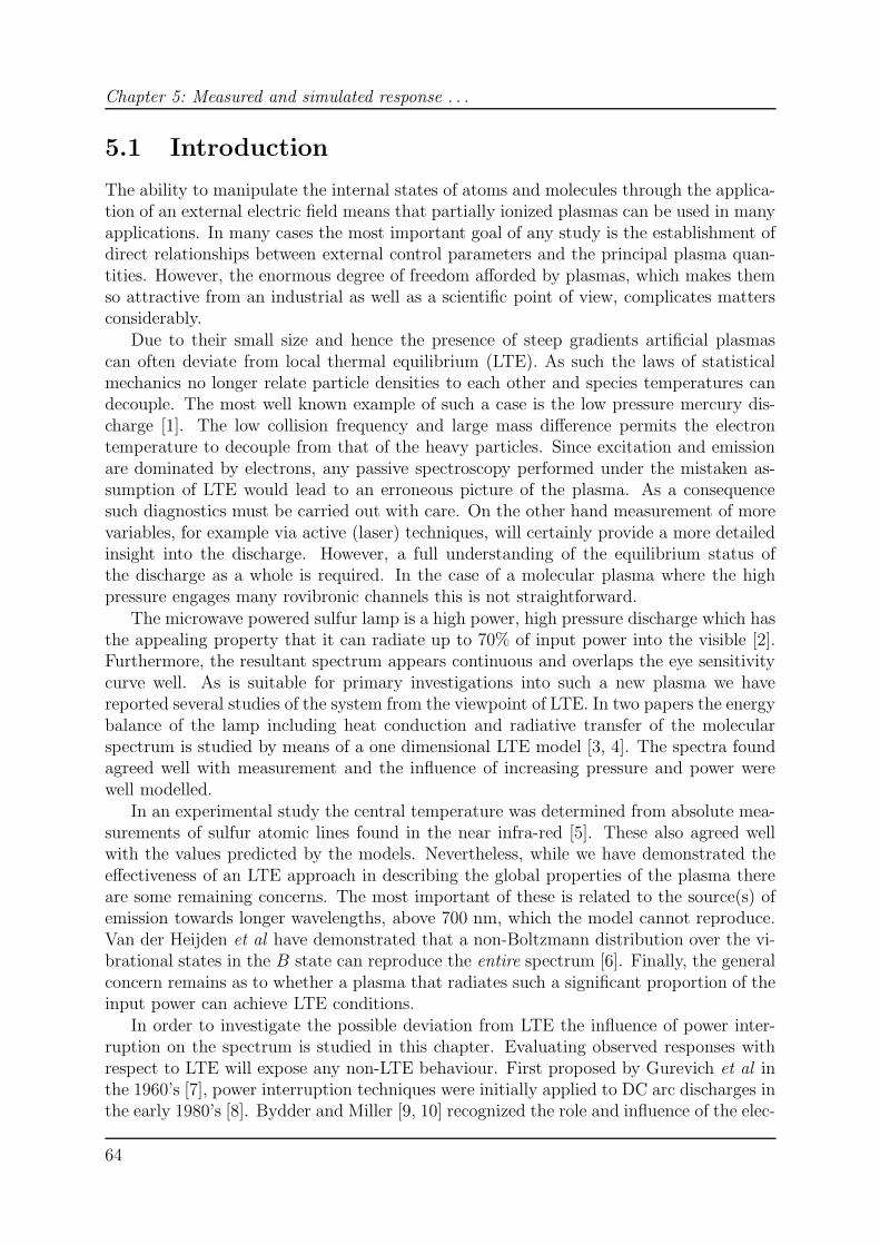
Chapter 5: Measured and simulated response . . .
5.1 Introduction
The ability to manipulate the internal states of atoms and molecules through the applica-tion of an external electric field means that partially ionized plasmas can be used in manyapplications. In many cases the most important goal of any study is the establishment ofdirect relationships between external control parameters and the principal plasma quan-tities. However, the enormous degree of freedom afforded by plasmas, which makes themso attractive from an industrial as well as a scientific point of view, complicates mattersconsiderably.
Due to their small size and hence the presence of steep gradients artificial plasmascan often deviate from local thermal equilibrium (LTE). As such the laws of statisticalmechanics no longer relate particle densities to each other and species temperatures candecouple. The most well known example of such a case is the low pressure mercury dis-charge [1]. The low collision frequency and large mass difference permits the electrontemperature to decouple from that of the heavy particles. Since excitation and emissionare dominated by electrons, any passive spectroscopy performed under the mistaken as-sumption of LTE would lead to an erroneous picture of the plasma. As a consequencesuch diagnostics must be carried out with care. On the other hand measurement of morevariables, for example via active (laser) techniques, will certainly provide a more detailedinsight into the discharge. However, a full understanding of the equilibrium status ofthe discharge as a whole is required. In the case of a molecular plasma where the highpressure engages many rovibronic channels this is not straightforward.
The microwave powered sulfur lamp is a high power, high pressure discharge which hasthe appealing property that it can radiate up to 70% of input power into the visible [2].Furthermore, the resultant spectrum appears continuous and overlaps the eye sensitivitycurve well. As is suitable for primary investigations into such a new plasma we havereported several studies of the system from the viewpoint of LTE. In two papers the energybalance of the lamp including heat conduction and radiative transfer of the molecularspectrum is studied by means of a one dimensional LTE model [3, 4]. The spectra foundagreed well with measurement and the influence of increasing pressure and power werewell modelled.
In an experimental study the central temperature was determined from absolute mea-surements of sulfur atomic lines found in the near infra-red [5]. These also agreed wellwith the values predicted by the models. Nevertheless, while we have demonstrated theeffectiveness of an LTE approach in describing the global properties of the plasma thereare some remaining concerns. The most important of these is related to the source(s) ofemission towards longer wavelengths, above 700 nm, which the model cannot reproduce.Van der Heijden et al have demonstrated that a non-Boltzmann distribution over the vi-brational states in the B state can reproduce the entire spectrum [6]. Finally, the generalconcern remains as to whether a plasma that radiates such a significant proportion of theinput power can achieve LTE conditions.
In order to investigate the possible deviation from LTE the influence of power inter-ruption on the spectrum is studied in this chapter. Evaluating observed responses withrespect to LTE will expose any non-LTE behaviour. First proposed by Gurevich et al inthe 1960’s [7], power interruption techniques were initially applied to DC arc discharges inthe early 1980’s [8]. Bydder and Miller [9, 10] recognized the role and influence of the elec-
64
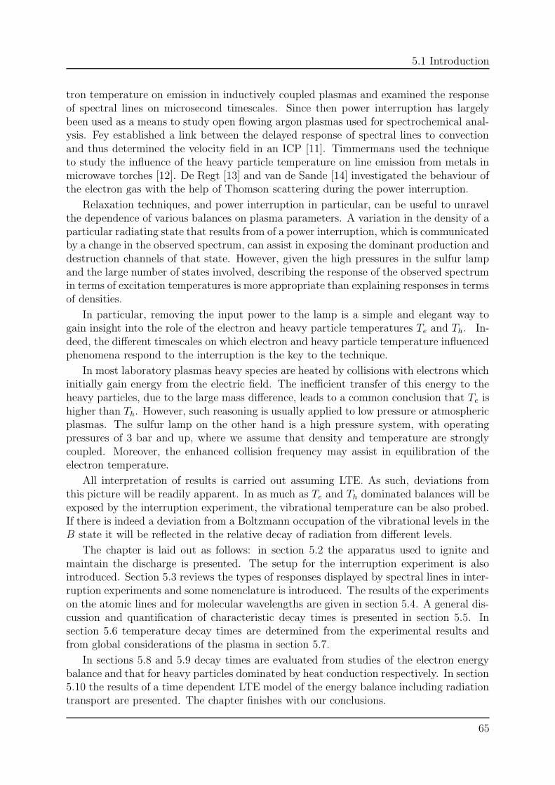
5.1 Introduction
tron temperature on emission in inductively coupled plasmas and examined the responseof spectral lines on microsecond timescales. Since then power interruption has largelybeen used as a means to study open flowing argon plasmas used for spectrochemical anal-ysis. Fey established a link between the delayed response of spectral lines to convectionand thus determined the velocity field in an ICP [11]. Timmermans used the techniqueto study the influence of the heavy particle temperature on line emission from metals inmicrowave torches [12]. De Regt [13] and van de Sande [14] investigated the behaviour ofthe electron gas with the help of Thomson scattering during the power interruption.
Relaxation techniques, and power interruption in particular, can be useful to unravelthe dependence of various balances on plasma parameters. A variation in the density of aparticular radiating state that results from of a power interruption, which is communicatedby a change in the observed spectrum, can assist in exposing the dominant production anddestruction channels of that state. However, given the high pressures in the sulfur lampand the large number of states involved, describing the response of the observed spectrumin terms of excitation temperatures is more appropriate than explaining responses in termsof densities.
In particular, removing the input power to the lamp is a simple and elegant way togain insight into the role of the electron and heavy particle temperatures Te and Th. In-deed, the different timescales on which electron and heavy particle temperature influencedphenomena respond to the interruption is the key to the technique.
In most laboratory plasmas heavy species are heated by collisions with electrons whichinitially gain energy from the electric field. The inefficient transfer of this energy to theheavy particles, due to the large mass difference, leads to a common conclusion that Te ishigher than Th. However, such reasoning is usually applied to low pressure or atmosphericplasmas. The sulfur lamp on the other hand is a high pressure system, with operatingpressures of 3 bar and up, where we assume that density and temperature are stronglycoupled. Moreover, the enhanced collision frequency may assist in equilibration of theelectron temperature.
All interpretation of results is carried out assuming LTE. As such, deviations fromthis picture will be readily apparent. In as much as Te and Th dominated balances will beexposed by the interruption experiment, the vibrational temperature can be also probed.If there is indeed a deviation from a Boltzmann occupation of the vibrational levels in theB state it will be reflected in the relative decay of radiation from different levels.
The chapter is laid out as follows: in section 5.2 the apparatus used to ignite andmaintain the discharge is presented. The setup for the interruption experiment is alsointroduced. Section 5.3 reviews the types of responses displayed by spectral lines in inter-ruption experiments and some nomenclature is introduced. The results of the experimentson the atomic lines and for molecular wavelengths are given in section 5.4. A general dis-cussion and quantification of characteristic decay times is presented in section 5.5. Insection 5.6 temperature decay times are determined from the experimental results andfrom global considerations of the plasma in section 5.7.
In sections 5.8 and 5.9 decay times are evaluated from studies of the electron energybalance and that for heavy particles dominated by heat conduction respectively. In section5.10 the results of a time dependent LTE model of the energy balance including radiationtransport are presented. The chapter finishes with our conclusions.
65
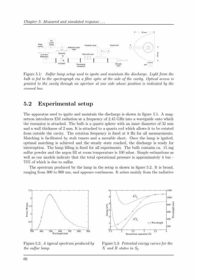
Chapter 5: Measured and simulated response . . .
2.45 GHzMagnetron
Circulator
Triple stub tuner
Movableshort
Rectangularwaveguide
HV-powersupply
Reflected powermeter
Absorber
Watercooling Parabolic cavity Quartz bulb
60 mm
80 mm
Wµ
Figure 5.1: Sulfur lamp setup used to ignite and maintain the discharge. Light from thebulb is fed to the spectrograph via a fibre optic at the side of the cavity. Optical access isgranted to the cavity through an aperture at one side whose position is indicated by thecrossed box.
5.2 Experimental setup
The apparatus used to ignite and maintain the discharge is shown in figure 5.1. A mag-netron introduces EM radiation at a frequency of 2.45 GHz into a waveguide onto whichthe resonator is attached. The bulb is a quartz sphere with an inner diameter of 32 mmand a wall thickness of 2 mm. It is attached to a quartz rod which allows it to be rotatedfrom outside the cavity. The rotation frequency is fixed at 8 Hz for all measurements.Matching is facilitated by stub tuners and a movable short. Once the lamp is ignited,optimal matching is achieved and the steady state reached, the discharge is ready forinterruption. The lamp filling is fixed for all experiments. The bulb contains ca. 15 mgsulfur powder and the argon fill at room temperature is 100 mbar. Simple estimations aswell as our models indicate that the total operational pressure is approximately 4 bar -75% of which is due to sulfur.
The spectrum produced by the lamp in the setup is shown in figure 5.2. It is broad,ranging from 300 to 900 nm, and appears continuous. It arises mainly from the radiative
300 400 500 600 700 800 900Wavlength [nm]
0
0.5
1
1.5
2
2.5
Pow
er [W
/nm
]
Figure 5.2: A typical spectrum produced bythe sulfur lamp.
1.5 2 2.5 3 3.5 4Internuclear separation [Å]
0
1
2
3
4
5
6
Ene
rgy
[eV
]
200
400
600
800
1000
1200
Wav
elen
gth
[nm
]
Wavelength
B3Σu-
X3Σg-
Figure 5.3: Potential energy curves for theX and B states in S2.
66
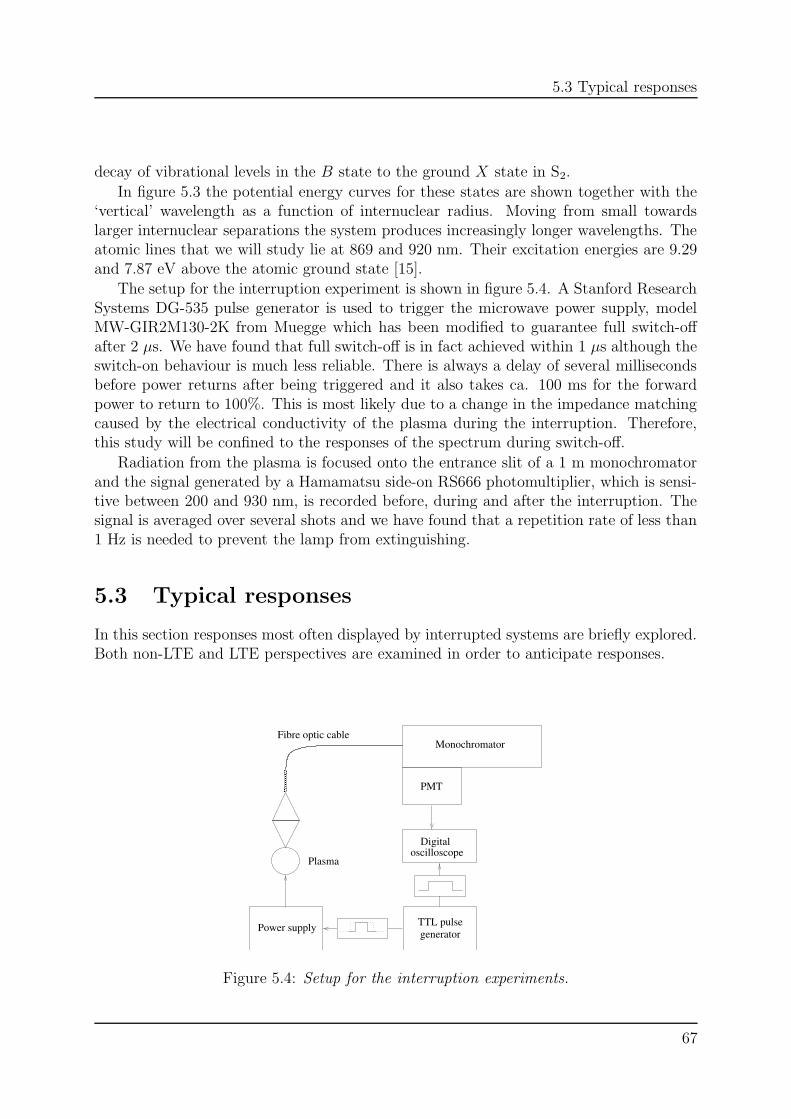
5.3 Typical responses
decay of vibrational levels in the B state to the ground X state in S2.
In figure 5.3 the potential energy curves for these states are shown together with the‘vertical’ wavelength as a function of internuclear radius. Moving from small towardslarger internuclear separations the system produces increasingly longer wavelengths. Theatomic lines that we will study lie at 869 and 920 nm. Their excitation energies are 9.29and 7.87 eV above the atomic ground state [15].
The setup for the interruption experiment is shown in figure 5.4. A Stanford ResearchSystems DG-535 pulse generator is used to trigger the microwave power supply, modelMW-GIR2M130-2K from Muegge which has been modified to guarantee full switch-offafter 2 µs. We have found that full switch-off is in fact achieved within 1 µs although theswitch-on behaviour is much less reliable. There is always a delay of several millisecondsbefore power returns after being triggered and it also takes ca. 100 ms for the forwardpower to return to 100%. This is most likely due to a change in the impedance matchingcaused by the electrical conductivity of the plasma during the interruption. Therefore,this study will be confined to the responses of the spectrum during switch-off.
Radiation from the plasma is focused onto the entrance slit of a 1 m monochromatorand the signal generated by a Hamamatsu side-on RS666 photomultiplier, which is sensi-tive between 200 and 930 nm, is recorded before, during and after the interruption. Thesignal is averaged over several shots and we have found that a repetition rate of less than1 Hz is needed to prevent the lamp from extinguishing.
5.3 Typical responses
In this section responses most often displayed by interrupted systems are briefly explored.Both non-LTE and LTE perspectives are examined in order to anticipate responses.
Fibre optic cableMonochromator
PMT
Digitaloscilloscope
TTL pulsegenerator
Power supply
Plasma
Figure 5.4: Setup for the interruption experiments.
67
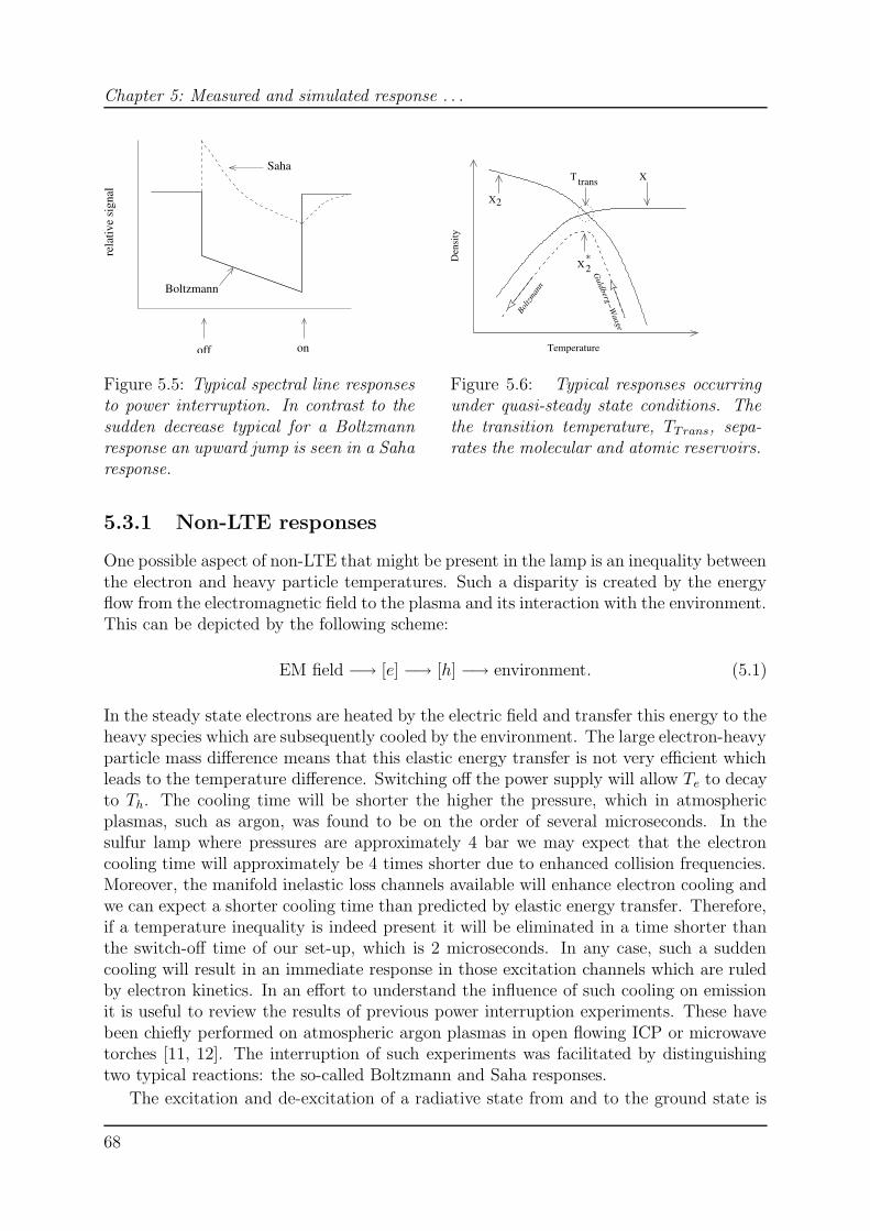
Chapter 5: Measured and simulated response . . .
Boltzmann
rela
tive
sign
al
onoff
Saha
Figure 5.5: Typical spectral line responsesto power interruption. In contrast to thesudden decrease typical for a Boltzmannresponse an upward jump is seen in a Saharesponse.
X2
XT trans
X*2
Temperature
Den
sity
Boltz
mann
Guldberg−
Waage
Figure 5.6: Typical responses occurringunder quasi-steady state conditions. Thethe transition temperature, TTrans, sepa-rates the molecular and atomic reservoirs.
5.3.1 Non-LTE responses
One possible aspect of non-LTE that might be present in the lamp is an inequality betweenthe electron and heavy particle temperatures. Such a disparity is created by the energyflow from the electromagnetic field to the plasma and its interaction with the environment.This can be depicted by the following scheme:
EM field −→ [e] −→ [h] −→ environment. (5.1)
In the steady state electrons are heated by the electric field and transfer this energy to theheavy species which are subsequently cooled by the environment. The large electron-heavyparticle mass difference means that this elastic energy transfer is not very efficient whichleads to the temperature difference. Switching off the power supply will allow Te to decayto Th. The cooling time will be shorter the higher the pressure, which in atmosphericplasmas, such as argon, was found to be on the order of several microseconds. In thesulfur lamp where pressures are approximately 4 bar we may expect that the electroncooling time will approximately be 4 times shorter due to enhanced collision frequencies.Moreover, the manifold inelastic loss channels available will enhance electron cooling andwe can expect a shorter cooling time than predicted by elastic energy transfer. Therefore,if a temperature inequality is indeed present it will be eliminated in a time shorter thanthe switch-off time of our set-up, which is 2 microseconds. In any case, such a suddencooling will result in an immediate response in those excitation channels which are ruledby electron kinetics. In an effort to understand the influence of such cooling on emissionit is useful to review the results of previous power interruption experiments. These havebeen chiefly performed on atmospheric argon plasmas in open flowing ICP or microwavetorches [11, 12]. The interruption of such experiments was facilitated by distinguishingtwo typical reactions: the so-called Boltzmann and Saha responses.
The excitation and de-excitation of a radiative state from and to the ground state is
68
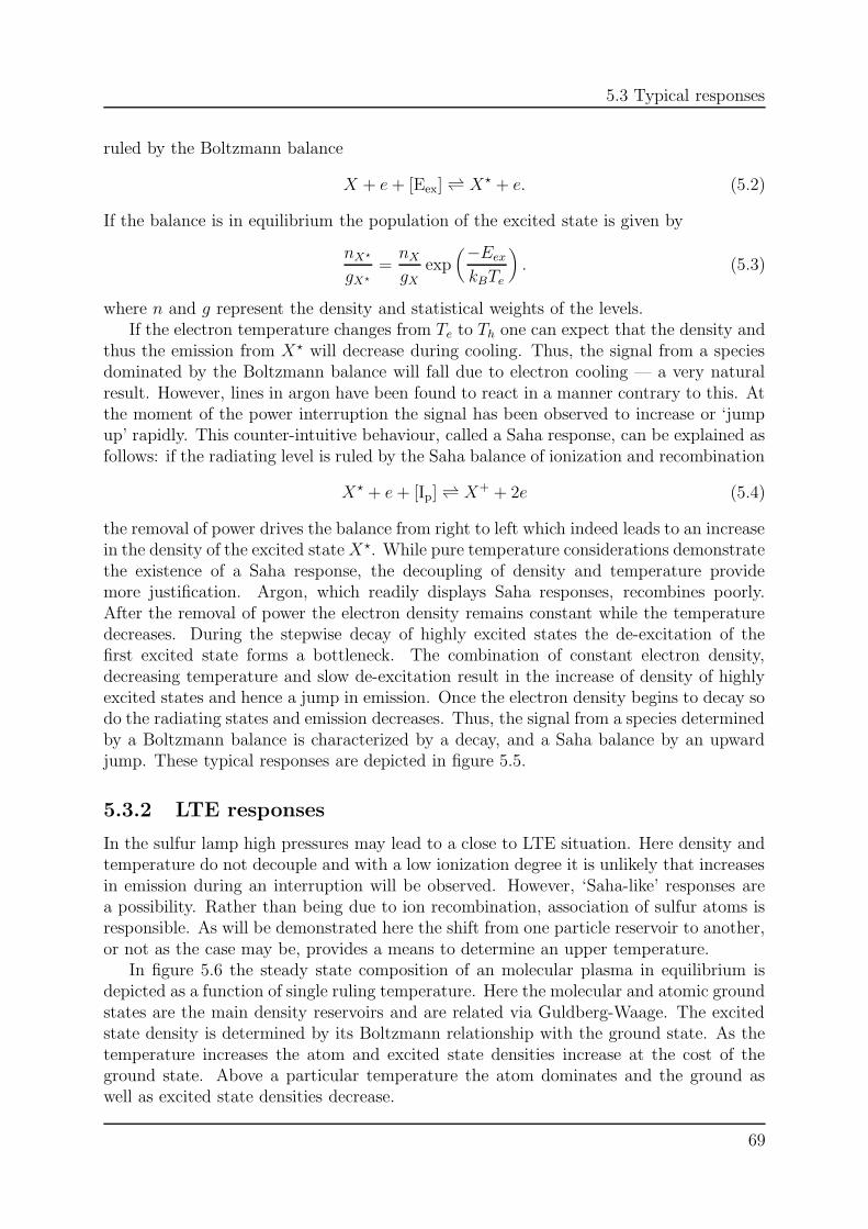
5.3 Typical responses
ruled by the Boltzmann balance
X + e+ [Eex] X? + e. (5.2)
If the balance is in equilibrium the population of the excited state is given by
nX?
gX?
=nX
gXexp
(−Eex
kBTe
). (5.3)
where n and g represent the density and statistical weights of the levels.If the electron temperature changes from Te to Th one can expect that the density and
thus the emission from X? will decrease during cooling. Thus, the signal from a speciesdominated by the Boltzmann balance will fall due to electron cooling — a very naturalresult. However, lines in argon have been found to react in a manner contrary to this. Atthe moment of the power interruption the signal has been observed to increase or ‘jumpup’ rapidly. This counter-intuitive behaviour, called a Saha response, can be explained asfollows: if the radiating level is ruled by the Saha balance of ionization and recombination
X? + e+ [Ip] X+ + 2e (5.4)
the removal of power drives the balance from right to left which indeed leads to an increasein the density of the excited stateX?. While pure temperature considerations demonstratethe existence of a Saha response, the decoupling of density and temperature providemore justification. Argon, which readily displays Saha responses, recombines poorly.After the removal of power the electron density remains constant while the temperaturedecreases. During the stepwise decay of highly excited states the de-excitation of thefirst excited state forms a bottleneck. The combination of constant electron density,decreasing temperature and slow de-excitation result in the increase of density of highlyexcited states and hence a jump in emission. Once the electron density begins to decay sodo the radiating states and emission decreases. Thus, the signal from a species determinedby a Boltzmann balance is characterized by a decay, and a Saha balance by an upwardjump. These typical responses are depicted in figure 5.5.
5.3.2 LTE responses
In the sulfur lamp high pressures may lead to a close to LTE situation. Here density andtemperature do not decouple and with a low ionization degree it is unlikely that increasesin emission during an interruption will be observed. However, ‘Saha-like’ responses area possibility. Rather than being due to ion recombination, association of sulfur atoms isresponsible. As will be demonstrated here the shift from one particle reservoir to another,or not as the case may be, provides a means to determine an upper temperature.
In figure 5.6 the steady state composition of an molecular plasma in equilibrium isdepicted as a function of single ruling temperature. Here the molecular and atomic groundstates are the main density reservoirs and are related via Guldberg-Waage. The excitedstate density is determined by its Boltzmann relationship with the ground state. As thetemperature increases the atom and excited state densities increase at the cost of theground state. Above a particular temperature the atom dominates and the ground aswell as excited state densities decrease.
69
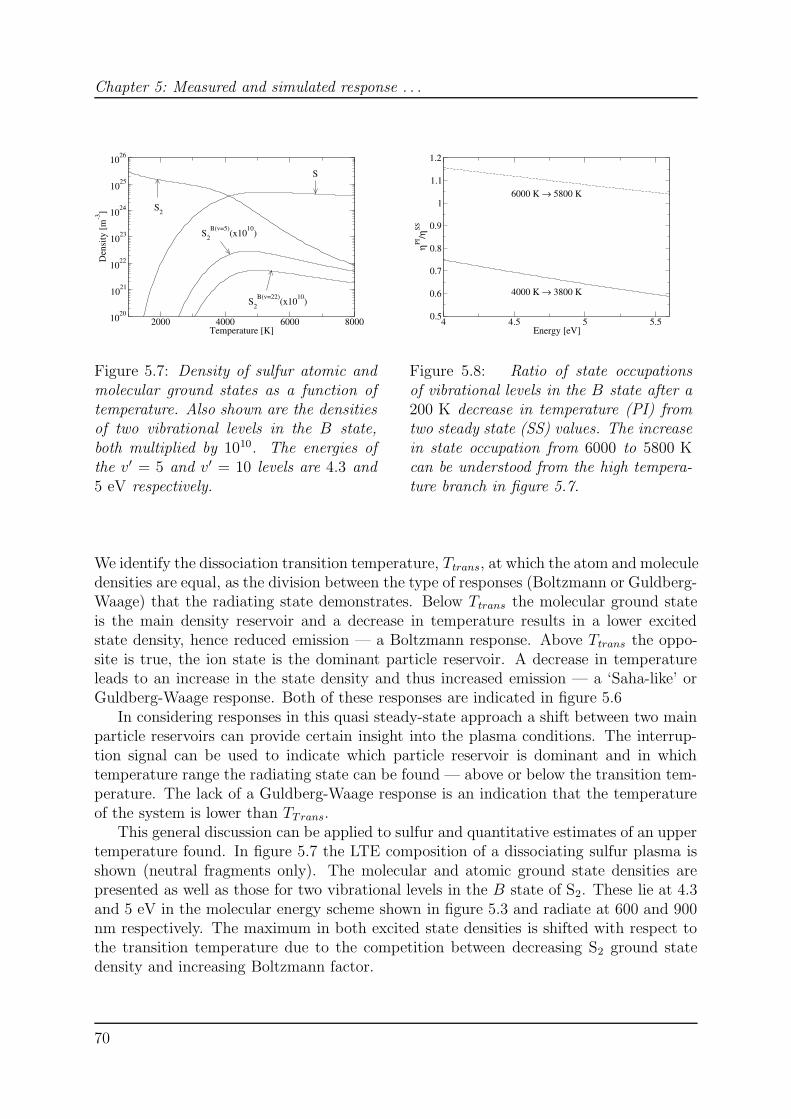
Chapter 5: Measured and simulated response . . .
2000 4000 6000 8000Temperature [K]
1020
1021
1022
1023
1024
1025
1026
Den
sity
[m-3
] S2
S
S2B(v=5)(x1010)
S2B(v=22)(x1010)
Figure 5.7: Density of sulfur atomic andmolecular ground states as a function oftemperature. Also shown are the densitiesof two vibrational levels in the B state,both multiplied by 1010. The energies ofthe v′ = 5 and v′ = 10 levels are 4.3 and5 eV respectively.
4 4.5 5 5.5Energy [eV]
0.5
0.6
0.7
0.8
0.9
1
1.1
1.2
ηPI/η
SS
4000 K → 3800 K
6000 K → 5800 K
Figure 5.8: Ratio of state occupationsof vibrational levels in the B state after a200 K decrease in temperature (PI) fromtwo steady state (SS) values. The increasein state occupation from 6000 to 5800 Kcan be understood from the high tempera-ture branch in figure 5.7.
We identify the dissociation transition temperature, Ttrans, at which the atom and moleculedensities are equal, as the division between the type of responses (Boltzmann or Guldberg-Waage) that the radiating state demonstrates. Below Ttrans the molecular ground stateis the main density reservoir and a decrease in temperature results in a lower excitedstate density, hence reduced emission — a Boltzmann response. Above Ttrans the oppo-site is true, the ion state is the dominant particle reservoir. A decrease in temperatureleads to an increase in the state density and thus increased emission — a ‘Saha-like’ orGuldberg-Waage response. Both of these responses are indicated in figure 5.6
In considering responses in this quasi steady-state approach a shift between two mainparticle reservoirs can provide certain insight into the plasma conditions. The interrup-tion signal can be used to indicate which particle reservoir is dominant and in whichtemperature range the radiating state can be found — above or below the transition tem-perature. The lack of a Guldberg-Waage response is an indication that the temperatureof the system is lower than TTrans.
This general discussion can be applied to sulfur and quantitative estimates of an uppertemperature found. In figure 5.7 the LTE composition of a dissociating sulfur plasma isshown (neutral fragments only). The molecular and atomic ground state densities arepresented as well as those for two vibrational levels in the B state of S2. These lie at 4.3and 5 eV in the molecular energy scheme shown in figure 5.3 and radiate at 600 and 900nm respectively. The maximum in both excited state densities is shifted with respect tothe transition temperature due to the competition between decreasing S2 ground statedensity and increasing Boltzmann factor.
70
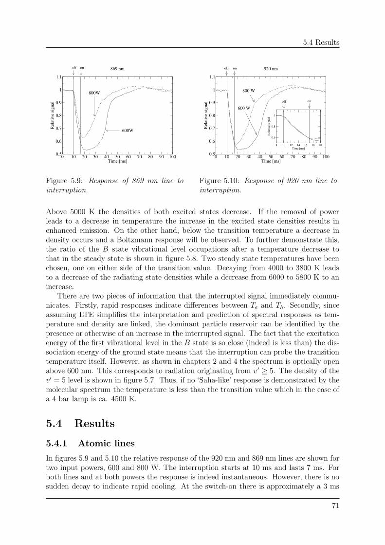
5.4 Results
0 10 20 30 40 50 60 70 80 90 100Time [ms]
0.5
0.6
0.7
0.8
0.9
1
1.1
Rel
ativ
e si
gnal
869 nm
800W
600W
off on
Figure 5.9: Response of 869 nm line tointerruption.
0 10 20 30 40 50 60 70 80 90 100Time [ms]
0.5
0.6
0.7
0.8
0.9
1
1.1
Rel
ativ
e si
gnal
920 nm
8 10 12 14 16 18 20Time [ms]
0.6
0.8
1
Rel
ativ
e si
gnal
800 W
600 W
off on
off on
Figure 5.10: Response of 920 nm line tointerruption.
Above 5000 K the densities of both excited states decrease. If the removal of powerleads to a decrease in temperature the increase in the excited state densities results inenhanced emission. On the other hand, below the transition temperature a decrease indensity occurs and a Boltzmann response will be observed. To further demonstrate this,the ratio of the B state vibrational level occupations after a temperature decrease tothat in the steady state is shown in figure 5.8. Two steady state temperatures have beenchosen, one on either side of the transition value. Decaying from 4000 to 3800 K leadsto a decrease of the radiating state densities while a decrease from 6000 to 5800 K to anincrease.
There are two pieces of information that the interrupted signal immediately commu-nicates. Firstly, rapid responses indicate differences between Te and Th. Secondly, sinceassuming LTE simplifies the interpretation and prediction of spectral responses as tem-perature and density are linked, the dominant particle reservoir can be identified by thepresence or otherwise of an increase in the interrupted signal. The fact that the excitationenergy of the first vibrational level in the B state is so close (indeed is less than) the dis-sociation energy of the ground state means that the interruption can probe the transitiontemperature itself. However, as shown in chapters 2 and 4 the spectrum is optically openabove 600 nm. This corresponds to radiation originating from v ′ ≥ 5. The density of thev′ = 5 level is shown in figure 5.7. Thus, if no ‘Saha-like’ response is demonstrated by themolecular spectrum the temperature is less than the transition value which in the case ofa 4 bar lamp is ca. 4500 K.
5.4 Results
5.4.1 Atomic lines
In figures 5.9 and 5.10 the relative response of the 920 nm and 869 nm lines are shown fortwo input powers, 600 and 800 W. The interruption starts at 10 ms and lasts 7 ms. Forboth lines and at both powers the response is indeed instantaneous. However, there is nosudden decay to indicate rapid cooling. At the switch-on there is approximately a 3 ms
71
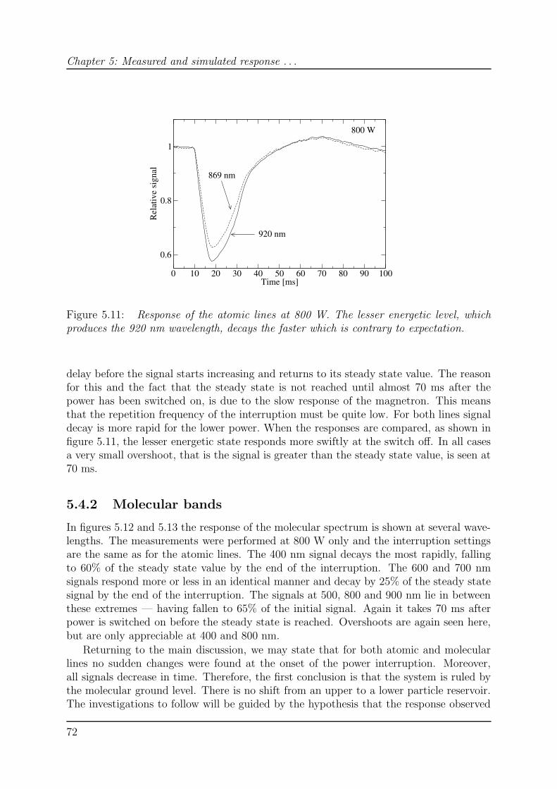
Chapter 5: Measured and simulated response . . .
0 10 20 30 40 50 60 70 80 90 100Time [ms]
0.6
0.8
1R
elat
ive
sign
al 869 nm
920 nm
800 W
Figure 5.11: Response of the atomic lines at 800 W. The lesser energetic level, whichproduces the 920 nm wavelength, decays the faster which is contrary to expectation.
delay before the signal starts increasing and returns to its steady state value. The reasonfor this and the fact that the steady state is not reached until almost 70 ms after thepower has been switched on, is due to the slow response of the magnetron. This meansthat the repetition frequency of the interruption must be quite low. For both lines signaldecay is more rapid for the lower power. When the responses are compared, as shown infigure 5.11, the lesser energetic state responds more swiftly at the switch off. In all casesa very small overshoot, that is the signal is greater than the steady state value, is seen at70 ms.
5.4.2 Molecular bands
In figures 5.12 and 5.13 the response of the molecular spectrum is shown at several wave-lengths. The measurements were performed at 800 W only and the interruption settingsare the same as for the atomic lines. The 400 nm signal decays the most rapidly, fallingto 60% of the steady state value by the end of the interruption. The 600 and 700 nmsignals respond more or less in an identical manner and decay by 25% of the steady statesignal by the end of the interruption. The signals at 500, 800 and 900 nm lie in betweenthese extremes — having fallen to 65% of the initial signal. Again it takes 70 ms afterpower is switched on before the steady state is reached. Overshoots are again seen here,but are only appreciable at 400 and 800 nm.
Returning to the main discussion, we may state that for both atomic and molecularlines no sudden changes were found at the onset of the power interruption. Moreover,all signals decrease in time. Therefore, the first conclusion is that the system is ruled bythe molecular ground level. There is no shift from an upper to a lower particle reservoir.The investigations to follow will be guided by the hypothesis that the response observed
72
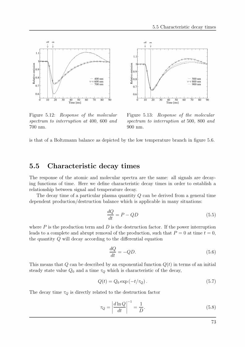
5.5 Characteristic decay times
0 10 20 30 40 50 60 70 80 90Time [ms]
0.6
0.7
0.8
0.9
1
1.1
Rel
ativ
e em
issi
on
400 nm600 nm700 nm
off on
Figure 5.12: Response of the molecularspectrum to interruption at 400, 600 and700 nm.
0 10 20 30 40 50 60 70 80 90Time [ms]
0.6
0.7
0.8
0.9
1
1.1
Rel
ativ
e em
issi
on
500 nm800 nm900 nm
off on
Figure 5.13: Response of the molecularspectrum to interruption at 500, 800 and900 nm.
is that of a Boltzmann balance as depicted by the low temperature branch in figure 5.6.
5.5 Characteristic decay times
The response of the atomic and molecular spectra are the same: all signals are decay-ing functions of time. Here we define characteristic decay times in order to establish arelationship between signal and temperature decay.
The decay time of a particular plasma quantity Q can be derived from a general timedependent production/destruction balance which is applicable in many situations:
dQ
dt= P −QD (5.5)
where P is the production term and D is the destruction factor. If the power interruptionleads to a complete and abrupt removal of the production, such that P = 0 at time t = 0,the quantity Q will decay according to the differential equation
dQ
dt= −QD. (5.6)
This means that Q can be described by an exponential function Q(t) in terms of an initialsteady state value Q0 and a time τQ which is characteristic of the decay,
Q(t) = Q0 exp (−t/τQ) . (5.7)
The decay time τQ is directly related to the destruction factor
τQ =
∣∣∣∣∣d lnQ
dt
∣∣∣∣∣
−1
=1
D. (5.8)
73
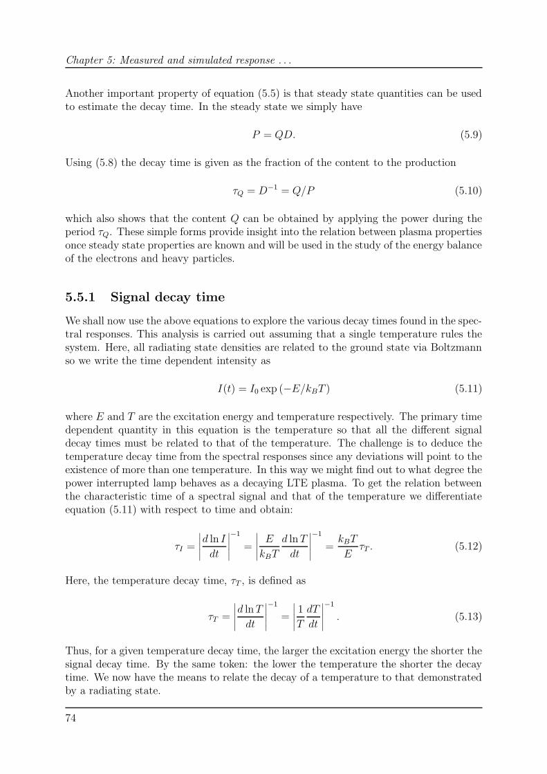
Chapter 5: Measured and simulated response . . .
Another important property of equation (5.5) is that steady state quantities can be usedto estimate the decay time. In the steady state we simply have
P = QD. (5.9)
Using (5.8) the decay time is given as the fraction of the content to the production
τQ = D−1 = Q/P (5.10)
which also shows that the content Q can be obtained by applying the power during theperiod τQ. These simple forms provide insight into the relation between plasma propertiesonce steady state properties are known and will be used in the study of the energy balanceof the electrons and heavy particles.
5.5.1 Signal decay time
We shall now use the above equations to explore the various decay times found in the spec-tral responses. This analysis is carried out assuming that a single temperature rules thesystem. Here, all radiating state densities are related to the ground state via Boltzmannso we write the time dependent intensity as
I(t) = I0 exp (−E/kBT ) (5.11)
where E and T are the excitation energy and temperature respectively. The primary timedependent quantity in this equation is the temperature so that all the different signaldecay times must be related to that of the temperature. The challenge is to deduce thetemperature decay time from the spectral responses since any deviations will point to theexistence of more than one temperature. In this way we might find out to what degree thepower interrupted lamp behaves as a decaying LTE plasma. To get the relation betweenthe characteristic time of a spectral signal and that of the temperature we differentiateequation (5.11) with respect to time and obtain:
τI =
∣∣∣∣∣d ln I
dt
∣∣∣∣∣
−1
=
∣∣∣∣∣E
kBT
d lnT
dt
∣∣∣∣∣
−1
=kBT
EτT . (5.12)
Here, the temperature decay time, τT , is defined as
τT =
∣∣∣∣∣d lnT
dt
∣∣∣∣∣
−1
=
∣∣∣∣∣1
T
dT
dt
∣∣∣∣∣
−1
. (5.13)
Thus, for a given temperature decay time, the larger the excitation energy the shorter thesignal decay time. By the same token: the lower the temperature the shorter the decaytime. We now have the means to relate the decay of a temperature to that demonstratedby a radiating state.
74
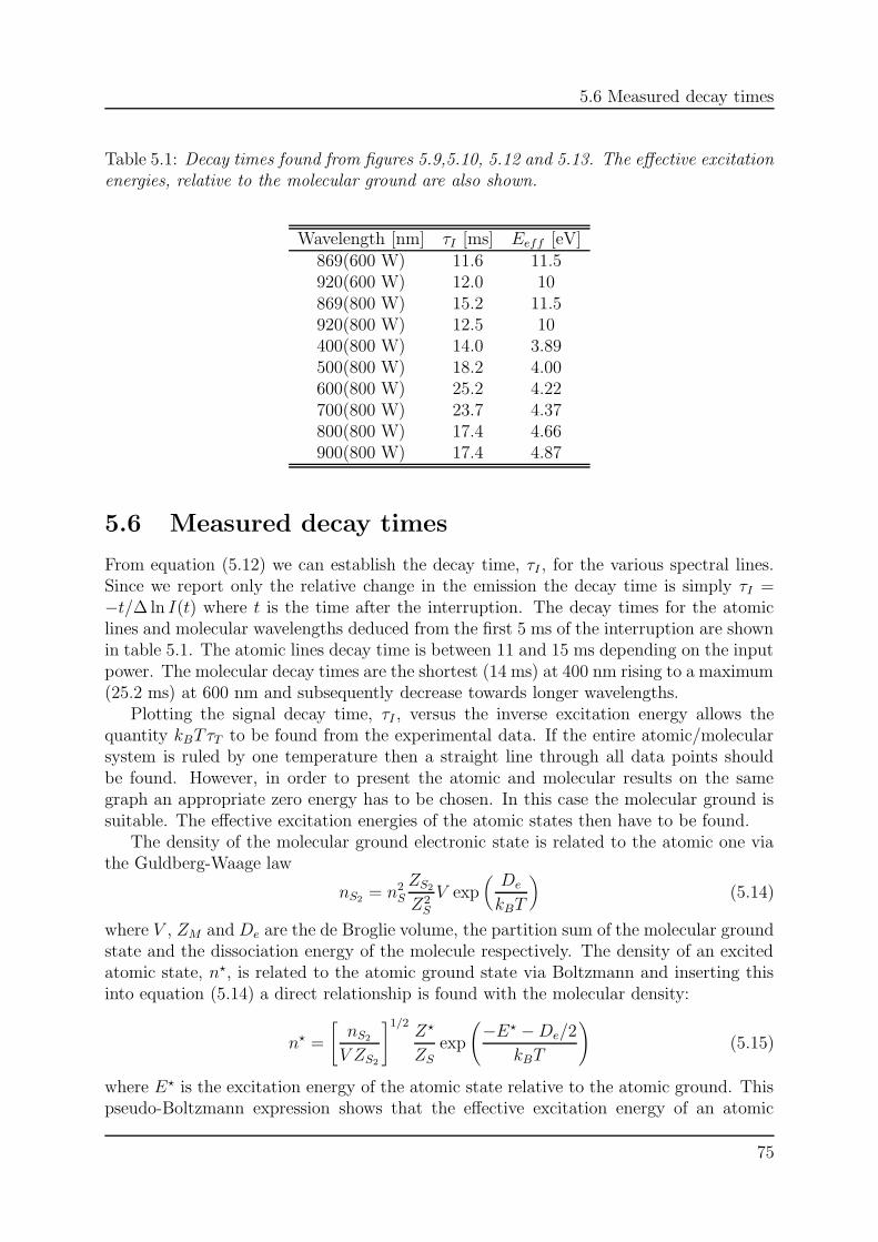
5.6 Measured decay times
Table 5.1: Decay times found from figures 5.9,5.10, 5.12 and 5.13. The effective excitationenergies, relative to the molecular ground are also shown.
Wavelength [nm] τI [ms] Eeff [eV]869(600 W) 11.6 11.5920(600 W) 12.0 10869(800 W) 15.2 11.5920(800 W) 12.5 10400(800 W) 14.0 3.89500(800 W) 18.2 4.00600(800 W) 25.2 4.22700(800 W) 23.7 4.37800(800 W) 17.4 4.66900(800 W) 17.4 4.87
5.6 Measured decay times
From equation (5.12) we can establish the decay time, τI , for the various spectral lines.Since we report only the relative change in the emission the decay time is simply τI =−t/∆ ln I(t) where t is the time after the interruption. The decay times for the atomiclines and molecular wavelengths deduced from the first 5 ms of the interruption are shownin table 5.1. The atomic lines decay time is between 11 and 15 ms depending on the inputpower. The molecular decay times are the shortest (14 ms) at 400 nm rising to a maximum(25.2 ms) at 600 nm and subsequently decrease towards longer wavelengths.
Plotting the signal decay time, τI , versus the inverse excitation energy allows thequantity kBTτT to be found from the experimental data. If the entire atomic/molecularsystem is ruled by one temperature then a straight line through all data points shouldbe found. However, in order to present the atomic and molecular results on the samegraph an appropriate zero energy has to be chosen. In this case the molecular ground issuitable. The effective excitation energies of the atomic states then have to be found.
The density of the molecular ground electronic state is related to the atomic one viathe Guldberg-Waage law
nS2 = n2S
ZS2
Z2S
V exp(De
kBT
)(5.14)
where V , ZM and De are the de Broglie volume, the partition sum of the molecular groundstate and the dissociation energy of the molecule respectively. The density of an excitedatomic state, n?, is related to the atomic ground state via Boltzmann and inserting thisinto equation (5.14) a direct relationship is found with the molecular density:
n? =
[nS2
V ZS2
]1/2Z?
ZS
exp
(−E? −De/2
kBT
)(5.15)
where E? is the excitation energy of the atomic state relative to the atomic ground. Thispseudo-Boltzmann expression shows that the effective excitation energy of an atomic
75
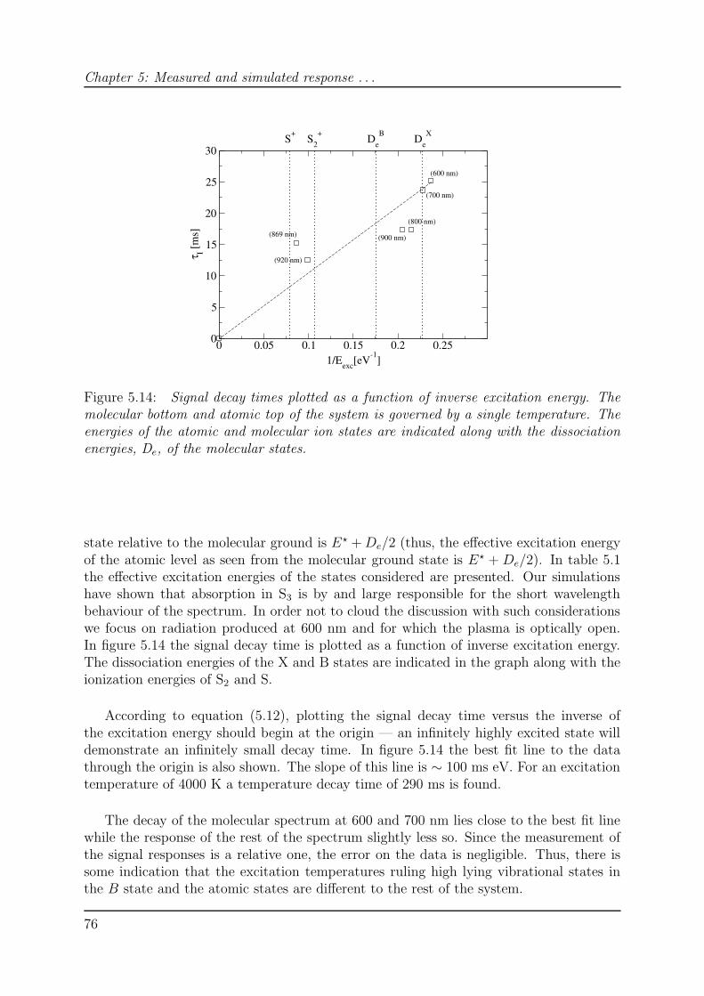
Chapter 5: Measured and simulated response . . .
0 0.05 0.1 0.15 0.2 0.251/Eexc[eV-1]
0
5
10
15
20
25
30
τ I [ms]
S+ S2+ De
B DeX
(600 nm)
(700 nm)
(900 nm)
(800 nm)
(920 nm)
(869 nm)
Figure 5.14: Signal decay times plotted as a function of inverse excitation energy. Themolecular bottom and atomic top of the system is governed by a single temperature. Theenergies of the atomic and molecular ion states are indicated along with the dissociationenergies, De, of the molecular states.
state relative to the molecular ground is E? +De/2 (thus, the effective excitation energyof the atomic level as seen from the molecular ground state is E? + De/2). In table 5.1the effective excitation energies of the states considered are presented. Our simulationshave shown that absorption in S3 is by and large responsible for the short wavelengthbehaviour of the spectrum. In order not to cloud the discussion with such considerationswe focus on radiation produced at 600 nm and for which the plasma is optically open.In figure 5.14 the signal decay time is plotted as a function of inverse excitation energy.The dissociation energies of the X and B states are indicated in the graph along with theionization energies of S2 and S.
According to equation (5.12), plotting the signal decay time versus the inverse ofthe excitation energy should begin at the origin — an infinitely highly excited state willdemonstrate an infinitely small decay time. In figure 5.14 the best fit line to the datathrough the origin is also shown. The slope of this line is ∼ 100 ms eV. For an excitationtemperature of 4000 K a temperature decay time of 290 ms is found.
The decay of the molecular spectrum at 600 and 700 nm lies close to the best fit linewhile the response of the rest of the spectrum slightly less so. Since the measurement ofthe signal responses is a relative one, the error on the data is negligible. Thus, there issome indication that the excitation temperatures ruling high lying vibrational states inthe B state and the atomic states are different to the rest of the system.
76
5.6 Measured decay times
5.6.1 Molecular response above 700 nm
The response of the 800 and 900 nm wavelengths do not lie near the best fit line. In factthey decay faster than they ought. The previous analysis, in equation (5.12), shows thatalower temperature or higher excitation energy leads to a shorter decay time. For thelatter to be true, the radiation would have to originate from 5.7 eV up in the system.This is in excess of the dissociation energy of the B state. However, as we have seen insection 4.4.3 no other state in S2 is more energetic than the B state and radiates at thesewavelengths. The other possibility is that the excitation temperature for the vibrationalstates that produce these wavelengths is lower than that which determines the distributionin the rest of the system. If we assume that the decay time is universal the excitationtemperature is
T = EτIτT
(5.16)
where T is the temperature in units of electron volt. We find an excitation temperatureof ca. 3200 K. In this view of the system the excitation temperature for large vibrationalquantum numbers in the B state is only ∼ 20% lower than that governing the rest of thesystem. While a non-LTE discussion of the possible reasons for the extra red and fasterdecay of the spectrum is beyond the scope of this work, some processes are discussed inappendix B.
5.6.2 Atomic line response
On the other hand the atomic lines decay more slowly than expected from equation(5.12). Moreover, the more highly excited state of the two decays the slower which is afurther contradiction. In this case it may be possible that we are observing a mixture ofBoltzmann and Saha responses. Since the density of atomic states with small ionizationpotentials is less than that of the ion, recombination into these may slow down the overallBoltzmann response. For states with a smaller ionization energy, whose density is alsolower, the effect will be more pronounced. In the formalism of equation (5.5) the timedependent density of the excited state, X?, is given by
dnX?
dt= P S + PB − nX?
(DS +DB
)(5.17)
where the superscripts S and B refer to Saha and Boltzmann processes. When power isremoved, only the Boltzmann production and Saha destruction paths are removed. Thedensity decay time is thus
τnX? =∣∣∣∣
1
nX?
nX?
dt
∣∣∣∣−1
=
[P S
nX?
−DB
]−1
. (5.18)
Thus, the addition of an extra (but not dominant) particle source increases the decaytime of the state density. Subsequently, emission lags behind the expected LTE value anda longer decay time is observed. While this is a purely qualitative view the fact that threeparticle recombination can decrease the destruction rate and hence slow down the decayin density is demonstrated.
77
Chapter 5: Measured and simulated response . . .
To conclude, while almost all of the excitation energy space is ruled by a single tem-perature, which has a characteristic decay time of 290 ms, the ‘red’ part of the spectrumis ruled by a different excitation temperature.
5.7 Global study of the response of energy balances
We will now use the general equation (5.10) to explore the relaxation times for the plasmaas a whole and for the various subgroups the electrons [e] and heavy particles [h]. Ourstrategy is to begin with a general exploration and to then proceed to more in-depthconsiderations.
Firstly, we assume that the plasma is in full LTE. Then P and Q in equation (5.10)refer to the power density and energy density respectively. For a total input power of 800W and lamp radius of 16 mm, P is ∼ 5 × 10⁷ Wm−3. The energy content of the plasmais the product of the specific heat and the temperature. Thus, we understand that therelaxation time found for the energy content is that of the corresponding temperature.For Q we take (70/2)p which as we will show in section 5.9.2 is a reasonable value for achemically reactive sulfur plasma at 4000 K. Then we find that τT = Q/P ∼ 300 ms whichagrees very well with the time found from the experimental data where the temperaturewas taken to be 4000 K.
Secondly, we assume that the plasma is a two temperature plasma ruled by the energychain
EM field −→ [e] −→ [h] −→ environment. (5.19)
Here we assume that Te Th and that the power along the links is the same. SinceDe = Pe/Qe and Dh = Ph/Qh the electron destruction factor can be written as De =Dh(Qh/Qe).
If we now use Dh ∼ 3 s−1 (the value found above), the relation Qh/Qe = (70/3)ph/pe,and the value of the ionization degree pe/ph of 10−5, we find the decay rate of the electrongas De = 7 × 10⁶s−1. This implies a τ value of about 0.1 µs. Knowing the decay timeand the destruction factor, the heat content of [e] and the electron temperature can beestimated. Employing equation Qe = Pe/De and taking a value of the electron densityne = 1020 m−3 we find Te = 3400 K. This is too low and in violation of the assumptionthat Te Th.
Although it has some shortcomings the global approach provides some insight. Inparticular it shows that electrons will respond much faster since the heat capacity is somuch smaller than that of the heavy particles. However, the assumption that Te Th
proves to violate itself. In fact the total energy reservoir of [e] does not drain into into[h] but only a fraction F = (Te − Th)/Te. The smaller this is, the faster the electrontemperature will react and (using FQ = P/D) the smaller F will be. To break thisvicious circle and to get more information in the actual value of electron response timewe need a more in-depth study for which the energy balances have to be consulted.
78
5.8 Electron temperature decay
5.8 Electron temperature decay
The rapid and large jumps of spectral lines in response to power interruption was inthe past attributed to the substantial difference between the electron and heavy particletemperature. And indeed, in the (atomic) argon ICP large differences between Te and Th
were found. Since we do not detect any sudden responses (in the order of µs) in the sulfurlamp we might conclude that (Te −Th) is small in this plasma. This is the subject of thissection in which we study the electron energy balance which expresses the relationshipbetween the ohmic input, ε, and the power lost per unit volume by electrons to heavyspecies in elastic and inelastic collisions:
0 = ε− nenS2
[〈σemve〉
3me
MkB (Te − Th) + 〈K〉 〈E〉
]. (5.20)
Here 〈σemve〉 is the rate coefficient for momentum transfer between electron and moleculeaveraged over the Maxwellian electron energy distribution function while 〈K〉 and 〈E〉 arethe mean values of the rate coefficient for electron excitation and the excitation energyrespectively. We assume that all inelastic losses are associated with electron impactexcitation from the X to the B state. In order to make this study possible 〈K〉 and 〈E〉must be determined in an averaging procedure which will be discussed at the end of thissection and in the appendix.
Comparing the electron energy balance with the general formulae, equations (5.5) to(5.9), shows that two destruction terms are present; one associated with elastic and theother with inelastic processes. We will start with the elastic rate. Since the loss term ofthe corresponding decay equation clearly scales with the energy difference (Te − Th) wecan use the elastic term directly in a simplified balance (see equation (5.6)) to describethe decay of the temperature difference (Te − Th)
Cvd(Te − Th)
dt= −nenS2 < σemve > 3
me
MkB(Te − Th). (5.21)
Using Cv = 3/2mekB for the specific heat of the electron gas leads to the following decayrate:
D = nS2
[〈σemve〉
2me
M
]. (5.22)
The elastic decay rate can now be estimated using the mass of the sulfur molecule, (64a.m.u.) while the rate for elastic processes, 〈σemve〉, is replaced by a simple product ofthe electron velocity, ve = 106 ms−1 and a cross section of 1 A2. Inserting for the groundstate nS2 = 1025 m−3 we get a decay frequency of ∼ 106 s−1. An estimate of the steadystate value of (Te − Th) can now be found by calculating the temperature increase of theelectron gas due to application of a power density of 5×10⁷ W m−3 during 1 µs. Applyingequation (5.9) leads to a value of (Te−Th) around 3000 K; a value which is neither realisticnor observed. Note that the decay rate and the corresponding temperature difference arecomparable to the values found in an atmospheric argon ICP. But this is not surprisingsince the elastic processes in the Ar-ICP are very important while the collision rates andpressure are of the same order as that in the sulfur lamp. The reason that we do not seethe comparable (Te − Th) value in the sulfur lamp must be due to the the large inelasticlosses.
79
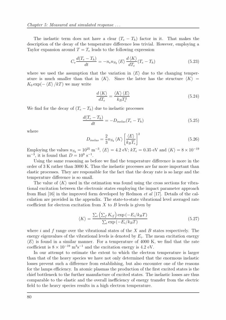
Chapter 5: Measured and simulated response . . .
The inelastic term does not have a clear (Te − Th) factor in it. That makes thedescription of the decay of the temperature difference less trivial. However, employing aTaylor expansion around T = Te leads to the following expression
Cvd(Te − Th)
dt= −nenS2 〈E〉
d 〈K〉dTe
(Te − Th) (5.23)
where we used the assumption that the variation in 〈E〉 due to the changing temper-ature is much smaller than that in 〈K〉. Since the latter has the structure 〈K〉 =K0 exp(−〈E〉 /kT ) we may write
d 〈K〉dTe
=〈K〉 〈E〉kBT 2
e
(5.24)
We find for the decay of (Te − Th) due to inelastic processes
d(Te − Th)
dt= −Dinelas(Te − Th) (5.25)
where
Dinelas =2
3nS2 〈K〉
[〈E〉kBTe
]2
(5.26)
Employing the values nS2 = 1025 m−3, 〈E〉 = 4.2 eV; kTe = 0.35 eV and 〈K〉 = 8× 10⁻¹⁹
m−3, it is found that D = 109 s−1.Using the same reasoning as before we find the temperature difference is more in the
order of 3 K rather than 3000 K. Thus the inelastic processes are far more important thanelastic processes. They are responsible for the fact that the decay rate is so large and thetemperature difference is so small.
The value of 〈K〉 used in the estimation was found using the cross sections for vibra-tional excitation between the electronic states employing the impact parameter approachfrom Hazi [16] in the improved form developed by Redmon et al [17]. Details of the cal-culation are provided in the appendix. The state-to-state vibrational level averaged ratecoefficient for electron excitation from X to B levels is given by
〈K〉 =
∑i
(∑f Kif
)exp (−Ei/kBT )
∑i exp (−Ei/kBT )
(5.27)
where i and f range over the vibrational states of the X and B states respectively. Theenergy eigenvalues of the vibrational levels is denoted by Ei. The mean excitation energy〈E〉 is found in a similar manner. For a temperature of 4000 K, we find that the ratecoefficient is 8 × 10⁻¹⁹ m3s−1 and the excitation energy is 4.2 eV.
In our attempt to estimate the extent to which the electron temperature is largerthan that of the heavy species we have not only determined that the enormous inelasticlosses prevent such a difference from establishing, but also encounter one of the reasonsfor the lamps efficiency. In atomic plasmas the production of the first excited states is thechief bottleneck to the further manufacture of excited states. The inelastic losses are thuscomparable to the elastic and the overall inefficiency of energy transfer from the electricfield to the heavy species results in a high electron temperature.
80
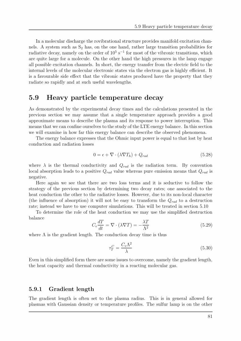
5.9 Heavy particle temperature decay
In a molecular discharge the rovibrational structure provides manifold excitation chan-nels. A system such as S2 has, on the one hand, rather large transition probabilities forradiative decay, namely on the order of 105 s−1 for most of the vibronic transitions, whichare quite large for a molecule. On the other hand the high pressures in the lamp engageall possible excitation channels. In short, the energy transfer from the electric field to theinternal levels of the molecular electronic states via the electron gas is highly efficient. Itis a favourable side effect that the vibronic states produced have the property that theyradiate so rapidly and at such useful wavelengths.
5.9 Heavy particle temperature decay
As demonstrated by the experimental decay times and the calculations presented in theprevious section we may assume that a single temperature approach provides a goodapproximate means to describe the plasma and its response to power interruption. Thismeans that we can confine ourselves to the study of the LTE energy balance. In this sectionwe will examine in how far this energy balance can describe the observed phenomena.
The energy balance expresses that the Ohmic input power is equal to that lost by heatconduction and radiation losses
0 = ε+ ∇ · (λ∇Th) +Qrad (5.28)
where λ is the thermal conductivity and Qrad is the radiation term. By conventionlocal absorption leads to a positive Qrad value whereas pure emission means that Qrad isnegative.
Here again we see that there are two loss terms and it is seductive to follow thestrategy of the previous section by determining two decay rates; one associated to theheat conduction the other to the radiative losses. However, due to its non-local character(the influence of absorption) it will not be easy to transform the Qrad to a destructionrate; instead we have to use computer simulations. This will be treated in section 5.10
To determine the role of the heat conduction we may use the simplified destructionbalance
CvdT
dt= ∇ · (λ∇T ) = −λT
Λ2(5.29)
where Λ is the gradient length. The conduction decay time is thus
τCT =
CvΛ2
λ(5.30)
Even in this simplified form there are some issues to overcome, namely the gradient length,the heat capacity and thermal conductivity in a reacting molecular gas.
5.9.1 Gradient length
The gradient length is often set to the plasma radius. This is in general allowed forplasmas with Gaussian density or temperature profiles. The sulfur lamp is on the other
81
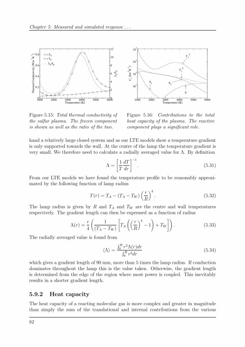
Chapter 5: Measured and simulated response . . .
1000 2000 3000 4000 5000 6000Temperature [K]
0
0.2
0.4
0.6
0.8
The
rmal
Con
duct
ivity
[Wm
-1K
-1] λT
λF
0
2
4
6
8
10
12
λ T/λ
F
λT/λF
Figure 5.15: Total thermal conductivity ofthe sulfur plasma. The frozen componentis shown as well as the ratio of the two.
1000 2000 3000 4000 5000 6000Temperature [K]
102
103
104
105
Cv [J
m-3
K-1
]
CvT
CvF
S3 S2
S
Figure 5.16: Contributions to the totalheat capacity of the plasma. The reactivecomponent plays a significant role.
hand a relatively large closed system and as our LTE models show a temperature gradientis only supported towards the wall. At the centre of the lamp the temperature gradient isvery small. We therefore need to calculate a radially averaged value for Λ. By definition
Λ =
[1
T
dT
dr
]−1
. (5.31)
From our LTE models we have found the temperature profile to be reasonably approxi-mated by the following function of lamp radius
T (r) = TA − (TA − TW )(r
R
)4
. (5.32)
The lamp radius is given by R and TA and TW are the centre and wall temperaturesrespectively. The gradient length can then be expressed as a function of radius
Λ(r) =r
4
(1
(TA − TW )
[TA
((r
R
)4
− 1
)+ TW
]). (5.33)
The radially averaged value is found from
〈Λ〉 =
∫ R0 r2Λ(r)dr∫ R0 r2dr
(5.34)
which gives a gradient length of 90 mm, more than 5 times the lamp radius. If conductiondominates throughout the lamp this is the value taken. Otherwise, the gradient lengthis determined from the edge of the region where most power is coupled. This inevitablyresults in a shorter gradient length.
5.9.2 Heat capacity
The heat capacity of a reacting molecular gas is more complex and greater in magnitudethan simply the sum of the translational and internal contributions from the various
82
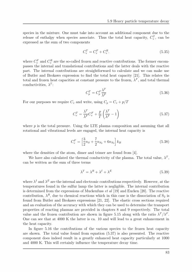
5.9 Heavy particle temperature decay
species in the mixture. One must take into account an additional component due to therelease of enthalpy when species associate. Thus the total heat capacity, CT
v , can beexpressed as the sum of two components
CTv = CF
v + CRv . (5.35)
where CFv and CR
v are the so-called frozen and reactive contributions. The former encom-passes the internal and translational contributions and the latter deals with the reactivepart. The internal contributions are straightforward to calculate and we can make useof Butler and Brokaws expression to find the total heat capacity [21]. This relates thetotal and frozen heat capacities at constant pressure to the frozen, λF , and total thermalconductivities, λT :
CTp = CF
p
λT
λF(5.36)
For our purposes we require Cv and write, using Cp = Cv + p/T
CTv =
λT
λFCF
v +p
T
(λT
λF− 1
)(5.37)
where p is the total pressure. Using the LTE plasma composition and assuming that allrotational and vibrational levels are engaged, the internal heat capacity is
CFv =
[3
2nS +
7
2nS2 + 6nS3
]kB (5.38)
where the densities of the atom, dimer and trimer are found from [4].
We have also calculated the thermal conductivity of the plasma. The total value, λT ,can be written as the sum of three terms
λT = λR + λI + λE (5.39)
where λI and λE are the internal and electronic contributions respectively. However, at thetemperatures found in the sulfur lamp the latter is negligible. The internal contributionis determined from the expressions of Muckenfuss et al [19] and Eucken [20]. The reactivecontribution, λR, due to chemical reactions which in this case is the dissociation of S2 isfound from Butler and Brokaws expressions [21, 22]. The elastic cross sections requiredand an evaluation of the accuracy with which they can be used to determine the transportproperties of reacting plasmas are provided in chapters 8 and 9 respectively. The totalvalue and the frozen contribution are shown in figure 5.15 along with the ratio λT/λF .One can see that at 4000 K the latter is ca. 10 and will lead to a great enhancement inthe heat capacity.
In figure 5.16 the contributions of the various species to the frozen heat capacityare shown. The total value found from equation (5.37) is also presented. The reactivecomponent does indeed result in a greatly enhanced heat capacity particularly at 1000and 4000 K. This will certainly influence the temperature decay time.
83
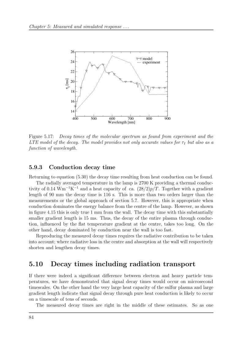
Chapter 5: Measured and simulated response . . .
400 500 600 700 800 900Wavelength [nm]
14
16
18
20
22
24
26
τ I [ms]
modelexperiment
Figure 5.17: Decay times of the molecular spectrum as found from experiment and theLTE model of the decay. The model provides not only accurate values for τI but also as afunction of wavelength.
5.9.3 Conduction decay time
Returning to equation (5.30) the decay time resulting from heat conduction can be found.The radially averaged temperature in the lamp is 2700 K providing a thermal conduc-
tivity of 0.14 Wm−1K−1 and a heat capacity of ca. (28/2)p/T . Together with a gradientlength of 90 mm the decay time is 116 s. This is more than two orders larger than themeasurements or the global approach of section 5.7. However, this is appropriate whenconduction dominates the energy balance from the centre of the lamp. However, as shownin figure 4.15 this is only true 1 mm from the wall. The decay time with this substantiallysmaller gradient length is 15 ms. Thus, the decay of the entire plasma through conduc-tion, influenced by the flat temperature gradient at the centre, takes too long. On theother hand, decay dominated by conduction near the wall is too fast.
Reproducing the measured decay times requires the radiative contribution to be takeninto account; where radiative loss in the centre and absorption at the wall will respectivelyshorten and lengthen decay times.
5.10 Decay times including radiation transport
If there were indeed a significant difference between electron and heavy particle tem-peratures, we have demonstrated that signal decay times would occur on microsecondtimescales. On the other hand the very large heat capacity of the sulfur plasma and largegradient length indicate that signal decay through pure heat conduction is likely to occuron a timescale of tens of seconds.
The measured decay times are right in the middle of these estimates. So as one
84
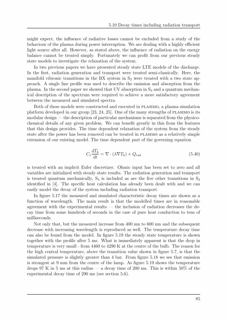
5.10 Decay times including radiation transport
might expect, the influence of radiative losses cannot be excluded from a study of thebehaviour of the plasma during power interruption. We are dealing with a highly efficientlight source after all. However, as stated above, the influence of radiation on the energybalance cannot be treated simply. Fortunately we can profit from our previous steadystate models to investigate the relaxation of the system.
In two previous papers we have presented steady state LTE models of the discharge.In the first, radiation generation and transport were treated semi-classically. Here, themanifold vibronic transitions in the BX system in S2 were treated with a two state ap-proach. A single line profile was used to describe the emission and absorption from theplasma. In the second paper we showed that UV absorption in S3 and a quantum mechan-ical description of the spectrum were required to achieve a more satisfactory agreementbetween the measured and simulated spectra.
Both of these models were constructed and executed in plasimo, a plasma simulationplatform developed in our group [23, 24, 25]. One of the many strengths of plasimo is itsmodular design — the description of particular mechanisms is separated from the physico-chemical details of any given problem. We can benefit greatly in this from the featuresthat this design provides. The time dependent relaxation of the system from the steadystate after the power has been removed can be treated in plasimo as a relatively simpleextension of our existing model. The time dependent part of the governing equation
CvdTh
dt= ∇ · (λ∇Th) +Qrad (5.40)
is treated with an implicit Euler discretizer. Ohmic input has been set to zero and allvariables are initialized with steady state results. The radiation generation and transportis treated quantum mechanically, S3 is included as are the five other transitions in S2
identified in [4]. The specific heat calculation has already been dealt with and we caneasily model the decay of the system including radiation transport.
In figure 5.17 the measured and simulated characteristic decay times are shown as afunction of wavelength. The main result is that the modelled times are in reasonableagreement with the experimental results — the inclusion of radiation decreases the de-cay time from some hundreds of seconds in the case of pure heat conduction to tens ofmilliseconds.
Not only that, but the measured increase from 400 nm to 600 nm and the subsequentdecrease with increasing wavelength is reproduced as well. The temperature decay timecan also be found from the model. In figure 5.19 the steady state temperature is showntogether with the profile after 5 ms. What is immediately apparent is that the drop intemperature is very small - from 4460 to 4290 K at the centre of the bulb. The reason forthe high central temperature, above the transition value shown in figure 5.7, is that thesimulated pressure is slightly greater than 4 bar. From figure 5.18 we see that emissionis strongest at 9 mm from the centre of the lamp. As figure 5.19 shows the temperaturedrops 97 K in 5 ms at this radius — a decay time of 200 ms. This is within 50% of theexperimental decay time of 290 ms (see section 5.6).
85
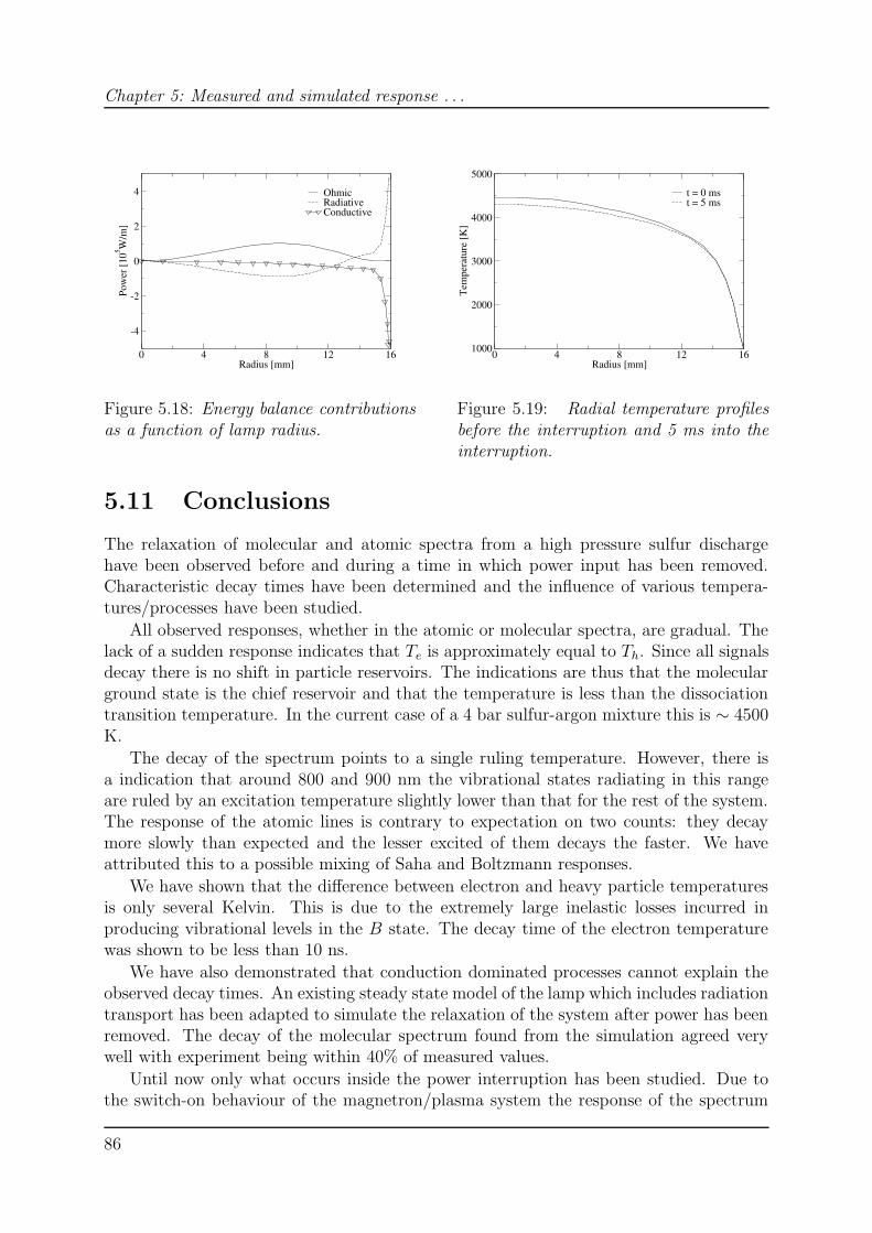
Chapter 5: Measured and simulated response . . .
0 4 8 12 16Radius [mm]
-4
-2
0
2
4
Pow
er [1
05 W/m
]
OhmicRadiativeConductive
Figure 5.18: Energy balance contributionsas a function of lamp radius.
0 4 8 12 16Radius [mm]
1000
2000
3000
4000
5000
Tem
pera
ture
[K]
t = 0 mst = 5 ms
Figure 5.19: Radial temperature profilesbefore the interruption and 5 ms into theinterruption.
5.11 Conclusions
The relaxation of molecular and atomic spectra from a high pressure sulfur dischargehave been observed before and during a time in which power input has been removed.Characteristic decay times have been determined and the influence of various tempera-tures/processes have been studied.
All observed responses, whether in the atomic or molecular spectra, are gradual. Thelack of a sudden response indicates that Te is approximately equal to Th. Since all signalsdecay there is no shift in particle reservoirs. The indications are thus that the molecularground state is the chief reservoir and that the temperature is less than the dissociationtransition temperature. In the current case of a 4 bar sulfur-argon mixture this is ∼ 4500K.
The decay of the spectrum points to a single ruling temperature. However, there isa indication that around 800 and 900 nm the vibrational states radiating in this rangeare ruled by an excitation temperature slightly lower than that for the rest of the system.The response of the atomic lines is contrary to expectation on two counts: they decaymore slowly than expected and the lesser excited of them decays the faster. We haveattributed this to a possible mixing of Saha and Boltzmann responses.
We have shown that the difference between electron and heavy particle temperaturesis only several Kelvin. This is due to the extremely large inelastic losses incurred inproducing vibrational levels in the B state. The decay time of the electron temperaturewas shown to be less than 10 ns.
We have also demonstrated that conduction dominated processes cannot explain theobserved decay times. An existing steady state model of the lamp which includes radiationtransport has been adapted to simulate the relaxation of the system after power has beenremoved. The decay of the molecular spectrum found from the simulation agreed verywell with experiment being within 40% of measured values.
Until now only what occurs inside the power interruption has been studied. Due tothe switch-on behaviour of the magnetron/plasma system the response of the spectrum
86
5.11 Conclusions
after the interruption has been left. Nevertheless, the overshoots observed at 400 and 800nm and in the atomic lines is worth noting and returning to in future investigations.
The technique of power interruption has proved to be very useful in increasing ourunderstanding of the sulfur lamp. This study was initiated by several questions regardingthe LTE status of the discharge and has answered several of them. One of the chiefconcerns is the behaviour of the spectrum towards longer wavelengths. Our LTE modelshave proven reasonably effective in all regions of the spectrum except in the ‘red’. In thisarticle we have seen that the excitation temperature through the B state is likely to bea function of the vibrational level. This points to a possible non-LTE route to enhanceemission in this range.
Acknowledgements
This work is part of the research program of the Dutch Technology Foundation (STW).The authors would like to thank Marco van de Sande and Loek Baede for their assistancein constructing and testing the experimental setup.
Appendix A — rate coefficients
First developed by Hazi [16] and extended by Redmon [17] the impact parameter methodfor the calculation of inelastic cross sections for molecular excitation is used very muchin contemporary works. Most recently it has been used to determine the excitation crosssections of a small number of vibronic transitions in O2 and S2. In the approach, the crosssection is written as the product of two terms: a structural factor that encompasses thespecifics of the interacting levels and a dynamical factor, which deals with the electronbehaviour. Thus,
σαiαfνiνf
(E) = Sαiαfνiνf
Dαiαfνiνf
(E) (A.1)
where α and ν indicate the electronic and vibrational states involved, and the subscriptsi and f discriminate between initial and final states. The structural factor is given by
Sif =m2
ee2
12πε0gih4 |〈ψi |M |ψf〉|2 (A.2)
where ψi and ψf are the wavefunctions for the initial and final vibrational states, gi is thestatistical weight of the electronic state and M the electronic transition dipole moment(ETDM). The dynamical factor is an involved function and for completeness is reproducedhere from [17]
Di,f(E) =2πh2
m2eu
2i
[γi
(K0(γi)K1(γi) −
π2
4S0(γi)S1(γi)
)
+γf
(K0(γf)K1(γf) −
π2
4S0(γf)S1(γf)
)
+γ
(K0(γi)K1(γf) +K0(γf)K1(γi) +
π2
4S0(γi)S1(γf) +
π2
4S0(γf)S1(γi)
)
87
Chapter 5: Measured and simulated response . . .
+u2
i − u2f
u2i + u2
f
(ln
(γf
γi
)∫ γf
γi
S0(γ)dγ
)]
where K and S are the modified Bessel and Struve functions. The initial and final electronvelocities ui and uf are given by
ui =
√2E
me
uf =
√2(E − ∆Eif )
me
where ∆Eif is the energy difference between the vibrational levels. The γi, γf and γ termsare defined as
γi =ρ |∆Eif |hui
γf =ρ |∆Eif |huf
γ =ρ |∆Eif |
h
2ui
u2i + u2
f
where ρ is the so-called cut-off parameter - a length required to prevent a divergent crosssection. The cutoff parameters are given by [26] as 0.921 and 0.974 A for oxygen andsulfur respectively. Energy gap details are found from the potential curves from figure5.3. The vibrational wavefunctions were calculated using the SCHROED program [27]and the Franck-Condon factors found using the quadrature routines supplied with theGnu Scientific Library [28]. The electronic transition dipole moments for the transitionswere found in the literature [29]. Once the elementary cross sections have been found therate coefficient is easily calculated from
KFT (Tv, ε) =
∫ ∞
0σT (Tv, ε)f
M(ε)ve(ε)dε (A.3)
where fM(ε) is the Maxwellian electron energy distribution function and ve(ε) is theelectron velocity.
Appendix B — the missing red problem
In this section a non-LTE process is presented as a possible solution to the missing redproblem and the too rapid decay of the long wavelength range of the spectrum.
In order for the B3Σ−u → X3Σ−
g transition to produce more red an overpopulation ofthe appropriate vibrational levels with respect to equilibrium is needed (the vibrationallevels v′ > 15 radiate at 800 nm and beyond). This applies to the steady state and whichever process is proposed must be consistent with the temporal behaviour of the spectrumduring an interruption — a more rapid decay must be seen.
Taking the dissociation-association balance as the sole cause of vibrational non-equilibrium,the main point is that densities can remain greater in space and decay more rapidly in
88
Bibliography
time than LTE predicts. The density of the atomic state is very important in this picture.However, before discussing the process some basic information is needed.
The reaction cross-section, σR, for the dissociation
S2(B) +M S? + S? +M (B.1)
can be taken as a fraction of the elastic cross-section [30]. We assume that this fractionis unity and set the cross-section to 1 A2. The rate coefficient for dissociation, kdiss, isto a first approximation the product of σR and the velocity. The latter is taken to be103 ms−1. In equilibrium the number of forward processes equals the number of reverseprocesses and the three particle (3p) association rate, k3p, is found from
k3p = kdissnS2(B)
n2S?
. (B.2)
The ratio of the molecular to atomic densities is found from the Guldberg-Waage relationgiven in equation (5.14). Thus,
k3p = kdiss
ZS2(B)
Z2S?
V exp(Ea
kBT
). (B.3)
Here ZS2/Z2SV is effectively constant (10−30 m3) and Ea is the activation energy. This is
taken to be 1 eV, the dissociation energy of the vibrational level v ′ = 15 which radiatesat 800 nm. The rate k3p is effectively constant with temperature and is 10−46 m6s−1.
In the steady state the temperature is ∼ 4000 K at the centre of the lamp. Theatomic (LTE) density is 1×10²³ m−3 and the association frequency is 1.8 s−1. This isextremely slow. Moreover, towards the wall the temperature and atom density decreasesand association slows down further. This slow production of vibrational levels is onepossible mechanism for the production of extra red. The higher atom density maintainedby poor association, can lead to a higher population of the vibrational levels in S2(B).
Once power is removed the decay of the spectrum is due to vibrational relaxationand three particle association. However, a higher atom density and slow association doesnot help in explaining the rapid decay of the spectrum. A possible explanation could bethat the vibrational levels relax on different timescales; higher levels redistributing morequickly due to the smaller energy gaps.
While molecular non-LTE is a complex subject, both broad and deep, what we havepresented here is one possible means to explain deviations and may serve as a startingpoint for future investigations. Nevertheless, the conclusion remains that the dischargecan be described to a very great extent by LTE.
References
[1] Waymouth J F, 1971, Electric discharge lamps (The M.I.T. Press, Massachussets,1971)
[2] Turner B, Ury M, Leng Y and Love W, J. Illuminating Engng Soc., Winter, 10 1997
[3] Johnston C W, van der Heijden H W P, Janssen G M, van Dijk J and van der MullenJ J A M, J. Phys. D: Appl. Phys. 35, 342 (2002), Chapter 2 this thesis
89
Bibliography
[4] Chapter 4 of this thesis
[5] Johnston C W, Jonkers J and van der Mullen J J A M, J. Phys. D: Appl. Phys. 35,2578 (2002), Chapter 3 of this thesis
[6] van der Heijden H and van der Mullen J A M J. Phys. D: Appl. Phys. 35, 2112(2002)
[7] Gurevich C B, and Podmoshenskii I V, Opt. Spectrosc. (USSR) 15, 319 (1963)
[8] Nick K P, Richter J, Helbig V, J. Quant. Spectrosc. Radiat. Transfer 32, 1 (1984)
[9] Bydder E L, Miller G P, Spectrochim. Acta B 42, 393 (1987)
[10] Bydder E L, Miller G P, Spectrochim. Acta B 43, 1431 (1988)
[11] Fey F H A G, Excitation balances and Transport in and Inductively Coupled Plasma,Ph.D. Thesis, Eindhoven University of Technology, The Netherlands, (1993)
[12] Timmermans E A H, Atomic and Molecular Excitation Processes in Microwave In-duced Plasmas: a spectroscopic study, Ph.D. Thesis, Eindhoven University of Tech-nology, The Netherlands, ISBN 90-386-0887-X (1999)
[13] de Regt J M, Fundamentals of Inductively Coupled Plasmas: a spectroscopic study,Ph.D. Thesis, Eindhoven University of Technology, The Netherlands, (1996)
[14] van de Sande M J, Laser Scattering on Low Temperature Plasmas: high resolutionand stray light rejection, Ph.D. Thesis, Eindhoven University of Technology, TheNetherlands, (2002) ISBN 90-386-1919-7 (2002)
[15] Wiese W L, Smith M W and Miles B M, Atomic transition probabilities, Natl. Stand.Ref. Data Ser. Natl. Bur. Stad., Circ. 4(U.S.GPO, Washington, D.C.) (1966), Vol. 1.
[16] Hazi A U, Phys. Rev. A 23, 2232 (1981)
[17] Redmon M J, Garrett B C, Redmon L T and McCurdy C W Phys. Rev. A 32, 3354(1985)
[18] Jonkers J, Excitation and Transport in Small Scale Plasmas, Ph.D. Thesis, EindhovenUniversity of Technology, The Netherlands, ISBN 90-386-0637-0 (1998)
[19] Muckenfuss C and Curtis C F, J. Chem. Phys. 29, 1273 (1958)
[20] Hirschfelder J O, Curtis C F and Bird R B, Molecular theory of gases and liquids,(John Wiley & Sons, New York, 1967)
[21] Butler J N and Brokaw R S, J. Chem. Phys. 26, 1636 (1957)
[22] Butler J N and Brokaw R S, J. Chem. Phys. 32, 1005 (1959)
[23] Janssen G M, van Dijk J, Benoy D A, Tas M A, Burm K T A L, Goedheer W J, vander Mullen J J A M and Schram D C, Plasma Sources Sci. Technol. 8, 1 (1999)
90
Bibliography
[24] van Dijk J, Modelling of plasma light sources : an object-oriented approach, PhDThesis, Eindhoven University of Technology, The Netherlands, ISBN 90-386-1819-0(2001)
[25] http://plasimo.phys.tue.nl/
[26] Garrett B C, Redmon L T, McCurdy C W and Redmon M J, Phys. Rev. A 32, 3366(1985)
[27] Pashov A, Jastrzebski W and Kowalcyzk P, Comput. Phys. Commun. 128, 622 (2000)
[28] http://sources.redhat.com/gsl/
[29] Kiljunen T, Eloranta J, Kunttu H, Khriachtchev L, Pettersson M, Rasanen M, J.Chem. Phys. 112, 163 (1996)
[30] Itina T E, Tokarev V N, Marine W, Autric M, J. Chem. Phys. 106, 8905 (1997).
91

CHAPTER 6
A scaling rule for molecular electronic transition dipole moments:
application to asymptotically allowed and forbidden transitions
Guided by the work of Woerdman [1] and Monyakin [2, 3], we propose rules that allowthe electronic transition dipole moment for a transition in one molecule to be determinedfrom that of a similar one in an isovalent species. The rule can be applied to asymptoticallyallowed and forbidden transitions. We have tested it by applying it in two specific cases:the moments for the A1Σ → X1Σ and X1Σ → B1Π transitions in Na2 are found fromthose in Li2, which are asymptotically allowed and the moments for the B → X transitionin O2, Se2 and Te2 which are asymptotically forbidden, are found from moment data forS2. Transition moments calculated with this rule are within 15% of the available literaturevalues and behaviour as a function of internuclear separation is well described.
C. W. Johnston and J. J. A. M. van der Mullen
Accepted for publication in the Journal of Chemical Physics
93
Chapter 6: A scaling rule for ETDMs . . .
6.1 Introduction
The electronic transition dipole moment (ETDM) is an especially important term in thespectroscopy of diatomic molecules as it determines the strength of a particular transi-tion. Detailed knowledge of it can be useful not only in diagnostics but also in dischargemodelling where it can be employed in the simulation of spectra as well as the determi-nation of electron impact excitation cross sections. While ETDM data is available in theliterature, certainly not all transitions that might be of interest are represented and eventhen often only over a limited range of internuclear distance.
The ETDM for a particular transition may be found from experiment by the optimizedfitting of simulated to measured spectra [4]. However, due to often limited dischargeconditions only a small part of the band system is observed. Thus the ETDM is oftenonly recovered for a small range of internuclear separation. On the other hand, theentire ETDM can be found by calculating it ab initio, which is however an involved andspecialized task. As such, possessing the means to reliably estimate the ETDM beforerecourse to theoretical or experimental measures can be of great use.
We are currently studying the high pressure sulfur lamp numerically as well as froman experimental point of view [5, 6]. The system is an efficient visible light radiator andproduces a seemingly continuous spectrum from 300 to 900 nm. In short, the spectrumcan be attributed to radiative transitions between all vibrational levels in the BX systemof the sulfur dimer. Thus quanta are produced over the complete range of internucleardistance. This is a situation where full knowledge of the ETDM is required and a rare onewhere the data is in fact available [7]. However, two other group VI elements, seleniumand tellurium, display similar high pressure spectra to the sulfur, also attributable to BXradiation, and we expect to verify and perhaps enhance our understanding of the sulfurlamp by studying these systems. For these dimers ETDM data has only recently appearedin the literature although only over a limited range of separation, centered around theequilibrium separation. So here is a specific case where the full ETDM is needed todescribe the physical behaviour of a system but where it is lacking and a semi-empiricalapproach would be valuable.
To this end we have sought and found two such approaches in the literature. Firstly,there is the direct approach of Woerdman [1] in which the ETDM is determined as a func-tion of internuclear distance using the transition frequency to provide its shape. Further-more, asymptotic correctness is ensured by establishing the magnitude of the molecularoscillator strength in terms of that of the associated atomic absorption as r → ∞. Asecond method, inferred from the work of Monyakin [2, 3], uses the ETDM of a referencetransition in one molecule to find that in an isovalent species, that is one with the samenumber of valence electrons. Here, a radial scaling is performed to allow the mappingbetween different sized molecules. The former approach is not applicable to asymptoti-cally forbidden transitions while there is no particular objection to this in the Monyakinmethod.
The article is laid out as follows: we first introduce relevant terms and examine thetwo empirical approaches. After discussing their efficacy we propose a new scaling rulewhich uses a reference ETDM to determine that for an identical transition in an isovalentmolecule, much like Monyakin’s method but which also ensures asymptotic correctness,the importance of which we learn from Woerdman’s approach. We provide an appropriate
94
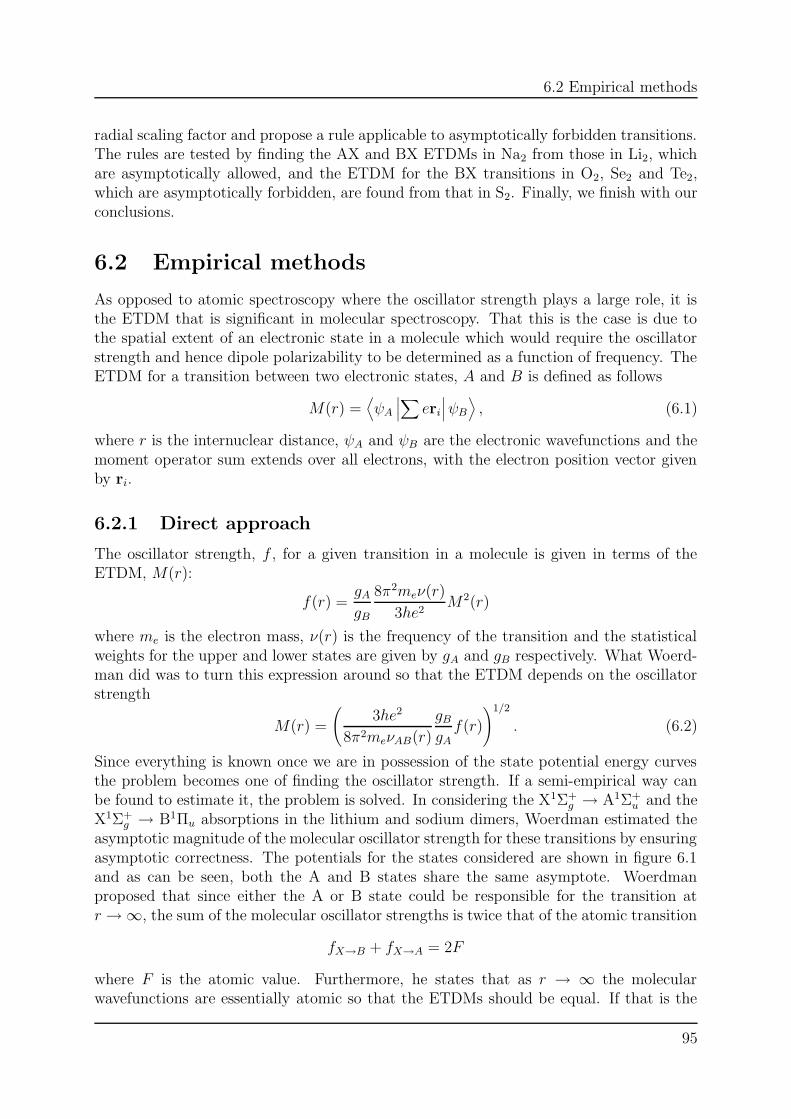
6.2 Empirical methods
radial scaling factor and propose a rule applicable to asymptotically forbidden transitions.The rules are tested by finding the AX and BX ETDMs in Na2 from those in Li2, whichare asymptotically allowed, and the ETDM for the BX transitions in O2, Se2 and Te2,which are asymptotically forbidden, are found from that in S2. Finally, we finish with ourconclusions.
6.2 Empirical methods
As opposed to atomic spectroscopy where the oscillator strength plays a large role, it isthe ETDM that is significant in molecular spectroscopy. That this is the case is due tothe spatial extent of an electronic state in a molecule which would require the oscillatorstrength and hence dipole polarizability to be determined as a function of frequency. TheETDM for a transition between two electronic states, A and B is defined as follows
M(r) =⟨ψA
∣∣∣∑
eri
∣∣∣ψB
⟩, (6.1)
where r is the internuclear distance, ψA and ψB are the electronic wavefunctions and themoment operator sum extends over all electrons, with the electron position vector givenby ri.
6.2.1 Direct approach
The oscillator strength, f , for a given transition in a molecule is given in terms of theETDM, M(r):
f(r) =gA
gB
8π2meν(r)
3he2M2(r)
where me is the electron mass, ν(r) is the frequency of the transition and the statisticalweights for the upper and lower states are given by gA and gB respectively. What Woerd-man did was to turn this expression around so that the ETDM depends on the oscillatorstrength
M(r) =
(3he2
8π2meνAB(r)
gB
gAf(r)
)1/2
. (6.2)
Since everything is known once we are in possession of the state potential energy curvesthe problem becomes one of finding the oscillator strength. If a semi-empirical way canbe found to estimate it, the problem is solved. In considering the X1Σ+
g → A1Σ+u and the
X1Σ+g → B1Πu absorptions in the lithium and sodium dimers, Woerdman estimated the
asymptotic magnitude of the molecular oscillator strength for these transitions by ensuringasymptotic correctness. The potentials for the states considered are shown in figure 6.1and as can be seen, both the A and B states share the same asymptote. Woerdmanproposed that since either the A or B state could be responsible for the transition atr → ∞, the sum of the molecular oscillator strengths is twice that of the atomic transition
fX→B + fX→A = 2F
where F is the atomic value. Furthermore, he states that as r → ∞ the molecularwavefunctions are essentially atomic so that the ETDMs should be equal. If that is the
95
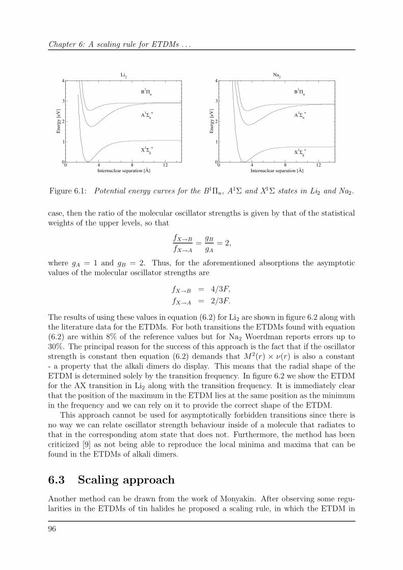
Chapter 6: A scaling rule for ETDMs . . .
0 4 8 12Internuclear separation [Å]
0
1
2
3
4
Ene
rgy
[eV
]
Li2
X1Σg+
A1Σu+
B1Πu
0 4 8 12Internuclear separation [Å]
0
1
2
3
4
Ene
rgy
[eV
]
Na2
B1Πu
A1Σu+
X1Σg+
Figure 6.1: Potential energy curves for the B1Πu, A1Σ and X1Σ states in Li2 and Na2.
case, then the ratio of the molecular oscillator strengths is given by that of the statisticalweights of the upper levels, so that
fX→B
fX→A=gB
gA= 2,
where gA = 1 and gB = 2. Thus, for the aforementioned absorptions the asymptoticvalues of the molecular oscillator strengths are
fX→B = 4/3F,
fX→A = 2/3F.
The results of using these values in equation (6.2) for Li2 are shown in figure 6.2 along withthe literature data for the ETDMs. For both transitions the ETDMs found with equation(6.2) are within 8% of the reference values but for Na2 Woerdman reports errors up to30%. The principal reason for the success of this approach is the fact that if the oscillatorstrength is constant then equation (6.2) demands that M 2(r) × ν(r) is also a constant- a property that the alkali dimers do display. This means that the radial shape of theETDM is determined solely by the transition frequency. In figure 6.2 we show the ETDMfor the AX transition in Li2 along with the transition frequency. It is immediately clearthat the position of the maximum in the ETDM lies at the same position as the minimumin the frequency and we can rely on it to provide the correct shape of the ETDM.
This approach cannot be used for asymptotically forbidden transitions since there isno way we can relate oscillator strength behaviour inside of a molecule that radiates tothat in the corresponding atom state that does not. Furthermore, the method has beencriticized [9] as not being able to reproduce the local minima and maxima that can befound in the ETDMs of alkali dimers.
6.3 Scaling approach
Another method can be drawn from the work of Monyakin. After observing some regu-larities in the ETDMs of tin halides he proposed a scaling rule, in which the ETDM in
96
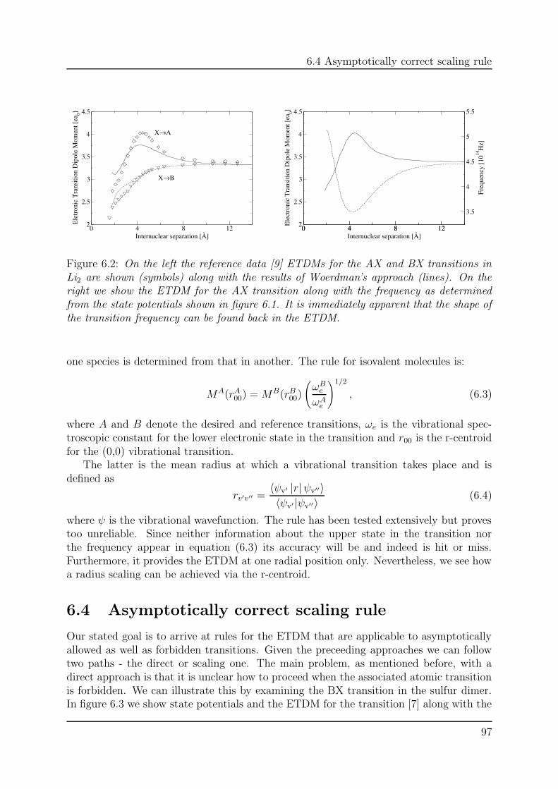
6.4 Asymptotically correct scaling rule
0 4 8 12Internuclear separation [Å]
2
2.5
3
3.5
4
4.5
Ele
tron
ic T
rans
ition
Dip
ole
Mom
ent [
ea0]
X→A
X→B
0 4 8 12
3.5
4
4.5
5
5.5
Freq
uenc
y [1
014H
z]
0 4 8 12Internuclear separation [Å]
2
2.5
3
3.5
4
4.5
Ele
ctro
nic
Tra
nsiti
on D
ipol
e M
omen
t [ea
0]
Figure 6.2: On the left the reference data [9] ETDMs for the AX and BX transitions inLi2 are shown (symbols) along with the results of Woerdman’s approach (lines). On theright we show the ETDM for the AX transition along with the frequency as determinedfrom the state potentials shown in figure 6.1. It is immediately apparent that the shape ofthe transition frequency can be found back in the ETDM.
one species is determined from that in another. The rule for isovalent molecules is:
MA(rA00) = MB(rB
00)
(ωB
e
ωAe
)1/2
, (6.3)
where A and B denote the desired and reference transitions, ωe is the vibrational spec-troscopic constant for the lower electronic state in the transition and r00 is the r-centroidfor the (0,0) vibrational transition.
The latter is the mean radius at which a vibrational transition takes place and isdefined as
rv′v′′ =〈ψv′ |r|ψv′′〉〈ψv′ |ψv′′〉 (6.4)
where ψ is the vibrational wavefunction. The rule has been tested extensively but provestoo unreliable. Since neither information about the upper state in the transition northe frequency appear in equation (6.3) its accuracy will be and indeed is hit or miss.Furthermore, it provides the ETDM at one radial position only. Nevertheless, we see howa radius scaling can be achieved via the r-centroid.
6.4 Asymptotically correct scaling rule
Our stated goal is to arrive at rules for the ETDM that are applicable to asymptoticallyallowed as well as forbidden transitions. Given the preceeding approaches we can followtwo paths - the direct or scaling one. The main problem, as mentioned before, with adirect approach is that it is unclear how to proceed when the associated atomic transitionis forbidden. We can illustrate this by examining the BX transition in the sulfur dimer.In figure 6.3 we show state potentials and the ETDM for the transition [7] along with the
97
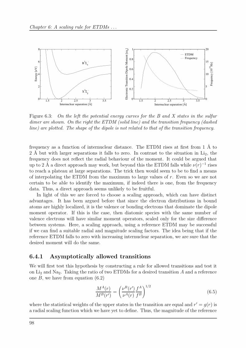
Chapter 6: A scaling rule for ETDMs . . .
1.5 2 2.5 3 3.5Internuclear separation [Å]
0
2
4
6
8
Ene
rgy
[eV
]
B3Σu-
X3Σg-
0
5
10
15
20
Freq
uenc
y [1
014H
z]
Frequency
1.5 2 2.5 3 3.50
0.2
0.4
0.6
0.8
1
Ele
ctro
nic
Tra
nsiti
on D
ipol
e M
omen
t [ea
0]
ETDM
Internuclear separation [Å]
Figure 6.3: On the left the potential energy curves for the B and X states in the sulfurdimer are shown. On the right the ETDM (solid line) and the transition frequency (dashedline) are plotted. The shape of the dipole is not related to that of the transition frequency.
frequency as a function of internuclear distance. The ETDM rises at first from 1 A to2 A but with larger separations it falls to zero. In contrast to the situation in Li2, thefrequency does not reflect the radial behaviour of the moment. It could be argued thatup to 2 A a direct approach may work, but beyond this the ETDM falls while ν(r)−1 risesto reach a plateau at large separations. The trick then would seem to be to find a meansof interpolating the ETDM from the maximum to large values of r. Even so we are notcertain to be able to identify the maximum, if indeed there is one, from the frequencydata. Thus, a direct approach seems unlikely to be fruitful.
In light of this we are forced to choose a scaling approach, which can have distinctadvantages. It has been argued before that since the electron distributions in boundatoms are highly localized, it is the valence or bonding electrons that dominate the dipolemoment operator. If this is the case, then diatomic species with the same number ofvalence electrons will have similar moment operators, scaled only for the size differencebetween systems. Here, a scaling approach, using a reference ETDM may be successfulif we can find a suitable radial and magnitude scaling factors. The idea being that if thereference ETDM falls to zero with increasing internuclear separation, we are sure that thedesired moment will do the same.
6.4.1 Asymptotically allowed transitions
We will first test this hypothesis by constructing a rule for allowed transitions and test iton Li2 and Na2. Taking the ratio of two ETDMs for a desired transition A and a referenceone B, we have from equation (6.2)
MA(r)
MB(r′)=
(νB(r′)
νA(r)
fA
fB
)1/2
(6.5)
where the statistical weights of the upper states in the transition are equal and r ′ = g(r) isa radial scaling function which we have yet to define. Thus, the magnitude of the reference
98
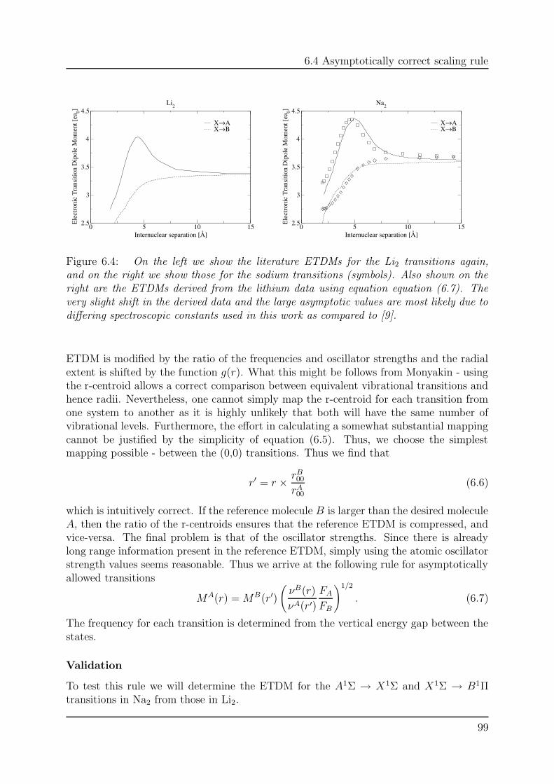
6.4 Asymptotically correct scaling rule
0 5 10 15Internuclear separation [Å]
2.5
3
3.5
4
4.5
Ele
ctro
nic
Tra
nsiti
on D
ipol
e M
omen
t [ea
0]
X→AX→Β
Li2
0 5 10 15Internuclear separation [Å]
2.5
3
3.5
4
4.5
Ele
ctro
nic
Tra
nsiti
on D
ipol
e M
omen
t [ea
0]
X→AX→B
Na2
Figure 6.4: On the left we show the literature ETDMs for the Li2 transitions again,and on the right we show those for the sodium transitions (symbols). Also shown on theright are the ETDMs derived from the lithium data using equation equation (6.7). Thevery slight shift in the derived data and the large asymptotic values are most likely due todiffering spectroscopic constants used in this work as compared to [9].
ETDM is modified by the ratio of the frequencies and oscillator strengths and the radialextent is shifted by the function g(r). What this might be follows from Monyakin - usingthe r-centroid allows a correct comparison between equivalent vibrational transitions andhence radii. Nevertheless, one cannot simply map the r-centroid for each transition fromone system to another as it is highly unlikely that both will have the same number ofvibrational levels. Furthermore, the effort in calculating a somewhat substantial mappingcannot be justified by the simplicity of equation (6.5). Thus, we choose the simplestmapping possible - between the (0,0) transitions. Thus we find that
r′ = r × rB00
rA00
(6.6)
which is intuitively correct. If the reference molecule B is larger than the desired moleculeA, then the ratio of the r-centroids ensures that the reference ETDM is compressed, andvice-versa. The final problem is that of the oscillator strengths. Since there is alreadylong range information present in the reference ETDM, simply using the atomic oscillatorstrength values seems reasonable. Thus we arrive at the following rule for asymptoticallyallowed transitions
MA(r) = MB(r′)
(νB(r)
νA(r′)
FA
FB
)1/2
. (6.7)
The frequency for each transition is determined from the vertical energy gap between thestates.
Validation
To test this rule we will determine the ETDM for the A1Σ → X1Σ and X1Σ → B1Πtransitions in Na2 from those in Li2.
99
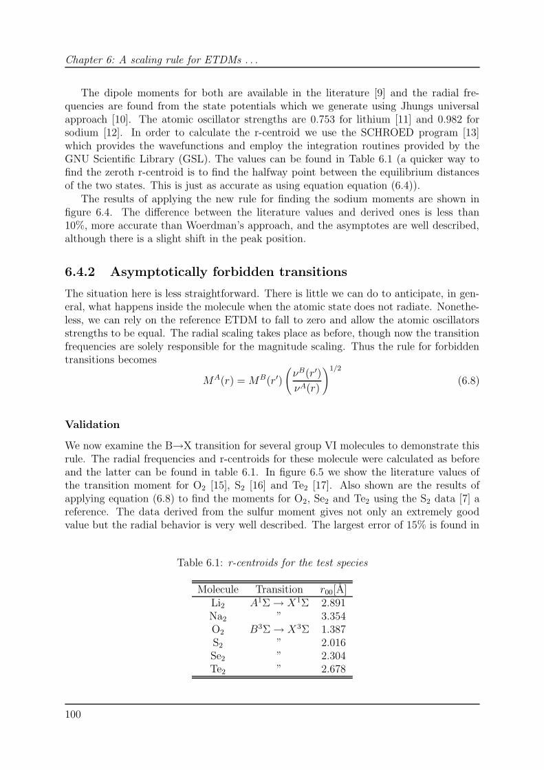
Chapter 6: A scaling rule for ETDMs . . .
The dipole moments for both are available in the literature [9] and the radial fre-quencies are found from the state potentials which we generate using Jhungs universalapproach [10]. The atomic oscillator strengths are 0.753 for lithium [11] and 0.982 forsodium [12]. In order to calculate the r-centroid we use the SCHROED program [13]which provides the wavefunctions and employ the integration routines provided by theGNU Scientific Library (GSL). The values can be found in Table 6.1 (a quicker way tofind the zeroth r-centroid is to find the halfway point between the equilibrium distancesof the two states. This is just as accurate as using equation equation (6.4)).
The results of applying the new rule for finding the sodium moments are shown infigure 6.4. The difference between the literature values and derived ones is less than10%, more accurate than Woerdman’s approach, and the asymptotes are well described,although there is a slight shift in the peak position.
6.4.2 Asymptotically forbidden transitions
The situation here is less straightforward. There is little we can do to anticipate, in gen-eral, what happens inside the molecule when the atomic state does not radiate. Nonethe-less, we can rely on the reference ETDM to fall to zero and allow the atomic oscillatorsstrengths to be equal. The radial scaling takes place as before, though now the transitionfrequencies are solely responsible for the magnitude scaling. Thus the rule for forbiddentransitions becomes
MA(r) = MB(r′)
(νB(r′)
νA(r)
)1/2
(6.8)
Validation
We now examine the B→X transition for several group VI molecules to demonstrate thisrule. The radial frequencies and r-centroids for these molecule were calculated as beforeand the latter can be found in table 6.1. In figure 6.5 we show the literature values ofthe transition moment for O2 [15], S2 [16] and Te2 [17]. Also shown are the results ofapplying equation (6.8) to find the moments for O2, Se2 and Te2 using the S2 data [7] areference. The data derived from the sulfur moment gives not only an extremely goodvalue but the radial behavior is very well described. The largest error of 15% is found in
Table 6.1: r-centroids for the test species
Molecule Transition r00[A]Li2 A1Σ → X1Σ 2.891Na2 ” 3.354O2 B3Σ → X3Σ 1.387S2 ” 2.016Se2 ” 2.304Te2 ” 2.678
100
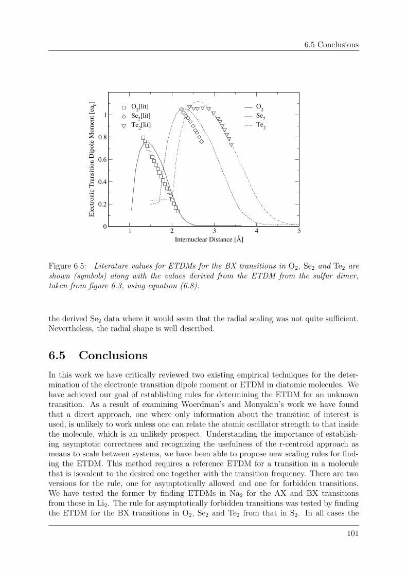
6.5 Conclusions
1 2 3 4 50
0.2
0.4
0.6
0.8
1
Ele
ctro
nic
Tra
nsiti
on D
ipol
e M
omen
t [ea
0]
O2Se2Te2
O2[lit]Se2[lit]Te2[lit]
Internuclear Distance [Å]
Figure 6.5: Literature values for ETDMs for the BX transitions in O2, Se2 and Te2 areshown (symbols) along with the values derived from the ETDM from the sulfur dimer,taken from figure 6.3, using equation (6.8).
the derived Se2 data where it would seem that the radial scaling was not quite sufficient.Nevertheless, the radial shape is well described.
6.5 Conclusions
In this work we have critically reviewed two existing empirical techniques for the deter-mination of the electronic transition dipole moment or ETDM in diatomic molecules. Wehave achieved our goal of establishing rules for determining the ETDM for an unknowntransition. As a result of examining Woerdman’s and Monyakin’s work we have foundthat a direct approach, one where only information about the transition of interest isused, is unlikely to work unless one can relate the atomic oscillator strength to that insidethe molecule, which is an unlikely prospect. Understanding the importance of establish-ing asymptotic correctness and recognizing the usefulness of the r-centroid approach asmeans to scale between systems, we have been able to propose new scaling rules for find-ing the ETDM. This method requires a reference ETDM for a transition in a moleculethat is isovalent to the desired one together with the transition frequency. There are twoversions for the rule, one for asymptotically allowed and one for forbidden transitions.We have tested the former by finding ETDMs in Na2 for the AX and BX transitionsfrom those in Li2. The rule for asymptotically forbidden transitions was tested by findingthe ETDM for the BX transitions in O2, Se2 and Te2 from that in S2. In all cases the
101
Bibliography
derived values agreed within 15% of the literature values. The strength of the approachis that we use the reference ETDM to describe that in a species where it is unknown anduse readily available data - the transition frequencies and atomic oscillator strengths toensure that the magnitude is correct. Furthermore, the r-centroid scaling we employ isreadily performed. We find the accuracy of the new approach more than sufficient givenits simplicity. Finally, while all examples here treated homonuclear molecules, extensionof the rules to hetero-nuclear species should be possible.
References
[1] Woerdman J P, J. Chem. Phys. 75, 5577 (1981)
[2] Monyakin P A , Kuznetsova L A, N. E. Kuzmenko N E, Kuzyakov Y Y and PlastininY A, Opt. Spectrosc. (USSR) 48, 11 (1980)
[3] Monyakin P A , Kuznetsova L A, N. E. Kuzmenko N E, Kuzyakov Y Y and PlastininY A, Opt. Spectrosc. (USSR) 48, 243 (1980)
[4] Akopyan M E, Bibinov M K, Kokh D B, Pravilov A M, Stepanov M B, Chem. Phys.242, 253 (1999)
[5] Johnston C W, van der Heijden H, Janssen G M, van Dijk J and van der Mullen JJ A M , J. Phys. D: Appl. Phys 35, 342 (2002), Chapter 2 of this thesis
[6] Johnston C W, Jonkers J and van der Mullen J J A M, J. Phys. D: Appl. Phys. 35,2578 (2002), Chapter 3 of this thesis
[7] Pradhan D A and Partridge H, Chem. Phys. Lett. 255, 163 (1996)
[8] Stevens W J, Hessel M M, Bertoncini P J, Wahl A C, J. Chem. Phys. 466, 1477(1977)
[9] Konowalow D D, Rosenkrantz M E and Hochauser D S, J. Mol. Spec. 99, 321 (1983)
[10] Jhung K S, Kim I H, Oh K, Hahn K B, Phys. Rev. A 42, 6497 (1990)
[11] Wiese W L, Smith M W and Miles B M, Atomic transition probabilities, Natl. Stand.Ref. Data Ser. Natl. Bur. Stad., Circ. 4(U.S.GPO, Washington, D.C.,1966), Vol. 1.
[12] Wiese W L, Smith M W and Miles B M, Atomic transition probabilities, Natl. Stand.Ref. Data Ser. Natl. Bur. Stad., Circ. 22(U.S.GPO, Washington, D.C.,1969), Vol. 2.
[13] Pashov A, Jastrzebski W and Kowalcyzk P, Comput. Phys. Commun. 128, 622 (2000)
[14] http://sources.redhat.com/gsl/
[15] Lewis B R and Gibson S T, J. Chem. Phys. 93, 7532 (1990)
[16] Heinemann C, Koch W, Linder G, Reinen D and Widmark P, Phys. Rev. A 54, 1979(1996)
[17] Zaitsevskii A, Ferber R and Teichteil C, Phys. Rev. A 63, 42511 (2001)
102
CHAPTER 7
A power law scaling between the atomic dipole polarizabilities and
the quadrupole and octupole values: application to molecules
A simple power scaling law is reported between the quadrupole, octupole polarizabilitiesand the dipole values of neutral atoms which has been deduced from the tabulations ofPatil [1]. The values 1.553 and 2.238 are found to relate the dipole to quadrupole anddipole to octupole. The scaling is applied to molecules and proves to be within 20% ofliterature values.
103
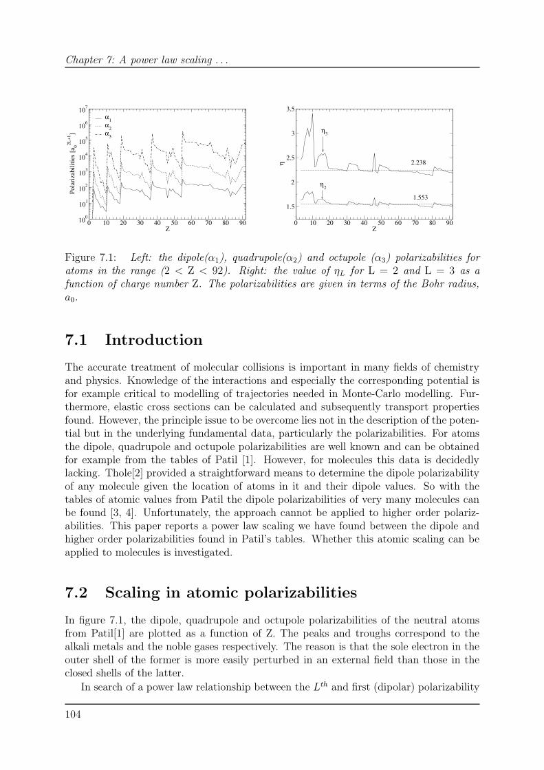
Chapter 7: A power law scaling . . .
0 10 20 30 40 50 60 70 80 90Z
100
101
102
103
104
105
106
107
Pola
riza
bilit
ies
[a02L
+1]
α1α2α3
0 10 20 30 40 50 60 70 80 90Z
1.5
2
2.5
3
3.5
η 2.238
1.553
η2
η3
Figure 7.1: Left: the dipole(α1), quadrupole(α2) and octupole (α3) polarizabilities foratoms in the range (2 < Z < 92). Right: the value of ηL for L = 2 and L = 3 as afunction of charge number Z. The polarizabilities are given in terms of the Bohr radius,a0.
7.1 Introduction
The accurate treatment of molecular collisions is important in many fields of chemistryand physics. Knowledge of the interactions and especially the corresponding potential isfor example critical to modelling of trajectories needed in Monte-Carlo modelling. Fur-thermore, elastic cross sections can be calculated and subsequently transport propertiesfound. However, the principle issue to be overcome lies not in the description of the poten-tial but in the underlying fundamental data, particularly the polarizabilities. For atomsthe dipole, quadrupole and octupole polarizabilities are well known and can be obtainedfor example from the tables of Patil [1]. However, for molecules this data is decidedlylacking. Thole[2] provided a straightforward means to determine the dipole polarizabilityof any molecule given the location of atoms in it and their dipole values. So with thetables of atomic values from Patil the dipole polarizabilities of very many molecules canbe found [3, 4]. Unfortunately, the approach cannot be applied to higher order polariz-abilities. This paper reports a power law scaling we have found between the dipole andhigher order polarizabilities found in Patil’s tables. Whether this atomic scaling can beapplied to molecules is investigated.
7.2 Scaling in atomic polarizabilities
In figure 7.1, the dipole, quadrupole and octupole polarizabilities of the neutral atomsfrom Patil[1] are plotted as a function of Z. The peaks and troughs correspond to thealkali metals and the noble gases respectively. The reason is that the sole electron in theouter shell of the former is more easily perturbed in an external field than those in theclosed shells of the latter.
In search of a power law relationship between the Lth and first (dipolar) polarizability
104
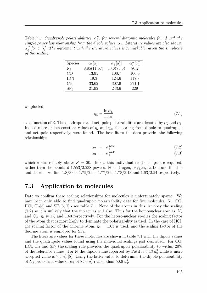
7.3 Application to molecules
Table 7.1: Quadrupole polarizabilities, αS2 , for several diatomic molecules found with the
simple power law relationship from the dipole values, α1. Literature values are also shown,αR
2 [5, 6, 7]. The agreement with the literature values is remarkable, given the simplicityof the scaling.
Species α1[a30] αS
2 [a50] αR
2 [a50]
N2 8.85(11.57) 50.6(85.6) 80.2CO 13.95 100.7 106.9HCl 19.3 124.6 117.8Cl2 33.62 307.9 371.1SF6 21.92 243.6 229
we plotted
ηL =lnαL
lnα1(7.1)
as a function of Z. The quadrupole and octupole polarizabilities are denoted by α2 and α3.Indeed more or less constant values of η2 and η3, the scaling from dipole to quadrupoleand octupole respectively, were found. The best fit to the data provides the followingrelationships
α2 = α1.5531 (7.2)
α3 = α2.2381 (7.3)
which works reliably above Z = 20. Below this individual relationships are required,rather than the standard 1.553/2.238 powers. For nitrogen, oxygen, carbon and fluorineand chlorine we find 1.8/3.09, 1.75/2.99, 1.77/2.9, 1.78/3.13 and 1.63/2.54 respectively.
7.3 Application to molecules
Data to confirm these scaling relationships for molecules is unfortunately sparse. Wehave been only able to find quadrupole polarizability data for five molecules; N2, CO,HCl, Cl2[5] and SF6[6, 7] - see table 7.1. None of the atoms in this list obey the scaling(7.2) so it is unlikely that the molecules will also. Thus for the homonuclear species, N2
and Cl2, η2 is 1.8 and 1.63 respectively. For the hetero-nuclear species the scaling factorof the atom that is most likely to dominate the polarizability is used. In the case of HCl,the scaling factor of the chlorine atom, η2 = 1.63 is used, and the scaling factor of thefluorine atom is employed for SF6.
The literature values for these molecules are shown in table 7.1 with the dipole valuesand the quadrupole values found using the individual scalings just described. For CO,HCl, Cl2 and SF6 the scaling rule provides the quadrupole polarizability to within 20%of the reference values. For N the dipole value reported by Patil is 5.43 a3
0 while a moreaccepted value is 7.5 a3
0 [8]. Using the latter value to determine the dipole polarizabilityof N2 provides a value of α2 of 85.6 a5
0 rather than 50.6 a50.
105
Bibliography
7.4 Conclusions
In this paper we have reported the existence of a simple power law scaling between thequadrupole and octupole polarizabilities and the dipole value for atoms. This has beenshown to be effective in reproducing the quadrupole polarizability for several diatomicspecies to within 20%. The simplicity of the method means that it can be used readilyand at least in the first instance provides a reasonably reliable first guess value for thehigher order polarizabilities of molecules.
References
[1] Patil S H, At. Data Nucl. Data Tables 71, 41 (1999)
[2] Thole B T, Chem. Phys. 59, 341 (1981)
[3] Jensen L, Anstrand P, Sylvester-Hvid K, Mikkelson K V, J. Phys. Chem. A 104,1563 (2000)
[4] Jensen L, Anstrand P, Osted A, Kongsted J, Mikkelson K V, J. Chem. Phys. 116,4001 (2002)
[5] Osinga V P, van Gisbergen S J A, Snijders G, Baerends E J, J. Chem. Phys. 106,5091 (1997)
[6] Fowler P W, Kelly H M, Vaidehi N, Mol. Phys. 82, 211 (1994)
[7] Maroulis G, Chem. Phys. Lett. 312, 255 (1999)
[8] Radzig A A, Smirnov B M, Reference data on atoms, molecules and ions, (Springer,Berlin, 1985)
106
CHAPTER 8
Born-Mayer parameters for arbitrary atomic and molecular
interactions
The model potential of Tang and Toennies [1] is used to determine the Born-Mayer param-eters for arbitrary atomic and molecular interactions. Several existing empirical relationsare collected in order to calculate the necessary data. The dispersion coefficients for anyatom-atom interaction are found from Patil’s tabulations of atomic hyperpolarizabilities[2]. Thole’s modified dipole approach [3] provides a means to determine the dipole polar-izability of any molecule and our own scaling law (chapter 7) permits the quadrupole andoctupole polarizabilities of any molecule to be found from the dipole value. Together withthe empirical expressions of Cambi et al [4] which relate the potential well parametersto the dipole polarizabilities of the colliding pair the repulsive part of the interaction isrecovered.
The potential parameters found with this approach are tested by comparing resultswith literature values for several noble gases interactions and collision integral data for theinteractions of nitrogen and oxygen atoms, molecules and ions. In all cases the computedcross sections and collision integrals are within 10% of the literature values.
107
Chapter 8: Born-Mayer parameters for arbitrary . . .
8.1 Introduction
The transport properties of a dilute (ionized) gas mainly depend on the elastic interac-tions between the gas particles. In principle the properties of these interactions can beestablished experimentally; in beam experiments for instance. However, if the objectiveis to obtain insight into plasma properties as function of their chemical composition anexperimental approach is a difficult one. The huge diversity of the plasma state meansthat the number of interacting pairs that might require treatment is vast. Therefore, atheoretical approach would appear to be more promising. In particular, the ease of useof semi-empirical methods can be attractive, especially so when one is interested in rapidprototyping of plasma transport properties. Currently the common practice is to use ahard sphere model to estimate cross sections when nothing is known about a particularinteraction. However, the approximate and temperature independent nature of this crosssection is far from realistic. In this chapter we show that there is a readily tractablealternative.
The transport properties of ionized plasmas are the result of the interaction of manydifferent types of species. For example, in a molecular plasma the interactions betweenmolecules, molecules and atoms, charged and neutral species and between charged speciescan all play important roles. In this chapter we confine ourselves to van der Waalsinteractions and their description; in chapter 9 the influence of these and other interactionson the transport properties as a whole are discussed.
By and large, most heavy particle collisions, including those between ions and neutrals,are characterized by a van der Waals interaction potential. These are closed-shell inter-actions, which means that the collision partners neither change their identity nor form amolecule during the collision. In general a van der Waals interaction potential consists ofan attractive part and at smaller internuclear distances, a repulsive branch. Under mostpartially ionized plasma conditions the majority of such interactions are determined bytheir repulsive nature. This is best described by an exponential function
V (r) = Ae−br (8.1)
where A and b are the so-called Born-Mayer parameters. The only empirical means thatwe are aware of to find these in a accurate way is via the full van der Waals potentialdescribed by the Tang and Toennies [1]. The advantage of using this potential is thatthere are no fit parameters. For each interacting pair the potential can be constructedusing properties of the collision partners solely. These properties turn out to be thepolarizabilities and the effective number of electrons of each of the interacting particles.Another advantage of the Tang and Toennies potential is that an algorithm is availableto find A and b [5] from these fundamental properties. The principal idea is that oncethe attractive part of the interaction is known accurately, the repulsive part can be foundas well. The goal of this chapter is to collect existing empirical formulae that will allowthe Born-Mayer parameters to be found for any atomic or molecular interaction via themodel potential function of Tang and Toennies.
The chapter is laid out as follows: in section 8.2 some basic definitions are introduced.The Tang and Toennies potential is presented in section 8.3 and the parameters requiredto recover the repulsive part of the potential are identified. In section 8.4 Cambi’s rela-tions to determine the potential well-depth parameters are presented and their efficacies
108
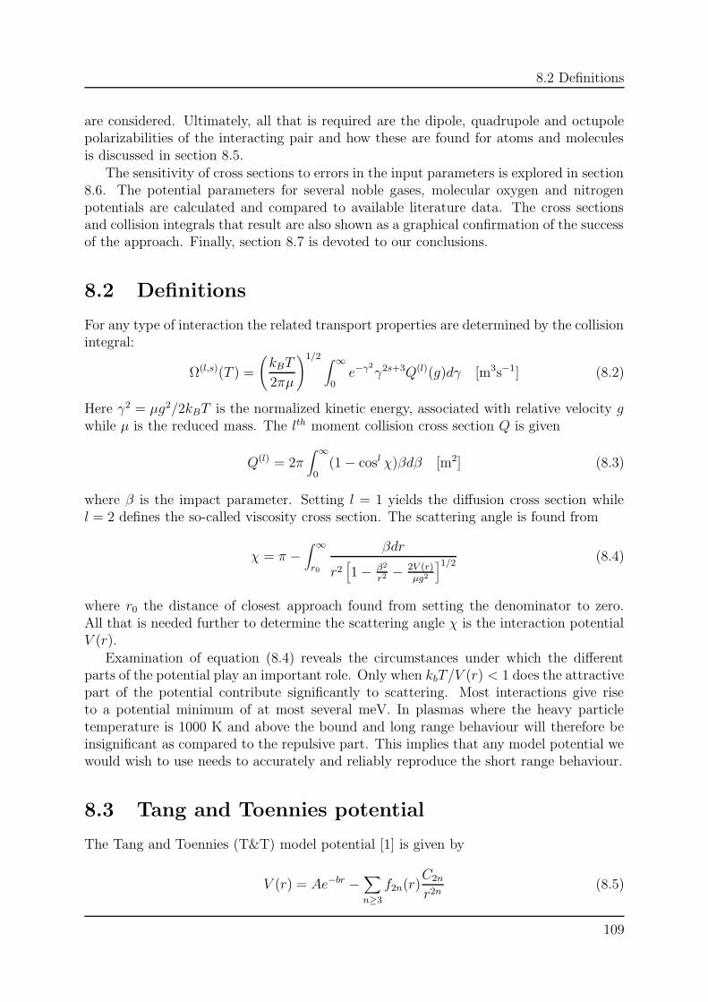
8.2 Definitions
are considered. Ultimately, all that is required are the dipole, quadrupole and octupolepolarizabilities of the interacting pair and how these are found for atoms and moleculesis discussed in section 8.5.
The sensitivity of cross sections to errors in the input parameters is explored in section8.6. The potential parameters for several noble gases, molecular oxygen and nitrogenpotentials are calculated and compared to available literature data. The cross sectionsand collision integrals that result are also shown as a graphical confirmation of the successof the approach. Finally, section 8.7 is devoted to our conclusions.
8.2 Definitions
For any type of interaction the related transport properties are determined by the collisionintegral:
Ω(l,s)(T ) =
(kBT
2πµ
)1/2 ∫ ∞
0e−γ2
γ2s+3Q(l)(g)dγ [m3s−1] (8.2)
Here γ2 = µg2/2kBT is the normalized kinetic energy, associated with relative velocity gwhile µ is the reduced mass. The lth moment collision cross section Q is given
Q(l) = 2π∫ ∞
0(1 − cosl χ)βdβ [m2] (8.3)
where β is the impact parameter. Setting l = 1 yields the diffusion cross section whilel = 2 defines the so-called viscosity cross section. The scattering angle is found from
χ = π −∫ ∞
r0
βdr
r2[1 − β2
r2 − 2V (r)µg2
]1/2(8.4)
where r0 the distance of closest approach found from setting the denominator to zero.All that is needed further to determine the scattering angle χ is the interaction potentialV (r).
Examination of equation (8.4) reveals the circumstances under which the differentparts of the potential play an important role. Only when kbT/V (r) < 1 does the attractivepart of the potential contribute significantly to scattering. Most interactions give riseto a potential minimum of at most several meV. In plasmas where the heavy particletemperature is 1000 K and above the bound and long range behaviour will therefore beinsignificant as compared to the repulsive part. This implies that any model potential wewould wish to use needs to accurately and reliably reproduce the short range behaviour.
8.3 Tang and Toennies potential
The Tang and Toennies (T&T) model potential [1] is given by
V (r) = Ae−br −∑
n≥3
f2n(r)C2n
r2n(8.5)
109
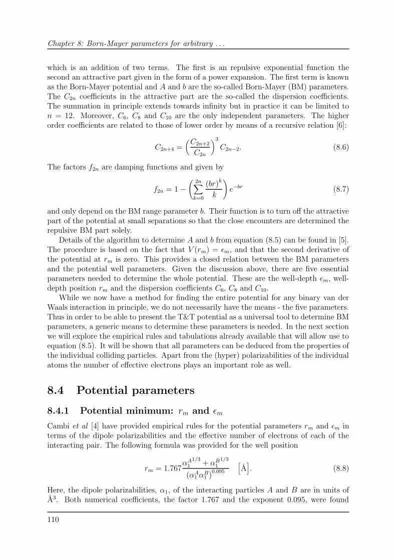
Chapter 8: Born-Mayer parameters for arbitrary . . .
which is an addition of two terms. The first is an repulsive exponential function thesecond an attractive part given in the form of a power expansion. The first term is knownas the Born-Mayer potential and A and b are the so-called Born-Mayer (BM) parameters.The C2n coefficients in the attractive part are the so-called the dispersion coefficients.The summation in principle extends towards infinity but in practice it can be limited ton = 12. Moreover, C6, C8 and C10 are the only independent parameters. The higherorder coefficients are related to those of lower order by means of a recursive relation [6]:
C2n+4 =(C2n+2
C2n
)3
C2n−2. (8.6)
The factors f2n are damping functions and given by
f2n = 1 −(
2n∑
k=0
(br)k
k
)e−br (8.7)
and only depend on the BM range parameter b. Their function is to turn off the attractivepart of the potential at small separations so that the close encounters are determined therepulsive BM part solely.
Details of the algorithm to determine A and b from equation (8.5) can be found in [5].The procedure is based on the fact that V (rm) = εm, and that the second derivative ofthe potential at rm is zero. This provides a closed relation between the BM parametersand the potential well parameters. Given the discussion above, there are five essentialparameters needed to determine the whole potential. These are the well-depth εm, well-depth position rm and the dispersion coefficients C6, C8 and C10.
While we now have a method for finding the entire potential for any binary van derWaals interaction in principle, we do not necessarily have the means - the five parameters.Thus in order to be able to present the T&T potential as a universal tool to determine BMparameters, a generic means to determine these parameters is needed. In the next sectionwe will explore the empirical rules and tabulations already available that will allow use toequation (8.5). It will be shown that all parameters can be deduced from the properties ofthe individual colliding particles. Apart from the (hyper) polarizabilities of the individualatoms the number of effective electrons plays an important role as well.
8.4 Potential parameters
8.4.1 Potential minimum: rm and εm
Cambi et al [4] have provided empirical rules for the potential parameters rm and εm interms of the dipole polarizabilities and the effective number of electrons of each of theinteracting pair. The following formula was provided for the well position
rm = 1.767αA
11/3
+ αB1
1/3
(αA1 α
B1 )
0.095
[A]. (8.8)
Here, the dipole polarizabilities, α1, of the interacting particles A and B are in units ofA3. Both numerical coefficients, the factor 1.767 and the exponent 0.095, were found
110
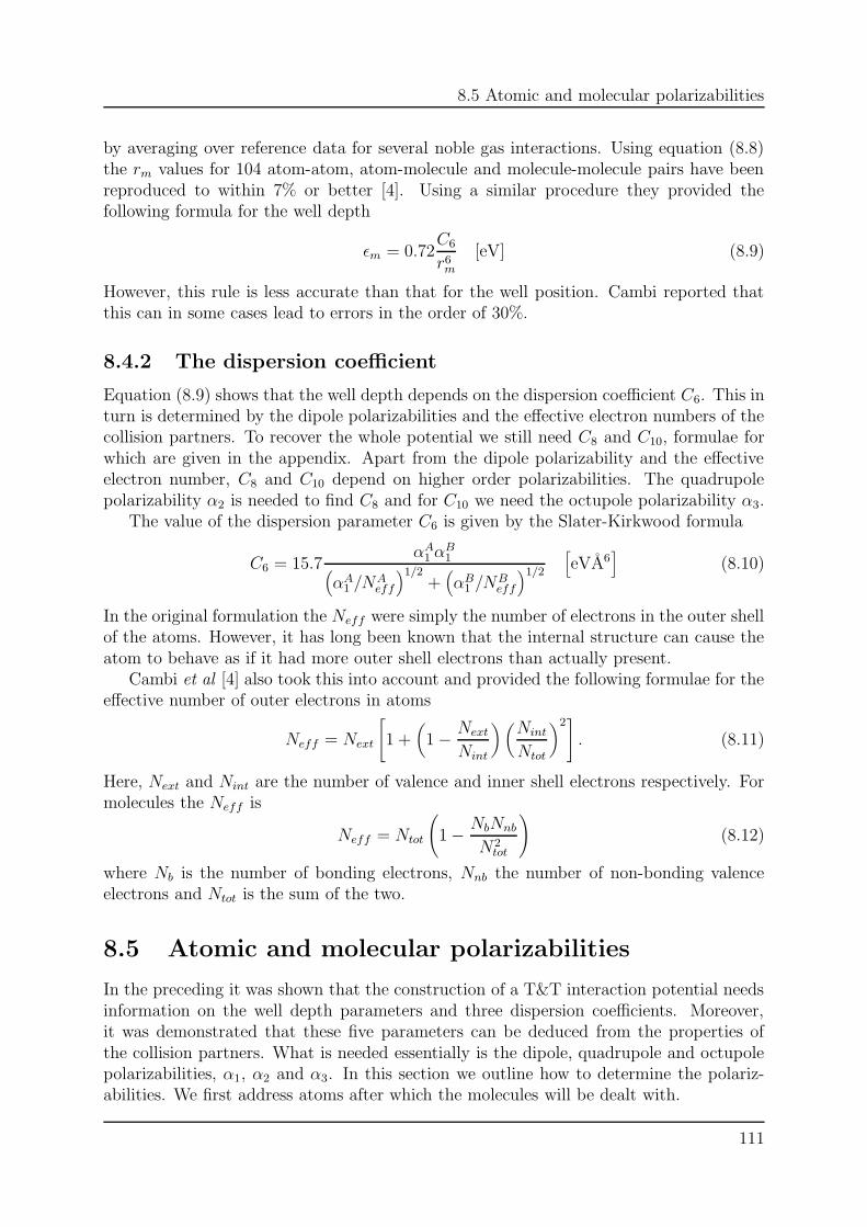
8.5 Atomic and molecular polarizabilities
by averaging over reference data for several noble gas interactions. Using equation (8.8)the rm values for 104 atom-atom, atom-molecule and molecule-molecule pairs have beenreproduced to within 7% or better [4]. Using a similar procedure they provided thefollowing formula for the well depth
εm = 0.72C6
r6m
[eV] (8.9)
However, this rule is less accurate than that for the well position. Cambi reported thatthis can in some cases lead to errors in the order of 30%.
8.4.2 The dispersion coefficient
Equation (8.9) shows that the well depth depends on the dispersion coefficient C6. This inturn is determined by the dipole polarizabilities and the effective electron numbers of thecollision partners. To recover the whole potential we still need C8 and C10, formulae forwhich are given in the appendix. Apart from the dipole polarizability and the effectiveelectron number, C8 and C10 depend on higher order polarizabilities. The quadrupolepolarizability α2 is needed to find C8 and for C10 we need the octupole polarizability α3.
The value of the dispersion parameter C6 is given by the Slater-Kirkwood formula
C6 = 15.7αA
1 αB1(
αA1 /N
Aeff
)1/2+(αB
1 /NBeff
)1/2
[eVA6
](8.10)
In the original formulation the Neff were simply the number of electrons in the outer shellof the atoms. However, it has long been known that the internal structure can cause theatom to behave as if it had more outer shell electrons than actually present.
Cambi et al [4] also took this into account and provided the following formulae for theeffective number of outer electrons in atoms
Neff = Next
[1 +
(1 − Next
Nint
)(Nint
Ntot
)2]. (8.11)
Here, Next and Nint are the number of valence and inner shell electrons respectively. Formolecules the Neff is
Neff = Ntot
(1 − NbNnb
N2tot
)(8.12)
where Nb is the number of bonding electrons, Nnb the number of non-bonding valenceelectrons and Ntot is the sum of the two.
8.5 Atomic and molecular polarizabilities
In the preceding it was shown that the construction of a T&T interaction potential needsinformation on the well depth parameters and three dispersion coefficients. Moreover,it was demonstrated that these five parameters can be deduced from the properties ofthe collision partners. What is needed essentially is the dipole, quadrupole and octupolepolarizabilities, α1, α2 and α3. In this section we outline how to determine the polariz-abilities. We first address atoms after which the molecules will be dealt with.
111
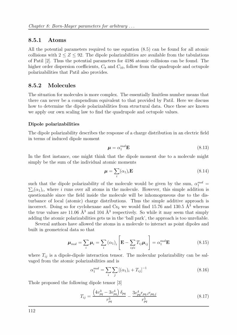
Chapter 8: Born-Mayer parameters for arbitrary . . .
8.5.1 Atoms
All the potential parameters required to use equation (8.5) can be found for all atomiccollisions with 2 ≤ Z ≤ 92. The dipole polarizabilities are available from the tabulationsof Patil [2]. Thus the potential parameters for 4186 atomic collisions can be found. Thehigher order dispersion coefficients, C8 and C10, follow from the quadrupole and octupolepolarizabilities that Patil also provides.
8.5.2 Molecules
The situation for molecules is more complex. The essentially limitless number means thatthere can never be a compendium equivalent to that provided by Patil. Here we discusshow to determine the dipole polarizabilities from structural data. Once these are knownwe apply our own scaling law to find the quadrupole and octupole values.
Dipole polarizabilities
The dipole polarizability describes the response of a charge distribution in an electric fieldin terms of induced dipole moment
µ = αmol1 E (8.13)
In the first instance, one might think that the dipole moment due to a molecule mightsimply be the sum of the individual atomic moments
µ =∑
i
(α1)iE (8.14)
such that the dipole polarizability of the molecule would be given by the sum, αmol1 =∑
i(α1)i, where i runs over all atoms in the molecule. However, this simple addition isquestionable since the field inside the molecule will be inhomogeneous due to the dis-turbance of local (atomic) charge distributions. Thus the simple additive approach isincorrect. Doing so for cyclohexane and Cs2 we would find 15.76 and 130.5 A3 whereasthe true values are 11.06 A3 and 104 A3 respectively. So while it may seem that simplyadding the atomic polarizabilities gets us in the ‘ball park’, the approach is too unreliable.
Several authors have allowed the atoms in a molecule to interact as point dipoles andbuilt in geometrical data so that
µmol =∑
i
µi =∑
i
(α1)i
E−
∑
i6=i
Tijµij
= αmol
1 E (8.15)
where Tij is a dipole-dipole interaction tensor. The molecular polarizability can be sal-vaged from the atomic polarizabilities and is
αmol1 =
∑
i
∑
j
[(α1)i + Tij]−1 (8.16)
Thole proposed the following dipole tensor [3]
Tij =
(4v3
pq − 3v4pq
)δpq
r3pq
− 3v4pqrpq,irpq,j
r5pq
(8.17)
112
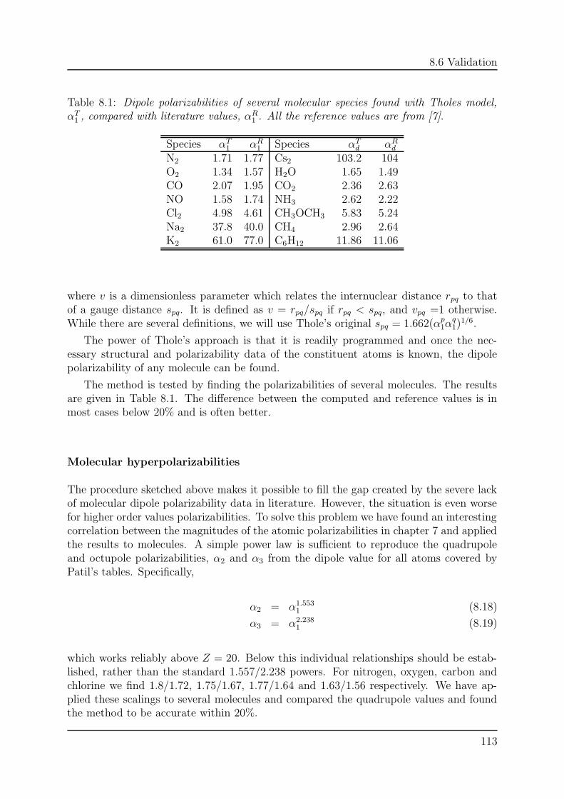
8.6 Validation
Table 8.1: Dipole polarizabilities of several molecular species found with Tholes model,αT
1 , compared with literature values, αR1 . All the reference values are from [7].
Species αT1 αR
1 Species αTd αR
d
N2 1.71 1.77 Cs2 103.2 104O2 1.34 1.57 H2O 1.65 1.49CO 2.07 1.95 CO2 2.36 2.63NO 1.58 1.74 NH3 2.62 2.22Cl2 4.98 4.61 CH3OCH3 5.83 5.24Na2 37.8 40.0 CH4 2.96 2.64K2 61.0 77.0 C6H12 11.86 11.06
where v is a dimensionless parameter which relates the internuclear distance rpq to thatof a gauge distance spq. It is defined as v = rpq/spq if rpq < spq, and vpq =1 otherwise.While there are several definitions, we will use Thole’s original spq = 1.662(αp
1αq1)
1/6.
The power of Thole’s approach is that it is readily programmed and once the nec-essary structural and polarizability data of the constituent atoms is known, the dipolepolarizability of any molecule can be found.
The method is tested by finding the polarizabilities of several molecules. The resultsare given in Table 8.1. The difference between the computed and reference values is inmost cases below 20% and is often better.
Molecular hyperpolarizabilities
The procedure sketched above makes it possible to fill the gap created by the severe lackof molecular dipole polarizability data in literature. However, the situation is even worsefor higher order values polarizabilities. To solve this problem we have found an interestingcorrelation between the magnitudes of the atomic polarizabilities in chapter 7 and appliedthe results to molecules. A simple power law is sufficient to reproduce the quadrupoleand octupole polarizabilities, α2 and α3 from the dipole value for all atoms covered byPatil’s tables. Specifically,
α2 = α1.5531 (8.18)
α3 = α2.2381 (8.19)
which works reliably above Z = 20. Below this individual relationships should be estab-lished, rather than the standard 1.557/2.238 powers. For nitrogen, oxygen, carbon andchlorine we find 1.8/1.72, 1.75/1.67, 1.77/1.64 and 1.63/1.56 respectively. We have ap-plied these scalings to several molecules and compared the quadrupole values and foundthe method to be accurate within 20%.
113
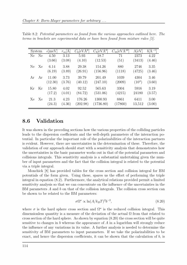
Chapter 8: Born-Mayer parameters for arbitrary . . .
Table 8.2: Potential parameters as found from the various approaches outlined here. Theterms in brackets are experimental data or have been found from mixture rules [5].
System ε[meV] rm[A] C6[eVA6] C8[eVA8] C10[eVA10] A[eV] b[A−1]Ne Ne 4.50 3.13 5.93 18.7 71 2373 4.22
(3.66) (3.08) (4.10) (12.53) (51) (3413) (4.46)
Ne Xe 6.14 3.88 29.38 154.26 880 2746 3.35(6.19) (3.89) (26.91) (156.96) (1118) (4725) (3.46)
Ar Ar 11.00 3.73 39.79 201.49 1039 4304 3.46(12.30) (3.76) (40.12) (247.10) (2009) (104) (3.60)
Kr Kr 15.80 4.02 92.52 565.63 3304 5916 3.19(17.2) (4.01) (84.72) (531.06) (4215) 24180 (3.57)
Xe Xe 21.3 4.23 176.26 1300.93 8861 6411 3.00(24.3) (4.36) (202.98) (1736.80) (17860) 13,512 (3.00)
8.6 Validation
It was shown in the preceding sections how the various properties of the colliding particlesleads to the dispersion coefficients and the well-depth parameters of the interaction po-tential. In particular the important role of the polarizabilities of the interaction partnersis evident. However, there are uncertainties in the determination of these. Therefore, thevalidation of our approach should start with a sensitivity analysis that demonstrates howthe uncertainties in the basic parameter works out in that of the potential parameters andcollisions integrals. This sensitivity analysis is a substantial undertaking given the num-ber of input parameters and the fact that the collision integral is related to the potentialvia a triple integral.
Monchick [8] has provided tables for the cross section and collision integral for BMpotentials of the form given. Using these, spares us the effort of performing the tripleintegral in equation (8.2). Furthermore, the analytical relations provided permit a limitedsensitivity analysis so that we can concentrate on the influence of the uncertainties in theBM parameters A and b on that of the collision integrals. The collision cross section canbe shown to be related to the BM parameters:
σΩ? ∝ ln(A/kBT )2b−2, (8.20)
where σ is the hard sphere cross section and Ω? is the reduced collision integral. Thisdimensionless quantity is a measure of the deviation of the actual Ω from that related tocross section of the hard sphere. As shown by equation (8.20) the cross section will be quitesensitive to changes in b whereas the appearance of A in a logarithm will strongly reducethe influence of any variations in its value. A further analysis is needed to determine thesensitivity of BM parameters to input parameters. If we take the polarizabilities to beexact, and hence the dispersion coefficients, it can be shown that the calculation of b, is
114
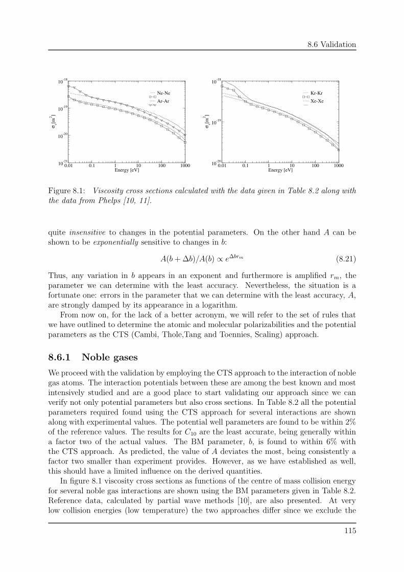
8.6 Validation
0.01 0.1 1 10 100 1000Energy [eV]
10-21
10-20
10-19
10-18
σ v[m2 ]
Ne-Ne
Ar-Ar
0.01 0.1 1 10 100 1000Energy [eV]
10-20
10-19
10-18
σ v[m2 ]
Kr-Kr
Xe-Xe
Figure 8.1: Viscosity cross sections calculated with the data given in Table 8.2 along withthe data from Phelps [10, 11].
quite insensitive to changes in the potential parameters. On the other hand A can beshown to be exponentially sensitive to changes in b:
A(b + ∆b)/A(b) ∝ e∆brm (8.21)
Thus, any variation in b appears in an exponent and furthermore is amplified rm, theparameter we can determine with the least accuracy. Nevertheless, the situation is afortunate one: errors in the parameter that we can determine with the least accuracy, A,are strongly damped by its appearance in a logarithm.
From now on, for the lack of a better acronym, we will refer to the set of rules thatwe have outlined to determine the atomic and molecular polarizabilities and the potentialparameters as the CTS (Cambi, Thole,Tang and Toennies, Scaling) approach.
8.6.1 Noble gases
We proceed with the validation by employing the CTS approach to the interaction of noblegas atoms. The interaction potentials between these are among the best known and mostintensively studied and are a good place to start validating our approach since we canverify not only potential parameters but also cross sections. In Table 8.2 all the potentialparameters required found using the CTS approach for several interactions are shownalong with experimental values. The potential well parameters are found to be within 2%of the reference values. The results for C10 are the least accurate, being generally withina factor two of the actual values. The BM parameter, b, is found to within 6% withthe CTS approach. As predicted, the value of A deviates the most, being consistently afactor two smaller than experiment provides. However, as we have established as well,this should have a limited influence on the derived quantities.
In figure 8.1 viscosity cross sections as functions of the centre of mass collision energyfor several noble gas interactions are shown using the BM parameters given in Table 8.2.Reference data, calculated by partial wave methods [10], are also presented. At verylow collision energies (low temperature) the two approaches differ since we exclude the
115
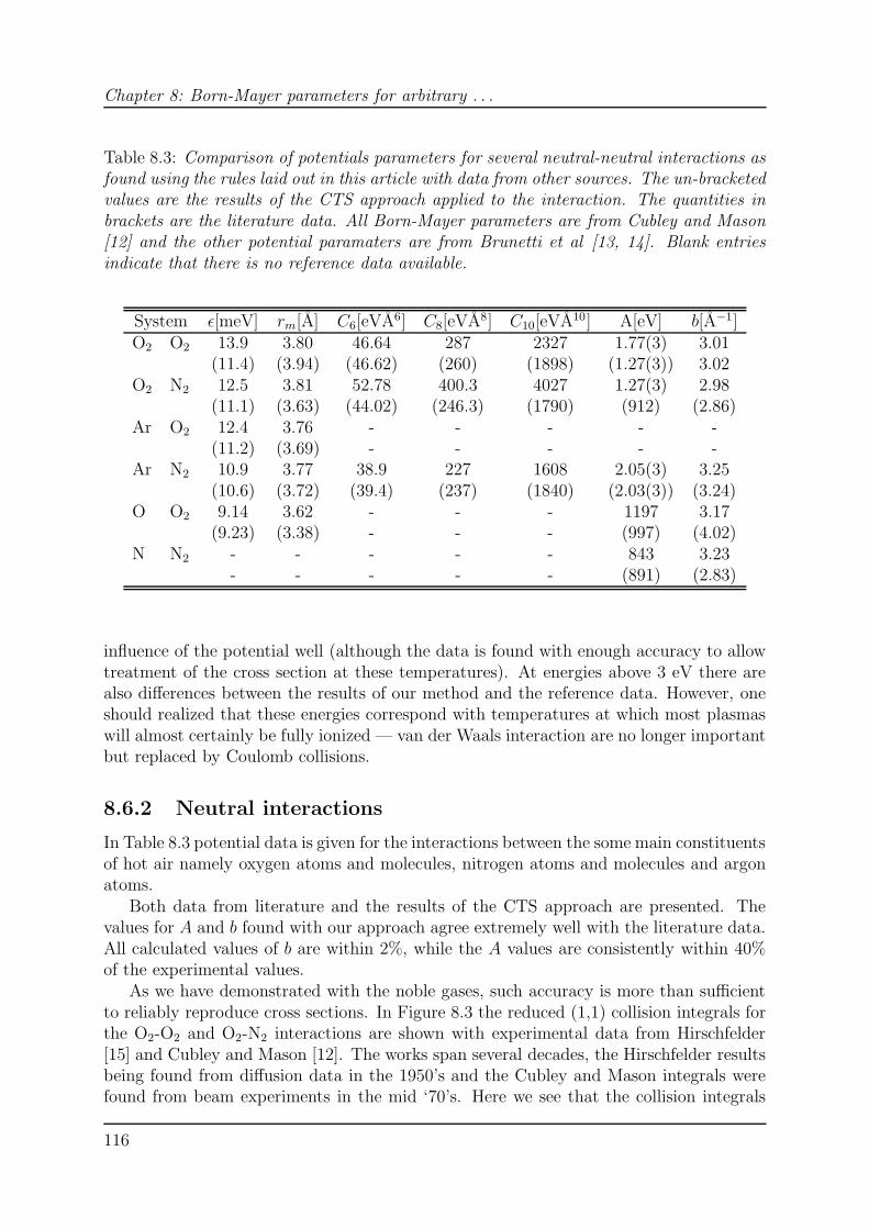
Chapter 8: Born-Mayer parameters for arbitrary . . .
Table 8.3: Comparison of potentials parameters for several neutral-neutral interactions asfound using the rules laid out in this article with data from other sources. The un-bracketedvalues are the results of the CTS approach applied to the interaction. The quantities inbrackets are the literature data. All Born-Mayer parameters are from Cubley and Mason[12] and the other potential paramaters are from Brunetti et al [13, 14]. Blank entriesindicate that there is no reference data available.
System ε[meV] rm[A] C6[eVA6] C8[eVA8] C10[eVA10] A[eV] b[A−1]O2 O2 13.9 3.80 46.64 287 2327 1.77(3) 3.01
(11.4) (3.94) (46.62) (260) (1898) (1.27(3)) 3.02O2 N2 12.5 3.81 52.78 400.3 4027 1.27(3) 2.98
(11.1) (3.63) (44.02) (246.3) (1790) (912) (2.86)Ar O2 12.4 3.76 - - - - -
(11.2) (3.69) - - - - -Ar N2 10.9 3.77 38.9 227 1608 2.05(3) 3.25
(10.6) (3.72) (39.4) (237) (1840) (2.03(3)) (3.24)O O2 9.14 3.62 - - - 1197 3.17
(9.23) (3.38) - - - (997) (4.02)N N2 - - - - - 843 3.23
- - - - - (891) (2.83)
influence of the potential well (although the data is found with enough accuracy to allowtreatment of the cross section at these temperatures). At energies above 3 eV there arealso differences between the results of our method and the reference data. However, oneshould realized that these energies correspond with temperatures at which most plasmaswill almost certainly be fully ionized — van der Waals interaction are no longer importantbut replaced by Coulomb collisions.
8.6.2 Neutral interactions
In Table 8.3 potential data is given for the interactions between the some main constituentsof hot air namely oxygen atoms and molecules, nitrogen atoms and molecules and argonatoms.
Both data from literature and the results of the CTS approach are presented. Thevalues for A and b found with our approach agree extremely well with the literature data.All calculated values of b are within 2%, while the A values are consistently within 40%of the experimental values.
As we have demonstrated with the noble gases, such accuracy is more than sufficientto reliably reproduce cross sections. In Figure 8.3 the reduced (1,1) collision integrals forthe O2-O2 and O2-N2 interactions are shown with experimental data from Hirschfelder[15] and Cubley and Mason [12]. The works span several decades, the Hirschfelder resultsbeing found from diffusion data in the 1950’s and the Cubley and Mason integrals werefound from beam experiments in the mid ‘70’s. Here we see that the collision integrals
116
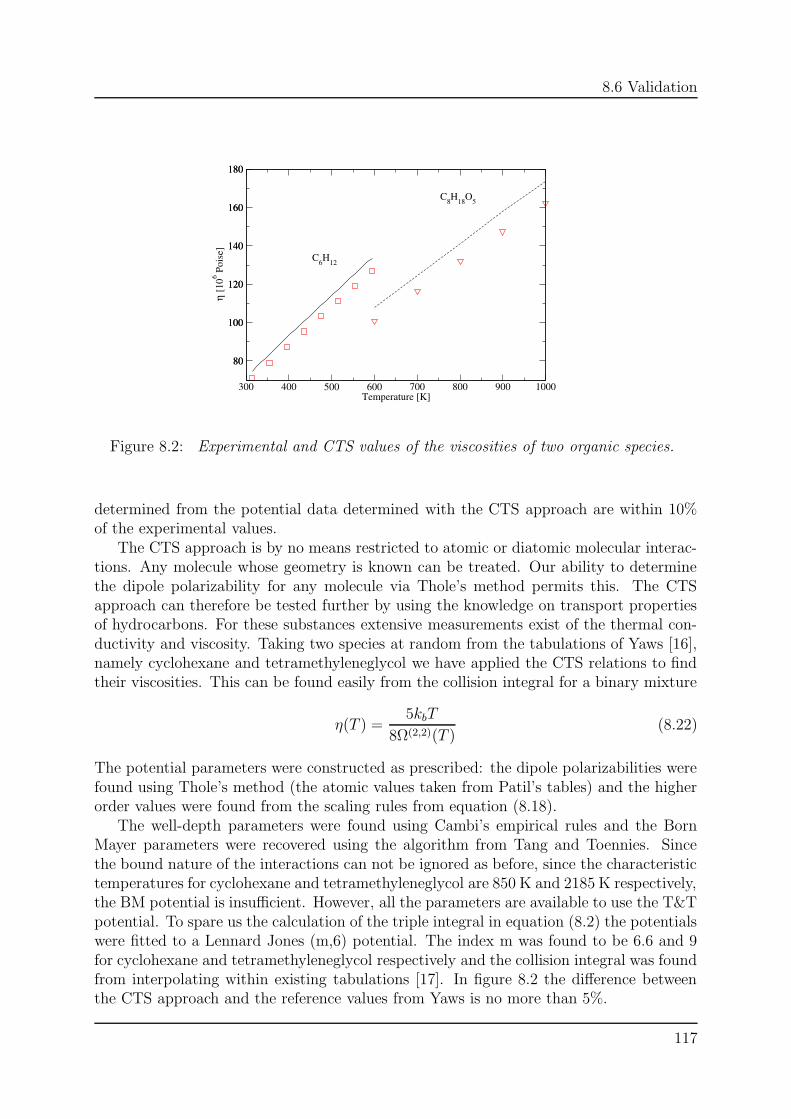
8.6 Validation
300 400 500 600 700 800 900 1000Temperature [K]
80
100
120
140
160
180
η [1
06 Poi
se]
80
100
120
140
160
180
C8H18O5
C6H12
Figure 8.2: Experimental and CTS values of the viscosities of two organic species.
determined from the potential data determined with the CTS approach are within 10%of the experimental values.
The CTS approach is by no means restricted to atomic or diatomic molecular interac-tions. Any molecule whose geometry is known can be treated. Our ability to determinethe dipole polarizability for any molecule via Thole’s method permits this. The CTSapproach can therefore be tested further by using the knowledge on transport propertiesof hydrocarbons. For these substances extensive measurements exist of the thermal con-ductivity and viscosity. Taking two species at random from the tabulations of Yaws [16],namely cyclohexane and tetramethyleneglycol we have applied the CTS relations to findtheir viscosities. This can be found easily from the collision integral for a binary mixture
η(T ) =5kbT
8Ω(2,2)(T )(8.22)
The potential parameters were constructed as prescribed: the dipole polarizabilities werefound using Thole’s method (the atomic values taken from Patil’s tables) and the higherorder values were found from the scaling rules from equation (8.18).
The well-depth parameters were found using Cambi’s empirical rules and the BornMayer parameters were recovered using the algorithm from Tang and Toennies. Sincethe bound nature of the interactions can not be ignored as before, since the characteristictemperatures for cyclohexane and tetramethyleneglycol are 850 K and 2185 K respectively,the BM potential is insufficient. However, all the parameters are available to use the T&Tpotential. To spare us the calculation of the triple integral in equation (8.2) the potentialswere fitted to a Lennard Jones (m,6) potential. The index m was found to be 6.6 and 9for cyclohexane and tetramethyleneglycol respectively and the collision integral was foundfrom interpolating within existing tabulations [17]. In figure 8.2 the difference betweenthe CTS approach and the reference values from Yaws is no more than 5%.
117
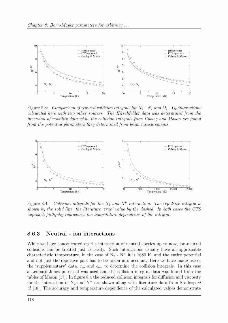
Chapter 8: Born-Mayer parameters for arbitrary . . .
0 5 10 15 20Temperature [kK]
4
6
8
10
Ω(1
,1)*
HirschfelderCTS approachCubley & Mason
N2 - N2
0 5 10 15 20Temperature [kK]
3
4
5
6
7
8
9
10
Ω(1
,1)*
HirschfelderCTS approachCubley & Mason
O2 - O2
Figure 8.3: Comparison of reduced collision integrals for N2 - N2 and O2 - O2 interactionscalculated here with two other sources. The Hirschfelder data was determined from theinversion of mobility data while the collision integrals from Cubley and Mason are foundfrom the potential parameters they determined from beam measurements.
0 5 10 15 20Temperature [kK]
2
4
6
8
Ω(1
,1)*
CTS approachCubley & Mason
N2 - N+
0 5000 10000 15000 20000Temperature [kK]
2
4
6
Ω(2
,2)*
CTS approachCubley & Mason
N2 - N+
Figure 8.4: Collision integrals for the N2 and N+ interaction. The repulsive integral isshown by the solid line, the literature ’true’ value by the dashed. In both cases the CTSapproach faithfully reproduces the temperature dependence of the integral.
8.6.3 Neutral - ion interactions
While we have concentrated on the interaction of neutral species up to now, ion-neutralcollisions can be treated just as easily. Such interactions usually have an appreciablecharacteristic temperature, in the case of N2 - N+ it is 1680 K, and the entire potentialand not just the repulsive part has to be taken into account. Here we have made use ofthe ‘supplementary’ data, rm and εm, to determine the collision integrals. In this casea Lennard-Jones potential was used and the collision integral data was found from thetables of Mason [17]. In figure 8.4 the reduced collision integrals for diffusion and viscosityfor the interaction of N2 and N+ are shown along with literature data from Stallcop etal [18]. The accuracy and temperature dependence of the calculated values demonstrate
118
8.7 Conclusions
that while we are generally interested in the Born-Mayer parameters, the interaction datafound via the various empirical approaches can serve a useful purpose themselves.
8.7 Conclusions
Since the scientific and industrial interest in plasmas containing exotic species will con-tinue to outstrip efforts to either reliably measure or calculate these properties we havedecided to assemble such empirical relations that exist to facilitate the accurate calculationof potential parameters for repulsive interactions that are characterized by exponentialpotential functions.
In this article we have assembled the works of Patil, Cambi and Thole, who haveprovided respectively tabulations of atomic hyperpolarizabilities from helium to uranium,accurate empirical means for the determination of the potential well parameters and areliable method to calculate molecular dipole polarizabilities. We have made our owncontribution in the form of a power law scaling that relates high order polarizabilities tothe dipole value.
The Tang and Tonnies potential, their algorithm to determine the Born-Mayer pa-rameters from the attractive part of the potential and the methods described to findthese allow one can generate sufficiently high quality data to abandon the standard pa-rameterized potentials. In this article we have outlined how to use each of the empiricaltechniques, demonstrated their accuracy and finally compared literature values for thepotential parameters, cross sections and collision integrals.
The effectiveness of the CTS approach has been demonstrated, which not only resultsin reliable, high quality cross section data for atomic and molecular repulsive interactionsbut also provides accurate parameters for van der Waals potentials. We feel that we haveamply demonstrated the approach which can be used with confidence to determine crosssections for previously unknown interactions.
Appendix A — dispersion coefficients
The dispersion coefficients can be written in terms of the polarizabilities of the interactingpair and the effective number of outer shell electrons[9].
The Slater-Kirkwood formula for the C6 dispersion coefficient is
CAB6 = 15.7
αA1 α
B1(
αA1 /N
Aeff
)1/2+(αB
1 /NBeff
)1/2
[eVA6
](A-1)
where the interacting atoms have dipole polarizabilities αA, αB and numbers of effectiveelectrons NA
eff and NBeff . Koutselos and Mason provided formulas for higher-order two-
body dispersion coefficients using the same effective numbers of electrons. The dipole-quadrupole coefficient C8 is given by
CAB8 = 3.75
αA1 α
B2(
αA1 /N
Aeff
)1/2+[(αB
2 )2/9NBeffα
B1
]1/4
119
Bibliography
+ 3.75αA
2 αB1(
αB1 /N
Beff
)1/2+[(αA
2 )2/9NAeffα
A1
]1/4[eVA
8]
where αA2 and αB
2 are the quadrupole polarizabilities of the species. The C10 coefficient isgiven by
CAB10 = 7
αA1 α
B3(
αA1 /N
Aeff
)1/2+ 0.365
[(αB
3 )4/9NBeffαB(α
(2)B )2
]1/4
+ 17.5αA
2 αB2[
(αA2 )2/9NA
effα1A
]1/4+[(αB
2 )2/9NBeffα
B1
]1/4[eVA
10]
where αA3 and αB
3 are the octupole polarizabilities of the species.
References
[1] Tang K T and Toennies J P, J. Chem. Phys 80, 3726 (1984)
[2] Patil S H, At. Data Nucl. Data Tables 71, 41 (1999)
[3] Thole, B T, Chem. Phys 59, 341 (1981)
[4] Cambi R, Cappelletti D, Lutti G and Pirani F, J. Chem. Phys. 95, 1852 (1991)
[5] Tang K T and Toennies J P, Zeit. Physik. D 1, 91 (1986)
[6] Tang K T and Toennies J P, J. Chem. Phys. 68, 5501 (1978)
[7] van Duijnen and Swart M, J. Phys. Chem. A 102, 2399, (1998)
[8] Monchick L, Phys. Fluids 2, 695 (1959)
[9] Koutselos A D and Mason E A, J. Chem. Phys. 85, 2154 (1986)
[10] Phelps A V, Greene C H and Burke Jr J P, J. Phys. B 33, 2965 (2000)
[11] Phelps A V, private communication
[12] Cubley S and Mason E A, Phys. Fluids 18, 1109 (1975)
[13] Brunetti B, Liuti G, Luzzatti E, Pirani F and Volpi G G, J. Chem. Phys. 79, 273(1983)
[14] Brunetti B, Liuti G, Luzzatti E, Pirani F and Vecchicattivi F, J. Chem. Phys. 74,6734 (1981)
[15] Cappitelli M, Gorse C, Longo S, Giordano D, AIAA Technical Paper 98-2936, Al-buqerque, New Mexico (1998)
120

Bibliography
[16] Yaws C L, Handbook of transport property data : viscosity, thermal conductivity,and diffusion coefficients of liquids and gases (Gulf Publ. Comp., London, 1995),ISBN 0-88415-392-4
[17] Klein M and Smith F J, J. Res. Nat. Bur. Stan. 72A, 359 (1968)
[18] Stallcop J R, Partridge H and Levin E, J. Therm. Phys. Heat Trans. 10, 697 (1996)
121

CHAPTER 9
Influence of model potentials on the transport properties of
reacting LTE plasma mixtures
A set of interaction potentials is given which can be used to determine the transportproperties of LTE plasma mixtures. These have been chosen since all necessary funda-mental data can be generated or are required to determine the composition. The goal is toprovide a standardized and automatic procedure for arbitrary plasma mixtures. Chargedparticle interactions are described by a shielded Coulomb potential, heavy particle inter-actions are treated with an exponential repulsive or Lennard-Jones potential. Electronneutral collisions are treated with a polarization model and resonant charge transfer isalso taken into account. The transport properties found for three well known plasmas -3 species argon, molecular oxygen and 11 species air - demonstrate that this regularizedprocedure is not only far superior to a hard spheres approach but also provides a reliableapproximation to the accepted reference data.
123
Chapter 9: Influence of model potentials . . .
9.1 Introduction
Accurate knowledge of transport properties is paramount to understanding plasma phe-nomena and the exploitation of plasma based applications. To be specific one requiresinformation on the viscosity and electrical and thermal conductivities. However, theseare particularly difficult to measure under plasma conditions and even if experimentaltechniques were effective the enormous variety of the plasma state remains a problem.Since the freedom in choosing the chemical composition of a plasma is in effect limitlessand as transport properties of any particular plasma depend on the contribution of thebinary interactions between all of the particles present, a broad range of conditions wouldhave to be considered. Therefore, we must resort to theoretical approaches in most cases.Fortunately, there are several analytical transport property formulae available of varyinglevels of sophistication. However, all these transport property formulae require the samebasic input, namely a set of collision integral (CI) between all species. These provide thevolumetric rates for momentum transfer that determine diffusion or viscosity.
In our group the plasma simulation platform, plasimo, has been developed [1, 2,3]. It provides an integrated environment for the construction and execution of plasmamodels. plasimo has been designed in such a way that the mathematical description aof a particular mechanism is divorced from any physico-chemical details. Using a objectoriented approach in C++, code re-use is optimized.
plasimo has be used to treat many different plasma applications. Models for DC,inductive and microwave power coupling have be constructed and we have experiencewith several chemistries, such as plasmas in argon [4, 5], mercury [6, 7], hydrogen [8],sodium-iodine [9] and sulfur [10, 11]. Its modular structure and design makes plasimo
ideal for investigating existing configurations and simulating new applications. However,the lack of fundamental data on elementary interactions, which is a widespread problem,is a serious handicap to the credibility of plasma models. Specifically, it has been foundthat exclusive use of the hard sphere interaction can lead to non-realistic results. As suchan alternative approach is required and that is the principal motivation for this work.
The goal of this chapter is to establish standard interaction models that describe allpossible elastic interactions that occur in a plasma. The superset of these interactionscan be used to determine the transport properties of LTE plasmas irrespective of theirchemical composition. This superset of collision integrals and the means to determineall necessary data results in what we call an automatic procedure — once the plasmacomposition is specified the transport properties follow.
This is achieved by the classification of all possible interactions and prescribing apriori the means to calculate the CIs. The latter is the most important as the approachmust be able to construct the CI for any interaction based solely on the properties ofthe collision partners. In making the interaction classification we assume the influence ofinelastic processes are negligible and we confine ourselves to elastic collisions. Denotingcharged particles c and neutrals n (which includes atoms a, and molecules m) leads tothe following interactions: c-c, c-n and n-n. The first class, interactions between chargedparticles, is well understood. Cross sections follow from classical mechanics and the onlyproperty required from the collision partners is their charge numbers.
The next grouping, c-n, is subdivided into e-n and i-n. The electron neutral interaction,e-n, can be treated with the classical Langevin model [12]. This solely depends on the
124
9.1 Introduction
electron charge and the dipole polarizability of the neutral. However, if accuracy is animportant issue we need to know the position and strength of the Ramsauer minimum.Therefore, accurate treatment of these collisions is possible only if existing literature coversthe interaction or if one has access to experimental or theoretical methods. Although sucha case-by-case treatment of interactions is facilitated by plasimo, we will confine ourselvesto the study of the influence of using simple models for use in the automatic procedure.
Two possibilities arise when treating the interaction of ions and neutrals, i-n. Thereare collisions where charge transfer takes place and those in which the partners retain theiridentity. In the first case only the resonant process is considered. The collision partnersmust have the same matching internal energies so that the interaction is essentially elas-tic, i.e the collision between an atom ands its parent ion. This is a complex process thatcan be treated with a classical model which requires only the ionization of the neutral todetermine the cross section. The other type of i-n collision can be described by a van derWaals (v/dW) potential. Thus belongs in a certain sense to the final category, n-n inter-actions. In chapter 8 it was shown that despite the large variety of interactions the genericapproach according to Tang and Toennies [14, 15] can be used to great effect. Moreover,we established a means by which all parameters required by the T&T-v/dW potential canbe described based solely on the properties of individual collision partners. However, dueto the mathematical complexity of using the T&T potential in the CI calculation, we choseto distinguish between two extremes: deep and shallow potentials. The relation betweenthe well depth, εm, and thermal kinetic energy, kBT , determines the separation betweenthese extremes. Since LTE plasmas usually have high temperatures above 1000 K whileabove 15000 K are often fully ionized the division between shallow, εm/kBT 1, anddeep potentials, εm/kBT 1, is straightforward. The only deep potentials treated arethose between species that form stable association products. However, these associationreactions and the corresponding well depths are included in the composition calculation.All the other v/dW interactions are treated with a exponential repulsive function, theso-called Born-Mayer potential.
Finally we should mention that although we primarily have LTE plasmas in mindwe can also use the insights of this study to non-LTE conditions; that is conditions forwhich temperature of the electrons Te and heavy particle Th differ from each other whilethe degree of ionization and dissociation does not obey the distribution laws of Saha andGuldberg-Waage. Basically this means that for the interactions between heavy particlesthe temperature should be replaced by Th whereas in the interaction in which an electronis involved the temperature must be replaced by Te. However, one should also realizethat under non-LTE conditions the reactive part of heat conductivity can no longer beexpressed simply. Instead we have to solve the energy equation of electrons and heavyparticles separately. The reactive heat transport has then to be incorporated in the heavyparticle energy balance as far as the non-equilibrium state of the association/dissociationbalance is concerned.
This chapter is laid out as follows: in section 9.2 basic definitions are presented.Section 9.3 details which model potential is used for each of the four types of elasticcollision that can take place in an LTE plasma. In section 9.5, the viscosity, thermalconductivity and electrical conductivities of the three reference plasmas are found withthe automatic approach. The results are compared to accepted literature values and those
125
Chapter 9: Influence of model potentials . . .
using hard sphere model exclusively. Finally, conclusions are presented in section 9.6.
9.2 Collision integrals
The kinetic motion of particles in a gas or plasma leads to collisions which are ruled bythe impact parameter, the relative velocity of the species and the nature of the force; i.e.the shape of the interaction potential. These determine the magnitude of the deflectioncaused by the collision. In their turn, the deflections determine the material propertiesof the gas. For any type of interaction the collision integral is the essential quantity thatdetermines transport property; it is given by
Ω(l,s)(T ) =
(kBT
2πµ
)1/2 ∫ ∞
0e−γ2
γ2s+3Q(l)(g)dγ [m3s−1] (9.1)
where γ2 = µg2/2kBT . The lth moment collision cross section Q is given
Q(l) = 2π∫ ∞
0(1 − cosl χ)βdβ [m2] (9.2)
where β is the impact parameter. Setting l = 1 yields the diffusion cross section whilel = 2 defines the so-called viscosity cross section. The scattering angle is found from
χ = π −∫ ∞
r0
βdr
r2[1 − β2
r2 − 2V (r)µg2
]1/2(9.3)
where r0 is the distance of closest approach. It can be found by setting the denominatorequal to zero. All that is needed further to determine the scattering angle χ is theinteraction potential V (r).
The interaction potential V (r) is the basic quantity that determines the cross sectionwhich on its turn leads to the collision integral. There are several situations that can arisewhen the interaction between a particular pair of particles has to be considered. In themost favorable and thus less laborious case, the collision integral itself is available so thatnothing further has to be done. This is for instance the case for the interaction betweennitrogen and oxygen neutral/ion pairs where Stallcop et al [16] have provided polynomialcoefficients for the collision collision integrals.
Somewhat less convenient is the situation in which not the CI but the cross sectionis known; this only demands for the computation of the integral in equation (9.1). Thesituation is more difficult when only potential data can be found. It is then required toevaluate the integrals (9.2) and (9.3). However, in the most general case we do not evenknow the potential. It is the main objective of this study to come to a general procedurein constructing the potential so that based on the properties of collision partners defaulttransport properties can be computed automatically.
9.3 Interactions
This section is devoted to the classification of elastic collisions and to establish whichappropriate model potentials are available. More specifically the aim is to determine
126
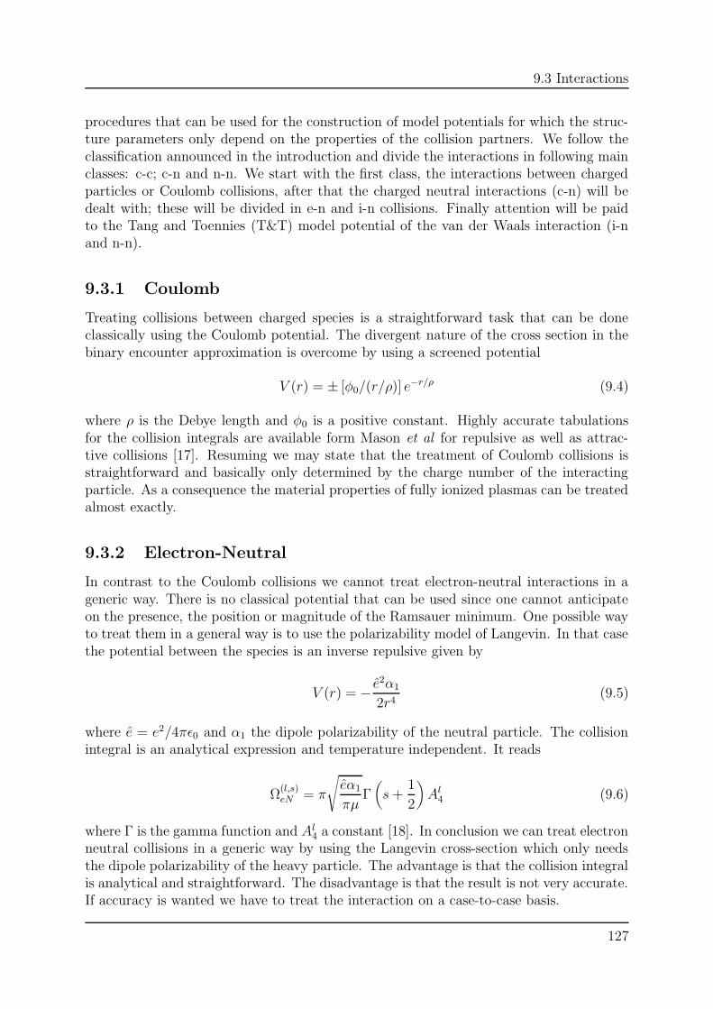
9.3 Interactions
procedures that can be used for the construction of model potentials for which the struc-ture parameters only depend on the properties of the collision partners. We follow theclassification announced in the introduction and divide the interactions in following mainclasses: c-c; c-n and n-n. We start with the first class, the interactions between chargedparticles or Coulomb collisions, after that the charged neutral interactions (c-n) will bedealt with; these will be divided in e-n and i-n collisions. Finally attention will be paidto the Tang and Toennies (T&T) model potential of the van der Waals interaction (i-nand n-n).
9.3.1 Coulomb
Treating collisions between charged species is a straightforward task that can be doneclassically using the Coulomb potential. The divergent nature of the cross section in thebinary encounter approximation is overcome by using a screened potential
V (r) = ± [φ0/(r/ρ)] e−r/ρ (9.4)
where ρ is the Debye length and φ0 is a positive constant. Highly accurate tabulationsfor the collision integrals are available form Mason et al for repulsive as well as attrac-tive collisions [17]. Resuming we may state that the treatment of Coulomb collisions isstraightforward and basically only determined by the charge number of the interactingparticle. As a consequence the material properties of fully ionized plasmas can be treatedalmost exactly.
9.3.2 Electron-Neutral
In contrast to the Coulomb collisions we cannot treat electron-neutral interactions in ageneric way. There is no classical potential that can be used since one cannot anticipateon the presence, the position or magnitude of the Ramsauer minimum. One possible wayto treat them in a general way is to use the polarizability model of Langevin. In that casethe potential between the species is an inverse repulsive given by
V (r) = − e2α1
2r4(9.5)
where e = e2/4πε0 and α1 the dipole polarizability of the neutral particle. The collisionintegral is an analytical expression and temperature independent. It reads
Ω(l,s)eN = π
√eα1
πµΓ(s+
1
2
)Al
4 (9.6)
where Γ is the gamma function and Al4 a constant [18]. In conclusion we can treat electron
neutral collisions in a generic way by using the Langevin cross-section which only needsthe dipole polarizability of the heavy particle. The advantage is that the collision integralis analytical and straightforward. The disadvantage is that the result is not very accurate.If accuracy is wanted we have to treat the interaction on a case-to-case basis.
127
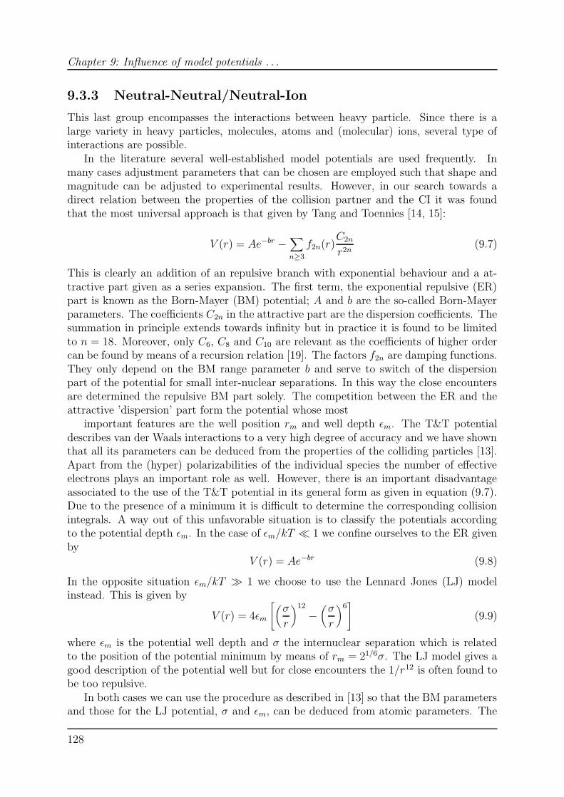
Chapter 9: Influence of model potentials . . .
9.3.3 Neutral-Neutral/Neutral-Ion
This last group encompasses the interactions between heavy particle. Since there is alarge variety in heavy particles, molecules, atoms and (molecular) ions, several type ofinteractions are possible.
In the literature several well-established model potentials are used frequently. Inmany cases adjustment parameters that can be chosen are employed such that shape andmagnitude can be adjusted to experimental results. However, in our search towards adirect relation between the properties of the collision partner and the CI it was foundthat the most universal approach is that given by Tang and Toennies [14, 15]:
V (r) = Ae−br −∑
n≥3
f2n(r)C2n
r2n(9.7)
This is clearly an addition of an repulsive branch with exponential behaviour and a at-tractive part given as a series expansion. The first term, the exponential repulsive (ER)part is known as the Born-Mayer (BM) potential; A and b are the so-called Born-Mayerparameters. The coefficients C2n in the attractive part are the dispersion coefficients. Thesummation in principle extends towards infinity but in practice it is found to be limitedto n = 18. Moreover, only C6, C8 and C10 are relevant as the coefficients of higher ordercan be found by means of a recursion relation [19]. The factors f2n are damping functions.They only depend on the BM range parameter b and serve to switch of the dispersionpart of the potential for small inter-nuclear separations. In this way the close encountersare determined the repulsive BM part solely. The competition between the ER and theattractive ’dispersion’ part form the potential whose most
important features are the well position rm and well depth εm. The T&T potentialdescribes van der Waals interactions to a very high degree of accuracy and we have shownthat all its parameters can be deduced from the properties of the colliding particles [13].Apart from the (hyper) polarizabilities of the individual species the number of effectiveelectrons plays an important role as well. However, there is an important disadvantageassociated to the use of the T&T potential in its general form as given in equation (9.7).Due to the presence of a minimum it is difficult to determine the corresponding collisionintegrals. A way out of this unfavorable situation is to classify the potentials accordingto the potential depth εm. In the case of εm/kT 1 we confine ourselves to the ER givenby
V (r) = Ae−br (9.8)
In the opposite situation εm/kT 1 we choose to use the Lennard Jones (LJ) modelinstead. This is given by
V (r) = 4εm
[(σ
r
)12
−(σ
r
)6]
(9.9)
where εm is the potential well depth and σ the internuclear separation which is relatedto the position of the potential minimum by means of rm = 21/6σ. The LJ model gives agood description of the potential well but for close encounters the 1/r12 is often found tobe too repulsive.
In both cases we can use the procedure as described in [13] so that the BM parametersand those for the LJ potential, σ and εm, can be deduced from atomic parameters. The
128
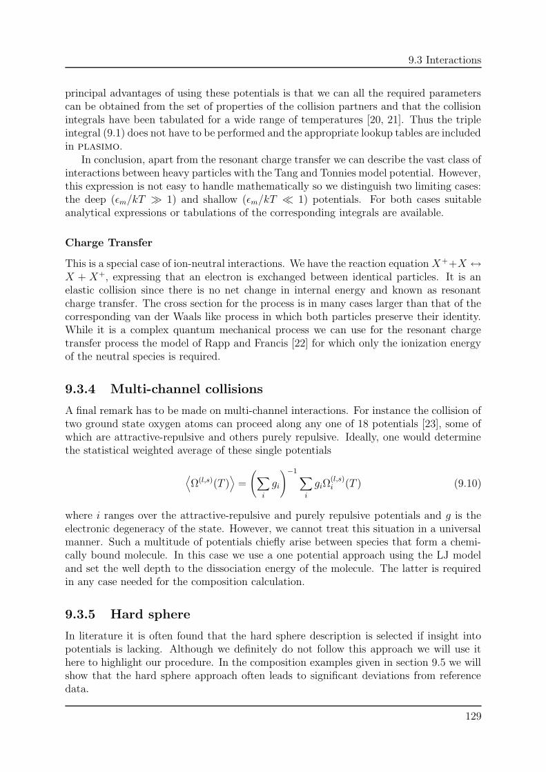
9.3 Interactions
principal advantages of using these potentials is that we can all the required parameterscan be obtained from the set of properties of the collision partners and that the collisionintegrals have been tabulated for a wide range of temperatures [20, 21]. Thus the tripleintegral (9.1) does not have to be performed and the appropriate lookup tables are includedin plasimo.
In conclusion, apart from the resonant charge transfer we can describe the vast class ofinteractions between heavy particles with the Tang and Tonnies model potential. However,this expression is not easy to handle mathematically so we distinguish two limiting cases:the deep (εm/kT 1) and shallow (εm/kT 1) potentials. For both cases suitableanalytical expressions or tabulations of the corresponding integrals are available.
Charge Transfer
This is a special case of ion-neutral interactions. We have the reaction equation X++X ↔X + X+, expressing that an electron is exchanged between identical particles. It is anelastic collision since there is no net change in internal energy and known as resonantcharge transfer. The cross section for the process is in many cases larger than that of thecorresponding van der Waals like process in which both particles preserve their identity.While it is a complex quantum mechanical process we can use for the resonant chargetransfer process the model of Rapp and Francis [22] for which only the ionization energyof the neutral species is required.
9.3.4 Multi-channel collisions
A final remark has to be made on multi-channel interactions. For instance the collision oftwo ground state oxygen atoms can proceed along any one of 18 potentials [23], some ofwhich are attractive-repulsive and others purely repulsive. Ideally, one would determinethe statistical weighted average of these single potentials
⟨Ω(l,s)(T )
⟩=
(∑
i
gi
)−1∑
i
giΩ(l,s)i (T ) (9.10)
where i ranges over the attractive-repulsive and purely repulsive potentials and g is theelectronic degeneracy of the state. However, we cannot treat this situation in a universalmanner. Such a multitude of potentials chiefly arise between species that form a chemi-cally bound molecule. In this case we use a one potential approach using the LJ modeland set the well depth to the dissociation energy of the molecule. The latter is requiredin any case needed for the composition calculation.
9.3.5 Hard sphere
In literature it is often found that the hard sphere description is selected if insight intopotentials is lacking. Although we definitely do not follow this approach we will use ithere to highlight our procedure. In the composition examples given in section 9.5 we willshow that the hard sphere approach often leads to significant deviations from referencedata.
129
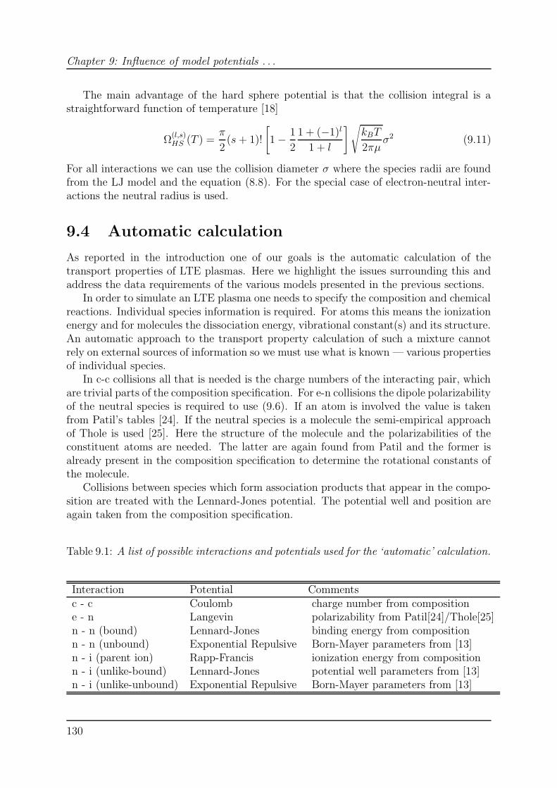
Chapter 9: Influence of model potentials . . .
The main advantage of the hard sphere potential is that the collision integral is astraightforward function of temperature [18]
Ω(l,s)HS (T ) =
π
2(s+ 1)!
[1 − 1
2
1 + (−1)l
1 + l
]√kBT
2πµσ2 (9.11)
For all interactions we can use the collision diameter σ where the species radii are foundfrom the LJ model and the equation (8.8). For the special case of electron-neutral inter-actions the neutral radius is used.
9.4 Automatic calculation
As reported in the introduction one of our goals is the automatic calculation of thetransport properties of LTE plasmas. Here we highlight the issues surrounding this andaddress the data requirements of the various models presented in the previous sections.
In order to simulate an LTE plasma one needs to specify the composition and chemicalreactions. Individual species information is required. For atoms this means the ionizationenergy and for molecules the dissociation energy, vibrational constant(s) and its structure.An automatic approach to the transport property calculation of such a mixture cannotrely on external sources of information so we must use what is known — various propertiesof individual species.
In c-c collisions all that is needed is the charge numbers of the interacting pair, whichare trivial parts of the composition specification. For e-n collisions the dipole polarizabilityof the neutral species is required to use (9.6). If an atom is involved the value is takenfrom Patil’s tables [24]. If the neutral species is a molecule the semi-empirical approachof Thole is used [25]. Here the structure of the molecule and the polarizabilities of theconstituent atoms are needed. The latter are again found from Patil and the former isalready present in the composition specification to determine the rotational constants ofthe molecule.
Collisions between species which form association products that appear in the compo-sition are treated with the Lennard-Jones potential. The potential well and position areagain taken from the composition specification.
Table 9.1: A list of possible interactions and potentials used for the ‘automatic’ calculation.
Interaction Potential Commentsc - c Coulomb charge number from compositione - n Langevin polarizability from Patil[24]/Thole[25]n - n (bound) Lennard-Jones binding energy from compositionn - n (unbound) Exponential Repulsive Born-Mayer parameters from [13]n - i (parent ion) Rapp-Francis ionization energy from compositionn - i (unlike-bound) Lennard-Jones potential well parameters from [13]n - i (unlike-unbound) Exponential Repulsive Born-Mayer parameters from [13]
130
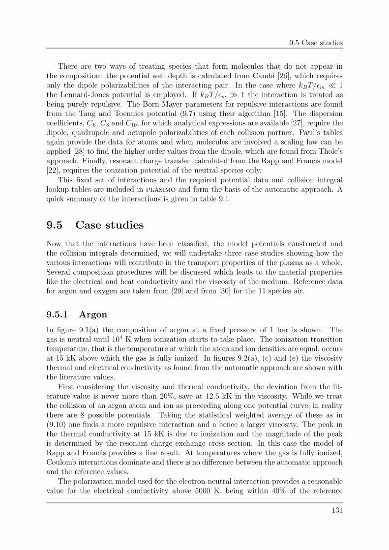
9.5 Case studies
There are two ways of treating species that form molecules that do not appear inthe composition: the potential well depth is calculated from Cambi [26], which requiresonly the dipole polarizabilities of the interacting pair. In the case where kBT/εm 1the Lennard-Jones potential is employed. If kBT/εm 1 the interaction is treated asbeing purely repulsive. The Born-Mayer parameters for repulsive interactions are foundfrom the Tang and Toennies potential (9.7) using their algorithm [15]. The dispersioncoefficients, C6, C8 and C10, for which analytical expressions are available [27], require thedipole, quadrupole and octupole polarizabilities of each collision partner. Patil’s tablesagain provide the data for atoms and when molecules are involved a scaling law can beapplied [28] to find the higher order values from the dipole, which are found from Thole’sapproach. Finally, resonant charge transfer, calculated from the Rapp and Francis model[22], requires the ionization potential of the neutral species only.
This fixed set of interactions and the required potential data and collision integrallookup tables are included in plasimo and form the basis of the automatic approach. Aquick summary of the interactions is given in table 9.1.
9.5 Case studies
Now that the interactions have been classified, the model potentials constructed andthe collision integrals determined, we will undertake three case studies showing how thevarious interactions will contribute in the transport properties of the plasma as a whole.Several composition procedures will be discussed which leads to the material propertieslike the electrical and heat conductivity and the viscosity of the medium. Reference datafor argon and oxygen are taken from [29] and from [30] for the 11 species air.
9.5.1 Argon
In figure 9.1(a) the composition of argon at a fixed pressure of 1 bar is shown. Thegas is neutral until 104 K when ionization starts to take place. The ionization transitiontemperature, that is the temperature at which the atom and ion densities are equal, occursat 15 kK above which the gas is fully ionized. In figures 9.2(a), (c) and (e) the viscositythermal and electrical conductivity as found from the automatic approach are shown withthe literature values.
First considering the viscosity and thermal conductivity, the deviation from the lit-erature value is never more than 20%, save at 12.5 kK in the viscosity. While we treatthe collision of an argon atom and ion as proceeding along one potential curve, in realitythere are 8 possible potentials. Taking the statistical weighted average of these as in(9.10) one finds a more repulsive interaction and a hence a larger viscosity. The peak inthe thermal conductivity at 15 kK is due to ionization and the magnitude of the peakis determined by the resonant charge exchange cross section. In this case the model ofRapp and Francis provides a fine result. At temperatures where the gas is fully ionized,Coulomb interactions dominate and there is no difference between the automatic approachand the reference values.
The polarization model used for the electron-neutral interaction provides a reasonablevalue for the electrical conductivity above 5000 K, being within 40% of the reference
131
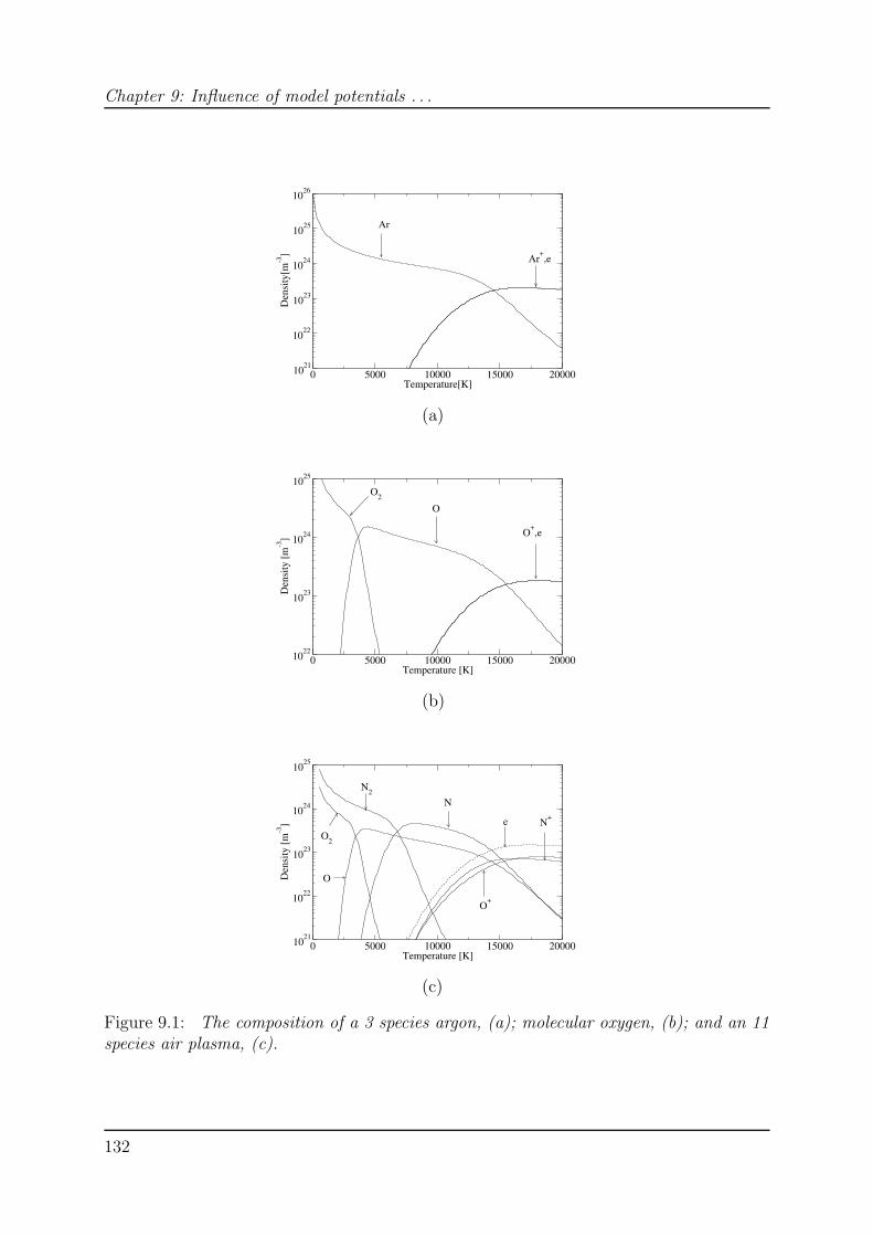
Chapter 9: Influence of model potentials . . .
0 5000 10000 15000 20000Temperature[K]
1021
1022
1023
1024
1025
1026
Den
sity
[m-3
]
Ar
Ar+,e
(a)
0 5000 10000 15000 20000Temperature [K]
1022
1023
1024
1025
Den
sity
[m-3
]
O2
O
O+,e
(b)
0 5000 10000 15000 20000Temperature [K]
1021
1022
1023
1024
1025
Den
sity
[m-3
]
O2
O
N2
N
O+
N+e
(c)
Figure 9.1: The composition of a 3 species argon, (a); molecular oxygen, (b); and an 11species air plasma, (c).
132
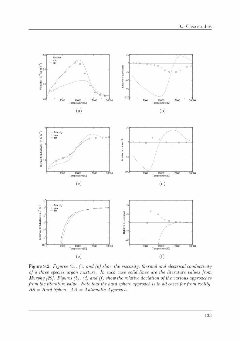
9.5 Case studies
0 5000 10000 15000 20000Temperature [K]
0.0
1.0
2.0
3.0
Vis
cosi
ty [1
0-4 k
g m
-1s-1
]
MurphyAAHS
0 5000 10000 15000 20000Temperature [K]
-120
-90
-60
-30
0
30
Rel
ativ
e %
Dev
iatio
n
(a) (b)
0 5000 10000 15000 20000Temperature [K]
0.1
1
10
The
rmal
Con
duct
ivity
[W m
-1K
-1] Murphy
AAHS
0 5000 10000 15000 20000Temperature [K]
-100
-50
0
50
Rel
ativ
e de
viat
ion
(%)
(c) (d)
0 5000 10000 15000 20000Temperature [K]
10-1
100
101
102
103
104
105
Ele
ctri
cal C
ondu
ctiv
ity [Ω
-1 m
-1] Murphy
AAHS
0 5000 10000 15000 20000Temperature [K]
-40
-20
0
20
40
Rel
ativ
e %
Dev
iatio
n
(e) (f)
Figure 9.2: Figures (a), (c) and (e) show the viscosity, thermal and electrical conductivityof a three species argon mixture. In each case solid lines are the literature values fromMurphy [29]. Figures (b), (d) and (f) show the relative deviation of the various approachesfrom the literature value. Note that the hard sphere approach is in all cases far from reality.HS = Hard Sphere, AA = Automatic Approach.
133
Chapter 9: Influence of model potentials . . .
0 5000 10000 15000 20000Temperature [K]
0.0
1.0
2.0
3.0
Vis
cosi
ty [1
0-4 k
g m
-1s-1
]
MurphyAAHS
0 5000 10000 15000 20000Temperature [K]
-250
-200
-150
-100
-50
0
50
Rel
ativ
e %
Dev
iatio
n
(a) (b)
0 5000 10000 15000 20000Temperature [K]
0.1
1
10
The
rmal
Con
duct
ivity
[W m
-1K
-1] Murphy
AAHS
0 5000 10000 15000 20000Temperature [K]
-200
-150
-100
-50
0
50
Rel
ativ
e %
Dev
iatio
n
(c) (d)
0 5000 10000 15000 20000Temperature [K]
10-1
100
101
102
103
104
105
Ele
ctri
cal C
ondu
ctiv
ity [Ω
-1 m
-1] Murphy
AAHS
0 5000 10000 15000 20000Temperature [K]
-80
-40
0
40
80
Rel
ativ
e %
Dev
iatio
n
(e) (f)
Figure 9.3: Figures (a), (c) and (e) show the viscosity, thermal and electrical conductivityof a molecular oxygen plasma. In each case the solid line is the literature value fromMurphy [29]. Figures (b), (d) and (f) show the relative deviation of the various approachesfrom the literature value. Note again that the hard sphere approach is in all cases far fromreality. HS = Hard Sphere, AA = Automatic Approach.
134
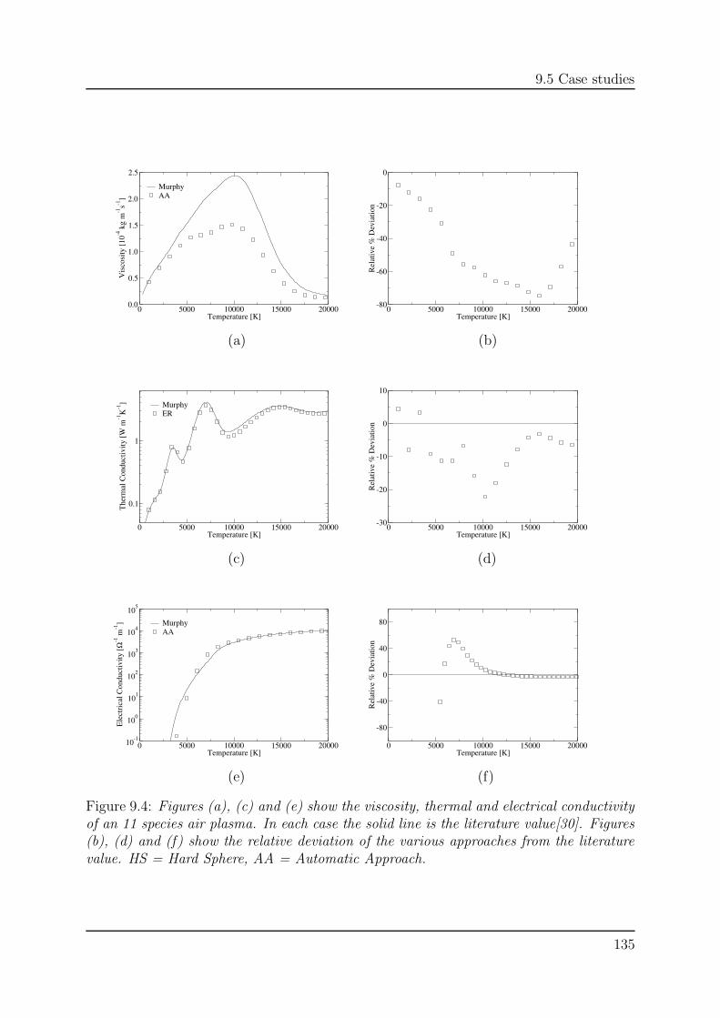
9.5 Case studies
0 5000 10000 15000 20000Temperature [K]
0.0
0.5
1.0
1.5
2.0
2.5
Vis
cosi
ty [1
0-4 k
g m
-1s-1
]
MurphyAA
0 5000 10000 15000 20000Temperature [K]
-80
-60
-40
-20
0
Rel
ativ
e %
Dev
iatio
n
(a) (b)
0 5000 10000 15000 20000Temperature [K]
0.1
1
The
rmal
Con
duct
ivity
[W m
-1K
-1] Murphy
ER
0 5000 10000 15000 20000Temperature [K]
-30
-20
-10
0
10
Rel
ativ
e %
Dev
iatio
n
(c) (d)
0 5000 10000 15000 20000Temperature [K]
10-1
100
101
102
103
104
105
Ele
ctri
cal C
ondu
ctiv
ity [Ω
-1 m
-1] Murphy
AA
0 5000 10000 15000 20000Temperature [K]
-80
-40
0
40
80
Rel
ativ
e %
Dev
iatio
n
(e) (f)
Figure 9.4: Figures (a), (c) and (e) show the viscosity, thermal and electrical conductivityof an 11 species air plasma. In each case the solid line is the literature value[30]. Figures(b), (d) and (f) show the relative deviation of the various approaches from the literaturevalue. HS = Hard Sphere, AA = Automatic Approach.
135
Chapter 9: Influence of model potentials . . .
value. However, the temperature independent nature of the collision integral conflictswith the actual behaviour of the interaction. The Ramsauer minimum occurs at 1500 Kabove which the cross section steadily increases. The polarization model clearly providesa value that is too low around 7000 K and too high below 5000 K. In order to solve thisproblem one should simply make use of existing literature data for the cross section whichin this case is given by Devoto [31]. This is easily added to plasimo, but beyond thisstudy. As regards the hard sphere model, we can state that it is substantially less accurateat all temperatures for each of the properties. As one might expect from a temperatureindependent cross section, there is only one temperature at which it actually reproducesthe interaction and for argon this seems to be at 104 K. For the thermal conductivity andviscosity the difference with the reference value is as much as 100%.
9.5.2 Oxygen
While argon presents the challenge of giving a good description of low temperature atomicand high temperature ionizing gas components, oxygen provides and additional challenge.At low temperatures the oxygen atoms are associated so there is a molecular and dissoci-ating component to the material properties. The plasma composition at a fixed pressureof 1 bar is shown as function of temperature in figure 9.1(b). Up to 2500 K the gas is al-most entirely molecular. The dissociation transition temperature, that is the temperatureat which the molecule and atom densities are equal occurs at 3500 K. In figures 9.3(a), (c)and (e) the viscosity, thermal and electrical conductivities are shown which were foundusing the automatic approaches together with the reference data.
The viscosity found with the automatic approach is slightly less accurate than was thecase for argon. Up to 104K the agreement with the literature value is reasonable, to within25%. The fact that an oxygen atom and ion can interact along 20 different potentials [23]has quite some affect on the transport properties at the ionization transition temperature.Our one potential approach provides a too low viscosity which is reflected also in thethermal conductivity. While the peak at the dissociation transition temperature is wellreproduced, demonstrating the effectiveness of the one potential approach for the O2-Ointeraction, the enhancement in the conductivity at the ionization transition temperatureis less than the reference value.
The use of the polarization model for the electron neutral interaction results in areasonable value for the electrical conductivity over a slightly larger temperature rangethan was found in argon. This is due to the Ramsauer minimum in oxygen being moreor less temperature independent up to 104 K with a value close to the hard sphere crosssection. Again the hard sphere approach is substantially less reliable for determining theviscosity and thermal conductivity than our automatic approach.
9.5.3 11 species Air
The next step in the scale of increasing difficultly, is that of a mixture of different chemi-cally reacting species. An 11 species air plasma provides such a challenge. In figure 9.1(c)the composition is shown as a function of temperature for a constant pressure of 1 bar.Now there is not only molecular oxygen but also nitrogen. Since the latter dissociates ata higher temperature it will behave as a buffer during the dissociation of O2. Due to the
136
9.6 Conclusions
large number of interactions and its proven lack of efficacy we no longer consider the hardsphere approach. (The density of nitrogen monoxide is too low to be seen in figure 9.1(c)and is ignored in the transport calculations.)
The viscosity, thermal conductivity and electrical conductivity are shown figures 9.4(a),(c) and (e) in respectively. There are three peaks in the thermal conductivity now at 3500K, 7500 K and 15000 K due to the dissociation of O2 and N2 and the ionization of O andN. The automatic approach is as accurate for this mixture as for argon and oxygen.
However, there is a marked deviation in the viscosity calculation. For the oxygenplasma at the ionization transition temperature our use of a single potential approach9.3.3 had its consequences. The calculated viscosities are deviates 75% from the literaturevalue. This time there are not only O-O+ and N-N+ collisions, both of which can followmany potentials but the attractive component of the potentials cannot be ignored. Theelectrical conductivity is deviates 40% from the literature value above 5000 K.
9.6 Conclusions
plasimo is a multi-faceted program for the simulation of plasma applications. While itcan be used to investigate the influence of complex phenomena it is ultimately restricteddue to the general lack of interaction data, as are other comparable programs, to plasmasfor which such data is available. This is a widespread problem that will become moreapparent as interest in novel plasmas increases. However, in contrast to the ever increasingaffordability of computing power, experimental facilities are few and cannot be relied uponto provide required data on elementary interactions.
One aspect of this problem are the cross sections for elastic scattering of various neutraland charged particles. These are crucial to the simulation of the momentum and energybalances of LTE plasmas. This paper embraces the results of two previous works thatpermit the accurate determination of interparticle potential functions for a wide range ofinteractions, based purely on properties of the colliding species. Such an approach is idealfor the automatic determination cross sections and hence transport properties.
Five temperature regions can be identified in which the transport properties are de-termined by different types of collision. There are the neutral regions on either side ofthe dissociation transition temperature where the symmetric interaction of the speciesis important, for instance in molecular oxygen the O2-O2 collision is dominant. At thedissociation temperature itself the non-symmetric interaction of the molecule and disso-ciation products play a determining role. Again taking molecular oxygen, the reactivecomponent of the thermal conductivity is determined by the O2−O interaction. Aroundthe ionization transition temperature ion neutral collisions are crucial, particularly sowhen resonant charge transfer comes into play. Finally, once the temperature is highenough and the gas is fully ionized Coulomb interactions are dominant and the transportproperties can be found exactly.
In the first four regions we have shown that the thermal conductivity can be foundto within 20% of the reference values for the three test-case plasmas. The viscosity isless successful, giving deviations of 75%. For electron neutral collisions we have used apolarizability model which has been shown to be accurate to within 40%.
137
Chapter 9: Influence of model potentials . . .
Appendix A — transport property formulae
While there are several methods available for each of the transport properties, work byothers in this field over the last few decades has lead to a more or less standardized useof the available transport property formulae.
The section gives an overview of the various transport property formulae needed tocompute the viscosity, thermal and electrical conductivities. The fundamental ingredientin all of these is the collision integral, discussed in section 9.2
A-1.1 Viscosity
The contribution of electrons to viscosity is negligible and as such the total viscosity canbe separated
η = ηh + ηe∼= ηh (A.1)
An accepted reliable means to determine the viscosity of a plasma mixture is the Wilkeapproximation [32, 33]
ηmix =∑ x2
i
x2i
ηi+ 1.385
∑k 6=i xixk
NkbTP
(A.2)
where xi is the molar fraction and ηi is the viscosity of the ith species:
η =5kBT
8Ω(2,2)(T )(A.3)
Higher order approximations provide little more than a 1% improvement on (A.2).
A-1.2 Thermal Conductivity
The total thermal conductivity can be written as the sum of the several contributions:the translational λt, the internal λi, the electronic λe and the reactive λr
λ = λt + λi + λr + λe (A.4)
Translational component
The second order translational contribution is given by Muckenfuss and Curtis [34]
λt = 4
∣∣∣∣∣∣∣∣∣
L11 . . L1µ x1
. . . . .Lµ1 . . Lµµ xµ
x1 . . xµ 0
∣∣∣∣∣∣∣∣∣
|Lij|(A.5)
The Lii terms are
Lii = −4x2i
λii
−µ∑
k=16=i
2xixj
λij
152m2
i + 254m2
k − 3m2kB
?ik + 4mimkA
?ik
A?ik (mi +mk)
2 (A.6)
138
9.6 Conclusions
Here A? = Ω(2,2)?/Ω(1,1)?, the ratio between the reduced collision integrals for viscosityand diffusion. The parameter B? is more complex
B? =5Ω(1,2)? − 2Ω(1,1)?
Ω(1,1)?(A.7)
The off diagonal coefficients, Lij are given by
Lij =2xixj
kij
mimj
(mi +mk)2
1
A?ij
(55
4− 3B?
ij − 4A?ij
)(A.8)
The binary thermal conductivities, λij, are given by
λij =75
64
k2BT
µΩ(2,2)(A.9)
The internal contribution can be calculated from the Eucken-like expression from Yos [35]
λi =∑
s
xsCp∑j 6=e (Dsj)
(A.10)
where Cp is the specific heat of species s.
Reactive contribution
In a mixture of gases a chemical reaction increases the thermal conductivity. This canbe understood by considering the dissociation of a molecule, A2 → 2A which requiresa certain amount of energy. In an LTE situation where the system is exposed to atemperature gradient a stationary state will be reached where the molecules diffuse tohigher temperature regions where their density is low. They subsequently dissociateby absorbing heat and the atoms so produced then diffuse to the lower temperatureregions where they recombine and release the dissociation energy. This is an enhancedchemical heat conductivity. It can only be described analytically under LTE and weuse the relations of Butler and Brokaw [36, 37]. Vanden Abeele[41] showed that theserelations, originally developed for dissociation balances, can be used equally for ionizinggases.
All reactions that occur in a plasma can be seen as a sequence of ν independentchemical reactions. Involving µ species these can be expressed as
µ∑
k=1
RikXk = 0 i = 1, 2, . . . ν (A.11)
where Xk is the kth species and Rik the stoichiometric coefficient of the species k inreaction i. Note that even if a species does not take part in any reaction it is still includedbut its stoichiometric coefficient is zero. In this way the influence of buffer gases and theirsuppression of reactive peaks in included. The reactive thermal conductivity, λr, is then
λr = − 1
RT 2
∣∣∣∣∣∣∣∣∣
A11 . . A1ν ∆H1
. . . . .Aν1 . . Aνν ∆Hν
∆H1 . . ∆Hν 0
∣∣∣∣∣∣∣∣∣
|Aij|(A.12)
139
Chapter 9: Influence of model potentials . . .
where ∆Hi is the enthalpy released in reaction i, in kJ mol−1. The Aij factors are givenby
Aij = Aji =µ−1∑
k=1
µ∑
l=k+1
( RTDklP
)xkxl
(Rik
xk− Ril
xl
)(Rjk
xk− Rjl
xl
)(A.13)
where R is the gas constant. Here Dkl is the binary diffusion coefficient between speciesk and l
Dkl =3
16
k2BT
2
pmklΩ(1,1)kl (T )
(A.14)
where p and mkl are the pressure and reduced mass of the kl system.
Electronic contribution
Devoto’s third order expression is used to find the electronic contribution [38]
λe =75n2
ekB
8
(2πkBT
me
)1/21
q11 − (q12)2 /q22(A.15)
The q terms are combinations of collision integrals for electron interactions with all otherspecies and we refer the reader to Devoto for more information.
A-1.3 Electrical Conductivity
The second order expression from Devoto for the electrical conductivity is given as [38]
σe =3n2
eq2e
2kBT
(2πkBT
me
)1/21
q00 − (q01)2 /q11. (A.16)
Again the q terms are combinations of collision integrals.
A-1.4 Some comments
All transport formulae are the highest order approximations that are widely used through-out the literature [39, 40, 41]. While we have demonstrated in chapter 8 that the accuracywith which n-n and i-n interactions can be found is high, the same cannot be said for e-ninteractions. Here we will discuss some implications of this inaccuracy.
The electronic contribution to the thermal conductivity is only significant when theplasma is substantially ionized. In that case Coulomb collisions will dominate the ther-mal conductivity and it will be found to a high degree of accuracy. Electrons have noinfluence on the viscosity and they are ignored in the calculations. However, the electricalconductivity, whose magnitude at low ionization degree will be important for applicationsusing partially ionized gases, is entirely determined by e-n interaction. So any inaccuracyin the e-n interaction will manifest itself. One may wonder why we have chosen to use thehighest order relation to determine the electrical conductivity and not just some simplemixing rule. Since the input data may not be of the highest quality the resulting transportproperty may well reflect this. In plasimo the above transport property formulae areimplemented and using the most sophisticated model allows individual interactions to be
140
Bibliography
treated on a case-by-case basis. Thus we may have a situation in which some interactionsare well known and others not. Using the ‘best’ approach possible provides the most free-dom to improve results if literature data is found and will expose the influence of using astandardized set of collision integrals. The latter case is ideal for testing the robustnessof the overall automatic approach.
References
[1] Janssen G M, van Dijk J, Benoy D A, Tas M A, Burm K T A L, Goedheer W J,van der Mullen J J A M and Schram D C, Plasma Sources Sci. Technol. 8, 1 (1999)
[2] van Dijk J, Modelling of plasma light sources : an object-oriented approach, PhDThesis, Eindhoven University of Technology, The Netherlands, ISBN 90-386-1819-0(2001)
[3] http://plasimo.phys.tue.nl/
[4] Benoy D A, van der Mullen J J A M and Schram D J. Phys. D: Appl. Phys. 26,1408 (1993)
[5] Benoy D A, van der Mullen J J A M , van de Sanden M C M, van der Sijde B andSchram D J. Quant. Spectrosc. Radiat. Transfer 49, 129 (1993)
[6] Hartgers A and van der Mullen J J A M, J. Phys. D: Appl. Phys. 34, 1907 (2001)
[7] van Dijk J, Hartgers A, Jonkers J and van der Mullen J J A M, J. Phys. D: Appl.Phys. 33, 2798 (2000)
[8] Janssen G M, Design of a General Plasma Simulation Model, fundamental aspectsand applications, PhD Thesis, Eindhoven University of Technology, The Nether-lands, ISBN 90-386-1599-X (2000)
[9] van der Heijden H W P, Modelling of Radiative Transfer in Light Sources, PhDThesis, Eindhoven University of Technology, The Netherlands, ISBN 90-386-1595-7(2003)
[10] Johnston C W, van der Heijden H W P, Janssen G M, van Dijk J and van derMullen J J A M, J. Phys. D: Appl. Phys. 35, 342 (2002), Chapter 2 of this thesis
[11] Chapter 4 of this thesis
[12] Langevin P, Ann. Chim. Phys. 28, 289 (1903)
[13] Chapter 8 of this thesis
[14] Tang K T and Toennies J P, J. Chem. Phys. 80, 3726 (1984)
[15] Tang K T and Toennies J P, Zeit. Physik. D 1, 91 (1986)
[16] Stallcop J R, Partridge H and Levin E, J. Therm. Phys. Heat Trans. 10, 697 (1996)
141
Bibliography
[17] Mason E A and Munn R J, Phys. Fluids 10, 1827 (1967)
[18] Kang S H and Kunc A, Phys. Rev. A 44, 3596 (1991)
[19] Tang K T and Toennies J P, J. Chem. Phys. 68, 5501 (1978)
[20] Klein M and Smith F J, J. Res. Nat. Bur. Stan. 72A, 359 (1968)
[21] Monchick L, Phys. Fluids 2, 695 (1959)
[22] Rapp D and Francis W E J. Chem. Phys. 37, 2631 (1962)
[23] Beebe N H F, Thulstrup E W and Andersen A, J. Chem. Phys. 64, 2080 (1976)
[24] Patil S H, At. Data Nucl. Data Tables 71, 41 (1999)
[25] Thole B T, Chem. Phys. 59, 341 (1981)
[26] Cambi R, Cappelletti D, Lutti G and Pirani F, J. Chem. Phys. 95, 1852 (1991)
[27] Koutselos A D and Mason E A, J. Chem. Phys. 85, 2154 (1986)
[28] Chapter 7 of this thesis
[29] Murphy A B and Arundell C J, Plas. Chem Plas. Proc. 14, 279 (1994)
[30] Murphy A B, Plas. Chem Plas. Proc. 15, 279 (1995)
[31] Devoto R S, Phys. Fluids 10, 354 (1967)
[32] Hirschfelder J O, Curtis C F and Bird R B, Molecular theory of gases and liquids,(John Wiley & Sons, New York, 1967)
[33] Beddenberg J W and Wilke C R, Ind. Eng. Chem. 41, 1345 (1949)
[34] Muckenfuss C and Curtis C F, J. Chem. Phys. 29, 1273 (1958)
[35] Gupta R N, Yos J M, Thompson R A, Lee K P, Reference Publication 1232, NASA(Langley), Virginia, August 1990
[36] Butler J N and Brokaw R S, J. Chem. Phys. 26, 1636 (1957)
[37] Butler J. N. and Brokaw R S, J. Chem. Phys. 32, 1005 (1959)
[38] Devoto R S, Phys. Fluids. 9, 1230 (1966)
[39] Gleizes A, Razafinimanana M and Vacquie S, J. Appl. Phys. 54, 3777 (1983)
[40] Chervy B, Gleizes A and Razafinimanana M, J. Phys. D: Appl. Phys. 27, 1193(1994)
[41] vanden Abeele D, An efficient computational model for inductively coupled airplasma flows under thermal and chemical non-equilibrium, PhD Thesis, CatholicUniversity of Leuven, Belgium, ISBN 2-96002430406 (2000)
142
CHAPTER 10
General conclusions
This thesis is primarily devoted to a scientific description of the high pressure sulfurplasma. The principal use of this plasma is for lighting purposes. The lamp features ahigh efficacy and a quasi-continuous distribution that matches the eye sensitivity curvevery well.
The main goal of this study is to understand the energy balance from an LTE per-spective and verify the resultant picture of the lamp through experiments. A general lackof fundamental data is a large bottleneck to the study of novel plasmas, molecular ones inparticular. Therefore, an additional goal of this study is to determine important param-eters needed to understand radiation from diatomic molecules and potential parametersneeded for the determination of the transport properties of LTE plasma mixtures, all thewhile concentrating on generality and completeness. The conclusions drawn from thiswork are listed below:
• More than 99% of the light generated by the high pressure sulfur lamp is molecularin origin and is produced by the S2.
Chapters 2 and 4
• The quantity and distribution of power in the spectrum from the plasma producedby the radiative decay of the vibrational levels in the B state of S2 to the groundX state can by and large be explained with an LTE view of the plasma. There isa discrepancy between reality and the model in the sense that the lamp producesmore red and near infra red than can be explained by the LTE model.
Chapters 2 and 4
• The short wavelength behaviour of the spectrum is determined solely by absorptionin a thin layer of S3 formed at the inner wall of the bulb.
Chapter 4
143
Chapter 10: General conclusions
• Using spectral lines found in the near infra-red in the spectrum of the lamp, at-tributable to atomic sulfur, a temperature characteristic of the centre of the bulbhas been found. The value of 4100 K determined aggress very well with those foundfrom the LTE modelling of the discharge.
Chapter 3
• The central temperature is ca. 4100 K and the profile is flat. This reveals that thelamp is operating close to the dissociation transition temperature of diatomic sulfurwhich implies that the heat capacity and heat conductivity of the bulk part of thelamp is very large.
Chapter 4
• The observed slow decay of the spectrum when power is removed confirms thevery large heat capacity of the plasma, for which the presence of molecules anddissociation reactions are responsible.
Chapter 5
• The magnitude of the decay and response of the molecular spectrum as a functionof wavelength can be reproduced well by an LTE model of the power interrup-tion experiment. Thus, the decay of the lamp during power interruption can bedescribed by the decrease of only one parameter; the temperature. There are devi-ations; namely the atomic lines decay slower whereas the red part of the molecularspectrum decays faster than according to that of the temperature. Non-LTE con-siderations that are required to repair the long wavelength deficit found from theLTE simulations are very likely related to the red and near infra red excess of thelamp.
Chapter 5
• Large inelastic losses incurred by electrons in the excitation of vibrational levels inthe B state from the ground X prevents any significant difference between electronand heavy particle temperatures.
Chapter 5
• Since the valence electrons in atoms are highly localized the dipole moment operatorbetween two atoms is dominated by these. Using this fact the transition dipolemoment (ETDM) for a molecular absorption in one species can be found from thatin an isovalent molecule for which the ETDM is well known. The resultant scalingrule is applicable to asymptotically allowed and forbidden transitions.
Chapter 6
144
• A simple power scaling law can be found between the dipole, quadrupole and oc-tupole polarizabilities of atoms. Applying this scaling to molecules and using themodel potential of Tang and Toennies the cross sections for van der Waals potentialscan be found with the same accuracy as provided by experiment.
Chapters 7 and 8
• A new standard set of potentials and collision integrals is proposed. From these thetransport properties of LTE plasma mixtures can be found in a general way with ahigh degree of confidence. All that is required is information needed to specify theplasma composition and the number of valence electrons in each of the particles inthe mixture.
Chapters 9
145

Summary
The central topic of this thesis is the high pressure sulfur plasma lamp which is maintainedby microwaves. Due to the large densities and the natural ability of the sulfur moleculeto radiate strongly, the plasma produces a spectrum which is very favourable for lightingapplications. Conversion of electrical energy to visible light is efficient and sulfur is lessenvironmentally damaging than mercury, a common lamp filling. Of particular interestis the manner in which the spectrum is produced — it is entirely molecular in origin.Understanding the sulfur lamp is the first step towards greater insight into molecularplasmas as light sources.
A subsidiary topic is that of fundamental data and the general lack of it. When onewishes to study molecular plasmas in which radiation plays a role there are at the veryleast three pieces of information required: knowledge on how a molecule radiates, conductselectricity and transports heat. Therefore any means to determine such data is a greatasset to the main subject of this thesis and to the plasma community as a whole.
The apparatus required to ignite and maintain a high pressure sulfur discharge mustconstitute one of the more unusual plasma lamps ever. The bulb is simply a hollow quartzball that contains several milligrams of sulfur powder and some argon gas. This is placedinside a resonant cavity that is fixed on top of a magnetron, similar to those found inmicrowave ovens. Furthermore, the bulb is rotated to achieve optimal vapour pressures.Since the only commercial lamp to use sulfur, the Solar 1000, was such a niche product,only the plasma medium is of interest.
The agreement of our LTE models with the observed spectra and reproduction ofoperational trends coupled with measurement of the central temperatures and response ofthe spectra to power removal strongly indicates that the system is indeed close to LTE. Thepicture of the sulfur lamp that emerges is of a molecular plasma where the radiating speciesdensity is uniform save at the wall where absorption in a heavier polymer is responsible forthe position of the spectral maximum. The temperature is uniform throughout, typicallyaround 4100 K, depending on the pressure and input power. A temperature gradient isonly supported towards the wall. S2 and S+
2 are the dominant neutral and ion species andthe radiation produced by the B3Σ−
u → X3Σ−g transition certainly produces light in the
quantities observed. However, it is only when S3 is included in the composition and UVabsorption in it is treated that the short wavelength behaviour of the spectrum and the
147
position of the spectral maximum can be explained. Indeed only a very thin layer of thepolymer, less than a millimeter, is required.
In short, the performance of the sulfur lamp both in the form and efficiency of thespectral output can be explained quite well with an LTE approach. Even the time depen-dent decay of the spectrum can be reproduced with an LTE model. The only discrepancybetween model and experiment is in the description of the spectrum above 800 nm. Sincethe B3Σ−
u → X3Σ−g transition cannot produce any more radiation in LTE than displayed
by the simulations a non-LTE process was suspected. The rapid decay of the spectrumin this range observed in the power interruption experiments indicates that the top ofthe vibrational state distribution function over the B state is ruled by a slightly lowerexcitation temperature than the rest of the system.
Considering fundamental data, scaling laws have proved highly useful. The electronictransition dipole moment for a molecular absorption in one species can be found byscaling that from another similar species. The scaling takes into account the differingspatial extent and energy schemes of the target and reference molecular transitions. Withsuch a tool radiative transitions can be treated without recourse to quantum-chemicalcalculations.
A scaling law for molecular polarizabilities on the other hand, determined from a scal-ing observed in atomic values, provides sufficient species data to determine cross sectionsfor elastic collisions for van der Waals potentials. The accuracy of the approach meansthat collisions between arbitrary atoms, ions and molecules can be found within exper-imental accuracy. This reliability means that transport coefficients for plasma mixturescan be found in a generic and reliable manner.
148
Samenvatting
Het hoofdonderwerp van dit proefschrift is de hogedruk zwavellamp, die wordt gevoeddoor microgolven. Door de hoge dichtheid en de natuurlijke eigenschap van het zwavel-molecuul om sterk te stralen, produceert het plasma een spectrum dat zeer voordelig isvoor verlichtingstoepassingen. Verder is de omzetting van electrische energie naar licht ef-ficient en is zwavel minder schadelijk voor het milieu dan kwik, wat vaak als lampvullingwordt gebruikt. Bijzonder interessant is de manier waarop het spectrum wordt gepro-duceerd — het is volledig moleculair van oorsprong. Het begrijpen van de zwavellamp isde eerste stap op weg naar een beter inzicht in moleculaire plasmas als een lichtbron.
Een bijonderwerp is dat van fundamentele data, of het gebrek daaraan. Wanneer menmoleculaire plasmas wil bestuderen, waarin straling een rol speelt, dan zijn er op zijn minstdrie gegevens nodig: kennis over hoe een molecuul straalt, over hoe het electriciteit geleidten over hoe het warmte geleidt. Daarom is een manier om deze gegevens te verkrijgenvan groot belang voor het hoofdonderwerp van dit proefschrift en voor de plasmafysicain het algemeen.
De apparatuur die nodig is een hogedruk zwavelontlading te ontsteken en te onder-houden vormt een van de meer ongebruikelijke plasmalampen. De ballon is eenvoudigwegeen holle bal van kwarts die gevuld is met een paar milligram zwavelpoeder en wat ar-gongas. Deze wordt geplaatst in een resonante trilholte die aan een magnetron, zoalsdie in een magnetronoven, bevestigd is. Verder wordt de ballon geroteerd om een opti-male dampdruk te verkrijgen. De enige cmmerciele zwavellamp, de Solar 1000, is zo’nnicheproduct dat alleen het plasmamedium van belang is.
De overeenkomst met onze LTE-modellen met de waargenomen spectra, de reproductievan operationele trends, de metingen van de centrale temperatuur en de respons van despectra op een onderbreking van het vermogen doen sterk vermoeden dat het systeeminderdaad dichtbij LTE is. Het beeld van de zwavellamp dat ontstaat is van is dat van eenmoleculair plasma waar de dichtheid van de stralende deeltjessoort uniform is, behalve bijde wand, waar absorptie in een zwaarder polymeer verantwoordelijk is voor de positie vanhet spectrale maximum. De temperatuur is uniform door het gehele plasma, typisch rond4100 K, afhankelijk van de druk en het vermogen. Er is alleen een temperatuurgradientbij de wand. S2 en S+
2 zijn de dominante neutraal- en ionsoorten, en de B3Σ−u → X3Σ−
g -overgang produceert zeker zoveel licht als waargenomen wordt. Echter, pas wanneer S3
149
wordt meegenomen in de samenstelling en de UV-absorptie erin wordt behandeld kan hetgedrag van het spectrum voor korte golflengten en de positie van het spectrale maximumworden verklaard. Slechts een dunne laag polymeer, minder dan een millimeter dik, isvoldoende.
Samengevat kan zowel de vorm van het spectrum als de efficiency van de zwavellampverklaard worden in een LTE-beschrijving. Zelfs het tijdsafhankelijke verval van het spec-trum kan worden gereproduceerd in een LTE model. De enige discrepantie tussen modelen experiment ligt in de beschrijving van het spectrum boven de 800 nm. Omdat deB3Σ−
u → X3Σ−g -overgang niet nog meer straling kan produceren in LTE dan door de sim-
ulaties wordt voorspeld wordt een non-LTE proces verondersteld. Het snelle verval van hetspectrum dat in dit gebied is waargenomen in de vermogensonderbrekingsexperimentengeeft aan dat de bovenkant van de distributiefunctie over de vibrationele toestanden vande B-toestand wordt bepaald door een iets lagere excitatietemperatuur dan de rest vanhet systeem.
Voor het verkrijgen van fundamentele data hebben schalingswetten hun nut bewezen.Het dipoolmoment voor de electronische absorptie-overgang van een deeltje kan gevon-den worden door dat van een ander deeltje te schalen. De schaling houdt rekening metverschillen tussen de ruimtelijke grootte en het energieschema van het onderzoeksdeeltjeen het referentiedeeltje. Met een dergelijk gereedschap kunnen stralingsovergangen wor-den behandeld zonder quantumchemische berekeningen. Verder geeft een schalingswetvoor moleculaire polarizeerbaarheden, bepaald aan de hand van een schaling die wordtwaargenomen in atomaire waarden, voldende gegevens over deeltjes om botsingsdoorsne-den voor Van der Waals-potentialen te vinden. De nauwkeurigheid van deze aanpakbetekent dat interacties tussen willekeurige atomen, ionen en moleculen bepaald kunnenworden binnen de experimentele nauwkeurigheid. Deze betrouwbaarheid betekent dat detransportcoefficienten van plasmamengsels gevonden kunnen worden op een algemene enbetrouwbare manier.
150
Acknowledgements
A thesis is never solely the result of individual effort, particularly so when one is a ‘buiten-lander’. First and foremost I must thank Joost van der Mullen for his sometimes enor-mous efforts on my behalf, encouragement and supervision. As important as an individualproject is, a positive and friendly environment in which to work is essential. I would liketo thank the following persons in particular for their inestimable contribution to my lifeand work over the last 7 years (in chronological order): Jan van Dijk, Apocalypse, GerJanssen, Jeroen Jonkers, Harm van der Heijden, Marco van de Sande, Carole Maurice,Bart Hartgers, Kurt Garloff, Bart Broks, Michiel van den Donker, Iain Houston and MarkBowden.
Colin Johnston, January 2003
About the author
Colin Johnston was born in county Dublin, Ireland, on the 21st of September 1975. From1992 to 1996 he studied physics at University College Dublin. After graduating with aBachelor of Science degree (first class) he began a masters course in technological designat the Stan Ackermans Institute, Eindhoven, in 1997. After completion of the masters in1999 he worked until 2003 as a doctoral student at the Eindhoven University of Technologyin the Equilibrium and Transport in Plasmas group.
Colophon
This thesis was typeset using LATEXa which is based on Donald Knuths TEXb program. Allgraphs were produced with Gracec, a 2D plotting tool for the X Window System which isa superior tool for the production of publication quality figures. Contour plots were madeusing gnuplotd together with Grace. The chapter headings are the Sonny predefined styleprovided by the FncyChap package written by Ulf A. Lindgrene.The cover image is a photo of a hollow quartz bulb used in the sulfur lamp. It containsnothing more than a few milligrams of sulfur powder and some argon gas. When rotatedin a high power microwave field the discharge produced radiates up to 70% of the inputpower in the visible part of the electromagnetic spectrum.
ahttp://www.latex.orgbhttp://www.tex.orgchttp://plasma-gate.weizmann.ac.il/Grace/dhttp://www.gnuplot.infoehttp://www.ctan.org
Stellingen, behorende bij het proefschrift
Transport and equilibrium in molecular plasmasthe sulfur lamp
Colin William Johnston
1. The operation of the high pressure sulfur lamp can be described to a great extentvia LTE.
Chapters 4 and 5 of this thesis
2. The short wavelength behaviour and pressure shift in the spectrum are due to ab-sorption in a thin layer of thiozone (S3) at the bulb wall.
Chapter 4 of this thesis
3. The hard sphere description of molecular interactions is no longer the last resort.
Chapter 8 of this thesis
4. Despite the trend towards fully quantitative descriptions of physical phenomena,empirical scaling laws remain important tools.
5. Reliance on national stereotypes perpetuates the prejudice of previous generations.
6. In international politics one’s enemies do not necessarily hold opposing beliefs butare rather those who can or will not purchase one’s friendship.
7. Het verwachten van ‘gezelligheid’ leidt vaak tot sociale dwang.

8. The costly access to the judiciary prevents the public truly holding government toaccount.
9. The most strongly held beliefs are usually someone else’s.
10. The liberalization of public monopolies leads to private ones.


![¢,Lc7t#C±mt=/Sprin±?0 ]7=>~=```pe=#};¥,echemunlimited.com/Proof Key - X0112SPG17 Version C.pdf · 2017. 2. 24. · X0112SPG17 -Solutions, Kinetics & Equilibrium 12. The following](https://static.fdocuments.nl/doc/165x107/60b61d2ed835aa2e243f34de/lc7tcmtsprin0-7pe-key-x0112spg17-version-cpdf.jpg)