MOLECULAR DYNAMICS SIMULATIONS OF

BARRIER CROSSINGS

IN THE CONDENSED PHASE

CONFORMATIONAL TRANSITIONS IN SUPRAMOLECULES

PROEFSCHRIFT

ter verkrijging van

de graad van doctor aan de Universiteit Twente,

op gezag van de rector magnificus,

prof. dr. F. A. van Vught,

volgens besluit van het College van Promoties

in het openbaar te verdedigen

op vrijdag 16 januari 1998 te 16.45 uur

door

Wouter Koenraad den Otter

geboren op 20 mei 1969

te Eindhoven

Dit proefschrift is goedgekeurd door:

Promotor : Prof. dr. D. Feil

Ass. promotor : Dr. W. J. Briels

Voor mijn ouders

ISBN 90 365 10848

Contents

1 Introduction 11 .1 Reaction rates...........................................................................................................11 .2 Supramolecules........................................................................................................21 .3 Survey ......................................................................................................................31 .4 References................................................................................................................4

2 Theory 52 .1 Statistical mechanics................................................................................................5

2 .1 .1 Static properties .........................................................................................52 .1 .2 Dynamic properties....................................................................................6

2 .2 Reaction rate theory .................................................................................................72 .2 .1 Macroscopic reaction rate..........................................................................82 .2 .2 Microscopic reaction rate ..........................................................................92 .2 .3 Transition state theory .............................................................................102 .2 .4 Transmission coefficient..........................................................................11

2 .3 Molecular dynamics simulations ...........................................................................132 .4 References..............................................................................................................17

3 The reactive flux method applied to complex isomerisation reactions:using the unstable normal mode as a reaction coordinate 193 .1 Introduction............................................................................................................193 .2 The reaction coordinate..........................................................................................223 .3 Sampling the transition state..................................................................................25

3 .3 .1 Constrained dynamics..............................................................................253 .3 .2 The conditional average at the transition state.........................................27

3 .4 Implementation ......................................................................................................313 .5 Results....................................................................................................................32

3 .5 .1 Flexible n-butane in carbon tetrachloride ................................................323 .5 .2 Liquid rigidified n-butane........................................................................383 .5 .3 Calix[4]arene ...........................................................................................40

3 .6 Conclusions............................................................................................................463 .7 Appendix: calculation of Zξ. ..................................................................................473 .8 References..............................................................................................................47

Contents

4 Free energy and conformational transition rates of calix[4]arene inchloroform 494 .1 Introduction ........................................................................................................... 494 .2 Theory....................................................................................................................51

4 .2 .1 Reaction coordinate................................................................................. 514 .2 .2 Theory of small vibrations....................................................................... 534 .2 .3 Umbrella sampling .................................................................................. 564 .2 .4 Transition state crossing velocity ............................................................ 57

4 .3 Results ...................................................................................................................584 .3 .1 Small vibrations....................................................................................... 594 .3 .2 Umbrella sampling .................................................................................. 604 .3 .3 Rate constants.......................................................................................... 63

4 .4 Conclusions ........................................................................................................... 674 .5 Appendix: Normal mode analysis and Q(ξ) .......................................................... 674 .6 References ............................................................................................................. 70

5 Solvent effect on the isomerisation rate of calix[4]arene studied by moleculardynamics simulations 715 .1 Introduction ........................................................................................................... 715 .2 Theory....................................................................................................................72

5 .2 .1 Reaction rate............................................................................................ 725 .2 .2 Reaction coordinate................................................................................. 745 .2 .3 Free energy .............................................................................................. 77

5 .3 Results ...................................................................................................................785 .3 .1 Free energy .............................................................................................. 795 .3 .2 Transmission coefficient ......................................................................... 82

5 .4 Conclusions ........................................................................................................... 845 .5 References ............................................................................................................. 84

6 The calculation of free energy differences by constrained molecular dynamicssimulations 876 .1 Introduction ........................................................................................................... 876 .2 Constraints and probability distributions............................................................... 88

6 .2 .1 Generalised coordinates .......................................................................... 886 .2 .2 Simulation in Cartesian coordinates........................................................ 91

6 .3 Thermodynamic integration and perturbation ....................................................... 926 .3 .1 Reaction coordinate ξ ............................................................................. 926 .3 .2 Coupling parameter λ ............................................................................. 95

6 .4 Relation between the thermodynamic force and the constraint force.................... 976 .5 Numerical examples .............................................................................................. 98

Contents

6 .6 Comments on the literature..................................................................................1026 .6 .1 Use and misuse of Zξ , Z σ and Z ξσ ...................................................1026 .6 .2 Equivalence of thermodynamic force and constraint force ...................1036 .6 .3 Potential force method...........................................................................1046 .6 .4 Mean force independent of complementary coordinates .......................1056 .6 .5 Generalised Alteration of Structure and Parameters (GASP)..................1066 .6 .6 Monte Carlo...........................................................................................107

6 .7 Conclusions..........................................................................................................1086 .8 References............................................................................................................108

7 Summary and outlook 1117 .1 Summary..............................................................................................................1117 .2 Outlook ................................................................................................................1127 .3 References............................................................................................................114

Samenvatting 115

Dankwoord 117

Curriculum Vitae 118

1

1 a

1

Chapter 1

Introduction

1 .1 Reaction ratesReaction rates have been the subject of experimental and theoretical research in chemistry

and physics for well over a century.1 Examples of reaction rates include chemical reactions,isomerisations, adatoms hopping over surfaces, nucleation in undercooled liquids, diffusionof molecules through polymers and ceramics, protein folding, and decay of uranium-235nuclei. The common characteristic of all these processes is that they are rare compared to thenormal dynamics of the system. For instance, in the reaction on which we shall focus in thisthesis a molecule reacts about once every 10-2 second, while the typical time of normal modeoscillations is of the order of 10-13 second: a difference of eleven orders of magnitude. Thereason why reactions are infrequent is well understood: the stable states of the system, i.e. theminima of the potential energy surface, are separated by barriers of higher energy, whichhave to be surmounted in order to go from one stable state to the next.2 If these barriers arehigh compared with the thermal energy of the system, E k Ttherm B= where kB isBoltzmann’s constant and T is the absolute temperature, there is only a very small chance ofthe system to arrive at the top of the energy barrier, the activated state. This notion isreflected in the well-known expression for the rate as a function of the temperature,3

k Ae E k Tf

act B= − , (1.1)

as formulated by Van ’t Hoff and Arrhenius in the 1880’s. Here A is the frequency factor,and Eact is the energy of activation. The Boltzmann factor, i.e. the exponential factor, isproportional to the probability of a molecule to be at the activated state. A molecule acquiresthe energy needed to reach the activated state by collisions with the molecules by which it issurrounded. An interesting aspect of Eq. (1.1) is that one and the same reaction, whenstudied in different solvents, may give different values for A and Eact . This indicates that thesolvent can stabilise or destabilise the activated state with respect to the stable states,4 justlike the solvent can stabilise or destabilise one stable state with respect to another stablestate.

The aim of the research presented in this thesis is to calculate the rate of a reaction in acondensed phase, and to study the influence of the particular solvent. In order to realistically

2 Chapter 1

account for the influence of the solvent on the reaction, we simulate the dynamics of themolecule and the surrounding solvent on a computer. In molecular dynamics simulations(MD) the atoms are modelled as interacting particles moving according to the laws ofclassical mechanics. Typical MD simulations cover the motion of several thousands of atomsover a period of a few nanoseconds; on current computers such a run would take of the orderof a week to complete. Comparing this time scale with the aforementioned rate constant ofcirca 100 s-1, it is obvious that MD simulations are much too slow to study reactions. Yet, bycombining simulations with statistical mechanics, in particular the transition state theory andthe reactive flux method, it proves possible to calculate even the slowest reaction rates. Thebasic idea is to reformulate the rate as the product of the probability for a molecule to reachthe activated state, and the probability for this activated state to proceed to the next stablestate; the second factor is called transmission coefficient. These ideas have previously beenapplied successfully to a wide variety of reactions.5-7 We shall apply them to anisomerisation reaction of a calix[4]arene, one of the building blocks in supramolecularchemistry.

1 .2 SupramoleculesChemical processes in living organisms often depend on the weak but very specific

non-covalent interactions between molecules.8 Supramolecular chemistry, the field foundedby the 1987 Nobel laureates Pedersen, Cram and Lehn, is devoted to the design of host-guestsystems that are stabilised by the same interactions. These synthetic hosts offer convenientmodel systems to get a better understanding of the recognition processes that occur in nature.A variety of hosts exists: crown-ethers, spherands, cyclodextrins, carcerands and calixarenes,to mention but a few.

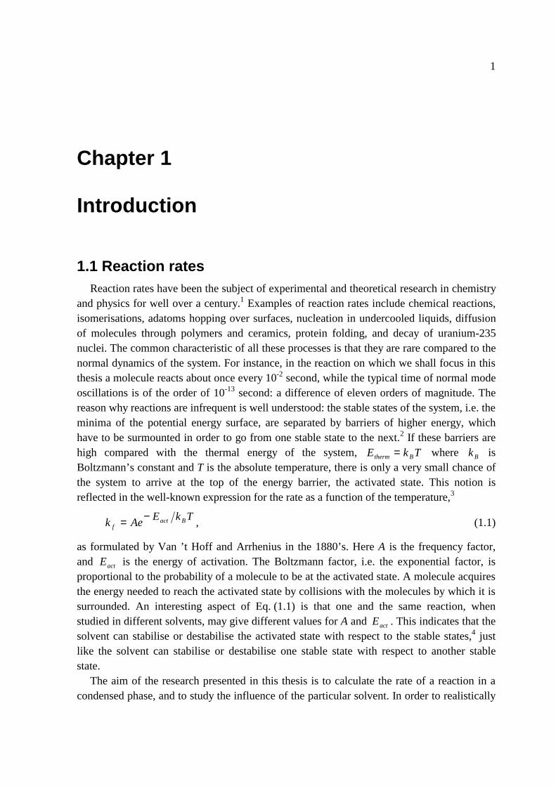
The name calix[n]arene was coined by Gutsche for a class of cavity-shaped cycliccompounds build from 4 to 8 phenol rings linked by methylene groups.9,10 Several of thesemolecules are shaped like a Greek vase, calix crater, which gives them their name, seeFig. 1.1. The explicit hydrogens in Fig. 1.1 can be replaced by sidegroups to give thecalixarene the desired property, a procedure called functionalisation. For instance, the

Figure 1.1. Cone (left) and partial cone (right) conformation of a calix[4]arene.

Introduction 3

calixarene can be made to bind selectively with sodium or potassium ions, or to bind organicmolecules in aqueous solution, or even to catalyse a hydrolysis reaction.

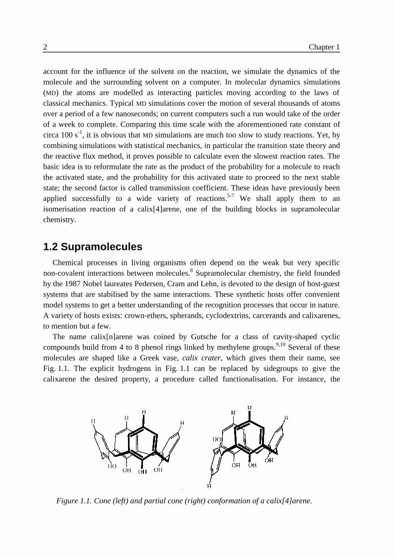
The calix[4]arene in Fig. 1.1 can take on four discrete forms. The most abundantconformation is the ‘cone’ conformation in which all phenol rings are orientated in the samedirection. The four hydroxyl groups at the lower rim then form a circular array of fourinternal hydrogen bonds which stabilise the molecule. In the ‘partial cone’ conformation oneof the phenol rings is rotated with respect to the other three, see Fig. 1.1. Since thisconformation allows for only two internal hydrogen bonds it is energetically less favourable.There are two conformations in which two phenols are orientated in one direction and theother two phenols in the other direction, namely the 1,2-alternate with two internal hydrogenbonds, and the 1,3-alternate devoid of internal hydrogen bonds. In this thesis we shall focuson the cone to partial cone isomerisation. In order to apply Eq. (1.1) we introduce theconcept of a reaction coordinate. This coordinate discriminates reactants from products. Inthe present case, for example, it may be the angle ξ between the central annulus and thephenol ring making the transition. In Fig. 1.2 the minimum potential energy, Φ, is plotted asa function of ξ. The activated state, also called transition state, is seen to be located atξ ≈ − °20 . The activation energy Eact of this reaction has been measured by 1H-NMR to varybetween 12 and 15 kcal/mol, depending on the solvent.

1 .3 SurveyIn chapter 2 we give a concise introduction to statistical mechanics, followed by a

derivation of the reaction rate expressions that will be used in latter chapters. The basic

Φ

ξ-20°

Eact

Figure 1.2. Energy, Φ, as a function of the angle, ξ, between the central annulus and thereacting phenol ring.

4 Chapter 1

concepts of molecular dynamics simulations are discussed. In these simulations the use of anangle ξ, as introduced above, would be very inconvenient. In chapter 3 a new reactioncoordinate is introduced, with suitable properties for use in molecular dynamics simulations.Also in this chapter the transmission coefficient of the isomerisation of a calix[4]arene invacuo and in chloroform is calculated. In the next chapter it will be shown that it is not theenergy but the free energy as a function of the reaction coordinate which determines theprobability factor of the exact reaction rate. Therefore, in chapter 4 the free energy of thecalix[4]arene in chloroform is calculated. The reaction rate calculated with these two resultsis in excellent agreement with experimental data. In chapter 5 we study the effect of twodifferent solvents, namely chloroform and benzene, on the reaction. The reader who wants toget familiar with the applied methods and its results without going through the mathematicalrigor will find this chapter most rewarding. In chapter 6 we discuss the calculation of freeenergies by means of constrained molecular dynamics simulations. The relation between thefree energy and the constraint force is shown to be less trivial than what was assumed bymany authors. We end with a summary and a brief look at the future in chapter 7.

1 .4 References1 P. Hanggi, P. Talkner and M. Borkovec, Rev. Mod. Phys. 62, 251 (1990).2 We shall not consider the quantum mechanical process of tunneling through the barrier,

since it is highly improbable for the reaction studied here.3 S. Glasstone, K. J. Laidler and H. Eyring, The Theory of Rate Processes (McGraw-Hill

Book Company, New York, 1941).4 Note that a distinctive explanation may hold for diffusion controlled reactions.5 D. L. Beveridge and F. M. DiCapua, Annu. Rev. Biophys. Biophys. Chem. 18, 431-92,

(1989).6 R. M. Whitnell and K. R. Wilson, Rev. Comp. Chem. IV , 67 (1993).7 J. B. Anderson, Adv. Chem. Phys XCI , 381 (1995).8 L. Stryer, Biochemistry (W. H. Freeman and Company, New York, 1995).9 C. D. Gutsche, Calixarenes (Royal Society of Chemistry, Cambridge, UK, 1989).10 J. Vicens and V. Böhmer, Eds., Calixarenes: A Versatile class of macrocyclic compounds

(Kluwer Academic Publishers, Dordrecht, The Netherlands, 1991).

5

Chapter 2

Theory

2 .1 Statistical mechanicsThermodynamics studies the mathematical relations between the experimental properties

of a macroscopic system in equilibrium, but it does not predict the magnitude of theseproperties, nor does it provide a link between these properties and the atomic constitution ofthe system. In statistical mechanics the microscopic or atomic point of view is used to studythe properties of the macroscopic system. As will be discussed below, statistical mechanicsoffers alternative interpretations for macroscopic properties and thermodynamical relations,as well as providing numerical values.

2 .1 .1 Static properties

At the heart of statistical mechanics lies the notion that a macroscopic system has anincredible large number of microscopic realisations.1 The probability for each of theserealisations to occur can be calculated, and a macroscopic property can be calculated as theaverage of the corresponding microscopic property over all realisations. Consider forexample the canonical ensemble, the collection of all realisations of a system of N identicalatoms in a volume V at an absolute temperature T. From the classical point of view anyrealisation can be characterised by the coordinates, r i , and the momenta, p i , of the atoms. Inthe canonical ensemble the probability to find a system in the volume element d NΓ centredat the point ( )Γ N

N N= r r p p1 1, , , , ,� � in phase space is given by the Boltzmann distribution,

( ) ( )[ ]ρ βΓ Γ Γ ΓN NN

N NdQ h N

H d= −1 1

3 !exp , (2.1)

where β = 1 k TB , kB is Boltzmann’s constant and H is the Hamiltonian, i.e. the energy ofthe realisation. The second factor on the right hand side, containing Planck’s constant h,arises to make the classical mechanical distribution agree with the quantum mechanicaldistribution. The first term on the right hand side is used to normalise the distribution, where

( )[ ]Qh N

H dNN N= −∫

13 !

exp β Γ Γ (2.2)

6 Chapter 2

is known as the partition function. The partition function is related to the Helmholtz freeenergy, A U TS= − , the macroscopic potential of a closed system of constant volume incontact with a heat bath, by

A k T QB= − ln . (2.3)

Combining this result with the usual thermodynamical expressions, one may relate the(derivatives of the) microscopic partition function to macroscopic properties, such as thepressure and the entropy.

If a macroscopic property, F, has a microscopic analogue, f, the measured value of F isequal to the expectation value of f over the microscopic realisations:

( ) ( )[ ]FQ h N

f H dNN N N= −∫

1 13 !

expΓ Γ Γβ , (2.4)

henceforth to be written as

F f= . (2.5)

The analytic solution of the integral is terribly complicated, so one normally resorts tonumerical methods to approximate the result. In Monte Carlo simulations a random numbergenerator is used to sample points in phase space according to the Boltzmann distribution.Another way of calculating F is based on the notion that the microscopic realisations of asystem by evolving according to classical or quantum mechanics, in the long term constitutea representation of the distribution ( )ρ Γ N . The average obtained by following a realisationover a time interval T is

( )[ ]fT

f t dtN

T

= ∫1

0

Γ . (2.6)

The ergodic hypothesis1 states that this average equals the phase space average, provided theinterval T is long enough:

f fT

=→∞

lim . (2.7)

The average of Eq. (2.6) is obtained by molecular dynamics simulations, as described insection 2.3. We will now switch from static to dynamic properties.

2 .1 .2 Dynamic properties

Suppose we have a macroscopic system prepared in a non-equilibrium condition by anexternal perturbation. The property F then differs from its equilibrium value by

( ) ( )∆F t F t Feq≡ − . At time t = 0 the perturbation is removed, and the system relaxes toequilibrium. If the perturbation is small enough to lie in the linear regime of the system, thedeviation ∆F gradually vanishes according to the macroscopic law

( ) ( ) ( )∆ ∆F t F t= 0 φ , (2.8)

Theory 7

where φ is the response function. We shall assume that this ‘phenomenological’ function isknown, either from experiments or from intuitive reasoning.

At the microscopic level the situation is more involved. Even without an externalperturbation, the parameter f will differ from its equilibrium value for nearly all realisationsat time t = 0 , simply because of the Boltzmann distribution. If we concentrate on a singlerealisation, we will see that as time progresses the value of f behaves very erratic because ofthe complex motion of the atoms in the system. All one knows is that for short times

( ) ( )∆f t f t f≡ − is correlated to ( )∆f 0 , while for long times the correlation will vanish,( )∆f ∞ = 0 . To reduce the noise, we now average over all realisations with the same initial

value ( )∆f 0 . Onsager’s regression hypothesis2,3 states that this average behaves as themacroscopic system,

( ) ( ) ( ) ( )∆ ∆∆

f t f tf 0

0= φ , (2.9)

where φ is the macroscopic response function of Eq. (2.8). Multiplying by ( )∆f 0 andintegrating over all values of ( )∆f 0 , we arrive at the more common notation,

( ) ( ) ( ) ( )∆ ∆ ∆f t f f t0 02= φ . (2.10)

Note that an external perturbation is not required; spontaneous fluctuations of the systemwill, on average, relax according to the macroscopic law too. We must, however, make theexception that the hypothesis does not hold for very short times, since the macroscopic lawof Eq. (2.8) only holds on a macroscopic time scale.

On the left hand side of Eq. (2.10) we encountered a correlation function,

( ) ( ) ( ) ( ) ( )f t g f t g dN N N N0 0 0= ∫ ρ Γ Γ Γ Γ, , , , (2.11)

where ( )f tNΓ , is to be interpreted as the value of f at time t for a realisation that was at Γ N

at time t = 0 . For a system in equilibrium the correlation function depends on the timeinterval only, so

( ) ( ) ( ) ( )f t g f t g+ =τ τ 0 . (2.12)

After differentiating with respect to τ the right hand side equals zero, and upon substitutingτ = 0 in the left hand side we arrive at

( ) ( ) ( ) ( )�

�f t g f t g0 0= − , (2.13)

where a dot indicates the derivative of a function with respect to time.

2 .2 Reaction rate theoryAs an application of the above described Onsager regression hypothesis, we will consider

the reversible unimolecular reaction between reactants, R, and products, P, dissolved in aliquid:

8 Chapter 2

R

k

kP

f

r

→←

. (2.14)

We shall first consider the macroscopic system, then the microscopic system.

2 .2 .1 Macroscopic reaction rate

The phenomenological equations for the population dynamics read as

� ,

� ,

R k R k P

P k R k P

f r

f r

= − +

= −(2.15)

where k f and kr are the rate constants of the forward and the reverse reaction respectively.In the above master equations it is assumed that a certain fraction of the reactants is turnedinto products per unit of time, and likewise for the products. The sum of reactants andproducts is seen to be constant. The equilibrium constant of the reaction is defined as theratio of the equilibrium fractions,

KR

P

k

keq

eq

r

f

= = , (2.16)

where the right hand side follows from the fact that both expressions of Eq. (2.15) are zero atequilibrium. By combining the last two equations, any deviation from equilibrium,

( ) ( )∆P t P t Peq≡ − , is seen to relax as

( ) ( )∆ ∆P t P e t= −0 λ , (2.17)

with the relaxation rate

λ = +k kf r . (2.18)

The forward rate constant is related to the overall relaxation rate by

kP

R Pf

eq

eq eq

=+

λ , (2.19)

as follows from combining Eqs. (2.16) and (2.18).We want to calculate the forward rate constant of a reaction in a solvent. Molecular

dynamics simulations, see sec. 2.3, provides the tools to calculate the motion of a solvatedmolecule, but unfortunately these simulations are fairly slow. On current computers thesimulation time span is limited to a dozen nanoseconds, so the obvious route of usingmolecular dynamics simulations to follow a non-equilibrium system as it evolves toequilibrium is not feasible for most reactions. For slow reactions we need the machinery ofstatistical mechanics, as described below, to calculate a rate constant.

Theory 9

2 .2 .2 Microscopic reaction rate

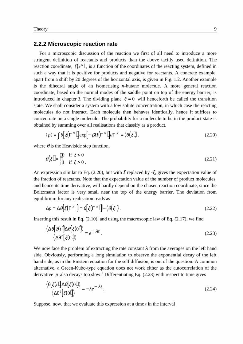
For a microscopic discussion of the reaction we first of all need to introduce a morestringent definition of reactants and products than the above tacitly used definition. Thereaction coordinate, ( )ξ r N , is a function of the coordinates of the reacting system, defined insuch a way that it is positive for products and negative for reactants. A concrete example,apart from a shift by 20 degrees of the horizontal axis, is given in Fig. 1.2. Another exampleis the dihedral angle of an isomerising n-butane molecule. A more general reactioncoordinate, based on the normal modes of the saddle point on top of the energy barrier, isintroduced in chapter 3. The dividing plane ξ = 0 will henceforth be called the transitionstate. We shall consider a system with a low solute concentration, in which case the reactingmolecules do not interact. Each molecule then behaves identically, hence it suffices toconcentrate on a single molecule. The probability for a molecule to be in the product state isobtained by summing over all realisations that classify as a product,

( )[ ] ( )[ ] ( )p H dN N N= − =∫θ ξ β θ ξΓ Γ Γexp , (2.20)

where θ is the Heaviside step function,

( )θ ξξξ=

<>

0 0

1 0

if

if .(2.21)

An expression similar to Eq. (2.20), but with ξ replaced by -ξ, gives the expectation value ofthe fraction of reactants. Note that the expectation value of the number of product molecules,and hence its time derivative, will hardly depend on the chosen reaction coordinate, since theBoltzmann factor is very small near the top of the energy barrier. The deviation fromequilibrium for any realisation reads as

( )[ ] ( )[ ] ( )∆ ∆p N N= = −θ ξ θ ξ θ ξΓ Γ . (2.22)

Inserting this result in Eq. (2.10), and using the macroscopic law of Eq. (2.17), we find

( )[ ] ( )[ ]( )[ ]

∆ ∆

∆θ

θ ξ θ ξ

ξλt

e t0

02= − . (2.23)

We now face the problem of extracting the rate constant λ from the averages on the left handside. Obviously, performing a long simulation to observe the exponential decay of the lefthand side, as in the Einstein equation for the self diffusion, is out of the question. A commonalternative, a Green-Kubo-type equation does not work either as the autocorrelation of thederivative �p also decays too slow.4 Differentiating Eq. (2.23) with respect to time gives

( )[ ] ( )[ ]( )[ ]

�θ ξ θ ξ

ξλ λte t∆

∆θ

0

02= − − . (2.24)

Suppose, now, that we evaluate this expression at a time t in the interval

10 Chapter 2

τλv « t «1

. (2.25)

As was remarked earlier, Onsager’s regression hypothesis does not hold on the very shorttime scale of molecular vibrations, τv . Under the second condition of Eq. (2.25) theexponential of Eq. (2.24) will be nearly unity, hence

( )[ ] ( ) ( )[ ]( )[ ]λ

θ ξ δ ξ

ξ=

t �ξ 0 0

02∆θ, (2.26)

where we have used Eq. (2.13). The Dirac delta function, ( )δ ξ , arises as the derivative of theHeaviside function; its defining properties are:

( )δ ξ ξ= ≠0 0if , (2.27)

and

( )δ ξ ξd a ba

b

= < <∫ 1 0if . (2.28)

From Eq. (2.20) one infers

∆θ2 2 2= − =θ θ r p , (2.29)

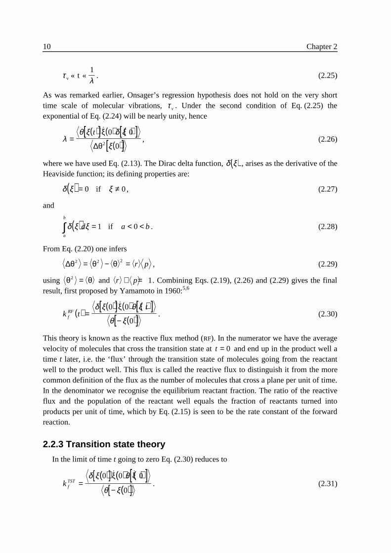
using θ θ2 = and r p+ = 1. Combining Eqs. (2.19), (2.26) and (2.29) gives the finalresult, first proposed by Yamamoto in 1960:5,6

( )( )[ ] ( ) ( )[ ]

( )[ ]k tt

fRF =

−

δ ξ θ ξ

θ ξ

0 0

0

�ξ. (2.30)

This theory is known as the reactive flux method (RF). In the numerator we have the averagevelocity of molecules that cross the transition state at t = 0 and end up in the product well atime t later, i.e. the ‘flux’ through the transition state of molecules going from the reactantwell to the product well. This flux is called the reactive flux to distinguish it from the morecommon definition of the flux as the number of molecules that cross a plane per unit of time.In the denominator we recognise the equilibrium reactant fraction. The ratio of the reactiveflux and the population of the reactant well equals the fraction of reactants turned intoproducts per unit of time, which by Eq. (2.15) is seen to be the rate constant of the forwardreaction.

2 .2 .3 Transition state theory

In the limit of time t going to zero Eq. (2.30) reduces to

( )[ ] ( ) ( )[ ]( )[ ]k f

TST =−

δ ξ θ

θ ξ

0 0 0

0

� �ξ ξ. (2.31)

Theory 11

(from Eq. (2.13), with f g= , it follows that the right hand side of Eq. (2.30) is zero at timet = 0 ). This is the renowned transition state theory (TST) expression for the rate, as proposedby Eyring7 in 1935. Unlike in Eq. (2.30), where the flux is calculated by averaging over allmolecules that end up in the product well after they cross the transition state in whateverdirection, the flux is now calculated by averaging over the molecules that cross the transitionstate in the positive direction. Wigner8 summarised the assumptions underlying transitionstate theory in 1937:• The Born-Oppenheimer approximation, i.e. the electron wavefunction is at all times

adapted to the nuclear configuration. The system always remains in the ground level. Asa result, the potential energy of the system is a well defined function of the coordinates ofthe nuclei (adiabatic condition).

• The motion of the nuclei on the potential energy surface can be described by classicalmechanics.

• Every reactant crossing the transition state will end up as a product.The first two assumptions are also the fundamentals of the reactive flux method and ofmolecular dynamics.

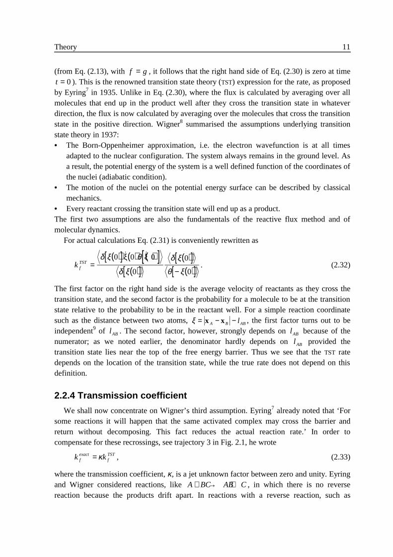
For actual calculations Eq. (2.31) is conveniently rewritten as

( )[ ] ( ) ( )[ ]( )[ ]

( )[ ]( )[ ]k f

TST =−

δ ξ θ

δ ξ

δ ξ

θ ξ

0 0 0

0

0

0

� �ξ ξ. (2.32)

The first factor on the right hand side is the average velocity of reactants as they cross thetransition state, and the second factor is the probability for a molecule to be at the transitionstate relative to the probability to be in the reactant well. For a simple reaction coordinatesuch as the distance between two atoms, ξ = − −x xA B ABl , the first factor turns out to beindependent9 of l AB . The second factor, however, strongly depends on l AB because of thenumerator; as we noted earlier, the denominator hardly depends on l AB provided thetransition state lies near the top of the free energy barrier. Thus we see that the TST ratedepends on the location of the transition state, while the true rate does not depend on thisdefinition.

2 .2 .4 Transmission coefficient

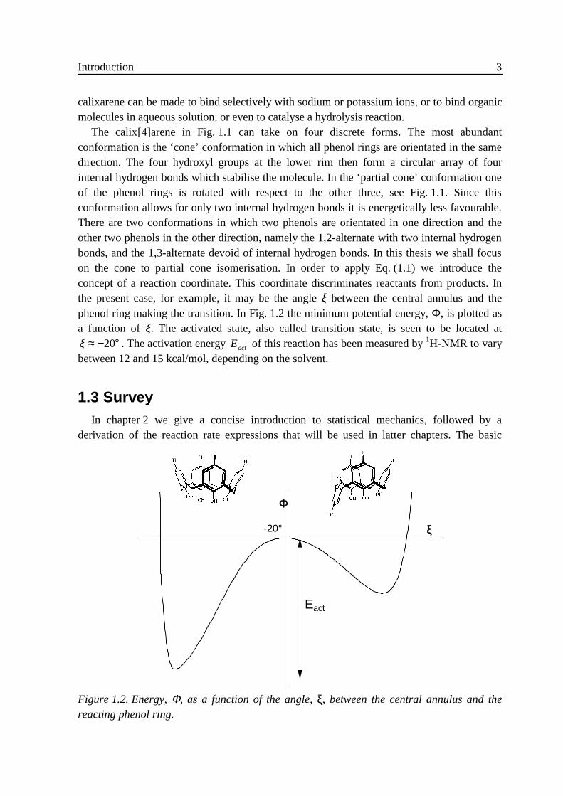
We shall now concentrate on Wigner’s third assumption. Eyring7 already noted that ‘Forsome reactions it will happen that the same activated complex may cross the barrier andreturn without decomposing. This fact reduces the actual reaction rate.’ In order tocompensate for these recrossings, see trajectory 3 in Fig. 2.1, he wrote

k kfexact

fTST= κ , (2.33)

where the transmission coefficient, κ, is a jet unknown factor between zero and unity. Eyringand Wigner considered reactions, like A BC AB C+ → + , in which there is no reversereaction because the products drift apart. In reactions with a reverse reaction, such as

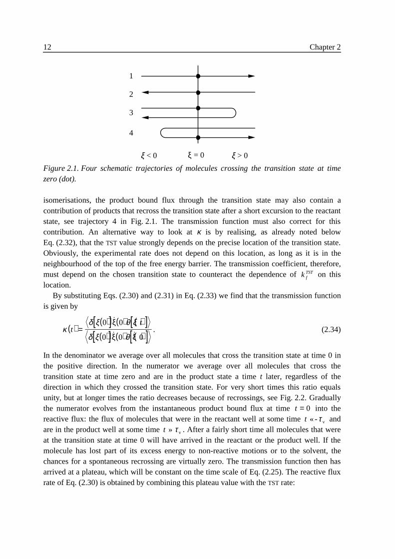
12 Chapter 2

isomerisations, the product bound flux through the transition state may also contain acontribution of products that recross the transition state after a short excursion to the reactantstate, see trajectory 4 in Fig. 2.1. The transmission function must also correct for thiscontribution. An alternative way to look at κ is by realising, as already noted belowEq. (2.32), that the TST value strongly depends on the precise location of the transition state.Obviously, the experimental rate does not depend on this location, as long as it is in theneighbourhood of the top of the free energy barrier. The transmission coefficient, therefore,must depend on the chosen transition state to counteract the dependence of k f

TST on thislocation.

By substituting Eqs. (2.30) and (2.31) in Eq. (2.33) we find that the transmission functionis given by

( )( )[ ] ( ) ( )[ ]( )[ ] ( ) ( )[ ]κ

δ ξ θ ξ

δ ξ θt

t=

0 0

0 0 0

�

� �

ξ

ξ ξ. (2.34)

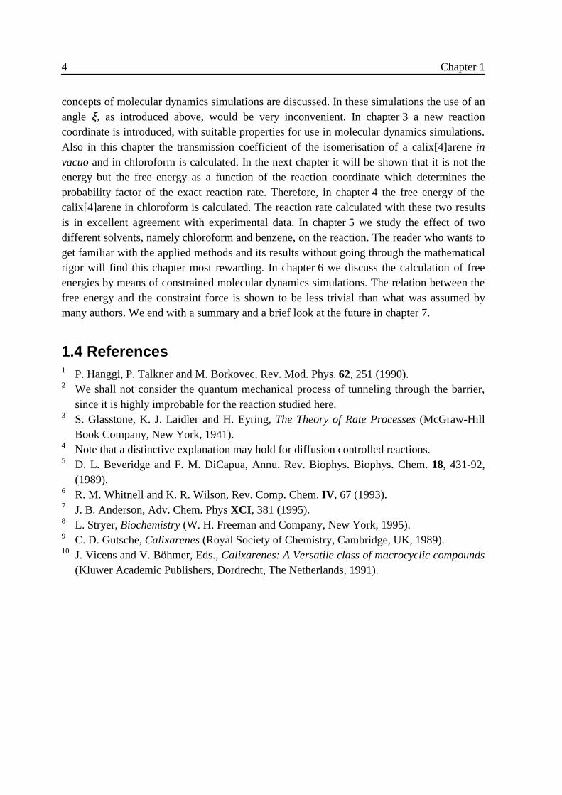
In the denominator we average over all molecules that cross the transition state at time 0 inthe positive direction. In the numerator we average over all molecules that cross thetransition state at time zero and are in the product state a time t later, regardless of thedirection in which they crossed the transition state. For very short times this ratio equalsunity, but at longer times the ratio decreases because of recrossings, see Fig. 2.2. Graduallythe numerator evolves from the instantaneous product bound flux at time t = 0 into thereactive flux: the flux of molecules that were in the reactant well at some time t «- vτ andare in the product well at some time t » vτ . After a fairly short time all molecules that wereat the transition state at time 0 will have arrived in the reactant or the product well. If themolecule has lost part of its excess energy to non-reactive motions or to the solvent, thechances for a spontaneous recrossing are virtually zero. The transmission function then hasarrived at a plateau, which will be constant on the time scale of Eq. (2.25). The reactive fluxrate of Eq. (2.30) is obtained by combining this plateau value with the TST rate:

1

2

3

4

ξ = 0ξ < 0 ξ > 0

Figure 2.1. Four schematic trajectories of molecules crossing the transition state at timezero (dot).

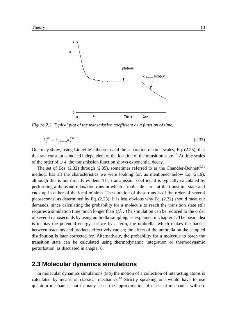
Theory 13

k kfRF

plateau fTST= κ . (2.35)

One may show, using Liouville’s theorem and the separation of time scales, Eq. (2.25), thatthis rate constant is indeed independent of the location of the transition state.10 At time scalesof the order of 1 λ the transmission function shows exponential decay.

The set of Eqs. (2.32) through (2.35), sometimes referred to as the Chandler-Bennett6,11

method, has all the characteristics we were looking for, as mentioned below Eq. (2.19),although this is not directly evident. The transmission coefficient is typically calculated byperforming a thousand relaxation runs in which a molecule starts at the transition state andends up in either of the local minima. The duration of these runs is of the order of severalpicoseconds, as determined by Eq. (2.25). It is less obvious why Eq. (2.32) should meet ourdemands, since calculating the probability for a molecule to reach the transition state stillrequires a simulation time much longer than 1 λ . The simulation can be reduced to the orderof several nanoseconds by using umbrella sampling, as explained in chapter 4. The basic ideais to bias the potential energy surface by a term, the umbrella, which makes the barrierbetween reactants and products effectively vanish; the effect of the umbrella on the sampleddistribution is later corrected for. Alternatively, the probability for a molecule to reach thetransition state can be calculated using thermodynamic integration or thermodynamicperturbation, as discussed in chapter 6.

2 .3 Molecular dynamics simulationsIn molecular dynamics simulations (MD) the motion of a collection of interacting atoms is

calculated by means of classical mechanics.12 Strictly speaking one would have to usequantum mechanics, but in many cases the approximation of classical mechanics will do.

0

1

0 Time

κκ

plateau

τv 1/λ

κplateau exp(-λt)

Figure 2.2. Typical plot of the transmission coefficient as a function of time.

14 Chapter 2

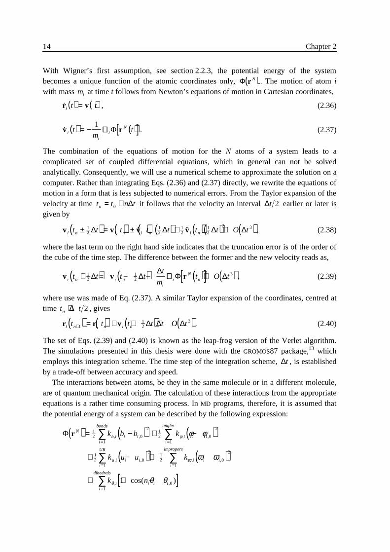
With Wigner’s first assumption, see section 2.2.3, the potential energy of the systembecomes a unique function of the atomic coordinates only, ( )Φ r N . The motion of atom iwith mass mi at time t follows from Newton’s equations of motion in Cartesian coordinates,

( ) ( )�r vi it t= , (2.36)

( ) ( )[ ]�v rii

iNt

mt= −

1∇ Φ . (2.37)

The combination of the equations of motion for the N atoms of a system leads to acomplicated set of coupled differential equations, which in general can not be solvedanalytically. Consequently, we will use a numerical scheme to approximate the solution on acomputer. Rather than integrating Eqs. (2.36) and (2.37) directly, we rewrite the equations ofmotion in a form that is less subjected to numerical errors. From the Taylor expansion of thevelocity at time t t n tn = +0 ∆ it follows that the velocity an interval ∆t 2 earlier or later isgiven by

( ) ( ) ( )( ) ( )( ) ( )v v v vi n i n i n i nt t t t t t t O t± = ± + +12

12

12

12

2 3∆ ∆ ∆ ∆� �� , (2.38)

where the last term on the right hand side indicates that the truncation error is of the order ofthe cube of the time step. The difference between the former and the new velocity reads as,

( ) ( ) ( )[ ] ( )v v ri n i ni

iN

nt t t tt

mt O t+ = − − +1

212

3∆ ∆∆

Φ ∆∇ , (2.39)

where use was made of Eq. (2.37). A similar Taylor expansion of the coordinates, centred attime t tn + ∆ 2 , gives

( ) ( ) ( ) ( )r r vi n i n i nt t t t t O t+ = + + +112

3∆ ∆ ∆ . (2.40)

The set of Eqs. (2.39) and (2.40) is known as the leap-frog version of the Verlet algorithm.The simulations presented in this thesis were done with the GROMOS87 package,13 whichemploys this integration scheme. The time step of the integration scheme, ∆t , is establishedby a trade-off between accuracy and speed.

The interactions between atoms, be they in the same molecule or in a different molecule,are of quantum mechanical origin. The calculation of these interactions from the appropriateequations is a rather time consuming process. In MD programs, therefore, it is assumed thatthe potential energy of a system can be described by the following expression:

( ) ( ) ( )

( ) ( )

[ ]

Φ r Nb i i i

i

bonds

i i ii

angles

u i i ii

UB

i i ii

impropers

i i i ii

dihedrals

k b b k

k u u k

k n

= − + −

+ − + −

+ + −

= =

= =

=

∑ ∑

∑ ∑

∑

12 0

2

1

12 0

2

1

12 0

2

1

12 0

2

1

01

1

, , , ,

, , , ,

, ,cos( )

φ

ω

θ

φ φ

ω ω

θ θ

Theory 15

+

−

+

>

∑ 44

12 6

0

εσ σ

πεij

ij

ij

ij

ij

i j

ijj i

N

r r

q q

r. (2.41)

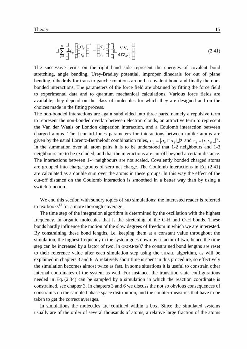
The successive terms on the right hand side represent the energies of covalent bondstretching, angle bending, Urey-Bradley potential, improper dihedrals for out of planebending, dihedrals for trans to gauche rotations around a covalent bond and finally the non-bonded interactions. The parameters of the force field are obtained by fitting the force fieldto experimental data and to quantum mechanical calculations. Various force fields areavailable; they depend on the class of molecules for which they are designed and on thechoices made in the fitting process.The non-bonded interactions are again subdivided into three parts, namely a repulsive termto represent the non-bonded overlap between electron clouds, an attractive term to representthe Van der Waals or London dispersion interaction, and a Coulomb interaction betweencharged atoms. The Lennard-Jones parameters for interactions between unlike atoms aregiven by the usual Lorentz-Berthelodt combination rules, ( )σ σ σij ii jj= + 2 and ( )ε ε εij ii jj= 1 2 .In the summation over all atom pairs it is to be understood that 1-2 neighbours and 1-3neighbours are to be excluded, and that the interactions are cut-off beyond a certain distance.The interactions between 1-4 neighbours are not scaled. Covalently bonded charged atomsare grouped into charge groups of zero net charge. The Coulomb interactions in Eq. (2.41)are calculated as a double sum over the atoms in these groups. In this way the effect of thecut-off distance on the Coulomb interaction is smoothed in a better way than by using aswitch function.

We end this section with sundry topics of MD simulations; the interested reader is referredto textbooks12 for a more thorough coverage.

The time step of the integration algorithm is determined by the oscillation with the highestfrequency. In organic molecules that is the stretching of the C-H and O-H bonds. Thesebonds hardly influence the motion of the slow degrees of freedom in which we are interested.By constraining these bond lengths, i.e. keeping them at a constant value throughout thesimulation, the highest frequency in the system goes down by a factor of two, hence the timestep can be increased by a factor of two. In GROMOS87 the constrained bond lengths are resetto their reference value after each simulation step using the SHAKE algorithm, as will beexplained in chapters 3 and 6. A relatively short time is spent in this procedure, so effectivelythe simulation becomes almost twice as fast. In some situations it is useful to constrain otherinternal coordinates of the system as well. For instance, the transition state configurationsneeded in Eq. (2.34) can be sampled by a simulation in which the reaction coordinate isconstrained, see chapter 3. In chapters 3 and 6 we discuss the not so obvious consequences ofconstraints on the sampled phase space distribution, and the counter-measures that have to betaken to get the correct averages.

In simulations the molecules are confined within a box. Since the simulated systemsusually are of the order of several thousands of atoms, a relative large fraction of the atoms

16 Chapter 2

will be in contact with the walls of the box. To minimise these effects, it is common practiceto apply periodic boundary conditions. For a rectangular box this means that a molecule nearthe wall on the right interacts with the molecules near the wall on the left, and likewise amolecule near the front or near the top interacts with the molecules near the back or near thebottom respectively. The simulation box can be envisioned as being surrounded by 26identical images. When calculating the interaction between atoms i and j, out of the 27images of j the one closest to i must be used (minimum image convention). The box size andthe cut-off radius of the non-bonded interactions must be chosen such that in the interactionbetween two molecules only one image of the second molecule is used, if possible. In oursimulations we will frequently use a box shaped like a truncated octahedron; the minimumimage convention is adapted accordingly.

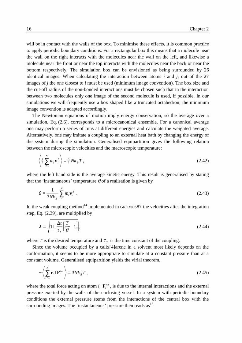
The Newtonian equations of motion imply energy conservation, so the average over asimulation, Eq. (2.6), corresponds to a microcanonical ensemble. For a canonical averageone may perform a series of runs at different energies and calculate the weighted average.Alternatively, one may imitate a coupling to an external heat bath by changing the energy ofthe system during the simulation. Generalised equipartition gives the following relationbetween the microscopic velocities and the macroscopic temperature:

12

2

1

32m Nk Ti i

i

N

Bv=∑ = , (2.42)

where the left hand side is the average kinetic energy. This result is generalised by statingthat the ‘instantaneous’ temperature θ of a realisation is given by

θ =1

32

1Nkm

Bi i

i

N

v=∑ . (2.43)

In the weak coupling method14 implemented in GROMOS87 the velocities after the integrationstep, Eq. (2.39), are multiplied by

λτ θ

= + −

1 1

∆t T

T

, (2.44)

where T is the desired temperature and τT is the time constant of the coupling.Since the volume occupied by a calix[4]arene in a solvent most likely depends on the

conformation, it seems to be more appropriate to simulate at a constant pressure than at aconstant volume. Generalised equipartition yields the virial theorem,

− ⋅ ==∑ r Fi i

tot

i

N

BNk T1

3 , (2.45)

where the total force acting on atom i, Fitot , is due to the internal interactions and the external

pressure exerted by the walls of the enclosing vessel. In a system with periodic boundaryconditions the external pressure stems from the interactions of the central box with thesurrounding images. The ‘instantaneous’ pressure then reads as15

Theory 17

π = + ⋅

= <∑ ∑2

312

2

1

12V

mi ii

N

ij iji j

N

v R F , (2.46)

where r ij and Fij are calculated by the minimum image convention. It is also possible toreplace the sum over all atoms by a sum over all molecules, as is done in GROMOS87, byadapting the quantities on the right hand side of Eq. (2.46) accordingly.16 In the weakcoupling method14 the coordinates after the integration step, Eq. (2.40), are multiplied by

( )µ βτ

π= − −13∆t

Pp

, (2.47)

where P is the desired pressure, τ p is the time constant of the coupling, and β is theisothermal compressibility.

2 .4 References1 D. A. McQuarrie, Statistical mechanics (Harper and Row, New York, 1976).2 L. Onsager, Phys. Rev. 37, 405 (1931), ibid 38, 2265 (1931).3 D. Chandler, Introduction to Modern Statistical Mechanics (Oxford University Press,

Oxford, U.K., 1987).4 D. Brown and J. H. R. Clarke, J. Chem. Phys. 92, 3062 (1990).5 T. Yamamoto, J. Chem. Phys. 33, 281 (1960).6 D. Chandler, J. Chem. Phys. 68, 2959 (1978).7 H. Eyring, J. Chem. Phys. 3, 107 (1935).8 E. Wigner, Trans. Faraday Soc. 34, 29 (1938).9 This follows from Eq. (4.29).10 W. H. Miller, Acc. Chem. Res. 9, 306 (1976).11 C. H. Bennet in Diffusion in Solids, edited by J. J. Burton and A. S. Nowick, (Academic

Press, NY, 1975), p. 73.12 M. P. Allen and D. J. Tildesley, Computer Simulations of Liquids (Clarendon Press,

Oxford, U. K., 1987); J. M. Haile, Molecular Dynamics Simulation: Elementary Methods(John Wiley and Sons, New York, NY, 1992); D. Frenkel and B. Smit, UnderstrandingMolecular Simulations (Academic Press, San Diego, CA, 1996).

13 H. J. C. Berendsen and W. F. van Gunsteren, GROMOS Reference Manual (University ofGroningen, Groningen, The Netherlands, 1987).

14 H. J. C. Berendsen, J. P. M. Postma, W. F. van Gunsteren, A. DiNola and J. R. Haak, J.Chem. Phys. 81, 3684 (1984).

15 A. J. C. Ladd in Computer Modelling of Fluids Polymers and Solids, edited by C. R. A.Catlow, S. C. Parker and M. P. Allen (Kluwer Academic Publishers, Dordrecht, TheNetherlands, 1990), p. 55; R. T. W. Koperdraad, graduation report (University of Twente,Enschede, The Netherlands, 1991).

16 G. Ciccotti and J.-P. Ryckaert, Comput. Phys. Rep. 4, 347 (1986).

19

Chapter 3

The reactive flux method applied to

complex isomerisation reactions:

using the unstable normal mode as a

reaction coordinate *

AbstractA basic problem when calculating reaction rates using the reactive flux method is the

introduction of a reaction coordinate. In this paper we show that it is advantageous to definea reaction coordinate by means of the unstable normal mode of the saddle point of thepotential energy surface. This particular choice is made since it yields a high transmissionfunction. Moreover, the reaction coordinate is calculated via a rapidly converging algorithm,and its derivative, which is needed in constrained runs, is calculated analytically.Calculations on the transmission coefficient of the isomerisation of n-butane are in goodagreement with results published by others. Runs with an isomerising calix[4]arene in vacuoproduce a very high transmission coefficient, as is the purpose of the reaction coordinate.The same molecule is also studied in chloroform.

3 .1 IntroductionConversion in condensed phases of reactants into products usually is a slow process

compared with all other molecular processes. The conversion rate is expressed in terms of arate coefficient, kf , giving the fraction of reactants turned into products per unit of time.This article focuses on isomerisation reactions, but most of the ideas to be described areequally well applicable to other reaction types as well. In isomerisation reactions thereactants and products are different conformations of the same molecule, and

* W. K. den Otter and W. J. Briels, J. Chem. Phys. 106 5494 (1997).

20 Chapter 3

interconversions are possible without forming or breaking chemical bonds. A well knownand thoroughly studied example is the trans-gauche isomerisation of n-butane. Thisparticular reaction is fast enough to be studied using regular equilibrium1 or non-equilibrium2

molecular dynamics simulations (MD), in spite of the simulation time being limited to a fewnanoseconds. Most other reactions, however, are much too slow for this kind of simulationsto be possible. To calculate their rate coefficients one needs to develop models providing thelink between macroscopic long time quantities like kf , and the microscopic short timebehaviour of a single molecule in a solvent.3

Reactant and product conformations correspond to local minima of the potential energysurface (PES), separated by a barrier of elevated energy. The conformation space at the top ofthe barrier is called the transition state. Most of the time a molecule will be trapped in eitherone of the minima. By intramolecular energy redistribution and by interactions with thesolvent a molecule may incidentally gain enough energy along its reactive coordinate to hopover the barrier from one well into the other. If the barrier is high compared with the thermalenergy of the reactive coordinate then the transition state is sparsely populated and crossingevents will be rare.

Eyring’s transition state theory4 (TST) expresses the forward rate constant as theinstantaneous flux through the transition state from reactants to products, divided by thenumber of reactants:

( )[ ] ( ) ( )[ ]( )[ ]k f

TST =−

δ ξ θ

θ ξ

0 0 0

0

� �ξ ξ. (3.1)

Here θ is the Heaviside function and the angular brackets denote a canonical average overphase space. The reaction coordinate { }( )ξ x i is a function of all molecular coordinates,defined in such a way that it is positive for products, negative for reactants and zero at thetransition state. The time indication (0) is added to stress that all quantities are calculated atthe same point in time. Assuming thermal equilibrium prevails throughout the reactants partof phase space, the rate constant may be shown to be given by Arrhenius’ law,

kk T

he A k T

fTST B B= − ≠∆ , (3.2)

where ∆A≠ is the free energy difference between reactants and the transition state. Thissimple expression and the widespread techniques of calculating free energy differences makeTST a popular technique for calculating rate constants.

At this point an important deficiency of TST needs to be addressed. The TST rateexpression very much depends on ∆A≠ , i.e. on the precise choice of the transition state. Inprinciple, of course, the rate expression should indeed depend on this choice, since it impliesthe definition of reactants and products. In practice, however, provided the reaction is slow,the rate constant should hardly depend on the details of this definition as long as the surfacedividing reactants from products lies somewhere near the top of the free energy barrier. Anatural choice for this dividing surface is such that it carries the least flux,5 i.e. such that

Using the unstable normal mode as a reaction coordinate 21

∆A≠ is as large as possible. Even then, however, the result will in general be an overestimateof the true reaction rate. The reason for this is that in transition state theory it is assumed thatevery molecule in the reactant well that reaches the transition state will end up in the productregion. Consequently, molecules which recross the transition state, e.g. after interaction withthe solvent, and eventually stay in the reactant well will be treated incorrectly.

In this article the reactive flux method6,7 (RF) will be used to calculate the transition rate.Instead of counting all crossing events, attention shifts towards those crossing trajectoriesthat actually reach the product well some time t after having crossed the transition state:

( )( )[ ] ( ) ( )[ ]

( )[ ]k tt

fRF =

−

δ ξ θ ξ

θ ξ

0 0

0

�ξ. (3.3)

One easily realises that the process of averaging in combination with the time delay turns thenumerator into the net flux from reactants to products.

Equation (3.3) is conveniently expressed as

( ) ( )k t t kfRF

fTST= κ , (3.4)

i.e. as the instantaneous flux at the transition state times the fraction that actually makes it tothe product state at time t. The transmission function κ(t) is given by

( )( )[ ] ( ) ( )[ ]( )[ ] ( ) ( )[ ]

( ) ( )[ ]( ) ( )[ ]κ

δ ξ θ ξ

δ ξ θ

θ ξ

θξ

ξ

tt t

= =0 0

0 0 0

0

0 0

�

� �

�

� �

ξ

ξ ξ

ξ

ξ ξ, (3.5)

where � ξ denotes a conditional average. Since most recrossings follow shortly after acrossing, κ(t) quickly decays on the time scale of molecular vibrations from one to a plateau7

value which remains constant on that time scale. The transmission function stabilises sinceafter some time the molecules have moved far enough from the transition state into one ofthe two wells for recrossings to become extremely rare. Of course, on the far longer timescale of 1 kf recrossings do still occur, so the plateau is in fact decaying extremely slowly.The real transmission coefficient κ is equal to the plateau value of κ(t), or more precisely tothe extrapolation of the plateau to its value at t = 0. The reactive flux method ensures that therate constant, i.e. the product κk f

TST, is insensitive to the precise definition of the reactioncoordinate and transition state.7

The problem usually encountered when performing MD simulations of reactions incondensed phases is the extremely small chance for molecules to surmount the barrier. In theexpression for κ(t) this problem does not occur, since all trajectories start at the barrier,making the improbable probable. Stabilising the transmission function on its plateau valuetypically requires the simulation of several thousand trajectories for a couple of picosecondsdirectly after the start at the transition state. Starting configurations in the transition plane areefficiently obtained by performing biased MD or Monte Carlo runs. The influence of theapplied constraint or restraint on the sampled positions and velocities is simply corrected for.Good statistics and fast convergence are obtained when the plateau value is as high as

22 Chapter 3

possible, i.e. when the TST rate is as small as possible. For a Cartesian dividing plane inconfiguration space this suggests identification of the reaction coordinate with thedisplacement along the unstable direction at the saddle point. The hyperplane perpendicularto the unstable mode which includes the saddle point then is the transition state.

The reactive flux method has been used to calculate the isomerisation rates for a numberof isomerisation reactions, including those of n-butane,8 dichloro-ethane,9 cyclohexane,10-12

cyclohexene13 and n-octane14 and even the side chain rotation of BPTI15 has been studied.

Numerous other reactions, including chemical reactions, have been simulated too.16,17 Inthese examples the reaction coordinates are defined in terms of distances or dihedrals. A rareexception is cyclohexane, where a special set of coordinates and an accompanying potentialwere introduced.18 For some of the molecules the chosen reaction coordinate indeed definesa dividing surface that includes the saddle point, while for others it is an educated guess.

Defining a reaction coordinate in a complex isomerising molecule may prove difficult.Often a torsion is the slowest internal motion, suggesting a dihedral angle as the reactioncoordinate. Concerted motions, however, may drastically complicate the choice. In thisarticle it will be shown that it is advantageous to define the reaction coordinate via theunstable normal mode at the saddle point. This objective many-body reaction coordinate iscalculated by a zero-point search. Its derivative, which is needed many times in thesubsequent MD simulations, may then be obtained non-iteratively, in contrast with otheriteratively determined coordinates. When properly implemented, a single MD program can beused to study a wide variety of reactions.

Normal modes and their properties are introduced in section 3.2. It proves simple todescribe any molecular configuration uniquely by a translation, a rotation and the amplitudesof the rotated vibrational normal modes of the saddle point. The coefficient of the unstablemode is then used as a reaction coordinate. Constraining this mode, as to sample thetransition state, can be done efficiently. The constraint and its side effects are discussed insection 3.3. A method for implementing the technique in an MD program is presented insection 3.4. In section 3.5 it is shown that the results of test runs with n-butane in carbontetrachloride and with liquid n-butane are in good agreement with previously publishedresults. As an example of a complicated reaction the isomerisation of a calix[4]arene inchloroform is discussed.

3 .2 The reaction coordinateAs we remarked already in the previous section, the precise definition of the reaction

coordinate is not crucial. A physically appealing reaction coordinate is the component alongthe unstable normal mode of the free molecule in its transition state. In this section we shallfirst make some remarks about normal mode analysis, mainly for the sake of setting ournotation. Next we shall describe a method to calculate the value of this reaction coordinatefor any molecule in whichever orientation and whichever configuration.

Using the unstable normal mode as a reaction coordinate 23

Suppose we are given the potential energy surface (PES) of a molecule containing N atomsin terms of its 3N Cartesian coordinates. We shall collect all coordinates in a 3N dimensionalcolumn vector X of mass-weighted 3 dimensional column vectors: X T =( )m m mT T

N NT

11 2

1 21 2

21 2x x x, , ,� . At the saddle point X 0 the gradient of the potential energy equals

zero, and its Taylor expansion up to second order reads

( ) ( ) ( )E Vpot

T= + − −X X X H X X0 1

20 0 . (3.6)

Here H denotes the Hessian, a matrix containing all second order derivatives of the potentialwith respect to the mass-weighted coordinates. Diagonalising the Hessian yields 3Neigenvectors and eigenvalues. In absence of external fields the potential energy isindependent of the position and orientation of the molecule, ensuring that at least sixeigenvalues (assuming we are dealing with a non-linear molecule) will be equal to zero. Thecorresponding six eigenvectors can easily be constructed:

( ) ( ) ( ) ( )( )E e e el T l T l T

Nl T

m m m= 1 2, , ,� , (3.7)

( ) ( ) ( ) ( )( )S e r e r e rl T l T l T

Nl

N

Tm m m= × × ×1 1

02 2

0 0, , ,� , (3.8)

where e1, e2 and e3 are three unit vectors along the Cartesian axes, and ri0 is the position of

atom i with respect to the centre of mass for a molecule in configuration X 0 . ChoosingX X− 0 proportional to one of the El or Sl amounts to translating or (infinitesimally)rotating the molecule as a whole away from its reference configuration. Noticing that Epot

remains unaltered under such an operation, one easily concludes that El and Sl areeigenvectors of H with eigenvalue zero. The remaining 3 6N − eigenvectors correspond tointernal vibrations,

( ) ( ) ( ) ( )( )Q q q qj T j T j T

N Nj T

m m m= 1 1 2 2, , ,� , (3.9)

and can only be obtained by explicitly diagonalising H. In a regular normal mode analysis,where X 0 corresponds to an energy minimum, all eigenvalues will be non-negative, equal tothe square of the oscillation frequencies. At the saddle point, however, one unstabledirection, Q r , occurs, which may be recognised by its negative eigenvalue or imaginaryfrequency.

The orthogonality of eigenvectors, or the possibility to orthogonalise eigenvectors in caseof degeneracy, has some interesting consequences. The scalar product of a vibration and atranslation gives

Q E e qj l li i

j

i

N

m l j⋅ = ⋅ = ∀=∑

1

0 , , (3.10)

and the scalar product of a vibration and a rotation gives

24 Chapter 3

Q S e r qj l li i i

j

i

N

m l j⋅ = ⋅ × = ∀=∑ 0

1

0 , . (3.11)

These equations are known as the Eckart conditions.19 They state that a molecule does nottranslate nor rotate during an infinitesimal vibration. Put differently: vibrations are the resultof internal forces while translations and rotations require external forces. Notice that the Sl

as defined above are not orthogonal among each other. By making linear combinations theyare simply made orthogonal. Henceforth it will be assumed that all eigenvectors have beenorthonormalised.

We now come to the definition of the reaction coordinate. When the molecule is close tothe transition state we may perform a harmonic analysis as described above, and identify thereaction coordinate with

( )X X Q− ⋅ =0 r ξ . (3.12)

We then immediately face the problem of how to define X 0 . Notice that this will not onlyaffect the first factor of the scalar product on the left hand side of Eq. (3.12), but also thesecond factor, Q r . Because we want the reaction coordinate to describe a molecularproperty, independent of the position and rotation of the molecule, we demand

( )X X E− ⋅ = ∀0 0l l , (3.13)

( )X X S− ⋅ = ∀0 0l l , (3.14)

i.e. we assume that the state X can be obtained from the state X0 without translating orrotating the molecule. Here too, the eigenvectors depend on X 0 . Together with the fact thatX 0 should correspond to a saddle point these equations completely specify X 0 .

Equation (3.13) is trivially satisfied when all coordinates refer to the centre of mass of themolecule, which we shall assume in the remaining part of this paper. To solve Eq. (3.14) forX 0 , we introduce a reference geometry Y 0 with the molecule in its saddle point, and write

X AY0 0= . (3.15)

Here A is a 3N dimensional rotation matrix, containing N copies of a three dimensionalrotation matrix a along the diagonal. Once the rotation matrix A has been found, the normalmodes of X 0 are given by AE l , ASl and AQ j , where El , Sl and Q j are the normalmodes belonging to the reference geometry Y 0 . Equation (3.14) now reads

( )X AY AS− ⋅ = ∀0 0l l , (3.16)

and the reaction coordinate is given by

( )X AY AQ− ⋅ =0 r ξ . (3.17)

These two equations combined uniquely define ξ for every configuration. A numericalmethod for solving Eq. (3.16) will be discussed in section 3.4.

Using the unstable normal mode as a reaction coordinate 25

In the neighbourhood of the transition state, where the harmonic expansion of thepotential is valid, the reaction coordinate has a clear physical interpretation as thedisplacement along the unstable normal mode. Since Q r is tangent to the mass-weightedpath of steepest descend, the definition of ξ is then closely related to the common intrinsicreaction coordinate20 (IRC). Far away from the transition state, i.e. for large ξ, the coordinateloses its physical interpretation and reduces to a mere mathematical description of themolecular configuration. This does not affect the validity of our reaction coordinate, since forlarge ξ, i.e. for t > 0, Eq. (3.3) only requires the sign of ξ. Accuracy is therefore demandedonly near the transition state, i.e. at t = 0 in Eqs. (3.1) and (3.3), and that is precisely where ξis stringently defined. Elsewhere a rough estimate of the reaction coordinate will do. Notethat Eqs. (3.16) and (3.17) can not ensure that ξ is positive (negative) throughout the entireproduct (reactant) region. This has to be verified before using the present definition of ξ.

Equations (3.16) and (3.17) may also be understood by using a slightly different point ofview. It is clear that any configuration X can be obtained from the reference geometry by asuperposition of Y 0 and all vibrations, followed by a rotation:

X A Y Q= +

=

−

∑0

1

3 6

α jj

j

N

. (3.18)

The amplitude of the unstable normal mode is then identified with the reaction coordinate,ξ α= r . By using the orthonormality of normal modes, the solution to this equation againyields the Eqs. (3.16) and (3.17).

3 .3 Sampling the transition state

3 .3 .1 Constrained dynamics

In order to efficiently calculate the numerator and denominator on the right hand side ofEq. (3.5) we need to perform a simulation with the molecule constrained to the saddle planeξ = 0 . This we do by means of the SHAKE algorithm of Ryckaert et al.21 Suppose we apply Lholonomic constraints ( )σ l l LX = =0 1, , ,� . As a result every atom in the moleculeexperiences an additional force, a constraint force of the form − ∇=Σ l

Ll i l1λ σ , where the λl are

L Lagrange multipliers. The λl are determined by imposing that the L constraints hold atevery time. Several methods may be chosen to solve for the λl , the most common being thatthe constraints are treated one at a time. Because imposing one constraint may do harm to allothers, one usually has to go through all constraints several times in a cyclical fashion. Thisiterative procedure allows for the λl to be calculated to lowest order only.

We shall now restrict our discussion to the constraint ξ = 0 . The result of imposing thisconstraint is that a constraint force

Fir

r i= − ∇λ ξ (3.19)

26 Chapter 3

applies to atom i. The Lagrange multiplier λ r has to be chosen such that the constraint issatisfied at every instant. When using the Verlet algorithm the displacement during theinterval ( )t t, + ∆ reads

( ) ( ) ( )x xi ii

r it tm

t+ = ′ + − ∇∆ ∆ ∆2

λ ξ , (3.20)

where ( )′ +x i t ∆ is the position atom i would have had at time t + ∆ had there been noconstraint force. Inserting this into the constraint equation ξ = 0 yields an expression for λ r .Usually this expression is solved to first order by writing

( ) ( ) ( ) ( )ξ ξ λ ξ ξt tm

t tri

i ii

N

+ = ′ + − ∇ ′ + ⋅ ∇=∑∆ ∆ ∆ ∆2

1

1, (3.21)

where ( )′ +ξ t ∆ is the value of the constraint coordinate when the atoms are at the positions( )′ +x i t ∆ . Putting the left hand side equal to zero yields λ r to first order. In successive

iterations the newly calculated ( )x i t + ∆ replace the old ( )′ +x i t ∆ .The important object to calculate now is ∇iξ . The main problem in evaluating the

gradient of Eq. (3.17) lies in the derivative of the rotation matrix, which will be dealt withfirst. Since a is a rotation matrix it satisfies a a IT = , from which, after differentiating withrespect to the α-coordinate of atom i, follow the six conditions

∂∂

∂∂α α

aa a

a0

x xi

T

T

i

+

= . (3.22)

Expressing the matrix derivative as the product

∂∂ α

αa

b axi

i= (3.23)

and substituting this into Eq. (3.22) we find

b biT

iα α= − . (3.24)

Any antisymmetric matrix can be expanded as a linear combination of three independentantisymmetric matrices ε k , so

bi ik k

k

cα α==

∑ ε1

3

. (3.25)

The unknown cikα may be obtained from the definition of a, Eq. (3.16). Differentiating this

equation with respect to the α-coordinate of atom i and substituting Eqs. (3.23) and (3.25)we get, after changing the order of summation,

( ) ( )011

3

= +

==∑∑m c mi i

lik k

j jl

jj

N

k

as a s xα α ε : . (3.26)

Using the unstable normal mode as a reaction coordinate 27

For every i and α this expression constitutes a set of three equations, i.e. one for every l, inthe three unknown c ki

kα , ,2,= 1 3 . Notice that the expression between curly brackets can be

regarded as an element of a matrix, M , which does not depend on i nor on α. Equation (3.26)is then easily solved for ci

kα , yielding the same linear combination of ( )mi i

las α ’s for every iand α.

We now return to the definition of the reaction coordinate, Eq. (3.17). Differentiating andsubstituting Eqs. (3.23) and (3.25) yields

( ) ( )∂ξ∂ α

α αxm c m

ii i

rik k

j jr

jj

N

k

= +

==∑∑aq a q xε :

11

3

. (3.27)

Again, the factor between curly brackets can be regarded as an element of a vector, N r ,which is independent of i and α. Upon substituting the ci

kα found from Eq. (3.26), the final

result reads

∇ = −

=

∑i i ir

lr

il

l

m dξ a q s1

3

, (3.28)

where the coefficients,

( )d Mlr

klk

= −

=∑N k

r 1

1

3

, (3.29)

are independent of i. From a calculation point of view this is a very attractive expression,since the cumbersome dl

r need to be evaluated only once for every X. At the saddle point thegradient takes a particular simple form, since then N 0r = and dl

r = 0 . Note that theconstraint force is derived from an internal coordinate, and hence does not affect the angularmomentum of the molecule. Therefore, one does not need to explicitly use this conservationproperty when defining the constraint force, as was done by Tobias and Brooks.22

3 .3 .2 The conditional average at the transition state

In this subsection we present the formulas needed to calculate the conditional averages inEq. (3.5). Things will be complicated a bit by the fact that apart from the constraint on ξ wewill also make use of the usual constraints on the bond lengths involving hydrogen atoms.We therefore have one constraint ξ = 0 and L constraints σ l = 0. We introduce thegeneralised coordinates q q N L L1 3 1 1, , , , , ,� �− − ξ σ σ , and write for the kinetic energy

Tq qT

q qξσ ξσ ξσ ξσ= −12

1p A p , (3.30)

where pqξσ represents the column vector of all generalised momenta. One of Hamilton’sequations of motion then reads

vp

A pq

q

qq q

Tξσ

ξσ

ξσξσ ξσ

∂∂

= = −1 , (3.31)

28 Chapter 3

where v qξσ is the column vector of all generalised velocities. We will make use of thefollowing notation

AA B

B Cq

q

Tξσξσ

ξσ ξσ=

, (3.32)

AX Y

Y Zq

q

Tξσξσ

ξσ ξσ

− =

1 , (3.33)

where A q is the ( ) ( )3 6 3 6N L N L− − × − − left upper block of A qξσ , etc.We are interested in the integral

( ) ( )[ ]d d d dp d d F Tq qq p p∫ ∫ ∫ − +ξ δ ξ βξ σ ξσσ exp Φ

( ) ( ) ( )[ ]≈ − +∫ ∫ ∫d d d dp d d F Tq qq p pξ δ ξ δ βξ σ ξσσ σ exp Φ , (3.34)

where Φ is the potential energy, β = 1 k TB , and F, the function to be averaged, may dependon all variables. In the second expression we have made the usual assumption for stiffvariables. Because of the δ-functions, ξ and σ may be put equal to zero in F, Tqξσ and Φ.

We intend to compute the integral (3.34) by using the constrained molecular dynamicssimulations described in the previous section. Since in these simulations not only ξ and σ areconstrained to zero, but also �ξ and �σ , it is advantageous to change coordinates from

( ) ( )p p p pq qp, , ,ξ σ ξσ= to ( ) ( )p p vq q, , � ,ξ σ = ξσ according to

p

v

1 0

Y Z

p

pq

T

q

ξσ ξσ ξσ ξσ

=

, (3.35)

where the second line follows from Eqs. (3.31) and (3.33). The Jacobian of this

transformation equals Z ξσ−1 . The kinetic energy can be calculated by inverting Eq. (3.35)

and introducing the result into Eq. (3.30):

Tq qT

q qT

ξσ ξσ ξσ ξσ= +− −12

1 12

1p A p v Z v . (3.36)

Integral (3.34) then reads

( )[ ] ( ) ( ) [ ]d d d d d d F Tq qTq p Z v Z v∫ ∫ ∫ − + −

− −ξ β δ ξ δ βξσ ξσ ξσ ξσ� � exp expξ σσ σ σΦ

112

1

( ) [ ]∝ −∫ ∫ ∫− −d d d d F Pq

cq

Tq p q p Z v Z v� � , expξ σσ ξσ ξσ ξσ ξσ ξσβ1

12

1 , (3.37)

where Tq qT

q q= −12

1p A p , and ( )Pcqξσ q p, is the probability distribution in ( )q p, q -space as it is

generated by a molecular dynamics simulation during which ξ and σ are constrained.23

In the application ahead of us F will be ( ) ( )[ ]�ξ 0 θ ξ t . We shall assume that this function israther independent of �σ , i.e. we assume that the evolution of the reaction coordinate hardly

Using the unstable normal mode as a reaction coordinate 29

depends on the vibrations of the C−H and O−H bonds. In this case we can easily calculatethe integral over �σ analytically. Defining

ZD

D Zξσξ

σ=

ZT , (3.38)

ZL

L Mξσξ

σ

− =

1

KT , (3.39)

we write

( ) ( )v Z v M L M M Lξσ ξσ ξσ ξ σ σ σT T

TTZ− − − −= + + +1 1 1 1� � � � � �ξ ξ ξ ξσ σ . (3.40)

Introducing this result into Eq. (3.37) and performing the Gaussian integral over �σ , weobtain, apart from a constant factor,

( ) [ ]d d d F P Zqc

qq p q p M Z∫ ∫ − − − −� , exp � �ξ ξ ξξσ ξ σ ξσβ1

21 1 2 1

( ) ( )∝ ∫ ∫ − −d d d F P P Zq

cqq p q p q M Z� , �ξ ξξσ ξ σ ξσ

1 2 1 2 1. (3.41)

In the second expression ( )P �ξ q is the normalised Gaussian probability density of thevelocity �ξ for a given value of q. Using Zξ ξσ σ= Z M , which is proven in the appendix, wederive the final result

( ) ( )[ ]d d d dp d d F Tq qq p p∫ ∫ ∫ − +ξ δ ξ βξ σ ξσσ exp Φ

( ) ( )∝ ∫ ∫−

d d d FP Pqc

qq p q p q Z� , �ξ ξξσ ξσ

1 2

. (3.42)

This expression can easily be used in computations by means of molecular dynamics

simulations. First a set of ( )q p, q distributed according to ( )Pcqξσ q p, is generated by means of

a molecular dynamics simulation during which both ξ and σ are constrained. Next, velocities�ξ are drawn according to ( )P �ξ q . In order to calculate the velocities v qξσ at this point, we

notice that

�q

vA A B

0 1

p

vξσ

ξσ

ξσ

=

−

− −q q q

1 1

. (3.43)

This result can easily be derived by using Eq. (3.31) in the form p A q B vq q= +� ξσ ξσ .Equation (3.43) tells us that after the first constrained run �q A p= −

q q1 , and that after having

drawn vξσ we should add − −A B vq1

ξσ ξσ . Since we shall continue to constrain σ we only needthe first column of Bξσ . The changes in the generalised velocities are then transformed intothe Cartesian velocities of the MD run by v Jv= qξσ , where

30 Chapter 3

{ }{ }J

x

q=

∂∂ ξ

i

, ,σ. (3.44)

In the final step F is calculated by means of a molecular dynamics run with σ constrained,

multiplied by Z ξσ−1 2 , and averaged.

We conclude this derivation with an expression for the matrix A qξσ and its inverse. Thekinetic energy of the molecule can be expressed in terms of the generalised velocities bycombining Eqs. (3.30) and (3.31),

T mi ii

N

qT

q q= ==∑1

22

1

12v v A vξσ ξσ ξσ . (3.45)

Introducing the aforementioned relation between the Cartesian velocities and the generalisedvelocities one finds23

( )Ax x

q jk ii

j

i

ki

N

mq q

= ⋅=∑ ∂

∂∂∂1

, (3.46)

and likewise for Bξσ and Cξσ . It is then straightforward to prove that the elements of theinverse matrix are given by

( )Xx xq jk

i

j

i

k

ii

N

m

q q= ⋅

=∑ 1

1

∂∂

∂∂

, (3.47)

and likewise for Yξσ and Z ξσ . A similar equation also holds for the width of ( )P �ξ q , whichby using Eq. (3.28) is found to be

( )Z dkr

kξ = +

=∑1

2

1

3

. (3.48)

An obvious drawback of the method presented so far is that Eq. (3.43) explicitly requiresan expression for the matrix A qξσ . Moreover, in order to transform all generalised velocitiesto the Cartesian velocities used in the simulation run, one needs the Jacobian matrix J. If weuse the normal mode based internal coordinates, Eq. (3.18), then the evaluation of J isstraightforward. Furthermore, at the saddle point we then have Zξ = 1 and B 0ξσ = . Thefluctuations around these values in a ξ-constrained run are small, as we will see insection 3.5.

An alternative expression for the constrained average was presented by Carter et al.24

Similar to the steps leading from Eq. (3.34) to Eq. (3.37), where pqξσ was replaced by

( )p vq , ξσ , we can also make the transformation from pqξσ to ( )pqξ , �σ . Integration over �σthen yields

( ) ( )[ ]d d d dp d d F Tq qq p p∫ ∫ ∫ − +ξ δ ξ βξ σ ξσσ exp Φ

( ) ( )∝ ∫−

d d FP Pqc

qq p q p q Zξ ξσ σ ξ ξσ

1 2

, (3.49)

Using the unstable normal mode as a reaction coordinate 31

where ( )Pcξσ q is the again the probability of finding a ξ and σ constrained molecule at point

q and ( )P qσ ξp q is the momenta distribution of a σ constrained molecule at this point. Thelatter distribution can be sampled without prior knowledge on A qξσ or J by assigning aMaxwellian velocity to all atoms and SHAKEing the coordinates after a single MD step.25 Ourexpression differs from the one by Carter et al.24 by a factor of Z σ

1 2 since we integratedover the �σ rather than demanding ( )δ �σ .

3 .4 ImplementationThe numerical results presented in this paper were calculated using the GROMOS8726

package. The molecular dynamics program was adapted to employ the above describedreaction coordinate. Some details of the implementation will be discussed here.

Several algorithms have been developed to locate the required saddle point Y 0 of apotential energy surface.27-30 We used the TRAVEL routine30 implemented in the QUANTA/CHARMM package.31 The atomic coordinates were transferred to GROMOS and refined byminimising the potential-gradient using Newton-Raphson. The Hessian matrix of secondderivatives of the potential energy was calculated by numerically differentiating the atomicforces with respect to the atomic coordinates. Standard routines32 were used to diagonalisethe matrix, yielding both the eigenvalues and the eigenvectors. Because of the sixfolddegeneracy of the zero frequency eigenvalue it is not simple to split the correspondingeigenvectors into rotational and translational modes. Therefore the rotational eigenvectorswere evaluated directly using the orthonormalised version of Eq. (3.8). All modes werenormalised to 1 a.m.u. 1/2 nm.

The rotation matrix of a molecule with coordinates X is found by solving Eq. (3.16).Using the orthogonality of Y 0 and Sk , Eq. (3.8), we find the three equations

a s x: mi ik

ii

N

=∑

=1

0 . (3.50)

All information about the orientation of the molecule is condensed in the bracketed term,which needs to be evaluated only once for each configuration. Several methods are availableto solve this equation.18,19 In our calculations we have used a numerical zero-point search. Arotation matrix can be defined as a function of three parameters, e.g. the Euler angles, bywriting each element as a function of these three parameters. Unfortunately, any threeparameter definition will contain singularities which complicate numerical handling of thematrix.33 This problem does not occur when using the four quaternions34 qi . In thisdefinition the elements of the matrix are second order polynomials in the qi ’s. Theredundancy of using a fourth parameters is elevated by the constraint

q q q q02

12

22

32 1 0+ + + − = . (3.51)

Eqs. (3.50) and (3.51) then constitute a set of four quadratic equations in four variables. Thederivatives of these equations with respect to the quaternions are straightforward to calculate,

32 Chapter 3

hence this set of coupled equations is efficiently solved numerically using the rapidlyconverging Newton-Raphson method.

A minor problem made its appearance during test runs: there are four solutions (eight ifleft-handed rotation matrices are also allowed) to Eq. (3.51), so care must be taken to pickthe right one. During MD runs, when the changes in atomic coordinates between successiveevaluations of the rotation are small, the correct matrix is simply identified as the one thatbest resembles its predecessor,

( ) ( )a a IT t t+ ≈∆ . (3.52)

In practice, the correct matrix will be found directly when the solution to the previous matrixevaluation is used as the starting point of the next iteration procedure. A different techniqueis needed at the start of the MD run. We note that in many molecules part of the molecule isnot affected by the reaction (in the current runs the starting configurations lie in the saddleplane, making this requirement less strict). A set of three orthonormal vectors can then beconstructed from the relative positions of at least three atoms of the ‘rigid’ section of thesaddle point configuration Y 0 . For instance, in the case of the calix[4]arene of section 3.5.3we used the hinge to hinge vectors. This procedure is also applied to the molecule ofunknown rotation. Comparing the two sets of vectors yields a good initial guess at therotation matrix.

The code was tested in a series of runs. It proved simple to reproduce the correct rotationmatrix of randomly rotated excited molecules. The normal mode constraint was found towork well, also when combined with simultaneous constraints on the hydrogen bond lengths.In vacuum runs the angular momentum of molecules was unaffected by the constraints.Leuwerink and Briels35 have successfully used the code to calculate the rotationautocorrelation function of 18-crown-6.

3 .5 ResultsThe reaction coordinate has been applied to calculate the transmission function of three

isomerisation models. Two models, namely n-butane in carbon tetrachloride and liquidn-butane, were taken from the literature, and the results show that the code reproducesknown transmission coefficients in those cases where our reaction coordinate is similar to theconventional reaction coordinate. Some features of these reactions are discussed. A thirdmodel describes an isomerising calix[4]arene dissolved in chloroform.

3 .5 .1 Flexible n-butane in carbon tetrachloride

In an early paper combining the reactive flux method and full-MD simulations Rosenberget al.8 calculated the transmission function of the trans-gauche isomerisation of n-butanedissolved in carbon tetrachloride (CCl4). This model serves as our first test case. By using theunited atom model the butane molecule is reduced to four interacting pointmasses, and thedihedral angle emerges as the designated reaction coordinate. The potential energy of the

Using the unstable normal mode as a reaction coordinate 33

molecule is modelled by the torsion potential of Ryckaert and Bellemans, in combinationwith harmonic potentials for bond stretching and angle bending.36 The molecule is immersedin a box of 122 pointmasses, each representing a carbon tetrachloride molecule. Allintermolecular interactions are described by Lennard-Jones potentials. Details on the forcefield can be found in the original article.

A butane molecule with a dihedral φ of 60° was made by hand. Starting from thisconfiguration the saddle point was calculated by reducing the force down to ( )Σ i

Ni=12 1 2F

= 2.4⋅10-14 kJ mol-1 nm-1, resulting in a slightly shifted dihedral, φ = 59.96°. Normal modesand eigenfrequencies were obtained by diagonalising the Hessian matrix. The positivedirection of the reaction coordinate was chosen to coincide with an increase in dihedralangle. From evaluating the derivatives ∂φ ∂α j at the saddle point it follows that four out ofsix vibrational modes affect the dihedral, in a 1.00/0.31/0.24/0.09 ratio. Our reactioncoordinate, therefore, differs from the obvious choice, the dihedral angle, even in theneighbourhood of the saddle point. Notice that it is possible to construct a set of orthonormalmass-weighted vectors, including El and Sl, such that at the saddle point only one vector,

( ) ( ) ( )( )Qφ φ φT T

N N

Tm m∝ ∇ ∇1 1 , ,� , (3.53)

couples to the dihedral. Along this vector the decrease in torsion energy reaches a maximum,but the accompanying increase in bending and stretching potential energy is even bigger.Since this vector is strongly correlated to the unstable mode, Q Qφ ⋅ =r 0 93. , it is to beexpected that our reaction coordinate and the dihedral will lead to equivalent results.

A cubic carbon tetrachloride box was made by placing 125 particles at random in spherescentred at lattice points of a simple cubic lattice with the proper density. The excess potentialenergy was discharged by a short energy minimisation run and a consecutive MD run. Threeparticles were then removed to provide space for a butane molecule in its saddle pointconfiguration. Again the excess potential energy was reduced, followed by a 0.1 nsequilibration MD run. The transition state was sampled in a production run of 10 ns, savingthe positions and velocities of all atoms in the box at intervals of 1 ps. The acceptationcriterion on the rotation matrix was such that the left hand side of Eqs. (3.50) and (3.51) didnot exceed 10-6 and 10-8 respectively. The constraint on the normal mode was satisfied towithin 10-10. Due to inaccuracies of the rotation matrix the actual precision of the reactioncoordinate is about 3⋅10-8. In the MD runs the time step was 2 fs, the temperature was kept at300 K using velocity scaling37 with a time constant of 0.1 ps and the volume of the box waskept constant.

The dihedral distribution of the sampled saddle plane configurations is shown in Fig. 3.1.This broad distribution results from the coupling of the dihedral to the unconstrained normalmodes. Obviously, the transition state differs from the dihedral constrained distribution ofRosenberg et al.8 Constraining the projection along the vector Qφ, i.e. using a basis whereonly one direction couples in first order to the dihedral, leads to a narrower distribution, seeFig. 3.1. The remaining dispersion reflects the second and higher order contributions of theother internal coordinates to the dihedral.

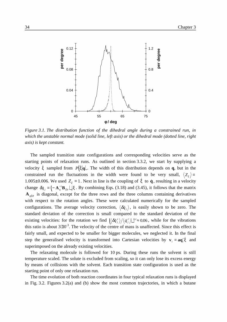
34 Chapter 3

The sampled transition state configurations and corresponding velocities serve as the

starting points of relaxation runs. As outlined in section 3.3.2, we start by supplying a

velocity �ξ sampled from ( )P �ξ q . The width of this distribution depends on q, but in the

constrained run the fluctuations in the width were found to be very small, Zξ =1.005±0.006. We used Zξ = 1. Next in line is the coupling of �ξ to �q , resulting in a velocity

change ( )δ ξσ�qj q j= − −A B1 ξ . By combining Eqs. (3.18) and (3.45), it follows that the matrix

A qξσ is diagonal, except for the three rows and the three columns containing derivatives

with respect to the rotation angles. These were calculated numerically for the sampled

configurations. The average velocity correction, δ �qj , is easily shown to be zero. The

standard deviation of the correction is small compared to the standard deviation of the

existing velocities: for the rotation we find ( )δ � � .q qj j2 2 1 2 0 06≈ , while for the vibrations

this ratio is about 3⋅10-3. The velocity of the centre of mass is unaffected. Since this effect is

fairly small, and expected to be smaller for bigger molecules, we neglected it. In the final

step the generalised velocity is transformed into Cartesian velocities by v aqi ir= �ξ and

superimposed on the already existing velocities.The relaxating molecule is followed for 10 ps. During these runs the solvent is still

temperature scaled. The solute is excluded from scaling, so it can only lose its excess energyby means of collisions with the solvent. Each transition state configuration is used as thestarting point of only one relaxation run.

The time evolution of both reaction coordinates in four typical relaxation runs is displayedin Fig. 3.2. Figures 3.2(a) and (b) show the most common trajectories, in which a butane

0

0.04

0.08

0.12

45 55 65 75

φφ / deg

per

degr

ee

0

0.4

0.8

1.2

per

degr

ee

Figure 3.1. The distribution function of the dihedral angle during a constrained run, inwhich the unstable normal mode (solid line, left axis) or the dihedral mode (dotted line, rightaxis) is kept constant.

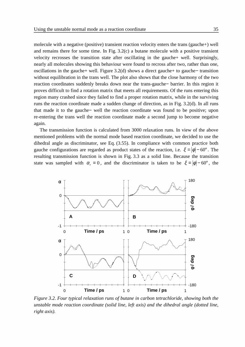
Using the unstable normal mode as a reaction coordinate 35

molecule with a negative (positive) transient reaction velocity enters the trans (gauche+) welland remains there for some time. In Fig. 3.2(c) a butane molecule with a positive transientvelocity recrosses the transition state after oscillating in the gauche+ well. Surprisingly,nearly all molecules showing this behaviour were found to recross after two, rather than one,oscillations in the gauche+ well. Figure 3.2(d) shows a direct gauche+ to gauche− transitionwithout equilibration in the trans well. The plot also shows that the close harmony of the tworeaction coordinates suddenly breaks down near the trans-gauche− barrier. In this region itproves difficult to find a rotation matrix that meets all requirements. Of the runs entering thisregion many crashed since they failed to find a proper rotation matrix, while in the survivingruns the reaction coordinate made a sudden change of direction, as in Fig. 3.2(d). In all runsthat made it to the gauche− well the reaction coordinate was found to be positive; uponre-entering the trans well the reaction coordinate made a second jump to become negativeagain.

The transmission function is calculated from 3000 relaxation runs. In view of the abovementioned problems with the normal mode based reaction coordinate, we decided to use thedihedral angle as discriminator, see Eq. (3.55). In compliance with common practice bothgauche configurations are regarded as product states of the reaction, i.e. ξ φ= − °60 . Theresulting transmission function is shown in Fig. 3.3 as a solid line. Because the transitionstate was sampled with αr = 0, and the discriminator is taken to be ξ φ= − °60 , the

A

-1

0

0 1Time / ps

α

B

0 1Time / ps-180

180

φ / d

eg

C

-1

0

0 1Time / ps

α

D

0 1Time / ps-180

180

φ / d

eg

Figure 3.2. Four typical relaxation runs of butane in carbon tetrachloride, showing both theunstable mode reaction coordinate (solid line, left axis) and the dihedral angle (dotted line,right axis).

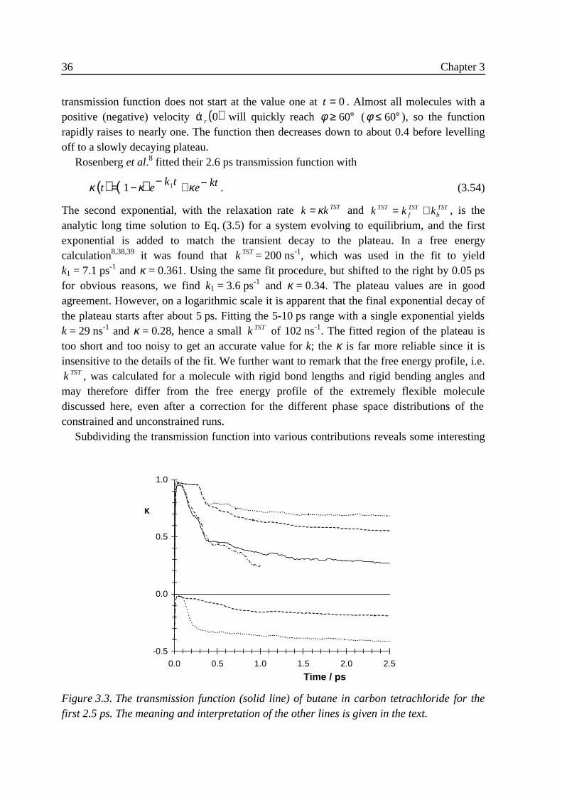
36 Chapter 3

transmission function does not start at the value one at t = 0 . Almost all molecules with apositive (negative) velocity ( )�α r 0 will quickly reach φ ≥ °60 (φ ≤ °60 ), so the functionrapidly raises to nearly one. The function then decreases down to about 0.4 before levellingoff to a slowly decaying plateau.

Rosenberg et al.8 fitted their 2.6 ps transmission function with

( ) ( )κ κ κt e k t e kt= − − + −1 1 . (3.54)

The second exponential, with the relaxation rate k kTST= κ and k k kTSTfTST

bTST= + , is the

analytic long time solution to Eq. (3.5) for a system evolving to equilibrium, and the firstexponential is added to match the transient decay to the plateau. In a free energycalculation8,38,39 it was found that kTST= 200 ns-1, which was used in the fit to yieldk1 = 7.1 ps-1 and κ = 0.361. Using the same fit procedure, but shifted to the right by 0.05 psfor obvious reasons, we find k1 = 3.6 ps-1 and κ = 0.34. The plateau values are in goodagreement. However, on a logarithmic scale it is apparent that the final exponential decay ofthe plateau starts after about 5 ps. Fitting the 5-10 ps range with a single exponential yieldsk = 29 ns-1 and κ = 0.28, hence a small kTST of 102 ns-1. The fitted region of the plateau istoo short and too noisy to get an accurate value for k; the κ is far more reliable since it isinsensitive to the details of the fit. We further want to remark that the free energy profile, i.e.kTST, was calculated for a molecule with rigid bond lengths and rigid bending angles andmay therefore differ from the free energy profile of the extremely flexible moleculediscussed here, even after a correction for the different phase space distributions of theconstrained and unconstrained runs.

Subdividing the transmission function into various contributions reveals some interesting

-0.5

0.0

0.5

1.0

0.0 0.5 1.0 1.5 2.0 2.5

Time / ps

κ

Figure 3.3. The transmission function (solid line) of butane in carbon tetrachloride for thefirst 2.5 ps. The meaning and interpretation of the other lines is given in the text.

Using the unstable normal mode as a reaction coordinate 37

features that are not apparent from the function itself. In Fig. 3.3 the upper (lower) dashedline represents the contribution f + ( f − ) to κ of molecules that have reached gauche+ attime t, after having started with a positive (negative) transient velocity, i.e.,

( )( )[ ] ( ) ( )[ ] ( )[ ]

( )[ ] ( ) ( )[ ]f ttr r r

r r r

± = ±± − °

±

δ α θ θ φ

δ α θ

0 0 0 60

0 0 0

� �

� �

α α

α α. (3.55)

The upper dashed line nearly starts at the value one, so almost all molecules with a positivetransient velocity are in the gauche+ well. After about 0.3 ps the line suddenly drops due to amassive recrossing, the elapsed time corresponding to twice the period of an oscillation inthe gauche+ well, as in Fig. 3.2(c). The decrease of the function is larger than the actualfraction of recrossing trajectories, indicating that the recrossing trajectories have on average ahigher initial velocity than the non-recrossing trajectories. As time goes by the functiongradually decreases to its equilibrium value without showing any structure. The lower dashedline corresponds to molecules that have reached the gauche+ well after having started with anegative transient velocity. This line starts at zero and decreases only gradually. The meantransient velocity of these trajectories is only about a third of the average transient velocity,meaning that this kind of trajectory is much more likely than it appears from the plot. Thegradual decrease of the line is predominantly caused by an increase in the average transientvelocity, rather than by the small rise in the number of molecules reaching gauche+.

The dotted lines give the contribution to κ of those molecules that have reached either oneof the two gauche wells, again grouped according to their transient velocity. They differ fromthe dashed lines by those molecules that have reached the gauche− well. At the bottom of theplot the difference between the dotted and the dashed line rapidly increases after about 0.1 psdue to direct gauche+ to gauche− transitions, as in Fig. 3.2(d). The average transient velocityof these trajectories is well above the overall average, since direct gauche+ to gauche−transitions account for only 17% of the trajectories with a negative transient velocity. Theupper dotted line and the upper dashed line coincide for the first 0.4 ps and then slowly growapart. It takes about 0.2 ps before the first molecules with a (small) positive transient velocityreach gauche−. After 0.4 ps their numbers start to increase and so does their average transientvelocity: it looks as though a considerable fraction of the molecules that leave gauche+ aftera double oscillation proceed directly to the gauche− well. The transmission function, thesolid line, is obtained as the sum of the two dotted lines. It is seen then that the rapid declinebetween 0.1 and 0.4 ps is the combined effect of two independent processes. From the abovediscussion and the plots of individual relaxation runs it is obvious that the reaction tends tothe low friction regime.

We also calculated the transmission function using the unstable normal mode as thereaction coordinate to monitor the relaxation runs. In view of the particular problems of thiscoordinate, as discussed above, we assumed that:i) Molecules with a positive reaction coordinate are in a product well. Considering the

jumpy behaviour of the coordinate in the gauche− well, this properly includes gauche− asbeing a product.

38 Chapter 3

ii) Crashed runs are in a product configuration for the rest of the run. Since runs are found tocrash when a molecule enters the gauche− well, this is correct as long as the moleculedoes not return to the trans well (which does occur after 0.5 ps).

Figure 3.3 shows the transmission function calculated from 1000 relaxation runs of 1 ps as adash-dotted line. There is a good resemblance to the solid line. The difference between thetwo curves after about 0.5 ps is attributed to the failure of the second assumption. In the 1 psinterval already 14% of the runs aborted prematurely.

In a third set of relaxation runs the usual technique of replacing all velocities of thesampled transition state configurations by velocities sampled from a Maxwellian distributionwas used, Eq. (3.49). The transient velocity of the reaction coordinate was obtained byprojecting the assigned Cartesian velocities onto the unstable normal mode. The transmissionfunction, which is not shown here, was identical to the one discussed above to within about0.01. This indicates that the assumptions underlying our velocity assignment are justified.

3 .5 .2 Liquid rigidified n-butane

As a second test-case we study the isomerisation process of liquid n-butane. Theappealing feature of this model is the high number of barrier crossings at little computationalexpense. This allows for a direct determination of the rate constant from the time evolutionof the fractions trans and gauche. Edberg et al.2 studied the relaxation of non-equilibriumboxes with all molecules initially in the same configuration. Brown and Clarke1 showed thatthe rate constant can also be calculated from an equilibrium run by studying the relaxation toequilibrium of those molecules that are trans (gauche) at some time t.

The butane model employed in this section is the one by Brown and Clarke.1 The butanemolecule consists of four pointmasses interacting by Lennard-Jones potentials. The bondlengths and the bending angles are rigidified by means of five distance constraints, leavingthe dihedral as the sole internal degree of freedom. The torsional energy is modelled by theRyckaert-Bellemans potential. The saddle point of this molecule is exactly identical to theone of the previous section. We now ought to calculate the unstable normal mode Qc of theconstrained molecule, a mode that does not couple to the constrained coordinates. Instead,we will make use of the unstable normal mode Q r of the unconstrained molecule. Thismode, in comparison with the other normal modes, is indeed only weakly coupled to theconstrained coordinates. For a molecule as simple as the current butane model it isstraightforward to calculate the accuracy of this approximation, Q Qc r⋅ = 0 995. , so it will beof little effect.

A simulation box was made by placing 108 randomly orientated molecules, all in thesaddle point configuration, at random points within spheres centred around the lattice pointsof a simple cubic lattice. The unstable normal mode of the first molecule is constrained in theruns to come, while the dihedrals of the remaining 107 bath molecules are free. The excessenergy of the box was released by an energy minimisation, followed by a 0.5 ns equilibrationMD run. In a subsequent 3 ns production run the saddle plane was sampled, saving aconfiguration every picosecond. A thermostat37 maintained an average temperature of

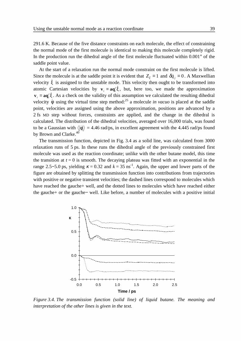
Using the unstable normal mode as a reaction coordinate 39

291.6 K. Because of the five distance constraints on each molecule, the effect of constrainingthe normal mode of the first molecule is identical to making this molecule completely rigid.In the production run the dihedral angle of the first molecule fluctuated within 0.001° of thesaddle point value.

At the start of a relaxation run the normal mode constraint on the first molecule is lifted.Since the molecule is at the saddle point it is evident that Zξ = 1 and δ �qj = 0 . A Maxwellianvelocity �ξ is assigned to the unstable mode. This velocity then ought to be transformed intoatomic Cartesian velocities by v aqi i

c= �ξ , but, here too, we made the approximationv aqi i

r= �ξ . As a check on the validity of this assumption we calculated the resulting dihedralvelocity �φ using the virtual time step method:25 a molecule in vacuo is placed at the saddlepoint, velocities are assigned using the above approximation, positions are advanced by a2 fs MD step without forces, constraints are applied, and the change in the dihedral iscalculated. The distribution of the dihedral velocities, averaged over 16,000 trials, was foundto be a Gaussian with �φ = 4.46 rad/ps, in excellent agreement with the 4.445 rad/ps foundby Brown and Clarke.40

The transmission function, depicted in Fig. 3.4 as a solid line, was calculated from 3000relaxation runs of 5 ps. In these runs the dihedral angle of the previously constrained firstmolecule was used as the reaction coordinate; unlike with the other butane model, this timethe transition at t = 0 is smooth. The decaying plateau was fitted with an exponential in therange 2.5−5.0 ps, yielding κ = 0.32 and k = 35 ns-1. Again, the upper and lower parts of thefigure are obtained by splitting the transmission function into contributions from trajectorieswith positive or negative transient velocities; the dashed lines correspond to molecules whichhave reached the gauche+ well, and the dotted lines to molecules which have reached eitherthe gauche+ or the gauche− well. Like before, a number of molecules with a positive initial

-0.5

0.0

0.5

1.0

0.0 0.5 1.0 1.5 2.0 2.5

Time / ps

κ

Figure 3.4. The transmission function (solid line) of liquid butane. The meaning andinterpretation of the other lines is given in the text.

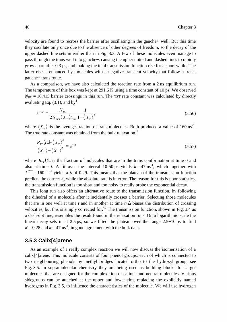
40 Chapter 3

velocity are found to recross the barrier after oscillating in the gauche+ well. But this timethey oscillate only once due to the absence of other degrees of freedom, so the decay of theupper dashed line sets in earlier than in Fig. 3.3. A few of these molecules even manage topass through the trans well into gauche−, causing the upper dotted and dashed lines to rapidlygrow apart after 0.3 ps, and making the total transmission function rise for a short while. Thelatter rise is enhanced by molecules with a negative transient velocity that follow a trans-gauche− trans route.

As a comparison, we have also calculated the reaction rate from a 2 ns equilibrium run.The temperature of this box was kept at 291.6 K using a time constant of 10 ps. We observedNBC = 16,415 barrier crossings in this run. The TST rate constant was calculated by directlyevaluating Eq. (3.1), and by1

kN

N X t XTST BC

mol T run T

=−2

1

1, (3.56)

where XT is the average fraction of trans molecules. Both produced a value of 160 ns-1.The true rate constant was obtained from the bulk relaxation,1

( )R t X

X Xe

TT T

T T

kt−

−= −

2

2 (3.57)

where ( )R tTT is the fraction of molecules that are in the trans conformation at time 0 andalso at time t. A fit over the interval 10-50 ps yields k = 47 ns-1, which together withkTST= 160 ns-1 yields a κ of 0.29. This means that the plateau of the transmission functionpredicts the correct κ, while the absolute rate is in error. The reason for this is poor statistics,the transmission function is too short and too noisy to really probe the exponential decay.

This long run also offers an alternative route to the transmission function, by followingthe dihedral of a molecule after it incidentally crosses a barrier. Selecting those moleculesthat are in one well at time t and in another at time t+∆ biases the distribution of crossingvelocities, but this is simply corrected for.40 The transmission function, shown in Fig. 3.4 asa dash-dot line, resembles the result found in the relaxation runs. On a logarithmic scale thelinear decay sets in at 2.5 ps, so we fitted the plateau over the range 2.5−10 ps to findκ = 0.28 and k = 47 ns-1, in good agreement with the bulk data.

3 .5 .3 Calix[4]arene

As an example of a really complex reaction we will now discuss the isomerisation of acalix[4]arene. This molecule consists of four phenol groups, each of which is connected totwo neighbouring phenols by methyl bridges located ortho to the hydroxyl group, seeFig. 3.5. In supramolecular chemistry they are being used as building blocks for largermolecules that are designed for the complexation of cations and neutral molecules. Varioussidegroups can be attached at the upper and lower rim, replacing the explicitly namedhydrogens in Fig. 3.5, to influence the characteristics of the molecule. We will use hydrogen

Using the unstable normal mode as a reaction coordinate 41

sidegroups only. The most interesting feature in the current context is that this molecule hasfour stable conformations. The favourable configuration is one in which all phenol groupspoint in the same direction. This conformation, the so-called ‘cone’, is stabilised by a cyclicarray of four hydrogen bonds at the lower rim. Its chalice-like shape gives its name to thisclass of molecules. Flipping one phenol group, with two methyl bridges acting as hinges andthe hydroxyl group swinging through the annulus, yields the partial cone or ‘paco’. It is thisparticular reaction step that will be studied here. In a following reaction step either one of thetwo neighbouring phenol groups can flip over to form the ‘1,2-alternate’, or the opposingphenol group can rotate to form the ‘1,3-alternate’. After two more steps the cone istransformed into an inverted cone. The rate of this inversion process has been measured by1H NMR to be about 150 s-1 at room temperature.41,42

Computational studies on the conformations of calix[4]arenes with various sidegroupshave mainly focused on the energy minima and the resulting conformational distribution,using a variety of force fields.43-46 In a recent article by Fischer et al.47 the saddle points andthe reaction paths between the local minima of the PES were calculated using the ConjugatedPeak Refinement algorithm. The cone to paco transition was found to be the rate limitingstep for cone inversion, but this energy-based picture could change if entropic effects areincluded. With the all-hydrogen CHARMM parameter set 2247,48 the saddle point lies15.2 kcal/mol above the minimum of the cone and 5.6 kcal/mol above the minimum of thepaco. This saddle point was taken as the starting point of the present calculations, employingthe same force field. The accuracy of the saddle point after minimising the gradient is( )Σ i iF2 1 2 = 5.8⋅10−10 kJ mol-1 nm-1. All 3N normal modes of the molecule were calculated bydiagonalising the Hessian matrix. The eigenvalues of the zero-frequency normal modes weresmaller than any other frequency by almost six orders of magnitude. The unstable normalmode, Q r , pointed in the direction of the paco.

Since we intend to do MD runs with a molecule with L constraints on the bonds containinghydrogen, we should have calculated the 3N − L normal modes

~Q j of the σ-constrainedmolecule. Only for these modes will the velocity transformation v aqi i

r= ~ �ξ hold (to lowestorder). If we use v aqi i

r= �ξ on the regular modes, then SHAKEing the molecule will eliminatethe velocities along σ, hence effectively reduce �ξ . We then would have to go through the

Figure 3.5. The cone (left) and paco (right) conformation of a calix[4]arene.

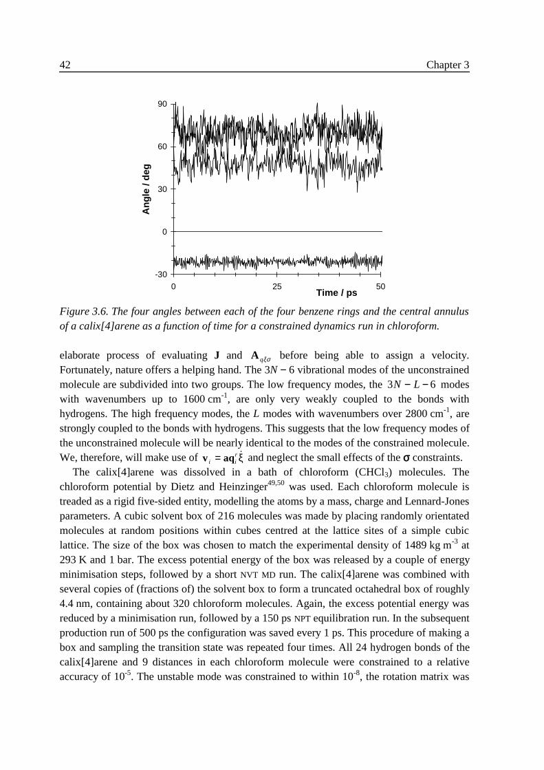
42 Chapter 3

elaborate process of evaluating J and A qξσ before being able to assign a velocity.Fortunately, nature offers a helping hand. The 3N − 6 vibrational modes of the unconstrainedmolecule are subdivided into two groups. The low frequency modes, the 3 6N L− − modeswith wavenumbers up to 1600 cm-1, are only very weakly coupled to the bonds withhydrogens. The high frequency modes, the L modes with wavenumbers over 2800 cm-1, arestrongly coupled to the bonds with hydrogens. This suggests that the low frequency modes ofthe unconstrained molecule will be nearly identical to the modes of the constrained molecule.We, therefore, will make use of v aqi i

r= �ξ and neglect the small effects of the σ constraints.The calix[4]arene was dissolved in a bath of chloroform (CHCl3) molecules. The

chloroform potential by Dietz and Heinzinger49,50 was used. Each chloroform molecule istreaded as a rigid five-sided entity, modelling the atoms by a mass, charge and Lennard-Jonesparameters. A cubic solvent box of 216 molecules was made by placing randomly orientatedmolecules at random positions within cubes centred at the lattice sites of a simple cubiclattice. The size of the box was chosen to match the experimental density of 1489 kg m-3 at293 K and 1 bar. The excess potential energy of the box was released by a couple of energyminimisation steps, followed by a short NVT MD run. The calix[4]arene was combined withseveral copies of (fractions of) the solvent box to form a truncated octahedral box of roughly4.4 nm, containing about 320 chloroform molecules. Again, the excess potential energy wasreduced by a minimisation run, followed by a 150 ps NPT equilibration run. In the subsequentproduction run of 500 ps the configuration was saved every 1 ps. This procedure of making abox and sampling the transition state was repeated four times. All 24 hydrogen bonds of thecalix[4]arene and 9 distances in each chloroform molecule were constrained to a relativeaccuracy of 10-5. The unstable mode was constrained to within 10-8, the rotation matrix was

-30

0

30

60

90

0 25 50Time / ps

Ang

le /

deg

Figure 3.6. The four angles between each of the four benzene rings and the central annulusof a calix[4]arene as a function of time for a constrained dynamics run in chloroform.

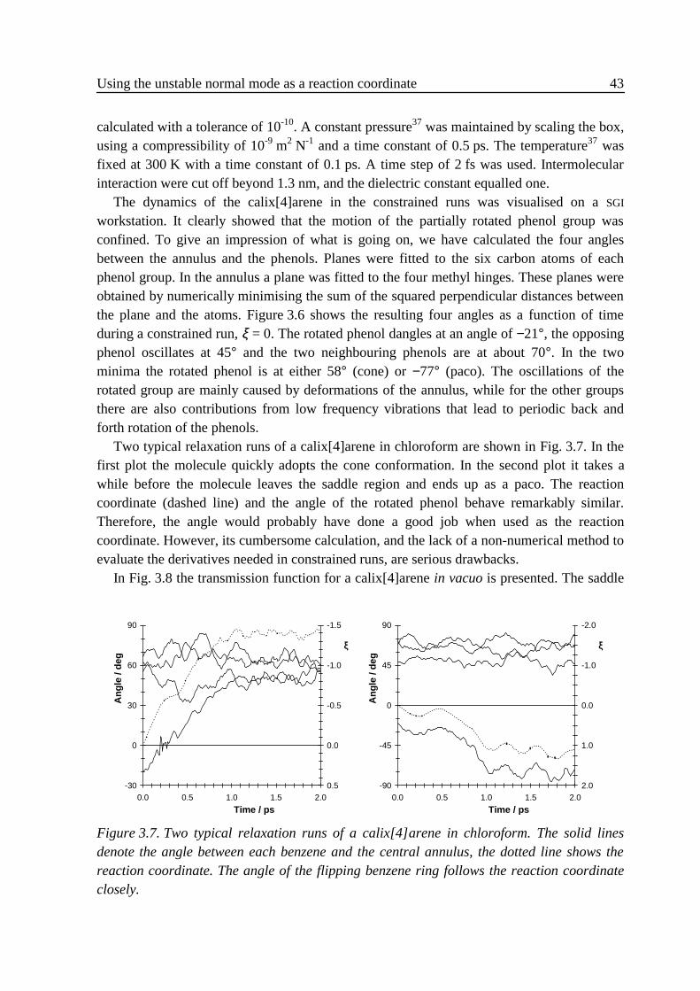
Using the unstable normal mode as a reaction coordinate 43

calculated with a tolerance of 10-10. A constant pressure37 was maintained by scaling the box,using a compressibility of 10-9 m2 N-1 and a time constant of 0.5 ps. The temperature37 wasfixed at 300 K with a time constant of 0.1 ps. A time step of 2 fs was used. Intermolecularinteraction were cut off beyond 1.3 nm, and the dielectric constant equalled one.

The dynamics of the calix[4]arene in the constrained runs was visualised on a SGI

workstation. It clearly showed that the motion of the partially rotated phenol group wasconfined. To give an impression of what is going on, we have calculated the four anglesbetween the annulus and the phenols. Planes were fitted to the six carbon atoms of eachphenol group. In the annulus a plane was fitted to the four methyl hinges. These planes wereobtained by numerically minimising the sum of the squared perpendicular distances betweenthe plane and the atoms. Figure 3.6 shows the resulting four angles as a function of timeduring a constrained run, ξ = 0. The rotated phenol dangles at an angle of −21°, the opposingphenol oscillates at 45° and the two neighbouring phenols are at about 70°. In the twominima the rotated phenol is at either 58° (cone) or −77° (paco). The oscillations of therotated group are mainly caused by deformations of the annulus, while for the other groupsthere are also contributions from low frequency vibrations that lead to periodic back andforth rotation of the phenols.

Two typical relaxation runs of a calix[4]arene in chloroform are shown in Fig. 3.7. In thefirst plot the molecule quickly adopts the cone conformation. In the second plot it takes awhile before the molecule leaves the saddle region and ends up as a paco. The reactioncoordinate (dashed line) and the angle of the rotated phenol behave remarkably similar.Therefore, the angle would probably have done a good job when used as the reactioncoordinate. However, its cumbersome calculation, and the lack of a non-numerical method toevaluate the derivatives needed in constrained runs, are serious drawbacks.

In Fig. 3.8 the transmission function for a calix[4]arene in vacuo is presented. The saddle

-30

0

30

60

90

0.0 0.5 1.0 1.5 2.0

Time / ps

Ang

le /

deg

-1.5

-1.0

-0.5

0.0

0.5

ξ

-90

-45

0

45

90

0.0 0.5 1.0 1.5 2.0

Time / ps

Ang

le /

deg

-2.0

-1.0

0.0

1.0

2.0

ξ

Figure 3.7. Two typical relaxation runs of a calix[4]arene in chloroform. The solid linesdenote the angle between each benzene and the central annulus, the dotted line shows thereaction coordinate. The angle of the flipping benzene ring follows the reaction coordinateclosely.

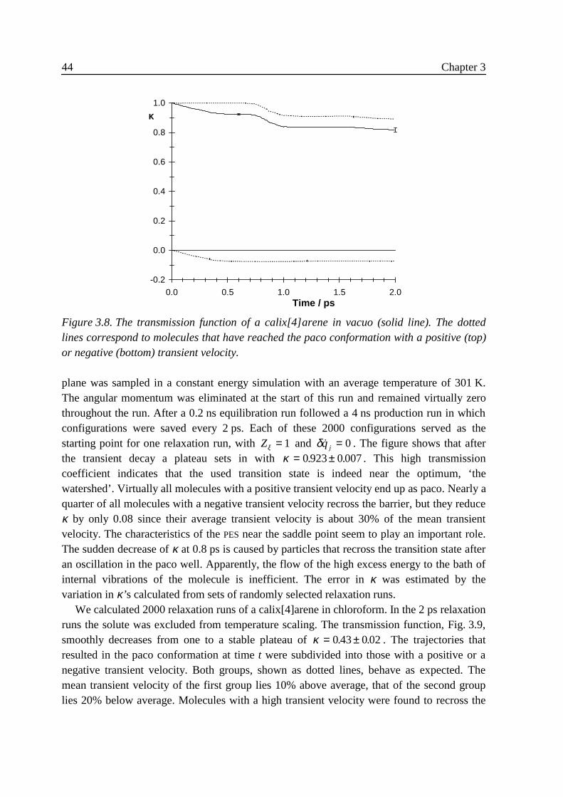
44 Chapter 3

plane was sampled in a constant energy simulation with an average temperature of 301 K.The angular momentum was eliminated at the start of this run and remained virtually zerothroughout the run. After a 0.2 ns equilibration run followed a 4 ns production run in whichconfigurations were saved every 2 ps. Each of these 2000 configurations served as thestarting point for one relaxation run, with Zξ = 1 and δ �qj = 0 . The figure shows that afterthe transient decay a plateau sets in with κ = ±0 923 0 007. . . This high transmissioncoefficient indicates that the used transition state is indeed near the optimum, ‘thewatershed’. Virtually all molecules with a positive transient velocity end up as paco. Nearly aquarter of all molecules with a negative transient velocity recross the barrier, but they reduceκ by only 0.08 since their average transient velocity is about 30% of the mean transientvelocity. The characteristics of the PES near the saddle point seem to play an important role.The sudden decrease of κ at 0.8 ps is caused by particles that recross the transition state afteran oscillation in the paco well. Apparently, the flow of the high excess energy to the bath ofinternal vibrations of the molecule is inefficient. The error in κ was estimated by thevariation in κ’s calculated from sets of randomly selected relaxation runs.

We calculated 2000 relaxation runs of a calix[4]arene in chloroform. In the 2 ps relaxationruns the solute was excluded from temperature scaling. The transmission function, Fig. 3.9,smoothly decreases from one to a stable plateau of κ = ±0 43 0 02. . . The trajectories thatresulted in the paco conformation at time t were subdivided into those with a positive or anegative transient velocity. Both groups, shown as dotted lines, behave as expected. Themean transient velocity of the first group lies 10% above average, that of the second grouplies 20% below average. Molecules with a high transient velocity were found to recross the

-0.2

0.0

0.2

0.4

0.6

0.8

1.0

0.0 0.5 1.0 1.5 2.0Time / ps

κ

Figure 3.8. The transmission function of a calix[4]arene in vacuo (solid line). The dottedlines correspond to molecules that have reached the paco conformation with a positive (top)or negative (bottom) transient velocity.

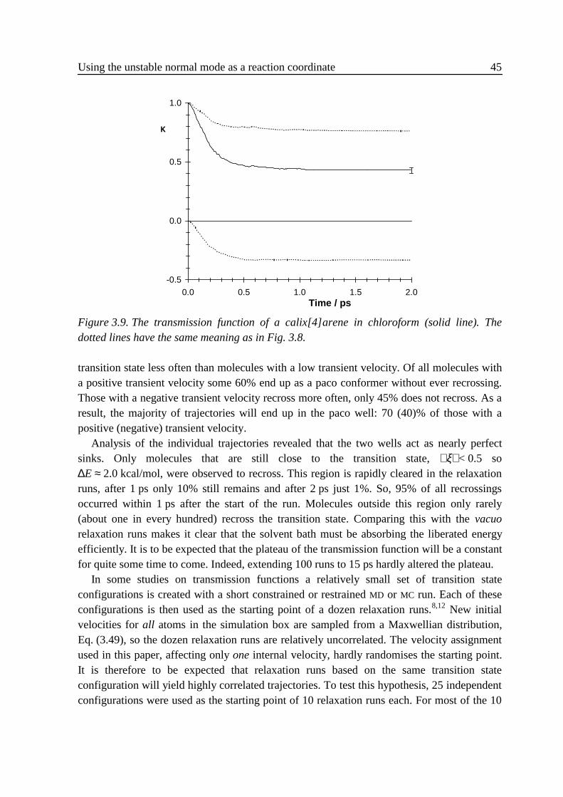
Using the unstable normal mode as a reaction coordinate 45

transition state less often than molecules with a low transient velocity. Of all molecules witha positive transient velocity some 60% end up as a paco conformer without ever recrossing.Those with a negative transient velocity recross more often, only 45% does not recross. As aresult, the majority of trajectories will end up in the paco well: 70 (40)% of those with apositive (negative) transient velocity.

Analysis of the individual trajectories revealed that the two wells act as nearly perfectsinks. Only molecules that are still close to the transition state, ξ< 0.5 so∆E ≈ 2.0 kcal/mol, were observed to recross. This region is rapidly cleared in the relaxationruns, after 1 ps only 10% still remains and after 2 ps just 1%. So, 95% of all recrossingsoccurred within 1 ps after the start of the run. Molecules outside this region only rarely(about one in every hundred) recross the transition state. Comparing this with the vacuorelaxation runs makes it clear that the solvent bath must be absorbing the liberated energyefficiently. It is to be expected that the plateau of the transmission function will be a constantfor quite some time to come. Indeed, extending 100 runs to 15 ps hardly altered the plateau.

In some studies on transmission functions a relatively small set of transition stateconfigurations is created with a short constrained or restrained MD or MC run. Each of theseconfigurations is then used as the starting point of a dozen relaxation runs.8,12 New initialvelocities for all atoms in the simulation box are sampled from a Maxwellian distribution,Eq. (3.49), so the dozen relaxation runs are relatively uncorrelated. The velocity assignmentused in this paper, affecting only one internal velocity, hardly randomises the starting point.It is therefore to be expected that relaxation runs based on the same transition stateconfiguration will yield highly correlated trajectories. To test this hypothesis, 25 independentconfigurations were used as the starting point of 10 relaxation runs each. For most of the 10

-0.5

0.0

0.5

1.0

0.0 0.5 1.0 1.5 2.0Time / ps

κ

Figure 3.9. The transmission function of a calix[4]arene in chloroform (solid line). Thedotted lines have the same meaning as in Fig. 3.8.

46 Chapter 3

trajectories the time evolution of the reaction coordinate is more or less the same, but runswith a high transient velocity were sometimes seen to deviate from the main stream. Thesame 25 configurations were also each used to start 10 relaxation runs with a Maxwellianvelocity for all atoms. These trajectories were found to be less correlated. Surprisingly then,the transmission functions calculated for both sets of 250 runs are similar.

Sofar, little has been said about the Z ξσ of Eq. (3.42). We first take a look at Z σ ,Eq. (3.38). The L constrained bond lengths are commonly defined as ( )σ l l H l A AHl= − −r r, ,

2 2 ,where l AH is the equilibrium length of the A−H bond.23 It then follows that the diagonalelements of Z σ are constants, ( )4 2 1 1l m mAH H A

− −+ . Since only four atoms are involved in twodistance constraints, namely the carbons of the methyl hinges, there are only eightnon-vanishing off-diagonal elements. They are of the form 42 1l mC C HCH

− cosϕ , which amountsto about −1/40th of the diagonal elements. These elements are not constants, but the harmonicbending potential limits the fluctuations. The Zξ , Eq. (3.48), is nearly constant during theconstrained run at 1.00010±0.00011. From the above discussion on low frequency and highfrequency modes it follows that the elements of D are of the order Σ k k

rkld d , Eq. (3.29); the

exact value amounts to about 0 ± 1⋅10-3. We then arrive at the final result, Z ξσ

= 3.658 ± 0.002⋅10-32. Because of the relatively very small fluctuations this term can savelybe neglected when calculating the constrained average.

In the so-called [14]metacyclophane the hydroxyl groups at the lower rim of thecalix[4]arene have been replaced by hydrogens. This molecule is extremely flexible due tothe absence of stabilising hydrogen bonds. The energy barriers between the local minima,3.8 kcal/mol,47 are only slightly higher than those of n-butane. A short constrained MD runshowed that this molecule is much to floppy to be studied with the reactive flux method.Even with a constraint on the unstable normal mode of the cone to paco saddle point, themolecule is still flexible enough to allow for spontaneous conformational changes. Thisclearly shows the limited effect of the normal mode constraint on the remaining vibrations ofthe molecule. In principle, this problem could also have occurred with the calix[4]arene, butthere the energy barriers are high enough to suppress side-reactions.

3 .6 ConclusionsA new versatile reaction coordinate was introduced that can be used on a wide variety of

reactions. In combination with the reactive flux method the transmission functions of severalreactions have been calculated. The results for isomerising n-butane are in good agreementwith results found previously. A calix[4]arene served as an example of a more complexisomerising molecule. Two pitfalls of the technique, in fact problems of any reactioncoordinate, were discussed: i) the sign of the reaction coordinate need not be the samethroughout the entire reactant or product well, and ii) simultaneous reactions in the moleculeare not suppressed. Provided these two problems do not arise, the reaction coordinate isfound to be a very efficient one. The coordinate is shown to yield a high plateau value, atleast for reactions in vacuo, at small computational expense. In the following chapter the

Using the unstable normal mode as a reaction coordinate 47

calculation of the free energy of a solvated calix[4]arene will be discussed using the samereaction coordinate.

3 .7 Appendix: calculation of Z ξ.Starting with the identity

Z ZT Tξ

ξσ ξσξ0

D 1Z Z

0

D 1

=

−1 , (3.58)

replacing Z ξσ−1 by equation (3.39) and evaluating all resulting matrix products by using the

combination rules that follow from Z Z 1ξσ ξσ− =1 yields

ZTξ

ξσσ

0

D 1Z

L

0 M

=

1. (3.59)

Taking the determinant produces the final result,

Zξ ξσ σ= Z M . (3.60)

3 .8 References1 D. Brown and J. H. R. Clarke, J. Chem. Phys. 92, 3062 (1990).2 R. Edberg, D. J. Evans and G. P. Morriss, J. Chem. Phys. 87, 5700 (1987).3 P. Hänggi, P. Talkner and M. Borkovec, Rev. Mod. Phys. 62, 251 (1990).4 H. Eyring, J. Chem. Phys. 3, 107 (1935).5 J. Horiuti, Bull. Chem. Soc. Jpn. 13, 210 (1938)6 T. Yamamoto, J. Chem. Phys. 33, 281 (1960).7 D. Chandler, J. Chem. Phys. 68, 2959 (1978).8 R. O. Rosenberg, B. J. Berne and D. Chandler, Chem. Phys. Lett. 75, 162 (1980).9 I. Benjamin and A. Pohorille, J. Chem. Phys. 98, 236 (1993).10 R. A. Kuharski, D. Chandler, J. A. Montgomery Jr., F. Rabii and S. J. Singer, J. Phys.

Chem. 92, 3261 (1988).11 D. Chandler and R. A. Kuharski, Faraday Discuss. Chem. Soc. 85, 329 (1988).12 M. A. Wilson and D. Chandler, Chem. Phys. 149, 11 (1990).13 J. M. Depaepe, J.-P. Ryckaert and A. Bellemans, Mol. Phys. 78, 1575 (1993).14 K. D. Hammonds, I. R. McDonald and J.-P. Ryckaert, Chem. Phys. Lett. 213, 27 (1993).15 I. Ghosh and J. A. McCammon, Biophys. J. 51, 637 (1987).16 R. M. Whitnell and K. R. Wilson, Rev. Comp. Chem. IV , 67 (1993).17 J. B. Anderson, Adv. Chem. Phys. XCI , 381 (1995).18 H. M. Pickett and H. L. Strauss, J. Am. Chem. Soc. 92, 7281 (1970).19 C. Eckart, Phys. Rev. 47, 552 (1935).20 K. Fukui, Acc. Chem. Res. 14, 363 (1981).

48 Chapter 3

21 J.-P. Ryckaert, G. Ciccotti and H. J. C. Berendsen, J. Comp. Phys. 23, 327 (1977).22 D. J. Tobias and C. L. Brooks III, J. Chem. Phys. 89, 5115 (1988).23 G. Ciccotti and J.-P. Ryckaert, Comp. Phys. Rep. 4, 347 (1986).24 E. A. Carter, G. Ciccotti, J. T. Hynes and R. Kapral, Chem. Phys. Lett. 156, 472 (1989).25 J.-P. Ryckaert and G. Ciccotti, Mol. Phys. 58, 1125 (1986).26 W. F. van Gunsteren and H. J. C. Berendsen, Groningen Molecular Simulation Library,

Groningen, The Netherlands, 1987.27 C. J. Cerjan and W. H. Miller, J. Chem. Phys. 75, 2800 (1981)28 S. Bell and J. S. Crighton, J. Chem. Phys. 80, 2464 (1984).29 F. Jensen, J. Chem. Phys. 102, 6706 (1995).30 S. Fischer and M. Karplus, Chem. Phys. Lett. 194, 252 (1992).31 B. R. Brooks, R. E. Bruccoleri, B. D. Olafson, D. J. States, S. Swaminathan and M.

Karplus, J. Comp. Chem. 4, 187 (1983).32 W. H. Press, B. P. Flannery, S. A. Teukolsky and W. T. Vetterling, Numerical recipes

(Cambridge University Press, Cambridge, U. K., 1986).33 D. J. Evans, Mol. Phys. 34, 317 (1977).34 H. Goldstein, Classical mechanics (Addison-Wesley, Reading MA, 1980).35 F. T. H. Leuwerink and W. J. Briels, J. Chem. Phys. 103, 4637 (1995).36 We used a bending potential that is quadratic in the angle θ rather than quadratic in cosθ.

The force constant was adapted accordingly, ′ =k kθ θ θsin 0 .37 H. J. C. Berendsen, J. P. M. Postma, W. F. van Gunsteren, A. DiNola and J. R. Haak, J.

Chem. Phys. 81, 3684 (1984).38 D. W. Rebertus, B. J. Berne and D. Chandler, J. Chem. Phys. 70, 3395 (1979).39 D. Chandler and B. J. Berne, J. Chem. Phys. 71, 5386 (79).40 D. Brown and J. H. R. Clarke, J. Chem. Phys. 93, 4117 (1990); 94, 4684 (1991).41 C. D. Gutsche and L. J. Bauer, J. Am. Chem. Soc. 107, 6052 (1985).42 K. Araki, S. Shinkai and T. Matsuda, Chem. Lett. 1989, 581 (1989).43 P. D. J. Grootenhuis, P. A. Kollman, L. C. Groenen, D. N. Reinhoudt, G. J. van Hummel,

F. Ugozzoli and G. D. Andreetti, J. Am. Chem. Soc. 112, 4165 (1990).44 T. Harada, J. M. Rudzinski and S. Shinkai, Chem. Soc. Perkin Trans. 2 1992, 2109

(1992).45 T. Harada, J. M. Rudzinski, E. Osawa and S. Shinkai, Tetrahedron 49, 5941 (1993).46 J. Royer, F. Bayard and C. Decoret, J. Chim. Phys. 87, 1695 (1990).47 S. Fischer, P. D. J. Grootenhuis, L. C. Groenen, W. P. van Hoorn, F. C. J. M. van Veggel,

D. N. Reinhoudt and M. Karplus, J. Am. Chem. Soc. 117, 1611 (1995).48 J. C. Smith and M. Karplus, J. Am. Chem. Soc. 114, 801 (1992)49 W. Dietz and K. Heinzinger, Ber. Bunsenges. Phys. Chem. 88, 543 (1984); 89, 968

(1985).50 I. G. Tironi and W. F. van Gunsteren, Mol. Phys. 83, 381 (1994).

49

Chapter 4

Free energy and conformational transition

rates of calix[4]arene in chloroform *

AbstractIn a previous article we introduced a reaction coordinate based on the unstable normal

mode at the saddle point of the potential energy surface. We here calculate the free energydistribution along this coordinate for the isomerisation of calix[4]arene in vacuo and inchloroform using umbrella sampling, with one umbrella covering the entire range of thereaction coordinate. An excellent first guess at this umbrella is obtained by performing anormal mode analysis at various points along the reaction path. The isomerisation rateconstant of this reaction is determined using the reactive flux method, and is found to be ingood agreement with experimental data. The rate was found to be independent of the locationof the transition state, as it should be.

4 .1 IntroductionThe forward rate constant k f of a reaction, i.e. the fraction of reactants turned into

products per unit of time, in a solvent is a complicated function of the internal potential ofthe reacting solute molecule(s), the solute-solvent interactions and the solvent-solventinteractions. Molecular dynamics simulations (MD) are perfectly well suited for the numericalanalysis of such involved situations. Based on the statistical mechanical ideas discussedbelow, it is possible to deduce from a total of about 10 nanosecond simulation time areaction rate that is slower by many orders of magnitude. The particular reaction studied hereis the isomerisation of a calix[4]arene in vacuo and in chloroform.

In Eyring’s transition state theory1 (TST) a hyperplane, the transition state, is introduced tosplit configuration space into a reactant space and a product space. This plane ischaracterised by { }( )ξ x i = ≠ξ , where the reaction coordinate { }( )ξ x i is a function of theatomic coordinates. Product space and reactant space are defined by ξ > ≠ξ and ξ < ≠ξ

* W. K. den Otter and W. J. Briels, J. Chem. Phys. 107 4968 (1997).

50 Chapter 4

respectively. The forward rate constant is calculated as the instantaneous product-bound fluxthrough the transition state, normalised by the population of the reactant space:2

( )[ ] ( ) ( )[ ]( )[ ]k f

TST =−

−

≠

≠

δ ξ θ

θ ξ

0 0 0

0

ξ ξ ξ

ξ

� �

. (4.1)

Here the angular brackets denote a canonical average and θ is the Heaviside function.The TST expression is conveniently rewritten as

( )[ ] ( ) ( )[ ]( )[ ]

( )[ ]( )[ ]k f

TST =−

−

−

−

≠

≠

≠

≠

δ ξ θ

δ ξ

δ ξ

θ ξ

0 0 0

0

0

0

ξ ξ ξ

ξ

ξ

ξ

� �

. (4.2)

The second term on the right hand side is the probability of finding the molecule at thetransition state, ( )P ξ ≠ , divided by the probability for the molecule to be in reactant space,

( )P P dR =−∞

≠

∫ ξ ξξ

. (4.3)

We will discuss two techniques for the calculation of the probability distribution ( )P ξ :normal mode analysis in section 4.2.2, and umbrella sampling in section 4.2.3. The first termon the right hand side of Eq. (4.2), the average positive velocity of the reaction coordinate atthe transition state, will be addressed in section 4.2.4. The particular reaction coordinate thatwe will use is discussed in section 4.2.1. Numerical results for the probability function andthe TST isomerisation rate of a calix[4]arene in vacuo and in chloroform are presented insection 4.3.

Transition state theory, by focusing on the instantaneous forward flux, neglects the factthat some fraction of this flux will recross the transition state shortly (order of a picosecond)after having crossed it. Likewise, the forward flux also contains a contribution of ‘productmolecules’ that have crossed the transition state with a negative velocity shortly before theyrecross with a positive velocity. These recrossings are the result of the normal dynamics of areacting molecule, induced by both the internal interactions of the molecule and itsinteractions with the solvent. To a macroscopic observer, though, these rapid recrossings areinvisible, irrelevant. He defines the rate by the number of molecules that are in the reactantwell at time t = 0 and are in the product well at time t, normalised by the overall number ofmolecules in the reactant well at time t = 0. Only if there are no recrossings will his rateequal the TST rate, otherwise TST overestimates the true rate.

In the reactive flux method (RF) the aforementioned macroscopic definition of the rate isrelated to the microscopic behaviour of a single molecule in a solvent by means of Onsager’sregression hypothesis.3,4 The resulting rate expression is

( )( )[ ] ( ) ( )[ ]

( )[ ]k tt

fRF =

− −

−

≠ ≠

≠

δ ξ ξ θ ξ ξ

θ ξ ξ

0 0

0

�ξ. (4.4)

Free energy and conformational transition rates of calix[4]arene in chloroform 51

In comparison with TST, attention has shifted from those molecules that cross the transitionstate with a positive velocity to those molecules that actually end up in the product space atsome time t after crossing the transition state in whatever direction. The rate is oftenexpressed as

( ) ( )k t t kfRF

fTST= κ , (4.5)

( )( )[ ] ( ) ( )[ ]

( )[ ] ( ) ( )[ ]κδ ξ ξ θ ξ ξ

δ ξ ξ θt

t=

− −

−

≠ ≠

≠

0 0

0 0 0

�

� �

ξ

ξ ξ, (4.6)

where ( )κ t is the transmission function. On the time scale of the recrossings, about apicosecond, the transmission function decays from unity at t = 0 to the so-called plateaulevel. The true rate constant is found by inserting this plateau value into Eq. (4.5). Actually,the plateau is not constant but decaying on the time scale of the reaction, but for mostreactions this is too slow to be seen in MD simulations. In a previous article5 we discussed thecalculation of the transmission function of the reaction studied here.

From Eqs. (4.1) and (4.4) one could infer that the calculated rate depends on the definitionof the transition state, i.e. on ξ ≠ and { }( )ξ x i (for simplicity we will neglect the latterdependence). The rate should of course depend on this definition, since it is embodied in thedefinition of the number of reactant molecules, PR , and hence in the therefrom derived rate.But, provided the free energy barrier is high and ξ ≠ lies somewhere near the top, the numberof reactants is virtually independent to the precise location of ξ ≠ , and so must the rate be.The TST rate obviously strongly depends on ξ ≠ ; in the RF method the dynamics incorporatedin the transmission function blurs the picture. Miller6 showed, using Liouville’s theorem, thatthe RF rate is independent of the precise location of the transition state. Chandler4 arrived atthe same conclusion in a discussion based on the separation in time scales betweenrecrossing and reactive events. In section 4.3.3 this independence is verified numerically.

4 .2 Theory

4 .2 .1 Reaction coordinate

We here briefly discuss the unstable normal mode reaction coordinate; an elaborateintroduction is to be found in a previous article.5 The reasoning behind this reactioncoordinate is the fact that in a reactive system most reactant to product trajectories willsurmount the potential energy barrier somewhere near the lowest point of the barrier, i.e. thesaddle point. It is therefore natural to construct a reaction coordinate based on the propertiesof the saddle point. The Taylor expansion of the potential energy around a saddle point, X 0 ,up to second order reads

( ) ( ) ( ) ( )Φ ΦX X X X H X X= + − −0 12

0 0T. (4.7)

52 Chapter 4

For notational convenience, we collect all coordinates of the reacting molecule in a single 3Ndimensional column vector of mass-weighted atomic coordinates, X T =( )m m mT T

N NT

11 2

1 21 2

21 2x x x, , ,� . The Hessian matrix, H, contains all second order derivatives of

the potential energy with respect to the components of X. Its eigenvectors are orthogonal, ororthogonalisable in case of degeneracy, since the Hessian is symmetric. Henceforth, alleigenvectors will be assumed to be normalised. We shall assume that there is no externalfield.

The set of 3N eigenvectors can be split into three groups. First, there are three independentvectors E l that correspond to an overall translation of the molecule. Obviously, they leavethe potential energy unchanged and therefore are eigenvectors of H with eigenvalues zero, asfollows from Eq. (4.7) after replacing X X− 0 by E l . Similarly, there are three independent(assuming a non-linear molecule) eigenvectors Sk corresponding to infinitesimal rotations ofthe molecule. If r x xi i com

0 0 0= − is the vector pointing from the centre of mass of the moleculeto atom i, then an infinitesimal rotation around an axes ek through the centre of mass leadsto the atomic displacements

( ) ( ) ( ) ( )( )S e r e r e rk T

k

T

k

T

N k N

Tm m m= × × ×1 1

02 2

0 0, , ,� . (4.8)

Obviously, assuming orthonormality of the eigenvectors Sk , the three ek are not orthogonal.The six modes of the first two groups are degenerate, they all have eigenvalue zero, if thereis no external field. Finally, the remaining 3 6N − eigenvectors Q j are the normal modes ofvibration.

At an energy minimum all vibrational modes have a non-negative eigenvalue, but at a firstorder saddle point there will be exactly one mode, Q r , with a negative eigenvalue. It is thisunstable normal mode that we are interested in; it points downhill, from the saddle pointtowards the reactant and product wells, while all other modes are pointing uphill. Motion ofthe molecule along this mode, therefore, corresponds to a reaction. The reaction coordinateof a molecule with coordinates X might now be defined as the projection of the displacementwith respect to the saddle point configuration onto the unstable normal mode,

( )ξ = − ⋅X X Q0 r . (4.9)

This coordinate, however, is not invariant under rotations of the molecule X. This problem issolved by making the saddle point X 0 depend on X. First we note that the rotated saddlepoint AR 0 , where A is a 3N dimensional rotation matrix containing N copies of a regularthree dimensional rotation matrix a down the diagonal, and R 0 is a mass-weighted columnvector of the r i

0 , is also a saddle point. The normal modes of this rotated configurationsimply are E l , ASk and AQ j . We next define the reaction coordinate by

( )ξ = − ⋅X AR AQ0 r . (4.10)

The rotation matrix A, which is a function of just three parameters, is determined from thethree equations

Free energy and conformational transition rates of calix[4]arene in chloroform 53

( ) { }0 1 2 30= − ⋅ ∈X AR AS k k, , , , (4.11)

and assures rotational invariance. One may check that the above two equations are invariantunder translation, as follows from the orthogonality of the eigenvectors of the Hessian.

The inverse transformation reads

X AR E R R Q= + = += =

−

∑ ∑γ αll

lj

j

j

N

1

30

1

3 6

, , (4.12)

where the centre of mass of R evidently lies at the origin. The reaction coordinate is one ofthe deviations, ξ α= r . At this point the reader might argue that the reaction coordinate nowis dimensionless, while in Eq. (4.10) it seems to have a dimension of kg m2. However, theorthonormality of the vectors Q j that is assumed in going from Eq. (4.12) to Eq. (4.10)cancels the dimensionality.

In the following we will make use of the derivative of ξ with respect to X. From theorthogonality of the rotation matrix in combination with the derivatives of Eqs. (4.10) and(4.11) it follows that

∇ = −

=

∑Xr

kr k

k

dξ A Q S1

3

. (4.13)

The expression relating dkr to X, A, Sk and Q r is given in a previous article.5

4 .2 .2 Theory of small vibrations

The free energy of a classical molecule in vacuo can be calculated in reasonableapproximation by the theory of small vibrations. If we assume that the potential energyfunction around the energy minimum is quadratic, and if we neglect the coupling betweenrotations and vibrations, then the well-known semi-classical partition function of theminimum reads7

( )[ ]

( )

[ ]

Qh

d d H

Mk T

hV

k T

hI I I

k TE k T

N x x

B BA B C

B

ii

N

e B

= −

=

⋅

× ⋅ −

∫ ∫

∏=

−

1

2 8

3

2

3 2 1 2 2

2

3 21 2

1

3 6

x p x pexp ,

exp .min

β

π πσ

π

ωω

�

(4.14)

Here β = 1 k TB , T is the absolute temperature, kB is the Boltzmann constant, H is theHamiltonian, h is the Planck constant, � = h 2π , M is the total mass of the molecule, V is thevolume of the box, σ is the symmetry number, the IX are the momenta of inertia, the ωi arethe eigenfrequencies of vibration (the square roots of the non-zero eigenvalues of theHessian), ωe is the electronic degeneracy and Emin is the energy at the potential minimum.

54 Chapter 4

We will now give a derivation of this expression, such that it later can be generalised tocalculate a ξ-dependent partition function.

To solve the integral of Eq. (4.14) we use the generalised coordinates of Eq. (4.12), wherenow the configuration R 0 is assumed to be a local minimum of the potential function, andSk , E l and Q j are evaluated at this point. The obvious reason is that the potential energy interms of these coordinates reduces to a simple formula,

Φ ≅ +=

−

∑Emin j jj

N12

2 2

1

3 6

ω α , (4.15)

provided the vibrations are small. After the canonical transformation of Eq. (4.14) fromCartesian coordinates to mass-weighted Cartesian coordinates the integration over theconjugate momenta yields ( )2 3 2πk TB

N . The subsequent transformation of the coordinates tothe generalised coordinates ψ k ,α j and γ l is accompanied by the Jacobi matrix

{ } ( )JX

A Q A E= = −∂∂ ψ α γk j l

k j l

, ,Ψ 1 , (4.16)

where the rightmost matrix is expressed in terms of ( )3 3 6 3+ − +N column vectors, and thethree ψ k parameterise the rotation matrix A. Since the derivative of the rotation matrix withrespect to its kth argument can be written as the product of the rotation matrix and anantisymmetric matrix, B k , we find

( ) ( )Ψ ψ ε ψkk

llk

l

c= ==∑B R R

1

3

. (4.17)

Here the ε l are three 3N dimensional matrices containing N copies of a three dimensionalantisymmetric matrix, an infinitesimal rotation generator,8 down the diagonal. The Jacobimatrix can then be written as

( )J A R Q A E

c 0 0

0 1 0

0 0 1

=

−ε k j l1 . (4.18)

If the Euler angles8 are used to parameterise the rotation matrix, then 0 21≤ ≤ψ π ,0 2≤ ≤ψ π , 0 23≤ ≤ψ π , and c = sinψ 2 . Obviously, A a= =N 1.

For small vibrations we may approximate R by R 0 in Eq. (4.18). Then ε kR is of theform of Eq. (4.8), hence perpendicular to both A E−1 l and Q j . Denoting the second matrixon the right-hand side of Eq. (4.18) by m, and using m m m= T 1 2 in combination withthese orthogonality relations and the orthonormality of the eigenvectors of the Hessian, theresulting Jacobian reads

( )J I= =0 1 2

20 0 0 1 2

2sin sinψ ψI I IA B C . (4.19)

Free energy and conformational transition rates of calix[4]arene in chloroform 55

The inertia tensor I 0 is the upper left 3 3× submatrix of m mT , with elements( ) ( )I lk

l k0 0 0= ⋅ε εR R , and the I X0 are the eigenvalues of this tensor. The integrals over the

generalised coordinates are straightforward, and combination with the previously evaluatedintegral over the momenta leads to Eq. (4.14). One should keep in mind that in a cubic boxof side L the coordinates γ l run from 0 to L M due to the normalisation of thetranslational eigenvectors. The integrals over the α j are supposed to run from minus infinityto plus infinity.

In order to be able to calculate the numerator in the second factor in Eq. (4.2), we nowderive an expression for the partition function as a function of the reaction coordinate,

( ) ( )[ ] ( )[ ]Qh

d d HN x xξ β δ ξ ξ* *exp ,= − −∫ ∫13 x p x p x , (4.20)

using the same assumptions that were used in the above derivation of Eq. (4.14). Thispartition function is often expressed in terms of a free energy by

( ) ( )A k T QBξ ξ* *ln= − . (4.21)

We first transform to mass-weighted coordinates, and define a standard minimum R * on thehyperplane ( )ξ ξX = * . This minimum is found by varying the α j in Eq. (4.12), whilekeeping αr equal to ξ * . The minimum R * is not rotated with respect to R 0 , and theircentres of mass coincide. In the present partition function the configuration R * plays a roleanalogous to that of R 0 in Eq. (4.14). In the appendix it is shown that

( ) ( )

[ ] ( )

QMk T

hV

k T

hI I I

k TE k T k T h

B BA B C

B

ii

N

e B B

ξπ π

σπ

ωω ξ π

* * * *

**

*exp ,

=

⋅

× ⋅ − ⋅ ∇ ⋅=

− −−∏

2 8

2

2

3 2 1 2 2

2

3 21 2

1

3 7 1 1 2 1

� R

(4.22)

where a superscript asterisk denotes a quantity that is to be calculated at R * . An alternativeexpression for the partition function is also derived in the appendix.

To locate the minimum R * on the hyperplane ( )ξ ξX = * we used a standard minimumsearch routine in combination with a constraint on the reaction coordinate. The resultingconfiguration was further refined by reducing the projection of the gradient of the potentialonto the tangent hyperplane. This was achieved by an iterative Newton-Raphson zero pointsearch, using forces and Hessians calculated in the plane spanned by the basisvectors T l

defined in the appendix. Since the tangent hyperplane is only locally correct, each iteratedpoint was reset to ( )ξ ξX = * by a SHAKE-routine,5,9 followed by a recalculation of the normalto the hyperplane, N, and of the basisvectors T l . If these minimisations are performed in thefull 3N dimensional space, then the molecule will rotate inevitably. This is easily correctedfor, either by rotating the vectors N and T l , or by counter-rotating the molecule after eachstep. This effect does not arise if the minimum is directly located in the 3 6N − dimensionalα-space.

56 Chapter 4

Eqs. (4.14) and (4.22) obviously do not take into account the anharmonicity of the forcefield, nor the coupling between rotations and vibrations. The inclusion of interactions with asolvent is difficult. In the next section an alternative technique is discussed which does notsuffer from these drawbacks.

4 .2 .3 Umbrella sampling

A straightforward way of obtaining the correct probability distribution ( )P ξ of a(dissolved) molecule is to calculate this distribution directly from a long MD run. The MD runshould include numerous barrier crossings to ensure that both wells and the barrier region aresampled sufficiently. For reactions with a high barrier, exceeding several kBT, such a runwould last prohibitively long. Two techniques are commonly employed to circumvent thisproblem.10–12 In the potential of mean force method the derivative of the free energy withrespect to the reaction coordinate is calculated in a series of ξ-constrained runs and thenintegrated. We will use the second method, and apply an ‘umbrella potential’, a modificationto the force field that can easily be corrected for, to effectively reduce the barrier.

We are interested in the probability distribution of the reaction coordinate,

( ) ( ) ( )[ ]P d pξ δ ξ ξ* *= −∫ X X X . (4.23)

Here

( ) ( )[ ]pZ

X X= −1

exp βΦ (4.24)

is the Boltzmann factor for a molecule in configuration X with potential Φ, and Z is anormalisation factor. X represents all coordinates, including the solvent coordinates, and Φincludes solvent-solvent and solute-solvent interactions. In the barrier region this probabilitybecomes extremely small, too small to be sampled efficiently. Addition of an umbrellapotential, U, changes the Boltzmann factor into

( ) ( ) ( ){ }[ ]pZ

UUU

X X X= − +1

exp β Φ . (4.25)

The umbrella potential is used to favour the distribution pU in areas that would otherwisehave been difficult to sample. The requested probability distribution of the reactioncoordinate is readily obtained from the biased distribution by combining Eqs. (4.23) through(4.25) into

( ) ( ) ( )[ ] ( )[ ]PZ

Zd p UU

Uξ β δ ξ ξ* *exp= −∫ X X X X . (4.26)

The normalisation factors ZU and Z do not have to be calculated independently, only thefactor which normalises the final distribution ( )P ξ * is needed.

In many applications the umbrella potential is chosen to be a function of the reactioncoordinate ξ only, in which case the exponential in the integral of Eq. (4.26) becomes a

Free energy and conformational transition rates of calix[4]arene in chloroform 57

constant.13,14 For molecules with more than two local minima, as in our case, it may provenecessary to use a somewhat more complicated umbrella potential to suppress unwanted sidereactions.

Often a series of L umbrellas of the form ( ) ( )Φ l l lkξ ξ ξ= −12

2 , l L= 1, ,� , is used. Ateach l a small area of configuration space, a so-called ‘window’, is sampled, resulting in adistribution ( )Pl ξ for each window. The various distributions are then combined into theoverall distribution, using the overlap of successive windows to match the partialdistributions.15 We use a single umbrella covering the whole range of ξ. Only if the diffusionalong the reaction coordinate is relatively fast this method will work, so care must be takento make the reaction coordinate distribution in the biased run as flat as possible.

4 .2 .4 Transition state crossing velocity

The first term on the right hand side of Eq. (4.2) is most easily calculated by using themass-weighted coordinates introduced above. The velocity of the reaction coordinate can beexpressed in terms of the mass-weighted Cartesian momenta as

� �ξ = ∇ ⋅ = ∇ ⋅X X Xξ ξX p , (4.27)

and the kinetic energy of the molecule reduces to Ekin X X= ⋅p p . These equations remain thesame if the coordinate system is rotated. We now apply a rotation such that the firstmass-weighted coordinate axis lies parallel to ∇ X ξ ; all other axes are then perpendicular tothe gradient. Integration over the momentum parallel to this axis, using

[ ] [ ]dp p apa

dp ap0

2 21

2

∞

−∞

∞

∫ ∫− = −exp expπ

, (4.28)

yields the average positive crossing velocity

( )[ ] ( ) ( )[ ]( )[ ]

( )[ ]( )[ ]

δ ξ ξ θ

δ ξ ξ πδ ξ ξ ξ

δ ξ ξ

0 0 0

0 2

0

0

−

−=

− ∇

−

≠

≠

≠

≠

� �ξ ξ k TB X. (4.29)

The length of the gradient, Eq. (4.42), is seen to act as the reciproke effective mass of thereaction coordinate. Combining Eqs. (4.2), (4.14), (4.22) and (4.29) yields the classicalanalogue to Eyring’s expression.

It is common practice to express the rate constant in terms of a free energy differencebetween the transition state and the reactant well, ∆A A AR

≠ ≠= − , as in

kk T

h

A

k TfB

B

= −

≠

exp∆

. (4.30)

This free energy difference should not be confused with the free energy difference calculatedby means of Eqs. (4.2) and (4.21). First, the free energy A≠ is based on the partition functionof a molecule which is constrained to ( )ξ ξX = ≠ and which explicitly excludes any motionalong the reaction coordinate, �ξ = 0 . In the harmonic approximation

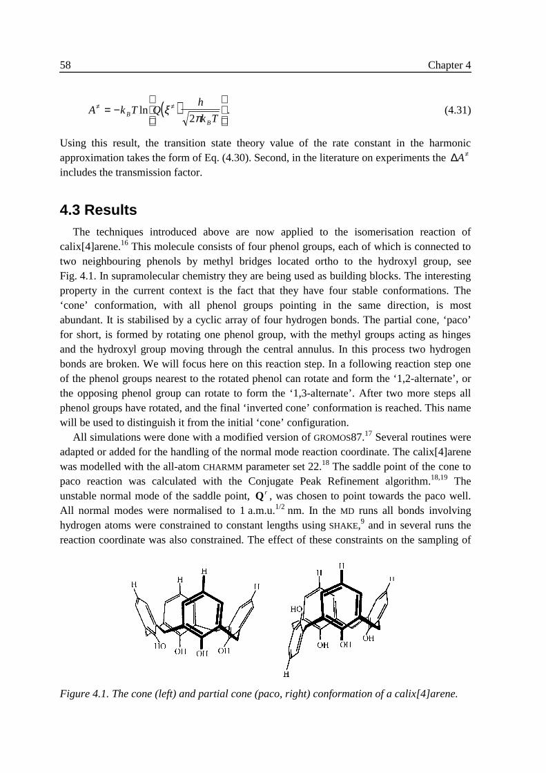
58 Chapter 4

( )A k T Qh

k TBB

≠ ≠= −

ln ξπ2

. (4.31)

Using this result, the transition state theory value of the rate constant in the harmonicapproximation takes the form of Eq. (4.30). Second, in the literature on experiments the ∆A≠

includes the transmission factor.

4 .3 ResultsThe techniques introduced above are now applied to the isomerisation reaction of

calix[4]arene.16 This molecule consists of four phenol groups, each of which is connected totwo neighbouring phenols by methyl bridges located ortho to the hydroxyl group, seeFig. 4.1. In supramolecular chemistry they are being used as building blocks. The interestingproperty in the current context is the fact that they have four stable conformations. The‘cone’ conformation, with all phenol groups pointing in the same direction, is mostabundant. It is stabilised by a cyclic array of four hydrogen bonds. The partial cone, ‘paco’for short, is formed by rotating one phenol group, with the methyl groups acting as hingesand the hydroxyl group moving through the central annulus. In this process two hydrogenbonds are broken. We will focus here on this reaction step. In a following reaction step oneof the phenol groups nearest to the rotated phenol can rotate and form the ‘1,2-alternate’, orthe opposing phenol group can rotate to form the ‘1,3-alternate’. After two more steps allphenol groups have rotated, and the final ‘inverted cone’ conformation is reached. This namewill be used to distinguish it from the initial ‘cone’ configuration.

All simulations were done with a modified version of GROMOS87.17 Several routines wereadapted or added for the handling of the normal mode reaction coordinate. The calix[4]arenewas modelled with the all-atom CHARMM parameter set 22.18 The saddle point of the cone topaco reaction was calculated with the Conjugate Peak Refinement algorithm.18,19 Theunstable normal mode of the saddle point, Q r , was chosen to point towards the paco well.All normal modes were normalised to 1 a.m.u.1/2 nm. In the MD runs all bonds involvinghydrogen atoms were constrained to constant lengths using SHAKE,9 and in several runs thereaction coordinate was also constrained. The effect of these constraints on the sampling of

Figure 4.1. The cone (left) and partial cone (paco, right) conformation of a calix[4]arene.

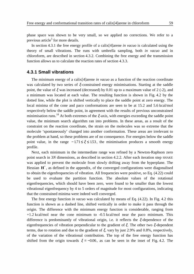
Free energy and conformational transition rates of calix[4]arene in chloroform 59

phase space was shown to be very small, so we applied no corrections. We refer to aprevious article5 for more details.

In section 4.3.1 the free energy profile of a calix[4]arene in vacuo is calculated using thetheory of small vibrations. The runs with umbrella sampling, both in vacuo and inchloroform, are described in section 4.3.2. Combining the free energy and the transmissionfunction allows us to calculate the reaction rates of section 4.3.3.

4 .3 .1 Small vibrations

The minimum energy of a calix[4]arene in vacuo as a function of the reaction coordinatewas calculated by two series of ξ-constrained energy minimisations. Starting at the saddlepoint, the value of ξ was increased (decreased) by 0.01 up to a maximum value of 2 (-2), anda minimum was located at each value. The resulting function is shown in Fig. 4.2 by thedotted line, while the plot is shifted vertically to place the saddle point at zero energy. Thelocal minima of the cone and paco conformations are seen to be at 15.2 and 5.6 kcal/molrespectively below the saddle point, in agreement with the results of previous unconstrainedminimisation runs.18 At both extremes of the ξ-axis, with energies exceeding the saddle pointvalue, the minimum search algorithm ran into problems. In these areas, as a result of theconstraint on the reaction coordinate, the strain on the molecules was so extreme that themolecule ‘spontaneously’ changed into another conformation. These areas are irrelevant tothe problem at hand, so these problems are of no consequence. For energies below the saddlepoint value, in the range − ≤ ≤171 153. .ξ , the minimisation produces a smooth energyprofile.

Next, each minimum in the intermediate range was refined by a Newton-Raphson zeropoint search in 3N dimensions, as described in section 4.2.2. After each iteration step SHAKE

was applied to prevent the molecule from slowly drifting away from the hyperplane. TheHessian H * , as defined in the appendix, of the converged configurations were diagonalisedto obtain the eigenfrequencies of vibration. All frequencies were positive, so Eq. (4.22) couldbe used to evaluate the partition function. The absolute values of the rotationaleigenfrequencies, which should have been zero, were found to be smaller than the lowestvibrational eigenfrequency by 4 to 5 orders of magnitude for most configurations, indicatingthat the constrained minima were indeed well converged.

The free energy function in vacuo was calculated by means of Eq. (4.22). In Fig. 4.2 thisfunction is shown as a dashed line, shifted vertically in order to make it pass through theorigin. The difference with the minimum energy function is considerable, ranging from+1.2 kcal/mol near the cone minimum to -0.5 kcal/mol near the paco minimum. Thisdifference is predominantly of vibrational origin, i.e. it reflects the ξ-dependence of theeigenfrequencies of vibration perpendicular to the gradient of ξ. The other two ξ-dependentterms, due to rotation and due to the gradient of ξ, vary by just 2.9% and 0.8%, respectively,of the variation of the vibrational contribution. The top of the free energy function hasshifted from the origin towards ξ = −0 06. , as can be seen in the inset of Fig. 4.2. The

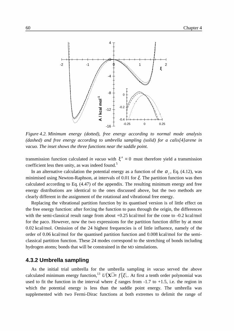
60 Chapter 4

transmission function calculated in vacuo with ξ≠ = 0 must therefore yield a transmissioncoefficient less then unity, as was indeed found.5

In an alternative calculation the potential energy as a function of the α j , Eq. (4.12), wasminimised using Newton-Raphson, at intervals of 0.01 for ξ. The partition function was thencalculated according to Eq. (4.47) of the appendix. The resulting minimum energy and freeenergy distributions are identical to the ones discussed above, but the two methods areclearly different in the assignment of the rotational and vibrational free energy.

Replacing the vibrational partition function by its quantised version is of little effect onthe free energy function: after forcing the function to pass through the origin, the differenceswith the semi-classical result range from about +0.25 kcal/mol for the cone to -0.2 kcal/molfor the paco. However, now the two expressions for the partition function differ by at most0.02 kcal/mol. Omission of the 24 highest frequencies is of little influence, namely of theorder of 0.06 kcal/mol for the quantised partition function and 0.008 kcal/mol for the semi-classical partition function. These 24 modes correspond to the stretching of bonds includinghydrogen atoms; bonds that will be constrained in the MD simulations.

4 .3 .2 Umbrella sampling

As the initial trial umbrella for the umbrella sampling in vacuo served the abovecalculated minimum energy function,13 ( ) ( )U fX = ξ . At first a tenth order polynomial wasused to fit the function in the interval where ξ ranges from -1.7 to +1.5, i.e. the region inwhich the potential energy is less than the saddle point energy. The umbrella wassupplemented with two Fermi-Dirac functions at both extremes to delimit the range of

-16

-12

-8

-4

0

4

-2 -1 0 1 2ξ

A /

kcal

mol

-1

Figure 4.2. Minimum energy (dotted), free energy according to normal mode analysis(dashed) and free energy according to umbrella sampling (solid) for a calix[4]arene invacuo. The inset shows the three functions near the saddle point.

-0.4

-0.2

0

-0.25 0 0.25

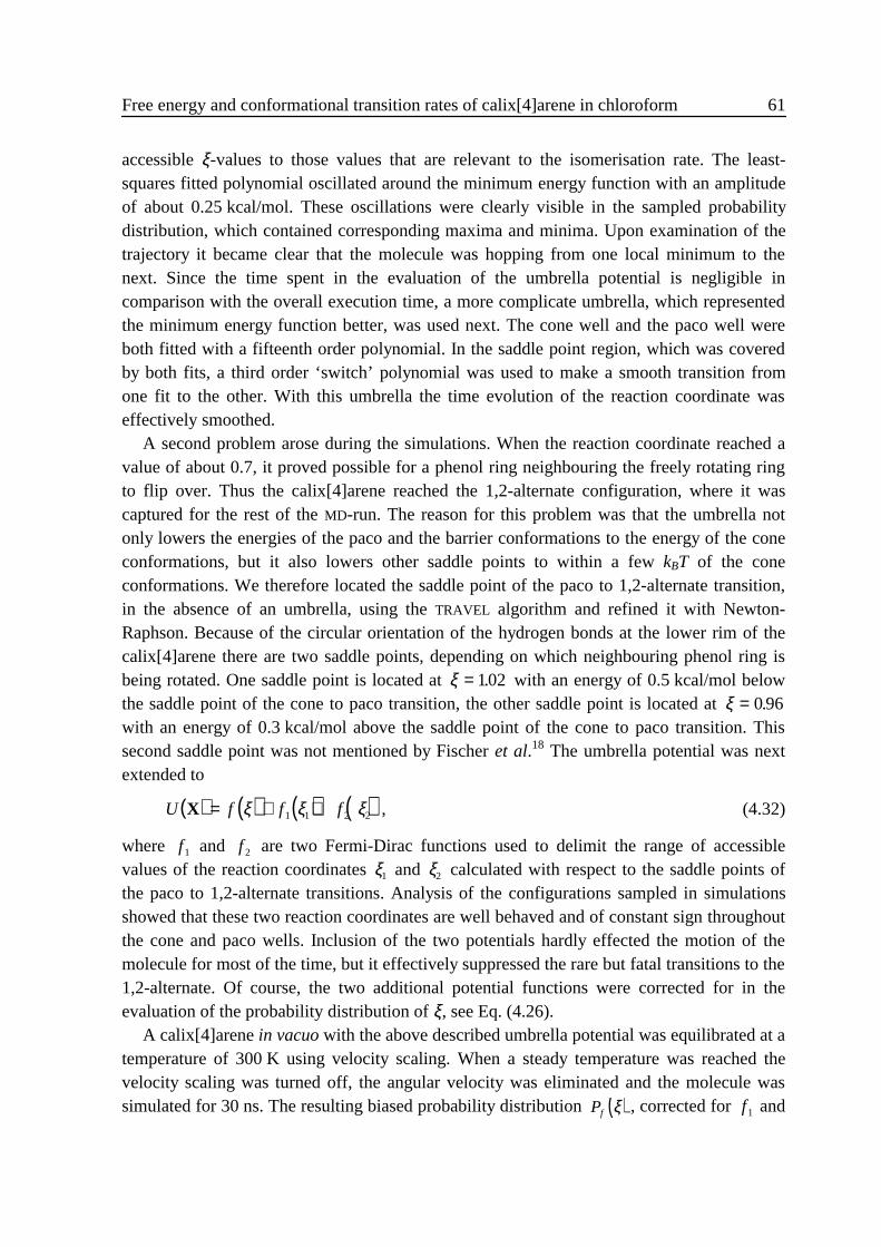
Free energy and conformational transition rates of calix[4]arene in chloroform 61

accessible ξ-values to those values that are relevant to the isomerisation rate. The least-squares fitted polynomial oscillated around the minimum energy function with an amplitudeof about 0.25 kcal/mol. These oscillations were clearly visible in the sampled probabilitydistribution, which contained corresponding maxima and minima. Upon examination of thetrajectory it became clear that the molecule was hopping from one local minimum to thenext. Since the time spent in the evaluation of the umbrella potential is negligible incomparison with the overall execution time, a more complicate umbrella, which representedthe minimum energy function better, was used next. The cone well and the paco well wereboth fitted with a fifteenth order polynomial. In the saddle point region, which was coveredby both fits, a third order ‘switch’ polynomial was used to make a smooth transition fromone fit to the other. With this umbrella the time evolution of the reaction coordinate waseffectively smoothed.

A second problem arose during the simulations. When the reaction coordinate reached avalue of about 0.7, it proved possible for a phenol ring neighbouring the freely rotating ringto flip over. Thus the calix[4]arene reached the 1,2-alternate configuration, where it wascaptured for the rest of the MD-run. The reason for this problem was that the umbrella notonly lowers the energies of the paco and the barrier conformations to the energy of the coneconformations, but it also lowers other saddle points to within a few kBT of the coneconformations. We therefore located the saddle point of the paco to 1,2-alternate transition,in the absence of an umbrella, using the TRAVEL algorithm and refined it with Newton-Raphson. Because of the circular orientation of the hydrogen bonds at the lower rim of thecalix[4]arene there are two saddle points, depending on which neighbouring phenol ring isbeing rotated. One saddle point is located at ξ = 102. with an energy of 0.5 kcal/mol belowthe saddle point of the cone to paco transition, the other saddle point is located at ξ = 0 96.with an energy of 0.3 kcal/mol above the saddle point of the cone to paco transition. Thissecond saddle point was not mentioned by Fischer et al.18 The umbrella potential was nextextended to

( ) ( ) ( ) ( )U f f fX = + +ξ ξ ξ1 1 2 2 , (4.32)

where f1 and f 2 are two Fermi-Dirac functions used to delimit the range of accessiblevalues of the reaction coordinates ξ1 and ξ2 calculated with respect to the saddle points ofthe paco to 1,2-alternate transitions. Analysis of the configurations sampled in simulationsshowed that these two reaction coordinates are well behaved and of constant sign throughoutthe cone and paco wells. Inclusion of the two potentials hardly effected the motion of themolecule for most of the time, but it effectively suppressed the rare but fatal transitions to the1,2-alternate. Of course, the two additional potential functions were corrected for in theevaluation of the probability distribution of ξ, see Eq. (4.26).

A calix[4]arene in vacuo with the above described umbrella potential was equilibrated at atemperature of 300 K using velocity scaling. When a steady temperature was reached thevelocity scaling was turned off, the angular velocity was eliminated and the molecule wassimulated for 30 ns. The resulting biased probability distribution ( )Pf ξ , corrected for f1 and

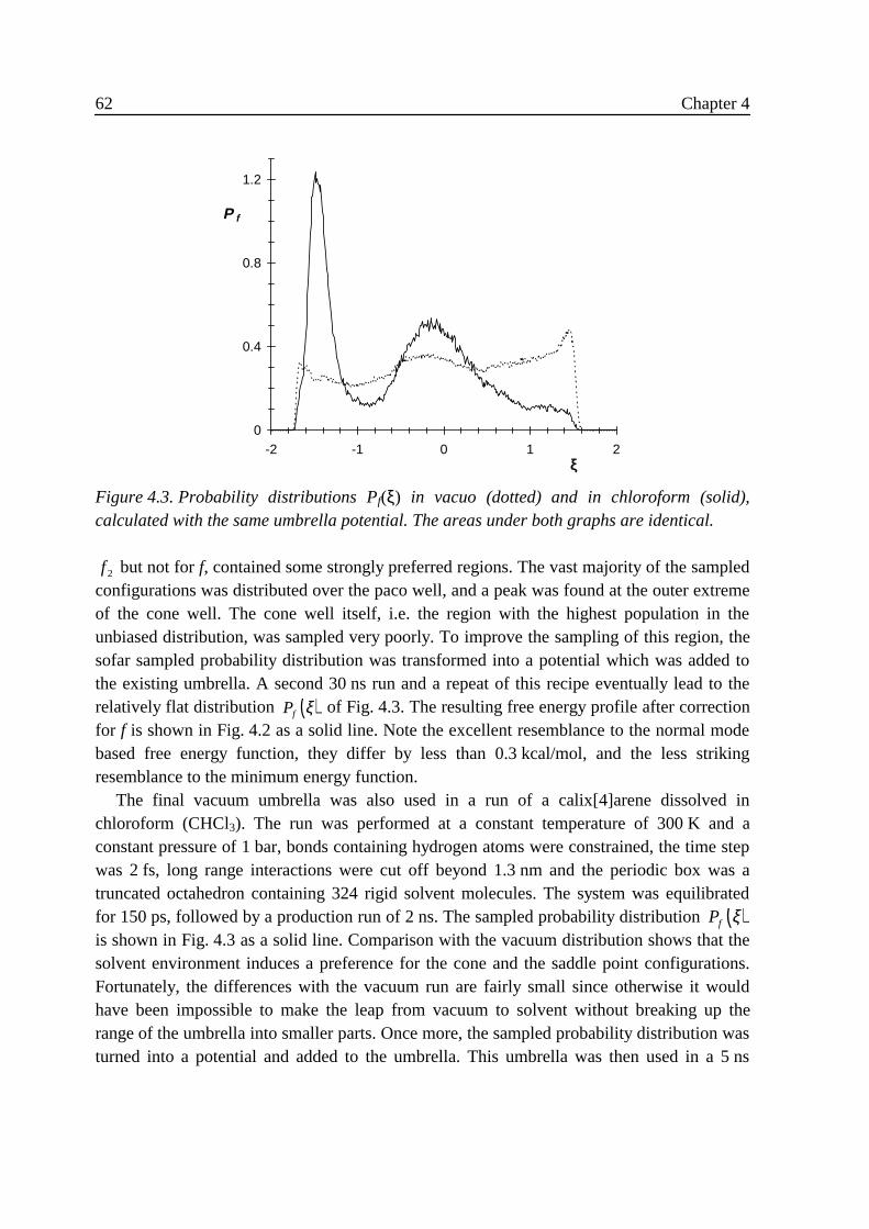
62 Chapter 4

f 2 but not for f, contained some strongly preferred regions. The vast majority of the sampledconfigurations was distributed over the paco well, and a peak was found at the outer extremeof the cone well. The cone well itself, i.e. the region with the highest population in theunbiased distribution, was sampled very poorly. To improve the sampling of this region, thesofar sampled probability distribution was transformed into a potential which was added tothe existing umbrella. A second 30 ns run and a repeat of this recipe eventually lead to therelatively flat distribution ( )Pf ξ of Fig. 4.3. The resulting free energy profile after correctionfor f is shown in Fig. 4.2 as a solid line. Note the excellent resemblance to the normal modebased free energy function, they differ by less than 0.3 kcal/mol, and the less strikingresemblance to the minimum energy function.

The final vacuum umbrella was also used in a run of a calix[4]arene dissolved inchloroform (CHCl3). The run was performed at a constant temperature of 300 K and aconstant pressure of 1 bar, bonds containing hydrogen atoms were constrained, the time stepwas 2 fs, long range interactions were cut off beyond 1.3 nm and the periodic box was atruncated octahedron containing 324 rigid solvent molecules. The system was equilibratedfor 150 ps, followed by a production run of 2 ns. The sampled probability distribution ( )Pf ξis shown in Fig. 4.3 as a solid line. Comparison with the vacuum distribution shows that thesolvent environment induces a preference for the cone and the saddle point configurations.Fortunately, the differences with the vacuum run are fairly small since otherwise it wouldhave been impossible to make the leap from vacuum to solvent without breaking up therange of the umbrella into smaller parts. Once more, the sampled probability distribution wasturned into a potential and added to the umbrella. This umbrella was then used in a 5 ns

0

0.4

0.8

1.2

-2 -1 0 1 2ξ

P f

Figure 4.3. Probability distributions Pf(ξ) in vacuo (dotted) and in chloroform (solid),calculated with the same umbrella potential. The areas under both graphs are identical.

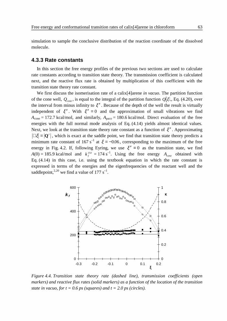
Free energy and conformational transition rates of calix[4]arene in chloroform 63

simulation to sample the conclusive distribution of the reaction coordinate of the dissolvedmolecule.

4 .3 .3 Rate constants

In this section the free energy profiles of the previous two sections are used to calculaterate constants according to transition state theory. The transmission coefficient is calculatednext, and the reactive flux rate is obtained by multiplication of this coefficient with thetransition state theory rate constant.

We first discuss the isomerisation rate of a calix[4]arene in vacuo. The partition functionof the cone well, Qcone, is equal to the integral of the partition function ( )Q ξ , Eq. (4.20), overthe interval from minus infinity to ξ ≠ . Because of the depth of the well the result is virtuallyindependent of ξ ≠ . With ξ ≠ = 0 and the approximation of small vibrations we findAcone = 172.7 kcal/mol, and similarly, Apaco = 180.6 kcal/mol. Direct evaluation of the freeenergies with the full normal mode analysis of Eq. (4.14) yields almost identical values.Next, we look at the transition state theory rate constant as a function of ξ ≠ . Approximating∇ =ξ Q r , which is exact at the saddle point, we find that transition state theory predicts aminimum rate constant of 167 s–1 at ξ = −0 06. , corresponding to the maximum of the freeenergy in Fig. 4.2. If, following Eyring, we use ξ ≠ = 0 as the transition state, we findA(0) = 185.9 kcal/mol and k f

TST = 174 s–1. Using the free energy Acone obtained withEq. (4.14) in this case, i.e. using the textbook equation in which the rate constant isexpressed in terms of the energies and the eigenfrequencies of the reactant well and thesaddlepoint,2,20 we find a value of 177 s–1.

0

200

400

600

-0.3 -0.2 -0.1 0 0.1 0.2ξ

k f

0

0.2

0.4

0.6

0.8

1

κ

Figure 4.4. Transition state theory rate (dashed line), transmission coefficients (openmarkers) and reactive flux rates (solid markers) as a function of the location of the transitionstate in vacuo, for t = 0.6 ps (squares) and t = 2.0 ps (circles).

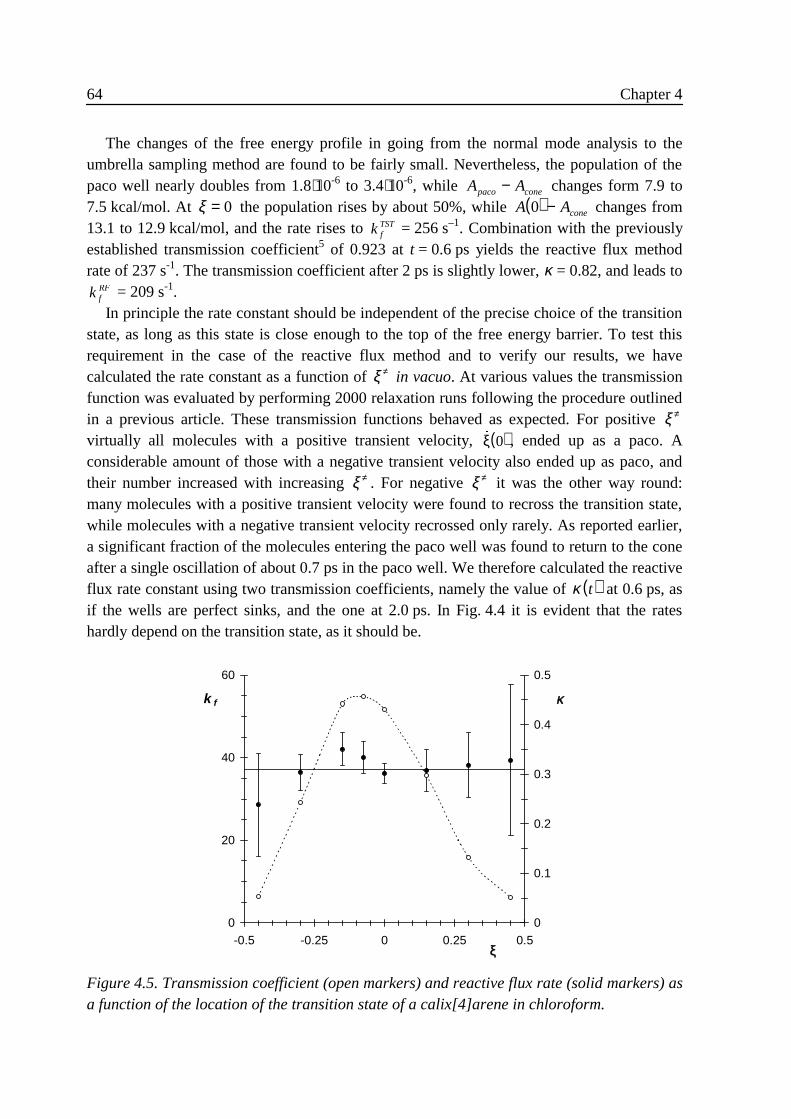
64 Chapter 4

The changes of the free energy profile in going from the normal mode analysis to theumbrella sampling method are found to be fairly small. Nevertheless, the population of thepaco well nearly doubles from 1.8⋅10-6 to 3.4⋅10-6, while A Apaco cone− changes form 7.9 to7.5 kcal/mol. At ξ = 0 the population rises by about 50%, while ( )A Acone0 − changes from13.1 to 12.9 kcal/mol, and the rate rises to k f

TST = 256 s–1. Combination with the previouslyestablished transmission coefficient5 of 0.923 at t = 0.6 ps yields the reactive flux methodrate of 237 s-1. The transmission coefficient after 2 ps is slightly lower, κ = 0.82, and leads tok f

RF = 209 s-1.In principle the rate constant should be independent of the precise choice of the transition

state, as long as this state is close enough to the top of the free energy barrier. To test thisrequirement in the case of the reactive flux method and to verify our results, we havecalculated the rate constant as a function of ξ ≠ in vacuo. At various values the transmissionfunction was evaluated by performing 2000 relaxation runs following the procedure outlinedin a previous article. These transmission functions behaved as expected. For positive ξ ≠

virtually all molecules with a positive transient velocity, ( )�ξ 0 , ended up as a paco. Aconsiderable amount of those with a negative transient velocity also ended up as paco, andtheir number increased with increasing ξ ≠ . For negative ξ ≠ it was the other way round:many molecules with a positive transient velocity were found to recross the transition state,while molecules with a negative transient velocity recrossed only rarely. As reported earlier,a significant fraction of the molecules entering the paco well was found to return to the coneafter a single oscillation of about 0.7 ps in the paco well. We therefore calculated the reactiveflux rate constant using two transmission coefficients, namely the value of ( )κ t at 0.6 ps, asif the wells are perfect sinks, and the one at 2.0 ps. In Fig. 4.4 it is evident that the rateshardly depend on the transition state, as it should be.

0

20

40

60

-0.5 -0.25 0 0.25 0.5ξ

k f

0

0.1

0.2

0.3

0.4

0.5

κκ

Figure 4.5. Transmission coefficient (open markers) and reactive flux rate (solid markers) asa function of the location of the transition state of a calix[4]arene in chloroform.

Free energy and conformational transition rates of calix[4]arene in chloroform 65

The effect of the chloroform solvent on the calix[4]arene is to shift the probabilitydistribution to the cone conformation, leading to an equilibrium constant of 2.4⋅10–7 andA Apaco cone− = 9.1 kcal/mol. With ( )A Acone0 − = 13.6 kcal/mol the transition state ratedecreases to 84 s-1. The transmission function for this system5 was found to be 0.43, so thereactive flux rate equals 36 s-1. The solvent is thus seen to reduce the reaction rate by a factorof six.

In a previous article we calculated the transmission coefficient in chloroform from a set of2000 relaxation runs. The transition velocities ( )�ξ 0 were sampled from a Gaussiandistribution and according to Eq. (4.6) these velocities were used as weight factor in anaverage over all runs. In order to reduce the number of relaxation runs we here used theproduct of the Gaussian and the weight factor as the new probability distribution from whichvelocities were drawn. Between 500 and 1000 relaxations runs were found to suffice for anaccurate calculation of the transmission coefficient. The effects of the transition state on thetransmission function and the reactive flux rate are shown in Fig. 4.5. In the range of ξ ≠

between +0.45 and -0.45 the transmission function is seen to vary by a factor of ten. Thereactive flux rate constant, on the other hand, is fairly constant.

Isomerisation rates of calix[4]arenes with various sidegroups and in various solvents havebeen measured with 1H-NMR.21-24 With the calix[4]arene of this paper, however, comparisonof the theoretical and experimental transition rates is complicated by the fact that the pacoconformation is only very short-lived. Hence, only the cone to inverted cone rate isexperimentally accessible. This inversion results from a series of independent reactions withone phenol ring flipping over in each step,18 as illustrated in Fig. 4.6. Because of symmetry,the flowchart can be reduced to

C

k

kP

k

kA

k

kP

k

kC

1

2

3

4

4

3

2

1

→←

→←

→←

′ →←

′ . (4.33)

Here C denotes the cone with all four phenol rings pointing upwards, P denotes the set offour conformations with three phenol rings pointing upwards, A denotes the set of sixalternate conformations with two phenol rings pointing upwards, and C’ and P’ are definedlikewise as inverted paco and inverted cone. The five time constants of the relaxationprocesses of this system are obtained as the eigenvalues of the matrix of the transitionprobabilities. The relevant eigenvalue is

( ) ( )k k k k k k k k k

kk

k k

= + + − + + −

≈+

1

241 2 3 1 2 3

2

1 3

13

2 3

,(4.34)

where in the second line it is assumed that k1 is much smaller than the other k-s. Thecorresponding eigenvector describes the exchange of molecules between C and C’ withaccompanying changes in P smaller by a factor of ( )k k k1 2 3+ and no changes in A. In

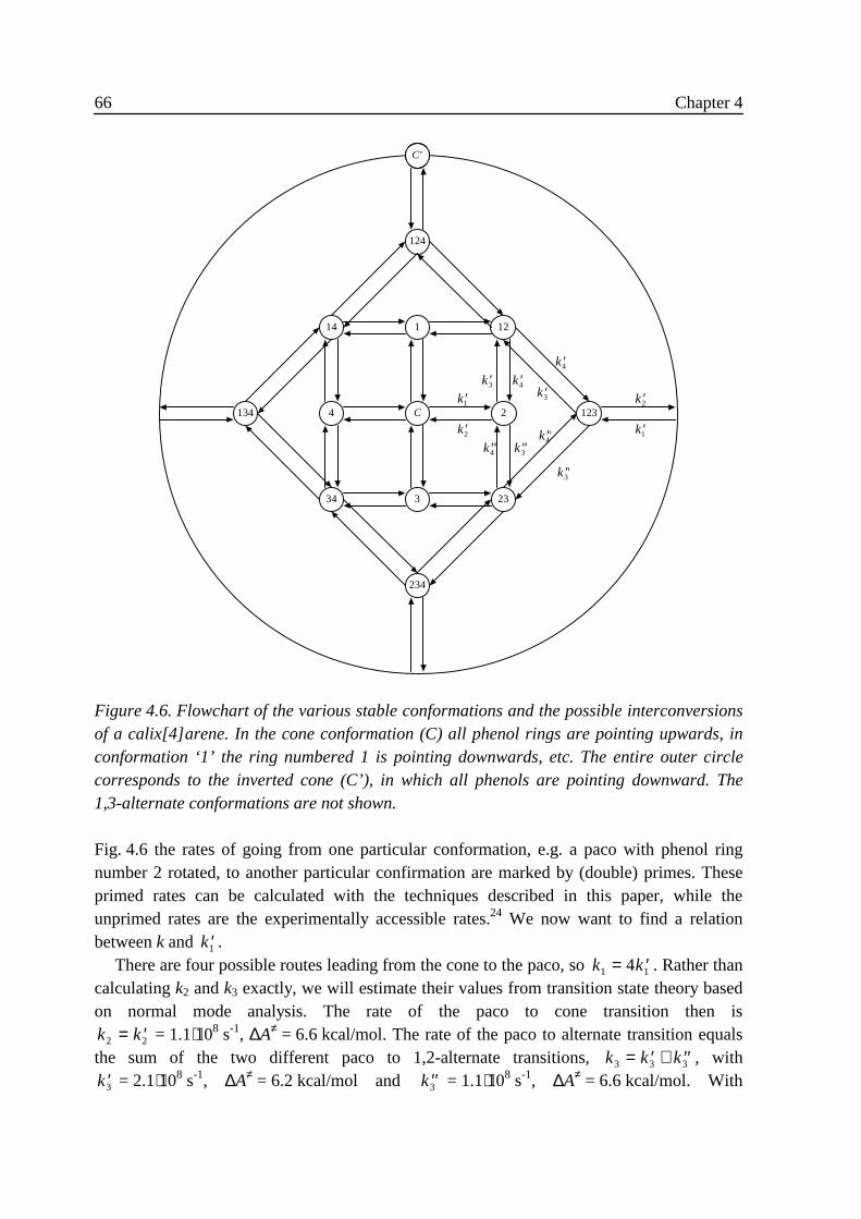
66 Chapter 4

Fig. 4.6 the rates of going from one particular conformation, e.g. a paco with phenol ringnumber 2 rotated, to another particular confirmation are marked by (double) primes. Theseprimed rates can be calculated with the techniques described in this paper, while theunprimed rates are the experimentally accessible rates.24 We now want to find a relationbetween k and ′k1 .

There are four possible routes leading from the cone to the paco, so k k1 14= ′ . Rather thancalculating k2 and k3 exactly, we will estimate their values from transition state theory basedon normal mode analysis. The rate of the paco to cone transition then isk k2 2= ′ = 1.1⋅108 s-1, ∆A≠ = 6.6 kcal/mol. The rate of the paco to alternate transition equalsthe sum of the two different paco to 1,2-alternate transitions, k k k3 3 3= ′ + ′′ , with

′k3 = 2.1⋅108 s-1, ∆A≠ = 6.2 kcal/mol and ′′k3 = 1.1⋅108 s-1, ∆A≠ = 6.6 kcal/mol. With

123134 4

1

3

234

124

1214

34 23

C’

C 2′k1

′k2

′k3 ′k4′k3

′k4

′′k3′′k4

′′k3

′′k4′k1

′k2

Figure 4.6. Flowchart of the various stable conformations and the possible interconversionsof a calix[4]arene. In the cone conformation (C) all phenol rings are pointing upwards, inconformation ‘1’ the ring numbered 1 is pointing downwards, etc. The entire outer circlecorresponds to the inverted cone (C’), in which all phenols are pointing downward. The1,3-alternate conformations are not shown.

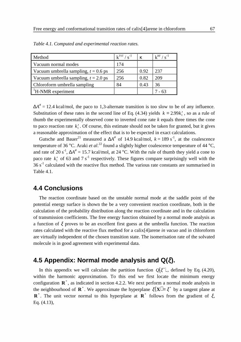
Free energy and conformational transition rates of calix[4]arene in chloroform 67

∆A≠ = 12.4 kcal/mol, the paco to 1,3-alternate transition is too slow to be of any influence.Substitution of these rates in the second line of Eq. (4.34) yields k k= ′2 99 1. , so as a rule ofthumb the experimentally observed cone to inverted cone rate k equals three times the coneto paco reaction rate ′k1 . Of course, this estimate should not be taken for granted, but it givesa reasonable approximation of the effect that is to be expected in exact calculations.

Gutsche and Bauer21 measured a ∆A≠ of 14.9 kcal/mol, k = 189 s-1, at the coalescencetemperature of 36 °C. Araki et al.22 found a slightly higher coalescence temperature of 44 °C,and rate of 20 s-1, ∆A≠ = 15.7 kcal/mol, at 24 °C. With the rule of thumb they yield a cone topaco rate ′k1 of 63 and 7 s-1 respectively. These figures compare surprisingly well with the36 s-1 calculated with the reactive flux method. The various rate constants are summarised inTable 4.1.

4 .4 ConclusionsThe reaction coordinate based on the unstable normal mode at the saddle point of the

potential energy surface is shown the be a very convenient reaction coordinate, both in thecalculation of the probability distribution along the reaction coordinate and in the calculationof transmission coefficients. The free energy function obtained by a normal mode analysis asa function of ξ proves to be an excellent first guess at the umbrella function. The reactionrates calculated with the reactive flux method for a calix[4]arene in vacuo and in chloroformare virtually independent of the chosen transition state. The isomerisation rate of the solvatedmolecule is in good agreement with experimental data.

4 .5 Appendix: Normal mode analysis and Q( ξξ).In this appendix we will calculate the partition function ( )Q ξ * , defined by Eq. (4.20),

within the harmonic approximation. To this end we first locate the minimum energyconfiguration R * , as indicated in section 4.2.2. We next perform a normal mode analysis inthe neighbourhood of R * . We approximate the hyperplane ( )ξ ξX = * by a tangent plane atR * . The unit vector normal to this hyperplane at R * follows from the gradient of ξ,Eq. (4.13),

Table 4.1. Computed and experimental reaction rates.

Method kTST / s-1 κ kRF / s-1

Vacuum normal modes 174Vacuum umbrella sampling, t = 0.6 ps 256 0.92 237Vacuum umbrella sampling, t = 2.0 ps 256 0.82 209Chloroform umbrella sampling 84 0.43 361H-NMR experiment 7 - 63

68 Chapter 4

( )N

Q S=

−

+

=

=

∑

∑

rkr k

k

kr

k

d

d

1

3

2

1

3

1. (4.35)

The tangent plane is spanned by a set of 3 1N − unit vectors perpendicular to N,

T

E

Q

S Q

l

k

j

kkr r

k

j N j r

d k

==

= − ≠+ =

1 2 3

1 3 6

1 2 3

, ,

, , ;

, ,

� , (4.36)

where the final three vectors still need to be orthonormalised. The eigenfrequencies ofvibration, ω j

* , in the hyperplane

X R T= +=

−

∑* τ ll

l

N

1

3 1

(4.37)

are found by diagonalising the 3 1N − dimensional Hessian at R * ,

Hklk l

* =∂

∂τ ∂τ

2Φ. (4.38)

Each 3 1N − dimensional eigenvector is next transformed into a 3N dimensional atomicdisplacements vector by summing over the T l using the components of the eigenvector asweight factors. The displacement vectors are again subdivided into three groups, thetranslational vectors E* l , identical to the E l , and the rotational vectors S* k , of the form ofEq. (4.8) with r i

0 replaced by r i* , all having eigenfrequency zero, and the vibrational vectors

Q* j all having positive eigenfrequencies. Analogously to Eq. (4.12), we now express anyconfiguration as

X A R E R R Q N= + = + += =

−

∑ ∑* * * * * * *,γ α βll

lj

j

j

N

1

3

1

3 7

, (4.39)

where the rotation matrix A * is determined by

( ) { }0 1 2 3= − ⋅ ∈X A R A S* * * * , , ,k k . (4.40)

It is obvious that ( )ξ X (with ξ still defined with respect to R 0 ) is a function of the α j* and

β* only, and does not depend on A * . Because of the construction of the Q* j , we have

( )ξ ξXR

= +ξ β* **∇ , (4.41)

up to first order in α j* and β* , where it was used that N is a unit vector parallel to ∇ Xξ .

The integrals of the partition function in Eq. (4.20) are solved analogously to those inEq. (4.14). The sole exception is the integral over β* which, because of the delta–function,yields not a frequency factor but ∇ R*ξ

−1, with

Free energy and conformational transition rates of calix[4]arene in chloroform 69

( )∇ =

= +

= =∑ ∑R x

* ξ∂ξ

∂md

i ii

N

kr

k

2

1

1 2

2

1

3 1 2

1 . (4.42)

We then arrive at

( ) ( )

[ ] ( )

QMk T

hV

k T

hI I I

kTE k T k T h

B BA B C

ii

N

e B B

ξπ π

σπ

ω ξ π

* * * *

**

*exp .

=

⋅

× ⋅ − ⋅ ∇ ⋅=

− −−∏

2 8

2

2

3 2 1 2 2

2

3 21 2

1

3 7 1 1 2 1

�ω R

(4.43)

We end this appendix with the derivation of an alternative expression for the aboveintegral. Rather than introducing a new set of coordinates based on R * , we keep on using thecoordinates defined with respect to R 0 . The delta-function in the partition function is thentrivially dealt with. The Jacobi matrix of the transformation from mass-weighted coordinatesto generalised coordinates is again given by Eq. (4.18). However, for small vibrations aroundR * the approximation of R by R * leads to three vectors ε kR * that are no longerorthogonal to the Q j . Expressing these vectors in the R 0 -based vectors yields

( )( )

J A R Q A E

I 0 0

1 0

0 0 1

c 0 0

0 1 0

0 0 1

=

−

−

εσ

ρk j l0 1

0 1 *

* , (4.44)

( )J =−

σ * sinI I IA B C0 0 0 1 2

2ψ , (4.45)

where

( ) ( ) ( )σ ρlkl k

ljl j* * * *,= ⋅ = ⋅ε ε εR R R Q0 , (4.46)

and the ( )I 0 1− arises because the ε kR 0 are not orthogonal. Performing the integration overthe generalised coordinates and multiplying with the integral over the momenta gives

( ) ( )

[ ] ( )

QMk T

hV

k T

hI I I

k TE k T k T h

B BA B C

B

ii

N

e B

E kBT

B

ξπ π

σπ

ω π

*

***

* / *exp .

=

⋅

× ⋅ − ⋅

−

=

−− −∏

2 8

2

2

3 2 1 2 2

2

3 2

0 0 0 1 2

1

3 71 2 1

�ωσ

(4.47)

The required eigenfrequencies are found as the square roots of the eigenvalues of the 3 7N −dimensional Hessian at R * ,

H j k rjkj k

** , ,= ≠∂

∂α ∂α

2Φ, (4.48)

and differ from the eigenfrequencies used in Eq. (4.22).

70 Chapter 4

4 .6 References1 H. Eyring, J. Chem. Phys. 3, 107 (1935).2 P. Hänggi, P. Talkner and M. Borkovec, Rev. Mod. Phys. 62, 251 (1990).3 T. Yamamoto, J. Chem. Phys. 33, 281 (1960).4 D. Chandler, J. Chem. Phys. 68, 2959 (1978).5 W. K. den Otter and W. J. Briels, J. Chem. Phys. 106, 5494 (1997) (Chapter 3).6 W. H. Miller, Acc. Chem. Res. 9, 306 (1976).7 D. A. McQuarrie, Statistical Mechanics (Harper and Row, New York, NY, 1976).8 H. Goldstein, Classical Mechanics (Addison–Wesley, Reading, MA, 1980).9 J. Ryckaert, G. Ciccotti and H. J. C. Berendsen, J. Comput. Phys. 23, 327 (1977).10 D. L. Beveridge and F. M. DiCapua, Annu. Rev. Biophys. Biophys. Chem. 18, 431

(1989).11 W. F. van Gunsteren, T. C. Beutler, F. Fraternali, P. M. King, A. E. Mark and P. E. Smith

in Computer Simulations of Biomolecular Systems: Theoretical and PracticalApplications, edited by W. F. van Gunsteren, P. K. Weiner and A. J. Wilkinson (ESCOM,Leiden, The Netherlands, 1993), pp. 315.

12 T. P. Straatsma, Rev. Comp. Chem. 9, 81 (1996).13 J.–M. Depaepe, J.–P. Ryckaert, E. Paci and G. Ciccotti, Mol. Phys. 79, 515 (1993).14 R. W. W. Hooft, B. P. van Eijck and J. Kroon, J. Chem. Phys. 97, 6690 (1992).15 S. Kumar, D. Bouzida, R. H. Swendsen, P. A. Kollman and J. M. Rosenberg, J. Comp.

Chem. 13, 1011 (1992).16 C. D. Gutsche, J. S. Rogers, D. Stewart and K.–A. See, Pure & Appl. Chem. 62, 485

(1990).17 H. J. C. Berendsen and W. F. van Gunsteren, GROMOS Reference Manual (University of

Groningen, Groningen, The Netherlands, 1987).18 S. Fischer, P. D. J. Grootenhuis, L. C. Groenen, W. P. van Hoorn, F. C. J. M. van Veggel,

D. N. Reinhoudt and M. Karplus, J. Am. Chem. Soc. 117, 1611 (1995).19 S. Fischer and M. Karplus, Chem. Phys. Lett. 194, 252 (1992)20 S. Glasstone, K. J. Laidler and H. Eyring, The Theory of Rate Processes (MacGraw–Hill,

New York, NY, 1941).21 C. D. Gutsche and L. J. Bauer, J. Am. Chem. Soc. 107, 6052 (1985).22 K. Araki, S. Shinkai and T. Matsuda, Chem. Lett. 1989, 581 (1989).23 W. P. van Hoorn, W. J. Briels, J. P. M. van Duynhoven, F. C. J. M. van Veggel and D. N.

Reinhoudt, to be published.24 J. Blixt and C. Detellier, J. Am. Chem. Soc. 116, 11957 (1994).

71

Chapter 5

Solvent effect on the isomerisation rate

of calix[4]arene studied by molecular

dynamics simulations *

AbstractThe isomerisation rates of a calix[4]arene in benzene and in chloroform have been

calculated using molecular dynamics simulations. The reaction coordinate that is employed isbased on the unstable normal mode at the saddle point of the potential energy surface. Thefree energy as a function of this coordinate has been calculated by means of umbrellasampling. Comparison of the free energies in the solvents with those in vacuum reveals thatboth solvents destabilise the paco conformation and stabilise the transition state region. Inchloroform the calix[4]arene shows a stronger preference for the cone conformation than inbenzene or in vacuum. The isomerisation rate has been determined by the reactive fluxmethod. Both solvents yield comparable transmission coefficients. The calculated rates are inperfect agreement with experimental data.

5 .1 IntroductionCalix[4]arenes, cyclic arrays of four phenol rings, are versatile molecules:1 they are used

as building blocks in supramolecular chemistry, they can selectively bind ions, they shownon-linear optical behaviour and they can take on various conformations. The latter propertywill be studied in this paper. In the cone conformation all phenol rings are orientated in thesame direction, see Fig. 5.1. The molecule is then stabilised by four internal hydrogen bondsat the lower rim of the molecule. In the partial cone conformation, ‘paco’ for short, one ofthe phenol rings is rotated with respect to the other three phenol rings. During theisomerisation from cone to paco the methyl groups between the phenol rings act as thehinges around which the phenol ring rotates, and the hydroxyl moiety moves through the

* W. K. den Otter and W. J. Briels, submitted to J. Am. Chem. Soc.

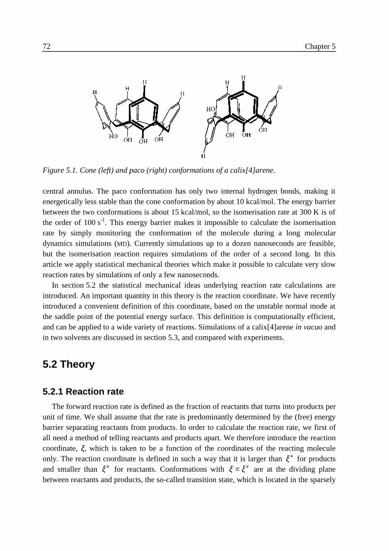
72 Chapter 5

central annulus. The paco conformation has only two internal hydrogen bonds, making itenergetically less stable than the cone conformation by about 10 kcal/mol. The energy barrierbetween the two conformations is about 15 kcal/mol, so the isomerisation rate at 300 K is ofthe order of 100 s-1. This energy barrier makes it impossible to calculate the isomerisationrate by simply monitoring the conformation of the molecule during a long moleculardynamics simulations (MD). Currently simulations up to a dozen nanoseconds are feasible,but the isomerisation reaction requires simulations of the order of a second long. In thisarticle we apply statistical mechanical theories which make it possible to calculate very slowreaction rates by simulations of only a few nanoseconds.

In section 5.2 the statistical mechanical ideas underlying reaction rate calculations areintroduced. An important quantity in this theory is the reaction coordinate. We have recentlyintroduced a convenient definition of this coordinate, based on the unstable normal mode atthe saddle point of the potential energy surface. This definition is computationally efficient,and can be applied to a wide variety of reactions. Simulations of a calix[4]arene in vacuo andin two solvents are discussed in section 5.3, and compared with experiments.

5 .2 Theory

5 .2 .1 Reaction rate

The forward reaction rate is defined as the fraction of reactants that turns into products perunit of time. We shall assume that the rate is predominantly determined by the (free) energybarrier separating reactants from products. In order to calculate the reaction rate, we first ofall need a method of telling reactants and products apart. We therefore introduce the reactioncoordinate, ξ, which is taken to be a function of the coordinates of the reacting moleculeonly. The reaction coordinate is defined in such a way that it is larger than ξ ≠ for productsand smaller than ξ ≠ for reactants. Conformations with ξ ξ= ≠ are at the dividing planebetween reactants and products, the so-called transition state, which is located in the sparsely

Figure 5.1. Cone (left) and paco (right) conformations of a calix[4]arene.

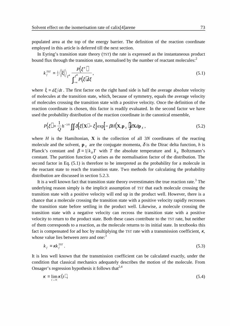
Solvent effect on the isomerisation rate of calix[4]arene 73

populated area at the top of the energy barrier. The definition of the reaction coordinateemployed in this article is deferred till the next section.

In Eyring’s transition state theory (TST) the rate is expressed as the instantaneous productbound flux through the transition state, normalised by the number of reactant molecules:2

( )( )

kP

P dfTST = ≠

≠

−∞

≠

∫12

�ξξ ξ

ξ

ξ ξ, (5.1)

where �ξ = d dtξ . The first factor on the right hand side is half the average absolute velocityof molecules at the transition state, which, because of symmetry, equals the average velocityof molecules crossing the transition state with a positive velocity. Once the definition of thereaction coordinate is chosen, this factor is readily evaluated. In the second factor we haveused the probability distribution of the reaction coordinate in the canonical ensemble,

( ) ( )[ ] ( )[ ]PQ

h H d dNX Xξ δ ξ ξ β= − −− ∫∫

1 3 X X p X pexp , , (5.2)

where H is the Hamiltonian, X is the collection of all 3N coordinates of the reactingmolecule and the solvent, p X are the conjugate momenta, δ is the Dirac delta function, h isPlanck’s constant and β = 1 k TB with T the absolute temperature and kB Boltzmann’sconstant. The partition function Q arises as the normalisation factor of the distribution. Thesecond factor in Eq. (5.1) is therefore to be interpreted as the probability for a molecule inthe reactant state to reach the transition state. Two methods for calculating the probabilitydistribution are discussed in section 5.2.3.

It is a well known fact that transition state theory overestimates the true reaction rate.3 Theunderlying reason simply is the implicit assumption of TST that each molecule crossing thetransition state with a positive velocity will end up in the product well. However, there is achance that a molecule crossing the transition state with a positive velocity rapidly recrossesthe transition state before settling in the product well. Likewise, a molecule crossing thetransition state with a negative velocity can recross the transition state with a positivevelocity to return to the product state. Both these cases contribute to the TST rate, but neitherof them corresponds to a reaction, as the molecule returns to its initial state. In textbooks thisfact is compensated for ad hoc by multiplying the TST rate with a transmission coefficient, κ,whose value lies between zero and one:3

k kf fTST= κ . (5.3)

It is less well known that the transmission coefficient can be calculated exactly, under thecondition that classical mechanics adequately describes the motion of the molecule. FromOnsager’s regression hypothesis it follows that2,4

( )κ κ=→∞limt

t , (5.4)

74 Chapter 5

( )( )[ ] ( ) ( )[ ]

( )[ ] ( ) ( )[ ]κδ ξ ξ θ ξ ξ

δ ξ ξ θt

t=

− −

−

≠ ≠

≠

0 0

0 0 0

�

� �

ξ

ξ ξ, (5.5)

where θ is the Heaviside step function, t and 0 denote the time, and the pointed bracketsindicate a canonical average. The denominator of Eq. (5.5) is the average velocity ofmolecules crossing the transition state at time 0 in the positive direction, i.e. the first factoron the right hand side of Eq. (5.1). The numerator is the average velocity of moleculescrossing the transition at time 0 of those molecules that are in the product state some time tafter crossing the transition state, regardless of the initial crossing direction. One readily seesthat in the limit of t going to zero the numerator equals the denominator. At longer times thecontributions of recrossing trajectories will start to diminish the transmission coefficient (itmay temporary increase, though, depending on the characteristics of the reaction). Aftersome time, which is longer than the typical time of the molecular motions but much shorterthan the time constant of the reaction, the transmission coefficient will stabilise at a plateaulevel. At this point all molecules which crossed the transition state at time 0 have reachedeither the product well or the reactant well, and will stay there for a long while until theyincidentally escape. The numerator of Eq. (5.5) then contains contributions only from thosemolecules that originated in the reactant well and have settled in the product well, hence thename reactive flux method (RF). By inserting the plateau value of the transmission coefficientinto Eq. (5.3) we find the exact rate. Note that the transmission coefficient is easilycalculated by MD simulations: first one samples configurations in the dividing plane, andnext one calculates relaxation runs to see where each of these configurations ends up about apicosecond later.

From Eq. (5.1) it follows that the TST rate constant depends on the precise definition ofthe dividing plane between reactants and products. Obviously, the dividing plane must lienear the top of the energy barrier to cohere with the intuitive notion of reactants andproducts. But, there is no clear reason why one plane in this region should be preferred overanother, or to put it differently, why one TST rate is better than another. The only thing oneknows for sure is that even the lowest TST rate will still overestimate the true rate. It has beenshown that the reactive flux method does not suffer from these problems: provided thedividing plane lies near the top of the barrier, the reactive flux method will always yield thesame rate constant.4,5 The only problem is that the number of relaxation runs required toaccurately calculate the transmission coefficient increases exponentially as the plateau valueof the transmission coefficient decreases. We therefore now set forth to find a reactioncoordinate which yields a high plateau value, i.e. a low TST rate.

5 .2 .2 Reaction coordinate

In the previous section we have pointed at the significance of the dividing plane to thereaction rate. A particularly important point in the dividing plane is the saddle point, thelowest point on the top of the energy barrier: any molecule going from the reactant state to

Solvent effect on the isomerisation rate of calix[4]arene 75

the product state must at least rise to the energy of the saddle point to overcome the reactionbarrier. According to the Boltzmann distribution, molecules crossing the barrier will do sopreferably with the least amount of energy, so the majority of the molecules will surmountthe barrier in the vicinity of the saddle point. It is only natural, therefore, to introduce areaction coordinate based on the properties of the saddle point, as will be done next.

Suppose we have located the first order saddle point, R 0 , of the potential energy surfaceof an N atom molecule. For notational convenience and to make the results more transparent,we have collected all 3N coordinates into a single mass-weighted column vector, R 0 =

( ) ( )( )m mTN N

T T11 2

10 1 2 0r r, ,� , where r i

0 is the column vector of the coordinates of atom i withmass mi . We shall assume that there is no external potential acting on the molecule. At thesaddle point the gradient of the potential energy is zero, so a Taylor expansion up to secondorder of the potential energy yields an energy of

( ) ( ) ( ) ( )Φ ΦX R X R H X R= + − −0 12

0 0T(5.6)

at a point X close to the saddle point. The Hessian matrix, H, contains all second derivativesof the potential energy with respect to the mass-weighted Cartesian coordinates. This matrixis then diagonalised to find its eigenvectors and eigenvalues, just as one normally does for amolecule at the potential energy minimum.

The eigenvectors of the Hessian can be subdivided into two groups. The first groupcontains the three eigenvectors which correspond to a rigid body translation and the threeeigenvectors which correspond to a rigid body rotation. In the absence of an external field,one easily sees that the potential energy of the molecule does not change during these moves,hence the eigenvalues of these six eigenvectors are all equal to zero. The second groupcontains the 3 6N − eigenvectors with a non-zero eigenvalue, the normal modes ofvibration.3 These vibrations are, in first order approximation, independent of one another; theeigenvalues are the squares of the frequencies of vibration, which are experimentallyaccessible. If the Hessian were to be evaluated at a local minimum of the potential energysurface, then all eigenvalues would be positive: move along any normal mode and thepotential energy will rise. At a first order saddle point, however, there is exactly oneeigenvector with a negative eigenvalue, i.e. an imaginary eigenfrequency. Move along thisdirection, henceforth called the unstable direction Q r , and the potential energy will fall. Inother words, in this direction the molecule is going from the saddle point towards the product(or reactant) well. As an illustration of this unstable normal mode, the resulting atomicdisplacements of a calix[4]arene at the cone to paco saddle point are depicted in Fig. 5.2.

We now define the reaction coordinate as the displacement of the molecule, with respectto the saddle point, along the unstable direction. For a molecule with coordinates X we thusarrive at the projection

( )ξ =

− ⋅⋅

X R Q

Q Q

0 r

r r . (5.7)

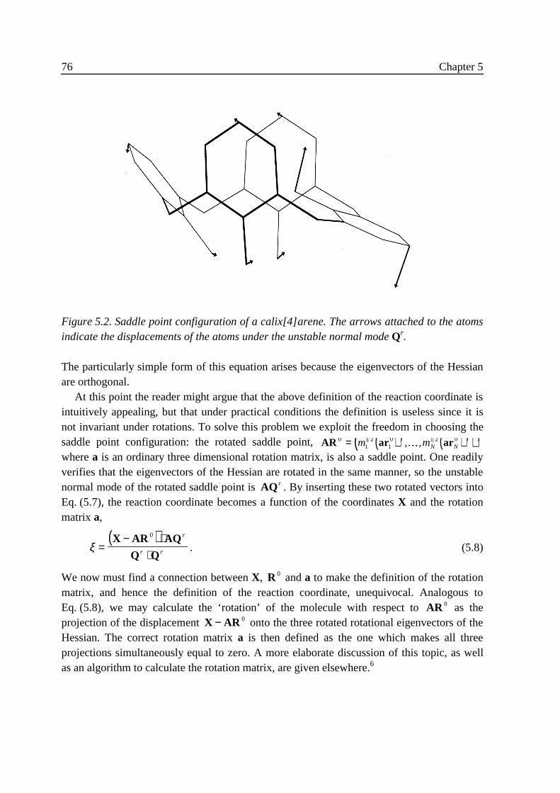
76 Chapter 5

The particularly simple form of this equation arises because the eigenvectors of the Hessianare orthogonal.

At this point the reader might argue that the above definition of the reaction coordinate isintuitively appealing, but that under practical conditions the definition is useless since it isnot invariant under rotations. To solve this problem we exploit the freedom in choosing thesaddle point configuration: the rotated saddle point, ( ) ( )( )AR ar ar0

11 2

10 1 2 0= m mT

N NT T, ,�

where a is an ordinary three dimensional rotation matrix, is also a saddle point. One readilyverifies that the eigenvectors of the Hessian are rotated in the same manner, so the unstablenormal mode of the rotated saddle point is AQ r . By inserting these two rotated vectors intoEq. (5.7), the reaction coordinate becomes a function of the coordinates X and the rotationmatrix a,

( )ξ =

− ⋅⋅

X AR AQ

Q Q

0 r

r r . (5.8)

We now must find a connection between X, R 0 and a to make the definition of the rotationmatrix, and hence the definition of the reaction coordinate, unequivocal. Analogous toEq. (5.8), we may calculate the ‘rotation’ of the molecule with respect to AR 0 as theprojection of the displacement X AR− 0 onto the three rotated rotational eigenvectors of theHessian. The correct rotation matrix a is then defined as the one which makes all threeprojections simultaneously equal to zero. A more elaborate discussion of this topic, as wellas an algorithm to calculate the rotation matrix, are given elsewhere.6

Figure 5.2. Saddle point configuration of a calix[4]arene. The arrows attached to the atomsindicate the displacements of the atoms under the unstable normal mode Qr.

Solvent effect on the isomerisation rate of calix[4]arene 77

5 .2 .3 Free energy

It is common practice to convert probability distributions and partition functions, asdefined by Eq. (5.2), into free energies,

( ) ( )A k T P cBξ ξ= − +ln , (5.9)

where c is an irrelevant constant arising from the partition function Q. The RF rate thenreads7

( )k

k T A A

k TfB R

B

= −−

≠

≠

κπ

ξξ

ξ2∇ X exp , (5.10)

where we have combined Eqs. (5.1) through (5.3). Here AR is the free energy of the reactantwell, obtained by replacing ( )P ξ in Eq. (5.9) by the denominator of Eq. (5.1). With thereaction coordinate as defined in section 5.2.2 we find ∇ Xξ = 1 kg-1/2 m-1 at the saddlepoint, and this value increases only slightly on taking the average over the saddle plane. Inthe experimental literature a slightly different definition of the free energy is commonly usedby writing a measured reaction rate as

kk T

h

A

k TfB

B

= −

≠

exp∆

. (5.11)

By comparing these two expressions we find

( )∆A A k Th

k TA k TB

BR B

≠ ≠≠= −

− −ξπ

ξ κξ

ln ln2

2∇ X . (5.12)

The second term on the right hand side removes from ( )A ξ ≠ the contribution of the velocity�ξ , so the free energy difference ∆A≠ is based on the probability of finding a molecule at thetransition state with zero crossing velocity, while the free energy ( )A ξ ≠ is based on theprobability for the molecule to be at the transition state regardless of the crossing velocity.Notice that ∆A≠ also includes a contribution from the transmission coefficient, while ( )A ξ ≠

does not.Perhaps the best known method of calculating the free energy of a molecule in vacuo, i.e.

AR , is to perform a normal mode analysis.3 Combining contributions from the 3 6N −eigenfrequencies of vibration, the inertia tensor and the total mass of the molecule gives thedesired result. The assumptions underlying this theory are that the amplitudes of thevibrations are small, and that there is no coupling between rotations and vibrations. As wehave shown elsewhere,7 it is straightforward to calculate the free energy as a function of thereaction coordinate under the same conditions. The basic task is to calculate the 3 7N −eigenfrequencies of vibrations in the hyperplane of configurations with a prescribed value ofthe reaction coordinate, and to calculate the moments of inertia of the correspondingdeformed molecule. The method is reliable and fast for calculations in vacuo, but it is of

78 Chapter 5

little practice for a molecule in a solvent, since the inclusion of solvent effects in the theoryis virtually impossible.

If we were to directly sample the probability distribution of the reaction coordinate of thesolvated molecule in one single long simulation, then the height of the energy barrierbetween reactants and products would obviously create insurmountable difficulties. Thebarrier region would be sampled very poorly, and the molecule might even stay in oneconformation for the entire run. In fact, this is precisely the problem that we try to avoid byusing reaction rate theory. Suppose now that we add to the existing potential energy surface aso-called umbrella potential,8 ( )U X . The probability distribution of the system with theumbrella reads as

( ) ( )[ ] ( ) ( ){ }[ ]PQ

h H U d dUU

NX Xξ δ ξ ξ β= − − +− ∫∫

1 3 X X p X X pexp , . (5.13)

In case the umbrella is a function of the reaction coordinate only, ( )P ξ may be calculatedaccording to

( ) ( ) ( )[ ]P cP UUξ ξ β= exp X , (5.14)

where c is a proportionality constant. The probability distribution of ξ in the biased run isthus seen to be easily converted into the probability distribution of the unbiased run. Thisremains true regardless of the kind of umbrella potential used, so we are free to chose theumbrella that suits us the best. The best choice is ( ) ( )U Aξ ξ= − , since it renders PU

independent of ξ. In the biased run the barrier between reactants and products theneffectively vanishes, and both configurations can be sampled efficiently with a single longsimulation. In such a simulation the reaction coordinate behaves like a diffusing particle. Anobvious problem is that we do not know ( )A ξ in advance, but by making a good initialguess, like according to the above discussed normal mode method, we can get close enoughfor the method to work properly. Alternatively, we may chose the umbrella in such a waythat only a small range of ξ, a so-called window, is sampled. Combining the probabilitydistributions from overlapping windows by making them match in the overlap region thenyields the desired result. Since diffusion over long distances is a slow process, it may beadvantageous to combine both methods: use a good guess of the free energy as umbrella andpartitionate the range into windows that are rapidly sampled.

5 .3 ResultsThe calix[4]arene was modelled with the all-atom CHARMM parameter set 22.9 The saddle

points on the potential energy surface of a calix[4]arene in vacuo were calculated using theconjugate peak refinement algorithm9,10 implemented in QUANTA/CHARMM.11 All othercalculations were done with GROMOS87,12 which we adapted to meet our specific needs. Thesaddle points were transported to GROMOS87, and further refined using Newton-Raphson to

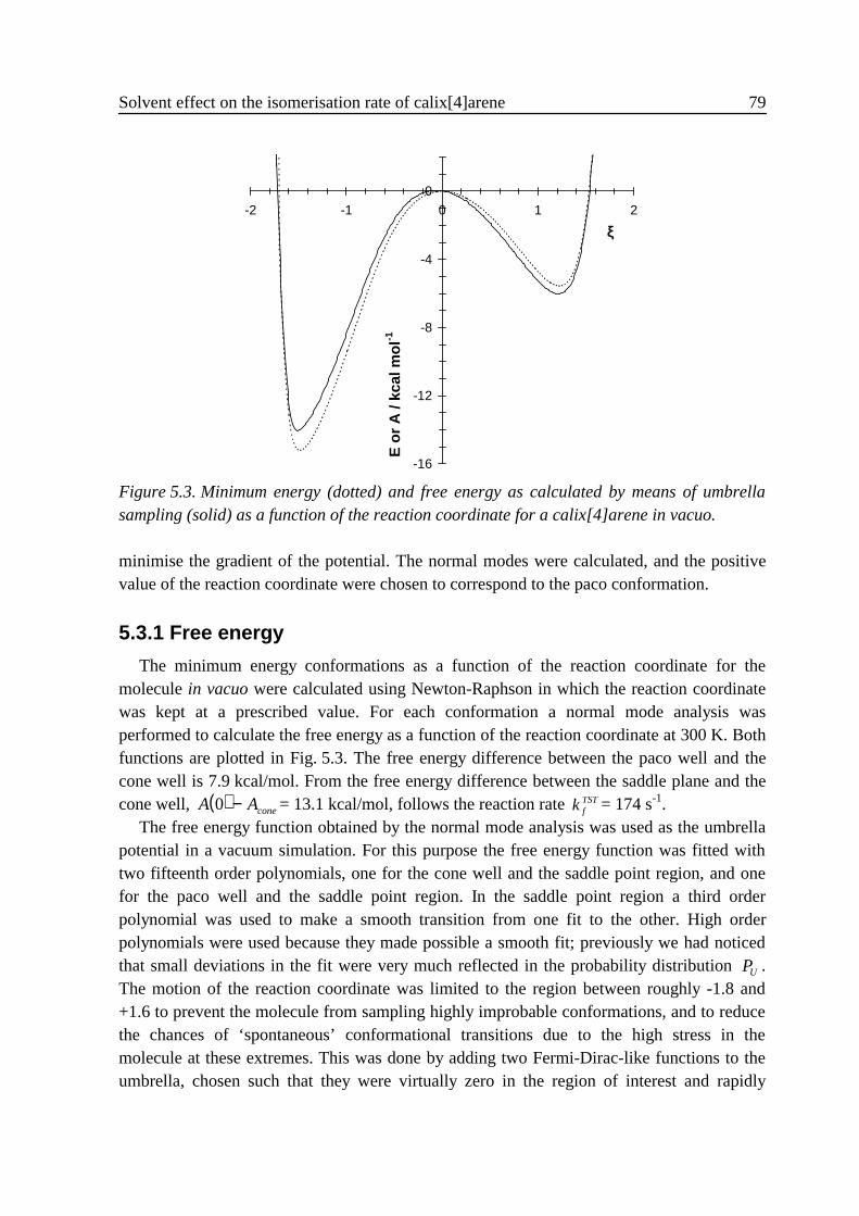
Solvent effect on the isomerisation rate of calix[4]arene 79

minimise the gradient of the potential. The normal modes were calculated, and the positivevalue of the reaction coordinate were chosen to correspond to the paco conformation.

5 .3 .1 Free energy

The minimum energy conformations as a function of the reaction coordinate for themolecule in vacuo were calculated using Newton-Raphson in which the reaction coordinatewas kept at a prescribed value. For each conformation a normal mode analysis wasperformed to calculate the free energy as a function of the reaction coordinate at 300 K. Bothfunctions are plotted in Fig. 5.3. The free energy difference between the paco well and thecone well is 7.9 kcal/mol. From the free energy difference between the saddle plane and thecone well, ( )A Acone0 − = 13.1 kcal/mol, follows the reaction rate k f

TST= 174 s-1.The free energy function obtained by the normal mode analysis was used as the umbrella

potential in a vacuum simulation. For this purpose the free energy function was fitted withtwo fifteenth order polynomials, one for the cone well and the saddle point region, and onefor the paco well and the saddle point region. In the saddle point region a third orderpolynomial was used to make a smooth transition from one fit to the other. High orderpolynomials were used because they made possible a smooth fit; previously we had noticedthat small deviations in the fit were very much reflected in the probability distribution PU .The motion of the reaction coordinate was limited to the region between roughly -1.8 and+1.6 to prevent the molecule from sampling highly improbable conformations, and to reducethe chances of ‘spontaneous’ conformational transitions due to the high stress in themolecule at these extremes. This was done by adding two Fermi-Dirac-like functions to theumbrella, chosen such that they were virtually zero in the region of interest and rapidly

-16

-12

-8

-4

0

-2 -1 0 1 2

ξ

E o

r A

/ kc

al m

ol-1

Figure 5.3. Minimum energy (dotted) and free energy as calculated by means of umbrellasampling (solid) as a function of the reaction coordinate for a calix[4]arene in vacuo.

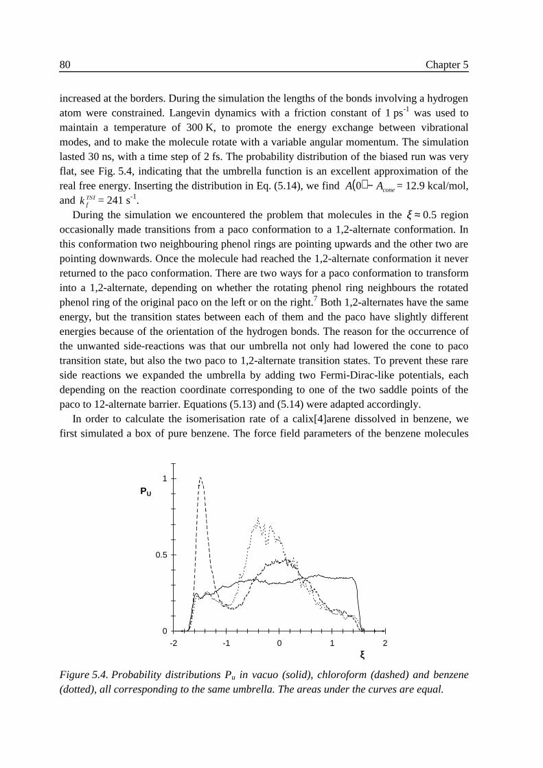
80 Chapter 5

increased at the borders. During the simulation the lengths of the bonds involving a hydrogenatom were constrained. Langevin dynamics with a friction constant of 1 ps-1 was used tomaintain a temperature of 300 K, to promote the energy exchange between vibrationalmodes, and to make the molecule rotate with a variable angular momentum. The simulationlasted 30 ns, with a time step of 2 fs. The probability distribution of the biased run was veryflat, see Fig. 5.4, indicating that the umbrella function is an excellent approximation of thereal free energy. Inserting the distribution in Eq. (5.14), we find ( )A Acone0 − = 12.9 kcal/mol,and k f

TST= 241 s-1.During the simulation we encountered the problem that molecules in the ξ ≈ 0.5 region

occasionally made transitions from a paco conformation to a 1,2-alternate conformation. Inthis conformation two neighbouring phenol rings are pointing upwards and the other two arepointing downwards. Once the molecule had reached the 1,2-alternate conformation it neverreturned to the paco conformation. There are two ways for a paco conformation to transforminto a 1,2-alternate, depending on whether the rotating phenol ring neighbours the rotatedphenol ring of the original paco on the left or on the right.7 Both 1,2-alternates have the sameenergy, but the transition states between each of them and the paco have slightly differentenergies because of the orientation of the hydrogen bonds. The reason for the occurrence ofthe unwanted side-reactions was that our umbrella not only had lowered the cone to pacotransition state, but also the two paco to 1,2-alternate transition states. To prevent these rareside reactions we expanded the umbrella by adding two Fermi-Dirac-like potentials, eachdepending on the reaction coordinate corresponding to one of the two saddle points of thepaco to 12-alternate barrier. Equations (5.13) and (5.14) were adapted accordingly.

In order to calculate the isomerisation rate of a calix[4]arene dissolved in benzene, wefirst simulated a box of pure benzene. The force field parameters of the benzene molecules

0

0.5

1

-2 -1 0 1 2ξ

PU

Figure 5.4. Probability distributions Pu in vacuo (solid), chloroform (dashed) and benzene(dotted), all corresponding to the same umbrella. The areas under the curves are equal.

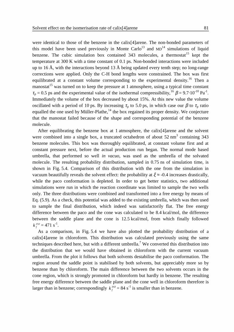
Solvent effect on the isomerisation rate of calix[4]arene 81

were identical to those of the benzene in the calix[4]arene. The non-bonded parameters ofthis model have been used previously in Monte Carlo13 and MD

14 simulations of liquidbenzene. The cubic simulation box contained 343 molecules, a thermostat15 kept thetemperature at 300 K with a time constant of 0.1 ps. Non-bonded interactions were includedup to 16 Å, with the interactions beyond 13 Å being updated every tenth step; no long-rangecorrections were applied. Only the C-H bond lengths were constrained. The box was firstequilibrated at a constant volume corresponding to the experimental density.16 Then amanostat15 was turned on to keep the pressure at 1 atmosphere, using a typical time constantτp = 0.5 ps and the experimental value of the isothermal compressibility,16 β = 9.7·10-10 Pa-1.Immediately the volume of the box decreased by about 15%. At this new value the volumeoscillated with a period of 10 ps. By increasing τp to 5.0 ps, in which case our β to τp ratioequalled the one used by Müller-Plathe,14 the box regained its proper density. We conjecturethat the manostat failed because of the shape and corresponding potential of the benzenemolecule.

After equilibrating the benzene box at 1 atmosphere, the calix[4]arene and the solventwere combined into a single box, a truncated octahedron of about 52 nm3 containing 343benzene molecules. This box was thoroughly equilibrated, at constant volume first and atconstant pressure next, before the actual production run began. The normal mode basedumbrella, that performed so well in vacuo, was used as the umbrella of the solvatedmolecule. The resulting probability distribution, sampled in 0.75 ns of simulation time, isshown in Fig. 5.4. Comparison of this distribution with the one from the simulation invacuum beautifully reveals the solvent effect: the probability at ξ ≈ -0.4 increases drastically,while the paco conformation is depleted. In order to get better statistics, two additionalsimulations were run in which the reaction coordinate was limited to sample the two wellsonly. The three distributions were combined and transformed into a free energy by means ofEq. (5.9). As a check, this potential was added to the existing umbrella, which was then usedto sample the final distribution, which indeed was satisfactorily flat. The free energydifference between the paco and the cone was calculated to be 8.4 kcal/mol, the differencebetween the saddle plane and the cone is 12.5 kcal/mol, from which finally followedk f

TST= 471 s-1.As a comparison, in Fig. 5.4 we have also plotted the probability distribution of a

calix[4]arene in chloroform. This distribution was calculated previously using the sametechniques described here, but with a different umbrella.7 We converted this distribution intothe distribution that we would have obtained in chloroform with the current vacuumumbrella. From the plot it follows that both solvents destabilise the paco conformation. Theregion around the saddle point is stabilised by both solvents, but appreciably more so bybenzene than by chloroform. The main difference between the two solvents occurs in thecone region, which is strongly promoted in chloroform but hardly in benzene. The resultingfree energy difference between the saddle plane and the cone well in chloroform therefore islarger than in benzene; correspondingly k f

TST= 84 s-1 is smaller than in benzene.

82 Chapter 5

5 .3 .2 Transmission coefficient

In order to calculate the transmission coefficient, Eq. (5.5), conformations needed to besampled in the transition plane. One thousand conformations were created by means of anMD simulation of a solvated calix[4]arene during which the value of the reaction coordinatewas constrained to zero; atomic coordinates and velocities were saved every picosecond.Each of these configurations was used as the starting point of a 2 ps relaxation run. At thestart of every relaxation run the velocity of the reaction coordinate, which was zero duringthe constrained run, was replaced by a new velocity drawn from a velocity-weightedMaxwell-Boltzmann distribution.6 The transmission coefficient as a function of time isshown in Fig. 5.5. The dotted line shows the contribution to the transmission coefficientfrom those molecules which cross the transition state at time zero with a positive velocityand finally settle in the product well, or to put differently, the fraction of the product boundflux through the transition state that ends up in the product well. Likewise, the dashed linegives the contribution to the transmission coefficient from those molecules which cross thetransition state at time zero with a negative velocity and end up in the product state; thesemolecules must therefore have crossed the transition state at least once. Both curves live upto their expectation: they start at respectively one and zero, at short times they decreasebecause of molecules recrossing the transition state, and at longer times they settle at a stablelevel. The solid line, the transmission function, is obtained by summing these twocontributions. After 2 ps a plateau of 0.56 is reached. In combination with the previouslycalculated k f

TST, the true reaction rate is then found to be k fRF = 264 s-1.

Similar simulations of calix[4]arene in chloroform yielded κ = 0.43, which together with

-0.25

0.00

0.25

0.50

0.75

1.00

0 0.5 1 1.5 2

Time / ps

κ

Figure 5.5. Transmission coefficient (solid) of a calix[4]arene in benzene. The dotted(dashed) line gives the contribution of molecules that settle in the paco conformation aftercrossing the transition state with a positive (negative) transient velocity.

Solvent effect on the isomerisation rate of calix[4]arene 83

the transition state value k fTST= 84 s-1 yielded k f

RF = 36 s-1. The influence of the solvent isseen to be more prominent in the free energy differences than on the transmissioncoefficients.

All results so far have been collected in Table 5.1, together with a few more results fromvacuum simulations. Simulations6 in vacuo with the same transition state produced atransmission coefficient which arrived at a plateau of 0.92 after 0.6 ps, indicating that in thiscase the TST rate is an excellent approximation of the real rate. After about 0.8 ps thetransmission function started to decrease again, and eventually settled at a second plateau of0.82. This decrease was caused by molecules which left the paco well after having made onefull oscillation in this well; this would not have occurred if the paco well had acted as aperfect sink.

The isomerisation rates of calix[4]arenes in solvents have been measured using1H-NMR.17,18 It was found that for the particular molecule studied here, the paco is tooshort-lived to be detectable. The measured rate constants correspond to the cone to invertedcone reaction, i.e. a process in which all four phenol rings rotate. This reaction consists offour steps, with one phenol ring rotating in each step.9 If we assume these steps to beindependent, the reaction scheme becomes

C

k

kP

k

kA

k

kP

k

kC

1

2

3

4

4

3

2

1

→←

→←

→←

′ →←

′ , (5.1)

where C, P and A denote respectively cone, paco and alternate, and where primes indicateconformations in which the majority of the phenols is pointing downwards. In reasonableapproximation the overall cone to inverted cone rate constant is found to be related to thecalculated cone to paco rate by7 k kCC f

RF′ ≈ 3 .

Gutsche and Bauer17 measured the coalescence temperature with temperature dependent1H-NMR, and derived the isomerisation rate at this temperature from the chemical shift.They converted the rate into a free energy by

Table 5.1. Computed and experimental rates for the cone to paco conversion.

Solvent and method kTST /s-1

κ kRF /s-1

kexp / s-1

Vacuum normal mode analysis 174Vacuum umbrella sampling, t = 0.6 ps 241 0.92 222Vacuum umbrella sampling, t = 2.0 ps 241 0.82 198Chloroform umbrella sampling 84 0.43 36 30,a 8b

Benzene umbrella sampling 471 0.56 264 202a

a Data by Gutsche and Bauer,17 converted to 300 K.b Data by Araki et al.18

84 Chapter 5

∆A RTkcoalescence

coalescence

≠ =⋅

ln

.6 62 1012

. (5.2)

For calix[4]arene in benzene they found ∆A≠ = 13.8 kcal/mol and Tcoalescence= 15 °C. Withthese data we have calculated the isomerisation rate at the coalescence temperature. By usingEq. (5.11), and assuming that the free energy is independent of the temperature, we thenfound a rate of 607 s-1 at 300 K for the cone to inverted cone reaction, hence a rate of 202 s-1

for the cone to paco reaction. The data for a calix[4]arene in chloroform were convertedlikewise, and yielded a rate of 30 s-1. Araki et al.18 measured the reaction rate and the freeenergy of a calix[4]arene in chloroform as a function of temperature, resulting in a rate of8 s-1 at 300 K. From their data it followed that the entropic contribution to the free energy isof minor importance in the above extrapolations, at most equal to about 0.1 kcal/mol, whichis comparable with the uncertainty of the ∆A≠ . All data are summarised in Table 5.1. Thecomputed reaction rates compare very well with the measured rates, the former being slightlyhigher.

5 .4 ConclusionsThe isomerisation rate of a calix[4]arene in benzene and in chloroform has been studied

with molecular dynamics simulations. The free energy as a function of the reactioncoordinate was calculated by means of umbrella sampling. The rate constants obtained withthe reactive flux method were in good agreement with the experimental values. Inchloroform the cone conformation was found to be stabilised by the solvent, appreciablyreducing the reaction rate with respect to the vacuum value. The reaction coordinate definedas the displacement along the unstable normal mode at the saddle point of the potentialenergy surface was shown to be very convenient in these calculations. An excellent firstguess at the umbrella potential was obtained by a straightforward normal mode analysis. Thesame reaction coordinate can, in principle, be applied to numerous reactions.

5 .5 References1 C. D. Gutsche, Calixarenes (Royal Society of Chemistry, Cambridge, U. K. 1989);

Calixarenes. A Versatile Class of Compounds, edited by J. D. Vicens and V. Böhmer(Kluwer Academic Publishers, Dordrecht, The Netherlands, 1991).

2 P. Hänggi, P. Talkner and M. Borkovec, Rev. Mod. Phys. 62, 251 (1990).3 P. W. Atkins, Physical Chemistry (Oxford University Press: Oxford, U. K., 1990).4 D. Chandler, J. Chem. Phys. 68, 2959 (1978).5 W. H. Miller, Acc. Chem. Res. 9, 306 (1976).6 W. K. den Otter and W. J. Briels, J. Chem. Phys. 106, 5494 (1997) (Chapter 3).7 W. K. den Otter and W. J. Briels, J. Chem. Phys. 107, 4968 (1997) (Chapter 4).

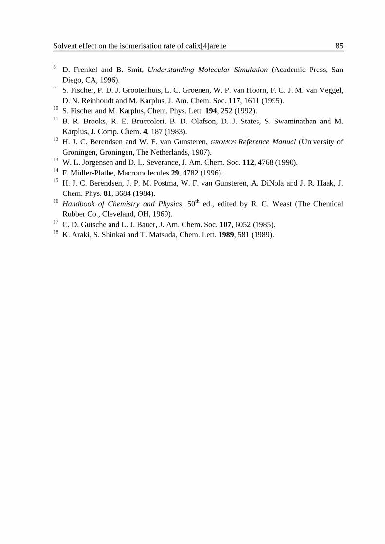
Solvent effect on the isomerisation rate of calix[4]arene 85

8 D. Frenkel and B. Smit, Understanding Molecular Simulation (Academic Press, SanDiego, CA, 1996).

9 S. Fischer, P. D. J. Grootenhuis, L. C. Groenen, W. P. van Hoorn, F. C. J. M. van Veggel,D. N. Reinhoudt and M. Karplus, J. Am. Chem. Soc. 117, 1611 (1995).

10 S. Fischer and M. Karplus, Chem. Phys. Lett. 194, 252 (1992).11 B. R. Brooks, R. E. Bruccoleri, B. D. Olafson, D. J. States, S. Swaminathan and M.

Karplus, J. Comp. Chem. 4, 187 (1983).12 H. J. C. Berendsen and W. F. van Gunsteren, GROMOS Reference Manual (University of

Groningen, Groningen, The Netherlands, 1987).13 W. L. Jorgensen and D. L. Severance, J. Am. Chem. Soc. 112, 4768 (1990).14 F. Müller-Plathe, Macromolecules 29, 4782 (1996).15 H. J. C. Berendsen, J. P. M. Postma, W. F. van Gunsteren, A. DiNola and J. R. Haak, J.

Chem. Phys. 81, 3684 (1984).16 Handbook of Chemistry and Physics, 50th ed., edited by R. C. Weast (The Chemical

Rubber Co., Cleveland, OH, 1969).17 C. D. Gutsche and L. J. Bauer, J. Am. Chem. Soc. 107, 6052 (1985).18 K. Araki, S. Shinkai and T. Matsuda, Chem. Lett. 1989, 581 (1989).

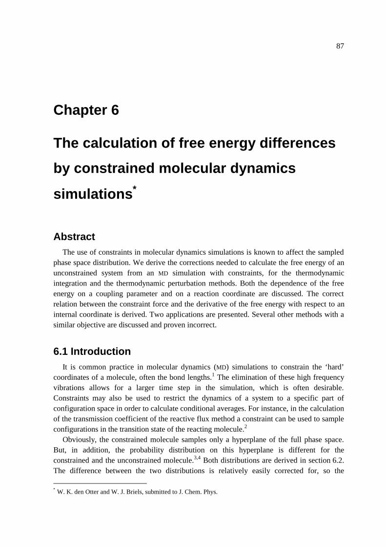
87

Chapter 6

The calculation of free energy differences

by constrained molecular dynamics

simulations ∗

AbstractThe use of constraints in molecular dynamics simulations is known to affect the sampled

phase space distribution. We derive the corrections needed to calculate the free energy of anunconstrained system from an MD simulation with constraints, for the thermodynamicintegration and the thermodynamic perturbation methods. Both the dependence of the freeenergy on a coupling parameter and on a reaction coordinate are discussed. The correctrelation between the constraint force and the derivative of the free energy with respect to aninternal coordinate is derived. Two applications are presented. Several other methods with asimilar objective are discussed and proven incorrect.

6 .1 IntroductionIt is common practice in molecular dynamics (MD) simulations to constrain the ‘hard’

coordinates of a molecule, often the bond lengths.1 The elimination of these high frequencyvibrations allows for a larger time step in the simulation, which is often desirable.Constraints may also be used to restrict the dynamics of a system to a specific part ofconfiguration space in order to calculate conditional averages. For instance, in the calculationof the transmission coefficient of the reactive flux method a constraint can be used to sampleconfigurations in the transition state of the reacting molecule.2

Obviously, the constrained molecule samples only a hyperplane of the full phase space.But, in addition, the probability distribution on this hyperplane is different for theconstrained and the unconstrained molecule.3,4 Both distributions are derived in section 6.2.The difference between the two distributions is relatively easily corrected for, so the

∗ W. K. den Otter and W. J. Briels, submitted to J. Chem. Phys.

88 Chapter 6

unconstrained averages needed in the calculation of the free energy can be calculated bymeans of a constrained MD simulation, as is described in section 6.3.

In rate theory one is interested in the free energy of a reacting system as a function of aninternal coordinate of the system, the reaction coordinate { }( )ξ x i . From this free energyfunction follow the equilibrium constant of the reaction and the transition state theoryestimate of the reaction rate. In section 6.4 it will be shown that the derivative of the freeenergy with respect to ξ is closely related to the constraint force needed to keep the system atthe hyperplane { }( )ξ x i = ξ . This relation is illustrated in section 6.5 with the simulations oftwo prototypical molecules. In the literature there have appeared a number of methods tocalculate the free energy as a function of a reaction coordinate. Several of these methods, andtheir shortcomings, are discussed in section 6.6. The GASP method, which in a sense is verysimilar to these methods, will also be discussed. We end with a short remark on how thetheory presented here for molecular dynamics simulations ought to be used in Monte Carlosimulations.

6 .2 Constraints and probability distributionsIn this section we introduce the probability distributions resulting from unconstrained and

constrained molecular dynamics simulations, and describe them. Their relation is derived insection 6.2.1 in terms of generalised coordinates. Some aspects of the implementation ofconstraints in Cartesian coordinates are discussed in section 6.2.2.

6 .2 .1 Generalised coordinates

Consider a molecule consisting of N atoms. The configuration of this molecule isdescribed by 3N Cartesian coordinates, { }X x= i , or by an equal number of generalisedcoordinates, ( )q,σ . We have split the generalised coordinates into two groups, namely the Lcoordinates σ that are going to be constrained in the MD run and the remaining 3N L−unconstrained coordinates.

First we consider the case in which none of the coordinates, including σ, is constrained.The Lagrangian of this system reads as

( ) ( )Luq q

Tq qq v v A v q, , ,σ σσ σ σ σ= −1

2 Φ , (6.1)

where ( )v qqT T

σ = � , �σ Τ is the row vector of all generalised velocities and Φ is the potentialenergy. The conjugate momenta are given by

p A vq q qσ σ σ= , (6.2)

with ( )p p pqT

qT T

σ σ= , , and the Hamiltonian reads

( ) ( )H uq q

Tq qq p p A p q, , ,σ σσ σ σ σ= +−1

21 Φ . (6.3)

The probability distribution of the unconstrained system with these coordinates is

Free energy differences by constrained molecular dynamics simulations 89

( ) ( )[ ]P Huq

uqq p q p, , exp , ,σ σσ σβ∝ − , (6.4)

where β = 1 k TB , kB is Boltzmann’s constant and T is the absolute temperature.For future convenience we will write the 3N×3N dimensional mass-metric matrix A qσ in

block form as

AA B

B Cq

q

Tσσ

σ σ=

, (6.5)

AX Y

Y Zq

q

Tσσ

σ σ

− =

1 , (6.6)

where A q is the ( ) ( )3 3N L N L− × − upper left block of A qσ , etc. The mass-metric matrixcan easily be obtained by transforming the kinetic energy of the unconstrained system fromCartesian coordinates to generalised coordinates:

A J MJqT

σ = , (6.7)

where M is a 3N×3N matrix containing all atomic masses down the diagonal, and

JXq

X=

∂∂

∂∂σ

(6.8)

is the Jacobi matrix of the transformation. The inverse matrix A qσ−1 is readily obtained from

Eqs. (6.7) and (6.8). In what follows we will use the matrices Z σ and Yσ , whosecomponents are then found to be

( )Zx xσ

∂σ∂

∂σ∂ij

k

i

k

j

kk

N

m= ⋅

=∑ 1

1

, (6.9)

( )Yx xσ

∂∂

∂σ∂ij

k

i

k

j

kk

N

m

q= ⋅

=∑ 1

1

. (6.10)

A second important relation is3

A A Zq q= σ σ , (6.11)

which follows from

A 0

B 1A A

A 0

B 1A

1 Y

0 Zq

T q q

q

T qσ

σ σσ

σσ

σ

=

=

−1 (6.12)

by using Eqs. (6.5) and (6.6), and taking the determinant on both sides.The Hamiltonian of the σ-constrained system must be derived from the Lagrangian of the

constrained system, which in turn is obtained form the Lagrangian of the unconstrainedsystem by imposing the constraints σ σ= and �σ = 0 . The usual operations yield

90 Chapter 6

( ) ( )H cq q

Tq qσ q p p A p q, ,= +−1

21 Φ σσ , (6.13)

with p A qq q= � . The corresponding probability distribution reads as

( ) ( )[ ]P Hcq

cqσ σβq p q p, exp ,∝ − . (6.14)

This is the distribution which is sampled with a constrained MD run. It differs from theunconstrained distribution not only by σ being equal to σ , but also by the absence of theimpulses pσ , so care must be taken if one is to calculate unconstrained conditional averages,with σ σ= being the conditions, by means of a constrained dynamics simulation.

We will denote by

( )( )F

d d FP

d d P

qc

q

qc

q

σ

σ

σ

= ∫ ∫∫ ∫

q p q p

q p q p

,

,(6.15)

the average of some function F over a constrained Hamiltonian, and by

( )( )F

d d FP

d d Pu

Xu

X

Xu

X

= ∫ ∫∫ ∫

X p X p

X p X p

,

,(6.16)

the corresponding unconstrained average. We will now express the unconstrained average ofthe function F in terms of a constrained average, for those cases when the usual assumptionfor ‘hard’ variables can be made, i.e. when a factor of ( )δ σ σ− can be introduced in theintegral. More precisely, we write the potential energy as5

( ) ( ) [ ] [ ]Φ Φq q F, ,σ σ σ − σ σ − σ≈ + 12

T , (6.17)

where F is assumed to be independent of q, and integrate over the σ to obtain for thenumerator of Eq. (6.16):

( ){ }[ ] [ ]N d d d Fq qT

q q∝ − +− −∫ ∫F q p p A p q1 2 12

1σ σ σ − σσ σ σ σβ δexp ,Φ . (6.18)

Making the same approximation in the denominator, Q, we arrive at the conditional averagereferred to above. Even though the variations in σ are so small that they can be replaced by aDirac-delta in the integral, the variations in the associated momenta are not small and mustbe taken into account explicitly. Writing

( ) ( )p A p p A p p Z Y p Z p Z Y pqT

q q qT

q qT

q

TT

qσ σ σ σ σ σ σ σ σ σ− − − −= + − −1 1 1 1 (6.19)

and integrating over the momenta pσ , we find

( ){ }[ ]N d d Fq qT

q q∝ − +∫ ∫ − −q p p A p q Zexp ,β σ

12

1 1 2Φ σσ . (6.20)

The exponential is proportional to the probability distribution of the constrained system,Eq. (6.14). The factor Z σ

−1 2 is seen to convert the integral over the constrained ensembleinto the corresponding integral over the unconstrained ensemble; this factor is to be

Free energy differences by constrained molecular dynamics simulations 91

interpreted as the ratio of the momentum spaces of the constrained and the unconstrainedsystems at ( )q,σ . By applying the above transformation rule, the expectation value of F in anunconstrained ensemble can be calculated from a constrained ensemble by

FF

u =

−

−

Z

Z

σσ

σσ

1 2

1 2. (6.21)

Almost all expressions in this article will be of this form. It is clear that F may not depend onσ, nor on ( )�σ = − −Z p Z Y pσ σ σ σ

1 Tq , for this expression to hold. Notice that the expression is

valid even if F depends on the momenta pq , a fact overlooked by Ruiz-Montero et al.,6 but

not if F depends on the velocities �q .

6 .2 .2 Simulation in Cartesian coordinates

The generalised coordinates of the previous section are very useful for the theoreticalunderstanding of the problem. However, in computer simulations the generalised coordinatesare rather awkward to use, and Cartesian coordinates are being used instead. The Cartesianequations of motion for a constrained system follow from the Lagrangian

( ) ( ) ( )( )L t L tul l l

l

L* , � , , � ,X X X X X= + ⋅ −

=∑λ σ σ

1

, (6.22)

where the Lagrange multipliers, λl , are determined by demanding that the constraints arefulfilled at all times. From the equations of motion it follows that each atom feels aconstraint force given by

Fic

l i ll

L

==∑λ σ∇

1

. (6.23)

If initially ( )σ l lX = σ and �σ l = 0, the constraints can be fulfilled by demanding ��σ l = 0;together with the equations of motion and Eq. (6.9) this leads to1,7

( )λ σ σσl lk i i k ii

N

j i j k ii j

N

k

L

m= ⋅ − ⋅ ⋅

− −

= ==∑ ∑∑ Z x x1 1

1 11

∇ ∇ ∇ ∇Φ � �

,

. (6.24)

Simulations in which these analytical expressions for the Lagrange multipliers are actuallybeing used, as a consequence of numerical inaccuracies due to the use of a finite time step,gradually drift away from the constraint hyperplane, ( )σ σX = . They therefore need to bereset to the hyperplane once every while.8

In the SHAKE9 algorithm the constraints are rigorously met every simulation step. First, in

a regular MD step without constraints the atomic positions are advanced from ( )x i t to( )′ +x i t t∆ , resulting in a violation of the constraints. In the second step a force of the form of

Eq. (6.23) is used in the Verlet algorithm to move the atoms to

92 Chapter 6

( ) ( ) ( )x xi i

il i l

l

L

t t t tt

m+ = ′ + +

=∑∆ ∆

∆ 2

1

λ σ∇ , (6.25)

again accompanied by a change of the constraints. The Lagrange multipliers are chosen suchthat the constraints are restored to their initial values. To this end a Taylor expansion of σ ismade to first order in ( ) ( )x xi it t+ − ′ +∆ ∆ , assuming that the gradients of σ l hardly changeduring the unconstrained MD step,

( ) ( ) ( ) ( ) ( )σ σ λ σ σl l ki

i l i ki

N

k

L

t t t t tm

t t+ = ′ + + ⋅==∑∑∆ ∆ ∆ 2

11

1∇ ∇ . (6.26)

With ( )σ l t t+ ∆ equal to σ l , this is a set of equations which may be solved for the λk . Thesecond step must be repeated until all constraints are met to within acceptable accuracy. TheLagrange multipliers obtained in this way are comparable with the ones calculatedanalytically, so in section 6.4 we shall assume them to be identical.

One particular system worth mentioning is a molecule in which only the distance betweenatoms 1 and 2 is constrained, σ = r12 , where r r r12 2 1= − . Equation (6.24) then yields

λ µ µ= −

⋅ +

⋅F F r r r1

1

2

2

12

12

12 12

12m m r r

� �

, (6.27)

the familiar result from the Gauss’ principle of least constraint.8

As a final remark we note that the constraint force resulting from constraining an internalcoordinate of a molecule does not effect the total momentum nor the total angularmomentum of this molecule. Therefore, there is no need to explicitly use this conservationproperty when calculating the constraint force, as was done by Tobias and Brooks.10

6 .3 Thermodynamic integration and perturbationSuppose one is interested to know the free energy of a system as a function of some

parameter. This parameter could be an internal coordinate of some molecule, for example areaction coordinate. Or it could be a parameter occurring in the potential energy of themolecule, a so-called coupling parameter. There are two common ways of calculating freeenergy differences in these cases, namely thermodynamic integration and thermodynamicperturbation. All four possible combinations will be briefly addressed in this section.

6 .3 .1 Reaction coordinate ξξIn this subsection we will calculate the probability distribution of a given molecule along

some internal coordinate ξ. Our main interest is when ξ is a reaction coordinate, since theprobability of finding the molecule at the transition state, i.e. when ξ ξ= ≠ , is directly relatedto the rate of the reaction. The calculation of this distribution by means of a standard MD runusually is an impossible task, since the high energy barriers prohibit sampling all values of ξ.With umbrella sampling the probability of crossing existing energy barriers is enhanced by

Free energy differences by constrained molecular dynamics simulations 93

deliberately lowering the barriers by means of an extra potential. In the subsequent analysisof the run appropriate corrections are made for this extra potential. In this section we willdiscuss an alternative method, using constrained MD simulations, in which the system isforced to sample only regions of phase space where ξ has some prescribed value. In additionto this constraint on the reaction coordinate ξ, L hard variables σ will also be constrained.The atomic masses and σ , the values to which the σ variables will be constrained, areassumed independent of ξ.

Our notation requires some minor changes to accommodate the extra constrainedcoordinate. The 3N×3N mass-metric matrix will henceforth be written as

AA B

B CA B

B Cq

q

TqTξσ

ξσ

ξσ ξσ

ξ σ

σ σ=

=

, (6.28)

AX Y

Y ZX Y

Y Zq

q

Tq

Tξσξσ

ξσ ξσ

ξ σ

σ σ

− =

=

1 , (6.29)

where A q and X q are ( ) ( )3 1 3 1N L N L− − × − − dimensional matrices, A qξ and X qξ are( ) ( )3 3N L N L− × − dimensional, etc. The results of section 6.2.1 can now easily begeneralised, for example Eq. (6.11) now reads as

A A Z A Zq q qξσ ξ σ ξσ= =− −1 1

. (6.30)

The probability distribution of the ( )ξ,σ -constrained ensemble can be shown to be

( ) ( ){ }[ ]Pcq q

Tq qξσ β ξq p p A p q, exp , ,∝ − +−1

21 Φ σσ , (6.31)

where q and pq have ( )3 1N L− − elements. Equation (6.15) generalises to

( )( )F

d d FP

d d P

qc

q

qc

q

ξσξσ

ξσ

= ∫ ∫∫ ∫

q p q p

q p q p

,

,. (6.32)

The probability distribution along the reaction coordinate reads

( ) ( ) ( )[ ] ( )[ ]pQ

Q Qd d HX

uXξ

ξβ δ ξ ξ= = − −∫ ∫

1X p X p Xexp , , (6.33)

where Q is a normalisation factor. This distribution is often expressed as a free energy by

( ) ( )A k T QBξ ξ= − ln . (6.34)

The direct evaluation of the partition function ( )Q ξ is virtually impossible, but its derivativeis relatively simple to calculate. This fact is used in the thermodynamic integration method,which allows ( )A ξ to be calculated up to some constant:

( ) ( ) ( )A A

dA

ddξ

ξξ

ξξ

= +′

′′∫0

0

, (6.35)

94 Chapter 6

with

( )( )

( )dA

d

k T

Q

dQ

dBξ

ξ ξξ

ξ= − . (6.36)

There are several ways to differentiate the partition function with respect to the reactioncoordinate, all leading to the same final result of course. The obvious way to go at this point,given what has been said in the previous sections, is to write

( ) [ ]Q d d Hqcξ β ξσ∝ −∫ ∫

−q p Zexp

1 2

, (6.37)

and to differentiate with respect to ξ, obtaining

( ) [ ]dQ

dd d Hq

c

qT q

q

ξξ

β

β∂

∂ξβ

∂∂ξ

∂∂ξ

ξσ

ξσξσ

∝ −

× − − −

∫ ∫−

−−

q p Z

pA

p ZZ

exp

.

1 2

12

1

12

1Φ(6.38)

Using

[ ]

[ ]

[ ]

d

k T d

k T d

q qT

q q qT q

q

B q

q

q qT

q q

B q

q

q qT

q q

p p A p pA

p

AA

p p A p

AA

p p A p

∫

∫

∫

−

=

−

= − −

−−

−−

− −

exp

exp

exp

12

1

1

1

12

1

112

1

β∂

∂ξ

∂∂ξ

β

∂∂ξ

β

Tr (6.39)

and Eq. (6.30) we arrive at

( )dA

dk TB

q

q

ξξ

∂∂ξ

∂∂ξ

ξσξσ

ξσξσ

ξσξσ ξσ

ξσ

= −

−

− − −11 2

1 212

1 1 2

ZZ

AA Z

Φ. (6.40)

In Eq. (6.39) Tr denotes the trace; in the first step of this equation we have used thesymmetry of A q , and in the second step we have used ( )Tr A Aq q∂ ∂ξ−1 = −∂ ∂ξ Tr ln A q

1

= −∂ ∂ξ ln A q1 = −∂ ∂ξ ln A q . If finally we would use Eq. (6.7) in the form A M Jqξσ = 2 , we

would arrive at a result similar to Eq. (6.40), with A qξσ in the last term replaced by J , andthe factor ½ replaced by unity.7 The two terms between the large square brackets are readilyrecognised by their temperature dependence as being the energetic and the entropiccontributions to the free energy difference.

A different technique for calculating free energy differences is the thermodynamicperturbation method. The free energy difference is then calculated directly by

Free energy differences by constrained molecular dynamics simulations 95

( ) ( ) ( )[ ] [ ]( )[ ] [ ]

[ ][ ]

A A k Td d H

d d H

k Td d H

d d H

B

Xu

X

Xu

X

B

qc

qc

ξ ξβ δ ξ ξ

β δ ξ ξ

β

β

ξ σ

ξ σ

2 1

2

1

2 2

1 2

1 1

1 2

− = −− −

− −

= −−

−

∫∫∫∫∫∫∫∫

−

−

lnexp ,

exp ,

lnexp

exp,

X p X p

X p X p

q p Z

q p Z

(6.41)

where Hic is the constrained Hamiltonian with ξ constrained to the value ξi . We now want

to refer the numerator to an average over the probability distribution used in thedenominator. To this end we use

( )[ ] ( )( )

( )[ ]d dq qT

q q

q

q

q qT

q qp p A pA

Ap p A p∫ ∫− = −− −exp exp1

21

2

2

1 2

1

1 212

11β ξ

ξ

ξβ ξ (6.42)

and A Z A M Jq qξσ ξσ− = =1 2 , obtaining

( ) ( )[ ] ( ) ( )

A A k TBξ ξβ ξ ξ ξ σ

ξ σ

ξ σξ σ

2 1

12 1

1

2 1

1 2

1

1

1 2

1

− = −

−− −

−ln

exp ∆Φ J J Z

Z, (6.43)

where ( ) ( )∆Φ Φ Φ12 2 1= −q q, , , ,ξ ξσ σ and ( )J ξi is the Jacobian with ξ put equal to ξi .Dividing Eq. (6.43) by ξ ξ2 1− and taking the limit of this difference going to zero we againobtain Eq. (6.40).

6 .3 .2 Coupling parameter λλA coupling parameter λ is used to transform the force field representative of molecule A

into the force field representative of molecule B via a series of intermediate, non-physical,molecules. For a linear transformation the intermediate force fields read as

( )Φ Φ Φλ λ λ= − ⋅ + ⋅1 A B . Non-linear transformations were found to be useful in caseswhere the number of atoms in molecules A and B differ. Examples where the method hasbeen used include the calculation of the difference of the free energy of hydration of ethanoland the free energy of hydration of ethane11, the difference of the free energies ofcomplexation of 18-crown-6 with sodium or potassium ions,12 and the solvability of methaneversus neopentane in water.13

The partition function of an unconstrained molecule with a λ-dependent Hamiltonian isgiven by

( ) ( )[ ]( ) ( ) ( ){ }[ ] ( )[ ]

Q d d H

d d d

Xu

X

q qT

q q

λ β λ

λ β λ λ δ λσ σ σ σ

∝ −

∝ − +

∫ ∫∫ ∫− −

X p X p

F q p p A q p q

exp , ;

exp , ; , ; ,1 2 1

21σ σ σ σ − σΦ

(6.44)

96 Chapter 6

where in the second line we have made the usual assumptions for the hard variables. Intrying to be as general as possible, we allow for a coupling parameter dependence of theforce field, the atomic masses and the value of the constrained coordinates. In the presentcase we shall explicitly assume that the force constant matrix F associated with theconstraints depends on λ, like for example when a constrained C-H bond is turned into aconstrained O-H bond.

The derivation of the expressions for thermodynamic integration is analogous to that ofthe previous section, and the final result reads

( )dA

d

d

dk T

d

d

k Td

d

B

q

q

B

λλ λ λ

λ

σσ λ

σσ λ

σσ σ

σ λ

= −

+

−

− − −

−

11 2

1 2 12

1 1 2

12

1

ZZ

AA Z

FF

;;

;

.

Φ

(6.45)

There are a few differences between this result and Eq. (6.40). First, the potential energyfunction may depend on the coupling parameter explicitly, but also implicitly via theconstrained coordinates,

( )( ) ( )( ) ( ) ( )( )d

d

d

dl

ll

LΦ Φ Φq q q, ; , ; , ;σ σ σλ λλ

∂ λ λ∂λ

λλ

∂ λ λ∂

= +=∑ σ

σ1

. (6.46)

Second, since the atomic masses may depend on λ, use of Eq. (6.7) yields

( )1 2 1

1A

A

JJ

MM

q

q

l

l

l

L d

dσ

σ∂∂λ

∂∂

λλ

∂∂λ

= +=∑ σ

σ. (6.47)

The first term on the right hand side is the usual term. The second term on the right handside, after having been used in Eq. (6.45), and after a subsequent integration with respect to λyields the obvious contribution to ∆A. In all meaningful applications this contribution will beirrelevant. Finally, there is an extra term in Eq. (6.45), stemming from the constrainedvariables, which in many applications, but not all, will be irrelevant.

The expression for thermodynamic perturbation is readily found to be

[ ] ( ) ( ) ( ) ( )∆

∆ΦA k TB= −

−− − −

−ln

exp;

;

β λ λ λ λ σσ λ

σσ λ

12 1

1 2

2

1 2

1

1

2

1 2

1 2

1

1

M M J J Z

Z, (6.48)

where ( )( ) ( )( )∆Φ Φ Φ12 2 2 1 1= −q q, ; , ;σ σλ λ λ λ , as follows by reasoning along the lines thatlead to Eq. (6.43).

Free energy differences by constrained molecular dynamics simulations 97

6 .4 Relation between the thermodynamic force and theconstraint force

We now return to Eq. (6.40), restricting ourselves to the case where no additionalconstraints σ are being applied. Using A M Jqξ = 2 , we may write

( ) ( )dA

d Zk T ZB

ξξ

∂∂ξ

ξ ξ

ξξ

= −−

−11 2

1 2Φ ln J . (6.49)

Calculation of the right hand side of this equation is rather cumbersome, because theevaluation of J and ∂ ∂ξ require the introduction of a full set of generalised coordinates.

The combination Φ − k TB ln J may be interpreted as a potential, whose negativederivative with respect to ξ is a force. Equation (6.49) then says that the average of this forceis equal to the thermodynamic force ( )− dA dξ ξ . On similar intuitive grounds vanGunsteren14 suggested that all that the constraint forces do during a constrained MD

simulation is to counterbalance the thermodynamic force, and that therefore ( )dA dξ ξ shouldbe equal to the constraint force. Later, Mülders et al.15 provided an almost correctjustification for this method. Based on their methods we shall now derive the correctrelationship between ( )dA dξ ξ and the average constraint force.

Since we shall need it further on in this section, we shall first derive the explicitexpression of the Lagrange multiplier λξ in terms of the quantities occurring in theLagrangian. From the Lagrangian L* , Eq. (6.22), expressed in generalised coordinates, weobtain the equation of motion of the constrained coordinate,

( )d

dtCT

qT q

qB q vA

vξ ξ ξξ

ξ ξ

∂∂ξ

∂∂ξ

λ�

�+ = − +ξ 12

Φ. (6.50)

Upon substitution of �ξ = 0, we solve for the Lagrange multiplier by demanding ��ξ = 0,obtaining

( )

( )

λ∂∂ξ

∂∂ξ

∂∂ξ

∂∂ξ

ξ ξ

ξ

= − + +

= + +−

12

12

1

� � �

� ,

qA

q B q

pA

p B q

T q T

qT q

qT

d

dt

d

dt

Φ

Φ(6.51)

where we have used �q A p= −q q1 in the second line.

We now start the main derivation of this section. In the present case, Eq. (6.38) reads

( ) [ ]dQ

dd d H Z Z

Zq

cqT q

q

ξξ

β β∂∂ξ

β∂∂ξ

∂∂ξξ ξ

ξ∝ − − − −

∫ ∫ −

−−q p p

Apexp 1 2 1

2

1

12

1Φ. (6.52)

Combining this equation with Eq. (6.51) we find

98 Chapter 6

( ) [ ]

[ ] ( )

dQ

dd d H Z Z

dZ

dtZ

Z

d d Hd

dtZ

qc T

qc T

ξξ

β βλ β∂∂ξ

β β

ξ ξ ξ ξξ

ξξ

ξ ξ

∝ − − + −

+ −

∫ ∫

∫ ∫

− − −

−

q p B q

q p B q

exp �

exp � .

1 2 12

1 12

1

1 2

(6.53)

The last term, being the average of a time derivative, vanishes when ergodicity is assumedand the ensemble average may be replaced by a time average. We next make use of

[ ] [ ]

[ ]

d HdZ

dtd H

Z

k TZ

d H

qc

qc T

B q qc

p q p qqq

Aq

p

∫ ∫

∫

− = −

= −−

exp � exp � �

exp ,

β β∂∂

∂∂

β

ξ ξ

ξ1

(6.54)

where ∂ ∂ξZ q denotes the column vector of derivatives of Zξ with respect to thegeneralised coordinates except ξ. Introducing Eq. (6.54) into Eq. (6.53), and replacingB Aξ

Tq−1 by - Zξ ξ

−1Y T , as follows from A A 1q qξ ξ− =1 , we obtain

( ) [ ]dQ

dd d H Z Z

ZZ

Zq

c Tξ

ξβ βλ

∂∂

∂∂ξξ ξ ξ ξ

ξξ

ξ∝ − − − +

∫ ∫ − −q p Yq

exp 1 2 12

2 . (6.55)

We finally introduce the analogues of Eqs. (6.9) and (6.10) to obtain

( )dA

d

Z k T m Z Z

Z

B i i ii

N

ξξ

λ ξξ ξ ξ ξ ξξ

ξ ξ

=

+ ⋅

− −

=

−

−

∑1 2 12

1

1

5 2

1 2

∇ ∇

. (6.56)

The importance of this expression is that it can be evaluated without explicitly introducingthe complementary generalised coordinates q; all that is needed is the readily availableexpression for ξ in terms of the Cartesian coordinates. A second important property ofEq. (6.56) is that it is manifestly independent of the coordinates q, as is obvious fromEq. (6.33), but which is not evident at all from Eq. (6.40).

6 .5 Numerical examplesTo illustrate Eq. (6.56) with concrete applications, we have calculated the free energies

along the reaction coordinate for two simple systems. As our first example serves a moleculeconsisting of three atoms, with the bending angle in the role of the reaction coordinate. TheJacobian determinant of the transformation from Cartesian coordinates to a set of coordinatescontaining the bond lengths l12 and l23 and the bending angle ξ, is J = l l12

2232

2sin sinξ ψ ,where ψ 2 is one of the Euler angles needed to describe the orientation of the molecule. Weshall assume that the potential energy can be written as a sum of terms, with only one termdepending on the reaction coordinate, ( ) ( )Φ = +V V l lrestξ 12 23, . The partition function is thenreadily evaluated, and the free energy reads

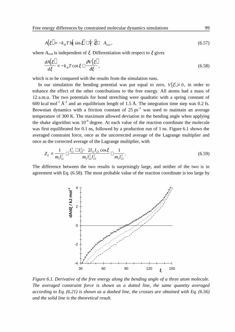
Free energy differences by constrained molecular dynamics simulations 99

( ) ( ) ( )A k T V AB restξ ξ ξ= − + +ln sin , (6.57)

where Arest is independent of ξ. Differentiation with respect to ξ gives

( ) ( )dA

dk T

VB

ξξ

ξ∂ ξ

∂ξ= − +cot , (6.58)

which is to be compared with the results from the simulation runs.In our simulation the bending potential was put equal to zero, ( )V ξ = 0, in order to

enhance the effect of the other contributions to the free energy. All atoms had a mass of12 a.m.u. The two potentials for bond stretching were quadratic with a spring constant of600 kcal mol-1 Å-2 and an equilibrium length of 1.5 Å. The integration time step was 0.2 fs.Brownian dynamics with a friction constant of 25 ps-1 was used to maintain an averagetemperature of 300 K. The maximum allowed deviation in the bending angle when applyingthe shake algorithm was 10-4 degree. At each value of the reaction coordinate the moleculewas first equilibrated for 0.1 ns, followed by a production run of 1 ns. Figure 6.1 shows theaveraged constraint force, once as the uncorrected average of the Lagrange multiplier andonce as the corrected average of the Lagrange multiplier, with

Zm l

l l l l

m l l m lξ

ξ= +

+ −+

1 2 1

1 122

122

232

12 23

2 122

232

3 232

cos. (6.59)

The difference between the two results is surprisingly large, and neither of the two is inagreement with Eq. (6.58). The most probable value of the reaction coordinate is too large by

-4

-2

0

2

4

30 60 90 120 150ξ

dA/d

ξ / k

J m

ol-1

Figure 6.1. Derivative of the free energy along the bending angle of a three atom molecule.The averaged constraint force is shown as a dotted line, the same quantity averagedaccording to Eq. (6.21) is shown as a dashed line, the crosses are obtained with Eq. (6.56)and the solid line is the theoretical result.

100 Chapter 6

10 to 20 degrees. The crosses in Fig. 6.1 represent the results obtained with Eq. (6.56), with

1 4

1

3

2 12 23mZ

m l lZ

ii i

i

∇ ∇ξξ

ξ ξ⋅ ==∑ sin

. (6.60)

The agreement with the theoretically predicted results is perfect; the differences between thecalculated points and the predicted values are of the order of 0.05 kJ mol-1, with thecalculated values being predominantly too high. With similar simulations of moleculesconsisting of three atoms of unequal masses and non-zero bending potentials Eq. (6.56) wasfound to be in good agreement with the theoretical predictions.

As a second example we have calculated the free energy of a four atom molecule as afunction of the dihedral angle. This particular example was chosen because there arenumerous reactions in which a rotation around a dihedral can serve as the reactioncoordinate. As internal coordinates we use the bond lengths l12 , l23 and l34 , the bendingangles φ2 and φ3 and the dihedral angle ξ. The transformation from Cartesian coordinates tothe internal coordinates yields the Jacobian5 determinant J = l l l12

2232

342

2 3 2sin sin sinφ φ ψ ,which is independent of ξ; ψ 2 again is one of the Euler angles needed to specify theorientation of the molecule. Assuming again that the potential energy can be split into partsof which only one term depends on ξ, the free energy is equal to this particular term,

( ) ( )A Vξ ξ= .The derivation of Zξ is considerably more complicated in this case. Using the expressions

for ∇ iξ given by Wilson et al.,16 which were recently rederived by Bekker et al.,17 we found

( ) ( )

Zm l m l

mA B A B

mA B A B

ξ φ φ

ξ ξ

=

+

+ + − + + −

1 1 1 1

12

12

1 12 2

2

4 34 3

2

222

32

2 33

32

22

3 2

sin sin

cos cos

(6.61)

with

Al l

l l223 12 2

12 23 2

=− cos

sin

φφ

, (6.62)

Al l

l l323 34 3

34 23 3

=− cos

sin

φφ

, (6.63)

Bl2

2

23 2

=cos

sin

φφ

, (6.64)

Bl3

3

23 3

=cos

sin

φφ

, (6.65)

in agreement with the result of Depaepe et al..18 Next, after some laborious mathematics wearrived at

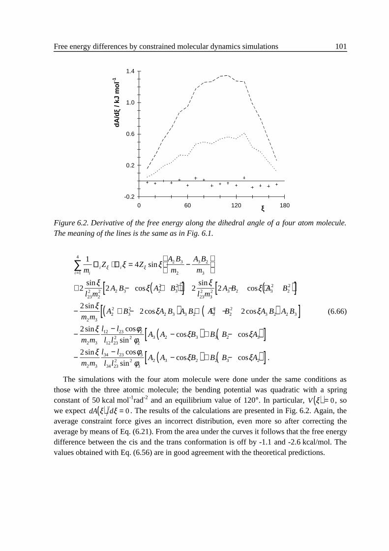
Free energy differences by constrained molecular dynamics simulations 101

( )[ ] ( )[ ]( ) ( )[ ]

14

2 2 2 2

22 2

2

1

42 3

2

3 2

3

232

22 2 3 2

232

232

32 3 2 3

222

2 322

32

2 3 3 2 32

22

3 2 2 3

2 3

12 23

mZ Z

A B

m

A B

m

l mA B A B

l mA B A B

m mA B A B A B A B A B A B

m m

l l

ii i

i

∇ ∇ξ ξξ ξ

ξξ

ξξ

ξξ ξ

ξ

⋅ = −

+ − + + − +

− + − + + −

−−

=∑ sin

sincos

sincos

sincos cos

sin cos ( ) ( )[ ]( ) ( )[ ]

φφ

ξ ξ

ξ φφ

ξ ξ

2

12 232 2

23 2 3 3 2 3

2 3

34 23 3

34 232 2

32 3 2 2 3 2

2

l lA A B B B A

m m

l l

l lA A B B B A

sincos cos

sin cos

sincos cos .

− + −

−−

− + −

(6.66)

The simulations with the four atom molecule were done under the same conditions asthose with the three atomic molecule; the bending potential was quadratic with a springconstant of 50 kcal mol-1rad-2 and an equilibrium value of 120°. In particular, ( )V ξ = 0, sowe expect ( )dA dξ ξ = 0. The results of the calculations are presented in Fig. 6.2. Again, theaverage constraint force gives an incorrect distribution, even more so after correcting theaverage by means of Eq. (6.21). From the area under the curves it follows that the free energydifference between the cis and the trans conformation is off by -1.1 and -2.6 kcal/mol. Thevalues obtained with Eq. (6.56) are in good agreement with the theoretical predictions.

-0.2

0.2

0.6

1.0

1.4

0 60 120 180ξ

dA/d

ξ / k

J m

ol-1

Figure 6.2. Derivative of the free energy along the dihedral angle of a four atom molecule.The meaning of the lines is the same as in Fig. 6.1.

102 Chapter 6

6 .6 Comments on the literatureThe topics covered in the previous sections have been the subject of various articles in the

literature. In this section we will comment on several of these articles.

6 .6 .1 Use and misuse of Zξ , Z σ and Z ξσ

If only bond lengths are constrained, Z σ in Eq. (6.21) is a function of the atomic massesof the atoms involved in the constrained bonds, and of the bending angles between theconstrained bonds. The latter dependence only arises if there are atoms that are involved inmore than one constraint. For instance, in the case of the three atom molecule of section 6.5with two bond length constraints one finds

Z σξ

= +

+

−

1 1 1 1

1 2 3 2

2

22m m m m m

cos. (6.67)

If atom 2 is much heavier than the other two atoms, or if the variation of the bending angle isstrongly limited by a bending potential, then the factor Z σ may be assumed constant andcan be neglected in the averages. For other constraints than the one considered here, or in thecase the atoms are of comparable masses, omission of Z σ should be considered with theoutmost care.

Many authors are aware of the difference between constrained and unconstrainedaverages, yet all too often they calculate the partition function of constrained rather thanunconstrained systems.14,15,19-22 When dealing with a coupling parameter they consequentlyhave no factor Z σ

−1 2 in the partition function. All terms in the derivative of the partitionfunction then lack a factor Z σ

−1 2 , and moreover a term − −12

1 2Z Zσ σ σ λλd dln ; ismissing. In the equivalent of Eq. (6.45) again all terms lack the factor Z σ

−1 2 , and in thesecond term on the right hand side A qσ is replaced by A q . Since in the coupling parametermethod often only bond lengths are constrained, the effect of neglecting Z σ

−1 2 turns out tobe of minor importance according to the considerations following Eq. (6.67).

When dealing with a reaction coordinate, however, the often complicated nature of thiscoordinate makes Zξ

−1 2 an essential, non-negligible, ingredient of the partition function.Omission of the factor Zξ

−1 2 , like it has been done by van Gunsteren et al.19 for the systemdescribed in section 6.4 produces the partition function of a ξ-constrained molecule, i. e. amolecule with a prescribed value for ξ and with �ξ = 0. However, one would like to know thepartition function of a molecule with a prescribed value of ξ, regardless of the velocity �ξ ; thecontribution of this velocity to the partition function is lost when Zξ

−1 2 is omitted. Ifsection 6.4 had been based on this partition function, the result would have been15

dA dξ λξ= . As a second example, consider a molecule with one reaction coordinate, ξ, andwith L constraints on the σ. Ciccotti, Kapral and co-workers21,22 have used the partitionfunction

Free energy differences by constrained molecular dynamics simulations 103

( ) ( )[ ] ( )[ ] ( )[ ] ( )′ ∝ − − −∫Q dξ β δ ξ δ σX X X X Z Xexp Φ ξ σσ σ1 2

( ){ }[ ] [ ]∝ − + −∫∫ −d d d q qT

q qq p p A p qξ β ξ δ ξξ ξ ξ ξexp , , .12

1 Φ σσ ξ (6.68)

for this case. From the second line this function is seen to be proportional to the probabilitydistribution along ξ of a σ-constrained system, i.e. with σ equal to the prescribed value σ ,and with �σ = 0 . Note that �ξ is treated correctly, and in this respect the procedure is superiorto the one of van Gunsteren et al.,19 but contributions to the partition function resulting frommotion along σ are still lost. The correct application of this partition function to thecalculation of the transmission coefficient in the reactive flux method has been discussedelsewhere.2

As was said above, van Gunsteren et al.14,19 in their discussion of the coupling parameterapproach ignore the factor Z σ

−1 2 . They then go on by ascribing the properties of Z σ

discussed above to A q , i.e. that in common cases the latter is nearly independent of q andcan therefore be ignored. Effectively then, by ignoring Z σ and A q they have performed acoordinate transformation from Cartesian coordinates to generalised coordinates withoutintroducing the appropriate Jacobian determinant.

6 .6 .2 Equivalence of thermodynamic force and constraint force

The possibility of a relationship between the thermodynamic force, Eq. (6.49), and theconstraint force was first suggested by van Gunsteren.14 His motivation is rather poor, sinceit is based on the work done by the constraint forces, which according to textbooks23 onclassical mechanics vanishes. The algorithm proposed to calculate the thermodynamic forcehas, to the best of our knowledge, never been used.

In the hands of Straatsma et al.11 the relationship underwent a drastic change. Theysuggested that in those cases where constraints can profitably be used, the constrainedcoordinates and the unconstrained coordinates are completely decoupled, i.e. that theHamiltonian can be split into two parts of which one depends on the unconstrainedcoordinates and one on the constrained coordinates. In the case of a coupling parameter andone constraint, for example,

( ) ( ) ( )( )H Hu cq q, ; ; ;σ σλ λ λ λ= +� . (6.69)

Neglecting the factor Zσ−1 2 in the partition function, they then conclude that the derivative of

the free energy with respect to λ is proportional to

dH

d

u

λ∂∂λ

λ∂σ∂λσ λ

σ σ λ= +

Φ

;;

. (6.70)

Obviously, the complete decoupling of the Hamiltonian needed for this derivation is a grossoversimplification. Incidentally, notice that λσ would be constant in this case. Continuing to

104 Chapter 6

neglect Zσ−1 2 , Mülders et al.15 have given a convincing derivation of Eq. (6.70). Using the

methods of sections 6.3 and 6.4 one easily obtains the correct expression:

( )dA

d

Z

Zk T

d

dk T

d

d

Z k T m Z Z

Z

d

d

B B

B i i ii

N

λλ

∂∂λ

λ λ

λ σσλ

σσ

σ σ

σ σ σ σ σσ

σ σ

= + −

+

+ ⋅

−

−− −

− −

=

−

−

∑

Φ 1 2

1 212

1 12

1

1 2 12

1

1

5 2

1 2

FF

MM

∇ ∇

.

(6.71)

From the results of Straatsma et al.11 it can be seen that the constraint force makes a majorcontribution to the free energy if a constrained bond length changes. This effect arises fromthe velocity term in the Lagrange multiplier, Eq. (6.24). Over the years several physicalinterpretations have been given to this term, ranging from momenta of inertia correction,11

dynamic stretch force resulting from the centrifugal force24 to the Jacobian.20 From theintricate nature of Eq. (6.56) it follows that all these interpretations are incorrect, and that aphysically intuitive explanation most likely does not exist.

6 .6 .3 Potential force method

Pearlman25 discussed a non-circular molecule with a constraint on the length of the bondbetween the atoms A and B, ξ = rAB . He used

∂∂ξ

∂∂ξ ξ

H ii

i

N

= − ⋅=∑ x

F1

, (6.72)

∂∂ξ

εx ri

iAB

ABr=

2, (6.73)

where εi = +1 for all atoms that are connected to atom A, and εi = −1 for all atoms that areconnected to atom B. It is clear that during the displacements ( )d di ix x= ∂ ∂ξ ξ internalcoordinates other than ξ do not change, but in general the external coordinates will beaffected. Obviously, in Eq. (6.72) the Jacobian term is missing, see Eq. (6.49).

As a test case, Pearlman transformed an ethane molecule with dummy atoms bonded to ahydrogen atom at a distance rA into an ethane molecule with dummy atoms bonded to adifferent hydrogen atom at a distance rB , expecting a zero free energy difference. In thesimulations in vacuo he indeed found no free energy difference between the two finalmolecules. However, direct evaluation of the partition function shows that the free energydifference is20,26 6k T r rB A Bln , which we verified numerically by normal mode analysis. Forr rA B≠ the free energy difference should therefore be non-zero. This incorrect ‘zero sum’test case has also been used by others.13,27 Only when performing two legs of a

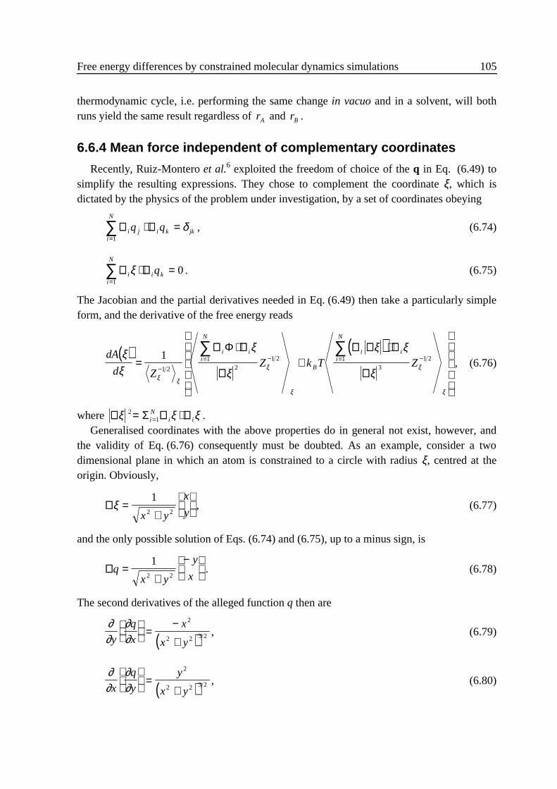
Free energy differences by constrained molecular dynamics simulations 105

thermodynamic cycle, i.e. performing the same change in vacuo and in a solvent, will bothruns yield the same result regardless of rA and rB .

6 .6 .4 Mean force independent of complementary coordinates

Recently, Ruiz-Montero et al.6 exploited the freedom of choice of the q in Eq. (6.49) tosimplify the resulting expressions. They chose to complement the coordinate ξ, which isdictated by the physics of the problem under investigation, by a set of coordinates obeying

∇ ∇i j i ki

N

jkq q⋅ ==∑

1

δ , (6.74)

∇ ∇i i ki

N

qξ ⋅ ==∑

1

0 . (6.75)

The Jacobian and the partial derivatives needed in Eq. (6.49) then take a particularly simpleform, and the derivative of the free energy reads

( ) ( )dA

d ZZ k T Z

i ii

N

B

i ii

N

ξξ

ξ

ξ

ξ ξ

ξξ ξ

ξ

ξ

ξ

ξ

=⋅

+⋅

−= − = −∑ ∑1

1 2

12

1 2 13

1 2

∇ ∇

∇

∇ ∇ ∇

∇

Φ, (6.76)

where ∇ ∇ ∇ξ ξ ξ21= ⋅=Σ i

Ni i .

Generalised coordinates with the above properties do in general not exist, however, andthe validity of Eq. (6.76) consequently must be doubted. As an example, consider a twodimensional plane in which an atom is constrained to a circle with radius ξ, centred at theorigin. Obviously,

∇ξ =+

12 2x y

x

y, (6.77)

and the only possible solution of Eqs. (6.74) and (6.75), up to a minus sign, is

∇qx y

y

x=

+

−

12 2

. (6.78)

The second derivatives of the alleged function q then are

( )∂∂

∂∂y

q

x

x

x y

=

−

+

2

2 2 3 2 , (6.79)

( )∂∂

∂∂x

q

y

y

x y

=

+

2

2 2 3 2 , (6.80)

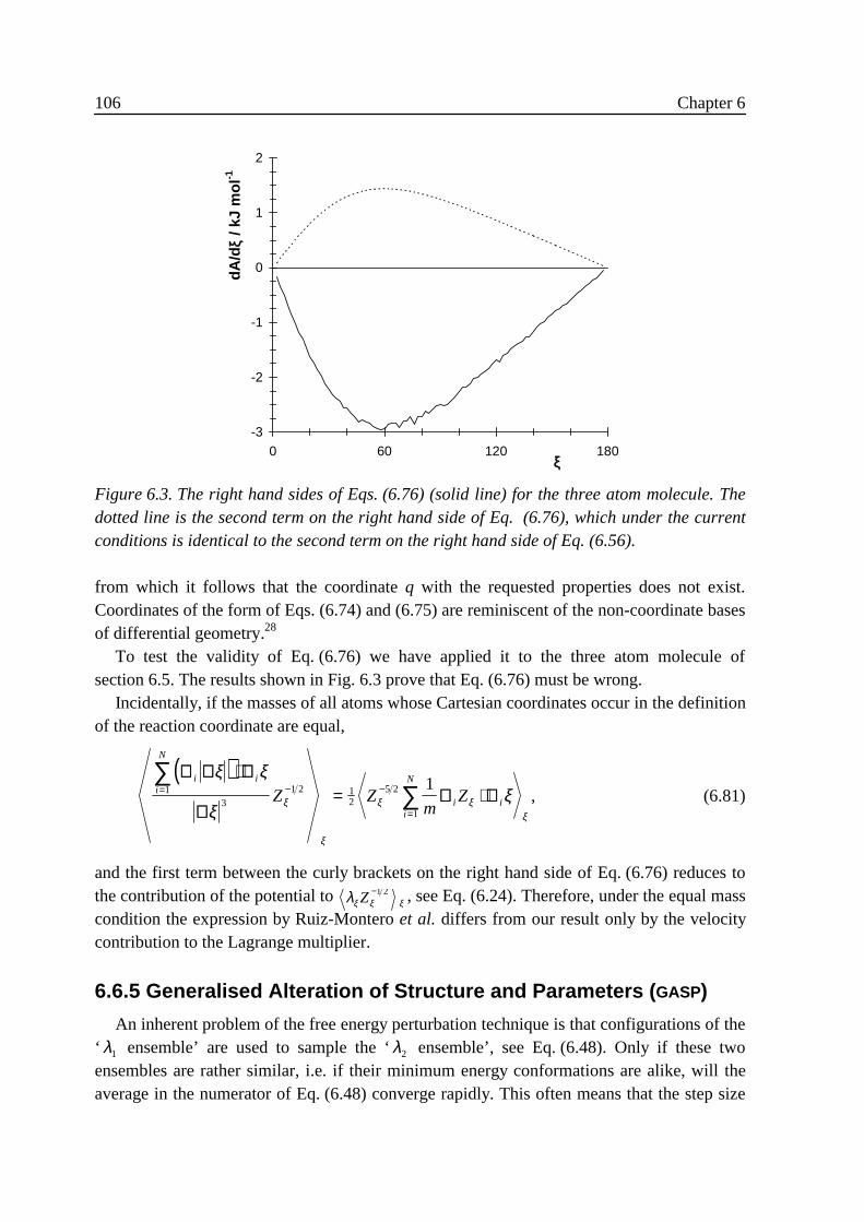
106 Chapter 6

from which it follows that the coordinate q with the requested properties does not exist.Coordinates of the form of Eqs. (6.74) and (6.75) are reminiscent of the non-coordinate basesof differential geometry.28

To test the validity of Eq. (6.76) we have applied it to the three atom molecule ofsection 6.5. The results shown in Fig. 6.3 prove that Eq. (6.76) must be wrong.

Incidentally, if the masses of all atoms whose Cartesian coordinates occur in the definitionof the reaction coordinate are equal,

( )∇ ∇ ∇

∇∇ ∇

i ii

N

i ii

N

Z Zm

Z

ξ ξ

ξξξ

ξ

ξ ξξ

⋅= ⋅= − −

=

∑∑1

31 2 1

25 2

1

1, (6.81)

and the first term between the curly brackets on the right hand side of Eq. (6.76) reduces tothe contribution of the potential to λξ ξ ξZ −1 2 , see Eq. (6.24). Therefore, under the equal masscondition the expression by Ruiz-Montero et al. differs from our result only by the velocitycontribution to the Lagrange multiplier.

6 .6 .5 Generalised Alteration of Structure and Parameters ( GASP)

An inherent problem of the free energy perturbation technique is that configurations of the‘ λ1 ensemble’ are used to sample the ‘λ2 ensemble’, see Eq. (6.48). Only if these twoensembles are rather similar, i.e. if their minimum energy conformations are alike, will theaverage in the numerator of Eq. (6.48) converge rapidly. This often means that the step size

-3

-2

-1

0

1

2

0 60 120 180ξ

dA/d

ξ / k

J m

ol-1

Figure 6.3. The right hand sides of Eqs. (6.76) (solid line) for the three atom molecule. Thedotted line is the second term on the right hand side of Eq. (6.76), which under the currentconditions is identical to the second term on the right hand side of Eq. (6.56).

Free energy differences by constrained molecular dynamics simulations 107

λ λ2 1− should be fairly small. Especially potentials with a quadratic contribution whoseminimum depends on the coupling parameter,

( ) ( ) ( )[ ]ϕ λ λ λq C q q; = −12 0

2, (6.82)

are prone to problems.13 An interesting way of avoiding these problems is by using thegeneralised alteration of structure and parameters method (GASP) of Severance et al.27 Theysuggested to transform to new coordinates r q qi i i= − ∆ in the λ2 ensemble, and r qi i= inthe λ1 ensemble. Here ∆qi = 0 , except for the coordinate q of Eq. (6.82), in which case it is∆q . The potential energy difference then reads

( ) ( )[ ] ( ) ( )[ ]∆ ∆ϕ λ λ λ λ1212 2 0 2

212 1 0 1

2= + − − −C r q q C r q . (6.83)

Obviously, if ∆q is of the order ( ) ( )q q0 2 0 1λ λ− , ( )exp − β∆Φ12 will fluctuate much less thanbefore. Notice that ∆Φ12 not only contains ∆ϕ12 , but also contributions resulting from achange of the Cartesian coordinates of all atoms in the molecule caused by the change of q.In the case of an ideal gas of two atom molecules, with q chosen to be the length of the bond,and if ( ) ( )C Cλ λ2 1= and ( ) ( )∆q q q= −0 2 0 1λ λ , then this exponent will even be constantlyequal to one. This should make us suspicious. Indeed, what has not yet been discussed is theJacobian determinant. To appreciate this factor, which is not present in the equations ofSeverance et al., we write the partition function as

( ) ( ) ( )[ ]( ) ( )[ ]

Q d

d

λ λ β λ

λ β λ

2 2

1 2

2

2

1 2

2

∝ −

= + − +

∫∫

q A q q

r A r q r q

; exp ;

; exp ; .

Φ

∆ Φ ∆(6.84)

Following the usual procedure we obtain

( ) ( )

( )[ ] ( )( )( )( )

( )( )

( )

A A

k TB

λ λ

βλ

λ

λ

λλσ

σ λ

σσ λ

2 1

12

2

1

2

1 2

1

1 2 1

1 2

1

1 2

1

− =

−

−+ −

−ln

exp;

;;

,;

;

∆Φ∆

XJ r X q

J r X

M

MZ X

Z

(6.85)

where we have added the possibility that constraints are applied to the σ variables. We couldhave anticipated this result from Eq. (6.48). Let us finally notice that in the derivation wehave tacitly assumed that the coordinates r in both ensembles are defined on the sameintervals.

6 .6 .6 Monte Carlo

So far we have concentrated on the calculation of free energies by molecular dynamicssimulations. We will now briefly consider doing the same thing with Monte Carlosimulations, restricting ourselves to the example of section 6.3.1. Starting with the partition

108 Chapter 6

function ( )Q ξ of Eq. (6.33), we integrate over all Cartesian momenta, transform to thegeneralised coordinates ( )q, ,ξ σ , integrate over σ using Eq. (6.17) and integrate over ξ toarrive at

( ) ( ) ( )[ ]Q dξ ξ β ξ∝ −− ∫F q J q q1 2 , , exp , ,σ σΦ . (6.86)

Differentiation with respect to ξ yields

( ) [ ][ ]

dA

d

d k T

d

Bξξ

β∂∂ξ

∂∂ξ

β=

− −

−

∫∫

−q J JJ

q J

exp

exp

ΦΦ

Φ

1

. (6.87)

From this example we see that the sampling of phase space with constrained Monte Carlorequires the rather cumbersome evaluation of the Jacobian to get the correct sampling ofconfiguration space. Secondly, the expressions for the derivative of the free energy are thesame as those for the molecular dynamics simulations, apart from the factors Z ξσ

−1 2 .

6 .7 ConclusionsWe have derived the correct relation between the constraint force needed to constrain an

internal coordinate in a molecular dynamics simulation and the derivative of the free energywith respect to this internal coordinate. Previously published methods with a similarobjective are critically discussed. We show that in most of these methods a term arising fromintegration over the momenta, i.e. a Jacobian, is included only partly, or not included at all.Two prototypical numerical examples are included to support our views. Of particularimportance is the discussion on the calculation of the free energy as a function of a dihedralangle, as the dihedral angle is often used as the reaction coordinate in reaction ratecalculations.

6 .8 References1 G. Ciccotti and J. P. Ryckaert, Comp. Phys. Rep. 4 , 347 (1986).2 W. K. den Otter and W. J. Briels, J. Chem. Phys. 106, 5494 (1997) (Chapter 3).3 M. Fixman, Proc. Nat. Acad. Sci. USA 71, 3050 (1974).4 E. Helfand, J. Chem. Phys. 71, 5000 (1979).5 N. G� and H. A. Scheraga, Macromolecules 9, 535 (1976).6 M. J. Ruiz-Montero, D. Frenkel and J. J. Brey, Mol. Phys. 90, 925 (1997).7 D. Frenkel and B. Smit, Understanding Molecular Simulation (Academic Press, San

Diego, CA, 1996).8 R. Edberg, D. J. Evans and G. P. Morris, J. Chem. Phys. 84, 6933 (1986).9 J.-P. Ryckaert, G. Ciccotti and H. J. C. Berendsen, J. Comp. Phys. 23, 327 (1977).10 D. J. Tobias and C. L. Brooks III, J. Chem. Phys. 89, 5115 (1988).

Free energy differences by constrained molecular dynamics simulations 109

11 T. P. Straatsma, M. Zacharias and J. A. McCammon, Chem. Phys. Lett. 196, 297 (1992).12 M. H. Mazor, J. A. McCammon and T. P. Lybrand, J. Am. Chem. Soc. 111, 55 (1989);

112, 4411 (1990).13 D. A. Pearlman and P. A. Kollman, J. Chem. Phys. 94, 4532 (1991).14 W. F. van Gunsteren in Computer Simulations of Biomolecular Systems: Theoretical and

Experimental Applications, edited by W. F. van Gunsteren and P. K. Weiner, (ESCOM,Leiden, The Netherlands, 1989), Vol. 1, pp. 27.

15 T. Mülders, P. Krüger, W. Swegat and J. Schlitter, J. Chem. Phys. 104, 4869 (1996).16 E. B. Wilson Jr., J. C. Decius and P. C. Cross, Molecular vibrations: the theory of

infrared and Raman vibrational spectra (McGraw-Hill, New York, NY, 1955).17 H. Bekker, H. J. C. Berendsen and W. F. van Gunsteren, J. Comp. Chem. 16, 527 (1995).18 J.-M. Depaepe, J.-P. Ryckaert, E. Paci and G. Ciccotti, Mol. Phys. 79, 515 (1993).19 W. F. van Gunsteren, T. C. Beutler, F. Fraternali, P. M. King, A. E. Mark and P. E. Smith

in Computer Simulation of Biomolecular Systems: Theoretical and ExperimentalApplications, edited by W. F. van Gunsteren, P. K. Weiner and A. J. Wilkinson, (ESCOM,Leiden, The Netherlands, 1993), Vol. 2, pp 315.

20 S. Boresch and M. Karplus, J. Chem. Phys. 105, 5145 (1996).21 E. A. Carter, G. Ciccotti, J. T. Hynes and R. Kapral, Chem. Phys. Lett. 156, 472 (1989).22 E. Paci, G. Ciccotti, M. Ferrario and R. Kapral, Chem. Phys. Lett. 176, 581 (1991).23 H. Goldstein, Classical Mechanics (Addison-Wesley, Reading, MA, 1980).24 L. Wang and J. Hermans, J. Chem. Phys. 100, 9129 (1994).25 D. A. Pearlman, J. Chem. Phys. 98, 8946 (1993).26 D. R. Herschbach, H. S. Johnston and D. Rapp, J. Chem. Phys. 31, 1652 (1959).27 D. L. Severance, J. W. Essex and W. L. Jorgensen, J. Comp. Chem. 16, 311 (1995).28 B. F. Schutz, A First Course in General Relativity (Cambridge University Press,

Cambridge, U. K., 1984).

111

Chapter 7

Summary and outlook

7 .1 SummaryThe isomerisation rates of a calix[4]arene in vacuo and in two solvents have been

computed by means of molecular dynamics simulations (MD). In MD the equations ofclassical mechanics are used to calculate the motion of the reacting molecule and thesurrounding solvent molecules. Thus, the intricate influence of the solvent on the reactingmolecule is realistically accounted for. Unfortunately, MD simulations are computationallyvery demanding because of the large number of non-bonded interactions between themolecules, and the rapid internal motions of the molecules which make it necessary tocalculate the interactions at femtosecond intervals.

During an isomerisation reaction a molecule goes from one energetically favourableconformation to another energetically favourable conformation without breaking or formingcovalent bonds. Such events are rare on the time scale of the normal dynamics of themolecule, i. e. the motion within a low energy region, since during the reaction the moleculehas to pass through an energetically unfavourable region. In MD simulations of theisomerisation of a calix[4]arene in a solvent, with an experimental rate constant of about100 s-1, a reaction event occurs roughly once every 100,000 CPU-years.

With the appropriate statistical mechanical methods, as explained in chapter 2, therequired CPU time can be reduced to the order of a month. Before these methods can beapplied to a particular reaction, one has to introduce a reaction coordinate, a method oftelling reactants and products apart. This coordinate also defines a dividing-plane betweenthe reactants and the products. In transition state theory (TST) the forward rate constant of areaction is expressed in terms of the instantaneous product bound flux through this plane andthe average number of molecules on the reactant side of the plane. The calculation of the TST

rate only requires knowing the free energy of the molecule as a function of the reactioncoordinate. In the reactive flux method (RF) the exact rate is obtained by multiplying the TST

rate by a transmission coefficient, κ, which takes into account that only a fraction of theproduct bound flux through the dividing plane will actually reach the product well.

In chapter 3 we propose a systematic definition of the reaction coordinate, based on theunstable normal mode at the saddle point of the potential energy surface. This coordinate has

112 Chapter 7

several features which make it a very useful coordinate in rate calculations. Although thecoordinate can not be expressed as a simple analytic function of the Cartesian coordinates ofthe reacting molecule, it can be computed swiftly by means of the rapidly convergingNewton-Raphson method. The gradient of the reaction coordinate, which is needed inconstrained runs and in umbrella sampling runs, is then obtained analytically. With thiscoordinate the transmission coefficient will be fairly high, thus reducing the CPU-time spentin the calculation of the rate constant. An excellent approximation of the free energy of themolecule in vacuo is obtained by performing a normal mode analysis at fixed values of thereaction coordinate.

These topics are discussed in detail in chapters 3 through 5, where the proposed reactioncoordinate is employed to calculate the TST and RF isomerisation rates of a calix[4]arene invacuo, in chloroform and in benzene. We find that both solvents destabilise the pacoconformation and stabilise the transition state configuration with respect to the situation invacuum. Chloroform stabilises the cone conformation, thus reducing the rate constant tobelow the value in vacuum, while in benzene the reaction is faster than in vacuum. Thecalculated rates are in good agreement with the experimental data. Although we haveconcentrated on the isomerisation of a calix[4]arene, the introduced reaction coordinate canin principle be applied to any reaction with a high energy barrier between the reactants andthe products. The isomerisation of n-butane is briefly discussed in chapter 3.

In chapter 6 we explore the connection between the derivative of the free energy as afunction of a coordinate, and the force needed to constrain this coordinate to a fixed value inan MD simulation. The relation between the two is found to be more complicated than waspreviously assumed by other authors. The correct formula is applied to calculate the freeenergy of a butane-like molecule as a function of the dihedral angle, as in manyisomerisation reactions a dihedral angle serves as the reaction coordinate. Several methodsfor calculating free energy differences that have appeared in the literature are commentedupon.

7 .2 OutlookThe erratic motion of the reaction coordinate, as calculated in the above discussed MD

simulations, is reminiscent of the motion of a Brownian particle. In some reaction ratetheories, therefore, the rate of escape from the reactant well is modelled by the statisticaltools developed in the study of Brownian dynamics. The idealised motion of the reactioncoordinate, ξ, with an effective mass, m, in a bath of non-reactive motions is given by theLangevin equation,

( ) ( )mdU

dR t�� �ξ = − ξ

ξξ

ζ− + . (7.1)

The potential is often approximated by a parabola near the transition state,U E mact b= − 1

22 2ω ξ . The motion of the reaction coordinate is opposed by the friction, ζ, of

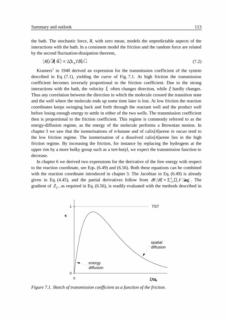
Summary and outlook 113

the bath. The stochastic force, R, with zero mean, models the unpredictable aspects of theinteractions with the bath. In a consistent model the friction and the random force are relatedby the second fluctuation-dissipation theorem,

( ) ( ) ( )R t R k T tB0 2= ζ δ . (7.2)

Kramers1 in 1940 derived an expression for the transmission coefficient of the systemdescribed in Eq. (7.1), yielding the curve of Fig. 7.1. At high friction the transmissioncoefficient becomes inversely proportional to the friction coefficient. Due to the stronginteractions with the bath, the velocity �ξ often changes direction, while ξ hardly changes.Thus any correlation between the direction in which the molecule crossed the transition stateand the well where the molecule ends up some time later is lost. At low friction the reactioncoordinates keeps swinging back and forth through the reactant well and the product wellbefore losing enough energy to settle in either of the two wells. The transmission coefficientthen is proportional to the friction coefficient. This regime is commonly referred to as theenergy-diffusion regime, as the energy of the molecule performs a Brownian motion. Inchapter 3 we saw that the isomerisations of n-butane and of calix[4]arene in vacuo tend tothe low friction regime. The isomerisation of a dissolved calix[4]arene lies in the highfriction regime. By increasing the friction, for instance by replacing the hydrogens at theupper rim by a more bulky group such as a tert-butyl, we expect the transmission function todecrease.

In chapter 6 we derived two expressions for the derivative of the free energy with respectto the reaction coordinate, see Eqs. (6.49) and (6.56). Both these equations can be combinedwith the reaction coordinate introduced in chapter 3. The Jacobian in Eq. (6.49) is alreadygiven in Eq. (4.45), and the partial derivatives follow from ∂ ∂ξF Fi

Ni i

r= ⋅=Σ 1∇ aq . Thegradient of Zξ , as required in Eq. (6.56), is readily evaluated with the methods described in

0

1

0 ζ/ωb

κ

TST

energy diffusion

spatial diffusion

Figure 7.1. Sketch of transmission coefficient as a function of the friction.

114 Chapter 7

section 3.3.1. Both methods can be applied to a set of ξ-constrained simulations to verify thefree energy distributions of chapters 4 and 5. With these simulations one may also calculatethe autocorrelation of the stochastic force. If this force is delta-correlated, as in Eq. (7.2), thetransmission coefficient follows directly from Kramers expression, and can then becompared with the results of chapters 3 and 5. Probably, the stochastic force will not bedelta-correlated, in which case the equation of motion for the reaction coordinate, Eq. (7.1),must be expanded to contain a friction coefficient with memory. Even for this situation thetransmission coefficient can be calculated analytically. 2,3

7 .3 References1 H. A. Kramers, Physica (Utrecht) 7, 284 (1940).2 R. F. Grote and J. T. Hynes, J. Chem. Phys. 73, 2715 (1980).3 E. Pollak, Chem. Phys. Lett. 127, 178 (1986); J. Chem. Phys. 85, 865 (1986).

115

Samenvatting

De isomerisatiesnelheden van een calix[4]areen in vacuüm en in twee oplosmiddelen zijnberekend gebruik makend van moleculaire dynamica simulaties (MD). In MD worden debewegingsvergelijkingen van de klassieke mechanica gebruikt om de bewegingen van hetreagerende molecuul en van de omringende oplosmiddelmoleculen te bepalen. Zodoendewordt de gecompliceerde invloed van het oplosmiddel op de reactie realistisch in rekeninggebracht. Helaas zijn MD simulaties erg rekenintensief vanwege het grote aantalwisselwerkingen tussen de moleculen, en door de snelle bewegingen van die moleculenwaardoor de interacties om de femtoseconde (10-15 s) opnieuw bepaald dienen te worden.

Tijdens een isomerisatiereactie gaat een molecuul van de ene energetisch gunstigeconformatie naar een andere energetisch gunstige conformatie, zonder dat daarbij covalentebindingen worden gevormd of verbroken. Deze overgangen zijn uiterst zeldzaam op detijdschaal van de normale bewegingen van de moleculen, omdat een reagerend molecuuldoor een energetisch ongustige overgangstoestand heen moet. In MD simulaties van deisomerisatie van een calix[4]areen in een oplosmiddel, waarvan de experimentelereactiesnelheid ongeveer 100 s-1 is, vindt er gemiddeld één reactie plaats per 100.000 jaarrekentijd.

Met de geschikte statistisch mechanische methoden, zoals beschreven in hoofdstuk 2, kande benodigde rekentijd worden teruggebracht tot de orde van grootte van een maand.Voordat deze methoden op een willekeurige reactie kunnen worden toegepast moet er eenreactiecoördinaat worden geïntroduceerd, een coördinaat om reactanten en producten tekunnen onderscheiden. Deze coördinaat definieert tevens een scheidingsvlak tussen dereactanten en de producten. In de overgangstoestand-theorie (transition state theory, TST)wordt de snelheid van de voorwaartse reactie uitgedrukt in termen van de instantane product-gerichte flux door dit scheidingsvlak en het gemiddelde aantal moleculen aan de reactantzijde van het scheidingsvlak. De berekening van de TST reactiesnelheid vereist alleen kennisvan de vrije energie van het molecuul als een functie van de reactiecoördinaat. In dereactieve flux methode (RF) wordt de reactiesnelheid verkregen door de TST snelheid tevermenigvuldigen met een transmissiecoëfficiënt, die verdisconteert dat slechts een deel vande product-gerichte flux door het scheidingsvlak ook daadwerkelijk aankomt aan deproductzijde.

In hoofdstuk 3 stellen we een systematische definitie van de reactiecoördinaat voor,gebaseerd op de instabiele normal mode van het zadelpunt van het potentiële-energie-oppervlak van de reactie. Deze coördinaat heeft verscheidene kenmerken die hem uitermategeschikt maken voor gebruik in reactiesnelheidsberekeningen. Alhoewel de coördinaat nietgeschreven kan worden als een analytische uitdrukking in termen van de Carthesische

116 Samenvatting

coördinaten van het molecuul, kan hij toch snel worden uitgerekend met de vlugconvergerende Newton-Raphson methode. De gradiënt van de reactiecoördinaat, die wenodig hebben in geconstrainde simulaties en bij umbrella sampling, kan dan analytischworden bepaald. Met deze reactiecoördinaat zal de transmissiecoëfficiënt vrij hoog zijn,waardoor de benodigde hoeveelheid rekentijd binnen de perken blijft. Een uitstekendebenadering van de vrije energie van een molecuul in vacuüm wordt verkregen door eenaantal normal mode analyses uit te voeren bij constante waarden van de reactiecoördinaat.

Deze onderwerpen worden verder toegelicht in de hoofdstukken 3 tot en met 5, waar devoorgestelde reactiecoördinaat gebruikt wordt om de TST en RF reactiesnelheden te bepalenvan een calix[4]areen in vacuüm, in chloroform en in benzeen. We vinden dat beideoplosmiddelen de paco conformatie destabiliseren en de overgangstoestand stabiliseren tenopzichte van de situatie in vacuüm. Chloroform stabiliseert de cone conformatie, waardoorde reactiesnelheid lager wordt dan in vacuüm, terwijl in benzeen de reactie sneller verlooptdan in vacuüm. De berekende snelheden zijn in goede overeenstemming met deexperimentele gegevens. Alhoewel we ons onderzoek geconcentreerd hebben op deisomerisatie van een calix[4]areen, kan de beschreven reactiecoördinaat in principe voor elkereactie met een hoge energiebarrière tussen de reactanten en de producten gebruikt worden.Zo wordt in hoofdstuk 3 de isomerisatie van n-butaan kort bekeken.

In hoofdstuk 6 onderzoeken we het verband tussen de afgeleide van de vrije energie alsfunctie van een coördinaat en de kracht die nodig is om deze coördinaat in een MD simulatieop een constante waarde te houden. Het verband blijkt veel gecompliceerder te zijn dan totnu toe in de literatuur wordt aangenomen. De gecorrigeerde formule wordt gebruikt om devrije energie van een butaan-achtig molecuul uit te rekenen als een functie van de dihedralecoördinaat, daar in veel isomerisatiereacties de dihedrale coördinaat als reactiecoördinaatwordt gebruikt. Verscheidene in de literatuur beschreven methoden om vrije energieverschillen uit te rekenen zijn kritisch bekeken.

117

Dankwoord

Met dit hoofdstuk wil ik iedereen die heeft bijgedragen aan de totstandkoming van hetvoor u liggende proefschrift hartelijk bedanken. Enkelen wil ik met naam en toenaamvermelden, zonder daarbij een ieder die niet vermeld wordt te kort te willen doen.

In de eerste plaats gaat mijn dank uit naar Wim Briels, die nooit om een leuk ideeverlegen zat en mij voortdurend gemotiveerd heeft om op de ingeslagen weg door te gaan.De promotor Dick Feil wil ik er voor bedanken dat hij mij in de gelegenheid heeft gesteld omdit onderzoek uit te voeren. Verder bedank ik Frank Leuwerink die howling mad otterw in dewondere wereld van GROMOS heeft ingeleid, Roelof de Vries die als kamergenoot enkelejaren lang mijn verbale uitingen bij het programmeren heeft moeten aanhoren, MaartenNollen en Santiago Diaz Fernandez die ik mocht begeleiden bij hun eerste schreden opsimulatie gebied, Willem Paul van Hoorn die de zadelpunten heeft uitgerekend, de overigecollega-AIO-s en studenten die de afgelopen jaren tot een leerzame en aangename periodehebben gemaakt, en, last but not least, mijn ouders.

118

Curriculum Vitae

De schrijver van dit proefschrift werd op 20 mei 1969 geboren te Eindhoven. Van 1981tot 1987 doorliep hij atheneum B op het ‘Serviam’ in Sittard. Daarna begon hij aan de studietechnische natuurkunde aan de Technische Universiteit Eindhoven. In april 1993 studeerdehij af bij Prof. dr. H. H. Brongersma, vakgroep fysica van oppervlakken en grenslagen, enDr. H. Feil, Philips Natlab, op de numerieke simulatie van lage energie ionen verstrooiingaan een gedragen rhodium katalysator. Vanaf juli 1993 heeft hij als AIO gewerkt in devakgroep chemische fysica, faculteit chemische technologie, van de Universiteit Twente. Hijwerd door Dr. W. J. Briels begeleid bij het onderzoek dat in dit proefschrift beschreven is.