
Bose-Einstein Condensation into Non-Equilibrium States · Bose-Einstein Condensation into...
103
Bose-Einstein Condensation into Non-Equilibrium States
Transcript of Bose-Einstein Condensation into Non-Equilibrium States · Bose-Einstein Condensation into...
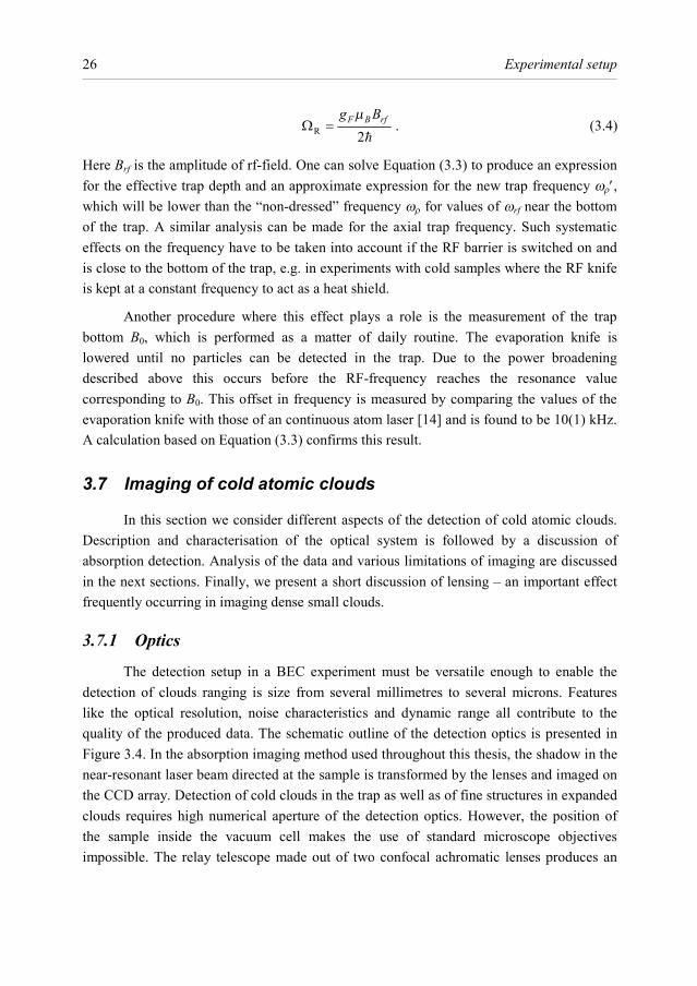
Bose-Einstein Condensation into
Non-Equilibrium States
Cover: false-colour representation of condensate focusing data. (Data processing by Wolf
von Klitzing.)
Bose-Einstein Condensation into
Non-Equilibrium States
ACADEMISCH PROEFSCHRIFT
ter verkrijging van de graad van doctor
aan de Universiteit van Amsterdam,
op gezag van de Rector Magnificus
prof. mr. P. F. van der Heijden
ten overstaan van een door het college voor promoties ingestelde
commissie, in het openbaar te verdedigen in de Aula der Universiteit
op donderdag 8 mei 2003, te 12:00 uur
door
Igor Yevgeniiovich Shvarchuck
geboren te Rostov-on-Don, Rusland
Promotiecommissie:
Promotor: prof. dr. J. T. M. Walraven
Overige leden: prof. dr. H. J. Bakker prof. dr. T. Esslinger prof. dr. H. B. van Linden van den Heuvell prof. dr. G. V. Shlyapnikov dr. R. J. C. Spreeuw prof. dr. B. J. Verhaar
Faculteit: Faculteit der Natuurwetenschappen, Wiskunde en Informatica
The work described in this thesis is part of the research program of the Stichting voor Funamenteel Onderzoek der Materie (FOM), which is financially supported by the Nederlandse Organisatie voor Wetenschappelijk Onderzoek (NWO).
This work was carried out at the
FOM Institute for Atomic and Molecular Physics (AMOLF)
Kruislaan 407, 1098 SJ Amsterdam, The Netherlands
A digital version of this thesis can be downloaded from http://www.amolf.nl.
ISBN 90-77209-01-8
To E.A.S. and V.G.V.
vi
This thesis is partially based on the following publications:
Broad-area diode laser system for a rubidium Bose-Einstein condensation experiment,
I. Shvarchuck, K. Dieckmann, M. Zielonkowski, J.T.M. Walraven,
Applied Physics B, 71(4), 475 (2000)
Focusing of Bose-Einstein condensates in free flight,
I. Shvarchuck, Ch. Buggle, D.S. Petrov, M. Kemmann, T.G. Tiecke, W. von Klitzing, G.V. Shlyapnikov and J.T.M. Walraven
in "Interaction in Ultracold Gases: From Atoms to Molecules", ed. by M. Weidemüller and C. Zimmermann (Wiley-VCH, Berlin, 2003)
Bose-Einstein condensation into nonequilibrium states studied by condensate focusing
I. Shvarchuck, Ch. Buggle, D.S. Petrov, K. Dieckmann, M. Zielonkovski, M. Kemmann, T.G. Tiecke, W. von Klitzing, G.V. Shlyapnikov, and J.T.M. Walraven
Phys. Rev. Lett. 89, art. no. 270404 (2002)

Contents
Chapter 1 Introduction 1 1.1 Background ....................................................................................................1 1.2 This thesis ......................................................................................................2
Chapter 2 Theoretical background 5 2.1 Rubidium........................................................................................................5 2.2 Magnetic trapping ..........................................................................................5 2.3 Bose-Einstein condensation ...........................................................................8 2.4 BEC formation and phase coherence ...........................................................10 2.5 Evaporative cooling .....................................................................................12
2.5.1 Evaporative cooling ............................................................................12 2.5.2 Local critical temperature in a cylindrical geometry ..........................13 2.5.3 Development of temperature gradients...............................................14
2.6 Scaling theory of gas evolution....................................................................15 2.6.1 Evolution of a condensate...................................................................15 2.6.2 Evolution of a hydrodynamic thermal cloud ......................................16
Chapter 3 Experimental setup 17 3.1 Introduction..................................................................................................17 3.2 Overview......................................................................................................17 3.3 Vacuum system ............................................................................................19 3.4 Laser system.................................................................................................21 3.5 Magnetic trap ...............................................................................................22 3.6 RF evaporative cooling ................................................................................24 3.7 Imaging of cold atomic clouds .....................................................................26
3.7.1 Optics..................................................................................................26 3.7.2 Absorption detection...........................................................................28 3.7.3 Fitting parameters ...............................................................................30 3.7.4 Lensing ...............................................................................................31
Chapter 4 Broad-area diode laser system 35 4.1 Abstract. .......................................................................................................35 4.2 Introduction..................................................................................................35 4.3 Experimental setup.......................................................................................36 4.4 Characteristics ..............................................................................................41 4.5 MOT application ..........................................................................................46 4.6 Summary ......................................................................................................47
Chapter 5 Hydrodynamic properties of dense atomic clouds 49
viii
5.1 Introduction..................................................................................................49 5.2 Density and temperature analysis.................................................................50 5.3 Anisotropic expansion of hydrodynamic clouds ..........................................54 5.4 Frequency shifts and damping of shape oscillations ....................................57
Chapter 6 Condensation into non-equilibrium states and focusing of a condensate 61 6.1 Introduction..................................................................................................61 6.2 Preparation of degenerate samples out of equilibrium .................................62 6.3 Kinetics of the condensate growth ...............................................................63 6.4 Formation of a non-equilibrium BEC ..........................................................64
6.4.1 Local critical temperature ...................................................................65 6.4.2 Truncation and local temperature .......................................................65
6.5 Oscillation modes.........................................................................................68 6.6 Non-equilibrium phase fluctuations .............................................................69 6.7 Focusing of a condensate .............................................................................70
6.7.1 Focusing principle ..............................................................................71 6.7.2 Focal broadening ................................................................................73 6.7.3 Applications of BEC focusing ............................................................74
6.8 High condensate fractions in non-equilibrium states ...................................74 Bibliography 79 Summary 85 Samenvatting 89 Acknowledgements 93
Chapter 1 Introduction
1.1 Background
After prediction of Bose-Einstein condensation (BEC) in 1925 [18, 35] it took seventy years to achieve its experimental realisation in pioneering experiments at JILA [4], MIT [28] and Rice [19, 20]. Experimental and theoretical studies of BEC address many-body physics. By 1995 there was an extensive literature on macroscopic quantum phenomena, such as superfluidity in liquid helium, and the closely related subject of superconductivity. BEC in dilute atomic quantum gases enabled the investigation of macroscopic quantum phenomena in the weakly interacting limit. With the availability of these systems it became possible to apply the broad range of standard tools of atomic physics to such investigations.
The first experiments on BEC revived an enormous interest in macroscopic behaviour of dilute atomic gases at low temperature, which resulted in rapid development of the research area.
Most of the theoretical groundwork on the interacting quantum gases has been developed in the 50’s and the 60’s in the context of superfluidity of 4He. However, a detailed comparison between theory and experiment is extremely difficult in the case of liquid helium because its density is rather high and can be varied only within a narrow range. In the 70’s the observation of BEC in dilute atomic gases under equilibrium conditions was known to be impossible. Therefore, the efforts shifted towards investigations of metastable systems.
The first attempts to reach BEC were done in spin-polarised atomic hydrogen. Foundations for many techniques and methods were laid in the course of that work. Hydrogen quantum gas was first stabilised in a cryogenic environment by Silvera and Walraven [93] and by Cline et al. [23]. Magnetic trapping was first demonstrated in sodium [79] and in hydrogen by Hess et al. [50] and van Roijen et al. [87]. Another critically important technique, evaporative cooling, was first experimentally demonstrated in hydrogen [51] and further developed in [74, 97, 105].
Bose-Einstein condensation in alkali systems was achieved in magnetic traps through the combination of optical cooling methods with the evaporative cooling technique.
2
Introduction
This led to a dramatic expansion of both experimental and theoretical work in the field of ultracold quantum gases. The contribution of this field to the understanding of Nature was acknowledged by the Nobel Prize in physics awarded in 2001. Although the macroscopic occupation of the ground state is the best known aspect of the phenomenon of Bose-Einstein condensation, the appearance of phase coherence is equally important.
The investigation of phase coherence phenomena provides new fundamental insights into the nature of macroscopic quantum states and is important for current and future applications. Those include, in particular, atom lasers – devices for continuous or pulsed generation of coherent matter waves, atom interferometry, improved frequency standards and systems of cold atoms for quantum computing. The first phase coherence experiments were relying on the interference of two independently prepared condensates [6] and on the measurement of single-particle correlations [15, 48, 95]. These experiments showed that trapped condensates are phase coherent, in accordance with the common understanding of BEC in three-dimensional gases. Recent theoretical [82] and experimental [31] studies revealed limitations on the phase coherence of the Bose-condensed state. It was shown that in elongated 3D traps the finite-temperature equilibrium state can be a quasicondensate: it shows the suppressed density fluctuations of a regular condensate but shows an axially fluctuating phase rather than full phase coherence.
The appearance of coherence in a condensate cannot be separated from the process of condensate formation. Theory of condensate formation was first explored by Svistunov [98] and Kagan et al. [57], and extensively studied later by Gardiner et al. [29, 38, 39, 70] and Bijlsma et al. [11]. Previous experimental investigations of formation kinetics of trapped condensates [65, 78] were decoupled from the studies of phase coherence mentioned above. Investigation of the evolution of phase coherence properties during the formation of a trapped condensate out of a non-equilibrium thermal cloud presents a great general physical interest. In particular it should allow a deeper understanding of phase coherence phenomena in macroscopic quantum states. One can expect that the evolution of phase coherence will be a primary issue for creation of CW atom lasers [22]. The rate at which the required phase coherence is formed will place an upper boundary on the feeding rate for the laser and, hence, on the generation rate of coherent matter waves.
1.2 This thesis
The main part of this Thesis is related to the studies of the condensate formation into non-equilibrium states and hydrodynamic behaviour of cold non-degenerate atomic clouds. In contrast to the experiments with equilibrium phase-fluctuating quasicondensates we investigate creation of a degenerate quantum state outside of equilibrium. This offers an
1.2 This thesis
3
fundamentally different path towards equilibrium as compared to the condensate formed in a quasi-static fashion.
The Thesis is organised in the following way. In Chapter 2 we compile main theoretical expressions relevant to the Bose-Einstein condensation. We begin with an introduction of the principle of magnetic trapping of spin-polarised gases and a description of the Ioffe-Pritchard quadrupole trap. It is followed by a description of trapped Bose gases below and above the phase transition temperature. Further we sketch theoretical ideas underlying phase coherence and formation of a BEC. We also introduce the bare fundamentals of evaporative cooling and derive several results specific to the experiments described further in this work. A separate section is dedicated to the scaling description of the gas clouds in harmonic traps.
In Chapter 3 various aspects of the experimental setup are described. Special attention is given to the features characteristic to the specific ideas which underlie the construction of the apparatus, e.g. creating Bose condensates with the highest density and particle number possible. An overview of the vacuum system is followed by the outline of the laser setup. A section on the magnetic trap describes the technical aspects of the generation and control of the trapping fields. Description of the experimental realisation of evaporative cooling in our experiments is presented together with details of the measurement methods. Emphasis is put on the description of imaging of cold atomic clouds. We discuss numerous sides of the problem, including the selection of the optical elements and details of the absorption detection with limitations of the method.
Chapter 4 gives a detailed description of the high-power diode laser system, the design and building of which was dictated by the needs of this experiment. In the experiments with large (rubidium) atom numbers the optical power requirements tend to go beyond the power available from the single-mode diode lasers operating at 780 nm. We introduce this setup based on a broad-area laser diode as an excellent alternative to the other solutions available commercially.
In Chapter 5 we present the experimental investigation of the hydrodynamic properties of dense atomic clouds. The understanding of the crossover to the hydrodynamic regime in thermal clouds is important from the experimental point of view. This understanding is vital for the correct interpretation of time-of-flight images of such clouds. In the collisionless regime the expansion of the gas, after release from a trap, is known to be isotropic, whereas in the hydrodynamic limit the gas expands anisotropically. We approach investigation of the hydrodynamic properties from three different sides. First, we go in detail into density and temperature analysis. Another indicator of hydrodynamic behaviour
4
is obtained by observation of the anisotropic character of the expansion. Finally, we measure frequency shifts and damping of shape oscillations.
In the final part of the Thesis, Chapter 6, we describe the results produced in the experiments on formation of condensates far from equilibrium. We compare our work with previous experiments on condensate formation and describe how the process of formation is triggered in our system. A brief section deals with the growth of the condensate fraction. Further, we show how the concepts of local sample temperature and the critical temperature arise in elongated clouds with high elastic collision rates. We present a simple model, which illustrates how the non-equilibrium character of the condensates leads to the quadrupole oscillations. We also discuss non-equilibrium phase fluctuations, which manifest themselves in the form of stripes in the time-of-flight absorption images. Condensate focusing is introduced as a novel method for investigation of Bose-Einstein condensates. The focusing of a condensate in free flight arises from axial contraction of the expanding cloud when the gas is released from the trap during the inward phase of a shape oscillation. Possible applications of BEC focusing are discussed, with an estimate of the coherence length given as an example. The last part of the chapter covers condensation into non-equilibrium states with high condensate fractions. The situations of large and small condensate fractions are compared.
Chapter 2 Theoretical background
In this chapter we compile main theoretical expressions relevant to the Bose-Einstein condensation. We also sketch some theoretical ideas underlying phase coherence and formation of a BEC. Further, we introduce the bare fundamentals of evaporative cooling and derive several results specific to the experiments described further in this work. A separate section is dedicated to the scaling description of the gas clouds in harmonic traps. For a complete review on the theory of Bose-Einstein condensation in trapped gases one can, for example, refer to [27].
2.1 Rubidium
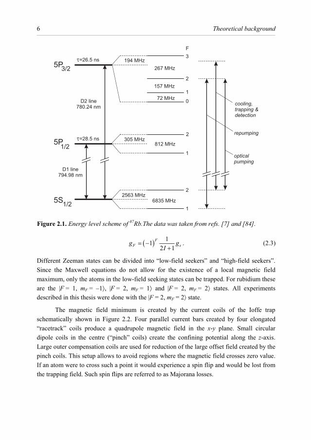
The diagram of energy levels of 87Rb isotope is shown in Figure 2.1. Cooling and trapping is performed with laser light red-detuned with respect to the |5S1/2, F = 2⟩ → |5P3/2, F = 3⟩ transition of the D2 line. This light also induces non-resonant pumping of the atoms to the |5P3/2, F = 2⟩ state, from where they decay according to the transitions’ strengths to F = 1 and F = 2 hyperfine states. To prevent atoms from accumulating in the F = 1 state, another laser – the repumper – tuned to a |5S1/2, F = 1⟩ → |5P3/2, F = 2⟩ transition is used. Another laser is employed for optical pumping of the atoms into a |5S1/2, F = 2, mF = 2⟩ Zeeman state.
2.2 Magnetic trapping
Trapping of neutral atoms in magnetic fields arises from Zeeman interaction of the magnetic moment µ of the atom with the external field B. The energy of the interaction is given by
( )E = − ⋅µ B r , (2.1)
where F F Bm gµ µ= , µB is the Bohr magneton. The Zeeman energy of the different magnetic sublevels can be expressed by the Breit-Rabi formula in the approximation of the Zeeman splitting s Bg Bµ being much smaller than the hyperfine splitting hfω
( ) ( ) ( )22
,1 11 4 const.2 16F
F s BF m hf F F B F
hf
g BE m g B m
µω µ
ω
= − + + − +
(2.2)
6
Theoretical background
( ) 112 1
FF sg g
I= −
+. (2.3)
Different Zeeman states can be divided into “low-field seekers” and “high-field seekers”. Since the Maxwell equations do not allow for the existence of a local magnetic field maximum, only the atoms in the low-field seeking states can be trapped. For rubidium these are the |F = 1, mF = –1⟩, |F = 2, mF = 1⟩ and |F = 2, mF = 2⟩ states. All experiments described in this thesis were done with the |F = 2, mF = 2⟩ state.
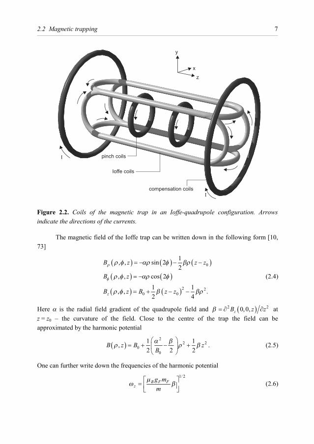
The magnetic field minimum is created by the current coils of the Ioffe trap schematically shown in Figure 2.2. Four parallel current bars created by four elongated “racetrack” coils produce a quadrupole magnetic field in the x-y plane. Small circular dipole coils in the centre (“pinch” coils) create the confining potential along the z-axis. Large outer compensation coils are used for reduction of the large offset field created by the pinch coils. This setup allows to avoid regions where the magnetic field crosses zero value. If an atom were to cross such a point it would experience a spin flip and would be lost from the trapping field. Such spin flips are referred to as Majorana losses.
Figure 2.1. Energy level scheme of 87Rb.The data was taken from refs. [7] and [84].
2.2 Magnetic trapping
7
The magnetic field of the Ioffe trap can be written down in the following form [10, 73]
( ) ( ) ( )
( ) ( )
( ) ( )
0
2 20 0
1, , sin 22
, , cos 2
1 1, , .2 4z
B z z z
B z
B z B z z
ρ
φ
ρ φ αρ φ βρ
ρ φ αρ φ
ρ φ β βρ
= − − −
= −
= + − −
(2.4)
Here α is the radial field gradient of the quadrupole field and ( )2 20,0,zB z zβ = ∂ ∂ at z = z0 – the curvature of the field. Close to the centre of the trap the field can be approximated by the harmonic potential
( )2
2 20
0
1 1,2 2 2
B z B zBα β
ρ ρ β
= + − +
. (2.5)
One can further write down the frequencies of the harmonic potential
1/ 2
B F Fz
g mm
µω β =
(2.6)
Figure 2.2. Coils of the magnetic trap in an Ioffe-quadrupole configuration. Arrows indicate the directions of the currents.
8
Theoretical background
1/ 22
0 2B F Fg m
m Bρµ α β
ω
= −
. (2.7)
Note that for strong confinement in the radial direction the term 20Bα is dominant and the
radial frequency can thus be adjusted by changing the value of the offset field B0.
2.3 Bose-Einstein condensation
In this section we summarize the main theoretical results required for the description of trapped Bose gases. Among these are the expressions for the critical temperature (TC) and the density distribution above and below the phase transitions. Detailed description and reviews can be found in refs. [8, 27, 53, 105].
The energy spectrum of an individual atom in a harmonic potential ( )U r is characterized by a set of three non-negative integer quantum numbers n = nx, ny, nz and is given by
, ,
12n i i
i x y z
nε ω=
= +
∑ , (2.8)
where ωi are the trap frequencies. The average number of particles in the state n is given by the Bose distribution:
1
exp 1nB
BN
k Tε µ
− −
= −
. (2.9)
The value of the chemical potential is fixed by the condition
( )BN Nλλ
ε =∑ , (2.10)
where N is the total number of particles. For this system the density distribution ( )n r above the phase transition can be calculated as
( ) ( )3 23
1 expBT
Un g z
k T
= − Λ
rr , (2.11)
with fugacity ( )exp Bz k Tµ= , where ( )3/ 2g x is a polylogarithm function
( )1
l
l
g x x lαα
∞
=
≡ ∑ . (2.12)
2.3 Bose-Einstein condensation
9
(Note that ( ) ( )1ng nζ= , where ( )nζ is Riemann zeta-function.) The thermal de Broglie wavelength is defined as
1/ 222
TBmk T
π Λ =
. (2.13)
Independently of trap geometry, BEC occurs if the so-called degeneracy parameter reaches the critical value:
( ) ( )33 20 1 2.61Tn gΛ = ≈ , (2.14)
where n(0) is the peak density in the centre of the trap. In the case of harmonic potential one can obtain an expression for the critical temperature:
( )
1/ 3
3 1CB
NTk gω
=
, (2.15)
where 1/ 32
zρω ω ω = is the mean trap frequency.
For a trapped Bose gas in the classical regime, where the chemical potential µ < 0 and Bk Tµ one can find that the density distribution has a Gaussian shape
( )2
3 2,0,0
exp i
iiii
rNnrrπ
= −
∑∏r , (2.16)
where ri,0 is the 1/e radius of the cloud in the i-direction:
1/ 2
,0 22 B
ii
k Tr
mω
=
. (2.17)
Appearance of the condensate in a trapped weakly interacting gas is characterised by the macroscopic wavefunction, which is determined by the Gross-Pitaevskii (GP) equation [45, 54]
( ) ( ) ( ) ( )2
20 0 02
U Um
µ ∆
− + + Ψ Ψ = Ψ
r r r r , (2.18)
where 24U a mπ= is the coupling constant, a is s-wave scattering length (a = 5.238(1) nm [103]), and the chemical potential µ is determined by the normalisation condition
230 0N d r= Ψ∫ . (2.19)
10
Theoretical background
The density profile of the condensate is given by ( ) 20 0n = Ψr . When the maximum level
spacing is much smaller than the chemical potential the interactions smear out the discrete structure of the trap levels. In this case the mean field term 0Un becomes dominant compared to the kinetic term, which can be neglected in what is referred to as the Thomas-Fermi approximation. In the case of a harmonic trap the density profile of the condensate assumes a parabolic shape
( ) ( )01max ,0n Ug
µ
= −
r r , (2.20)
and the Thomas-Fermi radius of the condensate Li is given by
01 2
ii
Lmµ
ω= . (2.21)
The total number of particles in the condensate can be calculated to be
( )5/ 2
30 0
215
hrN d r na
µω
= = ∫ r , (2.22)
where 1/ 2[ / ]hr mω= is the harmonic oscillator length.
2.4 BEC formation and phase coherence
Phase coherence properties of a BEC are closely related to the formation process of a quantum degenerate state. Studies of novel Bose-condensed gases, such as phase-fluctuating condensates, can provide new fundamental insights into the nature of macroscopic quantum states and are important for applications in atom optics. So far, phase coherence has been studied for equilibrium trapped Bose-condensed gases [6, 15, 31, 48, 82, 95], and these studies were decoupled from the experiments on the kinetics of growth of BECs [65, 78]. Evolution of the phase coherence properties during formation of a condensate is a matter of particular interest.
It is important to identify regimes of the formation kinetics of a trapped condensate. One expects the existence of two regimes, depending on the trap geometry and the mean-field interatomic interaction near the BEC transition temperature TC. In the first regime, the interatomic interaction is much smaller than the spacing between the lowest trap levels. Then, by doing evaporative cooling and crossing TC from above one has straightforward formation of a true condensate in the trap ground state, which then grows and acquires the Thomas-Fermi density profile. This regime requires a comparatively small number of particles as in the work at MIT on the growth of a condensate in real time [78] and related
2.4 BEC formation and phase coherence
11
theoretical work [38]. In our experiments we expect the second regime, where already above TC the discrete structure of the lowest trap levels is smeared out by the interatomic interaction, and, similarly to the spatially homogeneous case [57, 58, 61, 62], one expects the formation of a condensate with fluctuating phase (quasicondensate). The quasicondensate will have the same density profile and local correlation properties as a true condensate but will have drastically different phase coherence properties. This regime requires either a very large number of particles or a strongly elongated trapping geometry. In the latter case, already for a moderate particle number (~105 or 106) the interparticle interaction at TC exceeds the spacing between the axial trap levels. Then the axial fluctuations of the phase of the appearing Bose-condensed state acquire a 1D character and can be large, similar to the case of equilibrium 3D elongated quasicondensates discussed in ref. [82]. This regime is likely to be realized in the Munich experiment [65] on the formation and growth of a condensate in an elongated trap as well as in the experiments described in this thesis.
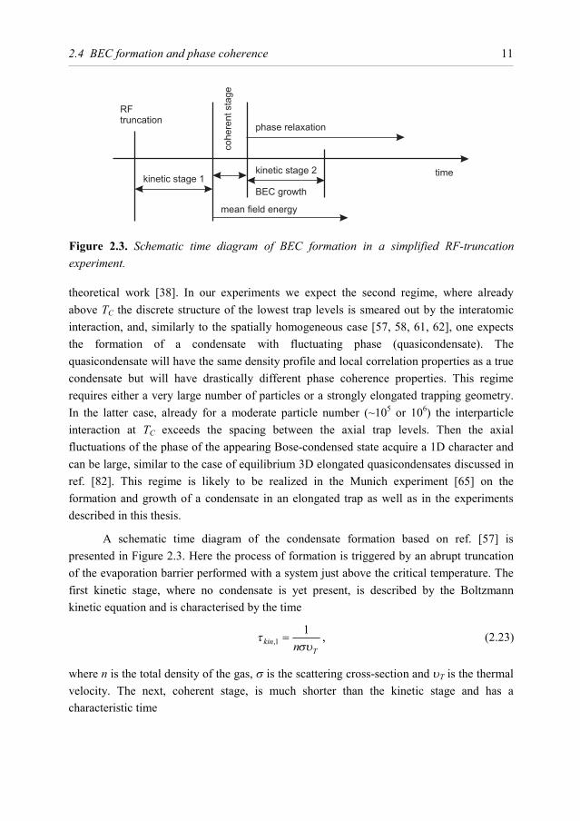
A schematic time diagram of the condensate formation based on ref. [57] is presented in Figure 2.3. Here the process of formation is triggered by an abrupt truncation of the evaporation barrier performed with a system just above the critical temperature. The first kinetic stage, where no condensate is yet present, is described by the Boltzmann kinetic equation and is characterised by the time
,11
kinTn
τσυ
= , (2.23)
where n is the total density of the gas, σ is the scattering cross-section and υT is the thermal velocity. The next, coherent stage, is much shorter than the kinetic stage and has a characteristic time
Figure 2.3. Schematic time diagram of BEC formation in a simplified RF-truncation experiment.
12
Theoretical background
04c
mn a
τπ
= , (2.24)
where a is the scattering length, and n0 is the density of the condensate. In this evolution stage the non-equilibrium density fluctuations die out. Finally, the second kinetic stage is also characterised by an expression identical to (2.23), with the density n replaced by the condensate density n0. During this stage the number of particles in the condensate grows to its equilibrium value. Further damping of phase fluctuations leads to formation of an equilibrium BEC.
2.5 Evaporative cooling
2.5.1 Evaporative cooling
Evaporative cooling plays a key role in the path towards BEC and has been used in all BEC experiments up to date. The basic principles of evaporative cooling are presented to the extent required for understanding of the experiments described in Chapter 5 and Chapter 6. For an extensive review on evaporative cooling one can refer to [105] and [63].
The description of evaporative cooling presented here is based on the model introduced in [74] and [105]. Evaporative cooling is a powerful cooling method based on the preferential removal of atoms with energy higher than average energy per atom. Subsequent thermalization by elastic collisions leads to an energy distribution with a lower temperature than the one before removal of the atoms.
For constant truncation barrier εt (“plain evaporation”) evaporation rate per atom can be written as
( )1 0ev evev T
e
N Vn e
N Vητ υ σ− −= = , (2.25)
where 28 aσ π= is the elastic collisional cross section,
t
Bk Tε
η = (2.26)
is the truncation parameter, and Vev ≈ Ve is the effective evaporation volume [105]. If the truncation barrier is constantly reduced one enters regime of forced evaporative cooling. If truncation parameter η is kept constant it can be shown that the temperature behaves as
T Nα∝ , (2.27)
2.5 Evaporative cooling
13
where efficiency parameter α depends only on η. In the course of evaporative cooling it is possible to enter the so-called “runaway” regime, when, despite the particle loss, the density of atoms increases. In the runaway regime the increase in density is sufficiently strong to compensate the dropping temperature and the elastic collision rate increases leading to ever faster evaporation. The efficiency of the evaporative cooling is limited by the loss mechanisms from the trap such as collisions with background gas or collisions with the products of three-body recombination. The figure of merit in this case is the ratio of “good” to “bad” collisions:
-body
1ev ev
i ei
N VR e
VNη
λ−≡ = , (2.28)
where 1 1i i colλ τ τ− −≡ , with τi
-1 being the i-body atomic loss rate and ( )1 0col Tnτ υ σ− = – the elastic collision rate.
2.5.2 Local critical temperature in a cylindrical geometry
Unlike a familiar result for the critical temperature in quasi-static systems (Section 2.3), experiments on non-equilibrium formation of a Bose-Einstein condensate described further in this thesis require understanding of a local critical temperature related to the local density of the sample. This concept becomes important if collisions occur on a length scale much shorter than the (axial) size of the cloud. We start calculation of local TC with writing down an expression for the density of states in a truncated harmonic trap [105]:
( ) ( )( )
( )3/ 2
3( )
2 2
2 U r
mdr U r
ε
πρ ε ε
π ≤
= −∫ . (2.29)
Here ( ) 2 2 2U r m rω= , and ε is the truncation energy. By integrating out the radial dimensions, we get for an infinitely long cylinder:
( ) ( )( )
( )03/ 2 3/ 22 2 3/ 2
1 3 3 20
2 2 22 2
32
r
Dm m
rdr m rmρ
ρ
πρ ε π ε ω ε
π ωπ= − =∫ , (2.30)
where 20 2r m ρε ω= .
Further, we can write down the total one-dimensional density of an ideal Bose gas [105] (see also Section 6.4.1), and substitute in Equation (2.30)
( ) ( )( ) ( )5/ 21/ 2
5/ 21 1 3 2
0
112exp 1
B CD D
B C
k T gmn dk T ρ
ε ρ επε ω
∞ = = − ∫ , (2.31)
where ( )5/ 2 1g is a polylogarithm function.
14
Theoretical background
Finally, the local critical temperature is
( ) ( ) 2 / 51
1.28C D
BT z n z r
kρ
ρ
ω ≈ , (2.32)
where 1/ 2[ ]r mρ ρω= is the radial oscillator length.
2.5.3 Development of temperature gradients
Investigation of a temperature profile induced in an elongated cloud by an abrupt lowering of the RF barrier (what we further refer to as RF truncation) is of particular interest with regard to the experiments described in Chapter 6.
To the zero approximation a gas above TC can be described by a simple model of a Boltzmann gas. To calculate the temperature profile in the thermal gas after truncation we write down the ratio of one-dimensional truncated density distribution n′1D to the initial, non-truncated density distribution n1D:
( ) ( )
( ) ( )
( )
1 001
11 0
0
exp
exp
l z
D BD
DD B
d k Tnn
d k T
ε
ε ρ ε ε
ε ρ ε ε∞
−′
=
−
∫
∫, (2.33)
where the density of states ρ1D is defined by Equation (2.30), and ( ) 2 2 2l z m zε ε ω= − is the local trap depth. The same ratio can be written down for the total energies excluding the axial component of the potential energy:
( ) ( )
( ) ( )
( )
1 00
1 00
exp
exp
l z
D B
D B
d k TEE
d k T
ε
ε ε ρ ε ε
ε ε ρ ε ε∞
−′
=
−
∫
∫, (2.34)
Combining Equations (2.34), (2.33) and (2.30) we can write down a local temperature of the Boltzmann gas as a function of the axial coordinate:
( ) ( ) ( )( ) ( )
( ) ( )( ) ( ) 0
1 1
7 2, 5 2, 7 2, 5 2,2 25 5 5 2, 7 2, 5 2, 7 2,
l lloc
D D l l
P P P PE ET z Tn n P P P P
η ηη η
∞ ∞′= = =
′ ∞ ∞ (2.35)
where
2 2
0
2l
B
m zk T
ε ωη
−= . (2.36)
2.6 Scaling theory of gas evolution
15
is the local truncation parameter, and the incomplete gamma function ( ),P a η is defined as
( ) 1
0
1,( )
a tP a dt t ea
η
η − −≡Γ ∫ . (2.37)
Here Γ(a) is the Euler gamma function.
2.6 Scaling theory of gas evolution
2.6.1 Evolution of a condensate
Let us consider a condensate with a fixed number of particles in an anisotropic harmonic potential ( ) 2 2 2i i iV m rω= ∑r with time-dependent frequencies ωi(t). Neglecting the thermal cloud, the condensate wave function follows a time-dependent Gross-Pitaevskii equation
( )2
22 200 02 2 i i
i
mi t r Ut m
ω ∂Ψ ∆
= − + + Ψ Ψ ∂ ∑ . (2.38)
Here 24U a mπ= , with a being the scattering length and m the atom mass. To describe the evolution of the Bose gas we follow the method described in ref. [21, 59, 60] and turn in Equation (2.38) to new coordinates ( )i i ir b tρ = . Here ( ) 0i i ib L t L≡ are the scaling parameters, where L0i is the initial size of the condensate in the trap, as defined by Equation (2.21). We then search for a solution in a density-phase representation. When equation of motion (2.38) in the new coordinates is reduced to a stationary GP equation (2.18), it sets the following condition on the scaling parameters:
( ) ( )2
2 0ii i i
i i ib t b
b b tω
ω+ =Π
, (2.39)
where ( )0 0i iω ω= . Considering the case of a cylindrical geometry and an abrupt switch-off of the trap Equations (2.39) can be rewritten in the form
2
3z
bb b
ρρ
ρ
ω= (2.40)
2
2 2z
zz
bb bρ
ω= (2.41)
with initial conditions ( )0 1ib = , ( )0 0ib = .
16
Theoretical background
2.6.2 Evolution of a hydrodynamic thermal cloud
Evolution of the thermal gas in the hydrodynamic regime is in many aspects similar to the evolution of the condensate. The Euler equation of motion for the gas in an anisotropic parabolic potential has the form
( ) ( )( )2 ,1 0
,i i
j i ij ij
P tv vv t r
t r mn t rω
∂∂ ∂+ + + =
∂ ∂ ∂∑ rr
, (2.42)
where ( ),n tr and ( ),P tr are the density and pressure profiles, and ( ),i tν r the velocity field. Like in Section 2.6.1 using a scaling approach which reduces Equation (2.42) to the equations for the scaling parameters:
( )( )
22 0
2 / 3i
i i ii i i
b t bb b t
ωω+ =
Π (2.43)
where ( )0 0i iω ω= and ( ) 0i i ib l t l≡ , with li is the 1/e radius of the thermal cloud and ( ) 2 1/ 2
0 00 [2 ]i i b il l k T mω= = is the initial size in the trap. Considering the case of a cylindrical geometry and an abrupt switch-off of the trap Equations (2.39) can be rewritten in the form
2
7 / 3 2 / 3z
bb b
ρρ
ρ
ω= (2.44)
2
5/ 3 4 / 3z
zz
bb bρ
ω= (2.45)
with initial conditions ( )0 1ib = , ( )0 0ib = .
Chapter 3 Experimental setup
3.1 Introduction
Experiments on Bose-Einstein condensates involve a wide range of techniques and methods. They include laser cooling, magnetic trapping, radio-frequency evaporative cooling, optical detection, vacuum technology and many others. Making no attempt to be a complete reference on the subject, this chapter introduces those aspects of the experimental setup, which are relevant to this thesis. A more detailed description of various aspects of the setup can be found in [33].
3.2 Overview
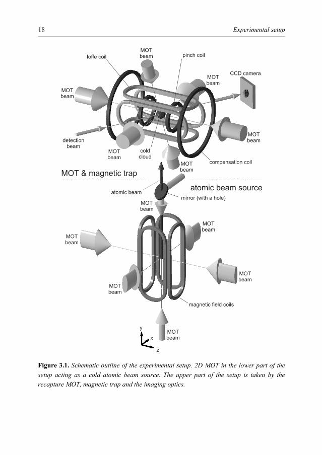
From the very first steps the design of our experimental setup was optimised for creation of samples with large atom numbers and experiments with high-density clouds. In Figure 3.1 we show a schematic view of the experimental setup. Two main parts can be distinguished here: the two-dimensional magneto-optical trap acting as an atomic beam source [32] in the bottom of the apparatus and the upper part, which combines the recapture MOT, the magnetic trap and the imaging system.
The path towards Bose-Einstein condensation begins with loading a magneto-optical trap (MOT) from an intense cold atom source [32]. The atom source operates at flux numbers of 5 × 10⁹ atoms/s with an average velocity of atoms of 8 m/s. The number of particles stored in a density-limited MOT is typically 1.2 × 10¹⁰. To maximise the number of atoms captured in the MOT, a dedicated high-power laser was designed and built (see Chapter 4). Atoms in the MOT are further cooled during an optical molasses stage to a temperature of 40 µK. After optical pumping into |F = 2, mF = 2⟩ state (with approximately 60% loss) the atoms are transferred into a weak roughly isotropic magnetic trap with the frequencies ω = 2π × 7.5 Hz. This frequency allows to match a 3 mm 1/e radius of the MOT cloud to the size of the cloud in the magnetic trap. To achieve a higher elastic collision rate and meet the condition for the runaway regime of evaporative cooling the trap is adiabatically compressed within 6.615 s. At the end of compression stage the temperature rises to 760 µK and the density increases to 7 × 1011 cm-3. After this the evaporation barrier is ramped down within 10.6 s to reach the condensation point. The critical temperature,
Experimental setup
18
Figure 3.1. Schematic outline of the experimental setup. 2D MOT in the lower part of the setup acting as a cold atomic beam source. The upper part of the setup is taken by the recapture MOT, magnetic trap and the imaging optics.
3.3 Vacuum system
19
TC = 1.5 µK and the number of particles at the transition point is ~ 107.
Both the atomic beam source and the recapture MOT are placed inside a cube created by six square coils (0.94 m side) which serve to compensate the magnetic field of the Earth. An additional function for one pair of these coils aligned with the axis of magnetic trap is the active control of the trap bottom.
In the course of experiments with BECs one has to control more than 300 events over the course of one minute. The precision and relative timing of some of these events can be as short as 1 µs, which places high demands on the control system. The control of the experiment is performed with a real-time automation system developed in-house and based on LabVIEW programming environment and the hardware from National Instruments and Viewpoint. Processing of the obtained data can be done in parallel with the experimental runs.
3.3 Vacuum system
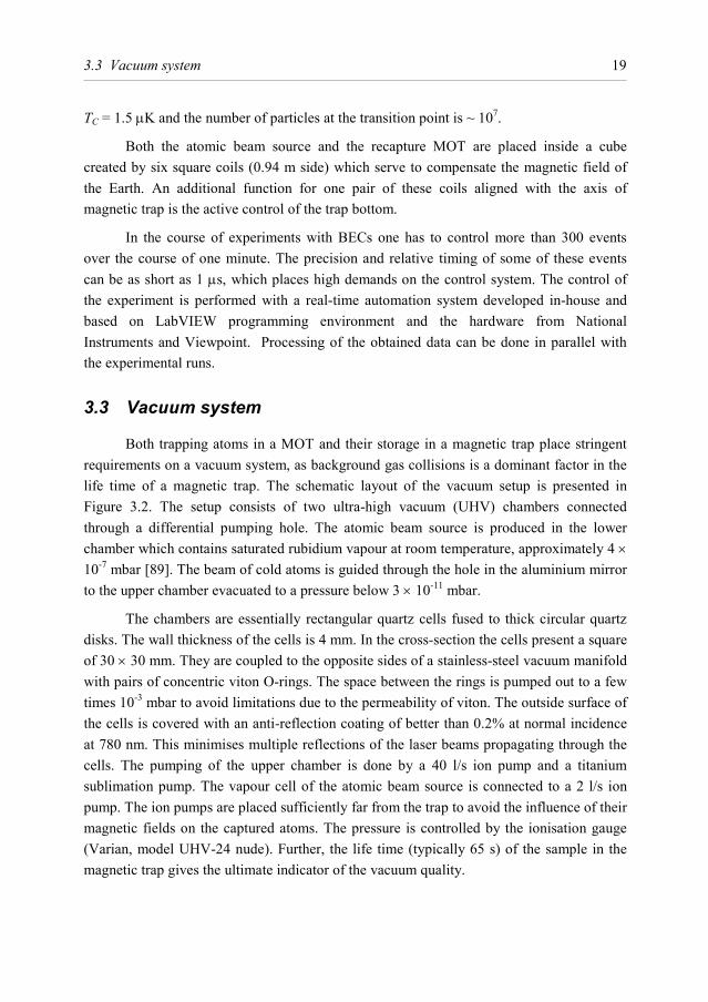
Both trapping atoms in a MOT and their storage in a magnetic trap place stringent requirements on a vacuum system, as background gas collisions is a dominant factor in the life time of a magnetic trap. The schematic layout of the vacuum setup is presented in Figure 3.2. The setup consists of two ultra-high vacuum (UHV) chambers connected through a differential pumping hole. The atomic beam source is produced in the lower chamber which contains saturated rubidium vapour at room temperature, approximately 4 × 10⁻⁷ mbar [89]. The beam of cold atoms is guided through the hole in the aluminium mirror to the upper chamber evacuated to a pressure below 3 × 10-11 mbar.
The chambers are essentially rectangular quartz cells fused to thick circular quartz disks. The wall thickness of the cells is 4 mm. In the cross-section the cells present a square of 30 × 30 mm. They are coupled to the opposite sides of a stainless-steel vacuum manifold with pairs of concentric viton O-rings. The space between the rings is pumped out to a few times 10-3 mbar to avoid limitations due to the permeability of viton. The outside surface of the cells is covered with an anti-reflection coating of better than 0.2% at normal incidence at 780 nm. This minimises multiple reflections of the laser beams propagating through the cells. The pumping of the upper chamber is done by a 40 l/s ion pump and a titanium sublimation pump. The vapour cell of the atomic beam source is connected to a 2 l/s ion pump. The ion pumps are placed sufficiently far from the trap to avoid the influence of their magnetic fields on the captured atoms. The pressure is controlled by the ionisation gauge (Varian, model UHV-24 nude). Further, the life time (typically 65 s) of the sample in the magnetic trap gives the ultimate indicator of the vacuum quality.
Experimental setup
20
Figure 3.2. Vacuum system. The lower part of the differentially pumped chamber accommodates the atomic source, while around the upper UHV cell the magneto-optical and magnetic traps are built.
3.4 Laser system
21
Two mirrors with protected gold coating are installed inside the UHV manifold. They permit introduction of the laser beams at an angle close to the vertical axis of the trap, e.g. MOT beams, optical pumping etc.
3.4 Laser system
Diode lasers are a common source of light used in spectroscopic and laser cooling applications at 780 nm. The essential requirements presented to a laser in such experiments are narrow linewidth (< 1 MHz), ability to tune the frequency, long- and short-term frequency stabilisation, and sufficient optical power. Diode lasers can have all these properties in addition to a low price and the ease of operation.
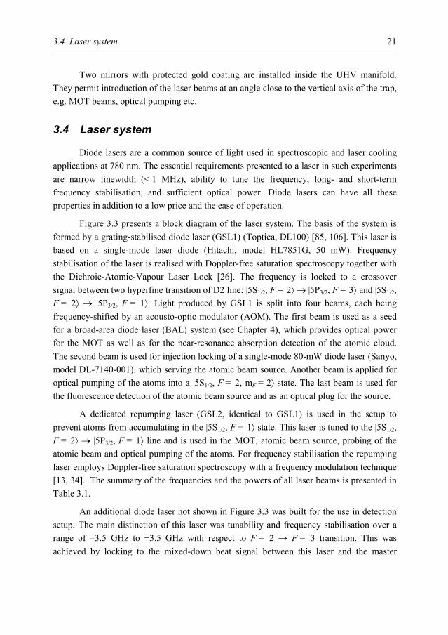
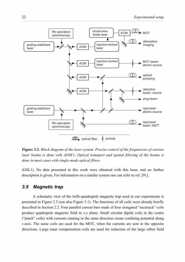
Figure 3.3 presents a block diagram of the laser system. The basis of the system is formed by a grating-stabilised diode laser (GSL1) (Toptica, DL100) [85, 106]. This laser is based on a single-mode laser diode (Hitachi, model HL7851G, 50 mW). Frequency stabilisation of the laser is realised with Doppler-free saturation spectroscopy together with the Dichroic-Atomic-Vapour Laser Lock [26]. The frequency is locked to a crossover signal between two hyperfine transition of D2 line: |5S1/2, F = 2⟩ → |5P3/2, F = 3⟩ and |5S1/2, F = 2⟩ → |5P3/2, F = 1⟩. Light produced by GSL1 is split into four beams, each being frequency-shifted by an acousto-optic modulator (AOM). The first beam is used as a seed for a broad-area diode laser (BAL) system (see Chapter 4), which provides optical power for the MOT as well as for the near-resonance absorption detection of the atomic cloud. The second beam is used for injection locking of a single-mode 80-mW diode laser (Sanyo, model DL-7140-001), which serving the atomic beam source. Another beam is applied for optical pumping of the atoms into a |5S1/2, F = 2, mF = 2⟩ state. The last beam is used for the fluorescence detection of the atomic beam source and as an optical plug for the source.
A dedicated repumping laser (GSL2, identical to GSL1) is used in the setup to prevent atoms from accumulating in the |5S1/2, F = 1⟩ state. This laser is tuned to the |5S1/2, F = 2⟩ → |5P3/2, F = 1⟩ line and is used in the MOT, atomic beam source, probing of the atomic beam and optical pumping of the atoms. For frequency stabilisation the repumping laser employs Doppler-free saturation spectroscopy with a frequency modulation technique [13, 34]. The summary of the frequencies and the powers of all laser beams is presented in Table 3.1.
An additional diode laser not shown in Figure 3.3 was built for the use in detection setup. The main distinction of this laser was tunability and frequency stabilisation over a range of –3.5 GHz to +3.5 GHz with respect to F = 2 → F = 3 transition. This was achieved by locking to the mixed-down beat signal between this laser and the master
Experimental setup
22
(GSL1). No data presented in this work were obtained with this laser, and no further description is given. For information on a similar system one can refer to ref. [91].
3.5 Magnetic trap
A schematic view of the Ioffe-quadrupole magnetic trap used in our experiments is presented in Figure 2.2 (see also Figure 3.1). The functions of all coils were already briefly described in Section 2.2. Four parallel current bars made of four elongated “racetrack” coils produce quadrupole magnetic field in x-y plane. Small circular dipole coils in the centre (“pinch” coils) with currents running in the same direction create confining potential along z-axis. The same coils are used for the MOT, when the currents are sent in the opposite directions. Large outer compensation coils are used for reduction of the large offset field
Figure 3.3. Block diagram of the laser system. Precise control of the frequencies of various laser beams is done with AOM’s. Optical transport and spatial filtering of the beams is done in most cases with single-mode optical fibres.
3.5 Magnetic trap
23
created by the pinch coils. This setup allows to avoid regions where magnetic field crosses zero value. The four coils of the Ioffe bars allow flexibility of the radial field control. In particular, it is important to compensate the magnetic field against the trap minimum shift due to gravitation in the transfer phase from the MOT to the magnetic trap. This is achieved by reducing the current in the upper coil of the quadrupole. For fine tuning and modulation of the trap potential all Ioffe coils and the compensation coils have additional double-winding coils placed next to them. This coils were for example used to realise a magnetic double-well potential by combining a static Ioffe-Pritchard trap with a time-orbiting potential (TOP). The atoms in such trap were successfully cooled and condensed to produce two spatially separated condensates [99].
In the quest for achieving high densities we produce the trap with the field gradient 353α = G/cm and the curvature 286β = G/cm2. This requires driving currents of
approximately 400 A through the copper wires of square cross-section (4 × 4 mm2 for pinch and Ioffe coils, 5 × 5 mm2 for compensation coils). The wires have a central hole of 2 and 2.5 mm respectively for active cooling of the trap, as the power dissipated by the coils reaches 5.4 kW. As a result, the coils are heated by only about 10 K, which results in high stability of the trapping field. In order to maximise thermal stability of the trap, a titanium holder for the coils is mounted on four quartz bars, with support elements designed to reduce the thermal drifts of the coil positions. The most sensitive indicator of the thermal effects in the trap is the stability of the offset field B0 = 886(1) mG in the centre of the trap. Translated into the units of the evaporation barrier (ν0 = 620 kHz), at full current the short-
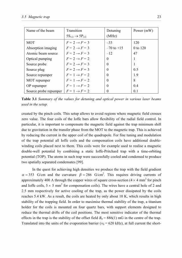
Name of the beam Transition 5S1/2 → 5P3/2
Detuning (MHz)
Power (mW)
MOT Absorption imaging Atomic beam source Optical pumping Source probe Source plug Source repumper MOT repumper OP repumper Source probe repumper
F = 2 → F = 3 F = 2 → F = 3 F = 2 → F = 3 F = 2 → F = 2 F = 2 → F = 3 F = 2 → F = 3 F = 1 → F = 2 F = 1 → F = 2 F = 1 → F = 2 F = 1 → F = 2
–33 –70 to +15 –12 0 0 0 0 0 0 0
120 0 to 120 47 1 1 0.5 1.9 8 0.4 0.1
Table 3.1 Summary of the values for detuning and optical power in various laser beams used in the setup.
Experimental setup
24
term thermal effects are less than 1 kHz/s. In the long term the trap shows drifts of approximately 5 kHz/hr.
For time-of-flight measurements on the cold atomic clouds the switch-off time of trapping field is an important parameter. The current flow through the coils is controlled by the programmed values of the power supplies as well as by the switching circuitry based on IGBT switches (IXYS, model IXGN200N60A). Fast switching-off behaviour is achieved by damping the energy of the coils into large electrolyte capacitors preloaded to 200 V. The full current of 400 A is measured to vanish on a time scale of ~ 60 µs, with the inductance of the coils being in the range of 30 µH. For high stability of the currents flowing through the trap coils all control elements are also water-cooled.
To minimise the noise on the magnetic field the pinch and compensation coils are driven in series. The compensation coils are bypassed by a passive bypass used for fine adjustment of the B0 value. The trap is compensated in such a way that the bottom of the trap is touching the zero-field value. At this point no modulation of the current through the axial coils would affect the bottom of the trap. The actual offset field B0 is then created by an additional pair of coils, also used in the Earth magnetic field compensation. This allows independent control of the frequencies of the trap.
Trap frequencies can be calculated using Equations (2.6), (2.7) and measured by exciting the centre-of-mass oscillations of the cloud. All experiments described in this thesis were performed in a trap with frequencies measured to be ωρ = 2π × 477(2) Hz and ωz = 2π × 20.8(1) Hz. These frequencies are given in the absence of evaporation knife which leads to trap deformation (see Section 3.6)
3.6 RF evaporative cooling
The principle of evaporative cooling outline in Section 2.5.1 is realised in practice by transferring the atoms to the untrapped Zeeman states with an oscillating magnetic field. For rubidium the frequency of the evaporation field lies in the radio-frequency (RF) range of approximately 50 MHz to 500 kHz. The transition occurs in the spatial region where the resonance condition is satisfied:
( )F B rfg Bµ ω=r , (3.1)
where ωrf is the angular frequency of the oscillating field. It is related to the truncation energy εt discussed in Section 2.5.1 through the following relation:
( )0t F rfmε ω ω= − , (3.2)
3.6 RF evaporative cooling
25
where 0 (0)B Fg Bω µ= is the resonance frequency corresponding to the centre of the trap (i.e. the bottom of the potential). The probability of the transition into an untrapped state is defined by the amplitude of the evaporation field and the speed at which the atom is passing through the resonance region. This problem was solved for a two level atom in [112] and is discussed in [90]. Additional studies of the transition probability for the F = 2 state of 87Rb were done by Valkering [102]. The probability is a function of the Landau-Zener parameter which is proportional to the square of Rabi frequency ΩR. At a certain amplitude of the evaporation field the transition probability approaches unity and this defines the minimum amplitude required for evaporation at a given temperature.
In the course of evaporative cooling the evaporation knife is ramped down in frequency from 50 MHz to a few hundred kHz. The total duration of the ramp is 10.6 s. For experiments described further in this thesis the precise timing and high stability of the RF signal are of great importance. No commercial device available on the market at the time could satisfy the set requirements. This motivated design and construction of the RF generator employing direct digital synthesis of the signal (DDS) and based on AD9852 chip from Analog Devices. The generator could be programmed from the LabVIEW interface as a part of the whole event sequence of the experimental cycle. The waveform produced by the synthesiser was typically made of a number of linear frequency ramps combined with several intervals of constant frequency generation.
After passing through a variable 60 dB attenuator the RF signal from the synthesiser is amplified by a power amplifier (Amplifier Research, model 25A250A). The level of the signal is controlled by a 12-bit analogue output of the computer connected to the variable attenuator. The output of the amplifier is coupled to a two-winding circular antenna 31 mm in diameter, which is positioned 16 mm from the trap centre. The final amplitude of the RF field in the trap varies from 15 × 10-6 T in the beginning of the ramp to 4 × 10⁻⁶ T in the end.
It is important to consider the effects of the oscillating magnetic field leading to an energy shift of magnetic sublevels in the “dressed” states picture. These shifts distort the effective shape of the potential and should also be taken into account in measurement of the trap bottom. By diagonalising the time-dependent Hamiltonian of the atom in an oscillating magnetic field, one can calculate the following expression for the dressed potential (in the presence of gravity):
( ) ( )( )21/ 222 0
0 22F rf R F B rfmg
U m g B mgρ
ρ ω µ ρ ω ρω
= − Ω + − + + , (3.3)
where B(ρ) is defined by Equation (2.5) at z = 0, and ΩR is the Rabi frequency
Experimental setup
26
R 2F B rfg Bµ
Ω = . (3.4)
Here Brf is the amplitude of rf-field. One can solve Equation (3.3) to produce an expression for the effective trap depth and an approximate expression for the new trap frequency ωρ′, which will be lower than the “non-dressed” frequency ωρ for values of ωrf near the bottom of the trap. A similar analysis can be made for the axial trap frequency. Such systematic effects on the frequency have to be taken into account if the RF barrier is switched on and is close to the bottom of the trap, e.g. in experiments with cold samples where the RF knife is kept at a constant frequency to act as a heat shield.
Another procedure where this effect plays a role is the measurement of the trap bottom B0, which is performed as a matter of daily routine. The evaporation knife is lowered until no particles can be detected in the trap. Due to the power broadening described above this occurs before the RF-frequency reaches the resonance value corresponding to B0. This offset in frequency is measured by comparing the values of the evaporation knife with those of an continuous atom laser [14] and is found to be 10(1) kHz. A calculation based on Equation (3.3) confirms this result.
3.7 Imaging of cold atomic clouds
In this section we consider different aspects of the detection of cold atomic clouds. Description and characterisation of the optical system is followed by a discussion of absorption detection. Analysis of the data and various limitations of imaging are discussed in the next sections. Finally, we present a short discussion of lensing – an important effect frequently occurring in imaging dense small clouds.
3.7.1 Optics
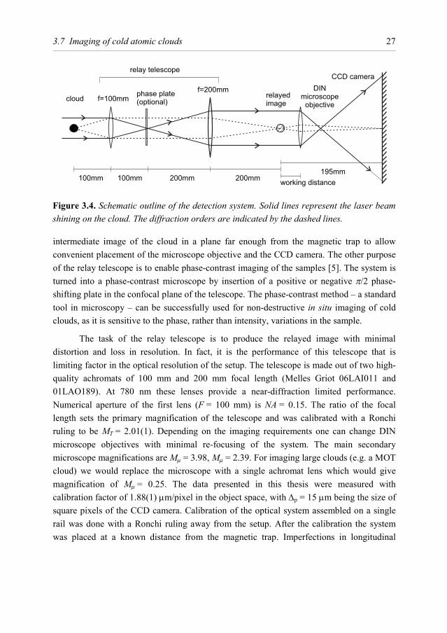
The detection setup in a BEC experiment must be versatile enough to enable the detection of clouds ranging is size from several millimetres to several microns. Features like the optical resolution, noise characteristics and dynamic range all contribute to the quality of the produced data. The schematic outline of the detection optics is presented in Figure 3.4. In the absorption imaging method used throughout this thesis, the shadow in the near-resonant laser beam directed at the sample is transformed by the lenses and imaged on the CCD array. Detection of cold clouds in the trap as well as of fine structures in expanded clouds requires high numerical aperture of the detection optics. However, the position of the sample inside the vacuum cell makes the use of standard microscope objectives impossible. The relay telescope made out of two confocal achromatic lenses produces an
3.7 Imaging of cold atomic clouds
27
intermediate image of the cloud in a plane far enough from the magnetic trap to allow convenient placement of the microscope objective and the CCD camera. The other purpose of the relay telescope is to enable phase-contrast imaging of the samples [5]. The system is turned into a phase-contrast microscope by insertion of a positive or negative π/2 phase-shifting plate in the confocal plane of the telescope. The phase-contrast method – a standard tool in microscopy – can be successfully used for non-destructive in situ imaging of cold clouds, as it is sensitive to the phase, rather than intensity, variations in the sample.
The task of the relay telescope is to produce the relayed image with minimal distortion and loss in resolution. In fact, it is the performance of this telescope that is limiting factor in the optical resolution of the setup. The telescope is made out of two high-quality achromats of 100 mm and 200 mm focal length (Melles Griot 06LAI011 and 01LAO189). At 780 nm these lenses provide a near-diffraction limited performance. Numerical aperture of the first lens (F = 100 mm) is NA = 0.15. The ratio of the focal length sets the primary magnification of the telescope and was calibrated with a Ronchi ruling to be MT = 2.01(1). Depending on the imaging requirements one can change DIN microscope objectives with minimal re-focusing of the system. The main secondary microscope magnifications are Mµ = 3.98, Mµ = 2.39. For imaging large clouds (e.g. a MOT cloud) we would replace the microscope with a single achromat lens which would give magnification of Mµ = 0.25. The data presented in this thesis were measured with calibration factor of 1.88(1) µm/pixel in the object space, with ∆p = 15 µm being the size of square pixels of the CCD camera. Calibration of the optical system assembled on a single rail was done with a Ronchi ruling away from the setup. After the calibration the system was placed at a known distance from the magnetic trap. Imperfections in longitudinal
Figure 3.4. Schematic outline of the detection system. Solid lines represent the laser beam shining on the cloud. The diffraction orders are indicated by the dashed lines.
Experimental setup
28
placement of the rail would result in the magnification error of well below that quoted for the primary magnification of the relay telescope.
The imaging device is a cooled CCD camera (Princeton Instruments, model TE/CCD-512EFT). The controller of the camera gives a choice between 12- and 16-bit analogue-to-digital conversion. A feature specific to this particular camera is the ability to operate in the so-called “kinetic transfer” mode. In this mode only part of the chip is exposed to light, while the rest of the chip is used as a storage area. One can thus take a burst of images at high speed (limited only by the array shift time) and read them out later at a slow speed. This feature can be particularly useful in non-destructive imaging of the cloud.
Resolution of the optical system is one of the crucial parameters. In the literature on Bose-Einstein condensation it is sometimes quoted in confusing terms. The diffraction performance of our imaging system was analysed both by measurement of a point-spread function (by looking at the end of a single-mode optical fibre) and by a standard tool in microscopy: a positive 1951 USAF resolution target. In line with the definition of a Raleigh criterion, a stripe pattern was defined as resolved if the transmitted intensity was modulated at least by 20%. The smallest resolved pattern had a repetition period of 6.9 micron, which corresponds to a resolution of R = 3.3 µm (1/e half-width). This measurement includes the effect of the aberrations added by the 4-mm thick wall of the quartz cuvette in the optical path. This value matches the one measured by imaging the output of a single-mode fibre: R = 3.1 µm. Calculation of the resolution for a diffraction-limited lens with a Raleigh criterion gives 0.61 3.2µmr NAλ= = . To compare with often quoted FWHM or 1/e2 resolution figures one should multiply the given numbers by an appropriate pre-factor. Resolution effects should be taken into account in the imaging of small objects such as cold clouds in situ, stripes due to phase fluctuations etc. While convolution of the instrumentation function with a gaussian density profile is a trivial task, additional care should be taken in the analysis of clouds with other (e.g. parabolic) density profiles.
3.7.2 Absorption detection
The main method of observation of the atomic clouds in our experiments is imaging the absorption profile produced by the cloud in a near-resonant laser beam. While most of the detection was done on the |5S1/2, F = 2⟩ → |5P3/2, F = 3⟩ transition, in some measurements we could benefit from using the weaker transitions |5S1/2, F = 2⟩ → |5P3/2, F = 1, 2⟩. Such measurements would usually involve dense small clouds where refraction effects (described in Section 3.7.4) were especially pronounced. In this case, using a small
3.7 Imaging of cold atomic clouds
29
(or zero) detuning from a weak transition would result in a higher image quality. For driving these transitions we used a separate laser briefly described in Section 3.4.
The intensity distribution in the detection beam after passing through the absorbing cloud follows directly from Lambert-Beer’s law:
( ) ( ) ( ),0, , D y zI y z I y z e−= , (3.5)
where ( )0 ,I y z is the initial density profile before the absorption and ( ),D y z is the optical density:
( ) ( ) ( ), , , ,D y z n x y z dx y zπ πσ σ η= =∫ . (3.6)
Here σπ is the photon absorption cross-section. The detection light is linearly polarised and in the zero-approximation the expression for the cross-section can be obtained by averaging over all π-transitions (see e.g. ref. [76] for discussion on the transition strengths):
( )
2
27 3 1
15 2 1 2π
λσ
π δ=
+ Γ, (3.7)
where δ is the detuning from the optical transition, Γ is the full natural linewidth, and λ is the wavelength of the laser. However, since the detection is not done on a closed transition, in the duration of the detection pulse optical pumping results in re-distribution of the atoms between different Zeeman sublevels. This changes the 7/15 factor in the expression for the cross-section and can lead to systematic errors in determination of the number of atoms.
The choice of the detection pulse duration is dictated by limitations of the ballistic blur caused by scattered photons to the sample [64]. In our experiments it was typically 40 µs. At the same time short detection times force one to go to higher optical powers of the detection beam to maximise the use of the dynamic range of the camera and increase the signal-to-noise ratio of the image. This is especially true for the use of high-power microscope objectives, when the light collection efficiency goes down. This increase in powers presents no problem if the detuning of the detection beam is large enough to stay away from saturation of the transition. However, once the sample expands one is forced to reduce the detuning to keep the optical density well above the noise floor. In such cases varying across the sample saturation effects should be taken into account by solving the following differential equation:
( ) ( ) ( ) ( )
12
0, , , ,21 , ,
s
I x y z I x y zn x I x y z
x Iδ
σ−
∂ = − + + ∂ Γ . (3.8)
Experimental setup
30
where Is is the saturation intensity. For the microscope objective Mµ = 3.98 the power of the detection beam was 2.5 mW, which corresponded to 0.85Is on resonance.
A single data shot of the optical density distribution contains in fact three images and is normalised according to the following rule:
( ) ( )( )
( ) ( )( ) ( )0
, ,,, ln ln
, , ,abs bg
ff bg
I y z I y zI y zD y z
I y z I y z I y z−
= − = −−
. (3.9)
Here ( ),absI y z is the beam profile with the shadow of the cloud, ( ),ffI y z is the flat-field profile taken in the absence of the cloud, and ( ),bgI y z is the background light illumination taken in the absence of the detection beam.
Ideally, the lower limit on the detuning of the detection laser is set by the noise performance of the whole imaging system and by the dynamic range of the analogue-to-digital converter of the CCD camera. For a 12-bit camera the minimum optical density would be D0 = 8. However, in practice the observed maximum optical density is limited to D0 = 5. This difference is due to the broad spectral background typical for diode lasers. This aspect of the spectral purity of the detection is discussed in Chapter 4. To avoid the systematic errors due to this effect the detuning of the detection beam is usually made large enough to keep the maximum optical density below 2.5.
3.7.3 Fitting parameters
All information about the condensates and cold clouds is extracted from analysis of the optical density profile defined by Equation (3.9). The total number of particles can be determined directly from the pixel sum of the image:
( )2p
,
,i ji j
N D y zπσ
∆= ∑ . (3.10)
where ∆p is the size of the square pixel.
More complete information is obtained by fitting a two-dimensional surface to the array of data described by Equation (3.9). The thermal cloud profile is fitted by the following function:
( ) ( ) ( ) ( )2 2
2 22 2, , 0,0 expth th thy z
y zD y z y z g z g zl lπ πσ η σ η
= = − −
. (3.11)
In the limit of collisionless gas the temperature can be obtained from the radial ly or axial lz 1/e size parameters of the profile [64]:
3.7 Imaging of cold atomic clouds
31
2
2 2 , , 2 1
ii
B i
mT l i y zk
ωω τ
= ∈
+ . (3.12)
In practice for cigar-shaped clouds the temperature can also be determined directly from the axial size at short expansion times 1 zτ ω . If the cloud can no longer be described by a collisionless gas model, the temperature determination becomes less trivial. This is discussed in detail in Chapter 5.
The condensed fraction of the cloud has a parabolic density profile, which, after integration along the ling of detection, yields the following distribution for the optical density:
( ) ( )( ) ( )
3/ 22 2
2 2, 0,0 max 1 ,0c cy z
y zD y zL Lπσ η
τ τ
= − − . (3.13)
Here the Thomas-Fermi size parameters Ly (or Lρ) and Lz are given by [21]:
( ) ( ) 2 20 1L Lρ ρ ρτ ω τ= + . (3.14)
( ) ( ) ( )( )2
2 20 1 arctan ln 1zz zL L ρ ρ ρ
ρ
ωτ ω τ ω τ ω τ
ω
= + − +
. (3.15)
The chemical potential is then given as
( )
( )2 2 2
22 2
02 2 1
m L m Lρ ρ ρρ
ρ
ω ωµ τ
ω τ
= = +
. (3.16)
The number of particles in the condensate is expressed through the chemical potential as (see Equation (2.22)
5/ 2
02
15hrNa
µω
=
, (3.17)
and the central density of the condensate is given by ( )0 0n Uµ= .
3.7.4 Lensing
In this section we briefly discuss the refractive effects of cold atomic clouds. In the description of absorption detection in Section 3.7.2 we only considered the effect of the imaginary part of the complex dielectric susceptibility. However, the real part of the susceptibility responsible for refraction cannot be neglected in sufficiently dense atomic
Experimental setup
32
clouds. Depending on the detuning such clouds can behave as a combination of the GRIN lens and a usual spherical lens. Lensing can lead to systematic errors in the determination of the cloud size and the number of particles. Thus, it is important to understand regimes in which lensing can appear.
The key limitations become obvious from the analysis of the expression for a refractive index of a two-level atom, classical derivation of which follows from e.g. [66]:
( )3
2 2 2 2 23 21 4 116 4 4
nn iλ δµ πχ
π δ δ
Γ Γ= + ≈ + − +
+ Γ + Γ . (3.18)
Here n is the density of the atoms. For more detailed discussion one can refer to [30], while quantum mechanical derivation of susceptibility of rubidium vapour is discussed in [3].
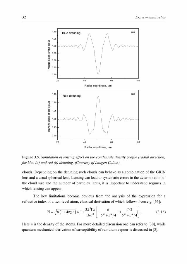
Figure 3.5. Simulation of lensing effect on the condensate density profile (radial direction) for blue (a) and red (b) detuning. (Courtesy of Imogen Colton).
3.7 Imaging of cold atomic clouds
33
The optical density can thus be written down as
0 2 21
1 4D D
δ=
+ Γ, (3.19)
where D0 is the maximum resonant optical density of the sample. All changes in the phase of the propagating light are described by the real part of Equation (3.18):
( )3 2 2
2 2 23 4Re 116 1 4
nλ δπ δ
Γ= −
+ Γ. (3.20)
It is clear that for blue detuning the real part of the refractive index is smaller than unity and the cloud acts as a diverging lens, while for red detuning it acts as a converging lens. In Figure 3.5 we show an example of simulation of the lensing effect on a pure condensate with a parabolic density profile [24].
If the phase shift induced by a cloud is sufficiently large to make the cloud act as a lens with the focal length comparable to its own size, lensing severely affects the image and this region should be avoided. This effect can be especially pronounced in imaging the clouds in the magnetic trap or at short expansion times. In such cases one can benefit from using weaker transitions, as described in Section 3.7.2, or go to the extreme of large detunings, where absorption is negligible, and use phase-contrast detection. The intensity distribution of the phase-contrast image is proportional to the phase shift induced by the cloud and is therefore proportional to density.
It is possible to extract information from images affected by lensing by doing sophisticated data processing. Moreover, there is current work on the use of non-interferometric methods of imaging the dense atomic samples using phase information. [25, 101].

Chapter 4 Broad-area diode laser system
This chapter is based on the publication:
Broad-area diode laser system for a rubidium Bose-Einstein condensation experiment, I. Shvarchuck, K. Dieckmann, M. Zielonkowski, J.T.M. Walraven, Applied Physics B, 71(4): 475 – 480, 2000
Addenda made in this text are related to the alignment procedure and the lifetime of the laser.
4.1 Abstract.
We report on master-oscillator power amplification using a broad-area laser diode (BAL) emitting at a wavelength of λ = 780 nm. The master oscillator is an injection-locked single-mode diode laser delivering a seeding beam of 35 mW, which is amplified in double pass through the BAL up to 410 mW. After beam shaping and spatial filtering by a single-mode fibre we obtain a clean Gaussian beam with a maximum power of 160 mW. There is no detectable contribution of the BAL eigenmodes in the spectrum of the output light. This laser system is employed for operation of a 87Rb magneto-optical trap (MOT) and for near-resonant absorption imaging in a Bose-Einstein condensation experiment.
4.2 Introduction
Diode-laser based systems have a profound impact on experiments in atomic physics. The excellent spectral properties and power stability make diode lasers a highly practical tool for laser cooling and trapping experiments as well as for spectroscopic applications. The ease of operation, small size and low cost of diode laser systems facilitate experiments in which multiple laser sources are used. These properties make diode lasers an attractive choice for experiments on Bose-Einstein condensation (BEC) of alkali systems, in particular for driving magneto-optical traps (MOTs). In BEC experiments with 87Rb diode lasers are successfully used for driving the 2S1/2 (F = 2) → 2P3/2 (F' = 3) transition at 780 nm [4]. Production of a condensate usually involves a magneto-optical trap with a variety of loading schemes ranging from double-MOT systems to Zeeman slowers [55]. The drive for realising condensates with large number of particles and fast condensate
Broad-area diode laser system
36
production schemes has triggered the development of high-flux sources [32, 64, 72] and large optically dense MOTs (see for instance [64]). To avoid unbalanced radiation pressure in the light field, optically dense MOTs are driven by six laser beams of large diameters. The power conserving use of three retroreflected beams is not optimal in this case. Large diameter of the beams is also important for recapture from a diverging atomic beam. Thus, the optical power required for driving a large MOT tends to go beyond the power available from single-mode diode lasers operating at 780 nm (typically not exceeding 50 mW). Alternative solutions like Ti-Sapphire lasers or diode tapered-amplifier systems provide high power but have their disadvantages aside from being expensive. The amplitude noise of an argon-ion laser pumped Ti-Sapphire laser is undesirable for many applications. Diode amplifiers with tapered waveguide offer a straightforward solution to the power limitations of narrow-bandwidth diode lasers but in practice turn out rather delicate to operate.
In this paper we report on double-pass master-oscillator power amplification with a broad-area laser diode (BAL). The advantageous properties of this system have been demonstrated and characterised in the past (see [1, 40, 44] and references therein), also in the context of laser cooling [37, 83]. We describe a BAL amplifier optimised for use in a 87Rb BEC experiment, both for driving a magneto-optical trap and for near-resonant absorption imaging. The system operates at a wavelength of 780 nm. Using 35 mW of seeding power we obtain 410 mW of locked laser power under conditions close to power saturation. After beam shaping and spatial filtering by a single mode fibre we obtain a clean Gaussian beam with a maximum power of 160 mW. The insertion loss of intensity modulation optics limits the available laser power to typically 135 mW under daily stable operation conditions. This allows us to trap 1010 rubidium atoms in a MOT loaded from a continuous slow atomic beam source [32].
4.3 Experimental setup
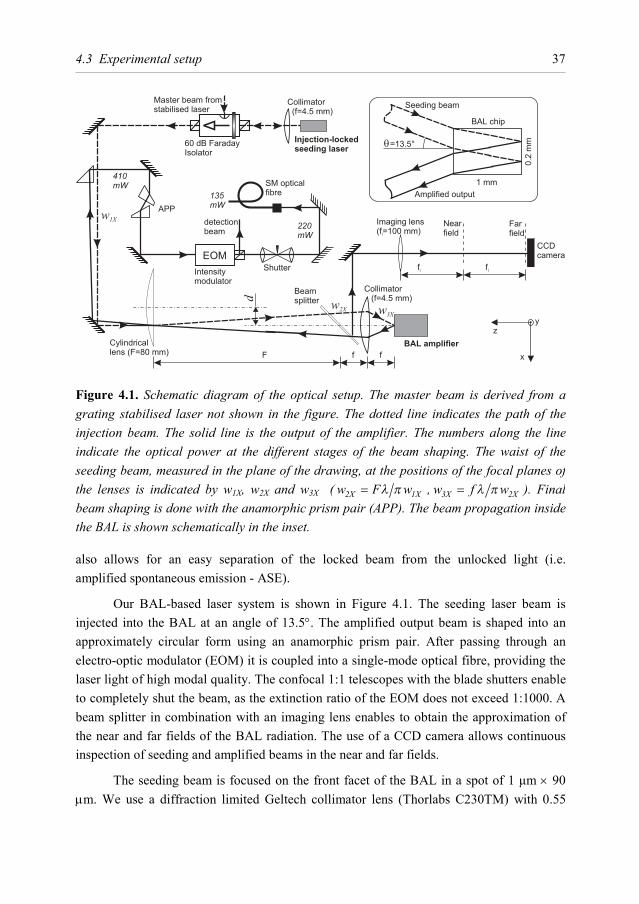
The heart of our experimental setup is a 2-watt broad-area laser-diode (High Power Devices Inc. HPD1120) used as a double-pass amplifier. As described in the literature, a free-running broad-area laser oscillates in multiple transverse modes which are caused by filamentation of the gain medium [2, 67]. A free-running BAL has a power spectrum with a bandwidth of the order of 2-3 nm on top of an even broader spectral background. This spectrum can be narrowed by injecting seeding light from a narrow-bandwidth laser source. At high operating currents only part of the light emitted by the BAL can be locked. The seeding light is usually injected under a small angle as shown in the inset of Figure 4.1. In this way one can suppress amplification in multiple transverse modes. Injecting at an angle
4.3 Experimental setup
37
also allows for an easy separation of the locked beam from the unlocked light (i.e. amplified spontaneous emission - ASE).
Our BAL-based laser system is shown in Figure 4.1. The seeding laser beam is injected into the BAL at an angle of 13.5°. The amplified output beam is shaped into an approximately circular form using an anamorphic prism pair. After passing through an electro-optic modulator (EOM) it is coupled into a single-mode optical fibre, providing the laser light of high modal quality. The confocal 1:1 telescopes with the blade shutters enable to completely shut the beam, as the extinction ratio of the EOM does not exceed 1:1000. A beam splitter in combination with an imaging lens enables to obtain the approximation of the near and far fields of the BAL radiation. The use of a CCD camera allows continuous inspection of seeding and amplified beams in the near and far fields.
The seeding beam is focused on the front facet of the BAL in a spot of 1 µm × 90 µm. We use a diffraction limited Geltech collimator lens (Thorlabs C230TM) with 0.55
BAL amplifier
Injection-lockedseeding laser
60 dB FaradayIsolator
APP
Intensitymodulator
SM opticalfibre
Cylindricallens (F=80 mm)
Collimator(f=4.5 mm)
Beamsplitter
Imaging lens(f=100 mm)i
Nearfield
Farfield
CCDcamera
1 mm
0.2
mm
Amplified output
f fF
w1X
w2X w
3X
410
mW
135
mW
220
mW
EOM
Seeding beam
BAL chip
fi fi
z
x
y
Collimator(f=4.5 mm)
Master beam fromstabilised laser
detectionbeam
d
=13.5°
Shutter
Figure 4.1. Schematic diagram of the optical setup. The master beam is derived from a grating stabilised laser not shown in the figure. The dotted line indicates the path of the injection beam. The solid line is the output of the amplifier. The numbers along the line indicate the optical power at the different stages of the beam shaping. The waist of the seeding beam, measured in the plane of the drawing, at the positions of the focal planes of the lenses is indicated by w1X, w2X and w3X ( 2X 1Xw F wλ π= , 3X 2Xw f wλ π= ). Final beam shaping is done with the anamorphic prism pair (APP). The beam propagation inside the BAL is shown schematically in the inset.
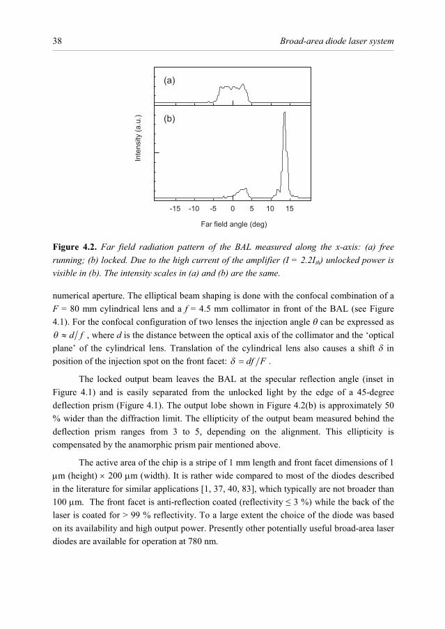
Broad-area diode laser system
38
numerical aperture. The elliptical beam shaping is done with the confocal combination of a F = 80 mm cylindrical lens and a f = 4.5 mm collimator in front of the BAL (see Figure 4.1). For the confocal configuration of two lenses the injection angle θ can be expressed as
d fθ ≈ , where d is the distance between the optical axis of the collimator and the ‘optical plane’ of the cylindrical lens. Translation of the cylindrical lens also causes a shift δ in position of the injection spot on the front facet: df Fδ = .
The locked output beam leaves the BAL at the specular reflection angle (inset in Figure 4.1) and is easily separated from the unlocked light by the edge of a 45-degree deflection prism (Figure 4.1). The output lobe shown in Figure 4.2(b) is approximately 50 % wider than the diffraction limit. The ellipticity of the output beam measured behind the deflection prism ranges from 3 to 5, depending on the alignment. This ellipticity is compensated by the anamorphic prism pair mentioned above.
The active area of the chip is a stripe of 1 mm length and front facet dimensions of 1 µm (height) × 200 µm (width). It is rather wide compared to most of the diodes described in the literature for similar applications [1, 37, 40, 83], which typically are not broader than 100 µm. The front facet is anti-reflection coated (reflectivity ≤ 3 %) while the back of the laser is coated for > 99 % reflectivity. To a large extent the choice of the diode was based on its availability and high output power. Presently other potentially useful broad-area laser diodes are available for operation at 780 nm.
Figure 4.2. Far field radiation pattern of the BAL measured along the x-axis: (a) free running; (b) locked. Due to the high current of the amplifier (I = 2.2Ith) unlocked power is visible in (b). The intensity scales in (a) and (b) are the same.
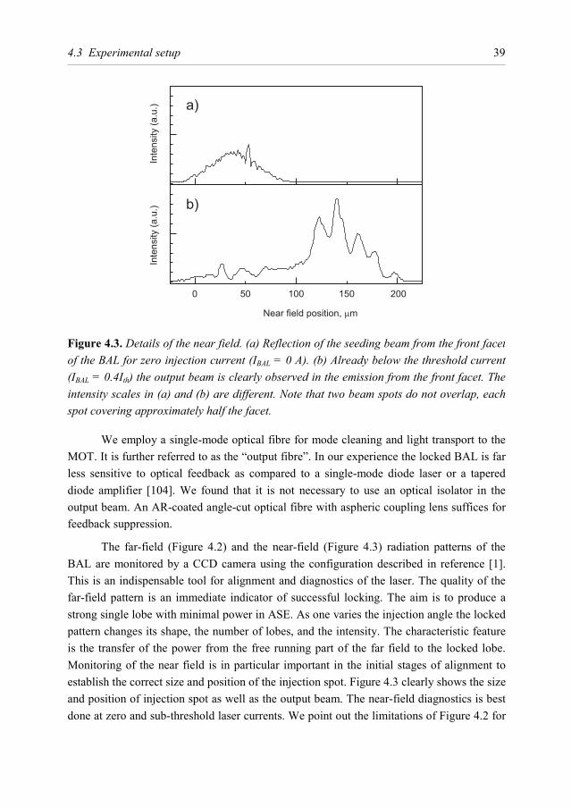
4.3 Experimental setup
39
We employ a single-mode optical fibre for mode cleaning and light transport to the MOT. It is further referred to as the “output fibre”. In our experience the locked BAL is far less sensitive to optical feedback as compared to a single-mode diode laser or a tapered diode amplifier [104]. We found that it is not necessary to use an optical isolator in the output beam. An AR-coated angle-cut optical fibre with aspheric coupling lens suffices for feedback suppression.
The far-field (Figure 4.2) and the near-field (Figure 4.3) radiation patterns of the BAL are monitored by a CCD camera using the configuration described in reference [1]. This is an indispensable tool for alignment and diagnostics of the laser. The quality of the far-field pattern is an immediate indicator of successful locking. The aim is to produce a strong single lobe with minimal power in ASE. As one varies the injection angle the locked pattern changes its shape, the number of lobes, and the intensity. The characteristic feature is the transfer of the power from the free running part of the far field to the locked lobe. Monitoring of the near field is in particular important in the initial stages of alignment to establish the correct size and position of the injection spot. Figure 4.3 clearly shows the size and position of injection spot as well as the output beam. The near-field diagnostics is best done at zero and sub-threshold laser currents. We point out the limitations of Figure 4.2 for
Figure 4.3. Details of the near field. (a) Reflection of the seeding beam from the front facet of the BAL for zero injection current (IBAL = 0 A). (b) Already below the threshold current (IBAL = 0.4Ith) the output beam is clearly observed in the emission from the front facet. The intensity scales in (a) and (b) are different. Note that two beam spots do not overlap, each spot covering approximately half the facet.
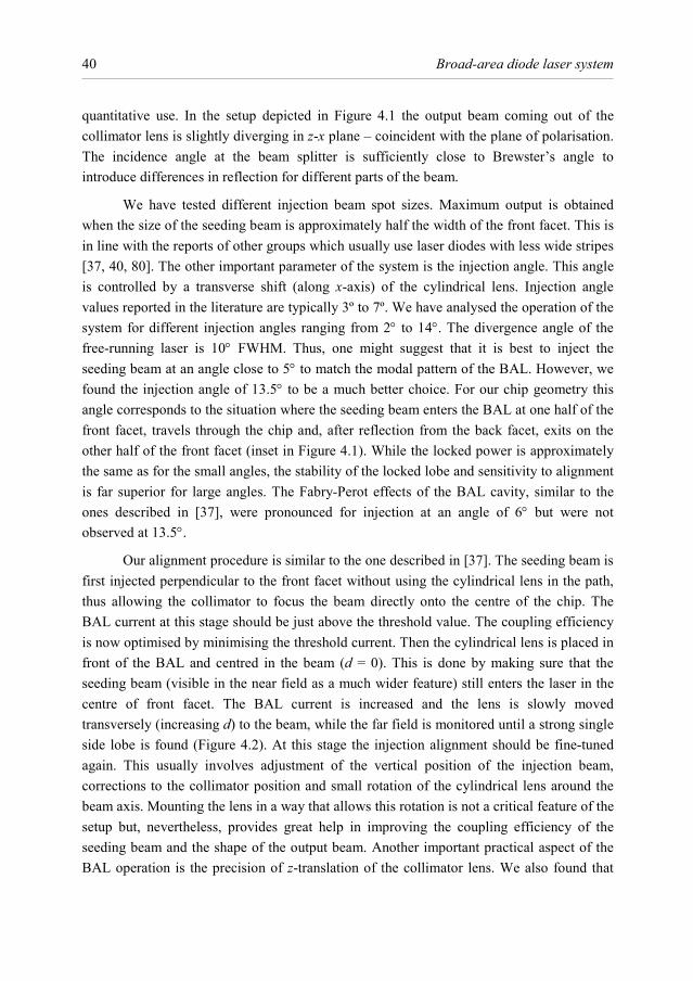
Broad-area diode laser system
40
quantitative use. In the setup depicted in Figure 4.1 the output beam coming out of the collimator lens is slightly diverging in z-x plane – coincident with the plane of polarisation. The incidence angle at the beam splitter is sufficiently close to Brewster’s angle to introduce differences in reflection for different parts of the beam.
We have tested different injection beam spot sizes. Maximum output is obtained when the size of the seeding beam is approximately half the width of the front facet. This is in line with the reports of other groups which usually use laser diodes with less wide stripes [37, 40, 80]. The other important parameter of the system is the injection angle. This angle is controlled by a transverse shift (along x-axis) of the cylindrical lens. Injection angle values reported in the literature are typically 3º to 7º. We have analysed the operation of the system for different injection angles ranging from 2° to 14°. The divergence angle of the free-running laser is 10° FWHM. Thus, one might suggest that it is best to inject the seeding beam at an angle close to 5° to match the modal pattern of the BAL. However, we found the injection angle of 13.5° to be a much better choice. For our chip geometry this angle corresponds to the situation where the seeding beam enters the BAL at one half of the front facet, travels through the chip and, after reflection from the back facet, exits on the other half of the front facet (inset in Figure 4.1). While the locked power is approximately the same as for the small angles, the stability of the locked lobe and sensitivity to alignment is far superior for large angles. The Fabry-Perot effects of the BAL cavity, similar to the ones described in [37], were pronounced for injection at an angle of 6° but were not observed at 13.5°.
Our alignment procedure is similar to the one described in [37]. The seeding beam is first injected perpendicular to the front facet without using the cylindrical lens in the path, thus allowing the collimator to focus the beam directly onto the centre of the chip. The BAL current at this stage should be just above the threshold value. The coupling efficiency is now optimised by minimising the threshold current. Then the cylindrical lens is placed in front of the BAL and centred in the beam (d = 0). This is done by making sure that the seeding beam (visible in the near field as a much wider feature) still enters the laser in the centre of front facet. The BAL current is increased and the lens is slowly moved transversely (increasing d) to the beam, while the far field is monitored until a strong single side lobe is found (Figure 4.2). At this stage the injection alignment should be fine-tuned again. This usually involves adjustment of the vertical position of the injection beam, corrections to the collimator position and small rotation of the cylindrical lens around the beam axis. Mounting the lens in a way that allows this rotation is not a critical feature of the setup but, nevertheless, provides great help in improving the coupling efficiency of the seeding beam and the shape of the output beam. Another important practical aspect of the BAL operation is the precision of z-translation of the collimator lens. We also found that
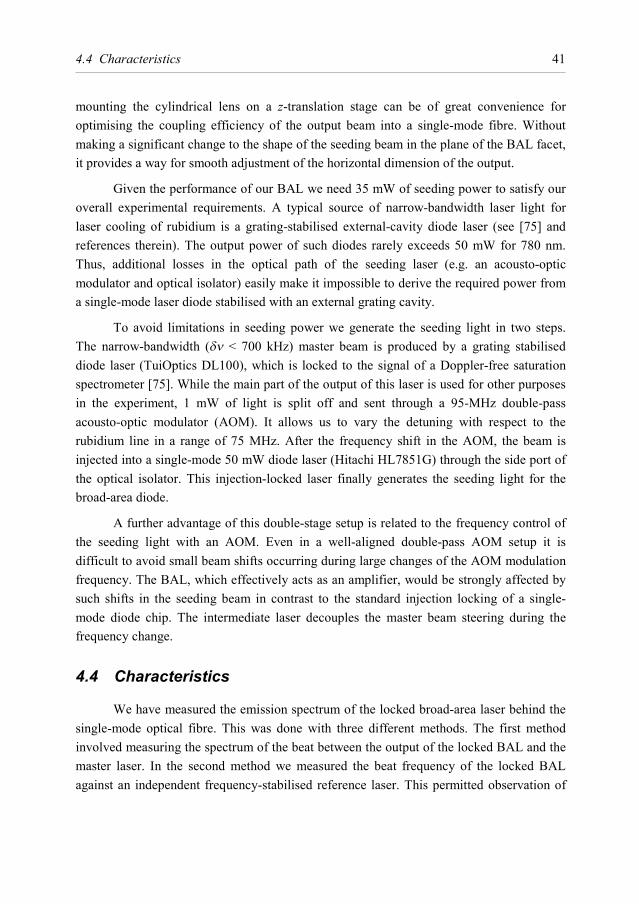
4.4 Characteristics
41
mounting the cylindrical lens on a z-translation stage can be of great convenience for optimising the coupling efficiency of the output beam into a single-mode fibre. Without making a significant change to the shape of the seeding beam in the plane of the BAL facet, it provides a way for smooth adjustment of the horizontal dimension of the output.
Given the performance of our BAL we need 35 mW of seeding power to satisfy our overall experimental requirements. A typical source of narrow-bandwidth laser light for laser cooling of rubidium is a grating-stabilised external-cavity diode laser (see [75] and references therein). The output power of such diodes rarely exceeds 50 mW for 780 nm. Thus, additional losses in the optical path of the seeding laser (e.g. an acousto-optic modulator and optical isolator) easily make it impossible to derive the required power from a single-mode laser diode stabilised with an external grating cavity.
To avoid limitations in seeding power we generate the seeding light in two steps. The narrow-bandwidth (δν < 700 kHz) master beam is produced by a grating stabilised diode laser (TuiOptics DL100), which is locked to the signal of a Doppler-free saturation spectrometer [75]. While the main part of the output of this laser is used for other purposes in the experiment, 1 mW of light is split off and sent through a 95-MHz double-pass acousto-optic modulator (AOM). It allows us to vary the detuning with respect to the rubidium line in a range of 75 MHz. After the frequency shift in the AOM, the beam is injected into a single-mode 50 mW diode laser (Hitachi HL7851G) through the side port of the optical isolator. This injection-locked laser finally generates the seeding light for the broad-area diode.
A further advantage of this double-stage setup is related to the frequency control of the seeding light with an AOM. Even in a well-aligned double-pass AOM setup it is difficult to avoid small beam shifts occurring during large changes of the AOM modulation frequency. The BAL, which effectively acts as an amplifier, would be strongly affected by such shifts in the seeding beam in contrast to the standard injection locking of a single-mode diode chip. The intermediate laser decouples the master beam steering during the frequency change.
4.4 Characteristics
We have measured the emission spectrum of the locked broad-area laser behind the single-mode optical fibre. This was done with three different methods. The first method involved measuring the spectrum of the beat between the output of the locked BAL and the master laser. In the second method we measured the beat frequency of the locked BAL against an independent frequency-stabilised reference laser. This permitted observation of
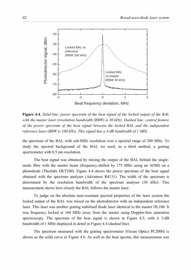
Broad-area diode laser system
42
the spectrum of the BAL with sub-MHz resolution over a spectral range of 200 MHz. To study the spectral background of the BAL we used, as a third method, a grating spectrometer with 0.5 nm resolution.
The beat signal was obtained by mixing the output of the BAL behind the single-mode fibre with the master beam (frequency-shifted by 175 MHz using an AOM) on a photodiode (Thorlabs DET200). Figure 4.4 shows the power spectrum of the beat signal obtained with the spectrum analyser (Advantest R4131). The width of the spectrum is determined by the resolution bandwidth of the spectrum analyser (30 kHz). This measurement shows how closely the BAL follows the master laser.
To judge on the absolute near-resonant spectral properties of the laser system the locked output of the BAL was mixed on the photodetector with an independent reference laser. This laser was another grating stabilised diode laser identical to the master DL100. It was frequency locked at 160 MHz away from the master using Doppler-free saturation spectroscopy. The spectrum of the beat signal is shown in Figure 4.5, with it 3-dB bandwidth of 1 MHz displayed in detail in Figure 4.4 (dashed line).
The spectrum measured with the grating spectrometer (Ocean Optics PC2000) is shown as the solid curve in Figure 4.6. As well as the beat spectra, this measurement was
-4 -2 0 2 4-80
-70
-60
-50
-40
-30
-20
Locked BALvs master(RBW 30 kHz)
Locked BAL vs reference(RBW 100 kHz)
Pho
tode
tect
or s
igna
l, dB
m
Beat frequency deviation, MHz
Figure 4.4. Solid line: power spectrum of the beat signal of the locked output of the BAL with the master laser (resolution bandwidth (RBW) is 30 kHz). Dashed line: central feature of the power spectrum of the beat signal between the locked BAL and the independent reference laser (RBW is 100 kHz). This signal has a 3-dB bandwidth of 1 MHz.
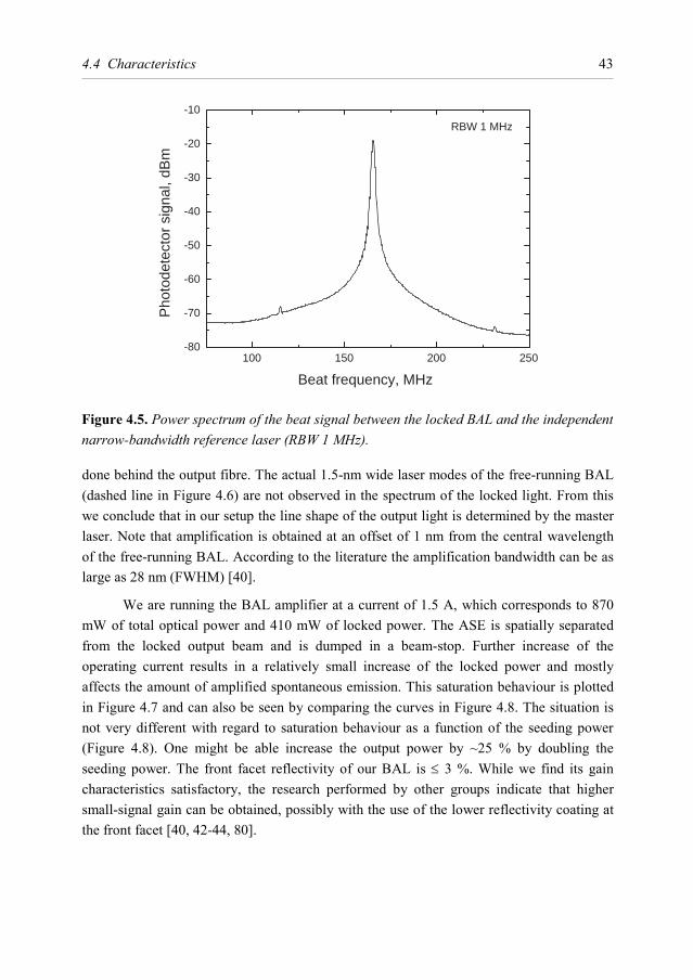
4.4 Characteristics
43
done behind the output fibre. The actual 1.5-nm wide laser modes of the free-running BAL (dashed line in Figure 4.6) are not observed in the spectrum of the locked light. From this we conclude that in our setup the line shape of the output light is determined by the master laser. Note that amplification is obtained at an offset of 1 nm from the central wavelength of the free-running BAL. According to the literature the amplification bandwidth can be as large as 28 nm (FWHM) [40].
We are running the BAL amplifier at a current of 1.5 A, which corresponds to 870 mW of total optical power and 410 mW of locked power. The ASE is spatially separated from the locked output beam and is dumped in a beam-stop. Further increase of the operating current results in a relatively small increase of the locked power and mostly affects the amount of amplified spontaneous emission. This saturation behaviour is plotted in Figure 4.7 and can also be seen by comparing the curves in Figure 4.8. The situation is not very different with regard to saturation behaviour as a function of the seeding power (Figure 4.8). One might be able increase the output power by ~25 % by doubling the seeding power. The front facet reflectivity of our BAL is ≤ 3 %. While we find its gain characteristics satisfactory, the research performed by other groups indicate that higher small-signal gain can be obtained, possibly with the use of the lower reflectivity coating at the front facet [40, 42-44, 80].
100 150 200 250-80
-70
-60
-50
-40
-30
-20
-10
RBW 1 MHz
Pho
tode
tect
or s
igna
l, dB
m
Beat frequency, MHz
Figure 4.5. Power spectrum of the beat signal between the locked BAL and the independent narrow-bandwidth reference laser (RBW 1 MHz).
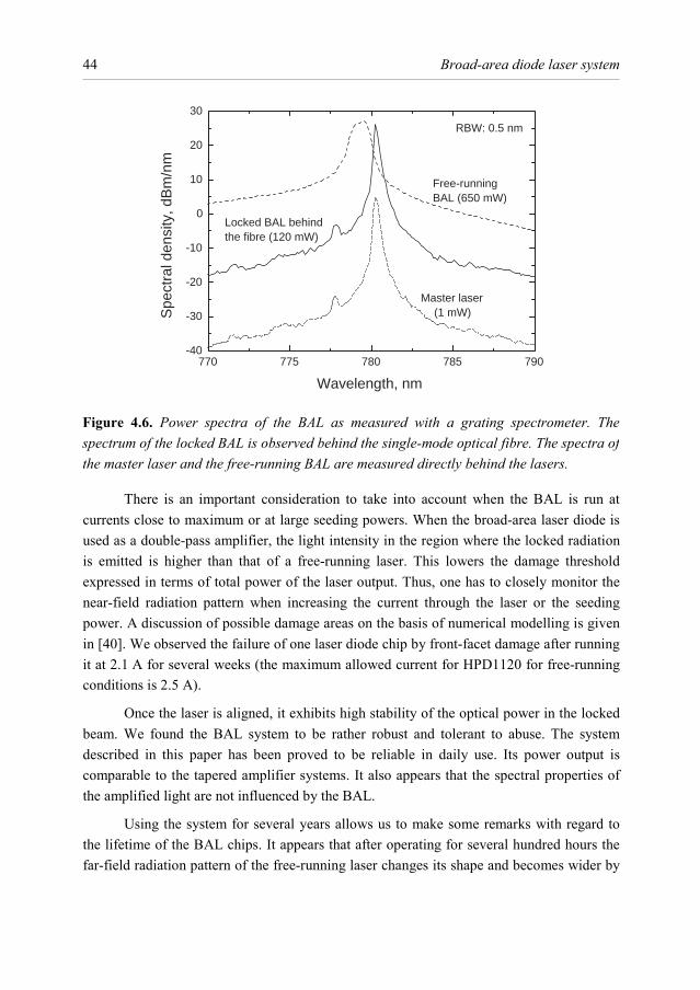
Broad-area diode laser system
44
There is an important consideration to take into account when the BAL is run at currents close to maximum or at large seeding powers. When the broad-area laser diode is used as a double-pass amplifier, the light intensity in the region where the locked radiation is emitted is higher than that of a free-running laser. This lowers the damage threshold expressed in terms of total power of the laser output. Thus, one has to closely monitor the near-field radiation pattern when increasing the current through the laser or the seeding power. A discussion of possible damage areas on the basis of numerical modelling is given in [40]. We observed the failure of one laser diode chip by front-facet damage after running it at 2.1 A for several weeks (the maximum allowed current for HPD1120 for free-running conditions is 2.5 A).
Once the laser is aligned, it exhibits high stability of the optical power in the locked beam. We found the BAL system to be rather robust and tolerant to abuse. The system described in this paper has been proved to be reliable in daily use. Its power output is comparable to the tapered amplifier systems. It also appears that the spectral properties of the amplified light are not influenced by the BAL.
Using the system for several years allows us to make some remarks with regard to the lifetime of the BAL chips. It appears that after operating for several hundred hours the far-field radiation pattern of the free-running laser changes its shape and becomes wider by
770 775 780 785 790-40
-30
-20
-10
0
10
20
30
RBW: 0.5 nm
Free-running BAL (650 mW)
Master laser(1 mW)
Locked BAL behind the fibre (120 mW)
Spe
ctra
l den
sity
, dB
m/n
m
Wavelength, nm
Figure 4.6. Power spectra of the BAL as measured with a grating spectrometer. The spectrum of the locked BAL is observed behind the single-mode optical fibre. The spectra of the master laser and the free-running BAL are measured directly behind the lasers.
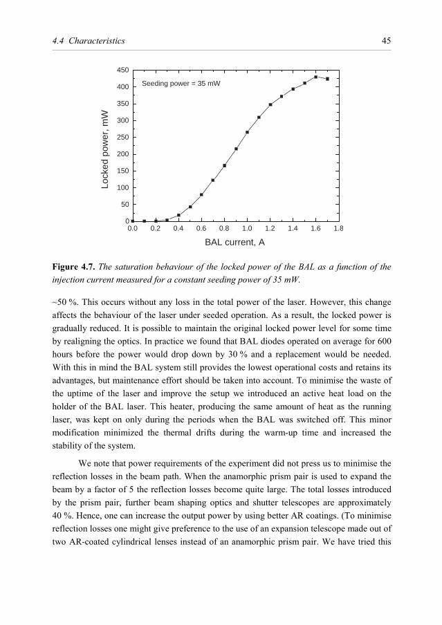
4.4 Characteristics
45
~50 %. This occurs without any loss in the total power of the laser. However, this change affects the behaviour of the laser under seeded operation. As a result, the locked power is gradually reduced. It is possible to maintain the original locked power level for some time by realigning the optics. In practice we found that BAL diodes operated on average for 600 hours before the power would drop down by 30 % and a replacement would be needed. With this in mind the BAL system still provides the lowest operational costs and retains its advantages, but maintenance effort should be taken into account. To minimise the waste of the uptime of the laser and improve the setup we introduced an active heat load on the holder of the BAL laser. This heater, producing the same amount of heat as the running laser, was kept on only during the periods when the BAL was switched off. This minor modification minimized the thermal drifts during the warm-up time and increased the stability of the system.
We note that power requirements of the experiment did not press us to minimise the reflection losses in the beam path. When the anamorphic prism pair is used to expand the beam by a factor of 5 the reflection losses become quite large. The total losses introduced by the prism pair, further beam shaping optics and shutter telescopes are approximately 40 %. Hence, one can increase the output power by using better AR coatings. (To minimise reflection losses one might give preference to the use of an expansion telescope made out of two AR-coated cylindrical lenses instead of an anamorphic prism pair. We have tried this
0.0 0.2 0.4 0.6 0.8 1.0 1.2 1.4 1.6 1.80
50
100
150
200
250
300
350
400
450
Seeding power = 35 mW
Lock
ed p
ower
, mW
BAL current, A
Figure 4.7. The saturation behaviour of the locked power of the BAL as a function of the injection current measured for a constant seeding power of 35 mW.
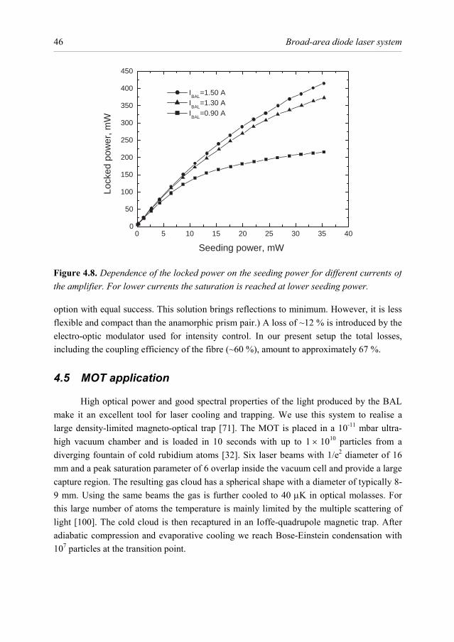
Broad-area diode laser system
46
option with equal success. This solution brings reflections to minimum. However, it is less flexible and compact than the anamorphic prism pair.) A loss of ~12 % is introduced by the electro-optic modulator used for intensity control. In our present setup the total losses, including the coupling efficiency of the fibre (~60 %), amount to approximately 67 %.
4.5 MOT application
High optical power and good spectral properties of the light produced by the BAL make it an excellent tool for laser cooling and trapping. We use this system to realise a large density-limited magneto-optical trap [71]. The MOT is placed in a 10-11 mbar ultra-high vacuum chamber and is loaded in 10 seconds with up to 1 × 10¹⁰ particles from a diverging fountain of cold rubidium atoms [32]. Six laser beams with 1/e2 diameter of 16 mm and a peak saturation parameter of 6 overlap inside the vacuum cell and provide a large capture region. The resulting gas cloud has a spherical shape with a diameter of typically 8-9 mm. Using the same beams the gas is further cooled to 40 µK in optical molasses. For this large number of atoms the temperature is mainly limited by the multiple scattering of light [100]. The cold cloud is then recaptured in an Ioffe-quadrupole magnetic trap. After adiabatic compression and evaporative cooling we reach Bose-Einstein condensation with 107 particles at the transition point.
0 5 10 15 20 25 30 35 400
50
100
150
200
250
300
350
400
450
Lock
ed p
ower
, mW
IBAL
=1.50 A I
BAL=1.30 A
IBAL
=0.90 A
Seeding power, mW
Figure 4.8. Dependence of the locked power on the seeding power for different currents of the amplifier. For lower currents the saturation is reached at lower seeding power.
4.6 Summary
47
The BAL-system is further used for (near-) resonant absorption imaging of atomic clouds to determine temperature, density and the number of atoms. For this application high optical power is not an issue. The detection beam is easily derived from the second output port of the EOM (see Figure 4.1) and coupled into an additional single-mode fibre. As the spectral properties of the locked output of the BAL do not differ noticeably from those of the master laser, the use of the BAL does not result in loss of accuracy in imaging measurements. The detection light conveniently becomes available whenever the main MOT beams are switched off. Thus, this solution eliminates the need for an additional detection laser.
4.6 Summary
We have developed a robust diode-laser based laser system producing 160 mW of narrow-linewidth light in a clean Gaussian mode. The spectral properties of the system are limited by those of the master laser which makes it suited for spectroscopic applications. The performance characteristics make it a good choice for laser cooling experiments, allowing at the same time to avoid drawbacks connected to alternative solutions like a tapered waveguide diode amplifier or a Ti-Sapphire laser. The laser system was successfully used for running a large MOT, sub-Doppler laser cooling and has been applied to absorption imaging of cold atomic clouds stored in magnetic traps.
Acknowledgements. We gratefully acknowledge help of K.A.H. van Leeuwen and A.C. Fey-den Boer, as well as very useful discussions with R. Spreeuw and D. Voigt. We thank L. Hillis of HPDI for his help at the different stages of this project. We also thank M. v.d. Mark and A. Valster of Philips Research for their assistance at the beginning of the project.

Chapter 5 Hydrodynamic properties of dense atomic clouds
5.1 Introduction
This chapter deals with dense ultracold clouds just above the Bose-Einstein condensation temperature (TC). These clouds represent the starting conditions for the experiments described in Chapter 6. However, they are of interest in their own right. Collective excitations of gases near and below the TC point were studied by many research groups [27, 41, 46, 47, 56, 69, 94]. The dynamical behaviour of a Bose-Einstein condensate can be described by hydrodynamic equations [27, 96]. Above TC the dynamical behaviour depends strongly on the mean free path. When the mean free path is large compared to the size of the cloud, we have free molecular flow (collisionless regime) where the motion of the individual atoms can be described by a single-particle Hamiltonian. Reducing the mean free path to a value smaller then the dimension of the cloud we obtain a crossover to viscous flow (hydrodynamic regime). Both the collisionless and the hydrodynamic regime were studied theoretically (see e.g. [46, 47, 60] and references therein).
From the experimental point of view it is important to understand the crossover to hydrodynamic behaviour in thermal clouds. This understanding is vital for the correct interpretation of time-of-flight absorption images of dense atomic clouds. In the collisionless regime the expansion of the gas, after release from a trap, is known to be isotropic, whereas in the hydrodynamic limit the gas expands anisotropically. As pointed out by Kagan et al. [60], little difference is to be expected between the aspect ratio of a fully expanded condensate and that of a hydrodynamic thermal cloud.
Previously the crossover regime was probed in experiments at MIT with a dense gas of sodium atoms [94] and at ENS using cold metastable triplet helium [69]. Our experiments have been done with thermal clouds of the 87Rb quantum gas in the |5S1/2, F = 2, mF = 2⟩ state. In the previous experiments the samples were investigated by measuring the density as well as the frequency and damping of collective excitations. In addition to this we also investigated the anisotropic expansion behaviour of the gas.
Hydrodynamic properties of dense atomic clouds
50
5.2 Density and temperature analysis
For our experiments with dense thermal clouds we load a magneto-optical trap with approximately 1010 atoms from the source described in Chapter 3. After optical pumping to the |5S1/2, F = 2, mF = 2⟩ state typically 4 × 10⁹ atoms are captured in the Ioffe-Pritchard quadrupole magnetic trap described in Section 3.5. Then the gas is compressed and evaporatively cooled to a temperature just above TC. The RF evaporation is forced at a final rate of 433trv = − kHz/s down to a value νtr,a = 740 kHz. As
, 0
trz
tr a
νω
ν ν−, (5.1)
the evaporation proceeds quasi-statically and yields a sample characterised by a single uniform temperature and an equilibrium shape. In Equation (5.1) the radio frequency ν0 = 620 kHz corresponds to a trap minimum B0 = 88.6(1) µT as described in Section 3.6. The preparation procedure is completed by 20 ms of plain evaporation at νtr = νtr,a. This leaves us with Ni ≈ 5 × 10⁶ atoms at a temperature T0 = 1.3(1) µK in a magnetic trap characterised by the frequencies ωρ = 2π × 477(2) Hz and ωz = 2π × 20.8(1) Hz (given for the absence of RF dressing).
From the temperature T0 we can calculate the density of the gas in the trap just before the expansion because both the trap frequencies and the number of atoms are known. Taking into account the RF truncation [74] we calculate n0 ≈ 4 × 1014 cm-3, which corresponds to a mean free path
00
1 3µm2n
λσ
= ≈ , (5.2)
where 28 aσ π= is the elastic scattering cross-section. The collision rate is
1 -10 5000 scol thnτ υ σ− ≈ ≈ , (5.3)
with 1/ 20[8 ]th Bk T mυ π= the thermal velocity.
Calculating the ratio of the axial size of the cloud to the mean free path, we find
0 50zl λ ≈ . Hence in the axial direction we are deeply into the hydrodynamic regime. For the radial direction we find 0 2lρ λ ≈ . Here we operate in the middle of the crossover between collisionless and hydrodynamic regime. A comparison with some other experiments [56, 69, 77, 78] on excitations and condensate formation is given in Figure 5.1.
In the crossover from collisionless to hydrodynamic behaviour the temperature determination is non-trivial. Unlike in a free expansion, as occurs in the collisionless
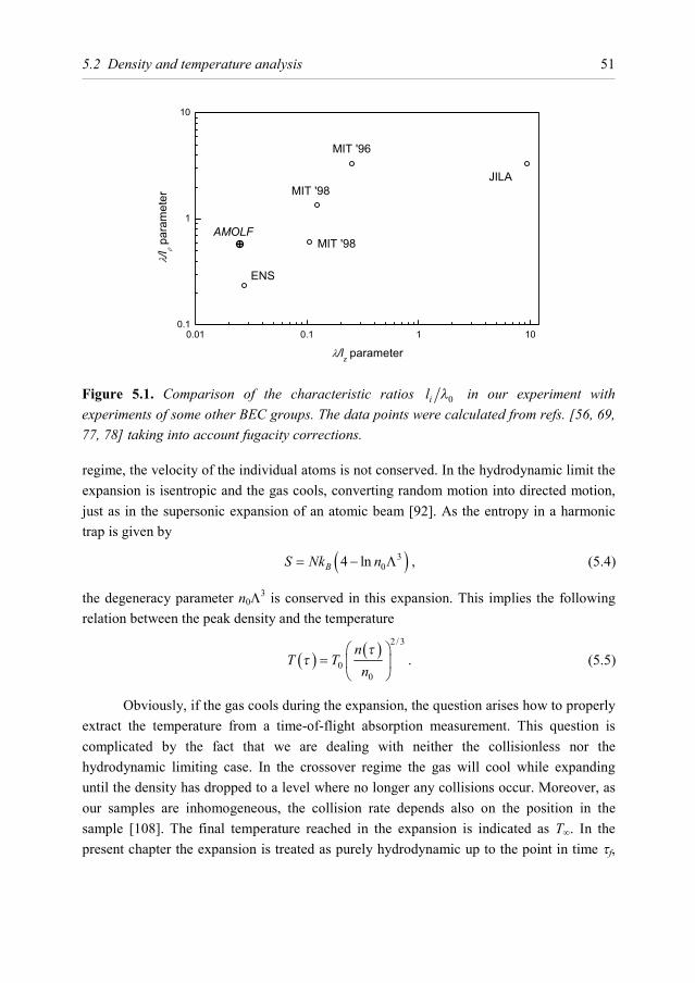
5.2 Density and temperature analysis
51
regime, the velocity of the individual atoms is not conserved. In the hydrodynamic limit the expansion is isentropic and the gas cools, converting random motion into directed motion, just as in the supersonic expansion of an atomic beam [92]. As the entropy in a harmonic trap is given by
( )304 lnBS Nk n= − Λ , (5.4)
the degeneracy parameter n0Λ3 is conserved in this expansion. This implies the following
relation between the peak density and the temperature
( ) ( ) 2 / 3
00
nT T
nτ
τ
=
. (5.5)
Obviously, if the gas cools during the expansion, the question arises how to properly extract the temperature from a time-of-flight absorption measurement. This question is complicated by the fact that we are dealing with neither the collisionless nor the hydrodynamic limiting case. In the crossover regime the gas will cool while expanding until the density has dropped to a level where no longer any collisions occur. Moreover, as our samples are inhomogeneous, the collision rate depends also on the position in the sample [108]. The final temperature reached in the expansion is indicated as T∞. In the present chapter the expansion is treated as purely hydrodynamic up to the point in time τf,
Figure 5.1. Comparison of the characteristic ratios 0il λ in our experiment with experiments of some other BEC groups. The data points were calculated from refs. [56, 69, 77, 78] taking into account fugacity corrections.
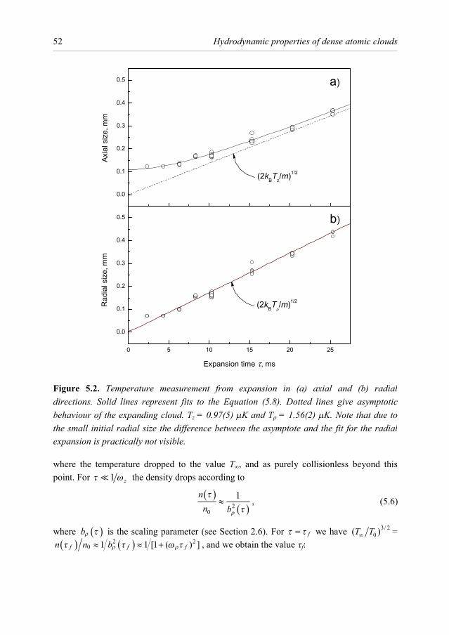
Hydrodynamic properties of dense atomic clouds
52
where the temperature dropped to the value T∞, and as purely collisionless beyond this point. For 1 zτ ω the density drops according to
( )
( )20
1nn bρ
τ
τ≈ , (5.6)
where ( )bρ τ is the scaling parameter (see Section 2.6). For fτ τ= we have 3/ 20( )T T∞ =
( ) ( )2 20 1 1 [1 ( ) ]f f fn n bρ ρτ τ ω τ≈ ≈ + , and we obtain the value τf:
Figure 5.2. Temperature measurement from expansion in (a) axial and (b) radial directions. Solid lines represent fits to the Equation (5.8). Dotted lines give asymptotic behaviour of the expanding cloud. Tz = 0.97(5) µK and Tρ = 1.56(2) µK. Note that due to the small initial radial size the difference between the asymptote and the fit for the radial expansion is practically not visible.
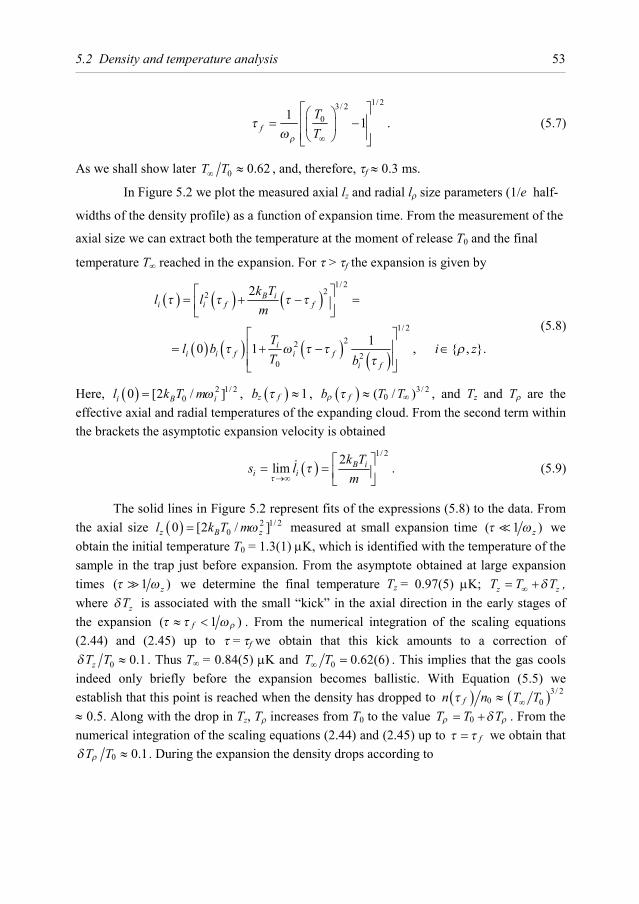
5.2 Density and temperature analysis
53
1/ 23/ 201 1f
TTρ
τω ∞
= −
. (5.7)
As we shall show later 0 0.62T T∞ ≈ , and, therefore, τf ≈ 0.3 ms.
In Figure 5.2 we plot the measured axial lz and radial lρ size parameters (1/e half-
widths of the density profile) as a function of expansion time. From the measurement of the
axial size we can extract both the temperature at the moment of release T0 and the final
temperature T∞ reached in the expansion. For τ > τf the expansion is given by
( ) ( ) ( )
( ) ( ) ( ) ( )
1/ 222
1/ 222
20
2
10 1 , , .
B ii i f f
ii i f i f
i f
k Tl l
m
Tl b i z
T b
τ τ τ τ
τ ω τ τ ρτ
= + − =
= + − ∈
(5.8)
Here, ( ) 2 1/ 200 [2 / ]i B il k T mω= , ( ) 1z fb τ ≈ , ( ) 3/ 2
0( / )fb T Tρ τ ∞≈ , and Tz and Tρ are the effective axial and radial temperatures of the expanding cloud. From the second term within the brackets the asymptotic expansion velocity is obtained
( )1/ 22
lim B ii i
k Ts l
mττ
→∞
= = . (5.9)
The solid lines in Figure 5.2 represent fits of the expressions (5.8) to the data. From the axial size ( ) 2 1/ 2
00 [2 / ]z B zl k T mω= measured at small expansion time ( 1 )zτ ω we obtain the initial temperature T0 = 1.3(1) µK, which is identified with the temperature of the sample in the trap just before expansion. From the asymptote obtained at large expansion times ( 1 )zτ ω we determine the final temperature Tz = 0.97(5) µK; z zT T Tδ∞= + , where zTδ is associated with the small “kick” in the axial direction in the early stages of the expansion ( 1 )f ρτ τ ω≈ < . From the numerical integration of the scaling equations (2.44) and (2.45) up to τ = τf we obtain that this kick amounts to a correction of
0 0.1zT Tδ ≈ . Thus T∞ = 0.84(5) µK and 0 0.62(6)T T∞ = . This implies that the gas cools indeed only briefly before the expansion becomes ballistic. With Equation (5.5) we establish that this point is reached when the density has dropped to ( ) 0fn nτ ≈ ( )3/ 2
0T T∞ ≈ 0.5. Along with the drop in Tz, Tρ increases from T0 to the value 0T T Tρ ρδ= + . From the numerical integration of the scaling equations (2.44) and (2.45) up to fτ τ= we obtain that
0 0.1T Tρδ ≈ . During the expansion the density drops according to
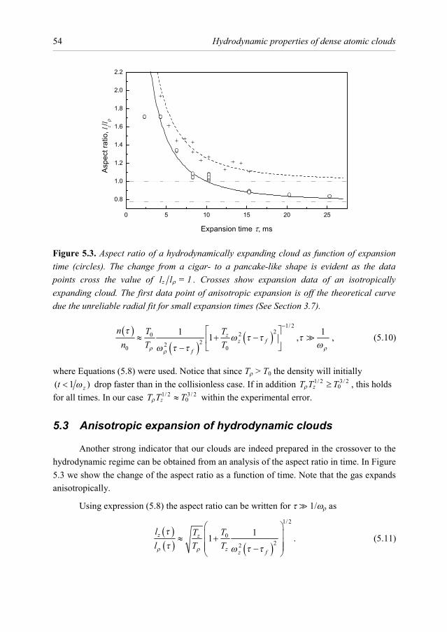
Hydrodynamic properties of dense atomic clouds
54
( )
( )( )
1/ 2220
220 0
1 11 ,zz f
f
n T Tn T Tρ ρρ
τω τ τ τ
ωω τ τ
−
≈ + − −
, (5.10)
where Equations (5.8) were used. Notice that since Tρ > T0 the density will initially ( 1 )zt ω< drop faster than in the collisionless case. If in addition 1/ 2 3/ 2
0zT T Tρ ≥ , this holds for all times. In our case 1/ 2 3/ 2
0zT T Tρ ≈ within the experimental error.
5.3 Anisotropic expansion of hydrodynamic clouds
Another strong indicator that our clouds are indeed prepared in the crossover to the hydrodynamic regime can be obtained from an analysis of the aspect ratio in time. In Figure 5.3 we show the change of the aspect ratio as a function of time. Note that the gas expands anisotropically.
Using expression (5.8) the aspect ratio can be written for τ 1/ωρ as
( )( ) ( )
1/ 2
022
11z z
z z f
l TTl T Tρ ρ
ττ ω τ τ
≈ + −
. (5.11)
Figure 5.3. Aspect ratio of a hydrodynamically expanding cloud as function of expansion time (circles). The change from a cigar- to a pancake-like shape is evident as the data points cross the value of zl l = 1ρ . Crosses show expansion data of an isotropically expanding cloud. The first data point of anisotropic expansion is off the theoretical curve due the unreliable radial fit for small expansion times (See Section 3.7).
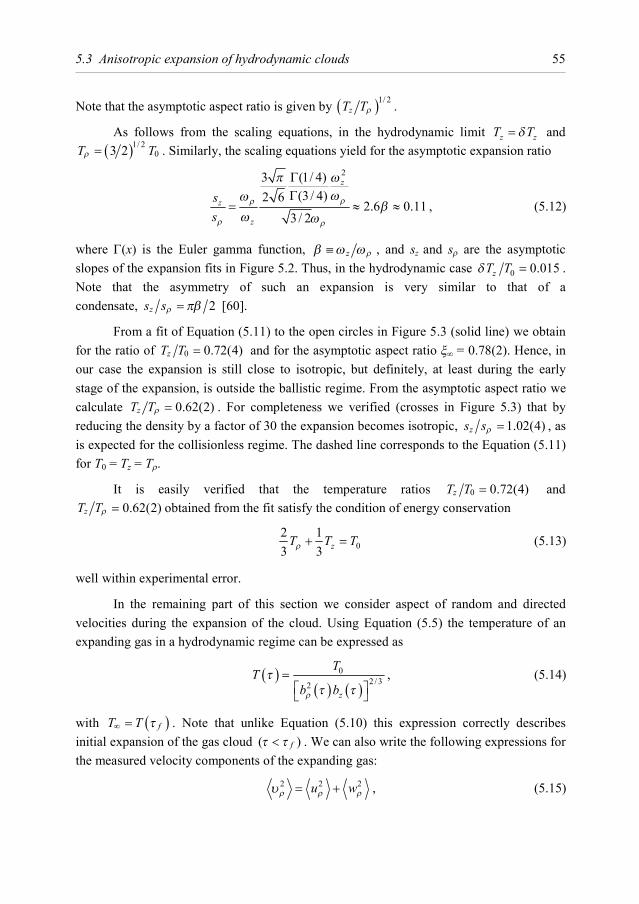
5.3 Anisotropic expansion of hydrodynamic clouds
55
Note that the asymptotic aspect ratio is given by ( )1/ 2zT Tρ .
As follows from the scaling equations, in the hydrodynamic limit z zT Tδ= and ( )1/ 2
03 2T Tρ = . Similarly, the scaling equations yield for the asymptotic expansion ratio
23 (1/ 4)(3 / 4)2 6
2.6 0.113 / 2
z
z
z
ss
ρρ
ρ ρ
π ωωω
βω ω
ΓΓ
= ≈ ≈ , (5.12)
where Γ(x) is the Euler gamma function, z ρβ ω ω≡ , and sz and sρ are the asymptotic slopes of the expansion fits in Figure 5.2. Thus, in the hydrodynamic case 0 0.015zT Tδ = . Note that the asymmetry of such an expansion is very similar to that of a condensate, 2zs sρ πβ= [60].
From a fit of Equation (5.11) to the open circles in Figure 5.3 (solid line) we obtain for the ratio of 0 0.72(4)zT T = and for the asymptotic aspect ratio ξ∞ = 0.78(2). Hence, in our case the expansion is still close to isotropic, but definitely, at least during the early stage of the expansion, is outside the ballistic regime. From the asymptotic aspect ratio we calculate 0.62(2)zT Tρ = . For completeness we verified (crosses in Figure 5.3) that by reducing the density by a factor of 30 the expansion becomes isotropic, 1.02(4)zs sρ = , as is expected for the collisionless regime. The dashed line corresponds to the Equation (5.11) for T0 = Tz = Tρ.
It is easily verified that the temperature ratios 0 0.72(4)zT T = and 0.62(2)zT Tρ = obtained from the fit satisfy the condition of energy conservation
02 13 3 zT T Tρ + = (5.13)
well within experimental error.
In the remaining part of this section we consider aspect of random and directed velocities during the expansion of the cloud. Using Equation (5.5) the temperature of an expanding gas in a hydrodynamic regime can be expressed as
( )( ) ( )
02 / 32
z
TT
b bρ
ττ τ
=
, (5.14)
with ( )fT T τ∞ = . Note that unlike Equation (5.10) this expression correctly describes initial expansion of the gas cloud ( )fτ τ< . We can also write the following expressions for the measured velocity components of the expanding gas:
2 2 2u wρ ρ ρυ = + , (5.15)
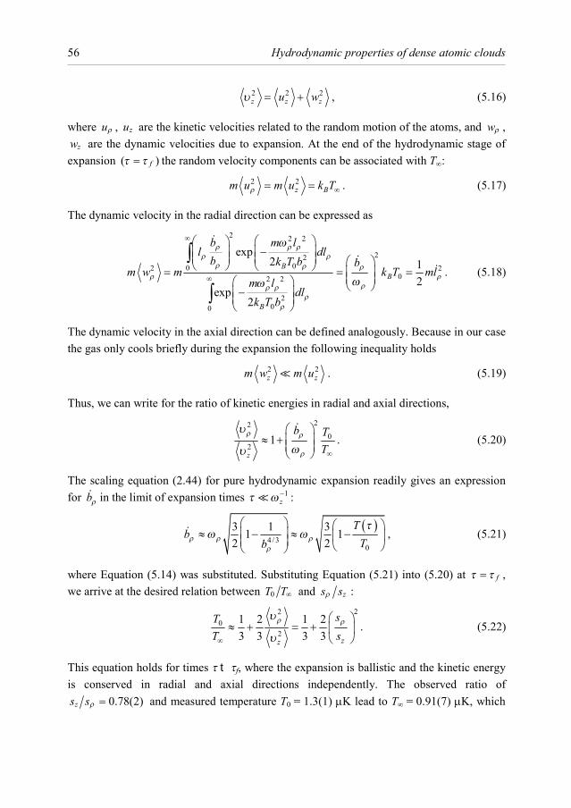
Hydrodynamic properties of dense atomic clouds
56
2 2 2z z zu wυ = + , (5.16)
where uρ , zu are the kinetic velocities related to the random motion of the atoms, and wρ , zw are the dynamic velocities due to expansion. At the end of the hydrodynamic stage of
expansion ( )fτ τ= the random velocity components can be associated with T∞:
2 2z Bm u m u k Tρ ∞= = . (5.17)
The dynamic velocity in the radial direction can be expressed as
2 2 2
22002 2
02 2
200
exp2 1
2exp
2
BB
B
b m ll dl
b k T b bm w m k T ml
m ldl
k T b
ρ ρ ρρ ρ
ρ ρ ρρ ρ
ρρ ρρ
ρ
ω
ωω
∞
∞
− = = = −
∫
∫. (5.18)
The dynamic velocity in the axial direction can be defined analogously. Because in our case the gas only cools briefly during the expansion the following inequality holds
2 2z zm w m u . (5.19)
Thus, we can write for the ratio of kinetic energies in radial and axial directions,
22
02
1z
b TT
ρ ρ
ρ
υ
ωυ ∞
≈ +
. (5.20)
The scaling equation (2.44) for pure hydrodynamic expansion readily gives an expression for bρ in the limit of expansion times 1
zτ ω− :
( )
4 / 30
3 1 31 12 2
Tb
Tbρ ρ ρρ
τω ω
≈ − ≈ −
, (5.21)
where Equation (5.14) was substituted. Substituting Equation (5.21) into (5.20) at fτ τ= , we arrive at the desired relation between 0T T∞ and zs sρ :
22
02
1 2 1 23 3 3 3 zz
sTT s
ρ ρυ
υ∞
≈ + = +
. (5.22)
This equation holds for times τ t τf, where the expansion is ballistic and the kinetic energy is conserved in radial and axial directions independently. The observed ratio of
0.78(2)zs sρ = and measured temperature T0 = 1.3(1) µK lead to T∞ = 0.91(7) µK, which
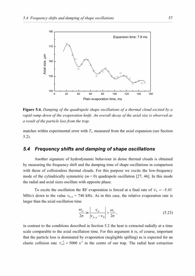
5.4 Frequency shifts and damping of shape oscillations
57
matches within experimental error with T∞ measured from the axial expansion (see Section 5.2).
5.4 Frequency shifts and damping of shape oscillations
Another signature of hydrodynamic behaviour in dense thermal clouds is obtained by measuring the frequency shift and the damping time of shape oscillations in comparison with those of collisionless thermal clouds. For this purpose we excite the low-frequency mode of the cylindrically symmetric (m = 0) quadrupole oscillation [27, 46]. In this mode the radial and axial sizes oscillate with opposite phase.
To excite the oscillation the RF evaporation is forced at a final rate of 5.43trν = − MHz/s down to the value νtr,a = 740 kHz. As in this case, the relative evaporation rate is larger than the axial oscillation time
, 02 2
tr z
tr a
ρω ν ωπ ν ν π
>−
, (5.23)
in contrast to the conditions described in Section 5.2 the heat is extracted radially at a time scale comparable to the axial oscillation time. For this argument it is, of course, important that the particle loss is dominated by evaporation (negligible spilling) as is expected for an elastic collision rate 1 5000colτ − = s-1 in the centre of our trap. The radial heat extraction
Figure 5.4. Damping of the quadrupole shape oscillations of a thermal cloud excited by a rapid ramp down of the evaporation knife. An overall decay of the axial size is observed as a result of the particle loss from the trap.
Hydrodynamic properties of dense atomic clouds
58
results in development of a temperature gradient along the axis of the cloud, which in turn means that the axial size of the sample lags behind the size defined by the temperature. This leads to the inward motion of the cloud in the axial direction and excitation of quadrupole oscillations. These oscillations are shown in Figure 5.4. The evaporation barrier is left at the final value of νtr,a = 740 kHz for the duration of a plain evaporation period and acts as a heat shield for the cold cloud.
The axial size of the cloud in Figure 5.4 is observed 7.8 ms after release from the trap as a function of plain evaporation time. Decay of 20 % in axial size was observed over a period of 130 ms. This is related to the particle losses from the trap. The data points are fitted with a simple model of an exponentially decaying harmonic oscillation. The measured ratio of the quadrupole frequency to the frequency of the trap is
1.56(5)Q zω ω = . The measurement of the damping rate of the oscillations τQ-1 gives
(ωzτQ)-1 = 0.10(3). Calculations of the dispersion law in ref. [47] give
2 2
2 2
1HD CL
CL iω ω
ω ωωτ
−= +
+, (5.24)
where for the cylindrically symmetric cigar-shape trap the frequency of the hydrodynamic mode ωHD = (12/5)1/2ωz [60], and the frequency of the collisionless mode ωCL = 2ωz.
Figure 5.5. Plot of relative damping rate versus frequency for the m=0 quadrupole mode. The solid line represents theoretical prediction of Equation (5.25). With the relative damping rate of 0.1 we are deeply in crossover to the hydrodynamic regime. Experimental data points of MIT and ENS experiments are taken from references [94] and [69] respectively.
5.4 Frequency shifts and damping of shape oscillations
59
Relaxation time τ for this case is equal to 3τcol [47]. Writing complex oscillation frequency as ω = ωQ + iτQ
-1 we obtain from Equation (5.24) the dependence of the damping rate τQ
-1 on the oscillation frequency ωQ:
1/ 21/ 22 2
2 21 8 4 11 15
5 5Q Q
z Q z z
ω ω
ω τ ω ω
= − − + − +
. (5.25)
For (ωzτQ)-1 = 0.10(3) this expression predicts 1.57(2)Q zω ω = , which is in excellent agreement with the measured value. The summary of data produced in our experiments as well as the experiments at ENS with metastable helium [69] and at MIT with sodium [94] is presented in Figure 5.5.
In conclusion, we presented the results of the experiments with hydrodynamic thermal clouds that go into the hydrodynamic regime further than any other reported experiment on collective excitations of the thermal samples. The hydrodynamic behaviour was explored from three different sides: through the measurement of temperature and density, through anisotropic expansion of the samples released from the trap, and through the measurement of damping rate and frequency of the quadrupole excitation mode. All three methods produced results consistent with each other and showed a good agreement with the theoretical predictions.

Chapter 6 Condensation into non-equilibrium states and focusing of a condensate
6.1 Introduction
Equilibrium condensates [4, 28] are produced by quasi-static growth, where heat extraction limits the formation rate. The condensate nucleates as a small feature in the center of the trap and grows as long as heat is extracted from the sample. To observe the formation kinetics, the gas has to be brought out of equilibrium, in practice by shock cooling. Since the first experiment on condensate growth, by Miesner et al. [78], this is done by fast RF removal of the most energetic atoms from the trap. Starting from a thermal gas just above the phase transition temperature (TC), the condensate appears as the result of thermalization. Miesner et al. [78] observed the growth under adiabatic conditions. Köhl et al. [65] continued the extraction of heat and atoms, also during growth. In both experiments, the condensate was observed to grow from the center of the trap, like in the quasi-static limit.
Kagan et al. [57] pointed out that qualitatively different stages have to be distinguished in the formation of equilibrium condensates with a large number of atoms. The early stage (kinetic stage) is governed by Boltzmann kinetic processes and leads to a preferential occupation of the lowest energy levels. Once a substantial fraction of the atoms gathers within an energy band of the order of the chemical potential of the emerging condensate during formation, their density fluctuations are suppressed in a fast interaction-dominated regime governed by a non-linear equation for the boson field. The appearing phase-fluctuating condensate then grows and the condensed fraction approaches its equilibrium value. However, the phase fluctuations still persist, giving rise to dynamically evolving flow patterns in search for the true equilibrium state. In elongated 3D trapped gases the phase fluctuations can be pronounced even under equilibrium conditions as was predicted by Petrov et al. [82] and observed experimentally by Dettmer et al. [31].
In this chapter we describe the formation of condensates into non-equilibrium states and a new path towards equilibrium in elongated traps. In contrast to the previous experiments our results were obtained starting from thermal clouds deep in the cross-over regime to hydrodynamic behaviour. The condensates are much longer than equilibrium
Condensation into non-equilibrium states and focusing of a condensate
62
condensates with the same number of atoms. Moreover, they display strong phase fluctuations and a dynamical evolution similar to that of a quadrupole shape oscillation decaying towards equilibrium. We identify 1 zω as a characteristic time that should be addressed explicitly for elongated cylindrical harmonic traps, i.e. for traps with ωρ ωz where ωρ and ωz are the radial and axial angular frequencies, respectively. We show that these exotic condensates emerge as the result of local thermalization when the nucleation time is short as compared to 1 zω . The dynamical evolution of the condensate in the trap has to be dealt with explicitly to properly interpret time-of-flight absorption images. In this context we introduce condensate focusing as an alternative to Bragg scattering [95] for measuring the phase-coherence length of phase-fluctuating Bose-Einstein condensates.
In the previous experiments on condensate formation the phase fluctuations were not studied. The results of Miesner et al. [78] were compared to an analytical expression for adiabatic growth of a condensate from a thermal cloud, derived by Gardiner et al. [38]. Although a qualitative agreement between theory and experiment was readily obtained it turned out to be impossible to obtain detailed agreement at the quantitative level [11, 29, 39, 70]. In the experiment of Köhl et al. [65] quantitative agreement with the quantum kinetic approach (see refs. [11, 29, 38, 39, 70] was obtained for strong truncation, whereas for weak truncation the observed behavior differed distinctly from theory.
6.2 Preparation of degenerate samples out of equilibrium
Evaporative cooling and preparation of cold near-Tc samples was previously described in detail in Section 5.2. The starting conditions of experiments on condensate formation are represented by a static, purely thermal cloud of Ni ≈ 5 × 10⁶ atoms at a temperature T0 = 1.3(1) µK. This cloud is placed in a magnetic trap characterised by the frequencies ωρ = 2π × 477(2) Hz and ωz = 2π × 20.8(1) Hz (given in the absence of RF dressing).
As discussed in Chapter 5 these samples are prepared far deeper in the cross-over to the hydrodynamic regime, as compared to the previous experiments [78] and [65].
Once the thermal cloud is prepared we distinguish three distinct stages (see Figure 6.1). First, in the truncation stage, the radio frequency is set to the value νtr,b = 660 kHz. This stage has a duration ttr = 1 ms, which is chosen to be long enough ( 1 )trt ρω> to allow atoms with radial energy ερ larger than the RF truncation energy εtr to escape from the trap, yet is short enough to disallow evaporative cooling. We found that in this stage 50% of the atoms are removed. Notice that due to the finite radial escape horizon 0( 0.4)lρλ ≈ the ejection is not expected to be complete. Furthermore, the escape efficiency is anisotropic as
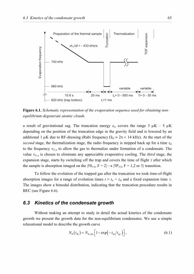
6.3 Kinetics of the condensate growth
63
a result of gravitational sag. The truncation energy εtr covers the range 3 µK – 5 µK depending on the position of the truncation edge in the gravity field and is lowered by an additional 1 µK due to RF-dressing (Rabi frequency Ωrf ≈ 2π × 14 kHz). At the start of the second stage, the thermalization stage, the radio frequency is stepped back up for a time tth to the frequency νtr,a to allow the gas to thermalize under formation of a condensate. The value νtr,a is chosen to eliminate any appreciable evaporative cooling. The third stage, the expansion stage, starts by switching off the trap and covers the time of flight τ after which the sample is absorption imaged on the |5S1/2, F = 2⟩ → |5P3/2, F = 1,2 or 3⟩ transition.
To follow the evolution of the trapped gas after the truncation we took time-of-flight absorption images for a range of evolution times t ≡ ttr + tth and a fixed expansion time τ. The images show a bimodal distribution, indicating that the truncation procedure results in BEC (see Figure 6.6).
6.3 Kinetics of the condensate growth
Without making an attempt to study in detail the actual kinetics of the condensate growth we present the growth data for the non-equilibrium condensates. We use a simple relaxational model to describe the growth curve
( ) ( )0 0, 1 expth fin th grN t N t t = − − , (6.1)
Figure 6.1. Schematic representation of the evaporation sequence used for obtaining non-equilibrium degenerate atomic clouds.
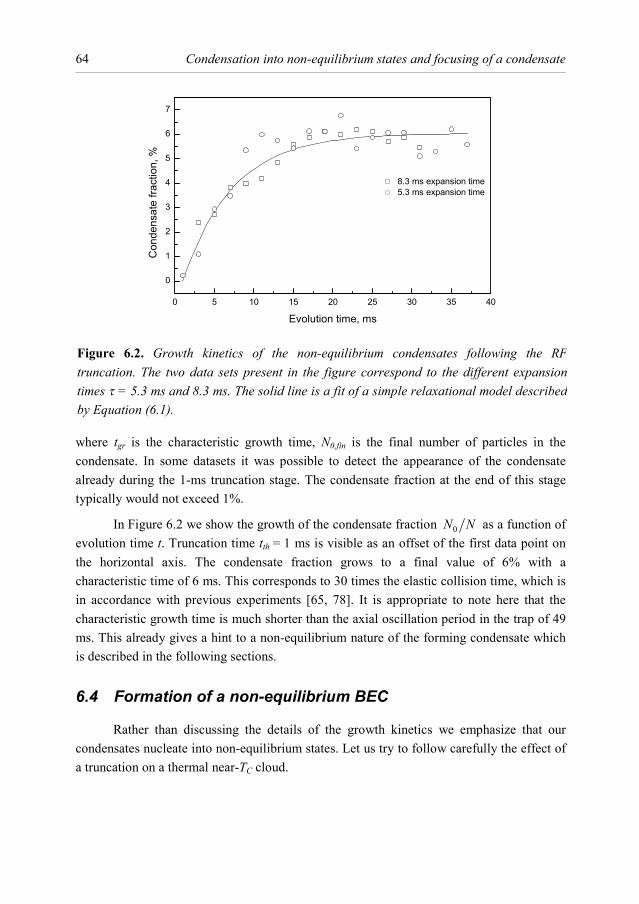
Condensation into non-equilibrium states and focusing of a condensate
64
where tgr is the characteristic growth time, N0,fin is the final number of particles in the condensate. In some datasets it was possible to detect the appearance of the condensate already during the 1-ms truncation stage. The condensate fraction at the end of this stage typically would not exceed 1%.
In Figure 6.2 we show the growth of the condensate fraction 0N N as a function of evolution time t. Truncation time tth = 1 ms is visible as an offset of the first data point on the horizontal axis. The condensate fraction grows to a final value of 6% with a characteristic time of 6 ms. This corresponds to 30 times the elastic collision time, which is in accordance with previous experiments [65, 78]. It is appropriate to note here that the characteristic growth time is much shorter than the axial oscillation period in the trap of 49 ms. This already gives a hint to a non-equilibrium nature of the forming condensate which is described in the following sections.
6.4 Formation of a non-equilibrium BEC
Rather than discussing the details of the growth kinetics we emphasize that our condensates nucleate into non-equilibrium states. Let us try to follow carefully the effect of a truncation on a thermal near-TC cloud.
Figure 6.2. Growth kinetics of the non-equilibrium condensates following the RF truncation. The two data sets present in the figure correspond to the different expansion times τ = 5.3 ms and 8.3 ms. The solid line is a fit of a simple relaxational model described by Equation (6.1).
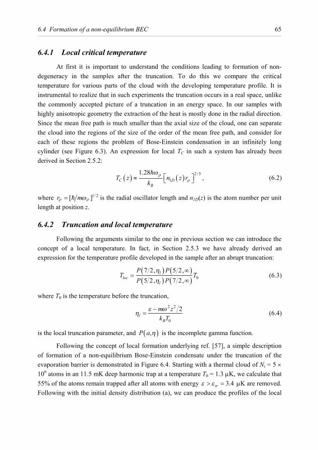
6.4 Formation of a non-equilibrium BEC
65
6.4.1 Local critical temperature
At first it is important to understand the conditions leading to formation of non-degeneracy in the samples after the truncation. To do this we compare the critical temperature for various parts of the cloud with the developing temperature profile. It is instrumental to realize that in such experiments the truncation occurs in a real space, unlike the commonly accepted picture of a truncation in an energy space. In our samples with highly anisotropic geometry the extraction of the heat is mostly done in the radial direction. Since the mean free path is much smaller than the axial size of the cloud, one can separate the cloud into the regions of the size of the order of the mean free path, and consider for each of these regions the problem of Bose-Einstein condensation in an infinitely long cylinder (see Figure 6.3). An expression for local TC in such a system has already been derived in Section 2.5.2:
( ) ( ) 2 / 51
1.28C D
BT z n z r
kρ
ρ
ω ≈ , (6.2)
where 1/ 2[ ]r mρ ρω= is the radial oscillator length and n1D(z) is the atom number per unit length at position z.
6.4.2 Truncation and local temperature
Following the arguments similar to the one in previous section we can introduce the concept of a local temperature. In fact, in Section 2.5.3 we have already derived an expression for the temperature profile developed in the sample after an abrupt truncation:
( ) ( )( ) ( ) 07 2, 5 2,5 2, 7 2,
lloc
l
P PT T
P Pηη
∞=
∞ (6.3)
where T0 is the temperature before the truncation,
2 2
0
2l
B
m zk T
ε ωη
−= (6.4)
is the local truncation parameter, and ( ),P a η is the incomplete gamma function.
Following the concept of local formation underlying ref. [57], a simple description of formation of a non-equilibrium Bose-Einstein condensate under the truncation of the evaporation barrier is demonstrated in Figure 6.4. Starting with a thermal cloud of Ni = 5 × 10⁶ atoms in an 11.5 mK deep harmonic trap at a temperature T0 = 1.3 µK, we calculate that 55% of the atoms remain trapped after all atoms with energy 3.4trε ε> = µK are removed. Following with the initial density distribution (a), we can produce the profiles of the local
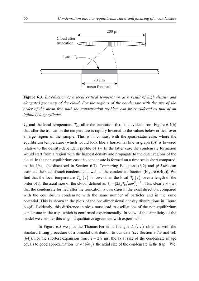
Condensation into non-equilibrium states and focusing of a condensate
66
TC and the local temperature Tloc after the truncation (b). It is evident from Figure 6.4(b) that after the truncation the temperature is rapidly lowered to the values below critical over a large region of the sample. This is in contrast with the quasi-static case, where the equilibrium temperature (which would look like a horizontal line in graph (b)) is lowered relative to the density-dependent profile of TC. In the latter case the condensate formation would start from a region with the highest density and propagate to the outer regions of the cloud. In the non-equilibrium case the condensate is formed on a time scale short compared to the 1 zω (as discussed in Section 6.3). Comparing Equations (6.2) and (6.3)we can estimate the size of such condensate as well as the condensate fraction (Figure 6.4(c)). We find that the local temperature ( )locT z is lower than the local ( )CT z over a length of the order of lz, the axial size of the cloud, defined as 2 1/ 2
0[2 ]z B zl k T mω= . This clearly shows that the condensate formed after the truncation is oversized in the axial direction, compared with the equilibrium condensate with the same number of particles and in the same potential. This is shown in the plots of the one-dimensional density distributions in Figure 6.4(d). Evidently, this difference in sizes must lead to oscillations of the non-equilibrium condensate in the trap, which is confirmed experimentally. In view of the simplicity of the model we consider this as good qualitative agreement with experiment.
In Figure 6.5 we plot the Thomas-Fermi half-length ( ),zL t τ obtained with the standard fitting procedure of a bimodal distribution to our data (see Section 3.7.3 and ref. [64]). For the shortest expansion time, τ = 2.8 ms, the axial size of the condensate image equals to good approximation ( 1 )zτ ω the axial size of the condensate in the trap. We
Figure 6.3. Introduction of a local critical temperature as a result of high density and elongated geometry of the cloud. For the regions of the condensate with the size of the order of the mean free path the condensation problem can be considered as that of an infinitely long cylinder.
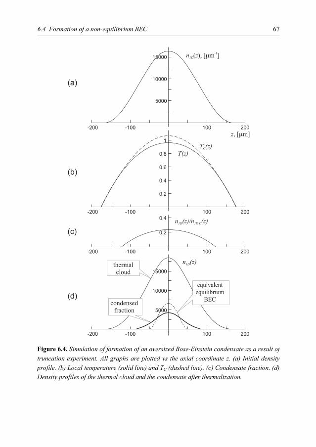
6.4 Formation of a non-equilibrium BEC
67
Figure 6.4. Simulation of formation of an oversized Bose-Einstein condensate as a result of truncation experiment. All graphs are plotted vs the axial coordinate z. (a) Initial density profile. (b) Local temperature (solid line) and TC (dashed line). (c) Condensate fraction. (d) Density profiles of the thermal cloud and the condensate after thermalization.
Condensation into non-equilibrium states and focusing of a condensate
68
see that ( )zL t is initially oversized by a factor ( ) ( )0 2.2(3)z zL L ∞ = and rapidly decreases to reach its equilibrium size after roughly one strongly damped shape oscillation (see open triangles Figure 6.5). Thus, the condensate is clearly not in equilibrium.
6.5 Oscillation modes
In Figure 6.5 we also show the oscillation in the axial size of the condensate as observed for 15.3 ms (open squares) and 25.3 ms (crosses) of expansion. Longer expansion times enhance the contrast of the data and the amplitude of the oscillation is increased as compared to the 2.8 ms results. For τ = 25.3 ms the shape oscillation is seen to exceed the noise for at least 100 ms. For evolution times t ≥ 20 ms this oscillation can be described by a linear response model which is discussed in detail in Section 6.7. We measure a damping time of τQ = 50(9) ms and a frequency ratio 1.54(4)Q zω ω = . The latter is slightly lower than the frequency expected for a quadrupole shape oscillation of a pure condensate in very elongated traps, ( )1/ 25 2 1.58Q zω ω ≈ ≈ [21, 60]. A 5% negative frequency shift was observed for the quadrupole mode in Na condensates just below TC [94] and is consistent
Figure 6.5. (b) Condensate length Lz(t, τ) versus evolution time t for three different expansion times τ. The dark grey line is a guide to the eye. The light grey line represents a fit to a damped quadrupole shape oscillation in the limit of a linear response model. Data set corresponding to 25.3 ms expansion time is also shown for the radial direction. (a) The oscillations of the radial size do not exceed the noise level.
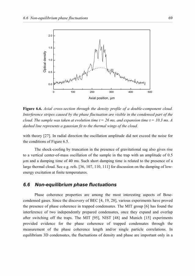
6.6 Non-equilibrium phase fluctuations
69
with theory [27]. In radial direction the oscillation amplitude did not exceed the noise for the conditions of Figure 6.5.
The shock-cooling by truncation in the presence of gravitational sag also gives rise to a vertical center-of-mass oscillation of the sample in the trap with an amplitude of 0.5 µm and a damping time of 40 ms. Such short damping time is related to the presence of a large thermal cloud. See e.g. refs. [36, 107, 110, 111] for discussion on the damping of low-energy excitation at finite temperatures.
6.6 Non-equilibrium phase fluctuations
Phase coherence properties are among the most interesting aspects of Bose-condensed gases. Since the discovery of BEC [4, 19, 28], various experiments have proved the presence of phase coherence in trapped condensates. The MIT group [6] has found the interference of two independently prepared condensates, once they expand and overlap after switching off the traps. The MIT [95], NIST [48] and Munich [15] experiments provided evidence for the phase coherence of trapped condensates through the measurement of the phase coherence length and/or single particle correlations. In equilibrium 3D condensates, the fluctuations of density and phase are important only in a
Figure 6.6. Axial cross-section through the density profile of a double-component cloud. Interference stripes caused by the phase fluctuation are visible in the condensed part of the cloud. The sample was taken at evolution time t = 26 ms, and expansion time τ = 10.3 ms. A dashed line represents a gaussian fit to the thermal wings of the cloud.
Condensation into non-equilibrium states and focusing of a condensate
70
narrow temperature range near TC. Outside this region, the fluctuations are suppressed and the condensate is phase coherent.
A case of special interest exist in very elongated 3D condensates, where the axial phase fluctuations are found to manifest themselves even at temperatures far below TC. Then, as the density fluctuations are suppressed, the equilibrium state is a condensate with fluctuating phase (quasicondensate) similar to that in 1D trapped gases [81]. With decreasing the temperature below a sufficiently low value, the 3D quasicondensate gradually turns into a true condensate. The equilibrium phase fluctuations in elongated 3D traps were predicted by Petrov et al. [82] and first observed by Dettmer et al. [31].
The process of condensation induced by shock cooling used in our experiments presents a picture of the condensate forming simultaneously across a large region of the atomic cloud (see Section 6.4). This evidently leads to the absence of phase correlation between different parts of the condensate and formation of large phase fluctuations of non-equilibrium origin. When the trap is switched off, the gradients in phase lead to local variations in expansion velocity. After some expansion they give rise to irregular stripes in the density profile (see Figure 6.6) similar to the ones observed in Hannover [31]. The damping of shape oscillations described in Section 6.4.2 and the phase fluctuations provide a fundamentally different path to equilibrium, as compared to the quasi-static formation of a condensate. Investigation of the statistical characteristics of the stripes in the density profile gives access to a wealth of information on the properties of the phase fluctuations. However, experiments described in this thesis were performed in the setup where the sample was observed at an angle of 73° to the trap axis. This limits the observation of the stripes at long expansion times. The detection setup has recently been modified and the physics of non-equilibrium phase fluctuations is currently under investigation in our group. The information on the phase coherence length can still be extracted by the use of a novel method described in the following section.
6.7 Focusing of a condensate
Since the first observation of Bose Einstein condensation (BEC) coherent atom optics has developed into an important field [88], providing tools for the investigation of macroscopic quantum phenomena in dilute atomic gases below their critical temperature. Many properties of quantum gases can be extracted by studying the interference between overlapping Bose-Einstein condensates after expansion from magnetic or optical traps [64]. With atom interferometry and quantum information processing as long term goals, atom waveguides as well as atom chips are being developed [9, 12, 52]. Mirrors, beam splitters
6.7 Focusing of a condensate
71
and beam shaping optics of various types have been demonstrated [17, 68, 86]. Bloch et al. [16] demonstrated the focusing of an atom laser beam by a harmonic potential.
To further investigate the formation process in our experiments we introduce the concept of condensate focusing. In our case one-dimensional focusing results from axial contraction of the expanding cloud when the gas is released from the trap during the inward phase of a shape oscillation.
6.7.1 Focusing principle
To describe the principle of focusing of a condensate in free flight (see Figure 6.1a), we consider a cloud of atoms confined in an axially symmetric harmonic trapping potential with angular frequencies ωz (axial) and ωρ (radial) and small aspect ratio 1z ρβ ω ω≡ . We presume the cloud to dilate periodically in shape with angular frequency ωQ in such a way that a linear velocity field ( ) ( )z zz t zυ α= − is present along the z-axis. At time t = 0 the gas is released from the trap by the sudden removal of the trapping potential. For t ≤ 0 the axial size, normalized to its value at release, is given in linear response by
( ) 1 sinz z Qb a tτ ω= − , (6.5)
where az is the rescaled axial amplitude of the oscillation. For the oscillation shown in Figure 6.1b, the axial size at t = 0 is contracting and we look for a focus at some later time t > 0.
Let use first consider a pure Bose-Einstein condensate drive on the low-frequency mode of a quadrupole shape oscillation for which 1.58Q zω ω≈ [59, 60]. At t = 0 the axial size is given by the equilibrium Thomas-Fermi radius, 2 1/ 2[2 ]zL m ρµ ω= , where µ is the chemical potential of the gas and m is the atomic mass. Within the Thomas-Fermi approximation the evolution of the axial and radial sizes of the cloud is given by the scaling equations (2.40)and (2.41),
2
2 , with , ii
i z
b i zb b bρ
ωρ= ∈ , (6.6)
subject to the initial conditions
( ) ( )( ) ( )0 0 1,
0 , 0 0.z
z z Q
b b
b a bρ
ρω
= =
= − ≈ (6.7)
As 1β we find to a good approximation for the radial expansion 2 2 1/ 2[1 ]b tρ ρω= + . The axial expansion at 1t ρω is given by
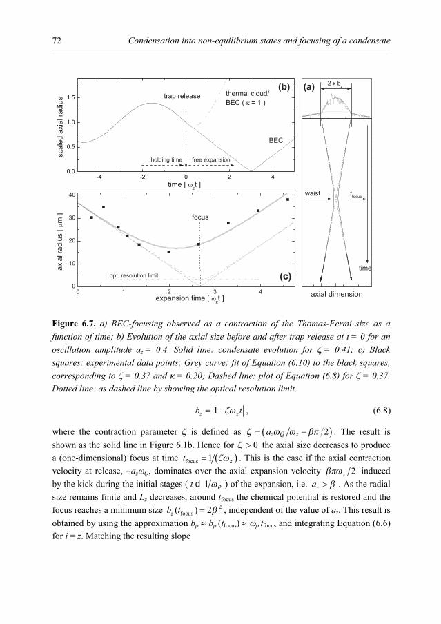
Condensation into non-equilibrium states and focusing of a condensate
72
1z zb tζω= − , (6.8)
where the contraction parameter ζ is defined as ( )2z Q zaζ ω ω βπ= − . The result is shown as the solid line in Figure 6.1b. Hence for 0ζ > the axial size decreases to produce a (one-dimensional) focus at time ( )focus 1 zt ζω= . This is the case if the axial contraction velocity at release, −azωQ, dominates over the axial expansion velocity 2zβπω induced by the kick during the initial stages ( t d 1 ρω ) of the expansion, i.e. za β> . As the radial size remains finite and Lz decreases, around tfocus the chemical potential is restored and the focus reaches a minimum size 2
focus( ) 2zb t β= , independent of the value of az. This result is obtained by using the approximation bρ ≈ bρ (tfocus) ≈ ωρ tfocus and integrating Equation (6.6) for i = z. Matching the resulting slope
Figure 6.7. a) BEC-focusing observed as a contraction of the Thomas-Fermi size as a function of time; b) Evolution of the axial size before and after trap release at t = 0 for an oscillation amplitude az = 0.4. Solid line: condensate evolution for ζ = 0.41; c) Black squares: experimental data points; Grey curve: fit of Equation (6.10) to the black squares, corresponding to ζ = 0.37 and κ = 0.20; Dashed line: plot of Equation (6.8) for ζ = 0.37. Dotted line: as dashed line by showing the optical resolution limit.
6.7 Focusing of a condensate
73
( ) ( )
1/ 22
2
2 zz
focus z focus
bb t b tρ
ω ≈
(6.9)
with the contraction velocity zb (1/ωρ d t tfocus) we get the mentioned result. The compression can be very light, e.g. 2β 2 ≈ 4 × 10⁻³ for the conditions in our apparatus. In such cases the optical resolution of the imaging system used for detection is likely to limit the minimum observable focal size as was reported in ref. [16].
6.7.2 Focal broadening
Beyond a certain expansion time the kinetic energy of the original condensate can no longer be neglected as it gives rise to spreading of the condensate wavefunction. This effect may be accounted for by writing
( ) ( )1/ 22 2 21z z zb t t tζω κω ≈ − + , (6.10)
where κ is a parameter determining the size of the focal waist. Note that for κ = 1, Equation (6.10) represents the spreading of a minimum uncertainty wavepacket released under conditions of axial contraction. Notice further that in this case no appreciable focusing is observed (see dotted line in Figure 6.1b) except for shape oscillations driven far outside ( 1)ζ > the linear regime. In general, Equation (6.10) gives rise to substantial focusing only if ζ κ> (at ζ κ= the condensate is compressed by 30%). The condition ζ κ> is satisfied for elongated Thomas-Fermi condensates at T = 0, because the momentum spread is strongly reduced compared to that of the oscillator ground state. This situation is described by approximating the waist parameter with the value 2zκ ω µ= . Then, for
2 20 2 zt t mLβ< = , the spreading can be neglected even with respect to the compression
minimum 22 zLβ . For our conditions we calculate t0 ≈ 7 ms.
For similar reasons it is virtually impossible to focus a collisionless thermal cloud. To illustrate this we consider a simple Boltzmann gas at temperature T with an oscillation described for t < 0 by Equation (6.5) and released from the trap at t = 0. If the collisional mean free path is much larger than the radial size of the cloud, the expansion proceeds ballistically and the momentum of the individual atoms is conserved (free expansion). The scaled axial size evolves according to
( ) ( )1/ 22 2 21z z Q zb t a t tω ω = − +
, (6.11)
which represents the convolution of two gaussians: the density profile of equilibrium width 2 1/ 2[2 ]z B zl k T mω= and the velocity field ( )z z Qz a zυ ω= − . In the absence of a shape
Condensation into non-equilibrium states and focusing of a condensate
74
oscillation (az = 0) this expression reduces to the well-known result used in time-of-flight analysis of collisionless thermal clouds [64, 109]. Presuming the same value of
z Q zaζ ω ω= as for the condensate (i.e. the solid line in Figure 6.1b), the thermal cloud is represented by the dotted line in Figure 6.1b.
Returning to elongated condensates we point out that at temperatures above the phase fluctuation temperature, 215( ) 32zT T Nφ ω µ> = , equilibrium phase fluctuations will dominate the focal broadening [31, 49, 82]. In this case the waist parameter may be approximated by 2 2( ) ( )z z hL L l Lφ φκ ω µ≈ ≈ , where Lφ is the phase coherence length and 1/ 2[ ]h zl mω= the axial harmonic oscillator length.
6.7.3 Applications of BEC focusing
The first application concerns the phase fluctuations discussed in Section 6.6 and deals with the focus shown in Figure 6.1c. The grey line represents a fit of Equation (6.10) to the data and yields 0.37ζ = and 0.20κ = . In this experiment the focus is strongly broadened, ( ) 2
focus 2zb t β exceeding the optical resolution limit of 3.3 µm – compare to the minimum size of 15.2 µm in Figure 6.1c. Hence, for the conditions of this experiment we may write 2( )hl Lφκ ≈ and find a phase coherence length of 0.45 1µmhL lφ ≈ ≈ .
Condensate focusing offers improved detection of small condensate fraction. Near the focus the axial condensate size is compressed by a factor ( )focus1 zb t . In time-of-flight absorption imaging the signal-to-noise can be improved accordingly by choosing the time of detection equal to tfocus. This is advantageous, particularly close to TC where the condensate fraction is small and has to be detected against the background of a large thermal cloud.
Condensate focusing also provides some advantage in detecting small thermal clouds as the separation time of the two components is reduced. Therefore, in time-of-flight absorption imaging detection can be shifted to shorter expansion times when the drop in optical density of the thermal cloud ( 1[ ]th z sepD tρω ω −∝ ) is less and an improvement in the signal-to-noise ratio of a factor of two can be obtained.
6.8 High condensate fractions in non-equilibrium states
So far we dealt with the data where the condensate fraction was of the order of a few percent. We used another method, different from the one described in Section 6.2, to produce out-of-equilibrium samples with high condensate fractions. In the first 10 seconds of evaporative cooling of these clouds the RF knife is linearly lowered from 50 MHz to 4 MHz, similar to the way it was described in Section 5.4. From 4 MHz onwards the speed of
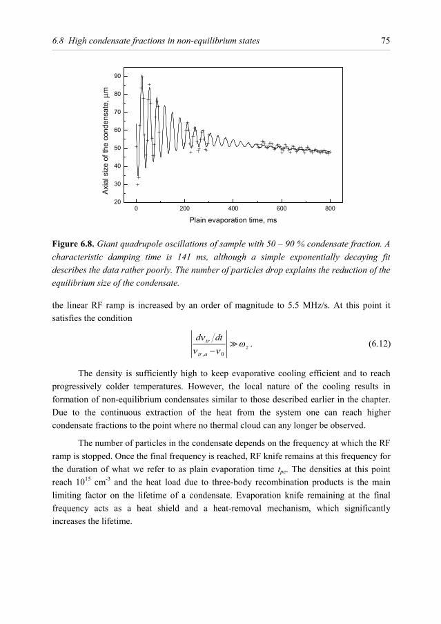
6.8 High condensate fractions in non-equilibrium states
75
the linear RF ramp is increased by an order of magnitude to 5.5 MHz/s. At this point it satisfies the condition
, 0
trz
tr a
d dtνω
ν ν−. (6.12)
The density is sufficiently high to keep evaporative cooling efficient and to reach progressively colder temperatures. However, the local nature of the cooling results in formation of non-equilibrium condensates similar to those described earlier in the chapter. Due to the continuous extraction of the heat from the system one can reach higher condensate fractions to the point where no thermal cloud can any longer be observed.
The number of particles in the condensate depends on the frequency at which the RF ramp is stopped. Once the final frequency is reached, RF knife remains at this frequency for the duration of what we refer to as plain evaporation time tpe. The densities at this point reach 1015 cm-3 and the heat load due to three-body recombination products is the main limiting factor on the lifetime of a condensate. Evaporation knife remaining at the final frequency acts as a heat shield and a heat-removal mechanism, which significantly increases the lifetime.
Figure 6.8. Giant quadrupole oscillations of sample with 50 – 90 % condensate fraction. A characteristic damping time is 141 ms, although a simple exponentially decaying fit describes the data rather poorly. The number of particles drop explains the reduction of the equilibrium size of the condensate.
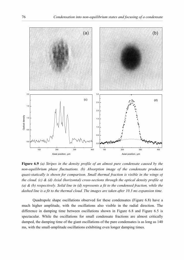
Condensation into non-equilibrium states and focusing of a condensate
76
Quadrupole shape oscillations observed for these condensates (Figure 6.8) have a much higher amplitude, with the oscillations also visible in the radial direction. The difference in damping time between oscillations shown in Figure 6.8 and Figure 6.5 is spectacular. While the oscillations for small condensate fractions are almost critically damped, the damping time of the giant oscillations of the pure condensates is as long as 140 ms, with the small-amplitude oscillations exhibiting even longer damping times.
Figure 6.9 (a) Stripes in the density profile of an almost pure condensate caused by the non-equilibrium phase fluctuations. (b) Absorption image of the condensate produced quasi-statically is shown for comparison. Small thermal fraction is visible in the wings of the cloud. (c) & (d) Axial (horizontal) cross-sections through the optical density profile of (a) & (b) respectively. Solid line in (d) represents a fit to the condensed fraction, while the dashed line is a fit to the thermal cloud. The images are taken after 10.3 ms expansion time.
6.8 High condensate fractions in non-equilibrium states
77
One can also observe strong non-equilibrium phase fluctuations in these condensates. Exhibited in the form of interference stripes in the beginning (see Figure 6.9 (a) & (c)), they are being damped out over the course of a few hundred milliseconds. These stripes show a higher contrast as compared to those displayed in Figure 6.6 due to the near absence of the thermal cloud in the trap. For comparison in Figure 6.9 (b) & (d) we also give an absorption picture and an optical density cross-section for a normal condensate produced with quasi-static ramping of the evaporation barrier. The analytical description of the condensates produced with such fast RF ramps is much more difficult as compared to the truncation method discussed above, and their use is limited to specific cases where a detailed analytical picture is not required.


Bibliography
[1] G. L. Abbas, S. Yang, V. W. S. Chan, and J. G. Fujimoto. Injection Behavior and Modeling of 100-mW Broad Area Diode Lasers, IEEE J. Quantum Electron. 24, 609 (1988).
[2] H. Adachihara, O. Hess, E. Abraham, P. Ru, and J. V. Moloney. Spatiotemporal Chaos in Broad-Area Semiconductor-Lasers, J. Opt. Soc. Am. B 10, 658 (1993).
[3] J. A. Andersen, M. E. J. Friese, A. G. Truscott, Z. Ficek, P. D. Drummond, N. R. Heckenberg, and H. Rubinsztein-Dunlop. Light Guiding Light: Nonlinear Refraction in Rubidium Vapor, Phys. Rev. A 63, 023820 (2001).
[4] M. H. Anderson, J. R. Ensher, M. R. Matthews, C. E. Wieman, and E. A. Cornell. Observation of Bose-Einstein Condensation in a Dilute Atomic Vapor, Science 269, 198 (1995).
[5] M. R. Andrews, M.-O. Mewes, N. J. van Druten, D. S. Durfee, D. M. Kurn, and W. Ketterle. Direct, Nondestructive Observation of a Bose Condensate, Science 273, 84 (1996).
[6] M. R. Andrews, C. G. Townsend, H.-J. Miesner, D. S. Durfee, D. M. Kurn, and W. Ketterle. Observation of Interference Between Two Bose Condensates, Science 275, 637 (1997).
[7] E. Arimondo, M. Inguscio, and P. Violino. Experimental Determination of the Hyperfine Structure in the Alkali Atoms, Reviews of Modern Physics 49, 31 (1977).
[8] V. Bagnato, D. E. Pritchard, and D. Kleppner. Bose-Einstein Condensation in an External Potential, Phys. Rev. A 35, 4354 (1987).
[9] M. Bartenstein, D. Cassettari, T. Calarco, A. Chenet, R. Folman, K. Brugger, A. Haase, E. Hartungen, B. Hessmo, A. Kasper, P. Kruger, T. Maier, F. Payr, S. Schneider, and J. Schmiedmayer. Atoms and Wires: Toward Atom Chips, IEEE J. Quantum Electron. 36, 1364 (2000).
[10] T. Bergeman, G. Erez, and H. J. Metcalf. Magnetostatic Trapping Fields for Neutral Atoms, Phys. Rev. A 35, 35 (1987).
[11] M. J. Bijlsma, E. Zaremba, and H. T. C. Stoof. Condensate Growth in Trapped Bose Gases, Phys. Rev. A 62, 063609 (2000).
[12] G. Birkl, F. B. J. Buchkremer, R. Dumke, and W. Ertmer. Atom Optics With Microfabricated Optical Elements, Opt. Commun. 191, 67 (2001).
[13] G. C. Bjorklund, M. D. Levenson, W. Lenth, and C. Oritz. Frequency Modulation (FM) Spectroscopy, Applied Physics B 32, 145 (1983).
[14] I. Bloch, T. W. Hänsch, and T. Esslinger. Atom Laser with a cw Output Coupler, Phys. Rev. Lett. 82, 3008 (1999).
[15] I. Bloch, T. W. Hänsch, and T. Esslinger. Measurement of the Spatial Coherence of a Trapped Bose Gas at the Phase Transition, Nature 403, 166 (2000).
[16] I. Bloch, M. Köhl, M. Greiner, T. W. Hänsch, and T. Esslinger. Optics With an Atom Laser Beam, Phys. Rev. Lett. 87, 030401 (2001).
[17] K. Bongs, S. Burger, G. Birkl, K. Sengstock, W. Ertmer, K. Rzazewski, A. Sanpera, and M.
Bibliography
80
Lewenstein. Coherent Evolution of Bouncing Bose-Einstein Condensates, Phys. Rev. Lett. 83, 3577 (1999).
[18] S. N. Bose. Plancks Gesetz und Lichtquantenhypothese, Zeitschrift für Physik 26, 178 (1924).
[19] C. C. Bradley, C. A. Sackett, J. J. Tollett, and R. G. Hulet. Evidence of Bose-Einstein Condensation in an Atomic Gas With Attractive Interactions, Phys. Rev. Lett. 75, 1687 (1995).
[20] C. C. Bradley, C. A. Sackett, and R. G. Hulet. Bose-Einstein Condensation of Lithium: Observation of Limited Condensate Number, Phys. Rev. Lett. 78, 985 (1997).
[21] Y. Castin and R. Dum. Bose-Einstein Condensates in Time Dependent Traps, Phys. Rev. Lett. 77, 5315 (1996).
[22] Y. Castin, R. Dum, E. Mandonnet, A. Minguzzi, and I. Carusotto. Coherence Properties of a Continuous Atom Laser, J. Mod. Opt. 47, 2671 (2000).
[23] R. A. Cline, D. A. Smith, T. J. Greytak, and D. Kleppner. Magnetic Confinement of Spin-Polarized Atomic Hydrogen, Phys. Rev. Lett. 45, 2117 (1980).
[24] Courtesy of Imogen Colton, University of Melbourne [25] Imogen Colton, Robert Scholten. University of Melbourne. Private communication. [26] K. L. Corwin, Z. T. Lu, C. F. Hand, R. J. Epstein, and C. E. Wieman. Frequency-Stabilized
Diode Laser with the Zeeman Shift in an Atomic Vapor, Appl. Opt. 37, 3295 (1998). [27] F. Dalfovo, S. Giorgini, L. P. Pitaevskii, and S. Stringari. Theory of Bose-Einstein
Condensation in Trapped Gases, Reviews of Modern Physics 71, 463 (1999). [28] K. B. Davis, M.-O. Mewes, M. R. Andrews, N. J. van Druten, D. S. Durfee, D. M. Kurn,
and W. Ketterle. Bose-Einstein Condensation in a Gas of Sodium Atoms, Phys. Rev. Lett. 75, 3969 (1995).
[29] M. J. Davis, C. W. Gardiner, and R. J. Ballagh. Quantum Kinetic Theory VII. The Influence of Vapor Dynamics on Condensate Growth, Phys. Rev. A 62, 3608 (2000).
[30] W. Demtröder, Laser Spectroscopy: Basic Concepts and Instrumentation (Springer Verlag, Berlin, 1996).
[31] S. Dettmer, D. Hellweg, P. Ryytty, J. J. Arlt, W. Ertmer, K. Sengstock, D. S. Petrov, G. V. Shlyapnikov, H. Kreutzmann, L. Santos, and M. Lewenstein. Observation of Phase Fluctuations in Elongated Bose-Einstein Condensates, Phys. Rev. Lett. 87, 160406 (2001).
[32] K. Dieckmann, R. J. C. Spreeuw, M. Weidemüller, and J. T. M. Walraven. Two-Dimensional Magneto-Optical Trap As a Source of Slow Atoms, Phys. Rev. A 58, 3891 (1998).
[33] K. Dieckmann. Bose-Einstein Condensation with High Atom Number in a Deep Magnetic Trap, PhD thesis, University of Amsterdam (2001).
[34] R. W. P. Drever, J. L. Hall, F. V. Kowalski, J. Hough, G. M. Ford, A. J. Munley, and H. Ward. Laser Phase and Frequency Stabilization Using an Optical Resonator, Applied Physics B 31, 97 (1983).
[35] A. Einstein. Quantentheorie des Einatomigen Idealen Gases: Zweite Abhandlung, Sitzungber. Preuss. Akad. Wiss. 1925, 3 (1925).
[36] P. O. Fedichev, G. V. Shlyapnikov, and J. T. M. Walraven. Damping of Low-Energy Excitations of a Trapped Bose-Einstein Condensate at Finite Temperatures, Phys. Rev. Lett. 80, 2269 (1998).
[37] A. C. Fey-den Boer, H. C. W. Beijerinck, and K. A. H. van Leeuwen. High-Power Broad-
81
Area Diode Lasers for Laser Cooling, Appl. Phys. B 64, 415 (1997). [38] C. W. Gardiner, P. Zoller, R. J. Ballagh, and M. J. Davis. Kinetics of Bose-Einstein
Condensation in a Trap, Phys. Rev. Lett. 79, 1793 (1997). [39] C. W. Gardiner, M. D. Lee, R. J. Ballagh, M. J. Davis, and P. Zoller. Quantum Kinetic
Theory of Condensate Growth: Comparison of Experiment and Theory, Phys. Rev. Lett. 81, 5266 (1998).
[40] E. Gehrig, B. Beier, K.-J. Boller, and R. Wallenstein. Experimental Characterization and Numerical Modelling of an AlGaAs Oscillator Broad Area Double Pass Amplifier System , Appl. Phys. B 66, 287 (1998).
[41] S. Giorgini, L. P. Pitaevskii, and S. Stringari. Scaling and Thermodynamics of a Trapped Bose-Condensed Gas, Phys. Rev. Lett. 78, 3987 (1997).
[42] L. Goldberg and M. K. Chun. Injection Locking Characteristics of a 1-W Broad Stripe Laser Diode, Appl. Phys. Lett. 53, 1900 (1988).
[43] L. Goldberg and J. F. Weller. Broad-Area High-Power Semiconductor Optical Amplifier, Appl. Phys. Lett. 58, 1357 (1991).
[44] L. Goldberg, D. Mehuys, M. R. Surette, and D. C. Hall. High-Power, Near-Diffraction-Limited Large-Area Traveling-Wave Semiconductor Amplifiers, IEEE J. Quantum Electron. 29, 2028 (1993).
[45] V. V. Goldman, I. F. Silvera, and A. J. Leggett. Atomic Hydrogen in an Inhomogeneous Magnetic Field - Density Profile and Bose-Einstein Condensation, Phys. Rev. B 24, 2870 (1981).
[46] A. Griffin, W. C. Wu, and S. Stringari. Hydrodynamic Modes in a Trapped Bose Gas above the Bose- Einstein Transition, Phys. Rev. Lett. 78, 1838 (1997).
[47] D. Guéry-Odelin, F. Zambelli, J. Dalibard, and S. Stringari. Collective Oscillations of a Classical Gas Confined in Harmonic Traps, Phys. Rev. A 60, 4851 (1999).
[48] E. W. Hagley, L. Deng, M. Kozuma, J. Wen, K. Helmerson, S. L. Rolston, and W. D. Phillips. A Well-Collimated Quasi-Continuous Atom Laser, Science 283, 1706 (1999).
[49] D. Hellweg, S. Dettmer, P. Ryytty, J. J. Arlt, W. Ertmer, K. Sengstock, D. S. Petrov, G. V. Shlyapnikov, H. Kreutzmann, L. Santos, and M. Lewenstein. Phase Fluctuations in Bose-Einstein Condensates, Appl. Phys. B 73, 781 (2001).
[50] H. Hess, G. P. Kochansky, J. M. Doyle, N. Masuhara, D. Kleppner, and T. J. Greytak. Magnetic Trapping of Spin-Polarized Atomic Hydrogen, Phys. Rev. Lett. 59, 672 (1987).
[51] H. F. Hess. Evaporative Cooling of Magnetically Trapped and Compressed Spin-Polarized Hydrogen, Physical Review B 34, 3476 (1986).
[52] E. A. Hinds and I. G. Hughes. Magnetic Atom Optics: Mirrors, Guides, Traps, and Chips for Atoms, J. Phys. D: Appl. Phys. 32, R119-R146 (1999).
[53] K. Huang, Statistical Mechanics (John Wiley & Sons, 1963). [54] D. A. Huse and E. D. Siggia. The Density Distribution of a Weakly Interacting Bose Gas in
an External Potential, J. Low Temp. Phys. 46 , 137 (1982). [55] Proceedings of the International School of Physics "Enrico Fermi". Bose-Einstein
Condensation in Atomic Gases, ed. by M. Inguscio, S. Stringari, and C. E. Wieman (IOS Press , Amsterdam, 1999).
[56] D. S. Jin, M. R. Matthews, J. R. Ensher, C. E. Wieman, and E. A. Cornell. Temperature-Dependent Damping and Frequency Shifts in Collective Excitations of a Dilute Bose-Einstein Condensate, Phys. Rev. Lett. 78, 764 (1997).
Bibliography
82
[57] Y. Kagan, B. V. Svistunov, and G. V. Shlyapnikov. The Bose-Condensation Kinetics in an Interacting Bose-Gas, Zh. Eksp. Teor. Fiz. (JETP) 101, 528 (1992).
[58] Y. Kagan and B. V. Svistunov. Kinetics of Long-Range Order Formation in Bose-Condensation in Interacting Gas, Zh. Eksp. Teor. Fiz. (JETP) 105, 353 (1994).
[59] Y. Kagan, E. L. Surkov, and G. V. Shlyapnikov. Evolution of a Bose-Condensed Gas Under Variations of the Confining Potential, Phys. Rev. A 54, R1753-R1756 (1996).
[60] Y. Kagan, E. L. Surkov, and G. V. Shlyapnikov. Evolution of a Bose Gas in Anisotropic Time-Dependent Traps, Phys. Rev. A 55, R18-R21 (1997).
[61] Y. Kagan and B. V. Svistunov. Evolution of Correlation Properties and Appearance of Broken Symmetry in the Process of Bose-Einstein Condensation, Phys. Rev. Lett. 79, 3331 (1997).
[62] Y. Kagan and B. V. Svistunov. Evolution of Large-Scale Correlations in a Strongly Nonequilibrium Bose Condensation Process, JETP Letters 67, 521 (1998).
[63] W. Ketterle and N. J. van Druten. Evaporative Cooling of Trapped Atoms, in Advances in Atomic, Molecular, and Optical Physics, ed. by B. Bederson and H. Walther, Vol. 37, 181 (1996).
[64] W. Ketterle, D. S. Durfee, and D. M. Stamper-Kurn, Making, probing and understanding Bose-Einstein condensates, in Proceedings of the International School of Physics 'Enrico Fermi'. Bose-Einstein Condensation in Atomic Gases, ed. by M. Inguscio, S. Stringari, and C. E. Wieman (IOS Press , Amsterdam, 1999).
[65] M. Köhl, M. J. Davis, C. W. Gardiner, T. W. Hänsch, and T. Esslinger. Growth of Bose-Einstein Condensates from Thermal Vapor, Phys. Rev. Lett. 88, 080402 (2002).
[66] L. D. Landau and E. M. Lifshitz, The Classical Theory of Fields (Butterworth-Heinemann, Oxford, 1999).
[67] R. J. Lang, D. Mehuys, A. Hardy, K. M. Dzurko, and D. F. Welch. Spatial Evolution of Filaments in Broad Area Diode-Laser Amplifiers, Appl. Phys. Lett. 62, 1209 (1993).
[68] D. C. Lau, R. J. Mclean, A. I. Sidorov, D. S. Gough, J. Koperski, W. J. Rowlands, B. A. Sexton, G. I. Opat, and P. Hannaford. Magnetic Mirrors With Micron-Scale Periodicities for Slowly Moving Neutral Atoms, Journal of Optics B 1, 371 (1999).
[69] M. Leduc, J. Leonard, F. P. Dos Santos, E. Jahier, S. Schwartz, and C. Cohen-Tannoudji. Hydrodynamic Modes in a Trapped Gas of Metastable Helium Above the Bose-Einstein Transition, Acta Phys. Pol., B 33, 2213 (2002).
[70] M. D. Lee and C. W. Gardiner. Quantum Kinetic Theory. VI. The Growth of a Bose-Einstein Condensate, Phys. Rev. A 62, 033606 (2000).
[71] K. Lindquist, M. Stephens, and C. Wieman. Experimental and Theoretical-Study of the Vapor-Cell Zeeman Optical Trap, Phys. Rev. A 46, 4082 (1992).
[72] Z. T. Lu, K. L. Corwin, M. J. Renn, M. H. Anderson, E. A. Cornell, and C. E. Wieman. Low-Velocity Intense Source of Atoms From a Magneto-Optical Trap, Phys. Rev. Lett. 77, 3331 (1996).
[73] O. J. Luiten. Lyman-alpha Spectroscopy of Magnetically Trapped Atomic Hydrogen, PhD thesis, University of Amsterdam (1993).
[74] O. J. Luiten, M. W. Reynolds, and J. T. M. Walraven. Kinetic Theory of the Evaporative Cooling of a Trapped Gas, Phys. Rev. A 53, 381 (1996).
[75] K. B. MacAdam, A. Steinbach, and C. Wieman. A Narrow-Band Tunable Diode-Laser System With Grating Feedback, and a Saturated Absorption Spectrometer for Cs and Rb,
83
American Journal of Physics 60, 1098 (1992). [76] H. J. Metcalf and P. van der Straten, Laser Cooling and Trapping (Springer Verlag, New
York, 1999). [77] M.-O. Mewes, M. R. Andrews, N. J. van Druten, D. M. Kurn, D. S. Durfee, C. G.
Townsend, and W. Ketterle. Collective Excitations of a Bose-Einstein Condensate in a Magnetic Trap, Phys. Rev. Lett. 77, 988 (1996).
[78] H.-J. Miesner, D. M. Stamper-Kurn, M. R. Andrews, D. S. Durfee, S. Inouye, and W. Ketterle. Bosonic Stimulation in the Formation of a Bose-Einstein Condensate, Science 279, 1005 (1998).
[79] A. L. Migdall, J. V. Prodan, W. D. Phillips, T. H. Bergeman, and H. J. Metcalf. First Observation of Magnetically Trapped Neutral Atoms, Phys. Rev. Lett. 54, 2596 (1985).
[80] T. Pawletko, M. Houssin, M. Knoop, M. Vedel, and F. Vedel. High Power Broad-Area Diode Laser at 794 Nm Injected by an External Cavity Laser, Opt. Commun. 174, 223 (2000).
[81] D. S. Petrov, G. V. Shlyapnikov, and J. T. M. Walraven. Regimes of Quantum Degeneracy in Trapped 1d Gases, Phys. Rev. Lett. 85, 3745 (2000).
[82] D. S. Petrov, G. V. Shlyapnikov, and J. T. M. Walraven. Phase-Fluctuating 3d Bose-Einstein Condensates in Elongated Traps, Phys. Rev. Lett. 87, 050404 (2001).
[83] M. Praeger, V. Vuletic, T. Fischer, T. W. Hänsch, and C. Zimmermann. A Broad Emitter Diode Laser System for Lithium Spectroscopy, Appl. Phys. B 67, 163 (1998).
[84] A. Radzig and Smirnov B.M., Reference Data of Atoms, Molecules and Ions (Springer Verlag, Berlin, 1985).
[85] L. Ricci, M. Weidemüller, T. Esslinger, A. Hemmerich, C. Zimmermann, V. Vuletic, W. König, and T. W. Hänsch. A Compact Grating-Stabilized Diode-Laser System for Atomic Physics, Opt. Commun. 117, 541 (1995).
[86] T. M. Roach, H. Abele, M. G. Boshier, H. L. Grossman, K. P. Zetie, and E. A. Hinds. Realization of a Magnetic-Mirror for Cold Atoms, Phys. Rev. Lett. 75, 629 (1995).
[87] R. v. Roijen, J. J. Berkhout, S. Jaakkola, and Walraven J. T. M. Experiments With Atomic Hydrogen in a Magnetic Trapping Field, Phys. Rev. Lett. 61, (1988).
[88] S. L. Rolston and W. D. Phillips. Nonlinear and Quantum Atom Optics, Nature 416, 219 (2002).
[89] A. Roth, Vacuum Technology (Elsevier Science Publishers, 1990). [90] J. R. Rubbmark, Kahs M.M., Littman M.G., and Kleppner D. Dynamical Effects at Avoided
Level Crossing: A Study of the Landau-Zener Effect Using Rydberg Atoms, Phys. Rev. A 23, 3107 (1981).
[91] U. Schünemann, H. Engler, R. Grimm, M. Weidemüller, and M. Zielonkowski. Simple Scheme for Tunable Frequency Offset Locking of Two Lasers, Rev. Sci. Instrum. 70, 242 (1999).
[92] G. Scoles, Atomic and Molecular Beam Methods (Oxford University Press, New York, 1992).
[93] I. F. Silvera and J. T. M. Walraven. Stabilization of Atomic Hydrogen at Low Temperature, Phys. Rev. Lett. 44, 164 (1980).
[94] D. M. Stamper-Kurn, H.-J. Miesner, S. Inouye, M. R. Andrews, and W. Ketterle. Collisionless and Hydrodynamic Excitations of a Bose-Einstein Condensate, Phys. Rev. Lett. 81, 500 (1998).
84
[95] J. Stenger, S. Inouye, A. P. Chikkatur, D. M. Stamper-Kurn, D. E. Pritchard, and W. Ketterle. Bragg Spectroscopy of a Bose-Einstein Condensate, Phys. Rev. Lett. 82, 4569 (1999).
[96] S. Stringari. Collective Excitations of a Trapped Bose-Condensed Gas, Phys. Rev. Lett. 77, 2360 (1996).
[97] E. L. Surkov, J. T. M. Walraven, and G. V. Shlyapnikov. Collisionless Motion and Evaporative Cooling of Atoms in Magnetic Traps, Phys. Rev. A 53, 3403 (1996).
[98] B. V. Svistunov. Highly Nonequilibrium Bose Condensation in a Weakly Interacting Gas, Journal of Moscow Physical Society 1, 373 (1991).
[99] T. G. Tiecke, M. Kemmann, Ch. Buggle, I. Shvarchuck, W. v. Klitzing, and J. T. M. Walraven. Bose-Einstein Condensation in a Magnetic Double-Well Potential, Journal of Optics B (accepted for publication).
[100] C. G. Townsend, N. H. Edwards, C. J. Cooper, K. P. Zetie, C. J. Foot, A. M. Steane, P. Szriftgiser, H. Perrin, and J. Dalibard. Phase-Space Density in the Magneto-optical Trap, Phys. Rev. A 52, 1423 (1995).
[101] L. D. Turner, I. Colton, K. P. Weber, D. Paganin, and R. E. Scholten, Non-interferometric Phase Imaging of a Rb Vapor, ICAP, XVIII International Conference on Atomic Physics, (to be published).
[102] P. Valkering. Optimization of evaporative cooling of rubidium atoms in a magnetic trap, MSc thesis, University of Utrecht, 1999.
[103] E. G. M. van Kempen, S. Kokkelmans, D. J. Heinzen, and B. J. Verhaar. Interisotope Determination of Ultracold Rubidium Interactions From Three High-Precision Experiments, Phys. Rev. Lett. 88, 093201 (2002).
[104] We thank D. Voigt for supplying the information on tapered amplifiers. [105] J. T. M. Walraven, Atomic hydrogen in magnetostatic traps, in Quantum Dynamics of
Simple Systems, ed. by G. L. Oppo, S. M. Barnett, E. Riis, and Wilkinson M., SUSSP Proceedings (IOP, Bristol, 1996).
[106] C. E. Wieman and L. Hollberg. Using Diode Lasers for Atomic Physics, Rev. Sci. Instrum. 62, 1 (1991).
[107] J. E. Williams and A. Griffin. Damping of Condensate Collective Modes Due to Equilibration With the Noncondensate, Phys. Rev. A 63, 3612 (2001).
[108] H. Wu and E. Arimondo. Expansion of the Non-Condensed Trapped Bose Gas in Bose- Einstein Condensation, Europhys. Lett. 43, 141 (1998).
[109] L. You and M. Holland. Ballistic Expansion of Trapped Thermal Atoms, Phys. Rev. A 53, R1-R4 (1996).
[110] E. Zaremba, A. Griffin, and T. Nikuni. Two-Fluid Hydrodynamics for a Trapped Weakly Interacting Bose Gas, Phys. Rev. A 57, 4695 (1998).
[111] E. Zaremba, T. Nikuni, and A. Griffin. Dynamics of Trapped Bose Gases at Finite Temperatures, J. Low Temp. Phys. 116, 277 (1999).
[112] C. Zener. Non-Adiabatic Crossing of Energy Levels, Proceedings of the Royal Society of London Series A 137, 696 (1932).
Summary
In this Thesis we describe experimental studies of the condensate formation into non-equilibrium states and investigation of the hydrodynamic behaviour of cold non-degenerate atomic clouds. Non-equilibrium nature of the condensates offers an essentially different path towards equilibrium as compared to the condensate formed in a quasi-static fashion. Investigation of the crossover between collisionless and hydrodynamic regimes is interesting from both experimental and theoretical points of view.
Bose-Einstein condensation (BEC) was predicted in 1925 [18, 35] and was achieved experimentally seventy years later in pioneering experiments at JILA [4], MIT [28] and Rice [19, 20]. This led to a dramatic expansion of both experimental and theoretical work in the field of ultracold quantum gases. Although the macroscopic occupation of the ground state is the best known aspect of the phenomenon of BEC, the appearance of phase coherence is equally important. The investigation of phase coherence phenomena provides new fundamental insights into the nature of macroscopic quantum states and is important for current and future applications. Those include, in particular, atom lasers – devices for continuous or pulsed generation of coherent matter waves, atom interferometry, improved frequency standards and systems of cold atoms for quantum computing. The appearance of coherence in a condensate cannot be separated from the process of condensate formation. Previous experimental investigations of formation kinetics of trapped condensates [65, 78] were decoupled from the studies of phase coherence [31, 82] Investigation of the evolution of phase coherence properties during the formation of a trapped condensate out of a non-equilibrium thermal cloud presents a great general physical interest. In particular it should allow a deeper understanding of phase coherence phenomena in macroscopic quantum states. One can expect that the evolution of phase coherence will be a primary issue for creation of CW atom lasers [22].
The Thesis is organised in the following way. In Chapter 2 we compiled main theoretical expressions relevant to the Bose-Einstein condensation, including the principle of magnetic trapping and the description of trapped Bose gases below and above the phase transition point. Further we sketched theoretical ideas underlying phase coherence and formation of a BEC. We also introduced the bare fundamentals of evaporative cooling and derived several results important for the experiments described in later chapters. A separate section was dedicated to the scaling description of the gas clouds in harmonic traps.
Summary
86
In Chapter 3 various aspects of the experimental setup were described. Special attention was given to the features characteristic to the specific ideas, which motivated the construction of the apparatus, e.g. creating Bose condensates with the highest density and particle number possible. An insight into evaporative cooling in our experiments was presented together with some details of the measurement methods. A great deal of emphasis was put on the description of imaging of cold atomic clouds.
Chapter 4 was fully dedicated to a detailed description of the high-power diode laser system, the design and building of which was dictated by the needs of this experiment.
In Chapter 5 we presented the experimental investigation of the hydrodynamic properties of dense atomic clouds. The understanding of the crossover to the hydrodynamic regime in thermal clouds is important from the experimental point of view. This understanding is vital for the correct interpretation of time-of-flight images of such clouds. In the collisionless regime the expansion of the gas, after release from a trap, is known to be isotropic, whereas in the hydrodynamic limit the gas expands anisotropically. We approached investigation of the hydrodynamic properties from three different sides. First, we go in detail into density and temperature analysis. Another indicator of hydrodynamic behaviour is obtained by observation of the anisotropic character of the expansion. Finally, we measure frequency shifts and damping of shape oscillations. All three methods proved to be consistent with each other and the completeness of our description was verified
In the final part of the Thesis, Chapter 6, we discussed the results produced in the experiments on formation of condensates far from equilibrium. We compared our work with the previous experiments on condensate formation. In a brief section some attention was given to the growth of the condensate fraction. Further, we showed how the concepts of local sample temperature and the critical temperature arise in elongated clouds with high elastic collision rates. We presented a simple model, which illustrates how the non-equilibrium character of the condensates leads to the quadrupole oscillations. This model was found to be in good agreement with the experiment. We also presented evidence of non-equilibrium phase fluctuations, which manifested themselves in the form of stripes in the time-of-flight absorption images. Condensate focusing was introduced as a novel method for investigation of Bose-Einstein condensates. The focusing of a condensate in free flight arises from axial contraction of the expanding cloud when the gas is released from the trap during the inward phase of a shape oscillation. Possible applications of BEC focusing were discussed. We applied BEC focusing to calculation of the coherence length of non-equilibrium condensate. The last part of the chapter covered condensation into non-equilibrium states with high condensate fractions. We discussed a method of achieving high condensate fractions, while keeping the system far from equilibrium. The phase fluctuations
87
and the excitation modes had the same qualitative character as in the experiments with small BEC fractions. However, in some aspects, such the damping rates of the quadrupole oscillations, we could observe significant differences.

Samenvatting
In dit proefschrift worden experimentele studies van het ontstaan van een Bose-Einstein condensaat in een ultrakoud atomair gas beschreven. In het bijzonder hebben we het ontstaan van condensaten in niet-evenwichtstoestanden en hydrodynamisch gedrag van koude, maar niet quantum-ontaarde, atomaire wolken bestudeerd.
Bose-Einstein condensatie (BEC) is een fasenovergang naar een macroscopische quantumtoestand, die bijvoorbeeld waar te nemen is in bepaalde ultrakoude gassen bij temperaturen rond 0.000001 Kelvin. BEC werd in 1925 voorspeld [18, 35] en zeventig jaar later gerealiseerd in experimenten in Boulder [4], Cambridge (USA) [28] en Houston [19, 20]. Dit was het startsein voor een enorme uitbreiding van zowel experimenteel als theoretisch werk in het veld van ultrakoude gassen. Het meest bekende kenmerk van BEC is de macroscopische bezetting van de grondtoestand, maar een minstens zo belangrijk aspect is het ontstaan van fasencoherentie. Het onderzoeken van coherentiefenomenen geeft fundamentele nieuwe inzichten in de eigenschappen van macroscopische quantumtoestanden en is belangrijk voor bestaande en nog te ontwikkelen toepassingen. Daaronder vallen in het bijzonder atoom-interferometrie, frequentiestandaards gebaseerd op ultrakoude atomen, atoomlasers – apparaten die continue of gepulste coherente materiegolven produceren – en systemen van koude atomen voor verwerking van quantum-informatie. Het ontstaan van coherentie in een condensaat is niet los te zien van het ontstaansproces van het condensaat zelf. Eerdere experimenten waarin de vorming van condensaten bestudeerd werd [65, 78], waren niet gekoppeld aan metingen van fasencoherentie [31, 82]. Het ontstaan van coherentie-eigenschappen tijdens de vorming van een condensaat uit een thermische wolk atomen die niet in evenwicht is, is een fysisch vraagstuk van groot belang. In het bijzonder kan begrip van dit proces in belangrijke mate bijdragen aan de ontwikkeling van continue atoomlasers [22].
Dit proefschrift is als volgt ingedeeld: Hoofdstuk 1 geeft een algemene inleiding. In hoofdstuk 2 hebben we de belangrijkste theoretische uitdrukkingen op het gebied van Bose-Einstein condensatie verzameld. Ook het principe van de magnetische val en de beschrijving van magnetisch opgesloten Bose gassen boven en onder de BEC fasenovergang worden uitgelegd. Bovendien schetsen we de theoretische ideeën die ten grondslag liggen aan de fasencoherentie en het ontstaan van een BEC. We beschrijven ook, zij het summier, de verdampingskoeling waardoor de BEC fasenovergang bereikt wordt en leiden enkele resulaten af die van belang zijn voor de experimenten die in de andere
Samenvatting
90
hoodstukken beschreven worden. Een sectie behandelt de schalingstheorie van gaswolken in een harmonische val.
In hoofdstuk 3 worden verschillende aspecten van de apparatuur beschreven. Bijzondere aandacht wordt uitgetrokken voor de eigenschappen die voortvloeien uit de specifieke doelen waarvoor de apparatuur gebouwd is, met name het maken van Bose condensaten met een zo hoog mogelijke dichtheid en een zo groot mogelijk aantal atomen. Een blik op de verdampingskoelmethode en enkele details van de meetmethoden worden gegeven, met nadruk op de afbeeldingstechnieken voor koude atoomwolken.
In hoofdstuk 4 wordt in detail het hoogvermogen diodenlasersysteem beschreven. Dit systeem is speciaal ontworpen en gebouwd voor de in dit proefschrift beschreven experimenten.
In hoofdstuk 5 beschrijven we experimentele onderzoekingen van de hydrodynamische eigenschappen van atoomwolken met hoge dichtheid. Het begrip van de overgang naar het hydrodynamische regime in thermische wolken is belangrijk voor de experimenten, in het bijzonder is dit noodzakeleijk voor het juist interpreteren van beelden van de vrije expansie van uit de magneetval losgelaten gaswolken. In het botsingsvrije regime is de vrije expansie van het gas isotroop, terwijl een gas in het hydrodynamische regime anisotroop expandeert. We benaderen het onderzoek van de hydrodynamische eigenschappen van drie verschillende kanten. Ten eerste beschouwen we de analyse van temperatuur en dichtheid in detail. Ten tweede observeren we de anisotropie van de vrije expansie van het gas. Tenslotte meten we de frequentieverschuiving en demping van vorm-oscillaties. Alle drie methoden blijken consistent met elkaar en tonen daarmee aan dat onze beschrijving volledig is.
In het laatste deel van het proefschrift, hoofdstuk 6, bespreken we experimenten waarin we condensaten ver buiten thermisch evenwicht geproduceerd hebben. We vergelijken ons werk met eerdere experimenten waarin het ontstaan van condensaten bestudeerd is. Enige aandacht wordt besteed aan de groei van de gecondenseerde fractie. Bovendien laten we zien hoe het idee van een lokale temperatuur en lokale kritische temperatuur van toepassing is op lange atoomwolken met hoge elastische botsingsfrekwenties. We presenteren een eenvoudig model, dat illustreert hoe het niet-evenwichtskarakter van het condensaat leidt tot oscillaties van de vorm van het condensaat (quadrupool oscillaties). De resultaten van dit model zijn in goede overeenstemming met de experimenten. We laten ook zien dat de fase van het condensaat buiten thermisch evenwicht fluctueert, wat zich manifesteert als interferentiestrepen in de afbeeldingen van de vrij geëxpandeerde condensaten. Het focusseren van het condensaat wordt geïntroduceerd als een nieuwe methode voor het bestuderen van Bose-Einstein
91
condensaten. Het focusseren van een condensaat in vrije vlucht, na het loslaten uit een magneetval, is een gevolg van de naar binnen gerichte axiale impuls wanneer het condensaat wordt losgelaten tijdens de ingaande fase van een vorm-oscillatie. We bespreken mogelijke toepassingen van het focusseren van het condensaat, en passen het toe om de coherentielengte van het condensaat buiten evenwicht te bepalen. Het laatste deel van het hoofdstuk behandelt condensatie in niet-evenwichtstoestanden waarin de gecondenseerde fractie hoog is. We bespreken de methode die we gebruiken om een hoge gecondenseerde fractie te bereiken en tegelijk ver buiten thermisch evenwicht te blijven. De fluctuaties van de fase en de excitatiemodes hebben in dit geval kwalitatief hetzelfde karakter als in de experimenten met kleine gecondenseerde fracties. In sommige eigenschappen, zoals de demping van de quadrupooloscillaties, vinden we wel significante verschillen.

Acknowledgements
As I started thinking about this last part of the thesis I realised the enormity of the task I was facing. In the years that I spent in Amsterdam I was blessed by the help and support of a great number of people. Retrospectively I can only battle to understand why I was so fortunate. I will try to thank at least some of them, hopefully without turning the acknowledgements into a full-size chapter.
Traditionally, the first place in the list belongs to a scientific advisor. However, traditions aside, no other place is more appropriate for Jook Walraven. His wise guidance, his profound understanding of Physics and his help had a great impact on my life and made the past few years a very special time. Jook, thank you.
Countless days and nights in the lab were shared with good friends and colleagues Kai Dieckmann and Martin Zielonkowski. It was through their persistence and extremely hard work that this experiment ever took off the ground. Their company was also much appreciated and valued outside of the lab.
It was a gloomy day when Martin and Kai left AMOLF, but it turned out to be the beginning of a new era in the lab with the arrival of Wolf von Klitzing, Christian Buggle and Mark Kemmann. They were the men with whom the essence of this thesis was made. Chris worked so hard that he radiated a certain air of invincibility which was a welcome component in the lab’s atmosphere. Wolf tackled the problems of awesome proportions and somehow always managed to make it look like no big deal. And serenity with which Mark would take on any job never ceased to amaze me. It was a great pleasure to work as one group with these men and their contribution to this book is hard to overestimate. I must also thank Tobias Tiecke not only for his hard work in the lab but also for merciless jokes that made our lunches so much more pleasant. A long-term guest from sunny Australia, Imogen Colton, contributed to this thesis and, even more importantly, elevated the level of extracurricular group discussions to a fundamentally different level.
A special place in this list belongs to the theory group of Gora Shlyapnikov. The presence of Gora always gave a unique comfort of knowing that no question would remain unanswered. Countless were stimulating discussions when Gora would offer his expertise with the generosity of a man with infinite resources. Just as with Gora, it would suffice to say that Peter Fedichev and Dmitry Petrov were as tough as it gets. However, they not only shared Gora’s affection for our experiment, they also never stopped on patiently explaining
Acknowledgements
94
what Metropolis really meant, where the centre of the Universe was and why it was there. It is to Peter’s credit that I can now navigate without a compass, and it is Dmitry’s fault that I no longer fall off a windsurfing board. They know the rest.
I know I will get into serious trouble for writing this, but when I think what Hinco Schoenmaker was to our lab all these years, the only image that comes to mind is that of a guardian angel. An angel, masquerading in heavy boots, a black overall, and on a mean-looking motorcycle. Admittedly it was as good a replacement as any for the wings.
The thought of Hinco naturally brings me to the magicians from Mechanical Workshop. Henk Neerings always kept our machine under his patronage and worked big and small miracles as a matter of routine. The same goes for Martijn Witlox, Jan van der Linden, Wim Barsingerhorn and Wim Brouwer who all made me suspect that “nominal” was actually a synonym for “state-of-the-art”. As for Iliya Cerjak and Dirk-Jan Spaanderman from Design Office, I can only say that sometimes I would walk in there just to picture how Olympus really looked.
The other excellent alternative to the dwelling place of gods was carefully disguised as the E&I department. People who populated it meant a lot more for our experiment than I can possibly tell. Duncan Verheijde, Idsart Attema, Ton Vijftigschild and Henk Dekker understood electronics. They designed it. They built it. They explained to me how it worked. And on top of this they tolerated my desire to pick their brains mostly on late Friday afternoons. (They also taught me that there is beer and there is more beer.) And, of course, I do not want to (or can-not?) picture the world without the programming skills of Hans Alberda, Marco Konijnenburg and Sjoerd Wouda. I could never understand why they were so friendly to a man who took for granted their ability to make very difficult things work. A special place in my heart is reserved for men who knew a thing or two about computers. Jan van Elst, Richard Schaafsma, Rutger Schoone and Dennis Driessen were incredibly efficient when it came to computer support and strangely patient with any ideas I had on the subject myself.
My work at AMOLF was made possible not only by the people who intimidated mortals by knowing what TTL was. Nothing in a day is as important as a good start. And that start was always brightened by the smiles of our receptionists Trees zur Kleinsmiede, Els Steunebrink, Marian ter Stroot-Schouw and Magda Roos. I cannot forget a four-year long neighbour from the next office, Piet Kistemaker. Whenever the problem came up that others could not solve, it was Piet who would come to the rescue. Huub Kersten, the building engineer, never ceased to surprise me as to how far he would go to make our work easier. Efficient, helpful and always smiling were the secretaries Thea Hoogesteijn, and Ernie Lammers. Countless times I was rescued by our librarians, Saskia
95
Windhouwer, Elin Sputnesset, Silvia de Jong, and Grace Joseph. To the patience and help of Michiel Witlox and Anne-Marie Post from the warehouse I can only bow in appreciation. As for the successive heads of the personnel department, Wouter Harmsen, Esther Coster and Danielle de Vries, I will always remember them for their assistance which went far beyond the call of duty. And, of course, big thanks go to Ed Kruller whose friendship and help made a difference so many times.
A lot can be said about the colleagues from the University of Amsterdam. Robert Spreeuw was never far away when his help was needed. I only wish I could learn his ability to make complicated things look simple. I would also like to thank other colleagues from UvA. With Dirk Voigt, Bas Wolschrijn and Ronald Cornelussen I enjoyed many stimulating discussions and they always had a spare piece of equipment which we could borrow. Pepijn Pinkse and Allard Mosk made my coming to Holland especially pleasant and I would like them to know that I do remember this. I am also grateful to Allard for the translation of the Samenvatting section. Among other people I met at UvA I must in particular mention Tom Hijmans, whose bright personality made my stay in Amsterdam a lot more enjoyable.
In no particular order, I feel it is my duty to acknowledge the wisdom of the Dutch government which some forty years ago decided to build a 400-metre speedskating track only a walking distance from AMOLF. It was Jaap Edenbaan where I learned my first Dutch words “Hoger op!”
I know I did not name a lot of colleagues and friends whose help was invaluable through all these years. However, I am already on the third page of this chapter and hope you will forgive me for an utterly inadequate “You know who you are, and … thank you all!”
I don’t really know how to properly thank my beautiful wife Aksinia who agreed to marry a man in the last months of his PhD work. Trying white-water canoeing on a moonless night would take less courage. It was her love and support that enabled me to get where I am today.
I leave the last and the greatest thanks to my parents. I owe them everything and there is nothing more to say.


![Universität Wien...Nima Arkani-Hamed, Hsin-Chia Cheng, Markus Luty, Shinji Mukohyama, JHEP 0405, 074 (2004); [arXive: hep-th/0312099] Illa. Ghost Condensation. Consider first the](https://static.fdocuments.nl/doc/165x107/60c0d32192556b05180291bb/universitt-wien-nima-arkani-hamed-hsin-chia-cheng-markus-luty-shinji-mukohyama.jpg)