Title Hunt, J.; Belcher, S.; Stretch, D.; Sajjadi, S.;...

Title Gas Transfer at Water Surfaces 2010( p.464 )

Author(s)

Hunt, J.; Belcher, S.; Stretch, D.; Sajjadi, S.; Clegg, J.;Kitaigorodskii, S.A.; Toba, Y.; Turney, D.; Banerjee, S.;Janzen, J.G.; Schulz, H.E.; Gonzalez, B.C.G.; Lamon, A.W.;Hughes, C.; Drennan, W.M.; Kiefhaber, D.; Balschbach, G.;Abe, A.; Heinlein, A.; Lee, G.A.; Jirka, G.H.; Kurose, R.;Waite, C.; Onesemo, P.; Ninaus, G.; Choi, Y.J.; Takahashi, K.;Baba, Y.; Komori, S.; Ohtsubo, S.; Takagaki, N.; Iwano, K.;Handa, K.; Shimada, S.; Akiya, Y.; Beya, J.; Peirson, W.;Banner, M.; Nezu, I.; Mizuno, S.; Sanjou, M.; Garbe, C.S.;Toda, A.; Takehara, K.; Takano, Y.; Etoh, T.G.; Caulliez, G.;Hung, L.-P.; Tsai, W.-T.; Tejada-Martínez, A.E.; Akan, C.;Khatiwala, S.; Grosch, C.E.; Jayathilake, P.G.; Khoo, B.C.;Rocholz, R.; Tan, Z.; Nicholson, D.P.; Leifer, I.; Emerson,S.R.; Hamme, R.C.; Mischler, W.; Simões, A.L.A.; Jähne, B.;Patro, R.; Loh, K.; Cheong, K.B.; Uittenbogaard, R.; Jeong, D.;Mori, N.; Nakagawa, S.; Soloviev, A.; Fujimura, A.; Gilman,M.; Hühnerfuss, H.; Monahan, E.C.; Haus, B.; Savelyev, I.;Matt, S.; Donelan, M.; Rhee, S.H.; Vlahos, P.; Huebert, B.J.;Edson, J.B.; Richter, K.E.; McNeil, C.L.; Yan, X.; Walker,J.W.; Zappa, C.J.; Ribas-Ribas, M.; McGillis, W.R.; Schimpf,U.; Rutgersson, A.; Nagel, L.; Orton, P.M.; D'Asaro, E.A.;Nystuen, J.A.; Gómez-Parra, A.; Forja, J.M.; Smedman, A.-S.;Sahlée, E.; Pettersson, H.; Kahma, K.K.; Perttilä, M.; Park, G.-H.; Chelton, D. B.; Bell, T.G.; Risien, C.M.; Kondo, F.;Suzuki, N.; Suzuki, Y.; Wanninkhof, R.; Johnson, M.T.;Campos, J.R.; Liss, P.S.; Tsukamoto, O.; Wanner, S.

Citation Kyoto University Press. (2011)

Issue Date 2011-07-04

URL http://hdl.handle.net/2433/156156

Right Copyright (C) S. Komori, W. McGillis, R. Kurose, KyotoUniversity Press 2011

Type Book

Textversion publisher

Kyoto University

A Rumsfeldian analysis of uncertainty

in air–sea gas exchange

Martin T. Johnson1, Claire Hughes, Thomas G. Bell and Peter S. Liss

School of Environmental Sciences, University of East Anglia, Norwich, United Kingdom,

E-mail: [email protected]

Abstract. The title of this paper alludes to the oft-repeated statement by ex-U.S.

Defense Secretary Donald Rumsfeld, considering ‘known knowns’ (KKs),

‘known unknowns’ (KUs) and ‘unknown unknowns’ (UUs); a qualitative

analysis which we apply to classify the degree of knowledge about uncertainties

in air-sea gas exchange. We have tried to be comprehensive in our analysis, so

this paper is broad in scope rather than deep in detail. We present a table

summarizing the uncertainties we can identify and their ‘Rumsfeldian

classification’ and go on to explain each source of uncertainty listed. We

interpret the classifications as follows: a ‘known known’ uncertainty is one

which is relatively well constrained, with some process-based understanding of

causes and likely magnitude; a ‘known unknown’ is a source of uncertainty

whose magnitude can be estimated at least for typical conditions / gases, but

where only limited empirical evidence is available to validate magnitude and

underlying processes; an ‘unknown unknown’ is an uncertainty for which we

have little or no means to quantify the importance or likely magnitude of a

process or phenomenon, with limited theoretical and/or little or no empirical

evidence. We hope that this paper will provide a useful ‘checklist’ for researchers

quantifying gas exchange and that it will aid in prioritizing future research on air-

sea gas fluxes.

Key Words: Gas exchange, ocean-atmosphere flux, transfer velocity, uncertainty

analysis

1. Introduction

The air-sea flux of a gas can be considered as a diffusion-limited process

driven by a Henry’ s law solubility-corrected thermodynamic concentration

gradient (ΔC); where the kinetics are controlled by a transfer velocity (K). K

represents both physical turbulence and the diffusivity of the gas and can be

broken down into kw and ka, the water-side and air-side transfer velocity terms

respectively see Liss and Slater (1974) [henceforth LS74] and Johnson (2010)

[Jo10] for derivations and relationships.

We discuss uncertainty here from the point-of-view of the experimentalist or

464

modeler taking the ‘K.ΔC’ approach to quantifying air-sea gas fluxes (i.e. applying

the product of a parameterized transfer velocity term and a concentration gradient

calculated from bulk concentrations and Henry’s law solubility). Uncertainties

therefore include i) those introduced by applying a particular parameterization or

assumption, ii) those from measurements, iii) those caused by not (or not

correctly) accounting for a particular process or phenomenon and iv) those due to

the averaging and extrapolations necessary to take any point measurement and

interpret it in a wider geographical or temporal context. Many of the uncertainties

discussed below are not universal; their magnitude may depend on e. g.

environmental conditions, or the chemical properties or biological source/sink of

the gas in question. Moreover, it is important to consider that many processes may

be asymmetrical in some or all cases i.e. their effects may differ for fluxes in and

out of the sea. For these reasons we must put the responsibility on the reader for

correctly assessing the potential uncertainty in flux estimates for their gases of

interest.

2. Summary of uncertainties and their classification

Table 1 presents an overview of the uncertainties in air-sea gas flux, our

qualitative analysis of their likely potential magnitudes and the degree of

knowledge we have about each one (the Rumsfeldian classification). These come

from extensive literature review and discussion on the part of the authors; where

no references are given this is because these potential uncertainties have not, to our

knowledge, been previously discussed in the literature. We divide the potential

sources of uncertainty into 4 groups, based on points i) to iv) in the previous

paragraph. Subsequent sections (3 to 6) of the text of this manuscript discuss these

groups of uncertainties in turn.

3. Parameterizations, models and assumptions

3.1 k-u parameterizations

Initially, parameterizations of transfer velocity from wind speed (u) were

theoretical or based on laboratory experiments (e.g. LS74 and references therein),

but they have subsequently been validated to first order by wind tunnel (e.g. Liss

and Merlivat 1986) and field studies employing various methods (e.g. Wanninkhof

1992 [W92], McGillis et al. 2001 [M01], Nightingale et al. 2000 [N00]). Modern

kw-u parameterizations can be divided into two groups: (i) those which represent

empirical fits through observationally-derived transfer velocity data by global 14C

back-calculation (e.g. W92) or multiple-tracer studies (e.g. N00) and (ii) outputs of

physically-based numerical models tuned to e.g. eddy covariance field data (e.g.

A Rumsfeldian analysis of uncertainty in air‒sea gas exchange 465

Section 6: Global Air‒Sea CO2 Fluxes466

Table 1 Summary of uncertainty sources in gas fl ux estimates and qualitative assessment of their likely magnitude (Ufl ux); with soluble and insoluble gases considered separately. ‘Worst case’ is the maximum likely magnitude (medium, M, large, L or very large, XL) in uncertainty when considered over medium to large time and space scales e.g. regionally, seasonally, globally for typical or average gases. Where key references outlining or quantifying the effects mentioned are available these are cited. Grey shaded lines denote key uncertainties (potentially large magnitude combined with low degree of knowledge), which are referred to in Section 7.

Source of Uncertainty k or

ΔC

?

Ufl u

x for

solu

ble

gase

s

Ufl u

x for

inso

lubl

e ga

ses

Wor

st c

ase

Rum

sfel

dian

C

lass

ifi ca

tion

Notes / key reference(s) where applicable

Parameterizations, models, assumptionskw-u parameterization K small ±50% XL KK Asher (2009)

ka-u parameterization K ±50% small XL KU Johnson (2010)

Gas exchange model K small M KK Jänhe and Hauβecker (1998), Jähne (2009)Gas and medium properties both small M KK Johnson (2010) estimates worst case: ±30%

Drag coeffi cient K ±50% small L KU Johnson (2010)Whitecap coverage both small ? L KU Goddijn-Murphy et al. in press., Woolf (2005)

Assume Kw=kw or Ka = ka K zero/small if correct KK Liss and Slater (1974) Concentration in one phase = 0 ΔC concn. dependent KK Liss and Slater (1974)

Measurement UncertaintyConcentration measurement ΔC gas dependent M KK Measurement/integration period, precision, accuracy.

Eddy covariance measurements both gas dependent L KK Prytherch et al. (2010) Processes and Phenomena

Bubbles: kinetic effect K assumed small M KU Probably small (Woolf et al. 2007)injection effect ΔC small * L KU Memery and Merlivat (1985), Keeling (1993), Woolf

and Thorpe (1994), Asher et al., (1996), Woolf (1997), Woolf et al. (2007). *see main text

exchange effect ΔC small * XL KU

adsorption effect ΔC gas dependent XL UU Vlahos et al. (2011), Vlahos and Monahan (2009) Microlayer kinetic inhibition K probably small XL KU Frew (1997), Lee and Saylor (2010)

Microlayer enrichment / depletion ΔC probably small L UU µ-layer effects may be large where a significantly chemically different surface layer exists. Turner and Liss (1985), Zhang et al., (2003).

Microlayer solubility ΔC probably small L UU

Chemical enhancement both gas dependent XL KU Johnson et al., (submitted).

Rainfall: direct turbulent effect K big if raining! M KU Ho et al. (1997), Zappa et al. (2009).Rainfall: indirect effects ΔC gas dependent L UU Turk et al. (2010)

Heat effects: stratifi cation K ? small L UU Liss et al., 1981. UU because effect on ka unknown

Cool skin / warm skin solubility K small M KU McGillis & Wanninkhof (2006); Takahashi et al. (2009)

Irreversible thermodynamics ΔC ? ? L UU Phillips (1994, 1997); Doney (1994, 1995).

Biological turbulence K zero small M UU Gladyshev (1997)

Biological enhancement both zero * L UU Upstill-Goddard et al. (2003). *Gas dependent ΔC due to biological response to

mixed layer deepeningΔC condition and

gas dependentL UU Effect of reduced light on community structure and

therefore gas production / consumption

Averaging, interpolation, extrapolation

Concentration averaging / interpolation / extrapolation

ΔC variable XL KU Depends on nature of data, conditions observed and geographical range and timescale of study. e.g. Lana et al. (2011)

Wind speed averaging K variable M KK Wanninkhof et al. (2009), Naegler et al. (2006)Temp and salinity averaging both small S* KK Wanninkhof et al. (2009). *T and S well constrained.

Steady-state assumptions ΔC timescale-dependent

L UU e.g. flux changes concentration or mixing causes concentration change with increasing winds.

M01).

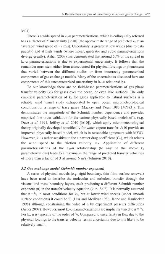
There is a wide spread in kw-u parameterizations, which is colloquially referred

to as a ‘factor of 2’ uncertainty [Jo10] (the approximate range of predicted kw at an

‘average’ wind speed of ~7 m/s). Uncertainty is greater at low winds (due to data

paucity) and at high winds (where linear, quadratic and cubic parameterizations

diverge greatly). Asher (2009) has demonstrated that around 50% of the spread in

kw-u parameterizations is due to experimental uncertainty. It follows that the

remainder must stem either from unaccounted-for physical forcings or phenomena

that varied between the different studies or from incorrectly parameterized

components of gas exchange models. Many of the uncertainties discussed here are

components of this uncharacterized uncertainty in kw-u relationships.

To our knowledge there are no field-based parameterizations of gas phase

transfer velocity (ka) for gases over the ocean, or even lake surfaces. The only

empirical parameterization of ka for gases applicable to natural surfaces is a

reliable wind tunnel study extrapolated to open ocean micrometeorological

conditions for a range of trace gases (Mackay and Yeun 1983 [MY83]). This

demonstrates the magnitude of the Schmidt number dependence and provides

empirical first-order validation for the various physically-based models of ka (e.g.

Duce et al. 1991, Jeffrey et al. 2010 [Je10]), which apply micrometeorological

theory originally developed specifically for water vapour transfer. Je10 provide an

improved physically-based model, which is in reasonable agreement with MY83.

However, ka is rather sensitive to the air-water drag coefficient (CD), which relates

the wind speed to the friction velocity, u. Application of different

parameterizations of the CD-u relationship (to any of the above ka

parameterizations) leads to a maxima in the range of predicted transfer velocities

of more than a factor of 3 at around 6 m/s (Johnson 2010).

3.2 Gas exchange model (Schmidt number exponent)

A series of physical models (e.g. rigid boundary, thin film, surface renewal)

have been used to describe the molecular and turbulent transfer through the

viscous and mass boundary layers, each predicting a different Schmidt number

exponent (n) in the transfer velocity equation (k ∝ Sc−n). It is normally assumed

that n=1/2 in most conditions for kw, but at lower wind speeds (under smooth

surface conditions) it could be 2/3 (Liss and Merlivat 1986, Jähne and Haußecker

1998) although constraining the value of n by experiment presents difficulties

(Asher 2009). However, most kw-u parameterizations are implicitly tuned to n=1/2.

For ka, n is typically of the order of 2/3. Compared to uncertainty in flux due to the

physical forcings to the transfer velocity terms, uncertainty due to n is likely to be

relatively small.


3.3 Estimation of physico-chemical gas and medium properties

The Henry’s law solubility of a gas is important in determining the magnitude

of ΔC and in the relative contribution of ka and kw to total transfer (LS74).

Solubility is highly sensitive to temperature and somewhat to salinity. Diffusion

coefficients (used to calculate Schmidt numbers in air and water) can be calculated

from simple molecular data but these are only accurate to within about ±20%

(Poling et al. 2001). For both solubility and diffusivity, accurate directly measured

values in seawater are the ideal. The densities and viscosities of air and water are

also required for calculating Schmidt numbers; these are relatively well

constrained in their relationships with temperature and salinity. For a gas where

solubility data in pure water is available, Jo10 estimates the maximum uncertainty

in flux calculation from estimating T and S dependent solubilities and Schmidt

numbers to be ~±30%. For gases where extensive study of physico-chemical

properties has been undertaken, uncertainty should be substantially less.

3.4 Common assumptions

Two assumptions are commonly applied to gas exchange calculations, which

may be appropriate in some cases or for some gases, but are not universal. Firstly,

following the findings of [LS74] that the exchange of the majority of gases they

considered was limited by kw, it is commonly assumed that Kw≈kw (i.e. that the

entirety of resistance to transfer is in the liquid phase). This assumption is often

made for DMS, although the air-side can contribute significantly to the resistance,

under some conditions leading to up to 20% estimates of the transfer velocity if it

is not considered (McGillis et al. 2000), whilst diiodomethane and methylnitrate

can both experience 50% contribution to transfer from each side of the interface

under typical conditions (Johnson et al. submitted). If the same assumption is

applied to a gas that is actually air-side controlled, then transfer velocity may be

overestimated by a factor of 10 to 100 for soluble gases such as methanol. These

uncertainties can be avoided by using the full flux equation with both ka and kw e.g.

according to Jo10.

Secondly it may be reasonable in some cases to assume that the concentration

in one of the phases is zero (i.e. that ΔC is dominated by the other phase). This

may be reasonable for e.g. gases such as DMS where production in seawater,

relatively low solubility and rapid reaction in the atmosphere lead to a water phase

driven concentration gradient. Nonetheless, in making this assumption there is

some overestimation of the flux, which may be as much as 5% in global estimates

(Turner et al. 1996; Turner et al. in prep). The same assumption has a much

greater effect for NH3, which occurs at similar concentrations in both phases but

has much greater solubility; it may lead to>30% overestimation of global marine

emissions (based on data in Johnson 2004 and Bouwman et al. 1997); and locally


may be much more significant.

4. Measurement uncertainty

4.1 Concentration measurements (for delta-C calculation)

With the appropriate expertise, most gas concentrations can be measured with

an analytical precision of a few percent or less. However uncertainties are

introduced in e.g. sample collection and storage issues, pressure, humidity and

salinity effects, etc. Nonetheless it is reasonable to assume that most bulk

concentration measurements should be within ±20% (and much better for high

quality measurements of well studied gases such as CO2). Measuring the

concentration at some distance from the interface does not account for sharp

concentration gradients approaching the surface due to biological heterogeneity or

photochemical production / loss near the surface. Furthermore, in the gas phase,

strong humidity gradients might potentially affect partitioning for some species

between gas and aerosol phases (e.g. Johnson 2004). Thus there is significant

uncertainty in the applicability of measured concentrations in either phase, which

we assume here, for simplicity, is part of the related uncertainties associated with

enrichment in the sea-surface microlayer (Section 5. 1) and averaging /

extrapolation of discrete measurements over time and space (Section 6).

4.2 Eddy covariance measurements

There is a large uncertainty associated with eddy covariance (EC)

measurements at sea, particularly due to the correction for the ships motion at very

high measurement frequency; plus drift and error corrections and (in some cases)

low precision from optical techniques. Precision depends on the gas in question;

e.g. CO2 EC fluxes are imprecise relative to DMS fluxes (Wannikhof et al. 2009),

due to the greater signal-to-noise ratio in DMS flux measurements as DMS is

relatively far from equilibrium between atmosphere and ocean. Also, concurrent

seawater concentration measurements are typically from 5m depth, subject to

some delay between sampling and analysis and often at lower frequency than gas

phase measurements (e.g. Jacobs et al. 2002). These uncertainties all contribute to

the overall uncertainty in kw-u parameterizations (Asher 2009). Recent

developments appear to have improved the precision of CO2 eddy covariance

measurements significantly (Prytherch et al. 2010).

5. Processes and phenomena

5.1 Microlayer effects

The sea-surface microlayer is (to a variable extent), physically, chemically and


biologically different from bulk surface seawater. It accumulates insoluble

organics produced in the surface ocean and can be a visible ‘oily’ film under some

conditions. It is subject to the maximum light intensity in the water column and

can be populated by very different microbial communities to those immediately

below in the bulk water, and in much higher (or lower) population densities

(Cunliffe et al. 2009). It can inhibit the kinetics of gas exchange by changing

turbulent properties at the surface, both as a ‘barrier’ to mass transport and by

inhibiting micro-turbulence in the bulk surface (Frew 1997). Recent experimental

work has suggested that this may be an important effect (Lee and Saylor 2010).

When the microlayer is sufficiently thick and dissimilar to bulk water, the two-

phase model of gas exchange may be incorrect and a three-phase model may be

more applicable (Martinelli 1979).

Enrichment or depletion of volatile compounds in the surface microlayer may

occur for 2 reasons: relatively insoluble gases may accumulate in the less polar

matrix of a microlayer rich in insoluble non-volatile organics; or there may be in-

situ production or destruction of a gas by photolytic or biological processes which

are enhanced in or unique to the microlayer environment. Enrichments of up to

and above an order of magnitude have been found for various chemical species

(e.g. Zhang et al. 2003), although for dissolved gases generally substantially less e.

g. Turner and Liss (1985). The collection and analysis of the microlayer is

extremely difficult, especially for volatile gases and so the potential uncertainty

introduced by measuring bulk seawater rather than microlayer surface

concentrations is largely unknown, although likely to be at a minimum in the open

ocean, where primary production and organic pollution are normally smaller than

in coastal environments, and where enrichment factors are likely to be relatively

small (Turner and Liss 1985; Yang and Tsunogai 2005).

In a microlayer that is physically and chemically different to bulk seawater, the

solubility of a gas may be altered. This will affect ΔC, but may also enhance or

inhibit transfer between the surface microlayer and the bulk water phase due to

differing solubilities. Neither of these effects has been quantified for any gas, to

our knowledge, and may vary greatly depending on the exact chemical

composition of the microlayer and the gas in question.

5.2 Bubbles

Bubbles become increasingly important in near-surface turbulence and water-

side controlled gas exchange processes with increasing wind, fetch and

whitecapping. There are at least four potential bubble effects, which are discussed

below. Wind tunnel and laboratory studies have indicated that there is a strong

solubility dependence of the importance of bubbles (backed up by theory e.g.

Memery and Merliva 1985; Keeling 1993; Asher et al. 1996; Woolf 1997; Woolf


et al. 2007). However the field data to support this in the ocean is rather limited,

particularly for far-from-equilibrium trace gases. The effect of bubbles in general,

and especially on gases of intermediate solubility is poorly understood, but of

potentially large significance to kw. Whether it increases the uncertainty beyond

that in the range of common kw parameterizations is unclear, even for gases of

different solubility to those used in the parameterizations. It is important to note

that whitecapping, bubble concentration and related parameters are not solely a

function of wind speed, with fetch and other factors such as wave age and wind-

wave orientation also being important. Therefore, no bubble effects can be entirely

represented by a gas exchange model driven solely by wind speed. As such, bubble

effects seem likely candidates for explaining a substantial amount of the>50% of

the deviation in kw-u relationships that cannot be explained by experimental /

measurement uncertainty (Asher 2009).

Disruption of the surface layer by bubble entrainment leads to a kinetic

enhancement of transfer, through increased turbulence and break-up of the

stagnant film with increasing bubble forcing; particularly through the return of the

turbulent bubble plume to the surface. There are contradictory observations in the

literature as to the significance of this bubble effect, however recent tank

experiments suggest that it is probably small relative to other bubble effects

(Woolf et al. 2007). This effect must be implicitly included in empirical kw-u

relationships, and there is no direct gas-specific (solubility / diffusivity related)

component. However, there may be secondary gas-specific effects with substantial

organic-rich microlayers, where breakup of such may modify microlayer

phenomenon (Section 4.1).

Bubbles also inject gases directly into surface water or can provide a

secondary pathway (on top of diffusive flux) for bidirectional exchange. Such

processes modify the composition of bulk surface seawater and are therefore ΔC

effects. There seems to be extensive confusion in the ‘secondary’ literature

(review papers, reference books, citing articles) regarding the causes, processes

and solubility-dependence of the bubble effect as proposed and developed by

Memery and Merlivat (1985), Woolf and Thorpe (1992), Keeling (1993), Asher et

al. (1996), Woolf (1997) etc. We suggest that much of this may be due to the

confusion caused by integrating the bubble fluxes (which are air-sea flux terms in

their own rights with their own concentration gradients and transfer velocities) into

the transfer velocity term of the diffusive flux. In practice is it difficult to

deconvolve the bubble flux and diffusive transfer velocity terms when deriving kw

from measured concentration gradients (e.g. from 14C, multiple tracer, or eddy

covariance studies), which is why the integrative approach is taken. Recent work

by Stanley et al. (2009) has presented a model where the bubble flux is considered

separately, which is an important development.


Some gas bubbles will fully dissolve and inject all their constituents directly

into surface water. This process is independent of any gas-specific properties and

depends only on the air-side concentration of the trace gas (and the bubble

volume). This process has been assessed and validated (e.g. Stanley et al. 2009)

and can lead to relative supersaturations of a few percent (where, at steady-state,

the downward injection flux is countered by an upward diffusive flux out of the

ocean). This effect is likely to be minor for gases which are far from equilibrium,

where a change in the degree of saturation of a few percent will represent a small

percentage change in ΔC.

Bubbles which don’t completely dissolve will tend to equilibrate (with respect

to the gas in question) with the water partially or completely. This ‘exchange

effect’ also favours supersaturation due to overpressure and surface tension

effects. It is complicated by the fact that some bubbles will inject gases into the

water column on their downward trajectory, but as they return to the surface and

their initial pressure they will be undersaturated and tend to re-absorb the gases;

and some gases may dissolve at a different rate to the bulk bubble gases (N2, O2).

The various models describing these bubble processes all predict a solubility-

dependence, which is due to the relative capacity of the small volume of air in a

bubble to carry molecules of insoluble and soluble gases at equilibrium between

water and bubble. It is the absence of this solubility-dependent bubble effect,

which has been proposed as the cause of apparently linear transfer velocities at

high wind speeds calculated from eddy covariance measurements of DMS fluxes

(Marandino et al. 2009; Huebert et al. 2010); and just such a kw-u relationship was

predicted for DMS by Woolf (1997). However, more field data is required to

validate the few observations currently available and field experiments to validate

the bubble process as the cause.

Vlahos and Monahan (2009) [VM09] propose a novel bubble-related process

which may affect any amphiphillic molecules (molecules with polar and non-

polar ends). They propose that the presence of bubbles would lead to adsorption of

such molecules to the bubble-water interface, removing them from exerting a

partial pressure at the air-sea interface, but not from being measured in seawater

concentration measurements. They interpret this as a change to the transfer

velocity, but it is really a ΔC effect, leading to similar confusion as for the

previous two bubble effects. Their proposed model can be used to explain the

apparent flattening of kw for DMS at high winds observed in recent Southern

Ocean data (Vlahos et al. 2011).

To date, there is limited empirical evidence that any bubble effects are strongly

gas-specific in the open ocean; at least not to the point where any uncertainty

introduced is greater than the range of standard kw-u parameterizations. Important

questions yet to be answered are i) what is the threshold gas solubility at which the


bubble effect stops being important for a particular set of conditions? and ii) how

robust are the ‘average’ wind-speed whitecapping relationships? e. g. Woolf

(2005), Goddijn-Murphy et al. (in press).

5.3 Chemical Enhancement

The enhancement of gas transfer by chemical reaction changing the

concentration gradient through the rate limiting surface layer has been assessed

and observed for a small number of gases (O3, CO2, SO2). The degree of possible

enhancement depends on the reaction rate relative to the rate of transport through

the mass boundary layer and is thus strongly dependent on the reactivity of the gas

of interest, wind speed and temperature. Because this effect occurs within the mass

boundary layer (s), it has characteristics of both a k and ΔC effect. It modifies the

apparent solubility and therefore the effective concentration gradient, but due to

the ‘bending’ effect on the concentration gradient (e.g. Wanninkhof and Knox,

1992) it also changes the apparent depth of the rate-limiting layer. However, the

only practical way to consider the enhancement mathematically is as a

multiplication factor (α) to ka or kw because the enhancement is specific to

reactions in one phase so the chemical enhancements must be applied to that

specific phase.

The chemical enhancement by hydration reactions of CO2 (e.g. Hoover and

Berkshire 1969 [HB69], Wanninkhof and Knox 1996, Keller 1994), SO2 (Liss

1971) and O3 (Fairall et al. 2007) have been studied previously. Hydration of CO2

to carbonic acid is a reversible reaction. Forward and reverse reactions rates differ,

thus the enhancement to flux is asymmetrical. Although this is a minor effect for

CO2 hydration it may be important in other reactions. The effect of this

enhancement on estimates of global CO2 flux is unresolved, with estimates ranging

from 0 to 20% (Keller 1994). It is worth noting that this effect is implicitly

accounted for in bomb 14C-derived kw-u relationships e. g. Wanninkhof 1992,

Naegler et al. 2006 etc. In contrast to CO2, SO2 is so reactive in water that (at

seawater pH) it almost instantaneously hydrates, such that the flux of SO2 is

always downwards. Liss and Slater (1974) demonstrate by adapting the HB69

model, that the enhancement to kw for SO2 is such that the resistance is entirely on

the air-side, as it would be for a much more soluble gas. Care must be taken when

considering the enhancement due to hydration for other gases. For extremely fast

hydration reactions, such as that of formaldehyde, it is impossible to measure the

Henry’ s law constant in isolation from this effect and so measured solubility

implicitly includes the hydration term (Johnson et al. submitted).

Other reversible reactions such as acid-base and redox reactions may also lead

to chemical enhancement, if they are sufficiently rapid. Protonation reactions tend

to be extremely fast, for example. In the case of ammonia it can be demonstrated


that significant chemical enhancement can occur at pH < ~8.5 (Johnson et al.

submitted) due to protonation to ammonium..

Irreversible reactions may also modify the flux, with one major difference to

the above: without a reservoir of reacted species to buffer the addition or removal

of gas from the surface layer through air-sea flux, a reaction can either enhance or

inhibit the flux depending on its direction. For example, if a compound is rapidly

photolysed at the surface this will enhance a flux into the ocean, but inhibit a flux

out. It is not uncommon for photolysis reaction rate constants in water to be of the

order of 10−3 s−1 e.g. Martino et al. (2005), which is sufficiently fast to modify the

flux under low-to-moderate wind conditions (Johnson et al. submitted).

Solving the HB69 equation for the rate of reaction required for a given

enhancement reveals that many candidate reactions might be rapid enough to

cause a significant enhancement at moderate windspeeds for a range of gases

(Johnson et al. submitted), so this uncertainty, which is not implicitly included in

empirical parameterizations of gas transfer, must be considered on a case-by-case

basis. The generalized version of the HB69 equation can equally be applied to the

air-side of the interface and such analysis demonstrates that much higher rate

constants are required for substantial enhancement. Gas phase reactions do tend to

be faster than those in seawater but we are yet to identify any that would

significantly enhance or inhibit the flux of gases of biogeochemical interest.

5.4 Heat and water fluxes

There are various ways in which the transfer of heat and water between ocean

and atmosphere might affect the flux of gases. In a laboratory study Ho et al.

(1997) found a ‘significant and systematic’ enhancement of the exchange of SF6

by simulated rainfall, due to the kinetic effect of increased turbulence.

Furthermore, it is possible that diluting the surface of the ocean may change the

concentration gradient across the air-sea interface and alter the solubility (through

the temperature, salinity or polarity of the medium), and may also change the

viscosity of the surface layer, leading to an alteration of the transfer velocity. Turk

et al. (2010) demonstrate that rainfall can also indirectly affect ΔC for CO2

substantially, by altering carbonate chemistry. Rainfall is also likely to

substantially deplete soluble gases in the boundary layer atmosphere, further

affecting ΔC.

Micro-scale stratification or instability due to temperature differences between

the atmosphere and ocean might be expected to affect the transfer velocity, at least

at low wind speeds when wind stress is small. However, there is limited evidence

to support this (Nightingale and Liss 2004). For example Liss et al. (1981) found

no significant evidence of enhancement to transfer by evaporative conditions in

their wind tunnel study, although under condensing conditions they did observe a


significant decrease in transfer velocity due to increased stability. Such stability

effects may be stronger and more significant on the air side of the interface, and so

of greater significance for soluble trace gases; this is uninvestigated to date,

however.

A ‘cool skin’ effect, due to surface evaporation, causes modification of the

solubility and therefore concentration gradient of the gas of interest across the rate-

limiting boundary layer (e.g. Robertson and Watson 1992). A warm skin due to

solar heating might have the opposite effect. However, McGillis and Wanninkhof

(2006) suggest that these effects are probably minor due to the difference in length

scales of the temperature and mass boundary layers and this is borne out in the

field data of Ward et al. (2004). Furthermore, in situations where an evaporative

cool skin may exist there is likely to be an enhancement to salinity at the surface,

which will approximately cancel out the temperature effect, at least for CO2

(Takahashi et al. 2009).

A further phenomenon arises from the effects of the interactions between heat

and gas fluxes. Such ‘irreversible thermodynamic’ effects, due to the inherent

coupling of heat and mass fluxes may be significant under certain conditions

(Phillips 1994, 1997), although this has been challenged by Doney (1994, 1995)

for the case of insoluble gases under water-phase control. This matter is

unresolved, although it is invariably assumed that under environmental conditions

where the temperature difference across the interface tends to be small, the effect

is insignificant (Nightingale and Liss, 2004). It is important to note that the

possible effect on soluble gases has not previously been studied (to our

knowledge) and any potential effect is entirely unknown.

5.5 Biological effects

Biological activity can potentially directly or indirectly affect air-sea flux in a

number of ways, most of which remain largely unstudied, and none are included in

models of air-sea gas exchange, in part due to the difficulty in parameterizing such

irregular effects. They may be included implicitly in the empirical kw-u

parameterizations, however, at least for the gases on which the parameterizations

are based, and the conditions under which the measurements were made.

Just as chemical reactions might enhance or inhibit transfer by modifying the

concentration gradient in the mass boundary layers, biological activity might

achieve the same, at least on the water side, by production or consumption. There

is some empirical evidence that this may be the case for methane (Upstill-

Goddard et al. 2003), and O2 / CO2 (Garabetian, 1991; Matthews, 1999) and the

rates required are not inconceivable (Johnson et al. submitted). Furthermore,

Calleja et al. (2005) found that planktonic metabolism in the top few cm of the

ocean can control the magnitude and direction of air-sea CO2 flux.


It is also interesting to consider the effect of changes in mixed layer depth in

response to wind speed during transient events and how this might affect

concentrations through biological responses. A deepening mixed layer may tend to

transiently reduce primary production (as phytoplankton are exposed to lower

average light intensities) or increase it (if nutrient limitation is relieved by

entrained nutrients from below the thermocline). Changes in UV stress on the

bacterial population associated with being mixed away from the surface may also

have significant effects on particular gas concentrations e.g. DMS consumption by

bacteria is thought to be UV limited. Deepening or shoaling of the mixed layer

could be considered as a form of intermediate disturbance and as such is likely to

lead to changes in ecosystem structure on relatively short timescales (days to

weeks). As many trace gas concentrations are the net result of a complex web of

production and loss terms, strongly dependent on ecosystem composition and

function, such changes are likely to be of significance to air-sea fluxes. However,

where fluxes are calculated from in-situ measured concentrations, and not

extrapolated in space or time, such biological effects are implicitly accounted for.

The effect of biologically-induced turbulence at or immediately below the

surface layer will enhance k. Whilst the turbulence caused by large organisms

(fish, seagulls, whales and the like) may be very significant in extremely localized

terms (i. e. scales of metres and minutes), we assume they are unlikely to be

significant at the larger scale (kilometres and days). However, it has been

suggested that the action of flagella of motile microorganisms may contribute

significantly to turbulence and gas transfer in the surface layer of the ocean (Paul

Twitchell, ONR Boston, pers. comm.; Gladyshev 1997). It is unclear (due to lack

of evidence) how significant this effect might be, but it is probably small.

6. Averaging and interpolation / extrapolation

To quantify the local, regional or global air-sea flux of a trace gas, it is

necessary to interpolate between spatial measurements and/or extrapolate from

near-instantaneous measurements in time. Furthermore, averaging of measured

data is necessary to generate pre-interpolation fields for 2D estimates from discrete

measurements (e. g. Lana et al. 2011). All of these processes introduce

uncertainties, some of which are well quantified, others less so.

6.1 What is a representative average concentration?

Biological production and consumption and physical mixing can lead to short

term / small scale variability in concentrations which means that all but the highest

resolution concentration measurements are rather difficult to average. For highly

bio-reactive compounds this is particularly problematic. For instance, the standing


stock of ammonia in surface waters can be turned over on timescales of a few

hours to a day in highly productive waters and de-coupling of production and loss

processes can lead to transient spikes in ammonium concentration of as much as an

order of magnitude above the ambient (Johnson et al. 2007). Other gases which are

rapidly turned-over by biological or chemical processes e. g. CH2I2 photolysis

(Martino et al. 2005) may be subject to similar transient peaks due to other

decouplings. In evidence of this, the frequency distributions of many observations

of trace gas concentrations in seawater are positively skewed, with a long ‘tail’ of

high values. Combined with spatial heterogeneity due to local-scale physical

processes, this means that low resolution measurements in seawater can yield

unrepresentative concentrations over e.g. a day on a research cruise. Gas phase

concentrations are more likely to be measured continuously, although possibly

integrating over long periods (which introduces uncertainties in itself); however if

low-temporal-resolution instantaneous concentrations are measured e.g. by flask

sampling, changes in concentration due to e.g. air-mass source may be overlooked.

Extrapolating to the regional or global scale introduces even greater

uncertainty. For instance, the recently published update to the global seawater

DMS database (Lana et al. 2011) contains approximately 5x104 discrete

measurements, making it the second most measured trace gas in the ocean, after

CO2. Nonetheless, the uncertainty introduced by interpolation and extrapolation

(as estimated by Lana et al. 2011), when applied over biogeochemical provinces to

give a regionally-resolved estimate of the net global DMS flux from the ocean, is

approximately the same as the difference between applying Liss and Merlivat

(1986) and Wanninkhof (1992) to calculate the flux from the concentration and

wind fields. This suggests that for less well studied gases, extrapolating global flux

estimates from concentration alone (without attempting to understand and model

underlying biogeochemical production and loss processes) is insufficient to

attempt anything other than single-point global average flux estimates (e.g. Turner

et al. in prep).

6.2 Environmental forcing parameters

In order to calculate fluxes from extrapolated concentrations it is necessary to

apply interpolated or averaged temperature, salinity and windspeeds. We assume

that temperature and salinity are relatively well constrained, with the average error

on e.g. satellite retrieval of temperature being less than 1oC (Wanninkhof et al.

2009) and much less from direct measurements; and salinity being relatively well

constrained in the field and in climatological data. In field studies quoting near-

instantaneous fluxes from concentration measurements it is common to use e.g. 7

day averaged winds to give a representative flux over a meaningful period of time

(e.g. Hughes et al. 2009), or where there is a long atmospheric integration time


over a spatial range, to apply mean windspeed over that time period (e.g. Johnson

et al. 2008). Either of these is a valid approach but they may yield substantially

different results. Nonetheless the in situ windspeed measurements used are likely

to be rather precise and at high temporal resolution so the uncertainty is likely to

be relatively minor. When extrapolating over wider spatial and temporal scales

longer term averaged and/or time-varying wind data e.g. NCEP reanalysis data or

satellite-retrieved winds are used. Reanalyis and satellite data can differ

significantly due to the lack of resolution of short time and spatial scale details in

the former, which leads to a 1.3 m/s difference in the global annual average wind

speed between NCEP and QuickSCAT (Naegler et al. 2006), and variability in

spatial wind distributions (Wanninkhof et al. 2009). Further error can be

introduced by incorrectly applying long-term averaged winds, due to the

inequality between e.g. the square of the mean wind speed and the mean of the

wind speed squared (Wanninkhof et al. 2009).

6.3 Steady-state assumption

Flux estimates are generally based on a steady-state assumption, i.e. that over

the integration / extrapolation period of a flux calculation, processes controlling

the concentration gradient are constant. One can envisage this assumption falling

down in a number of cases e.g. i) where the flux of the gas is rapid relative to its


Table 2 Key uncertainties

Source of uncertainty Wor

st c

ase

Ufl u

x

Rum

sfel

cian

Cla

ssifi

catio

n

Gas types and/or conditions under which uncertainty is maximized

ka-u parameterization XL KU Highly soluble gases; water-side highly chemically-enhanced e.g. SO2; ka windspeed relationship poorly known. Use of e.g. Jo10 may cause over or underestimation

Bubble exchange effect XL KU Gases of intermediate solubility where kw dominates transfer, but where bubble effect is much smaller than for the insoluble gases used in kw-u parameterizations e.g. DMS, alkyl nitrates, most halocarbons. Use of standard kw-u parameterizations will lead to overestimation of fl uxes.

Bubble adsorption effect XL UU Amphiphillic compounds; high winds. Overestimation of seawater partial pressure will lead to overestimation of sea-air fl uxes.

Microlayer kinetic inhibition XL KU Low to moderate winds; productive or polluted waters.Microlayer solubility L UU Low to moderate winds; particularly (water) soluble or insoluble gases

Chemical enhancement XL KU Compounds undergoing rapid reaction in surface ocean or atmosphere; low winds. May enhance or inhibit, and be very weakly or very strongly assymetrical.

Stratifi cation / instability L UU Large temperature difference between ocean and atmosphere. Effect for ka-controlled gases particularly poorly known.

Irreversible thermodynamics L UU largely unknownBiological enhancement L UU kw-controlled compounds rapidly produced or consumed by plankton community.

ΔC due to biological response to mixed layer

deepening

L UU Compounds whose production / consumption would be affected by community response to mixing to depth. May result in change in fl ux magnitude or direction. Signifi cant when average concentrations extrapolated over changing windspeeds.

Concentration averaging / interpolation / extrapolation

XL KU All gases. Averaging / extrapolations over large ranges of space and/or time, particularly when data is sparse and locally / regionally / seasonally biased.

Steady state assumptions L UU Long timescale / high wind / highly variable wind conditions.

concentration (or production / consumption rate) in one or both phases; ii) where

concentration changes occur coupled to changes in variables which drive transfer

velocity (e.g. wind speed, temperature). Both of the above almost certainly occur

under some conditions. For instance i) the typical amount of e.g. methanol or

ammonia in the atmosphere is small relative to the flux at high wind speeds

leading to a relatively rapid decrease in ΔC as winds become strong and ii) an

increase in wind strength may increase or decrease the concentration gradient

between atmosphere and ocean by mixing surface waters with deeper ones,

depending on the nature of any existing concentration gradient with depth in the

bulk ocean. Such a mixing-driven dilution might lead to a reduction in the

significance of the higher winds to the net flux of a gas which was supersaturated

in seawater (or an increase for one which was undersaturated); or even potentially

a reversal in net flux direction. Coupling between fluxes of different gases which

interact in atmosphere and/or water will also tend to break the steady-state

assumption. For instance, Johnson and Bell (2008) invoke the potential for DMS-

driven ‘co-emission’ of NH3 to explain the constancy in aerosol ammonium to

non-seasalt sulfate reactions; and the flux predicted from NH3 concentrations alone

is different to that with DMS emissions driving the ammonia flux in their model.

7. Conclusions

We have presented a wide range of potential uncertainties involved in

quantifying air-sea gas exchange, from the well-known to the obscure. Based on

their Rumsfeldian classification and their potential ‘worst case’ magnitude (Table

1), we can identify the key uncertainties which need improvement to better

constrain air-sea gas exchange. These are summarized in Table 2, along with

information on the types of gases affected and the conditions under which the

uncertainty is likely to be at a maximum. Note that other uncertainties may be

extremely important as well, particularly in atypical cases e.g. studies where heavy

rain dominated meteorological conditions, or polluted estuarine situations where

microlayer effects may be much more important than normal.

It is unrealistic to expect that all future studies will be able to investigate all

possible uncertainties for their gases of interest to produce robust uncertainty

estimates. Unfortunately no all-encompassing rules of thumb can be applied,

particularly in the case of biological effects or chemical enhancement. However, in

terms of the KKs and KUs associated with water-side transfer it is useful to

observe that application of the commonly-used N00 parameterization with error

bars of±50% covers more than 75% of the range of kw parameterizations at wind

speeds between approximately 4 and 13 m/s. As such, this might be considered a

reasonable uncertainty range, representative of the true magnitude of the


uncertainties in estimates of fluxes of insoluble gases under typical conditions. A

similar ±50% applied to ka might also be reasonable.

Acknowledgements

We are indebted to Dr. David Woolf (Environmental Research Institute,

Thurso, UK) for valuable discussion and advice on how to best present the effect

of bubbles on air-sea gas exchange. This work was funded by the Natural

Environment Research Council of the United Kingdom under the following grants:

NE/F017359/1 (M.T. J.), NER/E013287/1 (C.H.), NE/H020888 (T.G.B.) and

NE/E001696/1 (P.S.L.).

References

Asher, W. E., (2009), The effects of experimental uncertainty in parameterizing air-sea gas

exchange using tracer experiment data, Atmos. Chem. Phys., 9, 131-139.

Asher, W. E., L. M. Karle, B. J. Higgins, P. J. Farley et al. (1996) The influence of bubble

plumes on air-seawater gas transfer velocities, J. Geophys. Res. 101 (C5), 12027-12041.

Bouwman, A. F., D. S. Lee, W. A. H. Asman, F. J. Dentener et al. (1997) A global high-

resolution emission inventory for ammonia, Global Biogeochem. Cy. 11, 561-587, doi:10.

1029/97GB02266.

Calleja, M. L., C. M. Duarte, N. Navarro and Susana Agusti, (2005) Control of air-sea CO2

disequelibria in the subtropical NE Atlantic by planktonic metabolism under the ocean

skin, Geophys. Res. Lett.32,art. no. L08606, doi:10.1029/2004GL022120.

Cunliffe, M., A. Whitely, H. Schafer, L. Newbold et al. (2009) Comparison of

bacterioneuston and bacterioplankton dynamics during a phytoplankton bloom in an fjord

microcosm, Appl. Env. Microbiol., 75, 7173-7181.

Doney, S. C., (1994) Irreversible thermodynamic coupling between heat and matter fluxes

across a gas-liquid interface, J. Chem. Soc. Faraday Trans., 90, 1865-1874.

Doney, S. C., (1995) Irreversible thermodynamics and air-sea exchange, J. Geophys. Res.,

100(C5), 8541-8553.

Duce, R. M., P. S. Liss, J. T. Merrill, E. L. Atlas et al. (1991) The atmospheric input of trace

species to the World Ocean, Global Biogeochem. Cycles, 5, 193-259.

Fairall, C. W., D. Helmig, L. Ganzevald and J. Hare, (2007) Water-side turbulence

enhancement of ozone deposition to the ocean, Atmos. Chem. Phys., 7, 443-451.

Frew, N. M. (1997), The role of organic films in air-sea gas exchange, in The sea surface

and global change, Eds: P. S. Liss and R. A. Duce, Cambridge University Press, 121-173.

Garabetian, F., (1991), 14C-glucose uptake and 14C-CO2 production in surface microlayer

and surface water samples: influence of UV and visible radiation, Mar. Ecol. Prog. Ser,

77, 21-26..

Gladyshev, M. I. (1997), Biophysics of the surface film of aquatic ecosystems, in The sea

surface and global change, Eds: P. S. Liss and R. A. Duce, Cambridge University Press,

321-337.

Goddijn-Murphy, L., D. K. Woolf and A. H. Callaghan, Parameterizations and algorithms

for ocean whitecap coverage, J. Phys. Oceanog, in press.

Ho, D. T., L. F. Bliven, R. Wannkinkhof and P. Schlosser, (1997) The effect of rain on air-

water gas exchange, Tellus B., 49, 149-158.


Hoover, T. and D. Berkshire, (1969) Effects of hydration on Carbon Dioxide exchange

across an air-water interface, J. Geophys. Res., 74, 456-464.

Huebert, B. J., B. W. Blomquist, M. X. Yang, S. D. Archer et al. (2010) Linearity of DMS

transfer coefficient with both friction velocity and wind speed in the moderate wind speed

range, Geophys. Res. Lett.37, art. no. LO1605, doi:10.1029/2009GL041203.

Hughes, C., A. L. Chuck, H. Rossetti, P. J. Mann, et al. (2009) Seasonal cycle of seawater

bromoform and dibromomethane concentrations in a coastal bay on the Western Antarctic

Peninsula, Global. Biogeochem. Cy,. 23, art. no. GB2024, doi:10.1029/2008GB003268.

Jacobs, C., J. F. Kjeld, P. Nightingale, R. Upstill-Goddard, et al. (2002), Possible errors in

CO2 air-sea transfer velocity from deliberate tracer releases and eddy covariance

measurements due to near-surface concentration gradients.

Jähne, B. and Haußecker, (1998) Air-water gas exchange, Ann. Rev. Fluid. Mech., 30, 443-

468.

Jacobs, C., J. F. Kjeld, P. Nightingale, R. Upstill-Goddard et al. (2002) Possible errors in

CO2 air-sea transfer velocity from deliberate tracer releases and eddy covariance

measurements due to near-surface concentration gradients, J. Geophys. Res., 107, 3128,

doi:10.1029/2001JC000983.

Jeffery, C. D., I S. Robinson and D. K. Woolf, (2010) Tuning a physically-based model of

the air-sea gas transfer velocity, Ocean Modelling, 31, 28-35.

Johnson, M. T., (2004), The air-sea flux of ammonia, PhD Thesis, University of East

Anglia, Norwich, UK.

Johnson, M. T., (2007), Ammonium accumulation during a silicate-limited diatom bloom

indicates the potential for ammonia emission events, Mar. Chem., 106(1-2), 63-75.

Johnson, M. T., P. S. Liss, T. G. Bell, T. Lesworth et al. (2008), Field observations of the

ocean-atmosphere exchange of ammonia: fundamental importance of temperature as

revealed by a comparison of high and low latitudes, Global Biogeochem. Cy., 22, Art. No.

GB1019, doi:10.1029/2007GB003039.

Johnson, M. T. and T. G. Bell, Coupling between dimethylsulfide emissions and the ocean-

atmosphere exchange of ammonia, Environ. Chem., 5, 259-267.

Johnson, M. T. (2010) A numerical scheme to calculate the temperature and salinity

dependent air-water transfer velocity for any gas, Ocean Sci., 6, 913-932.

Johnson, M. T., C. Hughes, J. Woeltjen, T.G. Bell, M. Martino and P. S. Liss, Transfer

velocities for a suite of trace gases of emerging biogeochemical importance: Liss and

Slater (1974) revisited, submitted to Environmental Science and Technology.

Keeling, R., (1993) On the role of large bubbles in air-sea gas exchange and supersaturation

in the ocean, J. Mar. Res., 51, 237-271.

Keller, K., (1994) Chemical Enhancement of Carbon Dioxide Transfer across the Air-Sea

Interface, MSc Thesis, Massachusetts Institute of Technology, 1994.

Lana, A., T. G. Bell, R. Simo, S. M. Vallina et al. (2011, in press) An updated climatology

of surface dimethylsulfide concentrations and emission fluxes in the global ocean, Global

Biogeochem. Cycles, doi:10.1029/2010GB003850

Lee, R. J. and J. R. Saylor, (2010) The effect of a surfactant monolayer on oxygen transfer

across an air/water interface during mixed convection, Int. J. Heat Mass Transfer, 53,

3405-3413.

Liss, P.S., (1971) Exchange of SO2 between the atmosphere and natural waters, Nature, 233,

327-329.

Liss, P. S. and P. G. Slater (1974) Flux of gases across the air-sea interface, Nature, 247,


181-184.

Liss, P. S., P. Balls, F. N. Martinelli and M. Coantic, (1981) The effect of evaporation and

condensation on gas transfer across and air-water interface, Oceanol. Acta, 4, 129-138.

Liss, P. S. and L. Merlivat (1986) Air-sea gas exchange rates: Introduction and synthesis in:

The role of air-sea exchange in geochemical cycling, Ed: P. Buat-Menard, D. Riedel,

Hingham, MA, 113-139.

Mackay, D. and A. T. K. Yeun, (1983) Mass transfer coefficient correlations for

volatilization of organic solutes from water, Environ. Sci. Technol. 17, 211-217.

Marandino, C. A., W. J. De Bruyn, S. D. Miller and E. S. Saltzman, (2009) Atmos. Chem.

Phys. 9, 345-356.

Martinelli, F. M. (1979) The effect of surface films on gas exchange across the air-sea

interface, PhD Thesis, University of East Anglia, Norwich, UK.

Martino, M., P. Liss and J. Plane, (2005) The photolysis of dihalomethanes in seawater,

Environ.Sci. Technol. 39, 7097-7101.

Matthews, B. J. H, (1999) The rate of air-sea CO2 exchange: chemical enhancement and

catalysis by marine microalgae, PhD Thesis, University of East Anglia, Norwich, UK.

McGillis, W. R., J. W. H. Dacey, N. M. Frew, E. J. Bock et al. (2000) Water-air flux of

dimethylsulfide, J. Geophys. Res., 105 (C1), 1187-1193.

McGillis, W. R., J. B. Edson, J. D. Ware, J. W. H. Dacey et al. (2001) Carbon dioxide flux

techniques performed during GasEx-98, Mar. Chem., 75, 267-280.

McGillis, W. R. and R. Wanninkhof, (2006), Aqueous CO2 gradients for air-sea flux

estimates, Mar. Chem., 98 (1), 100-108.

Memery, L. And L. Merlivat, (1985) Modelling of the gas flux through bubbles at the air-

water interface, Tellus, 37B, 272-285.

Naegler, T., P. Ciais, K. Rodgers, I. Levin, (2006) Excess radiocarbon constraints on air-sea

gas exchange and the uptake of CO2 by the ocean, Geophys. Res. Lett., 33, art. no.

L11802, doi:10.1029/2005GL025408.

Nightingale, P. D., G. Malin, C. S. Law, A. J. Watson et al. (2000) In situ evaluation of air-

sea gas exchange parameterizations using novel conservative and volatile tracers, Global

Biogeochem. Cycles, 14, 373-387.

Nightingale, P. D. and Liss, P. S., (2004) Gases in Seawater. In Treatise on Geochemistry

volume 6: The Oceans and Marine Geochemistry, Ed. Elderfield, H., Elsevier Permagon,

Oxford.

Phillips, L. F., (1994) Experimental demonstration of coupling of heat and matter fluxes at a

gas-water interface, J. Geophys. Res., 100, 14347-14350.

Phillips, L. F. (1997) The physical chemistry of air-sea gas exchange, in The sea surface and

global change, Eds: P. S. Liss and R. A. Duce, Cambridge University Press,207-250.

Poling, B. E., J. M. Prausnitz and J. P. O’Connel, (2001) The Properties of Gases and

Liquids 5th Edition, McGraw-Hill, New York.

Prytherch, J., M. J. Yelland, R. W. Pascal, B. I. Moat et al. (2010) Direct measurements of

the CO2 flux over the ocean: Development of a novel method, Geophys. Res. Lett., 37, art.

no. L03607, doi:10.1029/2009GL041482.

Robertson, J.E., and A. J. Watson, (1992) Thermal skin effect of the surface ocean and its

implications for CO2 uptake, Nature, 358, 738-740.

Stanley R., W. J. Jenkins, D. E. Lott and S. C. Doney. (2009) Noble gas constraints on air-

sea gas exchange and bubble fluxes, J. Geophys. Res. 114, C11020, doi: 10.

1029/2009JC005396


Takahashi, T., S. C. Sutherland, R. Wanninkhof, C. Sweeney, et al. (2009), Climatological

mean and decadal change in surface ocean pCO2, and net sea-air CO2 flux over the global

oceans, Deep Sea Res. (II), 56 (8-10), 554-577.

Turk, D., C. J. Zappa, C. S. Meinen, J. R. Christian et al. (2010) Rain impacts on CO2

exchange in the western equatorial Pacific Ocean, Geophys. Res. Lett., 37, art. no.

L23610, doi:10.1029/2010GL045520.

Turner, S. M. and P. S. Liss, (1985) Measurements of various sulphur gases in a coastal

marine environment, J. Atmos. Chem., 2, 223-232.

Turner, S. M., G. Malin, P. D. Nightingale, P. S. Liss, (1996) Seasonal variation of dimethyl

sulphide in the North Sea and an assessment of fluxes to the atmosphere, Mar. Chem. 54,

245-262.

Turner, S., M. T. Johnson and P. S. Liss, Selenium: the marine perspective, in preparation

for submission to Proceedings of the Royal Society A.

Upstill-Goddard, R., T. Frost, G. R. Henry, M. Franklin et al. (2003) Bacterioneuston

control on air-water methane exchange determined with a laboratory gas exchange tank,

Global.Biogeochem. Cycles, art. no. 1108, doi:10.1029/2003GB002043.

Vlahos, P. and E. C. Monahan, (2009) A generalized model for the air-sea transfer of

dimethyl sulfide at high wind speeds, Geophys. Res. Lett., 36, L21605, doi: 10.

1029/2009GL040695.

Vlahos, P.. E. C. Monahan, B. J. Huebert and J. B. Edson, (2011) Wind-Dependence of

DMS Transfer Velocity: Comparison of Model with Recent Southern Ocean

Observations, this book.

Wanninkhof, R. (1992) Relationship between wind speed and gas exchange over the ocean,

J. Geophys. Res., 97, 7373-7382.

Wanninkhof, R. and M. Knox, (1996) Chemical enhancement of CO2 exchange in natural

waters, Limnol. Oceanogr. 41, 689-697.

Wanninkhof, R., W. E. Asher, D. T. Ho, C. Sweeney and W. R. McGillis, (2009) Advances

in quantifying air-sea gas exchange and environmental forcing, Annu. Rev. Mar. Sci., 1,

213-244.

Ward, B., R. Wanninkhof, W. R. McGillis, A. T. Jessup et al. (2004) Biases in the air-sea

flux of CO2 resulting from ocean surface temperature gradients, J. Geophys. Res. 109, art.

no. C08S08, doi:10.1029/2003JC001800.

Woolf, D. K. And S. Thorpe, (1992) Bubbles and the air-sea exchange of gases in near-

saturation conditions, J. Mar. Res., 49, 435-466.

Woolf, D. K. (1997), Bubbles and their role in gas exchange, in The sea surface and global

change, Eds: P. S. Liss and R. A. Duce, Cambridge University Press, 173-205.

Woolf, D. K., (2005) Parameterization of gas transfer velocities and sea-state-dependent

wave breaking, Tellus, 57B, 87-94.

Woolf, D. K., I. S. Leifer, P. D. Nightingale, T. S. Rhee et al. (2007) Modelling of bubble-

mediated gas transfer: fundamental principles and a laboratory test, J. Mar. Sys., 66, 71-

91.

Yang, G. and S. Tsunogai, (2005) Biogeochemistry of dimethylsulfide (DMS) and

dimethylsulfiopropionate (DMSP) in the surface microlayerof the western North Pacific,

Deep Sea Res. Pt. I., 52, 553-567.

Zappa, C. J., D. T. Ho, W. R. McGillis, M. L. Banner et al. (2009) Rain-induced turbulence

and air-sea gas transfer, J. Geophys. Res., 114, art. no. C07009, doi: 10.

1029/2008JC005008.


Zhang, Z., L. Liu, C. Liu and W. Cai, (2003) Studies on the sea surface microlayer: II. The

layer of sudden change of physical and chemical properties, J. Coll.Interface Sci., 264,

148-159.


Title Hunt, J.; Belcher, S.; Stretch, D.; Sajjadi, S.;...

Documents

Transcript of Title Hunt, J.; Belcher, S.; Stretch, D.; Sajjadi, S.;...