THREE-YEAR WILKINSON MICROWAVE ANISOTROPY PROBE …...redshift supernova (Riess et al. 2004; Astier...

THREE-YEAR WILKINSON MICROWAVE ANISOTROPY PROBE (WMAP) OBSERVATIONS:IMPLICATIONS FOR COSMOLOGY

D. N. Spergel,1,2

R. Bean,1,3

O. Dore,1,4

M. R. Nolta,4,5

C. L. Bennett,6,7

J. Dunkley,1,5

G. Hinshaw,6

N. Jarosik,5E. Komatsu,

1,8L. Page,

5H. V. Peiris,

1,9,10L. Verde,

1,11M. Halpern,

12R. S. Hill,

6,13

A. Kogut,6M. Limon,

6S. S. Meyer,

9N. Odegard,

6,13G. S. Tucker,

14

J. L. Weiland,6,13

E. Wollack,6and E. L. Wright

15

Received 2006 March 16; accepted 2007 January 12

ABSTRACT

A simple cosmological model with only six parameters (matter density,�mh2, baryon density,�bh

2, Hubble con-stant, H0, amplitude of fluctuations, �8, optical depth, � , and a slope for the scalar perturbation spectrum, ns) fits notonly the 3 yearWMAP temperature and polarization data, but also small-scale CMB data, light element abundances,large-scale structure observations, and the supernova luminosity/distance relationship.UsingWMAP data only, the best-fit values for cosmological parameters for the power-law flat � cold dark matter (�CDM) model are (�mh

2;�bh2;

h; ns; �; �8)¼ (0:1277þ0:0080�0:0079;0:02229� 0:00073;0:732þ0:031

�0:032;0:958� 0:016;0:089� 0:030; 0:761þ0:049�0:048). The 3 year

data dramatically shrink the allowed volume in this six-dimensional parameter space. Assuming that the primordialfluctuations are adiabatic with a power-law spectrum, the WMAP data alone require dark matter and favor a spectralindex that is significantly less than the Harrison-Zel’dovich-Peebles scale-invariant spectrum (ns ¼ 1; r ¼ 0). Addingadditional data sets improves the constraints on these components and the spectral slope. For power-lawmodels,WMAPdata alone puts an improved upper limit on the tensor-to-scalar ratio, r0:002 < 0:65 (95% CL) and the combination ofWMAP and the lensing-normalized SDSS galaxy survey implies r0:002 < 0:30 (95% CL). Models that suppress large-scale power through a running spectral index or a large-scale cutoff in the power spectrum are a better fit to theWMAPand small-scale CMB data than the power-law �CDMmodel; however, the improvement in the fit to theWMAP datais only ��2 ¼ 3 for 1 extra degree of freedom. Models with a running-spectral index are consistent with a higheramplitude of gravity waves. In a flat universe, the combination ofWMAP and the Supernova Legacy Survey (SNLS)data yields a significant constraint on the equation of state of the dark energy,w ¼ �0:967þ0:073

�0:072. If we assumew ¼ �1,then the deviations from the critical density, �K , are small: the combination of WMAP and the SNLS data implies�k ¼ �0:011� 0:012. The combination of WMAP 3 year data plus the HST Key Project constraint on H0 implies�k ¼ �0:014� 0:017 and �� ¼ 0:716� 0:055. Even if we do not include the prior that the universe is flat, by com-biningWMAP, large-scale structure, and supernova data, we can still put a strong constraint on the dark energy equationof state, w ¼ �1:08� 0:12. For a flat universe, the combination of WMAP and other astronomical data yield a con-straint on the sum of the neutrino masses,

Pm� < 0:66 eV (95%CL). Consistent with the predictions of simple infla-

tionary theories, we detect no significant deviations from Gaussianity in the CMBmaps using Minkowski functionals,the bispectrum, trispectrum, and a new statistic designed to detect large-scale anisotropies in the fluctuations.

Subject headinggs: cosmic microwave background — cosmology: observations

1. INTRODUCTION

The power-law �CDM model fits not only the WilkinsonMicrowave Anisotropy Probe (WMAP) first-year data, but also awide range of astronomical data (Bennett et al. 2003; Spergel et al.2003). In this model, the universe is spatially flat, homogeneous,and isotropic on large scales. It is composed of ordinary matter,radiation, and dark matter and has a cosmological constant. Theprimordial fluctuations in this model are adiabatic, nearly scale-invariant Gaussian random fluctuations (Komatsu et al. 2003).Six cosmological parameters (the density of matter, the densityof atoms, the expansion rate of the universe, the amplitude of the

primordial fluctuations, their scale dependence, and the opticaldepth of the universe) are enough to predict not only the statis-tical properties of the microwave sky, measured by WMAP atseveral hundred thousand points on the sky, but also the large-scale distribution of matter and galaxies, mapped by the SloanDigital Sky Survey (SDSS) and the 2dF Galaxy Redshift Survey(2dFGRS).

With 3 years of integration, improved beammodels, better un-derstanding of systematic errors (Jarosik et al. 2007), tempera-ture data (Hinshaw et al. 2007), and polarization data (Page et al.2007), theWMAP data have significantly improved. There havealso been significant improvements in other astronomical data

1 Department of Astrophysical Sciences, Princeton University, Princeton, NJ08544-1001; [email protected].

2 Visiting Scientist, Cerro-Tololo Inter-American Observatory.3 Cornell University, Ithaca, NY 14853.4 Canadian Institute for Theoretical Astrophysics, University of Toronto, ON

M5S 3H8, Canada.5 Department of Physics, Jadwin Hall, Princeton University, Princeton, NJ

08544-0708.6 NASA Goddard Space Flight Center, Greenbelt, MD 20771.7 Department of Physics and Astronomy, The Johns Hopkins University,

Baltimore, MD 21218-2686.

8 Department of Astronomy, University of Texas, Austin, TX.9 Deptartments of Astrophysics and Physics, KICP and EFI, University of

Chicago, Chicago, IL 60637.10 Hubble Fellow.11 Department of Physics, University of Pennsylvania, Philadelphia, PA.12 Department of Physics and Astronomy, University of British Columbia,

Vancouver, BC V6T 1Z1, Canada.13 Science Systems and Applications, Inc. (SSAI), Lanham, MD 20706.14 Department of Physics, Brown University, Providence, RI 02912-1843.15 UCLA Astronomy, Los Angeles, CA 90095-1562.

377

The Astrophysical Journal Supplement Series, 170:377 Y 408, 2007 June

# 2007. The American Astronomical Society. All rights reserved. Printed in U.S.A.

sets: analysis of galaxy clustering in the SDSS (Tegmark et al.2004a; Eisenstein et al. 2005) and the completion of the 2dFGRS(Cole et al. 2005); improvements in small-scale CMB measure-ments (Kuo et al. 2004; Readhead et al. 2004a, 2004b; Graingeet al. 2003; Leitch et al. 2005; Piacentini et al. 2006; Montroyet al. 2006; O’Dwyer et al. 2005); much larger samples of high-redshift supernova (Riess et al. 2004; Astier et al. 2005; Nobiliet al. 2005; Clocchiatti et al. 2006; Krisciunas et al. 2005); andsignificant improvements in the lensing data (Refregier 2003;Heymans et al. 2005; Semboloni et al. 2006; Hoekstra et al.2006).

In x 2, we describe the basic analysis methodology used, withan emphasis on changes since the first year. In x 3, we fit the�CDM model to the WMAP temperature and polarization data.With its basic parameters fixed at z � 1100, this model predictsthe properties of the low-redshift universe: the galaxy powerspectrum, the gravitational lensing power spectrum, the Hubbleconstant, and the luminosity-distance relationship. In x 4, wecompare the predictions of this model to a host of astronomicalobservations. We then discuss the results of combined analysis ofWMAP data, other astronomical data, and other CMB data sets. Inx 5, we use the WMAP data to constrain the shape of the powerspectrum. In x 6, we consider the implications of theWMAP datafor our understanding of inflation. In x 7, we use these data sets toconstrain the composition of the universe: the equation of state ofthe dark energy, the neutrino masses, and the effective number ofneutrino species. In x 8,we search for non-Gaussian features in themicrowave background data. The conclusions of our analysis aredescribed in x 9.

2. METHODOLOGY

The basic approach of this paper is similar to that of the first-year WMAP analysis: our goal is to find the simplest model that

fits the CMB and large-scale structure data. Unless explicitlynoted in x 2.1, we use the methodology described in Verde et al.(2003) and applied in Spergel et al. (2003). We use Bayesian sta-tistical techniques to explore the shape of the likelihood func-tion, we use Monte Carlo Markov chain methods to explore thelikelihood surface, and we quote both our maximum-likelihoodparameters and the marginalized expectation value for each pa-rameter in a given model:

�ih i ¼Z

dN�L(dj�)p(�)�i ¼1

M

XMj¼1

� ji ; ð1Þ

where � ji is the value of the ith parameter in the chain and j in-

dexes the chain element. The number of elements (M ) in thetypical merged Markov chain is at least 50,000 and is alwayslong enough to satisfy the Gelman&Rubin (1992) convergencetest with R < 1:1. In addition, we use the spectral convergencetest described in Dunkley et al. (2005) to confirm convergence.Most merged chains have over 100,000 elements. We use a uni-form prior on cosmological parameters, p(�), unless otherwisespecified. We refer to h�ii as the best-fit value for the parameterand the peak of the likelihood function as the best-fit model.The Markov chain outputs and the marginalized values of the

cosmological parameters listed in Table 1 are available online16

for all of the models discussed in the paper.

2.1. Changes in Analysis Techniques

We now use not only the measurements of the temperaturepower spectrum (TT) and the temperature polarization powerspectrum (TE), but also measurements of the polarization powerspectra (EE) and (BB).

TABLE 1

Cosmological Parameters Used in the Analysis

Parameter Description Definition

H0 ........................................... Hubble expansion factor H0 ¼ 100h Mpc�1 km s�1

!b ........................................... Baryon density !b ¼ �bh2 ¼ �b/1:88 ; 10�26 kg m�3

!c ............................................ Cold dark matter density !c ¼ �ch2 ¼ �c/18:8 yoctograms m�3

f� ............................................. Massive neutrino fraction f� ¼ �� /�cPm� ...................................... Total neutrino mass (eV)

Pm� ¼ 94��h

2

N� ........................................... Effective number of relativistic neutrino species

� k ........................................... Spatial curvature

�DE ........................................ Dark energy density For w ¼ �1, �� ¼ �DE

�m .......................................... Matter energy density �m ¼ �b þ �c þ ��

w ............................................. Dark energy equation of state w ¼ pDE/�DE�2

R .......................................... Amplitude of curvature perturbations R �2R(k ¼ 0:002 Mpc�1) � 29:5 ; 10�10A

A ............................................. Amplitude of density fluctuations (k ¼ 0:002 Mpc�1) See Spergel et al. (2003)

ns ............................................ Scalar spectral index at 0.002 Mpc�1

� ............................................. Running in scalar spectral index � ¼ dns/dlnk (assume constant)

r .............................................. Ratio of the amplitude of tensor fluctuations to scalar potential

fluctuations at k ¼ 0:002 Mpc�1

nt ............................................ Tensor spectral index Assume nt ¼ �r/8

� ............................................. Reionization optical depth

�8............................................ Linear theory amplitude of matter

fluctuations on 8 h�1 Mpc

�s ........................................... Acoustic peak scale (deg) See Kosowsky et al. (2002)

ASZ.......................................... SZ marginalization factor See Appendix A

bSDSS ...................................... Galaxy bias factor for SDSS sample b ¼ ½PSDSS(k; z ¼ 0)/P(k)�1/2 (constant)

C TT220 ........................................ Amplitude of the TT temperature power spectrum at l ¼ 220

zs ............................................. Weak lensing source redshift

Note.—The Web site http://lambda.gsfc.nasa.gov lists the marginalized values for these parameters for all of the models discussed in this paper.

16 See http:// lambda.gsfc.nasa.gov.

SPERGEL ET AL.378 Vol. 170

At the lowest multipoles, a number of the approximations usedin the first-year analysis were suboptimal. Efstathiou (2004) notesthat a maximum-likelihood analysis is significantly better than aquadratic estimator analysis at l ¼ 2. Slosar et al. (2004) note thatthe shape of the likelihood function at l ¼ 2 is not well approxi-mated by the fitting function used in the first-year analysis (Verdeet al. 2003). More accurate treatments of the low-l likelihoodsdecrease the significance of the evidence for a running spectralindex (Efstathiou 2004; Slosar et al. 2004; O’Dwyer et al. 2004 ).Hinshaw et al. (2007) and Page et al. (2007) describe our approachto addressing this concern: for lowmultipoles, we explicitly com-pute the likelihood function for the WMAP temperature and po-larization maps. For the analysis of the polarization maps, we usethe resolution Nside ¼ 8N�1 matrices. This pixel-based method isused for C TT

l for 2 � l � 30 and polarization for 2 � l � 23. Formost of the analyses in the paper, we use aNside ¼ 8 version of thetemperature map for the analysis of the low- l likelihood that usesa pixel-based version for l � 12. For theWMAP�CDMonly case,we use the more time-consuming Nside ¼ 16 version of the code.Hinshaw et al. (2007) compares various approaches toward com-puting the low-l likelihood. In Appendix A, we discuss variouschoices made in the maximum-likelihood code. For the �CDMmodel, we have computed the best-fit parameters using a rangeof assumptions for the amplitude of point source contaminationand different treatments of the low-l likelihood.

There are several improvements in our analysis of high-l tem-perature data (Hinshaw et al. 2007): better beam models, im-proved foreground models, and the use of maps with smallerpixels (Nside ¼ 1024). The improved foreground model is sig-nificant at l < 200. The Nside ¼ 1024 maps significantly reducethe effects of subpixel CMBfluctuations and other pixelization ef-fects. We found thatNside ¼ 512 maps had higher �2 thanNside ¼1024 maps, particularly for l ¼ 600Y700, where there is signifi-cant signal-to-noise and pixelization effects are significant.

We nowmarginalize over the amplitude of Sunyaev-Zel’dovich(SZ) fluctuations. The expected level of SZ fluctuations (Refregieret al. 2000; Komatsu & Seljak 2001; Bond et al. 2005) is l(lþ1)Cl/(2�) ¼ 19� 3 �K2 at l ¼ 450Y800 for �m ¼ 0:26, �b ¼0:044, h ¼ 0:72, ns ¼ 0:97, and �8 ¼ 0:80. The amplitude ofSZ fluctuations is very sensitive to �8 (Komatsu & Kitayama1999; Komatsu & Seljak 2001). For example at 60 GHz, l(lþ1)Cl/(2�) ¼ 65� 15 �K2 at l ¼ 450Y800 for �8 ¼ 0:91, whichis comparable to the WMAP statistical errors at the same multi-pole range. Since theWMAP spectral coverage is not sufficient tobe able to distinguish CMB fluctuations from SZ fluctuations(see discussion in Hinshaw et al. 2007), we marginalize over itsamplitude using the Komatsu & Seljak (2002) analytical modelfor the shape of the SZ fluctuations. We impose the prior that theSZ signal is between 0 and 2 times the Komatsu & Seljak (2002)value. Consistent with the analysis of Huffenberger et al. (2004)we find that the SZ contribution is not a significant contaminantto the CMB signal on the scales probed by theWMAP experiment.We report the amplitude of the SZ signal normalized to theKomatsu & Seljak (2002) predictions for the cosmological pa-rameters listed above with �8 ¼ 0:80. ASZ ¼ 1 implies that theSZ contribution is 8.4, 18.7, and 25.2 (�K)2 at l ¼ 220, 600, and1000, respectively. We discuss the effects of this marginalizationin Appendix A.We have checked that gravitational lensing of themicrowave background, the next most significant secondaryeffect after the thermal SZ effect (Lewis & Challinor 2006) doesnot have a significant effect on parameters.

We now use the CAMBcode (Lewis et al. 2000) for our analysisof the WMAP power spectrum. The CAMB code is derived fromCMBFAST (Zaldarriaga & Seljak 2000) but has the advantage of

running a factor of 2 faster on the Silicon Graphics, Inc. (SGI), ma-chines used for the analysis in this paper. For the multipole rangeprobed byWMAP, the numerical uncertainties and physical uncer-tainties in theoretical calculations of multipoles are about 1 part in103 (Seljak et al. 2003), significantly smaller than the experimentaluncertainties. When we compare the results to large-scale struc-ture and lensing calculations, the analytical treatments of the growthof structure in the nonlinear regime are accurate to better than 10%on the smallest scales considered in this paper (Smith et al. 2003).

2.2. Parameter Choices

We consider constraints on the hot big bang cosmological sce-nario with Gaussian, adiabatic primordial fluctuations as wouldarise from single field, slow-roll inflation.We do not consider theinfluence of isocurvature modes nor the subsequent productionoffluctuations from topological defects or unstable particle decay.

We parameterize our cosmological model in terms of 15parameters:

p¼f!b; !c; �;��; w;�k ; f�; N�;

�2R; ns; r; dns=d ln k; ASZ; bSDSS; zsg; ð2Þ

where these parameters are defined in Table 1. For the basic power-law �CDMmodel, we use !b, !c, exp (�2�),�s, ns, and C

TTl¼220,

as the cosmological parameters in the chain, ASZ as a nuisanceparameter, and unless otherwise noted, we assume a flat prior onthese parameters. Note that � is the optical depth since reioniza-tion. Prior to reionization, xe is set to the standard value for theresidual ionization computed in RECFAST (Seager et al. 2000).For other models, we use these same basic seven parameters plusthe additional parameters noted in the text. Other standard cos-mological parameters (also defined in Table 1), such as �8 and h,are functions of these six parameters. Appendix A discusses thedependence of results on the choice of priors.

With only 1 yr of WMAP data, there were significant degen-eracies even in the �CDM model: there was a long degeneratevalley in ns-� space, and there was also a significant degeneracybetween ns and�bh

2 (see Fig. 5 in Spergel et al. 2003). With themeasurements of the rise to the third peak (Hinshaw et al. 2007)and the EE power spectrum (Page et al. 2007), these degeneraciesare now broken (see x 3). However, more general models, mostnotably thosewith nonflat cosmologies andwith richer dark energyor matter content, have strong parameter degeneracies. For modelswith adiabatic fluctuations, the WMAP data constrain the ratio ofthe matter density/radiation density, effectively, �mh

2, the baryondensity, �bh

2, the slope of the primordial power spectrum andthe distance to the surface of last scatter. In a flat vacuum energy-dominated universe, this distance is a function only of � and h,so the matter density and Hubble constant are well constrained.On the other hand, in nonflat models, there is a degeneracy be-tween �m, h and the curvature (see x 7.3). Similarly, in modelswithmore complicated dark energy properties (w 6¼ �1), there isa degeneracy between�m, h, andw. In models where the numberof neutrino species is not fixed, the energy density in radiation isno longer known so that theWMAP data only constrain a combi-nation of �mh

2 and the number of neutrino species. These degen-eracies slow convergence as the Markov chains need to exploredegenerate valleys in the likelihood surface.

3. �CDM MODEL: DOES IT STILL FIT THE DATA?

3.1. WMAP Only

The �CDM model is still an excellent fit to the WMAP data.With longer integration times and smaller pixels, the errors in the

WMAP 3 YEAR IMPLICATIONS FOR COSMOLOGY 379No. 2, 2007

high-l temperature multipoles have shrunk by more than a factorof 3. As the data have improved, the likelihood function remainspeaked around the maximum-likelihood peak of the first-yearWMAP value. With longer integration, the most discrepant high-lpoints from the first-year data are now much closer to the best-fit model (see Fig. 2). For the first-yearWMAP TT and TE data(Spergel et al. 2003), the reduced �2

eA was 1.09 for 893 degreesof freedom (dof ) for the TT data and was 1.066 for the combinedTT and TE data (893þ 449 ¼ 1342 dof ). For the 3 year data,which has much smaller errors for l > 350, the reduced �2

eA for982 dof (l ¼ 13Y1000; 7 parameters) is now 1.068 for the TT dataand 1.041 for the combined TT and TE data (1410 dof, includ-ing TE l ¼ 24Y450), where the TE data contribution is evaluatedfrom l ¼ 24Y500.

For the T, Q, and U maps using the pixel-based likelihood weobtain a reduced �2

eA ¼ 0:981 for 1838 pixels (corresponding toC TTl for l ¼ 2Y12 and CTE

l for l ¼ 2Y23). The combined re-duced �2

eA ¼ 1:037 for 3162 degrees of freedom for the com-bined fit to the TTand TE power spectrum at high l and the T, Q,and U maps at low l.While many of the maximum-likelihood parameter values

(Table 2, cols. [3] and [7], and Fig. 1) have not changed signifi-cantly, there has been a noticeable reduction in the marginalizedvalue for the optical depth, � , and a shift in the best-fit value of�mh

2. (Each shift is slightly larger than 1 �). The addition of theEE data now eliminates a large region of parameter space withlarge � and ns that was consistent with the first-year data. Withonly the first-year data set, the likelihood surface was very flat. It

TABLE 2

Power-Law �CDM Model Parameters and 68% Confidence Intervals

Parameter First-Year Mean WMAPext Mean 3 Year Mean (No SZ) 3 Year Mean 3 Year + ALL Mean

100�b h2................... 2:38þ0:13

�0:12 2:32þ0:12�0:11 2.23 � 0.08 2.229 � 0.073 2.186 � 0.068

�mh2 ........................ 0:144þ0:016

�0:016 0:134þ0:006�0:006 0.126 � 0.009 0:1277þ0:0080

�0:0079 0:1324þ0:0042�0:0041

H0 ............................. 72þ5�5 73þ3

�3 73:5� 3:2 73:2þ3:1�3:2 70:4þ1:5

�1:6

� ............................... 0:17þ0:08�0:07 0:15þ0:07

�0:07 0:088þ0:029�0:030 0.089 � 0.030 0:073þ0:027

�0:028

ns .............................. 0:99þ0:04�0:04 0:98þ0:03

�0:03 0.961 � 0.017 0.958 � 0.016 0.947 � 0.015

�m ............................ 0:29þ0:07�0:07 0:25þ0:03

�0:03 0.234 � 0.035 0.241 � 0.034 0.268 � 0.018

�8.............................. 0:92þ0:1�0:1 0:84þ0:06

�0:06 0:76� 0:05 0:761þ0:049�0:048 0:776þ0:031

�0:032

Parameter First-Year ML WMAPext ML 3 Year ML (No SZ) 3 Year ML 3 Year + ALL ML

100�bh2 ................... 2.30 2.21 2.23 2.22 2.19

�mh2 ......................... 0.145 0.138 0.125 0.127 0.131

H0 ............................. 68 71 73.4 73.2 73.2

� ............................... 0.10 0.10 0.0904 0.091 0.0867

ns .............................. 0.97 0.96 0.95 0.954 0.949

�m ............................ 0.32 0.27 0.232 0.236 0.259

�8.............................. 0.88 0.82 0.737 0.756 0.783

Notes.—The 3Year fits in the columns labeled ‘‘No SZ’’ use the likelihood formalism of the first-year paper and assume no SZ contribution,ASZ ¼ 0, to allow direct comparisonwith the first-year results. Fits that include SZmarginalization are given in the last two columns of the upperand lower parts of the table and represent our best estimate of these parameters. The last column includes all data sets.

Fig. 1.—Improvement in parameter constraints for the power-law�CDMmodel (model M5 in Table 3). The contours show the 68% and 95% joint 2D marginalizedcontours for the (�mh

2; �8) plane (left) and the (ns; �) plane (right). The black contours represent the first-yearWMAP data (with no prior on �). The red contours showthe first-yearWMAP data combined with CBI and ACBAR (WMAPext in Spergel et al. 2003). The blue contours represent the three yearWMAP data only with the SZcontribution set to 0 to maintain consistency with the first-year analysis. TheWMAPmeasurements of EE power spectrum provide a strong constraint on the value of � .The models with no reionization (� ¼ 0) or a scale-invariant spectrum (ns ¼ 1) are both disfavored at��2

eA > 6 for five parameters (see Table 3). Improvements in themeasurement of the amplitude of the third peak yield better constraints on �mh

2.


covered a ridge in �-ns over a region that extended from � ’0:07 to nearly � ¼ 0:3. If the optical depth of the universe wereas large as � ¼ 0:3 (a value consistent with the first-year data),then the measured EE signal would have been 10 times largerthan the value reported in Page et al. (2007). On the other hand,an optical depth of � ¼ 0:05 would produce one-quarter of thedetected EE signal. As discussed in Page et al. (2007) the reion-ization signal is now based primarily on the EE signal rather thanthe TE signal. See Figure 26 in Page et al. (2007) for the like-lihood plot for � : note that the form of this likelihood function isrelatively insensitive to the cosmological model (over the rangeconsidered in this paper).

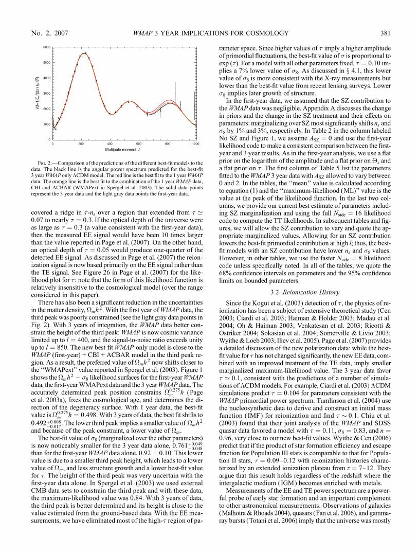
There has also been a significant reduction in the uncertaintiesin the matter density,�mh

2. With the first year ofWMAP data, thethird peakwas poorly constrained (see the light gray data points inFig. 2). With 3 years of integration, the WMAP data better con-strain the height of the third peak:WMAP is now cosmic variancelimited up to l ¼ 400, and the signal-to-noise ratio exceeds unityup to l ¼ 850. The new best-fitWMAP-only model is close to theWMAP (first-year) + CBI + ACBAR model in the third peak re-gion. As a result, the preferred value of�mh

2 now shifts closer tothe ‘‘WMAPext’’ value reported in Spergel et al. (2003). Figure 1shows the�mh

2 � �8 likelihood surfaces for the first-yearWMAPdata, the first-yearWMAPext data and the 3 yearWMAP data. Theaccurately determined peak position constrains �0:275

m h (Pageet al. 2003a), fixes the cosmological age, and determines the di-rection of the degeneracy surface. With 1 year data, the best-fitvalue is�0:275

m h ¼ 0:498.With 3 years of data, the best fit shifts to

0:492þ0:008�0:017

. The lower third peak implies a smaller value of �mh2

and because of the peak constraint, a lower value of �m.The best-fit value of �8 (marginalized over the other parameters)

is now noticeably smaller for the 3 year data alone, 0:761þ0:049�0:048

than for the first-yearWMAP data alone, 0:92� 0:10. This lowervalue is due to a smaller third peak height, which leads to a lowervalue of �m, and less structure growth and a lower best-fit valuefor �. The height of the third peak was very uncertain with thefirst-year data alone. In Spergel et al. (2003) we used externalCMB data sets to constrain the third peak and with these data,the maximum-likelihood value was 0.84. With 3 years of data,the third peak is better determined and its height is close to thevalue estimated from the ground-based data. With the EE mea-surements, we have eliminated most of the high-� region of pa-

rameter space. Since higher values of � imply a higher amplitudeof primordial fluctuations, the best-fit value of � is proportional toexp (�). For a model with all other parameters fixed, � ¼ 0:10 im-plies a 7% lower value of �8. As discussed in x 4.1, this lowervalue of �8 is more consistent with the X-ray measurements butlower than the best-fit value from recent lensing surveys. Lower�8 implies later growth of structure.

In the first-year data, we assumed that the SZ contribution totheWMAP data was negligible. Appendix A discusses the changein priors and the change in the SZ treatment and their effects onparameters: marginalizing over SZmost significantly shifts ns and�8 by 1% and 3%, respectively. In Table 2 in the column labeledNo SZ and Figure 1, we assume ASZ ¼ 0 and use the first-yearlikelihood code to make a consistent comparison between the first-year and 3 year results. As in the first-year analysis, we use a flatprior on the logarithm of the amplitude and a flat prior on�s anda flat prior on � . The first column of Table 5 list the parametersfitted to theWMAP 3 year data with ASZ allowed to vary between0 and 2. In the tables, the ‘‘mean’’ value is calculated accordingto equation (1) and the ‘‘maximum-likelihood (ML)’’ value is thevalue at the peak of the likelihood function. In the last two col-umns, we provide our current best estimate of parameters includ-ing SZ marginalization and using the full Nside ¼ 16 likelihoodcode to compute the TT likelihoods. In subsequent tables and fig-ures, we will allow the SZ contribution to vary and quote the ap-propriate marginalized values. Allowing for an SZ contributionlowers the best-fit primordial contribution at high l; thus, the best-fit models with an SZ contribution have lower ns and �8 values.However, in other tables, we use the faster Nside ¼ 8 likelihoodcode unless specifically noted. In all of the tables, we quote the68% confidence intervals on parameters and the 95% confidencelimits on bounded parameters.

3.2. Reionization History

Since the Kogut et al. (2003) detection of � , the physics of re-ionization has been a subject of extensive theoretical study (Cen2003; Ciardi et al. 2003; Haiman & Holder 2003; Madau et al.2004; Oh & Haiman 2003; Venkatesan et al. 2003; Ricotti &Ostriker 2004; Sokasian et al. 2004; Somerville & Livio 2003;Wyithe&Loeb 2003; Iliev et al. 2005). Page et al. (2007) providesa detailed discussion of the new polarization data: while the best-fit value for � has not changed significantly, the newEEdata, com-bined with an improved treatment of the TE data, imply smallermarginalized maximum-likelihood value. The 3 year data favor� ’ 0:1, consistent with the predictions of a number of simula-tions of�CDMmodels. For example, Ciardi et al. (2003)�CDMsimulations predict � ¼ 0:104 for parameters consistent with theWMAP primordial power spectrum. Tumlinson et al. (2004) usethe nucleosynthetic data to derive and construct an initial massfunction ( IMF) for reionization and find � � 0:1. Chiu et al.(2003) found that their joint analysis of the WMAP and SDSSquasar data favored a model with � ¼ 0:11, �8 ¼ 0:83, and n ¼0:96, very close to our new best-fit values. Wyithe & Cen (2006)predict that if the product of star formation efficiency and escapefraction for Population III stars is comparable to that for Popula-tion II stars, � ¼ 0:09Y0:12 with reionization histories charac-terized by an extended ionization plateau from z ¼ 7Y12: Theyargue that this result holds regardless of the redshift where theintergalactic medium (IGM) becomes enriched with metals.

Measurements of the EE and TE power spectrum are a power-ful probe of early star formation and an important complementto other astronomical measurements. Observations of galaxies(Malhotra &Rhoads 2004), quasars (Fan et al. 2006), and gamma-ray bursts (Totani et al. 2006) imply that the universe was mostly

Fig. 2.—Comparison of the predictions of the different best-fit models to thedata. The black line is the angular power spectrum predicted for the best-fit3 yearWMAP only�CDMmodel. The red line is the best fit to the 1 yearWMAPdata. The orange line is the best fit to the combination of the 1 yearWMAP data,CBI and ACBAR (WMAPext in Spergel et al. 2003). The solid data pointsrepresent the 3 year data and the light gray data points the first-year data.


ionized by z ¼ 6. The detection of large-scale TE and EE signal(Page et al. 2007) implies that the universe was mostly reionizedat even higher redshift. CMB observations have the potential toconstrain some of the details of reionization, as the shape of theCMB EE power spectrum is sensitive to reionization history(Kaplinghat et al. 2003; Hu&Holder 2003). Here we explore theability of the current EE data to constrain reionization by pos-tulating a two-stage process as a toy model. During the first stage,the universe is partially reionized at redshift zreion and completereionization occurs at z ¼ 7:

xe ¼0; z > z reion;

x0e ; z reion > z > 7;

1; z < 7:

8><>: ð3Þ

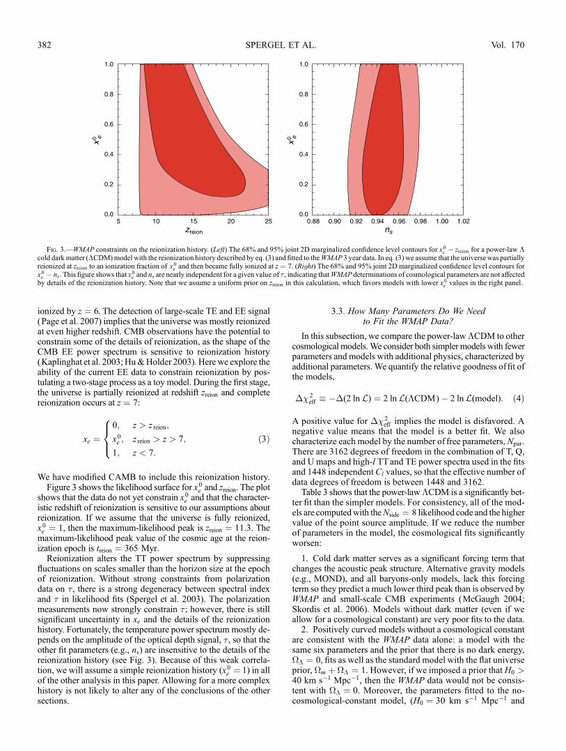
We have modified CAMB to include this reionization history.Figure 3 shows the likelihood surface for x0e and zreion. The plot

shows that the data do not yet constrain x0e and that the character-istic redshift of reionization is sensitive to our assumptions aboutreionization. If we assume that the universe is fully reionized,x0e ¼ 1, then the maximum-likelihood peak is zreion ¼ 11:3. Themaximum-likelihood peak value of the cosmic age at the reion-ization epoch is treion ¼ 365 Myr.

Reionization alters the TT power spectrum by suppressingfluctuations on scales smaller than the horizon size at the epochof reionization. Without strong constraints from polarizationdata on � , there is a strong degeneracy between spectral indexand � in likelihood fits (Spergel et al. 2003). The polarizationmeasurements now strongly constrain � ; however, there is stillsignificant uncertainty in xe and the details of the reionizationhistory. Fortunately, the temperature power spectrum mostly de-pends on the amplitude of the optical depth signal, � , so that theother fit parameters (e.g., ns) are insensitive to the details of thereionization history (see Fig. 3). Because of this weak correla-tion, we will assume a simple reionization history (x0e ¼ 1) in allof the other analysis in this paper. Allowing for a more complexhistory is not likely to alter any of the conclusions of the othersections.

3.3. How Many Parameters Do We Needto Fit the WMAP Data?

In this subsection, we compare the power-law�CDM to othercosmological models.We consider both simpler models with fewerparameters and models with additional physics, characterized byadditional parameters. We quantify the relative goodness offit ofthe models,

��2eA � ��(2 ln L) ¼ 2 lnL(�CDM)� 2 lnL(model): ð4Þ

A positive value for ��2eA implies the model is disfavored. A

negative value means that the model is a better fit. We alsocharacterize each model by the number of free parameters, Npar.There are 3162 degrees of freedom in the combination of T, Q,and U maps and high-l TTand TE power spectra used in the fitsand 1448 independent Cl values, so that the effective number ofdata degrees of freedom is between 1448 and 3162.Table 3 shows that the power-law�CDM is a significantly bet-

ter fit than the simpler models. For consistency, all of the mod-els are computedwith theNside ¼ 8 likelihood code and the highervalue of the point source amplitude. If we reduce the numberof parameters in the model, the cosmological fits significantlyworsen:

1. Cold dark matter serves as a significant forcing term thatchanges the acoustic peak structure. Alternative gravity models(e.g., MOND), and all baryons-only models, lack this forcingterm so they predict a much lower third peak than is observed byWMAP and small-scale CMB experiments (McGaugh 2004;Skordis et al. 2006). Models without dark matter (even if weallow for a cosmological constant) are very poor fits to the data.2. Positively curved models without a cosmological constant

are consistent with the WMAP data alone: a model with thesame six parameters and the prior that there is no dark energy,�� ¼ 0, fits as well as the standard model with the flat universeprior, �m þ �� ¼ 1. However, if we imposed a prior that H0 >40 km s�1 Mpc�1, then the WMAP data would not be consis-tent with �� ¼ 0. Moreover, the parameters fitted to the no-cosmological-constant model, (H0 ¼ 30 km s�1 Mpc�1 and

Fig. 3.—WMAP constraints on the reionization history. (Left) The 68% and 95% joint 2D marginalized confidence level contours for x0e � zreion for a power-law �cold darkmatter (�CDM)model with the reionization history described by eq. (3) and fitted to theWMAP 3 year data. In eq. (3) we assume that the universe was partiallyreionized at zreion to an ionization fraction of x

0e and then became fully ionized at z ¼ 7. (Right) The 68% and 95% joint 2D marginalized confidence level contours for

x0e � ns. This figure shows that x0e and ns are nearly independent for a given value of � , indicating thatWMAP determinations of cosmological parameters are not affected

by details of the reionization history. Note that we assume a uniform prior on zreion in this calculation, which favors models with lower x0e values in the right panel.


�m ¼ 1:3) are terrible fits to a host of astronomical data: large-scale structure observations, supernova data, and measurementsof local dynamics. As discussed in x 7.3, the combination ofWMAPdata and other astronomical data solidifies the evidence againstthese models. The detected cross-correlation between CMB fluc-tuations and large-scale structure provides further evidence for theexistence of dark energy (see x 4.1.10).

3. The simple scale-invariant (ns ¼ 1:0) model is no longer agood fit to the WMAP data. As discussed in the previous sub-section, combining theWMAP data with other astronomical datasets further strengthens the case for ns < 1.

The conclusion that the WMAP data demands the existence ofdark matter and dark energy is based on the assumption that theprimordial power spectrum is a power-law spectrum. By addingadditional features in the primordial perturbation spectrum, thesealternative models may be able to better mimic the�CDMmodel.This possibility requires further study.

The bottom half of Table 3 lists the relative improvement ofthe generalized models over the power-law �CDM. As the tableshows, theWMAP data alone do not require the existence of ten-sor modes, quintessence, or modifications in neutrino properties.Adding these parameters does not improve the fit significantly.For theWMAP data, the region in likelihood space where (r ¼ 0,w ¼ �1, and m� ¼ 0 lies within the 1 � contour. In x 7, we con-sider the limits on these parameters based on WMAP data andother astronomical data sets.

If we allow for a nonflat universe, thenmodels with small neg-ative�k are a better fit than the power-law �CDMmodel. Thesemodels have a lower intervening Sachs-Wolfe (ISW) signal atlow l and are a better fit to the low-l multipoles. The best-fitclosed universe model has �m ¼ 0:415, �� ¼ 0:630, and H0 ¼55 kms�1 Mpc�1 and is a better fit to theWMAP data alone thanthe flat universemodel(��2

eA ¼ 2)However, as discussed in x 7.3,the combination of WMAP data with either SNe data, large-scalestructure data, ormeasurements ofH0 favorsmodels with�K closeto 0.

In x 5, we consider several different modifications to the shapeof the power spectrum. As noted in Table 3, none of the modifi-cations lead to significant improvements in the fit. Allowing thespectral index to vary as a function of scale improves the good-ness of fit. The low-l multipoles, particularly l ¼ 2, are lowerthan predicted in the �CDM model. However, the relative im-provement in fit is not large,��2

eA ¼ 3, so theWMAP data alonedo not require a running spectral index.

Measurement of the goodness offit is a simple approach to testthe needed number of parameters. These results should be con-firmed by Bayesian model comparison techniques (Beltran et al.2005; Trotta 2007; Mukherjee et al. 2006; Bridges et al. 2006).Bayesian methods, however, require an estimate of the numberof data points in the fit. It is not clear whether we should use the�1010 points in the TOD, the 106 points in the temperature maps,the 3 ; 103 points in the TT, TE, or EE power spectrum, or the�10Y20 numbers needed to fit the peaks and valleys in the TTdata in evaluating the significance of new parameters.

4. WMAP �CDM MODEL AND OTHERASTRONOMICAL DATA

In this paper, our approach is to show first that a wide range ofastronomical data sets are consistent with the predictions of the�CDM model with its parameters fitted to the WMAP data (seex 4.1). We then use the external data sets to constrain extensionsof the standard model.

In our analyses, we consider several different types of datasets. We consider the SDSS LRGs, the SDSS full sample, andthe 2dFGRS data separately; this allows a check of systematiceffects. We divide the small-scale CMB data sets into low-frequency experiments (CBI, VSA) and high-frequency experi-ments (BOOMERANG, ACBAR).We divide the supernova datasets into two groups as described below. The details of the datasets are also described in x 4.1.

When we consider models with more parameters, there aresignificant degeneracies, and external data sets are essential forparameter constraints. We use this approach in x 4.2 and subse-quent sections.

4.1. Predictions from the WMAP Best-Fit �CDM Model

TheWMAP data alone are now able to accurately constrain thebasic six parameters of the �CDM model. In this section, wefocus on this model and begin by using only the WMAP data tofix the cosmological parameters. We then use the Markov chains(and linear theory) to predict the amplitude of fluctuations in thelocal universe and compare to other astronomical observations.These comparisons test the basic physical assumptions of the�CDM model.

4.1.1. Age of the Universe and H0

The CMB data do not directly measure H0; however, by mea-suring �mH

20 through the height of the peaks and the conformal

TABLE 3

Goodness of Fit, ��2eA � �2 lnL, for WMAP Data only Relative to a Power-Law �CDM Model

Model Number Model ��(2 lnL) Npar

M1........................................... Scale-invariant fluctuations (ns ¼ 1) 6 5

M2........................................... No reionization (� ¼ 0) 7.4 5

M3........................................... No dark matter (�c ¼ 0; �� 6¼ 0) 248 6

M4........................................... No cosmological constant (�c 6¼ 0; �� ¼ 0) 0 6

M5........................................... Power law �CDM 0 6

M6........................................... Quintessence (w 6¼ �1) 0 7

M7........................................... Massive neutrino (m� > 0) �1 7

M8........................................... Tensor modes (r > 0) 0 7

M9........................................... Running spectral index (dns/d ln k 6¼ 0) �4 7

M10......................................... Nonflat universe (�k 6¼ 0) �2 7

M11 ......................................... Running spectral index and tensor modes �4 8

M12......................................... Sharp cutoff �1 7

M13......................................... Binned �2R(k) �22 20

Note.—A worse fit to the data is ��2eA > 0.


distance to the surface of last scatter through the peak positions(Page et al. 2003b), the CMBdata produce a determination ofH0

if we assume the simple flat �CDMmodel. Within the context ofthe basic model of adiabatic fluctuations, the CMB data providea relatively robust determination of the age of the universe as thedegeneracy in other cosmological parameters is nearly orthogonalto measurements of the age (Knox et al. 2001; Hu et al. 2001).

The WMAP �CDM best-fit value for the age, t0 ¼13:73þ0:16

�0:15 Gyr, agrees with estimates of ages based on globularclusters (Chaboyer & Krauss 2002) and white dwarfs (Hansenet al. 2004; Richer et al. 2004). Figure 4 compares the predictedevolution ofH(z) to theHST Key Project value (Freedman et al.2001) and to values from analysis of differential ages as a func-tion of redshift (Jimenez et al. 2003; Simon et al. 2005).

TheWMAP best-fit value,H0 ¼ 73:2þ3:1�3:2 km s�1Mpc�1, is also

consistent with HSTmeasurements (Freedman et al. 2001), H0 ¼72� 8 km s�1 Mpc�1, where the error includes random and sys-tematic uncertainties and the estimate is based on several differentmethods (Type Ia supernovae, Type II supernovae, surface bright-ness fluctuations, and fundamental plane). It also agrees with de-tailed studies of gravitationally lensed systems such as B1608+656(Koopmans et al. 2003), which yields 75þ7

�6 km s�1 Mpc�1, mea-surements of the Hubble constant from SZ and X-ray obser-vations of clusters (Bonamente et al. 2006) that find H0 ¼76þ3:9

�3:4þ10:0�8:0 km s�1 Mpc�1, and recent measurements of the

Cepheid distances to nearby galaxies that host Type Ia supernova(Riess et al. 2005), H0 ¼ 73� 4� 5 km s�1 Mpc�1.

4.1.2. Big Bang Nucleosynthesis

Measurements of the light element abundances are among themost important tests of the standard big bang model. TheWMAPestimate of the baryon abundance depends on our understandingof acoustic oscillations 300,000 years after the big bang. TheBBNabundance predictions depend on our understanding of physics inthe first minutes after the big bang.

Table 4 lists the primordial deuterium abundance, yFITD , theprimordial 3He abundance, y3, the primordial helium abun-dance, YP, and the primordial 7Li abundance, yLi, based on ana-lytical fits to the predicted BBN abundances (Kneller & Steigman

2004) and the power-law �CDM 68% confidence range forthe baryon/photon ratio, 10 ¼ (273:9� 0:3)�bh

2. The lithiumabundance is often expressed as a logarithmic abundance,½Li�P ¼ 12þ log10(Li /H).The systematic uncertainties in the helium abundances are due

to the uncertainties in nuclear parameters, particularly neutronlifetime (Steigman 2005). Prior to the measurements of the CMBpower spectrum, uncertainties in the baryon abundance were thebiggest source of uncertainty in CMB predictions. Serebrov et al.(2005) argues that the currently accepted value, �n ¼ 887:5 s,should be reduced by 7.2 s, a shift of several times the reportederrors in the Particle Data Book. This (controversial) shorter life-time lowers the predicted best-fit helium abundance to YP ¼0:24675 (Mathews et al. 2005; Steigman 2005).The deuterium abundance measurements provide the strongest

test of the predicted baryon abundance. Kirkman et al. (2003) es-timate a primordial deuterium abundance, ½D�/½H� ¼ 2:78þ0:44

�0:38 ;10�5, based on five QSO absorption systems. The six systemsused in theKirkman et al. (2003) analysis show a significant rangein abundances: 1:65Y3:98ð Þ ; 10�5 and have a scattermuch largerthan the quoted observational errors. Recently, Crighton et al.(2004) report a deuterium abundance of 1:6þ0:5

�0:4; 10�5 for PKS

1937�1009. Because of the large scatter, we quote the range in[D]/[H] abundances in Table 4; however, note that the meanabundance is in good agreement with the CMB prediction.It is difficult to directly measure the primordial 3He abun-

dance. Bania et al. (2002) quote an upper limit on the primordial3He abundance of y3 < 1:1� 0:2 ; 10�5. This limit is compat-ible with the BBN predictions.Olive & Skillman (2004) have reanalyzed the estimates of pri-

mordial helium abundance based on observations of metal-poorH ii regions. They conclude that the errors in the abundance aredominated by systematic errors and argue that a number of thesesystematic effects have not been properly included in earlieranalyses. In Table 4, we quote their estimate of the allowed rangeof YP. Olive & Skillman (2004) find a representative value of0:249� 0:009 for a linear fit of [O]/[H] to the helium abundance,significantly above earlier estimates and consistent with WMAP-normalized BBN.While the measured abundances of the other light elements

appear to be consistent with BBN predictions, measurements ofneutral lithium abundance in low-metallicity stars imply valuesthat are a factor of 2 below the BBN predictions: most recentmeasurements (Charbonnel & Primas 2005; Boesgaard et al.2005) find an abundance of ½Li�P ’ 2:2Y2:25. While Melendez&Ramırez (2004) find a higher value, ½Li�P ’ 2:37� 0:05, eventhis value is still significantly below the BB-predicted value,2:64� 0:03. These discrepancies could be due to systematics inthe inferred lithium abundance (Steigman 2005), uncertainties inthe stellar temperature scale (Fields et al. 2005), destruction oflithium in an early generation of stars, or the signature of new earlyuniverse physics (Coc et al. 2004; Jedamzik 2004; Richard et al.

TABLE 4

Primordial Abundances Based on Using the Steigman (2005)

Fitting Formula for the �CDM 3 yr WMAP only Value

for the Baryon /Photon Ratio, 10 ¼ 6:116þ0:197�0:249

Abundance CMB-based BBN Prediction Observed Value

105yFITD ........................... 2:57þ0:17�0:13 1.6Y4.0

105y3 .............................. 1.05 � 0.03 � 0.03 (syst.) <1.1 � 0.2

YP ................................... 0:24819þ0:00029�0:00040 � 0:0006(syst:) 0.232Y0.258

[Li] ................................. 2.64 � 0.03 2.2Y2.4

Fig. 4.—�CDM model fit to the WMAP data predicts the Hubble param-eter redshift relation. The blue band shows the 68% confidence interval for theHubble parameter, H. The dark blue rectangle shows the HST Key Project esti-mate for H0 and its uncertainties (Freedman et al. 2001). The other points arefrommeasurements of the differential ages of galaxies, based on fits of syntheticstellar population models to galaxy spectroscopy. The squares show values fromJimenez et al. (2003) analyses of SDSS galaxies. The diamonds show valuesfrom the Simon et al. (2005) analysis of a high-redshift sample of red galaxies.


2005; Ellis et al. 2005; Larena et al. 2005; Jedamzik et al. 2005).The recent detection (Asplund et al. 2005) of 6Li in several low-metallicity stars further constrains chemical evolution modelsand exacerbates the tensions between the BBN predictions andobservations.

4.1.3. Small-Scale CMB Measurements

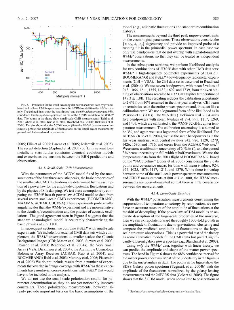
With the parameters of the �CDM model fixed by the mea-surements of the first three acoustic peaks, the basic properties ofthe small-scale CMB fluctuations are determined by the assump-tion of a power law for the amplitude of potential fluctuations andby the physics of Silk damping.We test these assumptions by com-paring the WMAP best-fit power-law �CDM model to data fromseveral recent small-scale CMB experiments (BOOMERANG,MAXIMA,ACBAR,CBI,VSA). These experiments probe smallerangular scales than theWMAP experiment and aremore sensitiveto the details of recombination and the physics of acoustic oscil-lations. The good agreement seen in Figure 5 suggests that thestandard cosmological model is accurately characterizing thebasic physics at z ’ 1100.

In subsequent sections, we combine WMAP with small-scaleexperiments.We include four external CMB data sets which com-plement the WMAP observations at smaller scales: the CosmicBackground Imager (CBI; Mason et al. 2003; Sievers et al. 2003;Pearson et al. 2003; Readhead et al. 2004a), the Very SmallArray (VSA; Dickinson et al. 2004), the Arcminute CosmologyBolometer Array Receiver (ACBAR; Kuo et al. 2004), andBOOMERANG (Ruhl et al. 2003;Montroy et al. 2006; Piacentiniet al. 2006) We do not include results from a number of experi-ments that overlap in l range coveragewithWMAP as these exper-iments have nontrivial cross-correlations withWMAP that wouldhave to be included in the analysis.

We do not use the small-scale polarization results for pa-rameter determination as they do not yet noticeably improveconstraints. These polarization measurements, however, al-ready provide important tests on the basic assumptions of the

model (e.g., adiabatic fluctuations and standard recombinationhistory).

The measurements beyond the third peak improve constraintson the cosmological parameters. These observations constrict thef�; !b; As; nsg degeneracy and provide an improved probe of arunning tilt in the primordial power spectrum. In each case weonly use bandpowers that do not overlap with signal-dominatedWMAP observations, so that they can be treated as independentmeasurements.

In the subsequent sections, we perform likelihood analysisfor two combinations of WMAP data with other CMB data sets:WMAP + high-frequency bolometer experiments (ACBAR +BOOMERANG) andWMAP + low-frequency radiometer experi-ments (CBI + VSA). The CBI data set is described in Readheadet al. (2004a). We use seven bandpowers, with mean l-values of948, 1066, 1211, 1355, 1482, 1692, and 1739, from the even bin-ning of observations rescaled to a 32 GHz Jupiter temperature of147.3 � 1.8K. The rescaling reduces the calibration uncertaintyto 2.6% from 10% assumed in the first-year analyses; CBI beamuncertainties scale the entire power spectrum and, thus, act like acalibration error. We use a lognormal form of the likelihood as inPearson et al. (2003). The VSA data (Dickinson et al. 2004) usesfive bandpowers with mean l-values of 894, 995, 1117, 1269,and 1407, which are calibrated to theWMAP 32 GHz Jupiter tem-perature measurement. The calibration uncertainty is assumed tobe 3%, and again we use a lognormal form of the likelihood. ForACBAR (Kuo et al. 2004), we use the same bandpowers as in thefirst-year analysis, with central l-values 842, 986, 1128, 1279,1426, 1580, and 1716, and errors from the ACBARWeb site.17

We assume a calibration uncertainty of 20% inCl, and the quoted3% beam uncertainty in full width at half-maximum. We use thetemperature data from the 2003 flight of BOOMERANG, basedon the ‘‘NA pipeline’’ (Jones et al. 2006) considering the 7 datapoints and covariance matrix for bins with mean l-values, 924,974, 1025, 1076, 1117, 1211, and 1370. While there is overlapbetween some of the small-scale power spectrum measurementsand WMAP measurements at 800 < l < 1000, the WMAP mea-surements are noise-dominated so that there is little covariancebetween the measurements.

4.1.4. Large-Scale Structure

With the WMAP polarization measurements constraining thesuppression of temperature anisotropy by reionization, we nowhave an accurate measure of the amplitude of fluctuations at theredshift of decoupling. If the power-law �CDM model is an ac-curate description of the large-scale properties of the universe,then we can extrapolate forward the roughly 1000-fold growth inthe amplitude of fluctuations due to gravitational clustering andcompare the predicted amplitude of fluctuations to the large-scale structure observations. This is a powerful test of the theoryas some alternative models fit the CMB data but predict signifi-cantly different galaxy power spectra (e.g., Blanchard et al. 2003).

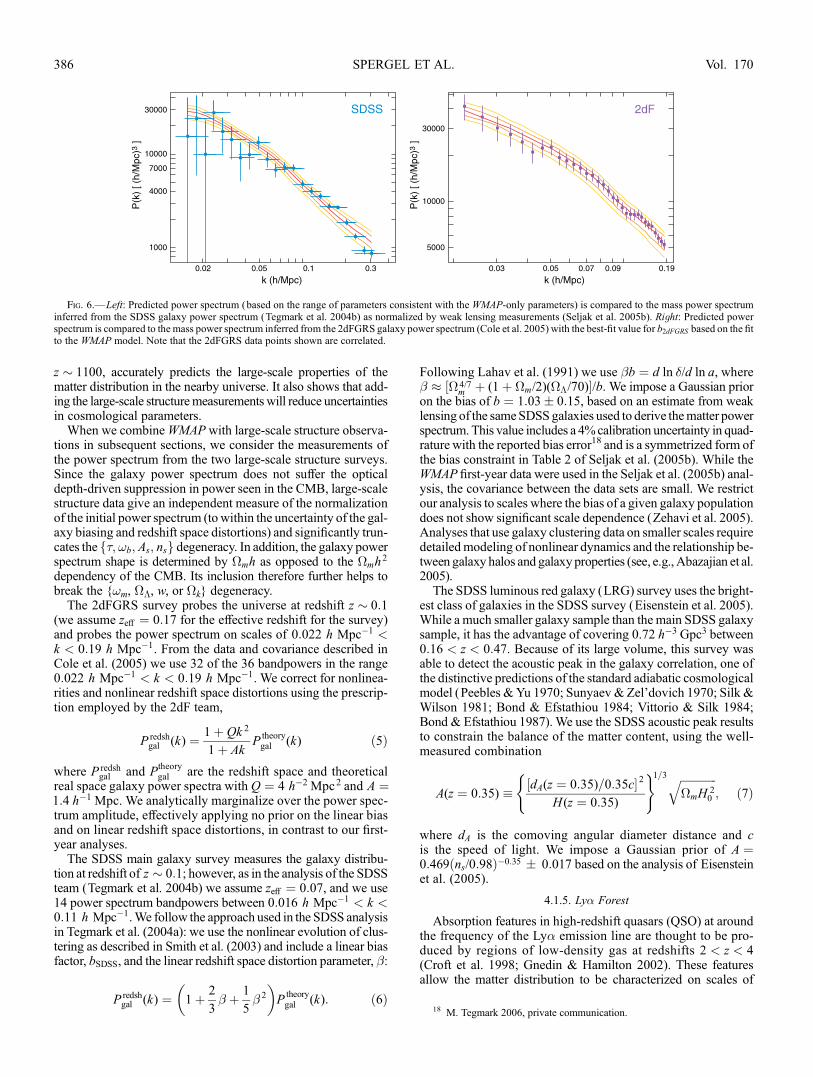
Using only the WMAP data, together with linear theory, wecan predict the amplitude and shape of the matter power spec-trum. The band in Figure 6 shows the 68% confidence interval forthe matter power spectrum.Most of the uncertainty in the figure isdue to the uncertainties in �mh. The points in the figure show theSDSS Galaxy power spectrum (Tegmark et al. 2004b) with theamplitude of the fluctuations normalized by the galaxy lensingmeasurements and the 2dFGRS data (Cole et al. 2005). The figureshows that the�CDMmodel, when normalized to observations at

Fig. 5.—Prediction for the small-scale angular power spectrum seen by ground-based and balloon CMB experiments from the�CDMmodel fit to theWMAP dataonly. The colored lines show the best-fit (red) and the 68% (dark orange) and 95%confidence levels (light orange) based on fits of the �CDM models to theWMAPdata. The points in the figure show small-scale CMB measurements (Ruhl et al.2003; Abroe et al. 2004; Kuo et al. 2004; Readhead et al. 2004a; Dickinson et al.2004). The plot shows that the �CDMmodel (fit to theWMAP data alone) can ac-curately predict the amplitude of fluctuations on the small scales measured byground and balloon-based experiments.

17 See http://cosmology.berkeley.edu /group /swlh /acbar/data.


z � 1100, accurately predicts the large-scale properties of thematter distribution in the nearby universe. It also shows that add-ing the large-scale structuremeasurements will reduce uncertaintiesin cosmological parameters.

When we combineWMAP with large-scale structure observa-tions in subsequent sections, we consider the measurements ofthe power spectrum from the two large-scale structure surveys.Since the galaxy power spectrum does not suffer the opticaldepth-driven suppression in power seen in the CMB, large-scalestructure data give an independent measure of the normalizationof the initial power spectrum (towithin the uncertainty of the gal-axy biasing and redshift space distortions) and significantly trun-cates the f�; !b; As; nsg degeneracy. In addition, the galaxy powerspectrum shape is determined by �mh as opposed to the �mh

2

dependency of the CMB. Its inclusion therefore further helps tobreak the {!m, ��, w, or �k} degeneracy.

The 2dFGRS survey probes the universe at redshift z � 0:1(we assume zeA ¼ 0:17 for the effective redshift for the survey)and probes the power spectrum on scales of 0:022 h Mpc�1 <k < 0:19 h Mpc�1. From the data and covariance described inCole et al. (2005) we use 32 of the 36 bandpowers in the range0:022 h Mpc�1 < k < 0:19 h Mpc�1. We correct for nonlinea-rities and nonlinear redshift space distortions using the prescrip-tion employed by the 2dF team,

P redshgal (k) ¼ 1þ Qk 2

1þ AkP

theorygal (k) ð5Þ

where P redshgal and P

theorygal are the redshift space and theoretical

real space galaxy power spectra with Q ¼ 4 h�2 Mpc2 and A ¼1:4 h�1 Mpc. We analytically marginalize over the power spec-trum amplitude, effectively applying no prior on the linear biasand on linear redshift space distortions, in contrast to our first-year analyses.

The SDSS main galaxy survey measures the galaxy distribu-tion at redshift of z � 0:1; however, as in the analysis of the SDSSteam (Tegmark et al. 2004b) we assume zeA ¼ 0:07, and we use14 power spectrum bandpowers between 0:016 h Mpc�1 < k <0:11 h Mpc�1.We follow the approach used in the SDSS analysisin Tegmark et al. (2004a): we use the nonlinear evolution of clus-tering as described in Smith et al. (2003) and include a linear biasfactor, bSDSS, and the linear redshift space distortion parameter, :

P redshgal (k) ¼

�1þ 2

3 þ 1

5 2

�P

theorygal (k): ð6Þ

Following Lahav et al. (1991) we use b ¼ d ln �/d ln a, where � ½�4/7

m þ (1þ �m/2)(��/70)�/b. We impose a Gaussian prioron the bias of b ¼ 1:03� 0:15, based on an estimate from weaklensing of the sameSDSSgalaxies used to derive thematter powerspectrum. This value includes a 4%calibration uncertainty in quad-rature with the reported bias error18 and is a symmetrized form ofthe bias constraint in Table 2 of Seljak et al. (2005b). While theWMAP first-year data were used in the Seljak et al. (2005b) anal-ysis, the covariance between the data sets are small. We restrictour analysis to scales where the bias of a given galaxy populationdoes not show significant scale dependence (Zehavi et al. 2005).Analyses that use galaxy clustering data on smaller scales requiredetailedmodeling of nonlinear dynamics and the relationship be-tween galaxy halos and galaxyproperties (see, e.g., Abazajian et al.2005).The SDSS luminous red galaxy (LRG) survey uses the bright-

est class of galaxies in the SDSS survey (Eisenstein et al. 2005).While a much smaller galaxy sample than the main SDSS galaxysample, it has the advantage of covering 0.72 h�3 Gpc3 between0:16 < z < 0:47. Because of its large volume, this survey wasable to detect the acoustic peak in the galaxy correlation, one ofthe distinctive predictions of the standard adiabatic cosmologicalmodel (Peebles &Yu 1970; Sunyaev & Zel’dovich 1970; Silk &Wilson 1981; Bond & Efstathiou 1984; Vittorio & Silk 1984;Bond & Efstathiou 1987). We use the SDSS acoustic peak resultsto constrain the balance of the matter content, using the well-measured combination

A(z ¼ 0:35) � ½dA(z ¼ 0:35)=0:35c�2

H(z ¼ 0:35)

( )1=3 ffiffiffiffiffiffiffiffiffiffiffiffiffi�mH

20

q; ð7Þ

where dA is the comoving angular diameter distance and cis the speed of light. We impose a Gaussian prior of A ¼0:469 ns/0:98ð Þ�0:35 � 0:017 based on the analysis of Eisensteinet al. (2005).

4.1.5. Ly� Forest

Absorption features in high-redshift quasars (QSO) at aroundthe frequency of the Ly� emission line are thought to be pro-duced by regions of low-density gas at redshifts 2 < z < 4(Croft et al. 1998; Gnedin & Hamilton 2002). These featuresallow the matter distribution to be characterized on scales of

Fig. 6.—Left: Predicted power spectrum (based on the range of parameters consistent with the WMAP-only parameters) is compared to the mass power spectruminferred from the SDSS galaxy power spectrum (Tegmark et al. 2004b) as normalized by weak lensing measurements (Seljak et al. 2005b). Right: Predicted powerspectrum is compared to the mass power spectrum inferred from the 2dFGRS galaxy power spectrum (Cole et al. 2005) with the best-fit value for b2dFGRS based on the fitto the WMAP model. Note that the 2dFGRS data points shown are correlated.

18 M. Tegmark 2006, private communication.


0:2 h Mpc�1 < k < 5 h Mpc�1 and as such extend the leverarm provided by combining large-scale structure data and CMB.These observations also probe a higher redshift range (z � 2Y3).Thus, these observations nicely complement CMBmeasurementsand large-scale structure observations. While there has been sig-nificant progress in understanding systematics in the past fewyears (McDonald et al. 2005; Meiksin & White 2004), time con-straints limit our ability to consider all relevant data sets.

Recent fits to the Ly� forest imply a higher amplitude of den-sity fluctuations: Jena et al. (2005) find that �8 ¼ 0:9, �m ¼0:27, h ¼ 0:71 provides a good fit to the Ly� data. Seljak et al.(2005a) combines first-yearWMAP data, other CMB experiments,large-scale structure, and Ly� to find ns ¼ 0:98� 0:02, �8 ¼0:90� 0:03, h ¼ 0:71� 0:021, and�m ¼ 0:281þ0:023

�0:021. Note thatif they assume � ¼ 0:09, the best-fit value drops to �8 ¼ 0:84.While these models have somewhat higher amplitudes than thenew best-fit WMAP values, a recent analysis by Desjacques &Nusser (2005) find that theLy� data are consistentwith�8 between0.7 and 0.9. This suggests that the Ly� data are consistent with thenewWMAP best-fit values; however, further analysis is needed.

4.1.6. Galaxy Motions and Properties

Observations of galaxy peculiar velocities probe the growthrate of structure and are sensitive to the matter density and theamplitude of mass fluctuations. The Feldman et al. (2003) anal-ysis of peculiar velocities of nearby ellipticals and spirals finds

�m ¼ 0:30þ0:17�0:07 and �8 ¼ 1:13þ0:22

�0:23, within 1 � of the WMAP

best-fit value for �m and 1.5 � higher than the WMAP value for�8. These estimates are based on dynamics and are not sensitiveto the shape of the power spectrum. Mohayaee & Tully (2005)apply orbit retracingmethods to motions in the local superclusterand obtain�m ¼ 0:22� 0:02, consistent with theWMAP values.

Modeled galaxy properties can be compared to the clusteringproperties of galaxies on smaller scales. The best-fit parametersfor WMAP only are consistent with the recent Abazajian et al.(2005) analysis of the preY3 year release CMB data combinedwith the SDSS data. In their analysis, they fit a Halo OccupationDistribution model to the galaxy distribution so as to use the gal-axy clustering data at smaller scales. Their best-fit parameters(H0 ¼ 70�2:6 km s�1 Mpc�1; �m ¼ 0:271� 0:026) are con-sistent with the results found here. Vale & Ostriker (2006) fit theobserved galaxy luminosity functions with �8 ¼ 0:8 and �m ¼0:25. Van den Bosch et al. (2003) use the conditional luminosityfunction to fit the 2dFGRS luminosity function and the corre-lation length as a function of luminosity. Combining with thefirst-yearWMAP data, they find�m ¼ 0:25þ0:10

�0:07 and �8 ¼ 0:78�0:12 (95%CL), again in remarkable agreement with the three yearWMAP best-fit values.

4.1.7. Weak Lensing

Over the past few years, there has been dramatic progress inusing weak lensing data as a probe of mass fluctuations in thenearby universe. Lensing surveys complement CMB measure-ments (Contaldi et al. 2003; Tereno et al. 2005), and their domi-nant systematic uncertainties differ from the large-scale structuresurveys.

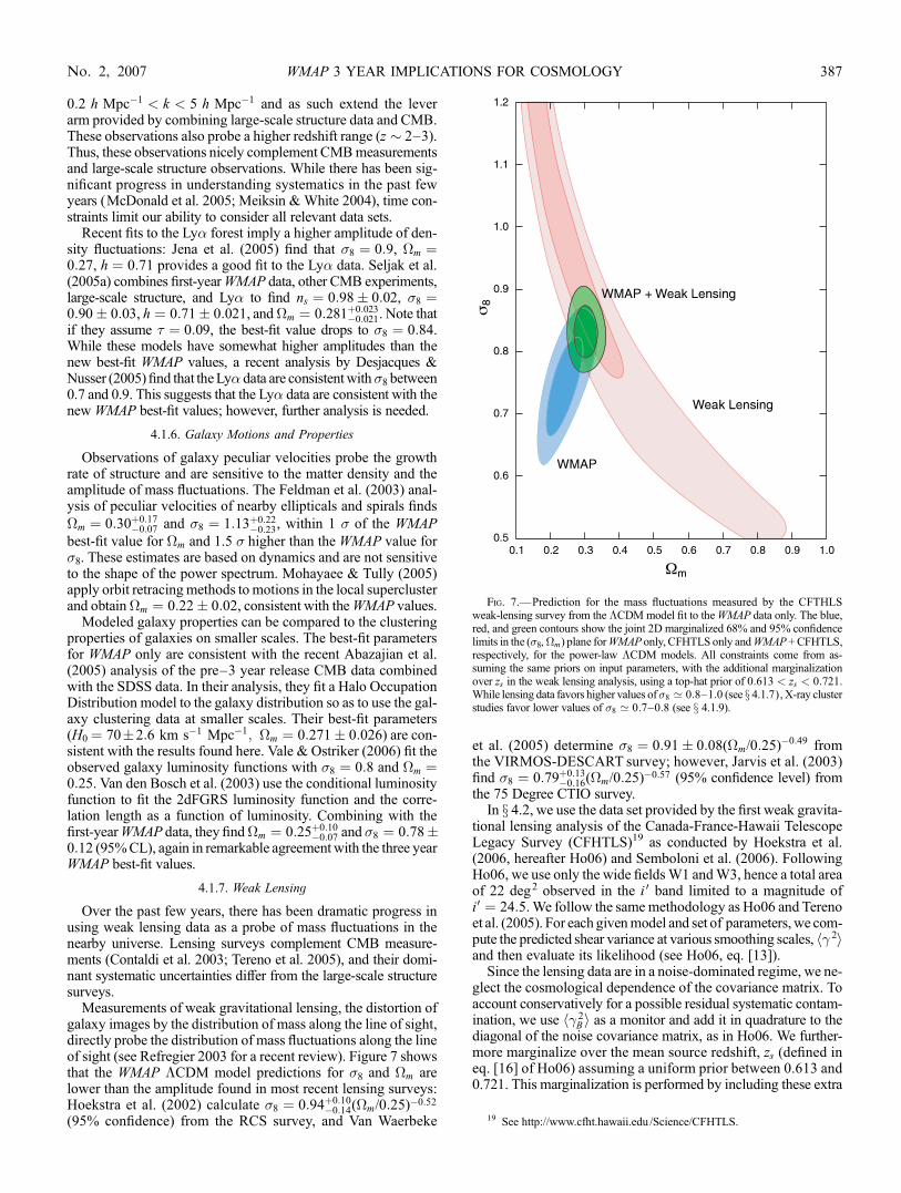
Measurements of weak gravitational lensing, the distortion ofgalaxy images by the distribution of mass along the line of sight,directly probe the distribution of mass fluctuations along the lineof sight (see Refregier 2003 for a recent review). Figure 7 showsthat the WMAP �CDM model predictions for �8 and �m arelower than the amplitude found in most recent lensing surveys:Hoekstra et al. (2002) calculate �8 ¼ 0:94þ0:10

�0:14(�m/0:25)�0:52

(95% confidence) from the RCS survey, and Van Waerbeke

et al. (2005) determine �8 ¼ 0:91� 0:08(�m/0:25)�0:49 from

the VIRMOS-DESCART survey; however, Jarvis et al. (2003)find �8 ¼ 0:79þ0:13

�0:16(�m/0:25)�0:57 (95% confidence level) fromthe 75 Degree CTIO survey.

In x 4.2, we use the data set provided by the first weak gravita-tional lensing analysis of the Canada-France-Hawaii TelescopeLegacy Survey (CFHTLS)19 as conducted by Hoekstra et al.(2006, hereafter Ho06) and Semboloni et al. (2006). FollowingHo06, we use only the wide fieldsW1 andW3, hence a total areaof 22 deg2 observed in the i 0 band limited to a magnitude ofi0 ¼ 24:5.We follow the samemethodology as Ho06 and Terenoet al. (2005). For each givenmodel and set of parameters, we com-pute the predicted shear variance at various smoothing scales, h� 2iand then evaluate its likelihood (see Ho06, eq. [13]).

Since the lensing data are in a noise-dominated regime, we ne-glect the cosmological dependence of the covariance matrix. Toaccount conservatively for a possible residual systematic contam-ination, we use h� 2

B i as a monitor and add it in quadrature to thediagonal of the noise covariance matrix, as in Ho06. We further-more marginalize over the mean source redshift, zs (defined ineq. [16] of Ho06) assuming a uniform prior between 0.613 and0.721. This marginalization is performed by including these extra

Fig. 7.—Prediction for the mass fluctuations measured by the CFTHLSweak-lensing survey from the �CDMmodel fit to theWMAP data only. The blue,red, and green contours show the joint 2D marginalized 68% and 95% confidencelimits in the (�8,�m) plane forWMAP only, CFHTLS only andWMAP +CFHTLS,respectively, for the power-law �CDM models. All constraints come from as-suming the same priors on input parameters, with the additional marginalizationover zs in the weak lensing analysis, using a top-hat prior of 0:613 < zs < 0:721.While lensing data favors higher values of�8 ’ 0:8Y1:0 (see x 4.1.7), X-ray clusterstudies favor lower values of �8 ’ 0:7Y0:8 (see x 4.1.9).

19 See http://www.cfht.hawaii.edu /Science/CFHTLS.


parameters in theMonte CarloMarkovChain. Our analysis differs,however, from the likelihood analysis of Ho06 in the choice of thetransfer function. We use the Novosyadlyj et al. (1999, hereafterNDL) CDM transfer function (with the assumptions of Tegmarket al. 2001) rather than the Bardeen et al. (1986) CDM transferfunction. The NDL transfer function includes more accuratelybaryon oscillations and neutrino effects. This modification altersthe shape of the likelihood surface in the two-dimensional (�8;�m)likelihood space.

4.1.8. Strong Lensing

Strong lensing provides another potentially powerful probe ofcosmology. The number of multiply lensed arcs and quasars isvery sensitive to the underlying cosmology. The cross section forlensing depends on the number of systems with surface densitiesabove the critical density, which in turn is sensitive to the angulardiameter distance relation (Turner 1990). The CLASS lensingsurvey (Chae et al. 2002) finds that the number of lenses detectedin the radio survey is consistent with a flat universe with a cos-mological constant and �m ¼ 0:31þ0:27

�0:14. The statistics of stronglenses in the SDSS is also consistent with the standard �CDMcosmology (Oguri 2004). The number and the properties of lensedarcs are also quite sensitive to cosmological parameters (but alsoto the details of the data analysis). Wambsganss et al. (2004) con-clude that arc statistics are consistent with the concordance�CDM model.

Soucail et al. (2004) has used multiple lenses in Abell 2218 toprovide another geometrical test of cosmological parameters.They find that 0 < �m < 0:33 andw < �0:85 for a flat universewith dark energy. This method is another independent test of thestandard cosmology.

4.1.9. Clusters and the Growth of Structure

The numbers and properties of rich clusters are another toolfor testing the emerging standard model. Since clusters are rare,the number of clusters as a function of redshift is a sensitiveprobe of cosmological parameters. Recent analyses of both op-tical and X-ray cluster samples yield cosmological parametersconsistent with the best-fitWMAP �CDMmodel (Borgani et al.2001; Bahcall & Bode 2003; Allen et al. 2003; Vikhlinin et al.2003; Henry 2004). The parameters are, however, sensitive touncertainties in the conversion between observed properties andcluster mass (Pierpaoli et al. 2003; Rasia et al. 2005).

Clusters can also be used to infer cosmological parametersthrough measurements of the baryon/dark matter ratio as a func-tion of redshift (Pen 1997; Ettori et al. 2003; Allen et al. 2004).Under the assumption that the baryon/darkmatter ratio is constantwith redshift, the universe is flat, and standard baryon densities,Allen et al. (2004) find �m ¼ 0:24� 0:04 and w ¼ �1:20þ0:24

�0:28:Voevodkin & Vikhlinin (2004) determine �8 ¼ 0:72� 0:04 and

�mh2 ¼ 0:13� 0:07 frommeasurements of the baryon fraction.

These parameters are consistent with the values found here andin x 7.1.

4.1.10. Integrated Sachs-Wolfe (ISW ) Effect

The �CDM model predicts a statistical correlation betweenCMB temperature fluctuations and the large-scale distribution ofmatter (Crittenden & Turok 1996). Several groups have detectedcorrelations between the WMAP measurements and various tra-cers of large-scale structure at levels consistent with the concor-dance �CDM model (Boughn & Crittenden 2004, 2005; Noltaet al. 2004; Afshordi et al. 2004; Scranton et al. 2003; Fosalba &Gaztanaga 2004; Padmanabhan et al. 2005; Corasaniti et al. 2005;Vielva et al. 2006). These detections provide an important inde-pendent test of the effects of dark energy on the growth of structure.However, the first-year WMAP data are already signal-dominatedon the scales probed by the ISWeffect, thus, improved large-scalestructure surveys are needed to improve the statistical significanceof this detection (Afshordi 2004; Bean & Dore 2004; Pogosianet al. 2005).

4.1.11. Supernova

With the realization that their light curve shapes could be usedto make SN Ia into standard candles, supernovae have becomean important cosmological probe (Phillips 1993; Hamuy et al.1996; Riess et al. 1996). They can be used to measure the lumi-nosity distance as a function of redshift. The dimness of z � 0:5supernova provide direct evidence for the accelerating universe(Riess et al. 1998; Schmidt et al. 1998; Perlmutter et al. 1999;Tonry et al. 2003; Knop et al. 2003; Nobili et al. 2005; Clocchiattiet al. 2006; Krisciunas et al. 2005; Astier et al. 2005). RecentHSTmeasurements (Riess et al. 2004) trace the luminosity distance/redshift relation out to higher redshift and provide additional evi-dence for presence of dark energy. Assuming a flat universe, theRiess et al. (2004) analysis of the supernova data alone finds that�m ¼ 0:29þ0:05

�0:03, consistent with the fits toWMAP data alone (seeTable 2) and to various combinations of CMB and LSS datasets (see Tables 5 and 6). Astier et al. (2005) find that �m ¼0:263þ0:042

�0:042(stat:)þ0:032�0:032(sys:) from the first-year supernova leg-

acy survey.Within the �CDM model, the supernovae data serve as a test

of our cosmological model. Figure 8 shows the consistency be-tween the supernova and CMB data. Using just the WMAP dataand the �CDM model, we can predict the distance/luminosityrelationship and test it with the supernova data.In x 4.2 and subsequent sections, we consider two recently pub-

lished high-z supernovae data sets in combinationwith theWMAPCMB data: the first sample is 157 supernova in the ‘‘Gold Sam-ple’’ as described in Riess et al. (2004) with 0:015 < z < 1:6based on a combination of ground-based data and the GOODS

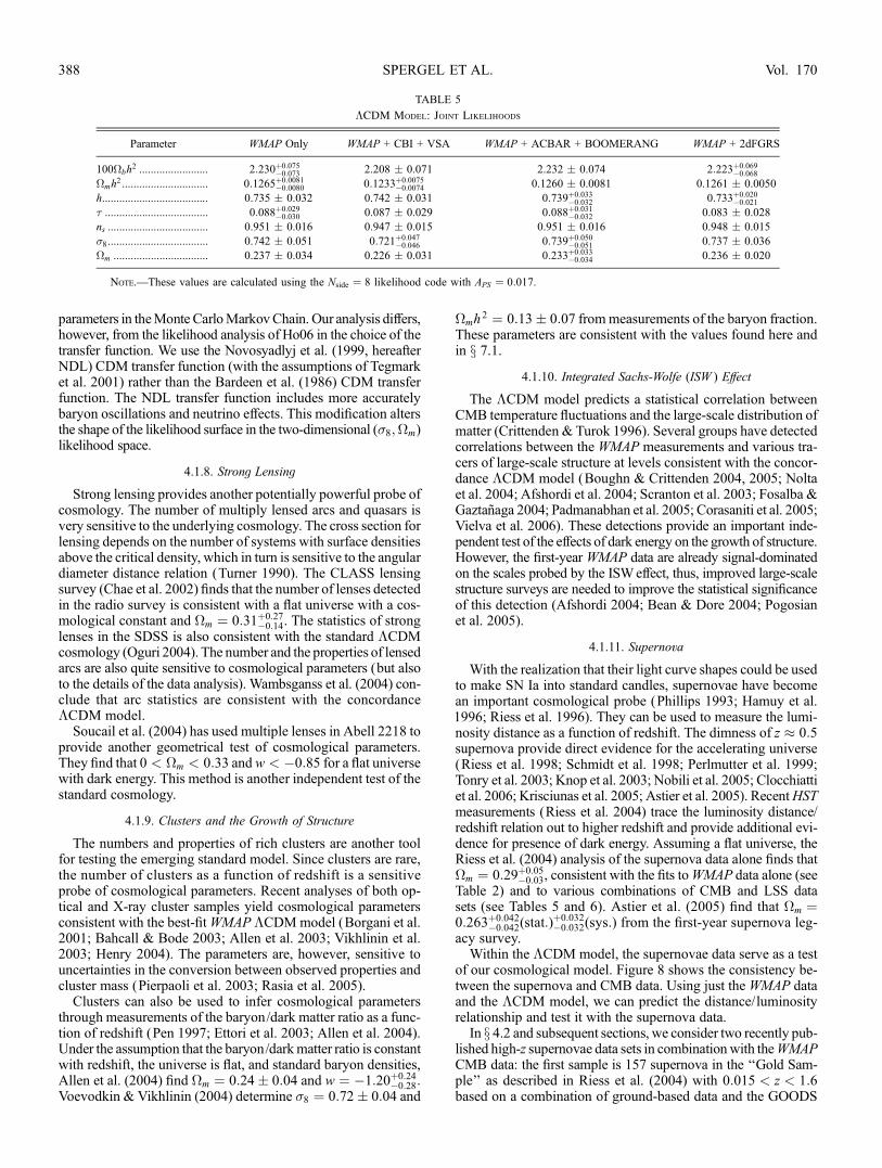
TABLE 5

�CDM Model: Joint Likelihoods

Parameter WMAP Only WMAP + CBI + VSA WMAP + ACBAR + BOOMERANG WMAP + 2dFGRS

100�bh2 ........................ 2:230þ0:075

�0:073 2.208 � 0.071 2.232 � 0.074 2:223þ0:069�0:068

�mh2 .............................. 0:1265þ0:0081

�0:0080 0:1233þ0:0075�0:0074 0.1260 � 0.0081 0.1261 � 0.0050

h..................................... 0.735 � 0.032 0.742 � 0.031 0:739þ0:033�0:032 0:733þ0:020

�0:021

� .................................... 0:088þ0:029�0:030 0.087 � 0.029 0:088þ0:031

�0:032 0.083 � 0.028

ns ................................... 0.951 � 0.016 0.947 � 0.015 0.951 � 0.016 0.948 � 0.015

�8................................... 0.742 � 0.051 0:721þ0:047�0:046 0:739þ0:050

�0:051 0.737 � 0.036

�m ................................. 0.237 � 0.034 0.226 � 0.031 0:233þ0:033�0:034 0.236 � 0.020

Note.—These values are calculated using the Nside ¼ 8 likelihood code with APS ¼ 0:017.


ACS Treasury program usingHST, and the second sample is 115supernova in the range 0:015 < z < 1 from theSupernova LegacySurvey (SNLS; Astier et al. 2005).

Measurements of the apparent magnitude, m, and inferredabsolute magnitude,M0, of each SN have been used to derive thedistance modulus �obs ¼ m�M0, from which a luminosity dis-tance is inferred, �obs ¼ 5 log ½dL(z)/Mpc� þ 25. The luminositydistance predicted from theory, �th, is compared to observationsusing a �2 analysis summing over the SN sample:

�2 ¼Xi

�obs; i(zi)� �th(zi;M0)� �2

�2obs; i

; ð8Þ

where the absolute magnitude, M0, is a ‘‘nuisance parameter,’’analytically marginalized over in the likelihood analysis (Lewis& Bridle 2002), and �obs contains systematic errors related tothe light curve stretch factor, K-correction, extinction, and theintrinsic redshift dispersion due to SNe peculiar velocities (as-sumed 400 and 300 km s�1 forHST/GOODS and SNLS data sets,respectively).

4.2. Joint Constraints on �CDM Model Parameters

In the previous section we showed that the power-law LCDMmodel fit toWMAP data only is consistent with other astronom-ical data.Motivated by this stringent series of cosmological tests,we combine theWMAP datawith other astronomical observationsto further constrain cosmological parameters.

Tables 5 and 6 show that adding external data sets has little ef-fect on several parameters:�bh

2, ns, and � . However, the variouscombinations do reduce the uncertainties on�m and the amplitudeof fluctuations. The data sets used in Table 5 favor smaller valuesof the matter density, higher Hubble constant values, and lowervalues of �8. The data sets used in Table 6 favor higher values of

�m, lower Hubble constants, and higher values of �8. The lens-ing data are most discrepant and it most strongly pulls the com-bined results toward higher amplitudes and higher�m (see Figs. 7and 9). The overall effect of combining the data sets is shown inFigure 10.

The best fits shown in Table 6 differ by about 1 � from the bestfits shown in Table 5 in their predictions for the total matter den-sity, �mh

2 (See Tables 5 and 6 and Fig. 9). More accurate mea-surements of the third peak will help resolve these discrepancies.

The differences between the two sets of data may be due to sta-tistical fluctuations. For example, the SDSS main galaxy samplepower spectrum differs from the power spectrum measured fromthe 2dfGRS: this leads to a lower value for the Hubble constantfor the WMAP + SDSS data combination, h ¼ 0:710� 0:026,than for WMAP + 2dFGRS, h ¼ 0:733þ0:020

�0:021. Note that while

the SDSS LRG data parameters values are close to those fromthe main SDSS catalog, they are independent determinationswith mostly different systematics.

Lensing measurements are sensitive to the amplitude of thelocal potential fluctuations, which scale roughly as �8�

0:6m , so that

lensing parameter constraints are nearly orthogonal to the CMBdegeneracies (Tereno et al. 2005). The CFHTLS lensing databest-fit value for �8�

0:6m is 1Y2 � higher than the best-fit three year

WMAP value. As a result, the combination of CFHT and WMAPdata favors a higher value of �8 and �m and a lower value of H0

thanWMAP data alone. Appendix A shows that the amplitude ofthis discrepancy is somewhat sensitive to our choice of priors.Because of the small error bars in the CFHT data set and the rela-tively small overlap region in parameter space, the CFHT data sethas a strong influence on cosmological parameters. Because of thesmall errors in the CFHT data and the relatively small overlap re-gion in parameter space, the CFHTdata have a strong influence oncosmological parameters. This effect is exacerbated when addi-tional cosmological data sets are included in the analysis. Because

TABLE 6

�CDM Model

Parameter WMAP + SDSS WMAP + LRG WMAP + SNLS WMAP + SNGold WMAP + CFHTLS

100�bh2 ........................... 2:230þ0:071

�0:070 2:242þ0:069�0:070 2:234þ0:075

�0:074 2:230þ0:069�0:072 2.255 � 0.067

�mh2 ................................ 0:1327þ0:0063

�0:0064 0.1336 � 0.0049 0.1293 � 0.0059 0:1349þ0:0061�0:0060 0.1409 � 0.0038

h........................................ 0.710 � 0.026 0:709þ0:019�0:018 0.724 � 0.023 0.701 � 0.021 0.687 � 0.018

� ....................................... 0:080þ0:029�0:030 0.082 � 0.029 0.085 � 0.030 0:079þ0:030

�0:029 0:088þ0:028�0:027

ns ...................................... 0:948þ0:016�0:015 0.951 � 0.016 0:950þ0:016

�0:017 0.946 � 0.016 0.953 � 0.016

�8...................................... 0:772þ0:040�0:041 0.780 � 0.036 0.758 � 0.041 0:784þ0:042

�0:041 0:827þ0:026�0:025

�m .................................... 0.265 � 0.030 0:266þ0:020�0:021 0:248þ0:024

�0:025 0.276 � 0.026 0.300 � 0.021

Fig. 8.—Using the WMAP �CDM parameters, we predict luminosity distance-redshift relationship and compare it to measurements from supernova surveys. Theplots show the deviations of the distance measure (DM) from the empty universe model. The solid lines represent the best WMAP �CDM parameters, and the blueband shows the 68% confidence range. (Left) SNLS data (Astier et al. 2005). (Right) ‘‘Gold’’ supernova data (Riess et al. 2004).


of this, we do not include the lensing data in the full combined dataset (WMAP. . .WMAP + ALL), rather we quote WMAP + CFHTresults separately. The combined data sets place the strongest lim-its on cosmological parameters. Because they are based on theoverlap between many likelihood functions, limits based on theWMAP + ALL data set should be treated with some caution. Fig-ure 10 shows the two-dimensional marginalized likelihood surfacefor both WMAP only and for the combination of WMAP + ALL.

5. CONSTRAINING THE SHAPE OF THE PRIMORDIALPOWER SPECTRUM

While the simplest inflationary models predict that the spec-tral index varies slowly with scale, inflationary models can pro-duce strong scale-dependent fluctuations (see e.g., Kawasaki et al.2003; Hall et al. 2004; Yamaguchi & Yokoyama 2004). The first-year WMAP observations provided some motivation for consid-ering these models as the data, particularly when combined withthe Ly� forest measurements, were better fitted by models with arunning spectral index (Spergel et al. 2003). Small-scale CMBmeasurements (Readhead et al. 2004a) also favor running spectralindex models over power-law models.

Here we consider whether a more general function for the pri-mordial power spectrum could better fit the newWMAP data.Weconsider three forms for the power spectrum:

1. �2R(k) with a running spectral index: 1þ d ln�2

R(k)/d ln k ¼ n(k0)þ dns/d ln (k) ln (k/k0).

2. �2R(k) allowed to freely vary in 15 bins in k-space, with

k1 ¼ 0; k2 ¼ 0:001 Mpc�1; k15 ¼ 0:15 Mpc�1; kiþ1 ¼ 1:47kifor 3 � i � 14.� 2

R(k) is given by linear interpolation within thebins and �2

R(k) ¼ � 2R(0:15/Mpc) for k > 0:15/Mpc.

3. �2R(k) with a sharp k cutoff at k ¼ kc,

�2R(k) ¼ 0; k � kc;

�2R(k) /

k

k0

� �(ns�1)

; k > kc; ð9Þ

Figure 11 shows howWMAP data alone can be used to recon-struct the primordial power spectrum as a function of scale, param-eterized by logarithmically spaced bins out to k ¼ 0:15 Mpc�1.Even allowing for these additional degrees of freedom, the dataprefer a nearly featureless power-law power spectrum.

The deviation of the primordial power spectrum from a simplepower law can be most simply characterized by a sharp cutoff inthe primordial spectrum. Analysis of this model finds that put-ting in a cutoff of kc � 3 ; 10�4 Mpc improves the fit by��2 ¼1:2, not enough to justify a radical change in the primordialspectrum.Table 3 demonstrates that, while models with reduced large-

scale power provide slightly improved fits to the CMB data, theimprovements do not warrant additional parameters.

5.1. External Data Sets and the Running Spectral Index

The uncertainties in the measurements of running is slightlyimproved by including the small-scale experiments. For modelswith only scalar fluctuations, the marginalized value for the de-rivative of the spectral index is dns/d ln k ¼ �0:055þ0:030

�0:031 forWMAP only, dns/d ln k ¼ �0:066þ0:029

�0:028 for the WMAP + CBI +VSA data, and dns/d ln k ¼ �0:058� 0:029 for WMAP +BOOM + ACBAR. For models with tensors, dns/d ln k ¼�0:085� 0:043 forWMAP only, dns/d ln k ¼ �0:090þ0:038

�0:039 forWMAP + CBI + VSA, and dns/d ln k ¼ �0:082� 0:040 forWMAP + BOOM + ACBAR. As Figure 12 shows, models withnegative running allow large tensor amplitudes; thus, when wemarginalize over r with a flat prior, these models favor a morenegative running.Figure 13 shows that both the power-law �CDM model and

the running spectral index model fit the CMB data. At present,the small-scale data do not yet clearly distinguish the two models.A large absolute value of running would be problematic for

most inflationary models, so further testing of this suggestivetrend is important for our understanding of early universe physics.AdditionalWMAP data and upcoming, more sensitive small-scaleCMB data will further test deviations from scale invariance. Cur-rent large-scale structure data do not strengthen the case for run-ning because these data sets probe similar physical scales to theWMAP experiment. Figure 12 shows that current data favor a largerunning; however, the evidence is not yet compelling. The con-straints fromWMAP + lensing andWMAP + 2dFGRS are similarto the WMAP + SDSS constraints shown in Figure 12.

5.2. Is the Power Spectrum Featureless?

Since inflation magnifies fluctuations that were once on sub-Planckian scales to scales of the observable horizon, trans-Planckian physics could potentially leave its imprint on the CMBsky. Over the past few years, there has been significant interestin the possibility of detecting the signature of trans-Planckianphysics in the angular power spectrum. Several studies (Martin& Brandenberger 2001, 2003; Danielsson 2002; Easther et al.2002; Bergstrom & Danielsson 2002; Kaloper et al. 2002; Martin& Ringeval 2004; Burgess et al. 2003; Schalm et al. 2004) havediscussed the possible form and the expected amplitude of thetrans-Planckian effects that might modify the spectrum comingfrom slow roll inflation. The scalar power spectra resulting frompower-law (PL) slow roll inflation can be written in the termsof Hubble Flow parameters, respectively, as (Leach & Liddle2003)

� 2RPL(k) ¼ As 1� 2(C þ 1) 1 � C 2 � (2 1 þ 2) ln

k

k0

� �� :

ð10Þ

Here 1 and 2 are slow roll parameters (Leach & Liddle 2003).After the release of the first-yearWMAP data, Martin & Ringeval

Fig. 9.—One-dimensional marginalized distribution of �mh2 for WMAP,

WMAP + CBI + VSA, WMAP + BOOM + ACBAR,WMAP + SDSS,WMAP +SN(SNLS), WMAP + SN(HST/GOODS), WMAP + 2dFGRS, and WMAP +CFHTLS for the power-law �CDM model.


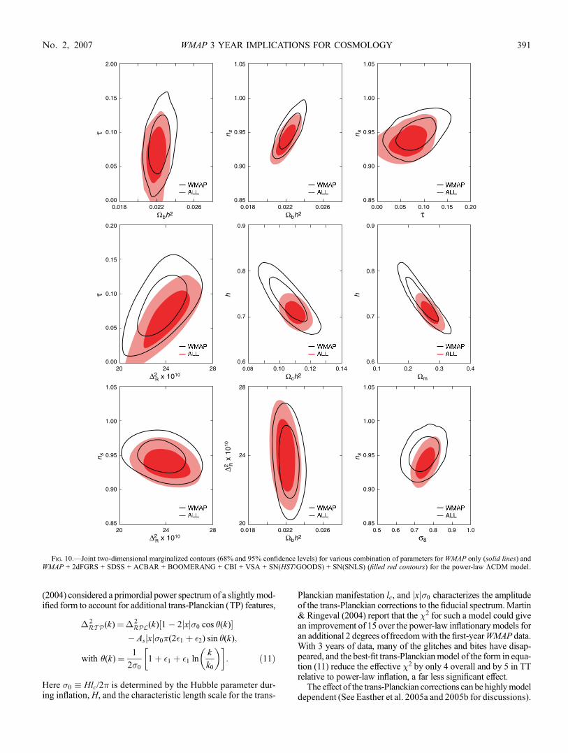
(2004) considered a primordial power spectrum of a slightlymod-ified form to account for additional trans-Planckian (TP) features,

� 2RT P(k)¼� 2

RPL(k) 1� 2jxj�0 cos �(k)½ �� Asjxj�0�(2 1 þ 2) sin �(k);

with �(k)¼ 1

2�01þ 1 þ 1 ln

k

k0

� �� : ð11Þ

Here �0 � Hlc/2� is determined by the Hubble parameter dur-ing inflation,H, and the characteristic length scale for the trans-

Planckian manifestation lc, and jxj�0 characterizes the amplitudeof the trans-Planckian corrections to the fiducial spectrum.Martin& Ringeval (2004) report that the �2 for such a model could givean improvement of 15 over the power-law inflationary models foran additional 2 degrees of freedomwith the first-yearWMAP data.With 3 years of data, many of the glitches and bites have disap-peared, and the best-fit trans-Planckianmodel of the form in equa-tion (11) reduce the effective �2 by only 4 overall and by 5 in TTrelative to power-law inflation, a far less significant effect.

The effect of the trans-Planckian corrections can be highlymodeldependent (See Easther et al. 2005a and 2005b for discussions).

Fig. 10.—Joint two-dimensional marginalized contours (68% and 95% confidence levels) for various combination of parameters for WMAP only (solid lines) andWMAP + 2dFGRS + SDSS + ACBAR + BOOMERANG + CBI + VSA + SN(HST/GOODS) + SN(SNLS) (filled red contours) for the power-law �CDM model.


As an alternative, we consider forms that are more general as away to look for oscillatory signals:

� 2RT P(k) ¼ �2

RPL(k)½1þ TP cos �(k)�; ð12Þ

where � ¼ � k/k0ð Þ þ � or � ¼ � ln k/k0ð Þ þ �. In these models,there are three new parameters: the amplitude, TP, the frequency,�, and the phase, �.

Assuming the �CDM model, we fit these three parameters tothe data and find reductions of 5 and 9.5 in the overall and TT�2eA. As in the Martin & Ringeval model, the improvements in

the�2eA are driven by improvements in the fit around l � 30Y100

and the first peak.

6. WMAP + INFLATION

The inflationary paradigm (Guth 1981; Sato 1981; Linde 1982;Albrecht & Steinhardt 1982) explains the homogeneity, isotropy,and flatness of the universe by positing an early epoch of accel-erated expansion. This accelerated period of expansion also gen-erated superhorizon fluctuations (Guth & Pi 1982; Starobinsky1982;Mukhanov&Chibisov 1981; Hawking 1982; Bardeen et al.1983). In the simplest inflationary models, these fluctuations areGaussian distributed in amplitude with random phase and a nearlyscale-invariant spectrum of fluctuations.The detailed predictions of inflationary models depend on the

properties of the inflaton potential (see Linde 2005 and Lyth &Riotto 1999 for recent reviews). Simple inflationary models pre-dict that the slope of the primordial power spectrum, ns, differsfrom 1 and also predict the existence of a nearly scale-invariantspectrum of gravitational waves. In this section, we compare thesimplest inflationary models to the WMAP 3 year data and toother cosmological data sets. Since we are constraining modelswith tensor modes, we also use theWMAP constraints on the am-plitude of the Bmode signal in the analysis. We characterize thesemodels by seven basic parameters (the six basic parameters of the�CDM model plus one additional parameter, r, the ratio of thetensor to scalar power spectrum). Figure 14 shows the likelihoodcontours for the slope of the scalar fluctuations and the amplitudeof the gravitational wave signal.The WMAP 3 year data place significant constraints on infla-

tionary models (see Table 7). The strength of these constraintsis apparent when we consider monomial models for the inflaton

Fig. 11.—Reconstructed primordial curvature fluctuation spectrum, �2R(k),

for a �CDM cosmology, in logarithmically spaced k bins, where k is in Mpc�1.The errors show the 68% (red ) and 95% (orange) constraints and the black dia-monds the peak likelihood value. The dashed line shows the values for k ¼ 0.Consistent with the predictions of simple inflationary theories, there are no sig-nificant features in the spectrum. The data are consistent with a nearly scale-invariant spectrum.

Fig. 12.—Joint two-dimensional marginalized contours (68% and 95%) forinflationary parameters, (r; ns) (left) and (r; dns/d ln k) (right), for model M11in Table 3, with parameters defined at k ¼ 0:002 Mpc�1. Top: WMAP only.Middle: WMAP + SDSS. Bottom: WMAP + CBI + VSA. Note that ns > 1 isfavored because r and ns are defined at k ¼ 0:002 Mpc�1. At k ¼ 0:05 Mpc�1

ns < 1 is favored. The data do not require a running spectral index, dns/d ln k, atmore than the 95% confidence level.

Fig. 13.—Running spectral index model provides a slightly better fit to thedata than the power-law spectral index model. The solid line shows the best-fitpower-law �CDM model, and the dashed line shows the best-fit running spec-tral index �CDM model (fit to WMAP + CBI + VSA). The insert compares themodels to the WMAP l < 20 data and shows that the running spectral indexmodel better fits the decline at l ¼ 2; however, the improvement in �2 is only 3,not enough to strongly argue for the addition of a new parameter. We have alsodone the same analysis for BOOMERANG and ACBAR data and found similarresults: the current high-l data are not yet able to distinguish between the run-ning spectral index and power-law models.


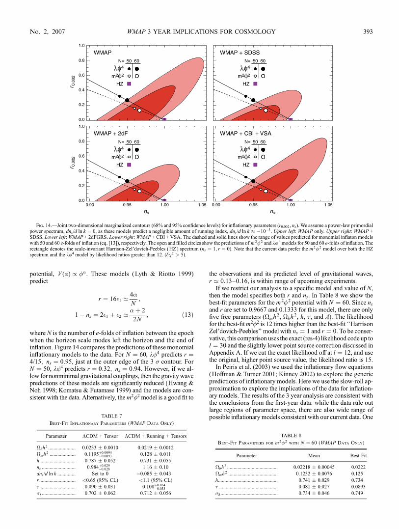
potential, V (�) / ��. These models (Lyth & Riotto 1999)predict

r ¼ 16 1 ’4�

N;

1� ns ¼ 2 1 þ 2 ’�þ 2

2N; ð13Þ

where N is the number of e-folds of inflation between the epochwhen the horizon scale modes left the horizon and the end ofinflation. Figure 14 compares the predictions of thesemonomialinflationary models to the data. For N ¼ 60, k�4 predicts r ¼4/15; ns ¼ 0:95, just at the outer edge of the 3 � contour. ForN ¼ 50, k�4 predicts r ¼ 0:32; ns ¼ 0:94. However, if we al-low for nonminimal gravitational couplings, then the gravitywavepredictions of these models are significantly reduced (Hwang &Noh 1998; Komatsu & Futamase 1999) and the models are con-sistent with the data. Alternatively, them2�2 model is a good fit to

the observations and its predicted level of gravitational waves,r ’ 0:13Y0:16, is within range of upcoming experiments.

If we restrict our analysis to a specific model and value of N,then the model specifies both r and ns. In Table 8 we show thebest-fit parameters for the m2�2 potential with N ¼ 60. Since nsand r are set to 0.9667 and 0.1333 for this model, there are onlyfive free parameters (�mh

2, �bh2, h, � , and A). The likelihood

for the best-fitm2�2 is 12 times higher than the best-fit ‘‘HarrisonZel’dovich-Peebles’’ model with ns ¼ 1 and r ¼ 0. To be conser-vative, this comparison uses the exact (res-4) likelihood code up tol ¼ 30 and the slightly lower point source correction discussed inAppendix A. If we cut the exact likelihood off at l ¼ 12, and usethe original, higher point source value, the likelihood ratio is 15.

In Peiris et al. (2003) we used the inflationary flow equations(Hoffman & Turner 2001; Kinney 2002) to explore the genericpredictions of inflationary models. Here we use the slow-roll ap-proximation to explore the implications of the data for inflation-ary models. The results of the 3 year analysis are consistent withthe conclusions from the first-year data: while the data rule outlarge regions of parameter space, there are also wide range ofpossible inflationary models consistent with our current data. One

Fig. 14.—Joint two-dimensional marginalized contours (68% and 95% confidence levels) for inflationary parameters (r0:002, ns). We assume a power-law primordialpower spectrum, dns/d ln k ¼ 0, as these models predict a negligible amount of running index, dns/d ln k � �10�3. Upper left: WMAP only. Upper right: WMAP +SDSS. Lower left:WMAP + 2dFGRS. Lower right:WMAP + CBI + VSA. The dashed and solid lines show the range of values predicted for monomial inflaton modelswith 50 and 60 e-folds of inflation (eq. [13]), respectively. The open and filled circles show the predictions of m2�2 and k� 4 models for 50 and 60 e-folds of inflation. Therectangle denotes the scale-invariant Harrison-Zel’dovich-Peebles (HZ) spectrum (ns ¼ 1; r ¼ 0). Note that the current data prefer the m2�2 model over both the HZspectrum and the k�4 model by likelihood ratios greater than 12. (��2 > 5).

TABLE 7

Best-Fit Inflationary Parameters (WMAP Data Only)

Parameter �CDM + Tensor �CDM + Running + Tensors

�bh2 ..................... 0.0233 � 0.0010 0.0219 � 0.0012

�mh2 .................... 0:1195þ0:0094

�0:0093 0.128 � 0.011

h............................ 0.787 � 0.052 0.731 � 0.055

ns .......................... 0:984þ0:029�0:028 1.16 � 0.10

dns/d ln k .............. Set to 0 �0.085 � 0.043

r ............................ <0.65 (95% CL) <1.1 (95% CL)

� ........................... 0.090 � 0.031 0:108þ0:034�0:033

�8.......................... 0.702 � 0.062 0.712 � 0.056

TABLE 8

Best-Fit Parameters for m2�2with N ¼ 60 (WMAP Data Only)

Parameter Mean Best Fit

�bh2 ....................................... 0.02218 � 0.00045 0.0222

�mh2 ...................................... 0.1232 � 0.0076 0.125

h.............................................. 0.741 � 0.029 0.734

� ............................................. 0.081 � 0.027 0.0893

�8............................................ 0.734 � 0.046 0.749


of the most intriguing features of Figure 14 is that the data nowdisfavor the exact Harrison-Zel’dovich-Peebles spectrum (ns ¼ 1,r ¼ 0). For power-law inflationary models, this suggests a detect-able level of gravity waves. There are, however, many inflationarymodels that predict a much smaller gravity wave amplitude. Al-ternative models, such as the ekpyrotic scenario (Khoury et al.2001; Khoury et al. 2002) also predict an undetectable level ofgravity waves.

There are several different ways of expressing the constraintsthat the CMB data impose on inflationary models. These param-eters can be directly related to observable quantities: ns � 1 ¼�2 1 � 2 and r ¼ 16 1. For the power-law models, theWMAPbound on r implies that 1 < 0:03 (95%CL). An alternative slowroll representation (see Liddle & Lyth 1992, 1993) uses

v �M 2

Pl

2

V 0

V

� �2

; ð14Þ

v � M 2Pl

V 00

V

� �: ð15Þ

These parameters can be related directly to observables: r ¼16 v and ns � 1 ¼ �6 v þ 2v. Peiris et al. (2003) discussesvarious classes of models in slow roll parameter space.

Models with a significant gravitational wave contributions,r � 0:3, make specific predictions for CMB and large-scale struc-ture observations: (1) a modified temperature spectrumwith morepower at low multipoles and (2) a lower amplitude of densityfluctuations (for fixedCMB temperature fluctuations). For power-law models, the strongest CMB constraints come from the shapeof the temperature spectrum and the amplitude of density fluctua-tions. In order to fit the CMB data, models with higher r valuesrequire larger values of ns and land a lower amplitude of scalarfluctuations,which impacts large-scale structure predictions. Thus,the strongest overall constraints on the tensor mode contributioncomes from the combination of CMB and large-scale structuremeasurements (see Table 9). These strong limits rely on our as-sumption of a power-law spectral index. If we allow for a run-ning index, then models with a large tensor components areconsistent with the data.

7. CONSTRAINING THE COMPOSITIONOF THE UNIVERSE

7.1. Dark Energy Properties

Over the past two decades, there has been growing evidencefor the existence of dark energy (Peebles 1984; Turner et al. 1984;Ostriker & Steinhardt 1995; Dunlop et al. 1996; Krauss & Turner1999; Bahcall et al. 1999). By measuring both the acceleration(Riess et al. 1998; Perlmutter et al. 1999) and deceleration (Riesset al. 2004) of the universe, supernova observations provide themost direct evidence for the existence of dark energy.

The nature of this dark energy is a mystery. From a field theo-retic perspective the most natural explanation for this would bethe presence of a residual vacuum energy density or cosmolog-ical constant,� (Carroll et al. 1992; Peebles & Ratra 2003). How-ever, there are well-known fine-tuning and coincidence problemsin trying to explain the 120 orders-of-magnitude discrepancy be-tween the expected ‘‘natural’’ Planck-scale energy density of acosmological constant and the observed dark energy density.These problems motivate a wide range of alternative explana-tions for the observations including the presence of an extra mat-ter candidate: for example a dynamical, scalar ‘‘quintessence’’field (Peebles & Ratra 1988; Wetterich 1988; Zlatev et al. 1999),minimally coupled (Caldwell et al. 1998; Ferreira & Joyce1998) or nonminimally coupled to gravity (Amendola 1999) orother matter (Bean & Magueijo 2001). In this latter case, themeasured acceleration is due to interactions in the matter bulk.Another alternative is that modifications to gravity (e.g., Deffayet2001; Deffayet et al. 2002) are responsible for the observedanomalies.The dark energy has two distinct cosmological effects:

(1) through the Friedman equation, it alters the evolution ofH(z),and (2) through the perturbation equations, it alters the evolutionofD(z), the growth rate of structure. The supernova data measureonly the luminosity distance, which depends on H(z), while thelarge-scale structure data are sensitive to both H(z) and D(z).While the presence of dark energy impacts the CMB primarily

through the distance to the surface of last scatter, the dark energyclustering properties also affect the CMB properties. The darkenergy response to gravitational perturbations depends on its iso-tropic and anisotropic sound speeds (Hu 1998; Bucher & Spergel1999). This affects the CMBfluctuations through the ISWeffect. Ifthe dark energy can cluster, then it produces a smaller ISWeffectand does not enhance the power spectrum at large angular scales.These effects are most dramatic for models with w < �1, as darkenergy effects in these models turn on suddenly at late times andsignificantly enhance the quadrupole. This can be understood interms of the constraints imposed by the shape of the angular powerspectrum: if we assume that the dark energy properties can be de-scribed by a constant value of w, then fixed peak position andheights (which determine �mh

2) confine our models to a narrowvalley in the (�m, w) likelihood surface as shown in Figures 15and 16. These figures and Table 10 show that the 3 year data en-able a more accurate determination of �mh

2 which narrows thewidth of the degeneracy valley. The pair offigures show that CMBdata can place strong limits on models withw < �1 and nonclus-tering dark energy. On the other hand, if the dark energy is amattercomponent that can cluster, evenmeagerly, as is the case for scalarfield theories where c2s ¼ 1, then this clustering counters thesuppression of perturbation growth during the accelerative epochand the quadrupole’s magnitude is reduced. This lessens the dis-criminating power of the quadrupole for measuring w: whileCMB data rule out the wT�1 region in Figure 15, they do notconstrain models in the same region in Figure 16.It is interesting to note that if we relax the assumption of spa-

tial flatness, the data still prefer models with w close to �1 (seeFigs. 17 and 18). In this analysis, we assume that the dark energyclusters.

7.2. Neutrino Properties

7.2.1. Neutrino Mass

Both atmospheric neutrino and solar neutrino experiments showthat neutrinos are massive and that there is significant mix-ing between the various neutrino interaction eigenstates (see

TABLE 9

Constraints on r, Ratio of Amplitude of Tensor Fluctuations

to Scalar Fluctuations (at k ¼ 0:002 Mpc�1)

Data Set r (No Running) r (with Running)

WMAP .............................................. <0.65 (95% CL) <1.1 (95% CL)

WMAP + BOOM + ACBAR........... <0.68 (95% CL) <1.1 (95% CL)

WMAP + CBI + VSA...................... <0.62 (95% CL) <1.1 (95% CL)

WMAP + 2df.................................... <0.38 (95% CL) <0.64 (95% CL)

WMAP + SDSS................................ <0.30 (95% CL) <0.38 (95% CL)


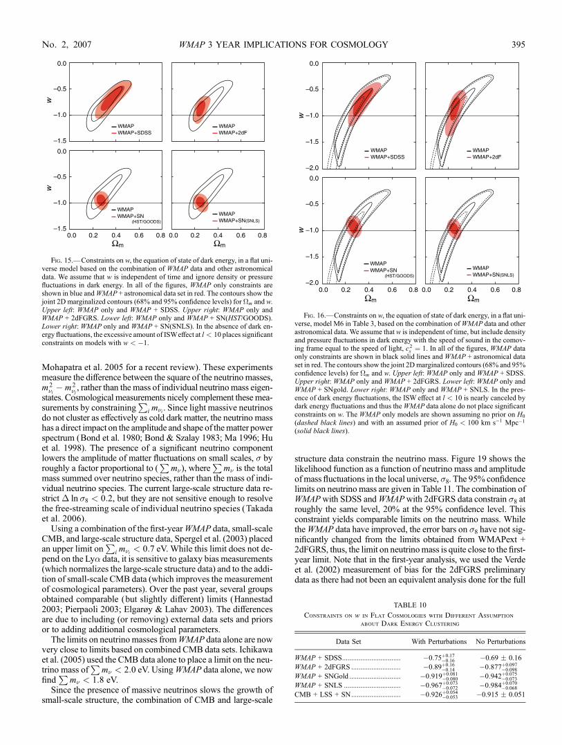
Mohapatra et al. 2005 for a recent review). These experimentsmeasure the difference between the square of the neutrino masses,m2�i� m2

�j, rather than the mass of individual neutrinomass eigen-

states. Cosmological measurements nicely complement thesemea-surements by constraining

Pi m�i . Since light massive neutrinos

do not cluster as effectively as cold dark matter, the neutrino masshas a direct impact on the amplitude and shape of thematter powerspectrum (Bond et al. 1980; Bond & Szalay 1983; Ma 1996; Huet al. 1998). The presence of a significant neutrino componentlowers the amplitude of matter fluctuations on small scales, � byroughly a factor proportional to (

Pm�), where

Pm� is the total

mass summed over neutrino species, rather than the mass of indi-vidual neutrino species. The current large-scale structure data re-strict � ln �8 < 0:2, but they are not sensitive enough to resolvethe free-streaming scale of individual neutrino species (Takadaet al. 2006).

Using a combination of the first-yearWMAP data, small-scaleCMB, and large-scale structure data, Spergel et al. (2003) placedan upper limit on

Pi m�i < 0:7 eV. While this limit does not de-

pend on the Ly� data, it is sensitive to galaxy bias measurements(which normalizes the large-scale structure data) and to the addi-tion of small-scale CMB data (which improves the measurementof cosmological parameters). Over the past year, several groupsobtained comparable (but slightly different) limits (Hannestad2003; Pierpaoli 2003; Elgarøy & Lahav 2003). The differencesare due to including (or removing) external data sets and priorsor to adding additional cosmological parameters.

The limits on neutrinomasses fromWMAP data alone are nowvery close to limits based on combined CMB data sets. Ichikawaet al. (2005) used the CMB data alone to place a limit on the neu-trino mass of

Pm� < 2:0 eV. UsingWMAP data alone, we now

findP

m� < 1:8 eV.Since the presence of massive neutrinos slows the growth of

small-scale structure, the combination of CMB and large-scale

structure data constrain the neutrino mass. Figure 19 shows thelikelihood function as a function of neutrino mass and amplitudeofmass fluctuations in the local universe, �8. The 95% confidencelimits on neutrino mass are given in Table 11. The combination ofWMAPwith SDSS andWMAPwith 2dFGRS data constrain �8 atroughly the same level, 20% at the 95% confidence level. Thisconstraint yields comparable limits on the neutrino mass. WhiletheWMAP data have improved, the error bars on �8 have not sig-nificantly changed from the limits obtained from WMAPext +2dFGRS, thus, the limit on neutrinomass is quite close to the first-year limit. Note that in the first-year analysis, we used the Verdeet al. (2002) measurement of bias for the 2dFGRS preliminarydata as there had not been an equivalent analysis done for the full

Fig. 15.—Constraints on w, the equation of state of dark energy, in a flat uni-verse model based on the combination of WMAP data and other astronomicaldata. We assume that w is independent of time and ignore density or pressurefluctuations in dark energy. In all of the figures, WMAP only constraints areshown in blue andWMAP + astronomical data set in red. The contours show thejoint 2D marginalized contours (68% and 95% confidence levels) for �m and w.Upper left: WMAP only and WMAP + SDSS. Upper right: WMAP only andWMAP + 2dFGRS. Lower left: WMAP only and WMAP + SN(HST/GOODS).Lower right: WMAP only and WMAP + SN(SNLS). In the absence of dark en-ergy fluctuations, the excessive amount of ISWeffect at l < 10 places significantconstraints on models with w < �1.

Fig. 16.—Constraints on w, the equation of state of dark energy, in a flat uni-verse, model M6 in Table 3, based on the combination ofWMAP data and otherastronomical data. We assume that w is independent of time, but include densityand pressure fluctuations in dark energy with the speed of sound in the comov-ing frame equal to the speed of light, c2s ¼ 1. In all of the figures, WMAP dataonly constraints are shown in black solid lines and WMAP + astronomical dataset in red. The contours show the joint 2D marginalized contours (68% and 95%confidence levels) for �m and w. Upper left: WMAP only and WMAP + SDSS.Upper right: WMAP only and WMAP + 2dFGRS. Lower left: WMAP only andWMAP + SNgold. Lower right: WMAP only and WMAP + SNLS. In the pres-ence of dark energy fluctuations, the ISW effect at l < 10 is nearly canceled bydark energy fluctuations and thus theWMAP data alone do not place significantconstraints on w. The WMAP only models are shown assuming no prior on H0

(dashed black lines) and with an assumed prior of H0 < 100 km s�1 Mpc�1

(solid black lines).

TABLE 10

Constraints on w in Flat Cosmologies with Different Assumption

about Dark Energy Clustering

Data Set With Perturbations No Perturbations

WMAP + SDSS................................ �0:75þ0:17�0:16 �0.69 � 0.16

WMAP + 2dFGRS ........................... �0:89þ0:16�0:14 �0:877þ0:097

�0:098

WMAP + SNGold ............................ �0:919þ0:081�0:080 �0:942þ0:075

�0:073

WMAP + SNLS ............................... �0:967þ0:073�0:072 �0:984þ0:070

�0:068

CMB + LSS + SN........................... �0:926þ0:054�0:053 �0.915 � 0.051


2dFGRS data set. As discussed in x 4.1.4, we now marginalizeover the 2dFGRS bias and use the bias measurements of Seljaket al. (2005b) for SDSS.

If the constraints on amplitude are reliable, then small-scalematter power spectrum structure data can significantly improvethese neutrino constraints. Goobar et al. (2006) have recently com-pleted a CMB + Ly� study and place a limit of

Pm� < 0:30 eV

(95% CL). Similarly, cluster-based measurements of �8 andlensing-based measurements of �8 have the potential to tightenthe constraint on m� .

7.2.2. Number of Relativistic Species

If there are other light stable neutral particles (besides the threelight neutrinos and the photon), then these particles will affect theCMB angular power spectrum and the evolution of large-scalestructure. Because of the details of freeze-out at electron-positronannihilation (Gnedin & Gnedin 1998; Dolgov et al. 1999), QEDcorrections at finite temperature (Mangano et al. 2002), and non-trivial terms in the neutrino mass matrix (Mangano et al. 2005),the effective number of neutrino species is slightly greater than 3.Any light particle that does not couple to electrons, ions, and pho-tons will act as an additional relativistic species. For neutrinos, wecan compute their effects accurately as their temperature is (4/11)1/3

of the CMB temperature. For other relativistic species, the limit onN eA� � 3:04 can be converted into a limit on their abundance by

scaling by the temperature.The shape of the CMB angular power spectrum is sensitive to

the epoch of matter/radiation equality. If we increase N� , the ef-fective number of neutrino species, then we will need to also in-crease the cold dark matter density, �ch

2, and slowly changeother parameters to remain consistent with theWMAP data (Bowenet al. 2002). In addition, the presence of these additional neutrinospecies alters the damping tail and leaves a distinctive signature onthe high-l angular power spectrum (Bashinsky & Seljak 2004)and on the small-scale matter power spectrum.

Fig. 17.—Constraints on a nonflat universe with quintessence-like dark energywith constant w (model M10 in Table 3). The contours show the 2D marginalizedcontours forw and�k based on the CMB+2dFGRS+SDSS+ supernova data sets.This figure shows thatwith the full combination of data sets, there are already stronglimits onwwithout the need to assume a flat universe prior. The marginalized best-fit values for the equation of state and curvature are w ¼ �1:08� 0:12 and �k ¼�0:026þ0:016

�0:015 at the 68% confidence level.

Fig. 18.—Constraints on a flat universe with quintessence-like dark energyand nonrelativistic neutrinos. The contours show the 2D marginalized constraintson the mass of nonrelativistic neutrinos,m� , and the dark energy equation of state,w, assumed constant, based on the CMB+ 2dFGRS + SDSS + supernova data sets.In this analysis, we assume that the dark energy clusters. With the combination ofCMB + 2dFGRS + SDSS + supernova data sets, there is not a strong degeneracybetween neutrino and dark energy properties. Even in this more general model,we still have an interesting constraint on the neutrino mass and equation of state:P

m� < 1:0 eV (95%CL) and w ¼ �1:07� 0:12 (68% CL). This suggests thatthe astronomical dark energy and neutrino limits are robust even when we start toconsider more baroque models.

Fig. 19.—Joint two-dimensional marginalized contours (68% and 95% con-fidence levels) on (�8; m�) forWMAP only, model M7 in Table 3, andWMAP +SDSS. By measuring the growth rate of structure from z ¼ 1088 to z ’ 0, theseobservations constrain the contribution of nonrelativistic neutrinos to the energydensity of the universe.

TABLE 11

Constraints on Neutrino Properties

Data SetP

m� (95% Limit for N� ¼ 3:04) N�

WMAP ............................... 1.8 eV (95% CL) . . .WMAP + SDSS................. 1.3 eV (95% CL) 7:1þ4:1

�3:5

WMAP + 2dFGRS ............ 0.88 eV (95% CL) 2.7 � 1.4

CMB + LSS + SN............ 0.66 eV (95% CL) 3.3 � 1.7


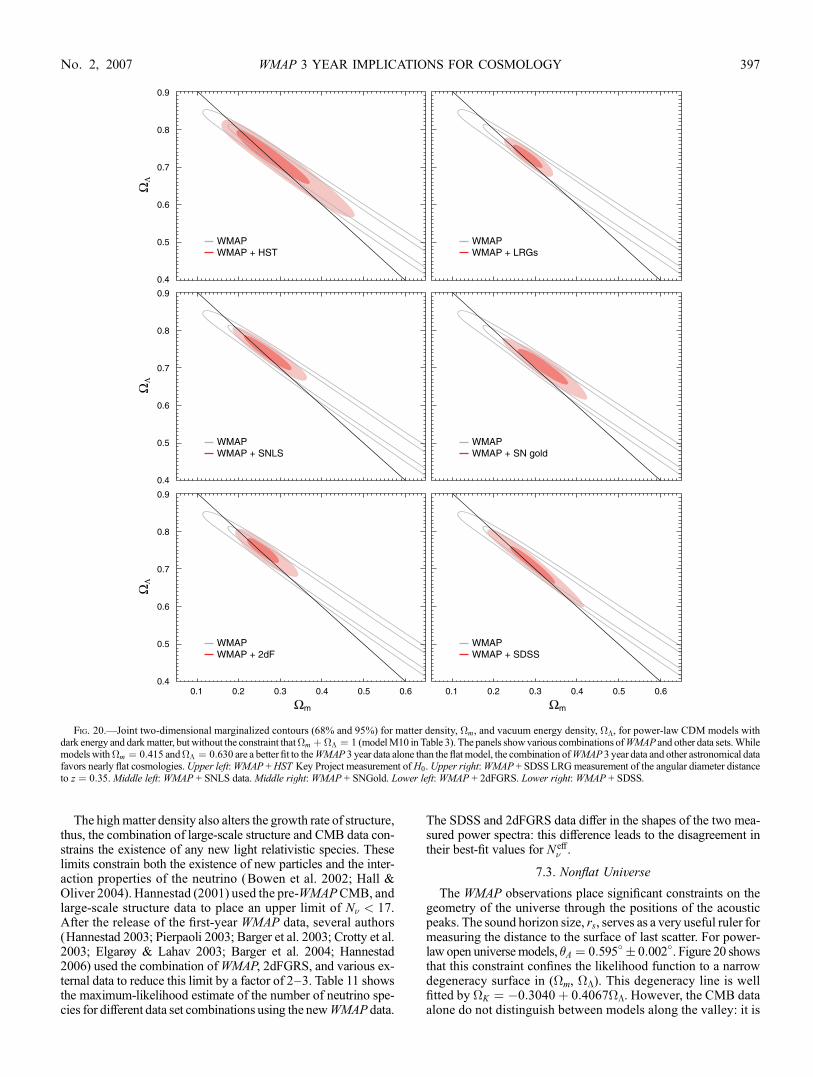
The highmatter density also alters the growth rate of structure,thus, the combination of large-scale structure and CMB data con-strains the existence of any new light relativistic species. Theselimits constrain both the existence of new particles and the inter-action properties of the neutrino (Bowen et al. 2002; Hall &Oliver 2004). Hannestad (2001) used the pre-WMAPCMB, andlarge-scale structure data to place an upper limit of N� < 17.After the release of the first-year WMAP data, several authors(Hannestad 2003; Pierpaoli 2003; Barger et al. 2003; Crotty et al.2003; Elgarøy & Lahav 2003; Barger et al. 2004; Hannestad2006) used the combination ofWMAP, 2dFGRS, and various ex-ternal data to reduce this limit by a factor of 2Y3. Table 11 showsthe maximum-likelihood estimate of the number of neutrino spe-cies for different data set combinations using the newWMAP data.

The SDSS and 2dFGRS data differ in the shapes of the two mea-sured power spectra: this difference leads to the disagreement intheir best-fit values for N eA

� .

7.3. Nonflat Universe

The WMAP observations place significant constraints on thegeometry of the universe through the positions of the acousticpeaks. The sound horizon size, rs, serves as a very useful ruler formeasuring the distance to the surface of last scatter. For power-law open universemodels, �A ¼ 0:595� � 0:002�. Figure 20 showsthat this constraint confines the likelihood function to a narrowdegeneracy surface in (�m, ��). This degeneracy line is wellfitted by �K ¼ �0:3040þ 0:4067��. However, the CMB dataalone do not distinguish between models along the valley: it is

Fig. 20.—Joint two-dimensional marginalized contours (68% and 95%) for matter density, �m, and vacuum energy density, ��, for power-law CDM models withdark energy and darkmatter, but without the constraint that�m þ �� ¼ 1 (modelM10 in Table 3). The panels showvarious combinations ofWMAP and other data sets.Whilemodels with�m ¼ 0:415 and�� ¼ 0:630 are a better fit to theWMAP 3 year data alone than the flat model, the combination ofWMAP 3 year data and other astronomical datafavors nearly flat cosmologies.Upper left:WMAP +HST Key Project measurement of H0.Upper right:WMAP + SDSS LRGmeasurement of the angular diameter distanceto z ¼ 0:35. Middle left: WMAP + SNLS data.Middle right: WMAP + SNGold. Lower left: WMAP + 2dFGRS. Lower right: WMAP + SDSS.


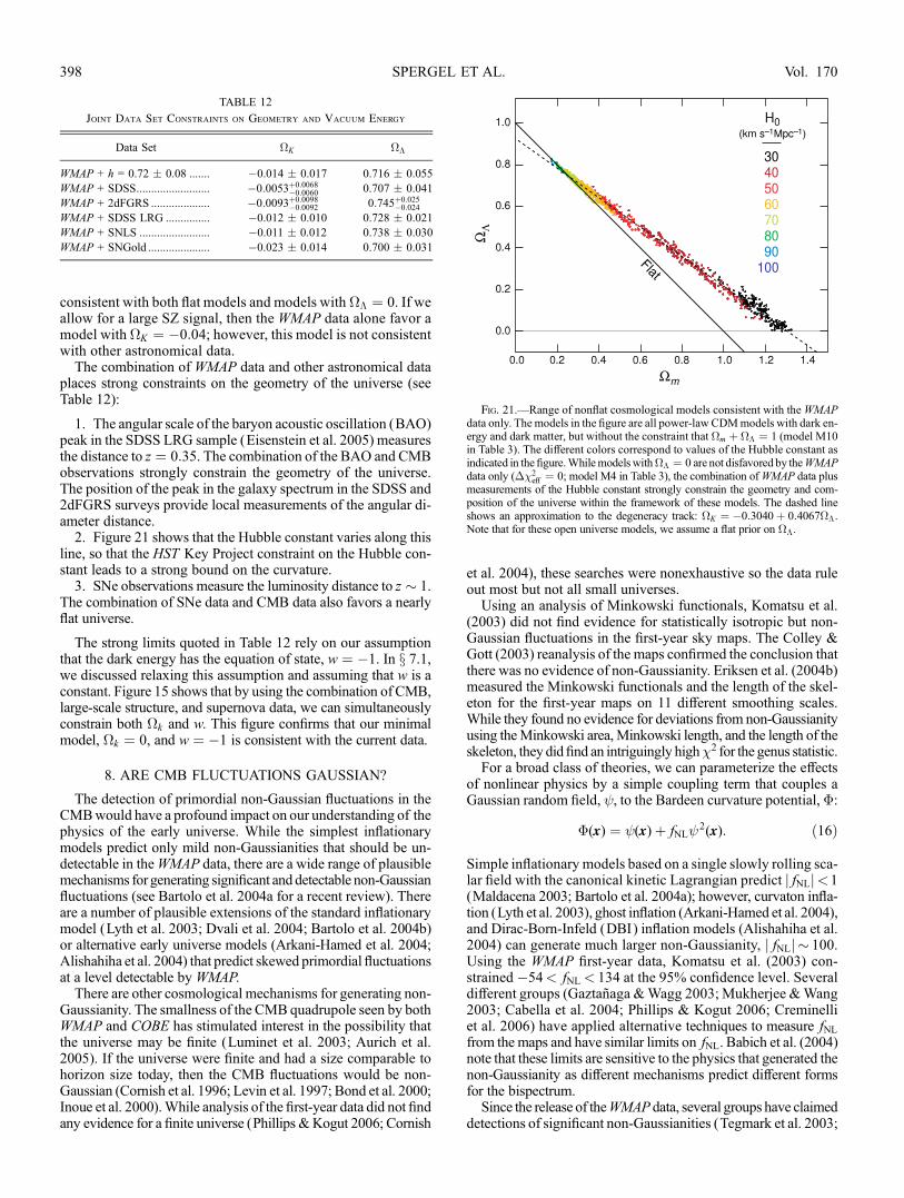
consistent with both flat models and models with�� ¼ 0. If weallow for a large SZ signal, then the WMAP data alone favor amodel with �K ¼ �0:04; however, this model is not consistentwith other astronomical data.

The combination of WMAP data and other astronomical dataplaces strong constraints on the geometry of the universe (seeTable 12):

1. The angular scale of the baryon acoustic oscillation (BAO)peak in the SDSS LRG sample (Eisenstein et al. 2005) measuresthe distance to z ¼ 0:35. The combination of the BAO and CMBobservations strongly constrain the geometry of the universe.The position of the peak in the galaxy spectrum in the SDSS and2dFGRS surveys provide local measurements of the angular di-ameter distance.

2. Figure 21 shows that the Hubble constant varies along thisline, so that the HST Key Project constraint on the Hubble con-stant leads to a strong bound on the curvature.

3. SNe observations measure the luminosity distance to z � 1.The combination of SNe data and CMB data also favors a nearlyflat universe.

The strong limits quoted in Table 12 rely on our assumptionthat the dark energy has the equation of state, w ¼ �1. In x 7.1,we discussed relaxing this assumption and assuming that w is aconstant. Figure 15 shows that by using the combination of CMB,large-scale structure, and supernova data, we can simultaneouslyconstrain both �k and w. This figure confirms that our minimalmodel, �k ¼ 0, and w ¼ �1 is consistent with the current data.

8. ARE CMB FLUCTUATIONS GAUSSIAN?

The detection of primordial non-Gaussian fluctuations in theCMBwould have a profound impact on our understanding of thephysics of the early universe. While the simplest inflationarymodels predict only mild non-Gaussianities that should be un-detectable in theWMAP data, there are a wide range of plausiblemechanisms for generating significant and detectable non-Gaussianfluctuations (see Bartolo et al. 2004a for a recent review). Thereare a number of plausible extensions of the standard inflationarymodel (Lyth et al. 2003; Dvali et al. 2004; Bartolo et al. 2004b)or alternative early universe models (Arkani-Hamed et al. 2004;Alishahiha et al. 2004) that predict skewed primordial fluctuationsat a level detectable by WMAP.

There are other cosmological mechanisms for generating non-Gaussianity. The smallness of the CMB quadrupole seen by bothWMAP and COBE has stimulated interest in the possibility thatthe universe may be finite (Luminet et al. 2003; Aurich et al.2005). If the universe were finite and had a size comparable tohorizon size today, then the CMB fluctuations would be non-Gaussian (Cornish et al. 1996; Levin et al. 1997; Bond et al. 2000;Inoue et al. 2000).While analysis of the first-year data did not findany evidence for a finite universe (Phillips &Kogut 2006; Cornish

et al. 2004), these searches were nonexhaustive so the data ruleout most but not all small universes.Using an analysis of Minkowski functionals, Komatsu et al.

(2003) did not find evidence for statistically isotropic but non-Gaussian fluctuations in the first-year sky maps. The Colley &Gott (2003) reanalysis of the maps confirmed the conclusion thatthere was no evidence of non-Gaussianity. Eriksen et al. (2004b)measured the Minkowski functionals and the length of the skel-eton for the first-year maps on 11 different smoothing scales.While they found no evidence for deviations from non-Gaussianityusing theMinkowski area,Minkowski length, and the length of theskeleton, they did find an intriguingly high�2 for the genus statistic.For a broad class of theories, we can parameterize the effects

of nonlinear physics by a simple coupling term that couples aGaussian random field, , to the Bardeen curvature potential,�:

�(x) ¼ (x)þ fNL 2(x): ð16Þ

Simple inflationary models based on a single slowly rolling sca-lar field with the canonical kinetic Lagrangian predict j fNLj<1(Maldacena 2003; Bartolo et al. 2004a); however, curvaton infla-tion (Lyth et al. 2003), ghost inflation (Arkani-Hamed et al. 2004),and Dirac-Born-Infeld (DBI) inflation models (Alishahiha et al.2004) can generate much larger non-Gaussianity, j fNLj � 100.Using the WMAP first-year data, Komatsu et al. (2003) con-strained �54< fNL< 134 at the 95% confidence level. Severaldifferent groups (Gaztanaga &Wagg 2003; Mukherjee &Wang2003; Cabella et al. 2004; Phillips & Kogut 2006; Creminelliet al. 2006) have applied alternative techniques to measure fNLfrom the maps and have similar limits on fNL. Babich et al. (2004)note that these limits are sensitive to the physics that generated thenon-Gaussianity as different mechanisms predict different formsfor the bispectrum.Since the release of theWMAP data, several groups have claimed

detections of significant non-Gaussianities (Tegmark et al. 2003;

Fig. 21.—Range of nonflat cosmological models consistent with theWMAPdata only. The models in the figure are all power-law CDMmodels with dark en-ergy and dark matter, but without the constraint that �m þ �� ¼ 1 (model M10in Table 3). The different colors correspond to values of the Hubble constant asindicated in the figure.Whilemodelswith�� ¼ 0 are not disfavored by theWMAPdata only (��2

eA ¼ 0; model M4 in Table 3), the combination ofWMAP data plusmeasurements of the Hubble constant strongly constrain the geometry and com-position of the universe within the framework of these models. The dashed lineshows an approximation to the degeneracy track: �K ¼ �0:3040þ 0:4067��.Note that for these open universe models, we assume a flat prior on ��.

TABLE 12

Joint Data Set Constraints on Geometry and Vacuum Energy

Data Set �K ��

WMAP + h = 0.72 � 0.08 ....... �0.014 � 0.017 0.716 � 0.055

WMAP + SDSS......................... �0:0053þ0:0068�0:0060 0.707 � 0.041

WMAP + 2dFGRS .................... �0:0093þ0:0098�0:0092 0:745þ0:025

�0:024

WMAP + SDSS LRG ............... �0.012 � 0.010 0.728 � 0.021

WMAP + SNLS ........................ �0.011 � 0.012 0.738 � 0.030

WMAP + SNGold ..................... �0.023 � 0.014 0.700 � 0.031


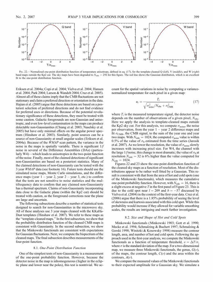
Eriksen et al. 2004a; Copi et al. 2004; Vielva et al. 2004; Hansenet al. 2004; Park 2004; Larson &Wandelt 2004; Cruz et al. 2005).Almost all of these claims imply that the CMBfluctuations are notstationary and claim a preferred direction or orientation in the data.Hajian et al. (2005) argue that these detections are based on a pos-teriori selection of preferred directions and do not find evidencefor preferred axes or directions. Because of the potential revolu-tionary significance of these detections, they must be treated withsome caution. Galactic foregrounds are non-Gaussian and aniso-tropic, and even low-level contamination in the maps can producedetectable non-Gaussianities (Chiang et al. 2003; Naselsky et al.2005) but have only minimal effects on the angular power spec-trum (Hinshaw et al. 2003). Similarly, point sources can be asource of non-Gaussianity at small angular scales (Eriksen et al.2004a). Because of the WMAP scan pattern, the variance in thenoise in the maps is spatially variable. There is significant 1/fnoise in several of the Difference Assemblies (DAs) (particu-larlyW4)—which leads to anisotropies in the two-point functionof the noise. Finally, most of the claimed detections of significantnon-Gaussianities are based on a posteriori statistics. Many ofthe claimed detections of non-Gaussianity can be tested with the3 yearWMAP data (see footnote 16). Future tests should use thesimulated noise maps, Monte Carlo simulations, and the differ-ence maps (year 1� year 2, year 2� year 3, etc.) to confirmthat the tests are not sensitive to noise statistics and the mul-tifrequency data to confirm that any claimed non-Gaussianityhas a thermal spectrum. Claims of non-Gaussianity incorporatingdata close to the Galactic plane (within the Kp2 cut) should betreated with caution, as the foreground corrections near the planeare large and uncertain.

The following subsections describe a number of statistical testsdesigned to search for non-Gaussianities in the microwave sky.All of these analyses use 3 year maps cleaned with the KKaHa-Dust templates (Hinshaw et al. 2007). We refer to these maps asthe ‘‘template-cleanedmaps.’’ In the first subsection, we show thatthe probability distribution function of the cleaned CMB maps isconsistent with Gaussianity. In the second subsection, we showthat the Minkowski functionals are consistent with expectationsfor Gaussian fluctuations. Next, we compute the bispectrum of thecleanedmaps. The final subsection describesmeasurements of thefour-point function.

8.1. One-Point Distribution Function

One of the simplest tests of non-Gaussianity is a measurementof the one-point probability function. However, because thedetector noise in the map is inhomogeneous (higher in the eclip-tic plane and lower near the poles), this test is nontrivial. We ac-

count for the spatial variations in noise by computing a variance-normalized temperature for each pixel in a given map:

ui ¼Tiffiffiffiffiffiffiffiffiffiffiffiffiffiffiffiffiffiffiffiffiffiffiffiffiffiffiffiffiffiffiffiffiffiffiffiffiffi

�2noise=Nobs þ �2

CMB

q ; ð17Þ

where Ti is the measured temperature signal, the detector noisedepends on the number of observations of a given pixel, Nobs.Here we apply the analysis to template-cleaned maps outsidethe Kp2 sky cut. For this analysis, we compute �noise, the noiseper observation, from the year 1� year 2 difference maps andfit �CMB, the CMB signal, to the sum of the year one and yeartwo maps. With Nside ¼ 1024, the computed �noise value is within0.5% of the value of �0 estimated from the time series (Jarosiket al. 2007). As we lower the resolution, the value of �noise slowlyincreases with increasing pixel size. For W4, the channel withthe large 1/f noise, this change is most dramatic; the value of �0 atresolution Nside ¼ 32 is 6% higher than the value computed forNside ¼ 1024.

Figures 22 and 23 show the one-point distribution function ofthe cleaned sky maps as a function of resolution. Most of the dis-tributions appear to be rather well fitted by a Gaussian. This re-sult is consistent with that from the area of hot and cold spots (oneof the Minkowski functionals), which measures the cumulativeone-point probability function. However, withNside ¼ 16, there isa slight excess at negative T in the first panel of Figure 23. This isdue to the cold spot near l ¼ 209 and b ¼ �57 discussed byVielva et al. (2004) in the context of the first-year data. Cruz et al.(2006) argue that there is a 1.85% probability of seeing the levelof skewness and kurtosis associatedwith this cold spot.While thisprobability would increase if they allowed for variable smoothingscales, the results are intriguing and merit further investigation.

8.2. Size and Shape of Hot and Cold Spots

Minkowski functionals (Minkowski 1903; Gott et al. 1990;Mecke et al. 1994; Schmalzing & Buchert 1997; Schmalzing &Gorski 1998; Winitzki & Kosowsky 1998) measure the contourlength, area, and number of hot and cold spots. Following the ap-proach used in the first-year analysis, we compute the Minkowskifunctionals as a function of temperature threshold, � ¼ �T /�,where� is the standard deviation of themap. For a two-dimensionalmap, we measure three Minkowski functionals, the genus, G(�),of the maps, the contour length, C(�) and the area within thecontours, A(�).

We compare themeasured values of theMinkowski functionalsto their expected amplitude for a Gaussian sky. We simulate a

Fig. 22.—Normalized one-point distribution function of temperature anisotropy, defined in eq. (17), for the template-cleaned Q (left), V (middle), and W (right)band maps outside the Kp2 cut. The sky maps have been degraded to Nside ¼ 256 for this figure. The red line shows the Gaussian distribution, which is an excellentfit to the one-point distribution function.


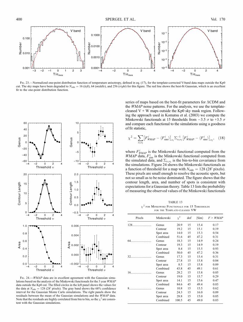
series of maps based on the best-fit parameters for �CDM andthe WMAP noise patterns. For the analysis, we use the template-cleaned V + W maps outside the Kp0 sky mask region. Follow-ing the approach used in Komatsu et al. (2003) we compute theMinkowski functionals at 15 thresholds from �3.5 � to +3.5 �and compare each functional to the simulations using a goodnessof fit statistic,

�2 ¼X�1�2

F iWMAP � hF i

simi� �

�1��1�1�2

F iWMAP � hF i

simi� �

�2; ð18Þ

where F iWMAP is the Minkowski functional computed from the

WMAP data, F isim is the Minkowski functional computed from

the simulated data, and ��1�2 is the bin-to-bin covariance fromthe simulations. Figure 24 shows the Minkowski functionals asa function of threshold for a map with Nside ¼ 128 (280 pixels).These pixels are small enough to resolve the acoustic spots, butnot so small as to be noise dominated. The figure shows that thecontour length, area, and number of spots is consistent withexpectations for a Gaussian theory. Table 13 lists the probabilityof measuring the observed values of the Minkowski functionals

Fig. 23.—Normalized one-point distribution function of temperature anisotropy, defined in eq. (17), for the template-corrected V-band data maps outside the Kp0cut. The sky maps have been degraded to Nside ¼ 16 (left), 64 (middle), and 256 (right) for this figure. The red line shows the best-fit Gaussian, which is an excellentfit to the one-point distribution function.

Fig. 24.—WMAP data are in excellent agreement with the Gaussian simu-lations based on the analysis of theMinkowski functionals for the 3 yearWMAPdata outside the Kp0 cut. The filled circles in the left panel shows the values forthe data at Nside ¼ 128 (280 pixels). The gray band shows the 68% confidenceinterval for the Gaussian Monte Carlo simulations. The right panels show theresiduals between the mean of the Gaussian simulations and the WMAP data.Note that the residuals are highly correlated from bin to bin, so the �2 are consis-tent with the Gaussian simulations.

TABLE 13

� 2for Minkowski Functionals for 15 Thresholds

for the Template-cleaned VW

Pixels Minkowski �2 dof hSimi F > WMAP

128........................ Genus 20.9 15 15.4 0.17

Contour 19.2 15 15.1 0.19

Spot area 14.0 15 15.3 0.54

Combined 51.6 45 47.2 0.31

64.......................... Genus 18.3 15 14.9 0.24

Contour 19.3 15 14.9 0.19

Spot area 8.4 15 15.5 0.93

Combined 50.0 45 47.2 0.36

32.......................... Genus 17.3 15 15.4 0.31

Contour 27.8 15 15.8 0.04

Spot area 8.5 15 15.8 0.89

Combined 43.8 45 49.1 0.61

16.......................... Genus 28.2 15 15.8 0.05

Contour 19.0 15 15.7 0.29

Spot area 14.1 15 15.6 0.47

Combined 84.6 45 49.4 0.03

8............................ Genus 10.8 15 15.5 0.62

Contour 24.3 15 16.0 0.09

Spot area 28.8 15 15.0 0.05

Combined 100.5 45 49.0 0.03


as a function of pixel size. At all resolutions, the maps are con-sistent with Gaussian simulations.

We have also simulated non-Gaussian sky with non-Gaussiansignals generated according to equation (16). By comparing thesesimulations to the data, we can constrain fNL ¼ 7� 66 at the 68%confidence level, consistent with the bispectrum measurement(x 8.3).

8.3. Bispectrum

The bispectrum is sensitive to both primordial non-Gaussianityand various sources of secondary anisotropy (Spergel &Goldberg1999; Goldberg & Spergel 1999; Komatsu & Spergel 2001). Herewe use the WMAP 3 year data to constrain the amplitude of pri-mordial non-Gaussianity and to detect the amplitude of the pointsource signal in the cleaned Q-, V-, and W-band maps.

The amplitude of the primordial non-Gaussian signal can befound by computing a cubic statistic on the map (Komatsu et al.2005):

Sprimordial ¼1

fsky

Z4�r 2 dr

Zd 2n

4�A(r; n)B2(r; n); ð19Þ

where fsky is the fraction of the sky used in the analysis, B(r; n) isa Weiner filtered map of the primordial fluctuations, and A is op-timized to detect the form of the nonlinearities. The amplitude ofSprimordial can be related directly to fNL. Here we use A and B asdefined in Komatsu et al. (2005). While we used lmax ¼ 265 forthe first-year analysis, we use lmax ¼ 350 for the present analysis,as noise is significantly lower with 3 years of data. The error onfNL begins to increase at lmax ¼ 350 due to the presence of in-homogeneous noise. Note that Creminelli et al. (2006) argue thatthe optimal estimator for Sprimordial should include a term that islinear in temperature anisotropy as well as a cubic term that we

already have in equation (19). They claim that their estimatorcould reduce the error on fNL by about 20%. While their result isattractive, we shall not include the linear term in our analysis, astheir estimator has not been tested against non-Gaussian simu-lations and thus it is not yet clear if it is unbiased.

Point sources are an expected cause of non-Gaussianity. Be-cause point sources are not very correlated on the angular scalesprobed by WMAP, the point sources make a constant contribu-tion to the bispectrum, bsrc. Komatsu et al. (2005) develops acubic statistic approach for computing bsrc:

Sps ¼1

m3

Zd 2n

4�D3(n); ð20Þ

where m3 ¼ (4�)�1Rd 2nM 3(n), M (n) ¼ ½�2

CMB þ N (n)��1, and

D(n) is a match filter optimized for point source detection:

D(n) ¼Xl;m

bl

Cl

almYlm(n); ð21Þ

where bl is a beam transfer function and Cl ¼ Ccmbl b2

l þ Nl. Weweight the temperature maps by M (n) before we calculate alm.We use lmax ¼ 1024 for calculatingD(n). (See x 3.2 of Komatsuet al. 2003 for details of the weighting method.) Given the un-certainties in the source cutoff and the luminosity function, thevalues for bsrc in Table 14 are consistent with the values of Aps inHinshaw et al. (2007).

Table 14 lists the measured amplitude of the non-Gaussian sig-nals in the 3 year maps. The values are computed for template-cleaned Q-, V-, andW-band maps. With 3 years of data, the limitson primordial non-Gaussianity have improved from�58< fNL <137 to �54< fNL < 114 at the 95% confidence level. The im-provement in limit on fNL is roughly consistent with the expec-tation that in the signal-dominated regime,� fNL / l�1

max (Komatsu& Spergel 2001). The level of point source non-Gaussianity inthe 3 year maps is lower than in the first-year maps. This drop isdue to the more sensitive 3 year masks removing additionalsources.

8.4. Trispectrum

Motivated by claims that there are large-scale variations in theamplitude of fluctuations, we consider a non-Gaussian modelthat generates a nontrivial four-point function for the curvature(and temperature) fluctuations but does not produce a three-pointfunction. This model describes a cosmology in which the value

TABLE 14

Amplitude of Non-Gaussianity

Band fNL

bsrc(10�5 �K3 sr 2)

Q........................... 41 � 55 4.8 � 2.0

V........................... 25 � 50 0.12 � 0.52

W.......................... 11 � 50 �0.21 � 0.34

V + W.................. 18 � 46 0.25 � 0.26

Q + V + W .......... 30 � 42 0.73 � 0.36

Fig. 25.—Constraints on the amplitude of the four-point function. The measured amplitude of the four-point function (expressed in terms of a non-Gaussianamplitude defined in eq. [23]) is compared to the same statistic computed for simulated Gaussian random fields. The yellow line shows the results for Q, V, and Wbands, and the red histogram shows the distribution of the results of the Monte Carlo realizations. Note that in both the simulations and the data A is greater than 0due to the inhomogeneous noise. The excess in Q is may be due to point source contamination.


of one field modulates the amplitude of fluctuations in a secondfield:

�(x) ¼ �(x)½1þ gNL (x)�; ð22Þ

where � and are Gaussian random fields and� is the Bardeencurvature potential. The presence of such a termwould generatevariations in the amplitude of fluctuations across the sky.

Appendix B derives an estimator for the amplitude of the non-Gaussian term, g 2

NLj j2. This estimator is based on approximat-

ing the CMB fluctuations as arising from an infinitely thin surfaceof last scatter. We measure the amplitude of the four-point func-tion by computing

G ¼Xi

(Tfi 9

2Tfi � N 2

i )2; ð23Þ

where T f is a smoothed map (e.g., anNside ¼ 128 map), Ti is anunsmoothed map, and Ni is the expected value of Tf92Ti for amap without any signal.

Figure 25 shows measurements of G from the Q-, V-, andW-band data. The V- and W-band data show any evidence for anontrivial four-point function, while Q-band data may show thecontamination from point sources. At the S/N level of the 3 yeardata, there are no significant cosmological or systematic effectsmodulating the amplitude of the fluctuations as a function of scale.

9. CONCLUSIONS

The standard model of cosmology has survived another rig-orous set of tests. The errors on theWMAP data at large l are now3 times smaller, and there have been significant improvements inother cosmological measurements. Despite the overwhelmingforce of the data, the model continues to thrive. This was the basicresult of Spergel et al. (2003) and was reinforced by subsequentanalyses of the first-year WMAP data with the SDSS (Tegmarket al. 2004a) and analysis of first-year WMAP plus the final2dFGRS survey (Sanchez et al. 2006). After the analyses in thispaper were completed, a larger SDSS LRG sample was released.An analysis of the 3 year WMAP data combined with the newlarger sample reached the same basic conclusions as this paper:the �CDM model is consistent with both CMB and large-scalestructure measurements and its basic parameters are now reason-ably well constrained (Tegmark et al. 2006).

The data are so constraining that there is little room for signifi-cant modifications of the basic �CDM model. The combinationof WMAP measurements and other astronomical measurementsplace significant limits on the geometry of the universe, the na-ture of dark energy, and even neutrino properties. While allow-ing for a running spectral index slightly improves the fit to theWMAP data, the improvement in the fit is not significant enoughto require a new parameter.

Cosmology requires new physics beyond the standard modelof particle physics: dark matter, dark energy, and amechanism togenerate primordial fluctuations. The WMAP data provide in-sights into all three of these fundamental problems:

1. The clear detection of the predicted acoustic peak structureimplies that the dark matter is nonbaryonic.

2. The WMAP data are consistent with a nearly flat universein which the dark energy has an equation of state close to that of acosmological constant, w ¼ �1. The combination of WMAPdata with measurements of the Hubble constant, baryon oscilla-tions, supernova data, and large-scale structure observations allreinforces the evidence for dark energy.

3. The simplest model for structure formation, a scale-invariantspectrum offluctuations, is not a good fit to theWMAP data. TheWMAP data require either tensor modes or a spectral index withns < 1 to fit the angular power spectrum. These observationsmatch the basic inflationary predictions and are well fitted by thepredictions of the simple m2�2 model.

Further WMAP observations and future analyses will test theinflationary paradigm. While we do not find convincing evidencefor significant non-Gaussianities, an alternative model that betterfits the low-l data would be an exciting development. Within thecontext of the inflationary models, measurements of the spectralindex as a function of scale and measurements of tensor modesdirectly will provide a direct probe into the physics of the first mo-ments of the big bang.

The WMAP mission is made possible by the support of theOffice of Space Sciences at NASA Headquarters and by the hardand capable work of scores of scientists, engineers, technicians,machinists, data analysts, budget analysts, managers, adminis-trative staff, and reviewers. We thank the referee for helpfulcomments, Henk Hoekstra, Yannick Mellier, and Ludovic VanWaerbeke for providing the CFHTLS data and discussions of thelensing data, John Sievers for discussions of small-scale CMBexperiments, AdamRiess and Kevin Kriscinius for discussion of

Fig. 26.—Effect of SZmarginalization on the likelihood function. The red curveis the likelihood surface for the 3 year WMAP data for the power-law �CDMmodel with ASZ ¼ 0. The black curve is the likelihood surface after marginal-izing over the amplitude of the SZ contribution.


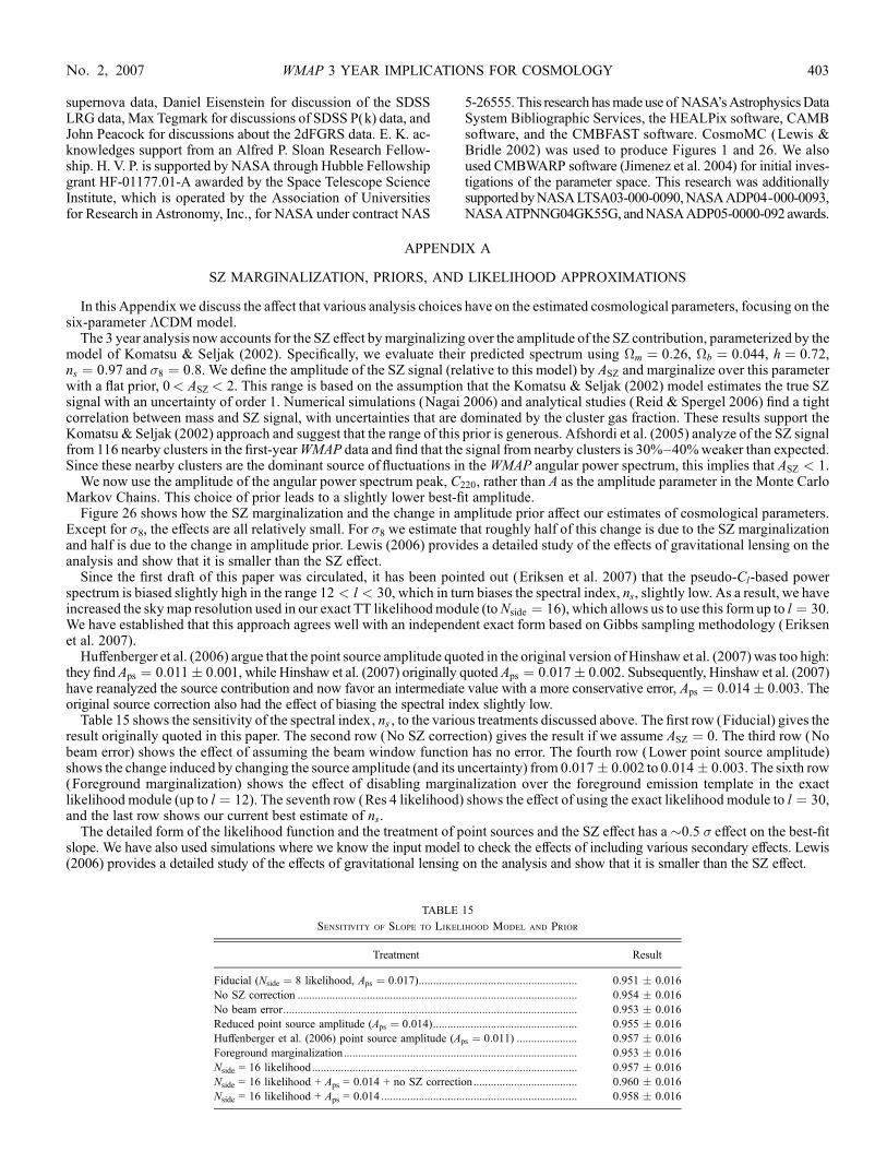
supernova data, Daniel Eisenstein for discussion of the SDSSLRG data, Max Tegmark for discussions of SDSS P(k) data, andJohn Peacock for discussions about the 2dFGRS data. E. K. ac-knowledges support from an Alfred P. Sloan Research Fellow-ship. H. V. P. is supported by NASA through Hubble Fellowshipgrant HF-01177.01-A awarded by the Space Telescope ScienceInstitute, which is operated by the Association of Universitiesfor Research in Astronomy, Inc., for NASA under contract NAS

5-26555. This research hasmade use of NASA’sAstrophysicsDataSystem Bibliographic Services, the HEALPix software, CAMBsoftware, and the CMBFAST software. CosmoMC (Lewis &Bridle 2002) was used to produce Figures 1 and 26. We alsoused CMBWARP software (Jimenez et al. 2004) for initial inves-tigations of the parameter space. This research was additionallysupported byNASALTSA03-000-0090,NASAADP04-000-0093,NASAATPNNG04GK55G, andNASAADP05-0000-092 awards.

APPENDIX A

SZ MARGINALIZATION, PRIORS, AND LIKELIHOOD APPROXIMATIONS

In this Appendix we discuss the affect that various analysis choices have on the estimated cosmological parameters, focusing on thesix-parameter �CDM model.

The 3 year analysis now accounts for the SZ effect bymarginalizing over the amplitude of the SZ contribution, parameterized by themodel of Komatsu & Seljak (2002). Specifically, we evaluate their predicted spectrum using �m ¼ 0:26, �b ¼ 0:044, h ¼ 0:72,ns ¼ 0:97 and �8 ¼ 0:8. We define the amplitude of the SZ signal (relative to this model) by ASZ and marginalize over this parameterwith a flat prior, 0< ASZ< 2. This range is based on the assumption that the Komatsu & Seljak (2002) model estimates the true SZsignal with an uncertainty of order 1. Numerical simulations (Nagai 2006) and analytical studies (Reid & Spergel 2006) find a tightcorrelation between mass and SZ signal, with uncertainties that are dominated by the cluster gas fraction. These results support theKomatsu & Seljak (2002) approach and suggest that the range of this prior is generous. Afshordi et al. (2005) analyze of the SZ signalfrom 116 nearby clusters in the first-yearWMAP data and find that the signal from nearby clusters is 30%Y40%weaker than expected.Since these nearby clusters are the dominant source of fluctuations in theWMAP angular power spectrum, this implies that ASZ < 1.

We now use the amplitude of the angular power spectrum peak, C220, rather than A as the amplitude parameter in the Monte CarloMarkov Chains. This choice of prior leads to a slightly lower best-fit amplitude.

Figure 26 shows how the SZ marginalization and the change in amplitude prior affect our estimates of cosmological parameters.Except for �8, the effects are all relatively small. For �8 we estimate that roughly half of this change is due to the SZ marginalizationand half is due to the change in amplitude prior. Lewis (2006) provides a detailed study of the effects of gravitational lensing on theanalysis and show that it is smaller than the SZ effect.

Since the first draft of this paper was circulated, it has been pointed out (Eriksen et al. 2007) that the pseudo-Cl-based powerspectrum is biased slightly high in the range 12 < l < 30, which in turn biases the spectral index, ns, slightly low. As a result, we haveincreased the skymap resolution used in our exact TT likelihoodmodule (toNside ¼ 16), which allows us to use this form up to l ¼ 30.We have established that this approach agrees well with an independent exact form based on Gibbs sampling methodology (Eriksenet al. 2007).

Huffenberger et al. (2006) argue that the point source amplitude quoted in the original version of Hinshaw et al. (2007) was too high:they find Aps ¼ 0:011� 0:001, while Hinshaw et al. (2007) originally quoted Aps ¼ 0:017� 0:002. Subsequently, Hinshaw et al. (2007)have reanalyzed the source contribution and now favor an intermediate value with a more conservative error, Aps ¼ 0:014� 0:003. Theoriginal source correction also had the effect of biasing the spectral index slightly low.

Table 15 shows the sensitivity of the spectral index, ns , to the various treatments discussed above. The first row (Fiducial) gives theresult originally quoted in this paper. The second row (No SZ correction) gives the result if we assume ASZ ¼ 0. The third row (Nobeam error) shows the effect of assuming the beam window function has no error. The fourth row (Lower point source amplitude)shows the change induced by changing the source amplitude (and its uncertainty) from 0:017� 0:002 to 0:014� 0:003. The sixth row(Foreground marginalization) shows the effect of disabling marginalization over the foreground emission template in the exactlikelihood module (up to l ¼ 12). The seventh row (Res 4 likelihood) shows the effect of using the exact likelihood module to l ¼ 30,and the last row shows our current best estimate of ns.

The detailed form of the likelihood function and the treatment of point sources and the SZ effect has a�0.5 � effect on the best-fitslope. We have also used simulations where we know the input model to check the effects of including various secondary effects. Lewis(2006) provides a detailed study of the effects of gravitational lensing on the analysis and show that it is smaller than the SZ effect.

TABLE 15

Sensitivity of Slope to Likelihood Model and Prior

Treatment Result

Fiducial (Nside ¼ 8 likelihood, Aps ¼ 0:017)....................................................... 0.951 � 0.016

No SZ correction ................................................................................................. 0.954 � 0.016

No beam error...................................................................................................... 0.953 � 0.016

Reduced point source amplitude (Aps ¼ 0:014).................................................. 0.955 � 0.016

Huffenberger et al. (2006) point source amplitude (Aps ¼ 0:011) ..................... 0.957 � 0.016

Foreground marginalization................................................................................. 0.953 � 0.016

Nside = 16 likelihood............................................................................................ 0.957 � 0.016

Nside = 16 likelihood + Aps = 0.014 + no SZ correction.................................... 0.960 � 0.016

Nside = 16 likelihood + Aps = 0.014 .................................................................... 0.958 � 0.016


APPENDIX B

TRISPECTRUM METHODOLOGY

B1. PREDICTED TRISPECTRUM SIGNAL

We consider here a model that generates a nontrivial trispectrum, but no bispectrum signal. We assume that the gravitationalpotential � is a product of two independent Gaussian fields, � and :

�(x) ¼ �(x)½1þ gNL (x)�; ðB1Þ

where gNL characterizes the strength of the nonlinear term.Following Komatsu et al. (2005) approach for the bispectrum, extended recently to the trispectrum in Kogo & Komatsu (2006) the

observed temperature multipoles are

alm ¼ bl

Zr 2dr�lm(r)�l(r)þ nlm; ðB2Þ

where bl is the beam, nlm is the noise, and �l(r) is the radiation transfer function:

�l(r) ¼2

�

Zk 2dkgTl(k) jl(kr): ðB3Þ

The nonlinear coupling term generates a second-order term:

alm ¼ nlm þ bl

Zr 2dr�l(r) �lm(r)þ �l 0m 0 (r) l 0 0m 0 0 (r)Cl 0m 0l 0 0m 0 0

lm

h i; ðB4Þ

where

Cl 0m 0l 0 0m 0 0

lm ¼

ffiffiffiffiffiffiffiffiffiffiffiffiffiffiffiffiffiffiffiffiffiffiffiffiffiffiffiffiffiffiffiffiffiffiffiffiffiffiffiffiffiffiffiffiffiffiffiffiffiffiffi4�

(2l þ 1)(2l 0 þ 1)(2l 00 þ 1)

sl l 0 l 00

0 0 0

� �l l 0 l 00

m m0 m00

� �: ðB5Þ

This term does not have any effect on the bispectrum as �3�

¼ 0 and 3�

¼ 0: However, it does have a nontrivial effect on thetrispectrum.

As with gravitational lensing (see Hu 2001), the largest trispectrum term is the diagonal term, Tllll (0) ¼ ClClh i � 3 Clh i2. This term

would generate an excess in the �2 of the fit of the model to the data:

Tllll (0) ¼ g2NLCl

Zr 2dr

Zr 2dr�l(r)�l(r)

;X

ml 0m 0l 0 0m 0 0

Xl 0m 0 l 0 0m 0 0

�l 0m 0 (r)� l 0m 0 (r)�

l 0 0m 0 0 (r) l 0 0m 0 0 (r)�

Cl 0m 0l 0 0m 0 0

lm Cl 0m 0 l 0 0m 0 0

lm : ðB6Þ

We can then use

�l 0m 0 (r)�l 0m 0 (r)�

¼ �l 0 l 0�m 0m 0

Zk 2dkP�(k) jl 0 (kr) jl 0 (kr); ðB7Þ

and the equivalent relationship for to rewrite the trispectrum as

Tllll (0) ¼ g2NL�lC

2l ; ðB8Þ

where

�l ¼4�

Cl

Zk 2dkP�(k)

Z(k 0)2dk 0P (k

0)

;l l 0 l 00

0 0 0

� �2Zr 2dr

Zr 2dr�l(r)�l(r) jl 0 (kr) jl 0 0 (k

0r) jl 0 (kr) jl 0 0 (k0r): ðB9Þ

While this full integral is numerically intractable, we approximate the surface of last scatter as a thin screen so that

alm ¼ bl�lm(r)al þ nlm; ðB10Þ


then, the trispectrum coupling term reduces to

�l ¼4�a2

l

Cl

Zk 2dkP�(k) j

2l 0 (kr)

Zk 02dk 0P (k

0) j2l 0 0 (k0r)

l l 0 l 00

0 0 0

� �2: ðB11Þ

Recall that in this limit,

Cl ¼ a2l

Zk 2dkP�(k) j

2l (kr): ðB12Þ

Thus,

�l ¼4�a2

l Cl 0

�2l 0Cl

Zk 02dk 0P (k

0) j2l 0 0 (k0r)

l l 0 l 00

0 0 0

� �2: ðB13Þ

The amplitude of �l is, thus, roughly the variance in the field on the scale r /l. Note that �l is a positive definite quantity so thatT llll (0) should be always positive.

B2. DETECTING THE NON-GAUSSIAN SIGNAL

If we assume that �l is constant, then we can follow Hu (2001) and compute an optimal quadratic statistic. We approximate theoptimal statistic as

Pi (T

fi 9

2Tfi � N 2

i )2, where T f is a smoothed map (e.g., a res 7 map) and we use the approximation that Cl ¼

A/l(l þ 1). This has the advantage that we can easily compute it and it has well-defined noise properties.

B2.1. Practical Implementations

We define for this purpose the dimensionless G statistic as

G¼X

p; b1; b2; b3; b4

wp; b1 Tp; b1wp; b2 Tp; b2wp; b3 Tp; b3wp; b4 Tp; b4

�X

b1; b2; b3; b4

Xp1

wp1; b1 Tp1; b1wp1; b2 Tp1; b2

�Xp2

wp2; b1 Tp2; b1wp2; b2 Tp2; b2

�; ðB14Þ

where bi refers to various bands (Q, V, and W for year 1, year 2, and year 3) that are all distinct for a single term so that the noisebias is null for this statistic, wp;bi is a particular pixel weight (we will consider it equal unity first) and Tb is a filtered map defined as

Tpb ¼TpbffiffiffiffiffiffiffiffiffiffiffiffiffiffiffiP

q T2qb

q ; ðB15Þ

Tpb ¼Xlm

flbaMlmbYlm(np); ðB16Þ

where a Mlm values are the spherical harmonic coefficients of the masked sky.We use at this level the Kp12mask to hide the brighter part

of the galaxy (and potentially the brighter point sources) and ignore cut sky effects in considering those pseudo-alm values. But whencomputing the sum over pixels in G, we consider only pixels outside the Kp2 area. The obvious advantage of this simple real spacestatistic is its ability to handle inhomogeneous noise and to localize its various contributions in real space. The second term in thedefinition of G aims at subtracting off the Gaussian unconnected part, so that if the T fields are homogeneous Gaussian fields, weobtain hG psi ¼ 0.

The exact nature of fl will depend on the source of the signal. For example, point sources do contribute to all n-points functions inreal or harmonic space and are as such visible in the power spectrum, bispectrum, and trispectrum. The first two have been used to setlimits and corrections.

Should we want to isolate the point sources contribution with the G statistic, we would proceed in the following manner. The pointsources power spectrum is well approximated by a constant, white noiseYlike, power spectrum C

psl (see Komatsu et al. 2003). Given

the measured power spectrum, Cl ¼ Clb2l þ C

psl b2

l þ Nl, theWiener like filter to reconstruct point sources is to fpsl ¼ b2

l /Cl. Note thatthis filter would be optimal only if point sources were drawn from a Gaussian distribution, which is not true. We can, however, expectit to be close to optimal.

In order to constrain the CMB contribution to the trispectrum and constrain gNL close to optimality, we will set fl1 and fl2 to theWiener filter for the CMB field, fl1 ¼ fl3 ¼ C

theoryl b2

l /Cmeasuredl and fl2 ¼ fl4 ¼ l(l þ 1) fl1, where C

theoryl is the best-fit model angular

power spectrum and Cmeasuredl is the measured raw power spectrum including the signal and the noise and not corrected for the beam

window function.We restrict ourselves to a unit weighting that is nearly optimal in the signal-dominated regime where we draw our conclusions from,

i.e., at resolution lower than Nside ¼ 64.


B2.2. Explicit relation to the trispectrum

Ignoring the weights and using the identities from Komatsu (2001)

hT1(n)T2(n)T3(n)T4(n)ic ¼Xp

T1pT2pT3pT4p ðB17Þ

¼X

l1m1l2m2l3m3l4m4

htl1m1tl2m2

tl3m3tl4m4

ic

;

Zd�(n)Yl1m1

(n)Yl2m2(n)Y

l3m3(n)Y

l4m4(n) ðB18Þ

¼X

l1m1l2m2l3m3l4m4LM

ffiffiffiffiffiffiffiffiffiffiffiffiffiffiffiffiffiffiffiffiffiffiffiffiffiffiffiffiffiffiffiffiffiffiffi(2l1 þ 1)(2l2 þ 1)

4�(2Lþ 1)

s ffiffiffiffiffiffiffiffiffiffiffiffiffiffiffiffiffiffiffiffiffiffiffiffiffiffiffiffiffiffiffiffiffiffiffi(2l3 þ 1)(2l4 þ 1)

4�(2Lþ 1)

s

; CL0l10l20

CL0l30l40

CLMl1m1l2m2

htl1m1tl2m2

tl3m3tl4m4

ic : CLMl3m3l4m4

ðB19Þ

It is then easy to relate to standard expression for the connected part of the trispectrum as in Hu (2001) and Komatsu (2001).

REFERENCES

Abazajian, K., et al. 2005, ApJ, 625, 613Abroe, M. E., et al. 2004, ApJ, 605, 607Afshordi, N. 2004, Phys. Rev. D, 70, 083536Afshordi, N., Lin, Y.-T., & Sanderson, A. J. R. 2005, ApJ, 629, 1Afshordi, N., Loh, Y.-S., & Strauss, M. A. 2004, Phys. Rev. D, 69, 083524Albrecht, A., & Steinhardt, P. J. 1982, Phys. Rev. Lett., 48, 1220Alishahiha, M., Silverstein, E., & Tong, D. 2004, Phys. Rev. D, 70, 123505Allen, S. W., Schmidt, R. W., Ebeling, H., Fabian, A. C., & van Speybroeck, L.2004, MNRAS, 353, 457

Allen, S. W., Schmidt, R. W., Fabian, A. C., & Ebeling, H. 2003, MNRAS,342, 287

Amendola, L. 1999, Phys. Rev. D, 60, 043501Arkani-Hamed, N., Creminelli, P., Mukohyama, S., & Zaldarriaga, M. 2004, J.Cosmol. Astropart. Phys., 4, 1

Asplund, M., Nissen, P. E., Lambert, D. L., Primas, F., & Smith, V. V. 2005, inIAU Symposium, ed. V. Hill, P. Francois, & F. Primas (Cambridge: CambridgeUniv. Press), 53

Astier, P., et al. 2005, BAAS, 37, 1176Aurich, R., Lustig, S., Steiner, F., & Then, H. 2005, Phys. Rev. Lett., 94,021301

Babich, D., Creminelli, P., & Zaldarriaga, M. 2004, J. Cosmol. Astropart.Phys., 8, 9

Bahcall, N. A., & Bode, P. 2003, ApJ, 588, L1Bahcall, N. A., Ostriker, J. P., Perlmutter, S., & Steinhardt, P. J. 1999, Science,284, 1481

Bania, T. M., Rood, R. T., & Balser, D. S. 2002, Nature, 415, 54Bardeen, J. M., Bond, J. R., Kaiser, N., & Szalay, A. S. 1986, ApJ, 304, 15Bardeen, J. M., Steinhardt, P. J., & Turner, M. S. 1983, Phys. Rev. D, 28, 679Barger, V., Kneller, J. P., Lee, H.-S., Marfatia, D., & Steigman, G. 2003, Phys.Lett. B, 566, 8

Barger, V., Marfatia, D., & Tregre, A. 2004, Phys. Lett. B, 595, 55Bartolo, N., Komatsu, E., Matarrese, S., & Riotto, A. 2004a, Phys. Rep. 402,103

Bartolo, N., Matarrese, S., & Riotto, A. 2004b, J. High Energy Phys., 4, 6Bashinsky, S., & Seljak, U. 2004, Phys. Rev. D, 69, 083002Bean, R., & Dore, O. 2004, Phys. Rev. D, 69, 083503Bean, R., & Magueijo, J. 2001, Phys. Lett. B, 517, 177Beltran, M., Garcıa-Bellido, J., Lesgourgues, J., Liddle, A. R., & Slosar, A.2005, Phys. Rev. D, 71, 063532

Bennett, C. L., et al. 2003, ApJS, 148, 1Bergstrom, L., & Danielsson, U. H. 2002, J. High Energy Phys., 12, 38Blanchard, A., Douspis, M., Rowan-Robinson, M., & Sarkar, S. 2003, A&A,412, 35

Boesgaard, A. M., Stephens, A., & Deliyannis, C. P. 2005, ApJ, 633, 398Bonamente, M., Joy, M., La Roque, S. Carlstrom, J., Reese, E., Dawson, K.2006, ApJ, 647, 25

Bond, J. R., & Efstathiou, G. 1984, ApJ, 285, L45———. 1987, MNRAS, 226, 655Bond, J. R., Efstathiou, G., & Silk, J. 1980, Phys. Rev. Lett., 45, 1980Bond, J. R., Pogosyan, D., & Souradeep, T. 2000, Phys. Rev. D, 62, 043005Bond, J. R., & Szalay, A. S. 1983, ApJ, 274, 443Bond, J. R., et al. 2005, ApJ, 626, 12Borgani, S., et al. 2001, ApJ, 561, 13Boughn, S., & Crittenden, R. 2004, Nature, 427, 45

Boughn, S. P., & Crittenden, R. G. 2005, MNRAS, 360, 1013Bowen, R., Hansen, S. H., Melchiorri, A., Silk, J., & Trotta, R. 2002, MNRAS,334, 760

Bridges, M., Lasenby, A. N., & Hobson, M. P. 2006, MNRAS, 369, 1123Bucher, M., & Spergel, D. 1999, Phys. Rev. D, 60, 043505Burgess, C. P., Cline, J. M., Lemieux, F., & Holman, R. 2003, J. High EnergyPhys., 2, 48

Cabella, P., Hansen, F., Marinucci, D., Pagano, D., & Vittorio, N. 2004, Phys.Rev. D, 69, 063007

Caldwell, R. R., Dave, R., & Steinhardt, P. J. 1998, Phys. Rev. Lett., 80, 1582Carroll, S. M., Press, W. H., & Turner, E. L. 1992, ARA&A, 30, 499Cen, R. 2003, ApJ, 591, L5Chaboyer, B., & Krauss, L. M. 2002, ApJ, 567, L45Chae, K.-H., et al. 2002, Phys. Rev. Lett., 89, 151301Charbonnel, C., & Primas, F. 2005, A&A, 442, 961Chiang, L., Naselsky, P. D., Verkhodanov, O. V., & Way, M. J. 2003, ApJ, 590,L65

Chiu, W. A., Fan, X., & Ostriker, J. P. 2003, ApJ, 599, 759Ciardi, B., Ferrara, A., & White, S. D. M. 2003, MNRAS, 344, L7Clocchiatti, A., et al. 2006, ApJ, 642, 1Coc, A., Vangioni-Flam, E., Descouvemont, P., Adahchour, A., & Angulo, C.2004, ApJ, 600, 544

Cole, S., et al. 2005, MNRAS, 362, 505Colley, W. N., & Gott, J. R. 2003, MNRAS, 344, 686Contaldi, C. R., Hoekstra, H., & Lewis, A. 2003, Phys. Rev. Lett., 90, 221303Copi, C. J., Huterer, D., & Starkman, G. D. 2004, Phys. Rev. D, 70, 043515Corasaniti, P.-S., Giannantonio, T., & Melchiorri, A. 2005, Phys. Rev. D, 71,123521

Cornish, N. J., Spergel, D. N., & Starkman, G. D. 1996, Phys. Rev. Lett., 77,215

Cornish, N. J., Spergel, D. N., Starkman, G. D., & Komatsu, E. 2004, Phys.Rev. Lett., 92, 201302

Creminelli, P., Nicolis, A., Senatore, L., Tegmark, M., & Zaldarriaga, M. 2006,J. Cosmol. Astropart. Phys., 5, 4

Crighton, N. H. M., Webb, J. K., Ortiz-Gil, A., & Fernandez-Soto, A. 2004,MNRAS, 355, 1042

Crittenden, R. G., & Turok, N. 1996, Phys. Rev. Lett., 76, 575Croft, R. A. C., Weinberg, D. H., Katz, N., & Hernquist, L. 1998, ApJ, 495, 44Crotty, P., Lesgourgues, J., & Pastor, S. 2003, Phys. Rev. D, 67, 123005Cruz, M., Martınez-Gonzalez, E., Vielva, P., & Cayon, L. 2005, MNRAS, 356,29

Cruz, M., Cayon, L, Martinez-Gonzalez, E., Vielva, P., & Jin, J. 2006, ApJ,655, 11

Danielsson, U. H. 2002, Phys. Rev. D, 66, 023511Deffayet, C. 2001, Phys. Lett. B, 502, 199Deffayet, C., Dvali, G., & Gabadadze, G. 2002, Phys. Rev. D, 65, 044023Desjacques, V., & Nusser, A. 2005, MNRAS, 361, 1399Dickinson, C., et al. 2004, MNRAS, 353, 732Dolgov, A. D., Hansen, S. H., & Semikoz, D. V. 1999, Nucl. Phys. B, 543, 269Dunkley, J., Bucher, M., Ferreira, P. G., Moodley, K., & Skordis, C. 2005,MNRAS, 356, 925

Dunlop, J., Peacock, J., Spinrad, H., Dey, A., Jimenez, R., Stern, D., &Windhorst, R. 1996, Nature, 381, 581

Dvali, G., Gruzinov, A., & Zaldarriaga, M. 2004, Phys. Rev. D, 69, 083505


Easther, R., Greene, B. R., Kinney, W. H., & Shiu, G. 2002, Phys. Rev. D, 66,023518

Easther, R., Kinney, W. H., & Peiris, H. 2005a, J. Cosmol. Astropart. Phys., 5, 9———. 2005b, J. Cosmol. Astropart. Phys., 8, 1Efstathiou, G. 2004, MNRAS, 348, 885Eisenstein, D. J., et al. 2005, ApJ, 633, 560Elgarøy, Ø., & Lahav, O. 2003, J. Cosmol. Astropart. Phys., 4, 4Ellis, J., Olive, K. A., & Vangioni, E. 2005, Phys. Lett. B, 619, 30Eriksen, H. K., Hansen, F. K., Banday, A. J., Gorski, K. M., & Lilje, P. B.2004a, ApJ, 605, 14

Eriksen, H. K., Banday, A. J., Gorski, K. M., & Lilje, P. B. 2004b, ApJ, 612,633

Eriksen, H. K. et al. 2007, ApJ, 656, 641Ettori, S., Tozzi, P., & Rosati, P. 2003, A&A, 398, 879Fan, X., et al. 2006, AJ, 131, 1203Feldman, H., et al. 2003, ApJ, 596, L131Ferreira, P. G., & Joyce, M. 1998, Phys. Rev. D, 58, 023503Fields, B. D., Olive, K. A., & Vangioni-Flam, E. 2005, ApJ, 623, 1083Fosalba, P., & Gaztanaga, E. 2004, MNRAS, 350, L37Freedman, W. L., et al. 2001, ApJ, 553, 47Gaztanaga, E., & Wagg, J. 2003, Phys. Rev. D, 68, 021302Gelman, A., & Rubin, D. 1992, Statistical Sci., 7, 457Gnedin, N. Y., & Gnedin, O. Y. 1998, ApJ, 509, 11Gnedin, N. Y., & Hamilton, A. J. S. 2002, MNRAS, 334, 107Goldberg, D. M., & Spergel, D. N. 1999, Phys. Rev. D, 59, 103002Goobar, A., Hannestad, S., Mortsell, E., & Tu, H. 2006, J. Cosmol. Astropart.Phys., 6, 19

Gott, J. R. I., Park, C., Juszkiewicz, R., Bies,W. E., Bennett, D. P., Bouchet, F. R.,& Stebbins, A. 1990, ApJ, 352, 1

Grainge, K., et al. 2003, MNRAS, 341, L23Guth, A. H. 1981, Phys. Rev. D, 23, 347Guth, A. H., & Pi, S. Y. 1982, Phys. Rev. Lett., 49, 1110Haiman, Z., & Holder, G. P. 2003, ApJ, 595, 1Hajian, A., Souradeep, T., & Cornish, N. 2005, ApJ, 618, L63Hall, L. J., & Oliver, S. 2004, Nucl. Phys. B Proc. Supp., 137, 269Hall, L. M. H., Moss, I. G., & Berera, A. 2004, Phys. Rev. D, 69, 083525Hamuy, M., Phillips, M. M., Suntzeff, N. B., Schommer, R. A., Maza, J., &Aviles, R. 1996, AJ, 112, 2391

Hannestad, S. 2001, Phys. Rev. D, 64, 083002———. 2003, J. Cosmol. Astropart. Phys., 5, 4———. 2006, J. Cosmol. Astropart. Phys., 1, 1Hansen, F. K., Cabella, P., Marinucci, D., & Vittorio, N. 2004, ApJ, 607, L67Hawking, S. W. 1982, Phys. Lett., B115, 295Henry, J. P. 2004, ApJ, 609, 603Heymans, C., et al. 2005, MNRAS, 361, 160Hinshaw, G., et al. 2003, ApJS, 148, 135———. 2007, ApJS, 170, 288Hoekstra, H., Yee, H. K. C., & Gladders, M. D. 2002, ApJ, 577, 595Hoekstra, H., et al. 2006, ApJ, 647, 116 (Ho06)Hoffman, M. B., & Turner, M. S. 2001, Phys. Rev. D, 64, 023506Hu, W. 1998, ApJ, 506, 485———. 2001, in RESCEU 1999, Birth and Evolution of the Universe, ed. K. Sato& M. Kawasaki (Tokyo: Universal Academy Press), 131

Hu, W., Eisenstein, D. J., & Tegmark, M. 1998, Phys. Rev. Lett., 80, 5255Hu, W., Fukugita, M., Zaldarriaga, M., & Tegmark, M. 2001, ApJ, 549, 669Hu, W., & Holder, G. P. 2003, Phys. Rev., D68, 023001Huffenberger, K. M., Eriksen, H. K., & Hansen, F. K. 2006, ApJ, 651, L81Huffenberger, K. M., Seljak, U., & Makarov, A. 2004, Phys. Rev. D, 70,063002

Hwang, J., & Noh, H. 1998, Phys. Rev. Lett., 81, 5274Ichikawa, K., Fukugita, M., & Kawasaki, M. 2005, Phys. Rev. D, 71, 043001Iliev, I. T., Mellema, G., Pen, U.-L., Merz, H., Shapiro, P. R., & Alvarez, M. A.2005, in IAU Colloq. 199, ed. P. R. Williams, C.-G. Shu, & B. Menard(Cambridge: Cambridge Univ. Press), 369

Inoue, K. T., Tomita, K., & Sugiyama, N. 2000, MNRAS, 314, L21Jarosik, N., et al. 2007, ApJS, 170, 263Jarvis, M., Bernstein, G. M., Fischer, P., Smith, D., Jain, B., Tyson, J. A., &Wittman, D. 2003, AJ, 125, 1014

Jedamzik, M. 2004, Phys. Rev. D, 70, 063524Jedamzik, K., Choi, K.-Y.,Roszkowski, L., & Ruiz de Austri, R. 2005, preprint( hep-ph/0512044)

Jena, T., et al. 2005, MNRAS, 361, 70Jimenez, R., Verde, L., Peiris, H., & Kosowsky, A. 2004, Phys. Rev., D70,023005

Jimenez, R., Verde, L., Treu, T., & Stern, D. 2003, ApJ, 593, 622Jones, W. C., et al. 2006, ApJ, 647, 823Kaloper, N., Kleban, M., Lawrence, A., Shenker, S., & Susskind, L. 2002,J. High Energy Phys., 11, 37

Kaplinghat, M., Chu, M., Haiman, Z., Holder, G. P., Knox, L., & Skordis, C.2003, ApJ, 583, 24

Kawasaki, M., Yamaguchi, M., & Yokoyama, J. 2003, Phys. Rev. D, 68,023508

Khoury, J., Ovrut, B. A., Seiberg, N., Steinhardt, P. J., & Turok, N. 2002, Phys.Rev., D65, 086007

Khoury, J., Ovrut, B. A., Steinhardt, P. J., & Turok, N. 2001, Phys. Rev., D64,123522

Kinney, W. H. 2002, Phys. Rev., D66, 083508Kirkman, D., Tytler, D., Suzuki, N., O’Meara, J. M., & Lubin, D. 2003, ApJS,149, 1

Kneller, J. P., & Steigman, G. 2004, New J. Phys., 6, 117Knop, R. A., et al. 2003, ApJ, 598, 102Knox, L., Christensen, N., & Skordis, C. 2001, ApJ, 563, L95Kogo, N., & Komatsu, E. 2006, Phys. Rev. D, 73, 3007Kogut, A., et al. 2003, ApJS, 148, 161Komatsu, E. 2001, Ph.D. thesis, Tohoku Univ. (astro-ph/0206039)Komatsu, E., & Futamase, T. 1999, Phys. Rev. D, 59, 064029Komatsu, E., & Kitayama, T. 1999, ApJ, 526, L1Komatsu, E., & Seljak, U. 2001, MNRAS, 327, 1353———. 2002, MNRAS, 336, 1256Komatsu, E., & Spergel, D. N. 2001, Phys. Rev. D, 63, 63002Komatsu, E., Spergel, D. N., & Wandelt, B. D. 2005, ApJ, 634, 14Komatsu, E., et al. 2003, ApJS, 148, 119Koopmans, L. V. E., Treu, T., Fassnacht, C. D., Blandford, R. D., & Surpi, G.2003, ApJ, 599, 70

Kosowsky, A., Milosavljevic, M., & Jimenez, R. 2002, Phys. Rev. D, 66, 63007Krisciunas, K., et al. 2005, AJ, 130, 2453Kuo, C. L., et al. 2004, ApJ, 600, 32Krauss, L. M., & Turner, M. S. 1999, Gen. Relativ. Gravitation, 31, 1453Lahav, O., Rees, M. J., Lilje, P. B., & Primack, J. R. 1991, MNRAS, 251, 128Larena, J., Alimi, J.-M., & Serna, A. 2005, preprint (astro-ph/0511693)Larson, D. L., & Wandelt, B. D. 2004, ApJ, 613, L85Leach, S. M., & Liddle, A. R. 2003, Phys. Rev. D, 68, 123508Leitch, E. M., Kovac, J. M., Halverson, N. W., Carlstrom, J. E., Pryke, C., &Smith, M. W. E. 2005, ApJ, 624, 10

Levin, J. J., Barrow, J. D., Bunn, E. F., & Silk, J. 1997, Phys. Rev. Lett., 79, 974Lewis, A., & Bridle, S. 2002, Phys. Rev. D, 66, 103511Lewis, A., Challinor, A., & Lasenby, A. 2000, ApJ, 538, 473Lewis, A. 2006, preprint (astro-ph/0603753)Lewis, A., & Challinor, A. 2006, Phys. Rep., 429, 1Liddle, A. R., & Lyth, D. H. 1992, Phys. Lett., B291, 391———. 1993, Phys. Rept., 231, 1Linde, A. 2005, NewA Rev., 49, 35Linde, A. D. 1982, Phys. Lett. B, 108, 389Luminet, J., Weeks, J. R., Riazuelo, A., Lehoucq, R., & Uzan, J. 2003, Nature,425, 593

Lyth, D. H., & Riotto, A. 1999, Phys. Rep., 314, 1Lyth, D. H., Ungarelli, C., & Wands, D. 2003, Phys. Rev. D, 67, 23503Ma, C.-P. 1996, ApJ, 471, 13Madau, P., Rees, M. J., Volonteri, M., Haardt, F., & Oh, S. P. 2004, ApJ, 604, 484Maldacena, J. 2003, J. High Energy Phys., 5, 13Mangano, G., Miele, G., Pastor, S., & Peloso, S. 2002, Phys. Lett. B, 534, 8Mangano, G., Miele, G., Pastor, S., Pinto, T., Pisanti, O., & Serpico, P. D. 2005,Nucl. Phys. B, 729, 221

Malhotra, S., & Rhoads, J. E. 2004, ApJ, 617, L5Martin, J., & Brandenberger, R. H. 2001, Phys. Rev. D, 63, 123501———. 2003, Phys. Rev. D, 68, 063513Martin, J., & Ringeval, C. 2004, Phys. Rev. D, 69, 083515Mason, B. S., et al. 2003, ApJ, 591, 540Mathews, G. J., Kajino, T., & Shima, T. 2005, Phys. Rev. D, 71, 021302McDonald, P., et al. 2005, ApJ, 635, 761McGaugh, S. S. 2004, ApJ, 611, 26Mecke, K. R., Buchert, T., & Wagner, H. 1994, A&A, 288, 697Meiksin, A., & White, M. 2004, MNRAS, 350, 1107Melendez, J., & Ramırez, I. 2004, ApJ, 615, L33Minkowski, H. 1903, Mathematische Ann., 57, 447Mohapatra, R. N., et al. 2005, preprintMohayaee, R., & Tully, B. 2005, ApJ, 635, L113Montroy, T. E., et al. 2006, ApJ, 647, 813Mukhanov, V. F., & Chibisov, G. V. 1981, J. Exp. Theor. Phys. Lett., 33, 532Mukherjee, P., Parkinson, D., & Liddle, A. R. 2006, ApJ, 638, L51Mukherjee, P., & Wang, Y. 2003, ApJ, 599, 1Nagai, D. 2006, ApJ, 650, 538Naselsky, P. D., Chiang, L.-Y., Novikov, I. D., & Verkhodanov, O. V. 2005, Int.J. Mod. Phys. D, 14, 1273

Nobili, S., et al. 2005, A&A, 437, 789Nolta, M. R., et al. 2004, ApJ, 608, 10


Novosyadlyj, B., Durrer, R., & Lukash, V. N. 1999, A&A, 347, 799 (NDL)O’Dwyer, I. J., et al. 2004, ApJ, 617, L99———. 2005, ApJS, 158, 93Oguri, M. 2004, Ph.D. thesis, Univ. TokyoOh, S. P., & Haiman, Z. 2003, MNRAS, 346, 456Olive, K. A., & Skillman, E. D. 2004, ApJ, 617, 29Ostriker, J. P., & Steinhardt, P. J. 1995, Nature, 377, 600Padmanabhan, N., Hirata, C. M., Seljak, U., Schlegel, D. J., Brinkmann, J., &Schneider, D. P. 2005, Phys. Rev. D, 72, 043525

Page, L., et al. 2003a, ApJS, 148, 39———. 2003b, ApJS, 148, 233———. 2007, ApJS, 170, 335Park, C. 2004, MNRAS, 349, 313Pearson, T. J., et al. 2003, ApJ, 591, 556Peebles, P. J. E. 1984, ApJ, 284, 439Peebles, P. J., & Ratra, B. 2003, Rev. Mod. Phys., 75, 559———. 1988, ApJ, 325, L17Peebles, P. J. E., & Yu, J. T. 1970, ApJ, 162, 815Peiris, H. V., et al. 2003, ApJS, 148, 213Pen, U. 1997, NewA, 2, 309Perlmutter, S., et al. 1999, ApJ, 517, 565Phillips, M. M. 1993, ApJ, 413, L105Phillips, N. G., & Kogut, A. 2006, ApJ, 645, 820Piacentini, F., et al. 2006, ApJ, 647, 833Pierpaoli, E. 2003, MNRAS, 342, L63Pierpaoli, E., Borgani, S., Scott, D., & White, M. 2003, MNRAS, 342, 163Pogosian, L., Corasaniti, P. S., Stephan-Otto, C., Crittenden, R., & Nichol, R.2005, Phys. Rev. D, 72, 103519

Rasia, E., Mazzotta, P., Borgani, S., Moscardini, L., Dolag, K., Tormen, G.,Diaferio, A., & Murante, G. 2005, ApJ, 618, L1

Readhead, A. C. S., et al. 2004a, ApJ, 609, 498———. 2004b, Science, 306, 836Refregier, A. 2003, ARA&A, 41, 645Refregier, A., Komatsu, E., Spergel, D. N., & Pen, U. 2000, Phys. Rev. D, 61,123001

Reid, B. A., & Spergel, D. N. 2006, ApJ, 651, 643Richard, O., Michaud, G., & Richer, J. 2005, ApJ, 619, 538Richer, H. B., et al. 2004, AJ, 127, 2904Ricotti, M., & Ostriker, J. P. 2004, MNRAS, 352, 547Riess, A. G., Press, W. H., & Kirshner, R. P. 1996, ApJ, 473, 88Riess, A. G., et al. 1998, AJ, 116, 1009———. 2004, ApJ, 607, 665———. 2005, ApJ, 627, 579Ruhl, J. E., et al. 2003, ApJ, 599, 786Sanchez, A., et al. 2006, MNRAS, 366, 189Sato, K. 1981, MNRAS, 195, 467Schalm, K., Shiu, G.,& van den Schaar, J. P. 2004, J. High Energy Phys., 0404, 076Schmalzing, J., & Buchert, T. 1997, ApJ, 482, L1Schmalzing, J., & Gorski, K. M. 1998, MNRAS, 297, 355Schmidt, B. P., et al. 1998, ApJ, 507, 46Scranton, R., et al. 2003, preprintSeager, S., Sasselov, D. D., & Scott, D. 2000, ApJS, 128, 407Seljak, U., Sugiyama, N.,White, & Zaldarriaga,M. 2003, Phys. Rev. D, 68, 3507———. 2005a, Phys. Rev. D, 71, 103515———. 2005b, Phys. Rev. D, 71, 043511

Semboloni, E., et al. 2006, A&A, 452, 51Serebrov, A., et al. 2005, Phys. Lett. B, 605, 72Sievers, J. L., et al. 2003, ApJ, 591, 599Silk, J., & Wilson, M. L. 1981, ApJ, 244, L37Simon, J., Verde, L., & Jimenez, R. 2005, Phys. Rev. D, 71, 123001Skordis, C., Mota, D. F., Ferreira, P. G., & BKhm, C. 2006, Phys. Rev. Lett.,96, 011301

Slosar, A., Seljak, U., & Makarov, A. 2004, Phys. Rev., D69, 123003Smith, R. E., et al. 2003, MNRAS, 341, 1311Sokasian, A., Yoshida, N., Abel, T., Hernquist, L., & Springel, V. 2004,MNRAS, 350, 47

Somerville, R. S., & Livio, M. 2003, ApJ, 593, 611Soucail, G., Kneib, J.-P., & Golse, G. 2004, A&A, 417, L33Spergel, D. N., & Goldberg, D. M. 1999, Phys. Rev. D, 59, 103001Spergel, D. N., et al. 2003, ApJS, 148, 175Starobinsky, A. A. 1982, Phys. Lett. B, 117, 175Steigman, G. 2005, preprintSunyaev, R. A., & Zel’dovich, Y. B. 1970, Ap&SS, 7, 3Takada, M., Komatsu, E., & Futamase, T. 2006, Phys. Rev. D, 73, 3520Tegmark, M., de Oliveira-Costa, A., & Hamilton, A. J. 2003, Phys. Rev. D, 68,123523

Tegmark, M., Zaldarriaga, M., & Hamilton, A. J. 2001, Phys. Rev. D, 63,043007

Tegmark, M., et al. 2004a, Phys. Rev. D, 69, 103501———. 2004b, ApJ, 606, 702Tegmark, M., et al. 2006, Phys. Rev. D, 74, 3507Tereno, I., Dore, O., van Waerbeke, L., & Mellier, Y. 2005, A&A, 429, 383Tonry, J. L., et al. 2003, ApJ, 594, 1Totani, T., Kawai, N., Kosugi, G., Aoki, K., Yamada, T., Iye, M., Ohta, K., &Hattori, T. 2006, PASJ, 58, 485

Trotta, R. 2007, MNRAS, 375, L26Tumlinson, J., Vankatesan, A., & Shull, J. M. 2004, ApJ, 612, 602Turner, E. L. 1990, ApJ, 365, L43Turner, M. S., Steigman, G., & Krauss, L. M. 1984, Phys. Rev. Lett., 52, 2090Vale, A., & Ostriker, J. P. 2006, MNRAS, 371, 1173Van den Bosch, F., Mo, H., & Yang, X. 2003, MNRAS, 345, 923Van Waerbeke, L., Mellier, Y., & Hoekstra, H. 2005, A&A, 429, 75Venkatesan, A., Tumlinson, J., & Shull, J. M. 2003, ApJ, 584, 621Verde, L., et al. 2002, MNRAS, 335, 432———. 2003, ApJS, 148, 195Vielva, P., Martınez-Gonzalez, E., Barreiro, R. B., Sanz, J. L., & Cayon, L.2004, ApJ, 609, 22

Vielva, P., Martınez-Gonzalez, E., & Tucci, M. 2006, MNRAS, 365, 891Vikhlinin, A., et al. 2003, ApJ, 590, 15Vittorio, N., & Silk, J. 1984, ApJ, 285, L39Voevodkin, A., & Vikhlinin, A. 2004, ApJ, 601, 610Wambsganss, J., Bode, P., & Ostriker, J. P. 2004, ApJ, 606, L93Wetterich, C. 1988, Nucl. Phys. B, 302, 668Winitzki, S., & Kosowsky, A. 1998, NewA, 3, 75Wyithe, J. S. B., & Cen, R. 2006, preprint (astro-ph/0602503)Wyithe, J. S. B., & Loeb, A. 2003, ApJ, 588, L69Yamaguchi, M., & Yokoyama, J. 2004, Phys. Rev. D, 70, 023513Zaldarriaga, M., & Seljak, U. 2000, ApJS, 129, 431Zehavi, I., et al. 2005, ApJ, 630, 1Zlatev, I., Wang, L., & Steinhardt, P. J. 1999, Phys. Rev. Lett., 82, 896

SPERGEL ET AL.408

THREE-YEAR WILKINSON MICROWAVE ANISOTROPY PROBE …...redshift supernova (Riess et al. 2004; Astier...

Documents

Transcript of THREE-YEAR WILKINSON MICROWAVE ANISOTROPY PROBE …...redshift supernova (Riess et al. 2004; Astier...