Draft version December 5, 2019Typeset using LATEX twocolumn style in AASTeX61

CHANDRA SPECTRAL AND TIMING ANALYSIS OF SGR A*’S BRIGHTEST X-RAY FLARES

Daryl Haggard,1, 2, 3 Melania Nynka,1, 2, 4 Brayden Mon,1, 2 Noelia de la Cruz Hernandez,1, 2

Michael Nowak,5 Craig Heinke,6 Joseph Neilsen,7 Jason Dexter,8, 9 P. Chris Fragile,10 Fred Baganoff,11

Geoffrey C. Bower,12 Lia R. Corrales,13 Francesco Coti Zelati,14, 15 Nathalie Degenaar,16

Sera Markoff,16, 17 Mark R. Morris,18 Gabriele Ponti,19, 8 Nanda Rea,14, 15 Jöern Wilms,20 andFarhad Yusef-Zadeh21

1Department of Physics, McGill University, 3600 University Street, Montréal, QC H3A 2T8, Canada2McGill Space Institute, McGill University, 3550 University Street, Montréal, QC H3A 2A7, Canada3CIFAR Azrieli Global Scholar, Gravity & the Extreme Universe Program, Canadian Institute for Advanced Research, 661 UniversityAvenue, Suite 505, Toronto, ON M5G 1M1, Canada

4MIT Kavli Institute for Astrophysics and Space Research, 77 Massachusetts Avenue, Cambridge, MA 02139, USA5Department of Physics, Washington University, 1 Brookings Drive, St. Louis, MO 63130, USA6Department of Physics, University of Alberta, CCIS 4-183, Edmonton AB T6G 2E1, Canada7Department of Physics, Villanova University, 800 Lancaster Avenue, Villanova, PA 19085, USA8Max-Planck-Institut für Extraterrestrische Physik, Giessenbachstrasse, D-85748 Garching, Germany9JILA and Department of Astrophysical and Planetary Sciences, University of Colorado, Boulder, CO 80309, USA10Department of Physics and Astronomy, College of Charleston, Charleston, SC 29424, USA11MIT Kavli Institute for Astrophysics and Space Research, 77 Massachusetts Avenue, Cambridge, MA, 02139, USA12Academia Sinica Institute of Astronomy and Astrophysics, 645 N. A’ohoku Place, Hilo, HI 96720, USA13Department of Astronomy, University of Michigan, 1085 S. University, Ann Arbor, MI 48109, USA14Institute of Space Sciences (CSIC), Campus UAB, Carrer de Can Magrans s/n, E-08193 Barcelona, Spain15Institut d’Estudis Espacials de Catalunya (IEEC), E-08034 Barcelona, Spain16Anton Pannekoek Institute for Astronomy, University of Amsterdam, Science Park 904, NL-1098 XH Amsterdam, the Netherlands17Gravitational and Astroparticle Physics Amsterdam, U. Amsterdam, Science Park 904, NL-1098 XH Amsterdam, the Netherlands18University of California, Los Angeles, CA 90095, USA19Osservatorio Astronomico di Brera, Via E. Bianchi 46, I-23807 Merate (LC), Italy20Dr. Karl-Remeis-Sternwarte and Erlangen Centre for Astroparticle Physics, Sternwartstr. 7, D-96049, Bamberg, Germany21Department of Physics and Astronomy and Center for Interdisciplinary Exploration and Research in Astrophysics (CIERA),Northwestern University, Evanston, IL 60208, USA

(Received Dec 21, 2018; Revised July 30, 2019; Accepted October 3, 2019)

Submitted to ApJ

ABSTRACTWe analyze the two brightest Chandra X-ray flares detected from Sagittarius A*, with peak luminosities more

than 600× and 245× greater than the quiescent X-ray emission. The brightest flare has a distinctive double-peakedmorphology — it lasts 5.7 ks (∼ 2 hr), with a rapid rise time of 1500 s and a decay time of 2500 s. The secondflare lasts 3.4 ks, with rise and decay times of 1700 s and 1400 s. These luminous flares are significantly harder thanquiescence: the first has a power-law spectral index Γ = 2.06± 0.14 and the second has Γ = 2.03± 0.27, compared toΓ = 3.0±0.2 for the quiescent accretion flow. These spectral indices (as well as the flare hardness ratios) are consistentwith previously detected Sgr A* flares, suggesting that bright and faint flares arise from similar physical processes.Leveraging the brightest flare’s long duration and high signal-to-noise, we search for intraflare variability and detectexcess X-ray power at a frequency of ν ≈ 3 mHz, but show that it is an instrumental artifact and not of astrophysical

Corresponding author: Daryl Haggarddaryl.haggard@mcgill.ca

arX

iv:1

908.

0178

1v2

[as

tro-

ph.H

E]

4 D

ec 2

019

2 Haggard et al.

origin. We find no other evidence (at the 95% confidence level) for periodic or quasi-periodic variability in either flares’time series. We also search for nonperiodic excess power but do not find compelling evidence in the power spectrum.Bright flares like these remain our most promising avenue for identifying Sgr A*’s short timescale variability in theX-ray, which may probe the characteristic size scale for the X-ray emission region.

Keywords: accretion, accretion disks, black hole physics, Galaxy: center, radiation mechanisms: non-thermal, X-rays: individual: Sgr A*

Sgr A* Bright X-ray Flares 3

1. INTRODUCTION

Near-infrared observations of massive stars orbitingSagittarius A* (Sgr A* ), the supermassive black hole(SMBH) at the Milky Way’s center, have yielded precisemeasurements of its mass and distance, (4.28 ± 0.1) ×106M� and 7.97 ± 0.07 kpc (e.g., Ghez et al. 2008;Gillessen et al. 2009, 2017; Boehle et al. 2016; Grav-ity Collaboration et al. 2018b, 2019; Do et al. 2019).Chandra X-ray observations have revealed Sgr A* asa compact (∼1′′ ), low-luminosity source (L2−10 keV ∼2 × 1033 erg s−1), with a very low Eddington ratio,L/LEdd ∼ 10−8 to 10−11 (Figure 1; e.g., Baganoff et al.2001, 2003; Xu et al. 2006; Genzel et al. 2010; Wanget al. 2013). The size of the X-ray emitting region issimilar to the black hole’s Bondi radius (∼ 6000 au,roughly 105 times the Schwarzschild radius), throughwhich the accretion rate is 10−6M� yr−1 (Melia 1992;Quataert 2002). The gas reservoir likely originates fromcaptured winds from the S stars or the cluster of massiveOB stars surrounding Sgr A* (Cuadra et al. 2005, 2006,2008; Yusef-Zadeh et al. 2016; Russell et al. 2017), onlya fraction of which reaches the SMBH — the vast ma-jority of the material is apparently ejected in an outflow(e.g., Wang et al. 2013).Ambitious X-ray campaigns with Chandra, XMM-

Newton, Swift, and NuSTAR have targeted Sgr A* andshown that its emission is relatively quiescent and hasbeen stable over two decades, punctuated by approxi-mately daily X-ray flares (Baganoff et al. 2001; Gold-wurm et al. 2003; Porquet et al. 2003, 2008; Bélangeret al. 2005; Nowak et al. 2012; Degenaar et al. 2013;Neilsen et al. 2013, 2015; Barrière et al. 2014; Pontiet al. 2015; Mossoux et al. 2016; Yuan & Wang 2016;Zhang et al. 2017; Bouffard et al. 2019). The quiescentcomponent is well-modeled by bremsstrahlung emissionfrom a hot plasma with temperature T ∼ 7× 107 K andelectron density ne ∼100 cm−3 located near the Bondiradius (Quataert 2002; Wang et al. 2013).Baganoff et al. (2001) identified the first Sgr A* X-

ray flare with Chandra and modeled it using a power-law spectrum with Γ = 1.3+0.5

−0.6 and NH = 4.6 × 1022

cm−2, but pile-up led to known biases in the analy-sis. X-ray flares were subsequently observed by XMM-Newton (Goldwurm et al. 2003; Porquet et al. 2003,2008; Bélanger et al. 2005; Ponti et al. 2015; Mossouxet al. 2016; Mossoux & Grosso 2017) for which pile-upis less severe, and Swift (e.g., Degenaar et al. 2013), es-tablishing X-ray flares as an important emission mech-anism.

These findings motivated the Chandra Sgr A* X-rayVisionary Program1 (XVP) in 2012, which utilized thehigh energy transmission gratings (HETG) to achievehigh spatial and spectral resolution, and to avoid com-plications from pile-up. The XVP uncovered a verybright flare reported by Nowak et al. (2012), and pro-vided a large, uniform sample of fainter flares (Neilsenet al. 2013, 2015). NuSTAR observations have since con-firmed that Sgr A*’s X-ray flares can have counterpartsat even higher energies (up to ∼ 79 keV; Barrière et al.2014; Zhang et al. 2017).Detection of large numbers of X-ray flares has al-

lowed us to establish correlations between the flare du-rations, fluences, and peak luminosities (Neilsen et al.2013, 2015). However, the physical processes drivingthe flares are still up for debate. Magnetic reconnec-tion is a favored energy injection mechanism and canexplain the trends, but current observations cannot ruleout tidal disruption of ∼kilometer-sized rocky bodies(Čadež et al. 2008; Kostić et al. 2009; Zubovas et al.2012), stochastic acceleration, shocks from jets or accre-tion flow dynamics, or even gravitational lensing of hotspots in the accretion flow (e.g., recent efforts by Dibiet al. 2014, 2016; Ball et al. 2016, 2018; Karssen et al.2017; Gravity Collaboration et al. 2018a). The radia-tion mechanisms are also debated, though synchrotronradiation is favored, particularly in recent joint X-rayand near-infrared (NIR) studies (e.g., Ponti et al. 2017;Zhang et al. 2017; Boyce et al. 2019; Fazio et al. 2018).X-ray monitoring of Sgr A* continued post-XVP, tar-

geting the pericenter passage of the enigmatic object“G2” (e.g., Gillessen et al. 2012; Plewa et al. 2017; Witzelet al. 2017). These surveys captured the first outburstfrom the magnetar SGR J1745−2900, separated fromSgr A* by only 2′′.4 (Figure 1; Kennea et al. 2013; Moriet al. 2013; Rea et al. 2013; Coti Zelati et al. 2015, 2017)— this bright source complicated X-ray monitoring forall but the Chandra X-ray Observatory, whose spatialresolution is sufficient to disentangle it from Sgr A*.We present an analysis of two of Sgr A*’s brightest X-

ray flares, discovered during the 2013–2014 post-XVPChandra campaigns. In §2 we describe the Chandra X-ray observations, in Sections 3, 4, and 5 we present theX-ray lightcurves, spectral models, and power spectra ofthese two spectacular events. We discuss our findings in§6 and conclude briefly in §7.

2. OBSERVATIONS

We report two extremely bright X-ray flares from SgrA* discovered during Chandra ObsID 15043 on 2013

1 Sgr A* Chandra XVP: http://www.sgra-star.com/

4 Haggard et al.

Figure 1. Chandra X-ray images of Sgr A* and the magnetar, SGR J1745−2900, on a logarithmic scale in the 2 − 8 keV band. Twobright X-ray flares from Sgr A* are clearly visible, as is the decay of the magnetar’s flux between 2013 September 14 (ObsID 15043) and2014 October 20 (ObsID 16218). The large panel (a) shows the full 45.41 ks exposure for ObsID 15043 — extraction regions for Sgr A*(∼1′′.25 radius) and the magnetar (1′′.3 radius) are shown as black and red circles, respectively, and the background region (matched to theSGR J1745−2900 analysis of Coti Zelati et al. 2017) is marked with a cyan annulus. Smaller panels show the flare and quiescent intervalsfor ObsID 15043 (b, c) and ObsID 16218 (d, e). The duration of the quiescent periods exceed the flare durations (Table 2), so the quiescentimages have been rescaled by their exposure time to match the contrast in the flare images.

September 14 (F1) and ObsID 16218 on 2014 October20 (F2). The observations and quiescent and flare char-acteristics are summarized in Tables 1 and 2, and visu-alized in Figures 1 and 2. Observations were acquiredusing the ACIS-S3 chip in FAINT mode with a 1/8 sub-array. The small subarray helps mitigate photon pile-up, and achieves a frame rate of 0.44 s (vs. Chandra’sstandard rate of 3.2 s).

Chandra data reduction and analysis are performedwith CIAO v.4.8 tools (CALDB v4.7.2; Fruscione et al.2006). We reprocess the level 2 event files, apply thelatest calibrations with the Chandra repro script, andextract the 2–8 keV light curves, as well as X-ray spec-tra, from a circular region with a radius of 1′′.25 (2.5pixels; Fig. 1) centered on the radio position of Sgr A*:R.A. = 17 : 45 : 40.0409, decl. = −29 : 00 : 28.118

(J2000.0; Reid & Brunthaler 2004). The small extrac-tion region and energy filter help isolate the flare emis-sion from Sgr A* and minimize contamination from dif-fuse X-ray background emission (e.g., Nowak et al. 2012;Neilsen et al. 2013). Light curves and spectra from themagnetar SGR J1745−2900 are also extracted from acircular aperture with radius = 1′′.3 (Figs. 1 and 2; seealso Coti Zelati et al. 2015, 2017).

3. LIGHTCURVES

We present lightcurves from Sgr A* and the magnetarSGR J1745−2900 during two bright Sgr A* X-ray flaresin Figure 2. The top panels show the flares with 300 sbinning, with an additional ∼20 ks before and after the

outbursts — the full data sets are roughly double thislength (Table 2) but do not contain additional flares.Sgr A*’s 2− 8 keV emission is shown in black; the blueand green curves represent the 4− 8 keV and 2− 4 keVlightcurves, respectively. Though each Sgr A* observa-tion shows stable quiescent emission punctuated by along, high contrast flare, the 2 − 8 keV lightcurve fromthe magnetar SGR J1745−2900 (orange curve) does notindicate variability during these epochs. Hence we at-tribute the flare emission to the SMBH alone.To determine the mean and variance of the quies-

cent count rates in nonflare intervals, we define quies-cent good time intervals (GTIs) separated by ∼ 6 ksfrom the flares, shown in Table 1. The quiescent GTIsamount to 29.5 ks and 22.4 ks of exposure for ObsID16218 and 15043, respectively. For flare F2 we also ex-clude the secondary flare at ∼ 56950.63 MJD. The grayshaded regions in Fig. 2 represent unused intervals notincluded in either the flare or quiescent GTIs. We definethe flare start and stop times as those points where thecount rate rises 2σ above the quiescent mean (markedwith the first and last cyan points in the top panels ofFigure 2).Ponti et al. (2015) calculated the relationship between

the incident 2−8 keV count rate and the observed countrate for the Chandra ACIS-S detectors and found thatpile-up produces detected count rates up to ∼ 90% lowerthan they should be, even in the 1/8 subarray mode. Weuse their relation to compensate for the effects of pile-up

Sgr A* Bright X-ray Flares 5

Table 1. Chandra Sgr A* Quiescent Properties

ObsID start stop mean variance

(MJD) (MJD) (cnts/s) (cnts/s)

15043 56549.22 56549.59 9.4 × 10−3 0.9 × 10−3

1621856950.36 56950.49

5.9 × 10−3 0.6 × 10−3

56950.67 56950.82

GTIs for the quiescent intervals in ObsID 15043 and 16218,and the corresponding mean and variance in the quiescentcount rate. Flare properties are detailed in Table 2.

(see §3.5) and report the fluence, mean, and max countrates for the raw and corrected lightcurves in Table 2.

3.1. F1: 2013 September 14

F1 is the brightest Sgr A* X-ray flare yet detected byChandra (Figure 2, left panels). It has a double-peakedmorphology with a rapid rise and a slight shoulder in thedecline. The rise time of 1500 s is measured from thestart of the flare to the maximum of the first peak (firsttwo cyan points; first peak occurs at 56549.10 MJD).The decay time of 2500 s is measured from the maxi-mum of the second peak to the end of the flare (secondtwo cyan points; second peak at 56549.12 MJD). Theentire flare lasts 5.7 ks (approximately 2 hr), and thetwo bright peaks are separated by 1.8 ks (∼30 minutes).F1 has a mean raw count rate of 0.48±0.01 counts s−1,

determined by averaging photons within the flare-onlyGTI, compared to the mean quiescent count rate of0.009 ± 0.01 counts s−1. The two individual sub-peaks reach their maxima at 1.04 ± 0.06 and 0.93 ±0.06 counts s−1, or a factor of 2.2±0.1 and 1.9±0.1 timesthe average flare-only count rate, respectively. (Theseare raw count rates, pile-up-corrected count rates arelisted in Table 2 and discussed further in §3.5.)

3.2. F2: 2014 October 20

F2 is a factor of ∼ 2.5 less luminous than F1, andyet is the second-brightest Sgr A* Chandra X-ray flarereported (Figure 2, right panels). This flare also hascomplex morphology, though it does not show the dis-tinctive double-peaked structure seen in F1 (peak occursat 56950.58 MJD). There is a small shoulder during itsrise (which may be a precursor flare or a substructure),after which it smoothly peaks and decays back to quies-cence. The flare lasts approximately 3.4 ks (∼ 1 hr) andits morphology is similar to the bright flare reported byNowak et al. (2012). The maximum F2 flare raw countrate of 0.52±0.04 counts s−1 is a factor of 2.4±0.2 timesits raw mean count rate of 0.22± 0.01 counts s−1. The

mean quiescent count rate is 0.006±0.01 counts s−1. Ap-proximately 2 ks after the end of the bright flare we de-tect another, smaller peak, rising ∼ 4× above the meanquiescent level.

3.3. Lightcurve Morphologies

The lightcurve models and best fit parameters for F1and F2 are described in detail in Appendix B; we sum-marize them here. The model for F1 is composed offour symmetric Gaussians: one for each of the two tallpeaks, one for the last small subpeak, and one to modelthe asymmetry in the rise and decay. The model for theF2 lightcurve has two components: a symmetric Gaus-sian representing the main flare and a skewed Gaussianto model the preflare shoulder. The F2 fit also includesa third skewed Gaussian to model the small secondaryflare near ∼ 56950.63 MJD. Both models contain a con-stant component for the quiescent contribution. Sincethe hardness ratios are relatively constant (§3.4), we fitthese 2 − 8 keV models to the 2 − 4 keV and 4 − 8 keVlightcurves as well. The best-fit, composite models areshown as solid red lines in the top panels of Figure 2and in Figure 3.

3.4. Hardness Ratio

We calculate flare hardness ratios (HRs) as the ratio ofthe numbers of hard (4− 8 keV) to soft (2− 4 keV) pho-tons, and plot them in the subpanels of the lightcurvesat the top of Figure 2. Errors on the hardness ratios arecalculated using the Bayesian analysis described in Parket al. (2006) and are shown in the subpanels below thelightcurves in Fig. 2. Bins containing zero counts in the4 − 8 keV lightcurve are replaced with the median qui-escent count rate for plotting purposes only. The hard-ness ratio for F1 exhibits two peaks that coincide withthe flare start/stop times. F2 has a similar structure,though it shows a more gradual increase in hardness ra-tio at the start of the flare, and the feature at the endof the flare is not as prominent. These features in theHR have large errors and we therefore do not considerthem significant.The HR between these two bright flares is fairly uni-

form, 1.7±0.3 and 1.5±0.2 for F1 and F2, respectively.These are consistent within errors, but somewhat lowerthan the average flare HR of ∼ 2 for the bright X-rayflare studied by Nowak et al. (2012). Different effec-tive areas for the ACIS-S and HETG instruments mayaccount for this discrepancy. Pile-up also impedes ourability to measure the spectral shape and timing of theflare photons — we assess the degree of pile-up in ourspectral fits in §3.5 and 4.

3.5. Pile-up Correction

6 Haggard et al.

Pile-up occurs when two or more photons strike a pixelduring a single CCD readout. The two photons are sub-sequently recorded as a single event with a summed en-ergy. This information loss reduces the incident countrate and falsely hardens the spectrum for bright X-rayevents like F1 and F2. Using a 1/8 subarray for theseobservations lowers the frame rate to ∆t ∼ 0.44 s (0.4 sfor the primary exposure, plus 0.04 s for readout) froma nominal ∆t = 3.2 s, which mitigates the effects ofpile-up, but does not fully eliminate them.To correct the lightcurve for pile-up, we use the for-

mula from the Chandra ABC Guide to Pileup,2

fr = 1− [exp(αΛ)− 1][exp(−Λ)]

αΛ(1)

where fr is the fraction of the incident count rate lostdue to pile-up, Λ is the incident rate, and α is the pile-upgrade migration parameter. Here the rates are expressedas counts per frame rather than the standard counts perunit time. We use this parameterization to calculatea pile-up-corrected incident count rate for each ∼50 sbin in the lightcurves shown in Figure 3. As expected,higher count rates are substantially more affected bypile-up degradation.

4. SPECTRAL ANALYSIS

Since Sgr A* and SGR J1745−2900 are separatedby only 2′′.4, we minimize spectral cross-contaminationby selecting small extraction regions and appropriateGTIs. We perform spectral fits with the InteractiveSpectral Interpretation System v1.6.2-32 (ISIS;Houck & Denicola 2000). The neutral hydrogen columnabsorption (NH) is modeled with TBnew, and we use thephotoionization cross sections of Verner et al. (1996)and the elemental abundances of Wilms et al. (2000).Interstellar dust can scatter X-ray photons and is acrucial component in X-ray spectral fitting of Galacticcenter sources (Corrales et al. 2016; Smith et al. 2016;Corrales et al. 2017; Jin et al. 2017). We apply the dustscattering model fgcdust (Jin et al. 2017) developed forAX J1745.6−2901 and tested on X-ray sources in theGalactic center region by Ponti et al. (2017). Spectralfits are detailed in the bottom half of Table 2.

4.1. SGR J1745−2900

We extract the magnetar’s spectrum during nonflareintervals to minimize contamination from Sgr A*. Thespectra from ObsID 15043 and 16218 are jointly fitusing an absorbed, dust-scattered blackbody model

2 http://asc.harvard.edu/ciao/download/doc/pileup_abc.ps

(fgcdust×TBnew×blackbody) with the neutral hydro-gen column tied between the data sets. An additionalpileup component is added to the model in ObsID15043 due to the moderately high count rate of the mag-netar during this observation. The best-fit absorptioncolumn is NH = (16.3 ± 0.8) × 1022 cm−2. The black-body temperatures (kT ) are allowed to vary betweenthe observations (the magnetar is known to fade andcool on timescales of months to years), yielding valuesof kT = 0.79± 0.02 keV and kT = 0.75± 0.04 keV with2−8 keV absorbed fluxes of 6.9±0.2×10−12 erg s−1 cm−2

and 1.5± 0.1× 10−12 erg s−1 cm−2, in agreement withCoti Zelati et al. (2015, 2017). These values for theabsorption column and the magnetar temperature areadopted in the spectral fits described below.

4.2. Sgr A* Quiescence

We extract spectra of Sgr A*’s quiescent emission us-ing the same off-flare GTIs as for SGR J1745−2900.We fit the emission with an absorbed power law modelthat includes dust scattering. Due to the low numberof counts (∼ 280 for ObsID 15043 and ∼ 140 for Ob-sID 16218), we find that NH and the power law index(Γ) are unconstrained when both are left free. Fixingthe absorption column to the magnetar value (NH =

16.3× 1022 cm−2) returns a PL index of Γq ∼ 3.7± 0.5.This value is still not well constrained, but matches qui-escent spectral fits from previous studies, e.g., Nowaket al. (2012). Since Nowak et al. (2012) incorporate allavailable Chandra observations of Sgr A* up to 2012(> 3 Ms), which are not complicated by potential mag-netar contamination, we adopt their well-constrained PLindex Γq = 3.0± 0.2 in all subsequent spectral analyses.

4.3. Sgr A* Flare

We use the on-flare GTIs to extract Sgr A* flare spec-tra for both observations. The majority of the photonsare from the bright Sgr A* flares, but also include countsfrom Sgr A*’s quiescent emission, plus a small contri-bution from the nearby magnetar. At the position ofSgr A*, the magnetar contributes 3% and 2.5% of theflux, for F1 and F2 respectively (estimated with the ray-trace simulation ChaRT/MARX and approximations of theGC dust scattering halo, e.g., Corrales et al. 2017; Jinet al. 2017, and references therein). We fix the mag-netar contribution manually with the model_flux tool.We jointly fit these three components with a flare powerlaw (powerlawf ), a quiescent power law (powerlawq),and a thermal blackbody (blackbody) for the magne-tar. The dust scattering model (fgcdust) and absorp-tion (TBnew) are applied to the total spectrum.Using the dedicated pile-up model in ISIS (see Eqn.

1), we test spectral fits for F1 and F2 with and without

Sgr A* Bright X-ray Flares 7

Time (s)0.0

0.2

0.4

0.6

0.8

1.0Co

unts

s−

1

ObsID 15043F1 (2013 Sept 14)

56549.05 56549.10 56549.15 56549.20 56549.25Time (MJD)

0246

HR

Time (s)0.0

0.2

0.4

0.6

0.8

1.0

Coun

ts s−

1

ObsID 16218F2 (2014 Oct 20)

56950.55 56950.60 56950.65 56950.70 56950.75Time (MJD)

0246

HR

10−3

0.01

0.1

2 5−4−2

024

Energy (keV)Energy (keV)2 5

-22

100.

010.

1

Cou

nts

s k

eV-3

-1-1

χ 0

10−3

0.01

0.1

2 5−4−2

024

Energy (keV)Energy (keV)

2 5

-20

210

0.01

0.1

Cou

nts

s k

eV-3

-1-1

χ

10-4 10-3 10-2

Frequency [Hz]10-1

100

101

102

103

Pow

er

10-210-30

10

20

30

10-4 10-3 10-2

Frequency [Hz]10-1

100

101

102

103

Pow

er

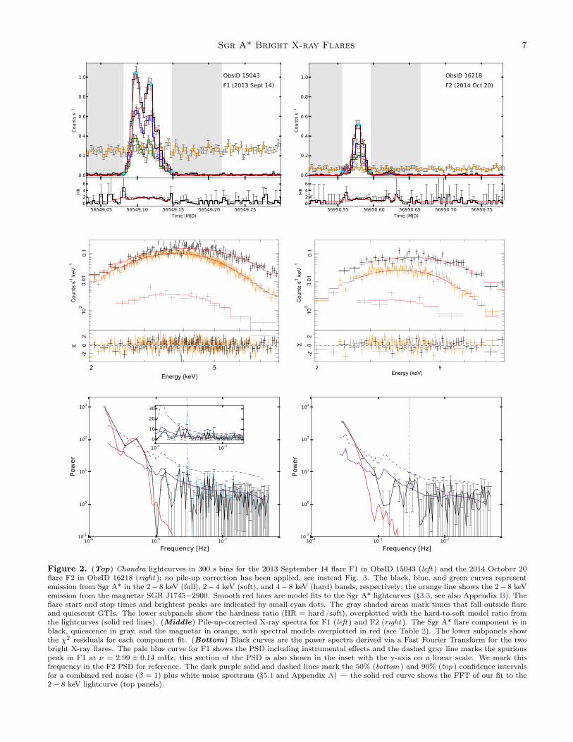
Figure 2. (Top) Chandra lightcurves in 300 s bins for the 2013 September 14 flare F1 in ObsID 15043 (left ) and the 2014 October 20flare F2 in ObsID 16218 (right ); no pile-up correction has been applied, see instead Fig. 3. The black, blue, and green curves representemission from Sgr A* in the 2− 8 keV (full), 2− 4 keV (soft), and 4− 8 keV (hard) bands, respectively; the orange line shows the 2− 8 keVemission from the magnetar SGR J1745−2900. Smooth red lines are model fits to the Sgr A* lightcurves (§3.3, see also Appendix B). Theflare start and stop times and brightest peaks are indicated by small cyan dots. The gray shaded areas mark times that fall outside flareand quiescent GTIs. The lower subpanels show the hardness ratio (HR = hard /soft), overplotted with the hard-to-soft model ratio fromthe lightcurves (solid red lines). (Middle) Pile-up-corrected X-ray spectra for F1 (left ) and F2 (right ). The Sgr A* flare component is inblack, quiescence in gray, and the magnetar in orange, with spectral models overplotted in red (see Table 2). The lower subpanels showthe χ2 residuals for each component fit. (Bottom) Black curves are the power spectra derived via a Fast Fourier Transform for the twobright X-ray flares. The pale blue curve for F1 shows the PSD including instrumental effects and the dashed gray line marks the spuriouspeak in F1 at ν = 2.99 ± 0.14 mHz; this section of the PSD is also shown in the inset with the y-axis on a linear scale. We mark thisfrequency in the F2 PSD for reference. The dark purple solid and dashed lines mark the 50% (bottom ) and 90% (top ) confidence intervalsfor a combined red noise (β = 1) plus white noise spectrum (§5.1 and Appendix A) — the solid red curve shows the FFT of our fit to the2 − 8 keV lightcurve (top panels).

8 Haggard et al.

Table 2. Chandra Sgr A* Bright Flare Properties

TIMING

Flare ObsID Tot Flare Flare Flare Rise Decay Fluence Mean Rate Peak1 Rate Peak2 Rate

Exp Start Stop Duration Time Time raw/corr raw/corr raw/corr raw/corr

(ks) (MJD) (MJD) (ks) (s) (s) (cnts) (cnts/s) (cnts/s) (cnts/s)

F1 15043 45.41 56549.08 56549.15 5.73 1500 2500 2769/3115 0.48 / 0.54 1.04 / 1.17 0.93 / 1.06

F2 16218 36.35 56950.56 56950.60 3.36 1700 1400 734/825 0.22 / 0.24 0.52 / 0.59 . . .

SPECTRAL FITS

——————————————— Flare ——————————————- ———— Magnetar ————

Flare State Fabs2−8 Funabs

2−8 Funabs2−10 Lunabs

2−10 Γ HR Fabs2−8 × 10−12 kT α χ2/DoF

(×10−12 erg/cm2/s) (×1034 erg/s) (erg/cm2/s) (keV)

F1 Mean 28.5+1.7−1.6 64.8+3.2

−3.1 74.4+3.7−3.5 57.0+2.8

−2.7 2.06 ± 0.14 1.7 ± 0.3 6.9 ± 0.2 0.79 ± 0.02 0.68+0.19−0.17 514.5/423

F1 Peak1 61.3+1.7−1.6 139.5+3.2

−3.1 160.1+3.7−3.5 122.6+2.8

−2.7 . . . . . . . . . . . . . . . . . .

F1 Peak2 54.8+1.7−1.6 124.8+3.2

−3.1 143.2+3.7−3.5 109.7+2.8

−2.7 . . . . . . . . . . . . . . . . . .

F2 Mean 10.8 ± 0.9 23.3 ± 1.8 26.9 ± 1.9 20.6 ± 1.5 2.03 ± 0.27 1.5 ± 0.2 1.5 ± 0.1 0.75 ± 0.04 0.5(f) 142.8/139

F2 Peak1 25.7 ± 0.9 55.5 ± 1.8 64.1+2.0−1.9 49.1 ± 1.5 . . . . . . . . . . . . . . . . . .

The top section contains timing parameters for F1 and F2, and the bottom contains the joint spectral fits. (Top) The 2 − 8 keV fluence, mean, and peakrates each have two entries, one for observed (raw) values, the other for the pile-up corrected (corr) values. These contain both flare and quiescent countssince both contribute to pile-up during the flares. The rise time for flare F1 is measured from the flare start time to the maximum of the first peak, thedecay time is measured from the maximum of the second peak to the flare stop time. For the double-peaked flare F1 each of the two peak rates are listed.(Bottom) Sgr A* flares are fit with the model fgcdust×TBnew×(powerlawf+powerlawq+blackbody), where the two power laws fit the flare and quiescentspectral components during the flare, and the blackbody fits the contribution from the magnetar. The magnetar-only fits employ a single blackbody andutilize data exclusively during Sgr A*’s quiescent periods to avoid contamination. Dust scattering and absorption are included in both fits. The quiescentPL index is fixed to Γ = 3.0 ± 0.2 (Nowak et al. 2012; Neilsen et al. 2013). The flux contribution from the magnetar is estimated to be 3% and 2.5% for F1(ObsID 15043) and F2 (ObsID 16218), respectively. NH is fixed to 16.3×1022 cm−2 and we assume a distance to the Galactic center of 8 kpc. Pile-up (α) isa free parameter in the F1 fit, but is fixed to α = 0.5 for the F2 fit because it could not be constrained by the data (§4.3). We list the 2-8 keV absorbed andunabsorbed fluxes, as well as the 2-10 keV unabsorbed flux and luminosity. The peak flux values are derived assuming peak/mean flux ratios of 2.2 ± 0.1,1.9±0.1, and 2.4±0.2 (90% confidence limits), for F1 peak1, F1 peak2, and the F2 peak, respectively, and errors are combined in quadrature (§3). Hardnessratios (HR) are defined as 4 − 8 keV/2 − 4 keV (§3.4).

Sgr A* Bright X-ray Flares 9

pile-up and find that both suffer from pile-up, thoughwe cannot directly constrain the impact for F2 (α =

0.0+1.0−0.0) and instead fix it to α = 0.5. We fix the ab-

sorption column, the quiescent photon index, and themagnetar temperatures to the values from §4.1 and §4.2.These joint spectral fits give flare power-law indices

of Γ = 2.06 ± 0.14 (F1) and Γ = 2.03 ± 0.27 (F2), cor-responding to 2 − 8 keV absorbed fluxes of F2−8 keV =

28.5+1.7−1.6 × 10−12 erg s−1 cm−2 for F1 and F2−8 keV =

10.8± 0.9× 10−12 erg s−1 cm−2 for F2. We show thesefits in the middle panels of Fig. 2 and report the fitparameters in Table 2, together with the derived fluxesand luminosities for the flares.As a check on our analysis, we subtract the off-flare

photons from the same 1′′.25 Sgr A* region using the qui-escent GTI. This removes contributions from the mag-netar, Sgr A*’s quiescent emission, as well as contam-ination from other sources in the crowded region (e.g.,Sgr A East). We fit these photons with a simple ab-sorbed power-law model fgcdust×TBnew×power-lawf ,fix the absorption column, and apply a pile-up modelas above. The resultant power-law indices are Γ =

1.83 ± 0.13 and Γ = 1.93 ± 0.30 for F1 and F2, respec-tively, in good agreement with our previous findings.This is a useful check on our joint spectral fits, but pileupmodels may not work properly on these subtracted spec-tra and are likely to result in harder powerlaw indices(§3.5). We thus prefer the joint spectral fits and adoptthose values throughout the remainder of the text andin Table 2.

5. POWER SPECTRA

We search for short timescale variability by creatingpower spectral densities (PSDs) for flares F1 and F2. Weperform a fast Fourier transform (FFT) with the Leahyet al. (1983) normalization on 10 s binned lightcurvesfrom the flare-only GTIs. The PSDs for F1 and F2 areshown in the bottom panels of Figure 2. The power spec-tra are complex, with broad features at lower frequenciesand smaller-scale modulation at higher frequencies.

5.1. PSD Noise Analysis

We examine the broad, low-frequency features bytransforming the lightcurve models described in §3.3(and Appendix B) using the same FFT procedure. Theresultant model PSDs are overplotted in red in the bot-tom panels of Figure 2. In both ObsIDs the powerspectrum from the flare is well matched to the low-frequency broad curves, but with a sharp drop in powerat ∼ 10−3 Hz.We investigate the high-frequency features at >

10−3 Hz to determine whether they can be attributed to

short period variability, e.g., quasi-periodic oscillations(QPOs), vs. noise in the lightcurve or aliasing, whichcan also produce sharp artificial features. We followa method similar to that of Timmer & Koenig (1995)(see also implementation by Mauerhan et al. 2005) andgenerate simulations where there is no signal. For eachflare we create 1000 data sets comprised solely of redand white noise, perform an inverse FFT, and scale theresultant lightcurves so that they have the same vari-ance and sampling as the flare lightcurve. Since theTimmer and Koenig algorithm is prone to windowing,we generate simulated lightcurves ∼10 times longer thanour flare lightcurves. The simulated data sets are thentransformed into a collection of power spectra.Our choice of noise spectra is motivated by the detec-

tion of red noise in past observations of Sgr A* (e.g.,Mauerhan et al. 2005; Meyer et al. 2008; Do et al. 2009;Witzel et al. 2012, 2018; Neilsen et al. 2015). Two val-ues are tested for the red noise slope (β =1.0, 2.0),which span the range of slopes detected in previous ob-servations (Yusef-Zadeh et al. 2006; Meyer et al. 2008)and simulations (Dolence et al. 2012). At higher fre-quencies the flare PSD curves taper off into flat Pois-son noise, and we therefore also include white noise(P (f) ∼ f0 = 1) in our simulations for a total noisemodel of P (f) = f−β + 1. The simulated PSD curvesfor two choices of β are shown in Appendix A; for clarityonly the results for β = 1.0 are plotted in the bottompanels of Figure 2, where the 50% and 90% confidenceintervals are shown as purple solid and dashed lines, re-spectively.F1 has three features that rise above the 90% confi-

dence interval: two broad curves at lower frequenciesand a sharp peak at ν ∼ 3 mHz (pale blue curve, mostprominent in the inset in the bottom left panel of Fig.2). The first two broad features at ν ∼ 0.17 mHz (5.7 ks)and ν = 0.49 mHz (2.0 ks) arise from the large-scale fea-tures in the lightcurve captured by our model, but wecannot attribute the third, narrower peak to the grossmorphology of the flare, as it is located well after theflare envelope model drops in power. We fit this peakwith a Lorentzian centered at ν = 2.99±0.01 mHz, witha width of δν = 0.26 ± 0.04 mHz, and a quality factorof q = ν/δν = 11.3. We indicate this frequency on thePSDs as a vertical dashed line in the bottom panels ofFigure 2, but argue in §5.2 that it is an instrumental arti-fact. The residual lightcurves and PSDs in Fig. 3 (darkgray lines) show the result of subtracting this large-scalecomponent and indicate the remaining unmodeled struc-ture. Hence, removing the flare envelop (fitted in thetime domain) before searching for high frequency fea-tures introduces a spurious signal in the PSD and we do

10 Haggard et al.

not pursue this approach further here. The only por-tion of the F2 PSD that rises above the 90% confidenceinterval is the flare envelope at low frequencies, thereare no significant high-frequency features. We mark the2.99 mHz position in the F2 PSD for comparison only.

5.2. Bad Pixel Analysis

The Chandra spacecraft dithers its pointing positionto reduce the effects of bad pixels, nodal boundaries,and chip gaps during an observation, as well as to aver-age the quantum efficiency of the detector pixels3. Thisobservational requirement can introduce spurious tim-ing signatures at either the pitch (X) or yaw (Y) ditherperiods or their harmonics.For ObsID 15043 we create an image binned in chip

coordinates and extract photons from the same 1′′.25 re-gion centered on Sgr A* from the level 1 and level 2 eventfiles. Both show the standard Lissajous dither pattern,but also two pixel columns that have been flagged asbad and thus excised in the standard level 2 files. Asthe Sgr A* extraction region crosses this sharp nodalboundary, the masked pixels create a discontinuity in thelightcurve that manifests as a peak in the power spec-trum of F1, at half the period of the yaw dither (becauseSgr A* crosses the column of bad pixels twice per oscil-lation). The Sgr A* extraction region in ObsID 16218does not overlap a bad column, and SGR J1745−2900is similarly unaffected in both ObsIDs. Analyses of theSgr A* and SGR J1745−2900 lightcurves extracted fromObsID 16218 do not reveal any flagged pixels.In light of this finding, we create new lightcurves for

F1 in ObsID 15043 without removing the bad pixelcolumns, and use these for all subsequent timing analy-sis. We adopt the extraction region, lightcurve binning,and GTI filtering described in §3. The resultant powerspectrum is shown in black in the bottom left panel ofFigure 2, while the pale blue curve represents the stan-dard level 2 Chandra filtering with the flagged columnsremoved. The peak at ∼ 3 mHz is no longer detectedand we conclude that the possible QPO in F1 arisesfrom instrumentation effects and cannot be attributedto Sgr A*.

5.3. PSD Permutation Error Analysis

To investigate the high frequency features still appar-ent in the PSDs, we perform a Monte Carlo (MC) per-mutation to simulate the errors on the X-ray lightcurvesand PSDs. We create 10,000 MC simulations of the full,unbinned Chandra lightcurve (rather than the flare-onlyintervals) by drawing a simulated count rate for each

3 http://cxc.harvard.edu/proposer/POG/html/chap5.html#tb:dither

Chandra frame (frame time = 0.44 s for a 1/8 subarray),using our model for the counts from §3.3 and AppendixB and a randomly generated Poisson error with an ex-pectation value equal to the larger of (1) the number ofcounts in that frame or (2) a constant expectation value(the expected number of counts) equal to the averagequiescent count rate times the frame time, i.e., 0.004and 0.003 for ObsID 15043 and 16218. This expecta-tion value is critical for frames where zero counts aredetected.We generate a Lomb–Scargle (L–S; Scargle 1982) pe-

riodogram for each simulated model lightcurve, which issubsequently binned (125 frames are combined to cre-ate ∼50 s bins) and corrected for pile-up. The left up-per panels of Figure 3 show the measured lightcurves(black lines), unbinned model fits (smooth red lines),and binned, pile-up-corrected models (dark blue lines),as well as the 5− 95% confidence intervals from the MCsimulations (light blue shaded regions). The lower sub-panels on the left show the residual between the dataand the model (gray lines). The right-hand panels showthe resultant LS periodogram on a log scale for each ofthese components and the insets highlight a subset ofthe higher frequencies. The black curves from the mea-sured LS periodograms have small peaks that rise justabove the 95% c.l., but these are weak and most likelyattributable to instrumental effects, noise, harmonics ofthe power in the stronger flare envelopes, and/or aliasing(see Appendix A).

6. DISCUSSION

Our analysis reveals two of the brightest X-ray flaresseen so far from Sgr A*, with peak 2 − 10 keV lumi-nosities of 12.3 × 1035 erg s−1 (F1) and 49.1 × 1034

erg s−1 (F2), durations of 5.7 and 3.4 ks, and totalenergies (0.7 − 3.3) × 1039 erg. These are as large orlarger than the peak luminosities, durations, and en-ergies found for previously detected bright X-ray flaresfrom Chandra (L2−10 keV = 48 × 1034 erg s−1, 5.6 ks,E2−10 keV ∼ 1039 erg; Nowak et al. 2012) and XMM-Newton (L2−10 keV ∼ (12−19)×1034 erg s−1, (2.8−2.9)

ks, E2−10 keV = (0.3−0.5)×1039 erg; Porquet et al. 2008;Nowak et al. 2012).

6.1. Flare Emission Scenarios

The X-ray spectral indices for F1 and F2 are consis-tent with Γ ∼ 2, similar to other bright X-ray flaresbut significantly harder than the spectrum in quies-cence (Γ ∼ 3; Nowak et al. 2012). Together with con-straints from the NIR, the spectrum seems to favor asynchrotron emission scenario wherein the NIR and X-ray spectral indices are set by the particle acceleration

Sgr A* Bright X-ray Flares 11

0255075

100125150175

coun

ts se

c1

15043 Data15043 Model15043 Residual15043 PU Model15043 MC Range

0.08 0.10 0.12 0.14 0.16time (MJD - 56549)

50

0

resid

uals

0

20

40

60

80

coun

ts se

c1

16218 Data16218 Model16218 Residual16218 PU Model16218 MC Range

0.54 0.56 0.58 0.60 0.62 0.64time (MJD - 56950)

25

0

resid

uals

Figure 3. (Left Panels) The F1 and F2 lightcurves (black line) and the best-fit model (red curve), binned to ∼50 s (vs. the 300 sbinning shown in Fig. 2). The residual lightcurve (data − model) is plotted in the lower subpanel (gray line). The pile-up-corrected modelsare plotted as dark blue lines. Overplotted are the 5–95% error intervals from 10,000 Monte Carlo simulations of the pile-up-correctedmodel, generated by adopting a randomly generated Poisson error with a value equal to the larger of either the number of counts in thatframe or an expectation value based on the average quiescent count rate (§5.3; light blue shaded regions); binning is performed after thelightcurve simulation is complete. (Right Panels) The L–S periodograms resulting from the measured and simulated lightcurves (linecolors as in left-hand panel).

process (Markoff et al. 2001; Dodds-Eden et al. 2009).When the NIR is bright, the spectral index is well de-scribed by νfν ∝ ν0.5 (e.g., Hornstein et al. 2007; Pontiet al. 2017) and synchrotron models predict a coolingbreak, such that Γ ∼ 2 at X-ray wavelengths. Evidenceof a similar spectral index for bright and faint flares (e.g.,Neilsen et al. 2013) also supports this interpretation.Alternative models invoke Compton processes (e.g.,

Markoff et al. 2001; Eckart et al. 2008; Yusef-Zadeh et al.2012). However, because the Compton bump can shiftdue to changing scattering optical depths or electronenergies (or other factors) flare spectra should show arange of spectral indices. Hence there is no clear ex-pectation that a constant NIR spectral index will leadto a constant X-ray photon index. On the other hand,the large difference between NIR and X-ray cumulativedistribution functions (Witzel et al. 2012, 2018; Neilsenet al. 2015) is not easily understood within the syn-chrotron scenario (Dibi et al. 2016). We must continue

to build up the statistics of simultaneous IR and X-rayflares to distinguish between these models.In addition to their spectral properties, X-ray studies

of Sgr A* point to a characteristic timescale for brightflares of ∼ 3 − 6 ks (detectable at all durations, e.g.,Porquet et al. 2003, 2008; Neilsen et al. 2013). Thistimescale is also consistent with F1 and F2, reportedhere. If we associate this timescale with a Keplerianorbital period then the orbital radius is 0.3 − 0.5 au,roughly two times the radius of the innermost stablecircular orbit (ISCO) for a stationary black hole withSgr A*’s mass and distance (Boehle et al. 2016; Grav-ity Collaboration et al. 2018b). This is equivalent to∼ 5× the Schwarzschild radius (RS ; see detailed mod-els in Markoff et al. 2001; Liu & Melia 2002; Liu et al.2004; Dodds-Eden et al. 2011). In this scenario, the flareemission is likely to arise from structures very near orat the event horizon.

12 Haggard et al.

Alternatively, we can estimate the size of the emissionregion (the emitting “spot”) by comparing the total X-ray energy radiated by the brightest flare, E2−10 keV =

3.3 × 1039 erg, to the energy available in the accre-tion flow. The volume of the accretion flow that con-tains an equal amount of magnetic energy is approxi-mately EB = (B2/8π)(4πR3

spot). Setting this equal tothe flare’s total energy radiated in X-rays (E2−10 keV )and assuming B = B0 (Rf/3RS)−1, where B0 = 30 Gis the magnetic field strength scaled to a typical valueclose to the black hole (Yuan et al. 2003; Dodds-Edenet al. 2009; Mościbrodzka et al. 2009; Dexter et al. 2010;Ponti et al. 2017), and Rf is the flare emission radius,gives

Rspot ∼ 2

(Rf

3RS

)2/3 (B0

30 G

)−2/3 (E2−10 keV

3.3× 1039 erg

)1/3

RS .

(2)Powering this flare requires a relatively large emitting

volume, even assuming a 100% efficiency of convert-ing magnetic energy into X-rays. Increasing the flareemission radius makes the relative size of the hot spotsmaller, but only slowly. This poses challenges for ex-plaining the rapid changes in the luminosity (e.g., thiswork, Barrière et al. 2014, among others), though an in-crease in the strength of the magnetic field in the flareregion could allow a smaller volume. In general, thisrepresents a lower limit on the size of the flare’s totalemitting region, because it only takes X-rays into ac-count. It is also consistent with a scenario in which thesize of the emitting region is larger for brighter flares.Recent results from the GRAVITY experiment on

the Very Large Telescope Interferometer (VLTI, GravityCollaboration et al. 2018b), argue that Sgr A*’s infraredvariability can be traced to orbital motions of gas cloudswith a period of ∼45 minutes (2.7 ks). Using ray-tracingsimulations, they match this timescale to emission froma rotating, synchrotron-emitting “hot spot” in a low in-clination orbit at ∼ 3 − 5 RS (Gravity Collaborationet al. 2018a).Since near-IR and X-ray outbursts from Sgr A* ap-

pear to be nearly simultaneous and highly correlated(e.g., Boyce et al. 2019), these well-matched timescalesgive further support to hot spot models and to emissionscenarios where the NIR and X-ray emission originatesnear the SMBH’s event horizon. We caution, however,that this timescale is not unique, and can also be re-produced by the tidal disruption of asteroid-size objects(Čadež et al. 2008; Kostić et al. 2009; Zubovas et al.2012) and the Alfvèn crossing time for magnetic loopsnear the black hole (Yuan et al. 2003; Yuan & Narayan2004).

The GRAVITY NIR flare detected on 2018 July 28 isalso double-peaked (see Figure 2 of Gravity Collabora-tion et al. 2018a), much like F1 reported in this work.The durations of these two outbursts, ∼115 minutes forthe NIR and ∼97 minutes for the X-ray, are similar andthe time between the two peaks, ∼40 minutes (NIR)and ∼30 minutes (X-ray), are also similar. The ratio ofthe total flare duration to the time between peaks is ap-proximately a factor of 3 in both cases. Double-peakedflares like these have previously been detected from SgrA* (e.g., Mossoux et al. 2015; Karssen et al. 2017; Boyceet al. 2019; Fazio et al. 2018), but even when they donot have multiple peaks, bright X-ray flares often dis-play asymmetric lightcurve profiles (e.g., this work, Por-quet et al. 2003, 2008; Nowak et al. 2012; Mossoux et al.2016). Further investigation of their statistical and tim-ing properties is ripe for further study.Despite differences in their morphologies, other flare

properties follow more predictable trends. Neilsen et al.(2013) present relationships between the fluence, countrate, and duration of ∼ 40 flares from the XVP. Tocompare F1 and F2 to the XVP flare population, weadjust for the different instrument configurations usingPIMMS4 and scale the reported XVP flare fluences totheir equivalent ACIS-S values (Figure 4). F1 and F2(filled dark blue circles) are considerably brighter thanmost of the XVP sample, but show the same trend to-ward higher fluences at longer durations. This againsupports a scenario in which the emission region is largerfor brighter flares. However, our observations and de-tection techniques are biased against long-duration, lowfluence (i.e., low contrast) flares. Comprehensive flaresimulations are under development (e.g., Bouffard et al.2019) and will aide in diagnosing these and other obser-vational biases.The flare X-ray hardness ratios and spectral indices

appear to be constant, indicating that the spectral slopedoes not change significantly over the duration of theflare. Strengthening this argument, the three brightestX-ray flares detected before our discoveries have photonspectral indices of Γ = 2.0+0.7

−0.6, 2.3 ± 0.3, and 2.4+0.4−0.3

(Porquet et al. 2003, 2008; Nowak et al. 2012), whichare similar to our results of Γ = 2.06± 0.14 and 2.03±0.27 for F1 and F2. Recent results from NuSTAR athigher energies (3-79 keV) provide additional support fora constant PL slope — Zhang et al. (2017) report photonindices of Γ ∼ 2.0− 2.8± 0.5 (90% confidence) for sevenSgr A* flares. Hence, it appears that Sgr A*’s brightX-ray flares belong to the same population (§3.4), and

4 Chandra proposal tools: http://cxc.harvard.edu/toolkit/pimms.jsp.

Sgr A* Bright X-ray Flares 13

500 1000 2000 5000Duration (s)

101

102

103

Flu

en

ce (

cou

nts

)

Flares F1, F2, no correctionFlares F1, F2, pileup correctedNeilson +13, pileup corrected

Figure 4. The 2-8 keV flare fluence as a function of flare du-ration. The large blue and red data points represent the incidentand pile-up corrected data, respectively, for F1 and F2. Smallerblue points represent the flares reported in Neilsen et al. (2013).Originally reported as fluxes from the HETG configuration, thevalues were converted to ACIS-S counts for a uniform compar-ison with the data presented in this work. The dashed greenline, from Neilsen et al. (2013), represents flares with luminositiesL = 5.4 × 1034 ergs s−1, the approximate demarcation between‘bright’ flares and ‘dim’ flares.

thus are likely to arise from the same energy injectionmechanism.

6.2. Multiwavelength Coverage

Multiwavelength campaigns targeting Sgr A* oftenemphasize variability in the X-ray and infrared (e.g.,recent studies by Boyce et al. 2019; Fazio et al. 2018,and references therein), where emission peaks are nearlysimultaneous. Unfortunately, neither F1 nor F2 havenear-IR coverage. The GRAVITY Collaboration hasdemonstrated the power of NIR interferometry in resolv-ing structures only ∼ 10 times the gravitational radius ofSgr A* and future simultaneous observations with thisinstrument and Chandra could offer a powerful probeof how bright X-ray flares are linked to changes in theaccretion dynamics near the event horizon.Longer wavelength observations have hinted at a lag

between X-ray flares and their candidate submillimeteror radio counterparts, with the long wavelength datalagging the X-ray. Capellupo et al. (2017) report ninecontemporaneous X-ray and Jansky Very Large Array(JVLA) radio observations of Sgr A*, including cover-age of the F1 flare. The JVLA lightcurve overlappingF1 lasts ∼ 7 hr and shows significant radio variabilityat 8-10 GHz (X-band) in the form of a 15% (0.15 Jy)increase during the second half of the observation. The

radio lightcurve is not long enough to show a clear startor stop time for the rise, but Capellupo et al. (2017) de-termine a lower limit on the radio flare duration of ∼176minutes, compared to ∼100 minutes for the full X-rayflare, with the radio rising before and peaking after theX-ray. This delay could be understood in the contextof the adiabatic expansion of an initially optically thickblob of synchrotron-emitting relativistic particles (e.g.,Yusef-Zadeh et al. 2006), offering an alternative to thehot spot models discussed above. However, due to theincomplete temporal coverage for F1 and inconclusivecorrelations between the other radio and X-ray peaks inthe study, Capellupo et al. (2017) suggest that strongerX-ray flares may lead to longer time lags in the radio,but do not find strong statistical evidence that the radioand X-ray are correlated.Observations at 1 mm were also performed at the Sub-

millimeter Array (SMA) a few hours in advance of theF1 flare and on subsequent days as part of a long-termmonitoring program (Bower et al. 2015). These obser-vations show flux densities that are significantly abovethe historical average on the date of the F1 flare andfor approximately one week afterwards. It is difficult toassociate these high flux densities directly with the F1flare, however, given the infrequent sampling of the SMAlight curves and the characteristic time scales of millime-ter/submillimeter variability (approximately 8 hr, Dex-ter et al. 2014).The lack of infrared and patchwork of longer wave-

length observations for F1 (and the paucity of multi-wavelength data for F2), underscores the importance ofcontinued multiwavelength monitoring of Sgr A*.Toward this end, the Event Horizon Telescope (EHT;

Doeleman et al. 2008) has recently undertaken its firstfull-array observations of Sgr A* and M87*. These haveoffered exquisite, high-precision submillimeter imagingof M87*’s event horizon (Event Horizon Telescope Col-laboration et al. 2019a) and are poised to do the samefor Sgr A*. Coordinated EHT and multiwavelength ob-servations, including with approved Chandra programs,have begun to inform models for M87* (Event HorizonTelescope Collaboration et al. 2019b) and will soon en-able a detailed comparison between Sgr A*’s X-ray andsubmillimeter emission, offering a new understanding ofits flares and underlying accretion flow.

7. CONCLUSION

We have performed an extensive study of the twobrightest Chandra X-ray flares yet detected from Sgr A*,discovered on 2013 September 14 (F1) and 2014 Octo-ber 20 (F2). After correcting for contamination from thenearby magnetar, SGR J1745−2900, and observational

14 Haggard et al.

and instrumental effects from the Galactic center X-raybackground, pile-up, and telescope dither, we report thefollowing key findings:

1. The brightest flare F1 has a distinctive double-peaked morphology, with individual peak X-rayluminosities more than 600× and 550× Sgr A*’squiescent luminosity. The second bright flare F2also has an asymmetric morphology and rises 245×above quiescence.

2. These bright flares have long durations, 5.7 ks (F1)and 3.4 ks (F2), and rapid rise and decay times: F1rises in 1500 s and decays in 2500 s, while F2 risesin 1700 s and decays in 1400 s. These timescalesmay correspond to emission from a hot spot or-biting the SMBH, in agreement with new NIR re-sults from the GRAVITY experiment. Their tim-ing properties also imply that the size of the emit-ting region may scale with the brightness of theflare.

3. Both flares have X-ray spectral indices and hard-ness ratios significantly harder than during qui-escence, Γ = 2.06 ± 0.14 and Γ = 2.03 ± 0.27

vs. Γ = 3.0 ± 0.2 in quiescence, consistent withpreviously detected Sgr A* flares and with a syn-chrotron emission mechanism, though Comptonemission models are not ruled out.

4. Statistical tests of the flare time series, includingMonte Carlo simulations of their noise properties,offer little evidence for high-frequency power (e.g.,QPOs) in either flare.

5. F1 and F2 are the brightest X-ray flares ever de-tected by Chandra, and are among the brightest X-ray flares from Sgr A* detected by any observatory.They appear to deviate in the fluence-durationplane from the distribution of fainter flares de-tected in the 2011 Sgr A* Chandra XVP. However,low fluence, long duration flares may not exist ormay suffer from selection bias, making this findingtentative at present.

6. Neither F1 nor F2 have near-IR coverage, butsome (near-)simultaneous coverage of F1 was col-lected at radio and submillimeter wavelengths.These data point to higher than average flux lev-els for Sgr A* near the F1 outburst, but do notallow definitive correlation between Sgr A*’s X-ray and longer wavelength behavior. Coordinatedmultiwavelength campaigns thus continue to be es-sential for a complete, statistically robust exami-nation of Sgr A*’s multiwavelength variability.

The authors thank Charles Gammie, Tiffany Kha,Matthew Stubbs, and Nicolas Cowan for discussionsrelated to this work. We acknowledge the Chandrascheduling, data processing, and archive teams for mak-ing these observations possible. This work was sup-ported by Chandra Award Numbers GO3-14121A andGO4-15091C, issued by the Chandra X-ray ObservatoryCenter, which is operated by the Smithsonian Astro-physical Observatory for and on behalf of the NationalAeronautics Space Administration (NASA) under con-tract NAS8-03060.D.H., M.N., and C.O.H. acknowledge support from

the Natural Sciences and Engineering Research Councilof Canada (NSERC) Discovery Grant. D.H. and M.N.also thank the Fonds de recherche du Québec–Nature etTechnologies (FRQNT) Nouveaux Chercheurs program.D.H. acknowledges support from the Canadian Insti-tute for Advanced Research (CIFAR). M.N. acknowl-edges funding from the McGill Trottier Chair in As-trophysics and Cosmology. G.P. acknowledges financialsupport from the Bundesministerium für Wirtschaft undTechnologie/Deutsches Zentrum für Luft-und Raum-fahrt (BMWI/DLR, FKZ 50 OR 1812, OR 1715 andOR 1604) and the Max Planck Society. S.M. is fundedby a VICI grant (639.043.512) from the Netherlands Or-ganisation for Scientific Research.

Facility: CXO

Software: Python, CIAO

APPENDIX

A. POWER SPECTRA COMPARISONS

In addition to the power spectral analysis of the two bright Sgr A* flares presented in Section 5, we further investigateSgr A* during quiescence to compare the respective behaviors at high frequencies. We obtain the quiescent PSD fromthe GTIs listed in Table 1 and process it with the same method as for the flare (see §5). For an additional comparison,we also obtain the power spectrum for the magnetar SGR J1745−2900 during the intervals when Sgr A* is in quiescenceto minimize contamination. The resultant Leahy-normalized PSDs are shown in Figure A.1 for ObsID 15043 (left)and ObsID 16218 (right). The Sgr A* flare and quiescence PSDs are plotted in black and blue, respectively, and themagnetar PSD is shown in orange.

Sgr A* Bright X-ray Flares 15

Figure A.1. Leahy-normalized power spectra for Sgr A* flares F1 and F2 (black), Sgr A* during quiescence (blue), and the magnetar,SGR J1745−2900 (orange). PSDs are shown for ObsID 15043 (left ) and 16218 (right ).

10-4 10-3 10-2

Frequency10-1

100

101

102

103

Pow

er

β=1 β=2

10-4 10-3 10-2

Frequency [Hz]10-1

100

101

102

103Po

wer

β=1 β=2

Figure A.2. Leahy-normalized power spectral densities, derived via a fast Fourier transform (FFT), for the bright flare F1 (left ) andflare F2 (right ). The pale blue curve for F1 shows the PSD from data obtained with standard Chandra data processing, which includesinstrumental effects. The spurious QPO at ν = 2.99 mHz in flare F1 is indicated by the dashed gray line, it is shown for flare F2 on theright for comparison only. The black curve shows the PSD with proper data filtering (§5.2). For both flares, errors with β = 1.0 and β = 2.0are shown in dark purple and dark yellow, respectively. The solid lines indicate 50% contours, while the dashed represent 90% contours.

F1 and F2 exhibit broad features at f < 10−3 Hz attributed to the flare envelopes as discussed in Section 5 andshown in Figure 2. In contrast, at higher frequencies (f > 10−2 Hz) both flares drop in power such that the flare PSDsoverlap with or are within the uncertainties of the Sgr A* quiescent and magentar data. Behavior in this regime is thusnot unique to the flares, and can be attributed to noise. Within the frequency range (10−3 < f < 10−2 Hz), however,the flare PSDs show hints of several small peaks that are not as visible in the quiescent or magnetar power spectra.These small-scale features have low significance and may be due to the instrumental effects discussed in Section 5.2 orharmonics of the structure from the flare envelope. Note that the ∼ 3s (∼ 3× 10−1 Hz) period of the magnetar wouldnot be visible on the frequency range plotted in Fig. A.1.We probe these midfrequency features by exploring two independent methods of quantifying the significance of the

PSD, discussed in detail in Sections 5.1 and 5.3. For the latter, we perform Monte Carlo simulations of the flare lightcurve, and for the former we generate PSDs under the worst-case assumption that all the flare photons arise froma combination of red and white noise. Figure 2 shows the 50% and 90% confidence intervals where the red noise isdefined by a slope of β = 1.0. The spurious ∼ 3 mHz QPO is the only feature aside from the flare envelope that risesabove the noise curve.

16 Haggard et al.

0.08 0.10 0.12 0.14 0.16time (MJD - 56549)

020406080

100120140

coun

ts se

c1

15043 Data15043 Gauss115043 Gauss215043 Gauss315043 Gauss415043 Const

0.54 0.56 0.58 0.60 0.62 0.64time (MJD - 56950)

010203040506070

coun

ts se

c1

16218 Data16218 Skew116218 Gauss16218 Skew216218 Const

Figure B.1. Model components for the F1 and F2 lightcurve fits from Equations B1 and B2 and parameters in Table B.1. The compositemodels are plotted as red curves in the top panels of Figure 2 and in all four panels of Figure 3. The Chandra X-ray data are shown inlight gray, with ∼100 s binning (see §5.3).

However, a range of red noise slopes are possible in Sgr A* (see Section 5.1) and we therefore investigate thesignificance of the power spectral features where β = 2.0 represents the red noise. Figure A.2 shows the PSD for theflare F1 with the standard Chandra data processing in pale blue and the updated filtering defined in Section 5.2 inblack. While the two curves are very similar, the QPO resulting from instrumentation effects is clearly seen in theblue PSD. Overlaid are the error curves from the simulations where the red noise is defined with slopes of β = 1.0 andβ = 2.0 in dark purple and dark yellow, respectively. The 50% confidence intervals are represented by a solid line,while the 90% confidence limits (c.l.) are dashed.The white noise β = 0 is dominant at higher frequencies, while the red noise component is relevant in the lower

frequency regime. This is evident as the curves with β = 1.0 and β = 2.0 diverge at f < 10−3 Hz. In both scenariosthere are a few features that rise above the solid 50% c.l., but none that rise above the dashed 90% confidence intervalsand we conclude that no high frequency signal is detected in these bright flares.

B. LIGHTCURVE MODELS

The models fit to the X-ray lightcurves for F1 and F2, and used in the analyses above, are composed of a sum offour Gaussians plus a constant for F1, and a sum of two Gaussians and two skewed Gaussians plus a constant for F2.These take the standard functional forms

g(t;A,µ, σ) =A

σ√

2πe−(t−µ)

2/2σ2

(B1)

f(t;A,µ, σ, γ) =A

σ√

2πe−(t−µ)

2/2σ2

{1 + erf

[γ(t− µ)

σ√

2

]}(B2)

where the parameters are amplitude (A), center (µ), characteristic width (σ), and gamma (γ), and erf() is the errorfunction.We plot these components in Figure B.1 and give the detailed fits in Table B.1 for reference. The composite lightcurve

models for F1 and F2 are shown as solid red lines in the top panels of Fig. 2 and in all four panels of Fig. 3.

Sgr A* Bright X-ray Flares 17

Table B.1. Lightcurve Models

Function A (cnts/s) µ (MJD) σ (MJD) γ

15043

Gaussian 1 0.0114 56549.098 0.0053 . . .

Gaussian 2 0.0173 56549.116 0.0140 . . .

Gaussian 3 0.0054 56549.117 0.0046 . . .

Gaussian 4 0.0006 56549.130 0.0016 . . .

Constant 0.0112 . . . . . . . . .

16218

Skew Gauss 1 0.0003 56950.561 0.0034 −15.950

Gaussian 0.0089 56950.579 0.0070 . . .

Skew Gauss 2 0.0006 56950.628 0.0094 −4.278

Constant 0.0066 . . . . . . . . .

The lightcurve models for F1 and F2 are described by the pa-rameters above, using a combination of Equations B1 and B2.Each component is shown separately in Fig. B.1 and the com-posite models are plotted as red curves in the top panels of Fig.2 and in all four panels of Fig. 3.

REFERENCES

Baganoff, F. K., Bautz, M. W., Brandt, W. N., et al. 2001,Nature, 413, 45

Baganoff, F. K., Maeda, Y., Morris, M., et al. 2003, ApJ,591, 891

Ball, D., Özel, F., Psaltis, D., & Chan, C.-k. 2016, ApJ,826, 77

Ball, D., Özel, F., Psaltis, D., Chan, C.-K., & Sironi, L.2018, ApJ, 853, 184

Barrière, N. M., Tomsick, J. A., Baganoff, F. K., et al.2014, ApJ, 786, 46

Bélanger, G., Goldwurm, A., Melia, F., et al. 2005, ApJ,635, 1095

Boehle, A., Ghez, A. M., Schödel, R., et al. 2016, ApJ, 830,17

Bouffard, É., Haggard, D., Nowak, M. A., et al. 2019, ApJ,884, 148

Bower, G. C., Markoff, S., Dexter, J., et al. 2015, ApJ, 802,69

Boyce, H., Haggard, D., Witzel, G., et al. 2019, ApJ, 871,161

Capellupo, D. M., Haggard, D., Choux, N., et al. 2017,ApJ, 845, 35

Corrales, L. R., García, J., Wilms, J., & Baganoff, F. 2016,MNRAS, 458, 1345

Corrales, L. R., Mon, B., Haggard, D., et al. 2017, ApJ,839, 76

Coti Zelati, F., Rea, N., Papitto, A., et al. 2015, MNRAS,449, 2685

Coti Zelati, F., Rea, N., Turolla, R., et al. 2017, MNRAS,471, 1819

Cuadra, J., Nayakshin, S., & Martins, F. 2008, MNRAS,383, 458

Cuadra, J., Nayakshin, S., Springel, V., & Di Matteo, T.2005, MNRAS, 360, L55

—. 2006, MNRAS, 366, 358Degenaar, N., Miller, J. M., Kennea, J., et al. 2013, ApJ,769, 155

Dexter, J., Agol, E., Fragile, P. C., & McKinney, J. C.2010, ApJ, 717, 1092

Dexter, J., Kelly, B., Bower, G. C., et al. 2014, MNRAS,442, 2797

Dibi, S., Markoff, S., Belmont, R., et al. 2014, MNRAS,441, 1005

—. 2016, MNRAS, 461, 552Do, T., Ghez, A. M., Morris, M. R., et al. 2009, ApJ, 691,1021

Do, T., Witzel, G., Gautam, A. K., et al. 2019, ApJL, 882,L27

Dodds-Eden, K., Porquet, D., Trap, G., et al. 2009, ApJ,698, 676

Dodds-Eden, K., Gillessen, S., Fritz, T. K., et al. 2011,ApJ, 728, 37

18 Haggard et al.

Doeleman, S. S., Weintroub, J., Rogers, A. E. E., et al.2008, Nature, 455, 78

Dolence, J. C., Gammie, C. F., Shiokawa, H., & Noble,S. C. 2012, ApJL, 746, L10

Eckart, A., Baganoff, F. K., Zamaninasab, M., et al. 2008,A&A, 479, 625

Event Horizon Telescope Collaboration, Akiyama, K.,Alberdi, A., et al. 2019a, ApJL, 875, L1

—. 2019b, ApJL, 875, L5Fazio, G. G., Hora, J. L., Witzel, G., et al. 2018, ApJ, 864,58

Fruscione, A., McDowell, J. C., Allen, G. E., et al. 2006, inProc. SPIE, Vol. 6270, Society of Photo-OpticalInstrumentation Engineers (SPIE) Conference Series,62701V

Genzel, R., Eisenhauer, F., & Gillessen, S. 2010, Reviews ofModern Physics, 82, 3121

Ghez, A. M., Salim, S., Weinberg, N. N., et al. 2008, ApJ,689, 1044

Gillessen, S., Eisenhauer, F., Fritz, T. K., et al. 2009,ApJL, 707, L114

Gillessen, S., Genzel, R., Fritz, T. K., et al. 2012, Nature,481, 51

Gillessen, S., Plewa, P. M., Eisenhauer, F., et al. 2017, ApJ,837, 30

Goldwurm, A., Brion, E., Goldoni, P., et al. 2003, ApJ,584, 751

Gravity Collaboration, Abuter, R., Amorim, A., et al.2018a, A&A, 618, L10

—. 2018b, A&A, 615, L15—. 2019, A&A, 625, L10Hornstein, S. D., Matthews, K., Ghez, A. M., et al. 2007,ApJ, 667, 900

Houck, J. C., & Denicola, L. A. 2000, Astronomical Societyof the Pacific Conference Series, Vol. 216, ISIS: AnInteractive Spectral Interpretation System for HighResolution X-Ray Spectroscopy, ed. N. Manset,C. Veillet, & D. Crabtree, 591

Jin, C., Ponti, G., Haberl, F., & Smith, R. 2017, MNRAS,468, 2532

Karssen, G. D., Bursa, M., Eckart, A., et al. 2017, MNRAS,472, 4422

Kennea, J. A., Burrows, D. N., Kouveliotou, C., et al. 2013,ApJL, 770, L24

Kostić, U., Čadež, A., Calvani, M., & Gomboc, A. 2009,A&A, 496, 307

Leahy, D. A., Darbro, W., Elsner, R. F., et al. 1983, ApJ,266, 160

Liu, S., & Melia, F. 2002, ApJL, 566, L77Liu, S., Petrosian, V., & Melia, F. 2004, ApJL, 611, L101

Markoff, S., Falcke, H., Yuan, F., & Biermann, P. L. 2001,A&A, 379, L13

Mauerhan, J. C., Morris, M., Walter, F., & Baganoff, F. K.2005, ApJL, 623, L25

Melia, F. 1992, ApJL, 387, L25Meyer, L., Do, T., Ghez, A., et al. 2008, ApJL, 688, L17Mori, K., Gotthelf, E. V., Zhang, S., et al. 2013, ApJL, 770,L23

Mościbrodzka, M., Gammie, C. F., Dolence, J. C.,Shiokawa, H., & Leung, P. K. 2009, ApJ, 706, 497

Mossoux, E., & Grosso, N. 2017, A&A, 604, A85Mossoux, E., Grosso, N., Vincent, F. H., & Porquet, D.2015, A&A, 573, A46

Mossoux, E., Grosso, N., Bushouse, H., et al. 2016, A&A,589, A116

Neilsen, J., Nowak, M. A., Gammie, C., et al. 2013, ApJ,774, 42

Neilsen, J., Markoff, S., Nowak, M. A., et al. 2015, ApJ,799, 199

Nowak, M. A., Neilsen, J., Markoff, S. B., et al. 2012, ApJ,759, 95

Park, T., Kashyap, V. L., Siemiginowska, A., et al. 2006,ApJ, 652, 610

Plewa, P. M., Gillessen, S., Pfuhl, O., et al. 2017, ApJ, 840,50

Ponti, G., De Marco, B., Morris, M. R., et al. 2015,MNRAS, 454, 1525

Ponti, G., George, E., Scaringi, S., et al. 2017, MNRAS,468, 2447

Porquet, D., Predehl, P., Aschenbach, B., et al. 2003, A&A,407, L17

Porquet, D., Grosso, N., Predehl, P., et al. 2008, A&A, 488,549

Quataert, E. 2002, ApJ, 575, 855Rea, N., Esposito, P., Pons, J. A., et al. 2013, ApJL, 775,L34

Reid, M. J., & Brunthaler, A. 2004, ApJ, 616, 872Russell, C. M. P., Wang, Q. D., & Cuadra, J. 2017,MNRAS, 464, 4958

Scargle, J. D. 1982, ApJ, 263, 835Smith, R. K., Valencic, L. A., & Corrales, L. 2016, ApJ,818, 143

Timmer, J., & Koenig, M. 1995, A&A, 300, 707Čadež, A., Calvani, M., & Kostić, U. 2008, A&A, 487, 527Verner, D. A., Ferland, G. J., Korista, K. T., & Yakovlev,D. G. 1996, ApJ, 465, 487

Wang, Q. D., Nowak, M. A., Markoff, S. B., et al. 2013,Science, 341, 981

Wilms, J., Allen, A., & McCray, R. 2000, ApJ, 542, 914

Sgr A* Bright X-ray Flares 19

Witzel, G., Eckart, A., Bremer, M., et al. 2012, ApJS, 203,18

Witzel, G., Sitarski, B. N., Ghez, A. M., et al. 2017, ApJ,847, 80

Witzel, G., Martinez, G., Hora, J., et al. 2018, ApJ, 863, 15Xu, Y.-D., Narayan, R., Quataert, E., Yuan, F., &Baganoff, F. K. 2006, ApJ, 640, 319

Yuan, F., & Narayan, R. 2004, ApJ, 612, 724Yuan, F., Quataert, E., & Narayan, R. 2003, ApJ, 598, 301Yuan, Q., & Wang, Q. D. 2016, MNRAS, 456, 1438

Yusef-Zadeh, F., Wardle, M., Schödel, R., et al. 2016, ApJ,819, 60

Yusef-Zadeh, F., Bushouse, H., Dowell, C. D., et al. 2006,ApJ, 644, 198

Yusef-Zadeh, F., Wardle, M., Dodds-Eden, K., et al. 2012,AJ, 144, 1

Zhang, S., Baganoff, F. K., Ponti, G., et al. 2017, ApJ, 843,96

Zubovas, K., Nayakshin, S., & Markoff, S. 2012, MNRAS,421, 1315