
Metaestabilidad para una EDP con blow-up y la dinámica FFG...
204
UNIVERSIDAD DE BUENOS AIRES Facultad de Ciencias Exactas y Naturales Departamento de Matemática Metaestabilidad para una EDP con blow-up y la dinámica FFG en modelos diluidos Tesis presentada para optar al título de Doctor de la Universidad de Buenos Aires en el área Ciencias Matemáticas Santiago Saglietti Director de tesis: Pablo Groisman Consejero de estudios: Pablo Groisman Buenos Aires, 2014 Fecha de defensa : 27 de Junio del 2014
Transcript of Metaestabilidad para una EDP con blow-up y la dinámica FFG...

UNIVERSIDAD DE BUENOS AIRES
Facultad de Ciencias Exactas y Naturales
Departamento de Matemática
Metaestabilidad para una EDP con blow-up y la dinámica FFGen modelos diluidos
Tesis presentada para optar al título de Doctor de la Universidad de Buenos Aires en elárea Ciencias Matemáticas
Santiago Saglietti
Director de tesis: Pablo Groisman
Consejero de estudios: Pablo Groisman
Buenos Aires, 2014
Fecha de defensa : 27 de Junio del 2014

2
Metaestabilidad para una EDP con blow-up y ladinámica FFG en modelos diluidos
Resumen
Esta tesis consiste de dos partes, en cada una estudiamos la estabilidad bajo pe-queñas perturbaciones de ciertos modelos probabilísticos en diferentes contextos. En laprimera parte, estudiamos pequeñas perturbaciones aleatorias de un sistema dinámicodeterminístico y mostramos que las mismas son inestables, en el sentido de que los sis-temas perturbados tienen un comportamiento cualitativo diferente al del sistema original.Más precisamente, dado p > 1 estudiamos soluciones de la ecuación en derivadas parcialesestocástica
∂tU = ∂2xxU + U |U |p−1 + εW
con condiciones de frontera de Dirichlet homogéneas y mostramos que para ε > 0 pequeñoséstas presentan una forma particular de inestabilidad conocida como metaestabilidad. Enla segunda parte nos situamos dentro del contexto de la mecánica estadística, dondeestudiamos la estabilidad de medidas de equilibrio en volumen infinito bajo ciertas per-turbaciones determinísticas en los parámetros del modelo. Más precisamente, mostramosque las medidas de Gibbs para una cierta clase general de sistemas son continuas conrespecto a cambios en la interacción y/o en la densidad de partículas y, por lo tanto,estables bajo pequeñas perturbaciones de las mismas. También estudiamos bajo quécondiciones ciertas configuraciones típicas de estos sistemas permanecen estables en ellímite de temperatura cero T → 0. La herramienta principal que utilizamos para nuestroestudio es la realización de estas medidas de equilibrio como distribuciones invariantes delas dinámicas introducidas en [16]. Referimos al comienzo de cada una de las partes parauna introducción de mayor profundidad sobre cada uno de los temas.
Palabras claves: ecuaciones en derivadas parciales estocásticas, metaestabilidad, blow-up, medidas de Gibbs, procesos estocásticos, redes de pérdida, Pirogov-Sinai.
3

4

Metastability for a PDE with blow-up and the FFGdynamics in diluted models
Abstract
This thesis consists of two separate parts: in each we study the stability under smallperturbations of certain probability models in different contexts. In the first, we studysmall random perturbations of a deterministic dynamical system and show that these areunstable, in the sense that the perturbed systems have a different qualitative behaviorthan that of the original system. More precisely, given p > 1 we study solutions to thestochastic partial differential equation
∂tU = ∂2xxU + U |U |p−1 + εW
with homogeneous Dirichlet boundary conditions and show that for small ε > 0 thesepresent a rather particular form of unstability known as metastability. In the second partwe situate ourselves in the context of statistical mechanics, where we study the stabilityof equilibrium infinite-volume measures under small deterministic perturbations in theparameters of the model. More precisely, we show that Gibbs measures for a generalclass of systems are continuous with respect to changes in the interaction and/or densityof particles and, hence, stable under small perturbations of them. We also study underwhich conditions do certain typical configurations of these systems remain stable in thezero-temperature limit T → 0. The main tool we use for our study is the realization ofthese equilibrium measures as invariant distributions of the dynamics introduced in [16].We refer to the beginning of each part for a deeper introduction on each of the subjects.
Key words: stochastic partial differential equations, metastability, stochastic processes,blow-up, Gibbs measures, loss networks, Pirogov-Sinai.
5

6
Agradecimientos
Un gran número de personas han contribuido, de alguna manera u otra, con la realizaciónde este trabajo. Me gustaría agradecer:
⋄ A mi director, Pablo Groisman, por todo. Por su constante apoyo y enorme ayudadurante la elaboración de esta Tesis. Por su infinita paciencia y gran predisposición.Por estar siempre para atender mis inquietudes, y por recibirme todas y cada unade las veces con una sonrisa y la mejor onda. Por compartir conmigo su manera deconcebir y hacer matemática, lo que ha tenido un gran impacto en mi formacióncomo matemático y es, para mí, de un valor incalculable. Por su amistad. Por todo.
⋄ A Pablo Ferrari, por estar siempre dispuesto a darme una mano y a discutir sobrematemática conmigo. Considero realmente un privilegio haber tenido la oportunidadde pensar problemas juntos y entrar en contacto con su forma de ver la matemática.Son muchísimas las cosas que he aprendido de él en estos últimos cuatro años, y espor ello que le voy a estar siempre inmensamente agradecido.
⋄ A los jurados de esta Tesis: Pablo De Napoli, Mariela Sued y Aernout Van Enter.Por leerla y darme sus sugerencias, con todo el esfuerzo y tiempo que ello requiere.
⋄ A Nicolas Saintier, por su entusiasmo en mi trabajo y su colaboración en esta Tesis.
⋄ A Roberto Fernández y Siamak Taati, por la productiva estadía en Utrecht.
⋄ A Inés, Matt y Leo. Por creer siempre en mí y enseñarme algo nuevo todos los días.
⋄ A Maru, por las muchas tardes de clase, estudio, charlas, chismes y chocolate.
⋄ A mis hermanitos académicos: Anita, Nico, Nahuel, Sergio L., Sergio Y. y Julián.Por todos los momentos compartidos, tanto de estudio como de amistad.
⋄ A Marto S., Pablo V., Caro N. y los chicos de la 2105 (los de ahora y los de antes).
⋄ A Adlivun, por los buenos momentos y la buena música.
⋄ A la (auténtica) banda del Gol, por ser los amigos incondicionales que son.
⋄ A Ale, por haber estado siempre, en las buenas y (sobre todo) en las malas.
⋄ A mi familia, por ser mi eterno sostén y apoyo.
Gracias!
7

8

Contents
I Metastability for a PDE with blow-up 13
1 Preliminaries 23
1.1 The deterministic PDE . . . . . . . . . . . . . . . . . . . . . . . . . . . . . 23
1.2 Brownian sheet . . . . . . . . . . . . . . . . . . . . . . . . . . . . . . . . . 27
1.3 Definition of solution for the SPDE . . . . . . . . . . . . . . . . . . . . . . 28
1.4 Freidlin-Wentzell estimates . . . . . . . . . . . . . . . . . . . . . . . . . . . 30
1.5 Truncations of the potential and localization . . . . . . . . . . . . . . . . . 32
1.6 Main results . . . . . . . . . . . . . . . . . . . . . . . . . . . . . . . . . . . 33
1.7 Resumen del Capítulo 1 . . . . . . . . . . . . . . . . . . . . . . . . . . . . 35
2 Asymptotic behavior of τuε for u ∈ De 37
2.1 Resumen del Capítulo 2 . . . . . . . . . . . . . . . . . . . . . . . . . . . . 44
3 Construction of an auxiliary domain 45
3.1 Resumen del Capítulo 3 . . . . . . . . . . . . . . . . . . . . . . . . . . . . 51
4 The escape from G 53
4.1 Asymptotic magnitude of τε(∂G) . . . . . . . . . . . . . . . . . . . . . . . 54
4.2 The escape route . . . . . . . . . . . . . . . . . . . . . . . . . . . . . . . . 60
4.3 Asymptotic loss of memory of τε(∂G) . . . . . . . . . . . . . . . . . . . . . 65
4.4 Resumen del Capítulo 4 . . . . . . . . . . . . . . . . . . . . . . . . . . . . 73
5 Asymptotic behavior of τuε for u ∈ D0 75
5.1 Asymptotic properties of τε for initial data in D0 . . . . . . . . . . . . . . 75
5.2 Stability of time averages . . . . . . . . . . . . . . . . . . . . . . . . . . . . 78
5.3 Resumen del Capítulo 5 . . . . . . . . . . . . . . . . . . . . . . . . . . . . 82
6 A finite-dimensional problem 83
6.1 Preliminaries . . . . . . . . . . . . . . . . . . . . . . . . . . . . . . . . . . 83
9
10 CONTENTS
6.2 Almost sure blow-up in the stochastic model . . . . . . . . . . . . . . . . . 87
6.3 Convergence of τuε for initial data in De . . . . . . . . . . . . . . . . . . . . 88
6.4 Construction of an auxiliary domain . . . . . . . . . . . . . . . . . . . . . 90
6.5 Resumen del Capítulo 6 . . . . . . . . . . . . . . . . . . . . . . . . . . . . 92
II The Fernández-Ferrari-Garcia dynamics on diluted models 95
7 Preliminaries 105
7.1 Particle configurations . . . . . . . . . . . . . . . . . . . . . . . . . . . . . 105
7.2 The space N (S ×G) of particle configurations . . . . . . . . . . . . . . . . 106
7.3 Poisson processes on S ×G . . . . . . . . . . . . . . . . . . . . . . . . . . 108
7.4 Resumen del Capítulo 7 . . . . . . . . . . . . . . . . . . . . . . . . . . . . 110
8 Diluted models 113
8.1 Definition of a diluted model . . . . . . . . . . . . . . . . . . . . . . . . . . 113
8.2 Some examples of diluted models . . . . . . . . . . . . . . . . . . . . . . . 118
8.3 Resumen del Capítulo 8 . . . . . . . . . . . . . . . . . . . . . . . . . . . . 125
9 The Fernández-Ferrari-Garcia dynamics 127
9.1 Local dynamics . . . . . . . . . . . . . . . . . . . . . . . . . . . . . . . . . 128
9.2 Infinite-volume dynamics . . . . . . . . . . . . . . . . . . . . . . . . . . . . 131
9.3 Finiteness criteria for the clan of ancestors . . . . . . . . . . . . . . . . . . 133
9.4 Reversible measures for the FFG dynamics . . . . . . . . . . . . . . . . . . 138
9.5 Exponential mixing of Gibbs measures . . . . . . . . . . . . . . . . . . . . 145
9.6 Applications . . . . . . . . . . . . . . . . . . . . . . . . . . . . . . . . . . . 149
9.7 A remark on perfect simulation of Gibbs measures . . . . . . . . . . . . . . 154
9.8 Resumen del Capítulo 9 . . . . . . . . . . . . . . . . . . . . . . . . . . . . 156
10 Continuity of Gibbs measures 157
10.1 A general continuity result . . . . . . . . . . . . . . . . . . . . . . . . . . . 157
10.2 Applications . . . . . . . . . . . . . . . . . . . . . . . . . . . . . . . . . . . 160
10.3 Resumen del Capítulo 10 . . . . . . . . . . . . . . . . . . . . . . . . . . . . 163
11 Discretization of Gibbs measures 165
11.1 A general discretization result . . . . . . . . . . . . . . . . . . . . . . . . . 165
11.2 Applications . . . . . . . . . . . . . . . . . . . . . . . . . . . . . . . . . . . 169
11.3 Resumen del Capítulo 11 . . . . . . . . . . . . . . . . . . . . . . . . . . . . 173
CONTENTS 11
12 Applications to Pirogov-Sinai theory 175
12.1 Discrete q-Potts model of interaction range r . . . . . . . . . . . . . . . . . 175
12.2 Discrete Widom-Rowlinson model . . . . . . . . . . . . . . . . . . . . . . . 183
12.3 Continuum Widom-Rowlinson model . . . . . . . . . . . . . . . . . . . . . 187
12.4 Resumen del Capítulo 12 . . . . . . . . . . . . . . . . . . . . . . . . . . . . 192
A 193
A.1 Comparison principle . . . . . . . . . . . . . . . . . . . . . . . . . . . . . . 193
A.2 Growth and regularity estimates . . . . . . . . . . . . . . . . . . . . . . . . 193
A.3 Properties of the potential S . . . . . . . . . . . . . . . . . . . . . . . . . . 198
A.4 Properties of the quasipotential V . . . . . . . . . . . . . . . . . . . . . . . 199

12 CONTENTS

Part I
Metastability for a PDE with blow-up
13

Introducción a la Parte I
Las ecuaciones diferenciales han probado ser de gran utilidad para modelar un ampliorango de fenómenos físicos, químicos y biológicos. Por ejemplo, una vasta clase deecuaciones de evolución, conocidas como ecuaciones en derivadas parciales parabólicassemilineales, surgen naturalmente en el estudio de fenómenos tan diversos como la di-fusión de un fluido a través de un material poroso, el transporte en un semiconductor,las reacciones químicas acopladas con difusión espacial y la genética de poblaciones. Entodos estos casos, la ecuación representa un modelo aproximado del fenómeno y por lotanto es de interés entender cómo su descripción puede cambiar si es sujeta a pequeñasperturbaciones aleatorias. Nos interesa estudiar ecuaciones del tipo
∂tU = ∂2xxU + f(U) (0.1)
con condiciones de frontera de Dirichlet en [0, 1], donde f : R → R es una fuente lo-calmente Lipschitz. Dependiendo del dato inicial, es posible que las soluciones de estaecuación no se encuentren definidas para todo tiempo. Decimos entonces que estamos antela presencia del fenómeno de blow-up o explosión, i.e. existe τ > 0 tal que la solución U seencuentra definida para todo tiempo t < τ y además satisface limt→τ− ‖U(t, ·)‖∞ = +∞.Agregando una pequeña perturbación aleatoria al sistema se obtiene la ecuación enderivadas parciales estocástica
∂tU = ∂2xxU + f(U) + εW (0.2)
donde ε > 0 es un parámetro pequeño y W es ruido blanco espacio-temporal. Uno puedepreguntarse entonces si existen diferencias cualitativas en comportamiento entre el sistemadeterminístico (0.1) y su perturbación estocástica. Para tiempos cortos ambos sistemasdeberían comportarse de manera similar, ya que en este caso el ruido será típicamente deun orden mucho menor que los términos restantes en el miembro derecho de (0.2). Sinembargo, debido a los incrementos independientes y normalmente distribuidos del ruidouno espera que, si es dado el tiempo suficiente, éste eventualmente alcanzará valoressuficientemente grandes como para inducir un cambio de comportamiento significativo en(0.2). Estamos interesados en entender qué cambios pueden ocurrir en el fenómeno deblow-up debido a esta situación y, más precisamente, cuáles son las propiedades asintóticascuando ε → 0 del tiempo de explosión de (0.2) para los diferentes datos iniciales. Enparticular, para sistemas como en (0.1) con un único equilibrio estable φ, uno espera elsiguiente panorama:
i. Para datos iniciales en el dominio de atracción del equilibrio estable, el sistemaestocástico es inmediatamente atraído hacia el equilibrio. Una vez cerca de éste,
15
16
los términos en el miembro derecho de (0.4) se vuelven despreciables de manera talque el proceso puede ser luego empujado lejos del equilibrio por acción del ruido.Estando lejos de φ, el ruido vuelve a ser superado por los términos restantes en elmiembro derecho de (0.2) y esto permite que el patrón anterior se repita: un grannúmero de intentos de escapar del equilibrio, seguidos de una fuerte atracción haciael mismo.
ii. Eventualmente, luego de muchos intentos frustrados, el proceso logra escaparse deldominio de atracción de φ y alcanza el dominio de explosión, aquel conjunto dedatos iniciales para los cuales la solución de (0.1) explota en tiempo finito. Como laprobabilidad de un evento tal es muy baja, esperamos que este tiempo de escape seaexponencialmente grande. Más aún, debido al gran número de intentos que fueronnecesarios, esperamos que este tiempo muestre escasa memoria del dato inicial.
iii. Una vez dentro del dominio de explosión, el sistema estocástico es forzado a explotarpor la fuente f , que se convierte en el término dominante.
Este tipo de fenómeno se conoce como metaestabilidad : el sistema se comporta porun tiempo muy largo como si estuviera bajo equilibrio, para luego realizar una transiciónabrupta hacia el equilibrio real (en nuestro caso, hacia infinito). La descripción anteriorfue probada rigurosamente en [20] en el contexto finito-dimensional para sistemas del tipo
U = −∇S(U)
donde U es un potencial de doble pozo. En este contexto, el comportamiento metaestablees observado en la manera en que el sistema estocástico viaja desde cualquiera de lospozos hacia el otro. Luego, en [29] y [5], el problema análogo infinito-dimensional fueinvestigado, obteniendo resultados similares.
El enfoque general sugerido en [20] para establecer el comportamiento metaestable eneste tipo de sistemas es estudiar el escape de un dominio acotado G satisfaciendo:
• G contiene al equilibrio estable φ y a los equilibrios inestables de mínima energía.
•• Existe una región ∂∗ en la frontera de G tal que:
i. El “costo” para el sistema de alcanzar ∂∗ comenzando desde φ es el mismo queel costo de alcanzar cualquiera de los equilibrios inestables de mínima energía.
ii. Con probabilidad que tiende a uno cuando ε → 0+ el sistema estocásticocomenzando en ∂∗ alcanza el verdadero equilibrio antes de un tiempo acotadoτ ∗ independiente de ε.
La construcción de este dominio para el potencial de doble pozo finito-dimensionalfue llevada a cabo en [20]. En el marco infinito-dimensional, sin embargo, este tipo deresultados fueron probados sin seguir estrictamente el enfoque de [20]: la pérdida dememoria asintótica fue lograda en [29] sin acudir a ningún dominio auxiliar, mientrasque el restante panorama fue establecido en [5] considerando un dominio que tiene a losequilibrios inestables de mínima energía en su frontera y por lo tanto no cumple (ii). Undominio de tales características no puede ser utilizado como sugiere [20] para obtener la
17
pérdida de memoria asintótica, pero es utilizado en [5] de todas maneras puesto a que dichapérdida de memoria ya había sido probada en [29] por otros métodos. Nosotros hemosdecidido aferrarnos al enfoque general sugerido en [20] para estudiar nuestro sistema yaque quizás éste sea el más sencillo de seguir y, además, ya que provee un único marcogeneral sobre el cual se pueden probar todos los resultados que nos interesan. Más aún,para seguirlo deberemos introducir herramientas que son también útiles para estudiarotros tipos de problemas, como el escape de un dominio con un único equilibrio.
En nuestro trabajo también consideraremos ecuaciones de tipo gradiente, pero lasituación en nuestro contexto es más delicada que en la del modelo del potencial dedoble pozo. En efecto, la construcción del dominio G dependerá en gran medida de lageometría del potencial asociado a la ecuación, la cual en general será más complicadaque la dada por el potencial de doble pozo. Además, (ii) en la descripción del dominio Gdada arriba es usualmente una consecuencia directa de las estimaciones de grandes desvíosdisponibles para el sistema estocástico. No obstante, la validez de estas estimaciones entodos los casos depende de un control apropiado sobre el crecimiento de las solucionesde (0.1). Como estaremos enfocándonos específicamente en trayectorias que explotan enun tiempo finito, está claro que para esta última parte un nuevo enfoque será necesarioen nuestro problema, uno que involucre un estudio cuidadoso del fenómeno de blow-up.Desafortunadamente, cuando se trata con perturbaciones de ecuaciones diferenciales conblow-up, entender cómo se modifica el comportamiento del tiempo de explosión o inclusomostrar la existencia del fenómeno de blow-up mismo no es para nada una tarea fácilen la mayoría de los casos. No existen resultados generales al respecto, ni siquiera paraperturbaciones no aleatorias. Esta es la razón por la cual el enfoque usual a este tipo deproblemas es considerar modelos particulares.
En esta primera parte estudiamos el comportamiento metaestable de la ecuación conblow-up
∂tU = ∂2xxU + U |U |p−1 (0.3)
con condiciones de frontera de Dirichlet homogéneas en [0, 1], para un cierto parámetrop > 1. Hemos elegido esta ecuación particular ya que ha sido tomada como problemamodelo por la comunidad de EDP, dado que exhibe las principales características deinterés que aparecen en la presencia de blow-up (ver por ejemplo los libros [38, 40] o lasnotas [3, 19]). También, trabajamos con una variable espacial unidimensional dado queno existen soluciones de (0.2) para dimensiones más altas en el sentido tradicional.
La Parte I está organizada de la siguiente manera. En el Capítulo 1 damos las defini-ciones necesarias y los resultados preliminares para ayudarnos a tratar nuestro problema,como también así detallamos los resultados principales que hemos obtenido. El Capítulo2 se enfoca en el tiempo de explosión para el sistema estocástico para datos iniciales enel dominio de explosión. La construcción del dominio auxiliar G en nuestro contexto esllevada a cabo en el Capítulo 3, mientras que estudiamos el escape de G en el capítulosiguiente. En el Capítulo 5 establecemos el comportamiento metaestable para solucionescon datos iniciales en el dominio de atracción del equilibrio estable. En el Capítulo 6 es-tudiamos una variante finito-dimensional de nuestro problema original e investigamos quéresultados pueden obtenerse en este marco simplificado. Finalmente, incluimos al finalun apéndice con algunos resultados auxiliares a ser utilizados durante nuestro análisis.

18
Introduction to Part I
Differential equations have proven to be of great utility to model a wide range of physical,chemical and biological phenomena. For example, a broad class of evolution equations,known as semilinear parabolic partial differential equations, naturally arise in the studyof phenomena as diverse as diffusion of a fluid through a porous material, transport in asemiconductor, coupled chemical reactions with spatial diffusion and population genetics.In all these cases, the equation represents an approximated model of the phenomenon andthus it is of interest to understand how its description might change if subject to smallrandom perturbations. We are concerned with studying equations of the sort
∂tU = ∂2xxU + f(U) (0.4)
with homogeneous Dirichlet boundary conditions on [0, 1], where f : R → R is a locallyLipschitz source. Depending on the initial datum, it is possible that solutions to thisequation are not defined for all times. We then say we are in the presence of a blow-upphenomenon, i.e. there exists τ > 0 such that the solution U is defined for all timest < τ and verifies limt→τ− ‖U(t, ·)‖∞ = +∞. Adding a small random perturbation to thesystem yields the stochastic partial differential equation
∂tU = ∂2xxU + f(U) + εW (0.5)
where ε > 0 is a small parameter and W is space-time white noise. One can then wonderif there are any qualitative differences in behavior between the deterministic system (0.4)and its stochastic perturbation. For short times both systems should behave similarly,since in this case the noise term will be typically of much smaller order than the remainingterms in the right hand side of (0.5). However, due to the independent and normallydistributed increments of the perturbation, one expects that when given enough timethe noise term will eventually reach sufficiently large values so as to induce a significantchange of behavior in (0.5). We are interested in understanding what changes mightoccur in the blow-up phenomenon due to this situation and, more precisely, which are theasymptotic properties as ε→ 0 of the explosion time of (0.5) for the different initial data.In particular, for systems as in (0.4) with a unique stable equilibrium φ, one expectsthe following scenario:
i. For initial data in the domain of attraction of the stable equilibrium, the stochasticsystem is immediately attracted towards this equilibrium. Once near it, the terms inthe right hand side of (0.4) become negligible and so the process is then pushed awayfrom the equilibrium by noise. Being away from φ, the noise becomes overpoweredby the remaining terms in the right hand side of (0.5) and this allows for the previouspattern to repeat itself: a large number of attempts to escape from the equilibrium,followed by a strong attraction towards it.
19
20
ii. Eventually, after many frustrated attempts, the process succeeds in escaping thedomain of attraction of φ and reaches the domain of explosion, i.e. the set of initialdata for which (0.4) blows up in finite time. Since the probability of such an eventis very small, we expect this escape time to be exponentially large. Furthermore,due to the large number of attempts that are necessary, we expect this time to showlittle memory of the initial data.
iii. Once inside the domain of explosion, the stochastic system is forced to explode bythe dominating source term f .
This type of phenomenon is known as metastability : the system behaves for a very longtime as if it were under equilibrium, but then performs an abrupt transition towardsthe real equilibrium (in our case, towards infinity). The former description was provedrigorously in [20] in the finite-dimensional setting for systems of the sort
U = −∇S(U)
where U is a double-well potential. In their context, metastable behavior is observed inthe way in which the stochastic system travels from one of the wells to the other. Later,in [29] and [5], the analogous infinite-dimensional problem was investigated, obtainingsimilar results.
The general approach suggested in [20] to establish metastable behavior in these kindof systems is to study the escape from a bounded domain G satisfying the following:
• G contains the stable equilibrium φ and all the unstable equilibria of minimal energy.
•• There exists a region ∂∗ in the boundary of G such that:
i. The “cost” for the system to reach ∂∗ starting from φ is the same as the costto reach any of the unstable equilibria of minimal energy.
ii. With overwhelming probability as ε→ 0+ the stochastic system starting in ∂∗
arrives at the real equilibrium before a bounded time τ ∗ independent of ε.
The construction of this domain for the finite-dimensional double-well potential wascarried out in [20]. In the infinite-dimensional setting, however, these type of resultswere proved without strictly following this approach: the asymptotic loss of memory wasachieved in [29] without resorting to any auxiliary domain, while the remaining parts ofthe picture were settled in [5] by considering a domain which has the unstable equilibria ofminimal energy in its boundary and hence does not satisfy (ii). Such a domain cannot beused as suggested in [20] to obtain the asymptotic loss of memory, but it is used nonethelessin [5] since this loss of memory had already been established in [29] by different methods.We have decided to hold on to this general approach introduced in [20] to study oursystem since it is perhaps the easiest one to follow and, also, since it provides with aunique general framework on which to prove all results of interest. Furthermore, in orderto follow it we will need to introduce tools which are also useful for treating other typeof problems, such as the escape from a domain with only one equilibrium.
21
In our work we shall also consider gradient-type equations, but the situation in ourcontext is more delicate than in the double-well potential model. Indeed, the constructionof the domain G will clearly rely on the geometry of the potential associated to theequation, which in general, will be more complicated than the one given by the double-well potential. Furthermore, (ii) in the description of the domain G above is usually adirect consequence of the large deviations estimates available for the stochastic system.The validity of these estimates always relies, however, on a proper control of the growthof solutions to (0.4). Since we will be focusing specifically on trajectories which blow upin finite time, it is clear that for this last part a new approach is needed in our setting, onethat involves a careful study of the blow-up phenomenon. Unfortunately, when dealingwith perturbations of differential equations with blow-up, understanding how the behaviorof the blow-up time is modified or even showing existence of the blow-up phenomenonitself is by no means an easy task in most cases. There are no general results addressingthis matter, not even for nonrandom perturbations. This is why the usual approach tothis kind of problems is to consider particular models.
In this first part we study metastable behavior for the following equation with blow-up:
∂tU = ∂2xxU + U |U |p−1 (0.6)
with homogeneous Dirichlet boundary conditions on [0, 1], for some fixed parameter p > 1.We chose this particular equation since it has been taken as a model problem for the PDEcommunity as it exhibits some of the essential interesting features which appear in thepresence of blow-up (see the books [38, 40] or the surveys [3, 19]). Also, we work with aone-dimensional space variable since there are no solutions to (0.5) for higher dimensionsin the traditional sense.
Part I is organized as follows. In Chapter 1 we give the necessary definitions andpreliminary results to help us address our problem, as well as detail the main resultswe have obtained. Chapter 2 focuses on the explosion time of the stochastic system forinitial data in the domain of explosion. The construction of the auxiliary domain G in ourcontext is performed in Chapter 3, we study the escape from G in the following chapter.In Chapter 5 we establish metastable behavior for solutions with initial data in the domainof attraction of the stable equilibrium. In Chapter 6 we study a finite-dimensional variantof our original problem and investigate which results can be obtained for this simplifiedsetting. Finally, we include at the end an appendix with some auxiliary results to be usedthroughout our analysis.

22
Chapter 1
Preliminaries
1.1 The deterministic PDE
Consider the partial differential equation
∂tU = ∂2xxU + g(U) t > 0 , 0 < x < 1U(t, 0) = 0 t > 0U(t, 1) = 0 t > 0U(0, x) = u(x) 0 < x < 1
(1.1)
where g : R → R is given by g(u) = u|u|p−1 for a fixed p > 1 and u belongs to the spaceof continuous functions defined on [0, 1] with homogeneous Dirichlet boundary conditions
CD([0, 1]) = v ∈ C([0, 1]) : v(0) = v(1) = 0.
Equation (1.1) can be reformulated as
∂tU = −∂S∂ϕ
(U) (1.2)
where the potential S is the functional on CD([0, 1]) given by
S(v) =
∫ 1
0
[
1
2
(
dv
dx
)2
− |v|p+1
p+ 1
]
if v ∈ H10 ((0, 1))
+∞ otherwise.
Here H10 ((0, 1)) denotes the Sobolev space of square-integrable functions defined on [0, 1]
with square-integrable weak derivative which vanish at the boundary 0, 1. Recall thatH1
0 ((0, 1)) can be embedded into CD([0, 1]) so that the potential is indeed well defined.We refer the reader to the Appendix for a review of some of the main properties of Swhich shall be required throughout our work.
The formulation on (1.2) is interpreted as the validity of∫ 1
0
∂tU(t, x)ϕ(x)dx = limh→0
S(U + hϕ)− S(U)
h
23
24 CHAPTER 1. PRELIMINARIES
for any ϕ ∈ C1([0, 1]) with ϕ(0) = ϕ(1) = 0. It is known that for any u ∈ CD([0, 1])there exists a unique solution Uu to equation (1.1) defined on some maximal time interval[0, τu) where 0 < τu ≤ +∞ is called the explosion time of Uu (see [38] for further details).In general this solution will belong to the space
CD([0, τu)× [0, 1]) = v ∈ C([0, τu)× [0, 1]) : v(·, 0) = v(·, 1) ≡ 0.
However, whenever we wish to make its initial datum u explicit we will do so by sayingthat the solution belongs to the space
CDu([0, τu)× [0, 1]) = v ∈ C([0, τu)× [0, 1]) : v(0, ·) = u and v(·, 0) = v(·, 1) ≡ 0.
The origin 0 ∈ CD([0, 1]) is the unique stable equilibrium of the system and is in factasymptotically stable. It corresponds to the unique local minimum of the potential S.There is also a family of unstable equilibria of the system corresponding to the remainingcritical points of the potential S, all of which are saddle points. Among these unstableequilibria there exists only one of them which is nonnegative, which we shall denote by z.It can be shown that this equilibrium z is in fact strictly positive for x ∈ (0, 1), symmetricwith respect to the axis x = 1
2(i.e. z(x) = z(1 − x) for every x ∈ [0, 1]) and that is of
both minimal potential and minimal norm among the unstable equilibria. More precisely,one has the following characterization of the unstable equilibria.
Proposition 1.1. A function w ∈ CD([0, 1]) is an equilibrium of the system if and only ifthere exists n ∈ Z such that w = z(n), where for each n ∈ N we define z(n) ∈ CD([0, 1])by the formula
z(n)(x) =
n2p−1z(nx − [nx]) if [nx] is even
−n 2p−1z(nx − [nx]) if [nx] is odd
and also define z(−n) := −z(n) and z(0) := 0. Furthermore, for each n ∈ Z we have
‖z(n)‖∞ = |n| 2p−1‖z‖∞ and S(z(n)) = |n|2( p+1
p−1)S(z).
Proof. It is simple to verify that for each n ∈ Z the function z(n) is an equilibrium of the
system and that each z(n) satisfies both ‖z(n)‖∞ = |n| 2p−1‖z‖∞ and S(z(n)) = |n|2(
p+1p−1)S(z).
Therefore, we must only check that for any equilibrium of the system w ∈ CD([0, 1])−0there exists n ∈ N such that w coincides with either z(n) or −z(n).
Thus, for a given equilibrium w ∈ CD([0, 1])− 0 let us define the sets
G+ = x ∈ (0, 1) : w(x) > 0 and G− = x ∈ (0, 1) : w(x) < 0.
Since w 6= 0 at least one of these sets must be nonempty. On the other hand, if only oneof them is nonempty then, since z is the unique nonnegative equilibrium different from 0,we must have either w = z or w = −z. Therefore, we may assume that both G+ and G−
are nonempty. Notice that since G+ and G− are open sets we may write them as
G+ =⋃
k∈NI+k and G− =
⋃
k∈NI−k
1.1. THE DETERMINISTIC PDE 25
where the unions are disjoint and each I±k is a (possibly empty) open interval.
Our first task now will be to show that each union is in fact finite. For this purpose,let us take k ∈ N and suppose that we can write I+k = (ak, bk) for some 0 ≤ ak < bk ≤ 1.It is easy to check that wk : [0, 1] → R given by
wk(x) = (bk − ak)2p−1w(ak + (bk − ak)x)
is a nonnegative equilibrium of the system different from 0 and thus it must be wk = z.This, in particular, implies that ‖w‖∞ ≥ (bk − ak)
− 2p−1‖wk‖∞ = (bk − ak)
− 2p−1‖z‖∞ from
where we see that an infinite number of nonempty I+k would contradict the fact that‖w‖∞ < +∞. Therefore, we conclude that G+ is a finite union of open intervals and that,by an analogous argument, the same holds for G−.
Now, by Hopf’s Lemma (see [14, p. 330]) we obtain that ∂xz(0+) > 0 and ∂xz(1−) < 0.In particular, this tells us that for each I+k we must have d(I+k , G
+ − I+k ) > 0, i.e. no twoplus intervals lie next to each other, since that would contradict the differentiability of w.Furthermore, we must also have d(I+k , G
−) = 0, i.e. any plus interval lies next to a minusinterval, since otherwise we would have a plus interval lying next to an interval in whichw is constantly zero, a fact which again contradicts the differentiability of w. Therefore,from all this we conclude that plus and minus intervals must be presented in alternatingorder, and that their closures must cover all of the interval [0, 1].
Finally, since z is symmetric with respect to x = 12
we obtain that ∂xz(0+) = −∂xz(1−).This implies that all intervals must have the same length, otherwise we would once againcontradict the differentiability of w. Since the measures of the intervals must add up toone, we see that their length must be l = 1
nwhere n denotes the total amount of intervals.
This concludes the proof.
Regarding the behavior of solutions to the equation (1.1) we have the following result,whose proof was given in [8].
Theorem 1.2. Let Uu be the solution to equation (1.1) with initial datum u ∈ CD([0, 1]).Then one of these two possibilities must hold:
i. τu < +∞ and Uu blows up as t→ τu, i.e. limt→τu ‖Uu(t, ·)‖∞ = +∞
ii. τu = +∞ and Uu converges (in the ‖·‖∞ norm) to a stationary solution as t→ +∞,i.e. a critical point of the potential S.
Theorem 1.2 is used to decompose the space CD([0, 1]) of initial data into three parts:
CD([0, 1]) = D0 ∪W ∪De (1.3)
where D0 denotes the stable manifold of the origin 0, W is the union of all stable manifoldsof the unstable equilibria and De constitutes the domain of explosion of the system, i.e.the set of all initial data for which the system explodes in finite time. It can be seen thatboth D0 and De are open sets and that W is the common boundary separating them.The following proposition gives a useful characterization of the domain of explosion De.Its proof is can be found on [38, Theorem 17.6].
26 CHAPTER 1. PRELIMINARIES
Proposition 1.3. Let Uu denote the solution to (1.1) with initial datum u ∈ CD([0, 1]).Then
De = u ∈ CD([0, 1]) : S(Uu(t, ·)) < 0 for some 0 ≤ t < τu.
Furthermore, we have limt→(τu)− S(Uu(t, ·)) = −∞.
As a consequence of these results one can obtain a precise description of the domainsD0 and De in the region of nonnegative data. The following theorem can be found on [9].
Theorem 1.4.
i. Assume u ∈ CD([0, 1]) is nonnegative and such that Uu is globally defined andconverges to z as t→ +∞. Then for v ∈ CD([0, 1]) we have that
• 0 v u =⇒ Uv is globally defined and converges to 0 as t→ +∞.
• u v =⇒ Uv explodes in finite time.
ii. For every nonnegative u ∈ CD([0, 1]) there exists λuc > 0 such that for every λ > 0
• 0 < λ < λuc =⇒ Uλu is globally defined and converges to 0 as t→ +∞.
• λ = λuc =⇒ Uλu is globally defined and converges to z as t→ +∞.
• λ > λuc =⇒ Uλu explodes in finite time.
From this result we obtain the existence of an unstable manifold of the saddle point zwhich is contained in the region of nonnegative initial data and shall be denoted by Wz
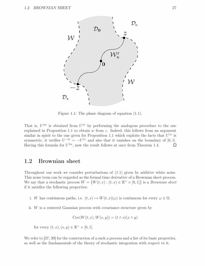
u.It is 1-dimensional, has nonempty intersection with both D0 and De and joins z with 0.By symmetry, a similar description also holds for the opposite unstable equilibrium −z.Figure 1.1 depicts the decomposition (1.3) together with the unstable manifolds W±z
u .By exploiting the structure of the remaining unstable equilibria given by Proposition 1.1one can verify for each of them the analogue of (ii) in Theorem 1.4. This is detailed inthe following proposition.
Proposition 1.5. If w ∈ CD([0, 1])− 0 is an equilibrium of the system then for everyλ > 0 we have that
• 0 < λ < 1 =⇒ Uλw is globally defined and converges to 0 as t→ +∞.
• λ = 1 =⇒ Uλw is globally defined and satisfies Uλw ≡ w.
• λ > 1 =⇒ Uλw explodes in finite time.
Proof. Let us suppose that w ≡ z(n) for some n ∈ Z − 0. Then for any λ > 0 thesolution to (1.1) with initial datum λw is given by the formula
Uλw(t, x) =
|n| 2p−1U sg(n)λz(|n|2t, |n|x− [|n|x]) if [|n|x] is even
−|n| 2p−1U sg(n)λz(|n|2t, |n|x− [|n|x]) if [|n|x] is odd
where sg(n) := n|n| and U±λz is the solution to (1.1) with initial datum ±λz, respectively.
1.2. BROWNIAN SHEET 27
Figure 1.1: The phase diagram of equation (1.1).
That is, Uλw is obtained from Uλz by performing the analogous procedure to the oneexplained in Proposition 1.1 to obtain w from z. Indeed, this follows from an argumentsimilar in spirit to the one given for Proposition 1.1 which exploits the facts that Uλz issymmetric, it verifies U−λz = −Uλz and also that it vanishes on the boundary of [0, 1].Having this formula for Uλw, now the result follows at once from Theorem 1.4.
1.2 Brownian sheet
Throughout our work we consider perturbations of (1.1) given by additive white noise.This noise term can be regarded as the formal time derivative of a Brownian sheet process.We say that a stochastic process W = W (t, x) : (t, x) ∈ R+ × [0, 1] is a Brownian sheetif it satisfies the following properties:
i. W has continuous paths, i.e. (t, x) 7→W (t, x)(ω) is continuous for every ω ∈ Ω.
ii. W is a centered Gaussian process with covariance structure given by
Cov(W (t, x),W (s, y)) = (t ∧ s)(x ∧ y)
for every (t, x), (s, y) ∈ R+ × [0, 1].
We refer to [37, 39] for the construction of a such a process and a list of its basic properties,as well as the fundamentals of the theory of stochastic integration with respect to it.
28 CHAPTER 1. PRELIMINARIES
1.3 Definition of solution for the SPDE
In this first part we study stochastic partial differential equations of the form
∂tX = ∂2xxX + f(X) + εW t > 0 , 0 < x < 1X(t, 0) = X(t, 1) = 0 t > 0X(0, x) = u(x)
(1.4)
where ε > 0 is some parameter, u ∈ CD([0, 1]) and f : R → R is a locally Lipschitz source.It is possible that such equations do not admit strong solutions in the usual sense as thesemay not be globally defined but instead defined up to an explosion time. In the followingwe review the usual definition of solution when the source is globally Lipschitz as well asformalize the idea of explosion and properly define the concept of solutions in the case oflocally Lipschitz sources.
1.3.1 Definition of strong solution for globally Lipschitz sources
We begin by fixing a probability space (Ω,F , P ) in which we have defined a Brownian sheetW (t, x) : (t, x) ∈ R+ × [0, 1]. For every t ≥ 0 we define
Gt = σ(W (s, x) : 0 ≤ s ≤ t, x ∈ [0, 1])
and denote its augmentation by Ft.1 The family (Ft)t≥0 constitutes a filtration on (Ω,F).A strong solution of the equation (1.4) on the probability space (Ω,F , P ) with respect tothe Brownian sheet W is a stochastic process
X = X(t, x) : (t, x) ∈ R+ × [0, 1]
satisfying the following properties:
i. X has continuous paths taking values in R.
ii. X is adapted to the filtration (Ft)t≥0, i.e. for every t ≥ 0 the mapping
(ω, x) 7→ X(t, x)(ω)
is Ft ⊗ B([0, 1])-measurable.
iii. If Φ denotes the fundamental solution of the heat equation on the interval [0, 1] withhomogeneous Dirichlet boundary conditions, which is given by the formula
Φ(t, x, y) =1√4πt
∑
n∈Z
[
exp
(
−(2n + y − x)2
4t
)
− exp
(
−(2n + y + x)2
4t
)]
,
then P -almost surely we have∫ 1
0
∫ t
0
|Φ(t− s, x, y)f(X(s, y))|dsdy < +∞ ∀ 0 ≤ t < +∞
1This means that Ft = σ(Gt ∪N ) where N denotes the class of all P -null sets of G∞ = σ(Gt : t ∈ R+).
1.3. DEFINITION OF SOLUTION FOR THE SPDE 29
andX(t, x) = IH(t, x) + IN (t, x) ∀ (t, x) ∈ R+ × [0, 1],
where IH and IN are respectively defined by the formulas
IH(t, x) =
∫ 1
0
Φ(t, x, y)u(y)dy
and
IN(t, x) =
∫ t
0
∫ 1
0
Φ(t− s, x, y) (f(X(s, y))dyds+ εdW (s, y)) .
It is well known that if f satisfies a global Lipschitz condition then for any initial datumu ∈ CD([0, 1]) there exists a unique strong solution to the equation (1.4) on (Ω,F , P ).Furthermore, this strong solution satisfies the strong Markov property and also behavesas a weak solution in the sense described in the following lemma. See [43] for details.
Lemma 1.6. If X is a strong solution to (1.4) with initial datum u ∈ CD([0, 1]) then forevery ϕ ∈ C2((0, 1)) ∩ CD([0, 1]) we have P -almost surely
∫ 1
0
X(t, x)ϕ(x)dx = IϕH(t) + IϕN(t) ∀ 0 ≤ t < +∞
where for each t ≥ 0
IϕH(t) =
∫ 1
0
u(x)ϕ(x)dx
and
IϕW (t) =
∫ t
0
∫ 1
0
((X(s, x)ϕ′′(x) + f(X(s, x))ϕ(x)) dxds+ εϕ(s, x)dW (s, x)) .
1.3.2 Solutions up to an explosion time
Just as in the previous section we begin by fixing a probability space (Ω,F , P ) in which wehave defined a Brownian sheet W (t, x) : (t, x) ∈ R+× [0, 1] and consider its augmentedgenerated filtration (Ft)t≥0. A solution up to an explosion time of the equation (1.4) on(Ω,F , P ) with respect to W is a stochastic process X = X(t, x) : (t, x) ∈ R+ × [0, 1]satisfying the following properties:
i. X has continuous paths taking values in R := R ∪ ±∞.
ii. X is adapted to the filtration (Ft)t≥0.
iii. If we define τ (n) := inft > 0 : ‖X(t, ·)‖∞ = n then for every n ∈ N we have P -a.s.
∫ 1
0
∫ t∧τ (n)
0
|Φ(t ∧ τ (n) − s, x, y)f(X(s, y))|dsdy < +∞ ∀ 0 ≤ t < +∞
andX(t ∧ τ (n), x) = I
(n)H (t, x) + εI
(n)N (t, x) ∀ (t, x) ∈ R+ × [0, 1],
30 CHAPTER 1. PRELIMINARIES
where
I(n)H (t, x) =
∫ 1
0
Φ(t ∧ τ (n), x, y)u(y)dy
and
I(n)N (t, x) =
∫ t
0
∫ 1
0
1s≤τ (n)Φ(t ∧ τ (n) − s, x, y) (f(X(s, y))dyds+ εdW (s, y))
with Φ being the fundamental solution of the heat equation as before.
We call τ := limn→+∞ τ (n) the explosion time for X. Let us notice that the assumptionof continuity of X over R implies that
• τ = inft > 0 : ‖X(t, ·)‖∞ = +∞
• ‖X(τ−, ·)‖∞ = ‖X(τ, ·)‖∞ = +∞ on τ < +∞.
We stipulate that X(t, ·) ≡ X(τ, ·) for t ≥ τ whenever τ < +∞ but we shall not assumethat limt→+∞X(t, ·) exists if τ = +∞. Furthermore, observe that since any initial datumu ∈ CD([0, 1]) verifies ‖u0‖∞ < +∞ we always have P (τ > 0) = 1 and also that ifP (τ = +∞) = 1 then we are left with the usual definition of strong solution.
In can be shown that for f ∈ C1(R) there exists an unique solution X of (1.4) up to anexplosion time. Furthermore, if f is globally Lipschitz then the solution is globally definedin the sense that P (τ = +∞) = 1. Finally, it is possible to prove that this solution Xmaintains the strong Markov property, i.e. if τ is a stopping time ofX then, conditional onτ < τ and X(τ , ·) = w, the future X(t+ τ , ·) : 0 < t < τ − τ is independent of the pastX(s, ·) : 0 ≤ s ≤ τ and identical in law to the solution of (1.4) with initial datum w.We refer to [30] for details.
1.4 Freidlin-Wentzell estimates
One of the main tools we shall use to study the solutions to (1.4) are the large deviationsestimates we briefly describe next. We refer to [15, 5, 42] for further details.
Let Xu,ε be the solution to the SPDE
∂tXu,ε = ∂2xxX
u,ε + f(Xu,ε) + εW t > 0 , 0 < x < 1Xu,ε(t, 0) = Xu,ε(t, 1) = 0 t > 0Xu,ε(0, x) = u(x)
(1.5)
where u ∈ CD([0, 1]) and f : R → R is bounded and satisfies a global Lipschitz condition.Let us also consider Xu the unique solution to the deterministic equation
∂tXu = ∂2xxX
u + f(Xu) t > 0 , 0 < x < 1Xu(t, 0) = Xu(t, 1) = 0 t > 0Xu(0, x) = u(x).
(1.6)
Given u ∈ CD([0, 1]) and T > 0, we consider the metric space of continuous functions
CDu([0, T ]× [0, 1]) = v ∈ C([0, T ]× [0, 1]) : v(0, ·) = u and v(·, 0) = v(·, 1) ≡ 0
1.4. FREIDLIN-WENTZELL ESTIMATES 31
with the distance dT induced by the supremum norm, i.e. for v, w ∈ CDu([0, T ]× [0, 1])
dT (v, w) := sup(t,x)∈[0,T ]×[0,1]
|v(t, x)− w(t, x)|,
and define the rate function IuT : CDu([0, T ]× [0, 1]) → [0,+∞] by the formula
IuT (ϕ) =
1
2
∫ T
0
∫ 1
0
|∂tϕ− ∂xxϕ− f(ϕ)|2 if ϕ ∈ W 1,22 ([0, T ]× [0, 1]) , ϕ(0, ·) = u
+∞ otherwise.
Here W 1,22 ([0, T ]× [0, 1]) is the closure of C∞([0, T ]× [0, 1]) with respect to the norm
‖ϕ‖W 1,22
=
(∫ T
0
∫ 1
0
[
|ϕ|2 + |∂tϕ|2 + |∂xϕ|2 + |∂xxϕ|2]
)
12
,
i.e. the Sobolev space of square-integrable functions defined on [0, T ] × [0, 1] with onesquare-integrable weak time derivative and two square-integrable weak space derivatives.
Theorem 1.7. The following estimates hold:
i. For any δ > 0, h > 0 there exists ε0 > 0 such that
P (dT (Xu,ε, ϕ) < δ) ≥ e−
IuT (ϕ)+h
ε2 (1.7)
for all 0 < ε < ε0, u ∈ CD([0, 1]) and ϕ ∈ CDu([0, T ]× [0, 1]).
ii. For any δ > 0, h > 0, s0 > 0 there exists ε0 > 0 such that
supu∈CD([0,1])
P (dT (Xu,ε, JuT (s)) ≥ δ) ≤ e−
s−hε2 (1.8)
for all 0 < ε < ε0 and 0 < s ≤ s0, where
JuT (s) = ϕ ∈ CDu([0, T ]× [0, 1]) : IuT (ϕ) ≤ s.
iii. For any δ > 0 there exist ε0 > 0 and C > 0 such that
supu∈CD([0,1])
P (dT (Xu,ε, Xu) > δ) ≤ e−
C
ε2 (1.9)
for all 0 < ε < ε0.
The first and second estimates are equivalent to those obtained in [15], except for theuniformity in the initial datum. This uniformity can be obtained as in [5] by exploitingthe fact that f is bounded and Lipschitz. On the other hand, the last estimate is in factimplied by the second one. Indeed, if V 0,ε and V 0 respectively denote the solutions to(1.5) and (1.6) with initial datum 0 and source term f ≡ 0, then (iii) is obtained from (ii)upon noticing that there exists K > 0 depending on f such that for any u ∈ CD([0, 1])
dT (Xu,ε, Xu) ≤ eKTdT (V
0,ε, V 0) (1.10)
32 CHAPTER 1. PRELIMINARIES
and that given δ > 0 there exists s0 > 0 such that
dT (V 0,ε, V 0) > δ ⊆
dT (V0,ε, JT (s0)) >
δ
2
(1.11)
where for s ≥ 0 we set
J0
T (s) = ϕ ∈ CD0([0, T ]× [0, 1]) : I0T (ϕ) ≤ s
and I0T is the rate function obtained by setting u = 0 and f ≡ 0 in the definition above.The estimate in (1.10) is obtained as in [5] whereas the inclusion in (1.11) follows fromthe fact that the level sets J0
T (s) are compact for all s ≥ 0 and also that the rate functionI0T vanishes only at V 0.
1.5 Truncations of the potential and localization
The large deviations estimates given on Section 1.4 demand a global Lipschitz conditionon the source term f which is unfortunately not satisfied for our model. Even thoughlarge deviations estimates have been obtained for systems with locally Lipschitz sources(see for example [15, 2]), these always rely on some sort of a priori control on the growth ofsolutions. Hence, we cannot hope to obtain similar results for our system in the study ofthe explosion time. Nonetheless, the use of localization techniques will help us solve thisproblem and allow us to take advantage of the estimates on Section 1.4. In the next lineswe give details about the localization procedure to be employed in the study of our system.
For every n ∈ N let G(n) : R −→ R be a smooth function such that
G(n)(u) =
|u|p+1
p+1if |u| ≤ n
0 if |u| ≥ 2n
and consider the potential S(n) given by the formula
S(n)(v) =
∫ 1
0
[
1
2
(
dv
dx
)2
−G(n)(v)
]
if v ∈ H10 ((0, 1))
+∞ otherwise.
For every u ∈ CD([0, 1]) there exists a unique solution U (n),u to the partial differentialequation
∂tU = −∂S(n)
∂ϕ(U)
with initial datum u. Since the source gn :=(
G(n))′
is globally Lipschitz, this solutionU (n),u is globally defined and describes the same trajectory as the solution to (1.1) startingat u until τ (n),u, the escape time from the ball
Bn := v ∈ CD([0, 1]) : ‖v‖∞ ≤ n.
1.6. MAIN RESULTS 33
In the same way, for each ε > 0 there exists a unique solution U (n),u,ε to the stochasticpartial differential equation
∂tU = −∂S(n)
∂ϕ(U) + εW (1.12)
with initial datum u and it is globally defined. Moreover, since for n ≤ m the functionsGn and Gm coincide on Bn by uniqueness of the solution we have that U (n),u,ε and U (m),u,ε
coincide until the escape from Bn. Therefore, if we write
τ (n),uε = inft ≥ 0 : ‖U (n),u,ε(t, ·)‖∞ ≥ n, τuε := limn→+∞
τ (n),uε ,
then for t < τuε we have that Uu,ε(t) := limn→+∞U (n), u, ε(t) is well defined and constitutesthe solution to (1.4) until the explosion time τuε with initial datum u. Let us observethat for each n ∈ N this solution Uu, ε coincides with U (n), u, ε until the escape from Bn.Furthermore, each U (n),u,ε is a positive recurrent Markov process which almost surely hitsany open set in CD([0, 1]) in a finite time. Finally, since each gn is bounded and Lipschitzwe have that for every n ∈ N the family
(
U (n),u,ε)
ε>0satisfies the large deviations estimates
given in Section 1.4. Hereafter, whenever we refer to the solution of (1.4) we shall meanthe solution constructed in this particular manner.
1.6 Main results
Our purpose in this first part of the thesis is to study the asymptotic behavior as ε → 0 ofUu,ε, the solution to the equation (1.4), for the different initial data u ∈ CD([0, 1]).We present throughout this section the main results we have obtained in this regard.From now onwards we shall write Pu to denote the law of the stochastic process Uu,ε.Whenever the initial datum is made clear in this way we shall often choose to drop thesuperscript u from the remaining notation for simplicity purposes.
Our first result is concerned with the continuity of the explosion time for initial datain the domain of explosion De. In this case one expects the stochastic and deterministicsystems to both exhibit a similar behavior for ε > 0 sufficiently small, since then the noisewill not be able to grow fast enough so as to overpower the quickly exploding source term.We show this to be truly the case for u ∈ De such that Uu remains bounded from one side.
Theorem I. Let D∗e be the set of those u ∈ De such that Uu explodes only through one
side, i.e. Uu remains bounded either from below or above until its explosion time τu.Then given δ > 0 and a bounded set K ⊆ D∗
e at a positive distance from ∂D∗e there exists
a constant C > 0 such that
supu∈K
Pu(|τε − τ | > δ) ≤ e−C
ε2 .
The main differences in behavior between the stochastic and deterministic systemsappear for initial data in D0, where metastable behavior is observed. According to thecharacterization of metastability for stochastic processes given in the articles [7] and [20],metastable behavior is given by two facts: the time averages of the process remain stableuntil an abrupt transition occurs and then a different value is attained; furthermore, the
34 CHAPTER 1. PRELIMINARIES
time of this transition is unpredictable in the sense that, when suitably rescaled, it shouldhave an exponential distribution. We manage to establish this description rigorously forour system whenever 1 < p < 5, where p is the parameter in the source term of (1.4).This rigorous description is contained in the remaining results. We begin by defining foreach ε > 0 the scaling coefficient
βε = inft ≥ 0 : P0(τε > t) ≤ e−1 (1.13)
and show that the family (βε)ε>0 verifies limε→0 ε2 log βε = ∆, where ∆ := 2(S(z)−S(0)).
In fact, we shall prove the following stronger statement which details the asymptotic orderof magnitude of τuε for initial data u ∈ D0.
Theorem II. Given δ > 0 and a bounded set K ⊆ D0 at a positive distance from ∂D0
we have
limε→0
[
supu∈K
∣
∣
∣Pu
(
e∆−δε2 < τε < e
∆+δ
ε2
)
− 1∣
∣
∣
]
= 0.
Next we show the asymptotic loss of memory of τuε for initial data u ∈ D0.
Theorem III. Given δ > 0 and a bounded set K ⊆ D0 at a positive distance from ∂D0
we have for any t > 0
limε→0
[
supu∈K
∣
∣Pu(τε > tβε)− e−t∣
∣
]
= 0.
Finally, we show the stability of time averages of continuous functions evaluated alongpaths of the process starting in D0, i.e. they remain close to the value of the function at 0.These time averages are taken along intervals of length going to infinity and times maybe taken as being almost (in a suitable scale) the explosion time. This tells us that, upuntil the explosion time, the system spends most of its time in a small neighborhood of 0.
Theorem IV. There exists a sequence (Rε)ε>0 with limε→0Rε = +∞ and limε→0Rεβε
= 0such that given δ > 0 for any bounded set K ⊆ D0 at a positive distance from W we have
limε→0
[
supu∈K
Pu
(
sup0≤t≤τε−3Rε
∣
∣
∣
∣
1
Rε
∫ t+Rε
t
f(Uε(s, ·))ds− f(0)
∣
∣
∣
∣
> δ
)]
= 0
for any bounded continuous function f : CD([0, 1]) → R.
Theorem I is proved in Chapter 2, the remaining results are proved in Chapters 4 and 5.Perhaps the proof of Theorem I is where one can find the most differences with other worksin the literature dealing with similar problems. In these works, the analogue of Theorem Ican be obtained as a direct consequence of the large deviations estimates for the system.However, since in our case Theorem I particularly focuses on trajectories of the process asit escapes any bounded domain, the estimates on Section 1.4 will not be of any use for theproof. Thus, a new approach is needed, one which is different from previous approachesin the literature and does not rely on large deviations estimates. The remaining resultswere established in [5, 29] for the tunneling time in an infinite-dimensional double-wellpotential model, i.e. the time the system takes to go from one well to the bottom of theother one. Our proofs are similar to the ones found in these references, although we havethe additional difficulty of dealing with solutions which are not globally defined.
1.7. RESUMEN DEL CAPÍTULO 1 35
1.7 Resumen del Capítulo 1
En este primer capítulo introducimos las nociones y conceptos preliminares para poderestudiar nuestro problema. La EDP con blow-up que vamos a considerar es
∂tU = ∂2xxU + g(U) t > 0 , 0 < x < 1U(t, 0) = 0 t > 0U(t, 1) = 0 t > 0U(0, x) = u(x) 0 < x < 1
donde g : R → R viene dada por g(u) = u|u|p−1 para p > 1 y u pertenece al espacio
CD([0, 1]) = v ∈ C([0, 1]) : v(0) = v(1) = 0.
Dicha ecuación puede reformularse como
∂tU = −∂S∂ϕ
(U)
donde el potencial S es el funcional en CD([0, 1]) dado por
S(v) =
∫ 1
0
[
1
2
(
dv
dx
)2
− |v|p+1
p+ 1
]
si v ∈ H10 ((0, 1))
+∞ en caso contrario.
El origen 0 ∈ CD([0, 1]) es el único equilibrio estable del sistema y es, de hecho, asin-tóticamente estable. Corresponde al único mínimo local del potencial S. Existe tambiénuna familia de equilibrios inestables del potencial S, todos ellos puntos de ensilladura.Entre estos equilibrios inestables existe un único equilibrio que es no negativo, z. Puedemostrarse que z es de hecho estrictamente positivo en (0, 1) y tanto de mínima energíacomo norma entre los equilibrios inestables. Además, CD([0, 1]) puede descomponerse entres partes:
CD([0, 1]) = D0 ∪W ∪De
donde D0 denota la variedad estable del origen, W es la unión de todas las variedadesestables de los equilibrios inestables y De constituye el dominio de explosión del sistema,i.e. el conjunto de todos aquellos datos iniciales u para los cuales el sistema explota en untiempo finito τu. Puede verse que tanto D0 como De son conjuntos abiertos y que W esla frontera común que los separa. Además, existe una variedad inestable Wz
u del punto deensilladura z contenida en la región de datos no negativos. La misma es 1-dimensional,tiene intersección no vacía tanto con D0 como con De y une a z con 0. Por simetría, unadescripción análoga también vale para el equilibrio inestable opuesto −z. La Figura 1.1describe esta descomposición.
Las perturbaciones estocásticas que consideramos son de la forma
∂tUε = −∇S + εW (1.14)
donde W es una sábana Browniana. Definimos formalmente el concepto de solución a unaecuación de este tipo, lo cual excede el marco tradicional ya que las mismas podrían no es-tar definidas globalmente sino hasta un tiempo de explosión τε finito. Estudiamos además
36 CHAPTER 1. PRELIMINARIES
dos propiedades importantes de las soluciones a este tipo de ecuaciones: la propiedadfuerte de Markov y el principio de grandes desvíos para los sistemas truncados asociados.
Por último, terminamos el capítulo presentando los resultados que habremos de probaren los capítulos siguientes. Incluimos una breve descripción de los mismos aquí.
Nuestro primer resultado es con respecto a la continuidad del tiempo de explosiónpara datos iniciales en De. En este caso uno espera que que los sistemas estocásticoy determinístico exhiban ambos un comportamiento similar para ε > 0 suficientementepequeño, ya que entonces el ruido no tendrá el tiempo suficiente como para crecer lonecesario para sobrepasar al término de la fuente que está explotando. Mostramos queesto es en efecto así para los casos en que u ∈ De es tal que la solución Uu de (1.1) condato inicial u permanece acotada por un lado.
Teorema I. Sea D∗e el conjunto de aquellos u ∈ De tales que Uu explota sólo por un lado,
i.e. Uu permanece acotada ya sea inferior o superiormente hasta su tiempo de explosiónτu. Entonces dado δ > 0 y un conjunto acotado K ⊆ D∗
e a una distancia positiva de ∂D∗e
existe C > 0 tal quesupu∈K
P (|τuε − τu0 | > δ) ≤ e−C
ε2 .
donde τuε denota el tiempo de explosión de Uu,ε, la solución de (1.14) con dato inicial u.
Las principales diferencias en comportamiento entre ambos sistemas surgen para datosiniciales en D0, donde se presenta el fenómeno de metaestabilidad. De acuerdo con [20],el comportamiento metaestable viene dado por dos hechos: los promedios temporales delproceso permanecen estables hasta que ocurre una transición abrupta y luego un valordiferente se obtiene; más aún, el tiempo en que ocurre esta transición es impredecibleen el sentido de que, bajo una normalización apropiada, debería tener una distribuciónexponencial. Logramos establecer esta descripción rigurosamente para nuestro sistemapara los casos en que 1 < p < 5, donde p es el parámetro en el término no lineal de lafuente en (1.1). Esta descripción rigurosa abarca los restantes resultados.
Teorema II. Dado δ > 0 y un conjunto acotado K ⊆ D0 a una distancia positiva de ∂D0
tenemos
limε→0
[
supu∈K
∣
∣
∣P(
e∆−δε2 < τuε < e
∆+δε2
)
− 1∣
∣
∣
]
= 0.
Teorema III. Dado δ > 0 y un conjunto acotado K ⊆ D0 a una distancia positiva de∂D0 tenemos para cualquier t > 0
limε→0
[
supu∈K
∣
∣P (τuε > tβε)− e−t∣
∣
]
= 0.
donde para cada ε > 0 definimos el coeficiente de normalización βε como
βε = inft ≥ 0 : P0(τε > t) ≤ e−1.
Teorema IV. Existe una sucesión (Rε)ε>0 con limε→0Rε = +∞ y limε→0Rεβε
= 0 tal quedado δ > 0 para cualquier conjunto acotado K ⊆ D0 a una distancia positiva de W
limε→0
[
supu∈K
Pu
(
sup0≤t≤τε−3Rε
∣
∣
∣
∣
1
Rε
∫ t+Rε
t
f(Uε(s, ·))ds− f(0)
∣
∣
∣
∣
> δ
)]
= 0
para cualquier función continua f : CD([0, 1]) → R.
Chapter 2
Asymptotic behavior of τuε for u ∈ De
In this chapter we investigate the continuity properties of the explosion time τuε for initialdata in the domain of explosion De. Our purpose is to show that under suitable conditionson the initial datum u ∈ De the explosion time τuε of the stochastic system converges inprobability to the deterministic explosion time τu. To make these conditions more precise,let us consider the sets of initial data in De which explode only through +∞ or −∞, i.e.
D+e =
u ∈ De : inf(t,x)∈[0,τu)×[0,1]
Uu(t, x) > −∞
and
D−e =
u ∈ De : sup(t,x)∈[0,τu)×[0,1]
Uu(t, x) < +∞
.
Notice that D+e and D−
e are disjoint and also that they satisfy the relation D−e = −D+
e .Furthermore, we shall see below that D+
e is an open set. Let us write D∗e := D+
e ∪ D−e .
The result we are to prove is the following.
Theorem 2.1. For any bounded set K ⊆ D∗e at a positive distance from ∂D∗
e and δ > 0there exists a constant C > 0 such that
supu∈K
Pu(|τε − τ | > δ) ≤ e−C
ε2 .
We shall split the proof of Theorem 2.1 into two parts: proving first a lower bound andthen an upper bound for τε. The first one is a consequence of the continuity of solutionsto (1.4) with respect to ε on intervals where the deterministic solution remains bounded.The precise estimate is contained in the following proposition.
Proposition 2.2. For any bounded set K ⊆ De and δ > 0 there exists a constant C > 0such that
supu∈K
Pu(τε < τ − δ) ≤ e−C
ε2 . (2.1)
Proof. Let us observe that by Proposition A.3 we have that infu∈K τu > 0 so that we mayassume without loss of generality that τu > δ for all u ∈ K. Now, for each u ∈ De let usdefine the quantity
Mu := sup0≤t≤max0,τu−δ
‖Uu(t, ·)‖∞.
37
38 CHAPTER 2. ASYMPTOTIC BEHAVIOR OF τUε FOR U ∈ DE
By resorting to Proposition A.3 once again, we obtain that the application u 7→ Mu isboth upper semicontinuous and finite on De and hence, with the aid of Propositions A.2and A.5, we conclude that M := supu∈KMu < +∞. Similarly, since the mapping u 7→ τu
is continuous and finite on De (see Corollary 2.5 below for proof of this fact) we alsoobtain that T := supu∈K τ
u < +∞. Hence, for u ∈ K we get
Pu(τuε < τu−δ) ≤ Pu
(
dτu−δ(
UMu+1,ε, UMu+1)
>1
2
)
≤ Pu
(
dT −δ(
UM+1,ε, UM+1)
>1
2
)
.
By the estimate (1.9) we conclude (2.1).
To establish the upper bound we consider for each u ∈ D+e the process
Zu,ε := Uu,ε − V 0,ε
where Uu,ε is the solution of (1.4) with initial datum u and V 0,ε is the solution of (1.5)with source term f ≡ 0 and initial datum 0 constructed from the same Brownian sheetas Uu,ε. Let us observe that Zu,ε satisfies the random partial differential equation
∂tZu,ε = ∂2xxZ
u,ε + g(Zu,ε − V 0,ε) t > 0 , 0 < x < 1Zu,ε(t, 0) = Zu,ε(t, 1) = 0 t > 0Zu,ε(0, x) = u(x).
(2.2)
Furthermore, since V 0,ε is globally defined and remains bounded on finite time intervals,we have that Zu,ε and Uu,ε share the same explosion time. Hence, to obtain the desiredupper bound on τuε we may study the behavior of Zu,ε. The advantage of this approachis that, in general, the behavior of Zu,ε will be easier to understand than that of Uu,ε.Indeed, each realization of Zu,ε is the solution of a partial differential equation which onecan handle by resorting to standard arguments in PDE theory.
Now, a straightforward calculation using the mean value theorem shows that whenever‖V 0,ε‖∞ < 1 the process Zu,ε satisfies the inequality
∂tZu,ε ≥ ∂2xxZ
u,ε + g(Zu,ε)− h|Zu,ε|p−1 − h (2.3)
where h := p2p−1‖V 0,ε‖∞ > 0. Therefore, in order to establish the upper bound on τuεone may consider for h > 0 the solution Z(h),u to the equation
∂tZ(h),u = ∂2xxZ
(h),u + g(Z(h),u)− h|Z(h),u|p−1 − h t > 0 , 0 < x < 1
Z(h),u(t, 0) = Z(h),u(t, 1) = 0 t > 0
Z(h),u(0, x) = u(x).
(2.4)
and obtain a convenient upper bound for the explosion time of this new process valid forevery h sufficiently small. If we also manage to show that for h suitably small the processZ(h),u explodes through +∞, then the fact that Zu,ε is a supersolution to (2.4) will yieldthe desired upper bound on the explosion time of Zu,ε, if ‖V 0,ε‖∞ remains small enough.To show this, however, we will need to impose the additional condition that u ∈ D+
e .Lemma 2.4 below contains the proper estimate on τ (h),u, the explosion time of Z(h),u.
39
Definition 2.3. For each h ≥ 0 we define the potential S(h) on CD([0, 1]) associated tothe equation (2.4) by the formula
S(h)(v)
∫ 1
0
[
1
2
(
dv
dx
)2
− |v|p+1
p+ 1+ hg(v) + hv
]
if v ∈ CD ∩H10 ([0, 1])
+∞ otherwise.
Notice that S(0) coincides with our original potential S. Moreover, it is easy to check thatfor all h ≥ 0 the potential S(h) satisfies all properties established for S in the Appendix.
Lemma 2.4. Given δ > 0 there exists M > 0 such that:
i. For every 0 ≤ h < 1 any u ∈ CD([0, 1]) such that S(h)(u) ≤ −M2
verifies τ (h),u < δ2.
ii. Given K > 0 there exist constants ρM,K , hM,K > 0 depending only on M and Ksuch that any u ∈ CD([0, 1]) satisfying S(u) ≤ −M and ‖u‖∞ ≤ K verifies
supv∈BρM,K (u)
τ (h),v < δ
for all 0 ≤ h < hM,K .
Proof. Given δ > 0 let us begin by showing that (i) holds for an appropriate choice of M .Thus, for fixed M > 0 and 0 ≤ h < 1, let u ∈ CD([0, 1]) be such that S(h)(u) ≤ −M
2and
consider the application φ(h),u : [0, τ (h),u) → R+ given by the formula
φ(h),u(t) =
∫ 1
0
(
Z(h),u(t, x))2
dx.
It is simple to verify that φ(h),u is continuous and that for any t0 ∈ (0, τ (h),u) it satisfies
dφ(h),u
dt(t0) ≥ −4S(h)(u
(h)t0
)+2
∫ 1
0
[(
p− 1
p+ 1
)
|u(h)t0|p+1 − h
(
p+ 2
p
)
|u(h)t0|p − h|u(h)t0
|]
(2.5)
where we write u(h)t0:= Z(h),u(t0, ·) for convenience. Hölder’s inequality reduces (2.5) to
dφ(h),u
dt(t0) ≥ −4S(h)(u
(h)t0)+2
[(
p− 1
p+ 1
)
‖u(h)t0‖p+1Lp+1 − h
(
p+ 2
p
)
‖u(h)t0‖pLp+1 − h‖u(h)t0
‖Lp+1
]
.
(2.6)Observe that, by definition of S(h) and the fact that the map t 7→ S(h)(u
(h)t ) is decreasing,
we obtain the inequalities
M
2≤ −S(h)(u
(h)t0) ≤ 1
p + 1‖u(h)t0
‖p+1Lp+1 + h‖u(h)t0
‖pLp+1 + h‖u(h)t0
‖Lp+1
from which we deduce that by taking M sufficiently large one can force ‖u(h)t0‖Lp+1 to be
large enough so as to guarantee that(
p− 1
p+ 1
)
‖u(h)t0‖p+1Lp+1 − h
(
p+ 2
p
)
‖u(h)t0‖pLp+1 − h‖u(h)t0
‖Lp+1 ≥ 1
2
(
p− 1
p+ 1
)
‖u(h)t0‖p+1Lp+1
40 CHAPTER 2. ASYMPTOTIC BEHAVIOR OF τUε FOR U ∈ DE
is satisfied for any 0 ≤ h < 1. Therefore, we see that if M sufficiently large then for all0 ≤ h < 1 the application φ(h),u satisfies
dφ(h),u
dt(t0) ≥ 2M +
(
p− 1
p+ 1
)
(
φ(h),u(t0))
p+12 (2.7)
for every t0 ∈ (0, τ (h),u), where to obtain (2.7) we have once again used Hölder’s inequalityand the fact that the map t 7→ S(h)(u
(h)t ) is decreasing. Now, it is not hard to show that
the solution y of the ordinary differential equation
y = 2M +(
p−1p+1
)
yp+12
y(0) ≥ 0
explodes before time
T =δ
4+
2p+12 (p+ 1)
(p− 1)2(Mδ)p−12
.
Indeed, either y explodes before time δ4
or y := y(·+ δ4) satisfies
˙y ≥(
p−1p+1
)
yp+12
y(0) ≥ Mδ2
which can be seen to explode before time
T =2p+12 (p+ 1)
(p− 1)2(Mδ)p−12
by performing the standard integration method. If M is taken sufficiently large then Tcan be made strictly smaller than δ
2which, by (2.7), implies that τ (h),u < δ
2as desired.
Now let us show statement (ii). Given K > 0 let us take M > 0 as above and consideru ∈ CD([0, 1]) satisfying S(u) ≤ −M and ‖u‖∞ ≤ K. Using Propositions A.10 and A.8adapted to the system (2.4) we may find ρM,K > 0 sufficiently small so as to guaranteethat for some small 0 < tu <
δ2
any v ∈ BρM,K (u) satisfies
S(h)(Z(h),v(tu, ·)) ≤ S(h)(u) +M
4
for all 0 ≤ h < 1. Notice that this is possible since the constants appearing in PropositionsA.10 adapted to this context are independent from h provided that h remains bounded.These constants still depend on ‖u‖∞ though, so that the choice of ρM,K will inevitablydepend on both M and K. Next, let us take 0 < hM,K < 1 so as to guarantee thatS(h)(u) ≤ −3M
4for every 0 ≤ h < hM,K . Notice that, since S(h)(u) ≤ S(u) + h(Kp +K),
it is possible to choose hM,K depending only on M and K. Thus, for any v ∈ BρM,K (u) weobtain S(h)(Z(h),v(tu, ·)) ≤ −M
2which, by the choice of M , implies that τ (h),v < tu+
δ2< δ.
This concludes the proof.
Let us observe that the system Z(0),u
coincides with Uu for every u ∈ CD([0, 1]). Thus,by the previous lemma we obtain the following corollary.
41
Corollary 2.5. The application u 7→ τu is continuous on De.
Proof. Given u ∈ De and δ > 0 we show that there exists ρ > 0 such that for all v ∈ Bρ(u)we have
−δ + τu < τ v < τu + δ.
To see this we first notice that by Proposition A.3 there exists ρ1 > 0 such that −δ+τu <τ v for any v ∈ Bρ1(u). On the other hand, by (i) in Lemma 2.4 we may takeM, ρ2 > 0 suchthat τ v < δ for any v ∈ Bρ2(u) with u ∈ CD([0, 1]) such that S(u) ≤ −M . For this choiceof M by Proposition 1.3 we may find some 0 < tM < tu such that S(Uu(tM , ·)) ≤ −Mand using Proposition A.3 we may take ρ2 > 0 such that Uv(tM , ·) ∈ Bρ2(U
u(tM , ·)) forany v ∈ Bρ2(u). This implies that τ v < tM + δ < tu + δ for all v ∈ Bρ2(u) and thus bytaking ρ = minρ1, ρ2 we obtain the result.
The following two lemmas provide the necessary tools to obtain the uniformity in theupper bound claimed in Theorem 2.1.
Lemma 2.6. Given M > 0 and u ∈ De let us define the quantities
T uM = inft ∈ [0, τu) : S(Uu(t, ·)) < −M and Ru
M = sup0≤t≤T uM
‖Uu(t, ·)‖∞.
Then the applications u 7→ T uM and u 7→ Ru
M are both upper semicontinuous on De.
Proof. We must see that the sets TM < α and RM < α are open in De for all α > 0.But the fact that TM < α is open follows at once from Proposition A.10 and RM < αis open by Proposition A.3.
Lemma 2.7. For each u ∈ D+e let us define the quantity
Iu := inf(t,x)∈[0,τu)×[0,1]
Uu(t, x).
Then the application u 7→ Iu is lower semicontinuous on D+e .
Proof. Notice that Iu ≥ 0 for any u ∈ D+e since Uu(t, 0) = Uu(t, 1) = 0 for all t ∈ [0, τu).
Therefore, it will suffice to show that the sets α < I are open in D+e for every α < 0.
With this purpose in mind, given α < 0 and u ∈ D+e such that α < Iu, take β1, β2 < 0
such that α < β1 < β2 < Iu and let y be the solution to the ordinary differential equation
y = −|y|py(0) = β2.
(2.8)
Define tβ := inft ∈ [0, tymax) : y(t) < β1, where tymax denotes the explosion time of y.Notice that by the lower semicontinuity of S for any M > 0 we have S(Uu(T u
M , ·)) ≤ −Mand thus, by Lemma 2.4, we may choose M such that
supv∈Bρ(Uu(T uM ,·))
τ v < tβ (2.9)
for some small ρ > 0. Moreover, if ρ < Iu − β2 then every v ∈ Bρ(Uu(T u
M , ·)) satisfiesinfx∈[0,1] v(x) ≥ β2 so that Uv is in fact a supersolution to the equation (2.8). By (2.9)
42 CHAPTER 2. ASYMPTOTIC BEHAVIOR OF τUε FOR U ∈ DE
this implies that v ∈ D+e and Iv ≥ β1 > α. On the other hand, by Proposition A.3 we
may take δ > 0 sufficiently small so that for every w ∈ Bδ(u) we have T uM < τw and
supt∈[0,T uM ]
‖Uw(t, ·)− Uu(t, ·)‖∞ < ρ.
Combined with the previous argument, this yields the inclusion Bδ(u) ⊆ D+e ∩ α < I.
In particular, this shows that α < I is open and thus concludes the proof.
Remark 2.8. The preceding proof shows, in particular, that the set D+e is open.
The conclusion of the proof of Theorem 2.1 is contained in the next proposition.
Proposition 2.9. For any bounded set K ⊆ D∗e at a positive distance from ∂D∗
e andδ > 0 there exists a constant C > 0 such that
supu∈K
Pu(τε > τ + δ) ≤ e−C
ε2 . (2.10)
Proof. Since D−e = −D+
e and U−u = −Uu for u ∈ CD([0, 1]), without any loss of generalitywe may assume that K is contained in D+
e . Let us begin by noticing that for any M > 0
TM := supu∈K
T uM < +∞ and RM := sup
u∈KRuM < +∞.
Indeed, by Propositions A.2 and A.5 we may choose t0 > 0 sufficiently small so thatthe orbits Uu(t, ·) : 0 ≤ t ≤ t0, u ∈ K remain uniformly bounded and the familyUu(t0, ·) : u ∈ K is contained in a compact set K′ ⊆ D+
e at a positive distance from ∂D+e .
But then we have
TM ≤ t0 + supu∈K′
T uM and RM ≤ sup
0≤t≤t0,u∈K‖Uu(t, ·)‖∞ + sup
u∈K′
RuM
and both right hand sides are finite due to Lemma 2.6 and the fact that T uM and RM are
both finite for each u ∈ De by Proposition 1.3. Similarly, by Lemma 2.7 we also have
IK := infu∈K
Iu > −∞.
Now, for each u ∈ K and ε > 0 by the Markov property we have for any ρ > 0
Pu(τε > τ + δ) ≤ P (dTM (U(RM+1),u,ε, U (RM+1),u) > ρ) + sup
v∈Bρ(Uu(T uM ,·))Pv(τε > δ). (2.11)
The first term on the right hand side is taken care of by (1.9) so that in order to show(2.10) it only remains to deal with the second term by choosing M and ρ appropriately.The argument given to deal with this term is similar to that of the proof of Lemma 2.7.Let y be the solution to the ordinary differential equation
y = −|y|p − |y|p−1 − 1y(0) = IK − 1
2.
(2.12)
Define tI := inft ∈ [0, tymax) : y(t) < IK−1, where tymax denotes the explosion time of y.By Lemma 2.4, we may choose M such that
supv∈BρM (Uu(T uM ,·))
τ (h),v < minδ, tI (2.13)
43
for all 0 ≤ h < hM , where ρM > 0 and hM > 0 are suitable constants. The key observationhere is that, since RM < +∞, we may choose these constants so as not to depend on ubut rather on M and RM themselves. Moreover, if ρM < 1
2then every v ∈ BρM (U
u(T uM , ·))
satisfies infx∈[0,1] v(x) ≥ IK − 12
so that Z(h),v is in fact a supersolution to the equation(2.12) for all 0 ≤ h < minhM , 1. By (2.13) the former implies that Z(h),v explodesthrough +∞ and that it remains bounded from below by IK − 1 until its explosion timewhich, by (2.13), is smaller than δ. In particular, we see that if ‖V 0,ε‖∞ < min1, hM
p2p−1then Zv,ε explodes before Z(h),v does, so that we have that τε < δ under such conditions.Hence, we conclude that
supv∈BρM (Uu(T uM ,·))
Pv(τε > δ) ≤ P
(
supt∈[0,δ]
‖V 0,ε(t, ·)‖∞ ≤ min
1,hMp2p−1
)
which, by recalling the estimate (1.9), gives the desired control on the second term in theright hand side of (2.11). Thus, by taking ρ equal to ρM in (2.11), we obtain the result.
This last proposition in fact shows that for δ > 0 and a given bounded set K ⊆ D∗e at
a positive distance from ∂D∗e there exist constants M,C > 0 such that
supu∈K
Pu(τε > T uM + δ) ≤ e−
C
ε2 .
By exploiting the fact TM < +∞ for every M > 0 we obtain the following useful corollary.
Corollary 2.10. For any bounded set K ⊆ D∗e at a positive distance from ∂D∗
e thereexist constants τ ∗, C > 0 such that
supu∈K
Pu(τε > τ ∗) ≤ e−C
ε2 .
44 CHAPTER 2. ASYMPTOTIC BEHAVIOR OF τUε FOR U ∈ DE
2.1 Resumen del Capítulo 2
En este capítulo investigamos la continuidad del tiempo de explosión τuε para datos ini-ciales en el dominio de De. Mostramos que el tiempo de explosión τuε del sistema estocás-tico converge en probabilidad al tiempo de explosión determinístico τu uniformementesobre compactos de D∗
e , el conjunto de aquellos datos iniciales u ∈ De para los cualesla solución Uu explota por un único lado, i.e. permanece acotada en alguna dirección(inferior o superiormente) hasta el tiempo de explosión. Más precisamente, tenemos elsiguiente resultado.
Teorema. Para cualquier conjunto acotado K ⊆ D∗e a una distancia positiva de ∂D∗
e yδ > 0 existe una constante C > 0 tal que
supu∈K
Pu(|τε − τ | > δ) ≤ e−C
ε2 .
Dividimos la demostración de este resultado en dos partes, las cotas (2.1) y (2.10).
La cota inferior (2.1) es una consecuencia directa de la estimación de grandes desvíos(1.9). En efecto, como la solución Uu permanece acotada en [0, τu − δ), la condiciónτuε < τu − δ implica que los sistemas estocástico y determinístico deben necesariamentesepararse antes de tiempo τu − δ y, por lo tanto, que lo mismo debe suceder para lossistemas truncados para los que se tiene (1.9).
La demostración de la cota superior (2.10) consiste en estudiar el proceso Zu,ε definidocomo la solución del problema (2.2). Dicho proceso posee el mismo tiempo de explosiónque Uu,ε pero es más sencillo de tratar debido a que cada realización del mismo resuelveuna ecuación diferencial en derivadas parciales que puede estudiarse mediante técnicasusuales. Además, dado 0 < h < 1 es posible mostrar que para cada realización ω en unconjunto Ωεh con probabilidad que tiende a uno cuando ε → 0 la trayectoria Zu,ε(ω) essupersolución de (2.4). A partir de esto, la estrategia que adoptamos para probar (2.10)si u ∈ D+
e (ver (??)) es mostrar que para un conjunto de realizaciones Ωu,ε ⊆ Ωεh conprobabilidad que tiende a uno (exponencialmente rápido en 1
ε2) cuando ε → 0 suceden
dos cosas:
i. La solución de (2.4) explota antes de tiempo τu + δ.
ii. La solución de (2.4) explota por +∞, i.e. permanece acotada inferiormente hastael tiempo de explosión.
Se sigue de la descripción anterior que para toda realización en Ωu,ε el tiempo de explosiónde Zu,ε (y por lo tanto τuε ) es menor a τu+ δ, lo cual (1.9) implica (2.10) a partir de (1.9).Para mostrar (i) utilizamos técnicas de ecuaciones similares a las que figuran en [8] y (ii)se deduce del hecho de que u ∈ D+
e . Por simetría se obtienen los mismos resultados paraD−e . Por último, la uniformidad sobre compactos se obtiene a partir de los resultados en
el Apéndice.
Chapter 3
Construction of an auxiliary domain
As suggested in [20], to study the behavior of the explosion time for initial data in D0
it is convenient to consider an auxiliary bounded domain G satisfying the conditionsstated in the Introduction. By doing so we can then reduce our problem to a simpler one:characterizing the escape from this domain. This is simpler because for it we may assumethat the source term g in (1.1) is Lipschitz, as the escape only depends on the behavior ofthe system while it remains inside a bounded region. It is then that the large deviationsestimates of Section 1.4 can be applied. To succeed in the construction of such a domain,we must first understand the behavior of exploding trajectories in the stochastic system.This is the purpose behind the following results.
Lemma 3.1. If p < 5 then for any a > 0 the sets u ∈ D0 : 0 ≤ S(u) ≤ a are bounded.
Proof. Let a > 0 and for v ∈ u ∈ D0 : 0 ≤ S(u) ≤ a consider ψ : R≥0 → R≥0 given bythe formula
ψ(t) :=
∫ 1
0
(Uv(t, ·))2.
A direct computation shows that for every t0 > 0 the function ψ satisfies
dψ(t0)
dt= −4S(Uv(t, ·)) + 2
(
p− 1
p+ 1
)∫ 1
0
|Uv(t, ·)|p+1.
By Proposition A.8 and Hölder’s inequality we then obtain
dψ(t0)
dt≥ −4a + 2
(
p− 1
p+ 1
)
(ψ(t0))p+12
which implies that ψ(0) ≤ B :=[
2a(
p+1p−1
)]2p+1
since otherwise ψ (and therefore Uv)
would explode in finite time. Now, by the Gagliardo-Niremberg interpolation inequality(recall that v is absolutely continuous since S(v) < +∞)
‖v‖2∞ ≤ CG−N‖v‖L2‖∂xv‖L2,
we obtain∫ 1
0
|v|p+1 ≤ ‖v‖2L2‖v‖p−1∞ ≤ CG−NB
p+34 ‖∂xv‖
p−12
L2 ≤ CG−NBp+34 (2a+
∫ 1
0
|v|p+1)p−14
45
46 CHAPTER 3. CONSTRUCTION OF AN AUXILIARY DOMAIN
which for p < 5 implies the bound
∫ 1
0
|v|p+1 ≤ B′ := max
2a,[
CG−NBp+34 2
p−14
]4
5−p
. (3.1)
Since S(v) ≤ a we see that (3.1) implies the bound ‖∂xv‖L2 ≤√2B′ and therefore we
conclude
‖v‖∞ ≤√
CG−N√2BB′
which shows that u ∈ D0 : 0 ≤ S(u) ≤ a is bounded.
Remark 3.2. The proof of Lemma 3.1 is the only instance throughout our entire work inwhich the assumption p < 5 is used. If p ≥ 5 is such that the sets u ∈ D0 : 0 ≤ S(u) ≤ aremain bounded for every a > 0, then all of our results remain valid for this choice of p.As a matter of fact, we shall only require the weaker condition that there exists α > 0such that the set u ∈ D0 : 0 ≤ S(u) ≤ S(z) + α is bounded. However, determining thevalidity of this condition for arbitrary p > 1 does not seem to be an easy problem.
Proposition 3.3. The potential S satisfies limn→+∞
[
infu∈∂Bn∩D0
S(u)
]
= +∞.
Proof. Given M > 0, by Lemma 3.1 we may take N ∈ N such that for every n ≥ N theset u ∈ D0 : 0 ≤ S(u) ≤ M is contained in B
n. Now, let us consider u ∈ ∂Bn ∩ D0.Since u ∈ D0, we know that S(u) ≥ 0 by Proposition A.8. Therefore, if u ∈ ∂Bn forn ≥ N , in particular we have that u /∈ u ∈ D0 : 0 ≤ S(u) ≤ M and thus it must beS(u) > M . This proves the claim.
Definition 3.4. Given T > 0 and ϕ ∈ CD([0, T ]× [0, 1]) we define the rate I(ϕ) of ϕ bythe formula
I(ϕ) := I(n),ϕ(0,·)T (ϕ)
for any n ∈ N larger than ‖ϕ‖∞, where I(n),ϕ(0,·)T denotes the rate function associated tothe system (1.5) with f = gn. Notice that I(ϕ) does not depend on the choice of n.
Definition 3.5. We say that a function ϕ ∈ CD([0, T ]×[0, 1]) is regular if both derivatives∂tϕ and ∂2xxϕ exist and belong to CD([0, T ]× [0, 1]).
Proposition 3.6. Given T > 0 for any ϕ ∈ CD ∩W 1,22 ([0, T ]× [0, 1]) such that ∂2xxϕ(0, ·)
exists and belongs to CD([0, 1]) we have that
I(ϕ) ≥ 2
[
sup0≤T ′≤T
(S(ϕ(T ′, ·))− S(ϕ(0, ·)))]
. (3.2)
Proof. Let us begin by assuming that ϕ is regular and take N ∈ N larger than ‖ϕ‖∞.
47
Using the identity (x− y)2 = (x+ y)2 − 4xy for x, y ∈ R and 0 ≤ T ′ ≤ T we obtain that
I(ϕ) = I(N),ϕ(0,·)T (ϕ) =
1
2
∫ T
0
∫ 1
0
|∂tϕ− ∂2xxϕ− gN(ϕ)|2 ≥1
2
∫ T ′
0
∫ 1
0
|∂tϕ− ∂2xxϕ− gN(ϕ)|2
=1
2
∫ T ′
0
∫ 1
0
[
|∂tϕ+ ∂2xxϕ+ gN(ϕ)|2 − 2(
∂2xxϕ+ gN(ϕ))
∂tϕ]
=1
2
∫ T ′
0
[(∫ 1
0
|∂tϕ+ ∂2xxϕ+ gN(ϕ)|2)
+ 2dS(N)(ϕ(t, ·))
dt
]
≥ 2(
S(N)(ϕ(T ′, ·))− S(N)(ϕ(0, ·)))
= 2 (S(ϕ(T ′, ·))− S(ϕ(0, ·)))
where the last equality follows from the fact that both S(N) and S coincide inside BN .Taking supremum on T ′ yields the result in this particular case.
Now, if ϕ is not necessarily regular then by of [15, Theorem 6.9] we may take a sequence(ϕn)n∈N of regular functions converging to ϕ on CDϕ(0,·)([0, T ]× [0, 1]) and also such thatlimn→+∞ I(ϕn) = I(ϕ). The result in the general case then follows from the validity of(3.2) for regular functions and the lower semicontinuity of S.
In order to properly interpret the content of Proposition 3.6 we need to introduce theconcept of quasipotential for our system. We do so in the following definitions.
Definition 3.7. Given u, v ∈ CD([0, 1]) a path from u to v is a continuous functionϕ ∈ CD([0, T ]× [0, 1]) for some T > 0 such that ϕ(0, ·) = u and ϕ(T, ·) = v.
Definition 3.8. Given u, v ∈ CD([0, 1]) we define the quasipotential V (u, v) from u to vby the formula
V (u, v) = infI(ϕ) : ϕ path from u to v.Furthermore, given a subset B ⊆ CD([0, 1]) we define the quasipotential from u to B as
V (u,B) := infV (u, v) : v ∈ B.
We refer the reader to the Appendix for a review of some of the main properties of Vwhich shall be required throughout our work.
In a limiting sense, made rigorous through the large deviations principle establishedin Section 1.4, the quasipotential V (u, w) represents the energy cost for the stochasticsystem to travel from u to (an arbitrarily small neighborhood of) v. In light of all thesedefinitions we see that the energy cost for the stochastic system starting from 0 to explodein a finite time while remaining inside D0 is infinite. Indeed, combining Propositions 3.3,3.6 and A.9 we see that limn→+∞ V (0, ∂Bn∩D0) = +∞ which implies that a path from 0
to infinity lying inside D0 should have, at least formally, an infinite rate. Thus, were thestochastic system starting from 0 to explode, it would have to do so by stepping outsideD0 and crossing W. In view of Proposition 3.6, the system will typically wish to cross Wthrough ±z since the energy cost for performing such a feat is the lowest there. Hence, if
48 CHAPTER 3. CONSTRUCTION OF AN AUXILIARY DOMAIN
we wish the problem of escaping the domain G to capture the essential characteristics ofthe explosion phenomenon in the stochastic system (at least when starting from 0) thenit is important to guarantee that the escape from this domain occurs by passing through(an arbitrarily small neighborhood of) ±z. Not only this, but we also require that oncethe system escapes this domain G then it explodes with overwhelming probability in aquick fashion, i.e. before a certain time τ ∗ which does not depend on ε. More precisely,we wish to consider a bounded domain G ⊆ CD([0, 1]) verifying the following properties:
Conditions 3.9.
i. There exists r0 > 0 such that B2r0 ⊆ D0 ∩G.
ii. There exists c > 0 such that Bc ⊆ Br0 and for all v ∈ Bc the solution Uv to (1.1)with initial datum v is globally defined and converges to 0 without escaping Br0 .
iii. There exists a closed subset ∂±z of the boundary ∂G which satisfies
• V (0, ∂G− ∂±z) > V (0, ∂±z) = V (0,±z).•• ∂±z is contained in D∗
e and at a positive distance from its boundary.
In principle, we have seen that such a domain is useful to study the behavior of theexplosion time whenever the initial datum of the stochastic system is (close to) the origin.Nevertheless, as we shall later see, when starting inside D0 the system will typically visita small neighborhood of the origin before crossing W and thus such a choice of G willalso be suitable to study the explosion time for arbitrary initial data in D0.
The construction of the domain G is done as follows. Since D0 is open we may chooser0 > 0 such that B3r0 is contained in D0. Moreover, by the asymptotic stability of 0 wemay choose c > 0 verifying (ii) in Conditions 3.9. Now, given ζ1 > 0 by Lemma 3.1 wemay take n0 ∈ N such that n0 > 3r0 and the set u ∈ D0 : 0 ≤ S(u) ≤ S(z) + ζ1 iscontained in the interior of the ball Bn0−1. We then define the pre-domain G as
G := Bn0 ∩ D0. (3.3)
Notice that since both Bn0 and D0 are closed sets we have that
∂G = (W ∩Bn0) ∪ (∂Bn0 ∩ D0)
which, by the particular choice of n0 and Proposition A.8, implies minu∈∂G S(u) = S(z).By Propositions 3.6 and A.9 we thus obtain V (0, ∂G) ≥ ∆. Next, if for u ∈ CD([0, 1])we let u− denote the negative part of u, i.e. u− = max−u, 0, then since z− = 0 wemay find rz > 0 such that u− ∈ D0 for any u ∈ Brz(z). Finally, if for r > 0 we writeBr(±z) := Br(z) ∪ Br(−z) and take rz > 0 such that rz < rz
2, B2rz(±z) is contained in
the interior of Bn0 and z is the unique equilibrium point of the system lying inside Brz(z),then we define our final domain G as
G = G ∪ Brz(±z).Let us now check that this domain satisfies all the required conditions. We begin bynoticing that (i) and (ii) in Conditions 3.9 are immediately satisfied by the choice of n0.Now, let us also observe that for any r > 0
infS(u) : u ∈ ∂G− Br(±z) > S(z). (3.4)
49
Indeed, if this were not the case then there would exist (uk)k∈N ⊆ [W ∩ Bn0 −Br(±z)]such that limk→+∞ S(uk) = S(z). By Proposition A.2 we have that there exists t0 > 0sufficiently small satisfying
supk∈N
[
supt∈[0,t0]
‖Uuk(t, ·)‖∞]
< +∞ and infk∈N
‖Uuk(t0, ·)− (±z)‖∞ >r
2
and therefore by Proposition A.5 we may conclude that there exists a subsequence (ukj)j∈Nsuch that Uukj (t0, ·) converges to a limit u∞ ∈ CD([0, 1]) as j → +∞. Since the potentialS is lower semicontinuous and W is both closed and invariant under the deterministicflow, by Proposition A.8 we conclude that u∞ = ±z which contradicts the fact thatthe sequence (Uukj (t0, ·))j∈N is at a positive distance from these equilibriums. Hence, weobtain the validity of (3.4). In particular, this implies that V (0, ∂G − Br(±z)) > ∆ forany r > 0. Let us then take ζ2 > 0 such that ∆+ ζ2 < V (0, ∂G− B rz
2(±z)) and define
∂z := u ∈ ∂Brz(z) ∩ De : V (0, u) ≤ ∆+ ζ2.
Notice that d(∂z,W) > 0. Indeed, if this were not the case we would have sequences(uk)k∈N ⊆ W and (vk)k∈N ⊆ ∂z such that limk→+∞ d(uk, vk) = 0. The growth estimateson the Appendix section then imply that there exists t1 > 0 sufficiently small such that
limk→+∞
d(Uuk(t1, ·), Uvk(t1, ·)) = 0 andrz2< inf
k∈Nd(Uvk(t1, ·), z) ≤ sup
k∈Nd(Uvk(t1, ·), z) < 2rz.
By Proposition A.5 we obtain that for some appropriate subsequence we have
limj→+∞
Uukj (t1, ·) = limj→+∞
Uvkj (t1, ·) = v∞.
Observe that v∞ ∈ W ∩Bn0 −B rz2(±z) and thus that v∞ ∈ ∂G−B rz
2(±z). Furthermore,
by the lower semicontinuity of V (0, ·) and the fact that the mapping t 7→ V (0, Uu(t, ·))is monotone decreasing for any u ∈ CD([0, 1]) (see the Appendix section for details), weobtain that V (0, v∞) ≤ ∆+ ζ2 which, together with the previous observation, implies thecontradiction ∆ + ζ2 ≥ V (0, ∂G − B rz
2(±z)). Hence, we see that d(∂z,W) > 0 and thus
we may define
∂z =
u ∈ ∂Brz(z) ∩ De : d(u,W) ≥ d(∂z,W)
2
and set ∂±z := ∂z ∪ (−∂z). Since one can easily check that
∂G = [∂G− Brz(±z)] ∪ [∂Brz(±z) ∩De]
we conclude that V (0, ∂G−∂±z) ≥ ∆+ζ2. On the other hand, by proceeding similarly tothe proof of Lemma 4.3 below, one can show that V (0, ∂z) = V (0, ∂z) = V (0,±z) = ∆,from which one obtains that
V (0, ∂G− ∂±z) > V (0, ∂z) = V (0,±z).
Furthermore, by the comparison principle and the choice of rz we have Brz(±z) ∩ De ⊆ D∗e .
Therefore, since we clearly have d(∂±z,W) > 0 by definition of ∂±z, upon recalling that∂±z ⊆ De and rz < rz
2we see that ∂±z ⊆ D+
e and d(∂±z, ∂D∗e) ≥ mind(∂±z,W), rz
2 > 0,
so that condition (iii) also holds. See Figure 3.1.
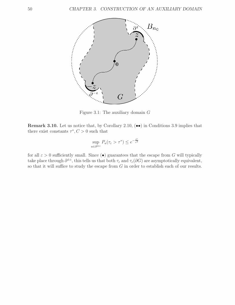
50 CHAPTER 3. CONSTRUCTION OF AN AUXILIARY DOMAIN
Figure 3.1: The auxiliary domain G
Remark 3.10. Let us notice that, by Corollary 2.10, (••) in Conditions 3.9 implies thatthere exist constants τ ∗, C > 0 such that
supu∈∂±z
Pu(τε > τ ∗) ≤ e−C
ε2
for all ε > 0 sufficiently small. Since (•) guarantees that the escape from G will typicallytake place through ∂±z , this tells us that both τε and τε(∂G) are asymptotically equivalent,so that it will suffice to study the escape from G in order to establish each of our results.
3.1. RESUMEN DEL CAPÍTULO 3 51
3.1 Resumen del Capítulo 3
En este capítulo damos la construcción del dominio auxiliar acotado con las característicasdiscutidas en la Introducción. La razón por la cual llevamos a cabo tal construcción esporque nos permite reducir nuestro problema original al de estudiar cómo el sistemaestocástico se escapa de dicho dominio. La ventaja de esto reside en que para estudiareste nuevo problema podemos asumir que la fuente es globalmente Lipschitz, dado que elescape depende únicamente del comportamiento del sistema mientras se encuentra en unaregión acotada. Es entonces que se pueden aplicar las estimaciones de grandes desvíos dela Sección 1.4.
Para poder precisar qué condiciones debe cumplir nuestro dominio, definimos primeroel quasipotencial V siguiendo la Definición ??. Dados u, v ∈ CD([0, 1]), el quasipotencial
V (u, v) = infIuT (ϕ) : ϕ ∈ CD([0, T ]× [0, 1]), ϕ(0, ·) = u, ϕ(T, ·) = v
representa el costo para el sistema estocástico (en términos de las estimaciones de laSección 1.4) de ir desde u hasta (un entorno arbitrariamente pequeño de) v. Asimismo,dado un conjunto B ⊆ CD([0, 1]), el quasipotencial
V (u,B) = infV (u, v) : v ∈ B
representa el costo para el sistema de ir desde u hasta B. Luego, el dominio G de interésdebe cumplir con las siguientes características:
i. Existe r0 > 0 tal que B2r0 ⊆ D0 ∩G.
ii. Existe c > 0 tal que Bc ⊆ Br0 y para todo v ∈ Bc la solución Uv de (1.1) con datoinicial v está globalmente definida y converge a 0 sin escapar de Br0 .
iii. Existe un subconjunto cerrado ∂±z de la frontera ∂G que satisface
• V (0, ∂G− ∂±z) > V (0, ∂±z) = V (0,±z).•• ∂±z está contenido en D∗
e y a una distancia positiva de su frontera.
La estabilidad asintótica del origen 0 garantiza que cualquier dominio que contenga a unentorno del origen va a satisfacer (i) y (ii). Por otro lado, mostramos que si el parámetrop en la fuente satisface 1 < p < 5 entonces existe un dominio acotado que ademássatisface (iii). Dicho dominio será la porción de D0 contenida en una bola de centro en0 y radio apropiadamente grande, unida a entornos pequeños de los equilibrios inestablesde mínima energía, ±z (ver Figura 3.1). La principal dificultad a la hora de demostrarque el dominio así construido cumple con las características buscadas yace en la falta decompacidad del espacio CD([0, 1]). Sin embargo, nos fue posible lidiar con este problemaapelando a algunos de los resultados contenidos en el Apéndice. Por último, la restricciónp < 5 surge de limitaciones geométricas impuestas por el potencial S. Esperamos que unaconstrucción similar sea posible aún en el caso p ≥ 5, aunque no tenemos una prueba.

52 CHAPTER 3. CONSTRUCTION OF AN AUXILIARY DOMAIN
Chapter 4
The escape from G
The behavior of the explosion time for initial data u ∈ D0 is proved by showing that, withoverwhelming probability as ε→ 0, the stochastic system describes the following path:
(i) The system enters the neighborhood of the origin Bc before some finite time T whichdoes not depend on ε.
(ii) Once inside Bc the system remains in G for a time of order e∆ε2 and then escapes
from G through ∂±z since the barrier imposed by the potential is the lowest there.
(iii) After escaping G through ∂±z the system explodes before some finite time τ ∗ whichdoes not depend on ε.
The fact that the domain G is bounded allows us to assume that the source term g isglobally Lipschitz if we wish to study the behavior of our system while it remains in G.Indeed, we may consider n0 ∈ N from the definition of G and study the behavior of thesolution to (1.12) for n = n0+1 since it coincides with our process until the escape from G.For this reason, in the following we shall often drop the superscript (n0+1) in the notationU (n0+1),u,ε unless it is completely necessary.
Our aim in this section is to obtain a complete and precise understanding of (ii) in thedescription above, since by (iii) the explosion time will inherit all the asymptotic propertiesof the escape time from G. In particular, we are interested in the asymptotic magnitudeand distribution of this escape time, as well as in a good understanding of which arethe typical paths that lead the stochastic system outside of our bounded domain G.The problem of escaping a bounded domain with these characteristics was first studiedin [20] for a finite-dimensional double-well potential, and later investigated in [5] for itsinfinite-dimensional analogue. The results we present in this chapter are an adaptationto our setting of the results featured in these references. Other references dealing withsimilar problems include [29, 4, 18].
Hereafter, Bc will denote the neighborhood of the origin highlighted in Conditions 3.9.Also, for a given closed set Γ ⊆ CD([0, 1]) we write
τuε (Γ) := inft ≥ 0 : Uu,ε(t, ·) ∈ Γ.
53
54 CHAPTER 4. THE ESCAPE FROM G
4.1 Asymptotic magnitude of τε(∂G)
We begin our study of the escape from G by studying its asymptotic magnitude as ε→ 0.The precise result we are to show is the following.
Theorem 4.1. Given δ > 0 we have
limε→0
[
supu∈Bc
∣
∣
∣Pu
(
e∆−δε2 < τε(∂G) < e
∆+δε2
)
− 1∣
∣
∣
]
= 0.
We shall split the proof of this result into two parts over Sections 4.1.1 and 4.1.2, thefirst of them dealing with the upper bound and the second one with the lower bound.
4.1.1 Upper bound on τε(∂G)
Our first goal is to establish the upper bound for the escape time from G contained inthe following theorem.
Theorem 4.2. For any δ > 0 we have
limε→0
[
supu∈G
Pu
(
τε(∂G) > e∆+δε2
)
]
= 0. (4.1)
The main idea behind the proof is to show that there exist paths escaping the domainG with rates arbitrarily close to ∆, so that the typical time one must wait for any of thesepaths to be described by the stochastic system is of lesser asymptotic order than e
∆+δ
ε2 .The precise estimate is contained in the following lemma.
Lemma 4.3. Given δ > 0 there exists T (δ) > 0 such that for each u ∈ G there exists aset of paths Eu,T (δ) ⊆ CDu([0, T
(δ)]× [0, 1]) satisfying
i. Every path in Eu,T (δ) escapes G before time T (δ).
ii. For any ε > 0 sufficiently small we have infu∈G Pu(Uε ∈ Eu,T (δ)) ≥ T (δ)e−
∆+ δ2ε2 .
Proof. We will prove the lemma with the aid of the large deviations principle establishedfor our system. The idea of the proof is to show that for each u ∈ G there exists a pathϕu ∈ CDu([0, T
(δ)]× [0, 1]) starting at u with rate less than ∆+ δ3
and such that not onlydoes ϕu itself escape fromG before time T (δ), but also any path sufficiently close to ϕu doesso as well. We construct ϕu explicitly for each u ∈ G. Each path ϕu will consist of severalpieces, each of which must either follow the trajectory described by the deterministicsystem (sometimes in the opposite direction) or be a linear interpolation between nearbyelements of CD ∩ W 2
2 ([0, 1]). In view of this last possibility, we first need to establishsome control on the contribution of these linear interpolations to the rate of ϕu. Thus,let us consider a velocity one linear interpolation s between two points u, w ∈ Bn0+1, i.e.s : [0, ‖w − v‖∞]× [0, 1] → R given by
s(t, x) = u(x) + t ·(
w(x)− u(x)
‖w − u‖∞
)
for (t, x) ∈ [0, ‖w − u‖∞]× [0, 1],
4.1. ASYMPTOTIC MAGNITUDE OF τε(∂G) 55
and suppose that both u and w have W 22 ([0, 1])-norm bounded by some constant M > 0.
Then we have
I(s) =1
2
∫ ‖w−u‖∞
0
∫ 1
0
|∂ts− ∂2xxs− gn0(s)|2 ≤∫ ‖w−u‖∞
0
∫ 1
0
[
|∂ts|2 + |∂2xxs+ gn0(s)|2]
.
Since ‖∂ts‖∞ = 1 by construction and ∂2xxs(t, ·) = ∂2xxu+ t ·(
∂2xxw−∂2xxu‖w−u‖∞
)
we obtain that
I(s) ≤ Cn0,M‖w − v‖∞where Cn0,M > 0 is a constant depending only on ‖gn0+1‖∞ and M .
Taking this into consideration, by using Propositions A.2, A.3 and A.4 in the Appendixwe may take a time T0 > 0 sufficiently small such that
supt∈[0,T0]
‖Uu(t, ·)− u‖∞ <1
2and sup
t∈[0,T0]‖Uu(T0, ·)− Uv(T0, ·)‖∞ ≤ 2‖u− v‖∞
for any u, v ∈ Bn0+1, a constantH > 0 such that ‖Uu(T0, ·)‖W 22 ([0,1])
≤ H for any u ∈ Bn0+1
and a distance r > 0 such that any linear interpolation between elements in Bn0+1 withW 2
2 ([0, 1])-norm bounded by 2H and at a distance smaller than 2r has rate less than δ9.
We may assume that both T0 and r are sufficiently small, e.g. T0 < 1 and r < min14, c.
We then define the set
W(r−) = u ∈ CD([0, 1]) : d(u,W) < r.
The construction of ϕu is done as follows. The first step is to follow the deterministic flowfor a time period of length T0. The remainder of the construction will vary according towhere v0 := Uu(T0, ·) is located. We describe the different scenarios below.
• If v0 ∈ Bcn0+r
then ϕu has already escaped G and reached a distance from G whichis greater than r. The construction in this scenario ends here.
• If v0 ∈ Bn0+r ∩W(r−) then:
⋄ We choose v ∈ W such that d(v0, v) < r and first let ϕu follow once again thedeterministic flow for a time period of length T0 and afterwards describe thelinear interpolation between the points Uv0(T0, ·) and v1 := Uv(T0, ·) in timeT u1 = d(Uv0(T0, ·), v1). Notice that Uv0(T0, ·) and v1 lie inside Bn0+1, are at adistance smaller than 2r from each other and both have W 2
2 ([0, 1])-norm lessthan H by the choice of T0 and the fact that both v0 and v lie inside Bn0+
12.
⋄ From there we let the path ϕu follow the deterministic flow Uv1 until the timeT u2 = inft ≥ T0 : d(U
v1(t, ·), z(n)) ≤ r for some n ∈ Z− 0.⋄ If for some t ∈ [0, T u2 ] we have Uv1(t, ·) /∈ Bn0+r then once again we have thatϕu has already escaped G and reached a distance from G greater than r, inwhich case we end the construction here.
⋄ If this is not the case then we continue ϕu by describing the linear interpolationbetween v2 := Uv1(T u2 , ·) and v3 := (1 + r)z(n) in time T u3 = d(v2, v3) ≤ 2r.Notice that v2 and v3 lie inside Bn0+1 and both have W 2
2 ([0, 1])-norm less than2H since we have that v2 = UUv1 (Tu2 −T0,·)(T0, ·) and Uz(n)(T0, ·) = z(n).
56 CHAPTER 4. THE ESCAPE FROM G
⋄ Finally, we follow once again the deterministic flow Uv3 until we reach a distancefrom G greater than r in a finite time T u4 which depends only on r and z(n).Notice that this is possible due to the fact that v3 ∈ De by Proposition 1.5.
• If v0 ∈ Bn0+r ∩ D0 ∩Wc(r−) then:
⋄ From there we let the path ϕu follow the deterministic flow Uv0 until the timeT u5 = inft ≥ T0 : U
u(t, ·) ∈ Br.⋄ Next we fix u∗ ∈ W z
u ∩ ∂Br and consider T ∗ = inft ≥ T0 : Uu∗(t, ·) ∈ Br, atime which only depends on the choice of u∗. We then continue ϕu by describingthe linear interpolation between v4 := Uu(T u5 , ·) and v5 := Uu∗(T ∗, ·) in timeT u6 = d(v4, v5) ≤ 2r. Notice that v4 and v5 lie inside G since r < c and bothhave W 2
2 ([0, 1])-norm less thanH by a similar argument to the one given above.
⋄ Once on Wzu we let ϕu follow the reverse deterministic flow until the time
T u7 = inft ≥ 0 : Uv5(−t, ·) ∈ G ∩ W(r−) which does not depend on u, butrather on the choice of u∗ instead.
⋄ We can then continue as in the second scenario, by noticing that Uv5(−T u7 , ·)belongs to Bn0 and has W 2
2 ([0, 1])-norm less than H since Wzu ∩D0 ⊆ G by the
mere construction of G.
• If v0 ∈ Bn0+r ∩De ∩Wc(r−) then we let the path ϕu follow the deterministic flow Uv0
until we reach a distance from G greater than r in a finite time T u8 .
If built in this way, the path ϕu verifies all the required properties. Indeed, we have that:
• Each ϕu belongs to CDu ∩ W 1,22 ([0, T u] × [0, 1]) for some Tu > 0 (the sum of the
corresponding T ui ) since by construction ϕu is piecewise differentiable.
• The total time length T u of the path ϕu is uniformly bounded in u ∈ G. Indeed, thetotal time which ϕu spends following the deterministic flow is uniformly bounded byProposition A.7 since there are only finitely many equilibrium points lying in Bn0+1.On the other hand, there are at most three linear interpolations in ϕu, each of whichlasts a time of length less than one. Finally, the time spent by ϕu following thereverse deterministic flow is finite and does not depend on u.
• Each ϕu has total rate less than ∆ + δ3. Indeed, its total rate can be computed as
the sum of the rate of each of its pieces. We have already seen that each linearinterpolation has rate less than δ
9and, since in any case there at most three of
them, their total contribution is less than δ3. On the other hand, the pieces in which
ϕu follows the deterministic flow have zero rate. Finally, if ϕu follows the reversedeterministic flow (i.e. ∂tϕ
u = −(∂2xxϕu + g(ϕu))) during the time interval [t1, t2]
then, similarly to Proposition A.8, we have
1
2
∫ t2
t1
∫ 1
0
|∂tϕu− (∂2xxϕu+ g(ϕu))|2 = 2
∫ t2
t1
dS(ϕu(t, ·))dt
= 2(S(ϕu(t2))−S(ϕu(t1)))
from where, upon recalling that ϕu(t2), ϕu(t1) ∈ Wzu, we obtain that the rate of this
last piece is less than ∆.
4.1. ASYMPTOTIC MAGNITUDE OF τε(∂G) 57
• Any path at a distance strictly less than r from ϕu in the supremum norm mustalso escape from G before T u, since by this time ϕu reaches a distance r from G.
Let us notice that for each u ∈ G we have built a path ϕu on the time interval [0, T u],but we wish all constructed paths to be defined on a same time interval. For this reason,we consider T (δ) := supu∈G T
u < +∞ and extend all ϕu to the time interval [0, T (δ)] byfollowing the deterministic flow. It is easy to check that these extended paths maintainthe aforementioned properties. We then define the set Eu,T (δ) for each u ∈ G as
Eu,T (δ) := ψ ∈ CDu([0, T(δ)]× [0, 1]) : dT (δ)(ψ, ϕu) < r.
It is clear that each Eu,T (δ) verifies condition (i) by construction, whereas (ii) follows fromthe large deviations estimate (i) in Section 1.4.
Now, if we write T+ε = e
∆+δε2 and split the interval [0, T+
ε ] into subintervals of lengthT (δ) given by Lemma 4.3, then by the Markov property for the solution of (1.4) we obtain
Pu(τε(∂G) > T+ε ) ≤ Pu
(
mε⋂
k=1
Uε(t, ·) ∈ G for all t ∈ [(k − 1)T (δ), kT (δ)])
≤ (1− αε)mε
(4.2)
where αε := T (δ)e−∆+ δ2ε2 , mε :=
⌊
T+ε
T (δ)
⌋
and for the second inequality we used that for u ∈ G
Uu,ε(t, ·) ∈ G for all t ∈ [0, T (δ)] ⊆ Uu,ε /∈ Eu,T (δ).Since the bound (4.2) is uniform on G, by taking ε → 0 a direct computation yields (4.1).
4.1.2 Lower bound on τε(∂G)
Our next purpose is to establish the lower bound on τε(∂G) contained in the theorem below.
Theorem 4.4. There exists r > 0 sufficiently small such that
limε→0
[
supu∈∂Br
Pu
(
τε(∂G) < e∆−δε2
)
]
= 0. (4.3)
The key to establishing this lower bound is to observe that for initial data in a smallneighborhood of the origin the path described by the stochastic system while it remainsinside G will typically consist of several failed attempts to reach ∂G followed by one lastattempt which is successful and thus leads to the escape from G. Each of these failedattempts is an excursion drifting away from the origin which, having failed to reach ∂G,later returns to (a small neighborhood of) the origin. Hence, the desired lower bound onthe time the process needs in order to escape from G can be obtained upon giving suitablebounds on the number and length of these excursions.
To accomplish this we consider, given constants r1, r2 > 0 such that r1 < r22
and r2 < c,for each u ∈ ∂Br1 and ε > 0 the increasing sequence of stopping times
η0 = 0
σ0 = inft ≥ 0 : Uu,εt ∈ ∂Br2
58 CHAPTER 4. THE ESCAPE FROM G
and for n ∈ N0
ηn+1 = inft > σn : Uu,εt ∈ ∂Br1 ∪ (∂G)(d)
σn+1 = inft > ηn+1 : Uu,εt ∈ ∂Br2
where ∂G is the pre-domain defined in (3.3) and d > 0 is taken such that Br2 and (∂G)(d)are at positive distance from each other, where
(∂G)(d) := u ∈ CD([0, 1]) : d(u, ∂G) ≤ d.
These positive constants r1, r2 and d will be later taken conveniently small during the proof.Also, whenever any of the sets involved is empty we take the corresponding time as +∞.We then define the Markov chain (Zu,ε
n )n∈N by the formula
Zu,εn = Uu,ε
ηn
for each n ∈ N0, and set ϑuε := minn ∈ N : Zu,εn ∈ (∂G)(d). Since the process Uu,ε
escapes G in a finite time almost surely and we are only interested in events occurringbefore τε(∂G), we need not worry about the possibility of Zε
n not being well defined.
Let us notice then that, since for any u ∈ ∂Br1 we have τuε (∂G) ≤ τuε (∂G) by thecontinuity of the trajectories of Uu, for each δ > 0 we obtain the bound
supu∈∂Br1
Pu
(
τε(∂G) < e∆−δε2
)
≤ supu∈∂Br1
Pu(νε ≤ kε) + supu∈∂Br1
Pu
(
ηkε < e∆−δε2
)
(4.4)
where kε ∈ N is to be determined next for each ε > 0. Thus, we see that to obtain (4.3)it suffices to show that, for a suitable choice of (kε)ε>0, both terms in the right hand sideof (4.4) vanish as ε→ 0. We will do this with the aid of the following two lemmas, whichare slight modifications of two results originally appearing in [5].
Lemma 4.5. Let F,B ⊆ CD([0, 1]) be bounded sets and suppose ψ ∈ CD([0, 1]) is suchthat d(ψ, F ) > 3r for some r > 0. Then for any h, T > 0 there exists r∗ > 0 such that
supu∈Bρ(ψ)
Pu(τε(F(r)) ≤ minT, τε(Bc)) ≤ e−V (ψ,F(2r))−h
ε2
for any 0 < ρ < r∗.
Lemma 4.6. Let B ⊆ CD([0, 1]) be bounded and closed. If for e > 0 we consider
Ce :=⋃
n∈ZBe(z
(n)).
then given K > 0 there exists T > 0 such that
supu∈B
Pu (minτ(Ce), τ(Bc) > T ) ≤ e−K
ε2 .
Now, in order to deal with the first term in the right hand side of (4.4) it will sufficeto establish the bound
supu∈∂Br1
Pu(ϑε = 1) ≤ e−∆− δ
4ε2 (4.5)
4.1. ASYMPTOTIC MAGNITUDE OF τε(∂G) 59
for ε > 0 sufficiently small. Indeed, if we prove (4.5) then by the Markov property of Zε
we obtain
infu∈∂Br1
Pu(ϑε > n) ≥(
1− e−∆− δ
4ε2
)n
for every n ∈ N and ε > 0 sufficiently small, which implies the inequality
supu∈∂Br1
Pu(ϑε ≤ kε) ≤ 1−(
1− e−∆− δ
4ε2
)kε
(4.6)
whose right hand side vanishes as ε → 0 if we set for example kε :=[
exp(
∆− δ2
ε2
)]
+ 1.
Thus, let us check that (4.5) holds. Notice that the strong Markov property for σ0 yields
supu∈∂Br1
Pu(ϑε = 1) ≤ supu∈∂Br2
Pu
(
τε((∂G)(d)) = τε(∂Br1 ∪ (∂G)(d)))
so that to check (4.5) it will suffice to find T > 0 such that
supu∈∂Br2
Pu
(
τε((∂G)(d)) ≤ T)
≤ e−∆− δ
8ε2 (4.7)
and
supu∈∂Br2
Pu
(
τε(∂Br1 ∪ (∂G)(d)) > T)
≤ e−∆− δ
8ε2 (4.8)
for every ε > 0 sufficiently small.
Now, let us observe that, since the potential S attains in ±z its minimum on ∂G, byproceeding as in the proof of Lemma 4.3 one can show that V (0, ∂G) = ∆. Therefore, byconducting a similar argument to the one given in the construction of G, it follows thatthe set
V :=
u ∈ CD([0, 1]) : V (0, u) ≤ ∆− δ
16
is contained in G and satisfies d(V,W) > 0. Furthermore, since V is contained in D0 andthe set u ∈ D0 : 0 ≤ S(u) ≤ S(z) is contained in Bn0−1, then Proposition 3.6 impliesthat d(V, ∂Bn0) > 0 and thus we obtain that d(V, ∂G) ≥ mind(V,W), d(V, ∂Bn0) > 0.
In particular, if we take d < d(V ,∂G)3
then we have V (0, (∂G)(2d)) ≥ ∆ − δ16
and thereforeby Lemma 4.5 we conclude that for a fixed T > 0 and r2 > 0 sufficiently small
supu∈∂Br2
Pu(τε((∂G)(d)) ≤ T ) ≤ e−∆− δ
8ε2
provided that ε > 0 is sufficiently small, which yields (4.7).
On the other hand, if we take 0 < e < minr1, d then we have that Be(z(n)) ⊆ (∂G)(d)
for any n ∈ Z− 0 such that z(n) ∈ G. In particular, we see that
supu∈∂Br2
Pu
(
τε(∂Br1 ∪ (∂G)(d)) > T)
≤ supu∈∂Br2
Pu
(
minτ(Ce), τ((∂G)(d)) > T)
. (4.9)
It then follows from Lemma 4.6 that T > 0 can be taken sufficiently large so that (4.8)holds. Together with (4.7), this yields (4.5) and establishes the convergence to zero of
60 CHAPTER 4. THE ESCAPE FROM G
the first term in the right hand side of (4.4). Thus, it only remains to establish the sameconvergence for the second term.
Notice that by Proposition A.2 there exists some Tr2 > 0 such that for any u ∈ ∂Br2
the system Uu spends a time of length at least Tr2 before reaching B r22. Furthermore, we
may assume that r2 is sufficiently small so that the path described by Uu until time Tr2is at a distance greater than r2
2from (∂G)(d). By the strong Markov property and (1.9)
we conclude that for ε > 0 sufficiently small
infu∈∂Br1
Pu(η1 ≥ Tr2) ≥ infu∈∂Br2
Pu
(
dTr2(
U (n0),ε, U (n0))
<r22− r1
)
≥ 2
3.
Let us observe that since for any k ∈ N we have the inequality ηk ≥∑k
i=1 Tr21ηi−ηi−1≥Tr2,by definition of kε we obtain that for ε > 0 sufficiently small
supu∈∂Br1
Pu
(
ηkε < e∆−δε2
)
≤ supu∈∂Br1
Pu
(
ηkεkε
< e−δ
2ε2
)
≤ P
(
1
kε
kε∑
i=1
Xi <e−
δ
2ε2
Tr2
)
where (Xi)i∈N is a sequence of i.i.d. Bernoulli random variables with parameter p = 23.
The result now follows at once from the law of large numbers.
4.2 The escape route
We are now interested in characterizing the typical route that the stochastic systemdescribes to escape fromG. By the considerations made at the beginning of this Section weexpect this typical path to escape G by going through the region of the boundary with thelowest quasipotential, namely ∂±z . More precisely, we wish to prove the following theorem.
Theorem 4.7. If c > 0 is given by (ii) in Conditions 3.9 then
limε→0
[
supu∈Bc
Pu(
Uε(τε(∂G), ·) /∈ ∂±z)
]
= 0. (4.10)
To prove this result we shall need to establish the following two crucial facts:
i. For each r > 0 strictly smaller than c
limε→0
[
supu∈Bc
Pu (τε(∂G) < τ (Br))
]
= 0.
ii. For any r > 0 sufficiently small
limε→0
[
supu∈∂Br
Pu(
Uε(τε(∂G), ·) /∈ ∂±z)
]
= 0. (4.11)
Indeed, (4.10) follows immediately from (i) and (ii) by applying the strong Markov property.Hence, it will suffice to establish (i) and (ii). Assertion (i) is shown in the following lemma.
4.2. THE ESCAPE ROUTE 61
Lemma 4.8. For each r > 0 strictly smaller than c we have
limε→0
[
supu∈Bc
Pu (τε(∂G) < τ (Br))
]
= 0.
Proof. Notice that by choice of c we have that any u ∈ Bc reaches the neighborhood B r2
ina finite time T ur while remaining at a distance greater than r0 in Conditions 3.9 from both∂G and W. By Proposition A.7 we therefore conclude that Tr = supu∈Bc T
ur must be finite.
Hence, for u ∈ Bc we obtain
Pu (τε(∂G) < τε (Br)) ≤ supv∈Bc
Pv
(
dTr(U(n0),ε, U (n0)) ≥ r0 ∧
r
2
)
which, by (1.9) and the uniformity of the bound in u ∈ Bc, implies the result at once.
In order to prove assertion (ii) we first show that it suffices to study the path describedby the stochastic system since its last visit to (a small neighborhood of) the origin.We shall do this by resorting to a Markov chain similar to the one introduced in thepreceding section to establish the lower bound. More precisely, given constants r1, r2 > 0such that r1 < r2
2and r2 < c, for each u ∈ ∂Br1 and ε > 0 we consider the increasing
sequence of stopping times
η0 = 0
σ0 = inft ≥ 0 : Uu,ε(t, ·) ∈ ∂Br2and for n ∈ N0
ηn+1 = inft > σn : Uu,ε(t, ·) ∈ ∂Br1 ∪ ∂G
σn+1 = inft > ηn+1 : Uu,ε(t, ·) ∈ ∂Br2
with the convention that inf ∅ = +∞. We then define the Markov chain (Zu,εn )n∈N as
Zu,εn := Uu,ε(ηn, ·)
for each n ∈ N0 and set ϑuε := minn ∈ N : Zu,εn ∈ ∂G. Just as in the previous section, for
our purposes we will not need to worry about the possibility of Zεn not being well defined.
Also, the constants r1 and r2 will be later taken conveniently small throughout the proof.It is not hard to see that for any u ∈ ∂Br1 the strong Markov property yields
Pu(
Uε(τε(∂G), ·) /∈ ∂±z)
≤ supv∈∂Br1
Pv(Zε1 ∈ ∂G− ∂±z)
Pv(Zε1 ∈ ∂G)
(4.12)
from which we conclude that in order to show (ii) it will suffice to give a lower boundfor the denominator and an upper bound for the numerator such that the quotient ofthese bounds goes to zero with ε. The following lemma, whose proof can be found in [5],provides the desired lower bound.
Lemma 4.9. Let us suppose that r1 is sufficiently small so as to guarantee that for anyu ∈ ∂Br1 the deterministic orbit Uu(t, ·) : t ≥ 0 does not intersect ∂B r2
2. Then for all
ε > 0 sufficiently small
infu∈∂Br1
Pu(Zε1 ∈ ∂G) ≥ e−
∆+kr2ε2 ,
where k > 0 is a constant which does not depend on the choice of r1 and r2.
62 CHAPTER 4. THE ESCAPE FROM G
The upper bound on the numerator in (4.12) is more involved and requieres severalsteps. We start by considering, for fixed constants d, e > 0 such that e < rz and d < rz−e
2
(which will be later made conveniently small), the stopping times
τ 0ε = τε(
(∂G− ∂±z)(d))
and τ 2ε = τε (Be(±z))
where(∂G− ∂±z)(d) := u ∈ CD([0, 1]) : d(u, ∂G− ∂±z) ≤ d.
where the initial datum is implicit. Notice that d is such that (∂G− ∂±z)(d) and Be(±z)are disjoint. Then we can decompose the event in the numerator into three disjoint parts:
A := Zu,ε1 ∈ ∂G− ∂±z =
2⋃
i=0
[A ∩ τ iε = minτ 0ε , τ 1ε , τ 2ε , τ 3ε ] (4.13)
where, for notational convenience, we have set τ 1ε as some fixed time T > 0 which is tobe conveniently determined later and τ 3ε as the escape time τε(∂G) from our domain G.Observe that the set A ∩ τ 3ε = minτ 0ε , τ 1ε , τ 2ε , τ 3ε is empty and is therefore left out ofthe decomposition. Thus, in order to provide an upper bound for the numerator we seethat it will suffice to estimate the probabilities of each of the sets in the decomposition.
4.2.1 Upper bound on P (A ∩ τ 0ε = minτ 0ε , τ 1ε , τ 2ε , τ 3ε )To bound the probability of the first set we observe that if d > 0 is taken sufficiently smallthen
V (0, (∂G− ∂±z)(2d)) > ∆. (4.14)
Indeed, since
(∂G− ∂±z)(2d) = (∂G− Brz(±z))(2d) ∪ ([∂Brz(±z) ∩ De]− ∂±z)(2d)
to establish (4.14) it will suffice to show that
V (0, (∂G−Brz(±z))(2d)) > ∆ and V (0, ([∂Brz(±z)∩De]−∂±z)(2d)) > ∆. (4.15)
From the definition of ∂±z it easily follows that if we take 2d < d(∂z ,W)2
then the sets ∂z
and ([∂Brz(z)∩De]− ∂z)(2d) are disjoint so that the second inequality in (4.15) is settled.To obtain the first inequality we begin by noticing that by an argument analogous to theone employed in the construction of G there exists α > 0 such that
infS(u) : u ∈ [W ∩Bn0+1]− B rz2(±z) > α > S(z).
Hence, to establish the first inequality in (4.15) it will suffice to consider the set
V ′ = u ∈ CD([0, 1]) : V (0, u) ≤ 2minα, S(z) + ζ1
and show that d(V ′, ∂G− Brz(±z)) > 0. But, if this were not so, then there would existsequences (uk)k∈N ⊆ V ′ and (vk)k∈N ⊆ ∂G−Brz(±z) such that d(uk, vk) → 0 as k → +∞.
4.2. THE ESCAPE ROUTE 63
By Propositions A.3 and A.5 we may find subsequences (ukj)j∈N, (vkj)j∈N and a time t > 0such that
limj→+∞
Uukj (t, ·) = limj→+∞
Uvkj (t, ·) = v∞
for some limit v∞ ∈ CD([0, 1]). Let us observe that, since we have v∞ = limj→+∞Uukj (t, ·),the lower semicontinuity of V (0, ·) and the fact that the mapping t 7→ V (0, Uu(t, ·)) ismonotone decreasing for any u ∈ CD([0, 1]) together imply that
V (0, v∞) ≤ 2minα, S(z) + ζ1. (4.16)
At least one of the following possibilities must then occur:
• If vk ∈ ∂Bn0 ∩ D0 for infinitely many k ∈ N, then (kj)j∈N and t > 0 can be takenso as to guarantee that the condition Uvkj (t, ·) /∈ Bn0−1 is satisfied for every j ∈ N.Since D0 is closed and invariant under the deterministic flow we therefore concludethat v∞ ∈ D0 − B
n0−1 and thus that S(v∞) > S(z) + ζ1. In particular, we obtainthat V (0, v∞) > 2(S(z) + ζ1), a fact which contradicts (4.16).
• If vk ∈ W ∩ Bn0 for infinitely many k ∈ N, then (kj)j∈N and t > 0 can be takenso as to guarantee that Uvkj (t, ·) ∈ Bn0+1 − B 2
3rz(±z) is satisfied for every j ∈ N.
Since W is closed and invariant under the deterministic flow we then conclude thatv∞ ∈ [W ∩ Bn0+1] − B rz
2(±z) and thus that S(v∞) > α. In particular, we obtain
that V (0, v∞) > 2α, which again contradicts (4.16).
Now that we have shown (4.14), Lemma 4.5 guarantees that if r1 is sufficiently smallthen there exists h > 0 such that
supu∈∂Br1
Pu(A ∩ τ 0ε = minτ 0ε , τ 1ε , τ 2ε , τ 3ε ) ≤ supu∈∂Br1
Pu(τ0ε ≤ minT, τε(∂G)) ≤ e−
∆+hε2
which provides the desired upper bound. Indeed, notice that if T > 0 is fixed and r2 > 0is taken sufficiently small then the upper bound obtained and Lemma 4.9 together yield
limε→0
[
supu∈∂Br1
Pu(A ∩ τ 0ε = minτ 0ε , τ 1ε , τ 2ε , τ 3ε )Pu(Zε
1 ∈ ∂G)
]
= 0. (4.17)
4.2.2 Upper bound on P (A ∩ τ 1ε = minτ 0ε , τ 1ε , τ 2ε , τ 3ε )To bound the probability of the second set we observe that any unstable equilibrium ofthe system lying inside G and different from ±z must necessarily belong to ∂G − ∂±z.This implies that if we take e < minr1, d then
supu∈∂Br1
Pu(A ∩ τ 1ε = minτ 0ε , τ 1ε , τ 2ε , τ 3ε ) ≤ supu∈∂Br1
Pu(T ≤ minτε(Ce), τε(∂G))
where Ce is defined as in Lemma 4.6. Hence, by the same lemma we obtain for T > 0sufficiently large the upper bound
supu∈∂Br1
Pu(A ∩ τ 1ε = minτ 0ε , τ 1ε , τ 2ε , τ 3ε ) ≤ e−∆+1ε2 .
64 CHAPTER 4. THE ESCAPE FROM G
Together with Lemma 4.9 this upper bound yields
limε→0
[
supu∈∂Br1
Pu(A ∩ τ 1ε = minτ 0ε , τ 1ε , τ 2ε , τ 3ε )Pu(Zε
1 ∈ ∂G)
]
= 0. (4.18)
4.2.3 Upper bound on P (A ∩ τ 2ε = minτ 0ε , τ 1ε , τ 2ε , τ 3ε )To conclude the proof it only remains to give an upper bound on the probability of thethird set in the right hand side of (4.13). If we write D2 = τ 2ε = minτ 0ε , τ 1ε , τ 2ε , τ 3ε then notice that by the strong Markov property one has
Pu(A ∩D2) ≤ E(1D2PUu,ε(τ2ε ,·)(Uε(τε(∂G), ·) ∈ ∂G− ∂±z, τε(Br1) > τε(∂G))).
The next lemma provides a suitable upper bound on the probability inside the expectation.
Lemma 4.10. There exists a constant C > 0 such that for every e > 0 sufficiently smallone has
supv∈Be(±z)
Pv(Uε(τε(∂G), ·) ∈ ∂G− ∂±z, τε(Br1) > τε(∂G))
Pv(τε(Br1) > τε(∂G))≤ e−
C
ε2 (4.19)
for every ε > 0 sufficiently small.
Proof. The idea is to consider once again a suitable embedded Markov chain. Fix f > 0such that Bf(±z) is at a positive distance from (∂G − ∂±z)(d) and assume that e < f
2.
Consider then the stopping times
η0 = 0
σ0 = inft ≥ 0 : Uu,ε(t, ·) ∈ ∂Bf (±z)and for n ∈ N0
ηn+1 = inft > σn : Uu,ε(t, ·) ∈ ∂Be(±z) ∪ ∂G
σn+1 = inft > ηn+1 : Uu,ε(t, ·) ∈ ∂Bf (±z)
with the convention that inf ∅ = +∞. We then define the Markov chain (W u,εn )n∈N as
W u,εn := Uu,ε(ηn, ·)
for n ∈ N0 and set ϑuε := minn ∈ N : W u,εn ∈ ∂G. To show (4.19) it suffices to check that
supv∈Be(±z)
Pv(Wε1 ∈ ∂G− ∂±z , τε(Br1) > τε(∂G), ϑε = 1)
Pv(τε(Br1) > τε(∂G), ϑε = 1)≤ e−
C
ε2
holds for all ε > 0 sufficiently small provided e > 0 is chosen adequately. To see this,let us observe that V (±z, ∂G) = 0 and thus, by Lemma 4.9, we obtain the lower bound
e−Kf
ε2 for the denominator, where K > 0 does not depend on the choice of both e and f .On the other hand, since
V (0, (∂G− ∂±z)(2d)) ≤ V (0,±z) + V (±z, (∂G − ∂±z)(2d))
we see that V (±, (∂G − ∂±z)(2d)) > 0 and thus, with the aid of Lemmas 4.5 and 4.6,
one concludes the upper bound e−h
ε2 for the numerator, for some small constant h > 0.The lemma follows at once by taking f sufficiently small.
4.3. ASYMPTOTIC LOSS OF MEMORY OF τε(∂G) 65
We are now ready to finish the proof of Theorem 4.7. Indeed, by (4.19) we obtain
Pu(A ∩D2) ≤ e−C
ε2E(1D2PUu,ε(τ2ε ,·)(τε(Br1) > τε(∂G))) ≤ e−C
ε2Pu(Zε1 ∈ ∂G)
for every u ∈ ∂Br1 provided that e > 0 is taken sufficiently small. This implies that
limε→0
[
supu∈∂Br1
Pu(A ∩ τ 2ε = minτ 0ε , τ 1ε , τ 2ε , τ 3ε )Pu(Zε
1 ∈ ∂G)
]
= 0. (4.20)
and thus concludes the proof.
Remark 4.11. By using (4.15), the same argument given here to prove Theorem 4.7 canbe used to show that for any δ > 0
limε→0
[
supu∈Bc
Pu
(
Uε(
τε(∂G), ·)
/∈ Bδ(±z))
]
= 0.
This result tells us, perhaps in a more explicit manner than Theorem 4.7 does, that forsufficiently small ε > 0 the escape from G of the stochastic system and thus its routetowards explosion typically involves passing through the unstable equilibria with minimalpotential, namely ±z, at least whenever the initial datum is close enough to the origin.By the argument to be used in the proof of Theorem 5.1 below, this implies that the samefate holds for arbitrary initial data in D0.
4.3 Asymptotic loss of memory of τε(∂G)
Our next goal is to show the asymptotic loss of memory as ε → 0 of τuε (∂G) for u ∈ G.To this end for each ε > 0 we define the normalization coefficient γε > 0 by the relation
P0(τε(∂G) > γε) = e−1.
Notice that γε is well defined since τ0ε is a continuous almost surely finite random variable,with a strictly increasing distribution function. The result we aim to prove reads as follows.
Theorem 4.12. For every ε > 0 consider the function νε : R≥0 → [0, 1] given by
νε(t) = P0(τε(∂G) > tγε).
Then
i. There exists (δε)ε>0 ⊆ R>0 satisfying limε→0 δε = 0 and such that for any s, t > 0
νε(s+ δε)νε(t)− ψε(s, t) ≤ νε(s+ t) ≤ νε(s)νε(t− δε) + ψε(s, t) (4.21)
where ψε(s, t) is a function which for any fixed t0 > 0 verifies
limε→0
[
sups≥0 , t≥t0
ψε(s, t)
]
= 0. (4.22)
ii. There exists ρ > 0 such that for every t ≥ 0
limε→0
[
supu∈Bρ
|Pu(τε(∂G) > tγε)− e−t|]
= 0. (4.23)
66 CHAPTER 4. THE ESCAPE FROM G
4.3.1 Coupling of solutions with small initial data
The key element in the proof of Theorem 4.12 is the fact that, uniformly over any pairu, v of initial data in a small neighborhood of the origin the corresponding escape timesτuε (∂G) and τ vε (∂G) possess the same asymptotic distribution. We shall establish this factrigorously on Lemma 4.14 below with the aid of a suitable coupling between Uu,ε and Uv,ε.More precisely, for n0 ∈ N as in the definition of G the result we require is the following.
Theorem 4.13. There exists ρ > 0 such that for any pair of initial data u, v ∈ Bρ andε > 0 sufficiently small there exists a coupling of U (n0+1),u,ε and U (n0+1),v,ε satisfying
U (n0+1),u,ε(t, ·) ≡ U (n0+1),v,ε(t, ·) for all t ≥ ηεu,v, (4.24)
whereηεu,v := inft ≥ 0 : U (n0+1),u,ε(t, ·) ≡ U (n0+1),v,ε(t, ·).
Furthermore, ηεu,v satisfies
limε→0
[
supu,v∈Bρ
P
(
ηεu,v ≥1
ε3
)
]
= 0. (4.25)
The existence of a coupling fulfilling these characteristics was first established in [34] fora class of stochastic differential equations with periodic boundary conditions of the sort
∂tUu = ∂2xxU
u − αUu + a(Uu) + b(Uu)W t > 0 , x ∈ S1
Uu(0, x) = u(x) x ∈ S1 (4.26)
where α > 0 is fixed parameter, a : R → R is a Lipschitz nonincreasing function andb : R → R is a positive, Lipschitz function bounded away from both zero and infinity.In this work, Mueller considers an arbitrary pair of continuous functions u, v ∈ C(S1) asinitial data and shows that the coupling time ηεu,v is almost surely finite. Later this verysame result was adapted in [4] to a particular system verifying the assumptions in [34]but including Dirichlet boundary conditions instead of periodic ones. Furthermore, in thissecond work Brassesco shows the asymptotic estimate (4.25) for the coupling time ηεu,v.Unfortunately, for our system the coefficient a fails to be increasing so that the resultson [4] cannot be directly applied. Nevertheless, it is still possible to obtain Theorem 4.13by performing some minor adjustments to the proof given there, although this comes atthe expense of losing the almost sure finiteness of the coupling time and also a certainfreedom in the choice of initial data. In what follows we present a brief summary of theproof of Theorem 4.13, highlighting the main differences with [4] and explaining how todeal with each of them. We refer the reader to [34] and [4] for the remaining details.
Let us begin by observing that it will suffice to show the coupling for initial data u, vsuch that u ≥ v. Indeed, it follows from the proof in this case that if w := maxu, vthen we can construct the three solutions U (n0+1),u,ε, U (n0+1),v,ε and U (n0+1),w,ε in thesame probability space so that U (n0+1),u,ε and U (n0+1),w,ε are identical after the time ηεu,wand also U (n0+1),u,ε and U (n0+1),w,ε are identical after the time ηεv,w. It then follows thatU (n0+1),u,ε and U (n0+1),v,ε must become identical after the ηεu,v ≤ maxηεu,w, ηεv,w, so thatit suffices to estimate the desired probability in (4.25) for the simpler case u ≥ v.
4.3. ASYMPTOTIC LOSS OF MEMORY OF τε(∂G) 67
Thus, we assume that u ≥ v and given two independent Brownian sheets W1 and W2
we consider the pair (U (n0+1),u,ε, U (n0+1),v,ε) which satisfies
∂tU(n0+1),u,ε = −∂S
(n0+1)
∂ϕ(U (n0+1),u,ε) + εW1
and
∂tU(n0+1),v,ε = −∂S
(n0+1)
∂ϕ(U (n0+1),v,ε) + ε
((
√
1−min|E|, 1W1 +√
min|E|, 1W2
))
with initial data u and v respectively and where
E := U (n0+1),u,ε − U (n0+1),v,ε.
Thus, both U (n0+1),u,ε and U (n0+1),v,ε are solutions (1.12) with the appropriate initialdata, constructed in the same probability space but with respect to different white noises.Following Lemma 3.1 of [34] it is possible to construct the pair (U (n0+1),u,ε, U (n0+1),v,ε) insuch a way that the process E is nonnegative almost surely for ε > 0 sufficiently small.Then, using the weak formulation of solutions to (1.4) available on Lemma 1.6 one canimmediately see as in [4] that if we write
U(t) =
∫ 1
0
E(t, x) sin(πx)dx
then U satisfies
U(t) = U(t) +
∫ t
0
C(s)ds+Mt (4.27)
where
C(s) =
∫ 1
0
(
gn0+1
(
U (n0+1),u,ε(s, x))
− gn0+1
(
U (n0+1),v,ε(s, x))
− π2E(s, x))
sin(πx)dx.
(4.28)and M is a continuous martingale with respect to the filtration generated by W1 and W2
satisfying
〈M〉(t) = 2ε2∫ t
0
∫ 1
0
minE(s, x), 11 +
√
1−minE(s, x), 1dxds. (4.29)
Notice that in order for (4.27) to hold, it was necessary to introduce a C∞ function inCD([0, 1]) in the definition of U . We selected sin(πx) as in [4] but the same reasoning alsoholds for other nonnegative C∞ functions. Now, from (4.29) we easily obtain
〈M〉(t)dt
≥ ε2∫ 1
0
sin2(πx)minE(t, x), 1dx.
Using Hölder’s inequality we obtain that
∫ 1
0
sin(πx)minE(t, x), 1dx ≤(∫ 1
0
sin2(πx)minE(t, x), 1dx)
58(∫ 1
0
sin− 23 (πx)dx
)38
68 CHAPTER 4. THE ESCAPE FROM G
which implies the estimate
〈M〉(t)dt
≥ Kε
[∫ 1
0
sin(πx)minE(t, x), 1dx]
85
≥ Kε
[∫ 1
0
sin(πx)E(t, x)
maxE(t, x), 1dx]
85
≥ Kε2
[
supx∈[0,1]maxE(t, x), 1]
85
(U(t))85
where
K :=
(∫ 1
0
sin− 23 (πx)dx
)− 35
.
Thus, we conclude that there exists an adapted process D such that for all t ≥ 0
〈M〉(t)dt
= (U(t))85 D(t)
and
D(t) ≥ Kε2
[
supx∈[0,1]maxE(t, x), 1]
85
. (4.30)
Next, we introduce the time change
ϕ(t) =
∫ t
0
D(s)ds
and consider the time-changed process
X(t) := U(ϕ−1(t)).
In [34] it is shown that whenever the condition
max
supt≥0
E
(
supx∈[0,1]
U (n0+1),u,ε(t, x)
)
, supt≥0
E
(
supx∈[0,1]
U (n0+1),v,ε(t, x)
)
< +∞ (4.31)
is met then limt→+∞ ϕ(t) = +∞ so that the process X is globally defined. Unfortunately,in this article condition (4.31) is seen to hold only under the presence of the linear termin (4.26), i.e. α > 0, which is missing in our system. However, since we are interested inachieving the coupling between the solutions before they escape the domain G, one canmodify the source term gn0+1 outside Bn0+1 in such a way that (4.31) is satisfied withoutit affecting our plans. Hence, by (4.27) and the definition of ϕ, it can be seen that Xsatisfies
X(t) = U(0) +
∫ t
0
C(s)ds+
∫ t
0
(X(t))810 dBt

4.3. ASYMPTOTIC LOSS OF MEMORY OF τε(∂G) 69
for a certain Brownian motion B and C given by the formula
C(t) := C(ϕ−1(t))1
ϕ′(ϕ−1(t)).
Now, Itô’s formula yields that, up until its arrival time at zero, the process Y := 5X15
satisfies
Y (t) = 5 (U(0))15 +
∫ t
0
(
C(s)
(Y (s))4− 2
5Y (s)
)
ds+Bt
In both [34] and [4] the corresponding term C is nonpositive, so that Y is guaranteed to
hit zero before the time the Brownian motion B takes to reach −5 (U(0))15 . However, in
our case the term C may eventually take positive values so that some additional work isneeded in order to arrive at the same conclusion. Notice that a straightforward calculationusing the definition of ϕ and the bound (4.30) shows that if for some h > 0 the term C(t)
is nonpositive for all t ≤ eh
ε2 then C(t) is also nonpositive but only for all t ≤ eh
2ε2 . Hence,if we set
γ := inft ≥ 0 : Bt = −5 (U(0))15
then Y is guaranteed to hit zero before γ provided that there exists h > 0 such thatγ ≤ e
h
2ε2 and the term C(t) is nonpositive for all t ≤ eh
ε2 . Now, Y (t) = 0 implies thatU(ϕ−1(t)) = 0 and ultimately that E(ϕ−1(t), x) ≡ 0 which means that both solutionsU (n0+1),u,ε and U (n0+1),v,ε coincide at time t. But, since the process E is governed by thedifferential equation
∂tE = ∂2xxE +(
gn0+1(U(n0+1),u,ε)− gn0+1(U
(n0+1),v,ε))
+ 2ε2minE(s, x), 1
1 +√
1−minE(s, x), 1W ,
we see that once the solutions meet each other, they remain identical forever afterwardsand thus the coupling is achieved. Hence, we conclude that the pair (U (n0+1),u,ε, U (n0+1),v,ε)
satisfies (4.24) and furthermore that, if there exists h > 0 such that γ ≤ eh
2ε2 and the term
C(t) is nonpositive for all t ≤ eh
ε2 , then ηεu,v is bounded from above by ϕ−1(γ). Our goalnow is then to find h > 0 such that both these conditions are satisfied with overwhelmingprobability as ε > 0 tends to zero for all u, v in a small neighborhood of the origin.
Notice that, since g′n0+1 is continuous and g′n0+1(0) = gn0+1(0) = 0, there exists δ > 0sufficiently small such that sup|y|≤δ gn0+1(y) ≤ π2. Therefore, if for some t ≥ 0 we havethat U (n0+1),u,ε(t, ·) and U (n0+1),v,ε(t, ·) both belong to Bδ then by (4.28) we obtain
C(t) ≤∫ 1
0
[
sup|y|≤δ
g′n0+1(y)− π2
]
E(t, x) sin(πx)dx ≤ 0.
Since one can show as in the proof of (3.4) that for every r > 0 sufficiently small one has
infu∈∂Br
S(u) > S(0) = 0
then by the methods applied in Section 4.1.2 we conclude that there exists 0 < ρ < δsufficiently small and h > 0 such that
limε→0
[
supu∈Bρ
Pu
(
τε(∂Bδ) ≤ eh
ε2
)
]
= 0.
70 CHAPTER 4. THE ESCAPE FROM G
Thus, by all these considerations we see that if δ < 12
then for ε > 0 sufficiently small
P
(
ηεu,v ≥1
ε3
)
≤ 2
(
P
(
γ >K
ε
)
+ supu∈Bρ
Pu
(
τε(∂Bδ) ≤ eh
ε2
)
)
(4.32)
where we have used the fact that if U (n0+1),u,ε(t, ·) and U (n0+1),v,ε(t, ·) both belong to Bδ
for all t ∈ [0, 1ε3] and δ < 1
2then supx∈[0,1] |E(t, x)| < 1 for all t ∈ [0, 1
ε3] so that ϕ( 1
ε3) ≥ K
ε.
Since the bound obtained in (4.32) holds for all pairs u, v ∈ Bρ and γ is almost surely finite,we conclude (4.25) and so Theorem 4.13 is proved.
As a direct consequence of Theorem 4.13 we now obtain the following lemma whichestablishes the claim in the beginning of the section regarding the asymptotic distributionof the escape time τε(∂G) for initial data in a small neighborhood of the origin.
Lemma 4.14. There exists ρ > 0 such that for every t0 > 0
limε→0
[
supu,v∈Bρ
[
supt>t0
|Pu(τε(∂G) > tγε)− Pv(τε(∂G) > tγε)|]
]
= 0. (4.33)
Proof. Let ρ > 0 be as in Theorem 4.13 and given a pair of initial data u, v ∈ Bρ let usconsider the coupling
(
U (n0+1),u,ε, U (n0+1),v,ε)
constructed in the aforementioned theorem.Since by the results established in Section 4.1.2 for any given t0 > 0 there exists ε0 > 0such that t0γε > 1
ε3for all 0 < ε < ε0, then for all t ≥ t0 we have
|Pu(τε(∂G) > tγε)− Pv(τε(∂G) > tγε)| ≤ P (ηεu,v ≥ tγε) ≤ P
(
ηεu,v ≥1
ε2
)
for all 0 < ε < ε0, so that the result follows at once by (4.25).
Remark 4.15. In [29] the authors study the asymptotic distribution of the tunneling in adouble-well potential model, i.e. the time needed for the stochastic system to go from onewell to a small neighborhood of the bottom of the other one. They show that, under propernormalization, the tunneling time converges in distribution to an exponential randomvariable, as it also happens with τ ε(∂G) in our case. To do this they show an analogueof Lemma 4.14 but using a different technique, which is based on an exponential loss ofmemory of the initial datum. The joining of trajectories due to the attractive drift in thefinal part of the motion plays an essential role in their argument, and so the reasoning nolonger works, for example, when studying the exit time from a bounded region containingonly the attractor. However, we point out that the approach we introduce here relyingon the coupling of solutions does not have the same limitation, and so it can also be usedto study these other type of problems. This is shown in detail in [4].
4.3.2 Proof of Theorem 4.12
We shall need the results contained in following lemma for the proof of Theorem 4.12.
Lemma 4.16. Let us consider 0 < α < ∆ and define ηε := eα
ε2 . Then
i. limε→0ηεγε
= 0
ii. limε→0
[
supu∈G
Pu(τε(∂G) > ηε , τε(Bρ) > ηε)
]
= 0 for any ρ > 0.
4.3. ASYMPTOTIC LOSS OF MEMORY OF τε(∂G) 71
Proof. Let us notice that by the bounds established for τε(∂G) in Sections 4.1.1 and 4.1.2we have that
limε→0
ε2 log γε = ∆
from where (i) immediately follows. Next, we establish (ii) with the aid from the largedeviations principle as in Lemma 4.3. We must show that there exists a time T > 0 suchthat for each u ∈ G there exists a set of paths Eu,T ⊆ CDu([0, T ]× [0, 1]) satisfying
• Every path in Eu,T reaches ∂G ∩ Bρ before times T .
• infx∈G Pu(Uε ∈ Eu,T ) ≥ αε, where αε := Te−α
2ε2 .
Once again, it suffices to show that for each u ∈ G there exists ϕu ∈ CDu([0, T ] × [0, 1])starting at u with rate less than α
3and such that not only does ϕu reach ∂G ∪Bρ before
time T , but also any path sufficiently close to ϕu does so as well. The construction ofsuch a ϕu is similar to the one given in the proof of Lemma 4.3. The remainder of theproof follows once again from the large deviations principle valid for our system.
With Lemmas 4.14 and 4.16 at our disposal, we are now ready to prove Theorem 4.12.Given s > 0 let us define
Ru,sε = infr > sγε : U
u,ε(r, ·) ∈ Bρ
where ρ > 0 is given by Lemma 4.14. We may then decompose νε(t+ s) as
νε(t+s) = P0(τε(∂G) > (s+ t)γε , Rsε > sγε+ηε)+P0(τε(∂G) > (s+ t)γε , R
sε ≤ sγε+ηε).
Let us observe that for u ∈ G the Markov property yields
Pu(τε(∂G) > sγε + ηε , Rsε > sγε + ηε) ≤ sup
u∈GPu (τε(∂G) > ηε , τε(Bρ) > ηε) .
Thus, by Lemma 4.16 we conclude that for any fixed t0 > 0
limε→0
[
sups≥0 , t≥t0
[
supu∈G
Pu(τε(∂G) > (s+ t)γε , Rsε > sγε + ηε)
]]
= 0.
To establish (i) it suffices then to give proper upper and lower bounds on the second termof the decomposition. But by applying the strong Markov property with respect to thestopping time R0,s
ε we obtain
P0(τε(∂G) > (s+ t)γε , Rsε ≤ sγε + ηε) ≤ P0(τε(∂G) > sγε)
[
supu∈Bρ
Pu(τε(∂G) > tγε − ηε)
]
and
P0(τε(∂G) > (s+ t)γε , Rsε ≤ sγε + ηε) ≥ P0(R
sε ≤ sγε + ηε)
[
infu∈Bρ
Pu(τε(∂G) > tγε)
]
.
From this we immediately obtain (i) by using Lemmas 4.14 and 4.16. Now, assertion (ii)will follow immediately from Lemma 4.14 once we manage to show that for every t > 0we have
limε→0
νε(t) = e−t. (4.34)
72 CHAPTER 4. THE ESCAPE FROM G
To see this, let us first observe that by applying (i) successively we obtain
νε(2k) ≤ [νε(2− δε)]k +
∑k−1i=1 ψε(2i, 2)
νε(1) = e−1 ≤ [νε(1k− δε)]
k +∑k−1
i=1 ψε(ik, 1k).
Thus, given 0 < δ < 1 and k ∈ N such that e−k < δ2
and (1− δ)k < e−1
2, in light of (4.22)
we may take ε0 > 0 such that for every ε ≤ ε0 the following conditions hold:
• ∑k−1i=1 ψε(2i, 2) <
δ2,
• ∑k−1i=1 ψε(
ik, 1k) < e−1
2,
• 2− δε > 1,
• 1k− δε >
12k.
Under these conditions it can be seen that νε(2k) < δ , νε(12k) > 1 − δ for every ε ≤ ε0.
In particular, this implies that any sequence (εj)j∈N ⊆ R>0 with limj→+∞ εj = 0 satisfiesthat the family (νεj )j→+∞ is tight, i.e.
limk→+∞
[
infj∈N
[
νεj (k)− νεj(k−1)]
]
= 1.
Therefore, by Prohorov’s theorem we see that in order to establish (4.34) we must onlycheck that any sequence (νεj )j∈N which is weakly convergent has the mean one exponentialdistribution as its limit. But if we denote this limit by ν, then (i) implies that ν mustsatisfy the memory loss property, i.e. for every s, t > 0
ν(s + t) = ν(s)ν(t)
and thus it must be ν(t) = e−λt for some λ ≥ 0. By recalling that νε(1) = e−1 for everyε > 0 we see that λ = 1. This concludes the proof.
4.4. RESUMEN DEL CAPÍTULO 4 73
4.4 Resumen del Capítulo 4
Este capítulo se encuentra dedicado a estudiar, para datos iniciales u en un entornopequeño de 0, el fenómeno del escape del dominio G construido en el Capítulo 3 por partedel sistema estocástico Uu,ε. El problema del escape de un dominio acotado con estascaracterísticas fue originalmente estudiado en [20] para el caso de un potencial de doblepozo finito-dimensional, y luego investigado en [5] en su variante infinito-dimensional. Losresultados que presentamos en este capítulo son una adaptación a nuestro contexto de losresultados que aparecen en dichas referencias.
El primer resultado caracteriza el orden de magnitud asintótico de τuε (∂G), el tiempode salida del dominio G.
Teorema. Dado δ > 0 se tiene
limε→0
[
supu∈Bc
∣
∣
∣Pu
(
e∆−δε2 < τε(∂G) < e
∆+δε2
)
− 1∣
∣
∣
]
= 0,
donde Bc es el entorno del origen resaltado en la construcción de G.
Para probar este resultado mostraremos por separado la cota superior (4.2) y la inferior(4.3).
La cota superior se sigue del hecho de que dado δ > 0 existe T > 0 tal que paratodo u ∈ G existe una trayectoria ϕu ∈ CD([0, T ] × [0, 1]) con ϕu(0) = u y de tasaIuT (ϕ
u) < ∆ + δ3
tal que toda trayectoria suficientemente cercana a φu se escapa de Gantes de tiempo T . Usando la estimación (1.7) podemos concluir entonces que
infu∈G
P (τuε (∂G) ≤ T ) ≥ e−∆+ δ2ε2
de modo tal que, por la propiedad de Markov, el tiempo que Uu,ε tarde en escapar de
G será típicamente menor a Te∆+ δ2ε2 . Observando que Te
∆+ δ2ε2 ≪ e
∆+δ
ε2 cuando ε → 0 seconcluye el resultado.
Para la cota inferior se divide el intervalo [0, τuε (∂G)] en subintervalos disjuntos quecorresponden a las excursiones que realiza el sistema Uu,ε alejándose de 0 en busca de ∂G.En todas estas excursiones el sistema Uu,ε fracasa en llegar a ∂G exceptuando la últimade ellas, donde finalmente consigue el éxito y alcanza ∂G. Es posible mostrar que cadauna de estas excursiones tiene típicamente una longitud mayor a cierto T ′ > 0 y que la
probabilidad de que sea exitosa es inferior a e−∆− δ
2ε2 , de modo tal que el tiempo que Uu,ε
tarde en escapar de G será típicamente mayor a Te∆− δ
2ε2 . Observando que Te
∆+ δ2ε2 ≫ e
∆−δε2
cuando ε→ 0 se concluye el resultado.
El siguiente resultado obtenido en este capítulo muestra que el sistema Uu,ε típicamentese escapa de ∂G por ∂±z .
Teorema. Si Bc es el entorno de 0 resaltado en la construcción de G entonces
limε→0
[
supu∈Bc
Pu(
Uε(τε(∂G), ·) /∈ ∂±z)
]
= 0.
Para probar este resultado es necesario nuevamente dividir el intervalo [0, τuε (∂G)] enlas distintas excursiones que realiza el sistema Uu,ε alejándose de 0 en busca de ∂G, y
74 CHAPTER 4. THE ESCAPE FROM G
estimar la probabilidad de que en la última de ellas el sistema haya alcanzado ∂±z . Por lapropiedad de Markov esto coincide con estimar la probabilidad de que la excursión inicialhaya alcanzado ∂±z condicionada a ser exitosa. Como V (0, ∂G − ∂±z) > V (0, ∂±z), i.e.el costo para el sistema U0,ε de escapar de G es menor si lo hace por ∂±z , con ayuda delas estimaciones de grandes desvíos es posible probar que dicha probabilidad condicionaltiende a cero cuando ε→ 0 y se obtiene así el resultado.
El último resultado de este capítulo concierne la distribución asintótica del tiempode escape τuε (∂G). Concretamente, mostramos que bajo una normalización adecuada,τuε (∂G) converge en distribución a una variable aleatoria exponencial.
Teorema. Si para cada ε > 0 definimos el coeficiente γε > 0 mediante la relación
P0(τε(∂G) > γε) = e−1
entonces existe ρ > 0 tal que para todo t ≥ 0 se tiene
limε→0
[
supu∈Bρ
|Pu(τε(∂G) > tγε)− e−t|]
= 0.
Para demostrar este resultado, primero tratamos el caso u = 0 separadamente. Paraprobar el resultado en este caso, si definimos νε(t) = P0(τε(∂G) > tγε), bastará converificar que
i. La familia de distribuciones (νε)ε>0 es asintóticamente acotada en probabilidad, i.e.uniformemente sobre ε > 0 suficientemente chico.
ii. Cualquier límite por subsucesiones de νε cuando ε→ 0 es exponencial de parámetro 1.
Tanto (i) como (ii) se obtienen fácilmente una vez que se demuestran las desigualdadesen (4.21). La dificultad más importante a la hora de mostrar (4.21) yace en verificarque la distribución asintótica de τuε (∂G) es la misma para datos iniciales u en un entornosuficientemente pequeño de 0, i.e. existe ρ > 0 tal que para todo t0 > 0
limε→0
[
supu,v∈Bρ
[
supt>t0
|Pu(τε(∂G) > tγε)− Pv(τε(∂G) > tγε)|]
]
= 0.
Para probar esto recurrimos a un acoplamiento entre soluciones del sistema estocásticopara datos en un entorno del origen similar al estudiado en [4]. Con este resultado, apartir del caso u = 0 se deduce inmediatamente el caso u ∈ Bρ.
Chapter 5
Asymptotic behavior of τuε for u ∈ D0
5.1 Asymptotic properties of τε for initial data in D0
In this section we devote ourselves to establishing the asymptotic properties as ε → 0 ofthe explosion time τuε for arbitrary u ∈ D0. Our first result in this direction, detailed onthe following theorem, is concerned with its asymptotic magnitude.
Theorem 5.1. For any bounded set K ⊆ D0 at a positive distance from W and δ > 0
limε→0
[
supu∈K
Pu
(
e∆−δε2 < τε < e
∆+δε2
)
]
= 1.
Proof. First let us suppose that K = Bc. In this case the continuity of trajectories andthe strong Markov property imply that for u ∈ Bc we have
Pu
(
τε < e∆−δε2
)
≤ Pu
(
τε(∂G) < e∆−δε2
)
and
Pu
(
τε > e∆+δε2
)
≤ Pu
(
τε(∂G) > e∆+ δ2ε2
)
+ Pu(
U(τε(∂G), ·) /∈ ∂±z)
+ supv∈∂±z
Pv(τε > τ ∗)
for every ε > 0 sufficiently small, from which we can conclude the result in this case bythe results in Section 4.
Now, let us observe that for any u ∈ D0 the system Uu reaches the set B c2
in a finitetime τu(B c
2) while remaining at all times inside the ballBru where ru := supt≥0 ‖Uu(t, ·)‖∞.
Therefore, if K is now any bounded set contained in D0 at a positive distance from W thenwe have that τK, c
2:= supu∈K τ
u(B c2) and rK := sup ru are both finite. Indeed, the finiteness
of τK, c2
follows at once from Proposition A.7 whereas rK is finite since by Proposition A.2one may find t0 > 0 sufficiently small such that supu∈K
[
supt∈[0,t0] ‖Uu(t, ·)‖∞]
is finite.That supu∈K
[
supt≥t0 ‖Uu(t, ·)‖∞]
is finite then follows as in the proof of Proposition A.7due to the fact that the mapping u 7→ ru is both upper semicontinuous and finite on D0.Using the strong Markov property we can then obtain the bounds
Pu
(
τε < e∆−δε2
)
≤ Pu(
τε(Bc) > τK, c2
)
+ Pu(
τε ≤ τK, c2
)
+ supv∈Bc
Pv
(
τε < e∆−δε2
)
75
76 CHAPTER 5. ASYMPTOTIC BEHAVIOR OF τUε FOR U ∈ D0
and
Pu
(
τε > e∆+δε2
)
≤ Pu(
τε(Bc) > τK, c2
)
+ supv∈Bc
Pv
(
τε > e∆+ δ2ε2
)
for any u ∈ K and ε > 0 sufficiently small. But let us observe that for u ∈ K we have
Pu(
τε(Bc) > τK, c2
)
≤ Pu
(
dτK, c2(U (rK+1),ε, U (rK+1)) > min
c
2,1
2
)
(5.1)
andPu(
τε ≤ τK, c2
)
≤ Pu
(
dτK, c2(U (rK+1),ε, U (rK+1)) > 1
)
.
Now the uniform bounds given by (1.9) allow us to conclude the result.
The next proposition shows that, for initial data in a small neighborhood of the origin,both the explosion time and the escape time from G are asymptotically of the same orderof magnitude. We will use this fact to conclude that the explosion time τε shares the sameasymptotic distribution with the escape time from G and thus obtain the asymptotic lossof memory for τε.
Proposition 5.2. If τ ∗ > 0 is taken as in Remark 3.10 then
limε→0
[
supu∈Bc
Pu(τε > τε(∂G) + τ ∗)
]
= 0. (5.2)
Proof. For any u ∈ Bc we have by the strong Markov property that
Pu(τε > τε(∂G) + τ ∗) ≤ supv∈Bc
Pv(
Uε(τε(∂G), ·) /∈ ∂±z)
+ supv∈∂±z
Pv(τε > τ ∗).
We may now conclude the result by Theorem 4.7 and Remark 3.10.
Corollary 5.3. Let ρ > 0 be as in Lemma 4.14 and for each ε > 0 define βε as in (1.13).Then
i. limε→0βεγε
= 1.
ii. limε→0
[
supu∈Bρ |Pu(τε(∂G) > tβε)− e−t|]
= 0.
Proof. Let us first notice that by the upper bound for the explosion time we have that βεis finite for every ε > 0 sufficiently small. Now, the continuity of trajectories implies that
P0(τε(∂G) > βε) ≤ P0(τε > βε) ≤ e−1,
from where we conclude γε ≤ βε and, thus, that lim infε→0βεγε
≥ 1. Let us now suppose
that lim supε→0βεγε> 1. Then there would exist λ > 0 and a sequence (εj)j∈N ⊆ R>0 with
limj→+∞ εj = 0 such that for all j ∈ N sufficiently large
e−1 < P0(τεj > βεj − 1) ≤ P0
(
τεj (∂G) > (1 + λ0) γεj)
+ P0
(
τεj > τεj(∂G) + τ ∗)
.
5.1. ASYMPTOTIC PROPERTIES OF τε FOR INITIAL DATA IN D0 77
Taking the limit on the right hand side of this inequality with j → +∞, by Proposition 5.2we arrive at the contradiction e−1 ≤ e−(1+λ). We thus conclude that lim supε→0
βεγε
≤ 1
which implies (i).
Notice that (i) itself implies by Theorem 4.12 that for every t > 0
limε→0
P0(τε(∂G) > tβε) = e−t.
We can now establish (ii) by following the proof of Theorem 4.12 since one can show asin Lemma 4.14 that for every t0 > 0
limε→0
[
supu,v∈Bρ
[
supt>t0
|Pu(τε(∂G) > tβε)− Pv(τε(∂G) > tβε)|]
]
= 0. (5.3)
We are now ready to show the asymptotic exponential distribution of the explosion timefor arbitrary initial data in D0. This is contained in the following theorem.
Theorem 5.4. For any bounded set K ⊆ D0 at a positive distance from W we have
limε→0
[
supu∈K
|Pu(τε > tβε)− e−t|]
= 0. (5.4)
for every t > 0.
Proof. Let us consider the radius ρ > 0 given by Lemma 4.14 and suppose ρ ≤ c where cis taken as in Conditions 3.9. Then from the inequalities
Pu(τε(∂G) > tβε) ≤ Pu(τε > tβε) ≤ Pu(τε(∂G) > tβε − τ ∗) + Pu(τε > τε(∂G) + τ ∗)
for u ∈ Bρ one can easily verify, using (ii) in Corollary 5.3 and Proposition 5.2, that
limε→0
[
supu∈Bρ
|Pu(τε > tβε)− e−t|]
= 0. (5.5)
Now, given a bounded set K ⊆ D0 at a positive distance from W, take τK, c2> 0 as in the
proof of Theorem 5.1. The strong Markov property implies for each u ∈ K the inequalities
infv∈K
Pv(τε(Bc) ≤ τK, c2) infv∈Bc
P (τε > tβε) ≤ Pu(τε > tβε)
and
Pu(τε > tβε) ≤ supv∈K
Pv(τε(Bc) > τK, c2) + sup
v∈BcP (τε > tβε − τK, c
2).
From these we may conclude (5.4) by recalling (5.5) and (5.1).
78 CHAPTER 5. ASYMPTOTIC BEHAVIOR OF τUε FOR U ∈ D0
5.2 Stability of time averages
Our purpose in this final section is to show the stability of time averages along typicalpaths of the stochastic system up until (almost) the explosion time. The precise statementwe wish to show is that of the following theorem.
Theorem 5.5. There exists a sequence (Rε)ε>0 with limε→0Rε = +∞ and limε→0Rεβε
= 0such that given δ > 0 for any bounded set K ⊆ D0 at a positive distance from W we have
limε→0
[
supu∈B
Pu
(
sup0≤t≤τε−3Rε
∣
∣
∣
∣
1
Rε
∫ t+Rε
t
f(Uε(s, ·))ds− f(0)
∣
∣
∣
∣
> δ
)]
= 0 (5.6)
for any bounded continuous function f : CD([0, 1]) → R.
This result was originally established in [20] for the double-well potential model in thefinite-dimensional setting. Later the analogous result in the infinite-dimensional settingwas obtained in [5]. We present here an adaptation of those proofs to our model.
Let us observe that it suffices to show the result for the particular case K = Bc(0).Indeed, if we take τK, c
2> 0 as in the proof of Theorem 5.1 then, since Rε > k holds for
ε > 0 sufficiently small, the strong Markov property then implies that for every u ∈ Kand bounded continuous function f : CD([0, 1]) → R we have
Pu
(
sup0≤t≤τε−3Rε
|ϑεt (f)| > δ
)
≤ supv∈K
P (τε(Bc) > τK, c2) + sup
v∈BcPv
(
sup0≤t≤τε−3Rε
|ϑεt (f)| >δ
2
)
where for 0 ≤ t < τε − Rε we write
ϑu,εt (f) =1
Rε
∫ t+Rε
t
f(Uu,ε(s, ·))ds− f(0).
Furthermore, by Proposition 5.2 we see that in fact it will suffice to show that
limε→0
[
supu∈Bc
Pu
(
sup0≤t≤τε(∂G)−2Rε
|ϑεt (f)| > δ
)]
= 0. (5.7)
This provides the advantage of only having to consider paths inside a bounded domain.Finally, let us notice that in order to obtain (5.7) for any bounded continuous functionf : CD([0, 1]) → R, it will be enough to show (5.7) only for the class of functions 1θ withθ > 0 sufficiently small, where 1θ denotes the indicator function of the ball Bθ. Indeed,this follows from the fact that for and θ > 0 one has
|ϑu,εt (f)| ≤ supu∈Bθ
|f(u)− f(0)| − 2‖f‖∞ϑu,εt (1θ)
for every 0 ≤ t < τε − Rε. Thus, let us fix δ, θ > 0 and for each u ∈ Bc and l ∈ N0 let usdefine the set
Au,εl := |ϑu,εlRε(1θ)| ≤ δwith the convention that |ϑu,εlRε(1θ)| = +∞ whenever l ≥ luε , where
luε := infl ∈ N0 : τuε (∂G) ≤ (l + 1)Rε.
5.2. STABILITY OF TIME AVERAGES 79
Let us observe that the validity of (5.7) for f = 1θ will follow if we manage to show that,for (Rε)ε as in the statement of the theorem, one has
limε→0
[
infu∈Bc
Pu
([
⋂
0≤l<lεAεl
]
∩ lε > 1)]
= 1. (5.8)
Now, for each u ∈ Bc and Kε ≥ 2 we have
Pu
([
⋂
0≤l<lεAεl
]
∩ lε > 1)
=
∞∑
L=2
Pu
([
⋂
0≤l<lεAεl
]
∩ lε = L)
= Pu(lε > 1)−∞∑
L=2
Pu
([
⋃
0≤l<lε(Aεl )
c
]
∩ lε = L)
≥ Pu(Kε ≥ lε > 1)−[Kε]∑
L=2
Pu
([
⋃
0≤l<lε(Aεl )
c
]
∩ lε = L)
so that we may obtain (5.8) provided that we can choose the sequences (Rε)ε>0 and (Kε)εin such a way that:
i. limε→0 [infu∈Bc Pu(Kε ≥ lε > 1)] = 1
ii. limε→0
[
supu∈Bc∑[Kε]
L=2 Pu([⋃
0≤l<lε(Aεl )c]
∩ lε = L)
]
= 0.
Since by definition of luε for every u ∈ Bc we have
Pu(Kε ≥ lε > 1) = Pu(2Rε < τε(∂G) ≤ (Kε + 1)Rε),
by Theorem 4.1 we see that (i) follows if for each ε > 0 we choose Rε = eα
ε2 with 0 < α < ∆
and Kε = eγ
ε2 with γ > ∆−α. Therefore, it only remains to check that (ii) holds for thischoice of the sequences (Rε)ε>0 and (Kε)ε. But notice that for each u ∈ Bc we have
[Kε]∑
L=2
Pu
([
⋃
0≤l<lε(Aεl )
c
]
∩ lε = L)
≤[Kε]∑
L=2
Pu
([
⋃
0≤l<lε(Aεl )
c
]
∩ lε > l)
≤[Kε]∑
L=2
L∑
l=0
Pu ((Aεl )c ∩ lε > l)
≤ K2ε sup0≤l<Kε
Pu ((Aεl )c ∩ lε > l)
≤ K2ε supu∈G
Pu ((Aε0)c ∩ lε > 0)
where in the last inequality we have used the Markov property. The fact that (ii) holdsnow follows from the following proposition. This concludes the proof.
80 CHAPTER 5. ASYMPTOTIC BEHAVIOR OF τUε FOR U ∈ D0
Proposition 5.6. If 0 < θ < c where c is given by Conditions 3.9 then there exists a > 0such that given δ > 0 for ε > 0 sufficiently small we have
supu∈G
Pu ((Aε0)c ∩ lε > 0) ≤ e−
δ16eaε2 . (5.9)
Proof. Notice that, since θ < c, we have that Bθ ⊆ D0 and thus that V (0, ∂Bθ) > 0.Thus, by the methods in Section 4.1.2 one can show that there exist sufficiently small0 < r < θ and 0 < b < α such that
limε→0
[
supu∈Br
Pu
(
τε(∂Bθ) ≤ eb
ε2
)
]
= 0. (5.10)
Now, for each ε > 0 let us set tε := eb
ε2 , Nε :=[
Rεtε
]
and for 1 ≤ i ≤ Nε and u ∈ G define
the random variable
Y u,εi =
0 if Uu,ε visits Bd in [(i− 1)tε, (i− 1)tε +√tε) and then
spends the rest of the time interval [(i− 1)tε, itε) in Bθ
1 otherwise.
Since limε→0Rεtε
= +∞ and limε→0 tε = +∞, for ε > 0 sufficiently small and any u ∈ Gwe have that
Pu ((Aε0)c ∩ lε > 0) = Pu
(∣
∣
∣
∣
1
Rε
∫ Rε
0
1θ(Uε(t, ·))dt−
∣
∣
∣
∣
> δ, τε(∂G) > Rε
)
≤ Pu
(∣
∣
∣
∣
1
Nεtε
∫ Nεtε
0
1θ(Uε(t, ·))dt−
∣
∣
∣
∣
>δ
2, τε(∂G) > Nεtε
)
≤ Pu
(
1
Nε
Nε∑
i=1
Y εi >
δ
2− 1√
tε, τε(∂G) > Nεtε
)
≤ Pu
(
Nε∑
i=1
Y εi >
δ
4Nε, τε(∂G) > Nεtε
)
≤ e−δ4NεEu
(
1τε(∂G)>Nεtεe∑Nεi=1 Y
εi
)
≤ e−δ4Nε
[
supv∈G
Ev(
1τε(∂G)>tεeY ε1)
]Nε
5.2. STABILITY OF TIME AVERAGES 81
where the last inequality is a consequence of the Markov property. Now
supv∈G
Ev(
1τε(∂G)>tεeY ε1)
≤ supv∈G
[Pv(Yε1 = 0, τε(∂G) > tε) + ePv(Y
ε1 = 1, τε(∂G) > tε)]
= supv∈G
[Pv(τε(∂G) > tε) + (e− 1)Pv(Yε1 = 1, τε(∂G) > tε)]
≤ e(e−1) supv∈G Pv(Yε1 =1,τε(∂G)>tε)
where in the last inequality we have used the fact that 1 + x ≤ ex is valid for all x ≥ 0.But let us observe that
supv∈G
Pv(Yε1 = 1, τε(∂G) > tε) ≤ sup
v∈GP (τε(Br) >
√tε, τε(∂G) > tε) + sup
v∈BrPv(τε(∂Bθ) ≤ tε)
where each term in the right hand side tends to zero as ε → 0 by Lemma 4.16 and (5.10)respectively. Thus, for ε > 0 sufficiently small we obtain that
supu∈G
Pu ((Aε0)c ∩ lε > 0) ≤ e−
δ8Nε ≤ e−
δ16Rεtε = e−
δ16eaε2
where a = α− b > 0.
82 CHAPTER 5. ASYMPTOTIC BEHAVIOR OF τUε FOR U ∈ D0
5.3 Resumen del Capítulo 5
En este capítulo damos la demostración de los Teoremas II, III y IV en la sección deresultados del Capítulo 1. Los Teoremas II y III se deducen de los resultados del Capítulo4 para el tiempo de escape del dominio G dado que τuε y τuε (∂G) son asintóticamenteequivalentes. Más precisamente, existe τ ∗ > 0 tal que
limε→0
[
supu∈G
|Pu(τε(∂G) ≤ τε ≤ τε(∂G) + τ ∗)− 1|]
= 0.
La desigualdad τε(∂G) ≤ τε vale siempre como consecuencia de la continuidad de lastrayectorias de Uu,ε. Por otro lado, la segunda desigualdad τε ≤ τε(∂G) + τ ∗ se deducede los resultados del Capítulo 2, puesto que Uu,ε se escapa de G típicamente por ∂G y,además, ∂G es un subconjunto cerrado de D∗
e a una distancia positiva de la frontera.
Por último, como τuε y τuε (∂G) son asintóticamente equivalentes, podemos suponer queen los promedios ergódicos en el enunciado del Teorema IV figura τuε (∂G) en lugar de τuε .La demostración del Teorema IV en este caso sigue los pasos de [20] y [5].
Chapter 6
A finite-dimensional problem
In this chapter we study the asymptotic properties of the explosion time for small randomperturbations of a particular ordinary differential equation with blow-up. This can be seenas a finite-dimensional version of our original problem. However, the equation we considerin this chapter is not the finite-dimensional analogue of the original equation (1.1), andthus one cannot perform the exact same analysis of the previous chapters. We decided toinclude this variant here for a number of reasons. First, because it serves as an exampleof the lack of an unified approach to treat perturbations of differential equations withblow-up: in general, different systems require different techniques to study them. We alsodo it to show that the finite-dimensional structure can simplify matters to some extent,allowing us to achieve more general results than for the infinite-dimensional alternative.Finally, we do it to show that the ideas developed in this first part are not restricted toequations with Dirichlet boundary conditions. The analysis of this chapter can be foundin more detail in [24].
6.1 Preliminaries
6.1.1 The deterministic system
We consider small random perturbations of the following ODE
U ′1 = 2
h2(−U1 + U2),
U ′i = 1
h2(Ui+1 − 2Ui + Ui−1) 2 ≤ i ≤ d− 1,
U ′d = 2
h2(−Ud + Ud−1 + hg(Ud))
U(0) = u.
(6.1)
Here g : R → R is a reaction term given by g(x) = (x+)p− x for p > 1 and h > 0 is fixed.These kind of systems arise as spatial discretizations of diffusion equations with nonlinearboundary conditions of Neumann type. In fact, it is well known that as h → 0 solutionsto this system converge to solutions of the PDE
∂tU(t, x) = ∂2xxU(t, x) 0 < x < 1, 0 ≤ t < T,∂xU(t, 0) = 0 0 ≤ t < T,∂xU(t, 1) = g(U(t, 1)) 0 ≤ t < T,U(0, x) = U0(x) 0 ≤ x ≤ 1.
83
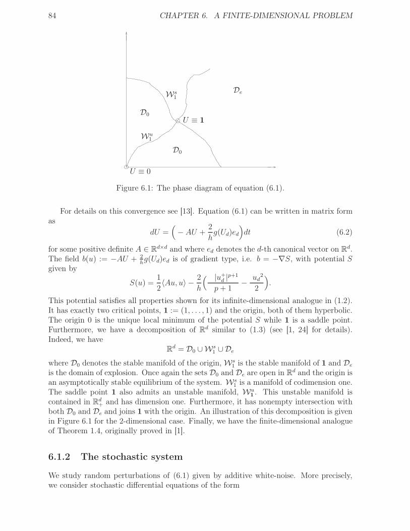
84 CHAPTER 6. A FINITE-DIMENSIONAL PROBLEM
U ≡ 0
U ≡ 1
De
D0
D0
Wu1
Ws1
Figure 6.1: The phase diagram of equation (6.1).
For details on this convergence see [13]. Equation (6.1) can be written in matrix formas
dU =(
− AU +2
hg(Ud)ed
)
dt (6.2)
for some positive definite A ∈ Rd×d and where ed denotes the d-th canonical vector on Rd.The field b(u) := −AU + 2
hg(Ud)ed is of gradient type, i.e. b = −∇S, with potential S
given by
S(u) =1
2〈Au, u〉 − 2
h
( |u+d |p+1
p+ 1− ud
2
2
)
.
This potential satisfies all properties shown for its infinite-dimensional analogue in (1.2).It has exactly two critical points, 1 := (1, . . . , 1) and the origin, both of them hyperbolic.The origin 0 is the unique local minimum of the potential S while 1 is a saddle point.Furthermore, we have a decomposition of Rd similar to (1.3) (see [1, 24] for details).Indeed, we have
Rd = D0 ∪Ws1 ∪ De
where D0 denotes the stable manifold of the origin, Ws1 is the stable manifold of 1 and De
is the domain of explosion. Once again the sets D0 and De are open in Rd and the origin isan asymptotically stable equilibrium of the system. Ws
1 is a manifold of codimension one.The saddle point 1 also admits an unstable manifold, Wu
1. This unstable manifold is
contained in Rd+ and has dimension one. Furthermore, it has nonempty intersection with
both D0 and De and joins 1 with the origin. An illustration of this decomposition is givenin Figure 6.1 for the 2-dimensional case. Finally, we have the finite-dimensional analogueof Theorem 1.4, originally proved in [1].
6.1.2 The stochastic system
We study random perturbations of (6.1) given by additive white-noise. More precisely,we consider stochastic differential equations of the form
6.1. PRELIMINARIES 85
dUε =(
−AUε +2
hg(Uε
d)ed
)
dt+ εdW (6.3)
for ε > 0 small and whereW = (W1, . . . ,Wd) a d−dimensional standard Brownian motion.Given a probability space (Ω,F , P ) and a standard d-dimensional Brownian motion W ,we say that a stochastic process Uε = (Uε(t))t≥0 is a solution up to an explosion time of(6.3) on (Ω,F , P ) and with respect to W if it satisfies the following:
• Uε has continuous paths taking values in Rd ∪ ∞• Uε is adapted to the augmented filtration generated by W .
• For every n ∈ N we have P -almost surely∫ t∧τ (n)
0
|b(Uε(s))| ds < +∞ ∀ 0 ≤ t < +∞
and
Uε(t ∧ τ (n)) = Uε(0) +
∫ t
0
b(Uε(s))1s≤τ (n) ds+ εW (t ∧ τ(n)); ∀ 0 ≤ t < +∞.
where τ (n),ε := inft ≥ 0 : ‖Uε(t)‖∞ ≥ n.• Uε has the strong Markov property.
We call τ ε := limn→+∞ τ (n),ε the explosion time of Uε.
As in the previous chapters, we shall write Uu,ε to denote the unique solution to (6.3)with initial datum u ∈ Rd and also write Uu to denote the corresponding solution to (6.1).Furthermore, for each n ∈ N we consider the truncation S(n) of the potential S given by
S(n)(u) =1
2〈Au, u〉 − 2
hGn(ud)
where Gn : R −→ R is a function of class C2 satisfying that
Gn(u) =
|u+|p+1
p+1− u2
2if u ≤ n
0 if u ≥ 2n.
The unique solution U (n),u to the equation U (n),u = −∇S(n)(U (n),u) with initial datum uis globally defined and coincides with Uu until the escape from the unbounded set
Πn := u ∈ Rd : ud < n.Similarly, for ε > 0 the unique solution U (n),u,ε to the equation
dU (n),u,ε = −∇S(n)(U (n),u,ε)dt+ εdW
with initial datum u is globally defined and coincides with Uu,ε until the escape from Πn.Moreover, since the field −∇S(n) is globally Lipschitz, the family of solutions
(
U (n),u,ε)
ε>0satisfies the analogous large deviations estimates of Section 1.4 with rate function
IuT (ϕ) =
1
2
∫ T
0
|ϕ(s) +∇S(n)(ϕ(s))|2ds if ϕ is absolutely continuous and ϕ(0) = u
+∞ otherwise
Finally, for each ε > 0 and u ∈ Rd the process U (n),u,ε is positive recurrent.
86 CHAPTER 6. A FINITE-DIMENSIONAL PROBLEM
6.1.3 Main results
We now state the main results obtained in this finite-dimensional setting. Some of theseresults are more refined than their infinite-dimensional counterparts. This is due to thefriendlier finite-dimensional setting and also to the convenient choice of reaction term.We maintain the notation of Chapter 1. Our first result is concerned with the almost sureexistence of blow-up for arbitrary initial data and noise parameter.
Theorem I. For any u ∈ Rd and ε > 0 we have Pu(τε < +∞) = 1.
Let us notice that for the infinite-dimensional system we were only able to show that
limε→0
Pu(τε < +∞) = 1.
This is because, by the particular choice of reaction term g, solutions in this setting onlyexplode in one direction, so that comparison arguments can be successfully applied.
Next, we study the asymptotic behavior of the explosion time for initial data in De.
Theorem II. Given δ > 0 and a compact set K ⊆ De there exists C > 0 such that
supu∈K
Pu(|τε − τ0| > δ) ≤ e−C
ε2
for every ε > 0 sufficiently small.
Finally, we show metastable behavior for solutions of (6.3) with initial data u ∈ D0.We have the following results.
Theorem III. Given δ > 0 and a compact set K ⊆ D0 we have
limε→+∞
[
supu∈K
∣
∣
∣Pu
(
e∆−δε2 < τε < e
∆+δ
ε2
)
− 1∣
∣
∣
]
= 0
where ∆ := 2(S(1)− S(0)).
Theorem IV. If for each ε > 0 we define the scaling coefficient
βε = inft ≥ 0 : P0(τε > t) ≤ e−1
then limε→0 ε2 log βε = ∆ and for each compact set K ⊆ D0 and t > 0 we have
limε→0
[
supu∈K
∣
∣Pu(τε > tβε)− e−t∣
∣
]
= 0.
Theorem V. There exists a sequence (Rε)ε>0 with limε→0Rε = +∞ and limε→0Rεβε
= 0such that given δ > 0 for any compact set K ⊆ D0 we have
limε→0
[
supu∈K
Pu
(
sup0≤t≤τε−3Rε
∣
∣
∣
∣
1
Rε
∫ t+Rε
t
f(Uε(s, ·))ds− f(0)
∣
∣
∣
∣
> δ
)]
= 0
for any bounded continuous function f : R → R.
6.2. ALMOST SURE BLOW-UP IN THE STOCHASTIC MODEL 87
With the exception of Theorem I, the proof of the remaining results follow very closelythe ideas featured in the previous chapters for the infinite-dimensional problem (perhapswith even fewer technical difficulties). Thus, we include here only the parts of the analysiswhich differ from the ones given in the previous setting. The main differences appear onthe proof of Theorem II and the construction of the auxiliary domain G. For the latter,we shall exploit the fact that we are in a finite-dimensional setting to obtain a differentconstruction of G, one which does not rely so heavily on the structure of the potential S.In particular, this will allow us to obtain our results for every p > 1 instead of p ∈ (1, 5).Finally, the results presented here can be extended to more general systems than (6.1).We refer the reader to [24] for details on possible extensions.
6.2 Almost sure blow-up in the stochastic model
In this section we devote ourselves to the proof of Theorem I. The idea is to show that,conditioned on non-explosion, the system is guaranteed to enter a specific region of spacein which we can prove that explosion occurs with total probability. From this we canconclude that non-explosion must happen with zero probability. We do this by comparisonwith an adequate Ornstein-Ühlenbeck process. Indeed, let Y y, ε be the solution to
dY y, ε = −(
AY y, ε +2
hY y, εd ed
)
dt+ εdW (6.4)
with initial datum y ∈ Rd. Notice that the drift term in (6.4) is linear and given bya negative definite matrix. Hence, Y y,ε is in fact a d-dimensional Ornstein-Ühlenbeckprocess which admits an invariant distribution supported in Rd. Since we also haveconvergence to this equilibrium measure for any initial distribution, the hitting time ofY y,ε of any open set is finite almost surely.
On the other hand, the drift term of (6.4) is smaller or equal than b so that by thecomparison principle we conclude that if u ≥ y then Uu,ε(t) ≥ Y y,ε holds almost surelyfor as long as Uu,ε is finite. From here, Theorem I follows at once from the next lemmaand the strong Markov property.
Lemma 6.1. If we consider the set
ΘM := y ∈ Rd : yk ≥ 0 for all 0 ≤ k ≤ d− 1 , yd ≥M,
then we have
limM→∞
[
infy∈ΘM
Py(τε <∞)
]
= 1.
Proof. Consider the auxiliary process Zy, ε := Uy, ε−εW . Notice that this process verifiesthe random differential equation
dZy,ε = b(Zy,ε + εW )dt, Zy,ε(0) = y.
Also observe that Zy,ε has the same explosion time as Uy,ε. For each k ∈ N let us definethe set Ak := sup0≤t≤1 |Wd(t)| ≤ k. On Ak we have that Zy,ε verifies the inequality
dZy, ε
dt≥ −AZy, ε − 4
h2εk∑
ei +2
h((Zy, ε
d − εk)p+ − Zy, εd − εk)ed. (6.5)
88 CHAPTER 6. A FINITE-DIMENSIONAL PROBLEM
Observe that (6.5) can be written as
dZy, ε
dt≥ QZy, ε + q + (Zy, ε
d − εk)p+ed ≥ QZy, ε + q,
where Q ∈ Rd×d verifies a comparison principle and q ∈ Rd both depend on ε, h and k,but not on M . This allows us to conclude the inequality Zy, ε
d−1 ≥ −(M + |q|)exp(|Q|)for all 0 ≤ t ≤ min1, τ yε . In particular, for all 0 ≤ t ≤ min1, τ yε the last coordinateverifies the inequality
dZy, εd
dt≥ −α1M + α2Z
y, εd + α3(Z
y, εd )p
Zy, εd (0) ≥M
for positive constants α1, α2, α3 which do not depend on M . It is a straightforwardcalculation to check that solutions to this one-dimensional inequality blow up in a finitetime that converges to zero as M → +∞. Therefore, for each k ∈ N there exists Mk suchthat P (Ak) ≤ infy∈ΘM Py(τε < ∞) for all M ≥ Mk. Since limk→+∞ P (Ak) = 1, thisconcludes the proof.
6.3 Convergence of τuε for initial data in De
Our purpose in this section is to prove Theorem II. We shall only give the upper bound forthe explosion time τuε since the lower bound can be obtained exactly as in Proposition 2.2.We need the following lemma, whose proof can be found on [24].
Lemma 6.2 (Maximum Principle). If U is a solution to (6.1) then for every t ≥ 0
maxk=1,...,d
|Uk(t)| ≤ max maxk=1,...,d
|Uk(0)|, max0≤s≤t
Ud(s). (6.6)
The upper bound for the explosion time is given in the following proposition.
Proposition 6.3. For any δ > 0 and compact set K ∈ De there exists C > 0 such that
supu∈K
Pu(τε > τ0 + δ) ≤ e−C
ε2
for every ε > 0 sufficiently small.
Proof. Given u ∈ K, let Y u be the solution to the ordinary differential equation
Y u = −(
AY u +2
hY u, εd ed
)
with initial datum u. Let us notice that we have Uu ≥ Y u for as long as Uu is definedby the comparison principle. Now, since Y u is the solution to a linear system of ordinarydifferential equations whose associated matrix is symmetric and negative definite, we getthat there exists ρK ∈ R such that for all u ∈ K every coordinate of Uu remains boundedfrom below by ρK + 1 up until τu0 . Thus, if for ρ ∈ R and M > 0 we write
ΘMρ := y ∈ Rd : yk ≥ ρ for all 0 ≤ k ≤ d− 1 , yd ≥M
6.3. CONVERGENCE OF τUε FOR INITIAL DATA IN DE 89
then by Lemma 6.2 we conclude that Tu := inft ≥ 0 : Uut ∈ ΘM+1
ρK+1 is finite. Furthermore,since UM+2, u agrees with Uu until the escape from ΠM+2, we obtain the expression
Tu = inft ≥ 0 : UM+2, ut ∈ ΘM+1
ρK+1.
Taking TK := supu∈K Tu < +∞ we may compute
Pu(
τε(ΘMρK) > Tu
)
≤ Pu(
πM+2ε ∧ τε(ΘM
ρK) > Tu
)
+ Pu(
πM+2ε ≤ Tu , τε(Θ
MρK) > Tu
)
≤ 2 supv∈Rd
Pv
(
sup0≤t≤TK
|UM+2, ε(t)− UM+2(t)| > 1)
.
On the other hand, by the strong Markov property for Uu,ε we get
Pu(
τε > τ0 + δ)
≤ Pu(
τε > Tu + δ)
≤ supy∈ΘMρK
Py(τε > δ) + supu∈K
Pu(
τε(ΘMρK) > Tu
)
. (6.7)
Thus, by (1.9) and the previous computation, in order to finish the proof it will suffice toshow that the first term on the right hand side of (6.7) tends to zero exponentially fast in1ε2
as ε → 0 for an adequate choice of M . To see this we consider for ε > 0 and y ∈ ΘMρK
the processes Y y, ε and Zy, ε defined by
dY y, ε = −(
AY y, ε +2
hY y, εd ed
)
dt+ εdW
and Zy, ε := Uy, ε − Y y, ε, respectively. Notice that Y y, ε is globally defined and thus thatboth Uy, ε and Zy, ε have the same explosion time. Furthermore, Zy, ε is the solution ofthe random differential equation
dZy, ε = −(
AZy, ε +2
h
([
(
Uy,εd
)+]p
− Zy, εd
)
ed
)
dt.
The continuity of trajectories allows us to use the Fundamental Theorem of Calculus toshow that almost surely Zy, ε(ω) is a solution to the ordinary differential equation
Zy, ε(t)(ω) = −AZy, ε(ω) +2
h
([
(
Uy,εd
)+]p
(ω)− Zy, εd (ω)
)
ed. (6.8)
Then, for each y ∈ ΘMρK
and ε > 0 let Ωyε be a set of probability one in which (6.8) holds.Notice that for every ω ∈ Ωyε we have the inequality
Zy, ε(ω) ≥ −AZy, ε(ω)− 2
hZy, εd (ω)ed.
By the comparison principle we conclude that Zy, ε(ω) ≥ 0 for every ω ∈ Ωyε and, therefore,that the inequality Uy, ε(ω) ≥ Y y, ε(ω) holds for as long as Uy, ε(ω) is defined.
For each y ∈ ΘMρK
and ε > 0 let us also consider the set
Ωyε =
ω ∈ Ω : sup0≤t≤δ
|Y y, ε(ω, t)− Y y(ω, t)| ≤ 1 , sup0≤t≤δ
|εW (ω, t)| ≤ 1
.
90 CHAPTER 6. A FINITE-DIMENSIONAL PROBLEM
Our goal is to show that if M is appropriate then for each y ∈ ΘMρK
the trajectory Uy, ε(ω)
explodes before time δ for all ω ∈ Ωyε ∩ Ωyε . From this we get that
infy∈ΘMρK
P (Ωyε) = infy∈ΘMρK
P (Ωyε ∩ Ωyε) ≤ infy∈ΘMρK
Py(τε ≤ δ).
and so by (1.9) we may conclude the result.
Hence, let us take y ∈ ΘMρK
, ω ∈ Ωyε ∩ Ωε and suppose that Uy, ε(ω) is defined in [0, δ].Notice that since ω ∈ Ωyε ∩ Ωε then the (d−1)-th coordinate of Y y, ε(ω, t) is bounded frombelow by ρK − 1 for all t ∈ [0, δ]. By comparison we know that the (d− 1)-th coordinateof Uy, ε
t (ω, t) is bounded from below by ρK − 1 as well. From here we deduce that the lastcoordinate of Uy,ε(ω) verifies the integral equation
Uy, εd (ω, t) ≥ Uy, ε
d (ω, s) +
∫ t
s
2
h
(
− Uy, εd (ω, r) + ρK − 1 + hg
(
Uy, εd (ω, r)
)
)
dr − 1
for s < t in the interval [0, δ]. We can take M ∈ N sufficiently large so as to guaranteethat there exists a constant α > 0 such that for all m ≥ M we have
2
h
(
−m+ ρK − 1 + hg(m))
≥ αmp.
If we recall that Uy, εd (ω, 0) ≥M then our selection of M implies that
Uy, εd (ω, t) ≥M − 1 + α
∫ t
0
(
Uy, εd (ω, u)
)pdu
for every t ∈ [0, δ]. But if this inequality holds and M is sufficiently large, one can checkthat Uy, ε(ω) explodes before time δ, a fact which contradicts our assumptions. Therefore,if y ∈ ΘM
ρKand ω ∈ Ωyε∩Ωε then Uy, ε(ω) explodes before time δ, which concludes the proof.
6.4 Construction of an auxiliary domain
In this final section we present the alternative construction of the auxiliary domain G.The reader will notice that the finite-dimensional environment plays an essential role inthe construction. Despite this fact, we point out that the only other ingredient which isrelevant in this alternative construction is the validity of an analogue of Theorem 1.4, sothat one may carry out the same construction in other systems with a similar description.
We wish to construct a bounded domain G satisfying the following properties:
i. G contains 1 and the origin.
ii. There exists c > 0 such that Bc ⊆ G and for all u ∈ Bc the system Uu is globallydefined and tends to 0 without escaping G.
iii. There exists a closed subset ∂1 of the boundary ∂G which satisfies:
• V (0, ∂G− ∂1) > V (0, ∂1) = V (0, 1).
• ∂1 is contained in De and at a positive distance from its boundary.
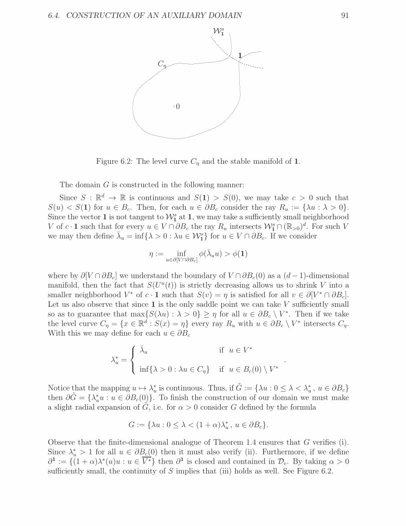
6.4. CONSTRUCTION OF AN AUXILIARY DOMAIN 91
0
1
Ws1
Cη
Figure 6.2: The level curve Cη and the stable manifold of 1.
The domain G is constructed in the following manner:
Since S : Rd → R is continuous and S(1) > S(0), we may take c > 0 such thatS(u) < S(1) for u ∈ Bc. Then, for each u ∈ ∂Bc consider the ray Ru := λu : λ > 0.Since the vector 1 is not tangent to Ws
1at 1, we may take a sufficiently small neighborhood
V of c · 1 such that for every u ∈ V ∩ ∂Bc the ray Ru intersects Ws1∩ (R>0)
d. For such Vwe may then define λu = infλ > 0 : λu ∈ Ws
1 for u ∈ V ∩ ∂Bc. If we consider
η := infu∈∂[V ∩∂Bc]
φ(λuu) > φ(1)
where by ∂[V ∩ ∂Bc] we understand the boundary of V ∩ ∂Bc(0) as a (d− 1)-dimensionalmanifold, then the fact that S(Uu(t)) is strictly decreasing allows us to shrink V into asmaller neighborhood V ∗ of c · 1 such that S(v) = η is satisfied for all v ∈ ∂[V ∗ ∩ ∂Bc].Let us also observe that since 1 is the only saddle point we can take V sufficiently smallso as to guarantee that maxS(λu) : λ > 0 ≥ η for all u ∈ ∂Bc \ V ∗. Then if we takethe level curve Cη = x ∈ Rd : S(x) = η every ray Ru with u ∈ ∂Bc \ V ∗ intersects Cη.With this we may define for each u ∈ ∂Bc
λ∗u =
λu if u ∈ V ∗
infλ > 0 : λu ∈ Cη if u ∈ Bc(0) \ V ∗.
Notice that the mapping u 7→ λ∗u is continuous. Thus, if G := λu : 0 ≤ λ < λ∗u , u ∈ ∂Bcthen ∂G = λ∗uu : u ∈ ∂Bc(0). To finish the construction of our domain we must makea slight radial expansion of G, i.e. for α > 0 consider G defined by the formula
G := λu : 0 ≤ λ < (1 + α)λ∗u , u ∈ ∂Bc.
Observe that the finite-dimensional analogue of Theorem 1.4 ensures that G verifies (i).Since λ∗u > 1 for all u ∈ ∂Bc(0) then it must also verify (ii). Furthermore, if we define∂1 := (1 + α)λ∗(u)u : u ∈ V ∗ then ∂1 is closed and contained in De. By taking α > 0sufficiently small, the continuity of S implies that (iii) holds as well. See Figure 6.2.
92 CHAPTER 6. A FINITE-DIMENSIONAL PROBLEM
6.5 Resumen del Capítulo 6
Estudiamos las propiedades asintóticas del tiempo de explosión para perturbaciones aleato-rias por ruido blanco aditivo de la ecuación diferencial ordinaria
U ′1 = 2
h2(−U1 + U2),
U ′i = 1
h2(Ui+1 − 2Ui + Ui−1) 2 ≤ i ≤ d− 1,
U ′d = 2
h2(−Ud + Ud−1 + hg(Ud))
U(0) = u
donde h > 0 es un parámetro fijo y g : R → R es un término de reacción dado porg(x) = (x+)p−x para p > 1. Este tipo de sistemas surge como discretizaciones espacialesde ecuaciones de difusión con condiciones de frontera no lineales de Neumann. De hecho,puede probarse que cuando h→ 0 las soluciones de este sistema convergen a las soluciónde la EDP
∂tU(t, x) = ∂2xxU(t, x) 0 < x < 1, 0 ≤ t < T,∂xU(t, 0) = 0 0 ≤ t < T,∂xU(t, 1) = g(U(t, 1)) 0 ≤ t < T,U(0, x) = U0(x) 0 ≤ x ≤ 1.
La ecuación diferencial ordinaria puede escribirse como en forma matricial como
dU = −∇S,
donde S viene dado por
S(u) =1
2〈Au, u〉 − 2
h
( |u+d |p+1
p+ 1− ud
2
2
)
.
para cierta matriz A ∈ Rd×d definida positiva. Este potencial S satisface las mismaspropiedades que su análogo infinito-dimensional en (1.2). Tiene exactamente dos puntoscríticos, 1 := (1, . . . , 1) y el origen, ambos ellos hiperbólicos. El origen 0 es el únicomínimo local de S mientras que 1 es un punto de ensilladura. Más aún, se tiene unadescomposición de Rd análoga a la de (1.3).
Las perturbaciones estocásticas que vamos a considerar son de la forma
dUε = −∇Sdt + εdW
par ε > 0 pequeño y dondeW = (W1, . . . ,Wd) es un movimiento Browniano d-dimensionalestándar. La solución Uε de esta EDOE conserva las propiedades de la solución de (1.4).
Los resultados que podemos probar en este contexto son esencialmente los mismosque para la EDP (1.1), con la excepción de que la restricción p < 5 desaparece en estecontexto puesto que la geometría del potencial S puede manejarse con mayor facilidadal estar definido sobre un espacio finito-dimensional como lo es Rd (el potencial de (1.1)estaba definido CD([0, 1]), un espacio infinito-dimensional). Por otro lado, la elecciónparticular del término g (con término no lineal acotado inferiormente) nos permite probarademás que el fenómeno de blow-up se hace presente casi seguramente.
Teorema. Para cualquier u ∈ Rd y ε > 0 tenemos P (τuε < +∞) = 1.
6.5. RESUMEN DEL CAPÍTULO 6 93
La idea de la demostración de este resultado consiste en mostrar que, condicionadoa no explotar, el sistema estocástico alcanza inexorablemente una región particular delespacio en donde uno puede probar que el fenómeno de blow-up ocurre con probabilidadtotal. A partir de esto se deduce inmediatamente que la ausencia de blow-up debe darsecon probabilidad nula. Mostramos que el proceso alcanza esta región particular mediantecomparación con un proceso de Ornstein-Ühlenbeck adecuado, mientras que la explosióncasi segura ocurre en esa región se obtiene mediante técnicas de ecuaciones similares a lasempleadas durante el Capítulo 2.
Con respecto a los resultados restantes, la demostración de los mismos sigue muy decerca las ideas presentadas en los capítulos anteriores para el problema infinito-dimensional(con quizás menos dificultades técnicas). Incluimos en este capítulo únicamente las partesdel análisis que difieren de aquellas dadas en el marco anterior. Estas aparecen en la de-mostración de lo que sería el Teorema I en este contexto y en la construcción del dominioauxiliar G. Con respecto al Teorema I, el potencial en este contexto tiene una estruc-tura ligeramente diferente al infinito-dimensional, lo cual no nos permite adaptar porcompleto las ideas desarrolladas en el Capítulo 2 y nos obliga por lo tanto a introduciralgunas variantes de las técnicas de ecuaciones empleadas durante éste. Finalmente, parala construcción de G explotamos el marco finito-dimensional de este nuevo problema paraproponer una nueva construcción que no impone la restricción p < 5. A partir de aquí,pueden obtenerse los resultados restantes para todo p > 1.

94 CHAPTER 6. A FINITE-DIMENSIONAL PROBLEM
Part II
The Fernández-Ferrari-Garcia dynamics
on diluted models
95

Introducción a la Parte II
La mecánica estadística del equilibrio intenta explicar el comportamiento macroscópicode sistemas en equilibrio térmico en términos de la interacción microscópica entre sugran número de constituyentes. Como un ejemplo típico, uno podría tomar un materialferromagnético como el hierro: sus constituyentes son entonces los spins de los imaneselementales en los sitios de un cierto reticulado de cristal. O también podemos pensar enuna aproximación discreta de un gas real, en cuyo caso los constituyentes son los númerosde partículas en las celdas elementales de cualquier partición del espacio. El objeto cen-tral en cualquiera de estos sistemas es el Hamiltoniano que describe la interacción entrelos constituyentes. Éste determina la energía relativa entre configuraciones que difierenúnicamente microscópicamente. Los estados de equilibrio con respecto a la interaccióndada son descritos por las medidas de Gibbs asociadas. Éstas son medidas de proba-bilidad en el espacio de configuraciones con probabilidades condicionales dadas respectoa configuraciones fijas fuera de regiones acotadas. Dichas probabilidades condicionalesson determinadas por el factor de Boltzmann: la exponencial de la temperatura inversamultiplicada por la energía relativa. Esto le permite a uno calcular, al menos en princi-pio, esperanzas en equilibrio y funciones de correlación espacial siguiendo el formalismode Gibbs estándar. El conjunto de medidas de Gibbs para una interacción dada es unsimplex cuyos vértices llamamos medidas de Gibbs extremales. Estas medidas extremalesson de mayor importancia puesto que describen los posibles macroestados (o fases deequilibrio) de nuestro sistema físico. En un estado tal, las observables macroscópicas nofluctúan mientras que la correlación entre observaciones locales hechas a larga distanciaentre ellas decaen a cero. Un aspecto muy importante en el estudio de cualquier sistemade la mecánica estadística del equilibrio es determinar cuando existe más de un posiblemacroestado para el sistema, un fenómeno conocido como transición de fase. Por la es-tructura de simplex del conjunto de medidas de Gibbs, la ocurrencia de transición de fasepara un sistema dado es equivalente a la existencia de medidas de Gibbs múltiples (nonecesariamente extremales).
Uno de los modelos más famosos y mejor entendidos de la mecánica estadística esel modelo de Ising ferromagnético estándar en el reticulado Z2. En este modelo, sobrecada sitio del reticulado se tiene una variable de spin que toma puede tomar solamentelos valores + y −. La interacción es entre vecinos más cercanos y tiende a alinear spinsvecinos en la misma dirección. Mediante los argumentos ingeniosos formulados en primerainstancia por Peierls en 1936, la transición de fase en este modelo puede entenderse através de la inspección de configuraciones típicas de contornos, i.e. líneas quebradas queseparan los dominios con spins + y −, respectivamente. Para temperaturas bajas, existeuna fase + que es realizada por un mar infinito de spins + con islas finitas de spins
97
98
− (que a su vez pueden contener lagos de spins +, y así sucesivamente). En términosde contornos, este panorama equivale a que haya únicamente finitos contornos rodeandocada sitio del reticulado. También se tiene una fase − que verifica la descripción simétrica.Por otro lado, por encima de cierta temperatura crítica no existe ningún camino infinitoque una vecinos más cercanos con el mismo spin. Por lo tanto, para este modelo laestructura geométrica de las configuraciones típicas está bien entendida (ver [41, 22] porejemplo). En general, sin embargo, se sabe mucho menos, y mucho menos es cierto. Aúnasí, ciertos aspectos de este análisis geométrico tienen amplias aplicaciones, al menos enciertos regímenes del diagrama de fases. Estos “ciertos regímenes” son, por un lado, elrégimen de alta temperatura (o, en el contexto de gases, baja densidad) y, al otro extremo,el comportamiento a baja temperatura (o altas densidades).
A temperaturas altas o baja densidad, todas las consideraciones termodinámicas estánbasadas en el hecho de que la entropía domina sobre la energía. Esto es, la interacciónentre los constituyentes no es lo suficientemente efectiva para forzar un ordenamientomacroscópico del sistema. Como resultado, los constituyentes se comportan aproximada-mente al azar, no muy influenciados por otros constituyentes que se encuentran lejos. Así,el comportamiento del sistema es casi el de un sistema libre con componentes indepen-dientes. Esto significa, en particular, que en el centro de una caja grande típicamentevamos a encontrar aproximadamente las mismas configuraciones sin importar qué condi-ciones de frontera sean impuestas fuera de dicha caja. A bajas temperaturas o densidadesgrandes (cuando la interacción es suficientemente fuerte), el panorama de arriba ya no esválido. En realidad, las características específicas de la interacción entrarán en juego ydeterminarán las cualidades específicas de los macroestados. En muchos casos, el compor-tamiento a baja temperatura puede ser descrito como una perturbación aleatoria de unestado fundamental, i.e. una configuración fija de energía mínima. Luego, a bajas tem-peraturas podemos esperar que las fases de equilibrio se realicen como una configuraciónde estado fundamental determinística, perturbada por finitas islas aleatorias en donde laconfiguración difiere con dicho estado fundamental. Esto significa que el patrón del estadofundamental puede percolar a través del espacio hasta el finito. Una manera prominentede confirmar este panorama general es provista por la llamada teoría de Pirogov-Sinai,descrita en detalle en [44].
Esencialmente, esta teoría introduce en primer lugar una noción generalizada de con-tornos que puede ser utilizada por una amplia gama de sistemas y luego da condicionesque garantizan cuando existen solamente finitos de estos contornos alrededor de cada sitiodel reticulado. Cuando esto suceda, un panorama similar al del modelo de Ising puedeobtenerse. Más allá de lo poderosa que sea como herramienta, una de las desventajas dela teoría de Pirogov-Sinai es que la mayoría de sus aplicaciones se apoyan fuertemente enla convergencia absoluta de ciertas expansiones, llamadas expansiones en aglomerados, yesta convergencia muchas veces depende de resultados combinatorios profundos. Así, lateoría de Pirogov-Sinai constituye en realidad (al menos hasta cierto grado) un enfoquemás combinatorio que probabilístico para entender las fases de equilibrio de un sistemafísico dado. Como el problema matemático mismo se encuentra formulado dentro de unmarco probabilístico, uno puede ver que este enfoque quizás no sea el más natural posible.Más aún, debido a la absoluta convergencia de las expansiones involucradas, uno obtienegratuitamente la analiticidad de las funciones de correlación con respecto a los parámet-ros del modelo (como lo son la temperatura inversa o la densidad de partículas). Aunque

99
la analiticidad es una buena propiedad para tener, es también un síntoma de que esteenfoque es quizás demasiado fuerte y no óptimo desde el punto de vista probabilístico.
Como una alternativa, en [16] los autores proveen un enfoque nuevo al estudio de estetipo de sistemas, uno que es puramente probabilístico. En lugar de depender de las ex-pansiones en aglomerados para probar que existe una medida de equilibrio que satisfaceel panorama de mar con islas descrito arriba, ellos realizan esta medida como la distribu-ción estacionaria de una red de pérdida que puede ser estudiada utilizando herramientasestándar y nociones de modelos probabilísticos y procesos. En este contexto, la existenciade la medida de equilibrio está relacionada con la ausencia de percolación en un procesode percolación orientada. Más aún, muestran que la dinámica converge exponencialmenterápido a la medida buscada, de manera que este enfoque es también valioso para propósi-tos de simulación. Para ser precisos, en su trabajo los autores consideran únicamente elmodelo de contornos de Peierls para la interacción de Ising a baja temperatura, mientrasque en [17] discuten como algunas de estas ideas pueden ser extendidas a otros modelos.
En esta segunda parte de la tesis introducimos una familia general de sistemas, laclase de los modelos diluidos, y mostramos que los resultados principales en [16] puedenextenderse a esta familia más amplia. El marco de modelos diluidos encaja perfectamentecon el rango de aplicabilidad de este nuevo enfoque: los modelos diluidos son, quizás, lafamilia más amplia de modelos a la cual la dinámica presentada en [16] pueda aplicarse.Este marco incluye tanto modelos discretos como continuos de manera unificada, pero eslo suficientemente concreto como para que aún sea posible obtener un criterio general parala existencia de la medida de equilibrio. Concretamente, en esta segunda parte vamos adesarrollar el siguiente plan:
i. Introducir la familia de modelos diluidos y mostrar que para cualquier elemento enesta familia podemos definir una dinámica con las características mostradas en [16].
ii. Utilizar la construcción de la dinámica para obtener un criterio general para launicidad de medidas de Gibbs en modelos diluidos y estudiar propiedades de esteúnico equilibrio, como la propiedad de mixing exponencial.
iii. Mostrar que la ausencia de percolación en el proceso de percolación orientada implicala continuidad de las funciones de correlación con respecto a los parámetros delmodelo.
iv. Explotar el marco general de los modelos diluidos y las características de sus dinámi-cas asociadas para mostrar que, bajo condiciones adecuadas, las medidas de equi-librio de sistemas discretos convergen, cuando son apropiadamente escaladas, a lamedida de equilibrio de sistemas continuos en el régimen de alta temperatura o bajadensidad.
v. Combinar las ideas y resultados previos con el marco de la teoría de Pirogov-Sinaipara obtener algunos resultados fuera del rango de convergencia de las expansionesen aglomerados.
vi. Combinar las ideas y resultados previos con el marco de la teoría de Pirogov-Sinaipara obtener un algoritmo de simulación perfecta para una clase medianamentegrande de medidas de equilibrio en el régimen de baja temperatura o alta densidad.

100
La Parte II está organizada de la siguiente manera. En el Capítulo 7 proveemos delmarco teórico en donde se definen los modelos diluidos. El Capítulo 8 se enfoca en ladefinición de modelos diluidos y alguna de sus propiedades básicas. En este capítulotambién adaptamos algunas nociones elementales de la mecánica estadística a este marcode trabajo. El capítulo siguiente esta destinado a mostrar lo restante de (i) y (ii) en el plande arriba. Los items (iii) y (iv) son establecidos en los Capítulos 10 y 11, respectivamente.Finalmente, los items (v) y (vi) se establecen en el Capítulo 12.
Introduction to Part II
Equilibrium statistical mechanics intends to explain the macroscopic behavior of systemsin thermal equilibrium in terms of the microscopic interaction between their great manyconstituents. As a typical example, one may take some ferromagnetic material like iron:the constituents are then the spins of elementary magnets at the sites of some crystallattice. Or we can also think of a lattice approximation to a real gas, in which case theconstituents are the particle numbers in the elementary cells of any partition of space.The central object in any of these systems is the Hamiltonian describing the interactionbetween the constituents. It determines the relative energy between configurations thatdiffer only microscopically. The equilibrium states with respect to the given interaction aredescribed by the associated Gibbs measures. These are probability measures on the spaceof configurations which have prescribed conditional probabilities with respect to fixedconfigurations outside of bounded regions. These conditional probabilities are given by theBoltzmann factor: the exponential of the inverse temperature times the relative energy.This allows one to compute, at least in principle, equilibrium expectations and spatialcorrelation functions following the standard Gibbs formalism. The set of Gibbs measuresfor a given interaction is a simplex whose vertices we call extremal Gibbs measures.These are most important since they describe the possible macrostates (or equilibriumphases) of our physical system. In such a state, macroscopic observables do not fluctuatewhile the correlation between local observations made far apart from each other decaysto zero. A very important aspect in the study of any system in equilibrium statisticalmechanics is determining whether there exists more than one possible macrostate for thesystem, a phenomenon known as phase transition. By the simplex structure of the set ofGibbs measures, the occurrence of phase transition for a given system is equivalent to theexistence of multiple (not necessarily extremal) Gibbs measures.
One of the most famous and better understood models in statistical mechanics is thestandard ferromagnetic Ising model on the square lattice. In this model, at each siteof the lattice we have a spin variable taking only two possible values, + and −. Theinteraction is nearest-neighbor and tends to align neighboring spins in the same direction.By the ingenious arguments first formulated in 1936 by Peierls, the phase transition inthis model can be understood from looking at the typical configurations of contours, i.e.broken lines separating the domains with plus and minus spins, respectively. For lowtemperatures, there exists a plus phase which is realized by an infinite sea of plus spinswith finite islands of minus spins (which in turn may contain lakes of plus spins, andso on). In terms of contours, this picture corresponds to there being only finitely manycontours surrounding any site in the lattice. One also has a minus phase verifying thesymmetric description. On the other hand, above a certain critical temperature there is no
101
102
infinite path joining nearest neighbors with the same spin value. Thus, for this model thegeometric structure of typical configurations is well understood (see [41, 22] for example).In general, however, much less is known, and much less is true. Still, certain aspects ofthis geometric analysis have wide applications, at least in certain regimes of the phasediagram. These “certain regimes” are, on the one hand, the high-temperature (or, in alattice gas setting, low-density) regime and, to the other extreme, the low temperaturebehavior (or high density).
At high temperatures, all thermodynamic considerations are based on the fact thatentropy dominates over energy. That is, the interaction between the constituents is noteffective enough to enforce a macroscopic ordering of the system. As a result, constituentsbehave more or less at random, not much influenced by constituents which are far apart.Thus, the behavior of the system is almost like that of a free system with independentcomponents. This means, in particular, that in the center of a large box we will typicallyencounter more or less the same configurations no matter what boundary conditions areimposed outside this box. At low temperatures or large densities (when the interaction issufficiently strong), the picture above no longer holds. Rather, the specific characteristicsof the interaction will come into play and determine the specific features of the lowtemperature macrostates. In many cases, the low temperature behavior can be describedas a random perturbation of a ground state, i.e. a fixed configuration of minimal energy.Then we can expect that, at low temperatures, the equilibrium phases are realized as adeterministic ground state configuration, perturbed by finite random islands on which theconfiguration disagrees with the ground state. This means that the ground state patterncan percolate through the space to infinity. One prominent way of confirming this generalpicture is provided by the so called Pirogov-Sinai theory, described in detail in [44].
Essentially, this theory first introduces a generalized notion of contours which can beused for a wide range of systems and then gives conditions which guarantee when are thereonly finitely many of such contours surrounding each site in the lattice. Whenever this isthe case, a similar picture to the one for the Ising model can be obtained. As powerfula tool as it may be, one of the disadvantages of Pirogov-Sinai theory is that most ofits applications rely heavily on the absolute convergence of certain expansions, knownas the cluster expansions, and this convergence often depends on deep combinatorialresults. Thus, in fact Pirogov-Sinai theory constitutes (at least to some degree) moreof a combinatorial approach to understanding the equilibrium phases of a given physicalsystem rather than a probabilistic one. Since the mathematical problem itself is posedwithin the probabilistic framework, one can see that this approach is perhaps not themost natural one to have. Furthermore, due to the absolute convergence of the expansionsinvolved, one obtains for free the analyticity of correlation functions with respect to theparameters in the model (e.g. inverse temperature or density of particles). Thoughanalyticity is a very nice property to have, it is also a symptom that this approach isperhaps too strong and not optimal from the probabilistic point of view.
As an alternative, in [16] the authors provide a fresh new approach to study this typeof systems, one which is purely probabilistic. Instead of relying on cluster expansionsto prove that there exists an equilibrium measure satisfying the sea with islands picturedescribed above, they realize this measure as the stationary distribution of a loss networkdynamics that can be studied using standard tools and notions from probabilistic modelsand processes. In this context, the existence of the equilibrium measure is related to the
103
absence of percolation in an oriented percolation process. Furthermore, they show thatthe dynamics converges exponentially fast to the desired measure, so that this approachis also valuable for simulation purposes. Strictly speaking, in their work the authorsonly consider the model of Peierls contours for the Ising interaction at low temperature(i.e. low density of contours), while in [17] they discuss how some of these ideas can beextended to other models in the low density regime.
In this second part of the thesis we introduce a general family of systems calleddiluted models, and show that the main results obtained in [16] can be extended to thisbroader family. The framework of diluted models perfectly fits the range of applicability ofthis new approach: diluted models are, perhaps, the broadest family of models for whichthe dynamics presented in [16] may be applied. This framework covers both discrete andcontinuum systems in an unified way, while remaining concise enough so that a generalcriterion for the existence of the equilibrium measure can still be obtained. Concretely,in this second part of the thesis we carry out the following plan:
i. Introduce the family of diluted models and show that for any element in this familywe can define a dynamics with the characteristics shown in [16].
ii. Use the construction of the dynamics to obtain a general criterion for uniqueness ofGibbs measures in diluted models and study properties of this unique equilibrium,such as exponential mixing.
iii. Show that the absence of percolation in the oriented percolation process implies thecontinuity of correlation functions with respect to the parameters of the model.
iv. Exploit the general framework of diluted models and the characteristics of theirassociated dynamics to show that, under suitable conditions, equilibrium measuresof discrete systems converge, when properly rescaled, to equilibrium measures ofcontinuum systems in the high temperature (or low density) regime.
v. Combine the previous ideas and results with the framework of Pirogov-Sinai theoryto obtain results outside the range of convergence of cluster expansions.
vi. Combine the previous ideas and results with the framework of Pirogov-Sinai theoryto obtain a perfect simulation algorithm for a large class of equilibrium measures inthe low temperature (or high density) regime. This extends the previous results in[16] obtained for the high temperature (or low density) regime.
Part II is organized as follows. In Chapter 7 we provide the theoretical setting inwhich diluted models are defined. Chapter 8 focuses on the definition of diluted modelsand some of their basic properties. In this chapter we also adapt some elementary notionsfrom statistical mechanics to this framework. The following chapter is devoted to showingthe remainder of (i) and (ii) in the plan above. Items (iii) and (iv) are established inChapters 10 and 11, respectively. Finally, items (v) and (vi) are settled in Chapter 12.

104
Chapter 7
Preliminaries
Since we intend the class of diluted models to include discrete and continuum models,we are interested in adopting a general framework which a priori makes no distinctionbetween both types of systems. The correct framework is that of particle configurations,which we introduce now. We refer to [26, 12, 11] for further details.
7.1 Particle configurations
Throughout this second part we fix two locally compact complete separable metric spaces:the allocation space or lattice (S, dS) and the animal set or spin set (G, dG). Typicalexamples of allocation spaces include S = Zd or S = Rd for some d ∈ N, whereas the spinset can range from finite sets such as G = +,−, to uncountable sets such as G = Sd−1.The product space S × G is also a locally compact complete separable metric space ifendowed with the product metric dS + dG. For convenience, we shall denote an element(x, γ) ∈ S ×G simply by γx, which we interpret as an animal γ positioned at location x.
Notation 7.1. Given a metric space (X, d) we write:
• BX for the class of all Borel subsets of X.
• B0X for the class of all Borel subsets of X with compact closure.
Definition 7.2. Let ξ be a measure on (S ×G,BS×G).
• ξ is said to be a Radon measure if ξ(B) < +∞ for every B ∈ B0S×G.
• ξ is said to be a particle configuration if ξ(B) ∈ N0 for every B ∈ B0S×G.
Proposition 7.3. A Radon measure ξ on (S×G,BS×G) is a particle configuration if andonly if there exist a countable set Qξ ⊆ S ×G and mξ : Qξ → N such that
ξ =∑
γx∈Qξmξ(γx)δγx (7.1)
with δγx being the Dirac measure centered at γx. We call (7.1) the standard representationof the particle configuration ξ.
105
106 CHAPTER 7. PRELIMINARIES
Thus any particle configuration on S × G may also be regarded as a locally finitepoint configuration on S × G where the points are allowed to have varied multiplicities.In the following we shall often view particle configurations in this manner if convenient.With this in mind, we define the support of ξ as
[ξ] := (γx, i) ∈ (S ×G)× N : γx ∈ Qξ and i ≤ mξ(γx)
which is merely the set of points that constitute ξ as a point configuration counted withtheir respective multiplicities. If we only wish to consider the set of points in ξ withoutregard for their multiplicities then we shall write 〈ξ〉, i.e. the projection onto S×G of [ξ].
Definition 7.4. A measure ξ on (S ×G,BS×G) is said to be of locally finite allocation ifit satisfies ξ(Λ×G) < +∞ for every Λ ∈ B0
S.
Notation 7.5.
• We shall write N (S×G) to denote the space of all particle configurations on S×Gwhich are of locally finite allocation.
• Given Λ ∈ B0S we write N (Λ×G) to denote the space of all particle configurations
of locally finite allocation which are supported on Λ×G.
7.2 The space N (S ×G) of particle configurations
7.2.1 Restriction and superposition of particle configurations
Definition 7.6. Given ξ ∈ N (S ×G) and A ∈ BS×G we define the restriction of ξ to Aas the particle configuration ξA given for every B ∈ BS×G by the formula
ξA(B) = ξ(A ∩B).
Equivalently, if ξ =∑
γx∈Qξ m(γx)δγx we define ξA through the standard representation
ξA =∑
γx∈Qξ∩Am(γx)δγx .
Definition 7.7. Given σ, η ∈ N (S × G) we define their superposition as the particleconfiguration σ · η given for every B ∈ BS×G by the formula
σ · η(B) = σ(B) + η(B).
Remark 7.8. Given Λ ∈ B0S there is a natural identification between N (S × G) and
N (Λ×G)×N (Λc×G) given by the restriction and superposition operations, i.e. we havethat the applications
N (S ×G)r−→ N (Λ×G)×N (Λc ×G) N (Λ×G)×N (Λc ×G)
s−→ N (S ×G)ξ 7−→ (ξΛ×G, ξΛc×G) and (σ, η) 7−→ σ · η.
are bijections and have each other as their respective inverse.
7.2. THE SPACE N (S ×G) OF PARTICLE CONFIGURATIONS 107
7.2.2 Measurable structure
The space N (S × G) can be endowed with a measurable space structure by consideringthe σ-algebra F generated by the counting events
F = σ(
ξ ∈ N (S ×G) : ξ(B) = k : k ∈ N0 and B ∈ B0S×G
)
. (7.2)
Furthermore, for any A ∈ BS×G we define FA, the σ-algebra of events occurring in A, byconsidering only the counting events inside A, i.e.
FA = σ(
ξ ∈ N (S ×G) : ξ(B) = k : k ∈ N0 and B ∈ B0A
)
.
Alternatively, if for every B ∈ BS×G we define the respective counting random variableNB : N (S×G) → N0 by the formula NB(η) = η(B) then for each A ∈ BS×G the σ-algebraFA can also be defined as the one generated by the counting random variables inside A,i.e.
FA = σ(
NB : B ∈ B0A
)
.
Remark 7.9. For any Λ ∈ B0s the identification N (S × G) = N (Λ × G) × N (Λc × G)
on Remark 7.8 is in fact a measurable isomorphism when endowing each space with theσ-algebras F and FΛ×G ⊗FΛc×G, respectively.
Definition 7.10.
• A function f : N (S × G) → R is called a local function if there exists Λ ∈ B0S such
that f is FΛ×G-measurable.
• An event A ∈ F is called a local event if 1A is a local function.
• Given a function f : N (S ×G) → R we define its measurability support as
Λf =⋂
Λ∈DfΛ
where Df = Λ ∈ BS : f is FΛ×G-measurable. That is, Λf is the smallest closed setΛ ∈ BS such that f is FΛ×G-measurable. Notice that if f is local then Λf ∈ B0
S.
Remark 7.11. Notice that a function f : N (S×G) → R is FΛ×G-measurable if and onlyif f(σ) = f(η) whenever σ, η ∈ N (S ×G) are such that σΛ×G = ηΛ×G.
7.2.3 Topological structure
The space N (S ×G) can also be endowed with a topological structure. We think of anytwo particle configurations ξ, η as close to each other whenever the particles in ξ lyinginside some sufficiently large compact set K can be matched with nearby particles of ηand viceversa. The precise definitions are given below.
Definition 7.12. Given δ > 0 and ξ, η ∈ N (S) we say that ξ is δ-embedded in η if thereexists an injective application p : [ξ] → [η] such that d (πS×G(x, i), πS×G(p(x, i))) < δfor each (x, i) ∈ [ξ], where πS×G : (S × G) × N → S is the projection onto S × G andd = dS + dG is the metric on S ×G. We denote it by ξ δ η.
108 CHAPTER 7. PRELIMINARIES
Definition 7.13. Given a particle configuration ξ ∈ N (S×G), a compact set K ⊆ S×Gand δ > 0 we define the (K, δ)-neighborhood of ξ by the formula
(ξ)K,δ = η ∈ N (S ×G) : ξK δ η and ηK δ ξ.
Definition 7.14. We define the vague topology on N (S×G) as the one generated by thebasis
B = (ξ)K,δ : ξ ∈ N (S ×G), K ⊆ S ×G compact and δ > 0.
Remark 7.15. It can be shown that N (S×G) admits a metric which is consistent withthe vague topology under which it is complete and separable.
Remark 7.16. The σ-algebra F defined in (7.2) is actually the Borel σ-algebra given bythe vague topology on N (S ×G).
7.3 Poisson processes on S ×G
We shall call any random element of N (S × G) a point process on S × G. Throughoutthis part we shall work with many different point processes on S ×G, all of them relatedin one way or another to the Poisson point process, which we define below.
Definition 7.17. Let ν be a measure on (S × G,BS×G) with locally finite allocation.The Poisson measure with intensity ν is defined as the unique measure πν on N (S ×G)which satisfies
πν(ξ ∈ N (S ×G) : ξ(Bi) = ki for all i = 1, . . . , n) =n∏
i=1
e−ν(Bi) (ν(Bi))ki
ki!
for all k1, . . . , kn ∈ N0, disjoint B1, . . . , Bn ∈ B0S×G and n ∈ N.
Definition 7.18. Let ν be a measure on (S × G,BS×G) with locally finite allocation.A point process X on S × G is called a Poisson process with intensity measure ν ifit is distributed according to πν , i.e. for every n ∈ N and all choices of disjoint setsB1, . . . , Bn ∈ B0
S×G the random variables X(B1), . . . , X(Bn) are independent and have aPoisson distribution with respective means ν(B1), . . . , ν(Bn).
It follows from Definition 7.18 that if X is a Poisson process with intensity measure νand we consider Λ ∈ B0
S then, conditioned on the event X(Λ×G) = n, the locations ofthese n particles inside Λ×G are independent and distributed according to ν
ν(Λ×G). The
next proposition found in [33, Proposition 3.1] generalizes this idea to obtain a convenientformula for the integral of functions with respect to the restricted Poisson measures.
Proposition 7.19. For any Λ ∈ B0S and any bounded nonnegative f : N (Λ × G) → R
we have the formula∫
f(σ)dπνΛ(σ) =
∞∑
n=0
e−ν(Λ×G)
n!
∫
(Λ×G)nf
(
n∑
i=1
δγix
)
dνn(γ1x, . . . , γnx ) (7.3)
where νn denotes the n-fold product measure of ν.
7.3. POISSON PROCESSES ON S ×G 109
In our work we shall, among other things, establish limit theorems for point processes.Therefore, we shall require a notion of convergence which is appropriate for our purposes.The most familiar notion available is that of convergence in distribution.
Definition 7.20. We say that a sequence (Xn)n∈N of point processes on S×G convergesin distribution to a point process X on S ×G if
limn→+∞
E(f(Xn)) = E(f(X))
for every bounded continuous function f : N (S ×G) → R. We denote it by Xnd−→ Xn.
At some points throughout our work the use of local functions shall be much morenatural than that of continuous ones. Under such circumstances we shall adopt insteadthe notion of local convergence for point processes, which we introduce next.
Definition 7.21. We say that a sequence (Xn)n∈N of point processes on S×G convergeslocally to a point process X on S ×G if
limn→+∞
E(f(Xn)) = E(f(X))
for every bounded local function f : N (S ×G) → R. We denote it by Xnloc−→ Xn.
It is important to notice that in most cases local functions need not be continuous.Therefore, in general the notions of local convergence and convergence in distribution donot coincide. Nevertheless, since local functions are always dense in the space of uniformlycontinuous functions with the supremum norm, we get the following result.
Theorem 7.22. Local convergence implies convergence in distribution.
110 CHAPTER 7. PRELIMINARIES
7.4 Resumen del Capítulo 7
En este primer capítulo de la segunda parte introducimos el marco teórico sobre el cuáldefiniremos todos los modelos que nos interesará estudiar. Todos estos modelos serán casosparticulares de configuraciones de partículas aleatorias. Dado un espacio de posiciones Sy otro de spines G, una configuración de partículas ξ en S×G es una medida sobre S×Gque admite la representación
ξ =∑
(x,γ)∈Qξ
mξ(x, γ)δ(x,γ)
para cierto conjunto numerable Qξ ⊆ S × G sin puntos de acumulación y una funciónmξ : Qξ → N. Denotamos por N (S × G) al espacio de aquellas configuraciones departículas ξ en S × G que satisfacen que Qξ ∩ (Λ × G) es finito para todo subconjuntoacotado Λ de S.
El espacio N (S×G) tiene una estructura de espacio medible bajo la σ-álgebra generadapor los eventos de conteo, i.e.
F = σ (ξ ∈ N (S ×G) : ξ(B) = k : k ∈ N0 y B ⊆ S boreliano acotado) .
También existe una topología natural en este espacio, la topología vaga, que es la generadapor la base
B = (ξ)K,δ : ξ ∈ N (S ×G), K ⊆ S ×G compacto y δ > 0,
donde el entorno (ξ)K,δ viene dado por
(ξ)K,δ = η ∈ N (S ×G) : ξK δ η and ηK δ ξ.
y cuando, dadas dos configuraciones de partículas ξ y η, por ξK δ η entendemos que existeuna correspondencia inyectiva (teniendo en cuenta la multiplicidad) entre las partículasde ξ dentro de K y las de η tal que las partículas correspondidas están a distancia menorque δ entre sí. Puede verse que esta topología es metrizable y que así N (S × G) resultacompleto y separable.
Provistos de este marco teórico, podemos definir el más básico de los modelos deinterés que es el Proceso de Poisson. Dada una medida ν en S ×G con ν(Λ×G) < +∞para todo Λ ⊆ S acotado, decimos que una configuración de partículas aleatoria X es unproceso de Poisson en S ×G si
1. Para cada B ⊆ S×G boreliano la variable aleatoria X(B) tiene distribución Poissonde parámetro ν(B)
2. Si B1, . . . , Bn son borelianos disjuntos de S × G entonces las variables aleatoriasX(B1), . . . , X(Bn) son independientes.
Todos los demás modelos que estudiemos en esta segunda parte se podrán obtener, deuna manera u otra, a partir de un proceso de Poisson adecuado.

7.4. RESUMEN DEL CAPÍTULO 7 111
Por último, introducimos las nociones de convergencia en distribución y local paraconfiguraciones de partículas aleatorias en S ×G. Decimos que una sucesión (Xn)n∈N deconfiguraciones de partículas aleatorias converge a otra X en distribución si
limn→+∞
E(f(Xn)) = E(f(X))
para toda función f : N (S × G) → R continua y acotada, mientras que decimos que lohace localmente si vale lo anterior para toda función acotada local (i.e., que depende delestado de la configuración sólo dentro de una región acotada) en lugar de continua. Puedeverificarse que la convergencia local implica la convergencia en distribución.

112 CHAPTER 7. PRELIMINARIES
Chapter 8
Diluted models
8.1 Definition of a diluted model
In this section we formally define the models which we shall study throughout this work.Diluted models on N (S×G) are always defined by specifying two characteristic elements:a measure ν on S×G called the intensity measure and a family H of measurable functions
HΛ : N (Λ×G)×N (S ×G) → [0,+∞]
called the local Hamiltonians, both satisfying the conditions on Assumptions 8.2 below.Essentially, the measure ν will be responsible for the way in which particles in G aredistributed throughout the location space S while the Hamiltonians HΛ will determinehow these particles interact among themselves. Also, the family H shall be referred to asthe Hamiltonian.
Notation 8.1. We establish the following applications:
• For Λ ∈ B0S and η ∈ N (S×G) we define HΛ|η : N (Λ×G) → [0,+∞] by the formula
HΛ|η = HΛ(·, η).
HΛ|η shall be called the local Hamiltonian on Λ with boundary condition η.
• For η ∈ N (S ×G) we define ∆Eη : S ×G→ [−∞,+∞] by the formula
∆Eη(γx) = Hx|η(ηx + δγx)−Hx|η(ηx).1
∆Eη shall be called the energy leap function with base configuration η. It representsthe energy cost for the model to add the particle γx to its current configurationwhenever the latter is given by η.
Assumptions 8.2. We assume that the pair (ν,H) satisfies the following:
1. Locally finite allocation. For every Λ ∈ B0S the measure ν satisfies ν(Λ×G) < +∞.
1Here we adopt the convention ∞−∞ = ∞.
113
114 CHAPTER 8. DILUTED MODELS
2. Diluteness condition. HΛ|η(∅) = 0 for every Λ ∈ B0S and η ∈ N (S ×G).
3. Bounded energy loss.
−∞ < ∆E := infη∈N (S×G)γx∈S×G
∆Eη(γx) < +∞.
4. Integrable local interaction range. If we define a relation on S ×G by setting
γy γx ⇐⇒ ∃ η ∈ N (S ×G) with ∆Eη(γx) 6= ∆Eη+δγy (γx)
then for every B ∈ BS×G the interaction range of B defined as the set
I(B) = γy ∈ S ×G : ∃ γx ∈ B such that γy γxis measurable and each Λ ∈ B0
S satisfies ν(I(Λ×G)) < +∞.
5. Consistent Hamiltonian.
i. Given ∆,Λ ∈ B0S such that ∆ ⊆ Λ and any η ∈ N (S ×G)
HΛ|η(σ) = H∆|σ(Λ−∆)×G·ηΛc×G(σ∆×G) +HΛ−∆|∅Λ×G·ηΛc×G(σ(Λ−∆)×G)
for every σ ∈ N (Λ×G).
ii. For every Λ ∈ B0S, η ∈ N (S ×G) and γx ∈ S ×G
HΛ|η(σ + δγx) = HΛ|η(σ) + ∆EσΛ×G·ηΛc×G(γx).
6. Interaction measurability of the Hamiltonian.
i. For every Λ ∈ B0S the application HΛ is (FΛ×G ⊗F(Λc×G)∩I(Λ×G))-measurable.
ii. For every γx ∈ S ×G the application η 7→ ∆Eη(γx) is FI(γx)-measurable.
In what follows we shall refer to the different diluted models by the pair (ν,H) whichdefines them. We shall say that a given diluted model is of bounded local interaction rangewhenever I(Λ × G) is bounded for every Λ ∈ B0
S. Also, whenever γy γx we shall saythat γy has an impact on γx. Notice that this impact relation need not be symmetric.
Definition 8.3. Given Λ ∈ B0S and a particle configuration η ∈ N (S ×G) we define the
corresponding Boltzmann-Gibbs distribution µΛ|η by the formula
µΛ|η = ωΛ|η × δηΛc (8.1)
where we identify N (S×G) with N (Λ×G)×N (Λc×G) and ωηΛ is the probability measureon N (Λ×G) defined through the relation
dωΛ|η =e−HΛ|η
ZΛ|ηdπνΛ
with πνΛ denoting the Poisson measure on N (Λ×G) of intensity measure νΛ×G and
ZΛ|η =
∫
N (Λ×G)
e−HΛ|η(σ)dπνΛ(σ)
serving as a normalizing constant. Notice that due to Assumptions 8.2 we have
ZΛ|η ≥ πν(NΛ×G = 0) = e−ν(Λ×G) > 0
and thus ωΛ|η is well defined.
8.1. DEFINITION OF A DILUTED MODEL 115
Remark 8.4. We would like to point out that for the discrete setting, i.e. when S = Zd,this is not the standard way in which most lattice systems are defined. Traditionally,discrete systems are defined on the configuration space GZd for a given spin set G, so thatin each configuration all sites in the lattice are assigned exactly one spin. In this context,a model is regarded as diluted whenever the element 0 belongs to the spin set G and asite with 0-spin is understood as an empty site, i.e. devoid of any particles. Furthermore,for any given Λ ∈ B0
Zdand η ∈ GZd , the corresponding Boltzmann-Gibbs distribution µηΛ
(notice the difference in notation) in this context is usually defined by the formula
µηΛ(σ) =1σΛc≡ηΛc
ZηΛ
e−β∑
B⊆Zd:B∩Λ6=∅ΦB(σ)
where β > 0 is a parameter known as the inverse temperature, σΛc indicates the restrictionof σ to the region Λc and also for every B ⊆ Zd the function ΦB : GZd → R dependsonly on the values of spins inside B. The family Φ = (ΦB)B⊆Zd is known as the potential.Nonetheless, we prefer to adopt the definition given in Definition 8.3 as it will allow usto treat discrete and continuum systems in the same manner. This will be necessary forChapter 11, where we study the convergence of discrete systems towards continuum ones.
The Boltzmann-Gibbs distribution µΛ|η is meant to describe the local behavior of themodel inside the bounded set Λ once the configuration outside Λ has been fixed as η.It then seems natural to expect Boltzmann-Gibbs distributions to exhibit some sort ofconsistency among themselves. This is indeed true, as our next proposition shows.
Proposition 8.5. For ∆ ⊆ Λ ∈ B0S and η ∈ N (S×G) we have the following consistency
property:
µΛ|η(A) =
∫
N (S×G)
µ∆|ξ(A)dµΛ|η(ξ) (8.2)
for every A ∈ F .
Proof. Notice that if we identify N (S×G) with N (∆×G)×N ((Λ−∆)×G)×N (Λc×G)and for every ξ ∈ N (S × G) we write ξ = (ξ(1), ξ(2), ξ(3)) accordingly then, since we haveπν = πν∆ × πνΛ−∆ × πνΛc , using the Fubini-Tonelli theorem and (i) in the the consistentHamiltonian property we obtain
µΛ|η(A) =1
ZΛ|η
∫
N ((Λ−∆)×G)
∫
N (∆×G)
e−HΛ|η(ξ(1)·ξ(2))
1(ξ(1),ξ(2),η(3))∈Adπν∆(ξ
(1))dπνΛ−∆(ξ(2))
=1
ZΛ|η
∫
N ((Λ−∆)×G)
Z∆|ξ(2)·η(3)µ∆|ξ(2)·η(3)(A)e−H
Λ−∆|η(3)(ξ(2))
dπνΛ−∆(ξ(2))
=1
ZΛ|η
∫
N ((Λ−∆)×G)
∫
N (∆×G)
e−HΛ|η(ξ(1)·ξ(2))µ∆|ξ(1)·ξ(2)·η(3)(A)dπ
ν∆(ξ
(1))dπνΛ−∆(ξ(2))
=
∫
N (S×G)
µ∆|ξ(A)dµΛ|η(ξ)
for every A ∈ F which concludes the proof.
116 CHAPTER 8. DILUTED MODELS
Definition 8.6. A probability measure µ on N (S ×G) is called a Gibbs measure for thediluted model with intensity measure ν and Hamiltonian family H if
µ(A) =
∫
N (S×G)
µΛ|η(A) dµ(η)
for every Λ ∈ B0S and A ∈ F .
Notice that by Definition 8.6 a probability measure µ is a Gibbs measure if and only if itis consistent, in the sense of equation (8.2), with every Boltzmann-Gibbs distribution, eachof which describes the local equilibrium state of the model inside some bounded region.Hence, we may think of Gibbs measures as those representing the global equilibriumstates of our model. For this reason they are sometimes referred to as infinite-volumeBoltzmann-Gibbs distributions. The next proposition validates this choice of terminology.
Proposition 8.7. Let (ν,H) be a diluted model of bounded local interaction range andµ be a probability measure on N (S ×G) such that
µΛ|ηloc−→ µ
as Λ ր S for some η ∈ N (S ×G). Then µ is a Gibbs measure for the model (ν,H).
Proof. Let us first notice that, by the interaction measurability of H in Assumptions 8.2,for any ∆ ∈ B0
S and ξ ∈ N (S ×G) we have
H∆|ξ = H∆|ξI(∆×G).
From this we obtain that for any local event A ∈ F the mapping
(σ, ξ) 7→ 1σ·ξ∆c×G∈Ae−H∆|ξ(σ)
is(
F∆×G ⊗ F(ΛA×G)∪I(∆×G)
)
-measurable which implies that the mapping ξ 7→ µ∆|ξ(A) isF(ΛA×G)∪I(∆×G)-measurable. Since the model is of bounded local interaction range we getthat for any local event A ∈ F the mapping ξ 7→ µ∆|ξ(A) is local as well. Therefore,
µΛn|ηloc−→ µ implies that for any local event A we have
∫
µ∆|ξ(A) dµ(ξ) = limΛրS
∫
µ∆|ξ(A) dµΛ|η(ξ) = limΛրS
µΛ|η(A) = µ(A)
where the second equality follows from the consistency property of the Boltzmann-Gibbsdistributions and the fact that Λ ր S. Since the class of local events is closed underintersections and it generates F , we see that
µ(A) =
∫
Ω
µ∆|ξ(A) dµ(ξ)
for any A ∈ F and ∆ ∈ B0S which allows us to conclude µ is a Gibbs measure.

8.1. DEFINITION OF A DILUTED MODEL 117
Standard compactness arguments imply that Gibbs measures for traditional latticesystems (see Remark 8.4) always exist. In the continuum setting the situation is muchmore delicate, although one can show that, under some reasonable additional assumptionson the pair (ν,H) (known as the almost sure Feller property), every diluted model ofbounded interaction range admits at least one Gibbs measure. Whenever a diluted modeladmits more than one Gibbs measure we say that the model exhibits a phase transition.In this second part of the thesis we shall be specifically interested in studying propertiesof Gibbs measures for diluted models in general, as well as developing tools to establishthe occurrence (or absence) of phase transitions. For the latter, the property detailed onthe following proposition will play an important role.
Definition 8.8. Let H be a Hamiltonian inducing a measurable local interaction range,i.e. I(B) is measurable for every B ∈ BS×G. A particle configuration σ ∈ N (S ×G) is offinite local interaction range with respect to H if σ(I(Λ × G)) < +∞ for every Λ ∈ B0
S.We write NH(S ×G) to denote the space of all particle configurations which are of finitelocal interaction range with respect to H .
Proposition 8.9. If the pair (ν,H) satisfies Assumptions 8.2 then
i. NH(S ×G) is a measurable subset of N (S ×G).
ii. Every Gibbs measure of the diluted model (ν,H) is supported on NH(S ×G).
Proof. If (Λn)n∈N ⊆ B0S is such that Λn ր S then we can write
NH(S ×G) =⋂
n∈Nσ ∈ N (S ×G) : σ(I(Λn ×G)) < +∞.
Since for each n ∈ N the set I(Λn×G) is measurable by Assumptions 8.2 then we obtainthat the sets σ ∈ N (S ×G) : σ(I(Λn×G)) < +∞ are also measurable for every n ∈ N
and (i) follows at once from this. To establish (ii) it suffices to show that for each n ∈ N
∫
N (S×G)
σ(I(Λn ×G))dµ(σ) = supk∈N
∫
N (S×G)
σ(I(Λn ×G) ∩ Λk)dµ(σ) < +∞. (8.3)
But since µ is a Gibbs measure for each n, k ∈ N we have∫
σ(I(Λn ×G) ∩ Λk)dµ(σ) =
∫ [∫
σ(I(Λn ×G) ∩ Λk)dµI(Λn×G)∩Λk |ξ(σ)
]
dµ(ξ)
≤∫[∫
σ(I(Λn ×G) ∩ Λk)
ZI(Λn×G)∩Λk|ξdπνI(Λn×G)∩Λk(σ)
]
dµ(ξ)
≤
∫
σ(I(Λn ×G))dπν(σ)
πν(NI(Λn×G) = 0)= eν(I(Λn×G))ν(I(Λn ×G))
which, by Assumptions 8.2, establishes (8.3) and thus concludes the proof.
118 CHAPTER 8. DILUTED MODELS
8.2 Some examples of diluted models
8.2.1 The Widom-Rowlinson model
The Widom-Rowlinson model is a classical hardcore interaction model in which particleslocated on Rd for d ≥ 2 may be of two different types, (+)-particles and (−)-particles, andany two particles of different type are forbidden to become within a certain distance r > 0of each other. In the present context of diluted models, the Widom-Rowlinson model isdefined as the diluted model on N (Rd × +,−) specified by
• The intensity measure νλ+,λ− defined as
νλ+,λ− =(
λ+Ld × δ+)
+(
λ−Ld × δ−)
where λ+, λ− > 0 are two fixed parameters known as the fugacities of (+)-particlesand (−)-particles respectively and Ld denotes the Lebesgue measure on Rd.
• The Hamiltonian H given for each Λ ∈ B0Rd
and η ∈ N (Rd×+,−) by the formula
HΛ|η(σ) =∑
(γx,γy)∈eΛ(σ|η)U(γx, γy)
where
U(γx, γy) :=
+∞ if γ 6= γ and ‖x− y‖∞ ≤ r0 otherwise
(8.4)
andeΛ(σ|η) := (γx, γy) ∈ 〈σ · ηΛc×G〉2 : x ∈ Λ.
Thus, in this model the measure ωΛ|η in (8.1) becomes the distribution of a superpositionof two independent homogeneous Poisson processes of respective intensities λ+ and λ−conditioned on the event that no particle inside Λ has a particle of the opposite type(including also particles in ηΛc×+,−) at a distance smaller than r from them.
There also exists a discrete version of the Widom-Rowlinson model, first introducedby Lebowitz and Gallavoti in [28]. In the traditional setting, this model is defined onthe configuration space +, 0,−Zd through the Boltzmann-Gibbs distributions given foreach Λ ∈ B0
Zdand η ∈ +, 0,−Zd by the formula
µηΛ(σ) =1σΛc≡ηΛc
ZηΛ
e−∑
B:B∩Λ6=∅ ΦB(σ) (8.5)
where for each B ⊆ Zd the interaction ΦB is given by
ΦB(σ) =
(+∞)1σ(x)×σ(y)=− if B = x, y with ‖x− y‖∞ ≤ r
−(1σ(x)=+ log λ+ + 1σ(x)=− log λ−) if B = x
0 otherwise.(8.6)
Notice that the inverse temperature β is missing in (8.5): since pair interactions are either0 or +∞, it is customary to set β = 1 and vary only the fugacity parameters in the model.
8.2. SOME EXAMPLES OF DILUTED MODELS 119
In the present setting of diluted models, this discrete version of the Widom-Rowlinsonmodel is defined as the diluted model on N (Zd × +,−) specified by
• The intensity measure νλ+,λ− defined as
νλ+,λ− =(
λ+cd × δ+
)
+(
λ−cd × δ−
)
where cd denotes the counting measure on Zd.
• The Hamiltonian H given for each Λ ∈ B0Zd
and η ∈ N (Zd×+,−) by the formula
HΛ|η(σ) =∑
(γx,γy)∈eΛ(σ|η)U(γx, γy) +
∑
x∈ΛVx(σ) (8.7)
where the pair interaction U is the same as in (8.4) and for each x ∈ Λ we set
Vx(σ) :=
+∞ if σ(x × +,−) > 10 otherwise.
The term V is introduced to allow at most one particle per site as in the traditional setting.Another possible (and perhaps more natural) way in which to define this discrete versionwithin the setting of diluted models is to leave the term V out of (8.7) and then avoidthe possibility of multiple particles of the same type per site by considering the projectedBoltzmann-Gibbs distributions 〈µΛ|η〉 instead, i.e. by considering particle configurationswithout any regard for their respective particle multiplicities. Both possibilities are indeedequivalent, but the latter introduces a change in fugacities: for a choice of fugacities λ±in the second alternative, one recovers the traditional discrete Widom-Rowlinson modelwith fugacities eλ± −1. For this reason, unless explicitly stated otherwise, we shall alwayswork with the first of these alternatives. We refer the reader to [23] for a review of thegeneral results known for these models.
8.2.2 The Widom-Rowlinson model with generalized interactions
There are several interesting generalizations of the Widom-Rowlinson model. One possiblegeneralization which has been well studied is to consider a model in which nearby pairs ofparticles of the opposite type are not necessarily forbidden, but merely discouraged instead.More precisely, given a decreasing function h : R+ → [0,+∞] with bounded support wedefine the Widom-Rowlinson model with interspecies repulsion function h by replacingthe previous pair interaction U in (8.4) by
Uh(γx, γy) := h(|x− y|)1γ 6=γ =
h(‖x− y‖∞) if γ 6= γ0 otherwise.
We may also add a type-independent repulsion by taking a second decreasing functionj : R+ → [0,+∞] with bounded support and redefining the Hamiltonian as
HΛ|η(σ) =∑
γx,γy∈euΛ(σ|η)h(‖x− y‖∞)1γ 6=γ + j(‖x− y‖∞)
whereeuΛ(σ|η) = γx, γy ⊆ 〈σ · ηΛc×G〉 : γx 6= γy, x, y ∩ Λ 6= ∅.
Notice that for h := (+∞)1[0,r] and j ≡ 0 we obtain the original Widom-Rowlinson model.We refer the reader to [21], where these type of generalizations were investigated.
120 CHAPTER 8. DILUTED MODELS
8.2.3 The thin rods model
Another possible generalization of the Widom-Rowlinson model is to consider q ≥ 3 typesof particles instead of just two. Furthermore, one could have different exclusion radii rijfor the different pairs of types of particles 1 ≤ i < j ≤ q. This asymmetric generalizationof the original model was studied in [6]. We introduce here a different asymmetric variantwhich is also featured on the former reference. Given q ≥ 3 and l > 0 we consider in R2
a system consisting of rods of length 2l and zero width positioned anywhere throughoutthe plane. We assume that these rods may possess q different orientations specified bysome fixed angles 0 ≤ θ1 < · · · < θq < π measured with respect to the x-axis. Finally,the interaction between these rods is that no two rods are allowed to intersect each other.More precisely, if we set
Li = t · (cos θi, sin θi) : t ∈ [−l, l]then the thin rods model is defined as the diluted model on N (R2×1, . . . , q) specified by
• The intensity measure
ν :=
q∑
i=1
λiLd × δθi
where for 1 ≤ i ≤ q the parameter λi > 0 is the fugacity of rods of orientation θi.
• The HamiltonianHΛ|η(σ) :=
∑
(γx,γy)∈eΛ(σ|η)U(γx, γy)
where
U(γx, γy) :=
+∞ if (Lγ + x) ∩ (Lγ + y) 6= ∅0 otherwise.
(8.8)
In general, given a probability measure ρ on S1∗ := [0, π) we define the thin rods model with
fugacity λ, rod length 2l and orientation measure ρ as the diluted model on N (R2 × S1∗)
specified by the intensity measure νλ := λL2 × ρ and the Hamiltonian H given by (8.8).Notice that this broader definition allows for an infinite number of possible orientationsdepending on the measure ρ. Also, notice that the original model with q orientations isrecovered by setting λ = λ1 + · · ·+ λq and ρ = 1
λ
∑qi=1 λiδθi .
8.2.4 The tolerant Widom-Rowlinson model
Yet another variant to consider is the tolerant Widom-Rowlinson model, in which particlescan tolerate up to k ∈ N particles of the opposite type within a distance r > 0 from them.In this case, the intensity measure remains unchanged while the Hamiltonian H becomes
HΛ|η(σ) =∑
(γ1x1 ,...,γk+1xn )∈ekΛ(σ|η)
U(γ1x1, . . . , γk+1xn
)
where
U(γ1x1 , . . . , γk+1xn
) :=
+∞ if γ1 6= γ2 = · · · = γk+1 and maxj=2,...,k+1 ‖x1 − xj‖∞ ≤ r0 otherwise
8.2. SOME EXAMPLES OF DILUTED MODELS 121
andekΛ(σ|η) := (γ1x1, . . . , γk+1
xn) ∈ 〈σ · ηΛc×G〉k+1 : x1 ∈ Λ.
Observe that, unlike all previous models, the interactions featured here are not pairwise.This fact is of interest since most continuum models featured in the literature present onlypairwise interactions. A discrete analogue of this model is also available just as it was inthe original setting. Its specification can be deduced from its continuum counterpart inthe same way as before, so we omit it here.
8.2.5 The symbiotic model
This is an example of a model in which the interactions involved are of attractive typeinstead of repulsive. It features particles of two types, hosts and parasites, which interactin the following way: the hosts spread freely throughout Rd without any care for thelocation of parasites, whereas the parasites prefer to locate themselves near the hosts.More precisely, the symbiotic model is defined as the diluted model on N (Rd × h, p)with intensity measure
νλh,λp = (λhLd × δh) + (λpLd × δp)
and Hamiltonian given for each Λ ∈ B0Rd
and η ∈ N (Rd × h, p) by the formula
HΛ|η(σ) =∑
px∈σ : x∈ΛJ1σ(B∗(x,r)×h)=0
where λh, λp, J and r are all positive constants, and for x ∈ Rd we set
B∗(x, r) := y ∈ Rd : 0 < ‖x− y‖2 < r.Unlike all the previous examples, notice that for this model we have ∆E < 0. Furthermore,this is the example of a model in which the impact relation is not symmetric: parasites donot have any impact on hosts, whereas hosts always have an impact on nearby parasites.
8.2.6 An inconsistent example: the Ising contours model
A very important tool in the study of phase transitions is the use of contour models.Perhaps one of the most popular examples in statistical mechanics of a contour model isthe Ising contours model (also known as Peierls contours), which arises as a geometricalrepresentation of the Ising model on Zd and was used originally by Peierls to establish theoccurrence of phase transition at low temperatures. The Ising model is not a diluted modelitself in the sense that particles are forced to occupy every site of the lattice.2 Nonetheless,it fits within the framework of Boltzmann-Gibbs distributions proposed in this chapter.
The Ising model (with zero external field) is defined on the configuration space +,−Zdthrough the Boltzmann-Gibbs distributions given for each Λ ∈ B0
Zdand η ∈ +,−Zd by
the formula
µηΛ(σ) =1σΛc≡ηΛc
ZηΛ
e−β∑
B:B∩Λ6=∅ ΦB(σ)
2Although there exists an equivalent representation of the Ising model as a lattice gas which falls intothe category of diluted models as presented in this chapter. See [36, p. 154].
122 CHAPTER 8. DILUTED MODELS
with ZηΛ being the normalizing constant, and for each B ⊆ Zd
ΦB(σ) =
1σ(x)σ(y)=−1 if B = x, y with ‖x− y‖1 = 1
0 otherwise.(8.9)
Now, the contour representation arises in the study of Boltzmann-Gibbs distributionswith a constant boundary condition, i.e. either η(x) = + or η(x) = − for all x ∈ Zd.To fix ideas let us consider the (+)-boundary condition and denote the correspondingBoltzmann-Gibbs distribution on the volume Λ by µ+
Λ . From (8.9) we immediately seethat the weight assigned by µ+
Λ to each configuration which is positively aligned outsideΛ depends only on the amount of misaligned nearest neighbors spins in the configuration.With this in mind, one may introduce the following alternative representation of any suchconfiguration which keeps track of misaligned spins:
• Consider the edge set e(Zd) consisting of all bonds joining nearest neighbors in Zd.
• For each bond e ∈ e(Zd) consider the plaquette p(e): the unique (d−1)-dimensionalunit cube with vertices in the dual lattice intersecting e in a perpendicular manner.Recall that the dual lattice (Zd)∗ is defined as
(Zd)∗ :=
(
x1 +1
2, . . . , xd +
1
2
)
: x ∈ Zd
.
• We call any collection of plaquettes a surface. We shall say that a surface P is closedif every (d−2)-dimensional face of P is shared by an even number of plaquettes in P .
• We say that two plaquettes are adjacent if they share a (d − 2)-dimensional face.A surface P is said to be connected if for every pair of plaquettes in P there existsa sequence of pairwise adjacent plaquettes joining them.
• A contour is then defined as a connected and closed surface. Two contours γ and γ′
are said to be incompatible if they share a (d − 2)-dimensional face, in which casewe denote this fact by γ 6∼ γ′.
• Given a configuration σ which is positively aligned outside Λ we may assign to ita family Γσ of pairwise compatible contours lying inside Λ∗, the smallest subset ofthe dual lattice which contains Λ. Indeed, given any such configuration σ we mayconsider the surface Pσ consisting of those plaquettes p(e) such that the bond e joinsmisaligned spins in σ. This surface Pσ is split into maximal connected components,each of which is a contour. If Γσ denotes the collection of these maximal components,we immediately see that Γσ satisfies all desired requirements.
• If Λ ∈ B0Zd
is simply connected3 then for any given family Γ of compatible contourslying inside Λ∗ there exists a unique configuration σ+
Γ such that Γσ+Γ= Γ. Indeed,
the value of σ+Γ (x) for x ∈ Λ can be computed as (−1)nΓ(x), where nΓ(x) denotes
the total number of contours in Γ around x. We call σ+Γ the (+)-alignment of Γ.
3We say that Λ ⊆ Zd is simply connected if the set⋃
x∈Λ(x+ [− 12 ,
12 ]
d) is simply connected in Rd.
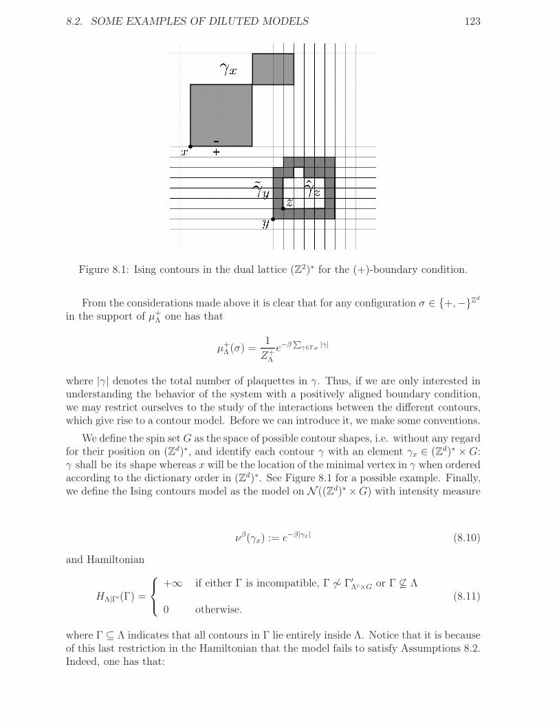
8.2. SOME EXAMPLES OF DILUTED MODELS 123
Figure 8.1: Ising contours in the dual lattice (Z2)∗ for the (+)-boundary condition.
From the considerations made above it is clear that for any configuration σ ∈ +,−Zdin the support of µ+
Λ one has that
µ+Λ(σ) =
1
Z+Λ
e−β∑
γ∈Γσ|γ|
where |γ| denotes the total number of plaquettes in γ. Thus, if we are only interested inunderstanding the behavior of the system with a positively aligned boundary condition,we may restrict ourselves to the study of the interactions between the different contours,which give rise to a contour model. Before we can introduce it, we make some conventions.
We define the spin setG as the space of possible contour shapes, i.e. without any regardfor their position on (Zd)∗, and identify each contour γ with an element γx ∈ (Zd)∗ ×G:γ shall be its shape whereas x will be the location of the minimal vertex in γ when orderedaccording to the dictionary order in (Zd)∗. See Figure 8.1 for a possible example. Finally,we define the Ising contours model as the model on N ((Zd)∗ ×G) with intensity measure
νβ(γx) := e−β|γx| (8.10)
and Hamiltonian
HΛ|Γ′(Γ) =
+∞ if either Γ is incompatible, Γ 6∼ Γ′Λc×G or Γ 6⊆ Λ
0 otherwise.(8.11)
where Γ ⊆ Λ indicates that all contours in Γ lie entirely inside Λ. Notice that it is becauseof this last restriction in the Hamiltonian that the model fails to satisfy Assumptions 8.2.Indeed, one has that:
124 CHAPTER 8. DILUTED MODELS
i. ∆Eη ≡ +∞ for all η ∈ N ((Zd)∗ ×G) since contours contain more than one vertex.Therefore, for each γx ∈ S×G the quantity ∆η(γx) fails to represent what it should:the energy cost for the infinite-volume system to add the particle γx when the currentconfiguration of the system is given by η. To fix this problem one considers insteadthe localized energy leap functions ∆EΛ|η : S ×G→ [−∞,+∞] defined as
∆EΛ|η(γx) =
+∞ if either γx 6∼ η or γx 6⊆ Λ
0 otherwise.
Notice that for every η ∈ N ((Zd)∗ ×G) and γx ∈ S ×G one has that
∆E∗η(γx) := lim
Λր(Zd)∗∆EΛ|η(γx) = (+∞)1γx 6∼η. (8.12)
Thus, for the localized energy leap functions one recovers in the limit as Λ ր (Zd)∗
the correct notion of energy cost. Taking this into consideration, one also redefinesthe impact relation by incompatibility, i.e. γy γx if and only if γy 6∼ γx.
ii. The consistent Hamiltonian property is not satisfied. As a consequence, one caneasily check that the resulting Boltzmann-Gibbs distributions are also inconsistent inthe sense of (8.2). In this context, Gibbs measures as defined in Definition 8.6 couldfail to exist. However, it is still possible for these contour model to admit “infinite-volume Boltzmann-Gibbs distributions” in the sense described by Proposition 8.7.These limiting measures will be of particular interest to us since, as we will see onChapter 9, their existence implies a phase transition in the Ising model.
Despite the fact that not all conditions on Assumptions 8.2 are satisfied, under the minoradjustments suggested above most of the analysis carried out in the next chapter fordiluted models will also hold in this context, which is why we decided to include thismodel among the examples even if it is not a diluted model as we understand them.Another fact worth mentioning is that this is the only given example which is of unboundedlocal interaction range. Finally, we point out the following crucial relation between theBoltzmann-Gibbs distributions in the original Ising and Ising contours models: for anysimply connected Λ ∈ B0
Zdand family Γ of compatible contours lying inside Λ∗ we have
µ+Λ(σ
+Γ ) = µΛ∗|∅(Γ). (8.13)
An analogous contour representation is also available for Boltzmann-Gibbs distributionswith negatively aligned boundary condition. We refer to [41] for a thorough review of theIsing model and the standard proof of phase transition using its contour representation.
8.3. RESUMEN DEL CAPÍTULO 8 125
8.3 Resumen del Capítulo 8
Definimos en este capítulo la clase de modelos diluidos, que habremos de estudiar enlo que resta de la segunda parte. Esencialmente, un modelo diluido se define a partirde sus distribuciones de Boltzmann-Gibbs, medidas sobre el espacio de configuracionesN (S ×G) que describen el comportamiento local del modelo en volúmenes finitos sujetosujeto a distintas condiciones de frontera. Concretamente, fijada una medida ν en S×G,dado Λ ⊆ S acotado y η ∈ N (S × G) se define la distribución de Boltzmann-Gibbs µΛ|ηen Λ con respecto a la condición de frontera η mediante la fórmula
µΛ|η = ωΛ|η × δηΛc
donde identificamos N (S×G) = N (Λ×G)×N (Λc×G) y ωηΛ es la medida de probabilidaden N (Λ×G) definida a través de la relación
dωΛ|η =e−HΛ|η
ZΛ|ηdπνΛ.
Aquí πνΛ denota la distribución de un proceso de Poisson en N (Λ × G) con intensidadνΛ×G, cuyo rol es el de distribuir las partículas dentro de Λ, mientras que HΛ|η es lo que sedenomina el Hamiltoniano relativo a Λ con condición de frontera η, encargado de asignarun peso a las distintas configuraciones de acuerdo a la interacción que haya entre laspartículas que la conforman. De esta manera, si H denota a la familia de Hamiltonianoslocales, el par (ν,H) determina por completo al modelo. Asumimos que (ν,H) cumplelas condiciones dadas en 8.2.
De particular interés en cada modelo son las medidas de Gibbs asociadas al mismo,es decir, las medidas µ sobre N (S × G) que son compatibles con las distribuciones deBoltzmann-Gibbs para cualquier volumen Λ, i.e.
µ(·) =∫
N (S×G)
µΛ|η(·)dµ(η).
Las medidas de Gibbs representan los distintos posibles estados de equilibrio globales delmodelo. En efecto, mostramos que bajo ciertas condiciones adicionales sobre el par (ν,H),cualquier límite local de las distribuciones de Boltzmann-Gibbs µΛ|η cuando Λ ր S esuna medida de Gibbs. En lo que resta, nos interesará estudiar qué condiciones garantizanexistencia y unicidad o multiplicidad de medidas de Gibbs.
Por último, culminamos el capítulo mostrando que algunos modelos clásicos, como loson el modelo de Widom-Rowlinson (tanto en su versión continua como discreta) y el decontornos de Ising, caen dentro de la familia de modelos diluidos. Explicamos en detalle ladualidad entre el modelo de Ising original y su modelo de contornos asociado, que será devital importancia para los desarrollos del Capítulo 12. Agregamos además algunos otrosejemplos, como los modelos de Widom-Rowlinson tolerante y el simbiótico, para mostrarla flexibilidad de nuestras definiciones y la amplitud de nuestro marco teórico.

126 CHAPTER 8. DILUTED MODELS
Chapter 9
The Fernández-Ferrari-Garcia dynamics
In this chapter we study the Fernández-Ferrari-Garcia dynamics first introduced in [16].In their work the authors focus on the Ising contours model and show that, for a sufficientlylarge value of the inverse temperature β, the infinite-volume Boltzmann-Gibbs distributionof this contour model can be realized as the unique invariant measure of these dynamics.Later on [17], the authors investigate the possibility of using this new approach as aperfect simulation scheme for Gibbs measures of a number of systems with exclusion inthe low density or extreme temperature regime. Our purpose now is to carry out thesame endeavor in general for the broader family of diluted models. The main ideas in thischapter are those originally featured in [16]: the majority of the results presented hereare direct generalizations of those found there. Nonetheless, some of the proofs we give inthis chapter are different from the ones in the original article, since not all of their proofscan be adapted to continuum models.
Given an intensity measure ν and a Hamiltonian H satisfying Asssumptions 8.2,one could summarize the essentials of the associated Fernández-Ferrari-García dynamicsas follows:
• At rate e−∆E the birth of new animals is proposed with intensity given by ν.
• Each γx proposed for birth will be effectively born with probability e−(∆Eη(γx)−∆E),where η is the state of the system at the time in which the birth of γx is proposed.
• Every effectively born animal has an independent random exponential lifetime ofparameter 1.
• After its lifetime has expired, each animal dies and vanishes from the configuration.
Our aim in this section is to make this description rigorous as well as to study some of thebasic properties enjoyed by these dynamics. We shall begin by introducing the dynamicsrestricted to a finite volume and then treat the more delicate scenario of infinite volume.All processes defined below shall be subsets of the product space C = (S ×G)×R×R+.The elements of C shall be called cylinders since any (γx, t, s) ∈ C can be seen as a cylinderon S×R of axis x× [t, t+ s] and diameter γ. However, we shall prefer to describe eachcylinder C = (γx, t, s) ∈ C in terms of its basis γx, its time of birth t and its lifespan s.We shall denote these three features of C by basis(C), bC and lC , respectively.
127
128 CHAPTER 9. THE FERNÁNDEZ-FERRARI-GARCIA DYNAMICS
Following this line of thought, we can identify any random element V ∈ C with a birthand death process on S ×G by means of its time sections, i.e. if for each t ∈ R we definethe random particle configuration Vt ∈ N (S ×G) by the formula
Vt(γx) = #C ∈ V : basis(C) = γx and bC ≤ t < bC + lC
for every γx ∈ S × G, then (Vt)t∈R constitutes a birth and death process on S × G.From this point of view we thus interpret any cylinder (γx, t, s) as a particle γ being bornat time t on location x which lives on for a period of length s.
9.1 Local dynamics
We begin our formal introduction of the Fernández-Ferrari-García dynamics (referred to asFFG dynamics from now on) by fixing a bounded set Λ ∈ B0
S and a particle configurationη ∈ N (S × G), and defining the dynamics on the finite volume Λ × G with η acting asa boundary condition. Though it may seem misleading at first, we choose to build theselocal dynamics from infinite-volume processes since it will provide a clear and direct wayin which to couple all local dynamics together.
Consider a Poisson process Π on C with intensity measure φν = ν×e−∆EL×E1, whereL is the Lebesgue measure on R and E1 is the exponential distribution of parameter 1.We shall refer to Π as the free process, whose time evolution can be described as follows:
• At rate e−∆E animals are born with intensity given by ν, regardless of the impactpreexisting animals may have upon them.
• Each animal has an independent random exponential lifetime of parameter 1.
• After its lifetime has expired, each animal dies and vanishes from the configuration.
This free process constitutes, as its name suggests, a stationary non-interacting birth anddeath process whose invariant measure is πν . To be able to define the dynamics we needto add an additional component to Π: to each cylinder in Π we will attach an independentrandom variable uniformly distributed on [0, 1], which will be called its flag. Each flagwill be used to determine the success of the associated cylinder’s attempted birth in thedynamics. One way in which to attach these flags would be to replace Π with the markedPoisson process Π on C × [0, 1] with intensity measure φν := φν×L[0,1]. Thus, elements ofΠ can be seen as cylinders in Π together with their respective independent flags in [0, 1].For any given (γx, t, s) ∈ Π we shall denote its corresponding flag by F (γx, t, s).1 Finally,recalling the identification N (S ×G) = N (Λ×G)×N (Λc ×G) we define the local FFGprocess KΛ|η on Λ×G with boundary condition η by the formula
KΛ|η = (γx, t, s) ∈ ΠΛ×G : F (γx, t, s) < M(γx|KΛ|ηt−
)×(γx, t, s) ∈ C : γx ∈ ηΛc×G (9.1)
where for γx ∈ S ×G and ξ ∈ N (S × G) we use the notation M(γx|ξ) := e−(∆Eξ(γx)−∆E)
and ΠΛ×G denotes the restriction of Π to (Λ×G)× R× R+. In other words, KΛ|η is the
1Notice that for each (γx, t, s) ∈ Π its flag is the unique u in[0, 1] such that (γx, t, s, u) ∈ Π. Thus,there is no ambiguity in this choice of notation.
9.1. LOCAL DYNAMICS 129
process obtained as a thinning of the free process inside Λ given by the rule on (9.1) withthe addition of a boundary condition η outside Λ which must be kept fixed for all times,i.e. (KΛ|η
t )Λc×G = ηΛc×G for every t ∈ R. Notice that the self-referential nature of thethinning rule in (9.1) could lead to KΛ|η not being well defined. Indeed, let us introducesome definitions that will help us give further details on this matter.
Definition 9.1.
• Given C, C ∈ C we say that C is a first generation ancestor of C and write C Cwhenever
basis(C) basis(C) and bC < bC < bC + lC .
We shall denote the set of all first generation ancestors of a given C ∈ C by P(C).
• For C ∈ C we define A1(C) := ΠP(C) and for n ∈ N we set
An+1(C) =⋃
C∈An(C)
A1(C).
We define the clan of ancestors of C in Π as
A(C) :=⋃
n∈NAn(C).
Furthermore, for Λ ∈ B0S and n ∈ N we define the n-th generation of ancestors of C
restricted to Λ as
AΛn(C) = C ∈ An(C) : basis(C) ∈ Λ×G.
We define AΛ(C), the clan of ancestors of C restricted to Λ, in an analogous fashion.
• For t ∈ R and Λ ∈ B0S let us define the clan of ancestors of Λ×G at time t as
At(Λ×G) :=⋃
n∈N0
Atn(Λ×G)
where At0(Λ×G) := C ∈ Π : basis(C) ∈ Λ×G , bC ≤ t < bC + lC and for n ∈ N
Atn(Λ×G) :=
⋃
C∈At0(Λ×G)
An(C).
For any ∆ ∈ B0S such that Λ ⊆ ∆ we define At,∆(Λ × G), the clan of ancestors of
Λ×G at time t restricted to ∆×G, in the same manner as above.
Having defined the notion of ancestors in the dynamics, we now return to discussthe good definition of KΛ|η. Notice that if we wish to determine whether a given cylinderC = (γx, t, s) ∈ ΠΛ×G belongs to KΛ|η or not then first we need to specify the configurationKΛ|ηt−
in order to evaluate whether the condition on (9.1) is satisfied. To be more accurate,
due to Assumptions 8.2 we will only need to specify KΛ|ηt−
inside the set I(γx). However,
130 CHAPTER 9. THE FERNÁNDEZ-FERRARI-GARCIA DYNAMICS
since KΛ|η is known outside Λ as it coincides with η for all times, it remains to specify KΛ|ηt−
inside I(γx)∩ (Λ×G). Therefore, recalling Definition 9.1, we see that to determine thefate of C we must first determine the fate of all its first generation ancestors with basesin Λ×G, i. e. cylinders in AΛ
1 (C). But this task itself involves determining the fate of asecond generation of ancestors of C, those cylinders with bases in Λ×G being ancestorsto cylinders in AΛ
1 (C). In general, to determine if C belongs to KΛ|η we must study thefate of every cylinder in AΛ(C), the clan of ancestors of C restricted to Λ. If AΛ(C)were to span over an infinite number of generations then it may be impossible to decidewhether to keep C or not and, therefore, KΛ|η may not be well defined in this situation.On the other hand, if we were able to guarantee that for every cylinder C ∈ ΠΛ×G therestricted clan AΛ(C) spans only over a finite number of generations then KΛ|η would bewell defined. Indeed, since M(γx|Kσ
t−) =M(γx|ηΛc×G) for any cylinder (γx, t, s) ∈ PiΛ×G
with no ancestors preceding it, we have that the fate of every cylinder in the last generationof ancestors restricted to Λ of a given cylinder C can be decided upon inspecting theirrespective flags (and nothing else) and thus it will also be possible to determine the fateof all their descendants, including C. More precisely, take C ∈ ΠΛ×G and let N be anonnegative integer such that AΛ
n(C) = ∅ for every n > N . If we set
KΛN(C) := (γy, r, l) ∈ AΛ
N(C) : F (γy, r) < M(γy|ηΛc×G)
and for 1 ≤ i ≤ N − 1 inductively define
KΛi (C) = KΛ
i+1(C) ∪ (γy, r, l) ∈ AΛi (C) : F (γy, r, l) < M(γy|KΛ
i+1(C))
then the cylinder C ∈ ΠΛ×G will be kept if and only if
F (C) < M(γy|KΛ1 (C)).
In other words, to decide if a cylinder C ∈ ΠΛ×G is kept one could conduct the followingprocedure:
i. If C has no first generation ancestors, i.e. AΛ1 (C) = ∅, then the value of its flag u
alone will determine whether C is kept or not. Otherwise, the value of u will decideif C is kept once we determine the fate of all the first generation ancestors of C.
ii. To decide whether any given first generation ancestor C ∈ AΛ1 (C) is kept, one must
repeat step (i) for C instead of C.
iii. Since the clan of ancestors of C restricted to Λ possesses only a finite number ofgenerations, one must go backwards in time and examine a previous generation ofancestors only a finite amount of times (at most N times) so that it is ultimatelypossible to determine whether C is kept.
Therefore, we are left to answer the question of under which conditions do the clans ofancestors restricted to Λ possess only a finite amount of generations. Fortunately, underAssumptions 8.2 this is always the case. This is the content of the following proposition.
Proposition 9.2. For every Λ ∈ B0S we have that At,Λ(Λ×G) is finite for all t ∈ R.
9.2. INFINITE-VOLUME DYNAMICS 131
Proof. Since Π is a stationary process whose invariant measure πν satisfies
πν(ξ ∈ N (S ×G) : ξ(Λ×G) = 0) = e−ν(Λ×G) > 0
we have that the entrance times (ti(Λ))i∈Z to the set ξ ∈ N (S ×G) : ξ(Λ×G) = 0 arewell defined (i.e. finite almost surely) and satisfy ti(Λ) → ±∞ as i→ ±∞. In particular,for every t ∈ R there exists i0 ∈ Z such that ti0−1(Λ) ≤ t < ti0(Λ). Since Πti(Λ)(Λ×G) = 0for each i ∈ Z by definition, this implies that there exist (random) k < r ∈ Z such that
At,Λ(Λ×G) ⊆ Π(Λ×G)×[t,ti0 ]×R+ ⊆ Π(Λ×G)×[k,r]×R+. (9.2)
Since for every k < r ∈ Z we have φ((Λ × G) × [k, r] × R+) = (r − k)ν(Λ × G) < +∞by Assumptions 8.2, with probability one we have that for every k < r ∈ Z the randomparticle configurations Π(Λ×G)×[k,r]×R+ are all finite. By (9.2) this concludes the proof.
By the discussion above, Proposition 9.2 yields that for Λ ∈ B0S and η ∈ N (S × G)
the process KΛ|η is well defined and constitutes an interacting birth and death process.Moreover, KΛ|η is stationary due to the time translational invariance of its constructionand that of Π.
9.2 Infinite-volume dynamics
9.2.1 Stationary dynamics
As stated before, some complications arise when lifting the restriction of finite volume inthe dynamics. The procedure to define the unrestricted FFG process in the entire spaceS ×G is completely analogous to that of the finite volume case: it suffices to take Λ = Severywhere in the previous section. Thus, the FFG process K on the whole space S ×Gis defined by the formula
K = (γx, t, s) ∈ Π : F (γx, t, s) ≤ M(γx|Kt−). (9.3)
Following the analysis of the previous section in this context, we see that in order for Kto be well defined we must guarantee that for every cylinder C ∈ Π its clan of ancestorsA(C) spans only over a finite number of generations. Notice that the argument used inProposition 9.2 will not go through this time as in general we have ν(S × G) = +∞.Therefore, we will need to impose additional conditions on both ν and H besides thoseon Assumptions 8.2 to guarantee that K is well defined in this case. This is the contentof the next proposition.
Proposition 9.3. If there exists a measurable function q : S × G → R satisfyinginfγx∈S×G q(γx) ≥ 1 and such that
αq := supγx∈S×G
[
e−∆E
q(γx)
∫
I(γx)q(γy)dν(γy)
]
< 1 (9.4)
then At(Λ×G) is finite for every t ∈ R and Λ ∈ B0S almost surely.
132 CHAPTER 9. THE FERNÁNDEZ-FERRARI-GARCIA DYNAMICS
Definition 9.4. Whenever (9.4) holds we say that ν and H satisfy the (F1)-dilutenesscondition with size function q and that the associated model is heavily diluted.
Thus, whenever dealing with a heavily diluted model we have that K is well definedand constitutes a stationary interacting birth and death process on the entire space S×G.We postpone the proof of Proposition 9.3 until Section 9.3.
9.2.2 Dynamics on a bounded time window
One can wonder whether it is possible that, upon relaxing the conditions on Proposition9.3, the FFG process remains well defined on the infinite volume but perhaps only for abounded time window, i.e. if given t1 < t2 ∈ R we replace φ in the construction above by
φ[t1,t2] = ν × e−∆EL[t1,t2] × E1.
This will occur if for every Λ ∈ B0S one has that
A[t1,t2](Λ×G) := C ∈ At2(Λ×G) : birth(C) ≥ t1 (9.5)
spans only over a finite number of generations. The next proposition shows that this isthe case whenever the coefficient αq defined on (9.4) is finite.
Proposition 9.5. If there exists a measurable function q : S × G → R satisfyinginfγx∈S×G q(γx) ≥ 1 and such that
αq := supγx∈S×G
[
e−∆E
q(γx)
∫
I(γx)q(γy)dν(γy)
]
< +∞ (9.6)
then A[t1,t2](Λ×G) is finite for every t1 < t2 ∈ R and Λ ∈ B0S almost surely.
Definition 9.6. Whenever (9.6) holds we say that ν and H satisfy the (F2)-dilutenesscondition with size function q and that the associated model is well diluted.
Let us observe that due to Proposition 9.5 we have that whenever a model is welldiluted it is possible to define the FFG dynamics as a forward time evolution on R+ for anyinitial condition σ ∈ N (S×G). Indeed, given any particle configuration σ ∈ N (S×G) anda family (L(γx,i))(γx,i)∈[σ] of i.i.d. exponential random variables of parameter 1 independentof Π we may set
Πσ= Π ∪ (γx, 0, L(γx,i), 0) : (γx, i) ∈ [σ]
and define (Kσt )t≥0 by the formula
Kσ = (γx, t, s) ∈ Πσ : F (γx, t, s) ≤M(γx|Kt−) (9.7)
where Πσ denotes the projection of Πσ
onto C+ := (S×G)×R+ ×R+ and by conventionwe set K0− ≡ ∅. Notice that, even though by Proposition 9.5 we have that A[0,t](Λ×G) isfinite for every t ≥ 0 and Λ ∈ B0
S almost surely, the clan of ancestors associated to theseforward dynamics contains also cylinders corresponding to the initial configuration σ andtherefore it may not be finite (unless σ has a finite local interaction range). Nonetheless,under the (F2)-diluteness condition it will always span over a finite number of generationsand so Kσ is ultimately well defined. Furthermore, since we have assigned a 0 flag valueto every particle in the initial condition σ, we get that the initial condition is always keptin Kσ even if σ is a particle configuration forbidden by H . We prove Proposition 9.5 inthe next section.
9.3. FINITENESS CRITERIA FOR THE CLAN OF ANCESTORS 133
9.3 Finiteness criteria for the clan of ancestors
The aim of this section is to give the proofs of Propositions 9.3 and 9.5, and to investigatesome of their consequences as well. In both proofs we shall make use of the crucial factthat each clan of ancestors can be contained in the offspring of some branching process.This is the content of the following lemma.
Lemma 9.7 (Domination lemma). Given Λ ∈ B0S and t ∈ R there exists a family of
random sets (Bn)n∈N0 ⊆ C such that
i. At0(Λ×G) = B0
ii.n⋃
i=0
Ati(Λ×G) ⊆
n⋃
i=0
Bi for every n ∈ N
iii. Conditional on (Bi)0≤i≤n, Bn+1 is a Poisson process with intensity measure∑
C∈BnφP(C).
Proof. Consider the space Mt of particle configurations ζ on Ct := (S×G)×(−∞, t]×R+
such that
• ζ is finite
• No two cylinders in ζ have the same time of birth.
For ζ ∈ Mt we shall set A0(ζ) := ζ and for n ∈ N write
An(ζ) :=⋃
C∈ζAn(C).
Furthermore, suppose that we have ordered the elements of ζ in some particular way.Then, if C1 · · · Ck denote the ordered elements of ζ , for each i = 1, . . . , k we define
Pζ(Ci) = P(Ci)−i−1⋃
j=1
[Cj ∪ P(Cj)].
To define the family (Bn)n∈N0 first we shall fix ζ ∈ Mt and construct a collection of sets(Bn(ζ))n∈N0 such that for every n ∈ N0 the following properties are satisfied:
i. Bn(ζ) belongs to Mt almost surely.
ii. Conditional on B0(ζ), . . . ,Bn(ζ), the random set Bn+1(ζ) is a Poisson process on Ctwith intensity measure
∑
C∈Bn(ζ) φP(C).
iii.n⋃
i=0
Ai(ζ) ⊆n⋃
i=0
Bi(ζ).
134 CHAPTER 9. THE FERNÁNDEZ-FERRARI-GARCIA DYNAMICS
We start by setting B0(ζ) := ζ and now proceed with the construction of the set B1(ζ).First we order the elements of ζ according to their times of birth, i.e. ζ = C1, . . . , Ckwhere 0 ≤ bC1 < · · · < bCk ≤ t. Then continue by considering a collection Π(1,1), . . . ,Π(1,k)
of independent Poisson processes on C of intensity measure φ such that Π(1,1) = Π anddefining for each i = 1, . . . , k
Bζ(Ci) := Π(1,i)P(Ci)−Pζ(Ci) ∪ ΠPζ(Ci).
If we set B1(ζ) :=k⋃
i=1
Bζ(Ci) then B1(ζ) satisfies the properties stated above. Indeed:
(1) Each Bζ(Ci) is a Poisson process with intensity measure φP(Ci) by virtue of theindependence of Π(1,1), . . . ,Π(1,k) and the disjointness of P(Ci)−Pζ(Ci) and Pζ(Ci).
(2) The independence of Bζ(C1), . . . ,Bζ(Ck) follows from the independence of the Π(1,i)
and the fact that Pζ(Ci) ∩ Pζ(Cj) = ∅ for i 6= j. Together with (1) this gives (ii).
(3) Property (iii) follows upon noticing that for i = 1, . . . , k
A1(Ci)−i−1⋃
j=1
A1(Cj) ⊆ ΠPζ(Ci).
(4) Property (i) is also a consequence of (1) and (2) since for each i = 1, . . . , k
φν(P(Ci)) = e−∆E
∫
I(basis(Ci))
∫ bCi
−∞
∫ +∞
bCi−te−sdsdtdν < +∞.
Having constructed B1(ζ), we now define the next generations in an inductive manner.For this we shall need to consider an array of N× N Poisson processes on C such that:
• Π(n,k) is a Poisson process with intensity measure φ for every n, k ∈ N
• Π(n,1) = Π for every n ∈ N
• The processes Π(n,k) : n ∈ N, k ≥ 2 are independent of each other and also of Π.
Suppose now that we have constructed the first n generation of sets B1(ζ), . . . ,Bn(ζ) andlet us construct the next generation, Bn+1(ζ). Order each of the constructed generationsseparately by their times of birth and write for each j = 1, . . . , n
Bj(ζ) = C(j,1), . . . , C(j,kj).
Now let us consider the joint configuration ζ (n) = C(j,i) : 1 ≤ j ≤ n and 1 ≤ i ≤ kjordered by the dictionary order, i.e. C(j,i) C(j′,i′) if either j < j′ or j = j′ and i ≤ i′.We then define
Bn+1(ζ) :=
kn⋃
i=1
Bζ(n)(C(n,i))
9.3. FINITENESS CRITERIA FOR THE CLAN OF ANCESTORS 135
whereBζ(n)(C(n,i)) = Π
(n+1,i)
P(C(n,i))−Pζ(C(n,i))∪ ΠPζ(C(n,i)).
Following a similar argument to the one given above it is possible show by inductivehypothesis that Bn+1(ζ) satisfies properties (i), (ii) and (iii). Finally, having defined thecollection (Bn(ζ))n∈N0 for each ζ ∈ Mt, for each n ∈ N0 we set
Bn := Bn(
At0(Λ×G)
)
.
One can check that, by construction of (Bn(ζ))n∈N0, the family (Bn)n∈N satisfies all thedesired properties. This concludes the proof.
Proof of Proposition 9.3. Let us first fix Λ ∈ B0S and t ∈ R and consider the family of
random sets (Bn)n∈N0 satisfying the conditions in the Domination lemma. By condition(ii) of this lemma we see that if we wish to show that At(Λ×G) is almost surely finite itwill suffice to prove that
∑
n∈N0|Bn| < +∞ almost surely. But this will follow immediately
once we show that for every n ∈ N0
E
(
∑
C∈Bnq(basis(C))
∣
∣
∣
∣
B0
)
≤(
∑
C∈B0
q(basis(C))
)
αnq . (9.8)
Indeed, if (9.8) holds then since infγx∈S×G q(γx) ≥ 1 we have
P
(
∑
n∈N0
|Bn| = +∞∣
∣
∣
∣
B0
)
≤ limk→+∞
P
(
∑
n∈N0
∑
C∈Bnq(basis(C)) > k
∣
∣
∣
∣
B0
)
≤ limk→+∞
∑
n∈N0E(∑
C∈Bn q(basis(C))|B0)
k
≤ limk→+∞
∑
C∈B0q(basis(C))
k(1− αq)= 0
since P (|B0| < +∞) = 1. From this we get that the unconditional probability is also null.Thus, in order to obtain (9.8) we first notice that by (iii) and (7.3) a simple calculationyields for every n ∈ N0
E
∑
C∈Bn+1
q(basis(C))
∣
∣
∣
∣
∣
Bn, . . . ,B0
≤(
∑
C∈Bnq(basis(C))
)
αq. (9.9)
Now, since (9.8) clearly holds for n = 0, the validity for every n ∈ N0 follows uponinduction by applying (9.9) and the tower property of conditional expectation. Finally,to show that with probability one this holds for every Λ ∈ B0
S and t ∈ R simultaneously,we take (Λn)n∈N ⊆ B0
S such that Λn ր S and observe that (with probability one) givenΛ ∈ B0
S and t ∈ R there exists n0 ∈ N and r ∈ Q such that
At(Λ×G) ⊆ Ar(Λn0 ×G).
Since there are only countable possibilities for n0 and r and we have shown that for everyfixed pair n, r the set Ar(Λn ×G) is finite almost surely, this yields the result.
136 CHAPTER 9. THE FERNÁNDEZ-FERRARI-GARCIA DYNAMICS
Proof of Proposition 9.5. By the same reasoning as in the proof of Proposition 9.3 it willsuffice to show that for each r < l ∈ Q and n ∈ N the random set A[r,l](Λn × G) isalmost surely finite, where (Λn)n∈N ⊆ B0
S is such that Λn ր S. But we can show this byperforming an inductive procedure once we manage to prove the following two facts:
1. There exists δ > 0 such that if 0 < t−s < δ then A[s,t](Λ×G) is finite almost surely.
2. If |h| < δ and A[s,t](Λ×G) is finite almost surely then A[s−h,t](Λ×G) is also finitealmost surely.
To establish (1) we fix Λ ∈ B0S, s < t and construct similarly to the Domination lemma a
family of random sets (Bn)n∈N satisfying
i. A[s,t]0 (Λ×G) = B0
ii.n⋃
i=0
A[s,t]i (Λ×G) ⊆
n⋃
i=0
Bi for every n ∈ N
iii. Conditional on (Bi)0≤i≤n, Bn+1 is a Poisson process with intensity∑
C∈Bn(φ[s,t])P(C)
where for n ∈ N we set A[s,t]n (Λ×G) = At
n(Λ×G)∩A[s,t](Λ×G). By performing a similarcomputation to the one yielding (9.9) we obtain
E
∑
C∈Bn+1
q(basis(C))
∣
∣
∣
∣
∣
Bn, . . . ,B0
≤(
∑
C∈Bnq(basis(C))
)
αq. (9.10)
where αq := αq(1 − e−(t−s)). Since αq < +∞, we may take t − s small enough so as toguarantee that αq < 1. From this one obtains (1) by proceeding as in Proposition 9.3.
To see (2) we first notice that if A[s,t](Λ × G) is finite then there exists a (random)set Λ′ ∈ B0
S such that the basis of every cylinder in A[s,t](Λ × G) belongs to Λ′ × G.Furthermore, since ν(I(Λ′ × G)) < +∞ we have that there exists another (random) setΛ′′ ∈ B0
S such that the basis of every cylinder in ΠI(Λ′×G)×[s−h,s)×R+ belongs to Λ′′ × G.Then, it is not hard to see that
A[s−h,t](Λ×G) ⊆ A[s,t](Λ×G) ∪A[s−h,s](Λ′′ ×G) (9.11)
Together with (1) (for Λ′′ instead of Λ) , (9.11) implies (2), which concludes the proof.
When dealing with a heavily diluted model, the finiteness of every clan of ancestorsforces the FFG dynamics to exhibit a loss of memory property. In particular, we obtain theconvergence of the forward dynamics to the invariant measure of the stationary dynamics.More precisely, we have the following proposition.
Proposition 9.8. Let us suppose that ν and H satisfy the (F1)-diluteness condition.Then for any initial particle configuration σ ∈ NH(S ×G) as t→ +∞ we have
Kσt
loc−→ K0.
9.3. FINITENESS CRITERIA FOR THE CLAN OF ANCESTORS 137
Proof. Given a particle configuration σ ∈ NH(S ×G) the idea is to construct a couplingof Kσ
t for each t ≥ 0 together with K0 where the local convergence can be easily verified.To achieve this, recall that the forward FFG dynamics are built from a set (Lγx,i)(γx,i)∈[σ]of exponential random variables of parameter 1 and a Poisson process Π on C × [0, 1]with intensity measure ν ×L× E1 ×L[0,1]. More precisely, for each Λ ∈ B0
S there exists ameasurable function ψΛ such that for each t > 0
(Kσt )Λ×G = ψΛ
(
A[0,t]σ (Λ×G), F (A[0,t]
σ (Λ×G)))
where A[0,t]σ (Λ × G) denotes the clan of ancestors of Λ × G defined as in (9.5) but using
Πσ instead of Π and F (A[0,t]σ (Λ×G)) denotes its corresponding set of flags. Furthermore,
both the clan of ancestors and its flags are determined by the evolution of the process Πσ
in the time interval [0, t], i.e., there exists a second measurable function θ such that
(Kσt )Λ×G = ψΛ θ
(
(
Πσ
s
)
s∈[0,t]
)
Similarly, the stationary FFG process is defined for each t ∈ R and Λ ∈ B0S by the formula
(Kt)Λ×G = ψΛ θ(
(
Πs
)
s∈(−∞,t]
)
. (9.12)
We shall construct our coupling by taking the Poisson process Π together with the family(Lγx,i)(γx,i)∈[σ] of independent exponential random variables of parameter 1 and for each
t > 0 defining the t-shifted free process Πσ,(t)
with initial condition σ by the formula
Πσ, (t)
= Πσ
0 ∪ Π(t)
where
Π(t)
= (γx, r + t, s, u) ∈ C × [0, 1] : (γx, r, s, u) ∈ Π , r > −t.
We then define for each t > 0 the random particle configuration Xt by the formula
(Xt)Λ×G := ψΛ θ(
(
Πσ, (t)
s
)
s∈[0,t]
)
for every Λ ∈ B0S and set X∞ := K0, where K is defined exactly as in (9.12), i.e. using Π.
In other words, Xt is the current state of the FFG process started at time −t withinitial condition σ and underlying free process Π, after having evolved for a time periodof length t. Let us observe that each Xt has the same distribution as Kσ
t by the timetranslational invariance of Π. Moreover, this construction possesses a crucial property:
the free processes Πσ, (t)
are “coupled backwards” with Π, i.e. for t > 0 we have
Πσ, (t)
s = Πs−t. (9.13)
Using this property we shall prove that for any given Λ ∈ B0S one has (Xt)Λ×G = (X∞)Λ×G
for every t sufficiently large, a fact from which we immediately obtain the validity of (i).Indeed, since the model is heavily diluted we know that A0(Λ×G) is finite almost surely.In particular, there exist (random) t∗ and Λ′ ∈ B0
S such that
A0(Λ×G) ⊆ (Λ′ ×G)× (−t∗, 0]× R+.
138 CHAPTER 9. THE FERNÁNDEZ-FERRARI-GARCIA DYNAMICS
Moreover, since the initial condition σ has a locally finite interaction range with respectto H we have that σ(I(Λ′ ×G)) < +∞ and so tσΛ := sup(γx,i)∈[σ|I(BΛ)]
Lγx,i < +∞ as well.Therefore, if t > t∗ + tσΛ then by (9.13) we have that
A[0,t]σ (Λ×G) = (γx, r + t, s) : (γx, r, s) ∈ A0(Λ×G).
i.e., all the cylinders in the initial configuration σ which could possibly interact with theclan of ancestors of the cylinders in (Π
σ, (t)t )Λ×G in the forward dynamics die out before
reaching it and, as a consequence, this clan coincides with the ancestors of cylinders in(Π0)Λ×G in the stationary dynamics modulo some appropriate time shift. In particular,we get that (Xt)Λ×G = (X∞)Λ×G if t > t∗ + tσΛ as we wanted to show.
9.4 Reversible measures for the FFG dynamics
The purpose of this section is to study the relationship between invariant measures forthe FFG dynamics and Gibbs measures of the associated diluted model. More precisely,we will show that Gibbs measures are reversible for the corresponding FFG dynamics.Together with Proposition 9.8, this will imply the existence of a unique Gibbs measurein all heavily diluted models. We begin our task by introducing the global and localevolution semigroups for the dynamics. However, in order to define the global semigroupwe need the infinite-volume forward dynamics to be well defined. Hence, for the rest ofthis section we assume that the model under consideration is well diluted.
Definition 9.9. Given t > 0, a bounded subset Λ ∈ B0S and a particle configuration
η ∈ N (S × G) we define the operators St and SΛ|ηt on the class of bounded functions
f : N (S ×G) → R by the formulas
St(f)(σ) = E (f(Kσt )) and S
Λ|ηt (f)(σ) = E(f(KΛ, σ, η
t ))
where Kσ denotes the infinite-volume forward process with initial condition σ and KΛ, σ, η
is the forward process on Λ with boundary condition η and initial condition σΛ×G ·ηΛc×G.2
The families of operators (St)t≥0 and (SΛ|ηt )t≥0 are called the global evolution semigroup
and local evolution semigroup on Λ with boundary condition η, respectively.
Remark 9.10. Both families (St)t≥0 and (SΛ|ηt )t≥0 satisfy the semigroup property, i.e.
St Ss = St+s and SΛ|ηt SΛ|η
s = SΛ|ηt+s
for every t, s ≥ 0, and hence their name.
Definition 9.11. Let µ be a measure on N (S ×G) and Λ ∈ B0S .
• We say that µ is invariant for the global FFG dynamics if for every t ≥ 0 we have∫
N (S×G)
St(f)(σ)dµ(σ) =
∫
N (S×G)
f(σ)dµ(σ)
for every bounded local function f : N (S ×G) → R.
2The forward dynamics on a finite volume are defined in the natural manner, following the approachof Section 9.2.2.
9.4. REVERSIBLE MEASURES FOR THE FFG DYNAMICS 139
• We say that µ is invariant for the local FFG dynamics on Λ with boundary conditionη ∈ N (S ×G) if
i. µ(ξ ∈ N (Rd ×G) : ξΛc×G = ηΛc×G) = 1
ii. For every t ≥ 0 we have
∫
N (S×G)
SΛ|ηt (f)(σ)dµ(σ) =
∫
N (S×G)
f(σ)dµ(σ)
for every bounded FΛ×G-measurable function f : N (S ×G) → R.
• We say that µ is reversible for the global FFG dynamics if it also satisfies
∫
N (S×G)
g(σ)St(f)(σ)dµ(σ) =
∫
N (S×G)
St(g)(σ)f(σ)dµ(σ) (9.14)
for every t ≥ 0 and bounded local functions f, g : N (S ×G) → R.
• We say that µ is reversible for the local FFG dynamics on Λ with boundary conditionη ∈ N (S ×G) if it is invariant and also satisfies for all t ≥ 0
∫
N (S×G)
g(σ)SΛ|ηt (f)(σ)dµ(σ) =
∫
N (S×G)
SΛ|ηt (g)(σ)f(σ)dµ(σ)
for every t ≥ 0 and bounded FΛ×G-measurable functions f, g : N (S ×G) → R.
Our first step in studying the invariant measures for the FFG dynamics will be toderive an explicit formula for the generator of the local evolution semigroup valid for asufficiently wide class of functions. Recall that, in general, the generator of a semigroup(Tt)t≥0 is defined as
L(f)(σ) =dTt(f)(σ)
dt
∣
∣
∣
∣
t=0
= limh→0+
Th(f)(σ)− f(σ)
h
whenever f is such that the limit exists for every particle configuration σ ∈ N (S ×G).
Proposition 9.12. For every Λ ⊆ B0S and η ∈ N (S × G) the local evolution semigroup
(SΛ|ηt )t≥0 has generator LΛ|η defined for any bounded FΛ×G-measurable f : N (S×G) → R
by the formulaLΛ|η(f)(σ) = DΛ|η(f)(σ) +BΛ|η(f)(σ)
whereDΛ|η(f)(σ) =
∑
γx∈〈σΛ×G〉σ(γx) (f(σ − δγx)− f(σ))
and
BΛ|η(f)(σ) =
∫
Λ×Ge−∆EσΛ×G · ηΛc×G
(γx) (f(σ + δγx)− f(σ)) dν(γx).
140 CHAPTER 9. THE FERNÁNDEZ-FERRARI-GARCIA DYNAMICS
Proof. Given a bounded FΛ×G-measurable function f : N (S × G) → R we must showthat for every particle configuration σ ∈ N (S ×G) we have
limh→0+
E(f(KΛ, σ, ηh )− f(σ))
h= L(f)(σ).
If we write B = Λ×G then notice that we have the decomposition
E(f(KΛ, σ, ηh )− f(σ))
h=
∞∑
k=0
E((f(KΛ, σ, ηh )− f(σ))1Bk)
h
where Bk = Π(B × (0, h] × R+) = k for each k ∈ N. We shall deal with each of theseterms separately. If for every j = 1, . . . , σ(B) we write L(j)
B for the j-th order statistic ofthe family (L(γx,i))(γx,i)∈[σB ] then the term with k = 0 can be decomposed into two parts
E((f(KΛ, σ, ηh )− f(σ))1B0)
h=
E((f(KΛ, σ, ηh )− f(σ))(1L(1)
B ≤h<L(2)B ∩B0
+ 1L(2)B ≤h∩B0
))
h
since f(KΛ, σ, ηh ) = f(σ) on L(1)
B > h ∩B0. Let us observe that due to the independencebetween (L(γx,i))(γx,i)∈[σB ] and Π, the first term in the right hand side can be rewritten as
∑
(γx,i)∈[σB ]
(f(σ − δγx)− f(σ))(1− e−h)e−(σ(B)−1+ν(B))h
h
where ν(B) < +∞ by hypothesis. Thus, we obtain that
limh→0+
E((f(KΛ, σ, ηh )− f(σ))1L(1)
B ≤h<L(2)B ∩B0
)
h= DΛ|η(f)(σ).
On the other hand, for the second term in the right hand side we have that∣
∣
∣
∣
∣
∣
E((f(KΛ, σ, ηh )− f(σ))1L(2)
B ≤h∩B0)
h
∣
∣
∣
∣
∣
∣
≤ 2‖f‖∞(
σ(B)2
)
(1− e−h)2
h−→ 0
which establishes the case k = 0. Now, to deal with the case k = 1 notice that
E((f(KΛ, σ, ηh )− f(σ))1B1)
h=
E((f(KΛ, σ, ηh )− f(σ))(1L(1)
B ≤h∩B1+ 1L(1)
B >h∩B1))
h
where the first term in the right hand side satisfies
∣
∣
∣
∣
∣
E((f(KΛ, σ, ηh )− f(σ))1L(1)
B ≤h∩B1)
h
∣
∣
∣
∣
∣
≤ 2‖f‖∞(1− e−σ(B)h)e−ν(B)hν(B) −→ 0
and the second one equals
E((f(σ + (Πh)B)− f(σ))1L(1)B >h,Π(C(B,h, σ|Λ×G · η|Λc×G))=1∩B1
)
h(9.15)
9.4. REVERSIBLE MEASURES FOR THE FFG DYNAMICS 141
where for ξ ∈ N (S ×G) we set
C(B, h, ξ) = (γx, t, s) ∈ C : γx ∈ B,F (γx, t, s) ≤M(γx|ξ), 0 < t ≤ h, t + s > h.By (7.3) the expression on (9.15) can be rewritten as
e−(σ(B)+ν(B))h
h
∫ h
0
∫ ∞
h−t
(∫
B
e−∆EσΛ×G · ηΛc×G(γx) (f(σ + δγx)− f(σ)) dν(γx)
)
e−sdsdt
from where a simple calculation yields
limh→0+
E((f(KΛ, σ, ηh )− f(σ))1L(1)
B >h∩B1)
h= BΛ|η(f)(σ).
Finally, to deal with the cases when k > 1 let us observe that∣
∣
∣
∣
∣
∞∑
k=2
E((f(KΛ, σ, ηh )− f(σ))1Bk)
h
∣
∣
∣
∣
∣
≤ 2‖f‖∞P (Π(B × (0, h]× R+) ≥ 2)
h−→ 0.
Together with the previous cases, this allows us to conclude the proof.
Having established a proper formula for the generator of the local evolution semigroupswe now show that the Boltzmann-Gibbs distributions are reversible for the local dynamics.We will do so with the aid of the following two lemmas.
Lemma 9.13. Let Λ ∈ B0S and η ∈ N (S × G). Then for for every pair f, g of bounded
FΛ×G-measurable functions the Boltzmann-Gibbs distribution µΛ|η satisfies∫
gLΛ|η(f)dµΛ|η =
∫
fLΛ|η(g)dµΛ|η. (9.16)
Proof. By Proposition 9.12 and symmetry it suffices to show that the two integrals
∫
N (S×G)
∑
γx∈〈σΛ×G〉σ(γx)g(σ)f(σ − δγx)
dµΛ|η(σ) (9.17)
and∫
N (S×G)
[∫
Λ×Ge−∆EσΛ×G · ηΛc×G
(γx)g(σ + δγx)f(σ)dν(γx)
]
dµΛ|η(σ) (9.18)
coincide.
A simple calculation using (7.3) yields that (9.17) equals
1
ZΛ|η
∞∑
n=1
e−ν(B)
(n− 1)!
∫
Bng(σ(n))f
(
σ(n) − δγ1x)
e−HΛ|η(σ(n))dνn
(
γ(n)x
)
and (9.18) equals
1
ZΛ|η
∞∑
n=0
e−ν(B)
n!
∫
Bne−HΛ|η(σ
(n))f(σ(n))
(∫
B
e−∆EσB · ηBc(γy)g(σ(n) + δγy)dν (γy)
)
dνn(
γ(n)x
)
where we write B = Λ×G, γ(n)x = (γ1x, . . . , γnx ) and σ(n) =
∑n
i=1 δγix . The equality between(9.17) and (9.18) now follows upon a change of index in (9.17) as a consequence of theFubini-Tonelli theorem and (ii) in the consistent Hamiltonian property.
142 CHAPTER 9. THE FERNÁNDEZ-FERRARI-GARCIA DYNAMICS
Lemma 9.14. Let f : N (S×G) → R be a bounded local function. Then for each particleconfiguration η ∈ NH(S ×G) and t ≥ 0 we have
SΛ|ηt (f) −→ St(f)
pointwise on NH(S ×G) as Λ ր S for each t ≥ 0.
Proof. For Λ ∈ B0S consider the coupling of Kσ
t and KΛ, σ, ηt obtained by constructing these
random particle configurations using the same Poisson process Π and exponential lifetimes(L(γx,i))(γx,i)∈[σΛ×G] for particles in σΛ×G. Recall that by Proposition 9.5 we know that if
σ has a finite local interaction range then A[0,t]σ (Λf × G) is almost surely finite and thus
there exists Λ′ ∈ B0S such that the basis of every cylinder in A[0,t]
σ (Λf × G) is containedin Λ′ × G. Furthermore, since η is also of finite local interaction range, by taking anyΛ ∈ B0
S sufficiently large so that Λ′ ⊆ Λ and η(I(Λ′ × G) ∩ (Λc × G)) = 0 we have that(KΛ, σ, η
t )Λf×G = (Kσt )Λf×G and thus f(KΛ, σ, η
t ) = f(Kσt ). In particular, we conclude that
f(KΛ, σ, ηt ) converges almost surely to f(Kσ
t ) as Λ ր S. The assertion now follows at oncefrom the dominated convergence theorem since f is bounded.
We are now ready to show the reversibility of Gibbs measures for the FFG dynamics.
Theorem 9.15. Any Gibbs measure µ for the diluted model (ν,H) is reversible for theglobal dynamics.
Proof. Let f and g be bounded local functions and consider Λ0 ∈ B0S such that f and g
are both FΛ0×G-measurable. Notice that by (i) in Lemma 9.14, Proposition 8.9 and thedominated convergence theorem we have that (9.14) will hold if we show that
∫
N (S×G)
g(σ)SΛ, σt (f)(σ)dµ(σ) =
∫
N (S×G)
f(σ)SΛ, σt (g)(σ)dµ(σ) (9.19)
is satisfied for every Λ ∈ B0S with Λ0 ⊆ Λ. Moreover, since µ is a Gibbs measure then we
can rewrite (9.19) as
∫ ∫
g(σ)SΛ|ηt (f)(σ)dµΛ|η(σ)dµ(η) =
∫ ∫
f(σ)SΛ|ηt (g)(σ)dµΛ|η(σ)dµ(η)
so that (9.14) will follow if we prove that for each η ∈ N (S ×G)
∫
N (S×G)
g(σ)SΛ|ηt (f)(σ)dµΛ|η(σ) =
∫
N (S×G)
f(σ)SΛ|ηt (g)(σ)dµΛ|η(σ) (9.20)
holds for every t ≥ 0 and Λ ∈ B0S containing Λ0. In order to simplify the notation ahead,
we shall fix Λ ∈ B0S containing Λ0, η ∈ N (S ×G) and through the rest of the proof write
St := SΛ,ηt for each t ≥ 0 and L := LΛ|η. Now, to establish (9.20), given 0 < h ≤ t let us
begin by rewriting the left-hand side of (9.20) as
h
∫
gL(St−h(f))dµΛ|η +
∫
g [Rh(St−h(f)) + St−h(f)] dµΛ|η (9.21)
9.4. REVERSIBLE MEASURES FOR THE FFG DYNAMICS 143
where for any bounded FΛ×G-measurable function u : N (S × G) → R the error termRh(u) : N (S ×G) → R is defined by the formula
Rh(u)(σ) = Sh(u)(σ)− u(σ)− L(u)(σ)h.
By Lemma 9.13 we obtain that (9.21) equals
h
∫
L(g)St−h(f)dµΛ|η +
∫
g [Rh(St−h(f)) + St−h(f)] dµΛ|η (9.22)
which, upon performing computations analogous to those made to obtain (9.21) but inreverse order, turns into
∫
Sh(g)St−h(f)dµΛ|η +
∫
[gRh(St−h(f))− Rh(g)St−h(f)] dµΛ|η. (9.23)
By iterating this procedure we ultimately obtain∫
gSt(f)dµΛ|η =
∫
St(g)fdµΛ|η +
∫
Rt,h(g, f)dµΛ|η (9.24)
where
Rt,h(g, f) =
⌈ th⌉
∑
k=1
(
S(k−1)h(g)Rh(St−kh(f))−Rh(S(k−1)h(g))St−kh(f))
.3
Now, let us observe that from the proof of Proposition 9.12 we get that for each boundedFΛ×G-measurable function u : N (S ×G) → R and σ ∈ N (S ×G) there exists a positiveconstant C depending only on ν(Λ×G) such that for any η ∈ N (S ×G) and 0 < h < 1
|Rh(u)(σ)| ≤ C‖u‖∞(1 + σ2(Λ×G))h2.
But since∫
σ2(Λ×G)dµΛ|η(σ) ≤1
ZΛ|η
∫
[σ(Λ×G)]2dπνΛ×G(σ)
≤ ν(Λ×G) + ν2(Λ×G)
πν(NΛ×G = 0)= eν(Λ×G)(ν(Λ×G) + (ν(Λ×G))2) < +∞
we obtain that there exists another positive constant Ct, this time depending only onν(Λ×G) and t, such that for 0 < h < mint, 1 we have
∣
∣
∣
∣
∫
Rt,h(g, f)dµΛ|η
∣
∣
∣
∣
≤ Ct‖g‖∞‖f‖∞h −→h→ 0
0.
Since the left-hand side of (9.24) does not depend on h, by letting h→ 0 we conclude theproof.
3There is a slight abuse of notation in the last term of the sum. The term corresponding to k = ⌈ t
h⌉
is actually[
S[ t
h]h(g)Rt−[ t
h]h(f)−Rt−[ t
h]h(S[ t
h]h(g))f
]
.
144 CHAPTER 9. THE FERNÁNDEZ-FERRARI-GARCIA DYNAMICS
As a consequence of Theorem 9.15 we obtain the following important result.
Theorem 9.16 (Uniqueness of Gibbs measures in heavily diluted models).Let (ν,H) be a heavily diluted model on N (S×G) and let µ be the invariant measure ofthe associated stationary global dynamics. Then the following holds:
i. For each Λ ∈ B0S and η ∈ N (S × G) the Boltzmann-Gibbs distribution µΛ|η is the
unique invariant measure of the local dynamics on Λ with boundary condition η.
ii. For any η ∈ NH(S ×G) we have µΛ|ηloc−→ µ as Λ ր S.
iii. µ is the unique Gibbs measure for the model.
Remark 9.17. Statements (i) and (ii) in Theorem 9.16 were obtained in [16] in the case ofthe Ising contours model, while (iii) is a new result which we present here. Notice that,in general, (iii) is not a direct consequence of (ii) since the diluted model might not be ofbounded local interaction range (see Proposition 8.7).
Proof. Notice that, since the clans of ancestors are always finite for the local dynamicsover any bounded region Λ ∈ B0
S, we can mimic the proof of Proposition 9.8 to show that,for any η ∈ N (S × G) and any bounded local function f , the local evolution SΛ, η
t (f)
converges pointwise as t→ +∞ to E(f(KΛ|η0 )), where KΛ|η is the stationary local process
on Λ with boundary condition η. In particular, this implies that there is a unique invariantmeasure for the local dynamics on Λ with boundary condition η which coincides with thedistribution of KΛ|η. Since by (9.20) in the proof of Theorem 9.15 we know that µΛ|η isinvariant for these dynamics, we conclude (i).
To see (ii), let us fix η ∈ NH(S × G) and given Λ ∈ B0S consider the coupling of µ
and µΛ|η obtained by constructing the stationary local process KΛ|η and the stationaryglobal process K (which is well defined due to the heavy diluteness condition) using thesame underlying process Π. Now, given some bounded local function f , Proposition 9.3gives that A0(Λf ×G) is almost surely finite and thus there exists Λ′ ∈ B0
S such that thebasis of every cylinder in A0(Λf ×G) is contained in Λ′ ×G. Furthermore, since η is alsoof finite local interaction range, by taking any Λ ∈ B0
S sufficiently large so that Λ′ ⊆ Λ
and η(I(Λ′ × G) ∩ (Λc × G)) = 0 we obtain that (KΛ|η0 )Λf×G = (K0)Λf×G. Thus, we get
that f(KΛ|η0 ) converges almost surely to f(K0) as Λ ր S and, since f is bounded, by the
dominated convergence theorem and (i) we obtain (ii).
To establish (iii), let us first show that µ is a Gibbs measure. Given ∆ ∈ B0S and a
local event A ∈ F , consider the mapping g∆,A : N (S ×G) → [0, 1] given by the formula
g∆,A(ξ) = µ∆|ξ(A).
By the proof of Proposition 8.7 we know that g∆,A is F(ΛA×G)∪I(∆×G)-measurable. Thus,to see that µ is a Gibbs measure it suffices to show that for any Λ ∈ B0
S sufficiently largewe have that (KΛ|η
0 )(ΛA×G)∪I(∆×G) = (K0)(ΛA×G)∪I(∆×G) holds for some η ∈ NH(S × G).Indeed, if this is the case then
limΛրS
g∆,A(KΛ|η0 ) = g∆,A(K0)
9.5. EXPONENTIAL MIXING OF GIBBS MEASURES 145
and so by (ii), the consistency of the Boltzmann-Gibbs distributions and the dominatedconvergence theorem we have that
µ(A) = limΛրS
µΛ|η(A) = limΛրS
E(g∆,A(KΛ|η0 )) = E(g∆,A(K0)) =
∫
µ∆|ξ(A)dµ(ξ)
which proves that µ is a Gibbs measure. Now, since Π0(I(∆×G)) < +∞ by the integrablelocal interaction range assumption, there exists Λ∗ ∈ B0
S such that (Π0)I(∆×G) is containedin Λ∗ ×G. Hence, since A0((ΛA ∪ Λ∗)×G) is almost surely finite, by taking any Λ ∈ B0
S
sufficiently large so that the basis of every cylinder in A0((ΛA ∪ Λ∗)×G) is contained inΛ × G we conclude that (KΛ, ∅
0 )(ΛA×G)∪I(∆×G) = (K0)(ΛA×G)∪I(∆×G) as we wished to see.Having shown that µ is a Gibbs a measure, it only remains to show that it is unique.But if µ is a Gibbs measure for the model then by Proposition 9.8 and assertion (ii) ofProposition 8.9 for any bounded local function f we have that
limt→+∞
∫
N (S×G)
St(f)(σ)dµ(σ) =
∫
N (S×G)
f(σ)dµ(σ).
Since µ must also be an invariant measure for the global dynamics by Theorem 9.15, fromthis we obtain µ = µ and thus we conclude (iii).
Remark 9.18. Notice that in Theorem 9.16 we have actually showed that µ is the onlyinvariant measure for the global dynamics which is supported on NH(S ×G).
9.5 Exponential mixing of Gibbs measures
Our next goal is to study mixing properties for Gibbs measures of translation invariantheavily diluted models. Let us begin by settling what we understand by mixing propertiesand translation invariant models in this context. Throughout this section we assume thatthe allocation space is endowed with an operation + : S × S → S such that (S,+) is acommutative group.
Definition 9.19. We say that a diluted model (ν,H) is translation invariant if it satisfiesthe following properties:
i. ν is translation invariant: for every a ∈ S we have
ν = ν τ−1a (9.25)
where τa : S ×G→ S ×G is defined as τa(γx) = γx+a.
ii. H is translation invariant: for every Λ ∈ B0S , η ∈ N (S ×G) and a ∈ S
HΛ|η(τ−a(σ)) = HΛ+a|τa(η)(σ)
for all σ ∈ N ((Λ + a)×G) with Λ + a := x + a : x ∈ Λ, where for any givenparticle configuration ξ we define τa(ξ) through the standard representation
τa(ξ) =∑
γx∈Qξmξ(γx)δτa(γx).
146 CHAPTER 9. THE FERNÁNDEZ-FERRARI-GARCIA DYNAMICS
Notice that as a straightforward consequence of Theorem 9.16 we conclude that if(ν,H) is a translation invariant heavily diluted model then its unique Gibbs measure istranslation invariant in the sense of (9.25). Also, observe that all models introduced inSection 8.2 are translation invariant.
Definition 9.20. A measure µ is said to satisfy the exponential mixing property whenthere exist c1, c2 > 0 such that for any pair of bounded local functions f, g : N (S×G) → R
with dS(Λf ,Λg) sufficiently large (depending only on c1) one has that∣
∣
∣
∣
∫
f(η)g(η)dµ(η)−∫
f(η)dµ(η)
∫
g(η)dµ(η)
∣
∣
∣
∣
≤ ‖f‖∞‖g‖∞e−c1dS(Λf ,Λg)+c2(ν(Λf )+ν(Λg)).(9.26)
Our purpose in this section is to show that Gibbs measures of translation invariantheavily diluted models satisfy the exponential mixing property. To achieve this, however,the size function q will need to satisfy some further conditions. The necessary requirementsare contained in Definition 9.22 below.
Definition 9.21. Consider the space M of particle configurations ζ on C such that
• ζ is finite
• No two cylinders in ζ have the same time of birth.
Let us order the cylinders of ζ by time of birth, ζ = C1, . . . , Ck with bCk < · · · < bC1 .We say that ζ is an ancestor family if for every j = 2, . . . , k there exists i < j such that Cjis a first generation ancestor of Ci. The cylinder C1 shall be referred to as the root of ζ :all cylinders of ζ are ancestors of C1.
Definition 9.22. Given a diluted model on N (S × G) we say that q : S ×G→ R is agood size function for the model if it satisfies the following properties:
i. infγx∈S×G q(γx) ≥ 1.
ii. Given two ancestor families ζ, ζ ′ ∈ M if∑
C∈ζq(basis(C)) +
∑
C′∈ζ′q(basis(C ′)) < dS (πS (basis(C1)) , πS (basis(C
′1)))
then none of the bases of ζ have an impact on any of the bases of ζ ′ and viceversa.Here dS denotes the metric in S and πS : S ×G→ S is the projection onto S.
iii. There exist b1, b2 > 0 such that for any Λ ∈ B0S
E(
eb1∑
C∈A0(Λ×G) q(C))
≤ eb2ν(Λ×G).
The idea behind property (ii) is that, if q is a good size function for the model, given anancestor family ζ ∈ M the quantity
∑
C∈ζ q(basis(C)) should represent in some way the“reach” (or size) of the family. Hence, it is natural to ask that whenever the combined sizesof two ancestor families cannot overcome the distance between their roots then neitherof the families has an impact on the other. On the other hand, notice that properties(i) and (iii) imply that the model under consideration admits exactly one Gibbs measure(see proof of Proposition 9.3).
9.5. EXPONENTIAL MIXING OF GIBBS MEASURES 147
Theorem 9.23. If (ν,H) is a translation invariant heavily diluted model with respect toa good size function q then its unique Gibbs measure is exponentially mixing.
Proof. Recall that for any Λ ∈ B0S there exists a measurable function ψΛ such that
(K0)Λ×G = ψΛ
(
A0F (Λ)
)
where we use the notation A0F (Λ) := (A0(Λ×G), F (A0(Λ×G))) . Keeping this in mind,
the left hand side of (9.26) can be rewritten as∣
∣
∣E(f(ψΛf (A0
F (Λf)))g(ψΛg(A0F (Λg)))− f(ψΛf (A0
F (Λf)))g(ψΛg(A0F (Λg))))
∣
∣
∣(9.27)
for A0F (Λg) carrying the same distribution as A0
F (Λg) while being independent of A0F (Λf ).
Furthermore, if we construct the triple so as to also verify that
A0F (Λf) ∼ A0
F (Λg) =⇒ A0F (Λg) = A0
F (Λg),
where A0F (Λf) ∼ A0
F (Λg) means that none of the bases of A0F (Λf) have an impact on any of
the bases of A0F (Λg) and viceversa, then we obtain the bound
∣
∣
∣
∣
∫
f(η)g(η)dµ(η)−∫
f(η)dµ(η)
∫
g(η)dµ(η)
∣
∣
∣
∣
≤ 2‖f‖∞‖g‖∞P (A0F (Λf) 6∼ A0
F (Λg)).
(9.28)The construction of this triple is similar in spirit to the one in the Domination Lemma.The idea is to construct the families A0
F (Λf) and A0F (Λg) using the same free process
Π and then to obtain A0F (Λg) by replacing those cylinders in A0
F (Λg) which have animpact on A0
F (Λf) (or receive an impact from A0F (Λf)) and their ancestors with cylinders
belonging to an independent free process Π′. We refer to [16].
Therefore, it suffices to produce a suitable bound for the right hand side of (9.28).Now, since q is a good size function we have
P (A0F (Λf) 6∼ A0
F (Λg)) ≤ P
∑
C∈A0(Λf×G)
q(C) +∑
C∈A0(Λg×G)
q(C) ≥ dS(Λf ,Λg)
≤ P
∑
C∈A0(Λf×G)
q(C) ≥ df,g2
+ P
∑
C∈A0(Λg×G)
q(C) ≥ df,g2
where we use the notation df,g := dS(Λf ,Λg). Now, since q is a good size function, by theexponential Tchebychev inequality we have that there exist b1, b2 > 0 such that for anybounded local function h : N (S ×G) one has the estimate
P
∑
C∈A0(Λh×G)
q(C) ≥ r
≤ e−b1r+b2ν(Λh) (9.29)
for every r > 0, which yields the bound
P (A0F (Λf) 6∼ A0
F (Λg)) ≤ e−b12dS(Λf ,Λg)(eb2ν(Λf ) + eb2ν(Λg)) ≤ 2e−
b12dS(Λf ,Λg)+b2(ν(Λf )+ν(Λg))
Thus, by taking c1 = b13, c2 = b2 and dS(Λf ,Λg) sufficiently large we conclude (9.26).
148 CHAPTER 9. THE FERNÁNDEZ-FERRARI-GARCIA DYNAMICS
Remark 9.24. Even though Theorem 9.16 ensures that finding any size function q whichsatisfies the (F1)-diluteness condition will be enough to conclude that the correspondingmodel is heavily diluted, if one wishes to obtain further properties of the unique Gibbsmeasure such as (9.26), then it is important for the size function q to be of geometricalrelevance within the context of the model, for example as (ii) in Definition 9.22 suggests.
We would like to point out that whenever checking if a certain size function is indeed agood size function for a given model, condition (iii) will be in general the hardest to verify.The following result proved in [35, Theorem 2.1] will be of much aid to us in this matter.
Definition 9.25. A Galton-Watson process is a family Z = (Zn)n∈N0 of random variablestaking values in N0 which satisfy for every n ∈ N0 the recurrence formula
Zn+1 =Zn∑
i=1
X(n+1)i
where (X(n+1)i )(i,n)∈N×N0 is a sequence of i.i.d. random variables taking values in N0.
The distribution of Z0 is called the initial distribution of the Galton-Watson process Z,while the distribution of the random variables X(n)
i is called its offspring distribution.
Theorem 9.26. Let Z be a Galton-Watson process with some offspring distribution X.If Z0 ≡ 1 and E(X) < 1 then there exists b > 0 which satisfies E(eb
∑
n∈N0Zn) < +∞
if and only if there exists s > 0 such that E(esX) < +∞.
The following corollary illustrates the use of Theorem 9.26 in this context.
Corollary 9.27. Let (ν,H) be a diluted model satisfying the following properties:
• ν(I(γx)) = ν(I(γy)) for every pair γx, γy ∈ S ×G.
•• ν(I(γx) < e∆E for every γx ∈ S ×G.
Then there exist b1, b2 > 0 such that for any Λ ∈ B0S
E(
eb1#(A0(Λ×G)))
≤ eb2ν(Λ×G). (9.30)
In particular, any bounded size function for (ν,H) satisfies (iii) in Definition 9.22.
Proof. Given Λ ∈ B0S, let us consider the family B constructed in the Domination lemma.
By definition of B = (Bn)n∈N0, for any b1 > 0 we have that
E(
eb1#(A0(Λ×G)))
≤ E(
eb1#B) = E
(
∏
C∈B0
E(eb1#B(C))
)
.
Now, by the assumptions on the pair (ν,H), we have that for every C ∈ C the familyZC = (ZC
n )n∈N0 defined by the formula ZCn = #Bn(C) is a Galton-Watson process whose
distribution does not depend on C. Indeed, ZC has initial value 1 for all C ∈ C and Poissonoffspring distribution with mean e−∆Eν(I(basis(C))) which does not depend on C.Furthermore, since ν(I(basis(C)) < e∆E by assumptions and the Poisson distributionhas well defined exponential moments, for b1 > 0 sufficiently small Theorem 9.26 yieldsthe existence of b2 > 1 such that for all C ∈ C we have
b2 := E(eb1#B(C)) < +∞.
9.6. APPLICATIONS 149
Hence, we obtain that
E(
eb1#(A0(Λ×G)))
≤ E(b#B0
2 ) = e(b2−1)e−∆Eν(Λ×G)
since #B0 has Poisson distribution with mean e−∆Eν(Λ×G). By taking b2 = (b2−1)e−∆E
we conclude the proof.
The hypotheses in Corollary 9.27 may seem restrictive, but in fact they can be relaxed:conditions (•) and (••) can be replaced by the weaker condition
(∗) supγx∈S×G ν(I(γx)) < e∆E.
Indeed, if (∗) holds then one can obtain (9.30) by enlarging B so that each individual in theenlarged process has Poisson offspring distribution with mean e−∆E supγx∈S×G ν(I(γx)).We leave the details to the reader.
9.6 Applications
In the following we investigate which conditions are implied by Theorems 9.16 and 9.23for the existence of a unique Gibbs measure and its exponential mixing property in someof the models introduced in Section 8.2. Bearing Remark 9.24 in mind, in each of theexamples we proceed as follows: first we propose a function q satisfying (i) and (ii) inDefinition 9.22 and then we investigate under which choice of parameters in the modelare the (F1)-diluteness condition and (iii) in Definition 9.22 also satisfied.
9.6.1 Widom-Rowlinson model with generalized interactions
Let us suppose that we have supp(h)= [0, mh] and supp(j)= [0, mj ] for some mh, mj > 0.Then a proper choice of size function for this model would be q(γx) = max1, mh, mj.Now, by (8.4) and the fact that h and j are both nonnegative we obtain that ∆E = 0,which implies that
αWR(λ±, h, j) = 2dmaxλ+md
j + λ− maxmdh, m
dj, λ−md
j + λ+ maxmdh, m
dj.
Furthermore, since q is constant we see that if αWR(λ±, h, j) < 1 then (∗) holds so that q
is a good size function for the model. Thus, we arrive at the following result.
Theorem 9.28. For αWR(λ±, h, j) < 1 the Widom-Rowlinson model with fugacities λ±
and generalized interactions given by the pair (h, j) admits a unique Gibbs measure.Furthermore, this Gibbs measure satisfies the exponential mixing property.
Let us notice that for the original Widom-Rowlinson model with equal fugacities we geta simpler expression for αWR:
αWR(λ, r) = λ(2r)d. (9.31)
For the discrete Widom-Rowlinson model we obtain an analogue of Theorem 9.28, butthe (F1)-diluteness condition in this context is given by the coefficient
αdiscreteWR (λ, r) = λ(2r)d + λ, (9.32)
where the extra term is due to the exclusion of equal-type particles with the same position.
150 CHAPTER 9. THE FERNÁNDEZ-FERRARI-GARCIA DYNAMICS
9.6.2 Thin rods model
The size function in this model is given by the length of the rods, q(γx) := max1, 2l.Once again, the structure of the Hamiltonian implies that ∆E = 0 and, since for everyγx ∈ R2 × S1
∗ we have
I(γx) ⊆ γy ∈ R2 × S1∗ : ‖x− y‖2 ≤ 2l,
we obtain the boundαTR(λ, l) ≤ 4λl2σ2
where σ2 denotes the Lebesgue measure of the 2-dimensional unit ball in the ‖ · ‖2 norm.Let us notice that, although this bound is valid for any choice of orientation measure ρ, itcan be improved considerably provided that one has some knowledge on ρ. In any case,regardless of the particular choice of ρ one may have, since q is constant we have that (∗)holds whenever 4λl2 < 1
σ2. Thus, we obtain the following result.
Theorem 9.29. If 4λl2 < 1σ2
then the thin rods model with fugacity λ (and arbitraryorientation measure ρ) admits a unique Gibbs measure. Furthermore, this Gibbs measuresatisfies the exponential mixing property.
9.6.3 Ising contours model
Since the Ising contours model does not satisfy Assumptions 8.2, one needs to be carefulwhen defining its FFG dynamics. We proceed as follows:
i. We replace ∆E in the construction of the local and global dynamics respectively with
∆E∗ := infη∈N (S×G)γx∈S×G
∆E∗η(γx) and ∆EΛ := inf
η∈N (S×G)γx∈S×G
∆EΛ|η(γx).
ii. We define the local dynamics on Λ by replacing M(γx|ξ) in the construction with
MΛ(γx|ξ) := e−(∆EΛ|ξ(γx)−∆EΛ).
iii. We define the global FFG dynamics by replacing M(γx|ξ) in the construction with
M∗(γ|ξ) := e−(∆E∗ξ (γx)−∆E∗).
One can easily see that, by replacing the original energy leap functions with their localizedversions, one recovers (ii) in the consistent Hamiltonian property of Assumptions 8.2.Furthermore, from the proof of Lemma 9.13 it is clear that this property alone is enough toshow (i) of Theorem 9.16. Finally, from this and (8.12) it is straightforward to also obtain(ii) of Theorem 9.16 in this particular context. Thus, the (F1)-diluteness condition for theIsing contours model implies the existence of an infinite-volume limit measure. Since thenatural choice of size function in this model is the size of a contour, q(γx) := |γx|, then(8.10) yields
αIC(β) = supγx∈(Zd)∗×G
1
|γx|∑
γy:γy 6∼γx|γy|e−β|γy |
.
9.6. APPLICATIONS 151
In particular, for αIC < 1 there exists a probability measure µ on N ((Zd)∗×G) which is theinfinite-volume limit of Boltzmann-Gibbs distributions with empty boundary condition,i.e.
µ = limΛր(Zd)∗
µΛ|∅.
In fact, Theorem 9.16 produces a coupling ((KΛ|∅0 )Λ⊆(Zd)∗ ,K0) of these measures satisfying
the following property: for any Λ0 ∈ B0(Zd)∗
there exists (a random) ∆ ∈ B0(Zd)∗
such that
for all Λ ⊆ (Zd)∗ with ∆ ⊆ Λ one has
(KΛ|∅0 )Λ0×G = (K0)Λ0×G . (9.33)
Now, let us observe that the condition αIC < 1 implies that almost surely there existonly finitely many contours in Π0 surrounding each point in the lattice Zd. Indeed, if γxis a contour surrounding a given point in the lattice, for example the origin 0, then γxcontains a plaquette which intersects the x1-axis on some negative value l(γx) which is ata distance not greater than |γx| from the origin. With this, a straightforward argumentusing the translational invariance of the model gives the bound
∑
γx:0∈Int(γx)
P (γx ∈ Π0) ≤∑
γx:0∈Int(γx)
e−β|γx| ≤∑
γx: p0 6∼ γx
|γx|e−β|γx| =: α0IC(β)
where the expression 0 ∈ Int(γx) means that γx is a contour surrounding 0, p0 denotes afixed plaquette in the dual lattice and the expression p0 6∼ γx means that p0 is adjacent tosome plaquette in γx. Notice that the value of α0
IC does not depend on the choice of p0.It is not hard to check that for any β > 0 one has the inequalities
αIC(β) ≤ α0IC(β) ≤ 2dαIC(β).
Thus, whenever αIC(β) < 1 we see that α0IC(β) is finite so that the Borel-Cantelli Lemma
implies that almost surely Π0 has only finitely many contours surrounding the origin.By translational invariance we conclude that the same conclusion must hold almost surelyfor all sites in the lattice Zd simultaneously. Observe that whenever this holds it is possibleto conduct an infinite-volume (+)-alignment σ+
K0of K0 as explained in Section 8.2.6.
This spin configuration σ+K0
satisfies what is known as the (+)-sea with islands picture:there are always finitely many contours around each point in Zd and thus there is nopercolation of the minority spin (−). In accordance to the discussion in the Introductionof Part II, we see that σ+
K0can thus be regarded as a small random perturbation of the
constant (+)-configuration, where this small perturbation consists of finite islands onwhich σ+
K0disagrees with the (+)-configuration. Together with (9.33), the (+)-sea with
islands picture implies that for any sequence (Λn)n∈N ⊆ B0Zd
of simply connected sets with
Λn ր Zd one has the (+)-alignment of the finite-volume dynamics KΛ∗n|∅
0 converging tothe infinite-volume (+)-alignment, i.e.
σ+
KΛ∗n|∅
0
loc→ σ+K0.4
4Here local convergence is defined in analogy with Definition 7.21, i.e. convergence of the expectation
of bounded local functions, where a function f : +,−Zd → R is said to be local if it depends only onthe spin values inside some bounded set Λ ∈ B0
Zd .
152 CHAPTER 9. THE FERNÁNDEZ-FERRARI-GARCIA DYNAMICS
Thus, by (8.13) there exists a probability measure µ+ on +,−Zd (the distribution of σ+K0
)such that
µ+Λn
loc→ µ+.
Using Proposition 8.7 we conclude that µ+ is a Gibbs measure for the Ising model on Zd
(the diluteness condition is not required throughout the proof). By symmetry we obtainthat there exists another Gibbs measure µ−, which is realized as the (−)-alignment of K0,i.e. σ−
K0:= −σ+
K0. However, since both “sea with islands” pictures cannot be satisfied
simultaneously, we must have µ+ 6= µ−. Thus, we see that whenever β is sufficiently largeso as to guarantee that αIC(β) < 1 then the Ising model exhibits a phase transition.
Now, with respect to establishing mixing properties for these measures, the exponentialmixing property for the Ising contours model was studied in [16]. However, the trueobjects of interest here are the aligned measures µ+ and µ−, whose mixing propertiescannot be immediately deduced from those of their underlying contour model. Indeed,local information on the original Ising model such as the spin at a given site in the latticedepends on the total amount of contours surrounding this site, which is highly non-localinformation in terms of contours. In general, given a bounded set Λ ∈ B0
Zd, the spin values
of the configuration σ+K0
inside Λ depend on the contour configuration K0 inside the set
r∗(Λ) = γx ∈ (Zd)∗ ×G : p(Λ∗) ∩ V(γx) 6= ∅
where p(Λ∗) denotes the set of plaquettes with vertices in Λ∗ and V(γx) denotes the volumeof the contour γx, i.e. the set of points in (Zd)∗ lying outside the only infinite componentof (Zd)∗ − supp(γx). In more precise terms, there exists a Fr∗(Λ)-measurable functionφ+Λ : N ((Zd)∗ ×G) → +,−Zd such that
(σ+K0)Λ = φ+
Λ(K0).
Thus, for every pair of bounded local functions f, g : +,−Zd → R we have that
∣
∣µ+(fg)− µ+(f)µ+(g)∣
∣ =∣
∣
∣µ((f φ+
Λf)(g φ+
Λg))− µ(f φ+
Λf)µ(g φ+
Λg)∣
∣
∣(9.34)
where we have used the standard integral notation
ϑ(f) :=
∫
f(η)dϑ(η).
The problem with (9.34) is that the functions on its right hand side are not local asfunctions on N ((Zd)∗ × G). Nevertheless, if for each Λ ∈ B0
Zdwe had ν(r∗(Λ)) < +∞
then we could construct a coupling between A0F (r
∗(Λf)) and A0F (r
∗(Λg)) as explained inthe proof of Theorem 9.23 and use it to obtain the bound
∣
∣µ+(fg)− µ+(f)µ+(g)∣
∣ ≤ 2‖f‖∞‖g‖∞P (A0F (r
∗(Λf)) 6∼ A0F (r
∗(Λg))). (9.35)
Fortunately, when αIC(β) < 1 this happens to be the case. Indeed, one has the estimate
ν(r∗(Λ)) ≤ (#Λ + 2d#∂Λ)α0IC
where ∂Λ := x ∈ Λ : d(x,Λc) = 1, which follows upon noticing that if γx ∈ r∗(Λ) thenγx is either surrounding a point in Λ or containing a plaquette whose associated bond
9.6. APPLICATIONS 153
connects Λ with Λc. Now, to estimate the probability in the right hand side of (9.35), bydefinition of r∗(Λ) one can check that
P (A0F (r
∗(Λf)) 6∼ A0F (r
∗(Λg))) ≤ P
∑
C∈A0(r∗(Λf ))
q(C) +∑
C∈A0(r∗(Λg))
q(C) ≥ dS(Λf ,Λg)
.
However, the right hand side cannot be bounded as in the proof of Theorem 9.23 by usingCorollary 9.27 directly: neither the size function q is bounded nor is condition (∗) satisfied.To fix this problem, for each Λ ∈ B0
S we consider the branching process B dominatingA0(r∗(Λ)) which can be constructed as in the proof of the Domination lemma. In thisprocess B, the individuals are the different contours, each having an independent numberof offspring which has Poisson distribution with mean proportional to their size. We wishto enlarge this branching process B, so that the enlarged process B satisfies:
i.∑
C∈A0(r∗(Λ)) q(C) ≤ #B,
ii. All individuals in B have the same offspring distribution.
If we manage to do this, then we can proceed as in the proof of Corollary 9.27 to boundthe right hand side of (9.35), provided that the offspring distribution in B has mean lessthan one. The way in which to achieve this is to enlarge B by considering plaquettesas individuals instead of whole contours. More precisely, the initial individuals in B willbe those plaquettes conforming the initial contours in B and for a given plaquette p wedefine its offspring as follows: we first draw an independent number of contours containingp with Poisson distribution of mean α0
IC(β) and then regard all the plaquettes whichconstitute these contours as the offspring of p. The detailed construction of this enlargedprocess is similar to the one in the Domination Lemma, so we omit the details. Thus,a straightforward computation using Theorem 9.26 yields that, whenever α0
IC(β) < 1,there exists b1 > 0 sufficiently small (depending on β) such that
E(eb1∑
C∈A0(r∗(Λ)) q(C)) ≤ eb1#B = eνβ(r∗(Λ))−νβ (r∗(Λ))
where we write the dependence of ν on the inverse temperature explicitly, and furthermoreset β := β − log b2 for a certain constant
b2 := E(eb1#B(p)) < +∞
which is strictly larger than one and depends only on b1 and β. Let us notice that β < βand also that:
• β is a increasing function of β satisfying β → +∞ as β → +∞,
• β is a increasing function of b1 satisfying β − β → 0 as b1 → 0.
Thus, if we set
β∗ = infβ > 0 : α0IC(β) < 1 and β∗∗ = infβ > 0 : α0
IC(β) < +∞ (9.36)
154 CHAPTER 9. THE FERNÁNDEZ-FERRARI-GARCIA DYNAMICS
then if β > β∗ we have that for each β ∈ (β∗∗, β) there exists a constant c > 0 such that∣
∣µ+(fg)− µ+(f)µ+(g)∣
∣ ≤ ‖f‖∞‖g‖∞e−cdS(Λf ,Λg)+νβ(r∗(Λf ))+ν
β (r∗(Λg)). (9.37)
for dS(Λf ,Λg) sufficiently large (depending only on c). Furthermore, if we take β ∈ (β∗, β)then we obtain the simpler (yet weaker) formula
∣
∣µ+(fg)− µ+(f)µ+(g)∣
∣ ≤ ‖f‖∞‖g‖∞e−cdS(Λf ,Λg)+(2d+1)(#Λf+#Λg). (9.38)
Clearly, the analogous conclusion also remains valid for the other Gibbs measure, µ−.We summarize our analysis in the following theorem.
Theorem 9.30. If β > 0 is sufficiently large so as to satisfy αIC(β) < 1 then:
i. The Ising model on Zd admits two distinct Gibbs measures, µ+ and µ−.
ii. The measures µ+ and µ− can be obtained as the local limits
µ+ := limn→+∞
µ+Λn
and µ− := limn→+∞
µ−Λn
for any sequence (Λn)n∈N ⊆ B0Zd
of simply connected sets with Λn ր Zd.
iii. µ+ and µ− satisfy the sea with islands picture for the (+) and (−) spins, respectively.
iv. If also β > β∗ where β∗ is defined in (9.36), then both µ+ and µ− also satisfy theexponential mixing property in the sense of (9.37) and (9.38).
Remark 9.31. Much sharper conditions than the one obtained here are known for theoccurrence of phase transition in the Ising model. However, the argument presented hereis of considerable relevance, since it shall be repeated when studying the applications ofthe FFG dynamics to the Pirogov-Sinai theory, where in general sharper conditions thanthe one given by Theorem 9.16 are not known. As for the exponential mixing property,the range of validity provided by standard cluster expansion methods is strictly smallerthan the one obtained here: these methods show that the exponential mixing property issatisfied as soon as β > β ′, where
β ′ = inf
β > 0 :∑
γx: p0 6∼ γx
eq(γx)e−β|γx| < 1
.
The coefficient β ′ can be improved (see [27] for example), although these methods are notcapable of getting rid of the exponential dependence in q.
9.7 A remark on perfect simulation of Gibbs measures
One of the advantages of the FFG dynamics is that not only do they yield a criterionfor the existence and uniqueness of the equilibrium measure, but they also provide a wayin which to perfectly sample from it. Indeed, if given a certain diluted model one wishesto obtain a perfect sample of its unique Gibbs measure on a finite volume Λ ∈ B0
S , thenall one has to do is to obtain a perfect sample of the clan of ancestors A0(Λ × G) andafterwards perform the deleting procedure discussed in Section 9.1. But by the definitionof A0(Λ×G), one has that:
9.7. A REMARK ON PERFECT SIMULATION OF GIBBS MEASURES 155
• A00(Λ×G) is a Poisson process on C with intensity measure φP(Λ×G), where
P(Λ×G) := C ∈ C : basic(C) ∈ Λ×G, bC ≤ 0 < bC + lC,
• Conditional on A00(Λ×G), . . . ,A0
n(Λ×G), the set A0n+1(Λ×G)−⋃n
i=0A0i (Λ×G)
is a Poisson process on C with intensity measure φ restricted to the set
⋃
C∈A0n(Λ×G)
P(C)−
P(Λ×G) ∪n−1⋃
i=1
⋃
C∈A0i (Λ×G)
P(C)
.
Thus, to obtain a perfect sample of A0(Λ×G) one may proceed as follows:
i. Sample A00(Λ×G) from a Poisson process on P(Λ×G) with intensity measure φ.
ii. Having sampled A00(Λ×G), . . . ,A0
n(Λ×G), obtain A0n+1(Λ×G) by sampling from
a Poisson process on⋃
C∈A0n(Λ×G) P(C) and discarding all those cylinders which are
ancestors of cylinders in generations lesser than n.
Since we are dealing with a diluted model, by the results on Section 9.3 we have thateventually we will reach a step in which no new ancestors are added. Once that happens,the algorithm stops and the ancestor family constructed until that moment constitutes theperfect sample of A0(Λ×G). Upon conducting the deleting procedure on it as explained inSection 9.1, all the kept cylinders with bases in Λ×G which are alive at time 0 constitutea perfect sample of the unique Gibbs measure on the finite volume Λ. We refer to [16, 17]for alternative sampling algorithms, results on speed of convergence and comments on theuser-impatience bias in the simulation scheme.
156 CHAPTER 9. THE FERNÁNDEZ-FERRARI-GARCIA DYNAMICS
9.8 Resumen del Capítulo 9
Aquí introducimos la dinámica de Fernández-Ferrari-Garcia desarrollada originalmente en[16] para el modelo de contornos de Ising y mostramos que se encuentra bien definida parala clase más general de modelos diluidos. Dado un par (ν,H) satisfaciendo las condicionesen 8.2, podríamos resumir la dinámica de Fernández-Ferrari-Garcia asociada como sigue:
• A tasa e−∆E se propone el nacimiento de nuevas partículas con intensidad ν.
• Cada partícula γx propuesta para nacer lo hará efectivamente con probabilidade−(∆Eη(γx)−∆E), donde η es el estado del sistema al momento en que el nacimientode la partícula γx es propuesto.
• Cada partícula que ha nacido efectivamente tiene un tiempo de vida aleatorio condistribución exponencial de parámetro 1.
• Luego de que su tiempo de vida haya expirado, cada partícula muere y desaparecede la configuración.
Estudiamos primero la dinámica sobre volúmenes finitos para luego dar condiciones quegaranticen la existencia de la dinámica en el volumen infinito. Bajo estas condiciones,mostramos que toda medida de Gibbs para el modelo dado por (ν,H) es una medidainvariante para la dinámica. Más aún, verificamos que bajo una condición adicional (lageneralización de la originalmente propuesta en [16] para el modelo de contornos de Ising)la dinámica en volumen infinito posee una única medida invariante, de donde se deduceque bajo dicha condición existe una única medida de Gibbs y que ésta coincide con lamedida invariante de la dinámica.
Para probar esto, primero mostramos que la unicidad de medida invariante está garan-tizada por la ausencia de percolación en un proceso particular de percolación orientadadependiente. Luego, mostramos que dicho proceso puede ser dominado por otro de perco-lación independiente y que, bajo la condición propuesta en [16], éste resulta ser subcrítico.A partir de esto se concluye que hay ausencia de percolación en el proceso original, lo cualimplica la unicidad buscada. Por último, probamos que, bajo la condición de unicidad,la medida invariante es límite local de distribuciones de Boltzmann-Gibbs y, por lo tanto,resulta ser también una medida de Gibbs para el modelo. Por el razonamiento anteriores, además, la única que existe.
Estudiamos también cómo se traduce dicha condición de unicidad a algunos de losmodelos introducidos en el Capítulo 8. Además, mostramos cómo este tipo de resultadospueden utilizarse en el modelo de contornos de Ising para probar la existencia de múltiplesmedidas de Gibbs en el modelo de Ising original a baja temperatura.
También investigamos bajo qué condiciones adicionales la única medida invarianteposee la propiedad de mixing exponencial; en el caso del modelo de contornos de Ising,adaptamos este análisis para obtener la propiedad de mixing exponencial para cada unade las medidas de Gibbs extremales en el régimen de baja temperatura. Para terminar,damos un algoritmo de simulación perfecta para la medida invariante (bajo la condiciónde unicidad) basado en la construcción hacia el pasado de la dinámica.
Chapter 10
Continuity of Gibbs measures
In this chapter we show the continuity of the Gibbs measures for heavily diluted modelswith respect to their intensity measure and Hamiltonian in the absolutely continuous case.This scenario typically includes continuity with respect to the parameters of the modelsuch as fugacity of particles, inverse temperature and interaction range among others.The main result is contained in Theorem 10.1 below. One important aspect to point outis that we not only obtain the local convergence of the corresponding Gibbs measures,but in fact in the proof of Theorem 10.1 we construct a coupling between these measuresin which a rather strong form of almost sure convergence takes place: given a finitevolume Λ ∈ B0
S, all realizations of these measures are identical on Λ × G for parametervalues which are sufficiently close to the limit values. This is a distinctive feature ofour approach since, in general, other methods used to establish these type of results (i.e.cluster expansion or disagreement percolation methods) are unable to obtain such a strongform of convergence, at least in the continuum setting.
10.1 A general continuity result
Theorem 10.1. Let (νε, Hε)ε≥0 be a family of diluted models such that
• There exists a heavily diluted model (ν,H) satisfying
i. For every ε ≥ 0 the intensity measure νε is absolutely continuous with respectto ν with density dνε
dνsuch that
0 ≤ dνε
dν≤ 1. (10.1)
ii. For every ε ≥ 0 and γx ∈ S ×G we have IHε
(γx) ⊆ IH(γx).iii.
∆EH ≤ infε≥0
infη∈N (S×G)γx∈S×G
∆EHε
η (γx)
(10.2)
where for each η ∈ N (S ×G) we define
∆EHε
η := ∆EHε
η − log
(
dνε
dν
)
.
157
158 CHAPTER 10. CONTINUITY OF GIBBS MEASURES
•• limε→0+ ∆EHε
η (γx) = ∆EH0
η (γx) for every η ∈ N (S ×G) and γx ∈ S ×G.
Then for each diluted model (νε, Hε) admits exactly one Gibbs measure µε and as ε→ 0+
µεloc−→ µ0.
The model (ν,H) is called a majorant model for (νε, Hε)ε≥0.
Proof. Let us start by noticing that, since νε ≪ ν, for every Λ ∈ B0S we have that πν
ε
Λ ≪ πνΛwith density given by
dπνε
Λ
dπνΛ(σ) = e−(νε(Λ×G)−ν(Λ×G))
∏
γx∈[σ]
dνε
dν(γx), (10.3)
a fact which can be deduced from (7.3). In particular, the Boltzmann-Gibbs distributionsµεΛ|η specified by the pair (νε, Hε) are also be specified by (ν, Hε), where Hε is given bythe formula
HεΛ|η(σ) = Hε
Λ|η(σ)−∑
γx∈[σ]log
(
dνε
dν(γx)
)
.
It is not difficult to check that for each ε ≥ 0 the pair (ν, Hε) satisfies Assumptions 8.2.Moreover, since for every γx ∈ S ×G it is possible to verify that IH
ε
(γx) = IHε
(γx),we have that the pair (ν, Hε) also satisfies the (F1)-diluteness condition for every ε ≥ 0,which guarantees that each diluted model (νε, Hε) admits exactly one Gibbs measure.
To establish the local convergence we shall couple all the measures µε simultaneously.For this purpose we consider the infinite-volume stationary FFG processes Kε constructedby taking a Poisson process Π with intensity measure ν × e−∆EHL × LR+ × U [0, 1] andsetting
Kε = (γx, t, s) ∈ Π : F (γx, t, s) < Mε(γx|Kεt−) (10.4)
where for each γx ∈ S ×G and ξ ∈ N (S ×G) we define
Mε(γx|ξ) := e−(∆EHε
ξ (γx)−∆EH).
By the arguments given in the previous sections we see that for each ε ≥ 0 the processKε is stationary with invariant measure µε. Thus it will suffice to show that as ε → 0+
Kε0
loc−→ K00.
Let us take then Λ ∈ B0S and consider the clan of ancestors of Λ×G ancestors at time 0
A0,H(Λ× G) with respect to H . Notice that, following this notation, for every ε ≥ 0 wehave the inclusion
A0,Hε
(Λ×G) ⊆ A0,H(Λ×G). (10.5)
Furthermore, recall that A0,H(Λ × G) is finite almost surely since (ν,H) is a heavilydiluted model. Now, since limε→0+ ∆EHε
η (γx) = ∆EH0
η (γx) for every η ∈ N (S × G) andγx ∈ S ×G, it follows that there exists (random) ε0 > 0 such that if 0 ≤ ε < ε0 then
KεA0,H (Λ×G) = K0
A0,H (Λ×G). (10.6)
10.1. A GENERAL CONTINUITY RESULT 159
Indeed, if (random) N ∈ N is such that A0,Hn (Λ× G) = ∅ for every n > N almost surely
then for every cylinder C ∈ A0,HN (Λ×G) and ε ≥ 0 we have that
C ∈ Kε ⇐⇒ F (C) < Mε(basis(C)|∅)from which we immediately obtain that for ε (randomly) small enough
Kε
A0,HN
(Λ×G)= K0
A0,HN
(Λ×G)
and one may proceed with the succeeding generations by induction. But (10.5) and (10.6)together imply that for 0 ≤ ε < ε0 we have
(Kε0)Λ×G = (K0
0)Λ×G
which establishes the local convergence and concludes the proof.
We would like to point out that although the condition of the existence of a majorantmodel may seem restrictive at first, in practice all heavily diluted models admit such amajorant. Indeed, as we will see on Section 10.2 below, most majorant models can beobtained by slightly increasing the fugacity (or decreasing the inverse temperature) and/orthe interaction range of the limit model (ν0, H0). Since this limit model is heavily dilutedby assumption, performing such an operation will yield once again a heavily diluted model.
Finally, let us notice that the hypothesis in Theorem 10.1 can be relaxed a little bit.Indeed, (10.1) needs to hold ν-almost surely since under this condition we can alwayschoose a version of dνε
dνsatisfying (10.1) for every γx ∈ S ×G. Similarly, the convergence
of the energy leap functions ∆EHε
η for every η ∈ N (S×G) can also be somewhat relaxed.The next definition explains how to do so.
Definition 10.2. A measurable set N ⊆ N (S ×G) is said to be dynamically impossiblefor an intensity measure ν on S ×G if it satisfies the following properties:
i. πν(N) = 0
ii. η ∈ N c =⇒ ξ ∈ N c for every ξ η, i.e. for every ξ ∈ N (S × G) such that itsstandard representation satisfies Qξ ⊆ Qη and mξ(γx) ≤ mη(γx) for every γx ∈ Qξ.
iii. If X ∈ N (C) satisfies Xt ∈ N for some t ∈ R then there exists h > 0 such thatXs ∈ N for every s ∈ [t, t + h).
Let us notice that if N is a dynamically impossible set for the intensity measure νthen the corresponding Poisson process Πφν on C satisfies
P (Πφνt ∈ N for some t ∈ R) = 0.
Indeed, we have that
P (Πφνt ∈ N for some t ∈ R) = P (Πφν
r ∈ N for some r ∈ Q)
≤∑
r∈QP (Πφν
r ∈ N) =∑
r∈Qπν(N) = 0.
If follows from (ii) in Definition 10.2 and the proof of Theorem 10.1 that condition (••)in the statement of Theorem 10.1 may be replaced with the following weaker condition:
160 CHAPTER 10. CONTINUITY OF GIBBS MEASURES
(••∗) There exists a dynamically impossible set N for the intensity measure ν such that
limε→0+
∆EHε
η (γx) = ∆EH0
η (γx)
for all η ∈ N (S ×G) and γx ∈ S ×G satisfying η, η + δγx ∈ N c.
10.2 Applications
In the following we show how Theorem 10.1 may be applied to the models in Section 8.2.
10.2.1 Continuity in the inverse temperature for the Ising model
Consider β0 > 0 such that αIC(β0) < 1 and a sequence (βε)ε>0 ⊆ R+ converging to β0. Foreach ε ≥ 0 we may consider the Ising contours model with inverse temperature βε, whichis specified by the intensity measure νβε as in (8.10) and Hamiltonian Hε as in (8.11),the latter being independent of ε. By Theorem 10.1 we have that for ε ≥ 0 sufficientlysmall the corresponding Ising contours model admits an infinite-volume Boltzmann-Gibbsdistribution µε and, furthermore, that
µεloc→ µ0.
Indeed, it suffices to check that these models satisfy the hypothesis of Theorem 10.1(with the energy leap functions ∆Eη replaced by their modified versions ∆E∗
η defined in(8.12) and the interaction ranges I(γx) given by incompatibility, see Section 9.6.3). Butnotice that if for 0 < β∗ < β0 such that αIC(β∗) < 1 we consider the Ising contours modelwith inverse temperature β∗ given by the pair (νβ
∗, H) then we see that:
• For ε ≥ 0 such that β∗ < βε we have that νε ≪ νβ∗
with density given by
dνε
dνβ∗ (γx) = e−(βε−β∗)|γx| (10.7)
which satisfies 0 ≤ dνε
dνβ∗ ≤ 1.
• The validity of (ii) and (iii) in the hypothesis of the theorem follows at once from thefact that the Hamiltonian is the same in all the contour models under consideration.Furthermore, since βε → β0 it also follows that limε→0+ ∆E∗H
ε
η (γx) = ∆E∗H0
η (γx)for every η ∈ N (Zd×G) and γx ∈ Zd×G, so that (νβ
∗, H) acts as a majorant model.
Finally, let us notice that since we are always under the heavily diluted regime, all theFFG processes under consideration have well defined (+)-alignments and (−)-alignments.As a direct consequence we obtain the following result.
Theorem 10.3. For any β0 > 0 such that αIC(β0) < 1 we have that
limβ→β0
µ+,β = µ+,β0 and limβ→β0
µ−,β = µ−,β0
where for β > 0 the measures µ+,β and µ−,β are respectively defined as the weak limits
µ+,β := limn→+∞
µ+,βΛn
and µ−,β := limn→+∞
µ−,βΛn
for any increasing sequence (Λn)n∈N ⊆ B0Zd
of simply connected sets with⋃
n∈N Λn = Zd.
10.2. APPLICATIONS 161
Remark 10.4. Let us observe that this continuity result is well known (even for arbitraryvalues of β0) and is a direct consequence of the monotonicity properties of the Ising model.The advantage of the approach presented here is that it can be applied in the same mannerto other contour models lacking these properties. We will do this in Chapter 12.
10.2.2 Widom-Rowlinson model with generalized interactions
For the Widom-Rowlinson model with generalized interactions we obtain the next result.
Theorem 10.5. Let us consider for ε ≥ 0 the Widom-Rowlinson model with fugacitiesλ+ε and λ−ε , interspecies repulsion function hε and type-independent repulsion function jε.Let us assume that the following conditions hold:
i. limε→0+ λ+ε = λ+0 and limε→0+ λ
−ε = λ−0 .
ii. limε→0+ hε(r) = h0(r) and limε→0+ j
ε(r) = j0(r) for every r ≥ 0.
iii. limε→0+ mhε = mh0 and limε→0+ mjε = mj0 where mhε and mjε are defined for eachε ≥ 0 through the relation supp(hε)= [0, mhε] and supp(jε)= [0, mjε].
iv. αWR(λ+0 , λ
−0 , h
0, j0) < 1.
Then for ε ≥ 0 sufficiently small there exists a unique Gibbs measure µε of the associatedWidom-Rowlinson model. Furthermore, we have the convergence
µεloc→ µ0.
Proof. It suffices to see that this family of models is under the hypothesis of Theorem10.1. For this purpose, consider L > mh0 and define the interspecies repulsion function
h := sup0≤ε<εL
hε
where εL > 0 is such that mhε < L for all 0 ≤ ε < εL. Next, take K > mj0 and define thetype independent repulsion function j in the analogous manner. Let us observe that hand j are both monotone decreasing, have bounded support and also satisfy hε ≤ h andjε ≤ j for every ε ≥ 0 sufficiently small. Furthermore, we may take L and K sufficientlyclose to mh0 and mj0 respectively so as to guarantee that there exist λ+ > λ+0 , λ− > λ−0such that
αWR(λ+, λ−, h, j) < 1.
Finally, if we consider the Widom-Rowlinson model with fugacities λ+ and λ−, interspeciesrepulsion function h and type-independent repulsion function j then for ε ≥ 0 sufficientlysmall this model acts as a majorant. Indeed, in the notation of Theorem 10.1 we have:
• νε ≪ ν with density given by
dνε
dν(γx) =
λ+ελ+
1γ=+ +λ−ελ−
1γ=−
which satisfies 0 ≤ dνε
dν≤ 1 for ε ≥ 0 sufficiently small.
162 CHAPTER 10. CONTINUITY OF GIBBS MEASURES
• (ii) is a direct consequence from the fact that hε ≤ h and jε ≤ j for every ε ≥ 0sufficiently small.
• (iii) follows from the fact that ∆EH = 0 and ∆EHε
= 0 for all ε ≥ 0 since all theinteractions are repulsive.
• limε→0+ ∆EHε
η (γx) = ∆EH0
η (γx) for all η ∈ N (Rd × +,−) and γx ∈ Rd × +,−such that both η and η + δγx are outside the dynamically impossible set
N = ξ ∈ N (Rd × +,−) : ∃ γx 6= γy ∈ 〈ξ〉 such that ‖x− y‖∞ ∈ m0h, m
0j
by assumptions (i), (ii) and (iii) in the statement of the theorem.
By Theorem 10.1 this concludes the proof.
Observe that Theorem 10.5 shows, in the particular example of the heavily dilutedWidom-Rowlinson model, that Gibbs measures of softcore models converge as the repulsionforce tends to infinity towards the Gibbs measure of its corresponding hardcore analogue.It is clear from the proof of Theorem 10.1 that this behavior also holds for other systemsin a similar situation.
10.2.3 Thin rods model
For the thin rods model Theorem 10.1 yields the following result.
Theorem 10.6. Let us consider for each ε ≥ 0 the thin rods model with fugacity λε, rodlength 2lε and orientation measure ρε. Assume that the following conditions hold:
i. limε→0+ λε = λ0.
ii. limε→0+ lε = l0.
iii. There exists a probability measure ρ on the circle such that ρε ≪ ρ for every ε ≥ 0with density dρε
dρsatisfying 0 ≤ dρε
dρ≤ 1.
iv. 4λ0(l0)2σ2 < 1.
Then for ε ≥ 0 sufficiently small there exists a unique Gibbs measure µε of the associatedthin rods model. Furthermore, we have the convergence
µεloc→ µ0.
The proof of this result is similar to that of Theorems 10.3 and 10.5 so we omit it here.Nonetheless, we would like to point out that, just as in Section 9.6, condition (iv) in thestatement of Theorem 10.6 may be relaxed provided that we have further knowledge onthe measures (ρε)ε≥0.

10.3. RESUMEN DEL CAPÍTULO 10 163
10.3 Resumen del Capítulo 10
En este capítulo mostramos la continuidad de las medidas de Gibbs de modelos altamentediluidos, i.e. bajo la condición de unicidad dada en el Capítulo 9, con respecto a su medidade intensidad ν y Hamiltoniano H en el caso absolutamente continuo. Este escenariotípicamente incluye continuidad con respecto a los parámetros del modelo como puedenser la densidad de partículas, la temperatura inversa y el rango de interacción entre otros.
El resultado principal está contenido en el Teorema 10.1 arriba. Esencialmente, éstegarantiza continuidad con respecto a pequeños cambios en (ν,H) que sean absolutamentecontinuos en ν bajo la existencia de un modelo mayorante (ver Teorema 10.1) que seaaltamente diluido. La demostración consiste en acoplar de manera conveniente las medidasde Gibbs del modelo original y el modificado mediante la construcción hacia el pasado dela dinámica de Fernández-Ferrari-Garcia. Es para poder construir este acoplamiento demanera exitosa que se requiere la existencia de un modelo mayorante.
Un aspecto importante a destacar de este resultado es que prueba la continuidad conrespecto a la convergencia local de medidas de probabilidad, mientras que hasta ahorasólo era conocida la continuidad con respecto a la convergencia en distribución que es, almenos en el contexto continuo, más débil que la local.
Por último, discutimos algunas aplicaciones de este resultado. Mostramos que enla práctica los modelos mayorantes siempre existen bajo la condición de unicidad, y quetípicamente se pueden obtener mediante un ligero incremento en la densidad de partículas(o disminución de la temperatura inversa) y/o del rango de interacción del modelo (ν,H).Obtenemos así, entre otros resultados, la continuidad de la medida de Gibbs con respecto ala densidad de partículas y rango de exclusión en el modelo de Widom-Rowlinson (tantocontinuo como discreto), continuidad con respecto a la temperatura inversa para cadamedida de Gibbs extremal en el modelo de Ising a baja temperatura y con respecto a lamedida de orientación en el modelo de las varas finas.

164 CHAPTER 10. CONTINUITY OF GIBBS MEASURES
Chapter 11
Discretization of Gibbs measures
In this chapter we establish the continuity of Gibbs measures in heavily diluted modelswith respect to discretization procedures. We begin by introducing a formal definition ofdiscretization and then move on to establish a general continuity result in this scenario.Finally, we conclude with some examples and applications.
11.1 A general discretization result
Definition 11.1. A metric space X is called absolutely locally compact if for any δ > 0the closed balls B(x, δ) are compact for all x ∈ X.
Remark 11.2.
• If X is an absolutely locally compact metric space then for any δ > 0 and compactset K ⊆ G the δ-neighborhood of K denoted by K(δ) has compact closure.
• If X and Y are absolutely locally compact metric spaces then so is X × Y .
Definition 11.3. A metric space X is called a discretizable if it is complete, separableand absolutely locally compact.
Remark 11.4. If X and Y are discretizable metric spaces then so is the product X ×Y .
Throughout the rest of the section we shall with diluted models where both S and Gare discretizable metric spaces so that S ×G remains a discretizable metric space underthe product metric dS×G := dS + dG.
Definition 11.5. A family (Dε)ε>0 of measurable applications Dε : S × G → S × G iscalled a discretization family if for every ε > 0 and γx ∈ S ×G one has
dS×G(Dε(γx), γx) ≤ ε. (11.1)
The application Dε shall be called the ε-discretization operator.
165
166 CHAPTER 11. DISCRETIZATION OF GIBBS MEASURES
Examples 11.6.
• Spatial discretization. Let us consider S = Rd and G = 1, . . . , q for some q ∈ N.For each ε > 0 we define ε-discretization operator Dε by the formula
Dε(x, γ) = (xε, γ)
where if x = (x1, . . . , xd) ∈ Rd we set
xε :=(
ε[x1ε
]
, . . . , ε[xdε
])
. (11.2)
• Spin discretization. Let us consider S = R2 and G = S1∗ := [0, π). For each ε > 0
we define ε-discretization operator Dε by the formula
Dε(x, γ) =
(
x, ε
[
θ
ε
])
(11.3)
Notice that, in order to remain faithful to the idea of discretization, in Definition 11.5 itwould be natural to also require the image of Dε to be countable for every ε > 0. However,this extra assumption is not needed for our results and so we leave it out of the definition.From now onwards, to simplify the notation we shall write γεx instead of Dε(γx).
Now, let us consider some fixed discretization family (Dε)ε>0 on the space S × G.Given a Poisson process Π on C × [0, 1] with intensity measure φν we may define for eachε > 0 the ε-discretized process Π
ε(or simply ε-process) by the formula
Πε:= (γεx, t, s, u) ∈ C × [0, 1] : (γx, t, s, u) ∈ Π. (11.4)
Let us observe that Πε
is a Poisson process on C × [0, 1] with intensity measure φνε whereνε denotes the ε-discretized intensity measure defined by the formula
νε := ν D−1ε .
Furthermore, (11.4) establishes a one-to-one correspondence between cylinders of Π and Πε.With this in mind, we shall write Cε to denote the ε-cylinder in Πε which corresponds tothe cylinder C ∈ Π, i.e., if C = (γx, t, s) then we shall set Cε = (γεx, t, s).
Proposition 11.7. For each t ∈ R we have Πεt
as−→ Πt as ε→ 0+ with the vague topology.
Proof. Straightforward consequence of the following lemma.
Lemma 11.8. Let ξ ∈ N (S×G) and for each ε > 0 consider the configuration ξε definedby the standard representation
ξε =∑
γx∈Qξm(γx)δγεx .
1
Then with respect to the vague topology in N (S ×G) we have limε→0+ ξε = ξ.
1The fact that for every ε > 0 the configuration ξε is indeed locally finite follows from the absolutelocal compactness of S ×G.
11.1. A GENERAL DISCRETIZATION RESULT 167
Proof. It suffices to show that for each compact set K ⊆ S × G and δ > 0 there existsε0 > 0 small enough such that ξε ∈ (ξ)K,δ for all 0 < ε < ε0. Notice that if we take
ε0 :=
(
1
2mindS×G (γx, γy) : γx 6= γy ∈ [ξKδ ]
)
∧ δ > 0
where Kδ = γx ∈ S × G : dS×G(γx, K) < δ is the δ-neighborhood of K then for every0 < ε < ε0 we have that ξε ∈ (ξ)K,δ since:
i. By the mere definition of Dε to each point of ξεK we can assign at least one point of ξat a distance smaller than ε (without any regard for their respective multiplicities).Moreover, since ε < ε0 we have that there is at most one point of ξ in these conditionsso that the multiplicity must be preserved. Thus we may define p : [ξεK ] → [ξ] bythe formula
p(γεx, i) =(
D−1ε (γεx), i
)
which is clearly injective. This shows that ξεK δ ξ.
ii. Once again, by definition of Dε to each point of ξK we can assign a point of ξε ata distance smaller than ε (without any regard for their respective multiplicities).Moreover, since 0 < ε < ε0 this assignation is injective. Hence, if p : [ξK ] → [ξε] isdefined by the formula
p(γx, i) = (γεx, i) .
then p is injective for 0 < ε < ε0, which shows that ξK δ ξε.
Theorem 11.9. Let (Dε)ε>0 be a discretization family and consider a family of dilutedmodels (νε, Hε)ε≥0 such that
• There exists a heavily diluted model (ν,H) satisfying
i. For every ε ≥ 0 the intensity measure νε satisfies
νε = ν D−1ε
where D0 is set as the identity operator, i.e. ν0 = ν.
ii. For every ε ≥ 0 and γx ∈ S × G we have that D−1ε
(
IHε
(γεx))
⊆ IH(γx),i.e. if γεy Hε γεx for some ε ≥ 0 then γy H γx.
iii. ∆EH ≤ infε≥0∆EHε
.
•• limε→0+ ∆EHε
ηε (γεx) = ∆EH0
η (γx) for every η ∈ N (S ×G) and γx ∈ S ×G.
Then each diluted model (νε, Hε) admits exactly one Gibbs measure µε and as ε→ 0+
µεd−→ µ0.
The model (ν,H) is called a majorant model for (νε, Hε)ε≥0.
168 CHAPTER 11. DISCRETIZATION OF GIBBS MEASURES
Proof. Let us start by showing that each model (νε, Hε) admits exactly one Gibbs measurefor every ε ≥ 0. To do this let us consider a Poisson process Π on C × [0, 1] with intensitymeasure ν × e−∆EHL × LR+ × U [0, 1] and and its corresponding discretizations (Π
ε)ε>0.
By the the proof of Theorem 9.16 we see that it suffices to show that for each ε ≥ 0 andΛ ∈ B0
S the clan of ancestors at time 0 with respect to the Hamiltonian Hε and underlyingfree process Πε is finite almost surely. But this follows from the heavy diluteness of (ν,H)since
A0,Hε
(Λ×G) ⊆ Dε
(
A0,H(Λε ×G))
(11.5)
where Λε denotes the closed ε-neighborhood of Λ and for Γ ⊆ C we set
Dε(Γ) = (γεx, t, s) ∈ C : (γx, t, s) ∈ Γ.
This settles the first statement.
To establish the local convergence, we shall proceed as in the proof of Theorem 10.1.We couple all measures µε simultaneously by considering the infinite-volume stationaryFFG processes Kε defined as
Kε = (γεx, t, s) ∈ Π : F (γεx, t, s) < Mε(γεx|Kεt−) (11.6)
where for each γx ∈ S ×G and ξ ∈ N (S ×G) we define
Mε(γx|ξ) := e−(∆EHε
ξ (γx)−∆EH).
Just as in the proof of Theorem 11.7, for each ε ≥ 0 the process Kε is stationary withinvariant measure µε and thus it will suffice to show that as ε→ 0+
Kε0
as−→ K00.
Let us take then a compact set K ∈ B0S×G and Λ ∈ B0
S such that K ⊆ Λ×G. Now, sincelimε→0+ ∆EHε
ηε (γεx) = ∆EH0
η (γx) for every η ∈ N (S × G) and γx ∈ S ×G, it follows thatthere exists (random) ε0 > 0 such that if 0 ≤ ε < ε0 then
KεDε(A0,H (Λ1×G)) = Dε
(
K0A0,H (Λ1×G)
)
, (11.7)
where Λ1 denotes the 1-neighborhood of Λ. Indeed, if (random) N ∈ N is such thatA0,Hn (Λ1×G) = ∅ for every n > N almost surely then for every cylinder C ∈ A0,H
N (Λ1×G)and ε ≥ 0 we have that
Cε ∈ Kε ⇐⇒ F (C) < Mε(basis(Cε)|∅)
from which we immediately obtain that for ε (randomly) small enough
Kε
Dε(A0,HN (Λ1×G))
= Dε
(
K0A0,HN (Λ1×G)
)
and one may proceed with the succeeding generations by induction using inclusion (11.5).From (11.7) and the inclusion
D−1ε (K) ⊆ Λ1 ×G
valid for every 0 < ε < 1 one can show as in the proof of Lemma 11.8 that given δ > 0for ε (randomly) small enough we have Kε
0 ∈ (K00)K,δ. This establishes the almost sure
convergence and thus concludes the proof.
11.2. APPLICATIONS 169
Just as it was the case for Theorem 10.1, majorant models in this context are fairlyeasy to obtain, and one can generally do so by slightly “inflating” the interaction of thecorresponding limit model in some appropriate sense. Also, let us notice that the proofof Theorem 11.9 does not only yield convergence in distribution but in fact provides acoupling between the corresponding Gibbs measures in which the convergence takes placein the stronger almost sure sense. Once again, we stress this fact since other methods usedto obtain these type of results (i.e. cluster expansion or disagreement percolation methods)in general cannot produce such a coupling. Finally, condition (••) in the statement of thetheorem may be replaced by the following weaker condition:
(••∗) There exists a dynamically impossible set N for the intensity measure ν such that
limε→0+
∆EHε
ηε (γεx) = ∆EH0
η (γx)
for all η ∈ N (S ×G) and γx ∈ S ×G satisfying η, η + δγx ∈ N c.
11.2 Applications
We now discuss two applications of Theorem 11.9 related to models in Section 8.2.
11.2.1 Widom-Rowlinson model
As a direct consequence of Theorem 11.9 one obtains that Gibbs measures in discreteheavily diluted models converge, when properly rescaled, towards the Gibbs measure ofthe analogous continuum model. As an example we study the particular case of theWidom-Rowlinson model. Other models may be handled in the same fashion.
Theorem 11.10. For λ0, r0 > 0 such that λ0(2r0)d < 1 we have the following:
i. The continuum Widom-Rowlinson model on N (Rd × +,−) with fugacity λ0 andexclusion radius r0 admits exactly one Gibbs measure, which we shall denote by µ0.
ii. For 0 < ε < d
√
1λ0
− (2r0)d the discrete Widom-Rowlinson model on N (Zd×+,−)with fugacity εdλ0 and exclusion radius r0
εadmits exactly one Gibbs measure µε.
iii. Provided 0 < ε < d
√
1λ0
− (2r0)d as ε→ 0+ we have
µε i−1ε
d−→ µ0.
where for each ε > 0 we define the shrinking map iε : Zd × +,− → Rd × +,−
by the formula
iε(x, γ) = (ε · x, γ).
170 CHAPTER 11. DISCRETIZATION OF GIBBS MEASURES
Proof. The first two statements are a direct consequence of Theorem 9.16, (9.31) and (9.32).To show (iii), first we consider the spatial discretization family (Dε)ε≥0 given by (11.2)and for each ε ≥ 0 set the intensity measure νε as
νε := ν D−1ε
whereν :=
(
λLd × δ+)
+(
λLd × δ−)
.
Then we set the Hamiltonian H0 as in Section 8.2, i.e.
HΛ|η(σ) =∑
(γx,γy)∈eΛ(σ|η)U(γx, γy)
where
U(γx, γy) :=
+∞ if γ 6= γ and ‖x− y‖∞ ≤ r0
0 otherwise.(11.8)
Finally, for every ε > 0 we consider the Hamiltonian Hε defined for each Λ ∈ B0Rd
andη ∈ N (Rd × +,−) by the formula
HεΛ|η(σ) :=
∑
(γx,γy)∈eεΛ(σ|η)U(γx, γy) +
∑
xε∈ΛVxε(σ)
whereeεΛ(σ|η) := (γx, γy) ∈ 〈σεΛ×G · ηΛc×G〉2 : x ∈ Λ,
the pair interaction U is the same as in (11.8), xε is defined as in (11.2) and
Vxε(σ) :=
+∞ if σ(xε × +,−) > 10 otherwise.
Now, the crucial observation is that for every ε > 0 the diluted model specified by thepair (νε, Hε) is essentially the shrunken version of the discrete Widom-Rowlinson modelof fugacity εdλ0 and exclusion radius r0
ε. More precisely, for every Λ ∈ B0
Zdand ε > 0 we
haveµεiε(Λ)|∅ = µεΛ|∅ i−1
ε (11.9)
where µεΛ|∅ is the Boltzmann-Gibbs distribution with empty boundary condition associatedto the discrete Widom-Rowlinson model whereas µεΛ|∅ is the one associated to (νε, Hε).
Thus, by taking the limit as Λ ր Zd, Theorem 9.16 yields for 0 < ε < d
√
1λ0
− (2r0)d
µε = µε i−1ε
where µε is the unique Gibbs measure of the diluted model given by the pair (νε, Hε).Hence, it suffices to show that the family (νε, Hε) is under the hypothesis of Theorem11.9. But notice that if for δ > 0 we define the Hamiltonian H by the formula
HΛ|η(σ) =∑
(γx,γy)∈eΛ(σ|η)U δ(γx, γy) +
∑
γx∈ΛV δx (σ)
11.2. APPLICATIONS 171
where
U δ(γx, γy) :=
+∞ if γ 6= γ and ‖x− y‖∞ ≤ r0 + δ0 otherwise.
V δx (σ) :=
+∞ if σ(y ∈ Rd : ‖x− y‖∞ ≤ δ × +,−) > 10 otherwise
then for δ > 0 small the diluted model (ν,H) acts a majorant for ε ≥ 0 sufficiently small.Indeed, we have that
• (i) holds trivially by the choice of measures νε.
• (ii) holds for all ε < δ2
by definition of Dε.
• (iii) holds since ∆EH = 0 = infε≥0∆EHε
due to the fact that all interactionsconsidered are repulsive.
• limε→0+ ∆EHε
ηε (γεx) = ∆EH0
η (γx) for all η ∈ N (Rd × +,−) and γx ∈ Rd × +,−such that both η and η + δγx are outside the dynamically impossible set N1 ∪ N2
where
N1 = ξ ∈ N (Rd × +,−) : ∃ γx 6= γy ∈ 〈ξ〉 such that ‖x− y‖∞ = r0
and
N2 = ξ ∈ N (Rd × +,−) : σ(x × +,−) > 1 for some x ∈ Rd.
If we take δ > 0 such that λ0(2(r0 + δ))d < 1 then the model (ν,H) is heavily diluted.Thus, by Theorem 11.9 we obtain the result.
11.2.2 Thin rods model
Another application of Theorem 11.9 is to study the limit of the thin rods model when thenumber of possible orientations tends to infinity. As expected, under the heavily dilutedregime we have the following result.
Theorem 11.11. Given λ, l > 0 and a probability measure ρ on S1∗ , for each ε > 0
consider the thin rods model on N (R2×S1∗) with fugacity λ, rod length 2l and orientation
measure
ρε =
nε∑
i=0
wε(i)δiε
where nε :=[
πε
]
and wε(i) := ρ(θ ∈ S1∗ :
[
πε
]
= i). If 4λl2σ2 < 1 then for everyε > 0 there exists a unique Gibbs measure µε of the corresponding thin rods model.Furthermore, as ε→ 0+ we have
µεd→ µ0
where µ0 is the unique Gibbs measure of the thin rods model with fugacity λ, rod length 2land orientation measure ρ.
We omit the proof of this result since it goes very much along the lines of Theorem 11.10but using the spin discretization family introduced in (11.3) instead of the spatial one.
172 CHAPTER 11. DISCRETIZATION OF GIBBS MEASURES
11.2.3 Some important remarks on discretization procedures
Suppose that we have some continuum heavily diluted model and let µ denote its uniqueGibbs measure. One could then ask what can be said about the discretized measuresµε := µ D−1
ε for ε > 0. For example,
i. Is it true that µε is a Gibbs measure for the corresponding discrete model?
ii. If not, is it close to the actual Gibbs measure of the discrete system?
The examples discussed above show that we cannot expect (i) to be true. Indeed, forexample in the Widom-Rowlinson model the discretized Gibbs measures µε can assignpositive weight to particle configurations in which particles of opposite type are within theexclusion radius; this is because certain allowed configurations in the continuum systemmay violate the exclusion radius restriction when discretized. Therefore, in general itis not enough to discretize the continuum Gibbs measure to obtain the Gibbs measureof the discrete system. What Theorem 11.9 in fact shows is that obtaining the actualdiscrete Gibbs measure demands a more complicated procedure: one has to discretize thecontinuum free process and then do the deleting procedure all over again. Nevertheless,(11.7) implies that µε is indeed close to the Gibbs measure of the discrete system.
On a similar note, observe that when trying to simulate Gibbs measures of continuumsystems using the FFG dynamics, practical limitations prevent the inclusion of all possibleconfigurations in the simulation, and so one inevitably has to replace the original modelby a discretized version of it. What Theorem 11.9 also shows is that no problems ariseby this replacement, since by (11.7) the simulated discrete measure will be close to theoriginal continuum one.

11.3. RESUMEN DEL CAPÍTULO 11 173
11.3 Resumen del Capítulo 11
Mostramos aquí la continuidad de medidas de Gibbs en modelos altamente diluidos conrespecto a procesos de discretización, i.e. la convergencia de modelos discretos a modeloscontinuos a nivel de las medidas de Gibbs correspondientes. En general, los modelosdiscretos a los que hacemos referencia pueden ser de dos tipos: con espacio de ubicacionesdiscreto (el modelo de Widom-Rowlinson discreto, por ejemplo) o con espacio de spinesdiscreto (el modelo de varas finas con finitas orientaciones posibles).
El resultado principal está contenido en el Teorema 11.9 arriba. Nuevamente, seobtiene la convergencia (en distribución) de modelos discretos a sus análogos continuosbajo la existencia un modelo mayorante altamente diluido. La demostración consiste unavez más en acoplar las medidas de Gibbs de los modelos discretos junto a la del modelocontinuo límite mediante la construcción hacia el pasado de la dinámica FFG. Aquí esdonde se vuelve evidente la necesidad de un marco teórico que nos permita encarar porigual la dinámica tanto en modelos discretos como continuos.
Cabe destacar que el problema de la continuidad con respecto a discretizaciones noha sido muy estudiado hasta ahora, y que muchas de las técnicas de mayor influenciadentro de la mecánica estadística (como por ejemplo la teoría de Pirogov-Sinai) no seencuentran, en principio, preparadas para lidiar con este tipo de problemas (especialmentepara discretizaciones en el espacio de spins). No obstante, en nuestro contexto este tipode problemas pueden plantearse y resolverse de manera natural.
Luego, a manera de aplicación mostramos que bajo el régimen de unicidad el modelode Widom-Rowlinson discreto apropiadamente escalado converge, cuando la densidad departículas tiende a cero y el radio de exclusión tiende a infinito, al correspondiente modelode Widom-Rowlinson continuo. También mostramos que el modelo de varas finas con norientaciones converge cuando n → +∞ al modelo con un continuo de orientaciones,nuevamente bajo el régimen de unicidad.
Por último, discutimos algunas conclusiones que pueden sacarse a partir del resultadoprobado. En primer lugar, la demostración del Teorema 11.9 muestra que al discretizaruna medida de Gibbs en un modelo continuo no se obtiene, en general, una medida deGibbs del correspondiente modelo discreto pero que, sin embargo, el resultado se encuentrarazonablemente próximo de esta última. Por otro lado, el Teorema 11.9 también garantizaque para simular numéricamente medidas de Gibbs de modelos continuos bajo el régimende unicidad es razonable simular medidas de Gibbs para modelos que sean aproximacionesdiscretas de los mismos, ya que éstas serán una buena aproximación de las verdaderasmedidas de interés.

174 CHAPTER 11. DISCRETIZATION OF GIBBS MEASURES
Chapter 12
Applications to Pirogov-Sinai theory
In this final chapter we combine the ideas of previous chapters with the framework ofPirogov-Sinai theory to show that some of the typical results in this theory can be obtainedwithout the use of cluster expansions. Moreover, we show that this allows us to enlargethe traditional range of validity of the theory in some cases. This constitutes a steptowards completing the approach first proposed in [16]. As a byproduct, we obtain aperfect simulation algorithm for systems at the low temperature or high density regime.For simplicity, we shall discuss the framework of Pirogov-Sinai theory and its applicationsonly in some particular cases, but the experienced reader will understand how to extendthese ideas to the general setting. We follow the presentation of this theory given in [45].
12.1 Discrete q-Potts model of interaction range r
Consider the discrete model on 1, . . . , qZd defined in the traditional manner through theBoltzmann-Gibbs distributions given for each Λ ∈ B0
Zdand η ∈ 1, . . . , qZd by
µηΛ(σ) =1σΛc≡ηΛc
ZηΛ
e−β∑
B:B∩Λ6=∅ ΦB(σB)
with β > 0 denoting the inverse temperature, ZηΛ being the normalizing constant and
ΦB(σB) :=
1σ(x)6=σ(y) , ‖x−y‖1≤r if B = x, y
0 otherwise.(12.1)
This model, known as the q-Potts model of interaction range r, can be interpreted as adirect generalization of the Ising model presented in Section 8.2.6.
We define the set R := η1, . . . , ηq of reference configurations, where for i = 1, . . . , qthe configuration ηi corresponds to the i-aligned configuration, i.e. ηi(x) ≡ i for all x ∈ Zd.For convenience purposes, for every i = 1, . . . , q we shall denote the correspondingBoltzmann-Gibbs distribution on Λ ∈ B0
Zdsimply by µiΛ instead of µηiΛ as we usually do.
These reference configurations shall be of particular interest to us since, as we will see,each of them will represent a different equilibrium state of the system at low temperature.
175
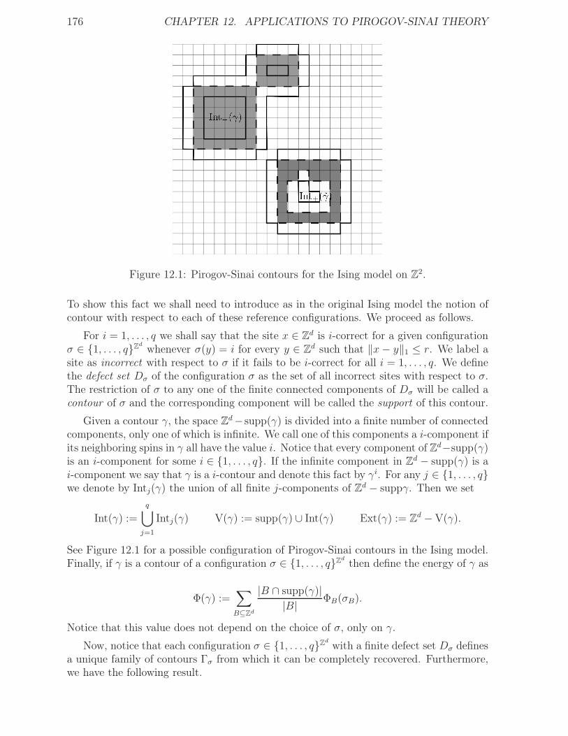
176 CHAPTER 12. APPLICATIONS TO PIROGOV-SINAI THEORY
Figure 12.1: Pirogov-Sinai contours for the Ising model on Z2.
To show this fact we shall need to introduce as in the original Ising model the notion ofcontour with respect to each of these reference configurations. We proceed as follows.
For i = 1, . . . , q we shall say that the site x ∈ Zd is i-correct for a given configurationσ ∈ 1, . . . , qZd whenever σ(y) = i for every y ∈ Zd such that ‖x− y‖1 ≤ r. We label asite as incorrect with respect to σ if it fails to be i-correct for all i = 1, . . . , q. We definethe defect set Dσ of the configuration σ as the set of all incorrect sites with respect to σ.The restriction of σ to any one of the finite connected components of Dσ will be called acontour of σ and the corresponding component will be called the support of this contour.
Given a contour γ, the space Zd− supp(γ) is divided into a finite number of connectedcomponents, only one of which is infinite. We call one of this components a i-component ifits neighboring spins in γ all have the value i. Notice that every component of Zd−supp(γ)is an i-component for some i ∈ 1, . . . , q. If the infinite component in Zd − supp(γ) is ai-component we say that γ is a i-contour and denote this fact by γi. For any j ∈ 1, . . . , qwe denote by Intj(γ) the union of all finite j-components of Zd − suppγ. Then we set
Int(γ) :=q⋃
j=1
Intj(γ) V(γ) := supp(γ) ∪ Int(γ) Ext(γ) := Zd − V(γ).
See Figure 12.1 for a possible configuration of Pirogov-Sinai contours in the Ising model.Finally, if γ is a contour of a configuration σ ∈ 1, . . . , qZd then define the energy of γ as
Φ(γ) :=∑
B⊆Zd
|B ∩ supp(γ)||B| ΦB(σB).
Notice that this value does not depend on the choice of σ, only on γ.
Now, notice that each configuration σ ∈ 1, . . . , qZd with a finite defect set Dσ definesa unique family of contours Γσ from which it can be completely recovered. Furthermore,we have the following result.
12.1. DISCRETE Q-POTTS MODEL OF INTERACTION RANGE R 177
Proposition 12.1. For Λ ∈ B0Zd
let us consider a configuration σ such that Dσ ⊆ Λ andσ(x) = i for every x ∈ Zd lying in the unique infinite connected component of Zd − Dσ.If Γσ denotes the family of contours associated to σ, then we have
µiΛ(σ) =1
Z iΛ
e−β∑
γ∈ΓσΦ(γ). (12.2)
Proof. For each finite B ⊆ Zd let us write
ΦB(σB) =∑
x∈B
1
|B|ΦB(σB) =∑
γ∈Γσ
|B ∩ supp(γ)||B| ΦB(σB) +
|B ∩ (Zd −Dσ)||B| ΦB(σB).
Notice that σ is necessarily constant on any B = x, y such that B ∩ (Zd − Dσ) 6= ∅,which implies that ΦB(σB) = 0 for such B. Thus, summing over all B such that B∩Λ 6= ∅we immediately obtain (12.2).
Looking at (12.2), one might be tempted to proceed as for the Ising contours modelon Section 8.2.6. However, the situation now is more complicated than it was before: itis no longer true that each family of contours with disjoint supports corresponds to someconfiguration in 1, . . . , qZd. Indeed, besides having disjoint supports, nested contoursmust have matching internal and external labels for the whole family to correspond tosome configuration. In particular, if one defines the q-Potts contour model by analogy withwhat was done on Section 8.2.6, the resulting model will violate the bounded energy losscondition, i.e. ∆E∗ = −∞, so that one cannot associate an FFG dynamics to it. Indeed,there exist contour configurations which are forbidden because they carry nested contourswith mismatched labels on them, but that can be turned into admissible configurations byadding a suitable contour in between. The energy leap function associated to an additionof this sort is thus −∞. Nonetheless, the following procedure by Minlos and Sinai [31, 32]will help solve this problem.
Let us fix i = 1, . . . , q and consider the contour model on N (Zd×Gi), where Gi denotesthe space of all i-contour shapes, given by the intensity measure
νi(γix) := e−βΦ(γix) (12.3)
and the Hamiltonian
H iΛ|Γ′(Γ) =
+∞ if either Γ is incompatible, Γ 6∼ Γ′Λc×G or Γ 6⊂ Λ
0 otherwise.(12.4)
where we say that two contours γ, γ′ are incompatible whenever d1(supp(γ), supp(γ′)) ≤ 1and the expression Γ ⊂ Λ indicates that d1(V (γi),Λc) > 1 for every contour γi ∈ Γ.Notice that, as it happened in the Ising contours model, this contour model will also failto satisfy Assumptions 8.2. Thus, when working with this model we will have to take thenecessary precautions already described for the Ising contours model, we omit them here.Also, observe that in this model we still have that compatible families of contours will not,in general, correspond to actual configurations in 1, . . . , qZd. Nonetheless, this artificialcontour model no longer violates the bounded energy loss condition since its interactionsare given only by intersections and it also preserves the distribution of exterior contours.
178 CHAPTER 12. APPLICATIONS TO PIROGOV-SINAI THEORY
Definition 12.2. Given a family Γ of contours with disjoint support we say that γ ∈ Γis an exterior contour of Γ if γ is not contained in the interior of any other contour of Γ.The set of all exterior contours of Γ shall be denoted by Ext(Γ). Furthermore, given aconfiguration σ ∈ 1, . . . , qZd with a finite defect set Dσ, we denote the set of all exteriorcontours of Γσ by Ext(σ).
Proposition 12.3. Let Γ be a finite family of i-contours which are pairwise compatible.Then for any Λ ∈ B0
Zdsuch that d1(V(γ),Λc) > 1 for all γ ∈ Γ we have that
µiΛ(σ ∈ 1, . . . , qZd : Ext(σ) = Γ)µiΛ(σ : d1(V(γ),Λc) > 1 for all γ ∈ Γσ)
= µΛ|∅(Γ′ ∈ N (Λ×Gi) : Ext(Γ′) = Γ)
where µΛ|∅ is the Boltzmann-Gibbs distribution of the model (νi, H i).
Proof. We can assume that all contours in Γ are exterior. Thus, we have to check that
∑
σ:Ext(σ)=Γ e−β∑
γ∈ΓσΦ(γ)
∑
σ∈Ci(Λ) e−β∑
γ∈ΓσΦ(γ)
=
∑
Γ′:Ext(Γ′)=Γ e−β∑
γi∈Γ′ Φ(γi)
∑
Γ′∈Di(Λ) e−β∑
γi∈Γ′ Φ(γi)(12.5)
where the sums in the left hand side are only over configurations σ in the support of µiΛ,those in the right hand side are only over families Γ′ of compatible i-contours and, finally,where we have set
C i(Λ) := σ : d1(V(γ),Λc) > 1 for all γ ∈ Γσ
andDi(Λ) := Γ′ : d1(V (γ
i),Λc) > 1 for all γi ∈ Γ′.We show that both numerators and both denominators in (12.5) are respectively identical.We shall proceed by induction. Given a contour γ we define its level as the maximumn ∈ N0 such that there exists a sequence of contours γ0, . . . , γn such that γ = γ0 andsupp(γi) ⊆ Int(γi−1) for all i = 1, . . . , n. Furthermore, define the level of a family Γ ofcontours as the maximum level of any contour γ ∈ Γ and also define the level of Λ ∈ B0
Zd
as the maximum level of any contour γ such that V (γ) ⊆ Λ. Thus, we shall proceed byinduction on the level of both Γ and Λ, respectively.
If Γ has level zero then we have that
Ext(σ) = Γ ⇐⇒ Γσ = Γ and Ext(Γ′) = Γ ⇐⇒ Γ′ = Γ.
which immediately implies that both numerators in (12.5) are identical in this case.We would like to point out the importance in the previous argument of the fact thatd1(V(γ),Λc) > 1 for all γ ∈ Γ. Indeed, notice that the sum in the numerator of the lefthand side of (12.5) is over all σ in the support of µiΛ and that, for arbitrary Λ, it couldvery well happen that there are no configurations σ in the support of µiΛ such that Γσ = Γ.The latter happens whenever there exists γ ∈ Γ such that Intj(γ) ∩ Λc 6= ∅ for some j 6= i,that is, when Λ is not simply connected and Γ has a contour whose interior labels comeinto conflict with the boundary configuration i. If this were to be the case, then bothnumerators would not coincide. However, due to the assumption that d1(V(γ),Λc) > 1for all γ ∈ Γ, we can rule out this possibility and thus conclude as we have.
12.1. DISCRETE Q-POTTS MODEL OF INTERACTION RANGE R 179
Similarly, if Λ has level zero we have that
σ ∈ C i(Λ) =⇒ Γσ ∈ Di(Λ) and Γ′ ∈ Di(Λ) =⇒ ∃ σ ∈ C i(Λ) such that Γ′ = Γσ
since for σ in the support of µiΛ we have that all contours in Γσ must be exterior i-contours.Thus we conclude that both denominators in (12.5) are equal as well.
Next, if Γ has level n+1 then, by reordering the sum in the left hand side by summingindependently over configurations in the interior of each γ ∈ Γ, we obtain that
∑
σ:Ext(σ)=Γ
e−β∑
γ∈ΓσΦ(γ) =
∏
γi∈Γ
e−βΦ(γi)
q∏
j=1
∑
σ∈Cj (Intj(γi))
e−β∑
γ∈ΓσΦ(γ)
where we have used the fact that all contours involved are compatible and, furthermore,that Intj(γ) has simply connected components for every contour γ ∈ Γ and j = 1, . . . , q.Now, since Intj(γ) is of level no greater than n for every contour γ ∈ Γ and j = 1, . . . , q,by inductive hypothesis we conclude that
∑
σ:Ext(σ)=Γ
e−β∑
γ∈ΓσΦ(γ) =
∏
γi∈Γ
e−βΦ(γi)
q∏
j=1
∑
Γj∈Dj(Intj(γi))
e−β∑
γj∈ΓjΦ(γj )
(12.6)
Furthermore, by the symmetry between spins in the q-Potts model, for each j = 1, . . . , qwe have that
∑
Γj∈Dj(Intj(γi))
e−β∑
γj∈ΓjΦ(γj) =
∑
Γi∈Di(Intj(γi))
e−β∑
γi∈Γi Φ(γi) (12.7)
so that the sums in the right hand of (12.6) become only over i-contours. Then, byreversing the summation order, we obtain the numerator in the right hand side of (12.5).
Finally, if Λ has level n+1 then we decompose the sum in the denominator of the lefthand side of (12.5) over all compatible families of exterior i-contours and use the fact thatall these families have level no greater than n+1, so that for each of them the numeratorsin (12.5) coincide by the argument given above.
As a consequence of Proposition 12.3 we have that for every simply connected Λ ∈ B0Zd
the measure µiΛ can be obtained by first sampling the external contours and then samplingthe spin configuration in the interior of each contour with the corresponding finite-volumeBoltzmann-Gibbs distributions. The precise statement is given in Proposition 12.5 below.
Definition 12.4. Given Λ ∈ B0Zd
we define its interior boundary ∂Λ as
∂Λ := x ∈ Λ : d1(x,Λc) = 1
and its r-interior Λ asΛ := x ∈ Λ : d1(x, ∂Λ) > r.
Proposition 12.5. For simply connected Λ ∈ B0Zd
and σ ∈ 1, . . . , qZd with µiΛ(σ) > 0we have
µiΛ(σ) = µΛ|∅(Γ′ : Ext(Γ′) = Ext(Γσ))∏
γi∈Ext(Γσ)
q∏
j=1
µjIntj (γ)
(σjIntj (γ)
) (12.8)
180 CHAPTER 12. APPLICATIONS TO PIROGOV-SINAI THEORY
where, for each j = 1, . . . , q and ∆ ∈ B0Zd
, the configuration σj∆ ∈ 1, . . . , qZd is definedby the formula
σj∆(x) :=
σ(x) if x ∈ ∆
j if x /∈ ∆.
Proof. Let us notice the following equivalences:
µiΛ(σ) > 0 ⇐⇒ σ(x) = i for all x ∈ Zd − Λ ⇐⇒ d(supp(γi),Λc) > 1 for all γi ∈ Γσ.
Since Λ is simply connected, this implies in fact that d(V(γi),Λc) > 1 for all γi ∈ Γσ.Thus, by the consistency of Boltzmann-Gibbs distributions and Proposition 12.3 we have
µiΛ(σ) =µiΛ(σ)
µiΛ(Ci(Λ))
= µΛ|∅(Γ′ : Ext(Γ′) = Ext(σ))µiΛ(σ|σ′ : Ext(σ′) = Ext(σ)).
Now, notice that if a configuration σ′ in the support of µiΛ is such that Ext(σ′) = Ext(σ)then the spin values of σ′ outside Int(Ext(σ)) :=
⋃
γi∈Ext(σ) Int(γi) are fully determined.More precisely, we have the following identity of events
σ′ : Ext(σ′) = Ext(σ) = σ′ : σ′Zd−Int(Ext(σ)) = σZd−Int(Ext(σ)).
This, combined with the fact that spins in different interiors never interact (either becausethey are too far apart or they have the same value), gives (12.8).
As a consequence of Proposition 12.5, we obtain the following simulation scheme for µiΛ.
Corollary 12.6. Given a simply connected set Λ ∈ B0Zd
, let Y be a random i-contourcollection distributed according to µΛ|∅ and X = Xj
∆ : ∆ ⊆ B0Zd, j = 1, . . . , q be a family
of random spin configurations satisfying:
• X is independent of Y .
• The random elements Xj∆ are all independent and with distribution µj∆, respectively.
If we take the random spin configuration Z with external contours matching those of Y andwith internal spin configuration given by the corresponding random configurations in X,i.e. the random spin configuration Z defined by the formula
Z(x) =
i if x ∈ ⋂γi∈Ext(Y ) Ext(γi)
YΛ(x) if x ∈ ⋃γi∈Ext(Y ) supp(γi)
j if x ∈ Intj(γi)− Intj(γi) for γi ∈ Ext(Y ) and j = 1, . . . , q
Xj
Intj (γi)(x) if x ∈ Intj(γ
i) for γi ∈ Ext(Y ),
then Z is distributed according to µiΛ . We call Z the i-alignment of Y with respect to X.
12.1. DISCRETE Q-POTTS MODEL OF INTERACTION RANGE R 181
The key advantage of this simulation scheme is that it can also be carried out in aninfinite volume with the help of the FFG dynamics. Indeed, consider the coefficient
αq-Potts(β) := supγix∈Zd×Gi
1
|γix|∑
γiy 6∼γix
|γiy|e−βΦ(γiy)
.
where, for a given contour γ, we denote the cardinal of its support by |γ|. Notice that, bythe symmetry of the q-Potts model, the coefficient α does not depend on the choice of i.Now, if αq-Potts < 1 then (νi, H i) admits an infinite-volume Gibbs distribution µ obtainedas the stationary measure of the corresponding FFG dynamics Ki. Furthermore, it followsas in the Ising contours model that the free process at time 0, Πi
0, has only finitely manycontours surrounding any point in Zd and, thus, external contours in Ki
0 are well defined.Hence, if we consider a family X independent of Ki as in Corollary 12.6, then it is possibleto conduct the i-alignment of Ki
0 with respect to X. By repeating a similar analysis tothe one carried out for the Ising contours model, one can verify that the distribution ofthis i-alignment is a Gibbs measure for the q-Potts model. Furthermore, by following theideas discussed in the proof of Theorem 9.23, it is possible to construct for any pair f, gof bounded local functions a triple
(
A0F (r(Λf)), (X
j∆)∆ 6⊆Λcf
)
,(
A0F (r(Λg)), (X
j∆)∆ 6⊆Λcg
)
,(
A0F (r(Λg)), (X
j∆)∆ 6⊆Λcg
)
where for Λ ∈ B0Zd
we define r(Λ) := γix ∈ Zd ×Gi : V(γix) ∩ Λ 6= ∅, such that
•(
A0F (r(Λf)), (X
j∆)∆ 6⊆Λcf
)
and(
A0F (r(Λg)), (X
j∆)∆ 6⊆Λcg
)
are independent,
•(
A0F (r(Λg)), (X
j∆)∆ 6⊆Λcg
)
and(
A0F (r(Λg)), (X
j∆)∆ 6⊆Λcg
)
have the same distribution,
• A0(r(Λf) ∼ A0(r(Λg)) =⇒(
A0F (r(Λg)), (X
j∆)∆ 6⊆Λcg
)
=(
A0F (r(Λg)), (X
j∆)∆ 6⊆Λcg
)
.
By combining these elements as in the proof of Theorem 9.30, we get the following result.
Theorem 12.7. If β > 0 is sufficiently large so as to satisfy αq-Potts(β) < 1 then:
i. The q-Potts model on Zd of interaction range r admits q distinct Gibbs measures,which we denote by µi for i = 1, . . . , q.
ii. For each i = 1, . . . , q the measure µi can be obtained as the local limit
µi := limn→+∞
µiΛn
for any sequence (Λn)n∈N ⊆ B0Zd
of simply connected sets with Λn ր Zd.
iii. For each i = 1, . . . , q the measure µi satisfies the i-sea with islands picture.
iv. If also β > β∗ where
β∗ := inf
β > 0 :∑
γix:d1(0,supp(γix))≤1
|γix|e−βΦ(γix) < 1
then each µi is exponentially mixing in the sense of (9.37) and (9.38).
182 CHAPTER 12. APPLICATIONS TO PIROGOV-SINAI THEORY
Remark 12.8. In principle it is not clear why for β > 0 sufficiently large one should haveαq-Potts(β) < 1 or even αq-Potts(β) < +∞ for that matter. Indeed, this will depend on thebehavior of contour energies Φ(γ) in the limit as |γ| → +∞. Fortunately, it is not hardto see that all contours γ in the q-Potts model satisfy the Peierls bound
Φ(γ) ≥ |γ|2.
This bound guarantees that for β > 0 sufficiently large one effectively has αq-Potts(β) < 1,so that the results of Theorem 12.7 have true meaning.
One can also adapt the arguments featured in Chapter 10 to this context and obtainthe following continuity result.
Theorem 12.9. For any β0 > 0 such that αq-Potts(β0) < 1 and any i = 1, . . . , q we havethe local convergence
limβ→β0
µi,β = µi,β0.
Proof. Let us consider a sequence (Xβ)β>0 of families as in Corollary 12.6 (where we writethe dependence in the inverse temperature explicitly) such that for each j = 1, . . . , q and∆ ⊆ B0
Zdwe have the almost sure convergence
limβ→β0
Xj,β∆ = Xj,β0
∆ .
Such a sequence can be constructed using the standard coupling from the past methods(see e.g. [25]). Notice then that, by Corollary 12.6 and the discussion following it,in order to obtain the result it will suffice to couple the FFG dynamics Ki,β independentlyof (Xβ)β>0 so that as β → β0 we have
Ki,β0
loc−→ Ki,β00 .
This, however, can be done as in Chapter 10.
Once again, we would like to point out that these results can also be obtained throughstandard Pirogov-Sinai theory. Nevertheless, the range of β > 0 for which these resultshold under the standard theory is strictly smaller than the one obtained with our approach:standard methods give these results for β > β ′ where
β ′ = inf
β > 0 :∑
γix:d(0,supp(γix))≤1
e|γix|e−βΦ(γix) < 1
.
Due to the fact that traditional Pirogov-Sinai theory relies on the convergence of certaincluster expansions, once again we obtain in the threshold value an exponential dependencein the size of contours which is only linear for our approach. Furthermore, another strengthof our approach is that it provides us with a perfect simulation scheme for the measures µi.We believe that such a scheme has not been developed before. It is essentially containedin Corollary 12.6 and the discussion following it (see also the discussion on Section 9.7).
12.2. DISCRETE WIDOM-ROWLINSON MODEL 183
12.2 Discrete Widom-Rowlinson model
In this section we show how the ideas discussed for the q-Potts model on Zd can beadapted to establish a phase transition in the discrete Widom-Rowlinson model on Zd
with fugacity λ > 0 and interaction range r ∈ N. Recall that this model is traditionallydefined on the configuration space +, 0,−Zd through the Boltzmann-Gibbs distributionsgiven for each Λ ∈ B0
Zdand η ∈ +, 0,−Zd by the formula
µηΛ(σ) =1σΛc≡ηΛc
ZηΛ
e−∑
B:B∩Λ6=∅ ΦB(σ) (12.9)
where for each B ⊆ Zd the interaction ΦB is given by
ΦB(σ) =
(+∞)1σ(x)×σ(y)=− if B = x, y with ‖x− y‖∞ ≤ r
−1σ(x)=± log λ if B = x
0 otherwise.
(12.10)
We wish to show that for sufficiently large values of λ > 0 the model admits at leasttwo different Gibbs measures. The idea is to follow the procedure for the q-Potts model.Once again we fix a set of reference configurations R := η+, η0, η−, where for eachi ∈ +, 0,− we let ηi denote the configuration on +, 0,−Zd with constant spin value i.Also, for each Λ ∈ B0
Zdwe let µiΛ denote the Boltzmann-Gibbs distribution on Λ with
boundary configuration ηi. The notion of contour for this model is defined in exactly thesame way as for the q-Potts model, except for the fact that in the definition of correctpoints here we use the supremum distance d∞ instead of d1. However, since in this modelit is no longer true that ΦB(η
i) = 0 for every ηi ∈ R, the expression for the energy ofa contour becomes slightly different: for an i-contour γi belonging to some configuration σwe define its energy Φ(γi) by the formula
Φ(γi) :=∑
B⊆Zd
|B ∩ supp(γi)||B| ΦB(σB)− ei|γi|
where ei is the mean energy of the configuration ηi defined as
ei :=∑
B⊆Zd:0∈B
1
|B|ΦB(ηiB) =
− log λ if i = ±
0 if i = 0.
By proceeding as in the proof of Proposition 12.1 one can show the following.
Proposition 12.10. For any Λ ∈ B0Zd
let us consider a configuration σ such that Dσ ⊆ Λand σ(x) = i for every x ∈ Zd lying in the unique infinite connected component of Zd−Dσ.If Γσ denotes the family of contours associated to σ, then we have
µiΛ(σ) =1
Z iΛ
e−(∑
γ∈ΓσΦ(γ)+
∑
u∈+,0,− eu|Λu|) (12.11)
where for each u ∈ +, 0,− we let Λu denote the set of all points in Λ which are eitheru-correct or belong to an u-contour of σ.
184 CHAPTER 12. APPLICATIONS TO PIROGOV-SINAI THEORY
The next step is to fix a spin i ∈ +, 0,− and define a contour model on N (Zd×Gi),where Gi is the space of all i-contour shapes, satisfying the bounded energy loss conditionand preserving the distribution of exterior contours. With this purpose in mind, we firstdefine for ∆ ∈ B0
Zdand j ∈ +, 0,− the diluted partition function
Zj(∆) :=∑
σ∈Cj (∆)
e−∑
B:B∩Λ ΦB(σ)
where Cj(∆) := σ ∈ supp(µj∆) : d1(V(γ),Λc) > 1 for all γ ∈ Γσ, and then consider thecontour model with intensity measure νi given by the formula
νi(γix) :=
[
∏
j 6=i
Zj(Intj(γix))Z i(Intj(γix))
]
e−Φ(γix) (12.12)
and Hamiltonian H i defined as
H iΛ|Γ′(Γ) =
+∞ if either Γ is incompatible, Γ 6∼ Γ′Λc×G or Γ 6⊂ Λ
0 otherwise.(12.13)
Notice that the intensity measure carries an additional product of partition functionswhich was missing in the q-Potts model. This is again attributed to the fact that not allreference configurations in this model have zero mean energy. By proceeding as in theprevious section we obtain for this context the analogues of Propositions 12.3, 12.5 andCorollary 12.6. Thus, if for i ∈ +, 0,− we define the coefficient
αi(λ) = supγix∈Zd×Gi
1
|γix|∑
γiy 6∼γix
|γiy|[
∏
j 6=i
Zj(Intj(γix))Z i(Intj(γix))
]
e−Φλ(γiy)
(12.14)
then the condition αi(λ) < 1 implies the existence of a Gibbs measure µi associated to ηi
which fulfills the description in Theorems 12.7 and 12.9. In particular, since α+ = α−by symmetry, the condition α+(λ) < 1 already implies a phase transition for the model.However, it is not clear why this condition should be fulfilled by any value of λ. Indeed,this will not only depend on the behavior of the energies Φ(γ+x ) as |γ+x | → +∞ on (12.14)but also on the growth of the additional factor
∏
j 6=+
Zj(Intj(γ+x ))Z+(Intj(γ+x ))
=Z0(Int0(γ+x ))Z+(Int0(γ+x ))
. (12.15)
Fortunately, it can be seen that for λ > 0 sufficiently large the condition α+(λ) < 1 issatisfied. Indeed, first let us notice that a straightforward combinatorial argument yields,for any +-contour γ+x , the Peierls bound
Φ(γ+x ) = (+∞)1Φ(γ+x )=+∞+#y ∈ supp(γ+x ) : σ(y) = 0 log λ1Φ(γ+x )<+∞ ≥|γ+x |(2r)d
log λ.
(12.16)On the other hand, the following lemma shows that the additional factor in (12.15) remainsbounded for large values of λ.
12.2. DISCRETE WIDOM-ROWLINSON MODEL 185
Lemma 12.11. There exist constants c1, c2 > 0, which depend only on d and r, such thatfor any ∆ ∈ B0
Zd
Z0(∆)
Z+(∆)≤(
2c1
λc2
)#∂e∆
, (12.17)
where ∂e∆ := y ∈ ∆c : d1(y,∆) = 1.
Proof. For ∆ ∈ B0Zd
we define its boundary and r-interior by the respective formulas
∂∆ = x ∈ ∆ : d1(x,∆c) = 1 and ∆ = x ∈ ∆ : d∞(x, ∂∆) > r.
Now, notice that we have the identities
Z0(∆) = Z0∆ and Z+(∆) = λ|∆|−|∆|Z+
∆
where Z0∆ and Z+
∆ are the normalizing constants given in (12.9). Furthermore, we have
Z0∆ = Z+
∆ +∑
σ∈A0+(∆)
e−∑
B:B∩∆6=∅ ΦB(σB)
where A0+(∆
) is the set of all configurations σ in the support of µ0∆ such that σ∆ ·η+
Zd−∆
does not belong to the support of µ+∆. Observe that a configuration σ in the support of
µ0∆ belongs to A0
+(∆) if and only if σ(x) = − for some x ∈ ∆ with d∞(x, ∂e(∆
)) ≤ r.
Now, for a fixed configuration σ in the support of µ0∆ , we say that two given sites
x, y ∈ supp(σ) := z ∈ ∆ : σ(z) 6= 0 are σ-connected if ‖x − y‖∞ ≤ r. Notice thatif x and y are σ-connected then σ must assign both sites x and y the same spin value.The maximal connected components of supp(σ) with respect to this notion of connectionwill be called σ-components. Next, assign to σ the configuration σ+ defined by the formula
σ+(x) :=
+ if either x ∈ Zd −∆ or x belongs a σ-component C ∈ Cσ(∂e(∆))
σ(x) otherwise,
where Cσ(∂e(∆)) is the set σ-components C of supp(σ) satisfying d∞(C, ∂e(∆)) ≤ r.
In other terms, σ+ is obtained from σ by flipping to + the spin of all σ-components whichinteract with the boundary ∂e(∆) and also the spin of sites outside ∆. Notice that σ+
belongs to the support of µ+∆ and that both σ and σ+ have the same energy in ∆, i.e.∑
B:B∩∆ 6=∅ΦB(σB) =
∑
B:B∩∆ 6=∅ΦB(σ
+B).
Hence, since there are at most 2#Cσ+(∂e(∆)) different configurations σ′ in the support of µ0∆
which can be assigned the same configuration σ+ and there exists c1 > 0 such thatfor any configuration σ there can be at most c1(#∂e(∆)) σ-components in Cσ(∂e(∆
)),we obtain the bound
∑
σ∈A0+(∆)
e−∑
B:B∩∆6=∅ ΦB(σB) ≤ 2c1(#∂e(∆))Z+
∆
which implies thatZ0(∆)
Z+(∆)≤ 1 + 2c1(#∂e(∆
))
λ|∆|−|∆| .
From here a straightforward calculation allows us to conclude the result.
186 CHAPTER 12. APPLICATIONS TO PIROGOV-SINAI THEORY
It follows from the Peierls bound on the energy of contours and the previous lemmathat for λ > 0 sufficiently large one has α+(λ) < 1. Thus, we obtain the following result.
Theorem 12.12. If λ > 0 is sufficiently large so as to satisfy α+(λ) < 1 then:
i. The discrete Widom-Rowlinson model on Zd with exclusion radius r admits twodistinct Gibbs measures, µ+ and µ−.
ii. The measures µ+ and µ− can be obtained as the local limits
µ+ = limn→+∞
µ+Λn
and µ− = limn→+∞
µ−Λn
for any sequence (Λn)n∈N ⊆ B0Zd
of simply connected sets with Λn ր Zd.
iii. The measures µ+ and µ− satisfy the sea with islands picture for the + and − spins,respectively.
iv. The measures µ+ and µ− are continuous in λ, i.e. if λ0 is such that α+(λ0) < 1 thenwe have the local convergence
limλ→λ0
µ±,λ = µ±,λ0.
v. If also λ > λ∗, where
λ∗ := inf
λ > 0 :∑
γ+x :d1(0,supp(γ+x ))≤1
|γ+x |[
Z0(Int0(γ+x ))Z+(Int0(γ+x ))
]
e−Φλ(γ+x ) < 1
,
then both µ+ and µ− are exponentially mixing in the sense of (9.37) and (9.38).
Even though we have established the occurrence of phase transition for large valuesof the fugacity λ, one could still wonder what can be said about the remaining 0-spin.Similar combinatorial arguments to the ones given above yield, for any 0-contour γ0x, theinverse Peierls bound
Φ(γ0x) ≤ − |γ0x|(2r)d
log λ
and the lower boundZ±(∆)
Z0(∆)≥(
λc2
2c1
)#∂e∆
for any ∆ ∈ B0Zd
, which implies that for every λ > 0 sufficiently large one actually hasα0(λ) = +∞ and thus our entire argument breaks down for the 0-spin. This suggests thatthe reference configuration η0 is unstable for large fugacities, in the sense that there is noGibbs measure of the model satisfying the 0-sea with islands picture. The other referenceconfigurations η+ and η− are thus regarded as stable.
As a final remark, we would like to point out that the occurrence of a phase transition inthe discrete Widom-Rowlinson model can be established by other methods beside clusterexpansion, such as random cluster representations (see e.g. [23]). However, the use ofsuch representations usually leads to a less complete picture than that of Theorem 12.12
12.3. CONTINUUM WIDOM-ROWLINSON MODEL 187
for very large fugacities: these cannot be used to show neither the ±-sea with islandspicture nor the continuity in λ, and also these representations alone are not enough toestablish exponential mixing properties. Furthermore, random cluster representations ingeneral are not robust, in the sense that they may work very well for certain modelsbut then fail to work whenever these models are subject to slight perturbations. Asan example we have the k-tolerant Widom-Rowlinson model, for which one expects asimilar behavior to the original Widom-Rowlinson model for small values of k, but whoserandom cluster representations become extremely more difficult to handle: each clusterof particles may not have a unique + or − spin value inside them, and the number of spinchanges allowed inside each cluster will vary depending on its own geometry. However,these considerations do not interfere with the general argument given in this section, sothat the Peierls bound in (12.16) and the upper bound in Lemma 12.11 still remain validfor the k-tolerant Widom-Rowlinson model provided that k is small enough to guaranteethat for any incorrect point of an admissible configuration there exists at least one emptysite at a distance no greater than r from it. We can therefore conclude the following resultwithout any additional difficulties.
Theorem 12.13. For λ > 0 sufficiently large and k, r ∈ N such that k < (r + 1)d − 1,the k-tolerant Widom-Rowlinson model with fugacity λ and exclusion radius r admits twodistinct Gibbs measures, µ+ and µ−, each satisfying the description of Theorem 12.12.
12.3 Continuum Widom-Rowlinson model
The ideas discussed in the previous section for the discrete Widom-Rowlinson model canbe adapted to the continuum setting to obtain analogous results. In this section wecomment briefly on how to perform such adaptation.
Given λ, r > 0, recall that the Widom-Rowlinson model on Rd with fugacity λ andexclusion radius r > 0 is defined as the diluted model on N (Rd×+,−) given by (ν,H),where
ν = λLd × (δ+ + δ−)
andHΛ|η(σ) =
∑
(γx,γy)∈eΛ(σ|η)U(γx, γy)
with
U(γx, γy) :=
+∞ if γ 6= γ and ‖x− y‖∞ ≤ r0 otherwise.
(12.18)
Now, consider the tiling T of Rd given by the cubic cells (Qx)x∈Zd , where for each x ∈ Zd
Qx := l · (x+ [0, 1)d),
where l > 0 is sufficiently small so that particles in any two adjacent cells are forbidden bythe Hamiltonian H to be of opposite type. Here we understand adjacent cells in the senseof the graph Zd with the supremum distance, i.e. we say that two cells Qx,Qy are adjacentif d∞(Qx,Qy) = 0 where d∞ is the supremum distance on Rd.
188 CHAPTER 12. APPLICATIONS TO PIROGOV-SINAI THEORY
Given a configuration σ ∈ N (Rd×G) we assign it the configuration sσ ∈ +, 0,−, ∗Zddefined by the formula
sσ(x) =
+ if there are only particles of type (+) in Qx
− if there are only particles of type (−) in Qx
0 if there are no particles in Qx
∗ if there are particles of both types in Qx.
We call sσ the skeleton of σ. Notice that for configurations σ which are not forbidden by Hwe have in fact that sσ(x) 6= ∗ for all x ∈ Zd. Next, fix a set of reference configurations
R = η+, η0, η− ⊆ N (Rd × +,−)
such that for each i ∈ +, 0,− the configuration ηi satisfies sηi(x) = i for all x ∈ Zd.Then, for i ∈ +, 0,− say that a site x ∈ Zd is i-correct with respect to the configurationsσ ∈ +, 0,−, iZd if sσ(y) = i for all y ∈ Zd with ‖x − y‖∞ ≤ r+1
land label a site as
incorrect if it is not i-correct for any i ∈ +, 0,−. Finally, we proceed to define thecontours of the configuration sσ by analogy with the previous sections. Observe thatcontours are not defined for particle configurations on N (Rd × +,−) but rather fortheir skeletons. Now, given an i-contour γi belonging to some skeleton configuration,we define its energy Φ(γi) by the formula
Φ(γi) :=
(
− log
∫
N (supp(γi)×+,−)1sσ=γie
−Hsupp(γi)|∅(σ)dπνsupp(γi)(σ)
)
− ei|supp(γi)|
where
ei = − log
∫
N (Q0×+,−)1sσ=idπ
νsupp(γi)(σ) =
− log(1− e−λld
) + λld if i = ±
2λld if i = 0.
We can write Boltzmann-Gibbs distributions in terms of the energy of contours as follows.
Proposition 12.14. For any Λ ∈ B0Zd
let us consider a skeleton configuration s′ suchthat Ds′ ⊆ Λ and s′(x) = i for every x ∈ Zd lying in the infinite component of Zd −Ds′.If Γs′ denotes the family of contours associated to s′, then we have
µηi
Λl(σ ∈ N (Rd × +,−) : sσ = s′) = 1
ZΛ|ηie−(
∑
γ∈Γs′
Φ(γ)+∑
u∈+,0,− eu|Λ(u)|)
(12.19)
whereΛl :=
⋃
x∈ΛQx
and for each u ∈ +, 0,− we let Λ(u) denote the set of all points in Λ which are eitheru-correct or belong to an u-contour of s∗.
12.3. CONTINUUM WIDOM-ROWLINSON MODEL 189
Proof. This follows from the consistent Hamiltonian property on Assumptions 8.2 bynoticing that particles lying inside correct cells do not interact with particles in other cellsand also that particles inside incorrect cells do not interact with particles in correct cells.We omit the details.
We then fix a spin i ∈ +, 0,− and consider the contour model on N (Zd×Gi), whereGi is the space of i-contour shapes, with Hamiltonian as in (12.13) and intensity measure
νi(γix) :=
[
∏
j 6=i
Zj(Intj(γix))Z i(Intj(γix))
]
e−Φ(γix)
where for each ∆ ∈ B0Zd
and j ∈ +, 0,− we set
Zj(∆) :=∑
sσ∈Cj(∆)
e−(∑
γ∈ΓsσΦ(γ)+
∑
u∈+,0,− eu|∆(u)|)
for Cj(∆) := sσ : sσ(x) = j for all x ∈ Zd −∆ and d1(V(γ),∆c) > 1 for all γ ∈ Γsσ.It is easy to verify that this contour model satisfies the bounded energy loss conditionand that it also preserves the distribution of exterior contours in skeleton configurations.Thus, in order to repeat the analysis of the previous section, it only remains to showan analogue of Corollary 12.6, i.e. we need to show how to conduct an (i)-alignment ofcontour configurations such that, whenever these are distributed according to (νi, H i),the resulting particle configurations carry the correct Boltzmann-Gibbs distributions.Given a simply connected set Λ ∈ B0
Zdand i ∈ +,−, we proceed as follows:
i. Consider a contour configuration Y with distribution µΛ|∅ specified by (νi, H i).
ii. Place an i-particle independently on each cell belonging to the set Λ ∩⋂γi∈Ext(Y ),so that each of these cells carries at least one (i)-particle. Here we let Λ denote ther+1l
-interior of Λ, as in the previous section. Then, on top of these particles placea Poisson process of (i)-particles on (Λ ∩ ⋂γi∈Ext(Y ))l with fugacity λ, which willaccount for the remaining (i)-particles in each of these cells.
iii. Proceed as in (ii) for cells in Intj(γi)− Intj(γi) for γi ∈ Ext(Y ) and j ∈ +, 0,−.
iv. For every contour γi ∈ Ext(Y ) place a particle independently on each cell belongingto supp(γi) of the type γi indicates by the acceptance-rejection method, so that theresulting configuration of particles inside the support of γi is not forbidden by H .If the contour γi assigns a 0-spin to some cell then place no particle in that cell.Then, place the remaining particles of the cells belonging to supp(γi) according tothe FFG dynamics on the finite volume (supp(γi))l with empty boundary condition,but keeping the particles of the acceptance-rejection method alive for all times t ∈ R.
v. For each contour γi ∈ Ext(Y ) place the particles inside the cells belonging to Int(γi)with the FFG dynamics on the finite volume (Int(γi))l with boundary conditiongiven by the portion of particle configuration constructed in (iii).
vi. Finally, place particles in the remaining cells according to ηi.
190 CHAPTER 12. APPLICATIONS TO PIROGOV-SINAI THEORY
It can be seen that this configuration carries the distribution µ(Λ)l|ηi specified by (ν,H).We may then proceed as in the previous section to show a phase transition for large λ.The Peierls bound for the energy of contours and Lemma 12.11 still hold in this setting;the latter being a consequence of the argument given in Lemma 12.11 combined with (7.3)and the Fubini theorem for the product measure ν. Thus, we obtain the following result.
Theorem 12.15. Given λ, r > 0 let us suppose that λ > 0 is sufficiently large so that
α+(λ, r) = supγ+x ∈Zd×G+
1
|γ+x |∑
γ+y 6∼γ+x
|γ+y |[
Z0(Int0(γ+x ))Z+(Int0(γ+x ))
]
e−Φλ,r(γ+y )
< 1.
Then:
i. The continuum Widom-Rowlinson model on Rd with exclusion radius r admits twodistinct Gibbs measures, µ+ and µ−.
ii. The measures µ+ and µ− can be obtained as the local limits
µ+ = limn→+∞
µ(Λn)l|η+ and µ− = lim
n→+∞µ(Λ
n)l|η−
for any sequence (Λn)n∈N ⊆ B0Zd
of simply connected sets with Λn ր Zd.
iii. The measures µ+ and µ− satisfy the sea with islands picture for the + and − spins,respectively.
iv. The measures µ+ and µ− are continuous in λ and r, i.e. if λ0, r0 > 0 are such thatα+(λ0, r0) < 1 then we have the local convergence
lim(λ,r)→(λ0,r0)
µ±,λ,r = µ±,λ0,r0.
v. If also λ > λ∗, where
λ∗ := inf
λ > 0 :∑
γ+x :d1(0,supp(γix))≤1
|γ+x |[
Z0(Int0(γ+x ))Z+(Int0(γ+x ))
]
e−Φλ,r(γ+x ) < 1
,
then both µ+ and µ− are exponentially mixing in the sense of (9.37) and (9.38).
Notice that Theorem 12.15 gives also continuity with respect to the exclusion radius.This is due to the fact that given r0 > 0 one can choose the size l of the tiling so that forany r > 0 sufficiently close to r0 the definition of correct point in the skeleton configurationremains unaltered. From this observation, a straightforward argument analogous to theone in Chapter 10 gives the result. Moreover, since the Peierls bound and the estimationin Lemma 12.11 still hold in this continuum setting, one can also obtain an analogueof Theorem 12.13 showing a phase transition in the k-tolerant Widom-Rowlinson modelfor sufficiently small values of k. Unfortunately, for the Widom-Rowlinson model withgeneralized interactions one can see that a more careful argument is needed than the onegiven here, we shall not pursue it here. Finally, we observe that the exact same analysisgiven here carries over to show a phase transition in the thin rods model for evenly spacedangles. The condition of evenly spaced is important, since it gives the symmetry betweenorientations which was used for the Widom-Rowlinson model. The result is the following.
12.3. CONTINUUM WIDOM-ROWLINSON MODEL 191
Theorem 12.16. Given n ≥ 2 consider the thin rods model of fugacity λ > 0, rod length2r > 0 and orientation measure ρ given by
ρ =1
n
n−1∑
i=0
δ inπ.
Then, for λ > 0 sufficiently large (depending on n and r) the model admits n distinctGibbs measures, (µi)i=1,...,n, each of which satisfies the description on Theorem 12.15.
As a final remark we point out that this same analysis can be carried out in the samemanner for more general models. However, for this analysis to be fruitful, one needs toguarantee a Peierls bound on the energy contours and a suitable control on the ratiosof diluted partition functions like the one given in Lemma 12.11. While in general thePeierls bound will not bring much problems, an estimate as in (12.17) is a priori not easyto obtain. Cluster expansion methods offer further tools to control these terms (see [45]),although at the cost of narrowing the range of validity of the results. Nevertheless, evenif we cannot control the ratios of diluted partition functions directly and we must relyon cluster expansion methods to obtain any results, the approach discussed here stillguarantees that in that smaller range one can still perform perfect simulation of thecorresponding equilibrium measures.
192 CHAPTER 12. APPLICATIONS TO PIROGOV-SINAI THEORY
12.4 Resumen del Capítulo 12
En este último capítulo combinamos las ideas en los capítulos anteriores con el marco de lateoría de Pirogov-Sinai para obtener algunos resultados bajo el régimen de no unicidad.Concretamente, la teoría de Pirogov-Sinai nos provee de un procedimiento sistemáticopara trasladar el estudio de las propiedades macroscópicas (existencia y propiedades demedidas de Gibbs) en sistemas bajo el régimen de no unicidad, i.e. alta densidad departículas o baja temperatura, al estudio de un modelo de contornos adecuado a bajadensidad que puede ser tratado con las técnicas desarrolladas en los capítulos previos. Dehecho, aprovechando estas técnicas nos es posible extender el rango de validez de algunosresultados con respecto al ofrecido por la teoría de Pirogov-Sinai clásica.
Por simplicidad, discutimos estas ideas primero para el modelo de Potts con q spines(q ≥ 2), en donde la simetría entre spines dada por el modelo facilita el análisis y nosevita algunas cuestiones técnicas. Para este modelo, mostramos que a temperaturas bajasexiste para cada spin i = 1, . . . , q una medida de Gibbs µi que verifica un escenario demar con islas para el spin i, análogo al descrito en la Introducción para el modelo deIsing. En particular, las medidas µi son singulares entre sí, lo cual implica una transiciónde fase para el modelo a bajas temperaturas. Además, probamos que cada medida µi esexponencialmente mixing y continua como función de la temperatura (con la noción deconvergencia local).
Luego, tratamos el caso del modelo de Widom-Rowlinson discreto, en donde la faltade simetría entre los spins introduce algunas complicaciones en el análisis. No obstante,conseguimos resultados análogos a los obtenidos para el modelo de Potts: si la densidadde partículas es suficientemente alta entonces existen dos medidas de Gibbs µ+ y µ− conlas propiedades descritas arriba (para los spins + y −, respectivamente). Por otro lado,por la falta de simetría entre los spins (±) y el 0, puede verse que no existe una medidacon estas características asociada al spin 0 restante.
A continuación, mencionamos cómo el análisis realizado en los dos casos anteriorespuede generalizarse a modelos discretos generales. También mostramos cómo puedenaplicarse estas ideas en modelos continuos (con espacio de spines finito y con simetríaentre spins), obteniendo así los mismos resultados para el modelo de Widom-Rowlinsoncontinuo y el modelo de varas finas con n orientaciones equidistantes.
Por último, en todos estos casos mostramos cómo puede ser aprovechada la dinámicaFFG para simular perfectamente las distintas medidas bajo consideración. Cabe destacarque hasta ahora sólo se conocían métodos de simulación perfecta a baja temperatura parael modelo de Ising original. Nuestro análisis extiende estos métodos a una gama muchomás amplia de modelos, tanto discretos como continuos.
Appendix A
A.1 Comparison principle
Theorem A.1. Let f and g be Lipschitz functions on R and, given u, v ∈ C([0, 1]),consider Uu and Uv the solutions of the equation
∂tU = ∂2xxU + f(U) + g(U)W
with initial data u and v, respectively, and boundary conditions satisfying
P (U(t, ·)|∂[0,1] ≥ V (t, ·)|∂[0,1] for all t ≥ 0) = 1.
Then, if u ≥ v we have that
P (Uu(t, x) ≥ Uv(t, x) for all t ≥ 0, x ∈ [0, 1]) = 1.
A proof of this theorem can be found on [10, p. 130]. Notice that if g ≡ 0 one obtainsa comparison principle for deterministic partial differential equations.
A.2 Growth and regularity estimates
Proposition A.2. Given a bounded set B ⊆ CD([0, 1]) there exists tB > 0 such that
• τu > tB for any u ∈ B
• There exists b : [0, tB] → R+ such that limt→0+ b(t) = 0 and for any t ∈ [0, tB]
supu∈B
‖Uu(t, ·)− u‖∞ ≤ b(t).
Proof. Let n ∈ N be such that B ⊆ Bn−1. Notice that for u ∈ B the truncated systemU (n),u verifies
∂2xxU(n),u − ‖gn‖∞ ≤ ∂tU
(n),ε ≤ ∂2xxU(n),u − ‖gn‖∞
and so, by the comparison principle there exists b : R+ → R+ such that limt→0+ b(t) = 0and for any t > 0
supu∈B
‖U (n),u(t, ·)− u‖∞ ≤ b(t).
193
194 APPENDIX A.
Now, if we take tB > 0 such that b(t) < 1 for all t ∈ [0, tB] then for any such t we havethat U (n),u(t, ·) ∈ B
n and so U (n),u(t, ·) coincides with Uu(t, ·). In particular, we see thatτu > t and also that
supu∈B
‖Uu(t, ·)− u‖∞ ≤ b(t)
which concludes the proof.
Proposition A.3. The following local and pointwise growth estimates hold:
i. Given a bounded set B ⊆ CD([0, 1]) there exist CB, tB > 0 such that
• τu > tB for any u ∈ B
• For any pair u, v ∈ B and t ∈ [0, tB]
‖Uu(t, ·)− Uv(t, ·)‖∞ ≤ eCBt‖u− v‖∞.
ii. Given u ∈ CD([0, 1]) and t ∈ [0, τu) there exist Cu,t, δu,t > 0 such that
• τ v > t for any v ∈ Bδu,t(u)
• For any v ∈ Bδu,t(u) and s ∈ [0, t]
‖Uu(s, ·)− Uv(s, ·)‖∞ ≤ eCu,ts‖u− v‖∞.
Proof. Given a bounded set B ⊆ CD([0, 1]) let us take n ∈ N and tB > 0 as in the proofof Proposition A.2. Since gn globally Lipschitz, there exists a constant Cn > 0 such thatfor any pair u, v ∈ CD([0, 1]) and t ≥ 0
‖U (n),u(t, ·)− U (n),v(t, ·)‖∞ ≤ eCnt‖u− v‖∞. (A.1)
In particular, since for every u ∈ B both U (n),u(t, ·) and Uu(t, ·) coincide for all t ∈ [0, tB],we see that if we take CB := Cn then from (A.1) and Proposition A.2 we obtain (i).
On the other hand, given u ∈ CD([0, 1]) and t < tu there exists n ∈ N such thatsups∈[0,t] ‖Uu(s, ·)‖∞ ≤ n−1 and a constant Cn > 0 such that for any pair u, v ∈ CD([0, 1])and s ≥ 0
‖U (n),u(s, ·)− U (n),v(s, ·)‖∞ ≤ eCns‖u− v‖∞. (A.2)
Then by taking Cu,t := Cn and δu,t < e−Cnt from (A.2) we see that for any v ∈ Bδu,t bothU (n),v(s, ·) and Uv(s, ·) coincide for all s ∈ [0, t] and so (ii) immediately follows.
Proposition A.4. If u ∈ CD([0, 1]) then ∂2xxUu exists for any t ∈ (0, τu). Furthermore,
for any bounded set B ⊆ CD([0, 1]) there exists a time tB > 0 such that
• τu > tB for any u ∈ B
• For any t ∈ (0, tB) we have supu∈B ‖∂2xxUu(t, ·)‖∞ < +∞.
A.2. GROWTH AND REGULARITY ESTIMATES 195
Proof. Given u ∈ CD([0, 1]) and t ∈ (0, τu) let us take n ∈ N such that
sups∈[0,t]
‖Uu(s, ·)‖∞ ≤ n.
It follows from this choice of n that Uu and U (n),u coincide on the interval [0, t], so thatit suffices to show that ∂2xxU
(n),u(t, ·) exists. For this purpose, recall that U (n),u satisfiesthe integral equation
U (n),u(t, x) =
∫ 1
0
Φ(t, x, y)u(y)dy +
∫ t
0
∫ 1
0
Φ(t− s, x, y)gn(U(n),u)(s, y))dyds (A.3)
where Φ denotes the fundamental solution of the heat equation with Dirichlet boundaryconditions given by the formula
Φ(t, x, y) =1√4πt
∑
n∈Z
[
exp
(
−(2n + y − x)2
4t
)
− exp
(
−(2n + y + x)2
4t
)]
.
The equation (A.3) can be rewritten as
U (n),u(t, x) =
∫
R
e−(y−x)2
4t√4πt
u(y)dy +
∫ t
0
∫
R
e−(y−x)2
4(t−s)
√
4π(t− s)gn(U (n),u)(s, y)dyds
where, for v ∈ CD([0, 1]), v denotes its odd 2-periodic extension to the whole real line and,for ϕ ∈ CD([0, T ] × [0, 1]), we set ϕ as ϕ(t, x) := ϕ(t, ·)(x) for all (t, x) ∈ [0, T ] × [0, 1].Since gn and u are both bounded it follows that the spatial derivative ∂xU (n),u(t, ·) existsand satisfies
∂xU(n),u(t, x) =
∫
R
ξe−ξ2
√πtu(x+
√4tξ)dξ+
∫ t
0
∫
R
ηe−η2
√
π(t− s)gn(U (n),u)(s, x+
√
4(t− s)η)dηds
(A.4)where we have performed the changes of variables
ξ =y − x√
4tand η =
y − x√
4(t− s).
Consequently, we obtain the bound
‖∂xU (n),u(t, ·)‖∞ ≤(
1√πt
+
√t√π
)
(‖u‖∞ + ‖gn‖∞).
Let us observe that if we set ψ := U (n),u( t2, ·) then U (n),u(t, ·) = U (n),ψ( t
2, ·) and by (A.4)
applied to the time t2
we obtain that dψ
dxexists and satisfies
∥
∥
∥
∥
dψ
dx
∥
∥
∥
∥
∞≤( √
2√πt
+
√t√2π
)
(‖u‖∞ + ‖gn‖∞).
Furthermore, since g′n is bounded and for any s ∈ (0, t) we have
‖∂xU (n),u(s, ·)‖∞ ≤(
1√πs
+
√s√π
)
(‖u‖∞ + ‖gn‖∞)
196 APPENDIX A.
then it follows that ∂2xxU(n),u(t, ·) exists and satisfies
∂2xxU(n),u(t, x) = ∂2xxU
(n),ψ
(
t
2, x
)
=
∫
R
√2ξe−ξ
2
√πt
dψ
dx(x+
√2tξ)dξ
+
∫ t2
0
∫
R
√2ηe−η
2
√
π(t− 2s)
(
g′n(U(n),u) · ∂xU (n),ψ
)
(s, x+√
2(t− 2s)η)dηds.
Consequently, we obtain the bound
‖∂2xxU (n),u(t, ·)‖∞ ≤
(
2
πt+
1
π
)
+ ‖g′n‖∞∫ t
2
0
1√πs
+√s√π
√
π( t2− s)
ds
(‖u‖∞ + ‖gn‖∞).
By observing that∫ t
2
0
1√s+√s
√
t2− s
ds ≤ 4 + t
we conclude that
‖∂2xxU (n),u(t, ·)‖∞ ≤ 1
π
(
1 +2
t+ ‖g′n‖∞(4 + t)
)
(‖u‖∞ + ‖gn‖∞). (A.5)
Finally, given a bounded set B ⊆ CD([0, 1]) then the uniformity of the bound in B followsfrom (A.5) since by Proposition A.2 we may take n ∈ N such that
supu∈B,t∈[0,tB ]
‖Uu(t, ·)‖∞ ≤ n
for some tB > 0 such that τu > tB for all u ∈ B.
Proposition A.5. For any bounded set B ⊆ CD([0, 1]) there exists tB > 0 such that
• τu > tB for any u ∈ B
• For any t ∈ (0, tB) there exist Rt, Nt > 0 such that for every u ∈ B the functionUu(t, ·) belongs to the compact set
γRt,Nt = v ∈ CD([0, 1]) : ‖v‖∞ ≤ Rt , |v(x)− v(y)| ≤ Nt|x− y| for all x, y ∈ [0, 1].
Proof. By Proposition A.2 there exists tB > 0 such that τu > tB for every u ∈ B and foreach t ∈ (0, tB) there exists Rt > 0 such that
supu∈B,s∈[0,t]
‖Uu(s, ·)‖∞ ≤ Rt.
It then follows from the proof of Proposition A.4 that
supu∈B
‖∂xUu(t, ·)‖∞ ≤(
1√πt
+
√t√π
)
(Rt + ‖gRt‖∞) := Nt
which by the mean value theorem implies that Uu(t, ·) ∈ γRt,Nt for all u ∈ B.
A.2. GROWTH AND REGULARITY ESTIMATES 197
Proposition A.6. The following local and pointwise growth estimates hold:
i. Given a bounded set B ⊆ CD([0, 1]) there exists tB > 0 such that
• τu > tB for any u ∈ B
• For any t ∈ (0, tB) there exists Ct,B > 0 such that for all u, v ∈ B
‖∂xUu(t, ·)− ∂xUv(t, ·)‖∞ ≤ Ct‖u− v‖∞.
ii. Given u ∈ CD([0, 1]) and t ∈ (0, τu) there exist Cu,t, δu,t > 0 such that
• τ v > t for any v ∈ Bδu,t(u)
• For any v ∈ Bδu,t(u)
‖∂xUu(t, ·)− ∂xUv(t, ·)‖∞ ≤ Cu,t‖u− v‖∞.
Proof. Notice that if tB > 0 is such that τu > tB for every u ∈ B and for each t ∈ (0, tB)there exists RB,t > 0 such that
supu∈B,s∈[0,t]
‖Uu(s, ·)‖∞ ≤ RB,t,
then it follows from (A.4) that
‖∂xUu(t, ·)− ∂xUv(t, ·)‖∞ ≤
[(
1√πt
+
√t√π
)
(1 + ‖g′Rt‖∞)
]
‖u− v‖∞.
which shows (i). Now, (ii) follows in the same way upon noticing that by Proposition A.3given t ∈ (0, τu) there exist Ru,t, δu,t > 0 such that τ v > t for any v ∈ Bδu,t(u) and
supv∈Bδu,t (u),s∈[0,t]
‖Uv(s, ·)‖∞ ≤ Ru,t.
Proposition A.7. For any equilibrium point w of the deterministic system let us considerits stable manifold Ww defined as
Ww := u ∈ CD([0, 1]) : Uu is globally defined and Uu(t, ·) −→
t→+∞w.
Notice that W0 = D0. Then for any bounded set B ⊆ Ww there exists tB > 0 such thatfor any t0 ∈ [0, tB] and r > 0 we have
supu∈B
[inft ≥ t0 : d(Uu(t, ·), w) ≤ r] < +∞
whenever one of the following conditions hold:
• w 6= 0
• w = 0 and B is at a positive distance from W :=⋃
n∈Z−0Wz(n) .
198 APPENDIX A.
Furthermore, if B ⊆ De is a bounded set at a positive distance from W then for anyn ∈ N we have
supu∈B
τ (n),u < +∞.
Proof. Let us suppose first that w 6= 0. Then, since Wω is a closed set, by PropositionA.5 we have that the family Uu(tB, ·) : u ∈ B is contained in a compact set B′ ⊆ Ww
for some suitably small tB > 0. Hence, we obtain that
supu∈B
[inft ≥ t0 : d(Uu(t, ·), w) ≤ r] ≤ tB + sup
v∈B′
[inft ≥ 0 : d(Uv(t, ·), w) < r]
Since the application v 7→ inft ≥ 0 : d(Uv(t, ·), w) < r is upper semicontinuous andfinite on Ww, we conclude that the right hand side is finite and thus the result followsin this case. Now, if w = 0 then once again by Proposition A.5 we have that the familyUu(tB, ·) : u ∈ B is contained in a compact set B′ ⊆ D0 but this time by PropositionA.2 we may choose tB > 0 sufficiently small so as to guarantee that B′ is at a positivedistance from W. From here we conclude the proof as in the previous case. Finally, thelast statement of the proposition is proved in a completely analogous fashion.
A.3 Properties of the potential S
Proposition A.8. The mapping t 7→ S(Uu(t, ·)) is monotone decreasing and continuousfor any u ∈ H1
0((0, 1)).
Proof. First, observe that a direct calculation shows that for any u ∈ CD([0, 1]) and t0 > 0
dS(Uu(t, ·))dt
(t0) =
∫ 1
0
(
∂xUu(t0, ·)∂2xtUu(t0, ·)− g(Uu(t0, ·))∂tUu(t0, ·)
)
= −∫ 1
0
(
∂2xxUu(t0, ·) + g(Uu(t0, ·))
)
∂tUu(t0, ·)
= −∫ 1
0
(∂tUu(t0, ·))2 ≤ 0.
On the other hand, it is well known (see [38] p.75) that the mapping t 7→ Uu(t, ·) iscontinuous on H1
0 ((0, 1)) whenever u ∈ H10 ((0, 1)) and on Lp+1([0, 1]) when u ∈ CD([0, 1]).
In particular, we see that t 7→ S(Uu(t, ·)) is continuous at t0 = 0 and so, by the previouscalculation, we conclude the result.
Proposition A.9. The potential S is lower semicontinuous.
Proof. Let (vk)k∈N ⊆ CD([0, 1]) be a sequence converging to some limit v∞ ∈ CD([0, 1]).We must check that
S(v∞) ≤ lim infk→+∞
S(vk). (A.6)
A.4. PROPERTIES OF THE QUASIPOTENTIAL V 199
Notice that since (vk)k∈N is convergent in the supremum norm we have, in particular, that
supk∈N
‖vk‖Lp+1 < +∞ (A.7)
and therefore that lim infk→+∞ S(vk) > −∞. Hence, by passing to an subsequence ifnecessary, we may assume that the limit in (A.6) exists and is finite so that, in particular,we have that the sequence (S(vk))k∈N remains bounded. This implies that vk is absolutelycontinuous for every k ∈ N and, furthermore, by (A.7) we conclude that the sequence(vk)k∈N is bounded in H1
0((0, 1)). Hence, there exists a subsequence (vkj)j∈N which isweakly convergent in H1
0((0, 1)) and strongly convergent in L2([0, 1]) to some limit v∗∞.Notice that since (vk)k∈N converges in the supremum norm to v∞, it also converges in Lq
for every q ≥ 1. In particular, we have that v∗∞ = v∞ and thus, by the lower semicontinuityof the H1
0 -norm with respect in the weak topology we conclude that
‖∂xv∞‖L2 ≤ lim infj→+∞
‖∂xvkj‖L2 .
Finally, since (vk)k∈N converges to v∞ in Lp+1 and we have S(u) = 12‖∂xu‖2L2 − 1
p+1‖u‖p+1
Lp+1
for all u ∈ H10 , we obtain (A.6).
Proposition A.10. Given u ∈ CD([0, 1]) and t ∈ (0, τu) there exist Cu,t, δu,t > 0 suchthat
• τ v > t for any v ∈ Bδu,t(u)
• For any v ∈ Bδu,t(u) one has
‖S(Uu(t, ·))− S(Uv(t, ·))‖∞ ≤ Cu,t‖u− v‖∞.
Proof. This is a direct consequence of Propositions A.6 and A.3.
A.4 Properties of the quasipotential V
Proposition A.11. The mapping u 7→ V (0, u) is lower semicontinuous on CD([0, 1]).
Proof. Let (uk)k∈N ⊆ CD([0, 1]) be a sequence converging to some limit u∞ ∈ CD([0, 1]).We must check that
V (0, u∞) ≤ lim infk→+∞
V (0, vk). (A.8)
If S(u∞) = +∞ then by Proposition 3.6 we see that V (0, u) = +∞ and thus by the lowersemicontinuity of S we conclude that limv→u V (0, v) = +∞ which establishes (A.8) inthis particular case. Now, if S(u∞) < +∞ then, by the lower semicontinuity of S andthe continuity in time of the solutions to (1.1), given δ > 0 there exists t0 > 0 sufficientlysmall such that S(Uu∞(t0, ·)) > S(u∞) − δ
2. Moreover, by Proposition A.3 we may even
assume that t0 is such that
‖Uuk(t0, ·)− Uu∞(t0, ·)‖∞ ≤ 2‖uk − u∞‖∞for any k ∈ N sufficiently large. Thus, given k sufficiently large and a path ϕk from 0 to ukwe construct a path ϕk,∞ from 0 to u∞ by the following steps:

200 APPENDIX A.
i. We start from 0 and follow ϕk until we reach uk.
ii. From uk we follow the deterministic flow Uuk until time t0.
iii. We then join Uuk(t0, ·) and Uu∞(t0, ·) by a linear interpolation of speed one.
iv. From Uu∞(t0, ·) we follow the reverse deterministic flow until we reach u∞.
By the considerations made in the proof of Lemma 4.3 it is not hard to see that thereexists C > 0 such that for any k ∈ N sufficiently large we have
I(ϕk,∞) ≤ I(ϕk) + C‖uk − u∞‖∞ + δ
so that we ultimately obtain
V (0, u∞) ≤ lim infk→+∞
V (0, uk) + δ.
Since δ > 0 can be taken arbitrarily small we conclude (A.8).
Proposition A.12. For any u, v ∈ CD([0, 1]) the map t 7→ V (u, Uv(t, ·)) is decreasing.
Proof. Given 0 ≤ s < t and a path ϕ from u to Uu(s, ·) we may extend φ to a path ϕfrom u to Uu(t, ·) simply by following the deterministic flow afterwards. It follows that
V (u, Uv(t, ·)) ≤ I(ϕ) = I(ϕ)
which, by taking infimum over all paths from u to Uu(s, ·), yields the desired monotonicity.

Bibliography
[1] Gabriel Acosta, Julián Fernández Bonder, and Julio D. Rossi. Stable manifold ap-proximation for the heat equation with nonlinear boundary condition. J. Dynam.Differential Equations, 12(3):557–578, 2000.
[2] R. Azencott. Grandes déviations et applications. In Eighth Saint Flour ProbabilitySummer School—1978 (Saint Flour, 1978), volume 774 of Lecture Notes in Math.,pages 1–176. Springer, Berlin, 1980.
[3] Catherine Bandle and Hermann Brunner. Blowup in diffusion equations: a survey.J. Comput. Appl. Math., 97(1-2):3–22, 1998.
[4] S. Brassesco. Unpredictability of an exit time. Stochastic Process. Appl., 63(1):55–65,1996.
[5] Stella Brassesco. Some results on small random perturbations of an infinite-dimensional dynamical system. Stochastic Process. Appl., 38(1):33–53, 1991.
[6] Jean Bricmont, Koji Kuroda, and Joel L. Lebowitz. The structure of Gibbs statesand phase coexistence for nonsymmetric continuum Widom-Rowlinson models. Z.Wahrsch. Verw. Gebiete, 67(2):121–138, 1984.
[7] Marzio Cassandro, Antonio Galves, Enzo Olivieri, and Maria Eulália Vares.Metastable behavior of stochastic dynamics: a pathwise approach. J. Statist. Phys.,35(5-6):603–634, 1984.
[8] Carmen Cortázar and Manuel Elgueta. Large time behaviour of solutions of a non-linear reaction-diffusion equation. Houston J. Math., 13(4):487–497, 1987.
[9] Carmen Cortázar and Manuel Elgueta. Unstability of the steady solution of a non-linear reaction-diffusion equation. Houston J. Math., 17(2):149–155, 1991.
[10] Robert Dalang, Davar Khoshnevisan, Carl Mueller, David Nualart, and Yimin Xiao.A minicourse on stochastic partial differential equations, volume 1962 of LectureNotes in Mathematics. Springer-Verlag, Berlin, 2009. Held at the University of Utah,Salt Lake City, UT, May 8–19, 2006, Edited by Khoshnevisan and Firas Rassoul-Agha.
[11] D. J. Daley and D. Vere-Jones. An introduction to the theory of point processes. Vol.I. Probability and its Applications (New York). Springer-Verlag, New York, secondedition, 2003. Elementary theory and methods.
201
202 BIBLIOGRAPHY
[12] D. J. Daley and D. Vere-Jones. An introduction to the theory of point processes. Vol.II. Probability and its Applications (New York). Springer, New York, second edition,2008. General theory and structure.
[13] R. G. Duran, J. I. Etcheverry, and J. D. Rossi. Numerical approximation of aparabolic problem with a nonlinear boundary condition. Discrete Contin. Dynam.Systems, 4(3):497–506, 1998.
[14] Lawrence C. Evans. Partial differential equations, volume 19 of Graduate Studies inMathematics. American Mathematical Society, Providence, RI, second edition, 2010.
[15] William G. Faris and Giovanni Jona-Lasinio. Large fluctuations for a nonlinear heatequation with noise. J. Phys. A, 15(10):3025–3055, 1982.
[16] Roberto Fernández, Pablo A. Ferrari, and Nancy L. Garcia. Loss network represen-tation of Peierls contours. Ann. Probab., 29(2):902–937, 2001.
[17] Pablo A. Ferrari, Roberto Fernández, and Nancy L. Garcia. Perfect simulation forinteracting point processes, loss networks and Ising models. Stochastic Process. Appl.,102(1):63–88, 2002.
[18] Mark I. Freidlin and Alexander D. Wentzell. Random perturbations of dynamicalsystems, volume 260 of Grundlehren der Mathematischen Wissenschaften [Funda-mental Principles of Mathematical Sciences]. Springer, Heidelberg, third edition,2012. Translated from the 1979 Russian original by Joseph Szücs.
[19] Victor A. Galaktionov and Juan L. Vázquez. The problem of blow-up in nonlin-ear parabolic equations. Discrete Contin. Dyn. Syst., 8(2):399–433, 2002. Currentdevelopments in partial differential equations (Temuco, 1999).
[20] Antonio Galves, Enzo Olivieri, and Maria Eulália Vares. Metastability for a class ofdynamical systems subject to small random perturbations. Ann. Probab., 15(4):1288–1305, 1987.
[21] H.-O. Georgii and O. Häggström. Phase transition in continuum Potts models.Comm. Math. Phys., 181(2):507–528, 1996.
[22] Hans-Otto Georgii. Gibbs measures and phase transitions, volume 9 of de GruyterStudies in Mathematics. Walter de Gruyter & Co., Berlin, second edition, 2011.
[23] Hans-Otto Georgii, Olle Häggström, and Christian Maes. The random geometry ofequilibrium phases. In Phase transitions and critical phenomena, Vol. 18, volume 18of Phase Transit. Crit. Phenom., pages 1–142. Academic Press, San Diego, CA, 2001.
[24] Pablo Groisman and Santiago Saglietti. Small random perturbations of a dynamicalsystem with blow-up. J. Math. Anal. Appl., 385(1):150–166, 2012.
[25] Olle Häggström. Finite Markov chains and algorithmic applications, volume 52 ofLondon Mathematical Society Student Texts. Cambridge University Press, Cam-bridge, 2002.

BIBLIOGRAPHY 203
[26] Olav Kallenberg. Random measures. Akademie-Verlag, Berlin; Academic Press, Inc.,London, fourth edition, 1986.
[27] J. L. Lebowitz and A. E. Mazel. Improved Peierls argument for high-dimensionalIsing models. J. Statist. Phys., 90(3-4):1051–1059, 1998.
[28] JL Lebowitz and G Gallavotti. Phase transitions in binary lattice gases. Journal ofMathematical Physics, 12(7):1129–1133, 2003.
[29] Fabio Martinelli, Enzo Olivieri, and Elisabetta Scoppola. Small random perturba-tions of finite- and infinite-dimensional dynamical systems: unpredictability of exittimes. J. Statist. Phys., 55(3-4):477–504, 1989.
[30] Henry P. McKean. Stochastic integrals. AMS Chelsea Publishing, Providence, RI,2005. Reprint of the 1969 edition, with errata.
[31] R. A. Minlos and Ja. G. Sinaı. The phenomenon of “separation of phases” at lowtemperatures in certain lattice models of a gas. I. Mat. Sb. (N.S.), 73 (115):375–448,1967.
[32] R. A. Minlos and Ja. G. Sinaı. The phenomenon of “separation of phases” at lowtemperatures in certain lattice models of a gas. II. Trudy Moskov. Mat. Obšč., 19:113–178, 1968.
[33] Jesper Møller and Rasmus Plenge Waagepetersen. Statistical inference and simula-tion for spatial point processes, volume 100 of Monographs on Statistics and AppliedProbability. Chapman & Hall/CRC, Boca Raton, FL, 2004.
[34] Carl Mueller. Coupling and invariant measures for the heat equation with noise.Ann. Probab., 21(4):2189–2199, 1993.
[35] Marvin K. Nakayama, Perwez Shahabuddin, and Karl Sigman. On finite exponentialmoments for branching processes and busy periods for queues. J. Appl. Probab.,41A:273–280, 2004. Stochastic methods and their applications.
[36] Enzo Olivieri and Maria Eulália Vares. Large deviations and metastability, volume100 of Encyclopedia of Mathematics and its Applications. Cambridge UniversityPress, Cambridge, 2005.
[37] É. Pardoux. Stochastic partial differential equations, a review. Bull. Sci. Math.,117(1):29–47, 1993.
[38] Pavol Quittner and Philippe Souplet. Superlinear parabolic problems. BirkhäuserAdvanced Texts: Basler Lehrbücher. [Birkhäuser Advanced Texts: Basel Textbooks].Birkhäuser Verlag, Basel, 2007. Blow-up, global existence and steady states.
[39] Daniel Revuz and Marc Yor. Continuous martingales and Brownian motion, volume293 of Grundlehren der Mathematischen Wissenschaften [Fundamental Principles ofMathematical Sciences]. Springer-Verlag, Berlin, third edition, 1999.
204 BIBLIOGRAPHY
[40] Alexander A. Samarskii, Victor A. Galaktionov, Sergei P. Kurdyumov, and Alexan-der P. Mikhailov. Blow-up in quasilinear parabolic equations, volume 19 of de GruyterExpositions in Mathematics. Walter de Gruyter & Co., Berlin, 1995. Translated fromthe 1987 Russian original by Michael Grinfeld and revised by the authors.
[41] Ya. G. Sinaı. Theory of phase transitions: rigorous results, volume 108 of Interna-tional Series in Natural Philosophy. Pergamon Press, Oxford-Elmsford, N.Y., 1982.Translated from the Russian by J. Fritz, A. Krámli, P. Major and D. Szász.
[42] Richard B. Sowers. Large deviations for a reaction-diffusion equation with non-Gaussian perturbations. Ann. Probab., 20(1):504–537, 1992.
[43] John B. Walsh. An introduction to stochastic partial differential equations. In Écoled’été de probabilités de Saint-Flour, XIV—1984, volume 1180 of Lecture Notes inMath., pages 265–439. Springer, Berlin, 1986.
[44] M. Zahradník. A short course on the Pirogov-Sinai theory. Rend. Mat. Appl. (7),18(3):411–486, 1998.
[45] Miloš Zahradník. An alternate version of Pirogov-Sinaı theory. Comm. Math. Phys.,93(4):559–581, 1984.